Water cycle algorithm for solving constrained multi-objective optimization problems

Wo

Aa

b

a

ARR1AA

KMWPBMC

1

ramh

e(sstc

efiSmtp

h1

Applied Soft Computing 27 (2015) 279–298

Contents lists available at ScienceDirect

Applied Soft Computing

j ourna l h o mepage: www.elsev ier .com/ locate /asoc

ater cycle algorithm for solving constrained multi-objectiveptimization problems

li Sadollaha, Hadi Eskandarb, Joong Hoon Kima,∗

School of Civil, Environmental and Architectural Engineering, Korea University, 136-713 Seoul, South KoreaFaculty of Mechanical Engineering, University of Semnan, Semnan, Iran

r t i c l e i n f o

rticle history:eceived 14 October 2013eceived in revised form1 September 2014ccepted 10 October 2014vailable online 28 November 2014

a b s t r a c t

In this paper, a metaheuristic optimizer, the multi-objective water cycle algorithm (MOWCA), is presentedfor solving constrained multi-objective problems. The MOWCA is based on emulation of the water cycleprocess in nature. In this study, a set of non-dominated solutions obtained by the proposed algorithm iskept in an archive to be used to display the exploratory capability of the MOWCA as compared to otherefficient methods in the literature. Moreover, to make a comprehensive assessment about the robustnessand efficiency of the proposed algorithm, the obtained optimization results are also compared with otherwidely used optimizers for constrained and engineering design problems. The comparisons are carried

eywords:ulti-objective optimizationater cycle algorithm

areto optimal solutionsenchmark functionetaheuristics

out using tabular, descriptive, and graphical presentations.© 2014 Elsevier B.V. All rights reserved.

onstrained optimization

. Introduction

In recent decades, solving real-world engineering design andesource-optimization problems via multi-objective evolutionarylgorithms (MOEAs) has become an attractive research area forany scientists and researchers [1]. Many optimization methods

ave been developed to deal with these kinds of problems [2,3].In contrast to single-optimization problems, the main goal of

volutionary algorithms in multi-objective optimization problemsMOPs) is to find a set of best solutions, so-called non-dominatedolutions or Pareto-optimal solutions. In addition, non-dominatedolutions obtained by different evolutionary algorithms are one ofhe most common ways to clarify and assess the robustness andapabilities of a proposed algorithm.

In this situation, metaheuristic methods as a component ofvolutionary algorithms have been significant owing to theirast convergence rate and accuracy [4]. Some of these methodsnclude the strength Pareto evolutionary algorithm (SPEA) [5],PEA2 [6], the Pareto archive evolution strategy (PAES) [7], the
icro-genetic algorithm (micro-GA) [8], the non-dominated sor-
ing genetic algorithm (NSGA) [9], NSGA-II [10], the multi-objectivearticle swarm optimization (MOPSO) [11], the Pareto dominant

∗ Corresponding author. Tel.: +82 02 290 3316; fax: +82 232903316.E-mail address: [email protected] (J.H. Kim).

ttp://dx.doi.org/10.1016/j.asoc.2014.10.042568-4946/© 2014 Elsevier B.V. All rights reserved.

based multi-objective simulated annealing with self-stopping cri-terion (PDMOSA-I) [4], the vector immune algorithm (VIS) [12], theelitist-mutation multi-objective particle swarm optimization (EM-MOPSO) [13], the weight-based multi-objective immune algorithm(WBMOIA) [14], the orthogonal simulated annealing (OSA) [15],and the hybrid quantum immune algorithm (HQIA) [16].

Recently, some researchers have expressed enthusiasmregarding immune-system algorithms for solving different typesof MOPs. In fact, many researchers have attempted to boost andamend the main characteristics of immune algorithms to increasethe efficiency and convergence speed of these methods for solvingMOPs.

Representatives of immune-based algorithms include theimmune forgetting multi-objective optimization algorithm(IFMOA) suggested by Zhang et al. [17], the immune dominanceclonal multi-objective algorithm (IDCMA) developed by Jiaoet al. [18], and the adaptive clonal selection algorithm for multi-objective optimization (ACSAMO) proposed by Wang and Mahfouf[19].

Furthermore, many studies prefer to combine metaheuristicmethods to take advantage of the predominant features of multi-ple methods simultaneously. These approaches are so-called hybrid
techniques. There have been many researchers in the past who havetried to use this idea to handle MOPs.
For instance, Kaveh and Laknejadi [20] introduced the novelhybrid charge system search and particle swarm multi-objective

dx.doi.org/10.1016/j.asoc.2014.10.042

http://www.sciencedirect.com/science/journal/15684946

www.elsevier.com/locate/asoc

http://crossmark.crossref.org/dialog/?doi=10.1016/j.asoc.2014.10.042&domain=pdf

mailto:[email protected]

dx.doi.org/10.1016/j.asoc.2014.10.042

2 ft Computing 27 (2015) 279–298

oicpTa

lmama

pMacts

rtEiiapba

SmSaepF

2

aaf

F

wnipl

F

ww

jsfs

sid

80 A. Sadollah et al. / Applied So

ptimization method (CSS-MOPSO). This multi-objective optimizers a hybridization of particle swarm optimization (PSO) and theharged-system search method [20]. Another approach, recentlyroposed by Narimani et al. [21], is called the HMPSO-SFLA method.his hybrid optimization algorithm is based on the concepts of PSOnd the shuffle frog-leaping algorithms (SFLA) [21].

Deferential evolutionary for multi-objective optimization withocal search based on rough set theory (DEMORS) is another hybrid

ethod, presented by Coello et al. [22]. The DEMORS method haslso been used to solve constrained MOPs (CMOPs). Looking at theentioned algorithms, we can notice that the majority of these

pproaches are classified as population-based methods.Hence, there is enough proof to support the idea that

opulation-based algorithms are the most common way to solvingOPs, primarily because this subject is linked to the characteristics

nd potentials of these methods. In other words, these methods areapable of handling both continuous and combinatorial optimiza-ion problems having high accuracy and satisfactory convergencepeed to the Pareto-optimal solutions [4].

In this research, a recently developed population-based algo-ithm, the multi-objective water cycle algorithm (MOWCA), is usedo tackle CMOPs. The proposed algorithm was first presented byskandar et al. [23] for ordinary optimization problems. The basicdea of the WCA is inspired by the real-world water cycle processn nature, including the motion of rivers to the sea. The MOWCAlgorithm is evaluated here by solving a set of engineering designroblems and CMOPs, and the final optimization results obtainedy the MOWCA are compared with those of other metaheuristiclgorithms in the literature.

The remaining of the present paper is organized as follows. Inection 2, the definition of standard MOPs is given, and the perfor-ance criteria used for quantitative assessments are described. In

ection 3, a short description of the WCA, the definition of MOWCA,nd the concept of MOWCA are introduced in detail. Numericalxamples and benchmark functions considered in this paper arerovided in Section 4, along with their results and discussion.inally, conclusions are drawn in Section 5.

. Multi-objective problems

Multi-objective optimization problems (MOPs) can be defineds optimization problems for which at least two objective functionsre to be optimized simultaneously. Mathematically, a MOP can beormulated as follows:

(X) = [f1(X), f2(X), . . ., fm(X)]T , (1)

here X = [x1, x2, x3, . . ., xd] is a vector of design variables (d is theumber of design variables). One initial approach for solving MOPs

s to use weight factors to convert a MOP into a single-optimizationroblem [24]. This technique can be formulated based on the fol-

owing equation:

=N∑

n=1

wnfn, (2)

here N is the number of objective functions and wn and fn areeighting factors and objective functions, respectively.

It is worth mentioning that single-optimization problems haveust one point as the optimal solution. Hence, in order to find a set ofolutions, Eq. (2) has to be solved by using a wide variety of weightactors; this is extremely time consuming and must be taken intoerious consideration as a major downside of this method.

In contrast, the most common way to solve MOPs is by keeping aet of best solutions in an archive and updating the archive at eachteration. In this approach, the best solutions are defined as non-ominated solutions or Pareto optimal solutions [25]. A solution

Fig. 1. Optimal Pareto solutions (A and B) for the 2D domain.

can be considered as a non-dominated solution if and only if thefollowing conditions become satisfied by the solution as given:

(a) Pareto dominance: U = (u1, u2, u3, . . ., un) < V = (v1, v2, v3, . . ., vn)if and only if U is partially less than V in the objective space, asfollows:{

fi(U) ≤ fi(V) ∀i

fi(U) < fi(V) ∃ii = 1, 2, 3, . . ., n, (3)

where n is the number of objective functions.(b) Pareto optimal solution: vector U is said to be a Pareto optimal

solution if and only if any other solutions cannot be determinedto dominate U. A set of Pareto optimal solutions is called a Paretooptimal front (PFoptimal).

Fig. 1 gives an overview of the concept of non-dominated solu-tions in MOPs. It can be seen from Fig. 1 that among three solutionsA, B, and C, solution C has the highest values for f1 and f2. Thismeans that this solution is a solution dominated by solutions Aand B. In contrast, both solutions A and B can be considered asnon-dominated solutions, as neither of them dominates each other.

2.1. Performance metric parameters

To make fair quantitative evaluations and judgments amongdifferent types of MOEAs, three performance parameters that arewidely used to evaluate the performance of metaheuristic algo-rithms are investigated in this paper. These criteria are defined indetail in the following subsections.

2.1.1. Generational distance metricThe generational distance (GD) metric was first presented by

Veldhuizen and Lamont [26]. The main objective of this criterion isto clarify the capability of the different algorithms of finding a setof non-dominated solutions having the lowest distance with thePareto optimal fronts (PFoptimal).

Based on this definition, it can be understood that the algorithmwith the minimum GD has the best convergence to PFoptimal. Thisevaluation factor is defined in mathematical form as can be seen inthe following equations [27]:

GD = 1( npf∑

d2

)1/2

, (4)
npf
i=1

i

where npf is the number of members in the generated Pareto front(PFg), and di is the Euclidean distance between member i in PFg and

A. Sadollah et al. / Applied Soft Computing 27 (2015) 279–298 281

t(

d

wfsbs

2

gshTl

S

wtsnteu

2

(ddmea

�

ws

close to the current best record) are chosen as rivers, while allother streams flow to the rivers and sea. In an N dimensional

Fig. 2. Schematic view of the GD criterion for MOPs.

he nearest member in PFoptimal. Meanwhile, the Euclidean distanced) is calculated based on the following equation:

(p, q) = d(q, p) =[

n∑i=1

(fiq − fip)2

]1/2

, (5)

here q = (f1q, f2q, f3q, . . ., fnq) is a point on PFg, and P = (f1p, f2p,3p, . . ., fnp) is the nearest member to q in PFoptimal. Fig. 2 shows achematic view of this performance metric for the 2D space. Theest obtained value for the GD metric is equal to zero which corre-ponds to PFg exactly covers the PFoptimal.

.1.2. Metric of spacingThe metric of spacing (S) was suggested by Scott [29]. The main

oal of this factor is to show the distribution of non-dominatedolutions obtained by a specified algorithm. This criterion can showow well the obtained solutions are distributed among each other.he mathematical definition of this parameter is given in the fol-owing equation [30]:

=

√√√√ 1npf − 1

npf∑i=1

(di − d̄)2, (6)

here npf is number of member in PFg and di is the Euclidean dis-ance between member ith in PFg and nearest member in PFg. Themallest value of S gives the best uniform distribution in PFg. If allon-dominated solutions are uniformly distributed in the PFg, then,he values of di and d̄ are the same, therefore, the value of S metricquals to zero. Fig. 3 shows a schematic view of the spacing metricsed in this paper.

.1.3. Metric of spreadThe third performance metric parameter is the spread metric

�) proposed by Deb [30]. This assessment parameter has beenefined to determine the extent of spread attained by the non-ominated solutions obtained from a specified algorithm. To beore precise, this criterion can analyze how the solutions are

xtended across PFoptimal. Hence, the � metric can be formulateds follows [30]:

df + dl +∑npf

i=1|di − d̄|
=
df + dl + (npf − 1)d̄, (7)

here df and dl are the Euclidean distances between the extremeolutions in PFoptimal and PFg, respectively. Further, di is the Euclidean

Fig. 3. Schematic view of the S metric for MOPs.

distance between each point in PFg and the closest point in PFoptimal.npf and d̄ are defined as the total number of members in PFg and theaverage of all distances, respectively.

Based on Eq. (7), it can be easily inferred that the value of the �metric is always greater than zero, and a small value of � meansbetter distribution and spread of the solutions. In this condition,� = 0 is the perfect condition indicating that extreme solutions ofPFoptimal have been found and that di = d̄ for all non-dominatedpoints. Fig. 4 shows a schematic view of the � performance metricfor a given Pareto front.

3. Multi-objective water cycle algorithm

3.1. Water cycle algorithm

The water cycle algorithm (WCA) mimics the flow of riversand streams toward the sea and derived by the observation ofwater cycle process. Let us assume that there are some rain or pre-cipitation phenomena. An initial population of designs variables(population of streams) is randomly generated after raining pro-cess. The best individual (i.e., the best stream), classified in termsof having the minimum cost function, is chosen as the sea [23].

Then, a number of good streams (i.e., cost function values

Fig. 4. Schematic view of the � metric [10].

2 ft Com

od

A

wsaoav

T

wbv(lo

C

trcr(m

N

N

oi


ptimization problem, a stream is an array of 1 × N. This array isefined as follows:

stream candidate = [x1, x2, x3, . . ., xN], (8)

here N is the number of design variables (problem dimension). Totart the optimization algorithm, an initial population representing

matrix of streams of size Npop × N is generated. Hence, the matrixf initial population, which is generated randomly, is given as (rowsnd column are the number of population and the number of designariables, respectively):

otal population =

⎡⎢⎢⎢⎢⎢⎢⎢⎢⎢⎢⎢⎢⎢⎢⎢⎢⎢⎢⎢⎢⎢⎣

Sea

River1

River2

River3

...

StreamNsr+1

StreamNsr+2

StreamNsr+3

...

StreamNpop

⎤⎥⎥⎥⎥⎥⎥⎥⎥⎥⎥⎥⎥⎥⎥⎥⎥⎥⎥⎥⎥⎥⎦

=

⎡⎢⎢⎢⎢⎢⎣

x11 x1

2 x13 · · · x1

N

x21 x2

2 x23 · · · x2

N

......

......

...

xNpop

1 xNpop

2 xNpop

3 · · · xNpop

N

⎤⎥⎥⎥⎥⎥⎦ , (9)

here Npop and N are the total number of population and the num-er of design variables, respectively. Each of the decision variablealues (x1, x2, . . ., xN) can be represented as floating point numberreal values) or as a predefined set for continuous and discrete prob-ems, respectively. The cost of a stream is obtained by the evaluationf cost function (C) given as follows:

i = Costi = f (xi1, xi

2, . . ., xiN) i = 1, 2, 3, . . ., Npop. (10)

At the first step, Npop streams are created. A number of Nsr fromhe best individuals (minimum values) are selected as a sea andivers. The stream which has the minimum value among others isonsidered as the sea. In fact, Nsr is the summation of number of
ivers (which is a user parameter) and a single sea as given in Eq.11). The rest of the population (streams which flow to the rivers or
ay directly flow to the sea) is calculated using Eq. (12) as follows:

sr = Number of Rivers + 1︸︷︷︸Sea

, (11)

Stream = Npop − Nsr. (12)

Eq. (13) shows the population of streams who flow to the riversr sea. Indeed, Eq. (13) is part of Eq. (9) (i.e., total individualnpopulation):

puting 27 (2015) 279–298

Population of Streams =

⎡⎢⎢⎢⎢⎢⎢⎢⎣

Stream1

Stream2

Stream3

...

StreamNStream

⎤⎥⎥⎥⎥⎥⎥⎥⎦

=

⎡⎢⎢⎢⎢⎢⎣

x11 x1

2 x13 · · · x1

N

x21 x2

2 x23 · · · x2

N

......

......

...

xNStream1 x

NStream2 x

NStream3 · · · x

NStreamN

⎤⎥⎥⎥⎥⎥⎦ .

(13)

Depending on flow magnitude, each river absorbs water fromstreams. The amount of water entering a river and/or the sea, hence,varies from stream to stream. In addition, rivers flow to the seawhich is the most downhill location. The designated streams foreach rivers and sea are calculated using the following equation [23]:

NSn = round

{∣∣∣∣∣ Costn∑Nsr

i=1Costi

∣∣∣∣∣× NStream

}, n = 1, 2, . . ., Nsr, (14)

where NSn is the number of streams which flow to the specific riversand sea. Based on the assumed concept for the WCA, rivers and seaabsorb streams as part of movement of individuals toward best(i.e., sea) and better (i.e., rivers) solutions. In fact, sea and riversdesignate streams based on their intensity of flow (i.e., fitness valueor objective function value).

Therefore, as sea is the best solution for the current population,based on Eq. (14), it absorbs (assigns) more streams than riversdo. If the problem is minimization problem (cost function), morestreams flow to sea which has the lowest cost, and other streamsflow to rivers which have lower costs.

For instance, if we have 50 streams (population size), one sea and4 rivers, we can assume that 22 streams flow to sea (the lowest cost),13 streams flow to the first best river, 7 streams flow to the secondbest river, 5 streams flow to the third best river, and 3 streams flowto the forth best river. The reason for using absolute value usedin Eq. (14) is that to eliminate the effect of negative sign. Also, thereason for using round operator is that we cannot assign 1.5 streamsto a river or sea. The numbers should be integer values.

As it happens in nature, streams are created from the raindropsand join each other to generate new rivers. Some stream may evenflow directly to the sea. All rivers and streams end up in the sea thatcorresponds to the current best record.

Let us assume that there are Npop streams of which Nsr − 1 areselected as rivers and 1 is selected as the sea. Fig. 5a shows theschematic view of a stream flowing toward a specific river alongtheir connecting line.

The distance X between the stream and the river may be ran-domly updated as the following relation:

X ∈ (0, C × d), C > 1, (15)

where 1 < C < 2 and the best value for C may be chosen as 2; d is thecurrent distance between stream and river. The value of X in rela-tion (15) corresponds to a random number (uniformly distributed
or determined from any appropriate distribution) between 0 and(C × d). Setting C > 1 allows streams to flow in different directionstoward rivers. This concept may also be used to describe rivers flow-ing to the sea. Therefore, as the exploitation phase in the WCA, the

A. Sadollah et al. / Applied Soft Com

Fs

ne

X

X

X

w0rsagiaba(ecept

ig. 5. (a) Schematic description of the stream’s flow to a specific river and (b)chematic of the WCA optimization process.

ew position for streams and rivers may be given in the followingquations [23]:

� i+1Stream = �Xi

Stream + rand × C × (�XiRiver − �Xi

Stream), (16)

� i+1Stream = �Xi

Stream + rand × C × (�XiSea − �Xi

Stream), (17)

� i+1River

= �XiRiver + rand × C × (�Xi

Sea − �XiRiver), (18)

here rand is an uniformly distributed random number between and 1. Eqs. (16) and (17) are for streams which flow to their cor-esponding rivers and sea, respectively. Notations having vectorign correspond to vector values, otherwise the rest of notationsnd parameters are considered as scalar values. If the solutioniven by a stream is better than its connecting river, the pos-tions of river and stream are exchanged (i.e., the stream becomes

river and the river becomes a stream). A similar exchange cane done for a river and the sea. The evaporation process operatorlso is introduced to avoid premature convergence to local optimaexploitation phase). Basically, evaporation causes sea water tovaporate as rivers/streams flow to the sea. This leads to new pre-ipitations. Therefore, we have to check if the river/stream is closenough to the sea to make the evaporation process occur. For thaturpose, the following criterion is utilized for evaporation condi-ion:∥ ∥
if ∥�Xi
Sea − �XiRiver

∥< dmax or rand < 0.1 i = 1, 2, 3, . . ., Nsr − 1

Perform raining process u sin g Eq. (19)

end

,

puting 27 (2015) 279–298 283

where dmax is a small number close to zero. After evaporation,the raining process is applied and new streams are formed in thedifferent locations (similar to mutation in the GAs). Indeed, theevaporation operator is responsible for the exploration phase in theWCA. The following equation is used to specify the new locationsof the newly formed streams:

�XnewStream = L�B + rand × (U �B − L�B), (19)

where LB and UB are lower and upper bounds defined by the givenproblem, respectively. Similarly, the best newly formed stream isconsidered as a river flowing to the sea. The rest of new streams areassumed to flow into the rivers or may directly flow into the sea.

A large value for dmax prevents extra searches and small valuesencourage the search intensity near the sea. Therefore, dmax con-trols the search intensity near the sea. The value of dmax adaptivelydecreases as follows:

di+1max = di

max − dimax

Max Iteration. (20)

The development of the WCA optimization process is illustratedby Fig. 5b where circles, stars, and the diamond correspond tostreams, rivers, and sea, respectively. The white (empty) shapesdenote the new positions taken by streams and rivers. In addition,Table 1 shows the pseudo-code and step by step processes of theWCA in detail.

3.1.1. PSO versus WCAIn this subsection, similarity and differences of WCA with the

particle swarm optimization (PSO) [31] are highlighted. Indeed,every metaheuristic algorithm has its own approach and method-ology in finding global optimum solution. As a similarity betweenthe WCA and PSO, we can say that all methods are categorized aspopulation-based metaheuristic algorithms; population of parti-cles in the PSO and population of streams in the WCA.

Except of this similarity, their concepts, parameters and oper-ators are different with each other. The PSO’s concept is based onthe movement of particles (e.g., fishes, birds, etc.) and their per-sonal and best individual experiences [31]. The WCA’s notions arederived by the water cycle process in nature and the observationof how streams and rivers flow to the sea.

The updating formulations for the positions of rivers andstreams differ from the updating formulations used in the PSO. TheWCA does not use the concept of moving directly to the best solu-tion (global best) as used in the PSO. In fact, the WCA utilizes theconcept of moving indirectly from streams to the rivers and fromrivers to the sea (i.e., the best temporal obtained optimum solution).

In the WCA, rivers (a number of best selected solutions exceptthe best one (sea)), (Eq. (11)) act as guidance points for guidingother individuals in the population (streams) toward better pos-itions (see Fig. 5b) and to avoid the search in inappropriate regionsin near-optimum solutions (see Eq. (16)).

It is worth pointing out that rivers, themselves, move towardthe sea (i.e., best obtained solution). They are not fixed points (seeEq. (18)). In fact, this procedure (moving streams to the rivers and,then moving rivers to the sea) leads to indirect movements towardthe best solution by the WCA.

On other hand, in the PSO, individuals (particles) based on theirpersonal and best experiences attempt to find the best solution asthe searching approach is moving directly toward the best optimalsolution [31]. In addition, in the WCA, a number of near-best to bestselected solutions (rivers + sea) attract other individuals of popula-tion (streams) based on their goodness of the function values (i.e.,
intensity of flow) using Eq. (14). However, in the classical PSO, thisprocess is not used.
Another difference between the WCA and PSO is the existenceof evaporation condition and raining process in the WCA which

284 A. Sadollah et al. / Applied Soft Computing 27 (2015) 279–298

Table 1Pseudo-code of the WCA.

• Set u ser p arameter o f the WCA: Npop, Nsr, dmax, and Maximum_ Iterati on.• Determine the number of streams (individuals) which flow to the rivers and sea

using Eq s. (11 ) and (12 ). • Crea te randomly initi al popu lati on. • Define the intensity of flow (How many streams flow to their corresponding

rivers and sea ) u sing Eq. (14 ). while (t < Maximum_Iteration) or (any stopping condition)

for i = 1 : Popu lation Size ( Npop) Stream flows to its corresponding rivers and sea using Eqs. (16) and (17) Calculate the objective function of the generated stream

if F_N ew_ Strea m < F_river River = N ew_ Strea m; if F_N ew_ Strea m < F_Sea Sea = N ew_ Strea m; end if

end if River flow s to the sea u sing Eq. (18 )

Calculate the ob jecti ve fun ction o f the generated river if F_N ew_ River < F_Sea Sea = N ew_ River; end if

end for for i = 1 : nu mber o f rivers ( Nsr )

if (distance (Sea and River) < dmax) o r ( rand < 0.1 ) New strea ms are crea ted using Eq. (19 )

end if end for Reduce the dmax using Eq. (20 )

end whil e

caat

uema

3

odIfbo

mssace

nt

a vital step in the MOWCA. It affects the convergence capabilityof the algorithm and maintains a good spread of non-dominatedsolutions. Therefore, for all iterations, the crowding-distance for all

Postprocess result s and v isuali zati on

orresponds to the exploration phase. The evaporation conditionnd raining process provide an escape mechanism for the WCA tovoid getting trapped in local optimum solutions, while in the PSO,he exploration mechanism (formulation) is different.

In the PSO, inertia weight (w) (i.e., a user parameter) in thepdating equation (movement equation) is responsible for thexploration phase and reduces at each iteration [31]. Table 2 sum-arizes the differences of two reported optimizers in terms of

pplied strategies.

.2. Proposed MOWCA

In order to convert the WCA to an efficient multi-objectiveptimization algorithm, it is crucially important to define the pre-ominant features of the algorithm (i.e., sea and rivers) correctly.

n ordinary optimization problems for the WCA, only one objectiveunction needs to be minimized and in this condition, a number ofest obtained solutions in the population are selected as a sea (bestbtained solution so far) and rivers.

Nevertheless, in MOPs, there is more than one function to beinimized (maximized). Therefore, the definition in the WCA for

electing sea and rivers has to be changed in the multi-objectivepace. To select the most efficient (best) solutions in the populations a sea and rivers, a crowding-distance mechanism is used. Theoncept of crowding-distance mechanism was first defined by Deb
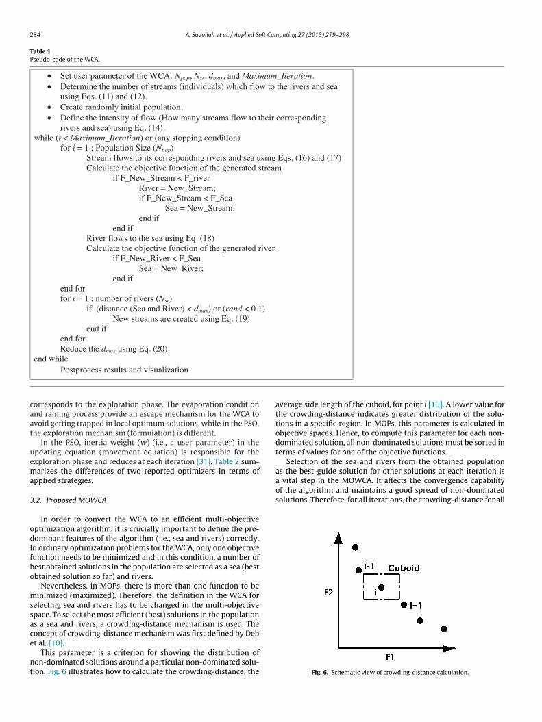
t al. [10].
This parameter is a criterion for showing the distribution ofon-dominated solutions around a particular non-dominated solu-ion. Fig. 6 illustrates how to calculate the crowding-distance, the

average side length of the cuboid, for point i [10]. A lower value forthe crowding-distance indicates greater distribution of the solu-tions in a specific region. In MOPs, this parameter is calculated inobjective spaces. Hence, to compute this parameter for each non-dominated solution, all non-dominated solutions must be sorted interms of values for one of the objective functions.

Selection of the sea and rivers from the obtained populationas the best-guide solution for other solutions at each iteration is

Fig. 6. Schematic view of crowding-distance calculation.


Table 2Differences between two optimization methods in terms of their approaches for finding global optimum solution.

Strategy PSO WCA

Population Particles (e.g., fishes, birds) Streams (including sea and rivers)

User parameter - Npopa - Npop- w (Inertia weight) - Nsr (Number of rivers + sea)- c1 (Personal learning constant) - dmax (Maximum allowable distance between

river and sea)- c2 (Global learning constant)- Vmax (Maximum velocity)

Global search Inertia weight (first term of the movement equation):w × vt

i

Evaporation condition:if norm(xi

Sea− xi

River) < dmax

Perform raining based on Eq. (19)end if

Local search The second and third terms of the movement equation:c1r1(pBes�ti − �Xi) + c2r2(gBes�ti − �Xi)

Moving streams to the rivers and rivers to thestreams (Eqs. (16)–(18))

Selection if Fb New < F Old if F Stream < F RiverAccept New Particle River = Stream;if F New < F Best if F Stream < F Sea

Accept New Particle Stream = Sea;end if end if

end if end ifif F River < F Sea

River = Sea;end if

ns

nrIbc

tiehdroame

deptsmt

TP

a Npop , total number of population.b F, value of objective function.

on-dominated solutions must be calculated to determine whicholutions have the highest crowding-distance values.

Afterwards, the obtained non-dominated solutions are desig-ated as a sea and rivers and, furthermore, the intensity of flow forivers and sea is calculated based on the crowding-distance values.n this situation, some non-dominated solutions will most likelye created around sea and rivers at the next iteration, and theirrowding-distance values will be amended and reduced.

Moreover, it is very important to save non-dominated solu-ions in an archive to generate the Pareto front sets. This archives updated at each iteration, and any dominated solutions areliminated from the archive. Based on the literature and due toaving fair comparison, the size of Pareto archive (number of non-ominated solutions in the archive) is set to be the same with othereported optimizers (see Table 3). Therefore, whenever the numberf members in the Pareto archive becomes greater than the Paretorchive size, the crowding-distance is applied again to eliminate asany as necessary of the non-dominated solutions having the low-

st crowding-distance values among the Pareto archive members.The MOWCA has the great potential for exploitation in the

esign space as it focuses in the near optimum solutions andxploits better solutions. Indeed, the exploration and exploitationhases in the MOWCA are combined and mixed. To clarify fur-
her, mostly the MOWCA starts with exploitation approach, movingtreams toward rivers and rivers toward the sea. In between theseovements, the MOWCA applies evaporation condition in order
o perform exploration phase. This trend can be considered as the

able 3arameters used for optimization of mathematical and engineering MOPs.

Constrained problems

NFEs Archive size

CONSTR 25,000 100

BNH 25,000 100

KITA 5000 100

TNK 25,000 100

OSY 40,000 200

SRN 25,000 100

potential of the MOWCA to search a wide range of design space,while concentrating to near optimum non-dominated solutions.

3.3. Constraint-handling approach

Many MOPs are subject to a set of constraints (e.g., inequal-ity, equality, linear, nonlinear, and the like). Therefore, it is vitalto find good, simple strategies to handle the imposed constraintsand detect solutions in the feasible area. Hence, a simple approachis defined here to apply on the MOWCA.

In this mechanism, after generating a set of solutions at eachiteration, all constraints are checked and some solutions that are inthe feasible area are selected. Afterward, non-dominated solutionsare selected from the feasible solutions and inserted into the Paretoarchive. Finally, sea and rivers are chosen from this archive for thenext iteration based on the strategy mentioned in Section 3.2.

3.4. Steps of the MOWCA

The steps of the MOWCA are summarized as follows:

Step 1: Choose the initial parameters for the MOWCA: Nsr, dmax,Npop, Max Iteration, and Pareto archive size.
Step 2: Generate random initial population and form the initialstreams, rivers, and sea using Eqs. (9), (11), and (12).Step 3: Calculate the value of multi-objective functions for eachstream using Eq. (10).
Engineering design problems

NFEs Archive size

4-bar truss 8000 100Speed reducer 24,000 100Gear train 10,000 100Spring 10,000 100Welded beam 15,000 100Disk brake 5000 100

2 ft Com

4

dMosMpNV

tiea

oaccmi


Step 4: Determine the non-dominated solutions in the initial pop-ulation and save them in the Pareto archive.Step 5: Determine the non-dominated solutions among the feasi-ble solutions and save them in the Pareto archive.Step 6: Calculate the crowding-distance for each Pareto archivemember.Step 7: Select a sea and rivers based on the crowding-distancevalue.Step 8: Determine the intensity of the flow for rivers and sea basedon the crowding distance values using Eq. (14).Step 9: Streams flow into the rivers using Eq. (16).Step 10: Exchange positions of river with a stream which gives thebest solution.Step 11: Some streams may directly flow into the sea using Eq.(17).Step 12: Exchange positions of sea with a stream which gives thebest solution.Step 13: Rivers flow into the sea using Eq. (18).Step 14: Exchange positions of sea with a river which gives thebest solution.Step 15: Check the evaporation condition using the pseudo-codein Section 3.1.Step 16: If the evaporation condition is satisfied, the raining pro-cess will occur using Eq. (19).Step 17: Reduce the value of dmax which is a user defined parameterusing Eq. (20).Step 18: Determine the new feasible solutions in the population.Step 19: Determine the new non-dominated solutions among thefeasible solutions and save them in the Pareto archive.Step 20: Eliminate any dominated solutions in the Pareto archive.Step 21: If the number of member in the Pareto archive is morethan the determined Pareto archive size, go to the Step 22, other-wise, go to the Step 23.Step 22: Calculate the crowding-distance value for each Paretoarchive member and remove as many members as necessary withthe lowest crowding-distance value.Step 23: Calculate the crowding-distance value for each Paretoarchive member to select new sea and rivers.Step 24: Check the convergence criteria. If the stopping criterionis satisfied, the algorithm will be stopped, otherwise return to theStep 9.

. Numerical examples and results

In this section, a set of well-known constrained and engineeringesign MOPs are used to clarify the performance of the proposedOWCA. These problems are various types of constrained multi-

bjective problems (CMOPs) with diverse features that have beenelected from a set of credible research studies. Moreover, theOWCA as a recently developed optimizer is compared with other

rominent methods employed in previous studies, such as theSGA-II, MOPSO, CMOPSO, EM-MOPSO, MOCSO, Micro-GA, PAES,IS, WBMOIA, and HQIA.

The MOWCA was coded in MATLAB programming software, andhe task of optimizing each test function was executed using 30ndependent runs. For all benchmark problems, the initial param-ters for the MOWCA (Ntotal, Nsr, and dmax) were selected as 50, 8,nd 1E−5, respectively.

The natures of the mentioned problems include various typesf objective functions having different numbers of design vari-bles and nonlinear constraints. In addition, some of the problems
onsidered, such as gear train and spring design problems, areategorized as discrete optimization problems (combinatorial opti-ization problems). In this study, both continuous, discrete, and
nteger MOPs are investigated using the MOWCA.

puting 27 (2015) 279–298

In addition, in order to have fair and reliable comparisons withother methods, the number of function evaluations (NFEs) usedand the Pareto archive size for all MOPs are the same as in otherprevious studies. In fact, the maximum number of NFEs is taken asthe stopping condition, similarly to other the methods in this paper.

In the literature, researchers utilized one (i.e., constrainedproblem 5) or two (i.e., constrained problem 2, four-bar truss,speed-reducer, disk brake, and welded beam design) performancemetrics for their examples using their optimization methods. Insome cases, they used all three performance metrics for constrainedproblems 1, 3, 4, and 6.

Therefore, in order to have comparative study with otheroptimization methods, we applied the MOWCA with existing per-formance metrics for each example and compared with the resultsobtained by other researchers in the literature.

These user parameters for all the MOPs are shown in Table 3. Thechosen values for the Pareto archive size are extracted from litera-ture [12–14,20] due to have fair comparisons with other optimizersin this study.

4.1. Multi-objective benchmark problems

In this subsection, twelve benchmark CMOPs and engineeringdesign problems are used to assess the capability and efficiencyof the proposed algorithm for handling multifaceted mathematicalproblems.

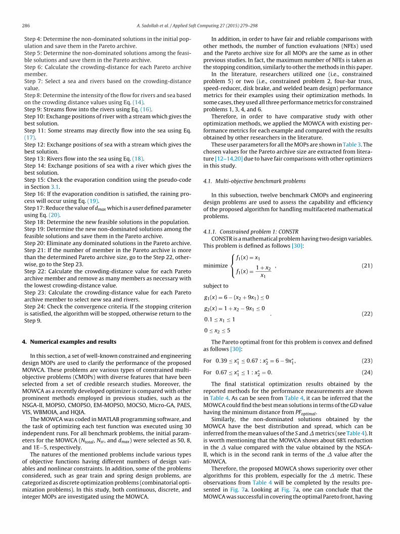
4.1.1. Constrained problem 1: CONSTRCONSTR is a mathematical problem having two design variables.

This problem is defined as follows [30]:

minimize

⎧⎨⎩

f1(x) = x1

f1(x) = 1 + x2

x1

, (21)

subject to

g1(x) = 6 − (x2 + 9x1) ≤ 0

g2(x) = 1 + x2 − 9x1 ≤ 0

0.1 ≤ x1 ≤ 1

0 ≤ x2 ≤ 5

. (22)

The Pareto optimal front for this problem is convex and definedas follows [30]:

For 0.39 ≤ x∗1 ≤ 0.67 : x∗

2 = 6 − 9x∗1, (23)

For 0.67 ≤ x∗1 ≤ 1 : x∗

2 = 0. (24)

The final statistical optimization results obtained by thereported methods for the performance measurements are shownin Table 4. As can be seen from Table 4, it can be inferred that theMOWCA could find the best mean solutions in terms of the GD valuehaving the minimum distance from PFoptimal.

Similarly, the non-dominated solutions obtained by theMOWCA have the best distribution and spread, which can beinferred from the mean values of the S and � metrics (see Table 4). Itis worth mentioning that the MOWCA shows about 68% reductionin the � value compared with the value obtained by the NSGA-II, which is in the second rank in terms of the � value after theMOWCA.

Therefore, the proposed MOWCA shows superiority over other
algorithms for this problem, especially for the � metric. Theseobservations from Table 4 will be completed by the results pre-sented in Fig. 7a. Looking at Fig. 7a, one can conclude that theMOWCA was successful in covering the optimal Pareto front, having


Fig. 7. Comparisons of the optimal Pareto fronts and generated Pareto front and distribution of non-dominated solutions using the MOWCA for the: (a) CONSTR, (b) TNK, (c)KITA, (d) SRN, (e) BNH, and (f) OSY (solid lines and cross points represent the optimal and generated (obtained) Pareto front, respectively).


Table 4Comparison of several algorithms based on the mean and standard deviation (SD) values of performance metrics for the CONSTR problem. “N/A” stands for not available.

Methods GD � S

Mean SD Mean SD Mean SD

NSGA-II 5.1349E−03 2.4753E−04 0.54863 2.7171E−02 0.0437 0.0041MOPSO 4.5437E−03 6.8558E−04 0.94312 3.6719E−01 N/A N/ACMOPSO 2.9894E−03 8.3111E−03 0.57586 2.2894E−02 N/A N/AEM-MOPSO N/A N/A N/A N/A 0.0406 0.0017MWCA 8.7102E−04 5.7486E−05 0.17452 2.0441E−02 0.0350 0.0010

Table 5Comparison of the various algorithms based on the mean and SD values of the performance metrics for the TNK problem.

Methods GD �

Mean SD Mean SD

NSGA-II 4.0488E−03 4.3465E−04 0.82286 2.8678E−0464E−034E−079E−0

stbo

4

i[

m

s

ovtios(

tlM

TC

MOPSO 5.0877E−03 4.55CMOPSO 5.4811E−04 7.96MWCA 1.3067E−03 6.19

atisfactory distribution and spread for the non-dominated solu-ions. In general, Fig. 7 demonstrates the graphical comparisonetween the exact and computed Pareto fronts using the proposedptimizer for solving the CMOPS studied in this paper.

.1.2. Constrained problem 2: TNKThe second constrained problem having two design variables

s suggested in the form of a mathematical description as follows32]:

inimize

{f1(x) = x1

f2(x) = x2

, (25)

ubject to

g1(x) = −x21 − x2

2 + 1 + 0.1 cos(

16 arctan(

x1

x2

))≤ 0

g2(x) = 0.5 − (x1 − 0.5)2 − (x2 − 0.5)2 ≤ 0

0 ≤ x1, x2 ≤ �

. (26)

This problem has a discontinuous Pareto optimal front that liesn the boundary of the first constraint and also includes some con-ex regions [30]. Table 5 compares the reported mean solutions forhe NSGA-II, MOPSO, CMOPSO, and MOWCA. According to Table 5,n terms of the mean values of the GD metric, the CMOPSO hasutperformed the other methods, and the MOWCA is placed in theecond rank, while having better stability for the obtained solutionsa lower SD value) compared with the other optimizers.

Likewise, the MOWCA has the second best mean solutions afterhe CMOPSO, judging by the mean values of the � metric. Moreover,ooking at Fig. 7b, we can see that PFoptimal is finely covered by the

OWCA with a good distribution of the non-dominated solutions.

able 6omparison of the various algorithms based on the mean and SD values of the performan

Methods GD �

Mean SD Mean

NSGA-II 0.04 0.044 0.786MOPSO 0.0467 0.0535 0.992MOCSO 0.0274 0.0324 1.016Micro-GA 0.1507 0.0897 N/A

PAES 0.1931 0.0332 N/A

MWCA 0.0049 0.0045 0.376

4 0.79363 5.1029E−025 0.25871 2.7272E−025 0.60211 2.8148E−02

4.1.3. Constrained problem 3: KITAKITA function, first introduced by Kita et al. [33], has been widely

analyzed [11,34]. The mathematical formulation proposed by Kitaet al. [33] is as follows:

maximize

⎧⎨⎩

f1(x) = −x21 + x2

f2(x) = 12

x1 + x2 + 1, (27)

subject to

g1(x) = 16

x1 + x2 − 132

≤ 0

g2(x) = 12

x1 + x2 − 152

≤ 0

g3(x) = 5x1 + x2 − 30 ≤ 0

0 ≤ x1, x2 ≤ 7

. (28)

The Pareto optimal front for the KITA function is convex andcontinuous. Despite the fact that KITA is a simple problem, mostalgorithms are unable to find all of the points on PFoptimal [11].The statistical optimization results of six algorithms for the per-formance metrics for this problem are shown in Table 6.

From Table 6, it is apparent that the MOWCA has the minimumGD and that there is also a huge difference between the mean GDvalue obtained by the MOWCA and those obtained by the othermethods (e.g., the PAES and Micro-GA). Moreover, the MOWCA notonly could reach the best GD value but also possesses the first rank
in terms of having the minimum values for the metrics of spacingand spread. Furthermore, based on Fig. 7c, it can be emphasizedthat the non-dominated solutions detected by the MOWCA havethe highest accuracy with the best distribution for this problem.
ce metrics for the KITA problem.

S

SD Mean SD

3 0.1951 0.1462 0.15185 0.1176 0.3184 0.47789 0.1147 0.1592 0.2338

N/A 0.3150 0.4217N/A 0.1101 0.0995

4 0.0744 0.0485 0.0478


Table 7Comparison of the various algorithms based on the mean and SD values of the performance metrics for the SRN problem.

Methods GD � S

Mean SD Mean SD Mean SD

NSGA-II 3.7069E−03 5.1034E−04 0.3869 2.5115E−02 1.5860 0.1337MOPSO 2.7623E−03 2.0794E−04 0.6655 7.2196E−02 N/A N/A

0.1965 2.4527E−02 N/A N/AN/A N/A 1.2439 0.10550.1477 1.3432E−02 0.4164 0.0779

4

dd

m

s

iMttws

znfot

4

pg

m

s

(ri

F

F

Mt

Table 8Comparison of the various algorithms in terms of the mean and SD values of the Smetric for the BNH problem.

Methods S

Mean SD

NSGA-II 0.7756 0.0727

CMOPSO 2.5331E−02 5.2561E−03

EM-MOPSO N/A N/A

MWCA 2.5836E−02 5.0102E−03

.1.4. Constrained problem 4: SRNThis problem, presented by Srinivas and Deb [35], has two

esign variables with a continuous Pareto optimal front. It isefined mathematically as follows:

inimize

{f1(x) = 2 + (x1 − 2)2 + (x2 − 1)2

f2(x) = 9x1 − (x2 − 1)2, (29)

ubject to

g1(x) = x21 + x2

2 − 225 ≤ 0

g2(x) = x1 − 3x2 + 10 ≤ 0

−20 ≤ x1, x2 ≤ 20

. (30)

The obtained values of three performance parameters are givenn Table 7 for the NSGA-II, MOPSO, CMOPSO, EM-MOPSO, and

OWCA. The mean values of GD for all of the algorithms indicatehat the MOPSO and NSGA-II have the best performances. Never-heless, their values of mean S and � indicate that these algorithmsere unable to find solutions having an acceptable distribution and

pread.In contrast, the MOWCA has surpassed those reported optimi-

ers in term of the metrics of spacing and spread; however, theon-dominated solutions attained by the MOWCA are slightly far

rom PFoptimal. Overall, it can be said that the MOWCA outperformedther algorithms in two out of three performance metrics. In addi-ion, Fig. 7d depicts how well the MOWCA could cover PFoptimal.

.1.5. Constrained problem 5: BNHThis problem is a 2D problem subject to two constraints. This

roblem was previously presented by Binh and Korn [36] and isiven as follows:

inimize

{f1(x) = 4x2

1 + 4x22

f2(x) = (x1 − 5)2 + (x2 − 5)2, (31)

ubject to

g1(x) = (x1 − 5)2 + x22 − 25 ≤ 0

g2(x) = 7.7 − (x1 − 8)2 − (x2 + 3)2 ≤ 0

0 ≤ x1 ≤ 5

0 ≤ x2 ≤ 3

. (32)

It is worth mentioning that the second constraint (g2(x) in Eq.32)) does not have any effect on the boundary of the infeasibleegion [30]. In addition, the Pareto optimal front for this problems as follows [30]:

or 0 ≤ x∗1 ≤ 3 : x∗

2 = x∗1, (33)

∗ ∗
or 3 ≤ x1 ≤ 5 : x2 = 3. (34)
The statistical results attained by the NSGA-II, EM-MOPSO, andOWCA are represented in Table 8. From Table 8, it can be seen that

he MOWCA has surpassed other methods in terms of having the

EM-MOPSO 0.6941 0.0385MWCA 0.5680 0.0265

minimum value of 0.5680 for the mean S metric and better stabilityfor finding non-dominated solutions (lower SD value).

Furthermore, Fig. 7e depicts the final solutions achieved by theMOWCA versus PFoptimal. As can be seen from Fig. 7e, the final solu-tions have suitable matches in terms of the GD metric with PFoptimal.

4.1.6. Constrained problem 6: OSYThe sixth constrained function was first suggested by Osyczka

and Kundu [37] and has been widely investigated [12,16]. Themathematical formulation of this problem is as follows:

minimize

⎧⎨⎩

f1(x) = −[25(x1 − 2)2 + (x2 − 2)2 + (x3 − 1)2

+ (x4 − 4)2 + (x5 − 1)2]

f2(x) = x21 + x2

2 + x23 + x2

4 + x25 + x2

6

, (35)

subject to

g1(x) = 2 − x1 − x2 ≤ 0

g2(x) = x1 + x2 − 6 ≤ 0

g3(x) = x2 − x1 − 2 ≤ 0

g4(x) = x1 − 3x2 − 2 ≤ 0

g5(x) = x4 + (x3 − 3)2 − 4 ≤ 0

g6(x) = 4 − x6 − (x5 − 3)2 ≤ 0

0 ≤ x1, x2, x6 ≤ 10

1 ≤ x3, x5 ≤ 5

0 ≤ x4 ≤ 6

. (36)

The OSY problem has six design variables, and its Pareto optimalfront is a concatenation of five regions, as shown in Fig. 8. For allthe Pareto optimal regions, x4 = x6 = 0. Accordingly, Table 9 showsother values of the design variables for each region [30].

The statistical optimization results from Table 10 illustrate thevalues of the performance parameters obtained by the NSGA-II, VIS,WBMOIA, HQIA, and MOWCA. Looking at the GD values summa-rized in Table 10, we can see that the best GD values obtained bythe NSGA-II and MOWCA are 9.89E−01 and 9.68E−02, respectively.

Hence, in this problem, the MOWCA is placed in the second rank
in terms of mean GD values after the HQIA. However, the distribu-tion of the non-dominated solutions reported by the MOWCA isacceptable, so the MOWCA is located in the first rank with respectto the S metric (see Table 10). Furthermore, Fig. 7f shows the final


Table 9Design variable values for the Pareto optimal front for the OSY problem.

Regions Optimal values of design variables

x∗1 x∗

2 x∗3 x∗

5

AB 5 1 (1, . . ., 5) 5BC 5 1 (1, . . ., 5) 1CD (4.056, . . ., 5) (x∗

1 − 2)/3 1 1DE 0 2 (1, . . ., 3.732) 1EF (0, . . ., 1) 2 − x∗

1 1 1

Table 10Comparison of the various algorithms based on the mean and SD of the performance metrics for the OSY problem.

Methods GD S

Mean SD Mean SD

NSGA-II 9.89E−01 9.78E−01 1.14E+00 2.75E−01VIS 3.15E−01 2.38E−01 8.30E−01 3.51E−01WBMOIA 9.85E−02 1.00E−01 9.46E−01 2.27E−01

0202

nP

4

mtd

4

wm

m

HQIA 3.49E−02 1.54E−MWCA 9.68E−02 7.18e−

on-dominated solutions obtained by the MOWCA compared withFoptimal for the OSY problem.

.2. Multi-objective engineering design problems

In this subsection, six mechanical component design opti-ization problems with multiple objectives are studied to show

he efficiency and performance of the MOWCA in finding non-ominated solutions having an acceptable distribution and spread.

.2.1. Four-bar truss design problemThe four-bar truss design problem, depicted in Fig. 9, has been

idely used to evaluate and validate different methods [11,27]. Theathematical formulation of this problem is as follows:⎧⎪⎨ f1(x) = L(2x1 +

√2x2 + √

x3 + x4)

inimize⎪⎩ f2(x) = FL

E

(2x2

+ 2√

2x2

− 2√

2x3

+ 2x4

) , (37)

Fig. 8. Schematic view of the Pareto optimal front for the OSY problem [30].

7.21E−01 1.60E−015.22E−01 9.52E−02

subject to(F

�

)≤ x1 ≤ 3 ×

(F

�

)√

2 ×(

F

�

)≤ x2 ≤ 3 ×

(F

�

)√

2 ×(

F

�

)≤ x3 ≤ 3 ×

(F

�

)(

F

�

)≤ x4 ≤ 3 ×

(F

�

), (38)

where

F = 10 KN, E = (2)105 KN/cm2

L = 200 cm, � = 10 KN/cm3. (39)

As can be seen from Eq. (37), the volume of the four-bar truss andthe joint displacement are to be optimized simultaneously. Table 11gives an overview of final optimization results reported by differentalgorithms.

Based on the GD values summarized in Table 11, the MOWCAhas the best performance in finding non-dominated solutions witha suitable match with PFoptimal (having the minimum distance toPFoptimal). In addition to having a lower GD value, the MOWCA wasable to maintain a suitable distance among the generated solutions
that were shown in the S metric values.
Although, the NSGA-II and MOPSO have slightly better perform-ances regarding the mean values of S, the SD value of the MOWCAfor the S metric shows better stability of solutions corresponding to

Fig. 9. Schematic view of a four-bar truss design problem.


F A, NSGr

tsPi

TCm

ig. 10. Comparison of non-dominated solutions obtained by the MOPSO, Micro-Gepresent the optimal and generated (obtained) Pareto fronts, respectively).

he distribution of the non-dominated solutions. Moreover, Fig. 10hows a graphical comparison of the NSGA-II, MOPSO, Micro-GA,
AES, and MOWCA. The discussion regarding Table 11 is confirmedn Fig. 10.
able 11omparison of the values for the mean and SD values for the used performanceetrics for the four-bar truss problem.

Methods GD S

Mean SD Mean SD

NSGA-II 0.3601 0.0470 2.3635 0.2551MOPSO 0.3741 0.0422 2.5303 0.2275Micro-GA 0.9102 1.7053 8.2742 16.8311PAES 0.9733 1.8211 3.2314 5.9555MOWCA 0.2076 0.0055 2.5816 0.0298

A-II, MOPSO, PAES, and MOWCA for the four-bar truss (Solid lines and dot points

4.2.2. Speed reducer design problemThe speed reducer design problem, shown in Fig. 11, has seven

design variables and has been studied widely in the literature[27,38–40].

Table 12Comparison of the various algorithms based on the mean and SD values of theperformance metrics for the speed-reducer design problem.

Methods GD S

Mean SD Mean SD

NSGA-II 9.843702 7.08103039 2.765449155 3.53493787Micro-GA 3.117536 1.67810867 47.80098 32.80151572PAES 77.99834 4.21026087 16.20129 4.26842769MOWCA 0.98831 0.17894217 16. 68520 2.69694436


i

m

s

poo

Table 13Comparison of the various algorithms based on the mean and SD values of theperformance metrics for the disk-brake design problem.

Methods GD �

Mean SD Mean SD

Fig. 11. Schematic view of a speed reducer design optimization problem.

The mathematical formulation used for modeling this problems as follows [41]:

inimize

⎧⎪⎪⎪⎪⎪⎪⎨⎪⎪⎪⎪⎪⎪⎩

f1(x) = 0.7854x1x22(10x2

3/3 + 14.933x3

− 43.0934) − 1.508x1(x26 + x2

7)

+7.477(x36 + x3

7) + 0.7854(x4x26 + x5x2

7)

f2(x) =√

(745.0x4/x2x3)2 + 1.69 × 107

0.1x36

, (40)

ubject to

g1(x) = 1.0

x1x22x3

− 1.027.0

≤ 0

g2(x) = 1.0

x1x22x2

3

− 1.0397.5

≤ 0

g3(x) = x34

x2x3x46

− 1.01.93

≤ 0

g4(x) = x35

x2x3x47

− 1.01.93

≤ 0

g5(x) = x2x3 − 40.0 ≤ 0

g6(x) = x1

x2− 12 ≤ 0

g7(x) = 5 − x1

x2≤ 0

g8(x) = 1.9 − x4 + 1.5x6 ≤ 0

g9(x) = 1.9 − x5 + 1.1x7 ≤ 0

g10(x) =√

(745x4/x2x3)2 + 1.69 × 107

0.1x36

− 1300 ≤ 0

g11(x) =√

(745x5/x2x3)2 + 1.575 × 108

0.1x37

− 1100 ≤ 0

2.6 ≤ x1 ≤ 3.6

0.7 ≤ x2 ≤ 0.8

17 ≤ x3 ≤ 28

7.3 ≤ x4 ≤ 8.3

7.3 ≤ x5 ≤ 8.3

2.9 ≤ x6 ≤ 3.9

5.0 ≤ x7 ≤ 5.5

. (41)

Table 12 represents the comparison of values for the considerederformance metrics for the speed reducer problem using the vari-us algorithms. In Table 12, the MOWCA shows its superiority overther methods in terms of the GD values. Note that there is a large

NSGA-II 3.0771 0.10782 0.79717 0.06608pa�-ODEMO 2.6928 0.24051 0.84041 0.20085MOWCA 0.0244 0.12314 0.46041 0.10961

discrepancy between the mean GD values obtained by the MOWCAand the Micro-GA as the second best method corresponding tovalues of 0.98 and 3.11, respectively (see Table 12).

In Fig. 12, graphical presentations are given for comparison pur-poses among the reported methods. Likewise, from Fig. 12, we cansay that the MOWCA has the best performance among the methods,and that the NSGA-II and PAES were unsuccessful in finding a set ofsolutions close to PFoptimal. Based on Fig. 12 and given the results inTable 12, it can be concluded that the MOWCA is the best algorithmregarding the mean S and GD values, and that it would be unwiseto introduce the NSGA-II as the best approach by considering themean S value for this problem.

4.2.3. Disk brake design problemThis problem has four design variables first studied by Ray and

Liew [42]. The main objective of this problem is to minimize thestopping time and the mass of a brake. The mathematical formula-tion of this problem is as follows:

minimize

⎧⎪⎨⎪⎩

f1(x) = 4.9 × 10−5(x22 − x2

1)(x4 − 1)

f2(x) = 9.82 × 106(x22 − x2

1)

x3x4(x32 − x3

1)

, (42)

subject to

g1(x) = 20 + x1 − x2 ≤ 0

g2(x) = 2.5(x4 + 1) − 30 ≤ 0

g3(x) = x3

3.14(x22 − x2

1)2

− 0.4 ≤ 0

g4(x) = 2.22 × 10−3x3(x32 − x3

1)

(x22 − x2

1)2

− 1 ≤ 0

g5(x) = 900 − 2.66 × 10−2x3x4(x32 − x3

1)

(x22 − x2

1)≤ 0

55 ≤ x1 ≤ 80

75 ≤ x2 ≤ 110

1000 ≤ x3 ≤ 3000

2 ≤ x4 ≤ 20

, (43)

where x1, x2, x3, and x4 are the inner radius of the disk, the outerradius of the disk, the engaging force, and the number of fric-tion surfaces, respectively. This engineering problem has beenoptimized previously using the NSGA-II and pa�-ODEMO [28].Comparisons of the performance metric parameters related tothe reported methods compared with the MOWCA are given inTable 13.Judging by Table 13, the MOWCA could find a wide vari-ety of solutions having uniform spread and the smallest deviationfrom PFoptimal. In this problem, the MOWCA proved its efficiencyagainst other optimizers. The mean values of the GD and � metricsobtained by the MOWCA, 0.02 and 0.46, respectively, support this
claim. In addition, Fig. 13 depicts graphical comparisons with theother reported methods.
Moreover, it is worth mentioning that the non-dominated solu-tions obtained by the MOWCA are in the range of (0.1274, 16.6549)


F icro-r

arfTsne

4

dcms

r

m

s

ig. 12. Comparison of distribution of non-dominated solutions obtained by the Mepresent the optimal and generated (obtained) Pareto fronts, respectively).

nd (2.7176, 2.0828), while those obtained by the NSGA-II are in theange of (0.1293, 17.598) and (2.7915, 2.1127). Similarly, this rangeor the pa�-ODEMO is (0.1274, 16.6549) and (2.8684, 2.0906) [28].hese results show that the brake mass of 2.8684 with minimumtopping time of 2.0906 obtained by the pa�-ODEMO is domi-ated by (2.7176, 2.0828) attained by the MOWCA, confirming thexploratory capabilities of the MOWCA for finding accurate results.

.2.4. Welded beam design problemThe welded beam design problem, shown in Fig. 14, has four

esign variables and is selected from Ray and Liew [42]. In thisase, the fabrication cost and end deflection of the beam must beinimized subject to imposed constraints on shear stress, bending

tress, and buckling load [43].The two objective functions and four nonlinear constraints

elated to this problem are as follows:

inimize

⎧⎨⎩

f1(x) = 1.10471h2l + 0.0481tb(14.0 + t)

f2(x) = 2.1952t3b

, (44)

ubject to

g1(x) = �(x) − 13, 600 ≤ 0

g2(x) = �(x) − 30, 000 ≤ 0

g3(x) = h − b ≤ 0

g4(x) = 6000 − Pc(x) ≤ 0

. (45)

GA, PAES, NSGA-II, and MOWCA for the speed reducer (solid lines and dot points

The first constraint in Eq. (45), g1(x), is related to the shear stressimposed on the support location of the beam, which must be lessthan the shear strength of the material (13,600 psi). In addition,the normal stress generated at the support location of the beam(the second constraint, g2(x), in Eq. (45)) must be smaller than theallowable yield strength of the material (30,000 psi). Also, the thirdconstraint, g3(x), indicates that the thickness of the beam must belarger than the weld thickness.

For the last constraint, g4(x), the allowable buckling load (alongthe thickness direction) of the beam must be greater than the valueof the applied load (F). The shear stress, normal stress, and otherparameters used in the constraints, Eq. (45), are defined as follows[28]:

�(x) =√

(� ′)2 + (� ′′)2 + l� ′� ′′√0.25(l2 + (h + t)2)

� ′ = 6000√2hl

� ′′ = 6000(14.0 + 0.5l)√

0.25(l2 + +(h + t)2)

2[0.707hl((l2/12) + 0.25(l2 + +(h + t)2))]

�(x) = 504, 000t2b

. (46)

Pc(x) = 64, 764.022(1 − 0.0282346t)tb3

0.125 ≤ h, b ≤ 5.0

0.1 ≤ l, t ≤ 10.0


NSGA

NRvhMtg

Mt

Fig. 13. Distribution of non-dominated solutions obtained by the

Final statistical optimization results obtained by applying theSGA-II, pa�-ODEMO, and MOWCA are collected in Table 14.egarding the mean GD values in Table 14, the MOWCA having a GDalue of 0.04909 and the pa�-ODEMO with a GD value of 0.09169ave stood in the first and second ranks, respectively. Similarly, theOWCA and pa�-ODEMO could maintain a uniform distribution of

he solutions with a good spread, as is revealed from the � values
iven in Table 14.
Moreover, the extreme solutions (ranges) obtained by theOWCA are (2.5325, 0.0115) and (37.9686, 0.000439). In contrast,

he minimum fabrication cost obtained by the pa�-ODEMO and

Fig. 14. Schematic view of a welded beam design optimization problem.

II, pa�-ODEMO, and MOWCA for the disk brake design problem.

NSGA-II are 2.8959 units with a deflection of 0.0131 inches and3.0294 units with a deflection of 0.0088 inches, respectively [28].

Hence, the MOWCA has the best performance based on thefabrication cost (having minimum fabrication cost). Likewise, theminimum deflection related to the fabrication cost obtained by theNSGA-II and pa�-ODEMO are (37.4018, 0.000439) and (36.6172,0.00044), respectively [28]. These statistics indicate that the pro-posed approach was successful in finding a wide variety ofPareto-optimal solutions. For more assessments, Fig. 15 demon-strates graphical comparisons among the reported multi-objectiveoptimizers.

4.2.5. Spring design problemThe spring problem requires a design based on minimum stress

and minimum volume. This problem has three design variables:number of spring coils (N: x ), an integer variable; wire diameter
1(d: x2), a discrete variable; and spring diameter (D: x3), a continuousdecision variable. This problem has two objective functions subject
Table 14Comparison of the various algorithms based on the mean and SD values of theperformance metrics for the welded-beam design problem.

Methods GD �

Mean SD Mean SD

NSGA-II 0.16875 0.08030 0.88987 0.11976pa�-ODEMO 0.09169 0.00733 0.58607 0.04366MOWCA 0.04909 0.02821 0.22478 0.09280


NSGA

ti

m

s

TC

Fig. 15. Distribution of the non-dominated solutions obtained by the

o eight constraints. The mathematical formulation of this problems as follows [43]:

inimize

⎧⎨⎩

f1(x) = 0.25�2x32x3(x1 + 2)

f2(x) = 8KPmaxx3

�x32

, (47)

ubject to

g1(x) = 1.05x2(x1 + 2) + Pmax

k− lmax ≤ 0

g2(x) = dmin − x2 ≤ 0

g3(x) = x2 + x3 − Dmax ≤ 0

g4(x) = 3 − C ≤ 0

g5(x) = ıp − ıpm ≤ 0

g6(x) = ıw − Pmax − P

k≤ 0

, (48)

g7(x) = 8KPmaxx3

�x32

− S ≤ 0

g8(x) = [0.25�2x32x3(x1 + 2)] − Vmax ≤ 0

able 15omparison of the extreme solutions for the objective functions (interval span) for the sp

Algorithms Solutions Design variables

x1 x

NSGA-II Min. volume 5 0Min. stress 24 0

MOWCA Min. volume 9 0Min. stress 19 0

II, pa�-ODEMO, and MOWCA for the welded beam design problem.

where the parameters used in the objective functions and con-straints (47) and (48), respectively, are as follows [43]:

K = 4C − 14C − 4

+ 0.615x2

x3P = 300 lb Dmax = 3 in.

k = Gx42

8x1x33

Pmax = 1000 lb ıw = 1.25 in.

ıp = P

klmax = 14 in. ıpm = 6 in.

S = 189, 000 kpsi dmin = 0.2 in. C = D

d

. (49)

In this problem, x2 is a discrete variable whose values will beselected from the set F = [0.009, 0.0095, 0.0104, 0.0118, 0.0128,0.0132, 0.014, 0.015, 0.0162, 0.0173, 0.018, 0.020, 0.023, 0.025,0.028, 0.032, 0.035, 0.041, 0.047, 0.054, 0.063, 0.072, 0.080, 0.092,0.105, 0.120, 0.135, 0.148, 0.162, 0.177, 0.192, 0.207, 0.225, 0.244,0.263, 0.283, 0.307, 0.331, 0.362, 0.394, 0.4375, 0.5]. In addition, x1will be taken to be integer values in the range of Refs. [1,33]. Inaddition, the lower and upper bounds for x3 are 0 and 3 inches,
respectively. There were no statistical results for performancemetrics (i.e., the GD, S, and �) for this problem in literature. There-fore, Table 15 compares extreme solutions obtained by the NSGA-IIand MOWCA in terms of interval span.
ring design problem.

Objective functions

2 x3 f1 f2

.307 1.619 2.690 187,053

.5 1.865 24.189 61,949

.283 1.227 2.668 188,448

.5 2.083 26.983 58,752

296 A. Sadollah et al. / Applied Soft Com

dvltbMtt

4

FTsot

m

h

lb

TC

TE

Fig. 16. Schematic view of a gear train design optimization problem.

Judging by Table 15, the MOWCA offers a wider range of non-ominated solutions compared to the NSGA-II. The minimumolume reported by the MOWCA is 2.668 units, which is 0.022 unitsess than the minimum volume attained by the NSGA-II. Likewise,he minimum stress as the second bound of the Pareto front gainedy the NSGA-II and MOWCA reveals the same results. In fact, theOWCA detected a wider range for both objective functions, and

he minimum values of f1 and f2 obtained by the MOWCA are lesshan the values found using the NSGA-II.

.2.6. Gear train design problemThe main purpose of the gear train design problem, shown in

ig. 16, is to find the number of teeth in each gear (x1: Td, x2: Tb, x3:a, and x4: Tf). In fact, this problem tries to minimize the maximumize of any of the four gears and minimize the error between thebtained gear ratio and a required gear ratio of 1/6.931 [43]. Hence,his problem is as follows [43]:

inimize

⎧⎨⎩ f1(x) =

[1

6.931− x1x2

x3x4

]2

f2(x) = max(x1, x2, x3, x4)

. (50)

It is worth mentioning that all design variables in this problem
ave integer values that vary from 12 to 60.
For performance metrics (i.e., the GD, S, and �) for this prob-em, there had not existed statistical reports in literature. Therefore,ased on the results in literature, comparison for extreme solutions

able 16omparison of the extreme solutions for objective functions (interval span) for the gear t

Algorithms Solutions Design variables

x1 x2

NSGA-II Min. F1 12 12

Min. F2 12 12

MOWCA Min. F1 12 15

Min. F2 12 12

able 17ffects of the MOWCA parameters on the GD metric for the CONSTR problem.

Results Maximum Iteration = 100

Npop = 50

dmax = 1E−5 Nsr = 8

Nsr = 4 Nsr = 8 Nsr = 10 dmax = 1e−1 dmax = 1e−3

Best 8.22E−4 7.98E−4 8.34E−4 8.28E−4 7.98E−4

Average 9.08E−4 9.01E−4 9.17E−4 9.12E−4 9.08E−4

Worst 1.08E−4 1.04E−3 1.04E−4 1.06E−3 1.04E−3

SD 5.86E−4 5.77E−5 5.21E−5 5.71E−5 5.77E−5

puting 27 (2015) 279–298

is provided. The results of the comparison for extreme solutionsobtained by the NSGA-II and MOWCA are tabulated in Table 16.By observing Table 16, there is an increase in the range of non-dominated solutions obtained by applying the MOWCA comparedwith the NSGA-II. This feature is more obvious for the f2 function(see Table 16).

To clarify further, the MOWCA could improve the minimumerror ratio from the 1.83E−08 value obtained by the NSGA-II toa value of 4.50E−09. Furthermore, a similar trend related to thesecond extreme solution (F2) is observed. Hence, these intervalssupport the idea that the MOWCA is better able to find a widerrange of solutions compared with the NSGA-II. Indeed, wider rangemeans giving more choices to the decision maker to select his orher optimum design from the set of non-dominated solutions.

As the WCA have shown its superiority for tackling single objec-tive functions [23], in this article, we demonstrated the advantagesof the concepts and strategy of WCA for handling constrained MOPs.The MOWCA, so for the WCA, proves its efficiency for solving MOPs.

Offering wider range for non-dominated solutions (disk brake,welded beam, spring design, and gear train design problems),obtaining the generated Pareto front close to the optimal Paretofront (i.e., for Section 4.2), and good distribution of the non-dominated solutions (metric of spacing) compared with otheroptimizers, discussed earlier (Sections 4.2 and 4.3), are consideredas advantages of MOWCA for handling MOPs.

4.3. Sensitivity analysis for initial parameters of MOWCA

The main objective of this subsection is to evaluate and studythe effects of each initial parameter used in the MOWCA. One ofthe most important concerns related to optimization algorithms isto find the most efficient user parameters. Performing sensitivityanalyses show the stability of the methods and importance of initialparameters to find the optimal solution against any changes in userparameters.

Especially, when the problem is complex having many localoptima, it is crucially important to use the proper and efficient userparameters to boost the convergence speed and efficiency of the
algorithms for finding global solution without getting trapped inlocal minima.
The problems considered are the CONSTR problem (Section4.1.1) and speed reducer design problem (Section 4.2.2) have been

rain design problem.

Objective functions

x3 x4 f1 f2

27 37 1.83E−08 3712 13 5.01E−01 13

43 29 4.50E−09 4312 12 7.32E−01 12

Nsr = 8 and dmax = 1e−5

Npop = 10 Npop = 30 Npop = 50

dmax = 1e−5 dmax = 1e−7

7.98E−4 8.31E−4 8.28E−4 8.89E−4 7.98E−49.01E−4 9.96E−4 9.36E−4 9.96E−3 9.01E−41.04E−3 1.13E−3 1.14E−3 5.95E−2 1.04E−35.77E−5 6.51E−5 8.32E−5 1.22E−2 5.77E−5


Table 18Effects of the MOWCA parameters on metric of spacing for the CONSTR problem.


Npop = 50 Nsr = 8 and dmax = 1e−5

dmax = 1E−5 Nsr = 8 Npop = 10 Npop = 30 Npop = 50

Nsr = 4 Nsr = 8 Nsr = 10 dmax = 1e−1 dmax = 1e−3 dmax = 1e−5 dmax = 1e−7

Best 2.97E−2 2.73E−2 2.83E−2 2.78E−2 2.89E−2 2.73E−2 2.80E−2 2.82E−2 4.45E−2 2.73E−2Average 3.52E−2 3.36E−2 3.39E−2 3.76E−2 3.39E−2 3.36E−2 3.54E−2 3.54E−2 3.41E−1 3.36E−2Worst 5.78E−2 4.79E−2 6.19E−2 6.67E−2 4.54E−2 4.79E−2 6.23E−2 6.99E−2 1.23 4.79E−2SD 5.03E−3 3.19E−3 7.05E−3 7.26E−3 3.42E−3 3.19E−3 6.46E−3 9.12E−3 2.62E−1 3.19E−3

Judging by three first columns of Tables 17 and 18, “Nsr = 8”, “dmax = 1e−5”, and “Npop = 50” have the best performance in terms of performance metrics in comparison withother values. Similarly, the speed reducer design problem is investigated and the optimization results are tabulated in Tables 19 and 20 for different performance evaluators.

Table 19Effects of the MOWCA parameters on the GD metric for the speed reducer problem.



dmax = 1e−5 Nsr = 8 Npop = 10 Npop = 30 Npop = 50


Best 0.94 0.87 0.91 0.91 0.88 0.87 0.99 1.24 0.92 0.87Average 1.67 1.42 1.45 1.44 1.52 1.42 1.46 11.93 1.59 1.42Worst 4.50 2.49 2.89 3.47 2.69 2.49 3.19 61.72 2.64 2.49SD 0.81 0.49 0.55 0.56 0.52 0.49 0.57 15.92 0.50 0.49

Table 20Effects of the MOWCA parameters on metric of spacing for the speed reducer problem.



dmax = 1E−5 Nsr = 8 Npop = 10 Npop = 30 Npop = 50


Best 11.77 11.05 12.67 15.12 11.85 11.05 12.44 13.55 12.95 11.05

ia

frpmt

opstpag

t(dipt

fcm

Average 16.24 16.63 16.92 17.14 16.33

Worst 18.54 18.04 18.84 19.25 21.34

SD 1.79 0.86 3.42 1.93 2.12

nvestigated by changing the user parameters of MOWCA whichre Npop, Nsr, dmax, and the maximum iteration number.

In each problem, different optimization results for various per-ormance metrics (i.e., GD and S) using diverse user parameters areepresented. Tables 17 and 18 represent the sensitivity of initialarameters with respect to the values for different performanceetrics including the GD and S for the CONSTR problem, respec-

ively.As the second user parameter, dmax is used for applying the evap-

ration condition and raining process and affects the explorationhase in the WCA. Generally, the large values for dmax reduce auitable search around the best obtained point (i.e., sea). By set-ing a large value for dmax (i.e., increasing the number of rainingrocess), the WCA operates as a random search method instead of

being metaheuristic one. Hence, it may not be able to find thelobal optimum solution.

Likewise, the small values of dmax have a negative influence onhe final results as it can reduce the number of raining processesi.e., fewer explorations). Therefore, the WCA concentrates on theomain solution near to the best obtained point (sea) without pay-

ng more attentions to other regions. As a consequence, for complexroblems having many local optima, the WCA traps in local solu-ions.

As it can be seen from Tables 17–20, dmax = 1e−1 and dmax = 1e−7ound the worst solutions with the largest SD values. Therefore, itan be concluded that if an unsuitable value select for dmax, theoving toward the best solution probably misdirects.

16.63 16.35 25.14 17.81 16.6318.04 18.36 66.72 18.82 18.04

0.86 1.61 17.66 2.98 0.86

The last parameter which can have effects on the performanceof WCA is the number of rivers and sea (Nsr). It is worth mention-ing that the Npop is considered as a common user parameter forthe most metaheuristic algorithms. In fact, the chosen value of Nsr

should be proportional with the chosen value of Npop.For instance, when values of Nsr and Npop are equal to 8 and 10,

respectively, it means that some rivers have been created withouthaving any streams moving toward those rivers. These parame-ters’ selection can cause the detrimental effects on the optimizationresults. By observing Tables 17–20, when Nsr is equal to 8, the worstand best performance corresponds to “Npop = 10” and “Npop = 50”,respectively.

In conclusion, it can be inferred that the best value for dmax isin the range of 1e−5 and 1e−3 and also, the value of Nsr should beselected based on the value of Npop. Indeed, the best value of theNsr may be chosen as one sixth of Npop. Therefore, for populationsize of 50, eight rivers and sea (Nsr) may be considered as a propervalue. Note that if the number of iteration increases, the WCA orother metaheuristic algorithms will have more chances (i.e., com-putational time) to find the best solution and explore the searchdomain.

5. Conclusions

This paper presented multi-objective water cycle algorithm(MOWCA), a novel multi-objective optimization technique forsolving constrained multi-objective problems (CMOPs). The basic

2 ft Com

cpsTusomPippritornP

A

o(

R

[

[

[

[

[

[

[

[

[

[

[

[

[

[

[

[

[

[

[

[

[

[

[

[

[

[

[

[

[

[

[

[


oncepts of the proposed MOWCA are inspired by the water cyclerocess in the real world. In this paper, the MOWCA was used toolve a number of well-known benchmark and engineering MOPs.he efficiency and performance of the MOWCA was demonstratedsing three popular criteria (i.e., generational distance, metric ofpacing, and spread metric). The statistical optimization resultsbtained from performance metrics revealed that the proposedulti-objective optimizer was able to approach a full optimal

areto front and provide a superior quality of solutions in compar-son to a variety of state-of-the art algorithms considered in thisaper. In general, the MOWCA offers competitive solutions com-ared with other population-based algorithms, according to theeported results and the numerical results in this research offer-ng a wider range of non-dominated solutions. In fact, althoughhe robustness and exploratory capability of the MOWCA dependn the nature and complexity of the problems, the optimizationesults obtained show that the MOWCA might be a suitable alter-ative method having an acceptable degree of accuracy for findingareto optimal solutions for different scales of MOPs.

cknowledgment

This work was supported by the National Research Foundationf Korea (NRF) grant funded by the Korean government (MSIP)NRF-2013R1A2A1A01013886).

eferences

[1] T. Ray, K.S. Won, An evolutionary algorithm for constrained bi-objective opti-mization using radial slots, Lect. Notes Comput. Sci. 3684 (2005) 49–50.

[2] Z. Zhang, Immune optimization algorithm for constrained nonlinear multiob-jective optimization problems, Appl. Soft. Comput. 7 (3) (2007) 840–850.

[3] Y. Gao, M. Qu, Constrained multi-objective particle swarm optimization algo-rithm, in: Emerging Intelligent Computing Technology and Applications, vol.304, 2012, pp. 47–50.

[4] B. Suman, Study of self-stopping PDMOSA and performance measure in multi-objective optimization, Comput. Chem. Eng. 29 (2005) 1131–1147.

[5] E. Zitzler, L. Thiele, Multi objective evolutionary algorithms: a comparative casestudy and the strength Pareto approach, IEEE Trans. Evol. Comput. 3 (4) (1999)257–260.

[6] E. Zitzler, M. Laumanns, L. Thiele, SPEA2: Improving the Strength Pareto Evo-lutionary Algorithm, Swiss Federal Institute Technology, Zurich, Switzerland,2001.

[7] J.D. Knowles, D.W. Corne, Approximating the nondominated front using thePareto archived evolution strategy, Evol. Comput. 8 (2) (2000) 149–150.

[8] C.A.C. Coello, G.T. Pulido, Multiobjective optimization using a micro-geneticalgorithm, in: L. Spector, E.D. Goodman, A. Wu, W.B. Langdon, H.M. Voigt, M.Gen, S. Sen, M. Dorigo, S. Pezeshk, M.H. Garzon, E. Burke (Eds.), San Francisco:Proc. Genetic and Evolutionary Computation Conf. (GECCO’2001), 2001, pp.274–282.

[9] K. Deb, Multi-objective genetic algorithms: problem difficulties and construc-tion of test problems, Evol. Comput. 7 (2002) 205–210.

10] K. Deb, A. Pratap, S. Agarwal, T. Meyarivan, A fast and elitist multi objectivegenetic algorithm: NSGA-II, IEEE Trans. Evol. Comput. 6 (2) (2002) 182–190.

11] C.A.C. Coello, G.T. Pulido, M.S. Lechuga, Handling multiple objectives with par-ticle swarm optimization, IEEE Trans. Evol. Comput. 8 (3) (2004) 256–260.

12] F. Freschi, M. Repetto, VIS: an artificial immune network for multi-objectiveoptimization, Eng. Optim. 38 (8) (2006) 975–980.

13] M.J. Reddy, D.N. Kumar, Multi-objective particle swarm optimization for gen-erating optimal trade-offs in reservoir operation, Hydrol. Process. 21 (2007)2897–2909.

14] J.Q. Gao, L. Wang, WBMOAIS: a novel artificial immune system for multiobjec-
tive, Comput. Oper. Res. 37 (1) (2010) 50–60.
15] B. Suman, N. Hoda, S. Jha, Orthogonal simulated annealing for multiobjectiveoptimization, Comput. Chem. Eng. 34 (2010) 1618–1631.

16] J. Gao, J. Wang, A hybrid quantum-inspired immune algorithm for multiobjec-tive optimization, Appl. Math. Comput. 217 (2011) 4754–4770.

[

[

puting 27 (2015) 279–298

17] X. Zhang, B. Lu, S. Gou, L. Jiao, Immune multiobjective optimization algorithmfor unsupervised feature selection, in: Proceedings of Applications of Evolu-tionary Computing, vol. 39, Springer, LNCS, Budapest, 2006.

18] L. Jiao, M. Gong, R. Shang, et al., Clonal selection with immune dominanceand energy based multiobjective optimization, in: Proceedings of Third Inter-national Conference on Evolutionary Multi-Criterion Optimization, vol. 3410,LNCS, Springer-Verlag, Guanajuato, 2005, pp. 474–489.

19] X.L. Wang, M. Mahfouf, ACSAMO: an adaptive multiobjective optimizationalgorithm using the clonal selection principle, in: Proceedings of Second Euro-pean Symposium on Nature-inspired Smart Information Systems, Puerto de laCruz, 2006.

20] A. Kaveh, K. Laknejadi, A novel hybrid charge system search and particle swarmoptimization method for multi-objective optimization, Expert Syst. Appl. 38(12) (2011) 15475–15488.

21] M.R. Narimani, A.A. Rasoul, Z.M.S. Behrouz, K. Gholami, A novel approachto multi-objective optimal power flow by a new hybrid optimization algo-rithm considering generator constraints and multi-fuel type, Energy 49 (2013)119–120.

22] V.S.Q. Luis, G.H.D. Alfredo, M. Julián, C.A.C. Coello, DEMORS: a hybrid multi-objective optimization algorithm using differential evolution and rough settheory for constrained problems, Comput. Oper. Res. 37 (2010) 470–480.

23] H. Eskandar, A. Sadollah, A. Bahreininejad, M. Hamdi, Water cycle algorithm – anovel metaheuristic optimization method for solving constrained engineeringoptimization problems, Comput. Struct. 110–111 (2012) 151–160.

24] R.L. Haupt, S.E. Haupt, Practical Genetic Algorithms, 2nd ed., John Wiley & Sons,Inc., USA, 2004.

25] C.A.C. Coello, An updated survey of GA-based multi-objective optimizationtechniques, ACM Comput. Surv. 32 (2) (2000) 109–110.

26] D.A.V. Veldhuizen, G.B. Lamont, Multiobjective Evolutionary AlgorithmResearch: A History and Analysis, Technical Report TR-98-03, Department ofElectrical and Computer Engineering, Graduate School of Engineering, Air ForceInstitute of Technology, Wright-Patterson AFB, OH, 1998.

27] C.A.C. Coello, G.T. Pulido, Multiobjective structural optimization using a microgenetic algorithm, Struct. Multidiscip. Optim. 30 (5) (2005) 388–390.

28] W. Gong, Z. Cai, L. Zhu, An efficient multiobjective differential evolution algo-rithm for engineering design, Struct. Multidiscip. Optim. 38 (2) (2009) 137–140.

29] J.R. Schott, Fault Tolerant Design Using Single and Multicriteria GeneticAlgorithm Optimization (Master’s thesis), Department of Aeronautics andAstronautics, Massachusetts Institute of Technology, Cambridge, MA, 1995.

30] K. Deb, Multi-objective Optimization Using Evolutionary Algorithms, Wiley,Chichester, 2001.

31] J. Kennedy, R. Eberhart, Particle swarm optimization, in: Proceedings of theIEEE International Conference on Neural Networks, Perth, Australia, 1995, pp.1942–1948.

32] M. Tanaka, GA-based decision support system for multicriteria optimization, in:IEEE International Conference on Systems, Man and Cybernetics, vol. 2, 1995,pp. 1556–1561.

33] H. Kita, Y. Yabumoto, N. Mori, Y. Nishikawa, Multi-objective optimization bymeans of the thermodynamical genetic algorithm, in: H.M. Voigt, W. Ebeling,I. Rechenberg, H.P. Schwefel (Eds.), Parallel Problem Solving From Nature-PPSN IV, Lecture Notes in Computer Science, Springer-Verlag, Berlin, 1996, pp.504–510.

34] P.M. Pradhan, G. Panda, Solving multiobjective problems using cat swarm opti-mization, Expert Syst. Appl. 39 (2012) 2956–2964.

35] N. Srinivas, K. Deb, Multi objective function optimization using nondominatedsorting genetic algorithms, Evol. Comput. 2 (3) (1995) 221–230.

36] T.T. Binh, U. Korn, MOBES: a multiobjective evolution strategy for constrainedoptimization problems, in: 3rd International Conference on Genetic Algo-rithms, 1997, pp. 176–182.

37] A. Osyczka, S. Kundu, A new method to solve generalized multicriteria opti-mization problems using the simple genetic algorithm, Struct. Multidiscip.Optim. 10 (1995) 94–100.

38] A. Farhang-Mehr, S. Azarm, Entropy-based multi-objective genetic algorithmfor design optimization, Struct. Multidiscip. Optim. 24 (2002) 351–360.

39] A. Kurpati, S. Azarm, J. Wu, Constraint handling improvements for multiobjec-tive genetic algorithms, Struct. Multidiscip. Optim. 23 (2002) 204–210.

40] L.V. Santana-Quintero, C.A.C. Coello, An algorithm based on differential evolu-tion for multi-objective problems, Int. J. Comput. Intell. Res. 1 (2005) 151–160.

41] J. Wu, Quality Assisted Multiobjective and Multidisciplinary Genetic Algo-rithms (PhD thesis), Department of Mechanical Engineering, University ofMaryland at College Park, College Park, MD, 2001.

42] T. Ray, K.M. Liew, A swarm metaphor for multiobjective design optimization,Eng. Optim. 34 (2002) 141–150.

43] K. Deb, A. Pratap, S. Moitra, Mechanical component design for multiple objec-tives using elitist non-dominated sorting GA, Parallel Probl. Solv. Nat. PPSN VI1917 (2000) 859–868.

http://refhub.elsevier.com/S1568-4946(14)00579-1/sbref0005




































































































































































































































































































































































































































































































































































































































































































































































































































































































































































































































































































































Water cycle algorithm for solving constrained multi-objective optimization problems

Documents