Water balance versus land surface model in the simulation of Rhine river discharges

Water balance versus land surface model in the

simulation of Rhine river discharges

R. T. W. L. Hurkmans,1 H. de Moel,2 J. C. J. H. Aerts,2 and P. A. Troch3

Received 11 May 2007; revised 19 September 2007; accepted 26 September 2007; published 12 January 2008.

[1] Accurate streamflow simulations in large river basins are crucial to predict timing andmagnitude of floods and droughts and to assess the hydrological impacts of climatechange. Water balance models have been used frequently for these purposes. Compared towater balance models, however, land surface models carry the potential to more accuratelyestimate hydrological partitioning and thus streamflow, because they solve the coupledwater and energy balance and are able to exploit a larger part of the information providedby regional climate model output than water balance models. Owing to increased modelcomplexity, however, they are also more difficult to parameterize. The purpose of thisstudy is to investigate and compare the accuracy of streamflow simulations of a waterbalance approach (Spatial Tools for River basins and Environment and Analysis ofManagement (STREAM)) and a land surface model (Variable Infiltration Capacity (VIC))approach. Both models are applied to the Rhine river basin using regional climatemodel output as atmospheric forcing, and are evaluated using observed streamflow andlysimeter data. We find that VIC is more robust and less dependent on model calibration.Although STREAM performs better during the calibration period (Nash-Sutcliffeefficiency (E) of 0.47 versus E = 0.29 for VIC), VIC more accurately simulates dischargeduring the validation period, including peak flows (E = 0.31 versus E = 0.21 forSTREAM). This is the case for most locations throughout the basin, except for the Alpinepart where both models have difficulties due to the complex terrain and surface reservoirs.In addition, the annual evaporation cycle at the lysimeters is more realistically simulatedby VIC.

Citation: Hurkmans, R. T. W. L., H. de Moel, J. C. J. H. Aerts, and P. A. Troch (2008), Water balance versus land surface model inthe simulation of Rhine river discharges, Water Resour. Res., 44, W01418, doi:10.1029/2007WR006168.

1. Introduction

[2] River discharge integrates hydrological processes atthe catchment scale and can be measured directly, asopposed to many other catchment fluxes (e.g., evaporation,precipitation). Streamflow is thus a suitable variable tovalidate and/or compare hydrological model performances.In Central Europe, recent floods in the Rhine (1993 and1995), Elbe (2002) and Danube (2002), as well as droughts(e.g., the summer of 2003) caused billions of euros ofdamage [Kleinn et al., 2005]. Improving streamflow simu-lations in these densely populated large river basins isimportant to accurately predict timing and magnitude offloods and droughts [Nijssen et al., 1997]. Climate change isbelieved to affect streamflow characteristics mainly becauseof two reasons: first, the warming-related shift from snow torainfall will change the seasonal streamflow cycle in rivers

which have their source region in the Alps (including theRhine). Second, there is increasing evidence for an accel-eration of the hydrological cycle and an associated increasein precipitation intensity during winter [Kleinn et al., 2005].Numerous studies have been carried out to quantify theimpact of climate change on extreme value distributions ofriver streamflow, indicating a projected increase in extremewinter floods and more droughts in summer [Middelkoop etal., 2001; Milly et al., 2005; Aerts et al., 2006; de Wit et al.,2007; Kwadijk, 1993; Buishand and Lenferink, 2004]. Inthese studies, future climate data were obtained fromclimate models, downscaled either using statistical weathergenerators [Beersma et al., 2001; Eberle et al., 2002; Dibikeand Coulibaly, 2005], or regional climate models (RCMs)[e.g., Christensen et al., 2004; Kleinn et al., 2005].Although the latter have the advantage to supply a sufficientnumber of meteorological variables at a high enough spatialand temporal resolution to force more sophisticated models,often conceptual water balance models have been used tosimulate future streamflow. Examples of water balancemodels for the Rhine include HBV (Hydrologiska ByrnsVattenbalansavdelning [Bergstrom and Forsman, 1973;Lindstrom et al., 1997]), Rhineflow [Kwadijk, 1993] andSTREAM (Spatial Tools for River basins and Environmentand Analysis of Management options [Aerts et al., 1999,2006]).

1Hydrology and Quantitative Water Management, Wageningen Uni-versity, Wageningen, Netherlands.

2Institute for Environmental Studies, Vrije Universiteit, Amsterdam,Netherlands.

3Department of Hydrology and Water Resources, University of Arizona,Tucson, Arizona, USA.

Copyright 2008 by the American Geophysical Union.0043-1397/08/2007WR006168$09.00

W01418

WATER RESOURCES RESEARCH, VOL. 44, W01418, doi:10.1029/2007WR006168, 2008ClickHere

for

FullArticle

1 of 14

[3] To accurately simulate streamflow, it is essential tohave a realistic description of all relevant land surfaceprocesses, including the partitioning of available energy.Errors in estimates of evaporation propagate into similarerrors in other terms of the energy and water balance andultimately affect streamflow prediction [Koster et al., 2000].Water balance models typically use empirical or statisticalmethods to estimate potential evaporation on the basis oftemperature. For example, Rhineflow and STREAM use anapproach developed by Thornthwaite and Mather [1957]that is based on daily temperature measurements. Presentday land surface models (LSMs) on the other hand, deriveevapotranspiration from coupled water and energy balancesimulations [Liang et al., 1994; Famiglietti and Wood,1994], and are able to utilize additional information pro-vided by RCM output, such as solar radiation, wind speed,specific humidity and atmospheric pressure. ThereforeLSMs carry the potential to more accurately estimatehydrological partitioning (evaporation, soil moisture, sur-face runoff and streamflow). Because of the complex modelstructure and the large number of parameters in LSMs, theyare generally more difficult to parameterize. LSM intercom-parison experiments have demonstrated large variability insimulated land surface-atmosphere fluxes and streamflowusing different LSMs [e.g., Pitman et al., 1999; Wood et al.,1998; Lohmann et al., 2004b]. The original purpose ofLSMs was to represent the land surface in (regional) climatesimulations used for climate models and numerical weatherprediction [e.g., Liang et al., 1994; Koster et al., 2000; Zenget al., 2002; Dai et al., 2003]. Recently, LSMs have beenused for (experimental) streamflow forecasting as well [e.g.,Wood et al., 2005]. However, many studies assessing climatechange impacts use water balance models, as well as short-term flood forecasting systems (e.g., in the Netherlands[Sprokkereef, 2001a]).[4] To our knowledge, no direct comparison between a

water balance model and a LSM in such application has yetbeen carried out. The purpose of this study is to investigateand compare the accuracy of streamflow simulations of awater balance approach and a more detailed land surfacemodeling approach, including the energy balance. We use astate of the art LSM (the Variable Infiltration Capacity(VIC) model, version 4.0.5) and a water balance model(STREAM) to simulate hydrological partitioning in theRhine river basin. STREAM is a distributed water balancemodel that has been adapted to simulate streamflow at thebasin outlet. Previous applications of VIC to a range ofcatchment scales have used streamflow indicators for veri-

fying simulations and have demonstrated satisfactory results[Nijssen et al., 1997, 2001; Lohmann et al., 1998b]. Inaddition to solving the coupled water and energy balance,we applied VIC in the water balance mode (VIC-WB):instead of obtaining surface temperature by solving theenergy balance, it is assumed equal to air temperature,thereby avoiding iterative solution of the energy balance.VIC-WB is an intermediate between VIC and STREAM inthat it does not solve the coupled water and energy balancebut does account for, for example, subgrid variability. In thisway the influence of solving the energy balance is separatedfrom that of other differences in the formulation of themodels, such as the subgrid variability parameterization inVIC (see section 3), and investigated more specifically. Allmodels are calibrated to a similar extent (as is furtherexplained in section 4) and subsequently applied to theRhine basin in the period between 1993 and 2003 usingRCM output as meteorological forcing [Jacob, 2001].Within this period, the Rhine basin experienced the near-floods in 1993 and 1995, as well as a severe low-flowperiod during the summer of 2003. We compare modelsimulations for these extreme flows. To evaluate streamflowsimulations from all three models, we use observed stream-flow data from main tributaries, as well as data from severallocations along the main Rhine branch. In addition, lysimeterdata is employed to evaluate the simulation of evaporation atspecific locations within the basin.

2. Study Area and Data

[5] The river Rhine originates in the Swiss Alps anddrains large parts of Switzerland, Germany and the Nether-lands. After crossing the German-Dutch border near Lobith,the river splits into three distributaries before discharging inthe North sea. Therefore only the area upstream of Lobith isconsidered here, which measures about 185,000 km2.Streamflow gauges at the mouths of five major tributaries(Lahn, Mosel, Main, Neckar and Ruhr) and at three loca-tions along the main branch (Maxau, Andernach andLobith) were used to compare the models. In Table 1streamflow gauges and main streamflow characteristics ofthe main Rhine tributaries are listed. The Rhine basin andthe location of the gauging stations are shown in Figure 1.[6] All three models are forced using downscaled

ECMWF ERA15 reanalysis data (http://www.ecmwf.int/research/era/), provided by the Max Planck Institut furMeteorologie, Hamburg, Germany (MPI). Downscalingwas carried out at MPI using the regional climate modelREMO [Jacob, 2001]. This data set will be referred to asERA15d hereafter. The data set comprises the years 1993through 2003, with data available every three hours at aspatial resolution of 0.088 degrees (about 9 km). In Figure 2monthly climatologies of the seven variables that were usedto force VIC and VIC-WB, i.e., precipitation, temperature,specific humidity, surface pressure, incoming longwave andshortwave radiation and wind speed, are shown. To comparethis data to observations, an additional meteorological dataset is used from the International Commission for theHydrology of the Rhine basin (CHR), referred to asCHR hereafter. This data set contains daily values ofprecipitation and temperature and is based on observationsfrom 36 stations throughout the basin [Sprokkereef, 2001b].

Table 1. Tributaries of the Rhine Basin and Their Characteristicsa

Tributary GaugeArea,km2

Mean Q,m3 s!1

Max Q,m3 s!1

MAM Q,m3 s!1

Lahn Kalkofen 5.304 48 587 394Main Raunheim 24.764 187 1991 1177Mosel Cochem 27.088 364 4009 2650Neckar Rockenau 12.710 154 2105 1396Ruhr Hattingen 4.118 75 867 611Rhine Lobith 185.000 2395 11775 8340

aMean, maximum, and mean annual maximum discharge (MAM Q) arecalculated over the period 1993–2003. The same numbers are also shownfor the basin outlet Lobith.

2 of 14

W01418 HURKMANS ET AL.: WATER BALANCE VERSUS LAND SURFACE MODEL W01418

Figure 1. (left) Location of Rhine basin and streamflow gauges and (right) the discretization of thebasin for routing purposes. In the left plot, lysimeter locations are also shown.

Figure 2. Monthly averages (solid lines) and maxima and minima (dash-dotted lines) of forcingvariables in the ERA15d data set. For (top left) precipitation and (top right) temperature the CHR data setis also shown. Annual averages (sums for precipitation) are also shown. Note that for the CHR data set,only 3 years of data are used because only 3 years were overlapping in the data sets.

W01418 HURKMANS ET AL.: WATER BALANCE VERSUS LAND SURFACE MODEL

3 of 14

W01418

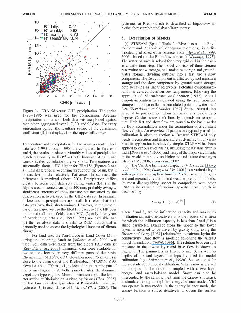
Temperature and precipitation for the years present in bothdata sets (1993 through 1995) are compared. In Figures 3and 4, the results are shown. Monthly values of precipitationmatch reasonably well (R2 = 0.73), however at daily andweekly scales, correlations are very low. Temperatures arestructurally about 1.5!C higher for ERA15d (Figures 2 and4). This difference is occurring throughout the basin, but itis smallest in the relatively flat areas. In summer, thedifference is maximal (about 2!C). Precipitation differsgreatly between both data sets during winter (DJF) in theAlpine area, in some areas up to 200 mm, probably owing tosignificant amounts of snow that are not measured by theobservation network used in the CHR data set. In summer,differences in precipitation are small. It is clear that bothdata sets have their shortcomings. However, in the remain-der of this paper we use the ERA15d because (1) CHR doesnot contain all input fields to run VIC, (2) only three yearsof overlapping data (i.e., 1993–1995) are available and(3) the reanalysis data is similar to RCM output that isgenerally used to assess the hydrological impacts of climatechange.[7] For land use, the Pan-European Land Cover Moni-

toring and Mapping database [Mucher et al., 2000] wasused. Soil data were taken from the global FAO data set[Reynolds et al., 2000]. Lysimeter data were available fortwo stations located in very different parts of the basin.Rheindahlen (51.16!N, 6.33, elevation about 75 m.a.s.l.) isclose to the basin outlet and Rietholzbach (47.38!N, 8.99,elevation about 700 m.a.s.l.) is located in the Alpine part ofthe basin (Figure 1). At both lysimeter sites, the dominantvegetation type is grass. More information about the lysim-eter station at Rheindahlen is given by Xu and Chen [2005].Of the four available lysimeters at Rheindahlen, we usedlysimeter 3, in accordance with Xu and Chen [2005]. The

lysimeter at Rietholzbach is described at http://www.ia-c.ethz.ch/research/rietholzbach/instruments/.

3. Description of Models

[8] STREAM (Spatial Tools for River basins and Envi-ronment and Analysis of Management options), is a dis-tributed, grid based water-balance model [Aerts et al., 1999,2006], based on the Rhineflow approach [Kwadijk, 1993].The water balance is solved for every grid cell in the basinat a daily time step. The model consists of three storagereservoirs: snow storage, soil moisture storage and ground-water storage, dividing outflow into a fast and a slowcomponent. The fast component is affected by soil moisturestorage and the slow component by ground water storage,both behaving as linear reservoirs. Potential evapotranspi-ration is derived from surface temperature, following theapproach of Thornthwaite and Mather [1957]. Actualevapotranspiration is calculated using the soil moisturestorage and the so-called ‘accumulated potential water loss’[see Thornthwaite and Mather, 1957]. Snow accumulationis equal to precipitation when temperature is below zerodegrees Celsius, snow melt linearly depends on tempera-ture. Both fast and slow flow are routed to the basin outletby flow accumulation under the assumption of a constantflow velocity. An overview of parameters typically used forcalibration is given in section 4. Because STREAM onlyneeds precipitation and temperature as dynamic input varia-bles, its application is relatively simple. STREAM has beenapplied to various river basins, including the Krishna river inIndia [Bouwer et al., 2006] andmany of themajor catchmentsin the world in a study on Holocene and future discharges[Aerts et al., 2006; Ward et al., 2007].[9] The Variable Infiltration Capacity (VIC) model [Liang

et al., 1994, 1996; Liang and Xie, 2001] is a variable-layersoil-vegetation-atmosphere transfer (SVAT) scheme for gen-eral and regional circulation and weather prediction models.Its most distinguishing aspect in comparison with otherLSM is its variable infiltration capacity curve, which isdescribed by

I " Im 1! 1! A# $1=bh i

#1$

where I and Im are the infiltration capacity and maximuminfiltration capacity, respectively. A is the fraction of an areafor which the infiltration capacity is less than I and b is ashape parameter. Drainage from the upper to the lowerlayers is assumed to be driven by gravity only, using theBrooks and Corey [1964] relationship to estimate hydraulicconductivity. Base flow is modeled following the ARNOmodel formulation [Todini, 1996]. The relation between soilmoisture in the lowest layer and base flow is shown inFigure 5. The parameters in Figure 5 and b, as well asdepths of the soil layers, are typically used for modelcalibration [e.g., Lohmann et al., 1998a]. See section 4 formore details about model calibration. When snow is presenton the ground, the model is coupled with a two layerenergy- and mass-balance model. Snow can also beintercepted by the canopy, melt from the canopy snowpackis simulated using a simplified energy balance model. VICcan operate in two modes: in the energy balance mode, theenergy balance is solved iteratively to obtain the surface

Figure 3. ERA15d versus CHR precipitation. The period1993–1995 was used for the comparison. Averageprecipitation amounts of both data sets are plotted againsteach other, aggregated over 1, 7, 30, and 90 days. For everyaggregation period, the resulting square of the correlationcoefficient (R2) is displayed in the upper left corner.

4 of 14

W01418 HURKMANS ET AL.: WATER BALANCE VERSUS LAND SURFACE MODEL W01418

temperature, whereas in the water balance mode, surfacetemperature is assumed equal to air temperature. In bothmodes, potential evapotranspiration is calculated using thePenman-Monteith equation. In the energy balance mode, atime step of 3 hours is used, in correspondence withavailability of forcing data, whereas in water balance modethe model is integrated at a daily time step. Thereforesimulation times are drastically reduced compared to the fullmode.[10] Routing of surface runoff and base flow from all

models is done by the algorithm developed by Lohmann etal. [1996], which has been applied in combination with VICby Lohmann et al. [1998a, 1998b]. The sum of base flowand runoff from the models is convoluted with a normalizedimpulse response function, based on the linearized St.Venant equation [e.g., Troch et al., 1994], assuming thatwater from each grid cell flows into the channel in thesteepest direction to one of its eight neighbors.

4. Model Calibration

[11] All three models were calibrated using daily ob-served streamflow at Lobith for the year 1993. Only one

year was used to limit the amount of calibration time.Because 1993 contains a relatively dry summer, as well asa near flood event, it was considered representative for thetotal period. Because no data were available before 1993

Figure 5. Relationship between soil moisture content inthe lowest layer Wc and base flow D. Dm representsmaximum base flow velocity, Ds is a fraction of Dm, and Ws

is a fraction of Wc. The point (Ws, Ds) represents the pointwhere the curve becomes nonlinear.

Figure 4. Spatial patterns of temperature and precipitation from the CHR and ERA15d data sets. Mapsshowing (top row) temperature and (bottom row) precipitation. In the left four maps, average differencesbetween the data sets are shown for two seasons: winter (DJF) and summer (JJA). In the right four maps,annual mean temperature and annual cumulative precipitation are plotted. Positive values indicate anoverestimation of ERA15d, with respect to CHR. Averages are computed from the years 1993 through1995.

W01418 HURKMANS ET AL.: WATER BALANCE VERSUS LAND SURFACE MODEL

5 of 14

W01418

and, on the basis of preceding streamflow observations,conditions and model storages in October 1993 wereassumed to be similar to January 1993, the model states(i.e., moisture contents, snow pack) of October 1993 wereused to initialize all model simulations in January 1993.STREAM was calibrated using a built-in optimizationroutine, iteratively changing the parameters one-at-a-timeand minimizing the mean absolute difference betweenobserved and simulated streamflow, and then fine-tunedmanually. Four parameters were optimized following, forexample, Aerts et al. [2006]: a factor C to adjust the land-use-dependent crop factor that defines potential evapotrans-piration for different land use types, a depletion factor D forthe groundwater reservoir, a factor X to separate betweendirect runoff and groundwater recharge, and finally aparameter H that defines the relation between temperatureand reference evapotranspiration. To calibrate VIC, sevenparameters influencing the shape of the hydrograph and thetotal outflow volume were subjected to a sensitivity analy-sis. On the basis of this analysis, the depth of the (very thin)upper layer and the base flow parameter Ws (see Figure 5)appeared to have no influence on the resulting hydrographand were therefore left out of the calibration procedure tosave computation time. Parameters influencing potentialevapotranspiration, differing per vegetation type, were leftat their default values. The resulting parameters for optimi-zation are, similar to former applications [Lohmann et al.,1998a; Liang et al., 1994]: Dm and Ds to define the relationbetween base flow and soil moisture in the lowest layer (seeFigure 5), the shape parameter b in equation (1) and thedepths of the lower two layers d2 and d3. Because theseparameters are not transferable between the full and energymodes, VIC was recalibrated for the water balance mode,

using the same parameters. For optimizing the objectivefunction O a power transformation was used to balancesensitivity to peak flows and low flows. The objectivefunction can be written as

O " 1

N

X

N

i"1

Qlobs;i ! Ql

sim;i

! "

l#2$

where N is the number of time steps and Qobs and Qsim areobserved and simulated discharge respectively. Both areraised to the power l which is taken as 0.3 in this studybecause this gives an optimal balance between sensitivity topeak and low flows [Misirli et al., 2003].[12] To calibrate the models to a comparable level, all

parameters were kept uniform in space. To enable stream-flow comparison at other streamflow gauges than Lobithonly, STREAM surface runoff and base flow were routedusing the VIC routing algorithm. Figure 6 shows dailystreamflow in 1993 for VIC (both modes) and STREAMcompared to observations. For STREAM, two hydrographsare plotted: one obtained by routing using the originalSTREAM routing scheme (STREAM1) and one obtainedby routing using the VIC algorithm (STREAM2). The VICrouting algorithm tends to slightly delay runoff peakscompared to the original STREAM routing scheme. Varyingcelerity and diffusivity in the VIC routing algorithm did notchange this behavior. To remove the influence of the routingalgorithm that was used, hereafter 10-day averaged stream-flow values are evaluated at gauging stations other thanLobith. For analyses at the Lobith gauging station thatrequire daily streamflow (such as peak flow analyses), daily

Figure 6. Simulated and observed daily streamflow at Lobith for the calibration period (1993). VIC-WB represents the VIC simulation in the water balance mode, STREAM1 represents the results ofSTREAM internal routing used for calibration, and STREAM2 represents result of STREAM outputrouted by the VIC algorithm. The top plot of the inset shows the difference between ERA15d and CHRprecipitation (positive shows higher ERA15d), and the bottom plot of the inset shows simulated minusobserved monthly discharge for VIC (solid line) and STREAM1 (dash-dotted line).

6 of 14

W01418 HURKMANS ET AL.: WATER BALANCE VERSUS LAND SURFACE MODEL W01418

discharge obtained by the original STREAM routing algo-rithm is used for the STREAM simulations.[13] In Table 2, correlation coefficients (r), Nash-Sutcliffe

modeling efficiencies (E) [Nash and Sutcliffe, 1970] andrelative volume errors (RVE) for both the calibration andvalidation period are shown for daily discharge at Lobith.During the calibration period, STREAM performs better:E = 0.47 for STREAM, whereas E = 0.29 for VIC. Also rfor STREAM is higher (0.77) than for VIC (0.67). Asmentioned before and can be seen in Table 3, routingSTREAM output with the VIC algorithm reducesSTREAM’s performance drastically for daily discharge.The performance of VIC-WB is in between VIC andSTREAM with E = 0.39 and r = 0.71. Changing parametersin STREAM has a more direct effect on the resultinghydrograph, whereas in VIC a more extensive calibrationincluding more parameters would have been necessary toobtain similar results. For VIC-WB, changing the calibra-tion parameters has a larger effect compared to VIC yieldingbetter results. The rather poor results in the calibrationperiod in terms of Nash-Sutcliffe values are partly explainedby an overestimation of streamflow in summer. The inset ofFigure 6 shows that this was mainly caused by too highprecipitation in the ERA15d data set.[14] To investigate the influence of this biased forcing

data, VIC and STREAM were also forced by precipitation

from CHR. The other required forcing variables are fromERA15d, because they were not available in the CHR dataset. Figure 7 shows daily simulated discharges at Lobith forVIC and STREAM, where precipitation from both ERA15dand CHR is used, for the period 1993 through 1995, i.e., theperiod where both forcing data sets overlap. Note that themodels were not recalibrated for the CHR data set. Itappears that both models improve drastically when forcedwith the CHR precipitation: for VIC, E increases from 0.45to 0.59, for STREAM from 0.47 to 0.56. The correlationcoefficient on the other hand increases especially forSTREAM; from 0.81 to 0.92, whereas for VIC this increaseis much less: from 0.79 to 0.83. In the summer of 1993, VICwith CHR precipitation now simulates discharge very well,while STREAM underestimates discharge, as was to beexpected because the model was not recalibrated.

5. Model Validation

[15] The calibrated models are evaluated using data fromthe remaining period, i.e., 1994 to 2003. Table 3 shows r,E and RVE for 10-day averaged discharge for all stream-flow gauges in this period. During the validation period, VIC(r = 0.74, E = 0.31) and VIC-WB (r = 0.70, E = 0.40)slightly improve with respect to the calibration period,whereas r (0.63) and E (0.14) for STREAM decrease. Whenconsidering all streamflow gauges, correlation coefficientsand most E values are higher for VIC, although the latter arehigher for STREAM at Maxau and Rockenau. For VIC-WB,correlation coefficients are mostly intermediate. E, however,is often higher for VIC-WB compared to VIC, suggesting amore efficient calibration procedure when VIC is run inwater balance mode. For Maxau and Rockenau, E values forall models are negative. The mountainous nature of theseareas, where complex terrain and snow processes play alarger role than in other parts of the basin, make these areasdifficult to simulate for all models. It is assumed, however,that applying distributed parameters in all models wouldprobably significantly improve their performances. FromFigure 8, it appears that these are also the areas where peakflows are most severely overestimated by VIC, which issurprising given the topography of the area where layerthicknesses are most likely overestimated by VIC, becauseof the uniform layer depths. There are three possibleexplanations for these overestimations. First, some large

Table 2. Statistics of Daily Streamflow at the Basin Outlet(Lobith) for Both the Calibration Period (1993) and the ValidationPeriod (1994–2003)a

VIC VIC-WB STREAM1 STREAM2

Calibration Periodr 0.68 0.71 0.77 0.66E 0.29 0.39 0.47 0.31RVE, % 7.49 6.82 !22.77 !21.36

Validation Periodr 0.74 0.70 0.73 0.63E 0.31 0.40 0.21 0.14RVE, % 8.04 !1.35 29.09 !25.05

aCorrelation coefficients (r), Nash-Sutcliffe modeling efficiencies (E),and volumetric errors of simulated discharge relative to observed discharge(RVE) are shown.

Table 3. Statistics of 10-Day Streamflow for Five Tributaries of the Rhine (Lahn, Main, Mosel, Neckar, and Ruhr) and Three LocationsAlong the Main Rhine Branch (Maxau, Andernach, and Lobith)a

r E RVE, %

VIC VIC-WB STREAM VIC VIC-WB STREAM VIC VIC-WB STREAM

Ruhr 0.74 0.71 0.67 0.52 0.49 0.38 0.80 !7.37 !26.28Lahn 0.69 0.68 0.62 0.35 0.45 0.19 !35.23 2.06 !47.17Mosel 0.74 0.78 0.67 0.47 0.53 0.28 !26.67 !19.89 !39.10Main 0.76 0.75 0.66 0.41 0.27 0.24 !2.88 34.66 !8.00Neckar 0.73 0.74 0.63 !0.80 !0.33 !0.13 17.89 26.67 !22.13Maxau 0.70 0.67 0.53 !0.34 !0.02 !0.32 16.42 !5.71 !23.21Andernach 0.76 0.71 0.63 0.39 0.42 0.03 2.34 !4.58 !27.82Lobith 0.79 0.75 0.68 0.39 0.49 0.18 8.14 !1.24 !24.87

aFor gauge locations, see Figure 1. Correlation coefficients (r), Nash-Suthcliffe modeling efficiencies (E), and volumetric errors of simulated dischargerelative to observed discharge (RVE) are shown for the full (with energy balance) VIC simulation, the water balance mode simulation (VIC-WB) andSTREAM.

W01418 HURKMANS ET AL.: WATER BALANCE VERSUS LAND SURFACE MODEL

7 of 14

W01418

surface reservoirs are present in the area, of which LakeConstance (north east Switzerland, see also Figure 1) is thelargest with a storage volume of 55 km3. These reservoirscan have a dampening effect on discharge and are not takeninto account in the models. Second, the snow model in VIC(see section 3) is not calibrated because no snowpack datawas available, leading to a possible overestimation of snowmelt. Third, the ERA15d data set may overestimateprecipitation in the periods corresponding to these peakflows, but no additional precipitation data is available toverify this. The fact that VIC also overestimates peak flowsat other gauges to a lesser degree, which can be seen inFigure 8 for a peak in early 1999, supports this explanation.In the STREAM simulation these peaks are much lessdistinct (Figure 8), which may be explained by the fact thatSTREAM is known to slightly underestimate snow meltbecause at pixels with very high elevations temperature doesnot exceed 0!C, causing snow to constantly accumulatewithout melting. During low-flow periods, all models un-derestimate streamflow frequently, although for STREAMthis is slightly more the case than for VIC and VIC-WB.[16] For Lobith, daily values are analyzed more closely

through a peak flow analysis. Because 1993 was a nearflood year in the Rhine basin, both the calibration andvalidation periods are taken into account for this analysis.Table 4 shows the five highest daily discharges and the fivelowest monthly discharges, as observed and simulated atLobith. In addition, two near-floods (1993 and 1995) andthe extreme low-flow period of 2003 are plotted in Figure 9.In Figure 9, a time window of 20 days before and after theday of the peaks in 1993 and 1995 is shown. For the low-flow period of 2003 the detailed window is 180 days. Alsothe average discharge during those periods is displayed. Themagnitude of the 1993 event is simulated accurately by VICwith a difference of only 1.5% in the peak flow, but the peakis delayed by about 2 days, as is the case for nearly all peaksshown in Table 4. All models significantly underestimatethe magnitude of the 1995 event, especially STREAM with

more than 40%. Because the 1993 event is the onlysignificant peak in the calibration period, it influenced thecalibration procedure. The accurate simulation of this eventis, therefore, not surprising. For the low-flow period in thesummer of 2003, all models, especially VIC-WB, overesti-mate average flow levels and show more variability than theobservations. Because allmodels showa similar pattern this ismost likely caused by overestimated precipitation events inthe forcing data, although in this period no additional precip-itation data is available to verify this possible explanation.[17] In Figure 10 extreme flows are further analyzed

through their return periods. A log-Pearson type III distribu-tion is fitted on the basis of peak discharges to compare andextrapolate extreme peak flows more easily. To fit the distri-bution, frequency factors were taken from Table 7.7 of Haan[1977]. Peaks were selected using the peak-over-threshold(POT) approach, where the threshold was defined as thedouble of the long-term mean, with the constraint that peaksshould be at least 20 days apart from each other to maintainindependency. This resulted in, on average per simulation,just below two peaks per year. Return periods and Pearsonfits were based on maximum 10-day discharges for theeight evaluated streamflow gauges, to remove the influ-ence of streamflow routing, as was discussed in section 4.For Lobith, the same is shown for maximum dailydischarges. As can also be seen in Figure 8, VIC over-estimates peak flows especially for Maxau and Rockenau,while for small tributaries, Kalkofen and Hattingen, allmodels underestimate them. For the most downstreamgauging stations, Andernach and Lobith, both data andPearson fits differ strongly for lower return times, whereasfor high return times (up to 11 years in case of data points),models and observations agree quite well. For Maxau,however, the range in simulated and fitted discharges keepsincreasing toward higher return times, although for VIC-WB the fit almost coincides with the fit based on observa-tions for Maxau. However, modeling efficiencies for allmodels including VIC-WB are negative, as was mentioned

Figure 7. Discharge as simulated by (top) VIC and (bottom) STREAM, with both ERA15d and CHRprecipitation, for the period 1993 through 1995. Model efficiencies (E) and correlation coefficients (r) arealso shown.

8 of 14

W01418 HURKMANS ET AL.: WATER BALANCE VERSUS LAND SURFACE MODEL W01418

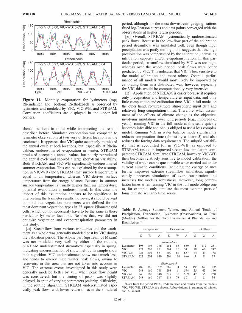
before. Correlations are also relatively low at this gauge:0.70, 0.67 and 0.53 for VIC, VIC-WB and STREAMrespectively (see Table 3). Neither of the models performsvery well for this part of the basin, mainly because of threereasons: first, the terrain is very complex, leading to localdifferences in precipitation and radiation that are not takeninto account in the models. Second, although all modelsaccount for snow storage and melt to some degree, snow(melt) and glaciers play an important role in this area, whichfurther complicates the situation. Third, there are surfacewater reservoirs present in this area that are not accountedfor in the models. These surface reservoirs explain the factthat VIC overestimates peak flows for this area, especiallypeaks in 1998 and 1999 that are overestimated by VICoriginate in the part upstream of Maxau. For gauges near theoutlet of the basin (Lobith and Andernach), STREAM, andto a lesser degree also VIC-WB, underestimate the relativelylow maxima. The fitted lines converge toward higher returnperiods, however. For these gauges, VIC simulates theextremes quite well: the fitted lines practically coincide,only for very high return times the fitted lines slightlydiverge.[18] Figure 11 shows monthly evaporation as observed at

the two lysimeters at Rheindahlen and Rietholzbach andsimulated by VIC and STREAM. VIC accurately mimicsthe annual cycle at both lysimeters, hence the high

correlations compared to STREAM: 0.97 and 0.80 versus0.71 and 0.42 for Rietholzbach and Rheindahlen respec-tively. Again, VIC-WB performs intermediate with 0.63(Rheindahlen) and 0.83 (Rietholzbach). VIC simulatessummer evaporation quite well for both locations, but under-estimates winter evaporation, especially for Rheindahlen.For STREAM, modeled evaporation shows more variabilityand in winter evaporation is mostly overestimated. VIC-WBalso shows more variability but simulates average winterevaporation very well at both lysimeters (Table 5). BothSTREAM and VIC-WB underestimate summer evapora-tion. The smaller amplitude in evaporation cycle for VIC-WB and STREAM can be explained by the fact both modelsassume the surface temperature to be equal to the airtemperature, while VIC computes the surface temperaturefrom the energy balance. In summer, the surface is warmerthan the air (giving higher evaporation then when airtemperature is used) while in winter the opposite is true.This difference is captured by VIC but neglected by VIC-WBand STREAM. When total annual evaporation is consid-ered, VIC simulated evaporation in Rheindahlen is too low,mainly owing to the underestimation in winter, whileevaporation simulated by STREAM and VIC-WB is com-parable to observations. VIC’s underestimation in wintermay partly be explained by vegetation parameters that donot completely correspond to the exact conditions at the

Figure 8. Time series of monthly discharge as observed, and simulated by VIC, VIC-WB, andSTREAM at eight gauges in the Rhine basin. Monthly correlation coefficients r with respect toobservations are also shown in each plot.

W01418 HURKMANS ET AL.: WATER BALANCE VERSUS LAND SURFACE MODEL

9 of 14

W01418

lysimeter location, an effect that is masked by the ‘damp-ened’ annual cycle in the other models that was mentionedbefore. Another partial explanation can be in VIC’s snowmodel that was not specifically calibrated and may contrib-ute to the underestimated evaporation in winter. In addition,in Table 5 it can be seen that observed precipitation inRietholzbach is higher than it is at the correspondinglocation in the ERA15d data set, however, practically all

extra rainfall leaves the lysimeter as outflow, hence evapo-ration is still similar to simulated values.

6. Discussion and Conclusions

[19] We applied three models (VIC, VIC-WB andSTREAM) with the same meteorological forcing to theRhine basin and evaluated them using observed streamflow

Table 4. Peak and Low Flows at the Outlet of the Basin (Lobith)a

Peak Flows 31 January 1995 25 December 1993 4 November 1998 7 January 2003 28 March 2001

Max Qobs, m3/s 11,775 11,034 9410 9366 8666

Dvic, % !26.7 1.5 !35.1 !15.5 12.5Dvic!wb, % !21.6 11.2 !41.2 !41.4 !13.9Dstream, % !44.5 !14.8 !53.2 !55.2 !38.6tvic, days 2 2 6 6 4tvic!wb, days 1 2 1 3 3tstream, days !2 0 !1 4 0

Low Flows September 2003 November 1997 August 1998 September 1996 March 1993

Max Qobs, m3/s 958 1153 1158 1297 1338

Dvic, % 38.8 51.4 37.9 6.1 !23.8Dvic!wb, % 46.6 4.9 41.0 !6.7 17.8Dstream, % 40.7 !10.7 32.8 2.0 !59.0

aThe five highest daily peaks and the five lowest monthly flows from both the calibration and validation period are shown. From top to bottom: observedpeak discharge, simulated peak discharge by VIC, VIC-WB and STREAM, relative difference between simulations and observations for VIC, VIC-WB,and STREAM (positive values denote higher simulated values), and, only for peak flows, the time lag (t) of the peaks for all models. A positive time lagdenotes a delay in the simulation of the peak.

Figure 9. Observed and simulated daily hydrographs at Lobith, zoomed in to three extreme events inthe Rhine basin. (top) Near-floods of (left) 1993 and (right) 1995. (bottom) Low-flow period of 2003. Forthe peak flows a time window of 20 days before and after the observed maximum is shown; for the lowflow the detailed window is 180 days. The text within the plots displays the average discharge over thedisplayed period for all simulations.

10 of 14

W01418 HURKMANS ET AL.: WATER BALANCE VERSUS LAND SURFACE MODEL W01418

and measured evaporation data from two lysimeters. Allmodels were calibrated to a similar level, using data fromonly one representative year and keeping calibration param-eters uniform over the catchment. STREAM is a simple,relatively easy to calibrate model, needing only temperatureand precipitation as input, while VIC is more physicallybased and requires more parameters and computation time.VIC-WB is an intermediate in that it does not solve thecoupled water and energy balance but does account for, forexample, subgrid variability. Streamflow at Lobith wassimulated best by STREAM during the calibration period.During the validation period, however, the performance ofSTREAM decreased while VIC and VIC-WB improved,indicating a smaller dependence on calibration for VIC:

while only calibrated to a limited extent, results in thevalidation period where still acceptable. It should be keptin mind that this relatively simple calibration process stillwas much more computationally demanding than theSTREAM calibration. Especially for the calibration period,most of the difference between observed and simulateddischarge for all models were explained by differencesbetween meteorological (reanalysis) forcing data and ob-served data for the same period. Because only three years ofoverlapping data and not all the input fields required to runVIC were available as observations, and because the re-analysis data is similar to RCM outputs that are generallyused to assess the hydrological impacts of climate change,we used the reanalysis data set to drive the models. This

Figure 10. Peak flows selected using a peak-over-threshold approach and their return periods, as well asa log-Pearson type III distribution fitted through the data points. (top) Eight plots showing the fits at theeight evaluated streamflow gauges, where STREAM is routed using the VIC routing algorithm, based on10-day discharges. (bottom) The same, only for Lobith, based on daily flows, where STREAM is routedusing the original STREAM algorithm.

W01418 HURKMANS ET AL.: WATER BALANCE VERSUS LAND SURFACE MODEL

11 of 14

W01418

should be kept in mind while interpreting the resultsdescribed before. Simulated evaporation was compared tolysimeter observations at two very different locations in thecatchment. It appeared that VIC quite accurately mimickedthe annual cycle at both locations, but, especially at Rhein-dahlen, underestimated evaporation in winter. STREAMproduced acceptable annual values but poorly reproducedthe annual cycle and showed a large short-term variability.Both STREAM and VIC-WB significantly underestimatedsummer evaporation. This can be explained by the assump-tion in VIC-WB (and STREAM) that surface temperature isequal to air temperature, whereas VIC derives surfacetemperature from the energy balance. Because in summersurface temperature is usually higher than air temperature,potential evaporation is underestimated. In this case, theimpact of this assumption appears to be significant. Ininterpreting the lysimeter results, however, it should be keptin mind that vegetation parameters were defined for themost dominant vegetation types in 25 square kilometer gridcells, which do not necessarily have to be the same as theseparticular lysimeter locations. Besides that, we did notoptimize vegetation and evapotranspiration parameters inthis study.[20] Streamflow from various tributaries and the catch-

ment as a whole was generally modeled best by VIC duringthe validation period. The Alpine part (upstream of Maxau)was not modeled very well by either of the models,STREAM underestimated streamflow especially in spring,indicating underestimation of snow melt by its simple snowmelt algorithm. VIC underestimated snow melt much less,and tends to overestimate winter peak flows, owing toreservoirs in this area that are not taken into account inVIC. The extreme events investigated in this study weregenerally modeled better by VIC when peak flow heightwas considered, but the timing of peaks was slightlydelayed, in spite of varying parameters (celerity, diffusivity)in the routing algorithm. STREAM underestimated espe-cially peak flows with lower return times in the simulated

period, although for the most downstream gauging stationsfitted log-Pearson curves and data points converged with theobservations at higher return periods.[21] Overall, STREAM systematically underestimated

peak flows. Because in the low-flow part of the calibrationperiod streamflow was simulated well, even though inputprecipitation was partly too high, this suggests that the highprecipitation was compensated by the calibration, increasinginfiltration capacity and/or evapotranspiration. In this par-ticular period, streamflow simulated by VIC was too high,whereas over the whole period, peak flows were betterpredicted by VIC. This indicates that VIC is less sensitive tothe model calibration and more robust. Overall, perfor-mance of all models would most likely be improved bycalibrating them in a distributed way, however, especiallyfor VIC this would be computationally very intensive.[22] Application of STREAM is easier because it requires

only precipitation and temperature as input data, and onlylittle computation and calibration time. VIC in full mode, onthe other hand, requires more atmospheric input data andrelatively long computation times. Therefore, when assess-ment of the effects of climate change is the objective,involving simulations over long periods (e.g., hundreds ofyears), running VIC in the full mode at this scale quicklybecomes infeasible and one is obliged to use a less complexmodel. Running VIC in water balance mode significantlyreduces computation time (almost by a factor 5) and alsoreduces the forcing data requirements. The subgrid variabil-ity that is accounted for in VIC-WB, as opposed toSTREAM, results in improved streamflow simulation com-pared to STREAM. Similar to STREAM, however, VIC-WBthen becomes relatively sensitive to model calibration, thevalidity of which can be questionable when carried out undercurrent climatic conditions. Including the energy balancefurther improves extreme streamflow simulation, signifi-cantly improves simulation of evapotranspiration andincreases the model’s robustness. However, long compu-tation times when running VIC in the full mode oblige oneto, for example, only simulate the most extreme parts oflong climate scenario time series.

Table 5. Average Summer, Winter, and Annual Totals ofPrecipitation, Evaporation, Lysimeter (Observations), or Pixel(Models) Outflow for the Two Lysimeters at Rheindahlen andRietholzbacha

Precipitation Evaporation Outflow

S W A S W A S W A

RheindahlenLysimeter 198 198 766 251 85 659 4 112 231VIC 221 205 851 264 16 541 18 66 242VIC-WB 221 204 851 209 84 657 24 49 188STREAM 221 204 849 209 130 686 5 8 37

RietholzbachLysimeter 487 386 1578 269 31 541 199 340 1035VIC 248 160 748 298 6 574 25 43 140VIC-WB 248 160 748 217 33 509 42 55 230STREAM 248 160 747 216 78 591 8 8 36

aData from the period 1993–1998 are used and results from the modelsVIC, VIC-WB, STREAM are shown. Abbreviations: S, summer; W, winter;and A, annual.

Figure 11. Monthly evaporation for lysimeters (top)Rheindahlen and (bottom) Rietholzbach as observed bylysimeters and modeled by VIC, VIC-WB, and STREAM.Correlation coefficients are displayed in the upper leftcorners.

12 of 14

W01418 HURKMANS ET AL.: WATER BALANCE VERSUS LAND SURFACE MODEL W01418

[23] Acknowledgments. This research was supported by the EuropeanCommission through the FP6 Integrated Project NeWater (http://www.newater.info) and the BSIK ACER project under the Dutch ClimateChanges Spatial Planning programme. Daniela Jacob and Eva Mazurkewitzfrom the Max Planck Institut fur Meteorologie are kindly acknowledged forproviding meteorological data, and we gratefully acknowledge Reto Stocklifrom ETH, Zurich for providing the lysimeter data. Finally, we thankHendrik Buiteveld from RIZA, Arnhem, Netherlands, for providing thestreamflow observations and the two anonymous reviewers for theirconstructive and helpful comments.

ReferencesAerts, J. C. J. H., M. Kriek, and M. Schepel (1999), STREAM (SpatialTools for River basins and Environment and Analysis of Managementoptions): ‘Set up and requirements’, Phys. Chem. Earth, 24, 591–595.

Aerts, J. C. J. H., H. Renssen, P. J. Ward, H. de Moel, E. Odada, L. M.Bouwer, and H. Goosse (2006), Sensitivity of global river dischargesunder Holocene and future climate conditions, Geophys. Res. Lett., 33,L19401, doi:10.1029/2006GL027493.

Beersma, J. J., T. A. Buishand, and R. Wojcik (2001), Rainfall generator forthe Rhine basin: Multi-site simulation of daily weather variables bynearest-neighbour resampling, in Generation of HydrometeorologicalReference Conditions for the Assessment of Flood Hazard in Large RiverBasins, edited by P. Krahe and D. Herpertz, pp. 69–77, Int. Comm. forHydrol., Lelystad, Netherlands.

Bergstrom, S., and A. Forsman (1973), Development of a conceptual de-terministic rainfall-runoff model, Nord. Hydrol., 4, 147–170.

Bouwer, L. M., J. C. J. H. Aerts, P. Droogers, and A. J. Dolman (2006),Detecting the long-term impacts from climate variability and increasingwater consumption on runoff in the Krishna river basin (India), Hydrol.Earth Syst. Sci., 3(4), 1249–1250.

Brooks, R. H., and A. T. Corey (1964), Hydraulic properties of porousmedia, Hydrol. Pap. 3, Civ. Eng. Dep., Colo. State Univ., Fort Collins.

Buishand, T. A., and G. Lenferink (2004), Estimation of future dischargesof the river Rhine in the SWURVE project, technical report, R. Neth.Meteorol. Inst. (KNMI), De Bilt, Netherlands.

Christensen, N. S., A. W. Wood, N. Voisin, D. P. Lettenmaier, and R. N.Palmer (2004), The effects of climate change on the hydrology and waterresources of the Colorado river basin, Clim. Change, 62, 337–363.

Dai, Y., et al. (2003), The Common Land Model, Bull. Am. Meteorol. Soc.,84, 1013–1023.

de Wit, M. J. M., B. van den Hurk, P. M. M. Warmerdam, P. J. J. F.Torfs, E. Roulin, and W. P. A. van Deursen (2007), Impact of climatechange on low-flows in the river Meuse, Clim. Change, 82, 351–372,doi:10.1007/s10584-006-9195-2.

Dibike, Y. B., and P. Coulibaly (2005), Hydrologic impact of climatechange in the Saguenay watershed: Comparison of downscaling meth-ods and hydrologic models, J. Hydrol., 307, 145–163, doi:10.1016/j.hydrol.2004.10.012.

Eberle, M., H. Buiteveld, J. Beersma, P. Krahe, and K. Wilke (2002),Estimation of extreme floods in the river Rhine basin by combiningprecipitation-runoff modelling and a rainfall generator, in Proceedings ofthe International Conference on Flood Estimation, edited byM. Spreaficoet al., pp. 459–467, Int. Comm. for the Hydrol. of the Rhine Basin (CHR),Lelystad, Netherlands.

Famiglietti, J. S., and E. F. Wood (1994), Multi-scale modeling of spatially-variable water and energy balance processes, Water Resour. Res., 30,3061–3078.

Haan, C. T. (1977), Statistical Methods in Hydrology, Iowa State Univ.Press, Ames.

Jacob, D. (2001), A note to the simulation of the annual and inter-annualvariability of the water budget over the Baltic Sea drainage basin,Meteorol. Atmos. Phys., 77, 61–73.

Kleinn, J., C. Frei, J. Gurtz, D. Luthi, P. L. Vidale, and C. Schar (2005),Hydrologic simulations in the Rhine basin driven by a regional climatemodel, J. Geophys. Res., 110, D04102, doi:10.1029/2004JD005143.

Koster, R. D., M. J. Suarez, A. Ducharne, M. Stieglitz, and P. Kumar(2000), A catchment-based approach to modeling land surface processesin a general circulation model: 1. Model structure, J. Geophys. Res.,105(D20), 24,809–24,822.

Kwadijk, J. (1993), The impact of climate change on the discharge of theriver Rhine, Ph.D. thesis, Univ. of Utrecht, Utrecht, Netherlands.

Liang, X., and Z. Xie (2001), A new surface runoff parameterization withsubgrid-scale soil heterogeneity for land surface models, Adv. WaterResour., 24, 1173–1193.

Liang, X., D. P. Lettenmaier, E. F. Wood, and S. J. Burges (1994), A simplehydrologically based model of land surface water and energy fluxes forgeneral circulation models, J. Geophys. Res., 99(D7), 14,415–14,458.

Liang, X., D. P. Lettenmaier, and E. F. Wood (1996), One-dimensionalstatistical dynamic representation of sub-grid spatial variability of pre-cipitation in the two-layer variable infiltration capacity model, J. Geo-phys. Res., 101(D16), 21,403–21,422.

Lindstrom, G., B. Johansson, M. Gardelin, and S. Bergstrom (1997),Development and test of the distributed HBV-96 hydrological model,J. Hydrol., 201, 272–288.

Lohmann, D., R. Nolte-Holube, and E. Raschke (1996), A large-scalehorizontal routing model to be coupled to land surface parameterizationschemes, Tellus, Ser. A, 48, 708–721.

Lohmann, D., E. Raschke, B. Nijssen, and D. P. Lettenmaier (1998a),Regional scale hydrology: I. Application of the VIC-2L model coupledto a routing model, Hydrol. Sci. J., 43(1), 131–141.

Lohmann, D., E. Raschke, B. Nijssen, and D. P. Lettenmaier (1998b),Regional scale hydrology: II. Application of the VIC-2L model to theWeser river, Germany, Hydrol. Sci. J., 43(1), 143–158.

Lohmann, D., et al. (2004), Streamflow and water balance intercomparisonsof four land surface models in the North American Land Data Assimila-tion System project, J. Geophys. Res., 109, D07S91, doi:10.1029/2003JD003517.

Middelkoop, H., et al. (2001), Impact of climate change on hydrologicalregimes and water resources management in the Rhine basin, Clim.Change, 49, 105–128.

Milly, P. C. D., K. A. Dunne, and A. Vecchia (2005), Global pattern oftrends in streamflow and water availability in a changing climate, Nature,438, 347–350.

Misirli, F., H. V. Gupta, S. Sorooshian, and M. Thiermann (2003), Bayesianrecursive estimation of parameter and output uncertainty for watershedmodels, in Calibration of Watershed Models, Water Sci. Appl. Ser.,vol. 6, edited by Q. Duan et al., pp. 113–124, AGU, Washington, D. C.

Mucher, S., K. Steinnocher, J.-L. Champeaux, S. Griguolo, K. Wester,C. Heunks, and V. van Katwijk (2000), Establishment of a 1-kmPan-European land cover database for environmental monitoring, inProceedings of the Geoinformation for All XIXth Congress of theInternational Society for Photogrammetry and Remote Sensing(ISPRS), edited by K. J. Beek and M. Molenaar, pp. 702–709,Int. Arch. Photogramm. Remote Sens. GITC, Amsterdam.

Nash, J. E., and I. V. Sutcliffe (1970), River flow forecasting throughconceptual models. Part I: A discussion of principles, J. Hydrol., 10,282–290.

Nijssen, B., D. P. Lettenmaier, X. Liang, S. W. Wetzel, and E. F. Wood(1997), Streamflow simulation for continental-scale river basins, WaterResour. Res., 33(4), 711–724.

Nijssen, B., G. M. O’Donnell, D. P. Lettenmaier, D. Lohmann, and E. F.Wood (2001), Predicting the discharge of global rivers, J. Clim., 14,3307–3323.

Pitman, A. J., et al. (1999), Key results and implications from Phase 1(c) ofthe project for intercomparison of land-surface parameterization schemes,Clim. Dyn., 15, 673–684.

Reynolds, C. A., T. J. Jackson, and W. J. Rawls (2000), Estimating water-holding capacities by linking the Food and Agriculture Organization soilmap of the world with global pedon databases and continuous pedotrans-fer functions, Water Resour. Res., 36(12), 3653–3662.

Sprokkereef, E. (2001a), Extension of the flood forecasting model FloRIJN,Tech. Rep. NCR 12-2001, Neth. Cent. for River Stud., Delft, Netherlands.

Sprokkereef, E. (2001b), Eine hydrologische Datenbank fur das Rheinge-biet, report, Int. Comm. for the Hydrol. of the Rhine Basin (CHR),Arnhem, Netherlands.

Thornthwaite, C. W., and J. R. Mather (1957), Instructions and tables forcomputing potential evapotranspiration and the water balance, Publ.Climatol. 10, pp. 183–247, Drexel Inst. of Technol., Philadelphia, Pa.

Todini, E. (1996), The ARNO rainfall-runoff model, J. Hydrol., 175, 339–382.

Troch, P. A., J. A. Smith, E. F. Wood, and F. P. de Troch (1994), Hydrologiccontrols of large floods in a small basin: Central Appalachian case study,J. Hydrol., 156, 285–309.

Ward, P. J., J. C. J. H. Aerts, H. de Moel, and H. Renssen (2007), Verifica-tion of a coupled climate-hydrological model against Holocene palaeo-hydrological records, Global Planet. Change, 57(3 – 4), 283 – 300,doi:10.1026/j.gloplacha.2006.12.002.

Wood, A. W., A. Kumar, and D. P. Lettenmaier (2005), A retrospectiveassessment of National Centers for Environmental Prediction climatemodel –based ensemble hydrologic forecasting in the western UnitedStates, J. Geophys. Res., 110, D04105, doi:10.1029/2004JD004508.

W01418 HURKMANS ET AL.: WATER BALANCE VERSUS LAND SURFACE MODEL

13 of 14

W01418

Wood, E. F., et al. (1998), The project for intercomparison of land-surfaceparameterization schemes (PILPS) Phase-2(c) Red-Arkansas River basinexperiment: 1. Experiment description and summary intercomparisons,Global Planet. Change, 19(1–4), 115–135.

Xu, C.-Y., and D. Chen (2005), Comparison of seven models for estimationof evapotranspiration and groundwater recharge using lysimeter measure-ment data in Germany, Hydrol. Processes, 19, 3717–3734, doi:10.1002/hyp.5853.

Zeng, X., M. Shaikh, Y. Dai, R. E. Dickinson, and R. Myneni (2002),Coupling of the Common Land Model to the NCAR Community ClimateModel, J. Clim., 15, 1832–1854.

!!!!!!!!!!!!!!!!!!!!!!!!!!!!J. C. J. H. Aerts and H. de Moel, Institute for Environmental Studies,

Vrije Universiteit, De Boelelaan 1085, NL-1081 HV, Amsterdam,Netherlands. ([email protected]; [email protected])

R. T. W. L. Hurkmans, Hydrology and Quantitative Water Management,Wageningen University, P.O. Box 47, NL-6700 AA, Wageningen,Netherlands. ([email protected])

P. A. Troch, Hydrology and Water Resources, University of Arizona,1133 East James E. Rogers Way, Tucson, AZ 85721, USA. ([email protected])

14 of 14

W01418 HURKMANS ET AL.: WATER BALANCE VERSUS LAND SURFACE MODEL W01418