Deutsche Geodätische Kommission der Bayerischen Akademie der Wissenschaften Reihe C Dissertationen Heft Nr. 725 Wassim Moussa Integration of Digital Photogrammetry and Terrestrial Laser Scanning for Cultural Heritage Data Recording München 2014 Verlag der Bayerischen Akademie der Wissenschaften in Kommission beim Verlag C. H. Beck ISSN 0065-5325 ISBN 978-3-7696-5137-9

Welcome message from author
This document is posted to help you gain knowledge. Please leave a comment to let me know what you think about it! Share it to your friends and learn new things together.
Transcript
Deutsche Geodätische Kommission
der Bayerischen Akademie der Wissenschaften
Reihe C Dissertationen Heft Nr. 725
Wassim Moussa
Integration of Digital Photogrammetry
and Terrestrial Laser Scanning
for Cultural Heritage Data Recording
München 2014
Verlag der Bayerischen Akademie der Wissenschaftenin Kommission beim Verlag C. H. Beck
ISSN 0065-5325 ISBN 978-3-7696-5137-9


Deutsche Geodätische Kommission
der Bayerischen Akademie der Wissenschaften
Reihe C Dissertationen Heft Nr. 725
Integration of Digital Photogrammetry
and Terrestrial Laser Scanning
for Cultural Heritage Data Recording
Von der Fakultät Luft- und Raumfahrttechnik und Geodäsie
der Universität Stuttgart
zur Erlangung der Würde eines
Doktors der Ingenieurwissenschaften (Dr.-Ing.)
genehmigte Abhandlung
Vorgelegt von
M.Sc. Wassim Moussa
aus Hama – Syrien
München 2014
Verlag der Bayerischen Akademie der Wissenschaftenin Kommission beim Verlag C. H. Beck
ISSN 0065-5325 ISBN 978-3-7696-5137-9

Adresse der Deutschen Geodätischen Kommission:
Deutsche Geodätische KommissionAlfons-Goppel-Straße 11 ! D – 80 539 München
Telefon +49 – 89 – 23 031 1113 ! Telefax +49 – 89 – 23 031 - 1283 / - 1100e-mail [email protected] ! http://www.dgk.badw.de
Hauptberichter: Prof. Dr.-Ing. habil. Dieter Fritsch
Mitberichter: Prof. Dr.-Ing. habil. Volker Schwieger
Tag der mündlichen Prüfung: 28.02.2014
Diese Dissertation ist auch auf dem Dokumentenserver der Universität Stuttgart veröffentlicht
<http://elib.uni-stuttgart.de/opus/doku/e-diss.php>
© 2014 Deutsche Geodätische Kommission, München
Alle Rechte vorbehalten. Ohne Genehmigung der Herausgeber ist es auch nicht gestattet,die Veröffentlichung oder Teile daraus auf photomechanischem Wege (Photokopie, Mikrokopie) zu vervielfältigen.
ISSN 0065-5325 ISBN 978-3-7696-5137-9
Contents 3
Contents
Contents ................................................................................................................................................ 3
Abstract .................................................................................................................................................. 8
Zusammenfassung ............................................................................................................................ 10
1 Introduction ..................................................................................................................................... 13
1.1 Motivation ................................................................................................................................. 13
1.2 Objectives ................................................................................................................................... 15
1.3 Thesis Outline ........................................................................................................................... 17
2 Generation of 3D Models - An Overview .................................................................................. 18
2.1 Data Acquisition and Geometric Reconstruction ................................................................ 18
2.1.1 Image-Based Approach .................................................................................................... 18
2.1.1.1 Image Acquisition ...................................................................................................... 19
2.1.1.2 Camera Orientation .................................................................................................... 20
2.1.1.3 Surface Points Recovering ......................................................................................... 22
2.1.2 Range-Based Approach .................................................................................................... 26
2.1.2.1 TLS Systems................................................................................................................. 27
2.1.2.2 Range Data Acquisition ............................................................................................. 34
2.1.2.3 Scan Registration ........................................................................................................ 35
2.1.3 Sensor Integration.............................................................................................................. 37
2.1.4 Georeferencing ................................................................................................................... 38
2.2 Surface Reconstruction ............................................................................................................ 38
2.3 Texture Mapping and Visualization ...................................................................................... 39
3 Building Reflectance and RGB Images ...................................................................................... 42
3.1 Imaging Laser Scanner Polar Coordinates ............................................................................ 42
3.2 Central Projection of Laser Scanner Cartesian Coordinates ............................................... 43
3.2.1 Defining 3D Virtual Camera Coordinate System ......................................................... 46
3.2.2 Improving Radiometry and Geometry ........................................................................... 48
3.2.3 Improving Keypoint Localization ................................................................................... 50
4 Contents
4 General Strategy for Digital Images and Laser Scanner Data Integration .......................... 51
4.1 Data Integration Using Accurate Space Resection Methods .............................................. 52
4.1.1 Experimental Evaluation .................................................................................................. 56
4.1.1.1 Evaluation of Correspondences ................................................................................ 57
4.1.1.2 Camera Orientation .................................................................................................... 59
4.1.1.3 Dense image matching ............................................................................................... 61
4.2 Data Integration Using Accurate Space Resection and SfM Reconstruction Methods... 63
4.2.1 Experimental Evaluation .................................................................................................. 65
4.2.1.1 Camera Orientation .................................................................................................... 66
4.2.1.2 Dense image matching ............................................................................................... 67
4.3 The Proposed General Workflow ........................................................................................... 69
4.3.1 Shifting the Principle Point of the Generated Images .................................................. 72
4.3.2 Advantages of the proposed approach .......................................................................... 72
4.3.2.1 Complementing TLS Point Clouds by Dense Image Matching ........................... 72
4.3.2.2 Automatic Registration of Point Clouds ................................................................. 74
4.3.3 Experimental Evaluation .................................................................................................. 74
4.3.3.1 Camera Orientation .................................................................................................... 74
4.3.3.2 Dense Image Matching .............................................................................................. 78
5 Target-Free Registration of Multiple Laser Scans .................................................................... 79
5.1 Target-Free Registration Using Accurate Space Resection Methods ................................ 79
5.1.1 Experimental Evaluation .................................................................................................. 85
5.1.1.1 Organizing Scans by Similarity ................................................................................ 85
5.1.1.2 Pairwise Registration ................................................................................................. 87
5.2 Target-Free Registration Based on Geometric Relationship of Keypoints ....................... 89
5.2.1 Experimental Evaluation .................................................................................................. 92
5.2.1.1 Organizing Scans by Similarity ................................................................................ 92
5.2.1.2 Pairwise Registration ................................................................................................. 92
5.3 Target-Free Registration Using SfM Reconstruction Method ............................................ 94
5.3.1 Experimental Evaluation .................................................................................................. 95
Contents 5
6 Recording Physical Models of Heritage ..................................................................................... 96
6.1 3D Surveying of the Hirsau Abbey Physical Model ............................................................ 97
6.1.1 TLS Data Acquisition and Processing ............................................................................ 97
6.1.2 Photogrammetric Data Acquisition and Processing .................................................... 97
6.1.3 Final Model ......................................................................................................................... 99
6.2 Summary.................................................................................................................................... 99
7 Case Studies .................................................................................................................................. 103
7.1 Data Acquisition ..................................................................................................................... 103
7.1.1 The Hirsau Abbey ........................................................................................................... 103
7.1.2 The Temple of Heliopolis ............................................................................................... 104
7.1.3 The Applied Sensors ....................................................................................................... 105
7.1.3.1 TLS Systems............................................................................................................... 105
7.1.3.2 Imaging Sensors ........................................................................................................ 107
7.2 Data Integration Results and Evaluations .......................................................................... 107
7.2.1 Case Study 1 ..................................................................................................................... 107
7.2.1.1 Camera Orientation .................................................................................................. 107
7.2.1.2 Dense Image Matching ............................................................................................ 109
7.2.2 Case Study 2 ..................................................................................................................... 111
7.2.2.1 Camera Orientation and Dense Matching ............................................................ 112
7.2.2.1 Coloring Laser Point Cloud .................................................................................... 117
7.3 Target-Free Registration Results and Evaluations ............................................................. 117
7.3.1 Results of the Target-Free Registration Using Accurate Space Resection
Methods ............................................................................................................................ 117
7.3.1.1 Organizing Scans by Similarity .............................................................................. 118
7.3.1.2 Pairwise Registration ............................................................................................... 118
7.3.2 Results of the Target-Free Registration Based on Geometric Relationship of
Keypoints .......................................................................................................................... 120
7.3.2.1 Pairwise Registration ............................................................................................... 120
7.3.3 Results of the Target-Free Registration Using SfM Reconstruction Method .......... 122
7.3.3.1 Case Study 1: The Lady Chapel .............................................................................. 122
7.3.3.2 Case Study 2: Building 1 at the Hirsau Abbey ..................................................... 124
7.3.3.3 Case Study 3: Building 2 at the Hirsau Abbey ..................................................... 126

6 Contents
8 Conclusions and Future Directions .......................................................................................... 130
8.1 Conclusions ............................................................................................................................. 130
8.2 Future Directions .................................................................................................................... 130
8.3 Registration of Non-Overlapping Laser Scans Using Mobile Phones ............................ 131
Appendices ....................................................................................................................................... 134
A: Structure-From-Motion (SfM)................................................................................................ 134
A.1 The Used SfM Method ...................................................................................................... 135
B: Dense Image Matching Methods ........................................................................................... 135
B.1 PMVS ................................................................................................................................... 135
B.1.1 Fundamentals .............................................................................................................. 136
B.1.2 Patch Reconstruction .................................................................................................. 137
B.2 SURE .................................................................................................................................... 138
C: The Random Sampling and Consensus (RANSAC) Algorithm ....................................... 139
D: 3D Transformation .................................................................................................................. 140
D.1 Helmert (seven-parameter) Transformation ................................................................. 140
D.2 Rigid-Body (six-parameter) Transformation ................................................................. 141
E: The Point-Based Environment Model (PEM) ....................................................................... 142
F: The Affine-Scale Invariant Feature Transform (Affine-SIFT/ASIFT) ................................ 142
F.1 Affine Camera Model ........................................................................................................ 143
F.2 Affine Local Approximation ............................................................................................. 144
F.3 Affine Map Decomposition............................................................................................... 144
F.4 Transition Tilt ..................................................................................................................... 144
F.5 ASIFT Algorithm ................................................................................................................ 145
G: Accurate Space Resection Methods ...................................................................................... 146
G.1 The Efficient Perspective-n-Point (EPnP) Algorithm ................................................... 146
G.2 The Orthogonal Iteration (OI) Algorithm ...................................................................... 148
H: Outlier Rejection Rule (X84) .................................................................................................. 148
I: Quaternions................................................................................................................................ 149
I.1 General Definitions ............................................................................................................. 149
I.2 Quaternions and Rotation .................................................................................................. 149
I.2.1 Converting Rotation Matrix to Axis-Angle Representation .................................. 150
I.2.2 Converting Axis-Angle Representation to Unit Quaternions................................ 150

Contents 7
Bibliography ..................................................................................................................................... 151
Acknowledgements......................................................................................................................... 161
Curriculum Vita ............................................................................................................................... 162
8 Abstract
Abstract
The surface reconstruction of objects by means of digital photogrammetry and terrestrial
laser scanning (TLS) has been a topic of research for long time. This has led to high advances
of such systems, which offer the opportunity to collect reliable and dense 3D points of object
surfaces. Because of the speed and efficiency of data acquisition using terrestrial laser
scanners, soon it was believed that close-range and/or terrestrial photogrammetry would be
replaced by TLS systems. Then again, many researchers stated that the photogrammetric
acquisition techniques can deliver similar results that can be realized with much lower cost
using dense image matching algorithms. However, to reach the highest possible degree in
efficiency and flexibility of data acquisition, it has become more obvious that the combined
use of both techniques would assure complete and consistent results, especially in the case of
complex objects like heritage sites. This combination enables the exploitation of the benefits
of these measurement principles. Time-of-flight (TOF) TLS systems can be used for acquiring
large-scale point clouds at medium range distances, while image based surface
reconstruction methods enable flexible acquisition with high precision at short distances.
Therefore, within this research the potential of combining digital images and TLS data for
close-range applications in particular, 3D data recording and preservation of cultural
heritage sites is discussed. Furthermore, besides improving both the geometry and the visual
quality of the model, this combination promotes new solutions for issues that need to be
investigated deeply. This covers issues such as filling gaps in laser scanning data to avoid
modeling errors, retrieving more details in higher resolution, target-free registration of
multiple laser scans. The integration method is based on reducing the feature extraction
from a 3D to a 2D problem by using synthetic/virtual images derived from the 3D laser data.
It comprises three methods for data fusion. The first method utilizes a scene database stored
in a point-based environment model (PEM), which stores the 3D laser scanner point clouds
associated with intensity and RGB values. The PEM allows the extraction of accurate control
information, camera positions related to the TLS data and 2D-to-3D correspondences
between each image and the 3D data, for the direct computation of absolute camera
orientations by means of accurate space resection methods. Precedent to that, in the second
method, the local relative orientations of the camera images are calculated through a
Structure-from-Motion (SfM) reconstruction method. These orientations are then used for
dense surface reconstruction by means of dense image matching algorithms. Subsequently,
the 3D-to-3D correspondences between the dense image point clouds and those extracted
from the PEM can be determined. This is performed by reprojecting the dense point clouds
onto at least one camera image, and then finding the 3D-3D correspondences between the
reprojected points and those extracted from the PEM. Alternatively, the 3D-3D camera
positions can be used for this purpose. Thereby, the seven-parameters transformation is
obtained and then employed in order to compute the absolute orientation of each image in
relation to the laser data.
Abstract 9
The results are improved further by introducing a general solution, as a third method, that
combines both the synthetic images and the camera images in one SfM process. It provides
accurate image orientations and the sparse point clouds, initially in an arbitrary model space.
This enables an implicit determination of 3D-to-3D correspondences between the sparse
point clouds and the laser data via 2D-to-3D correspondences stored in the generated
images. Alternatively, the sparse point clouds can be projected onto the virtual images using
the collinearity equations in order to increase measurement redundancy. Then, a seven-
parameter transformation is introduced and its parameters are calculated. This enables
automatic registration of multiple laser scans. This holds particularly in case of laser scans
that are captured at considerably changed viewpoints or non-overlapping laser scans.
Furthermore, surface information can also be derived from the imagery using dense image
matching algorithms. Due to the common bundle block adjustment, the results possess the
same scale and coordinate system as the laser data and can directly be used to fill gaps or
occlusions in the laser scanner point clouds and resolve small object details.
In addition, two image-based methods were developed for the automatic pairwise
registration of multiple laser scans based on the PEM and the geometric relationship of
common keypoints between scans. This includes a scan organization step using a directed
graph structure that accurately and quickly identifies scan connections sharing keypoints
between all unorganized laser scans.
Moreover, by taking advantage of the availability of cultural heritage objects in form of 3D
physical models, these models are recorded using image and range-based techniques. This is
not only for documentation and preservation issues, but also for historical interpretation,
restoration and educational purposes.
The proposed methods were tested on real case studies with various scene images and range
sensors in order to demonstrate the generality and effectiveness of the presented approaches.
It is hoped that this thesis not only introduces a new method for combining digital images
and laser scanner data, but also points out to some important issues together with some
solutions in practice for low-cost close-range applications. This motivates the fusion of other
available low-cost sensors such as Kinect range cameras or mobile phone cameras for indoor
and outdoor applications.
10 Zusammenfassung
Zusammenfassung
Die digitale Oberflächenrekonstruktion mit Hilfe von digitaler Photogrammetrie und
terrestrischem Laserscanning (TLS) stellt seit längerer Zeit ein Forschungsthema dar. Dies
führt zu einer ständigen Weiterentwicklung solcher Systeme, die eine zuverlässige und
dichte 3D-Punkterfassung von Objektoberflächen ermöglichen. Aufgrund der Geschwindig-
keit und Effizienz der Datenerfassung mittels TLS glaubte man bald nach dem Aufkommen
dieser Methode, dass die Nahbereichsphotogrammetrie durch TLS Systeme ersetzt werden
würde. Andererseits legten viele Wissenschaftler dar, dass die photogrammetrische Erfas-
sung durch die Verwendung von Verfahren zur dichten Bildzuordnung (Dense Image
Matching) mit viel geringeren Kosten realisiert werden könne. Jedoch wurde offensichtlich,
dass das Erreichen des höchsten Effizienz- und Flexibilitätsgrades nur durch den gemein-
samen Einsatz beider Techniken zu erreichen ist und komplette und konsistente Ergebnisse
sicherstellt, vor allem bei der Erfassung von komplexen Objekten wie Kulturdenkmälern.
Diese Kombination ermöglicht die Ausnutzung der Vorteile beider Messprinzipien: Laufzeit-
messung TLS können eingesetzt werden, um großräumige Punktwolken in mittleren
Distanzen zu erfassen, wohingegen die bildbasierte Oberflächenrekonstruktion eine flexible,
hochpräzise Erfassung auf kurze Distanzen ermöglicht.
Daher diskutiert diese Arbeit das Potential der Kombination von digitalen Bildern und TLS-
Daten für Anwendungen im Nahbereich, wobei im Speziellen auf die 3D-Datenerfassung für
die Konservierung von Kulturdenkmälern eingegangen wird. In dieser Arbeit wird ein
automatisches Verfahren für die Kombination von Bildern und Laserscanner-Daten
präsentiert, welche das Ziel verfolgt, eine vollständige digitale Repräsentation einer Szene zu
erstellen. Über diese Verbesserung der geometrischen und visuellen Qualität des Modells
hinaus hat diese Kombination des Weiteren zum Ziel, Probleme aufzuzeigen, die weiterer
Untersuchungen bedürfen. Dazu gehören das Füllen von Datenlücken in den TLS-Daten, um
Modellierungsfehler zu vermeiden, und die Erfassung von mehr Details in höherer Auf-
lösung sowie die Zielmarken freie Registrierung mehrerer Scans. Das Integrationsverfahren
basiert auf der Reduktion der Merkmalsextraktion von einem 3D- auf ein 2D-Problem durch
die Verwendung synthetischer bzw. virtueller Bilder, welche aus den 3D-Laser-Daten
berechnet werden.
Das Verfahren besteht aus drei Methoden zur Datenfusion. Die erste Methode verwendet
eine Szenendatenbank, welche in einem punktbasierten Umgebungsmodell (Point-based
Environment Model – PEM) gespeichert ist und die 3D TLS-Punktwolken zusammen mit
ihren Intensitäts- und RGB-Werten enthält. Das PEM erlaubt die Extraktion präziser
Kontrollinformation sowie Kamerapositionen relativ zu den TLS-Daten und 2D-3D-
Korrespondenzen zwischen jedem Bild und den 3D-Daten, was die direkte Berechnung von
absoluten Kameraorientierungen mit Hilfe von präzisen räumlichen Rückwärtsschnitten
Zusammenfassung 11
ermöglicht. Die zweite Methode verwendet einen Structure-from-Motion-(SfM)-Ansatz für
die vorangehende Berechnung der lokalen relativen Orientierungen der Bilder. Diese
Orientierungen werden eingesetzt, um eine Oberflächenrekonstruktion mittels Verfahren
zur dichten Bildzuordnung zu berechnen. Daraufhin können die 3D-3D-Korrespondenzen
zwischen dem Ergebnis der dichten Bildzuordnung und Punkten des PEM bestimmt
werden. Hierfür wird die dichte Punktwolke in mindestens ein Kamerabild projiziert und
die 3D-3D-Korrespondenzen zwischen den projizierten Punkten und jenen aus dem PEM
extrahierten gesucht. Alternativ können auch die 3D-3D-Kamerapositionen für diesen Zweck
eingesetzt werden. Dadurch werden die Parameter einer Helmert-Transformation berechnet
und eingesetzt, um die absolute Orientierung jedes Bildes in Bezug zu den TLS-Daten zu
bestimmen.
Die Ergebnisse werden durch die Einführung einer allgemeingültigen Lösung, der dritten
Methode, weiter verbessert, welche die synthetischen Bilder und die Kamerabilder in einem
gemeinsamen SfM-Prozess vereint. Dieser Prozess hat genaue Bildorientierungen und dünn
besetzte Punktwolken zum Ergebnis, welche zunächst in einem beliebigen Koordinaten-
system vorliegen. Dies ermöglicht eine implizite Bestimmung von 3D-3D-Korrespondenzen
zwischen der dünn besetzten Punktwolke und den TLS-Daten unter Verwendung der 2D-
3D-Korrespondenzen, die in den generierten Bildern enthalten sind. Alternativ können die
dünn besetzten Punktwolken mittels der Kollinearitätsgleichung auf die virtuellen Bilder
projiziert werden, um die Messredundanz zu erhöhen. Daraufhin werden die Parameter
einer Helmert-Transformation berechnet. Deren Verfügbarkeit ermöglicht eine automatische
Registrierung mehrerer Laserscans, insbesondere solcher, die mit stark unterschiedlichen
Sichtfeldern oder ohne Überlappung erfasst wurden. Darüber hinaus können über die dichte
Bildzuordnung weitere Oberflächeninformationen aus den Bildern extrahiert werden.
Aufgrund der gemeinsamen Bündelblockausgleichung liegen die Ergebnisse dieses Schrittes
im gleichen Koordinatensystem und mit dem gleichen Maßstab vor wie die TLS-Daten und
können daher direkt verwendet werden, um Datenlücken oder verdeckte Bereiche in den
TLS-Punktwolken zu füllen oder kleine Objektdetails aufzulösen.
Darüber hinaus wurden zwei bildbasierte Methoden für die automatische paarweise
Registrierung von mehreren Laserscans basierend auf dem PEM und den geometrischen
Beziehungen zwischen gemeinsamen Punkten entwickelt. Dies beinhaltet einen Schritt zur
Organisation der Scans auf Basis einer gerichteten Graphstruktur, die präzise und schnell
Verbindungen zwischen einzelnen Scans anhand von Merkmalspunkten zwischen allen
Scans identifiziert. Des Weiteren werden 3D-Modelle von Denkmälern genutzt, indem diese
mittels bild- und distanzmessenden Techniken erfasst und sowohl für Dokumentation und
digitale Erhaltung, als auch für geschichtliche Interpretation, Restaurierung und Bildung
nutzbar gemacht werden. Die vorgeschlagenen Methoden wurden im Rahmen von Fall-
studien anhand von verschiedenen Bildern und unter Verwendung verschiedener Sensoren
getestet, um ihre Allgemeingültigkeit und Effizienz aufzuzeigen.

12 Zusammenfassung
Über die Präsentation einer neuen Methode für die Kombination von Fotografien und
Laserscanner Daten hinaus, werden in dieser Arbeit einige wichtige Probleme und deren
Lösungen in der Praxis von Low-cost Nahbereichsanwendungen aufgezeigt. Dies soll die
Datenfusion von Low-cost Sensoren wie der Microsoft Kinect und Mobiltelefonen für
Anwendungen im Innen- und Außenbereich motivieren.
1.1 Motivation 13
1 Introduction
1.1 Motivation
Over recent years, the generation of three-dimensional (3D) photo-realistic models of the real
world has been one of the most interesting topics in digital photogrammetry and LiDAR
(Light Detection And Ranging) applications. A typical illustration is the 3D data recording
and preservation of cultural heritage sites by generating comprehensive virtual reality
models. Cultural heritage is invaluable and irreplaceable for humanity. It builds a bridge and
a link to the past for better understanding of history, and elevates a sense of spiritual, social
and common identity. Therefore, the cultural heritage data recording and preservation is still
significant at the present time as a result of a globally increase in population, industrial
developments, urbanization and armed struggles. As the Getty Conservation Institute, Los
Angeles, USA notes "Today the world is losing its architectural and archaeological heritage faster
than it can be documented". It is clear that 3D digital preservation of all areas, countries, and
communities should be performed and made easily obtainable and accessible for public use.
However, there are many challenges in digital preservation and documentation projects
related to the implemented technology, data management, data archiving, public delivery,
and educational resources. Thus, a complete process for heritage recording and preservation
is desirable (Kacyra, 2009).
Close-range photogrammetry and terrestrial laser scanning (TLS) are two typical techniques
to reconstruct 3D objects (Fritsch et al., 2011). Both techniques enable the collection of precise
and dense 3D point clouds. However, due to specific requirements in different
reconstruction projects and the different characteristics of both methods, none of the sensor
technologies is superior over the other. Typical requirements are principally related to the
geometric accuracy, photorealism, completeness, automation, portability, time, and cost. TLS
is a polar measurement system, which directly generates 3D object points. Many current TLS
systems provide color information as well. The resolution of the final point cloud is defined
by the angular resolution of the instrument, while the precision of the points is mainly
defined by the distance precision. This leads to a rather consistent precision behavior over a
medium range. However, the resolution of TLS point clouds at the object is limited due to
the minimum acquisition distance and the limited distance precision. Thus, small object
features might not be sufficiently resolved. A higher point density on the object can be
reached using photogrammetry. By using imagery acquired at short distance in combination
with photogrammetric surface reconstruction methods, point clouds with high resolution at
the object and high precision can be derived. This enables the reconstruction of small object
features. Since resolution and precision of the point cloud are directly dependent on the
image scale, the latter can be chosen flexibly according to the application needs. Beside
higher geometrical resolution, dense color information is available, which can be beneficial
14 1 Introduction
for analytical purposes besides making the visualization of the resulting 3D model more
compelling. A drawback of image-based reconstruction is the missing scale information.
Since photogrammetry is a triangulating measurement principle, additional ground truth
must be introduced to determine the object scale. Typically, this is solved by utilizing ground
control points (GCPs) or scale bars - which typically implies additionally manual work.
State-of-the-art TLS systems are integrated or can be equipped with a standard digital
camera. This enables the collection of high-resolution images, which are automatically
registered to the acquired 3D point clouds. But, there are considerable limitations due to
fixing the relative position between the two sensors (Liu et al., 2006). These limitations cover
the following aspects. At first, there is a lack of two-dimensional (2D) sensing flexibility since
the acquisition of the images and laser point clouds take place at the same viewpoint. This
also includes range sensor’s constrains like standoff distance (distance between the sensor
and the object) which results in limitations on the camera’s area coverage and image quality.
Moreover, in some cases there might be a need to collect additional images, e.g. for filling
gaps in laser point clouds due to occlusions that cannot be handled by the fixed relative
position of both sensors.
Even with the high advance of TLS systems, the resolution of laser point clouds can still be
insufficient to reconstruct small features, clean edges or breaklines. Furthermore, in case of
spatially complex objects and difficult topography as often occurring at heritage sites, a
complete coverage of data acquisition from different viewpoints is required. In order to
avoid occlusions resulting from such complex objects, many scanning positions and thus
high efforts for setting up and dismounting the laser scanner are required. Accordingly, TLS
data acquisition of such objects can be relatively time-consuming and effort-intensive. On the
contrary, state-of-the-art image based reconstruction algorithms offer more flexible data
acquisition and are depending on the selected image scale, higher resolution and precision.
Furthermore, this provides more accurate and reliable edge extraction (Chen et al., 2004;
Zhang, 2005). However, image based surface reconstruction has difficulties in case of limited
or poor texture. Furthermore, a large amount of imagery is needed to collect large objects at
high resolution. This leads to larger post processing efforts than for laser scanning, which
can however be covered with the constantly evolving development of more efficient
algorithms as well as computation hardware.
It has become more obvious that not only one particular sensor technology and associated
algorithms can pledge efficient and reliable results, particularly in case of complex scenes
like cultural heritage sites. Several authors have already proposed solutions for combined
usage of image and LiDAR data in order to exploit beneficial characteristics of both
photogrammetric and TLS techniques (Brenner, 2005; Chen et al., 2004). As (Ackermann,
1999) has put it: “The systematic combination of digital laser and image data will constitute an
effective fusion with photogrammetry, from a methodological and technological point of view. It would
resolve the present state of competition on a higher level of integration and mutual completion,
resulting in highly versatile systems and extended application potential. [...] It would be a complete
revolution in photogrammetry if image data could directly be combined with spatial position data”.
1.2 Objectives 15
Under this point of view, different integration solutions of photogrammetric and LiDAR
techniques have been attempted.
Some integration approaches aim at improving the generated point clouds in terms of
completeness and reliability by measuring corresponding straight lines (Alshawabkeh &
Haala, 2004) or using available surveying data such as GCPs and GPS stations (El-Hakim et
al., 2008). Others are combining radiometric data from the images and range information
acquired by TLS in order to simplify the extraction of information (Bornaz & Dequal, 2003;
Alshawabkeh, 2006). However, in the previously mentioned works, mostly single images
and manual extraction from laser data are taken into consideration. (Becker & Haala, 2007)
present a combined use of terrestrial image and LiDAR data for the extraction of façade
geometry and the refinement of the façade with detailed window structures. In (Nex &
Rinaudo, 2010), they consider a reciprocal cooperation between photogrammetric and
LiDAR techniques in order to extract building breaklines in space, to perform point cloud
segmentation and to speed-up the modeling process. (Zheng et al., 2013) propose a method
for registering optical images with LiDAR data by minimizing the distances from the
photogrammetric matching points to terrestrial LiDAR data surface with the collinearity
equations as the basic mathematical model. However, initial values (obtained by manual
selection of a minimum set of point correspondences) are still required and it is prone to fail
if the laser data surface is too flat.
As a logical follow-up, in order to achieve an improved results than could be achieved by the
use of a single sensor alone, a new integration approach of photogrammetric and LiDAR
techniques at the data level is proposed in this thesis. It utilizes synthetic images created
from the TLS data in order to simplify the extraction of 3D information. The term
“integration” can be defined as the fusion of two separate entities, resulting in the creation of
a new entity (Roennholm et al., 2007). Our proposed fusion approach is firstly based on the
potential to develop an efficient pipeline able to fuse multi data sources and sensors for
different applications. Secondly, it yields at an increase in automation and redundancy in
order to satisfy the demands of the final user (geodesist, archaeologist, architect, etc.).
Finally, it represents a direct solution for data registration and results in dense surfaces and
detailed structures with high resolution texture.
1.2 Objectives
The main objective of the thesis is to integrate/combine high-resolution digital images and
terrestrial laser scanner point clouds in order to have a complete representation of a scene. In
particular, this integration will serve photogrammetric close-range applications like cultural
heritage data recording by generating comprehensive 3D virtual reality models. Therefore,
the proposed method aims at complementing each technique with the other where
individual weakness of an individual technique can be defeated. Besides improving both the
geometry and the visual quality of the model, this integration directs at promoting issues
16 1 Introduction
that need to be investigated deeply such as filling gaps in laser scanner data to avoid
modeling errors, reconstructing more details in higher resolution and target-free registration
of multiple laser scans. For that, both input sources have to be registered in one coordinate
system. Then an automatic data fusion through certain steps can be followed. This also
provides a direct solution for multiple scan registration, especially in case of scans acquired
at significantly changed viewpoints or that have even no overlap. Furthermore, within this
thesis image-based methods for the pairwise registration of multiple scans are introduced.
In addition, this thesis will take advantage of the availability of cultural heritage objects in
form of 3D physical models by recoding these models not only for documentation and
preservation issues, but also for visual tourism, historical interpretation, restoration and
educational purposes.
Under that, the following tasks are the major contributions achieved in this thesis:
Generating reflectance and/or RGB image as a 2D representation of 3D TLS data by
projecting the 3D Cartesian coordinates of each single laser scanner point cloud to a
virtual image plane in a central perspective representation. The advantage of
generating such synthetic images is that the data registration can be performed
without feature extraction and segmentation processes in the 3D laser data.
Developing two automatic procedures for combining digital images and laser scanner
data based on a scene database stored in a point-based environment model (PEM).
The PEM allows the extraction of accurate control information for direct absolute
camera orientations by means of accurate space resection methods, and the
calculation of seven-parameter transformation for data combination.
Proposing a fully automatic fusion approach based on a bundle block adjustment for
the orientation estimation of camera images and synthetic images created from laser
scanner data by means of a Structure-from-Motion (SfM) reconstruction method.
Adding camera images to the registration of images from TLS can improve the block
geometry. This holds particularly in case of laser scans captured at considerably
changed viewpoints with little overlap between the scans or if parts of the scene are
occluded, as well as completely non-overlapping laser scans. Besides improving the
overlap and the block geometry, the registered camera images can be used for adding
texture to the geometry acquired by the scanner. Furthermore, gaps within the point
clouds can be filled by point clouds from dense image matching, where higher
resolution can also be used to recover more details than possible with TLS. This
approach, for several applications, can promote the data registration accuracies to a
point where an optimization step can be ignored.
Presenting and developing two image-based methods for the automatic pairwise
registration of multiple laser scans. These methods enable a coarse scan registration,
which provides very good a priori alignment for further global registration by means
of any surface matching algorithm, e.g. the Iterative Closest Point (ICP).
1.3 Thesis Outline 17
Introducing a method based on range and image acquisition techniques for recording
heritage sites, which are in form of 3D physical models for different purposes.
1.3 Thesis Outline
This dissertation is organized in eight chapters that give a description of the proposed
methods and the performed tests. Chapter 1 shows the motivation and the background for
our study, the objectives of the research and the thesis organization. In the following,
Chapter 2 reviews shortly the state-of-the-art methods and techniques of generating 3D
digital models. In particular, an overview of most common algorithms and already achieved
results is given and particular attention is kept to the limits of these methods.
The calculation steps of the reflectance and the RGB images from laser scanner data are
presented in Chapter 3. The focus is to build these virtual images in a central perspective
representation. In Chapter 4, details about our developed data integration methods starting
by two methods for combing digital images and TLS data using a scene database stored in a
point-based environment model are given. It provides accurate control information for
image and data combination. Then, a general integration approach based on a combination
of the generated images from laser data and the camera images in one bundle adjustment
(BA) is described. Furthermore, experimental results are shown using a real case study to
demonstrate the effectiveness of the presented approaches.
In Chapter 5, two image-based methods for the automatic pairwise registration of multiple
laser scans and a multi-view target-free registration method resulted from applying the
general integration approach are given with an illustration of experimental results. Chapter 6
presents a case study of recording 3D physical models of a heritage site and what
methodology and technique have been used. A selection of case studies of our developed
methods with description of the materials, what sensors have been used for the data
acquisition, all solved problems and achieved results are highlighted in Chapter 7. Finally,
Chapter 8 summarizes the solved tasks; extracts the conclusions from the work and gives
few future points to discuss. In particular, mobile phones as low-cost sensors have been also
utilized in the integration solution for registering non-overlapping scans.
18 2 Generation of 3D Models - An Overview
2 Generation of 3D Models - An Overview
The need for 3D digital models is increasing day after day. They became financially
manageable to some extend in diverse fields and applications such as visualization,
animation, navigation and virtual city models. In particular, 3D photo-realistic modeling is
desired for the 3D recording and preservation of cultural heritage sites. These models play
an essential role in case of loss or damage, tourism and museum purposes. The requirements
specified for several applications, mainly 3D recording, involve generating high quality 3D
models in terms of completeness, geometric accuracy and photo-realistic appearance. Under
that, the processing chain of generating these models comprises four well-known steps: data
acquisition and geometric reconstruction, surface generation, texture mapping and
visualization. In this chapter, an overview of the most relevant methods to the solved tasks
in this thesis from different viewpoints is given.
2.1 Data Acquisition and Geometric Reconstruction
Generally, in close-range and/or terrestrial applications, three approaches are used for data
capturing and surface point recovering of a scene. These methods are: image-based
approach, range-based approach and a combined approach of the latter both methods. The
former demands sensor calibration to obtain orientation information followed by a series of
measurements and calculations to get the recovered 3D object surface points. While, the
range-based approach hands over directly the measured surface points (3D point clouds)
without further effective processing steps. The combined use of the image- and range-based
techniques requires a registration step of both input sources that delivers efficiently complete
and detailed 3D models.
2.1.1 Image-Based Approach
The main idea of this approach is to derive reliable measurements and 3D geometric models
by means of photographs (mainly photogrammetry and computer vision). It utilizes 2D
image measurements to recover 3D object surface information through a mathematical
model (Luhmann et al., 2007). This method is widely used to recover geometric surfaces of
architectural objects (El-Hakim, 2002) or acquire 3D measurements from single or multiple
images where the projective geometry is present (Nister, 2004a). An intensive review of the
terrestrial image-based modeling technique is presented in (Remondino & El-Hakim, 2006).
They address the main problems and the available solutions for the generation of 3D models
from terrestrial images. (Remondino et al., 2008; Manferdini & Remondino, 2012) report
methodologies of image-based 3D reconstruction techniques for detailed surface measure-
ment and reconstruction.
2.1 Data Acquisition and Geometric Reconstruction 19
In the computer vision community, fully automated 3D reconstruction methods based on
structure-from-motion (SfM) algorithms, which refer to the simultaneous estimation of
camera orientations and sparse 3D point clouds from a set of image correspondences, have
been reported intensively, see (Pollefeys et al., 2004; Vergauwen & Van Gool, 2006; Snavely
et al., 2008; Farenzena et al., 2009; Barazzetti et al., 2011). Calibrated or uncalibrated cameras
can be involved in the SfM reconstruction method. This is since the computational solution
for the camera model is usually embedded in the SfM process using the actual object
measurements. In addition to that, the SfM method has been also adopted for commercial
use, capturing and viewing real objects in 3D, e.g. ARC3D, Microsoft Photosynth,
Autodesk®123DCatch and Agisoft PhotoScan. These methods usually require very short
intervals between consecutive images to ensure constant illumination and scale between
successive images. Therefore, they are primarily useful for visualization, object-based
navigation, object recognition, robot motion planning, and image browsing purposes and not
for metric and accurate 3D recording and modeling purposes (Manferdini & Remondino,
2012). However, the automation level has reached a substantial development with the
capability to orient huge numbers of images (Snavely et al., 2008). More details about the
SfM methods are reported in Appendix A.
Using passive1 sensors, the image-based approach generally involves three steps: capturing
photographs, providing and estimating camera orientation (interior and exterior
orientations) and surface point recovering by measuring interest points in the photos, which
results in calculating the 3D object coordinates of the interest points. This is usually followed
by a 3D dense reconstruction step. In the following, a general overview is presented.
2.1.1.1 Image Acquisition
In principle, a minimum of two images is sufficient to reconstruct a scene and 3D
information can then be derived using perspective/projective geometry formulations (Gruen
& Huang, 2001). In order to have precise 3D coordinates of the measured points in the
images and having adequate ray intersection, the image stations must be well distributed.
This accentuates the importance of the photogrammetric network design, which is
performed usually by photogrammetrists. These experts provide a set of rules on how to
collect images, where to set up the camera, how many images to capture etc. In the task of
planning, one could refer to the recommendations suggested by the comité international de
photogrammétrie architecturale (CIPA), 3x3 Rules for simple photogrammetric documenta-
tion of architecture, or the efficient capturing approach with “One panorama each step”
which ensures complete coverage and sufficiently redundant observations for a surface
reconstruction with high precision and reliability (Wenzel, et al., 2013).
Studies in close-range photogrammetry (Fraser, 1996; Clarke et al., 1998; Gruen & Beyer,
1 Passive sensors (e.g. digital cameras), as light measuring technologies, do not emit any kind of
radiation themselves, but instead rely on detecting reflected ambient radiation. They allow the
reconstruction of 3D coordinates from the analysis of 2D intensity images.
20 2 Generation of 3D Models - An Overview
2001;El-Hakim et al., 2003a) have confirmed several factors which influence the accuracy of
photogrammetric measurements:
The ratio base-to-depth (b/d): the network accuracy increases with the increase of this
ratio and using convergent images rather than images with parallel optical axes.
The number of captured images: the accuracy improves significantly with the number of
images where a point appears. But measuring the point in more than four images gives
less significant improvement.
The number of the measured points in each image: the accuracy increases with the
number of measured points per image. However the increase is not significant if the
geometric configuration is strong and the points being measured are well defined (like
targets) and well distributed in the image. In addition, this also applies for the utilized
control points.
The image resolution (number of pixels): on natural features, the accuracy improves
significantly with the image resolution, while the improvement is less significant on well-
defined largely resolved targets.
2.1.1.2 Camera Orientation
In order to understand camera orientation, the basic concepts2 of photogrammetry need to be
introduced. The collinearity equations, which are the mathematical fundamental model in
photogrammetry, can be exactly derived from the mathematical central projection. For that,
the camera coordinate system must be defined in advance.
Camera Coordinate System
Figure 2.1 illustrates the definition of a camera coordinate system; where ( , , )X Y Z and ( , )x y
are the world and the camera coordinate systems respectively. The perspective center and
the principal point are denoted by O and PP respectively. The camera coordinate system is a
right-hand system.
Central Projection
A mathematical form of the central projection in the three dimensions is given by
0 0
0 0
0
( , , )x
X X x x
Y Y m R y y
Z Z c
(2.1)
where ( , , )X Y Z are the coordinates of an object point in the world coordinates; 0 0 0( , , )X Y Z
are the coordinates of the camera perspective center in the world coordinates;
2 They also apply to computer vision with slight differences in definition and terminology, but this is
beyond the scope of this thesis.
2.1 Data Acquisition and Geometric Reconstruction 21
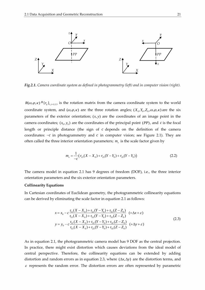
Fig.2.1. Camera coordinate system as defined in photogrammetry (left) and in computer vision (right).
, 1,2,3( , , ) [ ]ij i jR r is the rotation matrix from the camera coordinate system to the world
coordinate system, and ( , , ) are the three rotation angles; 0 0 0( , , , , , )X Y Z are the six
parameters of the exterior orientation; ( , )x y are the coordinates of an image point in the
camera coordinates; 0 0( , )x y are the coordinates of the principal point ( )PP , and c is the focal
length or principle distance (the sign of c depends on the definition of the camera
coordinates: c in photogrammetry and c in computer vision; see Figure 2.1). They are
often called the three interior orientation parameters; xm is the scale factor given by
13 0 23 0 33 0
1( ) ( ) ( )xm r X X r Y Y r Y Y
c
(2.2)
The camera model in equation 2.1 has 9 degrees of freedom (DOF), i.e., the three interior
orientation parameters and the six exterior orientation parameters.
Collinearity Equations
In Cartesian coordinates of Euclidean geometry, the photogrammetric collinearity equations
can be derived by eliminating the scale factor in equation 2.1 as follows:
11 0 21 0 31 00
13 0 23 0 33 0
12 0 22 0 32 00
13 0 23 0 33 0
r ( ) r ( ) r ( )( )
r ( ) r ( ) r ( )
r ( ) r ( ) r ( )( )
r ( ) r ( ) r ( )
X X Y Y Z Zx x c x
X X Y Y Z Z
X X Y Y Z Zy y c y
X X Y Y Z Z
(2.3)
As in equation 2.1, the photogrammetric camera model has 9 DOF as the central projection.
In practice, there might exist distortion which causes deviations from the ideal model of
central perspective. Therefore, the collinearity equations can be extended by adding
distortion and random errors as in equation 2.3, where ( , )x y are the distortion terms, and
represents the random error. The distortion errors are often represented by parametric
X
Y
Z
x
y z
O
PP
X
Y
Z
x
y
z
O
PP
22 2 Generation of 3D Models - An Overview
models which are known as self-calibration models. For example, the Brown self-calibration
model in close-range photogrammetry which includes the three interior orientation
parameters, the symmetric radial distortion (in the two image coordinates) and the
decentering distortion (radial and tangential components). Therefore, the interior parameters
are often represented by the three interior orientation parameters 0 0( , , )x y c as well as the
distortion parameters. These parameters are calculated by means of a camera calibration
process. Three methods based on the reference object used, time and location can be utilized:
laboratory calibration, test field calibration and self-calibration (Luhmann et al., 2007).
A typical solution to estimate the six exterior orientation parameters and/or the network
geometry, with or without self-calibration and having a number of control points, is by
performing bundle block adjustment based on the collinearity equations as a functional
model (Brown, 1976; Triggs et al., 2000). The required 2D image correspondences can be
measured in the photos manually or automatically. These 2D points are used also to estimate
the relative orientation between each image pair (translation and rotation of one image with
respect to the second) without considering the control points. This results in recovering the
photogrammetric model in an arbitrary model space. Furthermore, if we consider the
orientation of a single image, a number of control points in general position (according to
equations 2.3, ≥ 3 points if calibration is available or ≥ 6 points without calibration) and their
2D projections in the image are required. This enables solving the so-called Perspective-n-
Point (PnP) problem in computer vision, also known as space resection in photogrammetry.
It aims at estimating the camera orientation from a set of 3D-to-2D point correspondences.
Space resection by collinearity is a common used method to determine the orientation
parameters. This requires initial approximations for the unknown parameters, since the
collinearity equations are nonlinear, and thus have been linearized using Taylor’s theorem.
2.1.1.3 Surface Points Recovering
Once the images are oriented using the 2D image correspondences and the camera
calibration (if available), the corresponding 3D object points are recovered by means of a
forward intersection process by applying the collinearity equations. This, by definition for
single 3D point recovering requires at least two light rays formed by the camera station,
image and object point. However, to perform automatic image matching, the determination
of point correspondences between two or more images in order to reconstruct 3D surfaces is
still a crucial step in 3D reconstruction. Some automated matching algorithms, e.g.
(D’Apuzzo, 2003; Gruen et al., 2004; Ohdake & Chikatsu, 2005) rely on cross-correlation or
least squares matching (LSM) algorithm (Gruen, 1985a) on stereo or multiple images. Other
advanced matching approaches are based on feature and/or area-based techniques, e.g.
(Zhang, 2005). They allow us to match features between images taken with different cameras,
with different zoom and exposure settings, from different angles, and in some cases at
completely different times of day (Snavely et al., 2008).
Once the correspondences are matched, their corresponding image coordinates are trans-
formed into 3D information through a mathematical model like collinearity equations or
2.1 Data Acquisition and Geometric Reconstruction 23
camera projection matrix. (Remondino et al., 2008) review the recent developments and
performance analysis of the image matching techniques not only to develop a fully auto-
mated procedure for 3D object reconstruction, but also for detailed surface reconstruction of
heritage objects. These matching methods often show wrong matching results which appear
in areas with poor texture. Accurate dense 3D reconstructions can then be applied
automatically, see (Furukawa & Ponce, 2007 and 2010; Hirschmueller, 2005 and 2008; Hiep et
al., 2009; Rothermel et al., 2012) and free packages such as MicMac, PMVS, SURE. More
details about the PMVS and the SURE methods are reported in Appendix B.
Finding Correspondences
The goal of correspondence estimation or image matching is to find sets of matching 2D
pixels across a set of images, in which each set of the matching pixels ideally represents a
single point in 3D (Snavely et al., 2008). In general, image matching techniques can be
classified according to the procedure and the parameters used in the correspondence
(homologous point) extraction, as follows (Nex, 2010):
Feature Based Matching (FBM). It comprises the following steps: as a first step, interest
point, region or edge operators extract features in each individual image. Then, a set of
characteristic attributes (feature descriptors) is computed for each feature. These
descriptors are usually determined under certain assumptions regarding the local object
geometry and the geometric or the radiometric constraints. Furthermore, feature
description can be determined simultaneously by the features operators, e.g. the scale
invariant feature transform (SIFT) region operator (Lowe, 2004). Finally, features are
matched across all images by comparing their descriptors.
(Tuytelaars & Mikolajczyk, 2008) survey intensively the most widely used local invariant
feature detectors (interest points, regions or edge segments) with a qualitative evaluation
of their respective strengths and weaknesses. In (Haralick & Shapiro, 1993), they report
that a distinctive feature operator have to satisfy the following characteristics: (i)
Distinctness (features should stand out clearly against the background and be unique in
its neighborhood). (ii) Invariance (feature estimation should be independent of geo-
metrical and radiometric distortions). (iii) Stability (the selection of interest points should
be robust to noise and blunders). (iv) Uniqueness (features should possess a global
uniqueness, in order to improve the distinction of repetitive patterns). (v) Interpretability
(features should have a significant meaning to be used in correspondence analysis and
higher image interpretation). Examples of feature operators can be mentioned such as the
Harris interest point operator (Harris & Stephens, 1988), the MSER (Maximally Stable
Extremal Region) region operator (Matas et al., 2004) and the Canny edge operator
(Canny, 1986).
To conclude, feature points are more invariant to geometric and radiometric trans-
formations than area-based methods. The FBM methods are flexible with respect to sur-
face discontinuities with the availability of approximate values. But, they are computatio-
nally expensive and require setting up a large number of parameters. Furthermore, the
24 2 Generation of 3D Models - An Overview
number of extracted points per image is usually limited and the accuracy is also limited
to the accuracy of the feature extraction process (normally in sub-pixel range). The FBM
technique is largely implemented in image orientation algorithms, e.g. SfM methods.
Area Based Matching (ABM). This method determines correspondences based on the
similarity of the radiometric levels within image windows. It is used widely in aerial
photogrammetry, where the assumption that two local windows considered on two
homologous images have similar radiometric level values is fulfilled. Moreover, local
windows must represent contiguous (very close or connected) points in the object space
in order to assure stable matching. Examples of ABM methods are the cross-correlation
(e.g. Zhang, 2005; Zhao et al., 2006) and LSM techniques (e.g. Gruen, 1985a; Gruen &
Baltsavias, 1988). The ABM technique is widely used for dense surface reconstruction.
Compared to FBM techniques, the ABM methods provide higher performance and better
accuracy with reduced computational costs, particularly in well-textured image areas
and considering reduced geometric distortions. However, they require adopting several
constraints (e.g. epipolar3 geometry) to reduce the search area of the homologous points
in the images in order to discard mismatches and increase the redundancy as well
(Zhang, 2005).
Relational Matching (RM). These techniques can reduce the unreliability of the
matching results using FBM or ABM methods by introducing constraints that enable the
removal of blunders and mismatches. They define probabilistic cost functions, which
evaluate the relative position of the matching candidates. These functions exploit
compatibility or topological constraints such as surface smoothness and uniqueness
constraints. This involves assigning unique matches to a set of features in an image from
a given list of possible candidates. Then, the search space is restricted by means of a cost
function optimization analysis (Nex, 2010). For example, (Pajares et al., 1998) transform
the similarity, smoothness and uniqueness constraints into an energy function whose
minimum value corresponds to the best solution for solving the global stereovision
matching problem.
In general, automated algorithms based on image matching such as relative orientation/SfM
and dense surface reconstruction methods have to deal with erroneous measurements. For
that, a combination of different similarity measures and matching techniques together with
applying thresholds and additional constraints can reduce the amount of errors. Besides RM
techniques, data snooping or robust statistical algorithms are used to discard wrong matches
and blunders in order to estimate the model parameters using only correct matches. These
algorithms are usually based on robust adjustment techniques, e.g. (Gruen, 1985b) or the
3 Epipolar geometry is the geometry of stereo vision (two cameras view a 3D object from two distinct
positions). This compels a number of geometric relations between the object points and their
projections onto the 2D images that leads to constraints between the image points, under the
assumption that the pinhole camera model is applied (Hartley & Zisserman, 2003).
2.1 Data Acquisition and Geometric Reconstruction 25
Random Sampling and Consensus (RANSAC) algorithm (Fischler & Bolles, 1981). More
information about the RANSAC method is reported in Appendix C.
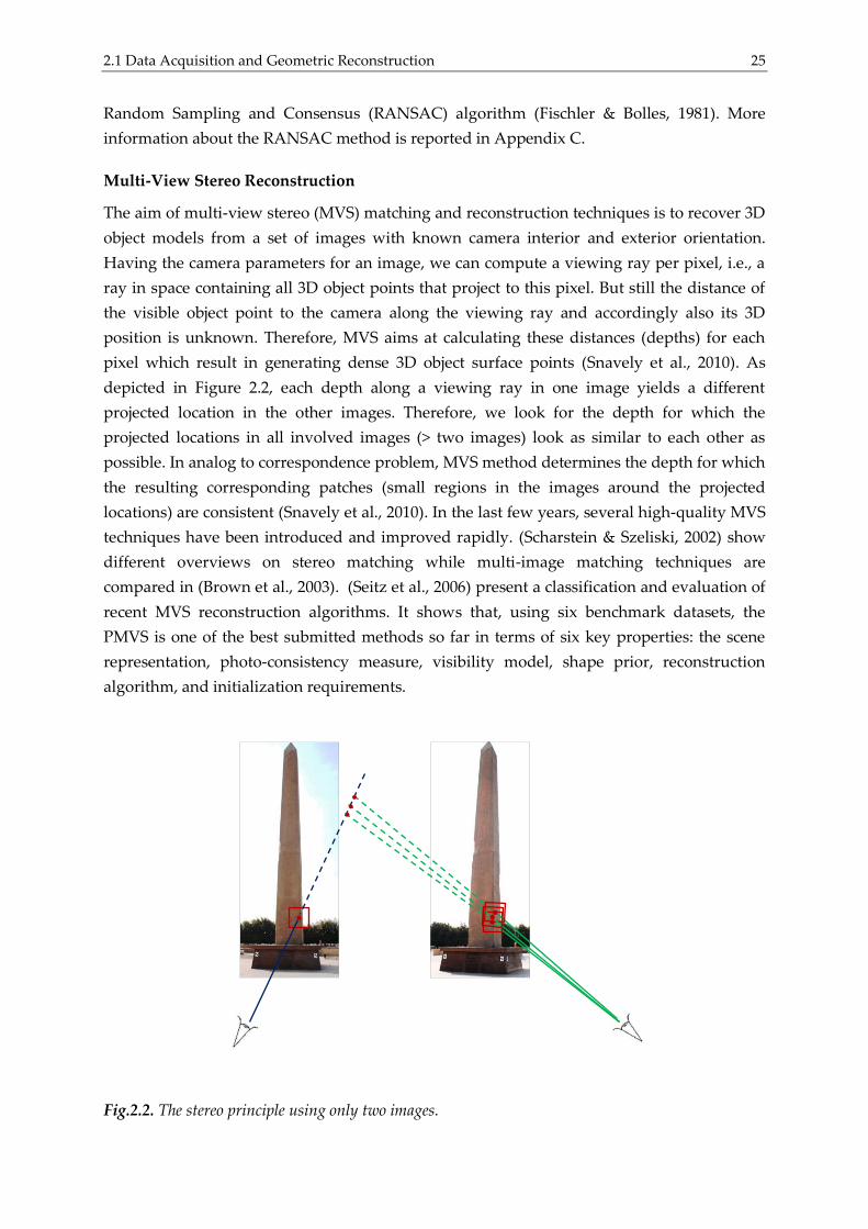
Multi-View Stereo Reconstruction
The aim of multi-view stereo (MVS) matching and reconstruction techniques is to recover 3D
object models from a set of images with known camera interior and exterior orientation.
Having the camera parameters for an image, we can compute a viewing ray per pixel, i.e., a
ray in space containing all 3D object points that project to this pixel. But still the distance of
the visible object point to the camera along the viewing ray and accordingly also its 3D
position is unknown. Therefore, MVS aims at calculating these distances (depths) for each
pixel which result in generating dense 3D object surface points (Snavely et al., 2010). As
depicted in Figure 2.2, each depth along a viewing ray in one image yields a different
projected location in the other images. Therefore, we look for the depth for which the
projected locations in all involved images (> two images) look as similar to each other as
possible. In analog to correspondence problem, MVS method determines the depth for which
the resulting corresponding patches (small regions in the images around the projected
locations) are consistent (Snavely et al., 2010). In the last few years, several high-quality MVS
techniques have been introduced and improved rapidly. (Scharstein & Szeliski, 2002) show
different overviews on stereo matching while multi-image matching techniques are
compared in (Brown et al., 2003). (Seitz et al., 2006) present a classification and evaluation of
recent MVS reconstruction algorithms. It shows that, using six benchmark datasets, the
PMVS is one of the best submitted methods so far in terms of six key properties: the scene
representation, photo-consistency measure, visibility model, shape prior, reconstruction
algorithm, and initialization requirements.
Fig.2.2. The stereo principle using only two images.
26 2 Generation of 3D Models - An Overview
Under the above, the complete automation in image-based technique is still an open topic of
research, particularly in case of complex structures as heritage and man-made objects. This
also applies to the obtained accuracy, which is still restricted and considered as a major task
in close-range photogrammetry. Therefore, semi-automatic methods might still be needed
for 3D accurate reconstruction.
2.1.2 Range-Based Approach
Range-based technique is founded on the usage of a laser beam for distance measurements.
This technique usually makes use of an active4 laser sensor to right away measure distance to
a large set of points in the target scene. Optical range sensors like triangulation-based, time-
delay-based laser scanners and stripe projection systems or close-range scanners (laser scan
arms) have received great attention in the last few years, particularly for their 3D modeling
capability (Manferdini & Remondino, 2012). Current laser scanner technologies can be
classified into static and kinematic systems. The former is kept in a fixed position during the
data acquisition, while the latter is mounted on a mobile platform where additional
positioning systems (e.g. INS, GPS) are required.
Static LiDAR systems have reached a high level of automation allowing fast and accurate
surveys like heritage documentation (Van Genechten, 2008; Grussenmeyer et al., 2010). These
systems have partly replaced some of the conventional methods for the spatial
documentation of heritage sites, despite their high costs, weight and the frequent lack of
good texture (Remondino & Rizzi, 2010; Rüther et al., 2012). Laser scanning systems can
produce data that can vary in terms of point density, field-of-view (FOV), amount of noise,
incident angle, waveform and texture information (Grussenmeyer et al., 2012).
A terrestrial laser scanner directly determines the 3D coordinates of all points in the scene: in
its FOV, horizontally and vertically. Each measured point has a range distance to the scan
station, a horizontal angle, a vertical angle and corresponding radiometric information
(reflectance and/or RGB values). In general, the scanner has to be placed in different
locations in order to cover the whole scene during the data acquisition. Sequentially, the
acquired 3D raw data requires cleaning (removal of noise and unwanted objects) and scan
registration into a unique reference system. This produces a single point cloud that forms the
full surveyed object. In the following, the main types of active TLS systems and scanning
mechanisms are described in more detail. Moreover, the steps of the range-based approach
are briefly introduced and the main typical challenges associated with each step are given.
4 Active sensors (e.g. TLS systems), as a light measuring technique, emit some kind of controlled
radiation and detect its reflection in order to probe an object or environment. They retrieve 3D object
coordinates automatically.
2.1 Data Acquisition and Geometric Reconstruction 27
2.1.2.1 TLS Systems
Triangulation-based Systems
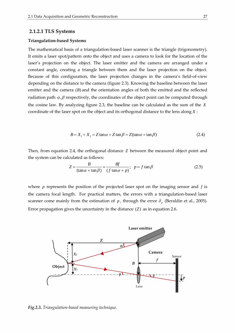
The mathematical basis of a triangulation-based laser scanner is the triangle (trigonometry).
It emits a laser spot/pattern onto the object and uses a camera to look for the location of the
laser’s projection on the object. The laser emitter and the camera are arranged under a
constant angle, creating a triangle between them and the laser projection on the object.
Because of this configuration, the laser projection changes in the camera’s field-of-view
depending on the distance to the camera (figure 2.3). Knowing the baseline between the laser
emitter and the camera ( )B and the orientation angles of both the emitted and the reflected
radiation path , respectively, the coordinates of the object point can be computed through
the cosine law. By analyzing figure 2.3, the baseline can be calculated as the sum of the X
coordinate of the laser spot on the object and its orthogonal distance to the lens along X :
1 2 tan tan (tan tan )B X X Z Z Z (2.4)
Then, from equation 2.4, the orthogonal distance Z between the measured object point and
the system can be calculated as follows:
; tan(tan tan ) ( tan )
B BfZ p f
f p
(2.5)
where p represents the position of the projected laser spot on the imaging sensor and f is
the camera focal length. For practical matters, the errors with a triangulation-based laser
scanner come mainly from the estimation of p , through the error p (Beraldin et al., 2005).
Error propagation gives the uncertainty in the distance ( )Z as in equation 2.6.
Fig.2.3. Triangulation-based measuring technique.
Camera Sensor
f
α
Z
β β
B
X2
Object
Laser emitter
Lens
X1
p

28 2 Generation of 3D Models - An Overview
2
.Z p
Z
f B (2.6)
Where p indicates the uncertainty in laser spot position on the sensor – depends on the type
of laser spot sensor, peak detector algorithm, signal-to-noise ratio and the image laser spot
shape. According to equation 2.6, the error in Z is inversely proportional to the triangulation
baseline ( )B and the camera focal length ( )f , but directly proportional to the square of Z.
Therefore, triangulation-based sensors are used in applications requiring an operating range
that is less than 10 meters (Beraldin et al., 2003). Moreover, the uncertainty in the distance is
directly proportional to p .
According to (Van Genechten, 2008), there are possible ways to decrease the uncertainty in
the distance measurements. (i) Decreasing the distance of the object to the scanner, but this
increases shadow effects. (ii) Increasing the triangulation baseline, but this also increases the
shadow effects. (iii) Increasing the camera focal length, but this reduces the FOV. (iv)
Decreasing the measurement uncertainty, but this leads to more pixels in the sensor.
However, compared to scanners based on time delay principles, triangulation-based
scanners have very high accuracies, in the order of microns. In order to avoid the use of
mechanical fixtures, some innovative modifications have been imposed. Instead of
moving/rotating the laser emitter to cover the whole object, patterns of points or lines can be
projected, which cover the whole object at once.
Time-Of-Flight Systems
Time-of-flight (TOF) TLS systems, as active scanners, exploit the TOF principle by measuring
a time frame between two events. In a given medium, light waves travel with a finite and
constant velocity ( )c . Therefore, when the time delay ( )t created by light travelling from a
source to a reflective target surface and back to the source (round-trip) can be measured
(figure 2.4). The distance to that surface ( )Z is given by
1
2Z c t (2.7)
The current accepted value for the speed of light in vacuum is exactly c = 299792,458
±0,0012km/s. If the light waves travel in air then a correction factor equal to the refraction
index (depending on the air density) must be applied to the speed value. By applying the
error propagation on equation 2.7 and considering that the speed of light is constant, the
range resolution of a TOF system ( )Z is determined by the resolution of the time
measurement ( )t as in equation 2.8.

2.1 Data Acquisition and Geometric Reconstruction 29
Fig. 2.4. Time-of-flight measurement principle, showing the pulse time measurement using the
leading edge principle (lift).
1
2Z c t (2.8)
Therefore, the accuracy depends on the clocking mechanism (time measurement). In
general, two strategies that exploit this measurement principle can be distinguished:
pulsed TOF and continuous wave (CW)/phase shift systems.
Pulsed TOF-Based Scanners. Pulsed TOF scanners exploit laser pulses instead of using
continuous laser beams. They directly measure the round-trip delay time of a single
pulse using equation 2.7. These systems scan their entire FOV one point at a time by
means of laser beam deflection units. They have a slow data acquisition speed compared
with the phase shift-based systems, but modern pulsed TOF laser scanners such as the
Leica ScanStation C10 can measure up to 50 kpts/s.
A TOF system emits a periodic signal whose amplitude varies between energy peaks and
zero values. Each peak has duration/pulse width - a rise time that determine the range
resolution of the system. The pulse has typically duration of a few nanoseconds, e.g.
pulse width of 5ns results in a length of 1.5m, using equation 2.7. Often the pulse is
assumed to have the Gaussian shape, which is more realistic than a rectangular pulse
shape. Besides the distribution in time, the pulse is distributed in space perpendicular to
the propagation direction. This causes a reduction of the pulse energy. The laser beam
diameter is limited by the boundary of the circular region in which the energy is higher
than 1,2(1/ )n
ne (Pfeifer & Briese, 2007). The energy irradiated with the pulse depends on
the pulse repetition frequency (PRF) as well. The higher frequency, the lower emitted
energy (short pulse duration), thus decreasing the measurement range.
Z
Transmitted Beam
Transmitter
Time Measurement
Unit
Receiver
Target Surface
Reflected Beam
t=t1
t=t2
Δt

30 2 Generation of 3D Models - An Overview
The time derivation method for measuring the return pulse depends on the desired time
resolution, the counting rate and the required dynamic range of the pulse. Commonly
used principles in discriminator design include leading edge timing (constant amplitude)
(figure 2.4 left), zero crossing timing (derivation), first moment timing (integration) and
constant fraction timing (find an instant in the pulse when its height bears a constant
ratio to pulse amplitude) (Van Genechten, 2008).
The range accuracy mainly depends on the time measurement accuracy and the accuracy
of the return pulse. Repeating measurements a number of times can increase precision.
Furthermore, the increase in measurement range and precision can be achieved by
increasing the emitted power, as the signal to noise ratio (SNR) raises (Pfeifer & Briese,
2007). However, systematic errors and eye-safety issues in such systems limit the
measurement range. (Beraldin et al., 2005) state the range uncertainty ( )Z for a single
pulse as follows:
2
rZ
cT
SNR (2.9)
where rT is the pulse rise time. The uncertainty in the distance is directly proportional to
rT and inversely proportional to the SNR ratio.
Most mid- and long range pulsed TOF scanners provide a range uncertainty of about
3mm to 50mm within a range of 50m. The advantage of using pulses for TOF systems is
the high concentration of transmitted laser power, which can achieve the required SNR
for higher precision at long ranges (up to several hundred meters). The disadvantage is
the difficulties in detecting the exact arrival time of the backscattered pulse due to the
changeable nature of the optical threshold and atmospheric attenuation.
CW/Phase Shift-Based Scanners. Continuous wave scanners go around the
measurement of short pulses and avoid using high precision clocks by modulating the
power or the wavelength of the laser beam. Their signals are typically modulated using
sinusoidal modulation, amplitude based (AM) or frequency based (FM) modulation,
pseudo-noise or polarization modulation (Van Genechten, 2008). For the AM, the source
transmits onto a surface as a continuous wave whose intensity is modulated with a
defined function, e.g., a sinusoid. The scattered reflection is collected and a circuit
measures the phase difference between the sent and received signals, which yields the
time-delay (figure 2.5). The subtraction of two sinusoidal modulated signals is given by
( ) sin( ) sin(2 ) sin(2 ( 2 ))m m mS t A t A f t A f t f (2.10)
where ( , , )m mA f are the amplitude, the modulation frequency and the modulated
wavelength of the light source respectively.
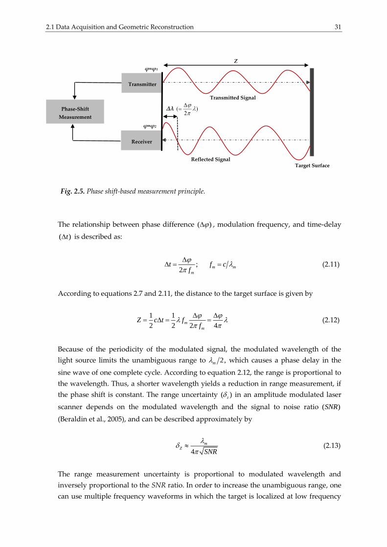
2.1 Data Acquisition and Geometric Reconstruction 31
Fig. 2.5. Phase shift-based measurement principle.
The relationship between phase difference ( ) , modulation frequency, and time-delay
( )t is described as:
;2
m m
m
t f cf
(2.11)
According to equations 2.7 and 2.11, the distance to the target surface is given by
1 1
2 2 2 4m
m
Z c t ff
(2.12)
Because of the periodicity of the modulated signal, the modulated wavelength of the
light source limits the unambiguous range to 2,m which causes a phase delay in the
sine wave of one complete cycle. According to equation 2.12, the range is proportional to
the wavelength. Thus, a shorter wavelength yields a reduction in range measurement, if
the phase shift is constant. The range uncertainty ( )z in an amplitude modulated laser
scanner depends on the modulated wavelength and the signal to noise ratio ( )SNR
(Beraldin et al., 2005), and can be described approximately by
4
mZ
SNR
(2.13)
The range measurement uncertainty is proportional to modulated wavelength and
inversely proportional to the SNR ratio. In order to increase the unambiguous range, one
can use multiple frequency waveforms in which the target is localized at low frequency
Z
Transmitted Signal
Transmitter
Phase-Shift
Measurement
Receiver
Target Surface Reflected Signal
ϕ=ϕ1
ϕ=ϕ2
Δλ
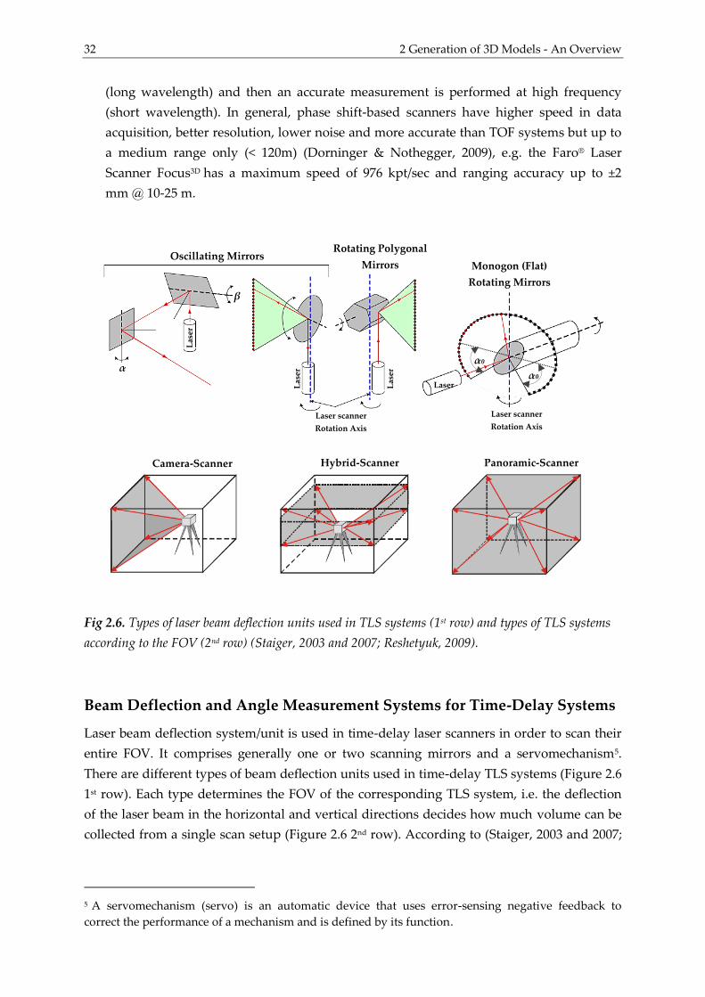
32 2 Generation of 3D Models - An Overview
(long wavelength) and then an accurate measurement is performed at high frequency
(short wavelength). In general, phase shift-based scanners have higher speed in data
acquisition, better resolution, lower noise and more accurate than TOF systems but up to
a medium range only (< 120m) (Dorninger & Nothegger, 2009), e.g. the Faro® Laser
Scanner Focus3D has a maximum speed of 976 kpt/sec and ranging accuracy up to ±2
mm @ 10-25 m.
Fig 2.6. Types of laser beam deflection units used in TLS systems (1st row) and types of TLS systems
according to the FOV (2nd row) (Staiger, 2003 and 2007; Reshetyuk, 2009).
Beam Deflection and Angle Measurement Systems for Time-Delay Systems
Laser beam deflection system/unit is used in time-delay laser scanners in order to scan their
entire FOV. It comprises generally one or two scanning mirrors and a servomechanism5.
There are different types of beam deflection units used in time-delay TLS systems (Figure 2.6
1st row). Each type determines the FOV of the corresponding TLS system, i.e. the deflection
of the laser beam in the horizontal and vertical directions decides how much volume can be
collected from a single scan setup (Figure 2.6 2nd row). According to (Staiger, 2003 and 2007;
5 A servomechanism (servo) is an automatic device that uses error-sensing negative feedback to
correct the performance of a mechanism and is defined by its function.
Panoramic-Scanner Hybrid-Scanner Camera-Scanner
Las
er
Las
er
Las
er
Laser
Oscillating Mirrors Rotating Polygonal
Mirrors Monogon (Flat)
Rotating Mirrors
Laser scanner
Rotation Axis
Laser scanner
Rotation Axis
α
β
α0
α0
2.1 Data Acquisition and Geometric Reconstruction 33
Gordon & Lichti, 2004; Wehr, 2005; Lichti, 2010), the laser beam deflection can be performed
by one of the following methods:
The laser beam is deflected horizontally and vertically by two mirrors oscillating around
the horizontal and vertical axes of the scanner. The scanning head remains fixed during
the data acquisition (figure 2.6 1st row left). Therefore, scanners which exploit this
technique have a limited FOV. They are called camera-scanners, e.g. the Leica HDS2500
laser scanner which has a maximum FOV of 400x400.
The laser beam is deflected vertically by an oscillating or a rotating polygonal mirror and
horizontally by means of a servomotor which enables the scanning head to rotate in
predefined steps around the vertical axis (figure 2.6 1strow middle). At first, a vertical
scanning profile is made with the mirror then, the scanning head rotates horizontally by
a specified step around the vertical axis, and afterwards the next vertical scanning profile
can be made. The latter process is repeating until the complete object is covered. Such
systems have a full FOV (3600) horizontally and a limited FOV vertically. They are called
hybrid-scanners, e.g. the Trimble® GX™ 3D Scanner which has a maximum FOV of
3600x600. Oscillating mirrors are comparatively slow and provide a limited vertical FOV
(max 900). They are typically utilized in the pulsed TOF scanners (e.g. the Leica HDS3000)
since the number of points measured per second using such systems is limited by the
PRF. While, rotating polygonal mirrors are very fast, rotate at constant velocity and can
provide up to a FOV of 1800 vertically (Reshetyuk, 2009). For example, the RIEGL VZ-
1000 3D terrestrial laser scanner which has a maximum FOV of 3600x1000.
The laser beam is deflected vertically by the monogon mirror (flat rotating mirror with a
single-facet centered on the rotational axis) from a lower vertical limit (-α0, usually a few
tens of degrees above nadir), up through zenith and down again to the lower limit of
(1800+ α0), and horizontally with a FOV of 1800, similar to the hybrid-scanners, by means
of a servomotor (figure 2.6 1st row right). Thus, a vertical scanning profile is made in front
of and behind the scanner in each step along the acquired profile. The scanned FOV is
spherical except for a small cone beneath the instrument (Lichti, 2010), i.e. a full FOV
horizontally and nearly the same vertically can be obtained. Therefore, these systems are
called panoramic-scanners, e.g., the Faro® Focus3D which has a maximum FOV of
3600x3050. Monogon mirrors are very fast and can nearly provide a full FOV vertically.
They are typically utilized in the phase shift-based TLS systems which exploit continuous
laser beams, and thus the number of points measured per second is limited by the point
sampling distance (Reshetyuk, 2009).
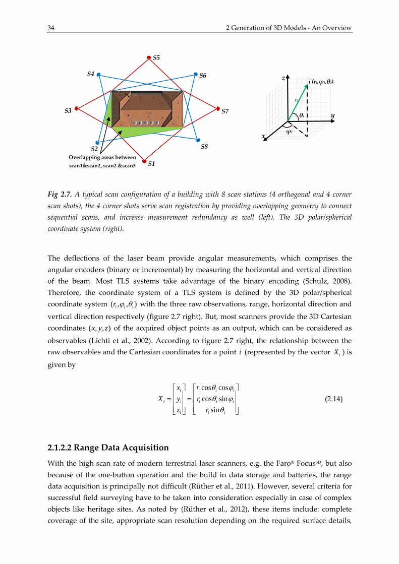
34 2 Generation of 3D Models - An Overview
Fig 2.7. A typical scan configuration of a building with 8 scan stations (4 orthogonal and 4 corner
scan shots), the 4 corner shots serve scan registration by providing overlapping geometry to connect
sequential scans, and increase measurement redundancy as well (left). The 3D polar/spherical
coordinate system (right).
The deflections of the laser beam provide angular measurements, which comprises the
angular encoders (binary or incremental) by measuring the horizontal and vertical direction
of the beam. Most TLS systems take advantage of the binary encoding (Schulz, 2008).
Therefore, the coordinate system of a TLS system is defined by the 3D polar/spherical
coordinate system ( , , )i i ir with the three raw observations, range, horizontal direction and
vertical direction respectively (figure 2.7 right). But, most scanners provide the 3D Cartesian
coordinates ( , , )x y z of the acquired object points as an output, which can be considered as
observables (Lichti et al., 2002). According to figure 2.7 right, the relationship between the
raw observables and the Cartesian coordinates for a point i (represented by the vector iX ) is
given by
cos cos
cos sin
sin
i i i i
i i i i i
i i i
x r
X y r
z r
(2.14)
2.1.2.2 Range Data Acquisition
With the high scan rate of modern terrestrial laser scanners, e.g. the Faro® Focus3D, but also
because of the one-button operation and the build in data storage and batteries, the range
data acquisition is principally not difficult (Rüther et al., 2011). However, several criteria for
successful field surveying have to be taken into consideration especially in case of complex
objects like heritage sites. As noted by (Rüther et al., 2012), these items include: complete
coverage of the site, appropriate scan resolution depending on the required surface details,
θi
ϕi
(ri,ϕi,θi)
ri
x
y
z S6
S7
S8
S4
S3
S2
S1
S5
Overlapping areas between
scan1&scan2, scan2 &scan3
i
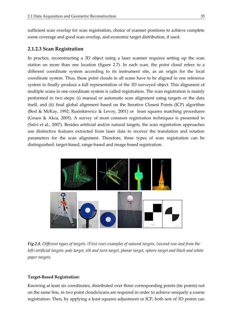
2.1 Data Acquisition and Geometric Reconstruction 35
sufficient scan overlap for scan registration, choice of scanner positions to achieve complete
scene coverage and good scan overlap, and economic target distribution, if used.
2.1.2.3 Scan Registration
In practice, reconstructing a 3D object using a laser scanner requires setting up the scan
station on more than one location (figure 2.7). In each scan, the point cloud refers to a
different coordinate system according to its instrument site, as an origin for the local
coordinate system. Thus, these point clouds in all scans have to be aligned in one reference
system to finally produce a full representation of the 3D surveyed object. This alignment of
multiple scans in one coordinate system is called registration. The scan registration is mainly
performed in two steps: (i) manual or automatic scan alignment using targets or the data
itself, and (ii) final global alignment based on the Iterative Closest Points (ICP) algorithm
(Besl & McKay, 1992; Rusinkiewicz & Levoy, 2001) or least squares matching procedures
(Gruen & Akca, 2005). A survey of most common registration techniques is presented in
(Salvi et al., 2007). Besides artificial and/or natural targets, the scan registration approaches
use distinctive features extracted from laser data to recover the translation and rotation
parameters for the scan alignment. Therefore, three types of scan registration can be
distinguished: target-based, range-based and image-based registration.
Fig.2.8. Different types of targets. (First row) examples of natural targets, (second row and from the
left) artificial targets: pole target, tilt and turn target, planar target, sphere target and black and white
paper targets.
Target-Based Registration:
Knowing at least six coordinates, distributed over three corresponding points (tie points) not
on the same line, in two point clouds/scans are required in order to achieve uniquely a coarse
registration. Then, by applying a least squares adjustment or ICP, both sets of 3D points can

36 2 Generation of 3D Models - An Overview
be aligned in one reference system. These tie points could be artificial targets or natural
targets (figure 2.8). Natural ones must be selected manually, on contrast to the artificial
target, which can be selected automatically. This automatic registration requires algorithms
for fitting shapes, which can detect the specific shapes of the targets such as sphere, reflective
targets and black and white paper targets. In general, this depends on target acquiring
distance, laser beam incidence angle and scanning resolution. This has been demonstrated in
some commercial software such as the Leica’s Cyclone and the Faro® Scene software. For
example, Faro® Scene is able to detect a completely visible sphere in a scan acquired by the
Faro® focus3D scanner when scanning with a resolution of 1/4, the distance to the scanner >
18m and < 1m then, the sphere should have at least 10-15 pixels/points in the scan (Faro
Technologies Inc., 2011).
Range-Based Registration:
The idea of this approach is to identify candidates of corresponding 3D points in the
overlapping area between each laser scan pair, see figure 2.7. These tie points are then
utilized in order to estimate initial approximation for the rigid-body transformation
parameters, see Appendix D.2. This is followed usually by an error minimization step using
any surface matching algorithm like ICP, which minimizes the distances between the scan
pair until certain criteria are met.
Several methods have been introduced in the literature. Point and line features have been
employed for the scan registration (Stamos & Leordeanu, 2003; Barnea & Filin, 2008). In
(Dold & Brenner, 2004 and 2006; Dold, 2005; Von Hansen, 2006; Brenner et al., 2008), planar
patches extracted from 3D LiDAR data have been employed for the calculation of trans-
formation parameters between different point clouds. Corresponding object models (planes,
spheres, cylinders and tori) extracted from different scans are used to determine the trans-
lation and rotation parameters of multiple scans (Rabbani et al., 2007). However, the extrac-
tion of line features, plane patches or geometric objects from LiDAR data is still uneasy task.
Therefore, (Bae & Lichti, 2004 and 2008) use the change of geometric curvature and
approximate normal vector of the local surface formed by a point and its neighborhood
search, in addition to the positional uncertainty of laser scanners, for the registration of two
partially overlapping point clouds.
Image-Based Registration:
Recent research work denotes that distinctive features can also be extracted from LiDAR data
using images that are provided simultaneously with the point clouds either by recording co-
registered camera images (captured by an integrated camera to the scanner) or by generating
reflectance and/or RGB images from the 3D data. (Forkuo & King, 2004) introduce a fusion
approach of 3D range data and 2D imagery based on the use of the 3D data and synthetic
camera images generated from the respective reflectance values via back-projection into a
regular grid. For that, the extraction of features from images was performed using the Harris
corner detector (Harris & Stephens, 1988). (Bendels et al., 2004; Al-Manasir & Fraser, 2006;
2.1 Data Acquisition and Geometric Reconstruction 37
Barnea & Filin, 2007) introduced SIFT features, proposed by (Lowe, 2004), for the registration
of TLS data where both range information and information from co-registered camera
images are used. In (Boehm & Becker, 2007), SIFT features are extracted from reflectance
images which are generated directly from the reflectance values of the TLS data. Reflectance
images are also used in (Wang & Brenner, 2008) where each SIFT feature descriptor is
modified with additional entry. The latter represents the mean geometric curvature of a
surface formed by the projection of a 2D SIFT feature into local 3D space and its 3D
neighborhood in the point clouds. (Kang et al., 2009) proposed also an automatic registration
of TLS data using panoramic reflectance images. In (Weinmann et al., 2011), radiometric and
geometric information derived from TLS data are utilized for estimating the transformation
parameters between each scan pair. (Alba et al., 2011) presented an automated methodology
able to register laser scanner point clouds using their panoramic images derived from
intensity values or RGB data obtained from a co-registered camera.
In addition, a solution combines both approaches, range and image-based is proposed by
(Yang et al., 2011) where 3D information are used to improve 2D image features and then the
latter are utilized for wide baseline 3D scene alignment. Further methods exploit the
knowledge of the shape, that best fits the local geometry of each 3D point neighborhood and
can improve the fine registration (using ICP) of two point clouds in terms of time and
accuracy (Gressin et al., 2013). However, it still requires good a priori alignment of both 3D
point sets.
2.1.3 Sensor Integration
Most of LiDAR systems are supplied or can be integrated with a standard digital camera.
But, as presented in chapter 1, getting on top of the limits caused by the fixed relative
position between both sensors, data acquisition obstacles and product quality (e.g.
photorealism) requires photogrammetry. The latter technique is of low-cost and can
complement individual weaknesses of the former one. Therefore, it is intuitive to consider
that data integration of photogrammetric images and laser scanner data can provide
opportunity for more specific inferences and larger potential (Elstrom et al., 1998; Jansa et al.,
2004; Wendt & Heipke, 2006). Furthermore, this integration shows promising prospects due
to the complementary characteristics of both data sources (Forkuo & King, 2004; Schneider &
Maas, 2007).
Based on the wanted end-product, the nature of the original data or difference in emphasis,
(Roennholm et al., 2007) denoted four different levels of integration of photogrammetric
images and laser scanner data as follows: (i) object-level integration where digital images
and laser data are processed and interpreted separately, e.g. (Remondino et al., 2008; Guidi et
al., 2008), (ii) photogrammetry aided by laser scanning: the main focus is on image data and
the laser data supplies necessary information, e.g. (Ressl et al., 2006; Wendt, 2007), (iii) laser
scanning aided by photogrammetry: image data provide additional information, e.g. (Al-
Manasir & Fraser, 2006; Kang et al., 2007), (iv) tightly integrated laser scanning and optical
38 2 Generation of 3D Models - An Overview
images: both sensors are integrated at the device level like in the case of current static and
dynamic LiDAR systems and frame-based 3D range cameras.
Over the past years, different fusion approaches were presented to integrate digital photos
with laser scanner data. These approaches were useful in texture mapping of point clouds to
generate 3D photorealistic models, e.g. (Alshawabkeh & Haala, 2005; Abdelhafiz, 2009),
extraction of reference targets for registration and calibration tasks, e.g. (El-Hakim &
Beraldin, 1994), registration of multiple scans by using photos, e.g. (Yang et al., 2011),
employing photos to reconstruct the main shape of the object and then using laser scanning
to reconstruct the detailed parts, e.g. (El-Hakim et al., 2003b), geometric reconstruction of
man-made objects, e.g. (Nex & Remondino, 2011) and last but not least filling gaps in laser
scanner point clouds caused by occlusions, e.g. (Alshawabkeh, 2006). However, it is clear
that the fully automatic integration between photogrammetric and LiDAR techniques has
not yet been introduced.
2.1.4 Georeferencing
An important step preceding surface reconstruction, sometimes coming before data fusion, is
usually the transformation of measurements of an arbitrary coordinate system into a
reference system, local or global one. This geometric alignment of the measurements with a
geodetic and/or known reference system is referred as georeferencing. (Schuhmacher &
Boehm, 2005) classify the geo-referencing methods of TLS as follows: (i) conventional
georeferencing: by introducing a supporting measurement system like a total station to
transfer the geodetic control information to the object space; (ii) sensor-driven method: it is
based on a combination of GPS and digital compass data as initial values for further iterative
refinement including additional control information; (iii) data-driven method: it is based on
the datasets which have been georeferenced before, such as digital surface models or virtual
city models where the acquired data can be matched with the georeferenced one, e.g. by ICP.
2.2 Surface Reconstruction
In general, redundant point clouds should be removed before a surface model is produced.
This is followed usually by a segmentation process which divides the point clouds into one
or more subsets in order to perform further operations on each subset such as fitting to
surfaces or basic geometrical shapes, and remove unwanted points, etc. The segmentation
process groups generally different regions of point clouds based on their shared
characteristics. (Wang & Shan, 2009) categorize roughly the segmentation algorithms based
on the used mathematical techniques into five groups: edge-based, e.g. (Sappa & Devy,
2001), surface-growing, e.g. (Rabbani et al., 2006), scan-line, e.g. (Khalifa et al., 2003),
clustering, e.g. (Sampath & Shan, 2006) and graph partitioning methods, e.g. (Wang & Chu,
2008). Then, each single point cloud resulted from the segmentation and/or the cleaning
2.3 Texture Mapping and Visualization 39
process can be converted into a continuous surface in a step referred as surface reconstruc-
tion or modeling. This can be done by fitting smooth surfaces, e.g. (Vosselman et al., 2004) or
fitting basic geometric shapes, e.g. (Guelch, 2009), or triangulation/meshing, e.g. (Kazhdan et
al., 2006), see figure 2.9.
A large number of meshing algorithms have been proposed for surface reconstructions, but
best results were achieved with a combination of methods where each algorithm responds
differently according to surface texture, complex details, point resolution and noise (Rüther
et al., 2012). Further hole filling (hole augmentation) would be desirable especially in case of
modeling complex objects like heritage sites. This can be solved using automated hole filling
methods like (Sharf et al., 2004), but their use is still limited. Therefore, semi-automatic
methods are still needed. Moreover, 3D modeling is considered as a state-of-the-art topic in
the point cloud processing research, particularly for modeling human body parts and
complex objects.
2.3 Texture Mapping and Visualization
Photo-realistic and accurate visualization in many applications like 3D preservation of
cultural heritage sites is often required. This is achieved usually with texture mapping and
good visualization engines. The basic idea of texture mapping is to map the real texture
(photos) to the corresponding 3D geometric surface, which is generated as wireframe or
mesh models. For each triangle in the mesh, the corresponding image coordinates on the
photo are computed using the corresponding camera orientations. Then, the textures in the
computed triangle on the photo are mapped to the triangle mesh to end with a photo-
realistic appearance for the model (figure 2.10). Several approaches have been proposed in
the literature, see (Wang et al., 2001; El-Hakim et al., 2003b; Alshawabkeh, 2006; Bannai et al.,
2007; Xu et al., 2010; Chen et al., 2012).
There are several factors that have an effect upon visual quality or photo-realism of a 3D
model. They are mainly the geometric and radiometric distortions, object occlusions and the
dynamic range (El-Hakim et al., 2003c; Abdelhafiz, 2009). Regarding the geometric distortion
factor, it can be reduced when a simple model is produced (by reducing the number of
triangles), having strong image-geometry registration, full camera calibration and applying
correct projective transformation between image plane and triangle surface. While the radio-
metric distortion is difficult to avoid due to the usage of multi views/images with different
illumination conditions, see figure 2.10 left. However, many techniques have been presented
to overcome this problem, e.g.(El-Hakim et al., 2003c).
To some extent, the object occlusion problem is still unsolved. Nevertheless, there are some
successful algorithms which are able to detect occlusions, particularly those which are part of
the modeled object. On the other hand, un-modeled occlusion such as trees and cars can be
removed in the pre-processing step by producing a virtual occlusion free image (Boehm,
2004) or using the photo occlusions finder algorithm (Abdelhafiz, 2009) which can detect the
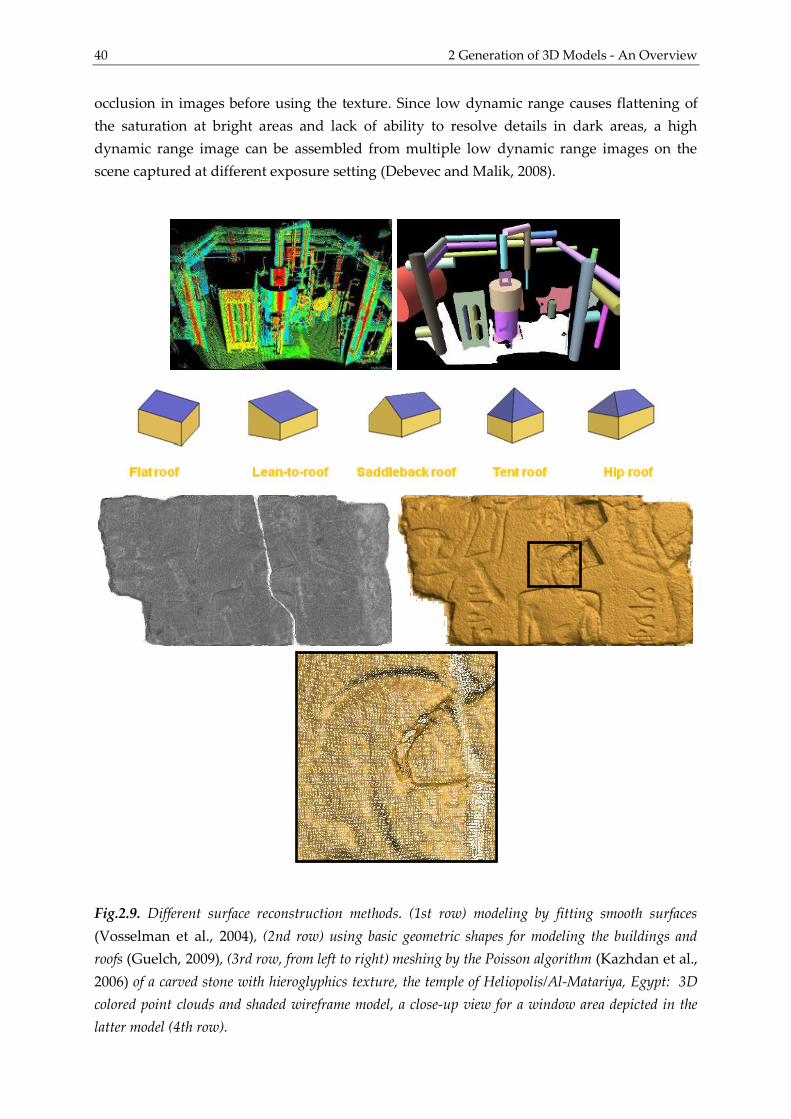
40 2 Generation of 3D Models - An Overview
occlusion in images before using the texture. Since low dynamic range causes flattening of
the saturation at bright areas and lack of ability to resolve details in dark areas, a high
dynamic range image can be assembled from multiple low dynamic range images on the
scene captured at different exposure setting (Debevec and Malik, 2008).
Fig.2.9. Different surface reconstruction methods. (1st row) modeling by fitting smooth surfaces
(Vosselman et al., 2004), (2nd row) using basic geometric shapes for modeling the buildings and
roofs (Guelch, 2009), (3rd row, from left to right) meshing by the Poisson algorithm (Kazhdan et al.,
2006) of a carved stone with hieroglyphics texture, the temple of Heliopolis/Al-Matariya, Egypt: 3D
colored point clouds and shaded wireframe model, a close-up view for a window area depicted in the
latter model (4th row).
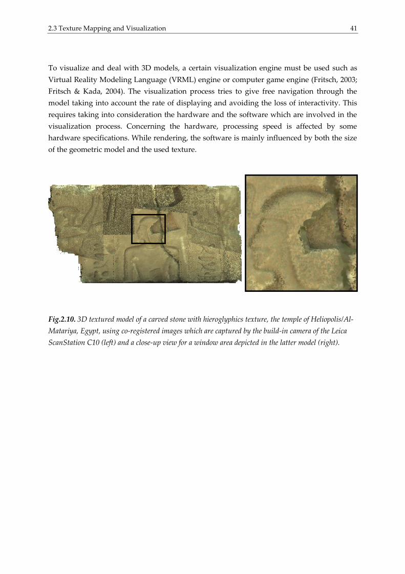
2.3 Texture Mapping and Visualization 41
To visualize and deal with 3D models, a certain visualization engine must be used such as
Virtual Reality Modeling Language (VRML) engine or computer game engine (Fritsch, 2003;
Fritsch & Kada, 2004). The visualization process tries to give free navigation through the
model taking into account the rate of displaying and avoiding the loss of interactivity. This
requires taking into consideration the hardware and the software which are involved in the
visualization process. Concerning the hardware, processing speed is affected by some
hardware specifications. While rendering, the software is mainly influenced by both the size
of the geometric model and the used texture.
Fig.2.10. 3D textured model of a carved stone with hieroglyphics texture, the temple of Heliopolis/Al-
Matariya, Egypt, using co-registered images which are captured by the build-in camera of the Leica
ScanStation C10 (left) and a close-up view for a window area depicted in the latter model (right).
42 3 Building Reflectance and RGB Images
3 Building Reflectance and RGB Images
Due to the difficulty and the intensive computation of the automatic extraction of distinctive
features from 3D point clouds, a solution simplifying the feature extraction to a 2D problem
has already been proposed. This solution is expressed in the generation of reflectance or RGB
images from the 3D data where other kinds of information such as range information
(distance of each point cloud), reflectance values (the energy of the backscattered laser beam)
and RGB data (provided by integrated or additional standard digital camera), can be
exploited. Employing these synthetic images results in registering both digital images and
laser scanner data, based on a matching between the generated and the camera images, see
(Alba et al., 2011). This has been the case since the associated given images by the latter
integrated or additional cameras might not be beneficial in the feature matching. In
particular, in case that laser scans are acquired at very different viewpoints where
conventional matching process using 2D image features can be prone to failure. This is
because of the considerable limitations due to fixing the relative position between the
sensors, the scanner and the integrated camera (Liu et al., 2006). Therefore, a solution that
able to handle large changes in the viewpoints of laser scans is desirable.
Most TLS systems record the reflectance value as the energy of the backscattered laser light.
However, the backscattered laser light is a signal of high dynamic range where the returned
gain from object surfaces is subject to changes over a large range especially for pulsed TOF
LiDAR systems (Böhm & Becker, 2007). Additionally, most laser scanners are equipped or
can be integrated by a standard digital camera, which provides color information (RGB
values) for each acquired 3D point cloud automatically. Therefore, the RGB image illustrates
the color information of the backscattered laser light.
In the following, two methods for calculating the reflectance or the RGB images as a 2D
representation of the 3D laser data can be distinguished. The first method utilizes the
scanning matrix to directly image the laser scanner polar coordinates (Section 3.1). While the
second method projects the Cartesian coordinates of each laser scanner point cloud to a
virtual image plane in a central perspective representation (Section 3.2).
3.1 Imaging Laser Scanner Polar Coordinates
Most used laser scanners record the measured polar coordinates, which are automatically
transformed into 3D Cartesian coordinates ( , , )X Y Z and signal amplitude (intensity i) and
color values (RGB) of the backscattered laser pulses. Thus, the simplest way to generate the
reflectance and/or RGB images is the direct imaging of the polar coordinates. As a result, the
image size is given by the obtained image/scanning matrix resulted by the raster-wise
sampling of the laser scanner point cloud. The number of pixels results from the defined scan
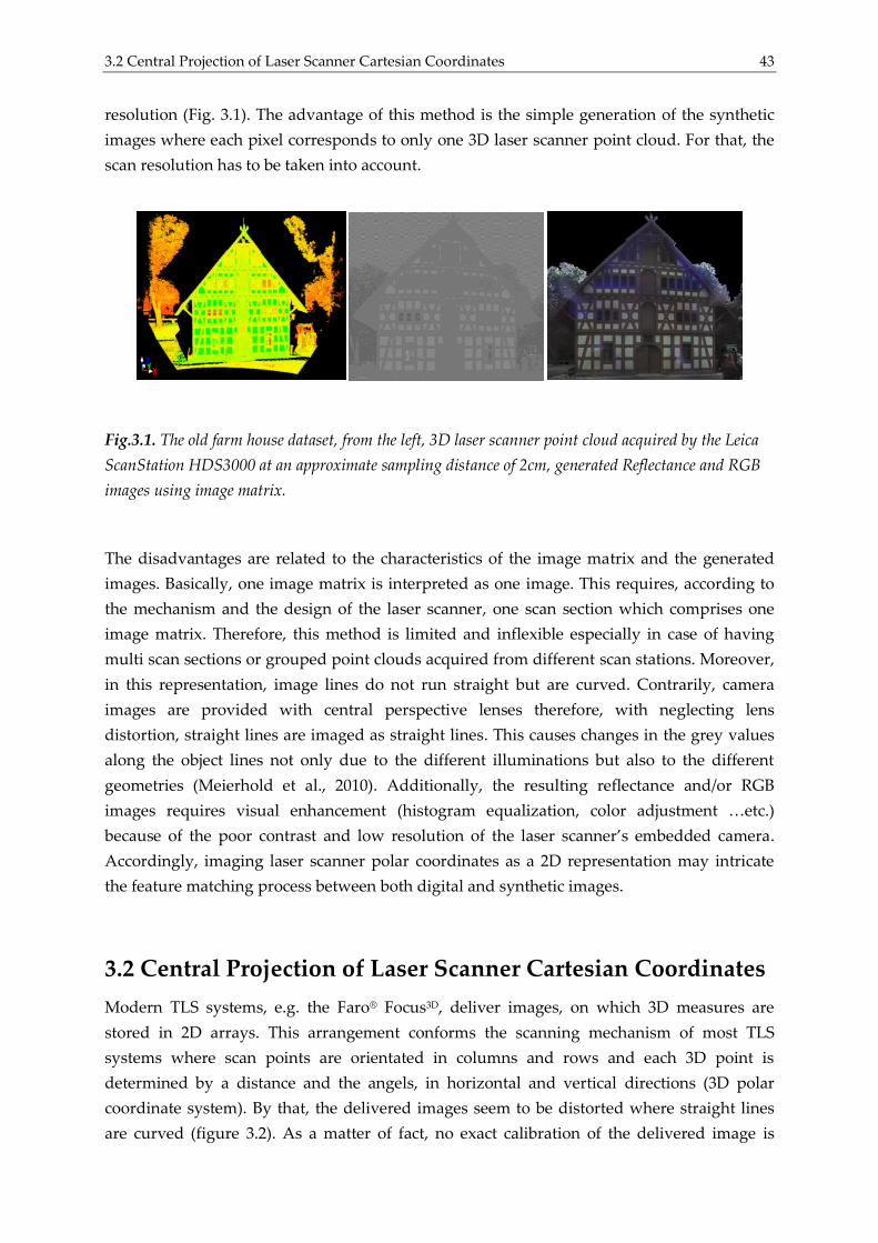
3.2 Central Projection of Laser Scanner Cartesian Coordinates 43
resolution (Fig. 3.1). The advantage of this method is the simple generation of the synthetic
images where each pixel corresponds to only one 3D laser scanner point cloud. For that, the
scan resolution has to be taken into account.
Fig.3.1. The old farm house dataset, from the left, 3D laser scanner point cloud acquired by the Leica
ScanStation HDS3000 at an approximate sampling distance of 2cm, generated Reflectance and RGB
images using image matrix.
The disadvantages are related to the characteristics of the image matrix and the generated
images. Basically, one image matrix is interpreted as one image. This requires, according to
the mechanism and the design of the laser scanner, one scan section which comprises one
image matrix. Therefore, this method is limited and inflexible especially in case of having
multi scan sections or grouped point clouds acquired from different scan stations. Moreover,
in this representation, image lines do not run straight but are curved. Contrarily, camera
images are provided with central perspective lenses therefore, with neglecting lens
distortion, straight lines are imaged as straight lines. This causes changes in the grey values
along the object lines not only due to the different illuminations but also to the different
geometries (Meierhold et al., 2010). Additionally, the resulting reflectance and/or RGB
images requires visual enhancement (histogram equalization, color adjustment …etc.)
because of the poor contrast and low resolution of the laser scanner’s embedded camera.
Accordingly, imaging laser scanner polar coordinates as a 2D representation may intricate
the feature matching process between both digital and synthetic images.
3.2 Central Projection of Laser Scanner Cartesian Coordinates
Modern TLS systems, e.g. the Faro® Focus3D, deliver images, on which 3D measures are
stored in 2D arrays. This arrangement conforms the scanning mechanism of most TLS
systems where scan points are orientated in columns and rows and each 3D point is
determined by a distance and the angels, in horizontal and vertical directions (3D polar
coordinate system). By that, the delivered images seem to be distorted where straight lines
are curved (figure 3.2). As a matter of fact, no exact calibration of the delivered image is
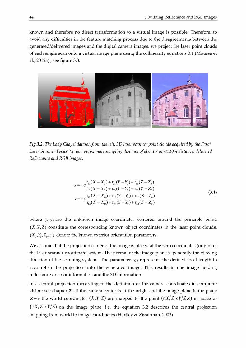
44 3 Building Reflectance and RGB Images
known and therefore no direct transformation to a virtual image is possible. Therefore, to
avoid any difficulties in the feature matching process due to the disagreements between the
generated/delivered images and the digital camera images, we project the laser point clouds
of each single scan onto a virtual image plane using the collinearity equations 3.1 (Moussa et
al., 2012a) ; see figure 3.3.
Fig.3.2. The Lady Chapel dataset, from the left, 3D laser scanner point clouds acquired by the Faro®
Laser Scanner Focus3D at an approximate sampling distance of about 7 mm@10m distance, delivered
Reflectance and RGB images.
11 0 21 0 31 0
13 0 23 0 33 0
12 0 22 0 32 0
13 0 23 0 33 0
r ( ) r ( ) r ( )
r ( ) r ( ) r ( )
r ( ) r ( ) r ( )
r ( ) r ( ) r ( )
X X Y Y Z Zx c
X X Y Y Z Z
X X Y Y Z Zy c
X X Y Y Z Z
(3.1)
where ( , )x y are the unknown image coordinates centered around the principle point,
( , , )X Y Z constitute the corresponding known object coordinates in the laser point clouds,
0 0 0 i j( , , , r )X Y Z denote the known exterior orientation parameters.
We assume that the projection center of the image is placed at the zero coordinates (origin) of
the laser scanner coordinate system. The normal of the image plane is generally the viewing
direction of the scanning system. The parameter ( )c represents the defined focal length to
accomplish the projection onto the generated image. This results in one image holding
reflectance or color information and the 3D information.
In a central projection (according to the definition of the camera coordinates in computer
vision; see chapter 2), if the camera center is at the origin and the image plane is the plane
Z c the world coordinates ( , , )X Y Z are mapped to the point ( , , )c X Z cY Z c in space or
( , )c X Z cY Z on the image plane, i.e. the equation 3.2 describes the central projection
mapping from world to image coordinates (Hartley & Zisserman, 2003).
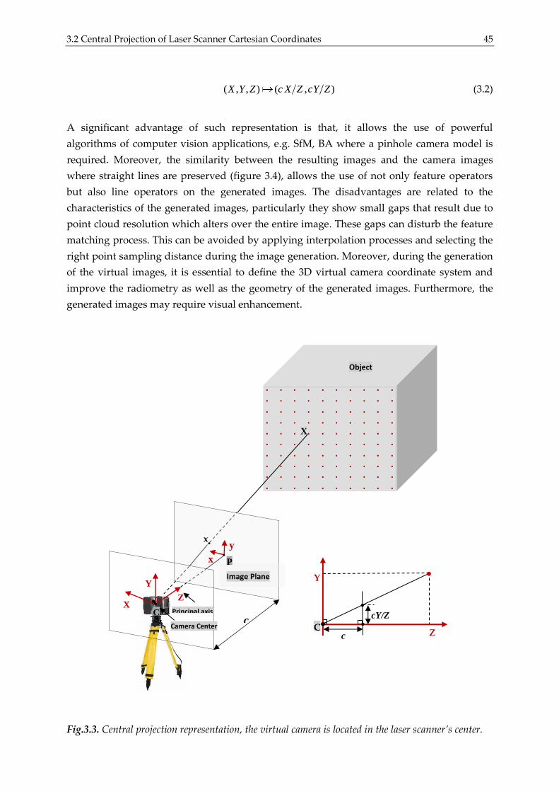
3.2 Central Projection of Laser Scanner Cartesian Coordinates 45
( , , ) ( , )X Y Z c X Z cY Z (3.2)
A significant advantage of such representation is that, it allows the use of powerful
algorithms of computer vision applications, e.g. SfM, BA where a pinhole camera model is
required. Moreover, the similarity between the resulting images and the camera images
where straight lines are preserved (figure 3.4), allows the use of not only feature operators
but also line operators on the generated images. The disadvantages are related to the
characteristics of the generated images, particularly they show small gaps that result due to
point cloud resolution which alters over the entire image. These gaps can disturb the feature
matching process. This can be avoided by applying interpolation processes and selecting the
right point sampling distance during the image generation. Moreover, during the generation
of the virtual images, it is essential to define the 3D virtual camera coordinate system and
improve the radiometry as well as the geometry of the generated images. Furthermore, the
generated images may require visual enhancement.
Fig.3.3. Central projection representation, the virtual camera is located in the laser scanner’s center.
c
X
Y
X
Image Plane
Principal axis
Camera Center
Z
x
y x
C
P
Z
Y
C c
cY/Z
Object
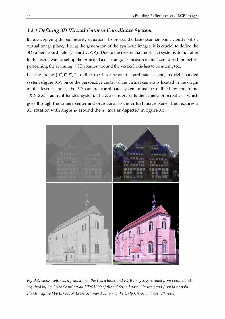
46 3 Building Reflectance and RGB Images
3.2.1 Defining 3D Virtual Camera Coordinate System
Before applying the collinearity equations to project the laser scanner point clouds onto a
virtual image plane, during the generation of the synthetic images, it is crucial to define the
3D camera coordinate system ( , , )X Y Z . Due to the reason that most TLS systems do not offer
to the user a way to set up the principal axis of angular measurements (zero direction) before
performing the scanning, a 3D rotation around the vertical axis has to be attempted.
Let the frame , , ,X Y Z C define the laser scanner coordinate system, as right-handed
system (figure 3.5). Since the perspective center of the virtual camera is located in the origin
of the laser scanner, the 3D camera coordinate system must be defined by the frame
, , ,X Y Z C , as right-handed system. The Z-axis represents the camera principal axis which
goes through the camera center and orthogonal to the virtual image plane. This requires a
3D rotation with angle around the Y axis as depicted in figure 3.5.
Fig.3.4. Using collinearity equations, the Reflectance and RGB images generated from point clouds
acquired by the Leica ScanStation HDS3000 of the old farm dataset (1st row) and from laser point
clouds acquired by the Faro® Laser Scanner Focus3D of the Lady Chapel dataset (2nd row).
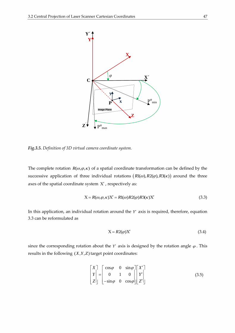
3.2 Central Projection of Laser Scanner Cartesian Coordinates 47
Fig.3.5. Definition of 3D virtual camera coordinate system.
The complete rotation ( , , )R of a spatial coordinate transformation can be defined by the
successive application of three individual rotations 1( ), 2( ), 3( )R R R around the three
axes of the spatial coordinate system , respectively as:
( , , ) 1( ) 2( ) 3( )R R R R (3.3)
In this application, an individual rotation around the Y axis is required, therefore, equation
3.3 can be reformulated as
2( )R (3.4)
since the corresponding rotation about the Y axis is designed by the rotation angle . This
results in the following ( , , )X Y Z target point coordinates:
cos 0 sin
0 1 0
sin 0 cos
X X
Y Y
Z Z
(3.5)
Y´
X´
Y
y
x
X
Image Plane
Z
C
P
Z´
Pφ
min
Pφ
max
φ
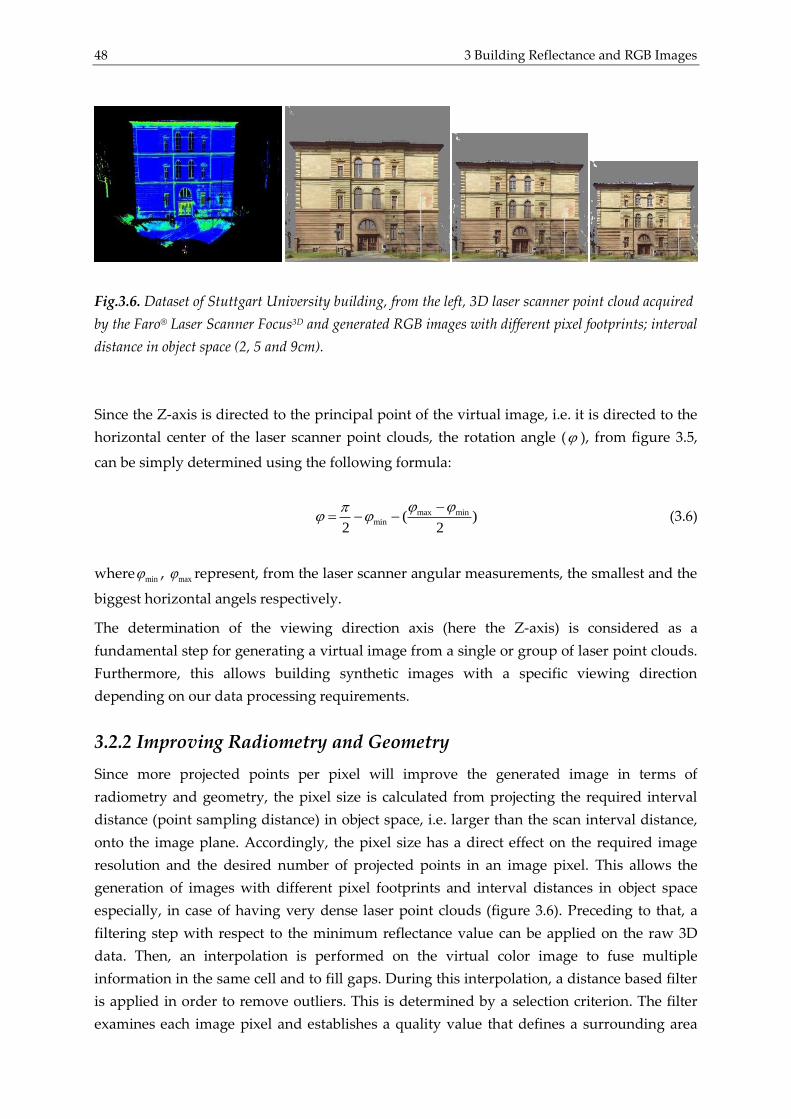
48 3 Building Reflectance and RGB Images
Fig.3.6. Dataset of Stuttgart University building, from the left, 3D laser scanner point cloud acquired
by the Faro® Laser Scanner Focus3D and generated RGB images with different pixel footprints; interval
distance in object space (2, 5 and 9cm).
Since the Z-axis is directed to the principal point of the virtual image, i.e. it is directed to the
horizontal center of the laser scanner point clouds, the rotation angle ( ), from figure 3.5,
can be simply determined using the following formula:
max minmin ( )
2 2
(3.6)
where min , max represent, from the laser scanner angular measurements, the smallest and the
biggest horizontal angels respectively.
The determination of the viewing direction axis (here the Z-axis) is considered as a
fundamental step for generating a virtual image from a single or group of laser point clouds.
Furthermore, this allows building synthetic images with a specific viewing direction
depending on our data processing requirements.
3.2.2 Improving Radiometry and Geometry
Since more projected points per pixel will improve the generated image in terms of
radiometry and geometry, the pixel size is calculated from projecting the required interval
distance (point sampling distance) in object space, i.e. larger than the scan interval distance,
onto the image plane. Accordingly, the pixel size has a direct effect on the required image
resolution and the desired number of projected points in an image pixel. This allows the
generation of images with different pixel footprints and interval distances in object space
especially, in case of having very dense laser point clouds (figure 3.6). Preceding to that, a
filtering step with respect to the minimum reflectance value can be applied on the raw 3D
data. Then, an interpolation is performed on the virtual color image to fuse multiple
information in the same cell and to fill gaps. During this interpolation, a distance based filter
is applied in order to remove outliers. This is determined by a selection criterion. The filter
examines each image pixel and establishes a quality value that defines a surrounding area
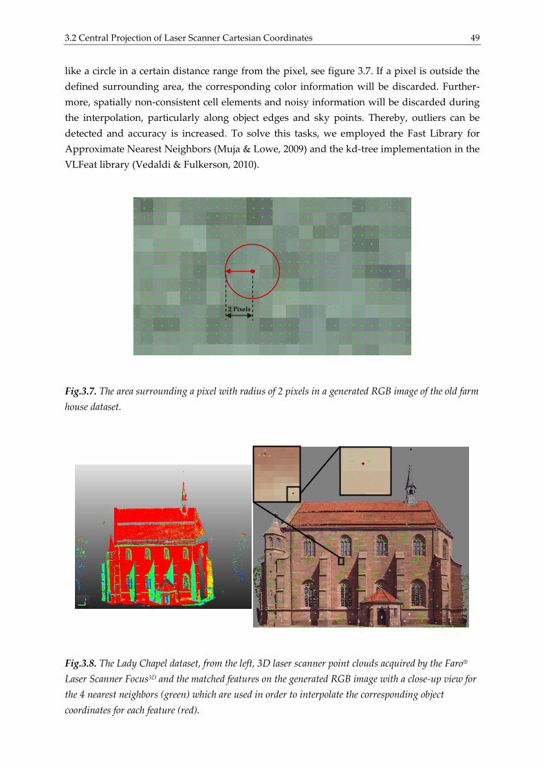
3.2 Central Projection of Laser Scanner Cartesian Coordinates 49
like a circle in a certain distance range from the pixel, see figure 3.7. If a pixel is outside the
defined surrounding area, the corresponding color information will be discarded. Further-
more, spatially non-consistent cell elements and noisy information will be discarded during
the interpolation, particularly along object edges and sky points. Thereby, outliers can be
detected and accuracy is increased. To solve this tasks, we employed the Fast Library for
Approximate Nearest Neighbors (Muja & Lowe, 2009) and the kd-tree implementation in the
VLFeat library (Vedaldi & Fulkerson, 2010).
Fig.3.7. The area surrounding a pixel with radius of 2 pixels in a generated RGB image of the old farm
house dataset.
Fig.3.8. The Lady Chapel dataset, from the left, 3D laser scanner point clouds acquired by the Faro®
Laser Scanner Focus3D and the matched features on the generated RGB image with a close-up view for
the 4 nearest neighbors (green) which are used in order to interpolate the corresponding object
coordinates for each feature (red).
2 Pixels

50 3 Building Reflectance and RGB Images
3.2.3 Improving Keypoint Localization
As the extracted keypoints from the generated images are located with subpixel accuracy,
e.g. SIFT (Lowe, 2004) features, the corresponding 3D locations have to be calculated from
the projected points using an interpolation process based on inverse weighted 3D distances
of nearest neighbor measurements (see figure 3.8). In case that 3D range measurements are
not available for all neighboring points (e.g. 4 neighbors) in the laser point clouds, this point
will be excluded. To accomplish these tasks, we employed also the Fast Library for
Approximate Nearest Neighbors (Muja & Lowe, 2009) and the kd-tree implementation in the
VLFeat library (Vedaldi & Fulkerson, 2010).
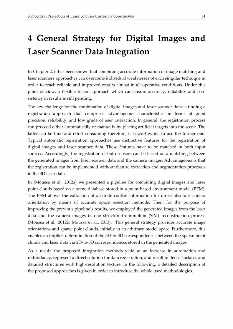
3.2 Central Projection of Laser Scanner Cartesian Coordinates 51
4 General Strategy for Digital Images and
Laser Scanner Data Integration
In Chapter 2, it has been shown that combining accurate information of image matching and
laser scanners approaches can overcome individual weaknesses of each singular technique in
order to reach reliable and improved results almost in all operative conditions. Under this
point of view, a flexible fusion approach which can ensure accuracy, reliability and con-
sistency in results is still pending.
The key challenge for the combination of digital images and laser scanner data is finding a
registration approach that comprises advantageous characteristics in terms of good
precision, reliability, and low grade of user interaction. In general, the registration process
can proceed either automatically or manually by placing artificial targets into the scene. The
latter can be time and effort consuming therefore, it is worthwhile to use the former one.
Typical automatic registration approaches use distinctive features for the registration of
digital images and laser scanner data. These features have to be matched in both input
sources. Accordingly, the registration of both sensors can be based on a matching between
the generated images from laser scanner data and the camera images. Advantageous is that
the registration can be implemented without feature extraction and segmentation processes
in the 3D laser data.
In (Moussa et al., 2012a) we presented a pipeline for combining digital images and laser
point clouds based on a scene database stored in a point-based environment model (PEM).
The PEM allows the extraction of accurate control information for direct absolute camera
orientation by means of accurate space resection methods. Then, for the purpose of
improving the previous pipeline’s results, we employed the generated images from the laser
data and the camera images in one structure-from-motion (SfM) reconstruction process
(Moussa et al., 2012b; Moussa et al., 2013). This general strategy provides accurate image
orientations and sparse point clouds, initially in an arbitrary model space. Furthermore, this
enables an implicit determination of the 3D-to-3D correspondences between the sparse point
clouds and laser data via 2D-to-3D correspondences stored in the generated images.
As a result, the proposed integration methods yield at an increase in automation and
redundancy, represent a direct solution for data registration, and result in dense surfaces and
detailed structures with high-resolution texture. In the following, a detailed description of
the proposed approaches is given in order to introduce the whole used methodologies.
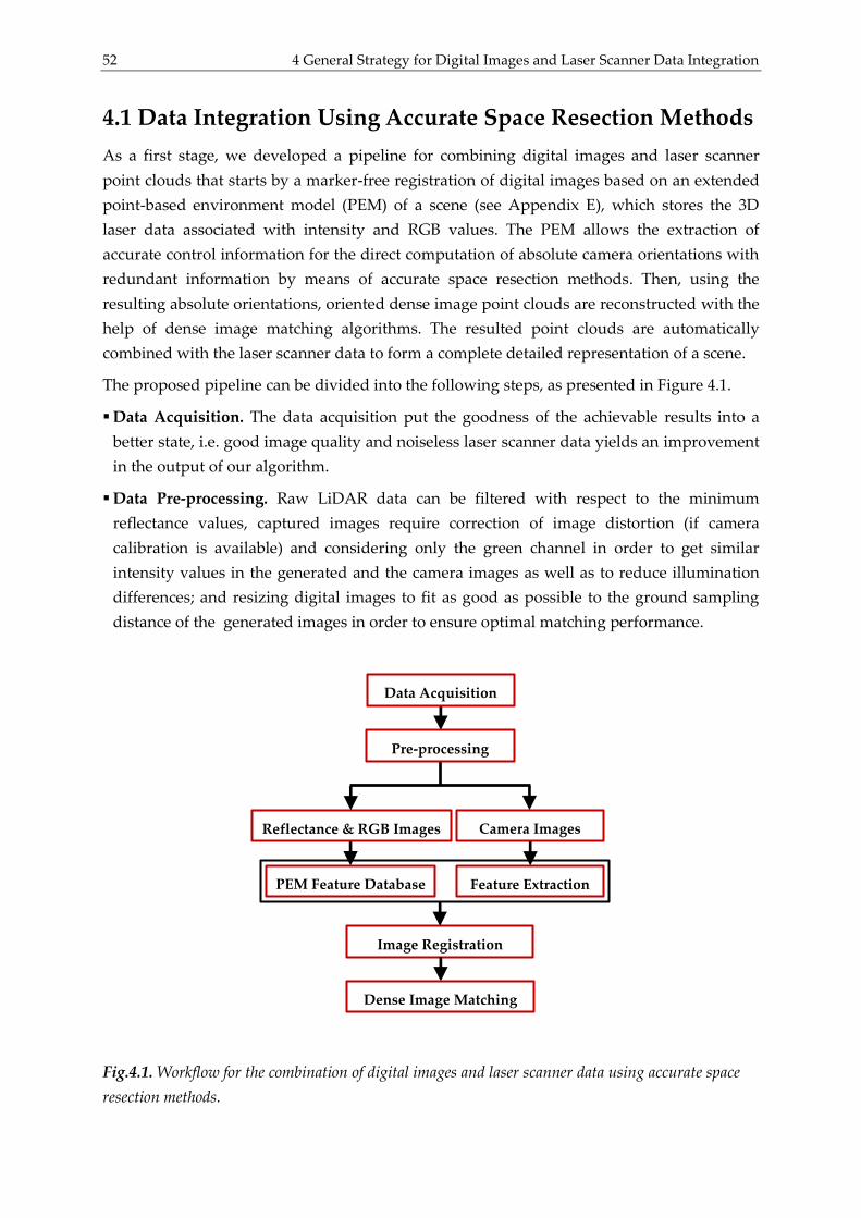
52 4 General Strategy for Digital Images and Laser Scanner Data Integration
4.1 Data Integration Using Accurate Space Resection Methods
As a first stage, we developed a pipeline for combining digital images and laser scanner
point clouds that starts by a marker-free registration of digital images based on an extended
point-based environment model (PEM) of a scene (see Appendix E), which stores the 3D
laser data associated with intensity and RGB values. The PEM allows the extraction of
accurate control information for the direct computation of absolute camera orientations with
redundant information by means of accurate space resection methods. Then, using the
resulting absolute orientations, oriented dense image point clouds are reconstructed with the
help of dense image matching algorithms. The resulted point clouds are automatically
combined with the laser scanner data to form a complete detailed representation of a scene.
The proposed pipeline can be divided into the following steps, as presented in Figure 4.1.
Data Acquisition. The data acquisition put the goodness of the achievable results into a
better state, i.e. good image quality and noiseless laser scanner data yields an improvement
in the output of our algorithm.
Data Pre-processing. Raw LiDAR data can be filtered with respect to the minimum
reflectance values, captured images require correction of image distortion (if camera
calibration is available) and considering only the green channel in order to get similar
intensity values in the generated and the camera images as well as to reduce illumination
differences; and resizing digital images to fit as good as possible to the ground sampling
distance of the generated images in order to ensure optimal matching performance.
Fig.4.1. Workflow for the combination of digital images and laser scanner data using accurate space
resection methods.
Image Registration
Data Acquisition
Pre-processing
Camera Images
Feature Extraction PEM Feature Database
Reflectance & RGB Images
Dense Image Matching
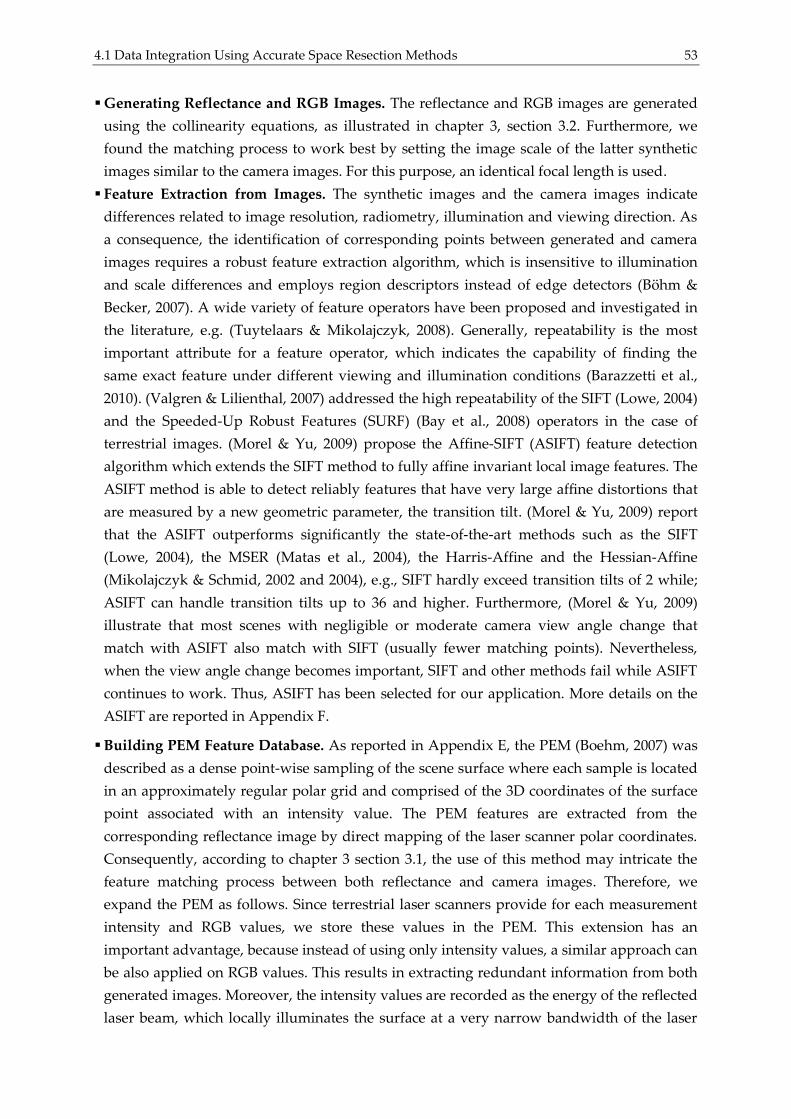
4.1 Data Integration Using Accurate Space Resection Methods 53
Generating Reflectance and RGB Images. The reflectance and RGB images are generated
using the collinearity equations, as illustrated in chapter 3, section 3.2. Furthermore, we
found the matching process to work best by setting the image scale of the latter synthetic
images similar to the camera images. For this purpose, an identical focal length is used.
Feature Extraction from Images. The synthetic images and the camera images indicate
differences related to image resolution, radiometry, illumination and viewing direction. As
a consequence, the identification of corresponding points between generated and camera
images requires a robust feature extraction algorithm, which is insensitive to illumination
and scale differences and employs region descriptors instead of edge detectors (Böhm &
Becker, 2007). A wide variety of feature operators have been proposed and investigated in
the literature, e.g. (Tuytelaars & Mikolajczyk, 2008). Generally, repeatability is the most
important attribute for a feature operator, which indicates the capability of finding the
same exact feature under different viewing and illumination conditions (Barazzetti et al.,
2010). (Valgren & Lilienthal, 2007) addressed the high repeatability of the SIFT (Lowe, 2004)
and the Speeded-Up Robust Features (SURF) (Bay et al., 2008) operators in the case of
terrestrial images. (Morel & Yu, 2009) propose the Affine-SIFT (ASIFT) feature detection
algorithm which extends the SIFT method to fully affine invariant local image features. The
ASIFT method is able to detect reliably features that have very large affine distortions that
are measured by a new geometric parameter, the transition tilt. (Morel & Yu, 2009) report
that the ASIFT outperforms significantly the state-of-the-art methods such as the SIFT
(Lowe, 2004), the MSER (Matas et al., 2004), the Harris-Affine and the Hessian-Affine
(Mikolajczyk & Schmid, 2002 and 2004), e.g., SIFT hardly exceed transition tilts of 2 while;
ASIFT can handle transition tilts up to 36 and higher. Furthermore, (Morel & Yu, 2009)
illustrate that most scenes with negligible or moderate camera view angle change that
match with ASIFT also match with SIFT (usually fewer matching points). Nevertheless,
when the view angle change becomes important, SIFT and other methods fail while ASIFT
continues to work. Thus, ASIFT has been selected for our application. More details on the
ASIFT are reported in Appendix F.
Building PEM Feature Database. As reported in Appendix E, the PEM (Boehm, 2007) was
described as a dense point-wise sampling of the scene surface where each sample is located
in an approximately regular polar grid and comprised of the 3D coordinates of the surface
point associated with an intensity value. The PEM features are extracted from the
corresponding reflectance image by direct mapping of the laser scanner polar coordinates.
Consequently, according to chapter 3 section 3.1, the use of this method may intricate the
feature matching process between both reflectance and camera images. Therefore, we
expand the PEM as follows. Since terrestrial laser scanners provide for each measurement
intensity and RGB values, we store these values in the PEM. This extension has an
important advantage, because instead of using only intensity values, a similar approach can
be also applied on RGB values. This results in extracting redundant information from both
generated images. Moreover, the intensity values are recorded as the energy of the reflected
laser beam, which locally illuminates the surface at a very narrow bandwidth of the laser
54 4 General Strategy for Digital Images and Laser Scanner Data Integration
beam. This may outcome in missing some good features which are not visible at the narrow
bandwidth of the light source (Boehm, 2007). To avoid difficulties in the feature matching
process between both the generated and the camera images, we generate both virtual
images in a central perspective representation. In addition to that, we employed several
improvements on the generated images as described in chapter 3. The generated PEM with
its list of features, PEM feature database, plays a key role to provide accurate control infor-
mation for direct absolute orientation of hand-held cameras.
Camera Image Registration to LiDAR Data. Finding the mathematical mapping by
calculating the relative orientation between the digital images and the extended PEM
database is referred as sensor registration. Most registration approaches are classified
according to their nature (area-based and feature-based) and according to four basic steps
of image registration procedure: feature detection, feature matching, transform model
estimation and image transformation and resampling (Zitova & Flusser, 2003). Therefore, in
the next paragraphs, a marker-free registration pipeline of camera images based on a
feature matching process with the PEM features database is introduced. This process
involves determination of correspondences and calculation of camera orientations.
Determination of Correspondences.
Feature Extraction: The ASIFT operator has been used for the extraction and description
of local invariant features from camera images.
Feature Matching: The ASIFT associates a descriptor to each detected image feature
following the standard SIFT operator. Then, feature matching is performed by employing
a pairwise comparison of descriptor space distances for interest features in each camera
image to the PEM feature databases, without any preliminary information about the
image network or epipolar geometry. Moreover, feature matching can be improved by
using methods that try to find more good matched features, e.g. (Guo & Cao, 2010).
Up to now, two methods are available for descriptor pairwise comparison: a quadratic
matching procedure and a kd-tree procedure. Let aI and bD be a camera image and a PEM
feature database for the same scene respectively, in which n and m are the number of
ASIFT features that listed and extracted with their descriptors ,a nd and ,b md respectively.
The quadratic matching procedure compares all descriptors of the image aI with all those
of the database bD . Then the Euclidean distance between both descriptors is computed as
a similarity measure and indication to the goodness of the match. To accept or reject a
match, a constraint (distance ratio) between the first candidate on the ordered list and the
second-best candidate is applied. The method can be summarized as follows: (i) each
descriptor ,a nd is compared with all the descriptors ,b md by calculating the Euclidean
distance , ,nm a n b md d d ; (ii) all distances nmd are listed from the shortest
1
nmd to the
longest m
nmd ; (iii) a match is accepted if 1 2
nm nmd d t , [0.5,0.8]t . This procedure is rigidly
accurate but it is potentially time consuming due to the high computation.
4.1 Data Integration Using Accurate Space Resection Methods 55
The second procedure is based on a kd-tree approach (Beis & Lowe, 1997). The kd-tree is a
data structure used to quickly solve nearest-neighbor queries. Once a kd-tree of the
database bD is built holding all its descriptors then it can be queried using descriptors
from image aI . For each query descriptor, the nearest and the next-nearest neighbors in
bD are returned. Then the distance ratio between the first two candidates is performed to
determine if there is a match. The kd-tree organizes descriptors in such a way that
descriptors close together live in nearby regions of the data structure. This results in
efficient searching. Kd-trees typically use an approximate nearest neighbor search such as
the approximate nearest neighbors (ANN) library (Arya et al., 1998) and the fast library
for approximate nearest neighbors (FLANN) (Muja & Lowe, 2009). This procedure is fast
but is approximate while it preserves more than 95% of correct nearest neighbors (Muja &
Lowe, 2009).
Practically, choosing the right descriptor comparison procedure depends on the number
of images or extracted features involved in the matching process, which results in an
increase in the computation time (Barazzetti et al., 2010).
Removal of Wrong Image Correspondences: Candidate correspondences usually have
fair mismatches. This is mainly as a result of the nature of the feature descriptors,
different intrinsic characteristics of images and the nature of the acquired surface
structure. To exclude these mismatches, the geometric relationship of the features
(geometric consistency) has to be considered. A typical approach to this problem is to use
the Random Sampling and Consensus (RANSAC) filtering scheme (Fischler & Bolles,
1981). The RANSAC is an iterative method to obtain initial parameter estimates of a
mathematical model together with a list of statistical inliers from a set of observed data
which contains outliers, and follow this with a refinement step (Winder, 2010). Since each
2D PEM feature is linked to a 3D laser scanner coordinates, the corresponding 2D camera
image feature is linked to the 3D coordinates. Therefore, the PEM features can be used as
3D control points which express the 3D-to-2D correspondences problem. For that, the
RANSAC is adapted to a closed-form space resection algorithm proposed by (Zeng &
Wang, 1992) as a mathematical model in order to exclude mismatches.
Camera Orientation Based on Accurate Space Resection. Once the 3D-to-2D correspon-
dences are known, the exterior camera orientation relative to the laser data (PEM) can be
calculated from solving the Perspective-n-Point (PnP) problem (space resection). For that,
accurate space resection methods are employed for the estimation of the absolute
orientation of the cameras using redundant information. To improve efficiency and
accuracy, an outlier rejection procedure based on noise statistics of correct and incorrect
correspondences is applied.
Accurate Camera Space Resection: Accurate space resection methods determine the
orientation of a camera given its intrinsic parameters and a set of correspondences
between 3D points and their 2D projections. These methods have received much attention
in both Photogrammetry and Computer Vision. Particularly, in applications which are
56 4 General Strategy for Digital Images and Laser Scanner Data Integration
computationally expensive like feature point-based camera tracking (Lepetit & Fua, 2006)
which handle hundreds of noisy feature points in real-time. However, for redundant data
handling, the most accurate methods for solving space resection problem rely on iterative
optimization methods (Lu et al., 2000). An essential prerequisite for the iterative methods
is having a reasonable initial estimate. With poor initial values it will be prone to failure.
In this application, we use the Efficient Perspective-n-Point (EPnP) algorithm (Moreno-
Noguer et al., 2007; Lepetit et al., 2009). EPnP proposed as a non-iterative solution to the
PnP problem, which is able to consider nonlinear constraints but requires only O(n)
operation, more description is reported in appendix G. It is used to calculate a good initial
guess for the orthogonal iteration (OI) algorithm (Lu et al., 2000), which minimizes the
error metric based on collinearity in object space in order to estimate efficiently the
camera pose (position and orientation), see appendix G.
It is worthwhile to mention that, in case of using an amateur digital camera for
photograph’s collection; we can consider the results of the EPnP method as initial values
in the extended collinearity equations by adding additional camera parameters in order to
estimate the camera calibration.
Outlier Rejection Procedure: To improve the estimated camera pose in terms of accuracy,
a statistical outlier removal process is applied to the reprojection errors, in image or object
space, in order to discard the remaining false correspondences and discriminate the good
ones. This has been considered under the assumption that a normal (Gaussian)
distribution of the residual for the good correspondences is present. We employed a
simple but effective rejection rule, called X84 proposed by (Hampel et al., 1986), which
utilizes robust estimates for location and scale, i.e., the spread of the distribution, to set a
rejection threshold, see appendix H.
Dense Image Matching. Using the absolute camera orientations, we can reconstruct dense
image point clouds from the corresponding camera images. For that, we applied a dense
image matching algorithm in order to reconstruct oriented dense image point clouds which
are automatically combined together with the laser scanner data. Further complementary
improvement step using any surface matching algorithm as a fine registration step is
possible.
The integration algorithm has been implemented in a Matlab code.
4.1.1 Experimental Evaluation
In order to evaluate our results, the developed pipeline was applied to the dataset of the old
farm house which is considered as a typical application for TLS. The aim was to reconstruct
the missing upper right part of the façade. 19 photographs have been employed for the
marker-free registration. The Leica ScanStation HDS3000 and the NIKON D2X (12 Mpix)
with 20mm lens were the applied sensors (figures 7.3). In the following, an evaluation for all
pipeline steps is presented.
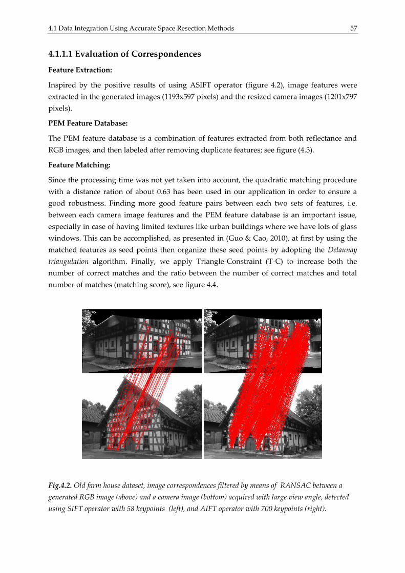
4.1 Data Integration Using Accurate Space Resection Methods 57
4.1.1.1 Evaluation of Correspondences
Feature Extraction:
Inspired by the positive results of using ASIFT operator (figure 4.2), image features were
extracted in the generated images (1193x597 pixels) and the resized camera images (1201x797
pixels).
PEM Feature Database:
The PEM feature database is a combination of features extracted from both reflectance and
RGB images, and then labeled after removing duplicate features; see figure (4.3).
Feature Matching:
Since the processing time was not yet taken into account, the quadratic matching procedure
with a distance ration of about 0.63 has been used in our application in order to ensure a
good robustness. Finding more good feature pairs between each two sets of features, i.e.
between each camera image features and the PEM feature database is an important issue,
especially in case of having limited textures like urban buildings where we have lots of glass
windows. This can be accomplished, as presented in (Guo & Cao, 2010), at first by using the
matched features as seed points then organize these seed points by adopting the Delaunay
triangulation algorithm. Finally, we apply Triangle-Constraint (T-C) to increase both the
number of correct matches and the ratio between the number of correct matches and total
number of matches (matching score), see figure 4.4.
Fig.4.2. Old farm house dataset, image correspondences filtered by means of RANSAC between a
generated RGB image (above) and a camera image (bottom) acquired with large view angle, detected
using SIFT operator with 58 keypoints (left), and AIFT operator with 700 keypoints (right).
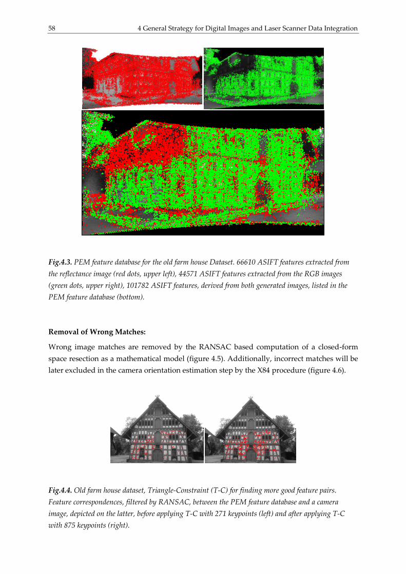
58 4 General Strategy for Digital Images and Laser Scanner Data Integration
Fig.4.3. PEM feature database for the old farm house Dataset. 66610 ASIFT features extracted from
the reflectance image (red dots, upper left), 44571 ASIFT features extracted from the RGB images
(green dots, upper right), 101782 ASIFT features, derived from both generated images, listed in the
PEM feature database (bottom).
Removal of Wrong Matches:
Wrong image matches are removed by the RANSAC based computation of a closed-form
space resection as a mathematical model (figure 4.5). Additionally, incorrect matches will be
later excluded in the camera orientation estimation step by the X84 procedure (figure 4.6).
Fig.4.4. Old farm house dataset, Triangle-Constraint (T-C) for finding more good feature pairs.
Feature correspondences, filtered by RANSAC, between the PEM feature database and a camera
image, depicted on the latter, before applying T-C with 271 keypoints (left) and after applying T-C
with 875 keypoints (right).
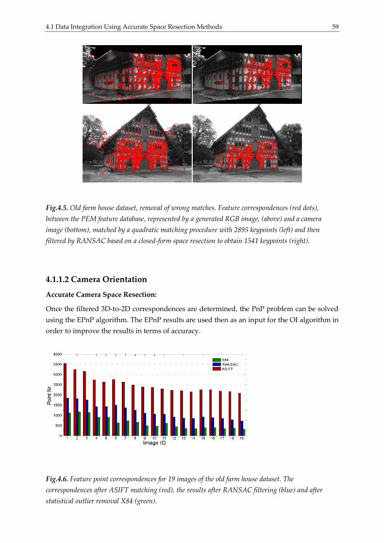
4.1 Data Integration Using Accurate Space Resection Methods 59
Fig.4.5. Old farm house dataset, removal of wrong matches. Feature correspondences (red dots),
between the PEM feature database, represented by a generated RGB image, (above) and a camera
image (bottom), matched by a quadratic matching procedure with 2895 keypoints (left) and then
filtered by RANSAC based on a closed-form space resection to obtain 1541 keypoints (right).
4.1.1.2 Camera Orientation
Accurate Camera Space Resection:
Once the filtered 3D-to-2D correspondences are determined, the PnP problem can be solved
using the EPnP algorithm. The EPnP results are used then as an input for the OI algorithm in
order to improve the results in terms of accuracy.
Fig.4.6. Feature point correspondences for 19 images of the old farm house dataset. The
correspondences after ASIFT matching (red), the results after RANSAC filtering (blue) and after
statistical outlier removal X84 (green).
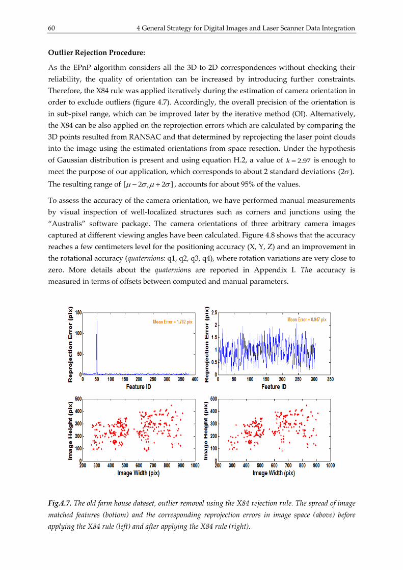
60 4 General Strategy for Digital Images and Laser Scanner Data Integration
Outlier Rejection Procedure:
As the EPnP algorithm considers all the 3D-to-2D correspondences without checking their
reliability, the quality of orientation can be increased by introducing further constraints.
Therefore, the X84 rule was applied iteratively during the estimation of camera orientation in
order to exclude outliers (figure 4.7). Accordingly, the overall precision of the orientation is
in sub-pixel range, which can be improved later by the iterative method (OI). Alternatively,
the X84 can be also applied on the reprojection errors which are calculated by comparing the
3D points resulted from RANSAC and that determined by reprojecting the laser point clouds
into the image using the estimated orientations from space resection. Under the hypothesis
of Gaussian distribution is present and using equation H.2, a value of 2.97k is enough to
meet the purpose of our application, which corresponds to about 2 standard deviations (2 ).
The resulting range of [ 2 , 2 ] , accounts for about 95% of the values.
To assess the accuracy of the camera orientation, we have performed manual measurements
by visual inspection of well-localized structures such as corners and junctions using the
“Australis” software package. The camera orientations of three arbitrary camera images
captured at different viewing angles have been calculated. Figure 4.8 shows that the accuracy
reaches a few centimeters level for the positioning accuracy (X, Y, Z) and an improvement in
the rotational accuracy (quaternions: q1, q2, q3, q4), where rotation variations are very close to
zero. More details about the quaternions are reported in Appendix I. The accuracy is
measured in terms of offsets between computed and manual parameters.
Fig.4.7. The old farm house dataset, outlier removal using the X84 rejection rule. The spread of image
matched features (bottom) and the corresponding reprojection errors in image space (above) before
applying the X84 rule (left) and after applying the X84 rule (right).
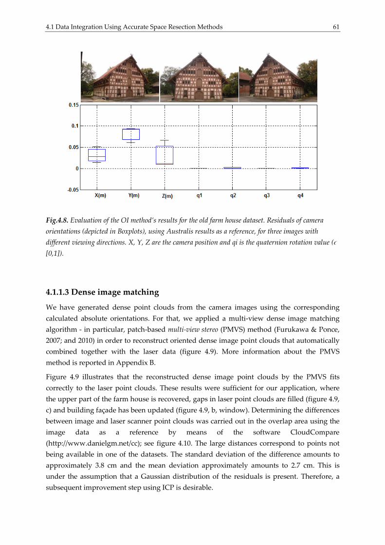
4.1 Data Integration Using Accurate Space Resection Methods 61
Fig.4.8. Evaluation of the OI method’s results for the old farm house dataset. Residuals of camera
orientations (depicted in Boxplots), using Australis results as a reference, for three images with
different viewing directions. X, Y, Z are the camera position and qi is the quaternion rotation value (ϵ
[0,1]).
4.1.1.3 Dense image matching
We have generated dense point clouds from the camera images using the corresponding
calculated absolute orientations. For that, we applied a multi-view dense image matching
algorithm - in particular, patch-based multi-view stereo (PMVS) method (Furukawa & Ponce,
2007; and 2010) in order to reconstruct oriented dense image point clouds that automatically
combined together with the laser data (figure 4.9). More information about the PMVS
method is reported in Appendix B.
Figure 4.9 illustrates that the reconstructed dense image point clouds by the PMVS fits
correctly to the laser point clouds. These results were sufficient for our application, where
the upper part of the farm house is recovered, gaps in laser point clouds are filled (figure 4.9,
c) and building façade has been updated (figure 4.9, b, window). Determining the differences
between image and laser scanner point clouds was carried out in the overlap area using the
image data as a reference by means of the software CloudCompare
(http://www.danielgm.net/cc); see figure 4.10. The large distances correspond to points not
being available in one of the datasets. The standard deviation of the difference amounts to
approximately 3.8 cm and the mean deviation approximately amounts to 2.7 cm. This is
under the assumption that a Gaussian distribution of the residuals is present. Therefore, a
subsequent improvement step using ICP is desirable.
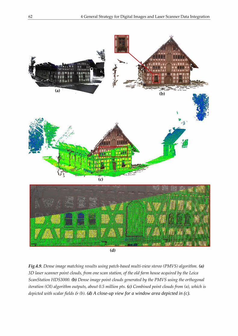
62 4 General Strategy for Digital Images and Laser Scanner Data Integration
Fig.4.9. Dense image matching results using patch-based multi-view stereo (PMVS) algorithm. (a)
3D laser scanner point clouds, from one scan station, of the old farm house acquired by the Leica
ScanStation HDS3000. (b) Dense image point clouds generated by the PMVS using the orthogonal
iteration (OI) algorithm outputs, about 0.5 million pts. (c) Combined point clouds from (a), which is
depicted with scalar fields & (b). (d) A close-up view for a window area depicted in (c).
(c)
(a) (b)
(d)
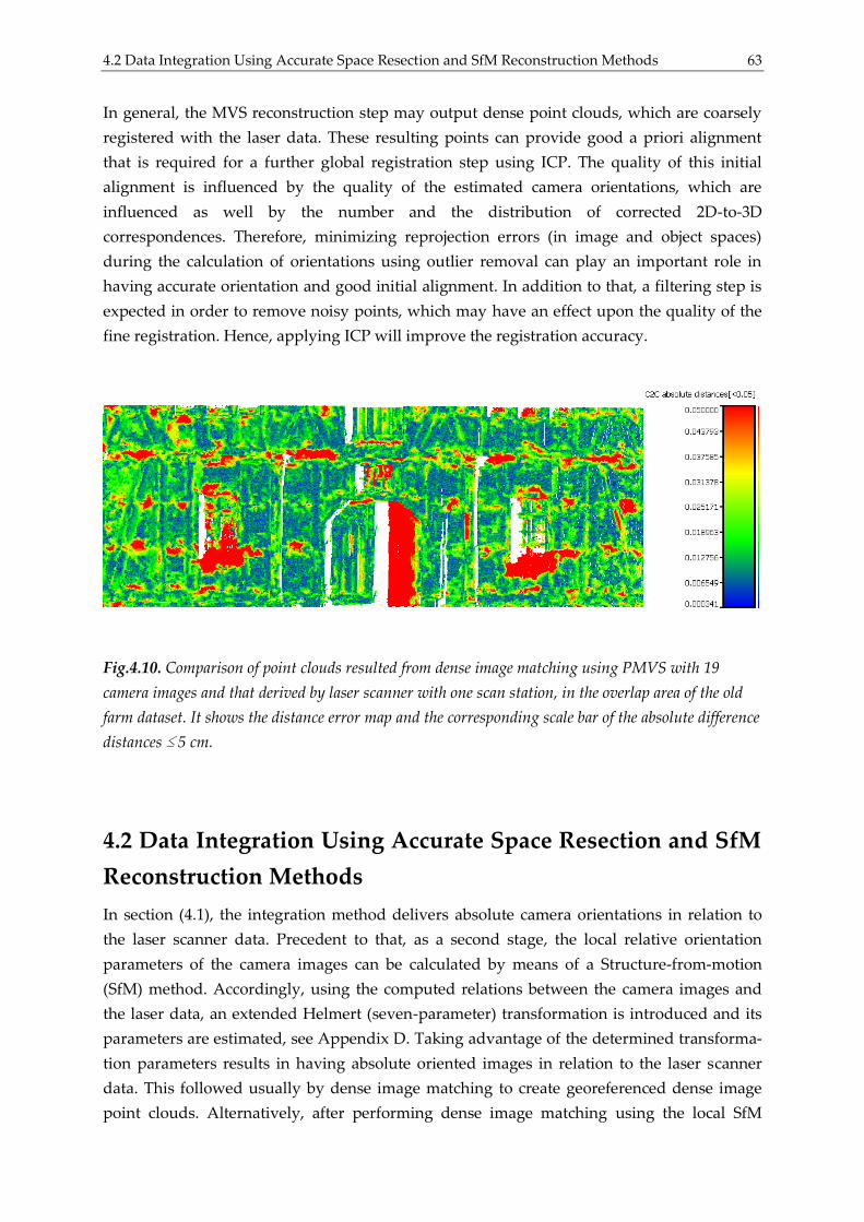
4.2 Data Integration Using Accurate Space Resection and SfM Reconstruction Methods 63
In general, the MVS reconstruction step may output dense point clouds, which are coarsely
registered with the laser data. These resulting points can provide good a priori alignment
that is required for a further global registration step using ICP. The quality of this initial
alignment is influenced by the quality of the estimated camera orientations, which are
influenced as well by the number and the distribution of corrected 2D-to-3D
correspondences. Therefore, minimizing reprojection errors (in image and object spaces)
during the calculation of orientations using outlier removal can play an important role in
having accurate orientation and good initial alignment. In addition to that, a filtering step is
expected in order to remove noisy points, which may have an effect upon the quality of the
fine registration. Hence, applying ICP will improve the registration accuracy.
Fig.4.10. Comparison of point clouds resulted from dense image matching using PMVS with 19
camera images and that derived by laser scanner with one scan station, in the overlap area of the old
farm dataset. It shows the distance error map and the corresponding scale bar of the absolute difference
distances ≤ 5 cm.
4.2 Data Integration Using Accurate Space Resection and SfM
Reconstruction Methods
In section (4.1), the integration method delivers absolute camera orientations in relation to
the laser scanner data. Precedent to that, as a second stage, the local relative orientation
parameters of the camera images can be calculated by means of a Structure-from-motion
(SfM) method. Accordingly, using the computed relations between the camera images and
the laser data, an extended Helmert (seven-parameter) transformation is introduced and its
parameters are estimated, see Appendix D. Taking advantage of the determined transforma-
tion parameters results in having absolute oriented images in relation to the laser scanner
data. This followed usually by dense image matching to create georeferenced dense image
point clouds. Alternatively, after performing dense image matching using the local SfM
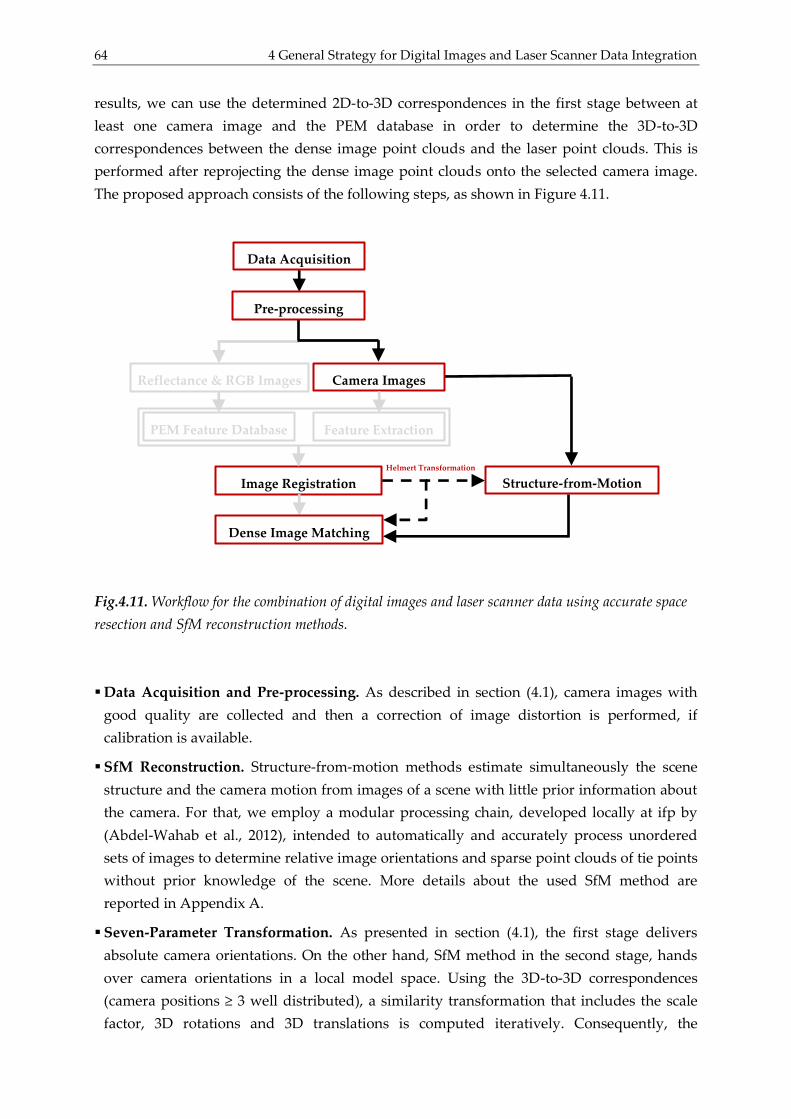
64 4 General Strategy for Digital Images and Laser Scanner Data Integration
results, we can use the determined 2D-to-3D correspondences in the first stage between at
least one camera image and the PEM database in order to determine the 3D-to-3D
correspondences between the dense image point clouds and the laser point clouds. This is
performed after reprojecting the dense image point clouds onto the selected camera image.
The proposed approach consists of the following steps, as shown in Figure 4.11.
Fig.4.11. Workflow for the combination of digital images and laser scanner data using accurate space
resection and SfM reconstruction methods.
Data Acquisition and Pre-processing. As described in section (4.1), camera images with
good quality are collected and then a correction of image distortion is performed, if
calibration is available.
SfM Reconstruction. Structure-from-motion methods estimate simultaneously the scene
structure and the camera motion from images of a scene with little prior information about
the camera. For that, we employ a modular processing chain, developed locally at ifp by
(Abdel-Wahab et al., 2012), intended to automatically and accurately process unordered
sets of images to determine relative image orientations and sparse point clouds of tie points
without prior knowledge of the scene. More details about the used SfM method are
reported in Appendix A.
Seven-Parameter Transformation. As presented in section (4.1), the first stage delivers
absolute camera orientations. On the other hand, SfM method in the second stage, hands
over camera orientations in a local model space. Using the 3D-to-3D correspondences
(camera positions ≥ 3 well distributed), a similarity transformation that includes the scale
factor, 3D rotations and 3D translations is computed iteratively. Consequently, the
Structure-from-Motion
(SfM)
Image Registration
Data Acquisition
Pre-processing
Camera Images
Feature Extraction PEM Feature Database
Reflectance & RGB Images
Dense Image Matching
Helmert Transformation

4.2 Data Integration Using Accurate Space Resection and SfM Reconstruction Methods 65
estimated seven-parameters are applied on the SfM output in order to have absolute
camera orientations in relation to the LiDAR data. An alternative method is using the
determined 2D-to-3D points in the first approach between at least one camera image and
the PEM database. This enables us to determine the transformation parameters. That is, by
applying dense image matching on the local SfM results and then reprojecting the latter
into the selected camera image using the collinearity equations (3.1) or the following
respective transformation equations (central projection in homogeneous coordinates).
|x K R t X (4.1)
where x represents the unknown 2D image homogeneous coordinates, K is the known
camera calibration matrix, ( , )R t denote the known exterior orientation parameters resulted
from the SfM method and X constitute the known 3D object homogeneous coordinates of
the laser data. This allows us to determine the 2D-to-2D correspondences between the
camera image and the reprojected image point clouds, i.e. the 3D-to-3D correspondences
between the PEM database or laser data and the image point clouds. Therefore, this method
requires performing the dense matching step before the calculation of transformation
parameters. In addition, the same approach can be applied on the sparse point clouds
resulted from the SfM method by projecting only the sparse points onto the selected image.
Then, the dense matching step can be employed after the calculation of transformation
parameters. But, this approach provides less redundant measurements.
Since some dense matching algorithms provide dense image point clouds separately for
almost each individual image, e.g. the software SURE (Rothermel et al., 2012), it is more
robust to only project the single dense point cloud onto the corresponding selected image
for the seven-parameters estimation. This can filter out incorrect projected points on the
image, i.e. projected points from object surfaces that are not covered by the selected image.
Consequently, the estimated transformation parameters can be computed with blunder
rejection and then are applied on the image data.
Dense Image Matching. Dense point clouds can be reconstructed using the resulted
absolute or local camera orientations with the help of any dense matching algorithm. The
resulted point clouds are automatically combined with the laser data to form a complete
representation of the scene, with an option for further improvement using ICP.
The algorithm has been implemented in a Matlab code.
4.2.1 Experimental Evaluation
To assess the results, the second stage in our developed pipeline was applied also to the
dataset of the old farm house. 19 photographs have been employed for SfM reconstruction.
In the following, an evaluation for the pipeline steps is demonstrated.

66 4 General Strategy for Digital Images and Laser Scanner Data Integration
4.2.1.1 Camera Orientation
SfM Reconstruction:
Using the SfM method developed locally at the Institute for Photogrammetry (ifp), we
successfully derived the orientations and the geometry from the used imagery (19 images);
the results are shown in figure 4.12 left with relative accuracy in image space (root mean
square of the reprojection error) less than a pixel, about 0.7 pixels. This is considered to meet
the requirements for the latter dense matching step.
Fig. 4.12. SfM output: sparse point clouds (colored), 19 camera positions (red dots) of the old farm
house dataset (left). Reprojected dense image point clouds onto a camera image (red dots) and the
resulted 3D correspondences (210 keypoints, blue dots) between the latter and the laser point clouds
which are used for the calculation of the seven- parameters, depicted on the camera image (right).
Seven-Parameter Transformation:
We have performed two methods for the estimation of the transformation parameters. The
first method utilizes the determined 3D-to-3D camera positions from space resection and
SfM methods. Then, a procedure based on an iterative computation of the seven-parameters
is curried out. After that, the camera orientations resulted from SfM are transformed by the
calculated parameters in order to have absolute values. While in the second method, the 3D-
to-3D correspondences between the laser and image point clouds are determined after
reprojecting the dense image point clouds onto at least one camera image (figure 4.12 right).
The transformation provides accurate a priori alignment of the dense image point clouds
with the laser data, which can be improved latter by ICP.
In order to evaluate the accuracy of the estimated orientations by the SfM method as well as
transformed by the calculated Helmert parameters, a comparison to the computed camera
orientation using the “Australis” software package was performed (figure 4.13). In case of
using the camera positions for the calculation of transformation, the positioning accuracy
(X,Y,Z) is a few centimeters and the rotation residuals are very small which indicates an
improvement in the rotational accuracy (q1, q2, q3, q4). While, using the second method
shows that the accuracies have improved. This is due to the redundant measurements and

4.2 Data Integration Using Accurate Space Resection and SfM Reconstruction Methods 67
the good distribution of the used 3D correspondences compared to the limited number of
camera positions and not very well distributed in the surrounding object of interest.
Fig.4.13. The old farm house dataset, evaluation of the SfM method’s results. Residuals of camera
orientations (depicted in Boxplots) resulted by using the camera positions (middle) and the reprojected
dense image point clouds (bottom) for the seven-parameters estimation, using Australis results as a
reference, for three images with different viewing directions (above). X, Y, Z are the camera position
and qi is the quaternion rotation value (ϵ [0,1]).
4.2.1.2 Dense image matching
Using the absolute camera orientations, we have reconstructed a georeferenced and dense
point clouds from the corresponding camera images (Figure 4.14). For that, we applied dense
image matching algorithms - in particular, a hierarchical multi-view stereo based on the
Semi-Global Matching. This solution was developed locally at ifp and implemented within a
software package called SURE; see (Rothermel et al., 2012). More details about the SURE
method are presented in Appendix B.

68 4 General Strategy for Digital Images and Laser Scanner Data Integration
Fig.4.14. Dense image matching results using the software SURE. (a) 3D laser scanner point clouds,
from one scan station, of the old farm building façade acquired by the Leica ScanStation HDS3000. (b)
Dense image point clouds generated by the software SURE using the SfM method’s outputs, about 11
million pts. (c) Combined point clouds from (a), which is depicted with scalar fields and (b). (d) A
close-up view for a window area depicted in (c).
(c)
(a) (b)
(d)

4.3 The Proposed General Workflow 69
Figure 4.14 shows that the resulted dense image point clouds fit correctly to the laser point
clouds and contain almost no noise. These results are considered to meet the requirements of
our application, where the upper part of the farm house is reconstructed, gaps in laser point
clouds are filled and building façade has been updated. In order to know the differences
between the models, point clouds acquired by laser scanner and that obtained by the
software SURE, a comparison in the overlap area was performed using the latter as a
reference by means of the software CloudCompare (figure 4.15). The large distances
correspond to points not being available in one of the datasets. The standard deviation of the
difference amounts to approximately 3.9 cm and the mean deviation approximately amounts
to 1.8 cm. These results were improved compared to those resulted by the previous method
in section (4.1). Nevertheless, a subsequent refinement step using ICP is preferable.
Fig.4.15. Comparison of point clouds resulted from dense image matching using the software SURE
with 19 camera images and that derived by laser scanner with one scan station, in the overlap area of
the old farm dataset. It shows the distance error map and the corresponding scale bar of the absolute
difference distances ≤ 5 cm.
4.3 The Proposed General Workflow
In section (4.1), imagery has been processed separately in order to calculate the camera
orientations not taking into account the relative geometry of all images. These orientations
are employed then to transform the SfM outputs, presented in section (4.2), into object model
space whereas all images are processed efficiently in one bundle. Using the transformation
parameters resulted with the help of space resection methods can lead to a reduction in the
accuracy of image or dense image point cloud alignment with the laser data. In order to
overcome these problems and improve the previous results a direct integration solution of
photogrammetric and LiDAR techniques has been attempted.
As presented in chapter 3, reflectance or RGB images are generated from 3D laser data in a
central projection. On the other hand, the SfM approach and the subsequent bundle block
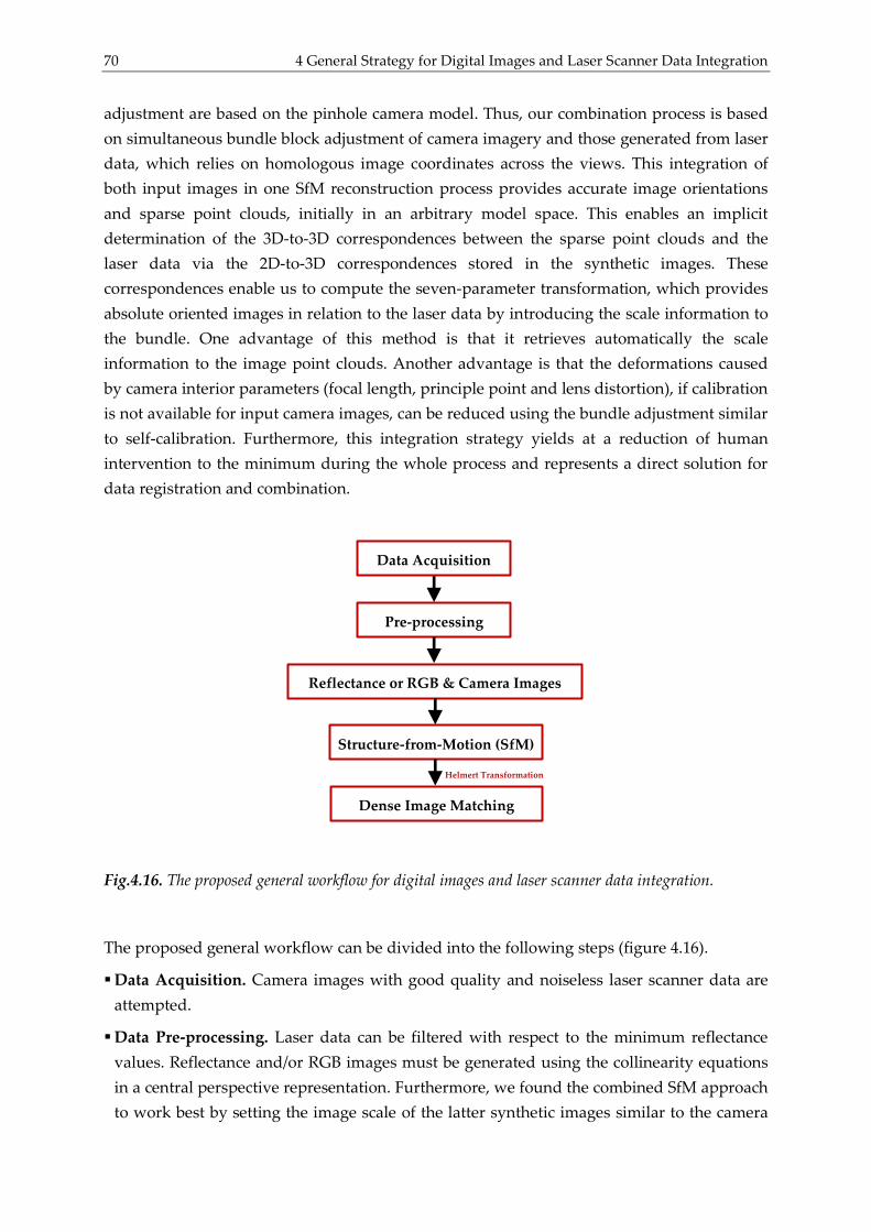
70 4 General Strategy for Digital Images and Laser Scanner Data Integration
adjustment are based on the pinhole camera model. Thus, our combination process is based
on simultaneous bundle block adjustment of camera imagery and those generated from laser
data, which relies on homologous image coordinates across the views. This integration of
both input images in one SfM reconstruction process provides accurate image orientations
and sparse point clouds, initially in an arbitrary model space. This enables an implicit
determination of the 3D-to-3D correspondences between the sparse point clouds and the
laser data via the 2D-to-3D correspondences stored in the synthetic images. These
correspondences enable us to compute the seven-parameter transformation, which provides
absolute oriented images in relation to the laser data by introducing the scale information to
the bundle. One advantage of this method is that it retrieves automatically the scale
information to the image point clouds. Another advantage is that the deformations caused
by camera interior parameters (focal length, principle point and lens distortion), if calibration
is not available for input camera images, can be reduced using the bundle adjustment similar
to self-calibration. Furthermore, this integration strategy yields at a reduction of human
intervention to the minimum during the whole process and represents a direct solution for
data registration and combination.
Fig.4.16. The proposed general workflow for digital images and laser scanner data integration.
The proposed general workflow can be divided into the following steps (figure 4.16).
Data Acquisition. Camera images with good quality and noiseless laser scanner data are
attempted.
Data Pre-processing. Laser data can be filtered with respect to the minimum reflectance
values. Reflectance and/or RGB images must be generated using the collinearity equations
in a central perspective representation. Furthermore, we found the combined SfM approach
to work best by setting the image scale of the latter synthetic images similar to the camera
Structure-from-Motion (SfM)
Data Acquisition
Pre-processing
Reflectance or RGB & Camera Images
Dense Image Matching
Helmert Transformation
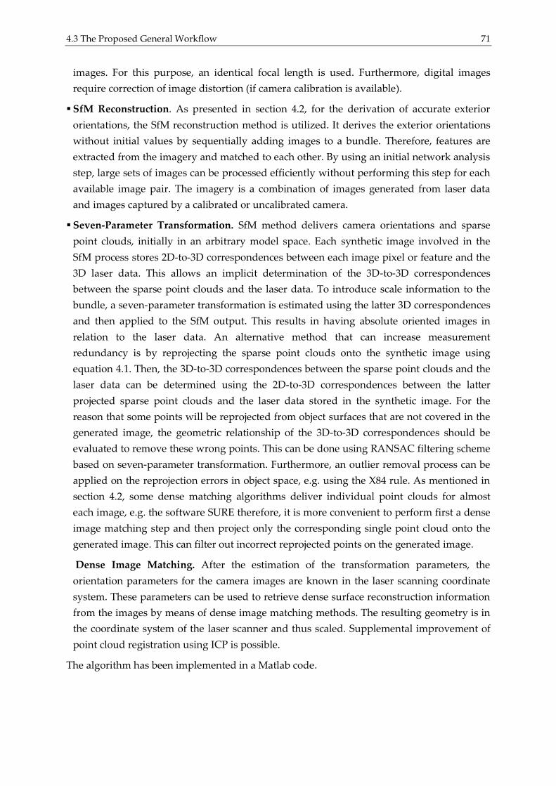
4.3 The Proposed General Workflow 71
images. For this purpose, an identical focal length is used. Furthermore, digital images
require correction of image distortion (if camera calibration is available).
SfM Reconstruction. As presented in section 4.2, for the derivation of accurate exterior
orientations, the SfM reconstruction method is utilized. It derives the exterior orientations
without initial values by sequentially adding images to a bundle. Therefore, features are
extracted from the imagery and matched to each other. By using an initial network analysis
step, large sets of images can be processed efficiently without performing this step for each
available image pair. The imagery is a combination of images generated from laser data
and images captured by a calibrated or uncalibrated camera.
Seven-Parameter Transformation. SfM method delivers camera orientations and sparse
point clouds, initially in an arbitrary model space. Each synthetic image involved in the
SfM process stores 2D-to-3D correspondences between each image pixel or feature and the
3D laser data. This allows an implicit determination of the 3D-to-3D correspondences
between the sparse point clouds and the laser data. To introduce scale information to the
bundle, a seven-parameter transformation is estimated using the latter 3D correspondences
and then applied to the SfM output. This results in having absolute oriented images in
relation to the laser data. An alternative method that can increase measurement
redundancy is by reprojecting the sparse point clouds onto the synthetic image using
equation 4.1. Then, the 3D-to-3D correspondences between the sparse point clouds and the
laser data can be determined using the 2D-to-3D correspondences between the latter
projected sparse point clouds and the laser data stored in the synthetic image. For the
reason that some points will be reprojected from object surfaces that are not covered in the
generated image, the geometric relationship of the 3D-to-3D correspondences should be
evaluated to remove these wrong points. This can be done using RANSAC filtering scheme
based on seven-parameter transformation. Furthermore, an outlier removal process can be
applied on the reprojection errors in object space, e.g. using the X84 rule. As mentioned in
section 4.2, some dense matching algorithms deliver individual point clouds for almost
each image, e.g. the software SURE therefore, it is more convenient to perform first a dense
image matching step and then project only the corresponding single point cloud onto the
generated image. This can filter out incorrect reprojected points on the generated image.
Dense Image Matching. After the estimation of the transformation parameters, the
orientation parameters for the camera images are known in the laser scanning coordinate
system. These parameters can be used to retrieve dense surface reconstruction information
from the images by means of dense image matching methods. The resulting geometry is in
the coordinate system of the laser scanner and thus scaled. Supplemental improvement of
point cloud registration using ICP is possible.
The algorithm has been implemented in a Matlab code.
72 4 General Strategy for Digital Images and Laser Scanner Data Integration
4.3.1 Shifting the Principle Point of the Generated Images
A combination of images generated from 3D laser data and images collected by a calibrated
or uncalibrated camera is involved in the SfM process. In particular, if the accuracy
requirements of the application like cultural heritage data recording are high and a camera
with high stability and fixed focal length is employed, we use calibration parameters
determined prior by standard calibration methods for camera imagery. On the other hand,
the virtual cameras, used to project the laser point clouds onto virtual/synthetic images, are
assumed to be calibrated. Except the principle point (P), which must be shifted (by an offset
of dx in x direction and dy in y direction) to the projected point of the laser scanner‘s center
point into the virtual image plane (P`), see figure 4.17. Thus, the image dimensions have to be
adapted accordingly. This being the case since in the SfM and the bundle adjustment
methods, it is considered that the principle point of each image, generated and captured, is
located in the middle. Therefore, the generated images can not be used directly in our
algorithm unless the re-centering process is applied. These offsets are calculated in pixels
using the following equations.
min( ) ( / 2)
min( ) ( / 2)
dx x w
dy y h
(4.2)
where ( , )x y represent the image coordinates in pixels resulted from applying collinearity
equations (3.1) and ( , )w h denote the image size in pixels (width and height) which are
determined by the minimum and maximum values of the latter image coordinates, in and
directions. The reason for that shift is related to the data acquisition. For practical reason,
there is no guaranty that laser scanner center point is corresponded to the center point of the
acquired scene. Furthermore, if the 3D virtual camera coordinates are correctly defined (see
chapter 3, section 3.2.1), the offset of dx will be equal to zero.
4.3.2 Advantages of the proposed approach
This general approach is directed at combining and complementing several aspects of the
individual technique. Therefore, the main attempted improvements of our proposed
approach are described as follows.
4.3.2.1 Complementing TLS Point Clouds by Dense Image Matching
Filling Gaps in Laser Scanner Point Cloud:
TLS data is free from scan gaps or holes only in very particular cases. These gaps occur
usually due to occlusions or weak reflectivity of object material such as building windows
with glasses, dark building pipes and so on. Current algorithms as the Poisson algorithm
(Kazhdan et al., 2006) fill in small gaps automatically during the surface reconstruction and
offer conventional modeling or cloning options for larger patches. These semi-automatic
approaches are considered time consuming since they require heavily human intervention.

4.3 The Proposed General Workflow 73
Moreover, using automated hole-filling or surface augmentation methods developed by
(Sharf et al., 2004), is limited and doubtful especially in heritage documentation applications
(Rüther et al., 2012). Thus, our proposed combination method allows us to fill gaps due to
occlusions or weak reflectivity of object materials using the registered camera images; see
chapter 7, section 7.2.1).
Retrieving More Surface Information:
TLS with distance measurements can be used for acquiring large-scale point clouds at
medium range distances, while image based surface reconstruction methods enable flexible
acquisition with high precision at short distances. Therefore, in our combination method,
camera imagery can complement surface information with higher density (see chapter 7,
section 7.2.2). Moreover, this combination can be used to retrieve dense surface information
for complex surface geometries where many scan stations would be needed. On the other
hand, laser scanning introduces the scale information and delivers high precision also on
longer distances with low efforts.
Fig.4.17. Shifting the principle point of the generated image from 3D laser scanner data.
dy
x
Y
X
Object
Z
y
Image Plane
C
Camera Center
C
P
P`
H
W
H/2
W/2
P`
x
y
P
h
w
h/2
w/2
dx
74 4 General Strategy for Digital Images and Laser Scanner Data Integration
4.3.2.2 Automatic Registration of Point Clouds
Finding the transformation parameters between different point clouds, referred as
registration, is still a critical task in the research community. Several approaches have been
developed and presented but still rely on a small dataset. In particular, the target-based
approach which is considered as a user-based technique, followed by the surface matching
methods among which the ICP algorithm is mostly used. Since the latter requires initial
values for the transformation parameters and not all surveyed objects show a geometry
adequate for application of surface matching algorithms, other methods have been
attempted using intensity and RGB values (Alba et al., 2011).
The proposed algorithm presents an automatic methodology able to register different point
clouds using a combination of camera images and others derived from LiDAR data, intensity
and RGB values, in one SfM process. Using the resulted absolute camera orientations, on the
one hand, a direct registration between dense image point clouds and laser scanner point
clouds is performed. On the other hand, this also results in registering multiple laser scans.
This is because of the relative orientations between the generated images which are already
determined at the SfM step and transformed to the absolute coordinate system auto-
matically. Thus, our method provides an efficient solution in one-step for the direct
registration of both image and laser scanner point clouds. Simultaneously, it performs target-
free registration of multiple laser scans. This also includes the automatic registration of scans
occluded partially by the neighboring buildings and trees where less overlap is occurred,
and completely non-overlapping laser scans. That is, since the proposed method allows us to
provide sufficient overlapping geometry by introducing additional overlapping images into
the SfM process, which can be matched with the surrounding scans; see chapter 5, section 5.3
and chapter 7, section 7.3.3. Thus, our general approach can be utilized almost in all
operative conditions.
4.3.3 Experimental Evaluation
To evaluate the results, our proposed general approach was applied also to the dataset of the
old farm house. 3 RGB images generated from LiDAR data and 35 camera images have been
employed for the SfM reconstruction. In the following, an evaluation for the whole method
steps is shown.
4.3.3.1 Camera Orientation
SfM Reconstruction:
We successfully derived the orientations and the geometry from all used imagery (3
generated and 35 camera images) with relative accuracy in image space (root mean square
error of the reprojection error) less than a pixel, about 0.8 pixels. This is considered to meet
the requirements for the latter dense image matching step.
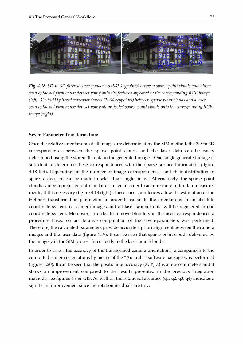
4.3 The Proposed General Workflow 75
Fig. 4.18. 3D-to-3D filtered correspondences (383 keypoints) between sparse point clouds and a laser
scan of the old farm house dataset using only the features appeared in the corresponding RGB image
(left). 3D-to-3D filtered correspondences (1064 keypoints) between sparse point clouds and a laser
scan of the old farm house dataset using all projected sparse point clouds onto the corresponding RGB
image (right).
Seven-Parameter Transformation:
Once the relative orientations of all images are determined by the SfM method, the 3D-to-3D
correspondences between the sparse point clouds and the laser data can be easily
determined using the stored 3D data in the generated images. One single generated image is
sufficient to determine these correspondences with the sparse surface information (figure
4.18 left). Depending on the number of image correspondences and their distribution in
space, a decision can be made to select that single image. Alternatively, the sparse point
clouds can be reprojected onto the latter image in order to acquire more redundant measure-
ments, if it is necessary (figure 4.18 right). These correspondences allow the estimation of the
Helmert transformation parameters in order to calculate the orientations in an absolute
coordinate system, i.e. camera images and all laser scanner data will be registered in one
coordinate system. Moreover, in order to remove blunders in the used correspondences a
procedure based on an iterative computation of the seven-parameters was performed.
Therefore, the calculated parameters provide accurate a priori alignment between the camera
images and the laser data (figure 4.19). It can be seen that sparse point clouds delivered by
the imagery in the SfM process fit correctly to the laser point clouds.
In order to assess the accuracy of the transformed camera orientations, a comparison to the
computed camera orientations by means of the “Australis” software package was performed
(figure 4.20). It can be seen that the positioning accuracy (X, Y, Z) is a few centimeters and it
shows an improvement compared to the results presented in the previous integration
methods, see figures 4.8 & 4.13. As well as, the rotational accuracy (q1, q2, q3, q4) indicates a
significant improvement since the rotation residuals are tiny.
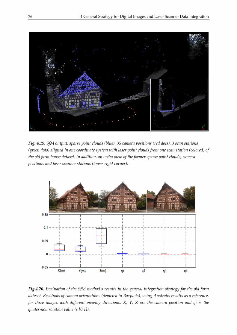
76 4 General Strategy for Digital Images and Laser Scanner Data Integration
Fig. 4.19. SfM output: sparse point clouds (blue), 35 camera positions (red dots), 3 scan stations
(green dots) aligned in one coordinate system with laser point clouds from one scan station (colored) of
the old farm house dataset. In addition, an ortho view of the former sparse point clouds, camera
positions and laser scanner stations (lower right corner).
Fig.4.20. Evaluation of the SfM method’s results in the general integration strategy for the old farm
dataset. Residuals of camera orientations (depicted in Boxplots), using Australis results as a reference,
for three images with different viewing directions. X, Y, Z are the camera position and qi is the
quaternion rotation value (ϵ [0,1]).
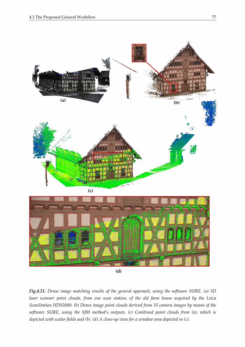
4.3 The Proposed General Workflow 77
Fig.4.21. Dense image matching results of the general approach, using the software SURE. (a) 3D
laser scanner point clouds, from one scan station, of the old farm house acquired by the Leica
ScanStation HDS3000. (b) Dense image point clouds derived from 35 camera images by means of the
software SURE, using the SfM method’s outputs. (c) Combined point clouds from (a), which is
depicted with scalar fields and (b). (d) A close-up view for a window area depicted in (c).
(c)
(a) (b)
(d)
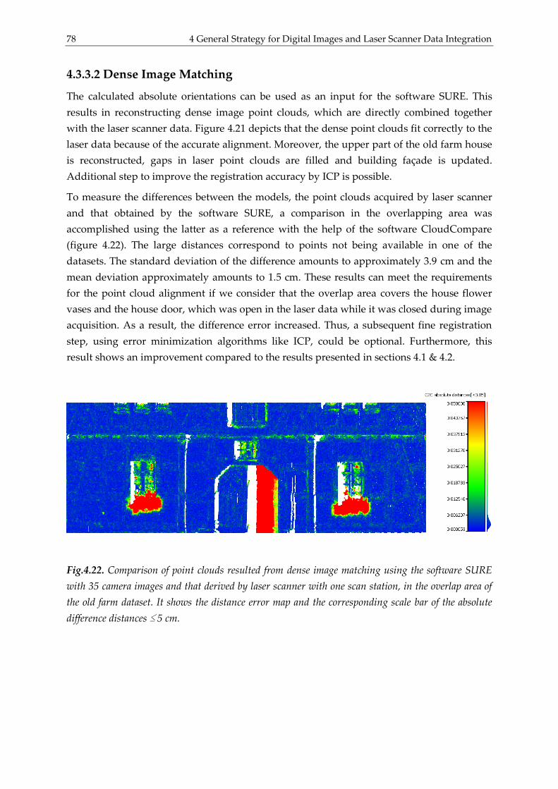
78 4 General Strategy for Digital Images and Laser Scanner Data Integration
4.3.3.2 Dense Image Matching
The calculated absolute orientations can be used as an input for the software SURE. This
results in reconstructing dense image point clouds, which are directly combined together
with the laser scanner data. Figure 4.21 depicts that the dense point clouds fit correctly to the
laser data because of the accurate alignment. Moreover, the upper part of the old farm house
is reconstructed, gaps in laser point clouds are filled and building façade is updated.
Additional step to improve the registration accuracy by ICP is possible.
To measure the differences between the models, the point clouds acquired by laser scanner
and that obtained by the software SURE, a comparison in the overlapping area was
accomplished using the latter as a reference with the help of the software CloudCompare
(figure 4.22). The large distances correspond to points not being available in one of the
datasets. The standard deviation of the difference amounts to approximately 3.9 cm and the
mean deviation approximately amounts to 1.5 cm. These results can meet the requirements
for the point cloud alignment if we consider that the overlap area covers the house flower
vases and the house door, which was open in the laser data while it was closed during image
acquisition. As a result, the difference error increased. Thus, a subsequent fine registration
step, using error minimization algorithms like ICP, could be optional. Furthermore, this
result shows an improvement compared to the results presented in sections 4.1 & 4.2.
Fig.4.22. Comparison of point clouds resulted from dense image matching using the software SURE
with 35 camera images and that derived by laser scanner with one scan station, in the overlap area of
the old farm dataset. It shows the distance error map and the corresponding scale bar of the absolute
difference distances ≤ 5 cm.
5.1 Target-Free Registration Using Accurate Space Resection Methods 79
5 Target-Free Registration of Multiple Laser
Scans
The registration of multiple laser scans as the task of transforming laser scanner point clouds
taken from different positions into a common reference system is still an active topic of
photogrammetric research, e.g. (Yang et al., 2011). A complete detailed representation of
object surfaces and structures is required for many applications such as heritage data
recording and preservation. Static LiDAR systems provide an accurate and dense three-
dimensional representation of object surfaces in local model space. However, due to
occlusion and field of view limitations, a single scan is not sufficient to produce full scene
coverage, such that multiple of views/scans have to be collected and then registered.
This scan registration is typically divided into two steps, at first, a coarse registration that
provides a priori alignment of the scans, and then a fine registration step in order to improve
the former one. In general, the registration process can either proceed automatically or
manually by placing artificial targets into the scene. The latter can be time and effort
consuming therefore, it is worthwhile to use the former one. Typical automatic/target-free
registration approaches use distinctive features extracted from 3D LiDAR data. These
features have to be matched between each two scans (scan pair) in order to estimate an initial
approximation for the 6-parameter rigid-body transformation. This is followed usually by an
error minimization step using any surface matching algorithm like ICP.
As presented in chapter 3, in order to simplify the feature extraction out of laser scanner
data, other kinds of information such as range information, reflectance values and RGB data
can be exploited; see (Al-Manasir & Fraser, 2006; Dold & Brenner, 2006; Böhm & Becker,
2007; Wang and Brenner, 2008; González-Aguilera et al., 2009; Barnea & Filin, 2010; Wein-
mann et al., 2011). In (Moussa et al., 2012a), we introduced a scene database for each single
laser scan stored in a point-based environment model (PEM). This PEM allows also the
extraction of accurate control information for the automatic pairwise registration of multiple
scans. A direct multi-view registration of multiple laser scans based on a combination of
synthetic images and camera images in one bundle block adjustment is presented in (Moussa
et al., 2012b). In the following, a detailed description of the developed approaches is given in
order to introduce the completely used methodologies.
5.1 Target-Free Registration Using Accurate Space Resection
Methods
We have developed an approach for the automatic pairwise registration of unorganized laser
scans based on a point-based environment model (PEM), which stores for each scan the 3D
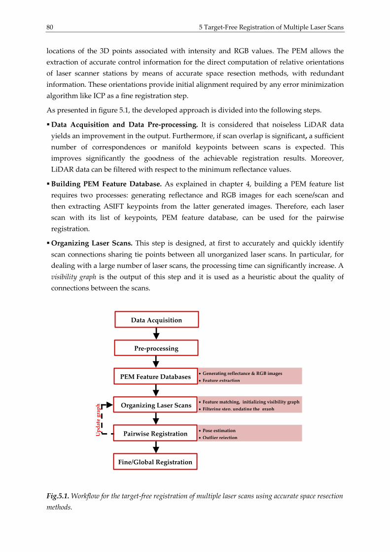
80 5 Target-Free Registration of Multiple Laser Scans
locations of the 3D points associated with intensity and RGB values. The PEM allows the
extraction of accurate control information for the direct computation of relative orientations
of laser scanner stations by means of accurate space resection methods, with redundant
information. These orientations provide initial alignment required by any error minimization
algorithm like ICP as a fine registration step.
As presented in figure 5.1, the developed approach is divided into the following steps.
Data Acquisition and Data Pre-processing. It is considered that noiseless LiDAR data
yields an improvement in the output. Furthermore, if scan overlap is significant, a sufficient
number of correspondences or manifold keypoints between scans is expected. This
improves significantly the goodness of the achievable registration results. Moreover,
LiDAR data can be filtered with respect to the minimum reflectance values.
Building PEM Feature Database. As explained in chapter 4, building a PEM feature list
requires two processes: generating reflectance and RGB images for each scene/scan and
then extracting ASIFT keypoints from the latter generated images. Therefore, each laser
scan with its list of keypoints, PEM feature database, can be used for the pairwise
registration.
Organizing Laser Scans. This step is designed, at first to accurately and quickly identify
scan connections sharing tie points between all unorganized laser scans. In particular, for
dealing with a large number of laser scans, the processing time can significantly increase. A
visibility graph is the output of this step and it is used as a heuristic about the quality of
connections between the scans.
Fig.5.1. Workflow for the target-free registration of multiple laser scans using accurate space resection
methods.
Up
dat
e g
rap
h
Generating reflectance & RGB images
Feature extraction
Feature matching, initializing visibility graph
Filtering step, updating the graph
Pose estimation
Outlier rejection
Organizing Laser Scans
Data Acquisition
Pre-processing
PEM Feature Databases
Pairwise Registration
Fine/Global Registration
5.1 Target-Free Registration Using Accurate Space Resection Methods 81
Similar approaches introduced to serve structure-from-motion (SfM) methods in order to
guide image matching and the reconstruction (Farenzena et al., 2009; Barazzetti et al., 2011;
Abdel-Wahab et al., 2012). Others were used for robust automatic registration of range
images (Bendels et al., 2004; Körtgen, 2006). In addition to that, this graph reveals the
structure of all scans and scan clusters in order to sort the scans for the pairwise registration
where the final registration error is minimal. Finally, it is served for guiding the process of
pairwise registration instead of trying to register every possible scan pair. In order to
calculate the graph, the PEM feature lists are matched to each other pairwise and then
followed by a geometry verification step.
Feature Matching.
The feature matching process is accomplished by employing a pairwise comparison of
descriptor space distances for the features in each PEM feature database to the other PEM
databases. For the latter comparison, a kd-tree search is utilized in order to speed up the
matching process. It is worthwhile to mention that, since we have double direction matching
between each PEM database pair, i.e., the first database matches to the second and the
contrary, we either consider one direction or the double direction matching. In case of the
latter, the matching result should be the intersection of the matching point pairs aggregate
from the double direction matching in order to consider the most stable keypoints. Taking
into account one direction matching is leading to the use of direct graph instead of
undirected one. This can simplify and speed up the construction of the graph.
Initialize Visibility Graph.
A set of unorganized views/scans can be directly described as a graph with two sets of
vertices and edges. These two view relations are encoded such that each vertex refers to a
scan while each edge is weighted with a similarity measure connects each scan pairs. For
that, we follow an approach having some analogy with (Farenzena et al., 2009). We extend a
2D deployed affinity measure, essentially used for SfM reconstruction tasks, so that befits the
pairwise registration of 3D laser data. It is calculated by taking into consideration the
number of common/matched keypoints between each scan pair and how well they are
spread over both the corresponding generated images (distribution in 2D) and the real scene
(distribution in 3D), see equation 5.1.
,
( ) ( )i j i j
i j dis
i j i j
S S CH S CH Sa f
S S A A
(5.1)
where ,(1 )i ja denotes the distance (similarity) measure between a scan pair ( , )i j as
, [0,1]i ja . iS and jS represent, for the scan pair ( , )i j , the set of matching keypoints in
scan ( )i and scan ( )j respectively. ()CH is the area of the convex hull of a set of points.
( )i jA A constitute to the total area of the generated image which is corresponded to a laser
scan ( )i j in a scan pair ( , )i j . disf stands for a distribution factor; equal to 0 if the common
82 5 Target-Free Registration of Multiple Laser Scans
keypoints of a scan pair are in one single plane otherwise it sets to 1. The sum of the
coefficients ( , , ) is equal to 1 where each coefficient is determined empirically or by
performing statistical tests.
The first term in the equation 5.1 is an affinity index which measures similarity between
sample sets, also known as Jaccard index or Jaccard similarity coefficient, and is defined as
the size of the intersection divided by the size of the union of the sample sets (Jaccard,
1901). The second term in the equation 5.1 refers to the approximate overlap between each
scan pair. The 3D distribution of the common keypoints is introduced approximately in
the last term in the equation 5.1. For that, a certain criterion is required in order to
determine if the common keypoints of a scan pair are belonging to one single plane or not.
This can be performed by checking the point-plane distances of the keypoints. At first, we
calculate the fitted plane and then we compute the point-plane distances of the common
point correspondences of the scan pair using the equation 5.2.
2 2 2
. . .i i i
i
a X bY c Z dD
a b c
(5.2)
where iD is the point-plane distance of a keypoint i to the fitted plane, ( , , , )a b c d
representing the fitted plane parameters and ( , , )i i iX Y Z are the 3D coordinates of the
keypoint i . Then, a certain criterion/threshold is required in order to verify the variance of
point-plane distances. This value can be determined empirically or self-adaptive by
applying the error propagation law on equation 5.2. The error of distance variance ( )D is
estimated by means of the location error of a keypoint to the fitted plane (equation 5.3).
2 2 2 2 2 2
2 2 2
1D X Y Za b c
a b c
(5.3)
The variances , ,i i iX Y Z (in X , Y and Z directions) are derived from the location error of
a single point i , which depends on the accuracy of the TLS system. These variances are
computed according to the error propagation law, which applied on the Cartesian
coordinates retrieved from the 3D polar/spherical coordinates (radius r, inclination ,
azimuth ); see equations 5.4.
2 2 2 2 2 2
2 2 2 2 2 2
2 2 2 2
sin sin ; (sin sin ) [(sin cos ) (sin cos ) ]
sin cos ; (sin sin ) [(cos cos ) ( sin sin ) ]
cos ; (cos ) ( sin )
X r
Y r
Z r
X r r
Y r r
Z r r
(5.4)
5.1 Target-Free Registration Using Accurate Space Resection Methods 83
For that, the range error ( )r and the angular errors (horizontal and vertical ) are
only considered. These three accuracies are provided by the manufacture under the
assumption that data acquisition is performed at a certain range, e.g. in case of the Leica
ScanStation HDS3000, σr = 4 mm; σφ = σθ = 60 µrad @ 1-50 m range.
Under the assumption that the range and the angular accuracies are approximately equal
for all acquired laser scanner point clouds in the certain range and since the influence of
the angle errors is very small compared to the range error, we can simplify the calculation
of keypoint variances as:
X Y Z r (5.5)
By substituting equation 5.5 in the equation 5.3, we find that the 3D distance error ( )D is
equal to the range error.
D r (5.6)
Three timers the error of distance variance ( )D is chosen as a threshold to determine if a
common keypoint i of each scan pair is a part of the fitted plane (equation 5.7). Then, we
look at the percentage of inliers to make decision if the common keypoints of a scan pair
belong to the single fitted plane or not.
3i DD (5.7)
Alternative method is to check the mean value of that absolute distances ( )m , which has to
be fulfill equation 5.7. Additional constrain can be considered that the determined
threshold should be at least equal or larger than the approximate sampling distance of the
acquired laser point clouds.
The three coefficients ( , , ) express the weight of each term/factor involved in the
equation 5.1. By means of the constrain 1 which is fulfilled by the latter
coefficients, the similarity measure between each scan pair is normalized and summarized
in one single value stored in the adjacency/distance matrix. A distance matrix by
definition is a two-dimensional array containing the distances, taken pairwise, of a set of
points. It has a size of N×N where N is the number of vertices in a graph. This symmetric
distance matrix, as the graph is directed, is used to determine the probable connections
and disconnections of the scans.
An initialization is the first step towards organizing the scans, which is performed by
selecting a defined initial scan pair, i.e., the two vertices connected by the edge with the
minimum weight/distance in the whole graph. This initial set is expanded then iteratively
until it contains all the vertices of the graph. Each iteration starts with searching
unidirectional edges starting from the initial vertices to the remaining vertices and
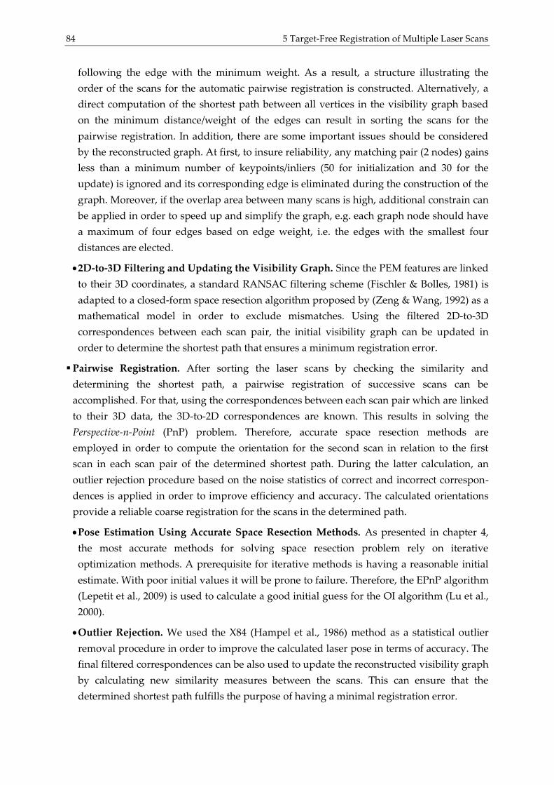
84 5 Target-Free Registration of Multiple Laser Scans
following the edge with the minimum weight. As a result, a structure illustrating the
order of the scans for the automatic pairwise registration is constructed. Alternatively, a
direct computation of the shortest path between all vertices in the visibility graph based
on the minimum distance/weight of the edges can result in sorting the scans for the
pairwise registration. In addition, there are some important issues should be considered
by the reconstructed graph. At first, to insure reliability, any matching pair (2 nodes) gains
less than a minimum number of keypoints/inliers (50 for initialization and 30 for the
update) is ignored and its corresponding edge is eliminated during the construction of the
graph. Moreover, if the overlap area between many scans is high, additional constrain can
be applied in order to speed up and simplify the graph, e.g. each graph node should have
a maximum of four edges based on edge weight, i.e. the edges with the smallest four
distances are elected.
2D-to-3D Filtering and Updating the Visibility Graph. Since the PEM features are linked
to their 3D coordinates, a standard RANSAC filtering scheme (Fischler & Bolles, 1981) is
adapted to a closed-form space resection algorithm proposed by (Zeng & Wang, 1992) as a
mathematical model in order to exclude mismatches. Using the filtered 2D-to-3D
correspondences between each scan pair, the initial visibility graph can be updated in
order to determine the shortest path that ensures a minimum registration error.
Pairwise Registration. After sorting the laser scans by checking the similarity and
determining the shortest path, a pairwise registration of successive scans can be
accomplished. For that, using the correspondences between each scan pair which are linked
to their 3D data, the 3D-to-2D correspondences are known. This results in solving the
Perspective-n-Point (PnP) problem. Therefore, accurate space resection methods are
employed in order to compute the orientation for the second scan in relation to the first
scan in each scan pair of the determined shortest path. During the latter calculation, an
outlier rejection procedure based on the noise statistics of correct and incorrect correspon-
dences is applied in order to improve efficiency and accuracy. The calculated orientations
provide a reliable coarse registration for the scans in the determined path.
Pose Estimation Using Accurate Space Resection Methods. As presented in chapter 4,
the most accurate methods for solving space resection problem rely on iterative
optimization methods. A prerequisite for iterative methods is having a reasonable initial
estimate. With poor initial values it will be prone to failure. Therefore, the EPnP algorithm
(Lepetit et al., 2009) is used to calculate a good initial guess for the OI algorithm (Lu et al.,
2000).
Outlier Rejection. We used the X84 (Hampel et al., 1986) method as a statistical outlier
removal procedure in order to improve the calculated laser pose in terms of accuracy. The
final filtered correspondences can be also used to update the reconstructed visibility graph
by calculating new similarity measures between the scans. This can ensure that the
determined shortest path fulfills the purpose of having a minimal registration error.

5.1 Target-Free Registration Using Accurate Space Resection Methods 85
Fine/Global Registration. Since the results of the previous coarse registration provide good
a priori alignment, the ICP algorithm as fine registration step can be applied. Alternatively,
the whole set of filtered correspondences between each scan pair in the determined path
can be used as an input for any surface matching algorithm like ICP or any commercial
software dealing with point cloud processing such as the Leica’s Cyclone or the Faro®
Scene software. Where the final registration is computed through a 3D global adjustment of
all scans by minimizing the registration errors across all scans (Scaioni & Forlani, 2003).
The algorithm has been implemented in a Matlab code. For graph visualization, a free tool is
used (http://www.graphviz.org).
5.1.1 Experimental Evaluation
In order to evaluate our results, the proposed approach was applied to the dataset of the old
farm house. The aim was to register 3 scans acquired to cover one building facade. Therefore,
3 PEM feature databases have been employed for the pairwise registration. In the following,
an evaluation for all the workflow steps is presented.
5.1.1.1 Organizing Scans by Similarity
Feature Matching:
The kd-tree descriptor comparison procedure with a distance ratio of about 0.6 has been used.
Furthermore, the Triangle-Constraint (Guo & Cao, 2010) can be applied to increase both the
number of correct matches and the matching score, see chapter 4, figure 4.3.
Initializing Visibility Graph:
After the determination of the similarity measures, which connect each scan pair, the three
unorganized scans can be directly described as a directed graph with three vertices and three
edges. These two view relations are encoded such that the three vertices refer to the number
of employed scans while the edges denote to the three possible scan pairs. Each edge is
weighted with a similarity measure calculated between the corresponding scan pair. For the
calculation of similarity measures, we set the following values: α = 0.5, β = 0.3, γ = 0.2, σr =
0.004 m (figure 5.2).
2D-to-3D Filtering and Updating the Visibility Graph:
Wrong matches are discarded by means of a RANSAC based computation of a closed-form
space resection (figure 5.3). Additionally, incorrect matches will be later excluded in the pose
estimation step, by the X84, see figure 5.4. The filtered matches are then used to update the
initialized visibility graph in order to determine the shortest path (figure 5.5 left). Finding
out the shortest path between all vertices in the constructed graph, based on the minimum
weight of the edges, leads to the order of the scans required for the automatic pairwise
registration. This ensures that the final registration error is minimal. According to the
shortest path (figure 5.5 right), we have to register, at first scan 1 to scan 2 pairwise then scan
2 to scan 3 pairwise.
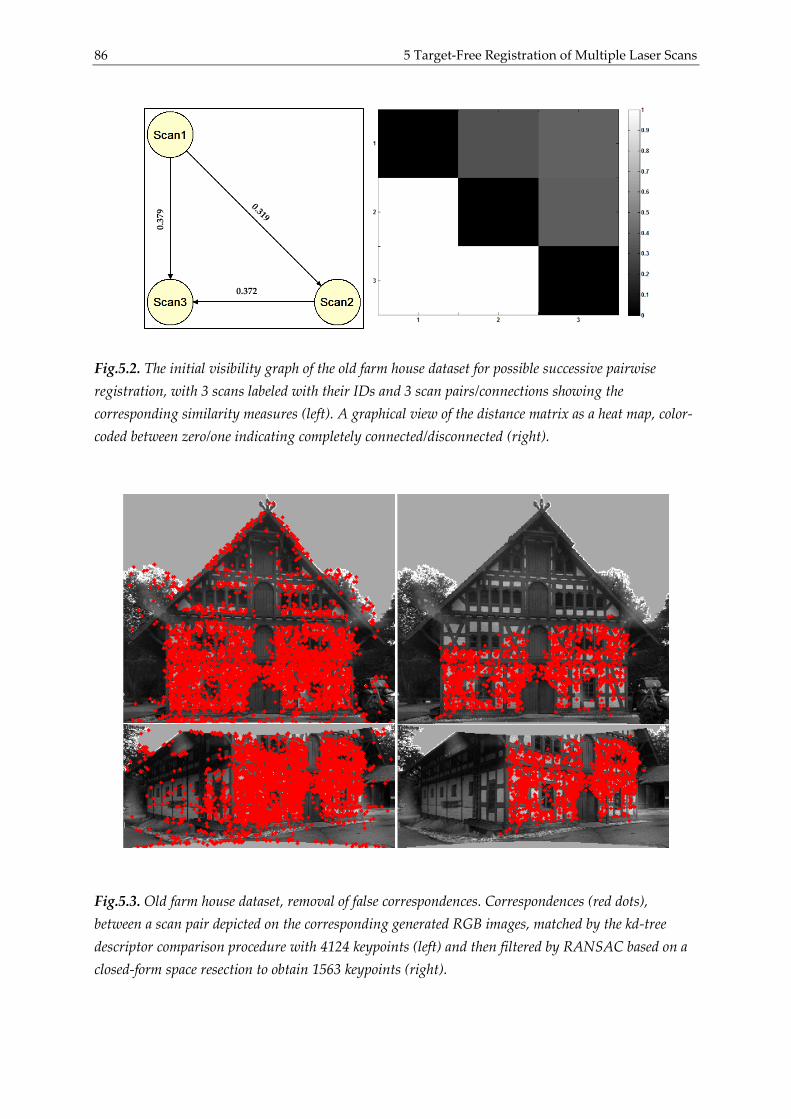
86 5 Target-Free Registration of Multiple Laser Scans
Fig.5.2. The initial visibility graph of the old farm house dataset for possible successive pairwise
registration, with 3 scans labeled with their IDs and 3 scan pairs/connections showing the
corresponding similarity measures (left). A graphical view of the distance matrix as a heat map, color-
coded between zero/one indicating completely connected/disconnected (right).
Fig.5.3. Old farm house dataset, removal of false correspondences. Correspondences (red dots),
between a scan pair depicted on the corresponding generated RGB images, matched by the kd-tree
descriptor comparison procedure with 4124 keypoints (left) and then filtered by RANSAC based on a
closed-form space resection to obtain 1563 keypoints (right).
0.372
0.37
9
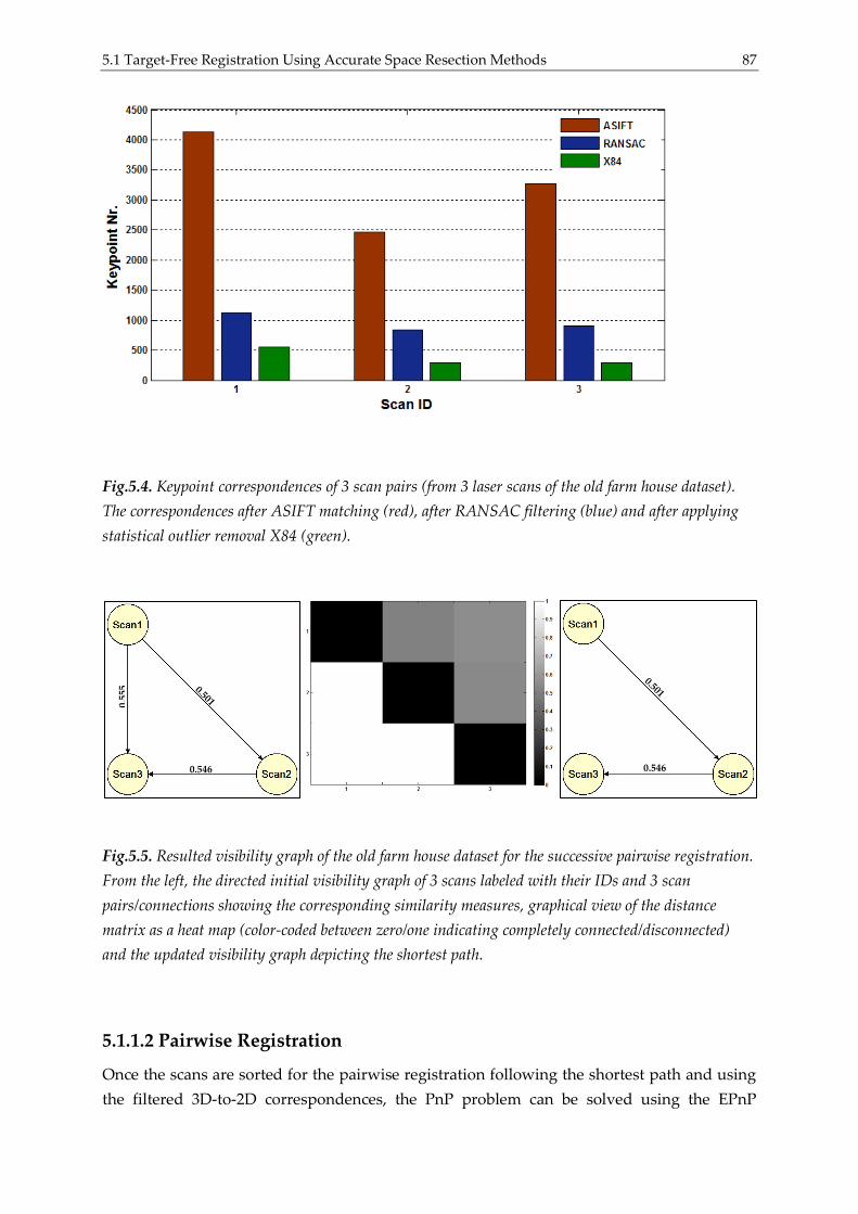
5.1 Target-Free Registration Using Accurate Space Resection Methods 87
Fig.5.4. Keypoint correspondences of 3 scan pairs (from 3 laser scans of the old farm house dataset).
The correspondences after ASIFT matching (red), after RANSAC filtering (blue) and after applying
statistical outlier removal X84 (green).
Fig.5.5. Resulted visibility graph of the old farm house dataset for the successive pairwise registration.
From the left, the directed initial visibility graph of 3 scans labeled with their IDs and 3 scan
pairs/connections showing the corresponding similarity measures, graphical view of the distance
matrix as a heat map (color-coded between zero/one indicating completely connected/disconnected)
and the updated visibility graph depicting the shortest path.
5.1.1.2 Pairwise Registration
Once the scans are sorted for the pairwise registration following the shortest path and using
the filtered 3D-to-2D correspondences, the PnP problem can be solved using the EPnP
0.546
0.55
5
0.546

88 5 Target-Free Registration of Multiple Laser Scans
method. This is performed in order to estimate the pose of the second scan in relation to the
first scan in each determined scan pair. The EPnP results are used then as an input for the OI
method in order to improve the results in terms of accuracy.
As the EPnP algorithm considers all the 3D-to-2D correspondences without checking their
reliability, the quality of the estimated pose can be increased by applying the X84 rule
iteratively during the estimation in order to discard outliers. Consequently, the overall
precision of the orientation is in sub-pixel range in image space, and less than 3σr in object
space. A value of 2.97k is enough to meet the purpose of our application. Figure 5.6 shows
the results for the pairwise registration of the successive scans.
In order to assess the accuracy of the pairwise registration, we have accomplished a manual
registration (with a mean registration error of 8mm) of the three scans using natural targets
by means of the Faro® Scene software. The latter targets (at least 6 targets/points per scan)
were selected over the object of interest with different heights and in different planes. This
has been the case since no GCPs are available. Table 5.1 shows that the registration reaches
about seven centimeters level for positioning accuracy (∆X, ∆Y, ∆Z) and less than nine
hundredths of a degree level for angular accuracy (∆ω, ∆ω, ∆κ). Additionally, table 1
demonstrates that the distance error (∆D) between scanner stations is about a centimeter.
This result provides a good coarse registration for further refinement step using ICP.
Fig.5.6. The result of the successive pairwise registration of the old farm house dataset: 3 laser
scans aligned in one coordinate system, additionally, an ortho view of the latter (upper right corner).
Scan1
Scan2
Scan3
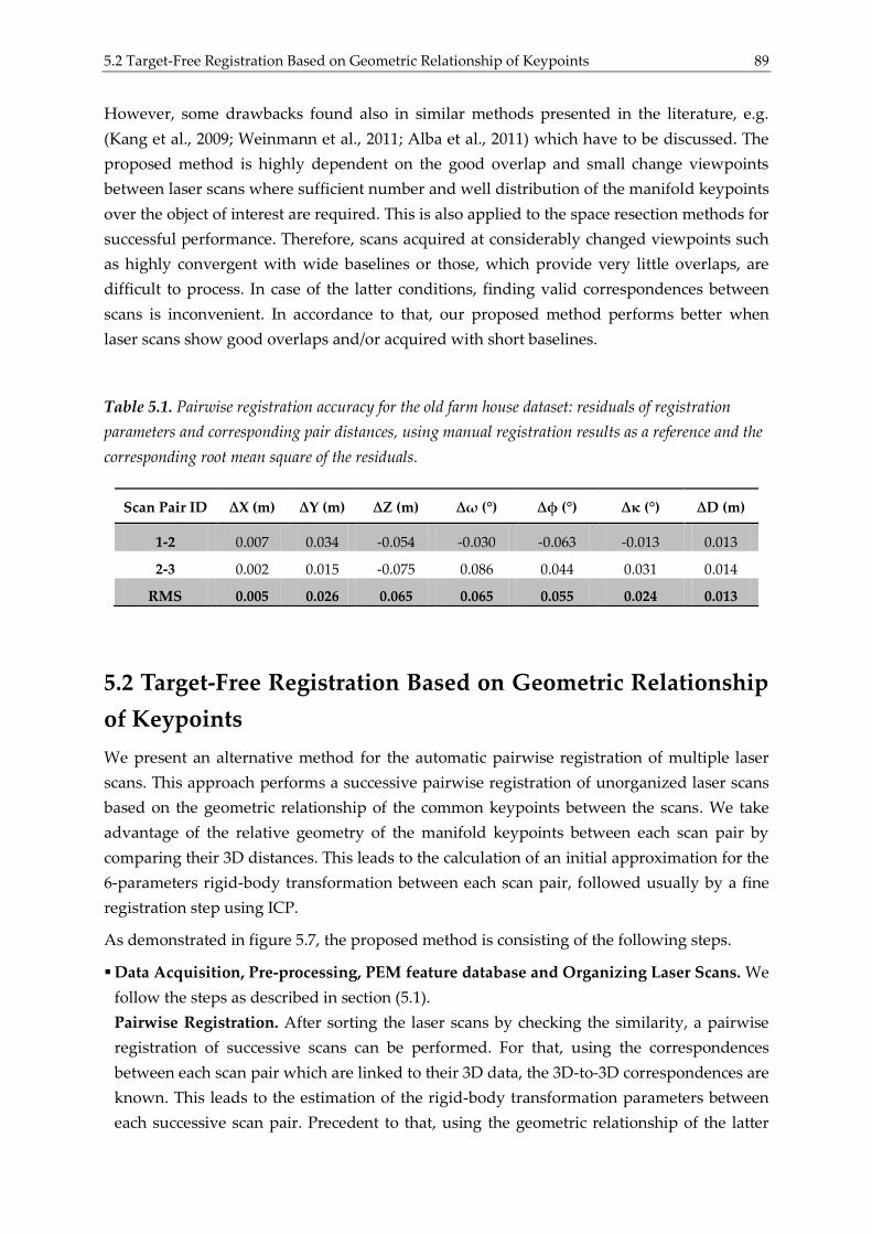
5.2 Target-Free Registration Based on Geometric Relationship of Keypoints 89
However, some drawbacks found also in similar methods presented in the literature, e.g.
(Kang et al., 2009; Weinmann et al., 2011; Alba et al., 2011) which have to be discussed. The
proposed method is highly dependent on the good overlap and small change viewpoints
between laser scans where sufficient number and well distribution of the manifold keypoints
over the object of interest are required. This is also applied to the space resection methods for
successful performance. Therefore, scans acquired at considerably changed viewpoints such
as highly convergent with wide baselines or those, which provide very little overlaps, are
difficult to process. In case of the latter conditions, finding valid correspondences between
scans is inconvenient. In accordance to that, our proposed method performs better when
laser scans show good overlaps and/or acquired with short baselines.
Table 5.1. Pairwise registration accuracy for the old farm house dataset: residuals of registration
parameters and corresponding pair distances, using manual registration results as a reference and the
corresponding root mean square of the residuals.
5.2 Target-Free Registration Based on Geometric Relationship
of Keypoints
We present an alternative method for the automatic pairwise registration of multiple laser
scans. This approach performs a successive pairwise registration of unorganized laser scans
based on the geometric relationship of the common keypoints between the scans. We take
advantage of the relative geometry of the manifold keypoints between each scan pair by
comparing their 3D distances. This leads to the calculation of an initial approximation for the
6-parameters rigid-body transformation between each scan pair, followed usually by a fine
registration step using ICP.
As demonstrated in figure 5.7, the proposed method is consisting of the following steps.
Data Acquisition, Pre-processing, PEM feature database and Organizing Laser Scans. We
follow the steps as described in section (5.1).
Pairwise Registration. After sorting the laser scans by checking the similarity, a pairwise
registration of successive scans can be performed. For that, using the correspondences
between each scan pair which are linked to their 3D data, the 3D-to-3D correspondences are
known. This leads to the estimation of the rigid-body transformation parameters between
each successive scan pair. Precedent to that, using the geometric relationship of the latter
Scan Pair ID ∆X (m) ∆Y (m) ∆Z (m) ∆ω (°) ∆φ (°) ∆κ (°) ∆D (m)
1-2 0.007 0.034 -0.054 -0.030 -0.063 -0.013 0.013
2-3 0.002 0.015 -0.075 0.086 0.044 0.031 0.014
RMS 0.005 0.026 0.065 0.065 0.055 0.024 0.013
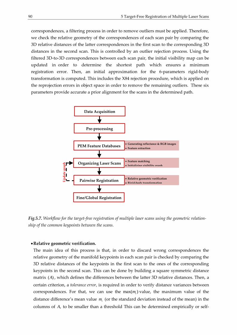
90 5 Target-Free Registration of Multiple Laser Scans
correspondences, a filtering process in order to remove outliers must be applied. Therefore,
we check the relative geometry of the correspondences of each scan pair by comparing the
3D relative distances of the latter correspondences in the first scan to the corresponding 3D
distances in the second scan. This is controlled by an outlier rejection process. Using the
filtered 3D-to-3D correspondences between each scan pair, the initial visibility map can be
updated in order to determine the shortest path which ensures a minimum
registration error. Then, an initial approximation for the 6-parameters rigid-body
transformation is computed. This includes the X84 rejection procedure, which is applied on
the reprojection errors in object space in order to remove the remaining outliers. These six
parameters provide accurate a prior alignment for the scans in the determined path.
Fig.5.7. Workflow for the target-free registration of multiple laser scans using the geometric relation-
ship of the common keypoints between the scans.
Relative geometric verification.
The main idea of this process is that, in order to discard wrong correspondences the
relative geometry of the manifold keypoints in each scan pair is checked by comparing the
3D relative distances of the keypoints in the first scan to the ones of the corresponding
keypoints in the second scan. This can be done by building a square symmetric distance
matrix ( )A , which defines the differences between the latter 3D relative distances. Then, a
certain criterion, a tolerance error, is required in order to verify distance variances between
correspondences. For that, we can use the max( )im value, the maximum value of the
distance difference’s mean value im (or the standard deviation instead of the mean) in the
columns of ,A to be smaller than a threshold This can be determined empirically or self-
Up
dat
e g
rap
h
Generating reflectance & RGB images
Feature extraction
Feature matching
Initializing visibility graph
Relative geometric verification
Rigid-body transformation
Organizing Laser Scans
Data Acquisition
Pre-processing
PEM Feature Databases
Pairwise Registration
Fine/Global Registration
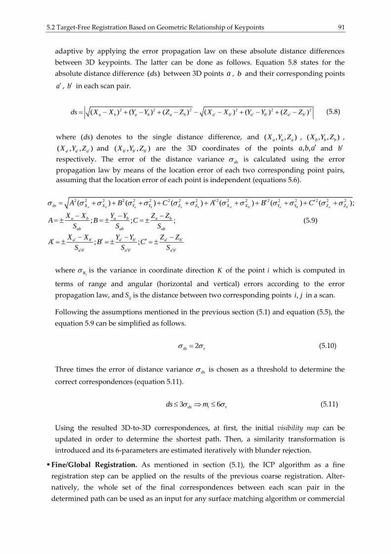
5.2 Target-Free Registration Based on Geometric Relationship of Keypoints 91
adaptive by applying the error propagation law on these absolute distance differences
between 3D keypoints. The latter can be done as follows. Equation 5.8 states for the
absolute distance difference ( )ds between 3D points a , b and their corresponding points
a , b in each scan pair.
2 2 2 2 2 2( ) ( ) ( ) ( ) ( ) ( )a b a b a b a b a b a bds X X Y Y Z Z X X Y Y Z Z (5.8)
where ( )ds denotes to the single distance difference, and ( , , )a a aX Y Z , ( , , )b b bX Y Z ,
( , , )a a aX Y Z and ( , , )b b bX Y Z are the 3D coordinates of the points , ,a b a and b
respectively. The error of the distance variance ds is calculated using the error
propagation law by means of the location error of each two corresponding point pairs,
assuming that the location error of each point is independent (equations 5.6).
2 2 2 2 2 2 2 2 2 2 2 2 2 2 2 2 2 2( ) ( ) ( ) ( ) ( ) ( );
; ; ; (5.9)
; ;
a b a b a b a b a b a bds X X Y Y Z Z X X Y Y Z Z
a b a b a b
ab ab ab
a b a b a b
a b a b a b
A B C A B C
X X Y Y Z ZA B C
S S S
X X Y Y Z ZA B C
S S S
where iK is the variance in coordinate direction K of the point i which is computed in
terms of range and angular (horizontal and vertical) errors according to the error
propagation law, and ijS is the distance between two corresponding points ,i j in a scan.
Following the assumptions mentioned in the previous section (5.1) and equation (5.5), the
equation 5.9 can be simplified as follows.
2ds r (5.10)
Three times the error of distance variance ds is chosen as a threshold to determine the
correct correspondences (equation 5.11).
3 6ds i rds m (5.11)
Using the resulted 3D-to-3D correspondences, at first, the initial visibility map can be
updated in order to determine the shortest path. Then, a similarity transformation is
introduced and its 6-parameters are estimated iteratively with blunder rejection.
Fine/Global Registration. As mentioned in section (5.1), the ICP algorithm as a fine
registration step can be applied on the results of the previous coarse registration. Alter-
natively, the whole set of the final correspondences between each scan pair in the
determined path can be used as an input for any surface matching algorithm or commercial
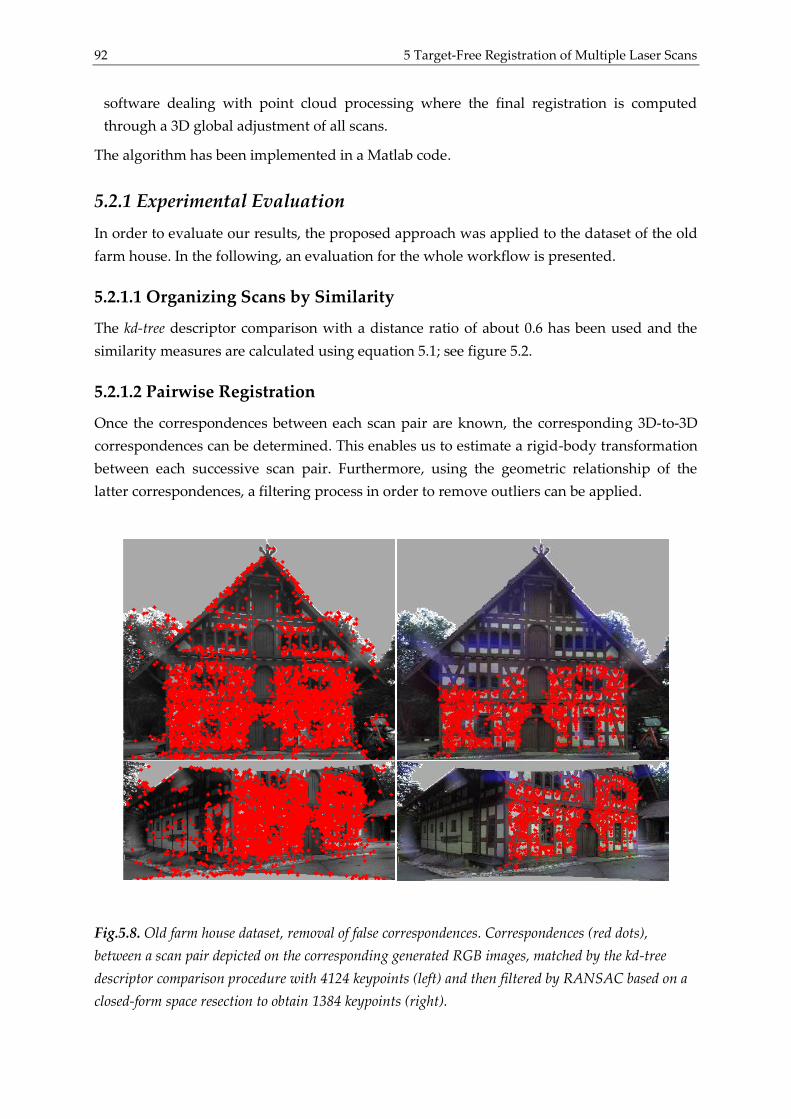
92 5 Target-Free Registration of Multiple Laser Scans
software dealing with point cloud processing where the final registration is computed
through a 3D global adjustment of all scans.
The algorithm has been implemented in a Matlab code.
5.2.1 Experimental Evaluation
In order to evaluate our results, the proposed approach was applied to the dataset of the old
farm house. In the following, an evaluation for the whole workflow is presented.
5.2.1.1 Organizing Scans by Similarity
The kd-tree descriptor comparison with a distance ratio of about 0.6 has been used and the
similarity measures are calculated using equation 5.1; see figure 5.2.
5.2.1.2 Pairwise Registration
Once the correspondences between each scan pair are known, the corresponding 3D-to-3D
correspondences can be determined. This enables us to estimate a rigid-body transformation
between each successive scan pair. Furthermore, using the geometric relationship of the
latter correspondences, a filtering process in order to remove outliers can be applied.
Fig.5.8. Old farm house dataset, removal of false correspondences. Correspondences (red dots),
between a scan pair depicted on the corresponding generated RGB images, matched by the kd-tree
descriptor comparison procedure with 4124 keypoints (left) and then filtered by RANSAC based on a
closed-form space resection to obtain 1384 keypoints (right).
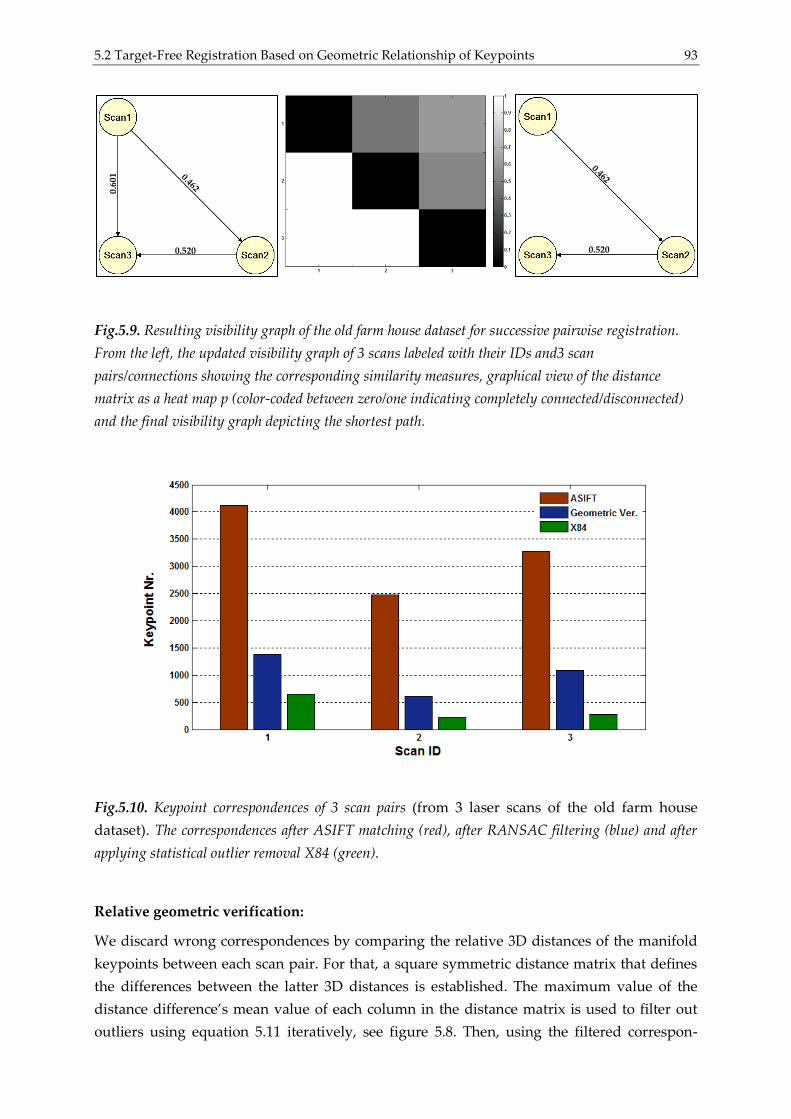
5.2 Target-Free Registration Based on Geometric Relationship of Keypoints 93
Fig.5.9. Resulting visibility graph of the old farm house dataset for successive pairwise registration.
From the left, the updated visibility graph of 3 scans labeled with their IDs and3 scan
pairs/connections showing the corresponding similarity measures, graphical view of the distance
matrix as a heat map p (color-coded between zero/one indicating completely connected/disconnected)
and the final visibility graph depicting the shortest path.
Fig.5.10. Keypoint correspondences of 3 scan pairs (from 3 laser scans of the old farm house
dataset). The correspondences after ASIFT matching (red), after RANSAC filtering (blue) and after
applying statistical outlier removal X84 (green).
Relative geometric verification:
We discard wrong correspondences by comparing the relative 3D distances of the manifold
keypoints between each scan pair. For that, a square symmetric distance matrix that defines
the differences between the latter 3D distances is established. The maximum value of the
distance difference’s mean value of each column in the distance matrix is used to filter out
outliers using equation 5.11 iteratively, see figure 5.8. Then, using the filtered correspon-
0.520
0.60
1
0.520
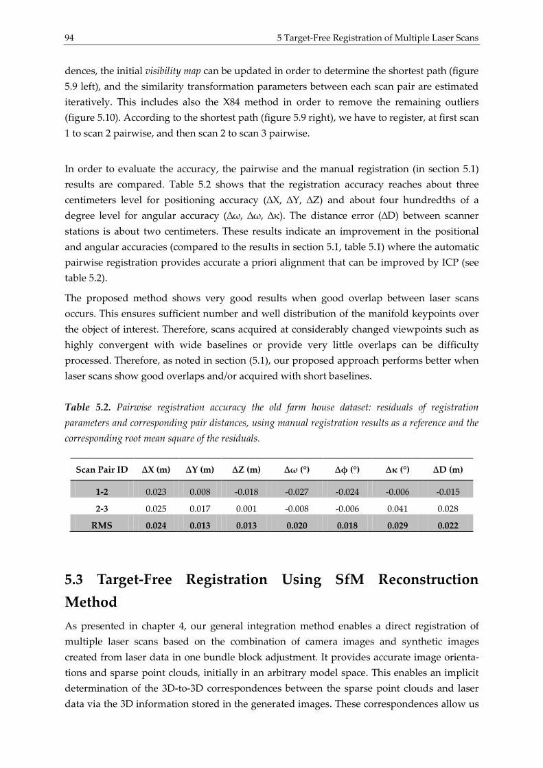
94 5 Target-Free Registration of Multiple Laser Scans
dences, the initial visibility map can be updated in order to determine the shortest path (figure
5.9 left), and the similarity transformation parameters between each scan pair are estimated
iteratively. This includes also the X84 method in order to remove the remaining outliers
(figure 5.10). According to the shortest path (figure 5.9 right), we have to register, at first scan
1 to scan 2 pairwise, and then scan 2 to scan 3 pairwise.
In order to evaluate the accuracy, the pairwise and the manual registration (in section 5.1)
results are compared. Table 5.2 shows that the registration accuracy reaches about three
centimeters level for positioning accuracy (∆X, ∆Y, ∆Z) and about four hundredths of a
degree level for angular accuracy (∆ω, ∆ω, ∆κ). The distance error (∆D) between scanner
stations is about two centimeters. These results indicate an improvement in the positional
and angular accuracies (compared to the results in section 5.1, table 5.1) where the automatic
pairwise registration provides accurate a priori alignment that can be improved by ICP (see
table 5.2).
The proposed method shows very good results when good overlap between laser scans
occurs. This ensures sufficient number and well distribution of the manifold keypoints over
the object of interest. Therefore, scans acquired at considerably changed viewpoints such as
highly convergent with wide baselines or provide very little overlaps can be difficulty
processed. Therefore, as noted in section (5.1), our proposed approach performs better when
laser scans show good overlaps and/or acquired with short baselines.
Table 5.2. Pairwise registration accuracy the old farm house dataset: residuals of registration
parameters and corresponding pair distances, using manual registration results as a reference and the
corresponding root mean square of the residuals.
5.3 Target-Free Registration Using SfM Reconstruction
Method
As presented in chapter 4, our general integration method enables a direct registration of
multiple laser scans based on the combination of camera images and synthetic images
created from laser data in one bundle block adjustment. It provides accurate image orienta-
tions and sparse point clouds, initially in an arbitrary model space. This enables an implicit
determination of the 3D-to-3D correspondences between the sparse point clouds and laser
data via the 3D information stored in the generated images. These correspondences allow us
Scan Pair ID ∆X (m) ∆Y (m) ∆Z (m) ∆ω (°) ∆φ (°) ∆κ (°) ∆D (m)
1-2 0.023 0.008 -0.018 -0.027 -0.024 -0.006 -0.015
2-3 0.025 0.017 0.001 -0.008 -0.006 0.041 0.028
RMS 0.024 0.013 0.013 0.020 0.018 0.029 0.022
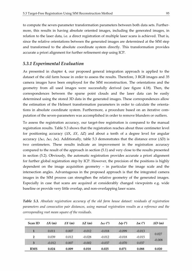
5.3 Target-Free Registration Using SfM Reconstruction Method 95
to compute the seven-parameter transformation parameters between both data sets. Further-
more, this results in having absolute oriented images, including the generated images, in
relation to the laser data, i.e. a direct registration of multiple laser scans is achieved. That is,
since the relative orientations between the generated images are determined at the SfM step
and transformed to the absolute coordinate system directly. This transformation provides
accurate a priori alignment for further refinement step using ICP.
5.3.1 Experimental Evaluation
As presented in chapter 4, our proposed general integration approach is applied to the
dataset of the old farm house in order to assess the results. Therefore, 3 RGB images and 35
camera images have been employed for the SfM reconstruction. The orientations and the
geometry from all used images were successfully derived (see figure 4.18). Then, the
correspondences between the sparse point clouds and the laser data can be easily
determined using the stored 3D data in the generated images. These correspondences allow
the estimation of the Helmert transformation parameters in order to calculate the orienta-
tions in absolute coordinate system. Furthermore, a procedure based on an iterative com-
putation of the seven-parameters was accomplished in order to remove blunders or outliers.
To assess the registration accuracy, our target-free registration is compared to the manual
registration results. Table 5.3 shows that the registration reaches about three centimeter level
for positioning accuracy (∆X, ∆Y, ∆Z) and about a tenth of a degree level for angular
accuracy (∆ω, ∆ω, ∆κ). Additionally, table 5.3 demonstrates that the distance error (∆D) is
two centimeters. These results indicate an improvement in the registration accuracy
compared to the result of the approach in section (5.1) and very close to the results presented
in section (5.2). Obviously, the automatic registration provides accurate a priori alignment
for further global registration step by ICP. However, the precision of the positions is highly
dependent on the image acquisition geometry – in particular the image scale and the
intersection angles. Advantageous in the proposed approach is that the integrated camera
images in the SfM process can strengthen the relative geometry of the generated images.
Especially in case that scans are acquired at considerably changed viewpoints e.g. wide
baseline or provide very little overlap, and non-overlapping laser scans.
Table 5.3. Absolute registration accuracy of the old farm house dataset: residuals of registration
parameters and consecutive pair distances, using manual registration results as a reference and the
corresponding root mean square of the residuals.
Scan ID ∆X (m) ∆Y (m) ∆Z (m) ∆ω (°) ∆φ (°) ∆κ (°) ∆D (m)
1 0.011 0.007 -0.012 -0.018 -0.099 -0.013 0.027
-0.008 2 0.039 0.012 -0.028 -0.012 -0.018 -0.015
3 -0.012 0.007 -0.002 -0.037 -0.070 0.037
RMS 0.024 0.009 0.018 0.025 0.071 0.088 0.020
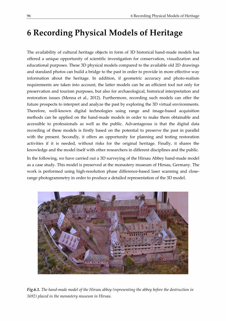
96 6 Recording Physical Models of Heritage
6 Recording Physical Models of Heritage
The availability of cultural heritage objects in form of 3D historical hand-made models has
offered a unique opportunity of scientific investigation for conservation, visualization and
educational purposes. These 3D physical models compared to the available old 2D drawings
and standard photos can build a bridge to the past in order to provide in more effective way
information about the heritage. In addition, if geometric accuracy and photo-realism
requirements are taken into account, the latter models can be an efficient tool not only for
preservation and tourism purposes, but also for archaeological, historical interpretation and
restoration issues (Menna et al., 2012). Furthermore, recording such models can offer the
future prospects to interpret and analyze the past by exploring the 3D virtual environments.
Therefore, well-known digital technologies using range and image-based acquisition
methods can be applied on the hand-made models in order to make them obtainable and
accessible to professionals as well as the public. Advantageous is that the digital data
recording of these models is firstly based on the potential to preserve the past in parallel
with the present. Secondly, it offers an opportunity for planning and testing restoration
activities if it is needed, without risks for the original heritage. Finally, it shares the
knowledge and the model itself with other researchers in different disciplines and the public.
In the following, we have carried out a 3D surveying of the Hirsau Abbey hand-made model
as a case study. This model is preserved at the monastery museum of Hirsau, Germany. The
work is performed using high-resolution phase difference-based laser scanning and close-
range photogrammetry in order to produce a detailed representation of the 3D model.
Fig.6.1. The hand-made model of the Hirsau abbey (representing the abbey before the destruction in
1692) placed in the monastery museum in Hirsau.
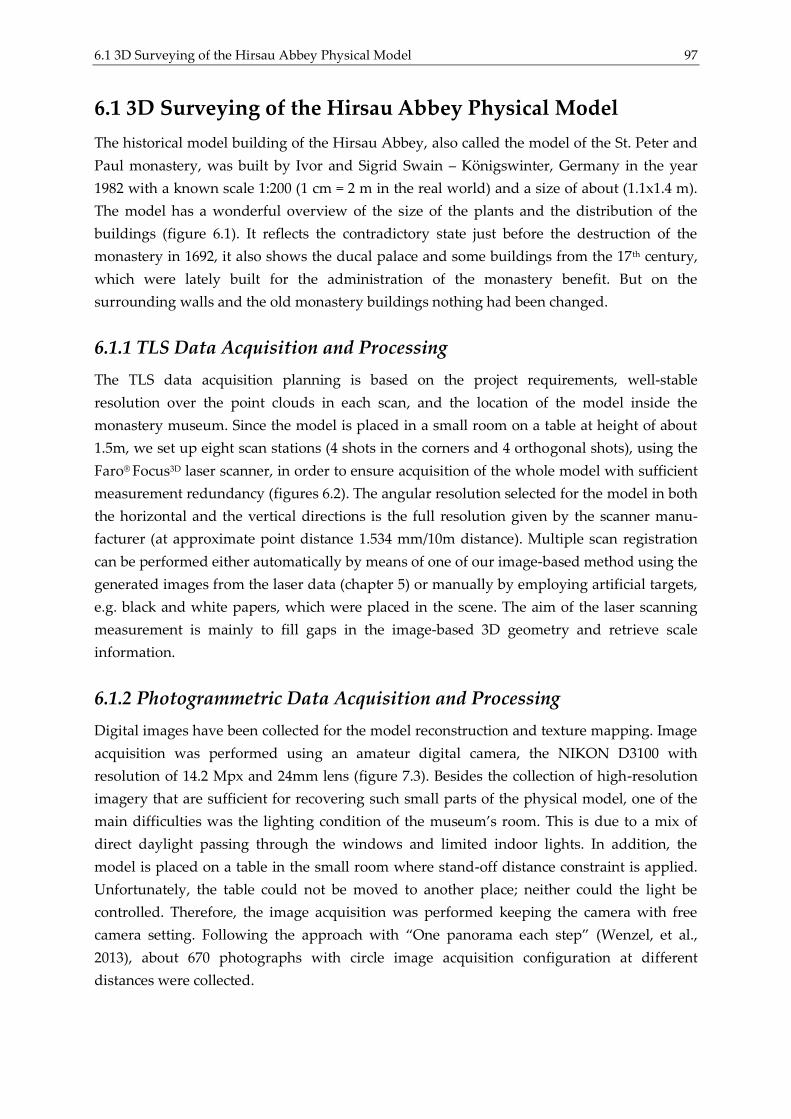
6.1 3D Surveying of the Hirsau Abbey Physical Model 97
6.1 3D Surveying of the Hirsau Abbey Physical Model
The historical model building of the Hirsau Abbey, also called the model of the St. Peter and
Paul monastery, was built by Ivor and Sigrid Swain – Königswinter, Germany in the year
1982 with a known scale 1:200 (1 cm = 2 m in the real world) and a size of about (1.1x1.4 m).
The model has a wonderful overview of the size of the plants and the distribution of the
buildings (figure 6.1). It reflects the contradictory state just before the destruction of the
monastery in 1692, it also shows the ducal palace and some buildings from the 17th century,
which were lately built for the administration of the monastery benefit. But on the
surrounding walls and the old monastery buildings nothing had been changed.
6.1.1 TLS Data Acquisition and Processing
The TLS data acquisition planning is based on the project requirements, well-stable
resolution over the point clouds in each scan, and the location of the model inside the
monastery museum. Since the model is placed in a small room on a table at height of about
1.5m, we set up eight scan stations (4 shots in the corners and 4 orthogonal shots), using the
Faro® Focus3D laser scanner, in order to ensure acquisition of the whole model with sufficient
measurement redundancy (figures 6.2). The angular resolution selected for the model in both
the horizontal and the vertical directions is the full resolution given by the scanner manu-
facturer (at approximate point distance 1.534 mm/10m distance). Multiple scan registration
can be performed either automatically by means of one of our image-based method using the
generated images from the laser data (chapter 5) or manually by employing artificial targets,
e.g. black and white papers, which were placed in the scene. The aim of the laser scanning
measurement is mainly to fill gaps in the image-based 3D geometry and retrieve scale
information.
6.1.2 Photogrammetric Data Acquisition and Processing
Digital images have been collected for the model reconstruction and texture mapping. Image
acquisition was performed using an amateur digital camera, the NIKON D3100 with
resolution of 14.2 Mpx and 24mm lens (figure 7.3). Besides the collection of high-resolution
imagery that are sufficient for recovering such small parts of the physical model, one of the
main difficulties was the lighting condition of the museum’s room. This is due to a mix of
direct daylight passing through the windows and limited indoor lights. In addition, the
model is placed on a table in the small room where stand-off distance constraint is applied.
Unfortunately, the table could not be moved to another place; neither could the light be
controlled. Therefore, the image acquisition was performed keeping the camera with free
camera setting. Following the approach with “One panorama each step” (Wenzel, et al.,
2013), about 670 photographs with circle image acquisition configuration at different
distances were collected.
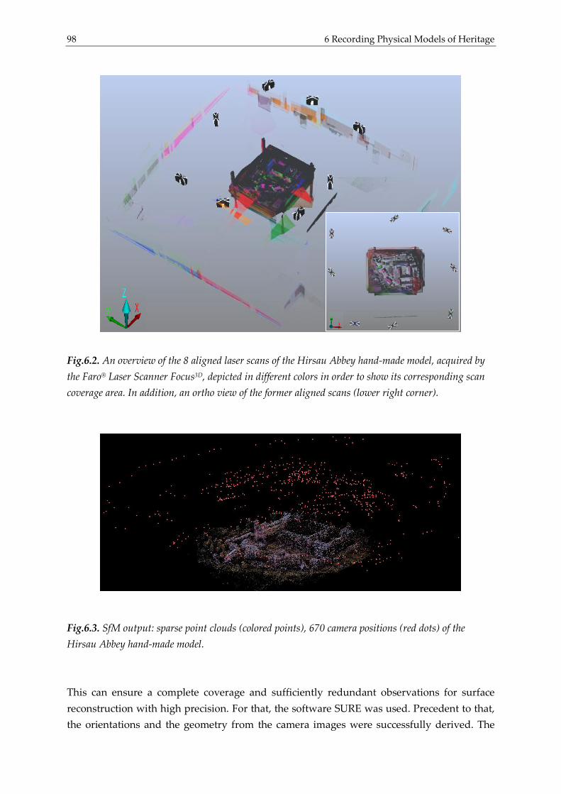
98 6 Recording Physical Models of Heritage
Fig.6.2. An overview of the 8 aligned laser scans of the Hirsau Abbey hand-made model, acquired by
the Faro® Laser Scanner Focus3D, depicted in different colors in order to show its corresponding scan
coverage area. In addition, an ortho view of the former aligned scans (lower right corner).
Fig.6.3. SfM output: sparse point clouds (colored points), 670 camera positions (red dots) of the
Hirsau Abbey hand-made model.
This can ensure a complete coverage and sufficiently redundant observations for surface
reconstruction with high precision. For that, the software SURE was used. Precedent to that,
the orientations and the geometry from the camera images were successfully derived. The
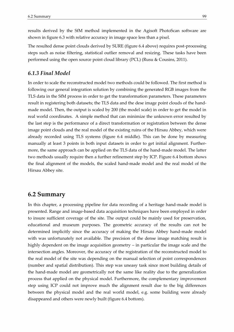
6.2 Summary 99
results derived by the SfM method implemented in the Agisoft PhotoScan software are
shown in figure 6.3 with relative accuracy in image space less than a pixel.
The resulted dense point clouds derived by SURE (figure 6.4 above) requires post-processing
steps such as noise filtering, statistical outlier removal and resizing. These tasks have been
performed using the open source point cloud library (PCL) (Rusu & Cousins, 2011).
6.1.3 Final Model
In order to scale the reconstructed model two methods could be followed. The first method is
following our general integration solution by combining the generated RGB images from the
TLS data in the SfM process in order to get the transformation parameters. These parameters
result in registering both datasets; the TLS data and the dese image point clouds of the hand-
made model. Then, the output is scaled by 200 (the model scale) in order to get the model in
real world coordinates. A simple method that can minimize the unknown error resulted by
the last step is the performance of a direct transformation or registration between the dense
image point clouds and the real model of the existing ruins of the Hirsau Abbey, which were
already recorded using TLS systems (figure 6.4 middle). This can be done by measuring
manually at least 3 points in both input datasets in order to get initial alignment. Further-
more, the same approach can be applied on the TLS data of the hand-made model. The latter
two methods usually require then a further refinement step by ICP. Figure 6.4 bottom shows
the final alignment of the models, the scaled hand-made model and the real model of the
Hirsau Abbey site.
6.2 Summary
In this chapter, a processing pipeline for data recording of a heritage hand-made model is
presented. Range and image-based data acquisition techniques have been employed in order
to insure sufficient coverage of the site. The output could be mainly used for preservation,
educational and museum purposes. The geometric accuracy of the results can not be
determined implicitly since the accuracy of making the Hirsau Abbey hand-made model
with was unfortunately not available. The precision of the dense image matching result is
highly dependent on the image acquisition geometry – in particular the image scale and the
intersection angles. Moreover, the accuracy of the registration of the reconstructed model to
the real model of the site was depending on the manual selection of point correspondences
(number and spatial distribution). This step was uneasy task since most building details of
the hand-made model are geometrically not the same like reality due to the generalization
process that applied on the physical model. Furthermore, the complementary improvement
step using ICP could not improve much the alignment result due to the big differences
between the physical model and the real world model, e.g. some building were already
disappeared and others were newly built (figure 6.4 bottom).
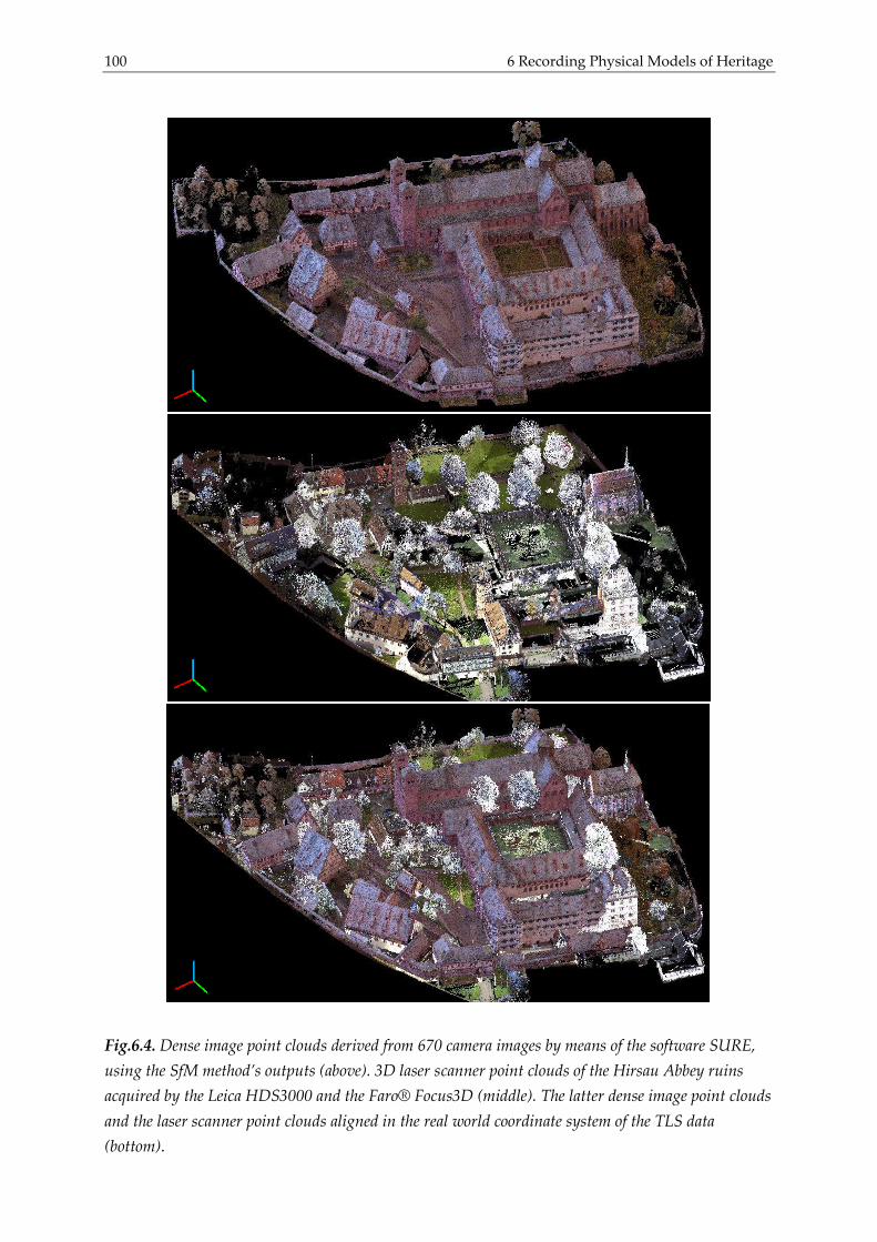
100 6 Recording Physical Models of Heritage
Fig.6.4. Dense image point clouds derived from 670 camera images by means of the software SURE,
using the SfM method’s outputs (above). 3D laser scanner point clouds of the Hirsau Abbey ruins
acquired by the Leica HDS3000 and the Faro® Focus3D (middle). The latter dense image point clouds
and the laser scanner point clouds aligned in the real world coordinate system of the TLS data
(bottom).
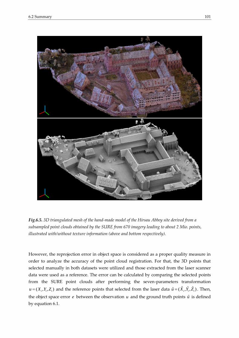
6.2 Summary 101
Fig.6.5. 3D triangulated mesh of the hand-made model of the Hirsau Abbey site derived from a
subsampled point clouds obtained by the SURE from 670 imagery leading to about 2 Mio. points,
illustrated with/without texture information (above and bottom respectively).
However, the reprojection error in object space is considered as a proper quality measure in
order to analyze the accuracy of the point cloud registration. For that, the 3D points that
selected manually in both datasets were utilized and those extracted from the laser scanner
data were used as a reference. The error can be calculated by comparing the selected points
from the SURE point clouds after performing the seven-parameters transformation
( , , )i i iu X Y Z and the reference points that selected from the laser data ˆ ˆ ˆˆ ( , , )i i iu X Y Z . Then,
the object space error e between the observation u and the ground truth points u is defined
by equation 6.1.
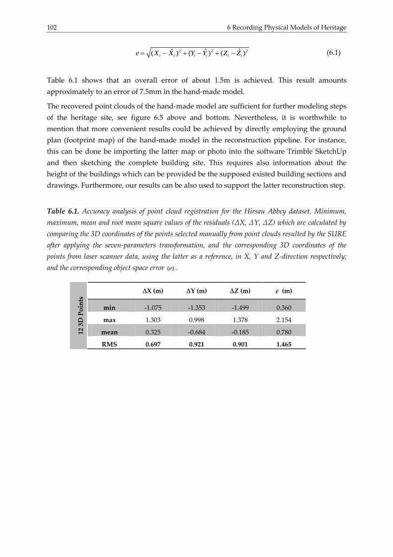
102 6 Recording Physical Models of Heritage
2 2 2ˆ ˆ ˆ( ) ( ) ( )i i i i i ie X X Y Y Z Z (6.1)
Table 6.1 shows that an overall error of about 1.5m is achieved. This result amounts
approximately to an error of 7.5mm in the hand-made model.
The recovered point clouds of the hand-made model are sufficient for further modeling steps
of the heritage site, see figure 6.5 above and bottom. Nevertheless, it is worthwhile to
mention that more convenient results could be achieved by directly employing the ground
plan (footprint map) of the hand-made model in the reconstruction pipeline. For instance,
this can be done be importing the latter map or photo into the software Trimble SketchUp
and then sketching the complete building site. This requires also information about the
height of the buildings which can be provided be the supposed existed building sections and
drawings. Furthermore, our results can be also used to support the latter reconstruction step.
Table 6.1. Accuracy analysis of point cloud registration for the Hirsau Abbey dataset. Minimum,
maximum, mean and root mean square values of the residuals (∆X, ∆Y, ∆Z) which are calculated by
comparing the 3D coordinates of the points selected manually from point clouds resulted by the SURE
after applying the seven-parameters transformation, and the corresponding 3D coordinates of the
points from laser scanner data, using the latter as a reference, in X, Y and Z-direction respectively;
and the corresponding object space error ( )e .
∆X (m) ∆Y (m) ∆Z (m) e (m)
min -1.075 -1.353 -1.499 0.360
max 1.303 0.998 1.378 2.154
mean 0.325 -0.684 -0.185 0.780
RMS 0.697 0.921 0.901 1.465
12 3
D P
oin
ts
7.1 Data Acquisition 103
7 Case Studies
In this chapter, the results of the automatic fusion of digital images and laser scanner data for
cultural heritage data recording purposes are highlighted. Particularly the efficiency of our
methods is shown by giving an attention to different case studies, in which the outputs of the
data integration are evaluated and discussed. In addition, the results of the target-free
registration of multiple laser scans are introduced and then assessed. This also includes the
automatic registration of scans occluded partially by the neighborhood and completely non-
overlapping laser scans. Therefore, this chapter refers to two case studies that have as input
data: laser scanner point clouds and terrestrial digital images. In the following, a short
overview about the data acquisition and sensor used as well as a detailed description of the
achieved results are presented.
7.1 Data Acquisition
Besides the old farm house dataset, which is used as a test data for our research, two datasets
have been used for our investigations: the Hirsau Abbey, Germany and the temple of
Heliopolis/Al-Matariya, Egypt datasets. The collection of the Hirsau Abbey data was per-
formed in cooperation with the “Association of Hirsau Abbey Friends (Verein Freunde
Kloster Hirsau e.V.)”, Calw/Germany (a registered association for taking care of the Hirsau
heritage site) and the “Public Office for Historical Monuments' Care (Landesamt für Denk-
malpflege)”, Stuttgart/Germany. The overall goal of this project, started on May 2009 is to
preserve digitally the Hirsau Abbey by generating comprehensive 3D virtual reality model
of the whole site, see (Moussa & Fritsch, 2010).
In cooperation with the Ministry of State of Antiquities in Egypt, the Egyptian Museum in
Leipzig/Germany, the Institute for Photogrammetry (ifp) at the University of Stuttgart/
Germany and the German University in Cairo (GUC)/Egypt, the acquisition of the Heliopolis
data was carried out from September 29th to October 25th 2012. The temple of Heliopolis is
heavily threatened by modern town development and high underwater level. Huge areas are
lost due to house constructions. Therefore, it was necessary to test new methods of
documentation that are considerably faster than former techniques. This project is aiming on
surveying and digital documentation of all structures and monuments in the archeological
site.
7.1.1 The Hirsau Abbey
Hirsau, a village in the northern part of the Black Forest, today a suburb of Calw/Germany,
has a great history. In particular, the Hirsau Abbey was one of the most prominent
Benedictine abbeys of Germany. Founded around 830 AD by Count Erlafried of Calw, it

104 7 Case Studies
served as an abbey until it was destroyed by French soldiers in 1692. By the way, the famous
William of Hirsau, abbot from 1069 to 1091, introduced the Astrolabe for measuring latitude
positions. Therefore, the abbey served already more than one millennium ago for geodetic
purposes, a fact not well-known to the geodetic community. More information about the site
can be found in (Teschauer, 1991; Würfel, 1998). Today, just ruins are found - one can see the
Cloister, the ruins of the Hunting Lodge, the Lady Chapel (marked in figure 7.1), the ruins of
the monastery church St. Peter and Paul and some other Buildings (Figure 7.1).
Fig. 7.1. An overview of the Hirsau Abbey buildings (© Große Kreisstadt Calw und Oberfinanz-
direktion Karlsruhe Copyright 1991).
7.1.2 The Temple of Heliopolis
Heliopolis, “City of the Sun” was one of the oldest cities of ancient Egypt, the capital of the
13th Lower Egyptian Nome that was located five miles (8 km) east of the Nile to the north of
the apex of the Nile Delta. Heliopolis was the center of the Egyptian Religion for about 2400
years (2700-300 BC). Today it is mostly destroyed; its temples and other buildings were used
for the construction of medieval Cairo. The site of Heliopolis has now been brought for the
most part under cultivation and suburbanization, but some ancient city walls of crude brick
can be seen in the fields, a few granite blocks bearing the name of Ramesses II remain, and
the position of the great Temple of Re-Atum is marked by the Al-Masalla obelisk, which is
located in Al-Matariya Museum (figures 7.2). It still stands in its original position. The 20.7
meter high red granite obelisk weighs 120 tons, more information about the site can be found
in (Petrie et al., 1915; Dobrowolska & Dobrowolski, 2006).
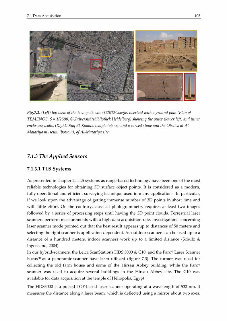
7.1 Data Acquisition 105
Fig.7.2. (Left) top view of the Heliopolis site (©2012Google) overlaid with a ground plan (Plan of
TEMENOS, S = 1/2500, ©Universitätsbibliothek Heidelberg) showing the outer (lower left) and inner
enclosure walls. (Right) Suq El-Khamis temple (above) and a carved stone and the Obelisk at Al-
Matariya museum (bottom), of Al-Matariya site.
7.1.3 The Applied Sensors
7.1.3.1 TLS Systems
As presented in chapter 2, TLS systems as range-based technology have been one of the most
reliable technologies for obtaining 3D surface object points. It is considered as a modern,
fully operational and efficient surveying technique used in many applications. In particular,
if we look upon the advantage of getting immense number of 3D points in short time and
with little effort. On the contrary, classical photogrammetry requires at least two images
followed by a series of processing steps until having the 3D point clouds. Terrestrial laser
scanners perform measurements with a high data acquisition rate. Investigations concerning
laser scanner mode pointed out that the best result appears up to distances of 50 meters and
selecting the right scanner is application-dependent. As outdoor scanners can be used up to a
distance of a hundred meters, indoor scanners work up to a limited distance (Schulz &
Ingensand, 2004).
In our hybrid-scanners, the Leica ScanStations HDS 3000 & C10, and the Faro® Laser Scanner
Focus3D as a panoramic-scanner have been utilized (figure 7.3). The former was used for
collecting the old farm house and some of the Hirsau Abbey building, while the Faro®
scanner was used to acquire several buildings in the Hirsau Abbey site. The C10 was
available for data acquisition at the temple of Heliopolis, Egypt.
The HDS3000 is a pulsed TOF-based laser scanner operating at a wavelength of 532 nm. It
measures the distance along a laser beam, which is deflected using a mirror about two axes.
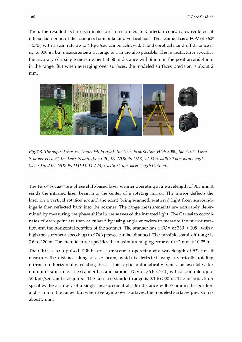
106 7 Case Studies
Then, the resulted polar coordinates are transformed to Cartesian coordinates centered at
intersection point of the scanners horizontal and vertical axis. The scanner has a FOV of 3600
× 2700, with a scan rate up to 4 kpts/sec can be achieved. The theoretical stand-off distance is
up to 300 m, but measurements at range of 1 m are also possible. The manufacturer specifies
the accuracy of a single measurement at 50 m distance with 6 mm in the position and 4 mm
in the range. But when averaging over surfaces, the modeled surfaces precision is about 2
mm.
Fig.7.3. The applied sensors, (From left to right) the Leica ScanStation HDS 3000, the Faro® Laser
Scanner Focus3D, the Leica ScanStation C10, the NIKON D2X, 12 Mpx with 20 mm focal length
(above) and the NIKON D3100, 14.2 Mpx with 24 mm focal length (bottom).
The Faro® Focus3D is a phase shift-based laser scanner operating at a wavelength of 905 nm. It
sends the infrared laser beam into the center of a rotating mirror. The mirror deflects the
laser on a vertical rotation around the scene being scanned; scattered light from surround-
ings is then reflected back into the scanner. The range measurements are accurately deter-
mined by measuring the phase shifts in the waves of the infrared light. The Cartesian coordi-
nates of each point are then calculated by using angle encoders to measure the mirror rota-
tion and the horizontal rotation of the scanner. The scanner has a FOV of 3600 × 3050, with a
high measurement speed: up to 976 kpts/sec can be obtained. The possible stand-off range is
0.6 to 120 m. The manufacturer specifies the maximum ranging error with ±2 mm @ 10-25 m.
The C10 is also a pulsed TOF-based laser scanner operating at a wavelength of 532 nm. It
measures the distance along a laser beam, which is deflected using a vertically rotating
mirror on horizontally rotating base. This optic automatically spins or oscillates for
minimum scan time. The scanner has a maximum FOV of 3600 × 2700, with a scan rate up to
50 kpts/sec can be acquired. The possible standoff range is 0.1 to 300 m. The manufacturer
specifies the accuracy of a single measurement at 50m distance with 6 mm in the position
and 4 mm in the range. But when averaging over surfaces, the modeled surfaces precision is
about 2 mm.
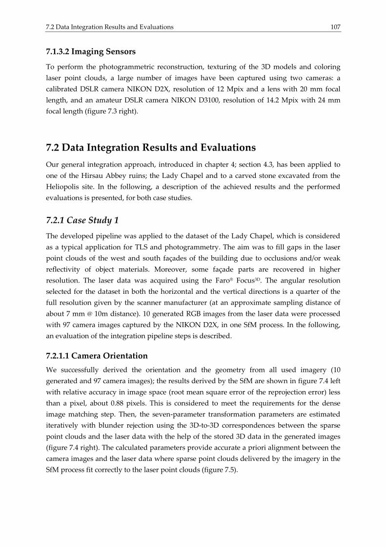
7.2 Data Integration Results and Evaluations 107
7.1.3.2 Imaging Sensors
To perform the photogrammetric reconstruction, texturing of the 3D models and coloring
laser point clouds, a large number of images have been captured using two cameras: a
calibrated DSLR camera NIKON D2X, resolution of 12 Mpix and a lens with 20 mm focal
length, and an amateur DSLR camera NIKON D3100, resolution of 14.2 Mpix with 24 mm
focal length (figure 7.3 right).
7.2 Data Integration Results and Evaluations
Our general integration approach, introduced in chapter 4; section 4.3, has been applied to
one of the Hirsau Abbey ruins; the Lady Chapel and to a carved stone excavated from the
Heliopolis site. In the following, a description of the achieved results and the performed
evaluations is presented, for both case studies.
7.2.1 Case Study 1
The developed pipeline was applied to the dataset of the Lady Chapel, which is considered
as a typical application for TLS and photogrammetry. The aim was to fill gaps in the laser
point clouds of the west and south façades of the building due to occlusions and/or weak
reflectivity of object materials. Moreover, some façade parts are recovered in higher
resolution. The laser data was acquired using the Faro® Focus3D. The angular resolution
selected for the dataset in both the horizontal and the vertical directions is a quarter of the
full resolution given by the scanner manufacturer (at an approximate sampling distance of
about 7 mm @ 10m distance). 10 generated RGB images from the laser data were processed
with 97 camera images captured by the NIKON D2X, in one SfM process. In the following,
an evaluation of the integration pipeline steps is described.
7.2.1.1 Camera Orientation
We successfully derived the orientation and the geometry from all used imagery (10
generated and 97 camera images); the results derived by the SfM are shown in figure 7.4 left
with relative accuracy in image space (root mean square error of the reprojection error) less
than a pixel, about 0.88 pixels. This is considered to meet the requirements for the dense
image matching step. Then, the seven-parameter transformation parameters are estimated
iteratively with blunder rejection using the 3D-to-3D correspondences between the sparse
point clouds and the laser data with the help of the stored 3D data in the generated images
(figure 7.4 right). The calculated parameters provide accurate a priori alignment between the
camera images and the laser data where sparse point clouds delivered by the imagery in the
SfM process fit correctly to the laser point clouds (figure 7.5).
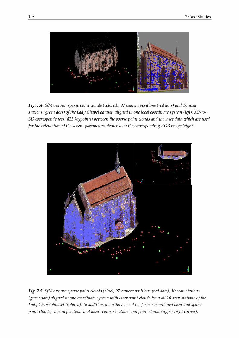
108 7 Case Studies
Fig. 7.4. SfM output: sparse point clouds (colored), 97 camera positions (red dots) and 10 scan
stations (green dots) of the Lady Chapel dataset, aligned in one local coordinate system (left). 3D-to-
3D correspondences (415 keypoints) between the sparse point clouds and the laser data which are used
for the calculation of the seven- parameters, depicted on the corresponding RGB image (right).
Fig. 7.5. SfM output: sparse point clouds (blue), 97 camera positions (red dots), 10 scan stations
(green dots) aligned in one coordinate system with laser point clouds from all 10 scan stations of the
Lady Chapel dataset (colored). In addition, an ortho view of the former mentioned laser and sparse
point clouds, camera positions and laser scanner stations and point clouds (upper right corner).
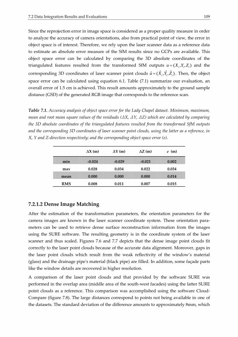
7.2 Data Integration Results and Evaluations 109
Since the reprojection error in image space is considered as a proper quality measure in order
to analyze the accuracy of camera orientations, also from practical point of view, the error in
object space is of interest. Therefore, we rely upon the laser scanner data as a reference data
to estimate an absolute error measure of the SfM results since no GCPs are available. This
object space error can be calculated by comparing the 3D absolute coordinates of the
triangulated features resulted from the transformed SfM outputs ( , , )i i iu X Y Z and the
corresponding 3D coordinates of laser scanner point clouds ˆ ˆ ˆˆ ( , , )i i iu X Y Z . Then, the object
space error can be calculated using equation 6.1. Table (7.1) summarize our evaluation, an
overall error of 1.5 cm is achieved. This result amounts approximately to the ground sample
distance (GSD) of the generated RGB image that corresponds to the reference scan.
Table 7.1. Accuracy analysis of object space error for the Lady Chapel dataset. Minimum, maximum,
mean and root mean square values of the residuals (∆X, ∆Y, ∆Z) which are calculated by comparing
the 3D absolute coordinates of the triangulated features resulted from the transformed SfM outputs
and the corresponding 3D coordinates of laser scanner point clouds, using the latter as a reference, in
X, Y and Z-direction respectively; and the corresponding object space error (e).
∆X (m) ∆Y (m) ∆Z (m) e (m)
min -0.024 -0.029 -0.021 0.002
max 0.028 0.034 0.022 0.034
mean 0.000 0.000 0.000 0.014
RMS 0.008 0.011 0.007 0.015
7.2.1.2 Dense Image Matching
After the estimation of the transformation parameters, the orientation parameters for the
camera images are known in the laser scanner coordinate system. These orientation para-
meters can be used to retrieve dense surface reconstruction information from the images
using the SURE software. The resulting geometry is in the coordinate system of the laser
scanner and thus scaled. Figures 7.6 and 7.7 depicts that the dense image point clouds fit
correctly to the laser point clouds because of the accurate data alignment. Moreover, gaps in
the laser point clouds which result from the weak reflectivity of the window’s material
(glass) and the drainage pipe's material (black pipe) are filled. In addition, some façade parts
like the window details are recovered in higher resolution.
A comparison of the laser point clouds and that provided by the software SURE was
performed in the overlap area (middle area of the south-west facades) using the latter SURE
point clouds as a reference. This comparison was accomplished using the software Cloud-
Compare (figure 7.8). The large distances correspond to points not being available in one of
the datasets. The standard deviation of the difference amounts to approximately 8mm, which
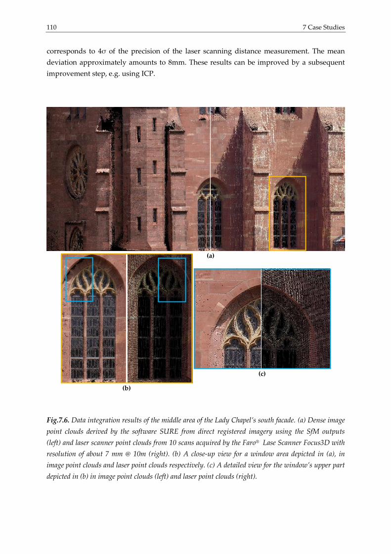
110 7 Case Studies
corresponds to 4σ of the precision of the laser scanning distance measurement. The mean
deviation approximately amounts to 8mm. These results can be improved by a subsequent
improvement step, e.g. using ICP.
Fig.7.6. Data integration results of the middle area of the Lady Chapel’s south facade. (a) Dense image
point clouds derived by the software SURE from direct registered imagery using the SfM outputs
(left) and laser scanner point clouds from 10 scans acquired by the Faro® Lase Scanner Focus3D with
resolution of about 7 mm @ 10m (right). (b) A close-up view for a window area depicted in (a), in
image point clouds and laser point clouds respectively. (c) A detailed view for the window’s upper part
depicted in (b) in image point clouds (left) and laser point clouds (right).
(a)
(b)
(c)

7.2 Data Integration Results and Evaluations 111
Fig.7.7. Data integration results of the upper area of the Lady Chapel’s south facade. (a) Dense image
point clouds derived by the software SURE from direct registered imagery using the SfM outputs
(left) and laser scanner point clouds from 10 scans acquired by the Faro® Laser Scanner Focus3D with
resolution of about 7 mm @ 10 m distance (right). (b) A close-up view for a drainage pipe area
depicted in (a), in image point clouds (left) and laser point clouds (right). (c) A close-up view
for a window area depicted in (a), in image point clouds and laser point clouds respectively. (d) A
detailed view for the window’s upper part depicted in (a) in image point clouds (left) and laser point
clouds (right).
7.2.2 Case Study 2
Our integration pipeline was also applied to the dataset of a carved stone excavated (about
1.7x0.9 meters) from the Heliopolis site, which is considered as an application of TLS and
close-range photogrammetry in archeology. The aim was to preserve digitally and records
the object in very high details. This includes each single relief and texture of the hiero-
glyphics showed on the stone.
(d)
(c)
(b)
(a)
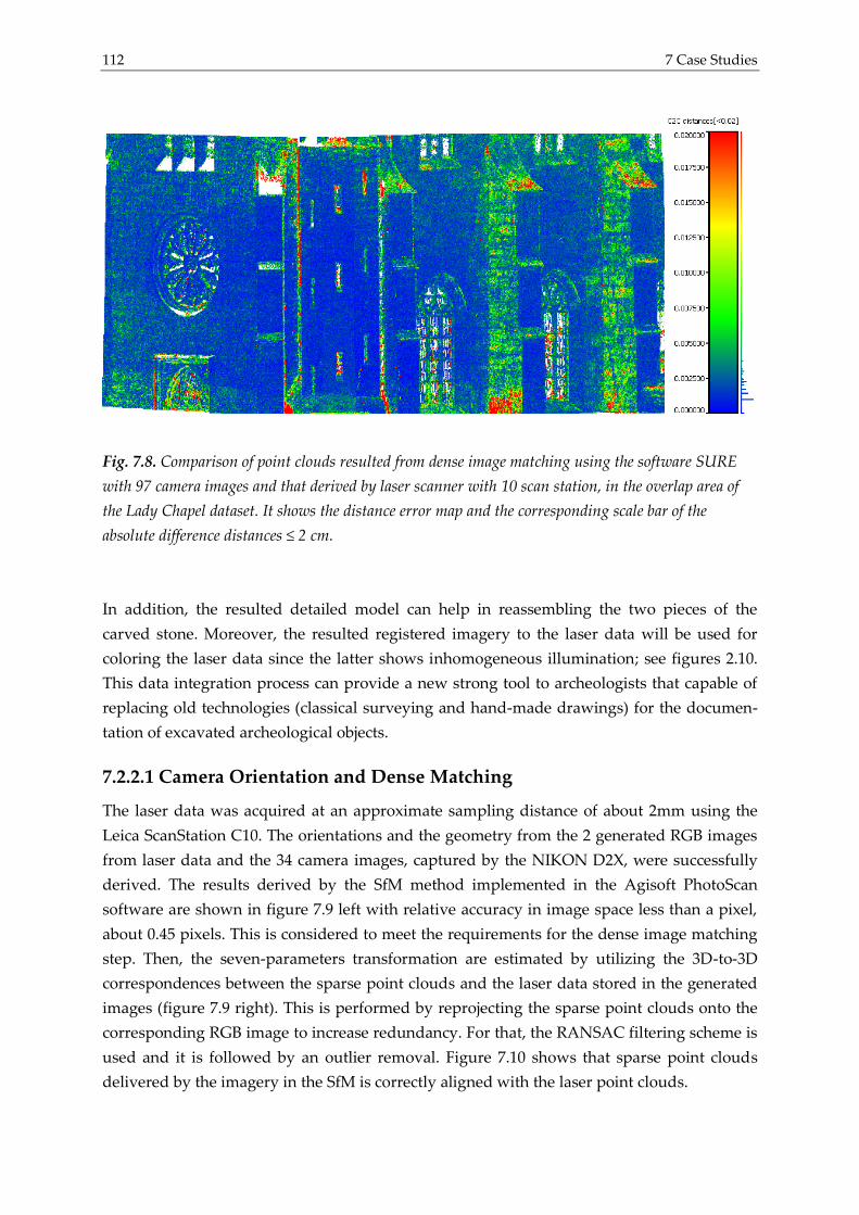
112 7 Case Studies
Fig. 7.8. Comparison of point clouds resulted from dense image matching using the software SURE
with 79 camera images and that derived by laser scanner with 10 scan station, in the overlap area of
the Lady Chapel dataset. It shows the distance error map and the corresponding scale bar of the
absolute difference distances ≤ 2 cm.
In addition, the resulted detailed model can help in reassembling the two pieces of the
carved stone. Moreover, the resulted registered imagery to the laser data will be used for
coloring the laser data since the latter shows inhomogeneous illumination; see figures 2.10.
This data integration process can provide a new strong tool to archeologists that capable of
replacing old technologies (classical surveying and hand-made drawings) for the documen-
tation of excavated archeological objects.
7.2.2.1 Camera Orientation and Dense Matching
The laser data was acquired at an approximate sampling distance of about 2mm using the
Leica ScanStation C10. The orientations and the geometry from the 2 generated RGB images
from laser data and the 34 camera images, captured by the NIKON D2X, were successfully
derived. The results derived by the SfM method implemented in the Agisoft PhotoScan
software are shown in figure 7.9 left with relative accuracy in image space less than a pixel,
about 0.45 pixels. This is considered to meet the requirements for the dense image matching
step. Then, the seven-parameters transformation are estimated by utilizing the 3D-to-3D
correspondences between the sparse point clouds and the laser data stored in the generated
images (figure 7.9 right). This is performed by reprojecting the sparse point clouds onto the
corresponding RGB image to increase redundancy. For that, the RANSAC filtering scheme is
used and it is followed by an outlier removal. Figure 7.10 shows that sparse point clouds
delivered by the imagery in the SfM is correctly aligned with the laser point clouds.

7.2 Data Integration Results and Evaluations 113
Fig. 7.9. SfM output: sparse point clouds (colored), 34 camera positions (red dots) and 2 scan stations
(green dots) of the carved stone dataset, aligned in one local coordinate system (left). Accurate 3D-to-
3D correspondences (2105 keypoints) between the sparse point clouds and the laser data which are
used for the calculation of the seven- parameters, depicted on the corresponding RGB image (right).
Fig. 7.10. SfM output: sparse point clouds (blue), 34 camera positions (red dots), 2 scan stations
(green dots) aligned in one coordinate system with laser point clouds from two scan stations (colored)
of the carved stone dataset. In addition, an ortho view of the former sparse point clouds, camera
positions and laser scanner stations (upper right corner).
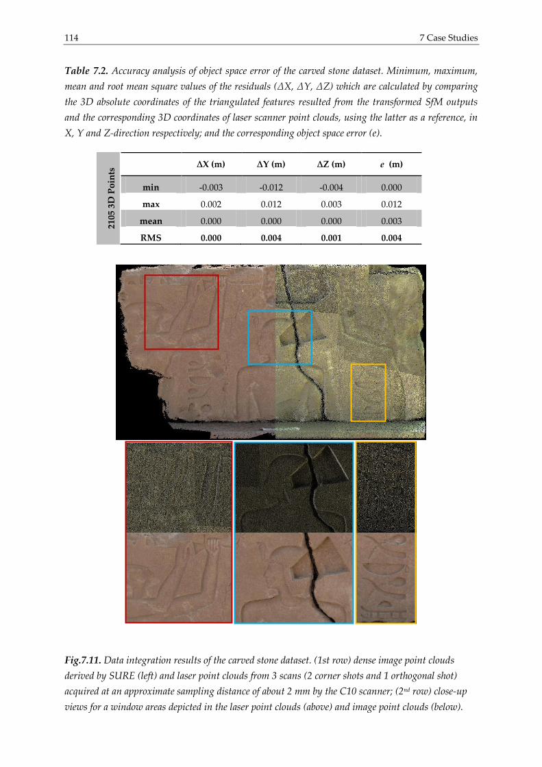
114 7 Case Studies
Table 7.2. Accuracy analysis of object space error of the carved stone dataset. Minimum, maximum,
mean and root mean square values of the residuals (∆X, ∆Y, ∆Z) which are calculated by comparing
the 3D absolute coordinates of the triangulated features resulted from the transformed SfM outputs
and the corresponding 3D coordinates of laser scanner point clouds, using the latter as a reference, in
X, Y and Z-direction respectively; and the corresponding object space error (e).
∆X (m) ∆Y (m) ∆Z (m) e (m)
min -0.003 -0.012 -0.004 0.000
max 0.002 0.012 0.003 0.012
mean 0.000 0.000 0.000 0.003
RMS 0.000 0.004 0.001 0.004
Fig.7.11. Data integration results of the carved stone dataset. (1st row) dense image point clouds
derived by SURE (left) and laser point clouds from 3 scans (2 corner shots and 1 orthogonal shot)
acquired at an approximate sampling distance of about 2 mm by the C10 scanner; (2nd row) close-up
views for a window areas depicted in the laser point clouds (above) and image point clouds (below).
2105
3D
Po
ints

7.2 Data Integration Results and Evaluations 115
Fig.7.12. 3D triangulated models of the carved stone dataset. 3D triangulated model using the laser
scanner point clouds from 3 scans acquired at an approximate sampling distance of about 2 mm by the
Leica ScanStation C10 of about 1.4 Mio. (1st row). 3D triangulated model using the dense image point
clouds derived by the software SURE from direct registered imagery with subsampled set of around
5.5 Mio. points, illustrated without/with texture information respectively (2nd and 3rd rows).
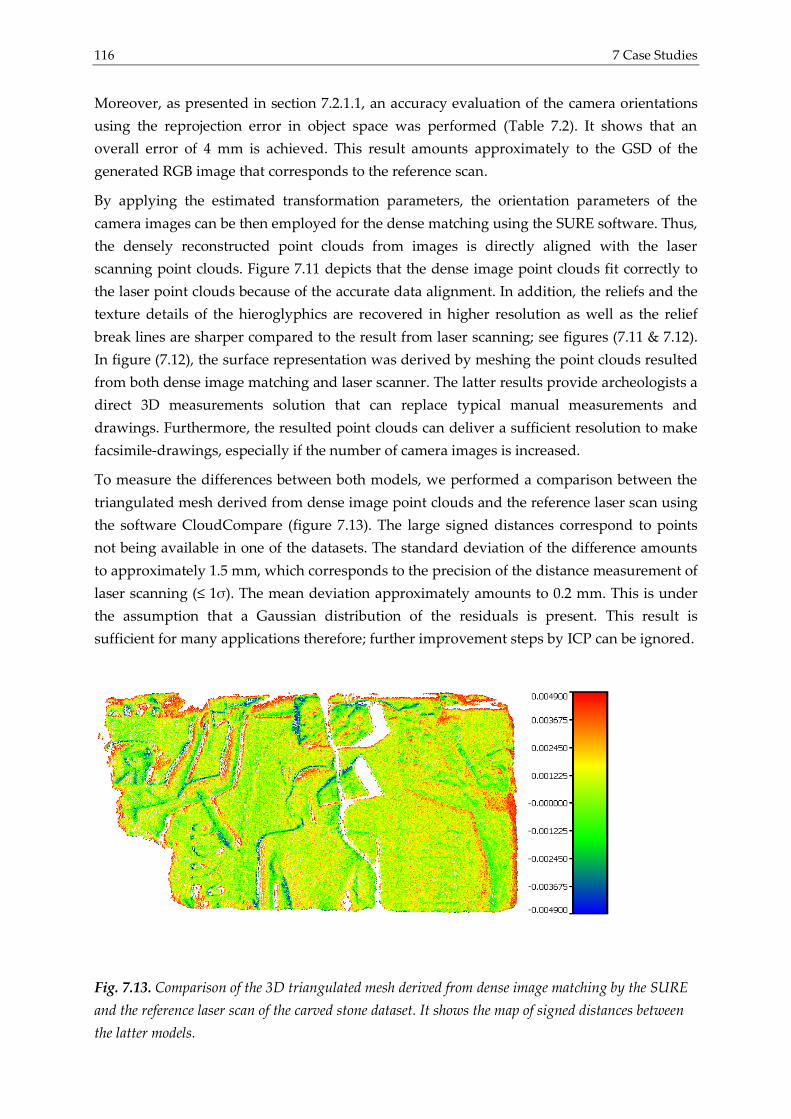
116 7 Case Studies
Moreover, as presented in section 7.2.1.1, an accuracy evaluation of the camera orientations
using the reprojection error in object space was performed (Table 7.2). It shows that an
overall error of 4 mm is achieved. This result amounts approximately to the GSD of the
generated RGB image that corresponds to the reference scan.
By applying the estimated transformation parameters, the orientation parameters of the
camera images can be then employed for the dense matching using the SURE software. Thus,
the densely reconstructed point clouds from images is directly aligned with the laser
scanning point clouds. Figure 7.11 depicts that the dense image point clouds fit correctly to
the laser point clouds because of the accurate data alignment. In addition, the reliefs and the
texture details of the hieroglyphics are recovered in higher resolution as well as the relief
break lines are sharper compared to the result from laser scanning; see figures (7.11 & 7.12).
In figure (7.12), the surface representation was derived by meshing the point clouds resulted
from both dense image matching and laser scanner. The latter results provide archeologists a
direct 3D measurements solution that can replace typical manual measurements and
drawings. Furthermore, the resulted point clouds can deliver a sufficient resolution to make
facsimile-drawings, especially if the number of camera images is increased.
To measure the differences between both models, we performed a comparison between the
triangulated mesh derived from dense image point clouds and the reference laser scan using
the software CloudCompare (figure 7.13). The large signed distances correspond to points
not being available in one of the datasets. The standard deviation of the difference amounts
to approximately 1.5 mm, which corresponds to the precision of the distance measurement of
laser scanning (≤ 1σ). The mean deviation approximately amounts to 0.2 mm. This is under
the assumption that a Gaussian distribution of the residuals is present. This result is
sufficient for many applications therefore; further improvement steps by ICP can be ignored.
Fig. 7.13. Comparison of the 3D triangulated mesh derived from dense image matching by the SURE
and the reference laser scan of the carved stone dataset. It shows the map of signed distances between
the latter models.

7.3 Target-Free Registration Results and Evaluations 117
7.2.2.1 Coloring Laser Point Cloud
The estimated camera calibration parameters during the SfM process were used to undistort
the involving 34 camera images in the SfM. Then, the calculated absolute orientations of the
latter images can be utilized for the colorization of the laser scanner point clouds, which are
resulted from 3 laser scans, see figure 7.14.
Fig. 7.14. Re-colored laser scanner point clouds from 3 scans acquired by the C10 scanner of the
carved stone dataset using 4 registered camera images.
7.3 Target-Free Registration Results and Evaluations
Our target-free registration approaches, introduced in chapter 5, have been applied to the
Lady Chapel dataset. The aim was to register 10 laser scans automatically. In addition, the
proposed general integration approach, presented in chapter 4, has been also applied on
additional two building of the Hirsau Abbey in order to investigate the capability of the
latter approach of registering completely non-overlapping laser scans. In the following, a
description of the achieved results and the performed evaluations is presented.
7.3.1 Results of the Target-Free Registration Using Accurate Space
Resection Methods
The proposed pairwise registration approach using accurate space resection methods,
presented in chapter 5; section (5.1), was applied to the Lady Chapel dataset. 10 PEM feature
databases have been employed for the pairwise registration. In the following, an evaluation
for the approach steps is given.

118 7 Case Studies
Fig.7.15. The initial visibility graph of the Lady Chapel dataset for the possible successive pairwise
registration, with 10 scans labeled with their IDs and connections, and a maximum of four edges per
node (left). A graphical view of the distance matrix as a heat map, color-coded between zero/one
indicating completely connected/disconnected (right).
7.3.1.1 Organizing Scans by Similarity
This starts by matching the PEM feature databases to each other then, the similarity
measures that connect each scan pair are determined using equation 5.1. For the calculation
of similarity measures, we set the following values: α = 0.5, β = 0.3, γ = 0.2, σr = 0.002m.
Accordingly, the unorganized scans can be directly described as a directed graph (figure 7.15
left). After that, false matches are discarded by means of a RANSAC based computation of a
closed-form space resection. The resulted filtered matches are used then to update the
initialized visibility graph (figure 7.16 1st row left). Then, the shortest path between all
vertices in the updated graph is determined based on the minimum weight/distance of the
edges (figure 7.16 2nd row left).
7.3.1.2 Pairwise Registration
Once the scans are sorted for the pairwise registration following the shortest path, for each
scan pair the orientation of the second scan in relation to the first scan is estimated using the
EPnP and OI methods. In addition, the quality of the calculated orientations can be increased
by applying the X84 rule iteratively with a value of 2.97k to discard outliers. Conse-
quently, the overall precision of the orientation is in sub-pixel range and less than 3σr in
image space and object space respectively. Then, the filtered correspondences are used to
update the reconstructed visibility graph by calculating a new similarity measures between
the scans (figure 7.16 2nd row right). The latter figure illustrates that 2 graph edges/connec-
tions were dropped out due to the small number of manifold keypoints maintained
therefore, 3 clusters of scans are resulted. That since our pairwise method is highly depended
on the good overlap and small change viewpoints between laser scans where sufficient
number and good distribution of the keypoints over the object of interest are required.
Therefore, the connections between the scan pair (Scan5-Scan6) which has large change
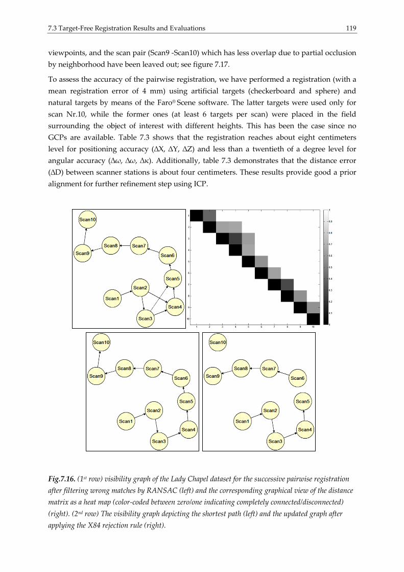
7.3 Target-Free Registration Results and Evaluations 119
viewpoints, and the scan pair (Scan9 -Scan10) which has less overlap due to partial occlusion
by neighborhood have been leaved out; see figure 7.17.
To assess the accuracy of the pairwise registration, we have performed a registration (with a
mean registration error of 4 mm) using artificial targets (checkerboard and sphere) and
natural targets by means of the Faro® Scene software. The latter targets were used only for
scan Nr.10, while the former ones (at least 6 targets per scan) were placed in the field
surrounding the object of interest with different heights. This has been the case since no
GCPs are available. Table 7.3 shows that the registration reaches about eight centimeters
level for positioning accuracy (∆X, ∆Y, ∆Z) and less than a twentieth of a degree level for
angular accuracy (∆ω, ∆ω, ∆κ). Additionally, table 7.3 demonstrates that the distance error
(∆D) between scanner stations is about four centimeters. These results provide good a prior
alignment for further refinement step using ICP.
Fig.7.16. (1st row) visibility graph of the Lady Chapel dataset for the successive pairwise registration
after filtering wrong matches by RANSAC (left) and the corresponding graphical view of the distance
matrix as a heat map (color-coded between zero/one indicating completely connected/disconnected)
(right). (2nd row) The visibility graph depicting the shortest path (left) and the updated graph after
applying the X84 rejection rule (right).
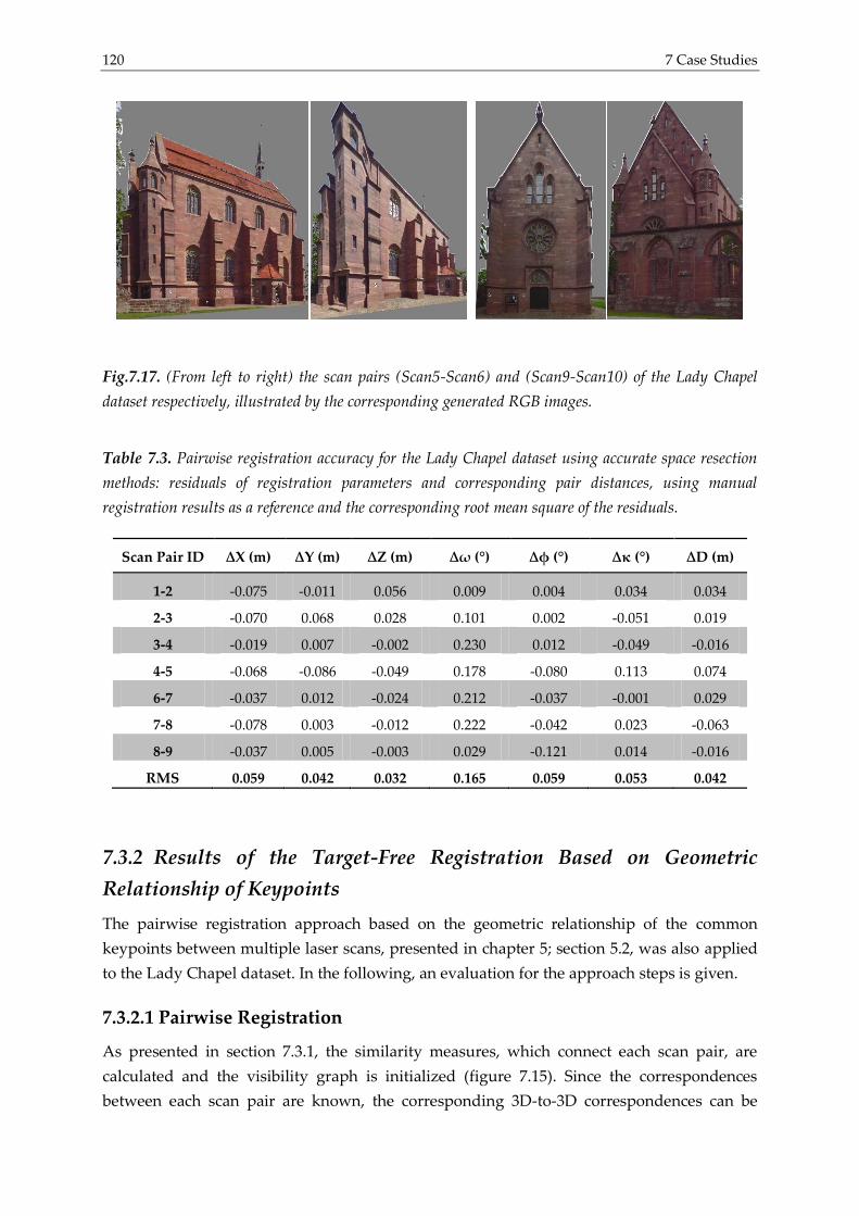
120 7 Case Studies
Fig.7.17. (From left to right) the scan pairs (Scan5-Scan6) and (Scan9-Scan10) of the Lady Chapel
dataset respectively, illustrated by the corresponding generated RGB images.
Table 7.3. Pairwise registration accuracy for the Lady Chapel dataset using accurate space resection
methods: residuals of registration parameters and corresponding pair distances, using manual
registration results as a reference and the corresponding root mean square of the residuals.
Scan Pair ID ∆X (m) ∆Y (m) ∆Z (m) ∆ω (°) ∆φ (°) ∆κ (°) ∆D (m)
1-2 -0.075 -0.011 0.056 0.009 0.004 0.034 0.034
2-3 -0.070 0.068 0.028 0.101 0.002 -0.051 0.019
3-4 -0.019 0.007 -0.002 0.230 0.012 -0.049 -0.016
4-5 -0.068 -0.086 -0.049 0.178 -0.080 0.113 0.074
6-7 -0.037 0.012 -0.024 0.212 -0.037 -0.001 0.029
7-8 -0.078 0.003 -0.012 0.222 -0.042 0.023 -0.063
8-9 -0.037 0.005 -0.003 0.029 -0.121 0.014 -0.016
RMS 0.059 0.042 0.032 0.165 0.059 0.053 0.042
7.3.2 Results of the Target-Free Registration Based on Geometric
Relationship of Keypoints
The pairwise registration approach based on the geometric relationship of the common
keypoints between multiple laser scans, presented in chapter 5; section 5.2, was also applied
to the Lady Chapel dataset. In the following, an evaluation for the approach steps is given.
7.3.2.1 Pairwise Registration
As presented in section 7.3.1, the similarity measures, which connect each scan pair, are
calculated and the visibility graph is initialized (figure 7.15). Since the correspondences
between each scan pair are known, the corresponding 3D-to-3D correspondences can be
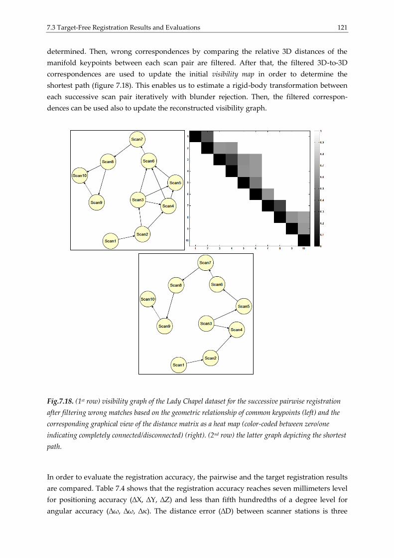
7.3 Target-Free Registration Results and Evaluations 121
determined. Then, wrong correspondences by comparing the relative 3D distances of the
manifold keypoints between each scan pair are filtered. After that, the filtered 3D-to-3D
correspondences are used to update the initial visibility map in order to determine the
shortest path (figure 7.18). This enables us to estimate a rigid-body transformation between
each successive scan pair iteratively with blunder rejection. Then, the filtered correspon-
dences can be used also to update the reconstructed visibility graph.
Fig.7.18. (1st row) visibility graph of the Lady Chapel dataset for the successive pairwise registration
after filtering wrong matches based on the geometric relationship of common keypoints (left) and the
corresponding graphical view of the distance matrix as a heat map (color-coded between zero/one
indicating completely connected/disconnected) (right). (2nd row) the latter graph depicting the shortest
path.
In order to evaluate the registration accuracy, the pairwise and the target registration results
are compared. Table 7.4 shows that the registration accuracy reaches seven millimeters level
for positioning accuracy (∆X, ∆Y, ∆Z) and less than fifth hundredths of a degree level for
angular accuracy (∆ω, ∆ω, ∆κ). The distance error (∆D) between scanner stations is three
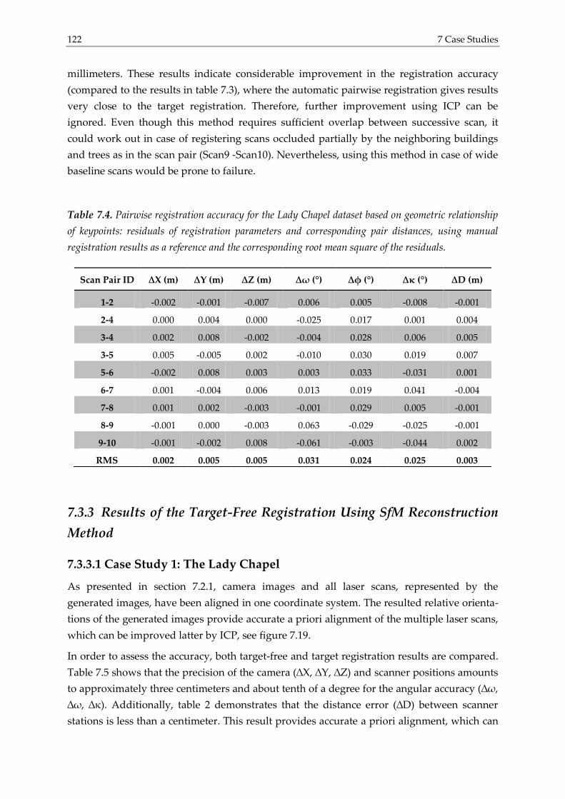
122 7 Case Studies
millimeters. These results indicate considerable improvement in the registration accuracy
(compared to the results in table 7.3), where the automatic pairwise registration gives results
very close to the target registration. Therefore, further improvement using ICP can be
ignored. Even though this method requires sufficient overlap between successive scan, it
could work out in case of registering scans occluded partially by the neighboring buildings
and trees as in the scan pair (Scan9 -Scan10). Nevertheless, using this method in case of wide
baseline scans would be prone to failure.
Table 7.4. Pairwise registration accuracy for the Lady Chapel dataset based on geometric relationship
of keypoints: residuals of registration parameters and corresponding pair distances, using manual
registration results as a reference and the corresponding root mean square of the residuals.
7.3.3 Results of the Target-Free Registration Using SfM Reconstruction
Method
7.3.3.1 Case Study 1: The Lady Chapel
As presented in section 7.2.1, camera images and all laser scans, represented by the
generated images, have been aligned in one coordinate system. The resulted relative orienta-
tions of the generated images provide accurate a priori alignment of the multiple laser scans,
which can be improved latter by ICP, see figure 7.19.
In order to assess the accuracy, both target-free and target registration results are compared.
Table 7.5 shows that the precision of the camera (∆X, ∆Y, ∆Z) and scanner positions amounts
to approximately three centimeters and about tenth of a degree for the angular accuracy (∆ω,
∆ω, ∆κ). Additionally, table 2 demonstrates that the distance error (∆D) between scanner
stations is less than a centimeter. This result provides accurate a priori alignment, which can
Scan Pair ID ∆X (m) ∆Y (m) ∆Z (m) ∆ω (°) ∆φ (°) ∆κ (°) ∆D (m)
1-2 -0.002 -0.001 -0.007 0.006 0.005 -0.008 -0.001
2-4 0.000 0.004 0.000 -0.025 0.017 0.001 0.004
3-4 0.002 0.008 -0.002 -0.004 0.028 0.006 0.005
3-5 0.005 -0.005 0.002 -0.010 0.030 0.019 0.007
5-6 -0.002 0.008 0.003 0.003 0.033 -0.031 0.001
6-7 0.001 -0.004 0.006 0.013 0.019 0.041 -0.004
7-8 0.001 0.002 -0.003 -0.001 0.029 0.005 -0.001
8-9 -0.001 0.000 -0.003 0.063 -0.029 -0.025 -0.001
9-10 -0.001 -0.002 0.008 -0.061 -0.003 -0.044 0.002
RMS 0.002 0.005 0.005 0.031 0.024 0.025 0.003
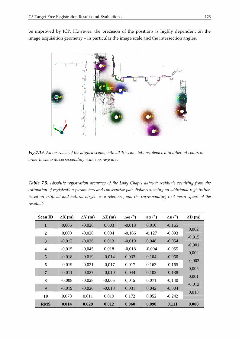
7.3 Target-Free Registration Results and Evaluations 123
be improved by ICP. However, the precision of the positions is highly dependent on the
image acquisition geometry – in particular the image scale and the intersection angles.
Fig.7.19. An overview of the aligned scans, with all 10 scan stations, depicted in different colors in
order to show its corresponding scan coverage area.
Table 7.5. Absolute registration accuracy of the Lady Chapel dataset: residuals resulting from the
estimation of registration parameters and consecutive pair distances, using an additional registration
based on artificial and natural targets as a reference, and the corresponding root mean square of the
residuals.
Scan ID ∆X (m) ∆Y (m) ∆Z (m) ∆ω (°) ∆φ (°) ∆κ (°) ∆D (m)
1 0,006 -0,026 0,003 -0,018 0,010 -0,165 0,002
-0,015
-0,001
0,002
-0,003
0,005
0,001
-0,013
0,013
2 0,000 -0,026 0,004 -0,166 -0,127 -0,093
3 -0,012 -0,036 0,013 -0,010 0,048 -0,054
4 -0,015 -0,045 0,018 -0,018 -0,004 -0,055
5 -0.018 -0.019 -0.014 0,033 0,104 -0,060
6 -0,019 -0,021 -0,017 0,017 0,163 -0,165
7 -0,011 -0,027 -0,010 0,044 0,103 -0,138
8 -0,008 -0,028 -0,005 0,015 0,071 -0,140
9 -0,019 -0,026 -0,013 0,031 0,042 -0,004
10 0.078 0.011 0.019 0.172 0.052 -0.242
RMS 0.014 0.029 0.012 0.060 0.090 0.111 0.008
S1
S2
.S3
.S4
.S5
.S6 .S7 .S8
.S9
.S10
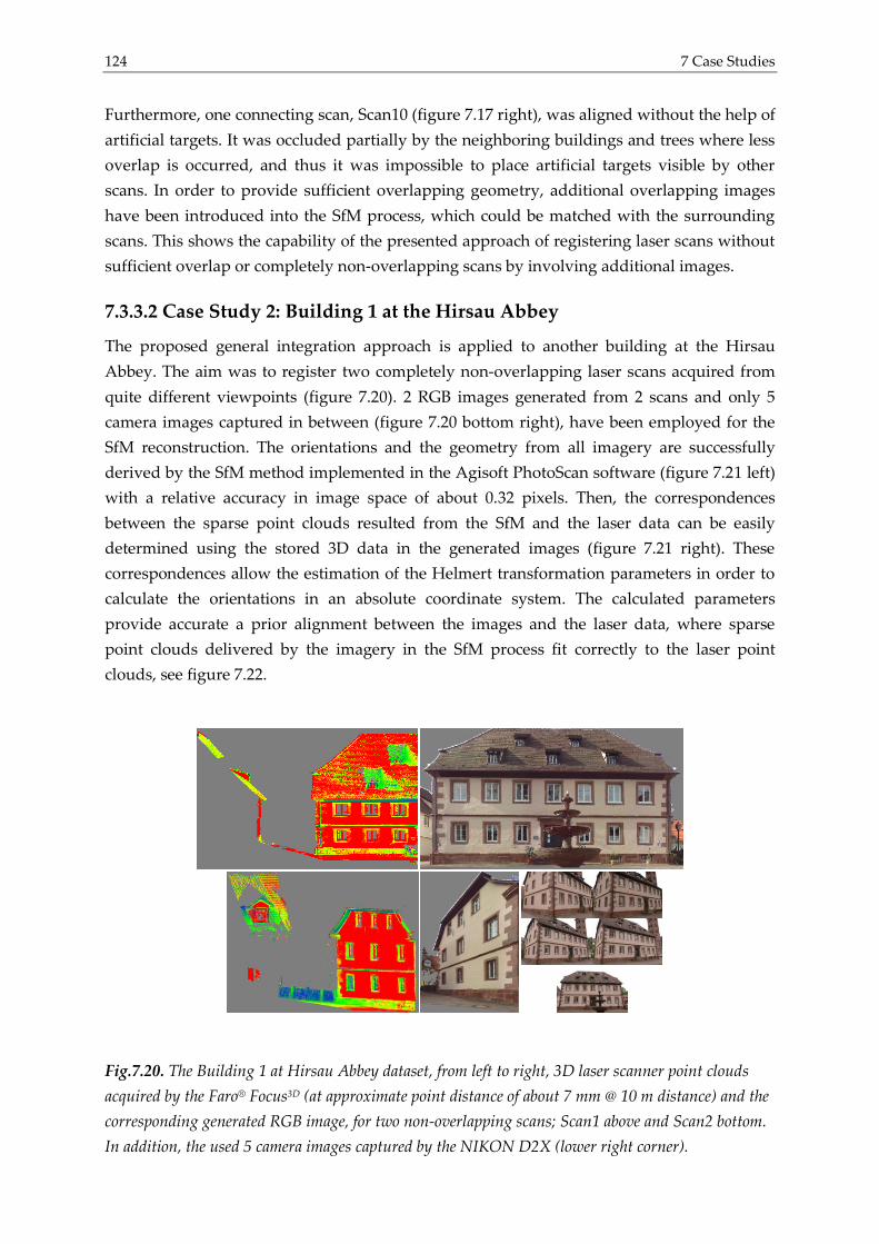
124 7 Case Studies
Furthermore, one connecting scan, Scan10 (figure 7.17 right), was aligned without the help of
artificial targets. It was occluded partially by the neighboring buildings and trees where less
overlap is occurred, and thus it was impossible to place artificial targets visible by other
scans. In order to provide sufficient overlapping geometry, additional overlapping images
have been introduced into the SfM process, which could be matched with the surrounding
scans. This shows the capability of the presented approach of registering laser scans without
sufficient overlap or completely non-overlapping scans by involving additional images.
7.3.3.2 Case Study 2: Building 1 at the Hirsau Abbey
The proposed general integration approach is applied to another building at the Hirsau
Abbey. The aim was to register two completely non-overlapping laser scans acquired from
quite different viewpoints (figure 7.20). 2 RGB images generated from 2 scans and only 5
camera images captured in between (figure 7.20 bottom right), have been employed for the
SfM reconstruction. The orientations and the geometry from all imagery are successfully
derived by the SfM method implemented in the Agisoft PhotoScan software (figure 7.21 left)
with a relative accuracy in image space of about 0.32 pixels. Then, the correspondences
between the sparse point clouds resulted from the SfM and the laser data can be easily
determined using the stored 3D data in the generated images (figure 7.21 right). These
correspondences allow the estimation of the Helmert transformation parameters in order to
calculate the orientations in an absolute coordinate system. The calculated parameters
provide accurate a prior alignment between the images and the laser data, where sparse
point clouds delivered by the imagery in the SfM process fit correctly to the laser point
clouds, see figure 7.22.
Fig.7.20. The Building 1 at Hirsau Abbey dataset, from left to right, 3D laser scanner point clouds
acquired by the Faro® Focus3D (at approximate point distance of about 7 mm @ 10 m distance) and the
corresponding generated RGB image, for two non-overlapping scans; Scan1 above and Scan2 bottom.
In addition, the used 5 camera images captured by the NIKON D2X (lower right corner).
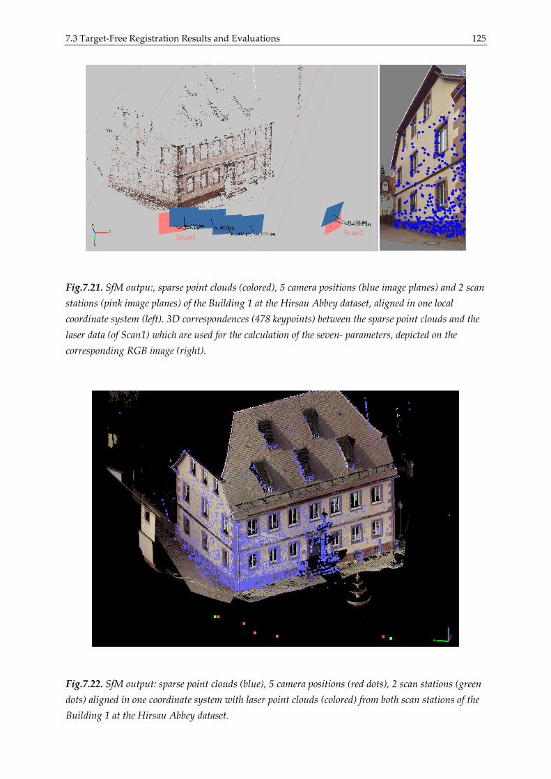
7.3 Target-Free Registration Results and Evaluations 125
Fig.7.21. SfM outpu:, sparse point clouds (colored), 5 camera positions (blue image planes) and 2 scan
stations (pink image planes) of the Building 1 at the Hirsau Abbey dataset, aligned in one local
coordinate system (left). 3D correspondences (478 keypoints) between the sparse point clouds and the
laser data (of Scan1) which are used for the calculation of the seven- parameters, depicted on the
corresponding RGB image (right).
Fig.7.22. SfM output: sparse point clouds (blue), 5 camera positions (red dots), 2 scan stations (green
dots) aligned in one coordinate system with laser point clouds (colored) from both scan stations of the
Building 1 at the Hirsau Abbey dataset.
Scan2 Scan1
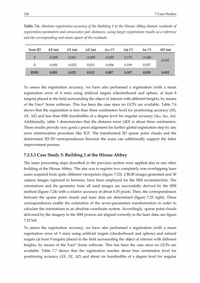
126 7 Case Studies
Table 7.6. Absolute registration accuracy of the Building 1 at the Hirsau Abbey dataset: residuals of
registration parameters and consecutive pair distances, using target registration results as a reference
and the corresponding root mean square of the residuals.
To assess the registration accuracy, we have also performed a registration (with a mean
registration error of 4 mm) using artificial targets (checkerboard and sphere, at least 8
targets) placed in the field surrounding the object of interest with different heights, by means
of the Faro® Scene software. This has been the case since no GCPs are available. Table 7.6
shows that the registration is less than three centimeters level for positioning accuracy (∆X,
∆Y, ∆Z) and less than fifth hundredths of a degree level for angular accuracy (∆ω, ∆ω, ∆κ).
Additionally, table 1 demonstrates that the distance error (∆D) is about three centimeters.
These results provide very good a priori alignment for further global registration step by any
error minimization procedure like ICP. The transformed 3D sparse point clouds and the
determined 3D-3D correspondences between the scans can additionally support the latter
improvement process.
7.3.3.3 Case Study 3: Building 2 at the Hirsau Abbey
The same processing steps described in the previous section were applied also to one other
building at the Hirsau Abbey. The aim was to register two completely non-overlapping laser
scans acquired from quite different viewpoints (figure 7.23). 2 RGB images generated and 30
camera images captured in between, have been employed for the SfM reconstruction. The
orientations and the geometry from all used images are successfully derived by the SfM
method (figure 7.24) with a relative accuracy of about 0.35 pixels. Then, the correspondences
between the sparse point clouds and laser data are determined (figure 7.25 right). These
correspondences enable the estimation of the seven-parameters transformation in order to
calculate the orientations in an absolute coordinate system. Accordingly, sparse point clouds
delivered by the imagery in the SfM process are aligned correctly to the laser data; see figure
7.25 left.
To assess the registration accuracy, we have also performed a registration (with a mean
registration error of 5 mm) using artificial targets (checkerboard and sphere) and natural
targets (at least 9 targets) placed in the field surrounding the object of interest with different
heights, by means of the Faro® Scene software. This has been the case since no GCPs are
available. Table 7.7 shows that the registration reaches about four centimeters level for
positioning accuracy (∆X, ∆Y, ∆Z) and about six hundredths of a degree level for angular
Scan ID ∆X (m) ∆Y (m) ∆Z (m) ∆ω (°) ∆φ (°) ∆κ (°) ∆D (m)
1 -0.008 0.001 -0.009 -0.009 0.173 -0.040
0.032
2 -0.001 -0.032 0.015 -0.006 0.199 0.037
RMS 0.005 0.023 0.012 0.007 0.187 0.039 0.032
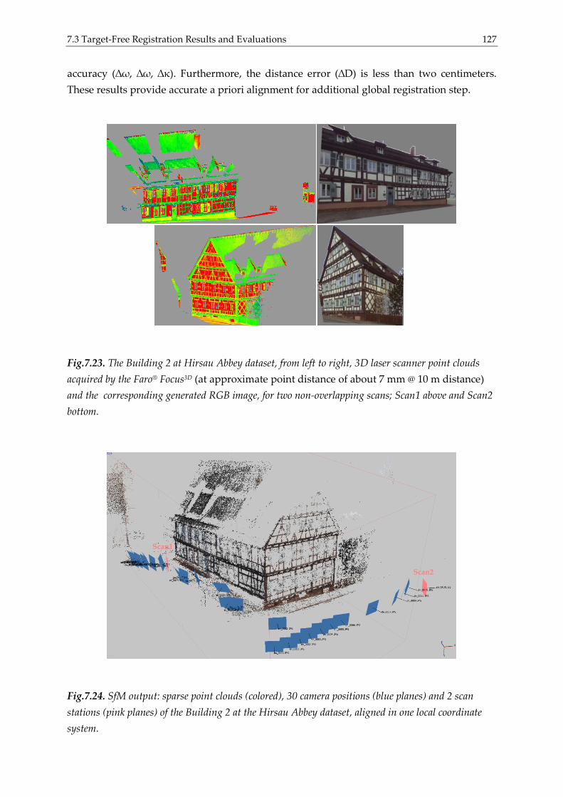
7.3 Target-Free Registration Results and Evaluations 127
accuracy (∆ω, ∆ω, ∆κ). Furthermore, the distance error (∆D) is less than two centimeters.
These results provide accurate a priori alignment for additional global registration step.
Fig.7.23. The Building 2 at Hirsau Abbey dataset, from left to right, 3D laser scanner point clouds
acquired by the Faro® Focus3D (at approximate point distance of about 7 mm @ 10 m distance)
and the corresponding generated RGB image, for two non-overlapping scans; Scan1 above and Scan2
bottom.
Fig.7.24. SfM output: sparse point clouds (colored), 30 camera positions (blue planes) and 2 scan
stations (pink planes) of the Building 2 at the Hirsau Abbey dataset, aligned in one local coordinate
system.
Scan2
Scan1
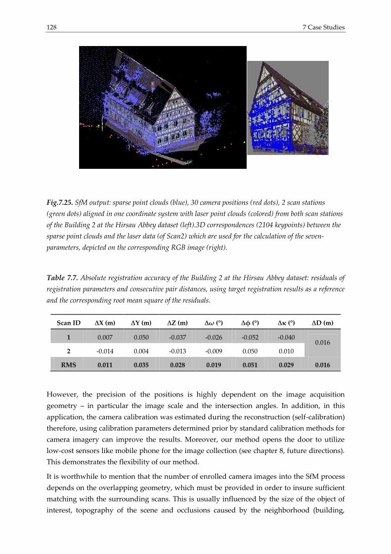
128 7 Case Studies
Fig.7.25. SfM output: sparse point clouds (blue), 30 camera positions (red dots), 2 scan stations
(green dots) aligned in one coordinate system with laser point clouds (colored) from both scan stations
of the Building 2 at the Hirsau Abbey dataset (left).3D correspondences (2104 keypoints) between the
sparse point clouds and the laser data (of Scan2) which are used for the calculation of the seven-
parameters, depicted on the corresponding RGB image (right).
Table 7.7. Absolute registration accuracy of the Building 2 at the Hirsau Abbey dataset: residuals of
registration parameters and consecutive pair distances, using target registration results as a reference
and the corresponding root mean square of the residuals.
However, the precision of the positions is highly dependent on the image acquisition
geometry – in particular the image scale and the intersection angles. In addition, in this
application, the camera calibration was estimated during the reconstruction (self-calibration)
therefore, using calibration parameters determined prior by standard calibration methods for
camera imagery can improve the results. Moreover, our method opens the door to utilize
low-cost sensors like mobile phone for the image collection (see chapter 8, future directions).
This demonstrates the flexibility of our method.
It is worthwhile to mention that the number of enrolled camera images into the SfM process
depends on the overlapping geometry, which must be provided in order to insure sufficient
matching with the surrounding scans. This is usually influenced by the size of the object of
interest, topography of the scene and occlusions caused by the neighborhood (building,
Scan ID ∆X (m) ∆Y (m) ∆Z (m) ∆ω (°) ∆φ (°) ∆κ (°) ∆D (m)
1 0.007 0.050 -0.037 -0.026 -0.052 -0.040
0.016
2 -0.014 0.004 -0.013 -0.009 0.050 0.010
RMS 0.011 0.035 0.028 0.019 0.051 0.029 0.016

7.3 Target-Free Registration Results and Evaluations 129
trees, etc.). One the other hand, higher accuracy and small image drift error can be acquired
be using image circle configuration and strong image network. But, this can be difficult to
fulfill from practical point of view especially in case of complex objects like heritage sites.
Furthermore, adding more images in the SfM process can improve the scan alignment due to
the stable image geometry as well as the increase in the redundancy, where more features
will be used for the calculation of transformation parameters. Nevertheless, large number of
images require more time for processing. Fortunately, latest developments in the SfM
methods are able to resolve the time issue, e.g. (Abdel-Wahab et al., 2012).
130 8 Conclusions and Future Directions
8 Conclusions and Future Directions
8.1 Conclusions
Within the thesis, the potential of combining digital photogrammetry and TLS techniques for
close-range applications such as cultural heritage data recording and preservation is
discussed. The proposed solution for data integration is based on the use of synthetic images
created from the TLS data in order to simplify the extraction of 3D information. This
integration directs at filling gaps in laser point clouds due to occlusion or weak reflectivity of
object material, retrieving more object details in higher resolution and registering multiple
laser scans especially, in case of scans occluded partially by the neighborhood and com-
pletely non-overlapping laser scans. Furthermore, the proposed method allows the use of
dense image matching algorithms such as SURE on the imagery and its orientation para-
meters. This derives correctly scaled point clouds in the laser scanning coordinate system.
Moreover, this can be beneficial for applications where high-resolution image point clouds
can complement large-scale laser scanning point clouds.
In addition, image-based methods for the automatic pairwise registration of multiple laser
scans based on the PEM and the geometric relationship of common keypoints between scans
are also discussed. A visibility graph structure has been exploited for organizing scans by
similarity. However, these methods are highly depended on the good overlap and small
change viewpoints between laser scans. Therefore, scans acquired at considerably changed
viewpoints such as highly convergent with wide baselines or those provide very little
overlaps, are difficult to process. Moreover, heritage objects in form of 3D physical models
are recorded not only for documentation issues, but also for historical interpretation,
restoration, cultural and educational purposes.
Advantageous is that the proposed integration approach introduces an efficient solution able
to fuse multi data sources and sensors for close-range applications. Secondly, it yields to an
increase in automation and redundancy in order to meet the demands of the final user
(geodesist, archaeologist, architect, etc.). Finally, it represents a direct solution for data
registration.
8.2 Future Directions
There are still issues that need to be investigated and studied in order to have further
improvements and developing. These issues can be summarized as the follows:
The use of low-cost sensors such as Kinect range camera and mobile phone should be
considered in the integration solution. Using their integrated cameras, these sensors can
be beneficial for recovering more surface information and registering multiple laser scans
8.3 Registration of Non-Overlapping Laser Scans Using Mobile Phones 131
for indoor and outdoor applications. Furthermore, this can be also expanded to the use of
the iPad tablet computers with their integrated cameras and online services. That is, since
modern TLS system can be controlled with such small computers.
One of the techniques that could be further integrated is the low-cost photogrammetry by
the unmanned aerial vehicle (UAV). The technique could be exploited for the integration
of images captured by the UAVs and those acquired by terrestrial cameras or data
collected by terrestrial laser scanners. For that, oblique images captured by the UAVs can
be matched with the imagery captured by terrestrial camera or synthetic images
generated from TLS data particularly, in case of sharing in the coverage of building
facades in urban environments.
A further robust solution for data fusion could be considered by not only integrating the
synthetic images in the SfM process, but also by exploiting the 3D data storied in those
images in the bundle adjustment process.
Raw RGB images captured by the laser scanner’s integrated camera could be also used
directly in the SfM process as well, since for modern TLS systems, e.g. the Leica C10 and
P20 the image calibration and orientation information is available.
Using linear features instead of point features for image matching in order to reduce
outliers and to improve registration accuracy. This is the case since the synthetic images
are generated in a central projection representation, where curved lines are no more
existed. Furthermore, employing planar patches could lead to better accuracies in the
final co-registration.
The proposed integration approach provides a solution for gap filling in TLS data. This
motivates us to develop a smarter solution, which can detect gaps or holes in laser point
clouds and then fills those using only images that cover geometrically the exact gaps in
both SfM and dense matching processes.
In the following, an exemplary test of using mobile phone as a low-cost sensor for the
automatic registration of non-overlapping laser scans is shown.
8.3 Registration of Non-Overlapping Laser Scans Using
Mobile Phones
The proposed general integration approach is applied to the building at the University of
Stuttgart. The aim was to register two completely non-overlapping laser scans acquired from
quite different viewpoints (figure 8.1 1st row). The laser data was acquired using the Faro®
Focus3D (at approximate point distance of about 7 mm @ 10 m distance). 2 RGB images
generated from 2 scans and 18 images captured by the 5 megapixel camera of the HTC
Wildfire A3333 mobile phone in between, have been employed for the SfM method
implemented in the Agisoft PhotoScan software (figure 8.1 2nd row left), with a relative
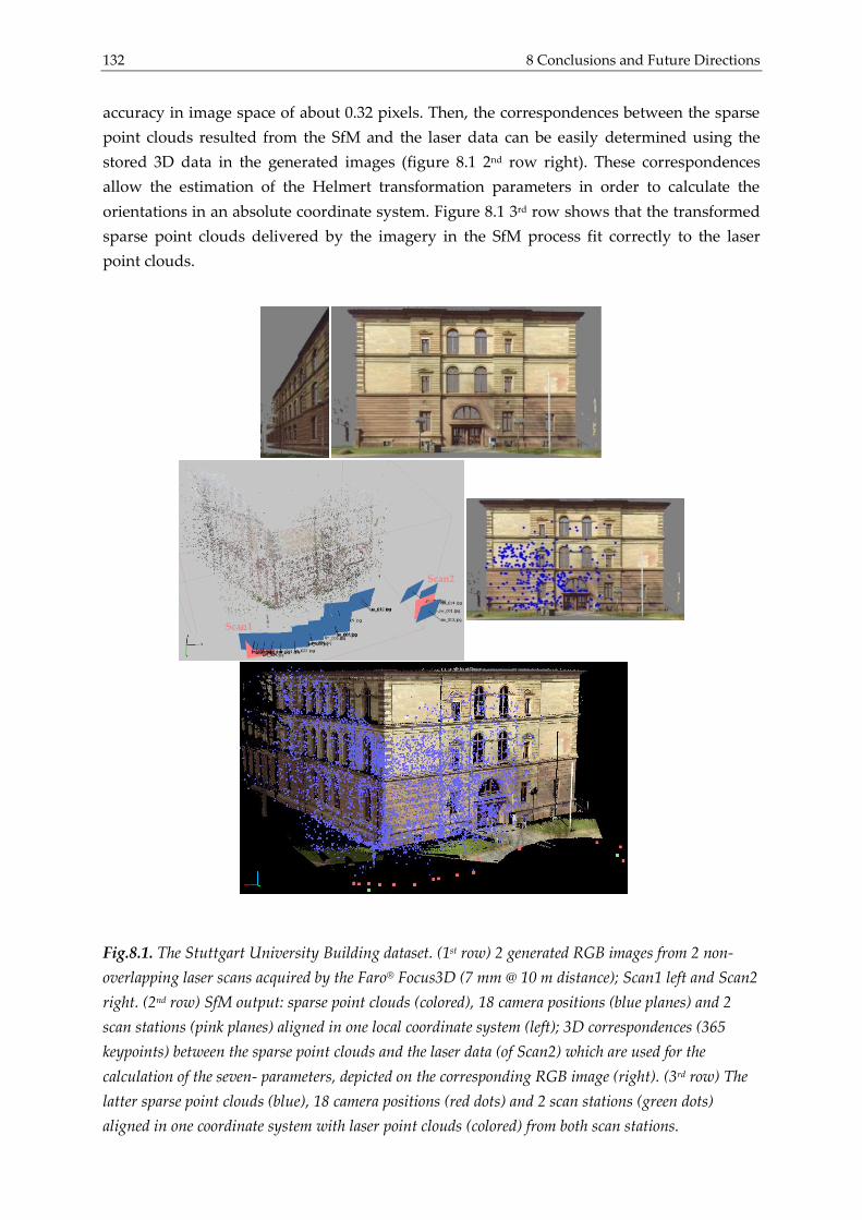
132 8 Conclusions and Future Directions
accuracy in image space of about 0.32 pixels. Then, the correspondences between the sparse
point clouds resulted from the SfM and the laser data can be easily determined using the
stored 3D data in the generated images (figure 8.1 2nd row right). These correspondences
allow the estimation of the Helmert transformation parameters in order to calculate the
orientations in an absolute coordinate system. Figure 8.1 3rd row shows that the transformed
sparse point clouds delivered by the imagery in the SfM process fit correctly to the laser
point clouds.
Fig.8.1. The Stuttgart University Building dataset. (1st row) 2 generated RGB images from 2 non-
overlapping laser scans acquired by the Faro® Focus3D (7 mm @ 10 m distance); Scan1 left and Scan2
right. (2nd row) SfM output: sparse point clouds (colored), 18 camera positions (blue planes) and 2
scan stations (pink planes) aligned in one local coordinate system (left); 3D correspondences (365
keypoints) between the sparse point clouds and the laser data (of Scan2) which are used for the
calculation of the seven- parameters, depicted on the corresponding RGB image (right). (3rd row) The
latter sparse point clouds (blue), 18 camera positions (red dots) and 2 scan stations (green dots)
aligned in one coordinate system with laser point clouds (colored) from both scan stations.
Scan2
Scan1
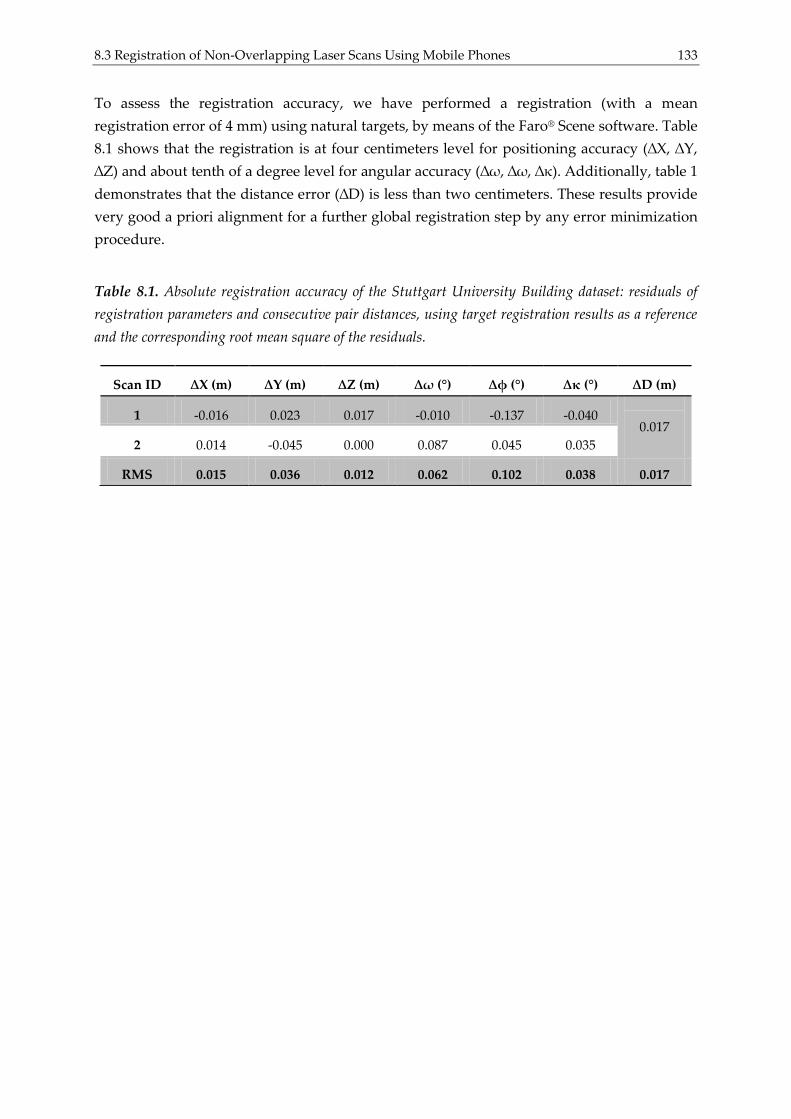
8.3 Registration of Non-Overlapping Laser Scans Using Mobile Phones 133
To assess the registration accuracy, we have performed a registration (with a mean
registration error of 4 mm) using natural targets, by means of the Faro® Scene software. Table
8.1 shows that the registration is at four centimeters level for positioning accuracy (∆X, ∆Y,
∆Z) and about tenth of a degree level for angular accuracy (∆ω, ∆ω, ∆κ). Additionally, table 1
demonstrates that the distance error (∆D) is less than two centimeters. These results provide
very good a priori alignment for a further global registration step by any error minimization
procedure.
Table 8.1. Absolute registration accuracy of the Stuttgart University Building dataset: residuals of
registration parameters and consecutive pair distances, using target registration results as a reference
and the corresponding root mean square of the residuals.
Scan ID ∆X (m) ∆Y (m) ∆Z (m) ∆ω (°) ∆φ (°) ∆κ (°) ∆D (m)
1 -0.016 0.023 0.017 -0.010 -0.137 -0.040
0.017
2 0.014 -0.045 0.000 0.087 0.045 0.035
RMS 0.015 0.036 0.012 0.062 0.102 0.038 0.017
134 Appendices
Appendices
A: Structure-From-Motion (SfM)
Reconstruction of camera orientations and geometry from multiple images of a scene has
long been and still is an active issue in computer vision and photogrammetry. It has inspired
a wide variety of different approaches and algorithms. A fully automated and general
solution of this task in terrestrial applications is still pending in case of unordered image
datasets especially for close-range and/or low-cost applications. The Structure-from-motion
(SfM) was originally developed by the computer vision community to simultaneously
estimate the scene structure and the camera motion from images of a scene with little prior
information about the camera.
Having two views, as the simplest SfM problem, has been long investigated. Kruppa,
hundred years ago, confirmed that knowing five point correspondences in two images
allows the estimation of the camera poses and the 3D point locations, up to a similarity trans-
form (Kruppa, 1913). Therefore, several five-point algorithms for estimating two-view geo-
metry have been proposed, e.g. (Nister, 2004b). The mathematical and algorithmic aspects of
the three-view problem have been also studied (Hartley & Zisserman, 2003). For multiple
views, only specific scenarios (such as the frames of a video) of SfM problem can be solved
exactly, but for the general case no such closed-form solutions exist, and thus a wide variety
of SfM methods have been reported (Snavely, 2008).
Most SfM methods process images in batches and handle the reconstruction process without
making assumptions about the images in the scene or the acquisition configuration. The
scalability- the ability to handle a growing amount of work in a capable manner- of a SFM
method is a key issue (Corsini et al., 2013). One approach is to use the so-called partitioning
methods (Fitzgibbon & Zisserman, 1998; Gibson et al., 2002), which reduce the reconstruction
problem to smaller and better conditioned sub-problems that can be then optimized (Steedly
et al., 2003; Ni et al., 2007). Advantageous is that in such methods, not only the equalized
error distribution on the entire dataset but also the speed up of the processing time. Lately,
(Klopschitz et al., 2010) proposed a robust and flexible SfM pipeline where reasoning about
feature track compatibility and image connectivity is based on image triplets.
Another approach is to select a subset of input images and feature points that represent the
entire solution. Hierarchical sub-sampling was firstly proposed by (Fitzgibbon & Zisserman,
1998) using a balanced tree of trifocal tensors over a video sequence then, this method was
latter refined by (Nister, 2000). (Shum et al., 1999) divide the sequence into segments, which
are resolved locally then, they are merged hierarchically, similar to the method presented by
(Gibson et al., 2002). A method proposed by (Snavely, 2008) deals with sparse datasets
(community photo collections) by selecting a subset of images whose reconstruction
approximates the result obtained using the entire dataset. Hierarchical and parallelizable
B: Dense Image Matching Methods 135
scheme for a SFM method was presented in (Gherardi et al., 2010). They organize images
into a hierarchical cluster tree and the reconstruction then proceeds from the leaves to the
root. Partial reconstructions correspond to internal nodes, whereas images are stored in the
leaves.
In our applications, besides the SfM method implemented in the Agisoft PhotoScan software,
a SfM pipeline was employed to retrieve image orientations and geometry by using a divide-
and-conquer strategy to speed up the SfM process from general imagery networks without
initial orientation values. In the following, an overview of the latter SfM method is given.
A.1 The Used SfM Method
An important factor driving the development of a SfM process is that it should make
effective use of the available data, and preserve as much information as possible. That is, the
algorithm should strive to obtain a maximum number of stable homologues image points
while eliminating erroneous measurements. Having a large number of precise and well-
matched image points improves the quality of the exterior orientation since more informa-
tion is available. Therefore, we employ a SfM pipeline, developed locally at ifp by (Abdel-
Wahab et al., 2012), that intended to automatically and accurately process unordered sets of
images to determine relative image orientations and sparse point clouds of tie points without
prior knowledge of the scene.
The pipeline used for that mainly consists of four processing steps: (i) employing fast image
indexing to avoid costly matching of all possible image pairs, which dominates computa-
tional complexity along with the multiple bundle adjustment steps, (ii) generating tie points
by means of feature extraction and matching where the required automatic measurements
are realized at maximum accuracy and reliability, (iii) building and optimizing a geometry
graph based on the image network, whereby the dataset can be split into reliable clusters of
neighboring images that can be processed independently and in parallel within the
reconstruction step, (iv) merging all clusters and then finally adjusting the full model with
integrating the ground control points if available. The number of unknowns within the SfM
process can be reduced by using the interior orientation determined in the test field calibra-
tion. Accordingly, the images are rectified by removing the distortion. A detailed description
of the individual processing steps and accuracy analyses of the SfM implementation is given
in (Abdel-Wahab et al., 2012).
B: Dense Image Matching Methods
B.1 PMVS
PMVS algorithm is a multi-view stereo (MVS) approach proposed by (Furukawa & Ponce,
2007 and 2010) to produce a dense set of small rectangular surfaces/patches covering the
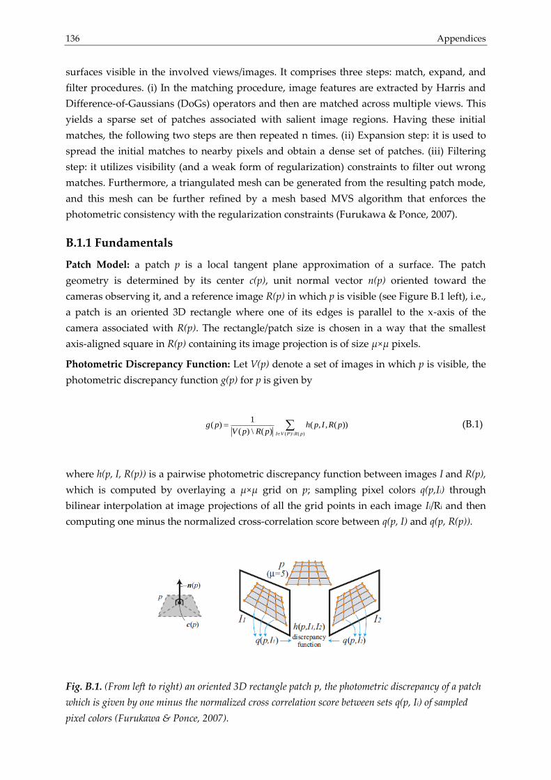
136 Appendices
surfaces visible in the involved views/images. It comprises three steps: match, expand, and
filter procedures. (i) In the matching procedure, image features are extracted by Harris and
Difference-of-Gaussians (DoGs) operators and then are matched across multiple views. This
yields a sparse set of patches associated with salient image regions. Having these initial
matches, the following two steps are then repeated n times. (ii) Expansion step: it is used to
spread the initial matches to nearby pixels and obtain a dense set of patches. (iii) Filtering
step: it utilizes visibility (and a weak form of regularization) constraints to filter out wrong
matches. Furthermore, a triangulated mesh can be generated from the resulting patch mode,
and this mesh can be further refined by a mesh based MVS algorithm that enforces the
photometric consistency with the regularization constraints (Furukawa & Ponce, 2007).
B.1.1 Fundamentals
Patch Model: a patch p is a local tangent plane approximation of a surface. The patch
geometry is determined by its center c(p), unit normal vector n(p) oriented toward the
cameras observing it, and a reference image R(p) in which p is visible (see Figure B.1 left), i.e.,
a patch is an oriented 3D rectangle where one of its edges is parallel to the x-axis of the
camera associated with R(p). The rectangle/patch size is chosen in a way that the smallest
axis-aligned square in R(p) containing its image projection is of size μ×μ pixels.
Photometric Discrepancy Function: Let V(p) denote a set of images in which p is visible, the
photometric discrepancy function g(p) for p is given by
( )\ ( )
1( ) ( , , ( ))
( ) \ ( ) I V P R p
g p h p I R pV p R p
(B.1)
where h(p, I, R(p)) is a pairwise photometric discrepancy function between images I and R(p),
which is computed by overlaying a μ×μ grid on p; sampling pixel colors q(p,Ii) through
bilinear interpolation at image projections of all the grid points in each image Ii/Ri and then
computing one minus the normalized cross-correlation score between q(p, I) and q(p, R(p)).
Fig. B.1. (From left to right) an oriented 3D rectangle patch p, the photometric discrepancy of a patch
which is given by one minus the normalized cross correlation score between sets q(p, Ii) of sampled
pixel colors (Furukawa & Ponce, 2007).

B: Dense Image Matching Methods 137
It is assumed that the surface of a scene is lambertian therefore, to discard non-lambertian
only images whose pairwise photometric discrepancy score with the reference image R(p) is
below a certain threshold α are used. Therefore, V(p) in equation B.1 is replaced by
*( ) \ ( ), ( , , ( ))V p I I V p h p I R p and thus g(p) is replaced by g*(p).
Patch Optimization: the aim is to recover patches whose discrepancy scores are small. Each
patch p is reconstructed separately in two steps: initialization of the patch parameters (c(p),
n(p), V∗(p), R(p)) and optimization of its geometric component, c(p) and n(p) using constrains
and parameterization methods respectively, see (Furukawa & Ponce, 2007).
Image Model: due to the lack of connectivity information, it is an uneasy task to search or
access neighboring patches, enforce regularization, etc. Therefore, the image projections of
reconstructed patches in their visible images are tracked.
B.1.2 Patch Reconstruction
Each image can be associated with a regular grid of pixel cells therefore; the PMVS algorithm
aims to reconstruct at least one patch in every image cell. The algorithm is divided into the
following steps:
1. Initial feature matching: the aim is to generate a sparse set of patches across all views.
This step comprises feature detection and matching processes. At first, blob and corner
features are detected in each image using the DoG and Harris operators. In the matching
process, for each image Ii, O(Ii) denotes the optical center of the corresponding camera.
For each feature f detected in Ii, the set F of features f ` of the same type in the other
images that lie within two pixels from the corresponding epipolar lines are collected and
then triangulated to get the 3D points associated with the pairs (f , f `). Then, these points
are considered in order of increasing distance from O(Ii) as potential patch centers, and
attempt to generate a patch from the points one by one until it is succeed; more details
are reported in (Furukawa & Ponce, 2007).
2. Expansion: it attempts to make patches dense, i.e., to reconstruct at least one patch in
every image cell, and to repeat taking existing patches and generating new ones in
nearby empty spaces. This covers, at first, identification of a set of neighboring image
cells that satisfy certain criteria, then performing a patch expansion procedure for each
one of these cells, see (Furukawa & Ponce, 2007).
3. Filtering: this process is iterated n times remove incorrect matches. Three filters are used
for this step. The first filter exploits visibility consistency (neighbor information). The
second filter enforces more strictly the visibility consistency using the depth map test.
Finally, in the third filter, a weak form of regularization (adjacency information) is
enforced.
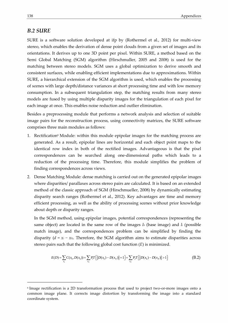
138 Appendices
B.2 SURE
SURE is a software solution developed at ifp by (Rothermel et al., 2012) for multi-view
stereo, which enables the derivation of dense point clouds from a given set of images and its
orientations. It derives up to one 3D point per pixel. Within SURE, a method based on the
Semi Global Matching (SGM) algorithm (Hirschmuller, 2005 and 2008) is used for the
matching between stereo models. SGM uses a global optimization to derive smooth and
consistent surfaces, while enabling efficient implementations due to approximations. Within
SURE, a hierarchical extension of the SGM algorithm is used, which enables the processing
of scenes with large depth/distance variances at short processing time and with low memory
consumption. In a subsequent triangulation step, the matching results from many stereo
models are fused by using multiple disparity images for the triangulation of each pixel for
each image at once. This enables noise reduction and outlier elimination.
Besides a preprocessing module that performs a network analysis and selection of suitable
image pairs for the reconstruction process, using connectivity matrices, the SURE software
comprises three main modules as follows:
1. Rectification6 Module: within this module epipolar images for the matching process are
generated. As a result, epipolar lines are horizontal and each object point maps to the
identical row index in both of the rectified images. Advantageous is that the pixel
correspondences can be searched along one-dimensional paths which leads to a
reduction of the processing time. Therefore, this module simplifies the problem of
finding correspondences across views.
2. Dense Matching Module: dense matching is carried out on the generated epipolar images
where disparities/ parallaxes across stereo pairs are calculated. It is based on an extended
method of the classic approach of SGM (Hirschmueller, 2008) by dynamically estimating
disparity search ranges (Rothermel et al., 2012). Key advantages are time and memory
efficient processing, as well as the ability of processing scenes without prior knowledge
about depth or disparity ranges.
In the SGM method, using epipolar images, potential correspondences (representing the
same object) are located in the same row of the images Ib (base image) and Ii (possible
match image), and the correspondences problem can be simplified by finding the
disparity (d = xi − xb). Therefore, the SGM algorithm aims to estimate disparities across
stereo pairs such that the following global cost function (E) is minimized.
1 2( ) ( , ( )) ( ) ( ) 1 ( ) ( ) 1b N N
b b b N b N
x x x
E D C x D x PT D x D x PT D x D x (B.2)
6 Image rectification is a 2D transformation process that used to project two-or-more images onto a
common image plane. It corrects image distortion by transforming the image into a standard
coordinate system.
C: The Random Sampling and Consensus (RANSAC) Algorithm 139
D is the disparity image that holding disparity estimations of all base image pixels bx . T
is an operator that amounts to one if the subsequent condition is true and amounts to
zero else. Nx represents base image pixels in the neighborhood of
bx . N is a certain
number of approximate (match) images with the base image (Ib). The first term in
equation B.2 represents a data term while, the subsequent two terms refer to surface
smoothness. The data term is computed by pixel-wise similarity measures ( , )b iC x x . The
penalty parameters P1 and P2 control the gain of surface smoothing. More details are
reported in (Hirschmueller, 2008).
3. Structure Computation Module: within this module redundancy is exploited to eliminate
blunders and increase the accuracy of depth measurements. Thereby only depth maps of
stereo models sharing the same base image, Ib, Ii, i=1,...,n are fused. The result is a depth
image (or point cloud) with respect to the base image. For example, the depth (Z) for a
stereo pair of epipolar images can be extracted using the well-known formula (Z=Bf/d)
(so-called normal-case of stereo imagery). B, f, d are the baseline, the focal length and the
disparity respectively. More details about the general cases such as varying focal length
in x and y directions and the present of sheering, as well as the case of multiple stereo
pairs can be found in (Rothermel et al., 2012).
The SURE determines the 3D object coordinates by minimizing the object space error
from multiple redundant depths by averaging the estimated depths. Therefore, accuracy
along the optical ray can be estimated using standard deviations. An approach that
minimizes the reprojection error in the rectified match images is also implemented. This
allows the use of a priori knowledge of matching accuracies in dependence of ray
intersection angles in order to discard outliers. Furthermore, weighted adjustment could
be used within the minimization of the reprojection error (Rothermel et al., 2012).
C: The Random Sampling and Consensus (RANSAC)
Algorithm
The RANdom SAmple Consensus (RANSAC) algorithm, proposed by (Fischler & Bolles,
1981), is a general parameter estimation approach for dealing with a large amount of outliers
in an input data. It was developed within the computer vision community unlike, common
robust estimation techniques such as M-estimators and least-median squares have been
adopted by the computer vision community from the statistics literature. RANSAC is a
resampling technique that generates candidate solutions by using the minimum number of
observations required to estimate the underlying model parameters. According to (Fischler
& Bolles, 1981), contrarily to the conventional sampling techniques which utilize as much of
the input data as possible in order to obtain an initial solution and then proceed to filter out
140 Appendices
outliers, the RANSAC uses the smallest set possible and proceeds to enlarge this set with
consistent observations. In general, the input to the RANSAC algorithm is a set of observed
data values, a parameterized model which can explain or be fitted to the observations, and
some confidence parameters.
The basic algorithm is summarized as follows:
1. Select randomly a minimum subset of the original data required to determine the model
parameters.
2. Estimate the parameters of the model using the selected subset.
3. Determine how many observations/points from the set of the data fit to the solved model,
with a predefined tolerance.
4. If the fraction of the number of inliers over the total number points in the set exceeds a
predefined threshold, re-estimate the model parameters using all the identified inliers
and terminate.
5. Otherwise, repeat steps 1 through 4, with a maximum number of iterations/tries (N).
N is defined high enough to ensure that the probability/confidence p (usually set to 0.99)
that at least one of the sets of random samples does not include an outlier. If u represents the
probability that any selected data point is an inlier, the probability of observing an outlier
will be 1v u . The confidence, that at least one minimal selection with m minimum
elements out of N data sets contains no outlier is given by
1 1 1 1 (1 )N N
m mp u v (C.1)
and thus with some manipulation, the minimal number of the tries is
log(1 )
log 1 (1 )m
pN
v
(C.2)
For more details on the basic RANSAC formulation, the readers are referred to (Fischler &
Bolles, 1981; Hartley & Zisserman, 2003). Moreover, extensions of RANSAC that include the
use of a Maximum Likelihood framework and importance sampling are reported in (Torr &
Zisserman, 2000) and (Torr & Davidson, 2003) respectively.
D: 3D Transformation
D.1 Helmert (seven-parameter) Transformation
The Helmert (seven-parameter) transformation is frequently used in geodesy- the science of
the measurement and the mapping of the earth’s surface. It produces distortion-free
transformations from one datum to another, and involves rotation, scaling and translation. It
D: 3D Transformation 141
is named after Prof. Dr. Friedrich Robert Helmert, 1843-1917. He was a German geodesist, an
important writer on the theory of errors and was considered as the founder of the
mathematical and physical theories of modern geodesy.
The seven-parameter transformation applies to point sets , ,i ip q 1,..., ,i m in 3R therefore, we
can write the following formula:
( ) ; ( ) 1( ), 2( ), 3( )i ip dR q t R R R R (D.1)
with ( , , ) represent the three rotation angles vector, and where
1 0 0 cos 0 sin cos sin 0
1( ) 0 cos sin ; 2( ) 0 1 0 ; 3( ) sin cos 0
0 sin cos sin 0 cos 0 0 1
R R R
i.e., ( )R is an orthogonal matrix 1( ( ) ( ) )TR R that results by a product of three
elementary rotation matrices in the three coordinate planes. The remaining parameters are a
scaling parameter d (unitless scale factor) and a translation vector t (the three translations
along the coordinate axes) so that the seven parameters are 3R , 3t R , d R (Watson,
2006). Thus, at least two points and one coordinate of a third point are required to determine
the seven parameters. This gives a system of linear equations with seven equations and
seven unknowns, which thus can be solved. The Helmert transformation is a similarity
transformation (preserve geometrical shapes).
D.2 Rigid-Body (six-parameter) Transformation
In mathematics, a rigid transformation (isometry) of a vector space preserves distances
between every pair of points. In general, rigid transformations of the space 3R include
rotations, translations, reflections, or their combination. In our application, the rigid-body
transformation is referred to a transformation which can be decomposed as 3D rotations
followed by 3D translations (six parameters). This transformation is also known as proper
rigid transformation. In mechanics, proper rigid transformations in a 3D Euclidean space are
used to represent the linear and the angular displacement of rigid bodies.
According to equation D.1, the rigid-body transformation can be defined as
( )i ip R q t (D.2)
where the scale factor is equal to unity. In our applications, a linear transformation
(translation, reflection, orthogonal rotation, and scaling if needed) was determined using the
Procrustes analysis implemented in Matlab, which is a form of statistical shape analysis used
to analyze the distribution of a set of shapes. Quite often more than seven equations are

142 Appendices
available for the transformation calculation therefore, this input information is used in a least
squares parameter estimation.
E: The Point-Based Environment Model (PEM)
(Boehm, 2007) introduced the point-based environment model (PEM) as a representation of
the absolute coordinate frame of a scene where a prior knowledge of the scene is stored. A
PEM is a dense point-wise sampling of the scene surface that can easily be acquired by 3D
active sensors, such as TLS systems and machine vision cameras. Where each sample is
comprised of the location of the surface point (3D coordinates) associated with an intensity
value. The PEM mainly comprises a laser scanner point cloud with associated intensity
values. The rigid geometry of the point cloud plays an important role in providing accurate
control information for camera orientation (Boehm, 2007). Laser scanners usually acquire
point clouds in almost a regular raster by two angles of deflection, horizontally and verti-
cally. Therefore, the recorded intensity values as the intensity of the reflected beam can be
interpreted as an intensity/reflectance image using the scanning matrix.
For a PEM, features are automatically extracted from the corresponding reflectance image.
These extracted landmarks are intensity features and are used for image orientation. But,
some good features which are not visible at the narrow bandwidth of the light source might
be missed. In (Boehm, 2007), image features were extracted using the Harris-Stephens corner
operator (Harris & Stephens, 1988). The PEM and its extracted landmarks were used as a
navigational frame for subsequent image orientation.
In (Moussa et al., 2012a), the PEM is expanded as follows: (i) since TLS systems provide for
each measured point intensity and RGB values, these values are stored in the PEM. (ii) Using
the latter values, intensity and RGB, synthetic images based on a central projection of the
laser scanner point clouds are generated (see chapter 3 section 3.2). Moreover, the PEM
features are extracted using the Affine-SIFT (ASIFT) operator (Morel & Yu, 2009).
F: The Affine-Scale Invariant Feature Transform (Affine-
SIFT/ASIFT)
The Scale invariant Feature Transform (SIFT) proposed by (Lowe, 2004) deals strictly with
the four similarity variances (2 translations, rotation, and scale (zoom)) of image local
features by simulating zooms out and by normalizing translations and rotation. Therefore,
(Morel & Yu, 2009) introduce the Affine-SIFT (ASIFT) feature detection algorithm which
extends the SIFT method to fully affine invariant local image features by covering
additionally the left two shearing parameters. This being the case since the deformations of
physical objects can be well approximated by the six affine parameters on the image plane.

F: The Affine-Scale Invariant Feature Transform (Affine-SIFT/ASIFT) 143
The ASIFT method simulates a set of sample views of the initial images, obtainable by
varying the two camera axis orientation parameters, namely the latitude and the longitude
angles, which are not considered by the SIFT. Then it applies the SIFT method itself to all
images therefore, the ASIFT covers effectively all six parameters of the affine transformation
without any dramatic computational load. The ASIFT method is able to detect reliably
features that have very large affine distortions which are measured by a new geometric
parameter, the transition tilt. Moreover, (Morel & Yu, 2009) report that state-of-the-art
methods hardly exceed transition tilts of 2 for the SIFT (Lowe, 2004), 2.5 for the Harris-
Affine and the Hessian-Affine (Mikolajczyk & Schmid, 2002 and 2004), and 10 for MSER
(Matas et al., 2004) while, ASIFT can handle transition tilts up to 36 and higher. Furthermore,
experiments performed by (Morel & Yu, 2009) showed that in case of scenes with important
camera view angle change, SIFT and other methods fail while ASIFT continues to work. In
the following, basic concepts and a description of the ASIFT method are given.
F.1 Affine Camera Model
As depicted in Figure F.1 left, digital image acquisition of a flat object can be described as
u=S1G1Aτu0 where τ is a plane translation due to the camera motion. The Gaussian kernel
(G1) is assumed to be broad enough to ensure no aliasing by the 1-sampling, therefore with a
Shannon-Whittaker7 interpolation (I), the continuous image from its discrete version is given
by IS1G1Aτu0 = G1Aτu0, where S1 will be omitted.
Fig. F.1. (From left to right) the projective camera model and the affine local approximation illustrated
by one of the first perspectively correct Renaissance paintings by Paolo Uccello, an Italian painter,
1397-1475 (Morel & Yu, 2009).
7 Shannon-Whittaker interpolation is a method to construct a continuous-time band-limited function
from a sequence of real numbers (Whittaker, 1935).
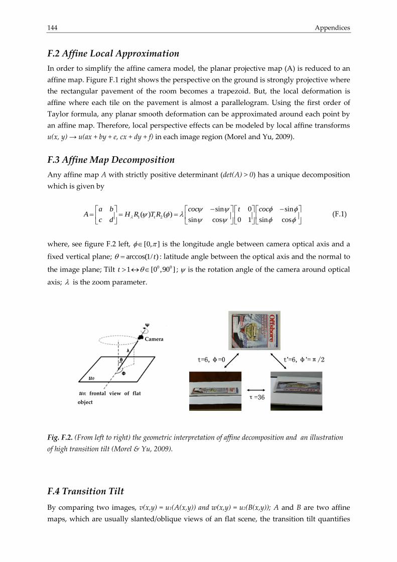
144 Appendices
F.2 Affine Local Approximation
In order to simplify the affine camera model, the planar projective map (A) is reduced to an
affine map. Figure F.1 right shows the perspective on the ground is strongly projective where
the rectangular pavement of the room becomes a trapezoid. But, the local deformation is
affine where each tile on the pavement is almost a parallelogram. Using the first order of
Taylor formula, any planar smooth deformation can be approximated around each point by
an affine map. Therefore, local perspective effects can be modeled by local affine transforms
u(x, y) → u(ax + by + e, cx + dy + f) in each image region (Morel and Yu, 2009).
F.3 Affine Map Decomposition
Any affine map A with strictly positive determinant (det(A) > 0) has a unique decomposition
which is given by
1 2
sin 0 sin( ) ( )
sin cos 0 1 sin cost
a b coc t cocA H R T R
c d
(F.1)
where, see figure F.2 left, [0, ] is the longitude angle between camera optical axis and a
fixed vertical plane; arccos(1/ )t : latitude angle between the optical axis and the normal to
the image plane; Tilt 0 01 [0 ,90 ]t ; is the rotation angle of the camera around optical
axis; is the zoom parameter.
Fig. F.2. (From left to right) the geometric interpretation of affine decomposition and an illustration
of high transition tilt (Morel & Yu, 2009).
F.4 Transition Tilt
By comparing two images, v(x,y) = u1(A(x,y)) and w(x,y) = u2(B(x,y)); A and B are two affine
maps, which are usually slanted/oblique views of an flat scene, the transition tilt quantifies
Camera
u0
u0: frontal view of flat
object
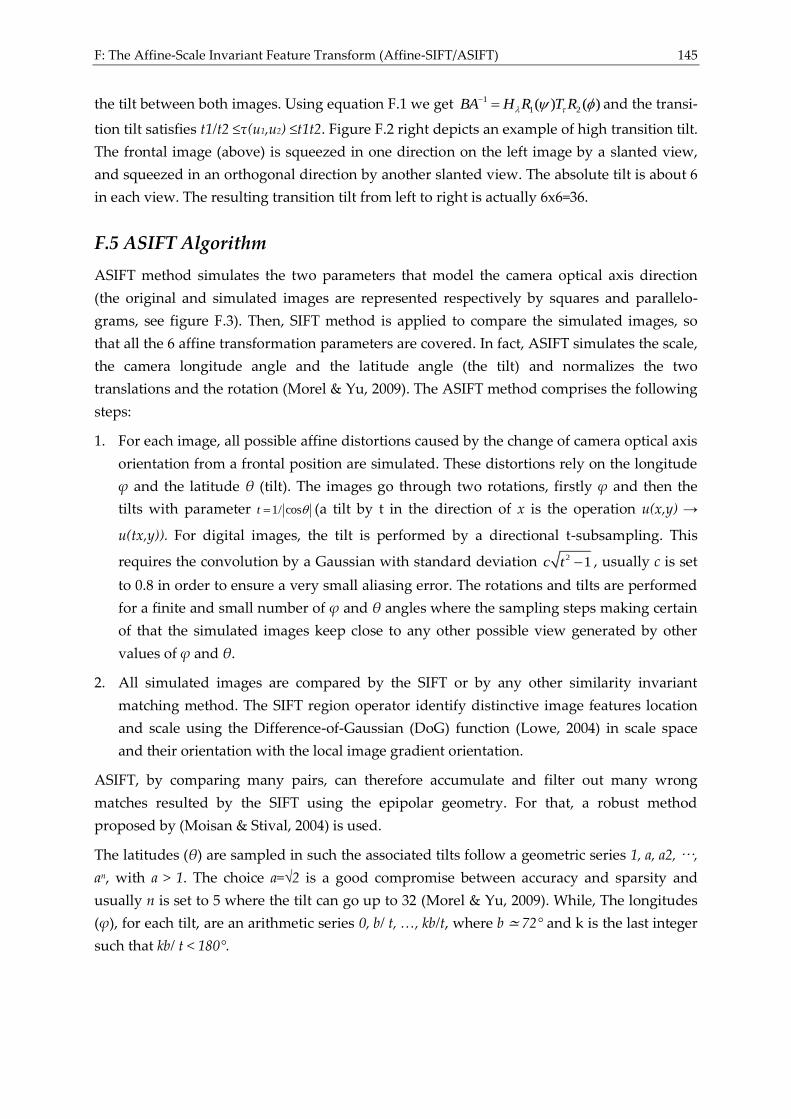
F: The Affine-Scale Invariant Feature Transform (Affine-SIFT/ASIFT) 145
the tilt between both images. Using equation F.1 we get 1
1 2( ) ( )BA H R T R and the transi-
tion tilt satisfies t1/t2 ≤τ(u1,u2) ≤t1t2. Figure F.2 right depicts an example of high transition tilt.
The frontal image (above) is squeezed in one direction on the left image by a slanted view,
and squeezed in an orthogonal direction by another slanted view. The absolute tilt is about 6
in each view. The resulting transition tilt from left to right is actually 6x6=36.
F.5 ASIFT Algorithm
ASIFT method simulates the two parameters that model the camera optical axis direction
(the original and simulated images are represented respectively by squares and parallelo-
grams, see figure F.3). Then, SIFT method is applied to compare the simulated images, so
that all the 6 affine transformation parameters are covered. In fact, ASIFT simulates the scale,
the camera longitude angle and the latitude angle (the tilt) and normalizes the two
translations and the rotation (Morel & Yu, 2009). The ASIFT method comprises the following
steps:
1. For each image, all possible affine distortions caused by the change of camera optical axis
orientation from a frontal position are simulated. These distortions rely on the longitude
ϕ and the latitude θ (tilt). The images go through two rotations, firstly ϕ and then the
tilts with parameter 1/ cost (a tilt by t in the direction of x is the operation u(x,y) →
u(tx,y)). For digital images, the tilt is performed by a directional t-subsampling. This
requires the convolution by a Gaussian with standard deviation 2 1c t , usually c is set
to 0.8 in order to ensure a very small aliasing error. The rotations and tilts are performed
for a finite and small number of ϕ and θ angles where the sampling steps making certain
of that the simulated images keep close to any other possible view generated by other
values of ϕ and θ.
2. All simulated images are compared by the SIFT or by any other similarity invariant
matching method. The SIFT region operator identify distinctive image features location
and scale using the Difference-of-Gaussian (DoG) function (Lowe, 2004) in scale space
and their orientation with the local image gradient orientation.
ASIFT, by comparing many pairs, can therefore accumulate and filter out many wrong
matches resulted by the SIFT using the epipolar geometry. For that, a robust method
proposed by (Moisan & Stival, 2004) is used.
The latitudes (θ) are sampled in such the associated tilts follow a geometric series 1, a, a2, …,
an, with a > 1. The choice a=√2 is a good compromise between accuracy and sparsity and
usually n is set to 5 where the tilt can go up to 32 (Morel & Yu, 2009). While, The longitudes
(ϕ), for each tilt, are an arithmetic series 0, b/ t, …, kb/t, where b ≃ 72° and k is the last integer
such that kb/ t < 180°.
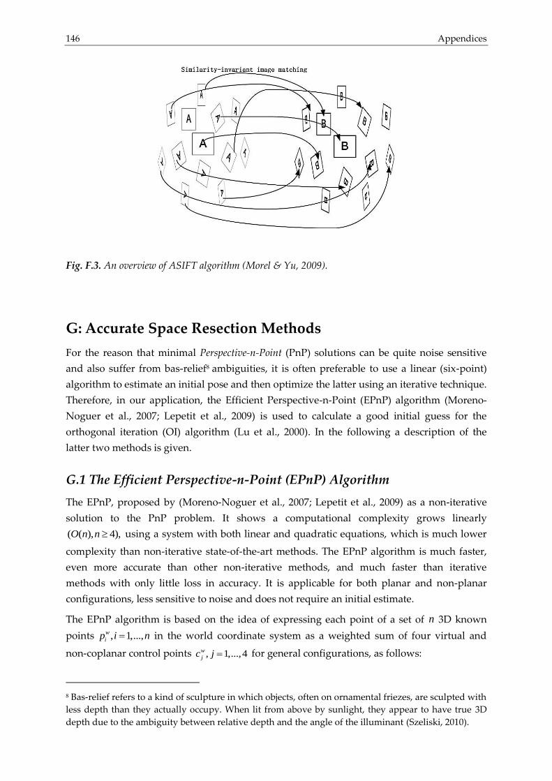
146 Appendices
Fig. F.3. An overview of ASIFT algorithm (Morel & Yu, 2009).
G: Accurate Space Resection Methods
For the reason that minimal Perspective-n-Point (PnP) solutions can be quite noise sensitive
and also suffer from bas-relief8 ambiguities, it is often preferable to use a linear (six-point)
algorithm to estimate an initial pose and then optimize the latter using an iterative technique.
Therefore, in our application, the Efficient Perspective-n-Point (EPnP) algorithm (Moreno-
Noguer et al., 2007; Lepetit et al., 2009) is used to calculate a good initial guess for the
orthogonal iteration (OI) algorithm (Lu et al., 2000). In the following a description of the
latter two methods is given.
G.1 The Efficient Perspective-n-Point (EPnP) Algorithm
The EPnP, proposed by (Moreno-Noguer et al., 2007; Lepetit et al., 2009) as a non-iterative
solution to the PnP problem. It shows a computational complexity grows linearly
( ( ), 4),O n n using a system with both linear and quadratic equations, which is much lower
complexity than non-iterative state-of-the-art methods. The EPnP algorithm is much faster,
even more accurate than other non-iterative methods, and much faster than iterative
methods with only little loss in accuracy. It is applicable for both planar and non-planar
configurations, less sensitive to noise and does not require an initial estimate.
The EPnP algorithm is based on the idea of expressing each point of a set of n 3D known
points , 1,...,w
ip i n in the world coordinate system as a weighted sum of four virtual and
non-coplanar control points , 1,...,4w
jc j for general configurations, as follows:
8 Bas-relief refers to a kind of sculpture in which objects, often on ornamental friezes, are sculpted with
less depth than they actually occupy. When lit from above by sunlight, they appear to have true 3D
depth due to the ambiguity between relative depth and the angle of the illuminant (Szeliski, 2010).
G: Accurate Space Resection Methods 147
4
1
,w w
i ij j
j
p c
with 4
1
1ij
j
(G.1)
where ij are homogeneous barycentric coordinates. As in the world coordinate system,
,w w
i jp c and ij are known, the same relation holds in the camera coordinate system. Hence,
the points c
ip can be expressed via the control points c
jc , which leads to the equation (G.2):
4
1
,1
i c c
i i ij j
j
ui w Kp K c
(G.2)
where iw are scalar projective parameters, K denotes to the camera calibration matrix and iu
represents the 2D projections of the reference 3D points. Expanding equation (G.2) yields the
following:
0 4
0
1
0
, 0
0 0 11
c
i x j
c
i i y ij j
j c
j
x f x X
i w y f y Y
Z
(G.3)
where ( , )x yf f constitute to the focal length coefficients, 0 0( , )x y represents the principal
point coordinates, ( , , )c c c
j j jX Y Z are the coordinates of the control points and ( , )i ix y are the 2D
coordinates of iu . This linear system has 12 unknown parameters from the control points
and, additionally n unknown parameters iw . The last row of equation G.3 implies that
4
1
.w
i ij j
j
w z
By submitting the latter expression in the first two rows and catenating and
arranging the resulting linear equations (two for each reference point) for all n reference
points, a linear system can be generated (equation G.4).
0Mx (G.4)
where 1 2 3 4( , , , )cT cT cT cTx c c c c is a 12-vector made of the unknowns and M is 2 12n matrix.
The solution x then leads to the camera coordinates c
ip of the 3D points. Once the world
coordinates and the camera coordinates of the 3D reference points are known, the rotation
and the translation parameters aligning both coordinate systems can be recovered by means
of standard methods (Arun et al., 1987; Horn et al., 1988; Umeyama, 1991). A further
optimization step using the Gauss–Newton algorithm is presented in (Lepetit et al., 2009).
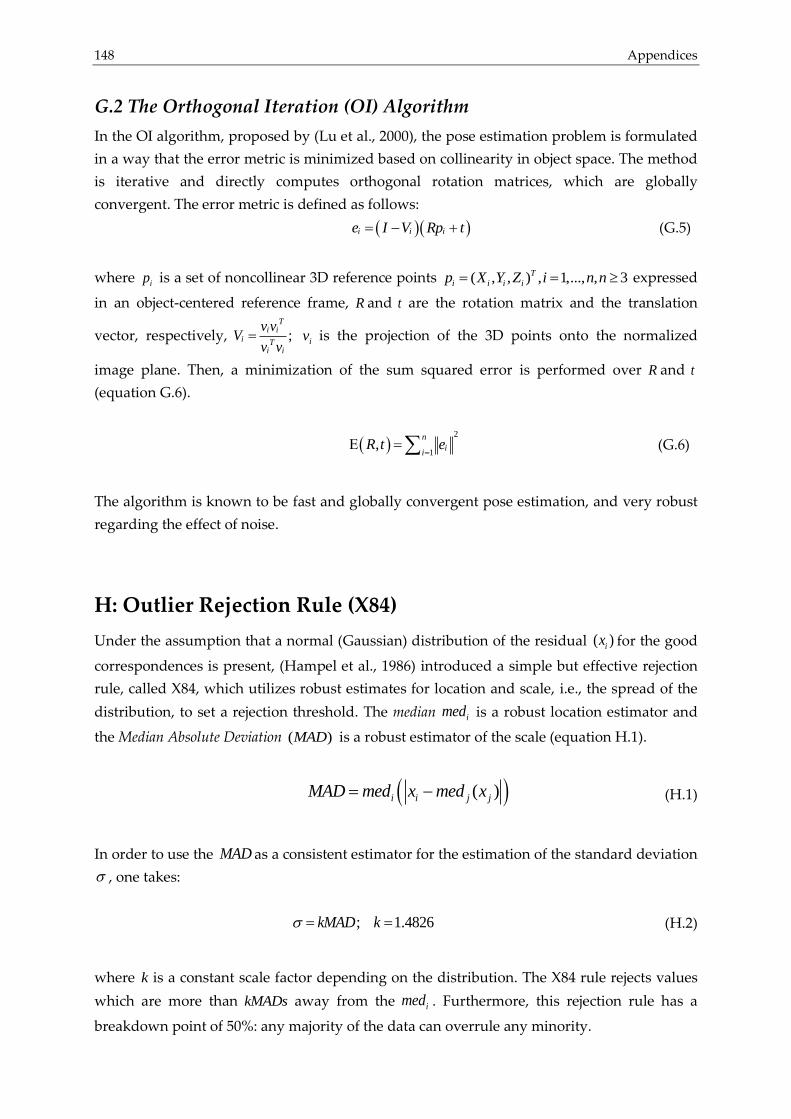
148 Appendices
G.2 The Orthogonal Iteration (OI) Algorithm
In the OI algorithm, proposed by (Lu et al., 2000), the pose estimation problem is formulated
in a way that the error metric is minimized based on collinearity in object space. The method
is iterative and directly computes orthogonal rotation matrices, which are globally
convergent. The error metric is defined as follows:
i i ie I V Rp t (G.5)
where ip is a set of noncollinear 3D reference points ( , , ) , 1,..., , 3T
i i i ip X Y Z i n n expressed
in an object-centered reference frame, R and t are the rotation matrix and the translation
vector, respectively, ;T
i ii T
i i
v vV
v v
iv is the projection of the 3D points onto the normalized
image plane. Then, a minimization of the sum squared error is performed over R and t
(equation G.6).
2
1,
n
ii
R t e
(G.6)
The algorithm is known to be fast and globally convergent pose estimation, and very robust
regarding the effect of noise.
H: Outlier Rejection Rule (X84)
Under the assumption that a normal (Gaussian) distribution of the residual ( )ix for the good
correspondences is present, (Hampel et al., 1986) introduced a simple but effective rejection
rule, called X84, which utilizes robust estimates for location and scale, i.e., the spread of the
distribution, to set a rejection threshold. The median imed is a robust location estimator and
the Median Absolute Deviation ( )MAD is a robust estimator of the scale (equation H.1).
( )i i j jMAD med x med x (H.1)
In order to use the MAD as a consistent estimator for the estimation of the standard deviation
, one takes:
; 1.4826kMAD k (H.2)
where k is a constant scale factor depending on the distribution. The X84 rule rejects values
which are more than kMADs away from the imed . Furthermore, this rejection rule has a
breakdown point of 50%: any majority of the data can overrule any minority.

I: Quaternions 149
I: Quaternions
Quaternions were first described by William Rowan Hamilton, a 19th-century Irish
mathematician, as a number system that extends the complex numbers. A quaternion can be
conveniently thought of as either (i) a vector with four components; or (ii) a scalar plus a
vector with three components; or (iii) a complex number with three different imaginary parts
(Horn, 2001). There is a substantial body of quaternion mathematics that is beyond the scope
of this thesis. Therefore, we report the general definitions required to use the quaternions as
a representation of the orientations and rotations of objects in three dimensional space. Then,
a particular attention is given to the relationship between the quaternions and the spatial
rotations. For more details on the basic formulation of quaternions, see (Kuipers, 1999).
I.1 General Definitions
A quaternion, 4q R , is represented as a vector with 4 components, 3 of which are
imaginary: 0 1 2 3q q q i q j q k .
Multiplication is defined using the rules: 2 2 2 1i j k ijk .
Conjugation of a quaternion can be expressed as *
0 1 2 3q q q i q j q k .
The norm of the quaternion is 2 2 2 2
0 1 2 3q q q q q .
A unit quaternion is a quaternion of norm one: qU q q .
The inverse of a quaternion is 1 *q q q .
A rotation can be represented with composite product by a unit quaternion r :
*( )R q rqr where 1
( )2 cos ( )sin
2 2
x y zu i u j u k
x y zr e u i u j u k
, ( )x y zu u i u j u k is the
unit vector representing the three Cartesian axes. Therefore, the unit quaternion
corresponds to a rotation with the angle around the axis which is defined by the unit
vector u .
I.2 Quaternions and Rotation
Unit quaternions provide a convenient mathematical notation for representing orientations
and rotations of objects in three-dimensional space. Compared to Euler angles they are
simpler to compose, able to avoid the problem of gimbal lock9 and more numerically stable
and might be more efficient than rotation matrices (Perumal, 2011). In our application, due
to the different constellation of the rotation matrices (because of the different combinations
of basic rotations) which are derived from different algorithms (e.g. space resection, the SFM
9 Gimbal lock is a phenomenon in which one of the rotation axes realigns with the other axis and
eventually causes loss of one degree of freedom (Perumal, 2011).
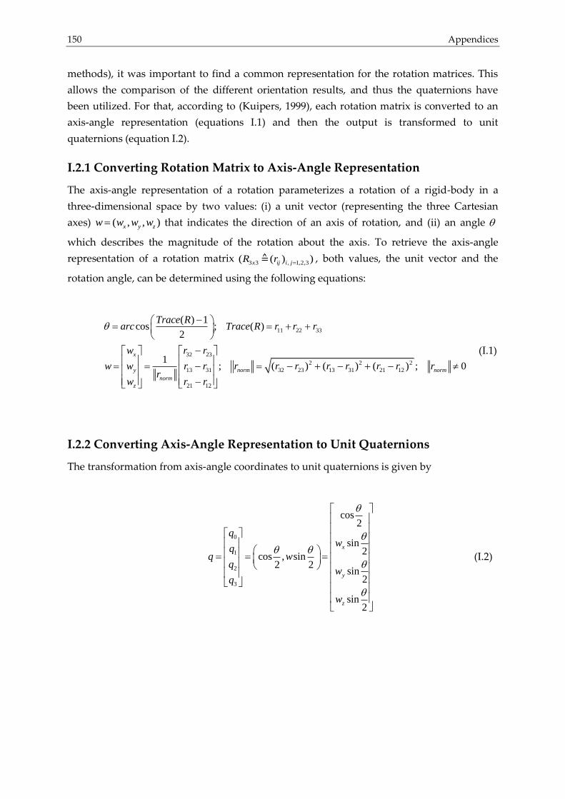
150 Appendices
methods), it was important to find a common representation for the rotation matrices. This
allows the comparison of the different orientation results, and thus the quaternions have
been utilized. For that, according to (Kuipers, 1999), each rotation matrix is converted to an
axis-angle representation (equations I.1) and then the output is transformed to unit
quaternions (equation I.2).
I.2.1 Converting Rotation Matrix to Axis-Angle Representation
The axis-angle representation of a rotation parameterizes a rotation of a rigid-body in a
three-dimensional space by two values: (i) a unit vector (representing the three Cartesian
axes) ( , , )x y zw w w w that indicates the direction of an axis of rotation, and (ii) an angle
which describes the magnitude of the rotation about the axis. To retrieve the axis-angle
representation of a rotation matrix 3 3 , 1,2,3( ( ) )x ij i jR r
, both values, the unit vector and the
rotation angle, can be determined using the following equations:
11 22 33
32 23
2 2 2
13 31 32 23 13 31 21 12
21 12
( ) 1cos ; ( )
2
1; ( ) ( ) ( ) ; 0
x
y norm norm
norm
z
Trace Rarc Trace R r r r
w r r
w w r r r r r r r r r rr
w r r
(I.1)
I.2.2 Converting Axis-Angle Representation to Unit Quaternions
The transformation from axis-angle coordinates to unit quaternions is given by
0
1
2
3
cos2
sin2
cos , sin2 2
sin2
sin2
x
y
z
qw
qq w
qw
q
w
(I.2)

Bibliography 151
Bibliography
Abdelhafiz, A. (2009). Integrating digital
photogrammetry and terrestrial laser scanning.
München: Deutsche Geodätische Kommission,
Reihe C, Nr. 631, ISBN 978-3-7696-5143-3,
117p.
Abdel-Wahab, M., Wenzel, K., and Fritsch, D.
(2012). Automated and Accurate Orientation of
Large Unordered Image Datasets for Close-
Range Cultural Heritage Data Recording.
Photogramm.-Fernerkund.-Geoinformation
2012(6), pp. 679–689.
Ackermann, F. (1999). Airborne laser
scanning—present status and future expecta-
tions. ISPRS J. Photogramm. Remote Sens. 54,
pp. 64–67.
Alba, M., Barazzetti, L., Scaioni, M., and
Remondino, F. (2011). Automatic registration
of multiple laser scans using panoramic rgb
and intensity images. In International Archives
of the Photogrammetry, Remote Sensing and
Spatial Information Sciences, (Calgary,
Canada), pp. 49–54.
Alshawabkeh, Y. (2006). Integration of Laser
Scanning and Photogrammetry for Heritage
Documentation. Stuttgart University, 98p.
Alshawabkeh, Y., and Haala, N. (2004). Inte-
gration of digital photogrammetry and laser
scanning for heritage documentation. Int.
Arch. Photogramm. Remote Sens. Spat. Inf. Sci.
35, pp. 424–429.
Alshawabkeh, Y., and Haala, N. (2005). Auto-
matic multi-image photo texturing of complex
3D scenes. (Torino, Italy), pp. 68–73.
Arun, K.S., Huang, T.S., and Blostein, S.D.
(1987). Least-squares fitting of two 3-D point
sets. Pattern Anal. Mach. Intell. IEEE Trans.
On, pp. 698–700.
Arya, S., Mount, D.M., Netanyahu, N.S.,
Silverman, R., and Wu, A.Y. (1998). An optimal
algorithm for approximate nearest neighbor
searching fixed dimensions. J. ACM JACM 45,
pp. 891–923.
Bae, K.-H., and Lichti, D.D. (2004). Automated
Registration Of Unorganised Point Clouds
From Terrestrial Laser Scanners. In Proceed-
ings of the ISPRS Working Group V/2, pp. 222–
227.
Bae, K.-H., and Lichti, D.D. (2008). A method
for automated registration of unorganised
point clouds. ISPRS J. Photogramm. Remote
Sens. 63, pp. 36–54.
Bannai, N., Fisher, R.B., and Agathos, A.
(2007). Multiple color texture map fusion for
3D models. Pattern Recognit. Lett. 28, pp. 748–
758.
Barazzetti, L., Scaioni, M., and Remondino, F.
(2010). Orientation and 3D modelling from
markerless terrestrial images: combining
accuracy with automation. Photogramm. Rec.
25, pp. 356–381.
Barazzetti, L., Remondino, F., and Scaioni, M.
(2011). Automated and accurate orientation of
complex image sequences. International
Archives of the Photogrammetry, Remote
Sensing and Spatial Information Sciences,
Volume XXXVIII-5/W16, ISPRS Trento 2011
Workshop, Trento, Italy, pp. 277-284.
Barnea, S., and Filin, S. (2007). Registration of
terrestrial laser scans via image based features.
Int. Arch. Photogramm. Remote Sens. Spat. Inf.
Sci. 36, pp. 32–37.
Barnea, S., and Filin, S. (2008). Keypoint based
autonomous registration of terrestrial laser
point-clouds. ISPRS J. Photogramm. Remote
Sens. 63, pp. 19–35.
Barnea, S., and Filin, S. (2010). Geometry-
image-intensity combined features for registra-
tion of terrestrial laser scans. Photo- gramm.
Comput. Vis. ISPRS Comm. III 2, pp. 145–150.
Bay, H., Ess, A., Tuytelaars, T., and Van Gool,
L. (2008). Speeded-up robust features (SURF).
Comput. Vis. Image Underst. 110, pp. 346–359.
Becker, S., and Haala, N. (2007). Combined
Feature Extraction for Facade Reconstruction.
In ISPRS Workshop on Laser Scanning 2007
152 Bibliography
and SilviLaser 2007, IAPRS, (Espoo, Finland),
pp. 44–49.
Beis, J.S., and Lowe, D.G. (1997). Shape
indexing using approximate nearest-neighbour
search in high-dimensional spaces. In
Computer Vision and Pattern Recognition,
1997. Proceedings., 1997 IEEE Computer
Society Conference on, pp. 1000–1006.
Bendels, G.H., Degener, P., Wahl, R., Körtgen,
M., and Klein, R. (2004). Image-based
registration of 3d-range data using feature
surface elements. In Proceedings of the 5th
International Conference on Virtual Reality,
Archaeology and Intelligent Cultural Heritage,
pp. 115–124.
Beraldin, J.-A., Blais, F., Cournoyer, L., Godin,
G., Rioux, M., and Taylor, J. (2003). Active 3D
sensing. In The E-Way into the Four
Dimensions of Cultural Heritage Congress,
(Vienna, Austria.), 4p.
Beraldin, J.-A., Picard, M., El-Hakim, S., Godin,
G., Borgeat, L., Blais, F., Paquet, E., Rioux, M.,
Valzano, V., and Bandiera, A. (2005). Virtual
reconstruction of heritage sites: opportunities
and challenges created by 3D technologies. In
The International Workshop on Recording,
Modeling and Visualization of Cultural
Heritage, (Ascona, Switzerland.), 15p.
Besl, P.J., and McKay, N.D. (1992). Method for
registration of 3-D shapes. In Robotics-DL
Tentative, pp. 586–606.
Boehm, J. (2004). Multi-image fusion for
occlusion-free fa\ccade texturing. Int. Arch.
Photogramm. Remote Sens. Spat. Inf. Sci. 35,
pp. 867–872.
Boehm, J. (2007). Orientation of image
sequences in a point-based environment
model. In 3-D Digital Imaging and Modeling,
2007. 3DIM’07. Sixth International Conference
on, pp. 233–240.
Boehm, J., and Becker, S. (2007). Automatic
Marker-Free Registration of Terrestrial Laser
Scans using Reflectance Features. In In:
Proceedings of 8th Conference on Optical 3D
Measurment Techniques, (Zurich, Switzer-
land), pp. 338–344.
Bornaz, L., and Dequal, S. (2003). The solid
image: A new concept and its applications. Int.
Arch. Photogramm. REMOTE Sens. Spat. Inf.
Sci. 34, pp. 78–82.
Brenner, C. (2005). Building reconstruction
from images and laser scanning. Int. J. Appl.
Earth Obs. Geoinformation 6, pp. 187–198.
Brenner, C., Dold, C., and Ripperda, N. (2008).
Coarse orientation of terrestrial laser scans in
urban environments. ISPRS J. Photogramm.
Remote Sens. 63, pp. 4–18.
Brown, D.C. (1976). The bundle adjustment—
progress and prospects. Int. Arch. of Photo-
gramm. 21(3), pp. 1–33.
Brown, M.Z., Burschka, D., and Hager, G.D.
(2003). Advances in computational stereo.
Pattern Anal. Mach. Intell. IEEE Trans. On 25,
pp. 993–1008.
Canny, J. (1986). A computational approach to
edge detection. Pattern Anal. Mach. Intell.
IEEE Trans. On, pp. 679–698.
Chen, L.C., Teo, T.-A., Shao, Y.-C., Lai, Y.-C.,
and Rau, J.-Y. (2004). Fusion of LIDAR data
and optical imagery for building modeling. Int.
Arch. Photogramm. Remote Sens. 35, pp. 732–
737.
Chen, Z., Zhou, J., Chen, Y., and Wang, G.
(2012). 3D Texture Mapping in Multi-view
Reconstruction. In Advances in Visual
Computing, (Springer), pp. 359–371.
Clarke, T.A., Wang, X., and Fryer, J.G. (1998).
The principal point and CCD cameras. Photo-
gramm. Rec. 16, pp. 293–312.
Corsini, M., Dellepiane, M., Ganovelli, F.,
Gherardi, R., Fusiello, A., and Scopigno, R.
(2013). Fully automatic registration of image
sets on approximate geometry. Int. J. Comput.
Vis. pp. 1–21.
D’Apuzzo, N. (2003). Surface Measurement
and Tracking of Human Body Parts from Multi
Station Video Sequences, Zurich, Switzerland:
Institut für Geodäsie und Photogrammetrie,
Diss. ETH No. 15271, ISBN 3-906467-44-9,
149p.
Debevec, P.E., and Malik, J. (2008). Recovering
high dynamic range radiance maps from
photographs. In ACM SIGGRAPH 2008
Classes, 10p.
Bibliography 153
Dobrowolska, A., and Dobrowolski, J. (2006).
Heliopolis: Rebirth of the City of the Sun.
American Univ. in Cairo Press, ISBN
9774160088, p.15.
Dold, C. (2005). Extended Gaussian images for
the registration of terrestrial scan data. ISPRS
WG III3 III4 3, pp. 12–14.
Dold, C., and Brenner, C. (2004). Automatic
matching of terrestrial scan data as a basis for
the generation of detailed 3D city models. Int.
Arch. Photogramm. Remote Sens. Spat. Inf. Sci.
35, pp. 1091–1096.
Dold, C., and Brenner, C. (2006). Registration
of terrestrial laser scanning data using planar
patches and image data. IAPRS XXXVI 5, pp.
78–83.
Dorninger, P., and Nothegger, C. (2009).
Automated Processing of Terrestrial Mid-
Range Laser Scanner Data for Restoration
Documentation at Millimeter Scale. In
Proceedings of the 14th International Congress
“Cultural Heritage and New Technologies, pp.
602–609.
El-Hakim, S. (2002). Semi-automatic 3D
reconstruction of occluded and unmarked
surfaces from widely separated views. In
International Archives of the Photogrammetry,
Remote Sensing and Spatial Information
Sciences, pp. 143–148.
El-Hakim, S.F., and Beraldin, J.-A. (1994). On
the integration of range and intensity data to
improve vision-based threedimensional
measurements. Videometrics III, pp. 306–321.
El-Hakim, S., Beraldin, J.-A., and Blais, F.
(2003a). Critical factors and configurations for
practical 3D image-based modeling. In VI
Conference on Optical 3D Measurement Tech-
niques, (Zurich, Switzerland: (Eds. A.Grün and
H.Kahmen)), pp. 159–167.
El-Hakim, S., Gonzo, L., Picard, M., Girardi, S.,
and Simoni, A. (2003b). Visualization of
Frescoed Surfaces: Buonconsiglio Castle-
Aquila Tower, “Cycle Of The Months.”In
Proceeding of International Workshop on
Visualisation and Animation of Reality-Based
3D Models, Tarasp-Vulpera, Switzerland, pp.
1–6.
El-Hakim, S., Remondino, F., and Voltolini, F.
(2008). Integrating Techniques for Detail and
Photo-Realistic 3D Modelling of Castles. GIM
Int. 22, pp. 21–25.
El-Hakim, S.F., Gonzo, L., Picard, M., Girardi,
S., Simoni, A., Paquet, E., Viktor, H., and
Brenner, C. (2003c). Visualisation of highly
textured surfaces. In Proceedings of the 4th
International Conference on Virtual Reality,
Archaeology and Intelligent Cultural Heritage,
pp. 203–212.
Elstrom, M.D., Smith, P.W., and Abidi, M.A.
(1998). Stereo-based registration of ladar and
color imagery. In Photonics East (ISAM,
VVDC, IEMB), pp. 343–354.
Faro Technologies Inc. (2011). Faro Scene
Manual, version 4.8, E875, p.117.
Farenzena, M., Fusiello, A., and Gherardi, R.
(2009). Structure-and-motion pipeline on a
hierarchical cluster tree. In Computer Vision
Workshops (ICCV Workshops), 2009 IEEE 12th
International Conference on, pp. 1489–1496.
Fischler, M.A., and Bolles, R.C. (1981). Random
sample consensus: a paradigm for model
fitting with applications to image analysis and
automated cartography. Commun. ACM 24,
pp. 381–395.
Fitzgibbon, A.W., and Zisserman, A. (1998).
Automatic camera recovery for closed or open
image sequences. In Computer Vision—
ECCV’98, (Springer), pp. 311–326.
Forkuo, E.K., and King, B. (2004). Automatic
fusion of photogrammetric imagery and laser
scanner point clouds. Int. Arch. Photogramm.
Remote Sens. 35, pp. 921–926.
Fraser, C.S. (1996). Network design. Close
Range Photogramm. Mach. Vis., pp. 256–281.
Fritsch, D. (2003). 3D Building Visualisation–
Outdoor and Indoor Applications. In Photo-
grammetric Week ’3, Ed. D. Fritsch, (Wich-
mann Verlag, Heidelberg), pp. 281–290.
Fritsch, D., and Kada, M. (2004). Visualisation
using game engines. In Proceedings of the
XXth Congress of the ISPRS, (Istanbul), 5p.
Fritsch, D., Khosravani, A.M., Cefalu, A., and
Wenzel, K. (2011). Multi-Sensors and Multiray
Reconstruction for Digital Preservation. In
154 Bibliography
Photogrammetric Week ’11, Ed. D. Fritsch,
(Wichmann, Berlin/Offenbach), pp. 305–323.
Furukawa, Y., and Ponce, J. (2007).
Accurate,Dense,andRobustMulti-
ViewStereopsis. In Computer Vision and
Pattern Recognition, 2007. CVPR ’07. IEEE
Conference on, 8p.
Furukawa, Y., and Ponce, J. (2010). Accurate,
dense, and robust multiview stereopsis.
Pattern Anal. Mach. Intell. IEEE Trans. On 32,
pp. 1362–1376.
Van Genechten, B. (2008). In Theory and
Practice on Terrestrial Laser Scanning:
Training Material Based on Practical Applica-
tions, (Universidad Politecnica de Valencia
Editorial), p. 19,24.
Gherardi, R., Farenzena, M., and Fusiello, A.
(2010). Improving the efficiency of hierarchical
structure-and-motion. In Computer Vision and
Pattern Recognition (CVPR), 2010 IEEE Con-
ference on, pp. 1594–1600.
Gibson, S., Cook, J., Howard, T., Hubbold, R.,
and Oram, D. (2002). Accurate camera
calibration for off-line, video-based augmented
reality. In Proceedings of the 1st International
Symposium on Mixed and Augmented Reality,
p. 37.
González-Aguilera, D., Rodríguez-Gonzálvez,
P., and Gómez-Lahoz, J. (2009). An automatic
procedure for co-registration of terrestrial laser
scanners and digital cameras. ISPRS J. Photo-
gramm. Remote Sens. 64, pp. 308–316.
Gordon, S.J., and Lichti, D.D. (2004). Terrestrial
laser scanners with a narrow field of view: the
effect on 3D resection solutions. Surv. Rev. 37,
pp. 448–468.
Gressin, A., Mallet, C., Demantké, J., and
David, N. (2013). Towards 3D lidar point cloud
registration improvement using optimal
neighborhood knowledge. ISPRS J. Photo-
gramm. Remote Sens. 79, pp. 240–251.
Gruen, A. (1985a). Adaptive least squares
correlation: a powerful image matching tech-
nique. South Afr. J. Photogramm. Remote Sens.
Cartogr. 14, pp. 175–187.
Gruen, A. (1985b). Data processing methods
for amateur photographs. Photogramm. Rec.
11, pp. 567–579.
Gruen, A., and Akca, D. (2005). Least squares
3D surface and curve matching. ISPRS J.
Photogramm. Remote Sens. 59, pp. 151–174.
Gruen, A., and Baltsavias, E.P. (1988). Geo-
metrically constrained multiphoto matching.
Photogramm. Eng. Remote Sens. 54, pp. 633–
641.
Gruen, A., and Beyer, H.A. (2001). System
calibration through self-calibration. In Calibra-
tion and Orientation of Cameras in Computer
Vision, (Springer Heidelberg), pp. 163–193.
Gruen, A., and Huang, T.S. (2001). In Calibra-
tion and Orientation of Cameras in Computer
Vision, (Springer, Berlin/Heidel- berg), pp. 7–
62.
Gruen, A., Remondino, F., and Zhang, L.
(2004). Photogrammetric reconstruction of the
great Buddha of Bamiyan, Afghanistan. Photo-
gramm. Rec. 19, pp. 177–199.
Grussenmeyer, P., Cazalet, B., Burens, A., and
Carozza, L. (2010). Close range terrestrial laser
scanning and photogrammetry for the 3D
documentation of the Bronze age cave «les
Fraux» Périgord, France. In Mining in
European History, Special Conference of the
SFB HiMAT, pp. 411–421.
Grussenmeyer, P., Alby, E., Landes, T., Koehl,
M., Guillemin, S., Hullo, J.-F., Assali, P., and
Smigiel, E. (2012). Recording Approach of
Heritage Sites based on Merging Point Clouds
from High Resolution Photogrammetry and
Terrestrial Laser Scanning. In International
Archives of the Photogrammetry, Remote
Sensing and Spatial Information Sciences,
(Melbourne, Australia), pp. 553–558.
Guelch, E. (2009). Advanced matching tech-
niques for high precision surface and terrain
models. In Photogrammetric Week ’9, Ed. D.
Fritsch, (Wichmann Verlag, Heidelberg), pp.
303–315.
Guidi, G., Remondino, F., Russo, M., Menna,
F., and Rizzi, A. (2008). 3D modeling of large
and complex site using multi-sensor integra-
tion and multi-resolution data. In Proceedings
of the 9th International Con- ference on Virtual
Reality, Archaeology and Cultural Heritage,
pp. 85–92.
Bibliography 155
Guo, X., and Cao, X. (2010). Triangle-constraint
for finding more good features. In Pattern
Recognition (ICPR), 2010 20th International
Conference on, pp. 1393–1396.
Hampel, F.R., Ronchetti, E.M., Rousseeuw, P.J.,
and Stahel, W.A. (1986). In Robust Statistics:
The Approach Based on Influence Functions.
1986, (Wiley, New York), pp. 56–70, 104–106.
Von Hansen, W. (2006). Robust automatic
marker-free registration of terrestrial scan
data. In Proceedings of the Photogrammetric
Computer Vision, pp. 105–110.
Haralick, R.M., and Shapiro, L.G. (1993).
Computer and robot vision. Addison-Wesley
Pub. Co., ISBN: 9780201569438, 630p.
Harris, C., and Stephens, M. (1988). A com-
bined corner and edge detector. In Alvey
Vision Conference, pp. 147–151.
Hartley, R., and Zisserman, A. (2003). In
Multiple View Geometry in Computer Vision,
(Cambridge University Press), pp. 153–154.
Hiep, V.H., Keriven, R., Labatut, P., and Pons,
J.-P. (2009). Towards high-resolution large-
scale multi-view stereo. In Computer Vision
and Pattern Recognition, 2009. CVPR 2009.
IEEE Conference on, pp. 1430–1437.
Hirschmueller, H. (2005). Accurate and
efficient stereo processing by semi-global
matching and mutual information. In
Computer Vision and Pattern Recognition,
2005. CVPR 2005. IEEE Computer Society
Conference on, pp. 807–814.
Hirschmueller, H. (2008). Stereo processing by
semiglobal matching and mutual information.
Pattern Anal. Mach. Intell. IEEE Trans. On 30,
pp. 328–341.
Horn, B.K. (2001). Some notes on unit
quaternions and rotation. Lect. Handouts 4p.
Horn, B.K., Hilden, H.M., and Negahdaripour,
S. (1988). Closed form solutions of absolute
orientation using orthonormal matrices. J. Opt.
Soc. A 5, pp. 1127–1135.
Jaccard, P. (1901). In Etude Comparative de La
Distribution Florale Dans Une Portion Des
Alpes et Du Jura, (Impr. Corbaz), pp. 547–579.
Jansa, J., Studnicka, N., Forkert, G., Haring, A.,
and Kager, H. (2004). Terrestrial laserscanning
and photogrammetry–acquisition techniques
complementing one another. In The Inter-
national Archives of the Photogrammetry,
Remote Sensing and Spatial Information
Sciences, 6p.
Kacyra, B. (2009). CyArk 500–3D Documen-
tation of 500 Important Cultural Heritage Sites.
In Photogrammetric Week ’9, Ed. D. Fritsch,
(Wichmann Verlag, Heidelberg), pp. 315–320.
Kang, Z., Zlatanova, S., and Gorte, B. (2007).
Automatic registration of terrestrial scanning
data based on registered imagery. In The XXX
FIG Working Week 2007, (Hong Kong SAR,
China), pp. 1–11.
Kang, Z., Li, J., Zhang, L., Zhao, Q., and
Zlatanova, S. (2009). Automatic registration of
terrestrial laser scanning point clouds using
panoramic reflectance images. Sensors 9, pp.
2621–2646.
Kazhdan, M., Bolitho, M., and Hoppe, H.
(2006). Poisson surface reconstruction. In 4th
Eurographics Symposium on Geometry pro-
cessing,Konrad Polthier, Alla Sheffer (Ed.s),
10p.
Khalifa, I., Moussa, M., and Kamel, M. (2003).
Range image segmentation using local
approximation of scan lines with application to
CAD model acquisition. Mach. Vis. Appl. 13,
pp. 263–274.
Klopschitz, M., Irschara, A., Reitmayr, G., and
Schmalstieg, D. (2010). Robust incremental
structure from motion. In Proc. 3DPVT, pp.1-7.
Koertgen, M. (2006). Robust automatic
registration of range images with reflectance.
Diplomarbeit, Computer Graphics Institute,
University of Bonn, Germany, 104p.
Kruppa, E. (1913). Zur Ermittlung eines
Objektes aus zwei Perspektiven mit innerer
Orientierung. Sitzungsberichte der Mathe-
matisch Naturwissenschaftlichen Kaiserlichen
Akademie der Wissenschaften, Vol. 122, pp.
1939-1948
Kuipers, J.B. (1999). Quaternions and rotation
sequences. Princeton university press,
Princeton, ISBN: 978-0691102986, pp. 45-136
Lepetit, V., and Fua, P. (2006). Keypoint
recognition using randomized trees. Pattern
156 Bibliography
Anal. Mach. Intell. IEEE Trans. On 28, pp.
1465–1479.
Lepetit, V., Moreno-Noguer, F., and Fua, P.
(2009). Epnp: An accurate o (n) solution to the
pnp problem. Int. J. Comput. Vis. 81, pp. 155–
166.
Lichti, D.D. (2010). Terrestrial laser scanner
self-calibration: correlation sources and their
mitigation. ISPRS J. Photogramm. Remote
Sens. 65, pp. 93–102.
Lichti, D.D., Gordon, S.J., and Stewart, M.P.
(2002). Ground-based laser scanners: opera-
tion, systems and applications. Geomatica
56,pp. 21–33.
Liu, L., Yu, G., Wolberg, G., and Zokai, S.
(2006). Multiview geometry for texture
mapping 2d images onto 3d range data. In
Computer Vision and Pattern Recognition,
2006 IEEE Computer Society Conference on,
pp. 2293–2300.
Lowe, D.G. (2004). Distinctive image features
from scale-invariant keypoints. Int. J. Comput.
Vis. 60, pp. 91–110.
Lu, C.-P., Hager, G.D., and Mjolsness, E.
(2000). Fast and globally convergent pose
estimation from video images. Pattern Anal.
Mach. Intell. IEEE Trans. On 22, pp. 610–622.
Luhmann, T., Robson, S., Kyle, S., and Hartley,
I. (2007). In Close Range Photogrammetry:
Principles, Techniques and Applications,
(Whittles, Dunbeath, UK), pp. 266–292, 449.
Al-Manasir, K., and Fraser, C.S. (2006).
Registration of terrestrial laser scanner data
using imagery. Photogramm. Rec. 21,pp. 255–
268.
Manferdini, A.M., and Remondino, F. (2012). A
review of reality-based 3D model generation,
segmentation and web-based visualization
methods. Int. J. Herit. Digit. Era 1, pp. 103–124.
Matas, J., Chum, O., Urban, M., and Pajdla, T.
(2004). Robust wide-baseline stereo from
maximally stable extremal regions. Image Vis.
Comput. 22, pp. 761–767.
Meierhold, N., Spehr, M., Schilling, A.,
Gumhold, S., and Maas, H.-G. (2010). Auto-
matic feature matching between digital images
and 2D representations of a 3D laser scanner
point cloud. In International Archives of
Photogrammetry, Remote Sensing and Spatial
Information Sciences, (Newcastle upon Tyne,
UK), pp. 446–451.
Menna, F., Rizzi, A., Nocerino, A., Remondino,
F., and Gruen, A. (2012). High Resolution 3D
Modeling of The Behaim Globe. In Inter-
national Archives of the Photogrammetry,
Remote Sensing and Spatial Information
Sciences, (Melbourne, Australia), pp. 115–120.
Mikolajczyk, K., and Schmid, C. (2002). An
affine invariant interest point detector. In
Computer Vision—ECCV 2002, (Springer), pp.
128–142.
Mikolajczyk, K., and Schmid, C. (2004). Scale &
affine invariant interest point detectors. Int. J.
Comput. Vis. 60, pp. 63–86.
Moisan, L., and Stival, B. (2004). A probabilistic
criterion to detect rigid point matches between
two images and estimate the fundamental
matrix. Int. J. Comput. Vis. 57, pp. 201–218.
Morel, J.-M., and Yu, G. (2009). ASIFT: A new
framework for fully affine invariant image
comparison. SIAM J. Imaging Sci. 2, pp. 438–
469.
Moreno-Noguer, F., Lepetit, V., and Fua, P.
(2007). Accurate non-iterative o (n) solution to
the pnp problem. In Computer Vision, 2007.
ICCV 2007. IEEE 11th International Conference
on, pp. 1–8.
Moussa, W., and Fritsch, D. (2010). A simple
approach to link 3D photorealistic models with
content of bibliographic repositories. In Digital
Heritage, LNCS 6436, (Limassol, Cyprus:
Springer-Verlag Berlin Heidelberg), pp. 482–
491.
Moussa, W., Abdel-Wahab, M., and Fritsch, D.
(2012a). An Automatic Procedure for Com-
bining Digital Images and Laser Scanner Data.
In International Archives of the Photogramme-
try, Remote Sensing and Spatial Information
Sciences, (Melbourne, Australia), pp. 229–234.
Moussa, W., Abdel-Wahab, M., and Fritsch, D.
(2012b). Automatic fusion of digital images
and laser scanner data for heritage preserva-
tion. In Progress in Cultural Heritage Preserva-
tion, LNCS 7616, (Limassol, Cyprus: Springer-
Verlag Berlin Heidelberg), pp. 76–85.
Bibliography 157
Moussa, W., Wenzel, K., Rothermel, M., Abdel-
Wahab, M., & Fritsch, D. (2013). Comple-
menting TLS Point Clouds by Dense Image
Matching. International Journal of Heritage in
the Digital Era, 2(3), pp. 453-470.
Muja, M., and Lowe, D.G. (2009). Fast
Approximate Nearest Neighbors with Auto-
matic Algorithm Configuration. In VISAPP (1),
pp. 331–340.
Nex, F. (2010). Multi-Image Matching and
LiDAR data new integration approach. Ph.D.
Thesis, Politecnico di Torino, Torino, 241p.
Nex, F., and Remondino, F. (2011). Range and
image data integration for man-made object
reconstruction. In In: Stilla U et Al (Eds) PIA11.
International Archives of Photogrammetry,
Remote Sensing and Spatial Information
Sciences, pp. 149–154.
Nex, F., and Rinaudo, F. (2010). Photogram-
metric and LiDAR integration for the cultural
heritage metric surveys. Int. Arch. Photo-
gramm. REMOTE Sens. Spat. Inf. Sci. 38, pp.
490–495.
Ni, K., Steedly, D., and Dellaert, F. (2007). Out-
of-core bundle adjustment for large-scale 3d
reconstruction. In Computer Vision, 2007.
ICCV 2007. IEEE 11th International Conference
on, pp. 1–8.
Nister, D. (2000). Reconstruction from un-
calibrated sequences with a hierarchy of
trifocal tensors. In Computer Vision-ECCV
2000, (Springer), pp. 649–663.
Nister, D. (2004a). Automatic passive recovery
of 3D from images and video. In In Proc. 2nd
Int. Symp. 3D Data Processing, Visualisation
and Trans- Mission, (Thessaloniki, Greece), pp.
438–445.
Nister, D. (2004b). An efficient solution to the
five-point relative pose problem. Pattern Anal.
Mach. Intell. IEEE Trans. On 26, pp. 756–770.
Ohdake, T., and Chikatsu, H. (2005). 3D
modelling of high relief sculpture using image-
based integrated measurement system. In
International Archives of the Photogrammetry,
Remote Sensing and Spatial Information
Sciences, 6p.
Pajares, G., Cruz, J.M., and Aranda, J. (1998).
Relaxation by Hopfield network in stereo
image matching. Pattern Recognit. 31, pp. 561–
574.
Perumal, L. (2011). Quaternion and Its Appli-
cation in Rotation Using Sets of Regions. Int. J.
Eng. Technol. 1, pp. 35–52.
Petrie, W.M.F., Mackay, E.J.H., Wainwright,
G.A., Engelbach, R., Derry, D.E., and Midgley,
W.W. (1915). Heliopolis, Kafr Ammar and
Shurafa. School of archaeology in Egypt, Uni-
versity college, 126p.
Pfeifer, N., and Briese, C. (2007). Laser
scanning–principles and applications. In 3rd
International Exhibition & Scientific Congress
on Geodesy, Mapping, Geology, Geophisics,
Cadaster GEO-SIBERIA, pp. 1–20.
Pollefeys, M., Van Gool, L., Vergauwen, M.,
Verbiest, F., Cornelis, K., Tops, J., and Koch, R.
(2004). Visual modeling with a hand-held
camera. Int. J. Comput. Vis. 59, pp. 207–232.
Rabbani, T., van Den Heuvel, F., and
Vosselmann, G. (2006). Segmentation of point
clouds using smoothness constraint. Int. Arch.
Photogramm. Remote Sens. Spat. Inf. Sci. 36,
pp. 248–253.
Rabbani, T., Dijkman, S., van den Heuvel, F.,
and Vosselman, G. (2007). An integrated
approach for modelling and global registration
of point clouds. ISPRS J. Photogramm. Remote
Sens. 61, pp. 355–370.
Remondino, F., and El-Hakim, S. (2006).
Image-based 3D Modelling: A Review. Photo-
gramm. Rec. 21, pp. 269–291.
Remondino, F., and Rizzi, A. (2010). Reality-
based 3D documentation of natural and
cultural heritage sites—techniques, problems,
and examples. Appl. Geomat. 2, pp. 85–100.
Remondino, F., El-Hakim, S.F., Gruen, A., and
Zhang, L. (2008). Turning images into 3-D
models. Signal Process. Mag. IEEE 25, pp. 55–
65.
Reshetyuk, Y. (2009). Self-calibration and
direct georeferencing in terrestrial laser
scanning. Stockholm,Sweden: Royal Institute
of Technology (KTH), Umeå University,
TRITA-TEC-PHD 09-001, 978-91-85539-34-5,
174p.
158 Bibliography
Ressl, C., Haring, A., Briese, C., and Rotten-
steiner, F. (2006). A concept for adaptive
mono-plotting using images and laserscanner
data. In Proc." Symposium of ISPRS Commis-
sion III-Photogrammetric Computer Vision-
PCV, pp. 1682–1750.
Roennholm, P., Honkavaara, E., Litkey, P.,
Hyyppä, H., and Hyyppä, J. (2007). Integration
of laser scanning and photogrammetry. Int.
Arch. Photogramm. Remote Sens. Spat. Inf. Sci.
36, pp. 355–362.
Rothermel, M., Wenzel, K., Fritsch, D., and
Haala, N. (2012). SURE: Photogrammetric
Surface Reconstruction from Imagery. In LC3D
Workshop, (Berlin), 9p.
Rusinkiewicz, S., and Levoy, M. (2001).
Efficient variants of the ICP algorithm. In 3-D
Digital Imaging and Modeling, 2001.
Proceedings. Third International Conference
on, pp. 145–152.
Rusu, R.B., and Cousins, S. (2011). 3D is here:
Point Cloud Library (PCL). In Robotics and
Automation (ICRA), 2011 IEEE International
Conference on, pp. 1–4.
Rüther, H., Held, C., Bhurtha, R., Schröder, R.,
and Wessels, S. (2011). Challenges in Heritage
Documentation with Terrestrial Laser
Scanning. In Proceedings of AfricaGeo, 14p.
Rüther, H., Bhurtha.,, R., Held, C., Schröder,
R., and Wessels, S. (2012). Laser Scanning in
Heritage Documentation: The Scanning Pipe-
line and its Challenges. Photogramm. Eng.
Remote Sens. 78, pp. 309–316.
Salvi, J., Matabosch, C., Fofi, D., and Forest, J.
(2007). A review of recent range image
registration methods with accuracy evaluation.
Image Vis. Comput. 25, pp. 578–596.
Sampath, A., and Shan, J. (2006). Clustering
based planar roof extraction from LiDAR data.
In American Society for Photogrammetry and
Remote Sensing Annual Conference, Reno,
Nevada, May, pp. 1–5.
Sappa, A.D., and Devy, M. (2001). Fast range
image segmentation by an edge detection
strategy. In 3-D Digital Imaging and Modeling,
2001. Proceedings. Third International Con-
ference on, pp. 292–299.
Scaioni, M., and Forlani, G. (2003).
Independent model triangulation of terrestrial
laser scanner data. Int. Arch. Photogramm.
REMOTE Sens. Spat. Inf. Sci. 34, pp. 308–313.
Scharstein, D., and Szeliski, R. (2002). A
taxonomy and evaluation of dense two-frame
stereo correspondence algorithms. Int. J.
Comput. Vis. 47, pp. 7–42.
Schneider, D., and Maas, H.-G. (2007). Inte-
grated bundle adjustment with variance com-
ponent estimation-fusion of terrestrial laser
scanner data, panoramic and central per-
spective image data. In Proceedings ISPRS
Workshop Laser Scanning and SilviLaser, pp.
373-378.
Schuhmacher, S., and Boehm, J. (2005). Geo-
referencing of terrestrial laserscanner data for
applications in architectural modeling. In 3D-
ARCH 2005: “Virtual Reconstruction and Visu-
alization of Complex Architectures,” (Mestre-
Venice, Italy), 7p.
Schulz, T. (2008). In Calibration of a Terrestrial
Laser Scanner for Engineering Geodesy,
(Institut für Geodäsie und Photogrammetrie an
der Eidgenössischen Technischen Hochschule
Zürich, Nr. 96 , 978-3-906467-71-9, pp. 17-20),
pp. 17–20.
Schulz, Th., and Ingensand, H. (2004).
Terrestrial laser scanning-investigations and
applications for high precision scanning. In
Proceedings of the’FIG Working Week-The
Olympic Spirit in Surveying’, Athens, Greece,
pp. 1-15.
Seitz, S.M., Curless, B., Diebel, J., Scharstein,
D., and Szeliski, R. (2006). A comparison and
evaluation of multi-view stereo reconstruction
algorithms. In Computer Vision and Pattern
Recognition, 2006 IEEE Computer Society Con-
ference on, pp. 519–528.
Sharf, A., Alexa, M., and Cohen-Or, D. (2004).
Context-based surface completion. In ACM
Transactions on Graphics (TOG), pp. 878–887.
Shum, H.-Y., Ke, Q., and Zhang, Z. (1999).
Efficient bundle adjustment with virtual key
frames: A hierarchical approach to multi-frame
structure from motion. In Computer Vision
and Pattern Recognition, 1999. IEEE Computer
Society Conference On., pp. 538-543.

Bibliography 159
Snavely, K.N. (2008). Scene reconstruction and
visualization from internet photo collections.
PhD thesis, Uni. of Washington, USA, 210p.
Snavely, N., Seitz, S.M., and Szeliski, R. (2008).
Modeling the world from internet photo
collections. Int. J. Comput. Vis. 80, pp. 189–210.
Snavely, N., Simon, I., Goesele, M., Szeliski, R.,
and Seitz, S.M. (2010). Scene reconstruction
and visualization from community photo
collections. Proc. IEEE 98, pp. 1370–1390.
Staiger, R. (2003). Terrestrial laser scanning-
technology, systems and applications. In FIG
Regional Conference, Marrakech, Morocco, pp.
2–5.
Staiger, R. (2007). Terrestrial Laser scanning –
Scanners and Methods. Presentation at
INTERGEO EAST, 1-2 March, Sofia, Bulgaria.
Stamos, I., and Leordeanu, M. (2003). Auto-
mated feature-based range registration of
urban scenes of large scale. In Computer
Vision and Pattern Recognition, 2003. Proceed-
ings. 2003 IEEE Computer Society Conference
on, pp. II–555.
Steedly, D., Essa, I., and Dellaert, F. (2003).
Spectral partitioning for structure from
motion. In Proceedings of the 2003 9th IEEE
International Conference on Computer Vision
(ICCV), pp. 996–1003.
Szeliski, R. (2010). In Computer Vision:
Algorithms and Applications, (Springer
London Dordrecht Heidelberg New York), p.
370.
Teschauer, O. (1991). Kloster Hirsau. Ein
Kurzführer. Karlsruhe: Hrsg. Große Kreisstadt
Calw, Staatliches Liegenschaftsamt Karlsruhe,
Außenstelle Calw, in Verbindung mit der
Oberfinanzdirektion Karlsruhe, pp. 6–22.
Torr, P.H., and Zisserman, A. (2000). MLESAC:
A new robust estimator with application to
estimating image geometry. Comput. Vis.
Image Underst. 78, pp. 138–156.
Torr, P.H.S., and Davidson, C. (2003).
IMPSAC: Synthesis of importance sampling
and random sample consensus. In Pattern
Analysis and Machine Intelligence, IEEE
Transactions on, pp. 354–364.
Triggs, B., McLauchlan, P.F., Hartley, R.I., and
Fitzgibbon, A.W. (2000). Bundle adjustment—a
modern synthesis. In Vision Algorithms:
Theory and Practice, (Springer), pp. 298–372.
Tuytelaars, T., and Mikolajczyk, K. (2008).
Local invariant feature detectors: a survey.
Found. Trends® Comput. Graph. Vis. 3, pp.
177–280.
Umeyama, S. (1991). Least-squares estimation
of transformation parameters between two
point patterns. Pattern Anal. Mach. Intell. IEEE
Trans. On 13, pp. 376–380.
Valgren, C., and Lilienthal, A.J. (2007). SIFT,
SURF and Seasons: Long-term Outdoor
Localization Using Local Features. In 3rd Euro-
pean Conference on Mobile Robots (EMCR),
6p.
Vedaldi, A., and Fulkerson, B. (2010). VLFeat:
An open and portable library of computer
vision algorithms. In Proceedings of the Inter-
national Conference on Multimedia, pp. 1469–
1472.
Vergauwen, M., and Van Gool, L. (2006). Web-
based 3d reconstruction service. Mach. Vis.
Appl. 17, pp. 411–426.
Vosselman, G., Gorte, B.G., Sithole, G., and
Rabbani, T. (2004). Recognising structure in
laser scanner point clouds. Int. Arch. Photo-
gramm. Remote Sens. Spat. Inf. Sci. 46, pp. 33–
38.
Wang, J., and Shan, J. (2009). Segmentation of
LiDAR point clouds for building extraction. In
American Society for Photogramm. Remote
Sens. Annual Conference, Baltimore, MD, pp.
9–13.
Wang, L., and Chu, H. (2008). Graph theoretic
segmentation of airborne lidar data. In SPIE
Defense and Security Symposium, pp.
69790N–69790N.
Wang, Z., and Brenner, C. (2008). Point based
registration of terrestrial laser data using
intensity and geometry features. In Beijing,
China, (ISPRS Congress (’08),), pp. 583–590.
Wang, L., Kang, S.B., Szeliski, R., and Shum,
H.-Y. (2001). Optimal texture map reconstruc-
tion from multiple views. In Computer Vision
and Pattern Recognition, 2001. CVPR 2001.
160 Bibliography
Proceedings of the 2001 IEEE Computer
Society Conference on, pp. 347–354.
Watson, G.A. (2006). Computing Helmert
transformations. J. Comput. Appl. Math. 197,
pp. 387–394.
Wehr, A. (2005). Laser scanning and its
potential to support 3D panoramic recording.
In Proceedings of the ISPRS Workshop on
Panoramic Photogrammetry, 8p.
Weinmann, M., Weinmann, M., Hinz, S., and
Jutzi, B. (2011). Fast and automatic image-
based registration of TLS data. ISPRS J.
Photogramm. Remote Sens. 66, pp. 62–70.
Wendt, A. (2007). A concept for feature based
data registration by simultaneous considera-
tion of laser scanner data and photogram-
metric images. ISPRS J. Photo- gramm. Remote
Sens. 62, pp. 122–134.
Wendt, A., and Heipke, C. (2006). Simulta-
neous orientation of brightness, range and
intensity images. In The International Archives
of the Photogram Metry, Remote Sensing and
Spatial Informa Tion Sciences, (Dresden,
Germany), pp. 315–322.
Wenzel,, K., Rothermel, M., Fritsch, D., and
Haala, N. (2013). Image Acquisition and Model
Selection for Multi-View Stereo. (Trento, Italy:
International Archives of Photogrammetry,
Remote Sensing and Spatial Information
Sciences), pp. 251–258.
Whittaker, J.M. (1935). Interpolatory function
theory. Cambridge Tracts in Mathematics and
Mathematical Physics, no. 33. Cambridge,
U.K.: Cambridge Univ. Press, ch. IV, 107p.
Winder, S.A. (2010). Pipelines for Image
Matching and Recognition. Microsoft Res, 7p.
Würfel, M. (1998). Lernort Kloster Hirsau.
Einhorn-Verlag, Eduard Dietenberger GmbH,
Schwäbish Gmünd, pp. 4–38.
Xu, L., Li, E., Li, J., Chen, Y., and Zhang, Y.
(2010). A general texture mapping framework
for image-based 3d modeling. In Image
Processing (ICIP), 2010 17th IEEE International
Conference on, pp. 2713–2716.
Yang, M.Y., Cao, Y., and McDonald, J. (2011).
Fusion of camera images and laser scans for
wide baseline 3D scene alignment in urban
environments. ISPRS J. Photogramm. Remote
Sens. 66, pp. S52–S61.
Zeng, Z., and Wang, X. (1992). A general
solution of a closed-form space resection.
Photogramm. Eng. Remote Sens. 58, pp. 327–
338.
Zhang, L. (2005). Automatic digital surfece
model(DSM) generation from linear array
images. Ph.D Thesis. Institut fur Geodasie und
Photogrammetrie an der Eidgenossischen
Technischen Hochschule Zurich, 199p.
Zhao, F., Huang, Q., and Gao, W. (2006). Image
matching by normalized cross-correlation. In
Acoustics, Speech and Signal Processing, 2006.
ICASSP 2006 Proceedings. 2006 IEEE Inter-
national Conference on, (Toulouse, France),
pp. II–729 – II–732.
Zheng, S., Huang, R., and Zhou, Y. (2013).
Registration of Optical Images with Lidar Data
and Its Accuracy Assessment. Photogramm.
Eng. Remote Sens. 79, pp. 731–741.
Zitova, B., and Flusser, J. (2003). Image
registration methods: a survey. Image Vis.
Comput. 21, pp. 977–1000.

Acknowledgements 161
Acknowledgements
I owe my gratitude to all those who helped in making this thesis possible. If I have left any
name behind, please be sure that you are only missing from this page, not from my heart or
my mind.
I would like to express my sincere gratitude to my supervisor, Professor Dieter Fritsch, for
giving me the opportunity to do my doctoral study under his guidance and for the kind
hospitality at the Institute for Photogrammetry (ifp), Stuttgart. It has been definitely his
invaluable advice, support and particularly encouragement that have made this work come
true. My sincere thanks are extended to Professor Volker Schwieger, my co-advisor, for his
interest in my work.
My appreciations and sincere thanks also go to my colleagues and friends at the University
of Stuttgart, who made my stay here a most pleasant one. I would like to thank my
officemates: Mohammed O. Abdel-Wahab for his scientific support and helping in solving
different programming difficulties which had definitely an impact on my work, and Ali M.
Khosravani for his friendship and kindness.
I would like to convey my gratitude to my colleagues: Michael Peter for his friendship and
permanent help during the entire time of my stay at the ifp, Konrad Wenzel for his kindness
and his scientific help by providing very helpful tools that supported my work. I am very
grateful also to my colleagues: Prof. Norbert Haala, Dr. Michael Cramer, Dr. Susanne Becker,
Alessandro Cefalu, Mathias Rothermel, Markus Englich and Martina Kroma for the warm
and friendly working atmosphere, technical and scientific support as well as for the fruitful
discussions we had during my stay at the ifp.
Special thanks are due to my sincere friends, Yousef Heider and Fadi Aldakheel, particularly
for the nice and best memories we had in Stuttgart and their grateful support as well.
I would like to convey my heartfelt thanks to my parents, my wife and my siblings for their
everlasting love and constant encouragement. My grateful thanks also go to my relatives and
friends in Syria and abroad.
Finally, the financial support for my research work at ifp was mostly provided through a
scholarship by the Al-Baath University, Syria. This support is respectfully acknowledged and
gratefully appreciated.
Stuttgart, January 2014 Wassim Moussa

162 Curriculum Vita
Curriculum Vita
Personal Information:
Name: Wassim Moussa
Date of birth: December 11, 1979
Place of birth: Hama, Syria
Nationality: Syrian
Marital status: married
Education:
Since 02/2010: doctoral candidate and research associate at the Institute for Photogrammetry
(ifp), University of Stuttgart, Germany
11/2007 – 01/2010: M. Sc. in Geodesy and Geoinformation Science, Technical University of
Berlin, Germany
1999 – 2004: B. Sc. in Civil Engineering / Topography, Al-Baath University, Homs, Syria
1995 – 1998: High school education / scientific section, Hama, Syria
Related Documents


