WASHINGTON UNIVERSITY SEVER INSTITUTE OF TECHNOLOGY DEPARTMENT OF CHEMICAL ENGINEERING ____________________________________________________________ __ PERFORMANCE STUDIES OF TRICKLE BED REACTORS by Mohan R. Khadilkar Prepared under the direction of Prof. M. P. Dudukovic and Prof. M. H. Al-Dahhan ____________________________________________________________ _______ A dissertation presented to the Sever Institute of Washington University in partial fulfillment of the requirements for the degree of DOCTOR OF SCIENCE August, 1998

Welcome message from author
This document is posted to help you gain knowledge. Please leave a comment to let me know what you think about it! Share it to your friends and learn new things together.
Transcript

WASHINGTON UNIVERSITY
SEVER INSTITUTE OF TECHNOLOGY
DEPARTMENT OF CHEMICAL ENGINEERING
______________________________________________________________
PERFORMANCE STUDIES OF TRICKLE BED REACTORS
by
Mohan R. Khadilkar
Prepared under the direction of Prof. M. P. Dudukovic and Prof. M. H. Al-Dahhan
___________________________________________________________________
A dissertation presented to the Sever Institute of
Washington University in partial fulfillment
of the requirements for the degree of
DOCTOR OF SCIENCE
August, 1998
Saint Louis, Missouri, USA

WASHINGTON UNIVERSITY
SEVER INSTITUTE OF TECHNOLOGY
DEPARTMENT OF CHEMICAL ENGINEERING____________________________________________________
ABSTRACT
_____________________________________________________________________
PERFORMANCE STUDIES OF TRICKLE BED REACTORS
by Mohan R. Khadilkar
__________________________________________________________
ADVISORS: Prof. M. P. Dudukovic and Prof. M. H. Al-Dahhan
___________________________________________________
August, 1998
Saint Louis, Missouri, USA
_______________________________________
A thorough understanding of the interaction between kinetics, transport, and
hydrodynamics in trickle bed reactors under different reaction and operating conditions is
necessary to design, scale-up, and operate them in such a way as to achieve the best
performance. In this study, systematic experimental and theoretical investigations have
been carried out to study trickle bed performance in different modes of operation and
reaction conditions in order to improve our understanding of the factors governing scale-
up and performance.
The first part of this study is focused on comparison of performance of down-
flow (trickle bed reactors-TBR) and up-flow reactors (packed bubble columns-PBC)

without and with fines to assess their applicability as test reactors for scale-up and scale-
down studies for different reaction systems (gas and liquid reactant limited). This has
been accomplished by experimentation on hydrogenation of a-methylstyrene to cumene
in hexane solvent over 2.5% Pd on alumina extrudate catalyst as a test reaction, and, by
comparing the predictions of existing models for both modes of operation with each
other and with the data. Comparison of results obtained at different pressures, liquid
reactant feed concentrations, and gas flow rates has been presented, and differences in
performance of the two reactor modes of operation explained on the basis of the observed
shift from gas limitation to liquid limitation. Experiments in the bed diluted with fines
have been conducted to demonstrate the fact that hydrodynamics and kinetics can be de-
coupled by using fines. It has also been shown that the advantage of upflow or downflow
mode of operation depends on whether liquid or gas reactant is rate limiting, and that an
approximate criterion for identifying the limiting reactant can explain most of the data
reported in the literature on these two modes of operation. Comparison of experimental
observations and predictions of the reactor scale and pellet scale models available in the
literature is also reported. A rigorous steady state model for the solution of the reactor
and pellet scale flow-reaction-transport phenomena based on multicomponent transport is
proposed to overcome assumptions in earlier models such as non-volatile reactants, dilute
solutions, isothermal, isobaric operation, and constant phase velocities. Predictions of
this model are compared against data available in literature for a system with volatile
liquids.
The second part of this study is devoted to investigating the performance of
trickle bed reactors under unsteady state liquid flow modulation (periodic operation) for
gas and liquid limited reactions. Exploitation of the opportunity of alternately and
systematically supplying the liquid and gaseous reactants to the catalyst during and after
the liquid pulse, respectively, has been shown to result in performance different from that
obtained under steady state conditions. The effect of key parameters such as extent of
gas/liquid limitation, total cycle period, cycle split, liquid mass velocity, and liquid solid
contacting have been investigated experimentally to demonstrate the cause-effect
relationships in unsteady state operation. Performance enhancement has been
demonstrated to be dependent on cycling parameters such as cycle period, split and
iii

induced flow modulation frequency for gas limited conditions. It has been observed to be
strongly dependent on extent of catalyst wetting under liquid limited conditions.
Rigorous modeling of the interphase transport of mass and energy based on the Maxwell-
Stefan approach at the reactor and catalyst level has been used to simulate the processes
occurring under unsteady state conditions for a general multi-component system. Reactor
performance results for several flow modulation simulation tests for a hydrogenation
reaction have been presented and discussed.
iv

ContentsPage
List Of Tables...................................................................................................... ix
List Of Illustrations............................................................................................... x
Acknowledgements............................................................................................ xiv
Nomenclature.................................................................................................... xvi
Chapter 1. Introduction......................................................................................... 1
1.1 Motivation........................................................................................... 4
1.1.1 Comparison of Down-flow (Trickle Bed Reactor-TBR) and
Up-flow (Packed Bubble Column-PBC) Reactors........................4
1.1.2 Unsteady State Operation of Trickle Bed Reactors...............7
1.2 Objectives.........................................................................................12
1.2.1 Comparison of Down-flow (TBR) and Up-flow (PBC)
Performance................................................................................12
1.2.2 Unsteady State Operation of Trickle Bed Reactors.............13
Chapter 2. Background.......................................................................................15
2.1 Laboratory Reactors – Performance Comparison and Scaleup Issues 15
2.1.1 Literature on Performance Comparison..............................15
2.1.2 Criterion for Gas and Liquid Reactant Limitation...............16
2.2 Literature on Unsteady State Operation of Trickle Bed Reactors.......20
2.2.1 Strategies for Unsteady State Operation..............................21
2.3 Review of Models for TBR Performance..........................................27
2.3.1 Steady State Models............................................................27
2.3.2 Unsteady State Models for Trickle Bed Reactors................28
2.4 Modeling Multicomponent Effects....................................................35
2.5 Balance Relations for Multiphase Systems........................................39
v

Chapter 3. Experimental Facility........................................................................42
3.1 High Pressure Trickle Bed Setup.......................................................42
3.1.1 Reactor and Distributors for Upflow and Downflow...........42
3.1.2 Gas-Liquid Separator and Level Control.............................43
3.1.4 Liquid and Gas Delivery System........................................44
3.1.5 Data Acquisition and Analysis............................................49
3.2 Operating Procedures and Conditions................................................50
3.2.1 Steady State TBR-PBC Comparison Experiments..............50
3.2.2 Bed Dilution and Experiments with Fines...........................52
3.2.3 Unsteady State Experiments...............................................54
Chapter 4. Experimental Results.........................................................................57
4.1 Steady State Experiments on Trickle Bed Reactor and Packed Bubble
Column................................................................................................... 57
4.1.1 Effect of Reactant Limitation on Comparative Performance
of TBR and PBC..........................................................................57
4.1.2 Effect of Reactor Pressure on Individual Mode of Operation61
4.1.3 Effect of Feed Concentration of a-methylstyrene on
Individual Mode of Operation.....................................................62
4.1.5 Effect of Gas Velocity and Liquid-Solid Contacting
Efficiency....................................................................................67
4.2 Comparison of Down-flow (TBR) and Up-flow (PBC) Reactors with
Fines....................................................................................................... 69
4.2.1 Effect of Pressure in Diluted Bed on Individual Mode of
Operation..................................................................................... 72
4.2.2 Effect of Feed Concentration in Diluted Bed on Individual
Mode of Operation......................................................................72
vi
4.3 Unsteady State Experiments in TBR.................................................74
4.3.1 Performance Comparison for Liquid Flow Modulation under
Gas and Liquid Limited Conditions.............................................74
4.3.2 Effect of Modulation Parameters (Cycle Period and Cycle
Split) on Unsteady State TBR Performance.................................77
4.3.3 Effect of Amplitude (Liquid Mass Velocity) on Unsteady
State TBR Performance...............................................................80
4.3.4 Effect of Liquid Reactant Concentration and Pressure on
Performance................................................................................82
4.3.5 Effect of Cycling Frequency on Unsteady State Performance85
4.3.6 Effect of Base-Peak Flow Modulation on Performance.......88
Chapter 5. Modeling Of Trickle Bed Reactors....................................................90
5.1 Evaluation of Steady State Models for TBR and PBC.......................90
5.1.1 Reactor Scale Model (El-Hisnawi et al., 1982)...................90
5.1.2 Pellet Scale Model (Beaudry et al., 1987)...........................92
5.2 Unsteady State Model for Performance of Trickle Bed Reactors in
Periodic Operation................................................................................102
5.2.1 Reactor Scale Transport Model and Simulation................105
5.2.2 Flow Model Equations......................................................110
5.2.3 Multicomponent Transport at the Interface.......................116
5.2.4 Catalyst Level Rigorous and Apparent Rate Solution........120
Chapter 6. Conclusions.....................................................................................138
6.1 Recommendations for Future Work.................................................140
Appendix A. Slurry Experiments: Intrinsic Rate At High Pressure..................143
Appendix B. Correlations Used In Model Evaluation.......................................146
Appendix C. Flow Charts For The Unsteady State Simulation Algorithm.........147
vii

Appendix D Maxwell-Stefan Equations For Multicomponent Transport...........150
Appendix E Evaluation Of Parameters For Unsteady State Model....................155
Appendix F. Experimental Data From Steady And Unsteady Experiments.......158
Appendix G. Simulation of Flow using CFDLIB..............................................177
Appendix H. Improved Prediction of Pressure Drop in High Pressure Trickle Bed
Reactors............................................................................................................ 188
References........................................................................................................ 196
VITA................................................................................................................ 201
viii
List Of TablesTable Page
Table 2. 1 Identification of the Limiting Reactant for Literature and Present Data..Error!
Bookmark not defined.
Table 2. 2 Literature Studies on Unsteady State Operation in Trickle Beds....................24
Table 2. 3 Review of Recent Steady State Reaction Models for Trickle Bed Reactors. . .30
Table 2. 4 Review of Unsteady State Models for Trickle Bed Reactors..........................33
Table 3. 1 Catalyst and Reactor Properties for Steady State Experiments.......................53
Table 3. 2 Range of Operating Conditions for Steady State Experiments.......................53
Table 3. 3 Catalyst and Reactor Properties for Unsteady State Conditions.....................56
Table 3. 4 Reaction and Operating Conditions for Unsteady State Experiments.............56
Table 5. 1 Governing Equations for El-Hisnawi (1982) Model......................................96
Table 5. 2 Governing Equations for Beaudry (1987) Model...........................................97
Table 5. 3 Typical Equation Vector for the Stefan-Maxwell Solution of Gas-Liquid
Interface............................................................................................................... 119
Table 5. 4 Typical Stefan Maxwell Equation Vector for a Half Wetted Pellet..............122
Table 5. 5 Energy Flux Equations for Gas-Liquid, Liquid-Solid, and Gas-Solid Interfaces
............................................................................................................................. 124
Table 5. 6 Equation Set for Single Pellet Model...........................................................126
Table 5. 7 Catalyst Level Equations for Rigorous Three Pellet Model..........................128
Table 5. 8 List of Model Variables and Equations........................................................129
Table A. 1 Rate Constants Obtained from Slurry Data at Different Pressures...............144
ix

List Of FiguresFigure Page
Figure 1. 1 Trickle bed Reactor: Flow Regimes and Catalyst Wetting Conditions............3
Figure 2. 1 Time Averaged SO2 Oxidation Rates of Haure et al. (1990)........................26
Figure 2. 2 Experimental and Predicted Temperature Profiles of Haure et al. (1990)....26
Figure 2. 3 Enhancement in Periodic Operation Observed by Lange et al. (1993)..........26
Figure 3. 1 Reactor and Gas-Liquid Separator................................................................46
Figure 3. 2 Down-flow and Up-flow Distributor for TBR and PBC Operation...............47
Figure 3. 3 Experimental Setup for Unsteady State Flow Modulation Experiments........48
Figure 3. 4 Data Acquisition System..............................................................................49
Figure 3. 5 Basket Reactor Catalyst Stability Test for Palladium on Alumina Catalyst..50
Figure 4. 1 Trickle Bed and Up-flow Performance at CBi=7.8%(v/v) and Ug =4.4 cm/s at
30 psig.................................................................................................................... 60
Figure 4. 2 Comparison of Down-flow and Up-flow Performance at CBi=3.1%(v/v) at
200 psig.................................................................................................................. 60
Figure 4. 3 Effect of Pressure at Low a-methylstyrene Feed Concentration on Upflow
Reactor Performance.............................................................................................. 63
Figure 4. 4 Effect of Pressure at Low a-methylstyrene Feed Concentration (3.1% v/v) on
Downflow Performance.......................................................................................... 63
Figure 4. 5 Effect of Pressure at Higher a-methylstyrene Feed Concentration on
Downflow Performance.......................................................................................... 64
x

Figure 4. 6 Effect of a-methylstyrene Feed Concentration at 100 psig on Upflow
Performance........................................................................................................... 65
Figure 4. 7 Effect of a-methylstyrene Feed Concentration at 100 psig on Downflow
Performance........................................................................................................... 65
Figure 4. 8 Effect of a-methylstyrene Feed Concentration at 200 psig on Downflow
Performance........................................................................................................... 66
Figure 4. 9 Effect of a-methylstyrene Feed Concentration at 200 psig on Upflow
Performance........................................................................................................... 66
xi

Figure 4. 10 Effect of Gas Velocity on Reactor Performance at 100 psig......................68
Figure 4. 11 Pressure Drop in Downflow and Upflow Reactors and Contacting Efficiency
for Downflow Reactor at 30 and 200 psig..............................................................68
Figure 4. 12 Effect of Fines on Low Pressure Down-flow Versus Up-flow Performance
............................................................................................................................... 71
Figure 4. 13 Effect of Fines on High Pressure Down-flow Versus Up-flow Performance
............................................................................................................................... 71
Figure 4. 14 Effect of a-methylstyrene Feed Concentration at Different Pressures on
Performance of Downflow with Fines....................................................................73
Figure 4. 15 Effect of a-methylstyrene Feed Concentration at Different Pressures on
Performance of Upflow with Fines.........................................................................73
Figure 4. 16 Comparison of Steady and Unsteady State Performance under Liquid
Limited Conditions ( < 4).....................................................................................76
Figure 4. 17 Comparison of Steady and Unsteady State Performance under Gas Limited
Conditions ( ~25).................................................................................................76
Figure 4. 18 Effect of Cycle Split () on Unsteady State Performance under Gas Limited
Conditions.............................................................................................................. 79
Figure 4. 19 Effect of Total Cycle Period () on Unsteady State Performance under Gas
Limited Conditions................................................................................................. 79
Figure 4. 20 Effect of Liquid Mass Velocity on Unsteady State Performance under Gas
Limited Conditions................................................................................................. 81
Figure 4. 21 Effect of Liquid Reactant Feed Concentration on Unsteady State
Performance under Gas Limited Conditions...........................................................84
Figure 4. 22 Effect of Operating Pressure on Unsteady State Performance under Gas
Limited Conditions................................................................................................. 84
xii

Figure 4. 23 Effect of Cycling Frequency on Unsteady State Performance under Gas
Limited Conditions................................................................................................. 87
Figure 4. 24 Effect of Cycling Frequency on Unsteady State Performance....................87
Figure 4. 25 Unsteady State Performance with BASE-PEAK Flow Modulation under
Liquid Limited Conditions.....................................................................................89
Figure 4. 26 Effect of Liquid Mass Velocity on Steady State Liquid-Solid Contacting
Efficiency............................................................................................................... 89
Figure 5. 1 Upflow and Downflow Performance at Low Pressure (gas limited condition):
Experimental data and model predictions...............................................................99
Figure 5. 2 Upflow and Downflow Performance at High Pressure (liquid limited
condition): Experimental data and model predictions.............................................99
Figure 5. 3 Effect of Feed Concentration on Downflow Performance..........................100
Figure 5. 4 Effect of Feed Concentration on Predicted Upflow Performance...............100
Figure 5. 5 Estimates of volumetric mass transfer coefficients in the range of operation
from published correlations (G-L (downflow) Fukushima and Kusaka (1977), L-S
(downflow) Tan and Smith (1980), G-L (upflow) Reiss (1967), L-S (upflow)
Spechhia (1978)).................................................................................................. 101
Figure 5. 6 Phenomena Occurring in Trickle Bed under Periodic Operation................103
Figure 5. 7 Representation of the Catalyst Level Solution...........................................127
Figure 5. 8: Transient Alpha-methylstyrene (a-MS) Concentration Profiles at Different
Axial Locations.................................................................................................... 132
Figure 5. 9 Transient Alpha-methylstyrene Concentration Profile Development with
Time (shown in seconds in the legend table)........................................................132
Figure 5. 10 Axial Profiles of Cumene Concentration at Different Simulation Times
(shown in seconds in the legend table)..................................................................133
xiii
Figure 5. 11 Transient Hydrogen Concentration Profiles at Different Axial Locations.133
Figure 5. 12 Transient Liquid Holdup Profiles at Different Axial Locations in Periodic
Flow..................................................................................................................... 134
Figure 5. 13 Transient Liquid Velocity Profiles at Different Axial Locations in Periodic
Flow..................................................................................................................... 135
Figure 5. 14 Cumene Concentration Profiles during Periodic Flow Modulation...........136
Figure 5. 15 Intra-catalyst Hydrogen Concentration Profiles during Flow Modulation for
a Previously Externally Wetted Catalyst Pellet at Different Axial Locations........137
Figure 5. 16 Intra-Catalyst Alpha-methylstyrene Concentration Profiles during Flow
Modulation for a Previously Externally Dry Catalyst Pellet at Different Axial
Locations.............................................................................................................. 137
Figure A. 1 Slurry conversion versus time at different pressures..................................145
Figure A. 2 Comparison of the Model Fitted Alpha-methylstyrene concentrations to
experimental values..............................................................................................145
xiv

AcknowledgementsI wish to express my heartfelt gratitude to my advisor Professor Dudukovic for
the opportunity to undertake this work under his supervision. His advice, encouragement
of independent thought, and patience was indeed invaluable in making this work
possible. I would also like to thank my co-advisor Prof. Al-Dahhan, whose advice and
interest in experimental aspects of the project made it possible for me to overcome many
obstacles. I would like to acknowledge the members of my committee, namely, Prof.
Babu Joseph, Prof. R.Gardner, Dr. Manuk Colakyan of Union Carbide Corporation, and
Dr. Ramesh Gupta of Exxon Research and Engineering for taking interest in my work
and examining my thesis and providing useful comments and suggestions.
I wish to acknowledge the financial support of the Industrial Participants of the
CREL consortium, which made the research possible. In particular, I would like to thank
Dr. Colakyan of Union Carbide Corporation for allowing me to gain practical experience
related to the first part of this thesis by participating and reviewing my work on many
aspects of this project. I am also grateful to Dr. Ramesh Gupta for his ideas and insights
into the implementation of the second part of this work. Acknowledgements are also due
to the Agricultural Group at Monsanto Company, particularly Dr. R. Kahney, Dr. S.
Chou, and G. Ahmed for their project on complex reaction networks, experience form
which was helpful in several aspects of this work. I would also like to thank Dr. Patrick
Mills of DuPont Central Research for his advice and help with model development on
systems with volatiles.
Several people at CREL and in the Chemical Engineering Department have made
significant contributions in make my work and life at Washington University. In
particular, I would like to thank Mr. Yuanxin Wu and Mr. Yi Jiang for their help and
xv

support in the experimental work on several projects undertaken in the trickle bed reactor
laboratory. My sincere acknowledgements also go to Steve Picker and John Krietler for
their help in modifying and maintaining the high pressure trickle bed facility in good
shape throughout the projects involved. My sincere gratitude to Dr. S. Kumar and Dr. Y.
Yamashita for their help in resolving numerous computational aspects of the projects. My
sincere acknowledgements also go to Dr. M. Kulkarni, Dr. S. Karur, and Dr. S.
Degaleesan whose help and encouragement was invaluable throughout my stay at
Washington University.
I sincerely acknowledge the help and assistance offered by all the past and present
members of CREL including Zhen Xu, P. Gupta, S. Roy, Alain Chone, Dr. J. Chen, Dr.
Y. Pan, Marco Roveda and many others. I also wish to thank the entire Chemical
Engineering Department, particularly the secretaries for their help with numerous
formalities. Finally, thanks to my roommates and friends whose company made my stay
in St. Louis a pleasant and memorable one.
Last, but not the least, my heartfelt gratitude goes to my parents and my sister for
their patience and support and their sustained belief in my abilities which help me get
through the vicissitudes of student life.
Mohan R. Khadilkar
Washington University, St. Louis
August, 1998
xvi

NomenclatureaGS gas-solid interfacial area (m2/m3).
aGL gas-solid interfacial area (m2/m3).
a'GL gas-Liquid total interfacial area (m2/m3).
aLS liquid-solid interfacial area (m2/m3).
ct molar density (mol/m3)
C(AMS) alpha-methylstyrene concentration
C*(H2) saturation concentration of hydrogen
CA* concentration of gaseous reactant in liquid phase (mol/m3)
CBi concentration of liquid reactant in liquid phase (mol/m3)
CiL liquid phase concentration of species i (mol/m3).
CiCP concentration of species i in the catalyst (mol/m3).
CiG gas phase concentration of species i (mol/m3).
CPmixG gas phase specific heat (J/kg K).
CPmixL liquid phase specific heat (J/kg K).
De effective diffusivity (m2/s)
DeA effective diffusivity of gaseous reactant in the catalyst (m2/s)
DeB effective diffusivity of liquid reactant in the catalyst (m2/s)
Dei effective diffusivity of reactant i in the catalyst (m2/s)
EV energy transfer flux from bulk gas to gas-liquid interface (J/ m2s).
EL energy transfer flux from gas-liquid interface to liquid (J/ m2s).
ES energy transfer flux from solid to liquid-solid interface (J/ m2s).
ELS energy transfer flux from liquid-solid interface to liquid (J/ m2s).
g gravitational acceleration (m/s2).
GaL liquid phase Galileo number.
xvii

GaG gas phase Galileo number.
HiV partial molar enthalpy of component i in vapor phase (J/mol).
HiL partial molar enthalpy of component i in liquid phase (J/mol).
HiS partial molar enthalpy of component i in liquid phase (J/mol).
hL gas-liquid interface to liquid heat transfer coefficient (J/ m2 s K).
hLS solid-liquid interface to liquid heat transfer coefficient (J/ m2 s K).
hS solid-liquid interface to solid heat transfer coefficient (J/ m2 s K).
hV gas-liquid interface to gas heat transfer coefficient (J/ m2 s K).
J molar diffusion flux relative to average velocity (mol/m2s).
(ka)GL volumetric gas-liquid mass transfer coefficient ( 1/s)
kLS.aLS volumetric liquid-solid mass transfer coefficient (1/s)
[kLik] liquid side mass transfer coefficient (m/s).
[kVik] liquid side mass transfer coefficient (m/s).
ke effective thermal conductivity of catalyst (J/m s K).
K interphase momentum transfer coefficient (kg/m3).
L mass velocity of liquid (kg/m2s)
L half the length of characteristic pellet (m).
Mi molecular weight of species i (kg/kgmole).
NiV flux of component i (vapor to gas-liquid interface) (mol/m2s).
NiL flux of component i (gas-liquid interface to liquid) (mol/m2s).
NiLS flux of component i (liquid to liquid-solid interface) (mol/m2s).
NiS flux of component i (liquid-solid interface to solid) (mol/m2s).
P operating pressure (psig)
P pressure (N/m2).
DP pressure drop (N/m2).
QL, QG volumetric flow rate of liquid, gas
q heat flux (J/m2s)
xviii

RW reaction rate on fully wetted catalyst pellet (mol/m3s).
RDW reaction rate on half wetted catalyst pellet (mol/m3s).
RD reaction rate on fully externally dry catalyst pellet (mol/m3s).
ROV overall reaction rate (mol/m3s).
ReL liquid phase Reynolds number.
ReG gas phase Reynolds number.
(rA)obs observed rate of reaction (mol/m3s)
Sx catalyst external surface area (m2)
TCP catalyst temperature (K)
TG gas temperature (K)
TA ambient temperature (K)
TL liquid temperature (K)
TI gas-liquid interface temperature (K).
TILS liquid-Solid interface temperature (K).
UIL liquid interstitial (actual) velocity (m/s).
UIG gas interstitial (actual) velocity (m/s).
Ug gas velocity (m/s)
VL, VG superficial velocity of liquid, gas
VR reactor volume, (m3)
Vp catalyst Pellet Volume ( m3)
X(ss) steady state conversion
X(us) unsteady state conversion
x mole fraction in the liquid phase.
x' spatial coordinate in catalyst pellet (m).
y mole fraction in the gas phase.
z axial coordinate (m).
Greek Symbols
xix

reactant limitation criterion (=De (AMS) C(AMS) feed/ De (H2) C*(H2))
total cycle period, s
cycle split
flow modulation frequency, Hz
b bootstrap matrix in Maxwell-Stefan formulation
a',b' order of reaction with respect to species i and j.
e,eB bed voidage.
eG gas holdup.
eP porosity.
eL liquid holdup.
esL static holdup of liquid.
ni stoichiometric coefficient of component i
rL liquid phase density (kg/m3).
rG gas phase density (kg/m3).
hCE contacting efficiency.
yL dimensionless liquid phase drag.
yG dimensionless gas phase drag.
li difference in component molar enthalpies (J/mol).
axial coordinate (m).
temporal coordinate (s).
NOTATION
aGS Gas-solid interfacial area (m2/m3)
aGL Gas-solid interfacial area (m2/m3)
aLS Liquid-solid interfacial area (m2/m3)
xx

B Mass transfer coefficient matrix
ct Molar density (mol/m3)
CiL Liquid phase concentration of species i (mol /m3)
CCiL Liquid phase concentration of species i (mol /m3)
CiG Gas phase concentration of species i (mol/m3)
CCiG Gas phase concentration of species i (mol/m3)
Ct Gas phase concentration of species i (mol/m3)
De Effective diffusivity of gaseous reactant in the catalyst (m2/s)
dt Reactor diameter, m
EGL Energy transfer flux from gas to liquid phase (J/ m2s)
ELS Energy transfer flux from liquid to solid phase (J/ m2s)
EGS Energy transfer flux from gas to solid phase (J/ m2s)
ELA Energy transfer flux to ambient (J/ m2s)
fw Fractional wetting
Fd,liq Liquid-solid drag
xxi

Fd,gas Gas-solid drag
FL Liquid molar flow, mol/s
FV Liquid molar flow, mol/s
FA0 Molar flow of component A, mol/s
FB0 Molar flow of component A, mol/s
FC0 Molar flow of component A, mol/s
g Gravitational acceleration (m/s2)
HG Enthalpy of component i in vapor phase (J/kg)
HL Enthalpy of component i in liquid phase (J/kg)
hL Gas-liquid interface to liquid heat transfer coefficient (J/ m2 s K)
hLS Solid-liquid interface to liquid heat transfer coefficient (J/ m2 s K)
hGS Solid-liquid interface to solid heat transfer coefficient (J/ m2 s K)
hG Gas-liquid interface to gas heat transfer coefficient (J/ m2 s K)
h Henry’s constant
[kikL] Liquid side mass transfer coefficient (m/s)
[kikV] Liquid side mass transfer coefficient (m/s)
ke Effective thermal conductivity of catalyst (J/m s K)
k Rate constant in level I model
kW Wet pellet rate constant (1/s)
kD Dry pellet rate constant (1/s)
K Equilibrium constant
xxii

KGL Interphase momentum transfer coefficient (kg/m3s)
L Length of reactor (m)
LC Length of catalyst pellet (m)
Mi Molecular weight of species i (kg/kgmole)
N Hydrogen to cyclohexene molar feed ratio
NiGL Flux of component i (vapor to gas-liquid interface) (mol/m2s)
NCiL Intracatalyst liquid phase flux of component i (mol/m2s)
NCiG Intracatalyst gas phase flux of component i (mol/m2s)
NiLS Flux of component i (liquid to liquid-solid interface) (mol/m2s)
NiGS Flux of component i (gas to gas-solid interface) (mol/m2s)
P Pressure (N/m2)
q Heat flux (J/m2s)
R Universal gas constant (m3 atm/mol K)
RW Reaction rate on fully wetted catalyst pellet (mol/m3s)
Ri,Liq Intrinsic reaction rate in liquid filled catalyst pellet (=kWCCH2,L (mol/m3s))
RD Reaction rate on fully externally dry catalyst pellet (mol/m3s)
Ri,Gas Intrinsic reaction rate in gas filled catalyst pellet (=kDCCCyc-ene,G (mol/m3s))
Sx Catalyst external surface area (m2)
T Mixture temperature
To Inlet fluid temperature (K)
TW Wall temperature (K)
TG Gas temperature (K)
TA Ambient temperature (K)
xxiii
TL Liquid temperature (K)
TI Gas-liquid interface temperature (K)
T Liquid-solid interface temperature (K)
U Reactor to wall heat transfer coefficient
uIL Liquid interstitial (actual) velocity (m/s)
uIG Gas interstitial (actual) velocity (m/s)
uIIL Liquid interfacial velocity (m/s)
uIIG Gas interfacial velocity (m/s)
x Mole fraction in the liquid phase
Intra-pellet spatial coordinate, m
xIi Liquid phase mole fraction at the gas-liquid or liquid-solid interface for
component i
yIi Gas phase mole fraction at the gas-liquid or gas-solid interface for component i
y Mole fraction in the gas phase
z Axial coordinate (m)
Greek Symbols
a Conversion (based on cyclohexene)
b Bootstrap matrix in Maxwell-Stefan formulation
Activity correlation matrix
Intracatalyst gas-liquid interface location
e, eB Bed voidage
xxiv
eG Gas holdup
eP Porosity
eL Liquid holdup
ni Stoichiometric coefficient of component i
rL Liquid phase density (kg/m3)
rLi Liquid component mass density (kg/m3)
rG Gas phase density (kg/m3)
hCE Contacting efficiency
l Reactor effective thermal conductivity (J/m s K)
lx Latent heat (J/mol)
xxv

1
Chapter 1. Introduction
Trickle bed reactors are packed beds of catalyst with cocurrent down-flow of gas
and liquid, and are widely used in hydrocracking, hydrodesulfurization, etc., in the
petroleum industry, as well as in some selected chemical industry applications for
hydrogenation, oxidation, and chlorination and more recently in the waste treatment and
biochemical processing industry. In fact, tonnage wise, trickle beds are the most used
reactors in the entire chemical and related industries (1.6 billion metric tons annual
processing capacity (Al-Dahhan et al. (1997)), with an enormous capital invested in
design, set-up and operation of this type of reactors. Trickle bed reactors are generally
operated at high pressure (up to 30 MPa) and temperature (up to 300 o C) in the low
interaction or trickle flow regime i.e., the flowing gas is the continuous phase and liquid
flows as rivulets and films over the catalyst particles (Figure 1.1). The packing, which
occupies 55 - 65 % of the bed volume, is usually a supported catalyst in the form of
different shapes (spheres, extrudates, trilobes etc.) and sizes ranging from 1 to 3 mm.
Due to large throughputs, reactor volumes can be as high as 200 m3 with bed heights up
to 20 m in some cases. Trickle bed reactors have several advantages over other type of
multiphase reactors such as: plug flow like flow pattern, high catalyst loading per unit
volume of liquid, low power requirements, low energy dissipation, and greater flexibility
with respect to production rates and operating conditions used. Some disadvantages of
trickle bed reactors are their lower catalyst effectiveness factors due to large particle
sizes, higher pressure drops, limited use in viscous or foaming liquids, sensitivity to
thermal effects and inefficient heat removal. Despite the fact that the advantages

2
outweigh the disadvantages, trickle bed reactors have not found applications to their
fullest potential due to difficulties associated with their design and uncertainty in the
scale-up strategies used for their commercial application. These difficulties are
introduced by the complexities of two phase flow, flow distribution, and incomplete
catalyst wetting, which are not duplicated in laboratory scale experiments to the same
extent (Saroha and Nigam, 1996). In order to expand the horizon of applications of these
reactors, it is necessary to understand all the relevant complex phenomena, on the macro,
meso and micro scale as well as their interactions that can affect reactor performance
(Satterfield, 1975; Ramachandran and Chaudhari, 1983; Dudukovic and Mills, 1986;
Gianetto and Silveston, 1986). Some of these phenomena include intrinsic and apparent
kinetics on the catalyst scale, gas and liquid flow and distribution on the catalyst and
reactor scale, and their coupling with catalyst wetting and interphase transport of mass,
momentum, and energy, and finally on the conversion and selectivity of the reactor.
The above mentioned phenomena are typically studied in laboratory reactors at
much lower gas and liquid mass velocities (L < 0.1 kg/m2s and G < 10-2 kg/m2s in
laboratory reactors as compared to L < 50 kg/m2s, and G < 25 kg/m2s in industrial units)
to maintain the same scale up variable (liquid hourly space velocity, LHSV). Scale-up
strategies for trickle bed reactors to date have been considered an art and have not been
developed beyond the realm of hydrodesulphurization and to some extent, hydrotreating.
The proper choice of laboratory reactors for testing of catalysts and feedstocks, in order
to scale up or scale down has not been dealt with comprehensively. This results in
commercial trickle bed reactors which are either grossly over-designed or perform well
below design criteria. At the same time, a reliable method for scale-down in investigating
new catalysts and feedstocks is needed for rapid selection of optimal processing
conditions and for cost effective performance of existing commercial units. Thus,
rationalization of scale-up procedures is needed. Since the investment (to the order of
millions of dollars for each unit) has already been made, it may be worthwhile to

3
investigate if a strategy exists to obtain an enhancement in performance by modifying the
method of operation, such as unsteady state operation, and whether an optimal
performance can be obtained in an existing reactor by using this strategy. Any
enhancement in performance of the pre-existing reactors, even by a few percent, would
translate to a significant financial gain without further capital investment. Also, any small
improvement in the design of new reactors can also lead to substantial savings in the
future.
Figure 1. 1 Trickle bed Reactor: Flow Regimes and Catalyst Wetting Conditions
The major goal of this study is to conduct systematic experimental and theoretical
comparison of the performance of trickle bed reactors under different modes of
operation. The first part focuses on comparison of performance of laboratory scale trickle
bed reactor (TBR, down-flow) and packed bubble column (PBC, up-flow) reactors,

4
without and with fines, to ascertain their use as test reactors for scale-up and scale-down
studies based on different reaction systems (gas and liquid limited). The second part
focuses on studying (theoretically and experimentally) the effect of periodic operation of
trickle bed reactors on their performance and the magnitude of this effect as a function of
the system used (gas and liquid limited) over a wide range of operating conditions that
covers from poorly irrigated to completely wetted beds.
Thesis Organization
The thesis chapters are titled using generic chapter titles to be consistent with the
thesis format. Each chapter is divided into sections that cover the first part of the study
followed by sections pertinent to the second part of the work, and each section title
clearly identifies to which part of the work it pertains.
1.1 Motivation1.1.1 Comparison of Down-flow (Trickle Bed Reactor-TBR) and Up-
flow (Packed Bubble Column-PBC) Reactors
Trickle bed reactors are packed beds of catalyst over which liquid and gas
reactants flow cocurrently downwards, whereas in packed bubble columns the two phases
are in up-flow. In laboratory scale trickle beds (typically few inches in diameter) packed
with the commercially used catalyst shapes and sizes (the reactor to catalyst particle
diameter ratio is undesirably low), low liquid velocity is frequently used in order to
match the liquid hourly space velocity (LHSV) of the commercial unit. These conditions
give rise to wall effects, axial dispersion, maldistribution and incomplete catalyst wetting
which are not observed to the same extent in commercial reactors. Hence, in laboratory

5
reactors, an accurate estimate of catalyst wetting efficiency is essential to determine their
performance (Dudukovic and Mills, 1986, Beaudry et al., 1987). The reaction rate over
externally incompletely wetted packing can be greater or smaller than the rate observed
over completely externally wetted packing. This depends on whether the limiting reactant
is present only in the liquid phase or in both gas and liquid phases. For instance, if the
reaction is liquid limited and the limiting reactant is nonvolatile, such as occurs in some
hydrogenation processes, then a decrease in the catalyst-liquid contacting efficiency
reduces the surface available for mass transfer between the liquid and catalyst causing a
decrease in the observed reaction rate. However, if the reaction is gas limited, the
gaseous reactant can easily access the catalyst pores from the externally dry areas and
consequently a higher reaction rate is observed with decreased level of external catalyst
wetting (Dudukovic and Mills, 1986). Thus, the difficulties of using trickle bed reactors
in laboratory scale investigation for scale-up and scale-down are mainly caused by the
interactions between the gas, the liquid and the solid-catalyst phases; all of these
interactions being strongly dependent on the reacting system used.
Hence, up-flow reactors are frequently used in laboratory scale studies for testing
catalysts and alternative feedstocks for commercial trickle bed processes, since in them
complete catalyst wetting is ensured and better heat transfer (due to continuous liquid
phase), and higher overall liquid-solid mass transfer coefficients can be achieved.
However, as will be shown in the present study, and as the diversity of literature results
discussed herein indicate, the relative merit and the performance of up-flow and trickle
beds is dependent on the reaction system used. Up-flow, as a test reactor, may not portray
the trickle bed reactor performance for scale-up and scale-down for each and every
reaction and operating condition. It is therefore important to investigate the comparative
performance of both reactors in order to address the following important questions: a)
When will up-flow outperform down-flow and vice versa? b) When can up-flow be used
to produce accurate scale-up data for trickle bed operation?

6
Another alternative for scale-up and scale-down studies that is practiced in
industry is the use of trickle bed reactors diluted with fines (which are inert particles an
order of magnitude smaller in size compared to the catalyst pellets). The lack of liquid
spreading (due to the use of low liquid velocities) in laboratory reactors is compensated
by fines which provide additional solids contact points over which liquid films flow. This
improved liquid spreading helps achieve the same liquid-solid contacting in laboratory
reactors at much lower liquid velocities as obtained in industrial units at higher liquid
velocities. Fines can thus decouple the hydrodynamics and kinetics, and provide an
estimate of the true catalyst performance of the industrial reactor by improving wetting
and catalyst utilization in a laboratory scale unit at space velocities identical to those in
industrial reactors. The diluted bed studies reported in the open literature investigated the
performance of down-flow only, but did not compare it with up-flow performance
(without or with fines), nor did they incorporate the impact of the reaction system (Van
Klinken and Van Dongen, 1980; Carruthers and DeCamillo, 1988; Sei, 1991; Germain,
1988; and Al-Dahhan, 1993). It is noteworthy to mention that the use of fines in up-flow
reactors would also eliminate the possibility of channeling, while still making use of the
improved spreading due to dilution.
Most of the studies reported in the open literature deal with atmospheric pressure
air-water systems and very little is available at high pressure at which the transport and
kinetics may be quite different and result in completely different performance as will be
shown. A recent review by Al-Dahhan et al. (1997) elaborates on high pressure
hydrodynamic studies and touches upon the dearth of reaction studies at high pressure to
complement them.

7
1.1.2 Unsteady State Operation of Trickle Bed Reactors
Industrial trickle bed reactors have been conventionally designed through a
stepwise empirical approach and operated under steady state conditions, typically at high
pressures and temperatures in order to obtain desirable reaction-transport behavior in
these reactors. High pressures are used to remove or reduce the extent of gas reactant
limitation and keep the by products and poisons in solution. Higher temperatures are used
to improve reaction rates and fluidity (in case of petroleum feeds). In hydrogenation
applications, high temperature gives the added advantage of higher hydrogen solubility
and can thus reduce operating pressures. Any improvement in performance can help
reduce operating pressure and temperature. The development and acceptance of
alternative approaches for designing and operating existing and new reactors depends on
a better understanding of their performance under different operating conditions.
Thorough understanding and optimal design of trickle bed reactors is complicated by the
presence of multiple catalyst wetting conditions induced by two-phase flow, which can
affect the reactor performance depending upon whether the reaction is gas reactant
limited or liquid reactant limited (Mills and Dudukovic, 1980). Typically, high liquid
mass velocities and completely wetted catalyst are desirable for liquid limited reactions,
whereas low liquid mass velocities and partially wetted catalyst are preferable in gas
limited reactions. Due to the competition between the phases to supply reactants to the
catalyst, the possibility of performance enhancement by operating under unsteady state
conditions exists in these reactors. Unsteady state (periodic) operation can, in principle,
yield better performance, reduce operating pressures, improve liquid distribution, and

8
help control temperature (Silveston, 1990). It has not yet been used industrially as an
established strategy due to lack of information on operating conditions when
performance enhancement can be obtained. It is also unknown as yet as to the choice of
the correct tuning parameters, which can give an optimal performance under periodic
operation. Unsteady state operation has been shown to yield better performance in other
multiphase reactors on an industrial scale but has not been tried on industrial trickle beds
due to difficulty in prediction and control of unsteady state conditions. Industrial
implementation of unsteady (periodic) operation in trickle bed reactors will follow
rigorous modeling, simulation, and laboratory scale experimental investigation on test
reaction systems. Unsteady state operation can also yield a better insight into the
reaction-transport interactions occurring during steady state operation. Performance
improvement in reactors, both new and existing ones, can have significant economic
impact due to high capital costs and large capacity, particularly in the refining industry.
Unsteady state operation has not been seriously considered in design of trickle
beds, due to the empirical approach without recourse to any serious modeling. But the
development of advanced computational tools, and hence predictive capabilities,
demands rethinking of existing strategies for design and operation. The modeling effort
in unsteady state trickle bed operation has been preliminary and inconclusive (Silveston
1990) due to the large (and previously unavailable) computational effort required . This
has resulted in a lack of a generalized model or theoretical analysis of the phenomena
underlying unsteady state performance. Experimental data on periodic operation in
laboratory scale trickle beds is limited to a very few studies. Another concern in
operating trickle bed reactors under unsteady state is the problem of control which can be

9
addressed with advanced controllers available today. It is now plausible to consider
reaping the benefits which can be obtained by operating industrial trickle beds under
unsteady state conditions.
The use of trickle bed reactors under unsteady state or periodic conditions is
motivated by different factors depending upon the reacting system used. Before getting
into details of periodic operation we must address the two scenarios under which such a
strategy can be employed to achieve improvement in performance.
Gas Limited Reactions
These are reactions where the limiting reactant is in the gas phase, and the
performance of the trickle bed is governed by the access of this gaseous reactant to the
catalyst. The access of the limiting reactant, through the catalyst areas wetted by liquid,
to the catalyst particle is subject to an additional resistance due to the presence of the
external liquid film, and higher external wetting of the catalyst under these circumstances
can be detrimental to the accessibility of the gaseous reactant to the reaction sites in the
catalyst. The externally dry zones which exist at low liquid mass velocities, and the
resulting incomplete external catalyst wetting, result in improved performance of the
trickle bed reactor for a gas limited reaction (Beaudry et al., 1987). For this to happen,
the catalyst must be completely internally wetted and replenished with liquid phase
reactant from time to time to avoid liquid limited behavior to occur in these externally
dry pellets. In trickle bed reactors operated at steady state conditions, this may not occur
due to the fact that the externally dry pellets may not get fresh liquid reactant frequently
enough, and may remain depleted of liquid reactant indefinitely, so that any advantage
gained due to easier access of gas through dry areas to the particles will be negated. This
can be accentuated by the localized temperature rise and local increased evaporation of
the liquid reactant, and the advantage due to partial wetting may not be seen after an
10
initial surge in reaction rate. This temporary advantage could be sustained if the catalyst
were to be doused with liquid reactant periodically followed by the supply of gaseous
reactant during the period of low external wetting, thus facilitating the access of the
gaseous reactant to the catalyst which is internally full of liquid reactant. Hence, periodic
rewetting of the catalyst may be the best way to exploit the partial wetting phenomena
for maximum benefit.
It has also been observed in several cases that the liquid phase product(s) of the
reaction may be the cause of decreased catalytic activity or may exhibit an inhibiting
effect on the progress of reaction in catalyst pores (Haure et al., 1990). This necessitates
the periodic removal of products by large amount of fresh solvent or liquid and
restoration of catalytic activity.
The reactor scale maldistribution of the liquid may also cause local hot spots in
the zones where liquid may not wet the catalyst under steady state conditions. The
reaction rates in this zone of higher temperatures may be higher than in the zone of
actively wetted catalyst area, and may result in complete evaporation of the liquid
reactant and very high temperatures resulting in catalyst deactivation. This can be
prevented or put to productive use in periodic operation by allowing a predetermined rise
in the catalyst temperature after which introduction of fresh liquid will bring the
temperature down to a lower operating level.
Clearly, for all the reasons cited above, periodic operation via liquid flow
modulation, seems promising for gas phase limited reactions.
Liquid Limited Reactions
Many industrial trickle bed reactors operate under high pressures, typically 10-20
MPa, at which the extent of gas limitation is no longer significant due to high
concentration of the dissolved gaseous reactant (high solubility at high pressure). In fact,
they operate under liquid limited conditions at which the extent of external catalyst

11
wetting is tied intimately to reactor performance. In these cases, the higher the wetting
the better the performance since the rate of supply of the limiting reactant (liquid) is
improved at higher external wetting efficiencies. Due to the nature of the liquid flow, it
tends to occur in rivulets, which prefer to flow over externally pre-wetted catalyst areas
rather than dry ones. This leads to parts of the catalyst external areas remaining dry or
inactively wetted until there is a change in flow (and hence wetting) over that area.
Poorly irrigated beds are a cause of concern in industrial reactors due to possible catalyst
deactivation and hot spot formation. Distributors type and method of catalyst packing
play a major role in the quality of bed irrigation. The objective is an ideally wetted bed
so as to wet every area of the entire catalyst by film flow. This would achieve maximum
performance at a given liquid flow rate. It is also desirable to eliminate potential hot
spots, by ensuring complete wetting with high liquid flow introduced periodically. This
liquid would also open up multiple flow pathways for the rest of the low alternative paths
to flow over the catalyst and help achieve better film-like wetting of the catalyst (even at
low flow rates) resulting in higher catalyst utilization (i.e., higher conversions could be
achieved in shorter bed heights, thus reducing pressure drops) and eliminating hot spots
at the same time. A high flow rate slug introduced periodically would also help remove
stagnant liquid pockets by supplying fresh reactants and removing products.
It can be seen from the above discussion that under both scenarios of
operation it may be advantageous to consider periodic operation of trickle beds to
achieve maximum performance in existing reactors as well as to set-up new reactors
designed to operate under dynamic conditions. A comprehensive study of these
phenomena is not available in literature for a wide range of operating conditions and is
necessary to attempt industrial or even pilot scale implementation of unsteady state
operation.

12
1.2 Objectives The main objectives of both parts of this study are outlined below. Details of the
implementation of experiments and modeling are discussed in Chapter 3 and Chapter 5,
respectively.
1.2.1 Comparison of Down-flow (TBR) and Up-flow (PBC) Performance
I. Experimental Studies
The objectives of this part of the study are:
Investigate the comparative performance of laboratory trickle bed (TBR) and up-flow
reactors (PBC) under gas and liquid reactant limited conditions using hydrogenation
of a-methylstyrene to cumene as a test reaction.
Examine the effect of operating parameters such as pressure, feed concentration
liquid-solid contacting, gas velocity, etc., on upflow (PBC) and downflow (TBR)
performance.
Study the effect of bed dilution (with inert fines) on the comparative performance of
upflow (PBC) and downflow (TBR) performance.
Determine and recommend the most suitable mode of operation for scale-up and
scale-down studies for trickle bed reactors at different reaction and operating
conditions.
Study the effect of high pressure on intrinsic (slurry) reaction rate and determine
kinetic parameters based on these experiments.
II. Model Predictions
The objectives determined for this part are:

13
Test the experimental data obtained in part I against predictions of the models
developed at CREL by El-Hisnawi (1982) and Beaudry et al. (1987) for trickle bed
and upflow reactors. Suggest improvements to the models, if necessary.
Extend reactor and pellet scale models available in literature by incorporating effect
of volatile components on the performance.
1.2.2 Unsteady State Operation of Trickle Bed Reactors
The goals of this part of the study can be summarized in two sub parts as follows:
I. Experimental Study of Periodic Operation
Experimentally investigate the effect of liquid flow modulation (periodic operation)
on the performance of a test reaction under steady state and unsteady state conditions.
Examine the effect of reactant limitation i.e., gas and liquid limited conditions on
performance. Examine the effect of operating pressure and feed concentration on
performance at unsteady state conditions.
Investigate the effect of periodic operation parameters such as total cycle period,
cycle split, cycling frequency for the operating conditions at which performance
enhancement is observed.
Examine both ON/OFF and BASE/PEAK flow modulation under some of the
conditions chosen on the basis of the above results.
II. Model Development and Solution
The objectives of this part of the study are:
Develop a reaction-transport-flow model for trickle bed reactors which is capable of
simulating unsteady state behavior and capturing the phenomena observed in the
literature and our experiments on periodic operation. Quantify the enhancement in
performance with respect to parameters such as cycle period, cycle split, amplitude
and allowable exotherm.

14
Investigate the distribution of velocities and liquid holdup during periodic operation
using multiphase flow codes (CFDLIB of Los Alamos), and solution of one
dimensional momentum equations (for both gas and liquid phase) to illustrate the
qualitative picture of the key phenomena and provide a physical basis for the model.

15
Chapter 2. Background
2.1 Laboratory Reactors – Performance Comparison and Scaleup Issues
Literature studies on scale-up of trickle bed reactors have mainly followed an
empirical approach. Preliminary reaction studies with the system of interest are usually
conducted in slurry and basket reactors, in the later conditions assuming full wetting of
the catalyst are used. This is followed by tests in packed beds with either downflow or
upflow with the same size of catalyst to be used in industrial reactors. Simple models
have also been used to estimate the effect of the flow pattern and catalyst wetting. Such
models account for the effect of mass velocities on transport coefficients and external
wetting in evaluating the conversion expected in large scale reactors upon scaleup. No
systematic study has been reported which compares the performance of down-flow and
up-flow operation over a wide range of operating conditions, particularly reactor
pressure. The few studies that are available in the open literature (listed in Table 2-1 and
discussed below) do not relate the observed performance to the type of reaction system
used (gas-limited or liquid-limited), nor do they conclusively elucidate which is the
preferred reactor for scale-up/scale-down.
2.1.1 Literature Review: Upflow vs. Downflow Comparison
Goto and Mabuchi (1984) demonstrated that for atmospheric pressure oxidation
of ethanol in presence of carbonate, down-flow is superior at low gas and liquid
velocities but up-flow should be chosen for high gas and liquid velocities. Beaudry et al.
(1987) studied atmospheric pressure hydrogenation of a-methylstyrene in liquid solvents
at high liquid reactant concentrations and observed the down-flow performance to be

16
better than up-flow except at very high conversion. Mazzarino et al. (1989) observed
higher rates in up-flow than in down-flow for ethanol oxidation and attributed the
observed phenomenon to better effective wetting in up-flow without considering the type
of reaction system (gas or liquid limited). Liquid holdup measurements at elevated
pressure using water/glycol as liquid with H2, N2, Ar, CO2 as the gas phase by Larachi et
al. (1991) indicate that liquid saturation is much greater in up-flow than in downward
flow at all pressures (up to 5.1 MPa). Lara Marquez et al. (1992) studied the effect of
pressure on up-flow and down-flow using chemical absorption, and concluded that the
interfacial area and the liquid side mass transfer coefficient increase with pressure in both
cases. Goto et al. (1993) observed that down-flow is better than up-flow at atmospheric
pressure (for hydration of olefins), and noted that the observed rates in down-flow were
independent of gas velocity while those in up-flow were slightly dependent on it. Thus,
there is no clear guidance as to which reactor will perform better for a given reaction
system. A systematic study of the effect of operating conditions is necessary to
understand the interplay of factors in the particular reacting system in order to explain
why these reactors perform differently and whether up-flow can be used for scale-up of
trickle bed reactors. This study provides the rationale behind the results reported in the
literature and leads to the rules by which to 'a priori' judge whether an up-flow or down-
flow reactor is to be preferred for laboratory testing.
2.1.2 Criterion for Gas and Liquid Reactant Limitation
The performance of up-flow and down-flow reactors depends upon the type of
reaction, i.e., whether gas (reactant) limited or liquid (reactant) limited. A simple and
usable criterion for establishing gas or liquid limitation is needed. In order to obtain such
a criterion for the complex processes involved, a step by step comparison of the different
transport processes contributing to the observed rate, as illustrated below, is required. For
a typical reaction A(g) + bB(l) = Products(l), the limiting step can be identified by first
comparing the estimated rates of mass transfer with the observed reaction rates. The

17
estimated volumetric mass transfer coefficients for the system under study can be
evaluated from appropriate correlations in the literature (e.g., (ka)GL from Fukushima and
Kusaka (1977), and kLS from Tan and Smith (1982) or Lakota and Levec (1989) listed in
Appendix B). The comparison of maximum mass transfer rates, with the experimentally
observed rates, (rA)obs as per inequality (2.1), where CA* is the gas solubility at the
conditions of interest, confirms that external gas reactant mass transfer does not limit the
rate, if the strong inequality (2.1) is satisfied (by strong inequality, we mean that the left
hand side is several fold (3-5) larger than the right hand side).
(2. 3)
The observed rate in the above criterion is the mean rate for the reactor evaluated
from the overall mass balance on the system. For systems where the conversion space-
time relationship is highly nonlinear, criterion (2.1) should be applied both at the
entrance and at the exit conditions of the reactor. If inequality (2.1) is satisfied, further
comparison of the effective diffusion fluxes terms with the observed rate can help in
identifying the limiting reactant. This can be achieved by evaluation of the Weisz
modulus (fWe= (rA)obs(VP/SX)2/(DeC)), (where DeC is the smaller of the two, DeBCBi/b or
DeACA*) (which for our reaction system yielded fWe > 1 (see Table 2.1)). In order to
identify the limiting reactant in case of fWe > 1, the diffusion fluxes of the two reactants
should be compared (Doraiswamy and Sharma, 1984), whereas for fWe < 1, it is the ratio
of the liquid reactant concentration and the dissolved gas reactant concentration that
counts. The ratio ( = (DeB CBi ) /b(DeA CA*
)) is indicative of the relative availability of
the species at the reaction site. Thus, a value of >> 1 implies gaseous reactant
limitation, while << 1 indicates liquid reactant limitation for the conditions mentioned
above. This criterion, which is again regarded as a strong inequality, is relied on for
analyzing our results as well as the literature data.

18
The limiting reactant in a gas-limited reaction can enter the porous particles
through both the actively and inactively wetted surfaces, but it enters at different rates
(Mills and Dudukovic, 1980). Accordingly, for a gas limited reaction, the trickle bed
reactor is expected to perform better, due to its partially wetted catalyst over which gas
reactant has an easy access to the particles, than the up-flow reactor in which the only
access of the gaseous reactant to the catalyst is through the liquid film engulfing the
catalyst. For a liquid-limited reaction, the liquid reactant can only enter the catalyst
particle through its actively wetted surface, leaving the inactively wetted areas unutilized.
Liquid limited conditions, therefore, result in a better performance for up-flow, where
particles are completely surrounded by liquid, than for down-flow, where particles may
be only partially wetted.
The literature data confirm the above assertion and give support to the use of the
proposed criterion for identifying the limiting reactant (values of fWe and are listed in
Table 2.1). The experimental data of Goto and Mabuchi (1984) have values around 300
(approximate estimate using reported concentration and molecular diffusivities), which
indicate clearly a gas limited behavior, and so their observation that down-flow performs
better than up-flow at low liquid and gas velocities is a forgone conclusion. Beaudry et
al. (1987) operated under values ranging between 20 and 100, and again down-flow
outperformed up-flow, except at very high conversion when was lower than 3 (i.e., of
order one) and liquid reactant limitations set in, as explained by Beaudry et al. (1986), in
which case up-flow tends to perform close to down-flow. The range of values (=0.5
to 17) encountered by Mazzarino et al. (1989), indicate both liquid and gas limited
regimes. At one set of conditions (=0.5) liquid limitation is indicated based on our
criterion and the fact that upflow outperforms down-flow can be anticipated. However
Mazzarino et al. (1989) report that upflow performs better than downflow even at =17,
which should be a gas limited reaction. It may be noted that their experiments in down-
flow (Tukac et al., 1986) and up-flow (Mazzarino et al., 1989), while using presumably

19
the same catalyst, were not performed at the same time. Our experience with active
metals on alumina catalyst (Mazzarino et al. used Pt on alumina) is that exactly the same
state of catalyst activity is very difficult to reproduce after repeated regeneration. This
sheds some doubt whether the two sets of data can be compared. In addition, at the
temperature used, ethanol will not behave as a non-volatile reactant and does not satisfy
the conditions of our hypothesis. Goto et al. (1993) report down-flow performance
superior to up-flow for their reaction system, for which estimates of yield values of
over 8000, which is why any short circuiting of the gas via the dry areas yields higher
gas transfer rates to particles and hence higher conversion in down-flow.
Table 2- Identification of the Limiting Reactant for Literature and Present Data
Authors Reaction System Rate(obs)
mol/m3.s
CA*
mol/m3
Cbi
mol/m3
Weisz Modulus (fWe)
Gamma
()
LimitingReactant
Goto (1984) Oxidation of ethanol in presence of carbonate
1.50E-02 0.977 600 39.5 314 Gas
Beaudry (1987)
Hydrogenation of alpha-methylstyrene
1.7 3.76 1700 21.0 92 Gas
Mazzarino(1989)
Ethanol oxidation
Extreme I* 5.0E-04 0.55 0.55 1.52 0.51 LiquidExtreme II* 3.0E-02 1.66 55.31 15.3 17 GasGoto(1993) Oxidation of ethanol in
presence of carbonate1.0E-02 12.0 55000 0.04 10300 Gas
Khadilkar (1996) Wu
(1996)
Hydrogenation of alpha-methylstyrene
Extreme I** 1.4 14.0 520 107.7 8.8 GasExtreme II** 1.1 63 273 21.4 0.87 Liquid
Extreme I* : Low Liquid Reactant Feed Concentration, Atmospheric Pressure.Extreme II* : High Liquid Reactant Feed Concentration, Atmospheric Pressure.Extreme I** : High Liquid Reactant Feed Concentration, Low Pressure.Extreme II**: Low Liquid Reactant Feed Concentration, High Pressure.

20

21
2.2 Literature on Unsteady State Operation of Trickle Bed Reactors
The literature dealing with unsteady state behavior in chemical systems was
reviewed by Silveston (1990) and classified into two categories: (i) parameter forcing,
and (ii) flow reversal. Most of the investigations summarized in his review were
parameter forcing studies on stirred tanks, heat exchangers, ion exchangers, and a few
flow reversal studies on gas-solid fixed beds, adsorbers and fractionators. On the basis of
the observations on these systems, several strategies were suggested for possible
performance enhancement in trickle bed reactors (Silveston, 1990), such as modulation
of (i) flow, (ii) composition, or (iii) catalyst activity. Some of these have been
considered in the few studies that have appeared in past decade (as summarized in Table
1). However, none of these strategies has been implemented commercially due to a
number of factors: (i) lack of knowledge of the transport-kinetic parameters in processes
of interest under dynamic conditions, (ii) lack of an established methodology and set of
operating parameters for implementation of periodic operation, and (iii) apprehensions
about operation and control of large scale continuous reactors under transient conditions.
Rigorous experimental and modeling effort is necessary to understand the phenomena
underlying unsteady state operation in order to establish guidance for commercial
implementation. This study is a step in that direction and represents an attempt to expand
the knowledge and understanding of unsteady state behavior of trickle bed reactors.

22
The investigation of periodic operation in trickle beds is a relatively unexplored
area as very few studies reported in the open literature have been conducted to test
different strategies with which a performance improvement can be achieved. Most of the
reported investigations consist of a few experimental runs of isolated systems. They do
not consider quantitatively the extent of improvement achieved in each reaction system,
nor do they attribute it to a corresponding quantitative change in the manipulated
variables or controlling factors. For that reason we have tried to systematically review the
available information and classify it as much as possible. Our efforts in that direction are
explained below.
2.2.1 Strategies for Unsteady State Operation
Careful examination of the experimentation with periodic operation undertaken in
the literature, and the corresponding observed enhancement, leads us to classify the
strategies used into three categories.
I. Flow Modulation
a) Isothermal
1. Improvement in wetting and liquid distribution
2. Introduction of dry areas to improve direct access of gaseous reactants.
b) Adiabatic/Non Isothermal
1. Allow a controlled increase in temperature and, hence, enhance rate of reaction
as well as evaporation of external liquid film.
II. Composition Modulation
1. This involves pulsing the feed composition by adding another component
which changes reactant ratios to favor one particular reaction (in case of multiple
reactions). It can also be used to prevent the reaction from becoming a gas phase
reaction by quenching with an inert component or product of the reaction to still

23
operate the reactor under semi-runaway conditions. This is done typically under
adiabatic conditions.
III. Activity Modulation
a) Enhance activity by pulse feeding a selected component.
b) Removal of product from catalyst site to prevent deactivation or regenerate
catalyst sites by use of a pulse fed component.
Although the focus of the present study is primarily on strategy I, it is important
to consider all the above in some detail. In order to understand the factors causing the
actual enhancement, the literature results need to be examined in the light of gas and
liquid limited reactions, as introduced earlier. In case of a gaseous reactant limitation, the
necessity to obtain complete internal wetting to prevent hot spots and rejuvenation of the
liquid in each particle in addition to the need for externally dry areas indicates a
contradictory situation for steady state operation. However, this can be achieved using
periodic operation by replenishing the liquid reactant via periodic liquid pulses and
ensuring internal wetting. Then the liquid flow must be stopped in order to allow for the
gaseous reactant to enter the catalyst pores unhindered by external liquid film, which
means that the liquid feed pulse should be followed by a zero liquid feed interval. This
understanding is crucial to the modeling to be undertaken to achieve realistic predictions
for any given reaction system, as well as to obtain an optimal performance out of the
complex cause-effect relationships that result in the enhancement of performance. The
terminology used in studies of periodic operation must be noted here, i.e. the total time
duration between subsequent introduction of liquid is referred to as cycle time (or cycle
period, denoted as ) and the part when the liquid flow is active is referred to as the ON
part (denoted by , where is the fraction of total time corresponding to the ON part)
and the rest as the OFF part (corresponding to (1-)). Reported experimental studies of
unsteady state operation in trickle bed reactors are summarized in Table 2.2 and only the
key observations are briefly discussed here. Haure et al. (1990) and Lee et al. (1995)

24
studied periodic flow modulation of water in SO2 oxidation on carbon catalyst to obtain
concentrated sulfuric acid from dilute SO2 in air stream. They observed an enhancement
in supply of SO2 and O2 to the catalyst during the dry cycle, resulting in higher
performance (Figure 2-1), and a temperature rise of 10-15 oC (Figure 2-2) during this
time interval. Based on intrinsic kinetics of SO2 oxidation, the rate of reaction is first
order with respect to the gaseous reactant (O2), and the reaction results in formation of
SO3, which remains adsorbed on the catalyst until it is washed by the pulse of water,
resulting in sulfuric acid formation as well as restoration of the catalytic activity (strategy
IIIb). Lange et al. (1994) experimentally investigated the hydrogenation of cyclohexene,
and the hydrogenation of alpha-methyl styrene on Pd catalysts by manipulation of the
liquid feed concentration and feed rate, respectively. They used non-isothermal
composition modulation of cyclohexene to control conversion and keep the reaction
system from switching from a three phase system to a two phase one, and, designed their
total cycle time based on this switching time which was determined experimentally. For
the case of hydrogenation of alpha-methylstyrene under isothermal conditions, the
authors observed maximum improvement at a cycle period of 8 min. at cycle split of 0.5
(Figure 2-3). The observed improvement (between 2 and 15 %) was attributed to better
wetting due to the liquid pulse (and removal of stagnant liquid). Castellari and Haure
(1995) attributed the performance enhancement observed in their hydrogenation
experiments to large temperature rise during the OFF part of the cycle. They also
observed a gas phase reaction at semi-runaway conditions and a large enhancement
resulting from the high gas phase reaction rates.

25
Table 2- Literature Studies on Unsteady State Operation in Trickle Beds
Author(s) System Studied Modulation
Strategy
L and G flow
rates
Cycle Period ()
and Split ()
%
Enhancement
Haure et al.
(1990)
SO2
oxidation
Flow
(Non
Isothermal)
VL=0.03-1.75
mm/s
VG=1-2 cm/s
=10-80 min
(=0.1,0-0.5)
30-50 %
Lange et al.
(1994)
Cyclohexene
hydrogenation
Composition
(Non
isothermal)
QL=80-250 ml/h
Conc=5-100 %
=up to 30 min.
(=0.2-0.5)
2-15 % (Temp
Rise =30oC )
a-MS
hydrogenation
Liquid Flow
(Isothermal)
QL=0-300 ml/h,
QG= 20 l/h
=1-10 min
(=0.25-0.5)
Stegasov et
al. (1994)
SO2 oxidation Model VL=0.1-0.5 cm/s,
VG=1.7-2.5 cm/s
=10-30 min.
(=0.1-0.5)
Max=80 %
Lee et al.
(1995)
SO2 oxidation Adiabatic Flow
modulation
VL=0.085-0.212
cm/s,
SVG=1000 h-1
=up to 60 min
(=0.02-0.1)
Castellari
(1996)
a-MS
hydrogenation
Non Isothermal QL=2.27 ml/s
QG=900 ml/s
=5 to 45 min
(=0.3-0.5)
400 % (Temp.
Rise = 35oC)
Most of the studies reported in the open literature are restricted to gas limited
conditions with a very limited number of data available for the few studies published.
Periodic operation under gas limited conditions can ensure completely internally wetted
catalyst pellets, direct access of gaseous reactant to the external catalyst surface,
replenishment of catalyst with liquid reactant, periodic removal of products by fresh
liquid, and quenching of a predetermined rise in temperature. Under liquid limited
conditions, external wetting and liquid supply to the particles is crucial. It is believed that
periodic operation can reduce and eliminate liquid maldistribution, ensure a completely

26
irrigated bed, and, quench developing hotspots. Several industrial reactors are operated
under liquid limited conditions at high pressure and suffer from liquid maldistribution,
which can cause externally dry or even internally completely dry catalyst pellets. At high
liquid and gas mass velocities, in the pulsing flow regime, a significant improvement in
catalyst wetting and effective removal of hot spots has also been reported (Blok and
Drinkenburg, 1982). The use of this regime is not always practical in industrial reactors
due to a large pressure drop and little control over the slugging process. Periodic flow
modulation with a low base flow and a periodic slug of very high liquid flow referred to
as BASE-PEAK flow modulation can improve catalyst utilization even at low mean
liquid flows (lower pressure drop) and still achieve temperature and flow control due to
artificially induced pulses (or slugs). No study has been reported in the open literature on
periodic operation for liquid limited reactions or on translation of lab scale reactor
unsteady state performance data to large reactors. Some industrial processes do employ
periodic localized quenching of hot spots by injection of cold fluids at several axial
locations in the reactor (Yan, 1980).

27
Figure 2- Time Averaged SO2 Oxidation Rates of Haure et al. (1990)
Figure 2- Experimental and Predicted Temperature Profiles of Haure et al. (1990)
Figure 2- Enhancement in Periodic Operation Observed by Lange et al. (1993)

28
2.3 Review of Models for TBR PerformanceThis section briefly reviews trickle bed reactor models for steady and unsteady
state performance prediction by discussing their main assumptions and key features. The
list of contributors to model development of trickle bed reactors is presented in Table 2-3
and Table 2-4 for steady models and Table 2-5 for unsteady state models. This list is by
no means exhaustive and covers only the major contributions since 1980.
2.3.1 Steady State Models
Steady state models that are available in the open literature for predicting trickle
bed reactor performance were developed primarily for laboratory scale test reaction
systems (as listed in Table 2.3). Most of the trickle bed reactor models considered a
pseudo-homogeneous approach based on plug flow (Collins et al., 1984; Kheshgi et al.,
1992) or a heterogeneous approach based on plug flow for gas and liquid phase (El-
Hisnawi et al., 1982; Mills and Dudukovic, 1984; Hekmat and Vortmeyer, 1994;
Rajashekharam et al., 1998). Some models accounted for liquid flow non-uniformity and
maldistribution by using an axial dispersion model (Chu and Ng, 1986). Most
investigations dealt with hydrogenation or oxidation in pure or moderately concentrated
organic or aqueous solutions (large excess of liquid reactant) and, hence, mainly
considered zero order rate with respect to the liquid reactant and first order with respect
to gaseous reactant. Liquid reactants/solvents were assumed to be non-volatile and gas
phase assumed to be pure at constant partial pressure of the reacting gas. Thus, the
primary model variables of interest have been the liquid phase concentrations of the
dissolved gaseous reactant and resulting conversion of the liquid phase reactants. The key
effect that was incorporated in most recent models was that of partial wetting and
transport of gaseous reactant to externally dry areas of the catalyst resulting in higher

29
rates observed in most of the experimental data (El-Hisnawi et al., 1982; Sicardi, 1984;
Berruti et al., 1984; Ruzicka and Hanika, 1993). Some models considered non isothermal
effects and used a pseudo-homogeneous energy balance to solve for the temperature at
any axial location (Yang and Li, 1992; Harold and Watson, 1993; Rajashekharam et al.,
1998). Other variants include a cell model (Brad Sims et al., 1994), a cross-flow model
(Tsamatsoulis and Papaynnakos, 1995) , and some others based on liquid flow mal-
distribution (Funk et al., 1990) or stagnant liquid zones in the reactor (Rajashekharam et
al., 1998).
Pellet scale diffusion with reaction was studied by taking reactant limitation in to
account in simpler versions (Beaudry et al., 1987) and, in the general case, by
considering both gas and liquid phase reaction zones and solution of the gas-liquid
interface by considering liquid imbibition, pore filing and capillary condensation in a
partially internally wetted pellet (Harold and Watson, 1993). Approximate solutions
from gas-solid catalyst level equations have also been verified by numerical solution for
n-th order as well as Langmuir-Hinshelwood type of kinetics (Lemcoff et al., 1988).
Table 2- Review of Recent Steady State Reaction Models for Trickle Bed Reactors
Authors Model Features Reaction System Remarks
El-Hisnawi et
al.
(1982)
Heterogeneous, plug flow
of each phase, effect of
contacting efficiency,
Rate enhancement, gas
limited conditions
a-methylstyrene
hydrogenation
Effect of external incomplete
contacting on rate enhancement
shown
Mills and
Dudukovic
(1984)
Heterogeneous, plug flow
of each phase, isothermal,
partial wetting effect
a-methylstyrene
hydrogenation
Comparison of earlier models
illustrated
Collins et al.
(1984)
Isothermal, homogeneous
model with gas-liquid at
equilibrium
Hydrodesulfurization
of benzothiophene
Effect of solvent vaporization
considered

30
Sicardi
(1984)
Model for volatile reactant Developed correlation for
higher rate due to volatile
reactant on partially wetted
catalyst
Berruti et al.
(1984)
2 models developed
1. Two zone model (wet
and dry)
2. Single zone model
(wet)
SO2 oxidation on
carbon
Good prediction of experimental
rate and liquid velocity effect
Ring and
Missen
(1984)
Multizone external wetting
model for catalyst pellet
Hydrodesulfurization
of dibenzothiophene
Better predictions than 2 zone
model shown and effect of
liquid velocity on overall
effectiveness predicted.
Herskowitz
(1985)
Plug flow, isothermal,
partial wetting
Xylose hydrogenation Only gas limited conditions
considered
Chu and Ng
(1986)
Dispersion model for
trickling and pulsing flows
Dispersion coefficient from
Monte Carlo simulation used
Table 2-3 Review of Recent Steady State Reaction Models for Trickle Bed Reactors
(continued)Authors Model Features Reaction System Remarks
Beaudry et al.
(1987)
Pellet Scale diffusion
effects
(multiple wetting
conditions)
a-methylstyrene
hydrogenation
Effect of poor wetting and
liquid reactant limitation at low
liquid flow considered for a gas
limited reaction
LaVopa and
Satterfield
(1988)
Alternate CSTR’s and flash
units
Completely wetted catalyst
Hydrodeoxygenation
of dibenzofuran and
hydrogenation of n-
butylbenzene
Volatility effects considered,
but wetting changes not
accounted
Lemcoff et al.
(1988)
Pellet scale effectiveness
factor models
Ethanol Oxidation Numerical validation of
approximate solutions for
effectiveness factor
Funk et al.
(1990)
Computer generated 2-D
bed with flow distribution,
Effect of flow mal-distribution
effects and bed features

31
intraparticle effects
Kheshgi et al.
(1992)
Pseudo-homogeneous
model, non isothermal
effects, bed drying
Cyclohexene
hydrogenation
Hysteresis and multiplicity due
to dry and wet operation
predicted
Yang and Li
(1992)
Multizone reaction model
with stochastic flow
distribution
Hydro-dewaxing Effect of feed temperature and
flow well predicted
Ruzicka and
Hanika
(1993)
Vertical string of pellets,
decoupled hydrodynamics
from mass and heat transfer
Cyclohexene
hydrogenation
Three possible steady state
examined, a wetted, dry and
mixed phase reaction considered
Harold and
Watson (1993)
Pellet scale equations
considering partial filling,
imbibition, condensation
and evaporation in catalyst
pore.
Hydrazine
decomposition,
Alpha-methylstyrene
hydrogenation
Partial internal wetting,
nonisothermal effects and
hysteresis predicted
Brad Sims et
al.
(1994)
Isothermal, two-region cell
model with partial wetting
Decomposition of
hydrogen peroxide
Flow regime and liquid velocity
effects well predicted

32
Table 2-3 Review of Recent Steady State Reaction Models for Trickle Bed Reactors
(continued)Authors Model Features Reaction System Remarks
Sundmachar
and Hoffmann
(1994)
Multicomponent distillation
model, acid catalyzed
reaction on packing
MTBE synthesis Solid-liquid and gas-liquid
transport effects examined
Hekmat and
Vortmeyer
(1994)
Differential mass balance
model
Aerobic Oxidation of
ethanol and alkylated
benzenes
Both gas (oxygen) limitation
and substrate limitation well
predicted
Tsamatsoulis
and
Papayannakos
(1995)
Cross-flow model with
parameters obtained from
step response tests
Hydrotreating
Khadilkar et
al., Wu et al.
(1996) *
Reactor and pellet scale
models with pressure
dependent intrinsic kinetics
Alpha-methylstyrene
hydrogenation
Performance at both gas and
liquid limited extremes
predicted
Khadilkar et
al., Jiang et al.
(1998)
Reactor scale plug flow
model for network of
reactions
Hydrogenation Aryl
nitro-alcohol
Network kinetic parameters
fitted on the basis of reactor
data and simulated
concentrations
Toppinen et al.
(1996)
Plug flow, non-isothermal,
multicomponent transport
Toluene
hydrogenation
Comparison of multicomponent
and effective (lumped) transport
considered
Korsten and
Hoffmann
(1996)
Film theory based model,
wetting effects, LH kinetics
Hydrodesulfurization
of vacuum gas oil
Effect of wetting on pilot and
industrial performance well
predicted
Valerius et al.
(1996)
Multi-pellet and cylindrical
shell model
3-hydroxypropanol
hydrogenation
Comparison of pilot reactor data
with bed effectiveness from the
2 models
Rajashekhara
m et al. (1998)
Plug flow, non-isothermal,
wetted, dry, and stagnant
zones
Hydrogenation of 2,4
dinitrotoluene
Temperature rise, hysteresis
behavior well predicted
* This forms part of the present thesis work.
2.3.2 Literature on Models for Volatile Systems

33
Although literature on trickle-bed reactors is abundant, most of the studies
consider isothermal conditions, non-volatile liquid reactants, and constant phase
velocities and holdups. These simplifying assumptions are not suitable for the systems
considered here. Hence, studies that did not consider volatility, temperature, and related
effects have been excluded from the present discussion. Table 1 summarizes the studies
of trickle bed reactor with volatile components, each of which is discussed and analyzed
further in this section.
In one of the earliest investigations in the field of reactions in trickle bed with
volatile components, Hanika et al. (1975, 1976) studied the hydrogenation of
cyclohexene using a 3% palladium on charcoal catalyst at atmospheric pressure and
observed several interesting phenomena in their steady state experiments. They divided
their results into three categories: (1) liquid phase reaction with low conversion and a
small temperature rise; (2) gas phase reaction with high conversion and a large
temperature rise; and (3) intra-reactor transition from liquid phase to gas phase reaction
with hysteresis and steady state rate multiplicity. Hanika et al. (1977) also presented
some experimental results for the hydrogenation of 1,5-cyclooctadiene, and examined the
thermal behavior under transient conditions when the hot spot and the dry zone was seen
to start at the reactor exit and proceed backwards towards the reactor inlet to its steady
state location.
Mills and Dudukovic (1980) modeled the effect of contacting efficiency and Biot
number for the case of first-order gas or liquid limited reaction with volatile liquid
reactant for a slab, cylindrical, and spherical catalyst pellet geometries and obtained
series solutions for an overall catalyst effectiveness factor.

34
Kim and Kim (1981a, 1981b) examined the hydrogenation of cyclohexene using
Pt on alumina in liquid and gas filled pellets by exposing catalyst pellets with a vapor
containing cyclohexene and studied the influence of hydrogen partial pressure. They
observed rate multiplicity corresponding to the following three states of the catalyst: (1)
vapor filled micro and macro pores and gas phase reaction; (2) vapor filled macropres
and liquid filled micropores (liquid phase reaction); and (3) a combination of the two
states corresponding to an intermediate overall rate.
Collins et al. (1985) studied hydrodesulfurization of benzothiophene at a constant
pressure of 68 atm and a temperature range of 546 to 606 K by simulating the global
reaction rate in the presence of phase equilibrium effects at each point. The latter was
predicted using the Soave-Redlich-Kwong equation of state. They simulated the rate with
four solvents with different volatility to study the influence of relative solvent to reactant
volatility on the reaction rate, and concluded that liquid phase rates were reduced,
unaffected, and increased with lower, almost equal, and higher relative volatility,
respectively.
Kocis and Ho (1986) modeled their reaction by assuming a series of plug flow
reactors where each was preceded by a vapor-liquid separator where local
thermodynamic equilibrium was re-established after the reaction stage. They tested their
model for the hydrodesulfurization of dibenzothiophene at 325 oC and 3.15 MPa. They
assumed that liquid flow was not affected by the evaporation of solvent and that catalyst
particles were completely covered by liquid. These may be valid for their reaction system
at dilute liquid reactant concentration, but generally are not observed for situations with
higher volatility and high temperatures.

35
LaVopa and Satterfield (1988) studied the effect of volatility using two test
reactions, namely, the hydrodeoxygenation of dibenzofuran and hydrogenation of n-
butylbenzene. Their reactor model assumed a series of stirred tanks with both liquid and
vapor flows going in and out of each stage analogous to a distillation tray. They
examined the effect of changing the gas/liquid feed ratio on the conversion in the trickle
flow regime with liquid only. They also studied the complete vapor regime in presence of
solvents with different volatility (hexadecane and squalene) when compared to the
reactant. They observed an increase in conversion with a decrease in the gas/liquid ratio
due to an increase in liquid reactant partial pressure.
Harold (1988) and Harold and Watson (1993) studied the vaporization in a
partially wetted and partially filled pellet for a decomposition reaction (hydrazine
decomposition) and a bimolecular reaction (cyclohexene or alpha-methylstyrene
hydrogenation). The key features of their model involved the solution of reaction
diffusion equations for the gas filled and liquid filled part of a catalyst pellet. The gas-
liquid interface inside the catalyst was determined by the simultaneous solution of the
liquid imbibition velocity equation written as a combination of Darcy’s law and a
capillary pressure difference given by the Young-Laplace equation. They determined the
catalyst effectiveness factor for their model slab pellet and showed that as catalyst
activity is increased, the transition between a mostly liquid filled, low rate state, to a
mostly gas filled, high rate state, may be single valued or in form a hysteresis loop. They
predicted the existence of multiplicity over a large parameter space (gas/liquid flow
ratios, catalyst activity, activation energy etc.,). Their model is the most rigorous model
available for prediction of pellet scale phenomena, such as capillary condensation,

36
evaporation, and their influence on gas-liquid interface and reaction rates at the pellet
scale. Further discussion of the model equations is included in the model development
section of this report. Watson and Harold (1994) also experimentally investigated
cyclohexene hydrogenation in a single pellet under gas pre-filled, and liquid pre-filled
conditions to examine steady state multiplicity features and proposed bifurcation
diagrams for the observed high and low rates observed at different hydrogen feed
fraction and catalyst activity.
Bhatia (1988) and Jaguste and Bhatia (1991) theoretically demonstrated the effect
of capillary condensation for a vapor mixture containing a volatile and an inert
component and examined the possibility of internal recondensation of the volatile
reactants and products if the vapor phase is near or at saturation.
Kheshgi et al. (1992) developed a pseudo-homogeneous model to predict
conversion and temperature profiles for a gas-liquid mixture. The model was based on
fitted rate and wetting coefficients to predict temperature and conversion profiles as well
as the ignition and extinction points and multiplicity as observed in Hanika et al.’s (1976)
experiments.
Toppinen et al. (1996) used a multicomponent transport approach proposed by
Taylor and Krishna (1993) for energy and mass transport to solve a steady state plug
flow model for the hydrogenation of toluene. Although their model is rigorous in terms
of the equations for mass and energy transport, they have ignored the effects of
volatilization on the observed rates and assumed the catalyst pellets to be completely
wetted with an apparent rate expression used to solve for liquid-sold interface equations.

37
Table 2- Summary of Literature on Trickle Bed Reactor Studies with Volatile
Components
Authors Reaction System Nature of the
Study
Key Features
/ Observations
Hanika et al. (1975),
Hanika et. al. (1976)
Cyclohexene
hydrogenation
Experimental Dry and wet rates, multiplicity.
Measurements on Reactor scale
Hanika et al. (1977) 1-5 Cyclooctadiene
hydrogenation
Experimental Transient thermal behavior and
progress of dry zone studied
Mills and Dudukovic
(1980)
Alpha-methylstyrene Model Effect of gas and liquid limited
conditions with volatile liquid
examined for contacting and Biot
number dependence
Kim and Kim (1981a),
Kim and Kim (1981b)
Cyclohexene
hydrogenation
Experimental
and Modeling
Pellet scale measurements and
model. Three states observed
Collins et al. (1985) Hydrodesulfurizatio
n of benzothiophene
Experimental
and Modeling
Effect of solvent volatility on rate
was shown to be significant
Kocis and Ho (1986) Hydrodesulfurizatio
n of benzothiophene
Modeling Assumed that liquid flow not
affected by evaporation
LaVopa and Satterfield
(1988)
Hydrodeoxygenation
of dubenzofuran and
hydrogenation of n-
butylbenzene
Experimental
and Modeling
Effect of solvent and gas/liquid
feed ratio was demonstrated.
Table 2-4 Summary of Literature on Trickle Bed Reactor Studies with Volatile
Components (continued)

38
Authors Reaction System Nature of the
Study
Key Features
/ Observations
Harold (1988) and
Harold and Watson
(1993)
Hydrazine
decomposition,
Alpha-methylstyrene
Modeling Pellet scale equations
considering partial filling,
imbibition, condensation and
evaporation in catalyst pores.
Bhatia (1988) and
Jaguste and Bhatia
(1991)
Experimental and
Analysis
Effect of capillary condensation
Kheshgi et al. (1992) Cyclohexene
hydrogenation
Modeling Prediction of Hanika et al.
Experimental results.
Toppinen et al (1996) Toluene
hydrogenation
Modeling Multicomponent effects
considered, but no volatility
effects.
2.3.3 Unsteady State Models for Trickle Bed Reactors
The earliest reported unsteady state modeling approach relied on a plug flow
equilibrium assumption for predicting the hotspot formation and movement during
startup of a trickle bed and investigated the introduction of a gas /liquid quench stream at
an axial location to quench the developing hotspot (Yan, 1980). Pseudo transient
behavior was also modeled by considering similar equations (Warna and Salmi, 1996;
Sundmachar and Hoffmann, 1994). Mass transfer terms are considered in extensions of
these models to predict periodic variation of temperature and concentration (Haure et al.,
1990; Stegasov et al., 1994). Spatial variation terms were dropped in some variations of

39
this model to study time variation of mass transfer coefficients and enhancement in rates
and selectivity for model reaction system (Wu et al., 1995), and by addition of catalyst
wetting effects during periodic operation (Gabarain et al., 1997). This was done
primarily to reduce computational complexity. Activity modulation was incorporated in
recent transient models for optimizing performance on the basis of catalyst activity
(Yamada and Goto, 1997).
The above models capture the time variation of the reactor temperature fairly well
but are lacking in their ability to simulate dynamic concentration variation,
multicomponent effects, evaporation, condensation. They also ignore the coupling
between mass transfer and hydrodynamics due to the assumption of a specified (or no)
variation of holdup and phase velocities in temporal and spatial domains. There is a need
to incorporate the factors listed above and develop codes for ‘real’ industrial reaction
systems. This development has been limited so far by the lack of computational power
sufficient to handle realistic industrial systems especially under dynamic operating
conditions.

40
Table 2- Review of Unsteady State Models for Trickle Bed Reactors
Authors Model Features Reaction System Remarks
Yan
(1980)
Plug flow, gas-liquid equilibrium,
apparent rate on catalyst
Hydrocracking Temperature profiles with
and without quenching
predicted
Haure et al.
(1990)
Non-isothermal plug flow model
with liquid ON-OFF, mass transfer
controlling the rate
SO2 Oxidation Thermal waves and
temperature rise compared
with experimental
observations
Stegasov
et al.
(1994)
Non-isothermal plug flow with
liquid ON-OFF, mass transfer
control
SO2 Oxidation Temperature and
concentration profiles
predicted
Wu et al.
(1995)
Local transient model with multiple
reaction, mass transfer variation
with high frequency
Three model
systems of multiple
series and parallel
reactions
Rate enhancement with
varying frequency examined
for natural pulsing
Warna and
Salmi
(1996)
Parabolic PDE’s for gas and liquid
phases, pseudo-transient simulation
to steady state
Toluene
hydrogenation, SO2
Oxidation
Reactor dynamics from start-
up to steady state studied
Yamada
and
Goto
(1997)
Hydrogenation to
amino acid
Optimal cycle period for
product removal and catalyst
regeneration calculated
Gabarain et
al.
(1997)
Three zone model, completely
wetted, externally dry and
internally dry pellets
Hydrogenation of
a-methylstyrene
Variation of rate
enhancement with cycle
period predicted
The level of complexity and essential features available in the steady state models
in the literature are sufficient for evaluation of steady state experiments outlined in the
objectives in Section 1.2. These models are still far from mimicking reality in industrial
hydrocracking and hydrotreating applications both under steady and dynamic operation

41
due to the following general shortcomings (although some of the literature models have
addressed selectively some of the issues mentioned below):
1. Most of the models consider single, simple reactions and solve the reaction transport
of only the limiting species by keeping other concentrations constant. In contrast, in
many industrial reactors, a large set of reactions is typically occurring
simultaneously.
2. Multicomponent transport between the phases has not been considered in most
models. This means that net mass and energy fluxes across the interface such as that
occurring in evaporation, condensation etc., (as observed in industrial hydrocrackers)
are not accounted in the model calculations.
3. Transport coefficients for both mass and energy in most models are based on
correlations which are appropriate only at low flux, dilute solution,
thermodynamically ideal conditions. Such situations are not observed in most organic
solvents where fluxes and concentrations are not always low and behavior is far from
an ideal solution.
4. Most models for trickle beds assume no effect of interphase transport on the
hydrodynamics and assume constant phase velocities and holdups it is seen even
though it has been seen in some laboratory scale reactions and many industrial cases
that evaporation, condensation etc., can transform a completely liquid phase reaction
to a completely vapor phase reaction within the bed. Present models in the literature
cannot handle these situations.
Even the state of the art commercial multiphase codes do not inherently handle
multicomponent mass transfer and have not been used to investigate the coupling
between reaction-transport and hydrodynamics in industrial systems (in the open
literature). This motivates us to develop codes which can overcome some of the above

42
mentioned efficiencies which can then be tested on laboratory systems and then on some
industrial reactors to get realistic model predictions.
2.4 Modeling Multicomponent EffectsThe assumptions and simplifications of most of the steady and unsteady state
models presented are not valid for most real industrial reactors, as discussed in the
previous section, especially for cases where the effect of multiple components
transferring across the interface can influence the overall reaction-transport interactions
occurring in the system. Conventional models used on laboratory scale test reactors
cannot explain several phenomena that are observed in industrial reactors. Krishna
(1994) presented a clear analysis of three cases where the multicomponent interaction
effects observed in simple experiments were incapable of being explained by single
component approaches. Phenomena such as reverse diffusion, where the diffusive flux of
a component can occur against its own concentration gradient, osmotic diffusion, where
diffusion can occur despite a zero concentration gradient, and, mass transfer barrier
where a zero flux of a component is observed despite a non-zero gradient have been
demonstrated elegantly to bring forth the importance of multicomponent models. This
section reviews the basic equations used in multicomponent modeling of the transport
within and between phases required for the model developed in Chapter 5. The use of
Stefan-Maxwell equations is discussed briefly as a background for their incorporation in
the model equations presented in Chapter 5.
For non-ideal gases and liquids, the fundamental transport equation for a species i
in a multicomponent mixture can be written in terms of the balance between the net
driving force (di) and the drag (written as the product of the momentum exchange per
collision (ui-uj) and the collision frequency (proportional xixj)). This can also be
expressed in terms of the chemical potential gradient as the driving force for
transport given as

43
(2. 3)
The drag term can be rewritten in terms of the absolute fluxes Ni (using Ni=ciui) or in
terms of the relative fluxes Ji (using Ji=Ni - xiNt) for a n component system as
(2. 3)
In order to apply this equation and solve it for the transport fluxes, the chemical potential
gradient must be expressed in terms of concentration gradient. This is, however, subject
to the restriction imposed by the Gibbs-Duhem equation which states that summation of
the total driving forces must be zero. To account for this restriction, the right hand side
of Equation 2-2 is reduced to a n-1 term form as shown below:
(2. 3)
(2. 3)
Here ij are elements of the thermodynamic non-ideality matrix [] obtained from an
activity coefficient model such as the Wilson, UNIFAC etc. models as shown in
Appendix E. The RHS of Equation 2-3 is similarly reduced to a (n-1x n-1) matrix form
by assimilation of the terms corresponding to the nth component to equate to the results
obtained in Equation 2-5 as:
(2. 3)
The multicomponent diffusivity matrix [B] in Equation 2-6 is obtained as outlined in
Appendix D. The Equations 2.5 and 2.6 can then be combined to form the set of

44
equations used to obtain the species fluxes in a multicomponent mixture. Using the
definition of the absolute flux (Ni = Ji + xiNt) by elimination of di from Equations 2-5 and
2-6, we get:
(2. 3)
The LHS of Equation 2.7 is a vector of (n-1) unknown fluxes obtained by evaluation of
the RHS comprising of (n-1 x n-1) dimensional transport coefficient matrix. Note that
RHS contains Nt (= ) indicating the implicit nature of the multicomponent transport
equations. This set of equations also implies that only n-1 independent equations are
available for the n unknown fluxes. An additional condition or restriction is required to
make the system of equations complete. This extra condition, referred to as the
“bootstrap condition” (Taylor and Krishna, 1993) can, in principle, be obtained by
solution of the rigorous momentum equations in the region of interest. However, this is
not feasible in most cases, in particular for interphase transport which is typically
occurring in the direction transverse to the main flow direction at interfaces which are
extremely difficult to model. In practice, the real hydrodynamics is then replaced by
some approximate model such as the film model. This has found immense popularity in
engineering applications due to its simplicity which enhances both conceptual
understanding and calculations. The film model, however, stipulates the presence of a
stagnant film on both sides of the interface, implying that N t is automatically zero.
Nevertheless, this approach has been used to model non-equilibrium separation (Nt 0)
by incorporating other conditions based on a priori information available for the
particular system under consideration. This bootstrap condition is formulated using a
generalized flux equation (Taylor and Krishna, 1993) which can be incorporated in an (n-
1) dimensional matrix form to be combined into the Equation 2-7 discussed above. In
45
most cases, this bootstrap conditions is some relation between the fluxes (as illustrated in
examples below), which can in general be expressed as:
(2. 3)
where ni are known as determinacy coefficients values of which are based on the physics
of the problem and are known a priori. The use of this form of the bootstrap equation
allows its easy conversion to a matrix form to be combined with Equation 2-7. This
bootstrap matrix represented by “b”, is obtained (by converting the condition given in
Equation 2-8 to n-1 x n-1 dimension form) as
(2. 3)
where
(2. 3)
Equation 2.7 can then be rewritten (in terms of the mass transfer coefficient if film model
is accepted) by using the bootstrap matrix evaluated in Equation (2-7) as
(2. 3)
Here the mass transfer coefficient matrix [ko] consists of the high flux mass transfer
coefficient determined from the low flux coefficient matrix [k] by applying an
appropriate flux correction as shown in Appendix D. It must be noted again that this
correction is also based on flux necessitating implicit calculation even though Equation
2-11 appears explicit.
Special Cases for Bootstrap Condition
Several conditions have been suggested in distillation and absorption literature
(Taylor and Krishna, 1993) as an alternative to Equation 2-8 and they all rely upon prior

46
knowledge of the physics of the particular problem. Some of the special cases are as
follows:
Case I. Equimolar Counterdiffusion: This is typically assumed (and is approximately
valid) in simple distillation to simplify calculations and is expressed either as a zero net
flux condition
Equation 2.8 can then be written as
a) Nt = Ni= 0 set ni = nn (2. 3)
A more realistic conditions in case of multicomponent distillation based on a simplified
energy balance
b) N Hi VAPii
n
D 0
1 set ni = DHVAPi (2. 3)
Case II. Stefan Diffusion: This condition is commonly assumed in case of dilute
solutions for gas absorption in a stream of an inert component or evaporation/
condensation of a vapor into an inert component. This is written by forcing the n th
component flux to be zero.
Nn = 0 set ni = 0, nn 0 (2. 3)
Case III. Graham Diffusion: The condition for isobaric diffusion or Knudsen diffusion
through a porous medium can be expressed by Graham’s law.
set ni = M1/2 (2. 3)
Case IV. Stoichiometric Diffusion: This condition is employed typically for reaction-
diffusion problems, where fluxes are governed by stoichiometry of the reaction. It is also
used to relate condensation rates in presence of reactions where the ratio of the fluxes are
automatically governed by stoichiometry.
Ni = zi Nt set ni = - 1/ zi , nj = 1 (2. 3)

47
Case V. Simultaneous Energy and Mass Energy Balance: This is used when none of the
simpler assumptions above can be applied and is particularly valid for non-isothermal
conditions. The condition converted to the b matrix is nothing but the energy balance at
the interface given as
q N H T q N H TLiL
iL
Li
nV
iV
iv
Vi
n
( ) ( )
1 1(2. 3)
This equation cannot be completely converted to the form given by Equation 2.8, since it
has a component due to the qL and qV terms which cannot be converted to a matrix form
in terms of the fluxes Ni, which have to be added separately to each flux equation to get
the correct total flux (Nt). For the terms containing Ni, we can set:
ni i iV
G iL
Lx H T H T ( (@ ) (@ )) (2. 3)
Case VI. Zero Net Volumetric Flux: This condition is used typically for transport to
confined phases such as bubbles, droplets, or pellets and is used to ensure constant
volume of the phase into which mass transfer is occurring by forcing to zero the net
volumetric flux to that phase, which can be expressed as
N Mi i
ii
n
r
0
1 set n ri
i
i
M (2. 3)
One of the above conditions are used depending upon the physics of the problem
to supply the extra condition required to solve for interface fluxes, temperatures and
compositions, which are then used to calculate source terms for bulk phase transport
equations for the species, energy, and momentum equations discussed in the next section.
2.5 Balance Relations for Multiphase SystemsThe conservation equations for mass, momentum, and energy in multiphase
systems are typically written in the form of microscopic point equations (Bird et al.,
1960, Ishii, 1975), which are then expressed in a two-fluid model form and averaged
suitably (volume, ensemble, time etc.,) to obtain equations that can be used in simulation

48
of mass, momentum, and energy transfer in multiphase reactors. The point conservation
equation for all conserved properties is presented and briefly discussed here (refer to
Taylor and Krishna (1993) or Ishii (1975) for details). The two-fluid volume averaged
form of this equation, with some simplifying assumptions, is used in the model
development in Chapter 5. For any conserved property (expressed per unit mass of
mixture) at any time and position, the conservation equation can be written as
(2. 3)
where rt is the mass density of the fluid, v is the fluid velocity vector, is a non
convective flux through the surface, is the rate of production per unit volume. The
jump balance relation at the interface between two phases a and b can be written in
general as:
(2. 3)
where va, vb, and, vI are the velocities of the phases a, b, and the interface, respectively,
is the unit normal directed from a to b phase, is the rate of production of quantity at
the interface. Equation 2-20 can be used to express total mass, species mass, momentum,
and energy conservation by appropriately defining the quantities , , and (assumed to
be zero in mass and species balance for simplicity, implying no reaction).
I. For species balance equation, choose =xi, =ji, and =0
II. For total mass conservation, choose =1, =0, = 0, =0
III. For momentum conservation, choose =v, =p, and = rF
IV. For Energy balance, choose =U+1/2 v.v, =q + Hiji + p.v, and =0
The Equation (2-21) for mass transfer across the interface can also be written in terms of
concentrations and velocities in the bulk and at the interface (assuming no interfacial
reaction) as:

49
(2. 3)
which can be written in terms of interfacial fluxes as discussed in Section 2.4
(2. 3)
The evaluation of Ni required for substitution in Equation 2.23 and then into
Equation 2.20 is done by solution of the flux equation vector for multi-component
transport (Equation 2.7) as demonstrated in Section 2.4. These equations form the basis
of reaction transport modeling presented in Chapter 5, where all the four conservation
equations are used in form suitable for presence of multiple phases and in the volume
averaged form.

51
Chapter 3. Experimental Facility
3.1 High Pressure Trickle Bed SetupOur first objective was to experimentally investigate the comparative
performance (under identical imposed operating conditions) of the trickle bed (TBR) and
up-flow (PBC) reactors. This involved collecting data in up-flow and down-flow reactors
for a hydrogenation reaction over a range of pressures and liquid mass velocities in order
to create the data bank required for comparison of the two reactors. Identical
experimental investigation in the presence of fines was also outlined in the objectives.
Both these objectives required a versatile reactor setup in which the reaction could be
carried out with the same batch of a catalyst in both trickle bed (downflow) and packed
bubble column (upflow) configuration without removing and reactivating the catalyst
bed. This necessitated the modification of several components of the high pressure trickle
bed reactor facility previously set up by Al-Dahhan (1993) for high pressure
hydrodynamic studies. These are discussed in the following subsection. Several
modifications were also done to the system for the unsteady state operation experiments
conducted in the second part of the study and are presented subsequently.
3.1.1 Reactor and Distributors for Upflow and Downflow
Two reactors were designed for the two parts of this study, each consisting of a
60 cm long stainless steel tube with a 2.54 cm outer diameter and 2 mm wall thickness
enough to withstand 500 psig pressure. One of the reactors was designed to run at near
isothermal conditions by adding an external cooling jacket (5.08 cm outer diameter),

52
while the other was designed for adiabatic operation and the cooling jacket was
substituted by a fiber glass insulation with 3 ports for temperature and pressure drop
measurements. Connections between the reactor and the distributor sections are made
with flanges on both the bottom and the top of the reactor for ease of reactor installation
and removal. Liquid and gas are fed to the reactor through ¼ inch stainless steel lines
equipped with three way valves to allow for both down-flow and up-flow configurations
by merely switching the valve positions (Figure 3.1). For trickle bed operation, the
valves V1, V2, V3, and V4 are all switched to position #1, while for packed bubble
column (upflow) operation all of them are switched to position #2 (as shown in Figure
3.1). This allows switching between the two modes of operation without discharging the
catalyst and enables performance comparison at identical catalyst activity. Both gas and
liquid distribution are critical in downflow operation, while gas distribution is important
in upflow operation. The downflow distributor (Figure 3.2) consists of 21 stainless steel
tubes (1.6 mm inside diameter) to distribute the liquid phase through a perforated plate
welded inside the distributor. The gas phase enters the space surrounding these tubes and
leaves through 3.55 mm holes around the liquid tubes as well as through the extra holes
(0.76 mm in diameter) provided in between. The gas distributor at the bottom of the
reactor is used for upflow operation and is designed in the form of a U-shaped stainless
steel box welded to a ¼ inch stainless steel line. On top of the box are 7 holes (0.2 mm in
diameter) to distribute the gas uniformly in the reactor (Figure 3.2). The liquid line for
this distributor is just a ½ inch stainless steel tube concentric to the gas delivery line and
feeds the liquid all around the gas distributor box. The distributor was tested using a clear
acrylic reactor to ensure that no channeling of gas occurs during up-flow operation.
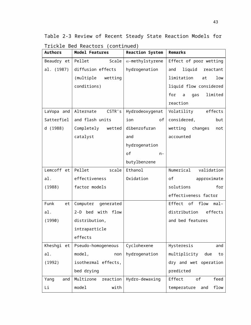
53
Figure 3. 1 Reactor and Gas-Liquid Separator

54
3.1.2 Gas-Liquid Separator and Level Control
The gas-liquid separator was designed and constructed from a 7 inch diameter
optically clear acrylic rod sealed at both ends by stainless steel flanges (Figure 3.3). The
top flange consists of a liquid level measurement device at the center with connections
for the gas-liquid mixture feed to the separator and gas exit from the separator on the
sides, while the bottom flange has a liquid exit line and a sampling line. The funnel shape
originally chosen by Al-Dahhan (1993) in order to minimize the liquid volume is also
used in this case. The small cylindrical section below it is used as a reservoir for the
paddle of a liquid level measurement device (Dynatrol, E-103C), which measures
frequency of vibration of the paddle in the liquid and transmits the liquid level signal to a
controller (Omega 7600). The controller signal is then converted to a pneumatic signal
using an I/P transducer and then used to operate a pneumatic valve controlling the liquid
leaving the separator. Liquid level control in the separator is crucial to maintaining a
stable pressure in the reactor as well as to prevent hydrogen escaping through the liquid
exit line. A stainless steel mesh demister is also placed in the top flange to trap the
solvent mist from the effluent gas stream.
3.1.4 Liquid and Gas Delivery System
The liquid reactant and solvent are delivered by a set of two high pressure
metering pumps (Calgon HP-15 and Eldex B-100) either to a high pressure feed tank, or
directly to a small tank used to damp the pulsation due to the pump, and then are sent on
to the reactor. The liquid feed rate is controlled by the pump head setting and also by a
recycle line from the small damper tank. Direct liquid supply from the pump is used in
steady state experiments, but this is not suitable for unsteady state experiments. A
pulsation free liquid supply is obtained by using the high pressure feed tank, which is

55
independently pressurized by nitrogen supplied from a high pressure cylinder. The liquid
supplied either from the high pressure tank or from the damper is sent through two sets
of parallel lines through needle valves to a combination of three way and solenoid valves
which are used to switch between steady flow and ON/OFF or BASE/PEAK flow
required for experiments operated under unsteady state conditions (Figure 3.3). The
solenoid valves are controlled by an electronic timer to which the cycle period and split
data are supplied.
The liquid outlet stream from the gas liquid separator is split into a sampling
stream and a waste stream. The sampling stream is connected to a needle valve for
withdrawal of samples to be analyzed by the gas chromatograph (Gow Mac Model 550).
The waste stream is passed through two liquid back pressure regulators used to drop the
liquid pressure from the operating pressure to atmospheric. The liquid is collected in a
110 liter stainless steel waste tank. Liquid flow measurement is also done by a rotameter
placed before the waste tank or manually by collecting the exit liquid over several time
intervals. Good level control is important in obtaining reproducible flow rate data
obtained by this method.
The gas delivery system consists of high pressure hydrogen gas cylinders
connected to the gas delivery line via a pressure regulator. Before the gas is delivered to
the reactor, it is bubbled through two small saturator tanks (similar to the damper tanks)
full of solvent in order to prevent excessive evaporation of solvent in the catalyst bed.
The gas is then supplied to the distributor via a needle valve used to control its feed rate.
The gas outlet stream from the gas-liquid separator passes through a series of back
pressure regulators used to drop the pressure from the reactor pressure to a pressure of 8
psig at which it flows through the rotameter which is pre-calibrated to determine the flow
rate at that pressure. This is then corrected to calculate the actual superficial velocity at
the operating pressure. The exit gas from this arrangement is then vented to the
atmosphere via a copper vent tube connected to the hood above the laboratory. Gas

56
pressure indicators and safety valves are mounted at several locations to prevent pressure
buildup in the gas delivery and exit stream.
Figure 3. 2 Down-flow and Up-flow Distributor for TBR and PBC Operation

57
Figure 3. 3 Experimental Setup for Unsteady State Flow Modulation Experiments

58
3.1.5 Data Acquisition and Analysis
Pressure drop measurements were conducted using a high pressure differential
pressure transducer (Viatran Model 374, 0-20” WCD), the output of which is connected
to the terminal block of a multiplexed data acquisition unit (National Instruments SCXI-
1100) which in turn is connected to a data acquisition board (National Instruments-AT
MIO-16) of a personal computer (Dell 486) as shown in Figure 3.4. Transducer outputs
from the thermocouples (type-K) are also connected similarly to the SCXI-1100 unit.
The software Labview (National Instruments V4.0) is utilized to develop the required
virtual instruments (VI’s) for both temperature and pressure drop measurements.
Figure 3. 4 Data Acquisition System
The reactant concentration data obtained from the gas chromatograph (Gow Mac
Model 550 with a thermal conductivity detector, TCD) is also sent to the same computer
using a separate data acquisition board and analyzed by a peak detection software
(Peaksimple-II, Sri Instruments) which can detect the prescribed species and evaluate
their concentrations using predetermined calibration curves.

59
3.2 Operating Procedures and Conditions3.2.1 Steady State TBR-PBC Comparison Experiments
Prior to experimentation in the trickle bed reactor, stirred basket reaction
tests were performed to establish a reproducible catalyst activation procedure and to test
the stability of the Pd on alumina catalyst before undertaking the packed bed reactor
studies. Preheating in an inert (Nitrogen) atmosphere to 140oC followed by activation
with Hydrogen at reaction temperature (~24oC) yielded consistent activity for over 40
hours of operation (after an initial 9 hours of stabilization runs).
Figure 3. 5 Basket Reactor Catalyst Stability Test for Palladium on Alumina Catalyst
The catalyst (2.5% Pd on alumina extrudate (properties as listed in Table 3.1))
supplied by Engelhard was packed to a height of 27.5 cm with glass beads (3 mm
diameter) packed on both sides to a total reactor length of 59 cm. The bed was activated
by first preheating it in a chromatographic-type oven at 140 oC for 4-5 hours with a low
flow rate of nitrogen passed through the bed to remove any moisture present in the

60
catalyst. The bed was cooled and activated by reducing it with a low flow of hydrogen at
near room temperature for 6-8 hours. The bed was then stored in solvent (hexane) under
a nitrogen atmosphere to maintain the activity and keep the catalyst wetted at all times.
a-methylstyrene (Eastman Chemicals) was pre-purified by passing over a bed of alumina
to remove the polymerization inhibitor. This was then diluted in hexane (ACS grade,
99.9% purity) and was used as the liquid phase delivered to the reactor by a precalibrated
high pressure pump or the pressurized feed tank as mentioned in Section 3.1.4. Pure
hydrogen (prepurified, analytical grade) bubbled through a hexane saturator (to prevent
evaporation of hexane in the reactor) was used as the gas phase. The reactor was kept
isothermal at 24oC with maximum 2oC temperature rise by using a cooling jacket. This
was readily accomplished due to dilute liquid reactant (maximum concentration < 8 %
v/v). At these conditions very little loss of liquid can occur due to volatilization.
Typically a high liquid flow rate was chosen for the first experiment and then the flow
was reduced for subsequent experiments and so on. This was done to eliminate the
possibility of hysteresis seen when flow rates are increased from lower values to higher
ones. Liquid samples were drawn from the gas-liquid separator after steady state was
reached at each liquid flow rate (about 20-25 minutes, after which no further change in
exit concentration of a-methylstyrene was observed). The samples were analyzed on a
gas chromatograph (Gow Mac Series 550, with a thermal conductivity detector) from
which the conversion of a-methylstyrene was determined. Pressure drop across the bed
was measured using a differential pressure transducer as shown in Figure 3.1.
Experiments were conducted at a fixed gas flow rate by varying liquid flow rate for each
mode of operation. The stability of the catalyst and the reproducibility of the data over
the duration of the experiments was verified by taking intermittent samples at identical
operating conditions. The reproducibility of the data was observed to be within 3%. The
range of operating conditions investigated in this study are presented in Table 3.2. These
operating conditions were selected on the basis of three considerations: i) liquid mass

61
velocities were chosen so as to cover a range of wetting conditions from partially wetted
to completely wetted catalyst, ii) liquid feed concentrations and pressures were picked to
encompass both gas and liquid limited conditions ( values range from 0.7 to 10), iii)
liquid reactant concentrations were kept low by dilution with solvent (n-hexane) to keep
the system nearly isothermal.
3.2.2 Bed Dilution and Experiments with Fines
Upon completion of the entire set of experiments without fines, the catalyst was
discharged and repacked with inert fines (Silicon Carbide, 0.2 mm) using a reproducible
packing procedure developed at CREL by Al-Dahhan et al. (1995). Several methods
(such as the dry and wet method) have been suggested in literature for packing laboratory
reactors with different proportions of fines to catalyst and have been shown by Al-
Dahhan et al. (1995) to give different and somewhat non-reproducible holdup and
pressure drop characteristics. The procedure developed at CREL, and followed in the
present experiments, was to use the dry method of packing, whereby the volume of the
fines added was calculated on the basis of the bed void volume in the undiluted
condition. The bed was packed in two portions (halves) in the present study. The catalyst
was packed to half the bed height first, followed by addition of the predetermined
volume of fines. These were packed in the interstices of the catalyst by using a vibrating
device on the bed until the top layer of catalyst was visible. This was then followed by
introducing the second half of the catalyst, which was similarly packed with fines as the
reactor was vibrated until the top layer of catalyst was visible. The increase in the overall
volume of the diluted bed over the undiluted bed was kept to within 2 % to ensure that
the structure of the original bed is not significantly disturbed by the addition of fines.
Experimental runs similar to those done previously were conducted now with the diluted
bed to study the effect of fines on the performance of down-flow and up-flow modes of
operation.

62
Table 3. 1 Catalyst and Reactor Properties for Steady State Experiments
Catalyst Properties Reactor
PropertiesActive metal 2.5% Pd. Total length 59 cmCatalyst support Alumina Catalyst length 27.5 cm
Packing shape Cylinder Diameter 2.2 cm
Packing dimensions (cm) 0.13 x 0.56
Fines
Surface area (m2 / g) 184 Material Silicon Carbide
Total pore volume (cm3 / g) 0.481 Diameter 0.02 cm
Pellet density rP (g / cm3) 1.222
True pellet density rt (g / cm3) 2.965
Pellet porosity eP 0.5878
Table 3. 2 Range of Operating Conditions for Steady State Experiments

63
Temperature 24oC
Pressure 30 - 200 psig (3 -15 atm.)
Concentration of a-methylstyrene 3.1 - 7.8 %(v/v) (230-600 mol/m3)
Superficial gas velocity (mass velocity) 3.8 - 14.4 cm/s (3.3x10⁻³-12.8x10⁻³ kg/m2 s)
Superficial liquid velocity
(mass velocity)
0.09-0.5 cm/s (0.63 - 3.85 kg/m2 s)
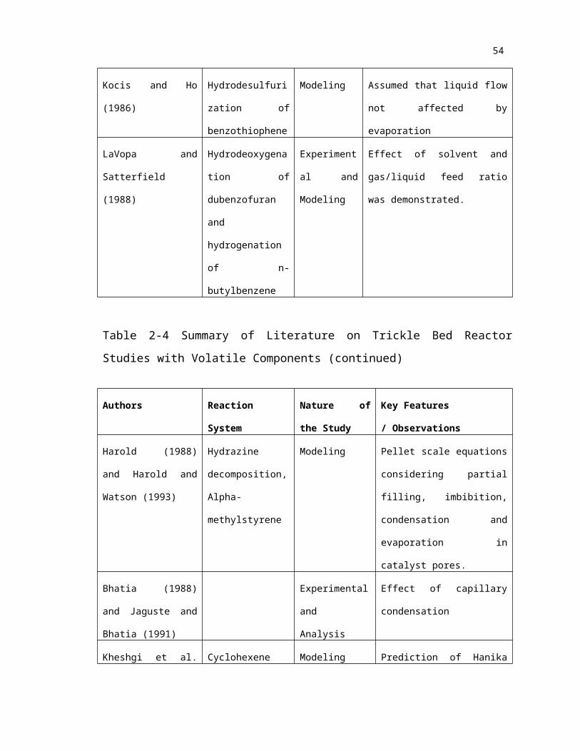
64
3.2.3 Unsteady State Experiments
The reaction chosen for this study was hydrogenation of alpha-methylstyrene to
iso-propyl benzene (cumene) which is the same system that was used for experiments in
Section 3.2.1. The high pressure packed bed reactor facility described in Section 3.1 was
used in this study (with the non-jacketed reactor). The liquid delivery system was
modified for unsteady state experiments by adding a set of solenoid valves and a timer
(as shown in Figure 3.5) to obtain liquid ON-OFF flow, liquid BASE-PEAK flow, and
steady liquid flow as desired (Figure 3.6). The catalyst used for these experiments, 0.5%
Pd on alumina spheres (different from that used in the earlier steady state experiments)
from Engelhard Corporation was packed to a height of 26 cm (with glass beads on both
sides to a total height of 59 cm) and was activated by reducing in situ (since this reactor
did not have an external jacket, it was easy to pre-heat, cool, and activate in situ). The
reaction was run in this activated bed for several hours at steady state until a constant
catalyst activity was obtained. Since the activity varied slightly between runs, steady state
experiments were performed before and after each set of unsteady state runs to ensure
reproducibility of the catalyst activity within each set. a-methylstyrene (99.9% purity
and prepurified over alumina to remove the polymerization inhibitor) in hexane (ACS
grade, 99.9% purity) was used as the liquid phase. Pure hydrogen (pre-purified, industrial
grade) was used as the gas phase. The reactor was operated under adiabatic conditions.
Liquid samples were drawn from the gas-liquid separator after steady state was reached
at each liquid flow rate. The samples were analyzed by gas chromatography (Gow Mac
Series 550, with thermal conductivity detector) from which the steady state conversion of
a-methylstyrene was determined. Unsteady state conversion was determined by
evaluating concentration of a liquid sample collected over multiple cycles to get the flow
average concentration. For example, if cycle time was 30 s, the sample was collected
over an interval of 150 s. The reproducibility of the data was observed to be within 2%.

65
The ranges of operating conditions investigated are presented in Table 3.4. The feed
concentrations and operating pressures were chosen so as to examine both gas limited
and liquid limited conditions (as evaluated approximately by the criterion as discussed
in Section 2.1.2). The liquid mass velocities were chosen so as to cover partial to
complete external wetting of the catalyst. Both liquid ON-OFF and BASE-PEAK flow
modulation were studied over a range of liquid mass velocities (Table 3.4) for each set of
experiments as illustrated in Figure 3.6 below.
Figure 3.6 Schematic of Flow Modulation: Connections and Cycling Strategy

66
Table 3. 3 Catalyst and Reactor Properties for Unsteady State Conditions
Catalyst Properties Reactor Properties
Active metal 0.5 % Pd Total Length 59 cm
Catalyst support Alumina Catalyst Length 26 cm
Packing shape Sphere Diameter 2.2 cm
Packing dimensions 3.1 mm
Table 3. 4 Reaction and Operating Conditions for Unsteady State Experiments
Superficial liquid mass velocity 0.05-2.5 kg/m2s
Superficial gas mass velocity 3.3x10⁻³-15x10-3 kg/m2s
Operating pressure 30 -200 psig (3-15 atm)
Feed concentration 2.5 - 30 % (200-2400 mol/m3)
Feed temperature 20-25 oC
Cycle time, (Total Period) 5-500 s
Cycle split, (ON Flow Fraction) 0.1-0.6
Max. allowed temperature rise 25 oC

67
Chapter 4. Experimental Results
4.1 Steady State Experiments in Trickle Bed Reactor (TBR) and Packed Bubble Column (PBC)
Comparison of the two reactors was achieved by studying the conversion at
identical nominal space times (defined as reactor length/ superficial liquid velocity) and
identical reactant feed concentration. This is the proper scale-up variable, (space time =
3600/LHSV) when the beds for upflow and downflow are identically packed (i.e., bed
voidage = constant) and the reaction rate is based per unit volume of the catalyst. The
results of all the experiments are tabulated in Appendix F.
4.1.1 Effect of Reactant Limitation on Comparative Performance of
TBR and PBCAt low pressure (30 psig) and high feed concentration of a-methylstyrene (CBi=
7.8 %v/v), the reaction is gas limited ( = 8.8). In this case, downflow performed better
than upflow reactor as shown in Figure 4-1. This is due to the nature of the
hydrogenation reactions which are typically hydrogen (gas reactant) limited at low
pressure (at or just above atmospheric) and high a-methylstyrene concentrations
(Beaudry et al., 1987). It is obvious that this is due to low hydrogen solubility at these
pressures which reduces the external transport rates of hydrogen. In downflow mode of
operation, the catalyst particles are not fully wetted at the liquid flow rates used (Figure
4-11 shows contacting efficiency calculated using the correlation of Al-Dahhan and
Dudukovic (1995)). This facilitates the access of the gas reactant to the pores of the

68
catalyst on the externally dry parts, and reduces the extent of gas limitation compared to
fully wetted pellets in the upflow reactor. The result is a higher conversion in downflow
than in the upflow mode of operation. In case of upflow, since the catalyst is almost
completely wetted, the access of gaseous reactant to the catalyst sites is limited to that
through liquid film only. This provides an additional resistance for the gaseous reactant
(especially at high space time i.e., low liquid flow rate) and results in conversion lower
than that obtained in downflow. This effect is more prominent at higher liquid reactant
feed concentrations, due to the larger extent of gas limitation at such conditions (higher
values). As liquid mass velocity increases (space time decreases), the downflow
performance approaches that of upflow due to catalyst wetting efficiency approaching
that of upflow (contacting efficiency approaches 1 as seen in Figure 4-11).
As the reactor pressure increases and the feed concentration of a-methylstyrene
decreases, the value of decreases and the reaction approaches liquid limited behavior as
postulated earlier. This is reflected in a complete reversal in performance at higher
pressures and at low a-methylstyrene concentration (Figure 4-2), where the performance
of upflow becomes better than downflow. This is because under these conditions the
catalyst in downflow is still partially wetted (since at the operating gas velocities and gas
densities (hydrogen), high pressure only slightly improves wetting in downflow (Figure
4-11 based on Al-Dahhan and Dudukovic, 1995) while catalyst is fully wetted in upflow.
In a liquid limited reaction, liquid reactant conversion is governed by the degree of
catalyst wetting, and since upflow has higher wetting (100 %) than downflow, it
outperforms downflow (Figure 4-2). As the liquid mass velocity increases, and the
contacting efficiency of downflow approaches 100 %, the performance of the two
reactors approaches each other, as evident in Figure 4-2 at low space times. Thus, as
pressure is increased from 30 to 200 psig, and feed concentration of a-methylstyrene is
decreased from 7.8% to 3.1%(v/v), the reaction is transformed from a gas-limited ( =
8.8) to a liquid-limited regime ( = 0.8). The criterion () is dependent on two factors
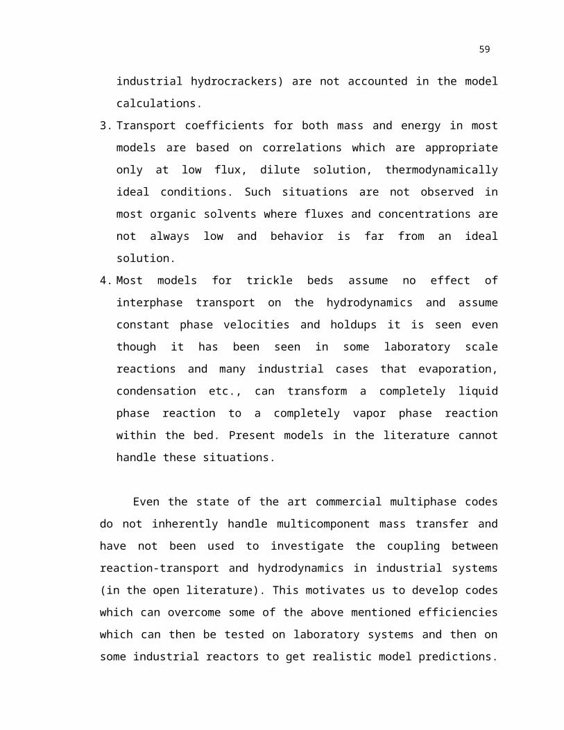
69
(apart from the diffusivity ratio), pressure (hydrogen solubility) and feed concentration of
the liquid reactant (a-methylstyrene) (as discussed in Section 2.1.2). Further insight into
the gas and liquid limitation can be obtained by investigating these two contributions
individually for the set of operating conditions examined.

70
Figure 4-. Trickle Bed and Up-flow Performance at CBi=7.8%(v/v) and Ug =4.4 cm/s at
30 psig.
Figure 4-. Comparison of Down-flow and Up-flow Performance at CBi=3.1%(v/v) at
200 psig.

71
4.1.2 Effect of Reactor Pressure on Individual Mode of Operation
As reactor pressure increases, the performance of both upflow and downflow
improves due to increase in gas solubility, which helps the rate of transport to the wetted
catalyst (in both modes) and improves the driving force for gas to catalyst mass transfer
to the inactively wetted catalyst in the downflow mode. At low feed concentration of the
liquid reactant (a-methylstyrene (3.1%v/v)) and at high pressure (>100 psig), the
reaction becomes liquid reactant limited (or liquid reactant affected) as can be seen from
Figures 4-3 and 4-4 where no further enhancement is observed when pressure is
increased from 100 to 200 psig (where drops from 1.5 at 100 psig to 0.8 at 200 psig).
This means that any further increase in the reactor pressure and hence liquid phase
hydrogen concentration, will have minimal effect since hydrogen is not the limiting
reactant anymore.
To confirm the above observation the reaction was studied at higher feed
concentration of a-methylstyrene (4.8 %v/v) in order to determine whether gas limited
behavior is observed at higher values. The performance indeed improves when pressure
is increased from 100 to 200 psig (Figures 4-5) implying that the reaction is not yet
completely liquid limited at this feed concentration at 100 psig operating pressure
(=2.44). Liquid limitations are felt at pressures above 200 psig ( =1.3) at this feed
concentration, whereas the reaction is indeed liquid limited at lower a-methylstyrene
concentration (3.1%v/v) even at lower pressures as noted previously in Figures 4-3 and
4-4. Both upflow and downflow conversion increases with increasing pressure, primarily
due to increase in the solubility of the gaseous reactant as the pressure increases. A
significant improvement in performance (conversion) occurs when pressure is changed
from 30 to 100 psig as compared to the change in conversion when pressure changes
from 100 to 200 psig. This confirms that the effect of pressure diminishes when liquid
limitation is approached (as approaches 1.0 from above (Figure 4-5)).

72
Figure 4-. Effect of Pressure at Low a-methylstyrene Feed Concentration on Upflow
Reactor Performance.
Figure 4-. Effect of Pressure at Low a-methylstyrene Feed Concentration (3.1% v/v) on
Downflow Performance.

73
Figure 4-. Effect of Pressure at Higher a-methylstyrene Feed Concentration on
Downflow Performance.
4.1.3 Effect of Feed Concentration of a-methylstyrene on Individual
Mode of Operation
Atmospheric pressure hydrogenation of a-methylstyrene has been known to
behave as a zero order reaction with respect to a-methylstyrene and first order with
respect to hydrogen (El-Hisnawi et al., 1982; Beaudry et. al, 1986). Our observations
confirm this observation at 30 psig as well as at 100 psig, the reaction is zero order with
respect to a-methylstyrene as shown in Figures 4-6 and 4-7 for upflow and downflow,
respectively. An inverse proportionality of conversion with liquid reactant feed
concentration (typical of zero order behavior) is observed especially at higher liquid flow
rates (lower space times). At lower liquid flow rates, at 100 psig the zero order
dependence appears to vanish and a first order dependence (due to a-methylstyrene
transport or intrinsic rate limitations), i.e., conversion independent of feed concentration,
is observed. Beaudry et al. (1987) also observed positive order with respect to the liquid

74
reactant at low liquid velocities (much higher space times) due to alpha-methylstyrene
affecting the rate. This shift in feed concentration dependence is confirmed by data at
higher pressure (200 psig, Figures 4-8 and 4-9). When liquid limitation is observed there
is no effect of feed concentration on the conversion in either mode of operation, as can be
seen in Figure 4-8 and 4-9. This is a consequence of the intrinsic rate limitation that
shows up as a first order dependence making conversion independent of feed
concentration (see also Appendix A for high pressure intrinsic rate data).
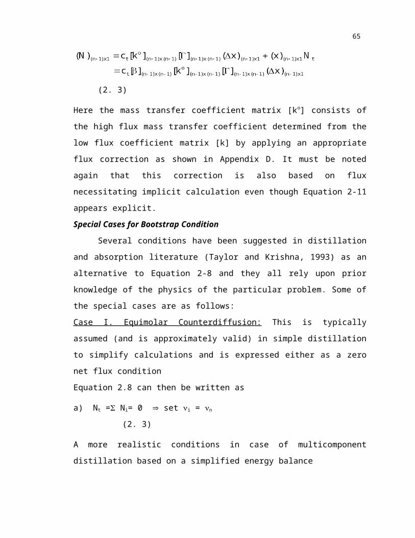
75
Figure 4-. Effect of a-methylstyrene Feed Concentration at 100 psig on Upflow
Performance.
Figure 4-. Effect of a-methylstyrene Feed Concentration at 100 psig on Downflow
Performance.

76
Figure 4-. Effect of a-methylstyrene Feed Concentration at 200 psig on Downflow
Performance.
Figure 4-. Effect of a-methylstyrene Feed Concentration at 200 psig on Upflow
Performance.

77
4.1.4 Effect of Gas Velocity and Liquid-Solid Contacting Efficiency
At low gas and liquid mass velocities, the level of interaction between the gas and
liquid phases is expected to be minimal in the downflow mode of operation. In case of
upflow, the effect of gas velocity on gas-liquid mass transfer is expected due to changing
interfacial area for transport with changing gas velocity. This would however only be
influential in determining the performance if the gas-liquid mass transfer were limiting
the overall reaction. The influence of gas velocity on the performance of both upflow and
downflow reactors is shown in Figure 4-10. The effect of gas velocity on reactor
performance was also examined for both upflow and downflow reactors. A significant
effect was not observed in the range of the gas velocities studied (3.8-14.4 cm/s, i.e., gas
Reynolds number in the range of 6-25) on either downflow or upflow performances at all
the feed concentrations and pressures tested. This is in agreement with earlier
observations of Goto et. al (1993). Experimental pressure drop measurements were also
made for both modes of operation during the reaction runs. The data obtained (shown in
Figure 4-11) indicates higher pressure drops for upflow at both ends of the pressure
range covered (30 and 200 psig) than for downflow, which is in agreement with
expectation and the pressure drop data reported in the literature. The better performance
(conversion) o the downflow mode of operation (TBR) at 30 psig, despite lower pressure
drop, confirms that poor contacting (Figure 4-11) does yield better conversion due to
reaction being gas limited, which seems contrary to the notion that higher transport
always involves higher pressure drop (which is observed to be true here in case of liquid
limited reaction at 200 psig).

78
Figure 4-. Effect of Gas Velocity on Reactor Performance at 100 psig.
Figure 4-. Pressure Drop in Downflow and Upflow Reactors and Contacting Efficiency
for Downflow Reactor at 30 and 200 psig.

79
4.2 Comparison of Down-flow (TBR) and Up-flow (PBC) Reactors with Fines Fines (nonporous inert particles, order of magnitude smaller than catalyst pellets
packed only in the voids of the catalyst) were used to investigate the performance of the
two modes of operation using the same reaction in an attempt to demonstrate the
decoupling of hydrodynamic and kinetic effects. A way to establish this decoupling is to
use the upflow and downflow modes, which are intrinsically hydrodynamically different
(as discussed earlier), and asses whether fines can indeed yield the "true" kinetic behavior
(more properly called "apparent" rates on catalyst pellets of interest, i.e., rates unmasked
by external transport resistances and hydrodynamic effects). The two extreme cases
discussed before, i.e., gas limitation (downflow performance better than upflow, Figure
4-1), and liquid limitation (upflow performance better than downflow, Figure 4-2) are
now conducted in the presence of fines. Figures 4-12 and 4-13 show the performance of
both reactors when the bed is diluted with fines. It can be seen by comparing Figure 4-12
with Figure 4-1 and Figure 4-13 with Figure 4-2 that fines have eliminated the disparities
between the two modes of operation even in the extreme cases of reactant limitation.
This is primarily due to the fact that fines improve liquid spreading considerably and
achieve comparable (and almost complete) wetting in both modes of operation. It must
be noted that Figures 4-1 and 4-12, or Figures 4-2 and 4-13, could not be directly
superimposed due to slightly different catalyst activity obtained after repacking the bed
with fines and catalyst and reactivating it. Nevertheless, fines have successfully
decoupled the hydrodynamics and apparent kinetics, and the data with fines reflect the
kinetics in the packed bed under "ideal" liquid distribution conditions. It can be observed
in Figure 4-12 that at low liquid flow rate and low pressure (gas limited reaction), a
trickle bed with fines still performs slightly better than upflow with fines, which
80
indicates that the degree of wetting is still not complete in downflow resulting in some
direct exposure of the internally wetted but externally dry catalyst to the gas . This may
be due to the fact that at low liquid flow rate even with fines , the catalyst is not
completely externally wetted (Al-Dahhan and Dudukovic, 1995). At high pressure (liquid
limited reaction) Figure 4-12 reveals identical performance of both reactors where
complete wetting is achieved in both modes.
Since we studied the impact of the two factors, pressure and feed concentration
on the performance without fines, the same study was conducted for the bed diluted with
fines.

81
Figure 4-. Effect of Fines on Low Pressure Down-flow Versus Up-flow Performance
Figure 4-. Effect of Fines on High Pressure Down-flow Versus Up-flow Performance

82
4.2.1 Effect of Pressure in Diluted Bed on Individual Mode of Operation
The effect of pressure on the performance of both modes of operation in beds
with fines is illustrated in Figures 4-14 and 4-15. At higher pressure the performance of
both upflow and downflow is better than that at low pressure. This observation is also
consistent with the data obtained without fines. The pressure dependence observed is as
expected due to the increase in gas solubility with increased pressure. The same rate
dependence in hydrogen concentration was reported by Beaudry et al. (1987) as was also
observed in slurry experiment at both pressures as discussed in Appendix A and reported
by El-Hisnawi et al. (1982). Beaudry et al. (1987) observed some liquid limitation effects
(on the externally dry areas of the catalyst resulting in somewhat lower rate than
predicted by gas limited conditions) at low liquid mass velocity (high space time) even
for the gas limited case. These were not seen at the lower space times examined in this
study.
4.2.2 Effect of Feed Concentration in Diluted Bed on Individual Mode of
Operation
At 30 psig, liquid reactant conversion is higher at lower feed concentration of a
methyl styrene (lower 2 curves for downflow (Figure 4-14) and upflow (Figure 4-15). At
higher reactor pressure, there is no effect of feed concentration (upper 2 curves, Figure 4-
14 and 4-15). This was also observed for the reactors without fines and explained on the
basis of liquid limitation in the previous section. The fact that it is observed with fines
confirms the feed concentration dependence (of performance) in case of gas and liquid
limited reaction.
Fines have been shown to successfully decouple the hydrodynamics and reaction
effects, and can yield true apparent kinetic data in the packed bed under "ideal" liquid
distribution conditions. Both gas and liquid limited conditions were investigated and
identical performance was shown under all conditions studied, implying that using fines
83
is the recommended strategy to be used in obtaining data for scale-up or during scale-
down.
Figure 4-. Effect of a-methylstyrene Feed Concentration at Different Pressures on
Performance of Downflow with Fines.

84
Figure 4-. Effect of a-methylstyrene Feed Concentration at Different Pressures on
Performance of Upflow with Fines.
4.3 Unsteady State Experiments in TBRThe objectives outlined in Chapter 1 for the study of unsteady state operation
were to conduct experiments to examine the effect of gas and liquid reactant limitation as
well as cycling parameters such as total cycle period, cycle split, and cycling frequency
(as described in Section 3.2.3) on TBR performance. Comparison of the data obtained (as
listed in Appendix F) is reported with the few data available in the literature on similar
systems.
4.3.1 Performance Comparison for Liquid Flow Modulation under Gas
and Liquid Limited Conditions
Trickle bed performance was investigated for the two cases of interest, (i) gas
reactant limitation, and (ii) liquid reactant limitation, by changing operating pressure and
feed concentration. Performance under unsteady state operation was determined by

85
evaluating the flow averaged conversion over several cycles of operation according to the
procedure outlines in Section 3.2.3. Based on several trial runs, a total cycle time of 60 s
and a cycle split of 0.5 were chosen for this set of experiments with liquid ON/OFF flow
(see Figure 4-26 for liquid mass velocities corresponding to the space times investigated).
Under near liquid-limited conditions (i.e., high pressure and low feed concentrations) no
enhancement is observed with this modulation strategy, except at very low liquid mass
velocities (high mean space times (= VR/QL(mean)). At high liquid mass velocity, the
catalyst is well irrigated and any advantage due to better wetting under unsteady state is
not feasible. This can be qualitatively seen by examining the convex shape of the
contacting efficiency curve (Figure 4-26) which would yield better catalyst wetting under
steady state conditions and hence better performance under steady state conditions. This
analysis cannot however be applied at low liquid mass velocity where the unsteady state
wetting and replenishment of stagnant liquid pockets with fresh liquid reactants can
make enhancement possible. Under these conditions, the bed is poorly irrigated and the
disadvantage due to liquid maldistribution (not seen in steady state contacting efficiency
plot as shown in Figure 4-26) can be overcome by the high flow rate liquid (Figure 4-16,
at high space times).
At low space times (high mass velocity, Figure 4-16), performance enhancement
is not seen under laboratory conditions due to several factors such as small reactor
diameter, good distributor, all leading to good catalyst wetting (as seen in Figure 4-26).
The conditions investigated in the present experiments correspond to fairly high liquid
hourly space velocities (LHSV) in comparison with industrial trickle beds, where this
maldistribution effect may be seen to be more pronounced. LHSV varied from 3 to 15 in
our experiments as compared to 1.5 to 10 used in industrial reactors.
In case of gas limited conditions (i.e., at low operating pressures and high feed
concentration), it can be seen in Figure 4-17 ( ~ 25) that unsteady state performance
(conversion) is significantly higher than that under steady state conditions at all space

86
times. This case illustrates the conditions of a liquid reactant full catalyst and enhanced
supply of the gaseous reactant leading to better performance. The observed enhancement
improves as the extent of partial wetting is increased as seen at higher space times (lower
liquid mass velocities). This also corroborates the findings of Lange et al. (1994) and
Castellari and Haure (1995) that under severe gas limitation (due to 50 % (v/v) and 100
% pure liquid reactants in their studies respectively) enhancement is feasible. Castellari
and Haure (1995) explored this enhancement further by increasing the total cycle time to
allow for complete internal drying of catalyst and corresponding large temperature
increase and semi-runaway conditions. This was not feasible in the present study, but
enhancement due to higher gas supply was expected to increase by increasing the gaseous
reactant supply and lower liquid ON times. A small exothermic contribution was also
observed during unsteady state operation here with maximum bed temperatures reaching
~ 6 oC higher than steady state temperatures.

87
Figure 4-. Comparison of Steady and Unsteady State Performance at Conditions
Approaching Liquid Limitation ( < 4)
Figure 4-. Comparison of Steady and Unsteady State Performance under Gas Limited
Conditions ( ~25)

88
4.3.2 Effect of Modulation Parameters (Cycle Period and Cycle Split) on
Unsteady State TBR Performance
To explore whether further performance enhancement is achievable for the gas
reactant limited case by increasing gaseous reactant supply to the catalyst, a constant
liquid mean flow was chosen (Space time = 660 s, L= 0.24 kg/m2s) and cycle split ()
was varied (to vary the ratio of the gas to liquid access times). It can be seen that further
enhancement was indeed possible the cycle split was lowered from steady state ( = 1) to
a split of = 0.25, the performance improved by as much as 60% over steady state at the
same mean liquid mass velocity (Figure 4-18). This improvement continues up to the
point where liquid limitation sets in at very low cycle split (indicating that the liquid is
completely consumed during a time interval shorter than the OFF time of the cycle),
beyond which the performance will be controlled by liquid reactant supply. This implies
that performance improvement can be maximized by choosing an appropriate cycle split
(at a given liquid mass velocity and total cycle period).
The effect of the total cycle period was investigated at the cycle split () value of
0.33, where performance enhancement was observed to be significant (Figure 4-18). The
performance enhancement is seen to increase with total cycle period up to a maximum,
after which it drops to near (or below) steady state values. A similar maximum was
observed by both Lange et al. (1994) and Haure et al. (1990) for different reaction
systems. A qualitative explanation for this phenomena can be developed on the basis of
their observations and the present data. At low cycle periods the liquid reactant is
supplied over shorter time intervals than needed for complete consumption by the
gaseous reactants leading to the aggravation of the gas limitation (or gas reactant
starvation). At long cycle periods (for the same cycle split), the opposite behavior is seen
due to longer gas access time than necessary to consume liquid reactants (liquid reactant
starvation). Gabarain et al. (1997) have examined the effect of very large cycle times (up

89
to 40 minutes) and seen that the temperature rise, initially observed due to large reaction
rates, drops off as liquid starvation sets in at the end of the long cycle. They attempted to
find an optimum total cycle period based on this maximum temperature rise (maximum
rate due to gas phase reaction on completely externally and then internally dry catalyst).
Due to the competition between gas reactant starvation at the lowest cycle periods and
liquid reactant starvation at the higher ones, a feasibility envelope can be determined
(Figure 4-19) based upon which the performance enhancement can be optimized. The
duration of the cycle for maximum enhancement is dependent upon the liquid reactant
concentration as seen in the experiments of Lange et al. (1994) (cycle period ~ 7.5
minutes for ~ 50 % v/v of alpha-methylstyrene) under similar operating conditions. This
maximum could be quantified by a complex function of an effective parameter (under
dynamic conditions) and the effect of cycle split and liquid mass velocity if transient
variation of concentration is known accurately. The above effects of cycle split and total
cycle period were examined at a constant liquid mass velocity. Due to the strong
dependence of catalyst wetting and reaction rate (both steady and unsteady), on liquid
mass velocity (also referred to as amplitude of the flow modulation) its effect is
important from the point of view of commercial scale application and is examined next.

90
Figure 4-. Effect of Cycle Split () on Unsteady State Performance under Gas Limited
Conditions
Figure 4-. Effect of Total Cycle Period () on Unsteady State Performance under Gas
Limited Conditions

91
4.3.3 Effect of Amplitude (Liquid Mass Velocity) on Unsteady State
TBR Performance
The feasibility envelope (region where performance enhancement is possible, as
shown in Figure 4-19) as discussed in Section 4.3.2 and observed in literature is strongly
dependent on the relative supply of gaseous and liquid reactants. Gaseous reactant access
is governed by the extent of external catalyst wetting (which depends on liquid flow rate)
and the formation of dry areas (which depends on evaporation rate). Castellari and Haure
(1995) examined the catalyst drying phenomenon in their experiments which they
attributed to complete external and internal evaporation of liquid (until liquid reactant is
completely consumed). However, all of their experiments were conducted at the same
mean liquid mass velocity (~ 10 times higher than in the present study) at which the
steady state wetting is complete. The change in catalyst external wetting due to
evaporation in the present study is not large (compared to that observed by Castellari and
Haure (1995)) as compared to that due to change in flow with time. It is thus important
to explore whether the feasibility region for enhancement can be altered with changing
liquid mass velocity. Two mean liquid mass velocities at which wetting should have the
most effect (lowest mass velocity possible, see Figure 4-26) were examined (at a cycle
split of 0.25). The results presented in Figure 4-20 compare normalized enhancement
(conversion at unsteady state over that at steady state). A significantly higher
enhancement is observed by lowering the mean liquid mass velocity. At a mass velocity
of 0.137 kg/m2s, a similar feasibility envelope is seen as in Figure 4-19 which ends in
degradation of performance to below steady state values at higher cycle periods due to
depletion of the liquid reactant (liquid starvation onset as discussed in the previous
section). The lower liquid mass velocity allows more time for liquid reactant supply
(higher mean space times) to the catalyst. This is reflected in the shift in the liquid
starvation to even higher total cycle periods (Figure 4-20), while the gas starvation side
remains unchanged (similar to that observed in Figure 4-19). The higher maximum

92
enhancement at lower liquid mass velocity (Figure 4-20) clearly indicates the trend
towards the limit of maximum possible enhancement (the ideal case of zero flow of
liquid reactant and complete conversion).
Figure 4-. Effect of Liquid Mass Velocity on Unsteady State Performance under Gas
Limited Conditions

93
4.3.4 Effect of Liquid Reactant Concentration and Pressure on
Performance
The two key parameters which decide the extent of gas or liquid reactant
limitation are the liquid reactant feed concentration and operating pressure. The
combined effect of these was discussed in Section 4.3.1 for two sets of steady and
unsteady state performance data corresponding to the gas limited and liquid limited
extremes. It was shown that with the ON/OFF liquid flow modulation strategy,
performance enhancement was possible under gas limited conditions (Figure 4-17). The
effect of individual contributions of pressure and liquid reactant feed concentration under
gas limited conditions needs to be carefully examined to determine the exact cause-effect
relationships in performance enhancement. The effect of liquid reactant feed
concentration was examined under gas limited conditions by evaluating the enhancement
at different cycle splits. With the increase in gas limitation due to higher liquid reactant
feed concentration, we would expect higher enhancement due to flow modulation at
higher liquid reactant feed concentration. However, this is not observed as expected
(Figure 4-21). Since the absolute value of the conversion at higher feed concentrations is
lower (due to gas reactant limitation), the enhancement seen is not as high even if lower
mean liquid mass velocity was used. The liquid mass velocity used at the higher liquid
reactant feed concentration was 0.1 kg/m2s as compared to 0.24 kg/m2s at the lower feed
concentration. The effect of operating pressure was examined at constant gas velocity of
5.4 cm/s and liquid mass velocity of 0.085 kg/m2s. Under gas limited conditions, both
steady and unsteady performance improves with increase in pressure as expected (due to
enhanced solubility at elevated pressures). This enhancement diminishes as liquid limited
conditions are approached at even higher pressures, especially at liquid mass velocities
where the bed irrigation is complete (under laboratory conditions). In the present
94
experiment the liquid mass velocity used is fairly low, hence the performance
enhancement is seen even at the highest pressure studied (Figure 4-22).
Figure 4-. Effect of Liquid Reactant Feed Concentration on Unsteady State Performance
under Gas Limited Conditions

95
Figure 4-. Effect of Operating Pressure on Unsteady State Performance under Gas
Limited Conditions

96
4.3.5 Effect of Induced Flow Modulation (IFM) Frequency on Unsteady
State Performance
Liquid ON/OFF flow modulation can be considered as square wave cycling about
the mean flow for the case with a cycle split of 0.5. Conversion under periodic conditions
can then be used to examine the dominant time scales affected by induced flow
modulation (IFM) by looking at the frequency () dependence of flow averaged
conversion. Both Figures 4-23 and 4-24 show performance enhancement as a function of
the IFM frequency with similar trends seen at different pressures, feed concentrations,
and even for a case of non-square wave pulsing ( = 0.2). The performance in both cases
shows degeneration of the enhancement at low frequencies tending to the steady state
operation at zero frequency. But as frequency is increased, the conversion reaches a clear
maximum improvement point. Ritter and Douglas (1970) observed a similar frequency
dependence for dynamic experiments in stirred tanks and attributed the maximum to the
resonance frequency of the rate controlling process. All transport processes typically
have a natural frequency corresponding to their characteristic time scale. Gas-liquid
transport in trickle beds corresponds to 0.2 to 0.8 Hz (at low pressures), liquid-solid
transport corresponds to 0.5 to 2 Hz (Gianetto and Silveston, 1986; Astarita, 1997),
whereas catalyst level reaction-diffusion processes correspond typically to much lower
frequency (larger time scale) depending upon intrinsic rates in pellets (Lee and Bailey,
1974; Kouris et al, 1998). Typical industrial reactions in trickle bed reactors have been
reported to correspond to a frequency range of 0.01 to 0.1 Hz (Wu et al., 1995). Natural
pulsing occurs in trickle beds at high liquid flows and displays frequencies of 1 to 10 Hz,
at which external transport is significantly improved (Blok and Drinkenberg, 1982; Wu
et al., 1995). The present IFM frequencies are much lower than those observed under
natural pulsing. The frequency dependence of the performance (Figure 4-23 and 4-24)
shows that the highest effect of IFM can be observed at low frequencies ( ~ 0.01 Hz) at

97
which catalyst level processes could be predominantly affected to obtain the observed
enhancement. Some effect on external transport processes can also be seen (in Figures 4-
23 and 4-24) where enhancement corresponding to their natural frequencies is observed.
This opens up the possibility of selectivity enhancement and control for complex reaction
schemes by controlling reactant supply by the proper choice of the IFM frequency for the
desired reactant (Wu et al., 1995). The low enhancement seen at both ends ( 0 and
) can be explained on the basis of the frequency analysis similar to that done by Lee
and Bailey (1974). The very low IFM frequency ( 0) corresponds to an equilibrium
state or pseudo steady state, where the reaction transport processes have time to catch up
with the modulated variable (flow in this case) and the overall system behaves as a
combination of discrete steady states. On the other hand at high IFM frequency ( ),
the input fluctuations are so rapid that none of the reaction-transport processes in the
system can respond fast enough to the induced flow modulation (IFM), and, no gain in
performance due to the modulated variable is again not feasible. This has been confirmed
by pellet scale reaction-diffusion simulations with time varying boundary conditions (at
high frequencies) by Lee and Bailey (1974) and Kouris et al. (1998). They have shown
that at low frequencies, the catalyst has a chance to react to external changes and effect of
time variation propagates to the interior of the catalyst, while at higher frequencies the
system (catalyst) cannot relax to the rapidly changing external conditions and
performance corresponding to a stationary state (time averaged wetting) is observed.

98
Figure 4-. Effect of Cycling Frequency on Unsteady State Performance under Gas
Limited Conditions
Figure 4-. Effect of Cycling Frequency on Unsteady State Performance under Gas
Limited Conditions

99
4.3.6 Effect of Base-Peak Flow Modulation on Performance
For the case of liquid limited conditions (i.e., at high pressure and low feed
concentrations) the use of complete absence of liquid during the OFF part of the cycle (as
done in ON-OFF flow modulation) is not beneficial, as this would worsen the liquid
limitation. This was confirmed in the discussion in Section 4.3.1 and experimental
observations of Lange et al. (1994). Instead of the conventional ON-OFF liquid flow, a
low base flow (with magnitude similar to the mean operating flow) is introduced during
the OFF part of the cycle (referred to as BASE flow) with a periodic high flow slug
introduced for a short duration (referred to as PEAK flow) to improve liquid distribution
and open up multiple liquid flow pathways during the rest of the cycle (Gupta, 1985;
Lange et al., 1994). The cycle split () here is the fraction of the cycle period during
which the high flow rate slug is on (typically chosen to be very short).
Tests were conducted at a cycle split of 0.1 and cycle times varying from 30 to
200 s at an operating pressure of 150 psig and low liquid reactant feed concentration
(C(AMS) feed = 784 mol/m3) to ensure liquid limited conditions. This strategy is shown to
yield some improvement over steady state performance (Figure 4-25, < 1.2), although
this is not as high as observed under gas limitation. The maximum enhancement
observed here was 12 % as against 60 % in case of gas limited conditions. The limited
enhancement is primarily due to intrinsically better flow distribution in small laboratory
reactors, which would not be the case in typical pilot or industrial reactors where much
higher enhancement can be anticipated.

100
Figure 4-. Unsteady State Performance with BASE-PEAK Flow Modulation under
Liquid Limited Conditions
Figure 4-. Effect of Liquid Mass Velocity on Steady State Liquid-Solid Contacting
Efficiency
L (peak)
L (mean) = L (peak)+(1-) L (base)
, (sec)
(1-) L (base)
L (mean)

101
Chapter 5. Modeling Of Trickle Bed Reactors 5.1 Evaluation of Steady State Models for TBR and PBC
The qualitative analysis presented in the discussion of the experimental results in
Section 4.1 on the basis of reactant limitation, liquid-solid contacting, and effect of
pressure on kinetics was verified by comparison with predictions of some of the existing
models as discussed in this section. A history of the model development for trickle bed
reactors was presented in Chapter 2 and the salient features of each model were presented
in Table 2.3. Based on the discussion therein, two models (developed at CREL), one with
reactor scale equations (El-Hisnawi, 1982) and the other with pellet scale equations
(Beaudry, 1987) were chosen to compare predictions to experimental data. The key
distinction in modeling downflow and upflow are the values of mass transfer parameters
(evaluated from appropriate correlations) and the catalyst wetting efficiency. The
solution of partially wetted pellet performance is required for downflow and fully wetted
pellets can be assumed for upflow. The effect of liquid mass velocity on simulated gas-
liquid and liquid-solid transport in both reactors was required. These were evaluated
from correlations proposed in the literature for the reactor under consideration. The
intrinsic kinetics required was obtained from slurry experiments as discussed in Section
4.1 and Appendix A.
5.1.1 Reactor Scale Model (El-Hisnawi et al., 1982)
The El-Hisnawi et al. (1982) model was originally developed for a low pressure
trickle bed reactor to account for rate enhancement for gas limited reaction due to

102
externally inactively wetted areas. The model was proposed in the form of heterogeneous
plug flow equations for the limiting reactant. The surface concentration of the limiting
reactant is obtained by solution of the reaction transport equation at the catalyst surface.
This is substituted into the plug flow equation of the non-limiting reactant to obtain its
profile (Table 5.1). For example, when A (gaseous reactant, hydrogen) is the limiting
reactant, its surface concentration is solved for, and, rate evaluated on its basis is
substituted in the plug flow equation for concentration of B (liquid reactant, alpha-
methylstyrene) to obtain the conversion of B at each velocity specified. Analytical
solutions were derived for the first order kinetics for the equations at low pressures. At
high pressure, however, the reaction was observed to be liquid reactant B limited with
non-linear kinetics (given in the Langmuir–Hinshelwood form in Appendix A). Surface
concentration of B was solved for from the non-linear rate equation (in Table 5.1) to get
the surface concentration. Then differential equation for the concentration of species B is
then solved numerically to get the concentration profile of B and reactor exit conversion
at each space time. The pellet effectiveness factor can be determined from the Thiele
modulus but was used here as a fitting parameter based on its value at one of the cases
and used for the rest. This was done due to the uncertainty in the catalyst activity (rate
constant) and the effective diffusivity values at high pressures. The liquid-solid
contacting efficiency was determined at low pressure by the correlations developed by
El-Hisnawi (1981) and at high pressure using the correlation of Al-Dahhan and
Dudukovic (1995). The upflow reactor was assumed to have completely wetted catalyst
in all cases. For downflow gas-liquid mass transfer coefficient was obtained from
Fukushima and Kusaka (1977) correlation, liquid-solid mass transfer coefficient was
calculated from Tan and Smith (1980), and gas-solid mass transfer coefficient was
estimated by the method of Dwiwedi and Upadhyay (1977). For upflow prediction, the
gas-liquid mass transfer coefficients were obtained from the correlation by Reiss (1967),
and, liquid-solid mass transfer coefficients from the correlation by Spechhia (1978). The

103
variation of the mass transfer coefficients calculated from the above correlations with
space time is shown in Figure 5-5. The predictions of the El-Hisnawi model at low
pressure (gas limited) compare well with the downflow experimental data as shown in
Figure 5-1. For the case of upflow performance, however, the model over predicts the
experimental data at low space time. This implies that the effect of external mass transfer
is felt in case of the predicted conversion profile for upflow, which is not observed
experimentally. The mass transfer correlations used typically predict higher values at
higher liquid velocity (lower space time) resulting in the higher predicted conversion at
low space times. At high pressure, liquid limited conditions, however, El-Hisnawi model
predictions compare well with the experimental data for upflow and downflow as shown
in Figure 5.2. The effect of mass transfer is not felt as much at high pressure and
predictions are qualitatively and quantitatively (within 5%) able to capture the
observed experimental behavior of both reactors.

104
Table 5. 1 Governing Equations for El-Hisnawi (1982) Model
Original model equations (gas limited conditions)
And
Boundary conditions:
Equilibrium feed
Non-Equilibrium feed
and
Model equations at high pressure (liquid limited conditions)
(boundary conditions are the same as at low pressure)
(for liquid reactant limitation)

105
Table 5. 2 Governing Equations for Beaudry (1987) Model
Pellet Scale Equations:
a) Low Pressure (Gas Reactant Limited) with rate first order in A.
Boundary conditions (Pellet):
(=0 for m<1)
(=0 for m<1)
Boundary conditions (Reactor):
Where,

106
Table 5-2. Governing Equations for Beaudry (1987) Model (continued)
b) High Pressure (Liquid Reactant (diffusional) Limitation for Langmuir-Hinshelwood rate form)
Boundary conditions:
For both case a) and b) above, the reactant conversion in general is given by
where
(at low pressure)
(at high pressure)
and overall effectiveness factor is given by
5.1.2 Pellet Scale Model (Beaudry et al., 1987).
Beaudry’s model considered the evaluation of catalyst pellet effectiveness subject
to different wetting conditions and substitution of the overall pellet effectiveness factor
into a simple plug flow equation to evaluate reactor conversion. The catalyst pellets were
modeled in the form of infinite slabs with the two sides exposed to either gas or liquid, or
a half-wetted pellet exposed to gas and liquid on one side only. At low pressure (gas

107
limited conditions), the gaseous reactant supplied from both sides of the pellet depletes to
almost zero within a short distance depending upon the extent of the gas reactant
limitation. Hence, the solution of the pellet effectiveness for downflow for the gas
limited case involved solution of both the dry and wetted side for a half wetted pellet,
and the solution of the completely wetted pellet (as shown Table 5-2). For the completely
dry pellet the effectiveness was zero since no liquid reactant could be supplied to this
pellet. The analytical solutions to this case for the reaction rate which is first order in
hydrogen are available in Beaudry et al. (1987) and were used to obtain the overall
effectiveness factor as a weighted average of the contacting and the effectiveness of each
type of pellet (as shown in Table 5-2). At high pressure (liquid limited conditions) the
solution is much more complicated due to the non-linear reaction rate which demands the
solution of the reaction diffusion equations for the externally wetted pellets on both sides
and the half wetted pellet only on the wetted side. Here, the value of is the point where
the liquid reactant depletes completely and is the boundary for the liquid reactant
concentration solution. This solution needs to be evaluated at each point in the reactor to
get a local effectiveness factor corresponding to the local concentration of the liquid
reactant. Instead of doing this as a coupled system of equation both on the pellet and
reactor scale, the pellet scale equations were solved at different bulk liquid reactant
concentrations and then fitted as a polynomial of pellet effectiveness as a function of
surface concentration. This polynomial is then used to solve the reactor scale equations
numerically to obtain conversion at each space time. Although this approach does not
require any fitted parameters as needed in the El-Hisnawi model, the rate constant was
similarly fitted to match the conversion at one space-time and used to compare with the
experimental data at all other space times. As can be seen from Figure 5-1 and 5-2, this
model predicts the observed data for down flow at low pressure and at high pressure
well, but not so well for up-flow especially at low pressure and high feed concentration.
The reason may be due to mass transfer correlations used for upflow which may predict a

108
lower performance (than observed experimentally) at high space times in the upflow
operating mode. This is also consistent with the predictions of El-Hisnawi model
discussed above.
The Beaudry et al. (1987) model predictions are also shown in Figure 5-1 and 5-2
for low and high pressure, respectively. As can be seen in the Figure 5-1, the Beaudry et
al. (1987) model predicts downflow performance at low pressure exactly as the El-
Hisnawi model does, but under-predicts upflow performance at higher space times (low
liquid velocities) due to the significant effect of mass transfer (as predicted by the
correlation used) particularly at high space times. At high pressure, on the other hand,
Beaudry's model predicts experimental data quite well both for downflow and upflow,
since the effect of mass transfer is not as pronounced as at low pressure.
The effect of the feed concentration on predictions of both models was also
examined for both downflow and upflow reactors as shown in Figures 5-3 and 5-4,
respectively. As mentioned earlier in the discussion, the predictions are almost identical
for both models for downflow and agree with experimental data. In both cases, however,
the inverse relationship of liquid feed concentration with conversion typical of low
pressure gas limited operation seen in the experiments is predicted correctly.
The predictions of the reactor scale and pellet scale models are
satisfactory for current conditions although there is a need for high pressure correlation
for mass transfer coefficient and interfacial area in order to predict performance with
greater certainty, especially in cases where the rate is affected significantly by external
mass transfer. The predicted performance of upflow and downflow for both models
presented and discussed in this section is seen to be strongly dependent on the reaction
system i. e., whether the reaction is gas or liquid limited under the conditions of
investigation. The laboratory reactors are often operated in the range of partially to fully
wetted catalyst and demonstrate the influence of wetting can be either detrimental or
beneficial, depending upon the reactant limitation. Models that account for these two

109
effects, i.e., reactant limitation and influence of catalyst wetting, can predict the
performance over the entire range of operating conditions. The intrinsic kinetics of the
reaction studied at different pressures is also important in obtaining good predictions.
Hence, for any given reaction it is recommended to study the slurry kinetics at the
specific operating pressure before any scale up or modeling is attempted. A rate
expression with different rate constants at each of the discrete pressures (as used here)
can be used to predict the trickle bed reactor data at the same pressures most accurately,
rather than using a general rate form which cannot fit all the data obtained at different
pressures. It must be mentioned that the reactor scale model failed to predict
experimental data well at the intermediate conditions (100 psig, ~ 1) when the reaction
is neither completely gas limited nor liquid limited (or switches from gas limited to
liquid limited at some location in the reactor) because the model assumptions were for
the extreme conditions of one reactant being limiting. Rigorous solution of the reactor
and pellet scale equations presented in the next section should be able to cover a general
case without the assumptions made here.

110
Figure 5. 1 Upflow and Downflow Performance at Low Pressure (gas limited condition):
Experimental data and model predictions
Figure 5. 2 Upflow and Downflow Performance at High Pressure (liquid limited
condition): Experimental data and model predictions

111
Figure 5. 3 Effect of Feed Concentration on Predicted Downflow Performance
Figure 5. 4 Effect of Feed Concentration on Predicted Upflow Performance

112
Figure 5. 5 Estimates of volumetric mass transfer coefficients in the range of operation
from published correlations (G-L (downflow) Fukushima and Kusaka (1977), L-S
(downflow) Tan and Smith (1980), G-L (upflow) Reiss (1967), L-S (upflow) Spechhia
(1978)).

113
5.2 Steady State Modeling of Systems with a Volatile Liquid Phase
A significant number of gas-liquid-solid catalyzed reactions in the petroleum
processing and chemical industries are carried out in trickle-bed reactors at conditions
under which substantial volatilization of the liquid phase can occur. Most of the models
available in the literature for trickle bed reactors are based on assumptions that are
invalid for complex reaction systems with volatile liquid species. Hence, a need exists for
comprehensive models that properly account for liquid phase volatilization under
conditions typically encountered in complex industrial processes. A review of the few
studies available in the literature on experiments and models for systems with volatile
liquids is presented. A rigorous model for the solution of the reactor and pellet scale
flow-reaction-transport phenomena based on multicomponent diffusion theory is
proposed. To overcome the assumptions in earlier models, such as non-volatile reactants,
dilute solutions, isothermal, isobaric operation, and constant phase velocities and
holdups, the Stefan-Maxwell formulation is used to model interphase and intra-catalyst
transport. The model predictions are compared with the experimental data of Hanika et
al. (1975) and with the predictions of a simplified model (Kheshgi et al., 1992) for the
test case of cyclohexene hydrogenation. Rigorous reactor and pellet scale simulations
carried out for both the liquid phase and gas phase reaction, as well as for intra-reactor
wet-dry transition (hysteresis and rate multiplicity), are presented and discussed.
Comparisons between various models, pitfalls associated with introducing simplifying
assumptions to predict complex behavior of highly non-ideal three phase systems, and
areas for future work are also suggested.MODEL DEVELOPMENT

114
Based on the observations reported in the above mentioned literature, the key features
that need to be incorporated into any model development for trickle bed reactor with
volatiles are:
1. Interphase transport and vapor-liquid equilibrium effects need to be modeled
rigorously.
2. Multi-component effects due to large inter-phase fluxes of mass and energy as well as
influence of varying concentration on transport of other components and the total
inter-phase fluxes need to be correctly modeled to maintain rigor.
3. The influence of volatilization and reaction on variation in holdup and velocity needs
to be incorporated.
4. Complete depletion of liquid reactants in the reactor should be modeled by correcting
or dropping the liquid phase equations based on computed holdup and temperature.
5. Partial catalyst wetting, either external or internal or both, should be incorporated.
6. The combined effects of imbibition, capillary condensation, liquid volatility, heats of
vaporization and reaction should be correctly solved for on the particle scale.
7. The existence of multiple steady states should be predicted by the model equations as
observed in the experimental results reported in literature.
The present model attempts to address the above requirements and extend the
models that account for some of the above effects. The level I and level II models
discussed below are catalyst and reactor level models and are extended to develop the
level III model as a combination of reactor and pellet scale models.
Level I: Pellet Scale Model

115
Kim and Kim (1981b) assumed that the macropores of the catalyst are filled with
vapor and have written reaction diffusion equations for slab geometry of the form
(1)
with standard boundary conditions. The reaction rate was then calculated as
(2)
and the heat generated was obtained directly from the rate. Their model considered
different effective diffusivity values, based on the state of their catalyst, as well as
different rate constants for the liquid and vapor phase reaction, which clearly gives the
multiplicity effects observed in their experiments.
As mentioned in the discussion above, Harold (1988) and Harold and Watson
(1993) considered partial internal wetting of a slab catalyst for a decomposition and
bimolecular reaction for which the effect of capillary condensation, evaporation,
reaction, and incomplete internal catalyst filling were used to investigate the multiplicity
of rates. The level III model developed in this study has incorporated the key features of
this model and they will be discussed along with the model equations in subsequent
sections.
Level II: Reactor Scale Model
In the model developed by LaVopa and Satterfield (1988), the reactor is chosen
as a series of stirred tanks alternated with flash units (which are not affected by the
reaction) for each of which there is a vapor and liquid inlet and outlet stream. This model

116
is suitable only for the case where large evaporation or thermal effects that will cause
change in liquid volatility are not present. Also, the effect of partial catalyst wetting and
existence of multiplicity has not been addressed by this model. Kheshgi et al. (1992)
developed a model based on a pseudo-homogeneous approach (for the reaction system of
Hanika et al. (1976)) coupled with a overall enthalpy balance that incorporates the
change in enthalpy of the liquid and vapor streams with reaction and phase change. The
resulting model equations given below by Equations 3 and 6, are solved in conjunction
with algebraic equilibrium and flow relations to obtain the velocity, conversion and
temperature profiles in the reactor. This model also incorporates partial catalyst wetting
and can predict multiplicity of rates as seen in experimental results of Hanika et al.
(1976). The authors have determined the rate parameters on the dry and wetted side of
the catalyst (kW, and kD respectively) as well as the bed thermal conductivity (l) and wall
heat transfer coefficient (U) for Hanika’s reactor based on their experimental data. Based
on Hanika et al.’s (1976) data, Kheshgi et al. (1992) assumed the order to be unity with
respect to cyclohexene for the dry pellet and unity with respect to hydrogen for the wet
pellet. The model equation for cyclohexane conversion along the reactor can be written
as:
(3)
where
(4)
(5)

117
The mole fractions in the vapor phase for components A (cyclohexene), B (hydrogen),
and C (cyclohexane) are then written in terms of vapor and liquid flows and used to
calculate liquid phase compositions using equilibrium relations. The energy balance for
the pseudo-homogeneous mixture is given by
(6)
with boundary conditions
at z=0, T=To, a = 0 and at z=L, dT/dz = 0 (7)
The wetting efficiency is calculated using the Mills and Dudukovic (1980) correlation,
but a large value of CW is chosen (CW =1000) so as to match the abrupt transition from
fully wetted to fully dry pellets in the bifurcation behavior observed by Hanika et al.
(1976). No distinction is made between external wetting and internal wetting of the
catalyst pellets, which means that an externally completely wetted is assumed to be
internally wetted pellet as well, and correspondingly, an externally dry pellet is assumed
to be internally dry as well (Kheshgi et al., 1992).
Level III: Reactor and Pellet Scale Multicomponent model (Combination of Level I
and II)
The level III model proposed here is a combination of a rigorous multi-
component model for the reactor scale and its extension to the pellet scale. The key
assumptions made are:
1. Only steady state profiles are modeled and any transient variation is ignored.

118
2. Variation of temperature, concentration, velocity and holdup in radial direction is
negligible as compared to the variation in axial direction.
3. All the parameter values are equal to the cross-sectionally averaged values and vary
only with axial location.
4. The catalyst pellets are modeled as half-wetted slabs exposed to liquid on one face
and gas on the other and partially internally filled as shown in Figure 1.
5. A change in state of internal wetting occurs due to a combination of the rate of
imbibition, evaporation, and pressure difference due to reaction in the internally dry
zone.
6. Pressure gradients can exist in the gas-filled zone, but not in the liquid-filled zone of
the catalyst pellet.
Level III Reactor Scale Equations
A two fluid approach is considered for the reactor scale model. Equations are
written for the gas and liquid phase mass, energy, and momentum transport with source
terms representing interphase fluxes that are modeled by multicomponent transport
across interfaces between the solid, liquid, and gas phase. For the special case of
complete volatilization of the liquid phase, the model is suitably modified by dropping
the liquid phase equations and corresponding interphase exchange terms. Since
multicomponent equations involve the solution of large number of non-linear
simultaneous equations coupled with the differential equations, the higher order terms in
the differential equations due to diffusion/dispersion are dropped to keep the problem to

119
an initial valued one (for computational suitability). For the reactor level equations
concerned, the number of unknowns for a nc component system are 10*nc+13 (as listed
in Appendix A) and the same number of equations are required to make the overall
problem consistent and solvable. The numbers in square brackets indicate the number of
such equations available for a system with nc number of components.
The continuity equations for the liquid and gas phase with total interphase fluxes as the
source terms are written as
[1] (8)
[1] (9)
Momentum equations (unexpanded form) for the liquid and gas phase with source term
contributions from gravity, pressure drop, drag due to solid, gas-liquid interaction and
added momentum due to interphase transport can be written as
[1] (10)
[1] (11)
[1] (12)
The momentum equations can be expanded and simplified using the continuity equations
and the assumption of identical interface and bulk velocity in each phase. The species
concentration equations written with source terms for absolute interphase fluxes for gas-
liquid, liquid-solid, and gas-solid transport are written as

120
[nc-1] (13)
[nc-1] (14)
The energy balance can be written for each of the three phases, all of which can have
different temperatures with source terms written as interphase energy flux terms and a
heat loss to ambient term from the gas and liquid phase for the case of non-adiabatic
conditions.
[1] (15)
[1] (16)
[1] (17)
Auxiliary relations required to complete the set of equations, such as equations for local
phase densities [2] and relations from which the ncth component concentrations can be
calculated for the liquid and gas phase [2], are listed in Appendix A.
So far, we have 2*nc+6+(4 auxiliary conditions) equations for 10*nc+13
unknowns, implying 8*nc+3 more are needed from interphase mass and energy transport
between the solid, liquid, and gas phases. The interphase mass transfer fluxes are written
using the Stefan-Maxwell formulation as a combination of relative and bulk flux given in
Tables 2 and 3 for gas-liquid and gas-catalyst-liquid transport (Taylor and Krishna, 1993,
Khadilkar et al., 1997). Energy fluxes are written as a combination of convective and
interphase fluxes as given in Tables 2 and 3 (with the individual terms explained in
Appendix A). The interphase transport equations written for the gas-liquid transport

121
consist of nc-1 flux relations for each phase (since only nc-1 can be written
independently using the Stefan-Maxwell formulation), nc equilibrium relations, two mole
fraction relations and an interface energy flux balance term (total = 3*nc+1). A similar
set of equations can be written for the catalyst level transport on the dry and wetted face
of the slab (2*nc+1 equations for the wetted side and 3*nc+1 equations for the dry side
as given in Table 3. This completes the set of 10*nc+13 equations required for the
description of this system. Dirichlet boundary conditions (inlet values) are specified for
the differential equations at the reactor inlet as usual. Multicomponent effects are
incorporated while calculating the transport parameters and correcting them using the so
called “bootstrap” condition given by [b] matrices (see Appendix A) using the energy
balance equation at the interface as the boot-strap for all the interphase transport
equations (Taylor and Krishna, 1993; Khadilkar et al., 1997). The transport coefficients
are also corrected for high flux as given by Taylor and Krishna (1993). The activity
correction matrix for [] is obtained from the Wilson equation for activity coefficients.
Level III Catalyst Scale Rigorous Equations
Harold and Watson (1993) and Jaguste and Bhatia (1991) have considered the
reaction and transport of the key component in their model of a single partially filled
pellet in the form of a slab exposed to gas on one side and liquid on the other (Figure 1).
The present model extends this approach using the multicomponent matrix form for the
reaction-diffusion equations for both the gas and liquid filled part of the pellet (Taylor
and Krishna, 1993; Toppinen et al., 1996; and Khadilkar et al., 1997). This approach

122
presents a simplified picture of lower dimensionality in physical space but a higher
complexity in concentration space, which keeps it computationally tractable. This has
been shown (Harold, 1988) to adequately represent the physics of the pellet scale
phenomena by. For a half-wetted pellet with internal evaporation, the reaction-diffusion
problem has to be solved for the gas-filled and the liquid-filled part of the pellet (Harold,
1988, Harold and Watson, 1993), with continuity conditions at the intra-catalyst interface
and boundary conditions at the catalyst-flowing phase interface obtained from Table 3.
The pellet scale model thus needs to be solved in conjunction with the reactor model
proposed earlier.
The number of unknowns in this set of equations for an nc component system is
nc values of gas and liquid fluxes, nc gas and liquid compositions, gas and liquid
temperatures (1 each), interface location and gas phase total pressure (total= 4*nc+4).
Some of these unknowns are expressed as differential equations (nc flux transport
relations for gas and liquid phase, nc-1 liquid flux-concentration relations, nc gas flux-
concentration equations, and 2 thermal energy equations for gas and liquid temperatures),
which yield 4*nc-1 first order ODE’s and 2 second order ODE’s, and 2 auxiliary
equations (Appendix B). Thus, we need 4*nc+3 boundary conditions with one additional
condition to complete the problem definition as listed in Appendix B. The differential
equations can be written for the species and energy fluxes in the gas and liquid filled part
of the catalyst as given below (remembering here that the individual species fluxes are a
combination of Fickian and bulk fluxes). For the gas phase, the dusty gas model with
bulk diffusion control allows independent equations for all the nc component fluxes with

123
a pseudo component flux (for the catalyst pore structure) for which a zero value is
assigned and used as the bootstrap.
[nc] (18)
[nc] (19)
[nc-1] (20)
[nc] (21)
[1] (22)
[1] (23)
In the above gas phase flux equation (Equation 21), the total flux consists of both
bulk diffusion and viscous flow in the pores, and can be explicitly written instead of one
of the component fluxes. The gas concentration accounts for both total pressure and mole
fraction driving force. The required conditions are obtained from mass and energy flux
boundary conditions for the dry and wetted interface of the catalyst. Continuity of mass
and energy fluxes is also imposed at the intra-catalyst gas-liquid interface (located at ).
Identical phase temperature and thermodynamic equilibrium are also enforced at the gas-
liquid interface. These are augmented by the liquid phase imbibition equation used to
obtain the location of the intra-catalyst gas-liquid interface. These conditions are listed in
detail in Appendix B.Solution Strategy

124
For the level III model, the reactor scale equations are be solved by a differential
algebraic equation solver capable of solving an initial value problem (LSODI, Painter
and Hindmarsh, 1983). This method, however, was not suitable to solve the catalyst
pellet scale equations in conjunction with the reactor scale problem, especially when the
liquid flow goes to zero and with abrupt volatilization, resulting in unfeasible solution of
the liquid phase equations. Hence the LSODI solver was used to obtain only the
coefficient values for the transport matrices, which were then supplied as constants to an
IPDAE solver (gPROMS, Oh and Pantelides, 1995). The reactor scale equations were
solved using a combination of backward finite difference for the differential equations
and a Newton solver for the algebraic equations. The catalyst level equations were solved
using orthogonal collocation on finite elements (OCFEM). Typically, the number of
elements chosen were between 10 and 20 (with a fourth order polynomial) as required to
capture the steepness of the profiles. The catalyst coordinate was normalized using the
wet zone length (xc =x/) for the liquid phase equations and the dry zone length (xc = (x-
)/(Lc-)) for the gas phase equations so as to retain invariant bounds on the independent
variable. The level II model (Kheshgi et al., 1992) was solved similarly using a
combination of orthogonal collocation (for the 2 differential equations) and a Newton
solver for the algebraic equations. The rate parameters used for the dry and wetted pellet
reaction rates were obtained from Kheshgi et al., (1992). Continuation of the dry branch
profiles for the case of multiple steady states was implemented by choosing thermal
conductivity (l, for the level II model) and the degree of internal catalyst wetting (, for
the level III model). Catalyst level multiplicity due to intra- and extra-catalyst heat

125
transfer limitations as reported by Harold and Watson (1993) was encountered, but not
investigated in the present study.
SIMULATION RESULTS AND DISCUSSION
Predictions of the level II and level III models (referred henceforth as LII and
LIII respectively) are presented for the case of hydrogenation of cyclohexene to
cyclohexane (Hanika et al., 1975, 1976). The simulation results for multiplicity of
reaction rates, the corresponding temperature profiles, wet (liquid phase) and dry (gas
phase) reaction and wet-dry transition are also discussed.
Multiplicity Behavior of Reaction Rate
The most interesting observation of Hanika et al. (1976) was that clear
multiplicity of the reaction rate was observed in this reaction system (hydrogenation of
cyclohexene). As the hydrogen to cyclohexene molar ratio or feed temperature are
increased, the reaction progresses along the fully wetted catalyst branch and then
abruptly shifts to the high rate (dry catalyst) branch as shown in Figure 2. However, if
the reactor is operated at the high rate state and the hydrogen molar ratio is reduced, the
reaction continues along the high rate branch until the extinction point at which it
abruptly shifts to the low rate branch. This is the location where the hydrogen flow
cannot support the cyclohexene and cyclohexane vapor due to equilibrium constraints.
Both branches were simulated successfully using the present model (LIII) as well as the
pseudo-homogeneous model (LII of Kheshgi et al., 1992). In case of the LII model,

126
continuation of the dry branch was obtained by tuning the thermal conductivity, which
acts to conduct heat downstream during the high rate dry branch to extend the dry
operation even at lower hydrogen to cyclohexene molar ratios. For the present model
(LIII), the degree of internal catalyst wetting was used as a continuation parameter (
0 for dry branch continuation and Lc for wet branch continuation). Figure 2 shows
that conversion along both branches is well predicted by the present model (LIII) in
comparison to the experimental data and the pseudo-homogeneous (LII) model.
Effect of hydrogen to cyclohexene molar ratio (N) on temperature rise in wet and dry
operation
At low hydrogen to cyclohexene feed ratio (N < 6), it can be seen that the catalyst
stays in a internally fully wetted condition throughout the reactor and the conversion
obtained corresponds almost entirely to the wetted pellet contribution resulting in lower
rates and hence lower temperature rise (lower branch, Figure 3). In contrast to this, at
high hydrogen to cyclohexene ratios (N > 8), the catalyst in the entire reactor is dry and
much higher rates and corresponding temperature rise (as reported by Hanika et al.
(1976)) are observed (higher branch, Figure 3). Both branches are well simulated by LII
and LIII models using different continuation parameters as mentioned above. The effect
of hydrogen to cyclohexene molar ratio on the observed temperature profiles under wet
and dry operation was seen by simulating the reactor (with the LIII model) by changing
the molar ratio N (at T0=310 K, FA0=2.3x10⁻⁴ mol/s). The observed and the predicted
temperature profiles in wet operation decrease (Figure 3) with increasing N, which is
expected since the higher hydrogen flow rate enhances evaporation of some of the liquid
127
and cools the liquid (even though it is slightly heated by the reaction). The actual
temperature profiles are over-predicted by the model in all the cases (not shown). This is
most likely due to the fact that the actual heat transfer to the ambient was higher than
estimated with the model due to the presence of liquid whereas the gas-based heat
transfer coefficient was used in all calculations (U=2.8 J/m2K, Kheshgi et al., 1992). The
dry branch temperature profile is well predicted by both the LII and LIII model for a test
case (FA0=8x10⁻⁵ mol/s, N=11) for which experimental data is available in Hanika et al.
(1975) as shown in Figure 4. The effect of hydrogen to cyclohexene feed ratio (N) was
simulated by the LIII model in dry branch operation (gas phase reaction) (Figure 3). The
dry branch profiles showed a decrease in maximum temperature rise with increase in N,
which implies that some of the heat of reaction is picked up by the excess hydrogen at
large N values, thus resulting in a smaller temperature rise.
Wet Branch Simulation (LIII Model)
The reactor scale equations proposed in the present model (LIII) allow for the
variation of phase holdup and velocity as the volatile components are transported from
the liquid to the gas phase due to evaporation and temperature rise due to reaction.
Significant changes in holdup and velocity, as illustrated in Figure 5, can occur under
these conditions. These effects were not considered in earlier models and are especially
important as the boiling point of the liquid is approached (~ 355 K for the present
liquids). Liquid phase concentration profiles, on both the reactor and the pellet scale

128
(Figures 6 and 7, respectively), show clear hydrogen limitation as observed in
experimental studies of Hanika et al. (1975) and Watson and Harold (1994). It must be
noted here that the imbibition equation (Appendix B) yielded complete internal wetting
of the catalyst pellet ( Lc), which implies that the intracatalyst gas phase contribution
(Lc- zone) was only to transport species and energy.
The intra-catalyst fluxes as modeled by the multicomponent matrix form of the
Maxwell-Stefan equations clearly show non-zero net flux, which could not be modeled
using earlier single component reaction-diffusion models (Figure 8). Hydrogen fluxes
(Figure 8) indicate hydrogen supply from both the externally wetted side and the
internally dry side with zero flux in the central core due to complete hydrogen
consumption (Figure 7). Cyclohexene flux profiles in the pellet are similar to those of
hydrogen in shape, but exhibit negative values at the reactor entrance due to
condensation on the internally dry side and transport to the liquid solid interface. Only
positive cyclohexene flux values are seen downstream in the reactor, where the pellet
contains a high concentration of the product (commensurate with single component
models). Higher temperatures at this location can enhance internal evaporation in the
catalyst as seen in the positive fluxes of both liquid reactant (cyclohexene) and product
(cyclohexane) at the intra-catalyst gas-liquid interface (Figure 8). This represents the
initiation point of intracatalyst drying as the temperature exceeds the boiling point of the
liquid. The intra-catalyst temperature rise for the liquid full zone was observed to be
small at all reactor locations for the case of the low rate branch wetted operation (N=2.8,
Figure 9) as expected (Froment and Bischoff, 1979).

129
Dry Branch SimulationAt high hydrogen to cyclohexene molar ratios (N>6.3), the reaction was
observed to occur be completely in the gas phase, with very high reaction rates (Table 4).
This was simulated in the present model (LIII) by setting the intracatalyst gas-liquid
interface location at =0.0, and dropping the liquid phase equations, corresponding
exchange terms, and setting gas holdup equal to bed porosity. Pellet scale equations for
this case were solved by imposing symmetry conditions to simplify the numerical
solution. Reactor-scale variation of gas velocity, pressure, and concentration (Figures 10
and 11) show a significant change in gas velocity (due to mass transfer to catalyst and a
temperature rise along the reactor).
The concentration profiles on the reactor scale and the pellet scale (Figures 11
and 12) indicate cyclohexene reactant limitation under high hydrogen to cyclohexene
molar ratio (N=8) and gas phase reaction. The intra-catalyst fluxes in case of gas phase
transport do not show any peculiarities since they are decoupled from each other due to
the use of dusty gas model (with bulk diffusion control).
The assumption of isobaricity usually made in simpler models in the literature
and in the wet branch solution cannot be made here as large pressure buildup inside the
pellet was observed (Figure 13). For reactions with net reduction in the number of moles,
a decrease in the centerline pressure over the bulk pressure is expected (Krishna, 1993).
However, in the present case, a significant increase in pressure was observed. This is due
to the large temperature rise caused by high reaction rates near the reactor inlet (Figure

130
14). Consequently, this pressure buildup is also seen to diminish at downstream locations
where the reaction rate and corresponding intracatalyst temperature rise is negligible.
Intra-reactor Wet-Dry TransitionThis intra-reactor transition from the wet to the dry branch (at N > 6.3) is not easy
to predict with a heterogeneous (LIII) model, since liquid phase and exchange equations
collapse at the transition point. Numerical problems were encountered in Level III
model simulation of the abrupt transition from =Lc to =0 as reported by Hanika et al.
(1976) and Watson and Harold (1994), and as seen in the level II model. This transition
region solution requires more robust algorithms as indicated by Harold and Watson
(1993). Since very little experimental data is available for comparison with the transition
profiles at the pellet scale, this aspect was not pursued in further details using the level III
model.
The level II model was also seen to be very unstable at this transition point even
with no explicit equation for liquid flow being solved, but yielded some predictions. The
phenomena of interest associated with intra-reactor phase transition were simulated by
introducing the feed in the reactor in the transition conditions (N=7) and examining the
change from the liquid to the vapor phase reaction as shown in Figures 15 and 16. The
liquid flow rate dropped to zero close to the inlet of the reactor when the heat of reaction
and the high hydrogen flow rate cause complete vaporization of the liquid reactants and
products (Figure 15). The temperature rise until this point was also negligible
(corresponding to a near isothermal phase change), after which the gas phase reaction
131
proceeded downstream with much higher rate and corresponding high temperature rise
typical of the dry rate branch as seen in Figure 15. The maximum temperature rise in this
case was between that observed for the wet and dry branch due to usage of some of the
heat of reaction for evaporation of the liquid and the transition to dry operation.
Figure 16 shows the corresponding change in wetting fraction from almost
completely wetted to completely dry catalyst. The mole fraction of both cyclohexene and
cyclohexane in the vapor phase increased slightly at the reactor inlet (cyclohexene due to
evaporation, and cyclohexane due to evaporation and reaction). After the transition to the
gas phase, the reaction progressed normally with a decrease in cyclohexene and hydrogen
mole fraction and a corresponding increase in the cyclohexane mole fraction (Figure 16)
as expected in the dry rate branch of the reaction.
Appendix A: Reactor Scale Model Equations
Number of unknowns: gas and liquid velocities (2), holdups (2), Pressure (1), nc
liquid and gas phase concentrations, 3 temperatures (gas, liquid, and solid), densities of
gas and liquid (2). Total unknowns = 2*nc+10.
Interphase transport (3 interfaces)
For each interface the unknowns are nc fluxes, nc liquid, and nc vapor interface
compositions and interface temperature for gas-liquid, gas solid transport each (3*nc+1
for gas-liquid, 3*nc+1 for gas-solid and 2*nc+1 for liquid solid interface). Total
unknowns = 8*nc+3.

132
Auxiliary Equations
(A1)
(A2)
(A3)
(A4)
Bootstrap matrix [b] (for liquid phase based on energy flux)
(A5)
(A6)
, (A7)
Mass transfer coefficient matrix
(for i = j ) (A8)
(for i j) (A9)
Enthalpy of gas and liquid phase
(A10)
(A11)
Activity correction matrix

133
(A12)
Interface energy transport equation
(A13)
Appendix B: Catalyst Level Equations
Number of conditions required for complete problem definition of catalyst level
equations are 4*nc+4 as listed below:
Boundary Conditions (at the catalyst-bulk fluid boundary)
Liquid Solid Boundary
NCL
(x=0)= NLS [nc-1] (A14)
Similarly the energy flux boundary condition
[1] (A15)
Gas Solid Boundary (nc conditions can be used due to dusty gas model)
NCG
(x=Lc)= NGS [nc] (A16)
Energy flux boundary Condition
[1] (A17)

134
Relationships between Variables at the Gas-liquid Intracatalyst Interface
NCL
(x=) = NCG
(x=) [nc] (A18)
(x=) [nc] (A19)
TCL(at x=)= TC
G(at x=) [1] (A20)
[1] (A21)
Liquid imbibition velocity
v=NCtL/CC
tL=(RP2/8 L)(P(x=Lc)-P(x=)+2cos/RP) [1] (A22)
Table 2. Gas-Liquid Transport Calculation Vector

135
Table 3. Gas-Catalyst-Liquid Transport Calculation Vector

136

137
Table 4. Parameter Values Used in LII and LIII Models
LII Model LIII Model
h =exp(7+164/(T+3.19)) DHfL (cyc-ene)= -38937.2 J/mol
K(cyc-ene)=exp(13.809-2813/(T-49.9))/
101.3
DHfL (cyc-ane)= -156753.7 J/mol
K(cyc-ane)=exp(13.773-2766.63/(T-
50.5))/101.1
DHfG (cyc-ene)= -5359.1 J/mol
kD=1.5x10⁻² mol/s DHfG (cyc-ane)= -123217.7 J/mol
kW=0.14 mol/s kvsW= 0.8 1/s
L = 0.18 m kvsW= 30 1/s
dt = 0.03 m aGL= 150 m2/m3
U=2.8 J/m2 s K aLS= aGS= 300 m2/m3
l=0.44 J/m s K keL=0.15 J/msK,
keG=1.7x10⁻² J/msK
Lc = 2x10⁻³
Rp = 10 x10-6 m
eB = 0.4
Figure 1. Partially Internally Wetted Model Pellet

138
Figure 2. Multiplicity Behavior: Conversion Dependence on Hydrogen to
Cyclohexene Ratio
Figure 3. Effect of Hydrogen to Cyclohexene Ratio (N) on Temperature
Profiles (LIII Model)

139
Figure 4. Comparison of Experimental and Predicted Temperature Profiles in Dry
Operation (LIII Model)
Figure 5. Axial Variation of Phase Holdup and Velocity in Wet Branch Operation

140
Figure 6. Axial Variation of Liquid Phase Concentration of Components
Figure 7. Intra-catalyst Hydrogen Concentration Profiles at Different Axial
Locations

141
Figure 8. Intra-catalyst Fluxes at Different Axial Reactor Locations in Wet Branch
operation (ene: cyclohexene, ane: cyclohexane)

142
Figure 9. Intra-catalyst Temperature Variation at Different Axial Locations in Wet
Branch operation
Figure 10. Reactor Scale Profiles of Gas Velocity and Pressure

143
Figure 11. Axial Concentration Profiles for Dry Branch Simulation (LIII
Model)
Figure 12. Intra-catalyst Cyclohexene Concentration Profiles at Different Axial
Locations (LIII Model)
144
Figure 13. Intra-catalyst Pressure Profiles at Different Axial Locations (LIII Model)
Figure 14. Intra-catalyst Temperature Profiles at Different Axial Locations (LIII
Model)

145
Figure 15. Simulated Flow and Temperature Profiles for Intra-Reactor Wet-to-Dry
Transition (LII Model)
Figure 16. Simulated Vapor Phase Compositions and Catalyst Wetting for
Intra-Reactor Wet-to-Dry Transition (LII Model)

146
5.3 Unsteady State Model for Performance of Trickle Bed Reactors in Periodic Operation
This section discusses the development of a generalized model, which can
account for phenomena occurring in trickle bed reactors under unsteady state operating
conditions as presented in experimental results and discussion in Section 4.3. The models
available in literature on unsteady state operation are discussed in Section 2.3.2 and form
the basis of the model equations presented in this section. The following steps can help
understand the phenomena occurring during unsteady state flow modulation presented in
section 4.2. A typical cycle period can be considered in terms of the steps outlined below.
1. Supply of liquid reactants by a slug of liquid to the catalyst with almost complete
wetting when the slug passes (Figure 5.6(a)). Mass transfer rates of reactants to and
products from the catalyst are enhanced in this step.
2. This is followed by a liquid OFF (or a low liquid flow as described in Section 4.3.6)
period (Figure 5.6 (b) and (c)) in which supply of gaseous reactants to the catalyst is
enhanced leading to high reaction rate and consumption of the liquid reactant..
3. The reaction may occur isothermally or non-isothermally depending upon
concentration of the liquid reactant and heat removal rate. Temperature rises and,
hence, higher rates are achieved during the OFF part of the cycle (Figure 5.6 (c)).
The effect of increased temperature affects the evaporation of liquid reactant. In case
of a gas reactant limited reactions, no liquid flow is allowed in the OFF part of the
cycle(Figure 5.6 (c)). In case of liquid reactant limited reaction a low flow of liquid is
used in the OFF (referred to as BASE flow in section 4.3.6) part following the slug of
higher liquid flow rate (Figure 5.6 (b)) This is followed by re-introduction of another

147
slug of liquid which quenches the heat and replenishes the liquid reactant (Figure 5.6
(a)).
These steps also confirm the explanation of Gabarain et al. (1997) and their simplified
model for periodic flow modulation in terms of three different zones, (i) completely
externally wetted pellets, (ii) partially externally wetted pellets and completely externally
and (iii)internally dry pellets.
Figure 5. 6 Phenomena Occurring in Trickle Bed under Periodic Operation
Scope of the Model:
148
The phenomena occurring in periodic operation as described above can be summarized
and converted to the required equations as follows
1. Dynamic variation in the gas and liquid phase species concentrations is obtained by
solving species mass balance equations for the gas and liquid phase.
2. Gas-liquid, liquid-solid, and gas-solid mass transfer is modeled by the Maxwell-
Stefan equations for multicomponent transfer.
4. Variation of holdup with time and axial position, during and after the pulse of
liquid/gas, is obtained by solving the continuity equations for the liquid and the gas
phase.
5. Variation of interstitial velocity with time and axial position is accounted for by
solving the liquid and gas phase momentum balance equations.
6. Possible evaporation, condensation, and heat of reaction are incorporated by solution
of separate energy balance equations for gas, liquid, and solid phase. The interface
energy balance is coupled with multicomponent mass transfer to solve for interphase
fluxes and temperatures.
7. Allowance for the reaction to continue due to static holdup during the OFF pulse part,
and for the exchange of species during both parts of the cycle, is made by inserting
catalyst level accumulation terms (and Maxwell-Stefan diffusion flux terms) for
reactant and product species.
8. Allowance for variation of parameters such as contacting efficiency and mass transfer
coefficients with axial position and time is made by dynamic evaluation of the
parameters at each time instant at all the axial locations.
The model equations proposed here are based on the assumptions mentioned
below. A list of the number of variables and corresponding equations necessary to solve

149
the model is given in Table 5.8. It must be emphasized here that the use of Maxwell-
Stefan formulation is made in order to account for concentration effects, thermodynamic
non-idealities and bulk transport of heat and mass across the interfaces as discussed in
Section 2.4.
Assumptions :
1. Variation of temperature, concentration, velocity and holdup in radial direction is
negligible as compared to axial direction.
2. All the parameter values are equal to the cross sectionally averaged values and vary
only with axial location and time. These are determined at every time instant for the
different axial location and used to solve for pertinent variables at the next time
instant.
3. The heat of reaction is released only to the solid and then transferred to other phases
through interphase heat transfer.
4. No temperature gradients exist inside the catalyst pellet.
5. The catalyst pellets are modeled as slabs of three types: fully externally wetted, half
wetted and fully dry (different approaches to solution of catalyst level equations are
discussed in a separate section).
5.2.1 Reactor Scale Transport Model and Simulation
As discussed in the background Section (2.5), the point equations for mass,
energy and momentum can be written by converting to two-fluid volume-averaged one
dimensional form (based on the assumptions above) as follows
Bulk phase equations for species and energy for gas, liquid and solid
150
Equations for the bulk phase species concentrations can be written in terms of the
convection, accumulation and interphase fluxes as given below. The expressions and
models for the fluxes are discussed in detail in the next section and play a key role as far
as solution of these equations is concerned.
Liquid Phase Species Balance Equations
The generalized 1-D equation for flowing liquid phase species concentrations can
be written as a balance of convection, interphase (gas-liquid, liquid-solid) mass transfer
and net accumulation terms (nc-1 equations) (where nc is the number of species).
e
et
Cz
u C N a N aL iL IL L iL iGL
GL iLS
LS( ) (5. 6)
Gas Phase Species Balance Equations
These are written as a balance between convection and interphase transport to get
accumulation term for any given species. Thus, nc-1 equations can be written (for a total
of nc species) as:
e
et
Cz
u C N a N aG iG IG G iG iGL
GL iGS
GS( ) (5. 6)
The catalyst level species balance equations are discussed in a separate subsection due to
several strategies used for their formulation and solution.
Energy Balance Equations

151
A three temperature model with catalyst, liquid and gas having different
temperatures is considered to be consistent with solution of interphase energy balance
equations
Gas Phase Energy Balance
This incorporates convection, liquid to gas phase heat transfer (conductive and
bulk transport such as evaporation and condensation), heat loss to ambient and
accumulation written in terms of gas enthalpy. All other contributions (such as due to
viscous dissipation, pressure effect and mechanical work etc.) are not considered in the
equations. The terms for heat loss to ambient has been put in for sake of generality, but
solution will primarily focus on adiabatic conditions where this are omitted.
r e
e
( ) ( )G G G G IG G GLGL
GSGS GA GA
Ht
u Hz
E a E a E a (5. 6)
where the overall enthalpy HG can be written in terms of molar enthalpy of each species
HiG as
(5. 6)
Liquid Phase Energy Balance
Similarly, writing balances for liquid phase in terms of convection, liquid to gas
heat transfer, solid to liquid heat transfer, heat loss to ambient and accumulation, we have
r e
e r
( ) ( )L L L L IL L L GLGL
LSSL LA LA
Ht
u Hz
E a E a E a (5. 6)
where the overall enthalpy HL can be written in terms of molar enthalpy of each species
HiL as

152
(5. 6)
Catalyst (Solid Phase) Energy Balance
Catalyst is assumed to be fully internally wetted and to have no internal
temperature gradients. Axial temperature variation is obtained by
(5. 6)
where the overall enthalpy HCP can be written as a combination of the solid and occluded
liquid phase enthalpy (in terms of molar enthalpy of each species HiCP ) as
(5. 6)
The interphase mass and heat transfer fluxes are evaluated as discussed later in
this chapter. The species enthalpy shown in equations 5.4, 5.6, and 5.8 are obtained as a
combination of heat of formation and a heat capacity x temperature term which gives the
phase temperature. Several approaches that have been suggested in literature for solution
of these types of equations were considered as alternatives. A moving boundary approach
suggested by Finlayson (1990) was not found to be suitable due to different phases
present and moving at different velocity (i.e., a stationary solid phase, a pulsing liquid
phase and a constant velocity gas phase). The other popular approach is the use of
orthogonal collocation on finite elements (OCFEM) (Villadsen and Michelsen, 1978;
Laura Gardini et al., 1985) which is known to work well for non-steep concentration and
temperature profiles, which was not the case in the present problem. The large set of non-
linear algebraic equations to be solved for the interphase fluxes, temperatures and
compositions (as discussed subsequently) prevented usage of any Ordinary Differential
Equation solvers (LSODE and DDASSL with method of lines, PDECOL etc.). Matrix

153
solution of the interphase transport could not be handled by other packages such as the
Integral, Partial Differential and Algebraic Equation (IPDAE) solvers such as gPROMS
(Oh and Panetelides, 1995). A finite difference approach with semi-implicit solution of
the differential equations (using explicit source terms) followed by separate solution of
algebraic equations was also attempted with limited success. Finally, the equations 5.1,
5.2, 5.3, 5.5, and 5.7 are solved at each time and axial location by marching in space
using a semi-implicit predictor step (for all concentrations and temperatures) which is
used as the guess value for the fully implicit corrector step which solves the interphase
equations (for source terms to the above mentioned set of equations) and simultaneously
corrects the above variables. The source terms involve evaluation of interphase mass and
energy fluxes, compositions and temperatures are evaluated by solution of the non-linear
equations at the interface (discussed in subsequent sections) by using a globally
convergent multivariable Newton solver with a line search algorithm incorporated into it
(Press et al., 1992).
All the concentrations, temperatures and other scalar variables are defined at the
cell centers of a staggered grid employed here for convenience in solution of pressure
and continuity in the flow solver discussed in the next section. Although it is convenient
in many cases to non-dimensionalize the equations using characteristic values of each
variable to obtain the familiar dimensionless groups, it was found to be inappropriate in
this case due to two reasons 1) large variations in the variables during each periodic cycle
yielding no single characteristic value for non-dimensionalization, and 2) The transport
coefficients differ for each pair of components and are written in matrix form, which

154
would result in a matrix of dimensionless Sherwood or Stanton numbers resulting again
in no single dimensionless group to analyze effects. However, non-dimensionalizing the
variables was deemed necessary for the successful usage of the numerical routines used.
This was done by considering the guess vector at each point to be the characteristic set of
values of the variables and was used to non-dimensionalize the variables before the
Newton solver was called. This dynamic non-dimensionalization improved the
effectiveness of the non-linear solver considerably.
5.2.2 Flow Model Equations
Continuity Equation for the flowing liquid and gas
The liquid present in the reactor is divided into flowing liquid and stagnant (intra-
catalyst) liquid for the sake of convenience in modeling. The continuity equation for the
flowing liquid and gas can be given in terms of the accumulation and convection terms
balanced by the total mass transferred to and from the other phase (written in terms of
interphase fluxes for gas-liquid, liquid-solid and gas-solid equations, each discussed in
the subsequent section).
(5. 6)
(5. 6)
The momentum equations for liquid and gas can be written in terms of
accumulation, convection terms on the left hand side and the gravity, pressure, drag due
to the packed phase, gas-liquid interphase momentum exchange (with exchange

155
coefficient K) and momentum gain due to mass exchange (assuming it is added at the
interfacial velocities for liquid and gas phase, uIIL and uI
IG respectively) terms on the right
hand side as
(5. 6)
(5. 6)
Expanding and simplifying using continuity equations with the assumption of identical
velocity of bulk and interface in each of the phases (i.e., uIG= uIIG, uIL= uI
IL)
r e
r e
e r eL L
ILL L IL
ILL L L
LD Liq IG IL
ut
uuz
gPz
F K u u , ( ) (5. 6)
r e
r e
e r eG G
IGG G IG
IGG G G
GD Gas IL IG
ut
uuz
gPz
F K u u , ( ) (5. 6)
Here K is the momentum exchange coefficient between the gas and liquid (suitably
defined or dropped for low interaction between gas and liquid) and FD is the drag term is
obtained from Holub's three zone approach (Holub, 1990) (with zone selection based on
the local value of liquid holdup obtained from the continuity equation and Reynolds
numbers calculated at each axial location denoted by subscripts R, F, and D for rivulet,
film and dry zones respectively). The expression for the film zone is the most general
form and can be used as an alternative to switching between the zones if numerical

156
problems are encountered. The drag between liquid-solid and gas-solid phases is given
for the film zone as
F gE
GaE
GaD Gas G GL
G F
G
G F
G,
, ,Re Re
e r
ee e
31 2
2
(5. 6)
F gE
GaE
GaD Liq L LL
L F
L
L F
L,
, ,Re Re
e r
ee
31 2
2
(5. 6)
Solution of Continuity and Momentum Balance Equations
The method of solution of the continuity and momentum equations is the
modified MAC method (Harlow and Welch, 1965) which is a semi-implicit method, i.e.,
it is implicit in pressure and exchange terms and explicit in all other terms such as
gravity, drag and convection. A staggered grid is used for scalars i.e., pressure and phase
holdups for which values are evaluated at the midpoint of the computational cell,
whereas vectors such as velocity, drag, etc. are evaluated at the cell faces themselves
following the approach used in typical Computational Fluid Dynamic (CFD)
computations (Patankar, 1980; Versteeg and Malalsekhara, 1996). A simplification was
made here for executing this code is that both the phases are incompressible (which is
discussed in the subsequent discussion section).
The algorithm thus consists of three main steps:
1) Evaluation of the explicit terms to obtain an intermediate velocity u*IL and u*
IG (which
does not satisfy continuity).

157
2) Substituting these to evaluate pressure at the next time instant by solution of Poisson
equation for pressure.
3) Evaluating the velocities and holdups at the new time instant based on the newly
evaluated pressure (which ensures that continuity is satisfied).
The calculations at each of the above steps are as described below (here n represents the
current time values and n+1 represents the next time instant values). To begin the
calculations at each time, interstitial velocities are needed for the reactor inlet. These are
calculated by estimating liquid holdup using any of the steady state correlations available
in literature. The superficial velocities are then corrected to obtain inlet interstitial
velocities. The computations at each step can then be summarized as follows:
Step 1. Evaluation of intermediate velocities from explicit equations. The momentum
equation is evaluated explicitly (at nth time instant) to obtain an estimate of the velocities
at the next time (n+1). Since these velocities will not satisfy continuity, they are
considered only as intermediate value for further calculations. The phase holdups used
here are also the nth level values to be updated later.
(5. 6)
e r e r e r
e r eG G iG G G iG
nG G iG
n iGn
G G G
n
D Gasn
iGn
iGnu u t u
uz
gpz
F K u u*,( ( )) D (5. 6)
Step 2. Similarly we can write implicit equations for the velocities at the next time
instant with all the terms evaluated implicitly. Subtracting above equations from the
implicit equations, we can get a relationship between the intermediate values and the
actual velocity values (at the n+1th time step).

158
(5. 6)
(5. 6)
In order to calculate the pressure at the next time step, we need to eliminate the
velocities of gas and liquid at the next time instant (n+1). This is done by substituting the
above equations into the continuity equations (and eliminating the time derivatives by
addition) to obtain the Poisson equation for pressure.
This is done differently in two cases as follows:
a) Constant Density (Volume Fraction Addition) Method: This is done in two stages, first
by simplifying the RHS of above equations to eliminate non-primary intermediate
variables (u*IG in liquid equation and u*
IL in gas equation), to get
(5. 6)
(5. 6)
where
p p pn n 1 (5. 6)
and a r e r e r e r e r e K t K tG G G G L L L L G GD D/ ( ( ) ) (5. 6)
b r e r e r e r e r e K t K tL L L L G G L L G GD D/ ( ( ) ) (5. 6)
Substituting these in the continuity equation and eliminating n+1 level velocities of gas
and liquid, we have

159
where ea
rar
eb
rbr
L
L GG
G L
1 1(5. 6)
This is the familiar Poisson equation for pressure, written here for the pressure difference
in time (p p pn n 1 ). This has to be solved for the entire z domain and can be
arranged in the form of a tri-diagonal matrix of equations (when written for all z). The
boundary conditions for pressure used are that the pressure gradients in time (p) just
outside the inlet and the exit are zero, which is true based on the physics of the problem.
It must be noted here that the pressure values are evaluated at the center of the grid over
which velocity is calculated. The tri-diagonal system is then solved efficiently by the
Thomas algorithm (Press et al., 1992).
b) Variable Density Correction (Rigorous Algorithm): Here Equations 5.22 and 5.23 are
substituted in their respective continuity equations by pre-multiplying them with the
corresponding density and phase holdups. Equation 5.27 is written on elimination of the
time derivatives of holdup (which get eliminated on summation of the continuity
equations) as
(5. 6)

160
where
and . (5. 6)
Here the derivatives of density may be neglected for simplicity.
Step 3. The pressure obtained from the solution of the above set of equations is used to
update the velocities (using the above equations for the n+1 th time instant). These
velocities are in turn used to update holdup at the next instant using the continuity
equations.
(5. 6)
(5. 6)
This procedure for pressure calculation and velocity correction is continued until velocity
and pressure converges. Adaptive time stepping is used in the flow solution due to the
explicit part of the procedure. Solution for holdup and velocity over the entire reactor
length calculated using a full and two half time steps are compared to check for
convergence as shown in the flow sheet in Appendix B.
5.2.3 Multicomponent Transport at the Interface
Interphase Mass and Energy Transport using Maxwell-Stefan equations
The interphase fluxes for the three transport processes must be rigorously
modeled for periodic operation due to the fact that assumptions for conventional
isothermal, steady state dilute solution transport of single species do not apply in this

161
case. Since flow rates are changing with time and axial position by a large magnitude,
any assumption of simple (or equilibrium) mass or heat transfer controlling steps will not
hold for the entire simulation. Hence the use of Stefan-Maxwell equations to model
interphase fluxes is made in the simulations. The important factor in modeling Stefan-
Maxwell processes is that an extra equation connecting the relative flux equations to the
total (or some reference) flux is necessary. This reference relation (referred to as
“bootstrap”) is discussed for each process after the individual solution sections.
Solution of Stefan-Maxwell Equations at the Gas-Liquid Interface:
The number of unknown variables in these relations is nc fluxes, nc interphase
mole fractions for liquid and vapor interface each and interface temperature (total =
3nc+1). The number of equations available for solution are the liquid and gas phase
absolute flux equations (nc-1 each), the equilibrium relations at the interface (nc), the
mole fraction summations (to unity) of the gas and liquid interface compositions (2) and
the energy balance relation to obtain gas-liquid interface temperature. Several
alternatives are available for use as bootstrap as discussed in Section 2.4. However, at
unsteady state, the only condition applicable is the energy balance relation itself. Using
this condition the gas-liquid flux can be written for each component as follows:
(5. 6)
where is the liquid side (high flux) mass transfer coefficient matrix, is the
bootstrap matrix ( lx denotes the mean heat of vaporization of the liquid). The non-

162
matrizable contribution due to Dq is due to the net conductive heat flux at the interface is
evaluated as Dq h T T h T TL GLI
L G G GLI ( ) ( ) . Similar equations can be written for the
gas side using , the gas side mass transfer coefficient matrix as well as the gas side
bootstrap matrix based on ly (the mean heat of vaporization based on gas side mole
fractions) (Table 5.3). The actual calculation of the [bG] matrix is given in Appendix D.
It has been assumed here that the interface reaches equilibrium instantaneously, and that
there is no accumulation at the interface from which one can write N N NiG
iL
iGL (which
is used in further reference to the gas-liquid flux).
The equilibrium at the gas-liquid interface also provides with relations for interface
concentrations given for each species as
(5. 6)
The equilibrium constants are determined as given in Appendix D. Other conditions are
the summation of mole fractions on the gas and liquid side at the gas-liquid interface.
These are coupled simultaneous non-linear equations, expressed as a combined vector of
the functions to be solved as in Table 5.3. The solution of this matrix of non-linear
equations is accomplished by a modified multi-variable Newton’s method (as mentioned
earlier) for which the Jacobian evaluation is done either analytically (ignoring
composition dependence of [kG], [kL] and, [b]) or numerically.

163
Table 5. 3 Typical Equation Vector for the Stefan-Maxwell Solution of Gas-Liquid
Interface

164
5.2.4 Catalyst Level Rigorous and Apparent Rate Solution

165
Combined Solution of Stefan-Maxwell Equations for Liquid-solid and Gas-Solid
Interface
The total number of unknowns at the liquid-solid interface of the catalyst is
2nc+1 (nc liquid solid fluxes, nc liquid-solid interface compositions and 1 liquid-solid
interface temperature). The liquid solid transport equations can be formulated in the
Stefan-Maxwell scheme by writing flux equations of the general form
N c k xLSt LS LS [ ][ ].b D (5. 6)
The number of independent equations that can be written for the liquid solid
system are only 2nc (Table 5.4, of which nc-1 are the mass transfer flux equations on the
liquid side, nc-1 are the catalyst wetted side fluxes from the reaction diffusion equations,
one equations from the interface mole fraction summation and one from the energy flux
equation). The additional equation required for complete definition of the problem is
used to ensure constant liquid volume in the pellet by ensuring zero net volumetric flux
condition (as discussed in Section 2.4). The bootstrap condition on the liquid side is still
the energy balance equation, while on the solid side the above mentioned zero volumetric
flux condition is implemented (as presented in Appendix D).
Similar equations are written for the (externally) dry side of the catalyst. The number of
unknowns in this case are 3nc+1(nc gas-solid fluxes, nc gas side and solid side interface
compositions each, and one gas-solid interface temperature). The number of independent
equations available are also 3nc+1 (nc-1 flux equations on the gas side, nc-1 catalyst side
flux equations from reaction diffusion equations, nc equilibrium relations between the

166
gas and solid (wetted) interface compositions, 1 equation each for the interface mole
fraction summation on the gas and solid side, and 1 equation for the energy flux). The
two sets of equations are coupled through the catalyst level reaction-diffusion equations
(they incorporate the boundary conditions on the pellet scale equations). The bootstrap
condition used here is the same as that used on the liquid side (in order to make the entire
set of equations consistent). This condition is simply expressed as
(5. 6)
This completes the set of equations that are necessary to solve for all the
transport processes on the liquid-solid and gas-solid interfaces (5nc+2 total equations).
This is in addition to the catalyst level equations (which are discussed in the next
section). The system of equations for the liquid-solid and gas-solid boundary of a typical
half-wetted pellet is presented in Table 5.4.

167
Table 5. 4 Typical Stefan Maxwell Equation Vector for a Half Wetted Pellet

168
Inspection of the origin of some of the variables listed in Table 5.4 such as intra-catalyst
concentrations shows that the catalyst flux equations need to be solved simultaneously
with the above (since neither the flux nor the interface concentrations at the next time
step are known until the Stefan Maxwell solution is converged).
Energy Flux Relations for Interphase Transport by Stefan Maxwell Approach
For gas-liquid, liquid-solid and gas-solid transport, the interphase energy flux
equations can be written based on the Maxwell-Stefan formulation (as described in
section 2.4) as a combination of the conductive (without mass exchange) and bulk
transport (such as with evaporation, condensation etc.,) flux for bulk to interface
transport for each phase and then for continuity of the flux at the interface as shown in
Table 5.5 for energy transport flux from bulk to the interface.

169
Table 5. 5 Energy Flux Equations for Gas-Liquid, Liquid-Solid, and Gas-Solid Interfaces
___________________________________________________________________
Gas-Liquid Interface
Interface Equilibrium
Liquid-Solid Interface
Interface Equilibrium
Gas-Solid Interface
Interface Equilibrium
___________________________________________________________________

170
Solid Phase Species Balance Equations
Catalyst level equations need to be solved at each axial location separately at each
time and are typically of the reaction-diffusion type. The catalyst pellets are considered
to be in the form of infinite slabs with the two sides exposed to the flowing phases
similar to those assumed by Beaudry et al. (1987). Three approaches are considered as
alternatives to solve the catalyst level equations and are discussed below (with pros and
cons of each approach). The general equation in all the approaches is as given below
(5. 6)
where x’ is the intra-catalyst spatial dimension
i) Rigorous Single Half Wetted Pellet Approach
This formulation considers a single half-wetted pellet exposed to flowing liquid
on one side and flowing gas on the other (Figure 5.7(a)). For the intra-catalyst
calculations, the flux can be expressed in terms of the Stefan Maxwell diffusion matrix as
a product of the inverse of the diffusion matrix and the non-ideality matrix ([B] -1[] as
discussed in Section 2.4). But this is a function of the concentration and location thus
complicating the solution of the reaction-diffusion equations. This is simplified by using
and average diffusivity matrix or by evaluating the diffusivity matrix at each location.
This simplification is still not as unrealistic as the usage of the film model for the
extracatalyst equation as discussed in Section 2.4. This leads to the set of equations
(written for nc-1 species) in terms of central finite difference for the spatial derivatives
(as shown in Table 5.6). This approach, however, has several disadvantages, 1) it

171
assumes a half wetted pellet at all times and axial locations, which is not the case in the
system of our interest, where the flow modulation causes all three cases i.e., fully
externally wetted, half wetted and fully externally dry pellets, 2) this approach assumes
constant wetting conditions and is typically suitable for steady state simulation, and, 3)
the total number of equations ((nc-1)x(ncat-1)) is prohibitively large to be solved at each
axial location and each time instant due to the use of finite difference (where the
discretization points, ncat, required to capture the concentration profiles of all species can
be quite large).
Table 5. 6 Equation Set for Single Pellet Model
________________________________________________________________________
________________________________________________________________________
ii) Apparent Rate Three Pellet Form
This approach considers all the possible wetting conditions for a slab type of
catalyst, i.e., it considers three types of pellets which can have (i) both its side wetted, (ii)
a half wetted pellet, and (iii) a pellet with both sides externally dry (Figure 5.7 (b)). But
this necessitates the use of three times the number of equations and a correspondingly

172
large computational effort. This is bypassed by using apparent rates with locally
calculated effectiveness factors (by assuming that the reaction occurs at the apparent rate
at the interface, or at the intrinsic rate in the bulk of the catalyst). This assumption is
realistic only at very high thiele modulus (reaction near the surface) and very low thiele
modulus (reaction inside the catalyst), but is not suitable for intermediate values of thiele
modulii. Nevertheless, it is used due to its advantage of allowing multiple wetting
conditions and accumulation of the non-limiting reactant in the catalyst, which can then
be consumed during some part of the transient cycle. The governing equations for this
case are given for a half-wetted pellet (with sides 1a and 1b).
(5. 6)
Figure 5. 7 Representation of the Catalyst Level Solution

173
iii) Rigorous Three Pellet Form (Collocation Solution)
The disadvantages of both the approaches discussed above i.e., large
computational requirement for rigorous finite difference solution three pellet model
(approach ii) and the inability of modeling multiple wetting (in approach (i)) are
overcome by using a collocation solution (Villadsen and Michelsen, 1978) for the spatial
derivative which requires less number of computational points and hence less number of
equations to be solved. This approach does not have the shortcomings of the approach ii,
but does require extra effort in solution of the catalyst level equations, particularly since
both the multicomponent and the collocation solution involve matrices for diffusivity
([b][B]-1[]) and spatial second derivatives [Bcol]. The set of equations thus can be
written as shown in Table 5.7
Table 5. 7 Catalyst Level Equations for Rigorous Three Pellet Model
_______________________________________________________________

174
_______________________________________________________________
Table 5. 8 List of Model Variables and Equations
(component i, c = total number of components)
Variable Symbol # of variables
Equation basis # of Equation
s
Equation / Table
Liquid phase concentration
CiL c-1 Liquid phase mass
balancec-1 Equation 5.1
Gas phase concentration
CiG c-1 Gas phase mass balance c-1 Equation 5.2

175
Gas temperature TG 1 Gas phase energy balance 1 Equation 5.3
Liquid temperature TL 1 Liquid phase energy balance
1 Equation 5.5
Temperature of Catalyst
TS 1 Solid phase energy balance
1 Equation 5.7
Liquid holdup eL 1 Liquid phase continuity 1 Equation 5.9
Gas holdup eG 1 Gas phase continuity 1 Equation 5.10
Velocity of Gas UG 1 Gas phase momentum 1 Equation 5.14
Velocity of Liquid UL 1 Liquid phase momentum 1 Equation 5.13
Gas density rG 1 Gas Equation of State 1 Appendix E
Liquid density rL 1 Liquid density equation 1 Appendix E
Mass transfer of i across gas-liquid interface
NiGL c Gas phase
multicomponent transferc-1 Table 5.3
Liquid phase multicomponent transfer
c-1 Table 5.3
Interface vapor mole fraction of i
YiI c G-L Interface equilibrium c Table 5.3
Interface liquid XiI c

176mole fraction of I
Interface (G-L) temperature
TIGL 1 V-L Interface energy
Flux Balance1 Table 5.5
V-L interface vapor mole fraction sum
1 Table 5.3
V-L interface liquid mole fraction sum
1 Table 5.3
Liquid-solid mass transfer flux
NiLS c Liquid solid mass transfer c-1 Table 5.4
Liquid-solid interface concentration
xiLS c Catalyst side flux
relationsc-1 Table 5.4
L-S interface mole fraction sum
1 Table 5.4
Zero net volumetric flux 1 Equation 5.35
Temperature of Catalyst
TILS 1 Liquid-Solid energy flux
balance1 Table 5.5
Gas-solid mass transfer rate
NiGS c Gas-solid mass transfer c-1 Table 5.4
Gas-Solid interface compositions
xiGS c Catalyst side flux
relations c-1 Table 5.4
Gas-Solid interface compositions
yiLS Equilibrium equations on
catalyst surface c Table 5.4
G-S interface mole fraction sum
1 Table 5.4

177
G-S interface mole fraction sum
1 Table 5.4
Liquid-Solid energy flux balance
1 Table 5.5
Intra-catalyst concentrations
Approach (i) Table 5.6
Approach (ii) Equation 5.38Approach (iii) Table 5.7
DISCUSSION OF RESULTS
A four component system is considered in the simulation of hydrogenation of
Alpha-methylstyrene to Cumene in n-hexane solvent. The conditions of the bed, catalyst
activity, rate form, flow rates etc. are as in section 4.3. The transient simulation of the
apparent rate three pellet approach (approach ii) yields a set of equations ranging from 92
to 116 depending upon the wetting conditions which are solved using an implicit finite
difference approach with simultaneous solution of the non-linear system of equations
resulting from the Maxwell-Stefan equations using either the multivariable Newton
method with linear search as discussed earlier in this chapter. For the pseudo-transient
simulation to steady state, the velocity and holdup of each phase is supplied to the code,
and concentration, flux, and temperature profiles are simulated. Liquid inlet flow at the
feed concentration and temperature is specified and the reaction transport equations are
solved at each time at all the axial locations to follow the development of concentration
profiles in the gas, bulk liquid, and catalyst phase until steady state is achieved.
Figures 2 and 3 show the alpha-methylstyrene concentration profile development
at different locations in the reactor with time. As can be seen in the Figures 2 and 3 the
alpha-methylstyrene concentration reaches steady state relatively early compared to the
cumene concentration profiles which are shown (Figure 4). Since this is the case of gas-

178
limited conditions with zero order rate with respect to alpha-methylstyrene, linear
concentration profiles for steady state profiles are observed as expected. Figures 4 and 5
show the buildup of liquid phase cumene and hydrogen concentration at different axial
positions in time. The liquid phase hydrogen concentration is seen to build to saturation
at the exit where low alpha-methylstyrene concentration is present, whereas at the inlet it
is consumed faster than transferred from the gas phase and results in much lower
concentrations as indicated by the lower curves in Figure 5.
0
50
100
150
200
250
0 5 10 15time, (s)
-met
hylst
yren
e co
ncen
tratio
n, (m
ol/m3 )
z=0
z=0.1
z=0.2
z=0.3
z=0.4
z=0.5
z=0.6
z=0.7
z=0.8
z=0.9
z=1.0
Figure 5. 8: Transient Alpha-methylstyrene (a-MS) Concentration Profiles at Different
Axial Locations

179
Figure 5. 9 Transient Alpha-methylstyrene Concentration Profile Development with
Time (shown in seconds in the legend table).

180
Figure 5. 10 Axial Profiles of Cumene Concentration at Different Simulation Times
(shown in seconds in the legend table)
0
2
4
6
8
10
12
14
16
0 5 10 15 20
time (s)
Liqu
id P
hase
Hyd
roge
n C
once
ntra
tion
(mol
/m3)
z=0
z=0.1
z=0.2
z=0.3
z=0.4
z=0.5
z=0.6
z=0.7
z=0.8
z=1

181
Figure 5. 11 Transient Hydrogen Concentration Profiles at Different Axial Locations
Flow Modulation : Velocity and Holdup Simulation
A typical set of simulated velocity and holdup profiles for a total cycle time of 80
seconds and LIQUID ON time of 15 seconds are shown in Figure 5.12 and 5.13. The liquid
flow rate used is 42 ml/min (1.4 kg/m2s) during LIQUID ON time and 2 ml/min (0.067
kg/m2s) during the rest of the cycle with gas flow of 400 cc/min (0.0192 kg/m2s). The inlet
pulse is seen to be sharp with significant spreading as the liquid pulse travels down the
reactor. This is observed even with an order of magnitude reduction in spatial and temporal
step size and corroborates experimental observations.
0
0.01
0.02
0.03
0.04
0.05
0.06
0.07
0.08
0.09
0.1
0 10 20 30 40time (s)
Liqu
id H
oldu
p
z=0.0
z=0.25
z=0.45
z=0.65
z=0.85
z=1.0
Figure 5. 12 Transient Liquid Holdup Profiles at Different Axial Locations in Periodic
Flow

182
0
0.01
0.02
0.03
0.04
0.05
0.06
0 10 20 30 40
time (s)
Liqu
id V
eloc
ity,m
/sz=0.0
z=0.25
z=0.45
z=0.65
z=0.85
z=1.0
Figure 5. 13 Transient Liquid Velocity Profiles at Different Axial Locations in Periodic
Flow
Periodic Flow: Reaction-Transport Simulation
This involves the solution of the transient reaction transport equations (described
in section 5._) when coupled with the flow simulation (described in section 5._) for
reaching a steady state and then with periodic flow modulation. The coupling between
evaporative fluxes and their influence on holdup is solved in an explicit manner at each
step for the momentum equations. The converged velocity and holdup profile is then
used to do the rest of the reaction transport calculations implicitly. Reaction rates at
steady state and time averaged rates under periodic flow conditions are then compared to

183
evaluate performance under unsteady state conditions. For a test case with liquid flow
cycling for 20 seconds each with liquid ON flow mass velocity of 1.01 kg/m2s and OFF
(Base) flow mass velocity of 0.05 kg/m2s with a constant gas mass velocity of 0.017
kg/m2s, typical product (cumene) concentration in the bulk liquid phase is shown in
Figure 8. It can be observed that the access of gas and liquid and hence the rate of
product (cumene) formation is enhanced during the periodic flow modulation cycle.
Figures 9 and 10 show intra-catalyst concentration of hydrogen (in a previously wetted
pellet with very small reaction rate) and concentration of alpha-methylstyrene in a
previously dry pellet during the entire 40 second cycle. This demonstrates the access (to
the catalyst) of gaseous reactant during the OFF cycle and that of the liquid reactant
during the ON cycle, which can cause enhancement in overall reactor performance.
0.341
10.479
20.644
29.291
39.455
0.1
0.20.3
0.40.5
0
10
20
30
40
50C
umen
e C
onc.
, mol
/m3
time, s Axial Location, m
Figure 5. 14 Cumene Concentration Profiles during Periodic Flow Modulation

184
0.1 0.3 0.5 0.7 0.9
0.035
5.078115.1737
20.005725.4597
30.175135.0302
02468101214
Hyd
roge
n C
once
ntra
tion,
m
ol/m
3
time,s
Axial Position, m
Figure 5. 15 Intra-catalyst Hydrogen Concentration Profiles during Flow Modulation for
a Previously Externally Wetted Catalyst Pellet at Different Axial Locations.
Figure 5. 16 Intra-Catalyst Alpha-methylstyrene Concentration Profiles during Flow
Modulation for a Previously Externally Dry Catalyst Pellet at Different Axial Locations.
185

186
Chapter 6. Conclusions
Performance (conversion) comparison of downflow and upflow modes of
operation of laboratory packed bed reactors over a range of identical feed and pressure
conditions yields two conclusions. Gas limited conditions imply better downflow
performance (due to easier access of the gas to the partially externally wetted catalyst
areas in downflow), while liquid limited conditions result in better upflow performance
over downflow. Conversion is seen to improve with pressure in the gas limited domain
and remains fairly constant once liquid limitation sets in. Zero order behavior with
respect to liquid reactant feed concentration is exhibited at the gas limited end, and first
order behavior with respect to the liquid reactant (either transport or kinetic) at the liquid
limited end. Gas velocity has no significant effect on the performance of either mode of
operation in the range of velocities examined.
Studies of the downflow and upflow mode of operation in bed diluted with fines
under identical conditions show that fines do indeed neutralize the differences between
the two modes of operation for both gas and liquid limited conditions and successfully
decouple hydrodynamics (flow pattern and wetting) and "apparent" kinetics. This implies
that the performance of the diluted bed is not dependent on the reactant limitation and
flow mode used. This conclusion is important in establishing the use of fines in
laboratory scale reactors as an effective and viable scale-up tool possibly to be preferred
to upflow reactors. While one can argue that upflow reactors also provide rates on
completely wetted particles and, hence, to some extent decouple the kinetics and
hydrodynamics, they do so only at the expense of increased liquid holdup which can alter
the relative amount of homogeneous and heterogeneous reactions occurring in more

187
complex systems and should be avoided. In addition, upflow can lead to more dispersion
and flow non-idealities than encountered in beds with fines. Finally, holdup and flow
regimes in diluted beds are closer to those in trickle beds than in upflow.
Further understanding and quantitative comparison of the performance with and
without fines, under upflow and downflow conditions, requires detailed modeling which
is currently under investigation.
The performance of upflow and downflow is reaction system dependent i. e.,
whether the reaction is gas or liquid limited under the conditions of investigation. The
laboratory reactors are operated in the range of partially to fully wetted catalyst to
demonstrate that the influence of wetting can be detrimental or beneficial, depending
upon the reactant limitation. Models that account for these two effects can predict the
performance over the entire range of operating conditions.
The intrinsic kinetics of the reaction studied is different at different pressures and
hence it is recommended to study slurry kinetics at the operating pressure before any
scale up or modeling is attempted. A rate expression with different rate constants at
different pressures can be used to predict the trickle bed reactor data well.
The predictions of the reactor scale and pellet scale models are satisfactory for
current conditions although there is a need for high pressure correlation for mass transfer
coefficient and interfacial area in order to predict performance with greater certainty,
especially in cases where the rate is affected significantly by external mass transfer.
Unsteady state liquid flow modulation (periodic operation) has been investigated in this
study using hydrogenation of alpha-methylstyrene to cumene in a hexane solvent over
0.5% Pd on alumina spheres as a test reaction for gas and liquid limited conditions.
Performance enhancement has been observed for a wide range of operating conditions
with ON/OFF flow modulation under gas reactant limitation, but seen to be strongly
dependent upon the extent of catalyst wetting under liquid limited conditions and

188
observed with BASE/PEAK flow modulation. The enhancement feasibility has been
shown to be dependent upon the extent of reactant limitation and mean liquid mass
velocity. Performance enhancement has shown to be dependent upon the induced flow
modulation (IFM) frequency and discussed in relation to the natural frequency of the
performance governing process. Further experiments are necessary to investigate this
effect to obtain insight into the cause of enhancement under a wide range of operating
conditions, particularly when the rate controlling processes are different. Test simulation
results show possibility of describing dynamic access of gaseous and liquid reactants and
has to be tested for the entire set of experimental conditions presented here and in
literature.
6.1 Recommendations for Future Work

189

190

191
Appendix A. Slurry Experiments: Intrinsic Rate At High Pressure
Generation of intrinsic kinetic data was necessary before any trickle bed model
predictions could be attempted. Hence, the reaction rate in a slurry reactor at different
pressures and over a range of initial liquid reactant concentrations was investigated. This
was done in a high pressure slurry reactor using crushed catalyst (< 50 size). Sufficient
agitation was maintained to ensure no external transport limitations in the system, along
with a supply of fresh hydrogen to replace whatever was consumed and, hence, maintain
saturation concentration of hydrogen in the liquid phase.
Slurry reactions at low pressure (30 psig) showed the expected dependence (El-
Hisnawi, 1981) of zero order with respect to a-methylstyrene concentration. A peculiar
behavior, encountered sometimes only at very high pressure (>1000 psig), was observed
in our high pressure experiments (max. pressure 300 psig) as shown in the Figure 15
below. The rate for a system with approximately the same liquid reactant concentration
increased when pressure was raised from 30 to 100 psig but decreased when pressure was
increased further from 100 to 200 and further to 300 psig. This was further augmented by
the slight inhibiting effect observed at high pressure which could be attributed due to the
presence of cumene, particularly at higher conversions when 8-10% (volume
cumene/volume liquid solution) cumene is present in the system. This pressure
dependence, and product inhibition, has been observed at pressures over 1000 psig in
commercial hydrogenation and hydrodesulphurizations (Satterfield and Roberts, 1968).
A mechanism based single rate form was first used to fit the data. Different single and
dual site adsorption-reaction mechanisms were tried by considering a shift in the rate
limiting step. No simple mechanism was capable of representing this reaction at all

192
pressures, and since the primary objective was to study and predict trickle bed and
upflow performance at the same discrete pressure values, separate fits were used at each
pressure for the general Langmuir-Hinshelwood rate expression as shown below. The
hydrogen concentration dependence was lumped in the numerator in the rate constant and
the adsorption equilibrium constants were obtained by a constrained non-linear fit to at
least 30 points of data at each pressure. The fitted parameters at different pressures are
presented in Table 7 (Khadilkar et al., 1996).
Table A. 1 Rate Constants Obtained from Slurry Data at Different Pressures
Pressure (psig) kvs
(m3liq./m3cat./s)
*(mol/m3 liq)m'-1
K1 K2 b
30 0.0814 0 0 0
100 1.14 4.41 11.48 1
200 0.022 2.73x10⁻² 2.1x10⁻² 2

193
Figure A. 1 Slurry conversion versus time at different pressures
Figure A. 2 Comparison of the Model Fitted Alpha-methylstyrene concentrations to
experimental values

194
Appendix B. Correlations Used In Model EvaluationDownflow correlations
El-Hisnawi (1982)
Al-Dahhan and Dudukovic (1995)
Tan and Smith (1980)
Fukushima and Kusaka (1977)
Fukushima and Kusaka (1977)
Dwivedi and Upadhyah (1977)
Lakota and Levec (1989)
Upflow Correlations
Specchia (1978)
Reiss (1967)

195
Appendix C. Flow Charts For The Unsteady State Simulation Algorithm

196 Initialize bulk concentrations (Cil, Cig, Cs1, Cs2, Cs3),
Temperatures (Tl, Tg, Ts1,Ts2,Ts3) and Interfacecompositions (xI
gl,yIgl,TI
gl, xIls,TI
ls,xIgs,yI
gs,) andFluxes (NI
vl, NIls, NI
gs)
Increment t
Check t<tON
Feed conditions forflow ON
Feed conditions forflow OFF/ base flow
Calculate interfacial areas (G-L, L-S, and G-S)and heat transfer coefficients (liquid and gas)
Increment z
Based on contacting efficiency, assign wetted ordry sides of Type I , Type II and Type III catalyst
Assign Guess vector (U) for Multivariable Newton Solver
(mnewt)Ui = aVn+1
j-1+(1-a)Vnj
10
20
Uil, el, Uig Profile (Module A)
Y N

197
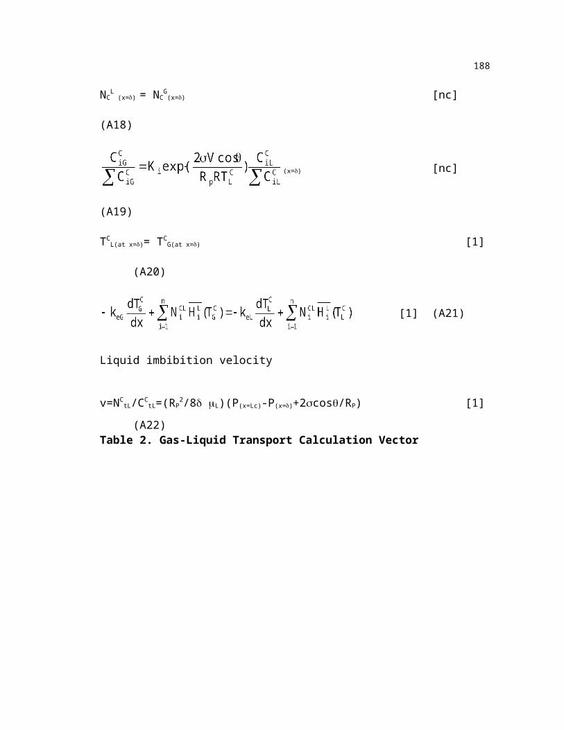
198
Appendix D Maxwell-Stefan Equations For Multicomponent TransportSolution of simultaneous mass and energy transfer equations:
For a system with n components, the number of unknowns in the problem are 2n
mole fractions at the interface (xiI and yi
I), n molar fluxes (incorporating NiL=Ni
V=NiVL )
and an interface temperature (TI). Since energy equilibrium at the interface is also
considered, it acts as a bootstrap to relate the total flux to the absolute quantities without
needing any further assumptions (of inert flux being zero or stoichiometric fluxes etc.).
Thus the total number of variables are 3n+1. The number of equations relating these
variables is
a) n-1 rate equations for the liquid phase given by
(D. 1)
where (in matrix form, (n-1)x(n-1)) (D. 2)
and Lk=(lk-ln)/lx , Dq=h.L(TI-TL)-h.
V(TG-TI) (D. 3)
( and , ) (D. 4)
b) n-1 rate equations for the vapor(gas) phase given by
(D. 5)
where (in matrix form, (n-1)x(n-1)) (D. 6)
c) n equilibrium relations (D. 7)
d) Interfacial energy balance

199
(D. 8)
e) Two more equations are necessary to complete the set and are given by mole fraction
sum for both gas and liquid compositions at the interface.
(D. 9)
(D. 10)
This completes the set of equations required to solve for all the fluxes,
compositions and temperatures. The mass and heat transfer coefficients are the corrected
values at the fluxes and can be revised based on this flux calculation until converged
values are obtained. Details of iteration for finite flux transfer coefficients can be found
in Taylor and Krishna (1993).
A.) The “Bootstrap” matrix for interphase transport
1. Bootstrap matrix for gas transport is evaluated based on interphase energy flux for
the gas -liquid interface
[ ],b i k G ik i ky L (D. 11)
where Lik k nc y ( ) /l l l (D. 12)
and l ly i ii
y , li i iV
G iL
Ly H T H T ( (@ ) (@ )) (D. 13)
For the gas-solid interface similar equations are used except the enthalpy is now of the
liquid in the solid (liquid at solid temperature).
2. Bootstrap matrix for the liquid phase is also based on the energy flux term and given
by
[ ],b i k L ik i kx L (D. 14)

200
where Lik k nc x ( ) /l l l (D. 15)
and l lx i ii
x , li i iV
G iL
Lx H T H T ( (@ ) (@ )) (D. 16)
3. Catalyst level equations have unsymmetric boundary conditions due to gas and liquid
bulk flow streams on either side of partially wetted pellets and suitable boundary
conditions have to be incorporated into the bootstrap matrix to ensure that mass
balance is satisfied in the pellets. Several bootstraps are possible in this case such as
stoichiometric fluxes, zero flux for inert component, and net zero flux for zero net
mole production. But these are not deemed suitable for the present problem. Hence
the most likely condition would be that net volumetric flux entering on the wetted
side is equal to net mass flux leaving on the dry side. This can be incorporated
directly in the fully implicit beta evaluation as
(D. 17)
or in general since beta is not evaluated at each intra-catalyst location, it can be
represented as
[ ],b i k CP ik ci kx L (D. 18)
where Lk k nc mxM M ( ) / l (D. 19)
and lmx i ii
x M (D. 20)
B) The transport matrices for interphase mass and energy flux
1. For the gas phase the low flux mass transfer coefficient matrix can be calculated as
[ ] [ ] [ ]k BG 1 (D. 21)
where [ ],, ,
By
kyki j
i
i nc
k
i kk (for i = j ) (D. 22)
[ ] ( ),, ,
B yk ki j i
i j i nc
1 1
(for i j) (D. 23)

201
Here [ ],,k
Dli ji j
where the diffusivity coefficients are calculated from infinite dilution
diffusivities (from kinetic theory) using mole fraction weighting factors. The [] matrix
is the non-ideality coefficient matrix, which is considered to be identity for the gas side.
2. The liquid phase mass transfer coefficient matrix are calculated similarly as
[ ] [ ] [ ]k BL 1 (D. 24)
where [ ],, ,
By
kyki j
i
i nc
k
i kk (for i = j ) (D. 25)
[ ] ( ),, ,
B yk ki j i
i j i nc
1 1
(for i j) (D. 26)
Here [ ],,k
Dli ji j
where the diffusivity coefficients are calculated from infinite dilution
diffusivities (using the Wilke-Chang correlation as given in Appendix E) using mole
fraction weighting factors. The [] matrix is the non-ideality coefficient matrix, which is
considered to be identity for the gas side.
C. High flux correction
1. High flux correction is important for the gas side mass and heat transfer coefficients
and has been incorporated as below.
Determine [] matrix based on the calculated fluxes
iii
t in
k
t ik
Nc k
Nc k
(D. 27)
ii it ij t in
Nc k c k
( )1 1
(D. 28)
correct the low flux mass transfer coefficient matrix by the correction as
[ ] [ ] [ ][exp([ ]) [ ]]k k Ihighflux lowflux 1 (D. 29)
where exp[] is evaluated by a Pade approximation as

202
exp[ ][ ] [ ] /[ ] [ ] /
II
22
(D. 30)
Similarly, heat transfer coefficient is also corrected by
hti piN C
h (D. 31)
h hhighflux lowflux ht ht / ((exp( ) )1 (D. 32)

203
Appendix E Evaluation Of Parameters For Unsteady State ModelLiquid phase infinite dilution diffusivities are determined using the Wilke and Chang
(1955) correlation as
(E. 1)
Gas phase infinite dilution diffusivities are determined as given by Reid et al. (1987)
(E. 2)
These are corrected for concentration effect using the Vignes (1966) correlation as
recommended by taylor and Krishna (1993)
(E. 3)
The film thickness for gas and liquid phase is determined using the Sherwood correlation
by using the particle diameter as the characteristic dimension as
(E. 4)
The Schmidt number used in the above correlation is different for each species and can
give multiple values of film thickness according to the species used in the calculation.
This dilemma is resolved using either an average value of diffusivity or the diffusivity of
the gas phase key reactant.
Heat transfer coefficients for gas and liquid phase are determined using either the Nusselt
(E.5 ) number or the Chilton-Colburn analogy (E.6) as recommended by Taylor and
Krishna (1993)

204
(E. 5)
(E. 6)
The interfacial areas required for interphase transport (gas-liquid, liquid-solid, and gas-
solid) are evaluated using the following correlations. ,
(E. 7)
(E. 8)
(E. 9)
The modeling of liquid phase non-ideality effects can be done by using any of the several
approaches available (such as simple 2 parameter models such as the Margules, Van-
Laar, or the Wilson equation or complex rigorous methods such as the UNIQUAC or
UNIFAC). In the present study, the Wilson equation was used to obtain the equilibrium
constants as well as the activity matrix ([]) as given by the equations below.
For the Wilson equation, the excess energy Q is given by
(E. 10)
where
(E. 11)
(E. 12)

205
First and second derivatives of Q w.r.t. compositions i and j are then given by
(E. 13)
(E. 14)
The activity coefficients needed for calculating the equilibrium constants are then given
directly by
(E. 15)
The thermodynamic factors (ij) required for the nonideality matrix are given by
(E. 16)

206
Appendix F. Experimental Data From Steady And Unsteady Experiments
Table F.1 Performance of Downflow and Upflow Reactors under Gas and Liquid
Limited Conditions
Mode Space time (s) Pressure
(psig)
Feed Concentration
(% v/v)
Conversion
Upflow 32 30 7.8 0.03653 30 7.8 0.06580 30 7.8 0.079155 30 7.8 0.169297 30 7.8 0.447
Downflow 32 30 7.8 0.05453 30 7.8 0.08880 30 7.8 0.133155 30 7.8 0.28297 30 7.8 0.638
Upflow 155 200 3.1 0.729105 200 3.1 0.51064 200 3.1 0.31946 200 3.1 0.247
Downflow 155 200 3.1 0.63105 200 3.1 0.42864 200 3.1 0.28946 200 3.1 0.231
Upflow 190 30 3.1 --155 30 3.1 0.404105 30 3.1 0.26564 30 3.1 0.188
Downflow 190 30 3.1 0.534155 30 3.1 0.397105 30 3.1 0.25464 30 3.1 0.183

207Table F.1 Performance of Downflow and Upflow Reactors under Gas and Liquid Limited Conditions (continued)
Upflow 190 200 4.8 --155.4 200 4.8 0.750105.2 200 4.8 0.50564.5 200 4.8 0.32545.6 200 4.8 0.252
Downflow 190 200 4.8 0.801155.4 200 4.8 0.735105.2 200 4.8 0.44864.5 200 4.8 0.29045.6 200 4.8 --

208
Table F.2 Pressure Effects on Upflow and Downflow Performance
Mode Space time (s) Pressure
(psig)
Feed Concentration
(% v/v)
Conversion
Upflow 190 30 3.1 0.462155 30 3.1 0.405105 30 3.1 0.26664 30 3.1 0.18846 30 3.1 --190 100 3.1 0.874155 100 3.1 0.711105 100 3.1 0.49764 100 3.1 0.32546 100 3.1 --190 200 3.1 --155 200 3.1 0.729105 200 3.1 0.5164 200 3.1 0.31946 200 3.1 0.247
Downflow 190 30 3.1 0.534155 30 3.1 0.397105 30 3.1 0.25464 30 3.1 0.18346 30 3.1 --190 100 3.1 0.648155 100 3.1 0.599105 100 3.1 0.4264 100 3.1 0.27946 100 3.1 --190 200 3.1 --155 200 3.1 0.632105 200 3.1 0.42964 200 3.1 0.28946 200 3.1 0.231

209Table F.2 Pressure Effects on Upflow and Downflow Performance (continued)
Downflow 214 30 4.8 --190 30 4.8 0.357155 30 4.8 0.262105 30 4.8 0.1565 30 4.8 0.112214 100 4.8 0.741190 100 4.8 --155 100 4.8 0.55105 100 4.8 0.36365 100 4.8 0.236214 200 4.8 --190 200 4.8 0.801155 200 4.8 0.735105 200 4.8 0.44865 200 4.8 0.29
Upflow 214 30 4.8 --190 30 4.8 0.385155 30 4.8 0.243105 30 4.8 0.17365 30 4.8 0.1246 30 4.8 --214 100 4.8 1190 100 4.8 --155 100 4.8 0.746105 100 4.8 0.41165 100 4.8 0.25646 100 4.8 --214 200 4.8 --190 200 4.8 --155 200 4.8 0.75105 200 4.8 0.50565 200 4.8 0.32546 200 4.8 0.252

210
Table F.3 Alpha-methylstyrene Feed Concentration Effect on Upflow and Downflow
Performance
Mode Space time (s) Pressure
(psig)
Feed Concentration
(% v/v)
Conversion
Downflow 214 100 3.1 --190 100 3.1 --155 100 3.1 0.41105 100 3.1 0.23880 100 3.1 0.19865 100 3.1 0.158214 100 4.8 0.741190 100 4.8 --155 100 4.8 0.55105 100 4.8 0.36380 100 4.8 --65 100 4.8 0.236214 100 6.8 --190 100 6.8 0.648155 100 6.8 0.599105 100 6.8 0.4280 100 6.8 --65 100 6.8 0.279
Upflow 214 100 3.1 --190 100 3.1 0.874155 100 3.1 0.711105 100 3.1 0.49780 100 3.1 --65 100 3.1 0.328214 100 4.8 1190 100 4.8 --155 100 4.8 0.746105 100 4.8 0.41180 100 4.8 --65 100 4.8 0.256214 100 6.8 --

211Table F.3 Alpha-methylstyrene Feed Concentration Effect on Upflow and Downflow Performance (continued)
190 100 6.8 --155 100 6.8 0.465105 100 6.8 0.26780 100 6.8 0.21565 100 6.8 0.175
Downflow 190 200 3.1 --155 200 3.1 0.632105 200 3.1 0.42964 200 3.1 0.28946 200 3.1 0.231190 200 4.8 0.801155 200 4.8 0.735105 200 4.8 0.44864 200 4.8 0.2946 200 4.8 --
Upflow 155 200 3.1 0.729105 200 3.1 0.5164 200 3.1 0.31946 200 3.1 0.247155 200 4.8 0.75105 200 4.8 0.50564 200 4.8 0.32546 200 4.8 0.252

212
Table F. 4 Performance Comparison with Bed Dilution
Mode Space time (s) Pressure
(psig)
Feed Concentration
(% v/v)
Conversion
Downflow 190 30 6.7 0.319155 30 6.7 0.247105 30 6.7 0.15364 30 6.7 0.103
Upflow 190 30 6.7 0.283155 30 6.7 0.224105 30 6.7 0.15264 30 6.7 0.102
Downflow 155 200 3.1 0.715105 200 3.1 0.50164 200 3.1 0.31246 200 3.1 0.241
Upflow 155 200 3.1 0.72105 200 3.1 0.48264 200 3.1 0.30246 200 3.1 0.237
Downflow 190 30 3.18 0.651155 30 3.18 0.451105 30 3.18 0.25164 30 3.18 0.18246 30 3.18 --190 30 6.7 0.32155 30 6.7 0.248105 30 6.7 0.15464 30 6.7 0.10446 30 6.7 --190 200 3.18 0.816155 200 3.18 0.501105 200 3.18 0.31364 200 3.18 0.241

213Table F.4 Performance Comparison with Bed Dilution
46 200 3.18 --190 200 6.7 0.916155 200 6.7 0.786105 200 6.7 0.50464 200 6.7 --46 200 6.7 0.228
Upflow 190 30 3.18 0.618155 30 3.18 0.418105 30 3.18 0.25764 30 3.18 0.15646 30 3.18 --190 30 6.7 0.284155 30 6.7 0.225105 30 6.7 0.15264 30 6.7 0.10246 30 6.7 --190 200 3.18 --155 200 3.18 0.729105 200 3.18 0.48264 200 3.18 0.30346 200 3.18 0.241190 200 6.7 --155 200 6.7 0.827105 200 6.7 0.48764 200 6.7 0.30746 200 6.7 0.233

214
Table F. 5 Gas Velocity Effect on Upflow and Downflow Performance
Mode Space time (s) Pressure
(psig)
Feed Concentration
(% v/v)
Conversion
Downflow 1.39 100 4.1 0.2872.78 100 4.1 0.2984.18 100 4.1 0.2905.57 100 4.1 0.2776.97 100 4.1 0.2828.36 100 4.1 0.279
Upflow 1.39 100 4.1 0.3052.78 100 4.1 0.3014.18 100 4.1 0.2985.57 100 4.1 0.2906.97 100 4.1 0.3028.36 100 4.1 0.293

215
Table F. 6 Experimental Data from High Pressure Slurry Experiments
Time(min)
Alpha-methylstyrene (% v/v)
Cumene(% v/v)
Hydrogen Concentration
(mol/m3)
Alpha-methylstyrene Concentration
(mol/m3)
Cumene Concentration
(mol/m3)
0 4.89 6.56 14.08 377.17 471.3420 4.71 6.73 14.08 363.88 483.5240 4.48 7.12 14.08 345.60 511.7060 4.33 7.34 14.08 333.97 526.9390 4.11 7.44 14.08 317.36 534.54110 3.64 7.69 14.08 280.80 552.05140 3.25 8.22 14.08 250.89 590.13170 3.10 8.63 14.08 239.26 619.82210 2.88 8.82 14.08 222.65 633.53
0 4.20 3.75 14.08 324.00 269.5610 3.96 3.90 14.08 305.73 280.2220 3.73 3.88 14.08 288.28 278.6940 3.64 4.06 14.08 280.80 291.6460 3.49 4.40 14.08 269.17 316.0090 3.13 4.67 14.08 241.76 335.80110 2.93 4.78 14.08 225.97 343.42140 2.63 5.12 14.08 202.71 367.78170 2.41 5.37 14.08 186.09 386.06210 2.14 5.65 14.08 165.32 405.86240 1.89 5.96 14.08 146.22 427.94
0 4.21 2.22 14.08 324.83 159.1410 4.13 2.26 14.08 319.02 162.1920 3.97 2.47 14.08 306.56 177.4230 3.74 2.64 14.08 289.11 189.6050 3.57 2.82 14.08 275.82 202.5570 3.36 3.34 14.08 259.20 239.86120 2.81 3.66 14.08 216.83 262.70150 2.38 4.14 14.08 183.60 297.73240 1.81 4.66 14.08 139.57 335.04

216
Table F.6 Experimental Data from High Pressure Slurry Experiments (continued)
0 4.90 2.32 35.76 378.00 166.7610 4.49 2.63 35.76 346.43 188.8420 3.59 3.38 35.76 277.48 242.9040 3.02 4.14 35.76 233.45 297.7370 2.13 4.90 35.76 164.49 351.79100 1.39 5.78 35.76 107.17 414.99
0 3.97 2.53 35.76 306.56 181.9910 3.48 2.75 35.76 268.34 197.2220 2.88 3.28 35.76 222.65 235.2940 2.43 3.83 35.76 187.76 274.8970 1.82 4.57 35.76 140.40 328.19100 1.27 4.82 35.76 98.03 346.46
0 7.17 1.96 35.76 553.30 140.8710 6.80 2.20 35.76 525.05 158.3820 6.26 2.78 35.76 483.51 199.5030 5.91 3.02 35.76 456.10 217.0150 5.68 3.29 35.76 438.65 236.0570 5.43 3.35 35.76 419.54 240.62100 5.15 3.71 35.76 397.94 266.51140 4.98 3.92 35.76 384.65 281.74180 4.82 4.22 35.76 372.19 303.06220 4.48 4.58 35.76 345.60 328.95
0 4.29 2.06 35.76 331.48 147.7210 3.94 2.28 35.76 304.06 163.7120 3.40 2.84 35.76 262.53 204.0740 2.75 3.50 35.76 212.68 251.2870 2.13 4.08 35.76 164.49 293.16100 1.56 4.93 35.76 120.46 354.08
0 2.12 1.35 35.76 163.66 96.7010 1.87 1.53 35.76 144.56 109.6520 1.62 1.98 35.76 125.45 142.3930 1.40 2.04 35.76 108.00 146.2050 1.13 2.13 35.76 87.23 153.0570 1.04 2.35 35.76 80.59 169.04100 0.52 2.55 35.76 39.88 183.51

217
Table F.6 Experimental Data from High Pressure Slurry Experiments (continued)
0 5.43 1.89 64.90 419.54 135.5410 4.91 2.33 64.90 378.83 167.5220 4.18 3.14 64.90 322.34 225.3930 3.76 3.60 64.90 289.94 258.8950 3.28 3.90 64.90 253.39 280.2270 2.94 4.53 64.90 226.80 325.1490 2.71 4.62 64.90 209.36 331.99120 2.52 4.71 64.90 194.40 338.09150 2.39 5.02 64.90 184.43 360.93
0 4.30 2.00 64.90 332.31 143.9110 4.01 2.55 64.90 309.88 183.5120 3.33 3.02 64.90 256.71 217.0130 3.16 3.24 64.90 244.25 233.0150 2.98 3.45 64.90 230.13 247.4770 2.65 3.68 64.90 204.37 264.2290 2.49 3.99 64.90 191.91 286.31120 2.31 4.19 64.90 178.62 300.77150 2.01 4.39 64.90 155.36 315.24
0 7.56 1.83 64.90 584.04 131.7310 7.41 2.04 64.90 572.41 146.2020 7.05 2.51 64.90 544.16 180.4630 6.84 2.58 64.90 528.37 185.0370 6.49 2.95 64.90 500.96 211.68100 6.38 3.13 64.90 492.65 224.63140 6.04 3.55 64.90 466.07 255.09180 5.89 3.61 64.90 454.44 259.66
0 1.90 2.08 64.90 147.05 149.255 1.49 2.34 64.90 114.65 168.2810 1.18 2.62 64.90 91.39 188.0820 1.04 2.81 64.90 80.59 201.7950 0.81 3.07 64.90 62.31 220.8270 0.56 2.97 64.90 43.20 213.21100 0.50 3.10 64.90 38.22 222.34

218
Table F.6 Experimental Data from High Pressure Slurry Experiments (continued)
0 3.71 2.16 86.80 286.62 155.345 3.51 2.51 86.80 270.83 180.4610 3.31 2.68 86.80 255.88 192.6520 3.26 3.01 86.80 251.73 216.2550 2.82 3.37 86.80 217.66 242.1470 2.74 3.34 86.80 211.85 239.86100 2.63 3.53 86.80 202.71 253.56140 2.34 3.81 86.80 180.28 273.36180 2.18 4.07 86.80 168.65 292.40

219
Table F.7 Unsteady State Performance Comparison under Gas and Liquid Limited
Conditions
Pressure(psig)
Feed Concentra
tion (mol/m3)
Flow Rate,
Qmean (ml/min)
Space time (s)
Cycle Time (s)
Cycle SplitConversion
30 1484 4.5 1199 Steady Steady 0.254830 1484 7.0 771 Steady Steady 0.2330 1484 12.0 449 Steady Steady 0.161330 1484 3.6 1499 60 0.5 0.436530 1484 7.0 771.08 60 0.5 0.285760 690 3.2 1686.7 Steady Steady 0.75560 690 7.0 771.08 Steady Steady 0.70360 690 12.5 431.80 Steady Steady 0.47360 690 19 284.08 Steady Steady 0.304560 690 2.1 2570.2 60 0.5 0.7960 690 4.5 1199.4 60 0.5 0.62160 690 10.0 539.7 60 0.5 0.420560 690 12.0 449.8 60 0.5 0.38
Table F.8 Effect of Cycle Split on Performance under Gas Limited Conditions
Pressure(psig)
Feed Concentra
tion (mol/m3)
Flow Rate,
Qmean (ml/min)
Space time (s)
Cycle Time (s) Cycle Split Conversion
30 1484 7.0 771.0 Steady Steady 0.2330 1484 7.0 771.0 60 0.5 0.293630 1484 7.0 771.0 60 0.33 0.342230 1484 7.0 771.0 60 0.25 0.3577

220
Table F. 9 Total Cycle Period / Liquid Mass Velocity Effect (Liquid Solid Contacting)
Pressure(psig)
Feed Concentra
tion (mol/m3)
Flow Rate,
Qmean (ml/min)
Space time (s)
Cycle Time (s) Cycle Split Conversion
30 1553 7.0 771.0 Steady Steady 0.205930 1553 7.0 771.0 18 0.33 0.218830 1553 7.0 771.0 30 0.33 0.260530 1553 7.0 771.0 60 0.33 0.292230 1553 7.0 771.0 120 0.33 0.233430 1579 4.0 1344.21 Steady Steady 0.242630 1579 4.0 1344.21 20 0.25 0.260930 1579 4.0 1344.21 40 0.25 0.305930 1579 4.0 1344.21 60 0.25 0.2841930 1579 4.0 1344.21 160 0.25 0.235530 1579 4.0 1344.21 320 0.25 0.163730 1579 2.0 2688.4 Steady Steady 0.285830 1579 2.0 2688.4 20 0.25 0.393330 1579 2.0 2688.4 48 0.25 0.444630 1579 2.0 2688.4 120 0.25 0.436730 1579 2.0 2688.4 240 0.25 0.3996

221
Table F.10 Effect of Cycling Frequency on Performance under Gas Limited Conditions
Pressure(psig)
Feed Concentra
tion (mol/m3)
Flow Rate,
Qmean (ml/min)
Space time (s)
Cycle Time (s) Cycle Split Conversion
30 1494 3.0 1792.2 Steady Steady 0.307730 1494 3.0 1792.2 6.0 (0.166 Hz) 0.5 0.329330 1494 3.0 1792.2 12.0
(0.0833 Hz)0.5 0.3815
30 1494 3.0 1792.2 24.0 (0.0416 Hz)
0.5 0.3954
30 1494 3.0 1792.2 48.0 (0.0208 Hz)
0.5 0.4123
30 1494 3.0 1792.2 96.0 (0.0104 Hz)
0.5 0.4342
30 1494 3.0 1792.2 192.0 (0.0052 Hz)
0.5 0.3815
Table F. 11 Effect of Pressure (Transition from Gas Liquid to Liquid Limited
Conditions)
Pressure(psig)
Feed Concentra
tion (mol/m3)
Flow Rate,
Qmean (ml/min)
Space time (s)
Cycle Time (s) Cycle
Split
Conversion
30 1545 2.5 2150.7 Steady Steady 0.406530 1545 2.5 2150.7 60 0.33 0.462660 1545 2.5 2150.7 Steady Steady 0.5141260 1545 2.5 2150.7 60 0.33 0.6067120 1545 2.5 2150.7 Steady Steady 0.6109120 1545 2.5 2150.7 60 0.33 0.7167180 1545 2.5 2150.7 Steady Steady 0.6721180 1545 2.5 2150.7 60 0.33 0.7469

222Table F.12 Effect of Cycle Time and Split at Higher Feed Concentration (~ 30 % v/v AMS)
Pressure(psig)
Feed Concentr
ation (mol/m3)
Flow Rate,
Qmean (ml/min)
Space time (s)
Cycle Time (s) Cycle
Split
Conversion
30 1484.0 7.0 771.0 Steady Steady 0.2330 1484.0 7.0 771.0 60 0.5 0.29330 1484.0 7.0 771.0 60 0.33 0.342230 1484.0 7.0 771.0 60 0.25 0.357730 2082.0 3.0 1799.2 Steady Steady 0.23930 2082.0 3.0 1799.2 60 0.5 0.263430 2082.0 3.0 1799.2 60 0.25 0.280430 2082.0 3.0 1799.2 60 0.1 0.2874

223Table F.13 Effect of Cycling frequency at Higher Feed Concentration (~ 30 % v/v AMS)
Pressure(psig)
Feed Concentr
ation (mol/m3)
Flow Rate (ml/min) Qmean
Space time (s)
Cycle Time (s)
Cycle Split Conversion
60 2084 3.0 1792.2 Steady Steady 0.2360 2084 3.0 1792.2 6.0
(0.166 Hz)0.5 0.2408
60 2084 3.0 1792.2 12.0(0.0833 Hz)
0.5 0.2635
60 2084 3.0 1792.2 24.0(0.0416 Hz)
0.5 0.2726
60 2084 3.0 1792.2 48.0(0.0208 Hz)
0.5 0.2844
60 2084 3.0 1792.2 96.0(0.0104 Hz)
0.5 0.2647
60 2084 3.0 1792.2 Steady Steady 0.2360 2084 3.0 1792.2 10.0
(0.1 Hz)0.2 0.2483
60 2084 3.0 1792.2 30.0(0.033 Hz)
0.2 0.2546
60 2084 3.0 1792.2 90.0(0.0111 Hz)
0.2 0.2698
60 2084 3.0 1792.2 180.0(0.0055 Hz)
0.2 0.2562
Table F. 14 Base Flow Pulsing under Liquid Limited Conditions (High Pressure and Low
Feed Concentration) (~ 5 % v/v feed concentration)
Pressure(psig)
Feed Concentr
ation (mol/m3)
Flow Rate,
Qmean (Qbase) (ml/min)
Space time (s)
Cycle Time (s)
Cycle Split Conversion
150 784 5.0 2148.6 Steady Steady 0.7881150 784 5.0 2148.6 30 0.1 0.8595150 784 5.0 2148.6 50 0.1 0.871150 784 5.0 2148.6 100 0.1 0.877150 784 5.0 2148.6 200 0.1 0.8812

224

225
Appendix G. Simulation of Flow using CFDLIBA. Problem Definition
Predicting the fluid dynamics of trickle bed reactors is important for their proper
scale-up to industrial scale. Previous studies have resorted primarily to prediction of
overall phase holdup and pressure drop based on an empirical or phenomenological
approach. Recent advances in simulation of multiphase flow and development of robust
codes that can handle two and three dimensional simulations have made flow simulation
feasible in complex flows such as those observed in trickle beds. CREL has access to the
CFDLIB multiphase flow codes developed by the Los Alamos National Laboratory
which are used in this study.
B. Research Objectives
The objective of this study is to simulate the effect of single point and multi-point
inlet flow distribution on the flow distribution inside the reactor and to expand the test
database beyond the preliminary simulations presented by Kumar (1995,1996). This
involves modification of conventional drag and interfacial exchange terms implemented
in CFDLIB using drag formulations developed at CREL as well as those available in
trickle bed literature. Another objective is to study the influence of surface tension on the
spreading of liquid in single and multi-point inlet conditions. This will serve as a
benchmark for comparison with experimental velocities and phase holdup data which
have not yet been reported in the open literature.

226
C. Research Accomplishments
C1. Modeling Interphase Exchange and Interfacial Tension Terms
The underlying equations for the CFDLIB code have been discussed in detail in
earlier reports by Kumar (1996) and can be found in Kashiwa et al. (1994). The special
case of one fixed phase (the catalyst bed) has also been incorporated in the code for
single and two phase flow simulation. The important terms in simulating trickle bed
reactors is the drag equation and the influence of phasic pressure difference due to
interfacial tension. Phenomenological models developed at CREL by Holub (1990) are
incorporated in simulating the drag between the stationary solid phase and each of the
flowing phases. The code models the drag force in terms of phase fractions and relative
velocity given for any combination of phases k and l as
F X u uD k l k l kl k l( ) ( ) (1)
where the Xkl is modeled by the modified Ergun equation (Holub, 1990, Saez and
Carbonell, 1985) with Ergun constants either determined by single phase experiments or
using universal values.
XEGa
EGa
gul S
S
L
L
L
L
L
L
LS S( )
( ) Re Re| |( )
11
31 2
2
r
(2)
XEGa
EGa
guG S
S
G
G
G
G
G
G
GS S( )
( ) Re Re| |( )
11
31 2
2
r
(3)
For gas-liquid drag either no interaction is assumed or interaction based on a drag coefficient is used as
XC udG L
L D GL
L p( )
. | |
0 75r
(4)

For modeling interfacial tension the famous Leverett’s J function (Dankworth et al.,
1990) is used to yield the difference between the gas and liquid pressure calculated in the
code in terms of the interfacial tension ( ), bed permeability (k) and phase fractions as
p pkL G
S S L
L
10 48 0 036
11 2
/
. . .ln( )
(5)
The bed permeability (k) is related to Erguns constant E1 and equivalent particle diameter
(de) as
(( ) / )( )( )
/11
1 2 1
SS
S e
kEd
(6)
The simulations are conducted both by discounting and incorporating the above equation
and results presented in the next section.
C2. Simulation of Test Cases: Results and Discussion
Case I: (Reactor Dimensions 60x11 cm, eB=0.4, dp= 1.5 mm,
UsL=0.036 cm/s, UsG=3.63 cm/s)
(a) Point Source Inlet with Uniform Bed Porosity
(b) Point Source Inlet: Including Surface Tension Effects
For the test case of point source liquid inlet when the surface tension forces are
ignored, Figure 1 shows that the liquid stays mainly in the central core without much
spreading and with almost negligible wall flow. For the case where interfacial tension
was included and modeled using a capillary pressure given by the Leverett Function,
significant liquid spreading was observed at a depth of over 10 cm from the inlet. Figures
2 and 3 show the contours of the liquid holdup and development of the velocity and
holdup profile down the reactor to a constant and fairly uniform flow profile at the
reactor exit. In this case some wall flow is indeed observed after a depth of 28 cm as

shown in Figure 2. This is corroborated by visual and photography experiments done at
CREL on a 2D bed (Jiang, 1997) and by the tomography results of Lutran et al.(1991).
Case II: Uniform Liquid and Gas Inlet : No Surface Tension Effects, Uniform Porosity
everywhere except at the wall and exit section (Reactor Dimensions 28.8x7.2 cm, eB=0.4
in the core and eB=0.5 at the wall, dp= 3 mm, UsL=0.1 cm/s, UsG=5.0 cm/s)
(a) No Gas Flow (Unsaturated Liquid Flow)
(b) Low Gas Flow (Low Interaction)
(c) High Gas Flow (Moderate Interaction)
For the uniform distribution tests, it was assumed that the wall zone extends three
particle diameters from the wall and the exit of the reactor for which a higher porosity
was assigned, and to the rest of the central core a uniform lower porosity was assigned. It
is much more difficult to discern the flow distribution profiles in this case as compared to
Case I, primarily due to local non-uniformity in the phase holdups and velocity. The only
obvious effect is that of higher wall flow of gas at the wall as compared to the central
core as depicted in Figure 4 for the moderate gas flow rate (case IIc). For the low and
zero gas flow rate such clear gas wall flow was not observed. Larger reactor size tests for
this case are underway and results will be reported in future reports.
Case III: Multipoint Inlet of Liquid (Including Surface Tension Effects) (Reactor
Dimensions 60x23 cm, eB=0.4, dp= 1.5 mm, UsL=0.052 cm/s, UsG=3.47 cm/s)
This case is shown to illustrate conditions similar to industrial distributors with
multiple points of a large distributor each of which is similar to that in Case I. The
holdup contour plot shown in Figure 5 shows underutilization of the top part of the bed
indicating the required pitch between distributor inlet points should be smaller than 5 cm
that was used here to achieve better distribution. This mal-distribution may result in

zones where hotspots may develop such as in the gas phase adjacent to the boundary of
the gas-liquid zone (where both gas and liquid reactants are abundantly supplied to the
catalyst for the case of non-volatile liquid reactant) and in the gas rich zones in the case
of volatile liquid reactant between the well irrigated zones. Such simulations can yield
direct information as to the extent and consequence of maldistribution due to well
separated multi-point inlets typical in industrial reactors.
D. Future Work
The potential for CFDLIB to predict flow distribution in trickle bed reactors is
shown in this report for several test cases. Further work will encompass simulation of
more complex reactor geometry and flow situations and extension of flow simulations
from cold-flow modeling to reactive cases where accurate prediction of product
distribution and hot-spot formation is crucial to optimal and safe operation of pilot and
large scale reactors.
E. Nomenclature
CD = Drag Coefficient
dp = Particle Diameter
de = Particle Equivalent Diameter
E1,E2 = Erguns Constants
FD(kl) = Drag Force between Phases k and l.
g = Gravitational Acceleration
Gaa = Phase Galileo Number
k = Bed Permeability

pa = Phase Pressure
Rea = Phase Reynolds Number
uk = Interstitial Velocity of Phase k.
Xkl = Interphase Exchange Coefficient between phases k and l.
Greek Symbols
k = Phase Fraction of Phase k.
ra = Phase Density
= Interfacial Tension
F. References
1. Dankworth, D. C., Kevrekidis, I.G., and Sundaresan, S., Time Dependent
Hydrodynamics in Multiphase Reactors, Chem. Eng. Sci., Vol. 45, No. 8, pp. 2239-
2246 (1990).
2. Holub, R. A., Hydrodynamics of Trickle Bed Reactors. Ph.D. Thesis, Washington
University in St. Louis, MO (1990).
3. Jiang. Y., Unpublished Results on 2-D Trickle Bed Reactors using Point and Uniform
Liquid Inlet Distributors (1997).
4. Kashiwa, B. A., Padial, N. T., Rauenzahn, R. M. and W. B. VanderHeyden , A Cell
centered ICE Method for Multiphase Flow Simulations, ASME Symposium on
Numerical Methods for Multiphase Flows, Lake Tahoe, Nevada (1994)
5. Kumar, S. B., Simulation of Multiphase Flow Systems using CFDLIB code CREL
Annual Meeting Workshop (1995).
6. Kumar, S. B., Numerical Simulation of Flow in Bubble Columns, CREL Annual
Report (1996).

7. Lutran, P. G., Ng, K. M. and Delikat, E. P., Liquid distribution in trickle beds: An
experimental study using Computer-Assisted Tomography. Ind. Engng. Chem. Res.
30 (1991)
8. Saez, A. G. and Carbonell, R. G., Hydrodynamic Parameters for Gas-Liquid Cocurrent
Flow in Packed Beds, AIChE J. 31, 52 (1985)
Title: Creator: TECPLOTCreationDate:
Figure 1: Liquid Holdup Contours for Single Point Source Inlet (Case Ia)

Title: Creator: TECPLOTCreationDate:
Figure 2: Liquid Holdup Contours for Single Point Source Inlet Including Interfacial Tension
Effects (Case Ib)
0
0.01
0.02
0.03
0.04
0.05
0.06
0.07
0.08
0 5 10X(cm)
Liqu
id H
oldu
p (e L
)
Y=50 cm from InletY=30 cm from InletY=10 cm from Inlet
0.00E+00
2.00E-01
4.00E-016.00E-01
8.00E-01
1.00E+00
1.20E+00
1.40E+001.60E+00
1.80E+00
2.00E+00
0 5 10
X(cm)
Liqu
id V
eloc
ity (V
iL)
Y=50 cm from InletY=30 cm from InletY=10 cm from Inlet
Figure 3: Liquid Holdup and Velocity Profiles for Single Point Source Liquid Inlet (with Interfacial
Tension Effects)(Case Ib)

0.35
0.4
0.45
0.5
0.55
0 1.8 3.6 5.4 7.2
X(cm)
Gas
Hol
dup
(eG
)
Y=27 cm from Inlet
Y=18 cm from Inlet
Y=9 cm from Inlet
3
3.5
4
4.5
5
5.5
6
0 1.8 3.6 5.4 7.2
X(cm)G
as F
low
(e G
*ViG
)
Y=27 cm from InletY=18 cm from InletY=9 cm from Inlet
Figure 4: Gas Holdup and Flow Profiles for Case IIc (Moderate Gas Flow)
Title: Creator: TECPLOTCreationDate:
Title: Creator: TECPLOTCreationDate:

Figure 5: Liquid Holdup and Velocity for Multipoint Inlet Distributor (Case III).

Title: Creator: TECPLOTCreationDate:
Title: Creator: TECPLOTCreationDate:
Appendix H. Improved Prediction of Pressure Drop in High Pressure Trickle Bed ReactorsA. Problem Definition
Trickle-bed reactors are fixed beds of catalyst particles contacted by downflow of gas and liquid. They are used widely in petroleum, petrochemical, and chemical industry and are usually operated at high pressure (20-30 MPa). A basic understanding of the hydrodynamics of trickle bed reactors is essential to their design, scale-up, scale-down, and performance. Pressure drop and liquid holdup are important operational parameters. Several correlations have been proposed in recent years to predict pressure drop and holdup at low and high pressure conditions (as listed in Table 1). The Holub et al. (1993) phenomenological model predicts pressure drop and liquid holdup in trickle flow regime better than the available correlations at atmospheric pressure. Al-Dahhan and Dudukovic (1994) noted that although it also predicts pressure drop and liquid holdup better than all the reported high pressure correlations (Table 1), it underpredicts them at high pressure and high gas flow rates within trickle flow regime. This is because the interactions between phases increase at high pressure and high gas flow rate which are not currently accounted for in the present simplest form of Holub et al. model.
The Holub et al. (1993) model has been extended to account for the interaction between the gas and liquid phases by incorporating the velocity and the shear slip factors between the phases. It is necessary to examine the extended model predictions and the nature and numerical values of the correction factors (shear slip factor, fs and velocity slip factor, fv) and their contribution to the prediction of pressure drop and holdup.
B. Research Objectives
The objective of this study is to examine the prediction of previous pressure drop and holdup prediction correlations and Holub’s (1992) simple and extended model for high pressure data. Based on the predictions for high pressure, develop correlations for the shear and velocity slip factors (fs and fv, respectively) and estimate pressure drop and holdup predictions at moderate interaction conditions encompassing high pressure and high gas flow rates.
C. Research Accomplishments
Holub et al. (1993), (1992) proposed a phenomenological model based on representation of the complex geometry of the actual void space in a packed bed of particles at the pore level by a single flat walled slit of average half width. The developed
model is a modified Ergun equation that ties together the pressure drop and holdup in trickle flow regime (Table 1).
E1 and E2 are the Ergun constants that characterize the bed. They are determined from single phase (gas) flow through the packing of interest (dry bed). Hence, this simplest form does not contain any parameters which need to be fitted to two phase flow data and neglects the interaction between gas and liquid phases. As a result the model predicts pressure drop and liquid holdup better than the available correlations only in the region of low interaction between the phases, at atmospheric pressure and at low flow rates (Holub et al., (1993,1992); Holub, (1990)). Al-Dahhan and Dudukovic (1994) noted that although the model also predicts pressure drop and liquid holdup better than the recently reported high pressure correlations (Larachi et al., (1991); Wammes et al., (1991); Ellman et al., (1988, 1990)) (Table 1), it systematically underpredicts them at high pressure and high gas flow rates. Under these conditions, the relative error in pressure drop prediction (~-48%) is more noticeable compared to that of holdup prediction (~-9%). This is because the interaction between phases increases at high pressure and high gas flow rate which were not accounted for in the original form of the Holub's model .
The degree of interaction between the gas and liquid phases can be accounted for by incorporating the velocity and shear slip factors between the phases. Holub (1990) and Holub et al. (1993) derived a detailed model based on the two phase flow momentum balance for the slit, which incorporates the velocity slip factor (fv) and the shear slip factor (fs) as shown below.
C1. The Extended Model
The degree of interaction between the gas and liquid phases accounted for by
1. Velocity slip factor (fv)ViG=fv ViL
2. Shear slip factor (fs) iL=fs iG
Equations based on the two phase flow momentum balance for the slit
GB
B L
G v G i
G
G v G i
G
E fGa
E fGa
ee e
e e3
1 22(Re Re ) (Re Re )
Re( )i
iL p
L B
V D
n e1

LB
L
L
L
L
Ls
G
L
G
LL
EGa
EGa
f
ee
ee
rr
31 2
2
1Re Re
( )
Re i Lh 0 5 hL Re ( . ln( ))i L 3 05 5 h 5 30 hL Re ( . . ln( ))i L 5 5 2 5 h hL 30
where
L
L
GL L
L
Bs
G
L
G
L
G
LEGa f
10 11
0 75 3( )( )
.
nn
ee
ee
rr
hee
ee
rrL L L
L
Bs
G
L
G
L
G
LEGa f
15
11
0 25
3
( )( ).
and
LG
LG 1 1
rr
( )
Physical Interpretation of fs and fv
fs fv0 0 No Interaction1 1 Continuity of profiles between phases
<0 <0 Circulation
Case 1: Case 2:
fs = 0.0 f xs G L 4 4 10 2 0 15 0 15. Re Re. .
fv = 0.0 fv L G 2 3 0 05 0 05. Re Re. .
fs and fv characterize the degree of phase interaction at the gas-liquid interface. Hence, when fs=fv=0 (i.e., no interaction occurs), the extended model simplifies to the Holub et al. model shown in Table 1. The rationale behind assuming fs=fv=0 is that for atmospheric pressure data, Holub et al. (1993) have shown that fv and fs can both be zero (no interaction) with only a small increase in error over the observed minimum error. However, this is not the case when high interaction between the phases occurs at high pressure and high gas flow rate in the trickle flow regime (Al-Dahhan and Dudukovic, (1994)). Accordingly, the model represented by the extended model equations is

suggested as a two phase flow form of the Ergun equation containing the two phase interaction parameters, fs and fv, which must be determined from two phase flow experimental data. Ergun's constants E1 and E2, characterize the bed, and are still determined from single (gas) phase flow experiments. The last equation in the model is an implicit equation in liquid holdup formed by equating the dimensional pressure gradient in the gas and liquid phase and is solved for liquid holdup from which pressure drop is then evaluated.
C2. Results
Experimental data of Al-Dahhan (1993) and Al-Dahhan and Dudukovic (1994) that cover low to high pressure and gas flow rates are used to evaluate fv and fs using the extended model. Due to the limited number of data points available (see Table 2), it was not possible to observe a strong discernible dependence of fs and fv with either ReL or ReG. Therefore, correlations for fs and fv are developed by fitting the values of fs and fv based on minimizing the pressure drop error. The correlation can be used to predict f s and fv as the two phase flow parameters in the model equations. As a result, the prediction of pressure drop improves significantly compared to the simplified model as shown in Figure (1)(relative error decreased from 48 % to 20%). Liquid holdup prediction remains within the same range of predictability as that by Holub's simplified model as shown in Figure (2)(relative error is about 9% for both simple and extended model). This reveals that pressure drop is more affected by the interaction between phases compared to liquid holdup.
D. Conclusions and Future work
This study demonstrates that shear or velocity based correction factors are necessary for accurate predictions of pressure drop and holdup particularly in the moderate interaction range within the trickle flow regime. It is noteworthy to mention that a large bank of high pressure and gas flow rate data is needed to develop sound correlations for the prediction of fs and fv which is not available at present. Moreover, high pressure data in the literature cannot be used directly since E1 and E2 were not reported and these parameters can only be obtained from single phase flow experiments. More work on correlation of fs and fv using data at moderate phase interaction is recommended in order to understand their dependence on flow variables.
E. Nomenclature
Dp = Equivalent spherical diameter of packing particleE1,E2 = Ergun equation constants for single phase flowf = Phase interaction parametersg = Gravitational acceleration

Gaa = Galileo number (g Dp3 eB3/na2(1-eB)2)Rea = Reynolds number of a phase (VaDp/na(1-eB))Va = Superficial velocity of a phase
Greek symbolseB = Bed Porosityea = Bed holdup of a phaseha = Pseudo bed Reynolds number based on a phasea = Viscosity of a phasena = Kinematic viscosity of a phasera = Density of the a phasea = Dimensionless body force on the a phase
Subscriptsa = General subscript meaning gas (G) or liquid (L) phaseG = Gas phaseL = Liquid phases = Shearv = Velocity
F. Bibliography
1. Al-Dahhan, M. H., "Effects of High Pressure and Fines on the Hydrodynamics of Trickle-Bed Reactors" DSc thesis, Washington University, St. Louis (1993).
2. Al-Dahhan, M. H., and M. P. Dudukovic, Chem. Engng. Sci., 49 (24B) (1994).3. Ellman, M. J., Midoux, N., Laurent, A., and J. C. Charpentier, Chem. Engng. Sci.,
43, 2201 (1988).4. Ellman, M. J., Midoux, N., Wild, G., Laurent, A., and J. C. Charpentier, Chem.
Engng. Sci., 45, 7, 1677(1990).5. Holub, R. A., "Hydrodynamics of Trickle Bed Reactors", DSc Thesis, Washington
University, St. Louis (1990).6. Holub, R. A., M. P. Dudukovic, and P. A. Ramachandran, Chem. Engng. Sci., 47,
9/11, 2343 (1992). 7. Holub, R. A., Dudukovic, M. P., and P. A. Ramachandran, AIChE J., 39(2) (1993).8. Larachi, F., Laurent, A., Midoux, N., and G. Wild, Chem. Engng. Sci., 46, 5-6, 1233
(1991).9. Wammes, W. J. A., Mechielsen, S. J., and K. R. Westerterp, Chem. Engng. Sci., 46,
409 (1991).
JT, 01/03/-1,
Page: 4

Table 1. Recent Pressure drop correlations
Correlation Equations for DP Prediction Error (%)
Ellman et al. (1988) ( / )( ) ( )
Re( . Re )
. .
.
DP Z dG
X X
X GL
h GG G
GL
G
L
L
r
rr
2200 85
0 001
2 21 2
20 5
2
2
1 5
65
Larachi et al. (1991)
( / )
(Re ).
.
(Re ). . . .
DP Z dG We X We X
XGL
WeL d
h G
L L G L L G
GL
GL
p
L L
r
rr r
21
31317 3
2 0 25 1 5 0 25 0 5
2
89
Wammes et al. (1991)
DPU
dZ
U d
G G
p G G p B
G B
B
B t05155
11
12
0 37
. ( ) ( )
.
rr e e
ee b
88
Holub et al. (1992)
DL
L
B
L
L
L
L
L
P Zg
EGa
EGa
/ Re Rer
ee
13
1 22
D
GG
B
B L
G
G
G
G
P Zg
EGa
EGa
/ Re Rer
ee e
13
1 22
LG
LG 1 1
rr
( )
40
Table 2. Range of Operating Conditions for the Data Used in developing fv and fs Correlations
System(# of data)
Hexane-Nitrogen -glass beads/ cylinders (63)
Hexane-Helium-glass beads(15)
Water-Nitrogen-glass beads/ cylinders (43)
Water-Helium-cylinders (4)
Pressure (0.3-3.5 MPa)
Gas Velocity (0.01-0.09 m/s)
Liquid Velocity(0.001-0.005 m/s)

Liquid Mass Velocity, L (kg/m2s)
Dimensionless pressure drop
0
2
4
6
8
10
12
0 1 2 3 4
exp.data
simplemodel (48%rel. err.)
extendedmodel (20%rel. err.)
Water-N2, p=3.55[MPa]
Ug=8.75e-2[m/s], Glass beads (1.1e-3 m)
Figure 1. Comparison of Dimensionless Pressure Drop (DP/(rLgZ)) Prediction by Simple and Extended Model and Experimental Data.
Figure 2. Comparison of Liquid Holdup Prediction by Simple and Extended Model and Experimental Data.


References
Al-Dahhan, M. H., “Effects of High Pressure and Fines on the Hydrodynamics of Trickle Bed Reactors” D.Sc. Dissertation, Washington University, St. Louis, Missouri, (1993).
Al-Dahhan, M. H., Y. Wu, and M. P. Dudukovic, “A Reproducible Technique for Packing Beds with Mixture of Catalyst and Fines”, Ind. & Eng. Chem. Res., 34, 741 (1995).
Al-Dahhan, M. H. and M. P. Dudukovic, ‘Liquid Solid External Contacting in Trickle-Bed Reactors with Fines’, Chem. Eng. Sci. 50, 2377 (1995).
Al-Dahhan, M. H., F. Larachi, M. P. Dudukovic, and A. Laurent, ”High-pressure Trickle-bed Reactors: A Review” Ind. Eng. Chem. Res., 36, 3292 (1997).
Beaudry, E. G., M. P. Dudukovic, and Mills P. L., ‘Trickle Bed Reactors: Liquid Diffusional Effects in a Gas Limited Reaction’, AIChE J., 33, 1435 (1987).
Berruti, F., R. R. Hudgins, E. Rhodes, and S. Sicardi, ”Oxidation of Sulfur-dioxide in a Trickle Bed Reactor: A Study of Reactor Modeling” Can. J. Chem. Eng. 62, 644 (1984).
Blok, J. R. and A. A. H. Drinkenburg “Hydrodynamics and Mass Transfer in Pulsing Trickle-bed Columns” Chem. Eng. J., 25, 89 (1982).
Brad Sims, W., S. W. Gaskey, and D. Luss, “Effect of Flow Regime and Liquid Velocity on Conversion in a Trickle Bed Reactor” Ind. Eng. Chem. Res. 22, 2530 (1994).
Carruthers, D. J. and D. J. DiCamillo, ‘Pilot plant testing of Hydrotreating Catalyst: Influence of Catalyst Condition, Bed Loading and Bed Dilution’, Applied Catalysis ,43 (1988).
Castellari, A. and P. M. Haure, “Experimental Study of the Periodic Operation of a Trickle-bed Reactor” AIChE J., 41, 1593 (1995).
Chu, C. F. and K. M. Ng, Liquid Dispersion in Trickle Bed Reactors with Gas-Liquid Cocurrent Downflow, Paper 10p, AIChE Annual Meeting, Miami Beach, FL (1986).
Collins, G. M., R. K. Hess, B. D. Hook, and A. Ackgerman, Paper 31p AIChE Annual Meeting, San Fransisco, CA (1984).
Dudukovic, M. P. and P. L. Mills, ‘Contacting and Hydrodynamics of Trickle Bed Reactors’, Encyclopedia of Fluid Mechanics, Gulf Publishing Company, Houston, 969 (1986).
Doraiswamy, L. K. and M. M. Sharma, Heterogeneous Reactions, Vol-I, John Wiley and Sons, New York (1984).
Dwivedi, P. N. and Upadhyah, S. N. “Particle-Fluid Mass Transfer in Fixed and Fluidized Beds”, Ind. Eng. Chem. Process Des. Dev., 16, 157 (1977).
Fukushima, S. and K. Kusaka ‘Liquid-Phase Volumetric Mass Transfer Coefficient and Boundary of Hydrodynamic Flow Region in Packed Column with Cocurrent Downward Flow’, J. Chem. Eng. of Japan, 10, 468 (1977).
244

Funk, G. A., M. P. Harold, and K. M. Ng, “Novel Model for Reaction in Trickle Beds with Flow Maldistribution”, 29, 738 (1990).
Gabarain, L., A. T. Castellari, J. Cechini, A. Tobolski, and P. Haure, “Analysis of Rate Enhancement in a Periodically Operated Trickle-bed Reactor”, 43, 166 (1997).
Germain, H., ‘Design of Laboratory Hydrotreating Reactors: Scaling down of Trickle Flow Reactors’, Applied Catalysis, 43, 285, (1988).
Germain, A., M., P. Crine, P. Marchot, and G. A. L’Homme, “Modeling of a Trickle-Bed Reactor: The Hydrogenation of 2-Butanone on a Ruthenium Catalyst” ACS. Symp. Ser. Int. Symp. On Chem. React. Eng. (1978).
Goto, S., and K. Mabuchi, “Oxidation of Ethanol in Gas-Liquid Cocurrent Up-flow and Down-flow Reactors”, Can. J. Chem. Eng., 62, 865, (1984).
Goto, S., T. Chatani, and M. H. Matouq ‘Hydration of 2-Methyl-2-Butene in Gas-Liquid Cocurrent Up-flow and Down-flow Reactors’, Can. J. Chem. Eng., 71, 821, (1993).
Gregory, A. R., and, N. H. Sweed,”Parametric Pumping: Behavior of Open Systems Part 1: Analytical Solutions” Chem. Eng. J., 4, 139 (1972).
Gupta, R., “Pulsed Flow Vapor-Liquid Reactors”, U.S. Patent # 4526757, (1985).Harold, M. P. and P. C. Watson, P. C., “Bimolecular Exothermic Reaction with
Vaporization in the Half-wetted Slab Catalyst” Chem. Eng. Sci., 48, 981 (1993).Hasokawati, W., R. R. Hudgins, and P. L. Silveston, ‘Loading, Draining, and Hold-up in
Periodically operated Trickle bed Reactors’, The Canadian Journal of Chemical Engineering, 72, 405 (1994).
Haure, P.M., S. M. Bogdashev, M. Bunimovich, A. N. Stegasov, R. R. Hudgins, and P. L. Silveston, ‘Thermal Waves in Periodic Operation of Trickle Bed Reactor’, Chem. Eng. Sci., 45, 2255 (1990).
Hekmat, D. and Vortmeyer, D. “Modeling of Biodegradation Processes in Trickle Bed Bioreactors” Chem. Eng. Sci. 49, 25 (1994).
Herskowitz, M. “Modeling of a Trickle Bed Reactor: The Hydrogenation of Xylose to Xylitol”, Chem. Eng. Sci. 40, 1309 (1985)
Herskowitz, M., R. G. Carbonnel, and J. M. Smith, “Effectiveness Factor and Mass Transfer in Trickle-bed Reactors” AIChE J. 25, 272 (1978).
Holub, R. A., ‘Hydrodynamics of Trickle Bed Reactors’, D.Sc. Dissertation, Washington University, St. Louis, Missouri (1990).
Jackson, R., Transport in Porous Catalysts, Elsevier Scientific, New York (1977).Kheshgi, H. S., S. C. Reyes, R. Hu, and T. C. Ho, “Phase Transition and Steady State
Multiplicity in a Trickle-bed Reactor” Chem. Eng. Sci., 47, 1771 (1992).Korsten, H. and U. Hoffmann, “Three Phase Reactor Model for Hydrotreating in Pilot
Trickle-bed Reactors” AIChE J., 42, 1350 (1996).Krishna, R., ‘Problems and Pitfalls in the use of Fick Formulation for Intraparticle
Diffusion’, Chem. Eng. Sci., 48, 845 (1993).LaVopa, V., and C. N. Satterfield, “Some Effects of Vapor-liquid Equilibriaa on
Performance of a Trickle-bed Reactor” Chem. Eng. Sci. 43, 2175 (1988).Lakota, A. and J. Levec ‘Solid-Liquid Mass Transfer and Wetting Efficiency in Packed
Beds with Cocurrent Downwards Two-phase Flow’, AIChE J., (1990). Lapidus, L. and R. Luss, Optimal Control of Engineering Processes, Blaisdell Publishing
Company, Waltham, Mass.,(1967).
245

Lange, R., J. Hanika, D. Stradiotto, R. R. Hudgins, and P. L. Silveston, ‘Investigations of Periodically operated Trickle-bed Reactors’, Chem. Eng. Sci.,49, 5615 (1996).
Lara Marquez, A., F. Larachi, G. Wild, and A. Laurent ‘Mass Transfer Characteristics of Fixed Beds with Cocurrent Up-flow and Down-flow. A Special Reference to Effect of Pressure’ Chem. Eng. Sci., 47, 3485 (1992).
Larachi, F., A. Laurent, G. Wild, and N. Midoux, ‘Some Experimental Liquid Saturation Results in Fixed bed Reactors Operated Under Elevated Pressure in Cocurrent Up-flow and Down-flow of Gas and Liquid’, Ind. Eng. Chem. Res., 30, 2404, (1991).
Laximinarsimhan, C. S., R. P. Verma, and P.A. Ramachandran, “Continuous Lumping Model for Simulation of Hydrocracking” AIChE J., 42, 2645 (1996).
Lekshmi-Narayanan, H., C. Pan, P. Haure, and R. R. Hudgins, “Model for Trickle Bed Reactors in View of Changing Gas Velocity”, 68, 327 (1990).
Lee, C. K., and J. E. Bailey, “Diffusion Waves and Selectivity Modifications in Cyclic Operation of a Porous Catalyst” 1974, Chem. Engng. Sci., 29, 1157-1163.
Lee, J. K., R. R. Hudgins, and P. L. Silveston, “Cycled Trickle Bed Reactor for SO2 Oxidation”, Chem. Eng. Sci., 50, 2523 (1995).
Lemcoff, N. O., A. L. Cukierman, and O. M. Martinez, “Effectiveness Factor of Partially Wetted Catalyst Particles: Evaluation and Application to the Modeling of Trickle Bed Reactors” Catal. Rev. Sci. Eng. 30, 393 (1988).
Mazzarino, I., M. Occhetti, G. Baldi, and S. Sicardi, ‘Performance of a Packed Bed reactor with a Two Phase Upward Flow’, Chem. Eng. Comm., 75, 225 (1989).
Mills, P. L. and M. P. Dudukovic, ‘Analysis of Catalyst Effectiveness in Trickle-Bed Reactors Processing Volatile or Nonvolatile Reactants’, Chem. Eng. Sci., 35, 2267 (1980).
Mills, P. L., E. G. Beaudry, and M. P. Dudukovic, ‘Comparison and Prediction of reactor Performance for Packed Beds with Two Phase Flow : Down-flow, Up-flow and Countercurrent Flow’, Inst. Chem. Eng. Symp. Ser., 87, 527 (1984).
Oh, M., and C. C. Pantelides ‘A Modeling and Simulation Language for Combined Lumped and Distributed Parameter Systems’, Computers and Chemical Engineering, (1995).
Park I. H., M. Petkovska, and D. D. Do, “ Frequency Response of an Adsorber with Modulation of the Inlet Molar Flow Rate-I. A Semi-batch Adsorber” Chem. Eng. Sci., 53, 819-832 (1998).
Rajashekharam, M. V., R. Jaganathan, and R. V. Chaudhari “A Trickle-bed Reactor Model for Hydrogenation of 2,4 Dinitrotolune: Experimental Verification” Chem. Eng. Sci. 53, 787 (1998).
Ramachandran, P.A. and R. V. Chaudhari, R. V., Three Phase Catalytic Reactors, Gordon Breach Publishers, NY, (1983).
Reiss, L. P. “Cocurrent Gas-Liquid Contacting in Packed Columns”, Ind. Eng. Chem. Proc. Des. Dev. 6, 486 (1967).
Ring Z. E. and R. W. Missen “Trickle-bed Reactors: Effect of Wetting Geometry on Overall Effectiveness Factor”, 34th Can. Chem. Eng. Conf. , Quebec. (1984).
Ritter, A. B. and J. M. Douglas, “Frequency Response of Nonlinear Systems”, Ind. Eng. Chem. Fundam., 9, 21 (1970).
246

Ruzicka, J. and J. Hanika “Partial Wetting and Forced Reaction Mixture Transition in a Model Trickle Bed Reactor” Cat. Today. Proc. (International Symposium on the Dynamics of Catalytic Systems) 20, 467 (1994).
Saroha, A. K. and K. D. P. Nigam, “Trickle Bed Reactors” Reviews in Chemical Engineering, 12, 207 (1996).
Satterfield, C. N., and Roberts, G.W., 1968, AIChE J. 14, 159. Sei, S. T., ‘Scale Effects in Laboratory and Pilot plant reactors For Trickle-Flow
Processes’, Revue De L'Institut Francais Du Petrole, 46, 4 (1991).Silveston, P., 1990, in Unsteady State Processes in Catalysis, 217-232.Shah, Y. T., R. D. Mhaskar, and J. A. Paraskos, Ind. Eng. Chem. (Proc. Des. Dev), 15,
400, (1976).Sicardi, S., “Modeling and Design of a Trickle Bed Reactor”, ISCRE-8 Edinburgh
Scotland, (1984).Stegasov, A.N., V. A. Kirillov, and P. L. Silveston, ‘Modeling of Catalytic SO2
Oxidation for Continuous and Periodic Liquid Flow Through a Trickle Bed’, Chem. Eng. Sci., 49, 3699 (1994).
Sundmacher, K. and U. Hoffmann, “Multicomponent Mass and Energy Transport on Different Length Scales in a Packed Reactive Distillation Column for Heterogeneously Catalyzed Fuel Ether Production”, Chem. Eng. Sci., 49, 4443 (1994).
Sweed, N. H., and R. H. Wilhelm, “Parametric Pumping”, Ind. Eng. Chem. Fundam., 8, 221 (1969).
Tan, C. S. and J. M. Smith ‘Catalyst particle Effectiveness with Unsymmetrical Boundary Conditions’, Chem. Eng. Sci., 35, 1601 (1980).
Taylor, R., and R. Krishna, Multicomponent Mass Transfer, John Wiley and Sons Inc., New York, (1993).
Toppinen, S., J. Aittamaa, and Salmi, T., “Interfacial Mass Transfer in Trickle-Bed Reactor Modeling” Chem. Eng. Sci., 51, 4335 (1996).
Tremblay, M. D., and R. Luss, ‘Optimization of Non-Steady-State Operation of Reactors’, Can. J. Chem. Eng., 67, 494, (1989).
Tsamatsoulis, D. and N. Papayannakos, “Simulation of Non-ideal Flow in a Trickle Bed Reactor by a Cross-flow Model”, Chem. Eng. Sci., 50, 3685 (1995).
Tukac, V., I. Mazzarino, G. Baldi, A. Gianetto, S. Sicardi, and V. Specchia ‘Conversion rates in a Laboratory Trickle-bed Reactor during the Oxidation of Ethanol’ Chem. Eng. Sci., 41, 17 (1986).
Valerius, G., X. Zhu, H. Hofmann, D. Arntz, and T. Haas, “Modelling of a Trickle Bed Reactor: II. The Hydrogenation of 3-hydroxy propanal to 1,3-propanediol”, Chem. Eng. Processing., 35, 11 (1996).
Van Klinken, J. and R. H. Van Dongen, ‘Catalyst Dilution for Improved performance of Laboratory Trickle-flow Reactors’, Chem. Eng. Sci., 35, 59 (1980).
Villadsen, J.V. and M. L. Michelsen Solution of Differential Equation Models by Polynomial Approximation, Prentice Hall, Englewood Cliffs, New Jersey (1978).
Warna, J. and T. Salmi, “Dynamic Modeling of Three Phase Reactors”, Compu. And Chem. Eng. 20, 39 (1996).
247

Weekman, V.W., and J. E. Myers, “Fluid Flow Characteristics of Cocurrent Gas-Liquid Flow in Packed Beds” AIChE J., 10, 951 (1964).
Wilhelm, R. H., A. W. Rice, and A. R. Bendelius, Ind. Eng. Chem. Fundam., 5, 141 (1966).
Wu R., M. J. McReady, and A. Varma, A., “Influence of Mass Transfer Coefficient Fluctuation Frequency on Performance of Three-Phase Packed Bed Reactors” Chem. Eng. Sci., 50, 3333 (1995).
Wu, X., and P. C. Wankat, “Continuous multicomponent Parametric Pumping”, Ind. Eng. Chem. Fundam., 22, 172 (1983).
Yan, T. Y., “Dynamics of a Trickle Bed Hydrocracker with a Quenching System” Can. J. Chem. Eng., 58, 259 (1980).
Yang, J. and J. Li, “Simulation of Hydrodewaxing Reactor by Stochastic Method” J. Chem. Eng. Chin. Univ., 6, 264 (1992).
Yamada, H. and S. Goto, “Periodic Operation of Trickle Bed Reactor for Hydrogenolysis in Gas-Liquid-Liquid-Solid Four Phases”, J. Chem. Eng. Jpn., 30, 478 (1997).
REFERENCES
Bhatia, S. K., 1988, A.I.Ch.E. J., 34, 969-979.
Collins, G. M., Hess, R, K, and Ackgerman, A., 1985, Chem. Engng. Commun., 35, 281-
291.
Dudukovic, M. P., and Mills, P. L., 1986, Encyclopedia of Fluid Mechanics, Gulf
Publishing Company, Houston, 969-1017.
Froment, G., F. and Bischoff, K. B., 1979, Chemical Reactor Analysis and Design,
Wiley, New York.
Hanika, J., Sporka, K., Ruzika, V., and Krausova, J., 1975, Chem. Engng. Comm., 2, 19-
25.
Hanika, J., Sporka, K., Ruzika, V., and Hrstka, J., 1976, Chem. Engng. J., 12, 193-197.
Hanika, J., Sporka, K., Ruzika, V., and Pistek, R., 1975, Chem. Engng. Sci., 32, 525-528.
Harold, M. P., and Watson, P. C., 1993, Chem. Engng. Sci., 48, 981-1004.
Harold, M. P., 1988, Chem. Engng. Sci. 43, 3197-3216.
248

Harold, M. P., 1995, in Computer Aided Design of Catalysts, (C. J. Parreira, Ed.) Marcel
Dekker.
Jaguste, D. N., and Bhatia, S. K., 1991, A.I.Ch.E. J. 37, 661-670.
Khadilkar, M. R., Al-Dahhan, M. H. and Dudukovic, M. P., 1997, A.I.Ch.E. Annual
Meeting, Los Angeles, CA.
Kheshgi, H. S., Reyes, S. C., Hu, R., and Ho, T. C.,1992, Chem. Engng. Sci., 47, 1771-
1777.
Kim, D. Y., and Kim, Y. G., 1981a, J. Chem. Engng Japan, 14, 311-317.
Kim, D. Y., and Kim, Y. G., 1981b, J. Chem. Engng. Japan, 14, 318-322.
Krishna, R., 1993, Chem. Engng. Sci., 48, 845-862.
LaVopa, V., and Satterfield, C. N., 1988, Chem. Engng. Sci. 43, 2175-2180.
Mills, P. L., and Dudukovic, M. P., 1980, Chem. Engng. Sci, 35, 2267.
Oh, M., and Pantelides, C. C., 1995, Compu. Chem. Engng.
Painter, J. F., and Hindmarsh, A., C., 1983, Scientific Computing, (R. S. Stepleman et al.
Eds.), North-Holland, Amsterdam, 55-64.
Ramachandran, P.A., and Chaudhari, R. V., 1983, Three Phase Catalytic Reactors,
Gordon Breach Publishers, NY.
Satterfield, C. N., 1975, A.I.Ch.E. J., 21, 209-228.
Taylor R., and Krishna, R., 1993, Multicomponent Mass Transfer; John Wiley and Sons,
New York.
Toppinen, S., Aitamma, J., and Salmi, T., 1996, Chem. Engng. Sci., 51, 4335-4345.
Watson, P. C., and Harold, M. P., 1994, A.I.Ch.E. J., 40, 97-111.
249

250

VITA
Publications
“Investigation of a Complex Reaction Network for Production of Amino Alcohol: Part I. Experimental Observations in a Trickle Bed Reactor”, Khadilkar, M. R., Jiang, Y., Al-Dahhan, M., Dudukovic, M. P., Chou, S. K., Ahmed, G., and Kahney, R., Accepted for Publication, AIChE Journal (1997).
“Investigation of a Complex Reaction Network for Production of Amino Alcohol: Part II. Kinetics, Mechanism and Model Based Parameter Estimation”, Jiang, Y., Khadilkar, M. R., Al-Dahhan, M., Dudukovic, M. P., Chou, S. K., Ahmed, G., and Kahney, R., Accepted for Publication, AIChE Journal (1997).
“Prediction of Pressure Drop and Liquid Holdup in High Pressure Trickle Bed Reactors”, Al-Dahhan, M., Khadilkar, M. R., Wu. Y., and Dudukovic, M. P., Accepted for Publication, I&EC Research (1997).
“Comparison of Trickle-Bed and Upflow Reactor Performance at High Pressure: Model Predictions and Experimental Observations”, Khadilkar, M. R., Wu. Y., Al-Dahhan, M., Dudukovic’, M. H. and Colakyan, M., Chem. Eng. Sci., 51, 10, 2139 (1996).
“Simulation of Flow Distribution in Trickle Bed Reactors Using CFDLIB”, Khadilkar, M. R. and Dudukovic, M. P, CREL Annual Report, Washington University (1996-1997)
“Evaluation of Trickle-bed Reactor Models for a Liquid Limited Reaction” Wu, Y., Khadilkar, M. R., Al-Dahhan, M., and Dudukovic, M. P., Chem. Eng. Sci., 51, 11, 2721 (1996).
“Comparison of Upflow and Downflow Two Phase Flow Reactors With and Without Fines”, Wu. Y., Khadilkar, M. R., Al-Dahhan, M., and Dudukovic, M. P., I&EC Research, 35, 397 (1996).
Presentations
“Simulation of Unsteady State Operation of Trickle Bed Reactors” Khadilkar, M. R., Al-Dahhan, M., and Dudukovic’, M. P., Presentation 254e, AIChE Annual Meeting, Los Angeles, CA (1997).
“Investigation of a Complex Reaction Network in a High Pressure Trickle Bed Reactor” , Khadilkar, M. R., Jiang, Y., Al-Dahhan, M., Dudukovic, M. P., Chou, S. K., Ahmed, G., and Kahney, R., Presentation 252a, AIChE Annual Meeting, Los Angeles, CA (1997).
“Prediction of Two Phase Flow Distribution in Two Dimensional Trickle bed Reactors” Jiang, Y.,
251

Khadilkar, M. R., Al-Dahhan, M., Dudukovic, M. P., Poster Presentation 276a, AIChE Annual Meeting, Los Angeles, CA (1997).
“Simulation of Unsteady State Operation of Trickle Bed Reactors” Khadilkar, M. R., Al-Dahhan, M., and Dudukovic’, M. P., Poster Presentation TRP19, Engineering Foundation Conference, Banff, Canada (1997).
“Effect of Catalyst Wetting on the Performance of Trickle Bed Reactors” Wu. Y., Khadilkar, M. R., Al-Dahhan, M., and Dudukovic, M. P., Second Joint AIChE/CSCE Chemical Engineering Conference, Beijing China (1997).
“Comparison of Trickle-Bed and Upflow Reactor Performance at High Pressure: Model Predictions and Experimental Observations”, Khadilkar, M. R., Wu. Y., Al-Dahhan, M., Dudukovic’, M. H. and Colakyan, M., Presentation at ISCRE-14, Brugge, Belgium (1996).
“Evaluation of Trickle-bed Reactor Models for a Liquid Limited Reaction” Wu. Y., Khadilkar, M. R., Al-Dahhan, M., and Dudukovic, M. P., Poster Presentation at ISCRE-14, Brugge, Belgium (1996).
“Effect of Fines on the Performance of Downflow (trickle-bed) and Upflow (packed bubble column) Reactors”, Khadilkar, M. R., Wu, Y., Al-Dahhan, M., and Dudukovic’, M. P., Presentation 66e, AIChE Annual Meeting, Miami Beach, Florida (1995).
252
Related Documents