War and relatedness

econstor www.econstor.eu

Der Open-Access-Publikationsserver der ZBW – Leibniz-Informationszentrum WirtschaftThe Open Access Publication Server of the ZBW – Leibniz Information Centre for Economics

Nutzungsbedingungen:Die ZBW räumt Ihnen als Nutzerin/Nutzer das unentgeltliche,räumlich unbeschränkte und zeitlich auf die Dauer des Schutzrechtsbeschränkte einfache Recht ein, das ausgewählte Werk im Rahmender unter→ http://www.econstor.eu/dspace/Nutzungsbedingungennachzulesenden vollständigen Nutzungsbedingungen zuvervielfältigen, mit denen die Nutzerin/der Nutzer sich durch dieerste Nutzung einverstanden erklärt.

Terms of use:The ZBW grants you, the user, the non-exclusive right to usethe selected work free of charge, territorially unrestricted andwithin the time limit of the term of the property rights accordingto the terms specified at→ http://www.econstor.eu/dspace/NutzungsbedingungenBy the first use of the selected work the user agrees anddeclares to comply with these terms of use.

zbw Leibniz-Informationszentrum WirtschaftLeibniz Information Centre for Economics

Spolaore, Enrico; Wacziarg , Romain

Working Paper

War and relatedness

CESifo working paper, No. 2696

Provided in Cooperation with:Ifo Institute – Leibniz Institute for Economic Research at the University ofMunich

Suggested Citation: Spolaore, Enrico; Wacziarg , Romain (2009) : War and relatedness, CESifoworking paper, No. 2696, http://hdl.handle.net/10419/30573

War and Relatedness

ENRICO SPOLAORE ROMAIN WACZIARG

CESIFO WORKING PAPER NO. 2696 CATEGORY 2: PUBLIC CHOICE

JUNE 2009

An electronic version of the paper may be downloaded • from the SSRN website: www.SSRN.com • from the RePEc website: www.RePEc.org

• from the CESifo website: Twww.CESifo-group.org/wp T

CESifo Working Paper No. 2696

War and Relatedness

Abstract We develop a theory of interstate conflict in which the degree of genealogical relatedness between populations has a positive effect on their conflict propensities because more closely related populations, on average, tend to interact more and develop more disputes over sets of common issues. We examine the empirical relationship between the occurrence of interstate conflicts and the degree of relatedness between countries, showing that populations that are genetically closer are more prone to go to war with each other, even after controlling for a wide set of measures of geographic distance and other factors that affect conflict, including measures of trade and democracy.

JEL Code: D74, F51, F59, H56.

Keywords: conflict, genetic distance, common issues, rival issues.

Enrico Spolaore Department of Economics

Tufts University USA – Medford, MA 02155-6722

[email protected]

Romain Wacziarg UCLA Anderson School of Management

110 Westwood Plaza USA – Los Angeles CA 90095

[email protected]

June 2009 We are grateful to Don Cox, Klaus Desmet, Rajeev Dehejia, Jim Fearon, Michelle Garfinkel, Yannis Ioannides, Michael Klein, Philippe Martin, Deborah Menegotto, Massimo Morelli, Daniele Paserman, Vickie Sullivan and seminar participants at Stanford University and UCLA for helpful comments. We gratefully acknowledge financial support from Stanford University’s Presidential Fund for Innovation in International Studies and from UCLA’s Center for International Business Education and Research.

1 Introduction

Militarized conflicts have been among the most dramatic and costly events in human history, and

at the center of an enormous historical and political literature for centuries.1 In recent years, econo-

mists and political scientists have started to use formal theoretical tools and systematic empirical

analyses to provide insights into the determinants of conflicts and wars.2 Great progress has been

made in our understanding of the effects of economic and political factors - such as trade and

democracy - on the likelihood of international conflict.3 Nonetheless, wars continue to be elusive

phenomena, and fundamental questions about their roots remain open. A key question, which has

not yet received a satisfactory empirical answer, is whether armed conflicts are more or less likely to

emerge between populations that differ along cultural and historical dimensions, such as ethnicity,

language, and religion.

In this paper we present a new theoretical approach, new data and new empirical findings

shedding light on the determinants of international conflict. We use information about human

genetic distance - a summary statistic of very long-run historical and cultural relatedness between

populations - to explore the relationship between kinship and conflict.4 Genetic distance measures

1For recent salient examples, see Blainey (1988), Keegan (1984), Ferguson (2006) and Nye (2008).

2Classic contributions are Schelling (1960) and Boulding (1962). More recent economic formalizations of conflict

and wars include, for example, Garfinkel (1990), Hirshleifer (1991, 1995), Skaperdas (1992), Hess and Orphanides

(1995, 2001), Jackson and Morelli (2009). Garfinkel and Skaperdas (2006) provide an overview of the economics

literature on conflict. Influential contributions by political scientists on the formal theory of conflict include Bueno de

Mesquita and Lalman (1992), Fearon (1995) and Powell (1999). Systematic empirical work on interstate conflict was

pioneerd by Wright (1942), Richardson (1960) and Singer (1972). For discussions of the recent empirical literature

on the correlates of war see Vasquez (2000) and Schneider, Barbieri and Gleditsch (2003).

3The liberal peace view that trade and democracy should reduce the risk of war goes back to Montesquieu (1748)

and Kant (1795), and has been the subject of a vast literature (e.g., see Oneal and Russett, 1999a and Russett

and Oneal, 2001). Contributions on the empirics of trade and conflict include Polacheck (1980), Oneal and Russett

(1999b), Barbieri (2002), and Martin, Mayer and Thoenig (2008), among many others. On the democratic peace

hypothesis see, for example, Maoz and Russett (1993), Bueno de Mesquita et al. (1999), Gowa (2000), and Levy and

Razin (2004).

4Specifically, we use measures of FST distance between human populations from Cavalli-Sforza et al. (1994).

The measure FST was first suggested by the great geneticist and statistician Sewall Wright (1950). Interestingly,

Sewall was the older brother of Quincy Wright, the professor of international law who pioneered empirical research

on conflict (Wright, 1942). According to Singer (2000): "The story has it that [Sewall] admired Quincy’s scholarship

and his preoccupation with the scourge of war but lamented the lack of methodological rigor in his work and thus

1

the difference in gene distributions between two populations, where the genes under considerations

are neutral: they change randomly and independently of selection pressure, and thus do not affect

traits that directly matter for survival and fitness. Most random genetic change takes place regularly

over time, as in a molecular clock (Kimura, 1968). Consequently, genetic distance measures the time

since two populations have shared common ancestors - i.e., since they were the same population.

In other words, divergence in neutral genes provides information about lines of descent : genetic

distance is a summary measure of general relatedness between populations. Heuristically, the

concept is analogous to relatedness between individuals: two siblings are more closely related

than two cousins because they share more recent common ancestors - their parents rather than

their grandparents. Since a very large number of characteristics - including cultural traits - are

transmitted across generations over the long run, genetic distance provides a comprehensive measure

of long-term cultural and historical distance across populations.

This paper’s main result is that, surprisingly, genetic distance reduces the risk of conflict.

Populations that are more closely related are more likely to engage in interstate conflict and wars,

even after controlling for a wide range of geographic measures, measures of linguistic and religious

distance, and other factors that affect interstate conflict including trade and democracy. These

findings are consistent with a simple theoretical framework in which the degree of genealogical

relatedness between populations has a positive effect on their conflict propensities, because closely

related populations, on average, tend to share common traits and preferences, to interact with

each other more, and to care about a larger set of common issues. In principle, such a conflict-

generating effect could be offset by countervailing forces. More closely related populations could

also have closer ideal points or could be better at coordinating on peaceful equilibria. However,

in the data these other forces, if they exist, do not seem to be strong enough to counteract the

main effect stemming from the greater set of common issues arising among genetically related

populations. In a nutshell, from a long-term world-wide perspective, issues of war and peace are

(unhappy) family matters.5

introduced him to the scientific method - hence the fifteen-year project that culminated in the monumental Study of

War (1942)." We hope that the Wright brothers would appreciate our joining their two lines of research in a study

titled "War and Relatedness." The Wrights were a truly remarkable family. As explained in Stock and Trebbi (2003),

Sewall and Quincy’s father Philip Wright was the inventor of instrumental variable regression (and Sewall might have

contributed to that discovery as well).

5We apologize to Leo Tolstoy for the double plagiarism.

2

This paper builds on a large and diverse literature. Broad questions about cultural distance, re-

latedness and conflict are probably as old as wars themselves, but have received increasing attention

following the recent debate over the clash of civilizations (Huntington, 1993) and surging concerns

about ethnic conflict within and across countries. For instance, Maynes (1993, p. 5) writes: "Ani-

mosity among ethnic groups is beginning to rival the spread of nuclear weapons as the most serious

threat to peace that the world faces". Several commentators have wondered whether there may

be a general tendency towards violent confrontation between populations that are culturally and

ethnically distant. For example, Bremer (2000, p. 27), referring to evidence from social psychology,

wonders whether "cultural differences [...] should lead to misunderstandings, stereotyping, clashes

of values, and so forth, which in turn promote intercultural fights". This debate can partly be

traced back to the sociologist William G. Sumner (1906), who formulated the primordialist view

that ethnic dissimilarity between groups should be associated with war and plunder, while soci-

eties that are culturally related would tend to fight less with each other. In contrast, others have

emphasized instrumentalist views of ethnicity, implying that such differences should not be closely

correlated with inter-group conflict (e.g., Merton, 1957). A related hypothesis, proposed but not

tested by Gleditsch and Singer (1975), is that the paramount force in conflict is geographical con-

tiguity, and that, controlling for contiguity, one would not find a significant correlation between

cultural relatedness and interstate conflict (see Henderson, 1997, for a review of this debate). At

the same time, the few scholars who have attempted to estimate the effects of common culture,

language or religion on international conflict have found little or no evidence that such variables are

systematically associated with a lower probability of conflict.6 In their influential study on conflict

within states, Fearon and Laitin (2003) also found no evidence that ethnically diverse states would

be more likely to experience civil conflict.

Our results go further in casting doubts over primordialist theories, as we show not only that

their predictions are falsified when applied to interstate conflict, but that the effect goes into the

opposite direction. The negative effect of genetic distance holds when controlling for a vast range

of geographic measures (contiguity, geodesic distance, latitudinal and longitudinal differences, and

other measures of geographic barriers), contrary to Gleditsch and Singer’s (1975) hypothesis that

6For example, see Richardson (1960, p. 296), who found no general pacifying effect for either common language or

common religion, and Henderson (1997), who, controlling only for contiguity, found a negative association between a

measure of religious similarity and interstate conflict, and a positive (but insignificant) correlation between a measure

of ethnic similarity and conflict. See also the more recent contribution of Gartzke and Gleditsch (2006).

3

geographic proximity should be the predominant force in international conflict. It seems that

the paramount effect attributed by some scholars to geographic proximity may in part be due

to its correlation with cultural and historical relatedness. Once genetic distance is taken into

account, geographic variables have smaller effects (although they remain significant). The effect

of genetic distance is even higher - and the effects of geography smaller - when we instrument for

modern genetic distance using genetic distance between ancestor populations of current countries

as of 1500, to account for measurement error and possible endogeneity issues due to post-1500

migrations. The effect of genetic distance is also robust when accounting for other measures of

cultural similarity, such as religious and linguistic distance, and for differences in income per capita

across countries. Interestingly, religious distance also reduces the likelihood of conflict. This would

be hard to rationalize within a clash-of-civilizations view, but is consistent with the predictions of

our common-issues model.

Interesting results also emerge when adding measures of trade and democracy, to capture the

central predictions of liberal peace theory: extensive bilateral trade links and the extent of democ-

racy among countries in a pair should reduce their propensity to go to war. Not only are the effect

of relatedness robust to controlling for trade and democracy variables, but the effects of trade

and democracy on conflict hold even after controlling for relatedness. We are therefore able to

address one of the most important criticisms of the empirical work on this subject: observers who

believe that culturally related countries fight less with each other have often questioned whether

there is a direct causal link going from trade and democracy to lower conflict, on the ground that

culturally more similar societies also tend to trade more with each other and to share more similar

political arrangements (such as democratic regimes). Following this reasoning, the observed low

level of conflict might not be the direct effect of trade and democracy, but rather the outcome

of deeper cultural similarities (for discussions of this debate see, for example, Schneider, Barbieri

and Gleditsch, 2003). In contrast, our estimates provide strong evidence that the premise that

closely related populations fight less with each other is incorrect, and hence cannot account for the

pacifying effects of bilateral trade and democracy. In sum, our findings validate the liberal view

concerning the pacifying effects of trade and democracy.

This paper is the first, to our knowledge, to study the relationship between genetic distance

and the likelihood of international conflict and wars.7 It is part of a small but growing empirical

7 In general, there are few formal or empirical analyses of the relations between war and genetic variables. Con-

4

literature on the connections between long-term relatedness and societal outcomes. In particular,

while human genetic distance is not commonly used in the social sciences, recent work has pointed

out to its usefulness and predictive power in economics and related areas. Spolaore and Wacziarg

(2009) document the relation between genetic distance and differences in income per capita across

countries, and provide an economic interpretation in terms of diffusion of economic development

from the world technological frontier. Desmet et al. (2007) find a close relationship between

genetic distance and cultural differences measured by the World Values Survey, which supports

our interpretation of genetic distance as a broad measure of differences in intergenerationally-

transmitted traits, including cultural characteristics.8 More broadly, our paper is related to the

evolutionary literature on cultural transmission of traits and preferences (e.g., Cavalli-Sforza and

Feldman, 1981; Boyd and Richerson, 1985; Richerson and Boyd, 2004; for economic analyses of

cultural transmission, see for instance Bisin and Verdier, 2000, 2001).

The rest of the paper is organized as follows. Section 2 presents a stylized model of conflict

and relatedness (an extension is included in Appendix 1). Section 3 introduces our data and

methodology. Section 4 discusses the empirical findings. Section 5 concludes.

2 A Model of Conflict and Relatedness

War is a very complex and multi-faceted phenomenon, and the relationship between conflict and

long-term relatedness is also likely to be quite complex. That’s exactly why it is useful to address

this topic with the simplest possible framework we can design, keeping in mind that the main

goal of our theoretical exercise is not to provide a complete and realistic description of actual

interstate wars, but to obtain clear, testable implications that can shed light on the facts we

will document in our empirical section. Therefore, in this section we present a stylized model

tributions by economists are Hirshleifer (1998), who provided a theoretical discussion of the evolutionary motives for

warfare, including the "affiliative instinct" (partially related to the primordialist view), and, more recently, Bowles

(2009), who studies whether warfare among ancestral hunters-gathers may have affected the evolution of group-

beneficial behavior.

8Desmet et al. (2007) find that European populations that are genetically closer give more similar answers to

a broad set of 430 questions about norms, values and cultural characteristics, included in the 2005 World Values

Suvey sections on perceptions of life, family, religion and morals. They also find that the correlation between

genetic distance and differences in cultural values remains positive and significant after controlling for linguistic and

geographic distances.

5

of conflict, which captures the interrelations among international disputes, probability of violent

conflict and relatedness in a crude but direct way, abstracting from unnecessary complications

while highlighting the simple logic of the main mechanisms. In 2.1 we specify states’ preferences

over sets of issues, and define the concepts of common issues and disputes between states. In 2.2

we model states’ choices over war and peace, and derive the equilibrium conditions under which

disputes are resolved peacefully or violently. In 2.3 we link current preferences over issues to

intergenerational transmissions of characteristics, and derive the relation between probability of

conflict and relatedness.

2.1 Preferences and Common Issues

Consider two sovereign states (1 and 2), facing a set of issues M .9 Each issue k ∈ M can take

values x(k) ∈ X(k), where M and X(k) are sets of real numbers. Each state i’s utility function is:

Ui = −Zk∈M

αi(k)|x(k)− x∗i (k)|dk − ci (1)

where x(k) is the actual outcome for issue k, x∗i (k) is state i’s most preferred outcome, αi(k) ≥ 0 isthe weight that state i attributes to issue k, and ci denotes net costs from conflict (which are zero

if disputes are solved peacefully, positive otherwise). We introduce the following straightforward

definitions:

Definition 1

Issue k is a common issue between the two states if both states care about issue k - that is, if

and only if α1(k) > 0 and α2(k) > 0.

Definition 2

A common issue k is disputed when the two states prefer different outcomes x∗1(k) 6= x∗2(k),

where ∆(k) ≡ |x∗1(k)− x∗2(k)| denotes the difference between ideal outcomes. We say that the two

states face a dispute when one or more common issues are disputed.

2.2 The Resolution of Disputes

Disputes between the two states are resolved either peacefully or violently. When a dispute is

resolved peacefully, either state bears conflict costs (ci = 0, i = 1, 2), and the outcome for each

9For simplicity we treat a state - or, equivalently, its government - as a unitary agent.

6

disputed issue k is:

x(k) = βx∗1(k) + (1− β)x∗2(k) (2)

where β denotes state 1’s bargaining power in a peaceful dispute, with 0 ≤ β ≤ 1. In contrast, if aviolent conflict occurs the winner sets all disputed issues according to its preferences. Let P denote

the probability that state 1 will win in a violent conflict and set x(k) = x∗1(k) for all k ∈M , while

with probability 1 − P state 2 will win and set x(k) = x∗2(k).10 Therefore, the expected outcome

of a violent dispute for each k is:

x(k) = Px∗1(k) + (1− P )x∗2(k) (3)

Each state can choose whether to "start a conflict" (strategy C) or "not to start a conflict" (strategy

NC). Peace results if and only if both states choose NC, in which case all issues are settled

peacefully, and the payoffs are:

U1(NC,NC) = −Zk∈M

α1(k)(1− β)∆(k)dk (4)

U2(NC,NC) = −Zk∈M

α2(k)β∆(k)dk (5)

If both states choose C, P = π, with 0 ≤ π ≤ 1, and ci = ψi > 0, and payoffs are:

U1(C,C) = −Zk∈M

α1(k)(1− π)∆(k)dk − ψ1 (6)

U2(C,C) = −Zk∈M

α2(k)π∆(k)dk − ψ2 (7)

If state 1 chooses C while state 2 chooses NC, we assume P = π + σ1 with 0 < σ1 ≤ (1− π). σ1

captures the increased probability of winning that results from a first-mover’s advantage, in the

tradition of Schelling (1960). The costs of conflict are c1 = φ1 ≥ 0 and c2 = φ02 ≥ ψ2,11 and payoffs

are:

U1(C,NC) = −Zk∈M

α1(k)(1− π − σ1)∆(k)dk − φ1 (8)

U2(C,NC) = −Zk∈M

α2(k)(π + σ1)∆(k)dk − φ02 (9)

10Since utility functions are linear, we will not distinguish between ex-ante (expected) outcomes and ex-post (actual)

outcomes in our notation, and denote both with x(k).

11This assumption means, quite reasonably, that when state 2 enters into a conflict "unwillingly," it will face conflict

costs at least as high as if it had decided to start the conflict willingly (i.e., if it had selected C rather than NC).

7

Analogous equations hold for U1(NC,C) and U2(NC,C).12

If one state plays C, the other state is better off to play C rather than NC, given that σi > 0

and φ0i ≥ ψi, which implies:

Remark 1

(C,C) is a Nash equilibrium for all values of the parameters.

However, (C,C) may or may not be the unique Nash equilibrium. If (C,C) is the unique Nash

equilibrium, war occurs with certainty. If (NC,NC) is also a Nash equilibrium, war may be avoided

if both states coordinate on such peaceful equilibrium. Therefore, our model is consistent with

Fearon’s (1995) discussion of war as emerging from an inability to commit to a Pareto-superior

outcome. In our framework both states would be better off if each could commit to play NC,

but they can do that credibly only if (NC,NC) is also a Nash equilibrium. By substituting

U1(NC,NC) ≥ U1(C,NC) and U2(NC,NC) ≥ U2(NC,C) with the respective expressions above,

we have:

Remark 2

The peaceful outcome (NC,NC) is a Nash equilibrium if and only if:

(π − β + σ1)

Zk∈M

α1(k)∆(k)dk ≤ φ1 (10)

(β − π + σ2)

Zk∈M

α2(k)∆(k)dk ≤ φ2 (11)

These conditions can be simplified by assuming:

(i) symmetry (σ1 = σ2 and φ1 = φ2).

(ii) peaceful bargaining "under the shadow of war," (that is, a state’s bargaining power depends

on its strength should negotiations break up), which implies β = π.13

To simplify notation, defineφ

σ≡ ω. The parameter ω captures the relative cost of starting a

war, increasing in the cost of going to war (φ) and decreasing in the temptation to start a war (σ).

Under (i) and (ii) the results in Remark 2 can be re-written as:

Remark 3

12When state 1 chooses NC and state 2 chooses C, P = π−σ2, with 0 < σ2 ≤ π, c1 = φ01 and c2 = φ2, and payoffs

are U1(NC,C) = −k∈M α2k(1− π + σ2)∆(k)dk − φ01 U2(NC,C) = −

k∈M α2k(π − σ2)∆(k)dk − φ2

13This is a common assumption in the literature. For example, see Alesina and Spolaore (2005).

8

The peaceful outcome (NC,NC) is a Nash equilibrium if and only if:

maxi=1,2

{Zk∈M

αi(k)∆(k)dk − ω} ≤ 0 (12)

In contrast, if maxi{Rk∈M αi(k)∆(k)dk − ω} > 0, conflict (C,C) is the unique Nash equilibrium.

Therefore, for a given relative cost of starting a war (measured by ω), violent conflict is more

likely to be the unique Nash equilibrium the larger are the set of common issues under dispute, and

the extent the two states care about those issues. But what is the probability of observing actual

conflict between states, and how does it depend on long-term relatedness? We will address these

questions in the rest of this section.

2.3 Relatedness and the Probability of Conflict

So far we have taken the set of common issues under dispute as given. Now we will consider the

relationship between common issues and long-term connections between populations. The general

idea is that if preferences over issues are persistent across time, and current populations inherit

such preferences with variation from their ancestors, on average populations that are more closely

related will be more likely to share a larger range of common issues.

A first step is to assume that each state cares about a mass R of issues denoted by a compact

set of points on the real line: specifically, state i cares about all issues between point ai and point

bi > ai, with bi − ai = R, but does not care about issues outside that range. In addition, assume

that all relevant issues receive equal weight α > 0 - that is, αi(k) = α > 0 if and only if ai ≤ k ≤ bi,

while αi(k) = 0 otherwise. These assumptions allow to characterize the set of issues that state i

cares about by a single real number vi (to fix ideas, the mid-point in state i’s set of relevant issues),

which we can interpret as that state’s type or fundamental characteristics:

vi = ai +R

2= bi − R

2(13)

Therefore, a state of type vi has the following preferences:14

Ui = −Z vi+

R2

vi−R2

α|x(k)− x∗i (k)|dk − ci (14)

14 In this simplified analysis we assume that each state is a unified agent, formed by one population with homoge-

neous characteristics vj . In principle, two states can be of the same type - that is, they may care about the identical

set of issues. So we abstract from the possibility that states may include mixed populations with different preferences

over issues (however, population heterogeneity within states will be taken into account in the empirical analysis).

9

Let V (i, j) ≡ |vi− vj | denote the distance between state i and state j in their fundamental charac-

teristics.15 We are now ready to consider conflicts between states over such common issues.

2.3.1 Basic Setting

In what follows we derive the probability of conflict under two simplifying assumptions (we present

an extension relaxing Assumption 1 at the end of this section, while Assumption 2 is relaxed in

Appendix 1):

Assumption 1

The extent of disagreement over all issues is constant and normalized to one - that is, ∆(k) = 1

for all k.

Assumption 2

When (NC,NC) is a Nash equilibrium, the two states will always coordinate on the peaceful

equilibrium (no coordination failure).16

An economic interpretation of Assumption 1 is in terms of conflict over rival issues. A good is

rival when (a) any increase in a state’s use of that good reduces the extent of the other state’s use,

and (b) each state’s preferred outcome is to have full and exclusive use of the good. In such context,

outcome x(k) can be conveniently defined as the extent to which state 1 can use the good once the

dispute has been resolved, so that x∗1(k) = 1 denotes state 1’s ideal outcome (state 1 has full and

exclusive use), and x∗2(k) = 0 denotes state 2’s ideal outcome (state 2 has full and exclusive use).

Henceforth, ∆(k) = 1 for all rival issues. For instance, rival issues may arise when both states value

the same rival good (say, a religious/cultural center or an offshore natural resource) because they

have similar preferences over consumption and/or share similar production technologies. Rivalry

may also emerge when the two states interact extensively with each other over an international

15Our theoretical framework abstracts from explicit geographical considerations: we study the effects of relatedness

on conflict taking geographical factors as given, i.e. when considering the comparative statics of genetic distance on

conflict, we are implicitly looking at states that are at a constant geographic distance from each other. However,

empirically, geography and genetic distance are connected, and both have effects on the probability of conflict.

We explicitly address these points in the empirical section by controlling for a vast range of geographical distance

measures.

16This assumption is equivalent to limiting the analysis to Coalition-Proof Nash Equilibria, as defined in Bernheim,

Peleg and Whinston (1987). .

10

policy issue (e.g., labor flows), and each state wants to impose its exclusive control over that issue.

States may also interact with each other over non-rival issues. For example, both states may care

about a common set of international public goods (security against terrorist threats, regulation of

pollution or other externalities), where the use by one state would not reduce the other’s ability to

use the same public good, but may disagree about the ideal features of the public good, captured

by x(k) in our simplified setting. Such more general case where ∆(k) may differ from 1 is analyzed

at the end of this section, while right now we focus on the simpler case ∆(k) = 1.

How does the probability of violent conflict depend on the distance in fundamental character-

istics V (i, j)? First of all, conflict will never occur if V (i, j) > R. This captures the obvious but

important point that two states which are very distant in the set of issues they care about will have

no reason to fight. In contrast, if V (i, j) < R they will share a range of common issues, and we

have the following:

Remark 4

Violent conflict (C, C) is the unique equilibrium if and only if:17

α[R− V (i, j)] > ω (15)

This simple inequality illustrates a key result: for a given range R of common issues, populations

which are more distant in preferences over relevant issues are less likely to go to war with each

other. In particular, if ω is a random variable distributed uniformly between 0 and ω, we have 18

Proposition 1

The probability of conflict between state i and state j is:19

Prob(Conflict) =α

ω[R− V (i, j)] (16)

17For vi ≤ vj , the common range includes all points between vj−R

2and vi+

R

2, and (C,C) is the unique equilibrium

forvi+

R2

vj−R2

αdk > ω, (an immediate application of Remark 3). By the same token, if vi ≥ vj , (C,C) is the unique

equilibrium forvj+

R2

vi−R2

αdk > ω.

18Without loss of generality, we assume values of the parameters such thatα

ω[R− V (i, j)] ≤ 1.

19That is, conflict is increasing in the extent states care about specific common issues (α) and the range of common

issues each state cares about (R), decreasing in the relative costs to start a conflict (ω), and decreasing in the distance

between the two states’ fundamental characteristics V (i, j).

11

We now go a step further and derive the relation between probability of conflict and explicit mea-

sures of long-term relatedness (genetic distance). If preferences are transmitted intergenerationally

across populations (biologically and/or culturally) with variation, populations that are more closely

related will be more likely to care about the same issues. This can be illustrated with a simple

model of vertical transmission of characteristics. Assume that in period t a population i inherits its

type vit from an ancestor population with type vit−1, with variation captured by a random shock

εit:

vit = vit−1 + εit (17)

Without loss of generality, consider only two periods, and assume that εit follow a simple ran-

dom walk, taking value ε > 0 with probability 1/2 and −ε with probability 1/2 (with shocksindependently distributed across different populations). Let g(i, j) ("genetic distance") denote the

number of periods since two populations have shared common ancestors (in the empirical analysis,

we use FST genetic distance, a measure that is approximately linear in the time since two pop-

ulations shared their last common ancestors). Populations at g(i, j) = 1 will be at V (i, j) = 0

with probability 1/2 and V (i, j) = 2ε with probability 1/2, and hence at expected distance

E{V (i, j) | g(i, j) = 1} = ε. By contrast, two populations at g(i, j) = 2 (that is, sharing a

two-period-old last-common-ancestor population) will be at a higher expected distance E{V (i, j) |

g(i, j) = 2} = 1

22ε+

1

84ε =

3

2ε. Hence:

Remark 5

Expected distance in inherited characteristics V (i, j) is increasing in genetic distance g(i, j):

E{V (i, j) | g(i, j) = 2}−E{V (i, j) | g(i, j) = 1} = ε

2> 0 (18)

An immediate implication of Proposition 1 and Remark 5 is that genetic distance g(i, j) is inversely

related to their expected probability of conflict:20

Corollary 1

The expected probability of conflict between state i and state j is decreasing in genetic distance

g(i, j):

E[Prob(Conflict) | g(i, j) = 2]−E[Prob(Conflict) | g(i, j) = 1] = −εα2ω

< 0 (19)

20The equation in Corollary 1 is derived under the assumption that the parameters are such that V (i, j) < R for

all possible realizations of the shocks. The effect of genetic distance g(i, j) on the probability of conflict could be

even higher if V (i, j) > R - and hence no conflict were to occur - for some realizations of the shocks.

12

Corollary 1 is our central theoretical result, which we test directly in the empirical section. Even

though this result is obtained under a series of simplifications and abstractions, it highlights the

general logic of the relation among common issues, interactions across states, long-term relatedness,

and probability of conflict. As we will see, this result is indeed consistent with the empirical

evidence.

2.3.2 Extension

We now relax Assumption 1 and extend the analysis to the more general case in which the extent

of disagreement ∆ij(k) = |x∗i (k) − x∗j(k)| is not necessarily equal to 1 for all issues, but may vary

in functions of the inherited characteristics of the two states.21 A priori, the relationship between

inherited characteristics and extent of disagreement can go either way. On the one hand, it is

possible that culturally closer population may face less disagreement over non-rival common issues

(e.g., about the characteristics of specific international public goods), which, other things being

equal, would reduce the probability of conflict. On the other hand, two closely related populations

who care a lot about the same non-rival issue may also have strongly divergent preferences over

the details of how the issue should be settled, and hence be farther away in their ideal points

(for example, two closely related population that care about the same religious or cultural issue

may also greatly diverge in their ideal outcomes). In what follows we present a simple and direct

formalization linking the extent of disagreement to the distance in inherited characteristics, and

study the relation between probability of conflict and genetic distance in this more general setting

(in Section 4 we will present some evidence on voting patterns at the United Nations that empirically

sheds some light on the relation between relatedness and the extent of agreement or disagreement

over international issues).

Assume that for any set of issues between any two points on the real line, a fraction ρ is rival

and a fraction (1 − ρ) is non-rival, and that the extent of disagreement over non-rival common

issues between state i and state j may depend on the distance in inherited characteristics V (i, j):

∆ij(k) = ∆0 + δV (i, j) (20)

where∆0 ≥ 0 and δ is a parameter measuring the relation between distance V (i, j) and disagreement∆ij(k), and k is a non-rival issue. The other assumptions of our model are maintained. In particular,

21Clearly if ∆ij(k) is independent of V (i, j) for all issues, the qualitative results from the basic setting will not be

affected.

13

it is still the case that all states at a distance V (i, j) > R share no common issues, and hence face

no conflict. For states at a distance V (i, j) ≤ R, violent conflict is the only equilibrium if and only

if α[ρ+ (1− ρ)∆0][R− V (i, j)] > ω. To simplify notation, we assume that all relevant issues share

the same α (the results would not change qualitatively if we assume that relevant rival issues enter

the utility function with parameter αr > 0 while non-rival issues enter with parameter αnr > 0).

Assuming again that ω is a random variable distributed uniformly between 0 and ω, we now have:

Proposition 2

The probability of conflict between the two states is given by:

Prob(Conflict) =α

ω

©[ρ+ (1− ρ)∆0]R− [ρ+ (1− ρ)(∆0 − δ)]V (i, j)− (1− ρ)δ[V (i, j)]2

ª(21)

A negative relationship between probability of conflict and distance V (i, j) holds (i.e.,dProb(Conflict)

dV (i, j)<

0) if δ is small enough:

δ <ρ+ (1− ρ)∆0

(1− ρ)[1− 2V (i, j)] (22)

The above inequality is always satisfied if δ ≤ 0. If δ > 0, the inequality is more easily satisfied thelarger the fraction of rival issues ρ, and the larger the extent of disagreement which is independent

of distance ∆0. An analogous condition can be stated in terms of expected probability of conflict

and genetic distance. By taking expectations of the above Prob(Conflict), using the facts that

E{V (i, j) | g(i, j) = 1} = ε, E{V (i, j)2 | g(i, j) = 1} = 2ε2, E{V (i, j) | g(i, j) = 2} = 3

2ε and

E{V (i, j)2 | g(i, j) = 2} = 4ε2, we have:

E[Prob(Conflict) | g(i, j) = 2]−E[Prob(Conflict) | g(i, j) = 1] = (23)

−αω{[ρ+ (1− ρ)(∆0 − δ)]ε+ 2(1− ρ)δε2}

which immediately implies:

Corollary 2

Expected conflict is decreasing in genetic distance (i.e., E[Prob(Conflict) | g(i, j) = 2] <

E[Prob(Conflict) | g(i, j) = 1]) if:

δ <ρ+ (1− ρ)∆0(1− ρ)ε(1− 2ε) (24)

Consequently, an inverse relationship between conflict and genetic distance is consistent with a

small or negative effect of distance V (i, j) on the extent of disagreement over non-rival issues,

and/or with a predominance of rival issues in international disputes.

14

In general, the net effect of relatedness on conflict depends on the relative size of the different

effects, and is therefore an empirical question. As we will see, our empirical findings document

a strong and robust negative effect of genetic distance on the probability of conflict. In other

words, empirically we find that more closely related states fight more with each other, which is the

implication of our basic setting. These findings are therefore consistent with a predominant role

for the common-issue effect, which prevails over possible countervailing effects (such as the "extent

of disagreement" effect presented above or the "coordination failure" effect discussed in Appendix

1).

The basic results presented in this section could be viewed as the reduced forms of more de-

tailed and micro-founded settings in which specific interactions and common issues emerge from

more complex dynamic processes and decisions. For example, societies with more similar long-

term characteristics might endogenously end up with more similar production systems and/or

consumption patterns, which may induce them to compete over a similar set of resources. Another

(non-mutually exclusive) channel would emerge if genealogically more similar populations face lower

fixed costs to interacting with each other, and therefore have more incentives and opportunities to

interact over all sorts of common issues, multiplying the likelihood that some of those issues will

be disputed. These interpretations are consistent with our simplified framework, as they predict a

negative relationship between genetic distance and the probability of conflict.

3 Data and Methodology

Our model shows that the degree of relatedness between populations has a positive effect on their

conflict propensities due to a larger set of common issues (corollary 1). Genealogical relatedness

may also affect differences in ideal points (corollary 2) and may affect the likelihood of reaching

peaceful conflict resolution by facilitating coordination (corollary 3 in Appendix 1). Thus, the net

effect of relatedness on conflict is a priori ambiguous. In the remainder of this paper we examine

empirically the determinants of bilateral conflict across states, focusing on the degree of relatedness

between the populations of each pair of countries. We control for other determinants of bilateral

conflict, in particular a wide range of measures of geographic distance.

15

3.1 Measuring Conflict

We use panel data on interstate conflict between 1816 and 2001 from the Correlates of War Project

(www.correlatesofwar.org).22 We start from a discrete indicator of the intensity of a bilateral conflict

between countries i and j in year t. The indicator takes on a value from 0 for no militarized conflict

to 5 for an interstate war involving more than 1, 000 total battle deaths. Following the convention

in the literature, we define dummy variable taking a value of 1 if the intensity of militarized conflict

is equal to or greater than 3. Our main dependent variable is this binary indicator of conflict,

denoted Cijt. We separately examine the determinants of the intensity of conflict, as well as the

determinants of war (corresponding to a conflict intensity of 5). The database includes several

other useful bilateral variables such as war casualties, an indicator of whether a pair is linked by

an active military alliance, the number of other wars occurring in a given year and the number of

peaceful years in a country pair (i, j) at each time t. We make use of these variables in the analysis

below.

3.2 Measuring Relatedness

To capture genealogical relatedness, we use genetic distance. Since the interpretation and construc-

tion of this measure was discussed in detail in Spolaore and Wacziarg (2009), we provide only a

short overview. Genetic distance is a summary measure of differences in allele frequencies across a

range of neutral genes (or chromosomal loci). The measure we use mostly, FST genetic distance,

captures the length of time since two populations became separated from each other. When two

populations split apart, random genetic mutations result in genetic differentiation over time. The

longer the separation time, the greater the genetic distance computed from a set of neutral genes.

In other words, FST genetic distance is a direct measure of genealogical relatedness, resulting from

a molecular clock. The specific source for our data is Cavalli-Sforza et al. (1994), pp. 75-76.23

Our focus is on a set of 42 world populations for which there is data on bilateral genetic distance,

computed from 120 neutral alleles. Among the set of 42 world populations, the maximum genetic

distance is between Mbuti Pygmies and Papua New-Guineans (FST = 0.4573), and the minimum

22See also Jones et. al. (1996) and Faten et al. (2004).

23Cavalli-Sforza et al. (1994) also provide data on Nei genetic distance, a measure that is different but highly

correlated with FST distance. Our results are robust to using Nei distance rather than FST distance. Corresponding

estimates are available upon request.

16

is between the Danish and the English (FST = 0.0021). The mean genetic distance among the 861

available pairs is 0.1338.

While the data on genetic distance is available at the level of populations, the rest of our

data is at the country-pair level. It was therefore necessary to match genetic groups to countries.

The procedure to match populations to countries is described in detail in Spolaore and Wacziarg

(2009). To summarize, each of the 42 groups was matched to almost all of the 1, 120 ethnic groups

in Alesina et al. (2003). The same source provides the distribution of these ethnic groups across

virtually all the countries in the world. Thus, we could construct measures of genetic distance

between countries, rather than groups. We constructed two such measures. The first was the

distance between the plurality ethnic groups of each country in a pair, i.e. the groups with the

largest shares of each country’s population. The second was a measure of weighted genetic distance,

constructed as follows: assume that country i is composed of populations m = 1...M and country

j is composed of populations n = 1...N . Denote by s1m the share of population m in country i

(similarly for country j) and dmn the genetic distance between populations m and n. The weighted

FST genetic distance between countries i and j is then:

FSTWij =

MXm=1

NXn=1

(sim × sjn × dmn) (25)

where skm is the share of group m in country k, dmn is the FST genetic distance between groups m

and n. This represents the expected genetic distance between two randomly selected individuals,

one from each country. Weighted genetic distance is very highly correlated with genetic distance

based on plurality groups (the correlation is 91.9%), so for practical purposes it does not make

a big difference which one we use. We will use the weighted FST distance as the baseline mea-

sure throughout this study, as it is a more precise measure of average genetic distance between

countries.24

The match of populations to countries pertains to the contemporary period, after the great

migrations that followed the conquest of the New World. Hence, for instance, for the current

period the plurality population in Australia is the English population. To address bias resulting

from errors in the match populations to countries for the current period, as well as concerns that

current genetic distance may be endogenous with respect to past wars, we also matched countries

24All our results are robust to using genetic distance between plurality groups rather than weighted genetic distance.

The corresponding estimates are available upon request.

17

to their 1500 AD populations. Hence, for instance, in the 1500 match, Australia is matched to

Aborigines. Genetic distance between countries using the 1500 match can be used as an instrument

for current genetic distance.25

3.3 Summary Statistics

Table 1 and 2 provide summary statistics that can help to give a sense of the data and provide

clues concerning the relationship between conflict and relatedness.26 The baseline sample is an

unbalanced panel of 517, 251 observations covering 13, 575 country pairs, based on 176 underlying

countries, from 1816 to 2000. Table 1 displays the means of genetic distance, geodesic distance and

a dummy variable for contiguity between the two countries in a pair, conditional on the intensity

of conflict. The mean of genetic distance when there is no militarized conflict (0.102) is greater

than at any other level of the conflict intensity indicator (for hostility levels ranging from 2 to 5,

the mean of genetic distance ranges from 0.050 to 0.063), consistent with Corollary 1. Somewhat

to our surprise, a relatively small portion of full fledged-wars occur between contiguous countries

(18.2%), and the mean geodesic distance separating countries at war is relatively high (5, 562 km).

Table 2 shows the conditional frequency of both wars and conflicts. Wars are a relatively rare

occurrence, as only 1, 010 pair-year observations are characterized as wars, out of more than half

a million observations. Over a quarter of these wars occurred between countries in the bottom

decile of genetic distance, and almost half of all wars occurred in pairs in the bottom quartile.

Only 44 wars were observed in pairs in the top quartile, of which 32 involved South Africa as

one of the combatants. While South Africa is characterized as genetically distant from European

populations due to the large African majority, a historical examination of wars involving South

Africa reveals that the wars were spurred mainly by conflicts over issues separating European powers

and South Africa’s European power elite. In sum, there are very few wars between genetically

distant populations in our sample. Even wars occurring across large geographic distances typically

25Since we do not have detailed data on ethnic composition going back to 1500, the corresponding match only refers

to plurality groups. The matching of countries to populations for 1500 is more straightforward than for the current

period, since Cavalli-Sforza et al. (1994) attempted to sample populations as they were in 1500, likely reducing

the extent of measurement error. The correlation between weighted genetic distance matched using current period

populations and genetic distance between plurality groups as of 1500 is 0.714 in our baseline sample.

26Appendix 2 provides further summary statistics for the main variables in our study, in the form of means and

correlations, to aid in the interpretation of our empirical results.

18

involve mostly genetically similar participants - for instance it is still the case that almost half of

the wars occurring between non-contiguous countries involved country pairs in the bottom quartile

of genetic distance. Similar observations hold when we consider more broadly militarized conflicts

rather than wars per se: while there are vastly more of these conflicts (3, 728 versus 1, 010), the

relative frequency by quartile of genetic distance is roughly preserved. Similarly, the proportions do

not change very much when conditioning on geographic distance being large between the countries

in a pair - countries not sharing a common sea or ocean, non-contiguous countries, or countries

that are more than 1, 000 kilometers apart.

3.4 Empirical Specification

While these summary statistics are an informative starting point, we turn to a more formal regres-

sion setup, allowing us to control for a wide range of determinants of interstate militarized conflicts.

As a starting point for our empirical specification, we follow the practice in the existing literature

(for instance Bremer, 1992, Martin, Mayer and Thoenig, 2008) of regressing a binary indicator of

interstate conflict on a set of bilateral determinants. The baseline regression equation is:

Cijt = βXijt + γFSTWij + εijt (26)

The vector Xijt contains a series of controls such as a contiguity dummy, log geodesic distance, log

longitudinal and latitudinal distance, several other indicators of geographic isolation, as well as a set

of dummy variables representing whether both countries in the pair are democracies, whether they

were ever in a colonial relationship, whether they belong to an active military alliance, among other

controls. The choice of controls follows the existing literature closely, particularly the contribution

of Martin, Mayer and Thoenig (2008). A major difference is that we greatly augment the list of

geographic controls compared to existing contributions, in an effort to identify separately the effects

of geographic proximity from those of genealogical relatedness. It is important for our purposes

to adequately control for geographic isolation as genetic distance and geographic isolation tend to

be correlated (for instance the correlation between FST genetic distance and log geodesic distance

in our baseline sample is 0.404). Equation (26) is estimated using probit, clustering standard

errors at the country-pair level. Throughout, we report marginal effects evaluated at the mean

of the independent variables, providing a quantitative assessment of the magnitude of the effects.

Because the proportion of pair-year observations with conflicts is only 0.721%, to improve the

readability of the marginal effects we multiplied all of them by 100 in all tables.

19

4 Empirical Results

4.1 Baseline Estimates

Table 3 presents baseline estimates of the coefficients in equation (26). We start with a univariate

regression (column 1), showing a very strong negative relationship between genetic distance and the

incidence of militarized conflict. The magnitude of this effect is large, with a one standard deviation

change in genetic distance (0.066) associated with a 0.492 decline in the percentage probability of

conflict (the mean of this variable, again, is 0.721). Obviously, this estimate is tainted by omitted

variables bias, stemming mainly from the omission of geographic factors. Column (2) introduces

eight measures of geographic distance. These measures usually bear the expected signs, and their

inclusion greatly reduces the effect of genetic distance.27 However, this effect remains negative and

highly significant statistically. Its magnitude is still substantial - a one standard deviation shift

in genetic distance is associated with a reduction in the probability of conflict of 12.15% of that

variable’s mean.

Several other factors have been proposed as correlates of war. Chief among them is the central

tenet of liberal peace theory, namely the idea that democracies tend not to go to war with each

other. A dummy variable equal to 1 if both countries are democracies (defined as a combined

Polity score greater than 5) has a negative and highly significant marginal effect, with roughly the

same magnitude as that of genetic distance. Column 3 includes other controls such as whether

countries in a pair ever had colonial ties, the number of peaceful years prior to the current year,

the number of wars taking place globally at time t, and whether the two countries are members of

the same alliance. All of these bear coefficients with the expected signs. Once all these controls

are included, the coefficient on genetic distance falls further, but remains negative and significant

at the 1% level. The effect of a one standard deviation shift in genetic distance, with the full set

of controls, remains equal to 8.52% of the mean probability of conflict. We continue to condition

on this full set of controls in all the regressions that follow.

None of these observations change very much when using a logit estimator rather than a probit

estimator (column 4). We continue to use a probit estimator in the rest of this paper. Finally,

27Similarly, excluding genetic distance from the baseline specification generally raises the magnitude of the geo-

graphic effects, particularly that of log geodesic distance (results are available upon request). Thus, the exclusion

of relatedness from past empirical specifications seeking to explain conflict likely led to overstating the quantitative

impact of geographic factors.

20

in column 5, we instrument for genetic distance using genetic distance between populations as

they were in 1500. The results are very close to those previously reported, but the effect of

genetic distance rises by over 50% relative to the estimates of column 3, suggesting that the latter

understated the effect. It is likely that the higher effect of genetic distance under IV reflects the

fact that measurement error is less prevalent, since arguments about reverse causality or omitted

variables bias would suggest that instrumenting should reduce the effect of genetic distance. To

adopt a conservative approach, we refrain from instrumenting for genetic distance in the bulk of our

analysis, keeping in mid that our reported effect is likely an understatement of the true magnitude.

4.2 Estimates Across Time and Space

To examine if specific periods or regions account for the finding of a negative effect of relatedness on

conflict, we broke down the sample by time period and region. Results are presented in Tables 4 and

5. We find that results are remarkably robust within regions and periods. Table 4 shows that the

coefficient on genetic distance is negative and roughly of the same magnitude whether considering

the pre- or post-1900 periods. The coefficient for the pre-1900 period is not statistically significant,

perhaps because there are many fewer observations in the early periods (only 799 country pairs as

opposed to 13, 175 for the broader sample), and few observations with conflict (436 out of a total

of 3, 728 conflicts in the broader sample). Focusing on the 20th century, the effect is particularly

pronounced and significant for the post 1946 period - in other words our finding is not simply an

artifact of the Second World War, which pitted a lot of European populations against each other.28

In fact, our finding holds even after the end of the Cold War (column 7). The coefficient is negative

whatever the subperiod under consideration.

Turning to the regional breakdown in Table 5, we again uncover a negative effect of genetic

distance on conflict whatever the region under consideration. Column (2) starts by including a

dummy variable taking on a value of one if both countries in a pair are part of the same continent

(continents are defined as Africa, Americas, Asia, Europe, and Oceania). The concern is that

conflicts occur predominantly among countries located on the same continent (this was the case

for 2, 086 out of a total of 3, 728 conflicts in our baseline sample), and that populations located on

the same continent tend to be genetically close (the mean of FST genetic distance for pairs on the

282, 053 observations involve militarized conflicts in the post 1946 period, while the 1939-1946 period involved 634

bilateral conflict-years, or 17% of the total number of observations with conflicts between 1816 and 2001.

21

same continent is 0.066 versus a sample-wide mean of 0.102). However, the inclusion of the same

continent dummy hardly changes the coefficient on genetic distance at all.

Column (3) presents results for Europe. For this continent, we observe a separate matrix of

FST genetic distances, available for almost all the countries in Europe.29 Despite the paucity of

observations (only 291 country pairs), the effect of genetic distance remains negative and significant

at the 5% level. A one standard deviation change in genetic distance reduces the probability of

conflict by 12.531% of its mean, a magnitude slightly larger than, but roughly in line with, the

results found in the World sample. Columns (4) through (6) provide estimates for Asia, Africa and

the Americas (there were no conflicts within Oceania in our baseline sample, so this category is

missing). The coefficient on genetic distance is consistently negative, and significant at the 10%

level for Asia and Africa, but small and insignificant for the Americas.30 Overall, the regional

breakdown suggests that the negative effect of relatedness on war is remarkably consistent across

space, the results within Europe, where genetic distance is small, being particularly striking.

4.3 Adding Linguistic and Religious Distance

While genetic distance is a precise and continuous measure of the degree of relatedness between

populations and countries, alternative measures exist. The existing literature on interstate conflict

has examined linguistic and religious ties in an effort to tell apart primordialist theories of con-

flict from instrumentalist theories (Richardson, 1960, Henderson, 1997). Thus, it is important to

evaluate whether these variables trump genetic distance, and more generally how their inclusion

affects our main coefficient of interest. Linguistic relatedness is associated with genetic relatedness

because, like genes, languages are transmitted intergenerationally: populations speaking similar

languages are likely to be more related than linguistically distinct populations (Cavalli-Sforza et

al., 1994).31 Religious beliefs, also transmitted intergenerationally, are one type of difference in

29Details concerning the FST genetic distance matrix for the European continent can be found in Spolaore and

Wacziarg (2009). There are only 5 distinct European populations in the worldwide matrix, so estimates using the

European matrix, where there are 26 distinct genetic groups, are likely to be much more reliable.

30The number of intracontinental interstate conflicts experienced by these continents were 787 (Asia), 252 (Africa)

and 433 (Americas).

31On the other hand, there are many reasons why genetic and linguistic distance are imperfectly correlated. Rates

of genetic and linguistic mutations may differ; populations of a certain genetic make-up may adopt a foreign language

as the results of the edict of foreign rulers, as happened when the Magyar rulers imposed their language on the

22

human traits that can lead to conflict. In what follows, we evaluate whether the effect of genetic

distance is reduced or eliminated when controlling for linguistic and religious distance, and whether

these variables have an independent effect on the incidence of interstate conflict.32

Prior to showing the results, we briefly discuss how these measures were constructed. To capture

linguistic distance, we used the data and approach in Fearon (2003), making use of linguistic trees

from Ethnologue to compute the number of common linguistic nodes between languages in the

world, a measure of their linguistic similarity (the linguistic tree in this dataset involves up to

15 nested classifications, so two countries with populations speaking the same language will share

15 common nodes).33 Using data on the distribution of each linguistic group within and across

countries, from the same source, we again computed a measure of the number of common nodes

shared by languages spoken by plurality groups within each country in a pair. We also computed

a weighted measure of linguistic similarity, representing the expected number of common linguistic

nodes between two randomly chosen individuals, one from each country in a pair (the formula is

analogous to that of equation 25).34 Following Fearon (2003), we transformed these measures so

that they reflect linguistic distance (LD) rather than similarity, and are bounded by 0 and 1:

LD =

r(15−# Common Nodes)

15(27)

Hungarian population. Other salient examples include countries were colonized by European powers, adopting their

language (English, French, Portuguese or Spanish), while maintaining very distinct populations genetically. See

Spolaore and Wacziarg (2009) for an in-depth discussion of these points.

32Pairwise correlations between measures of genetic, linguistic and religious distances appear in Appendix 2, panel

b. These correlations are generally positive, as expected, but not very large. For instance, the correlation between

FST genetic distance and weighted linguistic distance is 0.164. Religious distance bears a correlation of 0.544 with

linguistic distance, and 0.210 with genetic distance.

33As an alternative, we used a separate measure of linguistic distance, based on lexicostatistics, from Dyen, Kruskal

and Black (1992). This is a more continuous measure than the one based on common nodes, but it is only available

for countries speaking Indo-European languages. It captures the number of common meanings, out of a list of 200,

that are conveyed using "cognate" or related words. Summing over the 200 meanings, a measure of linguistic distance

is the percentage of non-cognate words. Using the expected (weighted) measure of cognate distance led to effects of

genetic distance very similar to those obtained when controlling for the Fearon measure, albeit on a much smaller

sample of countries speaking Indo-European languages. These results are available upon request.

34The two measures deviate from each other whenever a country includes populations speaking different languages.

Using the measure based on the plurality language or the weigthed measure did not make any difference for our

results. As we did for genetic distance, we focus on weighted measures.

23

To measure religious distance we followed an approach based on religious trees, similar to that

used for linguistic distance, using a nomenclature of world religions obtained from Mecham, Fearon

and Laitin (2006). This nomenclature provides a family tree of World religions, first distinguishing

between monotheistic religions of Middle-Eastern origin, Asian religions and "others", and further

subdividing these categories into finer groups (such as Christians, Muslims and Jews, etc.). The

number of common classifications (up to 5 in this dataset) is a measure of religious similarity. We

matched religions to countries using Mecham, Fearon and Laitin’s (2006) data on the prevalence of

religions by country and transformed the data in a manner similar to that in equation (27), again

computing plurality and weighted distances separately.

Table 6 presents estimates of the effect of genetic distance on the propensity for interstate conflict

when linguistic and religious distance are included. Since the use of these variables constrains the

sample (a loss of some 77, 081 observations, or almost 15% of the sample), we start in column (1)

with the baseline estimates for this new sample: they are in line with those reported above. When

adding linguistic distance and religious distance either alone or together (columns 2-4), interesting

results emerge. First, the coefficient on genetic distance is barely affected. Second, linguistic

distance exerts a null effect when controlling for genetic distance. Third, religious distance is

negatively related with conflict, though the effect is only significant at the 7.6% level, and its

significance level drops to 13% when including linguistic distance along with religious distance.35

This latter finding, while weak, is consistent with the view that religion is one of the vertically

transmitted traits that make populations more or less related to each other, and its effect on

conflict goes in the same direction as that of genetic distance, a broader measure of relatedness.

4.4 Nonlinearities and Determinants of Conflict Intensity

In this subsection, we consider several extensions of our baseline specification. Our goal is to

characterize whether relatedness may operate differently for different pairs of countries, and to

investigate its effect on the intensity of conflict. To do so, we first look for interactive and nonlinear

effects of genetic distance (Table 7). We then seek to evaluate the effect of genetic distance on the

intensity of conflict, rather than on a binary indicator of conflict incidence (Table 8).

35This result contrasts with that in Henderson (1997), who found evidence that religious similarity was negatively

related to conflict. The difference may stem from a much bigger sample in our work, as well as our inclusion of a

much broader set of controls (Henderson only controlled for contiguity).

24

We first isolate countries that are non contiguous. In the baseline sample, 34% of conflicts

occur between contiguous countries, and isolating pairs composed of non-contiguous countries is a

further way to control for geographic proximity. The standardized effect of genetic distance actually

rises modestly, as a one standard deviation increase in genetic distance is associated with a 9.41%

decrease in the mean probability of conflict (versus 8.52% in the baseline regression). This reinforces

our confidence that the effect is not driven by geographic distance or other possibly omitted factors

specific to contiguous countries.

In columns (3) through (5) of Table 7 we add several interaction terms to the baseline spec-

ification. The effect of genetic distance does not appear quantitatively more or less pronounced

for pairs that are contiguous, for pairs that are geographically proximate (i.e. countries are either

contiguous or separated by a distance less than 2, 500 km), or for pairs that include a major power.

We then allow for a linear spline, i.e. a different slope for the effect of genetic distance whether

it is greater than the sample median of 0.095, or lower. Column (6) shows no evidence of such

a differential effect (varying the spline threshold did not matter greatly). Finally, introducing a

squared term in genetic distance (column 7) does not reveal much evidence of a nonlinear effect.

In sum, we find no evidence that the effect of genetic distance depends on some characteristic of

the pairs, or that it is nonlinear.

Table 8 seeks to explain the intensity of militarized conflict as opposed to its incidence only. To

do so, we modified the dependent variable in several ways. Column (1) simply uses the measure of

the intensity of conflict from the Correlates of War dataset, rather than the binary transform of this

variable we have been using so far. With least squares estimation, there is evidence that genetic

distance bears a negative relationship with conflict intensity. However, column (2), which limits

the sample to pairs having experienced conflict, demonstrates that genetic distance does not affect

the intensity of conflict (among levels 3, 4 and 5) once we condition on the subsample with conflict.

This result rationalizes our focus on a bilateral measure of conflict rather than on the continuous

measure. In line with results in Table 3, instrumenting for genetic distance based on the current

match of populations to countries using genetic distance based on the 1500 match increases the

estimated magnitude of the effect by 64% (column 3).

In columns (4) and (5) we consider the determinants of war casualties. We find that genetic

distance reduces war casualties, but again this effect is almost entirely driven by the extensive mar-

gin, since genetic distance has a statistically insignificant effect on war casualties for observations

25

with nonzero casualties. Our last test is to redefine the dependent variable as a binary indicator

of war, i.e. a dummy variable taking on a value of one if conflict intensity is 5 (corresponding to

conflicts with more than 1, 000 total battle deaths). Genetic distance reduces the propensity for

war in a statistically significant way: a standard deviation increase in genetic distance reduces the

probability of full-blown war by 2.956% of this variable’s mean, an effect quantitatively smaller

than that on conflict more broadly (the underlying probability of a country pair-year being at war

in our baseline sample is relatively low, on the order of 0.195%).

To summarize, the effect of genetic distance is very robust to using alternative measures of con-

flict, but we uncover little evidence that genetic distance affects the intensity of conflict conditional

on a conflict occurring.

4.5 Analysis for the 1950-2000 period

Several important correlates of war, such as measures of trade intensity and differences in income,

are missing from our specification due to their lack of availability over the long time period covered

by the baseline specification (1816-2001). In order to incorporate these additional controls, we

focus on the 1950-2000 period for which various measures of trade and income are available.

A long tradition associated with liberal peace theory, going back to Montesquieu (1748) and

Kant (1795), holds that extensive bilateral commercial links between countries reduces the probabil-

ity of conflict, essentially by raising its cost, since valuable trade links would be lost in a militarized

conflict. In an important paper, Martin, Mayer and Thoenig (2008, henceforth MMT) added an

additional hypothesis: if the countries in a pair trade a lot with third parties, their bilateral trading

link matters less, so controlling for bilateral trade, multilateral trade intensity should increase the

probability of conflict among the countries in a pair. The issue we face is that the omission of

these trade terms may bias the coefficient estimate on genetic distance, to the extent that genetic

distance and trade are correlated.

We obtained the same data on bilateral and multilateral trade openness used in MMT’s paper,

and included their measures of trade in our baseline specification.36 These measures include a

metric of bilateral trade openness (the ratio of bilateral imports to GDP, averaged across the two

countries in a pair), a metric of multilateral trade intensity (defined as the ratio of the sum of

all bilateral imports from third countries to GDP, averaged between the two countries in a pair),

36The data was obtained from http://team.univ-paris1.fr/teamperso/mayer/data/data.htm

26

and the interaction of each of these metrics with log geodesic distance. All of these measures were

lagged by 4 years to limit the incidence of reverse causality running from conflict to trade, exactly

as was done in MMT.

Results appear in Table 9. In column (1), we replicate the baseline specification for the smaller

sample covering 1950-2000. We are able to exactly recover the pattern of coefficients on the trade

terms as the one reported in MMT: bilateral openness reduces conflict, multilateral openness raises

conflict, and these effects are more pronounced quantitatively for pairs that are closer to each other.

Our finding lend further support to liberal peace theory, as recently amended by MMT. The effect of

genetic distance in this sample is slightly smaller than in the 1816-2001 sample: a standard deviation

increase in genetic distance reduces the probability of conflict by 6.612% of this variable’s mean.

Adding the trade terms in column (2), this effect falls further, but remains negative and highly

significant statistically. In column (3), we include additional trade-related variables, a dummy for

whether the two countries in a pair belong to a free trade area, and the number of GATT members

in the pair. The coefficient on genetic distance is barely affected.

Another omitted variables concern stems from the results in Spolaore and Wacziarg (2009),

where genetic distance was found to be robustly correlated with absolute differences in per capita

income across pairs of countries. To the extent that differences in income capture power imbalances,

or the extent of possible spoils of war, they may influence the probability of conflict (this could

go in either direction: power imbalances may make a weaker prey easier to capture militarily, but

also more willing to surrender peacefully). In column (5), we add the absolute value of log income

differences (the same variable used as a dependent variable in Spolaore and Wacziarg, 2009) to

the specification that includes the broadest set of controls (including trade controls from MMT).37

The coefficient on income differences is positive and significant, indicating that heterogeneity in

income levels across the countries in a pair is conducive to conflict, but its inclusion does not affect

the coefficient on genetic distance. Finally, column (6) substitutes the absolute difference in total

GDP instead of differences in per capita GDP. Heterogeneity in total GDP does not affect conflict

propensity, and its inclusion does not affect the coefficient on genetic distance.

To summarize, the inclusion of a wide set of trade-related controls and of income differences,

while confirming past results in MMT, does not change the basic message that relatedness has a

positive effect on conflict.

37The source for the income data is the Penn World Tables, version 6.1 (Heston, Summers and Aten, 2002).

27

4.6 Analysis of UN voting patterns

In our theoretical framework, Corollary 2 suggests that one way relatedness could affect conflict is

through its effect on the degree of similarity in countries’ ideal points over non rival issues. Stated

simply, related populations may have more or less similar preferences over sets of international

issues, quite apart from the effect of relatedness on the range of issues relevant to the pair, stemming

from past interactions. In the theory section, we remained agnostic as to the possible direction of

this relationship. In this subsection we seek to uncover empirically the direction of the effect by

analyzing the degree of countries’ similarity in stated preferences over global diplomatic issues. To

do so, we use data on their voting patterns at the UN General Assembly. The data comes from

Gartzke (2006), who states that "dozens or hundreds of resolutions appear in each session of the

General Assembly." Most of these votes constitute symbolic position taking by UN members, who

usually do not have a direct stake in the issue they vote on. Another advantage of this data is that

all UN members take positions (including abstaining) on a constant set of issues.

Based on data on votes themselves, Gartzke constructed an index of the "affinity of nations",

which is simply the bilateral correlation of votes for each country pair in a given year. The measure

ranges from−1 to 1 and is available from 1946 to 2002. Two separate indices are available dependingon whether abstentions are considered a form of position taking, or excluded. We use both indices

as dependent variables to examine the effect of genetic distance on the degree of similarity in

preferences over diplomatic issues considered at the UN General Assembly. We maintain the same

baseline specification used to estimate the determinants of conflicts (Table 3, column 3), regressing

UN vote correlation indices on genetic distance, geographic distance and other controls.

Estimates suggest that genetic distance is positively associated with UN vote correlations. That

is, countries that are more related have more different preferences over issues arising at the UN

Assembly. Column (2) of Table 10 shows this is the case unconditionally. The effect remains

positive and significant when including a set of geographic and historical controls (columns 2 and

3). The effect remains when considering only the 1990-2000 time period where votes were less

likely to be aligned with the major geopolitical blocs of the Cold War era. The effect is also robust

to excluding abstensions from the calculation of UN vote correlations. In terms of magnitude,

using the baseline regression of column (3), a one standard deviation increase in genetic distance is

associated with an increase in the UN vote correlation equal to 10.10% of this variables standard

deviation, i.e. the standardized beta is 10.10%. This standardized measure of magnitude rises to

28

11.49% when excluding abstentions.

To summarize, this evidence suggests that any positive effect of relatedness on conflict arising

from the role of past interactions in generating grievances is likely to be reinforced by the negative

effect of relatedness on preference similarity (in the parlance of our model, δ is negative).

5 Conclusion

In this paper, we examined the empirical relationship between the occurrence of international

conflicts and the degree of relatedness between countries. We found that populations that are

genetically closer are more prone to engage in militarized conflicts with each other, even after

controlling for a wide set of measures of geographic distance, income differences, and other factors

affecting conflict, including measures of bilateral and multilateral trade and differences in democracy

levels. We also provided a theoretical model of conflict and relatedness that is consistent with these

results. In the simplest version of our model, populations that share a more recent common history

have had less time to diverge in preferences and characteristics that determine the set of common

issues they care about, and over which they are prone to fight.

To our knowledge, this is the first paper that documents a link between genetic distance and

international conflict, and provides an interpretation in terms of cultural and historical related-

ness. As we have discussed in the introduction, our results provide strong evidence against the

primordialist view that cultural and ethnic dissimilarity should breed war and plunder.

More broadly, this paper is part of a growing literature in political economy focusing on the

effects of long-term cultural and historical variables on political, economic and institutional out-

comes, both theoretically and empirically. It would be interesting to link our approach to the

extensive literature on ethnic fractionalization and polarization within countries (see Alesina et al.

2003, Fearon, 2003) and to study the effects of long-term genealogical relatedness across groups

on civil conflicts and other intrastate outcomes. A positive relationship between relatedness and

conflict within states would be consistent, for example, with the finding in Fearon and Laitin (2003)

that ethnic fractionalization and civil wars are unrelated. Further research on this question should

focus on reliable subnational data on inter-group relatedness.38

38Another area of research where our approach could be fruitful is the study of national formation and breakup,

and their connections with international conflict (Spolaore, 2004; Alesina and Spolaore, 2005, 2006) and civil conflict

29

References

Alesina, A., A. Devleeschauwer, W. Easterly, S. Kurlat, and R. Wacziarg, "Fractionalization",

Journal of Economic Growth, 8 (2003), 55-194.

Alesina, A. and E. Spolaore (2005), "War, Peace and the Size of Countries", Journal of Public

Economics, 89(7): 1333-1354.

Alesina, A. and E. Spolaore (2006), "Conflict, Defense Spending, and the Number of Nations",

European Economic Review 50(1): 91-120

Barbieri, K. (2002), The Liberal Illusion: Does Trade Promote Peace?, University of Michigan

Press, Ann Arbor.

Bernheim, B., B. Peleg, and M. Whinston (1987) "Coalition-Proof Nash Equilibria I. Concepts",

Journal of Economic Theory, 42 (1), June: 1-12.

Bisin, Alberto and Thierry Verdier (2000), "Beyond the Melting Pot: Cultural Transmission, Mar-

riage, and the Evolution of Ethnic and Religious Traits", Quarterly Journal of Economics, 105,

955-988.

Bisin, A. and T. Verdier (2001), "The Economics of Cultural Transmission and the Evolution of

Preferences", Journal of Economic Theory, 97, 98-319.

Blainey, G. (1988), The Causes of War, Free Press, 3rd edition.

Boulding, K. E. (1962), Conflict and Defense: A General Theory, New York: Harper.

Boyd, R. and P. J. Richerson (1985), Culture and the Evolutionary Process, Chicago: University of

Chicago Press.

Bowles, Samuel (2009), "Did Warfare Among Ancestral Hunter-gatherers Affect the Evolution of

Human Social Behavior?", Science, June, 324 (5932): 1293 - 1298.

Bremer, S. A. (1992), "Dangerous Dyads: Conditions Affecting the Likelihood of Interstate War

1816-1965", Journal of Conflict Resolution, 36 (2): 309-341.

Bremer, S.A. (2000), "Who Fights Whom, When, Where, and Why?", in J.A. Vasquez, ed. (2000),

What Do We Know About War? Lanham: Rowman & Littlefield.

(Spolaore, 2008). A first attempt to use genetic distance to study the political economy of national borders is Desmet

et al. (2007).

30

Bueno de Mesquita, B. and D. Lalman (1992), War and Reason: Domestic and International

Imperatives. New Haven: Yale University Press.

Bueno de Mesquita, B., J. D. Morrow, R. M. Siverson, A. Smith (1999), “An Institutional Expla-

nation of the Democratic Peace”, American Political Science Review, 93 (4): 791-807.

Cavalli-Sforza, L. L. and M. W. Feldman (1981), Cultural Transmission and Evolution, Princeton:

Princeton University Press.

Cavalli-Sforza, L. L., P. Menozzi and A. Piazza (1994), The History and Geography of Human

Genes, Princeton: Princeton University Press.

Desmet, K., M. Le Breton, I. Ortuno-Ortin and S. Weber (2006), "Nation Formation and Genetic

Diversity", CEPR Discussion Paper 5918, November.

Dyen, I., J. B. Kruskal and P. Black (1992), "An Indo-European Classification: A Lexicostatistical

Experiment", Transactions of the American Philosophical Society, 82, .1-132.

Faten G., G. Palmer, and S. A. Bremer (2004), "The MID3 Data Set, 1993-2001: Procedures,

Coding Rules, and Description", Conflict Management and Peace Science, 21: 133-154.

Fearon, J. (1995), "Rationalist Explanations for War", International Organization, 49: 379-414.

Fearon, J. (2003), "Ethnic and Cultural Diversity by Country", Journal of Economic Growth, 8,

195-222.

Fearon, J. and D. Laitin (2003), "Ethnicity, Insurgency, and Civil War", American Political Science

Review 97(1): 75-90.

Ferguson, N. (2006), The War of the World. Twentieth-Century Conflict and the Descent of the

West, New York: The Penguin Press.

Garfinkel, M. R. (1990), "Domestic Politics and International Conflict", American Economic Review

84 (5): 1294-1309.

Garfinkel, M. R. and S. Skaperdas (2006), "Economics of Conflict: An Overview", in K. Hartley

and T. Sandler (eds) Handbook of Defense Economics, Volume 2, North Holland, Amsterdam.

Gartzke, E. (2006), "The Affinity of Nations Index, 1946-2002", Version 4.0, University of California

San Diego, http://dss.ucsd.edu/~egartzke/ (accessed 06/06/2009).

Gartzke, E. and K. S. Gleditsch (2006), “Identity and Conflict: Ties that Bind and Differences that

Divide.” European Journal of International Relations, 12(1): 53-87.

31

Gleditsch, N. P. and J. D. Singer (1975), “Distance and International War, 1816-1965”, in Pro-

ceedings of the International Peace Research Association (IPRA) Fifth General Conference (Oslo:

IPRA): 481-506.

Gowa, J. (2000), Ballots and Bullets: The Elusive Democratic Peace, Princeton University Press,

Princeton.

Henderson, E. A. (1997), "Culture or Contiguity. Ethnic Conflict, the Similarities of States, and

the Onset of War, 1820-1989", Journal of Conflict Resolution, 41, 5, 649-668.

Hess, G. D., Orphanides, A., (1995) "War Politics: an Economic Rational-Voter Framework",

American Economic Review 85 (4), 828—846. (September).

Hess, G. D., Orphanides, A., (2001) "War and Democracy", Journal of Political Economy, 776—

810. (August).

Heston, A., R. Summers, and B. Aten, "Penn World Table Version 6.1", Center for International

Comparisons at the University of Pennsylvania (CICUP), 2002.

Hirshleifer, J. (1991), "The Technology of Conflict as an Economic Activity", American Economic

Review 81(2): 130-134

Hirshleifer, J.(1995), "Anarchy and its Breakdown", Journal of Political Economy 103(1): 26-52

Hirshleifer, J. (1998), "The Bioeconomic Causes of War," Managerial and Decision Economics,

Nov./Dec., 19: (7/8): 457-466.

Huntington, S. (1993), "The Clash of Civilizations", Foreign Affairs 72 (3): 22-49.

Jackson M. and M. Morelli (2007), "Political Bias and War", American Economic Review, 97 (4),

September: 1353-1373

Jones, D. M., S. A. Bremer, and J. D. Singer (1996), "Militarized Interstate Disputes, 1816—1992:

Rationale, Coding Rules, and Empirical Patterns", Conflict Management and Peace Science, 15:

163-213

Kant, I. (1795), Toward Perpetual Peace, New Haven: Yale University Press, 2006.

Keegan, J. (1984), A History of Warfare, New York: Vintage.

Kimura, M. (1968), "Evolutionary Rate at the Molecular Level", Nature, 217, 624-626.

Levy, G. and R. Razin (2004), "It Takes Two: An Explanation for the Democratic Peace", Journal

of the European Economic Association, 2 (1), 1-29.

32

Maoz, Z. and B. Russet (1993), “Normative and Structural Causes of the Democratic Peace, 1946-

1986”, American Political Science Review, 89.

Martin, P., T. Mayer and M. Thoening (2008) "Made Trade Not War?", Review of Economic

Studies, 75, 865-900.

Maynes, C (1993), "Containing Ethnic Conflict", Foreign Policy, 90: 3-21.

Mecham, R. Q., J. Fearon and D. Laitin (2006), "Religious Classification and Data on Shares of

Major World Religions", unpublished, Stanford University.

Merton, R. (1957), Social Theory and Social Structure, Glencoe: Free Press.

Montesquieu, C. de (1748), The Spirit of the Laws, Cambridge: Cambridge University Press, 1989.

Nye, J. S. (2008), Understanding International Conflicts. An Introduction to Theory and History,

Longman, 7th edition.

Oneal, J. R. and B. M. Russett (1999a), "The Kantian Peace: The Pacific Benefits of Democracy,

Interdependence, and International Organizations", World Politics 52 (1): 1-37.

Oneal, J. R. and B. M. Russett (1999b), "Assessing the Liberal Peace with Alternative Specifica-

tions: Trade Still Reduces Conflict", Journal of Peace Research, 36 (4): 423-442.

Polachek, S. (1980), “Conflict and Trade,” Journal of Conflict Resolution, 24, 55-78.

Powell, R. (1999), In the Shadow of Power: States and Strategies in International Politics. Prince-

ton: Princeton University Press.

Richardson, L. (1960), Arms and Insecurity, Pacific Grove: Boxwood.

Richerson P. J. and R. Boyd (2004), Not By Genes Alone: How Culture Transformed Human

Evolution, Chicago: University of Chicago Press.

Russett, B.M. and J.R. Oneal (2001), Triangulating Peace. Democracy, Interdependence, and

International Organization. Norton: New York

Schelling, T. (1960), The Strategy of Conflict, Cambridge, MA: Harvard University Press.

Schneider, G, K. Barbieri and N. P. Gleditsch, eds. (2003), Globalization and Armed Conflict,

Lanham: Rowman and Littlefield.

Singer, J. D. (1972), The Wages of War, 1816-1965: A Statistical Handbook, New York: Wiley.

Singer, J. D. (2000), "The Etiology of Interstate War: A Natural History Approach", in J.A.

Vasquez, ed. (2000), What Do We Know About War? Lanham: Rowman & Littlefield.

33

Skaperdas, S. (1992), "Cooperation, Conflict and Power in the Absence of Property Rights", Amer-

ican Economic Review 82(4): 720-39.

Spolaore, E. (2004), "Economic Integration, International Conflict and Political Unions", Rivista

di Politica Economica, September-October, 3-50.

Spolaore, E. (2008) "Civil Conflict and Secessions", Economics of Governance, January, 9 (1):

45-63.

Spolaore E. and R. Wacziarg (2009), "The Diffusion of Development", Quarterly Journal of Eco-

nomics, 124 (2), May.

Stock, J. H. and F. Trebbi (2003), "Who Invented Instrumental Variable Regression?", Journal of

Economic Perspectives, 17 (3), Summer, 177—194.

Sumner, W. G. (1906), Folkways, New York: Ginn.

Vasquez, J. A. (1995), "Why Neighbors Fight? Proximity, Interaction or Territoriality", Journal

of Peace Research, 32(93): 277-293.

Vasquez, J. A. ed. (2000), What Do We Know About War? Lanham: Rowman & Littlefield.

Wright, Q. (1942), A Study of War [1964 abridged ed.], Chicago: University of Chicago Press.

Wright, S. (1950), "The Genetical Structure of Populations", Nature, 166 (4215), 247-249.

Appendix 1: Coordination Failure

We can further extend our basic framework by relaxing Assumption 2 (that is, by allowing for

the possibility of coordination failure). As we have noted in Section 2, (C,C) is always a Nash

equilibrium (Remark 1). Nonetheless, both states would be better off with a peaceful negotiation

than with violent conflict (C,C), because of the costs of war, which are not borne in a peaceful

outcome. As we have seen, if (NC,NC) is a Nash equilibrium, it is the unique coalition-proof

Nash equilibrium, as defined by Bernheim, Peleg and Whinston (1987). But what if states fail to

coordinate on such superior (NC,NC) equilibrium, and end up in the inferior (C,C) equilibrium,

even when the conditions for a peaceful equilibrium are satisfied? And what if such coordination

failure were to be more likely across populations that are genealogically more distant, since their

norms, habits, languages etc. are likely to be more different, and they may therefore find commu-

nication and coordination more difficult? If that were the case, such "coordination failure effect"

34

would reduce the negative correlation between genetic distance and probability of conflict (in con-

trast, if coordination failure were more likely between more closely related populations, the effect

of relatedness on conflict would be strengthened).

A formalization of these ideas can be provided as follows. Let χ(i, j) denote the probability

that state i and state j would fail to coordinate on the peaceful outcome when it is an equilibrium,

and assume that such coordination failure is more likely if the states are distant in their preferences

and characteristics, measured by vi and vj . Specifically, assume that:

χ(i, j) = χ0 + θV (i, j) (A1)

with χ0 ≥ 0 and θ is a parameter measuring the relation between distance V (i, j) and probability ofcoordination failure χ(i, j). We also assume that all parameters satisfy the appropriate restrictions

to ensure that 0 ≤ χ(i, j) ≤ 1. Therefore, for V (i, j) ≤ R, and assuming again that ω is a random

variable distributed uniformly between 0 and ω, we have:

Proposition 3

The probability of conflict between the two states when all common issues are rival ( ρ = 1) can

be written as:

Prob{Conflict} = χ(i, j) Pr ob[α[R− V (i, j)] ≤ ω] + Prob[α[R− V (i, j)] > ω] = (A2)

= χ(i, j) + [1− χ(i, j)]α

ω[R− V (i, j)]

The probability of conflict is decreasing in distance V (i, j) if:

θ <1− χ0

ω

α−R− 2V (i, j)

(A3)

An analogous condition holds for the more general case ρ ≤ 1 (see generalization below).

The above inequality always holds for θ < 0. For a positive θ, it is more easily satisfied for

smaller χ0, larger α and R, and larger V (i, j).

An analogous condition holds regarding the relation between expected probability of conflict

and genetic distance:

Corollary 3

Expected conflict is decreasing in genetic distance (i.e., E[Prob(Conflict) | g(i, j) = 2] <

E[Prob(Conflict) | g(i, j) = 1]) if:

35

θ <1− χ0

[ω

α−R− 2ε]ε

(A4)

Consequently, if observed conflict partly stems from coordination failure, an inverse relationship

between conflict and genetic distance (as the one we actually observe in the data) is consistent with

a small (or even negative) effect of relatedness on the probability of coordination failure (low θ).

Generalization of Proposition 3 for ρ ≤ 1

For the more general case ρ ≤ 1, we have:

Prob{Conflict} = χ(i, j) + [1− χ(i, j)] Prob{C,C Unique Eq} (A5)

where:

Prob{C,C Unique Eq} = α

ω

©[ρ+ (1− ρ)∆0]R− [ρ+ (1− ρ)(∆0 − δ)]V (i, j)− (1− ρ)δ[V (i, j)]2

ª(A6)

By substituting χ(i, j) = χ0 + θV (i, j) and taking the derivative of the probability of conflict with

respect to distance V (i, j), we have the following generalization of Proposition 3:

The effect of distance V (i, j) on the probability of conflict is negative if

θ <(1− χ0) {ρ+ (1− ρ)(∆0 − δ) + 2(1− ρ)δV (i, j)}

ω

α− [ρ+ (1− ρ)∆0]R− 2[ρ+ (1− ρ)(∆0 − δ)]V (i, j)− 3(1− ρ)δ[V (i, j)]2

(A7)

which reduces to the condition θ <1− χ0

ω

α−R− 2V (i, j)

for ρ = 1 (an analogous condition can be

obtained for the relation between expected probability of conflict and genetic distance, along the

lines illustrated above).

36

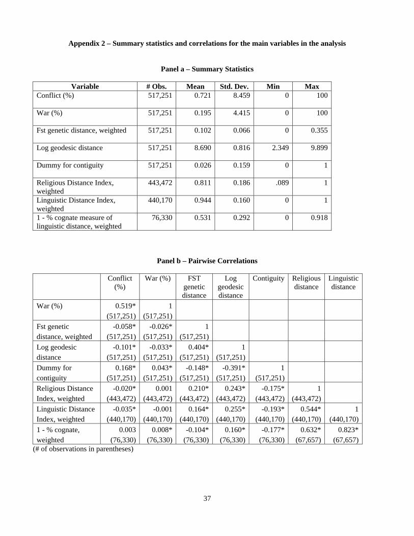
37

Appendix 2 – Summary statistics and correlations for the main variables in the analysis

Panel a – Summary Statistics

Variable # Obs. Mean Std. Dev. Min Max Conflict (%)

517,251 0.721 8.459 0 100

War (%)

517,251 0.195 4.415 0 100

Fst genetic distance, weighted

517,251 0.102 0.066 0 0.355

Log geodesic distance

517,251 8.690 0.816 2.349 9.899

Dummy for contiguity

517,251 0.026 0.159 0 1

Religious Distance Index, weighted

443,472 0.811 0.186 .089 1

Linguistic Distance Index, weighted

440,170 0.944 0.160 0 1

1 - % cognate measure of linguistic distance, weighted

76,330 0.531 0.292 0 0.918

Panel b – Pairwise Correlations

Conflict (%)

War (%) FST genetic distance

Log geodesic distance

Contiguity Religious distance

Linguistic distance

War (%) 0.519* 1(517,251) (517,251)

Fst genetic -0.058* -0.026* 1distance, weighted (517,251) (517,251) (517,251)Log geodesic -0.101* -0.033* 0.404* 1distance (517,251) (517,251) (517,251) (517,251)Dummy for 0.168* 0.043* -0.148* -0.391* 1contiguity (517,251) (517,251) (517,251) (517,251) (517,251)Religious Distance -0.020* 0.001 0.210* 0.243* -0.175* 1 Index, weighted (443,472) (443,472) (443,472) (443,472) (443,472) (443,472) Linguistic Distance -0.035* -0.001 0.164* 0.255* -0.193* 0.544* 1Index, weighted (440,170) (440,170) (440,170) (440,170) (440,170) (440,170) (440,170)1 - % cognate, 0.003 0.008* -0.104* 0.160* -0.177* 0.632* 0.823*weighted (76,330) (76,330) (76,330) (76,330) (76,330) (67,657) (67,657)

(# of observations in parentheses)

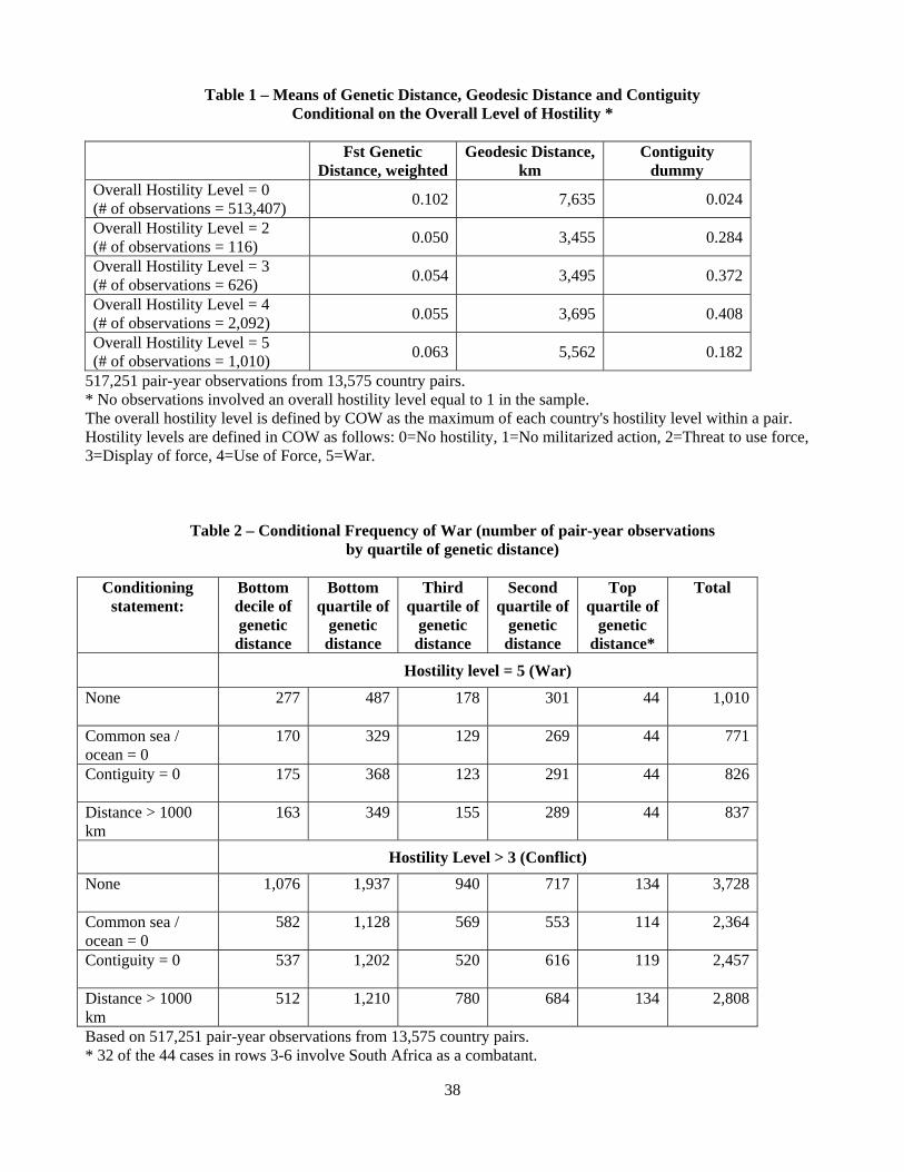
38

Table 1 – Means of Genetic Distance, Geodesic Distance and Contiguity Conditional on the Overall Level of Hostility *

Fst Genetic

Distance, weightedGeodesic Distance,

km Contiguity

dummy Overall Hostility Level = 0 (# of observations = 513,407) 0.102 7,635 0.024

Overall Hostility Level = 2 (# of observations = 116) 0.050 3,455 0.284

Overall Hostility Level = 3 (# of observations = 626) 0.054 3,495 0.372

Overall Hostility Level = 4 (# of observations = 2,092) 0.055 3,695 0.408

Overall Hostility Level = 5 (# of observations = 1,010) 0.063 5,562 0.182

517,251 pair-year observations from 13,575 country pairs. * No observations involved an overall hostility level equal to 1 in the sample. The overall hostility level is defined by COW as the maximum of each country's hostility level within a pair. Hostility levels are defined in COW as follows: 0=No hostility, 1=No militarized action, 2=Threat to use force, 3=Display of force, 4=Use of Force, 5=War.

Table 2 – Conditional Frequency of War (number of pair-year observations by quartile of genetic distance)

Conditioning

statement: Bottom decile of genetic

distance

Bottom quartile of

genetic distance

Third quartile of

genetic distance

Second quartile of

genetic distance

Top quartile of

genetic distance*

Total

Hostility level = 5 (War)

None

277 487 178 301 44 1,010

Common sea / ocean = 0

170 329 129 269 44 771

Contiguity = 0

175 368 123 291 44 826

Distance > 1000 km

163 349 155 289 44 837

Hostility Level > 3 (Conflict) None

1,076 1,937 940 717 134 3,728

Common sea / ocean = 0

582 1,128 569 553 114 2,364

Contiguity = 0

537 1,202 520 616 119 2,457

Distance > 1000 km

512 1,210 780 684 134 2,808

Based on 517,251 pair-year observations from 13,575 country pairs. * 32 of the 44 cases in rows 3-6 involve South Africa as a combatant.

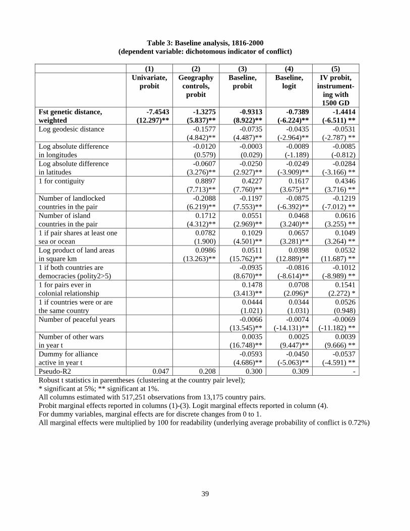
39

Table 3: Baseline analysis, 1816-2000 (dependent variable: dichotomous indicator of conflict)

(1) (2) (3) (4) (5) Univariate,

probit Geography

controls, probit

Baseline, probit

Baseline, logit

IV probit, instrument-

ing with 1500 GD

Fst genetic distance, -7.4543 -1.3275 -0.9313 -0.7389 -1.4414weighted (12.297)** (5.837)** (8.922)** (-6.224)** (-6.511) **Log geodesic distance -0.1577 -0.0735 -0.0435 -0.0531 (4.842)** (4.487)** (-2.964)** (-2.787) **Log absolute difference -0.0120 -0.0003 -0.0089 -0.0085in longitudes (0.579) (0.029) (-1.189) (-0.812)Log absolute difference -0.0607 -0.0250 -0.0249 -0.0284in latitudes (3.276)** (2.927)** (-3.909)** (-3.166) **1 for contiguity 0.8897 0.4227 0.1617 0.4346 (7.713)** (7.760)** (3.675)** (3.716) **Number of landlocked -0.2088 -0.1197 -0.0875 -0.1219countries in the pair (6.219)** (7.553)** (-6.392)** (-7.012) **Number of island 0.1712 0.0551 0.0468 0.0616countries in the pair (4.312)** (2.969)** (3.240)** (3.255) **1 if pair shares at least one 0.0782 0.1029 0.0657 0.1049sea or ocean (1.900) (4.501)** (3.281)** (3.264) **Log product of land areas 0.0986 0.0511 0.0398 0.0532in square km (13.263)** (15.762)** (12.889)** (11.687) **1 if both countries are -0.0935 -0.0816 -0.1012democracies (polity2>5) (8.670)** (-8.614)** (-8.989) **1 for pairs ever in 0.1478 0.0708 0.1541colonial relationship (3.413)** (2.096)* (2.272) *1 if countries were or are 0.0444 0.0344 0.0526the same country (1.021) (1.031) (0.948)Number of peaceful years -0.0066 -0.0074 -0.0069 (13.545)** (-14.131)** (-11.182) **Number of other wars 0.0035 0.0025 0.0039in year t (16.748)** (9.447)** (9.666) **Dummy for alliance -0.0593 -0.0450 -0.0537active in year t (4.686)** (-5.063)** (-4.591) **Pseudo-R2 0.047 0.208 0.300 0.309 -Robust t statistics in parentheses (clustering at the country pair level); * significant at 5%; ** significant at 1%. All columns estimated with 517,251 observations from 13,175 country pairs. Probit marginal effects reported in columns (1)-(3). Logit marginal effects reported in column (4). For dummy variables, marginal effects are for discrete changes from 0 to 1. All marginal effects were multiplied by 100 for readability (underlying average probability of conflict is 0.72%)

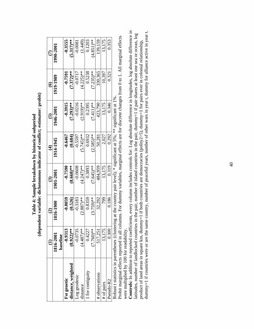
40

Tab

le 4

: Sam

ple

brea

kdow

n by

his

tori

cal s

ubpe

riod

(d

epen

dent

var

iabl

e: d

icho

tom

ous i

ndic

ator

of c

onfli

ct; e

stim

ator

: pro

bit)

(1

) (2

) (3

) (4

) (5

) (6

) (7

)

1816

-200

1 ba

selin

e 18

16-1

900

1901

-200

1 19

14-1

945

1946

-200

1 19

19-1

989

1990

-200

1

Fst g

enet

ic

-0.9

313

-0.8

059

-0.7

590

-0.6

467

-0.3

915

-0.7

591

-0.3

555

dist

ance

, wei

ghte

d (8

.922

)**

(0.5

26)

(8.6

68)*

*(0

.684

) (7

.293

)**

(7.3

72)*

*(5

.317

)**

Log

geod

esic

-0

.073

5 -0

.318

3-0

.060

8-0

.559

7 -0

.021

6-0

.071

7-0

.008

1di

stan

ce

(4.4

87)*

* (2

.887

)**

(4.2

47)*

*(5

.745

)**

(2.9

19)*

*(4

.225

)**

(1.4

49)

1 fo

r con

tigui

ty

0.42

27

0.83

590.

3893

0.69

32

0.23

950.

5238

0.12

03

(7.7

60)*

* (3

.759

)**

(7.6

45)*

*(2

.585

)**

(7.4

11)*

*(7

.235

)**

(4.8

51)*

*#

obse

rvat

ions

51

7,25

1 32

,292

484,

959

50,2

81

423,

790

330,

365

139,

159

# of

pai

rs

13,1

75

799

13,1

752,

027

13,1

7510

,397

13,1

75Ps

eudo

-R2

0.30

0 0.

186

0.31

90.

292

0.34

60.

321

0.35

3R

obus

t t st

atis

tics i

n pa

rent

hese

s (c

lust

erin

g at

the

coun

try p

air l

evel

); *

sign

ifica

nt a

t 5%

; **

sign

ifica

nt a

t 1%

. Pr

obit

mar

gina

l eff

ects

repo

rted

in a

ll co

lum

ns. F

or d

umm

y va

riabl

es, m

argi

nal e

ffec

ts a

re fo

r dis

cret

e ch

ange

s fro

m 0

to 1

. All

mar

gina

l eff

ects

w

ere

mul

tiplie

d by

100

for r

eada

bilit

y.

Con

trol

s: In

add

ition

to re

porte

d co

effic

ient

s, ev

ery

colu

mn

incl

udes

con

trols

for:

Log

abso

lute

diff

eren

ce in

long

itude

s, lo

g ab

solu

te d

iffer

ence

in

latit

udes

, num

ber o

f lan

dloc

ked

coun

tries

in th

e pa

ir, n

umbe

r of i

slan

d co

untri

es in

the

pair,

dum

my=

1 if

pair

shar

es a

t lea

st o

ne se

a or

oce

an, l

og

prod

uct o

f lan

d ar

eas i

n sq

uare

km

, dum

my=

1 if

both

cou

ntrie

s are

dem

ocra

cies

(pol

ity2>

5), d

umm

y=1

for p

airs

eve

r in

colo

nial

rela

tions

hip,

du

mm

y=1

if co

untri

es w

ere

or a

re th

e sa

me

coun

try, n

umbe

r of p

eace

ful y

ears

, num

ber o

f oth

er w

ars i

n ye

ar t,

dum

my

for a

llian

ce a

ctiv

e in

yea

r t.

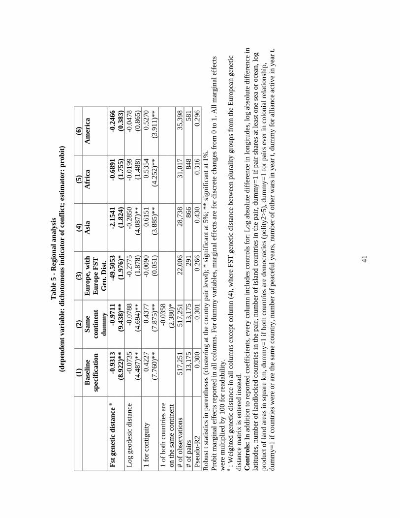
41

Tab

le 5

- R

egio

nal a

naly

sis

(dep

ende

nt v

aria

ble:

dic

hoto

mou

s ind

icat

or o

f con

flict

; est

imat

or: p

robi

t)

(1

) (2

) (3

) (4

) (5

) (6

)

Bas

elin

e sp

ecifi

catio

n Sa

me

cont

inen

t du

mm

y

Eur

ope,

with

E

urop

e FS

T

Gen

. Dis

t.

Asi

a A

fric

a A

mer

ica

Fst g

enet

ic d

ista

nce

a -0

.931

3-0

.971

1-4

9.50

53-2

.154

1 -0

.689

1-0

.246

6

(8.9

22)*

*(9

.438

)**

(1.9

76)*

(1.8

24)

(1.7

55)

(0.3

83)

Log

geod

esic

dis

tanc

e -0

.073

5-0

.078

8-0

.277

5-0

.285

0 -0

.019

9-0

.047

8

(4.4

87)*

*(4

.694

)**

(1.8

78)

(4.0

87)*

* (1

.488

)(0

.865

)1

for c

ontig

uity

0.

4227

0.43

77-0

.009

00.

6151

0.

5354

0.52

70

(7.7

60)*

*(7

.875

)**

(0.0

51)

(3.8

85)*

* (4

.252

)**

(3.9

11)*

*1

of b

oth

coun

tries

are

-0

.035

8

on th

e sa

me

cont

inen

t (2

.380

)*

# of

obs

erva

tions

51

7,25

151

7,25

122

,006

28,7

38

31,0

1735

,398

# of

pai

rs

13,1

7513

,175

291

866

848

581

Pseu

do-R

2 0.

300

0.30

10.

266

0.43

0 0.

316

0.29

6R

obus

t t st

atis

tics i

n pa

rent

hese

s (c

lust

erin

g at

the

coun

try p

air l

evel

); *

sign

ifica

nt a

t 5%

; **

sign

ifica

nt a

t 1%

. Pr

obit

mar

gina

l eff

ects

repo

rted

in a

ll co

lum

ns. F

or d

umm

y va

riabl

es, m

argi

nal e

ffec

ts a

re fo

r dis

cret

e ch

ange

s fro

m 0

to 1

. All

mar

gina

l eff

ects

w

ere

mul

tiplie

d by

100

for r

eada

bilit

y.

a : W

eigh

ted

gene

tic d

ista

nce

in a

ll co

lum

ns e

xcep

t col

umn

(4),

whe

re F

ST g

enet

ic d

ista

nce

betw

een

plur

ality

gro

ups f

rom

the

Euro

pean

gen

etic

di

stan

ce m

atrix

is e

nter

ed in

stea

d.

Con

trol

s: In

add

ition

to re

porte

d co

effic

ient

s, ev

ery

colu

mn

incl

udes

con

trols

for:

Log

abso

lute

diff

eren

ce in

long

itude

s, lo

g ab

solu

te d

iffer

ence

in

latit

udes

, num

ber o

f lan

dloc

ked

coun

tries

in th

e pa

ir, n

umbe

r of i

slan

d co

untri

es in

the

pair,

dum

my=

1 if

pair

shar

es a

t lea

st o

ne se

a or

oce

an, l

og

prod

uct o

f lan

d ar

eas i

n sq

uare

km

, dum

my=

1 if

both

cou

ntrie

s are

dem

ocra

cies

(pol

ity2>

5), d

umm

y=1

for p

airs

eve

r in

colo

nial

rela

tions

hip,

du

mm

y=1

if co

untri

es w

ere

or a

re th

e sa

me

coun

try, n

umbe

r of p

eace

ful y

ears

, num

ber o

f oth

er w

ars i

n ye

ar t,

dum

my

for a

llian

ce a

ctiv

e in

yea

r t.

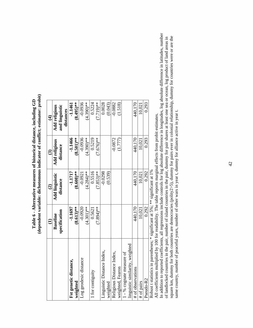
42

Tab

le 6

- A

ltern

ativ

e m

easu

res o

f his

tori

cal d

ista

nce,

incl

udin

g G

D

(dep

ende

nt v

aria

ble:

dic

hoto

mou

s ind

icat

or o

f con

flict

; est

imat

or: p

robi

t)

(1)

(2)

(3)

(4)

B

asel

ine

spec

ifica

tion

Add

ling

uist

ic

dist

ance

A

dd r

elig

ious

di

stan

ce

Add

rel

igio

us

and

lingu

istic

di

stan

ces

Fst g

enet

ic d

ista

nce,

-1

.169

7-1

.171

7-1

.146

6 -1

.146

1w

eigh

ted

(8.6

13)*

*(8

.608

)**

(8.5

01)*

* (8

.495

)**

Log

geod

esic

dis

tanc

e -0

.092

0-0

.092

1-0

.093

6 -0

.093

6

(4.3

01)*

*(4

.284

)**

(4.3

90)*

* (4

.390

)**

1 fo

r con

tigui

ty

0.56

210.

5516

0.52

19

0.52

24

(7.8

94)*

*(7

.853

)**

(7.6

76)*

* (7

.719

)**

Ling

uist

ic D

ista

nce

Inde

x,

-0.0

298

0.

0028

wei

ghte

d (0

.539

)

(0.0

43)

Rel

igio

us D

ista

nce

Inde

x,

-0.0

872

-0.0

882

wei

ghte

d, F

earo

n (1

.777

) (1

.518

)1

- % c

ogna

te m

easu

re o

f

lingu

istic

sim

ilarit

y, w

eigh

ted

#

of o

bser

vatio

ns

440,

170

440,

170

440,

170

440,

170

# of

pai

rs

10,0

2110

,021

10,0

21

10,0

21Ps

eudo

-R2

0.29

20.

292

0.29

3 0.

293

Rob

ust t

stat

istic

s in

pare

nthe

ses;

* si

gnifi

cant

at 5

%; *

* si

gnifi

cant

at 1

%

All

coef

ficie

nts m

ultip

lied

by 1

00 fo

r rea

dabi

lity.

The

tabl

e re

ports

mar

gina

l eff

ects

from

pro

bit e

stim

ates

. In

add

ition

to re

porte

d co

effic

ient

s, al

l reg

ress

ions

incl

ude

cont

rols

for l

og a

bsol

ute

diff

eren

ce in

long

itude

s, lo

g ab

solu

te d

iffer

ence

in la

titud

es, n

umbe

r of

land

lock

ed c

ount

ries i

n th

e pa

ir, n

umbe

r of i

slan

d co

untri

es in

the

pair,

dum

my

for p

air s

hare

s at l

east

one

sea

or o

cean

, log

pro

duct

of l

and

area

s in

squa

re k

m, d

umm

y fo

r bot

h co

untri

es a

re d

emoc

raci

es (p

olity

2>5)

, dum

my

for p

airs

eve

r in

colo

nial

rela

tions

hip,

dum

my

for c

ount

ries w

ere

or a

re th

e sa

me

coun

try, n

umbe

r of p

eace

ful y

ears

, num

ber o

f oth

er w

ars i

n ye

ar t,

dum

my

for a

llian

ce a

ctiv

e in

yea

r t.

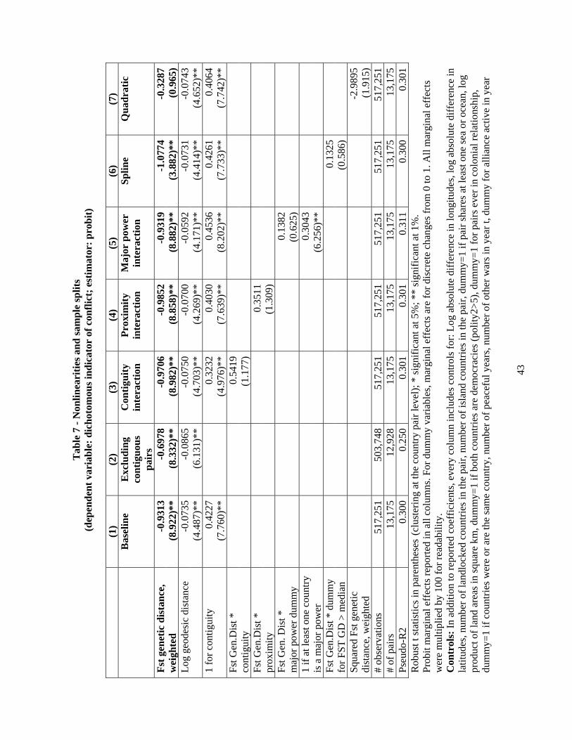
43

Tab

le 7

- N

onlin

eari

ties a

nd sa

mpl

e sp

lits

(dep

ende

nt v

aria

ble:

dic

hoto

mou

s ind

icat

or o

f con

flict

; est

imat

or: p

robi

t)

(1)

(2)

(3)

(4)

(5)

(6)

(7)

B

asel

ine

Exc

ludi

ng

cont

iguo

us

pair

s

Con

tigui

ty

inte

ract

ion

Prox

imity

in

tera

ctio

n M

ajor

pow

er

inte

ract

ion

Splin

e Q

uadr

atic

Fst g

enet

ic d

ista

nce,

-0

.931

3-0

.697

8-0

.970

6-0

.985

2 -0

.931

9-1

.077

4-0

.328

7w

eigh

ted

(8.9

22)*

*(8

.332

)**

(8.9

82)*

*(8

.858

)**

(8.8

82)*

*(3

.882

)**

(0.9

65)

Log

geod

esic

dis

tanc

e -0

.073

5-0

.086

5-0

.075

0-0

.070

0 -0

.059

2-0

.073

1-0

.074

3

(4.4

87)*

*(6

.131

)**

(4.7

03)*

*(4

.269

)**

(4.1

71)*

*(4

.414

)**

(4.6

52)*

*1

for c

ontig

uity

0.

4227

0.

3232

0.40

30

0.45

360.

4261

0.40

64

(7.7

60)*

*

(4.9

76)*

*(7

.639

)**

(8.2

02)*

*(7

.733

)**

(7.7

42)*

*Fs

t Gen

.Dis

t *

0.

5419

co

ntig

uity

(1.1

77)

Fs

t Gen

.Dis

t *

0.

3511

pr

oxim

ity

(1

.309

) Fs

t Gen

. Dis

t *

0.13

82m

ajor

pow

er d

umm

y

(0

.625

)1

if at

leas

t one

cou

ntry

0.

3043

is a

maj

or p

ower

(6

.256

)**

Fst G

en.D

ist *

dum

my

0.

1325

for F

ST G

D >

med

ian

(0.5

86)

Squa

red

Fst g

enet

ic

-2.9

895

dist

ance

, wei

ghte

d

(1

.915

)#

obse

rvat

ions

51

7,25

150

3,74

851

7,25

151

7,25

1 51

7,25

151

7,25

151

7,25

1#

of p

airs

13

,175

12,9

2813

,175

13,1

75

13,1

7513

,175

13,1

75Ps

eudo

-R2

0.30

00.

250

0.30

10.

301

0.31

10.

300

0.30

1R

obus

t t st

atis

tics i

n pa

rent

hese

s (c

lust

erin

g at

the

coun

try p

air l

evel

); *

sign

ifica

nt a

t 5%

; **

sign

ifica

nt a

t 1%

. Pr

obit

mar

gina

l eff

ects

repo

rted

in a

ll co

lum

ns. F

or d

umm

y va

riabl

es, m

argi

nal e

ffec

ts a

re fo

r dis

cret

e ch

ange

s fro

m 0

to 1

. All

mar

gina

l eff

ects

w

ere

mul

tiplie

d by

100

for r

eada

bilit

y.

Con

trol

s: In

add

ition

to re

porte

d co

effic

ient

s, ev

ery

colu

mn

incl

udes

con

trols

for:

Log

abso

lute

diff

eren

ce in

long

itude

s, lo

g ab

solu

te d

iffer

ence

in

latit

udes

, num

ber o

f lan

dloc

ked

coun

tries

in th

e pa

ir, n

umbe

r of i

slan

d co

untri

es in

the

pair,

dum

my=

1 if

pair

shar

es a

t lea

st o

ne se

a or

oce

an, l

og

prod

uct o

f lan

d ar

eas i

n sq

uare

km

, dum

my=

1 if

both

cou

ntrie

s are

dem

ocra

cies

(pol

ity2>

5), d

umm

y=1

for p

airs

eve

r in

colo

nial

rela

tions

hip,

du

mm

y=1

if co

untri

es w

ere

or a

re th

e sa

me

coun

try, n

umbe

r of p

eace

ful y

ears

, num

ber o

f oth

er w

ars i

n ye

ar t,

dum

my

for a

llian

ce a

ctiv

e in

yea

r

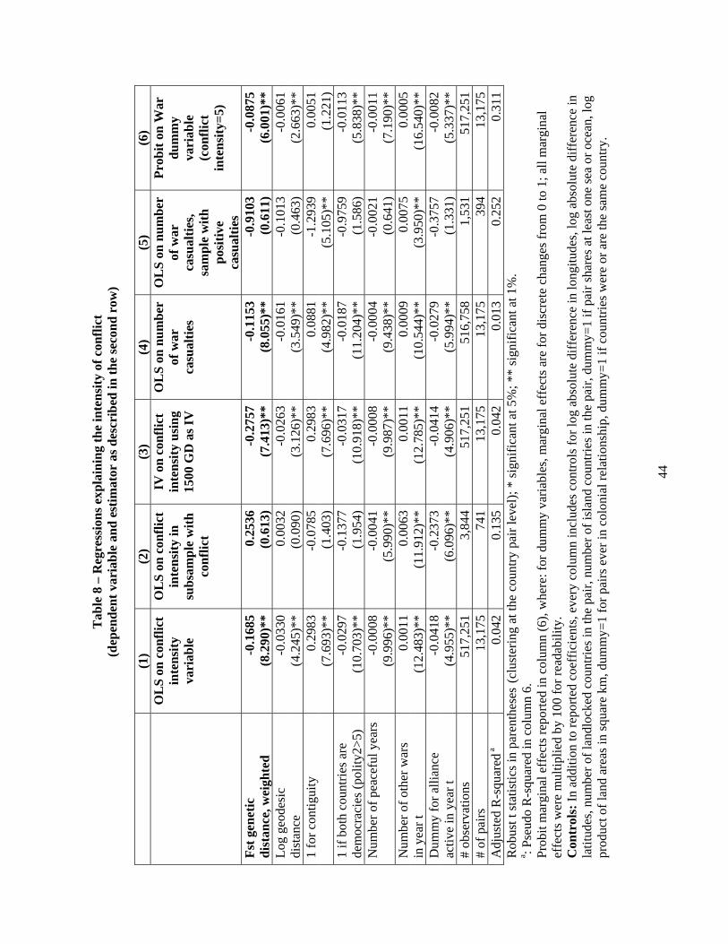
44

Tab

le 8

– R

egre

ssio

ns e

xpla

inin

g th

e in

tens

ity o

f con

flict

(d

epen

dent

var

iabl

e an

d es

timat

or a

s des

crib

ed in

the

seco

nd r

ow)

(1)

(2)

(3)

(4)

(5)

(6)

O

LS

on c

onfli

ct

inte

nsity

va

riab

le

OL

S on

con

flict

in

tens

ity in

su

bsam

ple

with

co

nflic

t

IV o

n co

nflic

t in

tens

ity u

sing

15

00 G

D a

s IV

OL

S on

num

ber

of w

ar

casu

altie

s

OL

S on

num

ber

of w

ar

casu

altie

s, sa

mpl

e w

ith

posi

tive

casu

altie

s

Prob

it on

War

du

mm

y va

riab

le

(con

flict

in

tens

ity=5

)

Fst g

enet

ic

-0.1

685

0.25

36-0

.275

7-0

.115

3-0

.910

3-0

.087

5di

stan

ce, w

eigh

ted

(8.2

90)*

*(0

.613

)(7

.413

)**

(8.0

55)*

*(0

.611

)(6

.001

)**

Log

geod

esic

-0

.033

00.

0032

-0.0

263

-0.0

161

-0.1

013

-0.0

061

dist

ance

(4

.245

)**

(0.0

90)

(3.1

26)*

*(3

.549

)**

(0.4

63)

(2.6

63)*

*1

for c

ontig

uity

0.

2983

-0.0

785

0.29

830.

0881

-1.2

939

0.00

51

(7.6

93)*

*(1

.403

)(7

.696

)**

(4.9

82)*

*(5

.105

)**

(1.2

21)

1 if

both

cou

ntrie

s are

-0

.029

7-0

.137

7-0

.031

7-0

.018

7-0

.975

9-0

.011

3de

moc

raci

es (p

olity

2>5)

(1

0.70

3)**

(1.9

54)

(10.

918)

**(1

1.20

4)**

(1.5

86)

(5.8

38)*

*N

umbe

r of p

eace

ful y

ears

-0

.000

8-0

.004

1-0

.000

8-0

.000

4-0

.002

1-0

.001

1

(9.9

96)*

*(5

.990

)**

(9.9

87)*

*(9

.438

)**

(0.6

41)

(7.1

90)*

*N

umbe

r of o

ther

war

s 0.

0011

0.00

630.

0011

0.00

090.

0075

0.00

05in

yea

r t

(12.

483)

**(1

1.91

2)**

(12.

785)

**(1

0.54

4)**

(3.9

50)*

*(1

6.54

0)**

Dum

my

for a

llian

ce

-0.0

418

-0.2

373

-0.0

414

-0.0

279

-0.3

757

-0.0

082

activ

e in

yea

r t

(4.9

55)*

*(6

.096

)**

(4.9

06)*

*(5

.994

)**

(1.3

31)

(5.3

37)*

*#

obse

rvat

ions

51

7,25

13,

844

517,

251

516,

758

1,53

151

7,25

1#

of p

airs

13

,175

741

13,1

7513

,175

394

13,1

75A

djus

ted

R-s

quar

ed a

0.04

20.

135

0.04

20.

013

0.25

20.

311

Rob

ust t

stat

istic

s in

pare

nthe

ses

(clu

ster

ing

at th

e co

untry

pai

r lev

el);

* si

gnifi

cant

at 5

%; *

* si

gnifi

cant

at 1

%.

a : Pse

udo

R-s

quar

ed in

col

umn

6.

Prob

it m

argi

nal e

ffec

ts re

porte

d in

col

umn

(6),

whe

re: f

or d

umm

y va

riabl

es, m

argi

nal e

ffec

ts a

re fo

r dis

cret

e ch

ange

s fro

m 0

to 1

; all

mar

gina

l ef

fect

s wer

e m

ultip

lied

by 1

00 fo

r rea

dabi

lity.

C

ontr

ols:

In a

dditi

on to

repo

rted

coef

ficie

nts,

ever

y co

lum

n in

clud

es c

ontro

ls fo

r log

abs

olut

e di

ffer

ence

in lo

ngitu

des,

log

abso

lute

diff

eren

ce in

la

titud

es, n

umbe

r of l

andl

ocke

d co

untri

es in

the

pair,

num

ber o

f isl

and

coun

tries

in th

e pa

ir, d

umm

y=1

if pa

ir sh

ares

at l

east

one

sea

or o

cean

, log

pr

oduc

t of l

and

area

s in

squa

re k

m, d

umm

y=1

for p

airs

eve

r in

colo

nial

rela

tions

hip,

dum

my=

1 if

coun

tries

wer

e or

are

the

sam

e co

untry

.

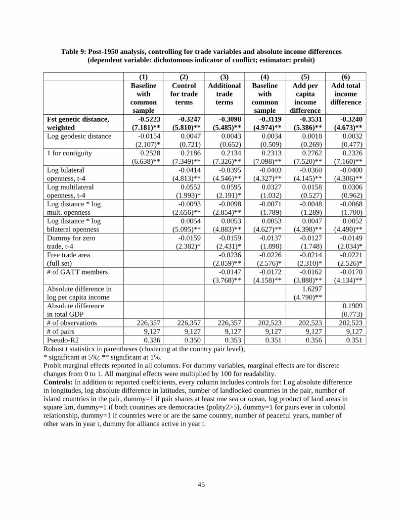
45

Table 9: Post-1950 analysis, controlling for trade variables and absolute income differences (dependent variable: dichotomous indicator of conflict; estimator: probit)

(1) (2) (3) (4) (5) (6) Baseline

with common sample

Control for trade

terms

Additional trade terms

Baseline with

common sample

Add per capita income

difference

Add total income

difference

Fst genetic distance, -0.5223 -0.3247 -0.3098 -0.3119 -0.3531 -0.3240weighted (7.181)** (5.810)** (5.485)** (4.974)** (5.386)** (4.673)**Log geodesic distance -0.0154 0.0047 0.0043 0.0034 0.0018 0.0032 (2.107)* (0.721) (0.652) (0.509) (0.269) (0.477)1 for contiguity 0.2528 0.2186 0.2134 0.2313 0.2762 0.2326 (6.638)** (7.349)** (7.326)** (7.098)** (7.520)** (7.160)**Log bilateral -0.0414 -0.0395 -0.0403 -0.0360 -0.0400openness, t-4 (4.813)** (4.546)** (4.327)** (4.145)** (4.306)**Log multilateral 0.0552 0.0595 0.0327 0.0158 0.0306openness, t-4 (1.993)* (2.191)* (1.032) (0.527) (0.962)Log distance * log -0.0093 -0.0098 -0.0071 -0.0048 -0.0068mult. openness (2.656)** (2.854)** (1.789) (1.289) (1.700)Log distance * log 0.0054 0.0053 0.0053 0.0047 0.0052bilateral openness (5.095)** (4.883)** (4.627)** (4.398)** (4.490)**Dummy for zero -0.0159 -0.0159 -0.0137 -0.0127 -0.0149trade, t-4 (2.382)* (2.431)* (1.898) (1.748) (2.034)*Free trade area -0.0236 -0.0226 -0.0214 -0.0221(full set) (2.859)** (2.576)* (2.310)* (2.526)*# of GATT members -0.0147 -0.0172 -0.0162 -0.0170 (3.768)** (4.158)** (3.888)** (4.134)**Absolute difference in 1.6297 log per capita income (4.790)** Absolute difference 0.1909in total GDP (0.773)# of observations 226,357 226,357 226,357 202,523 202,523 202,523# of pairs 9,127 9,127 9,127 9,127 9,127 9,127Pseudo-R2 0.336 0.350 0.353 0.351 0.356 0.351

Robust t statistics in parentheses (clustering at the country pair level); * significant at 5%; ** significant at 1%. Probit marginal effects reported in all columns. For dummy variables, marginal effects are for discrete changes from 0 to 1. All marginal effects were multiplied by 100 for readability. Controls: In addition to reported coefficients, every column includes controls for: Log absolute difference in longitudes, log absolute difference in latitudes, number of landlocked countries in the pair, number of island countries in the pair, dummy=1 if pair shares at least one sea or ocean, log product of land areas in square km, dummy=1 if both countries are democracies (polity2>5), dummy=1 for pairs ever in colonial relationship, dummy=1 if countries were or are the same country, number of peaceful years, number of other wars in year t, dummy for alliance active in year t.

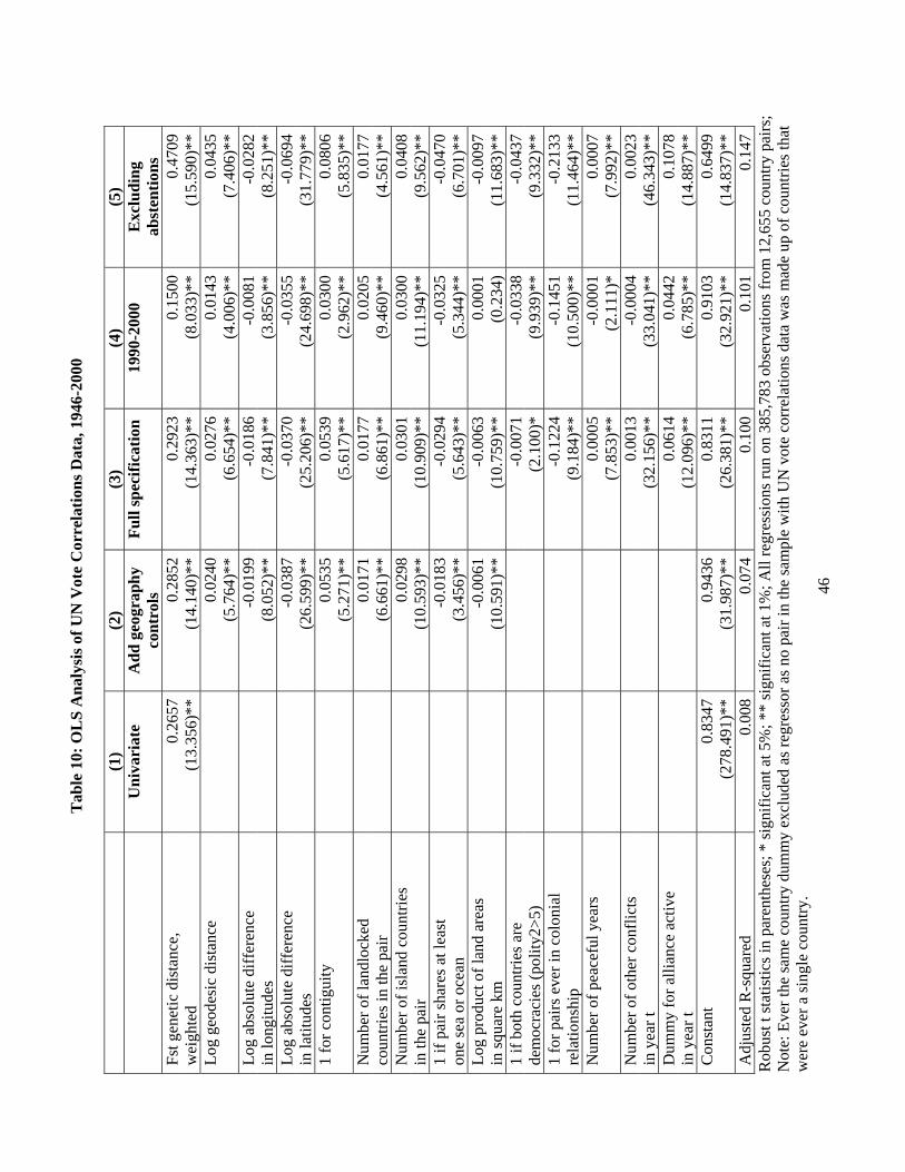
46

Tab

le 1

0: O

LS

Ana

lysi

s of U

N V

ote

Cor

rela

tions

Dat

a, 1

946-

2000

(1

) (2

) (3

) (4

) (5

)

Uni

vari

ate

Add

geo

grap

hy

cont

rols

Fu

ll sp

ecifi

catio

n 19

90-2

000

Exc

ludi

ng

abst

entio

ns

Fst g

enet

ic d

ista

nce,

0.

2657

0.28

520.

2923

0.15

000.

4709

wei

ghte

d (1

3.35

6)**

(14.

140)

**(1

4.36

3)**

(8.0

33)*

*(1

5.59

0)**

Log

geod

esic

dis

tanc

e 0.

0240

0.02

760.

0143

0.04

35

(5.7

64)*

*(6

.654

)**

(4.0

06)*

*(7

.406

)**

Log

abso

lute

diff

eren

ce

-0.0

199

-0.0

186

-0.0

081

-0.0

282

in lo

ngitu

des

(8.0

52)*

*(7

.841

)**

(3.8

56)*

*(8

.251

)**

Log

abso

lute

diff

eren

ce

-0.0

387

-0.0

370

-0.0

355

-0.0

694

in la

titud

es

(26.

599)

**(2

5.20

6)**

(24.

698)

**(3

1.77

9)**

1 fo

r con

tigui

ty

0.05

350.

0539

0.03

000.

0806

(5

.271

)**

(5.6

17)*

*(2

.962

)**

(5.8

35)*

*N

umbe

r of l

andl

ocke

d

0.01

710.

0177

0.02

050.

0177

coun

tries

in th

e pa

ir (6

.661

)**

(6.8

61)*

*(9

.460

)**

(4.5

61)*

*N

umbe

r of i

slan

d co

untri

es

0.02

980.

0301

0.03

000.

0408

in th

e pa

ir (1

0.59

3)**

(10.

909)

**(1

1.19

4)**

(9.5

62)*

*1

if pa

ir sh

ares

at l

east

-0

.018

3-0

.029

4-0

.032

5-0

.047

0on

e se

a or

oce

an

(3.4

56)*

*(5

.643

)**

(5.3

44)*

*(6

.701

)**

Log

prod

uct o

f lan

d ar

eas

-0.0

061

-0.0

063

0.00

01-0

.009

7in

squa

re k

m

(10.

591)

**(1

0.75

9)**

(0.2

34)

(11.

683)

**1

if bo

th c

ount

ries a

re

-0.0

071

-0.0

338

-0.0

437

dem

ocra

cies

(pol

ity2>

5)

(2.1

00)*

(9.9

39)*

*(9

.332

)**

1 fo

r pai

rs e

ver i

n co

loni

al

-0.1

224

-0.1

451

-0.2

133

rela

tions

hip

(9.1

84)*

*(1

0.50

0)**

(11.

464)

**N

umbe

r of p

eace

ful y

ears

0.

0005

-0.0

001

0.00

07

(7.8

53)*

*(2

.111

)*(7

.992

)**

Num

ber o

f oth

er c

onfli

cts

0.00

13-0

.000

40.

0023

in y

ear t

(3

2.15

6)**

(33.

041)

**(4

6.34

3)**

Dum

my

for a

llian

ce a

ctiv

e

0.06

140.

0442

0.10

78in

yea

r t

(12.

096)

**(6

.785

)**

(14.

887)

**C

onst

ant

0.83

470.

9436

0.83

110.

9103

0.64

99

(278

.491

)**

(31.

987)

**(2

6.38

1)**

(32.

921)

**(1

4.83

7)**

Adj

uste

d R

-squ

ared

0.

008

0.07

40.

100

0.10

10.

147

Rob

ust t

stat

istic

s in

pare

nthe

ses;

* si

gnifi

cant

at 5

%; *

* si

gnifi

cant

at 1

%; A

ll re

gres

sion

s run

on

385,

783

obse

rvat

ions

from

12,

655

coun

try p

airs

; N

ote:

Eve

r the

sam

e co

untry

dum

my

excl

uded

as r

egre

ssor

as n

o pa

ir in

the

sam

ple

with

UN

vot

e co

rrel

atio

ns d

ata

was

mad

e up

of c

ount

ries t

hat

wer

e ev

er a

sing

le c

ount

ry.

CESifo Working Paper Series for full list see Twww.cesifo-group.org/wp T (address: Poschingerstr. 5, 81679 Munich, Germany, [email protected])

___________________________________________________________________________ 2633 Thor O. Thoresen, Income Mobility of Owners of Small Businesses when Boundaries

between Occupations are Vague, April 2009 2634 Guido Schwerdt and Amelie C. Wuppermann, Is Traditional Teaching really all that

Bad? A Within-Student Between-Subject Approach, April 2009 2635 Kurt R. Brekke, Luigi Siciliani and Odd Rune Straume, Hospital Competition and

Quality with Regulated Prices, April 2009 2636 Peter Diamond, Taxes and Pensions, April 2009 2637 Shoshana Grossbard, How “Chicagoan” are Gary Becker’s Economic Models of

Marriage?, May 2009 2638 Roland Strausz, Regulatory Risk under Optimal Incentive Regulation, May 2009 2639 Holger Zemanek, Ansgar Belke and Gunther Schnabl, Current Account Imbalances and

Structural Adjustment in the Euro Area: How to Rebalance Competitiveness, May 2009 2640 Harald Hau and Marcel Thum, Subprime Crisis and Board (In-)Competence: Private vs.

Public Banks in Germany, May 2009 2641 Martin Halla, Mario Lackner and Friedrich G. Schneider, An Empirical Analysis of the

Dynamics of the Welfare State: The Case of Benefit Morale, May 2009 2642 Balázs Égert, Infrastructure Investment in Network Industries: The Role of Incentive

Regulation and Regulatory Independence, May 2009 2643 Christian Gollier, Expected Net Present Value, Expected Net Future Value, and the

Ramsey Rule, May 2009 2644 Sören Blomquist and Håkan Selin, Hourly Wage Rate and Taxable Labor Income

Responsiveness to Changes in Marginal Tax Rates, May 2009 2645 Dominique Demougin, Oliver Fabel and Christian Thomann, Implicit vs. Explicit

Incentives: Theory and a Case Study, May 2009 2646 Francesco C. Billari and Vincenzo Galasso, What Explains Fertility? Evidence from

Italian Pension Reforms, May 2009 2647 Kjell Arne Brekke, Karen Evelyn Hauge, Jo Thori Lind and Karine Nyborg, Playing

with the Good Guys – A Public Good Game with Endogenous Group Formation, May 2009

2648 Guglielmo Maria Caporale and Luis A. Gil-Alana, Multi-Factor Gegenbauer Processes

and European Inflation Rates, May 2009 2649 Henning Bohn, A Static Model for Voting on Social Security, May 2009 2650 Markus Haavio and Kaisa Kotakorpi, The Political Economy of Sin Taxes, May 2009 2651 Augusto de la Torre, María Soledad Martínez Pería and Sergio L. Schmukler, Drivers

and Obstacles to Banking SMEs: The Role of Competition and the Institutional Framework, May 2009

2652 Tobias Lindhe and Jan Södersten, Dividend Taxation, Share Repurchases and the

Equity Trap, May 2009 2653 Assaf Razin and Edith Sand, Migration-Regime Liberalization and Social Security:

Political-Economy Effect, May 2009 2654 Yin-Wong Cheung and Hiro Ito, A Cross-Country Empirical Analysis of International

Reserves, May 2009 2655 Bart Cockx and Bruno Van der Linden, Flexicurity in Belgium. A Proposal Based on

Economic Principles, May 2009 2656 Michael Melvin, Lukas Menkhoff and Maik Schmeling, Exchange Rate Management in

Emerging Markets: Intervention via an Electronic Limit Order Book, May 2009 2657 Susanne Neckermann, Reto Cueni and Bruno S. Frey, What is an Award Worth? An

Econometric Assessment of the Impact of Awards on Employee Performance, May 2009

2658 Steven Brakman, Harry Garretsen and Charles van Marrewijk, Economic Geography

within and between European Nations: The Role of Market Potential and Density across Space and Time, May 2009

2659 Giovanni Facchini and Cecilia Testa, Reforming Legislatures: Is one House better than

two?, May 2009 2660 Carsten Kowalczyk and Raymond Riezman, Trade Agreements, May 2009 2661 Oliver Falck, Stephan Heblich and Elke Luedemann, Identity and Entrepreneurship,

May 2009 2662 Christian Lessmann and Gunther Markwardt, One Size Fits All? Decentralization,

Corruption, and the Monitoring of Bureaucrats, May 2009 2663 Felix Bierbrauer, On the Legitimacy of Coercion for the Financing of Public Goods,

May 2009 2664 Alessandro Cigno, Agency in Family Policy: A Survey, May 2009

2665 Claudia M. Buch and Christian Pierdzioch, Low Skill but High Volatility?, May 2009 2666 Hendrik Jürges, Kerstin Schneider, Martin Senkbeil and Claus H. Carstensen,

Assessment Drives Learning: The Effect of Central Exit Exams on Curricular Knowledge and Mathematical Literacy, June 2009

2667 Eric A. Hanushek and Ludger Woessmann, Schooling, Cognitive Skills, and the Latin

American Growth Puzzle, June 2009 2668 Ourania Karakosta, Christos Kotsogiannis and Miguel-Angel Lopez-Garcia, Does

Indirect Tax Harmonization Deliver Pareto Improvements in the Presence of Global Public Goods?, June 2009

2669 Aleksandra Riedl and Silvia Rocha-Akis, Testing the Tax Competition Theory: How

Elastic are National Tax Bases in OECD Countries?, June 2009 2670 Dominique Demougin and Carsten Helm, Incentive Contracts and Efficient

Unemployment Benefits, June 2009 2671 Guglielmo Maria Caporale and Luis A. Gil-Alana, Long Memory in US Real Output

per Capita, June 2009 2672 Jim Malley and Ulrich Woitek, Productivity Shocks and Aggregate Cycles in an

Estimated Endogenous Growth Model, June 2009 2673 Vivek Ghosal, Business Strategy and Firm Reorganization under Changing Market

Conditions, June 2009 2674 Francesco Menoncin and Paolo M. Panteghini, Retrospective Capital Gains Taxation in

the Real World, June 2009 2675 Thomas Hemmelgarn and Gaёtan Nicodème, Tax Co-ordination in Europe: Assessing

the First Years of the EU-Savings Taxation Directive, June 2009 2676 Oliver Himmler, The Effects of School Competition on Academic Achievement and

Grading Standards, June 2009 2677 Rolf Golombek and Michael Hoel, International Cooperation on Climate-Friendly

Technologies, June 2009 2678 Martin Cave and Matthew Corkery, Regulation and Barriers to Trade in

Telecommunications Services in the European Union, June 2009 2679 Costas Arkolakis, A Unified Theory of Firm Selection and Growth, June 2009 2680 Michelle R. Garfinkel, Stergios Skaperdas and Constantinos Syropoulos, International

Trade and Transnational Insecurity: How Comparative Advantage and Power are Jointly Determined, June 2009

2681 Marcelo Resende, Capital Structure and Regulation in U.S. Local Telephony: An

Exploratory Econometric Study; June 2009 2682 Marc Gronwald and Janina Ketterer, Evaluating Emission Trading as a Policy Tool –

Evidence from Conditional Jump Models, June 2009 2683 Stephan O. Hornig, Horst Rottmann and Rüdiger Wapler, Information Asymmetry,

Education Signals and the Case of Ethnic and Native Germans, June 2009 2684 Benoit Dostie and Rajshri Jayaraman, The Effect of Adversity on Process Innovations

and Managerial Incentives, June 2009 2685 Peter Egger, Christian Keuschnigg and Hannes Winner, Incorporation and Taxation:

Theory and Firm-level Evidence, June 2009 2686 Chrysovalantou Milliou and Emmanuel Petrakis, Timing of Technology Adoption and

Product Market Competition, June 2009 2687 Hans Degryse, Frank de Jong and Jérémie Lefebvre, An Empirical Analysis of Legal

Insider Trading in the Netherlands, June 2009 2688 Subhasish M. Chowdhury, Dan Kovenock and Roman M. Sheremeta, An Experimental

Investigation of Colonel Blotto Games, June 2009 2689 Alexander Chudik, M. Hashem Pesaran and Elisa Tosetti, Weak and Strong Cross

Section Dependence and Estimation of Large Panels, June 2009 2690 Mohamed El Hedi Arouri and Christophe Rault, On the Influence of Oil Prices on Stock

Markets: Evidence from Panel Analysis in GCC Countries, June 2009 2691 Lars P. Feld and Christoph A. Schaltegger, Political Stability and Fiscal Policy – Time

Series Evidence for the Swiss Federal Level since 1849, June 2009 2692 Michael Funke and Marc Gronwald, A Convex Hull Approach to Counterfactual

Analysis of Trade Openness and Growth, June 2009 2693 Patricia Funk and Christina Gathmann, Does Direct Democracy Reduce the Size of

Government? New Evidence from Historical Data, 1890-2000, June 2009 2694 Kirsten Wandschneider and Nikolaus Wolf, Shooting on a Moving Target: Explaining

European Bank Rates during the Interwar Period, June 2009 2695 J. Atsu Amegashie, Third-Party Intervention in Conflicts and the Indirect Samaritan’s

Dilemma, June 2009 2696 Enrico Spolaore and Romain Wacziarg, War and Relatedness, June 2009

War and relatedness

Documents