Waiting times, recurrence times, ergodicity and quasiperiodic dynamics Waiting times, recurrence times, ergodicity and quasiperiodic dynamics Dong Han Kim Department of Mathematics, The University of Suwon, Korea Scuola Normale Superiore, 22 Jan. 2009

Welcome message from author
This document is posted to help you gain knowledge. Please leave a comment to let me know what you think about it! Share it to your friends and learn new things together.
Transcript

Waiting times, recurrence times, ergodicity and quasiperiodic dynamics
Waiting times, recurrence times, ergodicity andquasiperiodic dynamics
Dong Han Kim
Department of Mathematics,The University of Suwon, Korea
Scuola Normale Superiore, 22 Jan. 2009

Waiting times, recurrence times, ergodicity and quasiperiodic dynamics
Outline
Dynamical SystemsIntroductionThe Poincare Recurrence Theorem
Data compression scheme and the Ornstein-Weiss Theorem
Irrational rotations
Sequences from substitutions
Interval exchange map
Recurrence time of infinite invariant measure systemsInfinite invariant measure systemsManneville-Pomeau map

Waiting times, recurrence times, ergodicity and quasiperiodic dynamics
Dynamical Systems
Introduction
Dynamical Systems
X : a space (measure, topological, manifold)
T : X → X a map(continuous, measure-preserving, differentiable, . . . ).
To study asymptotic behaviour of T n(x).

Waiting times, recurrence times, ergodicity and quasiperiodic dynamics
Dynamical Systems
Introduction
Dynamical Systems
X : a space (measure, topological, manifold)
T : X → X a map(continuous, measure-preserving, differentiable, . . . ).
To study asymptotic behaviour of T n(x).
Assume that there is a measure µ on X which is T -invariant.(time invariant, stationary).(µ(E ) = µ(T−1E ) for all measurable E ⊂ X )
measure µ : volume, area, length, probability .....

Waiting times, recurrence times, ergodicity and quasiperiodic dynamics
Dynamical Systems
Introduction
An irrational rotation
T : [0, 1) → [0, 1), T (x) = x + θ (mod 1).
00
1
1
θ

Waiting times, recurrence times, ergodicity and quasiperiodic dynamics
Dynamical Systems
Introduction
An irrational rotation
T : S1 → S1, T (e2πit) = e2πi(t+θ).
00
1
1
θ
x
Tx

Waiting times, recurrence times, ergodicity and quasiperiodic dynamics
Dynamical Systems
Introduction
An irrational rotation
T : S1 → S1, T (e2πit) = e2πi(t+θ).
00
1
1
θ
x
Tx
T 2x
T 3x
T 4x
T 5x
T 6x

Waiting times, recurrence times, ergodicity and quasiperiodic dynamics
Dynamical Systems
Introduction
x 7→ 2x map
X = [0, 1) with Lebesgue measure,T : x 7→ 2x (mod 1).
00
1
1
1
2

Waiting times, recurrence times, ergodicity and quasiperiodic dynamics
Dynamical Systems
Introduction
x 7→ 2x map
X = [0, 1) with Lebesgue measure,T : x 7→ 2x (mod 1).
00
1
1
1
2

Waiting times, recurrence times, ergodicity and quasiperiodic dynamics
Dynamical Systems
Introduction
Shift spaces
X =∏∞
n=1 A, A is a finite set.T : (x1x2x3 . . . ) 7→ (x2x3x4 . . . ) left-shiftµ: an invariant(stationary) measure
Fair coin tossing: (i.i.d. process)X =
∏∞n=1{H,T}, e.g., HTHHHTHTTTT · · · ∈ X .
µ(xn = an | xn−11 = an−1
1 ) = µ(xn = an) = µ(x1 = an)
for all n ≥ 1, and an1 ∈ An.
µ is a product measure on AN.
(i.i.d. process ⇒ Chaotic or Random system)

Waiting times, recurrence times, ergodicity and quasiperiodic dynamics
Dynamical Systems
Introduction
P: a partition of X .(x0, x1, x2, . . . ): P name of x if T ix ∈ Pxi
, i = 0, 1, . . . .
P0 P1
P2
X
x
Tx
T 2x
T 3x
P = {P0,P1,P2}. P name of x is 0120 . . . .
(X ,T ) ⇐⇒ ({0, 1, 2}Z , σ), x ↔ 0120 . . .

Waiting times, recurrence times, ergodicity and quasiperiodic dynamics
Dynamical Systems
Introduction
X = [0, 1), T : x 7→ 2x (mod 1).
0 1
(X , µ,T ) is isomorphic to (12 , 1
2)-Bernoulli shift (coin tossing).
x = (x1x2x3 . . . )(2), x ↔ x1x2x3 . . .
since xi ∈ 0, 1 if T i−1x ∈ P0,P1 respectively.

Waiting times, recurrence times, ergodicity and quasiperiodic dynamics
Dynamical Systems
Introduction
Sequence of the powers of 2
2 2048 2097152 2147483648 21990232555524 4096 4194304 4294967296 43980465111048 8192 8388608 8589934592 8796093022208
16 16384 16777216 17179869184 1759218604441632 32768 33554432 34359738368 3518437208883264 65536 67108864 68719476736 70368744177664
128 131072 134217728 137438953472 140737488355328256 262144 268435456 274877906944 281474976710656512 524288 536870912 549755813888 562949953421312
1024 1048576 1073741824 1099511627776 1125899906842624
Last digits : 2 → 4 → 8 → 6 → . . .

Waiting times, recurrence times, ergodicity and quasiperiodic dynamics
Dynamical Systems
Introduction
Sequence of the powers of 2
2 2048 2097152 2147483648 21990232555524 4096 4194304 4294967296 43980465111048 8192 8388608 8589934592 8796093022208
16 16384 16777216 17179869184 1759218604441632 32768 33554432 34359738368 3518437208883264 65536 67108864 68719476736 70368744177664
128 131072 134217728 137438953472 140737488355328256 262144 268435456 274877906944 281474976710656512 524288 536870912 549755813888 562949953421312
1024 1048576 1073741824 1099511627776 1125899906842624
Last 2 digits :04 08 16 32 64 28 56 12 24 48 96 92 84 68 36 72 44 88 76 52

Waiting times, recurrence times, ergodicity and quasiperiodic dynamics
Dynamical Systems
Introduction
00
1
1
1
20
01
1
1
2

Waiting times, recurrence times, ergodicity and quasiperiodic dynamics
Dynamical Systems
Introduction
Sequence of the powers of 2
2 2048 2097152 2147483648 21990232555524 4096 4194304 4294967296 43980465111048 8192 8388608 8589934592 8796093022208
16 16384 16777216 17179869184 1759218604441632 32768 33554432 34359738368 3518437208883264 65536 67108864 68719476736 70368744177664
128 131072 134217728 137438953472 140737488355328256 262144 268435456 274877906944 281474976710656512 524288 536870912 549755813888 562949953421312
1024 1048576 1073741824 1099511627776 1125899906842624
log xn = log xn−1 + log 2, log10 2 = 0.3010 · · · ≈ 3
10.

Waiting times, recurrence times, ergodicity and quasiperiodic dynamics
Dynamical Systems
Introduction
An irrational rotation
T : [0, 1) → [0, 1), T (x) = x + θ (mod 1).T : S1 → S1, T (e2πit) = e2πi(t+θ).
00
1
1
θ
x
Tx
T 2x
T 3x
T 4x
T 5x
T 6x
Quasi-periodic : ∃ni s.t. |T ni − id | → 0.

Waiting times, recurrence times, ergodicity and quasiperiodic dynamics
Dynamical Systems
The Poincare Recurrence Theorem
The Poincare Recurrence Theorem
X
x
Tx
T 2x
T 3x
T 4x
T 5x
Under suitable assumptions a typicaltrajectory of the system comes backinfinitely many times in any neighbor-hood of its starting point.
How many iterations of an orbit isnecessary to come back within adistance r from the starting point?
The quantitative recurrence theory in-vestigates this kind of questions.

Waiting times, recurrence times, ergodicity and quasiperiodic dynamics
Dynamical Systems
The Poincare Recurrence Theorem
Define τr (x) to be the first return time of x into the ball B(x , r)centered in x and with radius r .
τr (x) = min{j ≥ 1 : T j(x) ∈ B(x , r)}.
Questions:
◮ Distribution of τr . Pr(τr (x) > s) ?
◮ Asymptotic limits oflog τr (x)
− log r
Define τr (x , y) to be the hitting time or waiting time of x into theball B(y , r) centered in y and with radius r .
Waiting times, recurrence times, ergodicity and quasiperiodic dynamics
Data compression scheme and the Ornstein-Weiss Theorem
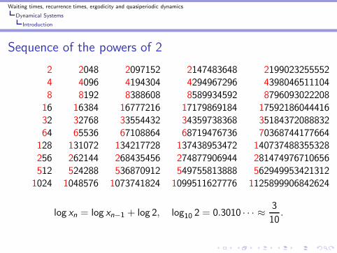
Let X = {0, 1}N and σ be a left-shift map.Define Rn to be the first return time of the initial n-block, i.e.,
Rn(x) = min{j ≥ 1 : x1 . . . xn = xj+1 . . . xj+n}.
x =
15︷ ︸︸ ︷
1 0 1 0 0 1 0 0 1 1 0 1 1 0 0 1 0 1 0 · · · ⇒ R4(x) = 15.
The convergence of1
nlog Rn(x) to the entropy h was studied in a
relation with data compression algorithm such as the Lempel-Zivcompression algorithm.
Waiting times, recurrence times, ergodicity and quasiperiodic dynamics
Data compression scheme and the Ornstein-Weiss Theorem
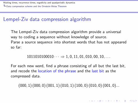
Lempel-Ziv data compression algorithm
The Lempel-Ziv data compression algorithm provide a universalway to coding a sequence without knowledge of source.Parse a source sequence into shortest words that has not appearedso far:
1011010100010 · · · ⇒ 1, 0, 11, 01, 010, 00, 10, . . .
For each new word, find a phrase consisting of all but the last bit,and recode the location of the phrase and the last bit as thecompressed data.
(000, 1) (000, 0) (001, 1) (010, 1) (100, 0) (010, 0) (001, 0)...

Waiting times, recurrence times, ergodicity and quasiperiodic dynamics
Data compression scheme and the Ornstein-Weiss Theorem
Theorem (Wyner-Ziv(1989), Ornstein and Weiss(1993))
For ergodic processes with entropy h,
limn→∞
1
nlog Rn(x) = h almost surely.

Waiting times, recurrence times, ergodicity and quasiperiodic dynamics
Data compression scheme and the Ornstein-Weiss Theorem
Theorem (Wyner-Ziv(1989), Ornstein and Weiss(1993))
For ergodic processes with entropy h,
limn→∞
1
nlog Rn(x) = h almost surely.
The meaning of entropy
◮ Entropy measures the information content or the amount ofrandomness.
◮ Entropy measures the maximum compression rate.
◮ Totally random binary sequence has entropy log 2 = 1. Itcannot be compressed further.

Waiting times, recurrence times, ergodicity and quasiperiodic dynamics
Data compression scheme and the Ornstein-Weiss Theorem
The Shannon-McMillan-Brieman theorem states that
limn→∞
−1
nlog Pn(x) = h a.e.,
where Pn(x) is the probability of x1x2 . . . xn.
If the entropy h is positive,
limn→∞
log Rn(x)
− log Pn(x)= 1 a.e.

Waiting times, recurrence times, ergodicity and quasiperiodic dynamics
Data compression scheme and the Ornstein-Weiss Theorem
For many hyperbolic (chaotic) systems
limr→0+
log τr (x)
− log r= dµ(x),
where dµ is the local dimension of µ at x .(Saussol, Troubetzkoy and Vaienti (2002), Barreira and Saussol(2001, 2002), G.H. Choe (2003), C. Kim and D. H. Kim (2004))
What happens, if h = 0, which implies that log Rn and log Pn donot increases linearly.

Waiting times, recurrence times, ergodicity and quasiperiodic dynamics
Irrational rotations
Diophantine approximation
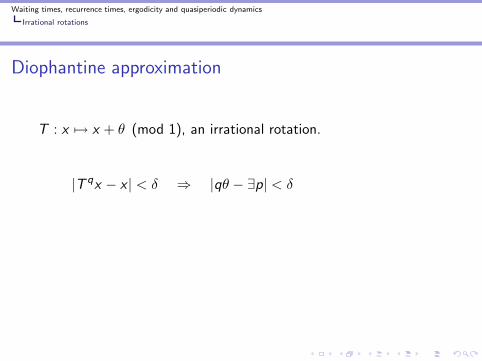
T : x 7→ x + θ (mod 1), an irrational rotation.
|T qx − x | < δ
Waiting times, recurrence times, ergodicity and quasiperiodic dynamics
Irrational rotations
Diophantine approximation
T : x 7→ x + θ (mod 1), an irrational rotation.
|T qx − x | < δ ⇒ |qθ − ∃p| < δ

Waiting times, recurrence times, ergodicity and quasiperiodic dynamics
Irrational rotations
Diophantine approximation
T : x 7→ x + θ (mod 1), an irrational rotation.
|T qx − x | < δ ⇒ |qθ − ∃p| < δ ⇒∣∣∣∣θ − p
q
∣∣∣∣<
δ
q.

Waiting times, recurrence times, ergodicity and quasiperiodic dynamics
Irrational rotations
Diophantine approximation
T : x 7→ x + θ (mod 1), an irrational rotation.
|T qx − x | < δ ⇒ |qθ − ∃p| < δ ⇒∣∣∣∣θ − p
q
∣∣∣∣<
δ
q.
Diophantine approximation:
∣∣∣∣θ − p
q
∣∣∣∣<
1√5q2
.

Waiting times, recurrence times, ergodicity and quasiperiodic dynamics
Irrational rotations
An irrational number θ, 0 < θ < 1, is said to be of type η if
η = sup{β : lim infj→∞
jβ‖jθ‖ = 0},
‖ · ‖ is the distance to the nearest integer (‖t‖ = minn∈Z |t − n|).◮ Note that every irrational number is of type η ≥ 1. The set of
irrational numbers of type 1 (Called Roth type) has measure 1.
◮ A number with bounded partial quotients is of type 1.
◮ There exist numbers of type ∞, called the Liouville numbers.For example θ =
∑∞i=1 10−i !.

Waiting times, recurrence times, ergodicity and quasiperiodic dynamics
Irrational rotations
Let T (x) = x + θ (mod 1) on [0, 1) for an irrational θ of type η,
Theorem (Choe-Seo (2001))
For every x
lim infr→0+
log τr (x)
− log r=
1
η, lim sup
r→0+
log τr (x)
− log r= 1.
Theorem (K-Seo (2003))
For almost every y
lim supr→0+
log τr (x , y)
− log r= η, lim inf
r→0+
log τr (x , y)
− log r= 1.
Waiting times, recurrence times, ergodicity and quasiperiodic dynamics
Sequences from substitutions
Fibonacci sequence
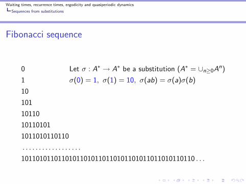
0 Let σ : A∗ → A∗ be a substitution (A∗ = ∪n≥0An)
1 σ(0) = 1, σ(1) = 10, σ(ab) = σ(a)σ(b)
10
101
10110
10110101
1011010110110
. . . . . . . . . . . . . . . . . .
10110101101101011010110110101101011011010110110 . . .

Waiting times, recurrence times, ergodicity and quasiperiodic dynamics
Sequences from substitutions
Sturmian sequence
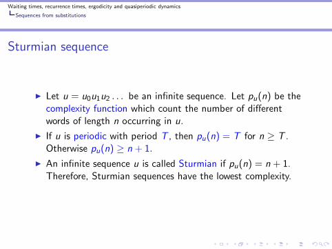
◮ Let u = u0u1u2 . . . be an infinite sequence. Let pu(n) be thecomplexity function which count the number of differentwords of length n occurring in u.

Waiting times, recurrence times, ergodicity and quasiperiodic dynamics
Sequences from substitutions
Sturmian sequence
◮ Let u = u0u1u2 . . . be an infinite sequence. Let pu(n) be thecomplexity function which count the number of differentwords of length n occurring in u.
◮ If u is periodic with period T , then pu(n) = T for n ≥ T .Otherwise pu(n) ≥ n + 1.
◮ An infinite sequence u is called Sturmian if pu(n) = n + 1.Therefore, Sturmian sequences have the lowest complexity.
◮ Example: Fibonacci sequence10110101101101011010110110101101011011010110110 . . .

Waiting times, recurrence times, ergodicity and quasiperiodic dynamics
Sequences from substitutions
Sturmian sequence
◮ Let u = u0u1u2 . . . be an infinite sequence. Let pu(n) be thecomplexity function which count the number of differentwords of length n occurring in u.
◮ If u is periodic with period T , then pu(n) = T for n ≥ T .Otherwise pu(n) ≥ n + 1.
◮ An infinite sequence u is called Sturmian if pu(n) = n + 1.Therefore, Sturmian sequences have the lowest complexity.
◮ Example: Fibonacci sequence10110101101101011010110110101101011011010110110 . . .p(2) = 3

Waiting times, recurrence times, ergodicity and quasiperiodic dynamics
Sequences from substitutions
Sturmian sequence
◮ Let u = u0u1u2 . . . be an infinite sequence. Let pu(n) be thecomplexity function which count the number of differentwords of length n occurring in u.
◮ If u is periodic with period T , then pu(n) = T for n ≥ T .Otherwise pu(n) ≥ n + 1.
◮ An infinite sequence u is called Sturmian if pu(n) = n + 1.Therefore, Sturmian sequences have the lowest complexity.
◮ Example: Fibonacci sequence10110101101101011010110110101101011011010110110 . . .p(3) = 4

Waiting times, recurrence times, ergodicity and quasiperiodic dynamics
Sequences from substitutions
Sturmian sequence
◮ Let u = u0u1u2 . . . be an infinite sequence. Let pu(n) be thecomplexity function which count the number of differentwords of length n occurring in u.
◮ If u is periodic with period T , then pu(n) = T for n ≥ T .Otherwise pu(n) ≥ n + 1.
◮ An infinite sequence u is called Sturmian if pu(n) = n + 1.Therefore, Sturmian sequences have the lowest complexity.
◮ Example: Fibonacci sequence10110101101101011010110110101101011011010110110 . . .p(4) = 5
Waiting times, recurrence times, ergodicity and quasiperiodic dynamics
Sequences from substitutions
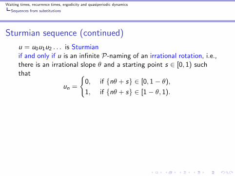
Sturmian sequence (continued)
u = u0u1u2 . . . is Sturmianif and only if u is an infinite P-naming of an irrational rotation, i.e.,there is an irrational slope θ and a starting point s ∈ [0, 1) suchthat
un =
{
0, if {nθ + s} ∈ [0, 1 − θ),
1, if {nθ + s} ∈ [1 − θ, 1).

Waiting times, recurrence times, ergodicity and quasiperiodic dynamics
Sequences from substitutions
Sturmian sequence (continued)
u = u0u1u2 . . . is Sturmianif and only if u is an infinite P-naming of an irrational rotation, i.e.,there is an irrational slope θ and a starting point s ∈ [0, 1) suchthat
un =
{
0, if {nθ + s} ∈ [0, 1 − θ),
1, if {nθ + s} ∈ [1 − θ, 1).
Theorem (K-K.K. Park (2007))
lim infn→∞
log Rn(u)
log n=
1
η, lim sup
n→∞
log Rn(u)
log n= 1, almost every s.
Moreover, if η > 1, then for every slog Rn(u)
log ndoes not converge.

Waiting times, recurrence times, ergodicity and quasiperiodic dynamics
Sequences from substitutions
Morse sequence (or Prouhet-Thue-Morse sequence)
σ(1) = 10, σ(0) = 01, σ(ab) = σ(a)σ(b)
0 7→ 01 7→ 0110 7→ 01101001 7→ . . . . . . . . . 7→01101001100101101001011001101001100101100110 . . .

Waiting times, recurrence times, ergodicity and quasiperiodic dynamics
Sequences from substitutions
Morse sequence (or Prouhet-Thue-Morse sequence)
σ(1) = 10, σ(0) = 01, σ(ab) = σ(a)σ(b)
0 7→ 01 7→ 0110 7→ 01101001 7→ . . . . . . . . . 7→01101001100101101001011001101001100101100110 . . .
un is the number of 1’s (mod 2) in the binary expansion of n.0 = (0)(2), u0 = 0, 1 = (1)(2), u1 = 1,
2 = (10)(2), u2 = 1, 3 = (11)(2), u3 = 0,
4 = (100)(2) , u4 = 1, 5 = (101)(2), u5 = 0, . . .
The complexity of the Morse sequence is
lim suppu(n)
n=
10
3, lim inf
pu(n)
n= 3.

Waiting times, recurrence times, ergodicity and quasiperiodic dynamics
Sequences from substitutions
Automatic sequence
◮ u is called k-automatic if it is generated by a k-automaton.

Waiting times, recurrence times, ergodicity and quasiperiodic dynamics
Sequences from substitutions
Automatic sequence
◮ u is called k-automatic if it is generated by a k-automaton.
◮ An infinite sequence is k-automatic if and only if it is theimage under a coding of a fixed point of a k-uniformmorphism σ.
◮ The Morse sequence is 2-automatic.
TheoremLet u be a non-eventually periodic k-automatic infinite sequence.Then we have
limn→∞
log Rn(u)
log n= 1.

Waiting times, recurrence times, ergodicity and quasiperiodic dynamics
Interval exchange map
An interval exchange map
Generalization of the irrational rotation
00
1
1

Waiting times, recurrence times, ergodicity and quasiperiodic dynamics
Interval exchange map
Comparing the interval exchange map and the irrationalrotation
torus

Waiting times, recurrence times, ergodicity and quasiperiodic dynamics
Interval exchange map
Comparing the interval exchange map and the irrationalrotation
torus
xTx

Waiting times, recurrence times, ergodicity and quasiperiodic dynamics
Interval exchange map
Comparing the interval exchange map and the irrationalrotation
torus
xTx
genus-2 surface

Waiting times, recurrence times, ergodicity and quasiperiodic dynamics
Interval exchange map
Comparing the interval exchange map and the irrationalrotation
torus
xTx
genus-2 surface

Waiting times, recurrence times, ergodicity and quasiperiodic dynamics
Interval exchange map
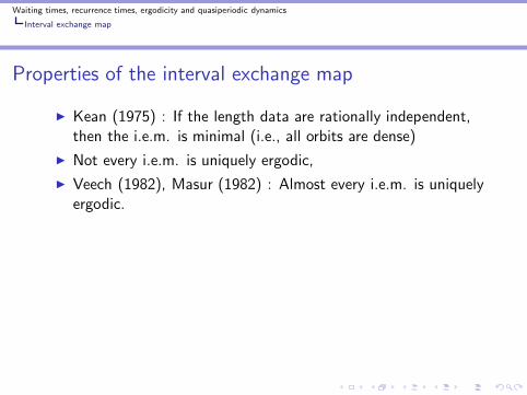
Properties of the interval exchange map
◮ Kean (1975) : If the length data are rationally independent,then the i.e.m. is minimal (i.e., all orbits are dense)

Waiting times, recurrence times, ergodicity and quasiperiodic dynamics
Interval exchange map
Properties of the interval exchange map
◮ Kean (1975) : If the length data are rationally independent,then the i.e.m. is minimal (i.e., all orbits are dense)
◮ Not every i.e.m. is uniquely ergodic,
Waiting times, recurrence times, ergodicity and quasiperiodic dynamics
Interval exchange map
Properties of the interval exchange map
◮ Kean (1975) : If the length data are rationally independent,then the i.e.m. is minimal (i.e., all orbits are dense)
◮ Not every i.e.m. is uniquely ergodic,
◮ Veech (1982), Masur (1982) : Almost every i.e.m. is uniquelyergodic.
◮ Marmi, Moussa, Yoccoz (2006) : Almost every i.e.m. is of“Roth type”.
◮ K, Marmi : For almost every i.e.m.
limr→0
log τr (x)
− log r= 1, lim
log Rn(x)
log n= 1, a.e.
Another definition of “Roth type” for i.e.m.

Waiting times, recurrence times, ergodicity and quasiperiodic dynamics
Recurrence time of infinite invariant measure systems
Infinite invariant measure systems
Infinite invariant measure systems
◮ Such systems are used for models of statistically anomalousphenomena such as intermittency and anomalous diffusionand they do have interesting statistical behavior.
◮ Many classical theorems of finite measure preserving systemsfrom ergodic theory can be extended to the infinite measurepreserving case.
◮ The Hopf ratio ergodic theorem: Let T be conservative andergodic and f , g ∈ L1 such that
∫gdµ 6= 0 , then
∑n−1k=0 f (T k(x))
∑n−1k=0 g(T k(x))
→∫
fdµ∫
gdµ, a.e.
Waiting times, recurrence times, ergodicity and quasiperiodic dynamics
Recurrence time of infinite invariant measure systems
Infinite invariant measure systems
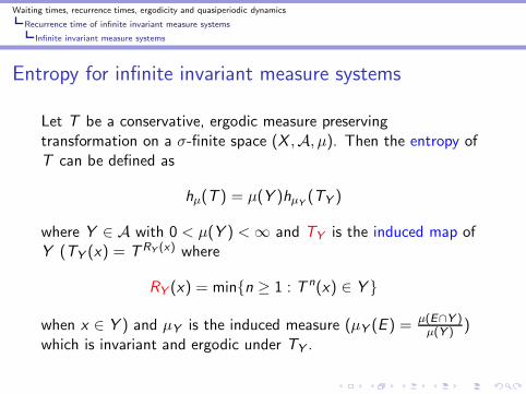
Entropy for infinite invariant measure systems
Let T be a conservative, ergodic measure preservingtransformation on a σ-finite space (X ,A, µ). Then the entropy ofT can be defined as
hµ(T ) = µ(Y )hµY(TY )
where Y ∈ A with 0 < µ(Y ) < ∞ and TY is the induced map ofY (TY (x) = TRY (x) where
RY (x) = min{n ≥ 1 : T n(x) ∈ Y }
when x ∈ Y ) and µY is the induced measure (µY (E ) = µ(E∩Y )µ(Y ) )
which is invariant and ergodic under TY .

Waiting times, recurrence times, ergodicity and quasiperiodic dynamics
Recurrence time of infinite invariant measure systems
Manneville-Pomeau map
The Manneville-Pomeau map
0 1/2 1
T (x) =
{
x + 2z−1xz , 0 ≤ x < 1/2,
2x − 1, 1/2 ≤ x < 1.
have an indifferent “slowly repulsive”fixed point at the origin. When z ∈[2,∞) this forces the natural invariantmeasure for this map to be infinite andabsolutely continuous with respect toLesbegue.
It is not hard to see that P = {[0, 1/2), [1/2, 1)} is a generatingpartition and the entropy hµ(T ) is positive and finite.

Waiting times, recurrence times, ergodicity and quasiperiodic dynamics
Recurrence time of infinite invariant measure systems
Manneville-Pomeau map
Shannon-McMillan-Breiman Theorem
For every f ∈ L1(µ), with∫
f 6= 0
− log(µ(Pn(x)))
Sn(f , x)→ hµ(T )
∫fdµ
a.e. as n → ∞.
Here Sn(f , x) is the partial sums of f along the orbit of x :
Sn(f , x) =∑
k∈[0,n−1]
f (T k(x)).
(“information content” growing as a sublinear power law as timeincreases)

Waiting times, recurrence times, ergodicity and quasiperiodic dynamics
Recurrence time of infinite invariant measure systems
Manneville-Pomeau map
(X ,T ,A, µ) : a measure preserving system.Let ξ be a partition of X and A be an atom of ξ.Let Sn(A, x) be the number of T ix ∈ A for 0 ≤ i ≤ n − 1, i.e.,
Sn(A, x) = Sn(1A, x) =n−1∑
i=0
1A(T i(x)).
DefineRn(x) = min{j ≥ 1 | ξn(x) = ξn(T
jx)}considering a fixed set A ∈ A we also define Rn(x) by
Rn(x) = min{Sj(A, x) ≥ 1 | ξn(x) = ξn(Tjx)}.
Note thatRn(x) = SRn(x)(A, x).

Waiting times, recurrence times, ergodicity and quasiperiodic dynamics
Recurrence time of infinite invariant measure systems
Manneville-Pomeau map
LemmaLet T be a conservative, ergodic measure preservingtransformation (c.e.m.p.t.) on the σ-finite space (X ,B, µ) and letξ be a finite generating partition (mod µ). Assume that there is asubset A which is a union of atoms in ξ with 0 < µ(A) < ∞ andH(ξA) < ∞. For almost every x ∈ A
limn→∞
log Rn(x)
Sn(A, x)=
hµ(T )
µ(A).
Let ξA be the induced partition on A,
ξA = ∪k≥1{V ∩ {RA = k} : V ∈ A ∩ ξk}.

Waiting times, recurrence times, ergodicity and quasiperiodic dynamics
Recurrence time of infinite invariant measure systems
Manneville-Pomeau map
Theorem (Galatolo-K-Park (2006))
Let T be a c.e.m.p.t. on the σ-finite space (X ,B, µ) and let ξ ⊂ Bbe a finite generating partition (mod µ). Assume that there is asubset A which is a union of atoms in ξ with 0 < µ(A) < ∞ andH(ξA) < ∞. Then for any f ∈ L1(µ) with
∫fdµ 6= 0,
lim supn→∞
log Rn(x)
Sn(f , x)=
hµ(T )
α∫
fdµa.e.,
where
α = sup0<µ(B)<∞,B∈B
(
sup{β :
∫
B
(RB)βdµ < ∞})
.
Moreover, if α = 0, then the limsup goes to infinity.

Waiting times, recurrence times, ergodicity and quasiperiodic dynamics
Recurrence time of infinite invariant measure systems
Manneville-Pomeau map
Darling-Kac set
A set A is called a Darling-Kac set, if ∃{an} such that
limn→∞
1
an
n∑
k=1
T k1A = µ(A), almost uniformly on A.
A function f is slowly varying at ∞ if f (xy)f (x) → 1 as x → ∞,∀y > 0.
Suppose that T has a Darling-Kac set and an(T ) = nαL(n), whereL(n) is a slowly varying. The Darling-Kac Theorem states
Sn(x)
an(T )→ Yα, in distribution,
Yα : the normalized Mittag-Leffler distribution of order α.

Waiting times, recurrence times, ergodicity and quasiperiodic dynamics
Recurrence time of infinite invariant measure systems
Manneville-Pomeau map
Theorem (Galatolo-K-Park (2006))
Let T be a c.e.m.p.t. on the σ-finite space (X ,B, µ) and let ξ ⊂ Bbe a finite generating partition (mod µ). Assume that there is asubset A which is a union of atoms in ξ with 0 < µ(A) < ∞ andH(ξA) < ∞. Suppose that T has a Darling-Kac set and an(T ) isregularly varying with index α. Then for any f ∈ L1(µ) with∫
f µ 6= 0,
limn→∞
log Rn(x)
Sn(f , x)=
hµ(T )
α∫
fdµa.e.
Moreover, if α = 0, then the limit goes to infinity.

Waiting times, recurrence times, ergodicity and quasiperiodic dynamics
Recurrence time of infinite invariant measure systems
Manneville-Pomeau map
A map T : [0, 1] → [0, 1] is a Manneville-Pomeau map (MP map)with exponent z if it satisfies the following conditions:
◮ there is c ∈ (0, 1) such that, if I0 = [0, c] and I1 = (c , 1], thenT
∣∣(0,c)
and T∣∣(c,1)
extend to C 1 diffeomorphisms,
T (I0) = [0, 1], T (I1) = (0, 1] and T (0) = 0;
0 c 1
◮ there is λ > 1 such that T ′ ≥ λ onI1, whereas T ′ > 1 on (0, c] andT ′(0) = 1;
◮ the map T has the followingbehaviour when x → 0+
T (x) = x + rxz + o(xz)
for some constant r > 0 and z > 1.

Waiting times, recurrence times, ergodicity and quasiperiodic dynamics
Recurrence time of infinite invariant measure systems
Manneville-Pomeau map
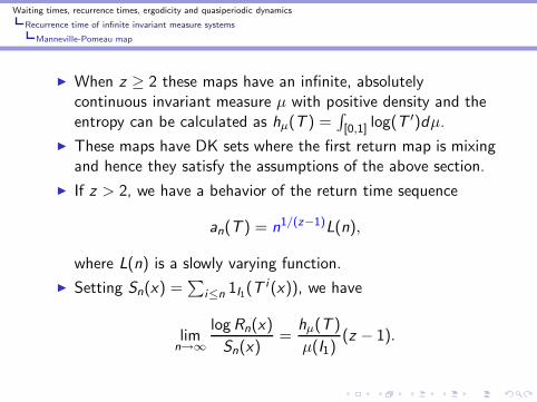
◮ When z ≥ 2 these maps have an infinite, absolutelycontinuous invariant measure µ with positive density and theentropy can be calculated as hµ(T ) =
∫
[0,1] log(T ′)dµ.

Waiting times, recurrence times, ergodicity and quasiperiodic dynamics
Recurrence time of infinite invariant measure systems
Manneville-Pomeau map
◮ When z ≥ 2 these maps have an infinite, absolutelycontinuous invariant measure µ with positive density and theentropy can be calculated as hµ(T ) =
∫
[0,1] log(T ′)dµ.
◮ These maps have DK sets where the first return map is mixingand hence they satisfy the assumptions of the above section.
◮ If z > 2, we have a behavior of the return time sequence
an(T ) = n1/(z−1)L(n),
where L(n) is a slowly varying function.
◮ Setting Sn(x) =∑
i≤n 1I1(Ti (x)), we have
limn→∞
log Rn(x)
Sn(x)=
hµ(T )
µ(I1)(z − 1).

Waiting times, recurrence times, ergodicity and quasiperiodic dynamics
Recurrence time of infinite invariant measure systems
Manneville-Pomeau map
Theorem (Galatolo-K-Park (2006))
Let (X ,T , ξ) satisfy (1)-(3) and µ be the absolutely continuousinvariant measure then
limr→0
log τr (x)
− log r=
{1 if z ≤ 2
z − 1 if z > 2
for almost all points x(recall that τr (x) is the first return time of x in the ball B(x , r)).
Related Documents