Wages and the City - Evidence from Italy

Electronic copy available at: http://ssrn.com/abstract=1002632

WWW.DAGLIANO.UNIMI.IT

CENTRO STUDI LUCA D’AGLIANO DEVELOPMENT STUDIES WORKING PAPERS

N. 231

May 2007

Wages and the City. Evidence from Italy

Sabrina Di Addario* Eleonora Patacchini**

* University of Oxford and Bank of Italy ** University of Rome “La Sapienza”

Electronic copy available at: http://ssrn.com/abstract=1002632

Wages and the City. Evidence from Italy

Sabrina Di Addario University of Oxford and Bank of Italy

Address: Economic Research Unit, Branch of Rome - Bank of Italy. Via XX Settembre, 97/e

00187, Rome, Italy [email protected]

Eleonora Patacchini

University of Rome “La Sapienza” Address: Facoltà di Scienze Statistiche, University of Rome “La Sapienza”

Piazzale Aldo Moro, 5 00100, Rome, Italy

[email protected]

Abstract We analyze empirically the impact of urban agglomeration on Italian wages. Using micro-

data from the Bank of Italy's Survey of Household Income and Wealth for the years 1995, 1998, 2000 and 2002 on more than 22,000 employees distributed in 242 randomly drawn local labor markets, we test whether the structure of wages varies with urban scale. We find that every additional 100,000 inhabitants in the local labor market raises earnings by 0.1 percent. The use of a geographical approach enables us to state that this effect decays very rapidly with distance, losing significance beyond approximately 12 kilometers. We also find that urbanization does not affect returns to experience and that it reduces returns to education and to tenure with current firm, while providing a premium to worker supervisors and office workers.

Keywords: Wages, Urbanization, Agglomeration Externalities, Population Clustering, Worker Mobility

JEL classification: R12; J31; J24; O15

--------------------------------------- Acknowledgements: We thank Margaret Stevens and William Strange for both having encouraged us to pursue

this project and for valuable suggestions on a previous draft. We also thank Erich Battistin, Simon Burgess, Luigi Cannari, Mary Gregory, Stefano Iezzi, Geeta Kingdon, Andrea Lamorgese, Claudio Lucifora, and two anonymous referees for helpful comments; Carla Bertozzi for valuable research assistance; and finally, the participants to: the Third Labor Economics Workshop “Brucchi Luchino” (10-11th December 2004, Florence); the Italian Congress of Econometrics and Empirical Economics (24-25th January 2005, Venice); the 2006 EALE Annual Meeting (21-23rd September 2006, Prague); and the 2006 North American Meeting of the Regional Science Association (16-18th November 2006, Toronto) for stimulating discussions. The views expressed herein are those of the authors and not necessarily those of the Bank of Italy.

2

1. Introduction

While the evidence on the magnitude of the labor-productivity gains generated by agglomeration is

fairly consistent across countries, the findings on the extent to which these gains accrue to workers show

considerable variation. Thus, while the elasticity of average labor productivity with respect to employment

density is estimated to be 5 percent in the US and 4.5 percent in Italy, France, Germany, Spain and the UK

(with no significant difference across countries; Ciccone (2002) and Ciccone and Hall, 1996), the estimates

of urban wage premia vary widely both across and within countries, depending on the agglomeration

variable and dataset used. For instance, the elasticity of wages is about 2 percent with respect to employment

density in the French zones d’emploi (Combes, Duranton, Gobillon, 2003); it is 2.7 percent with respect to

US Statistical Metropolitan Area (MSA) population level (Wheeler, 2001); and it amounts to 10 percent

when it is calculated with respect to the Japanese Standard Metropolitan Employment Area population

(Tabuchi and Yoshida, 2000).1 Furthermore, while Diamond and Simon (1990) find that every additional 1

million inhabitants in the US MSAs increases wages by 1-2 percent, Yankow (2006) obtains a 19 percent

wage premium in the MSAs with more than 1 million inhabitants (falling to 6 percent after removing the

time-invariant unobserved heterogeneity). Similarly, Glaeser and Maré (2001) find that in the MSAs

containing at least one municipality with more than 500,000 inhabitants earnings are 24-28 percent higher

than in rural areas, even though after controlling for individual-specific effects the wage premium from

moving between metropolitan and non-metropolitan areas is reduced to about 4.5 percent.2 Finally,

according to Fu (2007) earnings raise with occupation diversity, especially in the ring placed 6-9 miles away

from the city center.

Thus, urbanization3 estimates vary widely not only across- but also within-studies, largely because of

the presence of self-selection into the largest cities: the time-invariant unobserved heterogeneity can explain

up to 1/2 - 4/5 of the urban wage premium estimated by OLS. In this respect, the Italian case may be of

interest because the limited mobility of Italian workers reduces the likelihood that urbanization estimates are

biased by sorting into the largest markets,4 and this might cast some light on the importance of selection in

other countries. There are mainly two reasons for why Italians are less mobile than, for instance, Anglo-

Saxons. First, because they are more strongly tied to the place of residence of their family of origin. Apart

from the obvious cultural differences, this is probably due to a worse welfare-system, often requesting

siblings to take care of the elderly and grandparents to take care of grandchildren. Second, because the

imperfections of the housing market increase workers' moving costs, reducing the likelihood of migration.

Indeed, the sub-optimal size of the private rented sector (due to the presence of rent controls and to the lack

of laws protecting landlords’ property) together with the high transaction costs for buying and selling a

house lower home-owners’ propensity to move.5

3

The Italian literature has typically focused on regional disparities because of the large labor-

productivity gap between the North and the South of the country (the North-South divide). More recent

studies have analyzed the impact of industrial agglomeration and have found that localization does not affect

average wages, returns to experience or to seniority, while having a depressing effect on the returns to

education (de Blasio and Di Addario, 2005). The lack of studies on the impact of urbanization in Italy is

rather surprising, because despite the heterogeneity of the literature results, there is now a large consensus on

the existence of urban wage differentials. Thus, in contrast to other Italian studies, in this paper we estimate

the effect of urbanization on wages and its attenuation across space. In addition, we test for the presence of

urban differentials in the returns to education, tenure and experience.

Using a unique dataset of more than 22,000 employees distributed in 242 randomly drawn local labor

markets (30 percent of the total) from the Bank of Italy’s Survey of Household Income and Wealth (SHIW)

for the four available years between 1995 and 2002, we find that in Italy earnings rise by just 0.1 percent for

every 100,000-inhabitant increase in the local labor market (LLM). The magnitude of the urbanization effect

is strikingly invariant to the inclusion of individual ability, to controlling for region-specific effects and to

instrumenting urbanization with a number of variables (i.e., population size at the time of Italy’s birth, LLM

land area, the share of LLM covered by water, or by marsh, and the amount of LLM destined to agriculture).

Furthermore, we find that urban externalities attenuate rapidly across space. Indeed, the impact of population

mass on wages is highly localized: the estimated effect is greatest within 4 kilometers from the LLM

centroid, diminishes sharply with distance and has virtually no effect beyond approximately 12 kilometers.

This evidence confirms the appropriateness of LLMs as territorial units of analysis for the estimation of

urbanization effects, since the latter do not extend beyond the mean or the median radius of Italian LLMs.

The large difference between the Italian and the US urban wage premia could be explained by the fact

that the productivity gains generated by agglomeration economies are larger in the US than in Italy.6 There

are mainly two reasons for why this should be the case. First, because the longer history of wage flexibility

in the US gave agglomeration externalities more time to develop.7 Indeed, reforms aimed at increasing the

response of wages to productivity and market conditions (e.g., unemployment levels) have been introduced

only very recently in Italy. Before 1990s wages were rigid and had little scope to vary locally, because the

bargaining system was very centralized. Only in 1993 were reforms introduced to increase the degree of

firm-level bargaining and to reduce the gap between the public and the private sector wage setting

(Dell'Aringa, Lucifora and Origo, 1995). Second, the productivity gains generated by agglomeration

economies might be lower in Italy precisely because labor is less mobile. Indeed, the Italian population is

much more spatially dispersed than the US one,8 it is independent of geographical location and does not

reflect employment conditions (unemployment rates are typically low in the North and very high in the

South) because workers are not mobile enough. Thus, to the extent that the agglomeration-induced

productivity gains increase with the degree of inequality of the population distribution (see Ciccone and

Hall, 1996),9 the spatial distribution of the Italian population, exacerbated by the lack of migration, might

4

reduce the magnitude of urban wage premia. More research is probably needed on the relationship between

agglomeration economies, population spatial distribution and workers’ mobility.

While it is now widely recognized that urbanization is a determinant of average labor productivity,

and thus of average wages, its impact on the components of earnings is less frequently investigated (and, to

our knowledge, it has never been on Italian data).10 Although there are a few studies on the differentials in

returns to education generated by urban agglomeration, there is much less evidence on the differentials in

returns to experience and we have not found any work specifically addressing returns to tenure (except for

Wheeler, 2006).11 In this paper we find, somewhat surprisingly, that college graduates prefer living in the

largest labor markets in spite of earning 0.4-0.8 percent less there than elsewhere. This apparent puzzle could

be explained by the presence of heterogeneous preferences (though we cannot directly test this hypothesis).

Indeed, it could be the case that, in contrast to the large-LLM employees with a middle school or a secondary

school attainment (who do not suffer nor benefit from wage differentials with respect to their non-urban

counterparts), college graduates have a preference for urban consumption amenities strong enough to

compensate their wage loss (see next section).12 Moreover, we find that urbanization does not create

monetary incentives to invest in human capital, but “rewards” job qualification. In particular, while urban

agglomeration does not affect returns to experience, each additional 100,000 individuals in the LLM reduces

returns to seniority by 0.1 percent, and raises worker supervisors’ earnings by 0.5 percent.

The remainder of the paper is organized as follows. Section 2 summarizes the theoretical foundations

of urban wage premia. Section 3 describes the dataset, presenting the main features of workers in the most

highly populated LLMs. Section 4 investigates the existence and magnitude of urban wage premia and

compares the wage structure in large cities to that in the rest of the economy. Section 5 concludes.

2. Why should wages be affected by urban agglomeration?

According to the agglomeration literature, in order to exist cities must benefit from local increasing

returns or indivisibilities; in order not to explode, they must suffer from some sort of congestion cost. Urban

wage premia could be the outcome of either local increasing returns or congestion.13 In the former case,

earnings grow with urban agglomeration because of labor productivity gains. In the latter case, urban wage

premia are a compensation that workers receive for bearing a lower quality of life in more congested areas.

Labor productivity gains are mainly generated by (Marshallian or Jacobian) external scale economies

arising from the nearby location of similar firms and specialized workers; they can be of four types. First are

economies resulting from intra-industry specialization due to a finer inter-firm division of labor, increasing

the number of industrial linkages (including with the service sector). Second are economies due to the cost

reductions that result from producers’ physical proximity to input suppliers and/or final consumers. Third are

externalities due to the greater intensity of communication between agents, which generates knowledge

spillovers favoring innovation (technological spillovers) and increasing the speed of learning (intellectual

5

spillovers). Fourth are economies arising from the existence of pooled markets for specialized workers with

industry-specific skills (labor pooling), which reduce the mismatch between workers’ skills and firm’s job

requirements.14

Wages could be also affected by the fact that agglomeration leads to more intense competition, which

on the one hand raises producers’ or workers’ productivity,15 but on the other hand, might force employees to

work “too long” hours in order to signal effort, which could reduce productivity because of diminishing

marginal returns (Rosenthal and Strange, 2002). Moreover, in a context of monopsony power,16 more intense

competition may produce wage premia even in the absence of productivity gains, as the greater risk of

having their specialized workers poached by competitors might force firms to renounce part of their labor

market power - embodying transferable knowledge (see, for instance, Combes and Duranton, 2001).

In the quality-of-life framework, urban wage premia can exist in the absence of labor productivity

gains. In this type of compensating-differential model (see Gyourko, Kahn and Tracy (1999) for a review),

workers have a preference for amenities (indivisible consumption or public goods) that are profitable to

supply only in the largest cities (e.g., because of increasing returns in the provision of local public services).

Amenities can be “productive” (e.g., infrastructures such as airports or public intermediate inputs tailored to

firms’ specific needs, but also specialized schools and better quality services) or “unproductive” for firms.17

In these models, rents and wages adjust to make individuals indifferent between locations (Roback, 1982).

Thus, rents increase to ration the demand for space in the cities endowed with the best amenities (so as to

equalize workers’ utility in all locations), lowering wages in real terms. In case of unproductive amenities,

wages decrease in nominal terms as well, so as to equalize firms’ costs across locations (in order to make

them willing to localize where rents are higher). In the case of productive amenities, rents rise by a larger

amount, but the net effect on nominal wages depends on the strength of the amenity effect on workers

relatively to that on firms. Furthermore, as city size rises individuals’ utility declines because of congestion

disamenities (i.e., longer commuting, smaller houses, higher cost of living, pollution).18 Thus, all else equal,

the presence of urban wage premia depends on whether workers’ (firms’) disutility from urban disamenities

exceeds (falls short of) the utility from favorable amenities.

Whatever the source of average wage premia, their distribution might be unequal across educational,

experience and seniority groups.

For instance, the most educated workers might benefit more than the least educated employees from

knowledge spillovers, better match quality, or improved quality of life. In the first case, the returns to

education would increase with urban agglomeration if the latter was associated to higher levels of average

human capital (see Moretti, 2004) and those benefited the most educated individuals more than the less

skilled ones (see Benabou, 1993).19 The opposite would occur if the least educated workers had a higher

learning capability (e.g., because they had more to learn; Rosenthal and Strange, 2006). In the second case,

the returns to education could increase with urban scale if match quality improved more for the most

educated workers than for the least educated ones. In Wheeler (2001), for instance, the density of job seekers

6

in the market on the one hand increases the complexity of search, creating a congestion externality; on the

other hand, it reduces firms’ search cost per-worker (by enhancing workers’ arrival rate per job opening, in

the presence of fixed search costs for advertising and interviewing). Thus, provided that the agglomeration

benefits outweigh the costs, firms in large cities have a higher reservation quality than elsewhere, and high-

quality employers, more desirable for all job seekers, select the highest-skill workers. This mechanism, while

improving the efficiency of matches (as capital and worker’s skill are complementary), generates greater

between-skill-group wage inequality. Third, in the quality-of-life framework the correlation between returns

to education and urban agglomeration would be positive if the more-educated (or wealthier) people had a

stronger aversion to living in large cities than the less-educated ones (for instance, because they have more to

lose from crime; Adamson, Clark and Partridge, 2004); it would be negative if the more educated (or

wealthier) people were more willing (or capable) to forego part of their income in exchange for a higher

quality of life in the largest cities (Black, Kolesnikova and Taylor, 2005).

Finally, the sign of the correlation between returns to tenure and urban agglomeration is also a priori

ambiguous. It could be positive for at least two reasons.20 First, because, in a context of imperfect

competition, market size could increase the degree to which on-the-job training is transferable, and thus the

risk poaching (see Stevens, 1994), which forces firms to renounce part of their share of the return to training,

raising workers’ returns to tenure.21 Second, if firms deferred compensation in the form of wages increasing

over time as a strategic device to raise workers’ productivity, and if this induced the most productive

workers to stay longer with their current employer, returns to seniority would increase with urban scale (as in

Topel, 1991). In contrast, if it were the case that the workers with a greater tendency to stay with their

employers (even when badly matched) were the bad-quality ones (as in Stevens, 2003), agglomeration - by

increasing the length of tenure - would in fact reduce returns to seniority.

3. Data and descriptive evidence

We test the existence of urban wage premia with a Mincerian wage function (Mincer, 1958)

augmented with urbanization. We use data from the biannual Survey of Household Income and Wealth,

conducted by the Bank of Italy for the years 1995, 1998, 2000 and 2002. This is the only Italian survey that

allows the estimation of individuals’ returns to education, as it collects information on schooling besides

wages, work experience and tenure. We complement this data set with three Labor Force Survey variables:22

LLM population level, size, and unemployment rate.

Our territorial unit of analysis is the LLM. This choice is essentially motivated by three reasons. First,

LLMs are “self-contained” labor markets, since by definition they are characterized by a very high overlap

between the residing and the working population.23 As a consequence, labor mobility between LLMs is very

low (OECD, 2002), which minimizes the endogeneity issues that may arise when one estimates

agglomeration effects (see Section 4.1.1). Second, LLMs partition the entire national territory, allowing us to

7

draw conclusions with general validity (in contrast to case studies). Third, LLMs are increasingly used as the

territorial unit of analysis in the agglomeration literature (see Rosenthal and Strange (2004) for a survey) and

are now available in a number of countries (including the UK's Travel-to-Work Areas and the French zones

d'emploi).24

We measure urbanization with LLM population level.25

In the Appendix Table A1 we present some descriptive evidence based on the whole sample, the

largest labor markets (above the 90th percentile of the population distribution) and the rest of the country.

Our sample comprises all the wage-earners from a primary activity, for a total of 22,996 individuals

distributed over 242 LLMs (30 percent of the total). The table compares our sample’s wage mean values in

the largest LLMs to those elsewhere in the country and shows that the former are 5 percent higher than the

latter (at the 1 percent level statistical significance), suggesting the existence of an urban wage premium

(though quite limited in magnitude). To investigate on the possible sources of this wage differential, we also

report the statistics on the skill composition and unemployment rates. In summary, we find that the biggest

markets host a largeer share of college graduates and display higher unemployment rates than the rest of the

economy.

With respect to skill composition, our sample26 indicates that the employees who reside in the largest

markets tend to be more educated than elsewhere: the difference in the mean values between the share of

college graduates in the largest LLMs and that in the rest of the country is 3.3 percent and is statistically

significant at the 1 percent level. Using data on the Italian LLM universe, Figure 127 shows three maps

depicting the geographical distribution of: a) the residing population, b) the share of college graduates (or

higher qualification) in total residents and c) the unemployment rate. A comparison between the first two

maps reveals that in Italy high human capital workers concentrate in the most highly populated LLMs, thus

suggesting that urban wage premia could be due to workers’ education composition effects.

With respect to LLM unemployment rates, a visual inspection of Figure’s 1 last map would seem to

confirm the common view that in Italy regional unemployment differentials are more clearly associated to

the North-South divide than to a partition based on LLM population size. However, according to our sample,

average unemployment rates are more than 2 percent higher in the largest LLMs than in the rest of the

country (Table A1).28 This evidence shows that on average there is a positive association between earnings,

unemployment rates and population size, suggesting that in the largest LLMs wages might be higher than

elsewhere in order to offset the greater risk of unemployment.29 In contrast, the wage-curve literature (see

Card, 1995) finds a negative correlation between (log) wages and (log) local unemployment (note that next

section’s econometric results indicate that this is indeed the case once we control for individuals’ observable

characteristics and area-specific fixed effects).

Table A1’s descriptive statistics also shows that, as expected, the largest markets contain more office

workers, worker supervisors, and real estate employees than the rest of the economy. Furthermore, the

8

workers in the largest-LLMs are slightly older than those living elsewhere, again supporting the hypothesis

that urban wage premia might be explained by the presence of higher human capital. In the next section we

will obtain some indication on whether the most educated people prefer living in large cities because of the

consumption amenities these offer or because of higher returns.

4. The estimation results

In this section we examine whether the hypothesis of higher average wages in urban areas holds true

after controlling for individual and LLM characteristics by estimating a log-linear Mincerian function

augmented with urbanization:

iiiiiiiii uZURBANTENTENEXPEXPEDUαw ++++++++= βαααααα 62

542

3210log (1)

The dependent variable of our earnings function is the logarithm of employees’ hourly wage rates

from primary activities, deflated with the consumer price index for blue-collar worker and employee

households,30 which is the inflation indicator used in national contracts. In addition to the standard Mincerian

variables (experience, tenure, and education) we also control for the vector Z, including individual

characteristics (e.g., sex and marital status), job qualification, some features of the worker's firm (e.g., firm

size, industry dummies, type of contract, like, for instance, Adamson, Clark and Partridge, 2004), the

unemployment rate of LLM of residence (as in the “wage-curve” literature)31 and year dummies; u is the

error term. Finally, we capture the urban effect with the LLM population mass.

In Section 4.1.1 we tackle the potential endogeneity issues by undertaking a number of robustness

checks (i.e., controlling for region-specific fixed effects, replacing OLS with IV estimation, and restricting

the sample to the “stayers”), while in Section 4.1.2 we estimate the spatial reach of agglomeration

economies.

Finally, in Section 4.2 we study whether larger markets exhibit a different wage structure. We thus

estimate a version of the previous earnings functions where we add the interactions between all the

regressors and the agglomeration variables, to calculate, in particular, the urbanization differentials in the

returns to education, experience and tenure.

4.1 Urban wage premia

Table 1 reports the outcome of the ordinary least square estimates. We test six specifications (columns

(1.1)-(1.6)). Thus, the vector of control variables in column (1.1) includes the standard individuals'

observable characteristics (i.e., education, second-order effects of experience and tenure, sex, marital status,

macro-region of residence32) and the LLM unemployment rate.33 Then, we gradually introduce firm

characteristics and job qualification, and in column (1.2) we also control for the sector and the size of the

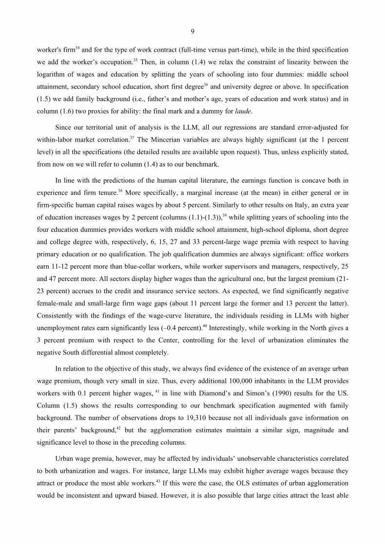
9

worker's firm34 and for the type of work contract (full-time versus part-time), while in the third specification

we add the worker’s occupation.35 Then, in column (1.4) we relax the constraint of linearity between the

logarithm of wages and education by splitting the years of schooling into four dummies: middle school

attainment, secondary school education, short first degree36 and university degree or above. In specification

(1.5) we add family background (i.e., father’s and mother’s age, years of education and work status) and in

column (1.6) two proxies for ability: the final mark and a dummy for laude.

Since our territorial unit of analysis is the LLM, all our regressions are standard error-adjusted for

within-labor market correlation.37 The Mincerian variables are always highly significant (at the 1 percent

level) in all the specifications (the detailed results are available upon request). Thus, unless explicitly stated,

from now on we will refer to column (1.4) as to our benchmark.

In line with the predictions of the human capital literature, the earnings function is concave both in

experience and firm tenure.38 More specifically, a marginal increase (at the mean) in either general or in

firm-specific human capital raises wages by about 5 percent. Similarly to other results on Italy, an extra year

of education increases wages by 2 percent (columns (1.1)-(1.3)),39 while splitting years of schooling into the

four education dummies provides workers with middle school attainment, high-school diploma, short degree

and college degree with, respectively, 6, 15, 27 and 33 percent-large wage premia with respect to having

primary education or no qualification. The job qualification dummies are always significant: office workers

earn 11-12 percent more than blue-collar workers, while worker supervisors and managers, respectively, 25

and 47 percent more. All sectors display higher wages than the agricultural one, but the largest premium (21-

23 percent) accrues to the credit and insurance service sectors. As expected, we find significantly negative

female-male and small-large firm wage gaps (about 11 percent large the former and 13 percent the latter).

Consistently with the findings of the wage-curve literature, the individuals residing in LLMs with higher

unemployment rates earn significantly less (–0.4 percent).40 Interestingly, while working in the North gives a

3 percent premium with respect to the Center, controlling for the level of urbanization eliminates the

negative South differential almost completely.

In relation to the objective of this study, we always find evidence of the existence of an average urban

wage premium, though very small in size. Thus, every additional 100,000 inhabitants in the LLM provides

workers with 0.1 percent higher wages, 41 in line with Diamond’s and Simon’s (1990) results for the US.

Column (1.5) shows the results corresponding to our benchmark specification augmented with family

background. The number of observations drops to 19,310 because not all individuals gave information on

their parents’ background,42 but the agglomeration estimates maintain a similar sign, magnitude and

significance level to those in the preceding columns.

Urban wage premia, however, may be affected by individuals’ unobservable characteristics correlated

to both urbanization and wages. For instance, large LLMs may exhibit higher average wages because they

attract or produce the most able workers.43 If this were the case, the OLS estimates of urban agglomeration

would be inconsistent and upward biased. However, it is also possible that large cities attract the least able

10

workers, because of their stronger informal labor market (e.g., illegal activities) drawing in ‘bad type’ job

seekers, or because of the availability of a larger offer of vacancies (e.g., from a more generous government

support), creating an additional demand for the less productive matches. If city size was in fact negatively

correlated with ability, our OLS agglomeration effect estimates would be inconsistent and downward biased.

Thus, the sign of the bias (provided it existed) is ultimately a matter of empirical estimation. To make sure

that our results are not due to omitted ability, in specification (1.6) we distinguish between high and low

quality individuals by controlling for both the final mark obtained (either at school or at college) and having

graduated with a laude (if graduated).44 Both these variables provide a 6 percent wage premium (statistically

significant, respectively, at the 5 and 1 percent level), and reduce the educational attainment estimates.

Nevertheless, including ability does not change our results on agglomeration, confirming the robustness of

our results to the sorting of the most capable workers into the largest LLMs.45

Table 1 THE URBAN WAGE PREMIUM (OLS estimates)

Notes: Regressions are weighted to population proportions and White-robust standard errors adjusted for clustering at the LLM level are reported in parentheses (the coefficients in bold are statistically significant at the 10 percent level at least). The basic control variables are: education, quadratic terms of experience and tenure, sex, marital status, macro-region of residence, LLM unemployment rate and the time dummies. In (1.5) the sample is restricted to all the persons who provided information on family background (parents’ age, education, and work status) and in column (1.6), which includes ability (the final mark obtained at high school or college and a dummy for laude), the sample is restricted to the 2000-02 SHIW waves.

Finally, we test whether the relationship between wages and urbanization is, indeed, log-linear. When

we lift the imposition of linearity between (log) earnings and the urbanization variables, we find that higher

order polynomials (including quadratic and cubic terms) of population size are never significant (results are

not reported due to space constraints). The log-linearity of the urbanization-wage curve is also confirmed by

the fact that when we add threshold dummies46 to LLM population size, they are never significant (results

available if requested).

Thus, our results confirm the existence of an urban wage premium, even if small in magnitude. This

necessarily implies that in Italy the combined positive effect of agglomeration-induced productivity gains,

Dep. var: log of wage (1.1) (1.2) (1.3) (1.4) (1.5) (1.6) LLM population 0.0142 0.0136 0.0102 0.0085 0.0081 0.0094

(0.0043) (0.0035) (0.0025) (0.0025) (0.0031) (0.0051) Basic controls Yes Yes Yes Yes Yes Yes Sector and size of firm No Yes Yes Yes Yes Yes Type of work-contract No Yes Yes Yes Yes Yes Occupation No No Yes Yes Yes Yes Family Background No No No No Yes No Ability No No No No No Yes Observations 22,996 22,996 22,996 22,996 19,310 10,802 R2 .3289 .3713 .4058 .4043 .4276 .3624

11

poaching diseconomies and people’s distaste for urban disamenities (e.g., higher house rents and prices)47

prevails over the negative impact of workers’ preferences for large-city amenities.

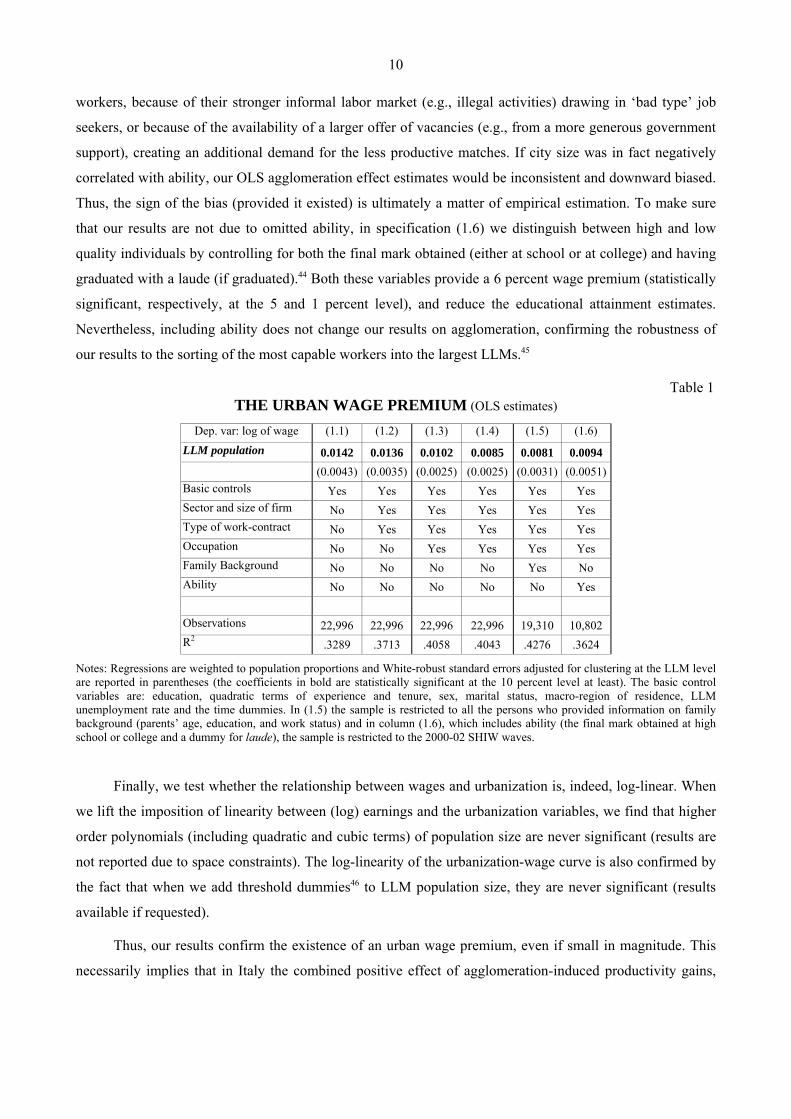
4.1.1 Robustness checks

We have just shown that our results are robust to both the inclusion of ability among the regressors

and the specification of the wage-urbanization functional form. However, there could still be sorting

generated by unobservable characteristics - other than ability - correlated to both urbanization and the

unexplained part of wages, which would bias and make our estimates inconsistent. For instance, the largest

labor markets might exhibit higher productivity and thus wages, but at the same time could be more

endowed with desirable amenities that attract people (since the provision of goods such as airports,

specialized schools, operas, ethnic restaurants, etc., might require a certain critical population mass). In this

section we undertake a number of robustness checks on our benchmark specification to investigate whether

this is the case (Table 2).

Thus, we first test whether our results could in fact be driven by area-specificities different from

urbanization by controlling for region-specific fixed effects.48 Column (2.1) confirms the existence of an

urban wage premium amounting to 0.1 percent every additional 100,000 inhabitants (statistically significant

at the 3 percent level).

Second, we test the exogeneity of our agglomeration variable with the standard instrumental variable

methodology, instrumenting LLM population level local labor market characteristics arguably not correlated

to the error term in the wage equation. In particular, in specification (2.2) we instrument urbanization with

LLM population in 1861, following Ciccone and Hall (1996). The validity of this instrument relies on the

assumption that the population pattern in the XVIII century (i.e., at the time of Italy’s foundation) is

uncorrelated to current wage levels, except for its effect through population size in 1991. In column (2.3) we

use LLM size, similarly to Ciccone (2002),49 while in specification (2.4) we utilize three instruments from

the Istituto Tagliacarne’s Geostarter dataset: the amount of LLM area covered by water (similarly to

Rosenthal and Strange, 2006) or by marsh, and the share of land destined to agriculture.50 Finally, in column

(2.5) we pool all the instruments together. In the first-step equation of both (2.4) and (2.5), the instruments

are all individually statistically significant at least at the 10 percent level,51 and, more importantly, the F-test

of joint significance of all the instruments rejects the null hypothesis at the 1 percent statistical significance

level. In the second stage, the Anderson canonical correlations likelihood-ratio test rejects the null

hypothesis of under-identification of both the regressions ((2.4) and (2.5)) at the 1 percent statistical

significance level, and the Hansen-Sargan test of over-identifying restrictions cannot reject the null

hypothesis of validity of our instruments. Columns (2.2)–(2.5) report the outcome of the instrumental

variable regressions corresponding to our benchmark specification. Results show that the IV urbanization

estimates are always positive and significant and have the same magnitude as the OLS estimates: a 100,000-

12

inhabitant increase in LLM population raises wages by 0.1 percent. The remarkable constancy of our finding

across different specifications and estimation methods, implies that our agglomeration variable is not

endogenous.

Table 2 SENSITIVITY CHECKS ON THE URBAN WAGE PREMIUM (IV and OLS estimates)

Dep. var: log of wage

Regional fixed

effects

IV estimation:

LLM population in

1861

IV estimation: LLM size

IV estimation: LLM % of

water, marsh, agriculture

IV estimation:

all instruments

Stayers sub-sample: council

tenants, rent controls

Stayers sub-sample: council tenants, rent

controls, home-owners

(2.1) (2.2) (2.3) (2.4) (2.5) (2.6) (2.7) LLM

population 0.0092 0.0124 0.0101 0.0061 0.0082 0.0117 0.0084

(0.0042) (0.0048) (0.0045) (0.0035) (0.0027) (0.0067) (0.0028) Observations 22,996 22,996 22,996 22,996 22,996 2,804 18,571 R2 .4107 .4074 .4074 .4074 .4074 .3235 .4144

Notes: Regressions are weighted to population proportions and White-robust standard errors adjusted for clustering at the LLM level are reported in parentheses (the coefficients in bold are statistically significant at the 10 percent level at least). The other control variables, not reported here for space constraints, are those corresponding to specification (1.4). In (2.6) the sample is restricted to all the persons either residing in council housing or benefiting from controlled rents; in (2.7) home-owners are added to the sample of specification (2.6).

An alternative method to separate agglomeration effects from the impact of self-selection into large

cities is the estimation of a balanced panel where the area-fixed effects are identified by the individuals who

change LLM of residence over time (the “movers”) and those who do not (the “stayers”).52 However, we are

not able to construct such a panel because none of the individuals interviewed by the SHIW changed LLM of

residence in the period 1995-2002. This is not too surprising, as LLMs are self-contained (see previous

section). Moreover, endogeneity issues are typically not a major concern in a country like Italy, where labor

mobility is particularly low in levels and has been decreasing over time (Cannari, Nucci, and Sestito, 2000)

and where people’s residential choices are conditioned to a large extent by the location of their family, while

being affected by the heavy imperfections of the housing market. However, it is precisely the imperfections

of the housing market that provides us with an indirect estimate of the group of stayers, enabling us to show

that an urban wage premium exists even for whom is unlikely to move (so that it cannot be due to self-

selection into LLMs).53 Indeed, we first consider as non-movers all the individuals residing in council

housing (like Patacchini and Zenou, 2006) and those benefiting from controlled rents (an “equo canone”

contract).54 Estimates, reported in column (2.6) have the same magnitude as Table 1’s and are statistically

significant at the 8 percent level. To increase the number of observations (from 2,804 to 18,571 individuals),

in specification (2.7) we add home-owners, who, in a country like Italy, are not very likely to move because

of the high transaction costs for selling and buying a house. Indeed, also in this case we obtain a 0.1 percent

large wage premium (statistically significant at the 1 percent level) every 100,000 individuals added to the

LLM.55

13

Summarizing, we can conclude that after controlling for endogeneity issues workers of given

individual characteristics tend to earn more, on average, in the largest local labor markets. We have shown

that this result is not just due to skill composition effects (e.g., the greater presence of college graduates in

large cities shown in the descriptive statistics), since we still find evidence of an urban wage premium after

controlling for both education and worker’s occupation. We can also disregard the hypothesis that urban

wage differentials are a compensation for a greater unemployment risk, since once we control for

individuals’ observable characteristics the effect of local unemployment rates on earnings becomes negative.

Finally, the urban wage premium is not due to region-specific effects, nor to LLM differentials in ability or

in other unobserved factors, such as LLM differences in the amenity endowment. As for the magnitude of

the urbanization effect, the constancy of our results across different specifications is striking: wages increase

by 0.1 percent every additional 100,000 individuals in the LLM.

4.1.2 The spatial decay

The purpose of this section is two-fold. We first aim at reducing any remaining bias arising from

measurement error (i.e., from measuring urbanization with population mass at the LLM level).56 Our second

objective is the calculation of the agglomeration economies’ spatial reach.

We thus follow the approach of Rosenthal and Strange (2006), who estimate the rate at which the

effect of agglomeration (measured by total employment) on wages attenuates with distance. Likewise, we

assume that each individual of the sample is situated at the geographic centroid of their LLM of residence,

and that the population of each LLM is evenly distributed within the area. Then: a) we compute the amount

of population residing within concentric rings of a given radius drawn around the LLM centroid;57 and b) we

add the population within each of the chosen distance bands to Table 1’s regressions. We are then able to

assess the spatial scale of the population mass effects by comparing estimates across the rings. The equation

we estimate is:

iiik

riki uZMVPopαw kr ++++= ∑ γβδα )(log ,0 , (2)

where δr,k is the share of the rth LLM population ( riPop , ) afferent to the kth band (with k=1,..,4), and

MVi and Zi are, respectively, the standard Mincerian variables and the vector of individual characteristics

presented in equation 1.

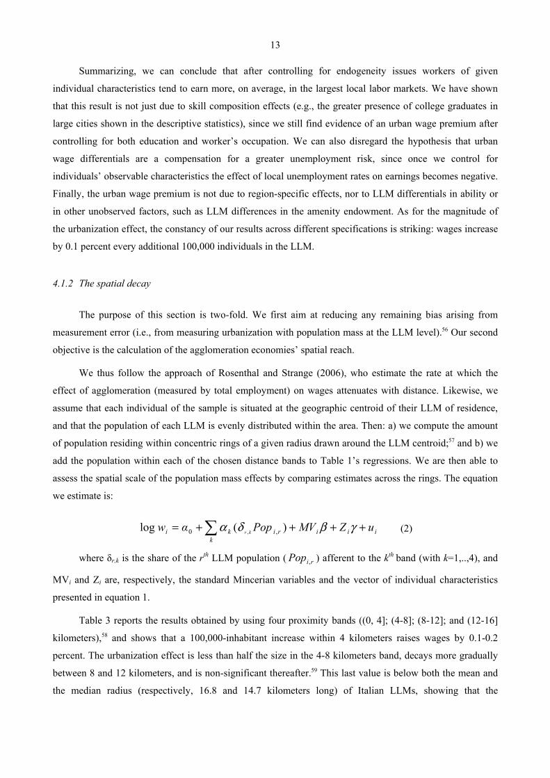
Table 3 reports the results obtained by using four proximity bands ((0, 4]; (4-8]; (8-12]; and (12-16]

kilometers),58 and shows that a 100,000-inhabitant increase within 4 kilometers raises wages by 0.1-0.2

percent. The urbanization effect is less than half the size in the 4-8 kilometers band, decays more gradually

between 8 and 12 kilometers, and is non-significant thereafter.59 This last value is below both the mean and

the median radius (respectively, 16.8 and 14.7 kilometers long) of Italian LLMs, showing that the

14

externalities associated with agglomeration economies are likely to occur within LLMs.60 Inter-area effects,

if any, are minimal, confirming the appropriateness of LLMs as territorial units of analysis for the estimation

of agglomeration effects.

Table 3

THE SPATIAL SCALE OF THE URBAN WAGE PREMIUM (OLS estimates)

Notes: Regressions are weighted to population proportions and White-robust standard errors adjusted for clustering at the LLM level are reported in parentheses (results in bold are statistically significant at the 10 percent level at least). The distance bands include the superior limit, exclude the lower. The specifications correspond to those of Table 1.

4.2 The urban wage structure

In this section we analyze whether urbanization affects the structure of wages. Indeed, agglomeration

effects may not be skill-neutral, unevenly affecting the wages of workers with different characteristics. In

particular, we are interested in examining whether returns to education, experience, and tenure vary with

LLM population level.

The descriptive statistics presented in Section 3 indicate that large cities attract or produce the most

experienced and educated workers. This phenomenon could possibly be due to returns to experience and

education increasing with urban scale, but also to the most skilled people having a relatively stronger

preference for large-city amenities than low skilled workers. In the former case we should observe higher

urban return-to-education and/or to experience differentials, in the latter case, the reverse.

Dep. var: log of wage (3.1) (3.2) (3.3) (3.4) (3.5) (3.6) Population mass within

(0-4 km] 0.0215*** 0.0206*** 0.0152*** 0.0102*** 0.0098*** 0.0115***

(0.0060) (0.0057) (0.0044) (0.0031) (0.0026) (0.0040)

(4-8 km] 0.0110** 0.0099 0.0074** 0.0050** 0.0042** 0.0052**

(0.0052) (0.0046) (0.0033) (0.0024) (0.0020) (0.0026)

(8-12 km] 0.0085** 0.0061** 0.0051** 0.0029** 0.0015** 0.0031**

(0.0041) (0.0029) (0.0025) (0.0014) (0.0007) (0.0015)

(12-16 km] 0.0012 0.0009 0.0008 0.0005 0.0002 0.0003

(0.0013) (0.0010) (0.0009) (0.0007) (0.0004) (0.0006)

Basic controls Yes Yes Yes Yes Yes Yes

Sector and size of firm No Yes Yes Yes Yes Yes

Type of work-contract No Yes Yes Yes Yes Yes

Work Status No No Yes Yes Yes Yes

Family Background No No No No Yes No

Ability No No No No No Yes

Observations 22,996 22,996 22,996 22,996 19,310 10,802

R2 .3452 .3907 .4109 .4112 .4425 .4053

15

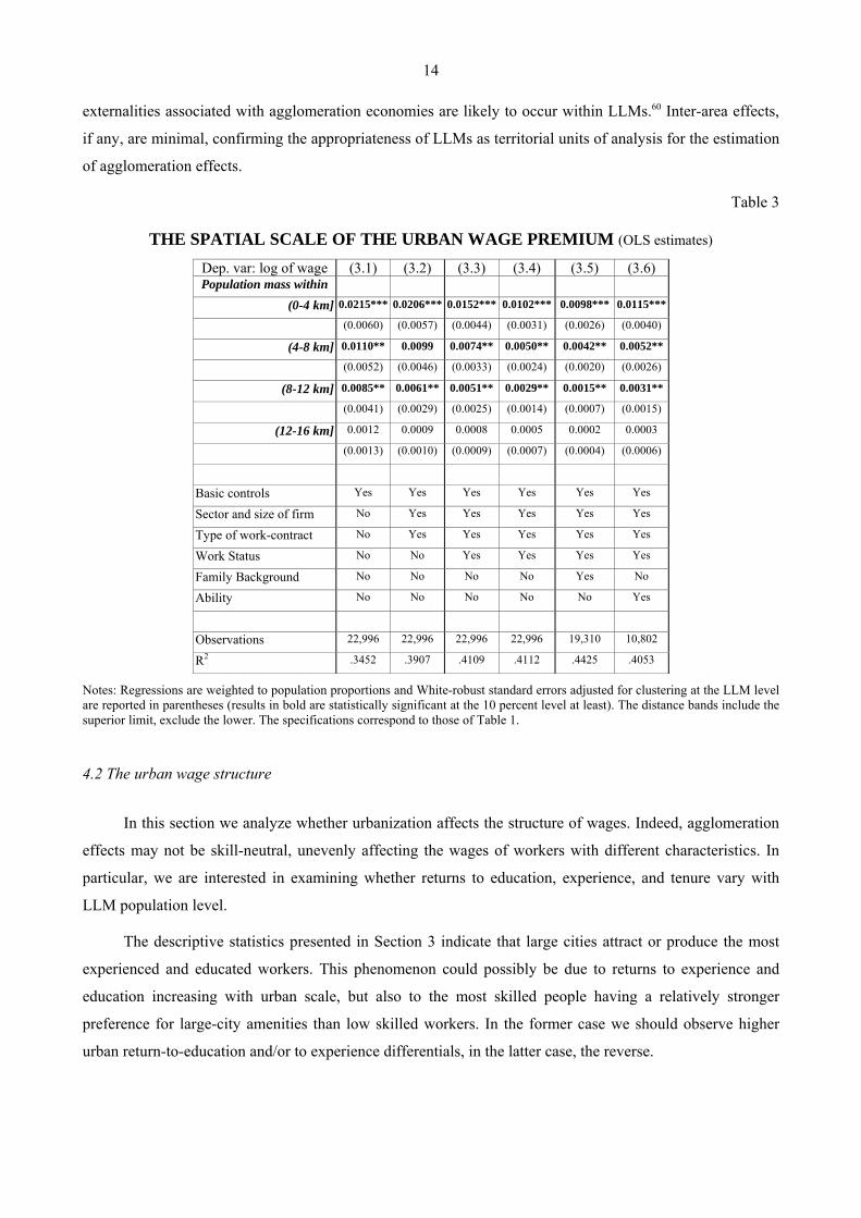
Table 4 shows the key results corresponding to a version of Table 1 augmented with the interactions

between all the regressors and LLM population size. Thus, for instance, the coefficient of the interaction

between population size and the college graduate dummy (column (4.4)) tells whether returns to university

degree vary with urban scale.

Table 4 THE URBAN WAGE STRUCTURE (OLS estimates)

Dep. var: log of wage (4.1) (4.2) (4.3) (4.4) (4.5) (4.6) LLM population 0.0540 0.0163 0.0105 -0.0043 -0.0213 -0.0107 (0.0386) (0.0332) (0.0288) (0.0278) (0.0337) (0.0376) Experience * Pop 0.0016 0.0018 0.0013 0.0015 0.0003 0.0052 (0.0009) (0.0008) (0.0008) (0.0008) (0.0017) (0.0010) Experience2 * Pop (x 100) -0.0034 -0.0031 -0.0025 -0.0026 0.0034 -0.0102 (0.0022) (0.0017) (0.0017) (0.0019) (0.0022) (0.0019) Tenure * Pop -0.0014 -0.0012 -0.0016 -0.0017 0.0006 -0.0040 (0.0006) (0.0007) (0.0007) (0.0007) (0.0007) (0.0010) Tenure2 * Pop (x 100) 0.0016 0.0055 0.0022 0.0026 -0.0013 0.0085 (0.0020) (0.0023) (0.0020) (0.0018) (0.0019) (0.0031) Education * Pop -0.0012 -0.0007 -0.0018

(0.0010) (0.0013) (0.0008) Middle school * Pop 0.0011 -0.0023 -0.0001

(0.0079) (0.0103) (0.0188) Secondary school * Pop -0.0062 -0.0068 0.0018

(0.0163) (0.0172) (0.0278) Short degree (3 years) * Pop 0.0058 0.0308 0.0634 (0.0265) (0.0266) (0.0427) First degree or above * Pop -0.0369 -0.0550 -0.0823 (0.0212) (0.0218) (0.0313) Basic controls Yes Yes Yes Yes Yes Yes

Sector and size of firm No Yes Yes Yes Yes Yes

Type of work-contract No Yes Yes Yes Yes Yes

Work Status No No Yes Yes Yes Yes

Family Background No No No No Yes No

Ability No No No No No Yes

Observations 22,996 22,996 22,996 22,996 19,310 10,802

R2 .3301 .3731 .4082 .4099 .4306 .3698

Notes: Regressions are weighted to population proportions and White-robust standard errors adjusted for clustering at the LLM level are reported in parentheses (the coefficients in bold are statistically significant at the 10 percent level at least). The basic control variables are: education, quadratic terms of experience and tenure, sex, marital status, macro-region of residence, LLM unemployment rate and the time dummies. In (4.5) the sample is restricted to all the persons who provided information on family background (parents’ age, education, and work status) and in column (4.6), which includes ability (the final mark obtained at high school or college and a dummy for laude), the sample is restricted to the 2000-02 SHIW waves.

On average, we find evidence of negative return-to-education differentials in the largest labor markets.

Indeed, even if the interaction between years of schooling and our agglomeration variable is almost never

significant (except for in column (4.3)), when we release the imposition of a linear relationship between

wages and education, we find that returns to bachelor's degree are systematically negatively correlated with

all LLM population size, while returns to lower attainment are not affected by location. In particular, a

16

100,000-inhabitant increase in LLM population size lowers college graduates' wages by 0.4 percent (column

(4.4)).61 When we control for family background or ability the effect increases to 0.6-0.8 percent

(specifications (4.5)-(4.6)). These outcomes, implying that urban amenities play an important role in the

location decisions of the most highly educated workers, are in line with both Adamson, Clark and Partridge

(2004), who find that doubling the population in the US MSA population lowers returns to university degree

by 2 percentage points,62 and with Black, Kolesnikova and Taylor (2005), who show that the US high-

amenity and expensive cities (i.e., San Francisco, New York and Seattle) exhibit lower returns to university

degree than the low-amenity ones (e.g., Houston, Pittsburgh). These results suggest that the education-biased

urban amenity effect dominates the education-biased agglomeration one both in Italy and in the US. Indeed,

since the most highly educated workers have a stronger preference for living in the largest cities than for

living elsewhere (see Section 3) in spite of earning lower wages, there must be urban consumption amenities

that compensate their income loss.63

We also find that urban agglomeration does not generate monetary incentives to invest in either in

general or on-the-job human capital accumulation. Indeed, the urbanization differentials in the returns to

experience are virtually zero,64 while those in the returns to tenure in current firm are significantly negative

(columns (4.1)-(4.6)).65 In particular, a 100,000-inhabitant increase in LLM population size reduces returns

to seniority by 0.1 percent. This finding is consistent with the view according to which tenure is negatively

correlated to the efficiency of the worker-firm match (as high quality workers tend to change job more

frequently, Stevens, 2003) and positively related to agglomeration.

In contrast to the previous results (but not with other results of the literature), we find that returns to

job qualification increase with urban scale.66 Thus, office workers’ and worker supervisors' earn,

respectively, an extra 0.1 and 0.5 percent of their wage for every additional 100,000 inhabitants in their

LLM.67 This result suggests that in Italy urbanization remunerates more job qualification than educational

attainment.

5. Concluding remarks

This paper has analysed the impact of urban agglomeration on average wages and the structure of

earnings in Italy.

We find evidence of an urban wage premium, though very small in size. In particular, a 100,000

inhabitant-increase in LLM population raises earnings by 0.1 percent. The nearly non-existence of urban

wage premia hides substantially different losses and gains for different categories of workers that cancel out

in a sort of zero-sum game. Indeed, we find that urbanization increases the monetary returns of worker

supervisors and office workers, does not affect returns to overall experience in the labor market, and reduces

the returns to education and to tenure with current firm. Thus, college graduates living in the largest LLMs

17

are subject to a 0.4-0.8 percent wage reduction. This apparent paradox can be explained in a quality-of-life

framework. Indeed, even if we cannot test whether the more educated employees benefit more than less

educated workers from urban productivity gains, our results say that even if this was the case, the enhanced

productivity effect is more than offset by the negative impact on wages deriving from education-biased

urban amenities.

These findings raise a number of policy-relevant issues.

First, to what extent does the lack of workers’ mobilty and the consequent spatial dispersion of the

Italian population constitute an obstacle to growth? Ciccone and Hall (1996) show that the more employment

is spatially concentrated the higher the productivity gains from agglomeration. Thus, a renewed increase in

labor mobility might benefit unemployed workers not only in terms of employment but also in terms of wage

premia.

Second, to what extent will productivity growth eventually be hampered by the presence of negative

return-to-education differentials in the Italian large cities? According to Glaeser and Saiz (2003) the most

important determinant of urban growth is skill composition. In the last twenty years, the US MSAs with a

higher share of educated workers have grown 3.4 times faster than those with a lower proportion of college

graduates. More generally, the rising level of educational attainment contributed to almost one-third of US

output-per-hour growth (over the period 1950-1993; Jones, 2002). While currently Italian cities do attract

highly educated workers, it is legitimate to wonder whether the presence of negative urban wage differentials

to college graduates will eventually lower their demand for cities (see Glaeser, 1999) and will thus diminish

Italy’s productivity growth in the long run.

Finally, if the most highly educated Italian workers concentrate in large cities in spite of obtaining

lower returns, there must either be consumption amenities that compensate their wage loss or a higher

demand of their skills (i.e., a higher probability of finding a job). In the former case, in order to keep

attracting high skilled workers city-planners should aim at improving the quality and at increasing the offer

of city services (schools, transportation system, hospitals, etc.). In the latter case, local governments should

rather ease regulations, cut business taxes and provide subsidies to attract firms (Adamson, Clark and

Partridge, 2004).

References

Adamson, D. W., D. E. Clark, and M. D. Partridge. 2004. "Do Urban Agglomeration Effects and Household Amenities Have a Skill Bias?," Journal of Regional Science, 44, 201-223.

Becker, Sasha O., Andrea Ichino and Giovanni Peri. 2003. “How Large is the “Brain Drain” from Italy?,” mimeo.

Beffy, Magali, Moshe Buchinsky, Denis Fougère, Thierry Kamionka and Francis Kramarz. 2006. “The Returns to Seniority in France (and Why they are Lower than in the Unites States?),” Discussion Paper 13, 6, IZA.

18

Benabou, Roland. 1993. “Workings of a City: Location, Education, and Production,” Quarterly Journal of Economics, 108, 619-652.

Black, Dan, Natalia Kolesnikova, and Lowell Taylor. 2005. “Understanding Returns to Education When Wages and Prices Vary by Location,” mimeo.

Brunello, Giorgio. 2001. “On the Complementarity between Education and Training in Europe,” Discussion Paper 309, Fondazione Eni Enrico Mattei.

Cannari, Luigi, Francesco Nucci, and Paolo Sestito. 2000. "Geographic Labor Mobility and the Cost of Housing: Evidence from Italy," Applied Economics, 32, 1899-1906.

Card, David. 1995. "The Wage Curve: A Review," Journal of Economic Literature, 33, 785-799.

Card, David. 2001. "Estimating the Return to Schooling: Progress on some Persistent Econometric Problems," Econometrica, 69, 1127-1160.

Ciccone, Antonio. 2002. “Agglomeration Effects in Europe,” European Economic Review, 46, 213-227.

Ciccone, Antonio, and Robert E. Hall. 1996. “Productivity and the Density of Economic Activity,” American Economic Review, 78, 89-107.

Combes, Pierre-Philippe, and Gilles Duranton. 2001. “Labor Pooling, Labor Poaching and Spatial Clustering,” CERAS Working Paper 01-03.

Combes, Pierre-Philippe, Gilles Duranton, and Laurent Gobillon. 2003. “Spatial Wage Disparities: Sorting Matters!,” Working Paper.

de Blasio, Guido, and Sabrina Di Addario. 2005. “Do Workers Benefit from Industrial Agglomeration?,” Journal of Regional Science, 45, 797-827.

Dell'Aringa, Carlo, Claudio Lucifora and Federica Origo. 2005. Public Sector Reforms and Wage Decentralisation: A First Look at Regional Public-Private Wage Differentials in Italy," mimeo.

Di Addario, Sabrina. 2006. “Job Search in Thick Markets: Evidence from Italy,” Temi di Discussione, no. 605, Bank of Italy.

Di Addario, Sabrina, and Eleonora Patacchini. 2006. “Is There an Urban Wage in Italy?,” Temi di Discussione, no. 570, Bank of Italy.

Di Addario, Sabrina. 2007. “Italian Household Tenure Choices and Housing Demand,” mimeo.

Diamond, Charles A., and Curtis J. Simon. 1990. “Industrial Specialization and the Returns to Labor,” Journal of Labor Economics, 8, 175-201.

Duranton, Gilles, and Diego Puga. 2004. “Micro-foundations of Urban Agglomeration Economies,” in J.V. Henderson and J.F. Thisse (eds.), Handbook of Regional and Urban Economics, Volume 4, Amsterdam: Elsevier.

Fu, Shihe. 2007. “Smart Café Cities: Testing Human Capital Externalities in the Boston Metropolitan Area,” Journal of Urban Economics, 61, 86-111.

Fu. Shihe and Ross, Stephen L. 2007. “Wage Premia in Employment Clusters: Agglomeration Economies or Worker Heterogeneity?,” mimeo.

Glaeser, Edward L. 1999. “Learning in Cities,” Journal of Urban Economics, 46, 254-277.

Glaeser, Edward L., and D. C. Marè. 2001. “Cities and Skills,” Journal of Labor Economics, 19, 316-342.

Glaeser, Edward L., and Albert Saiz. 2003. “The Rise of the Skilled City,” Discussion Paper 2025, Harvard Institute of Economic Research.

Gyourko, Joseph, Matthew Kahn, and Joseph Tracy. 1999. “Quality of Life and Environmental Comparisons,” in P. Cheshire and E.S. Mills (eds.), Handbook of Regional and Urban Economics, Volume 3, Amsterdam: Elsevier.

Istat. 1997. I sistemi locali del lavoro 1991, Rome: ISTAT.

19

Jones, Charles I. 2002. “Sources of U.S. Economic Growth in a World of Ideas,” American Economic Review, 92, 220-239.

Kim, Sunwoong. 1990. “Labor Heterogeneity, Wage Bargaining, and Agglomeration Economies,” Journal of Urban Economics, 28, 160-177.

Mincer, J. 1958. “Investment in Human Capital and Personal Income Distribution,” Journal of Political Economy, 66, 281-302.

Moomaw, Ronald L. 1983. “Is Population Scale a Worthless Surrogate for Business Agglomeration Economies?,” Regional Science and Urban Economics, 13, 525-545.

Moretti, Enrico. 2004. “Human Capital Externalities in Cities,” in J.V. Henderson and J.F. Thisse (eds.), Handbook of Regional and Urban Economics, Amsterdam and New York: North Holland.

OECD. 2002. Redefining Territories. The Functional Regions, OECD: Paris.

Patacchini, Eleonora and Yves Zenou. 2006. “Intergenerational Education Transmission: Neighborhood Quality and/or Parental Involvement?,” mimeo.

Porter, Michael. 1990. The Competitive Advantage of Nations, New York, The Free Press.

Psacharopoulos, George. 1994. “Returns to Investment in Education: A Global Update," World Development, 22, 1325-1343.

Putnam, Robert D. 1993. Making Democracy Work. Princeton: Princeton University Press.

Rice, Patricia, Anthony J. Venables, and Eleonora Patacchini. 2006. "Spatial Determinants of Productivity: Analysis for the Regions in Great Britain," Regional Science and Urban Economics, 36, 727-752.

Roback, Jennifer. 1982. “Wages, Rents and the Quality of Life,” Journal of Political Economy, 90, 1257-1278.

Rosenthal, Stuart S., and William C. Strange. 2002. “The Urban Rat Race," mimeo.

Rosenthal, Stuart S., and William C. Strange. 2004. “Evidence on the Nature and Sources of Agglomeration Economies," in J.V. Henderson and J.F. Thisse (eds.), Handbook of Regional and Urban Economics, Volume 4, Amsterdam: Elsevier.

Rosenthal, Stuart S., and William C. Strange. 2006. “The Attenuation of Human Capital Spillovers," mimeo.

Stevens, Margaret. 1994. “A Theoretical Model of On-the-job Training with Imperfect Competition," Oxford Economic Papers, 46, 537-562.

Stevens, Margaret. 2003. “Earning Functions, Specific Human Capital, and Job Matching: Tenure Bias is Negative," Journal of Labor Economics, 21, 783-805.

Tabuchi, Takatoshi, and Atsushi Yoshida. 2000. “Separating Urban Agglomeration Economies in Consumption and Production,” Journal of Urban Economics, 48, 70-84.

Topel, Robert. 1991. "Specific Capital, Mobility, and Wages: Wages Rise with Job Seniority," The Journal of Political Economy, 99, 145-176.

Wheeler, Christopher H. 2006. “Cities and the Growth of Wages Among Young Workers: Evidence from the NLSY,” Journal of Urban Economics, 60, 162-184.

Wheeler, Christopher H. 2001. “Search, Sorting, and Urban Agglomeration,” Journal of Labor Economics, 19, 879-899.

Yankow, Jeffrey J. 2006. “Why Do Cities Pay More? An Empirical Examination of Some Competing Theories of the Urban Wage Premium,” Journal of Urban Economics, 60, 139-161.

20

Appendix Tables and figures

Table A1

SAMPLE DESCRIPTIVE STATISTICS Total sample Top 10° percentile Bottom 90° percentile No. Mean St. Dev. No. Mean St. Dev. No. Mean St. Dev.

Wage (euro per hour) *** 22,996 6.621 4.566 6,981 6.850 5.568 16,015 6.521 4.048Age *** 22,996 39.499 10.834 6,981 39.810 10.853 16,015 39.363 10.823Labour Experience 22,996 19.522 11.609 6,981 19.603 11.699 16,015 19.486 11.570Tenure 22,996 14.566 10.915 6,981 14.725 10.980 16,015 14.497 10.886Years of education *** 22,996 11.016 3.889 6,981 11.213 4.024 16,015 10.931 3.826Middle school *** 22,996 0.310 0.463 6,981 0.295 0.456 16,015 0.317 0.465High school 22,996 0.452 0.498 6,981 0.448 0.497 16,015 0.454 0.498College graduates (3 years) 22,996 0.011 0.106 6,981 0.010 0.098 16,015 0.012 0.110College graduates (> 3 years) or higher *** 22,996 0.119 0.324 6,981 0.142 0.349 16,015 0.109 0.312Dummy if female 22,996 0.405 0.491 6,981 0.398 0.490 16,015 0.408 0.492Dummy if married 22,996 0.651 0.477 6,981 0.646 0.478 16,015 0.653 0.476Dummy if North resident *** 22,996 0.483 0.500 6,981 0.522 0.500 16,015 0.466 0.499Dummy if South resident ** 22,996 0.302 0.459 6,981 0.312 0.463 16,015 0.297 0.457Dummy if working in a SME ** 22,996 0.486 0.500 6,981 0.473 0.499 16,015 0.492 0.500Dummy if part-time worker 22,996 0.076 0.264 6,981 0.073 0.261 16,015 0.076 0.266Dummy if working in industry ** 22,996 0.300 0.458 6,981 0.289 0.453 16,015 0.304 0.460Dummy if work in construction ** 22,996 0.052 0.222 6,981 0.048 0.215 16,015 0.054 0.226Dummy if work in trade ** 22,996 0.107 0.310 6,981 0.112 0.315 16,015 0.106 0.307Dummy if work in transport *** 22,996 0.041 0.198 6,981 0.052 0.221 16,015 0.036 0.187Dummy if work in banks ** 22,996 0.038 0.191 6,981 0.043 0.203 16,015 0.036 0.186Dummy if work in real estate *** 22,996 0.036 0.187 6,981 0.045 0.208 16,015 0.032 0.177Dummy if working in the public sector ** 22,996 0.346 0.476 6,981 0.337 0.473 16,015 0.350 0.477Dummy if teacher *** 22,996 0.095 0.294 6,981 0.085 0.279 16,015 0.100 0.300Dummy if office worker *** 22,996 0.359 0.480 6,981 0.398 0.490 16,015 0.342 0.474Dummy if worker supervisor *** 22,996 0.066 0.247 6,981 0.089 0.284 16,015 0.055 0.229Dummy if manager * 22,996 0.027 0.161 6,981 0.030 0.170 16,015 0.025 0.156LLM unemployment rate *** 22,996 11.434 7.641 6,981 12.941 7.476 16,015 10.777 7.620LLM population level (in thousands) *** 22,996 574.692 888.856 6,981 1614.509 1017.592 16,015 121.432 79.654LLM size (square kilometers) *** 22,996 888.669 802.452 6,981 1571.249 1028.979 16,015 591.129 414.124

Source: Survey of Household Income and Wealth; Labour Force Survey. Notes: Figures refer to the pooled OLS sample of wage earners (as in Table 5). T-tests for equality in means have been performed. Variables denoted with * (**) [***] indicate statistical significance at the 10 (5) [1] percent level.

21

Figure 1 MAPS OF ITALIAN LLMS – POPULATION, HIGHLY-EDUCATED WORKERS SHARE AND UNEMPLOYMENT RATE

residing population2,898 - 67,77067,771- 215,072215,073 - 603,985603,986 - 1,516,3571,516,358 - 3,311,255

percentage of high-educated population0.04 - 1.551.56 - 5.425.43 - 8.828.83 - 14.1614.17 - 17.32

unemployment rate0.01 - 0.090.10 - 0.160.17 - 0.250.26 - 0.360.37 - 0.51

Source: The National Institute of Statistics, averages over the years 1998-2002.

22

1 In real terms, the elasticity is negative (between –12 and –7 percent; Tabuchi and Yoshida, 2000). 2 In Yankow (2006) the premium declines to 8 percent in the MSAs with a population between 250,000 and 1 million inhabitants (4 percent after controlling for the time-invariant unobserved heterogeneity); in Glaeser and Maré (2001) it falls to 13-19 percent in the MSAs not containing any municipality with at least 500,000 inhabitants. 3 In this paper we use the term urbanization as a synonymous of urban agglomeration, and the term localization to broadly mean industrial agglomeration, similarly to Rosenthal and Strange (2004), who take the former to represent the economies arising from the city itself, and the latter as the externalities from the spatial concentration of activity within a certain industry. Unlike us, other authors take urbanization to mean product variety or inter-industry size (i.e., Jacobs externalities), and localization to mean “sectoral specialization” or industry size (i.e., Marshall-Arrow-Romer or MAR externalities). While industry/occupation diversity and industry/occupation concentration have been empirically contrasted within the same study (see, for instance, Fu, 2007), the externalities typical of a city (not necessarily industrial) and those arising from industry (not necessarily urban) have not, so that the magnitude of urbanization and localization effects cannot be easily compared. 4 Furthermore, the National Institute of Statistics enables the estimation of agglomeration effects within self-contained territorial units (see Section 3), reducing further the potential problems of self-selection. 5 In Italy almost 80 percent of the households owner-occupy. See Section 4.1.2 and Di Addario (2006, 2007) for a more thorough discussion on these issues. 6 Moreover, Italians may have stronger preferences for large-city amenities (or a weaker distaste for urban congestion) than Americans (see next section). Preferences might be different for cultural, historical or even architectural reasons (Italians consider living in the center of cities more prestigious, while Americans prefer the suburbs), or because of differences in the availability of non-monetary benefits (e.g., more job posting by firms). In Italy, for instance, urbanization increases job seekers’ chances of finding employment per unit of search (Di Addario, 2006) - but we do not know of any similar study based on US data to be able to make a comparison. 7 See Rosenthal and Strange (2004) for a review on the temporal scope of agglomeration economies. However, while this literature usually refers to the dynamics of agglomeration economies (e.g., learning takes time to develop and then decays), here we are referring to a sort of structural break induced by the removal of institutional constraints (i.e., a fully centralized wage setting), lessening wage sensitivity to agglomeration externalities. 8 While in the US 80 percent of the whole population resides in large cities (i.e., MSAs) and less than 2 percent of the territory is paved (Duranton and Puga, 2004), in Italy the same percentage of land is occupied by just the first 4 most populated LLMs, collecting only 18 percent of the total population. 9 The authors show that productivity increases with the employment density distribution level of inequality. 10 The absence of empirical work on this subject is rather surprising, not only for the interest of the subject per se, but also because omitting a measure of labor market size (when it is significant) would systematically bias all the monetary-return estimates of any variable correlated to workers’ location. 11 The author shows that urban wage gains are due to more frequent job changes in large cities rather than to return-to-tenure differentials. 12 These results are in line, for instance, with Adamson, Clark and Partridge (2004), who find evidence of decreasing returns to education: a doubling of the population reduces returns to college degree and to high school attainment by 3 and 2 percent, respectively.

23

13 Note that there might also be institutional reasons for earnings to be higher in large cities (i.e., urban allowances), but these can be seen as a compensation from local governments for the higher congestion costs. 14 In this framework, the presence of frictions in the economy lowers the output of matches, equal to the productivity from the perfect match minus the loss from the mismatch between jobs and skills. In Helsely’s and Strange’s (1990) model, for instance, the expected quality of matches, and thus productivity and wages, increase with the number of firms locating in the city. In Kim (1990), specialization, increasing with the number of workers in the market, improves the average match, reducing the costs that firms have to incur to train the mismatched employees. Note that in the labor-pooling context, agglomeration may increase wages not only by lowering training costs, but also by reducing firms’ search costs per worker (as in Wheeler, 2001), or by facilitating the mobility of unsatisfied employees across firms. 15 For instance, by increasing firms’ propensity to innovate (Porter, 1990) or by improving the quality of matches (by facilitating the mobility of workers across jobs). 16 In the absence of productivity gains, in order to explain why firms do not flee from the largest cities it is necessary to assume the presence of some source of imperfection leading to wages below marginal product (see Stevens, 1994). However, when perfect competition is reached the poaching problem disappears. In contrast, all the agglomeration effects that enhance productivity could also exist in a context of perfect competition (i.e., the requirement being for the bargaining system to be such that at least some of the benefits from higher urban labor productivity are capitalized by workers). 17 By “unproductive amenities” we mean those increasing workers’ utility and either lowering or not affecting firms’ marginal costs (e.g., clean air, a wider offer of cultural and sport venues or a larger variety of shopping centers). 18 Utility should be first increasing and then decreasing in city size. 19 However, there might ultimately be decreasing returns to the agglomeration of high skills (Benabou (1993); see also Ciccone and Peri, 2000). Note also that in the short term, an imperfect substitution of workers with different levels of human capital could reduce returns to education in the most agglomerated areas by creating an excess supply of highly educated workers in large cities (see Moretti, 2004), forcing some of the most skilled workers to fill vacancies requiring lower levels of qualification (which would worsen the quality of the average match). 20 In Beffy at al. (2006) the steepness of the wage-tenure curve increases with the arrival rate of job offers. This model would predict returns to tenure to increase with urban agglomeration, as the latter should raise arrival rates per unit of time. 21 We are taking returns to tenure to proxy specific returns to training (which is common in the literature). In Stevens’ (1994) model, on-the-job training is neither completely specific nor completely general, so that part of its return accrues to the worker, part to his/her employer and part to other firms. The model would also predict less amount of on-the-job training, a higher component of specific (non-transferable) training and lower worker turnover (longer tenure) in large cities. 22 We match the SHIW and Labor Force Survey data to LLMs with an algorithm provided by the National Institute of Statistics on the basis of individuals’ municipality of residence. 23 The National Institute of Statistics obtains LLMs from the 1991 Population Census on the basis of the daily commuting flows from place of residence to place of work (Istat, 1997). The condition determining their boundaries requires both that at least three quarters of the LLM residents are employed there and that at least three quarters of the LLM employees reside there. 24 Note that the US MSAs are not directly comparable to LLMs as they are obtained with a different methodology (i.e., they must contain an urban center and are singled out on the basis of population density as

24

well as commuting conditions). 25 According to many authors (see, for instance, Moomaw (1983); Diamond and Simon (1990); or Adamson, Clark and Partridge, 2004) population scale is a better proxy for net agglomeration economies. 26 For the same comparison using data on the LLM universe (above the 95th percentile of the entire population distribution) see Di Addario and Patacchini (2006). 27 The maps are drawn using the ‘natural break’ classification method. This method identifies breakpoints between classes by minimizing the sum of the variance within each class, enabling us to visualize groupings and patterns inherent to the spatial structure of the data. 28 The two groups of areas appear to be quite homogeneous in terms of unemployment rate dispersion and the difference in mean values is statistically significant at the 1 percent level. Note that the largest LLMs seem to be characterized by higher unemployment rates also in the Italian Labor Force Survey data (see Di Addario, 2006). 29 According to the compensating wage differential hypothesis, in specialized markets wages are higher in order to compensate individuals from a greater unemployment risk (see Diamond and Simon, 1990). 30 Wages are net of taxes, social security contributions, and fringe benefits, but include overtime work, any additional monthly salary (e.g., “13th month” salary), bonuses and special emoluments. The CPI, based in the year 1995, is net of tobacco and gross of indirect tax variations. 31 Note that if labor was perfectly mobile across LLMs and sectors, local unemployment rates, industry and firm characteristics should not influence wages. However, in Italy labor mobility is rather low, and as a matter of fact these variables are commonly found to be important determinant of wages in the international empirical literature. 32 That is, dummies for North and South, intended to capture the amenities associated to the region rather than to the city. 33 After testing higher order polynomials of local unemployment rate, Blanchflower and Oswald (Blanchflower, David G. and Andrew J. Oswald. 1994. The Wage Curve. Cambridge, Massachussets and London: MIT Press; cited in Card, 1995) conclude that a linear term approximates well the unemployment-wage relation. 34 More specifically, we adopt the finest breakdown available in the SHIW: manufacturing; building and construction; wholesale and retail trade, repair of motor vehicles; transport, warehouse, storage and communication services; credit and insurance services; real estate and renting services, IT services, research, other professional and business activities; and public sector (general government, defence, education, health and other public services). The benchmark is thus the agricultural sector (plus domestic services provided to households). To control for firm size we use a dummy equal to one if the worker’s company has less than 100 employees. 35 The breakdown available for work status is the following: office worker; school teacher; worker supervisor or junior manager; manager, senior official, principal, headmaster, university professor, magistrate. Our benchmark is blue-collar workers (including apprentices and home-workers). 36 In contrast to the Anglo-Saxon countries, in Italy the great majority of university degrees lasted four years until 1999, when a reform (D.M. 509/99) split college degrees into a “first level degree” (3 years) and a “second level degree” (2 years) - with the exception of the faculties of Medicine (6 years), Pharmacy, Dentistry, and Veterinary Science (5 years). After the second level degree students can access to Master degrees and Ph.D.s. 37 We have enough degrees of freedom for our estimations, since our 22,996 observations are distributed over 230 LLMs in four time periods (see Card, 2001).

25

38 The estimates of the variables other than urbanization are not reported in the tables for space constraints. They are available, however, in Di Addario and Patacchini (2006). 39 Psacharopoulos (1994), for instance, examines returns to education for a large number of countries and obtains a 2.3 percent estimate for Italy. 40 The elasticity of wages with respect to local unemployment rate is about -0.04, half the size of that found by Blanchflower and Oswald using annual earnings for the UK (Card, 1995). Note that Glaeser and Maré (2001) do not control for area’s unemployment rates. If we omit this variable from our regressions the urban wage premium remains statistically significant but lowers in all specifications. This is because in the Italian largest cities unemployment rates are higher than in the rest of the economy (see previous section). Thus, including unemployment rates is important especially in countries like Italy, where labor mobility is slow. 41 Measuring this effect in logarithms provides an elasticity of wages with respect to population mass of 0.01. Thus, worker i's wage is 0.7 percent higher than worker j’s if the population size of his residing LLM is double the size of j’s. Di Addario and Patacchini (2006) find that working in a LLM with more than 400,000 inhabitants provides employees with a 2-3 percent higher wage, and that an increase of 100 LLM employees per square kilometer raises earnings by 0.4-0.6 percent. The magnitude of this last effect and that of Table 1 are of a comparable size, as the responsiveness of wages to changes in employment density or population size in terms of standard deviation is virtually the same. Indeed, one standard deviation increase in employment density raises (log) wages by 4.9 percent of their standard deviation, whereas one standard deviation rise in the level of population increases (log) earnings by 5.1 percent of their standard deviation. 42 To increase the number of observations we also did the same exercise using only father’s background as instrument. The number of observations rises to 20,692 but results are qualitatively the same. 43 The most able people might sort themselves in the largest markets because, by being more productive and thus earning more, might be better capable of affording the higher rents due to congestion. However, the largest LLMs could be characterized by a higher share of more able individuals also in the absence of mobility, in case they provided better education system (or youth mentoring systems) than the smaller markets. Note that the LLM distribution by residing population is independent from geographical location (see Di Addario and Patacchini, 2006), so that we doubt that the attitude toward work (which might be more positive in the municipalities of the Center-North; see Putnam, 1993) is correlated to LLM population size. 44 These two variables are available only for the 2000 and 2002 waves (for a total of 10,802 observations) and for the employees with at least a secondary school attainment. Thus, we assigned the variable final mark (laude) the value zero if the individual had less than a secondary attainment (college degree). 45 Ross and Fu (2007) identify the agglomeration effect by comparing observationally equivalent individuals who reside in the same location and work in a different location at the same commuting distance. This method solves the omitted ability problem under the assumption that workers with the same ability choose both residential locations of the same quality and also a job at the same commuting distance from their homes. In this case, residential location can be considered a proxy of unobserved ability. 46 In particular, we test the impact of dummy variables defined both on arbitrary cut-off points (i.e., LLM with at least 200,000, 250,000, and 300,000 inhabitants) and on the basis of the 75th, 90th-99th percentiles of the population size sample distribution. The 99th percentile of the population distribution (2,460,534 inhabitants) includes the three largest LLMs (Rome, Milan and Naples); the 95th percentile (604,009 inhabitants) adds Venice, Catania, Bologna, Genova, Palermo, Florence, Bari and Turin; while the 90th percentile (Caserta) and the 75th (Gallarate) contain, respectively, 382,734 and 190,659 inhabitants. The 200,000-inhabitant threshold corresponds to the LLM of Treviglio, the 250,000-inhabitant threshold to Trieste, and the 300,000-inhabitant threshold to Udine. 47 Similarly to Adamson, Clark and Partridge (2004), we do not control for LLM house prices and rents precisely

26

because we are interested in the net effect of all these factors on wages. 48 Since LLMs are more disaggregated than Regions, we are able to control for 19 regional fixed effects (Piedmont is the omitted Region). Note that in Table 1 we were just controlling for the macro-area of residence (North and South). 49 The author instruments Nuts 3-regions’ employment density with their total land area. 50 Rosenthal and Strange (2006) also use other soil-type characteristics (i.e., the amount of the ring underlain by sedimentary rock, or designated as seismic or landslide hazard), which are not available to us. Nevertheless, the coefficient of correlation between the logarithm of earnings and our instruments is very low: 0.002 (0.01) for the share of LLM covered by water (marsh) and 0.02 for the fraction of LLM destined to agriculture. 51 The only exceptions are the share of LLM’s area covered by water and by marsh, but just in specification (2.5). However, the redundancy likelihood-ratio test confirms the validity of these instruments (i.e., rejecting the null hypothesis at the 1 percent level). 52 See, for instance, Combes, Duranton and Gobillon (2003) or Yankow (2006). In alternative, Glaeser and Maré (2001) test whether the movers into a larger city receive a wage premium and whether the movers into a smaller town bear a wage loss. 53 We follow Wheeler (2006), who tests the robustness of agglomeration effects on wage growth by focusing on the non-movers sub-sample. 54 Even though rents were liberalized in 1992 (L.359/1992), in 2000 35 percent of the Italian households had contracts under the rent-control law (“equo canone”) and 16 percent of families where living in council housing (see Di Addario (2007) for a more complete discussion on these issues). Ceilings on rents were quite consistent: house characteristics (i.e., house size, number of bathrooms, presence of heating, house quality, and area quality) being the same, in 2000 monthly rents amounted to an average of 703 euros for the contracts stipulated in derogation of the rent-control law, to 532 euros for controlled-rents contracts and to 214 euros for council housing. 55 We also tried another specification where we identified the stayers with the individuals who are born in the same province of current residence. In this case, the number of observations amounts to 17,604 and the urban wage premium is slightly higher than before (0.16 percent for each additional 100,000 inhabitant-increase; statistically significant at the 1 percent level). We do not report these results here because their validity relies on the strong assumptions that: a) the people born in the same province of current residence had not changed province of residence in the past and that b) they did not move across LLMs within the same province (on average there are there are 7.6 LLMs per Italian province). 56 Note that measurement error would cause a downward (upward) bias if the true agglomeration effect was positive (negative). 57 Since LLMs are not necessarily circular and have, in fact, a rather irregular grid, it is likely that the rings include only parts of LLMs. Thus, we compute the ring’s total population by summing the population shares of each LLM according to the percentage of the LLM area afferent to the ring. In other words, if only x percent of LLM j’s surface is included in a ring, the latter’s population will contain just x percent of LLM j’s population (see Rosenthal and Strange, 2006). 58 Note that Italian LLMs are quite small areas. Assuming that each area is roughly circular, the smallest, the median, the mean and the largest radii, are long, respectively, 4.1, 14.7, 16.8 and 33.6 kilometres. Only less than 15 percent of the LLMs has a radius above 20 kilometres. 59 These results are consistent with other findings of literature. Rice, Patacchini and Venables (2006), for instance, find that in the UK population mass effects on aggregate productivity are greatest within 40 minutes

27

driving time, decay rapidly thereafter, and lose significance beyond 80 minutes travel distance. Rosenthal and Strange (2006) find that in the US wages rise by 1.5 percent for each 100,000 full-time worker increase within 5 miles (i.e., 8 kilometers), after which agglomeration effects fall off sharply (though they still persist beyond 50 miles). Finally, Fu (2007) finds that the agglomeration effects due to human capital depth decay after 3 miles (across census tracts and blocks), those due to occupation specialization fall after 1.5 miles (at the block level), while those due to occupation diversity persist up to 9 miles. 60 Another trial to verify that LLMs are the right territorial unit of analysis was undertaken on Table 1’s regressions, whereby, in order to test for the presence of residual spatial autocorrelation, which could potentially bias our estimation results, we also estimated LLMs’ fixed effects and performed a traditional test of spatial autocorrelation (Moran’s I) on the obtained series. The results (available upon request) provide no evidence on the presence of unexplained inter-area spatial spillover effects in all the model specifications. 61 In this respect, urban and industrial agglomeration effects are rather similar in Italy. Indeed, de Blasio and Di Addario (2006) show that the zero average premium in Industrial Districts reflects higher returns to education for the workers with an elementary attainment or less with respect to similarly qualified workers outside, and lower returns for the more educated employees. In particular, returns to bachelor’s degree (high school attainment) are 9-14 (8-9) percent lower in industrial clusters than elsewhere. Similarly, Di Addario and Patacchini (2006) find that living in a large city entails a 7 percent wage reduction, while a college graduate working in LLM j, with 100 employees per square kilometer more than LLM k’s, earns 0.9 percent less than a similar worker in k. 62 In contrast, Glaeser and Maré (2001), Rosenthal and Strange (2006) and Wheeler (2001) find evidence of increasing returns to education in the US. In particular, Rosenthal and Strange (2006) obtain that college graduates earn 3 percent more for each 100,000 worker-increase within 5 miles, while individuals with a lower educational attainment do not earn any differently. In Wheeler (2001), a doubling of the US MSA population increases hourly wages by 4 percent in the sub-sample of the individuals with at least 16 years of schooling (1.3 percent more than for the average worker); by 3 percent for those with 13-15 years of education; and by 2 percent (0.7 percent less than the average premium) for the sub-sample of workers with 9-12 years of education (the less educated workers do not earn any differently). 63 We cannot directly test whether college graduates benefit more than less educated workers from urban productivity gains, but our results say that even if this was the case, the enhanced-productivity effect is more than offset by the negative impact on wages deriving from skill-biased urban amenities. 64 A marginal increase in experience (at the mean) determines a mere 0.04 percent higher growth in worker j’s earnings than in worker k’s, if j resides in a LLM with 100,000 more inhabitants than k’s. 65 In countries with a low horizontal mobility of labor, such as Italy or France, the risk of having one’s workers poached is lower than in countries with a high mobility, like the US. Thus, we would expect the increase in the return to seniority deriving from the agglomeration-induced fear of poaching (see next section) to be lower in Europe than in the US, as workers tend to stay longer in the firm (Beffy at al., 2006). In fact, a longer tenure in large cities with respect to the rest of the economy would generate negative differentials in returns to seniority if it regarded bad-quality workers more than good-quality employees (as in Stevens, 2003). In constrast, if the incidence of training was higher among the most educated workers than among the least educated employees (see Brunello (2001) for some evidence on Europe), and if urban agglomeration increased the supply of highly educated workers (e.g., because of higher returns, as in Wheeler, 2001), urbanization would also raise the propensity to train and therefore returns to seniority. 66 In principle, agglomeration might also lower returns to job qualification, since the more intense rivalry may force young professionals to work harder (i.e., longer hours) than in smaller centers, which could reduce their wages because of fatigue. However, the empirical literature finds a positive relationship between agglomeration and returns to occupation. Rosenthal and Strange (2002), for instance, find that the elasticity of wages with

28

respect to employment density in the worker’s occupation is higher for professionals than for non-professionals. Rosenthal and Strange (2006) obtain that for every additional 10,000 college graduate workers within 5 miles, lawyers and scientists earn, respectively, a 12.8 and a 4.5 percent premium, while engineers’ and mechanics’ wages are not affected.66 Becker, Ichino and Peri (2003) find that while other large economies have been experiencing a “brain exchange” (both importing and exporting highly educated workers), Italy is the only country of the European Union to experience a “brain drain”, large in size and increasing over time. It would be interesting to understand the extent to which this phenomenon can be explained (besides, perhaps, an imperfect recruitment system) by negative college graduate return-to-education differentials in the largest cities (which is where the most highly educated people like to live). 67 We also find that LLM population size raises earnings in the real estate and in the public sectors.