Wages and Labor Productivity. Evidence from injuries in The ...

Wages and Labor Productivity. Evidence from injuries in The National Football League

Authors: Ian Gregory-Smith

ISSN 1749-8368

SERPS no. 2019018

June 2019

Wages and labor productivity. Evidence from injuries in

the National Football League

Ian Gregory-Smith∗

June 2019

Studies in labor economics face severe difficulties when identifying the relationship betweenwages and labor productivity. This paper presents a novel identification strategy anddemonstrates that the connection between wages and labor productivity is remarkablyrobust even when institutional constraints serve to distort the relationship. Identificationis achieved by considering injuries to professional football players as an exogenous shock tolabor productivity. This is an ideal empirical setting because injured players in the NFLcan not be replaced easily because franchises are constrained by the salary cap. Injuriesare shown to play a major role in franchise success and a tight connection between wagesand marginal productivity emerges. This is in spite of regulatory frictions that serve tohold down wages for some workers.

JEL codes: J31, Z22

Key Words: Wages, labor, productivity, injuries, sports

1 Introduction

In textbook labor markets wages are exactly equal to the employee’s marginal contribution tothe firm’s revenue, known as marginal revenue product (W = MRP ). If the firm is temptedto pay less than this, competition ensures that the worker can always find alternative workat W = MRP and the firm can always find another worker willing to work at W = MRP inthe event that the employee demands more. This result is found in economic models acrossthe discipline. In macroeconomic models with microeconomic foundations it is often assumedexplicitly that workers are paid their marginal product (Romer, 2011). In modern modelsof the labor market the competitive labor market is often working in the background. Forexample, in bilateral bargaining, wages may deviate from marginal revenue product accordingto how surpluses from production are split, but the employee’s participation constraint isdefined by their outside option, which is assumed to be equal to their marginal product inalternative employment (Binmore, 2007; Ashenfelter and Card, 2011).

Despite the equality between wages and marginal product being a fundamental result in thediscipline, modern empirical studies tend to avoid testing the relationship. This is becauseobserving and measuring the marginal productivity of labor is usually not possible. Instead,the literature typically uses secondary datasets of matched workers and firms to examinedifferences in earnings and uses panel data methods to control for heterogeneity in laborproductivity. These studies have provided indirect evidence that wages may depart from

∗[email protected]; University of Sheffield, 9 Mappin Street, S1 4DT. UK. Tel: +44(0)114 2223317.

1

This is an uncorrected submitted version. To view an updated version visit http://eprints.whiterose.ac.uk/165323/

marginal productivity for particular groups such as women (Goldin et al., 2017; Hellersteinet al., 1999) and black men and women (Charles and Guryan, 2008). Other studies find thatcompetitive market forces dominate pay-setting concerns even in controversial settings suchas the executive labor market (Gabaix and Landier, 2008; Kaplan and Rauh, 2013). However,none of these studies actually measures worker productivity because they do not assess theindividual’s marginal contribution to the firm’s revenue.

A small body of work has tried to measure marginal productivity directly. The approachrequires observations of firm’s output, the assignment of a production function so that theindividual contribution to the output can be plausibly determined as well as wages paid to theindividual workers. For example, Scully (1974) estimates marginal productivity of baseballplayers by assessing the effect of their performance on the probability of winning and theelasticity of the franchise’s revenue to winning. Frank (1984) estimates the marginal produc-tivity of salesmen in 13 automobile dealerships based on the number of sales and the piecerate paid to each salesmen to infer the relationship between wages and productivity. Frank(1984) finds that wages are far more compressed than the variation in marginal productivityestimates would imply. Lazear (2000) uses individual data on auto glass installers to demon-strate the productivity gains associated with moving from hourly wages to piece rates andnotes that workers on average see their pay rise by less than the productivity gains. However,confirming the relationship between individual productivity and individual wages is difficultbecause of standard identification issues such as omitted variable bias and reserve causality. Itis unlikely that all relevant variables determining marginal revenue product can be measuredwithout error and in Lazear (2000) there is clear evidence that the structure of wages impactsworker productivity. Therefore, a source of exogenous variation in productivity, together withindividual data on wages and productivity is necessary to identify the relationship betweenwages and labor productivity.

This paper uses injuries to professional American Football players in the National FootballLeague (NFL) to establish a direct link between wages and marginal productivity. The NFLoffers an exceptional opportunity to identify the relationship between wages and marginalproductivity. Injuries occur frequently in the NFL and team franchises are unable to replaceinjured players easily because the NFL operates a hard salary cap for every franchise inthe league. The marginal dollar value of talent to the franchise is equal to the marginalchange in win probability from employing the talent multiplied by the dollar value of a win(Szymanski, 2006). Therefore, the financial impact of an injury is the expected value lostfrom the reduced probability of winning. If the equality between wages and marginal productholds, the financial loss should be equal to the injured player’s wage; a dollar of injured talent

is a dollar of productivity lost.

Identification of the relationship between wages and productivity is possible because injuriesdo not fall evenly upon franchises. In fact, franchises experience significant variation in termsof the injuries they receive. Even a single injury to a star player can have a major impact ona season. Consider the 2011 Indianapolis Colts, who lost 14 out of a total of 16 games whentheir star quarterback Peyton Manning missed the season with a neck injury. In that year,Manning was paid $26.4M or 13% of the salary cap for no on field productivity. If Manning’swages were equal to his marginal revenue product one would expect the franchise to lose anequivalent amount of revenue from having their worst season in 20 years.

An alternative approach to identification has been undertaken by Nguyen and Nielsen (2014).

2

Therein, stock price reactions to the unexpected deaths2 of top executives are used to estimatethe relationship between executive compensation and their contribution to the firm’s marketcapitalisation. The authors find that higher paid CEOs do indeed have higher contributionsto shareholder value. This is a strong result but the NFL setting employed in this paperoffers some advantages in terms of identification. First, the incidence of sudden deaths to theCEO is rare, only 81 CEOs died at US firms unexpectedly between 1991 and 2008. Second,and perhaps more significantly, the CEO’s value must be estimated with reference to theexpected cost and benefits of the incoming replacement. For example, if the market believesthat the incoming CEO is, in expectation, just as good value as the deceased CEO, the marketreaction should be zero. The NFL setting does not suffer from this complication because thehard salary cap prevents highly paid injured players being replaced with like-for-like players3.Third, the stock market reaction must reflect only expected productivity differences betweenthe deceased and incoming CEO. This is perhaps a strong assumption if the market negativelyprices the uncertainty introduced when the CEO suddenly dies. For example, might otherkey employees now take the opportunity to leave the company? Therefore, while shocksto productivity can occur in other employment settings it is the high frequency of injuries,together with variation in player wages and the hard salary cap in the NFL offers specificadvantages in terms of identification. Additionally, unlike some empirical settings, all datanecessary for analysis are in the public domain including: player wages, contracts and precisestatistical measures of performance, and the market’s expectation of performance is capturedby the betting odds prior to kickoff.

The following section outlines the relevant economic theory associated with the wages ofprofessional sportsmen. One complication is that institutional features of the NFL, includingthe salary cap itself, may affect the market clearing wage rate for talent. In section 2.1, thepossibility of injury is added to the baseline model and it is shown that the prospect of injurydoes not impact upon the market clearing wage of talent. However, whether player wagesare actually below, equal to, or above marginal product is ultimately matter for empiricalexamination. Section 3 introduces the data and presents descriptive statistics, before theeconometric estimation of whether W = MRP in section 4. Section 5 concludes.

2 Wages and productivity in the NFL

Fort and Quirk (1995) is a well known model in the literature that captures the essentialfeatures of the NFL labor market. The problem for team i is to choose a level of talent ti tomaximise profits4 πi.

2The use of unexpected deaths in post as an identification strategy has been used in other empirical settingssuch as Jones and Olken (2005) who use unexpected deaths of country leaders to explain country growth rates.

3Even if a franchise is able to reorganise its team in the event of an injury to, for example the startingquarterback (QB), with an equally talented QB, it can only free up the salary cap space to do this by releasingtalent from elsewhere in the team, thereby suffering a loss of productivity from those players. In practice, whenstarting QBs get injured it is almost always the job of the substantially lower paid backup QB to take the fielduntil the starting QB recovers.

4Profit maximisation is the objective typically assumed in the literature for NFL franchises (Vrooman, 1995).Another possibility is that franchises maximise wins (Kesenne, 2000b) subject to a profit constraint (whichcould be negative if the owner is willing to bankroll the franchise). While win maximisation is thought to bemore appropriate in some European sports (Garcia-del Barrio and Szymanski, 2009), profit maximisation is areasonable approximation for North American sports (Zimbalist, 2003)

3

πi = Ri(wi(ti))− cti (1)

The share of talent tiT , generates a share of wins wi = ti

T in a season. The share of winsgenerates revenue Ri. Each unit of talent costs c in wages so team i’s wage bill is cti. Thereare no fixed costs. Total talent in the league is fixed at T units of talent5. With each team inthe league simultaneously maximising profits, the laissez-faire equilibrium condition is:

∂R

∂ti=

∂R

∂wi

∂w

∂ti=

∂R

∂tj= c∗ (2)

Each team in the league increases their share of the talent until the marginal revenues fromtalent are equal and equal to the marginal cost of talent6. Consequently players receive theirmarginal product in wages. Note this does not imply equal talent shares. In Fort and Quirk(1995), team i is able to leverage its talent stock to produce more revenue than team j becauseit draws from a larger fan base. A strong-drawing team will continue to increase their talentstock from weak-drawing teams until marginal revenues are equalised. This is the ‘dominantteam’ problem or the problem of ‘unbalanced contests’ (See Borland and Macdonald (2003)for a review). A desire for more balanced contests and less certain outcomes is the basis forregulations such as the salary cap.

The NFL salary cap constrains choices over talent with a view to restoring a more equaldistribution of talent. Each team’s annual wage bill must be below a limit7 determined by afraction k of total league revenues ΣR:

cti ≤ C hence c ≤C

ti(3)

where C = kΣR; k < 1

With c = Cti

equilibrium wages clear below the marginal revenue of talent ∂R∂t > c = C

ti. If

the cap C binds on both franchises then talent and wins are distributed evenly with wi

wj=

5It is argued that this is the appropriate assumption for a domestic league, such as the NFL, that is effectivelyclosed to international talent (Kesenne, 2014). This assumption implies that a when a team hires new talentit takes it away from another team in the league. This assumption is not appropriate for leagues open tointernational labor such as Association Football in the English Premier League where talent can be easily hiredfrom Europe.

6An alternative equilibrium condition is discussed by Symanski (2006). Therein a strong argument is madethat the choice made by teams in most professional sports is one over budget for talent and that becausechoices over budget are made simultaneously and independently by the teams (a la Nash-Cournot), teamsdo not internalise the externality that increasing their budget imposes on the other team. The result is thatbudget choices act as strategic substitutes and marginal revenues from talent are not equalised. However, forour purposes the simpler ‘Walrasian’ equilibrium (Kesenne, 2014) is appropriate as talent supply in the NFLis fixed making teams much more aware of the externalities that their hiring choices impose. Additionally,budgets are actually fixed by the salary cap.

7The cap is actually a window as NFL franchises must satisfy cti > C;C = lΣR, l < k. While theoretically,a team could desire to spend less on talent than allowed by the lower limit, more often than not, it is the upperlimit that binds on NFL franchises.

4

titj

=tjti

= 1. The impact of the cap on franchise profits is theoretically mixed. Since wages

are held lower, profits increase (especially for the smaller franchises) but, since talent is notalways able to move to where it is most profitable, franchises (particularly larger ones) loseprofits to misallocation (Kesenne, 2000a, 2014).

The other main regulations with the claimed intention of promoting competitive balancecurrently in operation in the NFL are the reverse order of finish college draft system andrevenue sharing. Under the draft, the worst performing teams from the prior year get thefirst choice from the pool of graduating college students entering the league. However, theliterature has emphasised the ‘invariance principle’ (Rottenberg, 1956), which, in the spirit ofthe Coase theorem, argues that the initial allocation of talent does not affect final distributionof talent when talent can be traded easily between teams (though it is debateable whetherthis is in fact the case). Additionally, franchises in the NFL share approximately 60% of theirrevenue. Quirk and Fort (1992) show that revenue sharing in the standard model reducesdemand for talent therefore lowers the market clearing wage relative to what would occurunder profit maximisation and no revenue sharing but does not affect competitive balance8.Therefore, it is the salary cap in the NFL which potentially plays the most important role inaffecting competitive balance and the extent to which players’ wages are tied to the players’marginal products.

2.1 Injuries

In Fort and Quirk (1995) the choices over talent map one-to-one with wins. I now extend theirbaseline model to consider the uncertainty that is introduced when injuries shock the talentstock. This section also considers the assumption underpinning the identification strategythat will be used when estimating the relation between wages and marginal productivity.

Let team i experience a talent shock due to injury µi ∼ N(0, σ). Ex ante, teams can not forseeinjuries to their talent or their rival’s talent so the expectation of the shock is normalised tozero. Positive realisations of µ can be interpreted as injuries to the opposing team (µi+µj = 0).In the NFL, talent is distributed unevenly between players within a team so an injury to asingle star player could be enough to change the sign of µ. A team is unable to replenish itstalent stock after the injury shock until the next season because of the salary cap. The wagesof injured players must be honoured and count towards the cap in the NFL.

When i plays j, the probability p that i wins is affected by the realisation of shock. Talentstock T in the league (after all injuries are realised) is fixed and normalised to 1. At thestart of the season spending on talent by the teams is equal as determined by the salary capti = tj =

Cc .

Prob(wini = 1) = p =ti + µi

T(4)

Injury shocks reduce the probability of winning and because wins generate revenue, expectedrevenue falls. If talent earns its marginal product, the total injury bill (holding j′s injuriesconstant) equals the expected loss in revenue L:

8Alternative models of franchise behaviour such as win maximisation as presented by Kesenne (2014) showthat revenue sharing increases the clearing rate for wages and could promote balance.

5

c∗µ =∂R

∂ti.µ =

∂R

∂wi.∂wi

∂tiµ = L (5)

Equation 5 is the key equality that this paper wishes to test. With data on injuries and playerwages, the dollar value sitting out due to injury c∗µ can be observed. While it is not possibleto observe directly the franchise revenue lost to injury ∂R

∂ti.µ it can be calculated by estimating

the reduction in win probability from injured players ∂wi

∂ti.µ together with the marginal revenue

from winning ∂R∂wi

. This task is conducted in section 4.

The crucial identifying assumption for an unbiased estimate of ∂R∂wi

.∂wi

∂tiµ is that the expectation

of the injury shock is zero and remains zero after conditioning upon the choice of talent byfranchise i, that is E(µi|ti) = 0. In other words, injuries are assumed to be exogenous to talentchoice. What are the threats to this identifying assumption? First, because the collisions thatoccur on the field of play are deliberate actions one may reasonably question whether injuriesare not also a part of deliberate strategy by opposing teams. Moreover, it will be seen belowthat injuries during the game, particularly to key players such as the starting quarterbacksignificantly impact the likelihood of winning that game. This provides an incentive to injureopponents and an incentive to take actions that mitigate the injury risk. Of course, targetingplayers for injury is illegal and heavy penalties are imposed for any team caught doing it,thereby reducing the incentive. However, there is sufficient ambiguity in tackling that apolicy of targeting players for injury could go undetected and anecdotal evidence suggeststhat ‘bounties’, small bonuses for a knock-out hit on an opponent, was a historical practice.This was brought to light in the case of the New Orleans Saints who were heavily penalised forallegedly offering bounties for players between 2009 and 2011. Coaches and players involvedwere given suspensions and the franchise was fined $0.5m and, more significantly, forfeitedtheir draft selections for 2012 and 2013. An issue emerges if high earning players are morelikely to be targeted than regular players9. This potentially introduces a correlation betweentalent ti and the injury shock µi. The pool of injured players from which lost productivity isbeing estimated could then over represent highly paid star players.

To indicate whether or not this is a likely problem affecting the estimates, two tests areprovided in the appendix. Table A1 performs a balance test on the control variables, accordingto whether an injury occurred to the starting quarterback during the game. If such injuriesoccur randomly, there should be no significant differences in the means of the observablevariables. All the monetary variables are calculated net of the opposition so should be zeroin expectation, irrespective of whether or not an injury occurs to the starting quarterback.This is indeed the case, for the total amount of injured money sitting on the bench, thegini coefficient, the ratio of starting wages to non-starting wages and the total wage bill.Additionally, the both in the injured and non-injured groups, the team plays Away fromhome 50% of the time and there is no difference in the number of rest days prior to the match.Crucially, the market is unable to predict within game injuries as the difference in the vegasspread is also approximately zero for the two groups. The table also shows the importance ofthe injury to the quarterback. The backup quarterback’s passing rating is 16 points less thanthe starting quarterback’s passing rating at the mean.

9Although the main identifying specification is restricted to the quarterback position only.

6

The second test is reported in Table A2 and explores the relationship between injuries andplayer wages in more detail. Supporting the identifying assumption that injuries are exogenousto talent choices, Table A2 finds no robust relationship between injuries and player wages.There are several plausible reasons why injuries remain exogenous despite apparent incentivesto injure star players. First, many injuries simply occur off the field or are triggered duringtraining and therefore are not the result of a single deliberate collision by an opponent. Second,to the extent that opponents may seek to injure talented players more than non-talentedplayers there is an equal incentive for teams to protect their talented players10. Third, it iswell known that there exists an informal code whereby players taking ‘dirty shots’ can expectretaliation by the more physical players on the field and sometimes a rebuke from their ownteammates. Fourth, players often continue to play through knocks received during a gameand are only diagnosed with a serious injury after the game. This means the beneficiaries ofan injury to a star player could be the teams who have yet to play against the injured player,rather than the team responsible for the injury. Given that any player can pick up an injuryat any time, both on and off the field and even after a serious collision with an opposing playerit is very difficult to predict whether or not an injure will occur, what the nature of that injurywould be and the likely duration of the injury. Since the market cannot predict injuries, it isargued that there always remains a substantial stochastic element to any footballer’s injury.

Section 4 tests whether equation 5 holds, although it can be noted here that are reasonsto suspect departures from this equality. In particular, with the salary cap binding, thetotal injury bill equals C

c µ < c∗µ = L. If wages are constrained below the market clearingequilibrium due to the salary cap the dollar value sitting out due to injury will be less thanthe franchise revenue lost due to injury. Players may be willing to accept with such termsif playing for an NFL franchise affords outside earnings such as lucrative deals for productendorsements. On the other hand, since entry to the league through the draft is controlled bythe existing player’s union, it is possible that wages are held up above their market clearingrate for some players, for example, in favour of veteran players at the expense of rookies.Therefore, whether players earn their marginal product is ultimately an empirical question 11.

3 Data

An advantage of the NFL setting is that most of the data necessary for analysis is locatedin the public domain. Detailed information on player wages and bonuses from 2011-2015was collected from spotsrac.com. Richard Borghesi provided the author with data on salariesfrom 1995-2001 which had been collected from USAToday12. While a player’s compensationcan exhibit complicating features such as singing on bonuses and performance incentives the

10The reason that the position of Left Tackle is the second highest paid position is because their job is toprotect the Quarterback. This is described in detail by Lewis (2007).

11The extent to which competition is balanced in a season is also affected by the realisation of the injuryshock in a similar way wi

wj= ti+µi

tj+µj. Since the expectation of the shock is zero, competitive balance ex-ante

is unchanged. However, the variance of the shock will influence the realisation of the distribution of wins. Ifteams are closely balanced ex ante, the prospect of injury is likely to reduce balance as injuries are realisedunevenly between teams. If teams are unbalanced ex ante, the prospect of irreplaceable injured talent couldincrease balance ex post as the dominant team has more talent to lose. However, the focus in this paper is onwages and productivity rather than competitive balance.

12Unfortunately, USAToday has withdrawn their salary data from the public domain.

7

bottom line is a ‘CAP number’ which is assigned to each year of the player’s contract forthe purposes of monitoring the franchise’s compliance with the annual Salary Cap. It is theCAP number which represents the opportunity cost of the player and is essentially sunk bythe franchise at the start of the season. If the player is injured, and can not play, the CAPnumber remains unchanged for the duration of the season.

Performance data was hand collected from sports-reference.com. The data is at a high level ofdisaggregation. In addition to a large number of variables which captures team performancein each game, performance statistics for each player is available on a game by game basis.For each season, each player is assigned a performance rating and for each game the QuarterBack, the highest paid and most important position in the NFL is assigned a passing ratingbased on each play that the player made during the game. Additionally, information frombetting markets can be incorporated to capture the expectation of a franchise’s performancein each game.

Data on injuries, games missed and substitution of starting players for backup players isobtained from sports-reference.com and mangameslost.com. Caporale and Collier (2015) cal-culate the number of man-games lost over the course of the season due to injuries and use thevariable as a control in a regression of win percentage over an NFL season, exploring the im-pact of rebalancing mechanisms such as the college draft. This paper adopts a fundamentallydifferent approach by exploiting data on injuries to individual players both over the courseof a season and during individual games, with a view to matching this information to eachplayer’s wage. This permits an analysis of injuries at the team-season level, the team-gamelevel and, in respect of the quarterback position, within games.

3.1 Descriptive Statistics

A large degree of variation in player wages will assist the identification of the causal impactof a dollar lost to injury on the probability of winning. Table 1 shows mean payments by keypositions between 2011 and 2015. Panel A provides a breakdown of the different elementscompensation by position. In addition, to salary, players receive additional payments whensigning the contract Singing and making the playing squad Roster. There is substantialvariation between positions. The Quarter Back (QB) commands a salary that is, on average,twice that of the running back. Panel A also shows that QBs receive more supplements totheir salary. The final column in Panel A labelled ‘Dead Money’ records the amount chargedto the Cap in the event that the player is cut in that year. Dead money indicates that thefranchise has committed to paying the player an amount which can not be recovered if theplayer is cut before the end of their contract.

As well as substantial variation between positions there is substantial variation within posi-tions. Panel B shows the breakdown by year of the Cap hit (all elements of pay charged tothe Cap for each year) within team franchises. The standard deviation on the QBs Cap hitimplies is $5m, more than twice the mean salary with larger variation at the top end of thedistribution. Consistent with Rosen’s 1981 ‘superstar’ theory of wages, the 90th percentileQB is paid 10 times more than the median QB, with the 99th percentile paid a further 1.5times the 90th percentile QB. Within the same position and team, variation is even greater.The starting QB is paid, on average, 10 times more than the backup QB. If the starting QBis injured, one can expect a substantial reduction in the probability that the team wins the

8

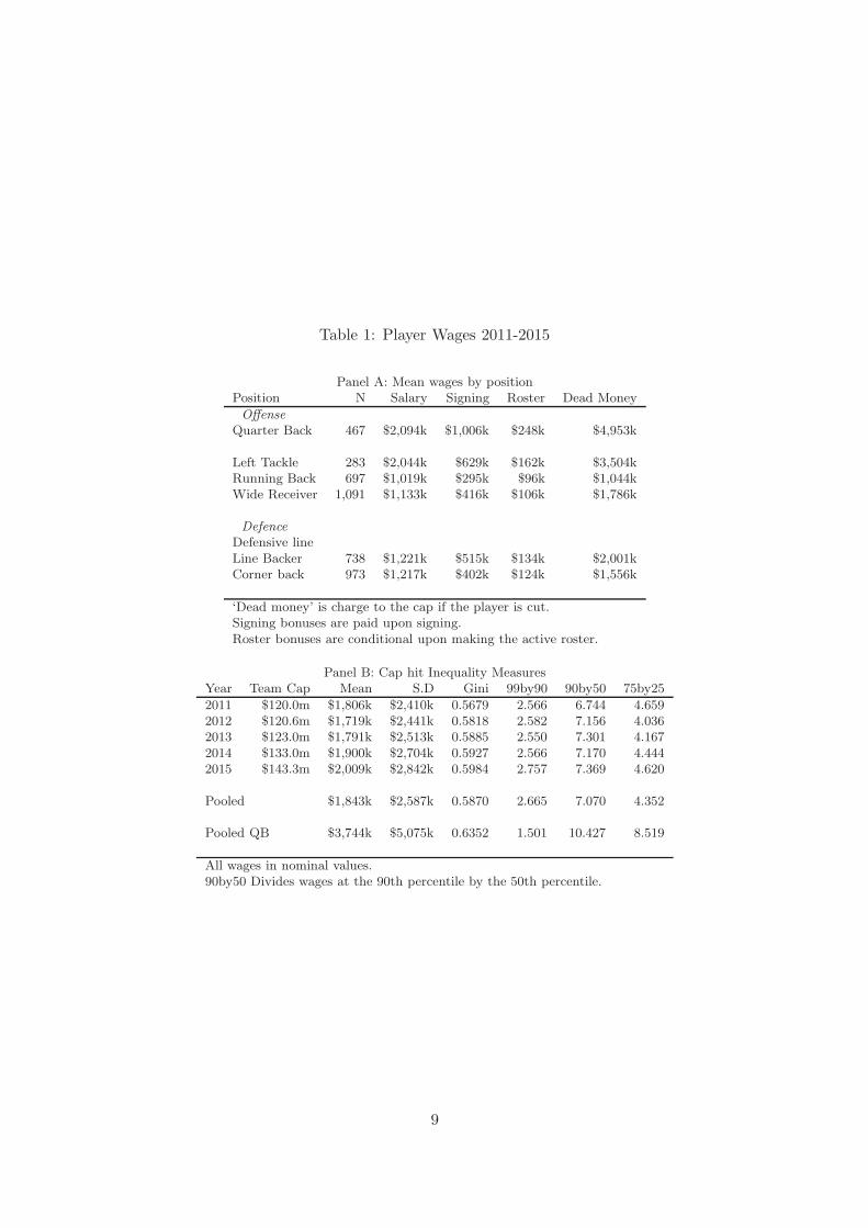
Table 1: Player Wages 2011-2015

Panel A: Mean wages by positionPosition N Salary Signing Roster Dead Money

OffenseQuarter Back 467 $2,094k $1,006k $248k $4,953k

Left Tackle 283 $2,044k $629k $162k $3,504kRunning Back 697 $1,019k $295k $96k $1,044kWide Receiver 1,091 $1,133k $416k $106k $1,786k

DefenceDefensive lineLine Backer 738 $1,221k $515k $134k $2,001kCorner back 973 $1,217k $402k $124k $1,556k

‘Dead money’ is charge to the cap if the player is cut.Signing bonuses are paid upon signing.Roster bonuses are conditional upon making the active roster.

Panel B: Cap hit Inequality MeasuresYear Team Cap Mean S.D Gini 99by90 90by50 75by25

2011 $120.0m $1,806k $2,410k 0.5679 2.566 6.744 4.6592012 $120.6m $1,719k $2,441k 0.5818 2.582 7.156 4.0362013 $123.0m $1,791k $2,513k 0.5885 2.550 7.301 4.1672014 $133.0m $1,900k $2,704k 0.5927 2.566 7.170 4.4442015 $143.3m $2,009k $2,842k 0.5984 2.757 7.369 4.620

Pooled $1,843k $2,587k 0.5870 2.665 7.070 4.352

Pooled QB $3,744k $5,075k 0.6352 1.501 10.427 8.519

All wages in nominal values.90by50 Divides wages at the 90th percentile by the 50th percentile.

9

Table 2: Player Injuries

Panel A: 1995-2001Injury Frequency

Position N N injured Missed 16 Missed 7-15 Missed 1-6 Missed 0

OffenseQuarterback 522 142 0.029 0.081 0.163 0.728Running Back 1,051 187 0.021 0.031 0.126 0.822Wide Receiver 1,102 190 0.018 0.038 0.116 0.828O Line 2,423 503 0.022 0.043 0.144 0.791

DefenceD Line 1,717 312 0.019 0.026 0.137 0.818Line Backer 1,431 237 0.018 0.030 0.117 0.836Cover 1,958 335 0.018 0.030 0.122 0.829

Special T eams 261 5 0.019 0.000 0.000 0.981

Panel B: 2011-2015Injury Frequency

Position N N injured Missed 16 Missed 7-15 Missed 1-6 Missed 0

OffenseQuarterback 349 92 0.049 0.106 0.109 0.736Running Back 574 115 0.017 0.052 0.130 0.801Wide Receiver 796 167 0.013 0.053 0.145 0.790O Line 1,635 439 0.026 0.072 0.174 0.731

DefenceD Line 1,144 227 0.013 0.047 0.140 0.801Line Backer 991 230 0.019 0.052 0.159 0.770Cover 1,384 328 0.017 0.062 0.160 0.762

Special T eams 163 1 0.006 0.000 0.000 0.994

Notes:1. N counts the number of player-seasons at each position.2. N injured counts the number of player-seasons with any injury of any duration.3. Injury frequency is the proportion of players who missed any part of X number of games that year. Forexample, in panel A, only 2.9% of QBs missed the entire season but only 72.8% of QBs went the entire seasonwithout missing any playing time due to injury.4. O Line comprises Guards, Centers, Tackles and Tight Ends. D Line comprises and Defensive Endsand Tackles. Cover comprises Safeties and Corners and Defensive Backs. Special T eams comprises Kickers,Punters and Long Snappers.

10

game. Further descriptives are provided in the appendix that demonstrate the high degree ofwage variation between NFL players.

Table 1 also shows inflation in nominal wages at the mean over a relatively short sampleperiod. There are small increases in the Gini coefficient over the same period, implying thatthe increase has gone to paying the higher paid players a little more. This has occurredalongside increases in the overall team cap. The overall cap is determined each year by aformula based on approximately 48% of total league revenues. If the salary cap is increasing,it implies aggregate franchise revenues are increasing. The Cap has increased substantiallysince its introduction in 1994 at $34.6m.

Panel A of Table 2 introduces the second time period for which data is available and shows theincidence of injury over the season by position for the years 1995-2001. Season long injuriesoccur relatively infrequently, with only 2.9% of QBs missing the entire season due to injury.However, injuries frequently cause players to miss part of the season. Only 72.8% of QBsmanage the entire season without any injury at all. Injury rates at other positions are lower,with 79% of Offensive Linesmen to 83.6% of Linebackers going the whole season uninjured.Injuries to Punters and Kickers in the Special Teams are very rare.

How has the incidence of injury changed over time? The NFL has become more consciousof ‘player safety’ over the sample period. In April 2016, a federal appeals court upheld anout of court settlement between the NFL and multiple concussion lawsuits filed by formerplayers. The settlement is thought to be worth approximately US$1 billion and will coverapproximately 20,000 players. Since 2009, the NFL has introduced a ‘concussion protocol’and tightened its rules on concussions. However, it is unclear whether this will increase ordecrease the number of observed cases of injury in the data. While the true injury risk islikely to be reduced, the recorded number of injuries might increase because the ability todiagnose this type of injury has improved13. Other restrictions on blocking and tackling havealso been introduced to decrease the likelihood of an injury occurring. For example, in 2016,the ‘chop block’, where a player blocks another high on the body, while a teammate hits thesame player low, became illegal due to risk of knee injuries.

Referring to panel B of Table 2 which pools data across the years 2011-2015, the incidence ofbeing injured for the whole season is 2 percentage points higher for Quarterbacks comparedto the 1995-2001 period. While a small increase in absolute terms, this is two-thirds higherthan the prior period. It appears the reduced injury risk has been offset by the increasedrate of injury detection (and perhaps an increased fear of litigation) between the two periods.However, the likelihood of the Quarterback going the entire season uninjured is marginallyhigher in the later period. Together, these descriptive statistics are consistent with increasedprotection of the Quarterback position so that minor injuries occur less often, but when majorinjuries do occur they are treated more seriously and force longer absences from the field ofplay.

The differences between the time periods at other positions are not so clear. The rates ofseason long injury are broadly similar in the second period and marginally fewer players gothe entire season uninjured. It would appear that it has been the Quarterbacks who havebeen the main beneficiaries of the rule changes that have targeted player safety. It is clear

13As of 2016, whenever a potential concussion is identified the player is removed from the game and anindependent Neurotrauma consultant will examine the player.

11

Table 3: Injury Types 2011:2015

Injury N Percent Duration St. Dev(weeks)

Knee 1,224 21.22% 8.85 13.08Ankle 710 12.31% 4.45 6.71Hamstring 668 11.58% 3.22 4.44Leg 408 7.07% 5.48 11.37Shoulder 380 6.59% 5.96 8.55Concussion 377 6.54% 3.27 6.07Foot 375 6.50% 7.25 9.60Groin 240 4.16% 2.81 3.01Hand 203 3.52% 4.72 4.92Back 174 3.02% 5.24 9.04Chest 158 2.74% 5.24 7.50Hip 132 2.29% 7.15 12.09Illness 132 2.29% 4.98 12.19Neck 103 1.79% 6.22 10.64Undisclosed 99 1.72% 12.70 10.48Achilles 96 1.66% 14.11 11.57Arm 85 1.47% 9.44 5.75Head 84 1.46% 2.57 3.51Elbow 60 1.04% 4.41 5.12Other 60 1.04% 3.33 3.26

Total 5,768 100.00% 5.95 9.58

Notes:1. N counts the number of unique injuries to players in the NFL between 2011 and 20152. Percent is the percentage of all injuries accounted for by the injury type3. In 2.7% of cases, two body parts were identified as injured. To avoid double counting, the injury was assignedto the first recorded category. E.g. “Knee/ankle” was classified as a knee injury, whereas “Ankle/knee” wasclassified as an ankle injury

then that the Quarterbacks, are not only paid very differently to other players but experienceinjuries differently as well. This motivates a separate analysis of injuries and wages to QBsbelow.

Table 3 uses more detailed data on injuries from mangameslost.com for the period 2011-2015.Here, injuries are classified to all NFL players on a game by game basis. Duration is calculatedby taking the number of days from being declared injured until the date of the next game whenthe player was available for selection and the mean number of weeks is reported. Durationis right censored at seven days after end of the regular season. Knee injuries are the mostcommon injuries and keep players out for a relatively long period of time, almost 9 weeks onaverage. Only 6.5% of injuries were due to concussions and these players were rested for anaverage of 3 weeks.

3.2 Injuries and the probability of winning: Season and Game level

The data allow estimation of the impact of injuries on the probability of willing at differentlevels of aggregation: at level of the season, the game and within the game itself. For thepurposes of identification, injuries that occur to Quarterbacks within the game itself represents

12

Table 4: Injuries on the probability of winning: season level 1995:2001

OLS FE(1) (2) (3) (4)

Ln Injured money -0.24*** -0.24*** -0.23*** -0.23***(-3.39) (-3.39) (-3.05) (-3.05)

Control VariablesLn(Wage bill) 1.93*** 1.93*** 2.56*** 2.56***

(3.79) (3.79) (4.81) (4.81)Ln(Wage bill standard deviation) -1.39*** -1.83***

(-3.59) (-4.71)

Year dummies Yes Yes Yes YesObservations 213 213 213 213Number of teams 31 31R-squared 0.119 0.119 0.153 0.153

Robust t-statistics in parentheses*** p<0.01, ** p<0.05, * p<0.1

the tightest specification. Prior to this, let it be shown that total injuries that occur over aseason are important enough to affect franchise’s record over that season and that injuriesprior to match day also have an impact on the likelihood of winning that particular match.Using data aggregated at the season level analysis for the period 1995-2001, the dependentvariable in Table 4 is the percentage of games won by team i in season t expressed in logodds wit = ln(wit/1 − wit). Estimation is by OLS and fixed effects (FE). The FE estimatorcontrols for unobserved team level fixed effects. Given that it is likely there are unobservedfactors that could contribute to the winning record, the FE estimates are preferred, alebit inpractice the estimated coefficients are similar.

The main explanatory variable of interest is Ln Injured money and is defined as the naturallog of the total amount spent on player wages while the players were injured. For example, aplayer who misses eight games out of the sixteen games in the regular season due to injury,would add 50% of their total compensation to Injured money. Total compensation in thisdataset is the sum of salary and bonuses received during the year. Controlling for team’s wagebill for the season, the total amount spent on players, the impact of Injured money on thefranchise’s playing record over the regular season is explored. Since not all teams qualify forthe small number of games that occur postseason the analysis is restricted to the regular seasononly. The median team wins and loses 8 games in the season (an 8-8 record). The estimatedcoefficients on LnInjured money show that injured money is important for a franchise’ssuccess in that season. The standard deviation of Ln Injured money is close is 1.05, makinginterpretation of the effect size relatively straightforward. Taking the FE estimate in column(4), a one standard deviation change in Injured money changes the log odds of winning by0.23. This implies a team with an 8-8 record who experiences a one standard deviation injuryshock sees their record fall on average by one game, to 7-9. Likewise, a two standard deviationinjury decrease in Injured money implies the median team would improve to 10-6 which istypically required to qualify for the post-season games with the prospect of playing in theSuper Bowl.

13

Ln(Wage bill) is the natural log of the total amount spent by the franchise on player wagesduring the season. If every team spent exactly the same on player wages as implied bythe theoretical version of the cap in Section 2, then this variable would not be identified.However, in practice, there is significant variation between teams spending and within team-years. Smaller franchises may not wish to spend the full amount permitted by the cap,although they must spend at least 90% of the cap. Additionally, since the cap permits certainelements of pay, such as signing bonuses to be charged over the life of the cap (see appendix)teams can strategically vary the amount charged to the cap in any one year. For these, reasonsthe wage bill does vary and as expected, teams that pay more in a season, win more gameson average in that season. From the FE estimate of column 4, a 10% increase in franchisespending in that season implies approximately 0.25 increase in the logodds, which is close tothe same effect size as a one standard deviation injury shock.

Table 4 also reports another interesting control variable. It has been argued in the literaturethat wage inequality within teams diminishes team performance (Borghesi, 2008) perhaps dueto a withdrawal of effort among relatively low-paid players. Ln(Wage bill standard deviation)measures the within team wage spread in each year and estimated coefficients are negative.From the FE result, a 10% increase in the standard deviation of the wage bill, holding thetotal bill constant, reduces the median team’s record by approximately 0.7 of a win. However,care is required when interpreting this estimate. A team that spends more typically does soby recruiting more star players, or by paying more for star players. This inevitably increasesthe standard deviation of wages within the team. Indeed, the Pearson’s correlation coefficientbetween the wage bill and its standard deviation is 0.889, highly collinear. Since it is unlikelythat significantly reducing the inequality of wages within the team is feasible without alsoreducing the total talent in the team one should caution against a strategy focused solely onwage equality without regard to total team spend.

While analysis at the season level provides a broad overview of the impact of injuries, alimitation of the analysis is that it aggregates information across all the games in the season.Important determinants of match outcomes, such as who the team is playing, the market oddsprior to kick off, whether or not the team is playing at home can only be controlled for on agame by game basis. Therefore a more precise analysis is offered with data in Table 5, whichreports the game level analysis where each of the 32 NFL franchises play 16 games over 5regular seasons 2011-2015. Additionally, the wage data available in the period 2011-2015 ismore detailed than that from 1995-2001 because the data records the official ‘cap number’that represents the charge to the salary cap for the franchise over that season.

For each game, the dependent variable takes the value of 1 if a win is recorded and zerootherwise. Estimation is by logit and a conditional logit which controls for team level fixedeffects. Controlling for fixed effects over a five year period should be a reasonably tightspecification because unobservables such as training facilities and franchise culture should notvary a great deal over this time period. Ln Injured Money (net) is the natural log of totalwages for players who were unable to play that game net of their opposition’s injured wages.This variable mirrors the injury shock c.µi outlined in the theory section above. Table 5reports the estimated coefficients and marginal effects for the main variables of interest areinterpreted below.

The estimated coefficient of the raw effect of Ln Injured Money (net) in column (1) impliesan average marginal effect (AME) of -0.07. A one standard deviation change in this variable

14

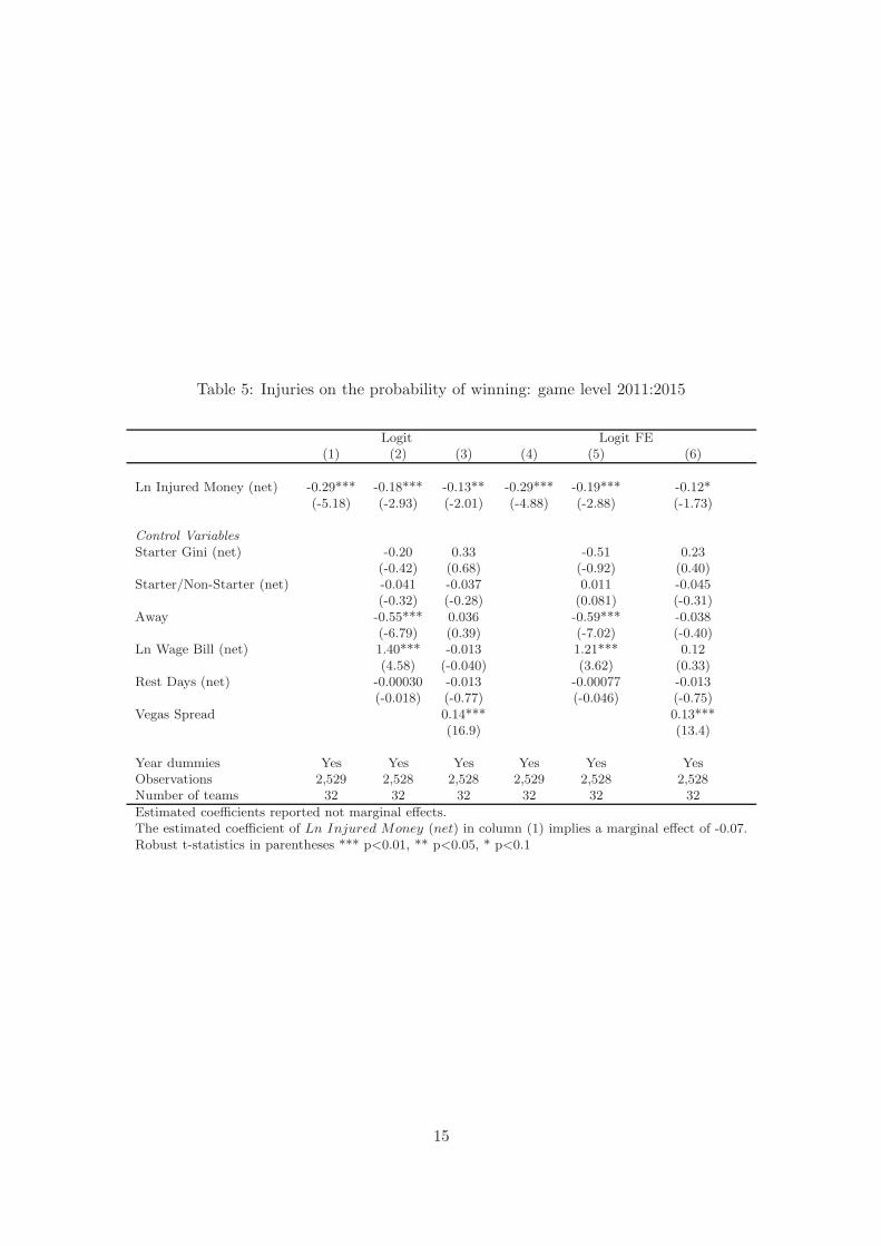
Table 5: Injuries on the probability of winning: game level 2011:2015

Logit Logit FE(1) (2) (3) (4) (5) (6)

Ln Injured Money (net) -0.29*** -0.18*** -0.13** -0.29*** -0.19*** -0.12*(-5.18) (-2.93) (-2.01) (-4.88) (-2.88) (-1.73)

Control VariablesStarter Gini (net) -0.20 0.33 -0.51 0.23

(-0.42) (0.68) (-0.92) (0.40)Starter/Non-Starter (net) -0.041 -0.037 0.011 -0.045

(-0.32) (-0.28) (0.081) (-0.31)Away -0.55*** 0.036 -0.59*** -0.038

(-6.79) (0.39) (-7.02) (-0.40)Ln Wage Bill (net) 1.40*** -0.013 1.21*** 0.12

(4.58) (-0.040) (3.62) (0.33)Rest Days (net) -0.00030 -0.013 -0.00077 -0.013

(-0.018) (-0.77) (-0.046) (-0.75)Vegas Spread 0.14*** 0.13***

(16.9) (13.4)

Year dummies Yes Yes Yes Yes Yes YesObservations 2,529 2,528 2,528 2,529 2,528 2,528Number of teams 32 32 32 32 32 32

Estimated coefficients reported not marginal effects.The estimated coefficient of Ln Injured Money (net) in column (1) implies a marginal effect of -0.07.Robust t-statistics in parentheses *** p<0.01, ** p<0.05, * p<0.1

15

implies an extra win over the course of the season consistent with the result found at theseason level above. When converted to dollars (in millions) the AME is -0.006. A one standarddeviation injury shock is approximately $15.25M in player wages. This implies a one standarddeviation increase in this variable implies a 9 percentage point reduction in the probability ofwinning that game (unconditional). With 16 games in the season, the one standard deviationinjury shock implies losing 1.47 games in the season. To equate wages with marginal revenueproduct a single win for the franchise would need to be equal to $10.4M.

The control variables that play an important role in win probability include Away, a dummywhich equals 1 for an Away fixture (AME 0.13) and the total wage bill of the franchise netof the opponent (AME 0.28) in the relevant year. Two measures on inequality within thefranchise are included; the Gini coefficient among starting players and the ratio of the starterswage bill to non-starters. However, nether of these variables are statistically significant. Theinconsistency between this result and that obtained at the season level, could be explainedby the tighter specification permitted by the game level analysis. In particular, the measuresof wage inequality of at the level of the game now control for the opposition’s inequality andwage bill as well. Once these variables are included, the measures of wage inequality do nothave a major impact.

The most important control variable for the analysis is the Vegas Spread for each game whichis included in columns (3) and (6). This provides the market’s expectation of the probabilityof winning. For each game, an under/over spread is offered on either team. If A plays B andthe Vegas spread is +7, then the market is predicting that A has a 50% chance of winning by7 or more points and that B has a 50% chance of winning or losing by 7 or less. Card andDahl (2011) show this variable is an unbiased predictor of match outcomes and a replicationof their test with this more recent data period is shown in the appendix. The estimatedcoefficient in column (6) implies an extra point on the spread is worth 3% in win probability.Since all the control variables in Table 5 are known to the market prior to kick off, onewould expect them to be priced in to the Vegas Spread, otherwise it would imply outstandingarbitrage opportunities, such as betting just on away teams. However, as shown in columns(3) and (6), the control these variables are no longer predictive of the match outcome once theVegas Spread is accounted for. However, there remains an effect on the margin of statisticalsignificance for the main variable of interest Ln Injured Money (net). This is likely due tosome uncertainty prior to kick off surrounding the extent of injury to some players. Whethera player misses a game due to injury is coded retrospectively as a one or zero and it is notknown whether the market gave an a player who is coded injured some chance of playing priorto kick off. In other words, the market is unable to price in all injuries perfectly prior tokick off. The following section presents a more precise analysis using injuries to quarterbacksduring the game itself but even at the broader levels of aggregation presented above, injuriesplay a role in winning games.

4 Main Results

4.1 Injuries and the probability of winning: Within game analysis

The most critical position in the NFL is the Quarterback (QB). They are the highest paid(see above) and play a unique role in the side as they are responsible for play selection as

16

well as play execution14. More so than a captain in Association Football or a Point Guardin Basketball, Quarterbacks have a major bearing on the outcome of the game. In their 53man squad (roster), a team will employ a starting QB and at least one and sometimes two orthree backup QBs in case of an injury to the starting QB. As such an injury within game tothe starting Quarterback represents the cleanest shock to labor productivity in the NFL.

For the period 2011 to 2015, it is observed in the data from sports-reference.com whetherthe starting QB was replaced by the backup QB during any game. One advantage with thedata from this period is that the replacement can be cross-referenced to data on injuries frommangameslost.com, where the specific nature of the injury, whether it is to the head or otherpart of the body, is observed. This means one is able to verify the seriousness of the injury,so that instances of ‘tactical substitutions’, where the starting QB is not really injured butreplaced by the backup QB for performance reasons can be correctly excluded. On occasions,QBs are substituted late in the game when the contest is already won and these can also beexcluded. Furthermore, historical match reports were cross-referenced from nfl.com to ensurethe in-game QB substitutions represented genuine injury shocks.

Table 6 shows the results. When the backup QB is required to take the field the team is morelikely to lose by 28 percentage points (average marginal effect ‘Injured QB’ col(1)). Likewiseif the opponent’s QB steps in the team is more likely to win by 28 percentage points. Theseestimated effects are equivalent to giving the other team 9.5 points on the spread. Column(2) confirms that this injury is not predicted by the market prior to kick-off and column (3)shows this is unaltered by unobserved franchise fixed effects. An injury to the starting QB isclearly a major shock to the franchise.

Most starting QBs experience variation in form over their career and therefore their contri-bution relative to a backup QB is likely to vary. It is possible to control for how well a QBplayed during the game with their official ‘passing rating’. Passing rating is measured on ascale from zero to 158.3 points for a perfect game15. The estimated coefficient on passingrating in column (4) shows how important the QB’s performance is to the probability of win-ning. A one standard deviation increase in the passing rating corresponds to a 19% pointincrease in the likelihood of winning. Backup QBs replacing injured QBs on average have 16fewer points in passing rating per game, which equates to 12 fewer percentage points in thelikelihood of winning each game. Passing rating is capturing approximately half of the effectof substituting in the Backup QB. Of course, in any one game a Backup QBs can play welland help their team win16. However, given the same passing rating in the game, an injury tothe starting QB further reduces the likelihood of winning. It is likely that the weaker passinggame of the backup QB allows the opposition defence to line up against running plays withgreater certainty, rendering non-passing plays less effective. Additionally, to the extent thatthe starting QB’s may possess superior leadership skills, are better at changing the play at theline of scrimmage or are better at running the ball themselves, franchises may benefit from

14Plays are also designed and selected by the Head Coach and Offensive Coordinator15Four categories are used as a basis for compiling a rating: Percentage of completions per at-

tempt, Average yards gained per attempt, Percentage of touchdown passes per attempt and Percent-age of interceptions per attempt. A passing rating of over 100 is considered a very good performancehttp://www.nfl.com/help/quarterbackratingformula

16Nick Foles won the Most Valuable Player award in his winning Super Bowl appearance in 2017 as a backupQB with an excellent passing rating of 106.1, 15 points above the average for a starting QB and 26 pointsabove the average for a backup QB.

17

these attributes.

There is considerable variation between franchises in the difference in wages between startingand backup QBs and therefore the shock of losing the starting QB to injury is also expectedto vary. Column (5) examines ‘∆ Injured-Backup QB wage’ which interacts an injury to thestarting QB during the game with the wage differential between the starting QB and backupQB who replaced them. The estimated coefficient for this variable implies a one standarddeviation increase in the wage differential is associated with a loss of 7 percentage pointsin the likelihood of winning, conditional upon the starting QB getting injured during thegame. For illustrative purposes, a one standard deviation in wage differential is approximately$11M at the median. Therefore, the implied marginal productivity for $10M of QB wageswould equal approximately 6.6 percentage points in the likelihood of winning each game , orapproximately 1 game over the course of the regular season. Therefore, a win would need tobe worth approximately $10M to the franchise in order to equate median QB wages with theirmarginal revenue product. This is almost exactly the same as the estimates obtained abovewhen adding up the wage bill of injuries at all playing positions, albeit the identification onQB injuries is much more precise.

As expected, the effects sizes in Table 6 are symmetric for the opposition variables (noneof the differences in magnitude of the estimated coefficients are statistically significant). Thecontrol variables act upon the match outcome in a similar way as in Table 5. The Vegas Spreadremains the most important predictor of the match outcome, albeit the magnitude, conditionalon what the QB achieved the game, is reduced in columns (4) and (5). This is expected as themarket can not predict perfectly how a QB will perform in any one game. After controllingfor V egas Spread, none of the control variables are expected to be statistically significantas all these variables are public information prior to kickoff. However, a negative coefficienton Away emerges because the specification requires passing rating (which is not known priorto kick off) to be held constant. Since passing rating is systematically lower when QBs playaway from home, holding this constant introduces collinearity with Away. If passing ratingis omitted, then the coefficient on Away returns to being statistically insignificant from zero.

Altogether, these estimates imply that an injury to the starting QB has a major bearingon the outcome of the match and the impact and the size of the effect is proportional tothe wage differential between the starting QB and backup QB. Note that the impact of theamount of injured money Ln Injured Money(net) is no longer statistically significant afterconditioning on the QB’s performance during the game and the Vegas Spread. Therefore, themost relevant identifier of a shock to labor productivity among NFL players, appears to bean injury to the starting QB. As stated above, the estimates imply that a win will need to beworth approximately $10M to justify the marginal difference in wages between the startingand backup QBs. The next section seeks to determine whether or not this is the case.

4.2 How much is a win worth?

Starting Quarterbacks are paid on average approximately 10 times the amount of the backupQuarterback. However, it has been seen that the team is not 10 times less likely to win, ratherapproximately 28 percentage points less likely to win each game. If the median 8-8 team wasforced to go the entire season with the backup quarterback they would still be predicted towin at least 3 or 4 games in the season. Such a team would not make the postseason playoffs

18

Table 6: Injuries on the probability of winning: Within game quarterbacks 2011:2015

(1) (2) (3) (4) (5)

Injured QB -1.18*** -1.28*** -1.24*** -0.72***(-6.69) (-6.83) (-6.53) (-2.95)

Injured QB (opp) 1.19*** 1.31*** 1.34*** 0.84***(6.80) (7.02) (7.14) (3.45)

Vegas Spread 0.15*** 0.14*** 0.095*** 0.095***(18.6) (16.0) (7.74) (7.77)

Passing rating 0.056*** 0.056***(19.3) (19.3)

Passing rating (opp) -0.058*** -0.058***(-19.2) (-19.2)

∆ Injured-Backup QB wage -0.048***(-2.98)

∆ Injured-Backup QB ∆ wage (opp) 0.055***(3.48)

Control variablesLn Injured Money (net) -0.028 -0.029

(-0.33) (-0.34)Starter Gini (net) 0.95 0.98

(1.21) (1.25)Starter/Non-Starter (net) 0.034 0.034

(0.19) (0.19)Away -0.25** -0.25**

(-2.01) (-2.00)Ln Wage Bill (net) 0.41 0.41

(0.65) (0.64)Rest Days (net) 0.0012 0.00095

(0.055) (0.043)

Year dummies No No No Yes YesFixed effects No No Yes Yes YesObservations 2,555 2,555 2,555 2,555 2,555Teams 32 32 32 32 32

Estimated Coefficients after logit (conditional logit for FE) reported.Robust t-statistics in parentheses *** p<0.01, ** p<0.05, * p<0.1

19

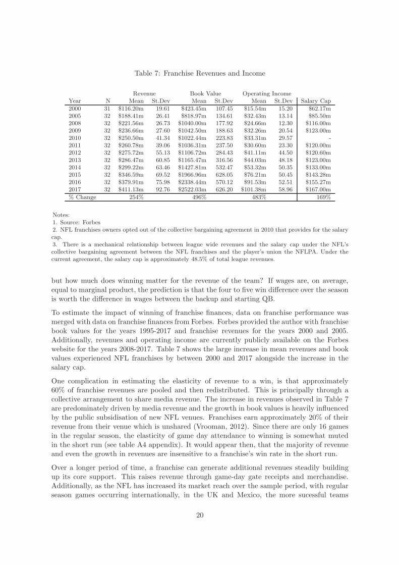
Table 7: Franchise Revenues and Income

Revenue Book Value Operating IncomeYear N Mean St.Dev Mean St.Dev Mean St.Dev Salary Cap

2000 31 $116.20m 19.61 $423.45m 107.45 $15.54m 15.20 $62.17m2005 32 $188.41m 26.41 $818.97m 134.61 $32.43m 13.14 $85.50m2008 32 $221.56m 26.73 $1040.00m 177.92 $24.66m 12.30 $116.00m2009 32 $236.66m 27.60 $1042.50m 188.63 $32.26m 20.54 $123.00m2010 32 $250.50m 41.34 $1022.44m 223.83 $33.31m 29.57 -2011 32 $260.78m 39.06 $1036.31m 237.50 $30.60m 23.30 $120.00m2012 32 $275.72m 55.13 $1106.72m 284.43 $41.11m 44.50 $120.60m2013 32 $286.47m 60.85 $1165.47m 316.56 $44.03m 48.18 $123.00m2014 32 $299.22m 63.46 $1427.81m 532.47 $53.32m 50.35 $133.00m2015 32 $346.59m 69.52 $1966.96m 628.05 $76.21m 50.45 $143.28m2016 32 $379.91m 75.98 $2338.44m 570.12 $91.53m 52.51 $155.27m2017 32 $411.13m 92.76 $2522.03m 626.20 $101.38m 58.96 $167.00m

% Change 254% 496% 483% 169%

Notes:1. Source: Forbes2. NFL franchises owners opted out of the collective bargaining agreement in 2010 that provides for the salarycap.3. There is a mechanical relationship between league wide revenues and the salary cap under the NFL’scollective bargaining agreement between the NFL franchises and the player’s union the NFLPA. Under thecurrent agreement, the salary cap is approximately 48.5% of total league revenues.

but how much does winning matter for the revenue of the team? If wages are, on average,equal to marginal product, the prediction is that the four to five win difference over the seasonis worth the difference in wages between the backup and starting QB.

To estimate the impact of winning of franchise finances, data on franchise performance wasmerged with data on franchise finances from Forbes. Forbes provided the author with franchisebook values for the years 1995-2017 and franchise revenues for the years 2000 and 2005.Additionally, revenues and operating income are currently publicly available on the Forbeswebsite for the years 2008-2017. Table 7 shows the large increase in mean revenues and bookvalues experienced NFL franchises by between 2000 and 2017 alongside the increase in thesalary cap.

One complication in estimating the elasticity of revenue to a win, is that approximately60% of franchise revenues are pooled and then redistributed. This is principally through acollective arrangement to share media revenue. The increase in revenues observed in Table 7are predominately driven by media revenue and the growth in book values is heavily influencedby the public subsidisation of new NFL venues. Franchises earn approximately 20% of theirrevenue from their venue which is unshared (Vrooman, 2012). Since there are only 16 gamesin the regular season, the elasticity of game day attendance to winning is somewhat mutedin the short run (see table A4 appendix). It would appear then, that the majority of revenueand even the growth in revenues are insensitive to a franchise’s win rate in the short run.

Over a longer period of time, a franchise can generate additional revenues steadily buildingup its core support. This raises revenue through game-day gate receipts and merchandise.Additionally, as the NFL has increased its market reach over the sample period, with regularseason games occurring internationally, in the UK and Mexico, the more sucessful teams

20

are the better positioned teams to attract new international support. Additionally, supportfor the public subsidisation of NFL infrastructure and franchise stadia is arguably relatedto the intensity of local support. But to what extent is winning important in this revenuedevelopment? Vrooman (1995) estimates a three-year win elasticity over the period 1990-1992of .12, which implies if the average win rate doubles over these three years franchise revenueswould increase by 12%. Vrooman (1995) also shows that NFL revenues are considerably lesswin elastic than the other major US sports. However, if measured over a longer period oftime, the arguments laid out in (Vrooman, 2012) would imply a higher win elasticities.

Table 8 shows the impact of winning on franchise book values and revenues as measured bya rolling average of the franchise’s win percentage between 2000 and 2017. Column 1 reportsthe unconditional coefficient suggesting a 10 percentage point increase in the rolling win rateis associated with approximately $50m in the annual book value over the sample period. A10% point increase is equal to the median 8-8 team improving to 9.6 wins on average periodseason, which is coincidentally almost exactly 1 standard deviation improvement. Thus a 2standard deviation improvement is broadly equivalent to an 11-5 season on average and worthapproximately $100m in book value and $30m in revenue per annum. Therefore, a single winin the regular season would be worth c.$10m per annum, on average in the long run. Recall,from the estimates in section 4.1, a win would need to be worth approximately $10m for themedian QB wages to be equal to their marginal revenue product. Even allowing for a degreeof imprecision in these sample estimates it is remarkable that such a tight connection betweenwages and marginal revenue product has emerged.

The set of control variables in Table 8 are also interesting. The set of year dummies capturethe growth in both book values and revenues and contribute to the high R-squared valuesfor the model’s fit. Indeed, there is more growth in the dependent variables over time thanthere is variation between franchises so even the worst performing franchise will have mademoney over the period. Nevertheless, the observable controls that capture variation betweenfranchises are also important. A set of controls for the initial conditions of the franchise in1995 are included to capture long term legacy effects. The total number of historical winsand the age of the franchise do not impact book value or revenue but a historical Super Bowlwin is worth approximately $63M ($13M in revenue). The stadium variables are statisticallyand economically significant. An extra 1,000 in capacity is associated with $10M in valueand $3M in revenue. More expensive stadia raise revenues and book values (a 10% increasein build cost is associated with $7M in book value and any stadia related debt is excludedfrom the book values). Building a new stadium in the franchise period is associated with$252M of value on average for that franchise (FE estimate) and each year the stadia is notrenewed costs the franchise $3.6M in book value. Turning to the Metropolian area controls: a10% increase in local population is associated with c.$5M in franchise value albeit the growthrate of the local area does not impact franchise values. Holding a monopoly over the localmetropolitan area is worth $295M relative to secondary franchises in the area (e.g. the NewYork Jets) and $177M more than primary franchises (e.g. the New York Giants). The numberof substitute franchises from the other three main sports, Baseball, Basketball and Hockeyis positively associated with NFL franchise values and revenues. This reflects the fact thatfranchise location is endogenous in the US and there are several examples of NFL franchisesrelocating to higher demand local areas. In sports outside of the US, such as the EnglishPremier League, team location is more plausibly exogenous and one might expect a inversecorrelation between revenues and the number of substitute sporting events in the local area.

21

Table 8: Sensitivity of winning to revenues and book values

Book Value RevenueOLS (1) OLS (2) FE (3) OLS (4) OLS (5) FE (6)

Rolling win percentage 498*** 352*** 377*** 152*** 85.8*** 147***(4.52) (3.67) (2.69) (4.65) (3.58) (3.18)

Initial conditions in 1995No. Wins 0.33 -0.059

(0.77) (-0.64)No. Super Bowls 63.0*** 13.6***

(7.14) (7.11)No. Post season years 1.94 1.28*

(0.55) (1.70)Franchise age -4.25* -0.43

(-1.93) (-0.91)

Stadium variablesCapacity 10.00*** 2.96***

(8.06) (10.5)Ln (total build cost) 71.0*** 15.9***

(6.50) (5.67)New stadium 108*** 252*** 21.8*** 45.3***

(4.68) (8.99) (3.95) (7.15)Yrs since expansion -3.66** -0.36

(-2.31) (-0.86)

Metropolitan Area controlsLn population 49.5*** 7.44**

(3.31) (2.37)Population growth rate -4.16 -3.52

(-0.27) (-1.05)Only franchise 295*** 72.0***

(7.41) (8.31)Main franchise 118** 12.5

(2.20) (1.08)No. substitutes 60.6*** 16.2***

(4.20) (5.14)

Year dummies Yes Yes Yes Yes Yes YesObservations 721 721 721 383 383 383R-squared 0.835 0.899 0.912 0.694 0.867 0.905No. teams 32 32 32 32 32 32

Notes:1. Book values available 1995-2017. Revenues available for 2000, 2005, 2008-2017.2. All monetary variables in Dec 2017 prices.3. The estimated coefficient in column (3) and (6) implies 10 percentage point increase in the rolling win rateincreases book values by $50M and revenues by $15M respectively.4. The R-squareds range between 69.4% and 91.2%. These high values are due to the large growth in franchisebook values and revenues that occurred over the sample period. This this growth is captured by the set of yeardummies. Excluding the year dummies reduces the R-squareds to between 0.4% and 46.2%.

After conditioning upon the set of observable controls in columns (2) and (5) the estimatesin row 1 for win percentage reduce by approximately one third. The fixed effects estimate

22

in column (3) is close to that of column (2) reflecting the fact that most of the observablecontrols relevant for book values do not change much over the sample period. The fixed effectestimate for revenue in column (6) however is closer to the unconditional estimate that ofcolumn (4). This is likely because the relevant controls for revenue do in fact vary withinfranchises over the sample period. In particular, a new stadium is built in the sample periodis worth $45.3M in new revenue.

4.3 Wages and Productivity: Heterogeneity between Rookies and Veterans

From the estimates in section 4.1, a win needed to be worth approximately c.$10m for themedian QB wages to be equal to their marginal revenue product and the section above appearto confirm that this is indeed the case. However, it is important to note that the estimatesof marginal productivity are derived from point estimates at the mean. As such, it can bestated with reasonable confidence that quarterbacks close to the mean of the wage distributionappear to be paid their close to their marginal revenue product. However, this result may maskheterogeneity in the relationship between wages and productivity elsewhere in the distribution.As shown in section 3, there is a wide distribution of wages both within the quarterbackposition and between quarterbacks and other positions. To what extent can these differencesbe explained by differences in productivity?

There are reasons to suspect that some players represent better value for money than others.In particular, an important institutional friction of the NFL is a player’s eligibility for freeagency. Newly drafted players out of college, known as ‘rookies’, are not free to leave thefranchise to which they are drafted within the first four years of their career. The franchisehowever can cut a player at any time. Only after four years do rookies become unrestricted‘free agents’17. Hence there is a considerable difference in bargaining power between rookiesand veteran players. For example, Patrick Mahomes is a second year rookie who was promotedto the starting QB for the Kansas City Chiefs at the beginning of the 2018 season and waspaid $3.7M in 2018, whereas the outgoing veteran QB Alex Smith was paid $13.4M in 2017and secured a 4-year deal with the Washington Redskins worth $94M in 2018. Mahomes’ 2018passing rating (to date) is 113.8 which is outperforming Smith’s rating 85.7 by a considerablemargin. Further, veterans are in short supply because many rookies will leave the NFL beforebeing eligible for free agency, either because they have a career ending injury or, more likely,because they fail to make the roster of their franchise. This has been highlighted by Vrooman(2012, p.8) who argues ‘It is common for veteran players to coalesce with management tobargain away the rights of future generations of disenfranchised rookies and forgotten formerplayers. This creates a twisted bilateral monopoly where veteran players are often overpaidbecause of upper-tier monopoly power, while rookies are exploited because of owners lower-tiermonopsony power’.

Table 9 shows the impact of being a rookie on wages. Rookies are paid 55%-56% less on averagethan veteran players. It is important to note that this difference remains after controlling forindividual productivity and team level fixed effects. Productivity up to the season in whichwages are determined is captured by the ‘approximate value’ (AV) metric. This metric issupplied by sports-reference.com and accounts for the points achieved (conceded) per drive

17Under current rules, franchises are also allowed to restrict the movement of one free agent known as the‘franchise tag’.

23

Table 9: Wages: Rookies vs Veterans

OLS FECoeff. t− stat Coeff. t− stat

Rookie -0.56*** (-16.1) -0.55*** (-16.0)

Age 0.012 (1.50) 0.017* (1.96)ApproximateV aluet − 1 0.12*** (15.8) 0.12*** (15.3)ProBowlt − 1 0.32*** (6.49) 0.32*** (6.54)No.gamest − 1 0.020*** (7.78) 0.019*** (7.46)Injury Reserve 0.015 (0.59) 0.016 (0.60)

Draft Round (1st round omitted)2nd round -0.38*** (-8.64) -0.38*** (-8.94)3rd round -0.60*** (-12.0) -0.60*** (-11.9)4th round -0.61*** (-10.4) -0.61*** (-10.5)5th round -0.75*** (-10.5) -0.75*** (-10.5)6th round -0.77*** (-13.6) -0.77*** (-13.9)7th round -0.84*** (-15.7) -0.85*** (-15.5)

Position (Quarterback omitted)Defensive line -0.15 (-1.58) -0.13 (-1.41)Defensive cover -0.099 (-0.99) -0.088 (-0.90)Linebacker -0.26** (-2.59) -0.24** (-2.47)Offensive line -0.14 (-1.68) -0.13 (-1.59)Running back -0.34*** (-3.89) -0.33*** (-3.78)Special teams -0.0100 (-0.088) -0.0059 (-0.052)Wide Receiver -0.18* (-2.04) -0.16* (-1.88)

Year dummies Yes YesFixed Effects No YesObservations 3,941 3,941Number Teams 32 32R-squared 0.540 0.545

Cluster Robust t-statistics in parentheses*** p<0.01, ** p<0.05, * p<0.1

Notes:1. The dependent variable is the natural log of the variable ‘CAPHIT’ which is the official amount of wagescharged to the franchise’s salary cap for the year. Column 1 are OLS estimates and column 2 controls forteam-level fixed effects.2. Rookie is a dummy identifying players on restricted contracts which typically last 4 or 5 years. Most playersenter the league at 21/22 years old and so players are typically 25/26 when they enter free agency. The estimatesimply that rookies are paid c.55% less than veterans for the same level of performance as measured by theirapproximate value. Approximate value is supplied by sportsrefernce.com and combines detailed informationabout on the field performances of players at all positions. Probowl identifies players who were invited to thePro Bowl which celebrates the best players in the two leagues (AFC and NFC) in that season.3. There is a tight relationship between draft pick order and rookie wages because initial wages in the firstyear out of the draft are set by collective bargaining. Undrafted players are excluded from the analysis abovebecause they immediately become free agents but have failed to make the draft selection.

and distributes these points based on the contribution of the player, in their position, tothose points. The AV metric for every player is recorded for every season on a scale of 0-26,with the mean of 4 and a standard deviation of 3.72. Therefore a one standard deviation in

24

productivity results in an increase in wages of approximately 44%. It is also noteworthy thatthere is no impact of being placed on injured reserve (IR). This shows that the wages ofinjured players are indeed honoured for the year and that the exclusion restriction requiringthat wages do not predict injuries appears to hold. Overall, the large differences in rookie andveterans wages can not be solely explained by differences in their productivity. Given thatit was argued above that the median player is being paid close to their net marginal revenueproduct, it is highly likely that rookies, (on average), are below their marginal product andveterans above it. This is consistent with monopsonistic exploitation of rookies as advancedby Vrooman (2012).

Alternatively, underpayment relative to marginal revenue product for rookies and overpaymentfor veterans could reflect an non-exploitative model of deferred compensation as in (Lazear,1979). One possible view of the large increase to player wages that occurs when players becomefree agents is as an incentive mechanism for players to exert full effort both before and afterfree agency. As rookies, players exert effort to maximise their marketability when they enterfree agency. If less than full effort is supplied the rookie risks dropping out of the league beforetheir big pay day. After entering free agency, veterans will also exert full effort because pay attheir franchise would exceed their outside option of their marginal product and so do not wantto risk being traded. Rookies are not exploited in this model because the optional value ofdeferred compensation offsets the underpayment in wages. However, deferred compensationcontracts are more readily applicable to working environments where monitoring productivityis prohibitively costly (Huck et al., 2011). Since rookie performances are easily observed andunder-performing rookies easily dismissed, it is hard to explain why a franchise would needto adopt this incentive mechanism. Moreover, deferred compensation contracts are expensive.Given the high degree of uncertainty associated with surviving until free agency rookies willdiscount the optional value of the free agency pay-day by a considerable amount. A preciseestimate of the option value is difficult because survival rates vary significantly by playerquality and will be distorted by idiosyncratic risk preferences. However, using the draft pickas a proxy for player quality, 77.4% of first round picks survive four years, while only 21.7%of 7th round picks survive. 34.3% of the median draft pick survives 4 years in the league18.Therefore the c.55% wage premium that veterans enjoy on average relative to rookies will bediscounted by average rookie by approximately 65% (assuming risk neutrality). As such itis safe to conclude that most rookies are underpaid relative to their marginal product evenconsidering the option value of the free agency payday. Additionally, it is observed thatplayers move regularly between franchises when they enter free agency implying that theircurrent franchise is not prepared to offer them a veteran contract above their outside option,as expected under the deferred compensation model.

5 Conclusion

The estimates obtained here for the marginal productivity of NFL players suggests that,notwithstanding heterogeneity between rookies and veteran players, sportsmen in the NFL arepaid, on average, at a rate which is very close to their marginal contribution to the franchise’srevenue. This was identified by observing the lost value from the reduction in win probability

18See https://www.milehighreport.com/2014/5/13/5713996/how-long-does-the-average-draft-pick-stick-around

25

from injured players being approximately equal to the wages earned by those injured playerson average. A dollar of injured talent is a dollar of productivity lost. This result providesempirical support for models of sporting leagues such as (Fort and Quirk, 1995) where talentis hired at a market clearing rate which is also equal to the firm’s marginal revenue of talent.More generally, it provides evidence for a tight connection between wages and productivityeven when specific institutional constraints, in this case a salary cap and restricted rookiecontracts, act to hold down wages for some workers. The broad connection between wagesand marginal revenue product appears remarkably robust despite these frictions.

An opportunity to extend the research here is to build a dataset that links the timing of anon-field injury to the real time movement of in-play betting odds. While historical in-playodds are not currently publicly available, private betting companies own datasets containingsuch information. This would provide an unambiguous connection between the injury to theplayer and the change in the probability of winning the game. If access to such data wasopened up to academics for research purposes, this would allow one to more precisely identifythe immediate impact of injury on the probability of winning by using the market reactionas a close proxy for the change in probability. These movements could then be compared theplayer’s wages19.

A second opportunity to build upon the research here would be to explore the role of non-productivity related characteristics such as the race of the player. Although race is notidentified in this data, the NFLPA collects self-identified demographic information on NFLplayers. If access to this data was made available to academics, given the detailed individuallevel data on productivity already in the public domain, it would be possible to determine theextent to which race played or continues to play a role in the wages of NFL players and thesuccess of NFL franchises.

19This was suggested by David Forrest at the European Sports Economics Association 2018.

26

References

Ashenfelter, O. and D. Card (2011). Handbook of labor economics, Volume 4. Elsevier B.V.

Binmore, K. (2007). Playing for real: A text on game theory. Oxford University Press.

Borghesi, R. (2008). Allocation of scarce resources: Insight from the nfl salary cap. Journal

of Economics and Business 60 (6), 536 – 550.

Borland, J. and R. Macdonald (2003). Demand for sport. Oxford Review of Economic Pol-

icy 19 (4), 478–502.

Caporale, T. and T. C. Collier (2015). Are we getting better or are they getting worse? draftposition, strength of schedule, and competitive balance in the national football league.Journal of Labor Research 36 (3), 291–300.

Card, D. and G. B. Dahl (2011). Family violence and football: The effect of unexpectedemotional cues on violent behavior. The Quarterly Journal of Economics 126 (1), 103–143.

Charles, K. and J. Guryan (2008). Prejudice and wages: An empirical assessment of Becker’sthe economics of discrimination. Journal of Political Economy 116 (5), 773–809.

Fort, R. and J. Quirk (1995). Cross-subsidization, incentives, and outcomes in professionalteam sports leagues. Journal of Economic Literature 33 (3), 1265–1299.

Frank, R. H. (1984). Are workers paid their marginal products? The American Economic

Review 74 (4), 549–571.

Gabaix, X. and A. Landier (2008). Why has CEO pay increased so much? Quarterly Journal

of Economics 123 (1), 49–100.

Garcia-del Barrio, P. and S. Szymanski (2009). Goal! Profit maximization versus win maxi-mization in soccer. Review of Industrial Organization 34 (1), 45–68.

Goldin, C., S. P. Kerr, C. Olivetti, and E. Barth (2017). The expanding gender earnings gap:Evidence from the LEHD-2000 census. American Economic Review 107 (5), 110–14.

Hellerstein, J. K., D. Neumark, and K. R. Troske (1999). Wages, productivity, and workercharacteristics: Evidence from plant-level production functions and wage equations. Journalof Labor Economics 17 (3), 409–446.

Huck, S., A. J. Seltzer, and B. Wallace (2011). Deferred compensation in multiperiod laborcontracts: An experimental test of Lazear’s model. American Economic Review 101 (2),819–43.

Jones, B. F. and B. A. Olken (2005). Do leaders matter? National leadership and growthsince world war II. The Quarterly Journal of Economics 120 (3), 835–864.

Kaplan, S. N. and J. Rauh (2013, September). It’s the market: The broad-based rise in thereturn to top talent. Journal of Economic Perspectives 27 (3), 35–56.

Kesenne, S. (2000a). The impact of salary caps in professional team sports. Scottish Journal

of Political Economy 47 (4), 422–430.

27

Kesenne, S. (2000b). Revenue sharing and competitive balance in professional team sports.Journal of Sports Economics 1 (1), 56–65.

Kesenne, S. (2014). The Economic Theory of Professional Team Sports: An Analytical Treat-

ment. Edward Elgar Publishing.

Lazear, E. P. (1979). Why is there mandatory retirement? Journal of Political Economy 87 (6),1261–1284.

Lazear, E. P. (2000). Performance pay and productivity. American Economic Review 90 (5),1346–1361.

Lewis, M. (2007). The Blind Side. W.W. Norton and Company.

Nguyen, B. D. and K. M. Nielsen (2014). What death can tell: Are executives paid for theircontributions to firm value? Management Science 60 (12), 2994–3010.

Quirk, J. and R. Fort (1992). Pay dirt. The business of professional team sports. PrincetonUniversity Press.

Romer, D. (2011). Advanced Macroeconomics (4 ed.). McGraw-Hill.

Rosen, S. (1981). The economics of superstars. The American Economic Review 71 (5),845–858.

Rottenberg, S. (1956). The baseball players’ labor market. Journal of political economy 64 (3),242–258.

Scully, G. W. (1974). Pay and performance in major league baseball. The American Economic

Review 64 (6), 915–930.

Szymanski, S. (2006). Handbook on the economics of sport, Chapter 34 The theory of tourna-ments, pp. 337–341. Edward Elgar Publishing Ltd.

Vrooman, J. (1995). A general theory of professional sports leagues. Southern Economic

Journal , 971–990.

Vrooman, J. (2012). The Economics of the National Football League. The State of the Art,Chapter Economic Structure of the NFL. Springer.

Zimbalist, A. (2003). Sport as business. Oxford Review of Economic Policy 19 (4), 503–511.

28

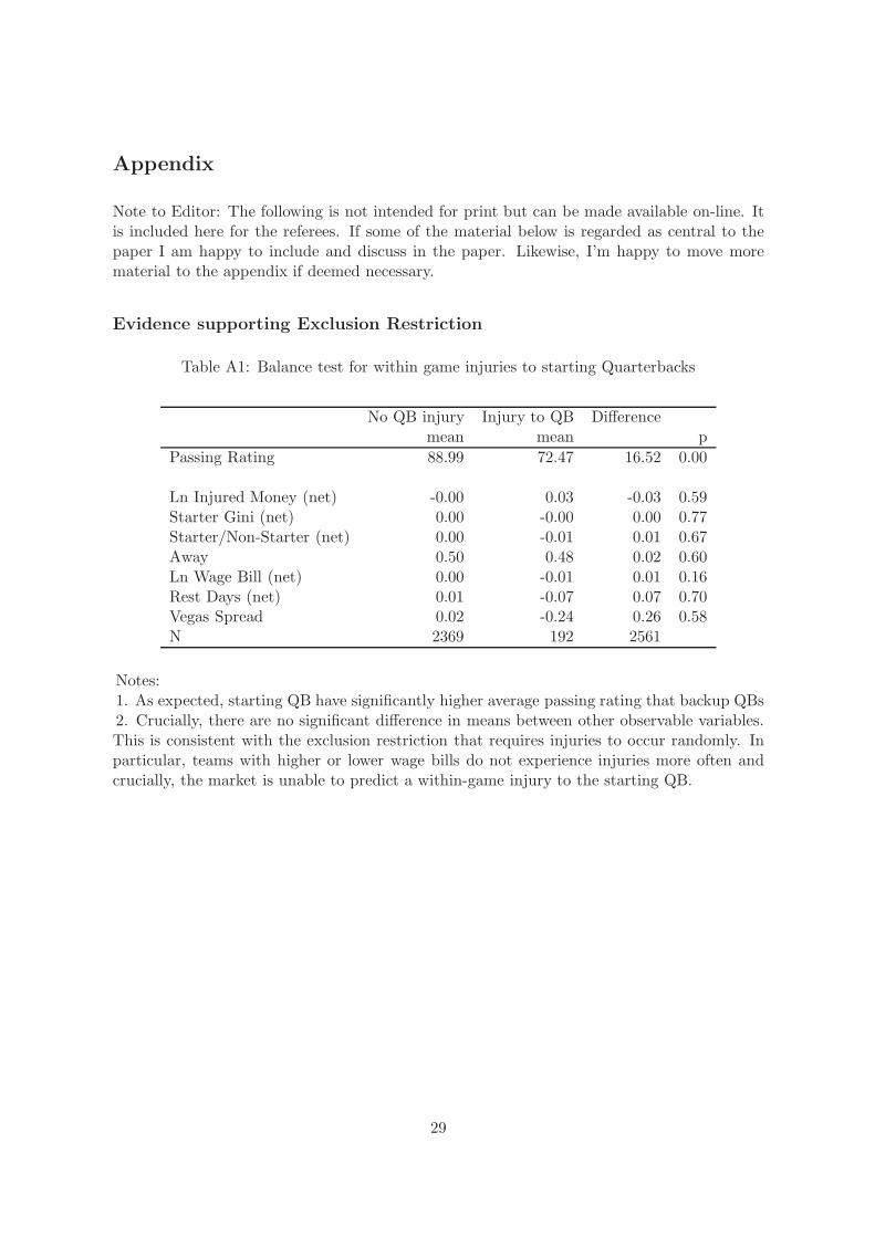
Appendix

Note to Editor: The following is not intended for print but can be made available on-line. Itis included here for the referees. If some of the material below is regarded as central to thepaper I am happy to include and discuss in the paper. Likewise, I’m happy to move morematerial to the appendix if deemed necessary.

Evidence supporting Exclusion Restriction

Table A1: Balance test for within game injuries to starting Quarterbacks

No QB injury Injury to QB Differencemean mean p

Passing Rating 88.99 72.47 16.52 0.00

Ln Injured Money (net) -0.00 0.03 -0.03 0.59Starter Gini (net) 0.00 -0.00 0.00 0.77Starter/Non-Starter (net) 0.00 -0.01 0.01 0.67Away 0.50 0.48 0.02 0.60Ln Wage Bill (net) 0.00 -0.01 0.01 0.16Rest Days (net) 0.01 -0.07 0.07 0.70Vegas Spread 0.02 -0.24 0.26 0.58N 2369 192 2561

Notes:1. As expected, starting QB have significantly higher average passing rating that backup QBs2. Crucially, there are no significant difference in means between other observable variables.This is consistent with the exclusion restriction that requires injuries to occur randomly. Inparticular, teams with higher or lower wage bills do not experience injuries more often andcrucially, the market is unable to predict a within-game injury to the starting QB.

29

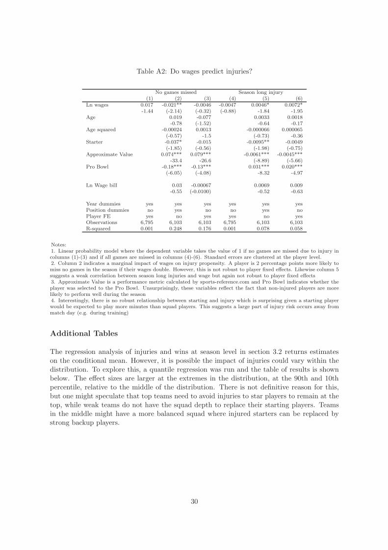
Table A2: Do wages predict injuries?

No games missed Season long injury(1) (2) (3) (4) (5) (6)

Ln wages 0.017 -0.021** -0.0046 -0.0047 0.0046* 0.0072*-1.44 (-2.14) (-0.32) (-0.88) -1.84 -1.95

Age 0.019 -0.077 0.0033 0.0018-0.78 (-1.52) -0.64 -0.17

Age squared -0.00024 0.0013 -0.000066 0.000065(-0.57) -1.5 (-0.73) -0.36

Starter -0.037* -0.015 -0.0095** -0.0049(-1.85) (-0.56) (-1.98) (-0.75)

Approximate Value 0.074*** 0.079*** -0.0061*** -0.0045***-33.4 -26.6 (-8.89) (-5.66)

Pro Bowl -0.18*** -0.13*** 0.031*** 0.020***(-6.05) (-4.08) -8.32 -4.97

Ln Wage bill 0.03 -0.00067 0.0069 0.009-0.55 (-0.0100) -0.52 -0.63

Year dummies yes yes yes yes yes yesPosition dummies no yes no no yes noPlayer FE yes no yes yes no yesObservations 6,795 6,103 6,103 6,795 6,103 6,103R-squared 0.001 0.248 0.176 0.001 0.078 0.058

Notes:1. Linear probability model where the dependent variable takes the value of 1 if no games are missed due to injury incolumns (1)-(3) and if all games are missed in columns (4)-(6). Standard errors are clustered at the player level.2. Column 2 indicates a marginal impact of wages on injury propensity. A player is 2 percentage points more likely tomiss no games in the season if their wages double. However, this is not robust to player fixed effects. Likewise column 5suggests a weak correlation between season long injuries and wage but again not robust to player fixed effects3. Approximate Value is a performance metric calculated by sports-reference.com and Pro Bowl indicates whether theplayer was selected to the Pro Bowl. Unsurprisingly, these variables reflect the fact that non-injured players are morelikely to perform well during the season4. Interestingly, there is no robust relationship between starting and injury which is surprising given a starting playerwould be expected to play more minutes than squad players. This suggests a large part of injury risk occurs away frommatch day (e.g. during training)

Additional Tables

The regression analysis of injuries and wins at season level in section 3.2 returns estimateson the conditional mean. However, it is possible the impact of injuries could vary within thedistribution. To explore this, a quantile regression was run and the table of results is shownbelow. The effect sizes are larger at the extremes in the distribution, at the 90th and 10thpercentile, relative to the middle of the distribution. There is not definitive reason for this,but one might speculate that top teams need to avoid injuries to star players to remain at thetop, while weak teams do not have the squad depth to replace their starting players. Teamsin the middle might have a more balanced squad where injured starters can be replaced bystrong backup players.

30

Table A3: Injuries and wins: Season level quantile regression

(1) (2) (3) (4) (5)q10 q25 q50 q75 q90

Ln Injured money -0.36*** -0.19* -0.11 -0.21* -0.40***(-3.28) (-1.66) (-1.10) (-1.71) (-2.83)

Ln Wage bill 0.16 1.48* 2.06*** 2.14* 2.82**(0.12) (1.67) (2.78) (1.96) (2.37)

Ln Wage bill SD -0.12 -1.28 -1.63*** -1.09 -1.65*(-0.087) (-1.57) (-3.23) (-1.19) (-1.84)

Observations 213 213 213 213 213t-statistics in parentheses

*** p<0.01, ** p<0.05, * p<0.1

Notes:1. This table presents quantile regression results of the total injured money incurred by a franchise during the seasonupon the proportion of wins in a season. The dependent variable is the percentage of games won wi in the season texpressed in log odds: wit = ln(wit/(1 −wit))2. The sign on injured money indicates a negative relationship at each percentile. While column (5) suggests a slightlystronger unconditional impact at the 90th percentile there is no significance difference between the 90th percentile andthe 10th percentile. The effect sizes in the middle of the distribution are more modest.

Table A4: Impact of winning on finances: short run

OLS FEValue Revenue Income Value Revenue Income(1) (2) (3) (4) (5) (6)

Winpct−1 187* 31.7* 10.1 -2.93 -16.6 -15.0*(1.80) (1.89) (0.85) (-0.29) (-0.22) (-1.72)

PostseasonWint−1 37.7 6.47 10.3 6.52 43.1 11.2**(0.69) (0.73) (1.63) (1.29) (1.16) (2.57)

ChampionshipWint−1 -42.1 -7.66 -14.2 -4.52 -12.6 -12.3(-0.40) (-0.44) (-1.15) (-0.46) (-0.18) (-1.45)

SuperBowlWint−1 202 28.1 24.8 12.1 49.9 16.6(1.50) (1.27) (1.57) (0.97) (0.54) (1.54)

Year Dummies Yes Yes Yes Yes Yes YesObservations 445 383 383 383 445 383R-squared 0.762 0.686 0.337 0.887 0.887 0.548Teams 32 32 32 32 32 32

t-statistics in parentheses*** p<0.01, ** p<0.05, * p<0.1

Notes:1. This table estimates the elasticity of winning in the season prior on the book value, revenue and operating income ofNFL franchises over the sample period. The sample period begins in 2000 and ends 2017 omitting the years 2001-2004and 2006-2007 as financial data was not available on NFL franchises in these years. Columns (1) to (3) report OLSregression and columns (4) through (6) the fixed effects estimates.2. While there has been a large appreciation in book values, revenues and income of NFL franchises over the sampleperiod there is no robust relationship between winning and any of the financial variables in the short run. This result isconsistent with the arguments laid out in Vrooman (2012).

Example Contracts

Panel A of Table A5 shows the structure of Andrew Luck’s contract which he signed in 2016.Luck was the starting QB for the Indianpollis Colts. Media reports will typically headline the

31

total value of the contract when it is signed, in this case “$140m” 20. However, this amount isspread over six years and while Luck received $47m guaranteed on signing (a $12m salary plus$32m signing bonus plus $3m roaster bonus) these amounts can be spread over the durationof the contract to even out the Cap Hit. While the player can be cut at any time, moniesguaranteed on signing would hit the cap immediately in the year that the player is cut. The‘Dead Money’ in the final column records the amount charged to the Cap in the event thatthe player is cut in that year.

Table A5: Andrew Luck’s contract vs Scott Tolzien

Panel A: Starting Quarter BackYear Salary Signing Roster Cap Hit Dead Money

2016 12m 6.4m 0 18.4m 47m2017 7m 6.4m 6m 19.4m 28.6m2018 12m 6.4m 6m 24.4m 19.2m2019 9.125m 6.4m 12m 27.525m 12.8m2020 11m 6.4m 11m 28.4m 6.4m2021 11m 0 10m 21m 0

Panel B: Back up Quarter BackYear Salary Signing Roster Cap Hit Dead Money

2016 1.25m 0.25m 0 1.5m 0.5m2017 1.75m 0.25m 0 2.0m 0.25m

By contrast, panel B details the Colt’s backup QB, Scott Tolzien’s contract. Tolzien signed a2 year contract with $0.5m guaranteed on signing and none of salary guaranteed. As a resultTolzien could be cut at the end of 2016 with only a $0.25M charge to the 2017 cap.

20See http://www.nfl.com/news/story/0ap3000000672131/article/andrew-luck-signs-sixyear-140-million-colts-contract

32

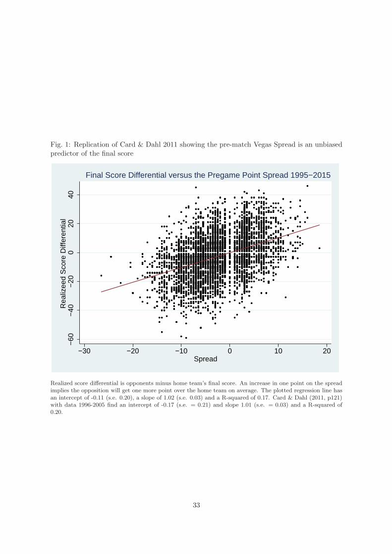
Fig. 1: Replication of Card & Dahl 2011 showing the pre-match Vegas Spread is an unbiasedpredictor of the final score

−60

−40

−20

020

40R

ealiz

eed

Sco

re D

iffer

entia

l

−30 −20 −10 0 10 20Spread

Final Score Differential versus the Pregame Point Spread 1995−2015

Realized score differential is opponents minus home team’s final score. An increase in one point on the spreadimplies the opposition will get one more point over the home team on average. The plotted regression line hasan intercept of -0.11 (s.e. 0.20), a slope of 1.02 (s.e. 0.03) and a R-squared of 0.17. Card & Dahl (2011, p121)with data 1996-2005 find an intercept of -0.17 (s.e. = 0.21) and slope 1.01 (s.e. = 0.03) and a R-squared of0.20.

33

Table A6: Variable Definitions

Variable DescriptionPlayer wage variablesSalary Annual salary in nominal dollarsSigning Signing bonus in nominal dollarsRoster Roster bonus in nominal dollarsDead Money The outstanding charge in nominal dollars to the franchise’s salary cap in the event that the player is cut before

the contract expiresLn wages The official charge to the salary cap for the player in year t

Injury variables: Season levelLn Injured money Natural log of the sum of all player wages * x/16, where x is the number of games of the regular season in year t

the player missed due to injuryLn(Wage bill) Natural log of the total wage bill of the franchise in year t

Ln(Wage bill standard deviation) Natural log of the standard deviation of the wage bill of the franchise in year t

Injury variables: Game levelLn Injured money (net) Natural log of the sum of all player wages who are injured in that game minus the same figure for the oppositionStarter Gini (net) The gini coefficient of the wages of starting players net of the oppositionStarter/Non-Starter (net) The ratio of the starting wages to non-starting wages net of the figure for the oppositionAway Dummy variable taking the value of one if the game is an away fixture*Ln Wage Bill (net) Natural log of the total wage bill of the franchise in year t net of the figure for the oppositionRest Days (net) Number of days since the last fixture, net of the figure for the oppositionVegas Spread Number of points on the pre-kickoff spread

Injury variables: Within game quarterbacks (QBs)Injured QB Dummy variable taking the value of 1 if the starting QB is injured during the gameInjured QB opponent Dummy variable taking the value of 1 if the opposition’s starting QB is injured during the gameBackup QB wage diff. The difference in natural log of wages between the starting and backup QB when the starting QB is injured

during the gameBackup QB opponent wage diff. The difference in natural log of wages between the opposition’s starting and backup QB when the opposition’s starting

QB is injured during the gamePassing Rating The official passing rating of the QB for the gamePassing Rating opponent The official passing rating of the opposition’s QB for the game

Franchise value dependent variablesRevenue Revenue in nominal dollars (millions) as recorded by Forbes.comBook Value Book value in nominal dollars (millions) of franchise based on current stadium deal at time t deducting stadium

debt (Forbes.com)Operating Income Earnings before interest, taxes, deprecation and amortization in nominal dollars (millions) (Forbes.com)

Franchise Value Control VariablesRolling win percentage Rolling average of the percentage of wins in the regular seasonInitial conditions in 1995No. Wins Number of wins in the regular season up to 1995No. Super Bowls Number of Super Bowl wins up to 1995No. Post season years Number of seasons up to 1995 when the team qualified for the post season playoffsFranchise age 1995 - the original year the franchise was founded

Stadium variablesCapacity Capacity of the stadium at time t

Ln (total build cost) Natural log of total build cost of stadium at time t in 2017 pricesNew stadium Dummy variable taking the value of 1 if a new stadium was built between 1995 and 2017Yrs since expansion Number of years at time t since the last increase in stadium capacity

Metropolitan Area controlsLn population Natural log the population in the metro areaPopulation growth rate Percentage change in population between 2016 and 2010Only franchise Dummy variable taking the value of 1 if franchise i is the only NFL franchise in the metropolitan areaMain franchise Dummy variable taking the value of 1 if franchise i is the largest NFL franchise in the metropolitan area

(e.g. New York Giants)No. substitutes Number of National Basketball Association, Major League Baseball or National Hockey League franchises in the

metropolitan area

Wage determinantsRookie Dummy variable taking the value of 1 if player is on their first contractAge Player’s age as recorded by sports − reference.com

Approximate Value Player’s Approximate value as recorded by sports − reference.com

Pro Bowl Dummy variable taking the value of 1 if player played in the season’s pro bowlNo. games Number of games where the player featured in at least one play in the seasonInjury Reserve Dummy variable taking the value of 1 if the player was on injury reserveDraft Round 2nd-7th Set of dummy variables taking the value of 1 according to where the player drafted. 1st round draft picks are the

baseline category

Short run franchise performance variablesWinpc Percentage of wins in the regular season of 16 gamesPostseason Win Dummy variable taking the value of 1 if the franchise won a game in the postseasonChampionship Win Dummy variable taking the value of 1 if the franchise won their championship game in the postseasonSuper Bowl Win Dummy variable taking the value of 1 if the franchise won the Super Bowl in the postseason

34