W-based versus latent variables spatial autoregressive models: evidence from Monte Carlo simulations

Ann Reg Sci (2011) 47:619–639DOI 10.1007/s00168-010-0398-0

SPECIAL ISSUE PAPER

W-based versus latent variables spatial autoregressivemodels: evidence from Monte Carlo simulations

An Liu · Henk Folmer · Johan H. L. Oud

Received: 7 July 2009 / Accepted: 1 April 2010 / Published online: 23 June 2010© The Author(s) 2010. This article is published with open access at Springerlink.com

Abstract In this paper, we compare by means of Monte Carlo simulations twoapproaches to take spatial autocorrelation into account: the classical spatial autore-gressive model and the structural equations model with latent variables. The formeraccounts for spatial dependence and spillover effects in georeferenced data by meansof a spatial weights matrix W. The latter represents spatial dependence and spillovereffects by means of a latent variable in the structural (regression) model while theobserved spatially lagged variables are related to the latent spatial dependence vari-able in the measurement model. The simulation results based on Anselin’s Columbus,Ohio, crime data set show that the misspecified latent variables approach slightly trailsthe correctly specified classical approach in terms of bias and root mean squared errorof the coefficient estimators.

JEL Classification C13 · C15 · C52 · R15

A. Liu (B) · H. FolmerDepartment of Spatial Sciences, University of Groningen,PO Box 800, 9700 AV Groningen, The Netherlandse-mail: [email protected]

H. FolmerDepartment of Social Sciences, Wageningen University,PO Box 8130, 6700 EW Wageningen, The Netherlandse-mail: [email protected]

J. H. L. OudBehavioural Science Institute, Radboud University Nijmegen,PO Box 9104, 6500 HE Nijmegen, The Netherlandse-mail: [email protected]

123

620 A. Liu et al.

1 Introduction

When it comes to applying econometric models to analyze georeferenced data,researchers are well aware of the fact that ignoring spatial dependencies leads toinefficient and biased estimators. A substantial theoretical and simulation literatureon efficient and consistent estimators for spatial dependence models has developed. Amajor issue concerns the specification of the structure of spatial dependence includingthe type of spatial weights to be incorporated into the model. This paper focuses on theevaluation of two approaches that explicitly model spatial dependence: the classicalW-based regression model and the recently proposed latent variables approach.1

In the spatial econometrics literature the W-based spatial regression approach hasbeen dominant and is most commonly used. The approach is based on a spatial weightsmatrix, usually denoted W, that accounts for spatial dependence or spill-over effectsamong the spatial units of observation. The selection of a spatial weights matrix is acrucial step in spatial modelling because it a priori imposes a model structure whichaffects estimates (Bhattacharjee and Jensen-Butler 2006; Anselin 2002; Fingleton2003) and the substantive interpretation of the research findings (Hepple 1995).

Several types of spatial weights matrices can be used to represent spatial depen-dence. Most common are the contiguity-based matrices. Two regions are said to befirst-order contiguous if they share a common border (rook) or vertex (bishop) or both(queen). The concept of spatial contiguity can be extended to higher orders. Anothercommon type of weights matrix is distance based, such as inverse distance or inversedistance squared, or a fixed distance band.

Much progress has been made with respect to the the construction and comparisonof spatial weights matrices including estimation of spatial weights matrices that areconsistent with an observed pattern of spatial dependence rather than assuming a priorithe nature of spatial interaction dependence (Hepple 1995; Aldstadt and Getis 2004,2006). In spite of all these developments the most common procedure in appliedresearch is still to assume a priori first-order contiguity, as expressed by a spatialweights matrix W with diagonal elements equal to zero and off-diagonal elementsequal to one if two regions are first-order contiguous and zero elsewhere.

The alternative under consideration here, the latent variables approach was intro-duced by Folmer and Oud (2008). It proceeds on the basis of a structural equationsmodel (SEM). SEM allows simultaneous handling of observed and latent variableswithin one model framework. Latent variables refer to those phenomena that aresupposed to exist but cannot be observed directly. An example of a latent variable issocio-economic status. This concept refers to an individual’s standing in society whichcannot be observed or measured directly. However, it can be measured via observableindicators like educational attainment, income, occupational status, etc. In a similarvein, the latent variable regional welfare can be measured by observable indicators

1 Another approach to dealing with spatial autocorrelation is spatial filtering. It comes down to the removalof spatial dependence in a spatially autocorrelated variable by partioning it into a filtered, nonspatial variableand a residual spatial variable such that conventional regression techniques can be applied to the filtereddata (see amongst others Getis and Griffith 2002; Tiefelsdorf and Griffith 2007). Spatial filtering is notconsidered in this paper.

123

W-based versus latent variables spatial autoregressive models 621

like GDP per capita, features of the income distribution, labour market opportunities,indicators of the healthcare system, environment quality and so on.

A SEM is made up of two submodels: (1) the structural model representing thecausal relationships among the latent variables and (2) the measurement model repre-senting the relationships between the latent variables and their observable indicators(Oud and Folmer 2008). The latent variables approach accounts for spatial dependencewith the spatially lagged variables represented by latent variables in the structuralmodel and models the relationship between latent spatially lagged variables and theirobserved indicators in the measurement model. Since one latent variable can be mea-sured by several indicators, this approach allows for the straightforward inclusion ofvarious kinds of spatial dependence in the model, e.g. spatial dependence due to theimpact of the nearest neighbours and distance-weighted impact from hotspots. It isalso capable of including different types of contiguity, including nonspatial contigu-ity, for instance, a dependent relationship between regions due to economic, socialor demographic similarity (see Case et al. 1993) rather than e.g. conventional spatialdependence such as first-order contiguity.2 Moreover, several types of spatial depen-dences can be included in a given model by using different latent variables in thestructural model with corresponding sets of indicators in the measurement model, e.g.one latent variable for conventional spatial contiguity and another for socio-economicdependency. Another important feature of the latent variable approach is that it allowstesting of the relationship of a latent variable and its indicators, e.g. whether or not thenext nearest neighbour contributes to the latent dependence variable.

Folmer and Oud (2008) show that the latent variables approach can produce esti-mates that are virtually identical to those obtained by the W-based approach but alsothat it is more general than the latter. They argue, however, that further comparison isneeded to draw up the pros and cons of each approach. To gain more insight into thequality of the estimators produced by both approaches, we carry out Monte Carlo sim-ulations. The simulations are performed on the basis of Anselin’s (1988) Columbus,Ohio, crime data set which was also used by Folmer and Oud (2008) for illustrativepurposes. The performance of the approaches will be analyzed in terms of bias and rootmean squared error (RMSE) for various values of spatial autocorrelation and kinds ofweight matrices.

The remainder of the paper is organized as follows. Section 2 summarizes theW-based spatial regression approach and the latent variables approach and specifiestheir model structures. A description of the experimental design is given in Sect. 3. InSect. 4 we present the simulation results while Sect. 5 concludes.

2 Non-spatial contiguity can also be handled by conventional W methods. However, if both spatial andnon-spatial contiguity are taken into account in a conventional model, more than one W matrix is required,particularly one corresponding to the former and one to the latter type of dependence.

123

622 A. Liu et al.

2 Model specifications

2.1 The W-based autoregressive model

There are two types of W-based spatial models that are most commonly used in appliedresearch: the spatial lag model and the spatial error model. Here, we restrict ourselvesto the former. The lag model assumes that the dependent variable in a given region,say i, is a function of exogenous variables in i and of the dependent variable in otherregions, different from i. Particularly, the classical W-based spatial lag or autoregres-sive model reads:

y = ρW y + Xβ + ε (1)

ε ∼ N(0, σ 2 In

)(2)

where y is an n × 1 vector of observations on the dependent variable, X is an n × kdata matrix of explanatory variables with associated coefficient vector β, ε is an n ×1vector of error terms. W is the n × n spatial weights matrix with diagonal elementsequal to zero and off-diagonal elements unequal to zero, if the regions correspondingto that element meet the adopted spatial dependence definition. The parameter ρ isthe spatial autoregressive or spatial lag parameter.

The log-likelihood function for model (1) reads Anselin’s (1988):

L =− N

2ln π− N

2ln σ 2+ln |A|− 1

2σ 2 (Ay−Xβ)′(Ay−Xβ) with A= I − ρW.

(3)

Since the likelihood function contains a Jacobian term ln |A| and the matrix A is ofdimension equal to the number of observations, its presence in the function to be opti-mized makes the numerical analysis considerably complex. Ord (1975) has derived asimplification of determinants such as |A| in terms of its eigenvalues. Specifically:

ln |I − ρW | = ln �i (1 − ρwi ) = �i ln(1 − ρwi ) (4)

where the wi are the eigenvalues of W .

2.2 The latent variables spatial autoregressive model

Before going into detail, we observe that a SEM is usually specified in terms of vari-ables in contrast to spatial regression models like model (1) which are specified interms of units of observation. Below we adopt the SEM convention. When we referto a SEM in terms of units of observation we use a tilde (∼).

A SEM in general form consists of two basic equations:

y = η + ε with cov(ε) = � (5)

η = Bη + ζ with cov(ζ ) = (6)

123


Equation (5) is the measurement model where the vector y contains m observed vari-ables. contains the loadings of the observed variables (indicators) on the vector of klatent variables η3, and � is the m × m measurement error covariance matrix. In thestructural model (6), B specifies the structural relationships among the latent variablesand is the k×k covariance matrix of the errors in the structural model. The measure-ment errors in ε are assumed to be uncorrelated with the latent variables in η. Observethat directly observed variables can be included in the structural model by specifyingin the measurement model an identity relationship between a given observed variableand the corresponding latent variable.

A SEM model is estimated by minimizing the distance between the model impliedcovariance matrix (on the basis of hypotheses relating to the model structure as spec-ified in the parameter matrices B, ,, and �) and the observed covariance matrix.Several estimators for SEM have been developed including instrumental variables(IV), two-stage least squares (TSLS), unweighted least squares (ULS), generalizedleast squares (GLS), fully weighted (WLS) and diagonally weighted least squares(DWLS), and maximum likelihood (ML). ML is the most commonly used estimatorand the default in the statistical packages Mx and LISREL. Below we discuss the MLestimator. It maximizes the log-likelihood function:

l(θ |Y ) = − N

2ln |�| − N

2tr(S�−1) − pN

2ln 2π (7)

where � is the theoretical covariance matrix in terms of the free and constrainedelements in the four parameter matrices. That is:

� = (I − B)−1 (I − B ′)−1′ + � (8)

and S is the observed covariance matrix for given data set Y .The ML-estimator θ = arg max l(θ |Y ) chooses that value of θ which maximizes

l(θ |Y ). Minimizing the fit function:

FML = ln |�| + tr(S�−1) − ln |S| − p (9)

gives the same results as maximizing the above likelihood function (Oud and Folmer2008). The LISREL software package also contains a variety of tests and model eval-uation statistics and gives reliable information about the identification status of themodel (see Jöreskog and Sörbom 1996 for details).

The SEM analog to model (1) is specified as follows. First, the spatially laggeddependent variable W y is taken as a latent variable in the structural model (i.e. W y in(1) is replaced by a latent variable η). Specifically:

y = ρη + γ ′x + ζ (10)

3 Observe that a SEM will not be identified if the latent variables have not been assigned measurementscales. It is convenient to fix the measurement scale of a latent variable by fixing one λi , usually at 1. Thatis, one often chooses λ1 = 1.

123

624 A. Liu et al.

The structural model (10) is completed by a measurement equation:

y = η + ε (11)4

with

y =

⎡

⎢⎢⎢⎣

y1y2...

ym

⎤

⎥⎥⎥⎦

, =

⎡

⎢⎢⎢⎣

λ1λ2...

λm

⎤

⎥⎥⎥⎦

, � =

⎡

⎢⎢⎢⎣

σ 2ε1

0 0 00 σ 2

ε20 0

0 0. . . 0

0 0 0 σ 2εm

⎤

⎥⎥⎥⎦

(12)

Observe that in (12) the latent spatial lag η is measured by more than one observedvariable. For instance, for Anselin’s crime model Folmer and Oud (2008) considerthe three, respectively, six, nearest neighbours as well as the distance from the crimecenter.

The measurement model is constructed by means of selection functions or selec-tion matrices Si which select relevant observations from the vector of observations asfollows [as indicated above, a tilde (∼) denotes (a vector of) observations]:

y1 = S1y,y2 = S2y,

...

ym = Smy.

(13)

That is, S1 selects the values for the first indicator vector y1, S2 for the second indicatorvector y2, etc. For example, for the simulations based on Anselin’s crime model, S1could select the value of crime in the nearest contiguous neighbour, S2 the crime valuein the next nearest contiguous neighbour and so on. Thus, for the measurement modelwe obtain:

y1 = S1y = λ1η + ε1,

y2 = S2y = λ2η + ε2,...

ym = Smy = λmη + εm.

(14)

From the above it follows that spatial dependence is captured by two kinds of parame-ters, ρ and λi , whereas in the standard lag model only the “average” effect ρW y showsup. This means that the latent variable approach offers a much richer representationof the spatial structure than the standard spatial econometric approaches. Moreover,it allows testing of the relationship between indicators and the corresponding latentvariables, for instance, whether the sixth nearest neighbour is a significant indicator.

The standard SEM log-likelihood function needs correction so as to accountfor the presence of the latent spatial lag variable among the explanatory variables.

4 Observe that in (10) y is a scalar while in (11) y is a vector.

123


Folmer and Oud (2008) show that ln |A| needs to be added to the log-likelihoodfunction (7) with5

A = I − ρ

mλ1S1 − ρ

mλ2S2 − · · · − ρ

mλmSm (15)

3 Experimental design

To investigate the performances of the two modelling approaches specified in Sect. 2,we conduct a number of Monte Carlo simulations. For that purpose we make useof Anselin’s (1988) Columbus, Ohio, crime data set. Particularly, we use its spatialstructure, the observed values of the exogenous variables and the parameter estimates.

The first step is sample generation. For that purpose we specify equation (1) interms of Anselin’s crime model:

y = ρW y + β0 + x1β1 + x2β2 + ε (16)

or:

y = (I − ρW )−1(β0 + x1β1 + x2β2 + ε) (17)

Next, y is generated as follows (cf. Florax and Folmer 1992; Florax et al. 2003):

1. Fix the exogenous variables x1 (income) and x2 (housing value) at the values inAnselin’s (1988) crime data set.

2. Choose Anselin’s (1988) estimate of the vector β6:

β0 = 45.079, β1 = −1.032, β2 = −0.266.

3. Generate values for the error term ε by randomly drawing from a normal (0,10)distribution. The variance of ε is approximately equal to Anselin’s (1988) estimate.

4. Vary ρ over the interval [0.1, 0.9] using increments of 0.2. Observe that ρ = 0 isthe non-spatial benchmark model.

5. Compute y according to (17) on the basis of Anselin’s (1988) first-order queencontiguity matrix, inverse distance matrix and inverse distance squared matrix,respectively.

5 First-order and higher order contiguity models with equal number of neighbours and inverse distancemodels are nested within the class of latent variables models. For the first case each λi in the measurementmodel is fixed at 1/n where n is the number of neighbours. For the inverse distance model each λi is fixedat 1/n if the observed value for each neighbour is weighted by the inverse of distance. Contiguity modelswith unequal numbers of neighbours are not nested within the latent variables model.6 The regression coefficients are chosen in line with Anselin’s estimates, since these values are known fromthe literature. Other values could have been chosen, however.

123

626 A. Liu et al.

For the data set thus generated we estimate both the classical spatial lag model andthe latent model. The classical models are estimated on the basis of a first-order conti-guity matrix, inverse distance matrix and inverse distance squared matrix for each setof samples. For the latent model the first six nearest neighbors are taken as indicatorsof the latent dependence variable.

The number of replications is 1,000. The estimates are evaluated in terms of bias andRMSE of the spatial lag parameter ρ and the main regression coefficients of interest,β1 and β2.

4 Simulation results

Table 1 and Fig. 1 report the biases of the estimators of ρ, β1 and β2 of the three clas-sical models and the latent variables model based on samples generated by first-ordercontiguity weights matrix. The comparison involves three types of classical models—Ccont (estimated on the basis of the first-order contiguity matrix), Cdinv (estimated onthe basis of the inverse distance matrix), Cdinv2 (estimated on the basis of the inversedistance squared matrix)—and one latent model—Latent6n (estimated on the basis ofthe first six nearest neighbors as indicators of the latent spatial dependence variable).

• From Table 1 and Fig. 1a it follows that when ρ = 0, the ‘true’ model—Ccont—has the smallest bias for ρ. For 0 < ρ < 0.5 this holds for Cdinv and for ρ ≥ 0.5for Cdinv2. Latent6n is outperformed by its three alternatives forρ < 0.5. Forρ ≥ 0.5, however, it outperforms Ccont but not the other two alternatives. ForLatent6n we observe a constantly descending trend of the bias.

• Table 1 and Fig. 1b also show that for β1 Cdinv2 has the smallest bias except forρ = 0 and ρ = 0.1 when Ccont and Cdinv have the smallest bias, respectively.For ρ = 0.3 Latent6n has smaller bias than Ccont but is outperformed by the twoalternative classical models. The bias of Latent6n (in absolute value) follows a Ucurve with minimum at ρ = 0.3.

• Table 1 and Fig. 1c show that for β2 Ccont has the smallest bias everywhere exceptfor ρ = 0 when Cdinv has the smallest bias and for ρ = 0.1 when this holds forLatent6n. Moreover, Latent6n outperforms Cdinv and Cdinv2 for ρ = 0.3 and 0.9.

It follows from the above that there are several cases where the latent model has smallerbias than one or several of the classical models. Particularly, Latent6n outperforms the“true” or correctly specified Ccont more frequently than the other two misspecifiedclassical models.

The RMSEs of the estimators are shown in Table 2. It shows that there are onlyvery small differences between the four models for each parameter. Figure 2 presentstotal RMSE, i.e., the sum of the RMSEs of all three parameters. The figure showsthat the classical models outperform the latent model. One reason for this is probablythat there are more parameters and thus bigger standard errors in the latent modelthan in its alternatives. Among the classical models the “true” Ccont outperforms theother classical models for ρ ≤ 0.5. However, Cdinv2 has the smallest RMSE whenρ > 0.5, closely followed by Cdinv. Notice that when ρ increases, the RMSE ofLatent6n decreases somewhat more than the RMSE of Ccont.

123


Tabl

e1

Bia

sof

the

estim

ator

sfo

rsa

mpl

esge

nera

ted

onth

eba

sis

ofth

efir

st-o

rder

cont

igui

tym

atri

x

ρβ

1β

2

ρC

cont

Cdi

nvC

dinv

2L

aten

t6n

Cco

ntC

dinv

Cdi

nv2

Lat

ent6

nC

cont

Cdi

nvC

dinv

2L

aten

t6n

0.0

−0.0

593

−0.0

806

−0.0

765

−0.0

871

−0.0

291

−0.0

367

−0.0

347

−0.0

659

0.00

160.

0011

0.00

130.

0031

0.1

−0.0

606

−0.0

521

−0.0

528

−0.0

807

−0.0

329

−0.0

243

−0.0

253

−0.0

373

0.00

130.

0019

0.00

190.

0009

0.3

−0.0

603

−0.0

039

−0.0

117

−0.0

644

−0.0

414

0.00

32−0

.002

90.

0173

0.00

060.

0037

0.00

33−0

.002

8

0.5

−0.0

561

0.02

540.

0158

−0.0

466

−0.0

518

0.03

220.

0224

0.06

310.

0001

0.00

520.

0046

−0.0

061

0.7

−0.0

473

0.03

130.

0242

−0.0

330

−0.0

659

0.05

540.

0447

0.09

980.

0001

0.00

550.

0050

−0.0

084

0.9

−0.0

329

0.01

040.

0081

−0.0

128

−0.0

943

0.04

090.

0339

0.14

590.

0008

0.00

290.

0027

−0.0

022

123

628 A. Liu et al.

Fig. 1 Bias of the estimators of ρ (a), β1 (b) and β2 (c) for the classical models (Ccont, Cdinv, Cdinv2)and the latent model (Latent6n) for samples generated by first-order contiguity matrix

123


Tabl

e2

RM

SEof

the

estim

ator

sfo

rsa

mpl

esge

nera

ted

onth

eba

sis

ofth

efir

st-o

rder

cont

igui

tym

atri

x

ρβ

1β

2

ρC

cont

Cdi

nvC

dinv

2L

aten

t6n

Cco

ntC

dinv

Cdi

nv2

Lat

ent6

nC

cont

Cdi

nvC

dinv

2L

aten

t6n

0.0

0.13

970.

1849

0.17

720.

1888

0.24

960.

2577

0.25

540.

2797

0.07

210.

0725

0.07

230.

0733

0.1

0.13

520.

1695

0.16

360.

1788

0.25

150.

2568

0.25

580.

2738

0.07

220.

0723

0.07

230.

0735

0.3

0.12

200.

1402

0.13

680.

1524

0.25

560.

2578

0.25

710.

2700

0.07

250.

0721

0.07

220.

0742

0.5

0.10

290.

1119

0.10

920.

1204

0.26

050.

2611

0.26

010.

2761

0.07

280.

0718

0.07

190.

0759

0.7

0 .07

740.

0790

0.07

730.

0849

0.26

600.

2654

0.26

410.

2816

0.07

310.

0714

0.07

160.

0786

0.9

0.04

370.

0345

0.03

450.

0441

0.27

360.

2596

0.25

950.

2934

0.07

350.

0715

0.07

160.

0743

123

630 A. Liu et al.

Fig. 2 Total RMSE for the four models for samples generated by first-order contiguity matrix

Taking bias and RMSE together, it follows that Ccont and Cdinv2 perform betterthan Cdinv and Latent6n.

The results for samples generated by inverse distance weights matrix are summa-rized in Tables 3 and 4 and shown in Figs. 3 and 4. From Table 3 it follows that allthe biases are negative for all four models and all parameters. Moreover, Cdinv, as the‘correct’ model, outperforms the other classical models and the latent model most ofthe time in terms of bias of all three parameters.

Figure 3a shows that for ρ Ccont has the smallest bias when ρ = 0 and Cdinv2 isthe best when ρ = 0.1. Other than that, Cdinv outperforms the other three models.Latent6n is better than Ccont when ρ = 0.9. With regard to the bias of β1, it can beconcluded from Fig. 3b that the ‘winners’ are the same as in the case of ρ except forρ = 0.9 where Latent6n has the lowest bias. Moreover, Latent6n also outperformsCcont when ρ ≥ 0.5. From Fig. 3c it follows that Cdinv is best again and Latent6n isoutperformed by Ccont except for ρ = 0.1 when their biases are equal.

Table 4 gives the RMSEs for ρ, β1 and β2 for the four models. As in the case ofsamples based on the first-order contiguity matrix, the differences between the fourmodels are very small. The latent model sometimes outperforms the classical models.For instance, for ρ = 0.1, Latent6n has smaller RMSE for ρ than Cdinv and it out-performs both Cdinv and Cdinv2 when ρ = 0. Also for values of ρ ≥ 0.7 Latent6noutperforms Ccont for β1.

Figure 4 presents the total RMSE of all three parameters. It follows that total RMSEis smallest for Ccont for the first three values of ρ while Cdinv leads for the next threevalues of ρ, closely followed by Cdinv2. However, unlike the previous case wheresamples are generated by first-order contiguity matrix, the classical models do notuniformly outperform the latent approach. Particularly, Latent6n beats Cdinv whenρ = 0 and outperforms Ccont when ρ = 0.9.

Considering both bias and RMSE, the “true” model Cdinv outperforms its threealternatives most of time. Furthermore, Cdinv2 and Ccont perform about equally well.

123


Tabl

e3

Bia

sof

the

estim

ator

sfo

rsa

mpl

esge

nera

ted

byin

vers

edi

stan

cem

atri

x

ρβ

1β

2

ρC

cont

Cdi

nvC

dinv

2L

aten

t6n

Cco

ntC

dinv

Cdi

nv2

Lat

ent6

nC

cont

Cdi

nvC

dinv

2L

aten

t6n

0.0

−0.0

554

−0.0

955

−0.0

847

−0.0

871

−0.0

387

−0.0

597

−0.0

539

−0.0

659

0.00

01−0

.001

8−0

.001

30.

0031

0.1

−0.0

869

−0.0

850

−0.0

838

−0.1

268

−0.0

638

−0.0

597

−0.0

594

−0.0

867

−0.0

021

−0.0

018

−0.0

018

−0.0

021

0.3

−0.1

216

−0.0

639

−0.0

724

−0.1

685

−0.1

117

−0.0

591

−0.0

669

−0.1

154

−0.0

062

−0.0

017

−0.0

024

−0.0

166

0.5

−0.1

180

−0.0

434

−0.0

527

−0.1

569

−0.1

516

−0.0

580

−0.0

695

−0.1

138

−0.0

095

−0.0

016

−0.0

025

−0.0

145

0.7

−0.0

805

−0.0

243

− 0.0

295

−0.1

073

−0.1

743

−0.0

561

−0.0

670

−0.0

695

−0.0

111

−0.0

013

−0.0

022

−0.0

137

0.9

−0.0

228

−0.0

074

−0.0

082

−0.0

186

−0.1

518

−0.0

535

−0.0

587

−0.0

412

−0.0

088

−0.0

009

−0.0

013

−0.0

123

123

632 A. Liu et al.

Tabl

e4

RM

SEof

the

estim

ator

sfo

rsa

mpl

esge

nera

ted

byin

vers

edi

stan

cem

atri

x

ρβ

1β

2

ρC

cont

Cdi

nvC

dinv

2L

aten

t6n

Cco

ntC

dinv

Cdi

nv2

Lat

ent6

nC

cont

Cdi

nvC

dinv

2L

aten

t6n

0.0

0.13

450.

2186

0.19

980.

1888

0.25

300.

2728

0.26

770.

2797

0.07

180.

0720

0.07

190.

0733

0.1

0.14

030.

1971

0.18

540.

1955

0.25

800.

2736

0.27

000.

2820

0.07

180.

0720

0.07

190.

0729

0.3

0.14

680.

1531

0.15

040.

1964

0.27

170.

2749

0.27

370.

2868

0.07

200.

0720

0.07

200.

0745

0.5

0.13

060.

1085

0.10

940.

1702

0.28

810.

2760

0.27

640.

2909

0.07

230.

0720

0.07

200.

0741

0.7

0 .08

760.

0642

0.06

530.

1129

0.30

060.

2768

0.27

780.

2867

0.07

240.

0719

0.07

190.

0731

0.9

0.02

710.

0210

0.02

120.

0343

0.29

690.

2773

0.27

790.

2817

0.07

220.

0719

0.07

190.

0724

123


Fig. 3 Bias of the estimators of ρ (a), β1 (b) and β2 (c) for the classical models (Ccont, Cdinv, Cdinv2)and the latent model (Latent6n) for samples generated by inverse distance matrix

123

634 A. Liu et al.

Fig. 4 Total RMSE for the four models for samples generated by inverse distance matrix

The latent model trails the “true” model, and, to a lesser extent, the misspecified clas-sical models. The differences are very small, however.

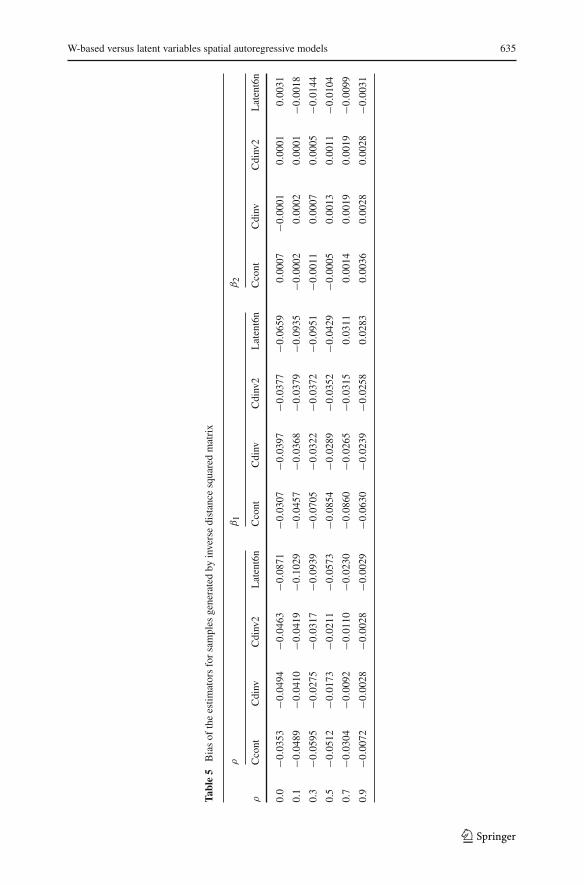
Table 5 gives the bias for samples generated by the inverse distance squared matrix.With a few exceptions Cdinv performs best, closely followed by the ‘correct’ modelCdinv2. Figure 5a–c show that Ccont has the lowest bias for ρ and β1 when ρ = 0and for β2 when ρ = 0.5 and 0.7. There are several cases where Latent6n outperformsCcont: for ρ when ρ ≥ 0.7, for β1 when ρ ≥ 0.5 and for β2 when ρ = 0.9.

The RMSE results are shown in Table 6. As in the previous cases, for each param-eter there are only slight differences between the models. Figure 6 which representsthe total RMSE summed over all estimators, shows that Ccont has the smallest totalRMSE for the first two values of ρ while Cdinv and Cdinv2 produce better and almostidentical results for ρ ≥ 0.3. For ρ ≥ 0.7 the total RMSE of four models stronglyconverge.

Considering bias and RMSE together we conclude that Cdinv and Cdinv2 bothperform better than Ccont and Latent6n in the case samples are generated on the basisof the inverse distance squared matrix. Latent6n trails the classical approaches, thoughthe differences are small.

The above results show that the “true” model tends to outperform the misspecifiedalternatives. This applies especially to Latent6n. However, the differences betweenLatent6n and the classical models tend to be very small. Moreover, in several casesLatent6n performs best or is the best among the misspecified models.

5 Conclusions

This paper evaluates the performance of estimators of two types of spatial autore-gressive models: the classical W-based spatial autoregressive model and the structuralequations model with latent variables. The former accounts for spatial dependenceand spillover effects by means of a spatial weights matrix W and the latter by means

123


Tabl

e5

Bia

sof

the

estim

ator

sfo

rsa

mpl

esge

nera

ted

byin

vers

edi

stan

cesq

uare

dm

atri

x

ρβ

1β

2

ρC

cont

Cdi

nvC

dinv

2L

aten

t6n

Cco

ntC

dinv

Cdi

nv2

Lat

ent6

nC

cont

Cdi

nvC

dinv

2L

aten

t6n

0.0

−0.0

353

−0.0

494

−0.0

463

−0.0

871

−0.0

307

−0.0

397

−0.0

377

−0.0

659

0.00

07−0

.000

10.

0001

0.00

31

0.1

−0.0

489

−0.0

410

−0.0

419

−0.1

029

−0.0

457

−0.0

368

−0.0

379

−0.0

935

−0.0

002

0.00

020.

0001

−0.0

018

0.3

−0.0

595

−0.0

275

−0.0

317

−0.0

939

−0.0

705

−0.0

322

−0.0

372

−0.0

951

−0.0

011

0.00

070.

0005

−0.0

144

0.5

−0.0

512

−0.0

173

−0.0

211

−0.0

573

−0.0

854

−0.0

289

−0.0

352

−0.0

429

−0.0

005

0.00

130.

0011

−0.0

104

0.7

−0.0

304

−0.0

092

−0.0

110

−0.0

230

−0.0

860

−0. 0

265

−0.0

315

0.03

110.

0014

0.00

190.

0019

−0.0

099

0.9

−0.0

072

−0.0

028

−0.0

028

−0.0

029

−0.0

630

−0.0

239

−0.0

258

0.02

830.

0036

0.00

280.

0028

−0.0

031

123

636 A. Liu et al.

Fig. 5 Bias of the estimators of ρ (a), β1 (b) and β2 (c) for the classical models (Ccont, Cdinv, Cdinv2)and the latent model (Latent6n) based on samples generated by inverse distance squared matrix

123


Tabl

e6

RM

SEof

the

estim

ator

sfo

rsa

mpl

esge

nera

ted

byin

vers

edi

stan

cesq

uare

dm

atri

x

ρβ

1β

2

ρC

cont

Cdi

nvC

dinv

2L

aten

t6n

Cco

ntC

dinv

Cdi

nv2

Lat

ent6

nC

cont

Cdi

nvC

dinv

2L

aten

t6n

0.0

0.11

440.

1469

0.14

100.

1888

0.25

870.

2686

0.26

660.

2797

0.07

170.

0717

0.07

170.

0733

0.1

0.11

010.

1299

0.12

660.

1778

0.26

140.

2683

0.26

710.

2839

0.07

170.

0717

0.07

170.

0729

0.3

0.09

670.

0969

0.09

660.

1449

0.26

650.

2675

0.26

720.

2843

0.07

180.

0717

0.07

170.

0733

0.5

0.07

410.

0658

0.06

630.

1044

0.27

010.

2661

0.26

640.

2773

0.07

190.

0717

0.07

170.

0729

0.7

0 .04

390.

0369

0.03

730.

0479

0.27

010.

2640

0.26

440.

2738

0.07

190.

0718

0.07

180.

0725

0.9

0.01

260.

0112

0.01

120.

0131

0.26

460.

2607

0.26

090.

2717

0.07

210.

0721

0.07

210.

0723

123

638 A. Liu et al.

Fig. 6 Total RMSE for the four models for samples generated by inverse distance squared matrix

of a latent variable in the structural model while the relationships between observedspatially lagged variables and the latent spatial dependence variable(s) are given in themeasurement model. The two classes of approaches are compared by means of MonteCarlo simulations based on Anselin’s Columbus, Ohio, crime data set in terms of biasand RMSE of the coefficient estimators for various values of the spatial lag parameterand different types of weight matrices. Data are generated on the basis of exogenousvariable values, parameter values and the first-order contiguity matrix, inverse distancematrix and inverse distance squared matrix, as given by Anselin’s (1988).

The simulation results show that the “true” model, i.e. the model whose W matrix isthe same as used for data generation, tends to perform best in terms of bias and RMSE.However, the differences between the “true” and the misspecified models includingthe structural equation model, are very small. Moreover, for several combinationsof the value of spatial autoregressive parameter and the weights matrix used in datageneration the latter produces results with the smallest bias or RMSE. In other words,the “true” models do not uniformly outperform the latent variables approach.

The fact that only the W-based model structure has been used to generate data isstrongly in favor of the W-based estimators, since it implies that in all cases the latentmodel is misspecified. The reason for analyzing the performance of the latent modelon the basis of data generated by means of a W-based model is that we wanted to getinsight into the performance of the latent variables approach in the case of misspeci-fication. Subsequent simulations will explore the behavior of both approaches underlevel playing field conditions.

It should also be noted that in contrast to the classical models, not all model speci-fication options of the latent variable approach have been fully expolited in the simu-lations. Particularly, in order to keep the simulations simple, the number of observedspatially lagged variables was a priori fixed at six, since in Folmer and Oud (2008) thisnumber gave parameter estimates virtually identical to those obtained by Anselin’s(1988). In the practice of structural equation modelling the optimal number of indi-cators, i.e. observed spatial lags, which may differ by e.g. type of W matrix, can be

123


identified by means of tests. Another unexploited specification search is the possibilityof covariances among the error terms in the measurement model (�).

To sum up, given the small differences between the latent variables approach andthe “true” classical alternatives with respect to bias and RMSE, its unexploited speci-fication search options, its flexibility and information content, it is worthwhile furtherconsidering its suitability to model spatial dependence.

Open Access This article is distributed under the terms of the Creative Commons Attribution Noncom-mercial License which permits any noncommercial use, distribution, and reproduction in any medium,provided the original author(s) and source are credited.

References

Aldstadt J, Getis A (2004) Constructing the spatial weights matrix using a local statistic. Geogr Anal 36(2):90–104

Aldstadt J, Getis A (2006) Using AMOEBA to create a spatial weights matrix and identify spatial clusters.Geogr Anal 38(4):327–343

Anselin L (1988) Spatial econometrics: methods and models. Kluwer, DordrechtAnselin L (2002) Under the hood: issues in the specification and interpretation of spatial regression models.

Agric Econ 27(3):247–267Bhattacharjee A, Jensen-Butler C (2006) Estimation of the spatial weights matrix in the spatial error model,

with an application to diffusion in housing demand. Available: http://www.econ.cam.ac.uk/panel2006/papers/Bhattacharjeepaper23.pdf

Case AC, Rosen S, Hines JR Jr (1993) Budget spillovers and fiscal policy interdependence: evidence fromthe states. J Public Econ 52(3):285–307

Fingleton B (2003) Externalities, economic geography and spatial econometrics: conceptual and modelingdevelopments. Int Reg Sci Rev 26(2):197–207

Florax R, Folmer H (1992) Specification and estimation of spatial linear regression models: Monte Carloevaluation of pre-test estimators. Reg Sci Urban Econ 22:405–432

Florax RJGM, Folmer H, Rey SJ (2003) Specification searches in spatial econometrics: the relevance ofHendry’s methodology. Reg Sci Urban Econ 33(5):557–579

Folmer H, Oud JHL (2008) How to get rid of W? A latent variables approach to modeling spatially laggedvariables. Environ Plan A 40:2526–2538

Getis A, Griffith DA (2002) Comparative spatial filtering in regression analysis. Geogr Anal 34(2):130–140Hepple LW (1995) Bayesian techniques in spatial and network econometrics: 1. Model comparison and

posterior odds. Environ Plan A 27:447–469Jöreskog KG, Sörbom D (1996) Lisrel 8: user’s reference guide. Scientific Software International, ChicagoNeale MC, Boker SM, Xie G, Maes HH (2003) Mx: Statistical Modeling, 6th edn. VCU Box 900126,

Richmond, VA 23298: Department of PsychiatryOrd JK (1975) Estimation methods for models of spatial interaction. J Am Stat Assoc 70:120–126Oud JHL, Folmer H (2008) A structural equation approach to models with spatial dependence. Geogr Anal

40:152–166Tiefelsdorf M, Griffith DA (2007) Semiparametric filtering of spatial autocorrelation: the eigenvector

approach. Environ Plan A 39(5):1193–1221

123

http://www.econ.cam.ac.uk/panel2006/papers/Bhattacharjeepaper23.pdf

http://www.econ.cam.ac.uk/panel2006/papers/Bhattacharjeepaper23.pdf

W-based versus latent variables spatial autoregressive models: evidence from Monte Carlo simulations

Documents