Vsevolod Ivanov, Yang Qi, and Liang Fu - California …authors.library.caltech.edu/44597/7/1310.1589v2.pdfreduces both the total number of loops and the number of wrong-way arrows

Loops, sign structures and emergent Fermi statistics in

three-dimensional quantum dimer models

Vsevolod Ivanov,1, ∗ Yang Qi,2 and Liang Fu1

1Department of Physics, Massachusetts Institute of Technology, Cambridge, MA 02139

2Institute of Advanced Study, Tsinghua University, Beijing 100084, China

Abstract

We introduce and study three-dimensional quantum dimer models with positive resonance terms.

We demonstrate that their ground state wave functions exhibit a nonlocal sign structure that can

be exactly formulated in terms of loops, and as a direct consequence, monomer excitations obey

Fermi statistics. The sign structure and Fermi statistics in these “signful” quantum dimer models

can be naturally described by a parton construction, which becomes exact at the solvable point.

PACS numbers: 75.10.Kt, 05.30.-d, 71.10.Pm

1

arX

iv:1

310.

1589

v2 [

cond

-mat

.str

-el]

27

Feb

2014

The Rokhsar-Kivelson (RK) quantum dimer model was originally introduced1 to describe

the short-range resonating-valence-bond (RVB) state in two dimensions2. Later it was dis-

covered that quantum dimer models provide particularly simple and elegant realizations

of topological phases of matter, including a two-dimensional (2D) gapped phase with Z2

topological order3, and a three-dimensional (3D) Coulomb phase described by an emer-

gent Maxwell electrodynamics4,5. Both phases possess a fractional quasiparticle called a

monomer, a deconfined pointlike excitation that carries half of the U(1) charge of a dimer.

The statistics of monomers was a subject of considerable attention and debate in early

studies6,7 and of continuing interest recently8. It was eventually settled9,10 that the statistics

of monomers in two-dimensional quantum dimer models cannot be assigned in a universal

way, because statistics can be altered by attaching a π flux (vison11) to a monomer. On the

other hand, a boson cannot be changed into a fermion by π-flux binding in three dimensions,

because particles and flux lines are objects of different dimensions. This leaves open the

possibility of monomers with Fermi statistics in 3D quantum dimer models, which is the

subject of this work. We note that Fermi statistics also arises in other 3D boson models

with an emergent Z2 gauge field12,13.

We introduce and study quantum dimer models in 3D non-bipartite lattices with positive

resonance terms, in contrast to terms with negative coefficients in the original RK model1.

We find a “twisted” Z2 topological phase in which monomers are deconfined and obey Fermi

statistics. The Fermi statistics arises from a nonlocal sign structure of the ground state wave

function, which is specified through loops in the transition graph by an exact sign rule. We

provide a parton construction for these “signful” quantum dimer models, which yields the

exact ground state dimer wave function and naturally explains the emergent Fermi statistics

of monomers. Finally, we discuss the implications of our study for doped quantum dimer

models and resonating-valence-bond (RVB) states in three dimensions.

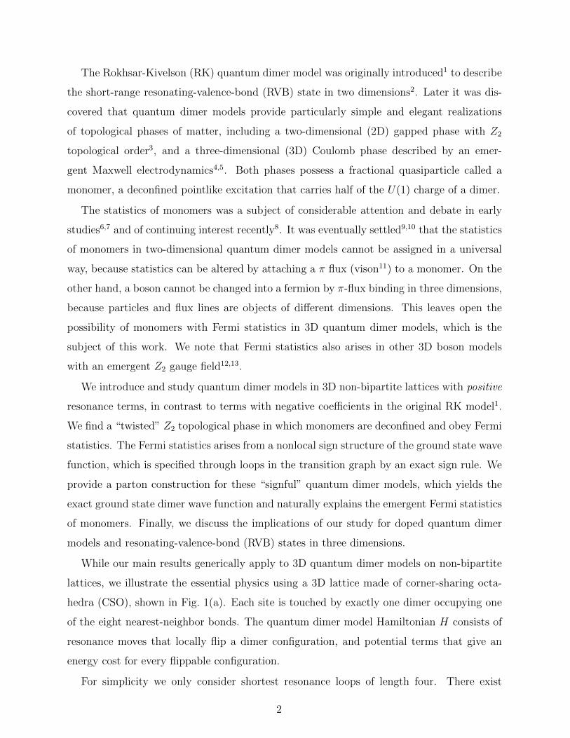
While our main results generically apply to 3D quantum dimer models on non-bipartite

lattices, we illustrate the essential physics using a 3D lattice made of corner-sharing octa-

hedra (CSO), shown in Fig. 1(a). Each site is touched by exactly one dimer occupying one

of the eight nearest-neighbor bonds. The quantum dimer model Hamiltonian H consists of

resonance moves that locally flip a dimer configuration, and potential terms that give an

energy cost for every flippable configuration.

For simplicity we only consider shortest resonance loops of length four. There exist

2

FIG. 1. (a) Eight cubic unit cells of the CSO lattice. (b) Two types of length-4 loops on the CSO

lattice. Left: square loop, right: bent-square loop.

two types of length-four resonance loops, having the shape of a square and a bent square

respectively [see Fig. 1(b)]. H is thus given by

H =J1

(∣∣∣ ⟩ ⟨ ∣∣∣+∣∣∣ ⟩ ⟨ ∣∣∣)

+K1

(∣∣∣ ⟩ ⟨ ∣∣∣+∣∣∣ ⟩ ⟨ ∣∣∣)

+ J2

(∣∣∣ ⟩ ⟨ ∣∣∣+∣∣∣ ⟩ ⟨ ∣∣∣)

+K2

(∣∣∣ ⟩ ⟨ ∣∣∣+∣∣∣ ⟩ ⟨ ∣∣∣)

+ · · ·

(1)

Here · · · denotes similar terms for resonance loops of longer length, whose form will be

discussed later.

When |Ji| = Ki > 0, H can be written as a sum of positive semidefinite projection

operators:

H =K1

(∣∣∣ ⟩+ η1

∣∣∣ ⟩)(⟨ ∣∣∣+ η1

⟨ ∣∣∣)+K2

(∣∣∣ ⟩+ η2

∣∣∣ ⟩)(⟨ ∣∣∣+ η2

⟨ ∣∣∣) (2)

3

where ηi = Ji/Ki = ±1. η1 = η2 = −1 corresponds to the original RK solvable point with

negative resonance terms. In this case, the ground state is an equal amplitude superposition

of all dimer coverings. Such a dimer-liquid state in a 3D CSO lattice is expected to represent

a gapped Z2 topological phase similar to the one in a face-centered-cubic lattice5. Since this

RK wave function is everywhere positive, monomer excitations above the ground state are

necessarily bosons.

Here we study quantum dimer models with positive resonance terms: J1, J2 > 0. In this

case, ground states are “signful”, taking both positive and negative values for different dimer

coverings. Such a nontrivial sign structure is a prerequisite to the emergence of fermionic

monomer excitations. Following the spirit of the RK approach, we first construct a signful

dimer wave function and then demonstrate that this wave function is the zero-energy ground

state of H at a generalized RK point Ji = Ki > 0.

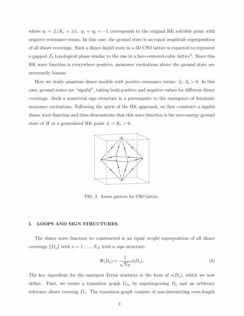
FIG. 2. Arrow pattern for CSO lattice.

I. LOOPS AND SIGN STRUCTURES.

The dimer wave function we constructed is an equal weight superposition of all dimer

coverings {Da} with a = 1, . . . , ND with a sign structure:

Ψ(Da) =1√ND

s(Da). (3)

The key ingredient for the emergent Fermi statistics is the form of s(Da), which we now

define. First, we create a transition graph G1a by superimposing Da and an arbitrary

reference dimer covering D1. The transition graph consists of non-intersecting even-length

4

loops. Since dimer coverings and transition loops are in one-to-one correspondence, we define

s(Da) ≡ s(G1a) as a function of transition loops.

The sign of transition loops is specified by endowing every nearest-neighbor bond with

an arrow. The arrow pattern we choose for the CSO lattice is shown in Fig. 2. Now we

define s(Gab) in terms of loops and arrows:

s(Gab) = (−1)N(Gab)+W (Gab), (4)

where N(Gab) is the total number of loops in Gab, and W (Gab) is the total number of

“wrong-way” arrows when all loops are traversed unidirectionally.

The sign structure (4) we introduced for the quantum dimer wave function (3) is a

central result of this work. It has several important properties. First, because all loops

in the transition graph have an even length, (−1)W (Gab) is independent of the direction of

traverse, as it should be for loops in three dimensions. Second, s(Gab) is multiplicative under

the composition of transition loops. For three different dimer coverings Da, Db and Dc,

s(Gac) = s(Gab)s(Gbc). (5)

This is obvious when Gab and Gbc do not overlap, and is also true when they do. For

example, when Gab and Gbc overlap on one bond, two loops combine into one in Gac, which

reduces both the total number of loops and the number of wrong-way arrows by one. This

result is proved for general cases in Appendix A and an alternative proof based on parton

construction is given in Sec. III. Equation (5) guarantees that the dimer wave function

defined using the sign structure s(Gab) does not depend on the choice of the reference dimer

covering, up to an overall factor of −1. Last but not the least, the arrow pattern in Fig. 2

guarantees that Ψ(Da) is invariant under all symmetry transformations of the CSO lattice,

despite that the arrow pattern itself is not.

To justify the last point, we consider the symmetry transformation of the arrow pattern

shown in Fig. 2. The symmetry of the CSO lattice can be represented by the Oh point

group, along with translation symmetry. We now check how the arrows transform under

the symmetry operations of Oh, with +1 signifying that all arrows are unchanged, and −1

signifying that all arrows reverse:

Oh E 8C3 6C2 6C4 3C24 i 6S4 8S6 3σh 6σd

A2g +1 +1 −1 −1 +1 +1 −1 +1 +1 −1

5

This arrow pattern behaves as the representation A2g of Oh point group. For a given tran-

sition graph, the sign of a particular loop given by Eq. (4) does not change under the trans-

formation of reversing all arrows, as each loop contains even number of dimers. Therefore

the wave function defined in Eq. (3) is invariant under symmetry.

According to the arrow pattern, the signs s(Gab) of the two shortest-length transition

loops, square and bent square, are −1. It then follows that the dimer wave function |Ψ〉 is

a zero-energy ground state of the quantum dimer model Hamiltonian (1) at the generalized

RK point Ji = Ki. This completes our construction of solvable 3D quantum dimer models

with a nontrivial sign structure.

It is worth pointing out that, as is common with quantum dimer models at RK point,

the Hamiltonian (1) has other zero-energy grounds states in addition to Ψ(Da), such as

“dead” dimer coverings that are completely non-flippable. Also, similar to quantum dimer

models on other 3D lattices14, we found that with only resonance terms on length-four loops

the Hamiltonian does not connect all coverings in a given topological sector. By including

additional resonance terms involving longer loops and choosing their signs according to the

arrow pattern, one can increase the connectivity of dimer coverings, although the issue of

ergodicity in 3D quantum dimer models is beyond the scope of this paper. On a positive

side, we expect the dimer liquid state (3) to be stabilized in an extended regime |Ji| > Ki, as

found for other non-bipartite lattices3,5. This issue can be studied numerically using Monte

Carlo methods14,15.

II. STATISTICS OF MONOMERS.

We now demonstrate that the nontrivial sign structure of the ground state (4) directly

gives rise to Fermi statistics of the monomer, a pointlike excitation associated with a site

that is not touched by any dimer. Since a missing dimer can break up into two monomers,

each monomer is a charge-1/2 fractional quasiparticle, which has a finite excitation energy

associated with breaking the rule of one dimer per site.

Following the approach of Ref. 6, we determine the statistics by adiabatically transporting

two monomers along a path which exchanges their positions, and examining the resulting

change in the phase of the many-body wave function. To implement the exchange, we

introduce dimer move terms HT into the quantum dimer model, which enables a monomer

6

to hop by exchanging with a nearby dimer. Without losing generality we consider the

following form of HT ,

HT = λ∑(∣∣∣ ⟩⟨ ∣∣∣+ h. c.

), (6)

where the sum runs over all symmetry-related moves that transport a monomer to the

nearest-neighbor site (see Fig. 3). Here we consider only nearest-neighbor hoppings, but a

general proof of Fermi statistics for general hopping terms is given in Sec. III.

We assume that λ is small and moves the monomer adiabatically. In the limit of λ→ 0,

the eigenstates of the system are the dimer wave functions with monomers at fixed loca-

tions. Particularly the dimer wave function with a monomer at site i, denoted as |Ψi〉, is

a superposition of dimer coverings that has no dimer connecting to site i, with the sign

rule in Eq. (4)16. Under the adiabatic assumption, each time HT is applied to a monomer

state to move a monomer from i to j, it takes dimer coverings in |Ψi〉 and converts them

to dimer coverings in |Ψj〉, and then the state of converted dimer coverings relaxes into the

eigenstate |Ψj〉 before the monomer is moved again. Therefore the relative sign of the wave

functions before and after the hopping is determined by projecting HT onto |Ψi〉 and |Ψj〉

as the following,

tij = 〈Ψj|HT |Ψi〉. (7)

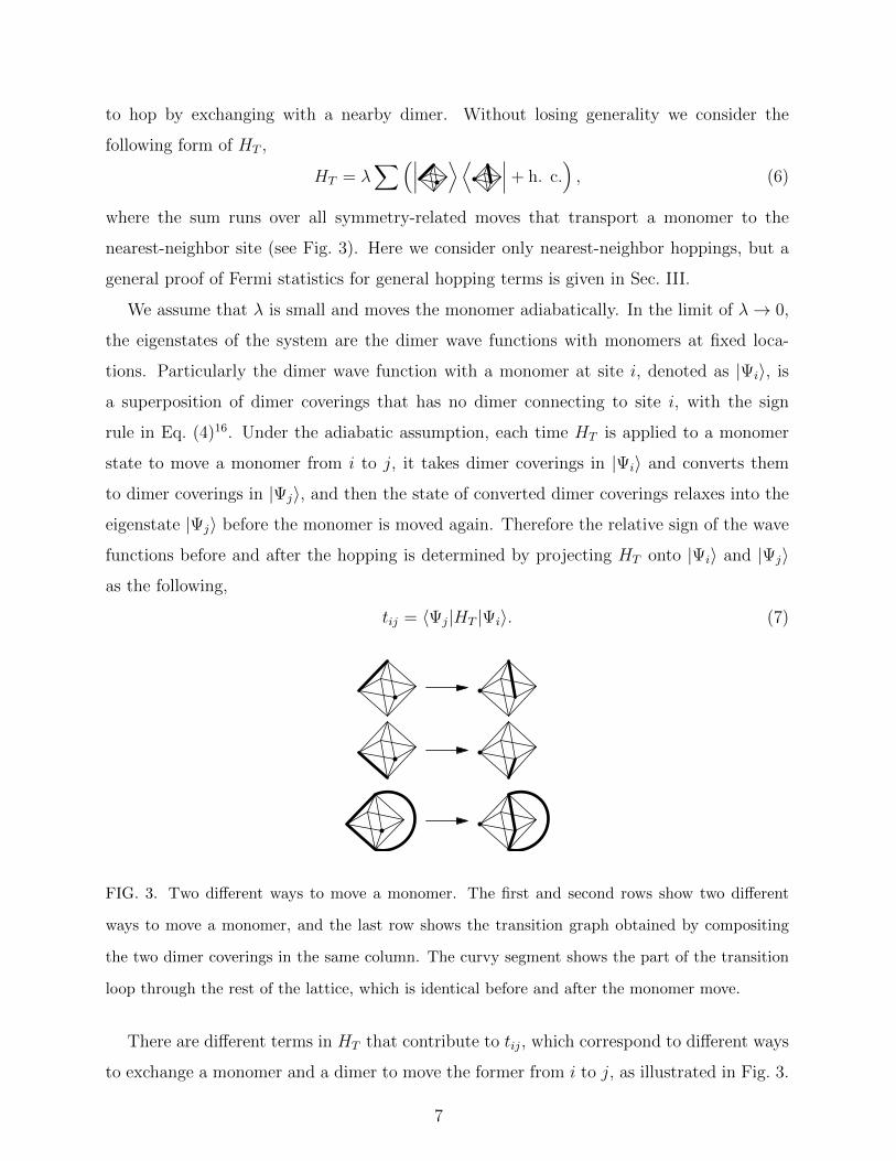
FIG. 3. Two different ways to move a monomer. The first and second rows show two different

ways to move a monomer, and the last row shows the transition graph obtained by compositing

the two dimer coverings in the same column. The curvy segment shows the part of the transition

loop through the rest of the lattice, which is identical before and after the monomer move.

There are different terms in HT that contribute to tij, which correspond to different ways

to exchange a monomer and a dimer to move the former from i to j, as illustrated in Fig. 3.

7

Here we show that these different terms contribute with the same sign to tij in Eq. (7). In

Fig. 3 it is illustrated that there are two ways to move a monomer from i to j by exchanging

it with two different dimers, as shown on the first and second row. The relative phase

between the two different dimer coverings in the initial and final states is determined by the

transition loop on the bottom. The two transition loops in the initial and final states differ

by moving two dimers from one side of a bent-square loop to the other side. Therefore the

two transition loops have the same sign according to Eq. (4), as the arrow pattern shown

in Fig. 2 has an even number of wrong-way arrows in any four-bond loop. This shows that

different terms in Eq. (7) contribute to tij with the same sign. Consequently the sign of tij

can be determined from any two dimer coverings in |Ψi〉 and |Ψj〉 that can be connected by

HT . Generally, this property holds for any arrow pattern with an even number of wrong-way

arrows in four-bond loops, and a proof will be given in Sec. III.

1 2

3 4

a)

b)

1 23

4

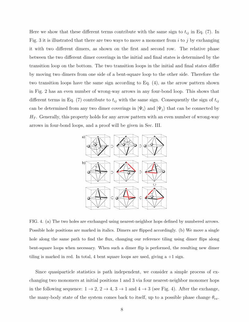
FIG. 4. (a) The two holes are exchanged using nearest-neighbor hops defined by numbered arrows.

Possible hole positions are marked in italics. Dimers are flipped accordingly. (b) We move a single

hole along the same path to find the flux, changing our reference tiling using dimer flips along

bent-square loops when necessary. When such a dimer flip is performed, the resulting new dimer

tiling is marked in red. In total, 4 bent square loops are used, giving a +1 sign.

Since quasiparticle statistics is path independent, we consider a simple process of ex-

changing two monomers at initial positions 1 and 3 via four nearest-neighbor monomer hops

in the following sequence: 1→ 2, 2→ 4, 3→ 1 and 4→ 3 (see Fig. 4). After the exchange,

the many-body state of the system comes back to itself, up to a possible phase change θex.

8

Since the dimer wave functions are real, θex is either 0 or π. θex can be determined from the

product of transition amplitudes at every stage of the exchange process12

tex = t12t24t31t43. (8)

The sign of tex is unambiguous (independent of the gauge choice of dimer wave functions),

and determines θex: θex = 0 for tex > 0 and π for tex < 0.

To evaluate (8), we use a natural sign convention for the many-body states |Ψij〉 where

i, j label the positions of the two monomers, such that their amplitudes on the first four

reference dimer coverings are positive:

Ψ13(Da) = Ψ23(Db) = Ψ34(Dc) = Ψ14(Dd) > 0,

where the sequence of reference dimer coverings Da → Db → Dc → Dd → De are the ones

that follow the sequence of dimer moves as illustrated in Fig. 4. Under this sign convention,

t12, t24, t31 have the same sign. Furthermore, since De and Da only differ by a resonance loop

on a bent square, the sign structure (4) dictates Ψ13(De) = −Ψ13(Da). Comparing with the

convention Ψ13(Da) > 0, this implies that t43 have an opposite sign from the rest of the t’s,

which makes tex negative. Therefore we conclude that the phase change after the monomer

exchange is θex = π.

θex is given by the sum of the statistical angle θs, which is 0 for bosons and π for fermions,

and the background flux φ passing through the exchange paths of two particles that join into

a loop Γ. Therefore to determine the quasiparticle statistics requires the knowledge of φ in

addition to θex. For a real wave function, φ can only be 0 or π. φ can be determined from the

phase change after transporting a single monomer around the loop Γ; here Γ is the boundary

of a single square plaquette. Thus we now use the same set of dimer move operators HT

and carry out a procedure similarly as before to compute φ, with two important differences.

First, the order in which the hopping terms are applied must change in order to form a

continuous path, which is reflected by the new ordering of transition amplitudes:

tex = t12t24t43t31. (9)

Second, each hole hop must be followed by a change in the reference dimer tiling, in order

to guarantee that there exists a dimer-hole configuration that allows the hopping operation

to be applied. The sequence of reference dimer tilings is Da → Db ⇒ Db′ → Dc ⇒ Dc′ →

9

Dd ⇒ Dd′ → De ⇒ De′ where → represents a hole hop, while ⇒ represents a change of

reference. This sequence of operations is shown in Fig. 4(b), with each Di′ after a change

of reference marked in red. We note that Da = De′ , and that the final change of reference

De ⇒ De′ is carried out for the sake of convenience, since it allows us to refer to all transition

loops as changes of reference. In this case, each change of reference corresponds to a bent-

square loop, and since we perform four such reference changes we find φ = 0. For clarity,

we can write down the relative amplitudes of the many-body states |Ψi〉, where i labels the

positions of the monomer:

Ψ1(Da) = Ψ2(Db) = −Ψ2(Db′) = −Ψ4(Dc) = Ψ4(Dc′)

= Ψ3(Dd) = −Ψ3(Dd′) = −Ψ1(De) = Ψ1(De′),

and we can see that in fact each reference change reverses the sign of the amplitude of the

many-body state.

By combining the two results θex = π and φ = 0, we conclude that monomers have a

statistical angle θs = π, i.e., they obey Fermi statistics. This conclusion is completely inde-

pendent of how the two monomers exchanged. This is demonstrated with more examples in

Appendix B, and can be proved for general cases using the parton wave function introduced

in the next section.

III. PARTON CONSTRUCTION.

In order to systemetically construct signful dimer wave functions with fermionic monomer

excitations, we present a parton approach by writing a dimer degree of freedom in terms of

two fermion variables:

b†ij = ξijf†iαf†jβ, ξij = −ξji = ±1 (10)

where b†ij is a hardcore boson operator that creates a dimer on a bond between two nearest-

neighbor sites i and j, and the fermion operators f †iα and f †jβ are defined at two new sites,

which are located near the two ends i and j of the bond ij, respectively (see Fig. 5). These

fermionic partons thus live on a decorated CSO lattice made of a 8-site cluster surrounding

every site of the original lattice. The subscripts α and β distinguish different sites within a

cluster.

10

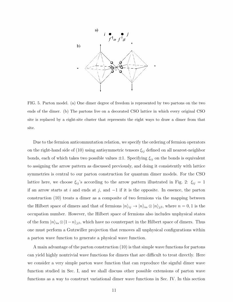
FIG. 5. Parton model. (a) One dimer degree of freedom is represented by two partons on the two

ends of the dimer. (b) The partons live on a decorated CSO lattice in which every original CSO

site is replaced by a eight-site cluster that represents the eight ways to draw a dimer from that

site.

Due to the fermion anticommutation relation, we specify the ordering of fermion operators

on the right-hand side of (10) using antisymmetric tensors ξij defined on all nearest-neighbor

bonds, each of which takes two possible values ±1. Specifying ξij on the bonds is equivalent

to assigning the arrow pattern as discussed previously, and doing it consistently with lattice

symmetries is central to our parton construction for quantum dimer models. For the CSO

lattice here, we choose ξij’s according to the arrow pattern illustrated in Fig. 2: ξij = 1

if an arrow starts at i and ends at j, and −1 if it is the opposite. In essence, the parton

construction (10) treats a dimer as a composite of two fermions via the mapping between

the Hilbert space of dimers and that of fermions |n〉ij → |n〉iα ⊗ |n〉jβ, where n = 0, 1 is the

occupation number. However, the Hilbert space of fermions also includes unphysical states

of the form |n〉iα⊗|1−n〉jβ, which have no counterpart in the Hilbert space of dimers. Thus

one must perform a Gutzwiller projection that removes all unphysical configurations within

a parton wave function to generate a physical wave function.

A main advantage of the parton construction (10) is that simple wave functions for partons

can yield highly nontrivial wave functions for dimers that are difficult to treat directly. Here

we consider a very simple parton wave function that can reproduce the signful dimer wave

function studied in Sec. I, and we shall discuss other possible extensions of parton wave

functions as a way to construct variational dimer wave functions in Sec. IV. In this section

11

we will focus on the following parton wave function

|Φf〉 =∏i

1√8

8∑α=1

f †iα|0〉, (11)

which is a product of non-overlapping “molecular” orbitals, one per cluster. For a given

cluster, the molecular orbital has equal amplitudes on all 8 sites. We further obtain physical

dimer wave function |Ψ〉 from |Φf〉:

Ψ(i1j1, ..., injn) = 〈0|

( ∏ilαl,jlβl

ξiljlfilαlfjlβl

)|Φf〉, (12)

where Ψ(i1j1, ..., injn) is the amplitude of having dimers on nearest-neighbor bonds i1j1, ..., injn.

The dimer wave function |Ψ〉 has several noteworthy properties that can be inferred

straightforwardly from the parent parton wave function |Φf〉. First, |Ψ〉 has exactly one

dimer touching every lattice site. This is because (i) |Φf〉 has exactly one parton per cluster,

and (ii) two partons in adjacent clusters that share a bond must be simultaneously present to

form a dimer. Second, since partons have a uniform density distribution in |Φf〉, all possible

dimer configurations appear with equal probability in |Ψ〉, i.e., |Ψ(i1j1, ..., injn)| = 1√ND

.

Last but most importantly, due to the fermion nature of partons, the sign of Ψ(i1j1, ..., injn)

is not all positive but depends nontrivially on the dimer coverings following the same sign

rule as stated in Eq. (4).

To obtain the nontrivial sign structure of |Ψ〉, we compare the relative sign of Ψ(D1) and

Ψ(D2), where D1 and D2 are two arbitrary dimer configurations. We claim that the relative

sign is determined from the transition graph G12 as the following,

Ψ(D1)

Ψ(D2)=∏m

(−1)1+W (Lm) = (−1)N(G12)+W (G12), (13)

where W (Lm) is the number of “wrong-way” arrows in the loop Lm, and N(G12) and W (G12)

are the same functions counting number of loops and “wrong-way” arrows that were used

in Eq. (4). To prove (13), it suffices to consider a single loop made of a sequence of lattice

sites: r1 → r2 → · · · → r2k. The two corresponding dimer configurations are then D1 =

(r1r2), · · · , (r2k−1r2k) and D2 = (r2kr1), · · · , (r2k−2r2k−1). It follows from (11) and (12) that

Ψ(D1) and Ψ(D2) are respectively given by

Ψ(D1) = ξr1r2 · · · ξr2k−1r2k〈0|fr1fr2 ...fr2k−1fr2k |Φf〉

Ψ(D2) = ξr2kr1 · · · ξr2k−2r2k−1〈0|fr2kfr1 ...fr2k−2

fr2k−1|Φf〉

12

The ratio is thus given by

Ψ(D1)

Ψ(D2)= −

2n∏i=1

ξriri+1, r2n+1 ≡ r1. (14)

where we have used the fermion anti-commutation relation. This proves the sign rule (13).

Comparing the sign structures in Eq. (4) and Eq. (13), one can see that the wave function

defined in Eq. (3) for a certain arrow configuration is the same as the parton wave function

in Eq. (12) using the corresponding ξij assignment. Therefore the parton approach gives

a systematic way to construct dimer wave functions with relative signs between different

dimer configurations. This construction also provides an explicit proof of Eq. (5).

Furthermore, the parton approach gives a straightforward way to demonstrate that the

monomer excitations carry Fermi statistics. To see this, we again study the phase difference

between exchanging two holes and moving one hole along the same path as we did in the

previous section, with the help of the reference parton wave function. For each step, a

monomer is moved by flipping one dimer. Particularly, assume that a monomer is moved

from site i to site j by moving one dimer from (jk) to (ik). Correspondingly, in the parton

wave function one moves a hole with the following fermion hopping term,

HfT =

∑ij

tfijfjf†i , (15)

where fi = 1√8

∑8α=1 fiα, and tfij = ±1 determines the relative sign between the wave func-

tions before and after hopping. Here tfij is chosen such that the fermion hopping term HfT has

the same sign as the dimer hopping term HT defined in Eq. (6). According to the relation

between dimer wave function and parton wave function in Eq. (12), the relative phase of

the physical wave function before and after the projection is

Ψ((ik) · · · )Ψ((jk) · · · )

=〈0|ξikfiαfkδtfijfjf

†i f†kf†j |0〉

〈0|ξjkfjβfkγf †kf†j |0〉

= ξikξkjtfij. (16)

Here the left-hand side of the equation has the same sign as the corresponding term in

Eq. (7). Hence we choose the sign of tfij such that the left-hand side has the sign of tij. This

is achieved by choosing

tfij = ξikξkj sgn tij. (17)

With the condition in Eq. (17) satisfied, after each step of monomer hopping and dimer

resonance, the sign of the dimer wave function is always determined from the corresponding

13

parton wave function using the projection in Eq. (12). Hence the monomer excitation in the

dimer wave function has the same Fermi statistics as the hole in the parton wave function.

It is important to note that the fermion hopping term in the parton construction only

depends on the beginning and ending sites i and j, while the monomer hopping from i to j

is meditated by a dimer move (jk)→ (ik). For lattices with high symmetry, a monomer hop

from i, j can be assisted by more than one such dimer movers that are symmetry-related

to each other, as shown in Fig. 3 for the CSO lattice. In this case, it is crucial that the

coefficients of tfij determined by Eq. (17) do not depend on the choice of possible dimer

moves specified by k. We find that this is indeed the case for the CSO lattice, thanks to

the arrow pattern specified in Fig. 2. This is because of the aforementioned fact that any

length-four loop has an even number of wrong-way arrows. In other words, for any four

points on a loop i→ k → j → k′ → i, we have ξikξkj = ξik′ξk′j, and therefore they give the

same tfij. This also implies that with a given tfij, different ways of exchanging the monomer

and a dimer contribute to tij with the same sign. Hence this provides a general proof of this

claim that was first introduced in Sec. II. Here our argument depends only on the fact that

the arrow pattern has an even number of wrong-way arrows for all length-four loops, and

can be generalized to other lattices where such arrow pattern can be assigned.

IV. DISCUSSIONS.

Using the CSO lattice as an example, we study a class of 3D quantum dimer models

with frustrated resonance terms. We construct an exact ground state wave function of

the model as a superposition of dimer configurations with a twisted sign structure. The

monomer excitations in such a state are deconfined fermions. Furthermore, we give a sys-

tematic approach to construct such states using parton projective wave functions, and such

construction naturally explains the Fermi statistics of the monomer excitations.

The dimer model studied in this work can potentially be realized in spin systems in a

short-range RVB state where the spin-triplet gap is much larger than the spin-singlet gap1.

In such a state, the spins are paired into spin-singlet valence bonds, and the ground state

is a superposition of different valence-bond configurations. Such a state can be mapped to

a dimer model by mapping spin valence bonds to dimers. In the RVB state, a valence bond

can be broken and a spin-triplet excitation is created, similarly to the way a dimer breaks up

14

into two monomers in a quantum dimer model. Therefore the monomer excitations in the

dimer model can be viewed as spinon excitations in the RVB state. The difference between

a monomer and a spinon, that the former carries a U(1) quantum number but the latter

carries an SU(2) quantum number, can be eliminated by applying a Zeeman field to the RVB

state. Therefore our signful wave function (3) can be used to describe a class of 3D spin

liquids with fermionic spinon excitations. It is interesting to note that antiferromagnetic

interactions between spins naturally lead to positive resonance terms in quantum dimer

models studied in this work1.

One can extend our wave function to study dimer models with finite density of monomers,

which can be induced by applying a Zeeman field larger than the spin-triplet gap to the

corresponding RVB state. Because monomers are fermions, the resulting state is likely to

realize a Bose metal state17, in which monomers form a Fermi sea and boson correlation

functions exhibit Fermi-surface-like singularities. Using the parton construction presented

in Sec. III, one can construct a variational wave function for the doped dimer models by

projecting a parton wave function with a parton Fermi surface. Such wave functions can be

studied numerically using the variational Monte Carlo method18.

One can further regard the above RVB state as a description of an electronic system at half

filling. Such a system will host spinless holon excitations in addition to chargeless spinons.

The Fermi statistics of spinons then implies Bose statistics of holons. Doping this system

away from half filling can induce holon condensation and leads to superconductivity1,2.

However, unlike the original quantum dimer model, the superconducting state of a doped

quantum dimer model studied in this work will have d-wave pairing symmetry. We shall

leave these interesting extensions of our model to future studies.

ACKNOWLEDGMENTS

We thank Senthil Todadri and Jeongwan Haah for invaluable discussions. Y.Q. is sup-

ported by NSFC Grant No. 11104154. L.F. is supported by the DOE Office of Basic Energy

Sciences, Division of Materials Sciences and Engineering under Award No. de-sc0010526.

We thank the hospitality of Tsinghua University during the LT26 Satellite conference “Topo-

logical Insulators and Superconductors”, when this work was initiated.

15

Appendix A: Proof of multiplicity of transition graph signs under composition.

In this appendix we discuss the relation between the signs of transition graphs and the

sign of their composition, as described in Eq. (5). In the main text we see that this equation

holds when loops in Gab and Gbc do not overlap or overlap on one bond. In this appendix

we give a general proof for this equation. Before going through the proof we first note

that according to the definition of s(Gab) in Eq. (4), length-two loops which are just two

overlapping dimers always contribute a factor of +1, so we can ignore them and only count

non-trivial loops in Eq. (4).

When two transition graphs Gab and Gbc are composited together, the transition loops

may overlap on several pieces of overlapping boundaries. The resulting graph Gac is obtained

by merging the loops at these overlapping boundaries. To prove Eq. (5) it is sufficient to

show that the sign of the transition graph does not change before and after merging one

piece of overlapping boundary.

First, we argue that each piece of overlapping boundary contains an odd number of bonds.

As shown in Fig. 6, a piece of overlapping boundary must start and end on a bond in dimer

covering Db, since for any bond on the boundary that belongs to coverings Da and Dc, the

bond adjacent to it belongs to Db and is thus present in both Gab and Gbc and also belongs

to the overlapping boundary. Between the two endings that belong to Db, the boundary

consists of alternating bonds from Da/Dc and from Db respectively. Therefore the total

number of bonds in an overlapping boundary must be odd.

FIG. 6. Overlapping boundary of two transition graphs. The black bonds belong to dimer covering

Db, green and orange bonds belong to dimer coverings Da and Dc, respectively, and the bond

painted in both green and orange belongs to both Da and Dc.

When merging a piece of overlapping boundary between two different loops, the two

loops can be oriented such that they travel through the overlapping boundary in opposite

directions (see Fig. 7), and after the merging the two loops are combined into one that

16

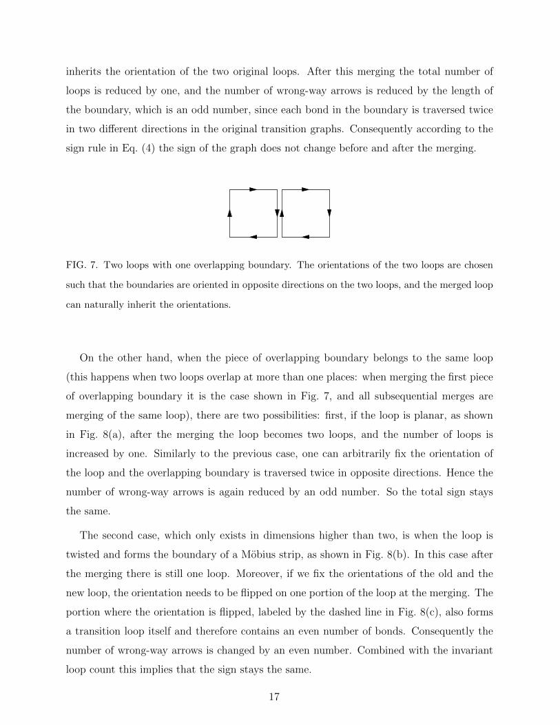
inherits the orientation of the two original loops. After this merging the total number of

loops is reduced by one, and the number of wrong-way arrows is reduced by the length of

the boundary, which is an odd number, since each bond in the boundary is traversed twice

in two different directions in the original transition graphs. Consequently according to the

sign rule in Eq. (4) the sign of the graph does not change before and after the merging.

FIG. 7. Two loops with one overlapping boundary. The orientations of the two loops are chosen

such that the boundaries are oriented in opposite directions on the two loops, and the merged loop

can naturally inherit the orientations.

On the other hand, when the piece of overlapping boundary belongs to the same loop

(this happens when two loops overlap at more than one places: when merging the first piece

of overlapping boundary it is the case shown in Fig. 7, and all subsequential merges are

merging of the same loop), there are two possibilities: first, if the loop is planar, as shown

in Fig. 8(a), after the merging the loop becomes two loops, and the number of loops is

increased by one. Similarly to the previous case, one can arbitrarily fix the orientation of

the loop and the overlapping boundary is traversed twice in opposite directions. Hence the

number of wrong-way arrows is again reduced by an odd number. So the total sign stays

the same.

The second case, which only exists in dimensions higher than two, is when the loop is

twisted and forms the boundary of a Mobius strip, as shown in Fig. 8(b). In this case after

the merging there is still one loop. Moreover, if we fix the orientations of the old and the

new loop, the orientation needs to be flipped on one portion of the loop at the merging. The

portion where the orientation is flipped, labeled by the dashed line in Fig. 8(c), also forms

a transition loop itself and therefore contains an even number of bonds. Consequently the

number of wrong-way arrows is changed by an even number. Combined with the invariant

loop count this implies that the sign stays the same.

17

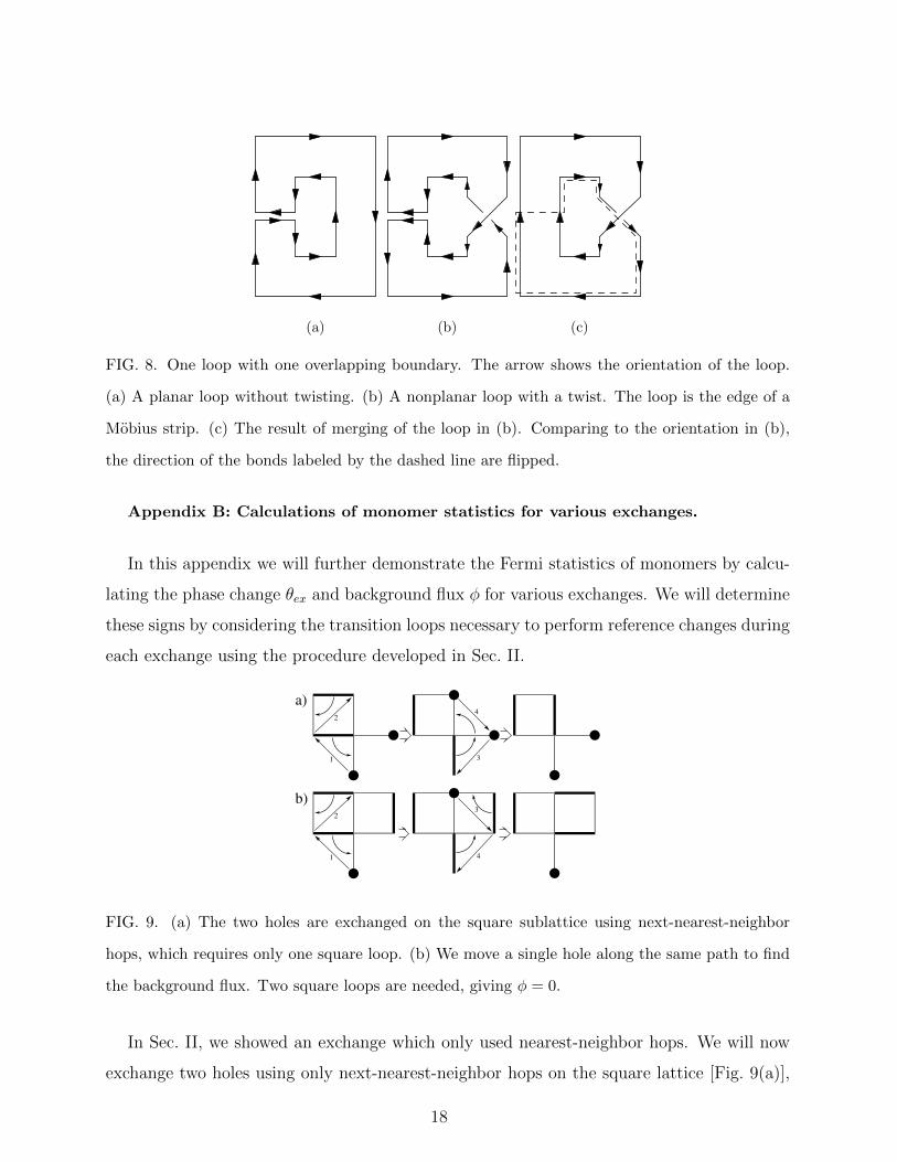
(a) (b) (c)

FIG. 8. One loop with one overlapping boundary. The arrow shows the orientation of the loop.

(a) A planar loop without twisting. (b) A nonplanar loop with a twist. The loop is the edge of a

Mobius strip. (c) The result of merging of the loop in (b). Comparing to the orientation in (b),

the direction of the bonds labeled by the dashed line are flipped.

Appendix B: Calculations of monomer statistics for various exchanges.

In this appendix we will further demonstrate the Fermi statistics of monomers by calcu-

lating the phase change θex and background flux φ for various exchanges. We will determine

these signs by considering the transition loops necessary to perform reference changes during

each exchange using the procedure developed in Sec. II.

1

2

3

4

1

2

4

3

a)

b)

FIG. 9. (a) The two holes are exchanged on the square sublattice using next-nearest-neighbor

hops, which requires only one square loop. (b) We move a single hole along the same path to find

the background flux. Two square loops are needed, giving φ = 0.

In Sec. II, we showed an exchange which only used nearest-neighbor hops. We will now

exchange two holes using only next-nearest-neighbor hops on the square lattice [Fig. 9(a)],

18

which can be obtained by taking the subset of lattice sites that lie on a plane bisecting a

layer of CSO unit cells. This exchange requires only one change of reference at the very end

to return to the initial dimer tiling, which uses a transition graph with a single square loop,

yielding θex = π. In order to calculate the statistical angle θs, we need to find the flux φ

for a single hole moving around the same path, using a different ordering of the hopping

terms, along with new corresponding reference changes [Fig. 9(b)]. This time, there are

two reference changes, each using a square loop. Since hopping terms do not affect the

relative signs of the many-body states in the process, we only need to find the effect of the

reference changes on the sign. For a general process with many different reference changes,

we calculate the signs of each loop involved individually using Eq. (4), and then determine

the overall sign by taking the product of all the individual signs of the loop using Eq. (5).

For this particular case, two square loops give us an overall sign of +1, meaning φ = 0.

Therefore, θs = θex − φ = π.

2

1

3

4

5

2

1

3

4

5a)

b)

FIG. 10. (a) A Levin-Wen exchange is performed on two holes. (b) We move a single hole along

the same path to find that background flux φ = 0.

We can perform a similar calculation using the five-step Levin-Wen exchange described

in Ref. 12. This approach sometimes has the advantage of producing more convenient

exchanges, and can be used to calculate both θex and φ using the same two monomers by

performing a process of exchange and nonexchange, respectively, which will depend on the

order of hopping terms (Fig. 10). In this case, the exchange process uses a single square loop,

while the nonexchange process uses two square loops, which gives θex = π, φ = 0, θs = π.

For completeness, we now present a similar Levin-Wen exchange using only nearest-

19

1

2

3

4

5

1

2

45

3

a)

b)

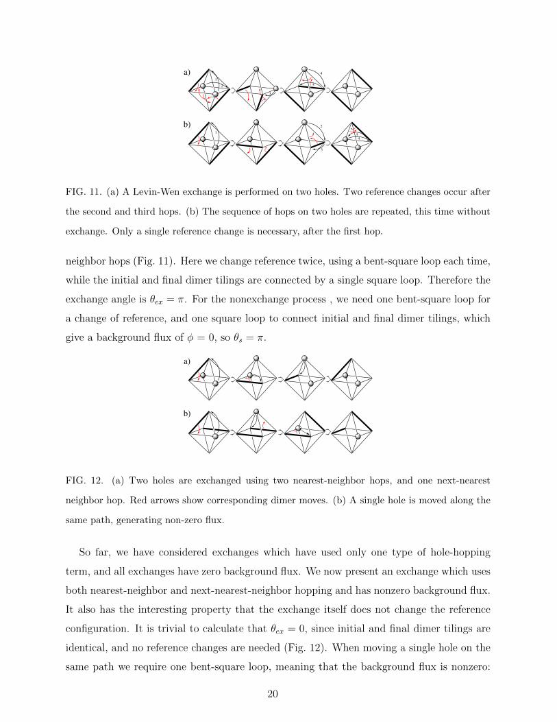
FIG. 11. (a) A Levin-Wen exchange is performed on two holes. Two reference changes occur after

the second and third hops. (b) The sequence of hops on two holes are repeated, this time without

exchange. Only a single reference change is necessary, after the first hop.

neighbor hops (Fig. 11). Here we change reference twice, using a bent-square loop each time,

while the initial and final dimer tilings are connected by a single square loop. Therefore the

exchange angle is θex = π. For the nonexchange process , we need one bent-square loop for

a change of reference, and one square loop to connect initial and final dimer tilings, which

give a background flux of φ = 0, so θs = π.

a)

b)

FIG. 12. (a) Two holes are exchanged using two nearest-neighbor hops, and one next-nearest

neighbor hop. Red arrows show corresponding dimer moves. (b) A single hole is moved along the

same path, generating non-zero flux.

So far, we have considered exchanges which have used only one type of hole-hopping

term, and all exchanges have zero background flux. We now present an exchange which uses

both nearest-neighbor and next-nearest-neighbor hopping and has nonzero background flux.

It also has the interesting property that the exchange itself does not change the reference

configuration. It is trivial to calculate that θex = 0, since initial and final dimer tilings are

identical, and no reference changes are needed (Fig. 12). When moving a single hole on the

same path we require one bent-square loop, meaning that the background flux is nonzero:

20

φ = π. In this case, however, the exchange angle was 0, so the statistical angle θs is still π.

These various examples demonstrate the persistence of Fermi statistics of monomer holes

on the CSO lattice, regardless of the type of hopping terms included in the Hamiltonian, or

the presence of background flux.

∗ Present Address: Department of Physics, California Institute of Technology, Pasadena, CA

91125, USA

1 D. S. Rokhsar and S. A. Kivelson, Phys. Rev. Lett. 61, 2376 (1988)

2 P. W. Anderson, Science 235, 1196 (1987).

3 R. Moessner and S. L. Sondhi, Phys. Rev. Lett. 86, 1881 (2001).

4 M. Hermele, M. P. A. Fisher and L. Balents, Phys. Rev. B 69, 064404 (2004).

5 D. A. Huse, W. Krauth, R. Moessner and S. L. Sondhi, Phys. Rev. Lett. 91, 167004 (2003)

6 S. A. Kivelson, D. S. Rokhsar, and J. P. Sethna, Phys. Rev. B 35, 8865 (1987)

7 F. D. M. Haldane and H. Levine, Phys. Rev. B 40, 7340 (1989).

8 C.A. Lamas, A. Ralko, M. Oshikawa, D. Poilblanc, P. Pujol, Phys. Rev. B 87, 104512 (2013).

9 S. A. Kivelson, Phys. Rev. B 39, 259 (1989).

10 N. Read and B. Chakraborty, Phys. Rev. B 40, 7133 (1989)

11 T. Senthil and M. P. A. Fisher, Phys. Rev. B 62, 7850 (2000)

12 M. Levin and X. G. Wen, Phys.Rev. B 67, 245316 (2003).

13 I. Kimchi, J. G. Analytis and A. Vishwanath, arXiv:1309.1171

14 O. Sikora, N. Shannon, F. Pollmann, K. Penc and P. Fulde, Phys. Rev. B 84, 115129 (2011).

15 The model with Ji > 0 can be studied with the quantum Monte Carlo method without the sign

problem after a nonlocal unitary transformation that changes the sign of the dimer basis using

the factor s(G) defined in Eq. (4), which maps the model to the one with Ji < 0.

16 Since monomers are fractionalized excitations, there must be an even number of monomers to

form a valid dimer configuration, and here in the single-monomer wavefunction |Ψi〉 we assume

there is another monomer fixed at a location far away from i.

17 O. I. Motrunich and M. P. A. Fisher, Phys. Rev. B 75, 235116 (2007); M. Levin and T. Senthil,

Phys. Rev. B 78, 245111 (2008).

18 C. Gros, Ann. Phys. 189, 53 (1989).

21