Johnson Matthey’s international journal of research exploring science and technology in industrial applications www.technology.matthey.com Volume 66, Issue 2, April 2022 Published by Johnson Matthey ISSN 2056-5135

Welcome message from author
This document is posted to help you gain knowledge. Please leave a comment to let me know what you think about it! Share it to your friends and learn new things together.
Transcript

Johnson Matthey’s international journal of research exploring science and technology in industrial applications
www.technology.matthey.com
Volume 66, Issue 2, April 2022Published by Johnson Matthey
ISSN 2056-5135

© Copyright 2022 Johnson Matthey
Johnson Matthey Technology Review is published by Johnson Matthey Plc.
This work is licensed under a Creative Commons Attribution-NonCommercial-NoDerivatives 4.0 International License. You may share, copy and redistribute the material in any medium or format for any lawful purpose. You must give appropriate credit to the author and publisher. You may not use the material for commercial purposes without prior permission. You may not distribute modified material without prior permission.
The rights of users under exceptions and limitations, such as fair use and fair dealing, are not affected by the CC licenses.
www.technology.matthey.com
www.technology.matthey.com
Johnson Matthey’s international journal of research exploring science and technology in industrial applications
Contents Volume 66, Issue 2, April 2022
120 Guest Editorial: The Digitalisation of Data at Johnson Matthey By Ian Peirson
122 Emacs as a Tool for Modern Science By Timothy Johnson
130 Accelerating the Design of Automotive Catalyst Products Using Machine Learning
By Thomas M. Whitehead, Flora Chen, Christopher Daly and Gareth J. Conduit
137 Discrete Simulation Model of Industrial Natural Gas Primary Reformer in Ammonia Production and Related Evaluation of the Catalyst Performance
By Nenad Zečević
154 Data-Driven Modelling of a Pelleting Process and Prediction of Pellet Physical Properties
By Joseph Emerson, Vincenzino Vivacqua and Hugh Stitt
164 “Digitalization” A book review by Flora Chen, Richard Head, Brendan Strijdom and Philippa
Stone
169 Basics of Fourier Analysis of Time Series Data By Carl Tipton
177 Examination of the Coating Method in Transferring Phase-Changing Materials
By Makbule Nur Uyar, Ayşe Merih Sarıışık and Gülşah Ekin Kartal
186 Towards the Enhanced Mechanical and Tribological Properties and Microstructural Characteristics of Boron Carbide Particles Reinforced Aluminium Composites: A Short Overview
By V. V. Monikandan, K. Pratheesh, P. K. Rajendrakumar and M. A. Joseph
198 Unlocking Scientific Knowledge with Statistical Tools in JMP®
By Pilar Gómez Jiménez, Andrew Fish and Cristina Estruch Bosch
212 Johnson Matthey Highlights
215 Interactions Between Collagen and Alternative Leather Tanning Systems to Chromium Salts by Comparative Thermal Analysis Methods
By Ali Yorgancioglu, Ersin Onem, Onur Yilmaz and Huseyin Ata Karavana
www.technology.matthey.com
https://doi.org/10.1595/205651322X16445069814187 Johnson Matthey Technol. Rev., 2022, 66, (2), 120–121
120 © 2022 Johnson Matthey
NON-PEER REVIEWED FEATURE
Received 11th January 2022; Online 1st March 2022
Introduction
Over the last decade, the term ‘digital transformation’ has become prevalent across a wide variety of organisations. It refers to converting existing manual processes to create a more efficient and agile business environment. In 2018, >70% of organisations were reported as having a digital strategy or working to implement one (1). Johnson Matthey has established both key innovation programmes and the Digital Johnson Matthey programme to bridge between IT and the business to deliver ‘digital spearhead’ initiatives to meet this goal.Digital transformation initiatives are part of a global
shift towards so-called Industry 4.0 programmes. Evolving from established industrialisation practices, this future way of working builds upon the foundations of streamlined value-chain operations and automation by embedding data, modern smart technology, artificial intelligence and robotics in a seamless manner.In order to stay competitive, organisations
need to improve their internal processes to deliver faster innovation across research and development (R&D) and manufacturing, while accommodating the shifting needs of customers and macroeconomic factors. Additionally, companies are increasing external collaborations with networks of partnerships and innovation centres, to access new technology and capabilities that complement in-house competencies (2). A modern digital infrastructure can facilitate this by providing effective exchange of information alongside a culture of continuous improvement, with an emphasis on operational agility and experimentation to drive the desired outcomes.
Guest Editorial: The Digitalisation of Data at Johnson Matthey
Expected benefits of recognising that data is an asset are operational efficiency gains, with the ability to improve product quality and reduce development time and cost. This directly yields an improved competitive position in the marketplace. Moreover, there may also be opportunities to develop new revenue streams by aligning physical product offerings with ancillary software optimisation applications. The Johnson Matthey LevoTM application for plant optimisation is a good example of this.The global impact of COVID-19 was widespread
and transformative in its own right, as organisations rapidly adapted. With remote working and a need for business continuity, companies accelerated digitisation of systems supporting all manner of business functions. The response to the pandemic and mitigating actions to ensure business continuity have helped to speed the adoption of digital technologies. Many of these changes are embedded and expected to be long lasting. The value of the digital strategic initiative is recognised: 53% of companies plan to cut or defer capital investments because of COVID-19, but just 9% will make cuts in digital transformation efforts (3).
Driving Value from FAIR Data
Data is the new digital fuel that is the heart of the Industry 4.0 initiative. Both legacy and current research data are used to create and power the artificial intelligence algorithms and modelling approaches that lead to break-through product innovations. Historically, attempts at mining legacy data were
challenging because data was often in disparate systems and formats, which took time to find, and transcribing information from paper records was cumbersome and error prone. Across many organisations, there has often been fragmentation of ownership of data across disparate groups, as
121 © 2022 Johnson Matthey
https://doi.org/10.1595/205651322X16445069814187 Johnson Matthey Technol. Rev., 2022, 66, (2)
well as segmentation across the organisation, creating barriers to shared information.The industry-recognised approach is now for data
to adhere to Findable, Accessible, Interoperable and Reusable (FAIR) guidelines. By moving to electronic records and systems that allow for structured data capture, i.e., with well-defined metadata and results fields, data scientists and modellers will have near real-time access to a wealth of research and process engineering records.
Culture of Change
As technology plays a more pivotal and crucial role in creating an agile business environment, organisations need to recognise that embracing digital tools and analytics helps to unlock the full potential of data. This in itself requires a shift in mindset, necessitating behavioural changes and learnings to manage data more effectively on a day-to-day basis. The community needs to store data in a meaningful manner, to open data repositories and to apply data governance and agreed practices that make the data accessible and clear for other people to use. This task is not insignificant, and conscious effort is required to align to this new way of working and for people to recognise the opportunities that their data presents. The transformation process is essentially facilitating
communication and exchange between stakeholders i.e., between different research, analytical, development and manufacturing departments, to those that ultimately service the external customer. As an organisation transitions from paper to spreadsheets to smart applications for managing these interactions, there is an opportunity to reconsider how processes are performed and how information is communicated, using digital technology.As organisations work to overcome obstacles and
drive operational efficiencies towards improved competitiveness, it is important to recognise that a digital transformation initiative cannot simply be solved by introducing a suite of new tools and applications. In a 2016 survey, 87% of companies thought that digital would disrupt their industry, while only 44% felt prepared for these potential digital changes, and little has changed since then (4, 5). As such, there needs to be a company-wide shift in thinking and process, alongside training and support. With CEO and senior management encouragement, the culture of change across the entire organisation
needs to be prioritised. Importantly, there is also a converse ‘bottom up’ alignment, with engagement from end-users who recognise inefficiencies in current practices and who are enthusiastic and contribute ideas about new ways of working.
Conclusions
The challenges of creating a world that is cleaner and healthier, today and for future generations, will only be solved by engaging with disruptive innovation that is driven by digital transformation. As a result, organisations are rapidly developing, adjusting or accelerating strategies to provide the required technical and business agility. This extends from how their employees work and collaborate to how they engage with partners, suppliers and customers. The technology disruptors of today will help make the workplace a data-driven organisation, leveraging technology and culture change to drive business strategy in ways that help promote growth, spur innovation, reduce costs, streamline operations and create satisfied, loyal customers.
IAN PEIRSONProgramme Lead, Johnson Matthey,
Blounts Court, Sonning Common, Reading, RG4 9NH, UK
Correspondence may be sent via the Editorial Team: [email protected]
References
1. B. Morgan, ‘100 Stats on Digital Transformation and Customer Experience’, Forbes Media, Jersey City, USA, 16th December, 2019
2. “Competing in 2020: Winners and Losers in the Digital Economy”, Harvard Business Review, Brighton, USA, 25th April, 2017
3. ‘How COVID-19 has Pushed Companies Over the Technology Tipping Point – And Transformed Business Forever’, McKinsey & Co, Atlanta, USA, 5th October, 2020
4. G. Hunt, ‘Is Your Business Ready for Inevitable Digital Disruption? (Infographic)’, Silicon Republic, Dublin, Ireland, 3rd August, 2016
5. G. C. Kane, A. N. Phillips, J. Copulsky and R. Nanda, ‘A Case of Acute Disruption: Digital Transformation Through the Lens of COVID-19’, Deloitte, London, UK, 6th August, 2020
www.technology.matthey.com
https://doi.org/10.1595/205651322X16316969040478 Johnson Matthey Technol. Rev., 2022, 66, (2), 122–129
122 © 2022 Johnson Matthey
Timothy Johnson Johnson Matthey, Blounts Court, Sonning Common, Reading, RG4 9NH, UK
Email: [email protected]
PEER REVIEWED
Received 14th July 2021; Revised 10th September 2021; Accepted 14th September 2021; Online 15th September 2021
It is human nature to prefer additive problem solving even if removal may be the more efficient solution. This heuristic has wide ranging implications when dealing with science, innovation and complex problem solving. This is compounded when dealing with these issues at an institutional level. Additive solutions to workflows with extra software tools and proprietary digital solutions can impede work without offering any advantages in terms of Findable, Accessible, Interoperable, Reusable (FAIR) data principles or productivity. This viewpoint highlights one possible workflow and the mentality underpinning it with an aim to incorporate FAIR data, improved productivity and longevity of written documents while improving workloads within industrial research and development (R&D).
Introduction
FAIR data principles have been held as the gold standard for ensuring data across the sciences and across individual institutions is generated and kept in as sustainable a way as possible (1). FAIR data principles unlock powerful ‘data lake’ workflows that allow for multiple interactions, machine learning and deep insight to be gained, adding value to already collected data (2). Reports and
Emacs as a Tool for Modern ScienceThe use of open source tools to improve scientific workflows
peer reviewed publications are needed to share knowledge with others at both an inter- and intra-institution level.One nemesis to this approach is the use of
proprietary software and proprietary data standards. It has been suggested that all research software should be free open source software (FOSS) and that closed source software should be the exception (3). The use of FOSS and open source hardware has been shown to offer flexibility and insight in a range of practical applications within chemical R&D (4–6).A wealth of new software is available every
year including productivity tools, document management, data analysis suites and code produced via individuals or research groups. One recent report showed that ~51,000 publications in the life sciences had 25,900 unique pieces of software cited (7). In addition to the wealth of new software offerings humans are keenly biased towards additive problem solving (8). Adding to an existing system rather than taking away in order to solve a problem is seen across sectors, job roles and in the digital tools used to enable science. An exemplar of this type of approach in software was seen with the introduction of the ribbon into Microsoft Office. Those more experienced with the software were more likely to be dissatisfied and impeded by the addition of the ribbon into the Office suite (9). Frustration stemming from unclear error messages, poor wording and lack of training lead to a loss of as much as 40% of a user’s time trying to solve software related issues (10).As we train the next generation of scientists, and
during the course of professional development, it is imperative that individuals reflect on and take control of the digital tools used to plan, conduct and share work. Frustration can be avoided if the tool being used is understood. Ideally, any skills learned during any part of an individual’s scientific
123 © 2022 Johnson Matthey
https://doi.org/10.1595/205651322X16316969040478 Johnson Matthey Technol. Rev., 2022, 66, (2)
career should be transferable. This is not possible if proprietary software solutions are used as there is no guarantee the software will be available at a new role either due to funding, dropped support or incompatibility with other systems.One part of the solution to this, as demonstrated
clearly by software projects like GNU/Linux (referred to herein as Linux), is the use of open source plain file formats like text files. Text files are human and computer readable, have demonstrable longevity and, crucially, are free and open source. Coupling this with tools that allow users to build, maintain and deploy their own solutions could resolve many of the frustrations seen with modern computer use.Herein a demonstration of a workflow using
a single tool, working with just text files, that can be used to radically change the workflow of a modern, flexible and agile scientist. The key benefits are increased productivity, return on investment, cost and environment, health and safety via improved ergonomics. In this viewpoint it will be demonstrated that such a solution exists and how it can be used in the context of corporate R&D.
Emacs and Org-Mode
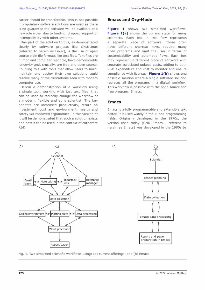
Figure 1 shows two simplified workflows. Figure 1(a) shows the current state for many scientists. Each box in this flow represents a separate piece of software. These often have different shortcut keys, require many open programs and limit the user in terms of customisability and automatic flows. Each box may represent a different piece of software with separate associated upkeep costs, adding to both R&D expenditure and cost to monitor and ensure compliance with licenses. Figure 1(b) shows one possible solution where a single software solution replaces all the programs in a digital workflow. This workflow is possible with the open source and free program: Emacs.
Emacs
Emacs is a fully programmable and extensible text editor. It is used widely in the IT and programming fields. Originally developed in the 1970s, the version used today (GNU Emacs - referred to herein as Emacs) was developed in the 1980s by
Fig. 1. Two simplified scientific workflows using: (a) current offerings; and (b) Emacs
Scientist
Emacs planning
Data collection
Emacs data processing
Report and paper preparation in Emacs
Scientist
Note takingEmail client
Todo/task lists
Reference manager
Data collection
Plotting suiteCoding environment Data processing
Word processor
Report/paper
(a) (b)
124 © 2022 Johnson Matthey
https://doi.org/10.1595/205651322X16316969040478 Johnson Matthey Technol. Rev., 2022, 66, (2)
Richard Stallman. It may seem retrograde that a decades old software solution can compete with newer offerings, but its longevity speaks to its utility. Emacs has been maintained and updated throughout this period with versions available across Windows, macOS and Linux.Out of the box Emacs is a blank canvas. The
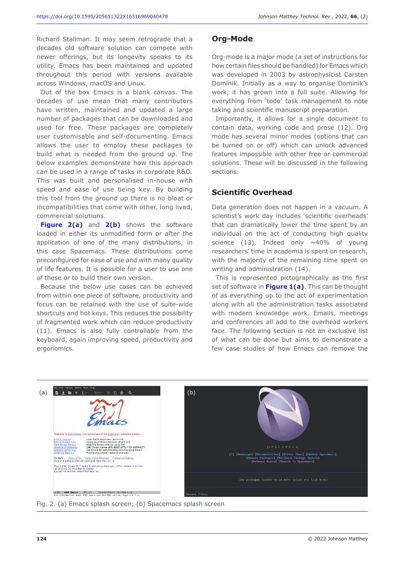
decades of use mean that many contributors have written, maintained and updated a large number of packages that can be downloaded and used for free. These packages are completely user customisable and self-documenting. Emacs allows the user to employ these packages to build what is needed from the ground up. The below examples demonstrate how this approach can be used in a range of tasks in corporate R&D. This was built and personalised in-house with speed and ease of use being key. By building this tool from the ground up there is no bloat or incompatibilities that come with other, long lived, commercial solutions.Figure 2(a) and 2(b) shows the software
loaded in either its unmodified form or after the application of one of the many distributions, in this case Spacemacs. These distributions come preconfigured for ease of use and with many quality of life features. It is possible for a user to use one of these or to build their own version.Because the below use cases can be achieved
from within one piece of software, productivity and focus can be retained with the use of suite-wide shortcuts and hot keys. This reduces the possibility of fragmented work which can reduce productivity (11). Emacs is also fully controllable from the keyboard, again improving speed, productivity and ergonomics.
Org-Mode
Org-mode is a major mode (a set of instructions for how certain files should be handled) for Emacs which was developed in 2003 by astrophysicist Carsten Dominik. Initially as a way to organise Dominik’s work, it has grown into a full suite. Allowing for everything from ‘todo’ task management to note taking and scientific manuscript preparation.Importantly, it allows for a single document to
contain data, working code and prose (12). Org mode has several minor modes (options that can be turned on or off) which can unlock advanced features impossible with other free or commercial solutions. These will be discussed in the following sections.
Scientific Overhead
Data generation does not happen in a vacuum. A scientist’s work day includes ‘scientific overheads’ that can dramatically lower the time spent by an individual on the act of conducting high quality science (13). Indeed only ~40% of young researchers’ time in academia is spent on research, with the majority of the remaining time spent on writing and administration (14).This is represented pictographically as the first
set of software in Figure 1(a). This can be thought of as everything up to the act of experimentation along with all the administration tasks associated with modern knowledge work. Emails, meetings and conferences all add to the overhead workers face. The following section is not an exclusive list of what can be done but aims to demonstrate a few case studies of how Emacs can remove the
(a) (b)
Fig. 2. (a) Emacs splash screen; (b) Spacemacs splash screen
125 © 2022 Johnson Matthey
https://doi.org/10.1595/205651322X16316969040478 Johnson Matthey Technol. Rev., 2022, 66, (2)
burden of scientific overheads by consolidation of tasks with Emacs and Org-mode.
Daily Planning
The act of producing, reviewing and executing a plan is an essential component of problem solving (15). Time management behaviours improve job satisfaction and health while negatively impacting stress (16). Org-mode allows for easy task management and planning from within the Emacs environment.By setting up ‘Org-capture’, a package that
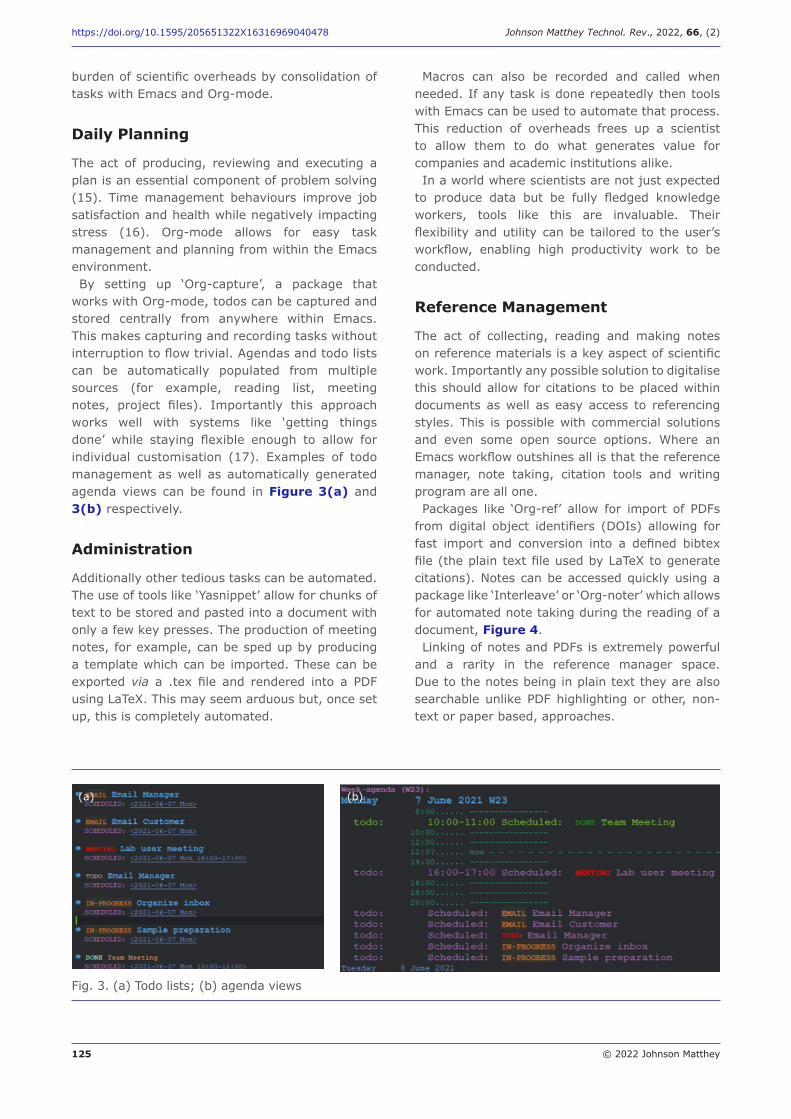
works with Org-mode, todos can be captured and stored centrally from anywhere within Emacs. This makes capturing and recording tasks without interruption to flow trivial. Agendas and todo lists can be automatically populated from multiple sources (for example, reading list, meeting notes, project files). Importantly this approach works well with systems like ‘getting things done’ while staying flexible enough to allow for individual customisation (17). Examples of todo management as well as automatically generated agenda views can be found in Figure 3(a) and 3(b) respectively.
Administration
Additionally other tedious tasks can be automated. The use of tools like ‘Yasnippet’ allow for chunks of text to be stored and pasted into a document with only a few key presses. The production of meeting notes, for example, can be sped up by producing a template which can be imported. These can be exported via a .tex file and rendered into a PDF using LaTeX. This may seem arduous but, once set up, this is completely automated.
Macros can also be recorded and called when needed. If any task is done repeatedly then tools with Emacs can be used to automate that process. This reduction of overheads frees up a scientist to allow them to do what generates value for companies and academic institutions alike.In a world where scientists are not just expected
to produce data but be fully fledged knowledge workers, tools like this are invaluable. Their flexibility and utility can be tailored to the user’s workflow, enabling high productivity work to be conducted.
Reference Management
The act of collecting, reading and making notes on reference materials is a key aspect of scientific work. Importantly any possible solution to digitalise this should allow for citations to be placed within documents as well as easy access to referencing styles. This is possible with commercial solutions and even some open source options. Where an Emacs workflow outshines all is that the reference manager, note taking, citation tools and writing program are all one.Packages like ‘Org-ref’ allow for import of PDFs
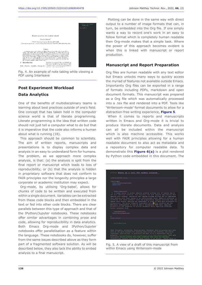
from digital object identifiers (DOIs) allowing for fast import and conversion into a defined bibtex file (the plain text file used by LaTeX to generate citations). Notes can be accessed quickly using a package like ‘Interleave’ or ‘Org-noter’ which allows for automated note taking during the reading of a document, Figure 4.Linking of notes and PDFs is extremely powerful
and a rarity in the reference manager space. Due to the notes being in plain text they are also searchable unlike PDF highlighting or other, non-text or paper based, approaches.
(a) (b)
Fig. 3. (a) Todo lists; (b) agenda views
126 © 2022 Johnson Matthey
https://doi.org/10.1595/205651322X16316969040478 Johnson Matthey Technol. Rev., 2022, 66, (2)
Post Experiment Workload
Data Analytics
One of the benefits of multidisciplinary teams is learning about best practices outside of one’s field. One concept that has taken hold in the computer science world is that of literate programming. Literate programming is the idea that written code should not just tell a computer what to do but that it is imperative that the code also informs a human about what is running (18).This approach should be common to scientists.
The aim of written reports, manuscripts and presentations is to display complex data and analysis in an easy to understand form for humans. The problem, as we approach more complex analysis, is that: (a) the analysis is split from the final report or manuscript which leads to loss of reproducibility; or (b) that the analysis is hidden in proprietary software that does not conform to FAIR principles nor the longevity principles a large corporate or academic institution may expect.Org-mode, by utilising ‘Org-babel’, allows for
chunks of code to be written and executed from within a single document. Variables can be extracted from these code blocks and then embedded in the text or fed into other code blocks. There are clear parallels between this type of approach and that of the IPython/Jupyter notebooks. These notebooks offer similar advantages in combining prose and code, allowing for reproducibility in data analytics. Both Emacs Org-mode and IPython/Jupyter notebooks offer parallelisation as a feature within the language. These notebooks do, however, suffer from the same issues described above as they form part of a fragmented software solution. As will be described below, they also lack the ability to embed analysis to a final manuscript.
Plotting can be done in the same way with direct output to a number of image formats that can, in turn, be embedded into the Org file. If one simply wants a way to record one’s work in an easy to follow format which is completely human readable then Org-mode makes that a simple task. Where the power of this approach becomes evident is when this is linked with manuscript or report production.
Manuscript and Report Preparation
Org files are human readable with any text editor but Emacs unlocks many ways to quickly access the myriad of features not available outside Emacs. Importantly Org files can be exported in a range of formats including PDFs, markdown and open document formats. This manuscript was prepared as a Org file which was automatically processed into a .tex file and rendered into a PDF. Tools like ‘Writeroom-mode’ format documents to allow for a distraction-free writing experience, Figure 5.When it comes to reports and manuscripts
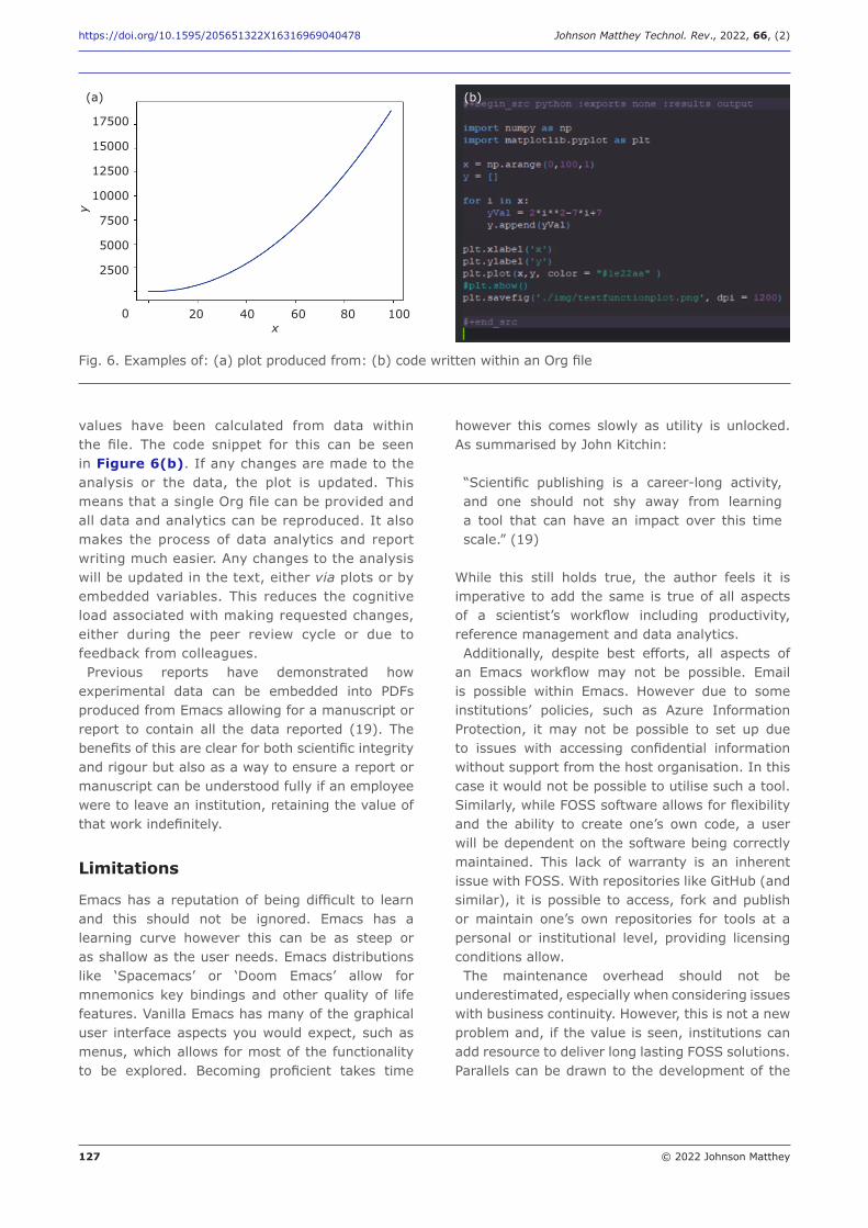
written in Emacs and Org-mode it is trivial to produce literate documents. Data and analysis can all be included within the manuscript which is also machine accessible. This works well with FAIR principles allowing for a human readable document to also act as metadata and a repository for computer readable data. To demonstrate this Figure 6(a) is a plot rendered by Python code embedded in this document. The
Fig. 4. An example of note taking while viewing a PDF using Interleave
Fig. 5. A view of a draft of this manuscript from within Emacs using Writeroom-mode
127 © 2022 Johnson Matthey
https://doi.org/10.1595/205651322X16316969040478 Johnson Matthey Technol. Rev., 2022, 66, (2)
values have been calculated from data within the file. The code snippet for this can be seen in Figure 6(b). If any changes are made to the analysis or the data, the plot is updated. This means that a single Org file can be provided and all data and analytics can be reproduced. It also makes the process of data analytics and report writing much easier. Any changes to the analysis will be updated in the text, either via plots or by embedded variables. This reduces the cognitive load associated with making requested changes, either during the peer review cycle or due to feedback from colleagues.Previous reports have demonstrated how
experimental data can be embedded into PDFs produced from Emacs allowing for a manuscript or report to contain all the data reported (19). The benefits of this are clear for both scientific integrity and rigour but also as a way to ensure a report or manuscript can be understood fully if an employee were to leave an institution, retaining the value of that work indefinitely.
Limitations
Emacs has a reputation of being difficult to learn and this should not be ignored. Emacs has a learning curve however this can be as steep or as shallow as the user needs. Emacs distributions like ‘Spacemacs’ or ‘Doom Emacs’ allow for mnemonics key bindings and other quality of life features. Vanilla Emacs has many of the graphical user interface aspects you would expect, such as menus, which allows for most of the functionality to be explored. Becoming proficient takes time
however this comes slowly as utility is unlocked. As summarised by John Kitchin:
“Scientific publishing is a career-long activity, and one should not shy away from learning a tool that can have an impact over this time scale.” (19)
While this still holds true, the author feels it is imperative to add the same is true of all aspects of a scientist’s workflow including productivity, reference management and data analytics.Additionally, despite best efforts, all aspects of
an Emacs workflow may not be possible. Email is possible within Emacs. However due to some institutions’ policies, such as Azure Information Protection, it may not be possible to set up due to issues with accessing confidential information without support from the host organisation. In this case it would not be possible to utilise such a tool. Similarly, while FOSS software allows for flexibility and the ability to create one’s own code, a user will be dependent on the software being correctly maintained. This lack of warranty is an inherent issue with FOSS. With repositories like GitHub (and similar), it is possible to access, fork and publish or maintain one’s own repositories for tools at a personal or institutional level, providing licensing conditions allow. The maintenance overhead should not be
underestimated, especially when considering issues with business continuity. However, this is not a new problem and, if the value is seen, institutions can add resource to deliver long lasting FOSS solutions. Parallels can be drawn to the development of the
Fig. 6. Examples of: (a) plot produced from: (b) code written within an Org file
(a) (b)
20 40 60 80 100x
17500
15000
12500
10000
7500
5000
2500
0
y
128 © 2022 Johnson Matthey
https://doi.org/10.1595/205651322X16316969040478 Johnson Matthey Technol. Rev., 2022, 66, (2)
Linux kernel. Here private companies contribute extensively to the FOSS development because there is an understanding of the value of that project to their business interest (20). While FOSS approaches offer great benefits,
the use of proprietary or closed source software is preferable when that software offers utility not possible by other routes. Complex analysis using statistical software, complex peak fitting or databases requiring subscriptions are still a reality of the profession. When these tools are needed the approach outlined above still works providing the data can be exported from such a program into a plain text format. If this is not possible and FAIR principles cannot be upheld, the use of such a tool should be re-evaluated to determine if its use can facilitate long term and sustainable analysis.
Conclusions
Emacs is a powerful and versatile tool for modern science. It facilitates the production, handling and analysis of data in a FAIR fashion while allowing modern scientists to be as agile as possible. By using tools under one FOSS umbrella huge productivity gains can be realised along with improvements in ergonomics and associated cost benefits with the removal of proprietary software tools. The learning curve should be viewed in the context of a lifelong scientific career. With institutions understanding the value of data beyond a single scientist, applying (or supporting individuals who wish to apply) this type of workflow more widely would have a profound and long last effect beyond the career of just one scientist.
Acknowledgements
The author would like to thank Ed Wright, Ludovic Briquet, Carl Tipton and Cristina Estruch Bosch of Johnson Matthey for fruitful discussion and feedback during the drafting process. Mac and macOS are trademarks of Apple Inc,
registered in the USA and other countries and regions. Microsoft, Azure, Office and Windows are trademarks of the Microsoft group of companies. All other trademarks are the property of their respective owners.
References
1. M. D. Wilkinson, M. Dumontier, I. J. Aalbersberg, G. Appleton, M. Axton, A. Baak, N. Blomberg, J.-W. Boiten, L. B. da Silva Santos, P. E. Bourne,
J. Bouwman, A. J. Brookes, T. Clark, M. Crosas, I. Dillo, O. Dumon, S. Edmunds, C. T. Evelo, R. Finkers, A. Gonzalez-Beltran, A. J. G. Gray, P. Groth, C. Goble, J. S. Grethe, J. Heringa, P. A. C. ’t Hoen, R. Hooft, T. Kuhn, R. Kok, J. Kok, S. J. Lusher, M. E. Martone, A. Mons, A. L. Packer, B. Persson, P. Rocca-Serra, M. Roos, R. van Schaik, S.-A. Sansone, E. Schultes, T. Sengstag, T. Slater, G. Strawn, M. A. Swertz, M. Thompson, J. van der Lei, E. van Mulligen, J. Velterop, A. Waagmeester, P. Wittenburg, K. Wolstencroft, J. Zhao and B. Mons, Sci. Data, 2016, 3, 160018
2. R. Hai, S. Geisler and C. Quix, ‘Constance: An Intelligent Data Lake System’, in “SIGMOD ’16: Proceedings of the 2016 International Conference on Management of Data”, Association for Computing Machinery, New York, USA, June, 2016, pp. 2097–2100
3. W. Hasselbring, L. Carr, S. Hettrick, H. Packer and T. Tiropanis, Inform. Technol., 2020, 62, (1), 39
4. F. Massingberd-Mundy, S. Poulston, S. Bennett, H. H.-M. Yeung and T. Johnson, Sci. Rep., 2020, 10, 17355
5. M. D. M. Dryden, R. Fobel, C. Fobel and A. R. Wheeler, Anal. Chem., 2017, 89, (8), 4330
6. N. M. O’Boyle, M. Banck, C. A. James, C. Morley, T. Vandermeersch and G. R. Hutchison, J. Cheminform., 2011, 3, 33
7. D. Schindler, B. Zapilko and F. Krüger, ‘Investigating Software Usage in the Social Sciences: A Knowledge Graph Approach’, 17th International Conference, ESWC 2020, Heraklion, Crete, Greece, 31st May–4th June, 2020, “The Semantic Web”, eds. A. Harth, S. Kirrane, A.-C. N. Ngomo, H. Paulheim, A. Rula, A. L. Gentile, P. Haase and M. Cochez, Lecture Notes in Computer Science, Vol. 12123, Springer, Cham, Switzerland, 2020, pp. 271–286
8. G. S. Adams, B. A. Converse, A. H. Hales and L. E. Klotz, Nature, 2021, 592, (7853), 258
9. 9th WSEAS International Conference on Data Networks, Communications, Computers (DNCOCO ’10), University of Algarve, Faro, Portugal, 3rd–5th November, 2010, “Advances in Data Networks, Communications, Computers”, eds. N. E. Mastorakis and V. Mladenov, World Scientific and Engineering Academy and Society Press, Athens, Greece, 2010
10. J. Lazar, A. Jones and B. Shneiderman, Behav. Inform. Technol., 2006, 25, (3), 239
11. A. N. Meyer, L. E. Barton, G. C. Murphy, T. Zimmermann and T. Fritz, IEEE Trans. Software Eng., 2017, 43, (12), 1178
12. E. Schulte and D. Davison, Comput. Sci. Eng., 2011, 13, (3), 66
129 © 2022 Johnson Matthey
https://doi.org/10.1595/205651322X16316969040478 Johnson Matthey Technol. Rev., 2022, 66, (2)
13. M. L. Pace, Limnol. Oceanogr. Bull., 2020, 29, (1), 20
14. B. Maher and M. S. Anfres, Nature, 2016, 538, (7626), 444
15. D. J. Simons and K. M. Galotti, Bull. Psychon. Soc., 1992, 30, (1), 61
16. B. J. C. Claessens, W. van Eerde, C. G. Rutte and R. A. Roe, Person. Rev., 2007, 36, (2), 255
17. F. Heylighen and C. Vidal, Long Range Plan., 2008, 41, (6), 585
18. D. Cordes and M. Brown, Computer, 1991, 24, (6), 52
19. J. R. Kitchin, ACS Catal., 2015, 5, (6), 3894
20. D. Homscheid, J. Kunegis and M. Schaarschmidt, ‘Private-Collective Innovation and Open Source Software: Longitudinal Insights from Linux Kernel Development’, 14th IFIP WG 6.11 Conference on e-Business, e-Services, and e-Society, I3E, Delft, The Netherlands, 13th–15th October, 2015, “Open and Big Data Management and Innovation”, eds. M. Janssen, M. Mäntymäki, J. Hidders, B. Klievink, W. Lamersdorf, B. van Loenen and A. Zuiderwijk, Lecture Notes in Computer Science, Vol. 9373, Springer, Cham, Switzerland, 2015, pp. 299–313
The Author
Timothy Johnson (PhD, MChem, CChem) is a Senior Scientist who has worked at Johnson Matthey since 2016. His research interests focus on the production, characterisation and testing of porous materials for industrial applications. He is passionate about understanding workflows to reduce workloads and improve productivity.
www.technology.matthey.com
https://doi.org/10.1595/205651322X16270488736796 Johnson Matthey Technol. Rev., 2022, 66, (2), 130–136
130 © 2022 Johnson Matthey
Thomas M. Whitehead*Intellegens Ltd, Eagle Labs, Chesterton Road, Cambridge, UK
Flora Chen, Christopher DalyJohnson Matthey, Orchard Road, Royston, Hertfordshire, SG8 5HE, UK
Gareth J. ConduitIntellegens Ltd, Eagle Labs, Chesterton Road, Cambridge, UK; and Theory of Condensed Matter, Department of Physics, University of Cambridge, J. J. Thomson Avenue, Cambridge, CB3 0HE, UK
*Email: [email protected]
PEER REVIEWED
Received 6th May 2021; Revised 8th July 2021; Accepted 22nd July 2021; Online 23rd July 2021
The design of catalyst products to reduce harmful emissions is currently an intensive process of expert-driven discovery, taking several years to develop a product. Machine learning can accelerate this timescale, leveraging historic experimental data from related products to guide which new formulations and experiments will enable a project to most directly reach its targets. We used machine learning to accurately model 16 key performance targets for catalyst products, enabling detailed understanding of the factors governing catalyst performance and realistic suggestions of future experiments to rapidly develop more effective products. The proposed formulations are currently undergoing experimental validation.
Accelerating the Design of Automotive Catalyst Products Using Machine LearningLeveraging experimental data to guide new formulations
IntroductionDomestic and commercial vehicles are leading sources of global pollution, with vehicle emissions risking the health of communities near roads (1). Fine and ultrafine particulate matter, oxides of nitrogen, hydrocarbons and carbon monoxide are key road traffic pollutants that are associated with adverse health effects (2). Catalytic converters have been used since the 1970s to reduce the emission of these pollutants by catalysing their reaction into less-toxic substances, typically carbon dioxide, nitrogen and water (3). However, current catalytic converters are not 100% efficient in their reactions of pollutants and moreover have variable efficiency at different operating temperatures. This work uses machine learning modelling to
analyse current catalytic converter performance and identify which future experimental tests would add most value to the ongoing development of improved catalytic converters. Previous work using machine learning in the catalysis domain has tended to focus on either augmenting quantum mechanical models of catalyst function (4–8), screening potential new catalysts (7–11), or predicting properties from carefully-selected chemical descriptors of catalysts (6, 8, 12–14). In contrast, in this work we focus on modelling catalyst properties from the formulation ingredients and processing variables of the catalyst. The ingredients and processing conditions of samples are easily accessible during the development process, lowering the barrier to application of machine learning in active development projects. In the following section we discuss the project objectives, detail the machine learning methodology used and the results it delivers, before looking forward to potential future applications of machine learning for materials science in the automotive field and beyond.
131 © 2022 Johnson Matthey
https://doi.org/10.1595/205651322X16270488736796 Johnson Matthey Technol. Rev., 2022, 66, (2)
Objectives
We collated data on 612 catalytic converter test sets that have been manufactured and experimentally tested by Johnson Matthey as part of an ongoing catalyst development project. The data contained information on the formulation used for the catalysts, including amounts and properties of 34 ingredients; 10 test parameters describing the testing process for each catalyst; and 16 experimentally measured properties for each catalyst including target gas conversions and selectivities. These output properties consisted of eight sets of tests, with each test run at both a high (approx. 500°C) and low (approx. 225°C) temperature on different samples of the same catalyst formulation. Each experimental property was reported as a steady-state average over 50–100 s of gas stream.Using this data, we aimed to build understanding
of the performance of this class of catalyst, using a machine learning model trained on the data to extract information on which input features of the formulation and processing parameters have most impact on the performance. Using this model, we then designed catalysts that offer both high performance and also add value to the machine learning model, which once made and measured can be added to the training dataset to enable more accurate modelling of high performance catalysts.
Methods
To model the catalyst data we used the AlchemiteTM multi-target machine learning platform. This method is described in detail in the literature (15–17), but in brief consists of iteratively generating predictions for all data series, both input and output, and using these predictions to impute missing data on the input side, before the final iteration of predictions are reported as the predictions for the output series. This method is designed to handle sparse input data, as was found in this work where up to 10% of the catalysts were missing information on each of the input properties. As the method is multi-target, generating predictions for all output properties simultaneously, we trained a model to predict all 16 experimentally measured properties at once. AlchemiteTM also generates estimates of the uncertainty in each prediction, which is vital to prioritise suggestions for future experiments that are most likely to achieve specified objectives. To test the performance of the model, data on 61 catalysts (10% of the data) was randomly
held back; the model was trained on data for the remaining 551 catalysts. Hyperparameters of the model were optimised using Bayesian Tree of Parzen Estimators via five-fold cross-validation within the training set only (17, 18). To test the performance of the model we
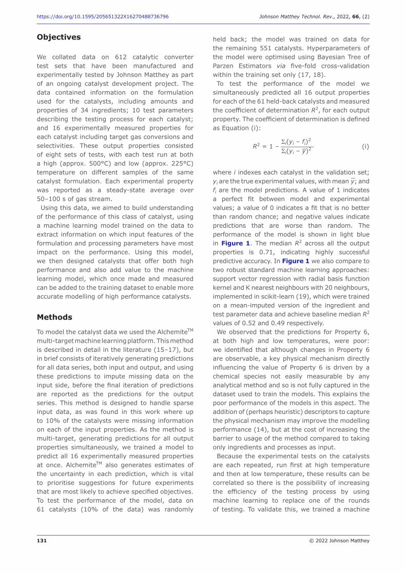
simultaneously predicted all 16 output properties for each of the 61 held-back catalysts and measured the coefficient of determination R2, for each output property. The coefficient of determination is defined as Equation (i):
R2 = 1 – (i)Si(yi – fi)2
Si(yi – y)2
where i indexes each catalyst in the validation set; yi are the true experimental values, with mean ̄y; and fi are the model predictions. A value of 1 indicates a perfect fit between model and experimental values; a value of 0 indicates a fit that is no better than random chance; and negative values indicate predictions that are worse than random. The performance of the model is shown in light blue in Figure 1. The median R2 across all the output properties is 0.71, indicating highly successful predictive accuracy. In Figure 1 we also compare to two robust standard machine learning approaches: support vector regression with radial basis function kernel and K nearest neighbours with 20 neighbours, implemented in scikit-learn (19), which were trained on a mean-imputed version of the ingredient and test parameter data and achieve baseline median R2 values of 0.52 and 0.49 respectively. We observed that the predictions for Property 6,
at both high and low temperatures, were poor: we identified that although changes in Property 6 are observable, a key physical mechanism directly influencing the value of Property 6 is driven by a chemical species not easily measurable by any analytical method and so is not fully captured in the dataset used to train the models. This explains the poor performance of the models in this aspect. The addition of (perhaps heuristic) descriptors to capture the physical mechanism may improve the modelling performance (14), but at the cost of increasing the barrier to usage of the method compared to taking only ingredients and processes as input.Because the experimental tests on the catalysts
are each repeated, run first at high temperature and then at low temperature, these results can be correlated so there is the possibility of increasing the efficiency of the testing process by using machine learning to replace one of the rounds of testing. To validate this, we trained a machine
132 © 2022 Johnson Matthey
https://doi.org/10.1595/205651322X16270488736796 Johnson Matthey Technol. Rev., 2022, 66, (2)
learning model that took as inputs the formulation ingredients and test parameters as well as the experimentally measured results on all eight tests at high temperature, and predicted the results of the eight tests at low temperature. This order (using high temperature results as input to predict low temperature results) was selected to align with the current testing methodology.The improved performance by using the high
temperature measurements to help predict the low temperature performance is exemplified in dark blue in Figure 1. For five of the eight experimental properties the accuracy significantly increased (increase in R2 of more than 0.1), and for Properties 1, 2 and 3 the resulting accuracy, with R2>0.95, is effectively equivalent to the experimental uncertainty in the measurement. For these three properties in particular, machine learning predictions could reliably replace experimental measurements, offering a saving in the time and effort required to run the experimental tests on new catalysts. The three experimental properties that were not improved by using the high temperature measurements are all related to the same target gas’ conversion rates,
although it is not clear why these properties are not improved by access to increased experimental data. These three experimental properties are less commercially important than Property 1, which is the property with most commercial relevance.
Machine Learning Results
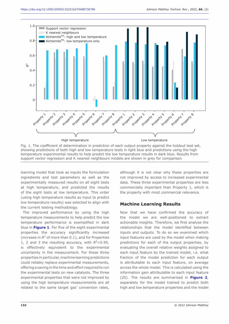
Now that we have confirmed the accuracy of the model we are well-positioned to extract actionable insights. Therefore, we first analyse the relationships that the model identified between inputs and outputs. To do so we examined which input features are used by the model when making predictions for each of the output properties, by evaluating the overall relative weights assigned to each input feature by the trained model, i.e. what fraction of the model prediction for each output is attributable to each input feature, on average across the whole model. This is calculated using the information gain attributable to each input feature (20). The results are summarised in Figure 2, separately for the model trained to predict both high and low temperature properties and the model
Support vector regressionK nearest neighboursAlchemiteTM: high and low temperatureAlchemiteTM: low temperature only
1.0
0.8
0.6
0.4
0.2
0
R2
Prop
erty 1
Prop
erty 2
Prop
erty 3
Prop
erty 4
Prop
erty 5
Prop
erty 6
Prop
erty 7
Prop
erty 8
Prop
erty 1
Prop
erty 2
Prop
erty 3
Prop
erty 4
Prop
erty 5
Prop
erty 6
Prop
erty 7
Prop
erty 8
High temperature Low temperature
Fig. 1. The coefficient of determination in prediction of each output property against the holdout test set, showing predictions of both high and low temperature tests in light blue and predictions using the high temperature experimental results to help predict the low temperature results in dark blue. Results from support vector regression and K nearest neighbours models are shown in grey for comparison
133 © 2022 Johnson Matthey
https://doi.org/10.1595/205651322X16270488736796 Johnson Matthey Technol. Rev., 2022, 66, (2)
trained to predict low temperature properties only. Averaging across each of the output properties, we find that for the high and low temperature model the test parameters and formulation ingredients are utilised in the proportion 0.59:1, and for the low temperature only model the test parameters, formulation ingredients and experimental high temperature measurements are utilised in the proportion 0.60:1:1.19. The consistent ratio of 0.6:1 in utilisation of the test parameters and formulation ingredients between the two models indicates that the high temperature experimental measurements (especially Properties 1, 2 and 3) are adding distinct information to the model that it was not capable of identifying from either the test parameters or formulation ingredients. The key operational insight derived from this
analysis was that although the formulation ingredients provide important information for the simultaneous modelling of the high and low temperature results, the variation in the test parameters also provides a key contribution. Historically the test parameters have been controlled within specification ranges but the impact of variation within these ranges has not been considered. These results show that the
test parameters have an impact on the resulting properties and that control and understanding of these parameters improves the value of the data.
Machine Learning Formulation Design
With increased understanding of the importance of the test parameters for measured catalyst performance, we used the machine learning model to design catalyst formulations. For performance targets, we focussed on the most commercially important property (Property 1), aiming to maximise its value at both high and low temperatures, and for that value to be stable with temperature. Although Property 1 is the most commercially important property, the values of the other properties are also required for product success.As well as looking for the formulations that
would be most likely to succeed against these performance targets (‘exploitation’ of the model) we also searched for formulations that, when measured, would increase the model’s understanding of the formulation landscape and so improve future rounds of predictive modelling and formulation design (‘exploration’ of the model), as
(a)
(b)
Low
tem
pera
ture
H
igh
tem
pera
ture
Low
tem
pera
ture
Property 1Property 2Property 3Property 4Property 5Property 6Property 7Property 8Property 1Property 2Property 3Property 4Property 5Property 6Property 7Property 8
Property 1Property 2Property 3Property 4Property 5Property 6Property 7Property 8
Test parameters Formulation ingredients
Test parameters Formulation ingredients High temperature measurements
0.12
0.10
0.08
0.06
0.04
0.02
0
Fig. 2. Importance of each input factor (horizontal axis) for making predictions of each output property (vertical axis). The upper plot shows the model trained to predict both high and low temperature results, whilst the lower plot shows the model trained to use the high temperature results to help predict the low temperature results. Higher values (darker colours) indicate more importance given to a variable. The importance values sum to one for each output property
134 © 2022 Johnson Matthey
https://doi.org/10.1595/205651322X16270488736796 Johnson Matthey Technol. Rev., 2022, 66, (2)
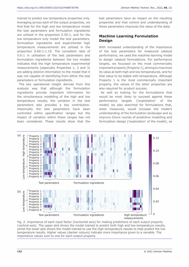
well as a balanced mix of the two objectives. We used a Bayesian search of the formulation space using Tree of Parzen Estimators (18) built into the AlchemiteTM platform, taking as the cost function the probability of simultaneously achieving all the performance targets, including a contribution from the uncertainty in each formulation’s predicted performance calculated as standard errors across the AlchemiteTM platform’s internal ensemble of sub-models (21). This cost function is the commercially relevant metric to aim to propose successful and useful new formulations. Exploitation-focused suggestions prioritise formulations with high probability of success, while exploration-focused suggestions prioritise formulations whose predictions are currently uncertain and will also help improve predictions over a wide range of formulation space. A two-dimensional Uniform Manifold
Approximation and Projection (UMAP) embedding (22) of the formulations is shown in Figure 3. The dark blue points show the historic experimental results, with more opaque points having higher performance against Property 1 and more transparent points having lower performance. We observe that there are several clusters of dissimilar formulations that had previously been measured, but that most of the formulations were relatively similar and are clustered in the centre of the plot (this clustering analysis being a key strength of the UMAP approach). Figure 3 also shows the formulations proposed by the machine learning approach, labelled by whether they are focused on exploration, exploitation or a balanced mixture. We observe that, as expected, the exploitation-
focused suggestions are clustered more tightly at the centre of the plot, demonstrating that they are attempting to exploit a class of formulations with a high probability (up to 60%) of achieving all of the design targets simultaneously. In contrast, the exploration-focused suggestions are more varied, focusing particularly on gaps in the existing coverage of the formulation space where additional information will improve the model. The balanced suggestions show aspects of both behaviours. A subset of the formulations suggested by the machine learning, including samples from the exploration, exploitation and balanced suggestions, are currently undergoing experimental validation.
Conclusions
In this work we have shown how machine learning analysis of catalyst formulations enables new insights into the factors that affect catalyst performance, including particularly that the test parameters more strongly impact the eventual performance than was initially anticipated: this will have operational significance for the future of this product development. We have also shown how the use of a machine learning platform, rather than a single predictive tool, can enable full design workflows, including prioritising exploration of the formulation space or exploitation of a model to achieve high product performance, accelerating the design process by enabling a holistic view of the formulation opportunities. Future progress in this project could focus on achieving multiple target properties simultaneously, beyond only Property 1, or utilising the accurate predictions
Training setSuggested experiments (exploration)Suggested experiments (balanced)Suggested experiments (exploitation)
Fig. 3. Two-dimensional UMAP embedding of the training data (blue points), with darker points those with higher performance on Property 1. Also shown are the experiments suggested by the machine learning approach, in light blue (exploration focused), purple (balanced search) and orange (exploitation focused)
135 © 2022 Johnson Matthey
https://doi.org/10.1595/205651322X16270488736796 Johnson Matthey Technol. Rev., 2022, 66, (2)
of low temperature measurements based on experimental high temperature measurements to halve the amount of experimental effort required when screening new formulations.The machine learning approach here is applicable
beyond catalytic converters, including the design of metal alloys (15, 23), batteries (24), and pharmaceutical drugs (21). A machine learning platform that can carry out the full cycle of formulation development, handling sparse real-world experimental data, building predictive models and proposing and interpreting new formulation designs adds value in each of these areas, with reduced barrier to entry by working directly on the composition and processing variables immediately accessible to project scientists.
Acknowledgements
Gareth Conduit acknowledges financial support from the Royal Society. There is Open Access to this paper online.
References
1. K. Zhang and S. Batterman, Sci. Total Environ., 2013, 450–451, 307
2. D. Brugge, J. L. Durant and C. Rioux, Environ. Health, 2007, 6, 23
3. C. Morgan, Johnson Matthey Technol. Rev., 2014, 58, (4), 217
4. K. Shakouri, J. Behler, J. Meyer and G.-J. Kroes, J. Phys. Chem. Lett., 2017, 8, (10), 2131
5. Z. W. Ulissi, A. J. Medford, T. Bligaard and J. K. Nørskov, Nat. Commun., 2017, 8, 14621
6. J. R. Kitchin, Nat. Catal., 2018, 1, (4), 230 7. W. Yang, T. T. Fidelis and W.-H. Sun, ACS Omega,
2019, 5, (1), 83 8. B. R. Goldsmith, J. Esterhuizen, J.-X. Liu, C. J.
Bartel and C. Sutton, AIChE J., 2018, 64, (7), 2311
9. Z. Li, S. Wang, W. S. Chin, L. E. Achenie and H. Xin, J. Mater. Chem. A, 2017, 5, (46), 24131
10. Z. W. Ulissi, M. T. Tang, J. Xiao, X. Liu, D. A. Torelli,
M. Karamad, K. Cummins, C. Hahn, N. S. Lewis, T. F. Jaramillo, K. Chan and J. K. Nørskov, ACS Catal., 2017, 7, (10), 6600
11. T. Williams, K. McCullough and J. A. Lauterbach, Chem. Mater., 2020, 32, (1), 157
12. Z. Li, X. Ma and H. Xin, Catal. Today, 2017, 280, (2), 232
13. I. Takigawa, K.-i. Shimizu, K. Tsuda and S. Takakusagi, RSC Adv., 2016, 6, (58), 52587
14. K. Suzuki, T. Toyao, Z. Maeno, S. Takakusagi, K.-i. Shimizu and I. Takigawa, ChemCatChem, 2019, 11, (18), 4537
15. B. D. Conduit, N. G. Jones, H. J. Stone and G. J. Conduit, Scr. Mater., 2018, 146, 82
16. P. Santak and G. Conduit, Fluid Phase Equilib., 2019, 501, 112259
17. T. M. Whitehead, B. W. J. Irwin, P. Hunt, M. D. Segall and G. J. Conduit, J. Chem. Inf. Model., 2019, 59, (3), 1197
18. J. Bergstra, R. Bardenet, Y. Bengio and B. Kégl, ‘Algorithms for Hyper-Parameter Optimization’, NIPS’11: Proceedings of the 24th International Conference on Neural Information Processing Systems, 12th–15th December, 2011, Granada, Spain, Curran Associates Inc, New York, USA, 2011, 9 pp
19. F. Pedregosa, G. Varoquaux, A. Gramfort, V. Michel, B. Thirion, O. Grisel, M. Blondel, P. Prettenhofer, R. Weiss, V. Dubourg, J. Vanderplas, A. Passos, D. Cournapeau, M. Brucher, M. Perrot and É. Duchesnay, J. Mach. Learn. Res., 2011, 12, 2825
20. B. Frénay, G. Doquire and M. Verleysen, Neural Networks, 2013, 48, 1
21. B. W. J. Irwin, J. R. Levell, T. M. Whitehead, M. D. Segall and G. J. Conduit, J. Chem. Inf. Model., 2020, 60, (6), 2848
22. L. McInnes, J. Healy and J. Melville, ‘UMAP: Uniform Manifold Approximation and Projection for Dimension Reduction’, arXiv:1802.03426v3 [stat.ML], 18th September, 2020, preprint
23. B. D. Conduit, N. G. Jones, H. J. Stone and G. J. Conduit, Mater. Des., 2017, 131, 358
24. M.-F. Ng, J. Zhao, Q. Yan, G. J. Conduit and Z. W. Seh, Nat. Mach. Intell., 2020, 2, (3), 161
The Authors
Thomas Whitehead holds a PhD in theoretical physics from the University of Cambridge, UK, and is now leading the application of Intellegens’ novel deep learning approaches to a wide variety of industrial applications. His work focuses on developing a series of application-specific machine learning modules to address high-value data analysis bottlenecks.
136 © 2022 Johnson Matthey
https://doi.org/10.1595/205651322X16270488736796 Johnson Matthey Technol. Rev., 2022, 66, (2)
Christopher Daly received an MChem (2008) and PhD (2012) in Chemistry from the University of Leicester, UK, where his research focused on the synthesis of organometallic compounds of the late transition metals and their applications in bifunctional catalysis. Since 2013 he has worked on automotive catalyst development at Johnson Matthey across several technologies, where he is currently a Senior Chemist.
Flora Chen is the Data Science Lead at Johnson Matthey. She has 15 years’ experience in global high-tech companies and has held technical and management roles spanning engineering, operations, R&D and quality. Since Flora joined Johnson Matthey in 2018, she has led several digital analytics projects, discovering and delivering the business value of data. Flora holds a PhD in Mechanical Engineering from Bristol University, UK, and is a chartered engineer.
Gareth Conduit has a track record of developing and applying machine learning methods to solve real-world problems. The approach, originally developed for materials design, is now being commercialised by startup Intellegens in materials design, healthcare and drug discovery. Gareth also has research interests in strongly correlated phenomena, in particular proposing spin spiral state in the itinerant ferromagnet that was later observed in CeFePO. Gareth’s group is based at the University of Cambridge.
www.technology.matthey.com
https://doi.org/10.1595/205651322X16221965765527 Johnson Matthey Technol. Rev., 2022, 66, (2), 137–153
137 © 2022 Johnson Matthey
Nenad Zečević*Petrokemija Plc, Avenija Vukovar 4, HR-44320 Kutina, Croatia
*Email: [email protected]
PEER REVIEWED
Received 4th March 2021; Revised 20th May 2021; Accepted 26th May 2021; Online 28th May 2021
The catalytic steam reforming process of natural gas consumes up to approximately 60% of overall energy used in ammonia production. The optimisation of the reforming catalyst performance can significantly improve the operation of the whole ammonia plant. An online model uses actual process parameters to optimise and reconcile the data of primary reforming products with possibility to predict the catalyst performance. The model uses a combination of commercial simulator and open-source code based on scripts and functions in the form of m-files to calculate various physical properties of reacting gases. The optimisation of steady-state flowsheet, based on real-time plant data from the distributed control system (DCS), is essential for the application of the model at the industrial level. The simplicity of the calculation method used by the model provides the fundamental basis for industrial application in the frame of digitalisation initiative. The principal aim of the optimisation procedure is to change the working curve for methane regarding its equilibrium curve as well as methane outlet molar concentration. This is the critical process
Discrete Simulation Model of Industrial Natural Gas Primary Reformer in Ammonia Production and Related Evaluation of the Catalyst PerformanceOptimising catalyst performance and lifetime
parameter in reforming catalyst operation. An industrial top fired primary reformer unit based on Kellogg Inc technology design served for the validation of the model. Calculation procedure is used for continuous online evaluation of the most commercially available primary reformer catalysts. Based on the conducted evaluation, the model can indicate possible recommendations which can mitigate marginal performance and prolong reformer catalyst lifetime.
1. Introduction
In ammonia production, approximately 60% of overall energy consumption relates to the front end of the production process, namely steam methane reforming (SMR) (1). The proper operation of the SMR unit is the primary focus for operators who aim to minimise costs in the whole ammonia plant. Primary reforming is a process in which gases containing hydrocarbon react with steam to generate a product which is a gas with, as much as possible, higher hydrogen content. The reacting conditions are such that the remaining product components also include methane, carbon monoxide, carbon dioxide and some inerts (nitrogen, argon and helium) that may have been present in the feedstock. The basic occurring reactions in the process are highly endothermic (2). As a result, the process operates by passing the mixture of hydrocarbon and steam reactants over a reformer catalyst in a fired furnace.Regarding such complex equipment, it is important
to consider the type of furnace used to transfer heat to the reactants, the catalyst properties such
138 © 2022 Johnson Matthey
https://doi.org/10.1595/205651322X16221965765527 Johnson Matthey Technol. Rev., 2022, 66, (2)
as the activity, life, size and strength together with other operating parameters such as feedstock characteristics, pressure, temperature, volume flows and the desired product composition.Latham (3) developed a mathematical model
of the SMR unit for use in process performance simulations and online monitoring of tube-wall temperatures using a plug flow pattern. According to the model inputs, it is able to calculate temperature profiles for the outer-tube wall, inner-tube wall, furnace gas and process gas. However, it was concluded that to make the current model usable by plant operators, an interface between the plant inputs and the model needs to be created and the model runtime of 4 min may need to be improved. Computational fluid dynamics (CFD) modelling and simulation of SMR reactors and furnaces has been deeply elaborated by Aguirre (4) and the same are applicable for both pilot-scale and full industrial scale furnaces. The author designed the workflow to be executed without the need of an expert user, to be deployed in cloud environment and to be fully or partially used. Model convergence is determined by a difference of standard deviation below 3.0%. In spite of successful trials, a total time of approximately 30 h was required for the simulation and optimisation to achieve convergence. The author suggested further study in the modelling process to speed up the CFD calculation by implementation of the smart-determination of variable numerical computation parameters which could be implemented by the different optimisation schemes. Moreover, Lao et al. (5) demonstrated that CFD software can be employed to create a detailed CFD model of an industrial-scale SMR tube using plug flow. It showed good approximation of the catalyst with the available industrial plant data. Simulation results were very close to the plant data for temperature and species composition. The only drawback of the proposed model was computational time which was at the level of 5 min with the steady state solver. It can be concluded that the CFD modelling technique provides high accuracy, but takes a long time to converge which is impractical for industrial applications. To overcome this drawback Holt et al. (6) created a SMR model in Python based on previous work by Xu and Froment (7, 8). The model was shown to be a reasonable replica of the original work of Xu and Froment (7, 8), however they did not regress the model against a real SMR unit.The general arrangement of the SMR unit
comprises a reformer furnace, reformer tubes and a related catalyst. The general furnace classification
according to firing pattern refers to top, side and bottom fired furnace. In all the furnaces, the catalyst is contained in heat resistant alloy reformer tubes, the inside diameter of which ranges typically from 6.0 cm to 20.0 cm and the wall thickness of which is from 0.9 cm to 1.9 cm. Fired lengths in commercial furnaces vary approximately from 2.5 m to 14 m. The most commonly encountered fired lengths, however, are 9.0 m to 12.0 m (1, 2). Firing is usually controlled in such a way that the tube wall temperature is maintained at values that will give reasonable tube lifetime. Different firing control strategies for SMR units have been developed over time using standard and advanced process control approaches based on proportional-integral-derivative controllers or model predictive control techniques (9–12). Each of them showed different advantages in implementation of control structures to describe the dynamic relationship between the reformer tube wall temperature (process outputs) and manipulated variables and disturbances (process inputs). The main focus of different control strategies is to keep the reformer tube wall temperature at a safe temperature level to protect the reformer tube wall material against mechanical degradation. By design and industry practice, maximum allowable tube wall temperatures will give in-service life of 100,000 h when considering the stress-to-rupture and creep damage properties of the particular alloy used in manufacturing the reformer tube (13).The discrete model was validated with Kellogg
Inc top fired furnace which is characterised by having the burners on the top and firing down. The reformer tubes in such a furnace are installed in parallel rows with the burners between each row.Catalyst performance has an important effect on
hydrocarbon conversion and on the reformer tube wall temperature, which is usually monitored by plant operators, and therefore subject to human error due to the lack of appropriate knowledge about correction actions. Primary reformer catalyst performance is usually estimated in terms of its methane approach to equilibrium (ATE), reformer furnace tube wall temperatures, pressure drop and the presence or absence of hot spots or bands on the reformer tubes. The most important variable for bringing the catalyst performance to the maximum activity is ATE. The ATE represents the difference between the actual value at the exit of the catalyst and the value at which the measured exit gas composition would be at equilibrium (2). The actual methane ATE cannot theoretically be less than zero (a negative number).
139 © 2022 Johnson Matthey
https://doi.org/10.1595/205651322X16221965765527 Johnson Matthey Technol. Rev., 2022, 66, (2)
Over the years, several applications were developed to make evaluations and recommendations regarding catalyst performance (5–6, 14–16). However, according to literature findings, none of them are designed to continuously (online) evaluate the catalyst performance during SMR operation. Most design calculations involve simply checking designs submitted by the major catalyst suppliers. These submitted requests give specific material balances (both at the inlet and at the exit of the reformer tubes), operating conditions (pressures, temperatures) and furnace configurations (number of tubes and tube dimensions). These data are then entered into the proprietary applications and the results are checked for methane ATE, heat flux versus catalyst size-type and pressure drop. After performing evaluation, the catalyst suppliers submit the report to the operators, which is then used for eventual corrective actions. In most cases the evaluation reports with related recommendations for corrective actions are submitted with a huge time delay and cannot be immediately applied to adjust catalyst performance.In order to overcome these limitations and bring
novelty in this research, the primary aim of this work is the delivery of a sophisticated online model which predicts the performance of reformer catalysts having specific design. The model can simulate the tube side process and provides a detailed profile of the reaction rates, molar gas composition, actual conversion of hydrocarbon feedstock, the pressure and temperature profiles inside of the tubes incrementally. The model can continuously receive real-time plant data from any commercial DCS, which is then reconciled against the model and subsequently used to
generate recommendations for the operators. The supplementary novelty in the proposed model is the simple and reliable calculation method with very fast computational routine, which brings to the operator sufficiently understandable recommendations to evaluate the catalyst performance and carry out necessary remediation measures.Furthermore, additional novelty is the development
of appropriate shared memory coupling for communication between steady-state model and MATLAB® via a shared memory area on the host system. The developed communication system with related open structure and user friendly interface enables implementation of the proposed solution to any DCS system which enables time savings in catalyst performance evaluation. In the frame of a digitalisation initiative and
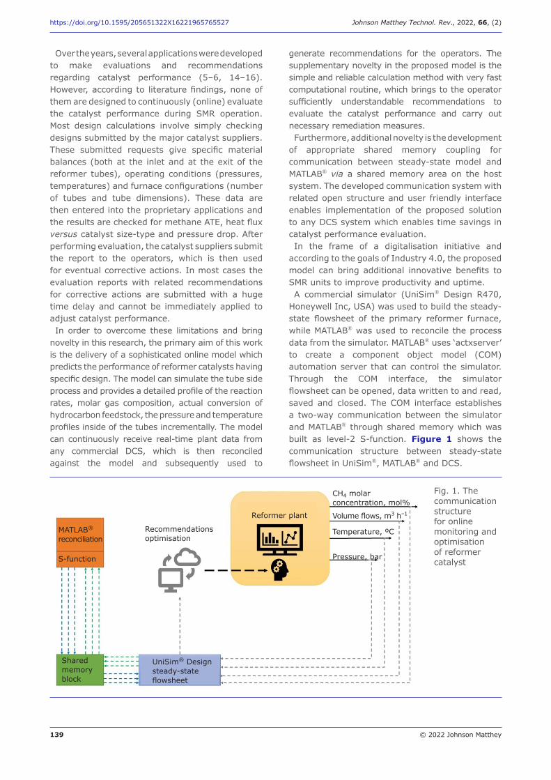
according to the goals of Industry 4.0, the proposed model can bring additional innovative benefits to SMR units to improve productivity and uptime.A commercial simulator (UniSim® Design R470,
Honeywell Inc, USA) was used to build the steady-state flowsheet of the primary reformer furnace, while MATLAB® was used to reconcile the process data from the simulator. MATLAB® uses ‘actxserver’ to create a component object model (COM) automation server that can control the simulator. Through the COM interface, the simulator flowsheet can be opened, data written to and read, saved and closed. The COM interface establishes a two-way communication between the simulator and MATLAB® through shared memory which was built as level-2 S-function. Figure 1 shows the communication structure between steady-state flowsheet in UniSim®, MATLAB® and DCS.
Recommendations optimisation
Reformer plant
CH4 molar concentration, mol%
Volume flows, m3 h–1
Temperature, ºC
Pressure, bar
MATLAB®
reconciliation
S-function
Shared memory block
UniSim® Design steady-state flowsheet
Fig. 1. The communication structure for online monitoring and optimisation of reformer catalyst
140 © 2022 Johnson Matthey
https://doi.org/10.1595/205651322X16221965765527 Johnson Matthey Technol. Rev., 2022, 66, (2)
2. Model Development
2.1. Process Description
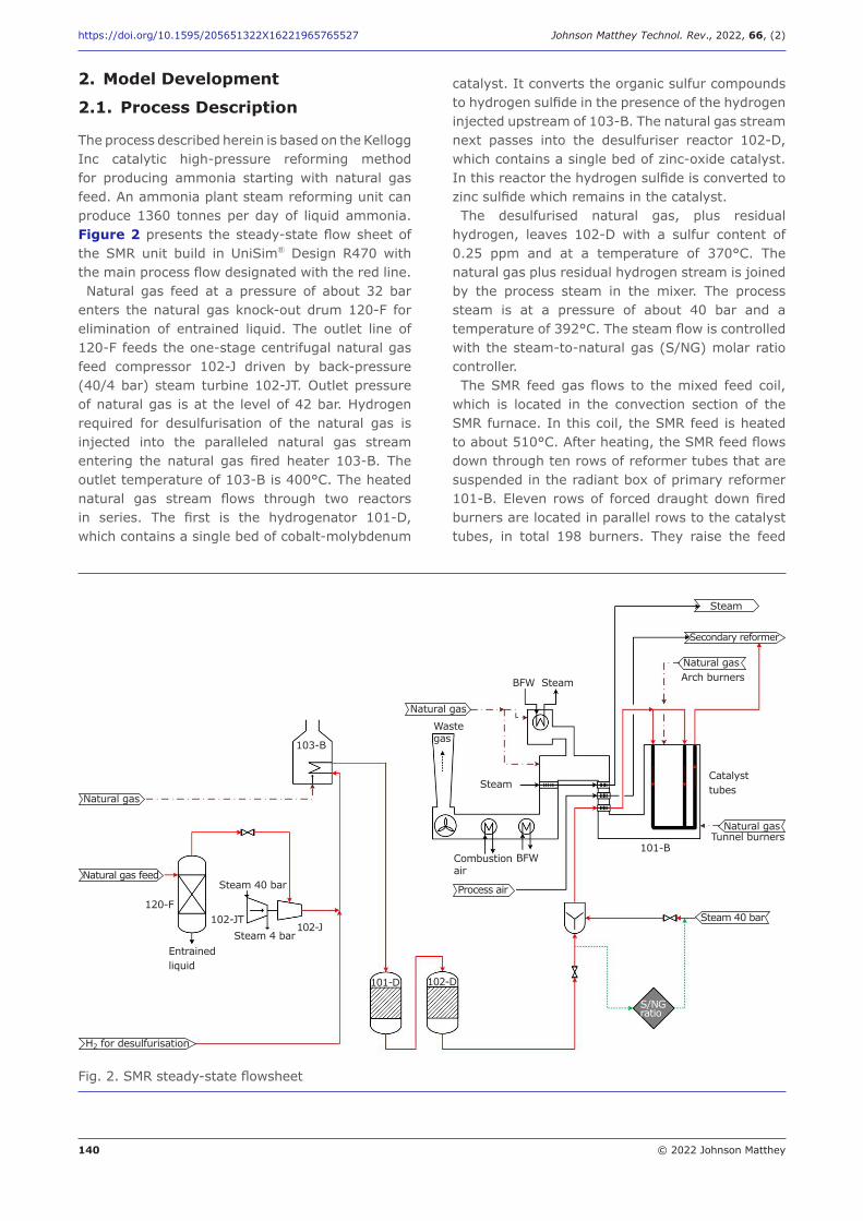
The process described herein is based on the Kellogg Inc catalytic high-pressure reforming method for producing ammonia starting with natural gas feed. An ammonia plant steam reforming unit can produce 1360 tonnes per day of liquid ammonia. Figure 2 presents the steady-state flow sheet of the SMR unit build in UniSim® Design R470 with the main process flow designated with the red line.Natural gas feed at a pressure of about 32 bar
enters the natural gas knock-out drum 120-F for elimination of entrained liquid. The outlet line of 120-F feeds the one-stage centrifugal natural gas feed compressor 102-J driven by back-pressure (40/4 bar) steam turbine 102-JT. Outlet pressure of natural gas is at the level of 42 bar. Hydrogen required for desulfurisation of the natural gas is injected into the paralleled natural gas stream entering the natural gas fired heater 103-B. The outlet temperature of 103-B is 400°C. The heated natural gas stream flows through two reactors in series. The first is the hydrogenator 101-D, which contains a single bed of cobalt-molybdenum
catalyst. It converts the organic sulfur compounds to hydrogen sulfide in the presence of the hydrogen injected upstream of 103-B. The natural gas stream next passes into the desulfuriser reactor 102-D, which contains a single bed of zinc-oxide catalyst. In this reactor the hydrogen sulfide is converted to zinc sulfide which remains in the catalyst.The desulfurised natural gas, plus residual
hydrogen, leaves 102-D with a sulfur content of 0.25 ppm and at a temperature of 370°C. The natural gas plus residual hydrogen stream is joined by the process steam in the mixer. The process steam is at a pressure of about 40 bar and a temperature of 392°C. The steam flow is controlled with the steam-to-natural gas (S/NG) molar ratio controller.The SMR feed gas flows to the mixed feed coil,
which is located in the convection section of the SMR furnace. In this coil, the SMR feed is heated to about 510°C. After heating, the SMR feed flows down through ten rows of reformer tubes that are suspended in the radiant box of primary reformer 101-B. Eleven rows of forced draught down fired burners are located in parallel rows to the catalyst tubes, in total 198 burners. They raise the feed
Natural gas
Fig. 2. SMR steady-state flowsheet
Natural gas
Steam
Secondary reformer
Arch burners
Catalyst tubes
Natural gasTunnel burners
101-BCombustion air
BFW
Steam
SteamBFW
Waste gas
103-B
Steam 40 bar
Natural gas
Natural gas feed
120-F102-JT
Steam 4 barEntrained liquid
H2 for desulfurisation
101-D 102-D
Process air
Steam 40 bar
S/NG ratio
102-J
141 © 2022 Johnson Matthey
https://doi.org/10.1595/205651322X16221965765527 Johnson Matthey Technol. Rev., 2022, 66, (2)
temperature to about 790°C at the outlet of the catalyst tubes. In addition, 11 tunnel burners are used to heat the waste gases passing from the radiant to the convection part of the SMR furnace. 520 catalyst tubes with a total length of 10 m and inside diameter of 0.0857 m contain 30 m3 of nickel reformer catalyst. The reformed gas (syngas) then flows to the secondary reformer for further processing.
2.2. Steam Reforming Model
In order to predict the performance of the SMR process, it is necessary to simulate the tube side process and provide a detailed profile of the heat flux, gas composition, carbon forming potential and the pressure inside of the reformer tubes incrementally. The calculations involve solving material and energy balance equations along with reaction kinetic expressions for the nickel catalyst.The general overall reaction for the steam
reforming of any hydrocarbons can be defined as Equation (i) (1, 2):
CnH(2n+2) + nH2O nCO + (2n+1)H2 (i)
In this work, steam reforming of the natural gas is described with the following equations, as the methane is the major constituent of the natural gas. Equation (ii) (1, 2):
CH4 + H2O CO + 3H2 (ii)
In parallel with this SMR equilibrium, the water gas shift (WGS) reaction proceeds according to Equation (iii) (1, 2):
CO + H2O CO2 + H2 (iii)
Minette et al. (17) in their work stated that the second SMR reaction is often not accounted for assuming it follows directly from combining Equations (i) and (ii). However, the work of Xu and Froment (7–8) showed that the second SMR reaction expressed by Equation (iv) follows an independent reaction path and must be accounted for in combination with Equations (i) and (ii), as confirmed by the measurements of Minette et al. (17):
CH4 + 2H2O CO2 + 4H2 (iv)
As mentioned, the described reactions proceed in indirectly heated reformer tubes filled with nickel-
containing reforming catalyst and are controlled to achieve only a partial methane conversion. In a top fired reformer usually up to 65% to 68% conversion based on methane feed can be accomplished, leaving around 10 mol% to 14 mol% methane per dry basis (1, 2).The overall SMR reaction of methane is
endothermic and proceeds with an increase of volume at the elevated pressure of 20 bar to 40 bar and temperatures from 800°C to 1200°C at the exit of the reformer tubes in the presence of metallic nickel catalyst as an active component. Besides pressure and temperature, the S/NG molar ratio has a beneficial effect on the equilibrium methane concentration (18).Another reason for applying the appropriate
(higher) S/NG molar ratio is to prevent carbon deposition on the reforming catalyst. The side effect of carbon deposition is a higher pressure drop and the reduction of catalyst activity. As the rate of endothermic reaction is lowered, this can cause local overheating of the reformer tubes (hot spots and bands) and the premature failure of the tube walls. The carbon formation may occur via Boudouard reaction, methane cracking and carbon monoxide and carbon dioxide reduction. These reactions are reversible with dynamic equilibrium between carbon formation and removal. Under typical steam reforming conditions, Boudouard reaction and carbon monoxide and carbon dioxide reduction cause carbon removal, whilst methane cracking leads to carbon formation in the upper part of the reformer tube (19). Greenfield SMR units based on natural gas regularly use a S/NG molar ratio of around 3.0, while older installations are in the range from 3.5 to 4.0 (1). From the theoretical point of view any S/NG molar ratio which is slightly over 1.0 will prevent cracking, because the rate of carbon removing reactions is faster than the rate of carbon deposition reactions. However, from the practical point of view (catalyst limitations and sufficient quantity of steam for the downstream process step of WGS conversion), the minimum molar ratio which applies at the industrial level is 2.5. To account for all these facts, the model was validated for S/NG molar ratios in the range from 2.0 to 6.0.The nickel content in relation to the composition
and structure of the support differs considerably from one catalyst supplier to another. This is the reason why it is difficult to relate data from industrial plants to laboratory experiments. Reformer simulations frequently use a numerical approach in which the experimental data serves
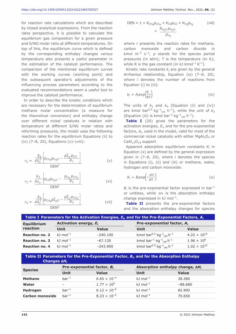
142 © 2022 Johnson Matthey
https://doi.org/10.1595/205651322X16221965765527 Johnson Matthey Technol. Rev., 2022, 66, (2)
for reaction rate calculations which are described by closed analytical expressions. From the reaction rates perspective, it is possible to calculate the equilibrium gas composition for a given pressure and S/NG molar ratio at different temperatures. On top of this, the equilibrium curve which is defined by the corresponding enthalpy changes versus temperature also presents a useful parameter in the estimation of the catalyst performance. The comparison of the mentioned equilibrium curves with the working curves (working point) and the subsequent operator’s adjustments of the influencing process parameters according to the evaluated recommendations seem a useful tool to improve the catalyst performance.In order to describe the kinetic conditions which
are necessary for the determination of equilibrium methane molar concentration (a measure for the theoretical conversion) and enthalpy change over different nickel catalysts in relation with temperature at different S/NG molar ratios and reforming pressures, the model uses the following reaction rates for the equilibrium Equations (ii) to (iv) (7–8, 20), Equations (v)–(viii):
r2 = (v) k2
pH2 pCOpH2 K1
2.5 pCH4pH2O –
DEN2
3
r3 = (vi) k3
pH2 pCO2pH2 K2
pCOpH2O –
DEN2
r4 = (vii) k4
pH2 pCO2pH2 K3
3.5 pCH4pH2O –
DEN2
42
DEN = 1 + KCH4pCH4 + KCOpCO + KH2pH2 (viii)
+ KH2O pH2O
pH2
where r presents the reaction rates for methane, carbon monoxide and carbon dioxide in kmol m–3 s–1; p stands for the species partial pressures (in atm); T is the temperature (in K); while R is the gas constant (in kJ kmol–1 K–1).Kinetic rate constants ki are given by the general
Arrhenius relationship, Equation (ix) (7–8, 20), where i denotes the number of reactions from Equation (i) to (iii):
ki = Aiexp (ix)Ei
RT( )The units of k2 and k4 (Equation (ii) and (iv)) are kmol bar0.5 kg–1
cat h–1), while the unit of k3 (Equation (iii) is kmol bar–1 kg–1
cat h–1).Table I (20) gives the parameters for the
activation energies, Ei, and for the pre-exponential factors, Ai, used in the model, valid for most of the commercial nickel catalysts with either MgAl2O4 or CaAl12O19 support.Apparent adsorption equilibrium constants Ki in
Equation (x) are defined by the general expression given in (7–8, 20), where i denotes the species in Equations (i), (ii) and (iii) or methane, water, hydrogen and carbon monoxide:
Ki = Biexp (x)DHi
RT(– )Bi is the pre-exponential factor expressed in bar-1 or unitless, while ΔHi is the absorption enthalpy change expressed in kJ mol–1.Table II presents the pre-exponential factors
and the absorption enthalpy changes for species
Table I Parameters for the Activation Energies, Ei, and for the Pre-Exponential Factors, Ai
Equilibrium reaction
Activation energy, Ei Pre-exponential factor, Ai Unit Value Unit Value
Reaction no. 2 kJ mol–1 –240.100 kmol bar0.5 kg–1cat
h–1 4.22 × 10¹⁵
Reaction no. 3 kJ mol–1 –67.130 kmol bar–1 kg–1cat
h–1 1.96 × 10⁶
Reaction no. 4 kJ mol–1 –243.900 kmol bar0.5 kg–1cat
h–1 1.02 × 10¹⁵
Table II Parameters for the Pre-Exponential Factor, Bi, and for the Absorption Enthalpy Changes ΔHi
SpeciesPre-exponential factor, Bi Absorption enthalpy change, ΔHi
Unit Value Unit ValueMethane bar–1 6.65 × 10⁻⁴ kJ mol–1 38.280
Water – 1.77 × 10⁵ kJ mol–1 –88.680
Hydrogen bar–1 6.12 × 10⁻⁹ kJ mol–1 82.900
Carbon monoxide bar–1 8.23 × 10⁻⁵ kJ mol–1 70.650
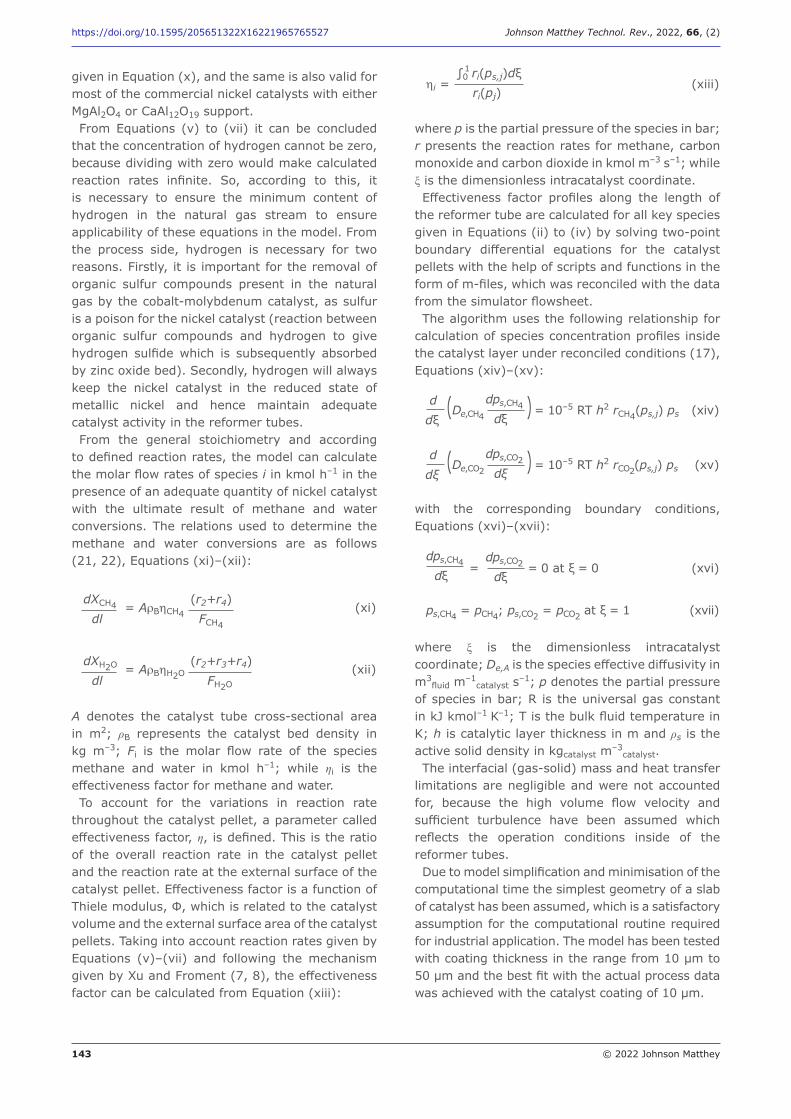
143 © 2022 Johnson Matthey
https://doi.org/10.1595/205651322X16221965765527 Johnson Matthey Technol. Rev., 2022, 66, (2)
given in Equation (x), and the same is also valid for most of the commercial nickel catalysts with either MgAl2O4 or CaAl12O19 support.From Equations (v) to (vii) it can be concluded
that the concentration of hydrogen cannot be zero, because dividing with zero would make calculated reaction rates infinite. So, according to this, it is necessary to ensure the minimum content of hydrogen in the natural gas stream to ensure applicability of these equations in the model. From the process side, hydrogen is necessary for two reasons. Firstly, it is important for the removal of organic sulfur compounds present in the natural gas by the cobalt-molybdenum catalyst, as sulfur is a poison for the nickel catalyst (reaction between organic sulfur compounds and hydrogen to give hydrogen sulfide which is subsequently absorbed by zinc oxide bed). Secondly, hydrogen will always keep the nickel catalyst in the reduced state of metallic nickel and hence maintain adequate catalyst activity in the reformer tubes.From the general stoichiometry and according
to defined reaction rates, the model can calculate the molar flow rates of species i in kmol h–1 in the presence of an adequate quantity of nickel catalyst with the ultimate result of methane and water conversions. The relations used to determine the methane and water conversions are as follows (21, 22), Equations (xi)–(xii):
= ArBhCH4 (xi)dXCH4
dl (r2+r4) FCH4
= ArBhH2O (xii)dXH2O
dl (r2+r3+r4) FH2O
A denotes the catalyst tube cross-sectional area in m2; ρB represents the catalyst bed density in kg m–3; Fi is the molar flow rate of the species methane and water in kmol h–1; while ηi is the effectiveness factor for methane and water.To account for the variations in reaction rate
throughout the catalyst pellet, a parameter called effectiveness factor, η, is defined. This is the ratio of the overall reaction rate in the catalyst pellet and the reaction rate at the external surface of the catalyst pellet. Effectiveness factor is a function of Thiele modulus, Φ, which is related to the catalyst volume and the external surface area of the catalyst pellets. Taking into account reaction rates given by Equations (v)–(vii) and following the mechanism given by Xu and Froment (7, 8), the effectiveness factor can be calculated from Equation (xiii):
∫0 ri(ps,j)dξ ri(pj)
hi = (xiii)1
where p is the partial pressure of the species in bar; r presents the reaction rates for methane, carbon monoxide and carbon dioxide in kmol m–3 s–1; while ξ is the dimensionless intracatalyst coordinate.Effectiveness factor profiles along the length of
the reformer tube are calculated for all key species given in Equations (ii) to (iv) by solving two-point boundary differential equations for the catalyst pellets with the help of scripts and functions in the form of m-files, which was reconciled with the data from the simulator flowsheet. The algorithm uses the following relationship for
calculation of species concentration profiles inside the catalyst layer under reconciled conditions (17), Equations (xiv)–(xv):
(De,CH4 ) = 10–5 RT h2 rCH4(ps,j) ps (xiv) ddξ
dps,CH4
dξ
(De,CO2 ) = 10–5 RT h2 rCO2(ps,j) ps (xv) ddξ
dps,CO2
dξ
with the corresponding boundary conditions, Equations (xvi)–(xvii):
= = 0 at ξ = 0 (xvi)dps,CO2
dξ
dps,CH4
dξ
ps,CH4 = pCH4; ps,CO2 = pCO2 at ξ = 1 (xvii)
where ξ is the dimensionless intracatalyst coordinate; De,A is the species effective diffusivity in m3
fluid m–1catalyst s–1; p denotes the partial pressure
of species in bar; R is the universal gas constant in kJ kmol–1 K–1; T is the bulk fluid temperature in K; h is catalytic layer thickness in m and ρs is the active solid density in kgcatalyst m–3
catalyst.The interfacial (gas-solid) mass and heat transfer
limitations are negligible and were not accounted for, because the high volume flow velocity and sufficient turbulence have been assumed which reflects the operation conditions inside of the reformer tubes.Due to model simplification and minimisation of the
computational time the simplest geometry of a slab of catalyst has been assumed, which is a satisfactory assumption for the computational routine required for industrial application. The model has been tested with coating thickness in the range from 10 μm to 50 μm and the best fit with the actual process data was achieved with the catalyst coating of 10 μm.
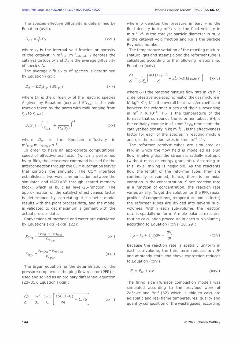
144 © 2022 Johnson Matthey
https://doi.org/10.1595/205651322X16221965765527 Johnson Matthey Technol. Rev., 2022, 66, (2)
The species effective diffusivity is determined by Equation (xviii):
De,A = DA (xviii)est
where εs is the internal void fraction or porosity of the catalyst in m3
fluid m–3catalyst; τ denotes the
catalyst tortuosity and DA is the average diffusivity of species A.The average diffusivity of species is determined
by Equation (xix):
DA = SiDA(rp,i) S(rp,i) (xix)
where DA is the diffusivity of the reacting species A given by Equation (xx) and S(rp,i) is the void fraction taken by the pores with radii ranging from rp,i to rp,i+1:
DA(rp) = ( + )–1 (xx)
1 1DmA DkA(rp)
where DkA is the Knudsen diffusivity in m3
fluid m–1catalyst s–1.
In order to have an appropriate computational speed of effectiveness factor (which is performed by m-file), the actxserver command is used for the interconnection through the COM automation server that controls the simulator. The COM interface establishes a two-way communication between the simulator and MATLAB® through shared memory block, which is built as level-2S-function. The approximation of the catalyst effectiveness factor is determined by correlating the kinetic model results with the plant process data, and the model is validated to get maximum alignment with the actual process data. Conversions of methane and water are calculated
by Equations (xxi)–(xxii) (22):
XCH4 = (xxi)FCH4in – FCH4out
FCH4in
XH2O = (xxii)FH2Oin – FH2Oout
FH2Oin
The Ergun equation for the determination of the pressure drop across the plug flow reactor (PFR) is used and solved as an ordinary differential equation (23–31), Equation (xxiii):
= + 1.75 (xxiii)dp rn2 1 – Є 150(1 – Є)dl dp Є Re
where p denotes the pressure in bar; ρ is the fluid density in kg m–3; v is the fluid velocity in m s–1; dp is the catalyst particle diameter in m; є is the catalyst void fraction and Re is the particle Reynolds number.The temperature variation of the reacting mixture
(natural gas and steam) along the reformer tube is calculated according to the following relationship, Equation (xxiv):
= ( + Si=1(–DHi) rbhi ri ) (xxiv)dT 1 4U (Tt,0–T)dl G cp di
3
where G is the reacting mixture flow rate in kg h–1; cp denotes average specific heat of the gas mixture in kJ kg–1 K–1; U is the overall heat transfer coefficient between the reformer tubes and their surrounding in m2 h K kJ–1; Tt,0 is the temperature of the furnace that surrounds the reformer tubes; ΔHi is the enthalpy change in kJ kmol–1; ρB represents the catalyst bed density in kg m–3; ηi is the effectiveness factor for each of the species in reacting mixture and ri is the reaction rates in kmol m–3 s–1.The reformer catalyst tubes are simulated as
PFR in which the flow field is modelled as plug flow, implying that the stream is radially isotropic (without mass or energy gradients). According to this, axial mixing is negligible. As the reactants flow the length of the reformer tube, they are continually consumed, hence, there is an axial variation in the concentration. Since reaction rate is a function of concentration, the reaction rate varies axially. To get the solution for the PFR (axial profiles of compositions, temperature and so forth) the reformer tubes are divided into several sub-volumes. Within each sub-volume, the reaction rate is spatially uniform. A mole balance executes routine calculation procedure in each sub-volume j according to Equation (xxv) (28, 29):
Fj0 – Fj + ∫V rjdV = (xxv)
dNj
dt
Because the reaction rate is spatially uniform in each sub-volume, the third term reduces to rjdV and at steady state, the above expression reduces to Equation (xxvi):
Fj = Fj0 + rjV (xxvi)
The firing side (furnace combustion model) was simulated according to the previous work of Zečević and Bolf (32) which is able to calculate adiabatic and real flame temperatures, quality and quantity composition of the waste gases, according
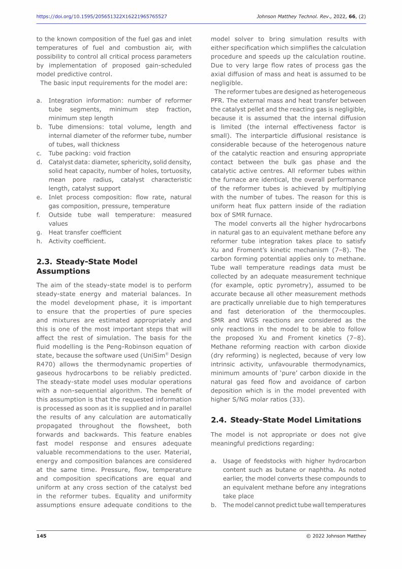
145 © 2022 Johnson Matthey
https://doi.org/10.1595/205651322X16221965765527 Johnson Matthey Technol. Rev., 2022, 66, (2)
to the known composition of the fuel gas and inlet temperatures of fuel and combustion air, with possibility to control all critical process parameters by implementation of proposed gain-scheduled model predictive control.The basic input requirements for the model are:
a. Integration information: number of reformer tube segments, minimum step fraction, minimum step length
b. Tube dimensions: total volume, length and internal diameter of the reformer tube, number of tubes, wall thickness
c. Tube packing: void fractiond. Catalyst data: diameter, sphericity, solid density,
solid heat capacity, number of holes, tortuosity, mean pore radius, catalyst characteristic length, catalyst support
e. Inlet process composition: flow rate, natural gas composition, pressure, temperature
f. Outside tube wall temperature: measured values
g. Heat transfer coefficienth. Activity coefficient.
2.3. Steady-State Model Assumptions
The aim of the steady-state model is to perform steady-state energy and material balances. In the model development phase, it is important to ensure that the properties of pure species and mixtures are estimated appropriately and this is one of the most important steps that will affect the rest of simulation. The basis for the fluid modelling is the Peng-Robinson equation of state, because the software used (UniSim® Design R470) allows the thermodynamic properties of gaseous hydrocarbons to be reliably predicted. The steady-state model uses modular operations with a non-sequential algorithm. The benefit of this assumption is that the requested information is processed as soon as it is supplied and in parallel the results of any calculation are automatically propagated throughout the flowsheet, both forwards and backwards. This feature enables fast model response and ensures adequate valuable recommendations to the user. Material, energy and composition balances are considered at the same time. Pressure, flow, temperature and composition specifications are equal and uniform at any cross section of the catalyst bed in the reformer tubes. Equality and uniformity assumptions ensure adequate conditions to the
model solver to bring simulation results with either specification which simplifies the calculation procedure and speeds up the calculation routine. Due to very large flow rates of process gas the axial diffusion of mass and heat is assumed to be negligible. The reformer tubes are designed as heterogeneous
PFR. The external mass and heat transfer between the catalyst pellet and the reacting gas is negligible, because it is assumed that the internal diffusion is limited (the internal effectiveness factor is small). The interparticle diffusional resistance is considerable because of the heterogenous nature of the catalytic reaction and ensuring appropriate contact between the bulk gas phase and the catalytic active centres. All reformer tubes within the furnace are identical, the overall performance of the reformer tubes is achieved by multiplying with the number of tubes. The reason for this is uniform heat flux pattern inside of the radiation box of SMR furnace.The model converts all the higher hydrocarbons
in natural gas to an equivalent methane before any reformer tube integration takes place to satisfy Xu and Froment’s kinetic mechanism (7–8). The carbon forming potential applies only to methane. Tube wall temperature readings data must be collected by an adequate measurement technique (for example, optic pyrometry), assumed to be accurate because all other measurement methods are practically unreliable due to high temperatures and fast deterioration of the thermocouples. SMR and WGS reactions are considered as the only reactions in the model to be able to follow the proposed Xu and Froment kinetics (7–8). Methane reforming reaction with carbon dioxide (dry reforming) is neglected, because of very low intrinsic activity, unfavourable thermodynamics, minimum amounts of ‘pure’ carbon dioxide in the natural gas feed flow and avoidance of carbon deposition which is in the model prevented with higher S/NG molar ratios (33).
2.4. Steady-State Model Limitations
The model is not appropriate or does not give meaningful predictions regarding:
a. Usage of feedstocks with higher hydrocarbon content such as butane or naphtha. As noted earlier, the model converts these compounds to an equivalent methane before any integrations take place
b. The model cannot predict tube wall temperatures
146 © 2022 Johnson Matthey
https://doi.org/10.1595/205651322X16221965765527 Johnson Matthey Technol. Rev., 2022, 66, (2)
and these must be assumed or measured in the plant
c. The model cannot provide any information about hot spot or hot band problems in the furnace.
3. Results and Discussion
The first step of this research is to simulate a chemical reaction system of the SMR operation in an ammonia plant by an appropriate commercial simulator and by application of scripts and functions in the accompanying m-file. The next step is the validation of the simulation results with the literature and process data from a real plant which uses commercially available reforming catalyst. The final and major step is to ensure adequate recommendations for adjustment of the process parameters during SMR operation which will bring the working curve of reforming catalyst performance much closer to the equilibrium curve (working point).In order to perform model testing, the process
parameters from the reference case (ammonia plant in Kutina, Croatia, owned by Petrokemija Plc) were used for the model validation. Table III presents the necessary input variables. This is the basis for the calculation of the equilibrium curves at different S/NG molar ratios, outlet temperatures, pressures and heat load. One part of the process information must be manually entered, while the other part is automatically fed from the DSC system (Table III).As mentioned, the primary aim of this work
is to provide process operators with adequate recommendations or advice which will enable them to adjust critical process parameters during SMR operation. With adequate change of process parameters, the working curve (working point) of the reformer catalyst will be brought as much as possible close to the theoretical equilibrium curve with the ultimate goal to improve the reformer catalyst performance and the overall conversion of the SMR endothermic reaction. In order to extract the maximum possible performance of the reformer catalyst, operators will have the possibility to adjust the methane outlet molar concentration and temperature ATE by changing the S/NG molar ratio, heat load or by adjusting the fuel flow distribution to the reformer tubes respectively.Figures 3 and 4 show the relationship between
theoretical equilibrium methane molar concentration (a measure for the theoretical conversion) and temperature, S/NG molar ratios and reforming
pressure which is relevant for the endothermic SMR reaction in the industrially interesting range. Simulated results in Figures 3 and 4 show a visible standard pattern of SMR reaction. Namely, at constant reforming pressure, higher S/NG molar ratios and higher temperatures have a beneficial effect on the equilibrium methane molar concentration, but the penalty is a higher energy consumption on account of higher steam mass flow and higher consumption of the fuel gas in the primary reformer furnace. The higher S/NG molar ratio prevents carbon deposition on the catalyst, which may not only increase the pressure drop but also reduce the catalyst activity. On account of this, local reformer tubes overheating (hot spots or bands) will be minimised. In contrast to this, higher temperature will cause higher tube wall temperatures and consequently the shorter lifetime of the reformer tubes due to creep damage and stress as well as rupture.Because the natural gas and steam are at high
pressure and the SMR reaction entails an increase in volume, significant savings in compression energy can be achieved if the process operates under elevated pressure. However, thermodynamically, this is unfavourable. Figure 4 shows results of the model test regarding the changes in reforming pressure (on account of the volume increase) versus methane theoretical equilibrium outlet molar concentration. Three different pressures at constant S/NG molar ratio were tested, namely 20 bar, 30 bar and 35 bar, which are common industrial pressure levels.It is also very important to determine the
quantity of heat load to the reformer tubes and to the related catalyst, which will secure sufficient heat for endothermic SMR reaction. Figure 5 shows the relationship between heat load and temperature at different S/NG molar ratios and constant pressure of 30 bar. The major goal is achieving the theoretical methane equilibrium concentrations.From the simulated results, it can be seen that
for higher S/NG molar ratios a higher input of heat load to achieve theoretical methane equilibrium molar concentrations is needed. This effect comes on account of higher feed gas volume flow because of a higher steam mass flow. Although a higher quantity of steam will shift SMR reaction in a favourable direction, consequently it will demand more energy to keep the same methane equilibrium molar concentration, which in the end will have a detrimental effect on the tube wall temperature.
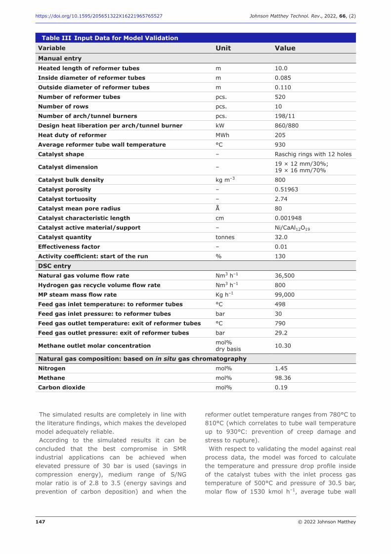
147 © 2022 Johnson Matthey
https://doi.org/10.1595/205651322X16221965765527 Johnson Matthey Technol. Rev., 2022, 66, (2)
The simulated results are completely in line with the literature findings, which makes the developed model adequately reliable.According to the simulated results it can be
concluded that the best compromise in SMR industrial applications can be achieved when elevated pressure of 30 bar is used (savings in compression energy), medium range of S/NG molar ratio is of 2.8 to 3.5 (energy savings and prevention of carbon deposition) and when the
reformer outlet temperature ranges from 780°C to 810°C (which correlates to tube wall temperature up to 930°C: prevention of creep damage and stress to rupture).With respect to validating the model against real
process data, the model was forced to calculate the temperature and pressure drop profile inside of the catalyst tubes with the inlet process gas temperature of 500°C and pressure of 30.5 bar, molar flow of 1530 kmol h–1, average tube wall
Table III Input Data for Model ValidationVariable Unit ValueManual entryHeated length of reformer tubes m 10.0
Inside diameter of reformer tubes m 0.085
Outside diameter of reformer tubes m 0.110
Number of reformer tubes pcs. 520
Number of rows pcs. 10
Number of arch/tunnel burners pcs. 198/11
Design heat liberation per arch/tunnel burner kW 860/880
Heat duty of reformer MWh 205
Average reformer tube wall temperature °C 930
Catalyst shape – Raschig rings with 12 holes
Catalyst dimension – 19 × 12 mm/30%; 19 × 16 mm/70%
Catalyst bulk density kg m–3 800
Catalyst porosity – 0.51963
Catalyst tortuosity – 2.74
Catalyst mean pore radius Å 80
Catalyst characteristic length cm 0.001948
Catalyst active material/support – Ni/CaAl12O19
Catalyst quantity tonnes 32.0
Effectiveness factor – 0.01
Activity coefficient: start of the run % 130
DSC entryNatural gas volume flow rate Nm3 h–1 36,500
Hydrogen gas recycle volume flow rate Nm3 h–1 800
MP steam mass flow rate Kg h–1 99,000
Feed gas inlet temperature: to reformer tubes °C 498
Feed gas inlet pressure: to reformer tubes bar 30
Feed gas outlet temperature: exit of reformer tubes °C 790
Feed gas outlet pressure: exit of reformer tubes bar 29.2
Methane outlet molar concentration mol% dry basis 10.30
Natural gas composition: based on in situ gas chromatographyNitrogen mol% 1.45
Methane mol% 98.36
Carbon dioxide mol% 0.19
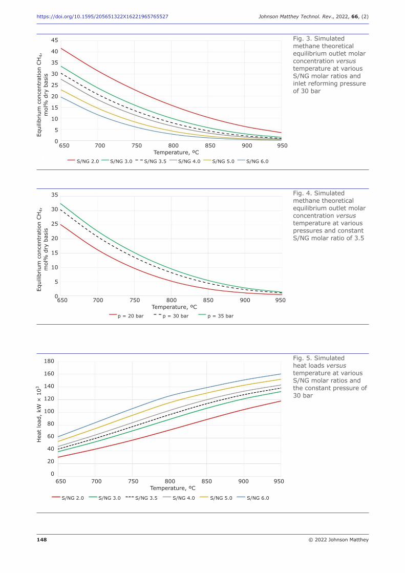
148 © 2022 Johnson Matthey
https://doi.org/10.1595/205651322X16221965765527 Johnson Matthey Technol. Rev., 2022, 66, (2)
45
40
35
30
25
20
15
10
5
0
Equi
librium
con
cent
ratio
n CH
4,
mol
% d
ry b
asis
Fig. 3. Simulated methane theoretical equilibrium outlet molar concentration versus temperature at various S/NG molar ratios and inlet reforming pressure of 30 bar
650 700 750 800 850 900 950Temperature, ºC
S/NG 2.0 S/NG 3.0 S/NG 3.5 S/NG 4.0 S/NG 5.0 S/NG 6.0
35
30
25
20
15
10
5
0
Equi
librium
con
cent
ratio
n CH
4,
mol
% d
ry b
asis
Fig. 4. Simulated methane theoretical equilibrium outlet molar concentration versus temperature at various pressures and constant S/NG molar ratio of 3.5
650 700 750 800 850 900 950Temperature, ºC
p = 20 bar p = 30 bar p = 35 bar
180
160
140
120
100
80
60
40
20
0
Hea
t lo
ad,
kW ×
103
Fig. 5. Simulated heat loads versus temperature at various S/NG molar ratios and the constant pressure of 30 bar
650 700 750 800 850 900 950Temperature, ºC
S/NG 2.0 S/NG 3.0 S/NG 3.5 S/NG 4.0 S/NG 5.0 S/NG 6.0
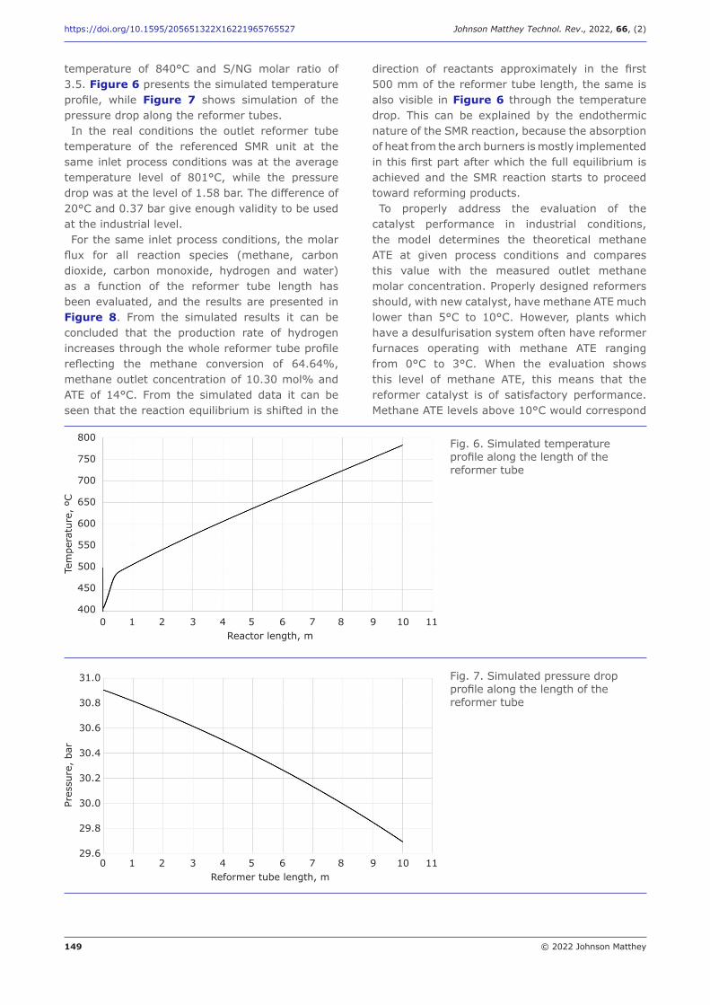
149 © 2022 Johnson Matthey
https://doi.org/10.1595/205651322X16221965765527 Johnson Matthey Technol. Rev., 2022, 66, (2)
temperature of 840°C and S/NG molar ratio of 3.5. Figure 6 presents the simulated temperature profile, while Figure 7 shows simulation of the pressure drop along the reformer tubes.In the real conditions the outlet reformer tube
temperature of the referenced SMR unit at the same inlet process conditions was at the average temperature level of 801°C, while the pressure drop was at the level of 1.58 bar. The difference of 20°C and 0.37 bar give enough validity to be used at the industrial level.For the same inlet process conditions, the molar
flux for all reaction species (methane, carbon dioxide, carbon monoxide, hydrogen and water) as a function of the reformer tube length has been evaluated, and the results are presented in Figure 8. From the simulated results it can be concluded that the production rate of hydrogen increases through the whole reformer tube profile reflecting the methane conversion of 64.64%, methane outlet concentration of 10.30 mol% and ATE of 14°C. From the simulated data it can be seen that the reaction equilibrium is shifted in the
direction of reactants approximately in the first 500 mm of the reformer tube length, the same is also visible in Figure 6 through the temperature drop. This can be explained by the endothermic nature of the SMR reaction, because the absorption of heat from the arch burners is mostly implemented in this first part after which the full equilibrium is achieved and the SMR reaction starts to proceed toward reforming products.To properly address the evaluation of the
catalyst performance in industrial conditions, the model determines the theoretical methane ATE at given process conditions and compares this value with the measured outlet methane molar concentration. Properly designed reformers should, with new catalyst, have methane ATE much lower than 5°C to 10°C. However, plants which have a desulfurisation system often have reformer furnaces operating with methane ATE ranging from 0°C to 3°C. When the evaluation shows this level of methane ATE, this means that the reformer catalyst is of satisfactory performance. Methane ATE levels above 10°C would correspond
800
750
700
650
600
550
500
450
400
Tem
pera
ture
, ºC
Fig. 6. Simulated temperature profile along the length of the reformer tube
0 1 2 3 4 5 6 7 8 9 10 11Reactor length, m
31.0
30.8
30.6
30.4
30.2
30.0
29.8
29.6
Pres
sure
, ba
r
Fig. 7. Simulated pressure drop profile along the length of the reformer tube
0 1 2 3 4 5 6 7 8 9 10 11Reformer tube length, m
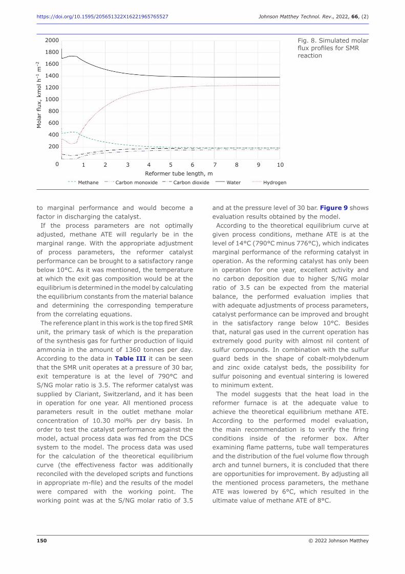
150 © 2022 Johnson Matthey
https://doi.org/10.1595/205651322X16221965765527 Johnson Matthey Technol. Rev., 2022, 66, (2)
to marginal performance and would become a factor in discharging the catalyst.If the process parameters are not optimally
adjusted, methane ATE will regularly be in the marginal range. With the appropriate adjustment of process parameters, the reformer catalyst performance can be brought to a satisfactory range below 10°C. As it was mentioned, the temperature at which the exit gas composition would be at the equilibrium is determined in the model by calculating the equilibrium constants from the material balance and determining the corresponding temperature from the correlating equations.The reference plant in this work is the top fired SMR
unit, the primary task of which is the preparation of the synthesis gas for further production of liquid ammonia in the amount of 1360 tonnes per day. According to the data in Table III it can be seen that the SMR unit operates at a pressure of 30 bar, exit temperature is at the level of 790°C and S/NG molar ratio is 3.5. The reformer catalyst was supplied by Clariant, Switzerland, and it has been in operation for one year. All mentioned process parameters result in the outlet methane molar concentration of 10.30 mol% per dry basis. In order to test the catalyst performance against the model, actual process data was fed from the DCS system to the model. The process data was used for the calculation of the theoretical equilibrium curve (the effectiveness factor was additionally reconciled with the developed scripts and functions in appropriate m-file) and the results of the model were compared with the working point. The working point was at the S/NG molar ratio of 3.5
and at the pressure level of 30 bar. Figure 9 shows evaluation results obtained by the model.According to the theoretical equilibrium curve at
given process conditions, methane ATE is at the level of 14°C (790°C minus 776°C), which indicates marginal performance of the reforming catalyst in operation. As the reforming catalyst has only been in operation for one year, excellent activity and no carbon deposition due to higher S/NG molar ratio of 3.5 can be expected from the material balance, the performed evaluation implies that with adequate adjustments of process parameters, catalyst performance can be improved and brought in the satisfactory range below 10°C. Besides that, natural gas used in the current operation has extremely good purity with almost nil content of sulfur compounds. In combination with the sulfur guard beds in the shape of cobalt-molybdenum and zinc oxide catalyst beds, the possibility for sulfur poisoning and eventual sintering is lowered to minimum extent.The model suggests that the heat load in the
reformer furnace is at the adequate value to achieve the theoretical equilibrium methane ATE. According to the performed model evaluation, the main recommendation is to verify the firing conditions inside of the reformer box. After examining flame patterns, tube wall temperatures and the distribution of the fuel volume flow through arch and tunnel burners, it is concluded that there are opportunities for improvement. By adjusting all the mentioned process parameters, the methane ATE was lowered by 6°C, which resulted in the ultimate value of methane ATE of 8°C.
2000
1800
1600
1400
1200
1000
800
600
400
200
0
Mol
ar fl
ux,
kmol
h–1
m–2
Fig. 8. Simulated molar flux profiles for SMR reaction
1 2 3 4 5 6 7 8 9 10Reformer tube length, m
Methane Carbon monoxide Carbon dioxide Water Hydrogen
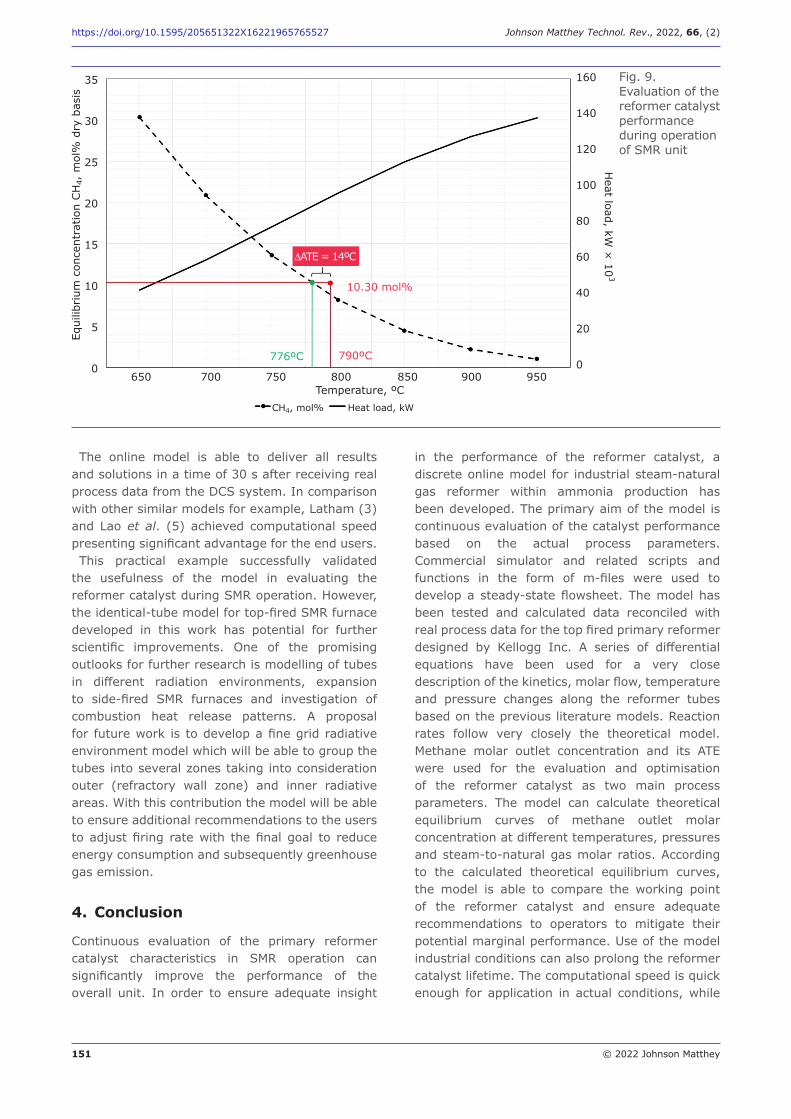
151 © 2022 Johnson Matthey
https://doi.org/10.1595/205651322X16221965765527 Johnson Matthey Technol. Rev., 2022, 66, (2)
The online model is able to deliver all results and solutions in a time of 30 s after receiving real process data from the DCS system. In comparison with other similar models for example, Latham (3) and Lao et al. (5) achieved computational speed presenting significant advantage for the end users.This practical example successfully validated
the usefulness of the model in evaluating the reformer catalyst during SMR operation. However, the identical-tube model for top-fired SMR furnace developed in this work has potential for further scientific improvements. One of the promising outlooks for further research is modelling of tubes in different radiation environments, expansion to side-fired SMR furnaces and investigation of combustion heat release patterns. A proposal for future work is to develop a fine grid radiative environment model which will be able to group the tubes into several zones taking into consideration outer (refractory wall zone) and inner radiative areas. With this contribution the model will be able to ensure additional recommendations to the users to adjust firing rate with the final goal to reduce energy consumption and subsequently greenhouse gas emission.
4. Conclusion
Continuous evaluation of the primary reformer catalyst characteristics in SMR operation can significantly improve the performance of the overall unit. In order to ensure adequate insight
in the performance of the reformer catalyst, a discrete online model for industrial steam-natural gas reformer within ammonia production has been developed. The primary aim of the model is continuous evaluation of the catalyst performance based on the actual process parameters. Commercial simulator and related scripts and functions in the form of m-files were used to develop a steady-state flowsheet. The model has been tested and calculated data reconciled with real process data for the top fired primary reformer designed by Kellogg Inc. A series of differential equations have been used for a very close description of the kinetics, molar flow, temperature and pressure changes along the reformer tubes based on the previous literature models. Reaction rates follow very closely the theoretical model. Methane molar outlet concentration and its ATE were used for the evaluation and optimisation of the reformer catalyst as two main process parameters. The model can calculate theoretical equilibrium curves of methane outlet molar concentration at different temperatures, pressures and steam-to-natural gas molar ratios. According to the calculated theoretical equilibrium curves, the model is able to compare the working point of the reformer catalyst and ensure adequate recommendations to operators to mitigate their potential marginal performance. Use of the model industrial conditions can also prolong the reformer catalyst lifetime. The computational speed is quick enough for application in actual conditions, while
35
30
25
20
15
10
5
0
Equi
librium
con
cent
ratio
n CH
4, m
ol%
dry
bas
isFig. 9. Evaluation of the reformer catalyst performance during operation of SMR unit
650 700 750 800 850 900 950Temperature, ºC
CH4, mol% Heat load, kW
10.30 mol%
790ºC
DATE = 14ºC
776ºC
160
140
120
100
80
60
40
20
0
Heat load, kW
× 10
3

152 © 2022 Johnson Matthey
https://doi.org/10.1595/205651322X16221965765527 Johnson Matthey Technol. Rev., 2022, 66, (2)
the output recommendations are simple enough to be used by working staff. The present paper brings innovation for easier implementation of an online model in an SMR unit, with possibility to ensure adequate recommendations for process parameters adjustment with respect to better catalyst performance. The related calculation method with benefit of a fast communication routine can significantly improve productivity and uptime and subsequently remediate plant performance deviations with possibility to recognise major catalyst efficiencies.
References
1. M. Appl, “Ammonia: Principles and Industrial Practice”, Wiley-VCH Verlag GmbH, Weinheim, Germany, 1999, 301 pp
2. “Catalyst Handbook”, ed. M. V. Twigg, 2nd Edn., CRC Press, Boca Raton, USA, 1989
3. D. Latham, “Mathematical Modelling of an Industrial Steam Methane Reformer”, Master’s Thesis, Department of Chemical Engineering, Queen’s University, Kingston, Canada, December, 2008, 279 pp
Glossary
A reformer tube cross sectional area; m2
Ai pre-exponential factor; kmol bar5 kg–1cat
h–1 or kmol kg–1cat bar–1 h–1
ATE approach to equilibrium; °C or K
Bj pre-exponential factor; bar–1
Cat catalyst
CH4 methane
CO carbon monoxide
CO2 carbon dioxide
CFD computational fluid dynamics
COM component object model
Cp,i specific heat capacity of process gas i; kJ kmol–1 K–1
DA diffusivity of the reacting species A
DkA Knudsen diffusivity; m3fluid m–1
catalyst s–1
De,CH4 effective diffusivity; m3fluid m–1
catalyst s–1
DA average diffusivity of species A
DCS distributed control system
DEN denominator
Ei activation energy; kJ mol–1
Fi molar flow rate; kmol h–1
G mass velocity of the process gas; kg m–2 h–1
H catalytic layer thickness; m
H2O water
H2 hydrogen
Ki adsorption constants for component i; bar–1
Keqi equilibrium constants for SR and WGS
ki rate coefficient for reaction; kmol bar5 kg–1
cat h–1 or kmol kg–1cat bar–1
L reformer tube heated length; m
M mass; kg or tonnes
M molecular weight; kg kmol–1
P pressure and partial pressure; Pa, bar or atm
pi partial pressure of component i; bar
PFR plug flow reactor
R gas constant; kJ kmol–1 K–1
Re Reynolds number
rCO, CO2, CH4, H2
rate of formation and disappearance; kmol kg–1
cat h–1
ri rate of chemical reaction; kmol kg–1
cat h–1
rp,i pore radii
S(rp,i) void fraction
S/NG steam-to-natural gas molar ratio
SMR steam methane reforming
T temperature; °C or K
TSK reformer tube skin temperature; K
t time; s, min or h
U heat transfer capacity; kJ m–2 h–1 K–1
v velocity of the fluid; m s–1
XCH4, H2O molar rate of conversion; mol%
WGS water gas shift
ΔHº298 enthalpy change at 298 K; kJ mol–1
αi convective heat transfer coefficient in the preheated bed; kJ m–2 h–1 K–1
є catalyst bed voidage or porosity; m3
fluid m–3cat
λg process gas thermal conductivity; kJ m–1 h–1 K–1
λst tube metal thermal conductivity; kJ m–2 h–1 K–1
μ dynamic viscosity of the fluid; Pa s, N s m–2 or kg m–1 s–1
ηCH4, H2O constant effectiveness factor
ρ fluid density; kg m–3
ρB catalyst bed density; kg m–3
Φ Thiele modulus
ξ intracatalyst coordinate
τ catalyst tortuosity
153 © 2022 Johnson Matthey
https://doi.org/10.1595/205651322X16221965765527 Johnson Matthey Technol. Rev., 2022, 66, (2)
4. A. Aguirre, “Computational Fluid Dynamics Modelling and Simulation of Steam Methane Reforming Reactors and Furnaces”, PhD Thesis, Department of Chemical and Biomolecular Engineering, University of California, Los Angeles, USA, 2017, 223 pp
5. L. Lao, A. Aguirre, A. Tran, Z. Wu, H. Durand and P. D. Christofides, Chem. Eng. Sci., 2016, 148, 78
6. J. E. Holt, J. K. Kreusser, A. Herritsch and M. Watson, ANZIAM J., 2017, 59, C112
7. J. Xu and G. F. Froment, AIChE J., 1989, 35, (1), 97
8. J. Xu and G. F. Froment, AIChE J., 1989, 35, (1), 88
9. Z. Wu, A. Aguirre, A. Tran, H. Durand, D. Ni and P. D. Christofides, Ind. Eng. Chem. Res., 2017, 56, (20), 6002
10. L. Sun, “Modelling and MPC for a Primary Gas Reformer”, Masters Thesis, Department of Chemical and Materials Engineering, University of Alberta, Edmonton, Canada, 2013, 88 pp
11. A. Meziou, P. B. Deshpande and I. M. Alatiqi, Int. J. Hydrogen Energy, 1995, 20, (3), 187
12. I. M. Alatiqi and A. M. Meziou, Comput. Chem. Eng., 1991, 15, (3), 147
13. C. M. Schillmoller and U. W. van den Bruck, Hydrocarbon Proc., 1984, 63, (12), 55
14. N. A. El Moneim, I. Ismail and M. M. Nasser, Int. J. Novel Res. Dev., 2018, 3, 11
15. D. A. Latham, K. B. McAuley, B. A. Peppley and T. M. Raybold, Fuel Process. Technol., 2011, 92, (8), 1574
16. J. S. Lee, J. Seo, H. Y. Kim, J. T. Chung and S. S. Yoon, Fuel, 2013, 111, 461
17. F. Minette, M. Lugo-Pimentel, D. Modroukas, A. W. Davis, R. Gill, M. J. Castaldi and J. De Wilde, Appl. Catal. B: Environ., 2018, 238, 184
18. J. R. Rostrup-Nielsen, J. Sehested and J. K.Nørskov, Adv. Catal., 2002, 47, 65
19. A. J. Forester and B. J. Cromarty, ‘Theory and Practice of Steam Reforming’, ICI/Katalco/KTI, UOP, 3rd Annual International Seminar of Hydrogen Plant Operation, 7th–9th June, 1995, Chicago, USA, 1995
20. S. Z. Abbas, V. Dupont and T. Mahmud, Int. J. Hydrogen Energy, 2017, 42, (5), 2889
21. J. Rostrup-Nielsen and L. J. Christiansen, “Concepts in Syngas Manufacture”, ed. G. J. Hutchins, Vol. 10, Catalytic Science Series, Imperial College Press, London, UK, 2011
22. S. S. E. H. Elnashaie and F. Uhlig, “Numerical Techniques for Chemical and Biological Engineers Using MATLAB®: A Simple Bifurcation Approach”, Springer Science and Business Media LLC, New York, USA, 2007, 588 pp
23. A. Olivieri and F. Vegliò, Fuel Process. Technol., 2008, 89, (6), 622
24. F. M. Alhabdan, M. A. Abashar and S. S. E. Elnashaie, Math. Comput. Model., 1992, 16, (11), 77
25. S. S. E. H. Elnashaie and S. S. Elshishini, “Modelling, Simulation and Optimization of Industrial Fixed Bed Catalytic Reactors”, Topics in Chemical Engineering, Vol. 7, Gordon and Breach Science Publishers SA, Yverdon, Switzerland, 1993
26. E. L. Cussler, “Diffusion: Mass Transfer in Fluid Systems”, 2nd Edn., Cambridge University Press, Cambridge, UK, 1997, 580 pp
27. E. B. Nauman, “Chemical Reactor Design, Optimization, and Scaleup”, 2nd Edn., John Wiley and Sons Inc, Hoboken, USA, 2008, 608 pp
28. G. M. Hampson, Chem. Eng., 1979, 523
29. G. F. Froment, K. B. Bischoff and J. De Wilde, “Chemical Reactor Analysis and Design”, 3rd Edn., John Wiley and Sons, New York, NY, USA, 2010, 606 pp
30. S. S. E. H. Elnashaie and A. Adris, “Fluidized Bed Steam Reformer for Methane”, Proceedings of the IV International Fluidization Conference, Banff, Canada, May, 1989
31. S. S. E. H. Elnashaie, A. M. Adris, M. A. Soliman and A. S. Al-Ubaid, Can. J. Chem. Eng., 1992, 70, (4), 786
32. N. Zecevic and N. Bolf, Ind. Eng. Chem. Res., 2020, 59, (8), 3458
33. J.-M. Lavoie, Front. Chem., 2014, 2, 81
The Author
Nenad Zečević joined Petrokemija Plc, Croatia, in 1999 after he obtained his Master’s degree in Chemical Engineering from the University of Zagreb, Faculty of Natural Sciences, Croatia. Having worked as an ammonia plant manager, he is currently a Production & Maintenance Manager with 20 years of operational experience in the fertiliser industry. He is also a PhD candidate from the University of Zagreb, Faculty of Chemical Engineering and Technology, Croatia with the thesis Advancement of Process Control System in Ammonia Production.
www.technology.matthey.com
https://doi.org/10.1595/205651322X16257309767812 Johnson Matthey Technol. Rev., 2022, 66, (2), 154–163
154 © 2022 Johnson Matthey
Joseph Emerson*, Vincenzino Vivacqua§, Hugh Stitt†
Johnson Matthey, PO Box 1 Belasis Avenue, Billingham, TS23 1LB, UK
Email: *[email protected], §[email protected], †[email protected]
PEER REVIEWED
Received 6th May 2021; Revised 5th July 2021; Accepted 7th July 2021; Online 8th July 2021
In the manufacture of pelleted catalyst products, controlling physical properties of the pellets and limiting their variability is of critical importance. To achieve tight control over these critical quality attributes (CQAs), it is necessary to understand their relationship with the properties of the powder feed and the pelleting process parameters (PPs). This work explores the latter, using standard multivariate methods to gain a better understanding of the sources of process variability and the impact of PPs on the density and strength of the resulting pellets. A compaction simulator machine was used to produce over 1000 pellets, whose properties were measured, with varied powder feed mechanism and powder feed rate. Process data recorded by the compaction simulator machine were analysed using principal component analysis (PCA) to understand the key aspects of variability in the process. This was followed by partial least squares (PLS) regression to predict pellet density and hardness from the compaction simulator data. Pellet density was predicted accurately, achieving an R2 metric
Data-Driven Modelling of a Pelleting Process and Prediction of Pellet Physical PropertiesControl of quality leads to improved economics and sustainability
of 0.87 in 10-fold cross-validation, and 0.86 in an independent hold-out test. Pellet hardness proved more difficult to predict accurately, with an R2 of 0.67 in 10-fold cross-validation, and 0.63 in an independent hold-out test. This may however simply be highlighting measurement quality issues in pellet hardness data. The PLS models provided direct insights into the relationships between pelleting PPs and pellet CQAs and highlighted the potential for such models in process monitoring and control applications. Furthermore, the overall modelling process boosted understanding of the key sources of process and product variability, which can guide future efforts to improve pelleting performance.
1. Introduction
Pelleting processes are used in the manufacture of a range of consumer and industrial products, including tableted pharmaceuticals, health products, consumer goods, food products and catalysts. In the manufacture of these pelleted products, it is important to produce pellets that are consistent in size, shape, composition, density and strength to ensure that they are fit for purpose. Usually, several of the aforementioned variables will be listed in the product specification along with appropriate bounds that need to be met. Poorly controlled pelleting processes can result in production of out-of-specification material, which is associated with negative economic and environmental impacts, and with potential safety implications in the case of pharmaceuticals for example. Conversely, operating pelleting processes with tight control over the CQAs can allow manufacturers to operate closer to the specification limits and to improve the product, the process economics and sustainability.
155 © 2022 Johnson Matthey
https://doi.org/10.1595/205651322X16257309767812 Johnson Matthey Technol. Rev., 2022, 66, (2)
To establish tight control over a manufacturing process, it is important to control all the variables in the manufacturing process that have the potential to impact the product CQAs. Before that can be achieved, it is necessary to understand the relationships between the manufacturing variables and the product CQAs and to identify those that are most influential, as well as those that can be manipulated to control the product CQAs (1). Henceforth, knowledge of the interactions between process variables and the response of the process is critical. Typically, models are deployed to help us gain understanding of process behaviour. In the literature, there are three main approaches that have been applied to modelling pelleting process behaviour, these are mechanistic, data-driven and hybrid modelling approaches.Traditionally, mechanistic models such as the
Drucker-Prager Cap (DPC) model and finite element models have been applied to better understand the behaviour of materials undergoing compaction and their resultant physical properties. Wu et al. (2) used finite element methods (FEM) to gain understanding of the behaviour of pharmaceutical powders during compaction. The DPC model was used as the yield surface of the medium, representing failure and yield behaviours. Experiments were carried out using a compaction simulator with an instrumented die to calibrate the DPC model and to investigate the relationship between relative density of the powder bed and the applied pressure during compaction. The DPC model generated realistic powder properties that were fed into finite element analysis (FEA), which was able to accurately model the relationship between relative powder bed density and the compaction force. FEA also allowed close examination of the evolution of stress distribution during relaxation, which revealed narrow bands of localised intensive shear stresses where potential failure mechanisms can initiate. Several other works have utilised purely mechanistic approaches to model pelleting behaviour (3–7).The drawback to mechanistic approaches is
that they take significant human resource to develop and they are not easily adapted to new processes or scenarios. In contrast, purely data-driven approaches are very fast to develop and deploy and are easily adapted to new contexts. Several works have focused on the application of data-driven models to pelleting processes (8–15). Haware et al. (9) applied multivariate analysis to quantify the relationships between material properties of α-lactose monohydrate grades, PPs and the tablet tensile strength. The materials were tableted on a
compaction simulator and the collected data were analysed with PCA and PLS regression. PCA provided insights into relationships between different powder and compression properties of the studied materials. PLS was successfully used to predict tablet tensile strength from the compression parameters, punch velocity and the lubricant fraction.Li et al. (10) used multivariate analysis to evaluate
the fundamental and functional properties of natural plant product (NPP) powders and their suitability for direct compaction. NPP powders were prepared by three different methods and data were produced in a single-punch compaction simulator. Results from a one-way analysis of variance, cluster analysis and PCA showed that the physical properties of the NPP powders were mainly determined by their particle structure, which derived from the preparation method. Stepwise regression analysis indicated that the compaction properties of the NPP powders could be improved by controlling physical properties, such as density, particle size, morphology and texture. Overall, the work provided guidance on the development of NPP powders for compaction.Matji et al. (16) conducted a multivariate
analysis on data from the production of ibuprofen tablets. In their study, regression methods were used to predict the CQAs of the tablets, such as disintegration time, dissolution, hardness, porosity and tensile strength, from the pressure applied in roller compaction (dry granulation) and tabletting. Tabletting compaction pressure was found to be positively correlated to disintegration time, tensile strength and hardness, and negatively correlated to the porosity and percentage of drug dissolved. Roller compaction pressure during dry granulation was observed to have those same correlations with the CQAs inversed. More recent works have also focused on the
development of hybrid models for pelleting processes, which combine mechanistic models with data-driven models to leverage benefits from both approaches (17, 18). For example, Benvenuti et al. (17) trained an artificial neural network (ANN) to model the relationship between macroscopic experimental results and microscopic parameters of discrete element method (DEM) simulations. The work showed that the ANNs could be used to generically identify DEM material parameters for any given non-cohesive granular material. Hybrid modelling approaches can offer great benefits where existing mechanistic models are available because they leverage the accuracy and interpretability of the mechanistic model, while offering increased flexibility.
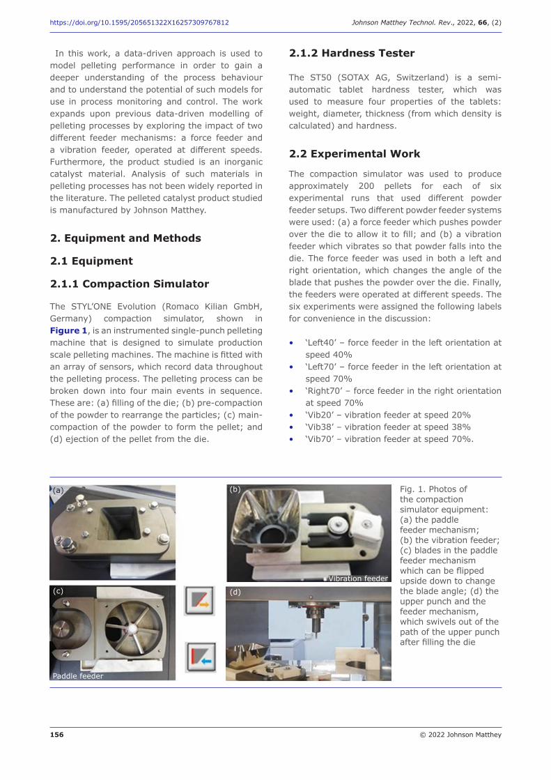
156 © 2022 Johnson Matthey
https://doi.org/10.1595/205651322X16257309767812 Johnson Matthey Technol. Rev., 2022, 66, (2)
In this work, a data-driven approach is used to model pelleting performance in order to gain a deeper understanding of the process behaviour and to understand the potential of such models for use in process monitoring and control. The work expands upon previous data-driven modelling of pelleting processes by exploring the impact of two different feeder mechanisms: a force feeder and a vibration feeder, operated at different speeds. Furthermore, the product studied is an inorganic catalyst material. Analysis of such materials in pelleting processes has not been widely reported in the literature. The pelleted catalyst product studied is manufactured by Johnson Matthey.
2. Equipment and Methods
2.1 Equipment
2.1.1 Compaction Simulator
The STYL’ONE Evolution (Romaco Kilian GmbH, Germany) compaction simulator, shown in Figure 1, is an instrumented single-punch pelleting machine that is designed to simulate production scale pelleting machines. The machine is fitted with an array of sensors, which record data throughout the pelleting process. The pelleting process can be broken down into four main events in sequence. These are: (a) filling of the die; (b) pre-compaction of the powder to rearrange the particles; (c) main-compaction of the powder to form the pellet; and (d) ejection of the pellet from the die.
2.1.2 Hardness Tester
The ST50 (SOTAX AG, Switzerland) is a semi-automatic tablet hardness tester, which was used to measure four properties of the tablets: weight, diameter, thickness (from which density is calculated) and hardness.
2.2 Experimental Work
The compaction simulator was used to produce approximately 200 pellets for each of six experimental runs that used different powder feeder setups. Two different powder feeder systems were used: (a) a force feeder which pushes powder over the die to allow it to fill; and (b) a vibration feeder which vibrates so that powder falls into the die. The force feeder was used in both a left and right orientation, which changes the angle of the blade that pushes the powder over the die. Finally, the feeders were operated at different speeds. The six experiments were assigned the following labels for convenience in the discussion:
• ‘Left40’ – force feeder in the left orientation at speed 40%
• ‘Left70’ – force feeder in the left orientation at speed 70%
• ‘Right70’ – force feeder in the right orientation at speed 70%
• ‘Vib20’ – vibration feeder at speed 20%• ‘Vib38’ – vibration feeder at speed 38%• ‘Vib70’ – vibration feeder at speed 70%.
Fig. 1. Photos of the compaction simulator equipment: (a) the paddle feeder mechanism; (b) the vibration feeder; (c) blades in the paddle feeder mechanism which can be flipped upside down to change the blade angle; (d) the upper punch and the feeder mechanism, which swivels out of the path of the upper punch after filling the die
Paddle feeder
Vibration feeder
(a) (b)
(c) (d)
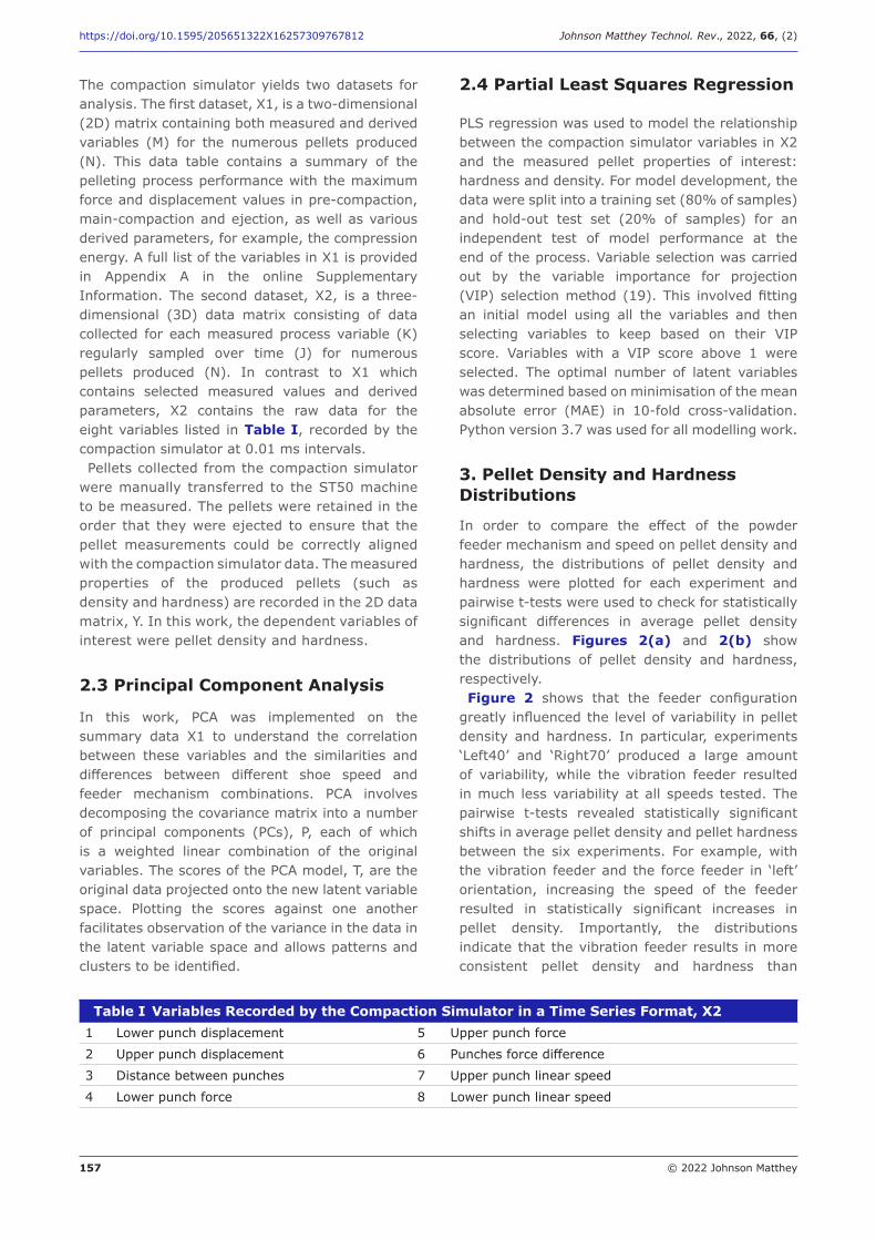
157 © 2022 Johnson Matthey
https://doi.org/10.1595/205651322X16257309767812 Johnson Matthey Technol. Rev., 2022, 66, (2)
The compaction simulator yields two datasets for analysis. The first dataset, X1, is a two-dimensional (2D) matrix containing both measured and derived variables (M) for the numerous pellets produced (N). This data table contains a summary of the pelleting process performance with the maximum force and displacement values in pre-compaction, main-compaction and ejection, as well as various derived parameters, for example, the compression energy. A full list of the variables in X1 is provided in Appendix A in the online Supplementary Information. The second dataset, X2, is a three-dimensional (3D) data matrix consisting of data collected for each measured process variable (K) regularly sampled over time (J) for numerous pellets produced (N). In contrast to X1 which contains selected measured values and derived parameters, X2 contains the raw data for the eight variables listed in Table I, recorded by the compaction simulator at 0.01 ms intervals.Pellets collected from the compaction simulator
were manually transferred to the ST50 machine to be measured. The pellets were retained in the order that they were ejected to ensure that the pellet measurements could be correctly aligned with the compaction simulator data. The measured properties of the produced pellets (such as density and hardness) are recorded in the 2D data matrix, Y. In this work, the dependent variables of interest were pellet density and hardness.
2.3 Principal Component Analysis
In this work, PCA was implemented on the summary data X1 to understand the correlation between these variables and the similarities and differences between different shoe speed and feeder mechanism combinations. PCA involves decomposing the covariance matrix into a number of principal components (PCs), P, each of which is a weighted linear combination of the original variables. The scores of the PCA model, T, are the original data projected onto the new latent variable space. Plotting the scores against one another facilitates observation of the variance in the data in the latent variable space and allows patterns and clusters to be identified.
2.4 Partial Least Squares Regression
PLS regression was used to model the relationship between the compaction simulator variables in X2 and the measured pellet properties of interest: hardness and density. For model development, the data were split into a training set (80% of samples) and hold-out test set (20% of samples) for an independent test of model performance at the end of the process. Variable selection was carried out by the variable importance for projection (VIP) selection method (19). This involved fitting an initial model using all the variables and then selecting variables to keep based on their VIP score. Variables with a VIP score above 1 were selected. The optimal number of latent variables was determined based on minimisation of the mean absolute error (MAE) in 10-fold cross-validation. Python version 3.7 was used for all modelling work.
3. Pellet Density and Hardness Distributions
In order to compare the effect of the powder feeder mechanism and speed on pellet density and hardness, the distributions of pellet density and hardness were plotted for each experiment and pairwise t-tests were used to check for statistically significant differences in average pellet density and hardness. Figures 2(a) and 2(b) show the distributions of pellet density and hardness, respectively.Figure 2 shows that the feeder configuration
greatly influenced the level of variability in pellet density and hardness. In particular, experiments ‘Left40’ and ‘Right70’ produced a large amount of variability, while the vibration feeder resulted in much less variability at all speeds tested. The pairwise t-tests revealed statistically significant shifts in average pellet density and pellet hardness between the six experiments. For example, with the vibration feeder and the force feeder in ‘left’ orientation, increasing the speed of the feeder resulted in statistically significant increases in pellet density. Importantly, the distributions indicate that the vibration feeder results in more consistent pellet density and hardness than
Table I Variables Recorded by the Compaction Simulator in a Time Series Format, X21 Lower punch displacement 5 Upper punch force
2 Upper punch displacement 6 Punches force difference
3 Distance between punches 7 Upper punch linear speed
4 Lower punch force 8 Lower punch linear speed
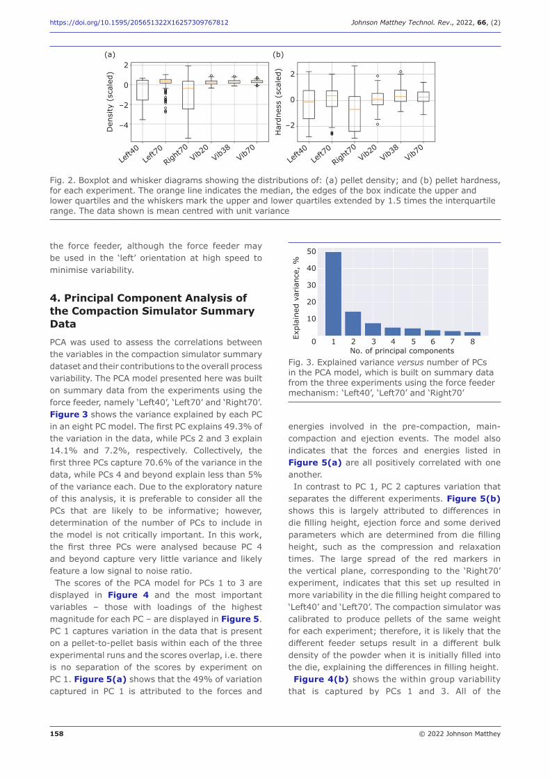
158 © 2022 Johnson Matthey
https://doi.org/10.1595/205651322X16257309767812 Johnson Matthey Technol. Rev., 2022, 66, (2)
the force feeder, although the force feeder may be used in the ‘left’ orientation at high speed to minimise variability.
4. Principal Component Analysis of the Compaction Simulator Summary Data
PCA was used to assess the correlations between the variables in the compaction simulator summary dataset and their contributions to the overall process variability. The PCA model presented here was built on summary data from the experiments using the force feeder, namely ‘Left40’, ‘Left70’ and ‘Right70’. Figure 3 shows the variance explained by each PC in an eight PC model. The first PC explains 49.3% of the variation in the data, while PCs 2 and 3 explain 14.1% and 7.2%, respectively. Collectively, the first three PCs capture 70.6% of the variance in the data, while PCs 4 and beyond explain less than 5% of the variance each. Due to the exploratory nature of this analysis, it is preferable to consider all the PCs that are likely to be informative; however, determination of the number of PCs to include in the model is not critically important. In this work, the first three PCs were analysed because PC 4 and beyond capture very little variance and likely feature a low signal to noise ratio.The scores of the PCA model for PCs 1 to 3 are
displayed in Figure 4 and the most important variables – those with loadings of the highest magnitude for each PC – are displayed in Figure 5. PC 1 captures variation in the data that is present on a pellet-to-pellet basis within each of the three experimental runs and the scores overlap, i.e. there is no separation of the scores by experiment on PC 1. Figure 5(a) shows that the 49% of variation captured in PC 1 is attributed to the forces and
energies involved in the pre-compaction, main-compaction and ejection events. The model also indicates that the forces and energies listed in Figure 5(a) are all positively correlated with one another.In contrast to PC 1, PC 2 captures variation that
separates the different experiments. Figure 5(b) shows this is largely attributed to differences in die filling height, ejection force and some derived parameters which are determined from die filling height, such as the compression and relaxation times. The large spread of the red markers in the vertical plane, corresponding to the ‘Right70’ experiment, indicates that this set up resulted in more variability in the die filling height compared to ‘Left40’ and ‘Left70’. The compaction simulator was calibrated to produce pellets of the same weight for each experiment; therefore, it is likely that the different feeder setups result in a different bulk density of the powder when it is initially filled into the die, explaining the differences in filling height.Figure 4(b) shows the within group variability
that is captured by PCs 1 and 3. All of the
Left4
0Le
ft70
Right70
Vib20
Vib38
Vib70
Left4
0Le
ft70
Right70
Vib20
Vib38
Vib70
Den
sity
(sc
aled
)
Har
dnes
s (s
cale
d)
2
0
–2
–4
2
0
–2
(a) (b)
Fig. 2. Boxplot and whisker diagrams showing the distributions of: (a) pellet density; and (b) pellet hardness, for each experiment. The orange line indicates the median, the edges of the box indicate the upper and lower quartiles and the whiskers mark the upper and lower quartiles extended by 1.5 times the interquartile range. The data shown is mean centred with unit variance
1 2 3 4 5 6 7 8
50
40
30
20
10
0No. of principal components
Expl
aine
d va
rian
ce,
%
Fig. 3. Explained variance versus number of PCs in the PCA model, which is built on summary data from the three experiments using the force feeder mechanism: ‘Left40’, ‘Left70’ and ‘Right70’
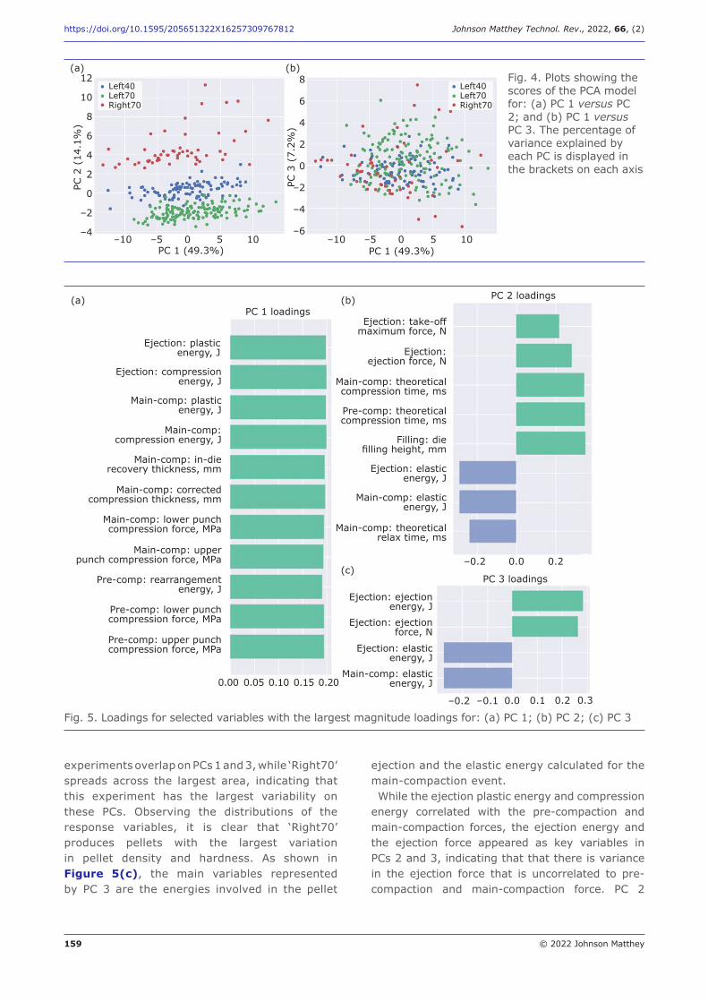
159 © 2022 Johnson Matthey
https://doi.org/10.1595/205651322X16257309767812 Johnson Matthey Technol. Rev., 2022, 66, (2)
experiments overlap on PCs 1 and 3, while ‘Right70’ spreads across the largest area, indicating that this experiment has the largest variability on these PCs. Observing the distributions of the response variables, it is clear that ‘Right70’ produces pellets with the largest variation in pellet density and hardness. As shown in Figure 5(c), the main variables represented by PC 3 are the energies involved in the pellet
ejection and the elastic energy calculated for the main-compaction event.While the ejection plastic energy and compression
energy correlated with the pre-compaction and main-compaction forces, the ejection energy and the ejection force appeared as key variables in PCs 2 and 3, indicating that that there is variance in the ejection force that is uncorrelated to pre-compaction and main-compaction force. PC 2
Fig. 4. Plots showing the scores of the PCA model for: (a) PC 1 versus PC 2; and (b) PC 1 versus PC 3. The percentage of variance explained by each PC is displayed in the brackets on each axis
12
10
8
6
4
2
0
–2
–4
8
6
4
2
0
–2
–4
–6
PC 1 (49.3%) PC 1 (49.3%)–10 –5 0 5 10 –10 –5 0 5 10
PC 2
(14
.1%
)
PC 3
(7.
2%)
Left40 Left70 Right70
Left40 Left70 Right70
(a) (b)
Ejection: plastic energy, J
Ejection: compression energy, J
Main-comp: plastic energy, J
Main-comp: compression energy, J
Main-comp: in-die recovery thickness, mm
Main-comp: corrected compression thickness, mm
Main-comp: lower punch compression force, MPa
Main-comp: upper punch compression force, MPa
Pre-comp: rearrangement energy, J
Pre-comp: lower punch compression force, MPa
Pre-comp: upper punch compression force, MPa
0.00 0.05 0.10 0.15 0.20
PC 1 loadings(a) (b)
(c)
PC 2 loadings
PC 3 loadings
Ejection: take-off maximum force, N
Ejection: ejection force, N
Main-comp: theoretical compression time, ms
Pre-comp: theoretical compression time, ms
Filling: die filling height, mm
Ejection: elastic energy, J
Main-comp: elastic energy, J
Main-comp: theoretical relax time, ms
–0.2 0.0 0.2
Ejection: ejection energy, J
Ejection: ejection force, N
Ejection: elastic energy, J
Main-comp: elastic energy, J
–0.2 –0.1 0.0 0.1 0.2 0.3
Fig. 5. Loadings for selected variables with the largest magnitude loadings for: (a) PC 1; (b) PC 2; (c) PC 3
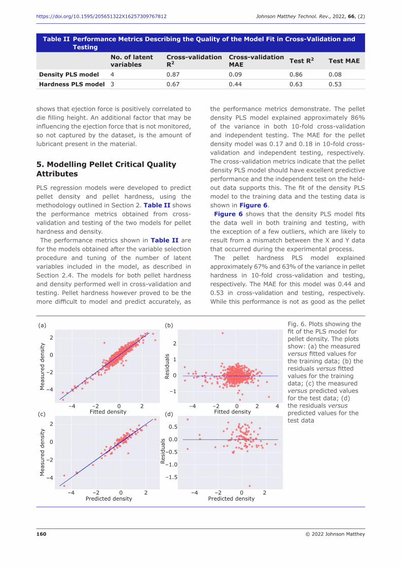
160 © 2022 Johnson Matthey
https://doi.org/10.1595/205651322X16257309767812 Johnson Matthey Technol. Rev., 2022, 66, (2)
shows that ejection force is positively correlated to die filling height. An additional factor that may be influencing the ejection force that is not monitored, so not captured by the dataset, is the amount of lubricant present in the material.
5. Modelling Pellet Critical Quality Attributes
PLS regression models were developed to predict pellet density and pellet hardness, using the methodology outlined in Section 2. Table II shows the performance metrics obtained from cross-validation and testing of the two models for pellet hardness and density.The performance metrics shown in Table II are
for the models obtained after the variable selection procedure and tuning of the number of latent variables included in the model, as described in Section 2.4. The models for both pellet hardness and density performed well in cross-validation and testing. Pellet hardness however proved to be the more difficult to model and predict accurately, as
the performance metrics demonstrate. The pellet density PLS model explained approximately 86% of the variance in both 10-fold cross-validation and independent testing. The MAE for the pellet density model was 0.17 and 0.18 in 10-fold cross-validation and independent testing, respectively. The cross-validation metrics indicate that the pellet density PLS model should have excellent predictive performance and the independent test on the held-out data supports this. The fit of the density PLS model to the training data and the testing data is shown in Figure 6.Figure 6 shows that the density PLS model fits
the data well in both training and testing, with the exception of a few outliers, which are likely to result from a mismatch between the X and Y data that occurred during the experimental process.The pellet hardness PLS model explained
approximately 67% and 63% of the variance in pellet hardness in 10-fold cross-validation and testing, respectively. The MAE for this model was 0.44 and 0.53 in cross-validation and testing, respectively. While this performance is not as good as the pellet
Table II Performance Metrics Describing the Quality of the Model Fit in Cross-Validation and Testing
No. of latent variables
Cross-validation R2
Cross-validation MAE Test R2 Test MAE
Density PLS model 4 0.87 0.09 0.86 0.08
Hardness PLS model 3 0.67 0.44 0.63 0.53
Fig. 6. Plots showing the fit of the PLS model for pellet density. The plots show: (a) the measured versus fitted values for the training data; (b) the residuals versus fitted values for the training data; (c) the measured versus predicted values for the test data; (d) the residuals versus predicted values for the test data
2
0
–2
–4
2
1
0
–1
2
0
–2
–4
0.5
0.0
–0.5
–1.0
–1.5
(a) (b)
(c) (d)–4 –2 0 2 –4 –2 0 2 4
–4 –2 0 2 –4 –2 0 2
Fitted density Fitted density
Predicted density Predicted density
Mea
sure
d de
nsity
Mea
sure
d de
nsity
Resi
dual
sRe
sidu
als
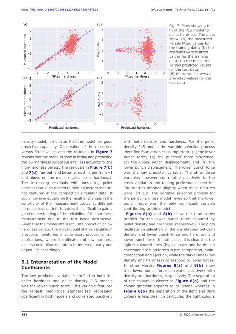
161 © 2022 Johnson Matthey
https://doi.org/10.1595/205651322X16257309767812 Johnson Matthey Technol. Rev., 2022, 66, (2)
density model, it indicates that the model has good predictive capability. Observation of the measured versus fitted values and the residuals in Figure 7 reveals that the model is good at fitting and predicting the low-hardness pellets but is far less accurate for the high-hardness pellets. The residuals in Figure 7(b) and 7(d) ‘fan-out’ and become much larger from –1 and above on the x-axis (scaled pellet hardness). The increasing residuals with increasing pellet hardness could be related to missing factors that are not captured in the compaction simulator data. It could however equally be the result of changes in the sensitivity of the measurement device at different hardness levels. Unfortunately, it is difficult to gain a good understanding of the reliability of the hardness measurement due to the test being destructive. Given that the model offers accurate prediction of low hardness pellets, the model could still be valuable in a process monitoring or supervisory process control applications, where identification of low hardness pellets could allow operators to intervene early and adjust PPs accordingly.
5.1 Interpretation of the Model Coefficients
The key predictive variable identified in both the pellet hardness and pellet density PLS models was the lower punch force. This variable featured the largest magnitude standardised regression coefficient in both models and correlated positively
with both density and hardness. For the pellet density PLS model, the variable selection process identified four variables as important: (a) the lower punch force; (b) the punches’ force difference; (c) the upper punch displacement; and (d) the lower punch displacement. The lower punch force was the key predictor variable. The other three variables however contributed positively to the cross-validation and testing performance metrics. The metrics dropped slightly when these features were left out. The variable selection process for the pellet hardness model revealed that the lower punch force was the only significant variable contributing to this model.Figures 8(a) and 8(b) show the time series
profiles for the lower punch force coloured by pellet density and hardness, respectively. The plots facilitate visualisation of the correlations between density and lower punch force and hardness and lower punch force. In both cases, it is clear that the lighter coloured lines (high density and hardness) correspond to high forces in pre-compaction, main-compaction and ejection, while the darker lines (low density and hardness) correspond to lower forces. In other words, Figures 8(a) and 8(b) show that lower punch force correlates positively with density and hardness, respectively. The separation of the colours is clearer in Figure 8(a) and the colour gradient appears to be linear, whereas in Figure 8(b) the separation of the light and dark colours is less clear. In particular, the light colours
Fig. 7. Plots showing the fit of the PLS model for pellet hardness. The plots show: (a) the measured versus fitted values for the training data; (b) the residuals versus fitted values for the training data; (c) the measured versus predicted values for the test data; (d) the residuals versus predicted values for the test data
2
1
0
–1
–2
–3
(a) (b)
(c) (d)–3 –2 –1 0 1 2
Fitted hardness Fitted hardness
Predicted hardness Predicted hardness
Mea
sure
d ha
rdne
ssM
easu
red
hard
ness
Resi
dual
sRe
sidu
als
3
2
1
0
–1
–2
–3–3 –2 –1 0 1 2 3 –3 –2 –1 0 1 2 3
2
1
0
–1
2
1
0
–1
–4 –3 –2 –1 0 1 2
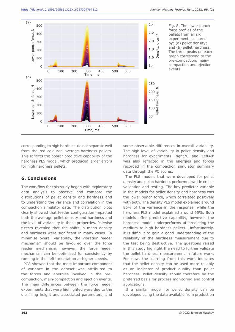
162 © 2022 Johnson Matthey
https://doi.org/10.1595/205651322X16257309767812 Johnson Matthey Technol. Rev., 2022, 66, (2)
corresponding to high hardness do not separate well from the red coloured average hardness pellets. This reflects the poorer predictive capability of the hardness PLS model, which produced larger errors for high hardness pellets.
6. Conclusions
The workflow for this study began with exploratory data analysis to observe and compare the distributions of pellet density and hardness and to understand the variance and correlation in the compaction simulator data. The distribution plots clearly showed that feeder configuration impacted both the average pellet density and hardness and the level of variability in those properties. Pairwise t-tests revealed that the shifts in mean density and hardness were significant in many cases. To minimise overall variability, the vibration feeder mechanism should be favoured over the force feeder mechanism, however, the force feeder mechanism can be optimised for consistency by running in the ‘left’ orientation at higher speeds. PCA showed that the most important component
of variance in the dataset was attributed to the forces and energies involved in the pre-compaction, main-compaction and ejection events. The main differences between the force feeder experiments that were highlighted were due to the die filling height and associated parameters, and
some observable differences in overall variability. The high level of variability in pellet density and hardness for experiments ‘Right70’ and ‘Left40’ was also reflected in the energies and forces recorded in the compaction simulator summary data through the PC scores.The PLS models that were developed for pellet
density and pellet hardness performed well in cross-validation and testing. The key predictor variable in the models for pellet density and hardness was the lower punch force, which correlated positively with both. The density PLS model explained around 86% of the variance in the response, while the hardness PLS model explained around 65%. Both models offer predictive capability, however, the hardness model underperforms at predicting the medium to high hardness pellets. Unfortunately, it is difficult to gain a good understanding of the reliability of the hardness measurement due to the test being destructive. The questions raised in this study highlight the need to further validate the pellet hardness measurement in future work. For now, the learning from this work indicates that the pellet density can be used more reliably as an indicator of product quality than pellet hardness. Pellet density should therefore be the preferred basis for process monitoring and control applications.If a similar model for pellet density can be
developed using the data available from production
Fig. 8. The lower punch force profiles of the pellets from all six experiments coloured by: (a) pellet density; and (b) pellet hardness. The three peaks on each graph correspond to the pre-compaction, main-compaction and ejection events
0 100 200 300 400 500 600
Time, ms
Time, ms
500
400
300
200
100
0
500
400
300
200
100
0
0 100 200 300 400 500 600
Low
er p
unch
for
ce,
NLo
wer
pun
ch for
ce,
N
(a)
(b)
2.4
2.2
2.0
1.8
1.6
1.4
250
200
150
100
50
Den
sity
, g
cm–3
Pelle
t ha
rdne
ss,
N
163 © 2022 Johnson Matthey
https://doi.org/10.1595/205651322X16257309767812 Johnson Matthey Technol. Rev., 2022, 66, (2)
scale pelleting machines, then there would be the potential for such a model to be used for process monitoring and control. This could provide real-time process monitoring that greatly improves upon existing techniques for monitoring pelleting performance, which are based on random sampling and testing of the pellets. The information could be used by plant operators at a supervisory level or in an automated control system to help inform and guide decision making to keep the process on track and producing on-specification material.
References
1. Z. Chen, D. Lovett and J. Morris, J. Process Control, 2011, 21, (10), 1467
2. C.-Y. Wu, O. M. Ruddy, A. C. Bentham, B. C. Hancock, S. M. Best and J. A. Elliott, Powder Technol., 2005, 152, (1–3), 107
3. S. Patel, A. M. Kaushal and A. K. Bansal, Pharm. Res., 2007, 24, (1), 111
4. S. Garner, J. Strong and A. Zavaliangos, Powder Technol., 2018, 330, 357
5. J. C. Cunningham, I. C. Sinka and A. Zavaliangos, J. Pharm. Sci., 2004, 93, (8), 2022
6. A. Mazor, L. Orefice, A. Michrafy, A. de Ryck and J. G. Khinast, Powder Technol., 2018, 337, 3
7. X. An, Y. Zhang, Y. Zhang and S. Yang, Metall. Mater. Trans. A, 2015, 46, (8), 3744
8. R. V. Haware, I. Tho and A. Bauer-Brandl, Eur. J. Pharm. Biopharm., 2009, 72, (1), 148
9. R. V. Haware, I. Tho and A. Bauer-Brandl, Eur. J. Pharm. Biopharm., 2009, 73, (3), 424
10. Z. Li, F. Wu, L. Zhao, X. Lin, L. Shen and Y. Feng, Adv. Powder Technol., 2018, 29, (11), 2881
11. S. Paul, L. J. Taylor, B. Murphy, J. F. Krzyzaniak, N. Dawson, M. P. Mullarney, P. Meenan and C. C. Sun, Int. J. Pharm., 2017, 521, (1–2), 374
12. M. S. Escotet-Espinoza, S. Vadodaria, R. Singh, F. J. Muzzio and M. G. Ierapetritou, Int. J. Pharm., 2018, 543, (1–2), 274
13. A. Özbeyaz and M. Söylemez, Turkish J. Electr. Eng. Comput. Sci., 2020, 28, (5), 3079
14. H. M. Zawbaa, S. Schiano, L. Perez-Gandarillas, C. Grosan, A. Michrafy and C.-Y. Wu, Adv. Powder Technol., 2018, 29, (12), 2966
15. T. Tanner, O. Antikainen, A. Pollet, H. Räikkönen, H. Ehlers, A. Juppo and J. Yliruusi, Int. J. Pharm., 2019, 566, 194
16. A. Matji, N. Donato, A. Gagol, E. Morales, L. Carvajal, D. R. Serrano, Z. A. Worku, A. M. Healy and J. J. Torrado, Int. J. Pharm., 2019, 565, 209
17. L. Benvenuti, C. Kloss and S. Pirker, Powder Technol., 2016, 291, 456
18. D. S. Shin, C. H. Lee, S. H. Kim, D. Y. Park, J. W. Oh, C. W. Gal, J. M. Koo, S. J. Park and S. C. Lee, Powder Technol., 2019, 353, 330
19. T. Mehmood, K. H. Liland, L. Snipen and S. Sæbø, Chemom. Intell. Lab. Syst., 2012, 118, 62
The Authors
Joe Emerson is a Process Control Engineer in the Process Measurement and Control team. He joined Johnson Matthey in 2020 and his background is in chemical engineering, process control and multivariate data analytics.
Vincenzino Vivacqua is a Senior Scientist who has been working at Johnson Matthey since 2017, where his research focuses on the optimisation of processes involving granular powder flow, powder compaction and modelling of particulate processes.
Hugh Stitt is a Senior Research Fellow in Johnson Matthey with over 30 years of experience in industrial research and development in reaction engineering as well as catalyst and specialist material manufacturing technology with specialisation in fluid processing and mixing, powder technology and advanced modelling. He has over 100 refereed publications and is a Visiting Professor at the University of Birmingham, UK. He is a Chartered Engineer, FIChemE and a Fellow of the Royal Academy of Engineering.
www.technology.matthey.com
https://doi.org/10.1595/205651322X16438153587355 Johnson Matthey Technol. Rev., 2022, 66, (2), 164–168
164 © 2022 Johnson Matthey
Flora Chen*, Richard Head, Brendan Strijdom, Philippa Stone Johnson Matthey, Gate 21, Orchard Road, Royston, UK, SG8 5HE
*Email: �[email protected]
NON-PEER REVIEWED FEATURE
Received�16th�November�2021;�Online�7th�March�2022
Introduction
In� recent� years,� whenever� the� subject� of�digitalisation� or� digital� transformation� is� brought�up� for� discussion,� we� normally� observe� two�distinguishing� reactions� from� the� attendees:� one�group�is�excited�and�satisfied,�the�other,�interested�and�worried.�Of�course,�some�have�a�good�mixture�of� both.� The� former� has� been� from� companies,�big� or� small,� which� have� a� clear� digitalisation�strategy�in�place�from�which�obvious�development�and� benefits� have� been� achieved.� For� the� latter,�people� are� as� keen� as� others� on� implementing�solid�steps�to�realise�the�long-waited�benefit�from�business�digitalisation.�However,�they�are�not�quite�sure where and what to start with, despite the continuously�advancing�technologies�in�the�market.�While� still� dealing� with� the� COVID-19� pandemic,�we� were� very� curious� about� what� the� book�“Digitalization”�(1)�would�bring�to�help�accelerate�digital�transformation�for�various�organisations.�Professor� Schallmo� and� Professor� Tidd� are� the�editors�of�“Digitalization”�with�a�list�of�distinguished�researchers� on� the� editorial� board.� Professor�Schallmo�is�a�well-known�key�researcher�focusing�on� business� digitalisation� at� various� stages,� and�
“Digitalization”Edited by Daniel R. A. Schallmo (Neu-Ulm University of Applied Sciences, Germany) and Joseph Tidd (SPRU, University of Sussex, UK), Management for Professionals Series, Springer Nature Switzerland AG, Cham, Switzerland, 2021, 426 pages, ISBN 978-3-030-69379-4, £64.99, €78.06, US$88.18
the� development� and� application� of� the�methods�to� innovate� business� models.� “Digitalization”�continues�his�research�focus�following�his�previous�book�“Digital�Transformation�Now!”�(2).�Besides� his� professorship� of� technology� and�innovation�management� at� University� of� Sussex,�UK,� Professor� Tidd� has� worked� with� numerous�technology-based� organisations� globally� on�technology�and� innovation�management�projects.�His�view�and�experience�of�connecting�innovation�and�digitalisation�is�always�insightful.�In�conjunction�with� “Digitalization”,� it� is� worth� expanding� the�reader’s� knowledge� through� his� bestselling�textbook�on�managing�innovation�(3).The� book� “Digitalization”� is� a� collection� of�25� research-based� studies� which� have� been�arranged�in�sections�to�emphasise�five�aspects�of�digitalisation:� ‘Digital� Drivers’,� ‘Digital� Maturity’,�‘Digital� Strategy’,� ‘Digital� Transformation’� and�‘Digital� Implementation’.� This� arrangement� gives�a� clear� statement� of� the� focus� of� each� part.�Throughout� the� book,� the� literature� review� of� all�subjects�is�very�rich�which�should�give�the�audience�a�wide�range�of�further�reading�if�required.
Digital Drivers
The� very� early� challenges� that� all� organisations�face� in� digital� transformation� are� to� discover� the�right� opportunities� and� initiatives� holistically.�In� the� section� ‘Digital� Drivers’,� four� articles�explore� this� subject� from� different� angles.�Disaster� management� and� future-led� innovation�framework,� presented� by� Vettorello� (Swinburne�University� of� Technology,� Australia)� et al., and technology-oriented� future� analysis� by� Urbano�(Politecnico� di� Milano,� Italy)� et al.,� aim� to�
165 © 2022 Johnson Matthey
https://doi.org/10.1595/205651322X16438153587355 Johnson Matthey Technol. Rev., 2022, 66, (2)
provide guidance to organisations on innovation management� with� fast� and� accurate� decision�making� within� highly� dynamic� and� complex�environments.�We� feel� these� concepts�may�also�have�a�place�for� individual�business�units�within�a�large�organisation�where�specific�needs�of�that�business�unit� can�be�addressed� to� capture� local�opportunity. Chiaroni� (Politecnico� di� Milano)� et al. present a real�example�of�how�a�circular�business�model�has�been� applied� in� the� building� industry� to� realise�business� transformation� from� linear� to� circular�by� adopting� digital� technologies.� Mutanov� and�Zhuparova� (al-Farabi� Kazakh� National� University,�Kazakhstan)� in� the� fourth� article� explain� several�fundamental� reasons� that� commodity� countries�such�as�Kazakhstan�and�other�post-Soviet�countries�are�falling�behind�on�digital�transformation.�These�findings� certainly� show� the� great� potential� of�digitalisation.�Among�the�literature�provided�by�the�authors,� two� popular� books�written� by� Cross� (4)�and� Tighe� (5)� are� worthy� of� extra� attention� to�expand�ways�of�thinking�and�setting�strategy.
Digital Maturity
‘Digital�Maturity’� in�Part�2� focuses�on�discovering�digitalisation�opportunities�from�a�different�angle,�by�assessing�the�current�digital�development�status�of�an�organisation�and�comparing�with�others�within�the� same�business� sector� or� even�wider� to� draw�action�plans�for�its�own�needs.�First,�a�systematic�literature�review�is�conducted�by�Ochoa-Urrego�and�Peña-Reyes� (Universidad� Nacional� de� Colombia)�which�includes�22�publications�on�formal�maturity�model�applications.�The� other� two� studies� from�Schallmo� (Neu-Ulm�University� of� Applied� Sciences,� Germany)� et al. and�Pierenkemper�and�Gausemeier�(Heinz�Nixdorf�Institute,�University�of�Paderborn,�Germany)�et al. emphasise� a� digital�maturity�models� assessment�of� small� and� medium-sized� enterprises� (SMEs).�It� is� recognised� that� the� examined� digital�maturity�models�cannot�provide�a�comprehensive�digitalisation� implementation� plan� for� SMEs� with�an� overarching� vision� like� that� typically� seen� at�large� corporations.� Although� Pierenkemper� and�Gausemeier� list� a� few� aspects� of� the� presented�model� that� may� require� further� investigation,�the� study� itself� shows� through� examples� how�SMEs�can�produce�a�simple�development�plan�for�digitalisation�using�the�model�provided.
Digital Strategy
Once�digitalisation�objectives�are�determined,�it�is�natural�to�move�onto�‘Digital�Strategy’�as�presented�in Part 3 on how we can capture the opportunities. The�first� paper� in� this� part� gives� a�deep�dive�on�how� disruptive� innovation� is� used� as� business�strategy� or� model� for� digital� transformation�among�80�companies� in�Germany.�To�expand�the�understanding�of�disruptive�innovation,�it�is�worth�exploring� relevant� resources� from� the� bestselling�author�(6).�It�is�followed�by�Hartmann�(HTW�Berlin�-�University�of�Applied�Science,�Germany)�et al. and Gernreich� (Ruhr-Universität� Bochum,� Germany)�et al.�who�separately�address�the�importance�of�top�management� or� an� innovation�manager�who� has�the�necessary�knowledge�in�digitalisation�and�can�drive�to�complete�the�plan�for�desired�productivity�and�benefits.�Kruft� and� Gamber� (Technische� Universität�Darmstadt,�Germany)�in�the�fourth�paper�present�a� critical� component� of� digital� transformation:�continuous� culture� change,�which�often�poses�an�even� bigger� challenge� on� the� entire� journey� of�digitalisation.� All� organisations� need� to� recognise�the� significance� of� cultural� renewal� and� work�closely�with� their�employees� to�bring� them�along�with�progress.� It� is� one�of� the� core� strategies� to�empower� people� with� the� right� tools,� knowledge�and�communication�via�digital�platforms�in�the�era�of�ever-changing�technology.�The� focus� in� the� paper� from� Koldewey� (Heinz�Nixdorf� Institute,� University� of� Paderborn)� et al. falls�in�the�mainstream�of�digitalisation,�i.e.,�smart�services� interconnecting� products� with� aftersales�service.� They� demonstrate� how� they� use� a�design� research�methodology� to�develop�a�smart�service�strategy�through�four�comprehensive�case�studies.�The�last�paper�in�Part�3,�from�Porté�(Ecole�Polytechnique�Fédérale�de�Lausanne,�Switzerland)�et al., draws� attention� to� the� potential� of� using�Systemic� Enterprise� Architecture� Methodology�(SEAM)� to� align� business� and� IT� perspectives� on�innovative� projects.� A� project� by� the� Society� of�Family�Doctors�(SFD)�is�used�to�showcase�how�we�structure�a�problem�based�on�who�sees�it�and�why,�instead�of�the�problem�itself.
Digital Transformation
Part� 4,� ‘Digital� Transformation’,� expands� on� the�first� three� parts� of� the� book� with� papers� from�
166 © 2022 Johnson Matthey
https://doi.org/10.1595/205651322X16438153587355 Johnson Matthey Technol. Rev., 2022, 66, (2)
governments,� universities� and� other� parts� of� the�public� sector.� Meier� (University� of� Innsbruck,�Austria)� provides� a� systematic� review� of� the�literature� on� SME� digitalisation.� Her� discovery�agrees� with� a� few� other� papers� in� the� book�on� challenges� that� traditional� SMEs� face� while�adopting� digitalisation:� time,� financial,� human�and�technical� resource�constraints.�For� the�public�sector,�Bjerke-Busch�and�Aspelund�(Department�of�Industrial� Economics� &� Technology� Management,�Norwegian�University�of�Science�and�Technology)�use� Norwegian� Court� Administration� (NCA)� to�explain�the�barriers�for�digital�transformation�in�a�typical�public�organisation.�The� study� from� Haslam� (Centre� for� IS�Management,� Department� of� Politics� and� Society,�Aalborg�University,�Denmark)�et al.�identifies�a�few�key� elements� of� how� digital� transformation� has�been�accelerated�at�a�Danish�university�during�the�pandemic�period.�Staying�connected�with�the�Danish�Government,� Rosenstand� (Aalborg� University)�shows� early�work� on� applying� a� digital� ecosphere�canvas�for�cultivating�multiple�digital�ecosystems�at�Digital�Hub�Denmark,� a�private-public� partnership�organisation.� Jütting� (Fraunhofer� IAO,� Fraunhofer�Institute� for� Industrial� Engineering,� Center� for�Responsible� Research� and� Innovation� (CeRRI),�Germany)�et al.�introduce�the�pro-poor�digitalisation�canvas�as�a�conceptual�framework�aiming�to�act�as�a�practical� tool� to�evaluate� the�potential�of�digital�innovations.�The�particular�interest�is�to�practically�turn�the�objectives�of�the�United�Nations�Sustainable�Development� Goals� (SDGs)� 1� (‘no� poverty’)� and�10� (‘reduced� inequality’)� into� actions� to�minimise�the� digitalisation� gap� between� the� advanced� and�developing�world.
Digital Implementation
Digital� implementation,� the� focus� of� Part� 5,� is�the� step� to� really� make� the� transformation.�Although� it� is� impossible� to� cover� all� areas� in�the� implementation� stage,� the� authors� have�attempted� in-depth� discussion� in� several� major�subjects.�Gfrerer�(University�of�Innsbruck)�et al. lead� the�discussion� in� the� composition�of� digital�leadership� and� gender� diversity,� particularly�targeting�female�managers�and�how�they�envisage�their� roles� and� challenges� to� digitalisation� and�innovation.� Reis� and�Hunt� (Thinkergy� Ltd,�Hong�Kong�and�Thailand)�in�the�second�paper�also�focus�on�the�effectiveness�of�leadership�in�digitalisation.�They�conclude�by�highlighting�the� importance�of�creative�leaders�in�the�success�of�digitalisation�and�
such�leaders�can�be�trained�up�through�selective�programmes� combining� effective� methodology�and pedagogy. Schallmo� and� Williams� (Neu-Ulm� University� of�Applied�Sciences)�bring�attention�to�an�integrated�theoretical� approach� to� digital� implementation�which� aims� to� realise� digitalisation� in� four�interactive�dimensions�and�five�procedural�phases.�The� study� presented� in� the� fourth� paper� by�Kruszelnicki� (Creative� Labs� sp.� zoo� ul,� Poland)�and� Breuer� (UXBerlin� Innovation� Consulting�and� HMKW� University� of� Applied� Sciences�for� Media,� Communication� and� Management,�Germany)� is� particularly� interesting.� Three� use�cases�are�presented� to�show�how�Adobe�Kickbox�has� effectively� promoted� ‘intrepreneurship’� to�unlock� innovation� opportunities.� Haag� (TH� Köln,�Germany)�et al.�have�sustainability�at�the�centre�of�their�research.�Their�main�contribution�is�to�provide�the�‘design-to-sustainability�matrix’�as�a�toolkit�to�address�ecological�challenges�through�the�life�cycle�of�both�new�and�existing�product�development.�The� last� two� studies� in� this� part� put� weight� on�innovation� management.� Johnsson� (Blekinge�Institute� of� Technology,� Sweden)� et al.� explore�the� key� success� factors� in� evaluating� innovation�teams.� In� the� last� paper� Colucci� and� Forciniti�(Evidentia� srl,� Italy)� recount� the� story� of� how�Ferrari� has� transformed� its� business� through�an� innovation� management� programme� which�involves�management�at� all� levels� and�processes�at�different�stages.
Conclusion
On�completing�the�book,�although�the�questions�we� had� at� the� start� of� this� review� are� not� fully�answered,� we� were� delighted� to� see� several�useful� case� studies� presented� throughout� the�book.�When�it�comes�to�real�implementation,�we�understand� that� it� is� impossible� to� write� down�all�details�due�to�confidentiality�and�variations�in�organisational� status� and� need.� The� richness� of�the�literature�resources�in�this�book�provided�by�all� authors� is� hugely� beneficial� to� the� audience�to� gain� a� theoretical� foundation.� There� is� also�wide� discussion� on� how� digitalisation� is� applied�to� various� areas� of� focus,� including� SMEs,�developing� countries,� gender� diversity,� SDGs,�high-tech�industry�leaders�and�the�public�sector.�Digitalisation�practitioners� such�as�management�and� innovation� consultants� and� organisations�would�find�it�useful�to�navigate�through�the�business�models� and� frameworks� presented� by� several�
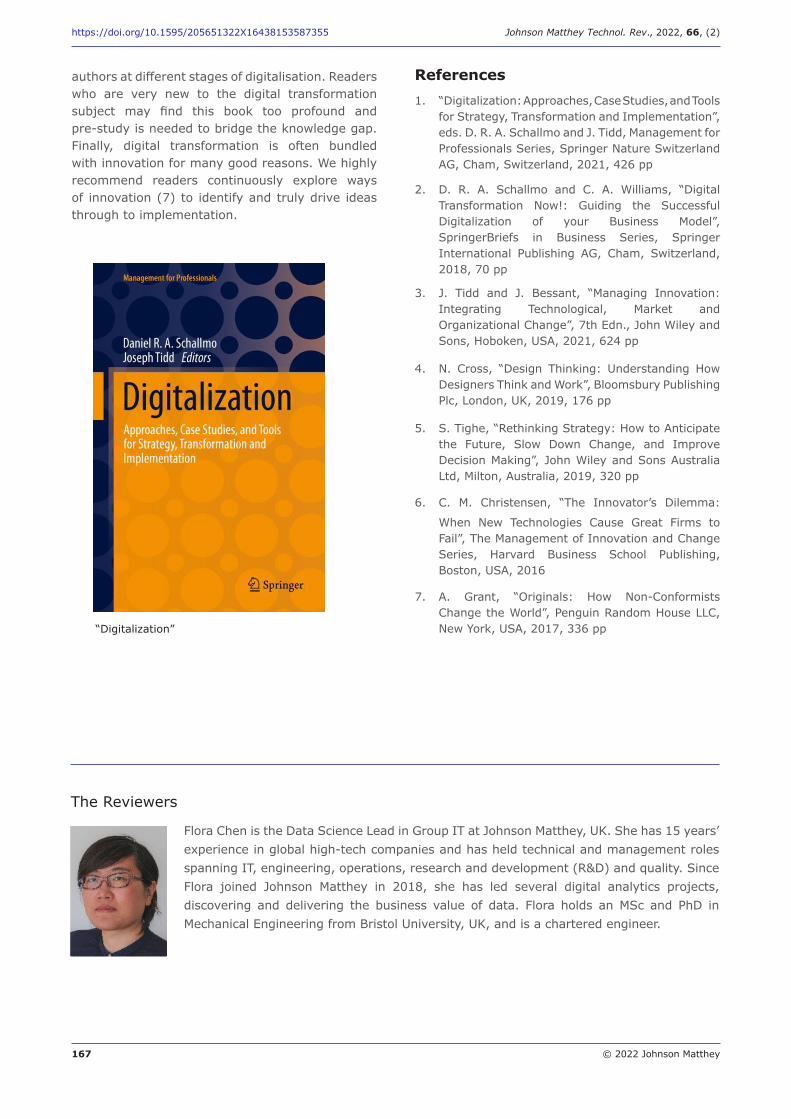
167 © 2022 Johnson Matthey
https://doi.org/10.1595/205651322X16438153587355 Johnson Matthey Technol. Rev., 2022, 66, (2)
authors�at�different�stages�of�digitalisation.�Readers�who� are� very� new� to� the� digital� transformation�subject� may� find� this� book� too� profound� and�pre-study�is�needed�to�bridge�the�knowledge�gap.�Finally,� digital� transformation� is� often� bundled�with�innovation�for�many�good�reasons.�We�highly�recommend� readers� continuously� explore� ways�of� innovation�(7)�to� identify�and�truly�drive� ideas�through�to�implementation.
References1. “Digitalization:�Approaches,�Case�Studies,�and�Tools�
for�Strategy,�Transformation�and�Implementation”,�eds.�D.�R.�A.�Schallmo�and�J.�Tidd,�Management�for�Professionals�Series,�Springer�Nature�Switzerland�AG,�Cham,�Switzerland,�2021,�426�pp
2. D.� R.� A.� Schallmo� and� C.� A.� Williams,� “Digital�Transformation� Now!:� Guiding� the� Successful�Digitalization� of� your� Business� Model”,�SpringerBriefs� in� Business� Series,� Springer�International� Publishing� AG,� Cham,� Switzerland,�2018, 70 pp
3. J.� Tidd� and� J.� Bessant,� “Managing� Innovation:�Integrating� Technological,� Market� and�Organizational�Change”,�7th�Edn.,�John�Wiley�and�Sons,�Hoboken,�USA,�2021,�624�pp
4. N.� Cross,� “Design� Thinking:� Understanding� How�Designers�Think�and�Work”,�Bloomsbury�Publishing�Plc,�London,�UK,�2019,�176�pp
5. S.�Tighe,�“Rethinking�Strategy:�How�to�Anticipate�the� Future,� Slow� Down� Change,� and� Improve�Decision�Making”,�John�Wiley�and�Sons�Australia�Ltd,�Milton,�Australia,�2019,�320�pp
6. C.� M.� Christensen,� “The� Innovator’s� Dilemma:�
When� New� Technologies� Cause� Great� Firms� to�Fail”,�The�Management�of�Innovation�and�Change�Series,� Harvard� Business� School� Publishing,�Boston,�USA,�2016�
7. A.� Grant,� “Originals:� How� Non-Conformists�Change�the�World”,�Penguin�Random�House�LLC,�New�York,�USA,�2017,�336�pp�“Digitalization”
The�Reviewers
Flora�Chen�is�the�Data�Science�Lead�in�Group�IT�at�Johnson�Matthey,�UK.�She�has�15�years’�experience�in�global�high-tech�companies�and�has�held�technical�and�management�roles�spanning�IT,�engineering,�operations,�research�and�development�(R&D)�and�quality.�Since�Flora� joined� Johnson� Matthey� in� 2018,� she� has� led� several� digital� analytics� projects,�discovering� and� delivering� the� business� value� of� data.� Flora� holds� an�MSc� and� PhD� in�Mechanical�Engineering�from�Bristol�University,�UK,�and�is�a�chartered�engineer.

168 © 2022 Johnson Matthey
https://doi.org/10.1595/205651322X16438153587355 Johnson Matthey Technol. Rev., 2022, 66, (2)
Richard�Head�is�the�IT�Digital�Strategy�Partner�at�Johnson�Matthey.�Richard�has�35�years’�experience�in�IT,�data�and�analytics�and�has�led�global�data�and�analytics�teams�at�Financial�Times�Stock�Exchange�(FTSE)�companies�including�Cadburys,�Burberry�and�Diageo.�Since�joining�Johnson�Matthey�in�2014�he�initially�led�the�data�and�analytics�team�on�the�global�SAP®�rollout.�Subsequently�he�established�the�overall�data�platforms�for�both�corporate�and�agile�analytics�and�set�up�and�built�out�the�group�data�office�before�moving�to�his�current�role.
Brendan�Strijdom�is�the�Architecture�Office�Manager�at�Johnson�Matthey�with�oversight�of�digital�and�data�innovations.�He�has�30�years’�experience�working�with�leading�edge�companies� and� technology� vendors� pushing� the� boundary� of� what� is� possible� across�numerous�industries�and�geographies.�He�has�a�BSc�degree�in�Computer�Science�and�in�Psychology.
Philippa�Stone�is�currently�seconded�into�Johnson�Matthey’s�IT�Data�Office�as�part�of�the�Johnson�Matthey�UK�Graduate�Scheme.�While� roles� in� her� early� career� have� primarily�focused�on�R&D�and�operations,�Philippa�recognises�the�value�that�digitalisation�can�bring�and� is� now� contributing� to� projects� that� improve�use� of� data� across� Johnson�Matthey.�Philippa�holds�an�MChem�from�Durham�University,�UK.
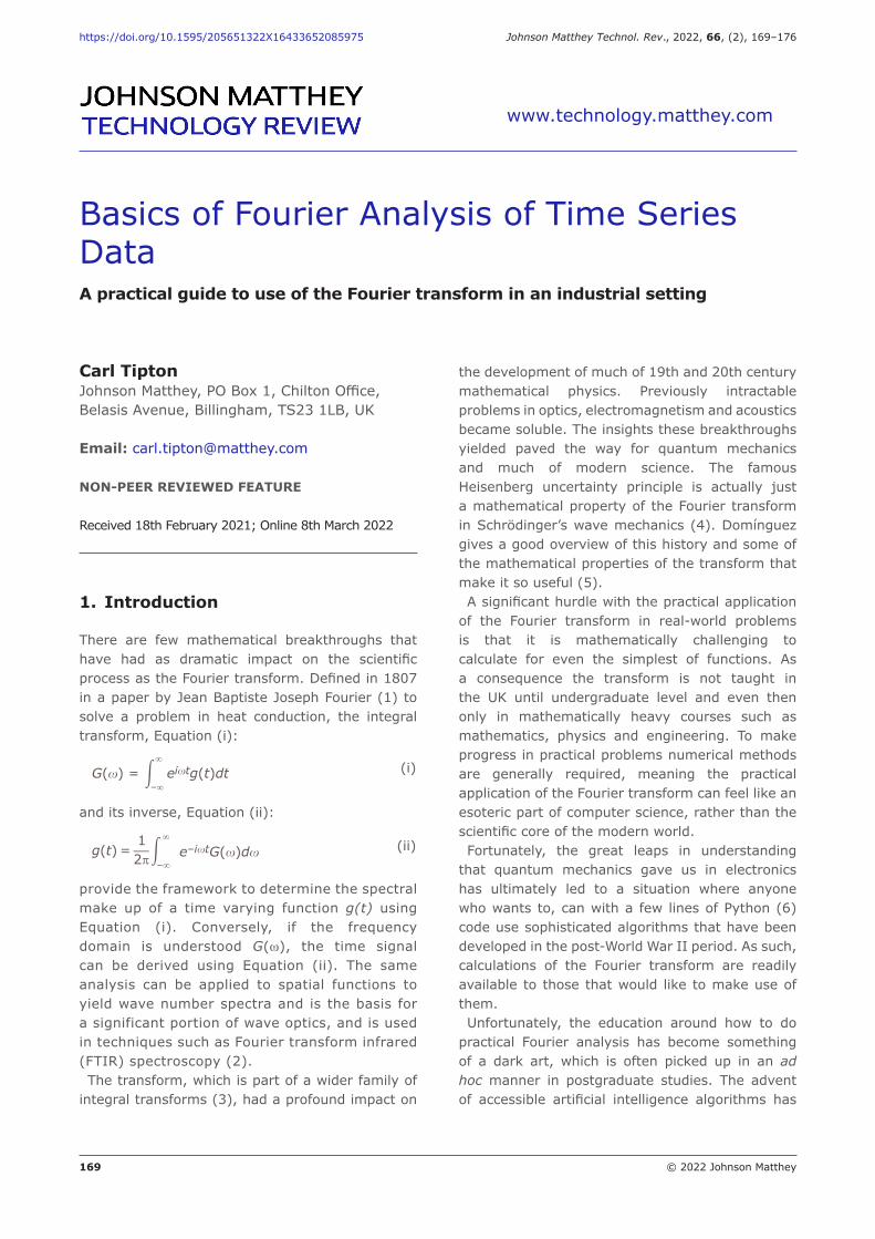
www.technology.matthey.com
https://doi.org/10.1595/205651322X16433652085975 Johnson Matthey Technol. Rev., 2022, 66, (2), 169–176
169 © 2022 Johnson Matthey
Carl TiptonJohnson Matthey, PO Box 1, Chilton Office, Belasis Avenue, Billingham, TS23 1LB, UK
Email: [email protected]
NON-PEER REVIEWED FEATURE
Received 18th February 2021; Online 8th March 2022
1. Introduction
There are few mathematical breakthroughs that have had as dramatic impact on the scientific process as the Fourier transform. Defined in 1807 in a paper by Jean Baptiste Joseph Fourier (1) to solve a problem in heat conduction, the integral transform, Equation (i):
G(�) = ei�tg(t)dt–�
� (i)
and its inverse, Equation (ii):
g(t) =12� –�
�
e–i�tG(�)d� (ii)
provide the framework to determine the spectral make up of a time varying function g(t) using Equation (i). Conversely, if the frequency domain is understood G(ω), the time signal can be derived using Equation (ii). The same analysis can be applied to spatial functions to yield wave number spectra and is the basis for a significant portion of wave optics, and is used in techniques such as Fourier transform infrared (FTIR) spectroscopy (2).The transform, which is part of a wider family of
integral transforms (3), had a profound impact on
the development of much of 19th and 20th century mathematical physics. Previously intractable problems in optics, electromagnetism and acoustics became soluble. The insights these breakthroughs yielded paved the way for quantum mechanics and much of modern science. The famous Heisenberg uncertainty principle is actually just a mathematical property of the Fourier transform in Schrödinger’s wave mechanics (4). Domínguez gives a good overview of this history and some of the mathematical properties of the transform that make it so useful (5).A significant hurdle with the practical application
of the Fourier transform in real-world problems is that it is mathematically challenging to calculate for even the simplest of functions. As a consequence the transform is not taught in the UK until undergraduate level and even then only in mathematically heavy courses such as mathematics, physics and engineering. To make progress in practical problems numerical methods are generally required, meaning the practical application of the Fourier transform can feel like an esoteric part of computer science, rather than the scientific core of the modern world.Fortunately, the great leaps in understanding
that quantum mechanics gave us in electronics has ultimately led to a situation where anyone who wants to, can with a few lines of Python (6) code use sophisticated algorithms that have been developed in the post-World War II period. As such, calculations of the Fourier transform are readily available to those that would like to make use of them.Unfortunately, the education around how to do
practical Fourier analysis has become something of a dark art, which is often picked up in an ad hoc manner in postgraduate studies. The advent of accessible artificial intelligence algorithms has
Basics of Fourier Analysis of Time Series DataA practical guide to use of the Fourier transform in an industrial setting
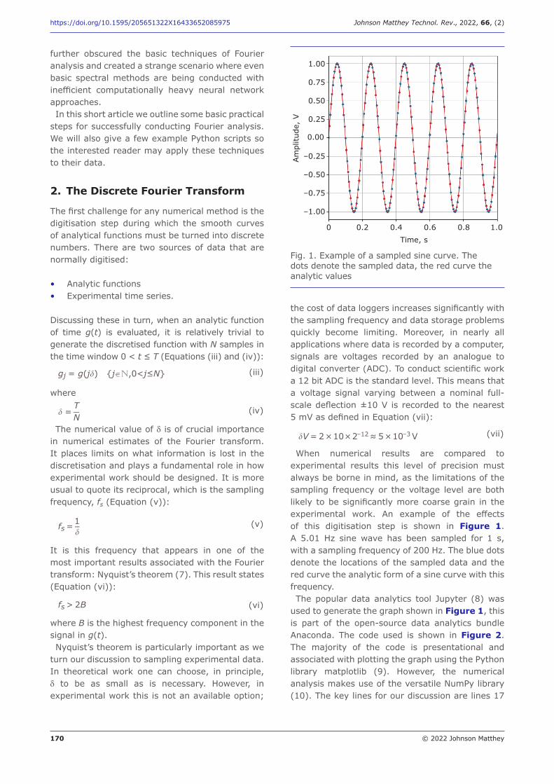
170 © 2022 Johnson Matthey
https://doi.org/10.1595/205651322X16433652085975 Johnson Matthey Technol. Rev., 2022, 66, (2)
further obscured the basic techniques of Fourier analysis and created a strange scenario where even basic spectral methods are being conducted with inefficient computationally heavy neural network approaches. In this short article we outline some basic practical
steps for successfully conducting Fourier analysis. We will also give a few example Python scripts so the interested reader may apply these techniques to their data.
2. The Discrete Fourier Transform
The first challenge for any numerical method is the digitisation step during which the smooth curves of analytical functions must be turned into discrete numbers. There are two sources of data that are normally digitised:
• Analytic functions• Experimental time series.
Discussing these in turn, when an analytic function of time g(t) is evaluated, it is relatively trivial to generate the discretised function with N samples in the time window 0 < t ≤ T (Equations (iii) and (iv)):
gj = g(j�) {j�n,0<j≤N} (iii)
where
� =TN
(iv)
The numerical value of δ is of crucial importance in numerical estimates of the Fourier transform. It places limits on what information is lost in the discretisation and plays a fundamental role in how experimental work should be designed. It is more usual to quote its reciprocal, which is the sampling frequency, fs (Equation (v)):
fs =1� (v)
It is this frequency that appears in one of the most important results associated with the Fourier transform: Nyquist’s theorem (7). This result states (Equation (vi)):
fs > 2B (vi)
where B is the highest frequency component in the signal in g(t).Nyquist’s theorem is particularly important as we
turn our discussion to sampling experimental data. In theoretical work one can choose, in principle, δ to be as small as is necessary. However, in experimental work this is not an available option;
the cost of data loggers increases significantly with the sampling frequency and data storage problems quickly become limiting. Moreover, in nearly all applications where data is recorded by a computer, signals are voltages recorded by an analogue to digital converter (ADC). To conduct scientific work a 12 bit ADC is the standard level. This means that a voltage signal varying between a nominal full-scale deflection ±10 V is recorded to the nearest 5 mV as defined in Equation (vii):
�V=2×10×2–12≈ 5×10⁻³V (vii)
When numerical results are compared to experimental results this level of precision must always be borne in mind, as the limitations of the sampling frequency or the voltage level are both likely to be significantly more coarse grain in the experimental work. An example of the effects of this digitisation step is shown in Figure 1. A 5.01 Hz sine wave has been sampled for 1 s, with a sampling frequency of 200 Hz. The blue dots denote the locations of the sampled data and the red curve the analytic form of a sine curve with this frequency.The popular data analytics tool Jupyter (8) was
used to generate the graph shown in Figure 1, this is part of the open-source data analytics bundle Anaconda. The code used is shown in Figure 2. The majority of the code is presentational and associated with plotting the graph using the Python library matplotlib (9). However, the numerical analysis makes use of the versatile NumPy library (10). The key lines for our discussion are lines 17
Fig. 1. Example of a sampled sine curve. The dots denote the sampled data, the red curve the analytic values
1.00
0.75
0.50
0.25
–0.25Am
plitu
de,
V
–0.50
–0.75
–1.00
0
0 0.2 0.4Time, s
0.6 0.8 1.0
0.00
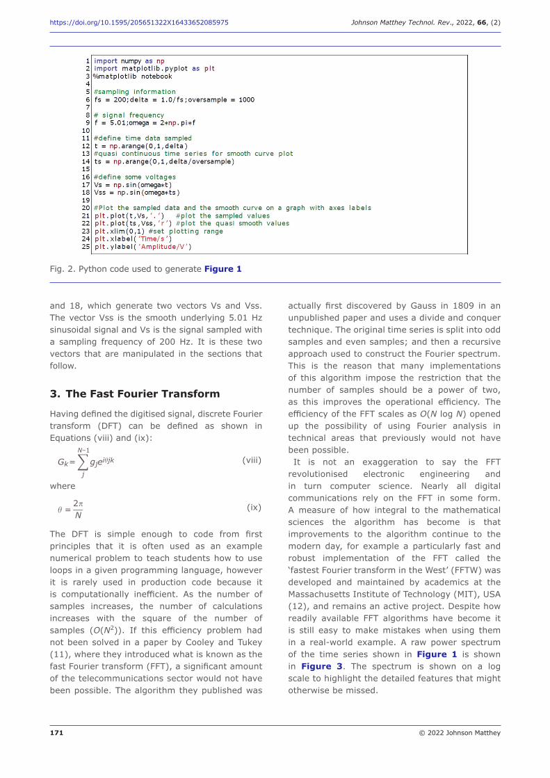
171 © 2022 Johnson Matthey
https://doi.org/10.1595/205651322X16433652085975 Johnson Matthey Technol. Rev., 2022, 66, (2)
and 18, which generate two vectors Vs and Vss. The vector Vss is the smooth underlying 5.01 Hz sinusoidal signal and Vs is the signal sampled with a sampling frequency of 200 Hz. It is these two vectors that are manipulated in the sections that follow.
3. The Fast Fourier Transform
Having defined the digitised signal, discrete Fourier transform (DFT) can be defined as shown in Equations (viii) and (ix):
Gk= gjei�jkN–1
j
(viii)
where
� =2�
N (ix)
The DFT is simple enough to code from first principles that it is often used as an example numerical problem to teach students how to use loops in a given programming language, however it is rarely used in production code because it is computationally inefficient. As the number of samples increases, the number of calculations increases with the square of the number of samples (O(N2)). If this efficiency problem had not been solved in a paper by Cooley and Tukey (11), where they introduced what is known as the fast Fourier transform (FFT), a significant amount of the telecommunications sector would not have been possible. The algorithm they published was
actually first discovered by Gauss in 1809 in an unpublished paper and uses a divide and conquer technique. The original time series is split into odd samples and even samples; and then a recursive approach used to construct the Fourier spectrum. This is the reason that many implementations of this algorithm impose the restriction that the number of samples should be a power of two, as this improves the operational efficiency. The efficiency of the FFT scales as O(N log N) opened up the possibility of using Fourier analysis in technical areas that previously would not have been possible.It is not an exaggeration to say the FFT
revolutionised electronic engineering and in turn computer science. Nearly all digital communications rely on the FFT in some form. A measure of how integral to the mathematical sciences the algorithm has become is that improvements to the algorithm continue to the modern day, for example a particularly fast and robust implementation of the FFT called the ‘fastest Fourier transform in the West’ (FFTW) was developed and maintained by academics at the Massachusetts Institute of Technology (MIT), USA (12), and remains an active project. Despite how readily available FFT algorithms have become it is still easy to make mistakes when using them in a real-world example. A raw power spectrum of the time series shown in Figure 1 is shown in Figure 3. The spectrum is shown on a log scale to highlight the detailed features that might otherwise be missed.
Fig. 2. Python code used to generate Figure 1
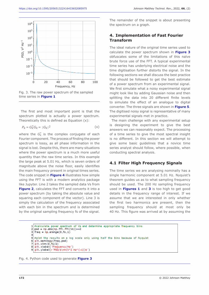
172 © 2022 Johnson Matthey
https://doi.org/10.1595/205651322X16433652085975 Johnson Matthey Technol. Rev., 2022, 66, (2)
The first and most important point is that the spectrum plotted is actually a power spectrum. Theoretically this is defined as Equation (x):
Pk = GkGk = �Gk�2* (x)
where the G* is the complex conjugate of each Fourier component. The process of finding the power spectrum is lossy, as all phase information in the signal is lost. Despite this, there are many situations where the power spectrum is a much more useful quantity than the raw time series. In this example the large peak at 5.01 Hz, which is seven orders of magnitude above the noise floor, easily identifies the main frequency present in original times series. The code snippet in Figure 4 illustrates how simple using the FFT is with a modern analytics package like Jupyter. Line 2 takes the sampled data Vs from Figure 2, calculates the FFT and converts it into a power spectrum (by taking the absolute value and squaring each component of the vector). Line 3 is simply the calculation of the frequency associated with each bin in the spectrum and is determined by the original sampling frequency fs of the signal.
The remainder of the snippet is about presenting the spectrum on a graph.
4. Implementation of Fast Fourier Transform
The ideal nature of the original time series used to calculate the power spectrum shown in Figure 3 obfuscates some of the limitations of this naïve brute force use of the FFT. A typical experimental time series has underlying electrical noise and the time digitisation further distorts the signal. In the following sections we shall discuss the best practice that should be followed to get the best estimate of a power spectrum from an experimental signal. We first simulate what a noisy experimental signal might look like by adding Gaussian noise and then splitting the data into 20 different finite levels to simulate the effect of an analogue to digital converter. The three signals are shown in Figure 5. The digitised noisy signal is representative of many experimental signals met in practice.The main challenge with any experimental setup
is designing the experiment to give the best answers we can reasonably expect. The processing of a time series to give the most spectral insight is no different. In this section we will attempt to give some basic guidelines that a novice time series analyst should follow, where possible, when conducting spectral analysis.
4.1 Filter High Frequency Signals
The time series we are analysing nominally has a single harmonic component at 5.01 Hz. Nyquist’s theorem guides us as to what sampling frequency should be used. The 200 Hz sampling frequency used in Figures 1 and 3 is too high to get good details in the frequency range of interest. If we assume that we are interested in only whether the first two harmonics are present, then the sampling frequency should at most only be 40 Hz. This figure was arrived at by assuming the
Fig. 3. The raw power spectrum of the sampled time series in Figure 1
PSD
/V2
Hz–
1
10–3
10–2
10–1
100
101
102
103
104
0 20 40Frequency, Hz
60 80 100
PSD
, V2
Hz–1
Fig. 4. Python code used to generate Figure 3
k
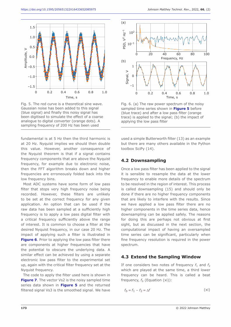
173 © 2022 Johnson Matthey
https://doi.org/10.1595/205651322X16433652085975 Johnson Matthey Technol. Rev., 2022, 66, (2)
fundamental is at 5 Hz then the third harmonic is at 20 Hz. Nyquist implies we should then double this value. However, another consequence of the Nyquist theorem is that if a signal contains frequency components that are above the Nyquist frequency, for example due to electronic noise, then the FFT algorithm breaks down and higher frequencies are erroneously folded back into the low frequency bins.Most ADC systems have some form of low pass
filter that stops very high frequency noise being recorded. However, these filters are unlikely to be set at the correct frequency for any given application. An option that can be used if the raw data has been sampled at a sufficiently high frequency is to apply a low pass digital filter with a critical frequency sufficiently above the range of interest. It is common to choose a filter at the desired Nyquist frequency, in our case 20 Hz. The impact of applying such a filter is illustrated in Figure 6. Prior to applying the low pass filter there are components at higher frequencies that have the potential to obscure the underlying data. A similar effect can be achieved by using a separate electronic low pass filter to the experimental set up, again with the critical filter frequency set at the Nyquist frequency.The code to apply the filter used here is shown in
Figure 7. The vector Vs2 is the noisy sampled time series data shown in Figure 5 and the returned filtered signal Vs3 is the smoothed signal. We have
used a simple Butterworth filter (13) as an example but there are many others available in the Python toolbox SciPy (14).
4.2 Downsampling
Once a low pass filter has been applied to the signal it is sensible to resample the data at the lower frequency to enable more details of the spectrum to be resolved in the region of interest. This process is called downsampling (15) and should only be done if there are no higher frequency components that are likely to interfere with the results. Since we have applied a low pass filter there are no higher components in the time series data, hence downsampling can be applied safely. The reasons for doing this are perhaps not obvious at first sight, but as discussed in the next section, the computational impact of having an oversampled time series can be significant, particularly when fine frequency resolution is required in the power spectrum.
4.3 Extend the Sampling Window
If one considers two notes of frequency f1 and f2 which are played at the same time, a third lower frequency can be heard. This is called a beat frequency, fb (Equation (xi)):
fb = f1 – f2 = ∆f (xi)
0.5
1.0
1.5Am
plitu
de,
V
–0.5
–1.5
–1.0
0
0 0.2 0.4Time, s
0.6 0.8 1.0
Fig. 5. The red curve is a theoretical sine wave. Gaussian noise has been added to this signal (blue signal) and finally this noisy signal has been digitised to simulate the effect of a coarse analogue to digital converter (orange dots). A sampling frequency of 200 Hz has been used
0.00
–1
20 40Frequency, Hz
60 80 100
0
0
1
0.2 0.4Time, s
Sig
nal,
V
0.6 0.8 1.0
PSD
/V2
Hz–
1
10–1
102
Fig. 6. (a) The raw power spectrum of the noisy sampled time series shown in Figure 5 before (blue trace) and after a low pass filter (orange trace) is applied to the signal; (b) the impact of applying the low pass filter
(a)
(b)
PSD
, V2
Hz–1
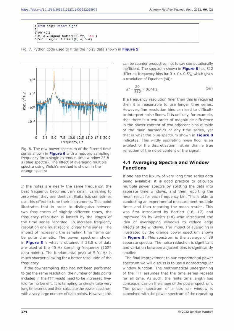
174 © 2022 Johnson Matthey
https://doi.org/10.1595/205651322X16433652085975 Johnson Matthey Technol. Rev., 2022, 66, (2)
If the notes are nearly the same frequency, the beat frequency becomes very small, vanishing to zero when they are identical. Guitarists sometimes use this effect to tune their instruments. This point illustrates that in order to distinguish between two frequencies of slightly different tones, the frequency resolution is limited by the length of the time series recorded. To increase frequency resolution one must record longer time series. The impact of increasing the sampling time frame can be quite dramatic. The power spectrum shown in Figure 8 is what is obtained if 25.8 s of data are used at the 40 Hz sampling frequency (1024 data points). The fundamental peak at 5.01 Hz is much sharper allowing for a better resolution of the frequency.If the downsampling step had not been performed
to get the same resolution, the number of data points included in the FFT would need to be increased five-fold for no benefit. It is tempting to simply take very long time series and then calculate the power spectrum with a very large number of data points. However, this
can be counter productive, not to say computationally inefficient. The spectrum shown in Figure 8 has 512 different frequency bins for 0 < f < 0.5fs, which gives a resolution of Equation (xii):
∆f =20512 ≈ 0.04Hz (xii)
If a frequency resolution finer than this is required then it is reasonable to use longer time series. However, fine resolution bins can lead to difficult-to-interpret noise floors. It is unlikely, for example, that there is a two order of magnitude difference in the power content of two adjacent bins outside of the main harmonics of any time series, yet that is what the blue spectrum shown in Figure 8 indicates. This wildly oscillating noise floor is an artefact of the discretisation, rather than a true reflection of the noise content of the signal.
4.4 Averaging Spectra and Window Functions
If one has the luxury of very long time series data being available, it is good practice to calculate multiple power spectra by splitting the data into separate time windows, and then reporting the mean result for each frequency bin. This is akin to conducting an experimental measurement multiple times and then reporting the mean results. This was first introduced by Bartlett (16, 17) and improved on by Welch (18) who introduced the idea of overlapping windows to reduce edge effects of the windows. The impact of averaging is illustrated by the orange power spectrum shown in Figure 8. This spectrum is the average of 39 separate spectra. The noise reduction is significant and variation between adjacent bins is significantly smaller.The final improvement to our experimental power
spectrum we will discuss is to use a non rectangular window function. The mathematical underpinning of the FFT assumes that the time series repeats for all time. As such, the finite time length has consequences on the shape of the power spectrum. The power spectrum of a box car window is convolved with the power spectrum of the repeating
Fig. 7. Python code used to filter the noisy data shown in Figure 5
PSD
/V2
Hz–
1
10–2
100
102
104
0 2.5 5.0 7.5 10.0 12.5 15.0 17.5 20.0Frequency, Hz
Fig. 8. The raw power spectrum of the filtered time series shown in Figure 6 with a reduced sampling frequency for a single extended time window 25.8 s (blue spectra). The effect of averaging multiple spectra using Welch’s method is shown in the orange spectra
PSD
, V2
Hz–1
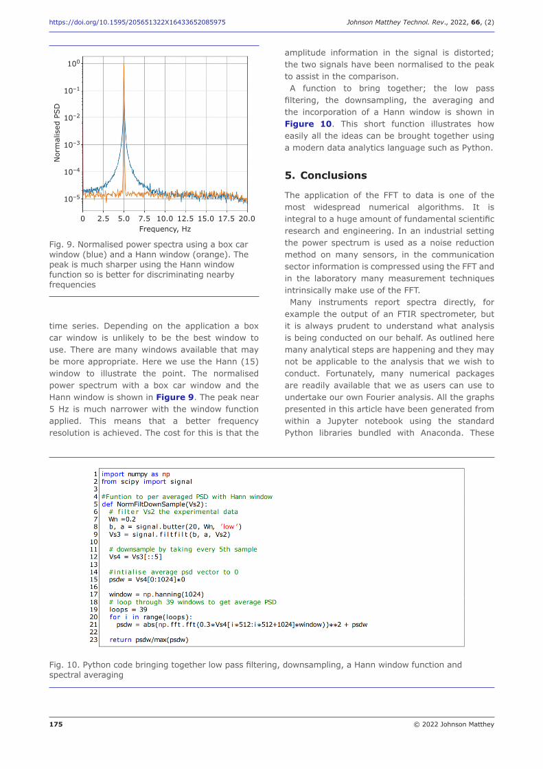
175 © 2022 Johnson Matthey
https://doi.org/10.1595/205651322X16433652085975 Johnson Matthey Technol. Rev., 2022, 66, (2)
time series. Depending on the application a box car window is unlikely to be the best window to use. There are many windows available that may be more appropriate. Here we use the Hann (15) window to illustrate the point. The normalised power spectrum with a box car window and the Hann window is shown in Figure 9. The peak near 5 Hz is much narrower with the window function applied. This means that a better frequency resolution is achieved. The cost for this is that the
amplitude information in the signal is distorted; the two signals have been normalised to the peak to assist in the comparison.A function to bring together; the low pass
filtering, the downsampling, the averaging and the incorporation of a Hann window is shown in Figure 10. This short function illustrates how easily all the ideas can be brought together using a modern data analytics language such as Python.
5. Conclusions
The application of the FFT to data is one of the most widespread numerical algorithms. It is integral to a huge amount of fundamental scientific research and engineering. In an industrial setting the power spectrum is used as a noise reduction method on many sensors, in the communication sector information is compressed using the FFT and in the laboratory many measurement techniques intrinsically make use of the FFT.Many instruments report spectra directly, for
example the output of an FTIR spectrometer, but it is always prudent to understand what analysis is being conducted on our behalf. As outlined here many analytical steps are happening and they may not be applicable to the analysis that we wish to conduct. Fortunately, many numerical packages are readily available that we as users can use to undertake our own Fourier analysis. All the graphs presented in this article have been generated from within a Jupyter notebook using the standard Python libraries bundled with Anaconda. These
Fig. 9. Normalised power spectra using a box car window (blue) and a Hann window (orange). The peak is much sharper using the Hann window function so is better for discriminating nearby frequencies
Nor
mal
ised
PSD
10–1
10–2
10–3
10–4
10–5
100
0 2.5 5.0 7.5 10.0 12.5 15.0 17.5 20.0Frequency, Hz
Fig. 10. Python code bringing together low pass filtering, downsampling, a Hann window function and spectral averaging
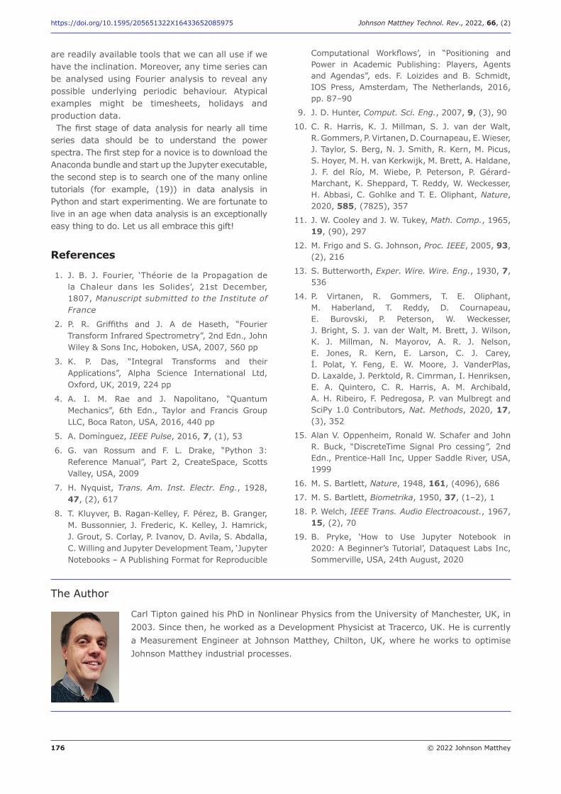
176 © 2022 Johnson Matthey
https://doi.org/10.1595/205651322X16433652085975 Johnson Matthey Technol. Rev., 2022, 66, (2)
are readily available tools that we can all use if we have the inclination. Moreover, any time series can be analysed using Fourier analysis to reveal any possible underlying periodic behaviour. Atypical examples might be timesheets, holidays and production data.The first stage of data analysis for nearly all time
series data should be to understand the power spectra. The first step for a novice is to download the Anaconda bundle and start up the Jupyter executable, the second step is to search one of the many online tutorials (for example, (19)) in data analysis in Python and start experimenting. We are fortunate to live in an age when data analysis is an exceptionally easy thing to do. Let us all embrace this gift!
References
1. J. B. J. Fourier, ‘Théorie de la Propagation de la Chaleur dans les Solides’, 21st December, 1807, Manuscript submitted to the Institute of France
2. P. R. Griffiths and J. A de Haseth, “Fourier Transform Infrared Spectrometry”, 2nd Edn., John Wiley & Sons Inc, Hoboken, USA, 2007, 560 pp
3. K. P. Das, “Integral Transforms and their Applications”, Alpha Science International Ltd, Oxford, UK, 2019, 224 pp
4. A. I. M. Rae and J. Napolitano, “Quantum Mechanics”, 6th Edn., Taylor and Francis Group LLC, Boca Raton, USA, 2016, 440 pp
5. A. Domínguez, IEEE Pulse, 2016, 7, (1), 53
6. G. van Rossum and F. L. Drake, “Python 3: Reference Manual”, Part 2, CreateSpace, Scotts Valley, USA, 2009
7. H. Nyquist, Trans. Am. Inst. Electr. Eng., 1928, 47, (2), 617
8. T. Kluyver, B. Ragan-Kelley, F. Pérez, B. Granger, M. Bussonnier, J. Frederic, K. Kelley, J. Hamrick, J. Grout, S. Corlay, P. Ivanov, D. Avila, S. Abdalla, C. Willing and Jupyter Development Team, ‘Jupyter Notebooks – A Publishing Format for Reproducible
Computational Workflows’, in “Positioning and Power in Academic Publishing: Players, Agents and Agendas”, eds. F. Loizides and B. Schmidt, IOS Press, Amsterdam, The Netherlands, 2016, pp. 87–90
9. J. D. Hunter, Comput. Sci. Eng., 2007, 9, (3), 90
10. C. R. Harris, K. J. Millman, S. J. van der Walt, R. Gommers, P. Virtanen, D. Cournapeau, E. Wieser, J. Taylor, S. Berg, N. J. Smith, R. Kern, M. Picus, S. Hoyer, M. H. van Kerkwijk, M. Brett, A. Haldane, J. F. del Río, M. Wiebe, P. Peterson, P. Gérard-Marchant, K. Sheppard, T. Reddy, W. Weckesser, H. Abbasi, C. Gohlke and T. E. Oliphant, Nature, 2020, 585, (7825), 357
11. J. W. Cooley and J. W. Tukey, Math. Comp., 1965, 19, (90), 297
12. M. Frigo and S. G. Johnson, Proc. IEEE, 2005, 93, (2), 216
13. S. Butterworth, Exper. Wire. Wire. Eng., 1930, 7, 536
14. P. Virtanen, R. Gommers, T. E. Oliphant, M. Haberland, T. Reddy, D. Cournapeau, E. Burovski, P. Peterson, W. Weckesser, J. Bright, S. J. van der Walt, M. Brett, J. Wilson, K. J. Millman, N. Mayorov, A. R. J. Nelson, E. Jones, R. Kern, E. Larson, C. J. Carey, İ. Polat, Y. Feng, E. W. Moore, J. VanderPlas, D. Laxalde, J. Perktold, R. Cimrman, I. Henriksen, E. A. Quintero, C. R. Harris, A. M. Archibald, A. H. Ribeiro, F. Pedregosa, P. van Mulbregt and SciPy 1.0 Contributors, Nat. Methods, 2020, 17, (3), 352
15. Alan V. Oppenheim, Ronald W. Schafer and John R. Buck, “Discrete Time Signal Pro cessing”, 2nd Edn., Prentice-Hall Inc, Upper Saddle River, USA, 1999
16. M. S. Bartlett, Nature, 1948, 161, (4096), 686
17. M. S. Bartlett, Biometrika, 1950, 37, (1–2), 1
18. P. Welch, IEEE Trans. Audio Electroacoust., 1967, 15, (2), 70
19. B. Pryke, ‘How to Use Jupyter Notebook in 2020: A Beginner’s Tutorial’, Dataquest Labs Inc, Sommerville, USA, 24th August, 2020
The Author
Carl Tipton gained his PhD in Nonlinear Physics from the University of Manchester, UK, in 2003. Since then, he worked as a Development Physicist at Tracerco, UK. He is currently a Measurement Engineer at Johnson Matthey, Chilton, UK, where he works to optimise Johnson Matthey industrial processes.
www.technology.matthey.com
https://doi.org/10.1595/205651322X16273773896889 Johnson Matthey Technol. Rev., 2022, 66, (2), 177–185
177 © 2022 Johnson Matthey
Makbule Nur UyarAkar Tekstil AŞ, İzmir, Turkey
Ayşe Merih Sarıışık, Gülşah Ekin Kartal*Dokuz Eylül University, Department of Textile Engineering, Faculty of Engineering, Tınaztepe Campus, İzmir, Turkey
*Email: [email protected]
PEER REVIEWED
Received 9th April 2021; Revised 25th May 2021; Accepted 27th July 2021; Online 27th July 2021
This study intends to identify the characteristics of heat regulation in heat storage microencapsulated fabrics and to examine the effect of the microcapsules application method. For this purpose, phase-changing material (PCM) microcapsules were applied by impregnation and coating methods on cotton fabrics. The presence and distribution of microcapsules on the fabric surface were investigated by scanning electron microscopy (SEM). The temperature regulation of the fabrics was examined using a temperature measurement sensor and data recorder system (thermal camera). According to the differential scanning calorimetry (DSC) analysis, melting in fabrics coated with microcapsules occurred between 25.83°C–31.04°C and the amount of heat energy stored by the cotton fabric during the melting period was measured as 2.70 J g–1. Changes in fabric surface temperature due to the presence of microcapsules in the fabric structure were determined. When comparing the PCM capsules transfer methods, the contact angle of impregnated and coated
Examination of the Coating Method in Transferring Phase-Changing Materials Heat regulation in heat storage microencapsulated fabrics
fabric was obtained as 42° and 73°, respectively. Analysis of the microcapsules transferred to the fabric by impregnation and coating methods shows that the PCM transferred fabric prepared by the impregnation method performs more efficient temperature regulation. However, the analysis shows that PCM transferred fabrics prepared by coating also perform heat absorption, although not as much as the impregnation method. Performance evaluation according to the target properties of the textile will give the most accurate results for fabrics treated by coating and impregnation methods.
1. Introduction
The importance of functional processes that add value, create difference and increase market share in the textile sector is increasing day by day with developing technology. Not only aesthetic features but also functional features determine consumers’ wishes. For this purpose, technologies like plasma, sol-gel or microencapsulation can provide different functional properties to textile materials (1).The microencapsulation process produces
small spheres covered with a thin shell film to protect the active substance from outside. Using this technology, it is possible to protect easily perishable substances such as drugs, insecticides, antibacterials and antioxidants from environmental factors like heat, light and oxygen. In addition, the wearer is exposed to much lower doses of these substances. Using microcapsules in textile finishing makes it possible to produce resistant-to-wash textile products that are effective even when a less active substance is used. Another area where microcapsules can be used is energy storage (2–6).Problems like the climate crisis, greenhouse gas
emissions, air pollution, usage of finite resources and economic issues require solutions. Energy
178 © 2022 Johnson Matthey
https://doi.org/10.1595/205651322X16273773896889 Johnson Matthey Technol. Rev., 2022, 66, (2)
is needed for heating, air conditioning and ventilation. Energy storage plays an important role in conserving available energy and improving its utilisation since many energy sources, especially renewables, are intermittent. Short-term storage of only a few hours may be desirable in applications like clothes or curtains, while longer-term storage of a few months may be required in some applications like buildings, concrete or space clothes (7–9). A phase-change material or PCM can store and
release large amounts of energy. This energy is called latent heat. Latent heat is thermal energy released or absorbed, by a thermodynamic system, during a constant-temperature process — usually a first-order phase transition. Latent heat can be understood as heat energy in a hidden form which is supplied or extracted to change the state of a substance without changing its temperature. PCMs are classified as latent heat storage units. Each PCM has a specific melting and crystallisation temperature and a specific latent heat storage capacity. PCMs take advantage of latent heat that can be stored or released from material over a narrow temperature range. These materials absorb energy during the heating process as phase change takes place and release energy to the environment in the phase change range during a reverse cooling process. Textiles containing phase change materials react immediately to changes in environmental temperatures and the temperatures in different areas of the body. This system can be used in applications like protective clothing, beds, bedspreads, space suits, diving suits and curtains (10–28). For any PCM to be used in textile products, it must
have certain properties. The main ones are: high melting or hydration temperature, high thermal conductivity, high specific heat capacity, minimum volume change during phase transformation, appropriate phase change temperature, repeatability of phase transformation, low corrosion and degradation tendency and non-toxicity. The textiles should pass certain flame retardancy standards with the PCM material applied. Choosing the appropriate PCM for the protective clothing is crucial for an ideal thermal insulation and regulation effect. Many factors should be taken into consideration while making this choice. What is expected from PCM to be added to a textile product to be used as a garment is to minimise the heat flow between the person and the outside environment by keeping the body temperature constant at a
certain value that the person is comfortable with. Suitable materials for textile products in terms of phase change temperatures include: hydrate inorganic salts, polyhydric alcohol-water solution, polyethylene glycol (PEG), polytetramethylene glycol (PTGM), aliphatic polyester, linear long chain hydrocarbons, hydrocarbon alcohols or organic acids (28–39). In general, the impregnation and exhaustion
method can be used to transfer microcapsules in the textile industry. In the impregnation method, a liquor is prepared and the capsules are mixed into this liquor at a certain rate. Afterwards, the fabric is absorbed into the float, passed through a foulard machine and the process is completed with pressure from cylinders. In the coating method, a coating paste is prepared and the capsules are added to the paste at a certain rate. The coating paste is then applied to the fabric. To date, little research has been done on possible applications of microcapsules in functional coating processes.One of the most important problems of PCMs is
low thermal conductivity. For example, paraffin has 0.22 W m–1 K–1 thermal conductivity when compared with >3000 W m–1 K–1 for multiwall carbon nanotubes (MWCNTs). Moreover, microencapsulated PCMs have a polymeric shell, which not only prevents the content from leaking but also resists heat transition. When capsules are transferred to the fabrics by coating, another viscous coating layer is added on the shell material of the capsule. It is thought that this feature will increase in cases where PCM capsules are transferred by the coating method compared to those transferred by the impregnation method (27, 40–42). Within the scope of this study, it is thought
that the coating application can be applied especially in black out curtains. In this study, PCM microcapsules were used to develop thermoregulating textile materials and the effect of the microcapsules application method was examined. In this research, Mikrathermic® P PCM microcapsules were transferred to 100% cotton woven fabrics by the impregnation and coating methods. The thermal regulation properties of the fabrics were analysed by DSC and the surface morphological properties by SEM. In addition, the thermal properties of the fabrics were obtained with a thermal camera. Contact angles and water vapour permeability of coated and impregnated fabrics were investigated.
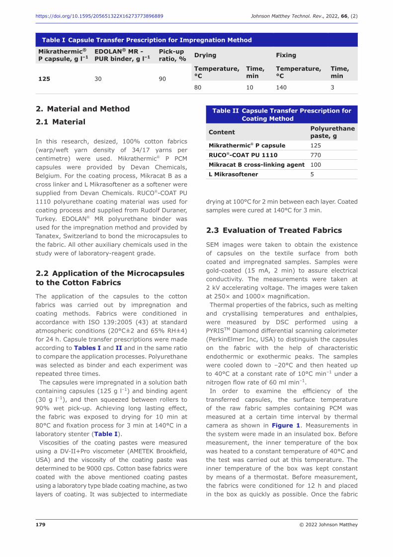
179 © 2022 Johnson Matthey
https://doi.org/10.1595/205651322X16273773896889 Johnson Matthey Technol. Rev., 2022, 66, (2)
2. Material and Method
2.1 Material
In this research, desized, 100% cotton fabrics (warp/weft yarn density of 34/17 yarns per centimetre) were used. Mikrathermic® P PCM capsules were provided by Devan Chemicals, Belgium. For the coating process, Mikracat B as a cross linker and L Mikrasoftener as a softener were supplied from Devan Chemicals. RUCO®-COAT PU 1110 polyurethane coating material was used for coating process and supplied from Rudolf Duraner, Turkey. EDOLAN® MR polyurethane binder was used for the impregnation method and provided by Tanatex, Switzerland to bond the microcapsules to the fabric. All other auxiliary chemicals used in the study were of laboratory-reagent grade.
2.2 Application of the Microcapsules to the Cotton Fabrics
The application of the capsules to the cotton fabrics was carried out by impregnation and coating methods. Fabrics were conditioned in accordance with ISO 139:2005 (43) at standard atmospheric conditions (20°C±2 and 65% RH±4) for 24 h. Capsule transfer prescriptions were made according to Tables I and II and in the same ratio to compare the application processes. Polyurethane was selected as binder and each experiment was repeated three times.The capsules were impregnated in a solution bath
containing capsules (125 g l–1) and binding agent (30 g l–1), and then squeezed between rollers to 90% wet pick-up. Achieving long lasting effect, the fabric was exposed to drying for 10 min at 80°C and fixation process for 3 min at 140°C in a laboratory stenter (Table I).Viscosities of the coating pastes were measured
using a DV-II+Pro viscometer (AMETEK Brookfield, USA) and the viscosity of the coating paste was determined to be 9000 cps. Cotton base fabrics were coated with the above mentioned coating pastes using a laboratory type blade coating machine, as two layers of coating. It was subjected to intermediate
drying at 100°C for 2 min between each layer. Coated samples were cured at 140°C for 3 min.
2.3 Evaluation of Treated Fabrics
SEM images were taken to obtain the existence of capsules on the textile surface from both coated and impregnated samples. Samples were gold-coated (15 mA, 2 min) to assure electrical conductivity. The measurements were taken at 2 kV accelerating voltage. The images were taken at 250× and 1000× magnification. Thermal properties of the fabrics, such as melting
and crystallising temperatures and enthalpies, were measured by DSC performed using a PYRISTM Diamond differential scanning calorimeter (PerkinElmer Inc, USA) to distinguish the capsules on the fabric with the help of characteristic endothermic or exothermic peaks. The samples were cooled down to –20°C and then heated up to 40°C at a constant rate of 10°C min–1 under a nitrogen flow rate of 60 ml min–1.In order to examine the efficiency of the
transferred capsules, the surface temperature of the raw fabric samples containing PCM was measured at a certain time interval by thermal camera as shown in Figure 1. Measurements in the system were made in an insulated box. Before measurement, the inner temperature of the box was heated to a constant temperature of 40°C and the test was carried out at this temperature. The inner temperature of the box was kept constant by means of a thermostat. Before measurement, the fabrics were conditioned for 12 h and placed in the box as quickly as possible. Once the fabric
Table I Capsule Transfer Prescription for Impregnation Method
Mikrathermic® P capsule, g l–1
EDOLAN® MR - PUR binder, g l–1
Pick-up ratio, % Drying Fixing
125 30 90
Temperature, °C
Time, min
Temperature, °C
Time, min
80 10 140 3
Table II Capsule Transfer Prescription for Coating Method
Content Polyurethane paste, g
Mikrathermic® P capsule 125
RUCO®-COAT PU 1110 770
Mikracat B cross-linking agent 100
L Mikrasoftener 5
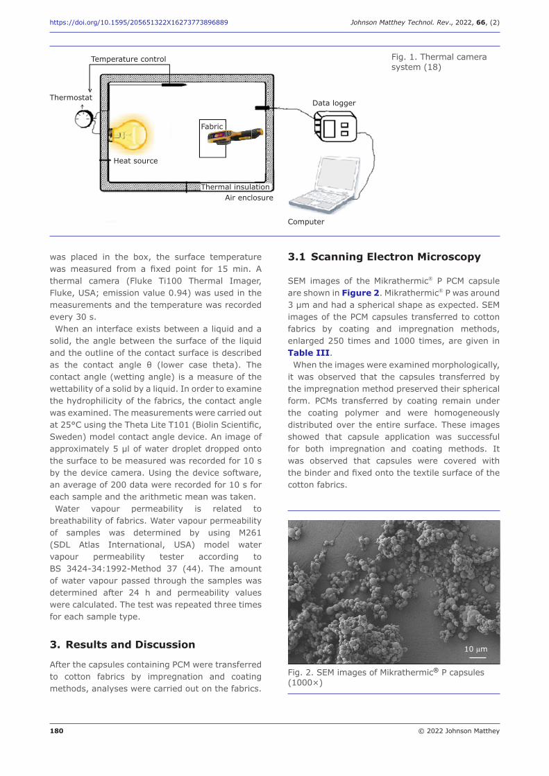
180 © 2022 Johnson Matthey
https://doi.org/10.1595/205651322X16273773896889 Johnson Matthey Technol. Rev., 2022, 66, (2)
was placed in the box, the surface temperature was measured from a fixed point for 15 min. A thermal camera (Fluke Ti100 Thermal Imager, Fluke, USA; emission value 0.94) was used in the measurements and the temperature was recorded every 30 s.When an interface exists between a liquid and a
solid, the angle between the surface of the liquid and the outline of the contact surface is described as the contact angle θ (lower case theta). The contact angle (wetting angle) is a measure of the wettability of a solid by a liquid. In order to examine the hydrophilicity of the fabrics, the contact angle was examined. The measurements were carried out at 25°C using the Theta Lite T101 (Biolin Scientific, Sweden) model contact angle device. An image of approximately 5 µl of water droplet dropped onto the surface to be measured was recorded for 10 s by the device camera. Using the device software, an average of 200 data were recorded for 10 s for each sample and the arithmetic mean was taken.Water vapour permeability is related to
breathability of fabrics. Water vapour permeability of samples was determined by using M261 (SDL Atlas International, USA) model water vapour permeability tester according to BS 3424-34:1992-Method 37 (44). The amount of water vapour passed through the samples was determined after 24 h and permeability values were calculated. The test was repeated three times for each sample type.
3. Results and Discussion
After the capsules containing PCM were transferred to cotton fabrics by impregnation and coating methods, analyses were carried out on the fabrics.
3.1 Scanning Electron Microscopy
SEM images of the Mikrathermic® P PCM capsule are shown in Figure 2. Mikrathermic® P was around 3 μm and had a spherical shape as expected. SEM images of the PCM capsules transferred to cotton fabrics by coating and impregnation methods, enlarged 250 times and 1000 times, are given in Table III.When the images were examined morphologically,
it was observed that the capsules transferred by the impregnation method preserved their spherical form. PCMs transferred by coating remain under the coating polymer and were homogeneously distributed over the entire surface. These images showed that capsule application was successful for both impregnation and coating methods. It was observed that capsules were covered with the binder and fixed onto the textile surface of the cotton fabrics.
Temperature control
ThermostatData logger
Computer
Heat source
Thermal insulationAir enclosure
Fabric
Fig. 1. Thermal camera system (18)
Fig. 2. SEM images of Mikrathermic® P capsules (1000×)
10 mm
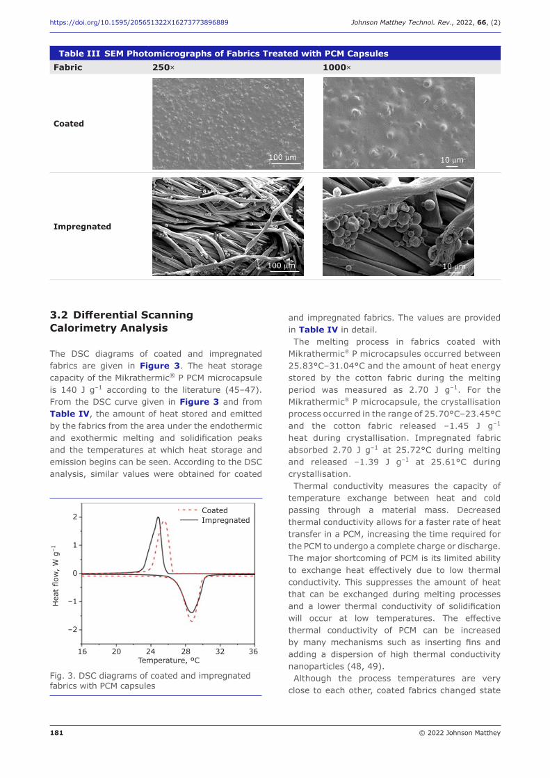
181 © 2022 Johnson Matthey
https://doi.org/10.1595/205651322X16273773896889 Johnson Matthey Technol. Rev., 2022, 66, (2)
3.2 Differential Scanning Calorimetry Analysis
The DSC diagrams of coated and impregnated fabrics are given in Figure 3. The heat storage capacity of the Mikrathermic® P PCM microcapsule is 140 J g–1 according to the literature (45–47). From the DSC curve given in Figure 3 and from Table IV, the amount of heat stored and emitted by the fabrics from the area under the endothermic and exothermic melting and solidification peaks and the temperatures at which heat storage and emission begins can be seen. According to the DSC analysis, similar values were obtained for coated
and impregnated fabrics. The values are provided in Table IV in detail.The melting process in fabrics coated with
Mikrathermic® P microcapsules occurred between 25.83°C–31.04°C and the amount of heat energy stored by the cotton fabric during the melting period was measured as 2.70 J g–1. For the Mikrathermic® P microcapsule, the crystallisation process occurred in the range of 25.70°C–23.45°C and the cotton fabric released –1.45 J g–1 heat during crystallisation. Impregnated fabric absorbed 2.70 J g–1 at 25.72°C during melting and released –1.39 J g–1 at 25.61°C during crystallisation. Thermal conductivity measures the capacity of
temperature exchange between heat and cold passing through a material mass. Decreased thermal conductivity allows for a faster rate of heat transfer in a PCM, increasing the time required for the PCM to undergo a complete charge or discharge. The major shortcoming of PCM is its limited ability to exchange heat effectively due to low thermal conductivity. This suppresses the amount of heat that can be exchanged during melting processes and a lower thermal conductivity of solidification will occur at low temperatures. The effective thermal conductivity of PCM can be increased by many mechanisms such as inserting fins and adding a dispersion of high thermal conductivity nanoparticles (48, 49).Although the process temperatures are very
close to each other, coated fabrics changed state
Table III SEM Photomicrographs of Fabrics Treated with PCM Capsules Fabric 250× 1000×
Coated
100 mm 10 mm
Impregnated
100 mm 10 mm
Hea
t flo
w,
W g
–1
2
1
0
–1
–2
16 20 24 28 32 36Temperature, ºC
Fig. 3. DSC diagrams of coated and impregnated fabrics with PCM capsules
CoatedImpregnated
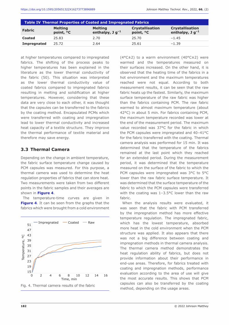
182 © 2022 Johnson Matthey
https://doi.org/10.1595/205651322X16273773896889 Johnson Matthey Technol. Rev., 2022, 66, (2)
at higher temperatures compared to impregnated fabrics. The shifting of the process peaks to higher temperatures has been explained in the literature as the lower thermal conductivity of the fabric (50). This situation was interpreted as the lower thermal conductivity value of coated fabrics compared to impregnated fabrics resulting in melting and solidification at higher temperatures. However, considering that these data are very close to each other, it was thought that the capsules can be transferred to the fabrics by the coating method. Encapsulated PCMs which were transferred with coating and impregnation lead to lower thermal conductivity and increased heat capacity of a textile structure. They improve the thermal performance of textile material and therefore may save energy.
3.3 Thermal Camera
Depending on the change in ambient temperature, the fabric surface temperature change caused by PCM capsules was measured. For this purpose, a thermal camera was used to determine the heat regulation properties of fabrics that can store heat. Two measurements were taken from two different points in the fabric samples and their averages are shown in Figure 4.The temperature-time curves are given in
Figure 4. It can be seen from the graphs that the fabrics which were brought from a cold environment
(4°C±2) to a warm environment (40°C±2) were warmed and the temperatures measured on their surfaces increased. On the other hand, it is observed that the heating time of the fabrics in a hot environment and the maximum temperatures reached were not equal. According to both measurement results, it can be seen that the raw fabric heats up the fastest. Similarly, the maximum surface temperature of the raw fabric was higher than the fabrics containing PCM. The raw fabric warmed to almost maximum temperature (about 42°C) in about 5 min. For fabrics containing PCM, the maximum temperature recorded was lower at the end of the measurement period. The maximum value recorded was 37°C for the fabric in which the PCM capsules were impregnated and 40–41°C for the fabric transferred with the coating. Thermal camera analysis was performed for 15 min. It was determined that the temperature of the fabrics remained at the last point which they reached for an extended period. During the measurement period, it was determined that the temperature measured on the surface of the fabric to which the PCM capsules were impregnated was 3°C to 5°C lower than the raw fabric surface temperature. It was determined that the surface temperature of the fabric to which the PCM capsules were transferred with the coating was 1–3.5°C lower than the raw fabric. When the analysis results were evaluated, it
was seen that the fabric with PCM transferred by the impregnation method has more effective temperature regulation. The impregnated fabric, which has the lowest temperature, absorbed more heat in the cold environment when the PCM structure was applied. It also appears that there was not a big difference between coating and impregnation methods in thermal camera analysis. The thermal camera method demonstrates the heat regulation ability of fabrics, but does not provide information about their performance in end-use areas. Therefore, for fabrics treated with coating and impregnation methods, performance evaluation according to the area of use will give the most accurate results. This shows that PCM capsules can also be transferred by the coating method, depending on the usage areas.
Table IV Thermal Properties of Coated and Impregnated Fabrics
Fabric Meltingpoint, °C
Meltingenthalpy, J g–1
Crystallisationpoint, °C
Crystallisationenthalpy, J g–1
Coated 25.83 2.70 25.70 –1.45
Impregnated 25.72 2.64 25.61 –1.39
Impregnated Coated Raw
Tem
pera
ture
, ºC
0 2 4 6 8 10 12 14 16Time, min
51474339353127231915
Fig. 4. Thermal camera results of the fabric

183 © 2022 Johnson Matthey
https://doi.org/10.1595/205651322X16273773896889 Johnson Matthey Technol. Rev., 2022, 66, (2)
3.4 Contact Angle Measurement
In order to evaluate the hydrophilicity properties of raw fabric and PCM-transferred fabrics with different methods, contact angle measurement was made as shown in Figure 5.The angle between the surface of the liquid and
the outline of the contact surface is described as the contact angle θ. The contact angle is a measure of the wettability of a solid by a liquid. In the case of complete wetting, the contact angle is 0°. Between 0° and 90°, the solid is wettable and above 90° it is not wettable. When the analysis results were examined, water was completely absorbed by raw fabric in 5 s and this indicates that the fabric is hydrophilic. When comparing the transfer methods of PCM capsules, contact angle of impregnated and coated fabric was obtained as 42° and 73°, respectively. In general, the coating paste has a more viscous structure and this structure causes a thick layer to form on the fabric. Due to this structure, the surface energy of the fabric decreases and it gains water repellency. In the impregnation method, since a viscous structure is not obtained and a layer is not formed on the fabric surface, the contact angle becomes lower causing the textile material to be more hydrophilic than the coated one. This result, as expected, was that the coated fabric was more hydrophobic than the impregnated fabric.
3.5 Water Vapour Permeability
Water vapour permeability analysis was carried out to examine the comfort properties of the fabrics obtained. Water vapour permeability of samples are tabulated in Table V.The highest water vapour permeability was
obtained from raw fabric with 625 g m–2 per 24 h
permeability value. It was determined that the fabrics with PCM transferred by the impregnation method gave a similar result to the raw fabric. On the other hand, water vapour permeability of coated samples reduced to approximately 50% that of the raw base fabric in parallel with the contact angle results. This was due to the additional polyurethane coating layer which contributed mass transfer limitation through the fabric. Even the most breathable coating polymer applied to the samples would add a resistance to vapour flow by closing the pores and creating an additional layer (51). The water vapour permeability of a material plays an important part in evaluating the physiological wearing comfort of clothing systems or determining the performance characteristics of textile materials used in technical applications. Therefore, it is important to choose the transfer method of PCM capsules considering the area where the fabric will be used.
4. Conclusion
Within the scope of this study, PCM capsules were applied to textile materials with coating and impregnation methods, successfully. As a result of the study, it was observed that the capsules transferred by the impregnation method preserved their spherical form according to the SEM images. It was seen that PCMs transferred by coating remain
(a) (b) (c)
Fig. 5. Contact angle images of fabrics: (a) raw fabric; (b) coated fabric; (c) impregnated fabric
73.14º 73.03º
42.40º 41.29º
Table V Water Vapour Permeability Results of Fabrics
Fabric Water vapour permeability, g m–2 per 24 h
Raw 625.44
Impregnated 619.02
Coated 352.18
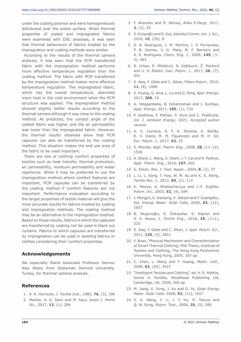
184 © 2022 Johnson Matthey
https://doi.org/10.1595/205651322X16273773896889 Johnson Matthey Technol. Rev., 2022, 66, (2)
under the coating polymer and were homogeneously distributed over the entire surface. When thermal properties of coated and impregnated fabrics were examined with DSC analyses, it was seen that thermal behaviours of fabrics treated by the impregnation and coating methods were similar. According to the results of the thermal camera
analysis, it was seen that the PCM transferred fabric with the impregnation method performs more effective temperature regulation than the coating method. The fabric with PCM transferred by the impregnation method makes more effective temperature regulation. The impregnated fabric, which has the lowest temperature, absorbed more heat in the cold environment when the PCM structure was applied. The impregnation method showed slightly better results according to the thermal camera although it was close to the coating method. As predicted, the contact angle of the coated fabric was higher and the air permeability was lower than the impregnated fabric. However, the thermal results obtained show that PCM capsules can also be transferred by the coating method. This situation makes the end use area of the fabric to be used important. There are lots of clothing comfort properties of
textiles such as heat transfer, thermal protection, air permeability, moisture permeability and water repellence. While it may be preferred to use the impregnation method where comfort features are important, PCM capsules can be transferred by the coating method if comfort features are not important. Performance evaluation according to the target properties of textile material will give the most accurate results for fabrics treated by coating and impregnation methods. The coating method may be an alternative to the impregnation method. Based on these results, fabrics in which the capsules are transferred by coating can be used in black out curtains. Fabrics to which capsules are transferred by impregnation can be used in bedding fabrics or clothes considering their comfort properties.
Acknowledgements
We especially thank Associate Professor Sennur Alay Aksoy from Süleyman Demirel University, Turkey, for thermal camera analysis.
References
1. A. R. Horrocks, J. Textile Inst., 1985, 76, (3), 196 2. Mamta, H. K. Saini and M. Kaur, Asian J. Home
Sci., 2017, 12, (1), 289
3. F. Akarslan and Ö. Altınay, Anka E-Dergi, 2017, 2, (2), 35
4. S. Eyüpoğlu and D. Kut, Istanbul Comm. Uni. J. Sci., 2016, 15, (29), 9
5. S. N. Rodrigues, I. M. Martins, I. P. Fernandes, P. B. Gomes, V. G. Mata, M. F. Barreiro and A. E. Rodrigues, Chem. Eng. J., 2009, 149, (1–3), 463
6. R. Urbas, R. Milošević, N. Kašiković, Ž. Pavlović and U. S. Elesini, Iran. Polym. J., 2017, 26, (7), 541
7. S. Alay, F. Göde and C. Alkan, Fibers Polym., 2010, 11, (8), 1089
8. X. Huang, G. Alva, L. Liu and G. Fang, Appl. Energy, 2017, 200, 19
9. A. Yataganbaba, B. Ozkahraman and I. Kurtbas, Appl. Energy, 2017, 185, (1), 720
10. P. Gadhave, F. Pathan, S. Kore and C. Prabhune, Int. J. Ambient Energy, 2021, Accepted author version
11. A. S. Carreira, R. F. A. Teixeira, A. Beirão, R. V. Vieira, M. M. Figueiredo and M. H. Gil, Eur. Polym. J., 2017, 93, 33
12. S. Mondal, Appl. Therm. Eng., 2008, 28, (11–12), 1536
13. A. Shaid, L. Wang, S. Islam, J. Y. Cai and R. Padhye, Appl. Therm. Eng., 2016, 107, 602
14. G. Erkan, Res. J. Text. Appar., 2004, 8, (2), 57
15. L. Li, L. Song, T. Hua, W. M. Au and K. S. Wong, Textile Res. J., 2012, 83, (2), 113
16. K. Mayya, A. Bhattacharyya and J.-F. Argillier, Polym. Int., 2003, 52, (4), 644
17. J. Mengjin, S. Xiaoqıng, X. Jianjun and Y. Guangdou, Sol. Energy Mater. Solar Cells, 2008, 92, (12), 1657
18. B. Akgünoğlu, S. Özkayalar, S. Kaplan and S. A. Aksoy, J. Textile Eng., 2018, 25, (111), 225
19. S. Alay, F. Göde and C. Alkan, J. Appl. Polym. Sci., 2011, 120, (5), 2821
20. Y. Boan, ‘Physical Mechanism and Characterization of Smart Thermal Clothing’, PhD Thesis, Institute of Textiles and Clothing, The Hong Kong Polytechnic University, Hong Kong, 2005, 267 pp
21. C. Chen, L. Wang and Y. Huang, Mater. Lett., 2008, 62, (20), 3515
22. “Intelligent Textiles and Clothing”, ed. H. R. Mattila, Series in Textiles, Woodhead Publishing Ltd, Cambridge, UK, 2006, 506 pp
23. M. Jiang, X. Song, J. Xu and G. Ye, Solar Energy Mater. Solar Cells, 2008, 92, (12), 1657
24. S. X. Wang, Y. Li, J. Y. Hu, H. Tokura and Q. W. Song, Polym. Test., 2006, 25, (5), 580
185 © 2022 Johnson Matthey
https://doi.org/10.1595/205651322X16273773896889 Johnson Matthey Technol. Rev., 2022, 66, (2)
25. K. Zhang, J. Wang, H. Xie, Z. Guo, R. Gao and L. Cai, J. Therm. Anal. Calorim., 2021, Published
26. A. Nejman, E. Gromadzińska, I. Kamińska and M. Cieślak, Molecules, 2020, 25, (1), 122
27. V. Skurkyte-Papieviene, A. Abraitiene, A. Sankauskaite, V. Rubeziene and J. Baltusnikaite-Guzaitiene, Polymers, 2021, 13, (7), 1120
28. S. Parvate, J. Singh, P. Dixit, J. R. Vennapusa, T. K. Maiti and S. Chattopadhyay, ACS Appl. Polym. Mater., 2021, 3, (4), 1866
29. X. Huang, C. Zhu, Y. Lin and G. Fang, Appl. Therm. Eng., 2019, 147, 841
30. D. G. Prajapati and B. Kandasubramanian, Polym. Rev., 2020, 60, (3), 389
31. D. Sun and K. Iqbal, Cellulose, 2017, 24, (8), 3525
32. G. Peng, G. Dou, Y. Hu, Y. Sun and Z. Chen, Adv. Polym. Technol., 2020, 9490873
33. A. Karaipekli, T. Erdoğan and S. Barlak, Thermochim. Acta, 2019, 682, 178406
34. G. Zhang, C. Cai, Y. Wang, G. Liu, L. Zhou, J. Yao, J. Militky, J. Marek, M. Venkataraman and G. Zhu, Textile Res. J., 2018, 89, (16), 3387
35. N. Kumar, S. K. Gupta and V. K. Sharma, Mater. Today: Proc., 2020, 44, (1), 368
36. P. Cheng, X. Chen, H. Gao, X. Zhang, Z. Tang, A. Li and G. Wang, Nano Energy, 2021, 85, 105948
37. N. Sarier and E. Onder, Thermochim. Acta, 2007, 452, (2), 149
38. N. Sarier, E. Onder and G. Ukuser, Thermochim. Acta, 2015, 613, 17
39. E. Onder, N. Sarier and E. Cimen, Thermochim. Acta, 2008, 467, (1–2), 63
40. “Functional Textiles for Improved Performance, Protection and Health”, eds. N. Pan and G. Sun, Series in Textiles, No. 120, Woodhead Publishing Ltd, Cambridge, UK, 2011, 528 pp
41. “Functional Finishes for Textiles: Improving Comfort, Performance and Protection”, ed. R. Paul, Series in Textiles, No. 156, Woodhead Publishing, Cambridge, UK, 2015, 656 pp
42. X. Wang, Y. Guo, J. Su, X. Zhang, N. Han and X. Wang, Nanomaterials, 2018, 8, (6), 364
43. ‘Textiles — Standard Atmospheres for Conditioning and Testing’, ISO 139:2005, Geneva, Switzerland
44. ‘Testing Coated Fabrics – Method 37: Method for Determination of Water Vapour Permeability Index (WVPI)’, BS 3424-34:1992, BSI, London, UK
45. M. Tözüm and S. Alay Aksoy, Süleyman Demirel Uni. J. Natur. Appl. Sci., 2014, 18, (2), 37
46. D. Snoeck, B. Priem, P. Dubruel and N. De Belie, Mater. Struct., 2014, 49, (1–2), 225
47. S. Çetiner and M. R. Belten, Kahra. Sutcu Imam Uni. J. Eng. Sci., 2017, 20, (4), 116
48. N. S. Dhaidan and J. M. Khodadadi, Renew. Sustain. Energy Rev., 2015, 43, 449
49. N. S. Dhaidan, Appl. Therm. Eng., 2017, 111, 193 50. F. Salaün, E. Devaux, S. Bourbigot and P. Rumeau,
Textile Res. J., 2009, 80, (3), 195 51. “Improving Comfort in Clothing”, ed. G. Song,
Woodhead Publishing Limited, Cambridge, UK, 2011, 459 pp
The Authors
Makbule Nur Uyar is a textile engineer. She graduated from Dokuz Eylül University, Turkey, in 2017. Currently she is working at Sun Textile as collection fabric buyer in the research and development department.
Merih Sariişik is a Professor in the Textile Engineering Department, Dokuz Eylül University, İzmir, Turkey. She has 34 years’ teaching and research experience. Her research interests are micro/nano encapsulation technology, enzyme treatment in textiles, medical textiles and layer-by-layer technology in textile treatment.
Gülşah Ekin Kartal is currently working as a Research Assistant in the Textile Engineering Department, Faculty of Engineering, Dokuz Eylül University, İzmir, Turkey. She received her master’s and PhD degrees from the Textile Engineering Department, Dokuz Eylül University. Her research interests are micro/nano encapsulation technology, functional textile finishing, textile dying, textile printing, layer-by-layer technology in textile treatment, liposomes and fishing nets.
www.technology.matthey.com
https://doi.org/10.1595/205651321X16238564889537 Johnson Matthey Technol. Rev., 2022, 66, (2), 186–197
186 © 2022 Johnson Matthey
V. V. Monikandan*§ MatRICS Technological Solutions, 3/4A, Aanavalli, Vellimalai, Kalpadi Post, Kanyakumari District, Tamil Nadu – 629 204, India
§Present address: School of Minerals, Metallurgy and Materials Engineering, Indian Institute of Technology Bhubaneswar, Jatni Road Argul, Bhubaneswar, Odisha – 752 050, India
K. Pratheesh Department of Mechanical Engineering, Mangalam College of Engineering, Mangalam Hills, Ettumanoor, Kottayam, Kerala – 686 631, India
P. K. Rajendrakumar, M. A. Joseph Department of Mechanical Engineering, National Institute of Technology Calicut, Kozhikode, Kerala – 673 601, India
*Email: [email protected]
PEER REVIEWED
Received 22nd March 2021; Revised 21st May 2021; Accepted 15th June 2021; Online 16th June 2021
This paper overviews the fabrication, microstructural characteristics, mechanical properties and tribological behaviour of B4C
Towards the Enhanced Mechanical and Tribological Properties and Microstructural Characteristics of Boron Carbide Particles Reinforced Aluminium Composites: A Short OverviewImproved properties compared to silicon carbide or alumina reinforced composites
reinforced aluminium metal matrix composites (AMMCs). The stir casting procedure and parameters used to fabricate the Al-B4C composites are discussed. The influence of physical parameters such as applied load, sliding speed and sliding distance on tribological behaviour is analysed. The role of the mechanically mixed layer (MML) and wear mechanisms on the wear behaviour and friction coefficient are emphasised. The overview of tribological behaviour revealed that the Al-B4C composites possess excellent abrasion resistance and the ability to operate over a wide range of physical parameters. The Al-B4C composites exhibited better tribological behaviour when compared with the composites reinforced with conventional reinforcement particles (SiC).
1. Introduction
Metal matrix composites (MMCs) are systematic combinations of two or more materials (one of the materials is a metal) engineered to achieve tailored properties (1). Thus, engineered MMCs have two or more chemically and physically distinct phases that are suitably distributed to provide properties not attainable with either of the individual phases (2). AMMCs exhibit better mechanical and physical properties than the aluminium-matrix alloy (3–5). The hardness and strength of AMMCs are significantly higher than that of the aluminium-matrix alloy, leading to improved wear resistance (6). AMMCs have found
187 © 2022 Johnson Matthey
https://doi.org/10.1595/205651321X16238564889537 Johnson Matthey Technol. Rev., 2022, 66, (2)
applications in aerospace, automotive, nuclear, telecommunications (7) and marine industries (6). The applications of AMMCs in the automotive and aerospace industry sectors can reduce fuel usage by replacing steel and cast-iron parts with lighter AMMCs. Some of these applications include pistons, piston rings, cylinder liners, connecting rods (1), cylinder blocks, driveshafts and brake drums (6). The tribological behaviour of particle reinforced AMMCs has been regularly reported. However, most of the studies have analysed the tribological behaviour of composites reinforced with SiC and Al2O3 particles. Besides these conventional reinforcement particles, aluminium alloys also can be reinforced with h-BN (8), TiC (9), TiO2 (10), ZrO2 (10) and B4C (11) to impart wear resistance. Studies on AMMCs reinforced with B4C particles have been limited mainly due to the higher cost of B4C particles than SiC and Al2O3 particles (12). Al-B4C composites are commonly used in automotive, sports (7) and neutron shielding applications (13). B4C possesses excellent properties such as high
hardness, low density, high melting point, chemical inertness and wear resistance, making it suitable for many high-performance applications (14). The hardness of B4C (Vickers Hardness under the load of 0.981 N (HV0.1) = 3200) is far superior to the hardness of conventional reinforcement particles, SiC (HV0.1 = 2500) and Al2O3 particles (HV0.1 = 1900) (15). The density of B4C (2.52 g cm–3) (16) is less than the density of solid aluminium (2.70 g cm–3) (17), which significantly improves specific properties. The densities of SiC, Al2O3 and B4C are 3.21 g cm–3, 3.92 g cm–3 and 2.52 g cm–3, respectively. The density of molten aluminium is 2.38 g cm–3 (17). Hence, it is evident that the difference in density between molten aluminium and B4C is lower when compared to the difference in density between molten aluminium and conventional reinforcement phases (SiC and Al2O3). This phenomenon minimises the sedimentation of B4C particles at the crucible bottom during stir casting (12). The abrasive resistance of B4C (0.4–0.422 (expressed in arbitrary units)) is higher than that of SiC (0.314 (expressed in arbitrary units)) due to its high hardness and strength (18). This overview aims to discuss the microstructural
characteristics, mechanical properties and tribological behaviour of Al-B4C composites. The different properties and microstructural characteristics of Al-B4C, Al-SiC and Al-Al2O3
composites are compared. Furthermore, the statistical significance of physical parameters (applied load, sliding speed and sliding distance) on the tribological behaviour of the composites is analysed. However, the literature that compares the microstructural characteristics, mechanical properties and tribological behaviour of Al-B4C, Al-SiC and Al-Al2O3 composites are insufficient. The literature on the statistical analysis of the tribological behaviour of Al-B4C composites is also sparse. Despite these shortcomings, this overview discusses the mechanical and tribological properties of the composites mentioned above. Section 2 gives a brief insight into the fabrication of Al-B4C composites through the stir casting technique. Section 3 compares the microstructural characteristics of Al-B4C, Al-SiC and Al-Al2O3 composites. Section 4 analyses the tribological behaviour of Al-B4C composites. The tribological properties of Al-B4C and Al-SiC composites are also compared in Section 4.
2. Fabrication of Aluminium-Boron Carbide Composites
Many methods are available to fabricate MMCs, and the commonly used two primary processes are: (a) solid-state processes; and (b) liquid state processes (6). Liquid state processes include infiltration techniques (pressure infiltration and squeeze casting) and dispersion techniques (stir casting and compocasting). The stir casting (vortex addition) technique has been the most studied method for producing AMMCs due to its simplicity, flexibility, commercial viability and ease of processing (19, 20). The core requirement of the stir casting of MMCs is close contact and bonding between the ceramic phase and the molten alloy. The wettability of the ceramic particles to molten melt is inherently weak. Thus, intimate contact and bonding between them are enhanced by artificially inducing wettability or using an external force to weaken the thermodynamic surface energy barrier. One of the commonly used methods to incorporate, wet and uniformly distribute the ceramic particles is to add the particles to a vigorously stirred molten melt. The stirring action (external force) enhances wetting and ensures homogenous dispersion of reinforcement particles through the matrix. Wettability is also induced artificially by modifying the chemical composition of the matrix alloy: small quantities of reactive elements, such as magnesium, calcium, lithium or sodium, are added (20). The addition of magnesium improves
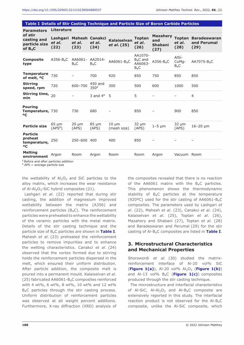
188 © 2022 Johnson Matthey
https://doi.org/10.1595/205651321X16238564889537 Johnson Matthey Technol. Rev., 2022, 66, (2)
the wettability of Al2O3 and SiC particles to the alloy matrix, which increases the wear resistance of Al-Al2O3-SiC hybrid composites (21). Lashgari et al. (22) reported that during stir
casting, the addition of magnesium improved wettability between the matrix (A356) and reinforcement particles (B4C). The reinforcement particles were preheated to enhance the wettability of the ceramic particles with the metal matrix. Details of the stir casting technique and the particle size of B4C particles are shown in Table I. Mahesh et al. (23) preheated the reinforcement particles to remove impurities and to enhance the wetting characteristics. Canakci et al. (24) observed that the vortex formed due to stirring holds the reinforcement particles dispersed in the melt, which ensured their uniform distribution. After particle addition, the composite melt is poured into a permanent mould. Kalaiselvan et al.
(25) fabricated AA6061-B4C composites reinforced with 4 wt%, 6 wt%, 8 wt%, 10 wt% and 12 wt% B4C particles through the stir casting process. Uniform distribution of reinforcement particles was observed at all weight percent additions. Furthermore, X-ray diffraction (XRD) analysis of
the composites revealed that there is no reaction of the AA6061 matrix with the B4C particles. This phenomenon shows the thermodynamic stability of B4C particles at the temperature (920ºC) used for the stir casting of AA6061-B4C composites. The parameters used by Lashgari et al. (22), Mahesh et al. (23), Canakci et al. (24), Kalaiselvan et al. (25), Toptan et al. (26), Mazahery and Shabani (27), Toptan et al. (28) and Baradeswaran and Perumal (29) for the stir casting of Al-B4C composites are listed in Table I.
3. Microstructural Characteristics and Mechanical Properties
Shorowordi et al. (30) studied the matrix-reinforcement interface of Al-20 vol% SiC (Figure 1(a)), Al-20 vol% Al2O3 (Figure 1(b)) and Al-13 vol% B4C (Figure 1(c)) composites produced through the stir casting technique.The microstructure and interfacial characteristics
of Al-SiC, Al-Al2O3 and Al-B4C composite are extensively reported in this study. The interfacial reaction product is not observed for the Al-B4C composite, unlike the Al-SiC composite, which
Table I Details of Stir Casting Technique and Particle Size of Boron Carbide Particles
Parameters of stir casting and particle size of B4C
Literature
Lashgari et al. (22)
Mahesh et al. (23)
Canakci et al. (24)
Kalaiselvan et al. (25)
Toptan et al. (26)
Mazaheryand Shabani (27)
Toptan et al. (28)
Baradeswaran and Perumal (29)
Composite type
A356-B4C AA6061-B4C
AA2014-B4C
AA6061-B4C
AA1070-B4C and AA6063-B4C
A356-B4CAlSi-CuMg-B4C
AA7075-B4C
Temperature of melt, ºC 730 – 700 920 850 750 850 850
Stirring speed, rpm 720 600–700 450 and
350a 300 500 600 1000 500
Stirring time, min 20 – 3 and 4a 5 5 – – 4
Pouring Temperature, ºC
730 730 680 – 850 – 900 850
Particle size 65 µm (APSb)
20 µm (APS)
85 µm (APS)
10 µm (mesh size)
32 µm (APS) 1–5 µm 32 µm
(APS) 16–20 µm
Particle preheat temperature, ºC
250 250–600 400 400 850 – – –
Melting environment Argon Room Argon Room Room Argon Vacuum Room
a Before and after particles additionb APS = average particle size
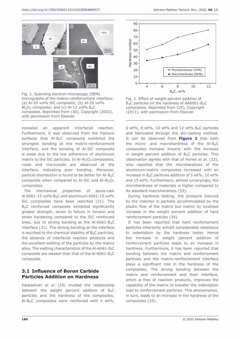
189 © 2022 Johnson Matthey
https://doi.org/10.1595/205651321X16238564889537 Johnson Matthey Technol. Rev., 2022, 66, (2)
revealed an apparent interfacial reaction. Furthermore, it was observed from the fracture surfaces that Al-B4C composite exhibited the strongest bonding at the matrix-reinforcement interface, and the bonding of Al-SiC composite is weak due to the low adherence of aluminium matrix to the SiC particles. In Al-Al2O3 composites, voids and microvoids are observed at the interface, indicating poor bonding. Moreover, particle distribution is found to be better for Al-B4C composite when compared to Al-SiC and Al-Al2O3
composites. The mechanical properties of spray-cast
Al 6061-15 vol% B4C and aluminium 6061-15 vol% SiC composites have been reported (31). The B4C reinforced composite exhibited significantly greater strength, strain to failure in tension and strain hardening compared to the SiC reinforced ones, due to strong bonding at the Al-6061-B4C interface (31). The strong bonding at the interface is ascribed to the chemical stability of B4C particles, the absence of interfacial reaction products and the excellent wetting of the particles by the matrix alloy. The wetting characteristics of the Al-6061-SiC composite are weaker than that of the Al-6061-B4C composite.
3.1 Influence of Boron Carbide Particles Addition on Hardness
Kalaiselvan et al. (25) studied the relationship between the weight percent addition of B4C particles and the hardness of the composites. Al-B4C composites were reinforced with 4 wt%,
6 wt%, 8 wt%, 10 wt% and 12 wt% B4C particles and fabricated through the stir-casting method. It can be observed from Figure 2 that both the micro- and macrohardness of the Al-B4C composites increase linearly with the increase in weight percent addition of B4C particles. This observation agrees with that of Hynes et al. (32), who reported that the microhardness of the aluminium-matrix composites increased with an increase in B4C particles addition of 5 wt%, 10 wt% and 15 wt%. Furthermore, almost unvaryingly, the microhardness of materials is higher compared to its standard macrohardness (33).During hardness testing, the pressure induced
by the indenter is partially accommodated by the plastic flow of the matrix but mainly by localised increase in the weight percent addition of hard reinforcement particles (34). It has been reported that hard reinforcement
particles inherently exhibit considerable resistance to indentation by the hardness tester. Hence the increase in weight percent addition of reinforcement particles leads to an increase in hardness. Furthermore, it has been reported that bonding between the matrix and reinforcement particles and the matrix-reinforcement interface plays a significant role in the hardness of the composites. The strong bonding between the matrix and reinforcement and their interface, which is free of reaction products, improves the capability of the matrix to transfer the indentation load to reinforcement particles. This phenomenon, in turn, leads to an increase in the hardness of the composites (25).
Fig. 1. Scanning electron microscopy (SEM) micrographs of the matrix-reinforcement interface: (a) Al-20 vol% SiC composite; (b) Al-20 vol% Al2O3 composite; and (c) Al-13 vol% B4C composite. Reprinted from (30), Copyright (2003), with permission from Elsevier
Fig. 2. Effect of weight percent addition of B4C particles on the hardness of AA6061-B4C composites. Reprinted from (25), Copyright (2011), with permission from Elsevier
90
80
70
60
50
40
30
20
10
04 6 8 10 12
B4C, wt%
Har
dnes
s nu
mbe
r
Microhardness (VHN)Macrohardness (BHN)
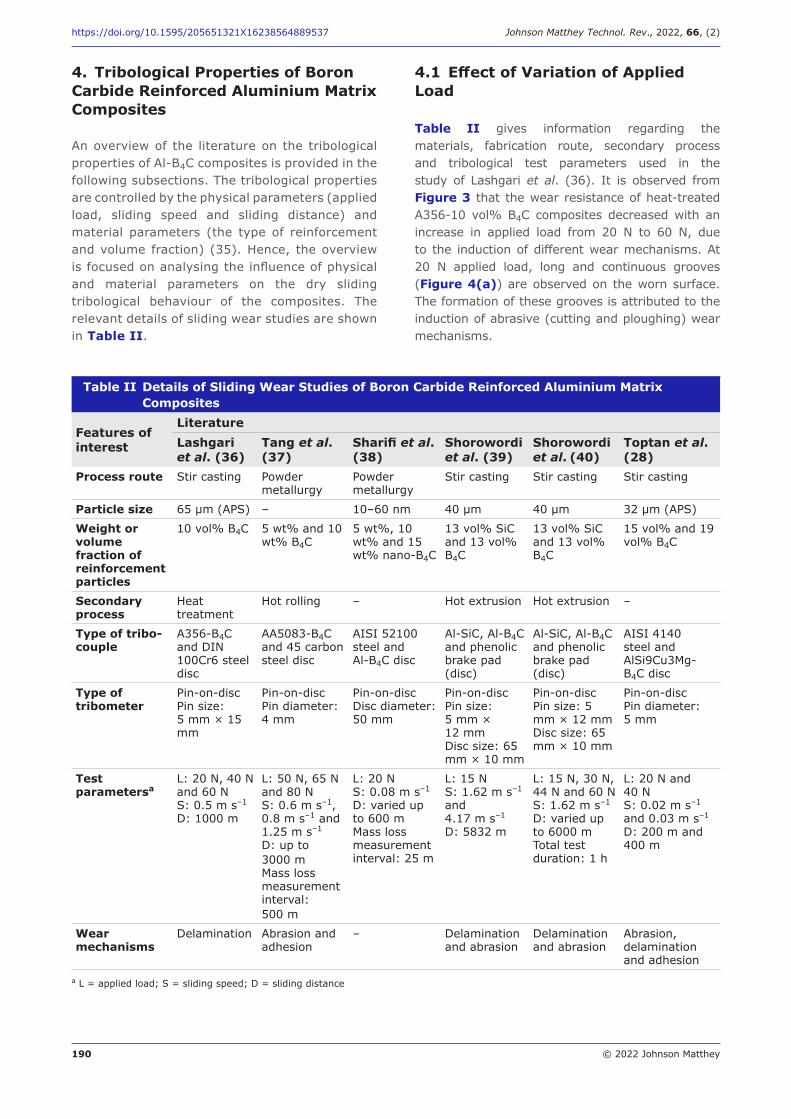
190 © 2022 Johnson Matthey
https://doi.org/10.1595/205651321X16238564889537 Johnson Matthey Technol. Rev., 2022, 66, (2)
4. Tribological Properties of Boron Carbide Reinforced Aluminium Matrix Composites
An overview of the literature on the tribological properties of Al-B4C composites is provided in the following subsections. The tribological properties are controlled by the physical parameters (applied load, sliding speed and sliding distance) and material parameters (the type of reinforcement and volume fraction) (35). Hence, the overview is focused on analysing the influence of physical and material parameters on the dry sliding tribological behaviour of the composites. The relevant details of sliding wear studies are shown in Table II.
4.1 Effect of Variation of Applied Load
Table II gives information regarding the materials, fabrication route, secondary process and tribological test parameters used in the study of Lashgari et al. (36). It is observed from Figure 3 that the wear resistance of heat-treated A356-10 vol% B4C composites decreased with an increase in applied load from 20 N to 60 N, due to the induction of different wear mechanisms. At 20 N applied load, long and continuous grooves (Figure 4(a)) are observed on the worn surface. The formation of these grooves is attributed to the induction of abrasive (cutting and ploughing) wear mechanisms.
Table II Details of Sliding Wear Studies of Boron Carbide Reinforced Aluminium Matrix Composites
Features of interest
LiteratureLashgari et al. (36)
Tang et al. (37)
Sharifi et al. (38)
Shorowordi et al. (39)
Shorowordi et al. (40)
Toptan et al. (28)
Process route Stir casting Powder metallurgy
Powder metallurgy
Stir casting Stir casting Stir casting
Particle size 65 µm (APS) – 10–60 nm 40 µm 40 µm 32 µm (APS)
Weight or volume fraction of reinforcement particles
10 vol% B4C 5 wt% and 10 wt% B4C
5 wt%, 10 wt% and 15 wt% nano-B4C
13 vol% SiC and 13 vol% B4C
13 vol% SiC and 13 vol% B4C
15 vol% and 19 vol% B4C
Secondary process
Heat treatment
Hot rolling – Hot extrusion Hot extrusion –
Type of tribo-couple
A356-B4C and DIN 100Cr6 steel disc
AA5083-B4C and 45 carbon steel disc
AISI 52100 steel and Al-B4C disc
Al-SiC, Al-B4C and phenolic brake pad (disc)
Al-SiC, Al-B4C and phenolic brake pad (disc)
AISI 4140 steel and AlSi9Cu3Mg-B4C disc
Type of tribometer
Pin-on-disc Pin size:5 mm × 15 mm
Pin-on-discPin diameter: 4 mm
Pin-on-discDisc diameter: 50 mm
Pin-on-discPin size: 5 mm × 12 mmDisc size: 65 mm × 10 mm
Pin-on-discPin size: 5 mm × 12 mmDisc size: 65 mm × 10 mm
Pin-on-disc Pin diameter: 5 mm
Test parametersa
L: 20 N, 40 N and 60 N S: 0.5 m s–1 D: 1000 m
L: 50 N, 65 N and 80 N S: 0.6 m s–1, 0.8 m s–1 and 1.25 m s–1 D: up to 3000 m Mass loss measurement interval: 500 m
L: 20 N S: 0.08 m s–1 D: varied up to 600 m Mass loss measurement interval: 25 m
L: 15 N S: 1.62 m s–1 and 4.17 m s–1 D: 5832 m
L: 15 N, 30 N, 44 N and 60 N S: 1.62 m s–1
D: varied up to 6000 m Total test duration: 1 h
L: 20 N and 40 N S: 0.02 m s–1 and 0.03 m s–1 D: 200 m and 400 m
Wear mechanisms
Delamination Abrasion and adhesion
– Delamination and abrasion
Delamination and abrasion
Abrasion, delamination and adhesion
a L = applied load; S = sliding speed; D = sliding distance
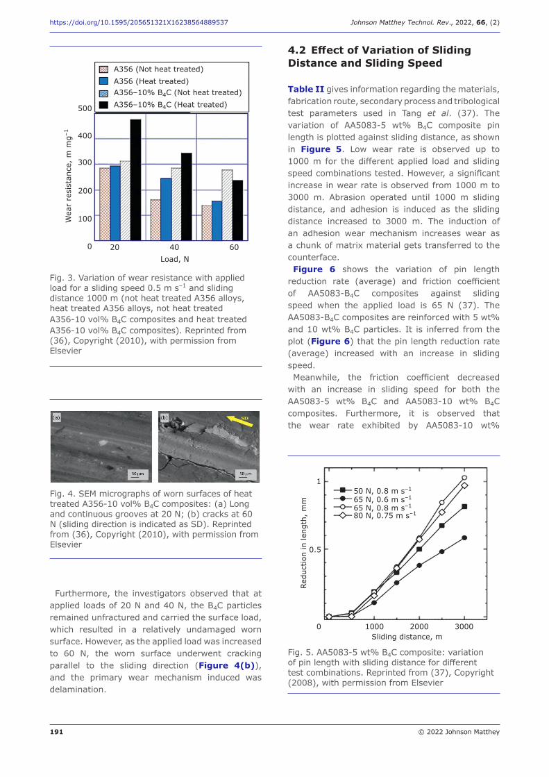
191 © 2022 Johnson Matthey
https://doi.org/10.1595/205651321X16238564889537 Johnson Matthey Technol. Rev., 2022, 66, (2)
Furthermore, the investigators observed that at applied loads of 20 N and 40 N, the B4C particles remained unfractured and carried the surface load, which resulted in a relatively undamaged worn surface. However, as the applied load was increased to 60 N, the worn surface underwent cracking parallel to the sliding direction (Figure 4(b)), and the primary wear mechanism induced was delamination.
4.2 Effect of Variation of Sliding Distance and Sliding Speed
Table II gives information regarding the materials, fabrication route, secondary process and tribological test parameters used in Tang et al. (37). The variation of AA5083-5 wt% B4C composite pin length is plotted against sliding distance, as shown in Figure 5. Low wear rate is observed up to 1000 m for the different applied load and sliding speed combinations tested. However, a significant increase in wear rate is observed from 1000 m to 3000 m. Abrasion operated until 1000 m sliding distance, and adhesion is induced as the sliding distance increased to 3000 m. The induction of an adhesion wear mechanism increases wear as a chunk of matrix material gets transferred to the counterface. Figure 6 shows the variation of pin length
reduction rate (average) and friction coefficient of AA5083-B4C composites against sliding speed when the applied load is 65 N (37). The AA5083-B4C composites are reinforced with 5 wt% and 10 wt% B4C particles. It is inferred from the plot (Figure 6) that the pin length reduction rate (average) increased with an increase in sliding speed. Meanwhile, the friction coefficient decreased
with an increase in sliding speed for both the AA5083-5 wt% B4C and AA5083-10 wt% B4C composites. Furthermore, it is observed that the wear rate exhibited by AA5083-10 wt%
Fig. 3. Variation of wear resistance with applied load for a sliding speed 0.5 m s–1 and sliding distance 1000 m (not heat treated A356 alloys, heat treated A356 alloys, not heat treated A356-10 vol% B4C composites and heat treated A356-10 vol% B4C composites). Reprinted from (36), Copyright (2010), with permission from Elsevier
500
400
300
200
100
0 20 40 60Load, N
Wea
r re
sist
ance
, m
mg–
1A356 (Not heat treated)A356 (Heat treated)A356–10% B4C (Not heat treated)A356–10% B4C (Heat treated)
Fig. 4. SEM micrographs of worn surfaces of heat treated A356-10 vol% B4C composites: (a) Long and continuous grooves at 20 N; (b) cracks at 60 N (sliding direction is indicated as SD). Reprinted from (36), Copyright (2010), with permission from Elsevier
Fig. 5. AA5083-5 wt% B4C composite: variation of pin length with sliding distance for different test combinations. Reprinted from (37), Copyright (2008), with permission from Elsevier
1
0.5
0 1000 2000 3000Sliding distance, m
Redu
ctio
n in
leng
th,
mm
50 N, 0.8 m s–1
65 N, 0.6 m s–1
65 N, 0.8 m s–1
80 N, 0.75 m s–1
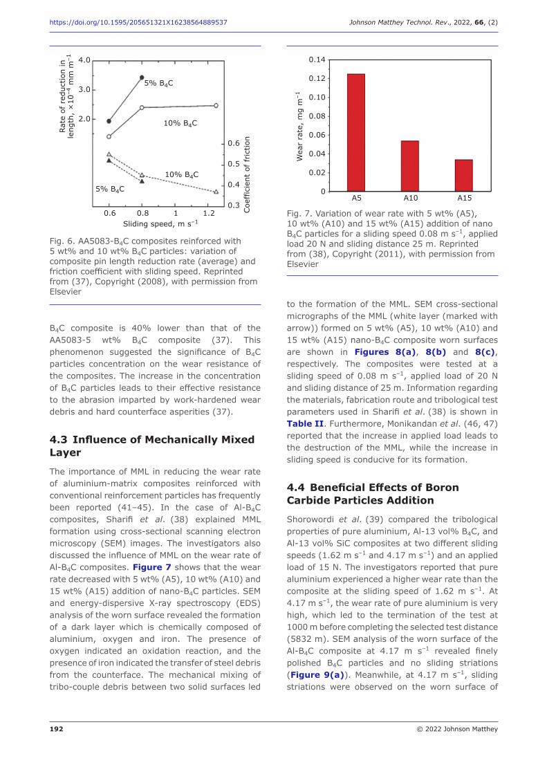
192 © 2022 Johnson Matthey
https://doi.org/10.1595/205651321X16238564889537 Johnson Matthey Technol. Rev., 2022, 66, (2)
B4C composite is 40% lower than that of the AA5083-5 wt% B4C composite (37). This phenomenon suggested the significance of B4C particles concentration on the wear resistance of the composites. The increase in the concentration of B4C particles leads to their effective resistance to the abrasion imparted by work-hardened wear debris and hard counterface asperities (37).
4.3 Influence of Mechanically Mixed Layer
The importance of MML in reducing the wear rate of aluminium-matrix composites reinforced with conventional reinforcement particles has frequently been reported (41–45). In the case of Al-B4C composites, Sharifi et al. (38) explained MML formation using cross-sectional scanning electron microscopy (SEM) images. The investigators also discussed the influence of MML on the wear rate of Al-B4C composites. Figure 7 shows that the wear rate decreased with 5 wt% (A5), 10 wt% (A10) and 15 wt% (A15) addition of nano-B4C particles. SEM and energy-dispersive X-ray spectroscopy (EDS) analysis of the worn surface revealed the formation of a dark layer which is chemically composed of aluminium, oxygen and iron. The presence of oxygen indicated an oxidation reaction, and the presence of iron indicated the transfer of steel debris from the counterface. The mechanical mixing of tribo-couple debris between two solid surfaces led
to the formation of the MML. SEM cross-sectional micrographs of the MML (white layer (marked with arrow)) formed on 5 wt% (A5), 10 wt% (A10) and 15 wt% (A15) nano-B4C composite worn surfaces are shown in Figures 8(a), 8(b) and 8(c), respectively. The composites were tested at a sliding speed of 0.08 m s–1, applied load of 20 N and sliding distance of 25 m. Information regarding the materials, fabrication route and tribological test parameters used in Sharifi et al. (38) is shown in Table II. Furthermore, Monikandan et al. (46, 47) reported that the increase in applied load leads to the destruction of the MML, while the increase in sliding speed is conducive for its formation.
4.4 Beneficial Effects of Boron Carbide Particles Addition
Shorowordi et al. (39) compared the tribological properties of pure aluminium, Al-13 vol% B4C, and Al-13 vol% SiC composites at two different sliding speeds (1.62 m s–1 and 4.17 m s–1) and an applied load of 15 N. The investigators reported that pure aluminium experienced a higher wear rate than the composite at the sliding speed of 1.62 m s–1. At 4.17 m s–1, the wear rate of pure aluminium is very high, which led to the termination of the test at 1000 m before completing the selected test distance (5832 m). SEM analysis of the worn surface of the Al-B4C composite at 4.17 m s–1 revealed finely polished B4C particles and no sliding striations (Figure 9(a)). Meanwhile, at 4.17 m s–1, sliding striations were observed on the worn surface of
Fig. 6. AA5083-B4C composites reinforced with 5 wt% and 10 wt% B4C particles: variation of composite pin length reduction rate (average) and friction coefficient with sliding speed. Reprinted from (37), Copyright (2008), with permission from Elsevier
4.0
3.0
2.0
0.6 0.8 1 1.20.3
0.4
0.5
0.6
5% B4C
10% B4C
10% B4C
5% B4C
Sliding speed, m s–1
Coe
ffic
ient
of fr
ictio
n
Rate
of re
duct
ion
inle
ngth
, ×
10–4
mm
m–1
Fig. 7. Variation of wear rate with 5 wt% (A5), 10 wt% (A10) and 15 wt% (A15) addition of nano B4C particles for a sliding speed 0.08 m s–1, applied load 20 N and sliding distance 25 m. Reprinted from (38), Copyright (2011), with permission from Elsevier
0.14
0.12
0.10
0.08
0.06
0.04
0.02
0A5 A10 A15
Wea
r ra
te,
mg
m–1
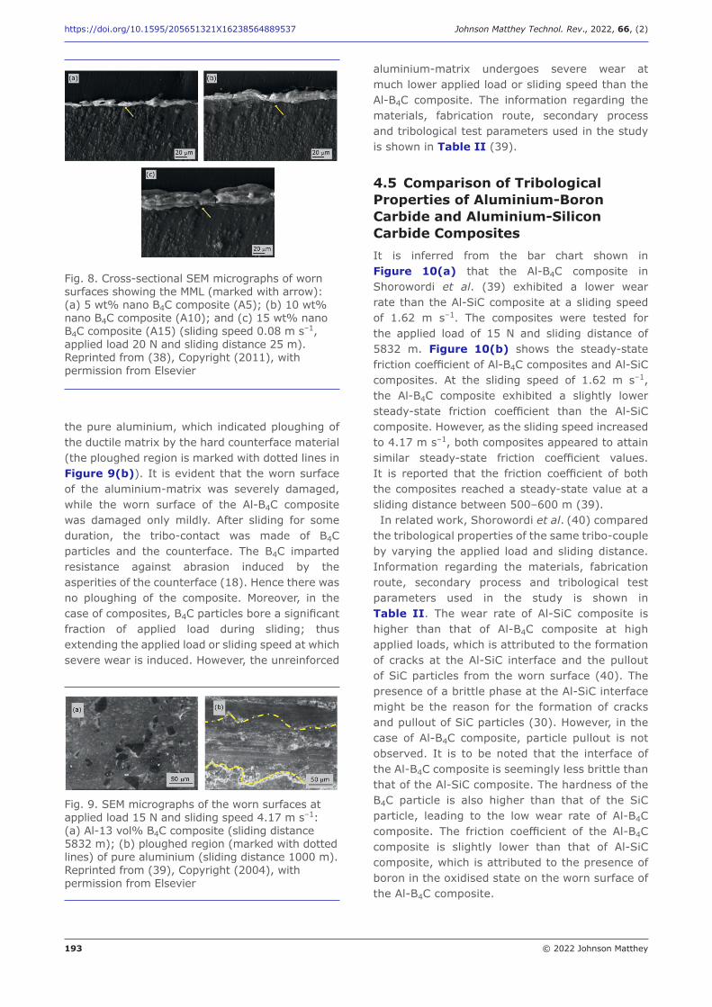
193 © 2022 Johnson Matthey
https://doi.org/10.1595/205651321X16238564889537 Johnson Matthey Technol. Rev., 2022, 66, (2)
the pure aluminium, which indicated ploughing of the ductile matrix by the hard counterface material (the ploughed region is marked with dotted lines in Figure 9(b)). It is evident that the worn surface of the aluminium-matrix was severely damaged, while the worn surface of the Al-B4C composite was damaged only mildly. After sliding for some duration, the tribo-contact was made of B4C particles and the counterface. The B4C imparted resistance against abrasion induced by the asperities of the counterface (18). Hence there was no ploughing of the composite. Moreover, in the case of composites, B4C particles bore a significant fraction of applied load during sliding; thus extending the applied load or sliding speed at which severe wear is induced. However, the unreinforced
aluminium-matrix undergoes severe wear at much lower applied load or sliding speed than the Al-B4C composite. The information regarding the materials, fabrication route, secondary process and tribological test parameters used in the study is shown in Table II (39).
4.5 Comparison of Tribological Properties of Aluminium-Boron Carbide and Aluminium-Silicon Carbide Composites It is inferred from the bar chart shown in Figure 10(a) that the Al-B4C composite in Shorowordi et al. (39) exhibited a lower wear rate than the Al-SiC composite at a sliding speed of 1.62 m s–1. The composites were tested for the applied load of 15 N and sliding distance of 5832 m. Figure 10(b) shows the steady-state friction coefficient of Al-B4C composites and Al-SiC composites. At the sliding speed of 1.62 m s–1, the Al-B4C composite exhibited a slightly lower steady-state friction coefficient than the Al-SiC composite. However, as the sliding speed increased to 4.17 m s–1, both composites appeared to attain similar steady-state friction coefficient values. It is reported that the friction coefficient of both the composites reached a steady-state value at a sliding distance between 500–600 m (39).In related work, Shorowordi et al. (40) compared
the tribological properties of the same tribo-couple by varying the applied load and sliding distance. Information regarding the materials, fabrication route, secondary process and tribological test parameters used in the study is shown in Table II. The wear rate of Al-SiC composite is higher than that of Al-B4C composite at high applied loads, which is attributed to the formation of cracks at the Al-SiC interface and the pullout of SiC particles from the worn surface (40). The presence of a brittle phase at the Al-SiC interface might be the reason for the formation of cracks and pullout of SiC particles (30). However, in the case of Al-B4C composite, particle pullout is not observed. It is to be noted that the interface of the Al-B4C composite is seemingly less brittle than that of the Al-SiC composite. The hardness of the B4C particle is also higher than that of the SiC particle, leading to the low wear rate of Al-B4C composite. The friction coefficient of the Al-B4C composite is slightly lower than that of Al-SiC composite, which is attributed to the presence of boron in the oxidised state on the worn surface of the Al-B4C composite.
Fig. 8. Cross-sectional SEM micrographs of worn surfaces showing the MML (marked with arrow): (a) 5 wt% nano B4C composite (A5); (b) 10 wt% nano B4C composite (A10); and (c) 15 wt% nano B4C composite (A15) (sliding speed 0.08 m s–1, applied load 20 N and sliding distance 25 m). Reprinted from (38), Copyright (2011), with permission from Elsevier
Fig. 9. SEM micrographs of the worn surfaces at applied load 15 N and sliding speed 4.17 m s–1: (a) Al-13 vol% B4C composite (sliding distance 5832 m); (b) ploughed region (marked with dotted lines) of pure aluminium (sliding distance 1000 m). Reprinted from (39), Copyright (2004), with permission from Elsevier
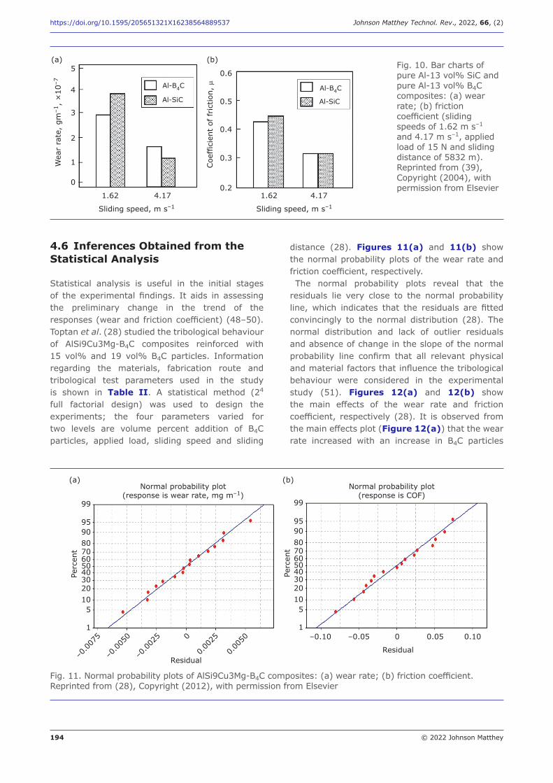
194 © 2022 Johnson Matthey
https://doi.org/10.1595/205651321X16238564889537 Johnson Matthey Technol. Rev., 2022, 66, (2)
4.6 Inferences Obtained from the Statistical Analysis
Statistical analysis is useful in the initial stages of the experimental findings. It aids in assessing the preliminary change in the trend of the responses (wear and friction coefficient) (48–50). Toptan et al. (28) studied the tribological behaviour of AlSi9Cu3Mg-B4C composites reinforced with 15 vol% and 19 vol% B4C particles. Information regarding the materials, fabrication route and tribological test parameters used in the study is shown in Table II. A statistical method (24 full factorial design) was used to design the experiments; the four parameters varied for two levels are volume percent addition of B4C particles, applied load, sliding speed and sliding
distance (28). Figures 11(a) and 11(b) show the normal probability plots of the wear rate and friction coefficient, respectively.The normal probability plots reveal that the
residuals lie very close to the normal probability line, which indicates that the residuals are fitted convincingly to the normal distribution (28). The normal distribution and lack of outlier residuals and absence of change in the slope of the normal probability line confirm that all relevant physical and material factors that influence the tribological behaviour were considered in the experimental study (51). Figures 12(a) and 12(b) show the main effects of the wear rate and friction coefficient, respectively (28). It is observed from the main effects plot (Figure 12(a)) that the wear rate increased with an increase in B4C particles
Fig. 10. Bar charts of pure Al-13 vol% SiC and pure Al-13 vol% B4C composites: (a) wear rate; (b) friction coefficient (sliding speeds of 1.62 m s–1 and 4.17 m s–1, applied load of 15 N and sliding distance of 5832 m). Reprinted from (39), Copyright (2004), with permission from Elsevier
4
5
3
2
1
0
1.62 4.17
Sliding speed, m s–1
1.62 4.17
Sliding speed, m s–1
Wea
r ra
te,
gm–1
, ×
10–7 Al-B4C
Al-SiC
Al-B4C
Al-SiC
0.6
0.5
0.4
0.3
0.2
Coe
ffic
ient
of fr
ictio
n, �
(a) (b)
Fig. 11. Normal probability plots of AlSi9Cu3Mg-B4C composites: (a) wear rate; (b) friction coefficient. Reprinted from (28), Copyright (2012), with permission from Elsevier
99
959080706050403020105
1
99
959080706050403020105
1
–0.0
075
–0.0
050
–0.0
025 0
0.00
25
0.00
50
ResidualResidual
Normal probability plot(response is wear rate, mg m–1)
Normal probability plot(response is COF)
Perc
ent
Perc
ent
–0.10 –0.05 0 0.05 0.10
(a) (b)
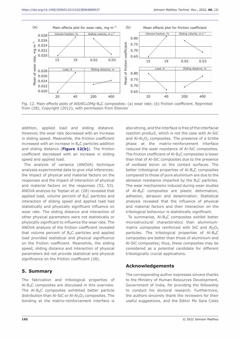
195 © 2022 Johnson Matthey
https://doi.org/10.1595/205651321X16238564889537 Johnson Matthey Technol. Rev., 2022, 66, (2)
addition, applied load and sliding distance. However, the wear rate decreased with an increase in sliding speed. Meanwhile, the friction coefficient increased with an increase in B4C particles addition and sliding distance (Figure 12(b)). The friction coefficient decreased with an increase in sliding speed and applied load. The analysis of variance (ANOVA) technique
analyses experimental data to give vital inferences: the impact of physical and material factors on the responses and the impact of interaction of physical and material factors on the responses (52, 53). ANOVA analysis by Toptan et al. (28) revealed that applied load, volume percent of B4C particles and interaction of sliding speed and applied load had statistically and physically significant influence on wear rate. The sliding distance and interaction of other physical parameters were not statistically or physically significant to influence the wear rate. The ANOVA analysis of the friction coefficient revealed that volume percent of B4C particles and applied load provided statistical and physical significance on the friction coefficient. Meanwhile, the sliding speed, sliding distance and interaction of physical parameters did not provide statistical and physical significance on the friction coefficient (28).
5. Summary
The fabrication and tribological properties of Al-B4C composites are discussed in this overview. The Al-B4C composites exhibited better particle distribution than Al-SiC or Al-Al2O3 composites. The bonding at the matrix-reinforcement interface is
also strong, and the interface is free of the interfacial reaction product, which is not the case with Al-SiC and Al-Al2O3 composites. The presence of a brittle phase at the matrix-reinforcement interface reduced the wear resistance of Al-SiC composites. The friction coefficient of Al-B4C composites is lower than that of Al-SiC composites due to the presence of oxidised boron on the contact surfaces. The better tribological properties of Al-B4C composites compared to those of pure aluminium are due to the abrasion resistance imparted by the B4C particles. The wear mechanisms induced during wear studies of Al-B4C composites are plastic deformation, adhesion, abrasion and delamination. Statistical analysis revealed that the influence of physical and material factors and their interaction on the tribological behaviour is statistically significant. To summarise, Al-B4C composites exhibit better
microstructural characteristics than aluminium-matrix composites reinforced with SiC and Al2O3
particles. The tribological properties of Al-B4C composites are better than those of aluminium and Al-SiC composites; thus, these composites may be considered as a potential candidate for different tribologically crucial applications.
Acknowledgements
The corresponding author expresses sincere thanks to the Ministry of Human Resources Development, Government of India, for providing the fellowship to conduct his doctoral research. Furthermore, the authors sincerely thank the reviewers for their useful suggestions, and the Editor Ms Sara Coles
Fig. 12. Main effects plots of AlSi9Cu3Mg-B4C composites: (a) wear rate; (b) friction coefficient. Reprinted from (28), Copyright (2012), with permission from Elsevier
0.0280.0260.0240.0220.020
0.0280.0260.0240.0220.020
15 19 0.02 0.03
Main effects plot for wear rate, mg m–1
Mea
n of
wea
r ra
te,
mg
m–1
Mea
n of
frict
ion
coef
ficie
nt
Mean effects plot for friction coefficient
Volume fraction, %
Load, N Sliding distance, m Load, N Sliding distance, m
Sliding velocity, m s–1 Volume fraction, % Sliding velocity, m s–1
20 40 200 400 20 40 200 400
0.80
0.75
0.70
0.65
0.80
0.75
0.70
0.65
15 19 0.02 0.03
(a) (b)
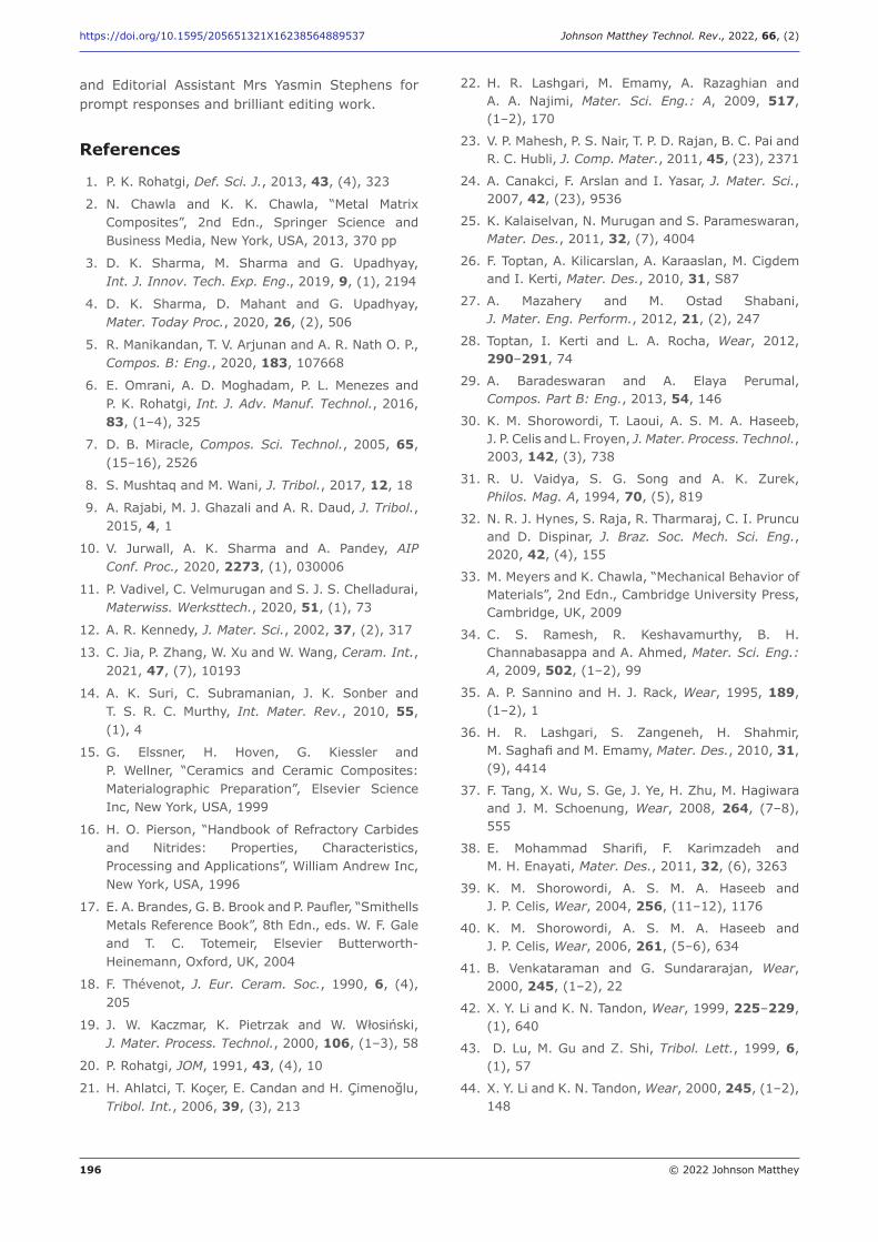
196 © 2022 Johnson Matthey
https://doi.org/10.1595/205651321X16238564889537 Johnson Matthey Technol. Rev., 2022, 66, (2)
and Editorial Assistant Mrs Yasmin Stephens for prompt responses and brilliant editing work.
References
1. P. K. Rohatgi, Def. Sci. J., 2013, 43, (4), 323
2. N. Chawla and K. K. Chawla, “Metal Matrix Composites”, 2nd Edn., Springer Science and Business Media, New York, USA, 2013, 370 pp
3. D. K. Sharma, M. Sharma and G. Upadhyay, Int. J. Innov. Tech. Exp. Eng., 2019, 9, (1), 2194
4. D. K. Sharma, D. Mahant and G. Upadhyay, Mater. Today Proc., 2020, 26, (2), 506
5. R. Manikandan, T. V. Arjunan and A. R. Nath O. P., Compos. B: Eng., 2020, 183, 107668
6. E. Omrani, A. D. Moghadam, P. L. Menezes and P. K. Rohatgi, Int. J. Adv. Manuf. Technol., 2016, 83, (1–4), 325
7. D. B. Miracle, Compos. Sci. Technol., 2005, 65, (15–16), 2526
8. S. Mushtaq and M. Wani, J. Tribol., 2017, 12, 18
9. A. Rajabi, M. J. Ghazali and A. R. Daud, J. Tribol., 2015, 4, 1
10. V. Jurwall, A. K. Sharma and A. Pandey, AIP Conf. Proc., 2020, 2273, (1), 030006
11. P. Vadivel, C. Velmurugan and S. J. S. Chelladurai, Materwiss. Werksttech., 2020, 51, (1), 73
12. A. R. Kennedy, J. Mater. Sci., 2002, 37, (2), 317
13. C. Jia, P. Zhang, W. Xu and W. Wang, Ceram. Int., 2021, 47, (7), 10193
14. A. K. Suri, C. Subramanian, J. K. Sonber and T. S. R. C. Murthy, Int. Mater. Rev., 2010, 55, (1), 4
15. G. Elssner, H. Hoven, G. Kiessler and P. Wellner, “Ceramics and Ceramic Composites: Materialographic Preparation”, Elsevier Science Inc, New York, USA, 1999
16. H. O. Pierson, “Handbook of Refractory Carbides and Nitrides: Properties, Characteristics, Processing and Applications”, William Andrew Inc, New York, USA, 1996
17. E. A. Brandes, G. B. Brook and P. Paufler, “Smithells Metals Reference Book”, 8th Edn., eds. W. F. Gale and T. C. Totemeir, Elsevier Butterworth-Heinemann, Oxford, UK, 2004
18. F. Thévenot, J. Eur. Ceram. Soc., 1990, 6, (4), 205
19. J. W. Kaczmar, K. Pietrzak and W. Włosiński, J. Mater. Process. Technol., 2000, 106, (1–3), 58
20. P. Rohatgi, JOM, 1991, 43, (4), 10
21. H. Ahlatci, T. Koçer, E. Candan and H. Çimenoğlu, Tribol. Int., 2006, 39, (3), 213
22. H. R. Lashgari, M. Emamy, A. Razaghian and A. A. Najimi, Mater. Sci. Eng.: A, 2009, 517, (1–2), 170
23. V. P. Mahesh, P. S. Nair, T. P. D. Rajan, B. C. Pai and R. C. Hubli, J. Comp. Mater., 2011, 45, (23), 2371
24. A. Canakci, F. Arslan and I. Yasar, J. Mater. Sci., 2007, 42, (23), 9536
25. K. Kalaiselvan, N. Murugan and S. Parameswaran, Mater. Des., 2011, 32, (7), 4004
26. F. Toptan, A. Kilicarslan, A. Karaaslan, M. Cigdem and I. Kerti, Mater. Des., 2010, 31, S87
27. A. Mazahery and M. Ostad Shabani, J. Mater. Eng. Perform., 2012, 21, (2), 247
28. Toptan, I. Kerti and L. A. Rocha, Wear, 2012, 290–291, 74
29. A. Baradeswaran and A. Elaya Perumal, Compos. Part B: Eng., 2013, 54, 146
30. K. M. Shorowordi, T. Laoui, A. S. M. A. Haseeb, J. P. Celis and L. Froyen, J. Mater. Process. Technol., 2003, 142, (3), 738
31. R. U. Vaidya, S. G. Song and A. K. Zurek, Philos. Mag. A, 1994, 70, (5), 819
32. N. R. J. Hynes, S. Raja, R. Tharmaraj, C. I. Pruncu and D. Dispinar, J. Braz. Soc. Mech. Sci. Eng., 2020, 42, (4), 155
33. M. Meyers and K. Chawla, “Mechanical Behavior of Materials”, 2nd Edn., Cambridge University Press, Cambridge, UK, 2009
34. C. S. Ramesh, R. Keshavamurthy, B. H. Channabasappa and A. Ahmed, Mater. Sci. Eng.: A, 2009, 502, (1–2), 99
35. A. P. Sannino and H. J. Rack, Wear, 1995, 189, (1–2), 1
36. H. R. Lashgari, S. Zangeneh, H. Shahmir, M. Saghafi and M. Emamy, Mater. Des., 2010, 31, (9), 4414
37. F. Tang, X. Wu, S. Ge, J. Ye, H. Zhu, M. Hagiwara and J. M. Schoenung, Wear, 2008, 264, (7–8), 555
38. E. Mohammad Sharifi, F. Karimzadeh and M. H. Enayati, Mater. Des., 2011, 32, (6), 3263
39. K. M. Shorowordi, A. S. M. A. Haseeb and J. P. Celis, Wear, 2004, 256, (11–12), 1176
40. K. M. Shorowordi, A. S. M. A. Haseeb and J. P. Celis, Wear, 2006, 261, (5–6), 634
41. B. Venkataraman and G. Sundararajan, Wear, 2000, 245, (1–2), 22
42. X. Y. Li and K. N. Tandon, Wear, 1999, 225–229, (1), 640
43. D. Lu, M. Gu and Z. Shi, Tribol. Lett., 1999, 6, (1), 57
44. X. Y. Li and K. N. Tandon, Wear, 2000, 245, (1–2), 148
197 © 2022 Johnson Matthey
https://doi.org/10.1595/205651321X16238564889537 Johnson Matthey Technol. Rev., 2022, 66, (2)
45. R. N. Rao and S. Das, Mater. Des., 2010, 31, (3), 1200
46. V. V. Monikandan, M. A. Joseph, P. K. Rajendrakumar and M. Sreejith, Mater. Res. Express, 2015, 2, (1), 016507
47. V. V. Monikandan, M. A. Joseph and P. K. Rajendrakumar, J. Mater. Eng. Perform., 2016, 25, (10), 4219
48. P. Ravindran, K. Manisekar, P. Narayanasamy, N. Selvakumar and R. Narayanasamy, Mater. Des., 2012, 39, 42
49. R. Pannerselvam, “Design and Analysis of Experiments”, PHI Learning Private Ltd, Delhi, India, 2012, 567 pp
50. S. Dharmalingam, R. Subramanian, K. S. Vinoth
and B. Anandavel, J. Mater. Eng. Perform., 2011,
20, (8), 1457
51. P. G. Mathews, “Design of Experiments with
MINITAB”, ASQ Quality Press, Wisconsin, USA,
2004
52. J. Antony, “Design of Experiments for Engineers
and Scientists”, 2nd Edn., Elsevier Ltd, London,
UK, 2014
53. S. Suresha and B. K. Sridhara, Compos. Sci. Technol.,
2010, 70, (11), 1652
The Authors
V. V. Monikandan is a Postdoctoral Researcher with the School of Minerals, Metallurgy and Materials Engineering, Indian Institute of Technology Bhubaneswar, India. Formerly, he was with Materials Research and Innovation Centric Solutions, India as a research associate. He received his PhD in tribological behaviour of aluminium matrix composites from the National Institute of Technology Calicut, India. He specialises in additive manufacturing of MMC coatings and synthesis of smart composites through pressureless infiltration process and biodegradable lubricants.
K. Pratheesh is a Professor of Mechanical Engineering and affiliated with Mangalam College of Engineering, Kottayam, Kerala, India. He received his PhD in grain size modification of aluminium-silicon alloys from the National Institute of Technology Calicut. His research interests include fabrication of as-cast alloys using liquid metallurgy technique, synthesis of grain modifier mixtures for non-ferrous alloy castings and solidification of castings.
P. K. Rajendrakumar is a Professor (HAG) of the Department of Mechanical Engineering, National Institute of Technology Calicut. His research interests include tribology, biomechanics and product design.
M. A. Joseph is a Professor (HAG) of the Department of Mechanical Engineering, National Institute of Technology Calicut. His research interests include MMCs, polymer materials and non-ferrous alloys.
www.technology.matthey.com
https://doi.org/10.1595/205651322X16445719154043 Johnson Matthey Technol. Rev., 2022, 66, (2), 198–211
198 © 2022 Johnson Matthey
Pilar Gómez Jiménez* Johnson Matthey, Blounts Court, Sonning Common, Reading, RG4 9NH, UK
Andrew Fish Johnson Matthey, PO Box 1, Belasis Avenue, Billingham, TS23 1LB, UK
Cristina Estruch BoschJohnson Matthey, Blounts Court, Sonning Common, Reading, RG4 9NH, UK
*Email: [email protected]
PEER REVIEWED
Received 6th June 2021; Revised 26th November 2021; Accepted 7th December 2021; Online 5th April 2022
The value of using statistical tools in the scientific world is not new, although the application of statistics to disciplines such as chemistry creates multiple challenges that are identified and addressed in this article. The benefits, explained here with real examples, far outweigh any short-term barriers in the initial application, overall saving resources and obtaining better products and solutions for customers and the world. The accessibility of data in current times combined with user-friendly statistical packages, such as JMP®, makes statistics available for everyone. The aim of this article is to motivate and enable both scientists and engineers (referred to subsequently in this article as scientists) to apply these techniques within their projects.
Unlocking Scientific Knowledge with Statistical Tools in JMP®
Benefits and challenges of new statistical tools
1. The Benefits
Cost reduction is possibly the first benefit considered when talking about statistical tools, especially with respect to statistical design of experiments (DoE). However, cost is not the only advantage or even the most significant one. Here is a list of some of the benefits which are discussed in this article:
• Cost and resource savings• Capacity for planning• Reliable conclusions, better decisions• Utilising historical data• Gaining control and adaptability• Recording and transferring knowledge• Visualisation – improving communication• Statistical significance for more objective decisions• Comparing to choose the right tool• Systematic and structured approach.
1.1 Cost and Resource Savings
DoE and multivariate statistical approaches have been identified before as a clear way of saving time and resources (1). They are systematic and structured approaches to product development and process improvement. The methodology is based on introducing variability into the system by changing a limited number of variables at controlled levels simultaneously, but systematically, in order to study the parameter space. The aim of a DoE is to maximise the knowledge obtained while minimising experimentation. It can also help to ‘fail quickly’; if, for example, the outcome of the study is that the variability cannot be explained by changes on any of the variables, further variables need to be considered. This leads again to saving time and resources.
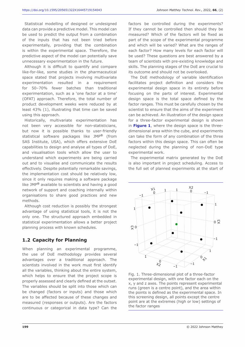
199 © 2022 Johnson Matthey
https://doi.org/10.1595/205651322X16445719154043 Johnson Matthey Technol. Rev., 2022, 66, (2)
Statistical modelling of designed or undesigned data can provide a predictive model. This model can be used to predict the output from a combination of the inputs that has not been tried before experimentally, providing that the combination is within the experimental space. Therefore, the predictive aspect of the model can potentially save unnecessary experimentation in the future. Although it is difficult to quantify and compare
like-for-like, some studies in the pharmaceutical space stated that projects involving multivariate experimentation resulted in a requirement for 50–70% fewer batches than traditional experimentation, such as a ‘one factor at a time’ (OFAT) approach. Therefore, the total number of product development weeks were reduced by at least 43% (1), illustrating that time can be saved using this approach.Historically, multivariate experimentation has
not been very accessible for non-statisticians, but now it is possible thanks to user-friendly statistical software packages like JMP® (from SAS Institute, USA), which offers extensive DoE capabilities to design and analyse all types of DoE, and visualisation tools which allow the user to understand which experiments are being carried out and to visualise and communicate the results effectively. Despite potentially remarkable savings, the implementation cost should be relatively low, since it only requires making a software package like JMP® available to scientists and having a good network of support and coaching internally within organisations to share good practices and new methods. Although cost reduction is possibly the strongest
advantage of using statistical tools, it is not the only one. The structured approach embedded in statistical experimentation allows a better project planning process with known schedules.
1.2 Capacity for Planning
When planning an experimental programme, the use of DoE methodology provides several advantages over a traditional approach. The scientists involved in the work must first identify all the variables, thinking about the entire system, which helps to ensure that the project scope is properly assessed and clearly defined at the outset. The variables should be split into those which can be changed (factors or inputs) and those which are to be affected because of these changes and measured (responses or outputs). Are the factors continuous or categorical in data type? Can the
factors be controlled during the experiments? If they cannot be controlled then should they be measured? Which of the factors will be fixed as part of the scope of the experimental programme and which will be varied? What are the ranges of each factor? How many levels for each factor will be used? These questions are best answered by a team of scientists with pre-existing knowledge and skills. The planning stages of the DoE are crucial to its outcome and should not be overlooked. The DoE methodology of variable identification
facilitates project definition and considers the experimental design space in its entirety before focusing on the parts of interest. Experimental design space is the total space defined by the factor ranges. This must be carefully chosen by the scientist to ensure that the aims of the experiment can be achieved. An illustration of the design space for a three-factor experimental design is shown in Figure 1, where the design space is the three-dimensional area within the cube, and experiments can take the form of any combination of the three factors within this design space. This can often be neglected during the planning of non-DoE type experimental work.The experimental matrix generated by the DoE
is also important in project scheduling. Access to the full set of planned experiments at the start of
X2
X1
X3
X3
X1 X2
10
–1
–1
0
1
–10
1 1 0 –1
1
0
–1
–1
0
1
Fig. 1. Three-dimensional plot of a three-factor experimental design, with one factor each on the x, y and z axes. The points represent experimental runs (green is a centre point), and the area within the points is defined as the experimental space. In this screening design, all points except the centre point are at the extremes (high or low) settings of the factor ranges
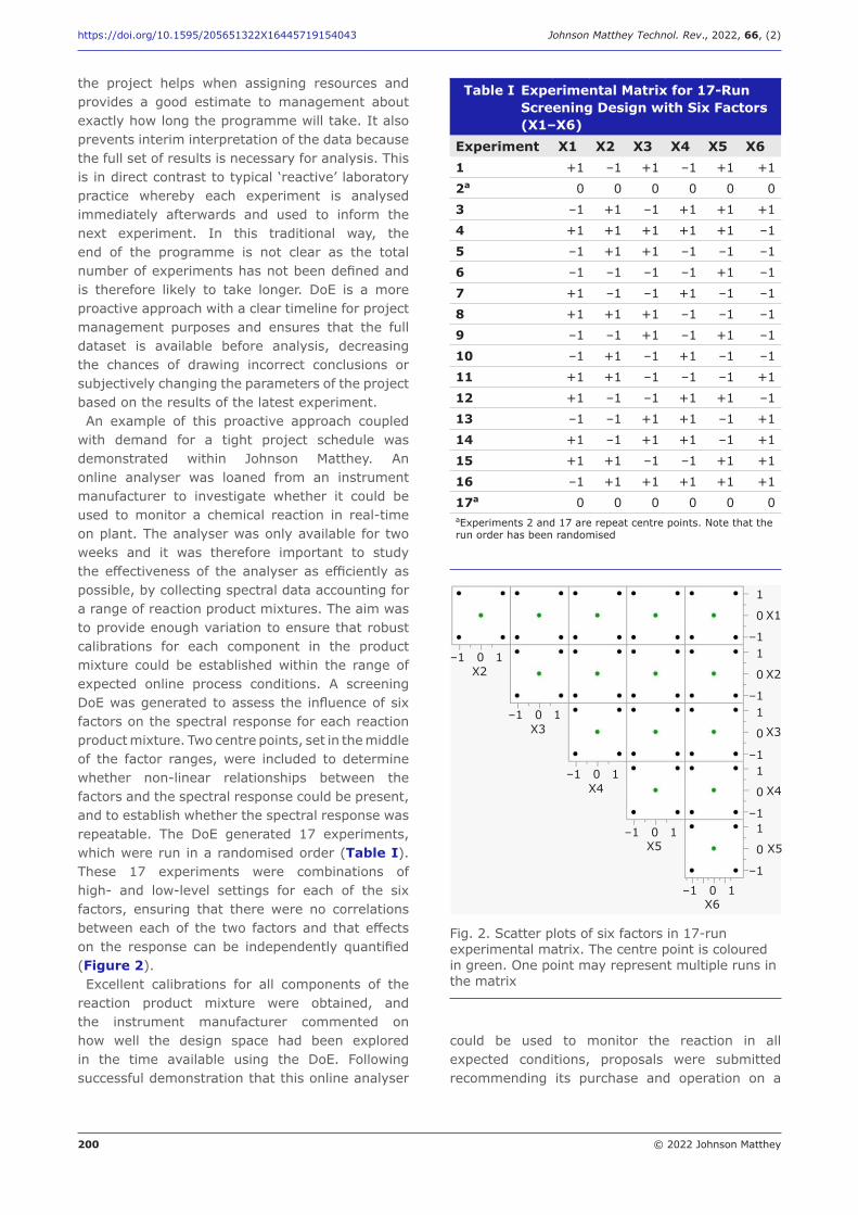
200 © 2022 Johnson Matthey
https://doi.org/10.1595/205651322X16445719154043 Johnson Matthey Technol. Rev., 2022, 66, (2)
the project helps when assigning resources and provides a good estimate to management about exactly how long the programme will take. It also prevents interim interpretation of the data because the full set of results is necessary for analysis. This is in direct contrast to typical ‘reactive’ laboratory practice whereby each experiment is analysed immediately afterwards and used to inform the next experiment. In this traditional way, the end of the programme is not clear as the total number of experiments has not been defined and is therefore likely to take longer. DoE is a more proactive approach with a clear timeline for project management purposes and ensures that the full dataset is available before analysis, decreasing the chances of drawing incorrect conclusions or subjectively changing the parameters of the project based on the results of the latest experiment. An example of this proactive approach coupled
with demand for a tight project schedule was demonstrated within Johnson Matthey. An online analyser was loaned from an instrument manufacturer to investigate whether it could be used to monitor a chemical reaction in real-time on plant. The analyser was only available for two weeks and it was therefore important to study the effectiveness of the analyser as efficiently as possible, by collecting spectral data accounting for a range of reaction product mixtures. The aim was to provide enough variation to ensure that robust calibrations for each component in the product mixture could be established within the range of expected online process conditions. A screening DoE was generated to assess the influence of six factors on the spectral response for each reaction product mixture. Two centre points, set in the middle of the factor ranges, were included to determine whether non-linear relationships between the factors and the spectral response could be present, and to establish whether the spectral response was repeatable. The DoE generated 17 experiments, which were run in a randomised order (Table I). These 17 experiments were combinations of high- and low-level settings for each of the six factors, ensuring that there were no correlations between each of the two factors and that effects on the response can be independently quantified (Figure 2).Excellent calibrations for all components of the
reaction product mixture were obtained, and the instrument manufacturer commented on how well the design space had been explored in the time available using the DoE. Following successful demonstration that this online analyser
could be used to monitor the reaction in all expected conditions, proposals were submitted recommending its purchase and operation on a
Fig. 2. Scatter plots of six factors in 17-run experimental matrix. The centre point is coloured in green. One point may represent multiple runs in the matrix
X2
X3
X4
X5
X6
X5
X4
X3
X2
X1
–1 0 1
–1 0 1
–1 0 1
–1 0 1
–1 0 1
1
0
–11
0
–11
0
–11
0
–11
0
–1
Table I Experimental Matrix for 17-Run Screening Design with Six Factors (X1–X6)
Experiment X1 X2 X3 X4 X5 X61 +1 –1 +1 –1 +1 +1
2a 0 0 0 0 0 0
3 –1 +1 –1 +1 +1 +1
4 +1 +1 +1 +1 +1 –1
5 –1 +1 +1 –1 –1 –1
6 –1 –1 –1 –1 +1 –1
7 +1 –1 –1 +1 –1 –1
8 +1 +1 +1 –1 –1 –1
9 –1 –1 +1 –1 +1 –1
10 –1 +1 –1 +1 –1 –1
11 +1 +1 –1 –1 –1 +1
12 +1 –1 –1 +1 +1 –1
13 –1 –1 +1 +1 –1 +1
14 +1 –1 +1 +1 –1 +1
15 +1 +1 –1 –1 +1 +1
16 –1 +1 +1 +1 +1 +1
17a 0 0 0 0 0 0aExperiments 2 and 17 are repeat centre points. Note that the run order has been randomised
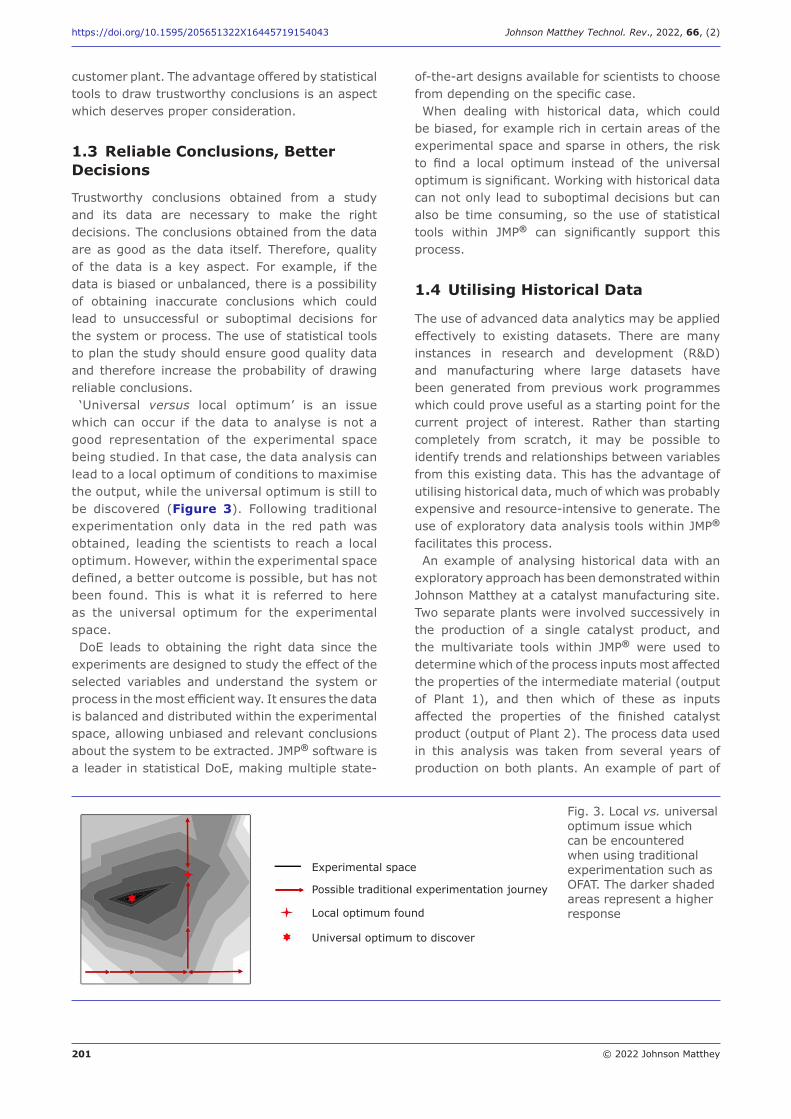
201 © 2022 Johnson Matthey
https://doi.org/10.1595/205651322X16445719154043 Johnson Matthey Technol. Rev., 2022, 66, (2)
customer plant. The advantage offered by statistical tools to draw trustworthy conclusions is an aspect which deserves proper consideration.
1.3 Reliable Conclusions, Better Decisions
Trustworthy conclusions obtained from a study and its data are necessary to make the right decisions. The conclusions obtained from the data are as good as the data itself. Therefore, quality of the data is a key aspect. For example, if the data is biased or unbalanced, there is a possibility of obtaining inaccurate conclusions which could lead to unsuccessful or suboptimal decisions for the system or process. The use of statistical tools to plan the study should ensure good quality data and therefore increase the probability of drawing reliable conclusions. ‘Universal versus local optimum’ is an issue
which can occur if the data to analyse is not a good representation of the experimental space being studied. In that case, the data analysis can lead to a local optimum of conditions to maximise the output, while the universal optimum is still to be discovered (Figure 3). Following traditional experimentation only data in the red path was obtained, leading the scientists to reach a local optimum. However, within the experimental space defined, a better outcome is possible, but has not been found. This is what it is referred to here as the universal optimum for the experimental space. DoE leads to obtaining the right data since the
experiments are designed to study the effect of the selected variables and understand the system or process in the most efficient way. It ensures the data is balanced and distributed within the experimental space, allowing unbiased and relevant conclusions about the system to be extracted. JMP® software is a leader in statistical DoE, making multiple state-
of-the-art designs available for scientists to choose from depending on the specific case. When dealing with historical data, which could
be biased, for example rich in certain areas of the experimental space and sparse in others, the risk to find a local optimum instead of the universal optimum is significant. Working with historical data can not only lead to suboptimal decisions but can also be time consuming, so the use of statistical tools within JMP® can significantly support this process.
1.4 Utilising Historical Data
The use of advanced data analytics may be applied effectively to existing datasets. There are many instances in research and development (R&D) and manufacturing where large datasets have been generated from previous work programmes which could prove useful as a starting point for the current project of interest. Rather than starting completely from scratch, it may be possible to identify trends and relationships between variables from this existing data. This has the advantage of utilising historical data, much of which was probably expensive and resource-intensive to generate. The use of exploratory data analysis tools within JMP® facilitates this process.An example of analysing historical data with an
exploratory approach has been demonstrated within Johnson Matthey at a catalyst manufacturing site. Two separate plants were involved successively in the production of a single catalyst product, and the multivariate tools within JMP® were used to determine which of the process inputs most affected the properties of the intermediate material (output of Plant 1), and then which of these as inputs affected the properties of the finished catalyst product (output of Plant 2). The process data used in this analysis was taken from several years of production on both plants. An example of part of
Experimental space
Possible traditional experimentation journey
Local optimum found
Universal optimum to discover
Fig. 3. Local vs. universal optimum issue which can be encountered when using traditional experimentation such as OFAT. The darker shaded areas represent a higher response
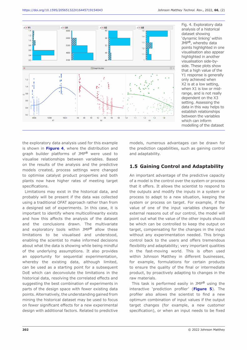
202 © 2022 Johnson Matthey
https://doi.org/10.1595/205651322X16445719154043 Johnson Matthey Technol. Rev., 2022, 66, (2)
Fig. 4. Exploratory data analysis of a historical dataset showing ‘dynamic linking’ within JMP®, whereby data points highlighted in one visualisation also appear highlighted in another visualisation side-by-side. These plots show that a high value of the Y1 response is generally only achieved when X2 is at a low setting, when X1 is low or mid-range, and is not really dependent on the X3 setting. Assessing the data in this way helps to establish relationships between the variables which can inform modelling of the dataset
the exploratory data analysis used for this example is shown in Figure 4, where the distribution and graph builder platforms of JMP® were used to visualise relationships between variables. Based on the results of the analysis and the predictive models created, process settings were changed to optimise catalyst product properties and both plants now have higher rates of meeting target specifications.Limitations may exist in the historical data, and
probably will be present if the data was collected using a traditional OFAT approach rather than from a designed set of experiments. In this case, it is important to identify where multicollinearity exists and how this affects the analysis of the dataset and the conclusions drawn. The multivariate and exploratory tools within JMP® allow these limitations to be visualised and understood, enabling the scientist to make informed decisions about what the data is showing while being mindful of the underlying assumptions. It also provides an opportunity for sequential experimentation, whereby the existing data, although limited, can be used as a starting point for a subsequent DoE which can deconvolute the limitations in the historical data, resolving the correlated effects and suggesting the best combination of experiments in parts of the design space with fewer existing data points. Alternatively, the understanding gained from mining the historical dataset may be used to focus on fewer significant effects for a new experimental design with additional factors. Related to predictive
models, numerous advantages can be drawn for the prediction capabilities, such as gaining control and adaptability.
1.5 Gaining Control and Adaptability
An important advantage of the predictive capacity of a model is the control over the system or process that it offers. It allows the scientist to respond to the outputs and modify the inputs in a system or process to adapt to a new situation, keeping the system or process on target. For example, if the value of one of the input variables changes for external reasons out of our control, the model will point out what the value of the other inputs should be which can be controlled to keep the output on target, compensating for the changes in the input without any experimentation needed. This brings control back to the users and offers tremendous flexibility and adaptability; very important qualities in the fast-moving world. This is often used within Johnson Matthey in different businesses, for example, formulations for certain products to ensure the quality of the final or intermediate product, by proactively adapting to changes in the raw materials. This task is performed easily in JMP® using the
interactive ‘prediction profiler’ (Figure 5). The profiler also allows the scientist to find a new optimum combination of input values if the output target changes (for example, a new customer specification), or when an input needs to be fixed
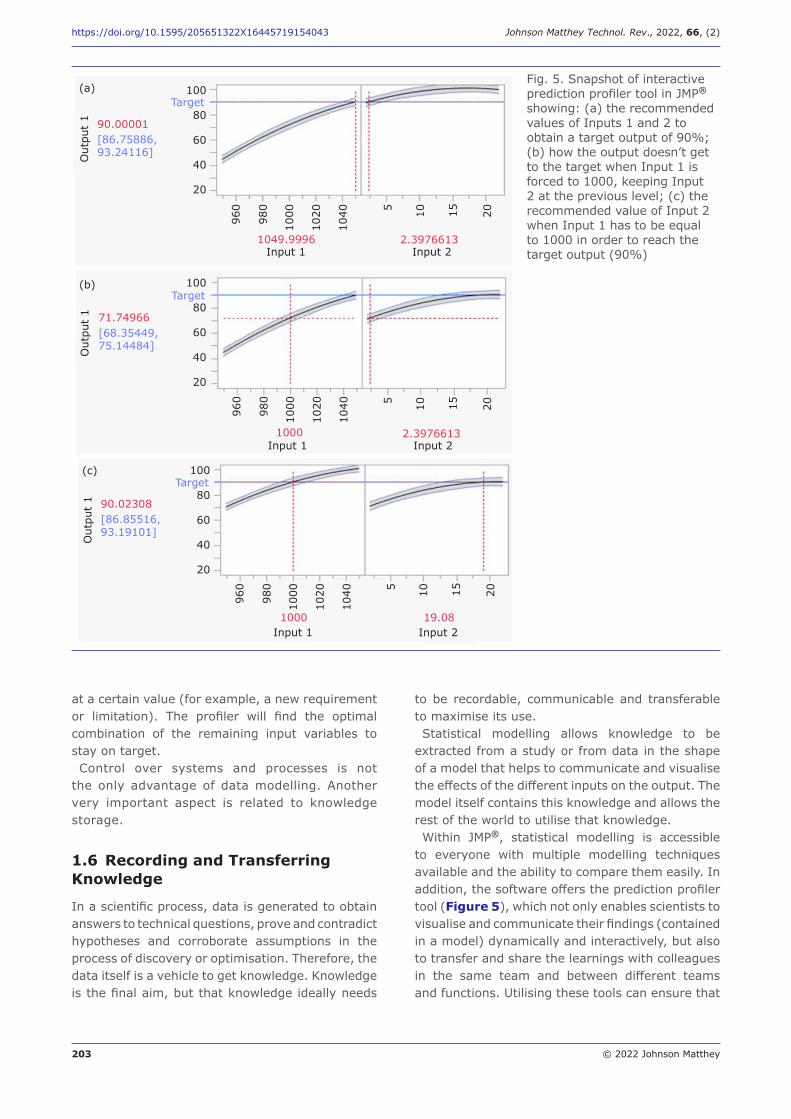
203 © 2022 Johnson Matthey
https://doi.org/10.1595/205651322X16445719154043 Johnson Matthey Technol. Rev., 2022, 66, (2)
at a certain value (for example, a new requirement or limitation). The profiler will find the optimal combination of the remaining input variables to stay on target. Control over systems and processes is not
the only advantage of data modelling. Another very important aspect is related to knowledge storage.
1.6 Recording and Transferring Knowledge
In a scientific process, data is generated to obtain answers to technical questions, prove and contradict hypotheses and corroborate assumptions in the process of discovery or optimisation. Therefore, the data itself is a vehicle to get knowledge. Knowledge is the final aim, but that knowledge ideally needs
to be recordable, communicable and transferable to maximise its use. Statistical modelling allows knowledge to be
extracted from a study or from data in the shape of a model that helps to communicate and visualise the effects of the different inputs on the output. The model itself contains this knowledge and allows the rest of the world to utilise that knowledge. Within JMP®, statistical modelling is accessible
to everyone with multiple modelling techniques available and the ability to compare them easily. In addition, the software offers the prediction profiler tool (Figure 5), which not only enables scientists to visualise and communicate their findings (contained in a model) dynamically and interactively, but also to transfer and share the learnings with colleagues in the same team and between different teams and functions. Utilising these tools can ensure that
Fig. 5. Snapshot of interactive prediction profiler tool in JMP® showing: (a) the recommended values of Inputs 1 and 2 to obtain a target output of 90%; (b) how the output doesn’t get to the target when Input 1 is forced to 1000, keeping Input 2 at the previous level; (c) the recommended value of Input 2 when Input 1 has to be equal to 1000 in order to reach the target output (90%)
(a)
(b)
(c)
100
80
60
40
20
100
80
60
40
20
100
80
60
40
20
960
980
1000
1020
1040
960
980
1000
1020
1040
960
980
1000
1020
1040
5 10 15 20
5 10 15 20
5 10 15 20
Out
put
1O
utpu
t 1
Out
put
1
Input 1
Input 1
Input 1 Input 2
Input 2
Input 2
90.00001[86.75886, 93.24116]
71.74966[68.35449, 75.14484]
90.02308[86.85516, 93.19101]
Target
Target
Target
1049.9996 2.3976613
2.39766131000
1000 19.08
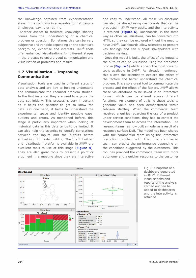
204 © 2022 Johnson Matthey
https://doi.org/10.1595/205651322X16445719154043 Johnson Matthey Technol. Rev., 2022, 66, (2)
the knowledge obtained from experimentation stays in the company in a reusable format despite employees leaving or retiring. Another aspect to facilitate knowledge sharing
comes from the understanding of a chemical problem or question. Sometimes this can be very subjective and variable depending on the scientist’s background, expertise and interests. JMP® tools offer enhanced visualisations for different stages in the process to ensure good communication and visualisation of problems and results.
1.7 Visualisation – Improving Communication
Visualisation tools are used in different steps of data analysis and are key to helping understand and communicate the chemical problem studied. In the first instance, they are used to explore the data set initially. This process is very important as it helps the scientist to get to know the data. On one hand, it helps to understand the experimental space and identify possible gaps, outliers and errors. As mentioned before, this stage is particularly important when looking at historical data as this data tends to be limited. It can also help the scientist to identify correlations between the inputs and the outputs before embarking into model building. The ‘graph builder’ and ‘distribution’ platforms available in JMP® are excellent tools to use at this stage (Figure 4). They are also great tools to present a point or argument in a meeting since they are interactive
and easy to understand. All these visualisations can also be shared using dashboards that can be produced in JMP® very easily, and the interactivity is retained (Figure 6). Dashboards, in the same way as other visualisations, can be converted into HTML so they can be explored without the need to have JMP®. Dashboards allow scientists to present key findings and can support stakeholders with decision making.Once the model is built, the effect of the inputs to
the outputs can be visualised using the prediction profiler (Figure 5) which is one of the most powerful tools available in JMP®. As already mentioned, this allows the scientist to explore the effect of the factors and better understand the chemical problem. It is also a great tool to communicate the process and the effect of the factors. JMP® allows these visualisations to be saved in an interactive format which can be shared across different functions. An example of utilising these tools to generate value has been demonstrated within Johnson Matthey. When the commercial team received enquiries regarding the use of a product under certain conditions, they had to contact the development team to access the information. The research team has now built a model as a result of a response surface DoE. The model has been shared with the commercial team using the interactive prediction profiler. With this, the commercial team can predict the performance depending on the conditions suggested by the customers. This tool has provided the commercial team with more autonomy and a quicker response to the customer
Fig. 6. Snapshot of a dashboard generated in JMP®. Different visualisations and reports of the analysis carried out can be added to dashboards and the interactivity is retained
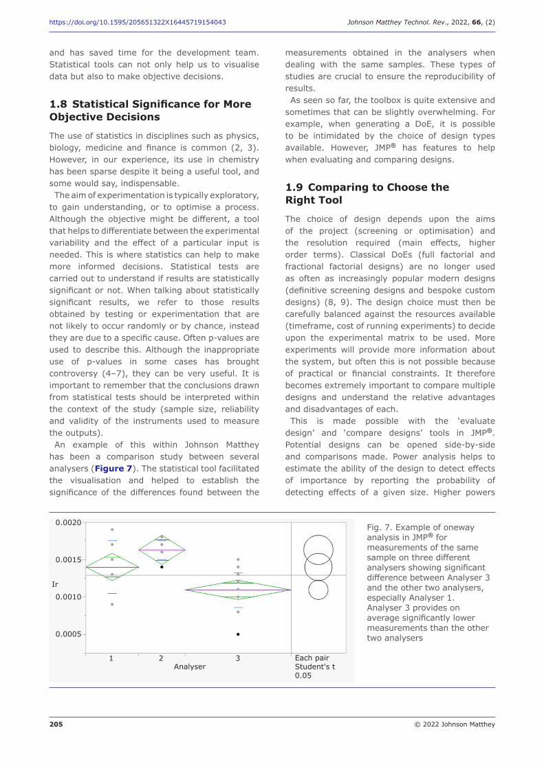
205 © 2022 Johnson Matthey
https://doi.org/10.1595/205651322X16445719154043 Johnson Matthey Technol. Rev., 2022, 66, (2)
and has saved time for the development team. Statistical tools can not only help us to visualise data but also to make objective decisions.
1.8 Statistical Significance for More Objective Decisions
The use of statistics in disciplines such as physics, biology, medicine and finance is common (2, 3). However, in our experience, its use in chemistry has been sparse despite it being a useful tool, and some would say, indispensable. The aim of experimentation is typically exploratory,
to gain understanding, or to optimise a process. Although the objective might be different, a tool that helps to differentiate between the experimental variability and the effect of a particular input is needed. This is where statistics can help to make more informed decisions. Statistical tests are carried out to understand if results are statistically significant or not. When talking about statistically significant results, we refer to those results obtained by testing or experimentation that are not likely to occur randomly or by chance, instead they are due to a specific cause. Often p-values are used to describe this. Although the inappropriate use of p-values in some cases has brought controversy (4–7), they can be very useful. It is important to remember that the conclusions drawn from statistical tests should be interpreted within the context of the study (sample size, reliability and validity of the instruments used to measure the outputs).An example of this within Johnson Matthey
has been a comparison study between several analysers (Figure 7). The statistical tool facilitated the visualisation and helped to establish the significance of the differences found between the
measurements obtained in the analysers when dealing with the same samples. These types of studies are crucial to ensure the reproducibility of results.As seen so far, the toolbox is quite extensive and
sometimes that can be slightly overwhelming. For example, when generating a DoE, it is possible to be intimidated by the choice of design types available. However, JMP® has features to help when evaluating and comparing designs.
1.9 Comparing to Choose the Right Tool
The choice of design depends upon the aims of the project (screening or optimisation) and the resolution required (main effects, higher order terms). Classical DoEs (full factorial and fractional factorial designs) are no longer used as often as increasingly popular modern designs (definitive screening designs and bespoke custom designs) (8, 9). The design choice must then be carefully balanced against the resources available (timeframe, cost of running experiments) to decide upon the experimental matrix to be used. More experiments will provide more information about the system, but often this is not possible because of practical or financial constraints. It therefore becomes extremely important to compare multiple designs and understand the relative advantages and disadvantages of each.This is made possible with the ‘evaluate
design’ and ‘compare designs’ tools in JMP®. Potential designs can be opened side-by-side and comparisons made. Power analysis helps to estimate the ability of the design to detect effects of importance by reporting the probability of detecting effects of a given size. Higher powers
Fig. 7. Example of oneway analysis in JMP® for measurements of the same sample on three different analysers showing significant difference between Analyser 3 and the other two analysers, especially Analyser 1. Analyser 3 provides on average significantly lower measurements than the other two analysers
1 2 3
0.0020
0.0015
0.0010
0.0005
Analyser
Ir
Each pair Student's t 0.05
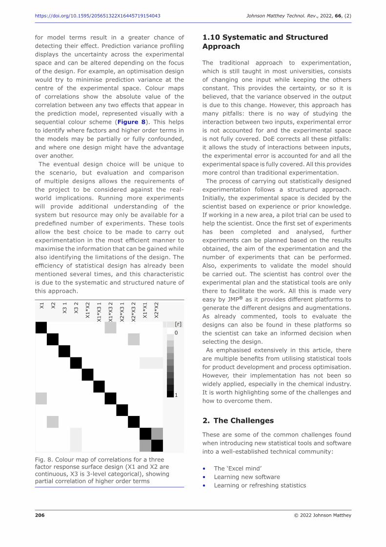
206 © 2022 Johnson Matthey
https://doi.org/10.1595/205651322X16445719154043 Johnson Matthey Technol. Rev., 2022, 66, (2)
for model terms result in a greater chance of detecting their effect. Prediction variance profiling displays the uncertainty across the experimental space and can be altered depending on the focus of the design. For example, an optimisation design would try to minimise prediction variance at the centre of the experimental space. Colour maps of correlations show the absolute value of the correlation between any two effects that appear in the prediction model, represented visually with a sequential colour scheme (Figure 8). This helps to identify where factors and higher order terms in the models may be partially or fully confounded, and where one design might have the advantage over another.The eventual design choice will be unique to
the scenario, but evaluation and comparison of multiple designs allows the requirements of the project to be considered against the real-world implications. Running more experiments will provide additional understanding of the system but resource may only be available for a predefined number of experiments. These tools allow the best choice to be made to carry out experimentation in the most efficient manner to maximise the information that can be gained while also identifying the limitations of the design. The efficiency of statistical design has already been mentioned several times, and this characteristic is due to the systematic and structured nature of this approach.
1.10 Systematic and Structured Approach
The traditional approach to experimentation, which is still taught in most universities, consists of changing one input while keeping the others constant. This provides the certainty, or so it is believed, that the variance observed in the output is due to this change. However, this approach has many pitfalls: there is no way of studying the interaction between two inputs, experimental error is not accounted for and the experimental space is not fully covered. DoE corrects all these pitfalls: it allows the study of interactions between inputs, the experimental error is accounted for and all the experimental space is fully covered. All this provides more control than traditional experimentation. The process of carrying out statistically designed
experimentation follows a structured approach. Initially, the experimental space is decided by the scientist based on experience or prior knowledge. If working in a new area, a pilot trial can be used to help the scientist. Once the first set of experiments has been completed and analysed, further experiments can be planned based on the results obtained, the aim of the experimentation and the number of experiments that can be performed. Also, experiments to validate the model should be carried out. The scientist has control over the experimental plan and the statistical tools are only there to facilitate the work. All this is made very easy by JMP® as it provides different platforms to generate the different designs and augmentations. As already commented, tools to evaluate the designs can also be found in these platforms so the scientist can take an informed decision when selecting the design.As emphasised extensively in this article, there
are multiple benefits from utilising statistical tools for product development and process optimisation. However, their implementation has not been so widely applied, especially in the chemical industry. It is worth highlighting some of the challenges and how to overcome them.
2. The Challenges
These are some of the common challenges found when introducing new statistical tools and software into a well-established technical community:
• The ‘Excel mind’• Learning new software• Learning or refreshing statistics
X1
X2
X3
1
X3
2
X1*
X2
X1*X
3 1
X1*X
3 2
X2*X
3 1
X2*X
3 2
X1*
X1
X2*
X2
1
0[r]
Fig. 8. Colour map of correlations for a three factor response surface design (X1 and X2 are continuous, X3 is 3-level categorical), showing partial correlation of higher order terms
207 © 2022 Johnson Matthey
https://doi.org/10.1595/205651322X16445719154043 Johnson Matthey Technol. Rev., 2022, 66, (2)
• Cultural shift• Fear of being redundant• The timings• Black box• Irreproducibility.
2.1 The ‘Excel Mind’
Commonly, data logging from scientific equipment and data analysis from experiments is done within Microsoft Excel (Microsoft Corporation, USA). Scientists are familiar with this program, having probably used it daily during the entirety of their career. There is a reluctance to move away from something to which we are so accustomed, in some cases to the point where we can no longer see the limitations. Microsoft Excel is an excellent spreadsheet program with simple user interface, ensuring it is used universally. However, it was never designed with the intention of handling and interpreting large volumes of data. A recent example of its misuse resulted in Public Health England failing to report nearly 16,000 coronavirus cases in 2020 (10). Add-ins are available to perform simple statistical functions, but specialist software like JMP® is required to thoroughly interrogate data and deliver greater understanding. As well as the tools available within JMP® to
provide greater insight, it has been purposely designed to manipulate and visualise large datasets. This is exemplified by features such as ‘graph builder’ and ‘dynamic linking’, as previously shown in Figure 4. The click-and-drag interface when building graphs in JMP® is a much simpler workflow to visualise data than creating graphs within Excel. There is also a JMP® add-in available for use in Excel which allows the user to transfer data between the two programmes in a single step and quickly access some of the common analysis platforms of JMP®. From experience within Johnson Matthey, we have found that the key to persuading people away from Excel and into specialist software is to show a direct comparison of a typical workflow with real-life data used in that part of the company. The improved visualisation and data analysis are immediately obvious, as are the time savings, which liberates more time for scientists to develop new technologies and products in the laboratory rather than handling and formatting data. However, there is also a barrier to overcome when learning to use new software.
2.2 Learning New Software
Johnson Matthey has recognised the benefits of promoting and instilling a culture of advanced data analytics. However, a common barrier to overcome when transitioning to new ways of working is the initial investment of time required to get to grips with new software. For research professionals whose time is a precious commodity, the investment of time needed upfront to learn new techniques and navigate around the software can be deterring. This is especially true as this part of the learning curve does not provide any immediate, tangible output. Furthermore, the wealth and variety of training resources available to new software users can make the learning process seem initially overwhelming. From experience within Johnson Matthey, we have found that setting aside time at regular intervals to progress through a predetermined training plan helps to make the process as simple as possible for new users. The training plan can be developed alongside a more experienced software user and will be bespoke to the requirements of the individual, concentrating on the functionality of the software with which the user will primarily be working. The training plan typically includes different resources, such as individual learning (online webinars, e-learning subscriptions, ‘Statistical Thinking for Industrial Problem Solving Modules’ – a free online statistics course provided by JMP®) and group learning (Johnson Matthey specific software introduction courses developed and run by experienced users). There is also an active JMP® user community within Johnson Matthey which was created to support new users, provide an informal environment for sharing knowledge and as an open forum to ask questions about specific problems. Demonstrations of Johnson Matthey projects
to senior management where the software has been used to improve process understanding have been critical to increase awareness of the benefits the software can bring. This has resulted in management encouraging staff to dedicate time towards software training. The impact of coronavirus has also accelerated this process, as developing new software skills is a task that can be carried out while working from home, either during forced periods of self-isolation or by minimising regular operations on site. But obviously it is not all about learning to use new software, it is also about learning statistics.
208 © 2022 Johnson Matthey
https://doi.org/10.1595/205651322X16445719154043 Johnson Matthey Technol. Rev., 2022, 66, (2)
2.3 Learning or Refreshing Statistics
As already mentioned, the use of statistics is more common in other fields such as biology or medicine than in chemistry. Traditionally statistics is not a featured component in chemistry undergraduate degrees. If some statistical content was taught in the first years, the learning was not normally reinforced with practical activities further on in the course. This can make chemists uncomfortable around statistics. Within Johnson Matthey we believe that a practical
understanding of statistics can be achieved to complement chemistry expertise by our scientists. The use of practical statistics is now totally accessible by using software packages like JMP®. The learning curve of statistics goes hand-in-hand with learning new software from a practical point of view. It allows scientists to practise and learn with their own data, which has been proved to be the best way to learn, always supported by the most experienced users within the company and learning from each other’s cases. This process is not easy because it requires a total change of culture.
2.4 Cultural Shift
While DoE methodology has been applied experimentally for decades, it is only relatively recently that its usage has gathered momentum across many scientific disciplines. This is due to a combination of advances in the algorithms used to tailor designs to the experiments and an increasing industrial need for rapid experimentation and decision making. For example, addressing design space constraints (11), handling mixture-type factors (12), comparing the effectiveness of different designs (13), introducing uncertainty in the factors and optimising using a variability simulator (14). However, for traditionally trained scientists who are used to changing OFAT in accordance with the scientific method, the transition to DoE methodology can be met with trepidation. There can be a concern that the scientist’s skills are not being fully utilised and that the recommended experiments in the matrix will not be enough to understand the system. Overcoming these anxieties is a significant challenge, particularly within established R&D departments. At Johnson Matthey, the way this has been approached is to demonstrate the power of DoE on small projects across a range of technology areas, and actively promote these results to the rest of the company, increasing the visibility and viability of the DoE
methodology. This generates additional interest and establishes confidence in the methods so that scientists have more faith in using DoE for larger, more complicated projects. The functionality of software such as JMP® to create designs, analyse the results and present the conclusions is essential in facilitating this cultural shift.At Johnson Matthey, the key principle when driving
this transition to an advanced experimentation and statistical approach to data is to empower our scientists to do it themselves. The scientists are the technical experts in their respective areas, and by giving them the understanding, tools and training to create and analyse DoE it is believed that this will result in better outcomes for both the current project and future work programmes.Indeed, recognising the technical expertise in
their respective areas when deploying a statistical software like JMP® is a very important step to overcome a very important concern; the fear of being substituted by a computer or a machine (15).
2.5 Fear of Being Redundant
The media can be overwhelming in this respect: listening and reading continuously about artificial intelligence, robotics, automation and machine learning. However, technical expertise will always be necessary, and the human being has proved to be indispensable in many fields. Statistical techniques like DoE are not designed to substitute the chemical expertise of a human scientist but to work in conjunction with them to get the most out of experimentation, and to make them more efficient. Statistical tools are exactly that: tools to be used, not to substitute scientists. Indeed, the first step in a statistical design is the
planning. For this step, chemical expertise plays a crucial role. The DoE is not going to tell the scientist which factors or responses should be studied. It is the scientist who should feed all this valuable information into the design. In the same way, as a result of a DoE it could be
found that a variable has or does not have an effect on the output, but it will not say why. It is up to the scientist to interpret the result, try to understand why and continue designing more experiments to test and prove that hypothesis. When teaching these techniques within Johnson
Matthey we are very careful to emphasise these tools are to help scientists, not to replace them. It is crucial to motivate scientists to believe in the process to overcome other major challenges, such as the timings.
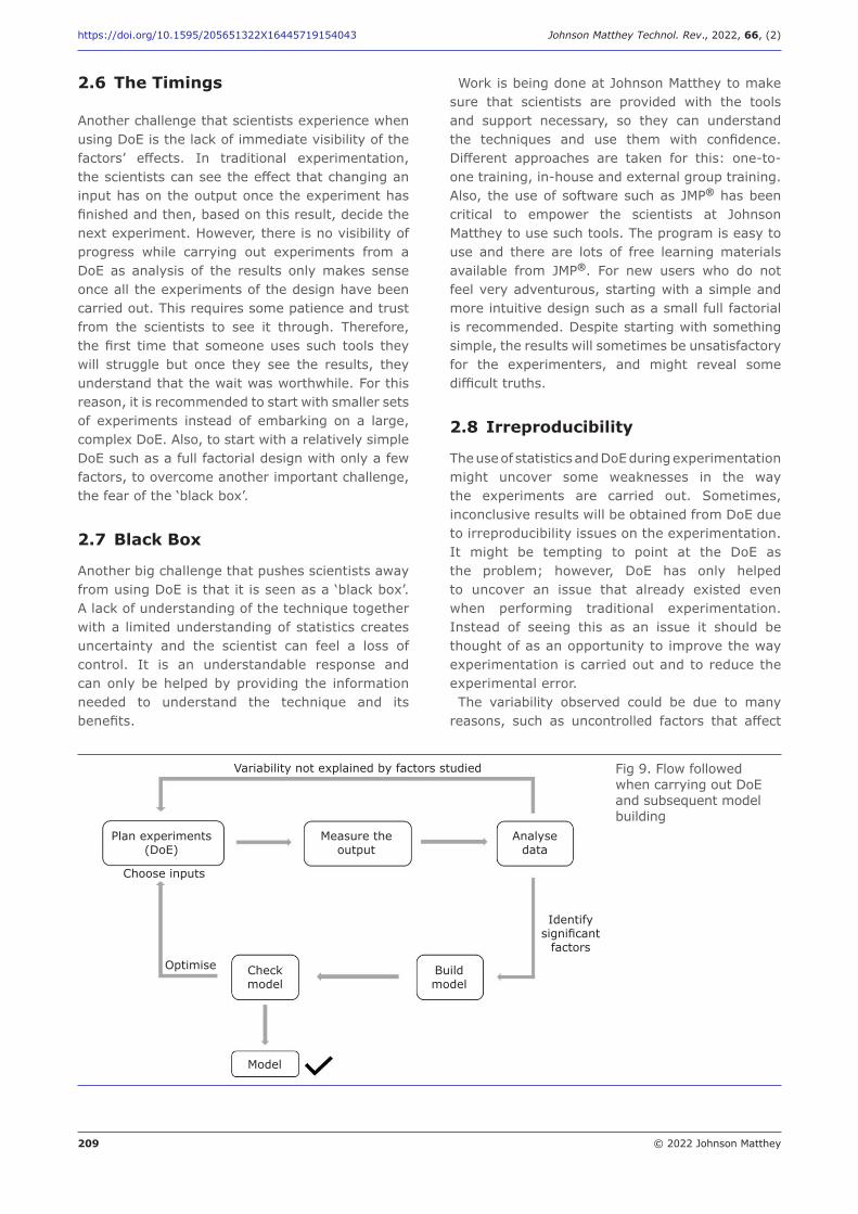
209 © 2022 Johnson Matthey
https://doi.org/10.1595/205651322X16445719154043 Johnson Matthey Technol. Rev., 2022, 66, (2)
2.6 The Timings
Another challenge that scientists experience when using DoE is the lack of immediate visibility of the factors’ effects. In traditional experimentation, the scientists can see the effect that changing an input has on the output once the experiment has finished and then, based on this result, decide the next experiment. However, there is no visibility of progress while carrying out experiments from a DoE as analysis of the results only makes sense once all the experiments of the design have been carried out. This requires some patience and trust from the scientists to see it through. Therefore, the first time that someone uses such tools they will struggle but once they see the results, they understand that the wait was worthwhile. For this reason, it is recommended to start with smaller sets of experiments instead of embarking on a large, complex DoE. Also, to start with a relatively simple DoE such as a full factorial design with only a few factors, to overcome another important challenge, the fear of the ‘black box’.
2.7 Black Box
Another big challenge that pushes scientists away from using DoE is that it is seen as a ‘black box’. A lack of understanding of the technique together with a limited understanding of statistics creates uncertainty and the scientist can feel a loss of control. It is an understandable response and can only be helped by providing the information needed to understand the technique and its benefits.
Work is being done at Johnson Matthey to make sure that scientists are provided with the tools and support necessary, so they can understand the techniques and use them with confidence. Different approaches are taken for this: one-to-one training, in-house and external group training. Also, the use of software such as JMP® has been critical to empower the scientists at Johnson Matthey to use such tools. The program is easy to use and there are lots of free learning materials available from JMP®. For new users who do not feel very adventurous, starting with a simple and more intuitive design such as a small full factorial is recommended. Despite starting with something simple, the results will sometimes be unsatisfactory for the experimenters, and might reveal some difficult truths.
2.8 Irreproducibility
The use of statistics and DoE during experimentation might uncover some weaknesses in the way the experiments are carried out. Sometimes, inconclusive results will be obtained from DoE due to irreproducibility issues on the experimentation. It might be tempting to point at the DoE as the problem; however, DoE has only helped to uncover an issue that already existed even when performing traditional experimentation. Instead of seeing this as an issue it should be thought of as an opportunity to improve the way experimentation is carried out and to reduce the experimental error. The variability observed could be due to many
reasons, such as uncontrolled factors that affect
Plan experiments (DoE)
Measure the output
Analyse data
Check model
Build model
Model
Variability not explained by factors studied
Choose inputs
Optimise
Identify significant
factors
Fig 9. Flow followed when carrying out DoE and subsequent model building
210 © 2022 Johnson Matthey
https://doi.org/10.1595/205651322X16445719154043 Johnson Matthey Technol. Rev., 2022, 66, (2)
the response or its measurement. These could be included in a subsequent DoE to be studied further and help to provide better understanding of the system (Figure 9). To be included in the study, the scientist needs to be able to measure and control the different inputs. Understanding the origin of the variability of an experiment can be used to improve the process. For example, if a more precise measurement of the output can be obtained, the scientist would be able to observe smaller effects of inputs which, combined, could drive larger improvements in the output. DoE and statistical tools allow experimenters to
obtain reliable data in order to extract objective conclusions and take decisions, even if those conclusions are that the experimentation needs to be redesigned or the measurement system improved.
3. Conclusions
It is hoped that this article has been able to show the importance of statistical tools in the scientific space and how challenges can be overcome by using statistical software, like JMP®, which makes statistics accessible to everyone, and by offering employees good support and multiple learning opportunities depending on their background, learning style and needs. At Johnson Matthey we believe scientists and engineers are in the best position to use statistical tools themselves, in order to design, capture, analyse and obtain conclusions from their own data, and that the value of this approach can be of immense benefit to an organisation.
Acknowledgements Thanks to Johnson Matthey management for its support on extending the use of statistical tools around Johnson Matthey, and to all the motivated
colleagues who have joined us in this journey for their enthusiasm and patience. Microsoft and Excel are trademarks of the
Microsoft group of companies. All other trademarks are the property of their respective owners.
References
1. R. Lievense, “Pharmaceutical Quality by Design Using JMP®: Solving Product Development and Manufacturing”, SAS Institute Inc, Cary, USA, 2018
2. B. Durakovic, Period. Eng. Nat. Sci., 2017, 5, (3), 421
3. S. E. Fienberg, Ann. Rev. Stat. Appl., 2014, 1, 14. R. Nuzzo, Nature, 2014, 506, (7487), 1505. L. G. Halsey, Biol. Lett., 2019, 15, (5), 201901746. V. Amrhein, S. Greenland and B. McShane, Nature,
2019, 567, (7748), 3057. R. L. Wasserstein, A. L. Schirm and N. A. Lazar,
Am. Stat., 2019, 73, 1 8. B. Jones and C. J. Nachtsheim, J. Qual. Technol.,
2011, 43, (1), 19. B. Jones and D. C. Montgomery, “Design of
Experiments: A Modern Approach”, John Wiley & Sons Inc, Hoboken, USA, 2019
10. L. Kelion, ‘Excel: Why Using Microsoft’s Tool Caused Covid-19 Results to be Lost’, BBC, London, UK, 5th October, 2020
11. D. C. Montgomery, E. N. Loredo, D. Jearkpaporn and M. C. Testik, Qual. Eng., 2002, 14, (4), 587
12. P. Goos, B. Jones and U. Syafitri, J. Am. Stat. Assoc., 2016, 111, (514), 899
13. A. Jankovic, G. Chaudhary and F. Goia, Energy Build., 2021, 250, 111298
14. R. S. Kenett and S. Zacks, “Modern Industrial Statistics: with Applications in R, MINITAB, and JMP”, 3rd Edn., John Wiley & Sons Inc, Hoboken, USA, 2021, 880 pp
15. E. Dahlin, Socius: Sociol. Res. Dynam. World, 2019, 5
The Authors
Pilar Gómez Jiménez works as a principal scientist in Johnson Matthey, UK. She has a Master’s degree and a PhD in Chemical Engineering, and she has been working in R&D of catalysts and materials for 17 years. She is enthusiastic about the application of DoE and the DoE mindset. This led to her current role extending the use of DoE and advanced data analytics through training, support and method development within Johnson Matthey.

211 © 2022 Johnson Matthey
https://doi.org/10.1595/205651322X16445719154043 Johnson Matthey Technol. Rev., 2022, 66, (2)
Andrew Fish is a principal researcher at Johnson Matthey. He holds a Bachelor’s degree in Applied Chemistry and has been working on the R&D of catalysts since 2005. His current role is focused on testing catalysts for the development and optimisation of syngas-based flowsheets. He also has a keen interest in data analytics and DoE methodology, providing advice and support on these topics to colleagues within Johnson Matthey.
Cristina Estruch Bosch has a Master’s degree in Catalysis and a PhD in Chemical Engineering. She is a senior scientist at Johnson Matthey where she has been working on R&D of catalysts since 2007. Her current role is to enable and support scientists and engineers in Johnson Matthey in the use of statistical tools.
www.technology.matthey.com
https://doi.org/10.1595/205651322X16475127763519 Johnson Matthey Technol. Rev., 2022, 66, (2), 212–214
212 © 2022 Johnson Matthey
Johnson Matthey HighlightsA selection of recent publications by Johnson Matthey R&D staff and collaborators
NON-PEER REVIEWED FEATURE
Received 17th March 2022; Online 6th April 2022
Operando XAFS Investigation on the Effect of Ash Deposition on Three-Way Catalyst Used in Gasoline Particulate Filters and the Effect of the Manufacturing Process on the Catalytic Activity M. Panchal, J. Callison, V. Skukauskas, D. Gianolio, G. Cibin, A. P. E. York, M. E. Schuster, T. I. Hyde, P. Collier, C. R. A. Catlow and E. K. Gibson, J. Phys.: Condens. Matter, 2021, 33, (28), 284001
Operando XAFS was performed on two model GPF systems, one from a catalyst washcoat not previously adhered to a GPF and the other which contained ash components extracted from a GPF (20 g ash). The catalytic activity profiles of the systems were compared to a GPF containing no ash components (0 g ash). The 20 g ash sample had a higher carbon monoxide light off temperature than the 0 g ash sample. It also demonstrated an oscillation profile for carbon monoxide, carbon dioxide and oxygen. Post ageing, the washcoat and 0 g ash samples reduced NO at 310ºC, whereas the 20 g sample maintained a higher temperature. The presence of ash combined with high temperature ageing was thought to have an irreversible negative impact on catalyst performance.
Restructuring Effects in the Platinum-Catalysed Enantioselective Hydrogenation of Ethyl PyruvateG. A. Attard, A. M. S. Alabdulrahman, D. J. Jenkins, P. Johnston, K. G. Griffin and P. B. Wells, Top. Catal., 2021, 64, 945
Three series of 5% platinum/graphite catalysts were prepared. One was sintered in pure argon, while the other two series were sintered in 5% hydrogen/argon. {100}-terraces, {111}-terraces and stepped features were observed on the platinum surfaces by CV. The catalytic performance of the surface structures in the enantioselective
hydrogenation of ethyl pyruvate to ethyl lactate was revealed. Progressive platinum particle growth with surface restructuring and faceting was observed for the two catalysts sintered in 5% hydrogen/argon. Of these two series, the one containing smaller platinum particles encompassed a higher fraction of surface Pt{111}-terraces. {100}-surfaces were found to be detrimental to high catalyst performance. The authors suggest that future catalyst design should either focus on procedures that contain poisons to deactivate {100}-surfaces or maximise {111}-terrace development.
Development and Application of 3D-PTV Measurements to Lab-Scale Stirred Vessel Flows M. G. Romano, F. Alberini, L. Liu, M. J. H. Simmons and E. H. Stitt, Chem. Eng. Res. Des., 2021, 172, 71
3D particle tracking velocimetry (3D-PTV) was used to measure the flow of water in a laboratory-scale cylindrical tank at Re = 12,000, stirred using a six blade Rushton turbine. Different tracer concentrations and camera frame rates were investigated and optimised. The Savitzky–Golay filter was employed and optimised to enhance
V
O
Fig. 1. Schematic illustration of polaron hopping direction in a V2O5 type phase. Reproduced from R. L. Gibson et al., Chem. Eng. Technol., 2022, 45, (2), 238, with permission from the Royal Society of Chemistry
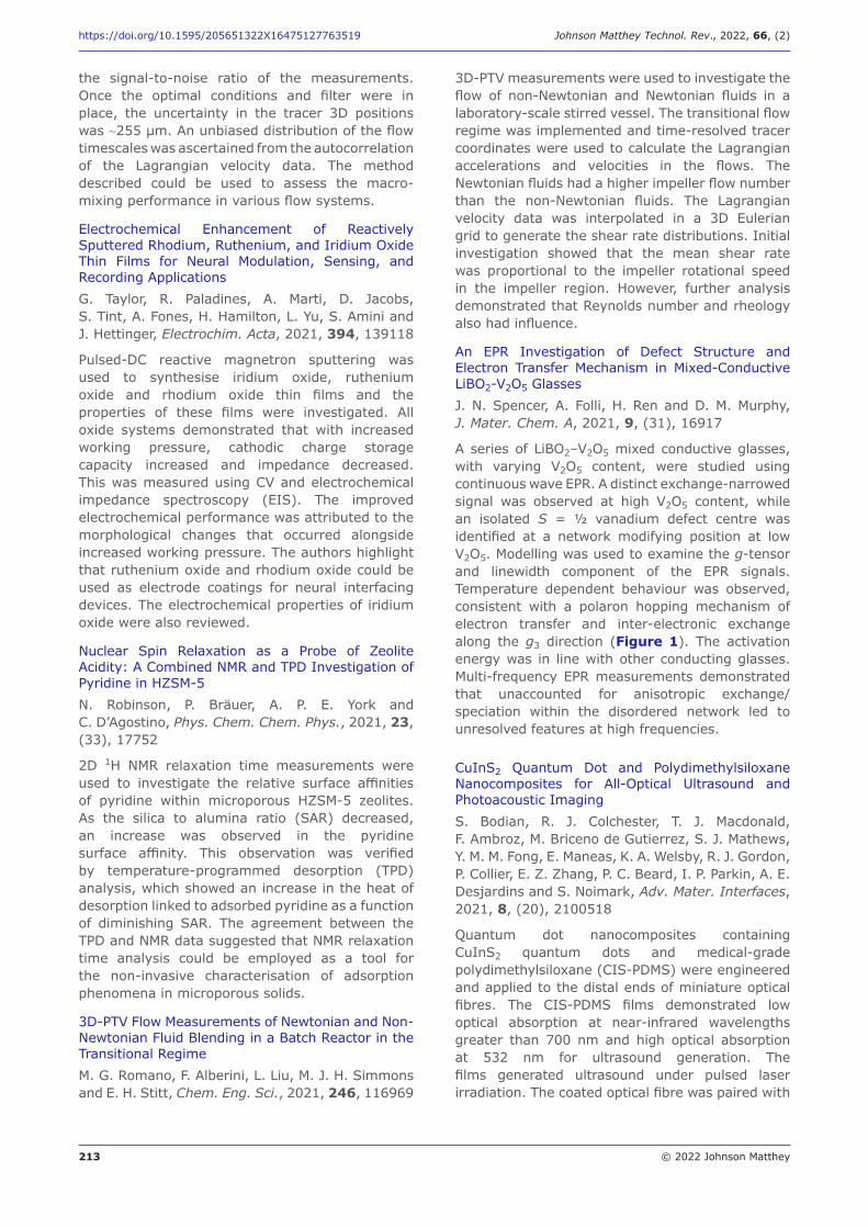
213 © 2022 Johnson Matthey
https://doi.org/10.1595/205651322X16475127763519 Johnson Matthey Technol. Rev., 2022, 66, (2)
the signal-to-noise ratio of the measurements. Once the optimal conditions and filter were in place, the uncertainty in the tracer 3D positions was ∼255 μm. An unbiased distribution of the flow timescales was ascertained from the autocorrelation of the Lagrangian velocity data. The method described could be used to assess the macro-mixing performance in various flow systems.
Electrochemical Enhancement of Reactively Sputtered Rhodium, Ruthenium, and Iridium Oxide Thin Films for Neural Modulation, Sensing, and Recording ApplicationsG. Taylor, R. Paladines, A. Marti, D. Jacobs, S. Tint, A. Fones, H. Hamilton, L. Yu, S. Amini and J. Hettinger, Electrochim. Acta, 2021, 394, 139118
Pulsed-DC reactive magnetron sputtering was used to synthesise iridium oxide, ruthenium oxide and rhodium oxide thin films and the properties of these films were investigated. All oxide systems demonstrated that with increased working pressure, cathodic charge storage capacity increased and impedance decreased. This was measured using CV and electrochemical impedance spectroscopy (EIS). The improved electrochemical performance was attributed to the morphological changes that occurred alongside increased working pressure. The authors highlight that ruthenium oxide and rhodium oxide could be used as electrode coatings for neural interfacing devices. The electrochemical properties of iridium oxide were also reviewed.
Nuclear Spin Relaxation as a Probe of Zeolite Acidity: A Combined NMR and TPD Investigation of Pyridine in HZSM-5 N. Robinson, P. Bräuer, A. P. E. York and C. D’Agostino, Phys. Chem. Chem. Phys., 2021, 23, (33), 17752
2D 1H NMR relaxation time measurements were used to investigate the relative surface affinities of pyridine within microporous HZSM-5 zeolites. As the silica to alumina ratio (SAR) decreased, an increase was observed in the pyridine surface affinity. This observation was verified by temperature- programmed desorption (TPD) analysis, which showed an increase in the heat of desorption linked to adsorbed pyridine as a function of diminishing SAR. The agreement between the TPD and NMR data suggested that NMR relaxation time analysis could be employed as a tool for the non-invasive characterisation of adsorption phenomena in microporous solids.
3D-PTV Flow Measurements of Newtonian and Non-Newtonian Fluid Blending in a Batch Reactor in the Transitional RegimeM. G. Romano, F. Alberini, L. Liu, M. J. H. Simmons and E. H. Stitt, Chem. Eng. Sci., 2021, 246, 116969
3D-PTV measurements were used to investigate the flow of non-Newtonian and Newtonian fluids in a laboratory-scale stirred vessel. The transitional flow regime was implemented and time-resolved tracer coordinates were used to calculate the Lagrangian accelerations and velocities in the flows. The Newtonian fluids had a higher impeller flow number than the non-Newtonian fluids. The Lagrangian velocity data was interpolated in a 3D Eulerian grid to generate the shear rate distributions. Initial investigation showed that the mean shear rate was proportional to the impeller rotational speed in the impeller region. However, further analysis demonstrated that Reynolds number and rheology also had influence.
An EPR Investigation of Defect Structure and Electron Transfer Mechanism in Mixed-Conductive LiBO2-V2O5 GlassesJ. N. Spencer, A. Folli, H. Ren and D. M. Murphy, J. Mater. Chem. A, 2021, 9, (31), 16917
A series of LiBO2–V2O5 mixed conductive glasses, with varying V2O5 content, were studied using continuous wave EPR. A distinct exchange-narrowed signal was observed at high V2O5 content, while an isolated S = ½ vanadium defect centre was identified at a network modifying position at low V2O5. Modelling was used to examine the g-tensor and linewidth component of the EPR signals. Temperature dependent behaviour was observed, consistent with a polaron hopping mechanism of electron transfer and inter-electronic exchange along the g3 direction (Figure 1). The activation energy was in line with other conducting glasses. Multi-frequency EPR measurements demonstrated that unaccounted for anisotropic exchange/speciation within the disordered network led to unresolved features at high frequencies.
CuInS2 Quantum Dot and Polydimethylsiloxane Nanocomposites for All-Optical Ultrasound and Photoacoustic ImagingS. Bodian, R. J. Colchester, T. J. Macdonald, F. Ambroz, M. Briceno de Gutierrez, S. J. Mathews, Y. M. M. Fong, E. Maneas, K. A. Welsby, R. J. Gordon, P. Collier, E. Z. Zhang, P. C. Beard, I. P. Parkin, A. E. Desjardins and S. Noimark, Adv. Mater. Interfaces, 2021, 8, (20), 2100518
Quantum dot nanocomposites containing CuInS2 quantum dots and medical-grade polydimethylsiloxane (CIS-PDMS) were engineered and applied to the distal ends of miniature optical fibres. The CIS-PDMS films demonstrated low optical absorption at near-infrared wavelengths greater than 700 nm and high optical absorption at 532 nm for ultrasound generation. The films generated ultrasound under pulsed laser irradiation. The coated optical fibre was paired with
214 © 2022 Johnson Matthey
https://doi.org/10.1595/205651322X16475127763519 Johnson Matthey Technol. Rev., 2022, 66, (2)
a Fabry– Pérot fibre optic sensor to produce an ultrasound transducer, and the film was exploited to facilitate co-registered photoacoustic imaging and all-optical ultrasound of an ink-filled tube phantom.
Determining the Electrochemical Transport Parameters of Sodium-Ions in Hard Carbon Composite ElectrodesD. Ledwoch, L. Komsiyska, E.-M. Hammer, K. Smith, P. R. Shearing, D. J. L. Brett and E. Kendrick, Electrochim. Acta, 2022, 401, 139481
Electrochemical potential spectroscopy (EPS), galvanostatic intermittent titration technique (GITT) and EIS were used to investigate the diffusivity and resistivity of sodium transport in hard carbon composite electrodes and various states-of-health. Impedance measurements and the diffusion coefficient from EPS and GITTS were used to extrapolate the charge transfer resistance, resistance contributions from the surface electrolyte interface and electrolyte transport in the electrode pores. The observed trends in desodiation, ageing and the diffusion coefficient during sodiation were similar for the different techniques. However, the orders of magnitude varied in the data. The calculated parameters were explored, and their accuracy examined.
Step Up: Gas–Liquid Mass-Transfer Characterization at Plant Scale Using the Pressure Step MethodR. W. Gallen, S. Smith, A. Burke and H. Stitt, Ind. Eng. Chem. Res., 2021, 60, (46), 16805
By accounting for background pressure loss, the authors adapted the pressure step method for use in a 1.3 m3 vessel. The adapted method produced theoretically comprehensive results at rapid speeds. Hydrogen solubility in water was measured and the results were in agreement with the scientific
literature. The overall mass-transfer coefficient was also measured. The measured values were compared to previously published modelling tools and correlations, which in turn demonstrated their poor predictive performance.
A Simple Liquid State 1H NMR Measurement to Directly Determine the Surface Hydroxyl Density of Porous SilicaC. Penrose, P. Steiner, L. F. Gladden, A. J. Sederman, A. P. E. York, M. Bentley and M. D. Mantle, Chem. Commun., 2021, 57, (95), 12804
The authors present a quick and simple liquid 1H NMR method to determine the surface hydroxyl density (αOH) of silica with the use of a benchtop 1H NMR spectrometer. The αOH of fully hydroxylated silicas ranged from 4.16 OH nm–2 to 6.56 OH nm–2, which aligned with previous studies in the literature. The cost, ease of use and speed associated with this method gives it an advantage over other techniques.
Selection of Formal Baseline Correction Methods in Thermal AnalysisR. L. Gibson, M. J. H. Simmons, E. H. Stitt, L. Horsburgh and R. W. Gallen, Chem. Eng. Technol., 2022, 45, (2), 238
An in silico study demonstrated the importance of choosing a suitable baseline correction method for thermal analysis data. Choosing the incorrect baseline correction led to a significant impact on the parameters obtained from kinetic modelling. A mass spectrometry dataset was employed to show the four formal baseline correction methods: linear with temperature, linear with time, no baseline correction and linear with extent of reaction. The authors recommended that Akaike weights should be compared to aid the selection of a correction method.
www.technology.matthey.com
https://doi.org/10.1595/205651322X16225583463559 Johnson Matthey Technol. Rev., 2022, 66, (2), 215–226
215 © 2022 Johnson Matthey
Ali Yorgancioglu, Ersin Onem, Onur Yilmaz, Huseyin Ata Karavana*Department of Leather Engineering, Faculty of Engineering, Ege University, 35100, Bornova-Izmir, Turkey
*Email: [email protected]
PEER REVIEWED
Received 16th February 2021; Revised 16th May 2021; Accepted 1st June 2021; Online 1st June 2021
This study aims to investigate the interactions between collagen and tanning processes performed by ecol-tan®, phosphonium, EasyWhite Tan®, glutaraldehyde, formaldehyde-free replacement synthetic tannin (syntan), condensed (mimosa) and hydrolysed (tara) vegetable tanning agents as alternatives to conventional basic chromium sulfate, widely used in the leather industry. Collagen stabilisation with tanning agents was determined by comparative thermal analysis methods: differential scanning calorimetry (DSC), thermogravimetric analysis (TGA) and conventional shrinkage temperature (Ts) measurement. Analysis techniques and tanning agents were compared and bonding characteristics were ranked by the thermal stabilisation they provided. Chromium tanning agent was also compared with the alternative tanning systems. The results provide a different perspective than the conventional view to provide a better understanding of the relationship between tanning and thermal stability of leather materials.
Interactions Between Collagen and Alternative Leather Tanning Systems to Chromium Salts by Comparative Thermal Analysis MethodsThermal stabilisation of collagen by tanning process
IntroductionTanning, in simple terms, refers to the treatment of rawhides or skins with tanning materials to render the material immune to microbial degradation (1). There are a large variety of chemicals used in the production of many different leather types. However, the major chemicals are the tanning agents as they define the process of leather manufacture as a whole (2). In the tanning process, tanning agent penetrates into the collagen matrix and is distributed evenly through its cross-section. It is then bound irreversibly to the collagen reactive sites (3). It has been accepted that the tanning ability of a substance is related to the type of interaction that occurs between the tanning agent and collagen (4). The tanning efficiency is conventionally defined by the Ts which is a measure of the resistance of leather to heat in aqueous medium. Fibre bundles of collagen can be induced to undergo an abrupt decrease in length at a characteristic Ts when subjected to slow heating in aqueous medium. The factors affecting shrinking include intramolecular interactions and superimposed intermolecular interactions. The latter is brought about by tanning and the sites available for tanning vary depending on the tanning agent. If the tanning agent forms strong bonds, such as covalent or coordinative, the leather has high hydrothermal stability i.e. high Ts values (5). The introduction of these crosslinks produces a more regular structure, decreases the entropy and so more energy is required to denature the collagen, hence the Ts rises.Today, tanners choose tanning chemicals based on
their performance, price, ease of use, environmental
216 © 2022 Johnson Matthey
https://doi.org/10.1595/205651322X16225583463559 Johnson Matthey Technol. Rev., 2022, 66, (2)
issues and their aesthetic properties (grain, colour, touch) (6). Chromium salts (commonly basic chromium sulfate) are the most widely used tanning agents with a global utilisation rate of 85% owing to their low cost, high versatility and quality of the final product obtained (7). Chromium compounds give high hydrothermal stability to leathers up to 100°C with light weight and soft touch. Besides these advantages, chromium also has disadvantages such as low exhaustion rate from floats (70% in 24 h), its blue-greenish colour, too much elasticity in some cases and a risk of forming carcinogenic Cr6+ species from unbound chromium (8). In conventional chromium tanning the low exhaustion rate results in discharging 30% of the chrome tanning agent into wastewater (9). These disadvantages motivate a move towards more environmental friendly tanning alternatives (10). For this purpose other inorganic tanning agents such as zirconium, aluminium, titanium or zinc compounds or organic tanning agents, i.e. vegetable tannins, syntans, polyaldehydes or phosphonium salts, are commonly used alone or in combination as chromium-free or metal-free tanning systems (11). It is worth noting that metal-free tanning agents employed for the production of ‘wet-white’ leather have limited application compared to chrome tanned leather (‘wet-blue’) since the physical and mechanical characteristics of wet-white leather are generally lower compared to wet-blue leather (12). Moreover, consumers’ anxieties about the possible effects of metals on human health as well as European Registration, Evaluation, Authorisation and Restriction of Chemicals (REACH) restrictions on heavy metals mean that metal-free tanning systems are increasingly attractive (13, 14).Vegetable tannins, syntans and aldehydes
are some alternative tanning agents for metal-free leather goods (13, 15, 16). Some chemical companies have developed new tanning systems for chrome-free and metal-free leathers for more sustainable leather making. The investigation of alternative tanning systems to basic chromium sulfate for the leather industry, together with detailed analysis of their tanning abilities, is extremely important.As mentioned above hydrothermal stability
of leather is generally measured by observing the temperature at which the leather specimen shrinks when heated in water at 2°C min–1. This phenomenon is called as Ts defined by the standard method ISO 3380:2002 [IULTCS/IUP 16] (17). On the other hand, there are also alternative
analytical techniques providing information about the thermal behaviours of tanned leathers (18–20). Fully hydrated (>200% water/collagen) native collagen undergoes denaturation when heated to approximately 62°C, as observed by shrinkage of the samples to a third of the original length, and by the peak in measurements taken by means of differential scanning calorimetry/differential thermoanalysis (DSC/DTA). The peak of the first endothermic event observed in the DSC thermograms usually refers to the Ts and the area below this peak corresponds to the heat requirement of the endothermal melting process. Thermal behaviour of the tanned collagen can be accurately measured using much smaller samples by thermogravimetry/derivative thermogravimetry (TG/DTG) and DSC methods (21). These thermal analyses are useful for fast evaluation of thermal stability and behaviour, degradation temperature, absorbed moisture content, crystallised water content, melting point and thermal decomposition kinetics in a closed measurement atmosphere (22). Application of these sensitive techniques provides more realistic evidence of denaturation or deterioration degree by the phase transitions of dry biomaterial in a short time using milligram quantities (23, 24), especially when the daily use conditions of leather materials are considered. Leather materials applied in automotive upholstery, furniture, military shoes, gloves and aircraft seating require high thermal resistance and must be analysed under interior and exterior extreme conditions (25). To our knowledge, there are only a few reports on the comparative thermal behaviour of dry and wet collagen (26) and less is known about the degradation mechanism of tanned leathers (27).The present study aims to investigate the thermal
behaviour of leathers with various tanning systems via different techniques and to provide a better understanding of the relationship between tanning and thermal stability of leather composed of collagen fibres.
Experimental Setup
Materials
Commercially pickled Turkish sheepskins were used for tanning operations. Tanning agents used in the study were industrially produced, commercially available products: chromium salts and ecol-tan® tanning agents (Şişecam Chemicals, Turkey); EasyWhite Tan® tanning agent (Granofin® Easy
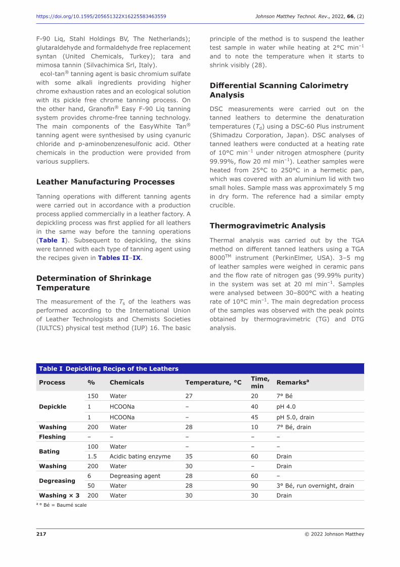
217 © 2022 Johnson Matthey
https://doi.org/10.1595/205651322X16225583463559 Johnson Matthey Technol. Rev., 2022, 66, (2)
F-90 Liq, Stahl Holdings BV, The Netherlands); glutaraldehyde and formaldehyde free replacement syntan (United Chemicals, Turkey); tara and mimosa tannin (Silvachimica Srl, Italy). ecol-tan® tanning agent is basic chromium sulfate
with some alkali ingredients providing higher chrome exhaustion rates and an ecological solution with its pickle free chrome tanning process. On the other hand, Granofin® Easy F-90 Liq tanning system provides chrome-free tanning technology. The main components of the EasyWhite Tan® tanning agent were synthesised by using cyanuric chloride and p-aminobenzenesulfonic acid. Other chemicals in the production were provided from various suppliers.
Leather Manufacturing Processes
Tanning operations with different tanning agents were carried out in accordance with a production process applied commercially in a leather factory. A depickling process was first applied for all leathers in the same way before the tanning operations (Table I). Subsequent to depickling, the skins were tanned with each type of tanning agent using the recipes given in Tables II–IX.
Determination of Shrinkage Temperature
The measurement of the Ts of the leathers was performed according to the International Union of Leather Technologists and Chemists Societies (IULTCS) physical test method (IUP) 16. The basic
principle of the method is to suspend the leather test sample in water while heating at 2°C min–1
and to note the temperature when it starts to shrink visibly (28).
Differential Scanning Calorimetry Analysis
DSC measurements were carried out on the tanned leathers to determine the denaturation temperatures (Td) using a DSC-60 Plus instrument (Shimadzu Corporation, Japan). DSC analyses of tanned leathers were conducted at a heating rate of 10°C min–1 under nitrogen atmosphere (purity 99.99%, flow 20 ml min–1). Leather samples were heated from 25°C to 250°C in a hermetic pan, which was covered with an aluminium lid with two small holes. Sample mass was approximately 5 mg in dry form. The reference had a similar empty crucible.
Thermogravimetric Analysis
Thermal analysis was carried out by the TGA method on different tanned leathers using a TGA 8000TM instrument (PerkinElmer, USA). 3–5 mg of leather samples were weighed in ceramic pans and the flow rate of nitrogen gas (99.99% purity) in the system was set at 20 ml min–1. Samples were analysed between 30–800°C with a heating rate of 10°C min–1. The main degredation process of the samples was observed with the peak points obtained by thermogravimetric (TG) and DTG analysis.
Table I Depickling Recipe of the Leathers
Process % Chemicals Temperature, °C Time, min Remarksa
Depickle
150 Water 27 20 7° Bé
1 HCOONa – 40 pH 4.0
1 HCOONa – 45 pH 5.0, drain
Washing 200 Water 28 10 7° Bé, drain
Fleshing – – – – –
Bating100 Water – – –
1.5 Acidic bating enzyme 35 60 Drain
Washing 200 Water 30 – Drain
Degreasing6 Degreasing agent 28 60 –
50 Water 28 90 3° Bé, run overnight, drain
Washing × 3 200 Water 30 30 Draina ° Bé = Baumé scale
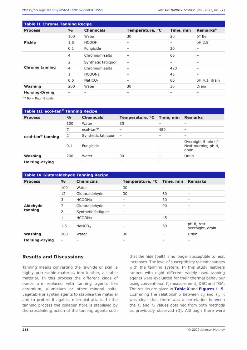
218 © 2022 Johnson Matthey
https://doi.org/10.1595/205651322X16225583463559 Johnson Matthey Technol. Rev., 2022, 66, (2)
Table II Chrome Tanning RecipeProcess % Chemicals Temperature, °C Time, min Remarksa
Pickle100 Water 30 20 6° Bé
1.5 HCOOH – – pH 2.8
0.1 Fungicide – 20 –
Chrome tanning
4 Chromium salts – 60 –
2 Synthetic fatliquor – – –
4 Chromium salts – 420 –
1 HCOONa – 45 –
0.5 NaHCO3 – 60 pH 4.1, drain
Washing 200 Water 30 30 Drain
Horsing-Drying – – – – –a ° Bé = Baumé scale
Table III ecol-tan® Tanning RecipeProcess % Chemicals Temperature, °C Time, min Remarks
ecol-tan® tanning
100 Water 30 – –
7 ecol-tan® – 480 –
2 Synthetic fatliquor – – –
0.1 Fungicide – –Overnight 5 min h–1
Next morning pH 4, drain
Washing 200 Water 30 – Drain
Horsing-drying – – – – –
Table IV Glutaraldehyde Tanning RecipeProcess % Chemicals Temperature, °C Time, min Remarks
Aldehyde tanning
100 Water 30 – –
12 Glutaraldehyde 30 60 –
3 HCOONa – 30 –
7 Glutaraldehyde – 90 –
2 Synthetic fatliquor – – –
1 HCOONa – 45 –
1.5 NaHCO3 – 60 pH 8, rest overnight, drain
Washing 200 Water 30 – Drain
Horsing-drying – – – – –
Results and Discussions
Tanning means converting the rawhide or skin, a highly putrescible material, into leather, a stable material. In this process the different kinds of bonds are replaced with tanning agents like chromium, aluminium or other mineral salts, vegetable or syntan agents to stabilise the material and to protect it against microbial attack. In the tanning process the collagen fibre is stabilised by the crosslinking action of the tanning agents such
that the hide (pelt) is no longer susceptible to heat increases. The level of susceptibility to heat changes with the tanning system. In this study leathers tanned with eight different widely used tanning agents were evaluated for their thermal behaviour using conventional Ts measurement, DSC and TGA. The results are given in Table X and Figures 1–5. Examining the relationship between Td and Ts, it was clear that there was a correlation between the Ts and Td values obtained from both methods as previously observed (3). Although there were
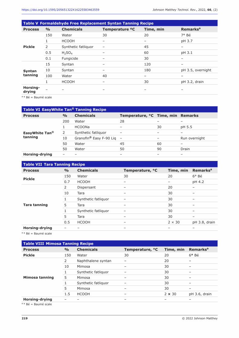
219 © 2022 Johnson Matthey
https://doi.org/10.1595/205651322X16225583463559 Johnson Matthey Technol. Rev., 2022, 66, (2)
Table VI EasyWhite Tan® Tanning RecipeProcess % Chemicals Temperature, °C Time, min Remarks
EasyWhite Tan® tanning
200 Water 28 – –1 HCOONa – 30 pH 5.52 Synthetic fatliquor – – –10 Granofin® Easy F-90 Liq – – Run overnight50 Water 45 60 –50 Water 50 90 Drain
Horsing-drying – – – – –
Table VII Tara Tanning RecipeProcess % Chemicals Temperature, °C Time, min Remarksa
Pickle150 Water 30 20 6° Bé0.7 HCOOH – – pH 4.2
Tara tanning
2 Dispersant – 20 –
10 Tara – 30 –
1 Synthetic fatliquor – 30 –
5 Tara – 30 –
1 Synthetic fatliquor – 30 –5 Tara – 30 –0.5 HCOOH – 2 × 30 pH 3.8, drain
Horsing-drying – – – – –a ° Bé = Baumé scale
Table VIII Mimosa Tanning RecipeProcess % Chemicals Temperature, °C Time, min Remarksa
Pickle 150 Water 30 20 6° Bé
Mimosa tanning
2 Naphthalene syntan – 20 –10 Mimosa – 30 –1 Synthetic fatliquor – 30 –5 Mimosa – 30 –1 Synthetic fatliquor – 30 –5 Mimosa – 30 –1.5 HCOOH – 2 × 30 pH 3.6, drain
Horsing-drying – – – – –a ° Bé = Baumé scale
Table V Formaldehyde Free Replacement Syntan Tanning RecipeProcess % Chemicals Temperature ºC Time, min Remarksa
Pickle
150 Water 30 20 7° Bé
1 HCOOH – – pH 3.7
2 Synthetic fatliquor – 45 –
0.5 H2SO4 – 60 pH 3.1
0.1 Fungicide – 30 –
Syntan tanning
15 Syntan – 120 –
10 Syntan – 180 pH 3.5, overnight
100 Water 40 – –
1 HCOOH – 30 pH 3.2, drain
Horsing-drying – – – – –
a ° Bé = Baumé scale
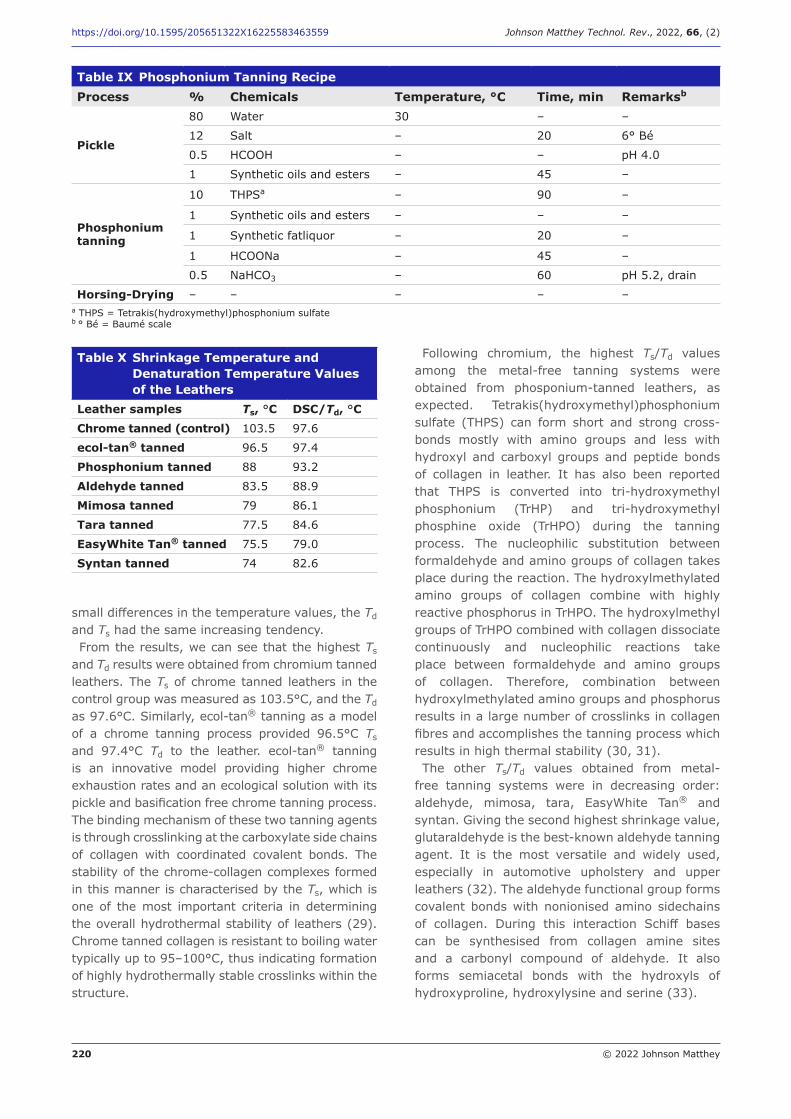
220 © 2022 Johnson Matthey
https://doi.org/10.1595/205651322X16225583463559 Johnson Matthey Technol. Rev., 2022, 66, (2)
small differences in the temperature values, the Td and Ts had the same increasing tendency.From the results, we can see that the highest Ts
and Td results were obtained from chromium tanned leathers. The Ts of chrome tanned leathers in the control group was measured as 103.5°C, and the Td as 97.6°C. Similarly, ecol-tan® tanning as a model of a chrome tanning process provided 96.5°C Ts and 97.4°C Td to the leather. ecol-tan® tanning is an innovative model providing higher chrome exhaustion rates and an ecological solution with its pickle and basification free chrome tanning process. The binding mechanism of these two tanning agents is through crosslinking at the carboxylate side chains of collagen with coordinated covalent bonds. The stability of the chrome-collagen complexes formed in this manner is characterised by the Ts, which is one of the most important criteria in determining the overall hydrothermal stability of leathers (29). Chrome tanned collagen is resistant to boiling water typically up to 95–100°C, thus indicating formation of highly hydrothermally stable crosslinks within the structure.
Following chromium, the highest Ts/Td values among the metal-free tanning systems were obtained from phosponium-tanned leathers, as expected. Tetrakis(hydroxymethyl)phosphonium sulfate (THPS) can form short and strong cross-bonds mostly with amino groups and less with hydroxyl and carboxyl groups and peptide bonds of collagen in leather. It has also been reported that THPS is converted into tri-hydroxymethyl phosphonium (TrHP) and tri-hydroxymethyl phosphine oxide (TrHPO) during the tanning process. The nucleophilic substitution between formaldehyde and amino groups of collagen takes place during the reaction. The hydroxylmethylated amino groups of collagen combine with highly reactive phosphorus in TrHPO. The hydroxylmethyl groups of TrHPO combined with collagen dissociate continuously and nucleophilic reactions take place between formaldehyde and amino groups of collagen. Therefore, combination between hydroxylmethylated amino groups and phosphorus results in a large number of crosslinks in collagen fibres and accomplishes the tanning process which results in high thermal stability (30, 31).The other Ts/Td values obtained from metal-
free tanning systems were in decreasing order: aldehyde, mimosa, tara, EasyWhite Tan® and syntan. Giving the second highest shrinkage value, glutaraldehyde is the best-known aldehyde tanning agent. It is the most versatile and widely used, especially in automotive upholstery and upper leathers (32). The aldehyde functional group forms covalent bonds with nonionised amino sidechains of collagen. During this interaction Schiff bases can be synthesised from collagen amine sites and a carbonyl compound of aldehyde. It also forms semiacetal bonds with the hydroxyls of hydroxyproline, hydroxylysine and serine (33).
Table X Shrinkage Temperature and Denaturation Temperature Values of the Leathers
Leather samples Ts, °C DSC/Td, °CChrome tanned (control) 103.5 97.6
ecol-tan® tanned 96.5 97.4
Phosphonium tanned 88 93.2
Aldehyde tanned 83.5 88.9
Mimosa tanned 79 86.1
Tara tanned 77.5 84.6
EasyWhite Tan® tanned 75.5 79.0
Syntan tanned 74 82.6
Table IX Phosphonium Tanning RecipeProcess % Chemicals Temperature, °C Time, min Remarksb
Pickle
80 Water 30 – –
12 Salt – 20 6° Bé
0.5 HCOOH – – pH 4.0
1 Synthetic oils and esters – 45 –
Phosphonium tanning
10 THPSa – 90 –
1 Synthetic oils and esters – – –
1 Synthetic fatliquor – 20 –
1 HCOONa – 45 –
0.5 NaHCO3 – 60 pH 5.2, drain
Horsing-Drying – – – – –a THPS = Tetrakis(hydroxymethyl)phosphonium sulfateb ° Bé = Baumé scale
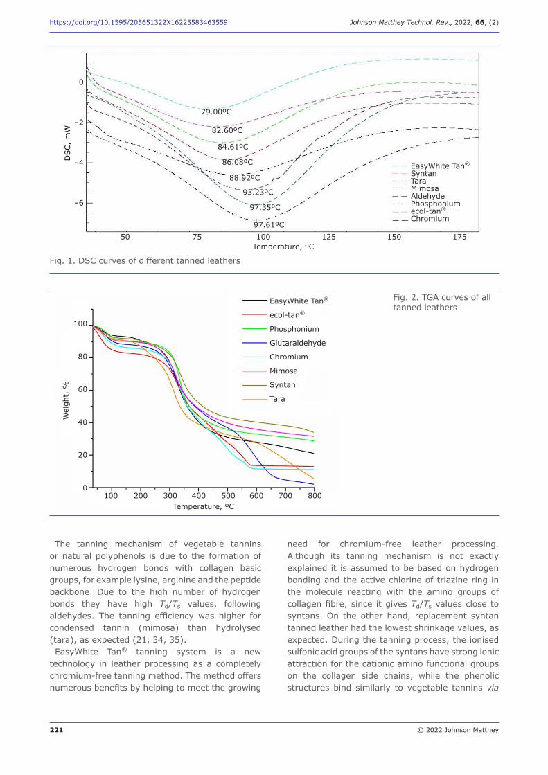
221 © 2022 Johnson Matthey
https://doi.org/10.1595/205651322X16225583463559 Johnson Matthey Technol. Rev., 2022, 66, (2)
The tanning mechanism of vegetable tannins or natural polyphenols is due to the formation of numerous hydrogen bonds with collagen basic groups, for example lysine, arginine and the peptide backbone. Due to the high number of hydrogen bonds they have high Td/Ts values, following aldehydes. The tanning efficiency was higher for condensed tannin (mimosa) than hydrolysed (tara), as expected (21, 34, 35).EasyWhite Tan® tanning system is a new
technology in leather processing as a completely chromium-free tanning method. The method offers numerous benefits by helping to meet the growing
need for chromium-free leather processing. Although its tanning mechanism is not exactly explained it is assumed to be based on hydrogen bonding and the active chlorine of triazine ring in the molecule reacting with the amino groups of collagen fibre, since it gives Td/Ts values close to syntans. On the other hand, replacement syntan tanned leather had the lowest shrinkage values, as expected. During the tanning process, the ionised sulfonic acid groups of the syntans have strong ionic attraction for the cationic amino functional groups on the collagen side chains, while the phenolic structures bind similarly to vegetable tannins via
50 75 100 125 150 175Temperature, ºC
0
–2
–4
–6
DSC,
mW
79.00ºC
82.60ºC
84.61ºC
86.08ºC
88.92ºC
93.23ºC
97.35ºC
97.61ºC
EasyWhite Tan®
SyntanTaraMimosaAldehydePhosphoniumecol-tan®
Chromium
Fig. 1. DSC curves of different tanned leathers
100 200 300 400 500 600 700 800Temperature, ºC
EasyWhite Tan®
ecol-tan®
Phosphonium
Glutaraldehyde
Chromium
Mimosa
Syntan
Tara
100
80
60
40
20
0
Wei
ght,
%
Fig. 2. TGA curves of all tanned leathers
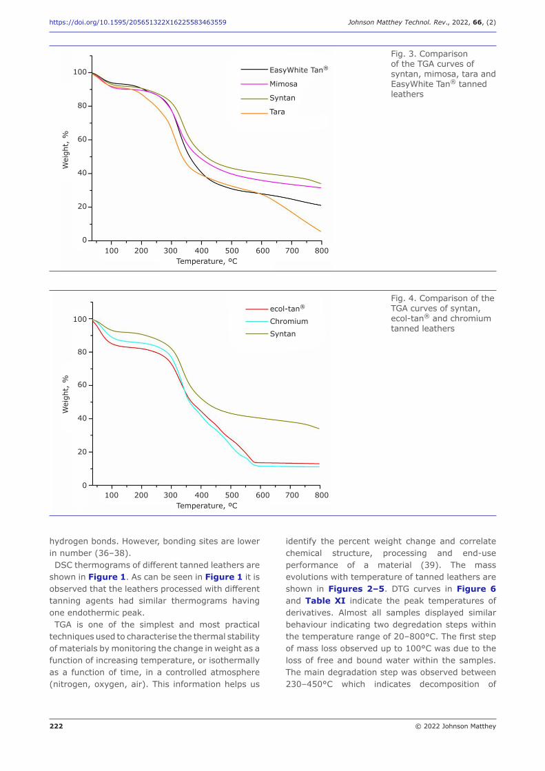
222 © 2022 Johnson Matthey
https://doi.org/10.1595/205651322X16225583463559 Johnson Matthey Technol. Rev., 2022, 66, (2)
hydrogen bonds. However, bonding sites are lower in number (36–38). DSC thermograms of different tanned leathers are
shown in Figure 1. As can be seen in Figure 1 it is observed that the leathers processed with different tanning agents had similar thermograms having one endothermic peak.TGA is one of the simplest and most practical
techniques used to characterise the thermal stability of materials by monitoring the change in weight as a function of increasing temperature, or isothermally as a function of time, in a controlled atmosphere (nitrogen, oxygen, air). This information helps us
identify the percent weight change and correlate chemical structure, processing and end-use performance of a material (39). The mass evolutions with temperature of tanned leathers are shown in Figures 2–5. DTG curves in Figure 6 and Table XI indicate the peak temperatures of derivatives. Almost all samples displayed similar behaviour indicating two degredation steps within the temperature range of 20–800°C. The first step of mass loss observed up to 100°C was due to the loss of free and bound water within the samples. The main degradation step was observed between 230–450°C which indicates decomposition of
100 200 300 400 500 600 700 800Temperature, ºC
EasyWhite Tan®
Mimosa
Syntan
Tara
100
80
60
40
20
0
Wei
ght,
%Fig. 3. Comparison of the TGA curves of syntan, mimosa, tara and EasyWhite Tan® tanned leathers
100 200 300 400 500 600 700 800Temperature, ºC
ecol-tan®
Chromium
Syntan
100
80
60
40
20
0
Wei
ght,
%
Fig. 4. Comparison of the TGA curves of syntan, ecol-tan® and chromium tanned leathers
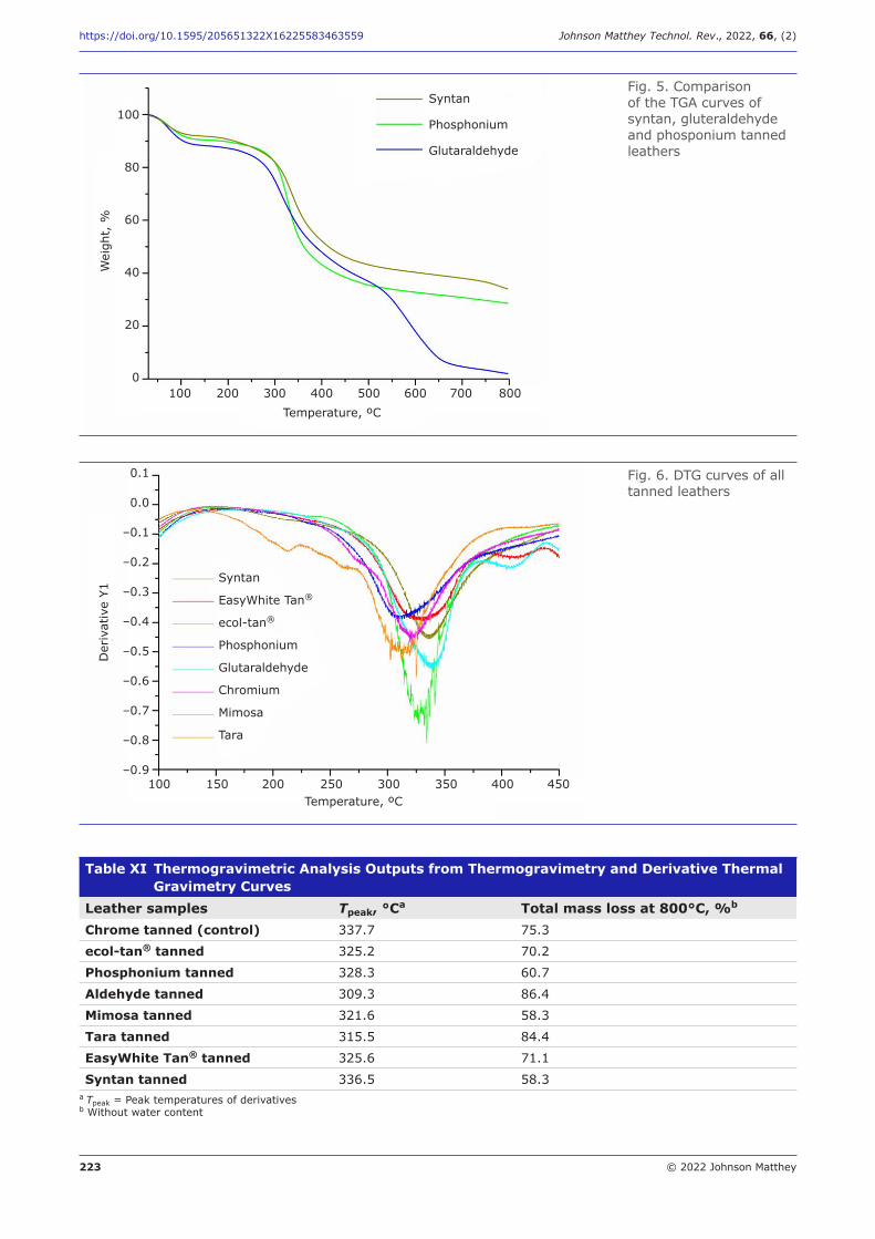
223 © 2022 Johnson Matthey
https://doi.org/10.1595/205651322X16225583463559 Johnson Matthey Technol. Rev., 2022, 66, (2)
100 200 300 400 500 600 700 800Temperature, ºC
Syntan
Phosphonium
Glutaraldehyde
100
80
60
40
20
0
Wei
ght,
%Fig. 5. Comparison of the TGA curves of syntan, gluteraldehyde and phosponium tanned leathers
100 150 200 250 300 350 400 450Temperature, ºC
Der
ivat
ive
Y1
Fig. 6. DTG curves of all tanned leathers
0.1
0.0
–0.1
–0.2
–0.3
–0.4
–0.5
–0.6
–0.7
–0.8
–0.9
Syntan
EasyWhite Tan®
ecol-tan®
Phosphonium
Glutaraldehyde
Chromium
Mimosa
Tara
Table XI Thermogravimetric Analysis Outputs from Thermogravimetry and Derivative Thermal Gravimetry Curves
Leather samples Tpeak, °Ca Total mass loss at 800°C, %b
Chrome tanned (control) 337.7 75.3
ecol-tan® tanned 325.2 70.2
Phosphonium tanned 328.3 60.7
Aldehyde tanned 309.3 86.4
Mimosa tanned 321.6 58.3
Tara tanned 315.5 84.4
EasyWhite Tan® tanned 325.6 71.1
Syntan tanned 336.5 58.3a Tpeak = Peak temperatures of derivativesb Without water content
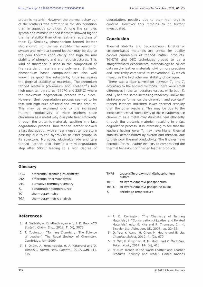
224 © 2022 Johnson Matthey
https://doi.org/10.1595/205651322X16225583463559 Johnson Matthey Technol. Rev., 2022, 66, (2)
proteinic material. However, the thermal behaviour of the leathers was different in the dry condition than in aqueous condition. Among the samples syntan and mimosa tanned leathers showed higher thermal stability than other leathers regardless of their Ts. Similarly, phosphonium tanned leather also showed high thermal stability. The reason for syntan and mimosa tanned leather may be due to the poor thermal conductivity and high thermal stability of phenolic and aromatic structures. This kind of substance is used in the composition of fire retardant materials and polymers. Similarly, phosponium based compounds are also well known as good fire retardants, thus increasing the thermal stability of materials. The chromium tanned leathers (chromium and ecol-tan®) had high peak temperatures (337°C and 325°C) where the maximum degredation process took place. However, their degradation process seemed to be fast with high burn-off ratio and low ash amount. This may be explained due to the increased thermal conductivity of these leathers since chromium as a metal may dissipate heat efficiently through the proteinic material, resulting in a fast degradation process. Tara tanned leather showed a fast degradation with an early onset temperature possibly due to the hydrolysis of ester groups in its structure. Moreover, gluteraldehyde and tara tanned leathers also showed a third degradation step after 500°C leading to a high degree of
degradation, possibly due to their high organic content. However this remains to be further investigated.
Conclusion
Thermal stability and decomposition kinetics of collagen-based materials are critical for quality control parameters of tanned leather products. TG-DTG and DSC techniques proved to be a straightforward experimental methodology to collect data on dry leather materials, giving more precision and sensitivity compared to conventional Ts which measures the hydrothermal stability of collagen.There was a clear correlation between Td and Ts
according to the applied methods. There were small differences in the temperature values, while both Td and Ts had the same increasing tendency. Unlike the shrinkage performance, the chromium and ecol-tan® tanned leathers indicated lower thermal stability than the other leathers. This may be due to the increased thermal conductivity of these leathers since chromium as a metal may dissipate heat efficiently through the proteinic material, resulting in a fast degradation process. It is interesting to see that the leathers having lower Ts may have higher thermal stability, demonstrated by syntan and mimosa, due to their poor thermal conductivity. The findings have potential for the leather industry to comprehend the thermal behaviour of finished leather products.
Glossary
DSC differential scanning calorimetry
DTA differential thermoanalysis
DTG derivative thermogravimetry
Td denaturation temperatures
TG thermogravimetry
TGA thermogravimetric analysis
THPS tetrakis(hydroxymethyl)phosphonium sulfate
TrHP tri-hydroxymethyl phosphonium
TrHPO tri-hydroxymethyl phosphine oxide
Ts shrinkage temperature
References
1. M. Sathish, A. Dhathathreyan and J. R. Rao, ACS Sustain. Chem. Eng., 2019, 7, (4), 3875
2. T. Covington, “Tanning Chemistry: The Science of Leather”, The Royal Society of Chemistry, Cambridge, UK, 2009
3. E. Onem, A. Yorgancioglu, H. A. Karavana and O. Yilmaz, J. Therm. Anal. Calorim., 2017, 129, (1), 615
4. A. D. Covington, ‘The Chemistry of Tanning Materials’, in “Conservation of Leather and Related Materials”, eds. M. Kite and R. Thomson, Ch. 4, Elsevier Ltd, Abingdon, UK, 2006, pp. 22–35
5. Q. Yao, Y. Wang, H. Chen, H. Huang and B. Liu, ChemistrySelect, 2019, 4, (2), 670
6. N. Örk, H. Özgünay, M. M. Mutlu and Z. Öndoğan, Tekst. Konf., 2014, 24, (4), 413
7. “Future Trends in the World Leather and Leather Products Industry and Trade”, United Nations
225 © 2022 Johnson Matthey
https://doi.org/10.1595/205651322X16225583463559 Johnson Matthey Technol. Rev., 2022, 66, (2)
Industrial Development Organization, Vienna, Austria, 2010, 120 pp
8. B. S. Scopel, C. Baldasso, A. Dettmer and R. M. C. Santana, J. Am. Leather Chem. Assoc., 2018, 113, (4), 122
9. M. Renner, E. Weidner and H. Geihsler, J. Am. Leather Chem. Assoc., 2013, 108, (8), 289
10. G. Krishnamoorthy, S. Sadulla, P. K. Sehgal and A. B. Mandal, J. Cleaner Prod., 2013, 42, 277
11. H. A. Karavana, B. Başaran, A. Aslan, B. O. Bitlisli and G. Gülümser, Tekst. Konf., 2011, 21, (3), 305
12. Y. Dilek, B. Başaran, A. Sancakli, B. O. Bitlisli and A. Yorgancioğlu, J. Soc. Leath. Tech. Chem., 2019, 103, (3), 129
13. R. Aravindhan, B. Madhan and J. R. Rao, J. Am. Leather Chem. Assoc., 2015, 110, (3), 80
14. V. Beghetto, L. Agostinis, V. Gatto, R. Samiolo and A. Scrivanti, J. Clean. Prod., 2019, 220, 864
15. K. J. Sreeram, R. Aravindhan, J. R. Rao and B. U. Nair, J. Am. Leather Chem. Assoc., 2010, 105, (12), 401
16. V. J. Sundar and C. Muralidharan, Environ. Process., 2020, 7, (1), 255
17. J. M. V. Williams, J. Soc. Leath. Tech. Chem., 2000, 84, 359
18. T. Bosch, A. M. Manich, J. Carilla, J. Cot, A. Marsal, H. J. Kellert and H. P. Germann, J. Am. Leather Chem. Assoc., 2002, 97, (11), 441
19. P. Budrugeac, V. Trandafir and M. G. Albu, J. Therm. Anal. Calorim., 2003, 72, (2), 581
20. Y. Wang, J. Guo, H. Chen and Z. Shan, J. Therm. Anal. Calorim., 2010, 99, (1), 295
21. C. Carşote, E. Badea, L. Miu and G. Della Gatta, J. Therm. Anal. Calorim., 2016, 124, (3), 1255
22. L. Yang, Y. Liu, Y. Wu, L. Deng, W. Liu, C. Ma and L. Li, J. Therm. Anal. Calorim., 2016, 123, (1), 413
23. P. Budrugeac, J. Therm. Anal. Calorim., 2015, 120, (1), 103
24. K. M. Nalyanya, R. K. Rop, A. S. Onyuka, T. Kilee, P. O. Migunde and R. G. Ngumbu, J. Therm. Anal. Calorim., 2016, 126, (2), 725
25. W. Xu, J. Li, F. Liu, Y. Jiang, Z. Li and L. Li, J. Therm. Anal. Calorim., 2017, 128, (2), 1107
26. L. Rosu, C.-D. Varganici, A.-M. Crudu and D. Rosu, J. Therm. Anal. Calorim., 2018, 134, (1), 583
27. P. Yang, X. He, W. Zhang, Y. Qiao, F. Wang and K. Tang, J. Therm. Anal. Calorim., 2017, 127, (3), 2005
28. ‘Leather – Physical and Mechanical Tests – Determination of Shrinkage Temperature up to 100oC’, BS EN ISO 3380:2015, British Standards Institution, London, UK, 30th September, 2015
29. K. H. Gustavson, “The Chemistry and Reactivity of Collagen”, Academic Press, New York, USA, 1956
30. Y. Li, Z. H. Shan, S. X. Shao and K. Q. Shi, J. Soc. Leath. Tech. Chem., 2006, 90, (5), 214
31. S. Shao, K. Shi, Y. Li, L. Jiang and C. Ma, Chin. J. Chem. Eng., 2008, 16, (3), 446
32. R. Li, Y. Z. Wang, Z. H. Shan, M. Yang, W. Li and H. L. Zhu, J. Soc. Leath. Tech. Chem., 2016, 100, (1), 19
33. V. Plavan, M. Koliada and V. Valeika, J. Soc. Leath. Tech. Chem., 2017, 101, (5), 260
34. C. Capparucci, F. Gironi and V. Piemonte, Asia-Pac. J. Chem. Eng., 2011, 6, (4), 606
35. Z. Sebestyén, E. Jakab, E. Badea, E. Barta-Rajnai, C. Şendrea and Z. Czégény, J. Anal. Appl. Pyrolysis, 2019, 138, 178
36. S. V. Kanth, G. C. Jayakumar, S. C. Ramkumar, B. Chandrasekaran, J. R. Rao and B. U. Nair, J. Am. Leather Chem. Assoc., 2012, 107, (5), 106
37. E. Onem, G. Gulumser, M. Renner and O. Yesil-Celiktas, J. Supercrit. Fluids, 2015, 104, 259
38. R. Saleem, A. Adnan and F. A. Qureshi, Indian J. Chem. Technol., 2015, 22, (1–2), 48
39. P. Budrugeac, A. Cucos and L. Miu, J. Therm. Anal. Calorim., 2014, 116, (1), 141
The Authors
Ali Yorgancioglu is a research assistant in the Department of Leather Engineering, Faculty of Engineering, Ege University, Turkey. He has a PhD degree in the field of leather engineering and studied in Fraunhofer UMSICHT, Germany for his PhD thesis. He assisted teaching Tanning Technologies, Leather Auxıliary and Chemistry courses. He teaches Raw Hide and Leather Histology courses for the Bachelors degree. He has participated in various national projects as a researcher. His research activities and fields of interests are emulsions, nanotechnology, leather fatliquors, tanning technologies and cleaner leather technologies.
226 © 2022 Johnson Matthey
https://doi.org/10.1595/205651322X16225583463559 Johnson Matthey Technol. Rev., 2022, 66, (2)
Ersin Onem graduated from the Department of Leather Engineering, Faculty of Engineering, Ege University in 2006. He received his MSc degree in the same department in Izmir, Turkey. After his MSc degree, he worked in the laboratories of TFL Ledertechnik GmbH, Germany. He cooperated with Fraunhofer Institute on ambient carbon dioxide for sustainable production in the leather industry using supercritical fluid technology and finished his PhD in 2015. After his PhD, he carried out postdoctoral studies in a European Union Project in Germany for nine months. Onem currently serves as Associate Professor in the Department of Leather Engineering in Ege University. His research interests are on tanning technologies, ecological production, environmentally friendly processing, supercritical fluid applications and high-pressure technologies.
Onur Yılmaz has been working as an Associate Professor at the Department of Leather Engineering in Ege University since 2015. He graduated from the Department of Leather Technology, Faculty of Engineering, Ege University in 2002. He finished his MSc studies in the Enviromental Sciences Department at Ege University. He carried out PhD studies in collaboration with the Institute of Macromolecular Chemistry “Petru Poni” in Iasi, Romania and completed his PhD in the Department of Leather Engineering, Ege University in 2011. He continued his postdoctoral studies in the Laboratory of Polymers in the Chemistry Department of University of Helsinki, Finland, between 2012–2014. His research interests are enviromentaly friendly systems in leather technology, polymer synthesis, nanocomposites, acrylates, coating and finishing systems.
Hüseyin Ata Karavana graduated from the Department of Leather Technology, Faculty of Agriculture, Ege University. He earned his MSc degree in Leather Technology in 2001 from that institution’s Graduate School of Natural and Applied Science. From 2006 to 2007 he continued his studies as an Erasmus student in the Department of Footwear Engineering and Hygiene at the Faculty of Technology, Tomas Bata University, Zlin, Czech Republic. Karavana completed his PhD degree in Leather Engineering at Ege University in 2008. Karavana currently serves as Associate Professor in the Department of Leather Engineering at Ege University’s Faculty of Engineering. His research interests are in all manner of leather and footwear engineering including plastic composites, microencapsulation, leather quality control and footwear quality control.

Johnson Matthey Technology Review is Johnson Matthey’s international journal of research exploring science and technology in industrial applications
www.technology.matthey.com

Editorial team
Manager Dan CarterEditor Sara ColesEditorial Assistant Yasmin StephensSenior Information Officer Elisabeth Riley
Johnson Matthey Technology ReviewJohnson Matthey PlcOrchard RoadRoystonSG8 5HEUKTel +44 (0)1763 253 000Email [email protected]
www.technology.matthey.com
Related Documents