VOLUME 6 ISSUE 1 JANUARY 2022 ISSN 2587-1366

Welcome message from author
This document is posted to help you gain knowledge. Please leave a comment to let me know what you think about it! Share it to your friends and learn new things together.
Transcript

VOLUME 6 ISSUE 1 JANUARY 2022
ISSN 2587-1366

EDITOR IN CHIEF
Prof. Dr. Murat YAKAR
Mersin University Engineering Faculty
Turkey
CO-EDITORS
Prof. Dr. Erol YAŞAR
Mersin University Faculty of Art and Science
Turkey
Prof. Dr. Cahit BİLİM
Mersin University Engineering Faculty
Turkey
Assist. Prof. Dr. Hüdaverdi ARSLAN
Mersin University Engineering Faculty
Turkey
ADVISORY BOARD
Prof. Dr. Orhan ALTAN
Honorary Member of ISPRS, ICSU EB Member
Turkey
Prof. Dr. Armin GRUEN
ETH Zurih University
Switzerland
Prof. Dr. Hacı Murat YILMAZ
Aksaray University Engineering Faculty
Turkey
Prof. Dr. Artu ELLMANN
Tallinn University of Technology Faculty of Civil Engineering
Estonia
Assoc. Prof. Dr. E. Cağlan KUMBUR
Drexel University
USA
TECHNICAL EDITORS
Prof. Dr. Roman KOCH
Erlangen-Nurnberg Institute Palaontologie
Germany
Prof. Dr. Hamdalla WANAS
Menoufyia University, Science Faculty
Egypt
Prof. Dr. Turgay CELIK
Witwatersrand University
South Africa
Prof. Dr. Muhsin EREN
Mersin University Engineering Faculty
Turkey
Prof. Dr. Johannes Van LEEUWEN
Iowa State University
USA

Prof. Dr. Elias STATHATOS
TEI of Western Greece
Greece
Prof. Dr. Vedamanickam SAMPATH
Institute of Technology Madras
India
Prof. Dr. Khandaker M. Anwar HOSSAIN
Ryerson University
Canada
Prof. Dr. Hamza EROL
Mersin University Engineering Faculty
Turkey
Prof. Dr. Ali Cemal BENIM
Duesseldorf University of Aplied Sciences
Germany
Prof. Dr. Mohammad Mehdi RASHIDI
University of Birmingham
England
Prof. Dr. Muthana SHANSAL
Baghdad University
Iraq
Prof. Dr. Ibrahim S. YAHIA
Ain Shams University
Egypt
Assoc. Prof. Dr. Kurt A. ROSENTRATER
Iowa State University
USA
Assoc. Prof. Dr. Christo ANANTH
Francis Xavier Engineering College
India
Prof. Dr. Bahadır K. KÖRBAHTİ
Mersin University Engineering Faculty
Turkey
Assist. Prof. Dr. Akın TATOGLU
Hartford University College of Engineering
USA
Assist. Prof. Dr. Şevket DEMİRCİ
Mersin University Engineering Faculty
Turkey
Assist. Prof. Dr. Yelda TURKAN
Oregon State University
USA
Assist. Prof. Dr. Gökhan ARSLAN
Mersin University Engineering Faculty
Turkey
Assist. Prof. Dr. Seval Hale GÜLER
Mersin University Engineering Faculty
Turkey
Assist. Prof. Dr. Mehmet ACI
Mersin University Engineering Faculty
Turkey

Dr. Ghazi DROUBI
Robert Gordon University Engineering Faculty
Scotland, UK
JOURNAL SECRETARY
Nida DEMİRTAŞ
TURKISH JOURNAL OF ENGINEERING (TUJE)
Turkish Journal of Engineering (TUJE) is a multi-disciplinary journal. The Turkish Journal of Engineering (TUJE) publishes
the articles in English and is being published 4 times (January, April, July and October) a year. The Journal is a multidisciplinary
journal and covers all fields of basic science and engineering. It is the main purpose of the Journal that to convey the latest
development on the science and technology towards the related scientists and to the readers. The Journal is also involved in
both experimental and theoretical studies on the subject area of basic science and engineering. Submission of an article implies
that the work described has not been published previously and it is not under consideration for publication elsewhere. The
copyright release form must be signed by the corresponding author on behalf of all authors. All the responsibilities for the
article belongs to the authors. The publications of papers are selected through double peer reviewed to ensure originality,
relevance and readability.
AIM AND SCOPE
The Journal publishes both experimental and theoretical studies which are reviewed by at least two scientists and researchers
for the subject area of basic science and engineering in the fields listed below:
Aerospace Engineering
Environmental Engineering
Civil Engineering
Geomatic Engineering
Mechanical Engineering
Geology Science and Engineering
Mining Engineering
Chemical Engineering
Metallurgical and Materials Engineering
Electrical and Electronics Engineering
Mathematical Applications in Engineering
Computer Engineering
Food Engineering
PEER REVIEW PROCESS
All submissions will be scanned by iThenticate® to prevent plagiarism. Author(s) of the present study and the article about the
ethical responsibilities that fit PUBLICATION ETHICS agree. Each author is responsible for the content of the article. Articles
submitted for publication are priorly controlled via iThenticate ® (Professional Plagiarism Prevention) program. If articles that
are controlled by iThenticate® program identified as plagiarism or self-plagiarism with more than 25% manuscript will return
to the author for appropriate citation and correction. All submitted manuscripts are read by the editorial staff. To save time for
authors and peer-reviewers, only those papers that seem most likely to meet our editorial criteria are sent for formal review.
Reviewer selection is critical to the publication process, and we base our choice on many factors, including expertise,
reputation, specific recommendations and our own previous experience of a reviewer's characteristics. For instance, we avoid
using people who are slow, careless or do not provide reasoning for their views, whether harsh or lenient. All submissions will
be double blind peer reviewed. All papers are expected to have original content. They should not have been previously
published and it should not be under review. Prior to the sending out to referees, editors check that the paper aim and scope of
the journal. The journal seeks minimum three independent referees. All submissions are subject to a double blind peer review;
if two of referees gives a negative feedback on a paper, the paper is being rejected. If two of referees gives a positive feedback
on a paper and one referee negative, the editor can decide whether accept or reject. All submitted papers and referee reports are
archived by journal Submissions whether they are published or not are not returned. Authors who want to give up publishing
their paper in TUJE after the submission have to apply to the editorial board in written. Authors are responsible from the writing
quality of their papers. TUJE journal will not pay any copyright fee to authors. A signed Copyright Assignment Form has to
be submitted together with the paper.

PUBLICATION ETHICS
Our publication ethics and publication malpractice statement is mainly based on the Code of Conduct and Best-Practice
Guidelines for Journal Editors. Committee on Publication Ethics (COPE). (2011, March 7). Code of Conduct and Best-Practice
Guidelines for Journal Editors. Retrieved from http://publicationethics.org/files/Code%20of%20Conduct_2.pdf
PUBLICATION FREQUENCY
The TUJE accepts the articles in English and is being published 4 times (January, April, July and October) a year.
CORRESPONDENCE ADDRESS
Journal Contact: [email protected]

CONTENTS Volume 6 – Issue 1
RESEARCH ARTICLES
Mature petroleum hydrocarbons contamination in surface and subsurface waters of Kızılırmak Graben (Central
Anatolia, Turkey): Geochemical evidence for a working petroleum system associated with a possible salt diapir
Adil Ozdemir, Yildiray Palabiyik, Atilla Karataş, Alperen Sahinoglu ..................................................................................... 01
Lateral response of double skin tubular column to steel beam composite frames
Ahmed Dalaf Ahmed, Esra Mete Güneyisi ............................................................................................................................... 16
A study on effects of system thinking and decision-making styles over entrepreneurship skills
Huseyin Yener ........................................................................................................................................................................... 26
The investigation of hardness and density properties of GFRP composite pipes under seawater conditions
Alper Gunoz, Yusuf Kepir, Memduh Kara ................................................................................................................................. 34
Multivariable generalized predictive control of reactive distillation column process for biodiesel production
Mehmet Tuncay Çağatay, Süleyman Karacan ........................................................................................................................... 40
Application of artificial intelligence methods for bovine gender prediction
Ali Öztürk, Novruz Allahverdi, Fatih Saday .............................................................................................................................. 54
Freeze-thaw resistance of blast furnace slag alkali activated mortars
Şinasi Bingöl, Cahit Bilim, Cengiz Duran Atiş, Uğur Durak .................................................................................................... 63
Numerical simulation and experimental investigation: Metal spinning process of stepped thin-walled cylindrical
workpiece
Mirsadegh Seyedzavvar, Mirali Seyedzavvar, Samet Akar, Hossein Abbasi ............................................................................. 67
Design and manufacture of the Torque test setup for small and shapeless materials
Zeliha Coşkun, Talip Çelik, Yasin Kişioğlu .............................................................................................................................. 81
Retrieving the SNR metrics with different antenna configurations for GNSS-IR
Cemali Altuntas, Nursu Tunalioglu ........................................................................................................................................... 87
* Corresponding Author Cite this article
*([email protected]) ORCID ID 0000-0002-3975-2846 ([email protected]) ORCID ID 0000-0002-6452-2858 ([email protected]) ORCID ID 0000-0001-9159-6804 ([email protected]) ORCID ID 0000-0002-1930-6574 Research Article / DOI: 10.31127/tuje.747379
Ozdemir A, Palabiyik Y, Karataş A & Sahinoglu A (2022). Mature petroleum hydrocarbons contamination in surface and subsurface waters of Kızılırmak Graben (Central Anatolia, Turkey): Geochemical evidence for a working petroleum system associated with a possible salt diaper. Turkish Journal of Engineering, 6(1), 01-15
Received: 03/06/2020; Accepted: 10/07/2020
Turkish Journal of Engineering – 2022; 6(1); 01-15
Turkish Journal of Engineering
https://dergipark.org.tr/en/pub/tuje
e-ISSN 2587-1366
Mature petroleum hydrocarbons contamination in surface and subsurface waters of Kızılırmak Graben (Central Anatolia, Turkey): Geochemical evidence for a working petroleum system associated with a possible salt diapir
Adil Ozdemir *1 , Yildiray Palabiyik 2 , Atilla Karataş 3 , Alperen Sahinoglu4 1Adil Ozdemir Engineering & Consulting, Ankara, Turkey 2Istanbul Technical University, Department of Petroleum and Natural Gas Engineering, Istanbul, Turkey
3Marmara University, Faculty of Science and Literature, Geography Department, Istanbul, Turkey 4Istanbul Esenyurt University, Institute of Science and Technology, Istanbul, Turkey
Keywords ABSTRACT Kızılırmak Graben Reservoir-targeted petroleum exploration TPH in water analysis Hydrocarbon-rich water Salt dome
Salt formations exist in Kızılırmak Graben (Central Anatolia, Turkey), which consists of volcano-sedimentary units, and it was stated in previous studies that these formations have a diapiric structure. The adjacent basin, Ayhan Basin, contains bituminous shale and operated coal deposits. For this reason, in this study, it is aimed to investigate the oil and gas potential of the Kızılırmak Graben by conducting TPH (Total Petroleum Hydrocarbons) analysis on the samples taken from natural cold-water resources by making use of the thought that hydrocarbon generation may come into existence from those units in the Ayhan basin. As a consequence of the analyses performed, hydrocarbons have been brought into the open in all the water samples. The organic geochemical methods have been used to find out the source of hydrocarbons determined in the water resources. The disclosed n-alkane hydrocarbons are the mature petroleum hydrocarbons derived from peat/coal type organic matter (Type III kerogen, gas-prone). These mature hydrocarbon-rich waters can be regarded as evidence for the availability of a working hydrocarbon system associated with possible salt diapir identified by using gravity and magnetic data obtained from the investigation area.
1. INTRODUCTION
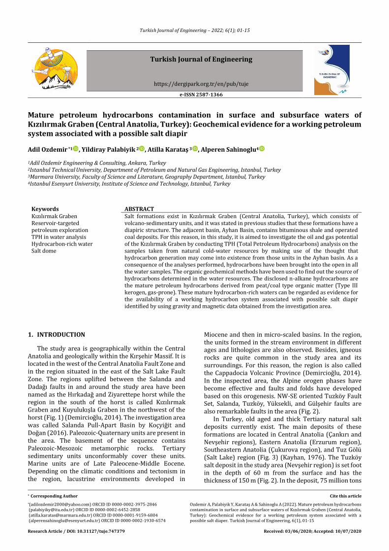
The study area is geographically within the Central Anatolia and geologically within the Kırşehir Massif. It is located in the west of the Central Anatolia Fault Zone and in the region situated in the east of the Salt Lake Fault Zone. The regions uplifted between the Salanda and Dadağı faults in and around the study area have been named as the Hırkadağ and Ziyarettepe horst while the region in the south of the horst is called Kızılırmak Graben and Kuyulukışla Graben in the northwest of the horst (Fig. 1) (Demircioğlu, 2014). The investigation area was called Salanda Pull-Apart Basin by Koçyiğit and Doğan (2016). Paleozoic-Quaternary units are present in the area. The basement of the sequence contains Paleozoic-Mesozoic metamorphic rocks. Tertiary sedimentary units unconformably cover these units. Marine units are of Late Paleocene-Middle Eocene. Depending on the climatic conditions and tectonism in the region, lacustrine environments developed in
Miocene and then in micro-scaled basins. In the region, the units formed in the stream environment in different ages and lithologies are also observed. Besides, igneous rocks are quite common in the study area and its surroundings. For this reason, the region is also called the Cappadocia Volcanic Province (Demircioğlu, 2014). In the inspected area, the Alpine orogen phases have become effective and faults and folds have developed based on this orogenesis. NW-SE oriented Tuzköy Fault Set, Salanda, Tuzköy, Yüksekli, and Gülşehir faults are also remarkable faults in the area (Fig. 2).
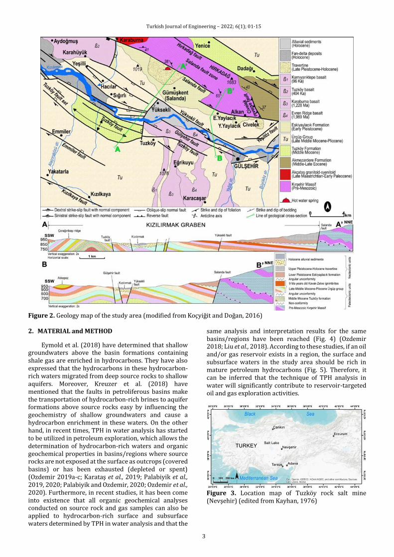
In Turkey, old aged and thick Tertiary natural salt deposits currently exist. The main deposits of these formations are located in Central Anatolia (Çankırı and Nevşehir regions), Eastern Anatolia (Erzurum region), Southeastern Anatolia (Çukurova region), and Tuz Gölü (Salt Lake) region (Fig. 3) (Kayhan, 1976). The Tuzköy salt deposit in the study area (Nevşehir region) is set foot in the depth of 60 m from the surface and has the thickness of 150 m (Fig. 2). In the deposit, 75 million tons
Turkish Journal of Engineering – 2022; 6(1); 01-15
2
of proved, 96 million tons of probable and 959 million tons of possible NaCl reserves have been determined. The presence of rock salt deposits in Gülşehir is not only limited to the Tuzköy rock salt deposit but also continue apart from the deposit (Kayakıran, 1979; Ünüçok, 1985). The folded rock salt deposit formation compatible with an NW-SE extended anticline is covered by younger units (Barutoğlu, 1961; Burkay and Önder, 1986). Rock salt formations in the study area are characterized by a diapiric structure (Bilginer, 1982).
There are numerous oil and gas production areas related to salt structures in the world. In those types of structures in Turkey, any economically viable hydrocarbon field has not been discovered so far and so, any significant hydrocarbon potential could not be determined as well. Therefore, in this study, it has been
aimed to identify the salt structure and its hydrocarbon potential based on the findings that it has a diapiric and deep structure which was stated by Bilginer (1982) and that it continues on the outside of the deposit that is the fact that was expressed by Ünüçok (1985). For this purpose, firstly, the possible boundaries of the salt structure are determined by regional gravity and magnetic data. Then, TPH (Total Petroleum Hydrocarbons) analyses are carried out on the samples taken from natural water resources within and around the specified limits. As a result of the analyses, mature petroleum hydrocarbons have been determined in all water samples. The detected mature hydrocarbons can be considered as evidence for a working petroleum system associated with possible salt diapir in the study area.
Figure 1. Location map of Kızılırmak Graben (modified from MTA, 2002 and Demircioğlu, 2014)
Turkish Journal of Engineering – 2022; 6(1); 01-15
3
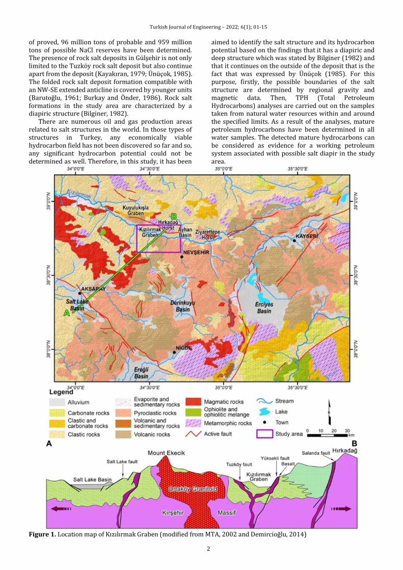
Figure 2. Geology map of the study area (modified from Koçyiğit and Doğan, 2016) 2. MATERIAL and METHOD
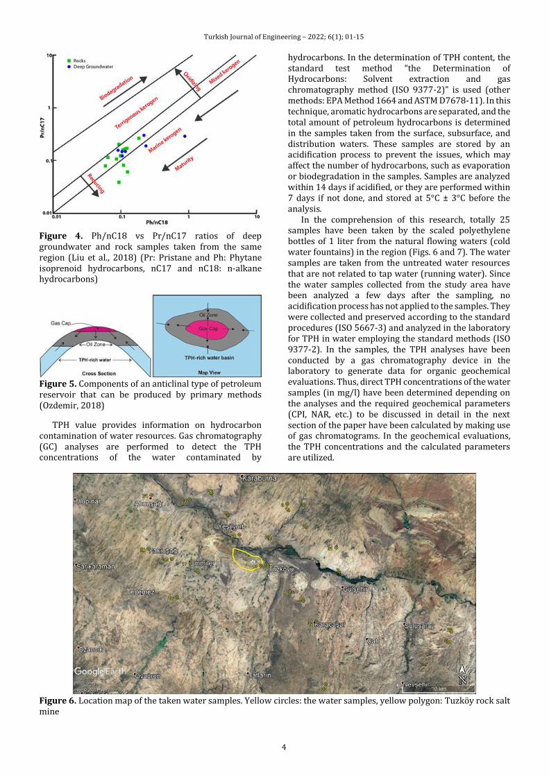
Eymold et al. (2018) have determined that shallow groundwaters above the basin formations containing shale gas are enriched in hydrocarbons. They have also expressed that the hydrocarbons in these hydrocarbon-rich waters migrated from deep source rocks to shallow aquifers. Moreover, Kreuzer et al. (2018) have mentioned that the faults in petroliferous basins make the transportation of hydrocarbon-rich brines to aquifer formations above source rocks easy by influencing the geochemistry of shallow groundwaters and cause a hydrocarbon enrichment in these waters. On the other hand, in recent times, TPH in water analysis has started to be utilized in petroleum exploration, which allows the determination of hydrocarbon-rich waters and organic geochemical properties in basins/regions where source rocks are not exposed at the surface as outcrops (covered basins) or has been exhausted (depleted or spent) (Ozdemir 2019a-c; Karataş et al., 2019; Palabiyik et al., 2019, 2020; Palabiyik and Ozdemir, 2020; Ozdemir et al., 2020). Furthermore, in recent studies, it has been come into existence that all organic geochemical analyses conducted on source rock and gas samples can also be applied to hydrocarbon-rich surface and subsurface waters determined by TPH in water analysis and that the
same analysis and interpretation results for the same basins/regions have been reached (Fig. 4) (Ozdemir 2018; Liu et al., 2018). According to these studies, if an oil and/or gas reservoir exists in a region, the surface and subsurface waters in the study area should be rich in mature petroleum hydrocarbons (Fig. 5). Therefore, it can be inferred that the technique of TPH analysis in water will significantly contribute to reservoir-targeted oil and gas exploration activities.
Figure 3. Location map of Tuzköy rock salt mine (Nevşehir) (edited from Kayhan, 1976)
Turkish Journal of Engineering – 2022; 6(1); 01-15
4
Figure 4. Ph/nC18 vs Pr/nC17 ratios of deep groundwater and rock samples taken from the same region (Liu et al., 2018) (Pr: Pristane and Ph: Phytane isoprenoid hydrocarbons, nC17 and nC18: n-alkane hydrocarbons)
Figure 5. Components of an anticlinal type of petroleum reservoir that can be produced by primary methods (Ozdemir, 2018)
TPH value provides information on hydrocarbon contamination of water resources. Gas chromatography (GC) analyses are performed to detect the TPH concentrations of the water contaminated by
hydrocarbons. In the determination of TPH content, the standard test method “the Determination of Hydrocarbons: Solvent extraction and gas chromatography method (ISO 9377-2)” is used (other methods: EPA Method 1664 and ASTM D7678-11). In this technique, aromatic hydrocarbons are separated, and the total amount of petroleum hydrocarbons is determined in the samples taken from the surface, subsurface, and distribution waters. These samples are stored by an acidification process to prevent the issues, which may affect the number of hydrocarbons, such as evaporation or biodegradation in the samples. Samples are analyzed within 14 days if acidified, or they are performed within 7 days if not done, and stored at 5°C ± 3°C before the analysis.
In the comprehension of this research, totally 25 samples have been taken by the scaled polyethylene bottles of 1 liter from the natural flowing waters (cold water fountains) in the region (Figs. 6 and 7). The water samples are taken from the untreated water resources that are not related to tap water (running water). Since the water samples collected from the study area have been analyzed a few days after the sampling, no acidification process has not applied to the samples. They were collected and preserved according to the standard procedures (ISO 5667-3) and analyzed in the laboratory for TPH in water employing the standard methods (ISO 9377-2). In the samples, the TPH analyses have been conducted by a gas chromatography device in the laboratory to generate data for organic geochemical evaluations. Thus, direct TPH concentrations of the water samples (in mg/l) have been determined depending on the analyses and the required geochemical parameters (CPI, NAR, etc.) to be discussed in detail in the next section of the paper have been calculated by making use of gas chromatograms. In the geochemical evaluations, the TPH concentrations and the calculated parameters are utilized.
Figure 6. Location map of the taken water samples. Yellow circles: the water samples, yellow polygon: Tuzköy rock salt mine

Turkish Journal of Engineering – 2022; 6(1); 01-15
5
Figure 7. A view of water sampling procedure from cold water fountains (pure and clean natural flowing waters) in the study area by using scaled polyethylene bottles
3. FINDINGS and DISCUSSION
Based on the TPH analysis results regarding the water samples taken from the study area, concentrations, biodegradation conditions, source, maturity, and redox conditions of the depositional environment of the hydrocarbons in the waters are investigated in a geochemical point of view. Moreover, the aeromagnetic and gravity maps prepared for the study area are interpreted in terms of geological and tectonic aspects, and the construction of the conceptual occurrence, migration, and accumulation model of the hydrocarbons is targeted.
3.1. Contents, Source, and Biodegradation of Hydrocarbons in Waters
Liu et al. (2018) have defined groundwater of which hydrocarbon concentration exceeds 0.05 mg/l as original hydrocarbon-rich groundwater. The TPH limit values recommended for surface and subsurface waters are given in Table 1. Surface and subsurface waters exceeding the TPH values in Table 1 are defined as hydrocarbon-rich waters. The n-alkane hydrocarbons have been found in all the water samples in the study area. The hydrocarbon content of the water samples is much higher than the limit values suggested for the waters (Tables 1 and 2). Hence, it can be mentioned that water-rock-hydrocarbon interactions have created this hydrocarbon enrichment in waters.
Table 1. The TPH limit values recommended for surface and subsurface waters
TPH (mg/l)
Reference
< 0.05 Liu et al. (2018) < 0.1 Zemo and Foote (2003) < 0.5 Ozdemir (2018) < 0.2 Ministry of Agriculture and Forestry of Turkey
(2004a), Surface Water Quality Regulation of Turkey (Appendix 5, Table 2: Oil and Grease)
< 0.02 Ministry of Agriculture and Forestry of Turkey (2004b), Water Pollution Control Regulation of Turkey (Appendices Table 1: Oil and Grease)
Table 2. TPH analysis results of the water samples and the calculated parameters
CPI = [(C23+C25+C27) + (C25+C27+C29)] / [2 *(C24+C26+C28)] (Bray and Evans, 1961), TAR = (C27+C29+C31)/(C15+C17+C19) (Bourbonniere and Meyers, 1996), NAR = [Σn-alk (C19-32) - 2Σ even n-alk (C20-32)] / Σ n-alk (C19-32) (Mille et al., 2007), Waxiness Index:∑ (n-C21-n-C31)/∑ (n-C15-n-C20) (Peters et al., 2005), Paq = (C23+C25)/(C23+C25+C27+C29+C31) (Ficken et al., 2000), Pwax = (C27+C29+C31)/(C23+C25+C27+C29+C31) (Zheng et al., 2007), - : Could not be calculated.
Sample No.
Water Resource
Coordinates TPH (mg/l)
CPI TAR Paq Pwax Waxiness Index
n-C17/n-C31 NAR Pr/Ph Pr/n-C17
Ph/n-C18
n-alkane maksimum
X Y
1 Natural flowing water 4300669 635154 0.52 1.24 - 0.28 0.72 - 0.20 0.32 4.88 0.29 0.14 C31 3 Mineral water 4300753 632969 < 0.4 1.34 - 0.26 0.74 - 0.14 - 7.67 0.39 0.13 C31 4 Natural flowing water 4299892 633152 0.72 1.35 - 0.26 0.74 - 0.15 0.25 5.84 0.26 0.10 C31 5 Natural flowing water 4297621 635602 0.56 1.36 - 0.26 0.74 - 0.19 0.23 5.95 0.29 0.09 C29 6 Natural flowing water 4291566 640269 0.64 1.18 5.79 0.29 0.71 4.80 0.14 0.37 10.87 0.24 0.09 C31 8 Natural flowing water 4288798 633507 0.62 1.41 - 0.23 0.77 - 0.21 0.25 5.30 0.27 0.11 C31 10 Water well 4287546 635389 0.63 1.27 7.91 0.22 0.78 - 0.14 0.37 5.68 0.28 0.12 C31 11 Natural flowing water 4292077 630459 0.68 1.82 - 0.10 0.90 5.58 0.10 0.27 9.28 0.25 0.08 C31 13 Salt discharge water 4292277 629466 0.57 1.26 - 0.28 0.72 - 0.15 0.29 3.63 0.21 0.13 C31 14 Natural flowing water 4291278 620839 0.53 1.36 - 0.24 0.76 - 0.15 0.25 5.45 0.30 0.10 C31 16 Natural flowing water 4287752 618043 0.72 1.26 - 0.22 0.78 - 0.13 0.37 5.61 0.23 0.10 C31 17 Natural flowing water 4292465 619808 0.41 - - - - - 0.11 - 8.43 0.40 0.09 C31 19 Water well 4292981 617241 0.52 1.55 - 0.17 0.83 - 0.08 0.20 10.12 0.32 0.06 C31 20 Natural flowing water 4294291 614037 0.43 1.60 7.70 0.18 0.82 4.27 0.12 0.10 9.95 0.30 0.08 C31 21 Water well 4301664 614292 0.48 1.90 10.03 0.07 0.93 3.63 0.22 0.12 13.05 0.30 0.05 C29 23 Natural flowing water 4301125 619556 0.53 1.71 7.91 0.12 0.88 2.95 0.11 0.08 10.00 0.24 0.06 C31 26 Natural flowing water 4302065 622556 0.65 - 7.20 - - - 0.17 - 15.95 0.25 0.04 C31 27 Natural flowing water 4299109 624796 0.97 1.93 7.25 0.08 0.92 3.37 0.17 0.00 4.60 0.21 0.09 C31 28 Caisson well 4296453 626478 0.80 1.72 7.01 0.11 0.89 1.92 0.22 0.00 5.52 0.19 0.10 C29 29 Natural flowing water 4295935 630637 0.63 1.93 6.89 0.07 0.93 1.86 0.17 0.05 11.60 0.23 0.05 C31 31 Natural flowing water 4294888 639800 0.60 1.75 - 0.11 0.89 - 0.17 0.02 9.82 0.26 0.05 C20 32 Water well 4284729 637224 0.54 1.85 - 0.11 0.89 - 0.10 0.02 7.42 0.32 0.08 C20 33 Natural flowing water 4276181 638653 0.59 1.64 - 0.17 0.83 - 0.15 0.05 18.50 0.27 0.04 C29 35 Mineral water 4282436 655103 0.47 1.66 - 0.10 0.90 - 0.32 0.12 9.43 0.24 0.07 C20 36 Mineral water well 4283652 655804 0.66 1.27 - 0.10 0.90 - 0.10 - 7.43 0.25 0.07 C31
Turkish Journal of Engineering – 2022; 6(1); 01-15
6
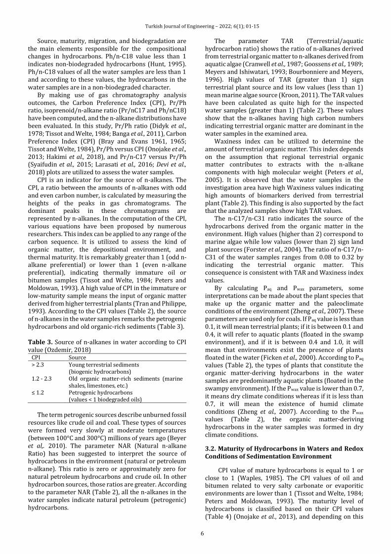
Source, maturity, migration, and biodegradation are the main elements responsible for the compositional changes in hydrocarbons. Ph/n-C18 value less than 1 indicates non-biodegraded hydrocarbons (Hunt, 1995). Ph/n-C18 values of all the water samples are less than 1 and according to these values, the hydrocarbons in the water samples are in a non-biodegraded character.
By making use of gas chromatography analysis outcomes, the Carbon Preference Index (CPI), Pr/Ph ratio, isoprenoid/n-alkane ratio (Pr/nC17 and Ph/nC18) have been computed, and the n-alkane distributions have been evaluated. In this study, Pr/Ph ratio (Didyk et al., 1978; Tissot and Welte, 1984; Banga et al., 2011), Carbon Preference Index (CPI) (Bray and Evans 1961, 1965; Tissot and Welte, 1984), Pr/Ph versus CPI (Onojake et al., 2013; Hakimi et al., 2018), and Pr/n-C17 versus Pr/Ph (Syaifudin et al., 2015; Larasati et al., 2016; Devi et al., 2018) plots are utilized to assess the water samples.
CPI is an indicator for the source of n-alkanes. The CPI, a ratio between the amounts of n-alkanes with odd and even carbon number, is calculated by measuring the heights of the peaks in gas chromatograms. The dominant peaks in these chromatograms are represented by n-alkanes. In the computation of the CPI, various equations have been proposed by numerous researchers. This index can be applied to any range of the carbon sequence. It is utilized to assess the kind of organic matter, the depositional environment, and thermal maturity. It is remarkably greater than 1 (odd n-alkane preferential) or lower than 1 (even n-alkane preferential), indicating thermally immature oil or bitumen samples (Tissot and Welte, 1984; Peters and Moldowan, 1993). A high value of CPI in the immature or low-maturity sample means the input of organic matter derived from higher terrestrial plants (Tran and Philippe, 1993). According to the CPI values (Table 2), the source of n-alkanes in the water samples remarks the petrogenic hydrocarbons and old organic-rich sediments (Table 3). Table 3. Source of n-alkanes in water according to CPI value (Ozdemir, 2018)
CPI Source > 2.3 Young terrestrial sediments
(biogenic hydrocarbons) 1.2 - 2.3 Old organic matter-rich sediments (marine
shales, limestones, etc.) ≤ 1.2 Petrogenic hydrocarbons
(values < 1 biodegraded oils)
The term petrogenic sources describe unburned fossil
resources like crude oil and coal. These types of sources were formed very slowly at moderate temperatures (between 100°C and 300°C) millions of years ago (Beyer et al,. 2010). The parameter NAR (Natural n-alkane Ratio) has been suggested to interpret the source of hydrocarbons in the environment (natural or petroleum n-alkane). This ratio is zero or approximately zero for natural petroleum hydrocarbons and crude oil. In other hydrocarbon sources, those ratios are greater. According to the parameter NAR (Table 2), all the n-alkanes in the water samples indicate natural petroleum (petrogenic) hydrocarbons.
The parameter TAR (Terrestrial/aquatic hydrocarbon ratio) shows the ratio of n-alkanes derived from terrestrial organic matter to n-alkanes derived from aquatic algae (Cranwell et al., 1987; Goossens et al., 1989; Meyers and Ishiwatari, 1993; Bourbonniere and Meyers, 1996). High values of TAR (greater than 1) sign terrestrial plant source and its low values (less than 1) mean marine algae source (Kroon, 2011). The TAR values have been calculated as quite high for the inspected water samples (greater than 1) (Table 2). These values show that the n-alkanes having high carbon numbers indicating terrestrial organic matter are dominant in the water samples in the examined area.
Waxiness index can be utilized to determine the amount of terrestrial organic matter. This index depends on the assumption that regional terrestrial organic matter contributes to extracts with the n-alkane components with high molecular weight (Peters et al., 2005). It is observed that the water samples in the investigation area have high Waxiness values indicating high amounts of biomarkers derived from terrestrial plant (Table 2). This finding is also supported by the fact that the analyzed samples show high TAR values.
The n-C17/n-C31 ratio indicates the source of the hydrocarbons derived from the organic matter in the environment. High values (higher than 2) correspond to marine algae while low values (lower than 2) sign land plant sources (Forster et al., 2004). The ratio of n-C17/n-C31 of the water samples ranges from 0.08 to 0.32 by indicating the terrestrial organic matter. This consequence is consistent with TAR and Waxiness index values.
By calculating Paq and Pwax parameters, some interpretations can be made about the plant species that make up the organic matter and the paleoclimate conditions of the environment (Zheng et al., 2007). These parameters are used only for coals. If Paq value is less than 0.1, it will mean terrestrial plants; if it is between 0.1 and 0.4, it will refer to aquatic plants (floated in the swamp environment), and if it is between 0.4 and 1.0, it will mean that environments exist the presence of plants floated in the water (Ficken et al., 2000). According to Paq values (Table 2), the types of plants that constitute the organic matter-deriving hydrocarbons in the water samples are predominantly aquatic plants (floated in the swampy environment). If the Pwax value is lower than 0.7, it means dry climate conditions whereas if it is less than 0.7, it will mean the existence of humid climate conditions (Zheng et al., 2007). According to the Pwax values (Table 2), the organic matter-deriving hydrocarbons in the water samples was formed in dry climate conditions.
3.2. Maturity of Hydrocarbons in Waters and Redox Conditions of Sedimentation Environment
CPI value of mature hydrocarbons is equal to 1 or close to 1 (Waples, 1985). The CPI values of oil and bitumen related to very salty carbonate or evaporitic environments are lower than 1 (Tissot and Welte, 1984; Peters and Moldowan, 1993). The maturity level of hydrocarbons is classified based on their CPI values (Table 4) (Onojake et al., 2013), and depending on this
Turkish Journal of Engineering – 2022; 6(1); 01-15
7
classification, all the hydrocarbons in the water samples (Table 2) can be classified as mature (more oxidizing) level.
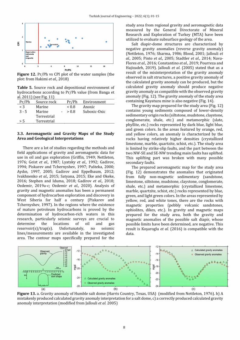
The n-alkanes, which are the closest to isoprenoids in gas chromatograms, are utilized for isoprenoid/n-alkane ratios. The Pr/Ph ratio is an appropriate correlation parameter. Even though pristane (Pr) and phytane (Ph) define other sources, they are derived from phytyl, which is the side chain of chlorophyll, particularly in phototropic organisms. Under anoxic conditions, the side chain of phytyl breaks down to form the phytol, while phytol is also reduced to pristane under oxic conditions (Peters and Moldowan, 1993). Hence, the Pr/Ph ratio shows the redox potential of the depositional environment. Pr/Ph values lower than 1 reflect anoxic conditions while the values higher than 1 remark oxic conditions (Didyk et al., 1978; Hunt, 1995). The water samples in the study area exhibit a high Pr/Ph ratio varying from 3.63 to 18.50 (Table 2). Therefore, the water samples contain the hydrocarbons derived from sediments deposited in an oxic environment (Pr/Ph > 1). The Pr/Ph ratio also provides information about paleoenvironment and maturity (Volkman and Maxwell, 1986) level. In the Pr/Ph versus CPI relationship, it can be observed that the hydrocarbons in the water samples are located in the more oxidizing zone and have similar maturity levels (Fig. 8).
Table 4. The maturity level of hydrocarbons according to CPI value (from Onojake et al., 2013) (see Fig. 8)
CPI Maturity >1 Mature (oxidizing-reducing) 0.8 - 1 Mature < 0.8 Immature
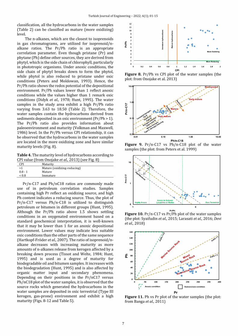
Pr/n-C17 and Ph/nC18 ratios are commonly made use of in petroleum correlation studies. Samples containing high Pr reflect an oxidizing source, and high Ph content indicates a reducing source. Thus, the plot of Pr/n-C17 versus Ph/n-C18 is utilized to distinguish petroleum or bitumen in different groups (Hunt, 1995). Although the Pr/Ph ratio above 1.5 shows settling conditions in an oxygenated environment based on a standard geochemical interpretation, it is well-known that it may be lower than 1 for an anoxic depositional environment. Lower values may indicate less suitable oxic conditions than the other parts of the same sequence (Hartkopf-Fröder et al., 2007). The ratio of isoprenoid/n-alkane decreases with increasing maturity as more amounts of n-alkanes release from kerogen affected by a breaking down process (Tissot and Welte, 1984; Hunt, 1995) and is used as a degree of maturity for biodegradable oil and bitumen samples. It increases with the biodegradation (Hunt, 1995) and is also affected by organic matter input and secondary phenomena. Depending on their positions in the Pr/nC17 versus Ph/nC18 plot of the water samples, it is observed that the source rocks which generated the hydrocarbons in the water samples are deposited in oxic terrestrial (Type III kerogen, gas-prone) environment and exhibit a high maturity (Figs. 8-12 and Table 5).
Figure 8. Pr/Ph vs CPI plot of the water samples (the plot: from Onojake et al. 2013)
Figure 9. Pr/n-C17 vs Ph/n-C18 plot of the water samples (the plot: from Peters et al. 1999)
Figure 10. Pr/n-C17 vs Pr/Ph plot of the water samples (the plot: Syaifudin et al., 2015; Larasati et al., 2016; Devi et al., 2018)
Figure 11. Ph vs Pr plot of the water samples (the plot: from Banga et al., 2011)
Turkish Journal of Engineering – 2022; 6(1); 01-15
8
Figure 12. Pr/Ph vs CPI plot of the water samples (the plot: from Hakimi et al., 2018)
Table 5. Source rock and depositional environment of hydrocarbons according to Pr/Ph value (from Banga et al. 2011) (see Fig. 11)
Pr/Ph Source rock Pr/Ph Environment < 3 Marine < 0.8 Anoxic 3 - 5 Marine -
Terrestrial > 0.8 Suboxic-Oxic
> 5 Terrestrial
3.3. Aeromagnetic and Gravity Maps of the Study Area and Geological Interpretations
There are a lot of studies regarding the methods and field applications of gravity and aeromagnetic data for use in oil and gas exploration (Griffin, 1949; Nettleton, 1976; Geist et al., 1987; Lyatsky et al., 1992; Gadirov, 1994; Piskarev and Tchernyshev, 1997; Pašteka, 2000; Aydın, 1997, 2005; Gadirov and Eppelbaum, 2012; Ivakhnenko et al., 2015; Satyana, 2015; Eke and Okeke, 2016; Stephen and Iduma, 2018; Gadirov et al., 2018; Ozdemir, 2019a-c; Ozdemir et al., 2020). Analysis of gravity and magnetic anomalies has been a permanent component of hydrocarbon exploration and discovery in West Siberia for half a century (Piskarev and Tchernyshev, 1997). In the regions where the existence of mature petroleum hydrocarbons is proved by the determination of hydrocarbon-rich waters in this research, particularly seismic surveys are crucial to determine the locations of oil and gas reservoir(s)/trap(s). Unfortunately, no seismic lines/measurements are available in the investigated area. The contour maps specifically prepared for the
study area from regional gravity and aeromagnetic data measured by the General Directorate of Mineral Research and Exploration of Turkey (MTA) have been utilized to evaluate subsurface geology of the area.
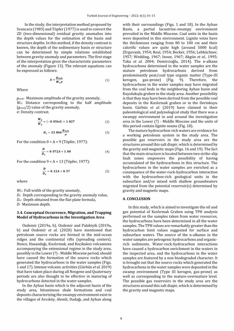
Salt diapir-dome structures are characterized by negative gravity anomalies (reverse gravity anomaly) (Nettleton, 1976; Sharma, 1986; Blood, 2001; Jallouli et al., 2005; Pinto et al., 2005; Stadtler et al., 2014; Nava-Flores et al., 2016; Constantino et al., 2019; Pourreza and Hajizadeh, 2019). Jallouli et al. (2005) stated that as a result of the misinterpretation of the gravity anomaly observed in salt structures, a positive gravity anomaly of the calculated gravity anomaly can be produced, but the calculated gravity anomaly should produce negative gravity anomaly as compatible with the observed gravity anomaly (Fig. 12). The gravity anomaly of the study area containing Kayatuzu mine is also negative (Fig. 14).
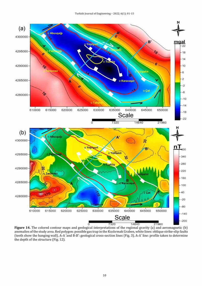
The gravity map prepared for the study area (Fig. 12) contains young sediments composed of lower-density sedimentary origin rocks (siltstone, mudstone, claystone, conglomerate, shale, etc.) and metamorphic (slate, phyllite, etc.) rocks represented by dark blue, light blue, and green colors. In the areas featured by orange, red, and yellow colors, an anomaly is characterized by the rocks having relatively higher densities (crystallized limestone, marble, quartzite, schist, etc.). The study area is limited by strike-slip faults, and the part between the two NW-SE and SE-NW trending main faults has uplifted. This uplifting part was broken with many possible secondary faults.
The prepared aeromagnetic map for the study area (Fig. 12) demonstrates the anomalies that originated from fully non-magnetic sedimentary (sandstone, limestone, siltstone, mudstone, claystone, conglomerate, shale, etc.) and metamorphic (crystallized limestone, marble, quartzite, schist, etc.) rocks represented by blue, green, and light green colors. In the areas represented by yellow, red, and white tones, there are the rocks with magnetic properties (pebbly volcanic sandstones, ophiolites, dikes, etc.). In gravity and magnetic maps prepared for the study area, both the gravity and magnetic anomalies of the possible salt diapir, whose possible limits have been determined, are negative. This result is Koşaroglu et al. (2016) is compatible with the data.
Figure 13. a. Gravity anomaly of Humble salt dome (Harris Country, Texas, USA) (modified from Nettleton, 1976). b) A mistakenly produced calculated gravity anomaly interpretation for a salt dome, c) a correctly produced calculated gravity anomaly interpretation (modified from Jallouli et al. 2005)
Turkish Journal of Engineering – 2022; 6(1); 01-15
9
In the study, the interpretation method proposed by Svancara (1983) and Töpfer (1977) is used to convert the 2D (two-dimensional) residual gravity anomalies into the depth values for the estimation of the basin and structure depths. In this method, if the density contrast is known, the depth of the sedimentary basin or structure can be determined by simple relations established between gravity anomaly and parameters. The first stage of the interpretation gives the characteristic parameters of the anomaly (Figure 13). The relevant equations can be expressed as follows:
𝑨 =𝒈𝒎𝒂𝒌
𝑾𝒂𝝈 (1)
Where
gmak: Maximum amplitude of the gravity anomaly, Wa: Distance corresponding to the half amplitude (gmak/2) value of the gravity anomaly, σ: Density contrast.
𝑾𝒃
𝑾𝒂
= (−𝟎. 𝟎𝟓𝟔𝑨) + 𝟏. 𝟖𝟐𝟕 (2)
𝑫𝒐 = 𝟐𝟑. 𝟖𝟔𝟔𝒈𝒎𝒂𝒌
𝝈 (3)
For the condition 0 < A < 9 (Töpfer, 1977):
𝑫
𝑫𝒐
= 𝟎. 𝟎𝟕𝟐𝑨 + 𝟏. 𝟎𝟎 (4)
For the condition 9 < A < 13 (Töpfer, 1977):
𝑫
𝑫𝒐
= 𝟎. 𝟏𝟐𝑨 + 𝟎. 𝟓𝟕 (5)
where Wb : Full width of the gravity anomaly, Di: Depth corresponding to the gravity anomaly value, Do: Depth obtained from the flat-plate formula, D: Maximum depth.
3.4. Conceptual Occurrence, Migration, and Trapping Model of Hydrocarbons in the Investigation Area
Ozdemir (2019a, b), Ozdemir and Palabiyik (2019a, b) and Ozdemir et al. (2020) have mentioned that petroleum source rocks are formed in the mid-ocean ridges and the continental rifts (spreading centers). Hence, Hasandağı, Kızılırmak, and Keçikalesi volcanisms accompanying the extensional regime in the study area, possibly in the Lower (?) - Middle Miocene period, should have caused the formation of the source rocks which generated the hydrocarbons in the water samples (Figs. 1 and 17). Intense volcanic activities (Gürbüz et al. 2019) that have taken place during all Neogene and Quaternary periods are also thought to be effective in maturing of hydrocarbons detected in the water samples.
In the Ayhan basin which is the adjacent basin of the study area, bituminous shale formations and coal deposits characterizing the swampy environment exist in the villages of Avcıköy, Alemli, Dadağı, and Ayhan along
with their surroundings (Figs. 1 and 18). In the Ayhan Basin, a partial lacustrine-swampy environment prevailed in the Middle Miocene. Coal units in the basin were deposited in this environment. Lignite veins have the thicknesses ranging from 80 to 100 cm and their calorific values are quite high (around 5000 kcal) (Erguvanlı, 1954; Reul, 1954; Becker, 1956; Lebküchner, 1957; Wedding, 1967; Inoue, 1967; Akgün et al., 1995; Taka et al. 2004; Demircioğlu, 2014). The n-alkane hydrocarbons determined in the water samples are the mature petroleum hydrocarbons derived from predominantly peat/coal type organic matter (Type-III kerogen, gas-prone) (Fig. 9). Therefore, the hydrocarbons in the water samples may have migrated from the coal beds in the neighboring Ayhan basin and Kuyulukışla graben to the study area. Another possibility is that they may have been derived from the possible coal deposits in the Kızılırmak graben or in the Derinkuyu basin. Gürbüz et al. (2019) have claimed in their paleontological and palynological study that there was a swampy environment in and around the investigation area in the Lower (?) - Middle Miocene and the units of this period contain lignite seams (Fig. 18).
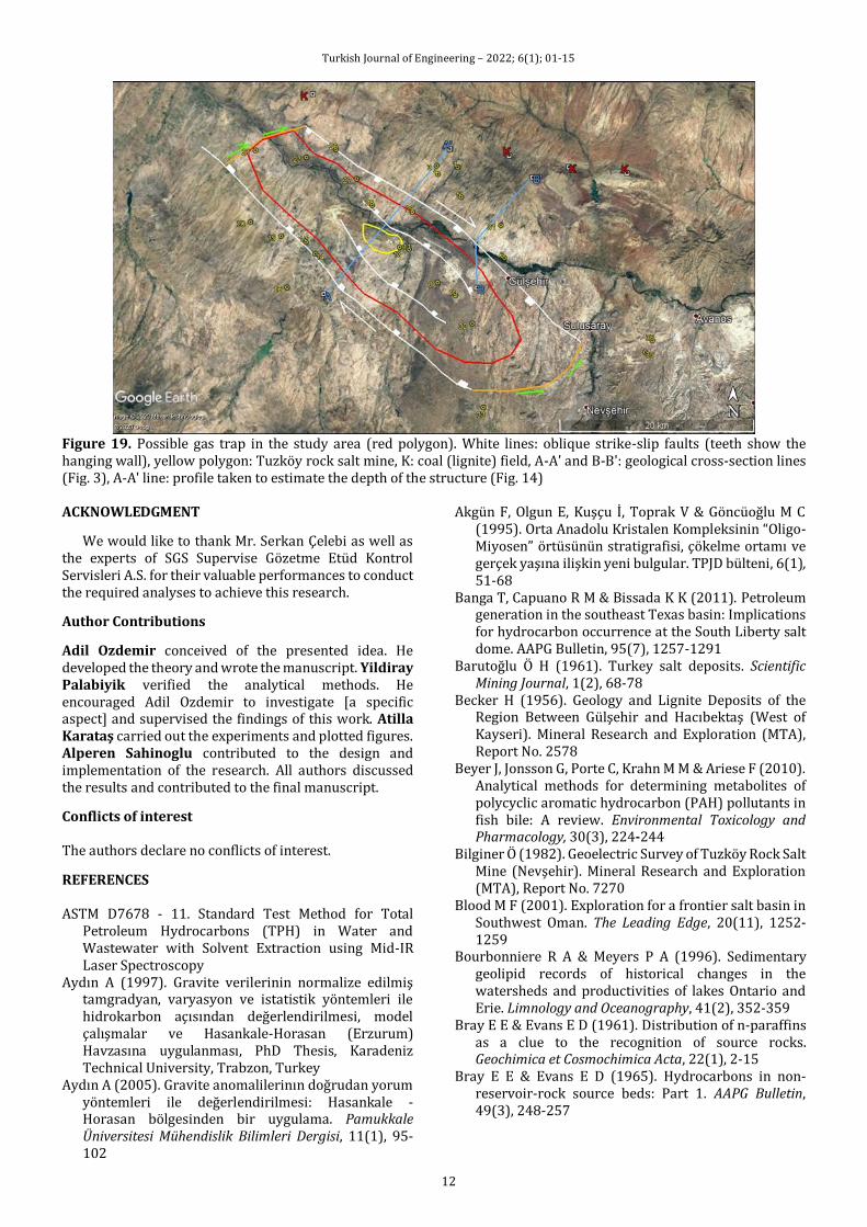
The mature hydrocarbon-rich waters are evidence for a working petroleum system in the study area. The possible gas reservoirs in the study area are the structures around this salt diapir, which is determined by the gravity and magnetic maps (Figs. 16 and 19). The fact that the main structure is located between two strike-slip fault zones empowers the possibility of having accumulated of the hydrocarbons in this structure. The hydrocarbons in the water samples are enriched as a consequence of the water-rock-hydrocarbon interaction with the hydrocarbon-rich geological units in the subsurface and/or mixed with shallow groundwaters migrated from the potential reservoir(s) determined by gravity and magnetic maps.
4. CONCLUSION
In this study, which is aimed to investigate the oil and gas potential of Kızılırmak Graben using TPH analysis performed on the samples taken from water resources, the hydrocarbons have been determined in all the water samples. The TPH values are remarkably greater than the hydrocarbon limit values suggested for surface and subsurface waters. The source of the n-alkanes in the water samples are petrogenic hydrocarbons and organic-rich sediments. Water-rock-hydrocarbon interactions have caused a hydrocarbon enrichment in the waters in the inspected area, and the hydrocarbons in the water samples are featured by a non-biodegraded character. It is brought out that the source rocks which generated the hydrocarbons in the water samples were deposited in the swamp environment (Type III kerogen, gas-prone) as well as corresponding to the mature-overmature level. The possible gas reservoirs in the study area are the structures around this salt diapir, which is determined by the gravity and magnetic maps.
Turkish Journal of Engineering – 2022; 6(1); 01-15
10
Figure 14. The colored contour maps and geological interpretations of the regional gravity (a) and aeromagnetic (b) anomalies of the study area. Red polygon: possible gas trap in the Kızılırmak Graben, white lines: oblique strike-slip faults (teeth show the hanging wall), A-A 'and B-B': geological cross-section lines (Fig. 3), A-A' line: profile taken to determine the depth of the structure (Fig. 12).

Turkish Journal of Engineering – 2022; 6(1); 01-15
11
Figure 15. Ideal gravity anomaly of a basin and characteristic parameters (Svancara, 1983)
Figure 16. Geological interpretation of A-A 'profile and depth of the possible salt diapir in the study area (see Fig. 12).
Figure 17. Schematic cross-section showing sil and dykes across a volcanic basin. The chemical composition of sedimentary rocks heated by igneous intrusions has a significant effect on the composition of the metamorphic fluid. For example, organic-rich shale produces CH4 during contact metamorphism, while coal produces CO2-derived fluids and also water. Many sedimentary basins with sil settlement may contain hydrogen-rich kerogen and oil and gas deposits, and fluids such as methane (CH4) and ethane (C2H6) can be enriched in the basin (Svensen et al., 2015). (a: Svensen et al., 2015; b: Ogden and Sleep, 2011)
Figure 18. The Miocene paleoenvironment reconstruction based on the geological unit, volcanic age, and palynological data of the study area and its surroundings (Gürbüz et al. 2019)
Turkish Journal of Engineering – 2022; 6(1); 01-15
12
Figure 19. Possible gas trap in the study area (red polygon). White lines: oblique strike-slip faults (teeth show the hanging wall), yellow polygon: Tuzköy rock salt mine, K: coal (lignite) field, A-A' and B-B': geological cross-section lines (Fig. 3), A-A' line: profile taken to estimate the depth of the structure (Fig. 14) ACKNOWLEDGMENT
We would like to thank Mr. Serkan Çelebi as well as the experts of SGS Supervise Gözetme Etüd Kontrol Servisleri A.S. for their valuable performances to conduct the required analyses to achieve this research.
Author Contributions
Adil Ozdemir conceived of the presented idea. He developed the theory and wrote the manuscript. Yildiray Palabiyik verified the analytical methods. He encouraged Adil Ozdemir to investigate [a specific aspect] and supervised the findings of this work. Atilla Karataş carried out the experiments and plotted figures. Alperen Sahinoglu contributed to the design and implementation of the research. All authors discussed the results and contributed to the final manuscript.
Conflicts of interest The authors declare no conflicts of interest.
REFERENCES ASTM D7678 - 11. Standard Test Method for Total
Petroleum Hydrocarbons (TPH) in Water and Wastewater with Solvent Extraction using Mid-IR Laser Spectroscopy
Aydın A (1997). Gravite verilerinin normalize edilmiş tamgradyan, varyasyon ve istatistik yöntemleri ile hidrokarbon açısından değerlendirilmesi, model çalışmalar ve Hasankale-Horasan (Erzurum) Havzasına uygulanması, PhD Thesis, Karadeniz Technical University, Trabzon, Turkey
Aydın A (2005). Gravite anomalilerinın doğrudan yorum yöntemleri ile değerlendirilmesi: Hasankale - Horasan bölgesinden bir uygulama. Pamukkale Üniversitesi Mühendislik Bilimleri Dergisi, 11(1), 95-102
Akgün F, Olgun E, Kuşçu İ, Toprak V & Göncüoğlu M C (1995). Orta Anadolu Kristalen Kompleksinin “Oligo-Miyosen” örtüsünün stratigrafisi, çökelme ortamı ve gerçek yaşına ilişkin yeni bulgular. TPJD bülteni, 6(1), 51-68
Banga T, Capuano R M & Bissada K K (2011). Petroleum generation in the southeast Texas basin: Implications for hydrocarbon occurrence at the South Liberty salt dome. AAPG Bulletin, 95(7), 1257-1291
Barutoğlu Ö H (1961). Turkey salt deposits. Scientific Mining Journal, 1(2), 68-78
Becker H (1956). Geology and Lignite Deposits of the Region Between Gülşehir and Hacıbektaş (West of Kayseri). Mineral Research and Exploration (MTA), Report No. 2578
Beyer J, Jonsson G, Porte C, Krahn M M & Ariese F (2010). Analytical methods for determining metabolites of polycyclic aromatic hydrocarbon (PAH) pollutants in fish bile: A review. Environmental Toxicology and Pharmacology, 30(3), 224-244
Bilginer Ö (1982). Geoelectric Survey of Tuzköy Rock Salt Mine (Nevşehir). Mineral Research and Exploration (MTA), Report No. 7270
Blood M F (2001). Exploration for a frontier salt basin in Southwest Oman. The Leading Edge, 20(11), 1252-1259
Bourbonniere R A & Meyers P A (1996). Sedimentary geolipid records of historical changes in the watersheds and productivities of lakes Ontario and Erie. Limnology and Oceanography, 41(2), 352-359
Bray E E & Evans E D (1961). Distribution of n-paraffins as a clue to the recognition of source rocks. Geochimica et Cosmochimica Acta, 22(1), 2-15
Bray E E & Evans E D (1965). Hydrocarbons in non-reservoir-rock source beds: Part 1. AAPG Bulletin, 49(3), 248-257
Turkish Journal of Engineering – 2022; 6(1); 01-15
13
Burkay İ & Önder İ (1986). Resistivity Survey of Tuzköy Rock Salt Mine (Nevşehir). Mineral Research and Exploration (MTA), Report No. 7875
Constantino R R, Molina E C, de Souza I A & Vincentelli M G C (2019). Salt structures from inversion of residual gravity anomalies: application in Santos Basin, Brazil. Brazilian Journal of Geology, 49(1), DOI: 10.1590/2317-4889201920180087
Cranwell P A, Eglinton G & Robinson N (1987). Lipids of aquatic organisms as potential contributors to lacustrine sediments-2. Organic Geochemistry, 11(6), 513-527
Demircioğlu, R. (2014). Gülşehir-Özkonak (Nevşehir) çevresinde Kırşehir masifi ve örtü birimlerinin jeolojisi ve yapısal özellikleri. PhD Thesis, Selçuk University, Konya, Turkey
Devi E A, Rachman F, Satyana A H, Fahrudin & Setyawan R (2018). Geochemistry of Mudi and Sukowati oils, East Java basin and their correlative source rocks: Biomarkers and isotopic characterisation. Proceedings, Indonesian Petroleum Association, Forty-Second Annual Convention & Exhibition, May 2018
Didyk B M, Simoneit B R T, Brassel S C & Englington G (1978). Organic geochemical indicators of paleoenvironmental conditions of sedimentation. Nature, 272, 216-222
Eke P O & Okeke F N (2016). Identification of hydrocarbon regions in Southern Niger Delta Basin of Nigeria from potential field data. International Journal of Scientific and Technology Research, 5(11), 96-99
EPA Method 1664. Revision A: N-Hexane Extractable Material (HEM; Oil and Grease) and Silica Gel Treated N-Hexane Extractable Material (SGTHEM; Non-polar Material) by Extraction and Gravimetry.
Erguvanlı K (1954). Geological Survey of the East of Kırşehir. Mineral Research and Exploration (MTA), Report No. 2373
Eymold W K, Swana K, Moore M T, Whyte C J, Harkness J S, Talma S, Murray R, Moortgat J B, Miller J, Vengosh A & Darrah T H (2018). Hydrocarbon-rich groundwater above shale-gas formations: A Karoo basin case study. Groundwater, 56(2), 204-224
Forster A, Sturt H & Meyers P A (2004). Molecular biogeochemistry of Cretaceous black shales from the Demerara Rise: Preliminary shipboard results from sites 1257 and 1258, Leg 207. in Erbacher, J., Mosher, D.C., Malone, M.J., et al., Proceedings of the Ocean Drilling Program, Initial Reports: 207, 1-22.
Gadirov V G, Eppelbaum L V, Kuderavets R S, Menshov O I & Gadirov K V (2018). Indicative features of local magnetic anomalies from hydrocarbon deposits: examples from Azerbaijan and Ukraine. Acta Geophysica, 66(6), 1463-1483. DOI: 10.1007/s11600-018-0224-0
Gadirov V G & Eppelbaum L V (2012). Detailed gravity, magnetics successful in exploring Azerbaijan onshore areas. Oil and Gas Journal, 110(11), 60-73
Gadirov V G (1994). The physical-geological principles of application of gravity and magnetic prospecting in searching oil and gas deposits. Proceed. of 10th Petroleum Congress and Exhibition of Turkey, Ankara, 197-203
Geist E L, Childs J R & Scholl D W (1987). “Evolution and petroleum geology of Amlia and Amukta intra-arc summit basins, Aleutian Ridge”. Marine and Petroleum Geology, 4(4), 334-352
Goossens H, Duren C, De Leeuw J W & Schenck P A (1989). Lipids and their mode of occurrence in bacteria and sediments-2. Lipids in the sediment of a stratified, freshwater lake. Organic Geochemistry, 14(1), 27-41
Griffin W R (1949). Residual gravity in theory and practice. Geophysics, 14(1), 39-58
Gürbüz A, Saraç G & Yavuz N (2019). Paleoenvironments of the Cappadocia region during the Neogene and Quaternary, central Turkey. Mediterranean Geoscience Reviews, 1(2), 271-296.
Hakimi M H, Al-Matary A M & Ahmed A (2018). Bulk geochemical characteristics and carbon isotope composition of oils from the Sayhut sub-basin in the Gulf of Aden with emphasis on organic matter input, age and maturity. Egyptian Journal of Petroleum, 27(3), 361-370
Hartkopf-Fröder C, Kloppisch M, Mann U, Neumann-Mahlkau P, Schaefer R G & Wilkes H (2007). The end-Frasnian mass extinction in the Eifel Mountains, Germany: new insights from organic matter composition and preservation. Geological Society, London, Special Publications, 278(1), 173-196. DOI: 10.1144/SP278.8
Hunt J M (1995). Petroleum Geochemistry and Geology. W.H. Freeman and Company, New York
Inoue E (1967). Geology and Coal Reserves of Dadağı-Arafa Coal Field. Mineral Research and Exploration (MTA), Report No. 3948
ISO 5667-3. Water Quality - Sampling - Part 3: Preservation and Handling of Water Samples.
ISO 9377-2. Water Quality - Determination of Hydrocarbon Oil Index - Part 2: Method Using Solvent Extraction and Gas Chromatography.
Ivakhnenko O P, Abirov R & Logvinenko A (2015). New method for characterisation of petroleum reservoir fluid-mineral deposits using magnetic analysis. Energy Procedia, 76, 454-462
Jallouli C, Chikhaoui M, Braham A, Turki M M, Mickus K & Benassi R (2005). Evidence for Triassic salt domes in the Tunisian Atlas from gravity and geological data. Tectonophysics, 396, 209-225
Karatas A, Ozdemir A & Sahinoglu A (2019). Investigation of Oil and Gas Potential of Karaburun Peninsula and Seferihisar Uplift (Western Anatolia) by Iodine Hydrogeochemistry and Total Petroleum Hydrocarbon (TPH) in Water Analysis. Marmara University, Project No (9505): SOS-A-100719-0267
Kayakıran S (1979). Research and Exploration of Gülşehir Rock Salt Mine (Studies in 1977 and 1978). Mineral Research and Exploration (MTA), Report No. 6606
Kayhan M (1976). Turkey Salt Inventory. Mineral Research and Exploration (MTA), Publication No: 164, 78
Koçyiğit A & Doğan U (2016). Strike-slip neotectonic regime and related structures in the Cappadocia region: a case study in the Salanda basin, Central

Turkish Journal of Engineering – 2022; 6(1); 01-15
14
Anatolia, Turkey. Turkish Journal of Earth Sciences, 25(5), 393-417
Kosaroglu S, Buyuksarac A & Aydemir A (2016). Modeling of shallow structures in the Cappadocia region using gravity and aeromagnetic anomalies. Journal of Asian Earth Sciences, 124, 214-226
Kreuzer R L, Darrah T H, Grove B S, Moore M T, Warner N R, Eymold W K & Poreda R J (2018). Structural and hydrogeological controls on hydrocarbon and brine migration into drinking water aquifers in Southern New York. Groundwater, 56(2), 225-244
Kroon J (2011). Biomarkers in the Lower Huron Shale
(Upper Devonian) As Indicators of Organic Matter Source, Depositional Environment, and Thermal Maturity. MSc. Thesis, Clemson University, US.
Larasati D, Suprayogi K & Akbar A (2016). Crude oil characterization of Tarakan basin: Application of biomarkers. The 9th International Conference on Petroleum Geochemistry in the Africa - Asia Region, Bandung, Indonesia, 15 -17 November 2016
Lebküchner R F (1957). Geology of Kayseri and Avanos-Ürgüp-Boğazlıyan. Mineral Research and Exploration (MTA), Report No. 2656
Liu S, Qi S, Luo Z, Liu F, Ding Y, Huang H, Chen Z & Cheng S (2018). The origin of high hydrocarbon groundwater in shallow Triassic aquifer in Northwest Guizhou, China. Environmental Geochemistry and Health, 40(1), 415-433
Lyatsky H V, Thurston J B, Brown R J & Lyatsky V B (1992). Hydrocarbon exploration applications of potential field horizontal gradient vector maps. Canadian Society of Exploration Geophysicists Recorder, 17(9), 10-15
Meyers P A & Ishiwatari R (1993). Lacustrine organic geochemistry-an overview of indicators of organic matter sources and diagenesis in lake sediments. Organic Geochemistry, 20(7), 867-900
Mille G, Asia L, Guiliano M, Malleret L & Doumenq P (2007). Hydrocarbons in coastal sediments from the Mediterranean Sea (Gulf of Fos area, France). Marine Pollution Bulletin, 54(5), 566-575
Ministry of Agriculture and Forestry of Turkey, 2004a. Surface Water Quality Regulation of Turkey, http://www.resmigazete.gov.tr/eskiler/2016/08/20160810-9.htm (Accessed 02 June 2020)
Ministry of Agriculture and Forestry of Turkey, 2004b. Water Pollution Control Regulation of Turkey (in Turkish),http://www.mevzuat.gov.tr/Metin.Aspx?MevzuatKod=7.5.7221&MevzuatIliski=0&sourceXmlSearch= (Accessed 02 June 2020)
MTA (General Directorate of Mineral Research and Exploration) (2002) Geological Map of Turkey: General Directorate of Mineral Research and Exploration Publication, scale 1/500,000, 18 sheets
Nava-Flores M, Ortiz-Aleman C, Orozco-del-Castillo M G Urrutia-Fucugauchi J, Rodriguez-Castellanos A, Couder-Castañeda C & Trujillo-Alcantara A (2016). 3D gravity modeling of complex salt features in the Southern Gulf of Mexico. International Journal of Geophysics, 1702164, 12
Nettleton L L (1976). Gravity and Magnetics in Oil Prospecting. McGraw-Hill
Ogden DE, Sleep NH, (2011) Explosive eruption of coal and basalt and the end-Permian mass extinction. Earth, Atmospheric, and Planetary Sciences, 109(1): 59-62.
Onojake M C, Osuji L C & Oforka N C (2013). Preliminary hydrocarbon analysis of crude oils from Umutu/Bomu fields, southwest Niger Delta, Nigeria. Egyptian Journal of Petroleum, 22(2), 217-224
Ozdemir A (2018). Usage of the Total Petroleum Hydrocarbons (TPH) in water analysis for oil and gas exploration: First important results from Turkey. Journal of Engineering Sciences and Design, 6(4), 615-636
Ozdemir A (2019a). Organic hydrogeochemical evidence of Hasanoğlan (Ankara) petroleum system. Pamukkale University Journal of Engineering Sciences, 25(6), 748-763
Ozdemir A (2019b). Mature hydrocarbons-rich waters as geochemical evidence of working petroleum system of Mamak (Ankara) and potential trap area in the region. European Journal of Science and Technology, 17, 244-260
Ozdemir A (2019c). Organic hydrogeochemical evidence of pre-Neogene petroleum system of the Buyuk Menderes graben and potential traps (Western Turkey). European Journal of Science and Technology, 16, 325-354
Ozdemir A & Palabiyik Y (2019a). A review of Paleozoic - Miocene petroleum source rocks of Turkey by paleogeographic and paleotectonic data: New interpretations and major outcomes. 7th International Symposium on Academic Studies in Science, Engineering and Architecture Sciences, November 15-17, Ankara, Turkey, 689-725
Ozdemir A & Palabiyik Y (2019b). A new approach to petroleum source rock occurrence: The relationships between petroleum source rock, ophiolites, mantle plume and mass extinction. IV. International Congress of Scientific and Professional Studies - Engineering (BILMES EN), November 07 - 10, Ankara, Turkey, 28-39
Ozdemir A, Karataş A, Palabiyik Y, Yaşar E & Sahinoglu A (2020). Oil and gas exploration in Seferihisar Uplift (Western Turkey) containing an operable-size gold deposit: Geochemical evidence for the presence of a working petroleum system. Geomechanics and Geophysics for Geo-Energy and Geo-Resources, 6(1), DOI: 10.1007/s40948-020-00152-2
Palabiyik Y, Ozdemir A & Sahinoglu A (2019). Investigation of Oil and Gas Potential of Uludag Massif (Northwestern Anatolia) by Iodine Hydrogeochemistry and Total Petroleum Hydrocarbon (TPH) in Water Analysis, Istanbul Technical University, Scientific Research Project, Project No: MAB-2019-42217, 76 p.
Palabiyik Y & Ozdemir A (2020). Use of TPH (Total Petroleum Hydrocarbons) in water analysis for oil and gas exploration in Turkey: The case studies from Western, Northwestern and Central Anatolia regions and major outcomes. Turkey IV. Scientific and Technical Petroleum Congress, October 26-28, Ankara, Turkey (in press)
Turkish Journal of Engineering – 2022; 6(1); 01-15
15
Palabiyik Y, Ozdemir A, Karataş A & Özyağcı M (2020). Identification of Oil and Gas Potential of Kastamonu and Sinop and their Surroundings (Central Pontides) by Using Total Petroleum Hydrocarbons (TPH) in Water Analysis, Istanbul Technical University, Scientific Research Project, Project No: MGA-2020-42587 (continue)
Pašteka R (2000). 2D semi-automated interpretation methods in gravimetry and magnetometry. Acta Geologica Universitatis Comeniana, 55, 5-50
Peters K E, Walters C C & Moldowan J M (2005). The
Biomarker Guide: Biomarkers and Isotopes in Petroleum Exploration and Earth History, Second Ed, Vol 2. Cambridge University Press
Peters K E, Fraser T H, Amris W, Rustanto B & Hermanto E (1999). Geochemistry of crude oils from eastern Indonesia. AAPG Bulletin, 83, 1927-1942
Peters K E & Moldowan J M (1993). The Biomarker Guide, Interpreting Molecular Fossils in Petroleum and Ancient Sediments. Englewood Cliffs, Jersey, Prentice Hall
Pinto V, Casas A, Rivero L & Torne M (2005). 3D gravity modeling of the Triassic salt diapirs of the Cubeta Alavesa (northern Spain). Tectonophysics, 405, 65-75
Piskarev A L & Tchernyshev M Y (1997). Magnetic and gravity anomaly patterns related to hydrocarbon fields in northern West Siberia. Geophysics, 62(3), 831-841
Pourreza S & Hajizadeh F (2019). Simulation of a salt dome using 2D linear and nonlinear inverse modeling of residual gravity field data. Bulletin of the Mineral Research and Exploration, 160, 231-244
Reul K (1954). Lignite occurrences around Kayseri. Mineral Research and Exploration (MTA), Report No. 2240
Satyana A H (2015). Subvolcanic hydrocarbon prospectivity of Java: Opportunities and challenges. Proceedings, Indonesian Petroleum Association. Thirty-Ninth Annual Convention & Exhibition, May 2015. IPA15-G-105
Sharma P V (1986). Geophysical Methods in Geology (2nd Edition). Elsevier
Stadtler C, Fichler C, Hokstad K, Myrlund E A, Wienecke S & Fotland B (2014). Improved salt imaging in a basin context by high resolution potential field data: Nordkapp Basin, Barents Sea. Geophysical Prospecting, 2014, 62, 615-630
Stephen O I & Iduma U (2018). Hydrocarbon potential of Nigeria’s Inland Basin: Case study of Afikpo basin. Journal of Applied Geology and Geophysics, 6(4), 1-24
Svancara J (1983). Approximate method for direct interpretation of gravity anomalies caused by surface three‐dimensional geologic structures. Geophysics, 48(3), 361-366 https://doi.org/10.1190/1.1441474
Svensen H, Fristad KE, Polozov AG, Planke S. (2015) Volatile generation and release from continental large igneous provinces. In: Schmidt, A., Fristad, K.E., and Elkins-Tanton, L.T., (Eds.), Volcanism and Global Environmental Change, Cambridge University Press, UK, https://doi.org/10.1017/CBO9781107415683.015
Syaifudin M, Eddy A, Subroto E A, Noeradi D & Kesumajana A H P (2015). Characterızation and correlatıon study of source rocks and oils in Kuang area, South Sumatra basin: The potential of Lemat formation as hydrocarbon source rocks. Proceedings of Indonesian Petroleum Association, Thirty-Ninth Annual Convention & Exhibition, May 2015, IPA15-G-034
Taka M, Dümenci S, Kalkan İ & Şener M (2004). Sedimentology and Coal Potential of Tertiary Cover of the Central Anatolian Crystalline Complex. Mineral Research and Exploration (MTA), Report No. 10722
Tissot B P & Welte D H (1984). Petroleum Formation and Occurrence. Springer-Verlag
Töpfer K D (1977). Improved technique for rapid interpretation of gravity anomalies caused by two-dimensional sedimentary basins. Journal of Geophysics, 43, 645-654
Tran K L & Philippe B (1993). Oil and rock extract analysis. Applied Petroleum Geochemistry (M.L., Bordenave, ed.), p. 373-394
Ünüçok C (1985). Geological Survey and Reserve Report of Tuzköy Rock Salt Mine (Nevşehir-Gülşehir), Mineral Research and Exploration (MTA), Report No. 7897
Volkman J K & Maxwell J R (1986). Acyclic isoprenoids as biological markers. Biological Markers in the Sedimentary Record (R.B. Johns, eds.), Elsevier, New York; 1-42
Waples D W (1985). Geochemistry in Petroleum Exploration. International Human Resources Development Corp., US.
Wedding H (1967). A Coal Prospection in Dadağı (Nevşehir-Gülşehir). Mineral Research and Exploration (MTA), Report No. 3927
Zemo D A & Foote G R (2003). The technical case eliminating the use of the TPH analysis in assessing and regulating dissolved petroleum hydrocarbons in groundwater. Ground Water Monitoring & Remediation, 23(3), 95-104
Zheng Y Zhou W Meyers PA & Xie S. (2007) Lipid biomarkers in the Zoigê- Hongyuan peat deposit: Indicators of Holocene climate changes in West China. Organic Geochemistry, 38: 1927-1940.
© Author(s) 2022. This work is distributed under https://creativecommons.org/licenses/by-sa/4.0/
* Corresponding Author Cite this article
([email protected]) ORCID ID 0000-0002-2694-9180 *([email protected]) ORCID ID 0000-0002-4598-5582 Research Article / DOI: 10.31127/tuje.749730
Ahmed A D & Güneyisi E M (2022). Lateral response of double skin tubular column to steel beam composite frames. Turkish Journal of Engineering, 6(1), 16-25
Received: 09/06/2020; Accepted: 28/09/2020
Turkish Journal of Engineering – 2022; 6(1); 16-25
Turkish Journal of Engineering
https://dergipark.org.tr/en/pub/tuje
e-ISSN 2587-1366
Lateral response of double skin tubular column to steel beam composite frames
Ahmed Dalaf Ahmed 1,2 , Esra Mete Güneyisi *2
1Anbar University, Department of Civil Engineering, AL Anbar, Iraq 2Gaziantep University, Department of Civil Engineering, Gaziantep, Turkey
Keywords ABSTRACT Double Skin Composite Column Composite Frame Lateral Load Numerical Analysis ANSYS
Concrete filled double-skin steel tubular (CFDST) column comprises two inner and outer steel tubes with infill concrete between tubes. CFDST columns are used in many structural systems such as offshore structures and high rise buildings. The aim of this research is to examine the performance of composite frames composed of CFDST columns and steel beam under the influence of lateral loading. The frames were modeled and analyzed utilizing ANSYS finite element (FE) software. The linear and nonlinear behavior of steel and concrete materials and confinement effects of inner and outer steel tubes on the infill concrete were considered in the analysis. Three key parameters were considered in the present study. They are the axial load and slenderness ratios of CFDST column as well as linear stiffness ratio of the beam–column. The effects of these parameters on the behavior of the composite frames were evaluated comparatively. Load-deformation responses were achieved for various cases of the investigation. The verification of the developed FE model was evaluated by considering the analysis results with the experimental data existing in the literature. The findings attained from the FE modeling were in consonance with the experimental results. Besides, it was observed that the above parameters had a substantial influence on the load-displacement relationship and the performance of the studied composite frames.
1. INTRODUCTION
Structural engineers aim to efficiently utilize the available construction materials. Composite structures, made of concrete and steel, take advantage of the strength characteristics of both materials. In this context, a column made of two concentric inner and outer steel tubes with concrete filled between tubes offers many advantages for the economic structural design. The two materials are mutually beneficial: the steel tubes confine the concrete, effectively rising its strength and ductility, avoiding the spalling of the concrete and protecting it from an accidental impact whereas the concrete delays the local buckling and prevent the sudden failure of the steel tubes. Concrete filled double-skin steel tubular (CFDST) columns provide technological benefits as well. Formwork and traditional reinforcement for the columns are no longer required, which significantly reduce material, labor costs and speed up the construction process. The use of steel tubes as erection columns, and
filling the space between them with concrete at a later construction stage, combines the speed of conventional steel erection with the cost effectiveness of reinforced concrete structures. Additionally, there is an evidence of improving fire resistance of CFDST columns due to the infill concrete, which reduces the need for fire protection in many cases. The outer and inner tubes of CFDST may have the same or different cross-section shapes like square-circular, square-square, circular-circular, etc. (Ritchie et al. 2017, Hassanein et al. 2015).
In the literature, several researchers have been investigated the performance of these columns such as Wei et al. (1995), Yagishita et al. (2000), Zhao et al. (2002a, 2002b, 2002c, 2002d), Elchalakani et al. (2002), Bradford et al. (2002), Han et al. (2004), Han et al. (2006), and Uenaka et al. (2010). It has been concluded that the inner and outer tubes can give a reliable support to the infill concrete prior to the ultimate stress achieved. The CFDST column has more advantages compared with the CFST column, like less weight, more damping
Turkish Journal of Engineering – 2022; 6(1); 16-25
17
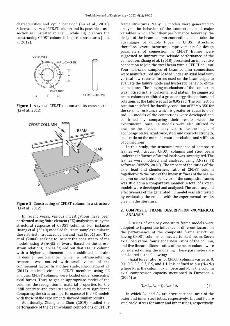
characteristics and cyclic behavior (Lu et al., 2010). Schematic view of CFDST column and its possible cross-section is illustrated in Fig. 1 while Fig. 2 shows the constructing CFDST column in high-rise structures (Li et al. 2012).
Figure 1. A typical CFDST column and its cross section (Li et al., 2012)
Figure 2. Constructing of CFDST column in a structure (Li et al., 2012)
In recent years, various investigations have been performed using finite element (FE) analysis to study the structural response of CFDST columns. For instance, Huang et al. (2010) modeled fourteen samples similar to those at first introduced by Lin and Tsai (2001) and Tao et al. (2004), seeking to inspect the consistency of the models using ABAQUS software. Based on the stress-strain relations, it was figured out that CFDST column with a higher confinement factor exhibited a strain-hardening performance while a strain-softening response was noticed with small values of the confinement factor. In another study, Pagoulatou et al. (2014) modeled circular CFDST members using FE analysis. CFDST columns were loaded under concentric axial forces. Thus, to get an appropriate model of the columns, the recognition of material properties for the infill concrete and steel seemed to be very significant. Comparing the structural performance of the FE models with those of the experiments showed similar results.
Additionally, Zhang and Zhou (2019) studied the performance of the beam-column connections of CFDST
frame structures. Many FE models were generated to analyze the behavior of the connections and major variables, which affect their performance. Generally, the design of the beam-column connections could take the advantages of double tubes in CFDST structure; therefore, several structural improvements for design parameters of connection in CFDST frames were suggested to improve the seismic performance of the connection. Zhang et al. (2018) presented an innovative connection to join the steel beam with a CFDST column. Four half-scale samples of beam-column connections were manufactured and loaded under an axial load with vertical low-reversal forces used on the beam edges to evaluate the failure mode and hysteretic behavior of the connections. The hinging mechanism of the connection was noticed in the horizontal end plates. The suggested beam-columns exhibited a great energy dissipations and rotations at the failure equal to 0.05 rad. The connection rotation satisfied the ductility condition of FEMA 350 for the seismic resistance which is greater or equal to 0.03 rad. FE models of the connections were developed and confirmed by comparing their results with the experimental ones. FE models were also utilized to examine the effect of many factors like the height of anchorage plates, axial force, steel and concrete strength, steel ratio on the moment-rotation relation, and stiffness of connections.
In this study, the structural response of composite frames with circular CFDST columns and steel beam under the influence of lateral loads was investigated. The frames were modeled and analyzed using ANSYS FE software (ANSYS, 2016). The impact of the ratios of the axial load and slenderness ratio of CFDST column together with the ratio of the linear stiffness of the beam–column on the lateral behavior of the composite frames was studied in a comparative manner. A total of sixteen models were developed and analyzed. The accuracy and effectiveness of the generated FE model was also tested by evaluating the results with the experimental results given in the literature.
2. COMPOSITE FRAME DESCRIPTION -NUMERICAL ANALYSIS
A series of one-bay one-story frame models were adopted to inspect the influence of different factors on the performance of the composite frame structures having CFDST columns connected to steel beam. Seven axial load ratios, four slenderness ratios of the column, and five linear stiffness ratios of the beam-column were considered during the modeling. These parameters are considered as the following:
-Axial force ratio (n) of CFDST columns varies as 0, 0.1, 0.3, 0.5, 0.7, 0.9, and 1.1. It is defined as n = (No/Nu) where No is the column axial force and Nu is the column axial compression capacity mentioned in Eurocode 4 (2004) as:
Nu= fysoAso + fysiAsi+ fcAc (1)
in which Aso and Asi are cross sectional area of the outer and inner steel tubes, respectively. fyso and fysi are steel yield stress for outer and inner tubes, respectively.
Turkish Journal of Engineering – 2022; 6(1); 16-25
18
fc is concrete compressive strength and Ac is cross sectional area of the concrete.
-Slenderness ratio (λ) of CFDST columns is 24, 48, 72, and 96 and defined as the height to outer diameter of the column (4H/Do) based on DL/T 5085 (1999).
-Linear stiffness ratio (k) of beam to column is 1.8, 3.0, 4.2, 5.4, and 6.6. It is given as iB/iC. iB is EsIeq/lb in which Ieq is the transformed section moment of inertia based on GB 50017 (2003) while lb is the steel beam length. iC is EhIh/H. The stiffness of the circular CFDST column (EhIh) as per AISC-LRFD (1999) is:
Eh Ih = Es Is + 0.8 Ec Ic (2)
In which Es and Ec are the elastic modulus of steel tubes (outer and inner) and concrete, respectively. Is is the moment of inertia of outer and inner tubes while Ic is the concrete moment of inertia.
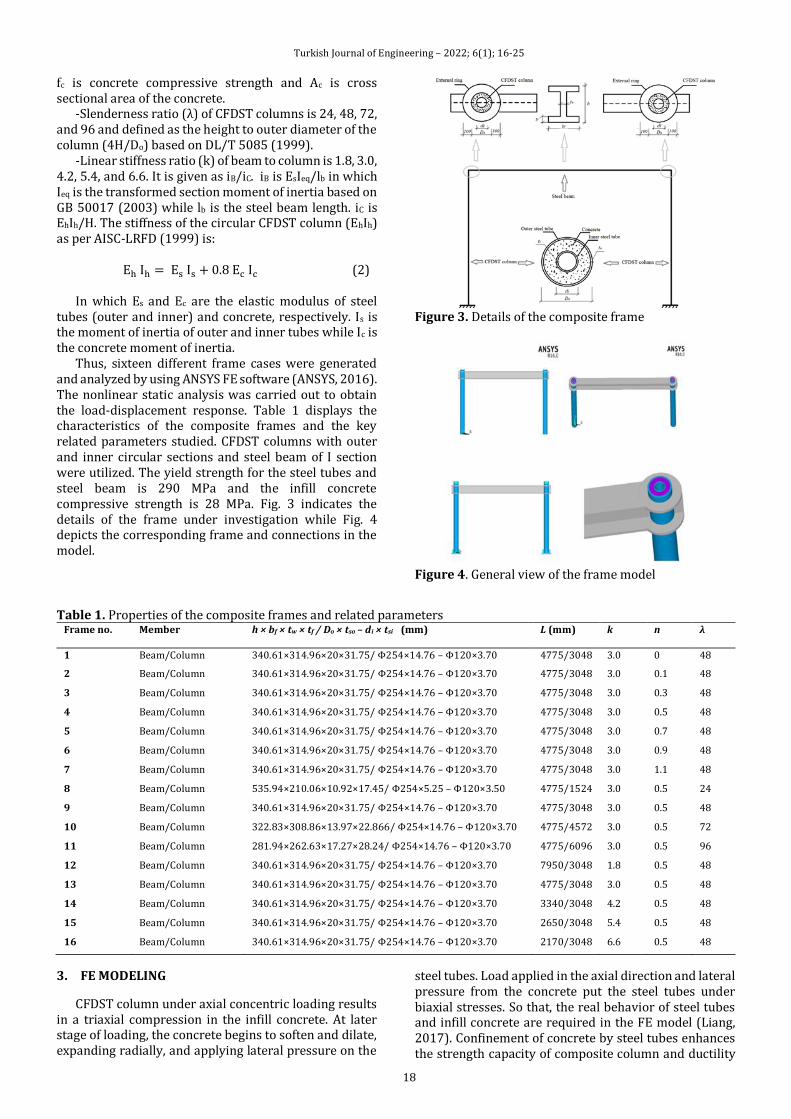
Thus, sixteen different frame cases were generated and analyzed by using ANSYS FE software (ANSYS, 2016). The nonlinear static analysis was carried out to obtain the load-displacement response. Table 1 displays the characteristics of the composite frames and the key related parameters studied. CFDST columns with outer and inner circular sections and steel beam of I section were utilized. The yield strength for the steel tubes and steel beam is 290 MPa and the infill concrete compressive strength is 28 MPa. Fig. 3 indicates the details of the frame under investigation while Fig. 4 depicts the corresponding frame and connections in the model.
Figure 3. Details of the composite frame
Figure 4. General view of the frame model
Table 1. Properties of the composite frames and related parameters Frame no. Member h × bf × tw × tf / Do × tso – di × tsi (mm)
L (mm) k n λ
1 Beam/Column 340.61×314.96×20×31.75/ Φ254×14.76 – Φ120×3.70 4775/3048 3.0 0 48
2 Beam/Column 340.61×314.96×20×31.75/ Φ254×14.76 – Φ120×3.70 4775/3048 3.0 0.1 48
3 Beam/Column 340.61×314.96×20×31.75/ Φ254×14.76 – Φ120×3.70 4775/3048 3.0 0.3 48
4 Beam/Column 340.61×314.96×20×31.75/ Φ254×14.76 – Φ120×3.70 4775/3048 3.0 0.5 48
5 Beam/Column 340.61×314.96×20×31.75/ Φ254×14.76 – Φ120×3.70 4775/3048 3.0 0.7 48
6 Beam/Column 340.61×314.96×20×31.75/ Φ254×14.76 – Φ120×3.70 4775/3048 3.0 0.9 48
7 Beam/Column 340.61×314.96×20×31.75/ Φ254×14.76 – Φ120×3.70 4775/3048 3.0 1.1 48
8 Beam/Column 535.94×210.06×10.92×17.45/ Φ254×5.25 – Φ120×3.50 4775/1524 3.0 0.5 24
9 Beam/Column 340.61×314.96×20×31.75/ Φ254×14.76 – Φ120×3.70 4775/3048 3.0 0.5 48
10 Beam/Column 322.83×308.86×13.97×22.866/ Φ254×14.76 – Φ120×3.70 4775/4572 3.0 0.5 72
11 Beam/Column 281.94×262.63×17.27×28.24/ Φ254×14.76 – Φ120×3.70 4775/6096 3.0 0.5 96
12 Beam/Column 340.61×314.96×20×31.75/ Φ254×14.76 – Φ120×3.70 7950/3048 1.8 0.5 48
13 Beam/Column 340.61×314.96×20×31.75/ Φ254×14.76 – Φ120×3.70 4775/3048 3.0 0.5 48
14 Beam/Column 340.61×314.96×20×31.75/ Φ254×14.76 – Φ120×3.70 3340/3048 4.2 0.5 48
15 Beam/Column 340.61×314.96×20×31.75/ Φ254×14.76 – Φ120×3.70 2650/3048 5.4 0.5 48
16 Beam/Column 340.61×314.96×20×31.75/ Φ254×14.76 – Φ120×3.70 2170/3048 6.6 0.5 48
3. FE MODELING
CFDST column under axial concentric loading results in a triaxial compression in the infill concrete. At later stage of loading, the concrete begins to soften and dilate, expanding radially, and applying lateral pressure on the
steel tubes. Load applied in the axial direction and lateral pressure from the concrete put the steel tubes under biaxial stresses. So that, the real behavior of steel tubes and infill concrete are required in the FE model (Liang, 2017). Confinement of concrete by steel tubes enhances the strength capacity of composite column and ductility
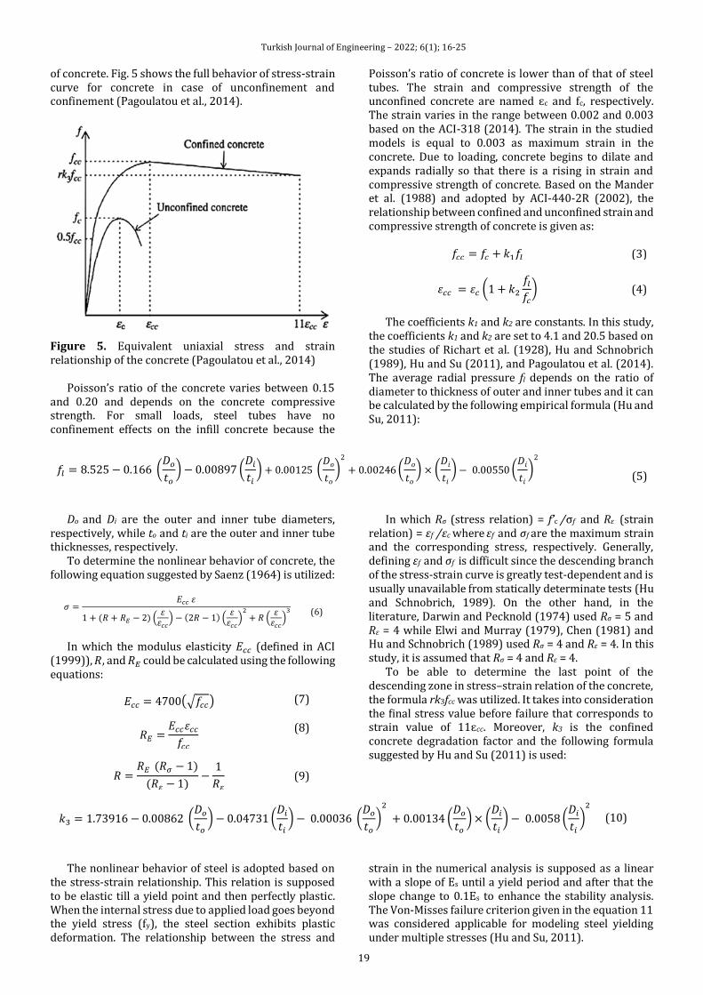
Turkish Journal of Engineering – 2022; 6(1); 16-25
19
of concrete. Fig. 5 shows the full behavior of stress-strain curve for concrete in case of unconfinement and confinement (Pagoulatou et al., 2014).
Figure 5. Equivalent uniaxial stress and strain relationship of the concrete (Pagoulatou et al., 2014)
Poisson’s ratio of the concrete varies between 0.15 and 0.20 and depends on the concrete compressive strength. For small loads, steel tubes have no confinement effects on the infill concrete because the
Poisson’s ratio of concrete is lower than of that of steel tubes. The strain and compressive strength of the unconfined concrete are named ɛc and fc, respectively. The strain varies in the range between 0.002 and 0.003 based on the ACI-318 (2014). The strain in the studied models is equal to 0.003 as maximum strain in the concrete. Due to loading, concrete begins to dilate and expands radially so that there is a rising in strain and compressive strength of concrete. Based on the Mander et al. (1988) and adopted by ACI-440-2R (2002), the relationship between confined and unconfined strain and compressive strength of concrete is given as:
𝑓𝑐𝑐 = 𝑓𝑐 + 𝑘1𝑓𝑙 (3)
𝜀𝑐𝑐 = 𝜀𝑐 (1 + 𝑘2
𝑓𝑙
𝑓𝑐
) (4)
The coefficients k1 and k2 are constants. In this study, the coefficients k1 and k2 are set to 4.1 and 20.5 based on the studies of Richart et al. (1928), Hu and Schnobrich (1989), Hu and Su (2011), and Pagoulatou et al. (2014). The average radial pressure fl depends on the ratio of diameter to thickness of outer and inner tubes and it can be calculated by the following empirical formula (Hu and Su, 2011):
𝑓𝑙 = 8.525 − 0.166 (𝐷𝑜
𝑡𝑜
) − 0.00897 (𝐷𝑖
𝑡𝑖
) + 0.00125 (𝐷𝑜
𝑡𝑜
)2
+ 0.00246 (𝐷𝑜
𝑡𝑜
) × (𝐷𝑖
𝑡𝑖
) − 0.00550 (𝐷𝑖
𝑡𝑖
)2
(5)
Do and Di are the outer and inner tube diameters,
respectively, while to and ti are the outer and inner tube thicknesses, respectively.
To determine the nonlinear behavior of concrete, the following equation suggested by Saenz (1964) is utilized:
𝜎 =𝐸𝑐𝑐 𝜀
1 + (𝑅 + 𝑅𝐸 − 2) (𝜀
𝜀𝑐𝑐) − (2𝑅 − 1) (
𝜀𝜀𝑐𝑐
)2
+ 𝑅 (𝜀
𝜀𝑐𝑐)
3 (6)
In which the modulus elasticity 𝐸𝑐𝑐 (defined in ACI (1999)), 𝑅, and 𝑅𝐸 could be calculated using the following equations:
𝐸𝑐𝑐 = 4700(√𝑓𝑐𝑐) (7)
𝑅𝐸 =𝐸𝑐𝑐𝜀𝑐𝑐
𝑓𝑐𝑐
(8)
𝑅 =𝑅𝐸
(𝑅𝜎 − 1)
(𝑅𝜀 − 1)−
1
𝑅𝜀
(9)
In which Rσ (stress relation) = f’c /σf and Rɛ (strain relation) = ɛf /ɛc where ɛf and σf are the maximum strain and the corresponding stress, respectively. Generally, defining ɛf and σf is difficult since the descending branch of the stress-strain curve is greatly test-dependent and is usually unavailable from statically determinate tests (Hu and Schnobrich, 1989). On the other hand, in the literature, Darwin and Pecknold (1974) used Rσ = 5 and Rɛ = 4 while Elwi and Murray (1979), Chen (1981) and Hu and Schnobrich (1989) used Rσ = 4 and Rɛ = 4. In this study, it is assumed that Rσ = 4 and Rɛ = 4.
To be able to determine the last point of the descending zone in stress–strain relation of the concrete, the formula rk3fcc was utilized. It takes into consideration the final stress value before failure that corresponds to strain value of 11ɛcc. Moreover, k3 is the confined concrete degradation factor and the following formula suggested by Hu and Su (2011) is used:
𝑘3 = 1.73916 − 0.00862 (𝐷𝑜
𝑡𝑜
) − 0.04731 (𝐷𝑖
𝑡𝑖
) − 0.00036 (𝐷𝑜
𝑡𝑜
)2
+ 0.00134 (𝐷𝑜
𝑡𝑜
) × (𝐷𝑖
𝑡𝑖
) − 0.0058 (𝐷𝑖
𝑡𝑖
)2
(10)
The nonlinear behavior of steel is adopted based on the stress-strain relationship. This relation is supposed to be elastic till a yield point and then perfectly plastic. When the internal stress due to applied load goes beyond the yield stress (fy), the steel section exhibits plastic deformation. The relationship between the stress and
strain in the numerical analysis is supposed as a linear with a slope of Es until a yield period and after that the slope change to 0.1Es to enhance the stability analysis. The Von-Misses failure criterion given in the equation 11 was considered applicable for modeling steel yielding under multiple stresses (Hu and Su, 2011).
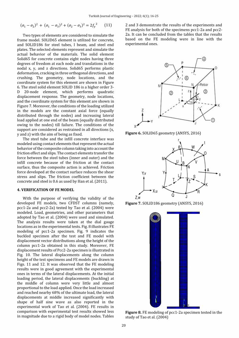
Turkish Journal of Engineering – 2022; 6(1); 16-25
20
(𝜎1 − 𝜎2)2 + (𝜎1 − 𝜎3)2 + (𝜎2 − 𝜎3)2 = 2𝑓𝑦2 (11)
Two types of elements are considered to simulate the
frame model. SOLID65 element is utilized for concrete, and SOLID186 for steel tubes, I beam, and steel end plates. The selected elements represent and simulate the actual behavior of the materials. The solid element Solid65 for concrete contains eight nodes having three degrees of freedom at each node and translations in the nodal x, y, and z directions. Solid65 performs plastic deformation, cracking in three orthogonal directions, and crushing. The geometry, node locations, and the coordinate system for this element are shown in Figure 6. The steel solid element SOLID 186 is a higher order 3-D 20-node element, which performs quadratic displacement response. The geometry, node locations, and the coordinate system for this element are shown in Figure 7. Moreover, the conditions of the loading utilized in the models are the constant axial force (equally distributed through the nodes) and increasing lateral load applied at one end of the beam (equally distributed owing to the nodes) till failure. The conditions of the support are considered as restrained in all directions (x, y and z) with the aim of being as fixed.
The steel tube and the infill concrete interface was modeled using contact elements that represent the actual behavior of the composite column taking into account the friction effect and slips. The contact elements transfer the force between the steel tubes (inner and outer) and the infill concrete because of the friction at the contact surface, thus the composite action is achieved. Friction force developed at the contact surface reduces the shear stress and slips. The friction coefficient between the concrete and steel is 0.6 as used by Han et al. (2011).
4. VERIFICATION OF FE MODEL
With the purpose of verifying the validity of the developed FE models, two CFDST columns (namely, pcc1-2a and pcc2-2a) tested by Tao et al. (2004) were modeled. Load, geometries, and other parameters that adopted by Tao et al. (2004) were used and simulated. The analysis results were taken at the dial gauge locations as in the experimental tests. Fig. 8 illustrates FE modeling of pcc1-2a specimen. Fig. 9 indicates the buckled specimen after the test and FE model with displacement vector distributions along the height of the column pcc1-2a obtained in this study. Moreover, FE displacement results of Pcc2-2a specimen is illustrated in Fig. 10. The lateral displacements along the column height of the test specimens and FE models are drawn in Figs. 11 and 12. It was observed that the FE modeling results were in good agreement with the experimental ones in terms of the lateral displacements. At the initial loading period, the lateral displacements (buckling) at the middle of column were very little and almost proportional to the load applied. Once the load increased and reached nearby 68% of the ultimate load, the lateral displacements at middle increased significantly with shape of half sine wave as also reported in the experimental work of Tao et al. (2004). FE results in comparison with experimental test results showed less in magnitude due to a rigid body of model nodes. Tables
2 and 3 demonstrate the results of the experiments and FE analysis for both of the specimens pcc1-2a and pcc2-2a. It can be concluded from the tables that the results based on the FE modeling were in line with the experimental ones.
Figure 6. SOLID65 geometry (ANSYS, 2016)
Figure 7. SOLID186 geometry (ANSYS, 2016)
Figure 8. FE modeling of pcc1-2a specimen tested in the study of Tao et al. (2004)

Turkish Journal of Engineering – 2022; 6(1); 16-25
21
Figure 9. Buckled specimen (pcc1-2a) tested by Tao et al. (2004) and the developed FE model
Figure 10. Displacement results of pcc2-2a specimen of Tao et al. (2004) (in mm)
Figure 11. Lateral displacement along the column height of experimentally tested specimen (pcc1-2a) of Tao et al. (2004) and the developed FE model
Figure 12. Lateral displacement along the column height of experimentally tested specimen (pcc2-2a) of Tao et al. (2004) and the developed FE model
Table 2. Experimental and numerical results for the specimen pcc1-2a of Tao et al. (2004)
Item Experimental
result (Tao et al., 2004) FE model result
Theoretical
Experimental (%)
Ultimate load (kN) 620 636 102.6 Max. lateral displacement
(Buckling) (mm) 19 18.54 97.6
Table 3. Experimental and numerical results for the specimen pcc2-2a of Tao et al. (2004)
Item Experimental
result (Tao et al., 2004) FE model result
Theoretical
Experimental (%)
Ultimate load (kN) 400 409 102.3 Max. lateral displacement
(Buckling) (mm) 33.5 32.86 98.1
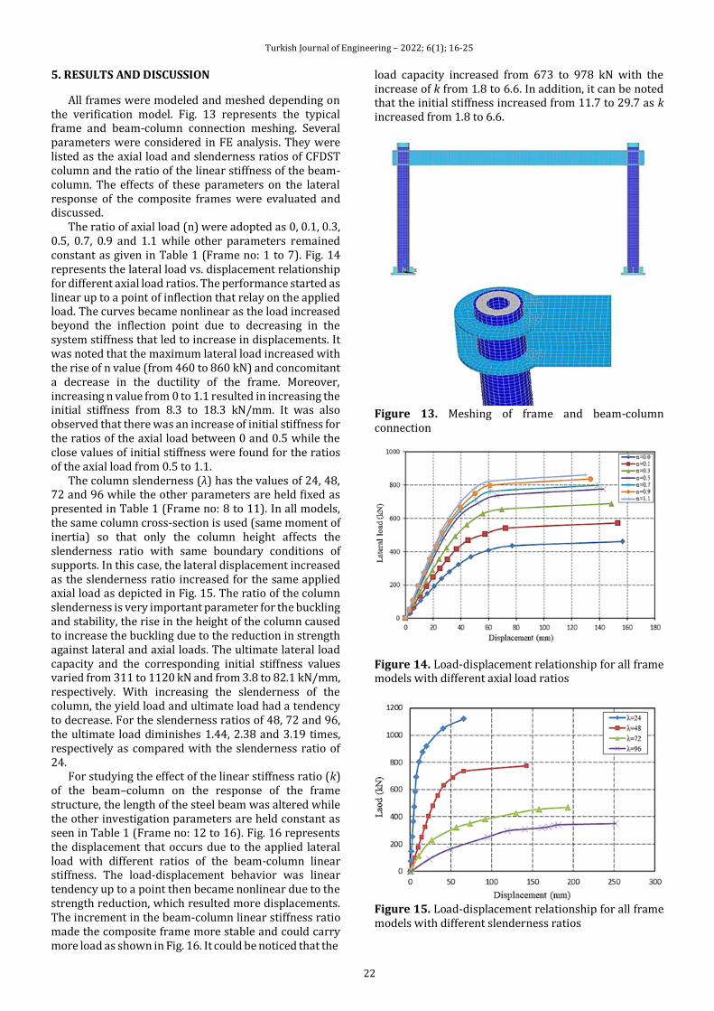
Turkish Journal of Engineering – 2022; 6(1); 16-25
22
5. RESULTS AND DISCUSSION
All frames were modeled and meshed depending on the verification model. Fig. 13 represents the typical frame and beam-column connection meshing. Several parameters were considered in FE analysis. They were listed as the axial load and slenderness ratios of CFDST column and the ratio of the linear stiffness of the beam-column. The effects of these parameters on the lateral response of the composite frames were evaluated and discussed.
The ratio of axial load (n) were adopted as 0, 0.1, 0.3, 0.5, 0.7, 0.9 and 1.1 while other parameters remained constant as given in Table 1 (Frame no: 1 to 7). Fig. 14 represents the lateral load vs. displacement relationship for different axial load ratios. The performance started as linear up to a point of inflection that relay on the applied load. The curves became nonlinear as the load increased beyond the inflection point due to decreasing in the system stiffness that led to increase in displacements. It was noted that the maximum lateral load increased with the rise of n value (from 460 to 860 kN) and concomitant a decrease in the ductility of the frame. Moreover, increasing n value from 0 to 1.1 resulted in increasing the initial stiffness from 8.3 to 18.3 kN/mm. It was also observed that there was an increase of initial stiffness for the ratios of the axial load between 0 and 0.5 while the close values of initial stiffness were found for the ratios of the axial load from 0.5 to 1.1.
The column slenderness (λ) has the values of 24, 48, 72 and 96 while the other parameters are held fixed as presented in Table 1 (Frame no: 8 to 11). In all models, the same column cross-section is used (same moment of inertia) so that only the column height affects the slenderness ratio with same boundary conditions of supports. In this case, the lateral displacement increased as the slenderness ratio increased for the same applied axial load as depicted in Fig. 15. The ratio of the column slenderness is very important parameter for the buckling and stability, the rise in the height of the column caused to increase the buckling due to the reduction in strength against lateral and axial loads. The ultimate lateral load capacity and the corresponding initial stiffness values varied from 311 to 1120 kN and from 3.8 to 82.1 kN/mm, respectively. With increasing the slenderness of the column, the yield load and ultimate load had a tendency to decrease. For the slenderness ratios of 48, 72 and 96, the ultimate load diminishes 1.44, 2.38 and 3.19 times, respectively as compared with the slenderness ratio of 24.
For studying the effect of the linear stiffness ratio (k) of the beam–column on the response of the frame structure, the length of the steel beam was altered while the other investigation parameters are held constant as seen in Table 1 (Frame no: 12 to 16). Fig. 16 represents the displacement that occurs due to the applied lateral load with different ratios of the beam-column linear stiffness. The load-displacement behavior was linear tendency up to a point then became nonlinear due to the strength reduction, which resulted more displacements. The increment in the beam-column linear stiffness ratio made the composite frame more stable and could carry more load as shown in Fig. 16. It could be noticed that the
load capacity increased from 673 to 978 kN with the increase of k from 1.8 to 6.6. In addition, it can be noted that the initial stiffness increased from 11.7 to 29.7 as k increased from 1.8 to 6.6.
Figure 13. Meshing of frame and beam-column connection
Figure 14. Load-displacement relationship for all frame models with different axial load ratios
Figure 15. Load-displacement relationship for all frame models with different slenderness ratios
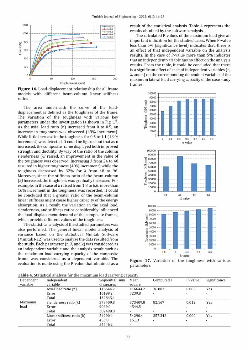
Turkish Journal of Engineering – 2022; 6(1); 16-25
23
Figure 16. Load-displacement relationship for all frame models with different beam-column linear stiffness ratios
The area underneath the curve of the load-displacement is defined as the toughness of the frame. The variation of the toughness with various key parameters under the investigation is shown in Fig. 17. As the axial load ratio (n) increased from 0 to 0.5, an increase in toughness was observed (49% increment). While little increase in the toughness for 0.5 to 1.1 (1.9% increment) was detected. It could be figured out that as n increased, the composite frame displayed both improved strength and ductility. By way of the ratio of the column slenderness (λ) raised, an improvement in the value of the toughness was observed. Increasing λ from 24 to 48 resulted in higher toughness (40% increment) while the toughness decreased by 32% for λ from 48 to 96. Moreover, since the stiffness ratio of the beam-column (k) increased, the toughness was gradually increased. For example, in the case of k raised from 1.8 to 6.6, more than 16% increment in the toughness was recorded. It could be concluded that a greater ratio of the beam-column linear stiffness might cause higher capacity of the energy absorption. As a result, the variation in the axial load, slenderness, and stiffness ratios considerably influenced the load-displacement demand of the composite frames, which provide different values of the toughness.
The statistical analysis of the studied parameters was also performed. The general linear model analysis of variance based on the statistical Minitab Software (Minitab R12) was used to analyze the data resulted from the study. Each parameter (n, λ, and k) was considered as an independent variable and the analysis result such as the maximum load carrying capacity of the composite frame was considered as a dependent variable. The evaluation is made using the P-value that obtained as a
result of the statistical analysis. Table 4 represents the results obtained by the software analysis.
The calculated P-values of the maximum load give an important indication for the studied cases. When P-value less than 5% (significance level) indicates that, there is an effect of that independent variable on the analysis results. In the case of P-value more than 5% indicates that an independent variable has no effect on the analysis results. From the table, it could be concluded that there is a significant effect of each of independent variables (n, λ, and k) on the corresponding dependent variable of the maximum lateral load carrying capacity of the case study frames.
Figure 17. Variation of the toughness with various parameters
Table 4. Statistical analysis for the maximum load carrying capacity
Dependent variable
Independent variable
Sequential sum of squares
Mean square
Computed F
P- value Significance
Maximum load
Axial load ratio (n) Error Total
116644.2 16199.2 132843.4
116644.2 3239.8 -
36.003 -
0.002 ـ ـ
Yes ـ ـ
Slenderness ratio (λ) Error Total
373409.8 9089.0 382498.8
373409.8 4544.5 -
82.167 - -
0.012 ـ ـ
Yes ـ ـ
Linear stiffness ratio (k) Error Total
54290.4 455.8 54746.2
54290.4 151.9 -
357.342 ـ
ـ
0.000 ـ
ـ
Yes ـ
ـ
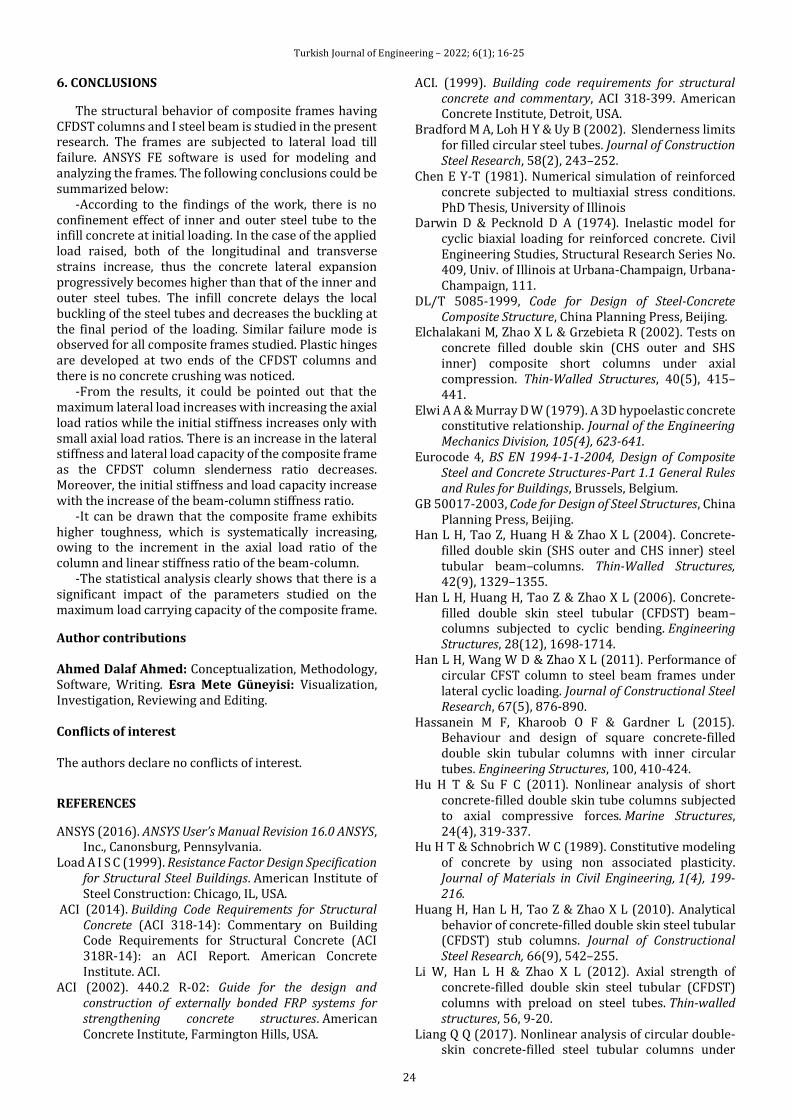
Turkish Journal of Engineering – 2022; 6(1); 16-25
24
6. CONCLUSIONS
The structural behavior of composite frames having CFDST columns and I steel beam is studied in the present research. The frames are subjected to lateral load till failure. ANSYS FE software is used for modeling and analyzing the frames. The following conclusions could be summarized below:
-According to the findings of the work, there is no confinement effect of inner and outer steel tube to the infill concrete at initial loading. In the case of the applied load raised, both of the longitudinal and transverse strains increase, thus the concrete lateral expansion progressively becomes higher than that of the inner and outer steel tubes. The infill concrete delays the local buckling of the steel tubes and decreases the buckling at the final period of the loading. Similar failure mode is observed for all composite frames studied. Plastic hinges are developed at two ends of the CFDST columns and there is no concrete crushing was noticed.
-From the results, it could be pointed out that the maximum lateral load increases with increasing the axial load ratios while the initial stiffness increases only with small axial load ratios. There is an increase in the lateral stiffness and lateral load capacity of the composite frame as the CFDST column slenderness ratio decreases. Moreover, the initial stiffness and load capacity increase with the increase of the beam-column stiffness ratio.
-It can be drawn that the composite frame exhibits higher toughness, which is systematically increasing, owing to the increment in the axial load ratio of the column and linear stiffness ratio of the beam-column.
-The statistical analysis clearly shows that there is a significant impact of the parameters studied on the maximum load carrying capacity of the composite frame.
Author contributions Ahmed Dalaf Ahmed: Conceptualization, Methodology, Software, Writing. Esra Mete Güneyisi: Visualization, Investigation, Reviewing and Editing. Conflicts of interest The authors declare no conflicts of interest.
REFERENCES
ANSYS (2016). ANSYS User’s Manual Revision 16.0 ANSYS, Inc., Canonsburg, Pennsylvania.
Load A I S C (1999). Resistance Factor Design Specification for Structural Steel Buildings. American Institute of Steel Construction: Chicago, IL, USA.
ACI (2014). Building Code Requirements for Structural Concrete (ACI 318-14): Commentary on Building Code Requirements for Structural Concrete (ACI 318R-14): an ACI Report. American Concrete Institute. ACI.
ACI (2002). 440.2 R-02: Guide for the design and construction of externally bonded FRP systems for strengthening concrete structures. American Concrete Institute, Farmington Hills, USA.
ACI. (1999). Building code requirements for structural concrete and commentary, ACI 318-399. American Concrete Institute, Detroit, USA.
Bradford M A, Loh H Y & Uy B (2002). Slenderness limits for filled circular steel tubes. Journal of Construction Steel Research, 58(2), 243–252.
Chen E Y-T (1981). Numerical simulation of reinforced concrete subjected to multiaxial stress conditions. PhD Thesis, University of Illinois
Darwin D & Pecknold D A (1974). Inelastic model for cyclic biaxial loading for reinforced concrete. Civil Engineering Studies, Structural Research Series No. 409, Univ. of Illinois at Urbana-Champaign, Urbana-Champaign, 111.
DL/T 5085-1999, Code for Design of Steel-Concrete Composite Structure, China Planning Press, Beijing.
Elchalakani M, Zhao X L & Grzebieta R (2002). Tests on concrete filled double skin (CHS outer and SHS inner) composite short columns under axial compression. Thin-Walled Structures, 40(5), 415–441.
Elwi A A & Murray D W (1979). A 3D hypoelastic concrete constitutive relationship. Journal of the Engineering Mechanics Division, 105(4), 623-641.
Eurocode 4, BS EN 1994-1-1-2004, Design of Composite Steel and Concrete Structures-Part 1.1 General Rules and Rules for Buildings, Brussels, Belgium.
GB 50017-2003, Code for Design of Steel Structures, China Planning Press, Beijing.
Han L H, Tao Z, Huang H & Zhao X L (2004). Concrete-filled double skin (SHS outer and CHS inner) steel tubular beam–columns. Thin-Walled Structures, 42(9), 1329–1355.
Han L H, Huang H, Tao Z & Zhao X L (2006). Concrete-filled double skin steel tubular (CFDST) beam–columns subjected to cyclic bending. Engineering Structures, 28(12), 1698-1714.
Han L H, Wang W D & Zhao X L (2011). Performance of circular CFST column to steel beam frames under lateral cyclic loading. Journal of Constructional Steel Research, 67(5), 876-890.
Hassanein M F, Kharoob O F & Gardner L (2015). Behaviour and design of square concrete-filled double skin tubular columns with inner circular tubes. Engineering Structures, 100, 410-424.
Hu H T & Su F C (2011). Nonlinear analysis of short concrete-filled double skin tube columns subjected to axial compressive forces. Marine Structures, 24(4), 319-337.
Hu H T & Schnobrich W C (1989). Constitutive modeling of concrete by using non associated plasticity. Journal of Materials in Civil Engineering, 1(4), 199-216.
Huang H, Han L H, Tao Z & Zhao X L (2010). Analytical behavior of concrete-filled double skin steel tubular (CFDST) stub columns. Journal of Constructional Steel Research, 66(9), 542–255.
Li W, Han L H & Zhao X L (2012). Axial strength of concrete-filled double skin steel tubular (CFDST) columns with preload on steel tubes. Thin-walled structures, 56, 9-20.
Liang Q Q (2017). Nonlinear analysis of circular double-skin concrete-filled steel tubular columns under

Turkish Journal of Engineering – 2022; 6(1); 16-25
25
axial compression. Engineering Structures, 131, 639-650.
Lin M L & Tsai K C (2001). Behavior of double-skinned composite steel tubular columns subjected to combined axial and flexural loads. In: Proceedings of the first international conference on steel and composite structures, 1145–1152.
Lu H, Han L H & Zhao X L (2010). Fire performance of self-consolidating concrete filled double skin steel tubular columns: Experiments. Fire safety journal, 45(2), 106-115.
Mander J B, Priestley M J & Park R (1988). Theoretical stress-strain model for confined concrete. Journal of structural engineering, 114(8), 1804-1826.
Minitab R12. Statistical Tool. Quality Plaza, 1829 Pine Hall Rd., State College, PA 16801-3008, USA.
Pagoulatou M, Sheehan T, Dai X H & Lam D (2014). Finite element analysis on the capacity of circular concrete-filled double-skin steel tubular (CFDST) stub columns. Engineering Structures, 72, 102-112.
Richart F E, Brandtzaeg A & Brown R L (1928). A study of the failure of concrete under combined compressive stresses. University of Illinois at Urbana Champaign, College of Engineering. Engineering Experiment Station.
Ritchie C B, Gow M I, Packer J A & Heidarpour A (2017). Influence of elevated strain rate on the mechanical properties of hollow structural sections. International Journal of Protective Structures, 8(3), 325-351.
Saenz L P (1964). Discussion of “Equation for the stress–strain curve of concrete” by Desayi and Krishnan. Journal of the American Concrete Institute, 61, 1229-1235.
Tao Z, Han L H & Zhao X L (2004). Behaviour of concrete-filled double skin (CHS inner and CHS outer) steel tubular stub columns and beam-columns. Journal of Constructional Steel Research, 60(8), 1129-1158.
Uenaka K, Kitoh H & Sonoda K (2010). Concrete filled double skin circular stub columns under compression. Thin-walled structures, 48(1), 19-24.
Wei S, Mau S T, Vipulanandan C & Mantrala S K (1995). Performance of new sandwich tube under axial loading: experiment. Journal of Structural Engineering, 121(12), 1806-1814.
Yagishita F, Kitoh H, Sugimoto M, Tanihira T & Sonoda K (2000). Double skin composite tubular columns subjected to cyclic horizontal force and constant axial force. In Proc., 6th ASCCS Int. Conf. on Steel-Concrete Composite Structures, Los Angeles: Univ. of Southern California, 497-503.
Zhao X L, Grzebieta R H & Elchalakani M. (2002a). Tests of concrete-filled double skin CHS composites tube columns. Steel and Composite Structures—An International Journal, 2(2), 129–142.
Zhao X L, Grzebieta R H, Ukur A & Elchalakani M (2002b). Tests of concrete-filled double skin (SHS outer and CHS inner) composite stub columns. In Advances in Steel Structures (ICASS'02), Elsevier, 567-574.
Zhao X L & Grzebieta R H (2002c). Strength and ductility of concrete filled double skin (SHS inner and SHS outer) tubes. Thin-Walled Structures, 40(2), 199–213.
Zhao X L, Han B & Grzebieta R H (2002d). Plastic mechanism analysis of concrete filled double-skin (SHS inner and SHS outer) stub columns. Thin-Walled Structures, 40(10), 815–833.
Zhang Y & Zhou Z (2019). Beam‐column connections of concrete‐filled double steel tubular frame structures. The Structural Design of Tall and Special Buildings, 28(5), e1592.
Zhang D, Zhao J & Zhang Y (2018). Experimental and numerical investigation of concrete-filled double-skin steel tubular column for steel beam joints. Advances in Materials Science and Engineering, 6514025
© Author(s) 2022. This work is distributed under https://creativecommons.org/licenses/by-sa/4.0/
* Corresponding Author Cite this article
*([email protected]) ORCID ID 0000 – 0002 – 2152 – 5362 Research Article / DOI: 10.31127/tuje.758921
Yener H (2022). A study on effects of system thinking and decision-making styles over entrepreneurship skills. Turkish Journal of Engineering, 6(1), 26-33
Received: 27/06/2020; Accepted: 13/11/2020
Turkish Journal of Engineering – 2022; 6(1); 26-33
Turkish Journal of Engineering
https://dergipark.org.tr/en/pub/tuje
e-ISSN 2587-1366
A study on effects of system thinking and decision-making styles over entrepreneurship skills
Huseyin Yener *1
1Maltepe University, Engineering Faculty, Industrial Engineering Department, Istanbul, Turkey
Keywords ABSTRACT Entrepreneurship Skills System Thinking Decision-Making Styles Relational Screening Model
Entrepreneurship has an uncertain environment requiring several abilities to achieve the goal. The article explores the effects of individuals’ system thinking level, decision-making styles and family background on their entrepreneurial skills. In the study relational screening model is used as a research method. The sample group of the study consists of 65 students of the 4th grade students of a private university in Istanbul, Turkey in 2019. Three questionnaires have been applied and descriptive statistics and all the other tests have been conducted by using SPSS 26 to examine the extent of involvement, significance, direction and degree of the relationships. The results show that there is a positive moderate significant (r = 0.542) relationship between individuals’ entrepreneurship skill and system thinking level. Also a positive low level relationship (r = 0.374 p <0.05) has been detected between entrepreneurship skills and vigilance type of decision-making style. Negative low level of relationships (r = -0.123 and r = -0.244, p <0.05) among entrepreneurship skills, hypervigilance and procrastination types of decision-making styles. Moreover, no significant relationship has been found among entrepreneurship skills, parental education/job status and entrepreneurship experience/history in the family supporting the idea that entrepreneurship is a learnable skill rather than an innate skill.
1. INTRODUCTION
Economic and social challenges all around the world motivates the idea of developing more entrepreneurial activities. Entrepreneurship can be realized with individuals that can approach complex problems and events in a holistic framework and make the right decisions. Decision-making is to select the optimum one out of several options (Saaty, 2008). Individuals’ innate abilities in decision-making process are very important and effective parameters. On the other hand, system thinking approach puts forward every action taken may or will have an effect on the other parts of a system. System thinking approach may give guidance individuals while they are producing solutions to the problems encountered. Besides, it is aimed to investigate whether the family experience and back-ground on entrepreneurship has an effect on both of these skills. In the literature, it is stated that “entrepreneurship, system thinking and decision-making are the features that can be developed with education” which should motivate education institutions to develop education programs to
foster these abilities for our world’s mutual benefits (Davidsson, 2006).
To reveal the interactions among family background, decision-making styles, system thinking on entrepreneurship skills, three questionnaires were applied to sample group and the results were analyzed in the application part of the study. Results of the study supported the idea that the entrepreneurship skill is not innate and can be improved by education activities. Similarly, it is found that there is a significant relation among entrepreneurship skills, system thinking and vigilance, hypervigilance and procrastination type of decision-making styles. No significant interaction with buck passing type of decision-making style was detected.
1.1. Entrepreneurship Education
Richard Cantillon, the father of entrepreneurial thinking, put forward the concept of entrepreneurial thinking in the 17th century against ambiguity (Patel and Mehta 2016). He defined entrepreneurship as self-employment of any kind. Entrepreneurs buy in the present and sell at uncertain prices in the future
Turkish Journal of Engineering – 2022; 6(1); 26-33
27
(Cantillon, 1775). The key term in his definition was ambiguity. Casson (2010) stated that “after about a century, Adam Smith described entrepreneurial thinking as a frugal and slow but steady progress agent for accumulating capital”. However, Michaels (2012) explained in his study that “entrepreneurship can be thought like any other subject. Above all, entrepreneurial thinking is a mindset that emphasizes learning about the opportunity and making use of the situation in a unique way”.
For this reason, Henry et al. (2003) put forward that “education and training programs constitutes a major role in training future entrepreneurs and developing the skills of existing entrepreneurs”. Gibb (1987) stated that “although the entrepreneurship has cultural and experimental portions, it can be improved gradually by education”. Traditional entrepreneurship carries risks (McGrath, 1995; McGrath, 2000). Therefore, it is necessary to make the right decision for successful entrepreneurship. For the right decision, system thinking skills are needed, which allow to look at the events and problems from multiple perspectives. Entrepreneurship education is considered as an education model to change attitudes, trends and motivations.
Studies report that the traditional entrepreneurship approach should change. According to this understanding, entrepreneurship should be developed with new education and training techniques. Among these techniques, the development of thinking skills, mentoring and group work are widely accepted. Implementation is required for project management and development of budget skills. Therefore, according to Kalyani and Kumar (2011) “it is increasingly recognized that teaching entrepreneurship skills should include interactive teaching requiring skillful instructors”.
Whether or not entrepreneurship is innate is a controversial issue. Despite common view that entrepreneurs are innate, there are also the other studies claiming entrepreneurship is a skill to learn. Drucker (1985) described that “entrepreneurship is a discipline and has been reported to be learnable like any other discipline”. According to this view, it is necessary to review the entrepreneurship trainings given at universities in the training of entrepreneurial individuals, including active methods.
According to Gibb (2011), the entrepreneurship education needs to be changed since the traditional entrepreneurship model can no longer be applied to the modern business environment. Entrepreneurship education is emphasized more by the relevant field experts Berglund and Wennberg (2006), Patır and Karahan (2010) which are important for the factors that determine entrepreneurship. It is stated that entrepreneurship education increases individuals' chances of becoming a successful entrepreneur, increases the level of knowledge by developing understanding and awareness of entrepreneurship, and promotes positive attitude and tendency. This understanding emphasizes the understanding that entrepreneurs are not born and that they are prone to education. Entrepreneurship education draws attention to the view that it supports young entrepreneur candidates to reveal entrepreneurial potential and
encourages them to start their own businesses (Guzmán and Liñán 2005). All these research results point out entrepreneurship training to be provided at various educational levels and types starting from an early age in developing entrepreneurship trends. In this sense, big tasks fall for the decision-makers on the subject in terms of effective policies they will produce to realize them.
Entrepreneurship is the power of economy, the source of discovery and imagination. In countries where there is no entrepreneurship or insufficiency, the level of economic welfare is low (Mueller, 2011). The rapid increase in globalization and competition, the inability of governments to provide appropriate funds for higher education, the increase in the need for qualified manpower and many other factors require universities to turn into an entrepreneurial structure (Greenspan and Rosan 2006).
1.2. System Thinking Skills
System thinking can be defined as an approach for examining and understanding complex problems from a holistic perspective (Orgill et al., 2019). Evagorou et al. (2009) described system thinking as “a method of seeing systems from a broad perspective”. Dori and Sillitto (2017) stated in their study that “complexity decision-making, especially with holistic or system approach. The holistic approach of system thinking is claimed to improve the quality of decision processes”. The system provides communication and collaboration with a holistic perspective on the basis of thinking. System thinking has been reported to be effective in giving a holistic perspective to a problem. The basic idea behind the system thinking to break down the whole into sub elements and study the interactions of elements (Patel and Mehta 2016).
To understand the system thinking, first thing is to define the system. System; is a group that consists of interdependent and interconnected units, consisting of different sections and established according to a general plan, and is oriented towards the purpose to achieve a certain result. Systems in engineering are fundamental, and natural events in science can be defined as systems. In engineering, systems are grouped into three sub-categories: function (benefit), structure (form) and behavior (dynamics) (Dori and Sillitto 2017) System thinking is a systematic evaluation of understanding the situation, taking into account of system perspective (Assaraf and Orion 2005).
According to Long (2012) “in engineering, design and system thinking can be used together. System thinking is sometimes described as a component of design thinking”. Scientists have emphasized the importance of system thinking approach in entrepreneurship education (Forrester, 2007). System thinking is necessary to increase the ability of societies to understand the system, find to the problems encountered bearing in mind the side effects of the solutions. Verhoeff et al., (2008) revealed that “system thinking ability is accepted as a higher level of thinking skill that is essential for understanding concepts and principles in science and engineering”. It has been reported that system thinking skills are necessary for understanding complex events
Turkish Journal of Engineering – 2022; 6(1); 26-33
28
and solving complex problems. In addition, it has been explained that thinking of the system requires more than innovation and entrepreneurship skills (Evagorou et al., (2009).
1.3. Decision-Making Styles
Everybody gives many decisions every time in his or her daily life. Some of them lead desired results, some of the others give undesirable results (Haan, 2010). Generally, decision-making includes a group of people or organizations rather than a person. Sustainable development means prosperity for today's society and future generations. Today, problems faced for sustainability development are quite complex. In order to solve these complex problems, decision-making and problems must be viewed from multiple perspectives (Arvai et al., 2004). Engineering can be considered as a complex process that consists of a successive decisions and does not compromise (Hernandez et al., 1998). Today's ambiguous and complex environment necessitates people and organizations to make better decisions to maintain competitive advantage.
Interdisciplinary approaches are important in educational activities, as real-world decisions often involve more than one area (Solomon and Aikenhead, 1994). From this perspective, students need to be equipped with more skills before entering the labor market or industrial society. However, in educational institutions, students are not properly equipped to solve and decide on disciplinary problems such as sociological issues, engineering and design skills (Zeidler et al., 2009). Scientific decision-making is important in developing students' learning abilities, scientific literacy, conceptual understanding, scientific research, attitude and social values. Sadler and Zeidler (2005) stated that “rapid changes are created in our lives with science. In order to keep up with this speed, rational thinking and information technology of learners should be equipped with the decision-making abilities”.
Saaty (2008) divides decision-making processes into two, intuitively and analytically. Intuitive decisions are not supported by data and are generally made arbitrarily. In some simple, depth-free decision situations, the intuitive approach can be successful. However, when faced with complex decision situations requiring information, decision makers can see that their decisions ultimately deviate from their own value judgments. Contrary to what has been believed for a long time nowadays, it has become a "science" rather than an "art". Yesilyaprak (2003) expressed that “decision-making activity is affected by both emotional and cognitive features”. Decision-making style affects a person's approach, reactions and actions in a decision-making process (Thunholm, 2009).
Today, companies have seen innovation as an imperative to survive in competitive environments. Entrepreneurship and decision making skills are very important for the development of innovation (Gelderen and Masurel 2012). Although there are important studies on the development of these skills in the literature, there are no studies examining them all together.
2. MATERIALS AND METHOD
2.1. The Second Level Headings
The main problem of the study constitutes the question; Is there a relationship among entrepreneurship skills, system thinking and decision-making styles? The sub-problems are defined as below:
1. Is there a relationship between entrepreneurship skills and system thinking levels?
2. Is there a relationship between entrepreneurship skills and decision-making styles?
3. Is there a relationship between system thinking levels and decision-making styles?
4. Is there a relation between entrepreneurship skills and parents’ education levels?
5. Is there a relationship between entrepreneurship skills and parents’ jobs?
6. Is there a relationship between entrepreneurship skills and families’ entrepreneurship history or experiences?
2.2. Model of the Research
In the study relational screening model was used as research method. The screening model is all of the processes that describe a situation as it exists in the past or present, and is applied to realize learning and to develop desired behaviors in the individual. In the general screening model, in a universe consisting of a large number of elements, in order to make a general judgment about the universe, the entire universe or a group of samples to be taken from it is scanned. The relational screening model aims to put forward the existence of co-variation among parameters. The goal of this study is to investigate the impact levels of family history and experiences about entrepreneurship, decision-making stiles and system thinking levels on individuals' entrepreneurship skills.
2.3. Study Group
Sample group of the study consisted of 65 students of the 4th grade students of a university in Istanbul, Turkey in 2019. In experimental studies it is advised that the sample group shall be at least 30 (Gay, 1996) which sample size of the study meets criterion. Students in the study group were selected on a voluntary basis.
2.4. Data Collection Tools
2.4.1. Entrepreneurship questionnaire
In the study, a 25-item entrepreneurship questionnaire developed by Kashif et al. (2016) was used to determine the level of entrepreneurship. Five-point Likert-type questionnaire was used. There are no inverse questions in the test. Cronbach's alpha coefficient was determined by using SPSS as 0.89 (N=100) for the reliability of the questionnaire (Kashif et al., 2016).
2.4.2. System thinking skill questionnaire
A 20-item questionnaire developed by Moore et al. (2010) to test system thinking skill. Five-point Likert-
Turkish Journal of Engineering – 2022; 6(1); 26-33
29
type questionnaire was used. There are no inverse questions in the test. reliability and validity were assessed. Moore et al. (2010) conducted test and retest reliability evaluation (n=36) resulting a correlation of 0.74 and internal consistency testing (n=342) Cronbach’s alpha coefficient of 0.89.
2.4.3. Decision-making styles questionnaire
Decision-making styles were tested by “Melbourne Decision-Making Questionnaire” developed by Mann et.al (2014). The scale has 22 items and measures decision-making styles. It has 4 sub-scales as “Vigilance type of decision-making”, “Hypervigilance type of decision making”, “Procrastination type of decision-making” and “Buck Passing type of decision-making”. Validity and reliability of the questionnaire were tested by Deniz (2004). Content validity was performed using similar scales validity method and expert opinion was consulted. Reliability of the questionnaire was calculated by repetition of the questionnaire and internal consistency methods. The repetition of the questionnaire was applied to 56 university students twice at three-week intervals and reliability coefficients were between r= 0.68 and r= 0.87. Internal consistency coefficients of the test applied to 154 university students were calculated as; vigilance type 0.80, hypervigilance type 0.78, procrastination type 0.65 and buck passing type 0.71.
2.5. Data Analysis
Entrepreneurship questionnaire, was organized with a 5-point Likert-type rating and consisted of 25 questions. Scale was calculated as “Most of the Time” (4 points), “Often” (3 points), “Some of the time” (2 points), “Seldom” (1 point) and “Never” (0 point). Total number is computed by adding up the points for each question. It can range from 0 to 100.
System thinking skill questionnaire was organized with a 5-point Likert-type rating and consisted of 20 questions. Scale was calculated as “Most of the Time” (4 points), “Often” (3 points), “Some of the time” (2 points), “Seldom” (1 point) and “Never” (0 point). Total number is computed by adding up the points for each question. It can range from 0 to 80.
Decision-making styles questionnaire has 4 sub-scales. It is organized with a 3-point Likert-type rating and consisted of 22 questions. Scale was calculated as "Right" (2 points), "Sometimes Right" (1 point), "Not Right" (0 point).
Vigilance Type of Decision-Making: It is the situation where the individual searches the necessary information carefully before giving a decision and makes a selection after carefully judging all the alternatives. It is expressed in six items (1, 2, 3, 4, 5, 6) in the questionnaire.
Hypervigilance Type of Decision-Making: is the situation where the individual refrains from making decisions, lets the giving decision to others, and therefore tries to avoid the decision by transferring responsibility to someone else. This factor is expressed in six items (7, 8, 9, 10, 11, 12) in the questionnaire.
Procrastination Type of Decision-Making: It is the state of the individual to postpone the decision, delay it
and drag it without an acceptable reason. It is expressed in five items (13, 14, 15, 16, 17) in the questionnaire.
Buck Passing Type of Decision-Making: When an individual is confronted with a decision situation, he or she feels hasty behavior under time pressure and tries to reach fast answers. It is expressed in five items (18, 19, 20, 21, 22) in the questionnaire.
3. RESULTS
In this study, test results are given in the tables below.
Table 1-3 contain information about the individuals’ family background information. These data were used to reveal the individuals’ family background and experience over their entrepreneurship skills.
According to Table 4, the reliability coefficient of the entrepreneurship questionnaire is 0.703; The reliability coefficient of the Melbourne decision-making styles questionnaire was 0.815 and the reliability coefficient of the system thinking questionnaire was found as 0.707. The reliability coefficient of 0.70 and above indicates that the measurement tool used is reliable and has internal consistency between items (Nunnally and Bernstein 1994).
Normality analysis test results of the questionnaires at 95% confidence interval, it was understood that the data showed normal distribution characteristics. Then t-Tests were conducted to understand whether there are significant relationships among them for each of the sub-problem questions of the study.
According to t- test results for mother education status, father education, mother job status and father job status shown in Table 5 since all p, sig. (2-tailed) values are larger than p = 0.05, it is understood that there is no significant relationship between university students’ entrepreneurship skills and their parents’ education and job status (sub-problem 4 and 5). It is not needed to apply further correlation tests to this category. Similarly, according to the results about family entrepreneurship experiences or history shown in Table 5, since p, sig. (2-tailed) = 0.018 value is less than p = 0.05, it is understood that there is a significant relationship between university students’ entrepreneurship skills and family entrepreneurship experiences (sub-problem 6).
The results of Table 5 for system thinking indicated that there is a significant relation between individuals’ system thinking and entrepreneurship skills (sub-problem 1) with the statistics of p value, sig. (2-tailed) = 0.004.
When the t-test results for four types of decision-making styles in Table 5 are analyzed, it is understood that there is a significant relationship among students’ entrepreneurship skills, system thinking levels, vigilance, hypervigilance and procrastination types of decision-making styles (sub-problem 2 and 3) because p, sig. (2-tailed) values are found as 0.042, 0.024 and 0,036 lower than p = 0.05 respectively. However, there is no significant relation between students’ entrepreneurship skills and buck passing type of decision-making style since p, sig. (2-tailed) = 0.334 value is greater than p = 0.05.
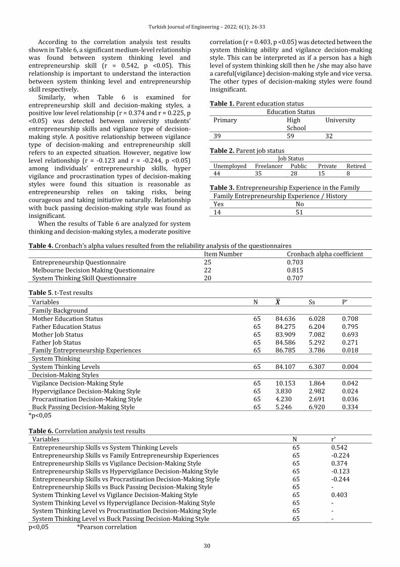
Turkish Journal of Engineering – 2022; 6(1); 26-33
30
According to the correlation analysis test results shown in Table 6, a significant medium-level relationship was found between system thinking level and entrepreneurship skill (r = 0.542, p <0.05). This relationship is important to understand the interaction between system thinking level and entrepreneurship skill respectively.
Similarly, when Table 6 is examined for entrepreneurship skill and decision-making styles, a positive low level relationship (r = 0.374 and r = 0.225, p <0.05) was detected between university students’ entrepreneurship skills and vigilance type of decision-making style. A positive relationship between vigilance type of decision-making and entrepreneurship skill refers to an expected situation. However, negative low level relationship (r = -0.123 and r = -0.244, p <0.05) among individuals’ entrepreneurship skills, hyper vigilance and procrastination types of decision-making styles were found this situation is reasonable as entrepreneurship relies on taking risks, being courageous and taking initiative naturally. Relationship with buck passing decision-making style was found as insignificant.
When the results of Table 6 are analyzed for system thinking and decision-making styles, a moderate positive
correlation (r = 0.403, p <0.05) was detected between the system thinking ability and vigilance decision-making style. This can be interpreted as if a person has a high level of system thinking skill then he /she may also have a careful(vigilance) decision-making style and vice versa. The other types of decision-making styles were found insignificant.
Table 1. Parent education status Education Status
Primary High School
University
39 59 32
Table 2. Parent job status Job Status
Unemployed Freelancer Public Private Retired 44 35 28 15 8
Table 3. Entrepreneurship Experience in the Family Family Entrepreneurship Experience / History Yes No 14 51
Table 4. Cronbach's alpha values resulted from the reliability analysis of the questionnaires Item Number Cronbach alpha coefficient Entrepreneurship Questionnaire 25 0.703 Melbourne Decision Making Questionnaire 22 0.815 System Thinking Skill Questionnaire 20 0.707
Table 5. t-Test results
*p<0,05 Table 6. Correlation analysis test results
Variables N r*
Entrepreneurship Skills vs System Thinking Levels 65 0.542 Entrepreneurship Skills vs Family Entrepreneurship Experiences 65 -0.224 Entrepreneurship Skills vs Vigilance Decision-Making Style 65 0.374 Entrepreneurship Skills vs Hypervigilance Decision-Making Style 65 -0.123 Entrepreneurship Skills vs Procrastination Decision-Making Style 65 -0.244 Entrepreneurship Skills vs Buck Passing Decision-Making Style 65 - System Thinking Level vs Vigilance Decision-Making Style 65 0.403 System Thinking Level vs Hypervigilance Decision-Making Style 65 - System Thinking Level vs Procrastination Decision-Making Style 65 - System Thinking Level vs Buck Passing Decision-Making Style 65 -
p<0,05 *Pearson correlation
Variables N Ss P*
Family Background Mother Education Status 65 84.636 6.028 0.708 Father Education Status 65 84.275 6.204 0.795 Mother Job Status 65 83.909 7.082 0.693 Father Job Status 65 84.586 5.292 0.271 Family Entrepreneurship Experiences 65 86.785 3.786 0.018 System Thinking System Thinking Levels 65 84.107 6.307 0.004 Decision-Making Styles Vigilance Decision-Making Style 65 10.153 1.864 0.042 Hypervigilance Decision-Making Style 65 3.830 2.982 0.024 Procrastination Decision-Making Style 65 4.230 2.691 0.036 Buck Passing Decision-Making Style 65 5.246 6.920 0.334
Turkish Journal of Engineering – 2022; 6(1); 26-33
31
4. CONCLUSION AND DISCUSSION
In this study, the relationships among entrepreneurial skills, system thinking level, decision-making styles and family education status, the presence of entrepreneurial history/experience in the family were examined.
4.1. Entrepreneurship and System Thinking
When the findings obtained in the study are analyzed, it is determined that there is a positive medium-level significant (r = 0.542) relationship between entrepreneurship skill and system thinking level. This shows that the more system thinking ability increases, the more entrepreneurship ability increases. It can be deducted that the development of any of the training activities will affect the other reciprocally.
It is stated in the literature that system thinking skills are effective in developing entrepreneurship skills. Today, problems have become increasingly complex. System thinking skills that require interdisciplinary, holistic and in-depth thinking come to the fore in solving these complex problems (Pagani and Otto 2013). Carlman et al.,2014 stated that “holistic approach also increases the quality of decision processes in entrepreneurship”. While making the system thinking approach, the decision-making process will help make the right decisions in turbulent and crisis environments. In order to develop entrepreneurship skills of individuals, it is recommended to use system thinking methods that encourages problem solving and innovation, from active learning methods (Hall et al., 2002; Pappas et al., 2012; Freeman et al., 2014).
Interdisciplinary approaches are important in educational practices; as real-world decisions often involve more than one area. From this perspective, individuals need to be equipped with more skills before entering the labor market or industrial society. However, in educational institutions, students are not properly equipped to solve and decide on interdisciplinary problems such as life-based sociological issues, engineering and design skills (Zeidler et al., 2009). Sadler and Zeidler (2005) stated that “rapid changes are created in our lives with science. In order to keep up with this speed, rational thinking and information technology of learners should be equipped with the ability to make decisions based on the data”.
4.2. Entrepreneurship and Decision-Making Styles
According to the data obtained, while there was a significant relationship among vigilance, hypervigilance and procrastination decision-making styles; In the buck passing decision-making style, no significant relationship was found. A low-level positive correlation (r = 0.374, p <0.05) was detected between entrepreneurship skill and vigilance type of decision-making style. Studies have reported that it provides practical information on how to take advantage of effective decision-making processes in entrepreneurship (Rayawan and Efrata 2017). Sustainable development means prosperity for today's society and future generations. The problems faced by entrepreneurs for sustainable development are quite
complex. In order to solve these complex problems, decision-making and problems should be viewed from multiple perspectives (Haan, 2010; Arvai et al., 2004). Scientific decision-making is important in developing individuals' learning abilities, scientific literacy, conceptual understanding, scientific research, attitude and social values.
4.3. Entrepreneurship Skills and Family Background
After the tests, no significant relationship between entrepreneurship skill and parental education/job status was found. This result was interpreted as the education and work status of the family have no effect on entrepreneurship skill. This indicates that individuals may have entrepreneurial skills independent of their families’ socio-demographic and occupational status. It gives the opportunity to develop entrepreneurial skills through education. According to the results, a significant opposite low-level (r=-0.224) relationship was found between entrepreneurship skill and family entrepreneurship experience. In order to explain this situation, the questionnaire questions were re-examined and it was understood that unsuccessful entrepreneurship experiences were frequently expressed in the free texts written by the participants and this situation might have caused this negative relationship.
In the literature review, it has been reported that entrepreneurship education is more important than the features that come from the family, which is a traditional approach of developing entrepreneurship. These results indicate that, depending on the entrepreneurship training received, entrepreneur candidates' attitudes towards entrepreneurship, perceptions of convenience and feasibility to become entrepreneurs, and thus entrepreneurship tendencies can increase positively. According to Korkmaz, (2012), entrepreneurship education is stated to be one of the most important factors especially in the formation of attitudes and behaviors of young entrepreneur candidates towards becoming entrepreneur. Matlay, (2008) determined that “entrepreneurship education had a positive effect on the individual's tendency towards entrepreneurship and increased it significantly”. Some researches like Mueller (2011), Fayolle and Gailly 2013 and Miller et al., 2009 indicated that “there is a positive and significant relationship between entrepreneurship education and entrepreneurship tendency and sub-dimensions, supporting the results obtained from this research”. Graevenitz et al. (2010) suggested that “to start at an early age in developing entrepreneurial skills”.
With the assessment of entrepreneurship as a discipline, the view that entrepreneurship is innate has changed and the view of entrepreneurship through education has started to be accepted. Drucker (1985) reported that “entrepreneurship is not a magic, a mystery, it is a subject and can be learned”. This judgment reached on entrepreneurship has changed the perspective and stated the opinions that entrepreneurship education can be done (Kuratko 2003). In line with the ideas that entrepreneurship is

Turkish Journal of Engineering – 2022; 6(1); 26-33
32
learnable, research and studies on entrepreneurship education have started.
As a result; Today’s global environment, forces everybody to take steps toward developing entrepreneurial skills at every level to sustain competitive advantage in the business environment. Entrepreneurship, system thinking skills and decision-making processes are very important for the development of innovation. It is recommended to include active teaching programs for the development of these three skills in universities and the other institutions. A future study will be useful to compare with initial results after completing entrepreneurship and system thinking education. New studies on entrepreneurship, system thinking skills and decision-making styles in the covid-19 pandemic period may be helpful to understand the interactions among them better in telecommuting and e-learning environment. Conflicts of interest The authors declare no conflicts of interest. REFERENCES Arvai J L, Campbell V E A, Baird A & Rivers L (2004).
Teaching students to make better decisions about the environment: lessons from the decision sciences. The Journal of Environmental Education, 36(1), 33-44.
Assaraf O B Z & Orion N (2005). Development of system thinking skills in the context of earth system education. Journal of Research in Science Teaching, 42(5), 518–560. DOI: 10.1002/tea.20061
Berglund H & Wennberg K (2006) Creativity among entrepreneurship students: Comparing engineering and business education. International Journal of Continuing Engineering Education and Life-long Learning. 16 (5), 366-379.
Cantillon R (1775). Essay on the nature of trade in general, London.
Carlman I, Grönlund E & Longueville A (2014). Models and methods as support for sustainable decision- making with focus on legal operationalization. Ecological Modelling, 306, 95-100
Casson M C (2010). Entrepreneurship: Theory, Networks, History. Edward Elgar: Cheltenham, U.K.
Davidsson P (2006). Nascent entrepreneurship: Empirical studies and developments. Foundations and Trends in Entrepreneurship, 2 (1), 1-76.
Deniz M E (2004). Investigation of the relation between decision self-esteem, decision making style and problem solving skill of the university students. Eurasian Journal of Educational Research, 4(15), 23-35.
Dori D & Sillitto H (2017). What is a system? An ontological framework. Systems Engineering, 20 (3), 207–219.
Drucker P F (1985). Innovation and entrepreneurship. New York, NY: Harper & Row.
Evagorou M, Korfiatis K, Nicolaou C & Constantinou C (2009). An investigation of the potential of interactive simulations for developing system thinking skills in elementary school: a case study with fifth-graders
and sixth graders. International. Journal of Science Education 31, 655–674. DOI: 10.1080/09500690701749313
Fayolle A & Gailly B (2013). The impact of entrepreneurship education on entrepreneurial attitudes and intention: Hysteresis and persistence. Journal of Small Business Management, 53(1), 75- 93.
Forrester J W (2007). System Dynamics – a personal view of the first fifty years. System Dynamics Review, 23(2-3), 345-358.
Freeman S, Eddy S L, McDonough M, Smith M K, Okoroafor N & Jordt H (2014). Active learning increases student performance in science, engineering, and mathematics. Proceedings of National Academy of Sciences of the United States of America, 111(23), 8410–8415.
Gay L R (1996). Educational research: Competencies for analysis and application. 5. Edition, Prentice-Hall, Inc., USA.
Gelderen M V & Masurel E (2012). Entrepreneurship in context. Routledge, New York
Gibb A (1987). Enterprise Culture - Its Meaning and Implications for Education and Training. Journal of European Industrial Training, 11(2), 2-38
Gibb A (2011). Concepts into practice: meeting the challenge of development of entrepreneurship educators around an innovative paradigm. International Journal of Entrepreneurial Behaviour & Research 17(2), 146–165.
Graevenitz G V, Hardoff D & Weber R (2010). The effects of Entrepreneurship Education. Journal of Economic Behavior Organization, 76, 90-112.
Greenspan A & Rosan R M (2006). The Role of Universities Today: Critical Partners in Economic Development and Global Competitiveness. http://www.icfconsulting.com/Markets/Community_Development/docfiles/role-niversities.pdf, [Accessed 30.12.2019].
Guzmán J Y & Liñán P (2005). Perspectives on Entrepreneurial Education: A US-Europe Comparison. Jean Monnet European Studies Centre Universidad Antonio de Nebrija
Hall S R, Waitz I, Brodeur D R, Soderholm D H & Nasr R (2002). Adoption of active learning in amlecture-based engineering class. In 32nd Frontiers in education conference, T2A-9. https://doi.org/10. 1109/fie.2002.1157921.
Haan G (2010). The development of ESD-related competencies in supportive institutional frameworks. International Review of Education, 56(2-3), 315-328.
Hernandez G, Allen J & Mistree F (1998). Approxımate-Cooperatıve Desıgn Formulatıons for Enterprıse Desıgn and Integratıon. Proceedings of Detc98/Dac. Asme Design Engineering Technical Conference September 13-16, Atlanta, GA
Henry C, Hill F & Leitch C (2003). Entrepreneurship Education and Training: The Issue of Effectiveness. Ashgate Publishing Ltd., London.
Kalyani B P R & Kumar D M (2011). Motivational factors, entrepreneurship and education: Study with reference to women in SMEs. For East Journal of Psychology and Business, 3(3), 14-35.
Turkish Journal of Engineering – 2022; 6(1); 26-33
33
Kashif M, Darain H, Islam S, Javed S & Irshad S (2016). Entrepreneurial Aptitude among the University Students of MBBS, BDS and DPT. Indian Journal of Physiotherapy and Occupational Therapy, 10(1), 66-70
Korkmaz O (2012). Üniversite öğrencilerinin girişimcilik eğilimlerini belirlemeye yönelik bir araştırma: Bülent Ecevit Üniversitesi örneği. Afyon Kocatepe Üniversitesi İİBF Dergisi. XIV (II), 209-226.
Kuratko D (2003). Entrepreneurship Education: Emerging Trends and Challenges for the 21st Century: From Legitimization to Leadership. Coleman Foundation White Paper Series.
Long C (2012). Teach Your Students to Fail Better with Design Thinking. Learning & Leading with Technology, 9(5), 16-20.
Mann L M, Radford P, Burnett S, Ford M, Bond K, Leung H, Nakamura G & Malindi M M (2014). Impact of Entrepreneurship Education on Entrepreneurial Intent at Further Education and Training (FET) Colleges in South Africa. Gordon Institute of Business Science. University of Pretoria, MBA.
Matlay H (2008). The impact of entrepreneurship education on entrepreneurial outcomes. Journal of Small Business and Enterprise Development, 15(2), 382-396.
McGrath R G & MacMillan L C (1995). Discovery Driven Planning.” Harvard Business Review, 73, 44-54.
McGrath R G & MacMillan I C (2000). The entrepreneurial mindset: Strategies for continuously creating opportunity in an age of uncertainty (Vol. 284). Harvard Business Press.
Michaels C (2012). Essentials of Entrepreneurial Thinking: What Successful People Didn't Learn in School. Amazon. Published by cliff Michaels and associated Inc. Santa Monica. USA.CA (www.CliffMichaels.com)
Miller B K, Bell J D, Palmer M & Gonzalez A (2009). Predictors of entrepreneurial intentions: A quasiexperiment comparing students enrolled in introductory management and entrepreneurship classes. Journal of Business & Entrepreneurship, 21 (2), 39-62.
Moore S M, Dolansky M A, Singh M, Palmieri P & Alemi F (2010). The Systems Thinking Scale. https://nursing.case.edu/nursing/media/nursing/pdf-dox/STS_Manual.pdf
Mueller S (2011). Increasing entrepreneurial intention: Effective entrepreneurship course characteristics. International Journal of Entrepreneurship and Small Business, 13, 55-74.
Nunnally J C & Bernstein I H (1994). The Assessment of Reliability. Psychometric Theory, 3, 248-292.
Orgill M, York S & MacKellar J (2019). Introduction to systems thinking for the chemistry education community. Journal of Chemical Education 2019 96 (12), 2720-2729, DOI: 10.1021/acs.jchemed.9b00169
Pagani M & Otto P (2013). Integrating strategic thinking and simulation in marketing strategy: Seeing the whole System. Journal of Business Research, 66, 1568–1575
Pappas E, Pierrakos O & Nagel R (2012). Using Bloom’s Taxonomy to teach sustainability in multiple contexts. Journal of Cleaner Production, 48, 54–64.
Patel S & Mehta K (2016). Systems, design, and entrepreneurial thinking: Comparative frameworks. Systemic Practice and Action Research, ISSN 1094-429X, 29(6), DOI 10.1007/s11213-016-9404-5
Patır S & Karahan M (2010). Girişimcilik eğitimi ve üniversite öğrencilerinin girişimcilik profillerinin belirlenmesine yönelik bir alan araştırması. İşletme ve Ekonomi Araştırmaları Dergisi. 1 (2), 27-44.
Rayawan W & Efrata T C (2017). The effect locus of control and need for achievement towards entrepreneurial performance. Review Management Entrepreneurship, 1, 36–49.
Saaty T L (2008). Decision making with the analytic hierarchy process. International Journal of Service Sciences 1(1), 83–98
Sadler T D & Zeidler D L (2005). The significance of content knowledge for informal reasoning regarding socioscientific issues: Applying genetics knowledge to genetic engineering issues. Science Education, 89(1), 71-93.
Solomon J & Aikenhead G S (Eds.). (1994). STS education: International perspectives on reform. New York: Teachers College Press
Thunholm P (2009). Military leaders and followers – do they have different decision styles? Scandinavian Journal of Psychology, 50(4), 317-324
Verhoeff R P, Waarlo A J & Boersma K T (2008) Systems modeling and the development of coherent understanding of cell biology. International Journal of Science Education, 30, 543–568
Yesilyaprak B (2003). Eğitimde rehberlik hizmetleri ve gelişimsel yaklaşım. Ankara: Nobel Yayincilik.
Zeidler D L, Sadler T D, Applebaum S & Callahan B E (2009). Advancing reflective judgment through socioscientific issues. Journal of Research in Science Teaching, 46(1), 74-101.
© Author(s) 2022. This work is distributed under https://creativecommons.org/licenses/by-sa/4.0/
* Corresponding Author Cite this article
*([email protected]) ORCID ID 0000-0001-7978-6306 ([email protected]) ORCID ID 0000-0002-3536-3931 ([email protected]) ORCID ID 0000-0002-5201-5453 Research Article / DOI: 10.31127/tuje.775536
Gunoz A, Kepir Y & Kara M (2022). The investigation of hardness and density properties of GFRP composite pipes under seawater conditions. Turkish Journal of Engineering, 6(1), 34-39
Received: 29/07/2020; Accepted: 21/12/2020
Turkish Journal of Engineering – 2022; 6(1); 34-39
Turkish Journal of Engineering
https://dergipark.org.tr/en/pub/tuje
e-ISSN 2587-1366
The investigation of hardness and density properties of GFRP composite pipes under seawater conditions
Alper Gunoz*1 , Yusuf Kepir1 , Memduh Kara1
1Mersin University, Faculty of Engineering, Mechanical Engineering Department, Mersin, Turkey
Keywords ABSTRACT Composite pipes Seawater effect Hardness Density
Glass fiber reinforced polymer (GFRP) composite pipes are mostly used in transmission lines of submarine oil, natural gas, and chemical fluids. The alterations in mechanical characteristics of composite pipes used in submarine applications are of great importance to the lifespan of the material. Some important mechanical properties of composite materials are density and hardness value. In this study, the changes in the density and hardness values of GFRP composite pipes which were unexposed to seawater and exposed to seawater for 1, 2 and 3 months were investigated. As a result of the present study, it was deduced that the characteristics of the sample changed with the effect of seawater.
1. INTRODUCTION
Glass Fiber Reinforced Polymers (GFRP) are composite materials produced by incorporating glass fiber into resin as a reinforcement material. Numerous studies have been conducted on the mechanical properties of glass fiber pipes due to the rapid increase in their usage. GFRP composites are suitable for use in naval constructions. On account of their superior wear resistance and lightness properties, GFRP composite pipes are mostly used in transmission lines of submarine oil, natural gas, and chemical fluids (Gellert and Turley, 1999; Kootsookos et al., 2001; Kara, 2012; Kara et al., 2014; Uyaner et al., 2014). It is also widely used in civil defense and aerospace sectors due to its many advantages, such as long lifespan and low cost (Schutte, 1994).
Fiber-reinforced composite pipes used in these fields are exposed to various fluids that may have aggressive effects on the pipes’ material composition. The mechanical properties of composite materials change irreversibly when exposed to environmental terms such as humidity and temperature for a long time. This change in the characteristics of composite materials is called ageing. Changes in mechanical characteristics of materials under environmental conditions such as humidity, temperature, pure water, saltwater, and ultraviolet radiation should be well known for determining the strength and service life of composite
materials at the places of usage (Doğan, 2014). Many polymer materials absorbed water when they left in water for a long time. This absorbed water disrupts the interfacial bonds and changes the characteristics of the polymers. Absorbed water softens the material, so it increases the distance of the polymer chains (Papanicolaou et al., 2006; Mouzakis et al., 2008; Baschek et al., 1998). Stresses procured by absorbed water cause expansion. Consequently, the damage tolerance and structural strength of the material is reduced. Water absorption creates reversible and irreversible interactions in the mechanical characteristics of polymer composites. Degradation of mechanical characteristics by water absorption causes some unwanted formation such as micro-cracks, interfacial damages, plastification, and swelling of the polymer. The plastification causes plastic deformation by reducing the glass transition temperature (Tg) of the material. The water absorbed into the material forms expansion forces and the polymer chains are forced under the influence of these forces (Saha and Bal 2018; Lee et al., 1993). Glass reinforced plastic materials when remained in the water for a long time, the damage caused by water creates a significant change in creep, tension and fatigue characteristics of the materials (Liao et al., 1998). The mechanical characteristics of the matrix and the fiber/matrix interface area are the essential factors in controlling the performance of GFRP in a fluid medium (Schutte, 1994).
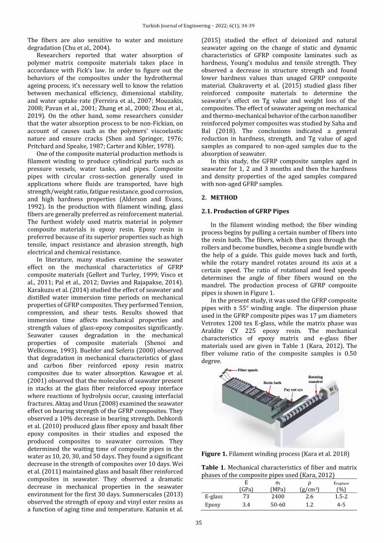
Turkish Journal of Engineering – 2022; 6(1); 34-39
35
The fibers are also sensitive to water and moisture degradation (Chu et al., 2004).
Researchers reported that water absorption of polymer matrix composite materials takes place in accordance with Fick's law. In order to figure out the behaviors of the composites under the hydrothermal ageing process, it's necessary well to know the relation between mechanical efficiency, dimensional stability, and water uptake rate (Ferreira et al., 2007; Mouzakis, 2008; Pavan et al., 2001; Zhang et al., 2000; Zhou et al., 2019). On the other hand, some researchers consider that the water absorption process to be non-Fickian, on account of causes such as the polymers’ viscoelastic nature and ensure cracks (Shen and Springer, 1976; Pritchard and Speake, 1987; Carter and Kibler, 1978).
One of the composite material production methods is filament winding to produce cylindrical parts such as pressure vessels, water tanks, and pipes. Composite pipes with circular cross-section generally used in applications where fluids are transported, have high strength/weight ratio, fatigue resistance, good corrosion, and high hardness properties (Alderson and Evans, 1992). In the production with filament winding, glass fibers are generally preferred as reinforcement material. The furthest widely used matrix material in polymer composite materials is epoxy resin. Epoxy resin is preferred because of its superior properties such as high tensile, impact resistance and abrasion strength, high electrical and chemical resistance.
In literature, many studies examine the seawater effect on the mechanical characteristics of GFRP composite materials (Gellert and Turley, 1999; Visco et al., 2011; Pal et al., 2012; Davies and Rajapakse, 2014). Karakuzu et al. (2014) studied the effect of seawater and distilled water immersion time periods on mechanical properties of GFRP composites. They performed Tension, compression, and shear tests. Results showed that immersion time affects mechanical properties and strength values of glass-epoxy composites significantly. Seawater causes degradation in the mechanical properties of composite materials (Shenoi and Wellicome, 1993). Buehler and Seferis (2000) observed that degradation in mechanical characteristics of glass and carbon fiber reinforced epoxy resin matrix composites due to water absorption. Kawagoe et al. (2001) observed that the molecules of seawater present in stacks at the glass fiber reinforced epoxy interface where reactions of hydrolysis occur, causing interfacial fractures. Aktaş and Uzun (2008) examined the seawater effect on bearing strength of the GFRP composites. They observed a 10% decrease in bearing strength. Dehkordi et al. (2010) produced glass fiber epoxy and basalt fiber epoxy composites in their studies and exposed the produced composites to seawater corrosion. They determined the waiting time of composite pipes in the water as 10, 20, 30, and 50 days. They found a significant decrease in the strength of composites over 10 days. Wei et al. (2011) maintained glass and basalt fiber reinforced composites in seawater. They observed a dramatic decrease in mechanical properties in the seawater environment for the first 30 days. Summerscales (2013) observed the strength of epoxy and vinyl ester resins as a function of aging time and temperature. Katunin et al.
(2015) studied the effect of deionized and natural seawater ageing on the change of static and dynamic characteristics of GFRP composite laminates such as hardness, Young’s modulus and tensile strength. They observed a decrease in structure strength and found lower hardness values than unaged GFRP composite material. Chakraverty et al. (2015) studied glass fiber reinforced composite materials to determine the seawater's effect on Tg value and weight loss of the composites. The effect of seawater ageing on mechanical and thermo-mechanical behavior of the carbon nanofiber reinforced polymer composites was studied by Saha and Bal (2018). The conclusions indicated a general reduction in hardness, strength, and Tg value of aged samples as compared to non-aged samples due to the absorption of seawater.
In this study, the GFRP composite samples aged in seawater for 1, 2 and 3 months and then the hardness and density properties of the aged samples compared with non-aged GFRP samples.
2. METHOD
2.1. Production of GFRP Pipes
In the filament winding method; the fiber winding process begins by pulling a certain number of fibers into the resin bath. The fibers, which then pass through the rollers and become bundles, become a single bundle with the help of a guide. This guide moves back and forth, while the rotary mandrel rotates around its axis at a certain speed. The ratio of rotational and feed speeds determines the angle of fiber fibers wound on the mandrel. The production process of GFRP composite pipes is shown in Figure 1.
In the present study, it was used the GFRP composite pipes with ± 55° winding angle. The dispersion phase used in the GFRP composite pipes was 17 µm diameters Vetrotex 1200 tex E-glass, while the matrix phase was Araldite CY 225 epoxy resin. The mechanical characteristics of epoxy matrix and e-glass fiber materials used are given in Table 1 (Kara, 2012). The fiber volume ratio of the composite samples is 0.50 degree.
Figure 1. Filament winding process (Kara et al. 2018)
Table 1. Mechanical characteristics of fiber and matrix phases of the composite pipes used (Kara, 2012)
E (GPa)
σt (MPa)
ρ (g/cm3)
εrupture
(%) E-glass 73 2400 2.6 1.5-2
Epoxy 3.4 50-60 1.2 4-5
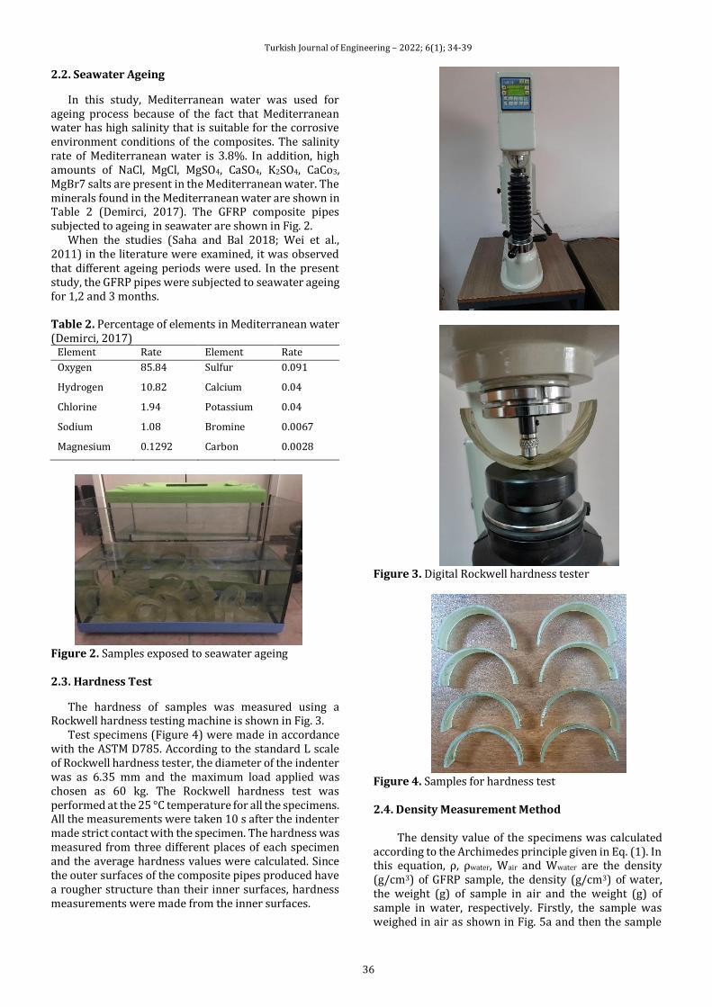
Turkish Journal of Engineering – 2022; 6(1); 34-39
36
2.2. Seawater Ageing
In this study, Mediterranean water was used for ageing process because of the fact that Mediterranean water has high salinity that is suitable for the corrosive environment conditions of the composites. The salinity rate of Mediterranean water is 3.8%. In addition, high amounts of NaCl, MgCl, MgSO4, CaSO4, K2SO4, CaCo3, MgBr7 salts are present in the Mediterranean water. The minerals found in the Mediterranean water are shown in Table 2 (Demirci, 2017). The GFRP composite pipes subjected to ageing in seawater are shown in Fig. 2.
When the studies (Saha and Bal 2018; Wei et al., 2011) in the literature were examined, it was observed that different ageing periods were used. In the present study, the GFRP pipes were subjected to seawater ageing for 1,2 and 3 months.
Table 2. Percentage of elements in Mediterranean water (Demirci, 2017)
Element Rate Element Rate
Oxygen 85.84 Sulfur 0.091
Hydrogen 10.82 Calcium 0.04
Chlorine 1.94 Potassium 0.04
Sodium 1.08 Bromine 0.0067
Magnesium 0.1292 Carbon 0.0028
Figure 2. Samples exposed to seawater ageing 2.3. Hardness Test
The hardness of samples was measured using a Rockwell hardness testing machine is shown in Fig. 3.
Test specimens (Figure 4) were made in accordance with the ASTM D785. According to the standard L scale of Rockwell hardness tester, the diameter of the indenter was as 6.35 mm and the maximum load applied was chosen as 60 kg. The Rockwell hardness test was performed at the 25 °C temperature for all the specimens. All the measurements were taken 10 s after the indenter made strict contact with the specimen. The hardness was measured from three different places of each specimen and the average hardness values were calculated. Since the outer surfaces of the composite pipes produced have a rougher structure than their inner surfaces, hardness measurements were made from the inner surfaces.
Figure 3. Digital Rockwell hardness tester
Figure 4. Samples for hardness test 2.4. Density Measurement Method
The density value of the specimens was calculated according to the Archimedes principle given in Eq. (1). In this equation, ρ, ρwater, Wair and Wwater are the density (g/cm3) of GFRP sample, the density (g/cm3) of water, the weight (g) of sample in air and the weight (g) of sample in water, respectively. Firstly, the sample was weighed in air as shown in Fig. 5a and then the sample
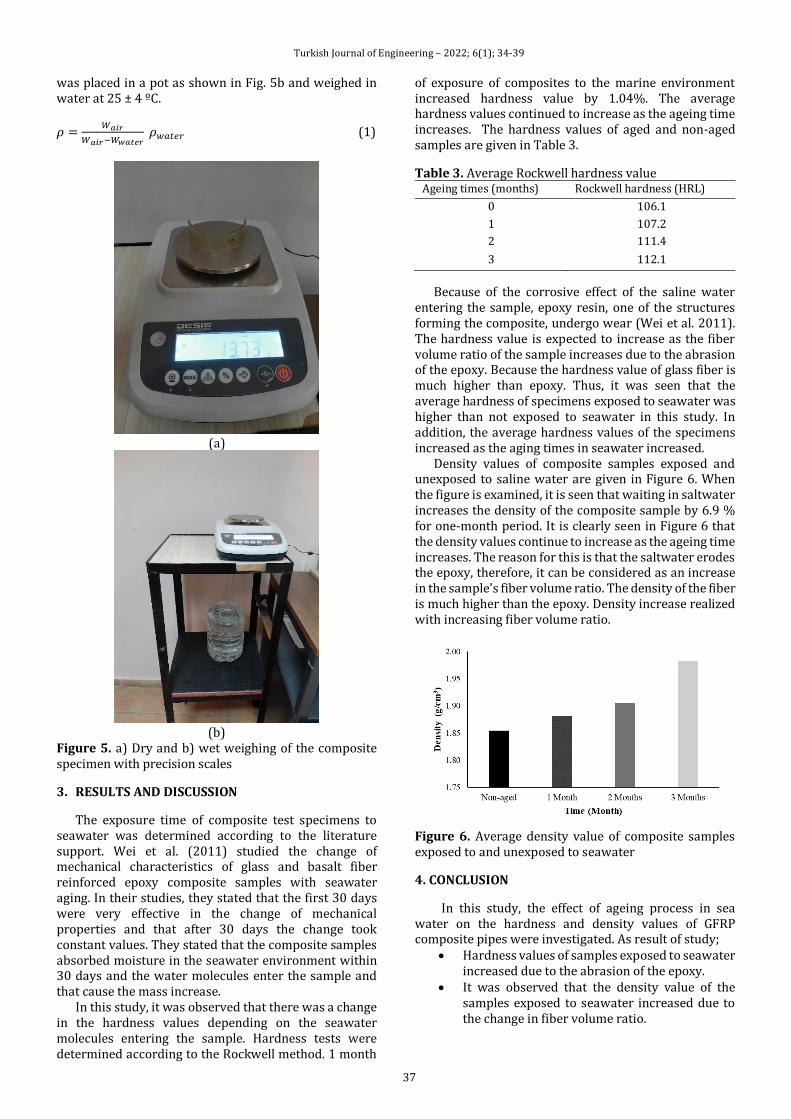
Turkish Journal of Engineering – 2022; 6(1); 34-39
37
was placed in a pot as shown in Fig. 5b and weighed in water at 25 ± 4 ºC.
𝜌 =𝑊𝑎𝑖𝑟
𝑊𝑎𝑖𝑟−𝑊𝑤𝑎𝑡𝑒𝑟 𝜌𝑤𝑎𝑡𝑒𝑟 (1)
(a)
(b)
Figure 5. a) Dry and b) wet weighing of the composite specimen with precision scales
3. RESULTS AND DISCUSSION
The exposure time of composite test specimens to seawater was determined according to the literature support. Wei et al. (2011) studied the change of mechanical characteristics of glass and basalt fiber reinforced epoxy composite samples with seawater aging. In their studies, they stated that the first 30 days were very effective in the change of mechanical properties and that after 30 days the change took constant values. They stated that the composite samples absorbed moisture in the seawater environment within 30 days and the water molecules enter the sample and that cause the mass increase.
In this study, it was observed that there was a change in the hardness values depending on the seawater molecules entering the sample. Hardness tests were determined according to the Rockwell method. 1 month
of exposure of composites to the marine environment increased hardness value by 1.04%. The average hardness values continued to increase as the ageing time increases. The hardness values of aged and non-aged samples are given in Table 3.
Table 3. Average Rockwell hardness value Ageing times (months) Rockwell hardness (HRL)
0 106.1
1 107.2
2 111.4
3 112.1
Because of the corrosive effect of the saline water entering the sample, epoxy resin, one of the structures forming the composite, undergo wear (Wei et al. 2011). The hardness value is expected to increase as the fiber volume ratio of the sample increases due to the abrasion of the epoxy. Because the hardness value of glass fiber is much higher than epoxy. Thus, it was seen that the average hardness of specimens exposed to seawater was higher than not exposed to seawater in this study. In addition, the average hardness values of the specimens increased as the aging times in seawater increased.
Density values of composite samples exposed and unexposed to saline water are given in Figure 6. When the figure is examined, it is seen that waiting in saltwater increases the density of the composite sample by 6.9 % for one-month period. It is clearly seen in Figure 6 that the density values continue to increase as the ageing time increases. The reason for this is that the saltwater erodes the epoxy, therefore, it can be considered as an increase in the sample's fiber volume ratio. The density of the fiber is much higher than the epoxy. Density increase realized with increasing fiber volume ratio.
Figure 6. Average density value of composite samples exposed to and unexposed to seawater
4. CONCLUSION
In this study, the effect of ageing process in sea water on the hardness and density values of GFRP composite pipes were investigated. As result of study;
Hardness values of samples exposed to seawater increased due to the abrasion of the epoxy.
It was observed that the density value of the samples exposed to seawater increased due to the change in fiber volume ratio.

Turkish Journal of Engineering – 2022; 6(1); 34-39
38
Author contributions Alper GÜNÖZ: Conceptualization; Material supplying; Data curation; Investigation; Methodology; Resources; Visualization; Manuscript writing. Yusuf KEPİR: Conceptualization; Material supplying; Investigation; Methodology; Visualization; Manuscript writing. Memduh KARA: Conceptualization; Material supplying; Supervision; Validation; Review & editing. Conflict of Interest: The authors have no conflicts of interest to declare.
REFERENCES
Aktaş A & Uzun İ (2008). Sea water effect on pinned-joint glass fibre composite materials. Composite structures, 85(1), 59-63.
Alderson K L & Evans K E (1992). Low velocity transverse impact of filament-wound pipes: Part 1. Damage due to static and impact loads. Composite structures, 20(1), 37-45.
ASTM D 785 (1993), Rockwell Hardness of Plastics and Electrical Insulating Materials. American Society for Testing and Materials, ASTM International, West Conshohocken, PA, 2006, www.astm.org.
Baschek G, Hartwig G & Zahradnik F (1998). Effect of water absorption in polymers at low and high temperatures. Polymer, 40, 3433-3441.
Buehler F U & Seferis J C (2000). Effect of reinforcement and solvent content on moisture absorption in epoxy composite materials. Composites Part A: Applied Science and Manufacturing, 31(7), 741-748.
Carter H G & Kibler K G (1978). Langmuir-type model for anomalous moisture diffusion in composite resins. Journal of Composite Materials, 12(2), 118-131.
Chakraverty A P, Mohanty U K, Mishra S C & Satapathy A. (2015). Sea water ageing of GFRP composites and the dissolved salts. In IOP conference series: materials science and engineering (Vol. 75, No. 1, p. 012029). IOP Publishing.
Chu W, Wu L & Karbhari V M (2004). Durability evaluation of moderate temperature cured E-glass/vinylester systems. Composite Structures, 66(1-4), 367-376.
Davies P & Rajapakse Y D (2014). Durability of composites in a marine environment (Vol. 208). Springer, Berlin, Germany.
Dehkordi M T, Nosraty H, Shokrieh M M, Minak G & Ghelli D (2010). Low velocity impact properties of intra-ply hybrid composites based on basalt and nylon woven fabrics. Materials and Design, 31(8), 3835-3844.
Demirci I (2017). Karbon nanotüp ve nano silika takviyeli bazalt/epoksi hibrit nanokompozitlerin korozif ortamda darbe davranışları. Master’s Thesis, Selçuk University, Konya, Turkey.
Doğan A (2014). Farklı çevresel koşullara maruz kompozitlerin mekanik davranışları. Master’s Thesis, Dokuz Eylül University, Izmir, Turkey.
Ferreira J M, Pires J T B, Costa J D, Errajhi O A & Richardson M (2007). Fatigue damage and environment interaction of polyester aluminized
glass fiber composites. Composite structures, 78(3), 397-401.
Gellert E P & Turley D M (1999). Seawater immersion ageing of glass-fibre reinforced polymer laminates for marine applications. Composites Part A: Applied Science and Manufacturing, 30(11), 1259-1265.
Kara M (2012). Düşük hızlı darbe sonrası yama ile tamir edilmiş filaman sarım CTP boruların iç basınç altındaki hasar davranışı. Doctoral Thesis, Selçuk University, Konya, Turkey.
Kara M, Uyaner M, Avcı A & Akdemir A (2014). Effect of non-penetrating impact damages of pre-stressed GRP tubes at low velocities on the burst strength. Composites: Part B, 60, 507-514.
Kara M, Kırıcı M, Tatar A C & Avcı A (2018). Impact behavior of carbon fiber/epoxy composite tubes reinforced with multi-walled carbon nanotubes at cryogenic environment. Composites Part B: Engineering, 145, 145-154.
Karakuzu R, Kanlioglu H, & Deniz M E (2014). Environmental Effects on Mechanical Properties of Glass-Epoxy Composites. Materials Testing, 56(5), 355-361.
Katunin A, Gnatowski A & Kajzer W (2015). Evolution of static and dynamic properties of GFRP laminates during ageing in deionized and seawater. Advanced Composites Letters, 24(3), 096369351502400302.
Kawagoe M, Doi Y, Fuwa N, Yasuda T & Takata K (2001). Effects of absorbed water on the interfacial fracture between two layers of unsaturated polyester and glass. Journal of materials science, 36(21), 5161-5167.
Kootsookos A, Mourotz A P & St John N A (2001). Comparison of the seawater durability of carbon and glass polymer composites. Proceedings of the 13th International Conference on Composite Materials, ID-1200, Proceedings of ICCM-13, Beijing.
Lee T H Y C, Freddy & Loh N L (1993). Characterization of a fibre-reinforced PPS composite by dynamic mechanical analysis: effect of aspect ratio and static stres. Composite science and technology, 49, 217-223.
Liao K, Schultesiz C R, Hunston D L & Brinson L C (1998). Long-term durability of fiber-reinforced polymer-matrix composite materials for infrastructure applications: a review. Journal of advanced materials, 30(4):3–40.
Mouzakis D E, Zoga H and Galiotis C (2008). Accelerated environmental ageing study of polyester/glass fiber reinforced composites (GFRPCs). Composites part B: engineering, 39(3), 467-475.
Pal R, Murthy H N, Sreejith M, Mahesh K V, Krishna M & Sharma S C (2012). Effect of laminate thickness on moisture diffusion of polymer matrix composites in artificial seawater ageing. Frontiers of Materials Science, 6(3), 225-235.
Papanicolaou G C, Kosmidou T V, Vatalis A S & Delides C G (2006). Water absorption mechanism and some anomalous effects on the mechanical and viscoelastic behavior of an epoxy system. Journal of Applied Polymer Science, 99(4), 1328-1339.
Pavan R M, Saravanan V, Dinesh A R, Rao Y J, Srihari S & Revathi A (2001). Hygrothermal effects on painted and unpainted glass/epoxy composites—Part A:

Turkish Journal of Engineering – 2022; 6(1); 34-39
39
moisture absorption characteristics. Journal of reinforced plastics and composites, 20(12), 1036-1047.
Pritchard G & Speake S D (1987). The use of water absorption kinetic data to predict laminate property changes. Composites, 18(3), 227-232.
Saha S & Bal S (2018). Long term hydrothermal effect on the mechanical and thermo-mechanical properties of carbon nanofiber doped epoxy composites. Journal of Polymer Engineering, 38(3), 251-261.
Schutte C L (1994). Environmental durability of glass-fiber composites. Materials Science and Engineering: R: Reports, 13(7), 265-323.
Shen C H & Springer G S (1976). Moisture absorption and desorption of composite materials. Journal of composite materials, 10(1), 2-20.
Shenoi R A & Wellicome J F (1993). Composite Materials in Maritime Structures: Fundamental Aspects (Vol. 1). Cambridge University Press, England.
Summerscales J (2013). Durability of composites in the marine environment. Solid Mechanics and Its Applications, Vol 208, no. 3, pp. 1–13.
Uyaner M, Kara M & Şahin A. (2014). Fatigue Behavior of Filament Wound E-Glass/Epoxy Composite Tubes Damaged by Low Velocity Impact. Composites: Part B, 61, 358-364.
Wei B, Cao H & Song S (2011). Degradation of basalt fibre and glass fibre/epoxy resin composites in seawater. Corrosion Science, 53(1), 426-431.
Visco A M, Campo N & Cianciafara P (2011). Comparison of seawater absorption properties of thermoset resins based composites. Composites Part A: Applied Science and Manufacturing, 42(2), 123-130.
Zhang S, Karbhari V M, Mai L Y & Mai Y W (2000). Evaluation of property retention in E-glass/vinylester composites after exposure to salt solution and natural weathering. Journal of reinforced plastics and composites, 19(9), 704-731.
Zhou H, Wang G, Chen L, Yu Z, Smith L M & Chen F (2019). Hydrothermal Aging Properties of Three Typical Bamboo Engineering Composites. Materials, 12(9), 1450.
© Author(s) 2022. This work is distributed under https://creativecommons.org/licenses/by-sa/4.0/
* Corresponding Author Cite this article
*([email protected]) ORCID ID 0000 – 0002 – 8625 – 8058 ([email protected]) ORCID ID 0000 – 0001 – 8113 – 7874 Research Article / DOI: 10.31127/tuje.801441
Çağatay M T & Karacan S (2022). Multivariable Generalized Predictive Control of Reactive Distillation Column Process for Biodiesel Production. Turkish Journal of Engineering, 6(1), 40-53
Received: 28/09/2020; Accepted: 11/01/2021
Turkish Journal of Engineering – 2022; 6(1); 40-53
Turkish Journal of Engineering
https://dergipark.org.tr/en/pub/tuje
e-ISSN 2587-1366
Multivariable generalized predictive control of reactive distillation column process for biodiesel production
Mehmet Tuncay Çağatay*1 , Süleyman Karacan 2
1Ministry of National Defence, Presidency of General Staff, Ankara, Turkey 2Ankara University, Engineering Faculty, Department of Chemical Engineering, Ankara, Turkey
Keywords ABSTRACT Multivariable Generalized Predictive Control PID Control Reactive Distillation Column Biodiesel
Most industrial control systems consist of a significant number of control loops. Generally, large processes are divided into many interconnected subsystems affecting each other, thus creating multivariable systems known as multiple–input multiple–output (MIMO) process. Generalized Predictive Control (GPC) based control algorithm is most suitable for MIMO systems. In this study, multivariate nonlinear (NL) GPC and discrete–time PID control of calcium oxide catalyst–packed reactive distillation (RD) column used for biodiesel production from waste cooking oil were investigated. Temperatures of reaction and reboiler sections were controlled by using non–decoupled and decoupled MIMO NLGPC and discrete–time MIMO PID algorithms. Feed flow rate with constant molar ratio and reboiler heat duty parameters were selected as manipulating variables. All recommended control methods, except for non-decoupled MIMO NLGPC, have been found to perform satisfactorily reference tracking and disturbance rejection in RD column. Consequently, the best control results were obtained in the decoupled MIMO NLGPC.
1. INTRODUCTION
In recent years, requirements for high quality process control have increased significantly in parallel to the growing complexity of plants and sharper specifications of product feature. But, smart and model–based control techniques have also been developed to accomplish strict control algorithms. On the other hand, computing power has increased to a very high level. Thus, computationally expensive computer models become appropriate to solve much complex problems.
The idea of the control strategy for a process is to maintain the desired operational variables smoothly and consistently. Thus, operating conditions of the system are fixed by control action to reach the target in the most effective way possible. When the process conditions change, the controllers need to be adjusted again to attain acceptable control results. Generalized Predictive Control (GPC) is considered as to be excellent to get satisfactory controls. This receding horizon method predicts the output of the plant in several sampling intervals, using assumptions about future control actions
(Clarke et al. 1987). It is also possible by GPC to achieve stable control of process with variable dead–time and an instantaneously–changing model order, providing the sufficient input/output data for reasonable plant recognition. It is effective for a plant which is simultaneously open–loop unstable and nonminimum–phase and with over parameter, as well. To establish the GPC algorithm, it is necessary to use a linearized model in terms of ARIMAX form (Clarke and Mohtadi 1989).
In the literature, there are a few model structures proposed for the definition of the nonlinear systems. Volterra series and Block oriented models are some examples for nonlinear patterns. The nonlinear difference equation model, NARIMAX, known as the Nonlinear Auto Regressive Moving Average with Exogenous, provides a combined representation for a wide range of nonlinear systems. Namely, a general nonlinear input/output polynomial model is used to recognize the system. It is well known that system identification is one of the most important and time–consuming tasks regarding proper application. Several control approaches to nonlinear process have been
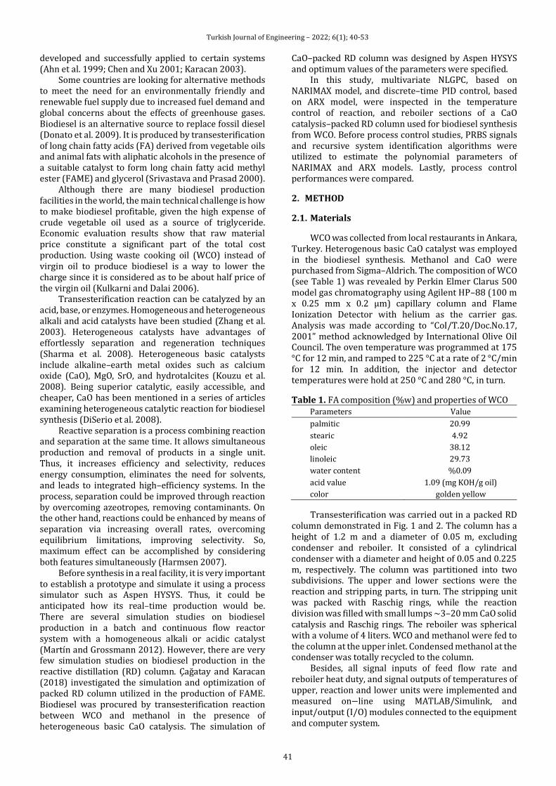
Turkish Journal of Engineering – 2022; 6(1); 40-53
41
developed and successfully applied to certain systems (Ahn et al. 1999; Chen and Xu 2001; Karacan 2003).
Some countries are looking for alternative methods to meet the need for an environmentally friendly and renewable fuel supply due to increased fuel demand and global concerns about the effects of greenhouse gases. Biodiesel is an alternative source to replace fossil diesel (Donato et al. 2009). It is produced by transesterification of long chain fatty acids (FA) derived from vegetable oils and animal fats with aliphatic alcohols in the presence of a suitable catalyst to form long chain fatty acid methyl ester (FAME) and glycerol (Srivastava and Prasad 2000).
Although there are many biodiesel production facilities in the world, the main technical challenge is how to make biodiesel profitable, given the high expense of crude vegetable oil used as a source of triglyceride. Economic evaluation results show that raw material price constitute a significant part of the total cost production. Using waste cooking oil (WCO) instead of virgin oil to produce biodiesel is a way to lower the charge since it is considered as to be about half price of the virgin oil (Kulkarni and Dalai 2006).
Transesterification reaction can be catalyzed by an acid, base, or enzymes. Homogeneous and heterogeneous alkali and acid catalysts have been studied (Zhang et al. 2003). Heterogeneous catalysts have advantages of effortlessly separation and regeneration techniques (Sharma et al. 2008). Heterogeneous basic catalysts include alkaline–earth metal oxides such as calcium oxide (CaO), MgO, SrO, and hydrotalcites (Kouzu et al. 2008). Being superior catalytic, easily accessible, and cheaper, CaO has been mentioned in a series of articles examining heterogeneous catalytic reaction for biodiesel synthesis (DiSerio et al. 2008).
Reactive separation is a process combining reaction and separation at the same time. It allows simultaneous production and removal of products in a single unit. Thus, it increases efficiency and selectivity, reduces energy consumption, eliminates the need for solvents, and leads to integrated high–efficiency systems. In the process, separation could be improved through reaction by overcoming azeotropes, removing contaminants. On the other hand, reactions could be enhanced by means of separation via increasing overall rates, overcoming equilibrium limitations, improving selectivity. So, maximum effect can be accomplished by considering both features simultaneously (Harmsen 2007).
Before synthesis in a real facility, it is very important to establish a prototype and simulate it using a process simulator such as Aspen HYSYS. Thus, it could be anticipated how its real–time production would be. There are several simulation studies on biodiesel production in a batch and continuous flow reactor system with a homogeneous alkali or acidic catalyst (Martín and Grossmann 2012). However, there are very few simulation studies on biodiesel production in the reactive distillation (RD) column. Çağatay and Karacan (2018) investigated the simulation and optimization of packed RD column utilized in the production of FAME. Biodiesel was procured by transesterification reaction between WCO and methanol in the presence of heterogeneous basic CaO catalysis. The simulation of
CaO–packed RD column was designed by Aspen HYSYS and optimum values of the parameters were specified.
In this study, multivariate NLGPC, based on NARIMAX model, and discrete–time PID control, based on ARX model, were inspected in the temperature control of reaction, and reboiler sections of a CaO catalysis–packed RD column used for biodiesel synthesis from WCO. Before process control studies, PRBS signals and recursive system identification algorithms were utilized to estimate the polynomial parameters of NARIMAX and ARX models. Lastly, process control performances were compared.
2. METHOD
2.1. Materials
WCO was collected from local restaurants in Ankara, Turkey. Heterogenous basic CaO catalyst was employed in the biodiesel synthesis. Methanol and CaO were purchased from Sigma–Aldrich. The composition of WCO (see Table 1) was revealed by Perkin Elmer Clarus 500 model gas chromatography using Agilent HP–88 (100 m x 0.25 mm x 0.2 μm) capillary column and Flame Ionization Detector with helium as the carrier gas. Analysis was made according to “CoI/T.20/Doc.No.17, 2001” method acknowledged by International Olive Oil Council. The oven temperature was programmed at 175 °C for 12 min, and ramped to 225 °C at a rate of 2 °C/min for 12 min. In addition, the injector and detector temperatures were hold at 250 °C and 280 °C, in turn.
Table 1. FA composition (%w) and properties of WCO Parameters Value
palmitic 20.99
stearic 4.92
oleic 38.12
linoleic 29.73
water content %0.09
acid value 1.09 (mg KOH/g oil)
color golden yellow
Transesterification was carried out in a packed RD column demonstrated in Fig. 1 and 2. The column has a height of 1.2 m and a diameter of 0.05 m, excluding condenser and reboiler. It consisted of a cylindrical condenser with a diameter and height of 0.05 and 0.225 m, respectively. The column was partitioned into two subdivisions. The upper and lower sections were the reaction and stripping parts, in turn. The stripping unit was packed with Raschig rings, while the reaction division was filled with small lumps ~3–20 mm CaO solid catalysis and Raschig rings. The reboiler was spherical with a volume of 4 liters. WCO and methanol were fed to the column at the upper inlet. Condensed methanol at the condenser was totally recycled to the column.
Besides, all signal inputs of feed flow rate and reboiler heat duty, and signal outputs of temperatures of upper, reaction and lower units were implemented and measured on−line using MATLAB/Simulink, and input/output (I/O) modules connected to the equipment and computer system.
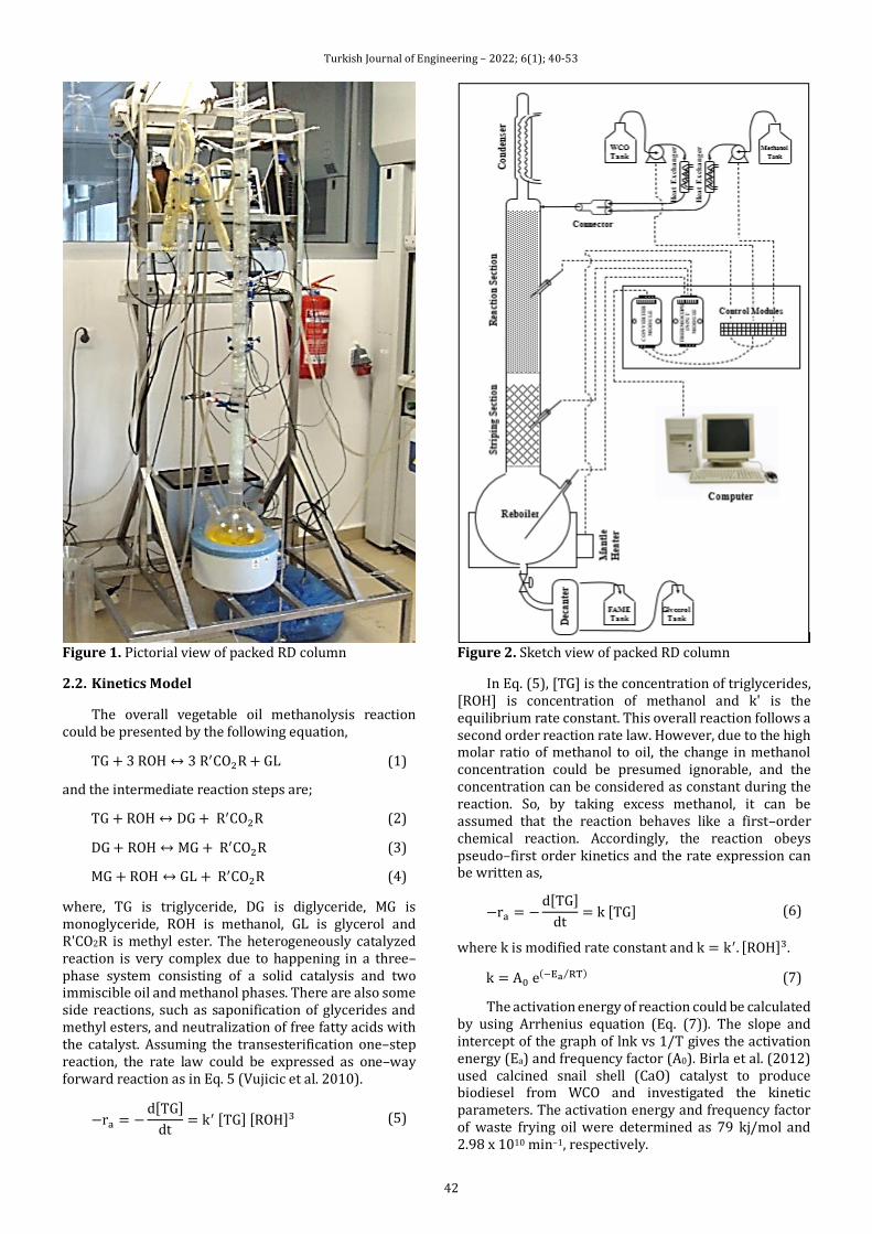
Turkish Journal of Engineering – 2022; 6(1); 40-53
42
Figure 1. Pictorial view of packed RD column
2.2. Kinetics Model
The overall vegetable oil methanolysis reaction could be presented by the following equation,
TG + 3 ROH ↔ 3 R′CO2R + GL (1)
and the intermediate reaction steps are;
TG + ROH ↔ DG + R′CO2R (2)
DG + ROH ↔ MG + R′CO2R (3)
MG + ROH ↔ GL + R′CO2R (4)
where, TG is triglyceride, DG is diglyceride, MG is monoglyceride, ROH is methanol, GL is glycerol and R'CO2R is methyl ester. The heterogeneously catalyzed reaction is very complex due to happening in a three–phase system consisting of a solid catalysis and two immiscible oil and methanol phases. There are also some side reactions, such as saponification of glycerides and methyl esters, and neutralization of free fatty acids with the catalyst. Assuming the transesterification one–step reaction, the rate law could be expressed as one–way forward reaction as in Eq. 5 (Vujicic et al. 2010).
−ra = −d[TG]
dt= k′ [TG] [ROH]3 (5)
Figure 2. Sketch view of packed RD column
In Eq. (5), [TG] is the concentration of triglycerides, [ROH] is concentration of methanol and k' is the equilibrium rate constant. This overall reaction follows a second order reaction rate law. However, due to the high molar ratio of methanol to oil, the change in methanol concentration could be presumed ignorable, and the concentration can be considered as constant during the reaction. So, by taking excess methanol, it can be assumed that the reaction behaves like a first–order chemical reaction. Accordingly, the reaction obeys pseudo–first order kinetics and the rate expression can be written as,
−ra = −d[TG]
dt= k [TG] (6)
where k is modified rate constant and k = k′. [ROH]3.
k = A0 e(−Ea RT⁄ ) (7)
The activation energy of reaction could be calculated by using Arrhenius equation (Eq. (7)). The slope and intercept of the graph of lnk vs 1/T gives the activation energy (Ea) and frequency factor (A0). Birla et al. (2012) used calcined snail shell (CaO) catalyst to produce biodiesel from WCO and investigated the kinetic parameters. The activation energy and frequency factor of waste frying oil were determined as 79 kj/mol and 2.98 x 10¹⁰ min–1, respectively.
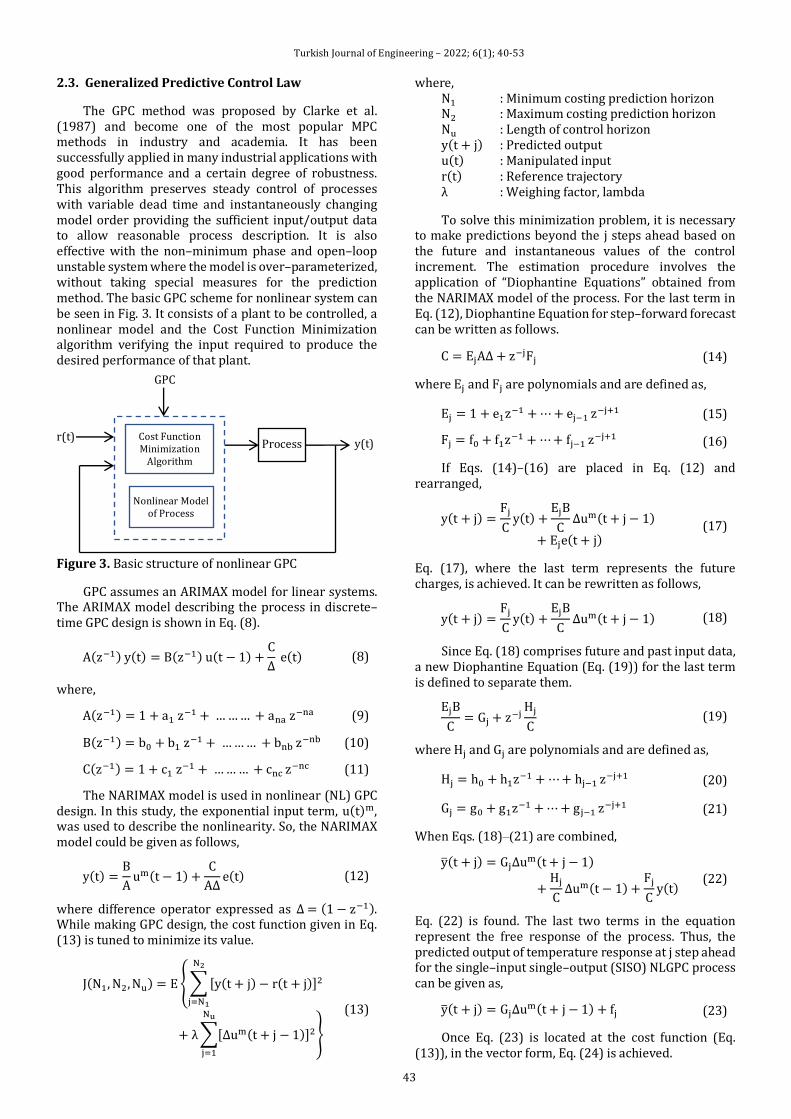
Turkish Journal of Engineering – 2022; 6(1); 40-53
43
2.3. Generalized Predictive Control Law
The GPC method was proposed by Clarke et al. (1987) and become one of the most popular MPC methods in industry and academia. It has been successfully applied in many industrial applications with good performance and a certain degree of robustness. This algorithm preserves steady control of processes with variable dead time and instantaneously changing model order providing the sufficient input/output data to allow reasonable process description. It is also effective with the non–minimum phase and open–loop unstable system where the model is over–parameterized, without taking special measures for the prediction method. The basic GPC scheme for nonlinear system can be seen in Fig. 3. It consists of a plant to be controlled, a nonlinear model and the Cost Function Minimization algorithm verifying the input required to produce the desired performance of that plant.
Figure 3. Basic structure of nonlinear GPC
GPC assumes an ARIMAX model for linear systems. The ARIMAX model describing the process in discrete–time GPC design is shown in Eq. (8).
A(z−1) y(t) = B(z−1) u(t − 1) +C
∆ e(t) (8)
where,
A(z−1) = 1 + a1 z−1 + … … … + ana z−na (9)
B(z−1) = b0 + b1 z−1 + … … … + bnb z−nb (10)
C(z−1) = 1 + c1 z−1 + … … … + cnc z−nc (11)
The NARIMAX model is used in nonlinear (NL) GPC design. In this study, the exponential input term, u(t)m, was used to describe the nonlinearity. So, the NARIMAX model could be given as follows,
y(t) =B
Aum(t − 1) +
C
A∆e(t) (12)
where difference operator expressed as ∆ = (1 − z−1). While making GPC design, the cost function given in Eq. (13) is tuned to minimize its value.
J(N1, N2, Nu) = E ∑ [y(t + j) − r(t + j)]2
N2
j=N1
+ λ ∑[Δum(t + j − 1)]2
Nu
j=1
(13)
where, N1 : Minimum costing prediction horizon N2 : Maximum costing prediction horizon Nu : Length of control horizon y(t + j) : Predicted output u(t) : Manipulated input r(t) : Reference trajectory λ : Weighing factor, lambda
To solve this minimization problem, it is necessary to make predictions beyond the j steps ahead based on the future and instantaneous values of the control increment. The estimation procedure involves the application of “Diophantine Equations” obtained from the NARIMAX model of the process. For the last term in Eq. (12), Diophantine Equation for step–forward forecast can be written as follows.
C = EjA∆ + z−jFj (14)
where Ej and Fj are polynomials and are defined as,
Ej = 1 + e1z−1 + ⋯ + ej−1 z−j+1 (15)
Fj = f0 + f1z−1 + ⋯ + fj−1 z−j+1 (16)
If Eqs. (14)–(16) are placed in Eq. (12) and rearranged,
y(t + j) =Fj
Cy(t) +
EjB
C∆um(t + j − 1)
+ Eje(t + j) (17)
Eq. (17), where the last term represents the future charges, is achieved. It can be rewritten as follows,
y(t + j) =Fj
Cy(t) +
EjB
C∆um(t + j − 1) (18)
Since Eq. (18) comprises future and past input data, a new Diophantine Equation (Eq. (19)) for the last term is defined to separate them.
EjB
C= Gj + z−j
Hj
C (19)
where Hj and Gj are polynomials and are defined as,
Hj = h0 + h1z−1 + ⋯ + hj−1 z−j+1 (20)
Gj = g0 + g1z−1 + ⋯ + gj−1 z−j+1 (21)
When Eqs. (18)–(21) are combined,
y(t + j) = Gj∆um(t + j − 1)
+Hj
C∆um(t − 1) +
Fj
Cy(t)
(22)
Eq. (22) is found. The last two terms in the equation represent the free response of the process. Thus, the predicted output of temperature response at j step ahead for the single–input single–output (SISO) NLGPC process can be given as,
y(t + j) = Gj∆um(t + j − 1) + fj (23)
Once Eq. (23) is located at the cost function (Eq. (13)), in the vector form, Eq. (24) is achieved.
Cost Function Minimization
Algorithm
r(t)
Nonlinear Model of Process
Process y(t)
GPC

Turkish Journal of Engineering – 2022; 6(1); 40-53
44
J(N1, N2, Nu) = (y − r)2 + λ(∆um)2 (24)
If the steps are carried out and reorganized,
J(N1, N2, Nu) = (G ∆um)T(G ∆um)+ (G ∆um)T(f − r)+ (f − r)T(G ∆um)+ (f − r)T(f − r)+ λ(∆um)T∆um
(25)
Eq. (25) is obtained. In terms of minimizing the cost function, the equation is derived and equated to zero. Reordering it, Eq. (26) has been found.
(GTG + λI) (∆um)T + (f − r)TG = 0 (26)
Modifying Eq. (26), the future input data at step j can be calculated using Eq. (27) and (28).
∆um = (GTG + λI)−1 GT(r − f) (27)
um(t) = um(t − 1) + (GTG + λI)−1 GT(r − f) (28)
Thus, SISO NLGPC algorithm will be fulfilled via control law, Eq. (27) and (28). The first element of the ∆um vector, including predicted (t+j) solutions for the value of j from 1 to Nu, is applied to the process and temperature response is read from the process. Here, Eq. (23) is used to calculate the theoretical temperature response of the system for the next (t+1) th step by using the value of 1 of j. These periods are repeated cyclically in this way until the system response reaches the set value. During the procedure, the control gain remains constant and only the f and r vectors are calculated at each sampling time, repeatedly.
The block diagram developed to be used in system identification and experimental control studies, which will enable the application of manipulating variable values to the process, reading system temperatures, and recording all data automatically in a computer-controlled environment is as shown in Fig. 4.
2.4. Design of MIMO NLGPC
The reboiler temperature y1 was controlled by the heat duty (∆u1
m) manipulating variable. Likewise, the reaction temperature y2 was controlled by the flow rate (∆u2
m) manipulating variable at constant molar ratio.
2.4.1. Design of non–decoupled MIMO NLGPC
In non–decoupled MIMO NLGPC method, the SISO control law, Eq. (27), is written separately for reboiler and reaction sections, as seen in Eq. (29) and (30).
∆u1m = (G11
T G11 + λ1I)−1 G11T (r1−f11) (29)
∆u2m = (G22
T G22 + λ2I)−1 G22T (r2−f22) (30)
Solving these equations alone, the vectors ∆u1m and
∆u2m are found and using them, the future values of the
manipulating variables, u1m and u2
m, are attained. Accordingly, system responses are obtained by applying the first term of those to the process at time t. Here, the responses are calculated theoretically for the next (t+1) th step for the value of 1 of j through Eq. (31) and (32).
Figure 4. Block diagram for on–line control of process
y1(t + 1) = Gj,11∆u1m(t) + fj,11
+ Gj,12∆u2m(t) + fj,12
(31)
y2(t + 1) = Gj,21∆u1m(t) + fj,21
+ Gj,22∆u2m(t) + fj,22
(32)
Thus, the effect of both manipulating variables on both sides due to interaction is taken into account via Eq. (31) and (32) while calculating the system response of each region for the next control step. Repeating this period cyclically, process response is intended to reach the desired set values. The free response functions described in the equations are defined in Eq. (33).

Turkish Journal of Engineering – 2022; 6(1); 40-53
45
fj,11 =Hj,11
C11
∆u1m(t − 1) +
Fj,11
C11
y11(t)
(33)
fj,12 =Hj,12
C12
∆u2m(t − 1) +
Fj,12
C12
y12(t)
fj,21 =Hj,21
C21
∆u1m(t − 1) +
Fj,21
C21
y21(t)
fj,22 =Hj,22
C22
∆u2m(t − 1) +
Fj,22
C22
y22(t)
2.4.2. Design of decoupled MIMO NLGPC
In the decoupled MIMO NLGPC method, the block diagram could be given as presented in Fig. 5.
Figure 5. Decoupled MIMO NLGPC diagram
The predicted temperature responses of the reboiler and reaction sections at the j step ahead are defined as Eq. (34) and (35).
y1(t + j) = G11∆u1m(t + j − 1) + f11
+ G12∆u2m(t + j − 1) + f12
(34)
y2(t + j) = G21∆u1m(t + j − 1) + f21
+ G22∆u2m(t + j − 1) + f22
(35)
If the cost function is applied to Eq. (34) and (35), Eq. (36) and (37) are achieved.
J1(N1, N2, Nu) = (G11 ∆u1m(t + j − 1)
+ G12 ∆u2m(t + j − 1)
+ f11 + f12 − r1)2
+ λ1(∆u1m(t + j − 1))
2
(36)
J2(N1, N2, Nu) = (G21 ∆u1m(t + j − 1)
+ G22 ∆u2m(t + j − 1)
+ f21 + f22 − r2)2
+ λ2(∆u2m(t + j − 1))
2
(37)
For minimization, if derivatives of them are taken separately depending on u1
m and u2m, equated to zero and
the adjustments are made, Eq. (38) and (39) are found.
(G11T G11 + λ1I) ∆u1
m(t + j − 1)+ (G11
T G12) ∆u2m(t + j − 1)
= G11T (r1 − f11 − f12)
(38)
(G22T G21) ∆u1
m(t + j − 1)+ (G22
T G22 + λ2I) ∆u2m(t + j
− 1) = G22T (r2 − f21 − f22)
(39)
To obtain predicted vectors, ∆u1m and ∆u2
m, a matrix solution is made simultaneously using Eq. (38) and (39).
Φ1 = G11T G11 + λ1I
(40) Φ2 = G11
T G12
Φ3 = G22T G21
Φ4 = G22T G22 + λ2I
If the definitions, Eq. (40) and (41), are put in Eq. (38) and (39), matrix solution form, Eq. (42), is attained.
Γ1 = G11T (r1 − f11 − f12)
(41) Γ2 = G22
T (r2 − f21 − f22)
The solution algorithm was developed in MATLAB environment and the vectors, ∆u1
m and ∆u2m, were
acquired by multiplying the right–side matrix by the inverse of the coefficient matrix. Then, using them, u1
m and u2
m input values were calculated and the first terms of them were applied to the process. As in the non–decoupled MIMO NLGPC, the responses are calculated theoretically for the next (t+1) th step for the value of 1 of j via Eq. (31) and (32). Likewise, repeating the cycle periodically, the process responses are intended to reach the desired set values.
[Φ1 Φ2
Φ3 Φ4] [
∆u1m(t + j − 1)
∆u2m(t + j − 1)
] = [ Γ1
Γ2 ] (42)
2.5. Discrete–time PID Control Law
Typically, in the PID control systems, the input to be applied to the process is calculated by Eq. (43) including proportional, integral, and derivative impact. Its magnitude depends on the error which is difference between the process output and the set value at time t.
Δu = Kc ε(t) +1
τI
∫ ε(t)d(t) + τD
dε(t)
dt
t
0
(43)
From the mathematical definitions of integral and derivative, Eq. (44) is obtained for the (n)th step.
un = u0 + Kc εn(t)
+Δt
τI
∑ εk(t) +τD
Δt
n
k=0
(εn(t)
− εn−1(t))
(44)
Next, if Eq. (44) is rewritten for the (n–1)th step and subtracted from the developed for the (n)th step, Eq. (45) and (46) are found in terms of the operator, z−j.
∆u = Kc (1 +Δt
τI
+τD
Δt) εn
− Kc (1 +2τD
Δt) εnz−1
+ Kc
τD
Δtεnz−2
(45)
G12
G21
G22
∆u1m
∆u2m
f11
f12
f21
f22
y1
y2
G11

Turkish Journal of Engineering – 2022; 6(1); 40-53
46
∆u(z)
εn(z)= Kc (1 +
Δt
τI
+τD
Δt) − (1 +
2τD
Δt) z−1
+ (τD
Δt) z−2
(46)
Here, a new polynomial, S, is defined by Eq. (47).
S = s0 + s1z−1 + s2z−2 (47)
where,
s0 = Kc (1 +Δt
τI
+τD
Δt)
(48) s1 = Kc (1 +2τD
Δt)
s2 = Kc (τD
Δt)
As mentioned before, the error, Eq. (49), is defined as the difference between the set value and the output in the PID control. If Eqs. (46)–(49) is restructured, the control law, Eq. (50), is attained for discrete–time SISO PID control application.
ε(z) = [r(t) − y(t)] (49)
u(t) =S
∆[r(t) − y(t)] (50)
2.6. Design of Discrete–time MIMO PID Control
In discrete–time PID control design, the process was stated in linear ARX model as shown in Eq. (51) and (52).
y(t) =B(z−1)
A(z−1)u(t − 1) (51)
y(t) = G(z−1) u(t − 1) (52)
2.6.1. Non–decoupled MIMO PID control
The discrete–time, interactive and non–decoupled MIMO PID control system is demonstrated as in Fig. 6.
Figure 6. Non–decoupled MIMO PID control diagram
Process temperature responses y1 and y2 at time t are defined as in Eq. (53) and (54) in the non–decoupled MIMO PID system.
y1(t) = G11(z−1)u1(t − 1) + G12(z−1)u2(t − 1) (53)
y2(t) = G21(z−1)u1(t − 1) + G22(z−1)u2(t − 1) (54)
If discrete–time SISO PID control law, Eq. (50), is
applied singly at each region Eq. (55) and (56) are gotten.
u1(t) =S1
∆ [r1(t) − y1(t)] (55)
u2(t) =S2
∆ [r2(t) − y2(t)] (56)
Then, calculated manipulating variables are applied to the process. Here, the interacted process responses are computed theoretically for the next (t+1) th step by Eq. (53) and (54) by using manipulating variable values achieved at time t. In this way, the cycle is continued repeatedly until reaching the desired set values.
2.6.2. Decoupled MIMO PID control
The discrete–time, interactive and decoupled MIMO PID control system is presented as in Fig. 7. In control scheme, the process temperature output y1 and y2 at time t will be as given by Eq. (57) and (58).
Figure 7. Decoupled MIMO PID control diagram
y1(t) = G11(z−1)[u1(t − 1) + T2u2(t − 1)]
+ G12(z−1)[u2(t − 1)
+ T1u1(t − 1)] (57)
y2(t) = G22(z−1)[u2(t − 1) + T1u1(t − 1)]
+ G21(z−1)[u1(t − 1)
+ T2u2(t − 1)] (58)
Eq. (59) and (60) are found if adjustments are made.
y1(t) = [G11(z−1) + G12(z−1) T1] u1(t − 1)
+ [G12(z−1)
+ G11(z−1) T2] u2(t − 1) (59)
y2(t) = [G21(z−1) + G22(z−1) T1] u1(t − 1)
+ [G22(z−1)
+ G21(z−1) T2] u2(t − 1) (60)
When the terms including u1 in Eq. (60) and u2 in Eq. (59) are equated to zero, Eq. (61) is acquired.
T1 = −[G21(z−1) G22(z−1)⁄ ] (61)
T2 = −[G12(z−1) G11(z−1)⁄ ]
In the control, initially, process inputs u1 and u2 are calculated by the control laws, Eq. (55) and (56), at time t. Then revised inputs, u1(t)–[u2(t)G12(z-1)/G11(z-1)] and u2(t)–[u1(t)(G21(z-1)/G22(z-1)], are applied to process. Once again, Eq. (53) and (54) are used to get theoretical responses for the next (t+1) th step as mentioned above.
G12
G21
G22
u1
u2
y1
y2
G11 r1
r2
PID C
PID C
1
2
G12
G21
G22
T1
T2
u1
u2
y1
y2
G11 r1
r2
PID C
PID C
1
2
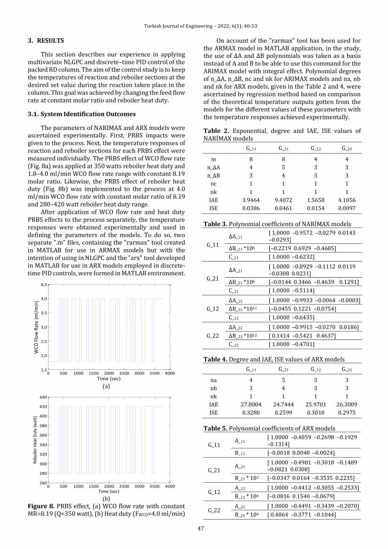
Turkish Journal of Engineering – 2022; 6(1); 40-53
47
3. RESULTS
This section describes our experience in applying multivariate NLGPC and discrete–time PID control of the packed RD column. The aim of the control study is to keep the temperatures of reaction and reboiler sections at the desired set value during the reaction taken place in the column. This goal was achieved by changing the feed flow rate at constant molar ratio and reboiler heat duty.
3.1. System Identification Outcomes
The parameters of NARIMAX and ARX models were ascertained experimentally. First, PRBS impacts were given to the process. Next, the temperature responses of reaction and reboiler sections for each PRBS effect were measured individually. The PRBS effect of WCO flow rate (Fig. 8a) was applied at 350 watts reboiler heat duty and 1.8–4.0 ml/min WCO flow rate range with constant 8.19 molar ratio. Likewise, the PRBS effect of reboiler heat duty (Fig. 8b) was implemented to the process at 4.0 ml/min WCO flow rate with constant molar ratio of 8.19 and 280–420 watt reboiler heat duty range.
After application of WCO flow rate and heat duty PRBS effects to the process separately, the temperature responses were obtained experimentally and used in defining the parameters of the models. To do so, two separate ".m" files, containing the "rarmax" tool created in MATLAB for use in ARMAX models but with the intention of using in NLGPC and the "arx" tool developed in MATLAB for use in ARX models employed in discrete-time PID controls, were formed in MATLAB environment.
(a)
(b)
Figure 8. PRBS effect, (a) WCO flow rate with constant MR=8.19 (Q=350 watt), (b) Heat duty (FWCO=4.0 ml/min)
On account of the "rarmax" tool has been used for the ARMAX model in MATLAB application, in the study, the use of ΔA and ΔB polynomials was taken as a basis instead of A and B to be able to use this command for the ARIMAX model with integral effect. Polynomial degrees of n_ΔA, n_ΔB, nc and nk for ARIMAX models and na, nb and nk for ARX models, given in the Table 2 and 4, were ascertained by regression method based on comparison of the theoretical temperature outputs gotten from the models for the different values of these parameters with the temperature responses achieved experimentally.
Table 2. Exponential, degree and IAE, ISE values of NARİMAX models
G_11 G_21 G_12 G_22
m 8 8 4 4
n_ΔA 4 5 3 3
n_ΔB 3 4 3 3
nc 1 1 1 1
nk 1 1 1 1
IAE 3.9464 9.4072 1.5658 4.1056
ISE 0.0386 0.0461 0.0154 0.0097
Table 3. Polynomial coefficients of NARİMAX models
G_11
ΔA_11 [ 1.0000 –0.9572 –0.0279 0.0143 –0.0293]
ΔB_11 *106 [–0.2219 0.6929 –0.4685]
C_11 [ 1.0000 –0.6232]
G_21
ΔA_21 [ 1.0000 –0.8929 –0.1112 0.0119 –0.0308 0.0231]
ΔB_21 *106 [–0.0144 0.3466 –0.4639 0.1291]
C_21 [ 1.0000 –0.5114]
G_12
ΔA_12 [ 1.0000 –0.9933 –0.0064 –0.0003]
ΔB_12 *1011 [–0.0455 0.1221 –0.0754]
C_12 [ 1.0000 –0.6435]
G_22
ΔA_22 [ 1.0000 –0.9915 –0.0270 0.0186]
ΔB_22 *1012 [ 0.1414 –0.5421 0.4637]
C_22 [ 1.0000 –0.4701]
Table 4. Degree and IAE, ISE values of ARX models
G_11 G_21 G_12 G_22
na 4 5 3 3
nb 3 4 3 3
nk 1 1 1 1
IAE 27.8004 24.7444 25.9701 26.3009
ISE 0.3280 0.2599 0.3010 0.2975
Table 5. Polynomial coefficients of ARX models
G_11 A_11
[ 1.0000 –0.4059 –0.2698 –0.1929 –0.1314]
B_11 [–0.0018 0.0040 –0.0024]
G_21 A_21
[ 1.0000 –0.4981 –0.3018 –0.1489 –0.0821 0.0308]
B_21 * 103 [–0.0347 0.0164 –0.3535 0.2235]
G_12 A_12 [ 1.0000 –0.4412 –0.3055 –0.2533]
B_12 * 104 [–0.0816 0.1540 –0.0679]
G_22 A_22 [ 1.0000 –0.4491 –0.3439 –0.2070]
B_22 * 104 [ 0.4864 –0.3771 –0.1044]
0 500 1000 1500 2000 2500 3000 3500 40001,5
2,0
2,5
3,0
3,5
4,0
4,5
Time (sec)
WC
O F
low
Rat
e (m
l/m
in)
0 500 1000 1500 2000 2500 3000 3500 4000260
280
300
320
340
360
380
400
420
440
Time (sec)
Reb
oile
r H
eat
Dut
y (w
att)
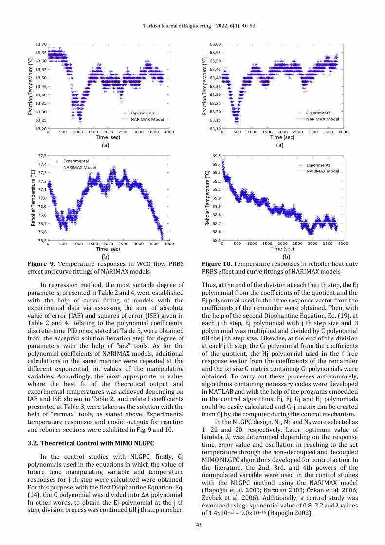
Turkish Journal of Engineering – 2022; 6(1); 40-53
48
(a)
(b)
Figure 9. Temperature responses in WCO flow PRBS effect and curve fittings of NARIMAX models
In regression method, the most suitable degree of parameters, presented in Table 2 and 4, were established with the help of curve fitting of models with the experimental data via assessing the sum of absolute value of error (IAE) and squares of error (ISE) given in Table 2 and 4. Relating to the polynomial coefficients, discrete–time PID ones, stated at Table 5, were obtained from the accepted solution iteration step for degree of parameters with the help of “arx” tools. As for the polynomial coefficients of NARIMAX models, additional calculations in the same manner were repeated at the different exponential, m, values of the manipulating variables. Accordingly, the most appropriate m value, where the best fit of the theoretical output and experimental temperatures was achieved depending on IAE and ISE shown in Table 2, and related coefficients presented at Table 3, were taken as the solution with the help of “rarmax” tools, as stated above. Experimental temperature responses and model outputs for reaction and reboiler sections were exhibited in Fig. 9 and 10.
3.2. Theoretical Control with MIMO NLGPC
In the control studies with NLGPC, firstly, Gj polynomials used in the equations in which the value of future time manipulating variable and temperature responses for j th step were calculated were obtained. For this purpose, with the first Diophantine Equation, Eq. (14), the C polynomial was divided into ΔA polynomial. In other words, to obtain the Ej polynomial at the j th step, division process was continued till j th step number.
(a)
(b)
Figure 10. Temperature responses in reboiler heat duty PRBS effect and curve fittings of NARIMAX models
Thus, at the end of the division at each the j th step, the Ej polynomial from the coefficients of the quotient and the Fj polynomial used in the f free response vector from the coefficients of the remainder were obtained. Then, with the help of the second Diophantine Equation, Eq. (19), at each j th step, Ej polynomial with j th step size and B polynomial was multiplied and divided by C polynomial till the j th step size. Likewise, at the end of the division at each j th step, the Gj polynomial from the coefficients of the quotient, the Hj polynomial used in the f free response vector from the coefficients of the remainder and the jxj size G matrix containing Gj polynomials were obtained. To carry out these processes autonomously, algorithms containing necessary codes were developed in MATLAB and with the help of the programs embedded in the control algorithms, Ej, Fj, Gj and Hj polynomials could be easily calculated and Gj,j matrix can be created from Gj by the computer during the control mechanism.
In the NLGPC design, N1, N2 and Nu were selected as 1, 20 and 20, respectively. Later, optimum value of lambda, λ, was determined depending on the response time, error value and oscillation in reaching to the set temperature through the non–decoupled and decoupled MIMO NLGPC algorithms developed for control action. In the literature, the 2nd, 3rd, and 4th powers of the manipulated variable were used in the control studies with the NLGPC method using the NARIMAX model (Hapoğlu et al. 2000; Karacan 2003; Özkan et al. 2006; Zeybek et al. 2006). Additionally, a control study was examined using exponential value of 0.8–2.2 and λ values of 1.4x10⁻¹² – 9.0x10⁻¹⁶ (Hapoğlu 2002).
0 500 1000 1500 2000 2500 3000 3500 400063,20
63,25
63,30
63,35
63,40
63,45
63,50
63,55
63,60
63,65
63,70
Time (sec)
Reac
tion
Tem
pera
ture
(°C)
Experimental
NARIMAX Model
0 500 1000 1500 2000 2500 3000 3500 400076,5
76,6
76,7
76,8
76,9
77,0
77,1
77,2
77,3
77,4
77,5
Time (sec)
Rebo
iler
Tem
pera
ture
(°C)
Experimental
NARIMAX Model
0 500 1000 1500 2000 2500 3000 3500 400063,10
63,15
63,20
63,25
63,30
63,35
63,40
63,45
63,50
63,55
63,60
Time (sec)
Reac
tion
Tem
pera
ture
(°C)
Experimental
NARIMAX Model
0 500 1000 1500 2000 2500 3000 3500 400068,5
68,6
68,7
68,8
68,9
69,0
69,1
69,2
69,3
69,4
69,5
Time (sec)
Rebo
ier
Tem
pera
ture
(°C)
Experimental
NARIMAX Model
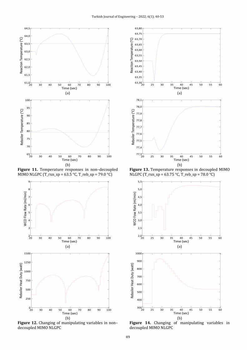
Turkish Journal of Engineering – 2022; 6(1); 40-53
49
(a)
(b)
Figure 11. Temperature responses in non–decoupled MIMO NLGPC (T_rxn_sp = 63.5 °C, T_reb_sp = 79.0 °C)
(a)
(b)
Figure 12. Changing of manipulating variables in non–decoupled MIMO NLGPC
(a)
(b)
Figure 13. Temperature responses in decoupled MIMO NLGPC (T_rxn_sp = 63.75 °C, T_reb_sp = 78.0 °C)
(a)
(b)
Figure 14. Changing of manipulating variables in decoupled MIMO NLGPC
20 30 40 50 60 70 80 90 10061,0
61,5
62,0
62,5
63,0
63,5
64,0
64,5
Time (sec)
Reac
tion
Tem
pera
ture
(°C)
20 30 40 50 60 70 80 90 10065
70
75
80
85
90
95
100
Time (sec)
Rebo
iler
Tem
pera
ture
(°C)
20 30 40 50 60 70 80 90 1002
3
4
5
6
7
8
9
Time (sec)
WCO
Flo
w R
ate
(ml/
min
)
20 30 40 50 60 70 80 90 1000
250
500
750
1000
1250
1500
Time (sec)
Rebo
iler
Hea
t D
uty
(wat
t)
20 25 30 35 40 45 50 55 6063,30
63,35
63,40
63,45
63,50
63,55
63,60
63,65
63,70
63,75
63,80
Time (sec)
Reac
tion
Tem
pera
ture
(°C)
20 25 30 35 40 45 50 55 6077,3
77,4
77,5
77,6
77,7
77,8
77,9
78,0
78,1
Time (sec)
Rebo
iler
Tem
pera
ture
(°C)
20 25 30 35 40 45 50 55 602,0
2,5
3,0
3,5
4,0
4,5
5,0
5,5
Time (sec)
WCO
Fow
Rat
e (m
l/m
in)
20 25 30 35 40 45 50 55 60300
400
500
600
700
800
900
1000
Time (sec)
Rebo
iler
Hea
t D
uty
(wat
t)
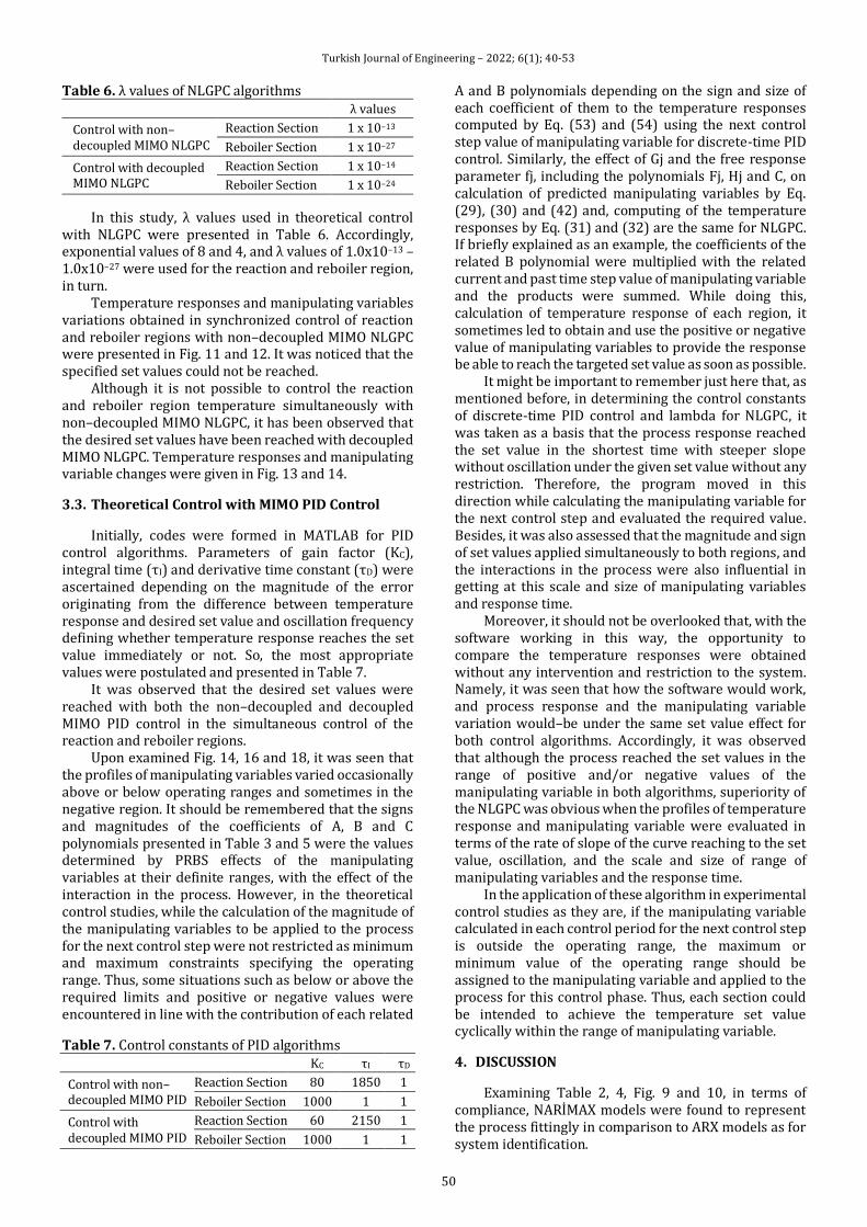
Turkish Journal of Engineering – 2022; 6(1); 40-53
50
Table 6. λ values of NLGPC algorithms λ values
Control with non–decoupled MIMO NLGPC
Reaction Section 1 x 10–13
Reboiler Section 1 x 10–27
Control with decoupled MIMO NLGPC
Reaction Section 1 x 10–14
Reboiler Section 1 x 10–24
In this study, λ values used in theoretical control with NLGPC were presented in Table 6. Accordingly, exponential values of 8 and 4, and λ values of 1.0x10⁻¹³ – 1.0x10⁻²⁷ were used for the reaction and reboiler region, in turn.
Temperature responses and manipulating variables variations obtained in synchronized control of reaction and reboiler regions with non–decoupled MIMO NLGPC were presented in Fig. 11 and 12. It was noticed that the specified set values could not be reached.
Although it is not possible to control the reaction and reboiler region temperature simultaneously with non–decoupled MIMO NLGPC, it has been observed that the desired set values have been reached with decoupled MIMO NLGPC. Temperature responses and manipulating variable changes were given in Fig. 13 and 14.
3.3. Theoretical Control with MIMO PID Control
Initially, codes were formed in MATLAB for PID control algorithms. Parameters of gain factor (KC), integral time (τI) and derivative time constant (τD) were ascertained depending on the magnitude of the error originating from the difference between temperature response and desired set value and oscillation frequency defining whether temperature response reaches the set value immediately or not. So, the most appropriate values were postulated and presented in Table 7.
It was observed that the desired set values were reached with both the non–decoupled and decoupled MIMO PID control in the simultaneous control of the reaction and reboiler regions.
Upon examined Fig. 14, 16 and 18, it was seen that the profiles of manipulating variables varied occasionally above or below operating ranges and sometimes in the negative region. It should be remembered that the signs and magnitudes of the coefficients of A, B and C polynomials presented in Table 3 and 5 were the values determined by PRBS effects of the manipulating variables at their definite ranges, with the effect of the interaction in the process. However, in the theoretical control studies, while the calculation of the magnitude of the manipulating variables to be applied to the process for the next control step were not restricted as minimum and maximum constraints specifying the operating range. Thus, some situations such as below or above the required limits and positive or negative values were encountered in line with the contribution of each related
Table 7. Control constants of PID algorithms KC τI τD
Control with non–decoupled MIMO PID
Reaction Section 80 1850 1
Reboiler Section 1000 1 1
Control with decoupled MIMO PID
Reaction Section 60 2150 1
Reboiler Section 1000 1 1
A and B polynomials depending on the sign and size of each coefficient of them to the temperature responses computed by Eq. (53) and (54) using the next control step value of manipulating variable for discrete-time PID control. Similarly, the effect of Gj and the free response parameter fj, including the polynomials Fj, Hj and C, on calculation of predicted manipulating variables by Eq. (29), (30) and (42) and, computing of the temperature responses by Eq. (31) and (32) are the same for NLGPC. If briefly explained as an example, the coefficients of the related B polynomial were multiplied with the related current and past time step value of manipulating variable and the products were summed. While doing this, calculation of temperature response of each region, it sometimes led to obtain and use the positive or negative value of manipulating variables to provide the response be able to reach the targeted set value as soon as possible.
It might be important to remember just here that, as mentioned before, in determining the control constants of discrete-time PID control and lambda for NLGPC, it was taken as a basis that the process response reached the set value in the shortest time with steeper slope without oscillation under the given set value without any restriction. Therefore, the program moved in this direction while calculating the manipulating variable for the next control step and evaluated the required value. Besides, it was also assessed that the magnitude and sign of set values applied simultaneously to both regions, and the interactions in the process were also influential in getting at this scale and size of manipulating variables and response time.
Moreover, it should not be overlooked that, with the software working in this way, the opportunity to compare the temperature responses were obtained without any intervention and restriction to the system. Namely, it was seen that how the software would work, and process response and the manipulating variable variation would–be under the same set value effect for both control algorithms. Accordingly, it was observed that although the process reached the set values in the range of positive and/or negative values of the manipulating variable in both algorithms, superiority of the NLGPC was obvious when the profiles of temperature response and manipulating variable were evaluated in terms of the rate of slope of the curve reaching to the set value, oscillation, and the scale and size of range of manipulating variables and the response time.
In the application of these algorithm in experimental control studies as they are, if the manipulating variable calculated in each control period for the next control step is outside the operating range, the maximum or minimum value of the operating range should be assigned to the manipulating variable and applied to the process for this control phase. Thus, each section could be intended to achieve the temperature set value cyclically within the range of manipulating variable.
4. DISCUSSION
Examining Table 2, 4, Fig. 9 and 10, in terms of compliance, NARİMAX models were found to represent the process fittingly in comparison to ARX models as for system identification.
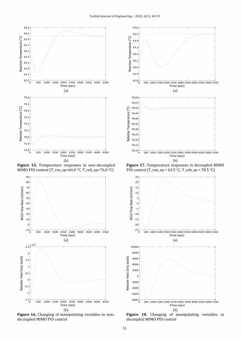
Turkish Journal of Engineering – 2022; 6(1); 40-53
51
(a)
(b)
Figure 15. Temperature responses in non–decoupled MIMO PID control (T_rxn_sp=64.0 °C, T_reb_sp=76.0 °C)
(a)
(b)
Figure 16. Changing of manipulating variables in non–decoupled MIMO PID control
(a)
(b)
Figure 17. Temperature responses in decoupled MIMO PID control (T_rxn_sp = 63.5 °C, T_reb_sp = 78.5 °C)
(a)
(b)
Figure 18. Changing of manipulating variables in decoupled MIMO PID control
0 500 1000 1500 2000 2500 3000 3500 4000 450062,5
62,7
62,9
63,1
63,3
63,5
63,7
63,9
64,1
64,3
Time (sec)
Reac
tion
Tem
pera
ture
(°C)
0 500 1000 1500 2000 2500 3000 3500 4000 450075,8
75,9
76,0
76,1
76,2
76,3
76,4
76,5
76,6
Time (sec)
Rebo
iler
Tem
pera
ture
(°C)
0 500 1000 1500 2000 2500 3000 3500 4000 4500-10
0
10
20
30
40
50
60
70
80
90
Time (sec)
WCO
Flo
w R
ate
(ml/
min
)
0 500 1000 1500 2000 2500 3000 3500 4000 4500-1.5
-1
-0.5
0
0.5
1
1.5
2
2.5x 10
4
Time (sec)
Rebo
iler
Hea
t D
uty
(wat
t)
0 500 1000 1500 2000 2500 3000 3500 4000 4500 5000 550062,8
62,9
63,0
63,1
63,2
63,3
63,4
63,5
63,6
Time (sec)
Reac
tion
Tem
pera
ture
(°C)
0 500 1000 1500 2000 2500 3000 3500 4000 4500 5000 550078,10
78,15
78,20
78,25
78,30
78,35
78,40
78,45
78,50
78,55
78,60
Time (sec)
Rebo
iler
Tem
pera
ture
(°C)
0 500 1000 1500 2000 2500 3000 3500 4000 4500 5000 5500-25
-20
-15
-10
-5
0
5
10
15
20
25
Time (sec)
WCO
Flo
w R
ate
(ml/
min
)
0 500 1000 1500 2000 2500 3000 3500 4000 4500 5000 5500-8000
-6000
-4000
-2000
0
2000
4000
6000
8000
10000
Time (sec)
Rebo
iler
Hea
t D
uty
(wat
t)
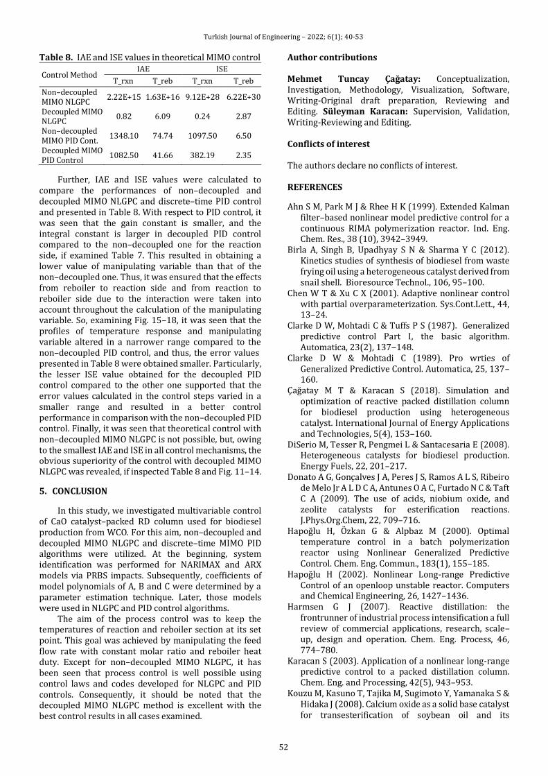
Turkish Journal of Engineering – 2022; 6(1); 40-53
52
Table 8. IAE and ISE values in theoretical MIMO control
Control Method IAE ISE
T_rxn T_reb T_rxn T_reb
Non–decoupled MIMO NLGPC
2.22E+15 1.63E+16 9.12E+28 6.22E+30
Decoupled MIMO NLGPC
0.82 6.09 0.24 2.87
Non–decoupled MIMO PID Cont.
1348.10 74.74 1097.50 6.50
Decoupled MIMO PID Control
1082.50 41.66 382.19 2.35
Further, IAE and ISE values were calculated to compare the performances of non–decoupled and decoupled MIMO NLGPC and discrete–time PID control and presented in Table 8. With respect to PID control, it was seen that the gain constant is smaller, and the integral constant is larger in decoupled PID control compared to the non–decoupled one for the reaction side, if examined Table 7. This resulted in obtaining a lower value of manipulating variable than that of the non–decoupled one. Thus, it was ensured that the effects from reboiler to reaction side and from reaction to reboiler side due to the interaction were taken into account throughout the calculation of the manipulating variable. So, examining Fig. 15–18, it was seen that the profiles of temperature response and manipulating variable altered in a narrower range compared to the non–decoupled PID control, and thus, the error values presented in Table 8 were obtained smaller. Particularly, the lesser ISE value obtained for the decoupled PID control compared to the other one supported that the error values calculated in the control steps varied in a smaller range and resulted in a better control performance in comparison with the non–decoupled PID control. Finally, it was seen that theoretical control with non–decoupled MIMO NLGPC is not possible, but, owing to the smallest IAE and ISE in all control mechanisms, the obvious superiority of the control with decoupled MIMO NLGPC was revealed, if inspected Table 8 and Fig. 11–14.
5. CONCLUSION
In this study, we investigated multivariable control of CaO catalyst–packed RD column used for biodiesel production from WCO. For this aim, non–decoupled and decoupled MIMO NLGPC and discrete–time MIMO PID algorithms were utilized. At the beginning, system identification was performed for NARIMAX and ARX models via PRBS impacts. Subsequently, coefficients of model polynomials of A, B and C were determined by a parameter estimation technique. Later, those models were used in NLGPC and PID control algorithms.
The aim of the process control was to keep the temperatures of reaction and reboiler section at its set point. This goal was achieved by manipulating the feed flow rate with constant molar ratio and reboiler heat duty. Except for non–decoupled MIMO NLGPC, it has been seen that process control is well possible using control laws and codes developed for NLGPC and PID controls. Consequently, it should be noted that the decoupled MIMO NLGPC method is excellent with the best control results in all cases examined.
Author contributions Mehmet Tuncay Çağatay: Conceptualization, Investigation, Methodology, Visualization, Software, Writing-Original draft preparation, Reviewing and Editing. Süleyman Karacan: Supervision, Validation, Writing-Reviewing and Editing. Conflicts of interest The authors declare no conflicts of interest. REFERENCES
Ahn S M, Park M J & Rhee H K (1999). Extended Kalman filter–based nonlinear model predictive control for a continuous RIMA polymerization reactor. Ind. Eng. Chem. Res., 38 (10), 3942–3949.
Birla A, Singh B, Upadhyay S N & Sharma Y C (2012). Kinetics studies of synthesis of biodiesel from waste frying oil using a heterogeneous catalyst derived from snail shell. Bioresource Technol., 106, 95–100.
Chen W T & Xu C X (2001). Adaptive nonlinear control with partial overparameterization. Sys.Cont.Lett., 44, 13–24.
Clarke D W, Mohtadi C & Tuffs P S (1987). Generalized predictive control Part I, the basic algorithm. Automatica, 23(2), 137‒148.
Clarke D W & Mohtadi C (1989). Pro wrties of Generalized Predictive Control. Automatica, 25, 137–160.
Çağatay M T & Karacan S (2018). Simulation and optimization of reactive packed distillation column for biodiesel production using heterogeneous catalyst. International Journal of Energy Applications and Technologies, 5(4), 153–160.
DiSerio M, Tesser R, Pengmei L & Santacesaria E (2008). Heterogeneous catalysts for biodiesel production. Energy Fuels, 22, 201–217.
Donato A G, Gonçalves J A, Peres J S, Ramos A L S, Ribeiro de Melo Jr A L D C A, Antunes O A C, Furtado N C & Taft C A (2009). The use of acids, niobium oxide, and zeolite catalysts for esterification reactions. J.Phys.Org.Chem, 22, 709–716.
Hapoğlu H, Özkan G & Alpbaz M (2000). Optimal temperature control in a batch polymerization reactor using Nonlinear Generalized Predictive Control. Chem. Eng. Commun., 183(1), 155–185.
Hapoğlu H (2002). Nonlinear Long-range Predictive Control of an openloop unstable reactor. Computers and Chemical Engineering, 26, 1427–1436.
Harmsen G J (2007). Reactive distillation: the frontrunner of industrial process intensification a full review of commercial applications, research, scale–up, design and operation. Chem. Eng. Process, 46, 774–780.
Karacan S (2003). Application of a nonlinear long-range predictive control to a packed distillation column. Chem. Eng. and Processing, 42(5), 943–953.
Kouzu M, Kasuno T, Tajika M, Sugimoto Y, Yamanaka S & Hidaka J (2008). Calcium oxide as a solid base catalyst for transesterification of soybean oil and its

Turkish Journal of Engineering – 2022; 6(1); 40-53
53
application to biodiesel production. Fuel, 87, 2798–2806.
Kulkarni M G & Dalai A K (2006). Waste cooking oil – an economical source for biodiesel: a review. Ind. Eng. Chem. Res., 45, 2901–2913.
Martín M & Grossmann I E (2012). Simultaneous optimization and heat integration for biodiesel production from cooking oil and algae. Ind. Eng. Chem. Res, 51, 7998−8014.
Özkan G, Hapoğlu H & Alpbaz M (2006). Non–linear Generalised Predictive Control of a jacketed well mixed tank as applied to a batch process—A polymerisation reaction. Applied Thermal Engineering, 26, 720–726.
Sharma Y C, Singh B & Upadhyay S N (2008). Advancements in development and characterization of biodiesel. Fuel, 87, 2355–2373.
Srivastava A & Prasad R (2000). Triglycerides–based diesel fuels. Renew. Sustainable Energy Rev., 4, 111–133.
Vujicic D J, Comic D, Zarubica A, Micic R & Boskovi G (2010). Kinetics of biodiesel synthesis from sunflower oil over CaO heterogeneous catalyst. Fuel, 89, 2054–2061.
Zeybek Z, Çetinkaya S, Hapoğlu H & Alpbaz M (2006). Generalized delta rule (GDR) algorithm with generalized predictive control (GPC) for optimum temperature tracking of batch polymerization. Chemical Engineering Science, 61, 6691–6700.
Zhang Y, Dube M A, McLean D D & Kates M (2003). Biodiesel production from waste cooking oil: 1. Process design and technological assessment. Bioresource Technology, 89, 1–16.
© Author(s) 2021. This work is distributed under https://creativecommons.org/licenses/by-sa/4.0/
* Corresponding Author Cite this article
*([email protected]) ORCID ID 0000-0002-1797-2039 ([email protected]) ORCID ID 0000-0001-9807-884X ([email protected]) ORCID ID 0000-0001-7496-2796 Research Article / DOI: 10.31127/tuje.807019
Ozturk A, Allahverdi N & Saday F (2022). Application of artificial intelligence methods for bovine gender prediction. Turkish Journal of Engineering, 6(1), 54-62
Received: 07/10/2020; Accepted: 07/12/2020
Turkish Journal of Engineering – 2022; 6(1); 54-62
Turkish Journal of Engineering
https://dergipark.org.tr/en/pub/tuje
e-ISSN 2587-1366
Application of artificial intelligence methods for bovine gender prediction
Ali Öztürk*1,2 , Novruz Allahverdi1 , Fatih Saday3 1KTO Karatay University, Engineering Faculty, Computer Engineering Department, Konya, Turkey 2Havelsan Inc., Ankara, Turkey 3Organized Industrial Zone Directorate, Konya, Turkey
Keywords ABSTRACT Bovine gender prediction Fuzzy logic Artificial neural networks Support vector machines Random forests
This study investigates determining the gender of calves using some artificial intelligence (AI) techniques. Gender identification is important in animal breeding, focusing on the desired outcome and planning. The data used to determine the gender of calves were the speed, magnitude, and density of the bull's semen. The analysis of the related studies showed that there was not a study on gender prediction of bovine with the application of AI methods. In this study, fuzzy logic (FL), artificial neural networks (ANN), support vector machines (SVM), and random forests (RF) were used. The efficiency of these approaches was verified by statistical analysis parameters such as accuracy, specificity, sensitivity (recall), precision, and F-score. The FL, ANN, SVM, and RF models had 84%, 96%, 97%, 99% accuracy, 93.75%, 96.88%, 100%, 100% sensitivity, 66.66%, 94.44%, 92.31%, 97.30% specificity, 83.33%, 96.88%, 95.31%, 98.44% precision results, respectively. Application of these AI techniques for prediction bovine gender proves that these methods may be used by semen breeders as supporting information tools. In particular, it was observed that the RF method yielded the highest accuracy results.
1. INTRODUCTION
Biotechnological progress is being exploited to improve herd fertility. One of the last points in biotechnology improvement is the development of a method for determining the features of bovine sperm to determine the offspring sex (Seidel, 2003). Bovine genders are largely determined by the bulls’ semen. In cattle, the gender of breeders is shaped during fertilization.
Gender identification enables the planning of production strategies and biotechnological study programs of enterprises that produce milk or meat. Today, alternative breeding systems are being studied in terms of calf production in cattle breeding (Erten and Yilmaz, 2012).
In cattle breeding, methods, such as centrifugation, electrophoresis, sedimentation, filtration, pH changes in the preservation medium, immunological techniques, and motility criteria, are used in the detection of the X and Y chromosomes in sperm. However, the practical use of the mentioned techniques is not very reliable because of the significant differences in the gender-
determined sperm rates obtained as a result of these methods (Anderson, 1997; Johnson et al. 1994; Niemann and Meinecke, 1993). In contrast, the gender selection of offspring of cows in cattle currently represents a great perspective for genetic improvement and for meeting market demand. A new proposal for determining the proportion of the X- and Y-bearing cells in a bovine sperm sample was settled using actual polymerase chain reaction (Parati et al. 2006).
The forecast of male fertility with sperm quality parameters in vitro remains a problem for the bull industry. Fluorescein staining furthermore computer semen analysis (CASA) provides kinetically correct and functionally objective results to improve sperm control parameters. Therefore, Inanc et al. (2018) sought to study the kinetic parameters of the CASA and fluorescein staining of cryopreserved bull semen. They concluded that various kinetic parameters obtained with the help of algorithms of the CASA software system and fluorescein dyes can be related to fertility. However, further research is needed to establish a more accurate relationship with fertility.
Turkish Journal of Engineering – 2022; 6(1); 54-62
55
A review by Sendag et al. (2005) about forecasting prenatal embryonic or fetal sex uses a variety of methods to apply sperm, embryo, or fetus. The review provides detailed information on these methods.
A Fuzzy Inference System (FES) for determining the productivity of livestock (milk and meat) was described by Vásquez et al. (2019). Using FL in terms of modeling the variables affecting livestock productivity, one can benefit from the knowledge and experience gained by producers, as well as from what they have learned from many years of observation and practice. Consequently, these results can be shared with agricultural producers and technicians to increase livestock productivity. The accuracy of the designed expert system was 86.67%.
RF method was used (Nicolas et al. 2016) to improve the downscaling of Gridded Livestock of the World database and provided better results than the stratified regression models. To identify the significant associations between single nucleotide polymorphism (SNP) and residual feed intake in dairy cattle, RF algorithm was used by Yao et al. (2013). The obtained results of RF could be used to identify large additive or epistatic SNP and informative quantitative trait loci. Multiple logistic regression, Naïve Bayes, and RF were compared to predict individual survival to the second lactation in dairy heifers (Heide et al. 2019). RF had the highest Area Under Curve (AUC) among the methods after first calving.
Mikail and Keskin (2013) evaluated SVM to assess its performance in detection of the mastitis in dairy cows. They achieved a sensitivity of 89% and specificity of 92% on the prediction of somatic cell counts in milk samples. SVM was also used by Miekley et al. (2013) to investigate its application for the mastitis detection in dairy cows. They obtained a sensitivity of 84.6% and specificity of 78.3%, and concluded that SVM could principally be applied for disease detection. Martiskainen et al. (2009) constructed SVM classification models based on nine features corresponding to different cow behaviors. The data were obtained using a three-dimensional accelerometer to investigate cow behavior pattern recognition. They concluded that SVM proved to be useful in the classification of measured behavior patterns. Huma and Iqbal (2019) used traditional linear models, regression trees, SVM, and RF methods to predict the bodyweight of farm animals. They found that RF had the best results among the methods for both the training and test datasets.
Allahverdi and Saday (2018) investigated the gender prediction of the bovine subject in a preliminary form, where they described the use of the ANN in predicting gender offspring. For the same goal, SVM and RF techniques were used in this study. The accuracy, sensitivity, specificity, precision, and F-score were determined for all these approaches. The problem of determining the gender of descendants in the animal herd with the methods of artificial intelligence described here is particularly lacking in the literature. In this study, bull sperm cells' features were used to predict the sex of descendants in the animal herd with the above-mentioned methods and their performances
were compared in terms of various statistical analysis parameters.
The rest of the paper is organized as follows: Section 2 discusses the procedure for obtaining semen signs and the dataset used; describes the artificial intelligence methods (FL, ANN, SVM, RF); gives the definitions on the accuracy, sensitivity, and specificity determinations; Section 3 gives details of the experimental study with the obtained results; and Section 4 concludes the study.
2. METHOD
2.1. Preparing the Dataset
Sperm processing was performed by the commercial company Super Genetics Ltd. Sti. via cryobiology method. To ensure the classification of X and Y sperm cells, semen was collected from sexually mature bulls using an artificial vagina. Sperm with mobility greater than 60% were separated. It was diluted in egg diluent with egg yolk which was determined as 4% for sperm freezing process. It was cooled at 4 ° C for 90 minutes. The sperm were transferred by machine to 0.25 ml tubes and the sexless sperm were frozen in a programmable freezer as described. At the end of the process, the sperm were immersed in nitrogen.
A total of 100 individual cells derived from the animals were marked using the labeling function of the analysis software. The original image was manually divided into segments by digital zooming. Sperm measurements were then performed. The data set, as a result of these measurements, includes speed, size, density, and gender type. As for the knowledge base, 100 samples described in the study (Allahverdi and Saday, 2018) were used. There were 64 males and 36 females in the knowledge base. The input parameters in the system were speed (μ/s), magnitude (μ), and density (µg/µm³). For the input parameters, the mean values were 45.61, 62.99, 49.76, the minimum values were 37.82, 52.99, 42.34 and the maximum values were 54.28, 72.62, 62.21, respectively. The output parameter was a numerical outcome which made a basis for female or male estimation depending on the predefined threshold value. The classification (male or female) was neither inferred by Super Genetic LTD tool, but the real genders of the animals were eventually determined and shared by the company in the dataset.
2.2. Fuzzy Logic Method
FL was introduced by Lotfi A. Zadeh (1965) to manage inaccurate and vague knowledge. If in the classical theory of sets elements either belong to a set or not, then in the fuzzy theory of sets elements may belong to a set to some extent. More formally, let X be a set of elements called a reference set. A fuzzy subset A of X is defined by a membership function µA(x), or simply A(x), which assigns a value to any x ϵ X within a real number range between 0 and 1. As in the classical case, 0 means no membership and 1 full membership, but now the value between 0 and 1 represents the extent to

Turkish Journal of Engineering – 2022; 6(1); 54-62
56
which x can be considered as an element X (Bobillo and Straccia, 2008).
The FL approach for applications is generally used as an FES, where instead of a strict knowledge base in an expert system, a fuzzy knowledge base is used. When the input data are entered into the system, one or a few rules can be activated, and an inference mechanism is used to calculate the correct fuzzy answer (Allahverdi, 2002; Allahverdi, 2020). The FES implementation details which are specific to this study are given in Section 3.1.
2.3. Artificial Neural Networks Method
ANN is a robust method against errors in training data for approximating real, discrete, or vector-valued functions (Adeli and Hung, 1995; Oztemel, 2016). They learn the input-output mapping given by the training data with a highly parallel and distributed process through automated weight tuning. Every bounded continuous function can be approximated with an arbitrarily small error by ANN with one hidden layer. For the ANN to be capable of representing nonlinear functions, the output of the neurons must be calculated with a differentiable nonlinear transfer function. One such function is the sigmoid defined as σ(net) = 1 / (1 + e-net) that squeezes the output between 0 and 1. The input to the sigmoid is defined on neuron xj as netj = ∑ wijxi
ni=0 , where wij is the weight between the
neurons xi and xj. The derivative of the sigmoid function was used to calculate the error value for the neurons and defined as dσ(y) / dy = σ(y)(1 – σ(y)).
The backpropagation is based on the stochastic gradient descent where the initial random weights are updated for each training example. The error between the target and computed output values is iteratively minimized until the termination condition is met. The termination condition can be either the reduction of the total network error to a predefined level or reaching to a predefined number of training steps. The error E is computed as follows:
𝐸 = (1 2)⁄ ∑ (𝑥o − 𝑥t)
2j (1)
Where 𝑥𝑜 is the output value, and 𝑥𝑡 is the actual
(target) value. The weights are updated according to the following
formula: Δ𝑊ji(𝑛 + 1) = 𝜂𝛿pj𝑂pi + αΔ𝑊ji(𝑛) (2)
Where η is the learning rate; δpj is the error value
for the neuron on Lth layer, and α is the momentum coefficient introduced to escape from the local minima during training.
δpj is calculated for the output layer neurons as
𝛿𝑝𝑗 = (𝑂𝑡𝑝𝑗 − 𝑂𝑝𝑗) 𝑂𝑝𝑗(1 − 𝑂𝑝𝑗) (3)
For the hidden layer neurons:
𝛿𝑝𝑗 = 𝑂𝑝𝑗(1 − 𝑂𝑝𝑗) ∑ 𝛿𝑝𝑘𝑤𝑘𝑗𝑘 (4)
2.4. Artificial Neural Networks Method
The SVM algorithm was first proposed by Vapnik (1995) for solving classification problems using a nonlinear function which maps an input dataset X into a high dimensional feature space F. The estimation function for the SVM is
𝑓(𝑥) = (𝑤 × ∅(𝑥)) + 𝑏 (5)
Where w and b are the estimated coefficients from the dataset, and Ø(x) is the non-linear function used in feature space.
The risk function to be minimized is
𝑅(𝑤, 𝜉∗) = 1
2‖𝑤‖2 + 𝐶 ∑ (𝜉𝑖 + 𝜉𝑖
∗)𝑁𝑖=1 (6)
And, 𝑑𝑖 − 𝑤∅(𝑥𝑖) − 𝑏𝑖 ≤ 휀 + 𝜉𝑖 (7) (𝑤∅(𝑥)) + 𝑏 − 𝑑𝑖 ≤ 휀 + 𝜉𝑖
∗ (8)
Where 𝜉𝑖 , 𝜉𝑖
∗ > 0. Vapnik (1999) introduced ε-insensitive loss
function as an extension to the SVM to solve regression problems as well. The Support Vector Regression estimation function is
𝑓(𝑥) = ∑ (𝛼𝑖 − 𝛼𝑖
∗)𝐾(𝑋, 𝑋𝑖) + 𝑏𝑁𝑆𝑉𝑖=1 (9)
Where 𝛼𝑖 and 𝛼𝑖
∗ are Lagrange multipliers and NSV is the number of support vectors. The kernel function 𝐾(𝑋𝑖 , 𝑋𝑗) = ∅(𝑋𝑖)∅(𝑋𝑗) is used in feature space to
perform computation in input space.
2.5. Random Forest Method
Random Forests are formed by a decision tree classifiers set (DTCS) as in the following.
𝐷𝑇𝐶𝑆 = ℎ(𝑥, 𝜃(𝑘)), 𝑘 = 1,2,3, … , 𝐾 (10)
Where x is the input vector and Θ(k) are random
vectors which independently determine the growth of a single tree. Each random tree in the set casts a unit vote for determining the output of the forest (Breiman, 2001). In the case of regression, the random trees take on numerical values rather than discrete labels and the output is obtained by taking the average over each random tree.
If A is continuous attribute and m is the sample subsets on a node, then the RF algorithm is defined as in the following: • The samples are sorted in ascending order on the
continuous attribute A using corresponding discrete sequence A1, A2,…, Am.
• On the sequence, m-1 division points are generated. The division point j(0<j<m) is adjusted by the formula
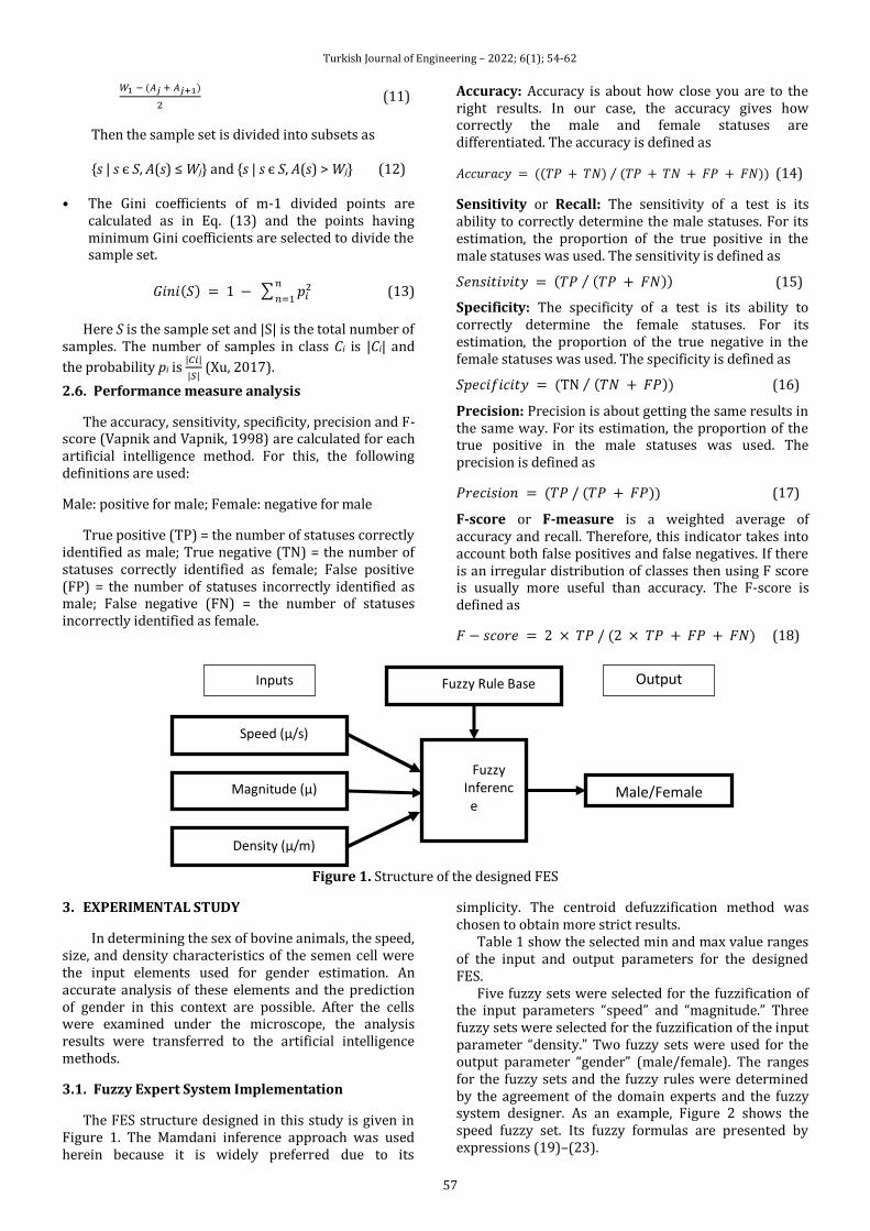
Turkish Journal of Engineering – 2022; 6(1); 54-62
57
𝑊1 − (𝐴𝑗 + 𝐴𝑗+1)
2 (11)
Then the sample set is divided into subsets as s | s є S, A(s) ≤ Wj and s | s є S, A(s) > Wj (12)
• The Gini coefficients of m-1 divided points are calculated as in Eq. (13) and the points having minimum Gini coefficients are selected to divide the sample set.
𝐺𝑖𝑛𝑖(𝑆) = 1 − ∑ 𝑝𝑖2𝑛
𝑛=1 (13)
Here S is the sample set and |S| is the total number of
samples. The number of samples in class Ci is |Ci| and
the probability pi is |𝐶𝑖|
|𝑆| (Xu, 2017).
2.6. Performance measure analysis
The accuracy, sensitivity, specificity, precision and F-score (Vapnik and Vapnik, 1998) are calculated for each artificial intelligence method. For this, the following definitions are used:
Male: positive for male; Female: negative for male
True positive (TP) = the number of statuses correctly identified as male; True negative (TN) = the number of statuses correctly identified as female; False positive (FP) = the number of statuses incorrectly identified as male; False negative (FN) = the number of statuses incorrectly identified as female.
Accuracy: Accuracy is about how close you are to the right results. In our case, the accuracy gives how correctly the male and female statuses are differentiated. The accuracy is defined as
𝐴𝑐𝑐𝑢𝑟𝑎𝑐𝑦 = ((𝑇𝑃 + 𝑇𝑁) (𝑇𝑃 + 𝑇𝑁 + 𝐹𝑃 + 𝐹𝑁))⁄ (14)
Sensitivity or Recall: The sensitivity of a test is its ability to correctly determine the male statuses. For its estimation, the proportion of the true positive in the male statuses was used. The sensitivity is defined as
𝑆𝑒𝑛𝑠𝑖𝑡𝑖𝑣𝑖𝑡𝑦 = (𝑇𝑃 (𝑇𝑃 + 𝐹𝑁)⁄ ) (15)
Specificity: The specificity of a test is its ability to correctly determine the female statuses. For its estimation, the proportion of the true negative in the female statuses was used. The specificity is defined as
𝑆𝑝𝑒𝑐𝑖𝑓𝑖𝑐𝑖𝑡𝑦 = (TN (𝑇𝑁 + 𝐹𝑃))⁄ (16)
Precision: Precision is about getting the same results in the same way. For its estimation, the proportion of the true positive in the male statuses was used. The precision is defined as
𝑃𝑟𝑒𝑐𝑖𝑠𝑖𝑜𝑛 = (𝑇𝑃 / (𝑇𝑃 + 𝐹𝑃)) (17)
F-score or F-measure is a weighted average of accuracy and recall. Therefore, this indicator takes into account both false positives and false negatives. If there is an irregular distribution of classes then using F score is usually more useful than accuracy. The F-score is defined as
𝐹 − 𝑠𝑐𝑜𝑟𝑒 = 2 × 𝑇𝑃 / (2 × 𝑇𝑃 + 𝐹𝑃 + 𝐹𝑁) (18)
Figure 1. Structure of the designed FES
3. EXPERIMENTAL STUDY
In determining the sex of bovine animals, the speed, size, and density characteristics of the semen cell were the input elements used for gender estimation. An accurate analysis of these elements and the prediction of gender in this context are possible. After the cells were examined under the microscope, the analysis results were transferred to the artificial intelligence methods.
3.1. Fuzzy Expert System Implementation
The FES structure designed in this study is given in Figure 1. The Mamdani inference approach was used herein because it is widely preferred due to its
simplicity. The centroid defuzzification method was chosen to obtain more strict results.
Table 1 show the selected min and max value ranges of the input and output parameters for the designed FES.
Five fuzzy sets were selected for the fuzzification of the input parameters “speed” and “magnitude.” Three fuzzy sets were selected for the fuzzification of the input parameter “density.” Two fuzzy sets were used for the output parameter “gender” (male/female). The ranges for the fuzzy sets and the fuzzy rules were determined by the agreement of the domain experts and the fuzzy system designer. As an example, Figure 2 shows the speed fuzzy set. Its fuzzy formulas are presented by expressions (19)–(23).
Speed (µ/s)
Magnitude (µ)
Density (µ/m)
Fuzzy Inference
Fuzzy Rule Base
Male/Female
Inputs Output

Turkish Journal of Engineering – 2022; 6(1); 54-62
58
Table 1. Min and max value range of the input and output parameters of FES
Input/Output
Fuzzy values Fuzzy Sets
Input Speed (µ/s) Very Slow Slow Medium Fast Very Fast
(30-37) (35-41) (38-46) (45-55) (> 50)
Input Magnitude (µ) Very Small Small Medium Big Very Big
(45-56) (52-62) (64-68) (64-74) (> 70)
Input Density (µg/µm³) Less Dense Dense Much Dense
(35-48) (42-58) (> 55)
Output Gender (%) Male Female
(< 35) (< 35)
Figure 2. Fuzzification of the speed input value
µVS(x) =
1 if x < 32
(37 - x)
(37 - 32)⁄ if 32 < x < 37 (19)
µS(x) =
(x - 35)
(37 - 35)⁄ if 35 < x ≤ 37
(41 - x)
(41 - 37)⁄ if 37 < x < 41
(20)
µM(x) =
(x - 37)
(42 - 37)⁄ if 37 < x ≤ 42
(46 - x)
(46 - 45)⁄ if 45 < x < 46
(21)
µF(x) =
(x - 45) (50 - 45)⁄ if 45 < x ≤ 50
(55 - x)
(55 - 50)⁄ if 50 < x < 55
(22)
µVF(x) =
(x - 50) (55 - 50)⁄ if 50 < x ≤ 55
1 if 55 < x
(23)
Note that the output parameter “gender” was determined as “Female% = 100% − Male%” or “Male% = 100% − Female%.” In addition, the value of 35% will be an undetermined answer when calculating the calf sex (Figure 3 and formulas (24-25)).
Some of the fuzzy sets of sperm speed will be described as the next expressions:
µ𝑉𝑆(𝑥) = 1 / 30 + 1 / 32 + 0.3 / 36 + 0 / 37
µ𝑀(𝑥) = 0 / 38 + 0.45 / 39 + 1 / 42 + 0.1 / 45.5 + 0 / 46
µ𝑉𝐹(𝑥) = 0 / 50 + 0.5 / 52.5 + 1 / 55 + 1 / 60 µ𝐹(𝑥) =
1 𝑖𝑓 𝑥 < 30
(40 − 𝑥)
(40 − 30)⁄ 𝑖𝑓 30 < 𝑥 < 40
(24) µ𝑀(𝑥) =
(𝑥 − 30) (40 − 30)⁄ 𝑖𝑓 30 < 𝑥 ≤ 40
1 𝑖𝑓 40 < 𝑥
(25)
Some of the fuzzy sets (Figure 3) of gender (output value) will be described as the next expressions:
µ𝐹(𝑥) = 1 / 0 + 1 / 30 + 0.5 / 35 + 0 / 40 µ𝑀(𝑥) = 0 / 30 + 0.5 / 35 + 1 / 40 + 1 / 100
The number of fuzzy rules is determined by the multiplication of the number of input fuzzy sets. In our case, it will be 5 × 5 × 3 = 75 rules. The dataset was applied to the FES containing 75 rules to obtain the outputs. Some fuzzy rules are also used in the designed FES:
R5: If (speed is very low) and (magnitude is small) and (density is dense), then gender is female.
R36: If speed is medium and magnitude is small and density is much dense then output is female. R67: If (speed is very fast) and (magnitude is medium) and (density is less dense), then gender is male.
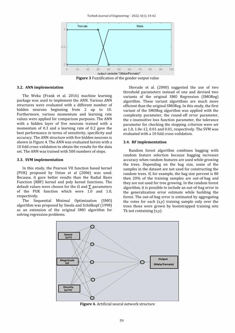
Turkish Journal of Engineering – 2022; 6(1); 54-62
59
Figure 3 Fuzzification of the gender output value
3.2. ANN implementation
The Weka (Frank et al. 2016) machine learning package was used to implement the ANN. Various ANN structures were evaluated with a different number of hidden neurons beginning from 2 up to 10. Furthermore, various momentum and learning rate values were applied for comparison purposes. The ANN with a hidden layer of five neurons trained with a momentum of 0.3 and a learning rate of 0.2 gave the best performance in terms of sensitivity, specificity and accuracy. The ANN structure with five hidden neurons is shown in Figure 4. The ANN was evaluated herein with a 10 fold cross-validation to obtain the results for the data set. The ANN was trained with 500 numbers of steps.
3.3. SVM implementation
In this study, the Pearson VII function based kernel (PUK) proposed by Ustun et al (2006) was used. Because, it gave better results than the Radial Basis Function (RBF) kernel and poly kernel functions. The default values were chosen for the Ω and ∑ parameters of the PUK function which were 1.0 and 1.0, respectively.
The Sequential Minimal Optimization (SMO) algorithm was proposed by Smola and Schölkopf (1998) as an extension of the original SMO algorithm for solving regression problems.
Shevade et al. (2000) suggested the use of two threshold parameters instead of one and devised two variants of the original SMO Regression (SMOReg) algorithm. These variant algorithms are much more efficient than the original SMOReg. In this study, the first variant of the SMOReg algorithm was applied with the complexity parameter, the round-off error parameter, the ε-insensitive loss function parameter, the tolerance parameter for checking the stopping criterion were set as 1.0, 1.0e-12, 0.01 and 0.01, respectively. The SVM was evaluated with a 10 fold cross-validation.
3.4. RF implementation
Random forest algorithm combines bagging with random feature selection because bagging increases accuracy when random features are used while growing the trees. Depending on the bag size, some of the samples in the dataset are not used for constructing the random trees. If, for example, the bag size percent is 80 then 20% of the training samples are out-of-bag and they are not used for tree growing. In the random forest algorithm, it is possible to include an out-of-bag error in the generalization error estimate while building the forest. The out-of-bag error is estimated by aggregating the votes for each (x,y) training sample only over the trees those were grown by bootstrapped training sets Tk not containing (x,y).
Figure 4. Artificial neural network structure
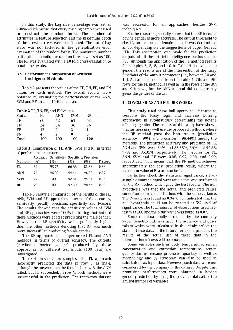
Turkish Journal of Engineering – 2022; 6(1); 54-62
60
In this study, the bag size percentage was set as 100% which means that every training sample was used to construct the random forest. The number of attributes in feature selection and the maximum depth of the growing trees were not limited. The out-of-bag error was not included in the generalization error estimation of the random forest. The maximum number of iterations to build the random forests was set as 100. The RF was evaluated with a 10 fold cross-validation to obtain the results.
3.5. Performance Comparison of Artificial Intelligence Methods
Table 2 presents the values of the TP, TN, FP, and FN
status for each method. The overall results were obtained by evaluating the performances of the ANN, SVM and RF on each 10-fold test set. Table 2 TP, TN, FP, and FN values. Status FL ANN SVM RF TP 60 62 61 63 TN 24 34 36 36 FP 12 2 3 1 FN 4 2 0 0 Total 100 100 100 100 Table 3. Comparison of FL, ANN, SVM and RF in terms of performance measures.
Methods Accuracy (%)
Sensitivity (%)
Specificity (%)
Precision (%) F-score
FL 84 93.75 66.66 83.33 0.88
ANN 96 96.88 94.44 96.88 0.97
SVM 97 100 92.31 95.31 0.98
RF 99 100 97.30 98.44 0.99
Table 3 shows a comparison of the results of the FL,
ANN, SVM, and RF approaches in terms of the accuracy, sensitivity (recall), precision, specificity and F-score. The results showed that the sensitivity values of SVM and RF approaches were 100% indicating that both of these methods were good at predicting the male gender. However, the RF specificity was significantly higher than the other methods denoting that RF was much more successful in predicting female gender.
The RF approach also outperformed FL and ANN methods in terms of overall accuracy. The outputs (predicting bovine gender) produced by these approaches for different test inputs (100 data) are investigated.
Table 4 provides ten samples. The FL approach incorrectly predicted the data in row 7 as male, although the answer must be female. In row 8, the ANN failed, but FL succeeded. In row 9, both methods were unsuccessful in the prediction. The tenth-row dataset
was successful for all approaches, besides SVM techniques.
So, the research generally shows that the RF forecast bovine gender is more accurate. The output threshold to classify an instance as female or male was determined as 35, depending on the suggestions of Super Genetic LTD. This assumption was made for the prediction outputs of all the artificial intelligence methods as in FES. Although the application of the FL method results for samples 3, 5, 8, and 10 in Table 4 indicate male gender, the results are at the intersection of the fuzzy functions of the output parameter (i.e., between 30 and 40). As can also be seen from the Table 4, 7th, and 9th rows for the FL method, as well as in the rows of the 8th and 9th rows, for the ANN method did not correctly guess the gender of the calf. 4. CONCLUSIONS AND FUTURE WORKS
This study used some bull sperm cell features to compare the fuzzy logic and machine learning approaches in automatically determining the bovine offspring gender. The results of this study have shown that farmers may well use the proposed methods, where the RF method gave the best results (prediction accuracy = 99% and precision = 98.44%) among the methods. The prediction accuracy and precision of FL, ANN and SVM were 84% and 83.33%, 96% and 96.88, 97% and 95.31%, respectively. The F-scores for FL, ANN, SVM and RF were 0.88, 0.97, 0.98, and 0.99, respectively. This means that the RF method achieves approximately the best prediction result, where the maximum value of F-score can be 1.
To further check the statistical significance, a two-sample assuming equal variances t-test was performed for the RF method which gave the best results. The null hypothesis was that the actual and predicted values come from normal distributions with the same variance. The P-value was found as 0.94 which indicated that the null hypothesis could not be rejected at 5% level of significance. The total number of observations used in t-test was 100 and the t-stat value was found as 0.07.
Since the data kindly provided by the company Super Genetics Ltd. was used, the accuracy and other values which were calculated in this study reflect the state of these data. In the future, for use in practice, the results of the actual use of these data in the insemination of cows will be obtained.
Some variables such as body temperature, semen concentration and extraction temperature, semen quality during freezing processes, quantity as well as morphology and % acrosome, can also be used in calculations as input data. However, such data were not considered by the company in the dataset. Despite this, promising performances were obtained in bovine gender prediction by using the provided dataset of the limited number of variables.
Turkish Journal of Engineering – 2022; 6(1); 54-62
61
Table 4. Comparison of some of the outputs for the FL, ANN; SVM and RF methods
Sample No
Inputs Outputs (Actual)
Calculated Outputs
ANN FL SVM RF
Speed (μ/s)
Magnitude (μ)
Density (µg/µm³)
Female (%)
Male (%)
Female (%)
Male (%)
Female (%)
Male (%)
Female (%)
Male (%)
Female (%)
Male (%)
1 47.07 68.60 61.08 81.89 18.11 82.54 17.46 82.95 17.05 81.83 18.17 83.58 16.42
2 40.60 56.03 44.76 16.06 83.94 21.42 78.58 48.22 51.78 16.71 83.29 16.71 83.29
3 45.18 60.66 45.96 10.04 89.96 18.02 81.98 34.51 65.49 8.16 91.84 14.11 85.89
4 43.78 62.02 61.00 86.25 13.75 97.50 2.50 83.63 16.37 84.03 15.97 79.27 20.73
5 49.35 64.77 47.96 10.65 89.35 3.05 96.95 33.53 66.47 9.40 90.60 7.42 92.58
6 43.87 63.94 56.93 76.32 23.68 70.46 29.54 81.95 18.05 78.60 21.40 84.32 15.68
7 44.74 62.02 50.98 80.64 19.36 74.82 25.18 32.91 67.09 46.12 53.88 77.83 22.17
8 50.99 69.42 48.20 14.27 85.73 79.47 20.53 33.39 66.61 20.48 79.72 37.83 62.17
9 45.37 64.28 51.93 86.27 13.73 42.91 57.09 46.05 53.95 85.65 14.35 83.66 16.34
10 43.78 63.55 49.15 9.66 90.34 27.91 72.09 33.72 66.28 43.70 56.30 16.56 83.44 ACKNOWLEDGEMENT
The research reported here is supported by KTO Karatay University. The calculations are performed at the Computer Engineering Laboratory at the Department of Computer Engineering, KTO Karatay University. The authors also thank the Company Super Genetics Ltd. in Konya for their sharing the data. Author Contributions Ali Öztürk: Random Forest method and Support Vector Machines method. Novruz Allahverdi: Fuzzy Logic method. Fatih Saday: Artificial Neural Networks method. The rest of the paper was prepared together. Conflict of Interest There is no conflict of interest between the authors.
REFERENCES Adeli H & Hung S L (1995). Machine learning - neural
networks, genetic algorithms and fuzzy systems. John Wiley & Sons Inc. ISBN: 9780471016335.
Allahverdi N & Saday F (2018). An artificial neural network study for predicting sex in bulls. 7th International Conference on Advanced Technologies (ICAT’18), 727-731, Antalya, Turkey.
Allahverdi N (2002). Uzman Sistemler. Atlas, Istanbul, Turkey (in Turkish). ISBN: 975-6574-11-9.
Allahverdi N (2020). Bulanık Mantık ve Tıptaki Uygulamaları. KTO Karatay Üniversitesi Yayınları, Konya, Turkey (in Turkish). ISBN:9786056934636.
Anderson G B (1997). Identification of embryonic sex by detection of H-Y antigens. Theriogenology, 27, 81-97.
Bobillo F & Straccia U (2008). Towards a Crisp Representation of Fuzzy Description Logics under Łukasiewicz Semantics. International Symposium on Methodologies for Intelligent Systems (ISMIS 2008), 309-318, Toronto, Canada.
Breiman L (2001). Random forests. Machine Learning, 45 (1), 5-32.
Erten O & Yılmaz O (2012). Techniques of sex-selected calf production in dairy cattle breeding. Van, Yüzüncü Yil Üniversitesi Journal of Veterinary Faculty, 23 (3), 155-157 (in Turkish).
Frank E, Hall M A & Witten I H (2016). The WEKA Workbench Online Appendix for Data Mining: Practical Machine Learning Tools and Techniques. 4th ed. San Francisco, CA, USA: Morgan Kaufmann. ISBN:9780128042915.
Heide, E.M.M., Veerkamp, R.F., Pelt, M.L., Kamphuis, C., Athanasiadis, I. et al., (2019), Comparing regression, naive Bayes, and random forest methods in the prediction of individual survival to second lactation in Holstein cattle, Journal of Dairy Science, 102 (10), 9409-9421.
Huma ZE & Iqbal F (2019). Predicting the body weight of Balochi sheep using a machine learning approach. Turkish Journal of Veterinary and Animal Sciences, 43, 500-506.
Inanc M E, Çil B, Tekin K & Alemdar H (2018). The combination of CASA kinetic parameters and fluorescein staining as a fertility tool in cryopreserved bull semen. Turkish Journal of Veterinary and Animal Sciences, 42, 452-458.
Johnson L A, Cran D G & Polge C (1994). Recent advances in sex preselection of cattle: Flow cytometric sorting of X-Y-chromosome bearing sperm based on DNA to progeny. Theriogenology, 4, 51-56.
Martiskainen P, Jarvinen M, Skön J P, Tiirikainen J, Kolehmainen M, et al. (2009). Cow behaviour pattern recognition using a three-dimensional accelerometer and support vector machines. Applied Animal Behaviour Science, 119 (1-2), 32-38.
Miekley B, Traulsen I & Krieter J (2013). Mastitis detection in dairy cows: the application of support vector machines. The Journal of Agricultural Science, 151 (6), 889-897.

Turkish Journal of Engineering – 2022; 6(1); 54-62
62
Mikail N & Keskin I (2013). Application of the support vector machine to predict subclinical mastitis in dairy cattle. The Scientific World Journal, 1: 603897.
Nicolas G, Robinson TP, Wint W & Conchedda G (2016). Using Random Forest to Improve the Downscaling of Global Livestock Census Data. PLoS ONE, 11 (3), e0150424.
Niemann H & Meinecke B (1993). Embryo transfer und assoziierte biotechniken bei landwirtschaftlichen nutztieren. Ferdinand Enke Verlag, Stuttgart (In German). ISBN: 9783432254715.
Oztemel E (2016). Yapay Sinir Ağları. Papatya Yayınları. Istanbul, Turkey (in Turkish). ISBN: 9789756797396.
Parati K, Bongioni G, Aleandri R & Galli A (2006). Sex ratio determination in bovine semen: A new approach by quantitative real-time PCR. Theriogenology, 66, 2202–2209.
Seidel G EJ (2003). Economics of selecting for sex: the most important genetic trait. Theriogenology, 59, 585-598.
Sendag S, Aydin I & Celik HA (2005). Prenatal embryonic or fetal sex determination in cows. J Fac Vet Med., Univ. Erciyes, 2 (1), 39-44 (in Turkish).
Shevade S K, Keerthi SS, Bhattacharyya C & Murthy K R K (2000). Improvements to SMO algorithm for SVM regression. IEEE Transactions on Neural Networks, 11(5), 1188–1193.
Smola A J & Schölkopf B (1998). A tutorial on support vector regression. NeuroCOLT Technical Report TR 1998-030, Royal Holloway College, London, UK.
Ustun B, Melssen WJ, Buydens LMC (2006). Facilitating the application of support vector regression by using a universal Pearson VII function-based kernel. Chemometrics and Intelligent Laboratory Systems, 81, 29-20.
Vapnik V (1995). The Nature of Statistical Learning Theory. Springer-Verlag, New York. ISBN:9781475724400.
Vapnik V (1999). An overview of statistical learning theory. IEEE Transactions on Neural Networks, 10(5), 988–999.
Vapnik VN, Vapnik V (1998). Statistical Learning Theory. New York, USA: Wiley. ISBN: 9780471030034.
Vásquez R P, Anguilar-Lasserre A A, Lopez-Segura M V, Rivero LC, Rodriguez-Duran AA & Rojaz-Luna AA (2019). Expert system based on a fuzzy logic model for the analysis of the sustainable livestock production dynamic system. Computers and Electronics in Agriculture, 161, 104-120.
Xu Y (2017). Research and implementation of improved random forest algorithm based on Spark. IEEE 2nd International Conference on Big Data Analysis, 499–503, Beijing, China.
Yao C, Spurlock DM, Armentano LE, Page Jr C D, VandeHaar MJ et al. (2013). Random Forests approach for identifying additive and epistatic single nucleotide polymorphisms associated with residual feed intake in dairy cattle. Journal of Dairy Science, 96 (10), 6716-6729.
Zadeh L (1965). Fuzzy sets. Information and Control, 8, 338-353.
© Author(s) 2022. This work is distributed under https://creativecommons.org/licenses/by-sa/4.0/
* Corresponding Author Cite this article
*([email protected]) ORCID ID 0000-0002-3708-3079 ([email protected]) ORCID ID 0000-0002-0975-1391 ([email protected]) ORCID ID 0000-0003-3459-329X ([email protected]) ORCID ID 0000-0003-2731-3886 Research Article / DOI: 10.31127/tuje.810937
Bingöl Ş, Bilim C, Atiş C D & Durak U (2022). Freeze-thaw resistance of blast furnace slag alkali activated mortars. Turkish Journal of Engineering, 6(1), 63-66
Received: 15/10/2020; Accepted: 21/12/2020
Turkish Journal of Engineering – 2022; 6(1); 63-66
Turkish Journal of Engineering
https://dergipark.org.tr/en/pub/tuje
e-ISSN 2587-1366
Freeze-thaw resistance of blast furnace slag alkali activated mortars
Şinasi Bingöl*1 , Cahit Bilim 2 , Cengiz Duran Atiş 3 , Uğur Durak 3 1 Tokat Gaziosmanpasa University, Engineering and Architecture Faculty, Civil Eng. Department, Tokat, Turkey 2Mersin University, Engineering Faculty, Civil Engineering Department, Mersin, Turkey
3Erciyes University, Engineering Faculty, Civil Engineering Department, Kayseri, Turkey
Keywords ABSTRACT Blast Furnace Slag Geopolymer mortars Freeze-Thaw Cycle
In this study, blast furnace slag geopolymer mortars were prepared in prism molds with the size of 4 x 4 x 16 cm by alkali activating powdered sodium meta silicate (Na2SiO3). The mortar mixtures prepared to contain sodium in different proportions were cured with 3 different curing methods, and 300 cycles of freeze-thaw were applied, and strength and weight losses were examined. Control samples prepared with PC were also exposed to freeze-thaw cycles and the results were compared with each other. It was observed that 8% sodium added geopolymer mortars significantly preserved their compressive strength and weight. Especially, the compressive strength of the samples produced with 8% sodium and exposed to freeze-thaw cycle after 28 days of air curing increased by around 32%.
1. INTRODUCTION
Geopolymers are defined as binders that reduce CO2 emission, provide recycling of waste materials, and have the potential to be an alternative to Portland Cement (PC)(Atabey et al., 2020). Waste materials with high silica and alumina content such as fly ash (FA) and blast furnace slag (BFS) are used in the production of geopolymer mortar. FA and BFS are activated with some alkaline materials to gain strength (Çelikten et al., 2019).
Portland cement is the most widely used hydraulic binder in the construction industry. This hydraulic binder has a composite structure made of materials such as limestone and gypsum. PC has high strength and high freeze-thaw resistance. However, excessive amount of energy need during production and causing high CO2 emission are among its disadvantages. Researchers state that it is responsible for 5-7% of the world's CO2, with around 0.66-0.82 kg CO2 emission per 1 kg of PC (Lämmlein et al., 2019; Peng et al., 2012; Xie et al., 2019; Zhang et al., 2018, 2020)
On the other hand, thanks to geopolymer material technology, it has been revealed that greenhouse gas emissions and energy consumption were reduced by 73% and 43%, respectively (Meyer, 2009). This makes it attractive to investigate geopolymer binders as an
alternative binder instead of Portland cement in concrete production (Juenger et al., 2011).
Frost resistance is an important property for concrete durability (Zhuang et al., 2016). Fu et al. (2011). determined that geopolymer concrete can withstand the freeze-thaw effect more than 300 cycles. It has been determined by researchers that F class fly ash based geopolymer concretes have poor frost resistance but can withstand up to 225 cycles with the addition of 50% slag (Zhao et al., 2019). It is also among the determined features that the freezing resistance of normal Portland cement concretes increases with the addition of air entraining admixture, but the air additive decreases the strength in geopolymer concretes (Brooks et al., 2010; Sun and Wu, 2013; Yuan et al., 2020).
In this study, the freeze-thaw resistance of blast furnace slag was investigated by activating alkali to contain different amounts of sodium. After the mortar mixes were kept under different curing conditions, they were subjected to freezing-thawing for 300 cycles and Flexural, compressive strength and mass losses were investigated. The results obtained were compared with the control samples prepared with Portland cement. The aim of the study is to contribute to the literature by conducting research on new binder materials in order to
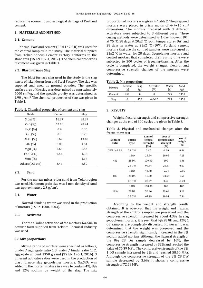
Turkish Journal of Engineering – 2022; 6(1); 63-66
64
reduce the economic and ecological damage of Portland cement.
2. MATERIALS AND METHOD
2.1. Cement
Normal Portland cement (CEM I 42.5 R) was used for the control samples in the study. The material supplied from Tokat Adoçim Cement Factory conforms to the standards (TS EN 197-1, 2012). The chemical properties of cement was given in Table 1.
2.2. Blast Furnace Slag
The blast furnace slag used in the study is the slag waste of İskenderun Iron and Steel Factory. The slag was supplied and used as ground powder. The specific surface area of the slag was determined as approximately 6000 cm2/g, and the specific gravity was determined as 2.90 g/cm3. The chemical properties of slag was given in Table 1. Table 1. Chemical properties of cement and slag
Oxide Cement Slag
SiO2 (%) 18.87 38.89
CaO (%) 62.78 28.94
Na2O (%) 0.4 0.36
K2O (%) 0.9 0.78
Al2O3 (%) 5.62 13.48
SO3 (%) 2.82 1.51
MgO (%) 2.63 5.53
Fe2O3 (%) 2.54 1.36
MnO (%) - 1.16
Others (LOI etc.) 3.44 6.50
2.3. Sand
For the mortar mixes, river sand from Tokat region was used. Maximum grain size was 4 mm, density of sand was approximately 2.3 g/cm3.
2.4. Water
Normal drinking water was used in the production of mortars (TS EN 1008, 2003).
2.5. Activator
For the alkaline activation of the mortars, Na2SiO3 in powder form supplied from Tekkim Chemical Industry was used.
2.6 Mix proportions
Mixing ratios of mortars were specified as follows; binder / aggregate ratio 1:3, water / binder ratio 1: 2, aggregate amount 1350 g sand (TS EN 196-1, 2016). 3 different activator ratios were used in the production of blast furnace slag geopolymer mortars. Na2SiO3 was added to the mortar mixture in a way to contain 4%, 8% and 12% sodium by weight of the slag. The mix
proportion of mortars was given in Table 2. The prepared mortars were placed in prism molds of 4×4×16 cm3 dimensions. The mortars prepared with 3 different activators were subjected to 3 different cures. These curing methods were determined as 1 day in oven (DO) at 75 , 28 days at 20±2 room temperature (DA) and 28 days in water at 21±2 (DW). Portland cement mortars that are the control samples were also cured at 21±2 in water for 28 days. Geopolymer mortars and control mortars that completed their curing time were subjected to 300 cycles of freezing-thawing. After the cycle is completed, the weight changes, flexural and compressive strength changes of the mortars were determined.
Table 2. Mix proportions
Mixture Cement
(g) Slag (g)
Activator (%)
Water (g)
Sand (g)
Cement 450 0 0 225 1350
Slag 0 450 4-8-12 225 1350
3. RESULTS
Weight, flexural strength and compressive strength changes at the end of 300 cycles are given in Table 3.
Table 3. Physical and mechanical changes after the freeze-thaw test
Sodium Ratio
Curing type
Loss of flexural strenght
(%)
Loss of compressive
strenght (%)
Loss of weigth
(%)
CEM I 42.5 R 28 DW 0.67 -4.29 0.86
4%
1 DO 28.94 20.95 7.28
28 DA 100.00 100 4.86
28 DW 90.84 -29.67 0.67
8%
1 DO 43.78 -2.04 -2.66
28 DA 16.50 -31.91 1.58
28 DW 28.97 3.67 -0.23
12%
1 DO 100.00 100 100
28 DA 30.96 59.69 5.18
28 DW 67.49 40.91 7.34
According to the weight and strength results obtained; It is observed that the weight and flexural strength of the control samples are preserved and the compressive strength increased by about 4.3%. In slag geopolymer mortars, it is seen that 4% 28 GH and 12% 1 GE samples are completely dispersed. However, it was determined that the weight was preserved and the compressive strength significantly increased in the 8% sodium added mortars. Although the flexural strength of the 8% 28 DA sample decreased by 16%, the compressive strength increased by 32% and reached the value of 76.39 MPa. The compressive strength of the 8% 1 DO sample increased by 2% and reached 58.60 MPa. Although the compressive strength of the 8% 28 DW sample decreased by 3.6%, it shows a compressive strength of 72.68 MPa.
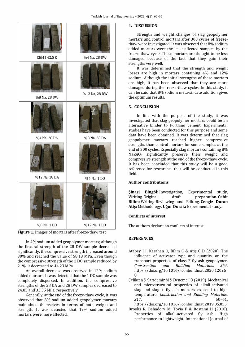
Turkish Journal of Engineering – 2022; 6(1); 63-66
65
CEM I 42.5 R
%4 Na, 28 DW
%8 Na, 28 DW
%12 Na, 28 DW
%4 Na, 28 DA
%8 Na, 28 DA
%12 Na, 28 DA
%4 Na, 1 DO
%8 Na, 1 DO
%12 Na, 1 DO
Figure 1. Images of mortars after freeze-thaw test In 4% sodium added geopolymer mortars; although
the flexural strength of the 28 DW sample decreased significantly, the compressive strength increased around 30% and reached the value of 58.13 MPa. Even though the compressive strength of the 1 DO sample reduced by 21%, it decreased to 44.23 MPa.
An overall decrease was observed in 12% sodium added mortars. It was detected that the 1 DO sample was completely dispersed. In addition, the compressive strengths of the 28 DA and 28 DW samples decreased to 24.85 and 33.35 MPa, respectively.
Generally, at the end of the freeze-thaw cycle, it was observed that 8% sodium added geopolymer mortars maintained themselves in terms of both weight and strength. It was detected that 12% sodium added mortars were more affected.
4. DISCUSSION
Strength and weight changes of slag geopolymer mortars and control mortars after 300 cycles of freeze-thaw were investigated. It was observed that 8% sodium added mortars were the least affected samples by the freeze-thaw cycle. These mortars are thought to be less damaged because of the fact that they gain their strengths very well.
It was determined that the strength and weight losses are high in mortars containing 4% and 12% sodium. Although the initial strengths of these mortars are high, it has been observed that they are more damaged during the freeze-thaw cycles. In this study, it can be said that 8% sodium meta-silicate addition gives the optimum results. 5. CONCLUSION
In line with the purpose of the study, it was investigated that slag geopolymer mortars could be an alternative binder to Portland cement. Experimental studies have been conducted for this purpose and some data have been obtained. It was determined that slag geopolymer mortars reached higher compressive strengths than control mortars for some samples at the end of 300 cycles. Especially slag mortars containing 8% Na2SiO3 significantly preserve their weight and compressive strength at the end of the freeze-thaw cycle. It has been concluded that this study will be a good reference for researches that will be conducted in this field.
Author contributions Şinasi Bingöl: Investigation, Experimental study, Writing-Original draft preparation. Cahit Bilim: Writing-Reviewing and Editing. Cengiz Duran Atiş: Methodology. Uğur Durak: Experimental study. Conflicts of interest The authors declare no conflicts of interest.
REFERENCES
Atabey İ İ, Karahan O, Bilim C & Atiş C D (2020). The influence of activator type and quantity on the transport properties of class F fly ash geopolymer. Construction and Building Materials, 264. https://doi.org/10.1016/j.conbuildmat.2020.120268
Çelikten S, Sarıdemir M & Deneme İ Ö (2019). Mechanical and microstructural properties of alkali-activated slag and slag + fly ash mortars exposed to high temperature. Construction and Building Materials, 217, 50–61. https://doi.org/10.1016/j.conbuildmat.2019.05.055
Brooks R, Bahadory M, Tovia F & Rostami H (2010). Properties of alkali-activated fly ash: High performance to lightweight. International Journal of

Turkish Journal of Engineering – 2022; 6(1); 63-66
66
Sustainable Engineering, 3(3), 211–218. https://doi.org/10.1080/19397038.2010.487162
Fu Y, Cai L & Yonggen W (2011). Freeze-thaw cycle test and damage mechanics models of alkali-activated slag concrete. Construction and Building Materials, 25(7), 3144–3148. https://doi.org/10.1016/j.conbuildmat.2010.12.006
Juenger M C G, Winnefeld F, Provis J L & Ideker J H (2011). Advances in alternative cementitious binders. Cement and Concrete Research, 41(12), 1232–1243. https://doi.org/10.1016/j.cemconres.2010.11.012
Lämmlein T D, Messina F, Wyrzykowski M, Terrasi G P & Lura P (2019). Low clinker high performance concretes and their potential in CFRP-prestressed structural elements. Cement and Concrete Composites, 100(February), 130–138. https://doi.org/10.1016/j.cemconcomp.2019.02.014
Meyer C (2009). The greening of the concrete industry. Cement and Concrete Composites, 31(8), 601–605. https://doi.org/10.1016/j.cemconcomp.2008.12.010
Peng J X, Huang L, Zhao Y B, Chen P, Zeng, L & Zheng W (2012). Modeling of Carbon Dioxide Measurement on Cement Plants. Advanced Materials Research, 610–613, 2120–2128.
Sun P & Wu H C (2013). Chemical and freeze-thaw resistance of fly ash-based inorganic mortars. Fuel, 111, 740–745. https://doi.org/10.1016/j.fuel.2013.04.070
TS EN 1008. (2003). Mixing water for concrete—Specifications for sampling, testing and assessing the suitability of water, including water recovered from processes in the concrete industry, as mixing water for concrete. TSI.
TS EN 196-1. (2016). Methods of testing cement—part 1: determination of strength. TSI.
TS EN 197-1. (2012). Cement–Part 1: compositions and conformity criteria for common cements. In Turkish Standard Institution. TSI.
Xie N, Dang Y & Shi X (2019). New insights into how MgCl 2 deteriorates Portland cement concrete. Cement and Concrete Research, 120(April), 244–255. https://doi.org/10.1016/j.cemconres.2019.03.026
Yuan Y, Zhao R, Li R, Wang Y, Cheng Z, Li F & John M Z (2020). Frost resistance of fiber-reinforced blended slag and Class F fly ash-based geopolymer concrete under the coupling effect of freeze-thaw cycling and axial compressive loading. Construction and Building Materials, 250, 118831. https://doi.org/10.1016/j.conbuildmat.2020.118831
Zhang P, Gao Z, Wang J, Guo J, Hu S & Ling Y (2020). Properties of fresh and hardened fly ash/slag based geopolymer concrete: A review. In Journal of Cleaner Production (Vol. 270). Elsevier Ltd. https://doi.org/10.1016/j.jclepro.2020.122389
Zhang P, Zheng Y, Wang K & Zhang J (2018). A review on properties of fresh and hardened geopolymer mortar. Composites Part B: Engineering, 152(April), 79–95. https://doi.org/10.1016/j.compositesb.2018.06.031
Zhao R, Yuan Y, Cheng Z, Wen T, Li J, Li F & Ma Z J (2019). Freeze-thaw resistance of Class F fly ash-based geopolymer concrete. Construction and Building Materials, 222, 474–483. https://doi.org/10.1016/j.conbuildmat.2019.06.166
Zhuang X Y, Chen L, Komarneni S, Zhou C H, Tong D S, Yang H M, Yu W H & Wang H (2016). Fly ash-based geopolymer: Clean production, properties and applications. Journal of Cleaner Production, 125, 253–267. https://doi.org/10.1016/j.jclepro.2016.03.019
© Author(s) 2022. This work is distributed under https://creativecommons.org/licenses/by-sa/4.0/
* Corresponding Author Cite this article
*([email protected]) ORCID ID 0000-0002-3324-7689 ([email protected]) ORCID ID 0000-0003-1458-437X ([email protected]) ORCID ID 0000-0002-3202-1362 ([email protected]) ORCID ID 0000-0003-3939-3676 Research Article / DOI: 10.31127/tuje.824890
Seyedzavvar M, Seyedzavvar M, Oliaei S N B & Abbasi H (2022). Numerical simulation and experimental investigation: Metal spinning process of stepped thin-walled cylindrical workpiece. Turkish Journal of Engineering, 6(1), 67-80
Received: 12/11/2020; Accepted: 27/01/2021
Turkish Journal of Engineering – 2022; 6(1); 67-80
Turkish Journal of Engineering
https://dergipark.org.tr/en/pub/tuje
e-ISSN 2587-1366
Numerical simulation and experimental investigation: Metal spinning process of stepped thin-walled cylindrical workpiece
Mirsadegh Seyedzavvar*1 , Mirali Seyedzavvar2 , Samet Akar3 , Hossein Abbasi4 1Adana Alparslan Turkeș Science and Technology University, Faculty of Engineering, Department of Mechanical Engineering, Adana, Turkey 2University of Tabriz, Faculty of Mechanical Engineering, Department of Manufacturing, Tabriz, Iran 3Çankaya University, Engineering Faculty, Department of Mechanical Engineering, Ankara, Turkey 4Technical and Vocational University, Tabriz Branch No.1, Department of Mechanical Engineering, Tabriz, Iran
Keywords ABSTRACT Sheet metal Spinning process Feed rate Mandrel rotational speed Stress and strain Wrinkling.
Many equipment and devices utilized in the aerospace industry are formed as symmetric parts through high plastic deformation of high strength sheet metal alloys with low thickness. Considering the inherent advantages of the spinning process of simple tooling and concentrated deformation loading, this process can be considered as one of the main options in producing these thin-sectioned lightweight parts. In this study, a Finite Element (FE) model has been developed to simulate the formation of a stepped thin-walled cylindrical workpiece of AISI 316 stainless steel alloy by spinning process. The FE simulation results were employed to investigate the effects of process parameters, including feed rate of the roller and rotational velocity of the mandrel on the distribution of stress and strain in the sheet metal, wrinkling failure, and thinning of the sheet metal during deformation. Experiments were carried out using selective input parameters based on the results of FE simulations. The comparison between FE simulations and experiments revealed that the developed model could predict the thinning of the sheet metals with over 93 % accuracy. Additionally, a good agreement between the experimentally deformed sheet configurations with those resulting from finite element simulations has been observed.
1. INTRODUCTION
The spinning process is an incremental metal forming process in which the raw material, in the form of sheet metal, is formed by a roller-type tool on a preformed die called mandrel. The mandrel and the sheet metal which is supported by a holder mounted at the end of the tailstock are rotated. A concentrated force is applied on the sheet metal by the roller, which acts as a lever tool and causes the material to flow along with the mandrel's surface profile (Kalpakjian and Schmid, 2006).
Several studies have been conducted on the spinning process of different symmetrical shapes to determine the distribution of stress and strain in the workpiece and to explore the governing mechanisms in the deformation process. Moria et al. (2009) performed a hot spinning process of cast aluminum alloy to remove the casting imperfections and produce parts with uniform wall thickness. Li et al. (2014) simulated the thickness variations and deformation of sheet metal by
the roller's movement in a die-less spinning process. Wong et al. (2008) studied the effects of the roller dimensions and reduction of the cross-section on the material flow in the thin-walled cup spinning process. The results showed that the roller edge radius determines the degree of plastic deformation along the wall length of the cup. Mori and Nonanka (2005) developed a finite element (FE) model to simulate the shear spinning process of an aluminum cone flange. They reported that the built-up edge of the material in front of the roller is promoted by an increase in the edge radius of the roller and the thickness reduction of the material during the deformation process. Jahazi and Ebrahimi (2000) studied the role of shear spinning process parameters on the spring back and tearing of the sheet metal in the deformation process. Wang et al. (2010) investigated the wrinkling failure of cylindrical cups in the spinning process. They reported that there is a threshold for the feed rate of the roller over which the wrinkling of the material occurs during the deformation
Turkish Journal of Engineering – 2022; 6(1); 67-80
68
process. Marghmaleki et al. (2011) employed FE method to evaluate the effects of heat generated during the plastic deformation of materials and the friction between the sheet metal and the tool on the distribution of stress and strain in the workpiece and the deformation energy of the spinning. Cheung et al. (2013) simulated the plastic flow of materials during the forming process using FE method. They employed the results to predict the equivalent strain and thickness of tubular cups in the spinning process. The authors predicted the probability of cracking and the location of a crack in the cup wall during the thickness reduction step and the height of the final part with 80% accuracy as compared with the experiments. Wang et al. (2017) studied the role of the spinning process in reducing the size of crystalline grains of aluminum-alloy plates. They showed that the increase of the equivalent strain during the spinning process causes a further reduction of the size of crystalline grains of the workpiece. Sangkharat and Dechjarern (2017) conducted FE modeling of the spinning process of SPCC sheet metals to investigate the thinning and wrinkling failure of the blank during the deformation process. Ahmed et al. (2015) investigated the wrinkling failure and wall thickness distribution of a cup specimen in a deep spinning process under different roller feed rates and nose radii. They considered a constant clearance between the roller and the mandrel. The results showed that the spinning ratio, defined as the blank to mandrel diameter ratio, and the roller feed rate could be doubled without failure of the sample by annealing the aluminum sheets before the spinning process.
Additionally, attempts to produce axisymmetric and asymmetric components by the spinning process without a mandrel have been reported in some papers. Jia et al. (2015) studied the effects of process parameters, including roller feed rate, nose radius, roller path, and half-core angle, on the surface quality of specimen in the square-section die-less spinning process. They also modeled Al 6061 blank as a deformable 3D solid. The other components of the spinning process were modeled as discrete-rigid in Abaqus/Explicit environment to achieve the strain fields in the workpiece during deformation. It was reported that a smaller roller nose radius causes higher axial plastic strains, deeper indentations, and lower surface quality of the specimen. Sugita and Arai (2015) performed multi-pass spinning to produce a circular cup and a rectangular box without using a mandrel. They evaluated the effects of tool trajectory and inclination angle on the wall thickness and wrinkling of the spun parts. They reported higher spinning ratio for axisymmetric components than asymmetric forms. Russo et al. (2020) investigated the formation of asymmetric parts of 1050-H14 aluminum alloy in a multi-pass mandrel-free spinning process by controlling the trajectory of two rollers, namely the blending and working rollers. Their study aimed to develop an algorithm of tool path generation that could be applied to all target geometries, while avoiding tearing and minimizing thinning and shape errors of the spun samples.
Furthermore, the spinning process has been employed in the flow forming of tubes. In this regard, Murata et al. (2005) showed that with increasing pipe
diameter reduction, the resistance of the workpiece to plastic deformation and the thickness of the tube wall increases, leading to higher rigidity of the deformed part and reduction of spring back of the material. Xia et al. (2012) conducted experiments and FE modeling to study the stress and strain distribution, thickness reduction, straightness, ellipticity, and elongation of the workpiece in the fabrication process of an automobile exhaust pipe muffler by a non-symmetric spinning method. They reported that the multi-pass spinning process causes longitudinal tensile strain and circumferential compressive strain at the spun workpiece. Davidson et al. (2008) studied the production of seamless thin-walled tubes of AA6061 annealed tubes using a spinning flow forming process. They reported that the diametric expansion of the tube can be avoided at a roller feed rate in the range of 0.83~1.67 mm/s. Parsa et al. (2009) simulated the deformation of tube stirred by forward material flow in the spinning process using explicit finite element method. Molladavoudi and Djavanroodi (2011) studied the role of thinning of the tubes as a result of the spinning process on the mechanical properties, surface finish, hardness, dimensional accuracy, and crystalline structure of the formed parts. Huang et al. (2011) used the FE method to study the effects of coefficient of friction, feed rate, and edge radius of the roller on the deformability of JIS G3141 steel in the throat spinning process. The results showed that the ellipticity of the cross-section and twisting of the tube increase with increasing the roller feed rate. Bi et al. (2012) simulated the automobile wheel forming in the spinning process using 3D Deform FE software to determine the required length of raw material and optimum parameter settings of the spinning process. Becker and Tekaya (2015) used a combination of spinning and tube bending processes to make exhaust pipes of automobiles. Zhan et al. (2018) investigated the formation of flaring defect at the opening end of the tube in the forward tube spinning process and reported that a small feed rate and reduction per path reduced maximum flaring at the expense of productivity.
Reviews of the previous research revealed that although the spinning process has a high potential in manufacturing complex shapes in response to the increasing demand by global manufacturing industries, especially aerospace engineering, it is complicated in terms of the influence of process parameters on the deformation characteristics. Among various spinning process parameters such as nose radius, attack angle, the feed rate of the roller, and the rotational speed of mandrel, the latter two variables have been shown to have the most significant influence on the spinnability of material (Wong et al. 2003). In this paper, the formation of a stepped thin-walled cylinder of AISI 316 stainless steel by the spinning process is presented. High hardness, high corrosion resistance, and strength against deformation are among the characteristics of this steel that promote its wide applications in the aerospace industry (AMS 5528). In contrast, these properties make it difficult to plastically deform thin sheet metals of this material by forming methods such as deep drawing. However, the spinning process has the advantage of creating a local plastic deformation zone at the sheet
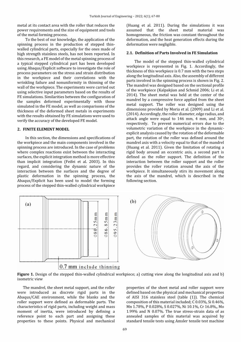
Turkish Journal of Engineering – 2022; 6(1); 67-80
69
metal at its contact area with the roller that reduces the power requirements and the size of equipment and tools of the metal forming process.
To the best of our knowledge, the application of the spinning process in the production of stepped thin-walled cylindrical parts, especially for the ones made of high strength stainless steels, has not been reported. In this research, a FE model of the metal spinning process of a typical stepped cylindrical part has been developed using Abaqus/Explicit software to investigate the role of process parameters on the stress and strain distribution in the workpiece and their correlations with the wrinkling failure and nonuniformity in thinning of the wall of the workpiece. The experiments were carried out using selective input parameters based on the results of FE simulations. Similarities between the configuration of the samples deformed experimentally with those simulated in the FE model, as well as comparisons of the thickness of the deformed sheet metals in experiments with the results obtained by FE simulations were used to verify the accuracy of the developed FE model.
2. FINITE ELEMENT MODEL
In this section, the dimensions and specifications of the workpiece and the main components involved in the spinning process are introduced. In the case of problems where complex reactions exist between the interacting surfaces, the explicit integration method is more effective than implicit integration (Feifei et al. 2003). In this regard, and considering the dynamic nature of the interaction between the surfaces and the degree of plastic deformation in the spinning process, the Abaqus/Explicit has been used to model the forming process of the stepped thin-walled cylindrical workpiece
(Huang et al. 2011). During the simulations it was assumed that the sheet metal material was homogeneous, the friction was constant throughout the deformation, and the heat generation effects during the deformation were negligible.
2.1. Definition of Parts Involved in FE Simulation
The model of the stepped thin-walled cylindrical workpiece is represented in Fig. 1. Accordingly, the thickness of this workpiece is 0.7 mm with the two steps along the longitudinal axis. Also, the assembly of different parts involved in the spinning process is shown in Fig. 2. The mandrel was designed based on the sectional profile of the workpiece (Kalpakjian and Schmid 2006; Li et al. 2014). The sheet metal was held at the center of the mandrel by a compressive force applied from the sheet metal support. The roller was designed using the dimensions provided by Moria et al. (2009) and Li et al. (2014). Accordingly, the roller diameter, edge radius, and attack angle were equal to 146 mm, 4 mm, and 30o, respectively. To prevent numerical errors due to the volumetric variation of the workpiece in the dynamic-explicit analysis caused by the rotation of the deformable part, the rotation of the roller was defined around the mandrel axis with a velocity equal to that of the mandrel (Huang et al. 2011). Given the limitation of rotating a rigid body around an eccentric axis, a second part is defined as the roller support. The definition of the interaction between the roller support and the roller provides the roller rotation around the axis of the workpiece. It simultaneously stirs its movement along the axis of the mandrel, which is described in the following section.
Figure 1. Design of the stepped thin-walled cylindrical workpiece; a) cutting view along the longitudinal axis and b) isometric view
The mandrel, the sheet metal support, and the roller were introduced as discrete rigid parts in the Abaqus/CAE environment, while the blanks and the roller support were defined as deformable parts. The characteristics of rigid parts, including weight and mass moment of inertia, were introduced by defining a reference point to each part and assigning these properties to these points. Physical and mechanical
properties of the sheet metal and roller support were defined based on the physical and mechanical properties of AISI 316 stainless steel (table (1)). The chemical composition of this material included; C 0.03%, Si 0.46%, Mn 1.78%, P 0.028%, S 0.027%, Ni 10.1%, Cr 16.8%,, Mo 1.99% and N 0.07%. The true stress-strain data of as annealed samples of this material was acquired by standard tensile tests using Amsler tensile test machine
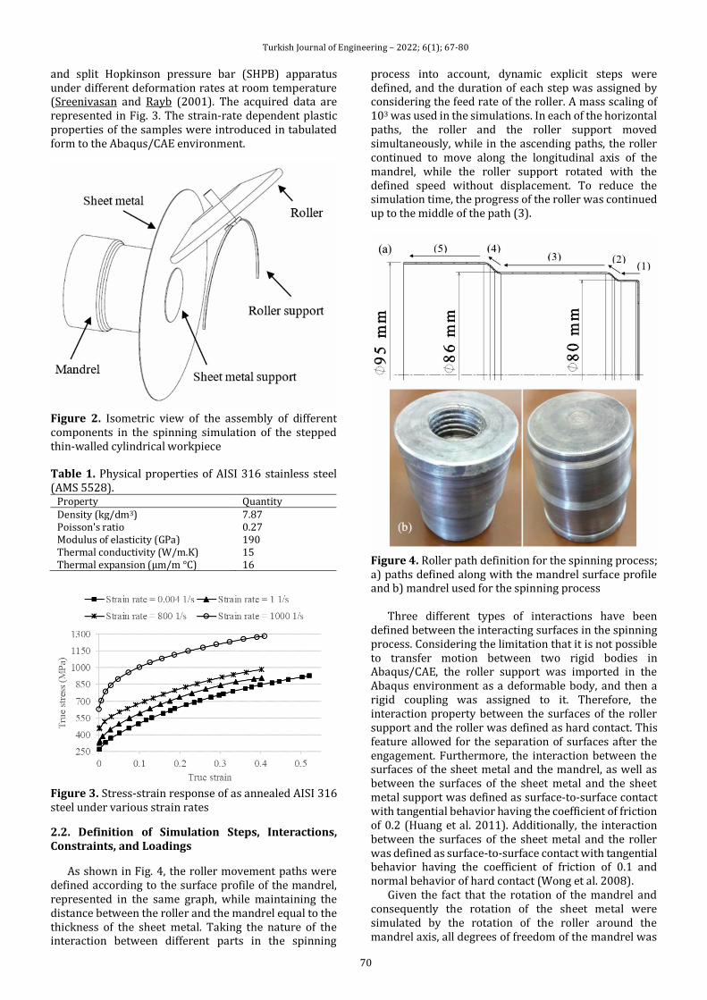
Turkish Journal of Engineering – 2022; 6(1); 67-80
70
and split Hopkinson pressure bar (SHPB) apparatus under different deformation rates at room temperature (Sreenivasan and Rayb (2001). The acquired data are represented in Fig. 3. The strain-rate dependent plastic properties of the samples were introduced in tabulated form to the Abaqus/CAE environment.
Figure 2. Isometric view of the assembly of different components in the spinning simulation of the stepped thin-walled cylindrical workpiece
Table 1. Physical properties of AISI 316 stainless steel (AMS 5528).
Property Quantity Density (kg/dm3) 7.87 Poisson's ratio 0.27 Modulus of elasticity (GPa) 190 Thermal conductivity (W/m.K) 15 Thermal expansion (μm/m °C) 16
Figure 3. Stress-strain response of as annealed AISI 316 steel under various strain rates
2.2. Definition of Simulation Steps, Interactions, Constraints, and Loadings
As shown in Fig. 4, the roller movement paths were defined according to the surface profile of the mandrel, represented in the same graph, while maintaining the distance between the roller and the mandrel equal to the thickness of the sheet metal. Taking the nature of the interaction between different parts in the spinning
process into account, dynamic explicit steps were defined, and the duration of each step was assigned by considering the feed rate of the roller. A mass scaling of 103 was used in the simulations. In each of the horizontal paths, the roller and the roller support moved simultaneously, while in the ascending paths, the roller continued to move along the longitudinal axis of the mandrel, while the roller support rotated with the defined speed without displacement. To reduce the simulation time, the progress of the roller was continued up to the middle of the path (3).
Figure 4. Roller path definition for the spinning process; a) paths defined along with the mandrel surface profile and b) mandrel used for the spinning process
Three different types of interactions have been defined between the interacting surfaces in the spinning process. Considering the limitation that it is not possible to transfer motion between two rigid bodies in Abaqus/CAE, the roller support was imported in the Abaqus environment as a deformable body, and then a rigid coupling was assigned to it. Therefore, the interaction property between the surfaces of the roller support and the roller was defined as hard contact. This feature allowed for the separation of surfaces after the engagement. Furthermore, the interaction between the surfaces of the sheet metal and the mandrel, as well as between the surfaces of the sheet metal and the sheet metal support was defined as surface-to-surface contact with tangential behavior having the coefficient of friction of 0.2 (Huang et al. 2011). Additionally, the interaction between the surfaces of the sheet metal and the roller was defined as surface-to-surface contact with tangential behavior having the coefficient of friction of 0.1 and normal behavior of hard contact (Wong et al. 2008).
Given the fact that the rotation of the mandrel and consequently the rotation of the sheet metal were simulated by the rotation of the roller around the mandrel axis, all degrees of freedom of the mandrel was
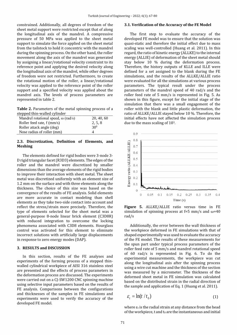
Turkish Journal of Engineering – 2022; 6(1); 67-80
71
constrained. Additionally, all degrees of freedom of the sheet metal support were restricted except that of along the longitudinal axis of the mandrel. A compressive pressure of 50 MPa was applied to the sheet metal support to simulate the force applied on the sheet metal from the tailstock to hold it concentric with the mandrel during the spinning process. On the other hand, the roller movement along the axis of the mandrel was generated by assigning a linear/rotational velocity constraint to its reference point and applying the desired velocity along the longitudinal axis of the mandrel, while other degrees of freedom were not restricted. Furthermore, to create the rotational motion of the roller, a linear/rotational velocity was applied to the reference point of the roller support and a specified velocity was applied about the mandrel axis. The levels of process parameters are represented in table 2. Table 2. Parameters of the metal spinning process of a stepped thin-walled cylinder
Mandrel rotational speed, ω (rad/s) 20, 40, 60
Roller feed rate, f (mm/s) 2, 5, 8
Roller attack angle (deg) 300
Nose radius of roller (mm) 4
2.3. Discretization, Definition of Elements, and Meshing
The elements defined for rigid bodies were 3-node 3-D rigid triangular facet (R3D3) elements. The edges of the roller and the mandrel were discretized by smaller dimensions than the average elements of the rigid bodies to improve their interaction with sheet metal. The sheet metal was discretized uniformly with an element size of 1.2 mm on the surface and with three elements along the thickness. The choice of this size was based on the convergence of the results of FE analysis. Solid elements are more accurate in contact modeling than shell elements as they take two-side contact into account and reflect the stress/strain more precisely. Therefore, the type of elements selected for the sheet metal was a general-purpose 8-node linear brick element (C3D8R) with reduced integration to overcome the locking phenomena associated with C3D8 elements. Hourglass control was activated for this element to eliminate incorrect solutions with artificially large displacements in response to zero energy modes (DAP).
3. RESULTS and DISCUSSION
In this section, results of the FE analyses and experiments of the forming process of a stepped thin-walled cylindrical workpiece of AISI 316 stainless steel are presented and the effects of process parameters in the deformation process are discussed. The experiments were carried out on a CJ-SW1200 CNC spinning machine using selective input parameters based on the results of FE analysis. Comparisons between the configurations and thicknesses of the samples in FE simulations and experiments were used to verify the accuracy of the developed FE model.
3.1. Verification of the Accuracy of the FE Model
The first step to evaluate the accuracy of the developed FE model was to ensure that the solution was quasi-static and therefore the initial effect due to mass scaling was well-controlled (Huang et al. 2011). In this regard, the ratio of kinetic energy (ALLKE) to the internal energy (ALLIE) of deformation of the sheet metal should stay below 10 % during the deformation process. Therefore, the history outputs of KLLE and ILLE were defined for a set assigned to the blank during the FE simulations, and the results of the ALLKE/ALLIE ratio were evaluated for all the simulations at various process parameters. The typical result under the process parameters of the mandrel speed of 40 rad/s and the roller feed rate of 5 mm/s is represented in Fig. 5. As shown in this figure, except for the initial stage of the simulation that there was a small engagement of the roller with the blank and little plastic deformation, the ratio of ALLKE/ALLIE stayed below 10 %. Therefore, the initial effects have not affected the simulation process due to the mass scaling of 103.
Figure 5. ALLKE/ALLIE ratio versus time in FE simulation of spinning process at f=5 mm/s and ω=40 rad/s
Additionally, the error between the wall thickness of the workpiece deformed in FE simulations with that of shaped experimentally was used to evaluate the accuracy of the FE model. The results of these measurements for the spun part under typical process parameters of the roller feed rate of 5 mm/s and mandrel rotational speed of 60 rad/s is represented in Fig. 6. To do the experimental measurements, the workpiece was cut along the longitudinal axis after the spinning process using a wire cut machine and the thickness of the section was measured by a micrometer. The thickness of the deformed sheet metal in FE simulation was calculated based on the distributed strain in the radial direction of the sample and application of Eq. 1 (Huang et al. 2011).
0ln( / )t t t
(1)
where εt is the radial strain at any distance from the head of the workpiece, t and t0 are the instantaneous and initial
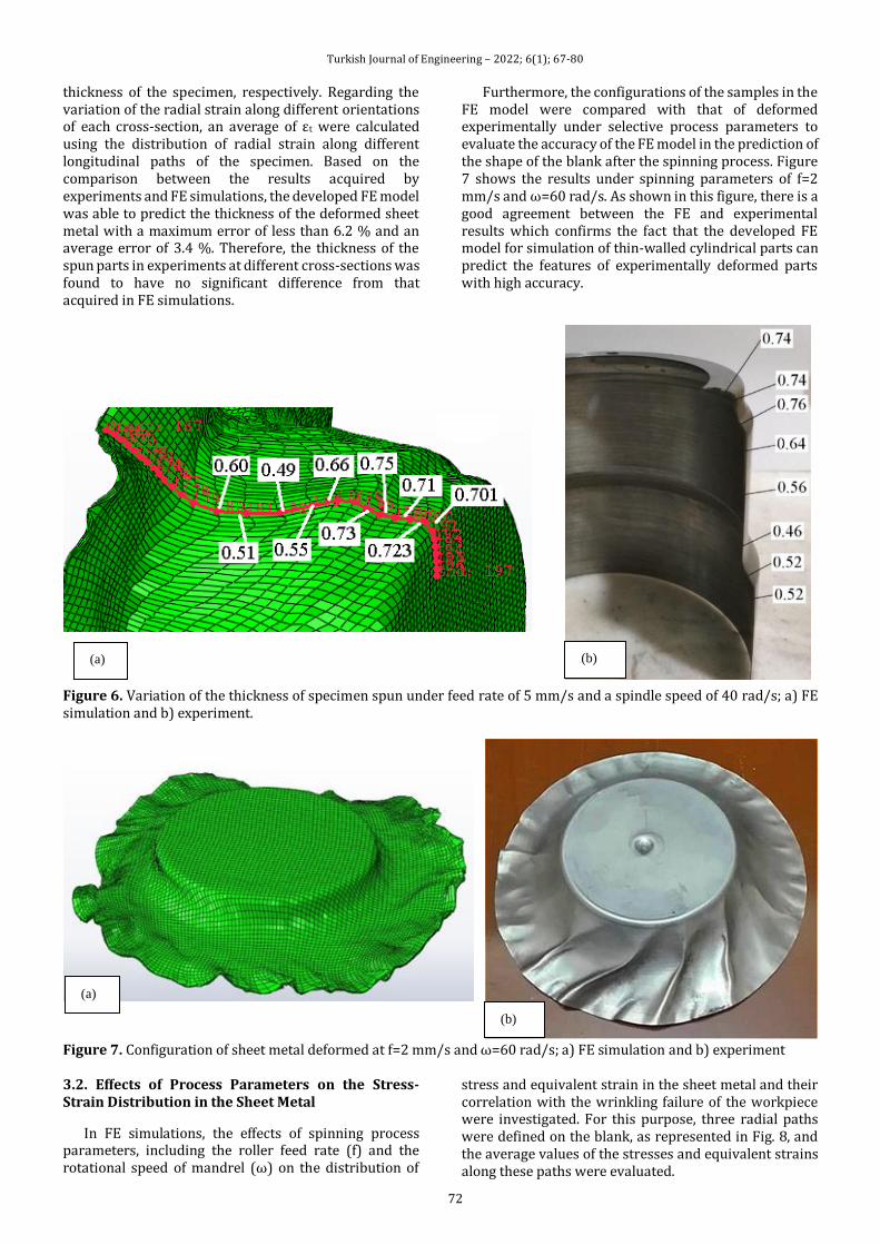
Turkish Journal of Engineering – 2022; 6(1); 67-80
72
thickness of the specimen, respectively. Regarding the variation of the radial strain along different orientations of each cross-section, an average of εt were calculated using the distribution of radial strain along different longitudinal paths of the specimen. Based on the comparison between the results acquired by experiments and FE simulations, the developed FE model was able to predict the thickness of the deformed sheet metal with a maximum error of less than 6.2 % and an average error of 3.4 %. Therefore, the thickness of the spun parts in experiments at different cross-sections was found to have no significant difference from that acquired in FE simulations.
Furthermore, the configurations of the samples in the FE model were compared with that of deformed experimentally under selective process parameters to evaluate the accuracy of the FE model in the prediction of the shape of the blank after the spinning process. Figure 7 shows the results under spinning parameters of f=2 mm/s and ω=60 rad/s. As shown in this figure, there is a good agreement between the FE and experimental results which confirms the fact that the developed FE model for simulation of thin-walled cylindrical parts can predict the features of experimentally deformed parts with high accuracy.
Figure 6. Variation of the thickness of specimen spun under feed rate of 5 mm/s and a spindle speed of 40 rad/s; a) FE simulation and b) experiment.
Figure 7. Configuration of sheet metal deformed at f=2 mm/s and ω=60 rad/s; a) FE simulation and b) experiment 3.2. Effects of Process Parameters on the Stress-Strain Distribution in the Sheet Metal
In FE simulations, the effects of spinning process parameters, including the roller feed rate (f) and the rotational speed of mandrel (ω) on the distribution of
stress and equivalent strain in the sheet metal and their correlation with the wrinkling failure of the workpiece were investigated. For this purpose, three radial paths were defined on the blank, as represented in Fig. 8, and the average values of the stresses and equivalent strains along these paths were evaluated.
(a) (b)
(a)
(b)
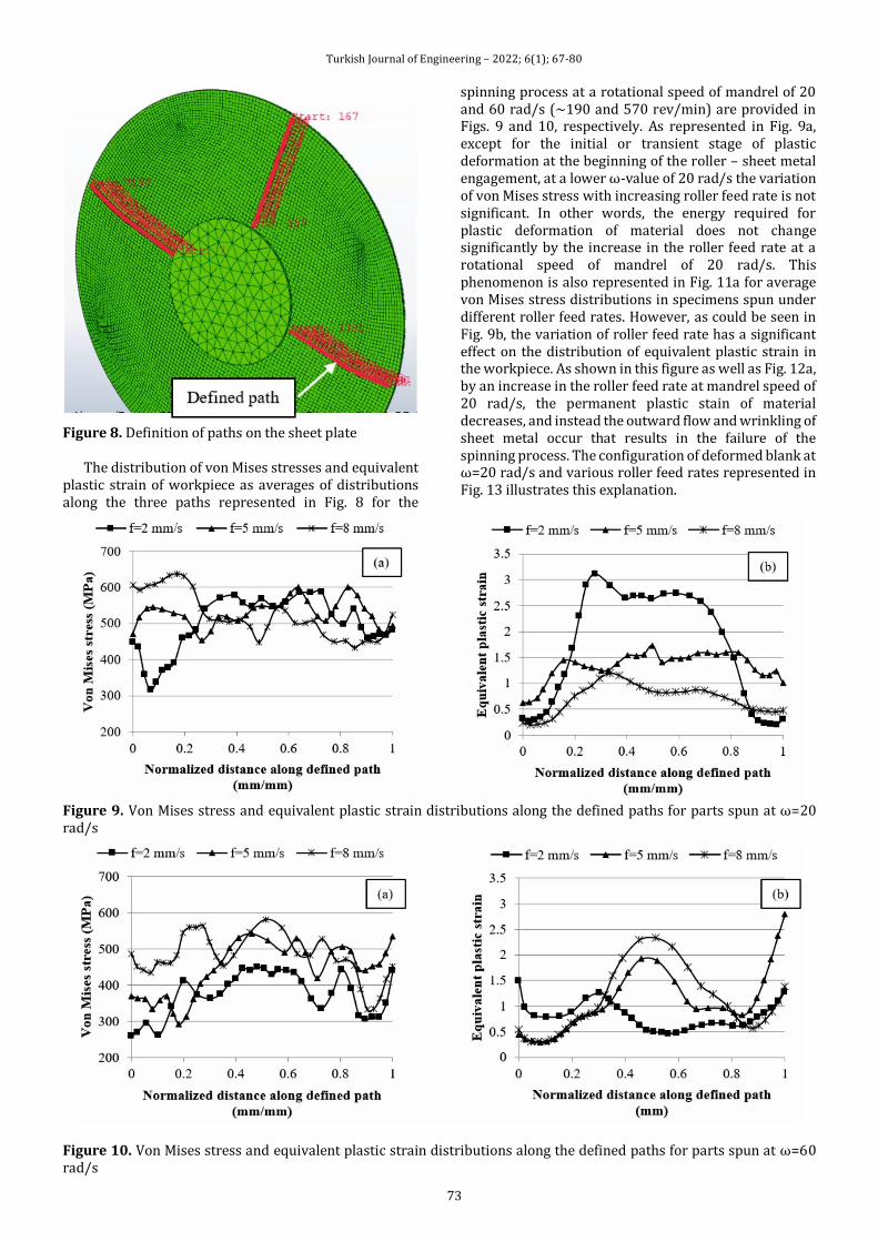
Turkish Journal of Engineering – 2022; 6(1); 67-80
73
Figure 8. Definition of paths on the sheet plate
The distribution of von Mises stresses and equivalent plastic strain of workpiece as averages of distributions along the three paths represented in Fig. 8 for the
spinning process at a rotational speed of mandrel of 20 and 60 rad/s (~190 and 570 rev/min) are provided in Figs. 9 and 10, respectively. As represented in Fig. 9a, except for the initial or transient stage of plastic deformation at the beginning of the roller – sheet metal engagement, at a lower ω-value of 20 rad/s the variation of von Mises stress with increasing roller feed rate is not significant. In other words, the energy required for plastic deformation of material does not change significantly by the increase in the roller feed rate at a rotational speed of mandrel of 20 rad/s. This phenomenon is also represented in Fig. 11a for average von Mises stress distributions in specimens spun under different roller feed rates. However, as could be seen in Fig. 9b, the variation of roller feed rate has a significant effect on the distribution of equivalent plastic strain in the workpiece. As shown in this figure as well as Fig. 12a, by an increase in the roller feed rate at mandrel speed of 20 rad/s, the permanent plastic stain of material decreases, and instead the outward flow and wrinkling of sheet metal occur that results in the failure of the spinning process. The configuration of deformed blank at ω=20 rad/s and various roller feed rates represented in Fig. 13 illustrates this explanation.
Figure 9. Von Mises stress and equivalent plastic strain distributions along the defined paths for parts spun at ω=20 rad/s
Figure 10. Von Mises stress and equivalent plastic strain distributions along the defined paths for parts spun at ω=60 rad/s
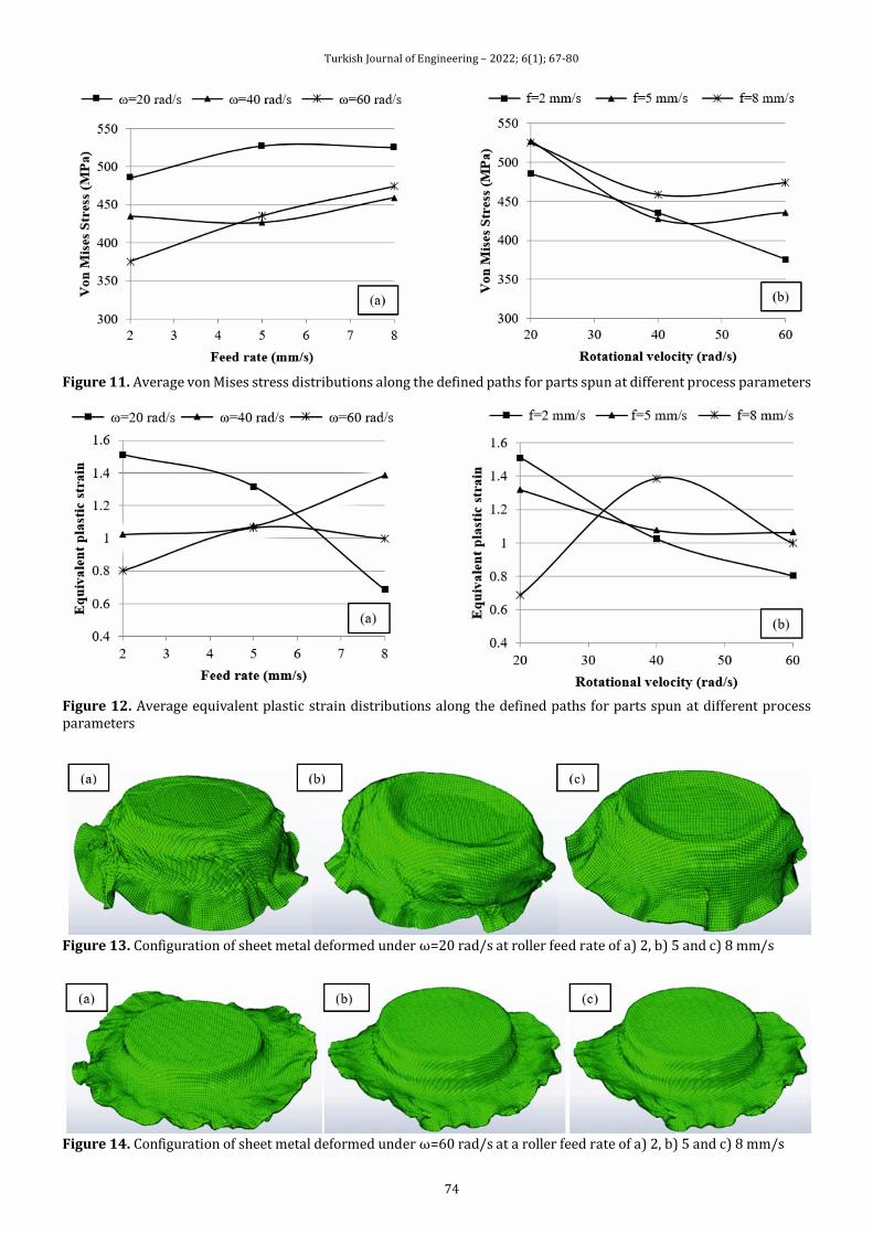
Turkish Journal of Engineering – 2022; 6(1); 67-80
74
Figure 11. Average von Mises stress distributions along the defined paths for parts spun at different process parameters
Figure 12. Average equivalent plastic strain distributions along the defined paths for parts spun at different process parameters
Figure 13. Configuration of sheet metal deformed under ω=20 rad/s at roller feed rate of a) 2, b) 5 and c) 8 mm/s
Figure 14. Configuration of sheet metal deformed under ω=60 rad/s at a roller feed rate of a) 2, b) 5 and c) 8 mm/s
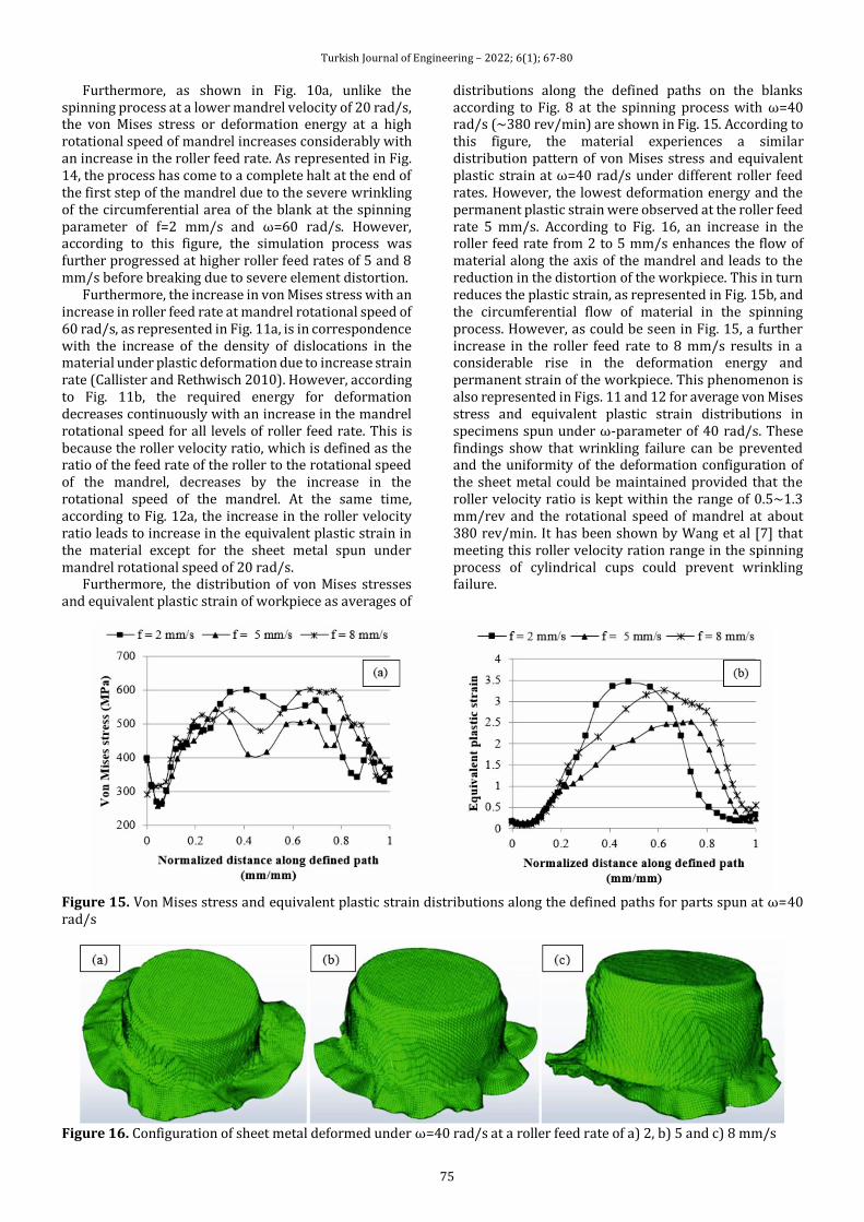
Turkish Journal of Engineering – 2022; 6(1); 67-80
75
Furthermore, as shown in Fig. 10a, unlike the spinning process at a lower mandrel velocity of 20 rad/s, the von Mises stress or deformation energy at a high rotational speed of mandrel increases considerably with an increase in the roller feed rate. As represented in Fig. 14, the process has come to a complete halt at the end of the first step of the mandrel due to the severe wrinkling of the circumferential area of the blank at the spinning parameter of f=2 mm/s and ω=60 rad/s. However, according to this figure, the simulation process was further progressed at higher roller feed rates of 5 and 8 mm/s before breaking due to severe element distortion.
Furthermore, the increase in von Mises stress with an increase in roller feed rate at mandrel rotational speed of 60 rad/s, as represented in Fig. 11a, is in correspondence with the increase of the density of dislocations in the material under plastic deformation due to increase strain rate (Callister and Rethwisch 2010). However, according to Fig. 11b, the required energy for deformation decreases continuously with an increase in the mandrel rotational speed for all levels of roller feed rate. This is because the roller velocity ratio, which is defined as the ratio of the feed rate of the roller to the rotational speed of the mandrel, decreases by the increase in the rotational speed of the mandrel. At the same time, according to Fig. 12a, the increase in the roller velocity ratio leads to increase in the equivalent plastic strain in the material except for the sheet metal spun under mandrel rotational speed of 20 rad/s.
Furthermore, the distribution of von Mises stresses and equivalent plastic strain of workpiece as averages of
distributions along the defined paths on the blanks according to Fig. 8 at the spinning process with ω=40 rad/s (~380 rev/min) are shown in Fig. 15. According to this figure, the material experiences a similar distribution pattern of von Mises stress and equivalent plastic strain at ω=40 rad/s under different roller feed rates. However, the lowest deformation energy and the permanent plastic strain were observed at the roller feed rate 5 mm/s. According to Fig. 16, an increase in the roller feed rate from 2 to 5 mm/s enhances the flow of material along the axis of the mandrel and leads to the reduction in the distortion of the workpiece. This in turn reduces the plastic strain, as represented in Fig. 15b, and the circumferential flow of material in the spinning process. However, as could be seen in Fig. 15, a further increase in the roller feed rate to 8 mm/s results in a considerable rise in the deformation energy and permanent strain of the workpiece. This phenomenon is also represented in Figs. 11 and 12 for average von Mises stress and equivalent plastic strain distributions in specimens spun under ω-parameter of 40 rad/s. These findings show that wrinkling failure can be prevented and the uniformity of the deformation configuration of the sheet metal could be maintained provided that the roller velocity ratio is kept within the range of 0.5~1.3 mm/rev and the rotational speed of mandrel at about 380 rev/min. It has been shown by Wang et al [7] that meeting this roller velocity ration range in the spinning process of cylindrical cups could prevent wrinkling failure.
Figure 15. Von Mises stress and equivalent plastic strain distributions along the defined paths for parts spun at ω=40 rad/s
Figure 16. Configuration of sheet metal deformed under ω=40 rad/s at a roller feed rate of a) 2, b) 5 and c) 8 mm/s
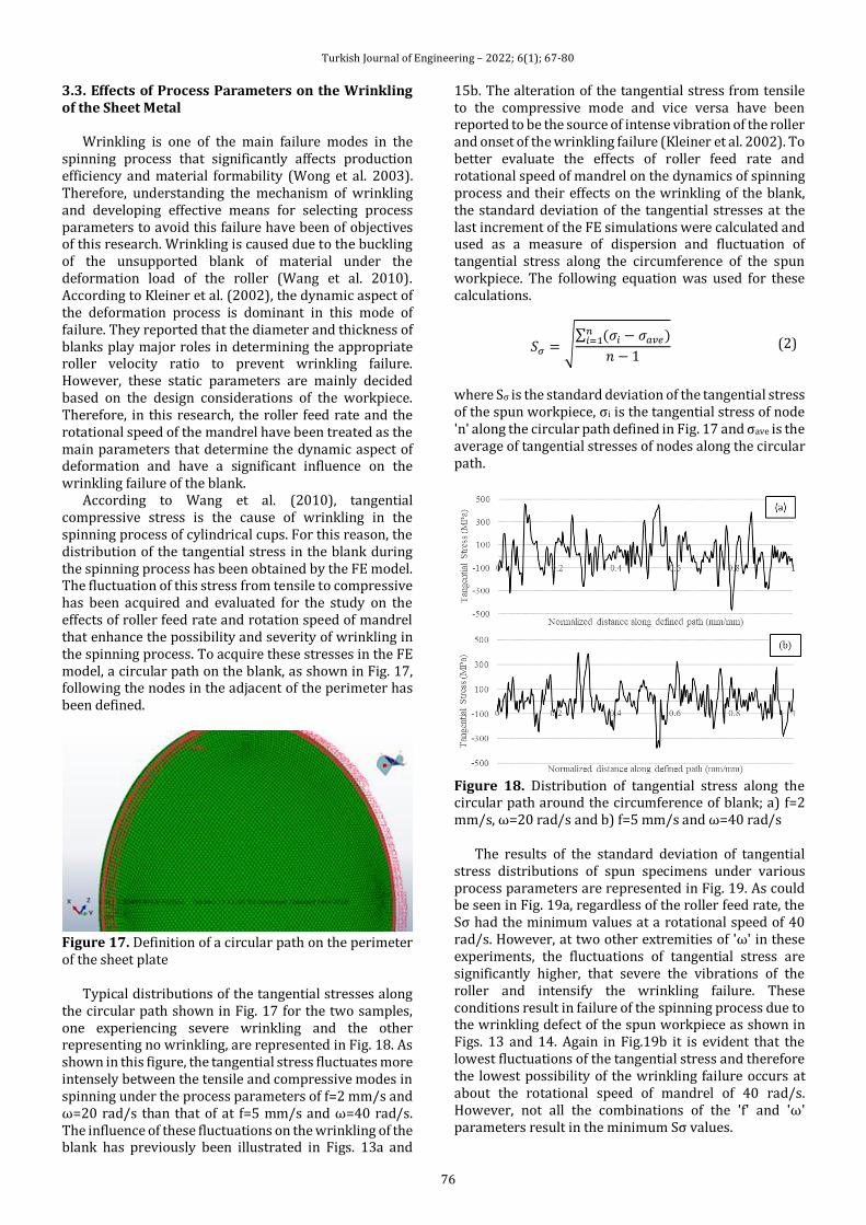
Turkish Journal of Engineering – 2022; 6(1); 67-80
76
3.3. Effects of Process Parameters on the Wrinkling of the Sheet Metal
Wrinkling is one of the main failure modes in the spinning process that significantly affects production efficiency and material formability (Wong et al. 2003). Therefore, understanding the mechanism of wrinkling and developing effective means for selecting process parameters to avoid this failure have been of objectives of this research. Wrinkling is caused due to the buckling of the unsupported blank of material under the deformation load of the roller (Wang et al. 2010). According to Kleiner et al. (2002), the dynamic aspect of the deformation process is dominant in this mode of failure. They reported that the diameter and thickness of blanks play major roles in determining the appropriate roller velocity ratio to prevent wrinkling failure. However, these static parameters are mainly decided based on the design considerations of the workpiece. Therefore, in this research, the roller feed rate and the rotational speed of the mandrel have been treated as the main parameters that determine the dynamic aspect of deformation and have a significant influence on the wrinkling failure of the blank.
According to Wang et al. (2010), tangential compressive stress is the cause of wrinkling in the spinning process of cylindrical cups. For this reason, the distribution of the tangential stress in the blank during the spinning process has been obtained by the FE model. The fluctuation of this stress from tensile to compressive has been acquired and evaluated for the study on the effects of roller feed rate and rotation speed of mandrel that enhance the possibility and severity of wrinkling in the spinning process. To acquire these stresses in the FE model, a circular path on the blank, as shown in Fig. 17, following the nodes in the adjacent of the perimeter has been defined.
Figure 17. Definition of a circular path on the perimeter of the sheet plate
Typical distributions of the tangential stresses along the circular path shown in Fig. 17 for the two samples, one experiencing severe wrinkling and the other representing no wrinkling, are represented in Fig. 18. As shown in this figure, the tangential stress fluctuates more intensely between the tensile and compressive modes in spinning under the process parameters of f=2 mm/s and ω=20 rad/s than that of at f=5 mm/s and ω=40 rad/s. The influence of these fluctuations on the wrinkling of the blank has previously been illustrated in Figs. 13a and
15b. The alteration of the tangential stress from tensile to the compressive mode and vice versa have been reported to be the source of intense vibration of the roller and onset of the wrinkling failure (Kleiner et al. 2002). To better evaluate the effects of roller feed rate and rotational speed of mandrel on the dynamics of spinning process and their effects on the wrinkling of the blank, the standard deviation of the tangential stresses at the last increment of the FE simulations were calculated and used as a measure of dispersion and fluctuation of tangential stress along the circumference of the spun workpiece. The following equation was used for these calculations.
𝑆𝜎 = √∑ (𝜎𝑖 − 𝜎𝑎𝑣𝑒)𝑛𝑖=1
𝑛 − 1 (2)
where Sσ is the standard deviation of the tangential stress of the spun workpiece, σi is the tangential stress of node 'n' along the circular path defined in Fig. 17 and σave is the average of tangential stresses of nodes along the circular path.
Figure 18. Distribution of tangential stress along the circular path around the circumference of blank; a) f=2 mm/s, ω=20 rad/s and b) f=5 mm/s and ω=40 rad/s
The results of the standard deviation of tangential stress distributions of spun specimens under various process parameters are represented in Fig. 19. As could be seen in Fig. 19a, regardless of the roller feed rate, the Sσ had the minimum values at a rotational speed of 40 rad/s. However, at two other extremities of 'ω' in these experiments, the fluctuations of tangential stress are significantly higher, that severe the vibrations of the roller and intensify the wrinkling failure. These conditions result in failure of the spinning process due to the wrinkling defect of the spun workpiece as shown in Figs. 13 and 14. Again in Fig.19b it is evident that the lowest fluctuations of the tangential stress and therefore the lowest possibility of the wrinkling failure occurs at about the rotational speed of mandrel of 40 rad/s. However, not all the combinations of the 'f' and 'ω' parameters result in the minimum Sσ values.
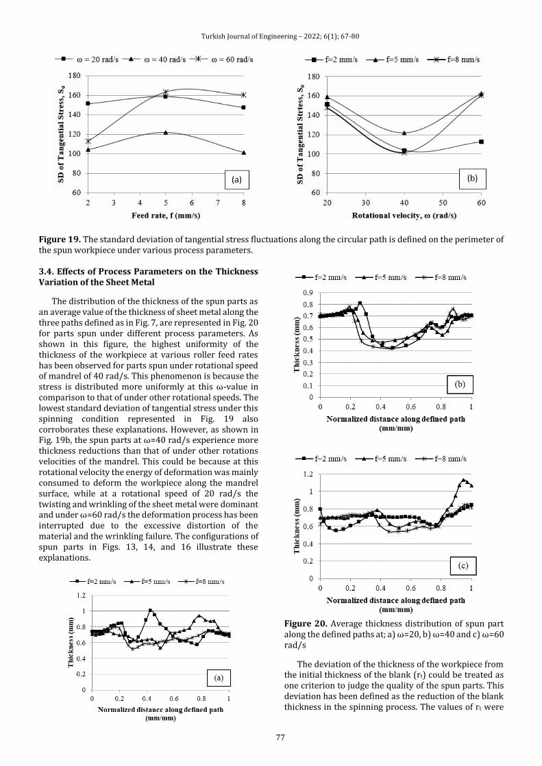
Turkish Journal of Engineering – 2022; 6(1); 67-80
77
Figure 19. The standard deviation of tangential stress fluctuations along the circular path is defined on the perimeter of the spun workpiece under various process parameters. 3.4. Effects of Process Parameters on the Thickness Variation of the Sheet Metal
The distribution of the thickness of the spun parts as an average value of the thickness of sheet metal along the three paths defined as in Fig. 7, are represented in Fig. 20 for parts spun under different process parameters. As shown in this figure, the highest uniformity of the thickness of the workpiece at various roller feed rates has been observed for parts spun under rotational speed of mandrel of 40 rad/s. This phenomenon is because the stress is distributed more uniformly at this ω-value in comparison to that of under other rotational speeds. The lowest standard deviation of tangential stress under this spinning condition represented in Fig. 19 also corroborates these explanations. However, as shown in Fig. 19b, the spun parts at ω=40 rad/s experience more thickness reductions than that of under other rotations velocities of the mandrel. This could be because at this rotational velocity the energy of deformation was mainly consumed to deform the workpiece along the mandrel surface, while at a rotational speed of 20 rad/s the twisting and wrinkling of the sheet metal were dominant and under ω=60 rad/s the deformation process has been interrupted due to the excessive distortion of the material and the wrinkling failure. The configurations of spun parts in Figs. 13, 14, and 16 illustrate these explanations.
Figure 20. Average thickness distribution of spun part along the defined paths at; a) ω=20, b) ω=40 and c) ω=60 rad/s
The deviation of the thickness of the workpiece from the initial thickness of the blank (rt) could be treated as one criterion to judge the quality of the spun parts. This deviation has been defined as the reduction of the blank thickness in the spinning process. The values of rt were
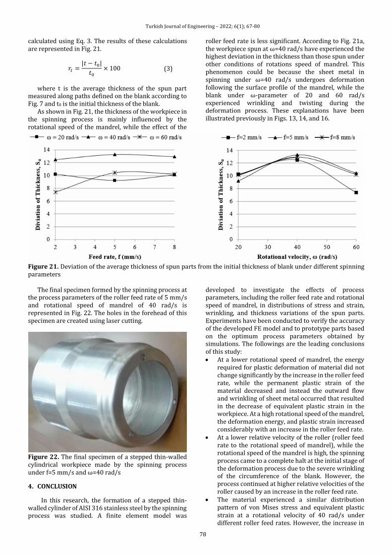
Turkish Journal of Engineering – 2022; 6(1); 67-80
78
calculated using Eq. 3. The results of these calculations are represented in Fig. 21.
𝑟𝑡 =|𝑡 − 𝑡0|
𝑡0× 100 (3)
where t is the average thickness of the spun part
measured along paths defined on the blank according to Fig. 7 and t0 is the initial thickness of the blank.
As shown in Fig. 21, the thickness of the workpiece in the spinning process is mainly influenced by the rotational speed of the mandrel, while the effect of the
roller feed rate is less significant. According to Fig. 21a, the workpiece spun at ω=40 rad/s have experienced the highest deviation in the thickness than those spun under other conditions of rotations speed of mandrel. This phenomenon could be because the sheet metal in spinning under ω=40 rad/s undergoes deformation following the surface profile of the mandrel, while the blank under ω-parameter of 20 and 60 rad/s experienced wrinkling and twisting during the deformation process. These explanations have been illustrated previously in Figs. 13, 14, and 16.
Figure 21. Deviation of the average thickness of spun parts from the initial thickness of blank under different spinning parameters
The final specimen formed by the spinning process at the process parameters of the roller feed rate of 5 mm/s and rotational speed of mandrel of 40 rad/s is represented in Fig. 22. The holes in the forehead of this specimen are created using laser cutting.
Figure 22. The final specimen of a stepped thin-walled cylindrical workpiece made by the spinning process under f=5 mm/s and ω=40 rad/s
4. CONCLUSION
In this research, the formation of a stepped thin-walled cylinder of AISI 316 stainless steel by the spinning process was studied. A finite element model was
developed to investigate the effects of process parameters, including the roller feed rate and rotational speed of mandrel, in distributions of stress and strain, wrinkling, and thickness variations of the spun parts. Experiments have been conducted to verify the accuracy of the developed FE model and to prototype parts based on the optimum process parameters obtained by simulations. The followings are the leading conclusions of this study: At a lower rotational speed of mandrel, the energy
required for plastic deformation of material did not change significantly by the increase in the roller feed rate, while the permanent plastic strain of the material decreased and instead the outward flow and wrinkling of sheet metal occurred that resulted in the decrease of equivalent plastic strain in the workpiece. At a high rotational speed of the mandrel, the deformation energy, and plastic strain increased considerably with an increase in the roller feed rate.
At a lower relative velocity of the roller (roller feed rate to the rotational speed of mandrel), while the rotational speed of the mandrel is high, the spinning process came to a complete halt at the initial stage of the deformation process due to the severe wrinkling of the circumference of the blank. However, the process continued at higher relative velocities of the roller caused by an increase in the roller feed rate.
The material experienced a similar distribution pattern of von Mises stress and equivalent plastic strain at a rotational velocity of 40 rad/s under different roller feed rates. However, the increase in
Turkish Journal of Engineering – 2022; 6(1); 67-80
79
the relative velocity of the roller by increase in the roller feed rate enhanced the flow of material along the axis of the mandrel and led to the reduction in distortion and wrinkling of the workpiece.
The tangential stress of the parts fluctuated more intensely between the tensile and compressive modes in spinning processes at which the spun parts experienced wrinkling and twisting failures. Regardless of the roller feed rate, these fluctuations had the minimum values at a rotational speed of 40 rad/s in comparison to other extremities of this parameter in the experiments. However, not all the combinations of the roller feed rate and rotational velocity of the mandrel resulted in the minimum standard deviations of tangential stresses of the spun parts.
The thickness of the workpiece in the spinning process was mainly influenced by the rotational speed of the mandrel, while the effect of the roller feed rate was less significant. The highest uniformity of the thickness of the workpiece has been observed for parts spun under rotational speed of mandrel of 40 rad/s because the stresses were distributed more uniformly under this process parameter. However, the parts experienced more thickness reductions under this condition since the energy of deformation was mainly consumed to deform the workpiece along the mandrel surface, while under other extremities of this parameter the twisting and wrinkling of the sheet metal were dominant.
Authors Contributions Mirsadegh Seyedzavvar wrote the manuscript getting contributions from all authors; Samet Akar and Mirsadegh Seyedzavvar have conceived the idea, designed the experiments, and analyzed the results and data; Mirali Seyedzavvar conducted the finite element simulations; Mirali Seyedzavvar and Hossein Abbasi conducted the experiments and collected the data. Conflict of Interest Statement
The authors of this work certify that they have NO affiliations with or involvement in any organization or entity with any financial or non-financial interest in the subject matter or materials discussed in this manuscript. The corresponding author is prepared to collect documentation of compliance with ethical standards and send it if requested during peer review or after publication. The Editors reserve the right to reject this manuscript if it does not comply with these certifications
REFERENCES
Ahmed K I, Gadala M S, El-Sebaie M G (2015). Deep spinning of sheet metals. International Journal of Machine Tools and Manufacture, 97, 72-85.
AMS 5528. Stainless Steel Sheet, United Performance Metals, https://www.upmet.com/products/stainless-steel/17-7-ph
Becker C, Erman Tekkaya A (2015) Wall thickness distribution during a combined tube spinning and bending process. Key Engineering Materials, 651-653:1614−1619.
Bi D, Yang G, Chu L, Zhang J, Wang Z (2012). Numerical simulation on spinning forming process of automotive wheel rim. Materials Science Forum, 704-705:1458–1464.
Callister W D, Rethwisch D G (2010). Materials science and engineering: An introduction, 8th edition. John Wiley & Sons, Inc.
Cheong W C, Kam H K, Wang C C, Lim Y P (2013). Study of cold rotary forming by using rigid-plastic finite element method. Advanced Materials Research, 626, 662–666.
Davidson M J, Balasubramanian K, Tagore G R N (2008). An experimental study on the quality of flow-formed AA6061 tubes. Journal of materials processing technology, 203(1-3), 321-325.
Dynamic analysis procedures (DAP): overview, Abaqus analysis user’s guide, Dassault Systemes, https://bit.ly/2IMZ80R
Feifei S, He Y, Heng L, Mei Z, Guangjun L (2013). Springback prediction of thick-walled high-strength titanium tube bending. Chinese Journal of Aeronautics, 26: 1336–1345.
Huang C C, Hung J C, Hung C, Lin C R (2011). Finite element analysis on neck-spinning process of tube at elevated temperature. The International Journal of Advanced Manufacturing Technology 56:1039–1048.
Jahazi M, EbrahimiG (2000). The influence of flow-forming parameters and microstructure on the quality of a D6ac steel. Journal of materials processing technology, 103, 362–366.
Jia Z, Han Z R, Xu Q, Peng W F, Kong Q M (2015). Effects of processing parameters on the surface quality of square section die-less spinning. The International Journal of Advanced Manufacturing Technology, 80(9), 1689-1700.
Kalpakjian S, Schmid S R (2006). Chp 16: Sheet metal forming process and equipment, Manufacturing engineering and technology. 6th edition, Pearson Publication.
Kleiner M, Göbel R, Kantz H, Klimmek C H, Homberg W (2002). Combined methods for the prediction of dynamic instabilities in sheet metal spinning. CIRP Annals 51:209–214.
Li Y, Wang J, Lu G D, Pan G J (2014). A numerical study of the effects of roller paths on dimensional precision in die-less spinning of sheet metal. J Zhej Uni-SCI A (App Phy Eng) 15(6):432−446.
Marghmaleki I S, Beni Y T, Noghrehabadi A R, Sadat Kazemi A, Abadyan M (2011). Finite element simulation of thermomechanical spinning process. Proc Eng 10:3769–3774.
Molladavoudi H R, Djavanroodi F (2011). Experimental study of thickness reduction effects on mechanical properties and spinning accuracy of aluminum 7075-O, during flow forming. The International Journal of Advanced Manufacturing Technology 52:949–957.
Mori K, Nonaka T (2005). Simplified three-dimensional finite element simulation of shear spinning process

Turkish Journal of Engineering – 2022; 6(1); 67-80
80
based on axisymmetric modeling. Journal of manufacturing processes, 7(1),51–56.
Moria K, Ishigurob M, Isomura Y (2009). Hot shear spinning of cast aluminum alloy parts. Journal of Materials Processing Technology, 209:3621–3627.
Murata M, Kuboki T, Murai T (2005). Compression spinning of circular magnesium tube using heated roller tool. Journal of materials processing technology, 162, 540-545.
Parsa M H, Pazooki A M A, Nili Ahmadabadi M (2009). Flow-forming and flow formability simulation. The International Journal of Advanced Manufacturing Technology, 42(5-6), 463-473.
Russo I M, Cleaver C J, Allwood J M, Loukaides E J (2020). The influence of part asymmetry on the achievable forming height in multi-pass spinning. Journal of Materials Processing Technology, 275, 116350.
Sangkharat T, Dechjarern S (2017). Spinning process design using finite element analysis and Taguchi method. Procedia Engineering, 207, 1713–1718.
Sreenivasan, P R, Rayb S K (2001). Mechanical Testing at High Strain Rates. Enc. Mater.: Sci. Tech. (2nd Ed.) 5269–5271.
Sugita Y, Arai H (2015). Formability in synchronous multipass spinning using simple pass set. Journal of Materials Processing Technology, 217, 336-344.
Wang L, Long H, Ashley D, Roberts M, White P (2010). Effects of the roller feed ratio on wrinkling failure in conventional spinning of a cylindrical cup.
Proceedings of the Institution of Mechanical Engineers, Part B: Journal of Engineering Manufacture, 225(11), 1991-2006
Wang X X, Zhan M, Fu M W, Guo J, Xu R Q, Lei X P (2017). A unique spinning method for grain refinement: repetitive shear spinning. Procedia Engineering, 207,1725–1730.
Wong C C, Danno A, Tong K K, Yong M S (2008). Cold rotary forming of thin-wall component from flat-disc blank. Journal of materials processing technology, 208:53–62.
Wong C C, Dean T A, Lin J (2003). A review of spinning, shear forming and flow forming processes. International Journal of Machine Tools and Manufacture, 43(14), 1419-1435.
Xia Q, Cheng X, Long H, Ruan F (2012). Finite element analysis and experimental investigation on deformation mechanism of non-axisymmetric tube spinning. The International Journal of Advanced Manufacturing Technology, 59(1-4), 263-272.
Zhan M, Guo J, Fu M W, Li R, Gao P F, Long H, Ma F (2018). Formation mechanism and control of flaring in forward tube spinning. The International Journal of Advanced Manufacturing Technology, 94, 59–72.
© Author(s) 2022. This work is distributed under https://creativecommons.org/licenses/by-sa/4.0/
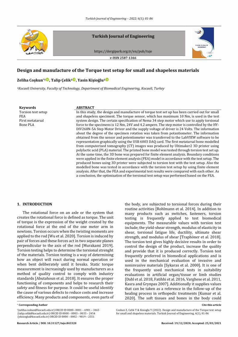
* Corresponding Author Cite this article
*([email protected]) ORCID ID 0000– 0001 – 6901 – 3465 ([email protected]) ORCID ID 0000 – 0003 – 0033 – 2454 ([email protected]) ORCID ID 0000 – 0002 – 9819 – 2551 Research Article / DOI: 10.31127/tuje.843320
Coskun Z, Celik T & Kisioglu Y (2022). Design and manufacture of the Torque test setup for small and shapeless materials. Turkish Journal of Engineering, 6(1), 81-86
Received: 19/12/2020; Accepted: 25/03/2021
Turkish Journal of Engineering – 2022; 6(1); 81-86
Turkish Journal of Engineering
https://dergipark.org.tr/en/pub/tuje
e-ISSN 2587-1366
Design and manufacture of the Torque test setup for small and shapeless materials
Zeliha Coşkun*1 , Talip Çelik1 , Yasin Kişioğlu1
1Kocaeli University, Faculty of Technology, Department of Biomedical Engineering, Kocaeli, Turkey
Keywords ABSTRACT Torsion test setup FEA First metatarsal Bone PLA
In this study, the design and manufacture of torque test set up has been carried out for small and shapeless speciment. The torque sensor, which has maximum 10 Nm, is used in the test system design. The certain specification of Nema 34 step motor which use to apply torsional force to the specimens is 12 Nm, 24V and 4.2 ampere. The step motor is controlled by the HY- DIV268N-5A Step Motor Driver and the supply voltage of driver is 24 Volts. The information about the degree of the specimen rotation was taken from potantiometer. The information obtained from the sensor and potentiometer was transferred to the LabVIEW software to be representation graphically using the USB 6003 DAQ card. The first metatarsal bone modelled from computerized tomography (CT) images was produced by Ultimaker2 3D printer using polylactic acid (PLA) material. The printed bone model was tested through torsion test set up. At the same time, the 3D bone was prepared for finite element analysis. Boundary conditions were applied in the finite element analysis (FEA) model in accordance with the test setup. The produced bones using 3D printer were subjected to torsion test with the test setup. Also the modelled bone was tested in accordance with the torsion test setup by using finite element analysis. After that, the FEA and experimental test results were compared with each other. As a conclusion, the optimization of the torsional test setup was performed based on the FEA.
1. INTRODUCTION
The rotational force on an axle or the system that creates the rotational force is defined as torque. The unit of torque is the expression of the weight created by the rotational force at the end of the one meter arm in newtons. Torsion occurs when the twisting moments are applied to the rod [Wu et al. 2020]. Torsion is induced by pair of forces and these forces act in two separate planes perpendicular to the axis of the rod [Murakami 2019]. Torsion testing helps to determine the torsional strenght of the materials. Torsion testing is a way of determining how an object will react during normal operation or when bent deliberately until it breaks. Static torque measurement is increasingly used by manufacturers as a method of quality control to comply with industry standards [Abutahoun et al. 2018]. It ensures the proper functioning of components and helps to research their safety and fitness for purpose. It could be useful identify the cause of various defects to reduce costs and increase efficiency. Many products and components, even parts of
the body, are subjected to torsional forces during their routine activities [Rohlmann et al. 2014]. In addition to many products such as switches, fasteners, torsion testing is frequently applied to test biomedical equipments. The measurable values with torsion test include; the yield-shear strength, modulus of elasticity in shear, torsional fatigue life, ductility, ultimate shear strength, and modulus of shear [Traphöner et al. 2018]. The torsion test gives highly decisive results in order to control the design of the product, increase the quality and provide that it is produced correctly. Torsion test frequently preferred in biomedical applications and is used in the mechanical evaluation of invasive and noninvasive materials [Sykaras et al. 2000]. It is one of the frequently used mechanical tests in suitability evaluations in artificial organ/tissue or limb studies [Dahl et al. 2018, Fatihhi et al. 2016, Varghese et al. 2011, Kasra and Grynpas 2007]. Additionally it supplies values that can be taken as a reference in the follow-up of the healing process in orthopedic treatments [Kumar et al. 2020]. The soft tissues and bones in the body could
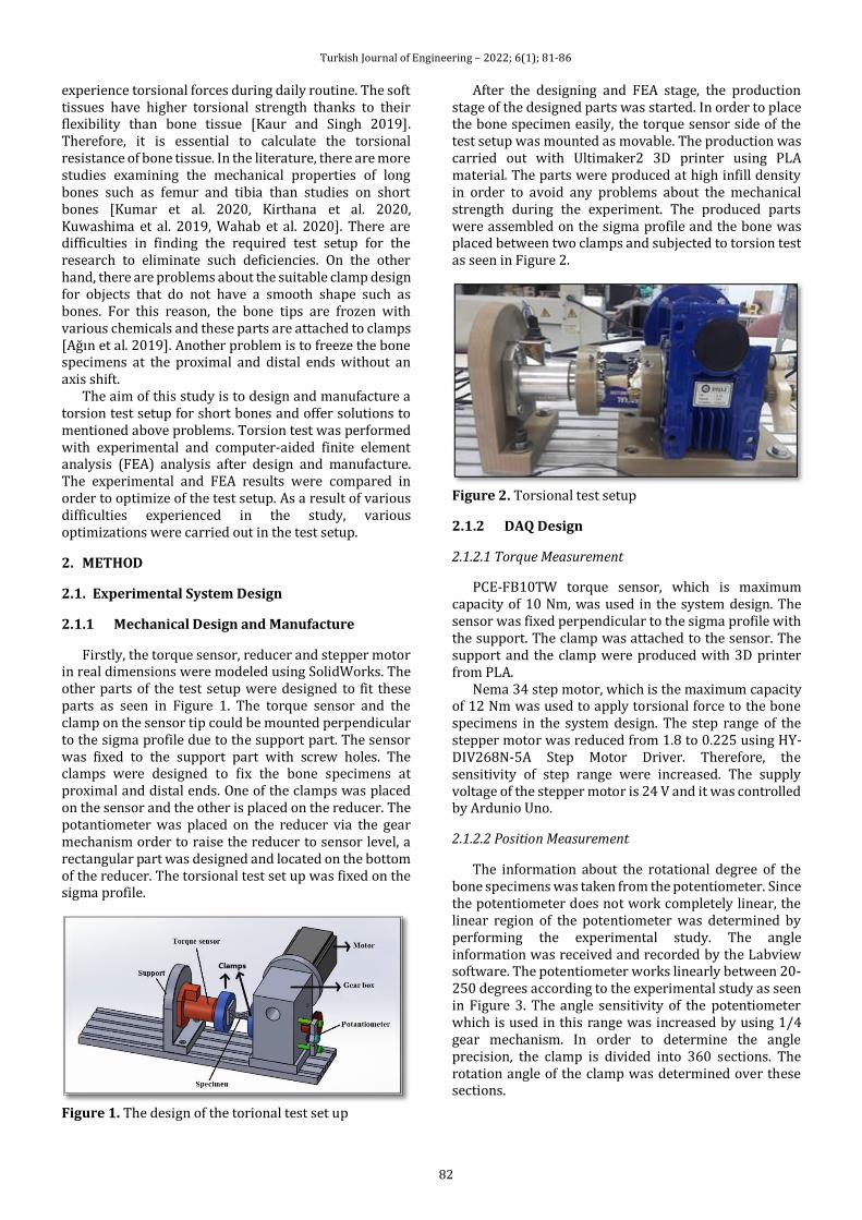
Turkish Journal of Engineering – 2022; 6(1); 81-86
82
experience torsional forces during daily routine. The soft tissues have higher torsional strength thanks to their flexibility than bone tissue [Kaur and Singh 2019]. Therefore, it is essential to calculate the torsional resistance of bone tissue. In the literature, there are more studies examining the mechanical properties of long bones such as femur and tibia than studies on short bones [Kumar et al. 2020, Kirthana et al. 2020, Kuwashima et al. 2019, Wahab et al. 2020]. There are difficulties in finding the required test setup for the research to eliminate such deficiencies. On the other hand, there are problems about the suitable clamp design for objects that do not have a smooth shape such as bones. For this reason, the bone tips are frozen with various chemicals and these parts are attached to clamps [Ağın et al. 2019]. Another problem is to freeze the bone specimens at the proximal and distal ends without an axis shift.
The aim of this study is to design and manufacture a torsion test setup for short bones and offer solutions to mentioned above problems. Torsion test was performed with experimental and computer-aided finite element analysis (FEA) analysis after design and manufacture. The experimental and FEA results were compared in order to optimize of the test setup. As a result of various difficulties experienced in the study, various optimizations were carried out in the test setup.
2. METHOD
2.1. Experimental System Design
2.1.1 Mechanical Design and Manufacture
Firstly, the torque sensor, reducer and stepper motor in real dimensions were modeled using SolidWorks. The other parts of the test setup were designed to fit these parts as seen in Figure 1. The torque sensor and the clamp on the sensor tip could be mounted perpendicular to the sigma profile due to the support part. The sensor was fixed to the support part with screw holes. The clamps were designed to fix the bone specimens at proximal and distal ends. One of the clamps was placed on the sensor and the other is placed on the reducer. The potantiometer was placed on the reducer via the gear mechanism order to raise the reducer to sensor level, a rectangular part was designed and located on the bottom of the reducer. The torsional test set up was fixed on the sigma profile.
Figure 1. The design of the torional test set up
After the designing and FEA stage, the production stage of the designed parts was started. In order to place the bone specimen easily, the torque sensor side of the test setup was mounted as movable. The production was carried out with Ultimaker2 3D printer using PLA material. The parts were produced at high infill density in order to avoid any problems about the mechanical strength during the experiment. The produced parts were assembled on the sigma profile and the bone was placed between two clamps and subjected to torsion test as seen in Figure 2.
Figure 2. Torsional test setup
2.1.2 DAQ Design
2.1.2.1 Torque Measurement
PCE-FB10TW torque sensor, which is maximum capacity of 10 Nm, was used in the system design. The sensor was fixed perpendicular to the sigma profile with the support. The clamp was attached to the sensor. The support and the clamp were produced with 3D printer from PLA.
Nema 34 step motor, which is the maximum capacity of 12 Nm was used to apply torsional force to the bone specimens in the system design. The step range of the stepper motor was reduced from 1.8 to 0.225 using HY- DIV268N-5A Step Motor Driver. Therefore, the sensitivity of step range were increased. The supply voltage of the stepper motor is 24 V and it was controlled by Ardunio Uno.
2.1.2.2 Position Measurement
The information about the rotational degree of the bone specimens was taken from the potentiometer. Since the potentiometer does not work completely linear, the linear region of the potentiometer was determined by performing the experimental study. The angle information was received and recorded by the Labview software. The potentiometer works linearly between 20- 250 degrees according to the experimental study as seen in Figure 3. The angle sensitivity of the potentiometer which is used in this range was increased by using 1/4 gear mechanism. In order to determine the angle precision, the clamp is divided into 360 sections. The rotation angle of the clamp was determined over these sections.
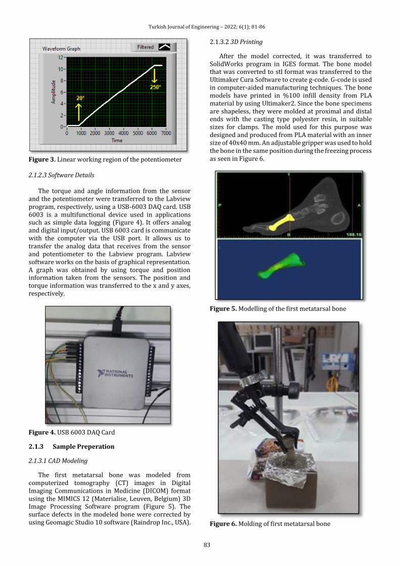
Turkish Journal of Engineering – 2022; 6(1); 81-86
83
Figure 3. Linear working region of the potentiometer 2.1.2.3 Software Details
The torque and angle information from the sensor and the potentiometer were transferred to the Labview program, respectively, using a USB-6003 DAQ card. USB 6003 is a multifunctional device used in applications such as simple data logging (Figure 4). It offers analog and digital input/output. USB 6003 card is communicate with the computer via the USB port. It allows us to transfer the analog data that receives from the sensor and potentiometer to the Labview program. Labview software works on the basis of graphical representation. A graph was obtained by using torque and position information taken from the sensors. The position and torque information was transferred to the x and y axes, respectively.
Figure 4. USB 6003 DAQ Card
2.1.3 Sample Preperation
2.1.3.1 CAD Modeling
The first metatarsal bone was modeled from computerized tomography (CT) images in Digital Imaging Communications in Medicine (DICOM) format using the MIMICS 12 (Materialise, Leuven, Belgium) 3D Image Processing Software program (Figure 5). The surface defects in the modeled bone were corrected by using Geomagic Studio 10 software (Raindrop Inc., USA).
2.1.3.2 3D Printing
After the model corrected, it was transferred to SolidWorks program in IGES format. The bone model that was converted to stl format was transferred to the Ultimaker Cura Software to create g-code. G-code is used in computer-aided manufacturing techniques. The bone models have printed in %100 infill density from PLA material by using Ultimaker2. Since the bone specimens are shapeless, they were molded at proximal and distal ends with the casting type polyester resin, in suitable sizes for clamps. The mold used for this purpose was designed and produced from PLA material with an inner size of 40x40 mm. An adjustable gripper was used to hold the bone in the same position during the freezing process as seen in Figure 6.
Figure 5. Modelling of the first metatarsal bone
Figure 6. Molding of first metatarsal bone
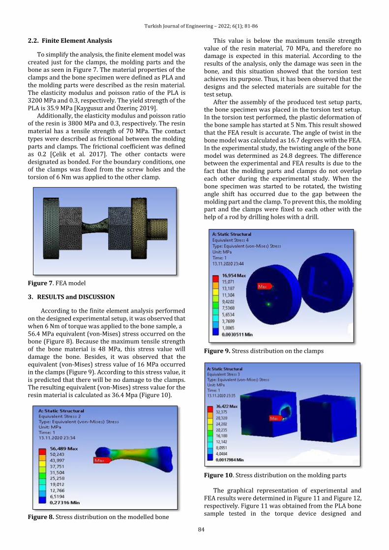
Turkish Journal of Engineering – 2022; 6(1); 81-86
84
2.2. Finite Element Analysis
To simplify the analysis, the finite element model was created just for the clamps, the molding parts and the bone as seen in Figure 7. The material properties of the clamps and the bone specimen were defined as PLA and the molding parts were described as the resin material. The elasticity modulus and poisson ratio of the PLA is 3200 MPa and 0.3, respectively. The yield strength of the PLA is 35.9 MPa [Kaygusuz and Özerinç 2019].
Additionally, the elasticity modulus and poisson ratio of the resin is 3800 MPa and 0.3, respectively. The resin material has a tensile strength of 70 MPa. The contact types were described as frictional between the molding parts and clamps. The frictional coefficient was defined as 0.2 [Çelik et al. 2017]. The other contacts were designated as bonded. For the boundary conditions, one of the clamps was fixed from the screw holes and the torsion of 6 Nm was applied to the other clamp.
Figure 7. FEA model
3. RESULTS and DISCUSSION
According to the finite element analysis performed on the designed experimental setup, it was observed that when 6 Nm of torque was applied to the bone sample, a 56.4 MPa equivalent (von-Mises) stress occurred on the bone (Figure 8). Because the maximum tensile strength of the bone material is 48 MPa, this stress value will damage the bone. Besides, it was observed that the equivalent (von-Mises) stress value of 16 MPa occurred in the clamps (Figure 9). According to this stress value, it is predicted that there will be no damage to the clamps. The resulting equivalent (von-Mises) stress value for the resin material is calculated as 36.4 Mpa (Figure 10).
Figure 8. Stress distribution on the modelled bone
This value is below the maximum tensile strength value of the resin material, 70 MPa, and therefore no damage is expected in this material. According to the results of the analysis, only the damage was seen in the bone, and this situation showed that the torsion test achieves its purpose. Thus, it has been observed that the designs and the selected materials are suitable for the test setup.
After the assembly of the produced test setup parts, the bone specimen was placed in the torsion test setup. In the torsion test performed, the plastic deformation of the bone sample has started at 5 Nm. This result showed that the FEA result is accurate. The angle of twist in the bone model was calculated as 16.7 degrees with the FEA. In the experimental study, the twisting angle of the bone model was determined as 24.8 degrees. The difference between the experimental and FEA results is due to the fact that the molding parts and clamps do not overlap each other during the experimental study. When the bone specimen was started to be rotated, the twisting angle shift has occurred due to the gap between the molding part and the clamp. To prevent this, the molding part and the clamps were fixed to each other with the help of a rod by drilling holes with a drill.
Figure 9. Stress distribution on the clamps
Figure 10. Stress distribution on the molding parts
The graphical representation of experimental and FEA results were determined in Figure 11 and Figure 12, respectively. Figure 11 was obtained from the PLA bone sample tested in the torque device designed and
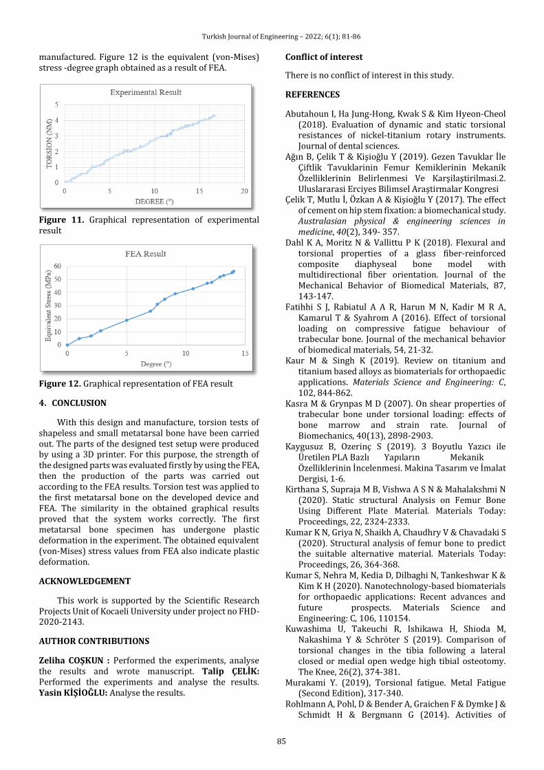
Turkish Journal of Engineering – 2022; 6(1); 81-86
85
manufactured. Figure 12 is the equivalent (von-Mises) stress -degree graph obtained as a result of FEA.
Figure 11. Graphical representation of experimental result
Figure 12. Graphical representation of FEA result
4. CONCLUSION
With this design and manufacture, torsion tests of shapeless and small metatarsal bone have been carried out. The parts of the designed test setup were produced by using a 3D printer. For this purpose, the strength of the designed parts was evaluated firstly by using the FEA, then the production of the parts was carried out according to the FEA results. Torsion test was applied to the first metatarsal bone on the developed device and FEA. The similarity in the obtained graphical results proved that the system works correctly. The first metatarsal bone specimen has undergone plastic deformation in the experiment. The obtained equivalent (von-Mises) stress values from FEA also indicate plastic deformation.
ACKNOWLEDGEMENT
This work is supported by the Scientific Research Projects Unit of Kocaeli University under project no FHD- 2020-2143.
AUTHOR CONTRIBUTIONS
Zeliha COŞKUN : Performed the experiments, analyse the results and wrote manuscript. Talip ÇELİK: Performed the experiments and analyse the results. Yasin KİŞİOĞLU: Analyse the results.
Conflict of interest
There is no conflict of interest in this study.
REFERENCES
Abutahoun I, Ha Jung-Hong, Kwak S & Kim Hyeon-Cheol (2018). Evaluation of dynamic and static torsional resistances of nickel-titanium rotary instruments. Journal of dental sciences.
Ağın B, Çelik T & Kişioğlu Y (2019). Gezen Tavuklar İle Çiftlik Tavuklarinin Femur Kemiklerinin Mekanik Özelliklerinin Belirlenmesi Ve Karşilaştirilmasi.2. Uluslararasi Erciyes Bilimsel Araştirmalar Kongresi
Çelik T, Mutlu İ, Özkan A & Kişioğlu Y (2017). The effect of cement on hip stem fixation: a biomechanical study. Australasian physical & engineering sciences in medicine, 40(2), 349- 357.
Dahl K A, Moritz N & Vallittu P K (2018). Flexural and torsional properties of a glass fiber-reinforced composite diaphyseal bone model with multidirectional fiber orientation. Journal of the Mechanical Behavior of Biomedical Materials, 87, 143-147.
Fatihhi S J, Rabiatul A A R, Harun M N, Kadir M R A, Kamarul T & Syahrom A (2016). Effect of torsional loading on compressive fatigue behaviour of trabecular bone. Journal of the mechanical behavior of biomedical materials, 54, 21-32.
Kaur M & Singh K (2019). Review on titanium and titanium based alloys as biomaterials for orthopaedic applications. Materials Science and Engineering: C, 102, 844-862.
Kasra M & Grynpas M D (2007). On shear properties of trabecular bone under torsional loading: effects of bone marrow and strain rate. Journal of Biomechanics, 40(13), 2898-2903.
Kaygusuz B, Ozerınç S (2019). 3 Boyutlu Yazıcı ile Üretilen PLA Bazlı Yapıların Mekanik Özelliklerinin İncelenmesi. Makina Tasarım ve İmalat Dergisi, 1-6.
Kirthana S, Supraja M B, Vishwa A S N & Mahalakshmi N (2020). Static structural Analysis on Femur Bone Using Different Plate Material. Materials Today: Proceedings, 22, 2324-2333.
Kumar K N, Griya N, Shaikh A, Chaudhry V & Chavadaki S (2020). Structural analysis of femur bone to predict the suitable alternative material. Materials Today: Proceedings, 26, 364-368.
Kumar S, Nehra M, Kedia D, Dilbaghi N, Tankeshwar K & Kim K H (2020). Nanotechnology-based biomaterials for orthopaedic applications: Recent advances and future prospects. Materials Science and Engineering: C, 106, 110154.
Kuwashima U, Takeuchi R, Ishikawa H, Shioda M, Nakashima Y & Schröter S (2019). Comparison of torsional changes in the tibia following a lateral closed or medial open wedge high tibial osteotomy. The Knee, 26(2), 374-381.
Murakami Y. (2019), Torsional fatigue. Metal Fatigue (Second Edition), 317-340.
Rohlmann A, Pohl, D & Bender A, Graichen F & Dymke J & Schmidt H & Bergmann G (2014). Activities of

Turkish Journal of Engineering – 2022; 6(1); 81-86
86
Everyday Life with High Spinal Loads. PloS one. 9. e98510. 10.1371/journal.pone.0098510.
Sykaras N, Iacopino A M, Marker V A, Triplett R G & Woody R D (2000). Implant materials, designs, and surface topographies: their effect on osseointegration. A literature review. International Journal of Oral & Maxillofacial Implants, 15(5).
Traphöner H, Clausmeyer T & Tekkaya A E (2018). Material characterization for plane and curved sheets using the in-plane torsion test–An overview. Journal of Materials Processing Technology, 257, 278-287.
Varghese B, Short D, Penmetsa R, Goswami T & Hangartner T (2011). Computed-tomography- based
finite-element models of long bones can accurately capture strain response to bending and torsion. Journal of biomechanics, 44(7), 1374- 1379.
Wahab A H A, Wui N B, Kadir M R A & Ramlee M H (2020). Biomechanical Evaluation of Three Different Configurations of External Fixators for Treating Distal Third Tibia Fracture: Finite Element Analysis in Axial, Bending and Torsion Load. Computers in Biology and Medicine, 104062.
Wu Z, Wu Y, Fahmy M (2020) Shear and torsional strengthening of structures. Structures Strengthened with Bonded Composites, 315- 386, 2020.
© Author(s) 2022. This work is distributed under https://creativecommons.org/licenses/by-sa/4.0/
* Corresponding Author Cite this article
*([email protected]) ORCID ID 0000-0002-9660-6124 ([email protected]) ORCID ID 0000-0001-9345-5220 Research Article / DOI: 10.31127/tuje.870620
Altuntas C & Tunalioglu N (2022). Retrieving the SNR metrics with different antenna
configurations for GNSS-IR. Turkish Journal of Engineering, 6(1), 87-94
Received: 29/01/2021; Accepted: 28/03/2021
Turkish Journal of Engineering – 2022; 6(1); 87-94
Turkish Journal of Engineering
https://dergipark.org.tr/en/pub/tuje
e-ISSN 2587-1366
Retrieving the SNR metrics with different antenna configurations for GNSS-IR
Cemali Altuntas*1 , Nursu Tunalioglu 1
1Yildiz Technical University, Faculty of Civil Engineering, Department of Geomatics Engineering, Istanbul, Turkey
Keywords ABSTRACT Multipath Signal-to-noise ratio (SNR) GNSS Interferometric Reflectometry (GNSS-IR) Smartphone Horizon-looking antenna
Multipath, which is a major source of error for precise positioning, is the effect that occurs when Global Navigation Satellite Systems (GNSS) signals reach the receiver by reflecting from one or more surfaces. Reflected signals affect the signal-to-noise ratio (SNR) data provided by the receiver, indicating the signal strength. The structure of the antenna of the receiver and the direction in which it is oriented also change the strength of the received signal. In this study, the effect of antenna orientation and polarization on SNR data was demonstrated by using the method called GNSS-Interferometric Reflectometry (GNSS-IR), in terms of reflector height estimates. A geodetic GNSS receiver (CHC i50) and two different smartphones (Xiaomi Mi8 and Xiaomi Mi8 Lite) were used in the four-day experiments. The geodetic receiver was established as zenith-looking (ZL) in the first two days and as horizon-looking (HL) in the last two days. Smartphones were placed on the same mast with the HL receiver in the last two days. It was seen that it is more appropriate to use a 0°-60° satellite elevation angle range in the common use of all receivers’ data. In the 30°-60° range where the ZL installation receives the multipath signals weakly, it has been found that the HL receiver and smartphones have reflector height estimation accuracies with values ranging from 1.9 cm to 2.5 cm. In short, for different elevation angle ranges, accuracies below 2 cm could be obtained with each receiver. Thus, different antenna configurations may be used in GNSS-IR studies, depending on the characteristics of the study area and the surface feature to be determined.
1. INTRODUCTION
Global Navigation Satellite Systems (GNSS) enable to estimate accurate three-dimensional (3D) Cartesian coordinates of the points where the receivers are located to desired locations to be computed. As commonly known, the signals received from GNSS satellites are subjected to various error sources depend on the satellite error, receiver error, geophysical error, and atmospheric error, etc. If the GNSS signal arrives at the receiving antenna with more than one or more paths by reflecting off surfaces, multipath error on the signal occurs due to those reflections. The traveling time of the reflected signal is slightly delayed when compared with the direct signal, which results in inaccurate positioning calculations. Among the error sources of GNSS, multipath is one of the major and significant error, which referred to as unmodelled, should be eliminated from the observations when accurate positioning is required. To reduce this effect on observations, location selection of
GNSS station such as establishing away from the reflective surfaces, and antenna type selection such as suppressing the multipath are the basic requirements. However, multipath, which is an undesired error source for GNSS positioning, has become an effective tool to determine the reflective surface characteristics recently.
The methodology of the GNSS–Interferometric Reflectometry (GNSS-IR) was first introduced by Martin-Neira (1993) to perform ocean altimetry for retrieving the height of the ocean over a reference ellipsoid. After that, in many studies related to the estimation of the snowpack (Larson et al. 2009; Ozeki & Heki 2012; Gutmann et al. 2012; Chen et al. 2014; Jin et al. 2016; Tunalioglu et al., 2019), soil moisture (Larson et al. 2008; Larson et al., 2010; Roussel et al. 2016; Zhang et al. 2017; Han et al. 2020; Altuntas & Tunalioglu, 2020a), sea-level tide (Anderson 2000; Xi et al. 2018), deformation monitoring (Yang et al. 2019), etc., the GNSS-IR methodology has been implemented successfully.
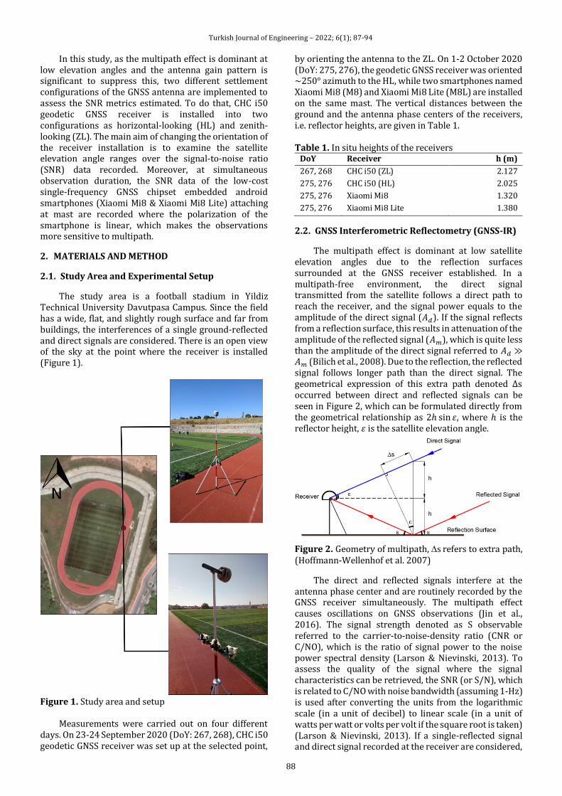
Turkish Journal of Engineering – 2022; 6(1); 87-94
88
In this study, as the multipath effect is dominant at low elevation angles and the antenna gain pattern is significant to suppress this, two different settlement configurations of the GNSS antenna are implemented to assess the SNR metrics estimated. To do that, CHC i50 geodetic GNSS receiver is installed into two configurations as horizontal-looking (HL) and zenith-looking (ZL). The main aim of changing the orientation of the receiver installation is to examine the satellite elevation angle ranges over the signal-to-noise ratio (SNR) data recorded. Moreover, at simultaneous observation duration, the SNR data of the low-cost single-frequency GNSS chipset embedded android smartphones (Xiaomi Mi8 & Xiaomi Mi8 Lite) attaching at mast are recorded where the polarization of the smartphone is linear, which makes the observations more sensitive to multipath.
2. MATERIALS AND METHOD
2.1. Study Area and Experimental Setup
The study area is a football stadium in Yildiz Technical University Davutpasa Campus. Since the field has a wide, flat, and slightly rough surface and far from buildings, the interferences of a single ground-reflected and direct signals are considered. There is an open view of the sky at the point where the receiver is installed (Figure 1).
Figure 1. Study area and setup
Measurements were carried out on four different
days. On 23-24 September 2020 (DoY: 267, 268), CHC i50 geodetic GNSS receiver was set up at the selected point,
by orienting the antenna to the ZL. On 1-2 October 2020 (DoY: 275, 276), the geodetic GNSS receiver was oriented ~250° azimuth to the HL, while two smartphones named Xiaomi Mi8 (M8) and Xiaomi Mi8 Lite (M8L) are installed on the same mast. The vertical distances between the ground and the antenna phase centers of the receivers, i.e. reflector heights, are given in Table 1.
Table 1. In situ heights of the receivers
DoY Receiver h (m)
267, 268 CHC i50 (ZL) 2.127
275, 276 CHC i50 (HL) 2.025
275, 276 Xiaomi Mi8 1.320
275, 276 Xiaomi Mi8 Lite 1.380
2.2. GNSS Interferometric Reflectometry (GNSS-IR)
The multipath effect is dominant at low satellite elevation angles due to the reflection surfaces surrounded at the GNSS receiver established. In a multipath-free environment, the direct signal transmitted from the satellite follows a direct path to reach the receiver, and the signal power equals to the amplitude of the direct signal (𝐴𝑑). If the signal reflects from a reflection surface, this results in attenuation of the amplitude of the reflected signal (𝐴𝑚), which is quite less than the amplitude of the direct signal referred to 𝐴𝑑 ≫𝐴𝑚 (Bilich et al., 2008). Due to the reflection, the reflected signal follows longer path than the direct signal. The geometrical expression of this extra path denoted ∆s occurred between direct and reflected signals can be seen in Figure 2, which can be formulated directly from the geometrical relationship as 2ℎ sin 𝜀, where ℎ is the reflector height, 𝜀 is the satellite elevation angle.
Figure 2. Geometry of multipath, s refers to extra path, (Hoffmann-Wellenhof et al. 2007)
The direct and reflected signals interfere at the antenna phase center and are routinely recorded by the GNSS receiver simultaneously. The multipath effect causes oscillations on GNSS observations (Jin et al., 2016). The signal strength denoted as S observable referred to the carrier-to-noise-density ratio (CNR or C/NO), which is the ratio of signal power to the noise power spectral density (Larson & Nievinski, 2013). To assess the quality of the signal where the signal characteristics can be retrieved, the SNR (or S/N), which is related to C/NO with noise bandwidth (assuming 1-Hz) is used after converting the units from the logarithmic scale (in a unit of decibel) to linear scale (in a unit of watts per watt or volts per volt if the square root is taken) (Larson & Nievinski, 2013). If a single-reflected signal and direct signal recorded at the receiver are considered,
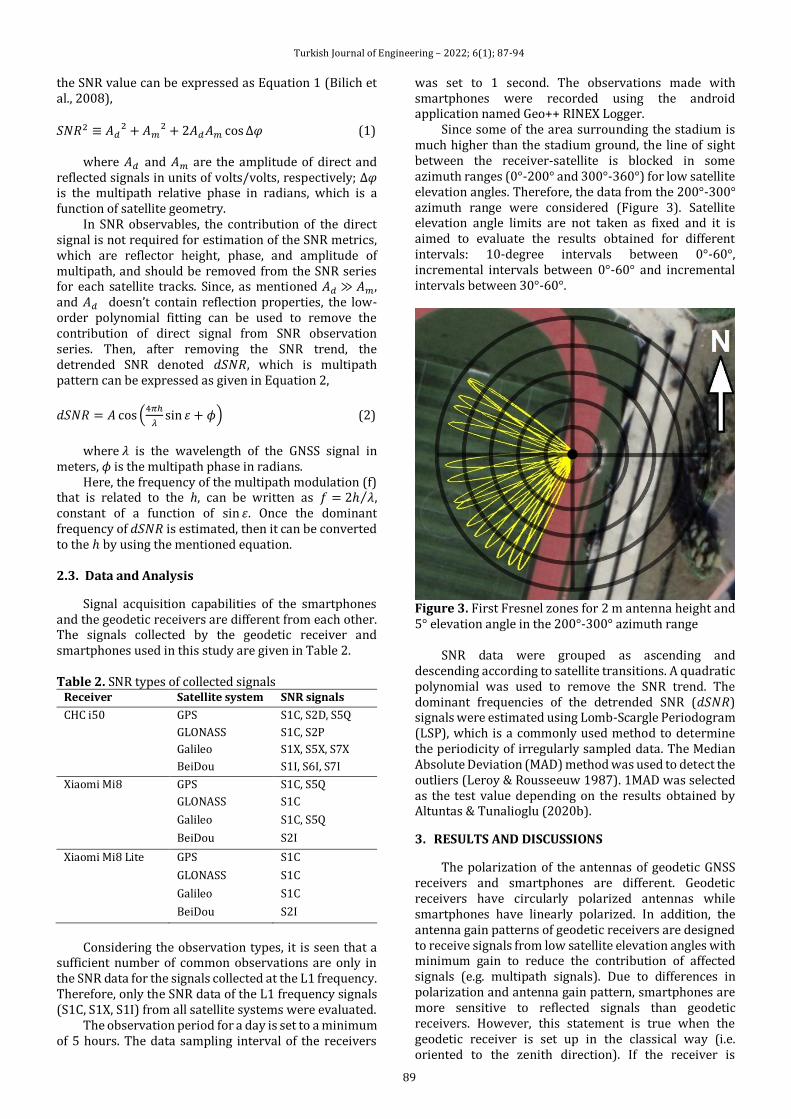
Turkish Journal of Engineering – 2022; 6(1); 87-94
89
the SNR value can be expressed as Equation 1 (Bilich et al., 2008),
𝑆𝑁𝑅2 ≡ 𝐴𝑑2 + 𝐴𝑚
2 + 2𝐴𝑑𝐴𝑚 cos ∆𝜑 (1)
where 𝐴𝑑 and 𝐴𝑚 are the amplitude of direct and reflected signals in units of volts/volts, respectively; ∆𝜑 is the multipath relative phase in radians, which is a function of satellite geometry.
In SNR observables, the contribution of the direct signal is not required for estimation of the SNR metrics, which are reflector height, phase, and amplitude of multipath, and should be removed from the SNR series for each satellite tracks. Since, as mentioned 𝐴𝑑 ≫ 𝐴𝑚, and 𝐴𝑑 doesn’t contain reflection properties, the low-order polynomial fitting can be used to remove the contribution of direct signal from SNR observation series. Then, after removing the SNR trend, the detrended SNR denoted 𝑑𝑆𝑁𝑅, which is multipath pattern can be expressed as given in Equation 2,
𝑑𝑆𝑁𝑅 = 𝐴 cos (4𝜋ℎ
𝜆sin 𝜀 + 𝜙) (2)
where 𝜆 is the wavelength of the GNSS signal in
meters, 𝜙 is the multipath phase in radians. Here, the frequency of the multipath modulation (f)
that is related to the h, can be written as 𝑓 = 2ℎ 𝜆⁄ , constant of a function of sin 𝜀. Once the dominant frequency of 𝑑𝑆𝑁𝑅 is estimated, then it can be converted to the ℎ by using the mentioned equation.
2.3. Data and Analysis
Signal acquisition capabilities of the smartphones and the geodetic receivers are different from each other. The signals collected by the geodetic receiver and smartphones used in this study are given in Table 2. Table 2. SNR types of collected signals
Receiver Satellite system SNR signals
CHC i50 GPS S1C, S2D, S5Q
GLONASS S1C, S2P
Galileo S1X, S5X, S7X
BeiDou S1I, S6I, S7I
Xiaomi Mi8 GPS S1C, S5Q
GLONASS S1C
Galileo S1C, S5Q
BeiDou S2I
Xiaomi Mi8 Lite GPS S1C
GLONASS S1C
Galileo S1C
BeiDou S2I
Considering the observation types, it is seen that a
sufficient number of common observations are only in the SNR data for the signals collected at the L1 frequency. Therefore, only the SNR data of the L1 frequency signals (S1C, S1X, S1I) from all satellite systems were evaluated.
The observation period for a day is set to a minimum of 5 hours. The data sampling interval of the receivers
was set to 1 second. The observations made with smartphones were recorded using the android application named Geo++ RINEX Logger.
Since some of the area surrounding the stadium is much higher than the stadium ground, the line of sight between the receiver-satellite is blocked in some azimuth ranges (0°-200° and 300°-360°) for low satellite elevation angles. Therefore, the data from the 200°-300° azimuth range were considered (Figure 3). Satellite elevation angle limits are not taken as fixed and it is aimed to evaluate the results obtained for different intervals: 10-degree intervals between 0°-60°, incremental intervals between 0°-60° and incremental intervals between 30°-60°.
Figure 3. First Fresnel zones for 2 m antenna height and 5° elevation angle in the 200°-300° azimuth range
SNR data were grouped as ascending and
descending according to satellite transitions. A quadratic polynomial was used to remove the SNR trend. The dominant frequencies of the detrended SNR (𝑑𝑆𝑁𝑅) signals were estimated using Lomb-Scargle Periodogram (LSP), which is a commonly used method to determine the periodicity of irregularly sampled data. The Median Absolute Deviation (MAD) method was used to detect the outliers (Leroy & Rousseeuw 1987). 1MAD was selected as the test value depending on the results obtained by Altuntas & Tunalioglu (2020b).
3. RESULTS AND DISCUSSIONS
The polarization of the antennas of geodetic GNSS receivers and smartphones are different. Geodetic receivers have circularly polarized antennas while smartphones have linearly polarized. In addition, the antenna gain patterns of geodetic receivers are designed to receive signals from low satellite elevation angles with minimum gain to reduce the contribution of affected signals (e.g. multipath signals). Due to differences in polarization and antenna gain pattern, smartphones are more sensitive to reflected signals than geodetic receivers. However, this statement is true when the geodetic receiver is set up in the classical way (i.e. oriented to the zenith direction). If the receiver is
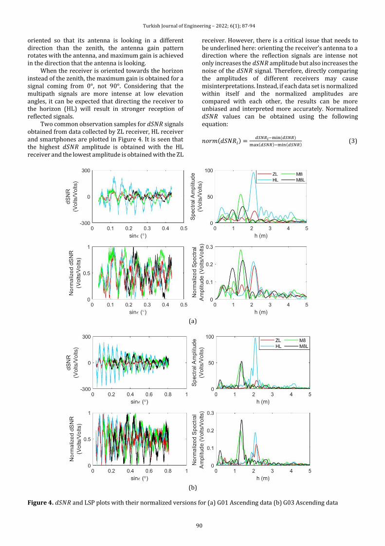
Turkish Journal of Engineering – 2022; 6(1); 87-94
90
oriented so that its antenna is looking in a different direction than the zenith, the antenna gain pattern rotates with the antenna, and maximum gain is achieved in the direction that the antenna is looking.
When the receiver is oriented towards the horizon instead of the zenith, the maximum gain is obtained for a signal coming from 0°, not 90°. Considering that the multipath signals are more intense at low elevation angles, it can be expected that directing the receiver to the horizon (HL) will result in stronger reception of reflected signals.
Two common observation samples for 𝑑𝑆𝑁𝑅 signals obtained from data collected by ZL receiver, HL receiver and smartphones are plotted in Figure 4. It is seen that the highest 𝑑𝑆𝑁𝑅 amplitude is obtained with the HL receiver and the lowest amplitude is obtained with the ZL
receiver. However, there is a critical issue that needs to be underlined here: orienting the receiver’s antenna to a direction where the reflection signals are intense not only increases the 𝑑𝑆𝑁𝑅 amplitude but also increases the noise of the 𝑑𝑆𝑁𝑅 signal. Therefore, directly comparing the amplitudes of different receivers may cause misinterpretations. Instead, if each data set is normalized within itself and the normalized amplitudes are compared with each other, the results can be more unbiased and interpreted more accurately. Normalized 𝑑𝑆𝑁𝑅 values can be obtained using the following equation:
𝑛𝑜𝑟𝑚(𝑑𝑆𝑁𝑅𝑖) =𝑑𝑆𝑁𝑅𝑖−min (𝑑𝑆𝑁𝑅)
max(𝑑𝑆𝑁𝑅)−min(𝑑𝑆𝑁𝑅) (3)
(a)
(b)
Figure 4. 𝑑𝑆𝑁𝑅 and LSP plots with their normalized versions for (a) G01 Ascending data (b) G03 Ascending data
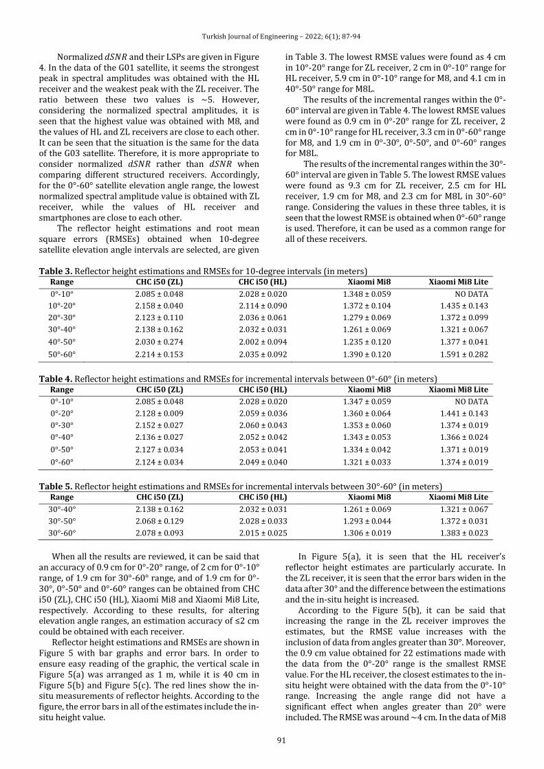
Turkish Journal of Engineering – 2022; 6(1); 87-94
91
Normalized 𝑑𝑆𝑁𝑅 and their LSPs are given in Figure 4. In the data of the G01 satellite, it seems the strongest peak in spectral amplitudes was obtained with the HL receiver and the weakest peak with the ZL receiver. The ratio between these two values is ~5. However, considering the normalized spectral amplitudes, it is seen that the highest value was obtained with M8, and the values of HL and ZL receivers are close to each other. It can be seen that the situation is the same for the data of the G03 satellite. Therefore, it is more appropriate to consider normalized 𝑑𝑆𝑁𝑅 rather than 𝑑𝑆𝑁𝑅 when comparing different structured receivers. Accordingly, for the 0°-60° satellite elevation angle range, the lowest normalized spectral amplitude value is obtained with ZL receiver, while the values of HL receiver and smartphones are close to each other.
The reflector height estimations and root mean square errors (RMSEs) obtained when 10-degree satellite elevation angle intervals are selected, are given
in Table 3. The lowest RMSE values were found as 4 cm in 10°-20° range for ZL receiver, 2 cm in 0°-10° range for HL receiver, 5.9 cm in 0°-10° range for M8, and 4.1 cm in 40°-50° range for M8L.
The results of the incremental ranges within the 0°-60° interval are given in Table 4. The lowest RMSE values were found as 0.9 cm in 0°-20° range for ZL receiver, 2 cm in 0°-10° range for HL receiver, 3.3 cm in 0°-60° range for M8, and 1.9 cm in 0°-30°, 0°-50°, and 0°-60° ranges for M8L.
The results of the incremental ranges within the 30°-60° interval are given in Table 5. The lowest RMSE values were found as 9.3 cm for ZL receiver, 2.5 cm for HL receiver, 1.9 cm for M8, and 2.3 cm for M8L in 30°-60° range. Considering the values in these three tables, it is seen that the lowest RMSE is obtained when 0°-60° range is used. Therefore, it can be used as a common range for all of these receivers.
Table 3. Reflector height estimations and RMSEs for 10-degree intervals (in meters)
Range CHC i50 (ZL) CHC i50 (HL) Xiaomi Mi8 Xiaomi Mi8 Lite
0°-10° 2.085 ± 0.048 2.028 ± 0.020 1.348 ± 0.059 NO DATA
10°-20° 2.158 ± 0.040 2.114 ± 0.090 1.372 ± 0.104 1.435 ± 0.143
20°-30° 2.123 ± 0.110 2.036 ± 0.061 1.279 ± 0.069 1.372 ± 0.099
30°-40° 2.138 ± 0.162 2.032 ± 0.031 1.261 ± 0.069 1.321 ± 0.067
40°-50° 2.030 ± 0.274 2.002 ± 0.094 1.235 ± 0.120 1.377 ± 0.041
50°-60° 2.214 ± 0.153 2.035 ± 0.092 1.390 ± 0.120 1.591 ± 0.282
Table 4. Reflector height estimations and RMSEs for incremental intervals between 0°-60° (in meters)
Range CHC i50 (ZL) CHC i50 (HL) Xiaomi Mi8 Xiaomi Mi8 Lite
0°-10° 2.085 ± 0.048 2.028 ± 0.020 1.347 ± 0.059 NO DATA
0°-20° 2.128 ± 0.009 2.059 ± 0.036 1.360 ± 0.064 1.441 ± 0.143
0°-30° 2.152 ± 0.027 2.060 ± 0.043 1.353 ± 0.060 1.374 ± 0.019
0°-40° 2.136 ± 0.027 2.052 ± 0.042 1.343 ± 0.053 1.366 ± 0.024
0°-50° 2.127 ± 0.034 2.053 ± 0.041 1.334 ± 0.042 1.371 ± 0.019
0°-60° 2.124 ± 0.034 2.049 ± 0.040 1.321 ± 0.033 1.374 ± 0.019
Table 5. Reflector height estimations and RMSEs for incremental intervals between 30°-60° (in meters) Range CHC i50 (ZL) CHC i50 (HL) Xiaomi Mi8 Xiaomi Mi8 Lite
30°-40° 2.138 ± 0.162 2.032 ± 0.031 1.261 ± 0.069 1.321 ± 0.067
30°-50° 2.068 ± 0.129 2.028 ± 0.033 1.293 ± 0.044 1.372 ± 0.031
30°-60° 2.078 ± 0.093 2.015 ± 0.025 1.306 ± 0.019 1.383 ± 0.023
When all the results are reviewed, it can be said that an accuracy of 0.9 cm for 0°-20° range, of 2 cm for 0°-10° range, of 1.9 cm for 30°-60° range, and of 1.9 cm for 0°-30°, 0°-50° and 0°-60° ranges can be obtained from CHC i50 (ZL), CHC i50 (HL), Xiaomi Mi8 and Xiaomi Mi8 Lite, respectively. According to these results, for altering elevation angle ranges, an estimation accuracy of ≤2 cm could be obtained with each receiver.
Reflector height estimations and RMSEs are shown in Figure 5 with bar graphs and error bars. In order to ensure easy reading of the graphic, the vertical scale in Figure 5(a) was arranged as 1 m, while it is 40 cm in Figure 5(b) and Figure 5(c). The red lines show the in-situ measurements of reflector heights. According to the figure, the error bars in all of the estimates include the in-situ height value.
In Figure 5(a), it is seen that the HL receiver’s reflector height estimates are particularly accurate. In the ZL receiver, it is seen that the error bars widen in the data after 30° and the difference between the estimations and the in-situ height is increased.
According to the Figure 5(b), it can be said that increasing the range in the ZL receiver improves the estimates, but the RMSE value increases with the inclusion of data from angles greater than 30°. Moreover, the 0.9 cm value obtained for 22 estimations made with the data from the 0°-20° range is the smallest RMSE value. For the HL receiver, the closest estimates to the in-situ height were obtained with the data from the 0°-10° range. Increasing the angle range did not have a significant effect when angles greater than 20° were included. The RMSE was around ~4 cm. In the data of Mi8
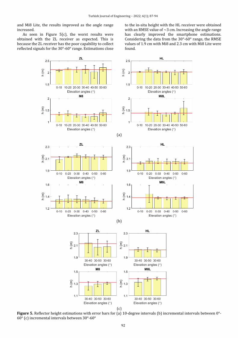
Turkish Journal of Engineering – 2022; 6(1); 87-94
92
and Mi8 Lite, the results improved as the angle range increased.
As seen in Figure 5(c), the worst results were obtained with the ZL receiver as expected. This is because the ZL receiver has the poor capability to collect reflected signals for the 30°-60° range. Estimations close
to the in-situ height with the HL receiver were obtained with an RMSE value of ~3 cm. Increasing the angle range has clearly improved the smartphone estimations. Considering the data from the 30°-60° range, the RMSE values of 1.9 cm with Mi8 and 2.3 cm with Mi8 Lite were found.
(a)
(b)
(c)
Figure 5. Reflector height estimations with error bars for (a) 10-degree intervals (b) incremental intervals between 0°-60° (c) incremental intervals between 30°-60°
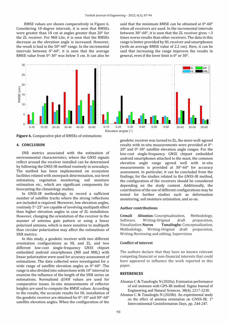
Turkish Journal of Engineering – 2022; 6(1); 87-94
93
RMSE values are shown comparatively in Figure 6. Considering 10-degree intervals, it is seen that RMSEs were greater than 10 cm at angles greater than 20° for the ZL receiver. For Mi8 Lite, it is seen that the RMSEs decrease as the elevation angle is increased. However, the result is bad in the 50°-60° range. In the incremental intervals between 0°-60°, it is seen that the average RMSE value from 0°-30° was below 5 cm. It can also be
said that the minimum RMSE can be obtained at 0°-60° when all receivers are used. In the incremental intervals between 30°-60°, it is seen that the ZL receiver gives ~3 times worse results than other receivers. The data in this range is better provided by HL receiver and smartphones (with an average RMSE value of 2.2 cm). Here, it can be said that increasing the range improves the results in general, even if the lover limit is 0° or 30°.
Figure 6. Comparative plot of RMSEs of estimations 4. CONCLUSION
SNR metrics associated with the estimation of environmental characteristics, where the GNSS signals reflect around the receiver installed can be determined by following the GNSS-IR method routinely in nowadays. The method has been implemented on ecosystem facilities related with snowpack determination, sea-level estimation, vegetation monitoring, soil moisture estimation etc., which are significant components for forecasting the climatology studies.
In GNSS-IR methodology, to record a sufficient number of satellite tracks where the strong reflections are included is required. Moreover, low elevation angles, routinely 5°-25° are capable of involving multipath effect than higher elevation angles in case of ZL installation. However, changing the orientation of the receiver in the manner of antenna gain pattern or using a linear polarized antenna, which is more sensitive to multipath than circular polarization may affect the estimations of SNR metrics.
In this study, a geodetic receiver with two different orientation configurations as HL and ZL, and two different low-cost single-frequency GNSS chipset embedded android smartphones (M8 and M8L) with linear polarization were used for accuracy assessment of estimations. The data collected were investigated for a wide range of satellite elevation angles as 0°-60°. The range is also divided into subsections with 10° interval to examine the influence of the length of the SNR series on estimations. Normalized 𝑑𝑆𝑁𝑅 values are used for comparative issues. In-situ measurements of reflector heights are used to compute the RMSE values. According to the results, the accurate results for HL installation of the geodetic receiver are obtained for 0°-10° and 30°-60° satellite elevation angles. When the configuration of the
geodetic receiver was turned to ZL, the more well-agreed results with in-situ measurements were provided at 0°-20° and 0°-30° satellite elevation angle ranges. For the low-cost single-frequency GNSS chipset embedded android smartphones attached to the mast, the common elevation angle range agreed well with in-situ measurements is provided at 30°-60° for accuracy assessment. In particular, it can be concluded from the findings, for the studies related to the GNSS-IR method, the configuration of the receivers should be considered depending on the study content. Additionally, the contribution of the use of different configurations may be tested for further studies such as deformation monitoring, soil moisture estimation, and so on. Author contributions
Cemali Altuntas: Conceptualization, Methodology, Software, Writing-Original draft preparation, Visualization Nursu Tunalioglu: Conceptualization, Methodology, Writing-Original draft preparation, Writing-Reviewing and editing, Supervision
Conflict of interest The authors declare that they have no known relevant competing financial or non-financial interests that could have appeared to influence the work reported in this paper.
REFERENCES
Altuntas C & Tunalioglu N (2020a). Estimation performance
of soil moisture with GPS-IR method. Sigma Journal of
Engineering and Natural Sciences, 38(4), 2217-2230. Altuntas C & Tunalioglu N (2020b). An experimental study
on the effect of antenna orientation on GNSS-IR. 1st
Intercontinental Geoinformation Days, pp. 244-247.
Turkish Journal of Engineering – 2022; 6(1); 87-94
94
Anderson K D (2000). Determination of water level and tides
using interferometric observations of GPS signals.
Journal of Atmospheric and Oceanic Technology.
17(8), 1118-1127, doi:10.1175/1520-0426(2000)017<1118:DOWLAT>2.0.CO;2.
Bilich A, Larson K M & Axelrad P (2008). Modeling GPS
phase multipath with SNR: Case study from the Salar
de Uyuni, Boliva, Journal of Geophysical Research,
113, B04401, doi:10.1029/2007JB005194.
Chen Q, Won D & Akos D M (2014). Snow depth sensing
using the GPS L2C signal with a dipole antenna.
EURASIP Journal on Advances in Signal Processing,
1(106). doi:10.1186/1687-6180-2014-106.
Gutmann E D, Larson K M, Williams M W, Nievinski F G
& Zavorotny V (2012). Snow measurement by GPS
interferometric reflectometry: an evaluation at Niwot Ridge, Colorado. Hydrological Processes, 26(19),
2951-2961, doi:10.1002/hyp.8329.
Han M, Zhu Y, Yang D, Chang Q, Hong X & Song S (2020).
Soil moisture monitoring using GNSS interference
signal: proposing a signal reconstruction method.
Remote Sensing Letters, 11(4), 373-382. DOI:
10.1080/2150704X.2020.1718235.
Hofmann-Wellenhof B, Lichtenegger H & Wasle E (2007).
GNSS–global navigation satellite systems: GPS,
GLONASS, Galileo, and more. Springer Science &
Business Media. Jin S, Qian X & Kutoglu H (2016). Snow depth variations
estimated from GPS-Reflectometry: A case study in
Alaska from L2P SNR data. Remote sensing, 8(1), 63.
doi:10.3390/rs8010063.
Larson K M, Nievinski F G (2013). GPS snow sensing:
results from the EarthScope Plate Boundary
Observatory, GPS Solut (2013) 17:41–52, DOI
10.1007/s10291-012-0259-7.
Larson K M, Small E E, Gutmann E D, Bilich A L, Braun J
J & Zavorotny V U (2008). Use of GPS receivers as a
soil moisture network for water cycle studies.
Geophysical Research Letters, Vol. 35, L24405, doi:10.1029/2008GL036013.
Larson K M, Gutmann E D, Zavorotny V U, Braun J J,
Williams M W & Nievinski F G (2009). Can we
measure snow depth with GPS receivers?. Geophysical
Research Letters, 36(17), doi:10.1029/2009GL039430.
Larson K M, Braun J J, Small E E, Zavorotny V U, Gutmann
E D & Bilich A L (2010). GPS Multipath and Its
Relation to Near-Surface Soil Moisture Content. IEEE
Journal of Selected Topics in Applied Earth Observations and Remote Sensing, 3(1), 91-99. doi:
10.1109/JSTARS.2009.2033612.
Leroy A M & Rousseeuw P J (1987). Robust regression and
outlier detection. Wiley Series in Probability and
Mathematical Statistics, New York.
Martin-Neira M (1993). A passive reflectometry and
interferometry system (PARIS): Application to ocean
altimetry. ESA Journal, 17(4), 331-355.
Ozeki M & Heki K (2012). GPS snow depth meter with
geometry-free linear combinations of carrier phases.
Journal of Geodesy, 86(3), 209-219,
doi:10.1007/s00190-011-0511-x. Roussel N, Frappart F, Ramillien G, Darrozes J, Baup F,
Lestarquit L & Ha M C (2016). Detection of Soil
Moisture Variations Using GPS and GLONASS SNR
Data for Elevation Angles Ranging From 2° to 70°.
IEEE Journal of Selected Topics in Applied Earth
Observations and Remote Sensing, 9 (10), 4781.
Tunalioglu N, Dogan A H, Durdag U M (2019). GPS sinyal
gürültü oranı verileri ile kar kalınlığının belirlenmesi.
HKMOJJD, 6(1) 1-9. Doi:
10.9733/JGG.2019R00601001.T.
Xi R, Zhou X, Jiang W & Chen Q (2018). Simultaneous estimation of dam displacements and reservoir level
variation from GPS measurements. Measurement, 122,
247-256. doi:10.1016/j.measurement.2018.03.036.
Yang Y, Zheng Y, Yu W, Chen W & Weng D (2019).
Deformation monitoring using GNSS-R technology.
Advances in Space Research 63 (2019) 3303–3314.
Zhang S, Roussel N, Boniface K, Ha M C, Frappart F,
Darrozes J, Baup F & Calvet J C (2017). Use of
reflected GNSS SNR data to retrieve either soil
moisture or vegetation height from a wheat crop.
Hydrol. Earth Syst. Sci., 21, 4767–4784,
https://doi.org/10.5194/hess-21-4767-2017.
© Author(s) 2022. This work is distributed under https://creativecommons.org/licenses/by-sa/4.0/
Related Documents