Voltammetric lability of multiligand complexes: the case of ML2

1

Voltammetric lability of multiligand complexes. The case of ML2

Jaume PUY*,a, Joan CECILIA

b, Josep GALCERAN

a, Raewyn M. TOWN

c and Herman P.

van LEEUWENd

a Departament de Química,

b Departament de Matemàtica, Universitat de Lleida (UdL).

Av. Rovira Roure, 191. E-25198 Lleida (Catalonia, Spain).

c School of Chemistry, The Queen’s University of Belfast, Belfast BT9 5AG, U.K

d Laboratory of Physical Chemistry and Colloid Science, Wageningen University, P.O. Box

8038, Dreijenplein 6, 6703 HB Wageningen (The Netherlands).

Keywords: voltammetry, lability, reaction layer, kinetic currents

*) corresponding author; e-mail: [email protected]; fax: (34)973238264

Abstract

The voltammetric lability of a complex system where a metal ion M and a ligand L form the

species ML and ML2 is examined. Together with the rigorous numerical simulation of the

problem, two limiting cases are analysed for the overall process ML2 → M: (i) the most

common case for aqueous complexes where ML → M is the kinetically limiting step and (ii)

the case where ML2 → ML is limiting. In both cases, analytical expressions for the lability

criteria are provided which show good agreement with the results obtained from the rigorous

numerical simulation of the problem.

Published in Journal of Electroanalytical Chemistry 2004, vol 571, p 121-132 DOI: 10.1016/j.jelechem.2004.04.017 reprints also to [email protected]

2

1. Introduction

The speciation of a metal (or any element), i.e. the distribution of its total concentration over a

range of physicochemical forms, is long recognised as being important for determining its

reactivity, mobility, bioavailability, and toxicity. Rigorous understanding of metal ion

speciation in this context must go beyond consideration of the equilibrium distribution of

species. A quantitative characterisation of dynamic aspects of metal ion speciation, i.e. the

kinetic characteristics of interconversion of metal complex species, is required for correct

interpretation of data furnished by dynamic analytical techniques [1] (e.g. permeation liquid

membranes, diffusive gradients in thin film, voltammetries), and for establishing a rigorous

foundation for the relationship between metal speciation and bioavailability [2].

In this context it is useful to introduce the concept of lability which refers to the extent to

which the complexes contribute to the metal flux (towards an analytical sensor or a

bioaccumulating organism) via dissociation. In a labile system, equilibrium between ML and

M is maintained on any relevant spatial scale so that conditions of maximum metal flux arise.

For a given surface reaction of the free metal, the lability of a metal complex species indicates

its contribution to the supply of uncomplexed metal. Lability criteria have been established

for a range of different situations, e.g. geometry and size of the accumulating surface. These

criteria allow an a priori evaluation of the contribution of the complex to the metal supply in

terms of characteristic parameters of the system: kinetic constants, diffusion coefficients, time

scale of the experiment, relevant size of the sensor, bulk concentrations, etc… Note that

lability refers to both the properties of the medium and to the geometrical features of the

sensing surface.

For dynamic systems, lability criteria are based on the comparison of the relative magnitudes

of the actual kinetic metal flux, Jkin , to the maximum pure diffusive flux of the complex, Jdif,


3

[3]. This arises logically from the definition of Jkin: this parameter represents the increase of

metal flux appearing in the system as compared to that for a system in the absence of

complexed species, but with the same free metal concentration (i. e. Jkin is the contribution of

the complex to the metal supply). The actual Jkin is compared with the maximum kinetic flux

that could arise in the system (i.e. when the complex is fully labile) which coincides with the

maximum purely diffusive flux of the complex, Jdif. For the practical application of this

comparison, Jdif is estimated by means of the diffusion layer approximation while Jkin is

obtained by means of the classical reaction layer approximation. Based on bulk

concentrations, this approach is a simplification that overestimates Jkin: the resulting Jkin is the

maximum kinetic flux attainable because it assumes an unlimited supply of complex, i.e. that

no depletion occurs in the diffusion layer. Using this formalism based on bulk solution

concentrations, Jkin largely outweighs the maximum Jdif of ML for fully labile complexes,

whilst in the non-labile case the maximum Jdif of ML is much larger than Jkin. Drastic changes

in lability can occur with time, and with spatial scale. The well-known dimensionless lability

criterion parameter, L, (= Jkin/Jdif) is used to quantify lability for a given system at a given

timescale, with L >> 1 for the fully labile case. An inert (static) complex represents the trivial

case in which ML does not contribute to the flux.

Until now, lability criteria have been established only for M-L complexes of 1:1

stoichiometry. In this case, the only possible kinetically limiting step is interconversion of ML

and M. In many systems, however, complexes of higher ligand stoichiometry, ML2, ML3, etc.

are formed. The formation of free M from complex species MLi then involves a sequence of

dissociation steps. Quantification of the overall interfacial flux of M requires consideration of

all equilibria and all association/dissociation rate constants. The present work opens up the

field by deriving analytical expressions for the lability criteria for complexes of 1:2


4

stoichiometry and comparing these with the results of rigorous numerical simulations.

Together with the validation of the classical lability criterion, we present a more refined

formulation (introducing Lφ) in terms of the relevant species concentrations along the reaction

layer.

2. Mathematical Formulation

Let us consider the complexation in solution of a metal ion M with a ligand L according to the

scheme

a,1

d,1

M+L MLk

k��⇀↽�� (1)

a,2

d,22ML+L ML

k

k��⇀↽�� (2)

under conditions where the free metal species is consumed by some process taking place at an

interface in contact with the solution, for instance a reduction to the metal atom Mº at an

electrode surface

0M Mn e

n e

−

−

+

−��⇀↽�� (3)

The quotients of the rate constants define the stability constants iK of the complexes,

a, d,i i iK k k= (4)

The ratios of concentrations iQ are defined as

i

i 1

ML

ML L

i

cQ

c c−

= (5)

and equal iK if the corresponding equilibrium is attained.


5

If diffusion towards a stationary planar electrode is the only relevant transport mechanism, the

conservation equations read

2

M MM d,1 ML a,1 M L2

c cD k c k c c

t x

∂ ∂= + −∂ ∂

(6)

2

2

L LL d,1 ML a,1 M L d,2 ML a,2 ML L2

c cD k c k c c k c k c c

t x

∂ ∂= + − + −∂ ∂

(7)

2

2

ML MLL d,1 ML a,1 M L d,2 ML a,2 ML L2

c cD k c k c c k c k c c

t x

∂ ∂= − + + −∂ ∂

(8)

2 2

2

2

ML ML

L d,2 ML a,2 ML L2

c cD k c k c c

t x

∂ ∂= − +

∂ ∂ (9)

where the diffusion coefficients of all species containing L are assumed to equal DL.

The initial conditions are, as usual,

( ) *

20 : ,0 M,L,ML,MLi it c x c i= = = (10)

For limiting diffusion conditions, the boundary value problem is given by

( ) 2MLL MLM

0 0 0

0 : 0, 0 0x x x

cc cx c t

x x x= = =

∂ ∂ ∂ = = = = = ∂ ∂ ∂ (11)

and

( ) *

2: , M,L,ML,MLi ix c t c i= ∞ ∞ = = (12)

which expresses semi-infinite diffusion.

Any one of the eqns. (7)-(9) may be eliminated by noticing that

2

*

L ML ML T,L2c c c c+ + = (13)


6

which comes from the fact that no physical phenomenon distorts the initially flat

concentration profile of the total ligand concentration and it can be used to determine, for

instance, 2MLc once the concentrations Mc , Lc and MLc are known.

The set of Eqs. (6)-(12) defines the concentration profiles of M, L and ML. The solution of

this system is cumbersome due to the presence of non-linear equations. As detailed in the

Appendix, we use the Galerkin Finite Element Method (GFEM) [4] to solve the spatial

distribution of all the species at any time, whereas a finite-difference method is used for the

time evolution. We are interested in the metal flux at the electrode surface given by

MM M

0x

cJ D

x =

∂ = ∂ (14)

In case of a sufficiently large excess of ligand ( ( ) *

L L,c x t c≈ ), the association reactions

become pseudo first-order and we define

1

*

ML* '

L *

ML

i

i

i i

cK c K

c−

= = (15)

L

' *

a, a,i ik k c= (16)

The limiting case of fully labile complexes under excess of ligand allows a simple analytical

solution for the metal flux:

*M,fully labile T,M

DJ c

tπ= (17)

where

' ' 'M L 1 L 1 2

' ' '1 1 21

D D K D K KD

K K K

+ +≡

+ + (18)


https://www.researchgate.net/publication/252748415_Variational_Principles_and_the_Finite-Element_Method_in_Partial_Differential_Equations?el=1_x_8&enrichId=rgreq-d972de80-aa6f-40d9-88a4-aa4e59993676&enrichSource=Y292ZXJQYWdlOzIzOTE0OTQ5ODtBUzoxOTc0MjAxMDY0MjQzMjBAMTQyNDA4MDAyOTEwNA==

7

is the weighted average diffusion coefficient.

3. The case where ML →→→→ M is the kinetically limiting step in ML2 →→→→M

3.1. Volume reactions

The complex formation/dissociation reactions in (1) and (2) are all involved with H2O

binding/release reactions. In terms of inner-sphere bound water, Eqs. (1)-(2) actually imply,

for a supposedly constant coordination number of 6:

( ) ( ) ( )a,1 a,2

d,1 d,22 2 2 26 5 4

M H O +L M H O L+L M H O Lk k

k k��⇀ ��⇀↽�� ↽�� (19)

For a great many types of ligand L, the Eigen mechanism applies to reactions (1) and (2),

implying that a,1k is determined by the rate of dehydration of the inner coordination sphere of

the hydrated metal ion: M(H2O)6 ( + L) → M(H2O)5 (L). Thus, a,1k is related to the rate

constant for water exchange, wk− , as tabulated for many ions [5]. The constant a,2k refers to

the removal of the second H2O from the original M(H2O)6, which is generally faster than that

of the first H2O. This is mentioned in treatments of the Eigen mechanism, see for instance [5],

but also follows from coordination chemical reasoning: the binding of a H2O molecule in

M(H2O)5L (formed in an aqueous system containing L) will generally be weaker than in

M(H2O)6 since L is bound more strongly than H2O. Hence, the common situation is that

a,1 a,2k k< (20)

The kd,i values are found by combining ka,i values with the thermodynamic stability constants

Ki. For any given combination of M and L, with very few exceptions [6]

1 2K K> (21)


https://www.researchgate.net/publication/240190302_Principles_and_Applications_of_Aquatic_Chemistry?el=1_x_8&enrichId=rgreq-d972de80-aa6f-40d9-88a4-aa4e59993676&enrichSource=Y292ZXJQYWdlOzIzOTE0OTQ5ODtBUzoxOTc0MjAxMDY0MjQzMjBAMTQyNDA4MDAyOTEwNA==

https://www.researchgate.net/publication/240190302_Principles_and_Applications_of_Aquatic_Chemistry?el=1_x_8&enrichId=rgreq-d972de80-aa6f-40d9-88a4-aa4e59993676&enrichSource=Y292ZXJQYWdlOzIzOTE0OTQ5ODtBUzoxOTc0MjAxMDY0MjQzMjBAMTQyNDA4MDAyOTEwNA==

8

which is consistent with basic coordination chemical principles predicting that the second L is

generally bound less strongly than the first one.

On the basis of Eqs. (20) and (21) we can already say something about the dynamic nature of

the volume reactions (1) and (2). For instance, if M is in equilibrium with ML in the volume,

we have

'

,1 d,1, 1ak t k t >> (22)

Then, for the reaction (2), we can say that, because of (20), certainly '

,2 1ak t >> . Besides, Eq.

(21) shows that d,2 d,1 a,2 a,1k k k k> and combined with Eq. (20) this gives

d,2 d,1k k> (23)

Thus, if Eq. (22) is obeyed then even more easily is

'

,2 d,2, 1ak t k t >> (24)

In other words, if in an aqueous M-ML-ML2 system the equilibrium between M and ML is

dynamic, then that between ML and ML2 is certainly dynamic (indeed, even more so than the

former).

3.2. Coupling to interfacial consumption

Returning to the reaction scheme, Eqs. (1) and (2), we now address the question of how ML2

will kinetically react if M is consumed at an interface which is in contact with the M-ML-ML2

system. As noted in the introduction, the conventional way to quantify this is to compare the

maximum diffusive flux difJ of ML2 to the interface with the kinetic flux kinJ as resulting

from the volume dissociation of ML2 into M, via ML. This limiting diffusive flux of ML2,

difJ , is simply


9

2

2

*

L ML

dif

ML

D cJ

δ= (25)

Formulation of kinJ usually derives from reaction layer theory, either or not in combination

with the Koutecký-Koryta (KK) approximation [7-9]. In the KK steady-state approximation,

the concentration profiles for M, ML and ML2 in the diffusion layer are spatially divided into

a non-labile and labile region, separated by the boundary of the reaction layer (with thickness,

µ). The concentrations of ML and ML2 in the reaction layer are constant. For the ML2-ML-M

system, the KK approximation thus implies that the gradients of ML2 and ML (as determined

by the kinetically most stable one of the two) in the reaction layer can be taken as negligibly

small.

Since we have seen above that d,2 d,1k k> , Eq. (23), the dissociation of ML to M (+L) is the

kinetically limiting step in ML2 → M. This means that ML is the (relatively stable)

intermediate for which in steady-state we can write

MLd0

d

c

t= (26)

Rigorously, MLd

d

c

t is given by the net yield of the four reactions involved, so that Eq. (26),

under excess ligand conditions is approximated by

( )2

' '

a,2 d,1 ML d,2 ML a,1 Mk k c k c k c+ = + (27)

Following the reaction layer approach [10], including the proviso that K1K2 is sufficiently

large, we neglect the reassociation term '

a,1 Mk c . It then follows that the concentration of ML in

the reaction layer, MLcφ , is related to the local 2MLc via the rate constants:

2

d,2

ML ML'

a,2 d,1

kc c

k k

φ φ=+

(28)


10

Note that kd,1 is smaller than kd,2, see Eq. (23), and that physically relevant complexation

requires that '

a,2 d,2k k> ( '

2 1K > ). Thus normally, Eq. (28) approaches

2

2

MLd,2

ML ML'

a,2 2 L

ckc c

k K c

φφ φ≈ = (29)

The kinetic flux Jkin is given by the volume dissociation rates of reactions (1) and (2) of which

(1) is the rate limiting:

2

2

MLd,1 d2

d d,1 ML ML d,1'

a,2 d1 2 L

ck kR k c c k

k k K c

φφ φ

φ= = ≈+

(30)

which implicitly illustrates that the equilibrium between ML2 and ML is approximately

retained, ML → M being the rate limiting step. The mean life time of free M is coupled to

a,1 Lk cφ and the reaction layer thickness µ, conventionally given by

( )L

1 2

M

1 2

a,1

D

k cφµ = (31)

which retains its classical form because ML⇌M is the kinetically relevant step. Combination

of Eqs. (30) and (31) yields the expression for kinJ

( ) 2

1 2

d,1 d,2 M

kin d d1 ML ML' ' 1 2

a,2 d,1 a,1

k k DJ R k c c

k k k

φ φµ µ= = =+

(32)

or approximately,

( ) 2 2 2

1 2 1 2 ' 1 2 1 2

d,1 d,2 M d,1 M a,1 M

kin ML ML ML' ' 1 2 ' '' ' 1 22 a,1 1 2a,2 d,1 a,1

k k D k D k DJ c c c

K k K Kk k k

φ φ φ= ≈ =+

(33)

which differs from the conventional expression for the 1:1 complex by the factor 1/ '

2K and

physically represents the concentration ratio between the relevant M producing species, ML,


11

and that which is predominantly present, ML2. ML2 acts as a buffer for ML because ML2 ⇌

ML is faster; this effect implies that ML can sustain larger kinetic fluxes than it would by

itself. Thus, although the kinetic flux can never be higher than that arising from dissociation

of ML, buffering by ML2 helps to keep kinJ as high as possible by maintaining MLcφ . We have

the interesting and unusual situation that the kinetic flux of ML may be larger than the

diffusive flux of ML. The kinetic flux always obeys d1 MLk cφ µ , because, so long as *

Mc is

sufficiently low, dissociation of ML is the only route for generation of M. The ensuing

concentration gradients in ML are instantaneously followed by corresponding gradients in

ML2 (as illustrated in the following sections).

The lability criterion compares the kinetic flux of ML to the maximum total diffusive flux of

ML plus ML2 and thus follows straightforwardly from combination of Eqs. (25) and (32):

2 2

2

kinML ML

dif,ML dif,ML

JL

J JΛ δ= =

+ (34)

with,

( )2

1 2

d,1 M

ML ' 1 2 '

a,1 2 L1

k D

k K DΛ =

+ (35)

and, for '

2K sufficiently larger than unity

2

1 2

d,1 M

ML ' 1 2 '

a,1 2 L

k D

k K DΛ = (36)

The lability criteria is

1L >> (37)

if kinJ is evaluated using the bulk concentrations in (32). In this case we denote the resulting

value as *

kinJ . This is the usual approach taken because it allows straightforward calculation of


12

Jkin from the bulk concentrations (concentrations at the reaction layer are unknown a priori).

When ML develops a concentration profile in the diffusion layer, *MLc is greater than MLcφ and

the resulting *

kinJ overestimates the real contribution of the complexes to the flux. So, under

labile conditions, *

kinJ is greater than the maximum kinetic contribution of all the complexes

which is given by the maximum total diffusive flux of ML plus ML2. It is for this reason that

the lability criterion based on bulk concentrations is formulated as L >> 1.

We can develop a more refined approach by using the concentrations at the reaction layer

obtained from the rigorous numerical simulation. The resulting Jkin , which can be labelled

kinJ φ , is a good estimation of the contribution of the complexes to the metal flux. We thus

formulate L as kinJ φ /Jdif =Lφ, with the ensuing criterion for lability being:

1Lφ → (38)

The approach presented above allows generalisation to complexes MLi for arbitrary values of

i.

3.3 Evaluation of the lability criteria, concentration profiles and fluxes

Typical concentration profiles along a chronoamperometric experiment under diffusion

limited conditions for the case where ML → M is the kinetically limiting step in ML2 → M

are given in Fig 1 for a range of kd,1 values.

3.3.1 Inert complexes.

For sufficiently low kd,1 (Fig 1a), the system is inert. There is no significant depletion of ML

in the diffusion layer and the flux of metal is given by the purely diffusive flux of the free

metal with a fixed concentration *Mc in the bulk solution.


13

*

M MM

M

D cJ

δ= (39)

Due to the excess of ligand and the values of the stability constants, the bulk concentration of

free metal in Figs. 1a and 1b is almost zero and the corresponding metal flux at the electrode

surface plotted in Fig. 2 is negligible in the inert regime. It should be noticed that kinJ , given

by (32), does not apply in this situation. This is evidenced by the fact that the effective

reaction layer thickness, µ , controlled by ka,1 as Eq. (31) indicates, is greater than the

effective diffusion layer thickness, Mδ .

3.3.2. Dynamic, non-labile complexes

For certain values of kd,1, the system is dynamic and non-labile. The reaction layer thickness

µ is now lower than Mδ , and the typical KK-behaviour is clearly demonstrated by the

explosion of the 1 1Q K values from 1 at distances close to µ as can be seen in Fig. 1b.

Conversely, 2 2Q K remains close to 1 also for x < µ indicating the equilibrium behaviour of

this step: the overall contribution of ML2 is limited by the dissociation of ML to M.

In this regime, if *

Mc is negligible, MJ is alternatively given by the effective width of the

metal concentration profile or by kinJ :

**M M

M d,1 ML

D cJ k c µ

µ= = (40)

leading to an increased metal flux with respect to the inert case as can be seen by comparing

the values of µ and Mδ (in Fig. 1b, Mδ >µ is not shown).

3.3.3. Dynamic, labile complexes

With increasing kd,1 values, Figs 1c and 1d, ML dissociates more and more rapidly. Thus

greater depletion of ML occurs in approaching equilibrium with M beyond the distance µ ,

which has been reduced according to Eq. (31). For x µ< , the dissociation process of ML is


14

not fast enough to maintain equilibrium with M, so 1 1Q K explodes from approximately unity

(its value for x beyond µ ) while MLc and 2MLc maintain an approximately constant value

along the reaction layer to reach the prescribed zero slope at the surface as the boundary value

problem defines. Conversely, the metal concentration drops to zero as required by the limiting

diffusion conditions. Figs. 1c and 1d show that as ML is depleted there is a corresponding

parallel depletion of ML2 all along the profile. As explained above, the dynamic behaviour of

ML2��⇀↽��ML prevents 2 2Q K from exploding at distances close to µ .

The role of ML2 dissociation in buffering ML in the reaction layer is highlighted in Fig. 1c.

The dashed line in this Fig. shows the normalised concentration profile of either M or ML in a

system with the same *Mc , *

MLc and kinetic constants as that depicted by the continuous lines in

the figure, but without ML2 (a sufficiently low 2ak value has been chosen to obtain a

negligible 2

*

MLc ; *

T,Mc and *

T,Lc have been respectively chosen as * *

M MLc c+ and * *

L MLc c+ of the

system depicted by the continuous lines). The dashed line accounts for both M and ML

concentration profiles indicating that there is equilibrium in this system along all the profile.

The comparison of M and ML concentration profiles (i.e. the continuous and dashed lines for

each species) provides clear evidence for the buffering effect of ML2: (i) when there is no

ML2 the concentration profile of M extends further into the solution since neither ML (whose

*

MLc is very low) nor the nonexistent ML2 can buffer the concentration of M, (ii) the slope of

the metal concentration profile at the electrode surface indicates that the metal flux decreases

when ML2 is not present, and (iii) the values reached by 0

MLc are larger when there is ML2. In

spite of the increased flux for the case with ML2, the system without ML2 appears to be more

labile (as seen through the practically null value of 0MLc ). This result is consistent with: (i) the

increase in 2MLΛ given by (35) when ML2 is absent, because

'

2K is missing in the denominator


15

of (35), and (ii) the decrease of the total maximum diffusional flux of ML + ML2 in the

absence of ML2 because in the case under consideration ML2 is the predominant metal species

in bulk solution.

Together with the metal flux at the electrode surface, MJ , obtained from the numerical

solution of the concentration profiles, Fig. 2 plots the approximate MJ value obtained from

the analytical expression Eq. (32). This value is labelled *

kinJ since we use *

Lc and 2

*

MLc

instead of the Lcφ and the

2MLcφ values appearing in Eq. (32), and is depicted in Fig. 2 as a

dashed line. A good agreement between MJ and *

kinJ is seen within the inert or dynamic non-

labile regimes (for values of the kinetic constant ka,1 up to 105 mol

-1 m3 s-1 in Fig. 2). In the

labile regime, *

kinJ is greater than the maximum MJ , as explained above, and the inequality

L>>1 applies.

The transition to the labile regime is recognised by the decrease of ML concentration in the

reaction layer (which can be monitored through the concentration at the electrode surface

0

MLc ). The decrease in 0

MLc is immediately followed by a parallel decrease in 2

0

MLc as is shown

in Fig 2 or going from Fig 1b to Fig 1c. In fact, despite the equilibrium nature of the step ML2

��⇀↽�� ML, 2

0

MLc cannot decrease unless sufficiently labile conditions for ML ��⇀↽�� M are

reached. In the course of this transition, the metal flux, MJ , increases due to the contribution

of the metal released by the dissociation of both ML and ML2 but *

kinJ explodes due to the

use of 2

*

MLc instead of 2MLcφ in Eq. (32). Fig. 1d clearly shows that

2

*

MLc differs from the

steady-state 2MLcφ value in the reaction layer by a factor of approximately 3 (this being the

factor responsible for the explosion of *

kinJ with respect to MJ ). If 2

*

MLc is replaced by 2

0

MLc ,


16

the resulting Jkin value, labelled as kinJ φ , shows good agreement with MJ up to ka1 = 108 mol

-1

m3 s-1 (see Fig. 2).

MJ in the labile regime can be compared to the limiting value given by Eq. (17). For data of

Fig. 2, Eq. (17) yields M, fully labileJ = 2.53×10-6mol m-2 s-1, depicted as bullets at the right-hand

side of fig. 2, and in good agreement with MJ in the labile regime, the small divergence being

due to the impact of the finite ligand-to-metal ratio. For the data of Fig. 2, MJ in the labile

regime is also close to the diffusional flux of ML2 given by Eq. (25), (2.46×10-6mol m-2 s-1),

since almost all the metal is present in the solution as ML2. As expected, the maximum Jkin is

then the maximum total diffusive flux of ML plus ML2 which justifies its use in the lability

criterion (34).

If the excess of ligand is reduced, for instance with *

T,Lc only 3 times *

T,Mc in Fig. 3, the

development of the concentration profiles of ML and ML2 in the transition to the labile

regime leads to the concomitant development of a ligand concentration profile, with Lc

increasing towards the electrode surface. In this case, the divergence between MJ and *

kinJ is

more critical and only the value of kinJ φ (given by Eq. (32)) reproduces with good accuracy

MJ in the labile limit, which is eventually close to the corresponding value given by Eq. (17)

(see bullets in Fig. 3). The extension of the reaction layer concepts to non ligand excess

conditions has been discussed before [10]. Fig. 3 also shows a small discrepancy between MJ

and kinJ φ at very low values of the kinetic constants ka,1, kd,1. This discrepancy results from the

diffusional flux associated with the free metal in solution. Actually, on increasing the stability


17

constant (see Fig 4), *

Mc decreases, the corresponding flux becomes more and more

negligible, and MJ is again well reproduced by kinJ .

All cases show the correctness of the lability criterion, Eq. (34), as evidenced by the increase

in kinJ or the increase of the lability parameter, 2MLΛ , just when 0MLc drops to zero. Thus, Eq.

(34) can be used as the lability criterion for the case where ML → M is the kinetically limiting

step in the overall process ML2 → M. This expression will hold even if 2MLΛ is calculated

with bulk concentrations, or there is a non-negligible bulk free metal concentration. The

criterion (34) holds even for 2 1K K> (a much less common situation) so long as ML → M is

the kinetically limiting step in the ML2 → M process, as can be seen from the reasoning

leading to Eq. (34).

4. The case where ML2 →→→→ ML is the kinetically limiting step in ML2 →→→→M

4.1 Lability criterion

For the sake of completeness of the theory, we also consider the case where the dissociation

of ML2 into ML and L is slower than that of ML into M and L, i.e. the case

d1 d2k k> (41)

together with the assumption concerning the stability constants

' '

2 1, 1K K ≫ (42)

Under these conditions, the kinetics of the step ML2 ��⇀↽�� ML are relevant in the problem

since almost all the metal is in the form ML2 in the bulk solution. Only if ' '

2 1, 1K K ≫ will the

expression for the kinetic metal flux arising from the dissociation of ML2 satisfactorily

approach the metal flux.


18

The kinetic contribution comes from the step ML2 → ML since the remaining dissociation

step, ML → M, is not rate limiting, and

2d d,2 MLR k cφ= (43)

Since ML2 is the kinetically relevant complex, we can approach this case by considering the

sum (M +ML) as a new formal species assuming that the interchanging process ML ⇌ M is

so fast that equilibrium conditions are instantaneously reached at any relevant spatial position.

The mean life-time of this new formal species (M +ML) will then be determined by Ra,2

which can be written as (under excess ligand conditions)

( ) ( )'

app1a,2 a,2 ML L a,2 M ML L a,2 M ML'

11

KR k c c k c c c k c c

K

φ φ φ φ φ φ φ= = + = ++

(44)

where app

a,2k (defined as '

' 1,2 '

11a

Kk

K+) is the apparent association constant for (M +ML).

Thus, the mean life-time of M+ML is coupled to app

a2k and the reaction layer thickness, µ, can

be expressed in the conventional way

( )( )

1 21 2 1 2 '

1 11

1 2app' '

a,2,2 1

1

a

D KD

k k Kµ

+ = =

(45)

where

'

11 M ML' '

1 1

1

1 1

KD D D

K K= +

+ + (46)

is the diffusion coefficient of the formal species (M+ML) obtained as the average of the M

and ML diffusion coefficients.

The kinetic flux then follows


19

( )1 2

2 2

1 2' 1 2 '

a,2 1 1

kin d d,2 ML ML1 2' '

2 1

1k D KJ R k c c

K K

φ φµ µ+

= = = (47)

and the lability criterion follows straightforwardly from the comparison of kinJ given by Eqn.

(47) with the maximum kinetic contribution. As the condition ' '

2 1, 1K K ≫ implies a negligible

*MLc , the diffusional flux of ML is negligible and the maximum kinetic flux is

2dif,MLJ . Then

2 2

2

kinML ML

dif,ML

JL

JΛ δ= = (48)

with 2MLΛ now given by

( )2

2

1 21 2' 1 2 '

2 1 1

ML 1 2' '

2 1 ML

1k D K

K K DΛ

+= a,

(49)

becoming

1L >> (50)

if kinJ is evaluated using the bulk concentrations in (47), while

1Lφ → (51)

if kinJ is evaluated using the reaction layer concentrations in (47). Comments on these

equations are parallel to those concerning Eqns. (37) and (38). Generalisation of this approach

to complexes MLi for arbitrary values of i is straightforward.

4.2 Evaluation of the lability criteria, concentration profiles and fluxes

Figs. 5 show the concentration profiles of M, ML and ML2 for cases (with various kd2 values)

where the dissociation step ML2 → ML limits the kinetic production of free metal ion.


20

For sufficiently low kd,2 (Fig. 5a), ML follows the depletion of M due to the lability of ML

although ML2 is not able to dissociate fast enough for x µ< given by Eq. (45) where 2 2Q K

explodes. Note that the normalisation factors for the concentrations in Fig. 5 magnify the

gradients of M and ML since, in fact, their bulk concentrations are much lower than that of

ML2 .

On increasing kd,2, Fig. 5a to Fig. 5c, the reaction layer thickness decreases and the explosion

of 2 2Q K takes place closer to the electrode as predicted by Eq. (45) and the profile of ML2

becomes increasingly steeper. As we are not in conditions of excess ligand, a ligand

concentration profile also develops in Figs. 5, with Lc increasing towards the electrode

surface. When the ligand concentration is almost constant, the normalised profiles of M and

ML converge (see Fig. 5a over the entire spatial range). This is a simple consequence of the

lability of ML which ensures that the concentration ratio of ML to M is constant along the

profile and equal to '

1K , or equivalently, * *

M M ML ML/ /c c c c=

When the increase of the ligand concentration profile becomes more pronounced (Fig. 5b and

5c), the normalised profiles of ML and M diverge due to the local changes in cL (while Q1

continues to equal K1).

According to Fig. 6, the metal flux obtained by the rigorous numerical simulation of the

problem, MJ , is generally well described by kinJ φ , i.e. the value resulting from Eq. (47)

obtained by using 0

Lc and 2

0

MLc instead of Lcφ and

2MLcφ . As can be seen in Fig. 6, the

agreement between MJ and kinJ φ holds, as expected, so long as the key condition (41) holds, i.

e. so long as ML2 → ML is the kinetically limiting step in ML2 → M up to ka,2 around 107


21

mol-1 m3 s-1. The transition to the labile regime, recognised by the decrease of

2MLcφ to zero, is

then well indicated by the lability criterion, Eq. (48).

On decreasing the ratio 2 1K K , Fig. 7, the lability parameter kin dif/J J still reproduces

correctly the transition from non-labile to labile regime for the ML2 complex. However, the

metal flux is not well reproduced by Eq. (47) due to the presence of a non-negligible bulk

concentration of ML which is not modelled by (47), but which does contribute to the metal

flux. The lability of ML is illustrated in Figs. 6 and 7 by the low value of 0

MLc in all the ka,2

range covered.

5. Conclusions

The metal flux at an interface in contact with a solution containing complexes of

stoichiometry ML and ML2 is examined in detail. The concept of lability is formulated as a

property of the system as a whole, regardless of the mechanisms involved. For aqueous metal

complexes, almost without exception, 1 2K K> , and hence d,1 d,2k k< . Thus, the step ML → M

is the kinetically limiting one in the overall reaction ML2 → ML → M under conditions of

consumption of M at a surface, e.g. an electrode or a biointerface. That is, if the equilibrium

between M and ML is dynamic, then that between ML and ML2 is certainly also dynamic.

ML2 effectively acts as a kinetically unlimited buffer of ML in the reaction layer, and we have

the unusual situation of the kinetic flux of ML being potentially larger than its diffusive flux.

When ML → M is the kinetically limiting step in ML2 → M, the reaction layer concept allows

an approximate analytical expression to be derived for the metal flux, together with a lability

criterion, by comparing the kinetix metal flux with the maximum total diffusive flux of ML


22

plus ML2. The accuracy of the corresponding expressions has been checked with the rigorous

numerical simulation of the problem. The metal flux is well reproduced by the reaction layer

concept when the concentrations at the reaction layer are used, these values differ from the

bulk concentrations when the complexes are semi-labile or there is no excess of ligand.

However, even in these cases, the lability criterion based on bulk concentrations can be used

to predict the critical conditions required to reach labile behaviour.

For the less common case where ML2 → ML is the kinetically limiting step in ML2 → M, the

reaction layer concept has allowed approximate analytical expressions to be obtained for the

metal flux when ' '

2 1, 1K K ≫ . The lability criterion has then been obtained by comparison of

this flux with the maximum diffusional flux of ML2. The results obtained are in good

agreement with numerical simulations.

Symbols and abbreviations

symbol meaning units equation

A, B Finite Element Method (FEM) matrices s-1/2 and s

-1/2 (A16)

ic concentration of species i (M, L, ML,

ML2)

mol m-3 (6)

Di diffusion coefficient of species i (M, L,

ML, ML2)

m2 s-1 (6)-(9)

D average diffusion coefficient m2 s-1 (18)


23

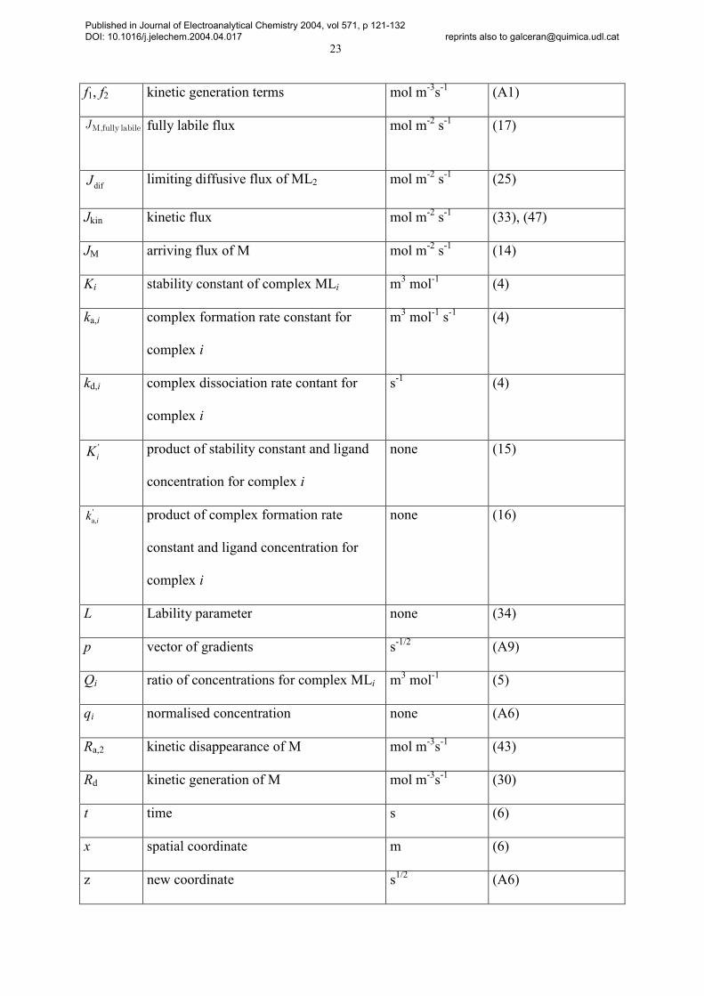
f1, f2 kinetic generation terms mol m-3s-1 (A1)

M,fully labileJ

fully labile flux mol m-2 s-1 (17)

difJ limiting diffusive flux of ML2 mol m-2 s-1 (25)

Jkin kinetic flux mol m-2 s-1 (33), (47)

JM arriving flux of M mol m-2 s-1 (14)

Ki stability constant of complex MLi m3 mol

-1 (4)

ka,i complex formation rate constant for

complex i

m3 mol

-1 s-1 (4)

kd,i complex dissociation rate contant for

complex i

s-1 (4)

'

iK product of stability constant and ligand

concentration for complex i

none (15)

'

a,ik product of complex formation rate

constant and ligand concentration for

complex i

none (16)

L Lability parameter none (34)

p vector of gradients s-1/2 (A9)

Qi ratio of concentrations for complex MLi m3 mol

-1 (5)

qi normalised concentration none (A6)

Ra,2 kinetic disappearance of M mol m-3s-1

(43)

Rd kinetic generation of M mol m-3s-1

(30)

t time s (6)

x spatial coordinate m (6)

z new coordinate s1/2

(A6)


24

δ 2MLδ≡

diffusion layer thickness

m (25)

ε normalised diffusion coefficient none (A6)

Λ lability parameter m-1

(34), (48)

µ reaction layer thickness

m (31)

SUPERSCRIPTS AND SUBSCRIPTS

* bulk solution

0 electrode (or bioactive) surface

φ within the reaction layer


25

Appendix

The rigorous numerical solution of the system stated by Eqs. (6)-(12) is done by solving the

problem

( )

2

M MM 12

2

L LL 1 22

2

ML MLL 1 22

1 d,1 ML a,1 M L

d,2 *

2 T,L L ML a,2 ML L2

c cD f

t x

c cD f f

t x

c cD f f

t x

f k c k c c

kf c c c k c c

∂ ∂= + ∂ ∂ ∂ ∂ = + + ∂ ∂

∂ ∂ = − + ∂ ∂

= −

= − − −

(A1)

with initial conditions and boundary conditions at ∞→x given by

*( ,0) ( , ) M,L,MLi i ic x c t c i= ∞ = = (A2)

( ,0) ( , ) 0 1, 2j jf x f t j= ∞ = = (A3)

and boundary conditions at 0=x

M (0, ) 0c t = (A4)

L ML

0 0

( , ) ( , )0

x x

c x t c x t

x x= =

∂ ∂ = = ∂ ∂ (A5)

Using the change of variables

L

*

MM

, ,ii

i

c Dxq z

c DDε= = = (A6)

the problem becomes


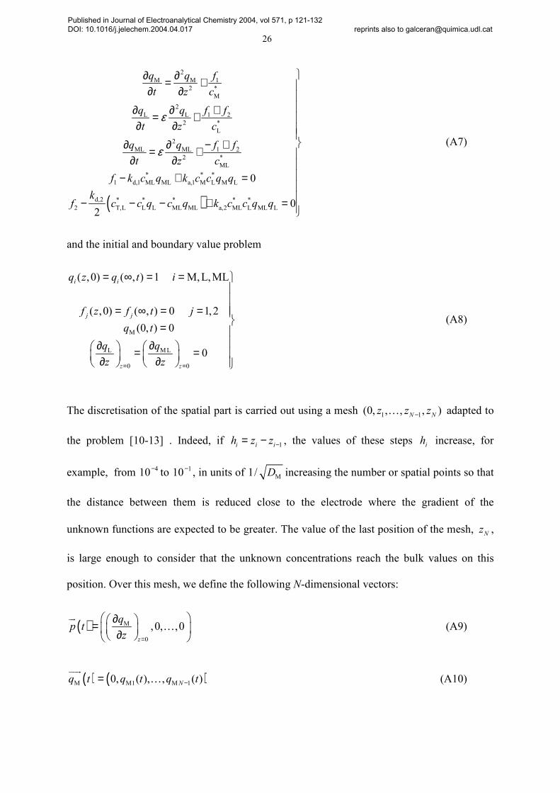
26

( )

2

M M 1

2 *

M

2

L L 1 2

2 *

L

2

ML ML 1 2

2 *

ML

* * *

1 d,1 ML ML a,1 M L M L

d,2 * * * * *

2 T,L L L ML ML a,2 ML L ML L

0

02

q q f

t z c

q q f f

t z c

q q f f

t z c

f k c q k c c q q

kf c c q c q k c c q q

ε

ε

∂ ∂= + ∂ ∂ ∂ ∂ += +

∂ ∂ ∂ ∂ − += + ∂ ∂ − + =− − − + =

(A7)

and the initial and boundary value problem

M

L ML

0 0

( ,0) ( , ) 1 M,L,ML

( ,0) ( , ) 0 1,2

(0, ) 0

0

i i

j j

z z

q z q t i

f z f t j

q t

q q

z z= =

= ∞ = = = ∞ = = = ∂ ∂ = = ∂ ∂

(A8)

The discretisation of the spatial part is carried out using a mesh 1 1(0, , , , )N Nz z z−… adapted to

the problem [10-13] . Indeed, if 1i i ih z z −= − , the values of these steps ih increase, for

example, from 410− to 110− , in units of M1/ D increasing the number or spatial points so that

the distance between them is reduced close to the electrode where the gradient of the

unknown functions are expected to be greater. The value of the last position of the mesh, Nz ,

is large enough to consider that the unknown concentrations reach the bulk values on this

position. Over this mesh, we define the following N-dimensional vectors:

( ) M

0

,0, ,0z

qp t

z =

∂ = ∂

��… (A9)

( ) ( )M M1 M 10, ( ), , ( )Nq t q t q t−=��

… (A10)


27

( ) ( )L L0 L1 L 1( ), ( ), , ( )Nq t q t q t q t−=��

… (A11)

( ) ( )ML ML0 ML1 ML 1( ), ( ), , ( )Nq t q t q t q t−=��

… (A12)

( ) ( )1 10 11 1 1( ), ( ), , ( )Nf t f t f t f t−=��

… (A13)

( ) ( )2 20 21 2 1( ), ( ), , ( )Nf t f t f t f t−=��

… (A14)

( )0, ,0, 1/ Nhβ = −��

… (A15)

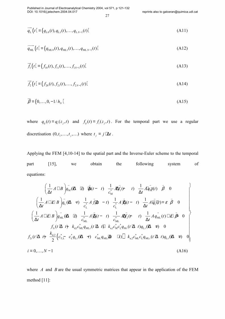
where ( ) ( , )ij i jq t q z t= and ( ) ( , )ij i jf t f z t= . For the temporal part we use a regular

discretisation ),,,,0( 1 …… jtt where tjt j ∆⋅= .

Applying the FEM [4,10-14] to the spatial part and the Inverse-Euler scheme to the temporal

part [15], we obtain the following system of

equations:

M 1 M*

M

L 1 2 L* *

L L

ML 1 2 ML* *

ML ML

1 1 1( ) ( ) ( ) ( ) 0

1 1 1 1( ) ( ) ( ) ( ) 0

1 1 1 1( ) ( ) ( ) ( )

A B q t t p t t A f t t Aq tt c t

A B q t t A f t t A f t t Aq tt c c t

A B q t t A f t t A f t t Aq tt c c t

β

ε ε β

ε

→ → → → →

→ → → → →

→ → → →

+ + ∆ + + ∆ − + ∆ − + = ∆ ∆

+ ⋅ + ∆ − + ∆ − + ∆ − + ⋅ = ∆ ∆

+ ⋅ + ∆ + + ∆ − + ∆ − ∆ ∆

( )

* * *

1 d,1 ML ML a,1 M L M L

d,2 * * * * *

2 T,L L L ML ML a,2 ML L ML L

0

( ) ( ) ( ) ( ) 0

( ) ( ) ( ) ( ) ( ) 02

i i i i

i i i i i

f t t k c q t t k c c q t t q t t

kf t t c c q t t c q t t k c c q t t q t t

ε β→

+ ⋅ = + ∆ − + ∆ + + ∆ + ∆ =+ ∆ − − + ∆ − + ∆ + + ∆ + ∆ =

1,,0 −= Ni … (A16)

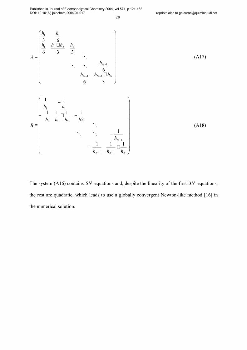
where A and B are the usual symmetric matrices that appear in the application of the FEM

method [11]:


28

+

+

=

−−

−

36

6

336

63

11

1

2211

11

NNN

N

hhh

h

hhhh

hh

A

⋱⋱

⋱ (A17)

+−

−

−+−

−

=

−−

−

NNN

N

hhh

h

hhhh

hh

B

111

1

2

1111

11

11

1

211

11

⋱⋱

⋱ (A18)

The system (A16) contains N5 equations and, despite the linearity of the first N3 equations,

the rest are quadratic, which leads to use a globally convergent Newton-like method [16] in

the numerical solution.


29

Acknowledgements

The authors gratefully acknowledge support of this research by the European Commission

under contract EVK1-CT-2001-00086 (BIOSPEC; RTD Programme "Preserving the

Ecosystem" (Key Action Sustainable Management and Quality of Water)), and by the Spanish

Ministry of Education and Science (DGICYT: Projects BQU2003-9698 and BQU2003-

07587) and the "Comissionat d'Universitats i Recerca de la Generalitat de Catalunya”.


30

Figure captions

1.- Normalised concentration profiles, *

i ic c , of M (◊), ML (∆), ML2 (×) and L (� ) referred to

the left ordinate axis and 1 1Q K (*) and 2 2Q K (o), referred to the right ordinate axis as a

function of the distance to the electrode surface measured as Mx D t . Parameters: a,1k =1

mol-1 m3 s-1, d,1k =0.01 s

-1, (Fig. 1a); ka,1 =10

4 mol

-1 m3 s-1, kd,1 =10

2 s-1 (Fig. 1b); ka,1 =10

7 mol

-

1 m3 s-1, kd,1 =10

5 s-1 (Fig. 1c) and ka,1 =10

8 mol

-1 m3 s-1, kd,1 =10

6 s-1 (Fig. 1d). The vertical

dashed line denotes the thickness of the reaction layer (µ ) given by (31) or that of the

diffusion layer thickness ( M MD tδ π= ). The dashed line in Fig. 1c corresponds to the

concentration profile of either M or ML for the hypothetical case of absence of ML2 with

parameters (kinetic constants, bulk M and ML concentrations, diffusion coefficients) as in the

continuous lines of Fig. 1c , but different total metal and ligand concentrations (see text for

details). Other parameters are: *T,Mc = 0.1 mol m-3, *T,Lc = 1 mol m-3, ka,2 = 108 mol-1 m3 s-1, kd,2

= 2 x 106 s-1, DM = 1 x 10-9 m2 s-1, DML = DL = 1 x 10-10 m2 s-1, t = 0.05 s.

2.- Metal flux at the electrode surface, MJ (continuous line), the kinetic flux, *

kinJ (short

dashed line) and kinJ φ (long dashed line), referred to the right ordinate axis and 0 *

ML MLc c and

2 2

0 *

ML MLc c , both referred to the left ordinate axis as functions of the association kinetic

constant log (ka1/ mol-1 m3 s-1). kinJ φ is calculated via (32) using the values of 0

Lc and 2

0

MLc

obtained from the numerical solution as approximate values for Lcφ and

2MLcφ . *

kinJ is obtained

using *

Lc and 2

*


2MLcφ appearing in (32). In each point, kd,1 takes the


31

value required to maintain a fixed 1K equal to 102 mol

-1 m3. The horizontal bullets on the

right side indicate the fully labile case given by Eq. (17). The rest of parameters as in Fig 1.


kinJ (short


ML MLc c and

2 2

0 *


constant log (ka1/ mol-1 m3 s-1). *

kinJ and kinJ φ are obtained as described in Fig. 2. Parameters:

*

T,Mc = 0.1 mol m-3, *T,Lc = 0.3 mol m-3. The rest of parameters as in Fig 2.


kinJ (short


ML MLc c and

2 2

0 *


constant log (ka1/ mol-1 m3 s-1). *

kinJ and kinJ φ are obtained as described in Fig. 2. Parameters:

*

T,Mc = 0.1 mol m-3, *T,Lc = 0.3 mol m-3, ka,2 = 108 mol-1 m3 s-1, kd,2 = 107 s-1 and in each point,

kd1 takes the value required to maintain a fixed 1K equal to 104 mol

-1 m

3. The rest of

parameters as in Fig. 2.

5.- Normalised concentration profiles, *

i ic c , of M (◊), ML (∆), ML2 (×) and L (� ) referred to

the left ordinate axis and 1 1Q K (*) and 2 2Q K (o), referred to the right ordinate axis as a

function of the distance to the electrode surface measured as Mx D t . Parameters: *T,Mc = 0.1

mol m-3, *T,Lc = 0.3 mol m-3, ka,1=108 mol-1 m3 s-1, kd,1 = 107 s-1 and ka,2 = 103 mol-1 m3 s-1, kd,2 =

1 s-1, (Fig. 5a); ka,2 = 10

4 mol

-1 m3 s-1, kd,2 = 10

1 s-1 (Fig. 5b); ka,2 = 10

5 mol

-1 m3 s-1, kd,2 = 10

2


32

s-1 (Fig. 5c). The vertical dashed line denotes the thickness of the reaction layer, µ , in

dimensionless units, given by (45). Other parameters as in Fig. 1.


kinJ (long

dashed line) and kinJ φ (short dashed line), referred to the right ordinate axis and 0 *

ML MLc c and

2 2

0 *


constant log ( 2ak / mol-1 m3 s-1). kinJ φ is calculated via (47) using the values of 0

Lc and 2

0

MLc

obtained from the numerical solution as approximate values for Lcφ and

2MLcφ . *

kinJ is obtained

using *

Lc and 2

*


2MLcφ appearing in (47). In each point, kd,2 takes the

value required to maintain a fixed 2K equal to 103 mol

-1 m3. The horizontal bullets on the

right side indicate the fully labile case given by eqn. (17). The rest of parameters as in Fig. 5.


kinJ (short


ML MLc c and

2 2

0 *


constant log (ka,2/ mol-1 m3 s-1). *

kinJ and kinJ φ are obtained as described in caption of Fig. 6. In

each point, kd,2 takes the value required to maintain a fixed 2K equal to 102 mol

-1 m3. The

rest of parameters as in Fig. 6.


33

Reference List

[1] J.Buffle, G.Horvai, (Eds.), In Situ Monitoring of Aquatic Systems. Chemical Analysis

and Speciation. Vol. 6. IUPAC Series on Analytical and Physical Chemistry of

Environmental Systems. J. Buffle, H. P. van Leeuwen (Series Eds.), John Wiley &

Sons, Chichester, 2000.

[2] H.P.van Leeuwen, W.Köster, (Eds.), Physicochemical Kinetics and Transport at

Biointerfaces. Vol. 9. IUPAC Series on Analytical and Physical Chemistry of

Environmental Systems. J. Buffle, H. P. van Leeuwen (Series Eds.), John Wiley &

Sons, Chichester, 2004.

[3] H.P.van Leeuwen, Electroanal. 13 (2001) 826.

[4] A.R.Mitchell, D.F.Griffiths, The Finite Element Method in Partial Differential

Equations, Wiley, New York, 1987.

[5] F.M.M.Morel, J.G.Hering, Principles and Applications of Aquatic Chemistry, John

Wiley, New York, 1993, Chapter 6, p. 319.

[6] K.J.Powell, SCDatabase, Academic Software, United Kingdom, 2000.

[7] J.Heyrovský, J.Kuta, Principles of Polarography, Academic Press, New York, 1966.

[8] J.Koutecký, J.Koryta, Electrochim. Acta 3 (1961) 318.

[9] J.Koryta, J.Dvorak, L.Kavan, Principles of Electrochemistry, Second ed. John Wiley,

Chichester, 1993.

[10] H.P.van Leeuwen, J.Puy, J.Galceran, J.Cecília, J. Electroanal. Chem. 526 (2002) 10.

[11] J.Cecília, J.Galceran, J.Salvador, J.Puy, F.Mas, Int. J. Quantum Chem. 51 (1994)

357.

[12] J.Puy, J.Galceran, J.Salvador, J.Cecília, M.S.Diaz-Cruz, M.Esteban, F.Mas, J.

Electroanal. Chem. 374 (1994) 223.

[13] J.Puy, M.Torrent, J.Monné, J.Cecília, J.Galceran, J.Salvador, J.L.Garcés, F.Mas,

F.Berbel, J. Electroanal. Chem. 457 (1998) 229.

[14] T.J.R.Hughes, The Finite Element Method, Prentice Hall, Englewood Cliffs,N.J.,

1987.

[15] W.F.Ames, Numerical Methods for Partial Differential Equations, Academic Press,

New York, 1992.

[16] W.H.Press, B.P.Flannery, S.A.Teukolsky, W.T.Vetterling, Numerical Recipes,

Cambridge University Press, Cambridge, 1986.


Voltammetric lability of multiligand complexes: the case of ML2

Documents