Welcome message from author
This document is posted to help you gain knowledge. Please leave a comment to let me know what you think about it! Share it to your friends and learn new things together.
Transcript


iii
Dedicated to my mother.

iv

AFFIDAVIT
Date 08.07.2020
I declare on oath that I wrote this thesis independently, did not use other than the specified sources and aids, and did not otherwise use any unauthorized aids. I declare that I have read, understood, and complied with the guidelines of the senate of the Montanuniversität Leoben for "Good Scientific Practice". Furthermore, I declare that the electronic and printed version of the submitted thesis are identical, both, formally and with regard to content.
Signature Author Pavel, Iastrebov

vi
vii
Abstract
Analyzing return cuttings during drilling is one of the opportunities, besides
core analysis, to observe and characterize the drilled rock. It gives real time
information needed for bit depth correction and lithology correlation, such as
rock type, color, texture (grain size, shape and sorting), cement amount,
fossils presence, porosity and permeability. Correct measurements of those
parameters (shape and size distribution in particular) improves the drilling
performance and anticipates possible problems and complications. Cuttings
and cavings presence in annular space increase the Equivalent Circulating
Density (ECD), which leads to higher pressure losses; they are also one of the
causes of Rate of Penetration (ROP) reduction because of chip hold down
effect. Their shape is the inference for probable causes of borehole instability
and quality of the mud cake.
Several techniques have been used in last decades for obtaining the return
cuttings parameters, such as their relative amount, particle size distribution
(PSD), size and shape. They comprise state of the art technology based on
computer vision techniques with machine learning algorithms as a software.
A number of such techniques is already available on the market, and have
their limitations and advantages. Basing on this principle, OMV is planning
to build in house intelligent and cost-effective system which is capable of
determining the cuttings parameters in real time. The built system should be
feasible from the point of proactive problem prevention, reduction of Non-
productive Time (NPT) by well complications mitigation and simplification
of tedious mud-logger labor.
After carefully reviewing and studying the shortcomings of the recent
techniques regarding cavings analysis, a conceptual design of automated
cavings analysis technology is proposed in this thesis. The system is split into
hardware and software parts. The first part includes circulation system for
washing the cavings, as well as the camera and lightning facility. The camera
is connected to the laptop with running software in the background, which is
based on the Convolutional Neural Network (CNN). This algorithm analyzes
the captured frames and delivers cavings’ shape, size and lithology as an
output. Furthermore, feasibility study is conducted, in which rough costs of
the proposed system are estimated.

viii

ix
Zusammenfassung
Die Analyse von Bohrschlamm während der Bohrung, abgesehen von der
Kernanalyse, ist eine der Möglichkeiten, die gebohrte Gesteine zu beobachten
und zu charakterisieren. Es liefert Echtzeitinformation, wie Gesteinstyp,
Farbe, Textur (Korngröße, Form und Sortierung), Zementmenge,
Vorhandensein von Fossilien, Porosität und Permeabilität, die für die
Meißeltiefeкоkorrektur und die Lithologiekorrelation benötigt wird. Die
korrekte Parametermessung (bzw. Form und Größenverteilung) verbessert
die Bohrleistung und vorbeugt mögliche Probleme und Komplikationen. Das
Vorhandensein von Bohrschlamm und Auskesslungen im Ringraum erhöht
die äquivalente Zirkulationsdichte, was zu höheren Druckverlusten führt. Sie
sind auch eine der Ursachen für die Reduzierung der Bohrgeschwindigkeit
wegen des Chip-Hold-Down-Effekts. Ihre Form ist die Voraussetzung für
wahrscheinliche Ursachen der Bohrlochinstabilität und der Qualität der
Filterkruste.
In den letzten Jahrzehnten verschiedene Techniken wurden verwendet, um
die Bohrschlammparameter zu erhalten, wie z. B. ihre relative Menge,
Partikelgrößenverteilung, Größe und Form. Sie umfassen modernste
Technologien, die auf Computer-Vision-Technologie mit Algorithmen für
maschinelles Lernen als Software basieren. Eine reihe Anzahl solcher
Techniken ist bereits auf dem Markt erhältlich und hat ihre Begrenzungen
und Vorteile. Basierend auf diesem Prinzip, plant OMV den Bau eines
eigenen intelligenten und kostengünstigen Systems, mit dem die
Bohrschlammparameter in Echtzeit ermittelt werden können. Das gebaute
System sollte unter dem Gesichtspunkt der proaktiven Problemverhütung,
der Reduzierung der unproduktiven Zeit durch Verhinderug von
Bohrlochkomplikationen und der Vereinfachung mühevoller Arbeit des
Feldgeologs machbar sein.
Nach sorgfältiger Prüfung und Untersuchung der Mängel der jüngsten
Technologien in Bezug auf die Auskesslunganalyse, wird in dieser Arbeit ein
Konzeptentwurf für die Technologie der automatisierten
Auskesslunganalyse vorgeschlagen. Das System ist in Hardware- und
Softwareteile unterteilt. Der erste Teil umfasst ein Zirkulationssystem zum
Waschen der Auskesslungen sowie die Kamera- und Blitzeinrichtung. Die
Kamera wird an den Laptop mit laufender Software im Hintergrund
angeschlossen. Die Software ist auf dem Convolutional Neural Network
(CNN) basiert. Dieser Algorithmus analysiert die erfassten Bilder und liefert
die Form, Größe und Lithologie der Auskesslungen als Ausgabe. Darüber
hinaus wird eine Machbarkeitsstudie durchgeführt, in der ein Etwapreis des
vorgeschlagenen Systems geschätzt wird.

x

xi
Acknowledgements
I would firstly like to thank my university thesis advisors Dipl.-Ing. B.Sc.
Asad Elmgerbi and Ass. Prof., Candidate of Technical Sciences, Alexey
Arhipov for their invaluable help in my research and comprehensive
guidance. In addition, Univ.-Prof. Mikhail Gelfgat faced the most of the
difficulties in organizing our study and helped us to accomplish the double-
degree program, what I am grateful for either.
I would like to thank OMV Exploration & Production GmbH including:
Senior Vice President Exploration, Development & Production OMV
Upstream Christopher Veit for such great opportunity of getting a
scholarship;
Drilling Engineer at OMV Exploration & Production, M.Sc. Richard Kucs for
constant supervision during thesis writing and assistance in developing a
concept;
Head of Exploration Ventures at OMV Exploration & Production, M.Sc.
Ph.D., my mentor Peter Krois for directing me in a right way and exciting the
curiosity of geology;
Sr Reservoir Engineer at OMV Exploration & Production, M.Eng. MBA
Daniel Kunaver for showing the robustness of coding in Python;
Expert Talent Pipeline at OMV AG Bernhard Ebinger and Senior Expert
Learning & Development at OMV AG Rafael Tomososchi for the help in my
internship organization.
I would like to thank my friends who I studied with for their joy and
fellowship: Timur Berdiev, Polina Gamayunova, Aleksandr Geraskin,
Rostislav Gupalov, Shamkhal Mammadov, Aleksey Olkhovikov and Kseniia
Frolova.
Special thanks to Anna, Daniil and Vladislav for helping me to land on my
own moon.
Finally, I am expressing the appreciation to my parents for granting me the
gift of life. You are the most valuable people to me.

xii

xiii
Contents
Chapter 1 Introduction .............................................................................................................. 1
1.1 Overview ........................................................................................................................... 1
1.2 Motivation ......................................................................................................................... 2
1.3 Objectives .......................................................................................................................... 4
1.4 Thesis Structure ................................................................................................................ 4
Chapter 2 Borehole Instability Signs During Drilling ........................................................... 7
2.1 Borehole Instability Mechanisms ................................................................................... 7
2.2 Cavings Morphology ..................................................................................................... 10
2.3 Cavings Comparative Matrix ....................................................................................... 14
Chapter 3 Cuttings Analysis Techniques .............................................................................. 17
3.1 Standard Method ........................................................................................................... 17
3.1.1 Cuttings Collection ................................................................................................. 17
3.1.2 Cleaning and Packing ............................................................................................ 19
3.1.3 Analysis .................................................................................................................... 21
3.1.3.1 Sieve Analysis .................................................................................................. 21
3.1.3.2 Laser Diffraction .............................................................................................. 22
3.1.3.3 Optical Microscopy and Image Analysis ..................................................... 23
3.1.3.4 Focused Beam Reflectance Measurement .................................................... 24
3.1.3.5 Ultrasonic Extinction ...................................................................................... 24
3.1.3.6 X-ray Fluorescence .......................................................................................... 25
3.1.3.7 X-ray Diffraction .............................................................................................. 26
3.1.4 Shortcomings (Standard Method) ........................................................................ 27
3.2 Automated Measurement Tools .................................................................................. 30
3.2.1 Cuttings Flow Meter .............................................................................................. 30
3.2.2 Computer-Based Techniques ................................................................................ 31
3.2.2.1 2D Machine Vision .......................................................................................... 31
3.2.2.2 Stereo Vision .................................................................................................... 33
3.2.2.3 Structured Light .............................................................................................. 34
3.2.2.4 Time-of-Flight .................................................................................................. 35
3.2.3 Shortcomings (Automated Method) .................................................................... 37
3.3 Field Application of Automated Methods ................................................................. 38
3.3.1 Schlumberger CLEAR Service .............................................................................. 38
3.3.2 Device for Measuring PSD and Cuttings Analysis ............................................ 39
3.3.3 Intelligent System for Cuttings Concentration Analysis .................................. 40
3.3.4 Classifying Cuttings Volume via Video Streaming ........................................... 42
3.3.5 Cuttings Shape Acquisition Using 3D Point Cloud Data ................................. 43
3.3.7 Rock Classification with a Deep Convolutional Network ................................ 47
3.3.8 Comparison Summary ........................................................................................... 49
Chapter 4 Convolutional Artificial Neural Network .......................................................... 53

xiv
4.1 Simplest Artificial Neural Network ............................................................................ 53
4.2 Training, Validation, and Testing ................................................................................ 55
4.2.1 Training .................................................................................................................... 55
4.2.2 Validation ................................................................................................................. 57
4.2.3 Testing and Splitting the Dataset ......................................................................... 57
4.3 Convolutional Artificial Neural Network .................................................................. 58
4.3.1 Input Layer .............................................................................................................. 58
4.3.2 Conv Layer .............................................................................................................. 59
4.3.3 ReLU Layer .............................................................................................................. 61
4.3.4 Pool Layer ................................................................................................................ 62
4.3.5 FC and Softmax Layers .......................................................................................... 63
Chapter 5 Conceptual Design of the Proposed Technology .............................................. 65
5.1 Overview ......................................................................................................................... 65
5.2 Hardware and equipment ............................................................................................ 66
5.2.1 Shale Shaker Modification ..................................................................................... 67
5.2.1.1 Tray .................................................................................................................... 69
5.2.1.2 Collector Pipe and Hoses ............................................................................... 69
5.2.1.3 Filter................................................................................................................... 69
5.2.1.4 Pump ................................................................................................................. 69
5.2.1.5 Sprinkler Head ................................................................................................. 70
5.2.2 Camera Design And Placement ............................................................................ 70
5.2.3 Light Source ............................................................................................................. 77
5.2.4 Cover ........................................................................................................................ 79
5.3 Software ........................................................................................................................... 79
5.3.1 Network Building ................................................................................................... 79
5.3.2 Algorithm Workflow .............................................................................................. 80
5.3.3 Decision Support Matrix ........................................................................................ 82
5.4 Cost Estimation for Proposed System ......................................................................... 83
5.5 Limitations ...................................................................................................................... 86
Chapter 6 Conclusion and Recommendations ..................................................................... 89
6.1 Conclusion....................................................................................................................... 89
6.2 Recommendations and Future Work .......................................................................... 90
Appendix A Cuttings description parameters ..................................................................... 91
A.1 Shape ............................................................................................................................... 91
A.2 Roundness and Sphericity ........................................................................................... 92
A.3 Colour ............................................................................................................................. 93
Overview
1
Chapter 1 Introduction
1.1 Overview
Borehole stability issues are one of the main problems, which occur frequently during
the well construction process. This happens due to mechanical failure of the rock, caused
by stresses reorientation, as well as improper mud weight selection. Most of the time
these complications are followed by rock cracking and moving towards the centre of the
borehole or falling down the bottom hole. This might lead to a series of costly issues such
as pipe sticking, low ROP, or poor cement job. In this context, drilling cuttings and
cavings monitoring are crucial for proactive detection and mitigating wellbore
instability, which is one of the main contributors in non-productive time. Cavings' size
and shape basically demonstrate the circumstances, under which they were formed. It
means that cuttings are the first piece of information, which gives the crew essential
knowledge about what is actually happening during drilling. The main aim, which is to
be achieved, is the reduction of NPT, caused by possible stuck pipe events, and
consequent cost reduction by saving on fishing services and rig rent time.
The most widely spread method of cuttings analysis is the conventional technique,
which is completely manual, utilizing human labour. As a rule, the cuttings are collected
every hour, packed, and sent to the wellsite laboratory for the measurement and
analysis. The resulting report contains the complete description of the collected sample,
including rock type, size, and texture.
As long as the conventional analysis is time-consuming, a series of automated
approaches have been invented. One of them is Cuttings Flow Meter (CFM), which
determines the mass of incoming cuttings. The main benefit of this system is that it is
fully automated and has very high accuracy due to its simplicity. However, it does not
analyze any other parameters. Another well-known technique is image analysis. The
overall concept resides in placing the camera at the shale shakers and utilizing software,
which would analyze the video frames and deliver the desired properties. Related
installations were designed to determine cuttings volume, Particle Size Distribution
(PSD), and shape profile.
Unfortunately, the considered methods do not give evidence of possible complications.
For that reason, there is a demand for another technique proposal, which could notify
about possible borehole instability events, having cuttings information as an input.
Machine learning techniques, which are already available on the market, show their
strength in comparison with other algorithms. Their benefit is a diversity of parameters,
which could be extracted from the analysis. It is possible because such methods can not
only conduct calculations but also classify the objects by referring them to a set of pre-
determined classes. In this case, each of the objects is inspected individually. By
assigning a number of classes within one category to the set of objects in advance (e.g.
different kinds of shapes), the machine learns to extract certain features from it. Basing
on the results of the learning phase, the machine can independently label the object
Introduction
2
during the testing phase. In addition, the algorithm is able to determine the location of
the object in a frame, giving the evidence of its accuracy.
1.2 Motivation
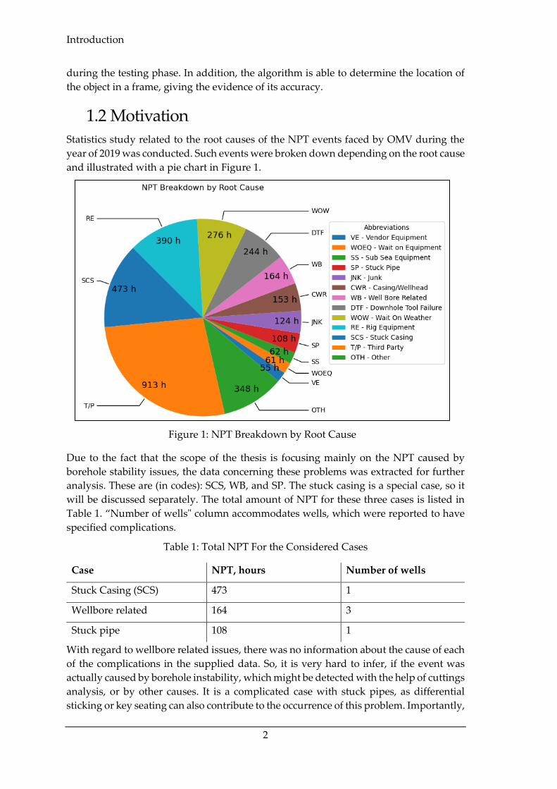
Statistics study related to the root causes of the NPT events faced by OMV during the
year of 2019 was conducted. Such events were broken down depending on the root cause
and illustrated with a pie chart in Figure 1.
Figure 1: NPT Breakdown by Root Cause
Due to the fact that the scope of the thesis is focusing mainly on the NPT caused by
borehole stability issues, the data concerning these problems was extracted for further
analysis. These are (in codes): SCS, WB, and SP. The stuck casing is a special case, so it
will be discussed separately. The total amount of NPT for these three cases is listed in
Table 1. “Number of wells" column accommodates wells, which were reported to have
specified complications.
Table 1: Total NPT For the Considered Cases
Case NPT, hours Number of wells
Stuck Casing (SCS) 473 1
Wellbore related 164 3
Stuck pipe 108 1
With regard to wellbore related issues, there was no information about the cause of each
of the complications in the supplied data. So, it is very hard to infer, if the event was
actually caused by borehole instability, which might be detected with the help of cuttings
analysis, or by other causes. It is a complicated case with stuck pipes, as differential
sticking or key seating can also contribute to the occurrence of this problem. Importantly,

Motivation
3
stuck pipe and casing issues happened in the same well deep multi-lateral well with two
completions. In one of the laterals, there were 108 hours of stuck pipe complications in
total, followed by 330 hours of stuck casing events. In another lateral, there were 143
hours of total NPT dedicated to the stuck casing. As long as the well is specified as a
deep well, there definitely should be narrow mud windows. That makes the mud
program more sophisticated and more sensitive to pressure changes, which affects the
likelihood of complications occurring. In addition, there were stuck pipe events only
during drilling operations of the first lateral, while the second was safe.
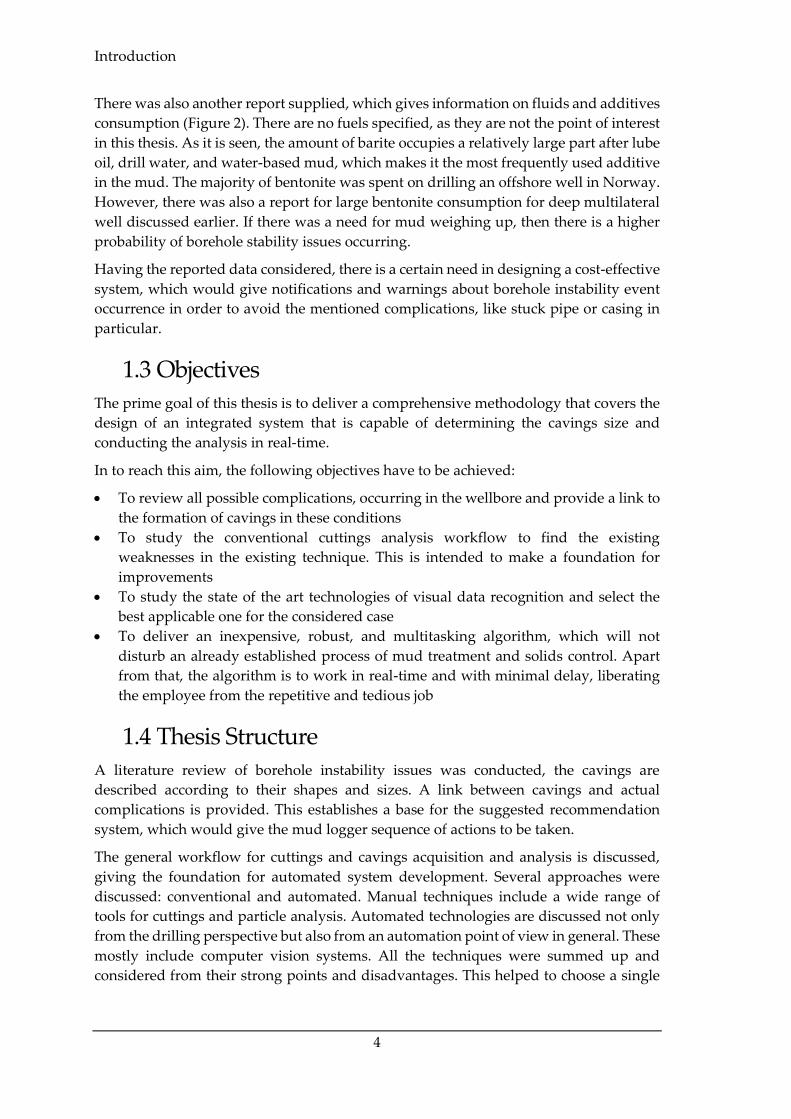
Figure 2: Reported Consumption of Fluids and Additives In 2019 By OMV
Introduction
4
There was also another report supplied, which gives information on fluids and additives
consumption (Figure 2). There are no fuels specified, as they are not the point of interest
in this thesis. As it is seen, the amount of barite occupies a relatively large part after lube
oil, drill water, and water-based mud, which makes it the most frequently used additive
in the mud. The majority of bentonite was spent on drilling an offshore well in Norway.
However, there was also a report for large bentonite consumption for deep multilateral
well discussed earlier. If there was a need for mud weighing up, then there is a higher
probability of borehole stability issues occurring.
Having the reported data considered, there is a certain need in designing a cost-effective
system, which would give notifications and warnings about borehole instability event
occurrence in order to avoid the mentioned complications, like stuck pipe or casing in
particular.
1.3 Objectives
The prime goal of this thesis is to deliver a comprehensive methodology that covers the
design of an integrated system that is capable of determining the cavings size and
conducting the analysis in real-time.
In to reach this aim, the following objectives have to be achieved:
• To review all possible complications, occurring in the wellbore and provide a link to
the formation of cavings in these conditions
• To study the conventional cuttings analysis workflow to find the existing
weaknesses in the existing technique. This is intended to make a foundation for
improvements
• To study the state of the art technologies of visual data recognition and select the
best applicable one for the considered case
• To deliver an inexpensive, robust, and multitasking algorithm, which will not
disturb an already established process of mud treatment and solids control. Apart
from that, the algorithm is to work in real-time and with minimal delay, liberating
the employee from the repetitive and tedious job
1.4 Thesis Structure
A literature review of borehole instability issues was conducted, the cavings are
described according to their shapes and sizes. A link between cavings and actual
complications is provided. This establishes a base for the suggested recommendation
system, which would give the mud logger sequence of actions to be taken.
The general workflow for cuttings and cavings acquisition and analysis is discussed,
giving the foundation for automated system development. Several approaches were
discussed: conventional and automated. Manual techniques include a wide range of
tools for cuttings and particle analysis. Automated technologies are discussed not only
from the drilling perspective but also from an automation point of view in general. These
mostly include computer vision systems. All the techniques were summed up and
considered from their strong points and disadvantages. This helped to choose a single

Thesis Structure
5
technology to focus on. This chosen technique was two-dimensional computer vision
thanks to inexpensiveness, simplicity, and a variety of possible parameters to determine.
The essence of artificial neural networks was discussed, as well as their features,
architecture, and working principle. Convolutional neural networks are used as a central
part of the proposed software system, which will take video frames as an input, filtering
them out, and taking out features like colour patterns, edges, etc.
The proposed solution based on state-of-the-art technology is described. The description
is split into two parts: describing hardware devices and equipment, which actually
acquire data from shaker screens. In addition, software workflow is also suggested and
discussed, giving the blueprint for the developers to write the code and link the software
with the camera. Apart from that, the cost assessment study is conducted, giving the
estimation of technology costs using a probabilistic approach.

Introduction
6

Borehole Instability Mechanisms
7
Chapter 2 Borehole Instability Signs
During Drilling
Borehole instability is a notable example of how to yield the drilling process into dire
straits. Such complications account for up to 40% of rig downtime and for nearly 25% of
drilling costs (Gallant, et al. 2007). Having such high percentages of time and budget
losses, instability-related NPT seriously jeopardizes the project economics and therefore
is desired to be reduced or avoided.
Borehole instabilities occur due to the creation of a wellbore by collapsing some portion
of the rock in the formation. As a result, the existing stresses are being reoriented, and a
stable formation loses its support. If the stability is not maintained, the stresses might
overcome rock strength and cause the borehole collapse or fracturing, these events are
often followed by the formation of crushed rock in the zones of excessive stress. As long
as the rock loses its integrity, it is broken off the borehole wall easily, either falling down
in the wellbore or being transported to the surface. Depending on the issue, these rocks
(or cavings) might have different shapes, which provide a link between the caving
morphology and the mechanism of its generation.
In this case, cavings, which are the first physical and valid material information, allow
us to relatively quickly analyze the current state of the wellbore condition and react
proactively on possible complications. Cavings are typically produced due to several
causes, such as underbalanced drilling, stress relief, pre-existing planes of weakness, or
as a response to an action of drilling tools (Kumar, et al. 2012).
In this chapter various types of borehole instabilities are discussed, the cavings are
described according to their shapes and sizes and a link between them is provided,
establishing causal relationships for recommending remedial actions to be taken.
2.1 Borehole Instability Mechanisms
Encountered wellbore instability events could be classified depending on the existing
conditions as following:
• Hole closure
• Hole enlargement
• Fracturing
Each of the mechanisms will be described thereunder considering associated
consequences and resulting problems.
Hole closure is a time-dependent process, which is referred to as swelling shale layers
and creeping salt formations. Shales lose their stability because of acquiring water from
the drilling mud, resulting in an increase of the rock volume. At some point, shales
cannot hold more water, so that their strength decreases, and they begin to slough,
falling inside the borehole. Salts, in contrast, creep under other circumstances. This rock
cannot withstand shear stresses (on a reservoir scale) and are similar to a very viscous

Borehole Instability Signs During Drilling
8
liquid. Under the overburden stress, such mobile formations behave in a plastic manner,
establishing deformation under pressure. In both cases, unstable rock might either
decrease the cross-section of the wellbore or fall inside the well. It happens, as the mud
weight is not high enough to withstand the formation squeezing into the wellbore
(Bowes and Procter 1997). The associated problems are:
• Torque and drag increase
• Stuck pipe events
• Troubles running casing
Hole enlargement issues could be separated into two categories: breakouts and
washouts. Breakouts are the result of surrounding the wellbore stresses exceeding the
rock strength. In this case, the wellbore wall is subjected to shear failure, which forms
zones of crushed rock in the direction of the least horizontal stress (in a vertical
wellbore). Breakouts might grow during the good drilling process, but they only deepen
into the formation, as illustrated in Figure 3. Washouts are a possible consequence of
breakouts due to incorrectly selected mud weight. Drilling fluid would leak into pre-
existing or drilling-induced cracks and cause further propagation of shear failure. As a
result, the formation produces extra cavings around the wellbore, increasing cross-
section. Therefore, mud velocity in the annulus decreases and the mud system is unable
to circulate the excessive amount of cavings. The difference between breakout and
washout is schematically drawn in Figure 4.
As a rule, this type of instability usually occurs in unconsolidated formations,
overpressured shales, and naturally fractured rock. This results in:
• Cavings sticking to the BHA
• Cuttings bed
• Mechanical erosion
• An increased volume of required cement and the overall difficulty of cementing
job
• The necessity of changing mud weight

Borehole Instability Mechanisms
9
Figure 3: Televiewer Image Logs of a Well With Wellbore Breakouts (Dark
Paths in South-East and North-West Directions) (Zoback, Barton, et al. 2003)
Figure 4: (a) Breakout, Showing Growth Deeper Inside the Formation. (b)
Washout Grows All Around the Wellbore, Increasing Its Instability (modified
after M. Zoback 2007)

Borehole Instability Signs During Drilling
10
Fracturing occurs when the wellbore hydrostatic pressure exceeds the least principal
stress at a certain depth, developing either in a form of consistent fracture or echelons of
fractures. Being the result of the tensile failure, those fractures are different from those,
which are formed during shear failure. The main feature of fracturing by exceeding the
least principal stress is the absence of cavings in the return flow. This leads to:
• Wellbore ballooning effects
• Lost circulation
In the scope of this thesis, only the first two of the complications will be considered. For
that purpose, it is needed to focus on different cavings types, shapes, and sizes.
2.2 Cavings Morphology
Cavings, unlike cuttings, are the fragments of the rock, which appear on the shale shaker
screens, and are usually two to three times larger, having odd shapes. They are produced
not from the destroyed rock by the bit action, but from the borehole wall. It is important
that cavings have practically no value in lithology understanding, as the borehole
instability might occur at any time during drilling. Thus, cuttings are mainly analyzed
for formation evaluation and hydrocarbon content estimation, whereas cavings are
crucial for shape and size determination. Here is to define, which cavings shapes
generally exist, and what are their size ranges.
Cavings morphology exhibits several types of them, depending on their shape, size and
lithology. Depending on their origin, they can be split into the following types (Skea, et
al. 2018):
• Angular
• Tabular
• Splintery
• Blocky
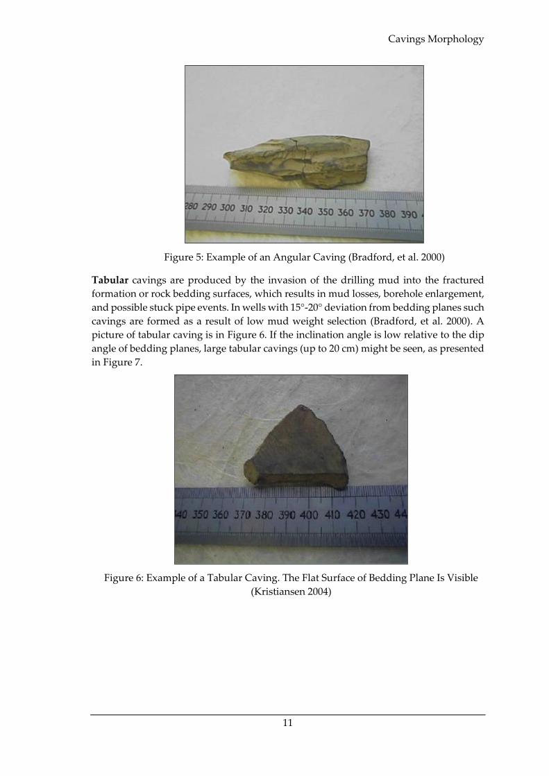
Angular cavings form by using a low-density mud by combination with low
compressive strength and high hoop stress, creating a shear failure in the wellbore. These
cavings could be described as arrowhead or triangular-shaped with a rough surface.
Such caving is shown in Figure 5.
Cavings Morphology
11
Figure 5: Example of an Angular Caving (Bradford, et al. 2000)
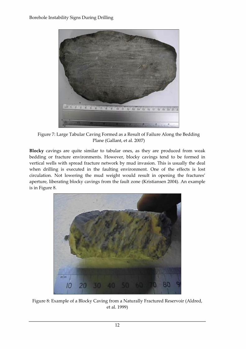
Tabular cavings are produced by the invasion of the drilling mud into the fractured
formation or rock bedding surfaces, which results in mud losses, borehole enlargement,
and possible stuck pipe events. In wells with 15°-20° deviation from bedding planes such
cavings are formed as a result of low mud weight selection (Bradford, et al. 2000). A
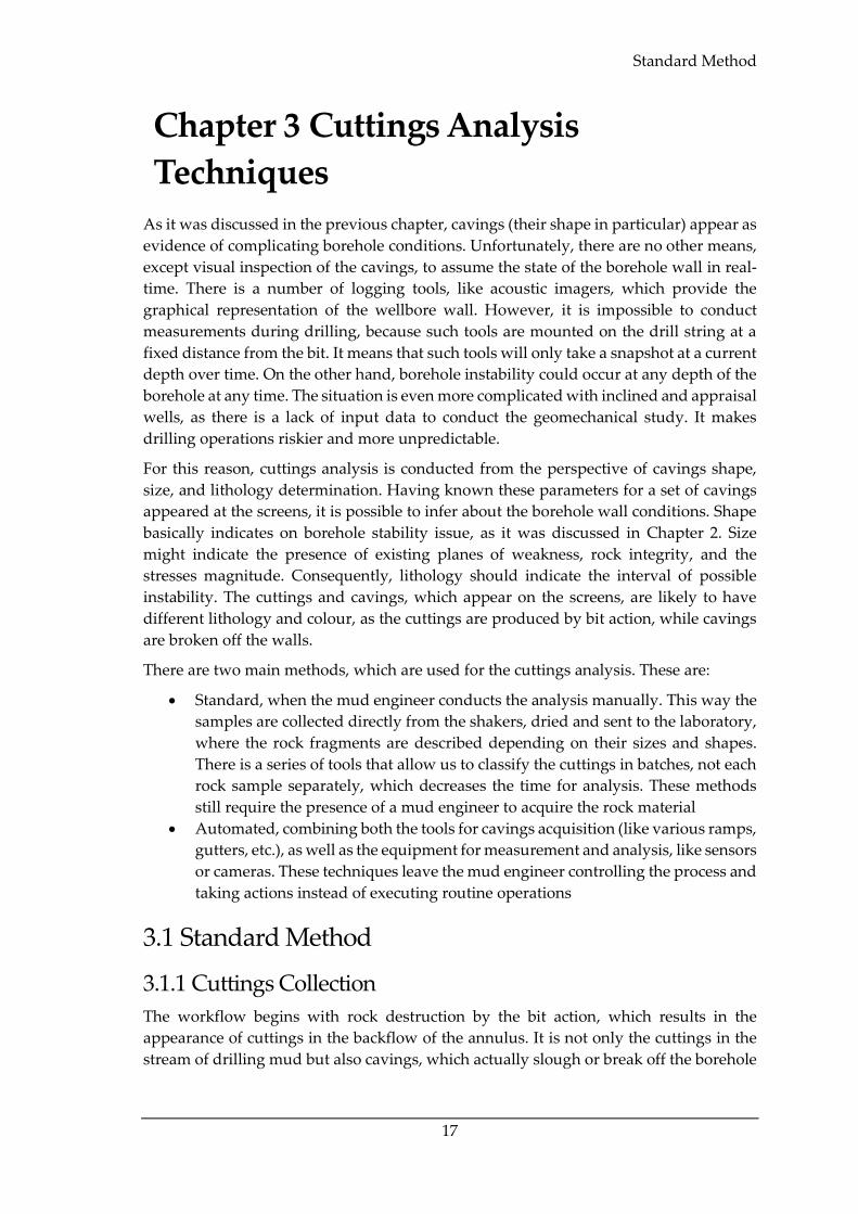
picture of tabular caving is in Figure 6. If the inclination angle is low relative to the dip
angle of bedding planes, large tabular cavings (up to 20 cm) might be seen, as presented
in Figure 7.
Figure 6: Example of a Tabular Caving. The Flat Surface of Bedding Plane Is Visible
(Kristiansen 2004)
Borehole Instability Signs During Drilling
12
Figure 7: Large Tabular Caving Formed as a Result of Failure Along the Bedding
Plane (Gallant, et al. 2007)
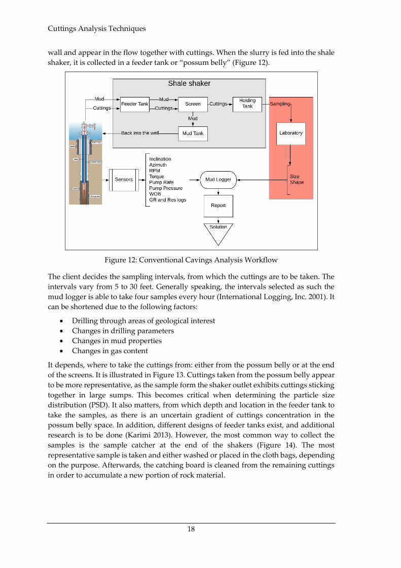
Blocky cavings are quite similar to tabular ones, as they are produced from weak
bedding or fracture environments. However, blocky cavings tend to be formed in
vertical wells with spread fracture network by mud invasion. This is usually the deal
when drilling is executed in the faulting environment. One of the effects is lost
circulation. Not lowering the mud weight would result in opening the fractures’
aperture, liberating blocky cavings from the fault zone (Kristiansen 2004). An example
is in Figure 8.
Figure 8: Example of a Blocky Caving from a Naturally Fractured Reservoir (Aldred,
et al. 1999)

Cavings Morphology
13
Splintery cavings are produced from the overpressured zones, where tensile fractures
tend to form (Figure 9). They usually occur in tectonically active regions, where
significant stresses are present. Here the rock is being compressed or stretched due to
movement of the Earth’s crust (Pašić, Gaurina-Međimurec and Matanović 2007). When
a hole is drilled in an area of high tectonic stresses the rock around the wellbore will
collapse into the wellbore and produce splintery cavings. In high-stress concentration
cases, the pressure required to stabilize the wellbore might be higher than the fracture
gradient. This usually occurs near mountainous regions. In this case, the formation is to
be cased as quickly as possible (Bowes and Procter 1997).
Figure 9: Example of a Splintery Caving (Kumar, et al. 2012)
Borehole instabilities are often followed by cuttings and cavings accumulation in the
well, especially if the well is inclined. In the last case, this leads to a cuttings bed, which
is one of the evidence of borehole enlargement. In order to mitigate this issue, the well
is usually circulated, transporting the rocks to the surface and solids control equipment.
As a consequence, an event called mud overflow occurs. At this point, it is practically
impossible to recognize the individual cavings during their travel along with the screens.
The first reason is the amount of mud and rocks being poured onto the shaker. The
cavings cannot be separated right after the weir, as the mud velocity is very high, and a
too large amount of fluid is dropped. In addition, the amount of cavings is very high,
and the screens are literally overloaded with rocks (Figure 10). Another reason is the
appearance of cuttings stuck together because of the excessive amount of clay particles.
As a result, drilled particles are grouped in large drops of dilatant fluid. Thanks to
constantly vibrating the screens’ surface, the viscosity increases, not allowing the
remaining fluid to seep through the screens (Figure 11). Therefore. it is not possible to
separate the cavings, as in the first case there is a large amount of fluid already, and
impossibility to separate the solid particles in the second case.

Borehole Instability Signs During Drilling
14
Figure 10: Mud Overflow After Addition of the Fibrous Material to Suspend
Cuttings and Clean the Well (Forta Corporation 1997)
Figure 11: Excessive Clay Appearance on the Screens (TR Solids Control 2016)
2.3 Cavings Comparative Matrix
Basing on the cavings classification and the circumstances under which they are formed,
an advisory matrix is suggested (Table 2). This table contains all possible borehole
complications causes, consequences, and treatment operations gathered from the
mentioned literature. It should be considered as part of the workflow in the intelligent
cuttings analysis system in a form of the automated advisory algorithm. It is assumed to
be the helping hand for the mud logger or wellsite geologist, proposing the actions to be
taken. The main disadvantage of this matrix is its ambiguity and uncertainty. In order to
include this methodology into the workflow, it should be more specific and work

Cavings Comparative Matrix
15
similarly to a conditional flowchart, having a specific response to every single condition
(e.g. cavings appearance and description, known stratigraphy or change in drilling
parameters). The evolution of this matrix is presented in Chapter 5, where the actual
flowchart is built, giving the recommendations for the crew, which action to take under
specific circumstances.
Table 2: Cavings Description, Causes, Consequences and Their Treatment (Kristiansen
2004) (Bowes and Procter 1997) (Gallant, et al. 2007) (Kumar, et al. 2012)
Shape Size Causes Consequences Treatment
Angular <8 cm Low mud weight
and insufficient
viscosity in a near-
vertical well. Formed
in low strength
formations
perpendicular to
bedding planes.
Further
enlargement of
breakouts, bad
hole cleaning,
stuck pipe and
improper
cementing
Mud weight
increase. Increase
flowrate to ensure
hole cleaning.
Tabular 2-25 cm Wellbore with 15°-
20° deviation from
bedding planes and
invasion of low mud
weight into the weak
bedding planes. Also
seen in ERD wells
Mud losses, stuck
pipe events, and
high caving rates.
Increase in torque
and drag.
Lowering ROP
with small
adjustments in the
mud weight.
Minimizing surge
and swab. LCM
introduction.
Blocky <9 cm Invasion of the
drilling mud into
pre-existing
fractures. Drilling
through the fault
zones. A high
exposure time of
mud penetration.
Lost circulation,
destabilizing the
well, cuttings bed.
Cavings settle
down with turned
off pumps.
Lowering the mud
weight. Lower the
inclination angle,
especially when
drilling through
faults. Avoiding
the faults, when
possible. Limit the
exposure time.
LCM introduction.
Splintery <8 cm Underbalanced
drilling through
tectonically stressed
and overpressure
areas. Having high
ROP when drilling
through low
permeable rocks.
Hole collapse,
torque and drag
increase, pack-
offs, and bridges.
Increasing the mud
weight, or reducing
the ROP. Casing
the hole as quickly
as possible.
The sizes of individual categories of cavings shapes listed in this table are taken from the
reviewed literature. It was not possible to inspect an actual set of cavings, as this

Borehole Instability Signs During Drilling
16
information was not submitted. Therefore, these values have an approximate nature and
correspond to the typical sizes of return cavings, which appear on the shaker screens. In
addition, in the “Causes” column all the possible causes are mentioned, which actually
makes the introduced matrix so uncertain. It is actually not possible to link all the listed
causes to the cavings shape, as cavings are the result of a certain instability type, which
is actually can be drawn by different actions. As long as the same action performed by a
crew leads to different complications in dependence from the drilling environment, the
causes for the formation of different cavings’ shapes might interfere.
Standard Method
17
Chapter 3 Cuttings Analysis
Techniques
As it was discussed in the previous chapter, cavings (their shape in particular) appear as
evidence of complicating borehole conditions. Unfortunately, there are no other means,
except visual inspection of the cavings, to assume the state of the borehole wall in real-
time. There is a number of logging tools, like acoustic imagers, which provide the
graphical representation of the wellbore wall. However, it is impossible to conduct
measurements during drilling, because such tools are mounted on the drill string at a
fixed distance from the bit. It means that such tools will only take a snapshot at a current
depth over time. On the other hand, borehole instability could occur at any depth of the
borehole at any time. The situation is even more complicated with inclined and appraisal
wells, as there is a lack of input data to conduct the geomechanical study. It makes
drilling operations riskier and more unpredictable.
For this reason, cuttings analysis is conducted from the perspective of cavings shape,
size, and lithology determination. Having known these parameters for a set of cavings
appeared at the screens, it is possible to infer about the borehole wall conditions. Shape
basically indicates on borehole stability issue, as it was discussed in Chapter 2. Size
might indicate the presence of existing planes of weakness, rock integrity, and the
stresses magnitude. Consequently, lithology should indicate the interval of possible
instability. The cuttings and cavings, which appear on the screens, are likely to have
different lithology and colour, as the cuttings are produced by bit action, while cavings
are broken off the walls.
There are two main methods, which are used for the cuttings analysis. These are:
• Standard, when the mud engineer conducts the analysis manually. This way the
samples are collected directly from the shakers, dried and sent to the laboratory,
where the rock fragments are described depending on their sizes and shapes.
There is a series of tools that allow us to classify the cuttings in batches, not each
rock sample separately, which decreases the time for analysis. These methods
still require the presence of a mud engineer to acquire the rock material
• Automated, combining both the tools for cavings acquisition (like various ramps,
gutters, etc.), as well as the equipment for measurement and analysis, like sensors
or cameras. These techniques leave the mud engineer controlling the process and
taking actions instead of executing routine operations
3.1 Standard Method
3.1.1 Cuttings Collection
The workflow begins with rock destruction by the bit action, which results in the
appearance of cuttings in the backflow of the annulus. It is not only the cuttings in the
stream of drilling mud but also cavings, which actually slough or break off the borehole
Cuttings Analysis Techniques
18
wall and appear in the flow together with cuttings. When the slurry is fed into the shale
shaker, it is collected in a feeder tank or “possum belly” (Figure 12).
Figure 12: Conventional Cavings Analysis Workflow
The client decides the sampling intervals, from which the cuttings are to be taken. The
intervals vary from 5 to 30 feet. Generally speaking, the intervals selected as such the
mud logger is able to take four samples every hour (International Logging, Inc. 2001). It
can be shortened due to the following factors:
• Drilling through areas of geological interest
• Changes in drilling parameters
• Changes in mud properties
• Changes in gas content
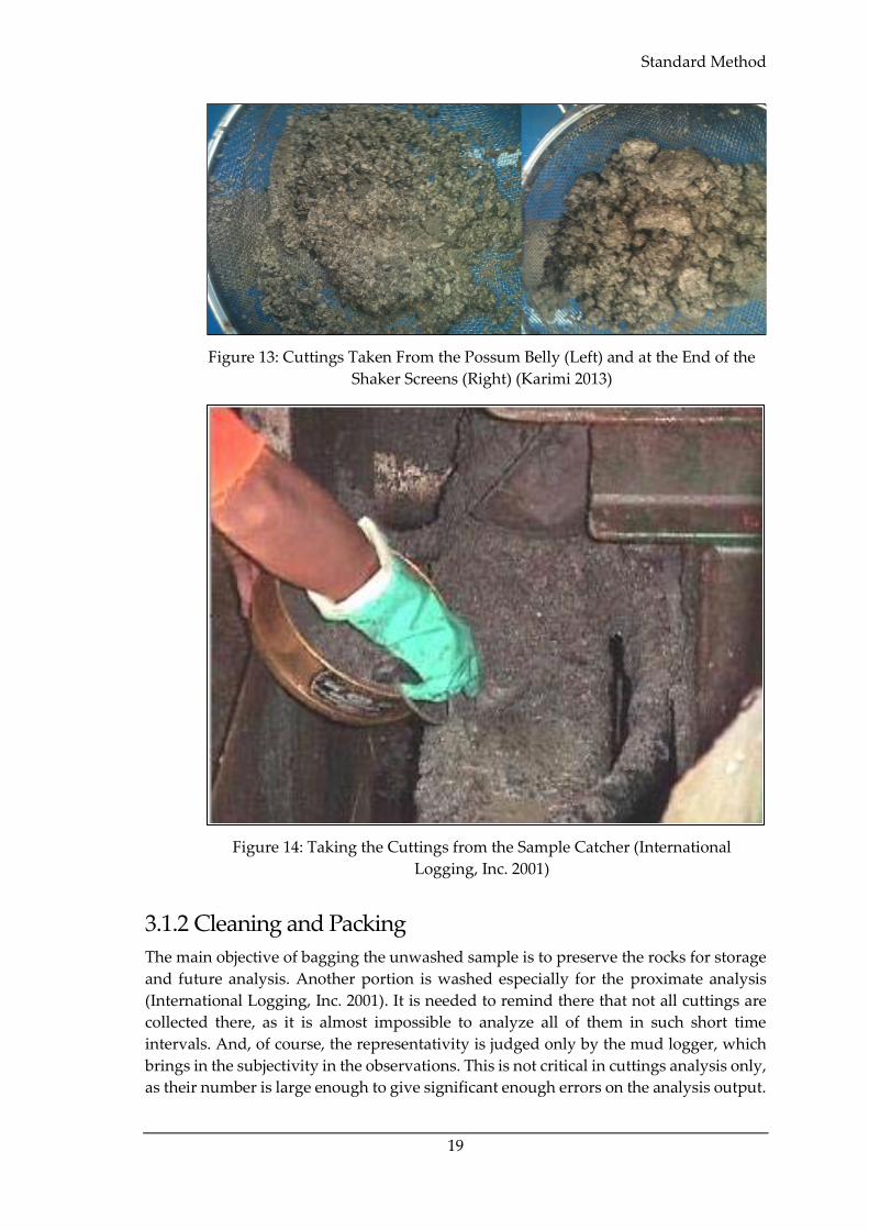
It depends, where to take the cuttings from: either from the possum belly or at the end
of the screens. It is illustrated in Figure 13. Cuttings taken from the possum belly appear
to be more representative, as the sample form the shaker outlet exhibits cuttings sticking
together in large sumps. This becomes critical when determining the particle size
distribution (PSD). It also matters, from which depth and location in the feeder tank to
take the samples, as there is an uncertain gradient of cuttings concentration in the
possum belly space. In addition, different designs of feeder tanks exist, and additional
research is to be done (Karimi 2013). However, the most common way to collect the
samples is the sample catcher at the end of the shakers (Figure 14). The most
representative sample is taken and either washed or placed in the cloth bags, depending
on the purpose. Afterwards, the catching board is cleaned from the remaining cuttings
in order to accumulate a new portion of rock material.
Standard Method
19
Figure 13: Cuttings Taken From the Possum Belly (Left) and at the End of the
Shaker Screens (Right) (Karimi 2013)
Figure 14: Taking the Cuttings from the Sample Catcher (International
Logging, Inc. 2001)
3.1.2 Cleaning and Packing
The main objective of bagging the unwashed sample is to preserve the rocks for storage
and future analysis. Another portion is washed especially for the proximate analysis
(International Logging, Inc. 2001). It is needed to remind there that not all cuttings are
collected there, as it is almost impossible to analyze all of them in such short time
intervals. And, of course, the representativity is judged only by the mud logger, which
brings in the subjectivity in the observations. This is not critical in cuttings analysis only,
as their number is large enough to give significant enough errors on the analysis output.

Cuttings Analysis Techniques
20
However, cavings should be observed in their full mass to present the whole information
about borehole walls conditions.
When the samples are to be analyzed, they need to be washed. To save the cuttings
characteristics the samples are washed in the base fluid of the drilling mud. Initially,
they are placed in an 8-mesh sieve (meaning that particles greater than 2,38 mm will not
be separated). Finer sieve is placed underneath to collect finer rocks during washing.
After the procedure, the rocks which are left on the 8-mesh sieve are considered as
cavings (Figure 15).
Figure 15: Cavings Collected in a Coarse Sieve (International Logging, Inc. 2001)
If the percentage of cavings is significant, the pressure engineer shall be informed about
it to take measures. At first instance, this information is needed for pore pressure
estimation (International Logging, Inc. 2001). Afterwards, the rocks are scooped on a
metal tray and tagged to distinguish between samples. Finally, they are observed using
the microscope or the UV box (as well as other tools). The cuttings and cavings are
inspected for the following parameters:
• Rock type
• Colour
• Texture
o Shape
o Grain size
o Sorting
o Hardness
o Lustre
o Slaking and swelling

Standard Method
21
• Cementation and matrix
• Fossils presence
• Sedimentary structure
• Visual porosity
• Oil show
As long as the scope of the thesis is to describe the cavings according to their shape, size,
and colour, only these parameters explanation is listed in Appendix A.
3.1.3 Analysis
In this subsection, the majority of tools and instruments for measuring the particle sizes,
shapes, morphology, and mineralogical content are discussed. It is important to mention
that not all existing equipment is intended to analyze drilling cuttings and cavings, but
it was designed for measuring solids content in the drilling mud (laser diffraction, image
analysis or FBRM methods), but it would be useful to focus on the technology, as the
principle stays the same, and this concept could be used for measuring cavings size,
shape and morphology.
Apart from that, to give a discussion of advantages and disadvantages of the methods
in terms of automation possibilities and time consumption, it is needed to give an
introduction to several ways of measuring the cuttings parameters (after Karimi 2013)
• In-Line Measurement: the instrument is inserted inside the pipe and conducts
measurement during circulation
• At-Line Measurement: sample is taken manually or automatically and analyzed
on-site
• On-Line Measurement: sample is collected and tested via the bypass line
• Off-Line Measurement: sample is collected and tested manually in the laboratory
It is worthy to mention that On-Line measurement has nothing in common with sending
the information in real-time. It is called so, as the device is attached directly on the
streaming line, which is called a bypass line, as written.
3.1.3.1 Sieve Analysis
This simple method is used for determining the PSD. Measurement is done by shaking
a sample through a set of the sieves until the rocks are distributed. The sieves are placed
in a descending order& from coarse to fine (Figure 16). When the shaking is completed,
the weight of each portion of rock left on the sieves is weighted, which gives information
about the PSD. This analysis is two-dimensional, however, which gives the information
of each cutting width and lacks the height (for flaky or platy pieces of rock).

Cuttings Analysis Techniques
22
Figure 16: Sieve Analysis Procedure (Left) and Cumulative Curve of PSD (Right)
(Karimi 2013)
3.1.3.2 Laser Diffraction
The essence of this technique is projecting a laser beam through a sample cell that
contains a stream of moving particles suspended in a solvent, usually water, air, or
alcohol (Karimi 2013). The concentration of particles has to be adjusted in order to allow
the light to pass through the sample. When a beam hits the particle, it is scattered. This
pattern, formed by scattered light, is registered by a number of detectors. Afterwardss,
the software compares the scattered pattern with a model. As the output, a histogram of
volume-weighted PSD is generated. the device is quite popular for PSD analysis because
of its fast operation and reliable results (van Oort and Buranaj Hoxha 2016).
Figure 17: Laser Diffraction Device (courtesy of Malvern Instruments)

Standard Method
23
3.1.3.3 Optical Microscopy and Image Analysis
Image analysis technology is relatively distinct from the previously described tools, as
here it is needed to process the image of the rocks itself, and not the reflected signal and
its patterns. Individual images are captured from dispersed rocks, and Afterwards one
receives the information about particle size, shape, and other parameters. There is also a
possibility of particle thickness measurement (Karimi 2013). The lower particle size limit
of image analysis is usually taken as 0,8 µm. The procedure is quite simple: the camera
captures an image of the sample, dispersed in a liquid, and applies imaging algorithms,
which derive the particle size and shape. This is the only technique, which delivers a full
batch of parameters, such as the longest and shortest diameter, perimeter, projected area,
equivalent spherical diameter, aspect ratio, and circularity. This is very important for
characterizing irregular particles, which take the majority of the input material (van Oort
and Buranaj Hoxha 2016). The Liquid Particle Analyzer (LPA) is the device used for this
purpose (Figure 18). In this image, LPA is used for drilling fluid analysis. A sampling
system takes a fixed volume of drilling fluid and mixes it with a diluter in a mixing tank.
Then the mixture is fed down the flow cell. The images are captured with a camera
placed opposite the flow cell. The light source is located below the camera. To obtain the
three-dimensional image, the particles are rotated (Saasen, et al. 2009).
Figure 18: LPA and Examples of Images; 1 – Sample Mixing Tank, 2 – Camera, 3 –
Flow Cell, 4 – Light Source (Saasen, et al. 2009)

Cuttings Analysis Techniques
24
3.1.3.4 Focused Beam Reflectance Measurement
Focused Beam Reflectance Measurement (FBRM) also utilizes a laser to obtain particle
size. This is achieved by focusing the beam very precisely and passing it through the
sample. The scattered and reflected light forms a return signal, and it is analyzed by the
system, which tells how long the particle was in contact with the beam. The output of
this procedure is the chord length, which is a line segment, connecting any two points
on the particle boundary (van Oort and Buranaj Hoxha 2016). There is a possibility of
obtaining the chord length distribution.
The tool illustrated in Figure 19 is used not only for the mud measurements but also for
medicine and food industry. In the actual device, the laser beam is passed through the
set of optics and focused on the sapphire window in a form of a beam spot. The optics
are rotating with the frequency of 400 rpm, allowing the beam to pass through all the
particles, as they flow near the window. The particles, as it was written earlier, scatter
the light in a form of pulses, which are registered and counted as the duration. Knowing
the speed of rotation, it is possible to calculate the distance, which was already
mentioned as the chord length.
Figure 19: FBRM Measurement Workflow (Pandalaneni 2016)
3.1.3.5 Ultrasonic Extinction
In contrast with previously reviewed techniques, Ultrasonic Extinction (USE) method
utilizes sound waves and not the light emission, which gives such devices a certain
advantage, as it can operate independently of light conditions (Karimi 2013).
The working principle is relatively simple (Figure 20). An electrical high-frequency
generator is connected to a piezoelectric ultrasonic transducer, which is generating the
ultrasonic waves. The signal is passed through the media and is received by an ultrasonic
detector, which converts mechanical waves into an electric signal. During travel through
the measurement zone, the signal is scattered only by those particles, which are equal to
or greater than the wavelength. During scattering the intensity of the signal decreases,
which is seen on the detector. This extinction is calculated from the ratio of amplitudes
on the generator and detector (Pankewitz and Geers 2020).

Standard Method
25
Figure 20: Measurement Principle of USE (Pankewitz and Geers 2020)
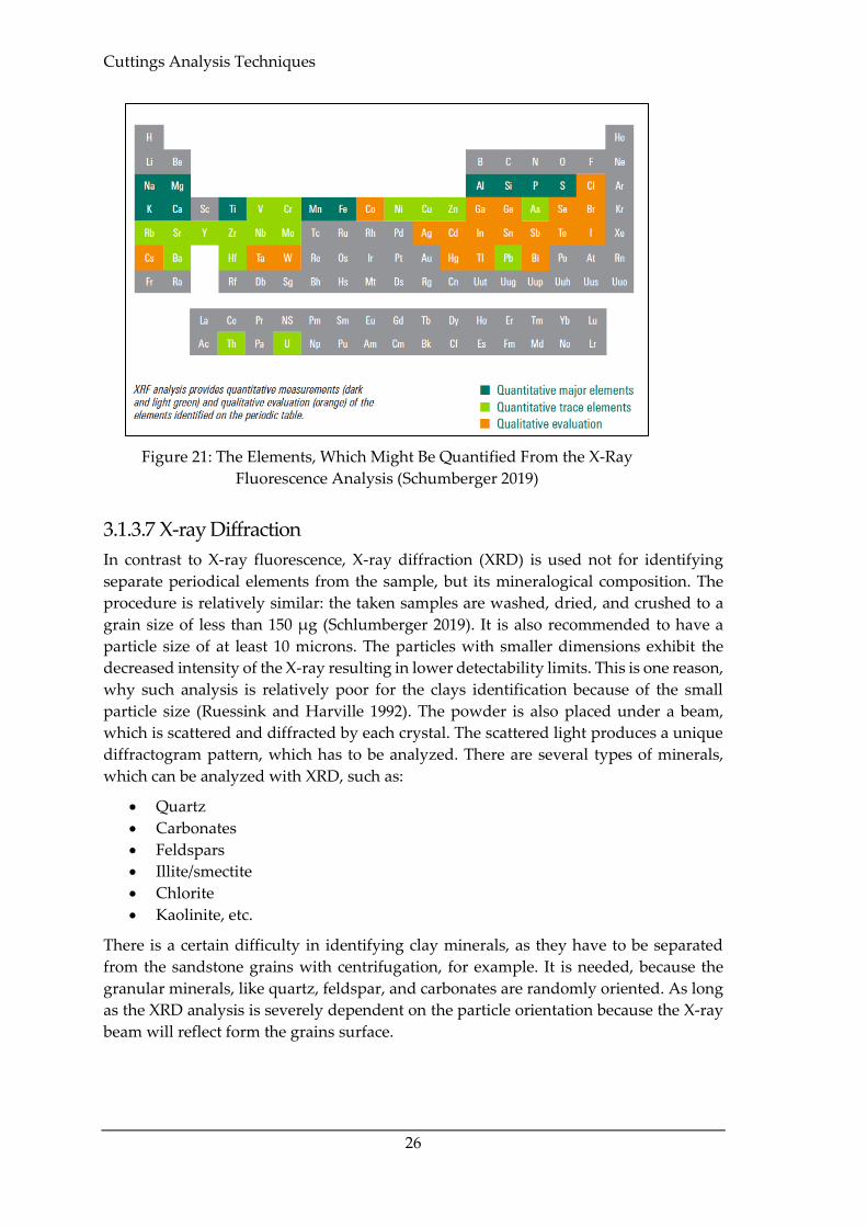
3.1.3.6 X-ray Fluorescence
The X-ray fluorescence (XRF) is used for determining the cuttings and cavings
composition from the major and trace elements. It works for both organic and inorganic
fingerprinting. In addition, it is used for identifying the mineralogy of the complex
lithologies (Schumberger 2019). This technique has a low limit in the low ppm range,
which is intended to give very precise results.
To conduct the measurement, the cuttings samples are to be cleaned, washed, and dried.
Afterwards, they are ground with a grain size of approximately 80 µm. The sample is
placed into plastic cups, which are used further for analysis.
During the analysis, the sample is irradiated with an X-ray beam, which excites the
electrons from the elements, of which the sample consists. When the electrons go back
to their energy level, they emit light in a form of a fluorescence signal with a specific
wavelength, which corresponds to the element type. This signal is amplified, measured,
and compared to a standards sample used as a reference (Carr, et al. 2014).
Cuttings Analysis Techniques
26
Figure 21: The Elements, Which Might Be Quantified From the X-Ray
Fluorescence Analysis (Schumberger 2019)
3.1.3.7 X-ray Diffraction
In contrast to X-ray fluorescence, X-ray diffraction (XRD) is used not for identifying
separate periodical elements from the sample, but its mineralogical composition. The
procedure is relatively similar: the taken samples are washed, dried, and crushed to a
grain size of less than 150 µg (Schlumberger 2019). It is also recommended to have a
particle size of at least 10 microns. The particles with smaller dimensions exhibit the
decreased intensity of the X-ray resulting in lower detectability limits. This is one reason,
why such analysis is relatively poor for the clays identification because of the small
particle size (Ruessink and Harville 1992). The powder is also placed under a beam,
which is scattered and diffracted by each crystal. The scattered light produces a unique
diffractogram pattern, which has to be analyzed. There are several types of minerals,
which can be analyzed with XRD, such as:
• Quartz
• Carbonates
• Feldspars
• Illite/smectite
• Chlorite
• Kaolinite, etc.
There is a certain difficulty in identifying clay minerals, as they have to be separated
from the sandstone grains with centrifugation, for example. It is needed, because the
granular minerals, like quartz, feldspar, and carbonates are randomly oriented. As long
as the XRD analysis is severely dependent on the particle orientation because the X-ray
beam will reflect form the grains surface.

Standard Method
27
3.1.4 Shortcomings (Standard Method)
The summary of conventional analysis considers only cavings size, shape, and lithology
measurements, and the strengths and weaknesses are collected in Table 3.
Table 3: Advantages and Disadvantages of Conventional Cavings Analysis
Advantages Disadvantages
Low cost of particle size and shape
analysis
Time-consuming
No necessity of equipment except sieves A requirement of personnel presence
Accuracy Subjectivity of observations
Individual analysis of cavings Not proactive
During the automation process, its strong points and advantages have to be preserved.
The strong points are definitely accuracy and individual approach when analyzing each
particle.
Furthermore, in order to automate the process of cuttings analysis and cavings detection,
in particular, it is needed to overcome the mentioned disadvantages. In order to improve
already existing technology, one has to split the workflow into separate operations and
search for those which may be removed or executed in parallel. In addition, it is needed
to specify the operations to be automated.
First of all, this technology requires a human presence to be executed. As it was
described in the corresponding section, the employee shall be present during the
following steps:
• Sample acquisition
• Washing of the sample in the 8-mesh sieve
• Packaging the samples depending on the purpose of analysis
• Manual measurement with sieves or other tools
• Comparison with the colour palette
• Writing the report
These procedures are subsequent, and all of them are part of the conventional workflow
cycle. An important moment in this sequence of procedures is washing the samples.
Only when the samples are collected with the 8-mesh sieve and washed, mud logger
notifies the crew about the cavings presence. If not specified, the frequency of the cavings
presence reporting is equal to one hour. This part makes the workflow non-proactive, as
a certain amount of time is lost for the cuttings collection and separation. In addition,
not all of the recovered cuttings are collected, but only a certain portion of them, which
was collected subjectively. These factors make their contribution to the lost time, which
could be used for decision making.
It was also mentioned, that the cuttings are to be washed intentionally for the analysis
e.g. colour identification. As long as washing is not critical for shape and size
determination because the mud layer is not thick enough to introduce large errors, it
becomes essential for the colour identification, which would give premises for

Cuttings Analysis Techniques
28
distinguishing between different types of lithology. In this case, an automatic circulation
system is required.
Having the analysis conducted at the time of the cavings' appearance on the shakers, all
the steps are automatically illuminated, which is followed by the acquisition and
washing operations. In addition, everything, which passes through the measurement
device, will be analyzed, excluding the selectivity of sample collection and subjectivity
in measurement.
Consequently, the proposed technology has to have the following features:
• It has to eliminate all the points discussed above, leaving the human as the
operator or supervisor, not the executor
• The presence of cavings should be noticed right at the moment of acquisition. If
the cuttings are stuck together, leaving no possibility of automatic caving
detection, they have to be washed and sieved automatically in advance
• The measurement device should exclude all the steps, which are to be done after
confirmation of cavings presence, so that not only cavings detection is executed,
but also their measurement and report generation is done
• The analysis should not be time-consuming and deliver the results within a
relatively short time range
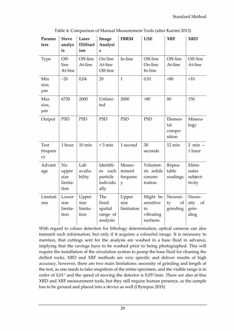
In order to select the tool for capturing cavings information, all the methods and tools
discussed above are coupled in Table 4. The best matching technique will be selected for
the cavings' shape, size, and colour determination with regards to the demands
mentioned above.
As long as the proposed system should be automated so that the tool should be chosen
depending on the type of measurement: In-line, At-line, or On-line in particular. In the
case of the At-line system, the measurement should be also done automatically, not
manually. Here the list is narrowed down to four methods: Laser diffraction, Image
analysis, FBRM, and USE. Focusing on the measurement technique itself, all the
mentioned above, except Image Analysis and USE, definitely have the upper particle
size limitation, as they are based on the scattering of the laser beam, which is too narrow
to detect larger particles on a scale of centimetres. The USE method could be the simplest,
in this case, to choose, however it has two main disadvantages: the existing tools for
ultrasonic measurements have a fixed limit of particle size of 3000 µm (Sympatec GmbH
2017). In addition, a shaking sieves’ surface may introduce errors in the measurements.
Since the design of the new tool is not the aim of this thesis, here only on the image
analysis techniques will be considered. For the considered case, it is not necessary to
disperse the cavings in a liquid in order to obtain images. As long as the imaging
algorithms are robust and fast enough to process the image in real-time, this is the best
matching technique. The strong side of this method is that it is able to calculate most of
particle parameters and dimensions by conducting measurement individually for each
particle, in contrast to other tools, which focus on capturing the scattered pattern.
Standard Method
29
Table 4: Comparison of Manual Measurement Tools (after Karimi 2013)
Parame
ters
Sieve
analys
is
Laser
Diffract
ion
Image
Analysi
s
FBRM USE XRF XRD
Type Off-
line
At-line
Off-line
At-line
On-line
At-line
Off-line
In-line Off-line
On-line
In-line
Off-line
At-line
Off-line
At-line
Min
size,
µm
~20 0,04 20 1 0,01 <80 >10
Max
size,
µm
6730 2000 Unlimi-
ted
2000 <80 80 150
Output PSD PSD PSD PSD PSD Elemen-
tal
compo-
sition
Minera-
logy
Test
frequen
cy
1 hour 10 min < 3 min 1 second 30
seconds
12 min 2 min –
1 hour
Advant
age
No
upper
size
limita-
tion
Lab
availa-
bility
Identifi-
es each
particle
individu
ally
Measu-
rement
frequenc
y
Volumet-
ric solids
concen-
tration
Repea-
table
readings
Elimi-
nates
subject-
tivity
Limitati
ons
Lower
size
limita-
tion
Upper
size
limita-
tion
The
fixed
spatial
range of
analysis
Upper
size
limitation
Might be
sensitive
to
vibrating
surfaces
Necessi-
ty of
grinding
Neces-
sity of
grin-
ding
With regard to colour detection for lithology determination, optical cameras can also
transmit such information, but only if it acquires a colourful image. It is necessary to
mention, that cuttings sent for the analysis are washed in a base fluid in advance,
implying that the cavings have to be washed prior to being photographed. This will
require the installation of the circulation system to pump the base fluid for cleaning the
drilled rocks. XRD and XRF methods are very specific and deliver results of high
accuracy, however, there are two main limitations: necessity of grinding and length of
the test, as one needs to take snapshots of the entire specimen, and the visible range is in
order of 0,01° and the speed of moving the detector is 0,05°/min. There are also at-line
XRD and XRF measurement tools, but they still require human presence, as the sample
has to be ground and placed into a device as well (Olympus 2019).

Cuttings Analysis Techniques
30
To sum up, the most flexible technique is Image Analysis, as it has the following
advantages:
• No limitation for the upper size of cuttings
• Identification of such parameters as the longest and shortest diameter, perimeter,
projected area, equivalent spherical diameter, aspect ratio, and circularity by
considering each particle individually
• Relatively low analysis time
• Inexpensiveness
• Absence of direct interaction with cuttings
3.2 Automated Measurement Tools
In this section, all the possible methods, which are used for determining the solids
content were collected, as well as describing the particles individually. There are two
different automated methods: physical and computer-based. The first technique
utilizes a direct measurement of cuttings mass within specified time intervals. The
second method comprises a wide range of techniques with various working principles.
A classification for these approaches was built, and the strengths and weaknesses were
discussed here.
3.2.1 Cuttings Flow Meter
Cuttings Flow Meter (CFM) continuously measures and records the cuttings flow at the
outlet of the shakers. Since the cuttings flow rate is often small relative to the mudflow
rate, measurement within the mudflow would not be accurate enough. Therefore, the
measurement is likely to be done at the outlet of the shale shakers. As long as this area
accommodates large and heavy equipment, there is little space left for another
mechanical system installation and for cleaning, maintenance, and screen’s check. In
addition, severe conditions are present in this zone, as the shakers are exposed to the
gas, high vibrations, and high-pressure cleaning jets. Being a simple mechanism, CFM
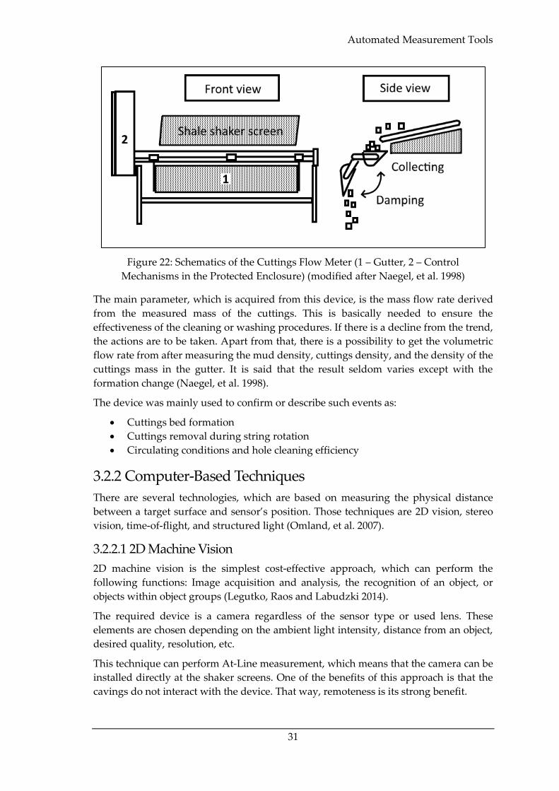
doesn’t disturb the operations and deliver its functions (Naegel, et al. 1998).
Figure 22 describes CFM construction. The device is located in front of each shale shaker
and collects cuttings in a tray. While the cuttings are being collected, the gutter is
prevented from rotating. At this period a strain gauge continuously measures the
increase in weight. On fixed time intervals, the gutter is flipped downwards, discharging
the collected cuttings. Then the tray stays in this state for a few seconds to ensure its
emptiness and flips back to the original position.
Automated Measurement Tools
31
Figure 22: Schematics of the Cuttings Flow Meter (1 – Gutter, 2 – Control
Mechanisms in the Protected Enclosure) (modified after Naegel, et al. 1998)
The main parameter, which is acquired from this device, is the mass flow rate derived
from the measured mass of the cuttings. This is basically needed to ensure the
effectiveness of the cleaning or washing procedures. If there is a decline from the trend,
the actions are to be taken. Apart from that, there is a possibility to get the volumetric
flow rate from after measuring the mud density, cuttings density, and the density of the
cuttings mass in the gutter. It is said that the result seldom varies except with the
formation change (Naegel, et al. 1998).
The device was mainly used to confirm or describe such events as:
• Cuttings bed formation
• Cuttings removal during string rotation
• Circulating conditions and hole cleaning efficiency
3.2.2 Computer-Based Techniques
There are several technologies, which are based on measuring the physical distance
between a target surface and sensor’s position. Those techniques are 2D vision, stereo
vision, time-of-flight, and structured light (Omland, et al. 2007).
3.2.2.1 2D Machine Vision
2D machine vision is the simplest cost-effective approach, which can perform the
following functions: Image acquisition and analysis, the recognition of an object, or
objects within object groups (Legutko, Raos and Labudzki 2014).
The required device is a camera regardless of the sensor type or used lens. These
elements are chosen depending on the ambient light intensity, distance from an object,
desired quality, resolution, etc.
This technique can perform At-Line measurement, which means that the camera can be
installed directly at the shaker screens. One of the benefits of this approach is that the
cavings do not interact with the device. That way, remoteness is its strong benefit.
Cuttings Analysis Techniques
32
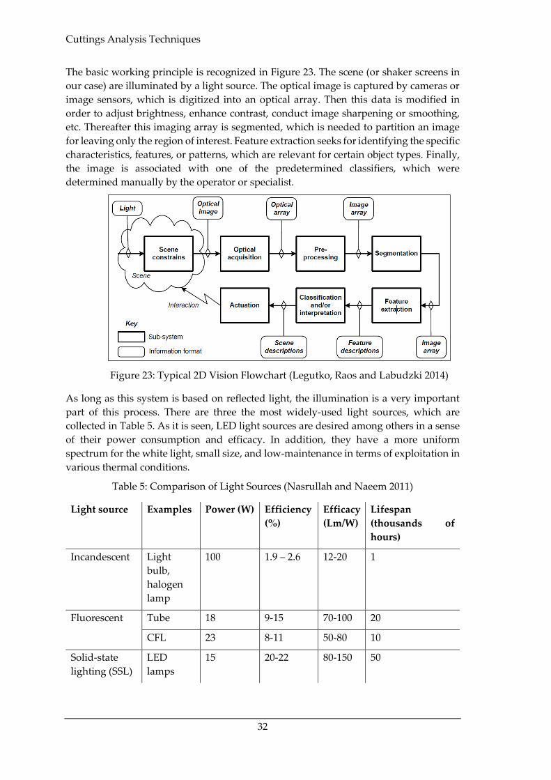
The basic working principle is recognized in Figure 23. The scene (or shaker screens in
our case) are illuminated by a light source. The optical image is captured by cameras or
image sensors, which is digitized into an optical array. Then this data is modified in
order to adjust brightness, enhance contrast, conduct image sharpening or smoothing,
etc. Thereafter this imaging array is segmented, which is needed to partition an image
for leaving only the region of interest. Feature extraction seeks for identifying the specific
characteristics, features, or patterns, which are relevant for certain object types. Finally,
the image is associated with one of the predetermined classifiers, which were
determined manually by the operator or specialist.
Figure 23: Typical 2D Vision Flowchart (Legutko, Raos and Labudzki 2014)
As long as this system is based on reflected light, the illumination is a very important
part of this process. There are three the most widely-used light sources, which are
collected in Table 5. As it is seen, LED light sources are desired among others in a sense
of their power consumption and efficacy. In addition, they have a more uniform
spectrum for the white light, small size, and low-maintenance in terms of exploitation in
various thermal conditions.
Table 5: Comparison of Light Sources (Nasrullah and Naeem 2011)
Light source Examples Power (W) Efficiency
(%)
Efficacy
(Lm/W)
Lifespan
(thousands of
hours)
Incandescent Light
bulb,
halogen
lamp
100 1.9 – 2.6 12-20 1
Fluorescent Tube 18 9-15 70-100 20
CFL 23 8-11 50-80 10
Solid-state
lighting (SSL)
LED
lamps
15 20-22 80-150 50

Automated Measurement Tools
33
However, even if the illumination is appropriate, the ambient light (e.g. sunlight) might
be present, if the installation is located outdoors, as in our case. In addition, fog and rain
might occur during the operation process. This might require the installation of the
insulation chamber.
3.2.2.2 Stereo Vision
The device set for the stereo-vision is similar to the 2D vision system. In the simplest
case, this method uses two Charged Coupled Device (CCD) equipped cameras placed
horizontally at a small fixed distance form a scanning object. The following assumptions
have to be introduced for the simplest stereo-vision system (National Instruments 2012):
• Both cameras have the same focal length
• The cameras are parallel to each other
• The X-axes of the two cameras intersect and align with the baseline
• The origin of the real-world coordinate system coincides with the origin of the
left camera coordinate system
There are two variants of cameras placement (Figure 24). The first one is compliant with
the demands mentioned above. In the second case, the cameras are located randomly.
This variant requires stereo calibration. Calibrating the camera basically done to
measure distances in length units, not in pixels. During this process, the real-world
coordinates are synchronized with cameras’ coordinates.
Figure 24: Simplest (Left) and Typical (Right) Stereo Vision Systems (National
Instruments 2012)
The working principle is illustrated in Figure 25. The process begins by sending two
images to the input. Thereafter the images are processed, the noise is filtered out, the
resolution is changed and optionally the colour channels are converted to monochrome.
Afterwards, the features have to be extracted. The correspondence problem is quite
challenging and is formulated as a question: how to find the same point on a real object
from the two images provided from cameras. If the correspondence is not established,
depth determination might be inaccurate. Generally, the salient points are chosen,
establishing high signal variations. The simplest examples are corners or color patches.
When the corresponding points in both images are found, they should be matched, so
that each of the points actually has relation to each other. Afterwards, the depth map is
built by computing actual coordinates of the points on both images.
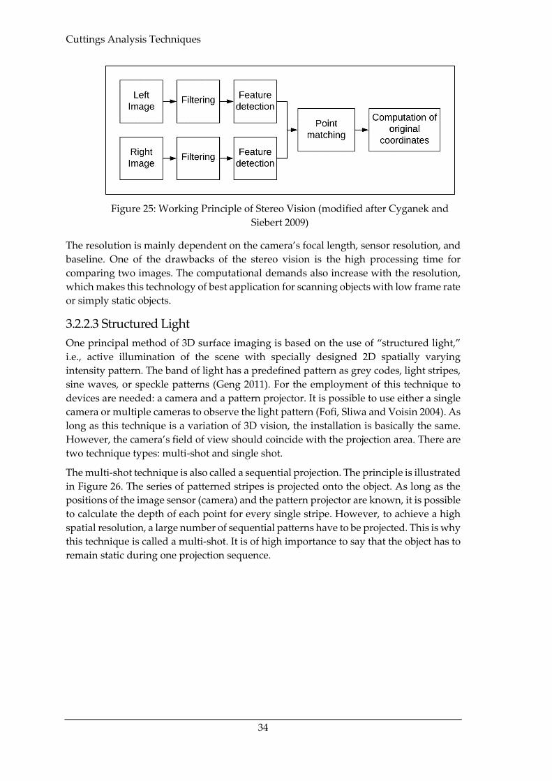
Cuttings Analysis Techniques
34
Figure 25: Working Principle of Stereo Vision (modified after Cyganek and
Siebert 2009)
The resolution is mainly dependent on the camera’s focal length, sensor resolution, and
baseline. One of the drawbacks of the stereo vision is the high processing time for
comparing two images. The computational demands also increase with the resolution,
which makes this technology of best application for scanning objects with low frame rate
or simply static objects.
3.2.2.3 Structured Light
One principal method of 3D surface imaging is based on the use of “structured light,”
i.e., active illumination of the scene with specially designed 2D spatially varying
intensity pattern. The band of light has a predefined pattern as grey codes, light stripes,
sine waves, or speckle patterns (Geng 2011). For the employment of this technique to
devices are needed: a camera and a pattern projector. It is possible to use either a single
camera or multiple cameras to observe the light pattern (Fofi, Sliwa and Voisin 2004). As
long as this technique is a variation of 3D vision, the installation is basically the same.
However, the camera’s field of view should coincide with the projection area. There are
two technique types: multi-shot and single shot.
The multi-shot technique is also called a sequential projection. The principle is illustrated
in Figure 26. The series of patterned stripes is projected onto the object. As long as the
positions of the image sensor (camera) and the pattern projector are known, it is possible
to calculate the depth of each point for every single stripe. However, to achieve a high
spatial resolution, a large number of sequential patterns have to be projected. This is why
this technique is called a multi-shot. It is of high importance to say that the object has to
remain static during one projection sequence.

Automated Measurement Tools
35
Figure 26: Principle of the Sequential Projection Imaging (Left) and Projected
Patterns (Right). LSB and MSB Stand for Least Significant Bit and Most
Significant Bit Correspondingly (Geng 2011)
The single-shot technique takes advantage of colour information of a unique encoding
scheme in the projection pattern and requires only one captured image of the colour
pattern to derive the 3D image with all three coordinates of each visible point. The
patterns take the form of the colour-indexed stripes or colour-coded grid (Figure 27).
The order, in which pattern is observed is not necessarily the order in which the pattern
is projected. This is due to the possibility of stripes missing from the acquired image
because of the occlusion of the object’s parts.
Figure 27: An Example of Single-Shot Techniques: Colour-Indexed Stripes
(Left) and Colour-Coded Grids (Right) (Geng 2011)
3.2.2.4 Time-of-Flight
The time-of-Flight technique, in contrast to some of the previously mentioned
installations, uses a single device is used, which accommodates two tools: light emitter
and receiver. Typically, an infra-red-light source (laser or LED) is used. Consequently,
the sensor is sensitive only to the frequency range of the emitter. Here it has to be

Cuttings Analysis Techniques
36
mentioned that the sensor responds not only to the reflected light but also an ambient
component, which is typically sunlight at the rig site (Figure 28). For this reason, the
camera, as well as the shaker screens have to be isolated in a separate chamber to ensure
the reliability of results. Apart from that, to capture the shape profile of cavings, it has
to be installed directly at the shakers in order to capture the size along the two largest
spatial dimensions. The time-of-flight camera works by illuminating the object with a
modulated light and capturing the reflected light. The measured phase shift is translated
as a parameter for object description. To detect phase shifts the emitted light is
modulated with a continuous wave, typically with a sinusoid or a square wave (Li 2014).
Figure 28: Principles of Time-of-Flight Camera Operation (Li 2014)
Thereafter the distance is measured for each pixel resulting in a depth map, which is a
series of 3D points (or voxels). In Figure 29 there is a 2D representation of a depth map,
formed from an image of soda cans set. The depth is visualized with a greyscale, where
white colour stands for closer voxels, whereas black – for farther. Alternatively, every
voxel can be visualized through a 3D point-cloud, where each point would have three
possible coordinates.
Figure 29: Input Image (Left) and a Depth Map (Right) (Li 2014)

Automated Measurement Tools
37
3.2.3 Shortcomings (Automated Method)
The observed methods are gathered in Table 6. They are split according to identified
parameters, depth accuracy, scanning speed, distance range, low light performance,
outdoor performance software complexity, and material cost. With respect to our
demands (cavings size is found within in the range of several cm) and the computing
power, 2D computer vision is the best choice among these types of techniques. There is
also a CFM device which has the best performance in outdoor and low light conditions,
however, as it was also mentioned in the previous subsection, only Image Analysis
techniques among listed in Table 6 allow us to analyze each rock piece individually.
Despite its simplicity, it gives no opportunity to detect the appearance of cavings on the
shakers.
Table 6: Comparison of Automated Measurement Tools (Based on Brading, et al. 2013)
Parameter CFM 2D
Computer
Vision
Stereoscopic
vision
Structured
light
Time of
flight
Identified
parameters
Mass
flow
rate
Shape and
size
Shape and
size
Shape and
size
Shape and
size
Depth
Accuracy
N/A mm to cm mm to cm µm to mm mm to cm
Scanning
speed/Testing
frequency
Low Medium.
Limited by
software
complexity
Medium.
Limited by
software
complexity
Fast/Medium.
Limited by
camera speed
Fast. Limited
by sensor
speed
Distance
Range
N/A Mid-Range Mid-Range Very short to
mid-range.
Depends on
illumination
power
Short to
long-range.
Depends on
laser power
and
modulation
Low Light
Performance
Good Weak Weak Good Good
Outdoor
Performance
Good Good Good Weak/Fair.
Depend on
illumination
power
Fair. Depend
on
illumination
power
Software
Complexity
Low Middle High Middle Low
Material Cost Middle Low Low Middle Middle
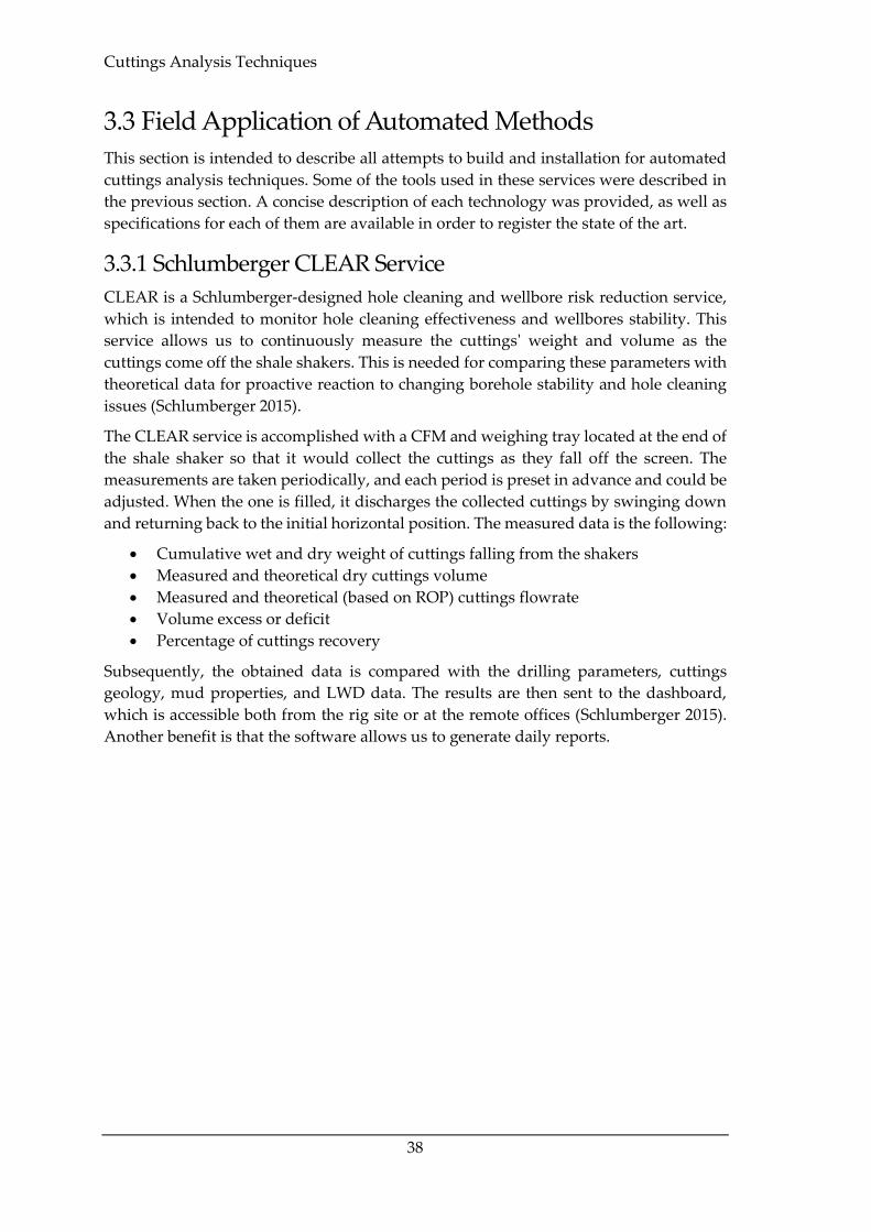
Cuttings Analysis Techniques
38
3.3 Field Application of Automated Methods
This section is intended to describe all attempts to build and installation for automated
cuttings analysis techniques. Some of the tools used in these services were described in
the previous section. A concise description of each technology was provided, as well as
specifications for each of them are available in order to register the state of the art.
3.3.1 Schlumberger CLEAR Service
CLEAR is a Schlumberger-designed hole cleaning and wellbore risk reduction service,
which is intended to monitor hole cleaning effectiveness and wellbores stability. This
service allows us to continuously measure the cuttings' weight and volume as the
cuttings come off the shale shakers. This is needed for comparing these parameters with
theoretical data for proactive reaction to changing borehole stability and hole cleaning
issues (Schlumberger 2015).
The CLEAR service is accomplished with a CFM and weighing tray located at the end of
the shale shaker so that it would collect the cuttings as they fall off the screen. The
measurements are taken periodically, and each period is preset in advance and could be
adjusted. When the one is filled, it discharges the collected cuttings by swinging down
and returning back to the initial horizontal position. The measured data is the following:
• Cumulative wet and dry weight of cuttings falling from the shakers
• Measured and theoretical dry cuttings volume
• Measured and theoretical (based on ROP) cuttings flowrate
• Volume excess or deficit
• Percentage of cuttings recovery
Subsequently, the obtained data is compared with the drilling parameters, cuttings
geology, mud properties, and LWD data. The results are then sent to the dashboard,
which is accessible both from the rig site or at the remote offices (Schlumberger 2015).
Another benefit is that the software allows us to generate daily reports.

Field Application of Automated Methods
39
Figure 30: CLEAR Hole Cleaning and Wellbore Risk Reduction Service
(Schlumberger 2015)
This technology was successfully used during drilling an ERD operation in Southeastern
Asia. CLEAR service indicated on the ineffective drilling mud rheology. Having this
information in mind, the drilling crew adjusted the fluid rheology, improving hole
cleaning. That allowed the company to save 16 rig hours or USD 194000 (Schlumberger
2015).
Another case study was conducted in the Shaybah field, Saudi Arabia. As proposed,
CLEAR service provided early detection of inadequate hole cleaning and excess returns
resulting in cavings appearance on the shale shakers. Having this support, the mud
system was kept in good condition during drilling. As a result, the section was drilled
2.46 days ahead of the plan with a cumulative cutting recovery of 84.4% (Schlumberger
2016).
3.3.2 Device for Measuring PSD and Cuttings Analysis
In 2009 an automated device was introduced, which was designed to measure drilling
fluid properties and conduct cuttings analysis. Here only the solids control part of this
system is covered. The device included the tools for measuring the cuttings Particle Size
Distribution (PSD), their concentration, morphology, and mineralogy (Saasen, et al.
2009). This cuttings analysis system is shown in Figure 31.
Cuttings Analysis Techniques
40
Figure 31: Schematic Diagram for Drilling Cuttings Analysis (Saasen, et al. 2009)
For testing purposes, different rock fragments, such as sands, shales, and carbonates
were added to simulate drill cuttings and cavings flow. The materials were added just
before the shaker. Then the major part of the cuttings is collected and measured with
cuttings flowmeter (Tool J). Right above the tool, a cuttings sampler is placed to
determine if there are any cavings in the flow. The cuttings morphology analyzer is
equivalent to Tool H. When the measurement is performed, the cuttings are transported
to Tool I to measure the cuttings mineralogy with a Raman spectroscope.
This system allows us to proceed with sampling, washing, and drying of cuttings and
image analysis. It was reported that the system worked without any problems during
the test period. In order to install such a device on the rig site, it would need certain
refinements to be done. It is said, that the Raman spectroscope should be broken down
automatically into individual mineral and fluid species. This is mainly needed to
monitor the mineral phases, not the cuttings’ size.
3.3.3 Intelligent System for Cuttings Concentration Analysis
The core of this system is a high definition camera installed above the shale shakers,
which sends the captured images to a computer with an installed data analysis system.
This module is responsible for classifying images obtained from the vibrating shale
shaker. If the image doesn’t match any of the classifiers, the mud logger is notified to
inspect the sample manually (Marana, et al. 2010).
Such a system has two main advantages: high accuracy in identifying anomalies during
the drilling operation and is of low cost. In addition, this system is non-intrusive,
meaning that it doesn’t consume much of the rig space, as the only video camera and the
laptop with the software are required (Figure 32).

Field Application of Automated Methods
41
Figure 32: Non-Intrusive Cuttings Analysis System Installation (Marana, et al.
2010)
The machine learning techniques used for the classification purposes were: Optimum-
Path Forest (OPF), Artificial Neural Network using Multilayer Perceptions (ANN-MLP),
Support Vector Machines (SVM) and Bayesian Classifier (BC).
The experiment on offshore drilling vessels for automatic image analysis was conducted.
The system was tested for three cuttings concentrations: None, Low and High, as
illustrated in Figure 33. It means that the cuttings were not analyzed individually, but
all together by texture analysis. The algorithm training was done with a supervisor; who
has selected 20 frames from each class of concentrations and labelled them accordingly,
which were used as a test set. Another 60 images were used for the test set, resulting in
a 50/50 relationship between training and test sets. The experimental results are gathered
in Table 7.
Figure 33: Images Captured by the Camera Placed Above the Shale Shakers: (a) None
Concentration, (b) Low Concentration and (c) High Concentration of Cuttings
(Marana, et al. 2010)
Table 7: Experimental Results for Different Classifiers (Marana, et al. 2010)
Classifier Mean Accuracy Mean execution time
OPF 99.89±0.001 0.0023
ANN-MLP 99.00±1.200 0.0330
SVM 99.25±0.612 1.5314
BC 99.33±0.970 0.0020
Authors concluded that with such low execution time and accuracy the system can
detect any anomaly with respect to changes in cuttings volume in real-time, indicating

Cuttings Analysis Techniques
42
problems during the drilling process. Importantly, this was the first attempt to develop
an image-based system for drilling operations monitoring based on cuttings analysis.
3.3.4 Classifying Cuttings Volume via Video Streaming
This approach proposed to analyze the volume of cuttings from a shale shaker also uses
video capturing. The model works in real-time and is able to perform classification in
relatively good accuracy in contrast to traditional video analysis methods, which take
too much of the processing time. The technology consists of two parts: multi-thread
engine for decoding, processing, and encoding video streams, as well as Region of
Interest (ROI) selector, and Convolutional Neural Network (CNN). This CNN is tested
to classify the cuttings volume into four labels: “Extra Heavy”, “Heavy”, “Light” and
“None” (Du, et al. 2020).
Figure 34: Real-Time Cuttings Volume Monitoring System. VGG Stands for
Visual Geometry Group, a Machine Learning Technique (Du, et al. 2020)
As seen from Figure 34, the process starts from capturing an image from the shaker by
the camera at the rig. Thereafter the data is streamed to a remote workstation through
intrusive rig transmission channels and protocols. Due to bandwidth limitations, the
video resolution is comprised. For testing purposes, 10 hours of video were collected
and labelled manually. In addition, a fast Graphics Processing Unit (GPU) is needed.
Then the model was tested on another set of videos. Testing results were verified by
comparing them to manually labelled frames. During the actual process, the videos are
labelled in real-time. The video framerate is equal to 5.84 frames/s, the bitrate is 137
Kbps. To guarantee steady interference results, the engineer is required to provide the
ROI in which cuttings are moving on the sieves. The ROI can be selected either manually
or automatically.
Figure 35: ROI Selected Manually (Left) or Automatically (Right) (Du, et al.
2020)

Field Application of Automated Methods
43
The testing results indicate that the algorithm easily distinguishes between all the
classifiers using the plain VCG-16 network. The results are also dependent on lightning
conditions, shooting angles, and distances.
3.3.5 Cuttings Shape Acquisition Using 3D Point Cloud Data
This technology provided by (Han, Ashok, et al. 2018) uses plane segmentation, which
is a computer vision algorithm, that constructs 3D point cloud data acquired by 3D
scanners. The test installation design included the conveyor belt, which was used to
simulate the sliding movement of artificially created rock fragments and field cuttings
on a ramp. Above the ramp, a 2D high-resolution camera with a 3D laser sensor was
installed in order to gain an integrated system. Whereas a camera was used for
measuring cuttings moving speed and analyze the size distribution of the cuttings, the
sensor was included to build the 3D profile basing on cuttings measurement. Both of
them were calibrated for the resolution and scanning frequency.
Figure 36: Integrated Cuttings Monitoring Design Setup (Han, Ashok, et al. 2017)
As for the software, Microsoft Visual Studio and C++ were selected as the Integrated
Development Environment (IDE) and the programming language respectively. As it is
seen from Figure 37, the workflow is the following. The laser sensor and camera are
triggered with Visual Studio. Thereafter they start to capture images and pass them to
the software via Gigabit Ethernet. The acquired 2D images from the camera allow us to
calculate the speed and PDS of the cuttings by comparing the frames. The speed data is
coupled with 2D profile depth data from the laser scanner, which results in cuttings
volume calculation.
3D depth profile is used further for edge detection and size calculation for each cutting
or caving individually. The cavings' shapes are proposed to be split into three categories:
tabular, angular, and splintered (Karimi 2013).
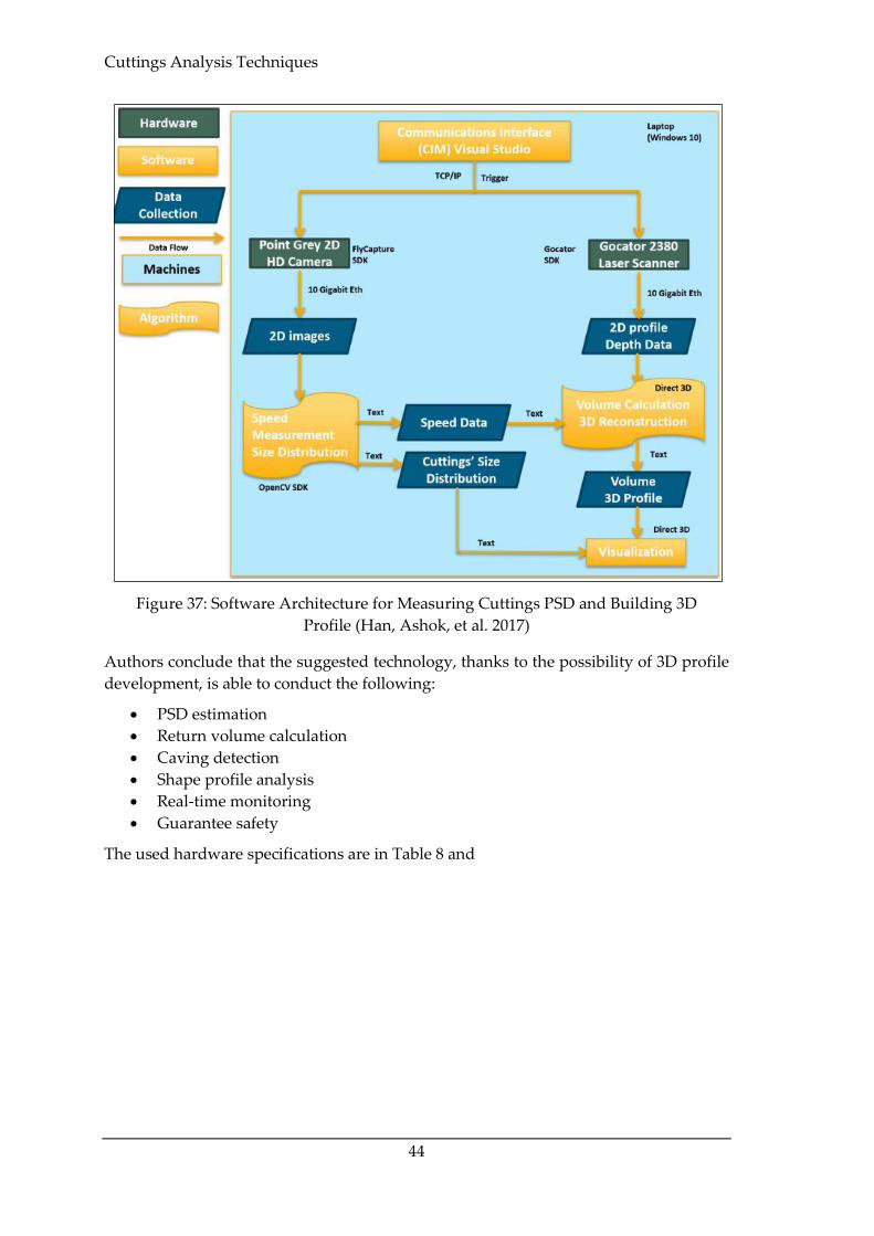
Cuttings Analysis Techniques
44
Figure 37: Software Architecture for Measuring Cuttings PSD and Building 3D
Profile (Han, Ashok, et al. 2017)
Authors conclude that the suggested technology, thanks to the possibility of 3D profile
development, is able to conduct the following:
• PSD estimation
• Return volume calculation
• Caving detection
• Shape profile analysis
• Real-time monitoring
• Guarantee safety
The used hardware specifications are in Table 8 and

Field Application of Automated Methods
45
Table 9.
Table 8: Gocator 2380 Laser Scanner Specifications (LMI Technologies 2016)
Specification Information
z-resolution 0.092 – 0,488 mm
x-resolution 0.375 – 1.100 mm
Measurement range 800 mm
Scan rate 5000 Hz
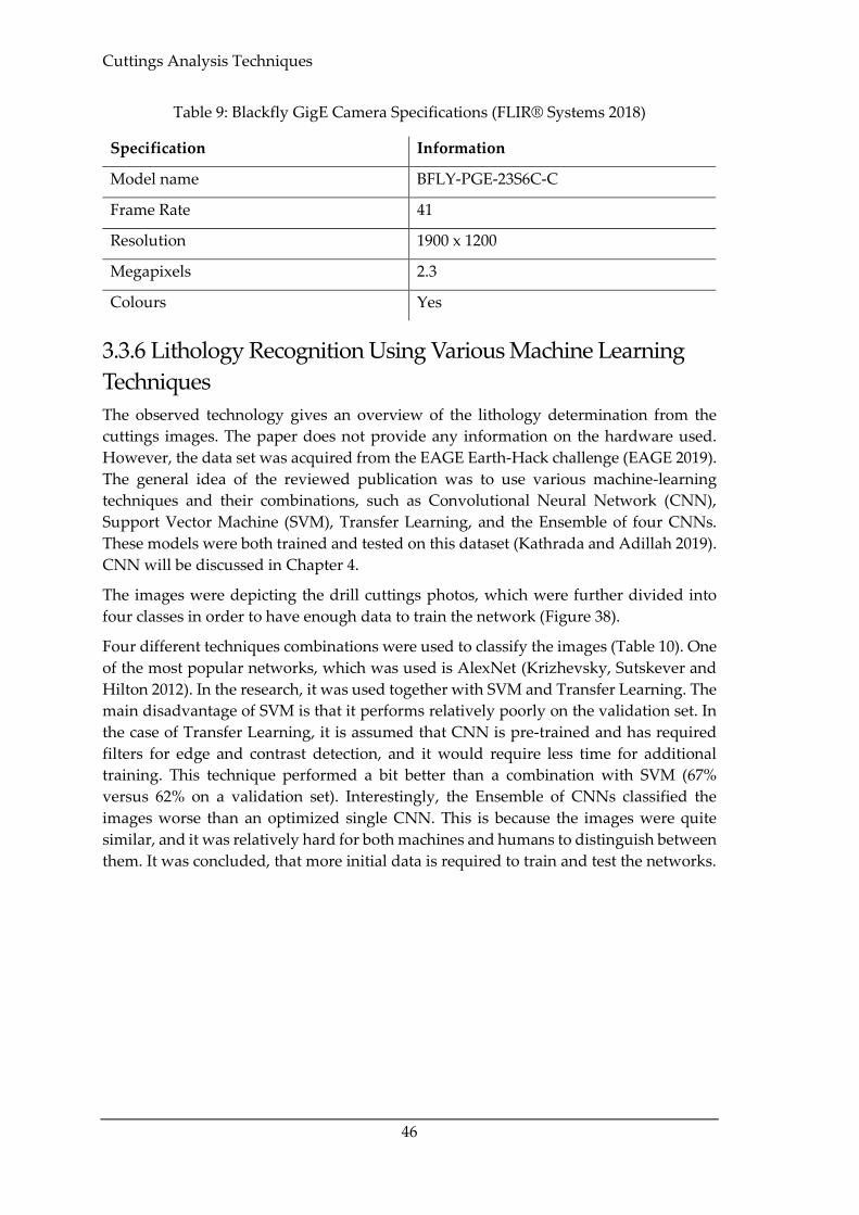
Cuttings Analysis Techniques
46
Table 9: Blackfly GigE Camera Specifications (FLIR® Systems 2018)
Specification Information
Model name BFLY-PGE-23S6C-C
Frame Rate 41
Resolution 1900 x 1200
Megapixels 2.3
Colours Yes
3.3.6 Lithology Recognition Using Various Machine Learning
Techniques
The observed technology gives an overview of the lithology determination from the
cuttings images. The paper does not provide any information on the hardware used.
However, the data set was acquired from the EAGE Earth-Hack challenge (EAGE 2019).
The general idea of the reviewed publication was to use various machine-learning
techniques and their combinations, such as Convolutional Neural Network (CNN),
Support Vector Machine (SVM), Transfer Learning, and the Ensemble of four CNNs.
These models were both trained and tested on this dataset (Kathrada and Adillah 2019).
CNN will be discussed in Chapter 4.
The images were depicting the drill cuttings photos, which were further divided into
four classes in order to have enough data to train the network (Figure 38).
Four different techniques combinations were used to classify the images (Table 10). One
of the most popular networks, which was used is AlexNet (Krizhevsky, Sutskever and
Hilton 2012). In the research, it was used together with SVM and Transfer Learning. The
main disadvantage of SVM is that it performs relatively poorly on the validation set. In
the case of Transfer Learning, it is assumed that CNN is pre-trained and has required
filters for edge and contrast detection, and it would require less time for additional
training. This technique performed a bit better than a combination with SVM (67%
versus 62% on a validation set). Interestingly, the Ensemble of CNNs classified the
images worse than an optimized single CNN. This is because the images were quite
similar, and it was relatively hard for both machines and humans to distinguish between
them. It was concluded, that more initial data is required to train and test the networks.

Field Application of Automated Methods
47
Figure 38: Image Examples for Each Lithology (Kathrada and Adillah 2019)
Table 10: Results for the Tested Methods (Kathrada and Adillah 2019)
Method Training set Validation set
AlexNet activations + SVM 100% 62%
Transfer Learning +
AlexNet
87% 67%
Bayesian optimized CNN 100% 82%
An ensemble of four CNNs 98% 73.5%
3.3.7 Rock Classification with a Deep Convolutional Network
Another methodology for rock types classification utilizing a CNN was developed (Ran,
et al. 2019). The technique was not developed to serve for cuttings lithology
identification purposes, but for classifying the field images of rocks. The overall
workflow, which is depicted in Figure 39, considers the following steps: taking pictures
of rocks, cropping the acquired images in order to focus the field of view directly on rock
mass, identification and labelling the rocks, model training, and actual application.
After taking the initial pictures of rocks outcrops, each of the images was divided into
regions of rocks with the most typical features in order to get the representative dataset.
The samples were taken from the mentioned regions so that they have the same
resolution. For providing an understanding of dataset sizes, the number of cropped
images for training, validation, and test datasets are listed in Table 11.

Cuttings Analysis Techniques
48
Figure 39: General Flowchart for the Rock Types Identification (Ran, et al. 2019)
Table 11: Datasets for Image Classification of Field Rocks (Ran, et al. 2019)
Type Training Data Validation Data Testing Data
Mylonite 1584 528 528
Granite 3753 1251 1251
Conglomerate 3372 1124 1124
Sandstone 2958 986 986
Shale 1686 562 562
Limestone 1236 412 412
Total 14589 4863 4863
Authors proposed a network with their own architecture in order to decrease computing
time and increase accuracy. The architecture is not shown in this section. The main
advantage of the proposed CNN is that the training could be carried out on a laptop,
with the following specifications including Central Processing Unit and Graphics
Processing Unit (CPU and GPU correspondingly) (Table 12).
The effectiveness of classification was tested with different CNNs, including the
proposed one. It employs two convolution operations, which is not much in comparison
with widely known networks. Apart from the proposed one, other techniques were
employed, such as Support Vector Machines (SVM), AlexNet, GoogleLeNet Inception
v3, and VGGNet-16 networks. Each of the models was trained in 200 epochs using the
batch (number of images in a training iteration) size, which is specified in Table 13. The
accuracy and training time is also listed in Table 13.
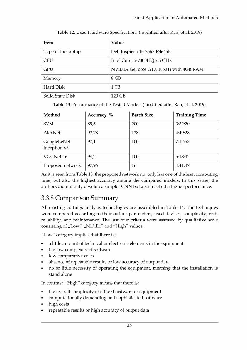
Field Application of Automated Methods
49
Table 12: Used Hardware Specifications (modified after Ran, et al. 2019)
Item Value
Type of the laptop Dell Inspiron 15-7567-R4645B
CPU Intel Core i5-7300HQ 2.5 GHz
GPU NVIDIA GeForce GTX 1050Ti with 4GB RAM
Memory 8 GB
Hard Disk 1 TB
Solid State Disk 120 GB
Table 13: Performance of the Tested Models (modified after Ran, et al. 2019)
Method Accuracy, % Batch Size Training Time
SVM 85,5 200 3:32:20
AlexNet 92,78 128 4:49:28
GoogleLeNet
Inception v3
97,1 100 7:12:53
VGGNet-16 94,2 100 5:18:42
Proposed network 97,96 16 4:41:47
As it is seen from Table 13, the proposed network not only has one of the least computing
time, but also the highest accuracy among the compared models. In this sense, the
authors did not only develop a simpler CNN but also reached a higher performance.
3.3.8 Comparison Summary
All existing cuttings analysis technologies are assembled in Table 14. The techniques
were compared according to their output parameters, used devices, complexity, cost,
reliability, and maintenance. The last four criteria were assessed by qualitative scale
consisting of „Low“, „Middle” and “High” values.
“Low” category implies that there is:
• a little amount of technical or electronic elements in the equipment
• the low complexity of software
• low comparative costs
• absence of repeatable results or low accuracy of output data
• no or little necessity of operating the equipment, meaning that the installation is
stand alone
In contrast, “High” category means that there is:
• the overall complexity of either hardware or equipment
• computationally demanding and sophisticated software
• high costs
• repeatable results or high accuracy of output data

Cuttings Analysis Techniques
50
• the necessity of frequent equipment maintenance or demand of human presence
Consequently, everything within the “Middle” category did not fall under each of the
previously mentioned labels. Therefore, the chosen items tend to have moderate
complexity, costs, performance, and self-sustainability.
Table 14: Comparison of Existing Installations for Cuttings Analysis. Green colour
shows the best category, red – the worst, and yellow – neutral
Name Outputs Device Compl
exity Cost
Reliabi
lity
Mainte
nance
Schlum-
berger
CLEAR
Mass,
Volume CFM Low Low High Low
Device after
(A. Saasen
2009)
PSD,
Morphol
ogy, Mi-
neralogy
CFM, Raman
spectroscope,
X-ray
High Middle Middle Middle
Device after
(A.N.
Marana
2010)
Volume Camera Low Low High Low
Device after
(Xunsheng
Du 2020)
Volume Camera Low High Middle Middle
Device after
(Han,
Ashok, et
al. 2017)
PSD,
Shape,
Volume
Camera and
laser scanner Middle Middle Middle Middle
Model after
(Kathrada
and Adillah
2019)
Litholog
y Camera Middle Middle Middle Low
Model after
(Ran, et al.
2019)
Rock
type Camera Middle Middle High Low
Mentioned techniques could be distinguished by the output parameters: the most
frequently determined were PSD and Volume. Others, such as Mass, Morphology,
Mineralogy, and Shape were mentioned only once. This trend could be described by the
simplicity of volume determination, as the rocks are analyzed in batches, and not
individually. This method is less computationally demanding and therefore is widely
used. At the same time, the last described approach is the only one, which is able to give
PSD, Shape, and Volume as the output simultaneously. This was achieved by installing
a laser scanner, which build the cuttings profile. Here it is to remind that the initial goal

Field Application of Automated Methods
51
of the authors was to calculate the volume and PSD, whereas shape was calculated as a
secondary parameter. It means that the shape could be determined for all the cuttings,
and not the cavings only. This is why this algorithm is demanding equipment and
processing power. For purposes of cavings analysis, it is not necessary to build a 3D
depth profile, which is storage prompting and time-consuming operation.
At the same time, the device after (Du, et al. 2020) could be used as part of the proposed
technology in this thesis. Even though it does not deal with shape determination, it
might alarm for mud overflow. Under these circumstances, it is not actually possible to
determine any cavings. Warning for excessive mud and rock on the screens might save
computational powers, as the cavings analysis system should stay in standby mode. In
addition, the goal of the thesis is not only to classify the cavings according to their shape
and size but also to warn the crew about possible complications, depending on the
conditions on the shale shakers. Mud overflow is not what usually reported, so, having
a system that notifies about it, could be a benefiting point from a proactivity perspective.
With regard to lithology determination, it is hard to presume in advance, if CNN would
actually determine the cavings lithology in real conditions, as none of the discussed
above models was tested on real cavings. Another complicating factor is the mud layer
and fine particle on the rocks, which seriously affect the measurement accuracy. It
means, that the cavings have to be either washed before appearing under the camera
field of view, or another means of analysis should be introduced.

Cuttings Analysis Techniques
52

Simplest Artificial Neural Network
53
Chapter 4 Convolutional Artificial
Neural Network
Artificial neural network (ANN) is a huge family of computing systems designed to
perceive the input data basing on the training data set without simple tasks like if-else
clauses. In considered case, ANN should be able to recognize cuttings and cavings from
the transmitted image data and classify them into predetermined sizes and shapes.
4.1 Simplest Artificial Neural Network
Convolutional neural networks are intended for recognizing image data, as their design
differs from the simplest ANN. The most general ANN design is illustrated in Figure 40.
It consists of an input layer of neurons, which transforms initial information into the
hidden layer (there might be several of them). In this layer, each neuron is connected to
every neuron in the previous layer. It is important to say that the neurons in the same
layer do not share any connections with each other. Being processed, the information is
passed to the layer of output neurons, giving the final result.
Figure 40: Principle Design of ANN
The single neutron structure is depicted in Figure 41. The neuron takes an array of inputs
and multiplies them by weights. Afterwards, all the multiplications are summed
together. Here, the bias is also added to the result. It is needed to adjust the results and
fit in the given data. The result is further passed to the activation function. There is a
high number of different activation functions:

Convolutional Artificial Neural Network
54
• Identity function
• Heaviside step function
• Rectifier function
• Gaussian
• Tangent
• Exponential and others
The type of function influences its robustness and the possibility of the neuron to pass
the information further or not. If the information gained after the summation function is
not enough to overcome the threshold, the neuron will not “fire”. In the end, the output
is generated which is either passed to other neurons or gives the actual outcome of the
calculation.
Figure 41: The General Neuron Structure
The operation of the neuron is formulated with the following equation:
�̂�1 = ∑ 𝑥𝑖𝑤𝑖 + 𝑏
𝑁
𝑖=1
(1)
Where 𝑥𝑖 – neuron input;
�̂�1 – computed output;
𝑤𝑖 – weight;
𝑏 – bias;
𝑖 – index of the input;
𝑁 – number of inputs.
The main goal of the ANN is to adjust weights so that the neurons would focus on one
type of information they get as an input. They might be adjusted either by supervised or
non-supervised learning. Supervised learning technique provides the ANN with the

Training, Validation, and Testing
55
labelled examples, so that the machine “knows”, what it should get. This kind of learning
technique is mainly used for bioinformatics, image, and pattern recognition. In the case
of unsupervised learning, ANN learns to label the inputs all by itself. Unsupervised
learning is needed for anomalies detection, hierarchical clustering, and generating data
with given patterns.
4.2 Training, Validation, and Testing
Prior to actual employment, the model has to be trained, tested, and validated. For that
purpose, the collected data is split into three datasets: training, testing, and validation
sets. The essence of these processes and methods of splitting the dataset are discussed in
the following subsections.
4.2.1 Training
The training dataset consists of the data (images, as in the considered case), which are
used to train an algorithm. This data is labelled in advance so that for every existing
input there is a corresponding output. The goal of the training session is to adjust the
weights in the network. For that reason, some fundamental concepts should be
explained.
The first concept to discuss is the cost function, which is determined as Mean Squared
Error (MSE):
𝐶(𝑤, 𝑏) =1
2𝑁∑(𝑦�̂� − 𝑦𝑖)2
𝑁
𝑖=1
(2)
Where 𝑤 – weights in the network;
𝑏 – biases in the network;
𝑦𝑖 – the target value of the output;
The purpose of the MSE introduction is to compute the error for each layer output
between the target value 𝑦𝑖 and calculated value �̂�1 for the given input 𝑥𝑖 and the
corresponding set of weights 𝑤 and biases 𝑏. From this perspective, there is an objective
to decrease MSE in order to obtain valid results.
In order to minimize the error and adjust weights, the backpropagation algorithm
should be introduced. Here it will be useful to link the weights and biases to the actual
neurons n the network. The weight between neuron 𝑗 in layer 𝑘 and neuron 𝑖 in layer
𝑘 − 1 will be denoted as 𝑤𝑖𝑗𝑘 , and bias for neuron 𝑗 in layer 𝑘 will be defined as 𝑏𝑗
𝑘 .
Neuron activations in the corresponding layer and input neuron will be denoted as 𝑎𝑗𝑘
for the outputs and 𝑎𝑖𝑘−1. Therefore, equation (1) could be updated as follows:
𝑎𝑗𝑘 = ∑ 𝑎𝑖
𝑘−1𝑤𝑖𝑗𝑘 + 𝑏𝑗
𝑘
𝑁𝑘−1
𝑖=1
(3)
Where 𝑁𝑘−1 – the number of neurons in level k-1.

Convolutional Artificial Neural Network
56
For the simplicity, bias 𝑏𝑗𝑘 will be defined as 𝑤𝑖0
𝑘 . Since the neurons are counted from 1
and not 0, this will not create any computational problems. Consequently, equation (3)
can be formulated as follows:
𝑎𝑗𝑘 = ∑ 𝑎𝑖
𝑘−1𝑤𝑖𝑗𝑘 + 𝑏𝑗
𝑘 =
𝑁𝑘−1
𝑖=1
∑ 𝑎𝑖𝑘−1𝑤𝑖𝑗
𝑘
𝑁𝑘−1
𝑖=0
(4)
Error minimization is computed by finding the gradients of the cost function with
respect to weights and biases:
∆𝑤𝑖𝑗𝑘 = −𝛼
𝜕𝐶
𝜕𝑤𝑖𝑗𝑘 (5)
Where 𝛼 – learning rate, which is usually taken in a range of (0,001 ÷ 0.1). It shows, how
fast the model should converge to the result.
Here it is needed to apply the chain rule:
𝜕𝐶
𝜕𝑤𝑖𝑗𝑘 =
𝜕𝐶
𝜕𝑎𝑗𝑘
𝜕𝑎𝑗𝑘
𝜕𝑤𝑖𝑗𝑘 (6)
The first term is defined as an error, denoted as:
𝛿𝑗𝑘 =
𝜕𝐶
𝜕𝑎𝑗𝑘 (7)
The second term is simplified as follows:
𝜕𝑎𝑗
𝑘
𝜕𝑤𝑖𝑗𝑘 =
𝜕
𝜕𝑤𝑖𝑗𝑘 ∑ 𝑎𝑖
𝑘−1𝑤𝑖𝑗𝑘 = 𝑎𝑖
𝑘−1
𝑁𝑘−1
𝑖=0
(8)
Hence, the partial derivative of the cost function with respect to 𝜕𝑤𝑖𝑗𝑘 is equal to:
𝜕𝐶
𝜕𝑤𝑖𝑗𝑘 = 𝛿𝑗
𝑘𝑎𝑖𝑘−1 (9)
It might be shown that:
𝛿𝑗𝑘 = 𝜎(𝑎𝑗
𝑘) ∑ 𝛿𝑙𝑘+1𝑤𝑗𝑙
𝑘+1
𝑁𝑘+1
𝑙=1
(10)
Where 𝑙 –neuron index on 𝑘 + 1 level;
𝑁𝑘+1 – number of neurons on 𝑘 + 1 level;
𝜎(𝑎𝑗𝑘) – activation function for the 𝑘 level.
As a result, the backpropagation is expressed as follows:
𝜕𝐶
𝜕𝑤𝑖𝑗𝑘 = 𝛿𝑗
𝑘𝑎𝑖𝑘−1 = 𝜎(𝑎𝑗
𝑘)𝑎𝑖𝑘−1 ∑ 𝛿𝑙
𝑘+1𝑤𝑗𝑙𝑘+1
𝑁𝑘+1
𝑙=1
(11)
It is seen that the error 𝛿𝑗𝑘 on the layer 𝑘 is computed from the error 𝛿𝑙
𝑘+1 on the next
layer 𝑘 + 1 , so that the error is propagated backwards. To sum up, when the network is
computing the outputs for each neuron, the process is called forward pass, while error
Training, Validation, and Testing
57
calculation is called a backward pass. As a result, after the whole forward pass up to the
final layer, the error is computed, and the weights and biases are adjusted. Afterwards,
another forward pass is conducted, but with already adjusted parameters. This process
continues until the error reaches its minimum.
On a large scale, when for the selected inputs the weights are adjusted in such manner
that the labels are determined correctly, that means that the network is trained.
4.2.2 Validation
In order to estimate, how well the network was trained, it is essential to prepare the
validation dataset. Again, all the inputs are also labelled in order to obtain the error. The
main difference between validation and training phase is that during validation the
model weights and biases basically stay unchanged. What could be changed is
hyperparameters of the ANN, such as learning rate, number of epochs to train, batch
size, or activation function. This combination of hyperparameters basically creates a
number of models to choose from. For that reason, the validation error is estimated. After
that such set of hyperparameters is selected, which gives the least validation error.
The training error is often compared to a validation error, giving the following
combinations:
• Underfitting – validation and training errors are high
• Overfitting – validation error is high, whereas training error is low
• Fitting – low validation and training errors
• Extra research is necessary - validation error is low, and training error is high
Obviously, the desired case is a fitting model, when both errors are low.
4.2.3 Testing and Splitting the Dataset
When the network architecture is finally defined and the hyperparameters are tuned,
the ANN evaluation is conducted. For that purpose, a test set is compiled. It is not
necessary to label the dataset unless to trace the network accuracy. The only demand is
that the labels should be the same in training, validation, and testing sets, so that the
model has actually learned the full number of classes and also performed on all of them.
If the testing phase was successful, the model can be employed in real-life conditions.
Apart from that, validation and testing errors are often compared. For the best case, these
errors should not differ within a high range, as overfitting or underfitting are likely to
occur.
In order to avoid such problems, the whole dataset should be correctly split. As a rule,
validation and testing sets are divided equally. The training set has to be the largest
among the three, as the network has to learn as many features as possible. If the initial
data is well prepared, and the network had enough data to adjust the weights and biases,
then it should perform well on the validation and test sets. The reason, why sets for the
last two phases are chosen to be equal is the fact, that during validation and testing the
number of layers is not changed. It means that the network basically doesn’t change
during validation. So, the overall process is the same. However, there might be the case,
where validation is conducted together with training on the same set. This is called cross-

Convolutional Artificial Neural Network
58
validation, and will not be discussed here. Therefore, the only use of the testing phase is
to approve and validate the tuned model on the data, which it has never seen before.
4.3 Convolutional Artificial Neural Network
In convolutional ANN (or CNN) the input layer is represented by image pixels, which
are to be captured and analyzed, whereas on the output layer there are pre-determined
classifiers or scores, which are intended to categorize the image (or, as in our case,
classify the cuttings, depending on the shape, size, and lithology). The general structure
of convolutional ANN is shown in Figure 42. Different types of layers with the help of
images from the CIFAR-10 dataset are discussed, which is commonly used for training
artificial networks.
Figure 42: Principle CNN Architecture
4.3.1 Input Layer
The input layer holds the initial image, which is desired to be analyzed. It is represented
by raw pixel values of horizontal and vertical position, as well as the number of channels
(in our case it is three, which corresponds to RGB). The resolution of the CIFAR-10 image
is 32x32 pixels. As a result, there is a 32x32x3 matrix as an input volume (Figure 43).
Figure 43: Schematics of the Input Layer

Convolutional Artificial Neural Network
59
4.3.2 Conv Layer
Conv (or convolutional) layer is three-dimensional, as the neurons are packed in stacks.
The number of stacks (or depth dimension) is equal to the number of filters needed to
actually identify the information from pixels (Figure 44). Within one stack the neurons
are aligned spatially into width and height dimensions. In the simplest case, each neuron
in a stack is to analyze one single pixel from the image. During forward pass the layer
slides (or convolves) along the image width and height and calculates the dot product
between the input and filter parameters. This process iterates along the depth
dimension, where different filters are applied. Usually, it is more useful to use a neuron
to capture not a single, but a certain number of pixels from the image to save processing
time.
Figure 44: Schematics of the Conv layer
From the mathematical point of view, filters are relatively small matrices, which are
filled with certain numbers. When the filter is applied to the array of pixels, it computes
the dot product with each corresponding pixel value and then gets the sum of the
products. Consequently, the filter produces only one value after projection on one part
of the pixel array. In the example in Figure 45 the filter slides along the array, computing
the sum of dot products of each of the three steps. As a result, a 5-number array as an
input and 3-number array as the output is obtained. Filters generally needed for
searching and extracting image features like edges, corners, or colour patterns. Visually,
the result looks like changing image contrast, brightness, saturation, etc.

Convolutional Artificial Neural Network
60
Figure 45: Working Principle of the Filter
As was said above, the output volume of the Conv layer is not necessarily of the same
size along spatial dimensions, as the input image. Here it is needed to consider Stride 𝑆
and Zero Padding 𝑃 parameters.
Stride is defined as the number of pixels, which filter passes through when sliding across
the image. For example, when 𝑆 = 1, then for each iteration the filter passes through
every neighbouring pixel. When 𝑆 = 2 , it “jumps” over one pixel (Figure 46).
Consequently, 𝑆 = 1 ensures larger output size spatially, however, the number of
iterations to count increases.
Figure 46: Demonstration of Stride Parameter. Blue Frame Represents a Filter, Which
Slides Along the Pixels
Zero-Padding parameter 𝑃 basically adds a frame around the image matrix filled with
zeros. It is very useful for controlling the spatial output size and fitting the filter with
certain 𝑆 value. In Figure 47 there is the following example: An input layer of size 5 is
convolved with a filter of size 4 with 𝑆 = 3. If 𝑃 = 0, then there is no place for the filter
to fit inside the INPUT layer. However, by adding zeros at the sides of the input layer,
the filter will stride and not yield errors. In this case, 𝑃 = 1, which means adding one
zero on each side.

Convolutional Artificial Neural Network
61
Figure 47: Demonstration of Zero Padding Application
Having the above parameters considered, one gets the following formulas, connecting
input size wit output size of the Conv layer:
𝑊𝑜𝑢𝑡 =
𝑊𝑖𝑛 − 𝐹 + 2𝑃
𝑆+ 1
(12)
𝐻𝑜𝑢𝑡 =
𝐻𝑖𝑛 − 𝐹 + 2𝑃
𝑆+ 1
(13)
𝐷𝑜𝑢𝑡 = 𝐾 (14)
Where 𝑊𝑖𝑛, 𝑊𝑜𝑢𝑡 – input and output widths correspondingly;
𝐻𝑖𝑛, 𝐻𝑜𝑢𝑡 – input and output height correspondingly;
𝐷𝑜𝑢𝑡 – output depth;
𝐹 – filter size;
𝑃 – zero padding;
𝑆 – stride;
𝐾 – number of filters
4.3.3 ReLU Layer
ReLU (or Rectified Linear Unit) layer is designed to apply the activation function. The
layer volume is similar to the previous one. Usually, among all activation functions, a
rectified linear unit function is used, because it is employed computational simplicity,
representativity, and linearity. This function can be described with the equation as
follows:
𝑓(𝑥) = max (0, 𝑥) (15)

Convolutional Artificial Neural Network
62
Where 𝑥 – function argument
Figure 48: Comparison of ReLU, TanH, and Sigmoid Functions
It means that the function will increase linearly and monotonously on a range of (0, ∞)
and flatten on a range of (−∞, 0]. In comparison with other activation functions, as it is
seen in Figure 48, TanH and Sigmoid functions are very sensitive to arguments in the
vicinity of zero, while having large or small numbers yield more or less the same result.
In addition, these functions utilize exponents to calculate the output. They also don’t
deliver the true zero value. In contrast, ReLU always returns zeros, if the argument is
negative, and uses no additional functions to give the output. This saves computational
time, which is demanding for training deep networks.
4.3.4 Pool Layer
Pool (or pooling) layer performs the downsampling operation along the width and
depth dimensions, which saves the computing power and avoids overfitting. This layer
is usually placed between Conv layers. Most commonly the image is upscaled, taking
the maximum value among each 2x2 region, discarding 75% of neurons. The working
principle of this layer is similar to the Conv layer: the filter slides across the matrix,
performing certain operations and yielding the result. However, in this case, the filter
takes the maximum value out of those, on which the filter is focused on. In Figure 49
there is an example, how the Pool layer works. There is a three-dimensional array as an
input and a filter with 𝐹 = 2 and 𝑆 = 2. When the filter slides across the array, it takes
every 2x2 squares of data, then takes maximum value out of each and outputs exactly
two times smaller array in sense of spatial dimensions.
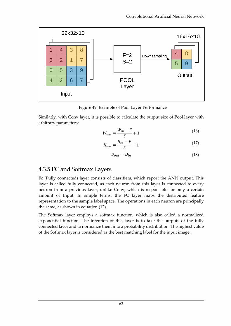
Convolutional Artificial Neural Network
63
Figure 49: Example of Pool Layer Performance
Similarly, with Conv layer, it is possible to calculate the output size of Pool layer with
arbitrary parameters:
𝑊𝑜𝑢𝑡 =
𝑊𝑖𝑛 − 𝐹
𝑆+ 1
(16)
𝐻𝑜𝑢𝑡 =
𝐻𝑖𝑛 − 𝐹
𝑆+ 1
(17)
𝐷𝑜𝑢𝑡 = 𝐷𝑖𝑛 (18)
4.3.5 FC and Softmax Layers
Fc (Fully connected) layer consists of classifiers, which report the ANN output. This
layer is called fully connected, as each neuron from this layer is connected to every
neuron from a previous layer, unlike Conv, which is responsible for only a certain
amount of Input. In simple terms, the FC layer maps the distributed feature
representation to the sample label space. The operations in each neuron are principally
the same, as shown in equation (12).
The Softmax layer employs a softmax function, which is also called a normalized
exponential function. The intention of this layer is to take the outputs of the fully
connected layer and to normalize them into a probability distribution. The highest value
of the Softmax layer is considered as the best matching label for the input image.

Convolutional Artificial Neural Network
64

Overview
65
Chapter 5 Conceptual Design of the
Proposed Technology
5.1 Overview
During the discussion in the previous chapters, it was stated that the borehole stability
issues are of high importance and should not be overlooked. One of the methods for
direct and proactive borehole instability signs identification is cavings analysis. The
main benefit of this method results not only in recognizing the instability but also in
determining its type and mechanism of generation. In this sense, cavings hold the
features, which indicate the complication type. These are basic shapes and sizes. Another
cavings feature to consider is lithology, which could link to the unstable interval, giving
the information about the possible complication occurrence.
One of the conclusions that were drawn from the previous chapters regarding the
conventional cavings analysis methods, is that these methods are time-consuming and
require several employees in the workflow to achieve good results. Hence, there is a
demand for an automated cavings analysis system, which can overcome the main
shortcomings of the conventional methods. The effective automated system should
minimally have the following features. Firstly, it should deliver results in real-time, as
soon as the cavings appear on the screens. That way the warning signs will be delivered
to the mud logger immediately so that the crew would have more time for making a
decision. Secondly, it should be completely autonomous, requiring only the installation
procedures and initial software or hardware adjustment. Thirdly, the system should
yield all the features mentioned above: shape, size, and lithology. For that reason, each
of the cavings should be analyzed individually. This creates additional requirements for
the associated algorithm, which increases its complexity. Lastly, the results should be
accurate and valid. This is the most challenging demand for the algorithm, as shape
determination is an uncertain and subjective process. Because of that, the system should
be tested in presence of an experienced employee who can give recommendations about
algorithm accuracy.
The road map of the proposed system is illustrated in Figure 50. It comes into effect when
the rocks appear at the screens. The cavings need to be washed to make it possible to
obtain their colour for lithology classification purposes. Afterwards, the image is
captured by a video camera, which transfers obtained data to the computer with pre-
installed software for cavings classification. As long as the software employs computer
vision technology, it will be powered by CNN, which requires training, validation, and
testing. These processes were explained in Chapter 4. Here it is to be assumed that the
algorithm is already trained. It is not possible to detect the cavings on the screens, the
system should also report on mud overflow events or absence of any complications at
all. If the cavings are detected, the shape and size are determined. These parameters are
reported immediately to the mud logger, notifying about a possible complication.
Afterwards, the software attempts to identify the lithology. If the cavings are poorly
washed, of there is another reason why the lithology could not be determined, this step
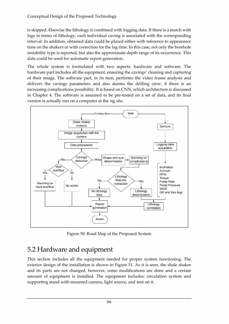
Conceptual Design of the Proposed Technology
66
is skipped. Elsewise the lithology is combined with logging data. If there is a match with
logs in terms of lithology, each individual caving is associated with the corresponding
interval. In addition, obtained data could be placed either with reference to appearance
time on the shakers or with correction for the lag time. In this case, not only the borehole
instability type is reported, but also the approximate depth range of its occurrence. This
data could be used for automatic report generation.
The whole system is formulated with two aspects: hardware and software. The
hardware part includes all the equipment, ensuring the cavings’ cleaning and capturing
of their image. The software part, in its turn, performs the video frame analysis and
delivers the cavings parameters and also alarms the drilling crew, if there is an
increasing complications possibility. It is based on CNN, which architecture is discussed
in Chapter 4. The software is assumed to be pre-tested on a set of data, and its final
version is actually run on a computer at the rig site.
Figure 50: Road Map of the Proposed System
5.2 Hardware and equipment
This section includes all the equipment needed for proper system functioning. The
exterior design of the installation is shown in Figure 51. As it is seen, the shale shaker
and its parts are not changed, however, some modifications are done and a certain
amount of equipment is installed. The equipment includes: circulation system and
supporting stand with mounted camera, light source, and tent on it.

Hardware and equipment
67
Figure 51: Exterior Design of the Hardware Part of the Proposed System
5.2.1 Shale Shaker Modification
As it was discussed, one of the major modification to the shale shaker is the circulation
system. The main function of the circulation system is to clean the cavings prior to their
appearance in the camera field of view. This is basically needed for lithology
determination. If it weren’t for cavings washing procedure, they would be covered in
remaining mud and finer particles. This system includes the pump, discharge hose,
sprinkler head with fixed sprinklers on it, a tray for collection of the base fluid, and filter,
as illustrated in Figure 52 and Figure 53. In this section, each of the elements is discussed.

Conceptual Design of the Proposed Technology
68
Figure 52: Proposed Modification of the Shale Shaker Design
Figure 53: Sideview of the Modified Shale Shaker

Hardware and equipment
69
5.2.1.1 Tray
The functioning of the system begins with the tray, which serves at the same time as a
holding tank for all of the base fluid and a discharge place, where the fluid is reflux from
the sprinklers. The tray is either screwed to the shaker base to the sides or to the bottom,
excluding the transmission of vibrations. Two points should be taken into consideration.
The first one is its volume, which should be enough to accommodate the volume of all
the pipes, pump itself, the sprinkler head, and some extra volume to maintain
continuous circulation without cavitation. The second one is its angle of inclination,
which ensures the gravity flow of the base fluid towards the pump intake. Another
important point is the location of the sprinkler head. There should be enough time for
the cavings before passing it to the camera for image capturing. At the same time, if it is
placed too close to the back tank, there is a high possibility of the actual mud appearing
on the tray.
5.2.1.2 Collector Pipe and Hoses
The most convenient way to allocate the collector pipe, which is attached to the tray
bottom, is to pull it out of the shaker's front side. There is likely to be little space for
hydraulic communications within the shaker. For that reason, either the pipe or the hose
could be used. In a system illustrated in Figure 52, a pipe is used, as it is easier to clean
and dismantle it. The possibility of pipe disassembling plays its role when fine particles
block the cross-section, and there is a need to unclog the pipe.
At the same time, the collector pipe should be connected to the pump with a hose, as the
pump location is not fixed. At the same time, the discharge part of the pump should also
be connected with a hose, as shale shaker’s vibrations might affect the threads of the
connections.
5.2.1.3 Filter
As long as the base fluid is sprinkled through the screens, there is a high possibility of
fluid contamination with mud and fine particles. This might be a very important issue,
as the particles can eventually block the collector pipe. This will lead to fluid loss at the
pump intake and its overheating. In addition, fine particles seriously affect the pump
performance independently of its type, as they erode the pump’s surfaces. For this
reason, either a water or an oil filter should be installed at the intake. The filters should
be changed during system functioning, and there is the only demand for the intervention
of the employee into the operation.
5.2.1.4 Pump
For the purposes of fluid circulation, a centrifugal pump is selected. Pumps of this type
have the following advantages:
• Simpler construction because of fewer moving parts
• Smaller dimensions
• Availability on the market
• Greater discharging capacity
• Stable flowrate
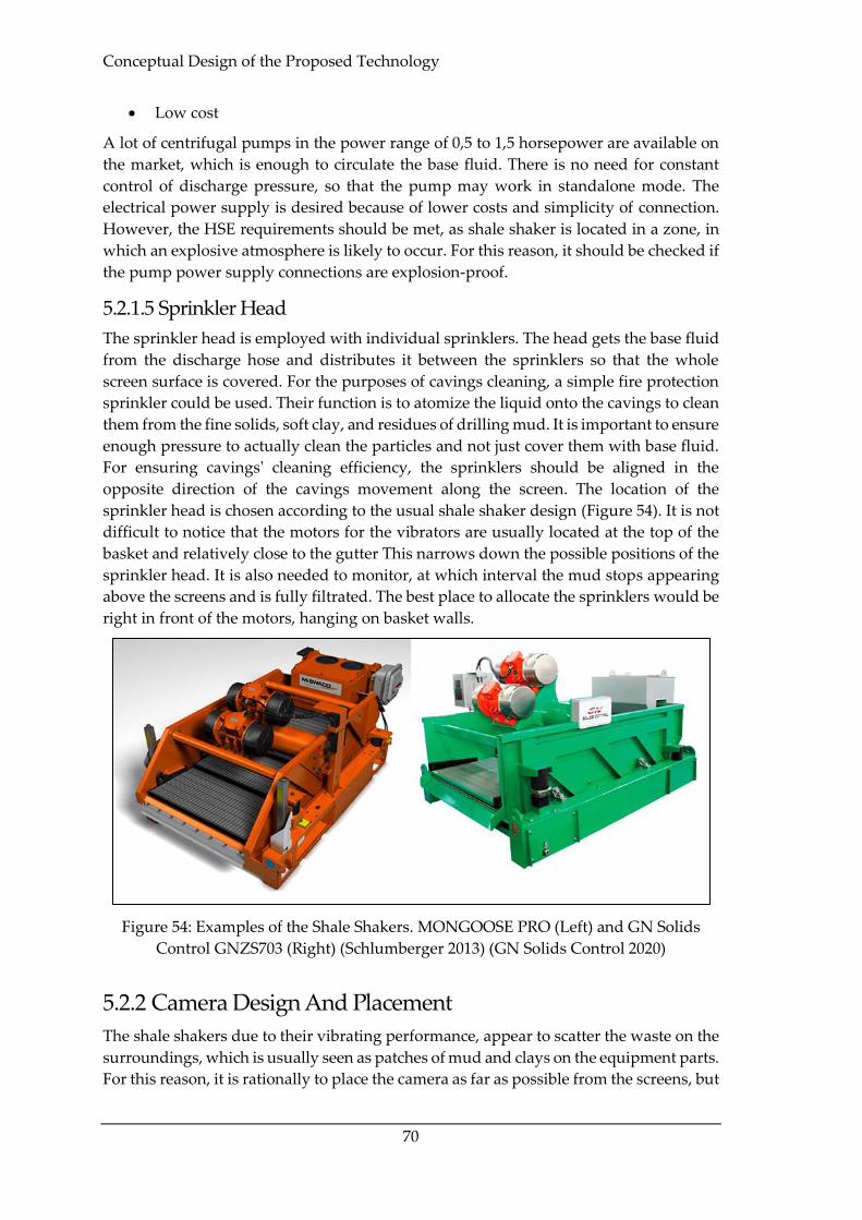
Conceptual Design of the Proposed Technology
70
• Low cost
A lot of centrifugal pumps in the power range of 0,5 to 1,5 horsepower are available on
the market, which is enough to circulate the base fluid. There is no need for constant
control of discharge pressure, so that the pump may work in standalone mode. The
electrical power supply is desired because of lower costs and simplicity of connection.
However, the HSE requirements should be met, as shale shaker is located in a zone, in
which an explosive atmosphere is likely to occur. For this reason, it should be checked if
the pump power supply connections are explosion-proof.
5.2.1.5 Sprinkler Head
The sprinkler head is employed with individual sprinklers. The head gets the base fluid
from the discharge hose and distributes it between the sprinklers so that the whole
screen surface is covered. For the purposes of cavings cleaning, a simple fire protection
sprinkler could be used. Their function is to atomize the liquid onto the cavings to clean
them from the fine solids, soft clay, and residues of drilling mud. It is important to ensure
enough pressure to actually clean the particles and not just cover them with base fluid.
For ensuring cavings' cleaning efficiency, the sprinklers should be aligned in the
opposite direction of the cavings movement along the screen. The location of the
sprinkler head is chosen according to the usual shale shaker design (Figure 54). It is not
difficult to notice that the motors for the vibrators are usually located at the top of the
basket and relatively close to the gutter This narrows down the possible positions of the
sprinkler head. It is also needed to monitor, at which interval the mud stops appearing
above the screens and is fully filtrated. The best place to allocate the sprinklers would be
right in front of the motors, hanging on basket walls.
Figure 54: Examples of the Shale Shakers. MONGOOSE PRO (Left) and GN Solids
Control GNZS703 (Right) (Schlumberger 2013) (GN Solids Control 2020)
5.2.2 Camera Design And Placement
The shale shakers due to their vibrating performance, appear to scatter the waste on the
surroundings, which is usually seen as patches of mud and clays on the equipment parts.
For this reason, it is rationally to place the camera as far as possible from the screens, but

Hardware and equipment
71
not too far, so that camera’s resolution is enough to capture as much information, as
possible.
The weather conditions are another problem to deal with. Rain, fog, and snow might
significantly affect camera in a sense of the appearance of water droplets on lenses,
blocking the camera’s field of view, interfering with shaker screens, creating artefacts in
images as a consequence. That means that the camera and its field of view have to be
fully isolated from the environment. This could be done cheaply be placing a shelter
above the device and the end of shaker screens. In the same way, this shelter shall allow
the employees to easily do shaker’s maintenance (e.g. repairing, changing screens,
checking the cuttings separation conditions). In addition, there shall not be the case,
when the sunlight is coming into the camera, so the employee should choose the best
place for the camera in order to avoid filming against the sun. The easiest way is to place
a small tent above the camera in order to make the measurements as pure as possible.
Another point to consider is explosion protection. Shale shakers' environment is not
explosion-proof, as the cuttings and mud could contain hydrocarbon traces. In addition,
gas separators are usually present in the vicinity of the shakers, as they are part of the
mud treatment system. The zone around shakers is classified as Zone 1 according to
ATEX directive as such: a place in which an explosive atmosphere consisting of a mixture
with air or flammable substances in the form of gas, vapour or mist is likely to occur in
normal operation occasionally. For that reason, explosion-proof enclosures are
manufactured. According to ATEX, the housing is labelled as an Ex-d code, meaning
that a device would withstand an internal explosion and provide relief of the external
pressure via gaps in the construction such as threaded connections or flanges (European
Commission 2000). An example of such an enclosure is illustrated in Figure 55. Such
enclosure shall also protect the camera lens from contamination.
Figure 55: An Example of Explosion-Proof Enclosure (SAMCON GmbH 2020)

Conceptual Design of the Proposed Technology
72
The camera itself should be cost-effective, compact, with high enough resolution sensor,
having no conflicts with the software, and being able for fast data transmission. For these
reasons, the camera from FLIR® Blackfly® S GigE series is used (Figure 56). The cameras
range depending on the lens mount type, frame rate, resolution, chroma, etc.
Figure 56: FLIR® Blackfly® S GigE Camera (FLIR® Systems 2018)
Technologies, discussed in Chapter 3, utilize cameras with frame rates not greater than
6 fps. The number of megapixels was around 2. The camera was chosen with regard to
these values, as there was no possibility to test and compare the cameras. The chosen
camera specifications are listed in Table 15. It is usually possible to change the frame
rate, so the initial amount of fps could be reduced.

Hardware and equipment
73
Table 15: Camera Specifications
Parameter Value
Serial number BFSPGE-23S3C-C
Frame Rate 53
Lens Mount C-mount
Pixel Size 3,45
Resolution 1920 x 1200 px
Sensor Type CMOS
Sensor Format (Diagonal) 1/2.3” (7.9 mm)
ADC (Analog-to-Digital Converter) 10 bit, 12-bit
Chroma Colour
Megapixels 2.3
Readout Method Global shutter
Sensor Name Sony IMX392
The camera transmits the data via the GigE interface standard, which is developed using
the Gigabit Ethernet communication protocol. The standard was introduced
intentionally for industrial cameras. Its advantages over other interfaces (like USB 3) are:
• The high bandwidth of 125 MB/s
• Allowable cable length of 100 meters
• Low-cost cables
Having the possibility of using long enough cables, it is reasonable to connect the camera
directly to the mud logger unit, where all the other data from sensors is acquired. That
would allow us to combine the acquired lithology from cavings with logs, obtained from
sensors. It would be reasonable to allocate enough Random-Access Memory (RAM) for
the software, because, as it was reviewed in Chapter 3, the software would require up to
8 GB of memory, which is a relatively high amount. Having the computer with an
installed software together with a data processing facility in the mud logger unit will
allow us to share the data within one framework and ensure faster data transmission. In
addition, all the computers will be held in the same place, which enhances convenience
for the mud logger.
With regards to the power supply, the camera should plug to the power source with 3.3
V and 120 mA voltage and current load correspondingly. It is also convenient to use the
DC-adapter, located in the mud logger unit.
The camera is manufactured without the lens. Usually, lenses for such cameras have
fixed focal length, which depends on the object size, distance from the object, and sensor
size. The focal length is calculated as follows:

Conceptual Design of the Proposed Technology
74
1
𝑢+
1
𝑣=
1
𝑓
(19)
Or
𝑓 =𝑢𝑣
𝑢 + 𝑣 (20)
Where 𝑢 – distance to the object;
𝑣 – distance to the image;
𝑓 – focal length.
The dimensions are illustrated in Figure 57.
Figure 57: Direction of Beams in a Thin Lens
The simplified diagram for the actual camera is shown in Figure 58 (actual direction of
beams is more complicated, in contrast to illustration).
Figure 58: Schematics of Camera Working Principle to Calculate the Focal Length
Constraining the equation for similar triangles:
𝑢
𝐻=
𝑣
𝑆 (21)

Hardware and equipment
75
𝑣 =𝑢 ∙ 𝑆
𝐻
(22)
Where 𝑆 – sensor size
𝐻 – object’s largest dimension (width or height)
After substitution:
𝑓 =𝑢𝑣
𝑢 + 𝑣=
𝑢𝑢 ∙ 𝑆
𝐻
𝑢 +𝑢 ∙ 𝑆
𝐻
=𝑢𝑆
𝐻 + 𝑆
(23)
The typical width of the shaker screens reaches 59.5 inches (1511 mm) (M-I L.L.C 2019).
The image sensor size is specified in Table 15. As long as the distance of the camera is
uncertain so far, it will be ranged from 1 to 3 m. The results are the following:
𝑓 =1000 ∙ 4.5
1511 + 4.5= 2.97 𝑚𝑚
(24)
𝑓 =3000 ∙ 4.5
1511 + 4.5= 8.91 𝑚𝑚
(25)
So, the selected camera will utilize a lens in a range of focal distances from 2.97 mm to
8.91 mm. There is an important fact that lenses designed for smaller sensors are not
applicable to larger sensors. As long as the sensor size is 1/2.3”, which is not very typical,
the lenses were selected in compatibility with sensors with sizes 1/2”, 1/1.8”, 2/3”, 1”, etc.
However, increasing the sensor increases the crop factor, which determines, how the
focal length will change. The most affordable lenses, designed intentionally for machine
learning applications are listed in Table 16.
In terms of sensor size, both Fujinon and Edmund Optics lenses would have minimal
distortions for our sensor size. These lenses are designed to fit 5MP and 8.8 MP sensors,
so this will definitely match the chosen camera. However, lenses manufactured by
Edmund Optics, are the cheapest ones. Importantly, Fujinon HF6XA-5M has anti-
vibration technology, which speaks well of its installation at the shale shakers. As long
as they have the same focal length, it does not matter, which one to choose.
The crop factor for this lens is calculated as follows:
𝑘𝑐𝑟 = 𝑑𝑚𝑎𝑥
𝑑𝑢𝑠𝑒𝑑=
8 𝑚𝑚
7.9 𝑚𝑚= 1.01
(26)
Where 𝑘𝑐𝑟 – crop factor
𝑑𝑚𝑎𝑥 – maximal sensor diagonal
𝑑𝑢𝑠𝑒𝑑 – used sensor diagonal
That way, the apparent focal distance is decreased times crop factor:
𝑓𝑎𝑝𝑝𝑎𝑟𝑒𝑛𝑡 =𝑓𝑎𝑐𝑡𝑢𝑎𝑙
𝑘𝑐𝑟=
6
1.01𝑚𝑚 = 5.94 𝑚𝑚
(27)
This means, that having the selected lens on the chosen camera installed, the image will
be a bit larger, as there is a smaller value of focal length. The difference is not high so
that the distortions are minimal. The resulting focal distance is located in the range of
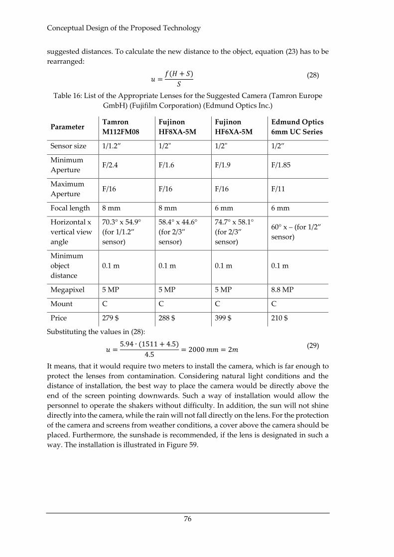
Conceptual Design of the Proposed Technology
76
suggested distances. To calculate the new distance to the object, equation (23) has to be
rearranged:
𝑢 =𝑓(𝐻 + 𝑆)
𝑆
(28)
Table 16: List of the Appropriate Lenses for the Suggested Camera (Tamron Europe
GmbH) (Fujifilm Corporation) (Edmund Optics Inc.)
Parameter Tamron
M112FM08
Fujinon
HF8XA-5M
Fujinon
HF6XA-5M
Edmund Optics
6mm UC Series
Sensor size 1/1.2” 1/2" 1/2" 1/2”
Minimum
Aperture F/2.4 F/1.6 F/1.9 F/1.85
Maximum
Aperture F/16 F/16 F/16 F/11
Focal length 8 mm 8 mm 6 mm 6 mm
Horizontal x
vertical view
angle
70.3° x 54.9°
(for 1/1.2”
sensor)
58.4° x 44.6°
(for 2/3”
sensor)
74.7° x 58.1°
(for 2/3”
sensor)
60° x – (for 1/2”
sensor)
Minimum
object
distance
0.1 m 0.1 m 0.1 m 0.1 m
Megapixel 5 MP 5 MP 5 MP 8.8 MP
Mount C C C C
Price 279 $ 288 $ 399 $ 210 $
Substituting the values in (28):
𝑢 =5.94 ∙ (1511 + 4.5)
4.5= 2000 𝑚𝑚 = 2𝑚
(29)
It means, that it would require two meters to install the camera, which is far enough to
protect the lenses from contamination. Considering natural light conditions and the
distance of installation, the best way to place the camera would be directly above the
end of the screen pointing downwards. Such a way of installation would allow the
personnel to operate the shakers without difficulty. In addition, the sun will not shine
directly into the camera, while the rain will not fall directly on the lens. For the protection
of the camera and screens from weather conditions, a cover above the camera should be
placed. Furthermore, the sunshade is recommended, if the lens is designated in such a
way. The installation is illustrated in Figure 59.

Hardware and equipment
77
Figure 59: Camera Installation Setup
5.2.3 Light Source
As it was mentioned in Chapter 3, the most efficient and economical light source,
ensuring uniform spectral distribution, is LED. For the considered case, the lightning
should be evenly spread across the screens to exclude the possibility of single spots
appearing brighter than others. This could be achieved with LED stripes. There are two
varieties of them existing on the market: addressable and non-addressable. Addressable
strips are designed in such a way, that each of the LEDs is a part of the array. Each of the
diodes fires is controlled individually and addressed in order of precession. These
stripes utilize three wires: power, ground, and data input. Non-addressable stripes fire
the diodes all together without the possibility to control each of the light sources
individually. These stripes may be both single colour or RGB (Red Green Blue). Single
colour LED strip consists usually of white diodes having either the same colour
temperature or different for the possibility of adjusting the light colour. For the aims of
the proposed technology, a white LED strip is the best option. The colour temperature
should be maximal, ensuring pure white light and absence of reflected colour
distortions.
The strip should be able to perform in outdoor conditions. Even though it is supposed
to be installed under the cover, there is also a possibility that humidity, fog, heavy rain,
or splashes from the shaker may damage the electronics. For that reason, an IP
(International Protection) codes were introduced (International Electrotechnical
Commission 2013). The most commonly sold stripes have protection codes IP 40, IP 54,
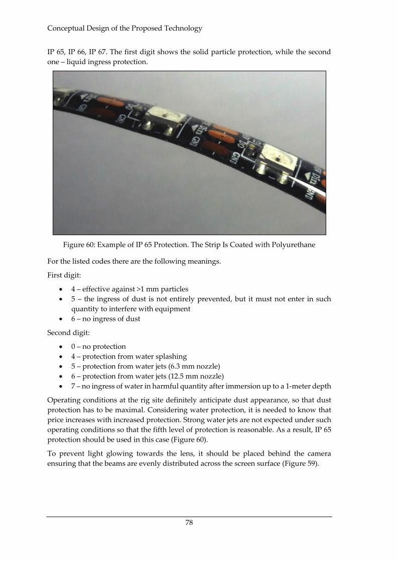
Conceptual Design of the Proposed Technology
78
IP 65, IP 66, IP 67. The first digit shows the solid particle protection, while the second
one – liquid ingress protection.
Figure 60: Example of IP 65 Protection. The Strip Is Coated with Polyurethane
For the listed codes there are the following meanings.
First digit:
• 4 – effective against >1 mm particles
• 5 – the ingress of dust is not entirely prevented, but it must not enter in such
quantity to interfere with equipment
• 6 – no ingress of dust
Second digit:
• 0 – no protection
• 4 – protection from water splashing
• 5 – protection from water jets (6.3 mm nozzle)
• 6 – protection from water jets (12.5 mm nozzle)
• 7 – no ingress of water in harmful quantity after immersion up to a 1-meter depth
Operating conditions at the rig site definitely anticipate dust appearance, so that dust
protection has to be maximal. Considering water protection, it is needed to know that
price increases with increased protection. Strong water jets are not expected under such
operating conditions so that the fifth level of protection is reasonable. As a result, IP 65
protection should be used in this case (Figure 60).
To prevent light glowing towards the lens, it should be placed behind the camera
ensuring that the beams are evenly distributed across the screen surface (Figure 59).

Software
79
5.2.4 Cover
The cover illustrated in Figure 59 is shown for demonstrative purposes. It may vary
depending on availability on the market, type, material, and size. It can also be crafted
by the drilling crew from a piece of water-resistant material, like nylon or polyamide
fabric by stretching it onto the carcass. The cover should be also mounted to the ground
with wire ropes to protect it from harsh weather conditions and strong wind in
particular. The supporting stand, which it is mounted to, shall also be attached to the
ground.
5.3 Software
After the images capturing with the camera, the information is streamed to the software
input, where it is to be analyzed. In order to get the algorithm working there are two
networks to be trained: one for classifying shapes and another one for classifying
lithology. Both of the networks belong to the CNN category, as long as they deal with
image analysis. When the frame arrives at the input, it is automatically prepared for
feature extraction. Afterwards, the first CNN for shape determination is run. If it is
impossible to identify any cavings on the screens, there is an additional check for mud
overflow conditions. If the cavings are detected successfully, the shape is determined.
The shape is automatically reported to mud logger at this stage to warn about
complications. Afterwards, size and lithology are detected in parallel. Size is calculated
by edge detection algorithms, whereas lithology is found by employing another CNN.
There is a chance of no lithology determination, as the cavings could not be cleaned
properly. At the output, each of the cavings is assigned with shape, size, and possibly
with lithology.
5.3.1 Network Building
The first stage is the input data collection. This should not necessarily be done at the rig
site, as it does not matter, where to take the pictures. However, to make the scenario
more real, the photos could be captured from the same position, as the features like edges
are texture is likely to appear the same that way in real conditions. Furthermore, the
cavings should be wet, as they are going to appear on the screens already washed by the
base fluid. In addition, the photos could be also taken by placing the rocks on the sieves.
The set should be split into training, validation, and testing sets. Training and validation
sets have to be labelled in advance so that the CNN actually learns the features from
given information. It was already mentioned in the literature, that the percentage of
samples is taken in the amount of 60%, 20% and 20% for the training, validation and
testing sets (Ran, et al. 2019).
After gaining the set for training and validation, the images should be fed into CNN. It
is not necessary to build the network from scratch, as there are already researchers
(mentioned in Chapter 3), who either used the already built model or designed a new
one. The same architecture could be used for both shape and lithology detection.
Training should stop when the loss reaches its minimum to avoid overfitting. After that
training should take place. If the accuracy of the model is high, then it is to be used at
the well site.

Conceptual Design of the Proposed Technology
80
5.3.2 Algorithm Workflow
The proposed algorithm is illustrated in Figure 61. It starts with the proportional
reshaping of the captured frame. Usually, up to six minimized copies of images are used.
The point is that the frame is to be scanned with a pre-determined stride by CNN with
a fixed size of the scanning matrix. It might be the case when the scanning matrix size is
not enough to cover large objects. In this case, the frame dimensions are decreased with
keeping the matrix size unchanged, which allows it to accommodate an object. When
these transformations are made, each of them is passed into the CNN input.
Figure 61: Workflow of the Parameters Detection Algorithm
There are three objectives to solve: detection, localization, and classification. Here it is
considered that CNN is already trained and has obtained all the necessary feature maps.
As it is seen in Figure 61, the algorithm is split into two directions. The left path goes to

Software
81
the classification of cavings into shapes, while the right one performs detection and
localization. These paths have FC layers and SF classifiers in each of them. The layers are
of the same size and work simultaneously, so that feature extraction is synchronized
with searching the object location. The detection is, as already was written above, is
conducted via scanning each of the frames and looking for similar features, like corners,
edges, patches, texture, etc. For each of the scanning steps the probability of the
appearance of the searched object is obtained, as well as the coordinates of the bounding
box. When the size of the scanning frame perfectly captures the object, the FC layer gives
the maximum probability of finding the desired part of the image. As long as the
movements inside the CNN are synchronized, for the obtained bounding box
coordinates the classified shape is obtained. As a result, there is a labelled object at the
output with a certain allocation on the frame.
In addition to shape labels, there could also be two extreme situations: mud overflow
and absence of cavings at the shakers. If there were only shapes in the SoftMax layer, the
CNN would only deliver shapes with a certain probability as an output, because the
neural network always tries to guess the probability of appearance of each label. For that
reason, two more labels should be introduced: the absence of cavings, when an only a
small amount of rock material appears on the screens, and mud overflow, when the
excess of the cuttings is visible. Both of the labels fall within the shape category and will
be analyzed by the first CNN.
There are two more parameters, which are to be extracted: size and lithology. The results
of previous operations will be used.
To detect the size, the Canny algorithm is applied, which determines the object contours.
Afterwards, another bounding box is applied, as it has the ability to rotate. This was not
the case with object detection, as the scanning of the image is proceeded by a matrix,
which is oriented strictly in a horizontal direction. The newly build bounding box fits
along the object’s largest dimension. Afterwards, the size of the box is calculated, giving
size on the output.
Lithology determination is proceeded inside of each localized objects. It is performed
similarly to shape determination: the CNN scans the images for the particular features.
Apart from patterns on the cavings surface and their contours, which are essential for
shape detection, lithology is determined to base mostly on cavings colour, as well as the
texture of the cavings surface. There are two reasons, why a separate network is desired
for classifying lithology located at this part of the algorithm. The first one is a distinct
group of features. It is not possible to allocate two different classifiers inside one CNN.
As long as the intention is to get two classes for each separate caving, there is a need for
an additional network. The second reason, why CNN is allocated at this stage is saving
computing power. The first CNN gets as input six images, which are to be scanned. And
each of these images is to be scanned multiple times. If it was the case, when two CNNs
were running in parallel, there would be too many unnecessary calculations. This means
that it is much more economically from the processing point of view to place the second
CNN sequentially and not in parallel.
Another important point is the detection part of the algorithm. In some cases, object
detection could be done not with CNN, but with the Canny algorithm, which detects
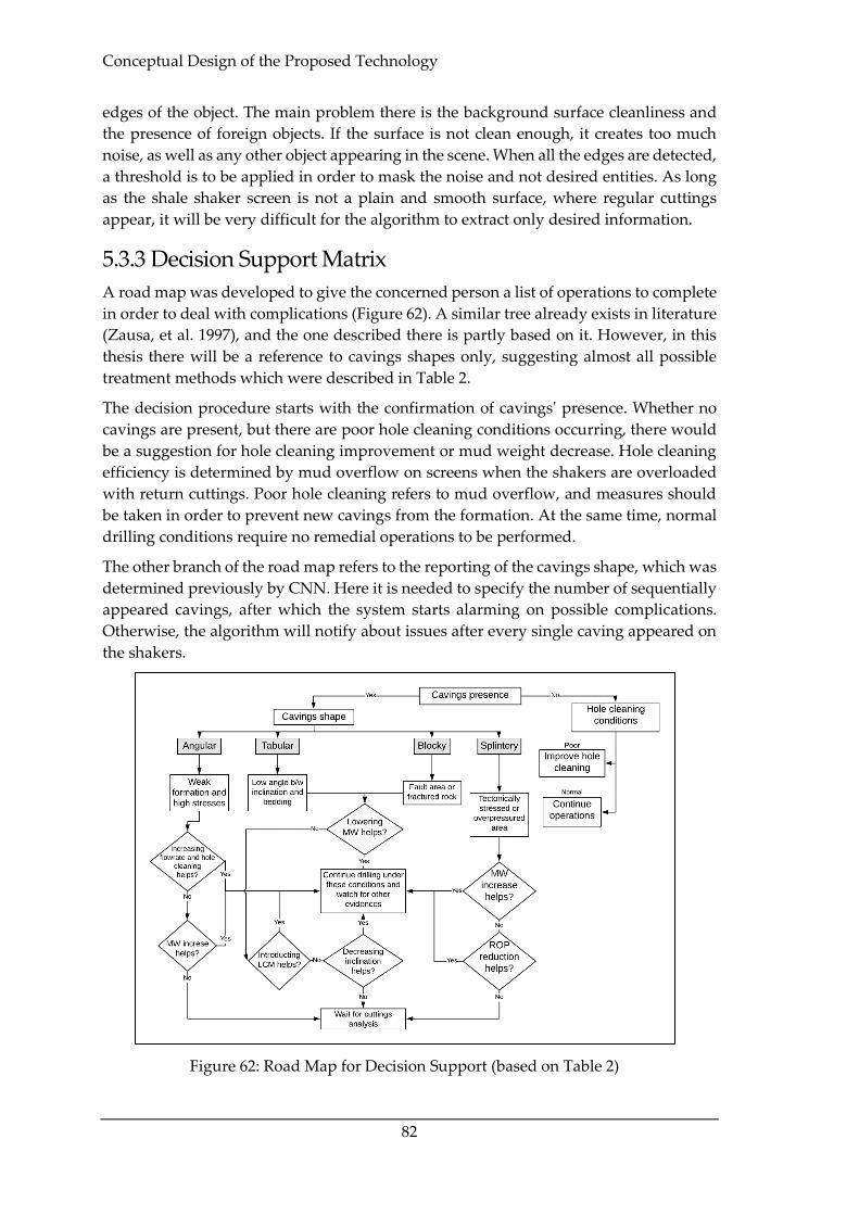
Conceptual Design of the Proposed Technology
82
edges of the object. The main problem there is the background surface cleanliness and
the presence of foreign objects. If the surface is not clean enough, it creates too much
noise, as well as any other object appearing in the scene. When all the edges are detected,
a threshold is to be applied in order to mask the noise and not desired entities. As long
as the shale shaker screen is not a plain and smooth surface, where regular cuttings
appear, it will be very difficult for the algorithm to extract only desired information.
5.3.3 Decision Support Matrix
A road map was developed to give the concerned person a list of operations to complete
in order to deal with complications (Figure 62). A similar tree already exists in literature
(Zausa, et al. 1997), and the one described there is partly based on it. However, in this
thesis there will be a reference to cavings shapes only, suggesting almost all possible
treatment methods which were described in Table 2.
The decision procedure starts with the confirmation of cavings' presence. Whether no
cavings are present, but there are poor hole cleaning conditions occurring, there would
be a suggestion for hole cleaning improvement or mud weight decrease. Hole cleaning
efficiency is determined by mud overflow on screens when the shakers are overloaded
with return cuttings. Poor hole cleaning refers to mud overflow, and measures should
be taken in order to prevent new cavings from the formation. At the same time, normal
drilling conditions require no remedial operations to be performed.
The other branch of the road map refers to the reporting of the cavings shape, which was
determined previously by CNN. Here it is needed to specify the number of sequentially
appeared cavings, after which the system starts alarming on possible complications.
Otherwise, the algorithm will notify about issues after every single caving appeared on
the shakers.
Figure 62: Road Map for Decision Support (based on Table 2)

Cost Estimation for Proposed System
83
As it is seen further, the cavings’ shape automatically indicates the possible cause of the
complication. Afterwards, there is a suggestion on changing the drilling parameters, e.g.
changing the mud weight or ROP. A series of such decisions are formed until two
outcomes are reached. The first one is quite straightforward and is achieved if one of the
changes in drilling parameters actually helped to remedy the situation. When none of
the taken actions resulted in successful operation, it would be suggested to consistently
wait for the cuttings analysis and possibly perform reaming or washing procedures.
5.4 Cost Estimation for Proposed System
The technology cost was estimated by summing the costs of all the included categories
of equipment: pump, sprinklers, tray, hoses and pipes, filter, camera, lens, cover, support
stand, LED lights, and GPU. The prices were taken from online stores in the
corresponding category of items. The costs presented in this section are a rough
estimation and the calculation performed here are basic, and the value of the whole
system can actually double. In case no other challenges are faced and no extra work is
required (installation, mounting, training the CNN, supplying additional computers for
the software, etc.), the cost can be close to the estimated one.
Regarding the hardware items, not all of the parts have fixed cost, as such parameters as
dimensions, amount of equipment and their performance are uncertain. In addition,
there is a tolerance in accordance with price change during time. Furthermore, the same
item might be available at different prices, depending on delivery costs and the policy
of the store or vendor. Basing on the extracted data, cost distribution for each of the items
was taken. Mean values, as well as standard deviation, are were calculated in order to
give an impression of the variability of items costs. They are listed in Table 17.
Table 17: Items for the Technology Cost Estimation
Item Mean, $ Standard deviation
Pump 333,18 285,76
Sprinkler 34,73 22,46
Tray 64,52 71,86
Hose and pipes 125,09 88,30
Filter 11,75 7,74
Camera 509,00 0,00
Lens 294,00 67,72
Cover 37,42 18,45
Support stand 43,27 22,05
LED 29,75 15,49
GPU 432,18 192,99

Conceptual Design of the Proposed Technology
84
In addition, other costs should be included in the technology (Table 18). These are the
base fluid costs, installation costs, and maintenance. The base fluid is chosen as diesel to
give higher cost expectations. The price is taken as 1,12 $ per litre. The amount of needed
base mud is expected to be 250 litres. Maintenance should include pipe unclogging, filter
change, pump inspection, as well as the camera setup and changing light conditions
when needed.
Table 18: Additional Cost Categories
Category Cost, $
Base fluid (diesel) 280
Installation costs 100
Maintenance 200
Technology cost was determined with the help of Monte Carlo Simulation. For each of
the items, the cost was determined, having in mind that the probability of its occurrence
was chosen randomly. All the costs were summed up, giving the final cost distribution
as an output. This process was conducted one thousand times, giving the distribution of
technology costs. This distribution is illustrated in Figure 63.
As it is seen, the mean value is located in the vicinity of 2500 $. Other parameters, like
standard deviation, were calculated and listed in Table 19.
Table 19: Parameters for the Technology Cost Distribution
Parameter Value
Mean 2495,7
Standard deviation 365,4
Min 1761,8
Max 3707,6
Skewness 0.634
Kurtosis -0.017
It is seen that skewness is relatively high and positive which says that the distribution
tail tends to the larger values. This could be explained by the fact that the prices are not
distributed normally and tend to be allocated in the vicinity of a certain value.
Furthermore, the higher the price gets, the lower number of items appears on the market.
In addition, kurtosis is negative, implying that the data is a little widely distributed than
the ideal normal distribution function.
Basing on the distributed values, the Cumulative Distribution Function (CDF) was built
in order to determine P10, P50, and P90 costs. The function is illustrated in Figure 64.

Cost Estimation for Proposed System
85
Figure 63: Total Cost Distribution of the Proposed Technology
Figure 64: Cumulative Distribution Function (CDF) of the Technology Cost
From this function, it is possible to determine P10, P50, and P90 values, which are
defined as 10th, 50th, and 90th percentiles correspondingly. Percentile basically means,
how much of the data is located below the chosen probability. For example, P50 value
in the considered case shows the cost, below which the probability of its likelihood of
appearance is below 50 percent. Consequently, P10 shows optimistic results, P90 stands
for the pessimistic result, and P50 shows the median value, which is located exactly in
the middle position of all the data. The values for P10, P50, and P90 costs are listed in
Table 20.

Conceptual Design of the Proposed Technology
86
Table 20: P10, P50, and P90 Values
Percentile Value, $
P10 2028,09
P50 2496,23
P90 2964,26
The proposed technology consists of quite a large number of items, which prices are
widely distributed on market. These items (pipelines, rack, and cover for the camera,
etc.) do not significantly affect the technology performance, which means that it is
possible to save budget on them. In addition, this gives some extra savings to buy more
powerful CPUs and GPUs. In addition, there is also a possibility to take better lenses,
which are shake and shock-resistant. It is especially important if the shakers will be
having large amplitudes. It might be the case, of the shaker is poorly dampen, and some
of the vibrations are transferred through the skid and rack, affecting camera
performance.
5.5 Limitations
There are a certain number of limitations in the proposed system, regarding mostly the
hardware part.
A high number of shale shaker models and manufacturers introduce a certain challenge
in the tray installation, as the space between the sieves and the shaker’s body may vary
in wide ranges. It implies that it might be not possible to install the circulation system at
all for some shakers' models. In another case, the tray volume may also vary.
The main complexity of the sprinkler head installation would be the shaking behaviour
of the shaker. To provide the rigidity of the construction, it is important to not only hang
the sprinklers on the shaker walls but also attach it with clamps, screw or weld them, if
it is necessary. In addition, the ability of a sprinkler head should be actually tested, if the
pressure and amount of fluid are enough to clean the cavings from mud and finer
particles. It also should be checked, if the tray could be actually located beneath the
shakers, as they all vary depending on their design features and dimensions. It is also
unclear so far if the base fluid will be contaminated by finer particles, which were
washed away. This might require the installation of filters at the pump intake and their
change. Otherwise, the sprinklers are likely to be blocked and damaged with time.
There are also challenges in camera installation. In some of the shale shaker models, the
screens could be covered with an enclosure. This creates a barrier between the camera
and screens, which makes the cavings image capturing impossible. In addition, there is
often a series of shaker in the solids control system. They are usually joined with a long
gasket for capturing the cuttings, which occupies sufficient space. Here it might be hard
to allocate the supporting stand with a camera and lightning facility.
Checks for illuminations should also be done, as it is not clear, how the camera sensor
will perform with specks of light, low light conditions at night shift, and whether the

Limitations
87
scene will change with alterations of ambient light. From that perspective, a light sensor
should be installed to automatically adjust the intensity of the LED.
It also should be checked, if the chosen GPU will actually deliver the results with
minimal delay, as it makes no sense if the determination of essential parameters will
proceed with too large lag time. As it was already mentioned, the algorithm has to react
fast, as time has to be spared.
As was mentioned, the circulation system might not be actually installed due to the
original shale shaker design. In this case, the lithology could not be determined properly.
Here it should be tested if CNN can actually determine the lithology of the unwashed
cavings.

Conceptual Design of the Proposed Technology
88
Conclusion
89
Chapter 6 Conclusion and
Recommendations
6.1 Conclusion
For ensuring the trouble-free drilling performance it is important to be aware of possible
complications and borehole instability events. For this reason, cavings analysis serves as
a powerful methodology in order to identify not only the signs of instability but also its
root cause. Conventional implementation of this technique is time-consuming and does
not allow to react proactively on changing drilling conditions.
In order to increase the effectiveness of the already existing workflow, a study on the
automated cuttings measurement and analysis techniques was conducted. The utilized
tools were compared and contrasted It was decided to focus on computer vision
techniques because of their robustness and the possibility of performing remote
measurements.
Such tools in the majority of cases are combined with specially designed software, which
conducts the image analysis and extracts features from objects. The software often
belongs to a large family of algorithms called Convolutional Neural Networks. In this
thesis, a review on them is conducted, discussing their working principle, as well as
preparation and training procedure.
Basing on the observed analysis techniques, an automated cavings analysis system is
proposed with respect to the following criteria:
• Simplicity
• Cost-effectiveness
• The ability of multiple parameters extraction
The heart of the installation is the camera, which performs all the data acquisition. A
cover and illumination provided in order to protect the camera from harsh weather
conditions and ensure the purity of data capturing. The main benefit of the camera is
that it does not disturb the mud separation process. The only modification of shale
shakers is the circulation system. This system might be removed if lithology
determination is not necessary in the considered case.
Apart from that, the system does not involve expensive sensors and heavy machinery
the system would require, however, maintenance costs for the circulation system. From
the side, the one-time investment might save hours of NPT and also the money spent on
third-party services, fishing equipment, and rig rent.
The final part of the system is the road map to support decision making, which basically
gives the recommendations to the involved personnel, based on determined cavings
morphology by the CNN ensemble. It was introduced to the associated algorithm
because the involved employees are demanding for the validation of their actions.
Usually, the actions to mitigate the complications are taken basing only on the
experience, and the amount of real-time data is often not enough to take control of the

Conclusion and Recommendations
90
situation correctly. For that reason, a flowchart is suggested, in which actions are
validated by causal reactions between return cavings and the nature of complications.
6.2 Recommendations and Future Work
It was already discussed that CNN has to be trained in advance, so it is required to collect
a set of proper images to train the network and also label them. This part is the most
labour-intensive and time-consuming. Training can be actually done at the rig site and
with actual shale shakers. This would ensure that the images are similar during training
and testing.
As long as the camera captures quite a lot of visual information, there is also a possibility
to extend the network and include some extra features to analyze. As long as there is a
freedom of choice in software installations and CNN architectures, the user has
alternatives of tools and frameworks to choose from. This is what makes the proposed
installation flexible and robust.
In addition, the road map for decision making should be updated and built on real data
in order to make it closer to reality. Furthermore, an additional analysis could be
conducted, establishing the relationship between cavings features and the least required
change to drilling parameters. This would give the employees a range of safe
adjustments to drilling parameters.

Shape
91
Appendix A Cuttings description
parameters
A.1 Shape
The shape is described in Table 21.
Table 21: Cuttings Shape Description (International Logging, Inc. 2001)
Cuttings type Description
Blocky Used to describe claystone, marl, limestone in which
fractures are developed at approximately right angles, so
that small blocks are formed
Subblocky Commonly used to describe PDC drilled cuttings that are
not quite 100% blocky with clean breaks and imperfect right
angles
Angular Used to describe well-lithified formations that break chips
with angular surfaces, generally as limestones and siliceous
hard formations
Amorphous or
Irregular
Cuttings with no distinct shape
Conchoidal Commonly seen in dense rocks such as chert, argillite, flint,
and coal. The term refers to concave and convex surfaces
developed on fractures
Elongated Used to describe rocks, which length is significantly greater
than their width
Tabular The cuttings samples, which were formed by breaking
along the bedding plane
Flaky The rock fractured into small flakes or chips. Common in
some marls and occasionally in metamorphic rocks
Platy Flaky, but used mostly with shales
Fissile Rock is which is capable of being split or divided in the
direction of the grain or along natural planes of cleavage; a
characteristic of shales
Splintery Used to describe shales in which the fissility is not strongly
developed, but exists sufficiently to cause irregular surfaces
and edges; mostly used to describe some carbonates coals
and shales.

Cuttings description parameters
92
A.2 Roundness and Sphericity
Cuttings grains are described according to their roundness and sphericity. This is very
important, that only the grains are inspected in the discussed way, and not the cuttings
or cavings themselves. However, the presented description method (or its analogue)
might be used to distinguish cavings.
Roundness refers to the roughness of the surface. Sphericity refers to the grain shape in
comparison with a sphere of the same volume as the inspected grain.
Basically, two most-frequently scales are present nowadays, presented by (Krumbein
and Sloss 1951) and (Powers 1953), which are illustrated in Figure 65 and Figure 66.
Figure 65: Chart for Roundness and Sphericity Estimation (Krumbein and Sloss 1951)
Figure 66: Roundness and Sphericity (Powers 1953)
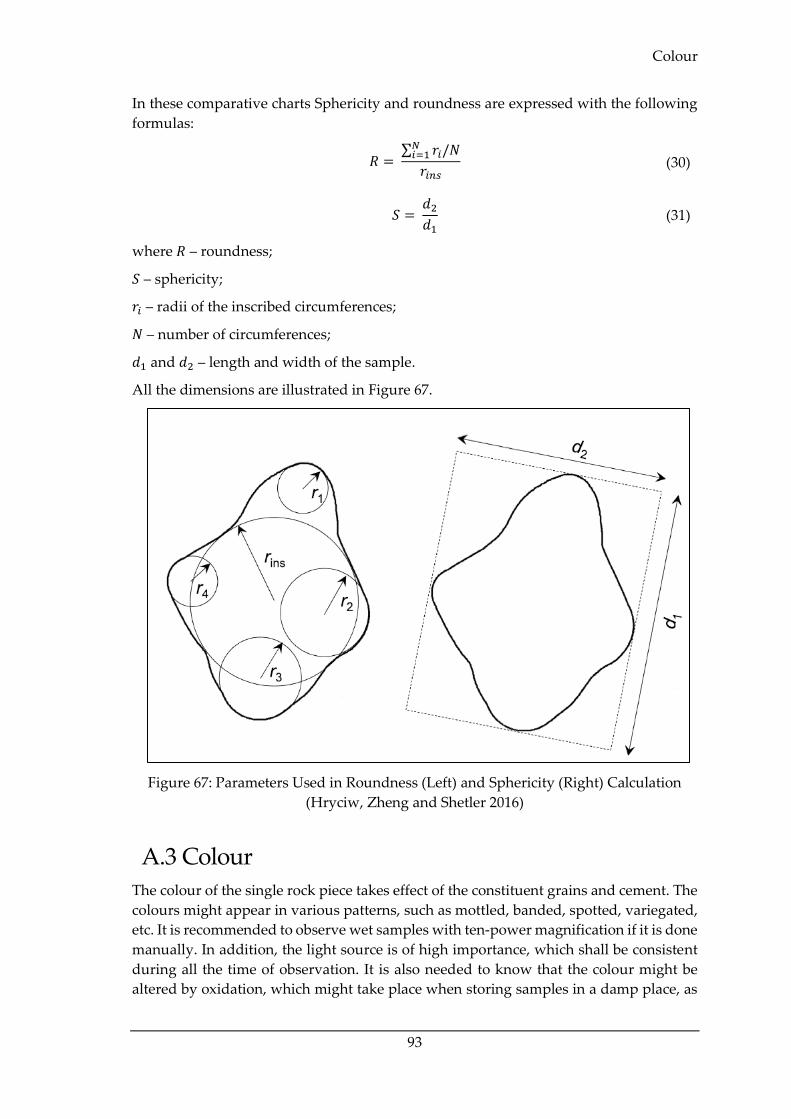
Colour
93
In these comparative charts Sphericity and roundness are expressed with the following
formulas:
𝑅 =
∑ 𝑟𝑖/𝑁𝑁𝑖=1
𝑟𝑖𝑛𝑠 (30)
𝑆 =
𝑑2
𝑑1 (31)
where 𝑅 – roundness;
𝑆 – sphericity;
𝑟𝑖 – radii of the inscribed circumferences;
𝑁 – number of circumferences;
𝑑1 and 𝑑2 – length and width of the sample.
All the dimensions are illustrated in Figure 67.
Figure 67: Parameters Used in Roundness (Left) and Sphericity (Right) Calculation
(Hryciw, Zheng and Shetler 2016)
A.3 Colour
The colour of the single rock piece takes effect of the constituent grains and cement. The
colours might appear in various patterns, such as mottled, banded, spotted, variegated,
etc. It is recommended to observe wet samples with ten-power magnification if it is done
manually. In addition, the light source is of high importance, which shall be consistent
during all the time of observation. It is also needed to know that the colour might be
altered by oxidation, which might take place when storing samples in a damp place, as
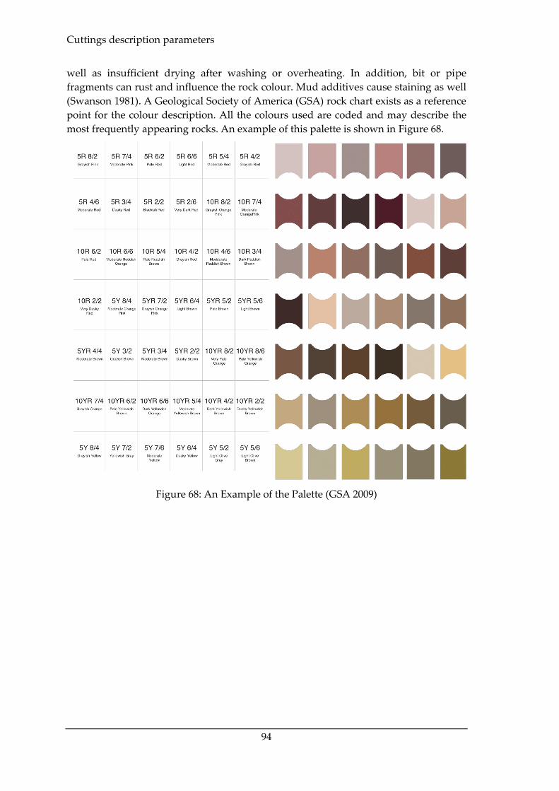
Cuttings description parameters
94
well as insufficient drying after washing or overheating. In addition, bit or pipe
fragments can rust and influence the rock colour. Mud additives cause staining as well
(Swanson 1981). A Geological Society of America (GSA) rock chart exists as a reference
point for the colour description. All the colours used are coded and may describe the
most frequently appearing rocks. An example of this palette is shown in Figure 68.
Figure 68: An Example of the Palette (GSA 2009)
Bibliography
95
Bibliography
Aldred, W., D. Plumb, I. Bradford, L. Cousins, J. Fuller, S. Goraya, and D. Tuker. 1999.
"Oilfiled Review - Managing Drilling Risk." Schlumberger.
Bowes, Colin, and Ray Procter. 1997. Drillers Stuck pipe Handbook. Ballater, Scotland:
Procter & Collins Ltd.
Bradford, I. D. R., W. A. Aldred, J. M. Cook, E. F. M. Elewaut, J. A. Fuller, T. G.
Kristiansen, and T. R. Walsgrove. 2000. "When Rock Mechanics Met Drilling:
Effective Implementation of Real-Time Wellbore Stability Control." IADC/SPE
Drilling Conference. New Orleans: SPE.
Brading, Michael, Kenneth Salsman, Manjunath Somayaji, Brian Dipert, Tim Droz,
Daniël Van Nieuwenhove, and Pedro Gelabert. 2013. "3-D Sensors Bring Depth
Discernment to Embedded Vision Designs." Embedded Vision Alliance. July 12.
Accessed April 15, 2020. https://www.edge-ai-vision.com/2013/07/3-d-sensors-
bring-depth-discernment-to-embedded-vision-designs/.
Carr, Russell, Lance Yarbrough, Nicholas Lentz, Kathleen Neset, Brian Lucero, and Tim
Kirst. 2014. "On-Site XRF Analysis of Drill Cuttings in the Williston Basin."
SPE/AAPG/SEG Unconventional Resources Technology Conference. Denver,
Colorado: Unconventional Resources Technology Conference.
Cyganek, Bogusław, and Paul J. Siebert. 2009. An Introduction to 3D Computer Vision
Techniques and Algorithms. West Sussex, United Kingdom: John Wiley & Sons,
Ltd.
Du, Xunsheng, Yuchen Jin, Xuqing Wu, Yu Liu, Xianping Wu, Omar Awan, Joey Roth,
et al. 2020. "Classifying Cutting Volume at Shale Shakers in Real-Time Via Video
Streaming Using Deep-Learning Techniques." SPE Drilling and Completion
(Society of Petroleum Engineers). doi:https://doi.org/10.2118/194084-PA.
EAGE. 2019. EAGE Earth-Hack. February. Accessed April 28, 2020.
https://students.eage.org/sitecore/content/events/home/2019/big-data-and-
machine-learning/eage-earth-hack?sc_lang=en.
Edmund Optics Inc. n.d. 6mm UC Series Fixed Focal Length Lens. Accessed May 28, 2020.
https://www.edmundoptics.com/p/6mm-uc-series-fixed-focal-length-lens/2967/.
European Commission. 2000. "DIRECTIVE 1999/92/EC OF THE EUROPEAN
PARLIAMENT AND OF THE COUNCIL." Official Journal of the European
Communities 57-64.
FLIR® Systems. 2018. BlackFly GigE | FLIR Systems. Accessed April 20, 2020.
https://www.flir.com/products/blackfly-gige/.
—. 2018. Blackfly S GigE | FLIR Systems. Accessed May 27, 2020.
https://www.flir.com/products/blackfly-s-gige/?model=BFS-PGE-23S3C-C.
Bibliography
96
Fofi, David, Tadeusz Sliwa, and Yvon Voisin. 2004. "A comparative survey on invisible
structured light." Accessed April 15, 2020.
http://www.le2i.cnrs.fr/IMG/publications/fofi04a.pdf.
Forta Corporation. 1997. "FORTA® Super-Sweep® Video." YouTube. Accessed May 27,
2020. https://www.youtube.com/watch?v=68cvNYizCf0.
Fujifilm Corporation. n.d. HF-XA-5M series. Accessed May 28, 2020.
http://mvlens.fujifilm.com/en/product/hfxa5m.html.
Gallant, C., J. Zhang, C. A. Wolfe, J. Freeman, T. M. Al-Bazali, and M. Reese. 2007.
"Wellbore Stability Considerations for Drilling High-Angle Wells Through
Finely Laminated Shale: A Case Study from Terra Nova." SPE Annual Technical
Conference and Exhibition. Anaheim, California: Society of Petroleum Engineers.
Geng, J. 2011. "Structured-light 3D surface imaging: a tutorial." Advances in Optics and
Photonics 128-160.
GN Solids Control. 2020. Shale shaker, linear motion shaker - GN Solids Control. Accessed
May 27, 2020. https://www.gnsolidscontrol.com/shale-shaker.
GSA. 2009. Geological Rock-Color Chart. Munsell Color.
Han, Runqi, Pradeepkumar Ashok, Mitchell Pryor, and Eric van Oort. 2018. "Real-Time
3D Computer Vision Shape Analysis of Cuttings and Cavings." SPE Annual
Technical Conference and Exhibition. Dallas, Texas: Society of Petroleum Engineers.
Han, Runqi, Pradeepkumar Ashok, Mitchell Pryor, Eric van Oort, Paul Scott, and Isaac
Reese and Kyle Hampton. 2017. "Real-Time Borehole Condition Monitoring
using Novel 3D Cuttings Sensing Technology." SPE/IADC Drilling Conference and
Exhibition. The Hague, Netherlands: Soсiety of Petroleum Engineers.
Hryciw, Roman D., Junxing Zheng, and Kristen Shetler. 2016. "Particle Roundness and
Sphericity from Images of Assemblies by Chart Estimates and Computer
Methods." Journal of Geotechnical and Geoenvironmental Engineering 142 (9).
doi:10.1061/(ASCE)GT.1943-5606.0001485.
International Electrotechnical Commission. 2013. IEC 60529 Degrees of protection provided
by enclosures (IP Code). Geneva.
International Logging, Inc. 2001. Basic Mud Logging. Singapore.
Karimi, Moji. 2013. "Drill-Cuttings Analysis for Real-Time Problem Diagnosis and
Drilling Performance Optimization." SPE Asia Pacific Oil & Gas Conference and
Exhibition. Jakarta, Indonesia: Society of Petroleum Engineers.
Kathrada, Muhammad, and Benjamin Jacob Adillah. 2019. "Visual Recognition of Drill
Cuttings Lithologies Using Convolutional Neural Networks to Aid Reservoir
Characterisation." SPE Reservoir Characterisation and Simulation Conference and
Exhibition. Abu Dhabi: Society of Petroleum Engineers.
Kristiansen, Tron Golder. 2004. "Drilling Wellbore Stability in the Compacting and
Subsiding Valhall Field." IADC/SPE Drilling Conference. Dallas, Texas: SPE.

Bibliography
97
Krizhevsky, Alex, Ilya Sutskever, and Geoffrey E. Hilton. 2012. "ImageNet Classification
with Deep Convolutional Neural Networks." Advances in Neural Information
Processing Systems 1097-1105.
Krumbein, W. C., and L. L. Sloss. 1951. Stratigraphy and Sedimentation. San Francisco:
Freeman & Co.
Kumar, D., S. Ansari, S. Wang, J. YiMing, S. Ahmed, M. Povstyanova, and B. Tichelaar.
2012. "Real-time Wellbore Stability Analysis: An Observation from Cavings at
Shale Shakers." AAPG International Convention and Exhibition. Singapore.
Legutko, Stanislaw, Pero Raos, and Remigiusz Labudzki. 2014. "The essence and
applications of machine vision." Tehnicki Vjesnik 903-909.
Li, Larry. 2014. "Time-of-Flight Camera - An Introduction." Texas Instruments. May.
Accessed April 14, 2020. http://www.ti.com/lit/wp/sloa190b/sloa190b.pdf.
LMI Technologies. 2016. Gocator 2380 | LMI3D. Accessed April 20, 2020.
https://lmi3d.com/gocator-2380.
Malvern Instruments. n.d. Mastersizer 2000. Accessed May 5, 2020.
https://www.malvernpanalytical.com/en/support/product-support/mastersizer-
range/mastersizer-2000/#manuals.
Marana, A.N., I.R. Guilherme, J.P. Papa, M.V.D. Ferreira, K. Miura, and F.A.C. Torres.
2010. "An Intelligent System to Detect Drilling Problems Through Drilled
Cuttings Return Analysis." IADC/SPE Drilling Conference and Exhibition. New
Orleana, Louisiana: Society of Petroleum Engineers.
M-I L.L.C. 2019. "Solid Control, Cuttings Management and Fluids Processing."
Schlumberger. Accessed May 28, 2020. https://www.slb.com/-
/media/files/mi/catalog/solids-control-cuttings-management-fluids-processing-
catalog.ashx.
Naegel, M., E. Pradie, T. Delahaye, C. Mabile, and G. Roussiaux. 1998. "Cuttings Flow
Meters Monitor Hole Cleaning in Extended Reach Wells." European Petroleum
Conference. The Hague, Netherland: Society of Petroleum Engineers. 401-408.
doi:https://doi.org/10.2118/50677-MS.
Nasrullah, K., and A. K. Naeem. 2011. "Comparative study of energy saving light
sources." Renewable and Sustainable Energy Reviews 15: 296-309. doi:DOI:
10.1016/j.rser.2010.07.072.
National Instruments. 2012. Parts o a Stereo Vision System. June. Accessed April 14, 2020.
https://zone.ni.com/reference/en-XX/help/372916M-
01/nivisionconceptsdita/guid-cb42607e-f256-40f5-ab6e-28ec3a33bcda/.
Olympus. 2019. Field Portable XRD and XRF for Shale Gas Drilling Efficiency. Accessed May
12, 2020. https://www.olympus-ims.com/en/applications/field-portable-xrf-
shale-gas/.
Omland, T.H., A. Saasen, K. Taugbøl, B. Dahl, T. Jørgensen, F. Reinholt, N. Scholz, et al.
2007. "Improved Drilling-Process Control Through Continuous Particle and

Bibliography
98
Cuttings Monitoring." SPE Digital Energy Conference. Houston, Texas: Society of
Petroleum Engineers.
Pandalaneni, Karthik. 2016. "Focused beam reflectance measurement as a tool for in situ
monitoring of the lactose crystallization process." Journal of Dairy Science 99 (7):
5244-5253. doi:http://dx.doi.org/10.3168/jds.2015-10643.
Pankewitz, Axel, and Helmut Geers. 2020. In-Line Crystal Size Distribution nalysis in
industrila crystallistion processes by Ultrasonic Extinction. Sampatec GmbH.
Pašić, B., N. Gaurina-Međimurec, and D. Matanović. 2007. "Wellbore instability: Causes
and Consequences." Rudarsko-geološko-naftni zbornik 19: 87-98.
Powers, M. C. 1953. "A New Roundness Scale for Sedmentary Basins." Journal of
Sedimentary Particles 23 (2): 117-119.
Ran, Xiangjin, Linfu Xue, Yanyan Zhang, Zeyu Liu, Xuejia Sang, and Jinxin He. 2019.
"Rock Classification from Field Image Patches Analyzed Using a Deep
Convolutional Neural Network." Mathematics.
Ruessink, B.H., and D.G. Harville. 1992. "Quantitative Analysis of Bulk Mineralogy: The
Applicability and Performance of XRD and FTIR." SPE Inti. Sympoalum on
Formation Damage Control. Lafayette, Louisiana: Society of Petroleum Engineers.
533-546.
Saasen, A, T.H. Omland, S. Ekrene, J. Brévière, E. Villard, N. Kaageson-Loe, A. Tehrani,
et al. 2009. "Automatic Measurement of Drilling Fluid and Drill-Cuttings
Properties." SPE Drilling & Completion (Society of Petroleum Engineers) 24 (04):
611-625. doi:https://doi.org/10.2118/112687-PA.
SAMCON GmbH. 2020. Ex-d camera enclosures. Accessed June 18, 2020.
https://www.samcon.eu/en/products/ex-d-camera-enclosures/.
Schlumberger. 2015. "CLEAR Hole cleaning and wellbore risk reduction service."
Schlumberger. Accessed April 11, 2020. https://www.slb.com/-
/media/files/geoservices/product-sheet/clear-ps.ashx.
—. 2015. "CLEAR Hole cleaning and wellbore risk reduction service brochure."
Schlumberger. Accessed April 11, 2020. https://www.slb.com/-
/media/files/drilling/brochure/clear-brochure-br.ashx.
—. 2016. "Integrated Drilling Approach Achieves Single-Run Lateral to Save 2.5 Days
and USD 148,000 off AFE." Schlumberger. Accessed April 11, 2020.
https://www.slb.com/-/media/files/geoservices/case-study/clear-middle-east-
cs.ashx.
—. 2013. MONGOOSE PRO Shale Shaker | Schlumberger. Accessed May 27, 2020.
https://www.slb.com/drilling/drilling-fluids-and-well-cementing/solids-
control/shale-shakers/mongoose-pro-shale-shaker.
—. 2015. "Operator Saves 16 Rig Hours and USD 194,000 Using CLEAR Service."
Schlumberger. Accessed April 11, 2020. https://www.slb.com/-
/media/files/geoservices/case-study/clear-indonesia-cs.ashx.

Bibliography
99
—. 2019. "X-Ray Diffraction While Drilling." Schlumberger. Accessed May 5, 2020.
https://www.slb.com/-/media/files/drilling/product-sheet/ecoflex-x-ray-
diffraction-ps.ashx.
Schumberger. 2019. "X-Ray Fluorescence While Drilling." Schlumberger. Accessed May 4,
2020. https://www.slb.com/-/media/files/drilling/product-sheet/ecoflex-
lithoflex-x-ray-fluorescence-ps.ashx.
Skea, Christopher, Alireza Rezagholilou, Pouria Behnoudfar, Raoof Gholami, and
Mohammad Sarmadivleh. 2018. "An approach for wellbore failure analysis using
rock cavings and image processing." Journal of Rock Mechanics and Geothechnical
Engineering. doi:https://doi.org/10.1016/j.jrmge.2018.04.011.
Swanson, R. G. 1981. Sample Examination Manual. Tulsa, Oklahoma: The American
Assiciation of Petroleum Geologists.
Sympatec GmbH. 2017. NIMBUS | Particle size and concentration analysis in laboratory.
Accessed May 12, 2020. https://www.sympatec.com/en/particle-
measurement/sensors/ultrasonic-extinction/nimbus/.
Tamron Europe GmbH. n.d. Machine Vision / FA / ITS Lenses. Accessed May 5, 2020.
https://www.tamron.eu/industrial-optics/products/mega-pixel-machine-vision-
fa-its-lenses/#M112FM08.
TR Solids Control. 2016. "Shale Shaker for Horizontal Directional Drilling." YouTube.
December 20. Accessed May 27, 2020.
https://www.youtube.com/watch?v=aS5r_PM9DQA.
van Oort, Eric, and Besmir Buranaj Hoxha. 2016. "Automated Drilling Fluid Analysis
using Advanced Particle Size Analyzers." IADC/SPE Drilling Conference and
Exhibition. Fort Worth, Texas: IADC/SPE.
Zausa, F., L. Civolani, M. Brignoli, and F.J. Santarelli. 1997. "Real-Time Wellbore Stability
Analysis at the Rig-Site." SPE/IADC Drilling Coference. Amsterdam: Society of
Petroleum Engineers. 837-846.
Zoback, M.D., C.A. Barton, M. Brudy, D.A. Castillo, T. Finkbeiner, B.R. Grollimund, D.B.
Moos, P. Peska, C.D. Ward, and D.J. Wiprut. 2003. "Determination of stress
orientation and magnitude in deep wells." International Journal of Rock Mechanics
and Mining Sciences 1049-1076.
Zoback, Mark. 2007. Reservoir Geomechanics. Cambridge: Cambridge University Press.

Bibliography
100

Acronyms
101
Acronyms
ADC Analog-to-Digital Converter
ANN Artificial Neural Network
BC Bayesian Classifier
CDF Cumulative Distribution Function
CNN Convolutional Neural Network
CFL Compact Fluorescent Lamp
CFM Cuttings Flow Meter
CNN Convolutional Neural Network
CPU Central Processing Unit
ERD Extended Reach Drilling
GPU Graphics Processing Unit
IDE Integrated Development Environment
IP International Protection
LCM Lost Circulation Material
LED Light-Emitting Diode
LPA Liquid particle Analyzer
LSB Least Significant Bit
MLP Multilayer Perception
MSB Most Significant Bit
MSE Mean Squared Error
OPF Optimum Path Forest
PDC Polycrystalline Diamond Composite
PSD Particle Size Distribution
RGB Red Green Blue
RAM Random-Access Memory
ReLU Rectified Linear Unit
ROI Region of Interest
ROP Rate of Penetration
SDK Software Development Kit
SSL Solid-state Lightning

Acronyms
102
SVM Support Vector Machines
VGG Visual Geometry Group
XRD X-ray Diffraction
XRF X-ray Fluorescence

Symbols
103
Symbols �̂� computed input -
𝑦 target value -
𝑥 neuron input -
𝑤 weight -
𝑏 bias -
𝑖 index -
𝑁 number of elements -
𝐶 cost function -
𝛿 error -
𝜎 activation function -
𝑊 array width -
𝐻 array height -
𝐷 array depth -
𝐹 filter size -
𝑃 zero padding -
𝑆 stride -
𝐾 number of filters -
𝑢 distance to the object mm
𝑣 distance to the image mm
𝑓 focal length mm
𝑆𝑠 sensor size mm
𝐻𝑜 object’s largest dimension mm
𝑘𝑐𝑟 crop factor -
𝑑𝑚𝑎𝑥 maximal sensor diagonal mm
𝑑𝑢𝑠𝑒𝑑 used sensor diagonal mm

Symbols
104

List of Figures
105
List of Figures
Figure 1: NPT Breakdown by Root Cause ............................................................................................. 2 Figure 2: Reported Consumption of Fluids and Additives In 2019 By OMV ................................... 3 Figure 3: Televiewer Image Logs of a Well With Wellbore Breakouts (Dark Paths in South-East
and North-West Directions) (Zoback, Barton, et al. 2003) ......................................................... 9 Figure 4: (a) Breakout, Showing Growth Deeper Inside the Formation. (b) Washout Grows All
Around the Wellbore, Increasing Its Instability (modified after M. Zoback 2007) ................. 9 Figure 5: Example of an Angular Caving (Bradford, et al. 2000) ..................................................... 11 Figure 6: Example of a Tabular Caving. The Flat Surface of Bedding Plane Is Visible (Kristiansen
2004) ................................................................................................................................................ 11 Figure 7: Large Tabular Caving Formed as a Result of Failure Along the Bedding Plane (Gallant,
et al. 2007) ....................................................................................................................................... 12 Figure 8: Example of a Blocky Caving from a Naturally Fractured Reservoir (Aldred, et al. 1999)
.......................................................................................................................................................... 12 Figure 9: Example of a Splintery Caving (Kumar, et al. 2012) .......................................................... 13 Figure 10: Mud Overflow After Addition of the Fibrous Material to Suspend Cuttings and Clean
the Well (Forta Corporation 1997) ............................................................................................... 14 Figure 11: Excessive Clay Appearance on the Screens (TR Solids Control 2016) ........................... 14 Figure 12: Conventional Cavings Analysis Workflow ...................................................................... 18 Figure 13: Cuttings Taken From the Possum Belly (Left) and at the End of the Shaker Screens
(Right) (Karimi 2013)..................................................................................................................... 19 Figure 14: Taking the Cuttings from the Sample Catcher (International Logging, Inc. 2001) ...... 19 Figure 15: Cavings Collected in a Coarse Sieve (International Logging, Inc. 2001) ....................... 20 Figure 16: Sieve Analysis Procedure (Left) and Cumulative Curve of PSD (Right) (Karimi 2013)
.......................................................................................................................................................... 22 Figure 17: Laser Diffraction Device (courtesy of Malvern Instruments) ......................................... 22 Figure 18: LPA and Examples of Images; 1 – Sample Mixing Tank, 2 – Camera, 3 – Flow Cell, 4 –
Light Source (Saasen, et al. 2009) ................................................................................................. 23 Figure 19: FBRM Measurement Workflow (Pandalaneni 2016) ....................................................... 24 Figure 20: Measurement Principle of USE (Pankewitz and Geers 2020) ......................................... 25 Figure 21: The Elements, Which Might Be Quantified From the X-Ray Fluorescence Analysis
(Schumberger 2019) ....................................................................................................................... 26 Figure 22: Schematics of the Cuttings Flow Meter (1 – Gutter, 2 – Control Mechanisms in the
Protected Enclosure) (modified after Naegel, et al. 1998) ........................................................ 31 Figure 23: Typical 2D Vision Flowchart (Legutko, Raos and Labudzki 2014) ............................... 32 Figure 24: Simplest (Left) and Typical (Right) Stereo Vision Systems (National Instruments
2012) ................................................................................................................................................ 33 Figure 25: Working Principle of Stereo Vision (modified after Cyganek and Siebert 2009) ......... 34 Figure 26: Principle of the Sequential Projection Imaging (Left) and Projected Patterns (Right).
LSB and MSB Stand for Least Significant Bit and Most Significant Bit Correspondingly
(Geng 2011) ..................................................................................................................................... 35 Figure 27: An Example of Single-Shot Techniques: Colour-Indexed Stripes (Left) and Colour-
Coded Grids (Right) (Geng 2011) ................................................................................................ 35 Figure 28: Principles of Time-of-Flight Camera Operation (Li 2014) ............................................... 36 Figure 29: Input Image (Left) and a Depth Map (Right) (Li 2014) ................................................... 36 Figure 30: CLEAR Hole Cleaning and Wellbore Risk Reduction Service (Schlumberger 2015) .. 39 Figure 31: Schematic Diagram for Drilling Cuttings Analysis (Saasen, et al. 2009)....................... 40 Figure 32: Non-Intrusive Cuttings Analysis System Installation (Marana, et al. 2010) ................ 41

List of Figures
106
Figure 33: Images Captured by the Camera Placed Above the Shale Shakers: (a) None
Concentration, (b) Low Concentration and (c) High Concentration of Cuttings (Marana, et
al. 2010) ........................................................................................................................................... 41 Figure 34: Real-Time Cuttings Volume Monitoring System. VGG Stands for Visual Geometry
Group, a Machine Learning Technique (Du, et al. 2020) .......................................................... 42 Figure 35: ROI Selected Manually (Left) or Automatically (Right) (Du, et al. 2020)...................... 42 Figure 36: Integrated Cuttings Monitoring Design Setup (Han, Ashok, et al. 2017) ..................... 43 Figure 37: Software Architecture for Measuring Cuttings PSD and Building 3D Profile (Han,
Ashok, et al. 2017) .......................................................................................................................... 44 Figure 38: Image Examples for Each Lithology (Kathrada and Adillah 2019) ............................... 47 Figure 39: General Flowchart for the Rock Types Identification (Ran, et al. 2019) ........................ 48 Figure 40: Principle Design of ANN ..................................................................................................... 53 Figure 41: The General Neuron Structure ............................................................................................ 54 Figure 42: Principle CNN Architecture ................................................................................................ 58 Figure 43: Schematics of the Input Layer ............................................................................................. 58 Figure 44: Schematics of the Conv layer .............................................................................................. 59 Figure 45: Working Principle of the Filter ........................................................................................... 60 Figure 46: Demonstration of Stride Parameter. Blue Frame Represents a Filter, Which Slides
Along the Pixels ............................................................................................................................. 60 Figure 47: Demonstration of Zero Padding Application ................................................................... 61 Figure 48: Comparison of ReLU, TanH, and Sigmoid Functions ..................................................... 62 Figure 49: Example of Pool Layer Performance .................................................................................. 63 Figure 50: Road Map of the Proposed System .................................................................................... 66 Figure 51: Exterior Design of the Hardware Part of the Proposed System ..................................... 67 Figure 52: Proposed Modification of the Shale Shaker Design ......................................................... 68 Figure 53: Sideview of the Modified Shale Shaker ............................................................................. 68 Figure 54: Examples of the Shale Shakers. MONGOOSE PRO (Left) and GN Solids Control
GNZS703 (Right) (Schlumberger 2013) (GN Solids Control 2020) ......................................... 70 Figure 55: An Example of Explosion-Proof Enclosure (SAMCON GmbH 2020) ........................... 71 Figure 56: FLIR® Blackfly® S GigE Camera (FLIR® Systems 2018)................................................... 72 Figure 57: Direction of Beams in a Thin Lens ...................................................................................... 74 Figure 58: Schematics of Camera Working Principle to Calculate the Focal Length ..................... 74 Figure 59: Camera Installation Setup ................................................................................................... 77 Figure 60: Example of IP 65 Protection. The Strip Is Coated with Polyurethane ........................... 78 Figure 61: Workflow of the Parameters Detection Algorithm .......................................................... 80 Figure 62: Road Map for Decision Support (based on Table 2) ........................................................ 82 Figure 63: Total Cost Distribution of the Proposed Technology ...................................................... 85 Figure 64: Cumulative Distribution Function (CDF) of the Technology Cost ................................ 85 Figure 65: Chart for Roundness and Sphericity Estimation (Krumbein and Sloss 1951) .............. 92 Figure 66: Roundness and Sphericity (Powers 1953) ......................................................................... 92 Figure 67: Parameters Used in Roundness (Left) and Sphericity (Right) Calculation (Hryciw,
Zheng and Shetler 2016) ............................................................................................................... 93 Figure 68: An Example of the Palette (GSA 2009)............................................................................... 94

List of Tables
107
List of Tables
Table 1: Total NPT For the Considered Cases ....................................................................................... 2 Table 2: Cavings Description, Causes, Consequences and Their Treatment (Kristiansen 2004)
(Bowes and Procter 1997) (Gallant, et al. 2007) (Kumar, et al. 2012) ...................................... 15 Table 3: Advantages and Disadvantages of Conventional Cavings Analysis ................................ 27 Table 4: Comparison of Manual Measurement Tools (after Karimi 2013) ...................................... 29 Table 5: Comparison of Light Sources (Nasrullah and Naeem 2011) .............................................. 32 Table 6: Comparison of Automated Measurement Tools (Based on Brading, et al. 2013) ............ 37 Table 7: Experimental Results for Different Classifiers (Marana, et al. 2010) ................................. 41 Table 8: Gocator 2380 Laser Scanner Specifications (LMI Technologies 2016) ............................... 45 Table 9: Blackfly GigE Camera Specifications (FLIR® Systems 2018) ............................................. 46 Table 10: Results for the Tested Methods (Kathrada and Adillah 2019) ......................................... 47 Table 11: Datasets for Image Classification of Field Rocks (Ran, et al. 2019) ................................. 48 Table 12: Used Hardware Specifications (modified after Ran, et al. 2019) ..................................... 49 Table 13: Performance of the Tested Models (modified after Ran, et al. 2019) ............................... 49 Table 14: Comparison of Existing Installations for Cuttings Analysis. Green colour shows the
best category, red – the worst, and yellow – neutral ................................................................ 50 Table 15: Camera Specifications ............................................................................................................ 73 Table 16: List of the Appropriate Lenses for the Suggested Camera (Tamron Europe GmbH)
(Fujifilm Corporation) (Edmund Optics Inc.) ............................................................................ 76 Table 17: Items for the Technology Cost Estimation .......................................................................... 83 Table 18: Additional Cost Categories ................................................................................................... 84 Table 19: Parameters for the Technology Cost Distribution ............................................................. 84 Table 20: P10, P50, and P90 Values ....................................................................................................... 86 Table 21: Cuttings Shape Description (International Logging, Inc. 2001) ....................................... 91
Related Documents