Copyright – June 2009 CAD package for electromagnetic and thermal analysis using finite elements FLUX ® 10 User’s guide volume 1 General tools

Vol1 Environment Geometry Mesh Import
Nov 21, 2014
Welcome message from author
This document is posted to help you gain knowledge. Please leave a comment to let me know what you think about it! Share it to your friends and learn new things together.
Transcript

Copyright – June 2009
CAD package for electromagnetic and thermal analysis using finite elements
FLUX® 10
User’s guide
volume 1
General tools


FLUX software : Copyright CEDRAT/INPG/CNRS/EDF CAOBIBS software : Copyright ECL/CEDRAT/CNRS/INPG FLUX documentation : Copyright CEDRAT
This user’s guide was published on 25 June 2009
Ref.: K101-10-EN-06/09
CEDRAT 15 Chemin de Malacher - Inovallée
38246 MEYLAN Cedex France
Phone: +33 (0)4.76.90.50.45 Fax: +33 (0)4.56.38.08.30
Email: [email protected]
Web: http://www.cedrat.com


FLUX® 10 TABLE OF CONTENTS VOLUME 1
USER'S GUIDE PAGE A
TABLE OF CONTENTS
Flux (2D and 3D applications) Volume 1: General tools
Geometry and mesh Volume 2: Physical description, Circuit coupling,
Kinematic coupling Volume 3: Physical applications:
Magnetic, Electric, Thermal, …
Flux 2D application Volume 4: Solving and results post-processing
Flux 3D application Volume 4: General tools (3D environment)
Solving and results post-processing Volume 5: Physical applications
(complements for advanced user)

TABLE OF CONTENTS VOLUME 1 FLUX® 10
PAGE B USER'S GUIDE

FLUX® 10 TABLE OF CONTENTS VOLUME 1
USER'S GUIDE PAGE C
TABLE OF CONTENTS VOLUME 1
1. Foreword ................................................................................................................................1 1.1. Version 10 and the 2D/3D unification project .................................................................3 1.2. Software documentation.................................................................................................5
1.2.1. Software documentation: whatever is available so far .....................................................6 1.2.2. User’s guide and the 2D/3D unification project ................................................................7 1.2.3. User’s guide: versions (on paper and on line)..................................................................8 1.2.4. Tutorials and technical papers for 2D applications ..........................................................9 1.2.5. Tutorials and technical papers for 3D applications ........................................................10
2. Supervisor ............................................................................................................................11 2.1. General presentation ....................................................................................................13
2.1.1. Start the Flux Supervisor ................................................................................................14 2.1.2. Appearance of the Flux Supervisor: Display menu ........................................................16 2.1.3. My programs...................................................................................................................18
2.2. Flux modules ................................................................................................................19 2.2.1. Program manager: overview ..........................................................................................20 2.2.2. Flux 2D modules.............................................................................................................22 2.2.3. Flux 3D modules.............................................................................................................25 2.2.4. Flux Skewed modules.....................................................................................................26 2.2.5. Open a module ...............................................................................................................27
2.3. Standard or user version ..............................................................................................29 2.3.1. Concept of a user version...............................................................................................30 2.3.2. Choose the working version ...........................................................................................31 2.3.3. User version manager ....................................................................................................32 2.3.4. Edit a user version ..........................................................................................................34 2.3.5. Create a new user version..............................................................................................35 2.3.6. Modify a user version......................................................................................................38 2.3.7. Delete a user version......................................................................................................39 2.3.8. Options for user version .................................................................................................40

TABLE OF CONTENTS VOLUME 1 FLUX® 10
PAGE D USER'S GUIDE
2.4. File compression and archive management ................................................................41 2.4.1. Archive concepts.............................................................................................................42 2.4.2. Archive manager.............................................................................................................43 2.4.3. Create an archive............................................................................................................44 2.4.4. Restore an archive..........................................................................................................45
2.5. Memory requirements management ............................................................................47 2.5.1. Memory requirements management: definitions ............................................................48 2.5.2. Memory size management: allocated memory size .......................................................49 2.5.3. Memory size management: 32 bits / 64 bits / 3GB mode...............................................50
2.6. Additional tools and options .........................................................................................51 2.6.1. Online Help .....................................................................................................................52 2.6.2. Skin depth calculator ......................................................................................................53 2.6.3. License manager ............................................................................................................54 2.6.4. General options: language, database.............................................................................55 2.6.5. Display options................................................................................................................56
3. Environment and graphic representation .........................................................................57 3.1. Working environment: role of different zones...............................................................59
3.1.1. Presentation of working environment .............................................................................60 3.1.2. Modifying the environment..............................................................................................65
3.2. Graphic representation: a graphic view........................................................................67 3.2.1. Concepts of view.............................................................................................................68 3.2.2. Modifying the view ..........................................................................................................69 3.2.3. Predefined views.............................................................................................................72 3.2.4. Four views.......................................................................................................................74
4. Flux project and Flux object management........................................................................75 4.1. Flux project...................................................................................................................77
4.1.1. Flux project: definition, type of data storage...................................................................78 4.1.2. Creation, opening and storage of projects......................................................................79
4.2. Flux object....................................................................................................................81 4.2.1. Flux object: user guide....................................................................................................82 4.2.2. Importation of Flux objects..............................................................................................83
5. General operation: data management ...............................................................................85 5.1. Data organization: Flux database ................................................................................87
5.1.1. Concept of “data” and “data structure” ...........................................................................88 5.2. Data presentation: dialog boxes...................................................................................89
5.2.1. Project data (entities) ......................................................................................................90 5.2.2. Dialog boxes: specialized box ........................................................................................92 5.2.3. Dialog boxes: data array.................................................................................................93
5.3. Entity Management .....................................................................................................95 5.3.1. Manipulation of the entities: Creating, Editing, …...........................................................96 5.3.2. Information on the entities: Display PyFlux , List and Entity used by .......................... 100 5.3.3. Export of entities .......................................................................................................... 101 5.3.4. Entity selection: circumstances and selection modes ................................................. 104 5.3.5. Entities selection: selection filter.................................................................................. 106 5.3.6. Entities selection: selection by criterion....................................................................... 107
5.4. Visualization of entities...............................................................................................111 5.4.1. Display and appearance of entities ............................................................................. 112 5.4.2. Visualization of entities: displaying the entities and displaying filter............................ 113 5.4.3. Visualization of entities: graphic appearance .............................................................. 114 5.4.4. Visualization of entities: saving and restoration of the graphic properties ................. 115

FLUX® 10 TABLE OF CONTENTS VOLUME 1
USER'S GUIDE PAGE E
6. PyFlux language, command files and macros................................................................117 6.1. PyFlux and Python languages....................................................................................119
6.1.1. PyFlux language syntax................................................................................................120 6.1.2. Python language syntax ...............................................................................................122 6.1.3. PyFlux in interactive mode............................................................................................125 6.1.4. How to find out the syntax of PyFlux expressions?......................................................127 6.1.5. How to Activate/inactivate the writing of graphic commands .......................................129 6.1.6. Other available PyFlux commands...............................................................................130
6.2. Command files............................................................................................................135 6.2.1. Overview.......................................................................................................................136 6.2.2. Structure of a command file..........................................................................................137 6.2.3. Management and execution of command files.............................................................138 6.2.4. Example 1: automatic creation of a series of mesh lines .............................................139 6.2.5. Example 2: automatic preparation of a series of Flux projects ready to be solved......142
6.3. Macros........................................................................................................................145 6.3.1. Overview.......................................................................................................................146 6.3.2. Structure of a macro file................................................................................................147 6.3.3. Management and execution of macros ........................................................................148 6.3.4. Example: creation of points starting from a file ............................................................149
7. Geometry: principles.........................................................................................................153 7.1. Modeling strategies ....................................................................................................155
7.1.1. 2D plane study, 2D axisymmetric study, 3D study .......................................................156 7.1.2. 2D Example: Geometry and mesh (Tutorial) ................................................................159 7.1.3. 3D Example: Geometry and mesh (Tutorial) ................................................................161
7.2. Study domain..............................................................................................................163 7.2.1. Study domain limits, generalities ..................................................................................164 7.2.2. Truncation method........................................................................................................167 7.2.3. The infinite box transformation .....................................................................................168 7.2.4. Reduction of the study domain: symmetries and periodicities .....................................170 7.2.5. Periodicity property and periodicity conditions on the boundaries ...............................172 7.2.6. Symmetry and symmetry conditions on the boundaries...............................................173
7.3. Characteristics of geometry building module..............................................................175 7.3.1. Presentation of the geometry building module .............................................................176 7.3.2. Lines and faces: authorized shapes.............................................................................178 7.3.3. Lines and faces: superpositions and intersections.......................................................179 7.3.4. Limits of the geometry building module ........................................................................181 7.3.5. Another functionality: nature of points, lines and faces................................................182
7.4. Tools of geometry building module.............................................................................185 7.4.1. Parameterization...........................................................................................................186 7.4.2. Concepts of propagation and extrusion........................................................................188
7.5. Geometry building: general steps...............................................................................189 7.5.1. Geometry building process...........................................................................................190

TABLE OF CONTENTS VOLUME 1 FLUX® 10
PAGE F USER'S GUIDE
8. Mesh: principles ................................................................................................................193 8.1. Mesh algorithms and field calculations: general points..............................................195
8.1.1. Mesh algorithms: different mesh generators available in Flux .................................... 196 8.1.2. Mesh and field calculations: different types of finite elements .................................... 199 8.1.3. A valid mesh: some rules to follow .............................................................................. 201
8.2. Mesh strategies: mixed mesh or automatic mesh......................................................203 8.2.1. Automatic mesh or mixed mesh? ................................................................................ 204 8.2.2. Limitations of the mixed mesh ..................................................................................... 206
8.3. Operation of the Mesh module: general steps ...........................................................209 8.3.1. Mesh construction process .......................................................................................... 210 8.3.2. Mesh adjustment: general information ........................................................................ 212 8.3.3. Mesh and geometry: from one module to the other..................................................... 214
8.4. Mesh generators specificities and limitations.............................................................215 8.4.1. Mapped mesh: 2D examples ....................................................................................... 216 8.4.2. Mapped mesh: 3D examples ....................................................................................... 218 8.4.3. Linked mesh: 2D examples ......................................................................................... 220 8.4.4. Extrusive mesh: 2D example ....................................................................................... 221 8.4.5. Extrusive mesh: 3D example ....................................................................................... 222
8.5. Description of specific meshes, examples .................................................................223 8.5.1. Mesh of thin regions: addition of lines ......................................................................... 224 8.5.2. Mesh of devices with skin effect .................................................................................. 225 8.5.3. Mesh of the translating air-gap (2D) ............................................................................ 227 8.5.4. Mesh of the rotating air-gap (2D)................................................................................. 229
9. Geometry / mesh importation: principles .......................................................................231 Geometry / mesh importation: overview..............................................................................233
9.1.1. Types of imports .......................................................................................................... 234 9.1.2. Import formats.............................................................................................................. 235
9.2. Geometry imports (IGES, STEP, DXF, STL, FBD, formats) ......................................237 9.2.1. Process of geometry importation ................................................................................. 238 9.2.2. Stage of conversion with options ................................................................................. 239 9.2.3. Stage of geometry checking: concept of geometric defect.......................................... 241 9.2.4. Stage of geometric defects correction / geometry simplification ................................. 243 9.2.5. Geometry importation: strategies................................................................................. 246
9.3. Import of geometry called « advanced mode » (format SAT, CATIA V4, CATIA V5, INVENTOR, PRO ENGINEER, STEP (advanced mode) and IGES (advanced mode))........................................................................................................................247 9.3.1. About import « advanced mode »................................................................................ 248 9.3.2. Import process ............................................................................................................. 249
9.4. Mesh importation (NASTRAN, PATRAN, UNV Ideas, MED formats) ........................251 9.4.1. Process of mesh importation ....................................................................................... 252 9.4.2. Stage of conversion with options ................................................................................. 253 9.4.3. Stage of fusion ............................................................................................................. 255 9.4.4. Stage of positioning ..................................................................................................... 258 9.4.5. Mesh importation: strategies........................................................................................ 259

FLUX®10 Foreword
1. Foreword
Introduction This new version:
• is part of the unification project of Flux 2D and Flux 3D software • and comprises the design of a new, more modern graphical user interface
This foreword places version 10 within the Flux project and presents the software-connected documentation associated to this version.
Contents This chapter covers the following topics:
• Version 10 and the 2D/3D unification project • Software documentation
USER'S GUIDE PAGE 1

Foreword FLUX®10
PAGE 2 USER'S GUIDE

FLUX®10 Foreword
1.1. Version 10 and the 2D/3D unification project
Introduction The Flux project comprises:
• on the one hand, the unification of the Flux 2D and Flux 3D software • on the other hand, the design of a new, more modern interface
History and perspectives
To place version 10 within the Flux project, we present the main phases of this project in the table below:
Phase Description
Version 8 2D/3D unification of geometrical preprocessor Version 9 2D/3D unification of physical preprocessor Version 10 Carrying out of a modern interface for
the 3D solver and the 3D postprocessor Version 11 General unification of the 2D and 3D applications
Today … Flux occurs in two main applications (2D application and 3D application), as
can be seen from the table below.
Flux 2D application
Flux 3D application /
Skewed
Geometrical and physical preprocessor
(Preflux)
Windows 2D/3D unified interface
2D solver
(SOLVER_2D) Windows interface specific to 2D
2D postprocessor(POSTPRO_2D)
3D solver 3D postprocessor
USER'S GUIDE PAGE 3

Foreword FLUX®10
PAGE 4 USER'S GUIDE
FLUX®10 Foreword
1.2. Software documentation
Introduction The software documentation associated to version 10 is also included in the
2D/3D software unification project.
Contents This section covers the following topics:
• Software documentation: whatever is available so far • User’s guide and the 2D/3D unification project • User’s guide: versions (on paper and on line) • Tutorials and technical papers for 2D applications • Tutorials and technical papers for 3D applications
USER'S GUIDE PAGE 5

Foreword FLUX®10
1.2.1. Software documentation: whatever is available so far
Whatever is available so far
The software documentation comprises: • an installation guide • a user’s guide (which is the document you are reading now) • tutorials permitting an assisted initial implementation of the software for
various physical applications (magnetostatics, electrostatics, thermal, motor, linear drive).
• technical papers which provide support in the modeling of more complex devices.
Where can the documents be found?
The documents are available (in pdf format): • on your working post in the installation folder
C:\Cedrat\DocExamples\Documentation\…
PAGE 6 USER'S GUIDE
FLUX®10 Foreword
1.2.2. User’s guide and the 2D/3D unification project
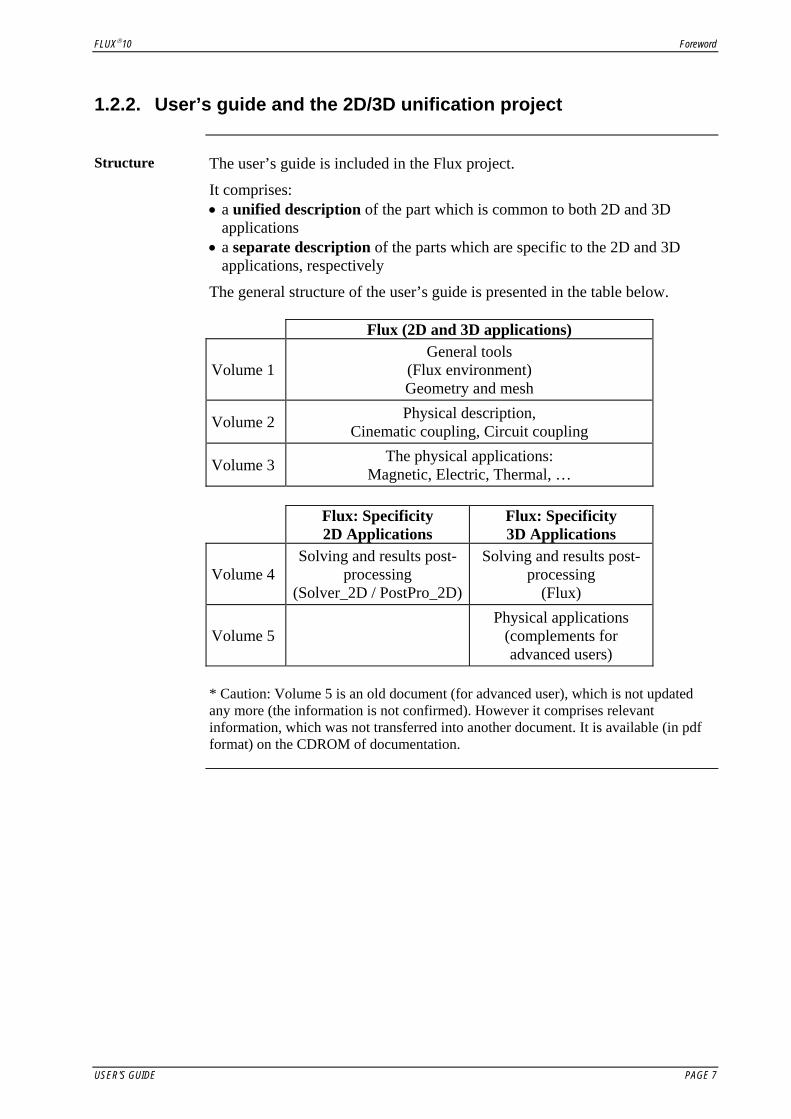
Structure The user’s guide is included in the Flux project.
It comprises: • a unified description of the part which is common to both 2D and 3D
applications • a separate description of the parts which are specific to the 2D and 3D
applications, respectively
The general structure of the user’s guide is presented in the table below.
Flux (2D and 3D applications)
Volume 1 General tools
(Flux environment) Geometry and mesh
Volume 2 Physical description, Cinematic coupling, Circuit coupling
Volume 3 The physical applications: Magnetic, Electric, Thermal, …
Flux: Specificity
2D Applications Flux: Specificity 3D Applications
Volume 4 Solving and results post-
processing (Solver_2D / PostPro_2D)
Solving and results post-processing
(Flux)
Volume 5 Physical applications
(complements for advanced users)
* Caution: Volume 5 is an old document (for advanced user), which is not updated any more (the information is not confirmed). However it comprises relevant information, which was not transferred into another document. It is available (in pdf format) on the CDROM of documentation.
USER'S GUIDE PAGE 7

Foreword FLUX®10
1.2.3. User’s guide: versions (on paper and on line)
Introduction The user’s guide appears in two versions:
• one version corresponding to the document on paper (or pdf) • one version corresponding to the online help
Why two versions?
The two versions of the user’s guide are not identical: • The document on paper comprises the necessary information in order to
understand well what can be carried out with Flux (pre-required knowledge)
• The online help includes the information mentioned above, to which the necessary information is added in order to make a good use of the software tools.
In order to identify information easily …
For each important description stage of a finite elements project, the information has been therefore split into two: • the ‘theoretical’ aspects (or principles) • the ‘practical’ aspects (or implemented at the level of the software)
The two aspects are described in different chapters, as presented in the table below.
The chapters headed … comprise information as follows …
Geometry: principles Mesh: principles Physics: principles …
• general information, reminder on physics • modeling principle (with Flux) • software operation (its strengths and limits) • advice in modeling: strategy, choice, … • general steps, flowcharts
Geometry: software aspects Mesh: software aspects Physics: software aspects …
• structure of Flux objects • handling of Flux objects • description of commands for specific actions
Concretely … The contents of the two versions of the user’s guide are presented in the table
below.
Document on paper Online help The theoretical aspects: Chapters headed: ” …: principles”
The theoretical aspects: Chapters headed: ” …: principles“
The practical aspects: Chapters headed: ” …: software aspects”
PAGE 8 USER'S GUIDE

FLUX®10 Foreword
1.2.4. Tutorials and technical papers for 2D applications
Definition A tutorial has the objective to show how to use the software by means of a
simple example. This type of document is useful for self-formation as regards the software. All the commands are described.
A technical paper has the objective to demonstrate the features of the software on a realistic technical example (emphasizing the interesting results which can thus be obtained). All the technical data are presented in the document, but the commands are not described in details.
Tutorials (2D) The available tutorials for the 2D applications are listed in the table below.
Tutorial: 2D application Description Generic tutorial of geometry and mesh Environment, geometry and mesh Magnetostatics Electrostatics Steady state and transient thermal
Basic applications
Translating motion Brushless permanent magnet motor Induction machine
Magnetic applications with kinematic coupling, circuit coupling
Induction heating Magneto-thermal application
Technical papers (2D)
The technical papers available for the 2D applications are listed in the table below.
Technical paper: 2D application
Synchronous motor Induction motor (Flux 2D version 7.60) Single phase and three-phase transformer (Flux 2D version 7.60) Drive motor with Simulink Flux to Simulink technology (Flux 2D version 7.60) Superconductors (Flux 2D version 7.60)
USER'S GUIDE PAGE 9

Foreword FLUX®10
1.2.5. Tutorials and technical papers for 3D applications
Definition The objective of a tutorial is to show how to utilize the software by means of
a simple example. This type of document is useful for self-formation as regards the software. All the commands are described.
A technical paper is meant to show the software features on a realistic technical example (emphasizing the interesting results which can thus be obtained). All the technical data are presented in the document, but the commands are not described in details.
Tutorials (3D) The available tutorials for the 3D applications are listed in the table below.
Tutorial: 3D application Description Generic tutorial of geometry and mesh Environment, geometry and mesh Magnetostatics Basic application
Translating motion Magnetic application with kinematic coupling, circuit coupling
Rotating motion Magnetic application with kinematic coupling, circuit coupling
Technical papers (3D)
The technical papers available for the 3D applications are listed in the table below.
Technical paper: 3D application Rear-view mirror motor analysis with Flux 3D End winding characterization with Flux 3D Permanent magnet machine Magneto-thermal Nondestructive testing with Flux 3D
PAGE 10 USER'S GUIDE

FLUX® 10 Supervisor
2. Supervisor
Introduction This chapter presents the Flux Supervisor.
Contents This chapter contains the following topics:
• General presentation • Flux modules • Standard or user version • File compression and archive management • Memory requirements management • Additional tools and options
USER'S GUIDE PAGE 11

Supervisor FLUX® 10
PAGE 12 USER'S GUIDE

FLUX® 10 Supervisor
2.1. General presentation
Introduction This section describes the Flux Supervisor, with which you can run Flux
modules and manage your Flux project files and directories.
Contents This section contains the following topics:
• Start the Flux Supervisor • Appearance of the Flux Supervisor: Display menu • My programs
USER'S GUIDE PAGE 13

Supervisor FLUX® 10
2.1.1. Start the Flux Supervisor
Start the Flux Supervisor
To start the Flux Supervisor from the Windows taskbar, proceed as follows: • point on Start/ Programs/ Cedrat (or your installation directory) and
click on Flux
The Supervisor Window
The Flux Supervisor window is divided into several zones. The different zones are identified in the figure below and then detailed in following blocks.
Menu bar
Tool bar
Program manager
My programs
Project files
Geometry view
Directory manager
Zones of the Supervisor
The different zones of the Flux Supervisor and their functions are presented in the table below.
Zone Function
Menu bar Windows commands for Flux • File • Display • Versions • Tools • Help
Tool bar Icons for common tasks in Flux • User version • Compression / Decompression of a project • Options (language, memory, etc.) • License manager • Help (link to online User’s Guide for Flux)
Continued on next page
PAGE 14 USER'S GUIDE
FLUX® 10 Supervisor
Zones of the Supervisor (continued)
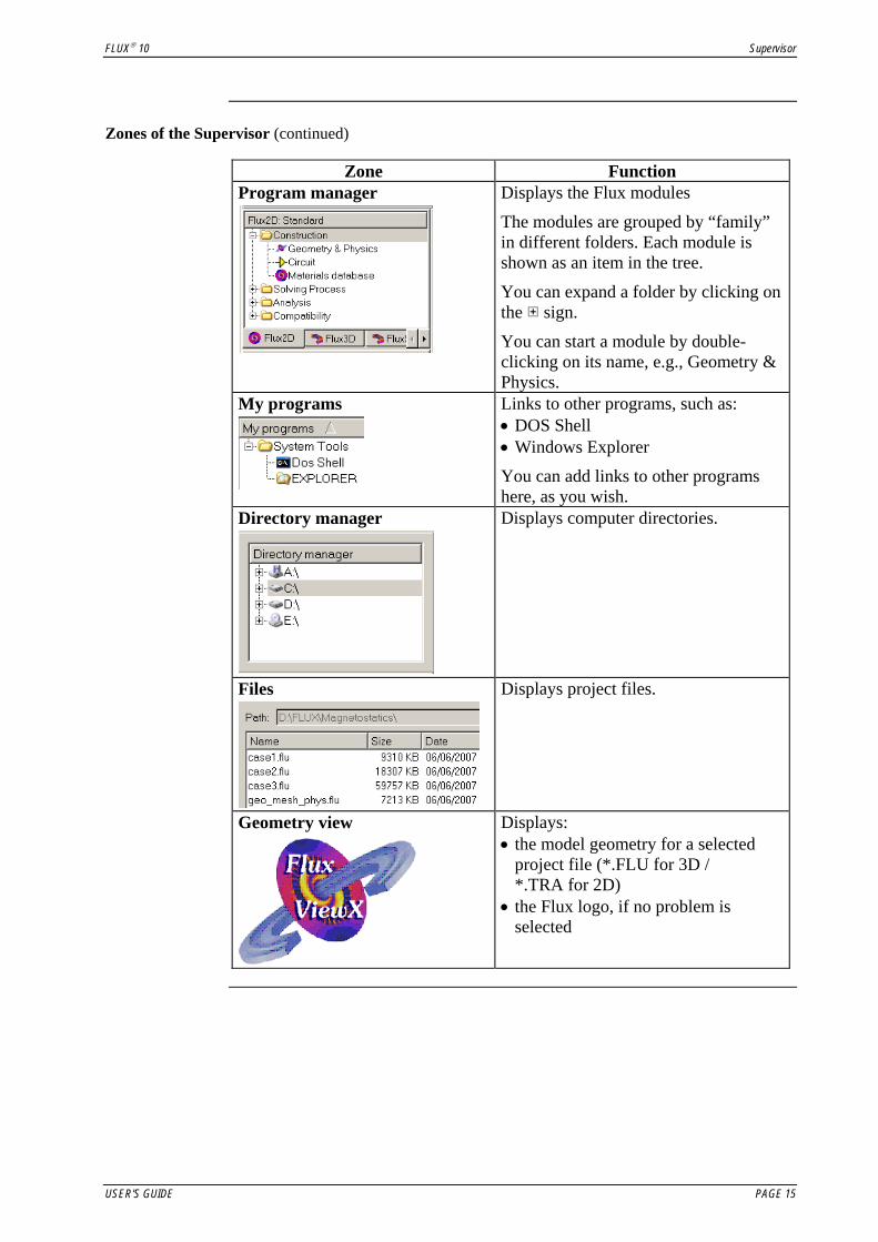
Zone Function Program manager
Displays the Flux modules
The modules are grouped by “family” in different folders. Each module is shown as an item in the tree.
You can expand a folder by clicking on the sign.
You can start a module by double-clicking on its name, e.g., Geometry & Physics.
My programs
Links to other programs, such as: • DOS Shell • Windows Explorer
You can add links to other programs here, as you wish.
Directory manager
Displays computer directories.
Files
Displays project files.
Geometry view
Displays: • the model geometry for a selected
project file (*.FLU for 3D / *.TRA for 2D)
• the Flux logo, if no problem is selected
USER'S GUIDE PAGE 15

Supervisor FLUX® 10
2.1.2. Appearance of the Flux Supervisor: Display menu
Introduction You can change the appearance of the Flux Supervisor screen, e.g.:
• show or hide zones of the Flux Supervisor • resize or move zones of the Flux Supervisor
Displaying different zones of the Flux Supervisor
The following figure illustrates the zones of the Flux Supervisor window that are affected by the Display commands: • the Tool bar • the Program manager • the Geometry view (for Flux 2D)
Geometry view
Tool bar
Program manager
Show/hide Flux Supervisor zones
To show or hide zones of the Flux Supervisor:
Step Action 1 Click on the Display menu
2 Choose the zones you want to display on your screen.
A check mark ( ) indicates that an option is selected or active. You can cancel the display of these three zones by clicking on the check mark to remove it.
Continued on next page
PAGE 16 USER'S GUIDE
Lillith Stoessel
Est-ce qu’on doit dire l’effet de cacher Program manager ? Sans « Program manager » comment est-ce qu’on utilise le logiciel ?

FLUX® 10 Supervisor
Effect on the Supervisor: example
The following figure shows the Supervisor when Display geometry is not selected:
Resize a zone of Flux Supervisor (with the mouse)
To resize (increase / reduce) the zone: • click on the side of the concerned zone when the resizing handle ( )
appears (with the left button of the mouse) ↔
• draw the side of the concerned zone in the new position (keep the left button pressed)
Resizing handle
USER'S GUIDE PAGE 17
Supervisor FLUX® 10
2.1.3. My programs
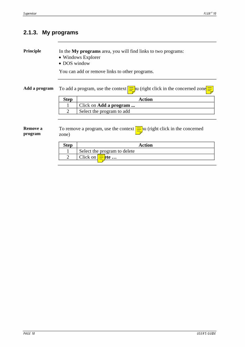
Principle In the My programs area, you will find links to two programs:
• Windows Explorer • DOS window
You can add or remove links to other programs.
Add a program To add a program, use the context menu (right click in the concerned zone)
Step Action 1 Click on Add a program ... 2 Select the program to add
Remove a program
To remove a program, use the context menu (right click in the concerned zone)
Step Action
1 Select the program to delete 2 Click on Delete …
PAGE 18 USER'S GUIDE
Lillith Stoessel
Je propose ajouter une figure du menu contextuel.
Lillith Stoessel
Je ne suis pas heureuse avec cette traduction...
Lillith Stoessel
Je propose ajouter une figure du menu là aussi
Lillith Stoessel
En effet la figure doit être là.

FLUX® 10 Supervisor
2.2. Flux modules
Introduction This section describes the program manager, which contains links /
commands to run Flux (2D, 3D or Skewed) modules.
Contents This section contains the following topics:
• Program manager: overview • Flux 2D modules • Flux 3D modules • Flux Skewed modules • Open a module
USER'S GUIDE PAGE 19

Supervisor FLUX® 10
2.2.1. Program manager: overview
Program manager
The program manager of the Flux Supervisor contains folders (in the form of a tree structure) in which you can find each of the main modules of Flux (2D, 3D or Skewed).
The program managers for Flux 2D, Flux 3D and Flux Skewed tabs are presented in the figures below and detailed in the following blocs:
Flux 2D module folders
The folders of the Flux 2D program manager are described in the table below:
Folder Function Construction • Create a geometric model, mesh, electrical circuit, and
materials • Assign material and source properties to different
components, to assign boundary conditions, link an external circuit, etc.
Solving process Solve a problem (direct or batch mode) Analysis Compute various quantities, create displays and
animations of results Compatibility Settings for use with modules from previous Flux
versions
Continued on next page
PAGE 20 USER'S GUIDE

FLUX® 10 Supervisor
Flux 3D / Flux Skewed module folders
The folders of the Flux 3D / Flux Skewed program manager are described in the table below:
Folder Function Flux 3D / Flux Skewed
• Create a geometric model, mesh, electrical circuit, and materials
• Assign material and source properties to different components, assign boundary conditions, link an external circuit, etc.
• Solve a problem in direct mode • Compute various quantities, create displays and
animations of results Tools • Draw and define electric circuits with ElectriFlux
• Add material models with Cslmat • Solve a problem in batch mode
Compatibility Settings for use with modules from previous Flux versions
Contents of the module folders
When you expand the folders, you will see icons and labels representing the Flux modules (2D, 3D or Skewed) contained in the folder.
USER'S GUIDE PAGE 21

Supervisor FLUX® 10
2.2.2. Flux 2D modules
Flux 2D modules: details
The Flux 2D modules are shown in the following figure:
Construction The Construction folder comprises the following modules:
Module Function Geometry & Physics • Build a geometric model and mesh
• Create and assign physical and material properties to components of a modeled device
Circuit Draw and define electric circuits Materials database Add material models to the database
Continued on next page
PAGE 22 USER'S GUIDE

FLUX® 10 Supervisor
Solving process The Solving process folder comprises the following modules:
Module Function Direct Solve a model (perform the FEM computations) in
interactive mode; the user can see the progress of the computation on screen and if necessary, stop the computation
Batch Solve a model in batch mode (e.g., to reduce computation time for complex models)
Transient start-up Solve a model beginning with results from a previous solution (e.g., with a modified time step)
Stop solve Stop a calculation before it is completed Delete results Delete results from a previous calculation Convert results Convert results from versions older than 7.50 Metal 7 Start Metal 7 (metallurgical calculations) Simulink Start a co-simulation with Matlab Simulink
Analysis The Analysis folder comprises the following modules:
Module Function Results Display results, create animations, etc. Coupling Create new Flux 2D problems from extracted values
(e.g., create a thermal problem from a magnetic application using the power density as thermal source)
Compatibility The Compatibility folder is divided into:
• Geometry Compatibility • Physical Compatibility • Tools
Geometry Compatibility
The Geometry Compatibility folder comprises the following modules:
Module Function Geometry with Preflu
Build a geometric model and mesh with Preflu (original Flux 2D preprocessor).
SPEED converter Convert a geometry created with SPEED software to a *.FLU file.
Preflux / Flux 3D Convertor
Convert the files preceding the 8.10 version
Continued on next page
USER'S GUIDE PAGE 23

Supervisor FLUX® 10
Physical Compatibility
The Physical Compatibility folder comprises the following modules:
Module Function Create Create and assign physical properties and materiasl to regions
of the studied device Modify Modify physical properties, e.g., to create multiple cases using
the same geometry and mesh but with varying physical properties
Copy Copy physical properties, e.g., to create multiple cases using the same physical properties but with different geometry or mesh models
Circuit with Cirflu
Draw and define electric circuits with Cirflu (circuit tool from previous Flux versions)
Tools The Tools folder comprises the following modules:
Module Function Solve with Resgen
Solve a model in interactive mode with Resgen (original Flux 2D solver).
Result with Expgen
Analyse results with Expgen (original Flux 2D postprocessor).
PAGE 24 USER'S GUIDE

FLUX® 10 Supervisor
2.2.3. Flux 3D modules
Flux 3D modules: details
The Flux 3D modules are represented in the following figure:
Flux 3D The Flux 3D folder comprises the following module:
Module Function Flux 3D • Create a geometric model, mesh, electrical circuit,
and materials • Assign material and source properties to different
components, assign boundary conditions, link an external circuit, etc.
• Solve a problem in direct mode • Compute various quantities, create displays and
animations of results
Tools The Tools folder comprises the following modules:
Module Function Circuit Draw and define electric circuits Materials database Add material models to the database Solve in batch Solve a model in batch mode (e.g., to reduce
computation time for complex models)
Compatibility The Compatibility folder comprises the following modules:
Module Function Circuit with Cirflu Draw and define electric circuits with Cirflu
(circuit tool from previous Flux versions) Preflux / Flux 3D Convertor
Convert the files preceding the 8.10 version
USER'S GUIDE PAGE 25
Lillith Stoessel
N’oubliez pas que « Arrêt de la résolution » doit être « Stop solve » ou telle qu’une expression…

Supervisor FLUX® 10
2.2.4. Flux Skewed modules
Flux Skewed modules: details
The Flux Skewed modules are represented in the following figure:
Flux Skewed The Flux Skewed folder comprises the following module:
Module Function Flux Skewed • Create a geometric model, mesh, electrical circuit,
and materials • Assign material and source properties to different
components, assign boundary conditions, link an external circuit, etc.
• Solve a problem in direct mode • Compute various quantities, create displays and
animations of results
Tools The Tools folder comprises the following modules:
Module Function Circuit Draw and define electric circuits Materials database Add material models to the database Solve in batch Solve a model in batch mode (e.g., to reduce
computation time for complex models)
Compatibility The Compatibility folder comprises the following modules:
Module Function Circuit with Cirflu Draw and define electric circuits with Cirflu
(circuit tool from previous Flux versions) Preflux / Flux 3D Convertor
Convert the files preceding the 8.10 version
PAGE 26 USER'S GUIDE

FLUX® 10 Supervisor
2.2.5. Open a module
Open a module To open a module:
• double-click on the module name in the data tree.
Open a module with a selected project file
If you want to open a module and a selected project at the same time (see § “General options: language, database”): • click on Options in the Tools menu or click on the icon
• select the General tab • under Other at the bottom of the dialog, check the box next to Open the
program with the selected project
USER'S GUIDE PAGE 27

Supervisor FLUX® 10
PAGE 28 USER'S GUIDE

FLUX® 10 Supervisor
2.3. Standard or user version
Introduction This section presents information about selecting and managing user versions
of Flux 2D or Flux 3D.
The Standard version is selected by default.
A user version is a version that extends the software’s basic modeling capabilities.
For example, with a user version you can define non-standard physical properties (voltage or current source, material characteristics, etc.) as a function of criteria you choose yourself (time, space, variable, etc.).
Contents This section contains the following topics:
• Concept of a user version • Choose the working version • User version manager • Edit a user version • Create a new user version • Modify a user version • Delete a user version • Options for user version
Reading advice In the chapter entitled “User subroutines” (for Flux 2D) the user will find
information pertaining to: • description of the user versions provided with the software • available possibilities of user versions: choice and writing of user
subroutines, etc.
USER'S GUIDE PAGE 29

Supervisor FLUX® 10
2.3.1. Concept of a user version
Flux versions There are two separate versions in Flux 2D / Flux 3D:
• standard version • user versions
User version: definition
A user version of Flux 2D / Flux 3D is a version that extends the software basic modeling capabilities.
User version: structure
From the point of view of its structure, a user version is a version that includes both: • the standard version of Flux 2D / Flux 3D and • a specified number of user subroutines.
Default location for user versions
User versions are located by default in the following directories: • C:\Cedrat\User\User2d for 2D user versions • C:\Cedrat\User\User3d for 3D user versions
User versions provided with the software
Predefined user versions are provided with the Flux software. They are listed in the following table:
User version Function
Brushlike_101 switch depending on position (Flux 2D version 10.1)
Table_101 read of properties (materials, sources) in a file (Flux 2D version 10.1)
Lamination_101 taking into account the lamination of a material without defining the geometry of the sheets (Flux 3D version 10.1)
Documentation on user versions
Informations about user versions included with the Flux software are available in the following directories: • C:\Cedrat\User\User2d\Brushlike_101.f2d_usr (brushlike_readme.pdf) • C:\Cedrat\User\User2d\Table_101.f2d_usr (table_readme.pdf) • C:\Cedrat\User\User3d\lamination_101.f3d_usr (lamination_readme.pdf)
PAGE 30 USER'S GUIDE

FLUX® 10 Supervisor
2.3.2. Choose the working version
Versions Flux versions are the following:
• the standard version • the user versions
The standard and user versions available are presented in the Versions menu.
For Flux 2D: For Flux 3D:
Version by default
By default the user will be working with the standard version of Flux 2D / Flux 3D.
To work with a standard or user version, it is necessary to specify the desired version.
Choose the working version
To choose a working version (standard or user):
Step Action 1 Open the Versions menu:
• click on Versions in the menu bar 2 Choose the version:
• click on the version of interest in the list The name of the version (standard / user) is displayed in the title
bar of the program manager
USER'S GUIDE PAGE 31

Supervisor FLUX® 10
2.3.3. User version manager
Introduction The available user versions are listed in the Versions menu.
You can edit a predefined user version, create new user versions, and modify or delete user versions.
The various operations to manage user versions are performed through the User version manager.
Open the User version manager
To open the User version manager: • click on User version in the Tools menu or on the icon
Overview The User version manager is shown in the figure below.
Location of the directory containing the user version files
Tool bar (shortcuts to the main functions: create, delete, compile user version, etc.)
Name of the user version
Names of the subroutines included in the user version
Date of compilation Flux version number
Continued on next page
PAGE 32 USER'S GUIDE

FLUX® 10 Supervisor
Location of user versions
In the Mode area, you can select the location of the directory for the user versions.
The two main locations are shown in the table below.
Mode Location on disk Local Defined by the user (see § 2.3.8) Shared Default directory:
• C:\Cedrat\User\User2d for 2D user versions • C:\Cedrat\User\User3d for 3D user versions
The User version toolbar
The user version toolbar provides shortcuts to the most common functions to work with user versions.
The icons and their functions are explained in the following figure: Create a new user version
Add sub-routines
Edit the subroutine
Delete the current user version
Delete the subroutine
Compile the current user version
Display the options
Display the online documen-tation
USER'S GUIDE PAGE 33

Supervisor FLUX® 10
2.3.4. Edit a user version
Edit a user version
To edit a user version:
Step Action 1 Open the User version manager with the icon 2 In the Name field, choose the name of the user version to edit 3 Click on OK to close the User version manager
Example The following figure shows information about a user version:
• The name of this version is brushlike.f2d_usr. • There are 2 subroutines included in this particular user version • The compilation report for this user version indicates that it was compiled on 12
May 2004 for Flux Version 8.1.
PAGE 34 USER'S GUIDE
FLUX® 10 Supervisor
2.3.5. Create a new user version
Introduction This section describes the creation and management of new user versions.
You should read the part concerning “User subroutines” (Flux 2D) before beginning this section.
Note In order to create a user version, a Fortran compiler must be installed on your
computer.
Process The different steps to create a user version are shown in the table below and
detailed in following blocks:
Step Action 1
(optional) Define the location of the directory for the new user version (in the local mode)
2 Create the new version: • enter a name • load the reference files that will serve as a basis for writing
the user subroutines 3 Edit the user subroutine(s) 4 Compile the new user version
Step 1: Define the location
To define the location of a new user version, choose the directory in which it will be placed (operating in Local mode):
Step Action
1 Click on Options in the Tools menu or on the icon
2 Choose the User version tab 3 Enter the name of the directory to place the new user version
• in the field Flux2D user version directory (for the local mode) • or in the field Flux3D user version directory (for the local
mode)
Continued on next page
USER'S GUIDE PAGE 35

Supervisor FLUX® 10
Step 2: Create the new user version
To create the new user version, proceed as follows:
Step Action 1 Open the New user version dialog from the User version
manager:
• click on the icon The New user version dialog is open.
2 Choose a name for your user version: • enter a name* in the Name field
3 Open the selection dialog box to add user subroutines: • click on Add
The selection dialog is open. 4 Select the user subroutines
• click on one or more files • click on Open
The names of subroutines appear in the New user version dialog. 5 Confirm the selection:
• click on OK The selection dialog is closed.
6 Confirm the creation: • click on OK
The New user version dialog is closed. The names of the new version and subroutines appear in the User
version manager. 4 Close the User version manager:
• click on OK The New user version dialog is closed and the name of the user
version is displayed in the title bar of the program manager.
* The name must not include any spaces.
Step 3: Edit the user subroutine
See the documentation concerned the writing of user subroutines in the user’s guide (chapter 3 volume 4 for Flux 2D).
Continued on next page
PAGE 36 USER'S GUIDE

FLUX® 10 Supervisor
Step 4: Compile To compile the version:
Step Action 1 In the User version manager:
• click on the icon The message User version successfully compiled appears.
2 Click on OK Information concerning the progress of the compilation is displayed in the
Compilation report area of the User version manager.
USER'S GUIDE PAGE 37

Supervisor FLUX® 10
2.3.6. Modify a user version
The changes you can make
These are the modifications you can make to a current user version: • Add user subroutines • Remove user subroutines from the current version (saving them in the
designated directory without compiling them with the current version) • Delete user subroutines from the current version
Modify a user version
To modify a user version (add or delete user subroutines), in the User version manager, proceed as follows:
Step Action
1 Choose the name of the user version you want to modify 2 In the tool bar of the User version manager:
To add a subroutine:
• click on the icon and select the user subroutines you want to add
To remove a subroutine: • click to remove the checkmark in front of the name of the user
subroutine To delete a subroutine:
• select the user subroutine you want to delete
• click on the icon 3 Modify the subroutine files 4 Compile the user version
PAGE 38 USER'S GUIDE

FLUX® 10 Supervisor
2.3.7. Delete a user version
Delete a user version
To delete a user version, in the User version manager, proceed as follows:
Step Action 1 In the User version manager:
• choose the name of the user version you want to delete 2 In the User version toolbar:
• click on the icon The confirmation box is open.
3 Confirm the deletion: • click on Yes
The user version is removed
USER'S GUIDE PAGE 39
Supervisor FLUX® 10
2.3.8. Options for user version
Access the Options dialog
To access the Options dialog:
• click on Options in the Tools menu or on the icon • click on the User version tab in the Options dialog
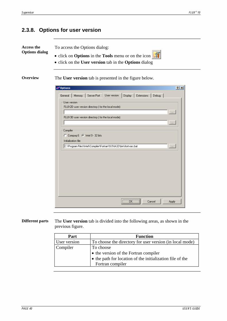
Overview The User version tab is presented in the figure below.
Different parts
The User version tab is divided into the following areas, as shown in the previous figure.
Part Function
User version To choose the directory for user version (in local mode) Compiler To choose
• the version of the Fortran compiler • the path for location of the initialization file of the
Fortran compiler
PAGE 40 USER'S GUIDE

FLUX® 10 Supervisor
2.4. File compression and archive management
Introduction This section presents information about file compression and archive
management.
Contents This section contains the following topics:
• Archive concepts • Archive manager • Create an archive • Restore an archive
USER'S GUIDE PAGE 41

Supervisor FLUX® 10
2.4.1. Archive concepts
File compression: benefits
The files of a complete project may become large (for example, for a complex geometry, or a fine mesh; during a multi-solving process that generates a large number of result files, etc.).
Therefore, it may be helpful to compress these files to facilitate the transfer or storage of the project.
Archive file: contents
The archive file (*.tar.bz file) can contain various files: • the set of files comprising the entire project, or only specified files
(geometry description, etc.) • other files such as Python files (*.py), etc.
For archiving Flux project files, several options are available as explained below.
Flux 2D options Flux 2D options allow the user to choose the project files to be archived:
Option Files Whole project Entire set of project files from the project Without results Project files without results
Flux 3D options Flux 3D options allow the user to choose the project files to be archived:
Option Files Whole project All files from the “*.FLU” directory:
PROBLEM_FLU.PFL, GEOM_FLU.PFL, MESH_FLU.PFL, SOLVE_i_j
Without finite element solution
Problem description files only: PROBLEM_FLU.PFL, GEOM_FLU.PFL, MESH_FLU.PFL
Without mesh Problem description files without mesh: PROBLEM_FLU.PFL, GEOM_FLU.PFL
PAGE 42 USER'S GUIDE

FLUX® 10 Supervisor
2.4.2. Archive manager
Introduction The various operations for managing archives (creation and restoration) are
carried out through the archive manager.
Open the Archive manager
To open the archive manager: • click on Compression / Decompression of a project in the Tools menu
or on the icon
The Archive manager
The Archive manager is shown in the following figure:
USER'S GUIDE PAGE 43

Supervisor FLUX® 10
2.4.3. Create an archive
Creation of an archive
The creation of an archive follows the process outlined below:
Stage Description
Initialization The user must choose: • the project to archive (and the compression option) • the name of the archive file and its place on the disk
Creation The user must choose: • files to include in the archive file and create the archive
Create a Flux project archive
To create a Flux project archive, proceed as follows:
Step Action 1 Click on one of the following two icons:
• create a Flux 2D project archive / a Flux 3D project
archive The Create a Flux 2D /3D project archive dialog is open.
2 Fill in the fields in the dialog window: • Project name • Directory where the archive will be created • Archive name
3 Choose the compression options 4 Click on Next
The next Create a Flux 2D /3D project archive dialog is open. 5 Add files to the archive file:
• click on Add new files… and select the files you want to add to the archive file.
6 Create the archive: • click on Finish
The Archive created with success message appears.
PAGE 44 USER'S GUIDE
FLUX® 10 Supervisor
2.4.4. Restore an archive
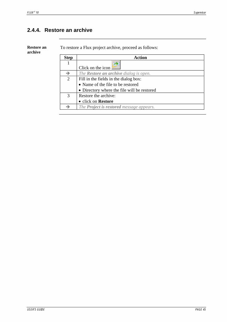
Restore an archive
To restore a Flux project archive, proceed as follows:
Step Action 1
Click on the icon The Restore an archive dialog is open.
2 Fill in the fields in the dialog box: • Name of the file to be restored • Directory where the file will be restored
3 Restore the archive: • click on Restore
The Project is restored message appears.
USER'S GUIDE PAGE 45

Supervisor FLUX® 10
PAGE 46 USER'S GUIDE

FLUX® 10 Supervisor
2.5. Memory requirements management
Introduction This section contains the information relating to the memory requirements
and its management.
Contents This section contains the following topics:
• Memory requirements management: definitions • Memory size management: allocated memory size • Memory size management: 32 bits / 64 bits / 3GB mode
USER'S GUIDE PAGE 47

Supervisor FLUX® 10
2.5.1. Memory requirements management: definitions
Memory requirements
From a point of view of computer science, Flux has two major components: • one ”computation” component (invisible part), in Fortran language • one “GUI” component (visible part), in Java language, and one connection between these two components, in Java.
A memory is allocated for each component. • As far as the computation part is concerned, Flux employs a pseudo-
dynamic* management system for the memory. This system manages a global memory volume comprising two Fortran components, one for the numerical memory and the other for the character memory. The size of each of these components is controlled by means of a Fortran parameter included in the main program.
* Definitions: Dynamic allocation: the allocated memory size is set by the user (it is therefore modifiable). Pseudo-dynamic allocation: Flux uses numerical and character tables and dynamically allocated to emulate a dynamic memory.
Definitions Numerical memory:
Numerical memory is the memory employed for the various modeling actions. 3D meshing and solving process (in 2D and in 3D) are the processes put a large demand on the memory size.
The memory size to be allocated is a function of the application type (real/complex) and of the solving process matrix size.
Example: in 2D with the default solver (SuperLU), for a project comprising approximately 20,000 nodes, the allocated memory size must be of 200 MB.
Character memory: Character memory is the memory used for storage of entity names (parameters/transformations/regions/…) and of project names presented in the directory.
GUI memory: GUI memory is the memory used for everything concerning the graphical user interface (graphic display, etc.)
In the graphic window, the flag located bottom left gives an image of the utilization of the graphic memory. When it is red, you can double-click on it to force the process to release the memory.
PAGE 48 USER'S GUIDE

FLUX® 10 Supervisor
2.5.2. Memory size management: allocated memory size
Allocated memory size
The allocated memory size is defined for each open module (Preflux 3D / Flux 3D) (Preflux2D / Solver 2D / PostPro2D).
The values are defined by means of the memory manager.
Access the memory manager
To access the options of the memory manager:
• click on Options in the Tools menu or on the icon • click on the Memory tab in the Options dialog
By default Standard values are assigned by default. These values are presented in the
table below.
2D Memory Numerical … Character … GUI … Preflux 2D 32 bits 200 Mo 10 Mo 200 Mo Preflux 2D 64 bits 400 Mo 10 Mo 400 Mo
Solver 2D 600 Mo 10 Mo 50 Mo PostPro 2D 200 Mo 10 Mo
3D / Skew Memory Numerical … Character … GUI … Flux 32 bits 700 Mo 10 Mo 300 Mo
Flux 32 bits (3GB)* 1700 Mo 10 Mo 300 Mo Flux 64 bits 4000 Mo 20 Mo 500 Mo
* Complementary information on memory size management for 32-bit and 64-bit operating systems and about the 3GB mode is presented in the following paragraph (see § 2.5.3).
USER'S GUIDE PAGE 49

Supervisor FLUX® 10
2.5.3. Memory size management: 32 bits / 64 bits / 3GB mode
32-bit processor With 32-bit processors, the program has maximum 2 GB distributed as
follows: • numerical memory => set at start • character memory => set at start • Java memory => set at start • executable memory => of the 250 MB order • cache memory (transfer Fortran / Java) => depends on the geometry, etc.
This memory is difficult to quantify, it can generate errors during the recovery of data.
3GB mode On specific Windows 32-bit systems the 3GB mode can increase the available
memory up to 3GB. The use of the 3GB mode is explained in the installation guide (see Installation guide § 2.4 “3GB mode (4GT RAM tuning mode of Windows) with Flux”).
64-bit processor Theoretically, the program has 264 Bytes of memory on the 64-bit processors,
which is much less limiting (practically, the current operating systems are limited to 128 GB).
PAGE 50 USER'S GUIDE

FLUX® 10 Supervisor
2.6. Additional tools and options
Introduction This section presents information regarding additional tools and options
available to the user.
Contents This section contains the following topics:
• Online Help • Skin depth calculator • License manager • General options: language, database • Display options
USER'S GUIDE PAGE 51

Supervisor FLUX® 10
2.6.1. Online Help
Access the online help
To access the online help: • click on Manual in the Help menu or on the icon
Flux online help
When you click on the Help icon, you are linked to the online version of the Flux User’s guide.
Click on hyperlinks to open the corresponding section of the Flux User’s Guide.
PAGE 52 USER'S GUIDE

FLUX® 10 Supervisor
2.6.2. Skin depth calculator
Introduction In the Tools menu there is a calculator specifically for computing the skin
depth.
Display the skin depth calculator
To display the skin depth calculator: • in the Tools menu, click on Skin depth…
Calculator for the skin depth computation
The skin depth calculator appears as shown below:
Calculate the skin depth
To calculate the skin depth: • In the Values area, fill in the fields: Resistivity, Relative permeability,
Frequency • In the Result area, choose the units Skin depth value can be read
USER'S GUIDE PAGE 53

Supervisor FLUX® 10
2.6.3. License manager
Open the license manager
To open the license manager: • click on License manager in the Tools menu or on the icon
Overview The license manager is presented in the figure below.
License manager: functionalities
In the License manager, the user can: • Select the license type – NodeLocked or Network • Configure the license server in automatic or manual mode
Reading advice The user will find more information in the “Installation guide” on:
• installation of the license • configuration of the license
PAGE 54 USER'S GUIDE

FLUX® 10 Supervisor
2.6.4. General options: language, database
Access the general options
To access the general options:
• click on Options in the Tools menu or on the icon • click on the General tab in the Options dialog
Overview The General tab of the Option dialog is presented in the figure below.
General options: functionalities
Within the General options tab, the user can: • choose the language for the Flux interface (English or French) • choose the directory for the Materials database: • run the Flux program by selecting the Flux project
Materials database
The user can • use the predefined databases, provided by Flux in the Materials directory:
- FLUX_xxx_MATERI.DAT - IMPHY_xxx_MATERI.DAT
• create a new materials database
The options to define the directory for the materials database are presented in the table below.
Option Directory Current directory working directory Shared default directory of the Flux installation Local defined by the user
USER'S GUIDE PAGE 55

Supervisor FLUX® 10
2.6.5. Display options
To access the Display options
To access the Display options:
• click on Options in the Tools menu or on the icon • click on the Display tab in the Options dialog
Overview The Display tab is presented in the figure below.
Display options: functionalities
Within the Display tab, the user can: • Start Flux in non-optimized graphics mode.
If there are any display errors in new graphics mode, the user can correct these problems by imposing the old graphics display.
• Choose options for the appearance of the DOS modules: - Choose the background color for the graphics display. Black is the default
background color. However, if you want to capture the graphics screen, for example, you may prefer a white background
- Set the number of lines for the console text. This setting controls how many lines are displayed in the History zone
• Choose the type of file. To add new file extensions to display them in the Files zone of the Flux Supervisor. The Flux project files – *.flu, *.py, *.tra, *.ccs, etc. – are displayed by default.
PAGE 56 USER'S GUIDE
FLUX® 10 Environment and graphic representation
3. Environment and graphic representation
Introduction This chapter presents:
• working environment: description and role of zones in Flux window • representations of devices in the graphic zone (graphic views).
Contents This chapter contains the following topics:
• Working environment: role of different zones • Graphic representation: a graphic view
Reading advice All aspects related to the data organization, manipulation and display are
treated in the chapter “General operation: data management”.
USER'S GUIDE PAGE 57

Environment and graphic representation FLUX® 10
PAGE 58 USER'S GUIDE

FLUX® 10 Environment and graphic representation
3.1. Working environment: role of different zones
Introduction This section concerns the working environment i.e.:
• the description and role of zones presented in the Flux window • customization possibilities proposed to the user
Contents This section contains the following topics:
• Presentation of working environment • Modifying the environment
USER'S GUIDE PAGE 59

Environment and graphic representation FLUX® 10
3.1.1. Presentation of working environment
Flux window The general Flux window consists of several zones. These zones are
identified in the figure below.
Title bar
Menus bar
Data tree
Graphic zone
toolbars
Status bar
Graphic zone
History
Menus toolbars
Transparency scale
Context bar
Configuration of the window
Flux desktop is automatically configured depending on: • dimension of the application (2D or 3D) • the physical application defined (no physics defined, magnetostatics,
electrostatics…) • the context: Geometry / Mesh / Physics / Solver / Post-processing (toolbars) • or sub context (healing context for the CAD geometry…)
Continued on next page
PAGE 60 USER'S GUIDE
FLUX® 10 Environment and graphic representation
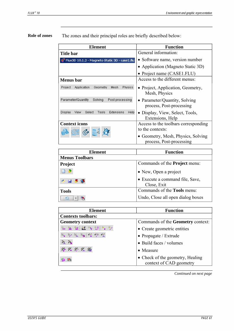
Role of zones The zones and their principal roles are briefly described below:
Element Function Title bar General information:
• Software name, version number • Application (Magneto Static 3D) • Project name (CASE1.FLU)
Menus bar Access to the different menus:
• Project, Application, Geometry, Mesh, Physics
• Parameter/Quantity, Solving process, Post-processing
• Display, View, Select, Tools, Extensions, Help
Context icons
Access to the toolbars corresponding to the contexts: • Geometry, Mesh, Physics, Solving
process, Post-processing
Element Function Menus Toolbars Project Commands of the Project menu:
• New, Open a project
• Execute a command file, Save,
Close, Exit Tools Commands of the Tools menu:
Undo, Close all open dialog boxes
Element Function Contexts toolbars: Geometry context Commands of the Geometry context:
• Create geometric entities • Propagate / Extrude
• Build faces / volumes
• Measure
• Check of the geometry, Healing
context of CAD geometry
Continued on next page
USER'S GUIDE PAGE 61

Environment and graphic representation FLUX® 10
Role of zones (continued 1)
Element Function Contexts toolbars: Mesh context Commands of the Mesh context:
• Create mesh entities
• Mesh domain, lines / faces / volumes,
Generate 2nd order elements • Delete the mesh
• Assign mesh information • Structure the mesh
• Check the mesh Physics context Commands of Physics context:
• Create physical entities
• Create I/O parameters / spatial
quantities
• Import materials, Orient a material,
Assign regions, Import a circuit • Check physics
Solving process context Commands of Solving process context:
• Create a scenario, Solving process options
• Check the project
• Solve a scenario, Continue the solving process
• Delete results Post-processing context* Commands of Post-processing context:
• Create post-processing entities
• Curves
• Isovalues
• Arrows • Compute quantities on points /
predefined quantities
• Evaluate sensors
* only for a solved problem
Continued on next page
PAGE 62 USER'S GUIDE

FLUX® 10 Environment and graphic representation
Role of zones (continued 2)
Element Function Menus Toolbars (in the graphic zone): View Commands of the View menu:
• Refresh view, Zoom all, Zoom region
• Standard view 1, Standard view 2, X plane view, Y plane view, Z plane view, Opposite view, Four-view mode
• View direction, Save / Restore graphics properties
Display Commands of the Display menu:
• Display geometric entities • Display point numbers / line numbers
• Display mesh entities
• Display physical entities
• Display post-processing entities Selection Commands of the Select menu:
• No selection, Free selection
• Select geometric entities
• Select physical entities
• Select solving process entities
Continued on next page
USER'S GUIDE PAGE 63

Environment and graphic representation FLUX® 10
Role of zones (continued 3)
Element Function Data tree
Entities tree of the Flux project
History zone
History zone
Information concerning different current actions (project evolution): • restoring of data during a project
opening, • comments about the current actions, • advance of computation during the
solving process, …
Command and Echo Zones*
History zone
Command zone
Echo zone
Access to functioning mode by commands in PyFlux language.
* These zones are masked by default. To display these zones, see § “Modifying the environment”.
PAGE 64 USER'S GUIDE

FLUX® 10 Environment and graphic representation
3.1.2. Modifying the environment
Introduction It is possible to modify the look of the Flux window on the screen, i.e.:
• modify the background color • display / hide certain zones • resize (reduce / enlarge) zones
Modify the background color
To modify the background color (reverse video): • in the View menu, click on Reverse video
Display / hide zones
To display / hide zones: • use the arrows located on the zones sides
(see example in the block below)
Display Command and Echo zones
To display the Command and Echo zones (enabling input and output of commands in the Python / PyFlux languages): • click on the arrow located on the bottom of the History zone as shown in
the figure below.
Arrow to display the Python command zone
⇒
Resize a view (with the mouse)
To resize (reduce / enlarge) the zone: • click on the side of concerned zone when the resizing handle ( ) appears
(with the left button of the mouse) ↔
• move the side of the concerned zone in the new position (keep the left button pressed).
Resizing handle
USER'S GUIDE PAGE 65

Environment and graphic representation FLUX® 10
PAGE 66 USER'S GUIDE

FLUX® 10 Environment and graphic representation
3.2. Graphic representation: a graphic view
Introduction This section concerns the graphic representation of the modeled device.
When referring to the graphic representation of a device, we are interested: • on one hand, in the different entities and their appearance: points and their
visibility, lines and their color, faces, surface elements…. • on the other hand, in the type of displayed view: side view, top view,
bottom view, global view, … in its position and dimensions in the graphic display zone.
The first aspect of the graphic representation (called visualization of entities) is treated in chapter “General operation: data management”.
The second aspect (called graphic view) is treated in this chapter.
This section presents the following: • concepts of graphic view • possibilities to modify the view (displacement, rotation, zoom, etc.) • presentation of predefined views (standard view, base plane views, opposite
view, etc.)
Contents This section contains the following topics:
• Concepts of view • Modifying the view • Predefined views • Four views
USER'S GUIDE PAGE 67

Environment and graphic representation FLUX® 10
3.2.1. Concepts of view
The graphic zone
The graphic zone is a zone where a graphic representation of the modeled device is displayed.
Scale of transparency
The coordinate system displayed in the left bottom of the zone gives the principal axes direction to orient the figure.
Concept of view The 2D or 3D view of a device in the graphic zone is called graphic view.
View transparency
The graphic view of the device can be displayed with more or less clear faces and volumes. This functionality controls the level of transparency of faces and volumes. It gives the possibility to visualize the inside of the device geometry, without setting faces and volumes invisible.
Scale of transparency
The transparency level of faces and volumes can be set using a scale of transparency located on the right bottom of the graphic zone.
Transparent Opaque
Scale of transparency Graphic view of device minimal value (T) transparent faces and volumes maximal value (0) opaque faces and volumes intermediate value (by default) more or less clear faces and volumes
PAGE 68 USER'S GUIDE

FLUX® 10 Environment and graphic representation
3.2.2. Modifying the view
Options It is possible to:
• move a view (translation) • resize a view (enlarge / reduce) • rotate a view (3D only)
How to modify a view
The modifications can be made: • using the mouse • using commands from the View menu (or the corresponding icons) • using keyboard shortcuts
Move a view (with the mouse)
To move a view (translate) in the graphic zone (cursor ): • click on the view in the graphic zone with the right button of the mouse • drag the view at the new location keeping the right button pressed
Move a view (with keyboard shortcuts)
To move a view (translate) in the graphic zone: • click on the graphic zone with the left button of the mouse • move the view in the required direction by clicking the arrow key
(← ↑ → ↓)
Resize a view (with the mouse)
To resize a view (i.e. reduce / enlarge the device): • click on the graphic zone with the left button of the mouse • reduce / enlarge the view with the mouse wheel
Resize a view (with keyboard shortcuts)
To resize a view (i.e. reduce / enlarge the device): • click on the graphic zone with the left button of the mouse • reduce the view by clicking the ‘ – ‘ key or enlarge the view by clicking the
‘+ ‘ key
Continued on next page
USER'S GUIDE PAGE 69

Environment and graphic representation FLUX® 10
Rotate a view: 3D only (with the mouse)
To rotate a view of the 3D device: • click on the view with the left button of the mouse • rotate the view in the new position keeping the left button pressed
Flux 3D provides three modes for rotating geometries, described in the table below. The user can see the active mode thanks different cursors.
Mode Mode activation Cursor
planar rotation about the center of the view.
Left button of the mouse and mouse far away from the view center
3D rotation about the center of the object
Left button of the mouse and mouse close to the view center
3D rotation about the point defined by mouse cursor
Left button of the mouse and Shift button pushed
Rotate a view: 3D only (with keyboard shortcuts)
To rotate a view of the 3D device about an axis: • click on the graphic zone with the left button of the mouse • rotate the view about the required axis in counter-clockwise or clockwise
direction by clicking the keys presented in the table below.
Mode View Keyboard shortcut Rotation about the horizontal axis in the graphic zone
Inser / Suppr
Rotation about the vertical axis in the graphic zone
/ Fin
Rotation about the perpendicular axis to the graphic zone
/
Continued on next page
PAGE 70 USER'S GUIDE

FLUX® 10 Environment and graphic representation
Change the view direction: 3D only
To change the view direction:
Step Action 1 In the View menu:
• click on View direction …
or on the icon 2 In the View direction box:
• enter the values: - x, y and z corresponding to the camera position - x, y and z corresponding to the target point position - rotation angle - zoom scale
Resize a view (with commands)
To resize (enlarge / reduce) a zone: • click on one of the commands in the View menu
(or on the corresponding icon)
The available commands and their corresponding icons are presented in the table below.
Command Icon Zoom all Total view
Zoom in - Enlarge the view Zoom out - Reduce the view
Zoom region This option enables the user to set with the mouse the rectangular zone to enlarge.
USER'S GUIDE PAGE 71

Environment and graphic representation FLUX® 10
3.2.3. Predefined views
Options It is possible to choose one (more) view(s) from a list of predefined views:
• standard view 1 and 2 • views on the reference planes X, Y, Z • opposite view
Standard views The standard views 1 and 2 are presented in the figures below.
Standard view 1 Standard view 2
Views on the reference planes
The views on the reference planes X, Y, Z are presented in the figures below.
X plane view Z plane view
Y plane view
Continued on next page
PAGE 72 USER'S GUIDE

FLUX® 10 Environment and graphic representation
Opposite view The opposite view is presented in the figure below
Standard view 1 Opposite view
Choose a view (with commands)
To choose a predefined view: • click on one of the commands in the View menu
(or on the corresponding icon).
The commands for predefined views and their corresponding icons are presented in the table below.
Command Icon
Standard view 1 Standard view 2 Opposite view
X plane view Y plane view Z plane view
Choose a view (with keyboard shortcuts)
To choose a predefined view: • click on the graphic zone with the left button of the mouse
choose the view by clicking the corresponding keyboard shortcut presented in the table below.
Command Keyboard shortcut
Standard view 1 F1 Standard view 2 F2 Opposite view - X plane view F4 Y plane view F5 Z plane view F3
USER'S GUIDE PAGE 73
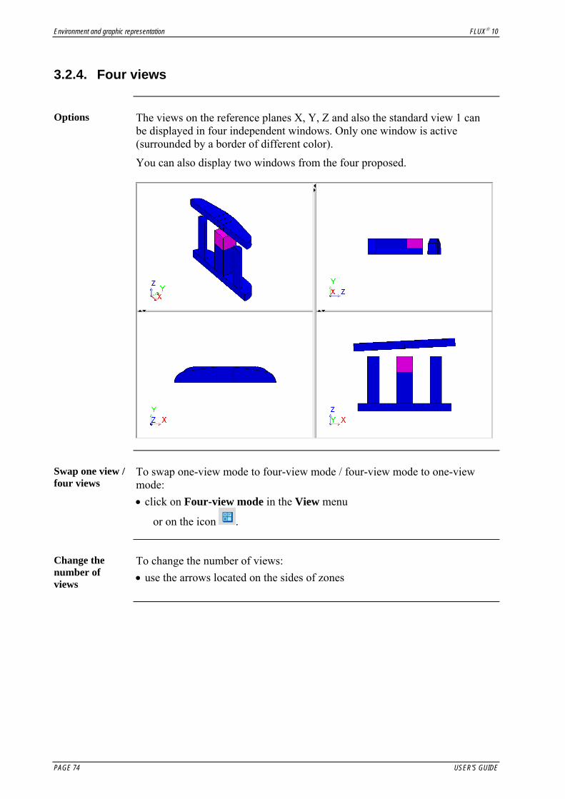
Environment and graphic representation FLUX® 10
3.2.4. Four views
Options The views on the reference planes X, Y, Z and also the standard view 1 can
be displayed in four independent windows. Only one window is active (surrounded by a border of different color).
You can also display two windows from the four proposed.
Swap one view / four views
To swap one-view mode to four-view mode / four-view mode to one-view mode: • click on Four-view mode in the View menu
or on the icon .
Change the number of views
To change the number of views: • use the arrows located on the sides of zones
PAGE 74 USER'S GUIDE

FLUX® 9.30 Flux project and Flux object management
4. Flux project and Flux object management
Introduction This chapter presents:
• the concept of Flux project and the commands of Project menu (New, Open, Save, Close)
• the concept of Flux object and the commands for object importation (Importation of Flux object)
Contents This chapter contains the following topics:
• Flux project • Flux object
USER'S GUIDE PAGE 75

Flux project and Flux object management FLUX® 9.30
PAGE 76 USER'S GUIDE

FLUX® 9.30 Flux project and Flux object management
4.1. Flux project
Introduction The user will find in this section the definition of a Flux project, and the
description of commands of project management (New, Open, Save, Close).
Contents This section contains the following topics:
• Flux project and Flux object management • Creation, opening and storage of projects
USER'S GUIDE PAGE 77

Flux project and Flux object management FLUX® 9.30
4.1.1. Flux project: definition, type of data storage
Flux project: definition
A Flux project is the data ensemble corresponding to a Flux study.
Storage type From the storage point of view, a Flux project consists in:
• a repertory, which includes the project name completed by the suffix “.FLU".
• a files ensemble, whose names are fixed and whose content is explained in the table below.
File name File content
PROBLEM_FLU.PFL general description of the problem GEOM_FLU.PFL visualization modes of the geometry MESH_FLU.PFL nodes of the mesh
Flux 3D features
For a FLUX3D study, the repertory corresponding to the project contains also a file(s) that contains the result(s).
File name File content
SOLVE_FLU.EFL or SOLVE_FLU_i.EFL
results of a static application or results of a transient or a parameterized application
The index i gives the information about the value of the time step or of the parameter.
PAGE 78 USER'S GUIDE

FLUX® 9.30 Flux project and Flux object management
4.1.2. Creation, opening and storage of projects
Project Menu Creating, opening and saving projects are carried out by usual commands for
file management. These commands are available by Project menu or by Project toolbar.
The operation of these commands is briefly pointed out below.
Project Menu Project Toolbar
Create a new project
To create a new project: • click on New from the Project menu
or on the icon from the Project toolbar.
Result: Flux recovers a lot of information from the database model, in order to build the proper database of the new project. The new project is temporarily named ANONYMOUS.
Open an existent project
To open an existent project, proceed as follows: • click on Open project … from the Project menu
or on the icon from the Project toolbar. • select the existing project (file) from the Open dialog box.
Result: When a project built with an old version is opening, Flux performs the update of the database.
Continued on next page
USER'S GUIDE PAGE 79

Flux project and Flux object management FLUX® 9.30
Save as a project
To save as a project in progress: • click on Save as … from the Project menu. • enter the project name in the Save dialog box
Save a project in progress
To save a project in progress: • click on Save from the Project menu
or on the icon from the Project toolbar
Close a project To close a project:
• click on Close from the Project menu or on the icon from the Project toolbar.
Result: When a project is closing, storage of project will be automatically proposed to the user if the project has been modified.
Flux 2D features
The .TRA file is automatically created for the surface meshed regions.
PAGE 80 USER'S GUIDE
FLUX® 9.30 Flux project and Flux object management
4.2. Flux object
Introduction The user will find in this section the definition of a Flux object, the operation
modes of Flux objects and the use of the importation object command.
Contents This section contains the following topics:
• Flux object: user guide • Importation of Flux objects
USER'S GUIDE PAGE 81
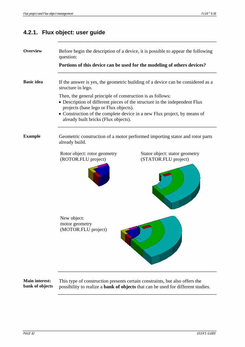
Flux project and Flux object management FLUX® 9.30
4.2.1. Flux object: user guide
Overview Before begin the description of a device, it is possible to appear the following
question:
Portions of this device can be used for the modeling of others devices?
Basic idea If the answer is yes, the geometric building of a device can be considered as a
structure in lego.
Then, the general principle of construction is as follows: • Description of different pieces of the structure in the independent Flux
projects (base lego or Flux objects). • Construction of the complete device in a new Flux project, by means of
already built bricks (Flux objects).
Example Geometric construction of a motor performed importing stator and rotor parts
already build.
Rotor object: rotor geometry (ROTOR.FLU project)
Stator object: stator geometry (STATOR.FLU project)
New object: motor geometry (MOTOR.FLU project)
Main interest: bank of objects
This type of construction presents certain constraints, but also offers the possibility to realize a bank of objects that can be used for different studies.
PAGE 82 USER'S GUIDE
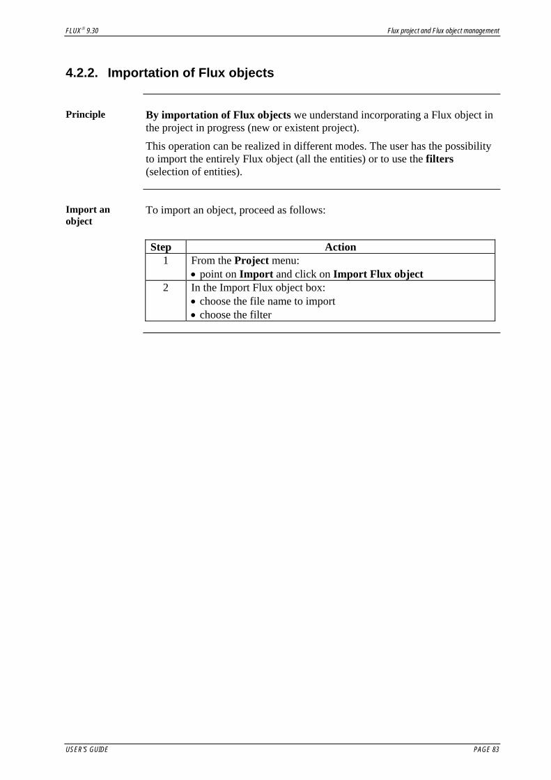
FLUX® 9.30 Flux project and Flux object management
4.2.2. Importation of Flux objects
Principle By importation of Flux objects we understand incorporating a Flux object in
the project in progress (new or existent project).
This operation can be realized in different modes. The user has the possibility to import the entirely Flux object (all the entities) or to use the filters (selection of entities).
Import an object
To import an object, proceed as follows:
Step Action
1 From the Project menu: • point on Import and click on Import Flux object
2 In the Import Flux object box: • choose the file name to import • choose the filter
USER'S GUIDE PAGE 83

Flux project and Flux object management FLUX® 9.30
PAGE 84 USER'S GUIDE

FLUX® 10 General operation: data management
5. General operation: data management
Introduction A finite element project contains a great volume of data, diverse and
interrelated.
In terms of Flux software, these data (points, lines, …) are called entities and depend on project context (geometry, mesh, …).
This chapter presents the mode of general operations of Flux software (independent of context), i.e.: • the general organization of data (Flux database) • the data presentation (dialog boxes) • management of the entities
(handling, information, export and selection of entities) • the tools of graphic entities visualization
(display and appearance of graphic entities in the graphic zone)
Contents This chapter contains the following topics:
• Data organization: Flux database • Data presentation: dialog boxes • Entity Management • Visualization of entities
Reading advice This chapter presents the mode of general operation of Flux software
(independently of context). For specific detail of geometry, mesh, physics, solver and post-processing modules refer to the corresponding chapters.
USER'S GUIDE PAGE 85

General operation: data management FLUX® 10
PAGE 86 USER'S GUIDE

FLUX® 10 General operation: data management
5.1. Data organization: Flux database
Introduction This section presents the general information on data structure in the Flux
database.
Contents This section contains the following topics:
• Concept of “data” and “data structure”
USER'S GUIDE PAGE 87

General operation: data management FLUX® 10
5.1.1. Concept of “data” and “data structure”
Introduction A finite elements project contains a great quantity of information, i.e. a
significant volume of data. These data are saved in a database, managed by specific tools.
Data and data structure
The Flux database makes a logical distinction between data structure (or data type) and data themselves (see blocks below).
Definitions The principal terms, used in this document to make a distinction between
data and data structure, are presented in the table below.
Term Definition Entity-type an entity-type is a logical data structure defined by a name
and a certain number of fields (attributes, relations, cases) Entity an entity is an object corresponding to an entity-type
characterized by an identifier (number/name) and fields (attributes, relations, case)
Caution on the vocabulary: the terms “entity” and “occurrence of entity” can be also used instead of “entity-type” and “entity”.
Example For points:
• the entity-type Point is a data structure of the database, that contains: - an identifier (a number) - cases: parameterized or propagated point - attributes: color, visibility - …
• the entities (Point[1], Point[2], …) are the objects (data) of Flux project
In practice From a practical point of view:
• during the creation of a new project the file (F3D_STR.SBD), which describes the data structure, is read by the program
• during the project saving the data structures and the data of the project are stored in the project directory (*.FLU).
Software version / compatibility
A new software version often corresponds to a development of the data structures.
The logical distinction between data structure and data makes it possible to ensure compatibility between an old Flux project and the more recent Flux version: during the old project opening, with a new software version the database is automatically updated.
PAGE 88 USER'S GUIDE

FLUX® 10 General operation: data management
5.2. Data presentation: dialog boxes
Introduction This section treats the data and the data presentation, i.e. dialog boxes:
specialized box and data array.
Contents This section contains the following topics:
• Project data (entities) • Dialog boxes: specialized box • Dialog boxes: data array
USER'S GUIDE PAGE 89

General operation: data management FLUX® 10
5.2.1. Project data (entities)
What are the handled data?
The handled data (entities) depend on the phase of the finite elements project description: geometry, mesh, physics.
They are listed in the data tree (figure below) and are detailed in the different corresponding chapters: Geometry / Mesh / Physics / Solver / Post-processing.
Continued on next page
PAGE 90 USER'S GUIDE

FLUX® 10 General operation: data management
Classification It is possible to distinguish two families of entities (graphic / non-graphic), as
presented in the table below.
Entity-type Identifier Entity (examples)
graphic Point, Line, …
Number allocated by the software
Point[1], Point[2] Line[25], Line[26], …
non graphic
Coordinate system, Transformation, …
Name given by the user
[CoordSys_1] [RotZ_90], …
USER'S GUIDE PAGE 91

General operation: data management FLUX® 10
5.2.2. Dialog boxes: specialized box
How are the data?
The interaction with the database is done using specific dialog boxes: specialized box, data array. This paragraph presents an example of specialized box.
Specialized box In this box the user can enter/check/modify information relating to the data.
A specialized box is presented in the figure below.
Entity-type: Coordinate system
Name Comment
Type (1)
Buttonsbar
Characteristics
Titlebar
Entity: [CORE]
Type (2)
Tag:Definition
The required fields (necessary and sufficient for the definition of the entity) are marked by an asterisk *.
General tools The general tools - available to carry out the data entry - are presented in the
table below.
Button Function
allow the direct access to the non-filled required fields OK validate information and close the dialog box
Apply validate information without closing the dialog box Cancel close the dialog box
access to the online help concerning the entity
Specific tools The user can create a missing entity using the button in a specialized box.
PAGE 92 USER'S GUIDE

FLUX® 10 General operation: data management
5.2.3. Dialog boxes: data array
How are the data?
The interaction with the database is done using dialog boxes: specialized box, data array. This paragraph presents an example of data array.
Data array In a data array, the user can:
• quickly check information relating to all data • easily carry out a "grouped" modification
(ex: to assign the same color to all regions, …) A data array is presented in the figure below.
Entity-type :Coord. Syst.
Name Comment
Type (1)
Characteristics
Entities : [CORE], [MAIN]
Type (2) Structure
(Database)
Buttonsbar
Titlebar
Information relating to the
group of entities
Information relating to the entity [CORE]
Information relating to the entity [MAIN]
The boxes clear gray are active boxes (data entry fields). The boxes dark gray are inactive boxes (general information).
General tools The general tools - available to carry out the data entry - are presented in the
table below (idem specialized box).
Button Function
allow the direct access to the non-filled required fields OK validate information and close the dialog box
Apply validate information without closing the dialog box Cancel close the dialog box
access to the online help concerning the entity
Continued on next page
USER'S GUIDE PAGE 93

General operation: data management FLUX® 10
Specific tools The specific tools, available in a data array are presented in the table below.
Box in the … Function Entities line
to open a specialized box Ex : by double-click on [CORE] in the Entities line, the user opens the specialized box corresponding to this entity.
Modify all column
to carry out a "grouped" modification: modification in only one step of all values on the same line Ex : by click on Initial values in the SubTypes line, the user can modify the coordinate system type of all coordinate systems in the array: [CORE] and [MAIN].
PAGE 94 USER'S GUIDE

FLUX® 10 General operation: data management
5.3. Entity Management
Introduction Building a Flux project consists of the application and manipulation of
entities.
This section describes the manipulation of entities (creation, selection, editing/modification, deletion, information and export)
Contents This section contains the following topics:
• Manipulation of the entities: Creating, Editing, … • Information on the entities: Display PyFlux , List and Entity used by • Export of entities • Entity selection: circumstances and selection modes • Entities selection: selection filter • Entities selection: selection by criterion
USER'S GUIDE PAGE 95

General operation: data management FLUX® 10
5.3.1. Manipulation of the entities: Creating, Editing, …
Introduction This paragraph presents the commands for manipulation of the entities:
New / Edit / Edit array / Delete / Force delete.
Commands of data manipulation
The basic procedures required to manipulate the entities are the operations of creating, editing/modification and deletion of data.
These operations are carried out by means of the commands presented in the table below.
Operation Command Function
creation New Creation of a new entity
Edit Editing/modification of one* entity in a Specialized box editing/
modification Edit array
Editing /modification of an array of entities in a Data Table
Delete Deletion of an entity if it is independent (no associated entities) deletion Force
deletion Deletion of an entity and of all the entities associated to it
* it is equally possible to edit several entities in a specialized box (only common characteristics are edited)
Modes of creating
To build the Flux project, the user must create the entities corresponding to the project data.
Giving consideration to a chronological order of entity creation generally facilitates the description process: points before lines, materials before regions … Consequently, if some entities have been ‘forgotten’, it is beneficial to have the option of creating them a posteriori.
Therefore, there are two modes of creation: • the direct creation is the « standard » mode of creation (the most natural) • the indirect creation is a mode of creation a posteriori. This is carried out
in a specialized dialog box by means of a button that facilitates the creation of a supporting entity.
Continued on next page
PAGE 96 USER'S GUIDE

FLUX® 10 General operation: data management
Modes of editing
To check the data, the user must edit (and modify if necessary) the entities that he has created.
There are two modes of editing: • editing in a Specialized box (generally), used to modify the characteristics
of one* entity • editing in a Table of data is used (in general) in order to verify the
characteristics of an array of entities
* it is equally possible to edit several entities in a specialized box (then only the common characteristics are edited)
Modes of deletion
The user may have to delete entities. He can easily destroy an independent entity. It is often the case that the entity is related to other entities. The deletion of the original entity can result in the deletion of all related entities.
Therefore, there are two destruction modes: • the simple deletion:
is carried out on independent entities (not related to other entities) • the force deletion :
is carried out on an entity and on all other related entities.
These two modes are described in the table below:
Mode Destructible entity What is deleted simple independent selected entity forced any type selected entity + connected entities
Function Processes
It is necessary to make a distinction between two function processes that differ for two distinct commands. The command Create does not require the selection of entities, while the commands (Edit/Edit array and Delete/Force delete) require the selection of entities.
The two function types are presented below and details are provided in the sections to follow: • the command Create does not require selection:
simply the activation of the (1) command • the other commands require selection of the entities
(Edit/Edit array and Delete/Force delete) : the user can choose: - either: to select the entities and then activate the command (2) - or: to activate the command and then select the entities (2’)
These two function types are presented in the sections to follow.
The selection and selection filtering is treated in the following paragraph.
Continued on next page
USER'S GUIDE PAGE 97

General operation: data management FLUX® 10
Access to the Create command
For the command Create, which does not require selection of entities, the access to the command can be carried out: • from the menu bar (1) • from the tool bar (2) • from the data tree* (3)
The command activations options are presented in the figure below.
1
3
2
* The creation of graphic entities can also be carried out from the graphic zone. The corresponding selection filter must be activated previous to the creation command (see § « Entities selection: selection filter »).
Continued on next page
PAGE 98 USER'S GUIDE

FLUX® 10 General operation: data management
Access to other commands
For the commands Edit/Edit array and Delete/Force delete, which require selection of entities, the access to the command can be carried out: • from the menu bar (1) :
- activation of the command then selection via a drop down menu (1) • from the data tree * (2 et 2’) :
- activation of the command then selection via a drop down menu(2) - direct selection then activation of the command (2’)
The command activation options are presented in the figure below .
1
2
2’
Selectionvia
a drop down menu
Selection via
a drop down menu
* The editing can equally be carried out from the graphic zone for the graphic entities. The corresponding selection filter must be activated preceding the edit (see §Entities selection: selection filter).
USER'S GUIDE PAGE 99

General operation: data management FLUX® 10
5.3.2. Information on the entities: Display PyFlux , List and Entity used by
Introduction This paragraph presents the different commands that equip the user to display
information regarding the entities: Displaying the PyFlux expression, Listing and Using by.
Role of information commands
The role of each of the information commands of an entity is described below.
Command Function/Use
Display PyFlux command
This command permits the display of the Pyflux expression associated with an entity. The user can recover it to use in a python sequence.
List This command permits the list of the contents of an entity type to be displayed. This command is accessible only starting from the contextual menu of an entity type.
Entity used by This command permits the user to know all the entities related to an entity
Access to entity information commands
The information commands are accessible starting from the contextual menu of each entity or entity-type.
PAGE 100 USER'S GUIDE

FLUX® 10 General operation: data management
5.3.3. Export of entities
Introduction This paragraph presents different formats for the export of entities.
Interest The export permits the user to extract information related to an entity. This
information is an image of the contents of the database. Once exported the information may be used outside the FLUX software.
Export formats
The export formats and their applications are presented in the table below:
Format Applications
Export XML Export python Programming
Export TXT Export Excel Export Clipboard
Presentation, storage, information, administration of results
Example The results for the export of a point, under two different formats, are
presented in the table below:
Export Python Export TXT PointCoordinates(color=Color['White'], visibility=Visibility['VISIBLE'], coordSys=CoordSys['CENTER'], uvw=['-60', '0', '0'], nature=Nature['STANDARD'], mesh=MeshPoint['E_SHAPE'])
02/03/09 17:05:24 PointCoordinates (1) color = Color (White) visibility = VISIBLE (VISIBLE) coordSys = CoordSysCartesian (CENTER) uvw =-60 0 0 globalCoordinates = -0.06 0.0 -0.05 nature = Nature (STANDARD) inAirPointFaceLocation =None inAirPointVolumeLocation =None region =None mesh = MeshPoint (E_SHAPE) domain = DomainType3D (DOMAIN1) ETAT =0 surface =None
Continued on next page
USER'S GUIDE PAGE 101

General operation: data management FLUX® 10
Writing mode In the dialog box corresponding to the export of an entity the user can choose
between different modes of writing in a file:
Export to Writing mode an existent file a new file Adding values
(by default) The values are added following the contents
Replacing file The file contents is replaced
The values are added
Access to export commands
The export commands are accessible from the contextual menu of each entity or entity-type. Starting from the contextual menu of an entity type, the user must choose the entity which he wants to export by means of a dialog box.
Continued on next page
PAGE 102 USER'S GUIDE
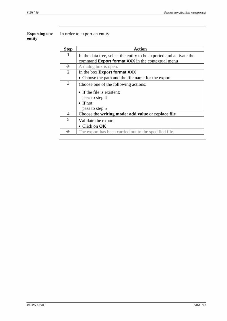
FLUX® 10 General operation: data management
Exporting one entity
In order to export an entity:
Step Action
1 In the data tree, select the entity to be exported and activate the command Export format XXX in the contextual menu
A dialog box is open. 2 In the box Export format XXX
• Choose the path and the file name for the export 3 Choose one of the following actions:
• If the file is existent: pass to step 4
• If not: pass to step 5
4 Choose the writing mode: add value or replace file 5 Validate the export
• Click on OK The export has been carried out to the specified file.
USER'S GUIDE PAGE 103

General operation: data management FLUX® 10
5.3.4. Entity selection: circumstances and selection modes
Introduction The most part of actions for handling the entities require the selection of
entities.
Indeed: • to modify the coordinates of a point, you should select the corresponding
point • to add a line (segment), you should define extremity points and then select
starting point and ending point • …
The different selection circumstances and selection modes are presented in this paragraph.
Selection circumstances: overview
Selection of entities can be done before or after the activation of a command; it can also be done, during an operation of creation.
These selection scenarios are presented through examples in the table below.
Selection before activation of a command
Graphic selection (with the mouse)
… Activation of a command: • Edit • Edit array • Delete • Force delete
Selection after activation of a command (via selection box)
Activation of a command: • Edit • Edit array • Delete • Force delete
Selection by name (choice in the list box)
or by other mode
Selection during an operation of creation
Activation of a command: • New
Selection by number (choice in the list) or by other mode
Continued on next page
PAGE 104 USER'S GUIDE

FLUX® 10 General operation: data management
Selection modes: overview
Selection of entities could be done with the following different selection modes: • graphic selection (directly with the mouse)
- in the data tree for all entities - in the graphic area for graphic entities
• identifier selection (by name / by number) • advanced selection* (by criterion / by …choice)
* the advanced selection is detailed in § “Entities selection: selection by criterion”.
Summary The different selection modes proposed function of selection circumstances
are gathered in the table below.
Selection circumstances … Selection modes Selection before
activation of a command - graphic
Selection after activation of a command
Selection box
graphic by identifier (name/number)
by criterion Selection during
an operation of creation Specialized
box graphic
by identifier (name/number)
USER'S GUIDE PAGE 105

General operation: data management FLUX® 10
5.3.5. Entities selection: selection filter
Selection filter: definition
During the selection of entities, only one entity-type is identified as being selectable: • it is possible
to select the points 1 and 2 or to select the lines 4 and 5
• it is not possible to select the points 1 and the line 5
A selection filter makes it consistently possible to identify the selectable entity-type.
Selection filter: actualization
How the selection filter is actualized?
For all the entities (graphic and non graphic), the selection filter is brought up to date with the operations of selection. i.e.: • with the choice of an entity-type in the data tree • with the opening of a selection box • … For the graphic entities, the selection filter can be activated directly by the user with the commands in the menu Selection or in the toolbar Selection.
Menu Selection The proposed choices in the menu Selection or in the toolbar Selection, relate
to the graphic entities; they are presented in the figure and the table below.
Noselection
Freeselection
Selection Point / Line / Face / Volume
Selection Face region / Volume region
Choice Description No selection nothing selectable
Free selection all is selectable The first entity which will be selected by the user will determine the entity-type selectable
Select points the points are selectable … …
PAGE 106 USER'S GUIDE

FLUX® 10 General operation: data management
5.3.6. Entities selection: selection by criterion
Relation between entities
All the entities are connected one to another by relations. • a volume is connected to the bordering faces • a face is connected to the bordering lines • a line is connected to the ending points, …
Thus, it is possible to select all the lines bordering a face by selecting this face, or all faces bordering a volume by selecting this volume.
The user can also plan to select entities via common characteristics: • lines with the same visibility, or with the same color, ... • points carrying the same mesh point
Definition / use One speaks about selection by criterion when the selection is carried out by:
• the intermediary of the existing relations between the various entities (points belonging to a line...)
• or the intermediary of characteristics common to several entities (faces with the same color, faces on the same surface...)
• …
Operation mode
The selection by criterion is available to the level of selection boxes and is carried out in three phases as that is presented in the table below (and on the example presented in the following block).
Stage Description
0 From a selection box … 1 The user :
• open the criteria list (with the button ) • and select a criterion to carry out his selection
The specific selection box (with logical operators) is open 2 Then, he selects the entities which interested him
(He chooses one of the proposed selection modes: graphic selection, by identifier or criterion)
3 And applies the selection operator to the group of entities
Continued on next page
USER'S GUIDE PAGE 107

General operation: data management FLUX® 10
Example To select all the lines belonging to the face 23:
1a. Click on
2. Enter the face number following by the Enter key
3. Click on Union
1b. Click on Selection by face
The stages of selection and management of the entities can be overlapped and reiterated.
Selection criteria
An outline of the selection criteria is presented in the tables below.
General criteria The option … allows …
Select all selection of all entities Clean selection deselection of all the entities previously selected Select last instance selection of the last selected entity Selection by coordinates
selection of the nearest entity to the entered coordinates
Specific criteria (implying the use of the operators) The selection by … allows the selection of all the entities …
line / face / volume belonging to a line / face / volume surface belonging to a surface (defined by a face) linear / face / volume region belonging to a line / face / volume region
mechanical set belonging to a mechanical set
The selection by … allows the selection of all the entities … color defined by a color (…) visibility defined by a visibility (visible or invisible) nature defined by a nature (standard, in air, no exist) discretization characterized by a discretization (point or line)
Continued on next page
PAGE 108 USER'S GUIDE

FLUX® 10 General operation: data management
Selection operators
To manage the logical operations on the groups of the selected entities, the user disposes the selection operators introduced in the table below.
Operator Function Exclude to remove entities from the list Union to add entities in the list
Intersect to carry out the intersection of two groups of selection
USER'S GUIDE PAGE 109

General operation: data management FLUX® 10
PAGE 110 USER'S GUIDE

FLUX® 10 General operation: data management
5.4. Visualization of entities
Introduction This section deals with the graphic representation of the modeled device.
When referring to the graphic representation of a device, we are interested: • in the type of displayed view: side view, top view, bottom view, global
view, … in its position and dimensions in the graphic display zone • in the different entities and their appearance: points and their visibility, lines
and their color, faces, surface elements…. The first aspect of the graphic representation (called graphic view) is treated in chapter “Environment and graphic representation” The second aspect of the graphic representation (called visualization of entities) is treated in this chapter.
Contents This section contains the following topics:
• Display and appearance of entities • Visualization of entities: displaying the entities and displaying filter • Visualization of entities: graphic appearance • Visualization of entities: saving and restoration of the graphic properties
USER'S GUIDE PAGE 111

General operation: data management FLUX® 10
5.4.1. Display and appearance of entities
Introduction The graphic representation of different objects is not the same during the
different steps of building the numerical model of the device.
From a step to another, we are interested in one kind of representation, or another: • representation of points and lines during the geometry building • representation of nodes and surface elements during the mesh building, ….
Examples
Possibilities to modify the visualization
To control the graphic representation, Flux provides default settings, but the user has the option to modify this representation.
User options are: • option one, use the display filters in order to decide what entity types he
wishes to see in the graphic zone: the assembly of points, or the points and the lines, or only the faces, … (see §5.4.2 «Visualization of entities: displaying the entities and displaying filter»)
• option two, modify, in a selective manner, the graphic appearance (namely the visibility and/or colour) of certain entities (see § 5.4.3 Visualization of entities: graphic appearance)
PAGE 112 USER'S GUIDE

FLUX® 10 General operation: data management
5.4.2. Visualization of entities: displaying the entities and displaying filter
Problem How to make the desired image of the device, in terms of displayed entities,
appear in the graphic zone on screen: the assembly of points, or the points and the lines, or only the faces, …
Displaying filter The display filters categorize the entity types displayed in the graphic zone:
the points, or the points and the lines, or only the faces, …
The display filters are accessible by means of the Display menu (or the tools bar Display)
Displaying menu
The list of the display filters available in the Display menu are presented below. The filters present the working context (geometry, meshing, physical, exploitation).
Filters associated with computation results (isovalues, arrows…) during post-processing (only available in a solved project)
Filters associated with post-processing supports
Filters associated with physical regions
Filters associated with mesh
Filters associated with geometry
USER'S GUIDE PAGE 113

General operation: data management FLUX® 10
5.4.3. Visualization of entities: graphic appearance
Subject How to make appear the desired representation of the device in the graphic
window, in terms of graphic appearance of entities: visibility, color.
Appearance The possible appearances are presented in the table below:
Appearance Characteristics color white, cyan, yellow, magenta, black, red, turquoise and green visibility visible or invisible
Appearance in the specialized box
The entities in the graphic window are displayed according to their appearance characteristics (visibility and color)
For each entity, the characteristics are saved in the Appearance tab of the specialized box.
PAGE 114 USER'S GUIDE
FLUX® 10 General operation: data management
5.4.4. Visualization of entities: saving and restoration of the graphic properties
Introduction This function permits to the user to:
• save a configuration of the display filters activated/inactivated for a specific time
• restore the configuration initially filed of the display filters activated/inactivated at another time
Saving the graphic properties
In order to save the graphic properties: • Click on icon
Restoring the graphic properties
In order to restore the graphic properties: • Click on icon
Remark The function of saving and restoring of the graphic properties exclusively
takes into consideration the display filter. Consequently, the position of the view and the zoom performed are not taken into consideration by this function.
USER'S GUIDE PAGE 115
Benjamin Vallet
À vérifier avec Claire si on met sauvegarde et restauration ou sauvegarder et restaurer

General operation: data management FLUX® 10
PAGE 116 USER'S GUIDE

FLUX® 10 SSPyFlux language, command files and macros
6. PyFlux language, command files and macros
Introduction A specific programming language is provided by Flux, which enables the
automation of certain recurrent actions or the generation of new functions.
This language, named PyFlux, is a language based on the Python programming language.
By means of this language, the user can: • edit and execute command files (scripts) • edit, load and execute macros
Contents This chapter contains the following topics:
• PyFlux and Python languages • Command files • Macros
USER'S GUIDE PAGE 117

SSPyFlux language, command files and macros FLUX® 10
PAGE 118 USER'S GUIDE

FLUX® 10 SSPyFlux language, command files and macros
6.1. PyFlux and Python languages
Introduction PyFlux is a Flux specific language, which can be defined in the following
manner:
PyFlux = Python programming language +
Flux command language
PyFlux is therefore an overload of Python to which Flux commands are inserted.
This section refers to information covering the PyFlux and Python languages, which should be reviewed before going over the various examples.
Contents This section contains the following topics:
• PyFlux language syntax • Python language syntax • PyFlux in interactive mode • How to find out the syntax of PyFlux expressions? • How to Activate/inactivate the writing of graphic commands • Other available PyFlux commands
USER'S GUIDE PAGE 119

SSPyFlux language, command files and macros FLUX® 10
6.1.1. PyFlux language syntax
PyFlux: what is it?
PyFlux is a Flux specific language, which can be defined in the following manner:
PyFlux = Python programming language +
Flux command language
PyFlux is therefore an overload of Python into which Flux commands are added.
PyFlux syntax The PyFlux syntax is based:
• on the syntax of the Python programming language (see § 6.1.2) • on the Flux database structure (Flux entities and commands)
Flux entities and PyFlux objects
PyFlux is an object-oriented programming language. There is a PyFlux type (class) corresponding to each Flux type-entity. The Flux entities are PyFlux objects (instances). The structure of the object is defined by fields called attributes, which possess a set of methods. The methods form the object interface.
A PyFlux type can have sub-types, which inherit the attributes and methods from their parent type. The sub-types are distinguished from their parent type by means of the supplementary attributes and methods.
Example: Point type
The structure of the Flux entity in the PyFlux language is presented in the example of the Point entity.
computePosition computePointDistancepropagate
color visibility mesh nature region globalCoordinates
Point
PointInfiniteBox PointCoordinates uvw coordSys
PointPropagated point transf
Name
Fields
Methods
Type
Sub-types
Continued on next page
PAGE 120 USER'S GUIDE
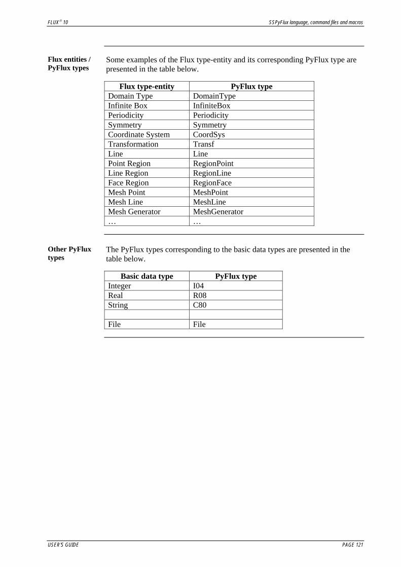
FLUX® 10 SSPyFlux language, command files and macros
Flux entities / PyFlux types
Some examples of the Flux type-entity and its corresponding PyFlux type are presented in the table below.
Flux type-entity PyFlux type
Domain Type DomainType Infinite Box InfiniteBox Periodicity Periodicity Symmetry Symmetry Coordinate System CoordSys Transformation Transf Line Line Point Region RegionPoint Line Region RegionLine Face Region RegionFace Mesh Point MeshPoint Mesh Line MeshLine Mesh Generator MeshGenerator … …
Other PyFlux types
The PyFlux types corresponding to the basic data types are presented in the table below.
Basic data type PyFlux type
Integer I04 Real R08 String C80 File File
USER'S GUIDE PAGE 121

SSPyFlux language, command files and macros FLUX® 10
6.1.2. Python language syntax
Python: what is it?
“Python is a portable, dynamic, extensible, free language, which allows a modular and object-oriented approach to programming. Python has been developed since 1989 by Guido van Rossum and several voluntary contributors” (Gerard Swinnen “Learn to program with Python”, pg. 6, 2005).
All the information about this language is accessible on the Python site: http://www.python.org.
The Python language is interpreted in Flux by Jython. Additional information about this interpreter is available on the Jython website: http://www.jython.org.
File Python files have the record extension *.py.
General rules General rules:
• A line should contain only one instruction • All the comments begin with the character # and continue until the end of
the line • Names of variables must follow some simple rules:
- names should begin with a letter or a _, and may contain letters (accented letters, cedillas, spaces, special characters are prohibited), numbers and the character _
- the case is significant (upper and lower case letters are differentiated) • Blocks are marked by indentation (in standard version, 4 spaces; do not
combine spaces and tabulations for indentation)
Variables and types
Declaration, assignment of variables: • It is not necessary to declare the variables. A variable is created at its first
assignment by means of = operator • The type of a variable is not explicitly declared and can change in time. The
type of a variable is the type of the value that is assigned to it. Types of standard data: • numerical types: integer, real, complex 312 3.13e10 0.1256 3.2+0.5j
• strings: between apostrophes or quotation mark 'hello' "followed by information"
• sequences: lists, sets, dictionaries ['a', 'b', 'c'] (1,2,3) ('a','b','c') {'jack' : 409, 'andy' : 860}
Continued on next page
PAGE 122 USER'S GUIDE
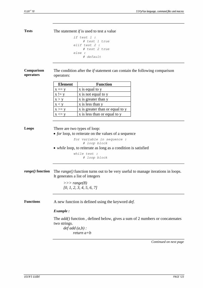
FLUX® 10 SSPyFlux language, command files and macros
Tests The statement if is used to test a value
if test 1 : # test 1 true elif test 2 : # test 2 true else : # default
Comparison operators
The condition after the if statement can contain the following comparison operators:
Element Function
x == y x is equal to y x != y x is not equal to y x > y x is greater than y x < y x is less than y x >= y x is greater than or equal to y x <= y x is less than or equal to y
Loops There are two types of loop:
• for loop, to reiterate on the values of a sequence
for variable in sequence : # loop block
• while loop, to reiterate as long as a condition is satisfied
while test : # loop block
range() fonction The range() function turns out to be very useful to manage iterations in loops.
It generates a list of integers
>>> range(8) [0, 1, 2, 3, 4, 5, 6, 7]
Functions A new function is defined using the keyword def.
Example :
The add() function , defined below, gives a sum of 2 numbers or concatenates two strings. def add (a,b) : return a+b
Continued on next page
USER'S GUIDE PAGE 123

SSPyFlux language, command files and macros FLUX® 10
Error handling The Python language has built-in system for exception handling. The program
can contain various types of errors: syntax errors, semantic errors (of logic) and errors of execution (exceptions). When an exception occurs, the program execution is stopped and the exception is handled. To handle syntax errors and exceptions, Python uses the following statement:
try : # instructions to execute (to raise exceptions)
except exception_class : # instructions to execute if the exception of the above class occurs
else : # instructions to execute if there is no exception
finally : # instructions to execute in all the cases
Python enables: • to catch several types of exceptions in same treatment • to raise the exceptions with the keyword raise
PAGE 124 USER'S GUIDE

FLUX® 10 SSPyFlux language, command files and macros
6.1.3. PyFlux in interactive mode
Introduction A programming language can be used:
• in interactive mode, directly in the Flux window • in script mode, via command files
Operation in interactive mode is presented in this paragraph. Operation in script mode is presented in section 6.2.
Different zones The Flux main window consists of several zones (graphic zone, data tree,
etc.). The principal zones are presented in § 3.1 “Working environment: role of different zones”.
The zones concerning the use of PyFlux in interactive mode are the zones presented in the figure below.
History zone
Command zone
Echo zone
Zone Function History result of the Pyflux command Command* input of the command in the PyFlux language Echo* echo of the command in the PyFlux language
* The Command and Echo zones are zones masked by default. To display / mask them use the arrows located above the zone.
Continued on next page
USER'S GUIDE PAGE 125

SSPyFlux language, command files and macros FLUX® 10
Example You can enter a line of PyFlux / Python command directly into the
Command zone, the answer is then displayed in the History zone.
An example of use of the Command zone as calculator is presented below.
Command (Python) Command
zone
⇒
Result
Echo of thecommand
History zone
Echo zone
Attention The variables, Python functions, etc. are preserved as long as the Flux module
is opened.
PAGE 126 USER'S GUIDE

FLUX® 10 SSPyFlux language, command files and macros
6.1.4. How to find out the syntax of PyFlux expressions?
Introduction To write in PyFlux language, the user needs to know the syntax of the PyFlux
expressions (Flux commands in the PyFlux language).
How to find out the PyFlux syntax
There are five methods to find out the syntax of the PyFlux expressions. These methods are presented in the table below and explained in the following blocks.
Method Description
1 recover the syntax in a command file 2 recover the syntax in the Echo zone 3 activate the entity command Display PyFlux command
(contextual menu, right click on item in the menu tree) 3’ apply the Python type() method to the entity (Command zone) 4 apply the Python help() method to the entity (Command zone)
(1) …in a command file
To recover the PyFlux expression of a Flux command applied during the session: • use the command file*to save the Flux commands** while the Flux
program is running
* Details on management of command files are presented in section: § 6.2.3 Management and execution of command files. ** The ‘graphic’ commands are not automatically written in the command file created by default. To recover these commands the user must activate the writing of the graphic commands. This command is described in section: § 6.1.5 How to How to Activate/inactivate the writing of graphic commands.
(2) … in the Echo zone
To recover the PyFlux expression of a Flux command: • activate the Flux command • directly recover the syntax within the Echo zone
Example: Echo of the command Open project / CASE1.FLU: loadProject('case1.flu')
Continued on next page
USER'S GUIDE PAGE 127

SSPyFlux language, command files and macros FLUX® 10
(3) Command Display the PyFlux expression
In order to find out the PyFlux expression of a Flux entity (the type and attributes): • in the contextual menu of the Flux entity, click on the Display PyFlux
command • recover the syntax within the History zone
Example: Display of the PyFlux expression of the command Point[1]: Typing Point[1]
PointCoordinates(color=Color['White'], visibility=Visibility['VISIBLE'], coordSys=CoordSys['CENTER'], uvw=['-60', '0', '0'], nature=Nature['STANDARD'], mesh=MeshPoint['E_SHAPE'])
End typing Point[1]
(3’) type() method
In order to find out the PyFlux expression of a Flux entity (the type and attributes): • in the Command zone, apply the Python type() method to the Flux entity • recover the syntax within the History zone
The Python type() method is equivalent to the Flux command Display PyFlux command
Example: Result of the command Point[1].type(): PointCoordinates(color=Color['White'], visibility=Visibility['VISIBLE'], coordSys=CoordSys['CENTER'], uvw=['-60', '0', '0'], nature=Nature['STANDARD'], mesh=MeshPoint['E_SHAPE'])
(4) help() method
In order to find out the PyFlux syntax of the complete structure of a Flux type-entity (its attributes, sub-types, methods, selection method): • in the Command zone, apply the Python help() method to the Flux type-
entity (type PyFlux). • recover the syntax within the History zone
Example: Result of the command ParameterGeom.help(): ParameterGeom (Entity for parametrizing a geometry) : Type Entity (read write) Fields : - ParameterGeom[id name].expression (Expression for the parameter) : [1...1] of C80 (read write) - ParameterGeom[id name].name (Name of Parameter) : [1...1] of C80 (read write) - ParameterGeom[id name].value (parameter value) : [1...1] of R08 (read)
PAGE 128 USER'S GUIDE

FLUX® 10 SSPyFlux language, command files and macros
6.1.5. How to Activate/inactivate the writing of graphic commands
Introduction The user can activate or inactivate the writing of graphic commands. The
commands called ‘graphic’ are associated with various display filters as described in section: § 5.4.
Writing the graphic commands
Activation of the writing of graphic commands ensures that the graphic commands corresponding to the graphic operations will be written in the History zone and in the PyFlux command file created automatically.
Activate/ Inactivate
To activate or inactivate the writing of the graphic commands: • click on the icon situated to the left of the transparency bar
Icon to activate/inactivate the graphic commands output
Transparency Bar
Icon state activated inactivated
By defaut By default the the graphic command icon is inactivated.
USER'S GUIDE PAGE 129

SSPyFlux language, command files and macros FLUX® 10
6.1.6. Other available PyFlux commands
Introduction There are additional commands available to the user that are not accessible by
recopying a sequence of PyFlux.
Commands The available commands are as follows:
• startMacroTransaction() / endMacroTransaction() • getProjectName() • [ALL] • getHelp() • getPyFluxCommande()
These commands are described in the next sections.
startMacroTransaction()/endMacroTransaction()
The description and applications of this command are explained in the table below.
Command startMacroTransaction() / endMacroTransaction() Function Permits the regrouping of a set of commands in a block.
Use startMacroTransaction() # set of PyFlux commands endMacroTransaction()
Continued on next page
PAGE 130 USER'S GUIDE

FLUX® 10 SSPyFlux language, command files and macros
Example : Pyflux
sequence
Creation of a triangle : startMacroTransaction() PointCoordinates(color=Color['White'], visibility=Visibility['VISIBLE'], coordSys=CoordSys['XYZ1'], uvw=['0', '0', '0'], nature=Nature['STANDARD']) PointCoordinates(color=Color['White'], visibility=Visibility['VISIBLE'], coordSys=CoordSys['XYZ1'], uvw=['0', '0', '10'], nature=Nature['STANDARD']) PointCoordinates(color=Color['White'], visibility=Visibility['VISIBLE'], coordSys=CoordSys['XYZ1'], uvw=['10', '0', '0'], nature=Nature['STANDARD']) LineSegment(color=Color['White'], visibility=Visibility['VISIBLE'], defPoint=[Point[1], Point[2]], nature=Nature['STANDARD']) LineSegment(color=Color['White'], visibility=Visibility['VISIBLE'], defPoint=[Point[2], Point[3]], nature=Nature['STANDARD']) LineSegment(color=Color['White'], visibility=Visibility['VISIBLE'], defPoint=[Point[3], Point[1]], nature=Nature['STANDARD']) endMacroTransaction()
Example : note
The commands are evaluated and the graphics refreshed at the end of the sequence, permitting the acceleration of the process.
getProjectName()
The description and applications of this command are explained in the table below.
Command getProjectName() Function Permits the recovery of the name of the project open in Flux
Use Name=getProjectName() permits the storage of the project name in the ‘Name’ variable
Example : PyFlux
sequence
Display of the Flux project name in a file : file = open("Name of project","a") file.write("Name of project :") file.write(getProjectName()) file.flush() file.close()
Continued on next page
USER'S GUIDE PAGE 131

SSPyFlux language, command files and macros FLUX® 10
[ALL] The description and applications of this command are explained in the table
below.
Command [ALL] Function Creates a the list of all entities of the same type which
facilitates the storage of this list in a ‘Flux variable’ Use Points = Point[ALL] creates a list of all entities of the point
type and enables the storage of this list in the « Points » variables.
Reminder / Comparison
The command List_instance(typeId='Point')* results in the display of all entities of the point type displayed in the History zone. * syntax equivalent to the command List described under § 5.3.2 Information on the entities: Display Pyflux, list, and entitiy used by.
Example : PyFlux
sequence
Display of a detailed list of entities belonging to the same entity type in a file: file = open("List of entities", "a") file.write("Detailed list of points") for I in Point[ALL] : file.write("\n\nInstance : ") file.write(repr(I)) for field in Point.__fields.keys() : file.write("\n") file.write(field) file.write(" : ") file.write(repr(I.__getattr__(field))) file.flush() file.close()
Example : result
Content of the created file: Detailed list of points: Instance : PointCoordinates[1] visibility : 'VISIBLE' surface : None color : 'White' domain : 'DOMAIN1 : Domain.' nature : 'STANDARD : Topologie standard' inAirPointFaceLocation : None region : None globalCoordinates : [-0.06, 0.0, -0.05] ETAT : 0 mesh : 'E_SHAPE : E_SHAPE VOLUMES' inAirPointVolumeLocation : None Instance : PointCoordinates[2] visibility : 'VISIBLE' surface : None color : 'White' domain : 'DOMAIN1 : Domain.' nature : 'STANDARD : Topologie standard' inAirPointFaceLocation : None region : None globalCoordinates : [-0.04, 0.02, -0.05] ETAT : 0 mesh : 'E_SHAPE : E_SHAPE VOLUMES' inAirPointVolumeLocation : None … …
Continued on next page
PAGE 132 USER'S GUIDE

FLUX® 10 SSPyFlux language, command files and macros
getHelp() The description and applications of this command are explained in the table
below.
Command getHelp() Function Permits to stor the help text dealing with an entity type in a
« Flux variable ». Use Point = Point.getHelp() retrieves the syntax describing the
« Point » entity type in order to support storage in the « Point » variable.
Reminder / Comparison
The command Point.help() permits the display of the support storage of the Point entity in the history zone.
Example : PyFlux
sequence
Display of support related to an entity type in a file: file = open("Aid PyFlux","a") file.write("Aid on the point :") file.write(Point.getHelp()) file.flush() file.close()
Example : result
File created comprising all of the supporting Pyflux command syntax associated with the « Point. » entity type.
getPyFluxCommand()
The description and applications of this command are explained in the table below.
Command getPyFluxCommand() Function Permits the storage of ann entity in a « Flux variable ».
Use P1=Point[1].getPyFluxCommand() permits the storage of the Point[1] entity in the « P1 » variable
Reminder / Comparison
The command Point[1].type() permits the display of the entity Point[1] in the history zone
Example : PyFlux
sequence
Display of an entity in a file: file = open("Entities of the Flux project ","a") file.write("Point P1 :") file.write(Point[1].getPyFluxCommand()) file.flush() file.close()
Example : result
Content of created file: Point P1:PointCoordinates(color=Color['White'], visibility=Visibility['VISIBLE'], coordSys=CoordSys['CENTER'], uvw=['-60', '0', '0'], nature=Nature['STANDARD'], mesh=MeshPoint['E_SHAPE'])
USER'S GUIDE PAGE 133

SSPyFlux language, command files and macros FLUX® 10
PAGE 134 USER'S GUIDE

FLUX® 10 SSPyFlux language, command files and macros
6.2. Command files
Introduction The command files, also called command programs or scripts, make possible
the automation of a certain number of specific actions.
Instead of manually executing a series of actions within Flux, you can save the sequences of commands, which you can later replay.
The saved sequences can be improved due to the Python language which authorizes the utilization of variables, the implementation of loops, conditional or unconditional connections, …
A command file is therefore of interest as it can: • accelerate the most frequent operations • automate a series of complex tasks
Contents This section contains the following topics:
• Overview • Structure of a command file • Management and execution of command files • Example 1: automatic creation of a series of mesh lines • Example 2: automatic preparation of a series of Flux projects ready to be
solved
Example The command files for the tutorials / technical papers are provided on the
CDROM with the software. By executing these command files, the user can quickly build the Flux projects described in the tutorials / technical papers.
For example, the command file GeoMeshPhys.py builds the whole geometry, generates the mesh of the computation domain and describes the physical properties for the technical paper “Rotating Motion”.
USER'S GUIDE PAGE 135

SSPyFlux language, command files and macros FLUX® 10
6.2.1. Overview
Definition A Flux command file is a text file, which contains one or more commands in
the PyFlux language. It uses the filename extension *.py.
Use A command file simplifies monotonous or repetitive tasks.
There are different levels of use: • the first level consists in saving and then replaying a «spied» sequence of
Flux commands • the second level consists in saving and then improving the «spied»
sequence of Flux commands by implementing loops and functions • the third level consists in directly writing the code in the programming
language
General operation
The more general operating mode is presented in the table below.
Stage Description Context
1 Saving in a command file a sequence of Flux commands Flux
2 Modification of the previous command file by writing the code in the programming language Text editor
3 Execution of a command file Flux
Location The command files can be stored in any directory chosen by the user. The
default command file created when the Flux program running (see § 6.2.3) is stored in the directory of current project.
PAGE 136 USER'S GUIDE

FLUX® 10 SSPyFlux language, command files and macros
6.2.2. Structure of a command file
Structure The structure of a command file (*.py) is presented in the example below.
1
2
Part Description 1 Header of an executable Flux program 2 One or more commands in a programming language
(1) Program header
The Flux program header is compulsory. It specifies which Flux program (2D and/or 3D) will execute the command file and its version*.
* The indicated version can correspond to the current software version or be of a previous version.
(2) Sequence of commands
The sequence of commands can comprise four types of principal instructions: assignment, loops, conditional statements, and statements without condition.
Note: A command file can contain the instructions to open another command file and so on up to 15 levels.
USER'S GUIDE PAGE 137
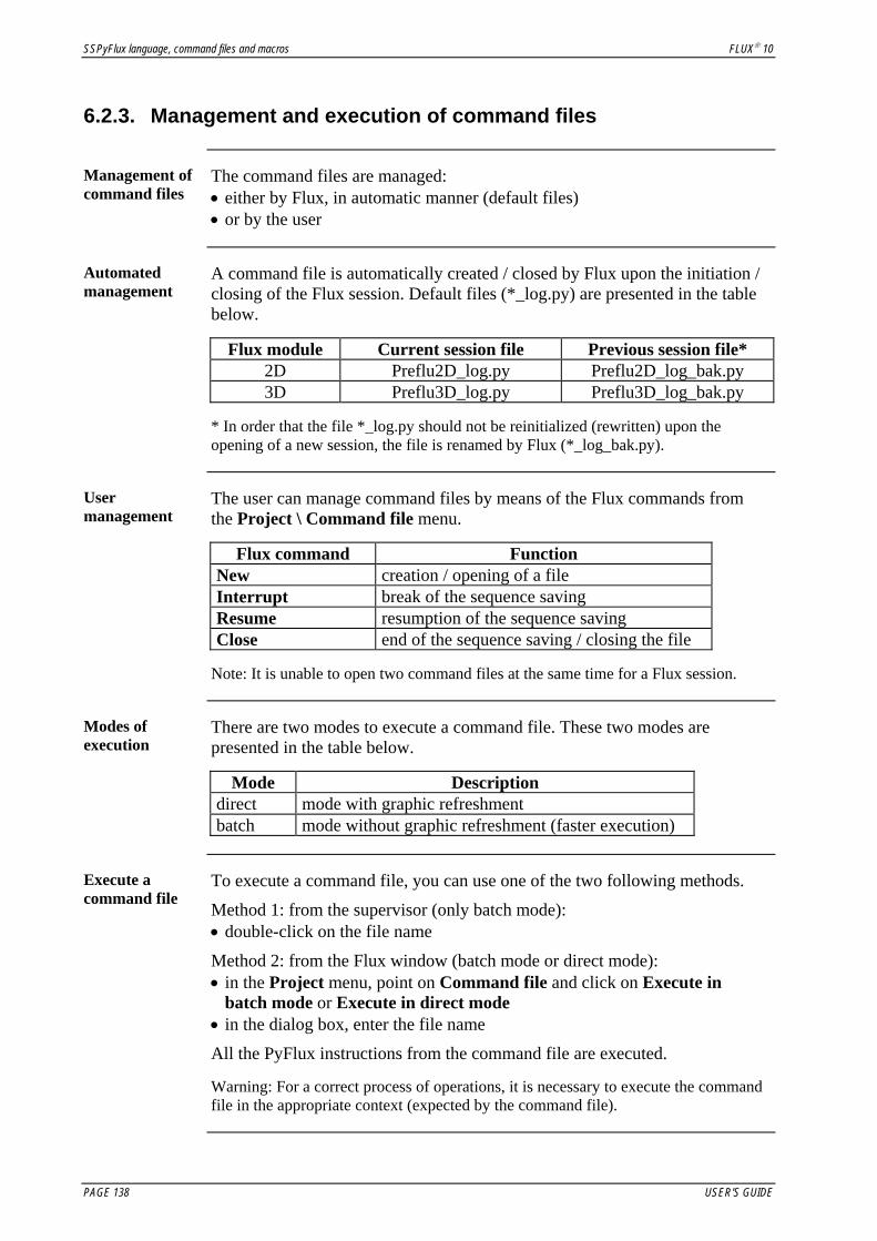
SSPyFlux language, command files and macros FLUX® 10
6.2.3. Management and execution of command files
Management of command files
The command files are managed: • either by Flux, in automatic manner (default files) • or by the user
Automated management
A command file is automatically created / closed by Flux upon the initiation / closing of the Flux session. Default files (*_log.py) are presented in the table below.
Flux module Current session file Previous session file* 2D Preflu2D_log.py Preflu2D_log_bak.py 3D Preflu3D_log.py Preflu3D_log_bak.py
* In order that the file *_log.py should not be reinitialized (rewritten) upon the opening of a new session, the file is renamed by Flux (*_log_bak.py).
User management
The user can manage command files by means of the Flux commands from the Project \ Command file menu.
Flux command Function New creation / opening of a file Interrupt break of the sequence saving Resume resumption of the sequence saving Close end of the sequence saving / closing the file
Note: It is unable to open two command files at the same time for a Flux session.
Modes of execution
There are two modes to execute a command file. These two modes are presented in the table below.
Mode Description direct mode with graphic refreshment batch mode without graphic refreshment (faster execution)
Execute a command file
To execute a command file, you can use one of the two following methods.
Method 1: from the supervisor (only batch mode): • double-click on the file name
Method 2: from the Flux window (batch mode or direct mode): • in the Project menu, point on Command file and click on Execute in
batch mode or Execute in direct mode • in the dialog box, enter the file name
All the PyFlux instructions from the command file are executed.
Warning: For a correct process of operations, it is necessary to execute the command file in the appropriate context (expected by the command file).
PAGE 138 USER'S GUIDE

FLUX® 10 SSPyFlux language, command files and macros
6.2.4. Example 1: automatic creation of a series of mesh lines
Objective The objective is to show, in a simple example, how to write a command file
to automatically create a series of mesh lines.
Example description
The command file allows the creation of eight Mesh lines A1, …, A8 of the arithmetic type with 1, …, 8 elements for different Flux projects (2D / 3D).
Process The process includes the following stages:
Stage Description Context 1 Saving in a command file the sequence of creation of
a Mesh line Flux
2 Modification of the previous command file using the PyFlux language Text editor
3 Executing this file to test it Flux
Stage 1 To save in a command file the sequence of creation of a Mesh Line:
Step Action 1 Create a new command file from a Flux Project :
• in the Project menu, point on Command file and click on New
• in the dialog box, enter the file name CreateMeshLine.py 2 Create a mesh line:
• in the data tree, double-click on Mesh line • in the New Mesh line dialog box, fill out different zones:
• click on OK • in the new dialog box, click on Cancel
3 Save and close the command file: • in the Project menu, point on Command file and click on Close
Continued on next page
USER'S GUIDE PAGE 139

SSPyFlux language, command files and macros FLUX® 10
Stage 1: file explanation
The command file CreateMeshLine.py containing the saved sequence is presented as follows:
Element Function #! Preflu3D 9.33 indication on the executable program (the #! symbol)
this file was saved by MeshLineArithmetic (name=A1, color=Color['White'], number=1)
creation of a Mesh Line with the following characteristics of the Flux command: • name = A1; • color = white; • number = 1
Stage 2 To modify the previous command file using the PyFlux syntax:
Step Action 1 Rewrite the command file CreateMeshLine.py by using a for
loop and a variable 2 Save the file
Continued on next page
PAGE 140 USER'S GUIDE

FLUX® 10 SSPyFlux language, command files and macros
Stage 2: file explanation
The command file CreateMeshLine.py containing the new instructions is presented as follows:
Element Function #! Preflu2D 10.3 #! Flux3D 10.3
indication of the two programs in which the file can be executed (the Preflu2D program is added in order to use this command file in Flux 2D)
for i in range(8) : carrying out a for loop to reiterate on the values of the sequence [0, …, 7]
name = 'A' + str(i+1) creation of a variable name which takes for successive values the strings: A1, A2, …, A8 (the method str() converts the numerical type in string)
MeshLineArithmetic (name=name, color=Color[i+1], number=i+1)
creation of a series of Mesh lines with the following characteristics: • name = A1; A2; A3; A4; A5; A6; A7; A8 • color = black; white; yellow; blue; turquoise;
magenta; red; green • number = 1; 2; 3; 4; 5; 6; 7; 8
Stage 3 Execute the command file directly from a Flux project :
• in the Project menu, point on Command file and click on Execute in direct mode
• in the dialog box, select the file name CreateMeshLine.py
Stage 3: final result
After executing the command file, the user will have 8 mesh line entities available in the current Flux project: A1 = 1, A2 = 2, …, A8 = 8
USER'S GUIDE PAGE 141

SSPyFlux language, command files and macros FLUX® 10
6.2.5. Example 2: automatic preparation of a series of Flux projects ready to be solved
Objective The objective is to study 3 specific configurations of a parameterized device.
Example description
The studied device is a simple geometrical figure (quadrilateral) defined using 6 parameters: X1, Y1, X2, Y2, X3, Y3.
This command file could be used to create different Flux projects in 2D.
Process The process includes the following stages:
Stage Description Context 1 Preparing a Flux project which contains the base
geometry Flux
Saving in a command file the sequence of the geometry modification with mesh rebuilding Flux
2 Modification of the previous command file using the PyFlux language Text editor
3 Executing this file to test it Flux
Stage 1 To build the basic geometrical figure on which the modifications will be
carried out, follow the following procedure:
Step Action 1 Open a new Flux project 2 Build the geometry:
• create the following 6 geometric parameters: X1 = 20, Y1 = 0, X2 = 0, Y2 = 10, X3 = 20, Y3 = 10
• create the following 4 points: (0, 0); (X1, Y1); (X2, Y2); (X3, Y3);
• create the 4 lines to close a rectangle with these 4 points • build the faces
3 Mesh the device: • modify the value of the MEDIUM Mesh line (value: 1 mm) • assign the MEDIUM Mesh line to the 4 points • mesh the faces
4 Save the project under the name BASE.FLU
Continued on next page
PAGE 142 USER'S GUIDE

FLUX® 10 SSPyFlux language, command files and macros
Stage 1: final result
The project BASE.FLU contains: • 6 parameters, • 4 points ((3 are
parameterized)) • 4 lines (segments) • 1 meshed face
(X3 = 20, Y3 = 10)
(X1 = 20, Y1 = 0)
(X2 = 0, Y2 = 10)
(0, 0)
Stage 2 To save in a command file the sequence of modification:
Step Action 1 Create a command file ModifParam.py 2 Carry out the modification actions:
• delete the mesh (to enable the geometrical modification) • modify the value of a geometric parameter • mesh the faces • save the project under another name
3 Close the command file
Stage 2: final result
The command file ModifParam.py containing the saved sequence is presented as follows:
Stage 3 To modify the previous command file using the PyFlux syntax:
Step Action 1 Write a function in the PyFlux language, which enables the
automatic creation of a Flux project (corresponding to a set of parameters) starting from a base project BASE.FLU.
2 Write the calls of the previous function to create the 3 desired cases
3 Save the command file
Continued on next page
USER'S GUIDE PAGE 143

SSPyFlux language, command files and macros FLUX® 10
Stage 3: file explanation
The command file ModifParam.py containing the modify() function and the calls of this function is presented as follows:
Element Function #! Preflu2D 9.33 indication on the executable program def modify(VX1,VY1,VX2,VY2, VX3,VY3,case) :
definition of the modify() function having as input 7 parameters (6 numerical values to define the geometric parameters X1, Y1, X2, Y2, X3, Y3 and 1 string to define the name of the project)
deleteMesh() deletion of the mesh ParameterGeom['X1'].expression=str(VX1) …
modification of geometric parameter (X1 takes the value VX1, converted into string by the method str(), …)
meshFaces() meshing faces saveProjectAs(case) saving the project under the name defined by
the input parameter case modify(10,0,0,10,20,10,"Case1") …
call of the function to build the first case, …
Stage 4 Execute the command file.
Stage 4: final result
After executing the command file, the user has in his/her working directory 4 Flux projects, whose characteristics are given in the table below.
BASE.FLU CASE1.FLU CASE2.FLU CASE3.FLU
P3 P4
P2 P1 P1: ( 0, 0) P1: ( 0, 0) P1: ( 0, 0) P1: ( 0, 0) P2: (20, 0) P2: (10, 0) P2: (10, 0) P2: (10, 0) P3: ( 0, 10) P3: ( 0, 10) P3: (10, 10) P3: ( 0, 10) P4: (20, 10) P4: (20, 10) P4: (20, 10) P4: (15, 5)
PAGE 144 USER'S GUIDE

FLUX® 10 SSPyFlux language, command files and macros
6.3. Macros
Introduction The macros enable the user to regroup the frequently used commands in an
extension integrated into the software.
You can build up a macro instead of manually executing a series of repetitive actions in Flux, which you will then be able to call regularly.
A macro is interesting because it can encapsulate within a new command a series of repetitive operations and thus improve the quality and efficiency of the user-software interaction.
Contents This section contains the following topics:
• Overview • Structure of a macro file • Management and execution of macros • Example: creation of points starting from a file
USER'S GUIDE PAGE 145

SSPyFlux language, command files and macros FLUX® 10
6.3.1. Overview
Definition A macro is a high-level command, added to the Flux application, which
regroups several commands in a given order. It receives (upon entry) one or more parameters and executes (upon exit) a series of predefined actions.
A macro file (*.py) is a text file, which defines the macro-function in the PyFlux language.
Use A macro improves the quality and efficiency of the user-software interaction
due to: • the regrouping of the repetitive commands • its dialog box especially designed for the entrance of the parameters
General operation
The operation mode of the most general type is presented in the table below.
Stage Description Context
1 Creation of the macro definition file Text editor
Creation of the image-formatted file for the associated icon (optional) Image editor
2 Loading of the macro into the Flux project Flux 3 Execution of the macro Flux
Some rules Within the storage on the disk, a macro corresponds to a directory which
includes: • a file of the macro • a file of the associated icon (optional)
The directory, the file of macro and the icon must be named after the macro-function.
Example: • Name of the function: Polypoint3D • Name of the directory of macro: Polypoint3D.PFM • Name of the file of macro: Polypoint3D.py • Name of the file of the associated icon: Polypoint3D.gif
Location The macros can be stored in any directory chosen by the user. The macros
provided by Flux are stored within the specific directory extensions.
PAGE 146 USER'S GUIDE

FLUX® 10 SSPyFlux language, command files and macros
6.3.2. Structure of a macro file
Structure The structure of a file defining the macro (*.py) is presented in the example below.
1
2
3
Part Description 1 Header of an executable Flux program 2 Description of input parameters of the macro 3 Definition of a parameterized function in the PyFlux language
(1) Program header
The Flux program header is compulsory. It specifies which Flux program (2D and/or 3D) will execute the macro and its version*.
* The indicated version can correspond to the current software version or be of a previous version.
(2) Description of parameters
This second part deals with the description of the input parameters of the macro. For each parameter it is necessary to define: • a parameter name • a PyFlux type (see § 6.1.1) • minimal and maximal cardinalities (numbers of minimal and maximal
values corresponding to the data structure) • a default value or a keyword None • a label associated to the parameter
(this label appears in the dialogue box for the running macro, see § 6.3.3)
(3) Parameterized function
This second part deals with the description of the parameterized function.
For this function it is necessary to define: • a function name (= name of the macro) • input parameters of the de function • a body of the function (PyFlux instructions)
USER'S GUIDE PAGE 147

SSPyFlux language, command files and macros FLUX® 10
6.3.3. Management and execution of macros
Management of macros
The user can load or unload macros within the project. The macro can be reloaded into the project, if the file of the macro loaded into the project has been modified for example.
The Flux commands for the management of macros are located in the Extensions menu.
Flux command Function
Load loading a new macro into the project Unload unloading the macro from the project Update updating the macro
Integration within Flux
All the macros loaded into the Flux project appear: • in the Extensions/ Macros node of the data tree • in the toolbar (icons)
The loaded macros are saved with the project.
Run a macro The user can run a macro by using the Run command from the macro
contextual menu or by clicking on the corresponding icon. The dialog box associated to the types of parameters is then displayed.
PAGE 148 USER'S GUIDE

FLUX® 10 SSPyFlux language, command files and macros
6.3.4. Example: creation of points starting from a file
Objective The objective is to show on a simple example how to write and use a macro.
This macro makes the repetitive tasks to enter the coordinates during the creation of points easier.
Example description
The Polypoint3D macro is designed to automatically create 3D points starting from a series of coordinates previously saved in a text file. The file name and the coordinate system for definition of the points are selected by the user during the execution of the macro.
Process The process includes the following stages:
Stage Description Context
1* Writing the definition of the macro into the *.py file using the PyFlux language Text editor
2 Writing the coordinates of points into the text file Text editor 3 Loading the macro into the Flux project Flux 4 Running the macro Flux
* The definition of macro requires good knowledge of the Flux database structure and concepts of programming.
Stage 1 To define the macro in the PyFlux language:
Step Action 1 Type a header of executable Flux program 2 Describe input parameters of the macro 3 Define the Polypoint3D parameterized function in the PyFlux
language 4 Save the file of the macro under the name Polypoint3D.py in the
Polypoint3D.PFM directory.
Continued on next page
USER'S GUIDE PAGE 149

SSPyFlux language, command files and macros FLUX® 10
Stage 1: file explanation
The file of the macro Polypoint3D.py is presented as follows:
Element Function #! Preflu3D 9.33 indication on the executable program @param parameter statement using the keyword @param filename coordSys
parameter names: filename, coordSys
File CoordSys
PyFlux types: File, CoordSys
1 1 minimal and maximal cardinalities points.txt None
default value points.txt keyword None
File of points coordinates Coordinate system for definition
labels of parameters
def Polypoint3D(filename,coordSys) : definition of the Polypoint3D function with 2 parameters (parameters to define the file name and the coordinate system)
f = file(filename) creation of a variable f which takes for values the data of the filename file
for line in f : realization of a for loop to reiterate on the file lines
coords = line.split() creation of a variable coords which takes for values the list of strings for each file line
PointCoordinates (color=Color['White'], visibility=Visibility['VISIBLE'], coordSys=coordSys, uvw=coords, nature=Nature['STANDARD'])
creation of the points with the following characteristics: • color = white • visibility = visible • coordinates = (0, 0, 0); (3, 0, 0); (3, 2, 0);
(2, 2, 0); (2, 1, 0); (1, 1, 0); (1, 2, 0); (0, 2, 0) • nature = standard
Continued on next page
PAGE 150 USER'S GUIDE

FLUX® 10 SSPyFlux language, command files and macros
Stage 2 To save the coordinates of points in the text file:
• type data in the form of table • save the file under the name point.txt
Stage 2: file The point.txt file is presented as follows:
Stage 3 To load the macro:
• click on the Load command in the Extensions/ Macro menu or in the contextual menu of the macro
Stage 4 To run the macro:
• click on the Run command in the contextual menu of the macro • fill out the fields in the dialog box Polypoint3D
Stage 4: final result
After running the Polypoint3D macro, the user has the following 8 points in his Flux project: (0, 0, 0), (3, 0, 0), (3, 2, 0), (2, 2, 0), (2, 1, 0), (1, 1, 0), (1, 2, 0), (0, 2, 0).
USER'S GUIDE PAGE 151

SSPyFlux language, command files and macros FLUX® 10
PAGE 152 USER'S GUIDE

FLUX® 10 Geometry: principles
7. Geometry: principles
Introduction This chapter gives the necessary knowledge to describe the geometry: study
domain definition and symmetry or periodicity use, Flux geometry building module, geometry building tools, …
This chapter also presents the general principles of geometry building and some considerations on the modeling strategy.
Contents This chapter contains the following topics:
• Modeling strategies • Study domain • Characteristics of geometry building module • Tools of geometry building module • Geometry building: general steps
USER'S GUIDE PAGE 153

Geometry: principles FLUX® 10
PAGE 154 USER'S GUIDE

FLUX® 10 Geometry: principles
7.1. Modeling strategies
Introduction This section presents some considerations on the modeling strategy.
It is about properly defining the study type to be carried out (2D plane, 2D with revolution symmetry, 3D) before choosing the 2D or 3D Flux application.
Contents This section contains the following topics:
• 2D plane study, 2D axisymmetric study, 3D study • 2D Example: Geometry and mesh (Tutorial) • 3D Example: Geometry and mesh (Tutorial)
USER'S GUIDE PAGE 155

Geometry: principles FLUX® 10
7.1.1. 2D plane study, 2D axisymmetric study, 3D study
Preliminary consideration
Before starting the description of a device, it is necessary to answer the following questions: • What type of study is possible to carry out on this device? • What application should be used: 2D or 3D?
Different study types
It is possible to distinguish the following different study types.
Study type Device characteristics Geometric representation
2D plane device supposed infinitely long in one direction in a cross section plane
2D axi symmetric
device having a revolution symmetry around an axis in a cross section plane
3D unspecified complete
2D plane study: characteristics
It is possible to carry out a 2D plane study if the device is supposed infinitely long in one direction.
The geometric representation of the device is carried out in a cross section plane (normal to this direction).
The device depth is taken into account (at physical level) to compute the global quantities (force, energy, …)
Example
real object
y
x
z
2D plane geometry
y
x
Continued on next page
PAGE 156 USER'S GUIDE

FLUX® 10 Geometry: principles
2D plane study: working assumptions
Working assumptions: The device is supposed infinitely long along a direction (depth). The magnetic flux is concentrated on the cross section plane, there is no extremity effect (magnetic flux leakage) in the 3rd direction (depth). Possible interpretations of these working assumptions: • The air gap thickness is reduced with respect to the device depth. • The magnetic flux leakage in the 3rd direction is neglected.
Example: 2D plane study or 3D study?
Two devices are represented in the figure below. These two devices are built on the same support (from the geometric point of view), but they do not function in the same way (from physical point of view).
Device consisting of: • two magnets in opposition • two magnetic cores (2 yokes)
Device consisting of: • two inductors • a magnetic circuit
Long device, but important 3D effect (leakage at extremities)
Long device and magnetic flux concentrated in the magnetic circuit
Discussion on the 2D / 3D choice: • From geometric point of view:
These two devices can be described on cross section planes. Thus, a 2D study can be considered in both situations.
• From physical point of view: - a 3D study is recommended in the 1st situation, because there is an
important magnetic flux leakage at the back and in the front of the device (due to the magnets in opposition).
- a 2D study is recommended in the 2nd situation, because the magnetic fluxes, created by the inductors, have the same orientation. Thus, the magnetic flux is strongly confined in the magnetic circuit, and therefore in the cross section plane.
3D study In this type of study any geometry can be represented, but within the software
possibilities limits.
Continued on next page
USER'S GUIDE PAGE 157
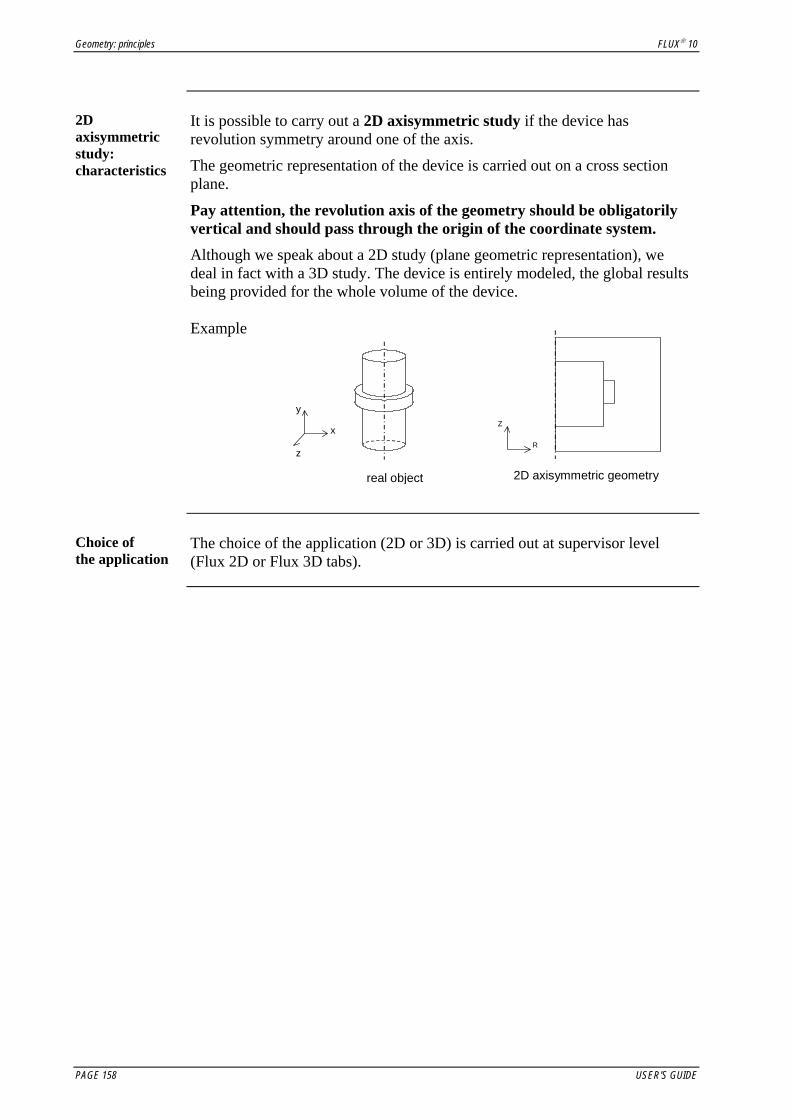
Geometry: principles FLUX® 10
2D axisymmetric study: characteristics
It is possible to carry out a 2D axisymmetric study if the device has revolution symmetry around one of the axis.
The geometric representation of the device is carried out on a cross section plane.
Pay attention, the revolution axis of the geometry should be obligatorily vertical and should pass through the origin of the coordinate system. Although we speak about a 2D study (plane geometric representation), we deal in fact with a 3D study. The device is entirely modeled, the global results being provided for the whole volume of the device.
Example
Z
R
2D axisymmetric geometry
y
x
z
real object
Choice of the application
The choice of the application (2D or 3D) is carried out at supervisor level (Flux 2D or Flux 3D tabs).
PAGE 158 USER'S GUIDE

FLUX® 10 Geometry: principles
7.1.2. 2D Example: Geometry and mesh (Tutorial)
Foreword This paragraph is a summary of cases treated in detail in the technical
document: "2D Generic Tutorial".
Flux files, relating to these various cases, are available on the CDROM of documentation of the software.
Realized study The study proposed in the 2D Generic Tutorial of Geometry and Mesh is the
study of a variable reluctance speed sensor. Only the geometry model and mesh of the device are studied in this tutorial.
Studied device The variable reluctance speed sensor consists of a cogged wheel, a magnet
and a coil connected to a measuring resistance.
Functionality The rotation of the target wheel near the tip of the sensor changes the
magnetic flux, creating an analog voltage signal that can be recovered in probes.
Continued on next page
USER'S GUIDE PAGE 159

Geometry: principles FLUX® 10
Geometric structure in Flux
The device is described in Flux as follows: • one cogged wheel with three teeth • two probes with a magnet and a coil around
PROBE 2
MAGNET 1
COIL 1-
COIL 1+
COIL 2-
COIL 2+
WHEEL
MAGNET 2
PROBE 1
Strategy Two strategies of description exist:
• one-phase description: • description of the whole device in only one Flux project
• two-phase description: • independent description of separated parts of the device in several Flux
projects • merging the independent projects into one
The second strategy is selected in this tutorial.
Of course, the geometry can be built in ways other than the presented one. The sensor geometry is defined in this particular way in order to introduce you to the most used PreFlux features.
PAGE 160 USER'S GUIDE

FLUX® 10 Geometry: principles
7.1.3. 3D Example: Geometry and mesh (Tutorial)
Foreword This paragraph is a summary of cases treated in detail in the technical
document: "3D Generic Tutorial".
Flux files, relating to these various cases, are available on the CDROM of documentation of the software.
Realized study The study proposed in the 3D Generic Tutorial of Geometry and Mesh is the
study of a variable reluctance speed sensor. Only the geometry model and mesh of the device are studied in this tutorial.
Studied device The variable reluctance speed sensor consists of a cogged wheel, a magnet
and a coil connected to a measuring resistance.
Functionality The rotation of the target wheel near the tip of the sensor changes the
magnetic flux, creating an analog voltage signal that can be recovered in probes.
Continued on next page
USER'S GUIDE PAGE 161

Geometry: principles FLUX® 10
Geometric structure in Flux
The device is described in Flux as follows: • one cogged wheel with three teeth • two probes with a magnet and a coil around
PROBE 2
MAGNET 1
COIL 1
COIL 2
WHEEL
MAGNET 2
PROBE 1
Strategy Two strategies of description exist:
• one-phase description: • description of the whole device in only one Flux project
• two-phase description: • independent description of separated parts of the device in several Flux
projects • merging the independent projects into one
The second strategy is selected in this tutorial.
Of course, the geometry can be built in ways other than the presented one. The sensor geometry is defined in this particular way in order to introduce you to the most used Flux features.
PAGE 162 USER'S GUIDE

FLUX® 10 Geometry: principles
7.2. Study domain
Introduction This section refers to the definition of the study domain, i.e.:
• the definition of the study domain limits (device model) • the possibilities of reduction the study domain with respect to the real
device by taking into account the repetitive patterns like periodicities and/or symmetry planes of the studied device.
Contents This section contains the following topics:
• Study domain limits, generalities • Truncation method • The infinite box transformation • Reduction of the study domain: symmetries and periodicities • Periodicity property and periodicity conditions on the boundaries • Symmetry and symmetry conditions on the boundaries
USER'S GUIDE PAGE 163

Geometry: principles FLUX® 10
7.2.1. Study domain limits, generalities
Electromagnetic phenomena
In the study of electromagnetic phenomena it is necessary to model both the device and the surrounding air. In fact, the quantities studied in electromagnetics (electric fields, magnetic fields), are not considered null in air or in a vacuum, contrary to other physics disciplines, mechanics, for example, where air is not taken into account.
Finite element method
The finite element method is based on the subdivision of the entire study domain in a finite number of sub domains of finite size. The physical problem is governed by a differential equation or with partial derivatives that should be satisfied on all the points of a domain. To ensure the uniqueness of the solution, boundary conditions on the outer edges must be imposed. Thus, to solve a problem with the finite element method, it is necessary to: • set limits on the device model, i.e. to define the limits or boundaries of the
domain, • impose boundary conditions on the edges, i.e., to define the values of the
state variable (potential, temperature) on the boundaries of the domain.
Apparent contradiction
The finite element method requires limits on the problem region, while the electromagnetic phenomena are unlimited.
In other words, open domains cannot be modeled by the finite element method, because it is impossible to subdivide an infinite domain into a finite number of finite sub-domains.
Study domain limits: different methods
To offset this contradiction, different methods can be used.
The first method (the truncation method) consists of closing the study domain with an outer boundary sufficiently far away from the device so as not to interfere with the results.
The second method consists of using a transformation that converts the open domain into a closed domain.
These two methods are described in the following paragraphs.
Continued on next page
PAGE 164 USER'S GUIDE

FLUX® 10 Geometry: principles
Study domain limits: truncation method
The truncation method consists of closing the study domain with an outer boundary sufficiently far away from the device so as not to interfere with the results.
The device is placed inside an air–filled box, and infinity is approximated by a closed and remote truncation boundary. The size of the air-filled box is adjusted so that the effects of the truncation boundary approximation can be neglected.
The user must determine the quantity of air to model around the device, i.e., he or she must evaluate the distance at which the computed fields become negligible.
Truncation method: disadvantages
The truncation method has certain disadvantages: • relatively high cost in terms of numbers of unknowns • negligible field values near the truncation boundary
Modeling infinity: using a transformation
To compensate for these disadvantages, a second method consists of using a transformation that converts the open domain into a closed domain.
The basic idea is to transform the open domain into a closed domain because the open domain cannot be meshed.
Use of a transformation, principle
The intial space is decomposed into two domains: • a closed interior domain, Eint • an open exterior domain, Eext
The initial space, with open borders, is transformed into a final space with closed borders, in the following way: • the interior domain (Eint) is not modified • the exterior domain (Eext) is linked to a closed domain (Eext_image) through
a spatial transformation T.
Thus, the final space is composed of two domains: • a closed interior domain Eint • a closed exterior domain Eext_image
These two (closed) domains are meshed with classical finite elements.
Illustration
m ( x, y, z ) M ( X, Y, Z )
Eext Eext_image Eint
Eint
Transformation T
Continued on next page
USER'S GUIDE PAGE 165

Geometry: principles FLUX® 10
Use of a transformation, principle (continued)
To take into account the transformations in the equations, we suppose that : • the finite elements formulations are not modified (the state variable of the
initial domain and the state variable of the image domain are equal) • new types of finite elements (transformed finite elements) are able to model
infinity.
Illustration Representation of the exterior domain
m ( x, y, z )M ( X, Y, Z )
TransformationT
y
x
M (x, y)
Y
X
M (X, Y)
Transformed finite element Image element
Inversetransformation
T-1
Choice of the transformation
Theoretically several space transformations can be used. The transformation of the real space into an image space must be bijective. It must also have properties of continuity and derivability on and between the elements, etc.
In practice, the transformations used in the software take into account various efficiency criteria: quality of the solution obtained for a number of elements or unknown factors, simplicity of implementation and so on.
PAGE 166 USER'S GUIDE
FLUX® 10 Geometry: principles
7.2.2. Truncation method
Introduction The truncation method consists of closing the study domain with an outer
boundary sufficiently far away from the device so as not to interfere with the most important results.
At what distance should be placed the border ?
To evaluate at what distance one should place the boundary, it is necessary to take into account the studied phenomena. Generally we can say that: • when the field is strongly confined within the structure (flux directed by
flux concentrators, Faraday cages, capacitor, etc.), a small quantity of air is sufficient. The boundary can be placed directly on the device outline or near it.
• when the field spreads strongly outside the structure (EMC, etc.), a large quantity of air is necessary. The difficulty consists in the estimation of this quantity.
Example Some rules for the positioning of the boundary for an open boundary
magnetic problem (device surrounded by air) are as follows: • for a 2D plane study or a 3D study:
the boundary should be placed at a distance ranging between 5 to 10 times the longest dimension of the device.
• for a 2D axi-symmetric study: in the direction normal to the revolution axis, the boundary should be placed at a distance ranging between 10 to 20 times the longest dimension of the device, the variable r*AZ decreasing slowly in this direction.
Boundary conditions
The user must impose boundary conditions on the external boundaries of the study domain.
USER'S GUIDE PAGE 167
Claire Blache
Pour un pb magnétique

Geometry: principles FLUX® 10
7.2.3. The infinite box transformation
Infinite box: definition
In the terminology of the software, using a transformation to model an infinite domain is called the infinite box technique or method.
The exterior domain (infinite) is linked to an image domain (called the infinite box) through a space transformation.
The use of the infinite box implicitly assumes a null field at infinity.
Infinite box, Flux 3D
The transformation used in Flux 3D, said to be in a parallelipipedic layer (not a skewed surface), is described by two superimposed parallelepipeds or cylinders. The faces of the exterior parallelepiped or cylinder are the image of the infinite, where the potential and field are equal to zero.
Interior domain
Exterior image domain,
i.e., infinite box Representation of the two domains by the software
Infinite box, Flux 2D
For Flux 2D, the infinite box is described by two superimposed discs (crown shaped). The external circle is the image of the infinite.
Interior domain External image domain, i.e. infinite box
Representation of the two domains by the software
Continued on next page
PAGE 168 USER'S GUIDE

FLUX® 10 Geometry: principles
How to choose the dimensions ?
The dimensions of the infinite box are defined by the user. This requires a certain experience because there is no general rule.
We can, however, give some advice: • the distance between the device and the interior surface of the infinite box is
at least equal to the dimension of the device in this direction • the dimensions of the infinite box are related to the mesh. In Flux 3D, the
number of elements on the thickness of the box must be roughly equal (at least) to two (second-order elements) or to three (first-order elements).
The mesh and the size of the infinite box must take into account the phenomena studied, and the computations to be performed as follows: • if one is interested in computing a global or a local quantity inside the
device, it is unnecessary to refine the mesh of the infinite box; • if on the contrary, one is interested in computing the field created outside
the device, one should define a box of more significant size and refine the mesh inside.
It is recommended to parameterize the dimensions of the infinite box to adjust its size during the meshing.
Boundary conditions
Flux automatically assigns boundary conditions on the infinite box.
USER'S GUIDE PAGE 169

Geometry: principles FLUX® 10
7.2.4. Reduction of the study domain: symmetries and periodicities
The main ideas: decrease the study domain
In most cases, a preliminary analysis of the device highlights the presence of repetitive patterns (periodicities) or symmetry planes.
Under these conditions, it is possible to reduce the study domain as follows: • representation of a fraction of the device • assignment of appropriate boundary conditions on the model boundaries
that reflect the periodicity property or symmetry conditions.
Interest The consequences of a reduction of the device model are as follows:
• a simplification of the geometrical description • a reduction of the finite element problem size (and thus the file size).
The rationale for reducing the problem size is the reduction of the computation time. The computation time is roughly proportional to the square of the number of unknowns.
Example: If a problem comprises N unknowns, but after reduction of the model only N/2 unknowns, the global computation time will be reduced by a factor of 4.
Reduction of study domain and boundary conditions
It is possible to simplify the device model if it has geometrical and physical periodicities and/or symmetries at the same time.
In other words, it is possible to simplify the device model, when specific conditions applied on the state variable (potential) allow the representation of a fraction of the device.
The boundary conditions are physical concepts. These concepts are briefly illustrated through a magnetic example (magneto-static, transient magnetic or magneto-harmonic application).
Continued on next page
PAGE 170 USER'S GUIDE

FLUX® 10 Geometry: principles
Example: presentation
The modeled device is a magnetic levitation device. It consists of a group of coils, a magnetic flux concentrator and a plate. Problem analysis: This device can be described as a group of repetitive linear patterns: a succession of coils in opposition. • from the geometrical point of view, the base pattern includes only one coil • from the physical point of view, the base pattern includes two coils in
opposition.
Example: different models
The authorized subdivisions of the model depend on the various types of boundary conditions set on the model boundaries. The various possible models are shown in the figures below. The boundary conditions set on the boundaries in these different configurations are explained in the following paragraphs.
USER'S GUIDE PAGE 171

Geometry: principles FLUX® 10
7.2.5. Periodicity property and periodicity conditions on the boundaries
Periodicity When a device has repetitive patterns, it is possible to model a fraction of the
device (the basic pattern), and to impose appropriate periodicity conditions on the periodicity planes.
From a physical point of view, periodicity boundary conditions are set via the state variable (potential).
Periodicity condition
(or cyclic) Anti-periodicity condition
(or anti-cyclic)
Identical values of the variable on the homologous nodes
Opposite values of the variable on the homologous nodes
Example Let’s reconsider the preceding example.
The boundary conditions to impose on boundaries 1 and 2 are periodicity conditions: • periodic type (or cyclic)
in the 1st case (study domain 1) • anti-periodic type (or anti-cyclic)
in the 2nd case (study domain 2 and 2')
PAGE 172 USER'S GUIDE

FLUX® 10 Geometry: principles
7.2.6. Symmetry and symmetry conditions on the boundaries
Symmetry When a device has symmetry planes, it is possible to represent a fraction of
the device, and to set appropriate symmetry conditions on the symmetry planes.
From a physical point of view, the symmetry boundary conditions are set on the state variable (potential).
Symmetry condition Anti-symmetry condition
Example Let’s reconsider the preceding example.
The boundary conditions applied on the device boundaries are symmetry conditions (tangential field) on boundary 1 and anti-symmetry (normal field) on boundary 2.
USER'S GUIDE PAGE 173

Geometry: principles FLUX® 10
PAGE 174 USER'S GUIDE

FLUX® 10 Geometry: principles
7.3. Characteristics of geometry building module
Introduction This section deals with the operation of the geometry building module:
principle of construction algorithms, authorized shapes, difficulties that may occur during the construction of geometry, ...
Contents This section contains the following topics:
• Presentation of the geometry building module • Lines and faces: authorized shapes • Lines and faces: superpositions and intersections • Limits of the geometry building module • Another functionality: nature of points, lines and faces
USER'S GUIDE PAGE 175

Geometry: principles FLUX® 10
7.3.1. Presentation of the geometry building module
Introduction The geometry building module of Flux is of boundary type, which means
that a volume is described by the bordering faces and a face is described by the bordering lines and a line is described by points.
Outline of the different steps
The geometry is created in ascending way: first the points, then the lines, and finally the faces and the volumes.
The table below gives a first outline of the description mode of the device geometry.
Step Description
1 Creation of points Manually by the user 2 Creation of lines Manually by the user 3 Identification/construction
of faces Automatically by the software
4 Identification/construction of volumes Automatically by the software
Creation of points and lines
The points and lines are defined manually (input of point coordinates, selection of the ends of the lines, …).
Construction of faces and volumes (new algorithms)
The faces and the volumes are automatically identified and created (algorithms of automatic construction).
Principle of automatic construction of faces: • Flux computes all the existing surfaces and it determines to which surfaces
belong the points and the lines (A surface contains faces but it is not limited and it is defined by three points linked by two lines).
• The automatic creation of faces is then realized with the aid of a technique of identification of closed outlines.
The principle of the construction of volumes is similar, but more complex, due to the 3D effect.
Construction of faces and volumes (old algorithms)
In case of difficulties at automatic construction of faces and volumes, the old algorithms of automatic construction are available.
With the old algorithm, each surface is automatically meshed with very loose meshes. By grouping the topological surface elements, the software identifies the faces inside each surface.
The principle of the construction of volumes is similar, but more complex, due to the 3D effect.
Continued on next page
PAGE 176 USER'S GUIDE

FLUX® 10 Geometry: principles
Specificities of the geometry building module
To define the geometry description possibilities offered by the geometry building module, it is necessary to answer to the following questions: • What are the different authorized shapes of lines and faces? • How are managed the intersections / superpositions of lines, of lines with
faces? • What are the limits of the algorithms of identification and of automatic
construction of faces and volumes?
These different items are treated in the following paragraphs.
USER'S GUIDE PAGE 177

Geometry: principles FLUX® 10
7.3.2. Lines and faces: authorized shapes
Lines and faces Lines and faces can be:
• created by Flux • or imported within a CAD file. Their shapes depend on their origin.
Lines created by Flux
The shape of line depends on the tool used by Flux to build the geometry. The lines created by Flux are as follows:
Shape of line Construction
• segment • arc of circle
• by entering extremity points of lines (mainly) • by propagation • by extrusion
• helical line • by extrusion only
Lines imported in Flux
Within the CAD file importation into Flux project, the lines of an unspecified shape can be imported.
Faces built by Flux
The shape of face depends on the tool used by Flux to build the geometry. The faces built by Flux are as follows:
Shape of face Construction
• planar • cylindrical • conical
• with the aid of automatic construction algorithm�
• planar • cylindrical • conical • spherical • toroidal • helical
• by propagation • by extrusion
Faces imported in Flux
Within the CAD file importation into Flux project, the faces of an unspecified shape can be imported.
PAGE 178 USER'S GUIDE

FLUX® 10 Geometry: principles
7.3.3. Lines and faces: superpositions and intersections
Intersections and superpositions
The bordering property of the geometry building module entails the interdiction of the intersections of lines, of faces and of lines with faces.
The superpositions of line/face type, i.e. lines belonging to a face, or face/face type, i.e. faces belonging to a face, are authorized.
These different cases are presented below.
Intersections, superpositions of lines
The intersections and partial or total superpositions of the lines presented in the figure below are not authorized and in this case the construction of faces is not possible.
Lines belonging to faces
The lines belonging to faces are authorized. An example is presented in the next figure.
Lines L5 and L6 are internal lines of face F1. F1
F2 L4
L7
L6L10
L1
L3
L2
L8
L5 L9
Intersections of line/face type
The intersections of line/face type are not authorized, but they do not block the construction of faces and volumes.
Faces belonging to faces
Faces belonging to faces are authorized. An example is presented in the figure below.
FACE 1 described by 8 lines
FACE 2 described by 4 lines
Continued on next page
USER'S GUIDE PAGE 179

Geometry: principles FLUX® 10
Intersections of faces
The intersections of faces are not authorized and thus the construction of volumes is blocked. An example is presented in the figure below.
The faces of the parallelepiped intersect the circular face of the inner cylinder of the torus.
Thus, the faces and the volumes cannot be built.
Intersections of faces: to avoid problems
To avoid the previous problem, it is possible to ignore some faces in the moment of volumes building. This method is presented in paragraph 7.3.5 “Another functionality: nature of points, lines and faces”.
Available corrections
Flux owns tools to correct the intersections and superposed entities in automatic or manual manner, presented in section 9.2 “Geometry importation (IGES, STEP, DXF, STL, FBD, INTER formats)”
PAGE 180 USER'S GUIDE

FLUX® 10 Geometry: principles
7.3.4. Limits of the geometry building module
Introduction The algorithms of automatic construction of faces and volumes are powerful,
but difficulties can however arise, being determined: • either by a «bad» geometrical description: problems of intersection or
superposition of entities, … • or by numerical problems, ….
Construction problems connected to intersection/ superposition of objects
Construction problems may occur in the presence of: • overlapping points, or lines of null length; • intersection or superposition of lines; • intersection of faces.
These different items are treated in the preceding paragraph.
Numerical problems of recognition of faces or volumes
Numerical problems of recognition of faces or volumes can also occur in the presence of faces characterized by too important numerical waves.
What is the problem ?
The algorithm of automatic construction of faces identifies in the first step all the existing surfaces, then, it determines to which surfaces belong the points and the lines. A surface is defined by four coefficients computed from the coordinates of three points. The test of association of points to surfaces is defined with an error criterion (epsilon tolerance criterion) and it may occur that the points and lines that the user consider in the same surface will not be considered in the same surface by the software. In this case, we speak about significant numerical waves.
This kind of situation may occur when the points are described by a "cascade" of parameters, of local coordinate systems and of transformations. When the point coordinates are evaluated in a global coordinate system, there is an accumulation of numerical errors and the tolerance is then exceeded.
In spite of a very particular care taken for solving these numerical problems, it may occur, in case of complex geometries, that the automatic construction of faces or volumes raises difficulties.
USER'S GUIDE PAGE 181

Geometry: principles FLUX® 10
7.3.5. Another functionality: nature of points, lines and faces
Problems There is a certain number of situations where the user may want to modify the
consideration of the entities (points, lines, faces) during the automatic construction of the faces and/or volumes. Two examples are given hereafter to illustrate this type of situation.
The first example reconsider the problem of intersection between faces (blocking for building the volumes). This example has already been presented.
Example 1
In this example (figure to the right) the constitutive faces of the internal parallelepiped intersect the internal circular face of the torus. The volume of the bar inside the torus cannot be built.
To avoid this difficulty, it is necessary to ignore the two circular faces during the automatic construction of volumes.
Example 2 The second example consists in the numerical modeling of a ship (“La
Fayette” frigate of the French Marine represented in the figure below). The ship structure is only made up of bars, which are represented and modeled via the lines (line regions). For this type of structure that is relatively complex, the use of the algorithm of faces and volumes construction is expensive, it often takes a long time and it generates many useless faces and volumes. To avoid this difficulty, we should place the lines within an air volume without building the group of faces and volumes that will not be used.
Continued on next page
PAGE 182 USER'S GUIDE

FLUX® 10 Geometry: principles
Solution: the nature attribute
To allow the user to modify the consideration of entities when building the faces and volumes, a specific feature (called nature) is attached to the points, lines and faces.
Attribute nature
The nature attribute allows us to set the following functions:
The entity is taken into account for: Nature the geometry the mesh Standard (STANDARD) yes Yes in air (IN_AIR) no Yes ignored (NO_EXIST) no No
Return to example 1
To ignore the annoying circular faces, the user should modify the nature of these faces (“ignored”) and restart the automatic building of volumes. These faces are then ignored at the geometry level (and also at the mesh level). Note: These faces are not destroyed. They still exist and are visible on the screen (in the visibility conditions that allow their visualization).
Return to example 2
To avoid the building of faces and volumes of the ship, the user should modify the nature of the points and lines of the ship (“in air”) and then start the construction of faces and volumes. Thus, a single group of faces (boundaries of the study domain) and one volume (air volume that includes the group of lines and faces) will be built.
The points and the lines: • are not taken into account during the construction of faces and volumes • are taken into account during the mesh building and assignment of line
regions
The simplified geometry in a wire-mesh shape of the “La Fayette” frigate consists of about 3 300 points and 8 556 lines on which the (“in air”) nature has been imposed. These points and lines are placed within an air volume surrounded by the infinite box (24 faces and 7 volumes).
USER'S GUIDE PAGE 183

Geometry: principles FLUX® 10
PAGE 184 USER'S GUIDE

FLUX® 10 Geometry: principles
7.4. Tools of geometry building module
Introduction This section deals with the assisting tools for geometry building: parameter
setting, tools for rapid construction of particular patterns, ...
Contents This section contains the following topics:
• Parameterization • Concepts of propagation and extrusion
USER'S GUIDE PAGE 185

Geometry: principles FLUX® 10
7.4.1. Parameterization
Introduction The parameterization of the geometry is one of the strong points of the
geometry building module.
It is possible to parameterize: • dimensions of workpieces • relative displacements of pieces (variable air-gap, …).
Parameterization tools
A geometrical object can be parameterized: • on one hand, using the geometrical parameters, • on the other hand, using the local coordinate systems (coordinate
systems defined with respect to a reference coordinate system).
These concepts are presented in the example below.
Example The example refers to the study of a contactor, concerning the force acting
on the moving part for various values of the air-gap. The fixed part is defined in a local coordinate system REP1 of center (0, 0, 0), and the moving part in a local coordinate system REP2 of center (0, 0, AIR-GAP). AIR-GAP is a parameter whose value is equal to the air-gap thickness. To study various positions of the moving part, and thus various values of the air-gap, it is enough to modify the value of the corresponding parameter (AIR-GAP) and to treat the corresponding case.
Continued on next page
PAGE 186 USER'S GUIDE

FLUX® 10 Geometry: principles
Principle and limits
Each time that a geometrical entity is modified, all the entities depending on this geometrical entity are automatically reevaluated through the database tools.
Modifying a parameter or a coordinate system entails the modification of the points, then of the lines, and then of the faces and volumes that are attached to this parameter.
Important: the coherence of the topology (intersection, superposition, …) is not verified by the software. This verification is a user task.
In the previous example, a null value of the AIR-GAP parameter leads to a modification of the geometry topology that can not be realized due to superposed points and lines. This limit case cannot be treated by parameterization.
Advice Defining local coordinate systems using a first coordinate system allows the
user to define a "father coordinate system", to which is attached a series of "children coordinate systems". By modifying the "father coordinate system" the user will modify the series of "children coordinate systems" attached to this first coordinate system and thus, the group of points, lines, …attached to it.
The user can also define a coordinate system in another coordinate system, and the latter defined in a third coordinate system, ... This description of intermediary coordinate systems “in cascade” can be useful, especially in case of multiple rotations. However, in this case, the risk of numerical problems for the algorithms of identification and construction of faces is more important.
USER'S GUIDE PAGE 187
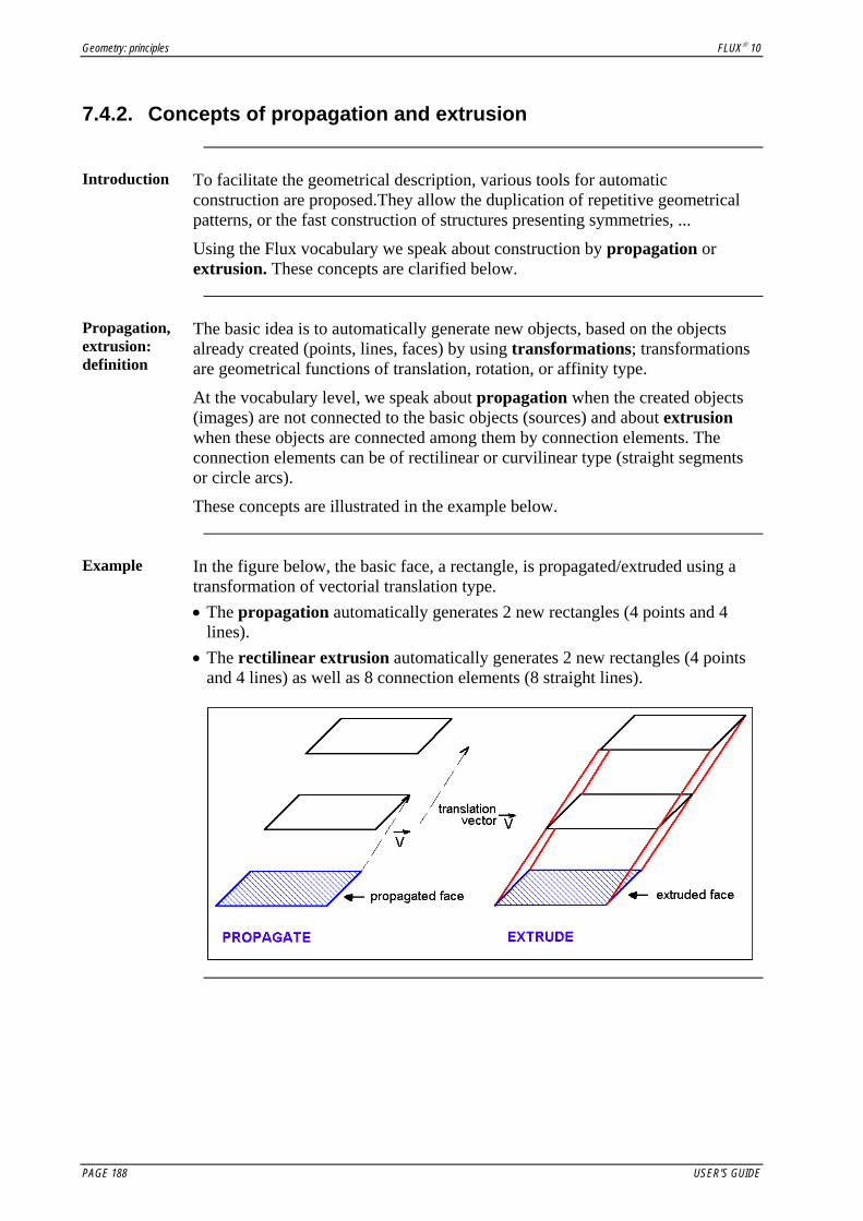
Geometry: principles FLUX® 10
7.4.2. Concepts of propagation and extrusion
Introduction To facilitate the geometrical description, various tools for automatic
construction are proposed.They allow the duplication of repetitive geometrical patterns, or the fast construction of structures presenting symmetries, ...
Using the Flux vocabulary we speak about construction by propagation or extrusion. These concepts are clarified below.
Propagation, extrusion: definition
The basic idea is to automatically generate new objects, based on the objects already created (points, lines, faces) by using transformations; transformations are geometrical functions of translation, rotation, or affinity type.
At the vocabulary level, we speak about propagation when the created objects (images) are not connected to the basic objects (sources) and about extrusion when these objects are connected among them by connection elements. The connection elements can be of rectilinear or curvilinear type (straight segments or circle arcs).
These concepts are illustrated in the example below.
Example In the figure below, the basic face, a rectangle, is propagated/extruded using a
transformation of vectorial translation type. • The propagation automatically generates 2 new rectangles (4 points and 4
lines). • The rectilinear extrusion automatically generates 2 new rectangles (4 points
and 4 lines) as well as 8 connection elements (8 straight lines).
PAGE 188 USER'S GUIDE

FLUX® 10 Geometry: principles
7.5. Geometry building: general steps
Introduction This section presents the general steps for building the device geometry
Contents This section contains the following topics:
• Geometry building process
USER'S GUIDE PAGE 189

Geometry: principles FLUX® 10
7.5.1. Geometry building process
Outline An outline of the geometry building process is presented in the table below.
The different steps are detailed in the following blocks.
Step Description 1 Device analysis 2 Definition of the study domain 3 Preparation of the geometric construction tools 4 Ascending construction of the geometry 5 Regrouping in regions
Device analysis (1)
The first step of the geometry building process is the device analysis: • to define the study domain, and • to prepare the geometric description
The questions that could arise at this level, before starting the description itself, are grouped in the tables below (non exhaustive list).
Analysis to: Device features
define the study domain
• Does the device have geometric and/or physical symmetries or periodicities?
• Can it be studied using the infinite box feature or should we limit the study domain in a different way?
Analysis to: Device features
prepare the geometric description
• Can the device be simplified without consequences on the study physics: approximation of complex shapes, removal of rounded corners, chamfered edges, holes, …?
• Does it have moving parts, variable thickness, repetitive patterns, …?
Analysis to: Is it necessary
prepare the mesh • to add points, lines, or faces in order to make easy the mesh building (skin depth, …)?
Analysis to: Device features
prepare the physical description
• Does the device have specific shapes (such as thin bars, air gaps or magnetic armatures, …) that can be replaced by points, lines or faces (considered as point, line or surface regions)?
Continued on next page
PAGE 190 USER'S GUIDE

FLUX® 10 Geometry: principles
Next steps (2, 3, 4, 5)
The other steps of the geometry building process are described in the table below.
The user Step of
… creates … builds … assigns …
Defining the study domain (2)
the symmetries the periodicities the infinite box
Preparing the geometric
building tools (3)
the geometric parameters
the local coordinate systems
the transformations
Ascending construction of
the geometry (4)
the points the lines
the faces the volumes
Regrouping in regions (5)
the point regions the line regions the face regions
the volume regions
the regions to points, lines,
faces, volumes respectively
Operations order
The different steps were presented in a “chronological” building order.
In practice, the geometry building process is not always linear and the user proceeds by successive steps. In this case, he makes “go and return” between different steps.
USER'S GUIDE PAGE 191

Geometry: principles FLUX® 10
PAGE 192 USER'S GUIDE

FLUX® 10 Mesh: principles
8. Mesh: principles
Introduction This chapter gives the necessary knowledge for the mesh realization:
presentation of the different mesh generators available in Flux, meshing strategies, …
It also presents the general operations of the mesh module (choice of mesh generator, mesh adjustment, …) and some considerations on specific meshes (thin regions, rotating air-gap, …)
Content This chapter contains the following topics:
• Mesh algorithms and field calculations: general points • Mesh strategies: mixed mesh or automatic mesh • Operation of the Mesh module: general steps • Mesh generators specificities and limitations • Description of specific meshes, examples
USER'S GUIDE PAGE 193

Mesh: principles FLUX® 10
PAGE 194 USER'S GUIDE

FLUX® 10 Mesh: principles
8.1. Mesh algorithms and field calculations: general points
Introduction This section refers to the mesh algorithms (mesh generators) available in
Flux.
Content This section contains the following topics:
• Mesh algorithms and field calculations: general points • Mesh and field calculations: different types of finite elements • A valid mesh: some rules to follow
USER'S GUIDE PAGE 195

Mesh: principles FLUX® 10
8.1.1. Mesh algorithms: different mesh generators available in Flux
Mesh: definition
The mesh is a subdivision of a domain into sub-domains called elements.
We discuss meshes or finite elements of the following types: • volume elements, for a volume domain • surface elements, for a surface domain • line elements, for a line domain.
Mesh generator: definition
A mesh generator is a tool to perform the subdivision into finite elements.
The algorithms for meshing (or mesh generators) used for subdivision are described below.
Delaunay mesh or automatic mesh
The Delaunay or automatic mesh algorithm is fairly general: it creates triangular elements on all the surfaces defined by their meshed outlines and tetrahedral elements on all the volumes defined by their meshed surface contours.
Example
Triangle Tetrahedron
“Topological” mesh or mapped mesh
This mesh generator allows the mesh of rectangular faces with rectangles (or quadrangular elements) and volumes such as parallelepiped with “bricks” (or hexahedron elements).
With the mapped mesh algorithm, the outline of a surface is divided into four lines, each one meshed so that two opposite lines have the same number of elements. The surface to be meshed is thus topologically equivalent to a rectangle. For the mapped mesh of a volume, the volume is topologically equivalent to a parallelepiped.
Exemple
Rectangle,
Quadrangle
“Brick”
Hexahedron
Continued on next page
PAGE 196 USER'S GUIDE

FLUX® 10 Mesh: principles
“Copy” mesh or linked mesh
This mesh generator allows you to impose the same mesh on faces linked by a geometrical transformation. This mesh generator can be used only for faces.
Example
Mesh by “movement” or by extrusion
This mesh generator generates a surface or volume mesh in layers on domains obtained by extrusion. This mesh is potentially anisotropic and the volume elements are prisms or hexahedrons, depending on the mesh of the base faces (triangles or rectangles).
With the extrusive mesh algorithm, a meshed line can be “moved” or shifted along a meshed path. (The movement must be simple, that is, translation or rotation.) Thus a mesh using quadrangles is generated. The same method is used to mesh volumes by moving or shifting a meshed surface.
Example rotation of a line
Example rotation of a face
“Prism” Pentahedron
“Brick” Hexahedron
Continued on next page
USER'S GUIDE PAGE 197

Mesh: principles FLUX® 10
The mesh on sub-domains or the mixed mesh
We divide the volume or surface domain to be meshed into sub-domains of simpler easy-to-mesh shapes using one of the following methods. The mesh on sub-domains or the mixed mesh is therefore a combination of the previous mesh generators.
The main difficulty with the mixed mesh is ensuring the coherence of the mesh on the interfaces between the sub-domains: the mesh on both sides of the sub-domain interfaces should be identical (we use the term mesh conformity). This conformity is not easy to obtain in 3D, when different mesh algorithms are used on neighboring sub-domains.
To ensure the coherence of the mesh on sub-domain interfaces, the 3D mixed mesh generator creates pyramidal volume elements that ensure the proper connection between triangular faces and rectangular faces.
Example
PAGE 198 USER'S GUIDE

FLUX® 10 Mesh: principles
8.1.2. Mesh and field calculations: different types of finite elements
Finite element computation
The finite element based computation allows the approximation of state variables such as scalar or vector potentials, temperature, etc. and of derived quantities, such as magnetic field and induction, magnetic flux density, electric field, thermal flux density, etc.
The quality of the approximate solution depends on the mesh. Thus, the quality of the solution depends on: • the number and the dimensions of the finite elements • the interpolation functions in each element, which can be 1st, 2nd… order
polynomial functions, and on the continuity conditions imposed on the sub-domain boundaries.
A detailed presentation of the finite element based computation method goes beyond the scope of this document.
Nodal element, edge elements
In terms of the geometry, a volume element is characterized by its vertices, edges and faces.
facet
edge
vertex
In terms of the finite element computation, we can use: • nodal elements (computation on element nodes) • edge elements (computation on element edges).
Elements of 1st
and 2nd order Different types of finite elements are available to the user, and in Flux terminology, these are called 1st order elements or 2nd order elements.
Specific information about these elements is presented in the following table.
Type of element
Position of nodes Interpolation function
1st order Vertices Linear (1st order polynomial) 2nd order Vertices + middle of edges Quadratic (2nd order polynomial)
Continued on next page
USER'S GUIDE PAGE 199

Mesh: principles FLUX® 10
Field calculation: 1st and 2nd order approach
Using 1st order elements: the potentials are approximated linearly and the fields derived from the potentials are constant.
Using 2nd order elements: the potentials are approximated quadratically and the fields are approximated linearly.
Element Potentials Field
1st order Linear approximation Constant 2nd order Quadratic approximation Linear approximation
PAGE 200 USER'S GUIDE
FLUX® 10 Mesh: principles
8.1.3. A valid mesh: some rules to follow
Introduction Mesh construction is surely the most time consuming step in defining a
problem. To obtain a valid mesh, one needs a certain level of experience, as well as some intuition about the computation result.
General rules We can, however, establish some general rules to follow:
• The finite elements should be well proportioned. The ideal elements for a surface mesh are equilateral triangles and squares. The ideal elements for a volume mesh are regular tetrahedrons and cubes. However, thanks to the second-order transformation used, the elements can be deformed within certain limits.
• The mesh should not be unnecessarily fine. A fine mesh requires a longer computation time. One may need to compromise an accurate geometrical representation of the study domain for a shorter computation time.
To mesh a complex shape domain is not an easy task and rarely can one succeed on the first attempt. One should try to combine the available mesh tools in order to obtain a satisfactory finite element discretization.
Mesh and the physics of the problem
It is necessary to adapt the mesh to the physics of the problem, as much as possible. The mesh refinement does in fact depend on the geometrical constraints, e.g., the mesh of a very thin region, but also on the physical constraints of the problem, such as a high variation of the permeability within an element, skin depth, etc.
As a general rule, a more rapid variation of the state variable requires the use of smaller elements. When one has some idea about the final result, one can decide on a coarse mesh in certain regions and a fine mesh in others. Analysis of the computation results may lead one to restart the computation with a new and better-adapted mesh.
Thus, one should always consider the mesh while the geometry is being constructed.
Examples of physical criteria to validate a mesh
Different physical criteria may be used to validate a mesh One can verify the following points: • if the field lines present cracks in the same region, the neighboring
elements are too large • in a rotating machine, if the reaction force is different from the action
force, the mesh on the air-gap region should be refined • when dealing with field problems coupled with circuit equations, if the
current through a coil computed by different methods differs significantly, the mesh on the coil region should be refined.
USER'S GUIDE PAGE 201

Mesh: principles FLUX® 10
PAGE 202 USER'S GUIDE

FLUX® 10 Mesh: principles
8.2. Mesh strategies: mixed mesh or automatic mesh
Introduction This section refers to the mesh strategies, i.e., the two mesh possibilities
available to the user: • To mesh the entire study domain using only the automatic mesh generator. • To generate a mixed mesh, using a mesh that is the best adapted to the
physics of the problem for each domain.
Content This section contains the following topics:
• Automatic mesh or mixed mesh? • Limitations of the mixed mesh
USER'S GUIDE PAGE 203

Mesh: principles FLUX® 10
8.2.1. Automatic mesh or mixed mesh?
Managing the constraints
The mesh building process should respect the constraints presented in table below, related to the modeled device.
Constraint Description of the constraint Managed byGeometrical To respect the geometry of the device
(interfaces between different volumes) The software
Physical To adapt the model to the physics of the problem (thin air-gap, skin depth)
The user
Two main situations
It is possible to distinguish the following two situations: • The mesh of the study domain is built using only one mesh generator (the
automatic mesh generator): this is the most common situation. The automatic mesh generator is simple, robust and easy to use. It is suitable for the majority of problems.
• The mesh of the study domain is carried out on different areas. The user should define the different areas and the appropriate mesh generators for each of them. In this case we use the term mixed mesh.
Automatic mesh
For an automatic mesh, the software completely ensures that the geometrical interfaces are respected.
To create the mesh of faces and volumes by respecting the geometrical interfaces, the algorithm of the automatic mesh generator can insert additional nodes on the faces or inside the volumes, so as to respect as much as possible the node density information assigned to the points and lines.
Mixed mesh For a mixed mesh, the user has more options to adapt the mesh to the physics
of the problem.
However, in 3D, the user may face software limitations; the conformity of the mesh on the interfaces between different domains may be a difficult task for the software to achieve (see the next section).
Mixed mesh: examples of use
When modeling electrotechnical devices, we mesh the air and volumes with complex topology with the automatic mesh generator, while the more sensitive parts (magnetic circuit, air-gap, skin depth, etc.) are generally meshed with the mapped or the extrusive mesh generator.
When modeling rotating machines, we generate an identical mesh on the faces (slots of machines, etc.), with the linked mesh generator.
Continued on next page
PAGE 204 USER'S GUIDE
Virgiliu FIRETEANU
???

FLUX® 10 Mesh: principles
The different mesh generators
A classification of different mesh generators with the type of mesh, name and advantages is presented in the table below.
Type Name Advantage
Automatic (Automatic)
The user can use this mesh in all situations (complex forms, etc.). The automatic mesh algorithm ensures low-distortion triangles and tetrahedrons. The mesh quality is controlled by the node distribution on the boundary contours.
Mapped (Mapped)
The user has full control over the number and the quality of the elements. The mapped mesh generator is used principally for meshing thin regions such as thin air-gaps, thin laminations, skin depth, etc.
General mesh generators,
always available
None (No Mesh)
The no-mesh mesh generator can be used if an internal area of the geometry should not be meshed. Example: exclusion from the study domain of a conductor with constant potential, in electrostatics problems.
Linked (Linked)
The linked mesh generator can be used to: • accelerate and parameterize the mesh of repetitive 2D
structures. This functionality is very useful for meshing motor slots.
• apply cyclic conditions on two faces (the faces should have the same number of nodes)
Specific mesh generators
using geometric
transformations Extrusion
(Extrusion) The user can perform a layered surface and volume mesh on domains obtained by extrusion.
USER'S GUIDE PAGE 205

Mesh: principles FLUX® 10
8.2.2. Limitations of the mixed mesh
Introduction The use of different mesh generators in different areas is possible thanks to
the algorithms that ensure the global coherence of the mesh on the interfaces.
There are, however, some limitations of the mixed mesh; these are detailed below.
Constraint of mesh conformity
The mesh must conform, i.e. there must be a “concordance” or matching of elements on the interfaces between different domains.
If it is common to mix triangular and rectangular elements in 2D, mixing hexahedral and tetrahedral elements in 3D can pose certain problems.
Through automatic insertion of pyramidal elements Flux 3D ensures the conformity of the mesh on the interface between domains meshed with hexahedrons or prisms and domains meshed with tetrahedrons. An example is shown in the figure below.
Continued on next page
PAGE 206 USER'S GUIDE

FLUX® 10 Mesh: principles
Example of non-conformity
An example of non-conformity on the interface between two domains, the first one meshed with hexadrons and the second one meshed with tetrahedrons, is shown below.
Two triangular surface elements, which are faces of two tetrahedral elements, correspond to a rectangular surface element that is a face of a hexahedron
Principle of algorithm to repair non-conformity
To ensure the conformity of the mesh, Flux uses an algorithm to repair non-conformities between hexahedrons and tetrahedrons or between rectangular faces of prisms and tetrahedrons by inserting pyramids.
In the presence of triangular and rectangular surface elements, Flux generates pyramids, starting from two triangular elements.
Two cases may occur: • The two tetrahedrons attached to the two triangular surface elements have
the same vertex node. In this case, the tetrahedrons can be connected to create a pyramid.
• If the two tetrahedrons do not have the same vertex node, Flux will insert a new node in an appropriate position.
New node
The insertion of pyramids is not always possible, and there are a certain number of limitations to the algorithm to repair non-conformities.
First limitation If the rectangular mesh is too distorted, the triangular elements belonging
to tetrahedrons may cut the rectangular elements. This case is illustrated in the figure below.
In this case, Flux 3D cannot ensure the mesh conformity.
Continued on next page
USER'S GUIDE PAGE 207

Mesh: principles FLUX® 10
Second limitation
The second limitation is less clear. To ensure the conformity of the mesh by inserting pyramids, Flux 3D adds a certain number of nodes. However, this algorithm does not work properly in the presence of sharp angles. This limitation is illustrated by the example below.
A simple device consisting of 3 hexahedral volumes is shown in the following figure: • Two external volumes are meshed using the mapped mesh generator • An inner volume is meshed using the automatic mesh generator
We note that in practice the mesh of this device is not possible. The failure of the non-conformity repairing algorithm is due to the fact that the insertion of nodes to construct pyramids is not possible for this configuration.
PAGE 208 USER'S GUIDE

FLUX® 10 Mesh: principles
8.3. Operation of the Mesh module: general steps
Introduction Mesh construction consists of partitioning a domain into sub-domains called
finite elements. This operation is assisted by the software, but it is not completely automatic.
Several mesh utilities permit the user to control the mesh process.
Content This section contains the following topics:
• Mesh construction process • Mesh adjustment: general information • Mesh and geometry: from one module to the other
USER'S GUIDE PAGE 209

Mesh: principles FLUX® 10
8.3.1. Mesh construction process
Overview Mesh construction includes different steps that depend, in part, on the mesh
generators used.
Generally, it is possible to distinguish the following steps:
Step Description 1 Preliminary consideration: choice of a mesh type
• automatic mesh (single mesh generator) • mixed mesh (multiple mesh generators)
2 If mixed mesh Then definition of the different areas
- and use of generic mesh generator - or creation of user mesh generator for these different areas
3 Mesh adjustment (adjustment of the size and number of elements)
4 Mesh construction (creation of line, surface, volume elements)
5 Choice of the type of elements: 1st order or 2nd order
Mesh strategy (1 and 2)
The two first phases of mesh process are consideration phases on mesh types and mesh generators choice. For this consideration, see section 8.2 concerning mesh strategies.
Creation, mesh generator assignment (2)
This phase concern the possible creation of user mesh generators and assignment of mesh generators to the different areas.
In the case of mixed mesh, the user can: • in one hand, use the generic mesh generators (Automatic, Mapped or No
Mesh) • in the other hand, use his own mesh generators (linked or extrusion mesh
generators)
Important: In the geometry context, if the building options “with mesh” are activated during propagation and/or extrusion phases, linked and/or extrusive mesh generators are automatically created.
Continued on next page
PAGE 210 USER'S GUIDE

FLUX® 10 Mesh: principles
Adjustment and mesh (3 and 4)
Meshing and mesh adjustment are two more or less interdependent processes: • meshing (subdivision of lines, faces and volumes) is carried out by the
software • adjustment (adjustment of the size of the elements) is performed by the user
The complete process is represented in the diagram below.
Mesh lines
Mesh adjustment
Mesh faces
Mesh volumes
The detail of adjustment operations is described in the following paragraph (§ 8.3.2 “Mesh adjustment: general information”).
Choice of the type of elements (5)
This last phase of mesh process is specific to PreFlux 3D. With PreFlux 2D, elements created are automatically 2nd order elements.
USER'S GUIDE PAGE 211
Claire Blache
Refaire un organigramme

Mesh: principles FLUX® 10
8.3.2. Mesh adjustment: general information
Adjustment: definition
Mesh adjustment consists of adjusting the size and the number of elements.
Two types of adjustment
To adjust the mesh, the user should take into account the geometry being modeled.
The user has the option to set: • the node density around selected points, • the number and the distribution of nodes on the lines.
Information related to the node density next to selected points is information assigned to the points; we use the phrase “mesh adjustment via the points” or by the intermediate of mesh points.
Information concerning the number and the distribution of nodes on the lines is assigned to the lines; we use the phrase “mesh adjustment via the lines” or by the intermediate of mesh lines.
Principle of adjustment “via the points”
The principle of mesh adjustment “via the points” is illustrated in the example below. 5 mm1 mm
• the user imposes a length of 1 mm on the left point and a length of 5 mm on
the right point • the program subdivides the line according to this information: the first line
element in contact with the left point has a length of 1 mm and the first line element in contact with the right point has a length of 5 mm. The program arranges the nodes between the two points, following a geometrical progression.
Principle of adjustment “via the lines”
The principle of mesh adjustment “via the lines” is illustrated in the example below. 10 equidistant elements
• the user imposes the number of elements and their distribution on the line:
10 line elements, equidistant nodes. • the program divides the line according to this information.
Continued on next page
PAGE 212 USER'S GUIDE

FLUX® 10 Mesh: principles
Priorities for the lines and the points
If both lines and points are assigned mesh information, the lines have priority over points.
Example • Points P1, P2, P3 and P4:
length of line elements next to points: 2 mm
• Line Lz: geometric progression of the line elements on the line: - minimum distance: 1 mm - ratio : 1.5
• Result: - on line Lx and Ly: division based on P1,
P2 and P3 points information - on line Lz: division base on the line
information
P1
P3
P2
P4
Lz Ly
Lx
USER'S GUIDE PAGE 213

Mesh: principles FLUX® 10
8.3.3. Mesh and geometry: from one module to the other
Problematic We have presented in the chapter concerning geometry one geometry
building process, and we present in this chapter one mesh construction process.
In the reality, the user generally proceeds by successive steps and he could repeat several building geometry processes and several mesh construction processes. So, he is going back and forth between geometry and mesh contexts (see examples hereafter).
Example 1 For a motor description, the user could proceed as follow:
Phase Description Context 1 Geometry building of a rotor slot (Creation of
slot points and lines, building faces). Geometry
2 Preparation of slot mesh (Creation of Mesh Point and/or Mesh lines and assignment to points and lines).
Geometry Mesh
3 Meshing of the slot, visualization of surface elements and mesh adjustment. Mesh
3 Propagation of the slot and mesh information. Geometry 4 …
In this example, the user switches from geometry context to mesh context, then go back to geometry context, …
Example 2 To facilitate the mesh of the device, the user often needs to add
supplementary points, lines, faces or volumes.
Based on these supplementary entities, the user can adjust the density of mesh nodes and control the mesh distribution between high node density areas with small elements and low node density areas with larger elements.
In this example, the user goes back to geometry context, …after a phase in the mesh context…
Return to geometry context after mesh operations
Important: To go back and forth between geometry and mesh modules are authorized for non-mesh structures. If the project is meshed, geometric modifications are not allowed. To modify a meshed geometry, it’s necessary to first delete the mesh.
PAGE 214 USER'S GUIDE

FLUX® 10 Mesh: principles
8.4. Mesh generators specificities and limitations
Introduction This section presents specificities (and limitations) of mesh generators trough
examples.
Content This section contains the following topics:
• Mapped mesh: 2D examples • Mapped mesh: 3D examples • Linked mesh: 2D examples • Extrusive mesh: 2D example • Extrusive mesh: 3D example
USER'S GUIDE PAGE 215
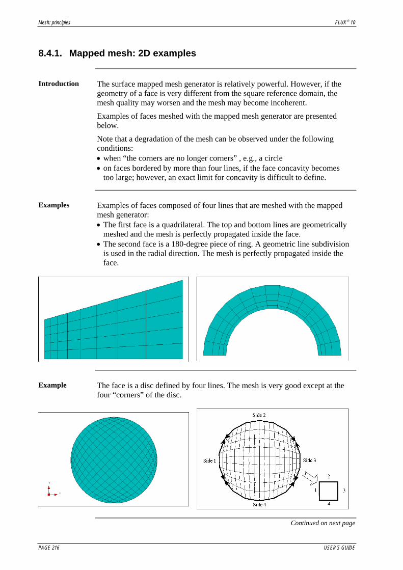
Mesh: principles FLUX® 10
8.4.1. Mapped mesh: 2D examples
Introduction The surface mapped mesh generator is relatively powerful. However, if the
geometry of a face is very different from the square reference domain, the mesh quality may worsen and the mesh may become incoherent.
Examples of faces meshed with the mapped mesh generator are presented below.
Note that a degradation of the mesh can be observed under the following conditions: • when “the corners are no longer corners” , e.g., a circle • on faces bordered by more than four lines, if the face concavity becomes
too large; however, an exact limit for concavity is difficult to define.
Examples Examples of faces composed of four lines that are meshed with the mapped
mesh generator: • The first face is a quadrilateral. The top and bottom lines are geometrically
meshed and the mesh is perfectly propagated inside the face. • The second face is a 180-degree piece of ring. A geometric line subdivision
is used in the radial direction. The mesh is perfectly propagated inside the face.
Example The face is a disc defined by four lines. The mesh is very good except at the
four “corners” of the disc.
Continued on next page
PAGE 216 USER'S GUIDE

FLUX® 10 Mesh: principles
Examples Two examples of faces, each composed of five lines (convex face and
concave face), are presented below. For these two faces the mesh is good.
Example The face shown below is composed of twelve lines and points and it is
characterized by significant concavities. The structuration is done using the four end points on the left and on the right. The other eight points are angular. The resulting mesh is incorrect.
To obtain a valid mesh, this face should be subdivided, e.g., into five faces.
Example Two types of mapped mesh of a concave face bordered by six lines.
Depending on the mesh discretization, the mesh is correct or not. Subdivision of the face into two faces is recommended.
USER'S GUIDE PAGE 217

Mesh: principles FLUX® 10
8.4.2. Mapped mesh: 3D examples
Introduction The volume mapped mesh generator is less powerful than the surface mapped
mesh generator. To get a good quality mesh, the shape of the geometry should be close to the cubic reference domain (see the 3D examples).
Some examples of volumes meshed with the mapped mesh generator are presented below. Note that a degradation of the mesh can be observed in cylindrical volumes. The mapped mesh generator does not accept volumes having cylindrical faces of 180 degrees or more. If the elements are too fine, the mesh may become incoherent.
Example Mapped mesh of a hexahedron with planar faces: The elements are of good
quality.
Continued on next page
PAGE 218 USER'S GUIDE

FLUX® 10 Mesh: principles
Examples Mapped mesh of a “tile”:
• The mesh of the first tile is not perfect, but since the deformation of the elements stays within acceptable limits, the mesh remains correct.
• The mesh of the second tile, which is finer, is densely meshed along the thickness. The elements are very distorted and the majority of those that touch the inner face are incorrect. To obtain a correct hexahedral mesh, one can either subdivide the volume, or, even better for this geometry, one can use a geometrically extruded mesh with a mapped base.
Mapped mesh of a tile: elements are correct although distorted
Refined mapped mesh of a tile: elements are incorrect because they are too distorted
USER'S GUIDE PAGE 219
Lillith Stoessel
Je pense que le mot “tile” est une traduction plus vraie que “lid”. “Lid,” c’est un peu bizarre.

Mesh: principles FLUX® 10
8.4.3. Linked mesh: 2D examples
Introduction Some examples of faces meshed using a linked mesh generator are presented
below.
Example Linked mesh of the stator slots of a motor.
This motor is described in detail in the tutorial “Brushless permanent magnet motor simulations in Flux 2D”.
Example Linked mesh of rotor and stator slots of a motor.
This motor is described in detail in the technical paper “End winding characterization with Flux 3D”.
PAGE 220 USER'S GUIDE

FLUX® 10 Mesh: principles
8.4.4. Extrusive mesh: 2D example
Extrusive mesh of faces
Though developed to mesh volumes, the extrusive mesh generator can also be assigned to faces.
To obtain an extrusive mesh on faces, a prerequisite is that the face be obtained by extrusion with an existing transformation (rectilinear extrusion by translation, positive ratio affinity, or curvilinear extrusion by rotation) and that this transformation exists.
Example Extrusive mesh of a quarter of circle.
Extrusion of the base line by a rotation of 90°.
USER'S GUIDE PAGE 221

Mesh: principles FLUX® 10
8.4.5. Extrusive mesh: 3D example
Example We consider below a device consisting of eight volumes, meshed by extrusion
(extrusion by translation for the first four volumes and extrusion by rotation for the other four volumes). We constructed two different extrusive meshes, one having a triangular base, the other a rectangular base. On this mesh, we note the following: • The capability of producing a cyclical mesh • The rotational extrusive mesh can use specific elements close to the axis
(prisms, tetrahedrons, pyramids). • The direction of extrusion is unimportant.
Example A geometry composed of six volumes is presented below. These volumes are
meshed using three extrusions in different directions. We also imposed linear geometric subdivisions on four lines corresponding to the four edges of the extrusion.
PAGE 222 USER'S GUIDE
Lillith Stoessel
Je pense que “cyclic” ou “cyclical” n’est pas correct. Est-ce qu’on peut dire “circular” ou telle expression?
Lillith Stoessel
Ou, peut-être, “has no effect” ou “does not matter”?
Lillith Stoessel
Ces quatre lignes doivent porter des etiquettes dans cette figure.

FLUX® 10 Mesh: principles
8.5. Description of specific meshes, examples
Introduction To generate a valid mesh, there are:
• mesh strategies and rules that facilitate the mesh of particular geometries (thin regions, etc.)
• a certain number of rules to follow to mesh rotating and translating air-gaps.
Content This section contains the following topics:
• Mesh of thin regions: addition of lines • Mesh of devices with skin effect • Mesh of the translating air-gap (2D) • Mesh of the rotating air-gap (2D)
USER'S GUIDE PAGE 223

Mesh: principles FLUX® 10
8.5.1. Mesh of thin regions: addition of lines
Mesh of thin regions
The mesh of a thin region can be simplified by adding supplementary points and lines that are not used in the construction of regions. This is illustrated in the figure below.
PAGE 224 USER'S GUIDE

FLUX® 10 Mesh: principles
8.5.2. Mesh of devices with skin effect
Mesh of skin depth: rules to follow
To obtain accurate results in skin effect problems (eddy currents, etc.), at least two elements should be used on the skin depth. The state variable actually has an exponential variation on the skin depth, but within an element, Flux 2D uses a parabolic approximation. Thus, the size of elements should be small enough that the arc of parabola can be assimilated to an exponential arc.
Computation of skin depth: recall
In magneto-harmonic problems with linear materials, the skin depth for eddy currents can be expressed as follows:
δρπµ
=f
where f is the frequency, ρ the resistivity and µ the magnetic permeability.
Choosing the mesh generator
To mesh the skin depth, elements of rectangular or hexahedral type are recommended, that is: • the mapped mesh generator (2D, 3D) • an extruded mesh generator with a mapped base (3D) The rest of the study domain is meshed using the automatic mesh generator.
2D Example A 2D example of mesh on the skin depth is shown in the figure below.
δ = skin depth
billet
magnetic circuit
inductor
Mapped mesh of skin depth {
Continued on next page
USER'S GUIDE PAGE 225

Mesh: principles FLUX® 10
3D Example A 3D example of mesh on the skin depth is shown in the figure below.
The most critical volumes (the volumes corresponding to the skin depth of the bar) are meshed using the extrusive mesh generator. The rest of the study domain is meshed using the automatic mesh generator (inside the bar and the surrounding air).
PAGE 226 USER'S GUIDE

FLUX® 10 Mesh: principles
8.5.3. Mesh of the translating air-gap (2D)
Principle of re-meshing
During the solving process, the mesh of the translating air-gap area is rebuilt for each change in the position of the moving part. The re-meshing is carried out as follows.
Step Description
1 The elements of the moving part are moved by translation 2 The elements of the displacement region are either distorted or
transferred to the other end, according to the following criteria: • for a small displacement of the moving part (smaller than half
the height of an element) the elements are flat. • for a large displacement of the moving part (larger than half the
height of an element) the elements are transferred to the other end.
3 The translating air gaps are re-meshed.
Continued on next page
USER'S GUIDE PAGE 227

Mesh: principles FLUX® 10
Translating air-gap in 2D: additional mesh rules
Besides the usual mesh rules, some additional rules must be respected for the mesh of the translating air-gap: The moving part can be meshed with triangular or quadrangular elements, but there must be always the same number of nodes on the upper and lower edges in contact with the displacement region. The displacement region, which consists of two distinct areas, should be meshed with quadrangular elements. There must be the same number of elements across the width of the displacement region. The translating air-gap should contain only one layer of triangular elements in its thickness, and these elements should have a shape as close as possible to an equilateral triangle.
Examples of mesh
Some examples of correct and incorrect mesh of the displacement region and of the translating air-gap are illustrated in the figure below.
PAGE 228 USER'S GUIDE
Lillith Stoessel
Je ne suis pas sûre de cette expression. Il dit “dans le sense de la longuer”, que je traduit “in the direction of the length.” Mais je pense qu’on faut le même nombre d’elements dans le largeur (width across) la partie mobile, pas dans le sens de mouvement. ???

FLUX® 10 Mesh: principles
8.5.4. Mesh of the rotating air-gap (2D)
Principle of remeshing
During the solving process, the mesh of the rotating air-gap is rebuilt at each change in the position of the moving part.
Rotating air-gap: additional mesh rules
In addition to the usual mesh rules, some rules must be respected for the mesh of the rotating air-gap: The rotating air-gap should contain only a single layer of triangular elements, and their shape must be as close as possible to an equilateral triangle. Some examples of correct and incorrect mesh for the rotating air-gap are illustrated in the following figure.
USER'S GUIDE PAGE 229

Mesh: principles FLUX® 10
PAGE 230 USER'S GUIDE

FLUX® 10 SSGeometry / mesh importation: principles
9. Geometry / mesh importation: principles
Introduction FLUX software has the ability to communicate with other software packages
and to carry out the transfer of data from CAD tools to the Finite Element (FE) analysis tools. This chapter presents the available choices for the different processes of importation with Flux: • import of geometry starting from geometric files • import of geometry starting from mesh files • import “Advanced Mode” • in addition, the associated tools for simplification and repair of imported
data are described
Item of Note (reminder)
The import of a CAD geometry file into FLUX takes into account projects possessing complex geometries (e.g. presenting twisted surfaces). These types of surfaces cannot be generated directly using the available tools in FLUX.
Contents This chapter contains the following topics:
• Geometry / mesh importation: overview • Geometry imports (IGES, STEP, DXF, STL, FBD, formats) • Import of geometry called « advanced mode » (format SAT, CATIA V4,
CATIA V5, INVENTOR, PRO ENGINEER, STEP (advanced mode) and IGES (advanced mode))
• Mesh importation (NASTRAN, PATRAN, UNV Ideas, MED formats)
USER'S GUIDE PAGE 231

SSGeometry / mesh importation: principles FLUX® 10
PAGE 232 USER'S GUIDE

FLUX® 10 SSGeometry / mesh importation: principles
9.1. Geometry / mesh importation: overview
Introduction This section presents a general point of view concerning the authorized
formats for importation and the principle of conversion.
Contents This section contains the following topics:
• Types of imports • Import formats
USER'S GUIDE PAGE 233

SSGeometry / mesh importation: principles FLUX® 10
9.1.1. Types of imports
Introduction Three different types of imports are possible with FLUX :
• import of geometry • import of mesh • import of geometry using “advanced mode”
Import of geometry
The import of geometry consists of importing geometric elements using entities compatible with the finite element environment of FLUX. The user is required to check the imported geometry and correct any faults that may be present.
Import of geometry called « advanced mode »
The import of geometry called «advanced mode » consists of importation of geometric elements for entities compatible with the finite element environment of FLUX. Using this model the user can choose the entities that he wishes to import, as well as having the option to automatically correct the geometry.
Mesh Import Mesh import consists of importing the mesh which results in the creation of
geometry in the FLUX environment.
PAGE 234 USER'S GUIDE

FLUX® 10 SSGeometry / mesh importation: principles
9.1.2. Import formats
Import formats The following table summarizes the different file formats accepted in Flux,
associated with the type of import.
Type of import Available File formats Extension Type of format IGES (Initial Graphics Exchange Specification)
*.IGES, *.IGS
STEP (Standard for Exchange of Product)
*.STEP, *.STP
DXF (Draw eXchange File) *.DXF STL (STereo Lithography) *.STL
standard geometry import called « standard »
FBD (Flux 2D géométrie) *.FBD proprietary NASTRAN neutral *.NAS, *.DAT PATRAN neutral *.PAN, *.DAT UNV (UNiVersel Ideas Master Serie)
*.UNV mesh import
MED (Model of data exchange)
*.MED
standard
IGES (Initial Graphics Exchange Specification)
*.IGES, *.IGS
STEP (Standard for Exchange of Product)
*.STEP, *.STP Standard
SAT *.SAT CATIA V4 *.MODEL CATIA V5 *.CATPRODUCT
*.CATPART INVENTOR *.IPT
geometry import called « advanced mode »
PROE (Pro Engineer) *.ASM , *.PRT
proprietary
Type of accepted file
For importation Flux accepts only files in text format. The binary files are not accepted.
Attention: It is not possible to import an assembly file consisting of several IGS files(*_ASM.IGS).
Multiple importation
Multiple importations are available. Flux is able to import the files with different formats (DXF, STL, etc) in the same project.
USER'S GUIDE PAGE 235

SSGeometry / mesh importation: principles FLUX® 10
PAGE 236 USER'S GUIDE

FLUX® 10 SSGeometry / mesh importation: principles
9.2. Geometry imports (IGES, STEP, DXF, STL, FBD, formats)
Introduction This section deals with the importation of geometry starting from geometry
files. The import of a CAD geometry in an FE (finite elements) project is an operation consisting of turning the data from the CAD type (in a specified format) into data of the FE type.
Note: the import selection ,“advanced mode,” integrates a certain number of repairs before the conversion of data (see § Import of geometry called « advanced mode » (format SAT, CATIA V4, CATIA V5, INVENTOR, PRO ENGINEER, STEP (advanced mode) and IGES (advanced mode))
Formats The following formats enable geometry import :
File format Extension Type of format IGES (Initial Graphics Exchange Specification)
*.IGES, *.IGS
STEP (Standard for Exchange of Product)
*.STEP, *.STP
DXF (Draw eXchange File) *.DXF ofSTL (STereo Lithography) *.STL
standard
FBD (Flux 2D géométrie) *.FBD proprietary
Contents This section contains the following topics:
• Process of geometry importation • Stage of conversion with options • Stage of geometry checking: concept of geometric defect • Stage of geometric defects correction / geometry simplification • Geometry importation: strategies
USER'S GUIDE PAGE 237
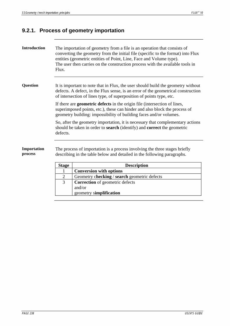
SSGeometry / mesh importation: principles FLUX® 10
9.2.1. Process of geometry importation
Introduction The importation of geometry from a file is an operation that consists of
converting the geometry from the initial file (specific to the format) into Flux entities (geometric entities of Point, Line, Face and Volume type). The user then carries on the construction process with the available tools in Flux.
Question It is important to note that in Flux, the user should build the geometry without
defects. A defect, in the Flux sense, is an error of the geometrical construction of intersection of lines type, of superposition of points type, etc.
If there are geometric defects in the origin file (intersection of lines, superimposed points, etc.), these can hinder and also block the process of geometry building: impossibility of building faces and/or volumes.
So, after the geometry importation, it is necessary that complementary actions should be taken in order to search (identify) and correct the geometric defects.
Importation process
The process of importation is a process involving the three stages briefly describing in the table below and detailed in the following paragraphs.
Stage Description
1 Conversion with options 2 Geometry checking / search geometric defects 3 Correction of geometric defects
and/or geometry simplification
PAGE 238 USER'S GUIDE

FLUX® 10 SSGeometry / mesh importation: principles
9.2.2. Stage of conversion with options
Introduction The first stage of importation is the stage of conversion of the imported
geometry into the Flux format.
Operation principle
The principle of operation of the importation is as follows: all the geometric entities of the initial file (specific to the standard and proper formats) are converted into the Flux format (geometric entities of type Point, Line, Face and Volume...) in the final file.
Conversion of entities
The entities of the initial file are read and converted into the Flux entities. The summary table is presented below.
The file
format … CAD entities contained… Convert into Flux entities …
points points defined by parameterized coordinates lines lines of type:
• segment defined by extremity points • arc defined by origin, intermediary and
extremity points • curve (for the unspecified lines)
IGES / STEP
faces faces of type: • automatically defined by plane, cylindrical
or conical surfaces • uneven type, defined by any kind of
surfaces POINT points defined by parameterized coordinates LINE lines of segment type defined by extremity
points POLYLINE N lines of segment type ARC, CIRCLE
lines of arc type defined by origin, intermediary and extremity points
DXF
3DFACE faces of automatic type, with triangular shape, defined by a plane surface
VERTEX points defined by parameterized coordinates STL FACET faces of automatic type, with triangular shape,
defined by a plane surface
Continued on next page
USER'S GUIDE PAGE 239

SSGeometry / mesh importation: principles FLUX® 10
Conversion of entities (continued)
The file
format … CAD entities contained… Convert into Flux entities …
points points defined by parameterized coordinates lines lines of type
• segment defined by extremity points • arc defined by origin, intermediary and
extremity points faces automatic faces geometric parameters
geometric parameters
FBD
regions regions
Options for conversion
To perform the data conversion, different options are available to the user.
There are two types of options: • general options, available for all formats
- choice of a coordinate system: locates the imported geometry in the Flux project
- choice of the unit: chooses the units of the device dimensions - choice of precision: defines the minimal distance that enables the distinction of two points
• particular options, specific to the format
Only the general options are described in this section.
PAGE 240 USER'S GUIDE

FLUX® 10 SSGeometry / mesh importation: principles
9.2.3. Stage of geometry checking: concept of geometric defect
Introduction The second stage is geometry checking. This stage is the stage of research
(identification) of the geometric defects; correction will be carried out in the following stage (stage 3).
Before describing the modes of defects search, the different defect types are described in the following blocks.
Geometric defects
The geometric defects can hinder or block the geometry building process.
The following can be therefore discerned: • blocking defects (intersections and superimposed entities):
these defects must be identified and corrected before building the geometry in Flux.
• non-blocking defects (very small lines and faces, wires not closed, …): these defects do not impede the geometry building in Flux, but they can influence, in a negative manner, the quality of the geometry building and/or the meshing
The geometric defects are presented in the table below.
Defect Example (or type) Consequence
blocking
• intersection type: - line-line - line-face - face-face*
• superposition type: - confused points - superimposed lines
• entities of small dimensions: - abnormal line - abnormal face
building of the faces and volumes impossible
• entities of small dimensions: - abnormal line (user epsilon) - abnormal face (user epsilon)
difficulties of meshing non-
blocking • open wire missing face
*In the next figure, the faces building after the importation of the geometry will generate the intersection of the faces. This type of defect is not identified by Flux in the Geometric defect entity, but it is blocking for the further volumes building. The connecting the points P1 and P2 by a new line before the faces building enables to avoid the intersection of the faces.
P1 P2
Continued on next page
USER'S GUIDE PAGE 241
csantamaria
A reporter dans html

SSGeometry / mesh importation: principles FLUX® 10
Defects research modes
The research of the geometric defects can be carried out in two ways: • for the assembly of types of defects (described as global checking of the
geometry) • by type of defect (described as research by type)
Research result Whatever the research mode, the result is the following:
• Flux creates a geometric entity of the Geometric defect type for each defect found (this entity contains the information about the defect localization: number of concerned points, lines or faces)
• Flux highlights this entity in a graphic window (specific display)
PAGE 242 USER'S GUIDE
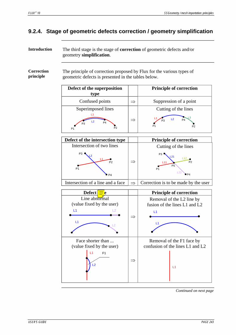
FLUX® 10 SSGeometry / mesh importation: principles
9.2.4. Stage of geometric defects correction / geometry simplification
Introduction The third stage is the stage of correction of geometric defects and/or
geometry simplification.
Correction principle
The principle of correction proposed by Flux for the various types of geometric defects is presented in the tables below.
Defect of the superposition
type Principle of correction
Confused points ⇒ Suppression of a point Superimposed lines
P2
P4 P3
⇒
Cutting of the lines
L2 P4 P3
P1 P2
L1 L1 L3
P1
L2
Defect of the intersection type Principle of correction Intersection of two lines
P4
P3
L1
P1
L2
P2
⇒
Cutting of the lines
L12 L11
L22
L21
P4
P1
P2
P3
P5
Intersection of a line and a face ⇒ Correction is to be made by the user
Defect type Principle of correction Line abnormal
(value fixed by the user) L2 L1
L1
L2
⇒
Removal of the L2 line by fusion of the lines L1 and L2
L1
L1
Face shorter than ...
(value fixed by the user) F1L1
L2
⇒
Removal of the F1 face by confusion of the lines L1 and L2
L1
Continued on next page
USER'S GUIDE PAGE 243
csantamaria
Reporter dans html

SSGeometry / mesh importation: principles FLUX® 10
Defect type Principle of correction
Open wire P2 P1 L1
⇒
Closing of contour by prolongation of the L1 line
P1 L2
L2 L1
Simplification principle
The principle of simplification proposed by Flux consists to remove some lines and points and thus “to reduce” the geometry. Simplification is expected only for the lines of the segment type and arc of circle type.
The principle of simplification is presented in the table below.
Geometry type Principle of simplification
Segments located on the tangent of the straight lines
P4P3 P1 P2 L3L1 L2
⇒
Removal of the lines L2 and L3 and suppression of the points P2 and P3 by fusion of the lines L1, L2 and L3
P4P1 L1
Arc of circle having the same curve angle
L1 P2 P1
P3 P4
Removal of the lines L2 and L3 and suppression of the points P2 and P3 by fusion of the lines L1, L2 and L3
P1 P4
L1
L2 L3
Continued on next page
PAGE 244 USER'S GUIDE
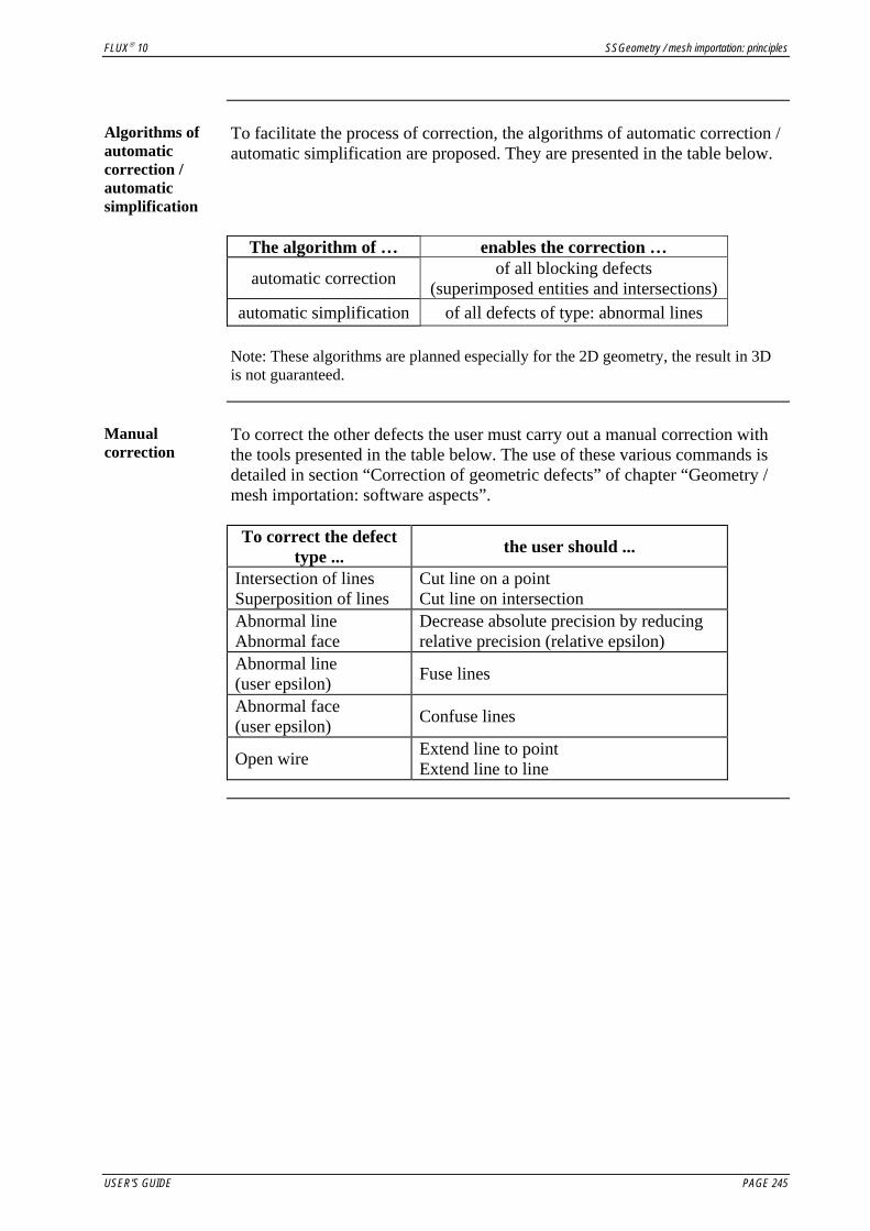
FLUX® 10 SSGeometry / mesh importation: principles
Algorithms of automatic correction / automatic simplification
To facilitate the process of correction, the algorithms of automatic correction / automatic simplification are proposed. They are presented in the table below.
The algorithm of … enables the correction …
automatic correction of all blocking defects (superimposed entities and intersections)
automatic simplification of all defects of type: abnormal lines
Note: These algorithms are planned especially for the 2D geometry, the result in 3D is not guaranteed.
Manual correction
To correct the other defects the user must carry out a manual correction with the tools presented in the table below. The use of these various commands is detailed in section “Correction of geometric defects” of chapter “Geometry / mesh importation: software aspects”.
To correct the defect
type ... the user should ...
Intersection of lines Superposition of lines
Cut line on a point Cut line on intersection
Abnormal line Abnormal face
Decrease absolute precision by reducing relative precision (relative epsilon)
Abnormal line (user epsilon) Fuse lines
Abnormal face (user epsilon) Confuse lines
Open wire Extend line to point Extend line to line
USER'S GUIDE PAGE 245

SSGeometry / mesh importation: principles FLUX® 10
9.2.5. Geometry importation: strategies
Introduction Although it is possible and necessary to correct the geometric defects after
importation, it is preferable to prepare the initial file so that the operations of correction in Flux are minima.
The checking of the geometry and the correction of possible geometric defects are essential.
Prepare the initial file
To prepare the initial file in general way: • define geometric elements in CAO software with respect to the
characteristics of the Flux geometry building module • remove the intersections of lines, lines and faces, the superposition of faces,
… The characteristics of geometry building module (description: the authorized shapes of faces and volumes, prohibited intersections and superimposed entities …) are given in chapter “Geometry: principles”.
Constraints of Flux software
It is not possible to perform the following operations in an imported geometry (containing lines of list edges type and faces of list facets type): • modify the imported faces / lines • propagate / extrude the imported faces / lines • mesh the faces / volumes using mapped mesh generator
Capabilities of Flux software
It is possible to perform the following operations in an imported geometry: • build the faces / volumes • mesh the faces / volumes using automatic mesh generator
PAGE 246 USER'S GUIDE

FLUX® 10 SSGeometry / mesh importation: principles
9.3. Import of geometry called « advanced mode » (format SAT, CATIA V4, CATIA V5, INVENTOR, PRO ENGINEER, STEP (advanced mode) and IGES (advanced mode))
Introduction This section refers to the import of geometry starting from geometric files in « advanced mode».
The import of CAD geometry into an FE (finite elements) project is an operation which consists of the conversion of the CAD data (in a specified format) into FE type data.
The advanced mode is a method that permits a CAD geometry transfer to the FE software in a more efficient manner while integrating repairs before the conversion of data. These repairs simplify the work of geometry checking/correction.
Format The formats which permit the import of geometry are as follows:
File format Extension Type of format IGES (Initial Graphics Exchange Specification)
*.IGES, *.IGS
STEP (Standard for Exchange of Product)
*.STEP, *.STP Standard
SAT *.SAT CATIA V4 *.MODEL CATIA V5 *.CATPRODUCT
*.CATPART INVENTOR *.IPT PROE (Pro Engineer) *.ASM , *.PRT
proprietary
Interest The user can import a geometry in advanced import mode thereby eliminating
the need for the geometric correction phase to follow in FLUX.
Contents This section contains the following topics:
• About import « advanced mode » • Import process
USER'S GUIDE PAGE 247

SSGeometry / mesh importation: principles FLUX® 10
9.3.1. About import « advanced mode »
Context In general, the CAD files used for the execution/ visualisation of a prototype
or device are not always adapted to finite element modelling. It is often necessary « to facilitate» the transfer of data from the CAD format to the finite elements analysis software format.
The advanced mode is an « optimised » mode, which, due to integrated supplementary functions, facilitates the work of data transfer.
Problem The CAD file assemblies comprise geometries of independent parts
positioned to one another by means of positioning constraints. Problems may arise at the moment of conversion to the FE model when these imported parts are adjoined or overlapping, resulting in collisions, as represented in the figure…
FE CAD
face/face intersection line/line
intersection
Model NOT SUITABLE for FE computation
Solution To solve the problem of adjoining geometries (parts in contact, see figure), a
number of integrated repair tools are included in the import selection called « advanced mode ». This consists of the appropriate construction of the interfaces (minus the intersections), respective to the contact faces between the parts. This must be designated before carrying out the proper operation of conversion.
PAGE 248 USER'S GUIDE

FLUX® 10 SSGeometry / mesh importation: principles
9.3.2. Import process
Import process
The import is carried out in two phases, as described in the table below and illustrated by the following figure.
Phase Description
1 Repair: • Detection of parts in contact • Construction of the contact faces • Union of solids in contact
2 Conversion: • Choice of elements of the CAD file to convert • Conversion of elements:
CAD type geometry -> Geometry of Finite Elements type 3 Result: the results are displayed in an import report in the History
zone.
Conversion The CAD entities of the initial file are read and converted into FLUX entities
of the type: • points defined by parametric coordinates • lines of type :
- segment defined by extremity points - arch defined by the origin, intermediate and extremity points - curve (for any kind of lines)
• faces of the type : - automatic defined by the plane, cylindrical or conical surfaces - twisted faces, defined by any kind of surface
• volumes
USER'S GUIDE PAGE 249

SSGeometry / mesh importation: principles FLUX® 10
PAGE 250 USER'S GUIDE
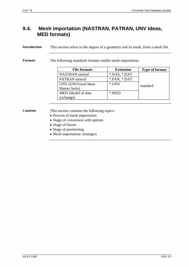
FLUX® 10 SSGeometry / mesh importation: principles
9.4. Mesh importation (NASTRAN, PATRAN, UNV Ideas, MED formats)
Introduction This section refers to the import of a geometry and its mesh, from a mesh file.
Formats The following standards formats enable mesh importation.
File formats Extension Type of format NASTRAN neutral *.NAS, *.DAT PATRAN neutral *.PAN, *.DAT UNV (UNiVersel Ideas Master Serie)
*.UNV
MED (Model of data exchange)
*.MED
standard
Contents This section contains the following topics:
• Process of mesh importation • Stage of conversion with options • Stage of fusion • Stage of positioning • Mesh importation: strategies
USER'S GUIDE PAGE 251

SSGeometry / mesh importation: principles FLUX® 10
9.4.1. Process of mesh importation
Introduction Mesh import enables the import of the geometry and mesh. The geometry
created is based on the imported mesh. This approach enables the introduction in Flux projects of uneven surfaces in the form of “cut surfaces”, but has the disadvantage of generating an important number of geometric entities (volumes, faces, lines). As consequence, the result of the mesh file conversion is not always compatible with the requirements of Flux analysis (for example, the use of sliding cylinder …).
At the moment of mesh importation (or right afterwards) additional operations are necessary, in order to simplify and adjust the imported data.
Importation process
The mesh import process involves three stages, briefly described in the table below and detailed in the next paragraphs.
Stage Description
1 Conversion with options 2 Fusion of the multiples faces and lines coming from the mesh
importation (facets and edges) 3 Positioning of the faces on a reference plan / cylinder
PAGE 252 USER'S GUIDE

FLUX® 10 SSGeometry / mesh importation: principles
9.4.2. Stage of conversion with options
Introduction The first stage is a stage of conversion of the mesh entities into geometric
entities.
Volume element: reminder
In Flux, a volume element of the mesh is characterized by vertexes, edges and facets, as shown in the next figure
side
edge
vertex
Principle of operation
The principle of conversion shown in the scheme below is the following: all the vertexes, edges and facets of volume elements of initial file are converted into points, lines and faces in the final file.
Importation in Flux
1 square face meshed with 6 elements
i l i
6 faces, 12 lines, 7 points
The group concept, regrouping volume elements having the same material in the initial file, enables the creation of volumes in the Flux project.
Conversion of entities
The entities of the initial file are read and converted into Flux entities, as presented in the table below.
The file in the format
…
CAD entities contained … Converted into Flux entities …
nodes points defined by parameterized coordinate position nodes
line elements lines of edges list type line elements
face elements faces of facets list type face elements
NASTRAN / PATRAN
/ UNV/ MED
groups: component or material
volumes
Continued on next page
USER'S GUIDE PAGE 253

SSGeometry / mesh importation: principles FLUX® 10
Structure of data
In Flux, the geometric entities resulting from the mesh importation differ from “standard” geometric entities: • the faces resulting from mesh importation are faces of facets list type • the lines resulting from mesh importation are lines of edges list type
Option selections for conversion
To perform the data conversion, different options are available to the user.
These options are of two types: • general options, available for all formats
- choice of a coordinate system: to place the imported geometry in the Flux project
- choice of the unit: to choose the units of the device dimensions - choice of precision: to define the minimal distance enabling to distinguish two points
• particular options, specific to the format
Only the general options are described in this section.
PAGE 254 USER'S GUIDE

FLUX® 10 SSGeometry / mesh importation: principles
9.4.3. Stage of fusion
Introduction Following the importation, the geometry of the imported device has multiple
lines and faces deriving from multiple facets and edges of the initial file.
The second stage is the stage of fusion (regrouping of the entities), which enables the reduction of number of lines and faces, and facilitates their handling, as well as the visualization of the device.
Fusion of faces: use
Although strongly advised, the fusion of faces / lines is optional. This operation becomes compulsory for the faces in the cases presented below.
If … The fusion …
kinematic coupling of dissociation faces (sliding cylinder, boundary of mobile mechanical set and compressible mechanical set)
symmetry and/or periodicity planes of faces located on these planes
… is compulsory
Concept of fusion
We call fusion of faces / lines the operation of regrouping faces/lines to form the main faces / lines of the device geometry.
Principle of fusion of faces and data structure
The principle of fusion of faces is shown on the scheme below. During fusion all faces belonging to the same surface are regrouped in one face.
Fusion
Set of faces that resultsfrom facets of the initial
file
A single face thatcontains many
facets
The faces resulting from mesh importation are faces defined by a list of facets. • Before the fusion of faces:
every face (of facets list type) contains a single facet • After the fusion of faces:
every face (of facets list type) contains many facets
Continued on next page
USER'S GUIDE PAGE 255

SSGeometry / mesh importation: principles FLUX® 10
Regrouping surface and angle of fusion
The surface of regrouping is defined by the user, using an angle named angle of fusion. All adjacent faces whose angle is less than the fusion angle are regrouped in a single face (See figure of example below).
Example: Three adjacent faces are regrouped in a single face with a fusion angle α
Angle [ ]α;0°∈
Angle [ ]α;0°∈
The regrouping surfaces can be of different shapes (plane, cylindrical, …) and depend on the chosen value of fusion angle as follows: • for an angle of small value (between 0 and 1°), the regrouping surface is a
planar surface • for a larger angle, the regrouping surface can be of any shape
Precaution So that the simplified geometry approaches with more real geometry, it is
necessary to take some care as for the choices of an angle of fusion, the risk being to gather faces, which should remain separate.
In general, it is advised to comply with the following rule: • start with an angle that is inferior or equal to 1° - to identify the plane faces • gradually increase the value of the angle - to identify the others faces
Attention The fusion process does not create even surfaces. The regrouping surface is
an uneven surface, (although this surface looks like an even one).
And for the lines …
The principle of lines fusion is the same with the one of faces fusion. It is illustrated in figure below.
Fusion
Set of lines that resultsfrom edges of the initial
file
A line thatcontains many
edges
Continued on next page
PAGE 256 USER'S GUIDE

FLUX® 10 SSGeometry / mesh importation: principles
Rules of fusion Two faces (lines) can be regrouped if they belong to same volumes (faces).
The mesh importation of a quarter cylinder before and after the fusion of faces and lines is shown in figure below.
Geometry created in Flux starting from an imported mesh
Geometry in Flux after fusion of faces and lines
USER'S GUIDE PAGE 257
SSGeometry / mesh importation: principles FLUX® 10
9.4.4. Stage of positioning
Introduction After importation of mesh and simplification of geometry, the quality of the
faces obtained starting from mesh data can be unsatisfactory for the Flux further operations (see examples below). In this case, it is necessary to adjust the geometry.
Examples: • If we want to impose the condition of periodicity on two faces which
theoretically form an angle of 60°, but in reality the imported faces form an angle of 59.9999°, it is necessary to adjust the geometry in such way that the real angle between the two faces to be 60°.
• If we want to use the sliding cylinder entity and if the face corresponding to the surface of dissociation not be really carried by a cylindrical surface, it will then be necessary to adapt the consequently geometry.
Positioning of faces: use
The positioning of the faces is optional but becomes compulsory for the faces in the following cases:
If … the positioning …
kinematics coupling of dissociation faces (sliding cylinder, boundary of mobile mechanical set and of compressible mechanical set)
Symmetry and/or periodicity planes of faces located on these planes
… is compulsory
Concept of positioning
We call positioning of a face on a plan or on a cylinder the operation that consists in projecting the face on a reference plan or cylinder, defined by the user.
The positioning is not intended to orient differently the plans with respect to imported geometry, but to homogenize this geometry in order to ensure a good Flux further operation.
Principle of positioning
The positioning of a face F on a surface S means the projection of points, nodes of F on S, the edges follow the movement. Thus, the use of positioning of faces by their displacement with many degrees with respect to the initial geometry can results in a geometry deformation.
Many successive displacements can emphasize the deformation of the geometry even if we return to an arrangement conform to the imported geometry.
PAGE 258 USER'S GUIDE

FLUX® 10 SSGeometry / mesh importation: principles
9.4.5. Mesh importation: strategies
Strategies of mesh importation
Previous to mesh data importation is important to choose a strategy for the importation. It is possible: • to import a complete geometry of the device, i.e. all its components, the
including box and the complete mesh of the study domain • to import the geometry and the mesh of a only one component or of a part
of the device and to complete the description of geometry and mesh in Flux.
The further steps of the project depend on the chosen strategy.
Strategy 1 The first strategy consists in importing the whole study domain. The process
of importation can be presented as follows:
Stage Description 1 Preparation of initial file in the origin software:
• full description of the device geometry • addition of an air region or of a box including the device • meshing of study domain
2 Data importation into Flux by using the option: • with mesh (mesh data importation)
3 Simplification of file: • fusion of faces / lines
4 Direct passage to physics
Strategy 2 The second strategy consists in importing a specific meshed part of the
device. The process of importation can be presented as follows:
Stage Description 1 Preparation of initial file in the origin software CAD (ex. rotor):
• description of the geometry of the device part • mesh of this part
2 Data importation into Flux by using the option • without mesh
3 Simplification and adjustment of file: • fusion of faces / lines • positioning of faces
4 Building in Flux of the rest of the device geometry (ex. stator) : • geometrical construction of other device parts • construction of faces and volumes • mesh of the whole computation domain
5 Direct passage to physics
Important: The device parts, added by Flux, do not have to touch the imported geometry (imported parts).
Continued on next page
USER'S GUIDE PAGE 259

SSGeometry / mesh importation: principles FLUX® 10
Constraints of Flux software
It is not possible to perform the following operations in an imported geometry containing lines of list edges type and faces of list facets type: • modify the imported faces / lines • propagate/extrude the imported faces / lines • modify the mesh of imported objects; the initial mesh is entirely preserved
Capabilities of Flux software
It is possible to perform the following operations in an imported geometry: • build the faces / volumes • mesh the faces / volumes using automatic mesh generator
Preparation of initial file
During the preparation of the initial file: • you must verify if the mesh is non-conform (ex: the addition of two parts
separately meshed is forbidden) • when the periodicity is present, you should perform an identical mesh on
the faces concerning the periodicity
Attention: A non-conform mesh in the initial file may generate intersections that cannot be removed.
PAGE 260 USER'S GUIDE
Related Documents