Visualizing and Forecasting Box-Office Revenues

Utah State University Utah State University

DigitalCommons@USU DigitalCommons@USU

All Graduate Plan B and other Reports Graduate Studies

8-2014

Visualizing and Forecasting Box-Office Revenues: A Case Study of Visualizing and Forecasting Box-Office Revenues: A Case Study of

the James Bond Movie Series the James Bond Movie Series

Vahan Petrosyan Utah State University

Follow this and additional works at: https://digitalcommons.usu.edu/gradreports

Part of the Statistics and Probability Commons

Recommended Citation Recommended Citation Petrosyan, Vahan, "Visualizing and Forecasting Box-Office Revenues: A Case Study of the James Bond Movie Series" (2014). All Graduate Plan B and other Reports. 422. https://digitalcommons.usu.edu/gradreports/422

This Thesis is brought to you for free and open access by the Graduate Studies at DigitalCommons@USU. It has been accepted for inclusion in All Graduate Plan B and other Reports by an authorized administrator of DigitalCommons@USU. For more information, please contact [email protected].

VISUALIZING AND FORECASTING BOX–OFFICE REVENUES: A CASE

STUDY OF THE JAMES BOND MOVIE SERIES

by

Vahan Petrosyan

A report submitted in partial fulfillmentof the requirements for the degree

of

MASTER OF SCIENCE

in

Statistics

Approved:

Dr. Jurgen Symanzik Dr. Daniel C. CosterMajor Professor Committee Member

Dr. Yan SunCommittee Member

UTAH STATE UNIVERSITYLogan, Utah

2014

ii

ABSTRACT

Visualizing and Forecasting Box–Office Revenues: A Case Study of the James Bond

Movie Series

by

Vahan Petrosyan, Master of Science

Utah State University, 2014

Major Professor: Dr. Jurgen SymanzikDepartment: Mathematics and Statistics

This Master’s report deals with the visualization and forecasting of the box–office

revenues and some related variables from the James Bond movie series. Visualiza-

tion techniques such as time series plots, scatterplot matrices, dotplots, boxplots,

histograms, normal quantile plots, parallel coordinates plots, heatmaps, mosaic plots,

association plots, and choropleth maps are used to provide some deeper insights into

the given dataset. Additionally, the results from an article published in 1997 are

reproduced and extended.This article modeled the box–office revenues of the James

Bond movie series. Numerous statistical models were examined to obtain the models

that are closest to the original models. Then, these reproduced models are compared

with newer methods such as LASSO and random forests to determine how to best

forecast the box–office revenues of recent (and future) James Bond movies.

(152 pages)

iii

CONTENTS

Page

ABSTRACT . . . . . . . . . . . . . . . . . . . . . . . . . . . . . . . . . . . ii

LIST OF TABLES . . . . . . . . . . . . . . . . . . . . . . . . . . . . . . . . v

LIST OF FIGURES . . . . . . . . . . . . . . . . . . . . . . . . . . . . . . . vi

1 INTRODUCTION . . . . . . . . . . . . . . . . . . . . . . . . . . . . . . 11.1 The Importance of the Movie Industry . . . . . . . . . . . . . . . . . 11.2 Previous Research . . . . . . . . . . . . . . . . . . . . . . . . . . . . . 21.3 James Bond Movies . . . . . . . . . . . . . . . . . . . . . . . . . . . . 31.4 Previous Research: James Bond Movies . . . . . . . . . . . . . . . . . 41.5 Data for James Bond Movies . . . . . . . . . . . . . . . . . . . . . . . 6

1.5.1 Data Sources . . . . . . . . . . . . . . . . . . . . . . . . . . . 61.5.2 Explanatory Variables: The Economist and Baimbridge Models 7

1.6 Objectives . . . . . . . . . . . . . . . . . . . . . . . . . . . . . . . . . 8

2 VISUALIZING THE ECONOMIST DATASET . . . . . . . . . . . 102.1 Statistical Graphics . . . . . . . . . . . . . . . . . . . . . . . . . . . . 102.2 Time Series Plots . . . . . . . . . . . . . . . . . . . . . . . . . . . . . 10

2.2.1 Kills . . . . . . . . . . . . . . . . . . . . . . . . . . . . . . . . 112.2.2 Conquests . . . . . . . . . . . . . . . . . . . . . . . . . . . . . 122.2.3 Martinis . . . . . . . . . . . . . . . . . . . . . . . . . . . . . . 122.2.4 Bond, James Bond (BJB) . . . . . . . . . . . . . . . . . . . . 14

2.3 Scatterplot Matrix . . . . . . . . . . . . . . . . . . . . . . . . . . . . 152.4 Dot Plots . . . . . . . . . . . . . . . . . . . . . . . . . . . . . . . . . 172.5 Box Plots . . . . . . . . . . . . . . . . . . . . . . . . . . . . . . . . . 192.6 Histogram and Normal QQ Plot . . . . . . . . . . . . . . . . . . . . . 212.7 Parallel Coordinates Plots . . . . . . . . . . . . . . . . . . . . . . . . 232.8 Heatmaps . . . . . . . . . . . . . . . . . . . . . . . . . . . . . . . . . 242.9 Mosaic Plot . . . . . . . . . . . . . . . . . . . . . . . . . . . . . . . . 282.10 Association Plot . . . . . . . . . . . . . . . . . . . . . . . . . . . . . . 302.11 Choropleth Maps . . . . . . . . . . . . . . . . . . . . . . . . . . . . . 322.12 Summary . . . . . . . . . . . . . . . . . . . . . . . . . . . . . . . . . 36

3 REPLICATION OF BAIMBRIDGE’S MODEL . . . . . . . . . . . 383.1 Reproducible Research (RR) . . . . . . . . . . . . . . . . . . . . . . . 383.2 Replication of Baimbridge (1997) . . . . . . . . . . . . . . . . . . . . 39

3.2.1 First Model . . . . . . . . . . . . . . . . . . . . . . . . . . . . 413.2.2 Second Model . . . . . . . . . . . . . . . . . . . . . . . . . . . 463.2.3 Third Model . . . . . . . . . . . . . . . . . . . . . . . . . . . . 49

iv

3.2.4 Fourth Model: First Attempt . . . . . . . . . . . . . . . . . . 533.2.5 Fourth Model: Second Attempt . . . . . . . . . . . . . . . . . 56

3.3 Replication Summary . . . . . . . . . . . . . . . . . . . . . . . . . . . 58

4 PREDICTING THE BOX-OFFICE REVENUES OF THE JB MOVIESERIES . . . . . . . . . . . . . . . . . . . . . . . . . . . . . . . . . . . . . . 60

4.1 Prediction Methods Overview . . . . . . . . . . . . . . . . . . . . . . 604.1.1 Ordinary Least Squares (OLS) . . . . . . . . . . . . . . . . . . 614.1.2 LASSO . . . . . . . . . . . . . . . . . . . . . . . . . . . . . . 614.1.3 Random Forests . . . . . . . . . . . . . . . . . . . . . . . . . . 614.1.4 Benchmarks . . . . . . . . . . . . . . . . . . . . . . . . . . . . 62

4.2 Comparison of the First Model . . . . . . . . . . . . . . . . . . . . . 624.3 Comparison of the Third Model . . . . . . . . . . . . . . . . . . . . . 644.4 Comparison of The Economist Model . . . . . . . . . . . . . . . . . . 664.5 Summary of the Model Comparison . . . . . . . . . . . . . . . . . . . 684.6 Usage of R Packages . . . . . . . . . . . . . . . . . . . . . . . . . . . 69

5 CONCLUSION AND OUTLOOK . . . . . . . . . . . . . . . . . . . . 715.1 Future Work . . . . . . . . . . . . . . . . . . . . . . . . . . . . . . . . 72

APPENDICES . . . . . . . . . . . . . . . . . . . . . . . . . . . . . . . . . . 80APPENDIX A DATASETS . . . . . . . . . . . . . . . . . . . . . . 81A.1 Inflation Adjusters . . . . . . . . . . . . . . . . . . . . . . . . . . . . 81A.2 The Response . . . . . . . . . . . . . . . . . . . . . . . . . . . . . . . 82A.3 The Economist . . . . . . . . . . . . . . . . . . . . . . . . . . . . . . 83A.4 The First Model . . . . . . . . . . . . . . . . . . . . . . . . . . . . . . 84A.5 The Second Model . . . . . . . . . . . . . . . . . . . . . . . . . . . . 85A.6 The Third Model . . . . . . . . . . . . . . . . . . . . . . . . . . . . . 86A.7 The Forth Model . . . . . . . . . . . . . . . . . . . . . . . . . . . . . 87APPENDIX B R CODE . . . . . . . . . . . . . . . . . . . . . . . . 88B.1 R Code for Chapter 2 . . . . . . . . . . . . . . . . . . . . . . . . . . . 88B.2 R Code for Chapter 3 . . . . . . . . . . . . . . . . . . . . . . . . . . . 109B.3 R Code for Chapter 4 . . . . . . . . . . . . . . . . . . . . . . . . . . . 131

v

LIST OF TABLES

Table Page

1 Summary table of James Bond movies. The values of BORs are inmillions of dollars. Inflation adjustment year is 2014. . . . . . . . . . 5

2 OLS summary results of kills, conquests, martinis, and BJB over time. 12

3 The characteristics of the “Best” replicated models. The column C&0shows the usage of the Cochrane and Orcutt technique. . . . . . . . . 59

4 Summary of the RMSE values for the test sets. . . . . . . . . . . . . 68

vi

LIST OF FIGURES

Figure Page

1 Number of JB kills per movie over time. . . . . . . . . . . . . . . . . 11

2 Number of Bond conquests per movie over time. . . . . . . . . . . . . 13

3 Number of martinis drunk by Bond per movie over time. . . . . . . . 13

4 Number of “Bond, James Bond” expressions made per movie over time. 15

5 Scatterplot matrix. . . . . . . . . . . . . . . . . . . . . . . . . . . . . 16

6 Summary of averages by actor. . . . . . . . . . . . . . . . . . . . . . . 18

7 BORs, with respect to high, medium and small number of kills, con-quests, martinis and BJB, sorted by median BOR within each category. 20

8 Box plots, showing the average inflation adjusted BOR by JB actor,sorted by median BOR within each JB actor. . . . . . . . . . . . . . 21

9 Histogram and normal QQ plot for box–office and log box–office revenues. 22

10 Parallel coordinate plot of number of Bond kills, martinis, conquests,“Bond, James Bond” expression. . . . . . . . . . . . . . . . . . . . . . 23

11 Heatmap plot of kills, conquests, martinis, and BJB expression byactor name and movie release date. The histogram on the top leftpanel shows the distribution of the data matrix. . . . . . . . . . . . . 25

12 Heatmap plot of square–root transformed kills, conquests, martinis,and BJB expression by actor name and movie release date. The his-togram on the top left panel shows the distribution of the data matrix. 26

13 Mosaic plot for kills, conquests, martinis and BJB expression. . . . . 29

14 Association plot for kills, conquests, martinis, and BJB expression. . . 31

15 Number of Bond visits before the collapse of the USSR. . . . . . . . . 33

16 Number of Bond visits after the collapse of the USSR. . . . . . . . . 34

17 Average BOR (in millions) by country before (top panel) and after(bottom panel) the collapse of the USSR. . . . . . . . . . . . . . . . . 35

vii

18 Summary results extracted from Baimbridge (1997), Table 1. . . . . . 40

19 The replication of the first model discussed in Baimbridge (1997). Theparallel coordinates plot shows the original (in black) and 96 replicatedmodels (in red and blue). Blue lines indicate the usage of the Cochraneand Orcutt technique. The dark red line shows the best model. Thedashed line represents 0. Min = -0.21 and Max = 2.01 here. . . . . . 43

20 OLS summary for the first model. . . . . . . . . . . . . . . . . . . . . 44

21 Comparison of the first model discussed in Baimbridge (1997) and thebest replicated model. The results of the replicated model are presentedvia red squares and the results of the original models are presented viablue circles. . . . . . . . . . . . . . . . . . . . . . . . . . . . . . . . . 45

22 The replication of the second model discussed in Baimbridge (1997).The parallel coordinates plot shows the original (in black) and 12 repli-cated models (in red and blue). Blue lines indicate the usage of theCochrane and Orcutt technique. The dark red line shows the bestmodel. The dashed line represents 0. Min = -0.30 and Max = 2.82 here. 47

23 OLS summary for the second model. . . . . . . . . . . . . . . . . . . 48

24 Comparison of the second model discussed in Baimbridge (1997) andthe best replicated model. The results of the replicated model arepresented via red squares and the results of the original models arepresented via blue circles. . . . . . . . . . . . . . . . . . . . . . . . . 49

25 The replication of the third model discussed in Baimbridge (1997). Theparallel coordinates plot shows the original (in black) and 48 replicatedmodels (in red and blue). Blue lines indicate the usage of the Cochraneand Orcutt technique. The dark blue line shows the best model. Thedashed line represents 0. Min = -0.53 and Max = 4.58 here. . . . . . 50

26 OLS summary for the third model. The variable names are differentbecause the Cochrane and Orcutt method was adopted. . . . . . . . . 51

27 Comparison of the third model discussed in Baimbridge (1997) andthe best replicated model. The results of the replicated model arepresented via red squares and the results of the original models arepresented via blue circles. . . . . . . . . . . . . . . . . . . . . . . . . 52

viii

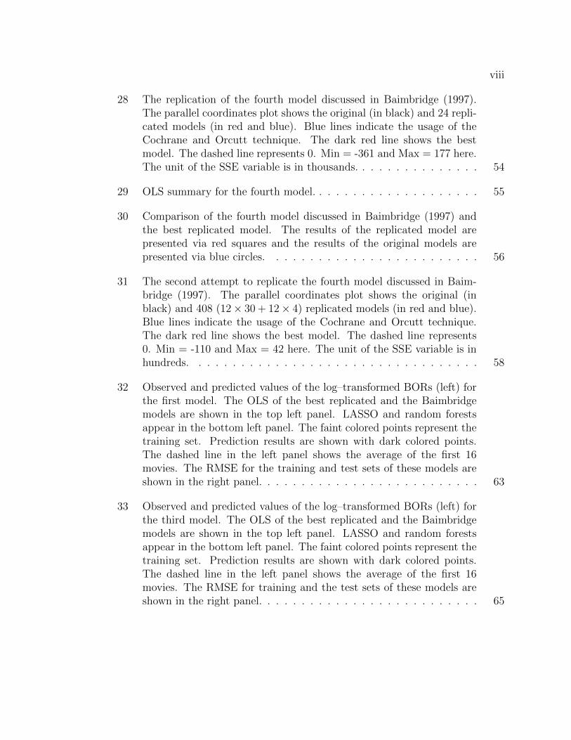
28 The replication of the fourth model discussed in Baimbridge (1997).The parallel coordinates plot shows the original (in black) and 24 repli-cated models (in red and blue). Blue lines indicate the usage of theCochrane and Orcutt technique. The dark red line shows the bestmodel. The dashed line represents 0. Min = -361 and Max = 177 here.The unit of the SSE variable is in thousands. . . . . . . . . . . . . . . 54

29 OLS summary for the fourth model. . . . . . . . . . . . . . . . . . . . 55

30 Comparison of the fourth model discussed in Baimbridge (1997) andthe best replicated model. The results of the replicated model arepresented via red squares and the results of the original models arepresented via blue circles. . . . . . . . . . . . . . . . . . . . . . . . . 56

31 The second attempt to replicate the fourth model discussed in Baim-bridge (1997). The parallel coordinates plot shows the original (inblack) and 408 (12× 30 + 12× 4) replicated models (in red and blue).Blue lines indicate the usage of the Cochrane and Orcutt technique.The dark red line shows the best model. The dashed line represents0. Min = -110 and Max = 42 here. The unit of the SSE variable is inhundreds. . . . . . . . . . . . . . . . . . . . . . . . . . . . . . . . . . 58

32 Observed and predicted values of the log–transformed BORs (left) forthe first model. The OLS of the best replicated and the Baimbridgemodels are shown in the top left panel. LASSO and random forestsappear in the bottom left panel. The faint colored points represent thetraining set. Prediction results are shown with dark colored points.The dashed line in the left panel shows the average of the first 16movies. The RMSE for the training and test sets of these models areshown in the right panel. . . . . . . . . . . . . . . . . . . . . . . . . . 63

33 Observed and predicted values of the log–transformed BORs (left) forthe third model. The OLS of the best replicated and the Baimbridgemodels are shown in the top left panel. LASSO and random forestsappear in the bottom left panel. The faint colored points represent thetraining set. Prediction results are shown with dark colored points.The dashed line in the left panel shows the average of the first 16movies. The RMSE for training and the test sets of these models areshown in the right panel. . . . . . . . . . . . . . . . . . . . . . . . . . 65

ix

34 Observed and predicted values of the log–transformed BORs (left) forThe Economist model. The OLS of the best replicated and the BenchMean 2 models are shown in the top left panel. LASSO and randomforests appear in the bottom left panel. The faint colored points rep-resent the training set. Prediction results are shown with dark coloredpoints. The dashed line in the left panel shows the average of the first16 movies. The RMSE for the training and the test set of these modelsare shown in the right panel. . . . . . . . . . . . . . . . . . . . . . . . 67

CHAPTER 1

INTRODUCTION

1.1 The Importance of the Movie Industry

The movie industry is not only an influential part of the arts but it is also a

vital participant of the business field. It plays an important role in the stage of the

world’s economy. Specifically, in the United States, the movie industry provided over

2.2 million jobs and paid over 137 billion dollars in total wages in 2009 (Pangarker

and Smit, 2013). Due to its large impact, the movie industry is an essential field to

explore and study.

Forecasting box-office revenues (BORs) of a particular movie has attracted many

scholars because this prediction is a difficult and challenging problem. To some ana-

lysts, “Hollywood is the land of hunch and the wild guess” (Litman and Ahn, 1998).

To others, “There are no formulas for success in Hollywood” (De Vani and Walls,

1999). These ideas are mostly related to the big uncertainty of audience response to

the movie before its release. Jack Valenti, president and CEO of the Motion Picture

Association of America (MPAA), once mentioned that “. . . No one, can tell you what

a movie is going to do in the marketplace . . . Not until that film opens in a darkened

theater, and sparks fly up between the screen and the audience can you say this film

is right” (Valenti, 1978).

Often, the movie industry leaves people with an impression of a lucrative field.

The images of celebrities with fancy cars and the gross revenues measured in hun-

dreds of million dollars contribute to this impression. However, most people only pay

attention to the most successful movies, which do generally make quite some profit,

yet in general, this impression is not true. Vogel (2010, p. 71), mentioned that “. . . of

2

any ten major theatrical films produced, on the average, six or seven may be broadly

characterized as unprofitable and one might break even . . . ”. These numbers suggest

that the movie industry is one of the riskiest markets in the entertainment industry,

which justifies the high return rates of the successful movies. It is because of these

high risks in producing movies that making an adequate budget plan and accurately

predicting the revenues become very important.

1.2 Previous Research

Presumably the most important aspect of the research in the movie industry is

forecasting. Forecasting BORs of a new movie is a very popular task. Scientists tried

various statistical and non–statistical methods to find a better estimation of BORs.

Litman (1983) was the first to develop a multiple regression model in an attempt to

predict the financial success of films. Independent variables such as movie genre (sci-

ence fiction, drama, action-adventure, comedy, and musical), critics’ ratings, MPAA

rating (G, PG, R, and X), superstar in the cast, production costs, release company

(major or independent), Academy Awards (nominations and winning in a major cat-

egory), and release date (Christmas, Memorial Day, summer) were used. Litman’s

model showed evidence that the variables of production costs, critics’ ratings, science

fiction genre, major distributor, Christmas release, Academy Award nomination, and

winning an Academy Award are all significant determinants of the success of a the-

atrical movie.

De Vani and Walls (1999) modeled BORs using Pareto and Levy distributions

and checked whether a movie star has any effect on the BORs. They did not find any

star effect and concluded that the movie is the real star. Some researchers tried to

forecast BORs of new motion pictures based on early box office data. Neelamegham

and Chintagunta (1999) constructed a Bayesian model which predicted BORs across

3

different countries. Sharda and Delen (2006) showed that the neural networks have

a better prediction rate than traditional statistical classification methods, such as

discriminant analysis, multiple logistic regression, and classification and regression

trees (CART). Delen et al. (2007) described a Web-based decision support system to

help Hollywood managers make better decisions on important movie characteristics,

such as genre, super stars, technical effects, release time, etc.

Research on predicting BORs is not limited to Hollywood movies. Some articles

were published trying to predict the BORs for the Korean and Chinese movie industry.

Lee and Chang (2009) predicted the BORs for the Korean movie industry using

Bayesian belief network (BNN). They stated that BNNs improved the forecasting

accuracy compared to artificial neural networks and decision trees. Zhang et al. (2009)

used back propagation neural networks to estimate Chinese BORs. Song and Han

(2013) focused on predicting the BORs for the Korean movie industry using techniques

such as ordinary stepwise regression, random forests and gradient boosting.

Non-traditional methods such as extreme value theory were used to model the

tails of the distribution for weekend box office returns (Bi and Giles, 2009).

1.3 James Bond Movies

All of the articles discussed in Section 1.2 were focused on movies with different

genres, actors, MPAA ratings, movie directors, etc. But, movie series have very

similar characteristics. Because of this, predicting the BORs for movie series will

require different input variables than the ones discussed in the articles in Section 1.2.

A perfect example of such a movie series to examine is the James Bond (JB) movie

series. This series is based on Ian Fleming’s 14 spy stories published from 1953 to

1966. The first JB movie, Dr. No, was released in 1963 which became a blockbuster

soon after the release date.

4

Up to now, producers created movies for all of Ian Fleming spy stories. Addition-

ally, nine other JB movies were created that were not based on those spy stories1. In

this Master’s report, the findings are based on the first 22 JB movies (not including

Skyfall) because the data were collected before the release date of Skyfall. There

are rumors about a 24th JB movie, Bond 24, which supposedly will be released in

November 2015. These 23 JB movies became one of the longest running and highest

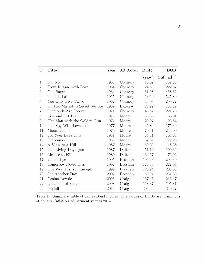
grossing franchises ever produced (see Table 1).

1.4 Previous Research: James Bond Movies

The James Bond movies and books are a research topic for scientists from differ-

ent fields. The areas of research range from marketing to health care, from political

science to statistics. Baimbridge (1997) used ordinary least squares (OLS) for pre-

dicting the BORs for JB franchises. Johnson et al. (2013) talked about the alcohol

consumption of James Bond and the possible health consequences that could happen

later. Marketing research done by Cooper et al. (2010) tried to understand the psy-

chology of James Bond movie fans. In particular, this paper discussed the meaning

of champagne and car brands and the possible influence on movie fans.

Some scientists examined the violence in the movie industry over time. For

example, by analyzing JB movies, McAnally et al. (2013) hypothesized that popular

movies are becoming more violent. Parallel to this MS report an article about the

JB movie series was published in the Chance magazine (Derek, 2014). This article

presented some visual techniques for variables kills, conquests, martinis and box–office

revenues, which is the main goal of the second chapter in this MS report. Additionally,

Chapter 2 will provide much more visualization techniques than in Derek (2014). The

1This research only follows the “official” releases through Metro-Goldwyn-Mayer (MGM) andleaves out the other JB movies such as Casino Royale (1954), Casino Royale (1967), and Never SayNever Again (1983), released by CBS, Columbia Pictures, and Warner Brothers, respectively.

5

# Title Year JB Actor BOR BOR

(raw) (inf. adj.)1 Dr. No 1963 Connery 16.07 157.862 From Russia, with Love 1964 Connery 24.80 222.673 Goldfinger 1964 Connery 51.08 458.624 Thunderball 1965 Connery 63.60 525.805 You Only Live Twice 1967 Connery 43.08 299.776 On Her Majesty’s Secret Service 1969 Lazenby 22.77 133.897 Diamonds Are Forever 1971 Connery 43.82 221.768 Live and Let Die 1973 Moore 35.38 166.919 The Man with the Golden Gun 1974 Moore 20.97 93.6410 The Spy Who Loved Me 1977 Moore 46.84 175.3911 Moonraker 1979 Moore 70.31 233.9012 For Your Eyes Only 1981 Moore 54.81 164.6313 Octopussy 1985 Moore 67.89 179.9614 A View to a Kill 1987 Moore 50.33 118.3815 The Living Daylights 1987 Dalton 51.19 109.3216 License to Kill 1989 Dalton 34.67 72.9217 GoldenEye 1995 Brosnan 106.43 204.3018 Tomorrow Never Dies 1997 Brosnan 125.30 227.9419 The World Is Not Enough 1999 Brosnan 126.94 208.6520 Die Another Day 2002 Brosnan 160.94 231.3021 Casino Royale 2006 Craig 167.45 213.4722 Quantum of Solace 2008 Craig 168.37 195.8123 Skyfall 2012 Craig 304.36 319.27

Table 1: Summary table of James Bond movies. The values of BORs are in millionsof dollars. Inflation adjustment year is 2014.

6

article The Economist (2012) in The Economist summarized the average number of

kills, conquests, and martinis drunk by the six different JB actors in the first 22 JB

movies. This article was the initial motivation for this Master’s report.

1.5 Data for James Bond Movies

1.5.1 Data Sources

Probably the most important variable for examining JB movies is the response

variable (US box–office revenues). This variable was collected from the Box Office

Mojo (http://www.boxofficemojo.com/franchises/chart/?id=jamesbond.htm).

This website also has the inflation adjusted US box-office revenues (IAUSBOR).

Two measurements of IAUSBOR were used from the Box-office Mojo website. The

first one (IAUSBOR1) was based on the webpage http://www.boxofficemojo.com/

franchises/chart/?id=jamesbond.htm and the second one (IAUSBOR2) was based

on the average ticket price (http://boxofficemojo.com/about/adjuster.htm).

Two measurements of the inflation adjuster were collected from the National

Association of Theatre Owners (NATO) (http://natoonline.org/data/ticket-

price/) and the Box–office Mojo (http://boxofficemojo.com/about/adjuster.

htm). The numerical values of these two adjusters were positively associated and

have a Pearson correlation coefficient, r = 0.999. Using the inflation adjuster from

Box–office Mojo, the measurements of IAUSBOR are almost identical (r = 0.99) with

the IAUSBOR at Box–office Mojo website, except for the two most successful JB

movies (Thunderball and Goldfinger). Choosing the adjustment year of 2008, these

two measurements gave about $100 million difference for these two JB movies.

The consumption price index (CPI) was used to calculate the IAUSBOR. The

CPI index was collected from the Bureau of Labor Statistics (Crawford and Church,

7

2014) (http://www.bls.gov/cpi/cpid1402.pdf). Using the CPI index, IAUSBOR3

was calculated. In this research, all three measurements of the IAUSBOR will be used

for the analysis in Chapter 3.

The variable PCEMOVIES was extracted from the Federal Reserve

Economic Data (FRED, http://research.stlouisfed.org/fred2/series/

DLIGRG3A086NBEA#). TOTADM and RELEASES were found in the follow-

ing websites: (http://www.waynesthisandthat.com/moviedata.html and

http://www.filmsonsuper8.com/censorship/mpaa-film-numbers-52000.html.

All these variables will also be used in Chapter 3.

JB is famous for visiting different countries when accomplishing the assigned

tasks. The list of countries visited by JB in a movie was found on a Wikipedia webpage

(http://en.wikipedia.org/wiki/List_of_James_Bond_film_locations) and was

verified through the http://www.sporcle.com/games/PumpkinBomb/bondgeography

webpage. The countries JB visited in movies are not necessarily the ones where the

filming took place. Two countries in this list, Republic of Isthmus and San Monique,

are fictional countries and, thus, were not included into the dataset.

1.5.2 Explanatory Variables: The Economist and Baimbridge Models

The Economist article The Economist (2012) summarized the average number

of kills, conquests, and martinis drunk per movie by all JB actors. This article didn’t

provide any information about these variables for each JB movie. Fortunately, The

Economist editor was very kind to share the data they have used for their article.

That dataset contained the number of kills, conquests, and martinis for each JB

movie. Additionally, it listed the number of “Bond, James Bond” (BJB) expressions

per movie.

8

Baimbridge (1997) discussed four regression models using OLS to predict log-

BORs. This paper was published in 1997, so finding the exact data used in this

paper was almost impossible. Thus, instead of trying to find the exact data, the

attempt was made to replicate his four models was performed using the information

given in his paper. In the first model, the author used dummy variables for each JB

actor. Another dummy variable, NEWBOND, indicated whether a new JB actor had

appeared. The last two variables of this model were ACTREND and ACTRENDSQ.

These variables show the number of appearances and the square of the number of

appearances, respectively, per JB actor.

The second model is described by nominations and ratings. Dummy variables for

Oscar nomination (MONOSCAR) and Oscar won (WONOSCAR) were created for

this model. Three other dummy variables (ONESTAR, TWOSTAR, THREESTAR)

were created showing the rating of the movies (Halliwell, 1989).

In the third model, variables SEQUENCE, GAP, GAPSQ and COLDWAR were

used. SEQUENCE represented the time order of the movies. The time period of each

subsequent Bond movie (GAP) was entered as a quadratic function. COLDWAR was

a dummy variable showing the end of the Cold War in 1989.

The last model used the following variables: deflated average ticket price (PRICE),

deflated aggregate personal consumption expenditure on movies (PCEMOVIES), to-

tal number of US admissions (TOTADM), and number of releases measured by the

MPAA (REALEASES). PRICESQ and PCEMOVIESSQ were the square of variables

PRICE and PCEMOVIES. CPI index (Crawford and Church, 2014) was used to

deflate the variables PRICE and PCEMOVIES.

1.6 Objectives

The research in this Master’s report is divided into three main parts. In Chapter

9

2, graphical summaries of the variables used in Section 1.5.2 will be given. In addi-

tion, the response variable BOR will be compared with possible explanatory variables

kills, conquests, martinis, and BJB expression. To present these graphical summaries,

many visualization techniques such as time series plots, dotplots, histograms, scat-

terplots, parallel coordinates plots, heatmaps, mosaic plots, association plots, and

choropleth maps will be displayed. Using these visualization techniques, the relation-

ship between the explanatory variables with each other as well as with the response

variable will be presented.

Chapter 3 will try to replicate the four regression models discussed in Baimbridge

(1997). This paper was published in 1997 and the datasets in this paper only contained

the movies released before 1990s.

Chapter 4 will examine linear regression as well as machine learning methods

such as lasso and random forest for predicting BORs. For each of these methods,

three datasets will be used described in Sections 1.5.2 (The Economist model, the

first model, and the third model). Movies released before 1990s will be considered

as the training dataset and the ones after 1990s will be used in the test set. Visual

comparison will be given to compare the difference between these methods.

In Chapter 5, we will summarize the findings and suggest which model and

method to use.

The appendix A will include all the datasets used in the Master’s report. All the

R code will be given in Appendix B.

10

CHAPTER 2

VISUALIZING THE ECONOMIST DATASET

2.1 Statistical Graphics

John Tukey introduced the term exploratory data analysis (EDA) in the late

1970s (Tukey, 1977). Rather than directly starting hypothesis testing as statisticians

traditionally did, he suggested to start the analysis by looking at the data first. Often,

it was done by visualization methods such as histograms, boxplots, etc.

Sometimes numerical statistical summaries can be very misleading. The quartet

dataset created by Anscombe (1973) showed that without visualization, completely

different datasets could lead to the same numerical results. Therefore, in this Master’s

report, various visualization methods were applied to data related to the James Bond

(JB) movies.

All graphical results and statistical analysis were conducted in R (R Core Team,

2013). Sweave (Leisch, 2002) was used for documentation in order to make the results

of this Master’s report fully reproducible.

2.2 Time Series Plots

In this section, time series plots (Figures 1 – 4) are presented to show the trend

of the variables kills, conquests, martinis, and BJB expressions with respect to time,

discussed in Section 1.5.2. In each of these plots, six symbols and colors are used

to distinguish all six JB actors. Additionally, these plots show the linear regression

line, a lowess smoother (with parameters f = 0.5, iter = 3) (Cleveland, 1979), and

a moving averages smoother (with parameters q = 5, p1 = · · · = pq = 0.2). These

smoothers and the regression line will help to see if there are some trends with these

11

variables over time. Each smoother and the line is given with a distinct color. Each of

these graphs has two legends, which clarify the symbol and color differences between

the six JB actors and the color difference of the smoothers and regression line.

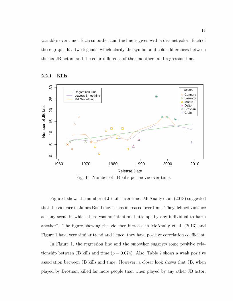
2.2.1 Kills

1960 1970 1980 1990 2000 2010

05

1015

2025

30

Release Date

Num

ber

of J

B k

ills

Actors

ConneryLazenbyMooreDaltonBrosnanCraig

Regression LineLowess SmoothingMA Smoothing

Fig. 1: Number of JB kills per movie over time.

Figure 1 shows the number of JB kills over time. McAnally et al. (2013) suggested

that the violence in James Bond movies has increased over time. They defined violence

as “any scene in which there was an intentional attempt by any individual to harm

another”. The figure showing the violence increase in McAnally et al. (2013) and

Figure 1 have very similar trend and hence, they have positive correlation coefficient.

In Figure 1, the regression line and the smoother suggests some positive rela-

tionship between JB kills and time (p = 0.074). Also, Table 2 shows a weak positive

association between JB kills and time. However, a closer look shows that JB, when

played by Brosnan, killed far more people than when played by any other JB actor.

12

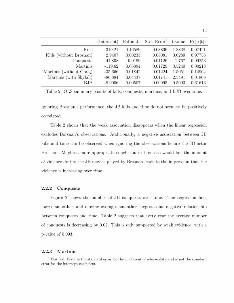
(Intercept) Estimate Std. Error1 t value Pr(>|t|)

Kills -319.21 0.16589 0.08806 1.8838 0.07421Kills (without Brosnan) 2.9407 0.00233 0.08081 0.0289 0.97733

Conquests 41.808 -0.0199 0.01126 -1.767 0.09253Martinis -119.62 0.06094 0.01729 3.5240 0.00213

Martinis (without Craig) -35.666 0.01842 0.01224 1.5051 0.14964Martinis (with Skyfall) -86.884 0.04437 0.01741 2.5491 0.01868

BJB -9.0006 0.00507 0.00995 0.5093 0.61613

Table 2: OLS summary results of kills, conquests, martinis, and BJB over time.

Ignoring Brosnan’s performance, the JB kills and time do not seem to be positively

correlated.

Table 2 shows that the weak association disappears when the linear regression

excludes Borsnan’s observations. Additionally, a negative association between JB

kills and time can be observed when ignoring the observations before the JB actor

Brosnan. Maybe a more appropriate conclusion in this case would be: the amount

of violence during the JB movies played by Brosnan leads to the impression that the

violence is increasing over time.

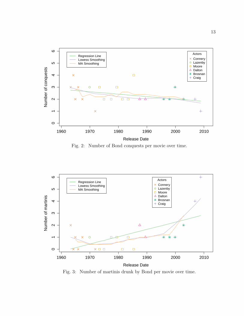
2.2.2 Conquests

Figure 2 shows the number of JB conquests over time. The regression line,

lowess smoother, and moving averages smoother suggest some negative relationship

between conquests and time. Table 2 suggests that every year the average number

of conquests is decreasing by 0.02. This is only supported by weak evidence, with a

p-value of 0.093.

2.2.3 Martinis

1This Std. Error is the standard error for the coefficient of release data and is not the standarderror for the intercept coefficient

13

1960 1970 1980 1990 2000 2010

01

23

45

6

Release Date

Num

ber

of c

onqu

ests

Actors

ConneryLazenbyMooreDaltonBrosnanCraig

Regression LineLowess SmoothingMA Smoothing

Fig. 2: Number of Bond conquests per movie over time.

1960 1970 1980 1990 2000 2010

01

23

45

6

Release Date

Num

ber

of m

artin

is

Actors

ConneryLazenbyMooreDaltonBrosnanCraig

Regression LineLowess SmoothingMA Smoothing

Fig. 3: Number of martinis drunk by Bond per movie over time.

14

Figure 3 shows the number of martinis drunk over time. The smoothers in

this Figure have a shape of convex parabola. It shows that the martini consumption

reached its minimum in the 1970s and started to increase afterwards. Here the picture

would not be so vivid if we had ignored JB actor Craig. He drunk four and six martinis

during the movies Casino Royale and Quantum of Solace. The average of five martinis

drunk for JB actor played by Craig is far above the number of martinis drunk by the

other JB actors.

The regression line in Figure 3 shows a positive relationship between martinis

and time. The p-value (p = 0.002) for martinis in Table 2 suggests a highly significant

linear relationship as well. In the last JB movie, Skyfall (which is not included in the

dataset), there are no martinis drunk by JB (Thomas, 2012). The linear regression

model between martinis and time would still give a significant association with a p-

value of 0.019, even if the martini value of zero would be used as the 23th observation

for the year 2012.

Table 2 shows that after ignoring the martinis drunk played by JB actor Craig

gives a non significant linear association between martinis and time (p = 0.15). Simi-

lar to Section 2.2.1, more appropriate conclusion of this section would be: Craig leads

to the impression that the number of martinis drunk by JB actors are increasing over

time.

2.2.4 Bond, James Bond (BJB)

Figure 3 shows the number of BJB expressions over time. In this figure, the

opposite pattern can be seen, compared to Figure 2. The smoothers have a shape of

concave parabola. In other words, the BJB expressions was not popular in 1960s and

2000s and achieved its peak in the 1970s and early 1980s. The regression line suggests

a small increase over time. However, the p-value in Table 2 (p = 0.62) suggests that

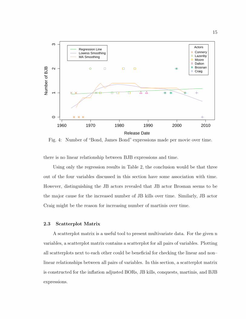
15

1960 1970 1980 1990 2000 2010

Release Date

Num

ber

of B

JB

01

23

Actors

ConneryLazenbyMooreDaltonBrosnanCraig

Regression LineLowess SmoothingMA Smoothing

Fig. 4: Number of “Bond, James Bond” expressions made per movie over time.

there is no linear relationship between BJB expressions and time.

Using only the regression results in Table 2, the conclusion would be that three

out of the four variables discussed in this section have some association with time.

However, distinguishing the JB actors revealed that JB actor Brosnan seems to be

the major cause for the increased number of JB kills over time. Similarly, JB actor

Craig might be the reason for increasing number of martinis over time.

2.3 Scatterplot Matrix

A scatterplot matrix is a useful tool to present multivariate data. For the given n

variables, a scatterplot matrix contains a scatterplot for all pairs of variables. Plotting

all scatterplots next to each other could be beneficial for checking the linear and non–

linear relationships between all pairs of variables. In this section, a scatterplot matrix

is constructed for the inflation adjusted BORs, JB kills, conquests, martinis, and BJB

expressions.

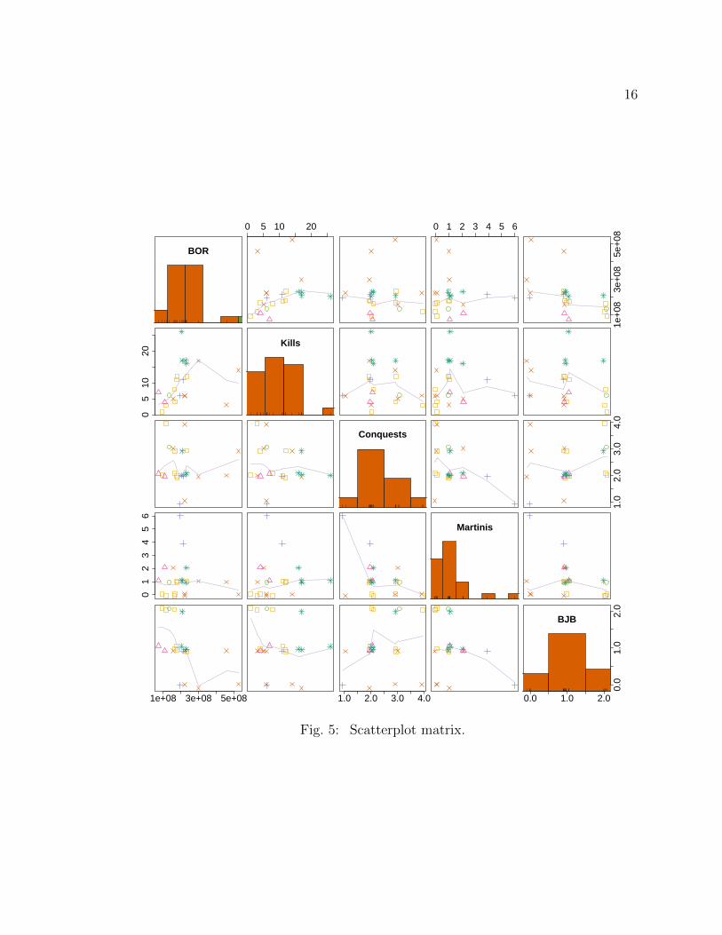
16

BOR

0 5 10 20 0 1 2 3 4 5 6

1e+

083e

+08

5e+

08

05

1020

Kills

Conquests

1.0

2.0

3.0

4.0

01

23

45

6

Martinis

1e+08 3e+08 5e+08 1.0 2.0 3.0 4.0 0.0 1.0 2.0

0.0

1.0

2.0

BJB

Fig. 5: Scatterplot matrix.

17

Figure 5 shows the scatterplot matrix for these five variables. Using the average

ticket price, the 2014 inflation adjusted BOR is shown in top left corner. The variables

kills, conquests, martinis and BJB are plotted on diagonal panels (from the second

row to the fifth). These variables have mostly integer values, and thus, a lot of

overplotting occurs. In order to avoid this overfitting, a small randomness, called

jitter was added to the explanatory variables. For all pairs of scatterplots, lowess

smoothing function (parameters: f = 2/3, iter = 3) is plotted in purple.

Colors and symbols are used to distinguish the JB actors. These colors and

symbols are consistent with the time series plots in Figures 1–4. Histograms are

shown in the diagonal panels, showing the distributions of all variables. A rug plot,

which simply draws a tick for each value, was added to each histogram to provide

more information about each observation.

Figure 5 shows some positive relationship between JB kills and BOR and some

negative association between BOR and BJB. A weak negative association can be

observed between martinis and conquests in the JB movies.

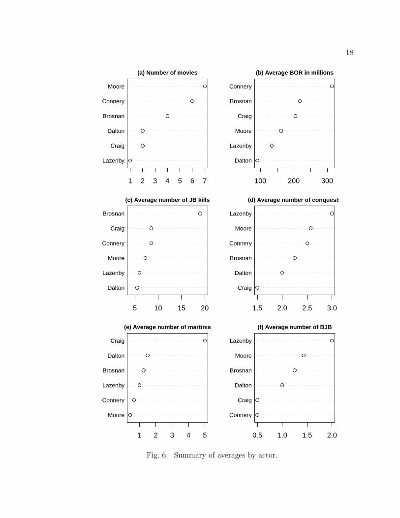
2.4 Dot Plots

Several dot plots were produced to show some simple statistical averages of the

JB actors. All dotplots are ordered highest (top) to the lowest (bottom). Figure 6(a)

shows the number of JB movies produced by each JB actor. Connery and Moore were

the most popular JB actors with 6 and 7 movies, respectively.

Figure 6(b) suggests that Connery is the most successful JB actor in terms of

inflation adjusted BOR. Here the 2014 was used for inflation adjustment year and

average ticket price was used as an adjustment method. The second and third suc-

cessful actors are Brosnan and Craig. The order of Brosnan and Craig will change

when the BOR of the last JB movie, Skyfall, will be included.

18

Moore

Connery

Brosnan

Dalton

Craig

Lazenby

1 2 3 4 5 6 7

(a) Number of movies

Connery

Brosnan

Craig

Moore

Lazenby

Dalton

100 200 300

(b) Average BOR in millions

Brosnan

Craig

Connery

Moore

Lazenby

Dalton

5 10 15 20

(c) Average number of JB kills

Lazenby

Moore

Connery

Brosnan

Dalton

Craig

1.5 2.0 2.5 3.0

(d) Average number of conquests

Craig

Dalton

Brosnan

Lazenby

Connery

Moore

1 2 3 4 5

(e) Average number of martinis

Lazenby

Moore

Brosnan

Dalton

Craig

Connery

0.5 1.0 1.5 2.0

(f) Average number of BJB

Fig. 6: Summary of averages by actor.

19

Figure 6(c) shows that JB actor Brosnan is the most violent actor by killing twice

as many people in JB movies as the second most violent JB actor, Connery. Figure

6(d) implies that JB actor, played by Lazenby, has the most conquests. However, this

is based only on one observation (movie). According to Figure 6(e), JB, when played

by Craig, is the biggest martini drinker with an average of 5 martinis per movie.

However, JB, when played by Craig, switches from martinis to beers during the most

recent JB movie, Skyfall (Thomas, 2012). JB, played by Dalton is the second most

martini drinker with less than 1.5 martinis on average. Figure 6(f) shows that the

most “Bond, James Bond” expression user was Lazenby. Similar to 6(d), this is also

based only on one observation (movie).

2.5 Box Plots

Similar to Figure 6, the 2014 inflation adjusted BOR using average ticket price as

an adjustment were examined. Figure 7 shows boxplots of kills, conquests, martinis,

and BJB. Each of these variables are divided into three categories. For example, the

number of kills consists of the categories 0–5 kills, 5–10 kills, and more than 10 kills.

All box plots were ordered from the highest to the lowest median BOR.

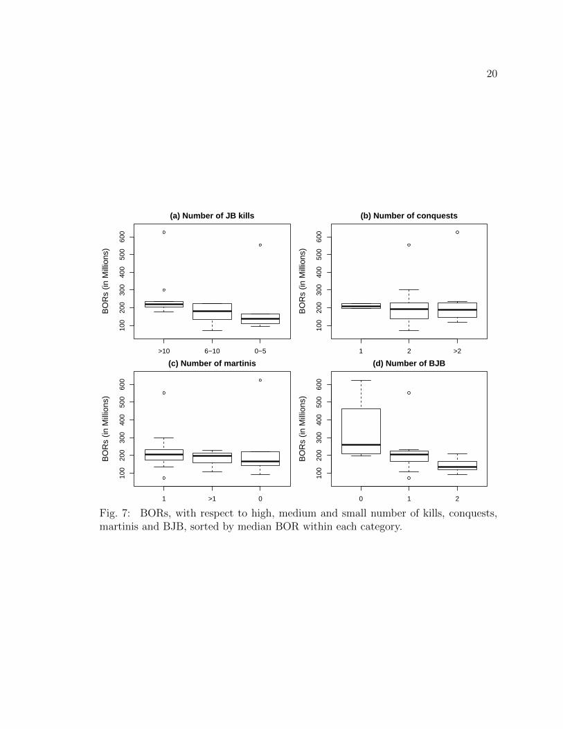
Figure 7(a) shows that decrease in number of kills is associated with decease in

BOR. Similarly, in Figure 7(d) when the number of BJB is increasing, the BORs seem

to decrease. These two relationships found in Figure 7(a), 7(d) are consistent with

the results shown in scatterplot matrix in Figure 5. Even though two of the most

successful JB movies, Thurderball and Goldfinger, have two and more conquests, there

exists a slight negative relationship between BOR and conquests. There is no obvious

relationship between BOR and martinis.

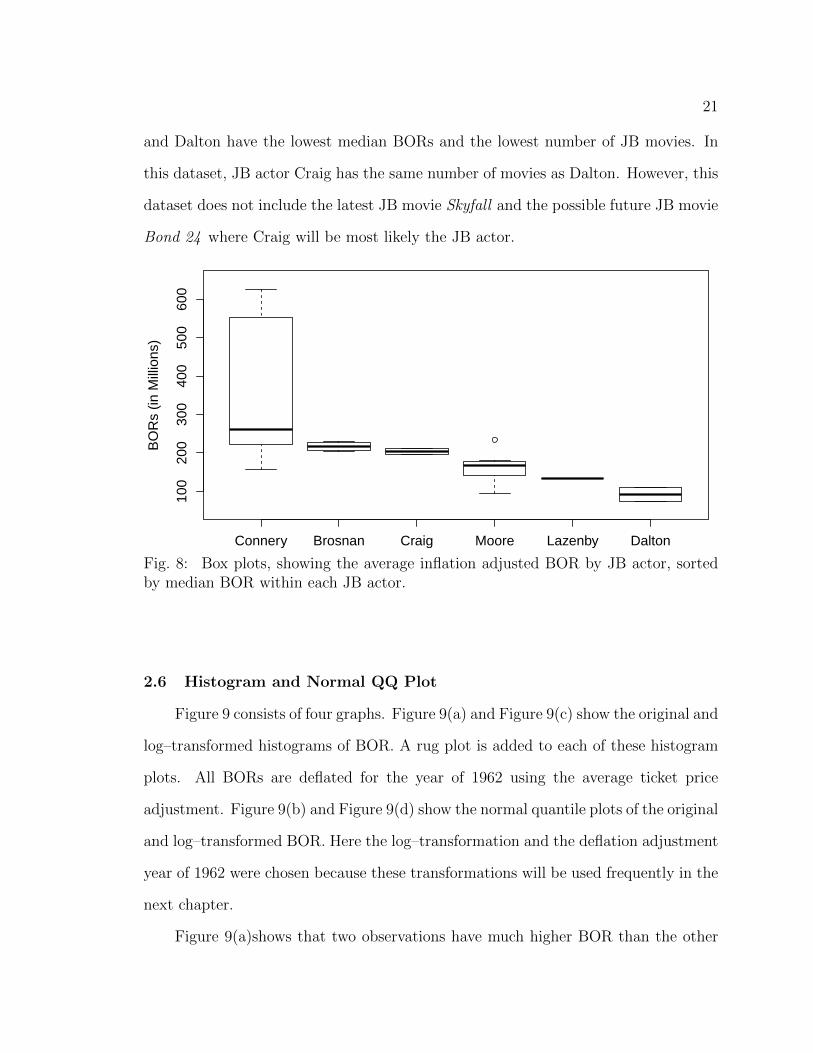
Figure 8 shows the distribution of revenues by actor. JB actor Connery has more

variability than any other actor. He also has the highest BORs. JB actors Lazenby

20

>10 6−10 0−5

100

200

300

400

500

600

(a) Number of JB kills

BO

Rs

(in M

illio

ns)

1 2 >2

100

200

300

400

500

600

(b) Number of conquests

BO

Rs

(in M

illio

ns)

1 >1 0

100

200

300

400

500

600

(c) Number of martinis

BO

Rs

(in M

illio

ns)

0 1 2

100

200

300

400

500

600

(d) Number of BJB

BO

Rs

(in M

illio

ns)

Fig. 7: BORs, with respect to high, medium and small number of kills, conquests,martinis and BJB, sorted by median BOR within each category.

21

and Dalton have the lowest median BORs and the lowest number of JB movies. In

this dataset, JB actor Craig has the same number of movies as Dalton. However, this

dataset does not include the latest JB movie Skyfall and the possible future JB movie

Bond 24 where Craig will be most likely the JB actor.

Connery Brosnan Craig Moore Lazenby Dalton

100

200

300

400

500

600

BO

Rs

(in M

illio

ns)

Fig. 8: Box plots, showing the average inflation adjusted BOR by JB actor, sortedby median BOR within each JB actor.

2.6 Histogram and Normal QQ Plot

Figure 9 consists of four graphs. Figure 9(a) and Figure 9(c) show the original and

log–transformed histograms of BOR. A rug plot is added to each of these histogram

plots. All BORs are deflated for the year of 1962 using the average ticket price

adjustment. Figure 9(b) and Figure 9(d) show the normal quantile plots of the original

and log–transformed BOR. Here the log–transformation and the deflation adjustment

year of 1962 were chosen because these transformations will be used frequently in the

next chapter.

Figure 9(a)shows that two observations have much higher BOR than the other

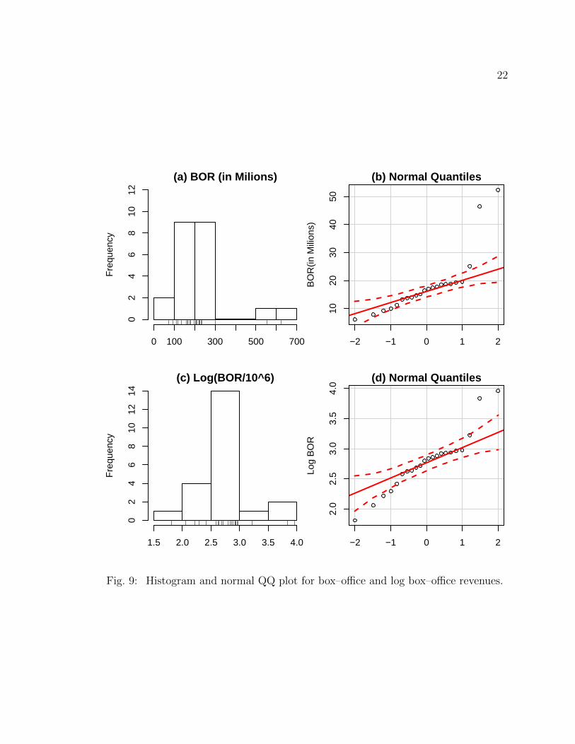
22

(a) BOR (in Milions)

Fre

quen

cy

0 100 300 500 700

02

46

810

12

−2 −1 0 1 210

2030

4050

(b) Normal Quantiles

BO

R(in

Mili

ons)

(c) Log(BOR/10^6)

Fre

quen

cy

1.5 2.0 2.5 3.0 3.5 4.0

02

46

810

1214

−2 −1 0 1 2

2.0

2.5

3.0

3.5

4.0

(d) Normal Quantiles

Log

BO

R

Fig. 9: Histogram and normal QQ plot for box–office and log box–office revenues.

23

observations. These two observations represent the movies Thurnderball and Goldfin-

ger. Even after the log–transformation, these two observations are distinctly apart

from the rest of the data. The QQ plots in Figure 9(b) and Figure 9(d) show that

neither the original nor the transformed BOR are close to being normally distributed.

2.7 Parallel Coordinates Plots

Kills Conquests Martinis BJB

0−5

6−10

>10

1

2

>2

0

1

>1

0

1

2

Fig. 10: Parallel coordinate plot of number of Bond kills, martinis, conquests, “Bond,James Bond” expression.

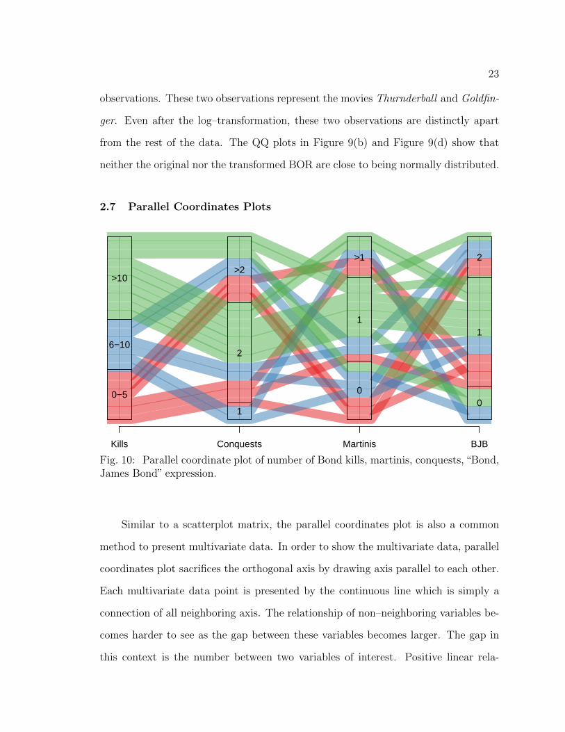
Similar to a scatterplot matrix, the parallel coordinates plot is also a common

method to present multivariate data. In order to show the multivariate data, parallel

coordinates plot sacrifices the orthogonal axis by drawing axis parallel to each other.

Each multivariate data point is presented by the continuous line which is simply a

connection of all neighboring axis. The relationship of non–neighboring variables be-

comes harder to see as the gap between these variables becomes larger. The gap in

this context is the number between two variables of interest. Positive linear rela-

24

tionship between two neighboring variables can be observed if the connection lines of

observation are parallel. If the connection lines of observations mostly cross, this is an

indicator of a negative association. The scale of each parallel axis does not necessarily

need be the same. It can have a common scale or individual scales varying from the

minimum to the maximum of that particular variable.

Figure 10 shows the parallel coordinates plot for kills, conquests, martinis and

BJB variables. Similar to boxplots in Section 2.5, these variables were divided into

three categories. Distinct colors were chosen to distinguish the categories of kills

variable. In Figure 10, the connection lines between conquests and martinis seem to

have a lot of crossing. This means that possible negative association between con-

quests and martinis can be observed. The same pattern can be seen in the scatterplot

matrix (Figure 5). Many interactions between the variables martinis and BJB also

suggest a negative association between these variables. This is also consistent with

the fourth bottom panel in Figure 5. In Figure 10, the conquest variable lies between

the variables kills and martinis meaning that it is hard to examine any relationship

between these variables.

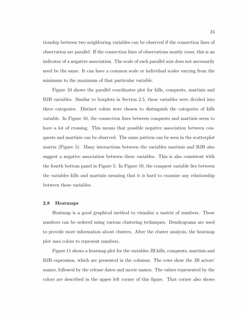
2.8 Heatmaps

Heatmap is a good graphical method to visualize a matrix of numbers. These

numbers can be ordered using various clustering techniques. Dendrograms are used

to provide more information about clusters. After the cluster analysis, the heatmap

plot uses colors to represent numbers.

Figure 11 shows a heatmap plot for the variables JB kills, conquests, martinis and

BJB expression, which are presented in the columns. The rows show the JB actors’

names, followed by the release dates and movie names. The values represented by the

colors are described in the upper left corner of this figure. That corner also shows

25

Mar

tinis

BJB

Con

ques

ts

Kill

s

Moore (1974) The Man with the Golden GunMoore (1985) A View to a KillConnery (1964) GoldfingerMoore (1973) Live and Let DieDalton (1987) The Living DaylightsConnery (1963) Dr. NoCraig (2008) Quantum of SolaceConnery (1964) From Russia With LoveMoore (1981) For Your Eyes OnlyConnery (1971) Diamonds Are ForeverDalton (1989) Licence to KillLazenby (1969) On Her Majesty's Secret ServiceBrosnan (1995) GoldenEyeCraig (2006) Casino RoyaleMoore (1979) MoonrakerMoore (1977) The Spy Who Loved MeMoore (1983) OctopussyConnery (1965) ThunderballBrosnan (1999) The World is Not EnoughBrosnan (2002) Die Another DayConnery (1967) You Only Live TwiceBrosnan (1997) Tomorrow Never Dies

0 5 10 20Value

010

20

Color Keyand Histogram

Cou

nt

Fig. 11: Heatmap plot of kills, conquests, martinis, and BJB expression by actor nameand movie release date. The histogram on the top left panel shows the distributionof the data matrix.

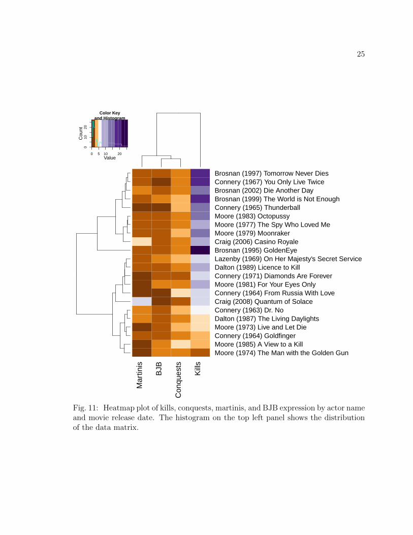
26

BJB

Mar

tinis

Con

ques

ts

Kill

s

Craig (2008) Quantum of SolaceCraig (2006) Casino RoyaleBrosnan (2002) Die Another DayConnery (1967) You Only Live TwiceBrosnan (1995) GoldenEyeBrosnan (1999) The World is Not EnoughMoore (1979) MoonrakerBrosnan (1997) Tomorrow Never DiesMoore (1977) The Spy Who Loved MeMoore (1983) OctopussyMoore (1973) Live and Let DieMoore (1985) A View to a KillMoore (1974) The Man with the Golden GunMoore (1981) For Your Eyes OnlyLazenby (1969) On Her Majesty's Secret ServiceConnery (1964) From Russia With LoveConnery (1965) ThunderballConnery (1971) Diamonds Are ForeverConnery (1964) GoldfingerDalton (1989) Licence to KillDalton (1987) The Living DaylightsConnery (1963) Dr. No

0 1 2 3 4 5 6Value

010

2030

Color Keyand Histogram

Cou

nt

Fig. 12: Heatmap plot of square–root transformed kills, conquests, martinis, andBJB expression by actor name and movie release date. The histogram on the top leftpanel shows the distribution of the data matrix.

27

the histogram of the data matrix in cyan. To create the dendrograms, hierarchical

clustering was implemented using Euclidean distance.

The top part of Figure 11 shows clustering for JB actor Brosnan. This cluster

contains all his movies except the Goldeneye. The dendrogram on the left shows that

the movie Goldeneye does not belong to any cluster group. The cluster of JB actor

Brosnan is mainly due to the variable kills.

Additionally, two separated clusters can be observed for JB actor Moore. The

cluster on top side including the movies The Man with the Golden Gun, A View

to a Kill, Live and Let Die has common low number of kills and low number of

martinis. The cluster on bottom for the movies Moonraker, The Spy Who Loved Me

and Octopussy has a medium number of kills, martinis, and BJB expressions. For the

latter movies, there is also a time cluster, because all these three movies were released

consequently in 1977, 1979 and 1983.

In contrast, there is no cluster for JB actor Connery. Not even two of the Con-

nery’s movies are clustered together in Figure 11, which means that all of his movies

have distinct characteristics. Earlier, Figure 8 showed that JB actor Connery is most

successful in term of BOR, and maybe his different appearance in each movie is one

of the secrets of this success.

Figure 11 also shows that the numerical values of the variable kills are much

higher than the values of conquests, martinis and BJB expression. This can be ob-

served from the top dendrogam as the variable kills is isolated. Due to these high

values, the variable kills could have a dramatic effect on clustering. To reduce the

effect of the this variable, a square–root transformation is applied. Specifically, the

upper left panel in Figure 11 shows that the variable kills vary between 4 and 25

meaning that it will take values between 2 and 5 after the square–root transforma-

tion. This new range is very similar to the range of other variables, and, hence will

28

reduce the effect of kills.

Figure 12 shows a heatmap plot for the variables square–root kills, conquests,

martinis and BJB expression. After the transformation, more JB actor clusters can

be observed. The movies The Living Daylights and Licence to Kill played by JB actor

Dalton can be observed on top of this figure. Similarly, a cluster for JB actor Craig

can be observed on the bottom. Similar to Figure 11 two clusters can be observed for

the JB actor Moore. Even though four movies by Connery are next to each other, less

clustering in observed from the dendrogram. The result found in Figure 11 does not

hold for Figure 12 after the transformation, however the “isolated” movie GoldenEye

is clustered with Die Another Day. The movies Tomorrow Never Dies and The World

is Not Enough does not appear in the same cluster either.

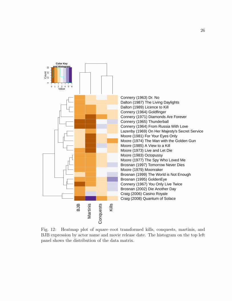
2.9 Mosaic Plot

A mosaic plot (Hartigan and Kleiner, 1984) is popular visualization method to

present categorical data. For the categorical data given in the two–way contingency

table, the mosaic plot creates rectangles with proportional horizontal and vertical

slices. The area of the rectangles is proportional to the corresponding frequency

number in the contingency table. Friendly (1994) generalizes the mosaic plots from

two–way to multi–way contingency table.

A mosaic plot using a four–way contingency table is shown in Figure 13. This

figure uses variables BJB expression (first vertical division) kills (first horizontal divi-

sion), conquests (second vertical division), and martinis (second horizontal division).

The vertical bar line on the right shows standardized Pearson residuals for the given

color. Note that the standardized Pearson residuals is not the only option for the ver-

tical bar line and hence, other independence hypothesis can be tested. The p–value

under the vertical bar is 0.0277 which suggest some association between the variables

29

−1.0

0.0

2.0

4.0

6.5

Pearsonresiduals:

p−value =0.027702

Conquests

BJB

Kill

s

Mar

tinis

0−5

01201 2

0

0 1 2

1>

1

>10

01

>1

6−10

1 2 >2

01

>1

Fig. 13: Mosaic plot for kills, conquests, martinis and BJB expression.

30

kills, conquests, martinis and BJB at 5% significance level.

A four–way contingency table was used in this mosaic plot. Each variable consists

of three categories which makes 34 = 81 possible combinations. However, there are

only 22 observation (movies) in the dataset meaning that most combinations will not

appear in the mosaic plot. For these observations the mosaic plot will draw vertical

or horizontal lines. The largest rectangle contains four observations. The area of the

widest rectangle is twice less than the area of largest rectangle, and hence the widest

rectangle contains two observations. The area of other rectangles are twice smaller

than the area of the widest rectangle meaning that these small rectangles have only

one observation.

2.10 Association Plot

The association plot (Cohen, 1980) is a useful tool to visually check the indepen-

dence of several categorical variables. Meyer et al. (2006) describes the association

plot as the following: “an association plot visualizes the standardized deviations of

observed frequencies from those expected under a certain independence hypothesis.

Each cell is represented by a rectangle that has (signed) height proportional to the

residual and width proportional to the square root of the expected counts, so that the

area of the box is proportional to the difference in observed and expected frequencies.”

Similar to mosaic plot in Figure 13, the vertical bar line on the right side of

Figure 14 shows standardized Pearson residuals for the given color. The p–value

(p = 0.0277) under the vertical bar suggests some association between these variables

at the 5% significance level. Figure 14 also shows a very high residual on the upper

left corner of the graph. This could be a possible reason of the highly significant

p–value observed under the vertical bar line.

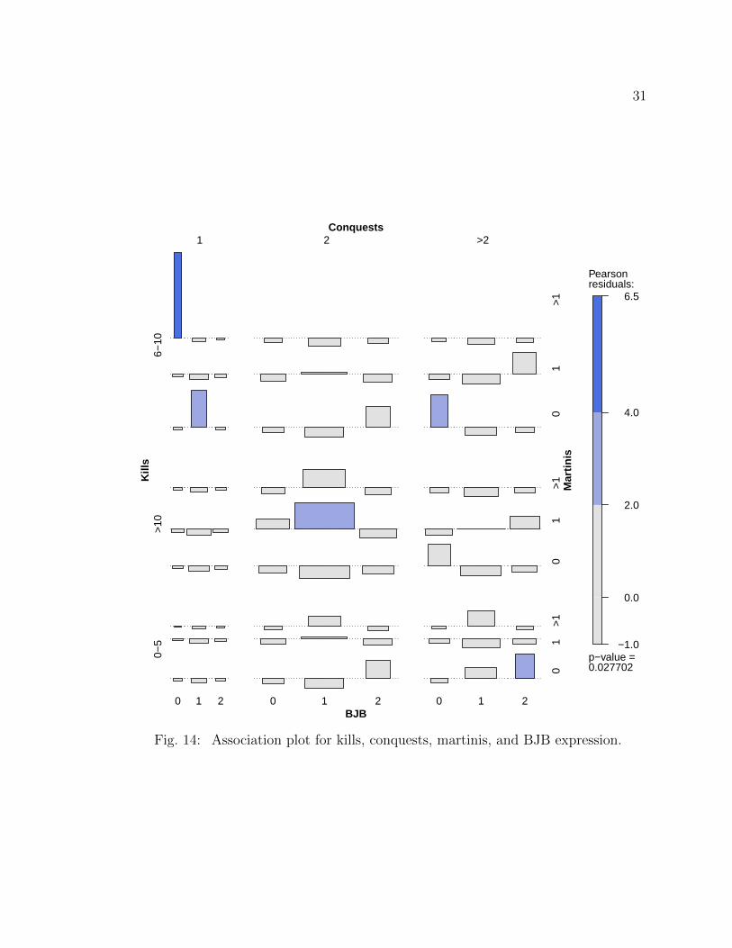
31

−1.0

0.0

2.0

4.0

6.5

Pearsonresiduals:

p−value =0.027702

Conquests

BJB

Kill

s

Mar

tinis

0−5

0 1 2 0 1 2

0

0 1 2

1>

1

>10

01

>1

6−10

1 2 >2

01

>1

Fig. 14: Association plot for kills, conquests, martinis, and BJB expression.

32

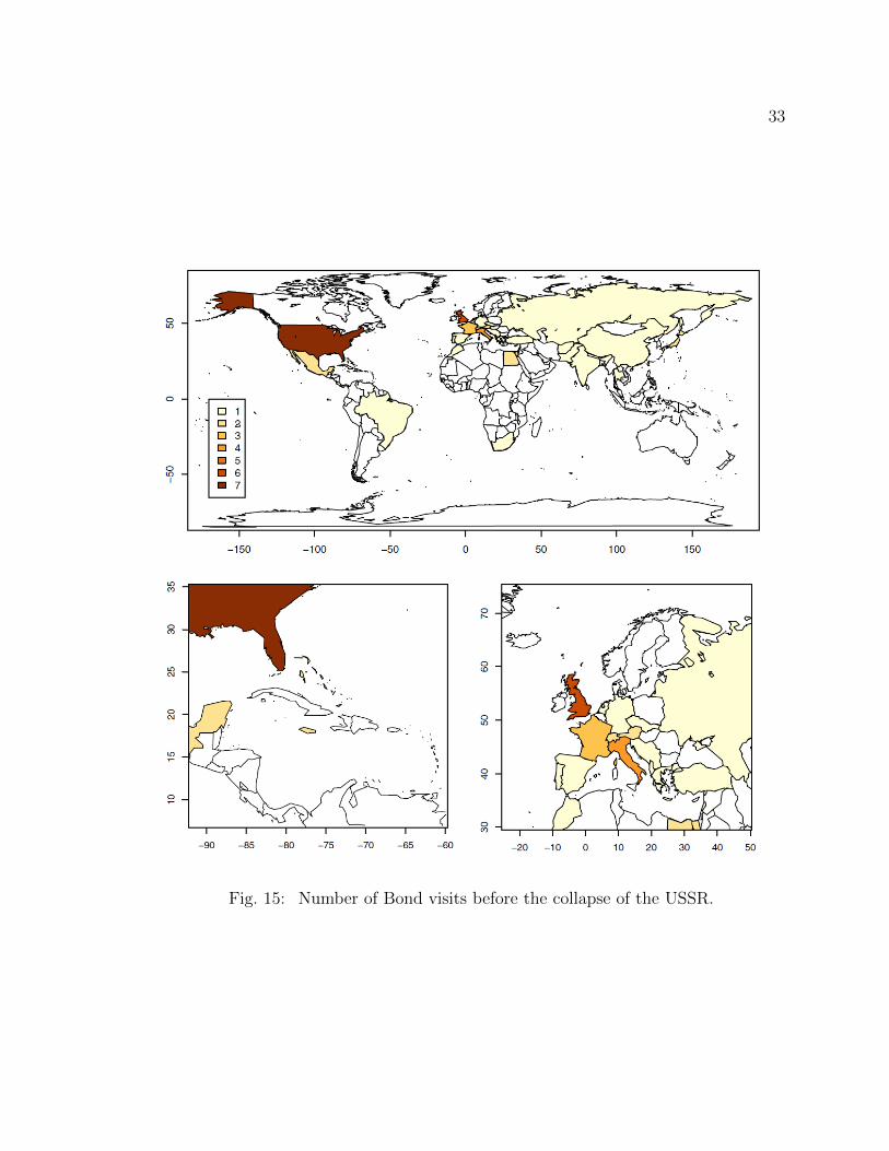
2.11 Choropleth Maps

Choropleth maps assign colors and shades to the individual areas in the map.

Colors correspond to a pre–defined values or a range of values. In each movie James

Bonds visited several countries and visiting exotic countries became another charac-

teristic of the JB movie series. To determine whether countries have any effect on the

BOR, three choropleth maps have been created. The world map changed significantly

after the collapse of the Union of Soviet Socialist Republics (USSR). Countries like

Yugoslavia, Czechoslovakia and the USSR split into 19 independent countries during

1990s. Therefore, creating a single choropleth map would be problematic as the first

JB movie was released in 1963. To create meaningful maps with countries that cor-

rectly show the borders at the time the movie was released, two maps were created

showing the Bond visits before and after collapse of the USSR.

Figure 15 shows the number of visits to different countries in the JB movie

series before the collapse of the USSR. These visits do not necessarily include all

the countries that the movies were filmed at. For example, in the Die Another Day

movie JB visits North Korea, but the filming did not take place in North Korea.

Furthermore, European and Caribbean counties are hard to see in the world map.

Therefore, the zoomed–in choropleth maps for European and Caribbean countries are

displayed in the bottom panels of Figure 15.

Figure 16 shows the frequency of JB visited countries after collapse of the USSR.

Figures 15 and 16 show that United States and European countries are the most

popular for Bond visits. Hong Kong is another popular country, but it is not visible

on these maps because of its small area. African and South American countries,

Canada, and Australia are the least popular countries for JB visits.

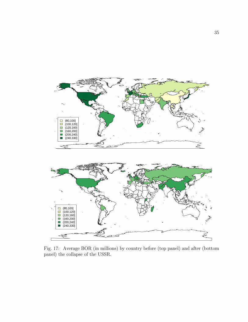
Figure 17 shows the average BORs across the countries before and after the

collapse of USSR. Here 16 movies were released before the collapse of the USSR and

33

Fig. 15: Number of Bond visits before the collapse of the USSR.

34

−200 −100 0 100 200

−50

050

1234567

−90 −85 −80 −75 −70 −65 −60

1015

2025

3035

−20 −10 0 10 20 30 40 50

3040

5060

70

Fig. 16: Number of Bond visits after the collapse of the USSR.

35

(80,100](100,120](120,160](160,200](200,240](240,330]

(80,100](100,120](120,160](160,200](200,240](240,330]

Fig. 17: Average BOR (in millions) by country before (top panel) and after (bottompanel) the collapse of the USSR.

36

six movies were released after the collapse of the USSR. Except for Japan, the average

BOR in Asian countries varies between $80 million to $200 million. The average BOR

is mostly higher in European, and South and North American countries compared to

Asian countries. The BOR seems quite evenly spread after the collapse of the USSR

.

2.12 Summary

This chapter presented various visual tools to better understand the the data

presented in The Economist magazine (The Economist, 2012). In Section 2.2, the

regression line showed an increasing trend of kills and martinis over time. Careful

look in Figure 1 and Figure 3 showed that JB actors Brosnan and Craig could lead

that increasing trend.

Section 2.3 presented a scatterplot matrix which indicated some positive rela-

tionship between BOR and kills, and some negative relationship between BOR and

BJB expression. The same pattern was observed via boxplots in Section 2.5. The

scatterplot matrix also showed some negative relationship between variables marti-

nis and conquests, and between the variables martinis and BJB expression. Similar

conclusion was made by using the parallel coordinates plot in Section 2.7.

Section 2.4 showed that the most violent JB actor was Brosnan with almost 20

kills per movie on average. Craig drunk on average five martinis per movie which was

at least three times higher than the next JB martini drinker. As shown in 2.2, high

numbers like this characterizing JB actors may change the trend of the particular

variables over time.

Section 2.6 showed that neither the inflation adjusted BOR nor log–transformation

of it are close to normal distribution. In particular, the two most successful movies,

Thunderball and Goldfinger, can be classified as big outliers under the assumption of

37

normality.

Section 2.8 presented a heatmap plots where at first clusters for JB actor Brosnan

were examined. This was due to the impact of kills variable as Brosnan was the

most violent one when played as JB actor (Sections 2.4 and 2.2.1). The square–root

transformation of kills variable reduces the impact of it which vanishing the Brosnan’s

cluster. The two separated clusters for JB actor Moore stayed consistent in both of the

heatmap plots. Additionally, new clusters for JB actors Danton and Craig appeared

after decreasing the impact of the kills variable.

The mosaic plot in Section 2.9 showed that there is some association between the

variables kills, conquests, martinis and BJB expressions. The same conclusion was

derived from the association plot in Section 2.10. The choropleth maps showed that

the BORs before the collapse of the USSR are slightly higher in Europe, South and

North Americas than the BORs in Asia. Finally, the JB movies were more popular

when JB visited the Unites States and Europe, compared to JB movies where he

visited other countries.

38

CHAPTER 3

REPLICATION OF BAIMBRIDGE’S MODEL

3.1 Reproducible Research (RR)

During the last decade, replication of scientific findings became an important

part of research. Research is often presented in condensed formats such as journal

articles and slideshows where findings could be extremely hard to check and extend.

For example, one difficulty can arise while trying to access the data. Without specific

information about the data and its sources, the replication of scientific findings be-

comes a hard task. Even a small difference in the data and its transformations may

cause a different output and, hence, a different conclusion.

Another difficulty in RR is the limited access to code written in various program-

ming languages. Publically available code makes it easier for peers to be involved in

the field and to extend previous ideas. Additionally, Stodden et al. (2013) demon-

strated the importance of reproducible research in computational research. Stodden

(2011) challenged the researchers to share their data and code if they are confident

in their research results. Fortunately, as the researchers’ awareness of RR rises, the

percentage of publically available code and data are increasing over time (Stodden,

2013).

RR is an important component in this MS report as well. This chapter reproduces

the results presented in Baimbridge (1997). Due to the absence of the original data,

various websites were used to recollect the data. Sometimes, more than one source was

found for the same variable (e.g, box–office revenue) with different outcomes values.

In that case, the values from different sources should be compared and discussed

39

separately, although it would be advantageous if Baimbridge (1997) had preserved

more reproducibility.

Recently, reproducible research with R became more and more popular (Gan-

drud, 2013). Leisch (2002) introduced sweave, which integrates R and LATEX, creating

tables and numerical outputs from R directly into LATEX. In this MS report, R and

R sweave were used to make this research fully reproducible.

3.2 Replication of Baimbridge (1997)

Baimbridge (1997) presented four linear regression models, which were related

to the James Bond (JB) box–office revenues (BOR). Each model used a natural log

transformation of the BORs to reduce the effect of highly successful movies. Addi-

tionally, a technique defined by Cochrane and Orcutt (1949) was applied to correct

the first order autocorrelation between the predictors.

The data in the first model includes dummy variables for three of the JB actors

(CONNERY, LAZENBY, MOORE). In this model, JB actor Dalton was omitted to

prevent the problems with perfect collinearity. Hence, the intercept coefficient will

represent JB actor Dalton and the coefficients of the other JB actors’ variable will be

relative to Dalton. The dummy variable NEWBOND represents the appearance of

a new JB actor. ACTREND and ACTRENDSQ count the appearances of each and

the square of each appearances, respectively.

The second model is related to the movie award nominations and ratings. The

dummy variables NOMOSCAR and WONOSCAR show whether a particular movie

was nominated or won an Oscar, respectively. The dummy variables ONESTAR,

TWOSTAR and THREESTAR, correspond to the movie ratings presented in Hal-

liwell (1989). Similar to the variable DALTON in the first model, the zero star

Halliwell rating was omitted to avoid perfect collinearity. This means that the inter-

40

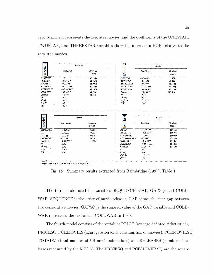
cept coefficient represents the zero star movies, and the coefficients of the ONESTAR,

TWOSTAR, and THREESTAR variables show the increase in BOR relative to the

zero star movies.

Fig. 18: Summary results extracted from Baimbridge (1997), Table 1.

The third model used the variables SEQUENCE, GAP, GAPSQ, and COLD-

WAR: SEQUENCE is the order of movie releases, GAP shows the time gap between

two consecutive movies, GAPSQ is the squared value of the GAP variable and COLD-

WAR represents the end of the COLDWAR in 1989.

The fourth model consists of the variables PRICE (average deflated ticket price),

PRICESQ, PCEMOVIES (aggregate personal consumption on movies), PCEMOVIESQ,

TOTADM (total number of US movie admissions) and RELEASES (number of re-

leases measured by the MPAA). The PRICESQ and PCEMOVIESSQ are the square

41

of variables PRICE and PCEMOVIES. The summary results of Baimbridge (1997)

are presented in Figure 18

3.2.1 First Model

In Baimbridge (1997), the descriptions of some variables were vague. For ex-

ample, it was not clear if the variable ACTREND starts from zero or from one.

Additionally, the value of the NEWBOND for the first (Dr. No) and the seventh

(Diamonds are Forever) JB movies were not specified (0 or 1). For the first movie,

Dr. No the JB actor Connery was a new JB actor, but there was not any other JB

actors before. Forth the seventh movie, Diamonds are Forever, JB actor Connery was

a new JB actor compare to the last movie, but not compared to all the other movies.

Furthermore, Baimbridge (1997) specified that the Cochrane and Orcutt (1949) tech-

nique was used to correct the first order autocorrelations, but he did not mention if

it was used for all four models. The inflation adjustment year is not known either.

Possible inflation adjustment years are 1963 (the year when the first JB movie Dr.

No was released in the United States) or 1962 (the year when the first JB movie Dr.

No was released in the United Kingdom).

The inflation adjustment method was also not clearly stated in Baimbridge

(1997). Common methods can be based on the Consumer Price Index (CPI) or

the average ticket price. Specifically, the 1962 inflation adjusted box–office revenues

using the CPI index and the average ticket price can be calculated using Equations

(1) and (2), respectively.

Y1962 = log

(Yx · T1962106 · Tx

)(1)

Y1962 = log

(Yx · CPI1962106 · CPIx

)(2)

where Yx is the unadjusted BOR for the given year x, Tx is the average ticket price

42

for the given year x, and CPIx is the consumption price index for the given year x.

Here the BORs are in millions

The average ticket price adjuster and the box–office mojo adjuster gave nearly iden-

tical results except for the movies Goldfinger and Thunderball as discussed in Sec-

tion 1.5.1. Therefore, inflation adjustment used in the box-office mojo (http://

www.boxofficemojo.com/franchises/chart/?id=jamesbond.htm) was considered

as well.

To obtain closer estimate found in Baimbridge (1997), all possible combinations

for the variables setting described above were considered. Two possibilities for AC-

TREND (starting from 0 and starting from 1), four possibilities for the NEWBOND

variable (NEWBOND1 = 0, NEWBOND1 = 1, NEWBOND7 = 0, NEWBOND7 =

1), the usage of the Cochrane and Orcutt (1949) technique (whether the technique

was used or not), two inflation adjustment years (1962 and 1963), and three inflation

adjustment strategies (using the CPI index, average ticket price, and box–office mojo

website) yield 96 different linear models. For all 96 models, linear regression coef-

ficients were obtained. The best model was chosen by the coefficients that had the

smallest sum of squared deviations (SSE) from the Baimbridge coefficients.

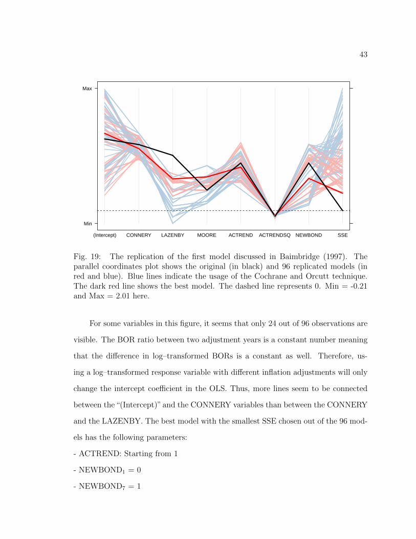
Figure 19 shows the parallel coordinates plot for all 96 models. The first seven columns

show the regression coefficients of these models. The last column is the SSE from the

Baimbridge’s coefficients. The faded blue lines represent the models in which the

Cochrane and Orcutt (1949) technique was applied. From the last column we can see

that the overall SSE is greater for the models using this technique than for the ones

without. Therefore, it is most likely that the Cochrane and Orcutt (1949) technique

was not performed on the first model.

43

Min

Max

(Intercept) CONNERY LAZENBY MOORE ACTREND ACTRENDSQ NEWBOND SSE

Fig. 19: The replication of the first model discussed in Baimbridge (1997). Theparallel coordinates plot shows the original (in black) and 96 replicated models (inred and blue). Blue lines indicate the usage of the Cochrane and Orcutt technique.The dark red line shows the best model. The dashed line represents 0. Min = -0.21and Max = 2.01 here.

For some variables in this figure, it seems that only 24 out of 96 observations are

visible. The BOR ratio between two adjustment years is a constant number meaning

that the difference in log–transformed BORs is a constant as well. Therefore, us-

ing a log–transformed response variable with different inflation adjustments will only

change the intercept coefficient in the OLS. Thus, more lines seem to be connected

between the“(Intercept)”and the CONNERY variables than between the CONNERY

and the LAZENBY. The best model with the smallest SSE chosen out of the 96 mod-

els has the following parameters:

- ACTREND: Starting from 1

- NEWBOND1 = 0

- NEWBOND7 = 1

44

- Cochrane and Orcutt: Not used

- Adjustment year: 1962

- Adjustment method: CPI

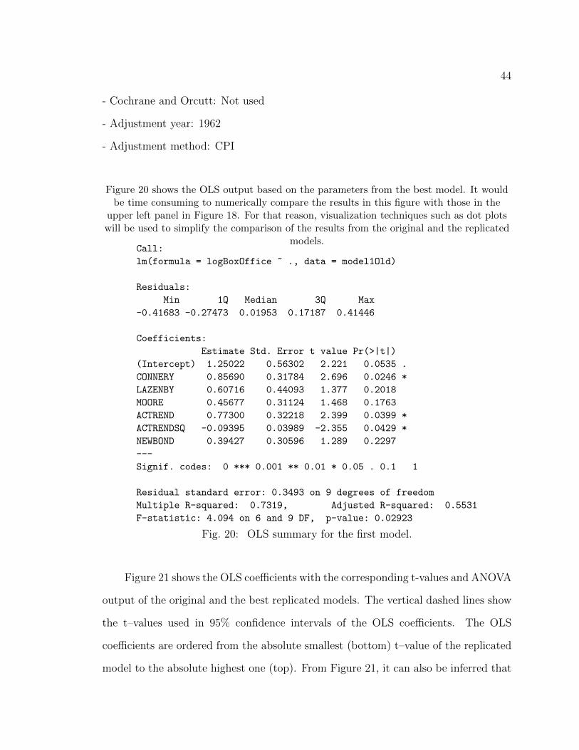
Figure 20 shows the OLS output based on the parameters from the best model. It wouldbe time consuming to numerically compare the results in this figure with those in the

upper left panel in Figure 18. For that reason, visualization techniques such as dot plotswill be used to simplify the comparison of the results from the original and the replicated

models.Call:

lm(formula = logBoxOffice ~ ., data = model1Old)

Residuals:

Min 1Q Median 3Q Max

-0.41683 -0.27473 0.01953 0.17187 0.41446

Coefficients:

Estimate Std. Error t value Pr(>|t|)

(Intercept) 1.25022 0.56302 2.221 0.0535 .

CONNERY 0.85690 0.31784 2.696 0.0246 *

LAZENBY 0.60716 0.44093 1.377 0.2018

MOORE 0.45677 0.31124 1.468 0.1763

ACTREND 0.77300 0.32218 2.399 0.0399 *

ACTRENDSQ -0.09395 0.03989 -2.355 0.0429 *

NEWBOND 0.39427 0.30596 1.289 0.2297

---

Signif. codes: 0 *** 0.001 ** 0.01 * 0.05 . 0.1 1

Residual standard error: 0.3493 on 9 degrees of freedom

Multiple R-squared: 0.7319, Adjusted R-squared: 0.5531

F-statistic: 4.094 on 6 and 9 DF, p-value: 0.02923

Fig. 20: OLS summary for the first model.

Figure 21 shows the OLS coefficients with the corresponding t-values and ANOVA

output of the original and the best replicated models. The vertical dashed lines show

the t–values used in 95% confidence intervals of the OLS coefficients. The OLS

coefficients are ordered from the absolute smallest (bottom) t–value of the replicated

model to the absolute highest one (top). From Figure 21, it can also be inferred that

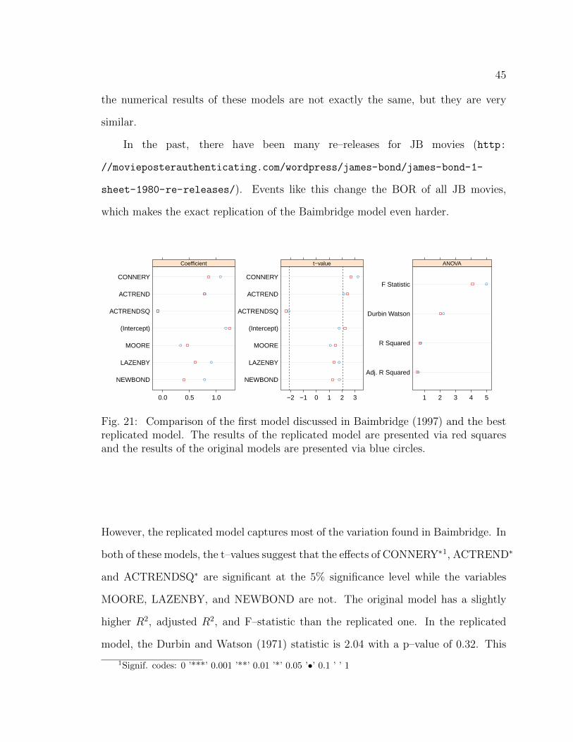
45

the numerical results of these models are not exactly the same, but they are very

similar.

In the past, there have been many re–releases for JB movies (http:

//movieposterauthenticating.com/wordpress/james-bond/james-bond-1-

sheet-1980-re-releases/). Events like this change the BOR of all JB movies,

which makes the exact replication of the Baimbridge model even harder.

NEWBOND

LAZENBY

MOORE

(Intercept)

ACTRENDSQ

ACTREND

CONNERY

0.0 0.5 1.0

Coefficient

NEWBOND

LAZENBY

MOORE

(Intercept)

ACTRENDSQ

ACTREND

CONNERY

−2 −1 0 1 2 3

t−value

Adj. R Squared

R Squared

Durbin Watson

F Statistic

1 2 3 4 5

ANOVA

Fig. 21: Comparison of the first model discussed in Baimbridge (1997) and the bestreplicated model. The results of the replicated model are presented via red squaresand the results of the original models are presented via blue circles.

However, the replicated model captures most of the variation found in Baimbridge. In

both of these models, the t–values suggest that the effects of CONNERY∗1, ACTREND∗

and ACTRENDSQ∗ are significant at the 5% significance level while the variables

MOORE, LAZENBY, and NEWBOND are not. The original model has a slightly

higher R2, adjusted R2, and F–statistic than the replicated one. In the replicated

model, the Durbin and Watson (1971) statistic is 2.04 with a p–value of 0.32. This

1Signif. codes: 0 ’***’ 0.001 ’**’ 0.01 ’*’ 0.05 ’•’ 0.1 ’ ’ 1

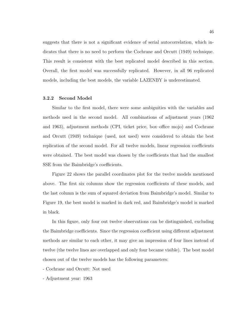
46

suggests that there is not a significant evidence of serial autocorrelation, which in-

dicates that there is no need to perform the Cochrane and Orcutt (1949) technique.

This result is consistent with the best replicated model described in this section.

Overall, the first model was successfully replicated. However, in all 96 replicated

models, including the best models, the variable LAZENBY is underestimated.

3.2.2 Second Model

Similar to the first model, there were some ambiguities with the variables and

methods used in the second model. All combinations of adjustment years (1962

and 1963), adjustment methods (CPI, ticket price, box–office mojo) and Cochrane

and Orcutt (1949) technique (used, not used) were considered to obtain the best

replication of the second model. For all twelve models, linear regression coefficients

were obtained. The best model was chosen by the coefficients that had the smallest

SSE from the Baimbridge’s coefficients.

Figure 22 shows the parallel coordinates plot for the twelve models mentioned

above. The first six columns show the regression coefficients of these models, and

the last column is the sum of squared deviation from Baimbridge’s model. Similar to

Figure 19, the best model is marked in dark red, and Baimbridge’s model is marked

in black.

In this figure, only four out twelve observations can be distinguished, excluding

the Baimbridge coefficients. Since the regression coefficient using different adjustment

methods are similar to each other, it may give an impression of four lines instead of

twelve (the twelve lines are overlapped and only four became visible). The best model

chosen out of the twelve models has the following parameters:

- Cochrane and Orcutt: Not used

- Adjustment year: 1963

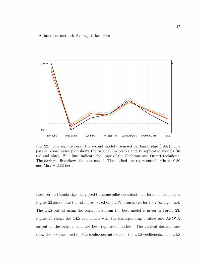
47

- Adjustment method: Average ticket price

Min

Max

(Intercept) ONESTAR TWOSTAR THREESTAR WONOSCAR NOMOSCAR SSE

Fig. 22: The replication of the second model discussed in Baimbridge (1997). Theparallel coordinates plot shows the original (in black) and 12 replicated models (inred and blue). Blue lines indicate the usage of the Cochrane and Orcutt technique.The dark red line shows the best model. The dashed line represents 0. Min = -0.30and Max = 2.82 here.

However, as Baimbridge likely used the same inflation adjustment for all of his models,

Figure 22 also shows the estimates based on a CPI adjustment for 1962 (orange line).

The OLS output using the parameters from the best model is given in Figure 23.

Figure 24 shows the OLS coefficients with the corresponding t-values and ANOVA

output of the original and the best replicated models. The vertical dashed lines

show the t–values used in 95% confidence intervals of the OLS coefficients. The OLS

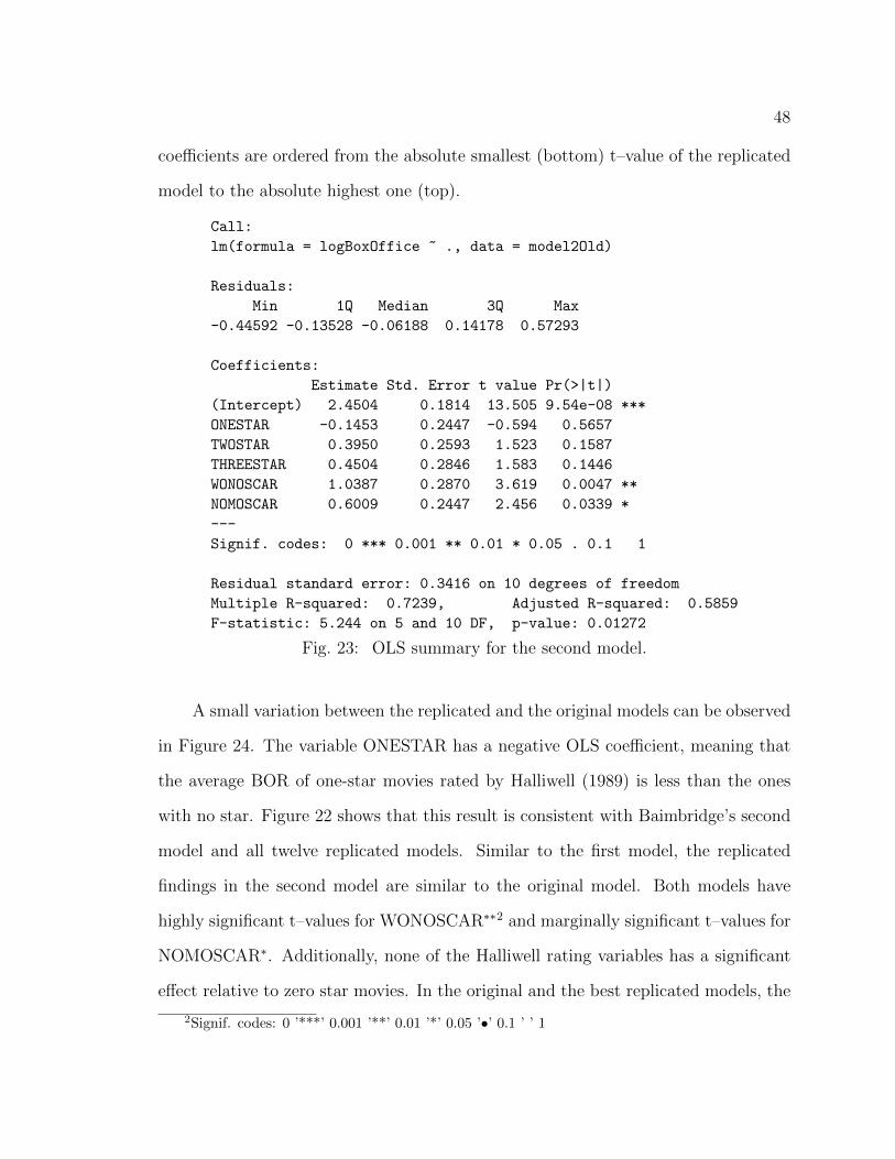
48

coefficients are ordered from the absolute smallest (bottom) t–value of the replicated

model to the absolute highest one (top).

Call:

lm(formula = logBoxOffice ~ ., data = model2Old)

Residuals:

Min 1Q Median 3Q Max

-0.44592 -0.13528 -0.06188 0.14178 0.57293

Coefficients:

Estimate Std. Error t value Pr(>|t|)

(Intercept) 2.4504 0.1814 13.505 9.54e-08 ***

ONESTAR -0.1453 0.2447 -0.594 0.5657

TWOSTAR 0.3950 0.2593 1.523 0.1587

THREESTAR 0.4504 0.2846 1.583 0.1446

WONOSCAR 1.0387 0.2870 3.619 0.0047 **

NOMOSCAR 0.6009 0.2447 2.456 0.0339 *

---

Signif. codes: 0 *** 0.001 ** 0.01 * 0.05 . 0.1 1

Residual standard error: 0.3416 on 10 degrees of freedom

Multiple R-squared: 0.7239, Adjusted R-squared: 0.5859

F-statistic: 5.244 on 5 and 10 DF, p-value: 0.01272

Fig. 23: OLS summary for the second model.

A small variation between the replicated and the original models can be observed

in Figure 24. The variable ONESTAR has a negative OLS coefficient, meaning that

the average BOR of one-star movies rated by Halliwell (1989) is less than the ones

with no star. Figure 22 shows that this result is consistent with Baimbridge’s second

model and all twelve replicated models. Similar to the first model, the replicated

findings in the second model are similar to the original model. Both models have

highly significant t–values for WONOSCAR∗∗2 and marginally significant t–values for

NOMOSCAR∗. Additionally, none of the Halliwell rating variables has a significant

effect relative to zero star movies. In the original and the best replicated models, the

2Signif. codes: 0 ’***’ 0.001 ’**’ 0.01 ’*’ 0.05 ’•’ 0.1 ’ ’ 1

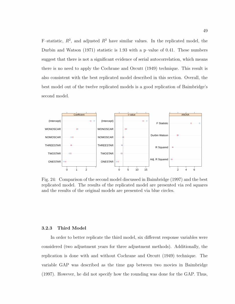
49

F–statistic, R2, and adjusted R2 have similar values. In the replicated model, the

Durbin and Watson (1971) statistic is 1.93 with a p–value of 0.41. These numbers

suggest that there is not a significant evidence of serial autocorrelation, which means

there is no need to apply the Cochrane and Orcutt (1949) technique. This result is

also consistent with the best replicated model described in this section. Overall, the

best model out of the twelve replicated models is a good replication of Baimbridge’s

second model.

ONESTAR

TWOSTAR

THREESTAR

NOMOSCAR

WONOSCAR

(Intercept)

0 1 2

Coefficient

ONESTAR

TWOSTAR

THREESTAR

NOMOSCAR

WONOSCAR

(Intercept)

0 5 10 15

t−value

Adj. R Squared

R Squared

Durbin Watson

F Statistic

2 4 6

ANOVA

Fig. 24: Comparison of the second model discussed in Baimbridge (1997) and the bestreplicated model. The results of the replicated model are presented via red squaresand the results of the original models are presented via blue circles.

3.2.3 Third Model

In order to better replicate the third model, six different response variables were

considered (two adjustment years for three adjustment methods). Additionally, the

replication is done with and without Cochrane and Orcutt (1949) technique. The

variable GAP was described as the time gap between two movies in Baimbridge

(1997). However, he did not specify how the rounding was done for the GAP. Thus,

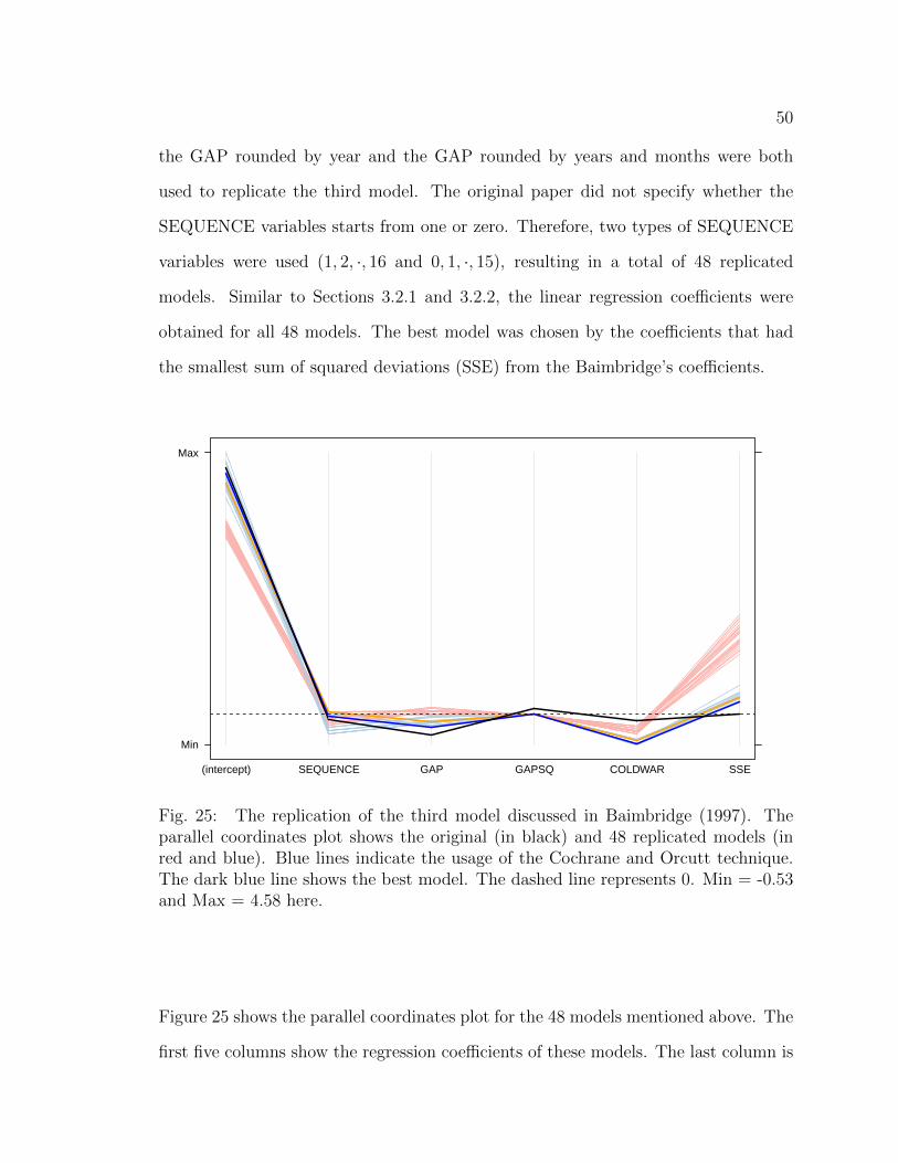
50

the GAP rounded by year and the GAP rounded by years and months were both

used to replicate the third model. The original paper did not specify whether the

SEQUENCE variables starts from one or zero. Therefore, two types of SEQUENCE

variables were used (1, 2, ·, 16 and 0, 1, ·, 15), resulting in a total of 48 replicated

models. Similar to Sections 3.2.1 and 3.2.2, the linear regression coefficients were

obtained for all 48 models. The best model was chosen by the coefficients that had

the smallest sum of squared deviations (SSE) from the Baimbridge’s coefficients.

Min

Max

(intercept) SEQUENCE GAP GAPSQ COLDWAR SSE

Fig. 25: The replication of the third model discussed in Baimbridge (1997). Theparallel coordinates plot shows the original (in black) and 48 replicated models (inred and blue). Blue lines indicate the usage of the Cochrane and Orcutt technique.The dark blue line shows the best model. The dashed line represents 0. Min = -0.53and Max = 4.58 here.

Figure 25 shows the parallel coordinates plot for the 48 models mentioned above. The

first five columns show the regression coefficients of these models. The last column is

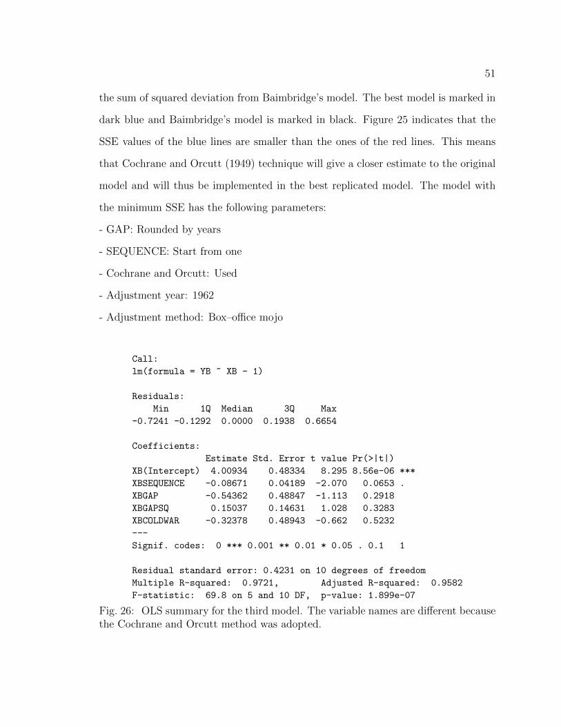
51

the sum of squared deviation from Baimbridge’s model. The best model is marked in

dark blue and Baimbridge’s model is marked in black. Figure 25 indicates that the

SSE values of the blue lines are smaller than the ones of the red lines. This means

that Cochrane and Orcutt (1949) technique will give a closer estimate to the original

model and will thus be implemented in the best replicated model. The model with

the minimum SSE has the following parameters:

- GAP: Rounded by years

- SEQUENCE: Start from one

- Cochrane and Orcutt: Used

- Adjustment year: 1962

- Adjustment method: Box–office mojo

Call:

lm(formula = YB ~ XB - 1)

Residuals:

Min 1Q Median 3Q Max

-0.7241 -0.1292 0.0000 0.1938 0.6654

Coefficients:

Estimate Std. Error t value Pr(>|t|)

XB(Intercept) 4.00934 0.48334 8.295 8.56e-06 ***

XBSEQUENCE -0.08671 0.04189 -2.070 0.0653 .

XBGAP -0.54362 0.48847 -1.113 0.2918

XBGAPSQ 0.15037 0.14631 1.028 0.3283

XBCOLDWAR -0.32378 0.48943 -0.662 0.5232

---

Signif. codes: 0 *** 0.001 ** 0.01 * 0.05 . 0.1 1

Residual standard error: 0.4231 on 10 degrees of freedom

Multiple R-squared: 0.9721, Adjusted R-squared: 0.9582

F-statistic: 69.8 on 5 and 10 DF, p-value: 1.899e-07

Fig. 26: OLS summary for the third model. The variable names are different becausethe Cochrane and Orcutt method was adopted.

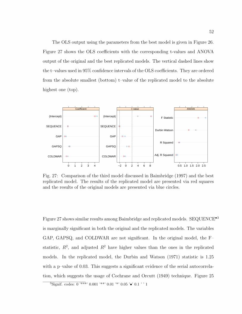
52

The OLS output using the parameters from the best model is given in Figure 26.

Figure 27 shows the OLS coefficients with the corresponding t-values and ANOVA

output of the original and the best replicated models. The vertical dashed lines show

the t–values used in 95% confidence intervals of the OLS coefficients. They are ordered

from the absolute smallest (bottom) t–value of the replicated model to the absolute

highest one (top).

COLDWAR

GAPSQ

GAP

SEQUENCE

(Intercept)

0 1 2 3 4

Coefficient

COLDWAR

GAPSQ

GAP

SEQUENCE

(Intercept)

−2 0 2 4 6 8

t−value

Adj. R Squared

R Squared

Durbin Watson

F Statistic

0.5 1.0 1.5 2.0 2.5

ANOVA

Fig. 27: Comparison of the third model discussed in Baimbridge (1997) and the bestreplicated model. The results of the replicated model are presented via red squaresand the results of the original models are presented via blue circles.

Figure 27 shows similar results among Baimbridge and replicated models. SEQUENCE•3

is marginally significant in both the original and the replicated models. The variables

GAP, GAPSQ, and COLDWAR are not significant. In the original model, the F–

statistic, R2, and adjusted R2 have higher values than the ones in the replicated

models. In the replicated model, the Durbin and Watson (1971) statistic is 1.25

with a p–value of 0.03. This suggests a significant evidence of the serial autocorrela-

tion, which suggests the usage of Cochrane and Orcutt (1949) technique. Figure 25

3Signif. codes: 0 ’***’ 0.001 ’**’ 0.01 ’*’ 0.05 ’•’ 0.1 ’ ’ 1

53

also shows that the model gives a closer estimate to Baimbridge’s coefficients when

using the Cochrane and Orcutt (1949) technique. Thus, using the Durbin Watson

statistic is a valid adjustment for this model. However, all the replicated estimates

seems to overestimated the GAP variable and underestimate the variables GAPSQ

and COLDWAR.

3.2.4 Fourth Model: First Attempt

In this section, the replication of the fourth model described in Baimbridge (1997)

is performed. Similar to Sections 3.2.1–3.2.3, six different response variables were

considered (two adjustment years for three adjustment methods). For each response

variable, a regression model is implemented with and without the Cochrane and

Orcutt (1949) technique.

In Baimbridge’s fourth model, shown in Figure 18, the coefficient estimate of the

TOTADM is -3.6111. The range of the response variables calculated by Equation (1)

and (2) varies between two and four, the TOTADM variable should not have high

variation. However, the range of the TOTADM variable varies around one billion in

the collected dataset. This suggests that some type of transformation is necessary

to obtain a closer coefficient of TOTADM. Therefore, a log transformation and unit

adjustment to billions were used.

Figure 28 shows the parallel coordinates plot for 24 replicated models. The first

seven columns show the regression coefficient of these models. The last column is the

sum of squared deviation (in thousands) from Baimbridge’s model. The best model

is marked in dark red and Baimbridge’s model is marked in black.

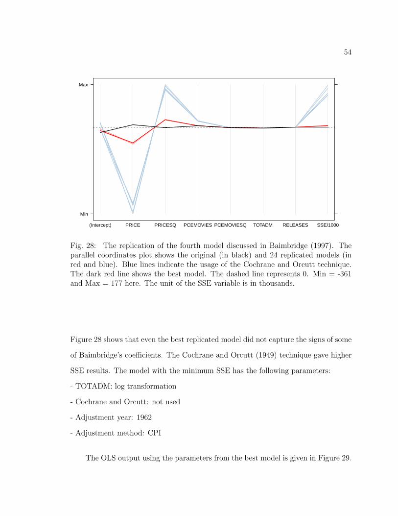
54

Min

Max

(Intercept) PRICE PRICESQ PCEMOVIES PCEMOVIESQ TOTADM RELEASES SSE/1000

Fig. 28: The replication of the fourth model discussed in Baimbridge (1997). Theparallel coordinates plot shows the original (in black) and 24 replicated models (inred and blue). Blue lines indicate the usage of the Cochrane and Orcutt technique.The dark red line shows the best model. The dashed line represents 0. Min = -361and Max = 177 here. The unit of the SSE variable is in thousands.

Figure 28 shows that even the best replicated model did not capture the signs of some

of Baimbridge’s coefficients. The Cochrane and Orcutt (1949) technique gave higher

SSE results. The model with the minimum SSE has the following parameters:

- TOTADM: log transformation

- Cochrane and Orcutt: not used

- Adjustment year: 1962

- Adjustment method: CPI

The OLS output using the parameters from the best model is given in Figure 29.

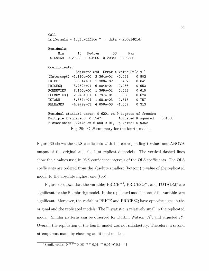
55

Call:

lm(formula = logBoxOffice ~ ., data = model4Old)

Residuals:

Min 1Q Median 3Q Max

-0.69468 -0.29080 -0.04265 0.20841 0.89356

Coefficients:

Estimate Std. Error t value Pr(>|t|)

(Intercept) -6.110e+00 2.364e+01 -0.258 0.802

PRICE -6.651e+01 1.380e+02 -0.482 0.641

PRICESQ 3.252e+01 6.984e+01 0.466 0.653

PCEMOVIES 7.140e+00 1.369e+01 0.522 0.615

PCEMOVIESQ -2.945e-01 5.797e-01 -0.508 0.624

TOTADM 5.354e-04 1.681e-03 0.318 0.757

RELEASES -4.979e-03 4.656e-03 -1.069 0.313

Residual standard error: 0.6201 on 9 degrees of freedom

Multiple R-squared: 0.1547, Adjusted R-squared: -0.4088

F-statistic: 0.2745 on 6 and 9 DF, p-value: 0.9352

Fig. 29: OLS summary for the fourth model.

Figure 30 shows the OLS coefficients with the corresponding t-values and ANOVA

output of the original and the best replicated models. The vertical dashed lines

show the t–values used in 95% confidence intervals of the OLS coefficients. The OLS

coefficients are ordered from the absolute smallest (bottom) t–value of the replicated

model to the absolute highest one (top).

Figure 30 shows that the variables PRICE∗∗4, PRICESQ∗∗, and TOTADM∗ are

significant for the Baimbridge model. In the replicated model, none of the variables are

significant. Moreover, the variables PRICE and PRICESQ have opposite signs in the

original and the replicated models. The F–statistic is relatively small in the replicated

model. Similar patterns can be observed for Durbin Watson, R2, and adjusted R2.

Overall, the replication of the fourth model was not satisfactory. Therefore, a second

attempt was made by checking additional models.

4Signif. codes: 0 ’***’ 0.001 ’**’ 0.01 ’*’ 0.05 ’•’ 0.1 ’ ’ 1

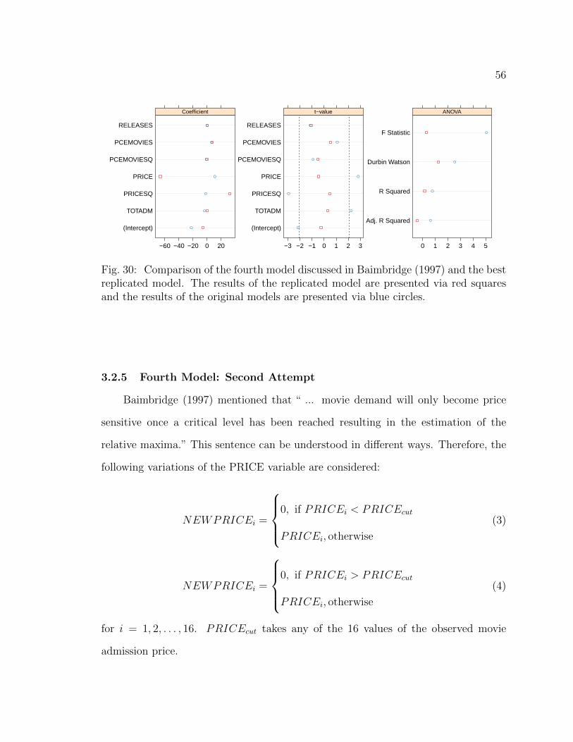
56

(Intercept)

TOTADM

PRICESQ

PRICE

PCEMOVIESQ

PCEMOVIES

RELEASES

−60 −40 −20 0 20

Coefficient

(Intercept)

TOTADM

PRICESQ

PRICE

PCEMOVIESQ

PCEMOVIES

RELEASES

−3 −2 −1 0 1 2 3

t−value

Adj. R Squared

R Squared

Durbin Watson

F Statistic

0 1 2 3 4 5

ANOVA

Fig. 30: Comparison of the fourth model discussed in Baimbridge (1997) and the bestreplicated model. The results of the replicated model are presented via red squaresand the results of the original models are presented via blue circles.

3.2.5 Fourth Model: Second Attempt

Baimbridge (1997) mentioned that “ ... movie demand will only become price

sensitive once a critical level has been reached resulting in the estimation of the

relative maxima.” This sentence can be understood in different ways. Therefore, the

following variations of the PRICE variable are considered:

NEWPRICEi =

0, if PRICEi < PRICEcut

PRICEi, otherwise

(3)

NEWPRICEi =

0, if PRICEi > PRICEcut

PRICEi, otherwise

(4)

for i = 1, 2, . . . , 16. PRICEcut takes any of the 16 values of the observed movie

admission price.

57

For the given 16 movies, these equations create 32 different variations of the

PRICE variable. However, in two of these variations the variable PRICESQ becomes

only a linear transformation of the variable PRICE, which gives “NA” values when

predicting the regression coefficient of PRICESQ. The exclusion of these two varia-

tions result in 30 different PRICE variables to consider.

When the Cochrane and Orcutt technique is applied, the calculation of the re-

gression coefficients for some variations of the PRICE variable took several hours.

Therefore, the Cochrane and Orcutt technique was only applied to the best four

models, i.e., the models with the smallest SSE, that resulted from all models without

using this technique. Thus, 30 PRICE variations without the Cochrane and Orcutt

technique and four PRICE variations with the Cochrane and Orcutt technique are

considered. For each of the above mentioned PRICE variations, two variations of the

adjustment year, three variations of the adjustment method, and two variations of

the TOTADM variable are applied creating a total of 408 (34× 2× 3× 2) models.

Figure 31 shows the parallel coordinates plot for these 408 replicated models.

The first seven columns show the regression coefficient of these models and the last

column is the sum of squared deviation (in hundreds) from Baimbridge’s model. Out

of these 408 models, the model with the minimum SSE has the following parameters:

- TOTADM: log transformation

- Cochrane and Orcutt: not used

- Adjustment year: 1962

- Adjustment method: Mojo

- PRICE cutoff: PRICEcut = 1.0096 withNEWPRICEi =

0, if PRICEi > PRICEcut

PRICEi, otherwise

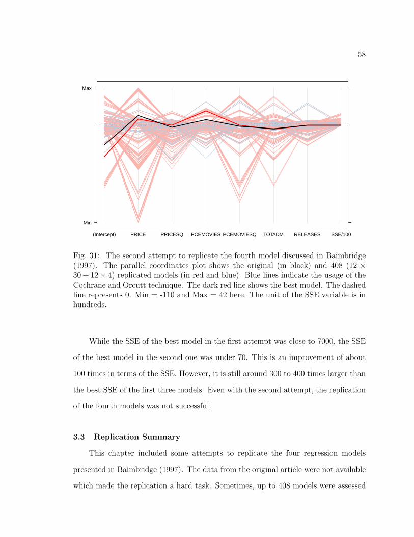
58

Min

Max

(Intercept) PRICE PRICESQ PCEMOVIES PCEMOVIESQ TOTADM RELEASES SSE/100

Fig. 31: The second attempt to replicate the fourth model discussed in Baimbridge(1997). The parallel coordinates plot shows the original (in black) and 408 (12 ×30 + 12× 4) replicated models (in red and blue). Blue lines indicate the usage of theCochrane and Orcutt technique. The dark red line shows the best model. The dashedline represents 0. Min = -110 and Max = 42 here. The unit of the SSE variable is inhundreds.

‘

While the SSE of the best model in the first attempt was close to 7000, the SSE

of the best model in the second one was under 70. This is an improvement of about

100 times in terms of the SSE. However, it is still around 300 to 400 times larger than

the best SSE of the first three models. Even with the second attempt, the replication

of the fourth models was not successful.

3.3 Replication Summary

This chapter included some attempts to replicate the four regression models

presented in Baimbridge (1997). The data from the original article were not available

which made the replication a hard task. Sometimes, up to 408 models were assessed

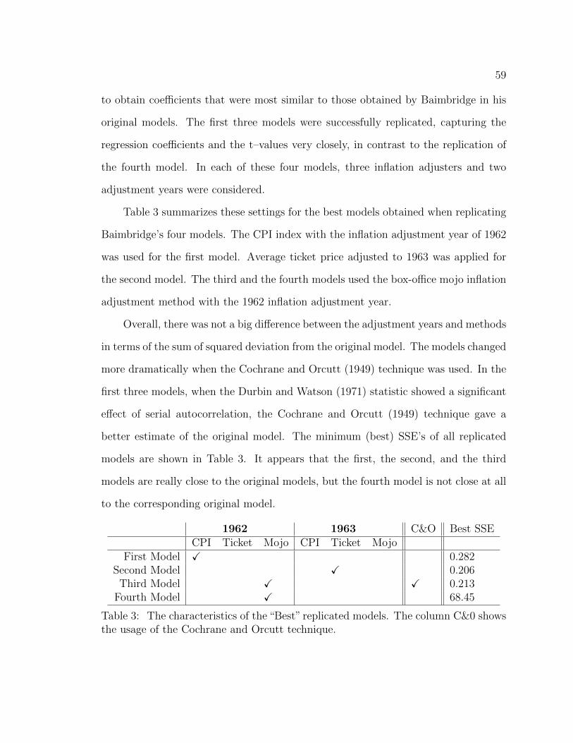
59

to obtain coefficients that were most similar to those obtained by Baimbridge in his

original models. The first three models were successfully replicated, capturing the

regression coefficients and the t–values very closely, in contrast to the replication of

the fourth model. In each of these four models, three inflation adjusters and two

adjustment years were considered.

Table 3 summarizes these settings for the best models obtained when replicating

Baimbridge’s four models. The CPI index with the inflation adjustment year of 1962

was used for the first model. Average ticket price adjusted to 1963 was applied for

the second model. The third and the fourth models used the box-office mojo inflation

adjustment method with the 1962 inflation adjustment year.

Overall, there was not a big difference between the adjustment years and methods

in terms of the sum of squared deviation from the original model. The models changed

more dramatically when the Cochrane and Orcutt (1949) technique was used. In the

first three models, when the Durbin and Watson (1971) statistic showed a significant

effect of serial autocorrelation, the Cochrane and Orcutt (1949) technique gave a

better estimate of the original model. The minimum (best) SSE’s of all replicated

models are shown in Table 3. It appears that the first, the second, and the third

models are really close to the original models, but the fourth model is not close at all

to the corresponding original model.

1962 1963 C&O Best SSECPI Ticket Mojo CPI Ticket Mojo

First Model X 0.282Second Model X 0.206Third Model X X 0.213

Fourth Model X 68.45

Table 3: The characteristics of the “Best” replicated models. The column C&0 showsthe usage of the Cochrane and Orcutt technique.

60

CHAPTER 4

PREDICTING THE BOX-OFFICE REVENUES OF THE JB MOVIE SERIES

4.1 Prediction Methods Overview

Forecasting the box–office revenues (BOR) is one of the most important aspects

of research in the movie industry. Sections 1.2 and 1.4 showed that prediction of the

BOR became a popular task over the last three decades. In this chapter, various

methods will be used to predict the BOR of the JB movie series. The 16 JB movies

that were released before 1990 are used as a training set and the six JB movies released

after 1990 are used as a test set.

The datasets used in the first and the third Baimbridge (1997) model and in

The Economist model are used to make the predictions (Section 1.5). The dataset

from the second Baimbridge model is not considered because the last version of the

Halliwell book was released in 1989. For movies released after 1989, this makes the

observations of the variables ONESTAR, TWOSTAR, and THREESTAR (Section

1.5.2) impossible to find. The replication of the fourth Baimbridge model was not

successful and, thus, the prediction for this dataset is not considered.

OLS (Section 4.1.1), LASSO (Section 4.1.2), and random forests (Section 4.1.3)

are applied on the first and the third Baimbridge model and on The Economist model

to predict the BORs. Additionally, for the first and third models Baimbridge’s OLS

coefficients were used to forecast the BOR. For each model, visualization tools are

used to compare the different methods and their results.

61

4.1.1 Ordinary Least Squares (OLS)

OLS is the most commonly used method in regression. It is easy to model

and interpret. In this chapter, OLS is used to predict the BORs. For the first

and third Baimbridge models we will start from the full model and will check all

possible combinations of explanatory variables. The best model will be selected by

the variables that will minimize the Akaike Information Criterion (AIC) (Claeskens

and Hjort, 2008, p. 22). In The Economist model, the AIC criteria deletes all the

variables (kills, conquests, martinis, and BJB expression). Therefore, instead of fitting

the minimum AIC model, the full model with four variables will be fitted. In the

first and the third Baimbridge model, the AIC criteria will not be used because the

Baimbridge (1997) fitted the full models.

4.1.2 LASSO

The LASSO (Tibshirani, 1996) is a shrinkage and selection method for linear

regression, which constraints the absolute sum of the regression coefficients,∑j

|βj|′s.

In other words, the LASSO estimates can be defined as:

β = arg minβ

N∑i=1

(yi − β0 −

p∑j=1

βjxij

)2 s.t.

p∑j=1

|βj| ≤ t (5)

where t ≥ 0 is the tuning parameter. The LASSO will be used for The Economist, the

first and the third models. Among hundred tuning parameters, the best parameter

will be chosen using cross–validation accuracy rates. Predictions will be made using

the best tuning parameter.

4.1.3 Random Forests

Random forests (Breiman, 2001) is a popular ensemble–learning algorithm for

62

classification and regression. It is one of the tree–based algorithms in which the

averages of multiple trees are taken for prediction (default number of trees, ntree =

500). At each node of the tree, random forests takes some number of variables (mtry)

to perform the next split (for regression, the default mtry is the square–root of the

number of variables). All trees are fully grown. The regression random forests are

applied to all three dataset discussed in Section 4.1.2. For this analysis, mtry = 2

and ntree = 5000 will be used.

4.1.4 Benchmarks

Two benchmark predictors were used to predict the BORs. The first benchmark

(bench mean) is simply the average BOR of the first 16 movies. This will be equivalent

to an OLS model with all β′s = 0. The second benchmark (bench mean 2) predicts

the next BOR based on the average of all BORs found before. This benchmark will

only be used in The Economist model, which will substitute the Baimbridge model.

Overall, the three or four methods will be compared with each other as well as

with the one or two benchmarks. The comparison will be based on the root mean

squared error (RMSE) which can be calculated with the following equation:

RMSE =

√√√√ k∑i=1

(yi − yi)2

k(6)

where k is the number of observations in the given dataset (k = 16 for the training

set and k = 6 for the test set. yis are the observed BORs and yis are the predicted

BORs for those k movies.

4.2 Comparison of the First Model

In this section, four regression and machine learning methods (OLS, Baimbridge

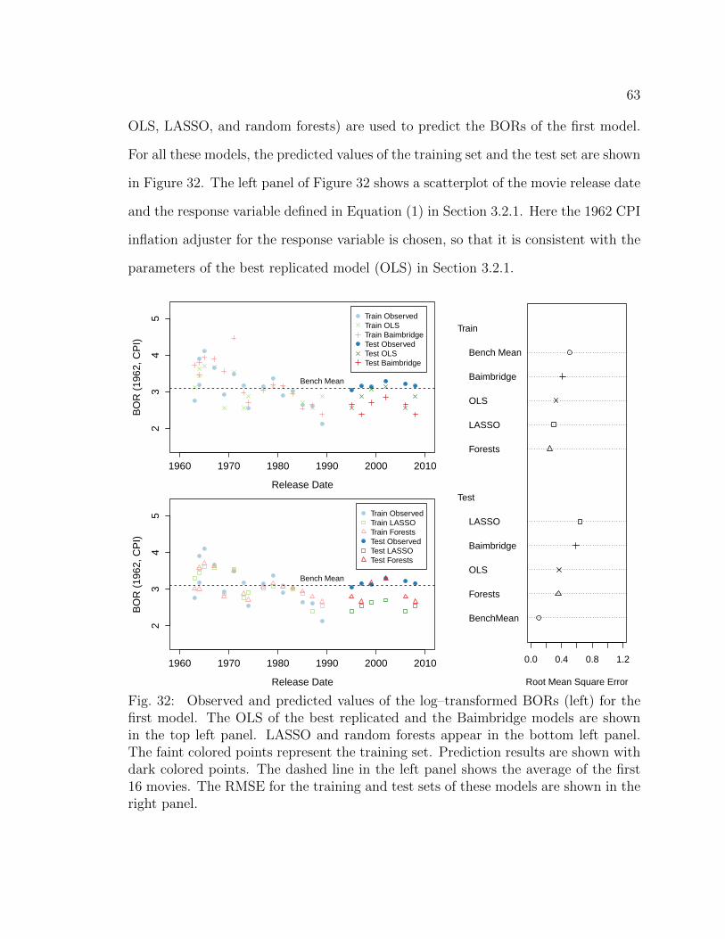
63

OLS, LASSO, and random forests) are used to predict the BORs of the first model.

For all these models, the predicted values of the training set and the test set are shown

in Figure 32. The left panel of Figure 32 shows a scatterplot of the movie release date

and the response variable defined in Equation (1) in Section 3.2.1. Here the 1962 CPI

inflation adjuster for the response variable is chosen, so that it is consistent with the

parameters of the best replicated model (OLS) in Section 3.2.1.

1960 1970 1980 1990 2000 2010

23

45

Release Date

BO

R (

1962

, CP

I)

Bench Mean

Train ObservedTrain OLSTrain BaimbridgeTest ObservedTest OLSTest Baimbridge

1960 1970 1980 1990 2000 2010

23

45

Release Date

BO

R (

1962

, CP

I)

Bench Mean

Train ObservedTrain LASSOTrain ForestsTest ObservedTest LASSOTest Forests

BenchMean

Forests

OLS

Baimbridge

LASSO

Forests

LASSO

OLS

Baimbridge

Bench Mean

Train

Test

0.0 0.4 0.8 1.2

Root Mean Square Error

Fig. 32: Observed and predicted values of the log–transformed BORs (left) for thefirst model. The OLS of the best replicated and the Baimbridge models are shownin the top left panel. LASSO and random forests appear in the bottom left panel.The faint colored points represent the training set. Prediction results are shown withdark colored points. The dashed line in the left panel shows the average of the first16 movies. The RMSE for the training and test sets of these models are shown in theright panel.

64

As discussed in Section 4.1.1, the model was chosen by the minimum AIC value.

In this model, the AIC criteria kept only the variables CONNERY, ACTREND,

and ACTRENDSQ. For the first model, the OLS and the random forests predicted

really well the third and fourth movies in the test set (see Figure 32). However, the

prediction of Baimbride and LASSO are not so impressive for any movies in the test

set. In this figure, the predictions from all four methods mostly underestimate the

observed BORs of the test set.

The dot plot in the right panel (Figure 32) shows the RMSE of the training and

the test sets. The RMSE of the bench mean gives the smallest value for the test

set, even though it has the largest value for the training set. Similar patterns can

be observed for LASSO. The RMSE of the training set and the test set for the OLS

and random forests are closer to each other. Random forests has the smallest RMSE

among the four methods described in Section 4.1, which has a slightly smaller RMSE

than that of the OLS. The benchmark mean has around three to four times smaller

RMSE than the other methods described in Section 4.1. The best BOR prediction

for future JB movies based on the first model is simply the average of the first 16 JB

movies.

4.3 Comparison of the Third Model

In this section, the same methods as in Section 4.2 are used to predict the BORs.

Here, the 1963 average ticket price inflation adjuster for the response variable is

chosen, so that it is consistent with the parameters of the best replicated model

(OLS) in Section 3.2.3. The minimum AIC criteria removed all variables except

the variable SEQUENCE. This makes the relationship between the SEQUENCE and

the response variable to be linear. The negative relationship between SEQUENCE

and the response variable can be observed in the top left panel in Figure 33. This

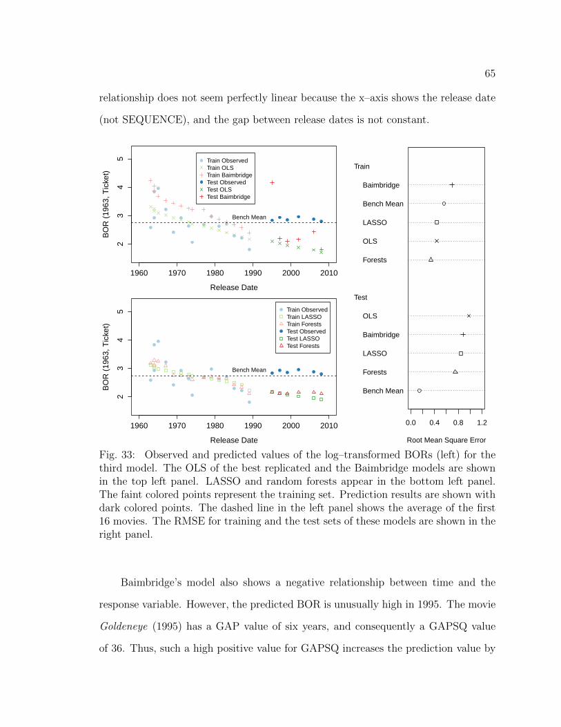
65

relationship does not seem perfectly linear because the x–axis shows the release date

(not SEQUENCE), and the gap between release dates is not constant.

1960 1970 1980 1990 2000 2010

23

45

Release Date

BO

R (

1963

, Tic

ket)

Bench Mean

Train ObservedTrain OLSTrain BaimbridgeTest ObservedTest OLSTest Baimbridge

1960 1970 1980 1990 2000 2010

23

45

Release Date

BO

R (

1963

, Tic

ket)

Bench Mean

Train ObservedTrain LASSOTrain ForestsTest ObservedTest LASSOTest Forests

Bench Mean

Forests

LASSO

Baimbridge

OLS

Forests

OLS

LASSO

Bench Mean

Baimbridge

Train

Test

0.0 0.4 0.8 1.2

Root Mean Square Error

Fig. 33: Observed and predicted values of the log–transformed BORs (left) for thethird model. The OLS of the best replicated and the Baimbridge models are shownin the top left panel. LASSO and random forests appear in the bottom left panel.The faint colored points represent the training set. Prediction results are shown withdark colored points. The dashed line in the left panel shows the average of the first16 movies. The RMSE for training and the test sets of these models are shown in theright panel.

Baimbridge’s model also shows a negative relationship between time and the

response variable. However, the predicted BOR is unusually high in 1995. The movie

Goldeneye (1995) has a GAP value of six years, and consequently a GAPSQ value

of 36. Thus, such a high positive value for GAPSQ increases the prediction value by

66

almost two. Except this observation for Baimbridge, the other predictions for the test

set are underestimated.

In the bottom left panel of Figure 33, a similar relationship can be observed for

the LASSO and random forests methods. The predictions of random forests stays

relatively constant for the test set, which allows random forests to have a smaller

RMSE than that of the Baimbridge, OLS, and LASSO methods.

The right panel of Figure 33 shows the RMSE rate for both, the training set and

the test set. Here, all methods (in the test set) perform worse in the third model

compared to the first one. In particular, the best method (random forests) for the

third model resulted in an RMSE that is almost twice as big as the RMSE for the

best method (random forests) for the first model. Similar to Section 4.2, the RMSE

of the benchmark gave the smallest RMSE which is more than six times smaller than

the RMSE of the random forests in the third model.

4.4 Comparison of The Economist Model

Baimbridge (1997) did not use the The Economist dataset because it was only

published in 2012. Thus, as a substitute to the Baimbridge model, the second bench-

mark (bench mean 2) is used. In Figure 34, red asterisks were used to mark fitted and

predicted values of the bench mean 2 method. As stated in Section 4.1, the minimum

AIC criteria was not applied to this dataset.

For The Economist dataset, the predicted values of the training set and the test

set are shown in Figure 34. The BORs for the test set seem to decrease over time.

The same pattern can be observed for LASSO, but with less a extreme decreasing

rate. Random forests predict extremely well for the fourth and sixth movies in the

test set. The prediction of the other four movies are acceptable. The right panel of

Figure 34 shows the RMSE rate for both, the training set and the test set. Again,

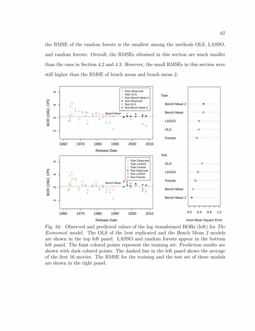
67

the RMSE of the random forests is the smallest among the methods OLS, LASSO,

and random forests. Overall, the RMSEs obtained in this section are much smaller

than the ones in Section 4.2 and 4.3. However, the small RMSEs in this section were

still higher than the RMSE of bench mean and bench mean 2.

1960 1970 1980 1990 2000 2010

23

45

Release Date

BO

R (

1962

, CP

I)

Bench Mean

Train ObservedTrain OLSTrain Bench Mean 2Test ObservedTest OLSTest Bench Mean 2

1960 1970 1980 1990 2000 2010

23

45

Release Date

BO

R (

1962

, CP

I)

Bench Mean

Train ObservedTrain LASSOTrain ForestsTest ObservedTest LASSOTest Forests

Bench Mean 2

Bench Mean

Forests

LASSO

OLS

Forests

OLS

LASSO

Bench Mean

Bench Mean 2

Train

Test

0.0 0.4 0.8 1.2

Root Mean Square Error

Fig. 34: Observed and predicted values of the log–transformed BORs (left) for TheEconomist model. The OLS of the best replicated and the Bench Mean 2 modelsare shown in the top left panel. LASSO and random forests appear in the bottomleft panel. The faint colored points represent the training set. Prediction results areshown with dark colored points. The dashed line in the left panel shows the averageof the first 16 movies. The RMSE for the training and the test set of these modelsare shown in the right panel.

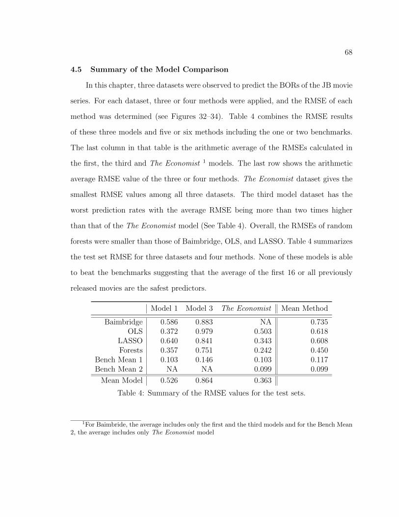
68

4.5 Summary of the Model Comparison

In this chapter, three datasets were observed to predict the BORs of the JB movie

series. For each dataset, three or four methods were applied, and the RMSE of each

method was determined (see Figures 32–34). Table 4 combines the RMSE results

of these three models and five or six methods including the one or two benchmarks.

The last column in that table is the arithmetic average of the RMSEs calculated in

the first, the third and The Economist 1 models. The last row shows the arithmetic

average RMSE value of the three or four methods. The Economist dataset gives the

smallest RMSE values among all three datasets. The third model dataset has the

worst prediction rates with the average RMSE being more than two times higher

than that of the The Economist model (See Table 4). Overall, the RMSEs of random

forests were smaller than those of Baimbridge, OLS, and LASSO. Table 4 summarizes

the test set RMSE for three datasets and four methods. None of these models is able

to beat the benchmarks suggesting that the average of the first 16 or all previously

released movies are the safest predictors.

Model 1 Model 3 The Economist Mean Method

Baimbridge 0.586 0.883 NA 0.735OLS 0.372 0.979 0.503 0.618

LASSO 0.640 0.841 0.343 0.608Forests 0.357 0.751 0.242 0.450

Bench Mean 1 0.103 0.146 0.103 0.117Bench Mean 2 NA NA 0.099 0.099

Mean Model 0.526 0.864 0.363

Table 4: Summary of the RMSE values for the test sets.

1For Baimbride, the average includes only the first and the third models and for the Bench Mean2, the average includes only The Economist model

69

4.6 Usage of R Packages

All the statistical analysis and visualization in this Master’s report were done

in R (R Core Team, 2013). Various R packages were used to produce the graphs

in Chapters 2, 3, and 4. The time series plots in Section 2.2, scatterplot matrix in

Section 2.3, boxplots in Section 2.5, and histograms in Section 2.6 were created by

the graphics package in R (R Core Team, 2013). The package Hmisc (Harrell et al.,

2014) was used to produce the the dotplots in Section 2.4. Normal quantiles plots

were created by the car package (Fox and Weisberg, 2011).

The R package PairViz (Hurley and Oldford, 2011) was used to generate the

parallel coordinates plot in Section 2.7. For the heatmap plots in section 2.8, the R

package gplot (Warnes et al., 2013) was used. The R package vcd (Meyer et al., 2006)

was used to generate the mosaic plot in Figure 13. The association plot in Figure

14 was created by using the vcd package (Meyer et al., 2006). The R package maps

(Becker, Wilks, Brownrigg and Minka, 2013) was used to produce the choropleth map

before the collapse of the USSR and the packages maptools (Bivand and Lewin-Koh,

2013) and mapdata (Becker, Wilks and Brownrigg, 2013) were used to produce the

choropleth map after the collapse of the USSR.

All dotplots and parallel coordinates plots in Chapter 3 (Figures 19, 21, 22, 24,

25, 27, 28, 30) were produced using the lattice package in R (Sarkar, 2008). The

Cochrane and Orcutt (1949) technique was done by the orcutt package in R (Spada

et al., 2012).

All figures in Chapter 4 (Figures 32–34) were based on the graphics package (R

Core Team, 2013). Computations and predictions to perform random forests were

obtained from the randomForest package (Liaw and Wiener, 2002). All computations

for LASSO were done using the glmnet package (Friedman et al., 2010).

The RColorBrewer (Neuwirth, 2011) package was used to color the lines or points

70

in the following figures: Chapter 2 – time series plots, scatterplot matrix, parallel

coordinates plot, heatmaps, choropleth maps; Chapter 3 – all figures; Chapter 4 – all

figures.

71

CHAPTER 5

CONCLUSION AND OUTLOOK

The movie industry plays a very important role in the US economy. Therefore,

research related to the movie industry has became an important topic for many sci-

entists over the last three decades. Being one of the riskiest industries, prediction of

box–office revenues (BOR) can play a vital role for many movies. In this Master’s

report, the visualization and prediction of the box–office revenues for the James Bond

movie series was performed. In Chapter 2, various visualization techniques were pre-

sented to understand the details in the data presented in The Economist article The

Economist (2012).

An increasing trend was observed for the variables JB kills and martinis drunk

over time (Figures 1 and 3). Some positive relationship was found between the BOR

and number of JB kills, and some negative relationship between BOR and BJB ex-

pressions (Figures 5 and 7). Additionally, some clustering for the JB actors Moore,

Dalton, Brosnan, and Craig (Figures 11 and 12) was observed.

Chapter 3 replicated four linear regression models that were presented in Baim-

bridge (1997). The first three models were successfully replicated, closely capturing

the regression coefficients, t–values, F–statistic, the R2, adjusted R2, and Durbin

Watson statistic. The total sum of squared deviations (SSE) of these models from

Baimbridge’s coefficients were between 0.2 and 0.3 (see Table 3). The SSE results for

these three models were impressively good, compared to the SSE value of the fourth

model which was 68.45.

Chapter 4 used three datasets (the first model, the third model, and The Economist

model; p. 7) to predict the BORs. For all these models, the ordinary least squares,

72

LASSO, and random forests were applied to make predictions. The Economist dataset

using random forests gave the best prediction results in terms of the error rate on

the test dataset. However, this is still worse than just using the past mean to make

predictions for future box–office revenues.

Overall, we found that more JB kills and less BJB expression would increase

the BORs. Additionally, we found some significant indicators to predict the BOR,

but this did not gives us much confidence to generalize the forecasting for upcoming

JB movies. After all, “. . . No one, can tell you what a movie is going to do in the

marketplace . . . Not until that film opens in a darkened theater, and sparks fly up

between the screen and the audience can you say this film is right” (Valenti, 1978).

Finally, there is a slogan that says “milk the cow as long as you can”. This seems

to be applicable to movie series, in particular to the James Bond movie series.

5.1 Future Work

Future research to forecast the BOR could look into the following:

- adjust for population growth

- adjust for the number of movie theaters

- adjust for the average capacity of movie theaters

- use other regression methods

- use time series analysis; in particular, autoregressive and moving averages methods

- include inflation–adjusted production costs

- include release information (holiday weekend vs. non–holiday weekend)

- include movie director information

- combine the significant variables from the first and the third model into a new model

73

REFERENCES

Anscombe, F. J. (1973), ‘Graphs in Statistical Analysis’, The American Statistician

27(1), 17–21.

Baimbridge, M. (1997), ‘Movie Admissions and Rental Income: the Case of James

Bond’, Applied Economics Letters 4(1), 57–61.

Becker, R. A., Wilks, A. R. and Brownrigg, R. (2013), mapdata: Extra Map Databases.

R package version 2.2-2.

URL: http://CRAN.R-project.org/package=mapdata

Becker, R. A., Wilks, A. R., Brownrigg, R. and Minka, T. P. (2013), maps: Draw

Geographical Maps. R package version 2.3-6.

URL: http://CRAN.R-project.org/package=maps

Bi, G. and Giles, D. E. (2009), ‘Modelling the Financial Risk Associated with

U.S. Movie Box Office Earnings’, Mathematics and Computers in Simulation

79(9), 2759–2766.

Bivand, R. and Lewin-Koh, N. (2013), maptools: Tools for Reading and Handling

Spatial Objects. R package version 0.8-27.

URL: http://CRAN.R-project.org/package=maptools

Breiman, L. (2001), ‘Random Forests’, Machine Learning 45(1), 5–32.

Claeskens, G. and Hjort, N. L. (2008), Model Selection and Model Averaging, 1 edn,

Cambridge University Press, Cambridge.

Cleveland, W. S. (1979), ‘Robust Locally Weighted Regression and Smoothing Scat-

terplots’, Journal of the American Statistical Association 74, 829–836.

74

Cochrane, D. and Orcutt, G. H. (1949), ‘Application of Least Squares Regression to

Relationships Containing Auto-Correlated Error Terms’, Journal of the American

Statistical Association 44(245), 32–61.

Cohen, A. (1980), ‘On the Graphical Display of the Significant Components in Two–

way Contingency Tables’, Communications in Statistics 9(10), 1025–1041.

Cooper, H., Schembri, S. and Miller, D. (2010), ‘Brand-self Identity Narratives in the

James Bond Movies’, Psychology and Marketing 27(6), 557–567.

Crawford, M. and Church, J. (2014), ‘CPI Detailed Report’.

http://www.bls.gov/cpi/cpid1402.pdf.

De Vani, A. and Walls, D. W. (1999), ‘Uncertainty in the Movie Industry: Does

Star Power Reduce the Terror of the Box Office?’, Journal of Cultural Economics

23(4), 285–318.

Delen, D., Shadra, S. and Kumar, P. (2007), ‘Movie Forecast Guru: A Web-Based

DSS for Hollywood Managers’, Decision Support Systems 43(4), 1151–1170.

Derek, Y. S. (2014), ‘Bond. James Bond. A Statistical Look at Cinema’s Most Famous

Spy’, Chance 27(2), 21–27.

URL: http://chance.amstat.org/2014/04/james-bond/

Durbin, J. and Watson, G. S. (1971), ‘Testing for Serial Correlation in Least Lquares

Regression, III’, Biometrika 58, 1–19.

Fox, J. and Weisberg, S. (2011), An R Companion to Applied Regression, second edn,

Sage, Thousand Oaks CA.

URL: http://socserv.socsci.mcmaster.ca/jfox/Books/Companion

75

Friedman, J., Hastie, T. and Tibshirani, R. (2010), ‘Regularization Paths for Gen-

eralized Linear Models via Coordinate Descent’, Journal of Statistical Software

33(1), 1–22.

URL: http://www.jstatsoft.org/v33/i01/

Friendly, M. (1994), ‘Mosaic Displays for Multi-way Contingency Tables’, Journal of

the American Statistical Association 89, 190–200.

Gandrud, C. (2013), Reproducible Research with R and RStudio, Chapman and

Hall/CRC, New York City.

Halliwell, L. (1989), Halliwell’s Film Guide, 7 edn, Harper and Row Publishers, New

York City.

Harrell, F. E., with contributions from Charles Dupont and many others. (2014),

Hmisc: Harrell Miscellaneous. R package version 3.14-0.

URL: http://CRAN.R-project.org/package=Hmisc

Hartigan, J. A. and Kleiner, B. (1984), ‘A Mosaic of Television Ratings’, The Amer-

ican Statistician 38(1), 32–35.

Hurley, C. B. and Oldford, R. W. (2011), PairViz: Visualization Using Eulerian

Tours and Hamiltonian Decompositions. R package version 1.2.1.

URL: http://CRAN.R-project.org/package=PairViz

Johnson, J., Guha, I. N. and Davies, P. (2013), ‘Were James Bond’s Drinks

Shaken Because of Alcohol Induced Tremor?’, British Medical Journal 347. Doi

10.1136/bmj.f7255.

76

Lee, K. J. and Chang, W. (2009), ‘Bayesian Belief Network for Box-Office Per-

formance: A Case Study on Korean Movies’, Expert Systems with Applications

36(1), 280–291.

Leisch, F. (2002), Sweave: Dynamic Generation of Statistical Reports Using Liter-

ate Data Analysis. In Wolfgang Hardle and Bernd Ronz, editors, Physica Verlag,

Heidelberg.

Liaw, A. and Wiener, M. (2002), ‘Classification and Regression by randomForest’, R

News 2(3), 18–22.

URL: http://CRAN.R-project.org/doc/Rnews/

Litman, B. (1983), ‘Predicting Success of Theatrical Movies: An Empirical Study’,

Journal of Popular Culture 16(4), 159–175.

Litman, B. and Ahn, H. (1998), Predicting Financial Success of Motion Pictures:

The Early 1990s Experience, Allyn & Bacon, Needham, Massachusett. Litman B.,

Motion Picture Mega-Industry, pp. 172–197.

McAnally, H. M., Robertson, L. A., Strasburger, V. C. and Hancox, R. J. (2013),

‘Bond, James Bond: A Review of 46 Years of Violence in Films’, The Journal of

the American Medical Association Pediatrics 167(2), 195–196.

Meyer, D., Zeileis, A. and Hornik, K. (2006), ‘The Strucplot Framework: Visualizing

Multi-way Contingency Tables with vcd’, Journal of Statistical Software 17(3), 1–

48.

Neelamegham, R. and Chintagunta, P. (1999), ‘A Bayesian Model to Forecast New

Product Performance in Domestic and International Markets’, Marketing Science

18(2), 115–135.

77

Neuwirth, E. (2011), RColorBrewer: ColorBrewer Palettes. R package version 1.0-5.

URL: http://CRAN.R-project.org/package=RColorBrewer

Pangarker, N. and Smit, E. (2013), ‘The Determinants of Box Office Performance

in the Film Industry Revisited’, South African Journal of Business Management

44(3), 47–58.

R Core Team (2013), R: A Language and Environment for Statistical Computing, R

Foundation for Statistical Computing, Vienna, Austria.

URL: http://www.R-project.org

Sarkar, D. (2008), Lattice: Multivariate Data Visualization with R, Springer, New

York. ISBN 978-0-387-75968-5.

URL: http://lmdvr.r-forge.r-project.org

Sharda, R. and Delen, D. (2006), ‘Predicting Box-Office Success of Motion Pictures

with Neural Networks’, Expert Systems with Applications 30(2), 243–254.

Song, J. and Han, S. (2013), ‘Predicting Gross Box Office Revenue for Domestic

Films’, Communications for Statistical Applications and Methods 20(4), 301–309.

Spada, S., Quartagno, M. and Tamburini, M. (2012), orcutt: Estimate Procedure in

Case of First Order Autocorrelation. R package version 1.1.

URL: http://CRAN.R-project.org/package=orcutt

Stodden, V. (2011), ‘Trust Your Science? Open Your Data and Code’, AMSTAT

June 1, 2011. http://magazine.amstat.org/blog/2011/07/01/trust-your-science/.

Stodden, V. (2013), ‘Reproducibility in Computational Science’. Statistics Seminar

Series, University of Minnesota, Oct 10, 2013, http://www.stanford.edu/~vcs/

talks/UMN-Oct102013-STODDEN.pdf.

78

Stodden, V., Guo, P. and Ma, Z. (2013), ‘Toward Reproducible Computational Re-

search: An Empirical Analysis of Data and Code Policy Adoption by Journals’,

PLoS ONE 6(8). e67111. doi:10.1371/journal.pone.0067111.

The Economist (2012), ‘Booze, Bonks and Bodies’, The Economist October 20,

2012. http://www.economist.com/news/books-and-arts/21564816-various-bonds-

are-more-different-you-think.

Thomas, L. (2012), ‘Is James Bond Ditching the Martini? Daniel Craig

to Trade Cocktails for Beer in New Film Skyfall’, Daily Mail April 4,

2012. http://www.dailymail.co.uk/femail/article-2125022/James-Bond-Skyfall-

Daniel-Craig-ditches-martini-beer-new-movie.html.

Tibshirani, R. (1996), ‘Regression Shrinkage and Selection via the Lasso’, Journal of

the Royal Statistical Society. Series B (Methodological) 58(1), 267–288.

Tukey, J. W. (1977), Exploratory Data Analysis, Behavioral Science: Quantitative

Methods, Addison-Wesley, Reading, Massachusetts.

Valenti, J. (1978), ‘Motion Pictures and Their Impact on Society in the Year

2000, A Speech Given at the Midwest Research Institute, Kansas City, Missouri’.

http://shs.umsystem.edu/kansascity/mcp/Valenti-4-25-78.pdf.

Vogel, H. L. (2010), Entertainment Industry Economics, 8 edn, Cambridge University

Press, Cambridge.

Warnes, G. R., Bolker, B., Bonebakker, L., Gentleman, R. and many others (2013),

gplots: Various R Programming Tools for Plotting Data. R package version 2.12.1.

URL: http://CRAN.R-project.org/package=gplots

79

Zhang, L., Luo, J. and Yang, S. (2009), ‘Forecasting Box Office Revenue of Movies

with BP Neural Network’, Expert Systems with Applications 36(3), 6580–6587.

80

APPENDICES

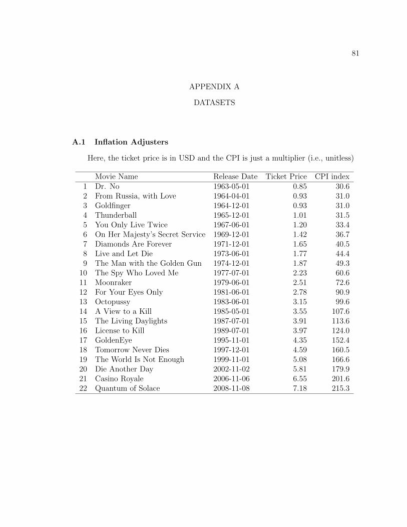
81

APPENDIX A

DATASETS

A.1 Inflation Adjusters

Here, the ticket price is in USD and the CPI is just a multiplier (i.e., unitless)

Movie Name Release Date Ticket Price CPI index1 Dr. No 1963-05-01 0.85 30.62 From Russia, with Love 1964-04-01 0.93 31.03 Goldfinger 1964-12-01 0.93 31.04 Thunderball 1965-12-01 1.01 31.55 You Only Live Twice 1967-06-01 1.20 33.46 On Her Majesty’s Secret Service 1969-12-01 1.42 36.77 Diamonds Are Forever 1971-12-01 1.65 40.58 Live and Let Die 1973-06-01 1.77 44.49 The Man with the Golden Gun 1974-12-01 1.87 49.3

10 The Spy Who Loved Me 1977-07-01 2.23 60.611 Moonraker 1979-06-01 2.51 72.612 For Your Eyes Only 1981-06-01 2.78 90.913 Octopussy 1983-06-01 3.15 99.614 A View to a Kill 1985-05-01 3.55 107.615 The Living Daylights 1987-07-01 3.91 113.616 License to Kill 1989-07-01 3.97 124.017 GoldenEye 1995-11-01 4.35 152.418 Tomorrow Never Dies 1997-12-01 4.59 160.519 The World Is Not Enough 1999-11-01 5.08 166.620 Die Another Day 2002-11-02 5.81 179.921 Casino Royale 2006-11-06 6.55 201.622 Quantum of Solace 2008-11-08 7.18 215.3

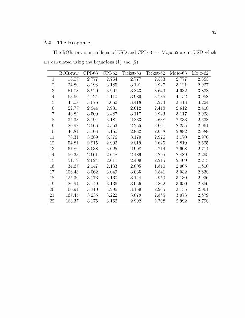
82

A.2 The Response

The BOR–raw is in millions of USD and CPI-63 · · · Mojo-62 are in USD which

are calculated using the Equations (1) and (2)

BOR-raw CPI-63 CPI-62 Ticket-63 Ticket-62 Mojo-63 Mojo-621 16.07 2.777 2.764 2.777 2.583 2.777 2.5832 24.80 3.198 3.185 3.121 2.927 3.121 2.9273 51.08 3.920 3.907 3.843 3.649 4.032 3.8384 63.60 4.124 4.110 3.980 3.786 4.152 3.9585 43.08 3.676 3.662 3.418 3.224 3.418 3.2246 22.77 2.944 2.931 2.612 2.418 2.612 2.4187 43.82 3.500 3.487 3.117 2.923 3.117 2.9238 35.38 3.194 3.181 2.833 2.638 2.833 2.6389 20.97 2.566 2.553 2.255 2.061 2.255 2.061

10 46.84 3.163 3.150 2.882 2.688 2.882 2.68811 70.31 3.389 3.376 3.170 2.976 3.170 2.97612 54.81 2.915 2.902 2.819 2.625 2.819 2.62513 67.89 3.038 3.025 2.908 2.714 2.908 2.71414 50.33 2.661 2.648 2.489 2.295 2.489 2.29515 51.19 2.624 2.611 2.409 2.215 2.409 2.21516 34.67 2.147 2.133 2.005 1.810 2.005 1.81017 106.43 3.062 3.049 3.035 2.841 3.032 2.83818 125.30 3.173 3.160 3.144 2.950 3.130 2.93619 126.94 3.149 3.136 3.056 2.862 3.050 2.85620 160.94 3.310 3.296 3.159 2.965 3.155 2.96121 167.45 3.235 3.222 3.079 2.885 3.073 2.87922 168.37 3.175 3.162 2.992 2.798 2.992 2.798

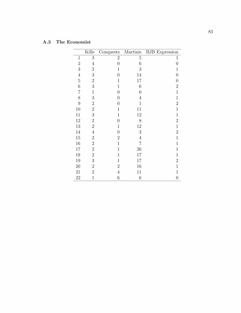
83

A.3 The Economist

Kills Conquests Martinis BJB Expression1 3 2 5 12 4 0 6 03 2 1 3 14 3 0 14 05 2 1 17 06 3 1 6 27 1 0 6 18 3 0 4 19 2 0 1 2

10 2 1 11 111 3 1 12 112 2 0 8 213 2 1 12 114 4 0 3 215 2 2 4 116 2 1 7 117 2 1 26 118 2 1 17 119 3 1 17 220 2 2 16 121 2 4 11 122 1 6 6 0

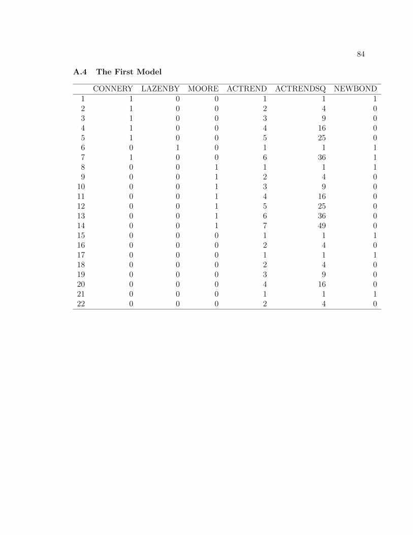
84

A.4 The First Model

CONNERY LAZENBY MOORE ACTREND ACTRENDSQ NEWBOND1 1 0 0 1 1 12 1 0 0 2 4 03 1 0 0 3 9 04 1 0 0 4 16 05 1 0 0 5 25 06 0 1 0 1 1 17 1 0 0 6 36 18 0 0 1 1 1 19 0 0 1 2 4 0

10 0 0 1 3 9 011 0 0 1 4 16 012 0 0 1 5 25 013 0 0 1 6 36 014 0 0 1 7 49 015 0 0 0 1 1 116 0 0 0 2 4 017 0 0 0 1 1 118 0 0 0 2 4 019 0 0 0 3 9 020 0 0 0 4 16 021 0 0 0 1 1 122 0 0 0 2 4 0

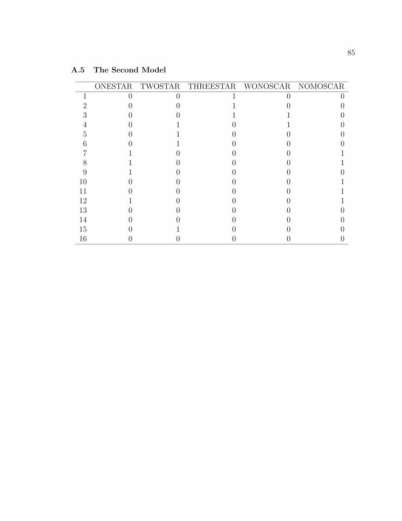
85

A.5 The Second Model

ONESTAR TWOSTAR THREESTAR WONOSCAR NOMOSCAR1 0 0 1 0 02 0 0 1 0 03 0 0 1 1 04 0 1 0 1 05 0 1 0 0 06 0 1 0 0 07 1 0 0 0 18 1 0 0 0 19 1 0 0 0 0

10 0 0 0 0 111 0 0 0 0 112 1 0 0 0 113 0 0 0 0 014 0 0 0 0 015 0 1 0 0 016 0 0 0 0 0

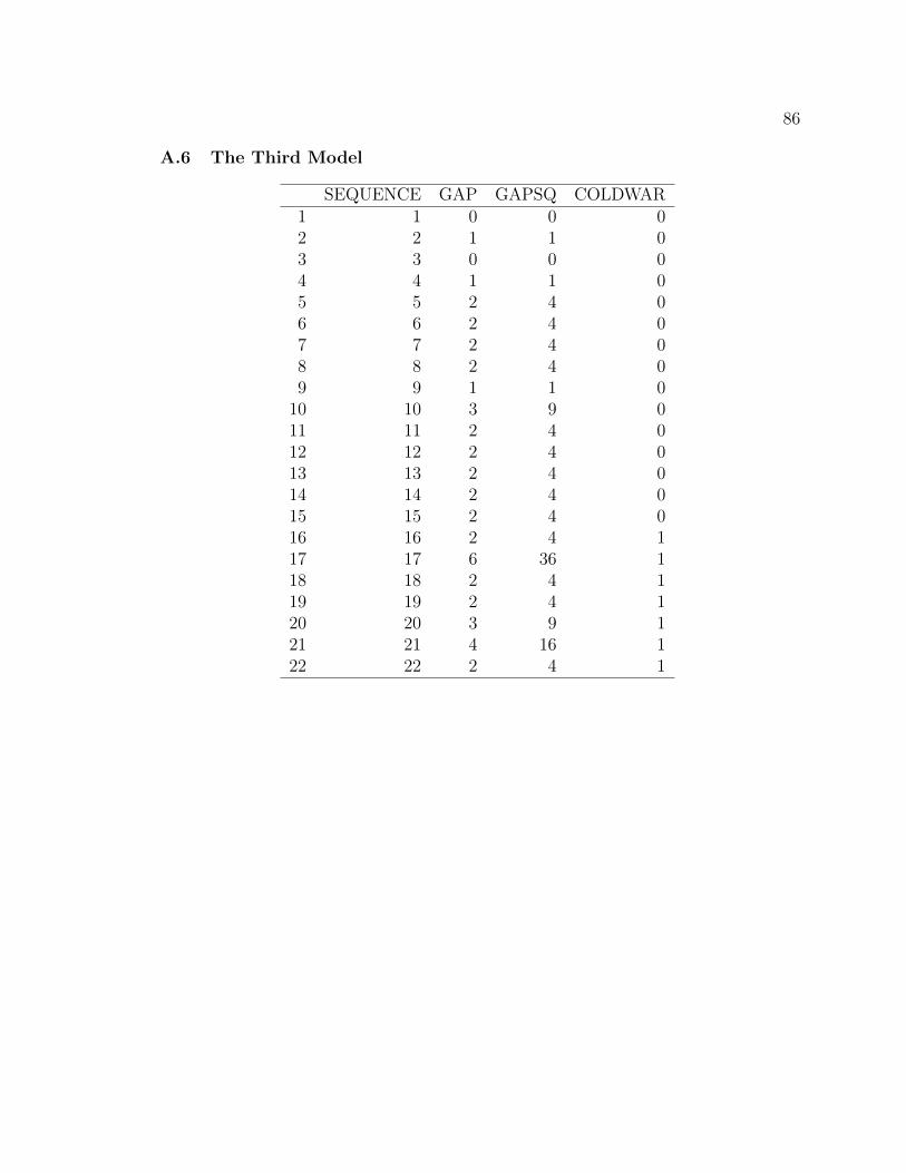
86

A.6 The Third Model

SEQUENCE GAP GAPSQ COLDWAR1 1 0 0 02 2 1 1 03 3 0 0 04 4 1 1 05 5 2 4 06 6 2 4 07 7 2 4 08 8 2 4 09 9 1 1 0

10 10 3 9 011 11 2 4 012 12 2 4 013 13 2 4 014 14 2 4 015 15 2 4 016 16 2 4 117 17 6 36 118 18 2 4 119 19 2 4 120 20 3 9 121 21 4 16 122 22 2 4 1

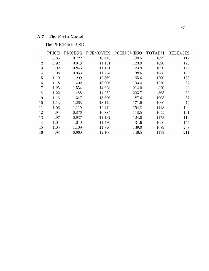
87

A.7 The Forth Model

The PRICE is in USD.

PRICE PRICESQ PCEMOVIES PCEMOVIESQ TOTADM RELEASES1 0.85 0.722 10.415 108.5 1092 1122 0.92 0.843 11.131 123.9 1020 1253 0.92 0.843 11.131 123.9 1020 1254 0.98 0.963 11.774 138.6 1288 1305 1.10 1.209 12.869 165.6 1200 1336 1.18 1.402 13.906 193.4 1270 877 1.25 1.554 14.628 214.0 820 988 1.22 1.488 14.272 203.7 865 699 1.16 1.347 13.696 187.6 1005 67

10 1.13 1.268 13.112 171.9 1060 7411 1.06 1.119 12.442 154.8 1118 10012 0.94 0.876 10.885 118.5 1055 10113 0.97 0.937 11.137 124.0 1173 11914 1.01 1.019 11.470 131.6 1056 14415 1.05 1.109 11.790 139.0 1089 20816 0.98 0.960 12.106 146.5 1133 211

88

APPENDIX B

R CODE

B.1 R Code for Chapter 2

library(car)

setwd("C:/Users/Vahan/Desktop/Masters/MS Project/Report")

BondData <- read.csv("MS_project_Data2.csv")

movieDate <- as.Date(BondData[, 13])

#model 1

CONNERY <- ifelse(as.character(BondData$Actors.Name) == "Connery", 1, 0)

LAZENBY <- ifelse(as.character(BondData$Actors.Name) == "Lazenby", 1, 0)

MOORE <- ifelse(as.character(BondData$Actors.Name) == "Moore", 1, 0)

DALTON <- ifelse(as.character(BondData$Actors.Name) == "Dalton", 1, 0)

BROSNAN <- ifelse(as.character(BondData$Actors.Name) == "Brosnan", 1, 0)

CRAIG <- ifelse(as.character(BondData$Actors.Name) == "Craig", 1, 0)

ACTREND <- rep(1, 22)

NEWBOND <- rep(1, 22)

k <- 1

for (i in 2:22) {

k <- ifelse(BondData$Actors.Name[i] == BondData$Actors.Name[i-1], k + 1, 1)

ACTREND[i] <- k

if (BondData$Actors.Name[i] == BondData$Actors.Name[i-1]) {

NEWBOND[i] <- 0

}

}

ACTREND[7] <- 6

ACTRENDSQ <- ACTREND ^ 2

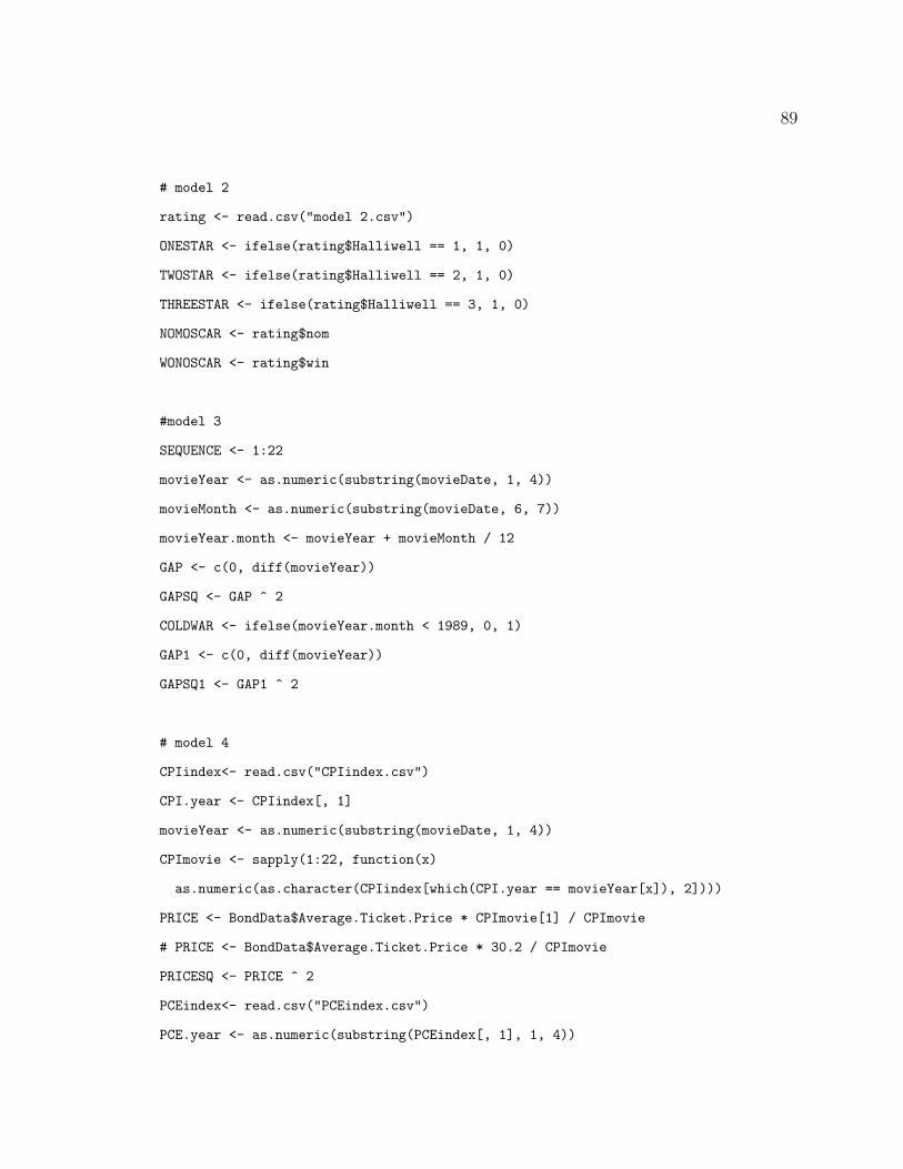
89

# model 2

rating <- read.csv("model 2.csv")

ONESTAR <- ifelse(rating$Halliwell == 1, 1, 0)

TWOSTAR <- ifelse(rating$Halliwell == 2, 1, 0)

THREESTAR <- ifelse(rating$Halliwell == 3, 1, 0)

NOMOSCAR <- rating$nom

WONOSCAR <- rating$win

#model 3

SEQUENCE <- 1:22

movieYear <- as.numeric(substring(movieDate, 1, 4))

movieMonth <- as.numeric(substring(movieDate, 6, 7))

movieYear.month <- movieYear + movieMonth / 12

GAP <- c(0, diff(movieYear))

GAPSQ <- GAP ^ 2

COLDWAR <- ifelse(movieYear.month < 1989, 0, 1)

GAP1 <- c(0, diff(movieYear))

GAPSQ1 <- GAP1 ^ 2

# model 4

CPIindex<- read.csv("CPIindex.csv")

CPI.year <- CPIindex[, 1]

movieYear <- as.numeric(substring(movieDate, 1, 4))

CPImovie <- sapply(1:22, function(x)

as.numeric(as.character(CPIindex[which(CPI.year == movieYear[x]), 2])))

PRICE <- BondData$Average.Ticket.Price * CPImovie[1] / CPImovie

# PRICE <- BondData$Average.Ticket.Price * 30.2 / CPImovie

PRICESQ <- PRICE ^ 2

PCEindex<- read.csv("PCEindex.csv")

PCE.year <- as.numeric(substring(PCEindex[, 1], 1, 4))

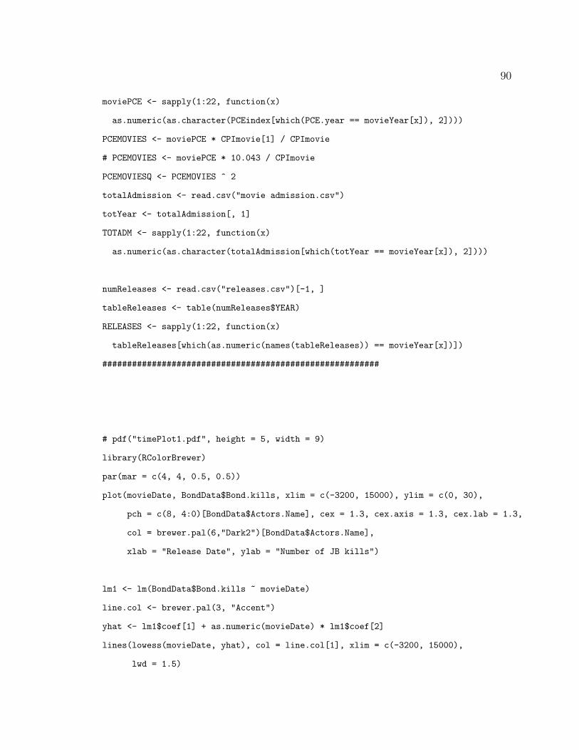
90

moviePCE <- sapply(1:22, function(x)

as.numeric(as.character(PCEindex[which(PCE.year == movieYear[x]), 2])))

PCEMOVIES <- moviePCE * CPImovie[1] / CPImovie

# PCEMOVIES <- moviePCE * 10.043 / CPImovie

PCEMOVIESQ <- PCEMOVIES ^ 2

totalAdmission <- read.csv("movie admission.csv")

totYear <- totalAdmission[, 1]

TOTADM <- sapply(1:22, function(x)

as.numeric(as.character(totalAdmission[which(totYear == movieYear[x]), 2])))

numReleases <- read.csv("releases.csv")[-1, ]

tableReleases <- table(numReleases$YEAR)

RELEASES <- sapply(1:22, function(x)

tableReleases[which(as.numeric(names(tableReleases)) == movieYear[x])])

########################################################

# pdf("timePlot1.pdf", height = 5, width = 9)

library(RColorBrewer)

par(mar = c(4, 4, 0.5, 0.5))

plot(movieDate, BondData$Bond.kills, xlim = c(-3200, 15000), ylim = c(0, 30),

pch = c(8, 4:0)[BondData$Actors.Name], cex = 1.3, cex.axis = 1.3, cex.lab = 1.3,

col = brewer.pal(6,"Dark2")[BondData$Actors.Name],

xlab = "Release Date", ylab = "Number of JB kills")

lm1 <- lm(BondData$Bond.kills ~ movieDate)

line.col <- brewer.pal(3, "Accent")

yhat <- lm1$coef[1] + as.numeric(movieDate) * lm1$coef[2]

lines(lowess(movieDate, yhat), col = line.col[1], xlim = c(-3200, 15000),

lwd = 1.5)

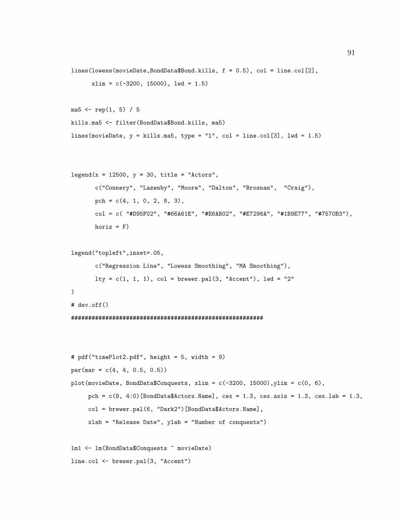
91

lines(lowess(movieDate,BondData$Bond.kills, f = 0.5), col = line.col[2],

xlim = c(-3200, 15000), lwd = 1.5)

ma5 <- rep(1, 5) / 5

kills.ma5 <- filter(BondData$Bond.kills, ma5)

lines(movieDate, y = kills.ma5, type = "l", col = line.col[3], lwd = 1.5)

legend(x = 12500, y = 30, title = "Actors",

c("Connery", "Lazenby", "Moore", "Dalton", "Brosnan", "Craig"),

pch = c(4, 1, 0, 2, 8, 3),

col = c( "#D95F02", "#66A61E", "#E6AB02", "#E7298A", "#1B9E77", "#7570B3"),

horiz = F)

legend("topleft",inset=.05,

c("Regression Line", "Lowess Smoothing", "MA Smoothing"),

lty = c(1, 1, 1), col = brewer.pal(3, "Accent"), lwd = "2"

)

# dev.off()

########################################################

# pdf("timePlot2.pdf", height = 5, width = 9)

par(mar = c(4, 4, 0.5, 0.5))

plot(movieDate, BondData$Conquests, xlim = c(-3200, 15000),ylim = c(0, 6),

pch = c(8, 4:0)[BondData$Actors.Name], cex = 1.3, cex.axis = 1.3, cex.lab = 1.3,

col = brewer.pal(6, "Dark2")[BondData$Actors.Name],

xlab = "Release Date", ylab = "Number of conquests")

lm1 <- lm(BondData$Conquests ~ movieDate)

line.col <- brewer.pal(3, "Accent")

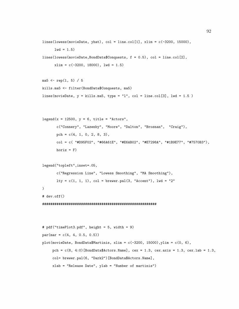
92

lines(lowess(movieDate, yhat), col = line.col[1], xlim = c(-3200, 15000),

lwd = 1.5)

lines(lowess(movieDate,BondData$Conquests, f = 0.5), col = line.col[2],

xlim = c(-3200, 18000), lwd = 1.5)

ma5 <- rep(1, 5) / 5

kills.ma5 <- filter(BondData$Conquests, ma5)

lines(movieDate, y = kills.ma5, type = "l", col = line.col[3], lwd = 1.5 )

legend(x = 12500, y = 6, title = "Actors",

c("Connery", "Lazenby", "Moore", "Dalton", "Brosnan", "Craig"),

pch = c(4, 1, 0, 2, 8, 3),

col = c( "#D95F02", "#66A61E", "#E6AB02", "#E7298A", "#1B9E77", "#7570B3"),

horiz = F)

legend("topleft",inset=.05,

c("Regression Line", "Lowess Smoothing", "MA Smoothing"),

lty = c(1, 1, 1), col = brewer.pal(3, "Accent"), lwd = "2"

)

# dev.off()

########################################################

# pdf("timePlot3.pdf", height = 5, width = 9)

par(mar = c(4, 4, 0.5, 0.5))

plot(movieDate, BondData$Martinis, xlim = c(-3200, 15000),ylim = c(0, 6),

pch = c(8, 4:0)[BondData$Actors.Name], cex = 1.3, cex.axis = 1.3, cex.lab = 1.3,

col= brewer.pal(6, "Dark2")[BondData$Actors.Name],

xlab = "Release Date", ylab = "Number of martinis")

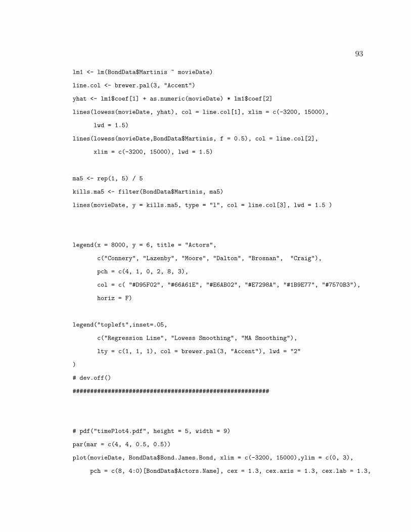
93

lm1 <- lm(BondData$Martinis ~ movieDate)

line.col <- brewer.pal(3, "Accent")

yhat <- lm1$coef[1] + as.numeric(movieDate) * lm1$coef[2]

lines(lowess(movieDate, yhat), col = line.col[1], xlim = c(-3200, 15000),

lwd = 1.5)

lines(lowess(movieDate,BondData$Martinis, f = 0.5), col = line.col[2],

xlim = c(-3200, 15000), lwd = 1.5)

ma5 <- rep(1, 5) / 5

kills.ma5 <- filter(BondData$Martinis, ma5)

lines(movieDate, y = kills.ma5, type = "l", col = line.col[3], lwd = 1.5 )

legend(x = 8000, y = 6, title = "Actors",

c("Connery", "Lazenby", "Moore", "Dalton", "Brosnan", "Craig"),

pch = c(4, 1, 0, 2, 8, 3),

col = c( "#D95F02", "#66A61E", "#E6AB02", "#E7298A", "#1B9E77", "#7570B3"),

horiz = F)

legend("topleft",inset=.05,

c("Regression Line", "Lowess Smoothing", "MA Smoothing"),

lty = c(1, 1, 1), col = brewer.pal(3, "Accent"), lwd = "2"

)

# dev.off()

########################################################

# pdf("timePlot4.pdf", height = 5, width = 9)

par(mar = c(4, 4, 0.5, 0.5))

plot(movieDate, BondData$Bond.James.Bond, xlim = c(-3200, 15000),ylim = c(0, 3),

pch = c(8, 4:0)[BondData$Actors.Name], cex = 1.3, cex.axis = 1.3, cex.lab = 1.3,

94

col = brewer.pal(6, "Dark2")[BondData$Actors.Name],

xlab = "Release Date", ylab = "Number of BJB", yaxt = "n")

axis(2, at=0:3, labels = 0:3, cex.axis = 1.3)

lm1 <- lm(BondData$Bond.James.Bond ~ movieDate)

line.col <- brewer.pal(3, "Accent")

yhat <- lm1$coef[1] + as.numeric(movieDate) * lm1$coef[2]

lines(lowess(movieDate, yhat), col = line.col[1], xlim = c(-3200, 15000),

lwd = 1.5)

lines(lowess(movieDate,BondData$Bond.James.Bond, f = 0.5), col = line.col[2],

xlim = c(-3200, 15000), lwd = 1.5)

ma5 <- rep(1, 5) / 5

kills.ma5 <- filter(BondData$Bond.James.Bond, ma5)

lines(movieDate, y = kills.ma5, type = "l", col = line.col[3], lwd = 1.5 )

legend(x = 12500, y = 3, title = "Actors",

c("Connery", "Lazenby", "Moore", "Dalton", "Brosnan", "Craig"),

pch = c(4, 1, 0, 2, 8, 3),

col = c( "#D95F02", "#66A61E", "#E6AB02", "#E7298A", "#1B9E77", "#7570B3"),

horiz = F)

legend("topleft",inset=.05,

c("Regression Line", "Lowess Smoothing", "MA Smoothing"),

lty = c(1, 1, 1), col = brewer.pal(3, "Accent"), lwd = "2"

)

# dev.off()

## put histograms on the diagonal

panel.hist <- function(x, ...)

95

{

usr <- par("usr"); on.exit(par(usr))

par(usr = c(usr[1:2], 0, 1.5))

if (max(x) < 3) {

h <- hist(x + 0.5, plot = FALSE, breaks = -1:3)

}

if (max(x) < 5 & max(x) > 3) {

h <- hist(x + 0.5, plot = FALSE, breaks = 0:5)

}

if (max(x) < 10 & max(x) > 5) {

h <- hist(x + 0.5, plot = FALSE, breaks = 0:7)

}

if (max(x) < 30 & max(x) > 10) {

h <- hist(x + 0.5, plot = FALSE, breaks = seq(0, 30, 6))

}

if (max(x) > 30) {

h <- hist(x + 0.5, plot = FALSE)

}

if (max(x) > 30) {

breaks <- (h$breaks + 25 * 10 ^ 6); nB <- length(breaks)

} else {

breaks <- (h$breaks - 0.5); nB <- length(breaks)

}

y <- h$counts; y <- y / max(y)

rect(breaks[-nB], 0, breaks[-1], y, ...)

rug(x)

}

96

BondData.jitter <- cbind(BondData[,c(7, 11, 9, 10, 12)])

BondData.jitter[, 1] <- BondData.jitter[, 1] * 8.35 / 7.94

BondData.jitter[, 2] <- jitter(BondData.jitter[, 2], amount = 0.1)

BondData.jitter[, 3] <- jitter(BondData.jitter[, 3], amount = 0.1)

BondData.jitter[, 4] <- jitter(BondData.jitter[, 4], amount = 0.1)

BondData.jitter[, 5] <- jitter(BondData.jitter[, 5], amount = 0.1)

names(BondData.jitter) <- c("BOR", "Kills", "Conquests", "Martinis", "BJB")

# pdf("scatterPlot1.pdf", height = 12, width = 12)

pairs(BondData.jitter, cex=2, cex.axis = 2, panel = panel.smooth,

col = brewer.pal(6,"Dark2")[BondData$Actors.Name],

pch = c(8, 4, 3, 2, 1, 0)[BondData$Actors.Name],

diag.panel = panel.hist, cex.labels = 2, font.labels = 2,

col.smooth = brewer.pal(3, "Accent")[2])

# dev.off()

########################################################

library(Hmisc)

counts.actor <- table(BondData$Actors.Name)

counts.actor <- sort(counts.actor, decreasing = F)

avg.kills <- tapply(BondData$Bond.kills, BondData$Actors.Name, mean)

avg.kills <- sort(avg.kills, decreasing = F)

avg.mart <- tapply(BondData$Martinis, BondData$Actors.Name, mean)

avg.mart <- sort(avg.mart, decreasing = F)

avg.conq <- tapply(BondData$Conquests, BondData$Actors.Name, mean)

avg.conq <- sort(avg.conq, decreasing = F)

avg.bjb <- tapply(BondData$Bond.James.Bond, BondData$Actors.Name, mean)

avg.bjb <- sort(avg.bjb, decreasing = F)

avg.bor <- tapply(BondData$Vahan.adjusted * 8.35 / 7.94,

BondData$Actors.Name, mean)

97

avg.bor <- sort(avg.bor, decreasing = F)

# pdf("dotPlot1.pdf", height = 9, width = 6)

par(mfrow = c(3, 2), mar = c(3, 5, 1.5, 0.5))

dotchart3(counts.actor, main = "(a) Number of movies", lty = 2,

cex.lab = 0.8, cex = 1, cex.main = 0.8)

dotchart3(avg.bor / 10 ^ 6, main = "(b) Average BOR in millions", lty = 2,

cex.lab = 0.8, cex = 1, cex.main = 0.8)

dotchart3(avg.kills, main = "(c) Average number of JB kills", lty = 2,

cex.lab = 0.8, cex = 1, xlim = c(4, 20), cex.main = 0.8)

dotchart3(avg.conq, main="(d) Average number of conquests", lty = 2,

cex.lab = 0.8, cex = 1, cex.main = 0.8)

dotchart3(avg.mart, main = "(e) Average number of martinis", lty = 2,

cex.lab = 0.8, cex = 1, cex.main = 0.8)

dotchart3(avg.bjb, main="(f) Average number of BJB", lty = 2,

cex.lab = 0.8, cex = 1, cex.main = 0.8)

# dev.off()

########################################################

bymedian.actor <- with(BondData, reorder(BondData$Actors.Name,

-BondData$Mojo.Adjusted, median))

killShort <- ifelse(BondData$Bond.kills <= 5, "0-5",

ifelse(BondData$Bond.kills > 5 & BondData$Bond.kills <= 10,

"6-10", ">10"))

martiniShort <- ifelse(BondData$Martinis >= 2, ">1",

BondData$Martinis)

conqShort <- ifelse(BondData$Conquests >= 3, ">2",

BondData$Conquests)

bondDataShort <- cbind(BondData$Vahan.adjusted, BondData$Bond.James.Bond,

killShort, martiniShort, conqShort)

bymedian.kills <- with(as.data.frame(bondDataShort),

98

reorder(bondDataShort[, 3],

-as.numeric(bondDataShort[, 1]), median))

bymedian.conquests <- with(as.data.frame(bondDataShort),

reorder(bondDataShort[, 5],

-as.numeric(bondDataShort[, 1]), median))

bymedian.martini <- with(as.data.frame(bondDataShort),

reorder(bondDataShort[, 4],

-as.numeric(bondDataShort[, 1]), median))

bymedian.bjb <- with(as.data.frame(bondDataShort),

reorder(bondDataShort[, 2],

as.numeric(bondDataShort[, 1]), median))

# pdf("boxPlot1.pdf", height = 6, width = 8)

par(mfrow = c(2, 2), mar = c(2, 4, 2, 1))

borMojo2014 <- BondData$Mojo.Adjusted / 10 ^ 6 * 8.35 / 7.94

boxplot(borMojo2014 ~ bymedian.kills,

ylab = "BORs (in Millions)", ylim = c(50, 650),

main = "(a) Number of JB kills", cex.lab = 1.2, cex.main = 1.2)

boxplot(borMojo2014 ~ bymedian.conquests,

ylab = "BORs (in Millions)", ylim = c(50, 650),

main = "(b) Number of conquests", cex.lab = 1.2, cex.main = 1.2)

boxplot(borMojo2014 ~ bymedian.martini,

ylab = "BORs (in Millions)", ylim = c(50, 650),

main = "(c) Number of martinis", cex.lab = 1.2, cex.main = 1.2)

boxplot(borMojo2014 ~ bymedian.bjb,

ylab = "BORs (in Millions)", ylim = c(50, 650),

main = "(d) Number of BJB", cex.lab = 1.2, cex.main = 1.2)

# dev.off()

########################################################

99

# pdf("boxPlot2.pdf", height = 4, width = 8)

par(mfrow = c(1, 1), mar = c(2, 4, 0.5, 0.5))

boxplot(borMojo2014 ~ bymedian.actor,

ylab = "BORs (in Millions)", ylim = c(50, 650),

cex.lab = 1.2, cex.axis = 1.2)

# dev.off()

library(car)

# pdf("histQQ1.pdf", height = 6, width = 6)

par(mfrow = c(2, 2), mar = c(4, 4, 1.5, 0.2))

hist(borMojo2014, ylim = c(0, 12), main = "(a) BOR (in Milions)",

breaks= as.integer(sqrt(nrow(BondData))), xlab = "")

rug(borMojo2014)

qqPlot((borMojo2014 * 0.7 / 8.35), main = "(b) Normal Quantiles",

ylab = "BOR(in Milions)", xlab = "")

hist(log(borMojo2014 * 0.7 / 8.35), ylim = c(0, 14), main = "(c) Log(BOR/10^6)",

breaks= as.integer(sqrt(nrow(BondData))),xlab = "")

rug(log(borMojo2014 * 0.7 / 8.35))

qqPlot(log(borMojo2014 * 0.7 / 8.35), main = "(d) Normal Quantiles",

ylab = "Log BOR", xlab = "")

# dev.off()

########################################################

library(PairViz)

library(RColorBrewer)

par(mfrow = c(1, 1))

par.coord <- BondData[, 9:12]

100

par.coord <- par.coord[, c(1, 2, 4, 3)]

colnames(par.coord) <- c("Conquests", "Martinis", "BJB", "Kills")

par.coord$Kills <- ifelse(par.coord$Kills <= 5, 1,

ifelse(par.coord$Kills > 5 & par.coord$Kills <= 10, 2, 3))

par.coord$Martinis <- ifelse(par.coord$Martinis >= 2, 2,

par.coord$Martinis)

par.coord$Conquests <- ifelse(par.coord$Conquests >= 3, 3,

par.coord$Conquests)

par.coord <- par.coord[order(par.coord[, 3]),]

par.coord <- par.coord[order(par.coord[, 2]),]

par.coord <- par.coord[order(par.coord[, 1]),]

par.coord <- par.coord[order(par.coord[, 4]),]

cols <- brewer.pal(3,"Set1")

cols <- paste(cols, 80,sep="")

cols <- cols[as.numeric(as.factor(par.coord[, 4]))]

ds <- factor_spreadout(par.coord)

rownames(ds$bars$Conquests) <- c("1", "2", ">2")

rownames(ds$bars$Martinis) <- c("0", "1", ">1")

rownames(ds$bars$Kills) <- c("0-5", "6-10", ">10")

# pdf("parCoordPlot1", height = 4, width = 7)

catpcp(ds$data,col = cols, lwd = 15,pcpbars = ds$bars, mar = c(2, 0.5, 0.5, 0.5),

pcpbars.labels = TRUE, main = "", order = c(4, 1, 2, 3))

# dev.off()

########################################################

library(heatmap.plus)

bond.mat <- t(as.matrix(cbind(BondData[, 9:12])))

101

movieNchar <- nchar(as.character(BondData[, 14]))

movieYearHeat <- substr(BondData[, 14], movieNchar - 5, movieNchar)

movieNameHeat <- substr(BondData[, 14], 1, movieNchar - 7)

# movieBOR2014 <- round(BondData[, 5] / BondData[, 6] * 8.35 /10^6, 1)

colnames(bond.mat) <- paste(BondData$Actors.Name, movieYearHeat,

movieNameHeat)

rownames(bond.mat) <- c("Conquests", "Martinis", "Kills", "BJB")

# heatmap.plus(bond.mat, margins = c(17, 8))

library(gplots)

# pdf("heatMap1.pdf", height = 10, width = 10)

breaks = c(-0.5:6.5, seq(11.5, 26.5, by = 5))

col = brewer.pal(11, "PuOr")

heatmap.2(as.matrix(t(bond.mat)), dendrogram = "both",

trace="none", margin = c(9, 32),

lwid = c(0.5, 2),keysize = 1,

cexRow = 1.7,

breaks = breaks, col = col)

# dev.off()

########################################################

bond.mat <- t(as.matrix(cbind(BondData[, c(9, 10, 12)],

sqrt(BondData[, 11]))))

colnames(bond.mat) <- paste(BondData$Actors.Name, movieYearHeat,

movieNameHeat)

rownames(bond.mat) <- c("Conquests", "Martinis", "BJB", "Kills")

breaks = -0.5:6.5

col = brewer.pal(7, "PuOr")

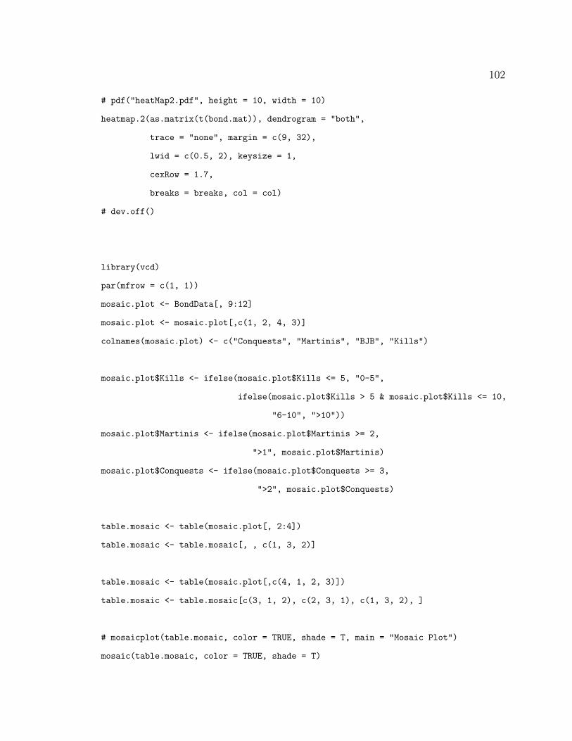
102

# pdf("heatMap2.pdf", height = 10, width = 10)

heatmap.2(as.matrix(t(bond.mat)), dendrogram = "both",

trace = "none", margin = c(9, 32),

lwid = c(0.5, 2), keysize = 1,

cexRow = 1.7,

breaks = breaks, col = col)

# dev.off()

library(vcd)

par(mfrow = c(1, 1))

mosaic.plot <- BondData[, 9:12]

mosaic.plot <- mosaic.plot[,c(1, 2, 4, 3)]

colnames(mosaic.plot) <- c("Conquests", "Martinis", "BJB", "Kills")

mosaic.plot$Kills <- ifelse(mosaic.plot$Kills <= 5, "0-5",

ifelse(mosaic.plot$Kills > 5 & mosaic.plot$Kills <= 10,

"6-10", ">10"))

mosaic.plot$Martinis <- ifelse(mosaic.plot$Martinis >= 2,

">1", mosaic.plot$Martinis)

mosaic.plot$Conquests <- ifelse(mosaic.plot$Conquests >= 3,

">2", mosaic.plot$Conquests)

table.mosaic <- table(mosaic.plot[, 2:4])

table.mosaic <- table.mosaic[, , c(1, 3, 2)]

table.mosaic <- table(mosaic.plot[,c(4, 1, 2, 3)])

table.mosaic <- table.mosaic[c(3, 1, 2), c(2, 3, 1), c(1, 3, 2), ]

# mosaicplot(table.mosaic, color = TRUE, shade = T, main = "Mosaic Plot")

mosaic(table.mosaic, color = TRUE, shade = T)

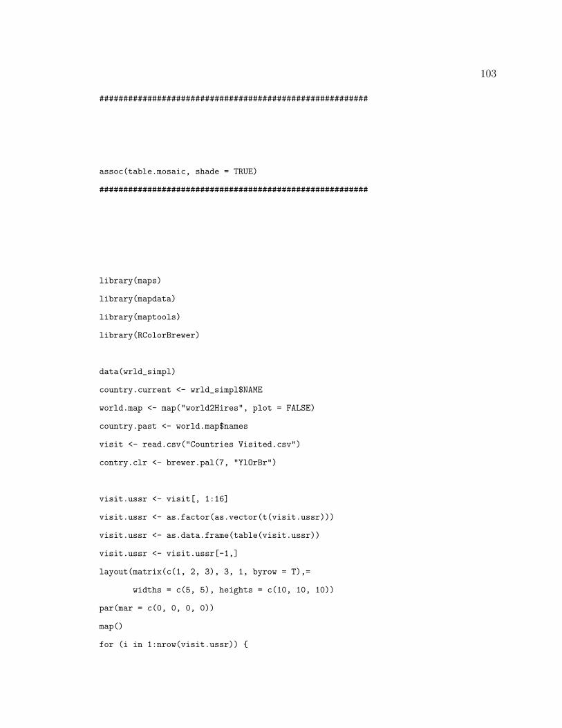
103

########################################################

assoc(table.mosaic, shade = TRUE)

########################################################

library(maps)

library(mapdata)

library(maptools)

library(RColorBrewer)

data(wrld_simpl)

country.current <- wrld_simpl$NAME

world.map <- map("world2Hires", plot = FALSE)

country.past <- world.map$names

visit <- read.csv("Countries Visited.csv")

contry.clr <- brewer.pal(7, "YlOrBr")

visit.ussr <- visit[, 1:16]

visit.ussr <- as.factor(as.vector(t(visit.ussr)))

visit.ussr <- as.data.frame(table(visit.ussr))

visit.ussr <- visit.ussr[-1,]

layout(matrix(c(1, 2, 3), 3, 1, byrow = T),=

widths = c(5, 5), heights = c(10, 10, 10))

par(mar = c(0, 0, 0, 0))

map()

for (i in 1:nrow(visit.ussr)) {

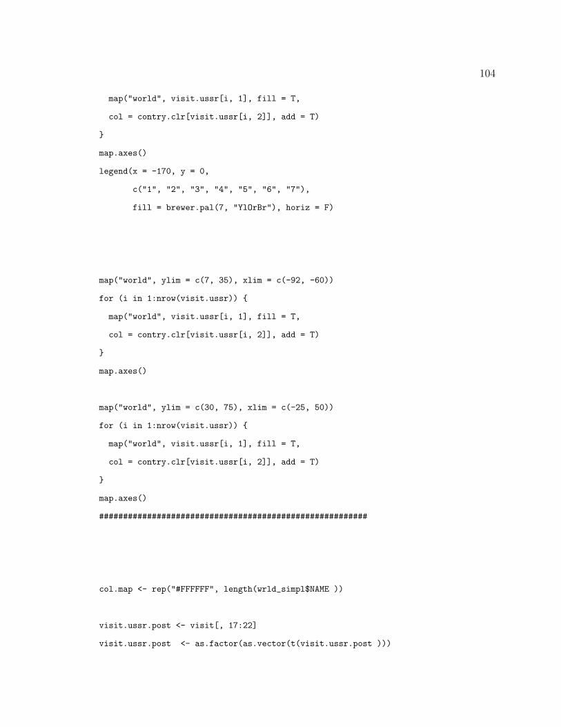
104

map("world", visit.ussr[i, 1], fill = T,

col = contry.clr[visit.ussr[i, 2]], add = T)

}

map.axes()

legend(x = -170, y = 0,

c("1", "2", "3", "4", "5", "6", "7"),

fill = brewer.pal(7, "YlOrBr"), horiz = F)

map("world", ylim = c(7, 35), xlim = c(-92, -60))

for (i in 1:nrow(visit.ussr)) {

map("world", visit.ussr[i, 1], fill = T,

col = contry.clr[visit.ussr[i, 2]], add = T)

}

map.axes()

map("world", ylim = c(30, 75), xlim = c(-25, 50))

for (i in 1:nrow(visit.ussr)) {

map("world", visit.ussr[i, 1], fill = T,

col = contry.clr[visit.ussr[i, 2]], add = T)

}

map.axes()

########################################################

col.map <- rep("#FFFFFF", length(wrld_simpl$NAME ))

visit.ussr.post <- visit[, 17:22]

visit.ussr.post <- as.factor(as.vector(t(visit.ussr.post )))

105

visit.ussr.post <- as.data.frame(table(visit.ussr.post ))

visit.ussr.post <- visit.ussr.post[-1,]

contry.clr <- brewer.pal(7, "YlOrBr")

par(mar = c(0, 0, 0, 0))

for (i in 1:nrow(visit.ussr.post)) {

position <- which(wrld_simpl$NAME == as.character(visit.ussr.post[i, 1]))

col.map[position] = contry.clr[visit.ussr.post[i, 2]]

}

layout(matrix(c(1, 1, 2, 3), 2, 2, byrow = T),

widths = c(5, 5), heights = c(10, 10))

par(mar = c(2, 2, 0.3, 0.3))

plot(wrld_simpl, col = col.map, axes = F)

map.axes()

legend(x = -200, y = 40,

c("1", "2", "3", "4", "5", "6", "7"),

fill = brewer.pal(7, "YlOrBr"), horiz = F)

plot(wrld_simpl, col = col.map, axes = F,

ylim = c(15, 32), xlim = c(-92,-60))

map.axes()

plot(wrld_simpl, col = col.map,

ylim = c(30, 65), xlim = c(-20, 50))

map.axes()

########################################################

visit <- read.csv("Countries Visited.csv")

visit.ussr <- visit[, 1:16]

106

visit.ussr <- as.factor(as.vector(t(visit.ussr)))

bo.adj <- rep(0, 16 * 8)

bo.adj[(0:7) * 16 + 1:16] <- BondData$Vahan.adjusted[1:16]

rev.country <- cbind(as.character(visit.ussr), bo.adj)

mean.country <- tapply(as.numeric(rev.country[, 2]), rev.country[, 1], mean)

mean.country <- mean.country[-1] / 10 ^ 6

breaks <- c(80, 100, 120, 160, 200, 240, 330)

m.class <- cut(mean.country, breaks)

m.col <- ifelse(mean.country <= breaks[2], brewer.pal(5, "YlGn")[1],

ifelse(mean.country > breaks[2] & mean.country <= breaks[3],

brewer.pal(6, "YlGn")[2],

ifelse(mean.country > breaks[3] & mean.country <= breaks[4],

brewer.pal(6, "YlGn")[3],

ifelse(mean.country > breaks[4] & mean.country <= breaks[5],

brewer.pal(6, "YlGn")[4],

ifelse(mean.country > breaks[5] & mean.country <= breaks[6],

brewer.pal(6, "YlGn")[5],

ifelse(mean.country > breaks[6] & mean.country <= breaks[7],

brewer.pal(6, "YlGn")[6],

""))))))

par(mfrow = c(2, 1), mar = c(0, 0, 0, 0))

map()

for (i in 1:length(mean.country)) {

map("world", names(mean.country)[i], fill = T,

col = m.col[i], add = T)

}

legend(x = -170, y = -10, legend = levels(m.class), fill = brewer.pal(6, "YlGn"))

107

visit <- read.csv("Countries Visited.csv")

visit.ussr.post <- visit[, 17:22]

visit.ussr.post <- as.factor(as.vector(t(visit.ussr.post)))

bo.adj <- rep(0, 6 * 8)

bo.adj[(0:7) * 6 + 1:6] <- BondData$Vahan.adjusted[1:16 + 16]

rev.country <- cbind(as.character(visit.ussr.post), bo.adj)

mean.country <- tapply(as.numeric(rev.country[, 2]), rev.country[, 1], mean)

mean.country <- mean.country[-1] / 10 ^ 6

m.col <- ifelse(mean.country <= breaks[2], brewer.pal(5, "YlGn")[1],

ifelse(mean.country > breaks[2] & mean.country <= breaks[3],

brewer.pal(6, "YlGn")[2],

ifelse(mean.country > breaks[3] & mean.country <= breaks[4],

brewer.pal(6, "YlGn")[3],

ifelse(mean.country > breaks[4] & mean.country <= breaks[5],

brewer.pal(6, "YlGn")[4],

ifelse(mean.country > breaks[5] & mean.country <= breaks[6],

brewer.pal(6, "YlGn")[5],

ifelse(mean.country > breaks[6] & mean.country <= breaks[7],

brewer.pal(6, "YlGn")[6],

""))))))

col.map <- rep("#FFFFFF", length(wrld_simpl$NAME ))

contry.clr <- brewer.pal(5, "YlGn")

for (i in 1:length(mean.country)) {

position <- which(wrld_simpl$NAME == names(mean.country)[i])

col.map[position] = m.col[i]

}

par(mar = c(0, 0, 0, 0))

108

plot(wrld_simpl, col = col.map, axes = F)

legend(x = -170, y = -10, legend = levels(m.class), fill = brewer.pal(6, "YlGn"))

########################################################

109

B.2 R Code for Chapter 3

setwd("C:/Users/Vahan/Desktop/Masters/MS Project/Report")

ReplicateSummary <- function(NEWBOND1 = 1, NEWBOND7 = 1) {

BondData <- read.csv("MS_project_Data2.csv")

movieDate <- as.Date(BondData[, 13])

#model 1

CONNERY <- ifelse(as.character(BondData$Actors.Name) == "Connery",

1, 0)[1:16]

LAZENBY <- ifelse(as.character(BondData$Actors.Name) == "Lazenby",

1, 0)[1:16]

MOORE <- ifelse(as.character(BondData$Actors.Name) == "Moore",

1, 0)[1:16]

DALTON <- ifelse(as.character(BondData$Actors.Name) == "Dalton",

1, 0)[1:16]

BROSNAN <- ifelse(as.character(BondData$Actors.Name) == "Brosnan",

1, 0)[1:16]

CRAIG <- ifelse(as.character(BondData$Actors.Name) == "Craig",

1, 0)[1:16]

ACTREND <- rep(1, 22)[1:16]

NEWBOND <- rep(1, 22)[1:16]

k <- 1

for (i in 2:16) {

k <- ifelse(BondData$Actors.Name[i] == BondData$Actors.Name[i-1],

k + 1, 1)

ACTREND[i] <- k

if (BondData$Actors.Name[i] == BondData$Actors.Name[i-1]) {

NEWBOND[i] <- 0

110

}

}

ACTREND[7] <- 6

ACTRENDSQ <- ACTREND ^ 2

NEWBOND[1] <- NEWBOND1

NEWBOND[7] <- NEWBOND7

movieYear <- as.numeric(substring(movieDate, 1, 4))

avgTicket <- BondData$Average.Ticket.Price

CPIindex <- read.csv("CPIindex.csv")

CPI <- sapply(1:22, function(x)

CPIindex$CPI[movieYear[x] == CPIindex$yearCPI])

mojoAdj <- read.csv("mojoAdj.csv")

CPIadj63 <- BondData$Mojo.Unadjusted * CPI[1] / CPI

CPIadj62 <- BondData$Mojo.Unadjusted * 30.2 / CPI

Ticketadj63 <- BondData$Mojo.Unadjusted * avgTicket[1] / avgTicket

Ticketadj62 <- BondData$Mojo.Unadjusted * 0.7 / avgTicket

respData <- log(cbind(mojoAdj[, 2:3], CPIadj63, CPIadj62,

Ticketadj63, Ticketadj62) / 10 ^ 6)

modelX <- as.data.frame(cbind(CONNERY, LAZENBY, MOORE, ACTREND,

ACTRENDSQ, NEWBOND))[1:16, ]

library(orcutt)

summaryCoef1 <- NULL

111

summaryorcutt1 <- NULL

for (j in 1:6) {

lmout <- (lm(respData[j][1:16, ] ~ CONNERY+ LAZENBY + MOORE +

ACTREND + ACTRENDSQ + NEWBOND))

summaryCoef1[[j]] <- (lm(respData[j][1:16, ] ~ CONNERY +

LAZENBY + MOORE +

ACTREND + ACTRENDSQ + NEWBOND))$coef

summaryorcutt1[[j]] <- (cochrane.orcutt(lmout)$Cochrane.Orcutt)$coef[, 1]

}

ACTREND <- ACTREND - 1

ACTRENDSQ <- ACTREND ^ 2

summaryCoef0 <- NULL

summaryorcutt0 <- NULL

for (j in 1:6) {

lmout <- (lm(respData[j][1:16, ] ~ CONNERY+ LAZENBY + MOORE +

ACTREND + ACTRENDSQ + NEWBOND))

summaryCoef0[[j]] <- (lm(respData[j][1:16, ] ~ CONNERY +

LAZENBY + MOORE +

ACTREND + ACTRENDSQ + NEWBOND))$coef

summaryorcutt0[[j]] <- (cochrane.orcutt(lmout)$Cochrane.Orcutt)$coef[, 1]

}

ActrendStart1 <- t(matrix(unlist(summaryCoef1), nrow = 7))

rownames(ActrendStart1) <- names(respData)

colnames(ActrendStart1) <- names((lm(respData[1][1:16, ] ~ CONNERY +

112

LAZENBY + MOORE +

ACTREND + ACTRENDSQ + NEWBOND))$coef)

ActrendStart1Orcutt <- t(matrix(unlist(summaryorcutt1), nrow = 7))

rownames(ActrendStart1Orcutt) <- names(respData)

colnames(ActrendStart1Orcutt) <- names((lm(respData[1][1:16, ] ~ CONNERY +

LAZENBY + MOORE +

ACTREND + ACTRENDSQ +

NEWBOND))$coef)

ActrendStart0 <- t(matrix(unlist(summaryCoef0), nrow = 7))

rownames(ActrendStart0) <- names(respData)

colnames(ActrendStart0) <- names((lm(respData[1][1:16, ] ~ CONNERY +

LAZENBY + MOORE +

ACTREND + ACTRENDSQ + NEWBOND))$coef)

ActrendStart0Orcutt <- t(matrix(unlist(summaryorcutt0), nrow = 7))

rownames(ActrendStart0Orcutt) <- names(respData)

colnames(ActrendStart0Orcutt) <- names((lm(respData[1][1:16, ] ~ CONNERY +

LAZENBY + MOORE +

ACTREND + ACTRENDSQ +

NEWBOND))$coef)

TotalSummary <- list(ActrendStart0 = ActrendStart0,

ActrendStart0Orcutt = ActrendStart0Orcutt,

113

ActrendStart1 = ActrendStart1,

ActrendStart1Orcutt = ActrendStart1Orcutt

)

baimCoef <- c(1.179, 1.08, 0.9056, 0.333, 0.7835, -0.0908, 0.7807)

modelSSE <- sapply(1:4, function(x)

(t(t(TotalSummary[[x]]) - baimCoef)) ^ 2 %*% rep(1, 7))

rownames(modelSSE) <- names(respData)

colnames(modelSSE) <- c("ActrendStart0", "ActrendStart0Orcutt",

"ActrendStart1", "ActrendStart1Orcutt")

return(list(TotalSummary = TotalSummary, modelSSE = modelSSE))

}

NewBond11 <- ReplicateSummary(1, 1)$TotalSummary

NewBond11SSE <- matrix(ReplicateSummary(1, 1)$modelSSE,

ncol = 1)

NewBond10 <- ReplicateSummary(1, 0)$TotalSummary

NewBond10SSE <- matrix(ReplicateSummary(1, 0)$modelSSE,

ncol = 1)

NewBond01 <- ReplicateSummary(0, 1)$TotalSummary

NewBond01SSE <- matrix(ReplicateSummary(0, 1)$modelSSE,

ncol = 1)

NewBond00 <- ReplicateSummary(0, 0)$TotalSummary

NewBond00SSE <- matrix(ReplicateSummary(0, 0)$modelSSE,

114

ncol = 1)

parCoordData11 <- cbind(rbind(NewBond11[[1]], NewBond11[[2]],

NewBond11[[3]], NewBond11[[4]]), NewBond11SSE)

parCoordData10 <- cbind(rbind(NewBond10[[1]], NewBond10[[2]],

NewBond10[[3]], NewBond10[[4]]), NewBond10SSE)

parCoordData01 <- cbind(rbind(NewBond01[[1]], NewBond01[[2]],

NewBond01[[3]], NewBond01[[4]]), NewBond01SSE)

parCoordData00 <- cbind(rbind(NewBond00[[1]], NewBond00[[2]],

NewBond00[[3]], NewBond00[[4]]), NewBond00SSE)

parCoordData <- rbind(parCoordData11, parCoordData10,

parCoordData01, parCoordData00,

c(1.179, 1.08, 0.9056, 0.333, 0.7835,

-0.0908, 0.7807, 0))

colnames(parCoordData)[8] <- "SSE"

library(RColorBrewer)

clr <- brewer.pal(3, "Pastel1")

plotClr <- rep(c(clr[1], clr[1], clr[2], clr[2], clr[3], clr[3]), 16)

plotClr <- rep(rep(c(clr[1], clr[2]), each = 6), 8)

plotClr[97] <- "#000000"

plotClr[64] <- "red"

panel.myplot <- function(..., common.scale) {

panel.parallel(..., common.scale = TRUE)

panel.abline(h = -min(parCoordData) / diff(range(parCoordData)), lty = 2)

}

pdf("repParCoord1.pdf", height = 5, width = 8)

115

parallelplot( ~ parCoordData[c(1:63, 65:96, 64, 97), ],

col = plotClr[c(1:63, 65:96, 64, 97)],

lwd = c(rep(2, 95), 3, 3),

horizontal.axis = FALSE,

panel = panel.myplot,

scales = list(y = list(lim = c(-0.05, 1.05))),

var.label = T)

dev.off()

##########################################################

CPIindex <- read.csv("CPIindex.csv")

CPI <- sapply(1:22, function(x)

CPIindex$CPI[movieYear[x] == CPIindex$yearCPI])

CPIadj62 <- BondData$Mojo.Unadjusted * 30.2 / CPI

logBoxOffice <- log(CPIadj62 / 10 ^ 6)

model1 <- as.data.frame(cbind(logBoxOffice, CONNERY, LAZENBY,

MOORE, DALTON, BROSNAN, CRAIG,

ACTREND, ACTRENDSQ, NEWBOND))

model1Old <- model1[1:16, -(5:7)]

model1New <- model1[, -5]

lmOld1 <- lm(logBoxOffice ~ ., model1Old)

Model1Coef <- lmOld1$coefficients

Model1T <- summary(lmOld1)$coefficients[, 3]

Model1F <- c(summary(lmOld1)$r.squared, summary(lmOld1)$adj.r.squared,

summary(lmOld1)$fstatistic[1], durbinWatsonTest(lmOld1)$dw)

names(Model1F) <- c("R Squared", "Adj. R Squared",

"F Statistic", "Durbin Watson")

BaimModel1Coef <- c(1.179, 1.08, 0.9056, 0.333, 0.7835, -0.0908, 0.7807)

BaimModel1T <- c(1.76, 3.231, 1.763, 1.097, 2.121, -2.135, 1.79)

116

BaimModel1F <- c(0.77, 0.61, 4.99, 2.22)

summary(lmOld1)

##########################################################

library(lattice)

library(RColorBrewer)

pdf("repDotplot1.pdf", height = 5, width = 12)

plot1 <- dotplot(reorder(names(Model1T), abs(Model1T))

~ Model1Coef + BaimModel1Coef | "Coefficient",

col = brewer.pal(3, "Set1"), pch = 0:1, xlab = "",

scales = list(y = list(cex = 1.2), x = list(cex = 1.2)))

plot2 <- dotplot(reorder(names(Model1T), abs(Model1T))

~ Model1T + BaimModel1T | "t-value",

col = brewer.pal(3, "Set1"), pch = 0:1, xlab = "",

panel = function(...) {

panel.abline(v = qt(0.025, nrow(model1)), lty = 2)

panel.abline(v = qt(0.975, nrow(model1)), lty = 2)

panel.dotplot(...)

},

scales = list(y = list(cex = 1.2), x = list(cex = 1.2)))

plot3 <- dotplot(reorder(names(Model1F), abs(Model1F))

~ Model1F + BaimModel1F | "ANOVA",

col = brewer.pal(3, "Set1"), pch = 0:1, xlab = "",

scales = list(y = list(cex = 1.2), x = list(cex = 1.2)))

print(plot1, position = c(0, 0, 0.36, 1), more = TRUE)

print(plot2, position = c(0.32, 0, 0.68, 1), more = TRUE)

print(plot3, position = c(0.64, 0, 1., 1))

dev.off()

##########################################################

117

# model 2

rating <- read.csv("model 2.csv")

ONESTAR <- ifelse(rating$Halliwell == 1, 1, 0)[1:16]

TWOSTAR <- ifelse(rating$Halliwell == 2, 1, 0)[1:16]

THREESTAR <- ifelse(rating$Halliwell == 3, 1, 0)[1:16]

NOMOSCAR <- rating$nom[1:16]

WONOSCAR <- rating$win[1:16]

movieYear <- as.numeric(substring(movieDate, 1, 4))

avgTicket <- BondData$Average.Ticket.Price

CPIindex <- read.csv("CPIindex.csv")

CPI <- sapply(1:22, function(x)

CPIindex$CPI[movieYear[x] == CPIindex$yearCPI])

mojoAdj <- read.csv("mojoAdj.csv")

CPIadj63 <- BondData$Mojo.Unadjusted * CPI[1] / CPI

CPIadj62 <- BondData$Mojo.Unadjusted * 30.2 / CPI

Ticketadj63 <- BondData$Mojo.Unadjusted * avgTicket[1] / avgTicket

Ticketadj62 <- BondData$Mojo.Unadjusted * 0.7 / avgTicket

respData <- log(cbind(mojoAdj[, 2:3], CPIadj63, CPIadj62,

Ticketadj63, Ticketadj62) / 10 ^ 6)

library(orcutt)

118

summaryCoef1 <- NULL

summaryorcutt1 <- NULL

for (j in 1:6) {

lmout <- (lm(respData[j][1:16, ] ~ ONESTAR + TWOSTAR + THREESTAR +

WONOSCAR + NOMOSCAR))

summaryCoef1[[j]] <- (lm(respData[j][1:16, ] ~ ONESTAR +

TWOSTAR + THREESTAR +

WONOSCAR + NOMOSCAR))$coef

summaryorcutt1[[j]] <- (cochrane.orcutt(lmout)$Cochrane.Orcutt)$coef[, 1]

}

ActrendStart1 <- t(matrix(unlist(summaryCoef1), nrow = 6))

rownames(ActrendStart1) <- names(respData)

colnames(ActrendStart1) <- names((lm(respData[1][1:16, ] ~ ONESTAR +

TWOSTAR + THREESTAR +

WONOSCAR + NOMOSCAR))$coef)

ActrendStart1Orcutt <- t(matrix(unlist(summaryorcutt1), nrow = 6))

rownames(ActrendStart1Orcutt) <- names(respData)

colnames(ActrendStart1Orcutt) <- names((lm(respData[1][1:16, ] ~ ONESTAR +

TWOSTAR + THREESTAR +

WONOSCAR + NOMOSCAR))$coef)

BaimModel2Coef <- c(2.8169, -0.30032, 0.25894, 0.45973, 1.1211, 0.45023)

parCoordData <- rbind(ActrendStart1, ActrendStart1Orcutt, BaimModel2Coef)

SSE <- NULL

for (i in 1:12) {

SSE[i] <- sum((parCoordData[i, ] - parCoordData[13, ]) ^ 2)

}

119

parCoordData <- cbind(parCoordData, c(SSE, 0))

colnames(parCoordData)[7] <- "SSE"

clr <- brewer.pal(3, "Pastel1")

plotClr <- rep(c(clr[1], clr[2]), each = 6)

panel.myplot <- function(..., common.scale) {

panel.parallel(..., common.scale = TRUE)

}

clr <- brewer.pal(3, "Pastel1")

plotClr <- rep(rep(c(clr[1], clr[2]), each = 6), 1)

plotClr[13] <- "#000000"

plotClr[5] <- "red"

plotClr[4] <- "orange"

panel.myplot <- function(..., common.scale) {

panel.parallel(..., common.scale = TRUE)

panel.abline(h = -min(parCoordData) / diff(range(parCoordData)), lty = 2)

}

pdf("repParCoord2.pdf", height = 5, width = 8)

parallelplot( ~ parCoordData[c(1:3, 6:12, 4, 5, 13), ],

col = plotClr[c(1:3, 6:12, 4, 5, 13)],

lwd = c(rep(1, 10), 2, 2, 2),

horizontal.axis = FALSE,

panel = panel.myplot,

scales = list(y = list(lim = c(-0.05, 1.05))),

var.label = T)

dev.off()

##########################################################

120

avgTicket <- BondData$Average.Ticket.Price

logBoxOffice <- log(10 ^ (-6) * BondData$Mojo.Unadjusted *

avgTicket[1] / avgTicket)[1:16]

model2 <- as.data.frame(cbind(logBoxOffice, ONESTAR, TWOSTAR,

THREESTAR, WONOSCAR, NOMOSCAR))

model2Old <- model2[1:16, ]

model2New <- model2[, ]

lmOld2 <- lm(logBoxOffice ~ ., model2Old)

Model2Coef <- lmOld2$coefficients

Model2T <- summary(lmOld2)$coefficients[, 3]

Model2F <- c(summary(lmOld2)$r.squared, summary(lmOld2)$adj.r.squared,

summary(lmOld2)$fstatistic[1], durbinWatsonTest(lmOld2)$dw)

names(Model2F) <- c("R Squared", "Adj. R Squared",

"F Statistic", "Durbin Watson")

BaimModel2Coef <- c(2.8169, -0.30032, 0.25894, 0.45973, 1.1211, 0.45023)

BaimModel2T <- c(15.51, -1.43, 1.03, 1.551, 4.105, 2.124)

BaimModel2F <- c(0.78, 0.38, 7.28, 2.07)

summary(lmOld2)

##########################################################

pdf("repDotplot2.pdf", height = 5, width = 12)

plot1 <- dotplot(reorder(names(Model2T), abs(Model2T))

~ Model2Coef + BaimModel2Coef | "Coefficient",

col = brewer.pal(3, "Set1"), pch = 0:1, xlab = "",

scales = list(y = list(cex = 1.2), x = list(cex = 1.2)))

121

plot2 <- dotplot(reorder(names(Model2T), abs(Model2T))

~ Model2T + BaimModel2T | "t-value",

col = brewer.pal(3, "Set1"), pch = 0:1, xlab = "",

panel = function(...) {

panel.abline(v = qt(0.025, nrow(model2)), lty = 2)

panel.abline(v = qt(0.975, nrow(model2)), lty = 2)

panel.dotplot(...)

},

scales = list(y = list(cex = 1.2), x = list(cex = 1.2)))

plot3 <- dotplot(reorder(names(Model2F), abs(Model2F))

~ Model2F + BaimModel2F | "ANOVA",

col = brewer.pal(3, "Set1"), pch = 0:1, xlab = "",

scales = list(y = list(cex = 1.2), x = list(cex = 1.2)))

print(plot1, position = c(0, 0, 0.36, 1), more = TRUE)

print(plot2, position = c(0.32, 0, 0.68, 1), more = TRUE)

print(plot3, position = c(0.64, 0, 1, 1))

dev.off()

##########################################################

#model 3

SEQUENCE <- 1:16

SEQUENCE <- 0:15

movieYear <- as.numeric(substring(movieDate, 1, 4))[1:16]

movieMonth <- as.numeric(substring(movieDate, 6, 7))[1:16]

movieYear.month <- movieYear + movieMonth / 12

GAP <- c(0, diff(movieYear))[1:16]

GAPSQ <- GAP ^ 2

COLDWAR <- ifelse(movieYear.month < 1989, 0, 1)[1:16]

122

# GAP <- c(0, diff(movieYear.month)) [1:16]

# GAPSQ <- GAP ^ 2

ReplicateSummary3 <- function(GAP, SEQUENCE) {

GAPSQ <- GAP ^ 2

library(orcutt)

summaryCoef1 <- NULL

summaryorcutt1 <- NULL

for (j in 1:6) {

lmout <- (lm(respData[j][1:16, ] ~ SEQUENCE + GAP + GAPSQ +

COLDWAR))

summaryCoef1[[j]] <- (lm(respData[j][1:16, ] ~ SEQUENCE + GAP + GAPSQ +

COLDWAR))$coef

summaryorcutt1[[j]] <- (cochrane.orcutt(lmout)$Cochrane.Orcutt)$coef[, 1]

}

return(rbind(t(matrix(unlist(summaryCoef1), nrow = 5)),

t(matrix(unlist(summaryorcutt1), nrow = 5))))

}

BaimModel3Coef <- c(4.3296, -0.094893, -0.36739, 0.10431, -0.1099)

parCoordData <- rbind(ReplicateSummary3(1:16, c(0, diff(movieYear))[1:16]),

ReplicateSummary3(1:16, c(0, diff(movieYear.month))[1:16]),

ReplicateSummary3(0:15, c(0, diff(movieYear))[1:16]),

ReplicateSummary3(0:15, c(0, diff(movieYear.month))[1:16]),

BaimModel3Coef)

123

SSE <- NULL

for (i in 1:48) {

SSE[i] <- sum((parCoordData[i, ] - parCoordData[49, ]) ^ 2)

}

parCoordData <- cbind(parCoordData, c(SSE, 0))

colnames(parCoordData) <- c("(intercept)", "SEQUENCE",

"GAP", "GAPSQ", "COLDWAR", "SSE")

clr <- brewer.pal(3, "Pastel1")

plotClr <- rep(rep(c(clr[1], clr[2]), each = 6), 8)

plotClr[49] <- "#000000"

plotClr[8] <- "blue"

plotClr[10] <- "orange"

panel.myplot <- function(..., common.scale) {

panel.parallel(..., common.scale = TRUE)

panel.abline(h = -min(parCoordData) / diff(range(parCoordData)), lty = 2)

}

pdf("repParCoord3.pdf", height = 5, width = 8)

parallelplot( ~ parCoordData[c(1:7,9, 11:48, 10, 8, 49), ],

col = plotClr[c(1:7,9, 11:48, 10, 8, 49)],

lwd = c(rep(1, 46), 2, 2, 2),

horizontal.axis = FALSE,

panel = panel.myplot,

scales = list(y = list(lim = c(-0.05, 1.05))))

dev.off()

##########################################################

124

library(orcutt)

logBoxOffice <- log(1 / 10 ^ 6 * read.csv("mojoAdj.csv")[, 3])

model3 <- as.data.frame(cbind(logBoxOffice, SEQUENCE, GAP, GAPSQ, COLDWAR))

model3Old <- model3[1:16, ]

model3New <- model3[, ]

lmOld3 <- lm(logBoxOffice ~ ., model3Old)

lmOld3C <- cochrane.orcutt(lmOld3)$Cochrane.Orcutt

Model3Coef <- lmOld3C$coef[, 1]

names(Model3Coef) <- substr(names(Model3Coef), 3, 13)

Model3T <- lmOld3C$coef[, 3]

names(Model3T) <- substr(names(Model3T), 3, 13)

Model3F <- c(summary(lmOld3)$r.squared, summary(lmOld3)$adj.r.squared,

summary(lmOld3)$fstatistic[1], durbinWatsonTest(lmOld3)$dw)

names(Model3F) <- c("R Squared", "Adj. R Squared",

"F Statistic", "Durbin Watson")

BaimModel3Coef <- c(4.3296, -0.094893, -0.36739, 0.10431, -0.1099)

BaimModel3T <- c(3.906, -2.213, -0.311, 0.346, -0.218)

BaimModel3F <- c(0.49, 0.3, 2.64, 1.83)

cochrane.orcutt(lmOld3)$Cochrane.Orcutt

##########################################################

pdf("repDotplot3.pdf", height = 5, width = 12)

plot1 <- dotplot(reorder(names(Model3T), abs(Model3T))

~ Model3Coef + BaimModel3Coef | "Coefficient",

col = brewer.pal(3, "Set1"), pch = 0:1, xlab = "",

125

scales = list(y = list(cex = 1.2), x = list(cex = 1.2)))

plot2 <- dotplot(reorder(names(Model3T), abs(Model3T))

~ Model3T + BaimModel3T | "t-value",

col = brewer.pal(3, "Set1"), pch = 0:1, xlab = "",

panel = function(...) {

panel.abline(v = qt(0.025, nrow(model3)), lty = 2)

panel.abline(v = qt(0.975, nrow(model3)), lty = 2)

panel.dotplot(...)

},

scales = list(y = list(cex = 1.2), x = list(cex = 1.2)))

plot3 <- dotplot(reorder(names(Model3F), abs(Model3F))

~ Model3F + BaimModel3F | "ANOVA",

col = brewer.pal(3, "Set1"), pch = 0:1, xlab = "",

scales = list(y = list(cex = 1.2), x = list(cex = 1.2)))

print(plot1, position = c(0, 0, 0.36, 1), more = TRUE)

print(plot2, position = c(0.32, 0, 0.68, 1), more = TRUE)

print(plot3, position = c(0.64, 0, 1, 1))

dev.off()

##########################################################

CPIindex<- read.csv("CPIindex.csv")

CPI.year <- CPIindex[, 1]

movieYear <- as.numeric(substring(movieDate, 1, 4))

CPImovie <- sapply(1:22, function(x)

as.numeric(as.character(CPIindex[which(CPI.year == movieYear[x]), 2])))

PRICE <- BondData$Average.Ticket.Price * CPImovie[1] / CPImovie

# PRICE <- BondData$Average.Ticket.Price * 30.2 / CPImovie

126

PRICESQ <- PRICE ^ 2

PCEindex<- read.csv("PCEindex.csv")

PCE.year <- as.numeric(substring(PCEindex[, 1], 1, 4))

moviePCE <- sapply(1:22, function(x)

as.numeric(as.character(PCEindex[which(PCE.year == movieYear[x]), 2])))

PCEMOVIES <- moviePCE * CPImovie[1] / CPImovie

# PCEMOVIES <- moviePCE * 10.043 / CPImovie

PCEMOVIESQ <- PCEMOVIES ^ 2

totalAdmission <- read.csv("movie admission.csv")

totYear <- totalAdmission[, 1]

TOTADM <- sapply(1:22, function(x)

as.numeric(as.character(totalAdmission[which(totYear == movieYear[x]), 2])))

numReleases <- read.csv("releases.csv")[-1, ]

tableReleases <- table(numReleases$YEAR)

RELEASES <- sapply(1:22, function(x)

tableReleases[which(as.numeric(names(tableReleases)) == movieYear[x])])

model4 <- cbind(log(CPIadj62 / 10 ^ 6), PRICE, PRICESQ, PCEMOVIES, PCEMOVIESQ,

TOTADM / 10 ^ 3, RELEASES)[1:16, ]

colnames(model4)[c(1, 6)] <- c("CPIadj62", "TOTADM")

TOTADM1 = log(TOTADM * 10 ^ 6)

TOTADM2 = TOTADM / 10 ^ 3

lm(respData[, 1] ~ PRICE + PRICESQ + PCEMOVIES +

PCEMOVIESQ + TOTADM2 + RELEASES)

127

summaryCoef1 <- NULL

summaryorcutt1 <- NULL

summaryCoef2 <- NULL

summaryorcutt2 <- NULL

for (j in 1:6) {

lmout1 <- lm(respData[, j][1:16] ~ PRICE[1:16] +

PRICESQ[1:16] + PCEMOVIES[1:16] +

PCEMOVIESQ[1:16] + TOTADM1[1:16] + RELEASES[1:16])

summaryCoef1[[j]] <- (lm(respData[, j][1:16] ~ PRICE[1:16] +

PRICESQ[1:16] + PCEMOVIES[1:16] +

PCEMOVIESQ[1:16] + TOTADM1[1:16] +

RELEASES[1:16]))$coef

summaryorcutt1[[j]] <- (cochrane.orcutt(lmout1)$Cochrane.Orcutt)$coef[, 1]

lmout2 <- lm(respData[, j][1:16] ~ PRICE[1:16] +

PRICESQ[1:16] + PCEMOVIES[1:16] +

PCEMOVIESQ[1:16] + TOTADM2[1:16] + RELEASES[1:16])

summaryCoef2[[j]] <- (lm(respData[, j][1:16] ~ PRICE[1:16]

+ PRICESQ[1:16] + PCEMOVIES[1:16] +

PCEMOVIESQ[1:16] + TOTADM2[1:16] +

RELEASES[1:16]))$coef

summaryorcutt2[[j]] <- (cochrane.orcutt(lmout2)$Cochrane.Orcutt)$coef[, 1]

}

128

BaimModel4Coef <- c(-22.368, 11.178, -1.8922, 6.332, -0.7743, -3.6111,

0.0046659)

parCoordData <- rbind(t(matrix(unlist(summaryCoef1), nrow = 7)),

t(matrix(unlist(summaryorcutt1), nrow = 7)),

t(matrix(unlist(summaryCoef2), nrow = 7)),

t(matrix(unlist(summaryorcutt2), nrow = 7)),

BaimModel4Coef)

SSE <- NULL

for (i in 1:24) {

SSE[i] <- sum((parCoordData[i, ] - BaimModel4Coef) ^ 2)

}

parCoordData <- cbind(parCoordData, c(SSE / 1000, 0))

colnames(parCoordData) <- c("(Intercept)", "PRICE", "PRICESQ",

"PCEMOVIES", "PCEMOVIESQ", "TOTADM",

"RELEASES", "SSE/1000")

# BaimModel4Coef %*% c(1, 1.2, 1.44, 4, 16, 0, 200)

clr <- brewer.pal(3, "Pastel1")

plotClr <- rep(rep(c(clr[1], clr[2]), each = 6), 2)

panel.myplot <- function(..., common.scale) {

panel.parallel(..., common.scale = TRUE)

panel.abline(h = -min(parCoordData) / diff(range(parCoordData)), lty = 2)

}

plotClr[25] <- "#000000"

129

plotClr[4] <- "red"

pdf("repParCoord4.pdf", height = 5, width = 8)

parallelplot( ~ parCoordData[c(1:3, 5:24, 4, 25), ],

col = plotClr[c(1:3, 5:24, 4, 25)],

lwd = c(rep(1, 23), 1.5, 1.5),

horizontal.axis = FALSE,

panel = panel.myplot,

scales = list(y = list(lim = c(-0.05, 1.05))),

var.label = T)

dev.off()

##########################################################

logBoxOffice <- log(1 / 10 ^ 6 * BondData$Mojo.Unadjusted * 30.2 / CPI)

model4 <- as.data.frame(cbind(logBoxOffice, PRICE, PRICESQ,

PCEMOVIES, PCEMOVIESQ, TOTADM,

as.numeric(RELEASES)))

colnames(model4)[7] <- "RELEASES"

model4Old <- model4[1:16, ]

model4New <- model4[, ]

lmOld4 <- lm(logBoxOffice ~ ., model4Old)

Model4Coef <- lmOld4$coefficients

Model4T <- summary(lmOld4)$coefficients[, 3]

Model4F <- c(summary(lmOld4)$r.squared, summary(lmOld4)$adj.r.squared,

summary(lmOld4)$fstatistic[1], durbinWatsonTest(lmOld4)$dw)

names(Model4F) <- c("R Squared", "Adj. R Squared",

"F Statistic", "Durbin Watson")

BaimModel4Coef <- c(-22.368, 11.178, -1.8922, 6.332, -0.7743, -3.6111,

0.004666)

BaimModel4T <- c(-2.165, 2.816, -2.939, 1.082, -0.922, 2.24, -1.138)

BaimModel4F <- c(0.77, 0.62, 5.06, 2.54)

130

summary(lmOld4)

##########################################################

pdf("repDotplot4.pdf", height = 5, width = 12)

plot1 <- dotplot(reorder(names(Model4T), abs(Model4T))

~ Model4Coef + BaimModel4Coef | "Coefficient",

col = brewer.pal(3, "Set1"), pch = 0:1, xlab = "",

scales = list(y = list(cex = 1.2), x = list(cex = 1.2)))

plot2 <- dotplot(reorder(names(Model4T), abs(Model4T))

~ Model4T + BaimModel4T | "t-value",

col = brewer.pal(3, "Set1"), pch = 0:1, xlab = "",

panel = function(...) {

panel.abline(v = qt(0.025, nrow(model4)), lty = 2)

panel.abline(v = qt(0.975, nrow(model4)), lty = 2)

panel.dotplot(...)

},

scales = list(y = list(cex = 1.2), x = list(cex = 1.2)))

plot3 <- dotplot(reorder(names(Model3F), abs(Model3F))

~ Model4F + BaimModel4F | "ANOVA",

col = brewer.pal(3, "Set1"), pch = 0:1, xlab = "",

scales = list(y = list(cex = 1.2), x = list(cex = 1.2)))

print(plot1, position = c(0, 0, 0.36, 1), more = TRUE)

print(plot2, position = c(0.32, 0, 0.68, 1), more = TRUE)

print(plot3, position = c(0.64, 0, 1, 1))

dev.off()

##########################################################

131

B.3 R Code for Chapter 4

logBoxOffice <- log(CPIadj62 / 10 ^ 6)

lmOld1 <- lm(logBoxOffice ~ ., model1Old[, -c(3, 4, 7)])

xTest1 <- model1[17:22, -c(1, 5:7)]

yTest1 <- logBoxOffice[17:22]

yTrain1 <- logBoxOffice[1:16]

xTrain1 <- model1[1:16, -c(1, 5:7)]

xTrainLM1 <- model1[1:16, -c(1, 3:7, 10)]

xTestLM1 <- model1[17:22, -c(1, 3:7, 10)]

yhatTest1 <- as.matrix(cbind(1, xTestLM1)) %*% lmOld1$coefficients

yhatTrain1 <- as.matrix(cbind(1, xTrainLM1)) %*% lmOld1$coefficients

yhatTestBaim1 <- as.matrix(cbind(1, xTest1)) %*% BaimModel1Coef

yhatTrainBaim1 <- as.matrix(cbind(1, xTrain1)) %*% BaimModel1Coef

rmseTrain1 <- sqrt(mean(resid(lmOld1) ^ 2))

rmseTest1 <- sqrt(mean((yTest1 - yhatTest1) ^ 2))

rmseBaimTrain1 <- sqrt(mean((yTrain1 - yhatTrainBaim1) ^ 2))

rmseBaimTest1 <- sqrt(mean((yTest1 - yhatTestBaim1) ^ 2))

rmseBench1Test <- sqrt(mean((yTest1 - mean(logBoxOffice[1:16])) ^ 2))

rmseBench1Train <- sqrt(mean((yTrain1 - mean(logBoxOffice[1:16])) ^ 2))

# Lasso: Model 1

library(glmnet)

grid = 10 ^ seq(10, -2, length = 100)

set.seed(1)

lassoMod = glmnet(as.matrix(xTrain1[1:16, ]), logBoxOffice[1:16],

132

alpha = 1, lambda = grid, thresh = 1e-12)

set.seed(1)

cvOut = cv.glmnet(as.matrix(xTrain1[1:16, ]), logBoxOffice[1:16],

alpha = 1)

bestlam = cvOut$lambda.min

lassoTest1 <- predict(lassoMod, s = bestlam,

newx = as.matrix(xTest1))

lassoTrain1 <- predict(lassoMod, s = bestlam,

newx = as.matrix(xTrain1))

rmseLassoTest1 <- sqrt(mean((yTest1 - lassoTest1) ^ 2))

rmseLassoTrain1 <- sqrt(mean((yTrain1 - lassoTrain1) ^ 2))

# Random Forest Model 1

library(randomForest)

set.seed(1)

rf1 <- randomForest(x = xTrain1[1:16, ], y = logBoxOffice[1:16],

mtry = 2, ntree=5000)

predRf1Test = predict(rf1, newdata = xTest1, type = "class")

predRf1Train = predict(rf1, newdata = xTrain1, type = "class")

rmseTest1Rf <- sqrt(mean((yTest1 - predRf1Test) ^ 2))

rmseTrain1Rf <- sqrt(mean((logBoxOffice[1:16] - predRf1Train) ^ 2))

rmseAll <- c(rmseTrain1, rmseBaimTrain1, rmseBench1Train,

rmseLassoTrain1, rmseTrain1Rf,rmseTest1, rmseBaimTest1,

rmseBench1Test, rmseLassoTest1, rmseTest1Rf)

rmseNames <- c("OLS", "Baimbridge", "Benchmark", "Lasso", "Forest",

"OLS", "Baimbridge", "Benchmark", "Lasso", "Forest")

rmseType <- c(rep("Train", 5), rep("Test", 5))

rmseDot <- as.data.frame(cbind(rmseNames, rmseAll, rmseType))

133

rmseDot$pch <- c(3, 0, 4, 4, 2, 2, 3, 1, 1, 0)

clr <- brewer.pal(6, "Paired")

rmseDot$color <- c(clr[3], clr[5], "black", clr[4], clr[6])

ordRmseDot <- rmseDot[order(rmseDot$rmseAll), ]

ordRmseDot$rmseType <- factor(ordRmseDot$rmseType)

dotVariable <- as.numeric(as.character(ordRmseDot$rmseAll))

ordRmseDot$rmseType <- factor(ordRmseDot$rmseType,

levels(ordRmseDot$rmseType)[2:1])

pdf("rmseModel1.pdf", height = 7, width = 9 )

layout(matrix(c(1, 2, 3, 3), 2, 2, byrow = F),

widths = c(6, 4), heights = c(1, 1))

par(mar = c(4, 4.2, 1, 0))

clr <- brewer.pal(6, "Paired")

plot(movieYear[1:16], logBoxOffice[1:16], ylim = c(1.5, 5.3), pch = 19,

xlim = c(1960, 2010), col = clr[1], cex.axis = 1.3, cex.lab = 1.3,

xlab = "Release Date", ylab = "BOR (1962, CPI)")

lines(movieYear[1:16], yhatTrain1, type = "p", pch = 4, col = clr[3])

lines(movieYear[1:16], yhatTrainBaim1, type = "p",

pch = 3, col = clr[5])

lines(x = movieYear[17:22], y = yTest1, type = "p",

pch = 19, col = clr[2])

lines(movieYear[17:22], yhatTest1, type = "p", col = clr[4], pch = 4)

lines(x = movieYear[17:22], y = yhatTestBaim1, type = "p",

pch = 3, col = clr[6])

text(x = 1989, y = 3.3, labels = "Bench Mean")

legend("topright", inset = 0.03,

c("Train Observed", "Train OLS", "Train Baimbridge",

"Test Observed", "Test OLS", "Test Baimbridge"),

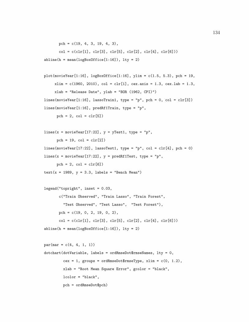
134

pch = c(19, 4, 3, 19, 4, 3),

col = c(clr[1], clr[3], clr[5], clr[2], clr[4], clr[6]))

abline(h = mean(logBoxOffice[1:16]), lty = 2)

plot(movieYear[1:16], logBoxOffice[1:16], ylim = c(1.5, 5.3), pch = 19,

xlim = c(1960, 2010), col = clr[1], cex.axis = 1.3, cex.lab = 1.3,

xlab = "Release Date", ylab = "BOR (1962, CPI)")

lines(movieYear[1:16], lassoTrain1, type = "p", pch = 0, col = clr[3])

lines(movieYear[1:16], predRf1Train, type = "p",

pch = 2, col = clr[5])

lines(x = movieYear[17:22], y = yTest1, type = "p",

pch = 19, col = clr[2])

lines(movieYear[17:22], lassoTest1, type = "p", col = clr[4], pch = 0)

lines(x = movieYear[17:22], y = predRf1Test, type = "p",

pch = 2, col = clr[6])

text(x = 1989, y = 3.3, labels = "Bench Mean")

legend("topright", inset = 0.03,

c("Train Observed", "Train Lasso", "Train Forest",

"Test Observed", "Test Lasso", "Test Forest"),

pch = c(19, 0, 2, 19, 0, 2),

col = c(clr[1], clr[3], clr[5], clr[2], clr[4], clr[6]))

abline(h = mean(logBoxOffice[1:16]), lty = 2)

par(mar = c(4, 4, 1, 1))

dotchart(dotVariable, labels = ordRmseDot$rmseNames, lty = 0,

cex = 1, groups = ordRmseDot$rmseType, xlim = c(0, 1.2),

xlab = "Root Mean Square Error", gcolor = "black",

lcolor = "black",

pch = ordRmseDot$pch)

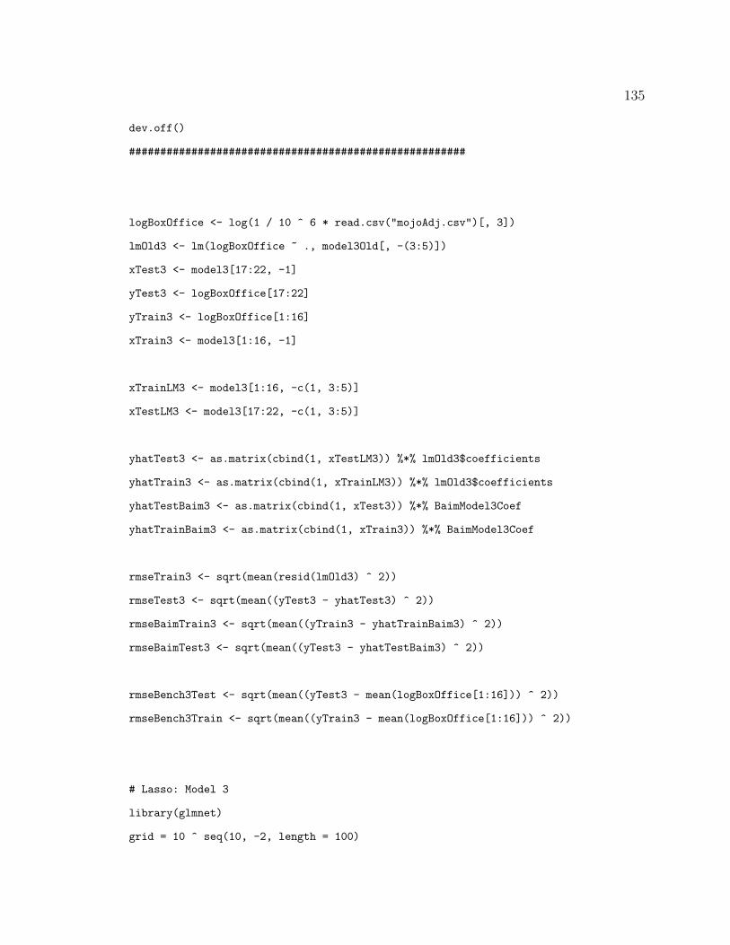
135

dev.off()

######################################################

logBoxOffice <- log(1 / 10 ^ 6 * read.csv("mojoAdj.csv")[, 3])

lmOld3 <- lm(logBoxOffice ~ ., model3Old[, -(3:5)])

xTest3 <- model3[17:22, -1]

yTest3 <- logBoxOffice[17:22]

yTrain3 <- logBoxOffice[1:16]

xTrain3 <- model3[1:16, -1]

xTrainLM3 <- model3[1:16, -c(1, 3:5)]

xTestLM3 <- model3[17:22, -c(1, 3:5)]

yhatTest3 <- as.matrix(cbind(1, xTestLM3)) %*% lmOld3$coefficients

yhatTrain3 <- as.matrix(cbind(1, xTrainLM3)) %*% lmOld3$coefficients

yhatTestBaim3 <- as.matrix(cbind(1, xTest3)) %*% BaimModel3Coef

yhatTrainBaim3 <- as.matrix(cbind(1, xTrain3)) %*% BaimModel3Coef

rmseTrain3 <- sqrt(mean(resid(lmOld3) ^ 2))

rmseTest3 <- sqrt(mean((yTest3 - yhatTest3) ^ 2))

rmseBaimTrain3 <- sqrt(mean((yTrain3 - yhatTrainBaim3) ^ 2))

rmseBaimTest3 <- sqrt(mean((yTest3 - yhatTestBaim3) ^ 2))

rmseBench3Test <- sqrt(mean((yTest3 - mean(logBoxOffice[1:16])) ^ 2))

rmseBench3Train <- sqrt(mean((yTrain3 - mean(logBoxOffice[1:16])) ^ 2))

# Lasso: Model 3

library(glmnet)

grid = 10 ^ seq(10, -2, length = 100)

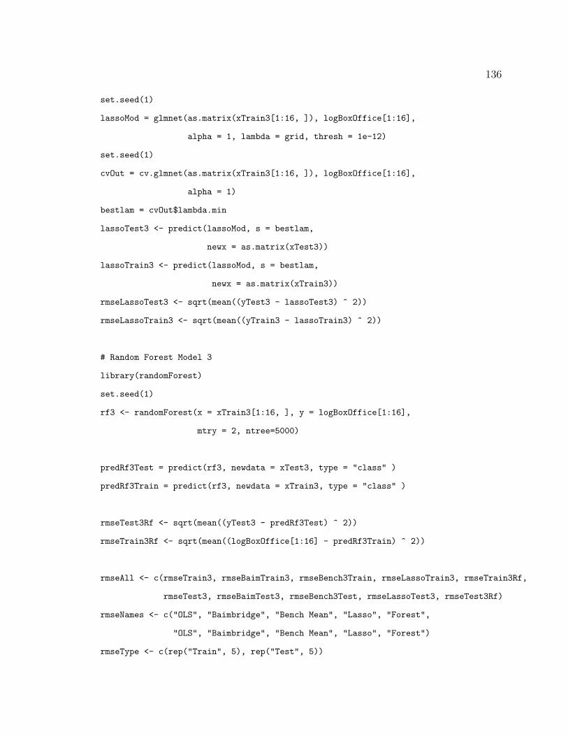
136

set.seed(1)

lassoMod = glmnet(as.matrix(xTrain3[1:16, ]), logBoxOffice[1:16],

alpha = 1, lambda = grid, thresh = 1e-12)

set.seed(1)

cvOut = cv.glmnet(as.matrix(xTrain3[1:16, ]), logBoxOffice[1:16],

alpha = 1)

bestlam = cvOut$lambda.min

lassoTest3 <- predict(lassoMod, s = bestlam,

newx = as.matrix(xTest3))

lassoTrain3 <- predict(lassoMod, s = bestlam,

newx = as.matrix(xTrain3))

rmseLassoTest3 <- sqrt(mean((yTest3 - lassoTest3) ^ 2))

rmseLassoTrain3 <- sqrt(mean((yTrain3 - lassoTrain3) ^ 2))

# Random Forest Model 3

library(randomForest)

set.seed(1)

rf3 <- randomForest(x = xTrain3[1:16, ], y = logBoxOffice[1:16],

mtry = 2, ntree=5000)

predRf3Test = predict(rf3, newdata = xTest3, type = "class" )

predRf3Train = predict(rf3, newdata = xTrain3, type = "class" )

rmseTest3Rf <- sqrt(mean((yTest3 - predRf3Test) ^ 2))

rmseTrain3Rf <- sqrt(mean((logBoxOffice[1:16] - predRf3Train) ^ 2))

rmseAll <- c(rmseTrain3, rmseBaimTrain3, rmseBench3Train, rmseLassoTrain3, rmseTrain3Rf,

rmseTest3, rmseBaimTest3, rmseBench3Test, rmseLassoTest3, rmseTest3Rf)

rmseNames <- c("OLS", "Baimbridge", "Bench Mean", "Lasso", "Forest",

"OLS", "Baimbridge", "Bench Mean", "Lasso", "Forest")

rmseType <- c(rep("Train", 5), rep("Test", 5))

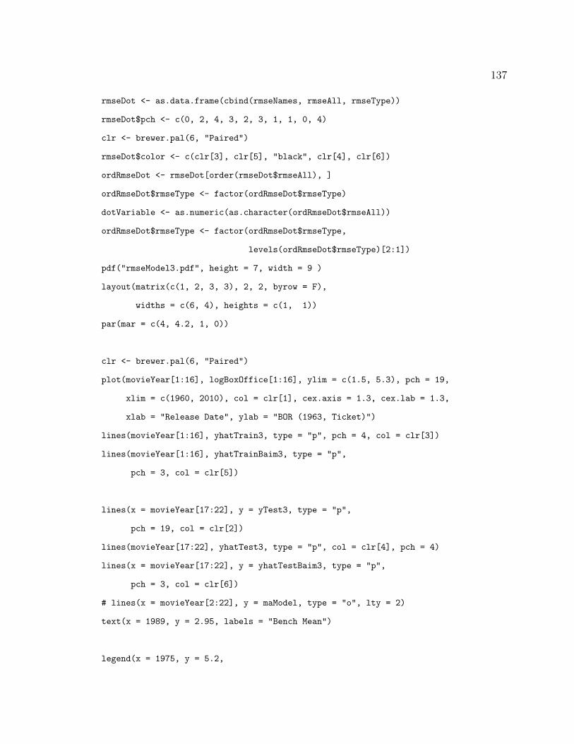
137

rmseDot <- as.data.frame(cbind(rmseNames, rmseAll, rmseType))

rmseDot$pch <- c(0, 2, 4, 3, 2, 3, 1, 1, 0, 4)

clr <- brewer.pal(6, "Paired")

rmseDot$color <- c(clr[3], clr[5], "black", clr[4], clr[6])

ordRmseDot <- rmseDot[order(rmseDot$rmseAll), ]

ordRmseDot$rmseType <- factor(ordRmseDot$rmseType)

dotVariable <- as.numeric(as.character(ordRmseDot$rmseAll))

ordRmseDot$rmseType <- factor(ordRmseDot$rmseType,

levels(ordRmseDot$rmseType)[2:1])

pdf("rmseModel3.pdf", height = 7, width = 9 )

layout(matrix(c(1, 2, 3, 3), 2, 2, byrow = F),

widths = c(6, 4), heights = c(1, 1))

par(mar = c(4, 4.2, 1, 0))

clr <- brewer.pal(6, "Paired")

plot(movieYear[1:16], logBoxOffice[1:16], ylim = c(1.5, 5.3), pch = 19,

xlim = c(1960, 2010), col = clr[1], cex.axis = 1.3, cex.lab = 1.3,

xlab = "Release Date", ylab = "BOR (1963, Ticket)")

lines(movieYear[1:16], yhatTrain3, type = "p", pch = 4, col = clr[3])

lines(movieYear[1:16], yhatTrainBaim3, type = "p",

pch = 3, col = clr[5])

lines(x = movieYear[17:22], y = yTest3, type = "p",

pch = 19, col = clr[2])

lines(movieYear[17:22], yhatTest3, type = "p", col = clr[4], pch = 4)

lines(x = movieYear[17:22], y = yhatTestBaim3, type = "p",

pch = 3, col = clr[6])

# lines(x = movieYear[2:22], y = maModel, type = "o", lty = 2)

text(x = 1989, y = 2.95, labels = "Bench Mean")

legend(x = 1975, y = 5.2,

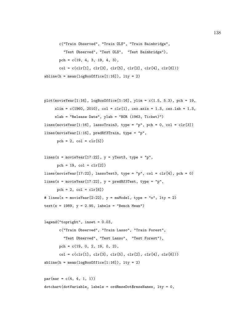
138

c("Train Observed", "Train OLS", "Train Baimbridge",

"Test Observed", "Test OLS", "Test Baimbridge"),

pch = c(19, 4, 3, 19, 4, 3),

col = c(clr[1], clr[3], clr[5], clr[2], clr[4], clr[6]))

abline(h = mean(logBoxOffice[1:16]), lty = 2)

plot(movieYear[1:16], logBoxOffice[1:16], ylim = c(1.5, 5.3), pch = 19,

xlim = c(1960, 2010), col = clr[1], cex.axis = 1.3, cex.lab = 1.3,

xlab = "Release Date", ylab = "BOR (1963, Ticket)")

lines(movieYear[1:16], lassoTrain3, type = "p", pch = 0, col = clr[3])

lines(movieYear[1:16], predRf3Train, type = "p",

pch = 2, col = clr[5])

lines(x = movieYear[17:22], y = yTest3, type = "p",

pch = 19, col = clr[2])

lines(movieYear[17:22], lassoTest3, type = "p", col = clr[4], pch = 0)

lines(x = movieYear[17:22], y = predRf3Test, type = "p",

pch = 2, col = clr[6])

# lines(x = movieYear[2:22], y = maModel, type = "o", lty = 2)

text(x = 1989, y = 2.95, labels = "Bench Mean")

legend("topright", inset = 0.03,

c("Train Observed", "Train Lasso", "Train Forest",

"Test Observed", "Test Lasso", "Test Forest"),

pch = c(19, 0, 2, 19, 0, 2),

col = c(clr[1], clr[3], clr[5], clr[2], clr[4], clr[6]))

abline(h = mean(logBoxOffice[1:16]), lty = 2)

par(mar = c(4, 4, 1, 1))

dotchart(dotVariable, labels = ordRmseDot$rmseNames, lty = 0,

139

cex = 1, groups = ordRmseDot$rmseType, xlim = c(0, 1.2),

xlab = "Root Mean Square Error", gcolor = "black",

lcolor = "black",

pch = ordRmseDot$pch)

dev.off()

######################################################

Bond.data <- read.csv("MS_project_Data2.csv")

movie.Date <- as.Date(Bond.data[,13])

theEconDataX <- Bond.data[, 9:12]

logBoxOffice <- log(CPIadj62 / 10 ^ 6)

theEconData <- cbind(logBoxOffice, theEconDataX)

lmTheEcon <- lm(logBoxOffice[1:16] ~ ., theEconData[1:16,])

yhatTestE <- as.matrix(cbind(1, theEconDataX[17:22, ])) %*% lmTheEcon$coefficients

yhatTrainE <- as.matrix(cbind(1, theEconDataX[1:16, ])) %*% lmTheEcon$coefficients

rmseTrainE <- sqrt(mean(resid(lmTheEcon) ^ 2))

rmseTestE <- sqrt(mean((yhatTestE - logBoxOffice[17:22]) ^ 2))

rmseTrainE <- sqrt(mean((yhatTrainE - logBoxOffice[1:16]) ^ 2))

# Lasso The Economist

set.seed(1)

lassoMod = glmnet(as.matrix(theEconDataX[1:16, ]), logBoxOffice[1:16],

140

alpha = 1, lambda = grid, thresh = 1e-12)

set.seed(1)

cvOut = cv.glmnet(as.matrix(theEconDataX[1:16, ]), logBoxOffice[1:16],

alpha = 1)

bestlam = cvOut$lambda.min

lassoTestE <- predict(lassoMod, s = bestlam,

newx = as.matrix(theEconDataX[17:22, ]))

lassoTrainE <- predict(lassoMod, s = bestlam,

newx = as.matrix(theEconDataX[1:16, ]))

rmseLassoTestE <- sqrt(mean((yTest1 - lassoTestE) ^ 2))

rmseLassoTrainE <- sqrt(mean((yTrain1 - lassoTrainE) ^ 2))

# Random Forest The Economist

set.seed(1)

rfE <- randomForest(x = theEconDataX[1:16, ], y = logBoxOffice[1:16],

mtry = 2, ntree=5000)

predRfE = predict(rfE, newdata = theEconDataX[17:22, ], type = "class" )

predRfETrain = predict(rfE, newdata = theEconDataX[1:16, ], type = "class" )

rmseTestRfE <- sqrt(mean((logBoxOffice[17:22] - predRfE) ^ 2))

rmseTrainRfE <- sqrt(mean((logBoxOffice[1:16] - predRfETrain) ^ 2))

# Benchmark Moving Averages

maModel <- sapply(1:21, function(x) mean(logBoxOffice[1:x]))

rmseMaTrain <- sqrt(mean((model1[2:16, 1] - maModel[1:15]) ^ 2))

rmseMaTest <- sqrt(mean((logBoxOffice[17:22] - maModel[16:21]) ^ 2))

pdf("rmseModelE.pdf", height = 7, width = 9 )

layout(matrix(c(1, 2, 3, 3), 2, 2, byrow = F),

141

widths = c(6, 4), heights = c(1, 1))

par(mar = c(4, 4.2, 1, 0))

clr <- brewer.pal(6, "Paired")

plot(movieYear[1:16],logBoxOffice[1:16], ylim = c(1.5, 5.3), pch = 19,

xlim = c(1960, 2010), col = clr[1], cex.axis = 1.3, cex.lab = 1.3,

xlab = "Release Date", ylab = "BOR (1962, CPI)")

lines(movieYear[1:16], yhatTrainE, type = "p", pch = 4, col = clr[3])

lines(movieYear[2:16], maModel[1:15], type = "p",

pch = 8, col = clr[5])

lines(x = movieYear[17:22], y = logBoxOffice[17:22], type = "p",

pch = 19, col = clr[2])

lines(movieYear[17:22], yhatTestE, type = "p", col = clr[4], pch = 4)

lines(x = movieYear[17:22], y = maModel[16:21], type = "p",

pch = 8, col = clr[6])

# lines(x = movieYear[2:22], y = maModel, type = "o", lty = 2)

text(x = 1989, y = 3.35, labels = "Bench Mean")

legend("topright", inset = 0.03,

c("Train Observed", "Train OLS", "Train Bench MA",

"Test Observed", "Test OLS", "Test Bench MA"),

pch = c(19, 4, 8, 19, 4, 8),

col = c(clr[1], clr[3], clr[5], clr[2], clr[4], clr[6]))

abline(h = mean(logBoxOffice[1:16]), lty = 2)

plot(movieYear[1:16], logBoxOffice[1:16], ylim = c(1.5, 5.3), pch = 19,

xlim = c(1960, 2010), col = clr[1], cex.axis = 1.3, cex.lab = 1.3,

xlab = "Release Date", ylab = "BOR (1962, CPI)")

lines(movieYear[1:16], lassoTrainE, type = "p", pch = 0, col = clr[3])

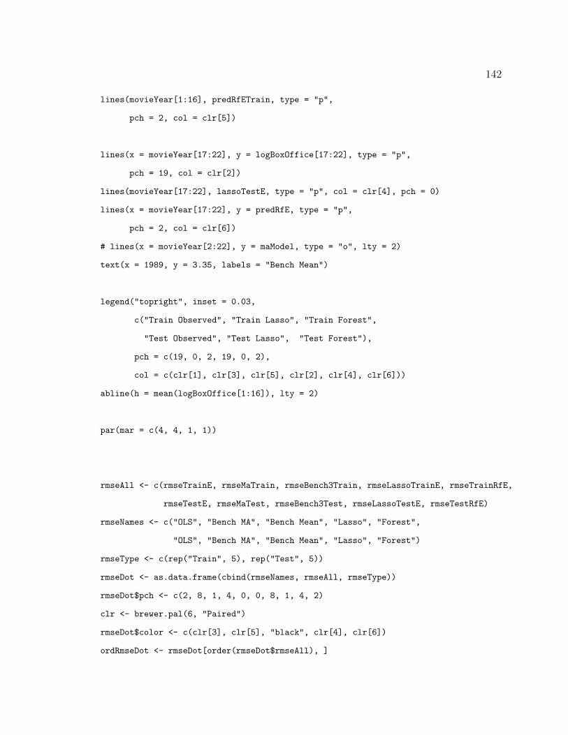
142

lines(movieYear[1:16], predRfETrain, type = "p",

pch = 2, col = clr[5])

lines(x = movieYear[17:22], y = logBoxOffice[17:22], type = "p",

pch = 19, col = clr[2])

lines(movieYear[17:22], lassoTestE, type = "p", col = clr[4], pch = 0)

lines(x = movieYear[17:22], y = predRfE, type = "p",

pch = 2, col = clr[6])

# lines(x = movieYear[2:22], y = maModel, type = "o", lty = 2)

text(x = 1989, y = 3.35, labels = "Bench Mean")

legend("topright", inset = 0.03,

c("Train Observed", "Train Lasso", "Train Forest",

"Test Observed", "Test Lasso", "Test Forest"),

pch = c(19, 0, 2, 19, 0, 2),

col = c(clr[1], clr[3], clr[5], clr[2], clr[4], clr[6]))

abline(h = mean(logBoxOffice[1:16]), lty = 2)

par(mar = c(4, 4, 1, 1))

rmseAll <- c(rmseTrainE, rmseMaTrain, rmseBench3Train, rmseLassoTrainE, rmseTrainRfE,

rmseTestE, rmseMaTest, rmseBench3Test, rmseLassoTestE, rmseTestRfE)

rmseNames <- c("OLS", "Bench MA", "Bench Mean", "Lasso", "Forest",

"OLS", "Bench MA", "Bench Mean", "Lasso", "Forest")

rmseType <- c(rep("Train", 5), rep("Test", 5))

rmseDot <- as.data.frame(cbind(rmseNames, rmseAll, rmseType))

rmseDot$pch <- c(2, 8, 1, 4, 0, 0, 8, 1, 4, 2)

clr <- brewer.pal(6, "Paired")

rmseDot$color <- c(clr[3], clr[5], "black", clr[4], clr[6])

ordRmseDot <- rmseDot[order(rmseDot$rmseAll), ]

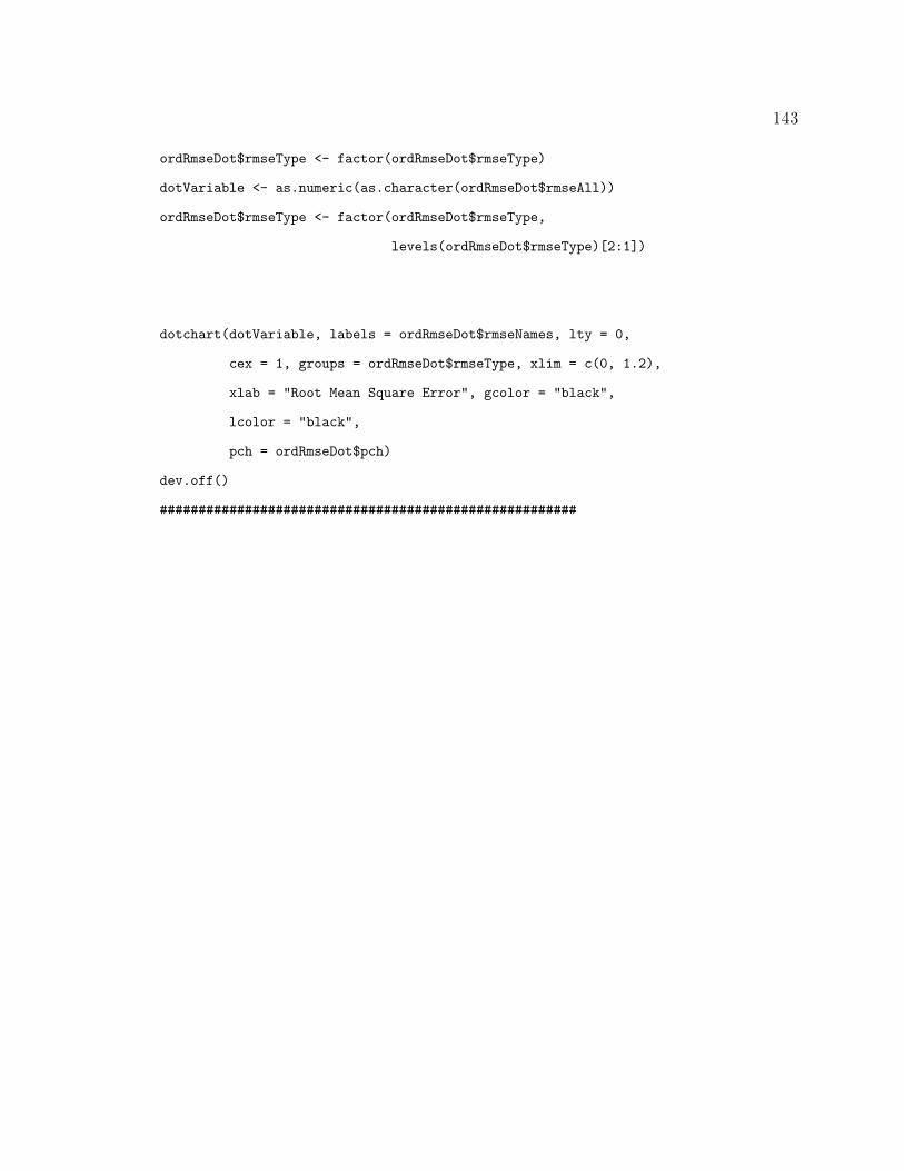
143

ordRmseDot$rmseType <- factor(ordRmseDot$rmseType)

dotVariable <- as.numeric(as.character(ordRmseDot$rmseAll))

ordRmseDot$rmseType <- factor(ordRmseDot$rmseType,

levels(ordRmseDot$rmseType)[2:1])

dotchart(dotVariable, labels = ordRmseDot$rmseNames, lty = 0,

cex = 1, groups = ordRmseDot$rmseType, xlim = c(0, 1.2),

xlab = "Root Mean Square Error", gcolor = "black",

lcolor = "black",

pch = ordRmseDot$pch)

dev.off()

######################################################