Visualisation and statistical modelling techniques for the ...

ANZIAM J. 57 (MISG2015) pp.M130–M162, 2016 M130

Visualisation and statistical modellingtechniques for the management of inventory

stock levels

Winston L. Sweatman1 James McGree2

C. Jacobien Carstens3 Kylie J. Foster4 Shen Liu5

Nicholas Tierney6 Eloise Tredenick7 Ayham Zaitouny8

(Received 15 November 2015; revised 20 August 2016)

Abstract

This paper describes the investigations conducted in a Mathematics-in-Industry Study Group project from the Australian meeting atQueensland University of Technology in 2015. This concerned themanagement of stock levels of raw materials used to construct aorticstents. The approaches used included network visualisation, classifica-tion and regression trees, and time series modelling. This work will beof general interest to those who are managing stock levels in a highlyvolatile context. The methods applied show that there is potential

doi:10.21914/anziamj.v57i0.10225 gives this article, c© Austral. Mathematical Soc.2016. Published August 29, 2016, as part of the Proceedings of the 2015 Mathematicsand Statistics in Industry Study Group. issn 1445-8810. (Print two pages per sheetof paper.) Copies of this article must not be made otherwise available on the internet;instead link directly to the doi for this article. Record comments on this article viahttp://journal.austms.org.au/ojs/index.php/ANZIAMJ/comment/add/10225/0

Contents M131

value in taking a statistical approach to understand and make decisionswithin such volatility. The work provides a basis for developing moreadvanced statistical approaches for specific inventory problems.

Contents1 Introduction M132

2 Data provide by Cook Medical M133

3 Methodology M1333.1 Visualisation of the manufacturing process . . . . . . . . . M1343.2 Classification and regression trees . . . . . . . . . . . . . . M1353.3 Time series modelling . . . . . . . . . . . . . . . . . . . . . M1373.4 Final comments on methodology . . . . . . . . . . . . . . . M140

4 Results M1404.1 Visualisation of the manufacturing process . . . . . . . . . M140

4.1.1 Assembly networks . . . . . . . . . . . . . . . . . . M1414.1.2 Monthly material use networks . . . . . . . . . . . M1434.1.3 Production times . . . . . . . . . . . . . . . . . . . M149

4.2 Classification and regression trees . . . . . . . . . . . . . . M1524.3 Time series modelling . . . . . . . . . . . . . . . . . . . . . M155

5 Discussion and conclusions M157

References M159

1 Introduction M132

1 Introduction

Cook Medical was established in 1963, and is the world’s largest family ownedmedical device manufacturing company, with annual sales greater than twobillion. One of its primary products is the aortic stent. These are usedfor endovascular aneurysm repair. Each month Cook Medical manufacturesabout 500 custom-made stents, 300 customised stents and 900 standard stents.The manufacturing process of each finished product is composed of multiplesub-assemblies which are ultimately composed of a set of raw materials.There are about 1000 different raw materials and hundreds of sub-assembliesinvolved in manufacturing a single finished product. Unfortunately, managingthe stock levels of the raw materials is particularly difficult for a number ofreasons. First, as these stents are being placed in individuals, the inherentvariability between individuals means that each stent needs to be customisedin a variety of different ways. Consequently, the production of every singlestent involves a different composition and number of raw materials. Secondly,the demand for stents varies over time, with urgent orders for patients withserious, life-threatening conditions affording further variability in demandfor raw materials. Thirdly, each raw material has a certain storage or ‘shelf-life’ which, when exceeded, means the raw material is discarded. So onecannot simply order excessive amounts of raw materials as this may result inmassive losses in expenditure. Thus, the management of inventory levels forCook Medical is a non-trivial task. Indeed, one must not forget the seriousimplications of not meeting demand, particularly for urgent orders.

In this study, we investigate some techniques for visualising the complexproduction process of a number of finished products to try to understandthe data at hand, and also to gain insight into potential bottlenecks and/orimportant raw materials in the production processes. Further, we use datamining techniques to discover what raw materials are causing delays inproduction as this will provide useful information for stock management.Finally, we develop a time series model to understand the variability in rawmaterials (for example, how the demand changes over the calendar year)

2 Data provide by Cook Medical M133

and then use this model to make predictions about demand. Then, once aprediction is made say for the next month, the current raw material levelscan be inspected and new materials are ordered, if required.

2 Data provide by Cook Medical

Cook Medical provided data on the production of stents for the five yearperiod of January 2010 to December 2014. The data included informationabout which raw materials (and the corresponding quantities of each) areneeded in manufacturing each stent. From the data, we are also able todetermine the timing and quantity of orders on a monthly basis, and also thetime taken to manufacture each stent.

As these data are readily available to Cook Medical, it is of interest todetermine what useful information could be extracted to assist in the efficientmanagement of stock levels of raw materials. The proposed visualisation andstatistical techniques that could be implemented are formally introduced inthe next section. Further work is needed to implement these techniques inan automated and structured manner at Cook Medical. However, throughthe application of these techniques to the data we have been provided, wedemonstrate the usefulness of these methods.

3 Methodology

We now describe the methodology used to address the aims of this research.Corresponding to the number of aims, we split this section into three parts.

3 Methodology M134

Algorithm 1: Code that generates assembly graphs for each product# Load the R-package and datalibrary(’igraph’)source(’load_data.R’)source(’functions.R’)

# Find the indices of all productsidx = which(data_2010_2014$WO. != "")

# Set the plotting layout of igraphigraph.options(plot.layout=layout.reingold.tilford)

# Create and plot the assembly graph of product no. iproduct = data_2010_2014[idx[i]:(idx[i+1]-1),]g <- create_assembly_graph(product)my_colors<-get_colors(get.vertex.attribute(g, ’name’))plot_graph_detail(g, col_v = my_colors)

3.1 Visualisation of the manufacturing process

The production process is visualised using networks. Finished products arelinked on a tree with their sub-assemblies’ subsequent raw materials. Byincluding several finished products on the same diagram it is clear how differentproducts are interdependent through incorporating common sub-assembliesor raw materials.

For the visualisation of the assembly networks we use the ‘Reingold–Tilford’layout [11]. For the visualisation of the monthly product networks we use the‘Fruchterman–Reingold’ layout [5].

The r-package ‘igraph’ [4] is used. Algorithm 1 lists the code that generatesassembly graphs for each product from the data provided by Cook Medical.Similarly, Algorithm 2 lists the code that generates a monthly network.

3 Methodology M135

Algorithm 2: Code that generates a monthly network# Load the R-package and datalibrary(’igraph’)source(’load_data.R’)source(’functions.R’)

# Create monthly networkg = create_monthly_network("jan", 2014)

# Set the graph layoutigraph.options(plot.layout=layout.fruchterman.reingold)

# Plot monthly product networkmy_colors<-get_colors(get.vertex.attribute(g, ’name’))plot_graph_detail(g, col_v = my_colors)

3.2 Classification and regression trees

Classification and regression trees (carts) are a widely used data miningtechnique to predict the response of a variable of interest [1, 6]. Classificationtrees predict a categorical response variable whereas regression trees are usedwhen the response is continuous. The response is modelled via a tree-likestructure based on identified thresholds or levels of important explanatoryvariables. The depth of the tree, or number of branches, is determined byvarious goodness of fit measures designed to trade off accuracy of estimationand parsimony. Cross-validation is used to explore how well the modelcan predict new data [1, 6, 3]. cart models handle missing data by usingsurrogate splits: when a value for a variable is missing and that variable needsto be used for a split, an alternative variable with a similar splitting propertydetermines the direction of the split [3, 1].

The tree-like structure for the model allows potentially complex interactions

3 Methodology M136

Algorithm 3: matlab code to produce the forecast# Call the R-packagelibrary(rpart)

# Find the treefit <- rpart(long ~ x1+x2+x3,method="class",data=Cook)

printcp(fit) # Show the resultsplotcp(fit) # Show results of cross-validationsummary(fit) # Show splits

# plot treeplot(fit,uniform=TRUE,main="Classification tree for long orders")

to be found but also facilitates straightforward interpretation of statisticalresults. This is one of the main reasons why such methods have been widelyused in applied research. Other reasons for using carts include the abilityto handle numerical and categorical data, the requirement for few statisticalassumptions to hold, and the ability to perform well for large data sets. Thestrength of the cart analysis is its simplicity in building a single tree that isreadily interpretable. This strength is balanced by a weakness in being lessable to predict linear relationships and being sensitive to small variations indata, potentially leading to an oversimplification of the real model [2].

For this study, the response of interest is whether a particular order takesa longer time to manufacture than normal. As this is a binary variable,classification trees are considered for this analysis. The trees were estimatedin the r-package called ‘Recursive partitioning and regression trees’ or ‘rpart’by Therneau, Atkinson and Ripley. Algorithm 3 lists example code to generatea simple classification tree.

3 Methodology M137

Figure 1: Monthly usage of two raw materials

3.3 Time series modelling

It is of critical importance to monitor the usage of raw materials whenmanaging inventory levels for finished products. The usage of each rawmaterial exhibits serial correlation through time which can be accounted forby time series models. For this approach, we demonstrate how time seriesmodels were applied to the raw material usage data, and how we obtainforecasts of the future usage.

We consider the monthly usage data of raw materials Z0016A and 60411-3that were recorded from January 2010 to December 2014. Figure 1 displaysthe time plots of the observed sample data. We split the sample into trainingand test sets, with the former covering the period from January 2010 to

3 Methodology M138

December 2013 and the latter covering January to December 2014.

The autoregressive integrated moving average (arima) model is fitted to thetraining set. Using the backshift notation an arima(p,d,q) model is

(1− φ1B− · · ·− φpBp)(1− B)dyt = µ+ (1+ θ1B+ · · ·+ θqBq)et

where p, d and q stand for the autoregressive order, the differencing orderand the moving average order, respectively, and B is the time lag (backshift)operator. The error term et is assumed to be independently and identicallydistributed with zero mean and finite, fixed variance. The p, d and q valuesare determined by the the Bayesian Information Criterion (bic).

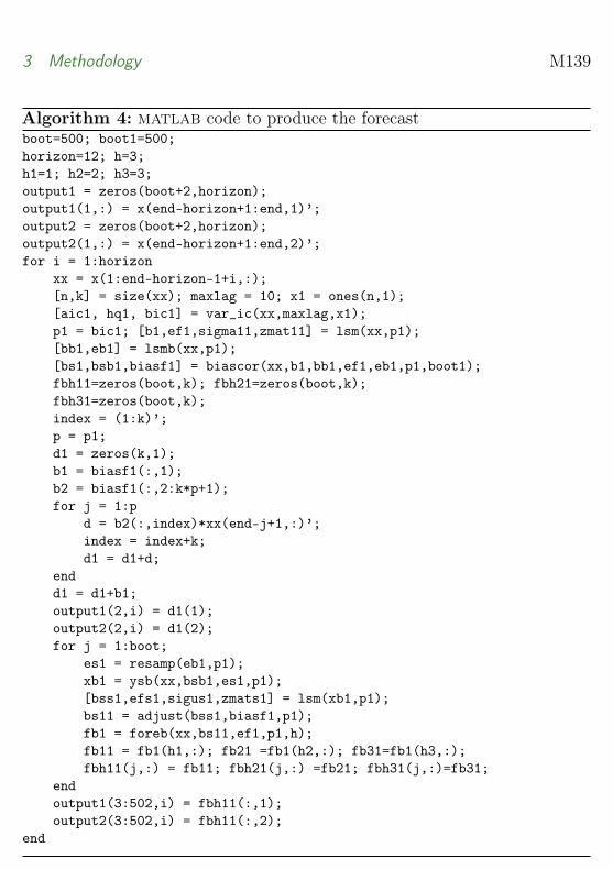
Once the unknown parameters are estimated, the fitted model is used toproduce one-step-ahead forecasts of the usage data, over the twelve monthperiod of the test set. To evaluate the associated uncertainty, standardresidual bootstrapping obtains forecast replicates at each forecasting horizon,which are used to approximate the forecast density function conditional on theobserved values. Inference is conducted based on the approximated forecastdensity functions. For instance, the 95% prediction intervals of the rawmaterial usage is constructed by taking the 2.5th and 97.5th quantiles asthe lower and upper limits, respectively. Algorithm 4 lists matlab code toproduce the forecast where:

• var_ic is the model selection function;

• lsm represents the least square estimator for the selected model;

• lsmb denotes the estimator for the backward autoregressive model [7, 8];

• biascor is the function that applies bias-correction to parameter esti-mates [9];

• the resamp function carries out bootstrap sampling of residuals;

• the ysb function generates pseudo time series using the estimatedparameter values, on the basis of the backward autoregressive model [9];

3 Methodology M139

Algorithm 4: matlab code to produce the forecastboot=500; boot1=500;horizon=12; h=3;h1=1; h2=2; h3=3;output1 = zeros(boot+2,horizon);output1(1,:) = x(end-horizon+1:end,1)’;output2 = zeros(boot+2,horizon);output2(1,:) = x(end-horizon+1:end,2)’;for i = 1:horizon

xx = x(1:end-horizon-1+i,:);[n,k] = size(xx); maxlag = 10; x1 = ones(n,1);[aic1, hq1, bic1] = var_ic(xx,maxlag,x1);p1 = bic1; [b1,ef1,sigma11,zmat11] = lsm(xx,p1);[bb1,eb1] = lsmb(xx,p1);[bs1,bsb1,biasf1] = biascor(xx,b1,bb1,ef1,eb1,p1,boot1);fbh11=zeros(boot,k); fbh21=zeros(boot,k);fbh31=zeros(boot,k);index = (1:k)’;p = p1;d1 = zeros(k,1);b1 = biasf1(:,1);b2 = biasf1(:,2:k*p+1);for j = 1:p

d = b2(:,index)*xx(end-j+1,:)’;index = index+k;d1 = d1+d;

endd1 = d1+b1;output1(2,i) = d1(1);output2(2,i) = d1(2);for j = 1:boot;

es1 = resamp(eb1,p1);xb1 = ysb(xx,bsb1,es1,p1);[bss1,efs1,sigus1,zmats1] = lsm(xb1,p1);bs11 = adjust(bss1,biasf1,p1);fb1 = foreb(xx,bs11,ef1,p1,h);fb11 = fb1(h1,:); fb21 =fb1(h2,:); fb31=fb1(h3,:);fbh11(j,:) = fb11; fbh21(j,:) =fb21; fbh31(j,:)=fb31;

endoutput1(3:502,i) = fbh11(:,1);output2(3:502,i) = fbh11(:,2);

end

4 Results M140

• the adjust function applies bias-adjustment on the estimated parametervalues [8];

• the foreb function produces forecast replicates, which are employedto approximate the distribution function at the h-step-ahead forecasthorizon [9].

3.4 Final comments on methodology

The data provided by the Cook Medical representatives presents an excellentopportunity for applying and developing methodologies for mathematical/statistical modelling techniques. The main challenge for this study is thecomplexity of the dataset, and hence suitable methods need to be developed toextract useful information in an efficient way. The study group concentratedon approaches to data visualisation, data mining and time series analysis.These techniques can be extended to achieve better performance. For example,to obtain more accurate forecasts, flexible covariance structures between rawmaterials are worth investigating. There are opportunities to further continuethe research.

4 Results

We now present the results of the three approaches discussed in Section 3.

4.1 Visualisation of the manufacturing process

Cook Medical produces both standard and customised grafts and graft deliverysystems. An assembled product consists of both a graft and a graft deliverysystem. The production varies in complexity: some products are made outof just a few raw materials whereas others are made out of a combination of

4 Results M141

raw materials and room stocks. Here, raw material refers to any material orpart that is bought by Cook Medical. The term raw material is thus not tobe taken literally: for example, Cook Medical buys ‘stockings’ of differentsizes, and each different size is classified as a different raw material. Roomstocks are complex assembled parts that themselves are constructed out ofraw materials.

We decided to represent the assembly of a product as a network. A networkconsists of nodes and connections between nodes. In our network representa-tion, nodes correspond to either the assembled product, a room stock or araw material. Connections point from either the assembled product or froma room stock, to their constituent parts. We refer to such a network as theassembly network of a product. We visualised assembly networks to get aninsight into the diversity of products and the complexity of the assemblyprocess. We discuss assembly networks in more details in Subsection 4.1.1.

After our initial exploration of the product assembly data, we wanted to getan insight into the overall use of materials in a certain time period. To doso we first simplified the assembly networks. We removed the room stocknodes, while retaining all of the raw materials and the quantity needed toassemble the room stock. We then combined all simplified assembly networksof products produced in a single month into one large network. In this networkthe number of incoming edges of a raw material corresponds to the number ofproducts in which it was used. The quantity of the product that was neededduring the month is extracted from the network. We discuss the monthlynetwork in more detail in Section 4.1.2.

4.1.1 Assembly networks

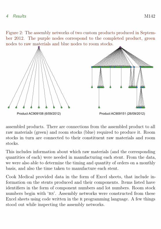
As discussed above, an assembly network consists of nodes correspondingto either an assembled product, a room stock or a raw material. Figure 2shows two examples of assembly networks. The complexity of these productsis vastly different. In each case, the purple ‘root’ nodes correspond to the

4 Results M142

Figure 2: The assembly networks of two custom products produced in Septem-ber 2012. The purple nodes correspond to the completed product, greennodes to raw materials and blue nodes to room stocks.

Product AC909108 (6/09/2012) Product AC909151 (26/09/2012)

assembled products. There are connections from the assembled product to allraw materials (green) and room stocks (blue) required to produce it. Roomstocks in turn are connected to their constituent raw materials and roomstocks.

This includes information about which raw materials (and the correspondingquantities of each) were needed in manufacturing each stent. From the data,we were also able to determine the timing and quantity of orders on a monthlybasis, and also the time taken to manufacture each stent.

Cook Medical provided data in the form of Excel sheets, that include in-formation on the stents produced and their components. Items listed haveidentifiers in the form of component numbers and lot numbers. Room stocknumbers begin with ‘rs’. Assembly networks were constructed from theseExcel sheets using code written in the r programming language. A few thingsstood out while inspecting the assembly networks.

4 Results M143

First, many room stocks that were used in the assembly of products, arenot in the list of room stock assemblies. In the assembly networks, theseroom stocks are identified as the blue nodes that have no outgoing edges.By further inspecting the data, we found that overall there are 22384 lotnumbers starting with ‘rs’ that are not in the list of room stock assemblies.These 22348 lot numbers correspond to 237 unique component numbers. Forthe investigation, these missing room stocks are treated as if they were rawmaterials.

Secondly, we found that there are several room stocks that only consist ofone raw material, see for instance the assembly network of product AC909151in Figure 2. It seems that treating these ‘room stocks’ as raw materialswould simplify the inventory administration, since at the moment there areessentially two names for a single inventory item. Specifically there is theroom stock name and the raw material name, both corresponding to the sameraw material.

Finally, there is a lot of variety in the complexity of the assembled products.This really stood out while visualising the assembly networks, as illustratedin Figure 2.

4.1.2 Monthly material use networks

We visualise and analyse the inventory problem by creating a network of all ofthe finished products produced and all of the raw materials used in January2014. This process is repeated for each month in the data set.

In order to analyse the large number of materials required to make multiplefinished products we simplified their assembly networks. This simplificationremoves all room stock nodes, while retaining all of the raw materials requiredto build these room stocks as well as the quantities of raw materials needed.We refer to this process as the flattening of the assembly network.

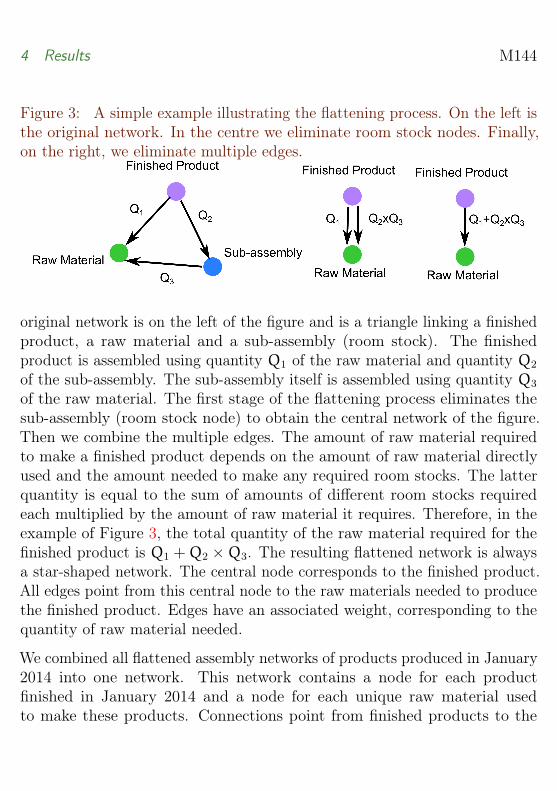
A simple example of the flattening process is illustrated in Figure 3. The

4 Results M144

Figure 3: A simple example illustrating the flattening process. On the left isthe original network. In the centre we eliminate room stock nodes. Finally,on the right, we eliminate multiple edges.

original network is on the left of the figure and is a triangle linking a finishedproduct, a raw material and a sub-assembly (room stock). The finishedproduct is assembled using quantity Q1 of the raw material and quantity Q2

of the sub-assembly. The sub-assembly itself is assembled using quantity Q3

of the raw material. The first stage of the flattening process eliminates thesub-assembly (room stock node) to obtain the central network of the figure.Then we combine the multiple edges. The amount of raw material requiredto make a finished product depends on the amount of raw material directlyused and the amount needed to make any required room stocks. The latterquantity is equal to the sum of amounts of different room stocks requiredeach multiplied by the amount of raw material it requires. Therefore, in theexample of Figure 3, the total quantity of the raw material required for thefinished product is Q1 +Q2 ×Q3. The resulting flattened network is alwaysa star-shaped network. The central node corresponds to the finished product.All edges point from this central node to the raw materials needed to producethe finished product. Edges have an associated weight, corresponding to thequantity of raw material needed.

We combined all flattened assembly networks of products produced in January2014 into one network. This network contains a node for each productfinished in January 2014 and a node for each unique raw material usedto make these products. Connections point from finished products to the

4 Results M145

Figure 4: The combined network of ten simplified assembly networks.

4 Results M146

raw materials required to assemble them. To illustrate this idea, Figure 4shows a network consisting of ten finished products. After inspecting thecorresponding assembly networks, it turns out that among these ten finishedproducts, there are two custom devices, and eight standard devices. Out of theeight standard devices, four are product 123999 and four are product 173881.This figure shows that these standard products have many raw materialsin common.

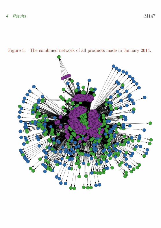
Figure 5 shows the whole network for January 2014. Further analysis gainssome valuable information.

First, raw materials corresponding to nodes with high in-degree (nodes witha large number of incoming connections) are raw materials that are requiredfor many finished products. On the other hand, raw materials correspondingto nodes with low in-degree are raw materials that are only required by a fewfinished products.

Secondly, for each raw material we calculate the sum of incoming edge weights(quantities). This sum corresponds to the quantity of the raw material neededin January. Again we identify the raw materials that were used most andleast, but this time in terms of quantity needed.

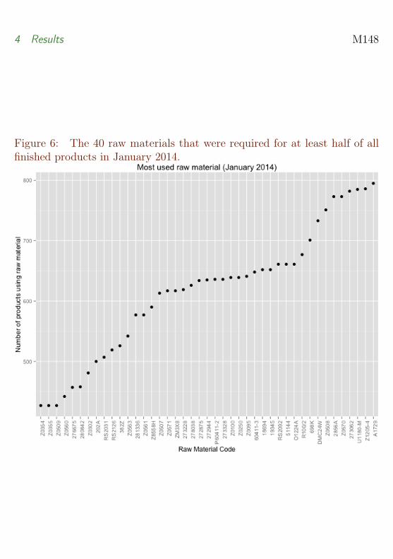
In January 2014, there were a total of 800 finished products. Figure 6 showsthe 40 raw materials that were used in half or more than half of these finishedproducts. Even though these materials are critical in the sense that they arerequired for most products, they may be very easy to acquire and thus not areal bottleneck in the production process. For example, A1729 corresponds toa silicon lubricant and U1180-M to glue. The silicon lubricant was the mostused raw material, and was used in all but three of the finished products.

A file was produced that contains the details of raw materials that were onlyused in the production of a single finished product.

4 Results M147

Figure 5: The combined network of all products made in January 2014.

4 Results M148

Figure 6: The 40 raw materials that were required for at least half of allfinished products in January 2014.

4 Results M149

Figure 7: Production time of stents in days.

0  

500  

1000  

1500  

2000  

2500  

5   10   15   20   25   30   35   40   45   50   55   60   65   70   75   80   85   90  

VOLU

ME  OF    STENTS  

DAYS  

2010  Freq   2011  Freq   2012  Freq   2013  Freq   2014  Freq  

4.1.3 Production times

Here we compare the shifts in production time in days of all stents created inthe last five years by year, showing a maximum of three months in productiontime. The stents taking longer than three months to produce were notincluded in the analysis. This is because such stents were typically outliers asthey often had much longer production times than three months. Further,such lengthy production times were associated with non-urgent patients, andtherefore the immediate availability of raw materials is not so vital.

Figure 7 shows that the total production time in 2011 had a higher volumepeaking around the thirty day mark, indicating production overall was slowerthan in 2013 and 2014, which were the most efficient years as the peaks areseen earlier.

4 Results M150

Figure 8: Production time in days for all stents.

0  

1000  

2000  

3000  

4000  

5000  

6000  

7000  

8000  

5   10   15   20   25   30   35   40   45   50   55   60   65   70   75   80   85   90  

VOLU

ME  OF  STEN

TS  

DAYS  

Figure 8 is production time over combined years with production time of upto three months. This figure is helpful to compare to 2014 (Figure 9) as thisgraph shows the production times for the last five years have been largely inthe 15–55 day range.

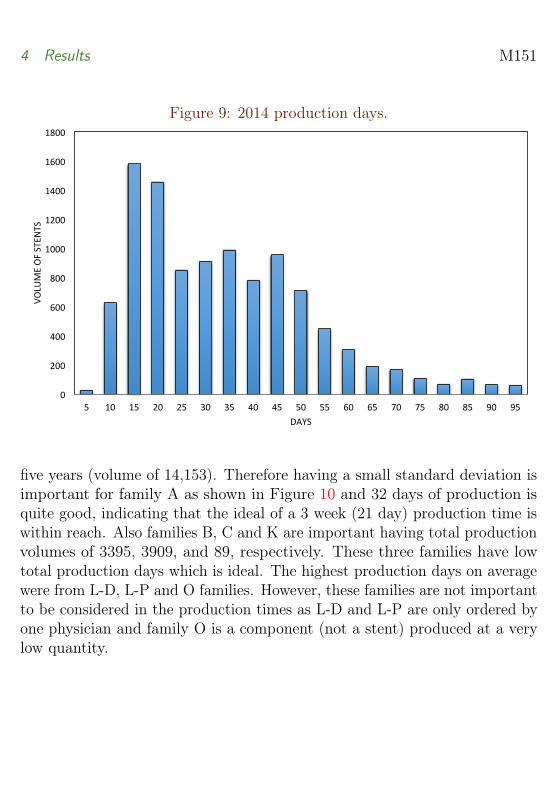
Figure 9 is 2014 production time in days showing most stents were producedin under 55 days and a high volume was created in 15–20 days. Comparingthis trend to the overall graph of all years in Figure 8 we see the productiontime in 2014 has improved as the production days are now in the 15–20 dayrange, instead of being spread over 15–55 days.

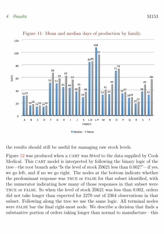
Figure 10 and Figure 11 show the mean and median days of production splitup into different families or categories of stents. Figure 10 shows that familiesL-D, L-P, 0 and F have the longest production times in days. The mostimportant family is A, as the stents are produced in the highest volume over

4 Results M151

Figure 9: 2014 production days.

0  

200  

400  

600  

800  

1000  

1200  

1400  

1600  

1800  

5   10   15   20   25   30   35   40   45   50   55   60   65   70   75   80   85   90   95  

VOLU

ME  OF  STEN

TS  

DAYS  

five years (volume of 14,153). Therefore having a small standard deviation isimportant for family A as shown in Figure 10 and 32 days of production isquite good, indicating that the ideal of a 3 week (21 day) production time iswithin reach. Also families B, C and K are important having total productionvolumes of 3395, 3909, and 89, respectively. These three families have lowtotal production days which is ideal. The highest production days on averagewere from L-D, L-P and O families. However, these families are not importantto be considered in the production times as L-D and L-P are only ordered byone physician and family O is a component (not a stent) produced at a verylow quantity.

4 Results M152

Figure 10: Mean days of production by family including standard deviation.

32  

18  16   16  

68  

59  63  

57  

45  38  

86  

97  

41  

49  

74  

37  29  

22  

49  

58  

0  

20  

40  

60  

80  

100  

120  

140  

A   B   C   D   F   G   H   I   J   K   L-­‐D   L-­‐P   M   N   O   P   Q   R   S   T  

MEA

N  DAY

S  

FAMILIES  

Mean  

4.2 Classification and regression trees

The data are explored using classification and regression trees (carts) in orderto determine which variables were associated with problematic orders. If suchvariables are identified, then one may be able to construct an early-warningsystem. As stated in Subsection 3.2, the response of interest was a binaryindicator for whether the production time for a particular order took longerthan expected; so true refers to production times longer than expected, andfalse refers to production times which are equal to or less than expected.This investigation is complicated by relevant variables in the decision treebeing dominated by common trivial sub-assemblies and materials, for examplestickers and tip protectors, which may mask more interesting effects. However,

4 Results M153

Figure 11: Mean and median days of production by family.

0  

20  

40  

60  

80  

100  

120  

A   B   C   D   F   G   H   I   J   K   L-­‐D   L-­‐P   M   N   O   P   Q   R   S   T  

31  

16   14   14  

52   51  45   44  

38  

29  

85  

108  

33   34  

71  

35  28  

19  

38  33  32  

18   16   16  

68  

59  63  

57  

45  

38  

86  

97  

41  

49  

74  

37  

29  22  

49  

58  

DAYS  

FAMILY  

Median   Mean  

the results should still be useful for managing raw stock levels.

Figure 12 was produced when a cart was fitted to the data supplied by CookMedical. This cart model is interpreted by following the binary logic of thetree—the root branch asks “Is the level of stock Z0621 less than 0.002?”—if yes,we go left, and if no we go right. The nodes at the bottom indicate whetherthe predominant response was true or false for that subset identified, withthe numerator indicating how many of those responses in that subset weretrue or false. So when the level of stock Z0621 was less than 0.002, ordersdid not take longer than expected for 2270 out of 2364 observations in thatsubset. Following along the tree we use the same logic. All terminal nodeswere false bar the final right-most node. We describe a decision that finds asubstantive portion of orders taking longer than normal to manufacture—this

4 Results M154Figure12

:Exa

mple

cart

sforalls

tents

4 Results M155

is quite a long decision rule, but it would be

When Z0621 is less than 0.002, and the month is May, June, or July,and L6691/1 is less than 0.84, and R100/2 is greater than 0.028,and L644/2 is less than 1.6 and L401/3 is less than 2.1, then wefind that orders take longer than expected to manufacture.

As the cart identifies those variables important in predicting the outcomeit is also worthwhile to investigate further the relationships amongst thesevariables and the outcome. Figure 12 exhibits example carts for all stents.

4.3 Time series modelling

Figure 13 displays the obtained forecast replicates against the observed realvalue, from July to December 2014. The observed real values are well coveredby the simulated forecast replicates, demonstrating desirable performance ofthe arima model. In addition, most of the approximated forecast densitiesshow a departure from a Gaussian distribution, indicating the appropriate-ness of the residual bootstrapping procedure. Had this not been considered,the uncertainty quantification would have been based on the normality as-sumption, and consequently the inference would be unreliable. With thereliability demonstrated, it is possible for forecasts of raw materials usage tobe incorporated into the management of inventory levels. For instance, ordersof those raw materials may be placed in advance so that they arrive on time.

The bootstrapping-based bias-correction technique was applied to achievebetter forecasting accuracy. In practice, it is recommended to carry outbias-correction especially when the size of time series is not fairly large. Aspointed out by Liu and Maharaj [8], the benefit from bias-correction tendsto be substantial when the length of time series is relatively short, as thebias-corrected coefficients almost always lead to more accurate forecasts thanthose from non-bias-corrected parameter values. As the length of time seriesincreases, the gain from bias-correction tends to reduce, but better results

4 Results M156Figure13

:Histogram

offorecastsversus

observed

value(red

line)

5 Discussion and conclusions M157

can be still achieved.

We also believe that the forecasting performance can be further improvedby considering multivariate time series models. Since the usage of multipleraw materials or sub-assemblies is sometimes highly correlated, the inter-dependency structure may be utilised to enrich the information throughoutthe forecasting process. Furthermore, as there are numerous raw materialsand sub-assemblies involved in manufacturing a single product, time seriesclustering may be useful to decide on groups of raw materials or sub-assembliesthat would have similar usage in future. Such tasks [9, 10] are out of thescope of this paper.

5 Discussion and conclusions

The analysis described in Section 4.1 only shows a small part of the informationthat can be derived from the network representation of the monthly productnetwork. We now describe some ideas that could be further developed.

1. Standard products with the same product code can be merged into oneproduct, simplifying the monthly product network. If there are smalldifferences between products that share a product code then this canbe taken into account by adjusting the edge weights.

2. Raw materials that are of little interest (such as glue or lubricant) canbe removed from the network to simplify it.

3. Raw materials can be assigned either a monetary value or a numericalvalue corresponding to the ease or difficulty of acquiring that rawmaterial. When we multiply this by the quantity needed, this wouldgive us a different indication of which raw materials are truly critical.

4. Comparing the monthly networks for a few consecutive months can giveus insights into trends.

5 Discussion and conclusions M158

5. We can create a one-mode projection of the monthly network to findcorrelations between raw materials. In the one-mode projection onlynodes corresponding to raw materials are present, they are connectedby an edge if they occur in the same finished product. Weights indicatehow many finished products contain both the materials.

6. Comparing assembly networks may reveal custom products that sharesimilar features.

Figure 14 illustrates the first of these ideas. Four simplified assembly networksare shown on the left of the figure. The normal result of merging these networksis shown in the top right; raw materials are identified and edges from finishedproducts to raw materials maintained. In contrast, on the bottom right,a simplified version of the combined network is shown. The four standardproducts are merged into one and the edge weights correspond to the totalquantities of raw materials required.

The results in Section 4.2 seemed biased towards the frequent but largelyunimportant raw materials in the production process. Hence, one couldimprove the results by only considering raw materials that have a shortershelf-life and/or longer ordering time. Further, imbalance in the proportion oflong orders compared to not so long orders meant that the not so long orderswere better predicted than long orders. Thus, the results could potentially beimproved by correcting for this. Approaches of interest here are replicatingor resampling the under- and over-represented groups, respectively.

The results presented in Section 4.3 appear to be satisfactory, demonstratingthe good performance of the arima model. However, it was the monthly usagedata that the arima model was applied to, whereas its performance remainsunknown if weekly or daily data are considered. In general, forecasting weeklyor daily time series data involves modelling short-term time-varying patterns,where high-frequency time series models would be more appropriate. Moreover,if the obtained usage data exhibit non-linearity, then one needs to consider non-linear time series models, such as the logistic smooth transition autoregressivemodel or the exponential smooth transition autoregressive model.

References M159

Figure 14: A illustration of network merging. On the left are four simplifiedassembly networks. On the top right is the normal result of merging thesenetworks. On the bottom right is a simplified version of the combined network.

4 4 41 1

1 1 1 1 1 1

1 1 111 1 11

Acknowledgement We are grateful to Cook Medical and to the Industryrepresentatives Jeremy Anderson, Vlad Campanu, Joshua Griffin for bringingthis problem to misg 2015 and for their valuable input. We also acknowledgeand thank the other team members who worked on the problem: MilesMcBain, Ed Macauley, Ali Zaidi, Johan Adreasson, David Shteinman, AndrewMacfarlane, Yoni Nazarathy and Philip Watson. The hospitality of our hostsat qut was much appreciated.

References

[1] Breiman, L. (1996) Bagging Predictors. Machine Learning, 24, 2,123–140. doi:10.1023/A:1018054314350 M135

References M160

[2] Breiman, L. (2001) Statistical Modeling: The Two Cultures StatisticalScience, 16, 3, 199–231. https://projecteuclid.org/download/pdf_1/euclid.ss/1009213726M136

[3] Breiman, L., Friedman, J.H., Olshen, R.A., Stone, C.J. (1984)Classification and Regression Trees Wadsworth, Belmont, Ca. ISBN-13:978-0412048418 ISBN-10: 0412048418 M135

[4] Csardi, G., Nepusz, T. (2006) The igraph software package for complexnetwork research. InterJournal: Complex Systems, 1695, 5, 1–9. http://www.interjournal.org/manuscript_abstract.php?361100992M134

[5] Fruchterman, T. M. J., Reingold, E. M. (1991) Graph drawing byforce-directed placement. Software: Practice and Experience, 21, 11,1129–1164. doi:10.1002/spe.4380211102 M134

[6] Hastie, T., Tibshirani, R., Friedman, J. H. (2009) The elements ofstatistical learning : Data mining, inference, and prediction, 2nd editionNew York: Springer Verlag. ISBN 978-0-387-84858-7 (eBook), ISBN978-0-387-84857-0 (Hardcover) doi:10.1007/978-0-387-84858-7 M135

[7] Kim, J. H., Wong, K., Athanasopoulos, G., Liu, S. (2011) Beyond pointforecasting: Evaluation of alternative prediction intervals for touristarrivals. International Journal of Forecasting, 27, 887–901.doi:10.1016/j.ijforecast.2010.02.014 M138

[8] Liu, S., Maharaj, E. A. (2013). A hypothesis test using bias-adjusted ARestimators for classifying time series in small samples. ComputationalStatistics and Data Analysis, 60, 32–49. doi:10.1016/j.csda.2012.11.014M138, M140, M155

[9] Liu, S., Maharaj, E. A., Inder, B. (2014) Polarization of forecastdensities: A new approach to time series classification. Computational

References M161

Statistics and Data Analysis, 70, 345–361.doi:10.1016/j.csda.2013.10.008 M138, M140, M157

[10] Liu, S., McGree, J., Ge, Z., Xie, Y. (2015) Computational andStatistical Methods for Analysing Big Data with Applications. Elsevier,London. ISBN: 978-0-12-803732-4 M157

[11] Reingold, E. M., Tilford, J. S. (1981) Tidier drawings of trees. IEEETransactions on Software Engineering, 7, 2, 223–228.doi:10.1109/TSE.1981.234519 M134

Author addresses

1. Winston L. Sweatman, Centre for Mathematics in Industry,Institute of Natural and Mathematical Sciences, Massey University,Auckland, New Zealand.mailto:[email protected]

2. James McGree, School of Mathematical Sciences, QueenslandUniversity of Technology, Australia.mailto:[email protected]

3. C. Jacobien Carstens, RMIT, Australia.mailto:[email protected]

4. Kylie J. Foster, University of South Australia, Australia.mailto:[email protected]

5. Shen Liu, Taylor Fry Analytics and Actuarial Consulting,Australia.mailto:mailto:[email protected]

6. Nicholas Tierney, Queensland University of Technology,Australia.mailto:[email protected]

References M162

7. Eloise Tredenick, Queensland University of Technology, Australia.mailto:[email protected]

8. Ayham Zaitouny, University of West Australia, Australia.mailto:[email protected]