Visual summaries for graph collections

Visual Summaries for Graph CollectionsDavid Koop∗

NYU-PolyJuliana Freire∗

NYU-PolyClaudio T. Silva∗

NYU-Poly

SS

CC

CC

NN

CCNN

CC

NN

NNCC

NN

HH

HHHH

HH

HH

SS CC

CC

NN

CC

NN

CC

NN

NN

CC

HH

HH

HH

HH

OO

CC

CCNN

CC

CC

CC

NNNN

NN

HH

HH

HH

HH

SS CC

CC

NN

CC

NN

NN

CC

NN

CC

SS

HH

HH

HH

HH

OOSS CC

CC

NN

CC

CCNN

CCNN

CCNN

NN

CCNN

NN

HH

HH

HH

HH

HH

HH

HH

SSHH

Figure 1: A summary graph (middle) constructed from four graphs of molecules; colors indicate which input graphs contain a given featurewith gray indicating the feature is common to all graphs.

ABSTRACT

Graphs can be used to represent a variety of information, frommolecular structures to biological pathways to computational work-flows. With a growing volume of data represented as graphs, theproblem of understanding and analyzing the variations in a collec-tion of graphs is of increasing importance. We present an algorithmto compute a single summary graph that efficiently encodes an en-tire collection of graphs by finding and merging similar nodes andedges. Instead of only merging nodes and edges that are exactlythe same, we use domain-specific comparison functions to collapsesimilar nodes and edges which allows us to generate more compactrepresentations of the collection. In addition, we have developedmethods that allow users to interactively control the display of thesesummary graphs. These interactions include the ability to high-light individual graphs in the summary, control the succinctness ofthe summary, and explicitly define when specific nodes should orshould not be merged. We show that our approach to generatingand interacting with graph summaries leads to a better understand-ing of a graph collection by allowing users to more easily identifycommon substructures and key differences between graphs.

1 INTRODUCTION

Graphs provide a natural structure to represent a wide array of dataincluding molecular structures, social networks, biological path-ways, and computational workflows. The ability to analyze andvisualize these graphs is essential to gain insight into the data andrelationships represented. In many applications, users need to inter-act with collections of related graphs—graphs that while differentshare similar overall structure or have common substructures. Inexploring such collections, one important task is to identify the sim-

∗e-mail:{dkoop,juliana,csilva}@poly.edu

ilarities and differences between the graphs. For example, a medic-inal chemist may be interested in comparing a set of molecules withsimilar properties to determine where specific drugs differ [44], ora visualization expert, given a series of pipelines for producing agiven type visualization, may be interested in different strategies(or techniques) used. Such questions are difficult to answer whengraphs are visualized independently, and this baseline approachdoes not scale well. We introduce summary graph visualization todisplay a collection of related graphs in a single, interactive view.

While there has been work on visual representations that supportgraph comparison, they have tended to focus on pairs of graphswhere the correspondences are given [21, 4]. In addition, much ofthis work has been domain-specific (e.g., workflows [22], prove-nance traces [6], or dependency graphs [8]). Our approach gener-alizes this idea to create a visualization of more than two graphs ina single view. A summary graph visualization is a single graph thatrepresents data and structure from all of its input graphs.

One of the challenges in composing a collection of graphs into asingle visualization is that there is no known computationally ef-ficient method for comparing them. Testing whether one graphis an exact subgraph of another (subgraph isomorphism) is NP-Complete [27], and relaxing constraints to allow for greater free-dom (e.g., by allowing nodes that belong to the same class to match)complicates things further. However, in many cases, there is signif-icant overlap among related graphs in a collection, and aligningsimilar substructures is less daunting than the general problem. Wediscuss methods that are effective at matching nodes and preservingcommon substructures.

We propose an algorithm that makes use of these methods tobuild a summary graph using hierarchical agglomeration, where in-termediate summary graphs are constructed recursively from pair-wise matchings. The final summary consists of a graph where eachnode (edge) represents at most one node (edge) from each of theinput graphs. Using color, lightness, and edge thickness, we candisplay relative frequencies of common features and highlight spe-cific differences. We note that the proposed algorithms and tools

57

IEEE Pacific Visualization Symposium 201326 February - 1 March, Sydney, NSW, Australia978-1-4673-4797-6/13/$31.00 ©2013 IEEE

were designed to handle collections of (relatively) small graphs thatare related. To use our approach for more diverse collections, it isbest to pre-process the collection to cluster the graphs into subcol-lections, and then create a summary for each subcollection.

In addition, we propose tools for interactively exploring and ma-nipulating the summary graph visualization. In a summary graph,there are tradeoffs between matching equivalent nodes and preserv-ing structures. Thus, there are situations where a user may wishto modify the visualization to emphasize similar structures even ifmerged nodes are not as well related. We provide break and joinoperations to allow users to make such modifications. In addition,users can control the amount of summarization and examine spe-cific relationships between a subset of the input graphs.

In this paper, we define summary graphs, show how they canbe constructed and visualized, and present use cases and studiesof their effectiveness. We begin by reviewing related work, thendefine a summary graph and give an overview of the technique inSection 3. In Section 4, we present algorithms to construct pairwisegraph matchings, and in Section 5, we detail how to construct asummary graph from a graph collection. Next, we describe the dis-play of summaries and how users can manipulate them (Section 6).In Section 7, we discuss specific applications, and then detail re-sults of a user study in Section 8. We conclude with a discussion offuture work in Section 9.

2 RELATED WORK

There has been substantial work in the area of graph visualization,including layout algorithms, methods for visualizing large graphs,and techniques for interacting with them [31, 47]. In addition, therehas been work on visualizing multiple trees and layout algorithmsfor multiple or evolving graphs. Our work focuses on the interactivevisualization of a collection of graphs as a single graph where therelationships between the input graphs are not given.

While general graph collections have seen less study, there hasbeen some significant work on visualizing collections of trees. Fur-nas and Zacks suggested Multitrees as a way to integrate sets ofhierarchical information [24], and the InfoVis 2003 Contest gener-ated significant work in tree comparison [39]. Much of it was rootedin work done for consensus trees used for phylogenies in the bio-logical community [1]. Munzer et al.’s TreeJuxtaposer tackled theproblem of comparing large trees using focus+context and visibil-ity criteria [38]. Graham and Kennedy used directed acyclic graphsto agglomerate multiple trees [28] and also provide a comprehen-sive survey of work on in the area of visualizing multiple trees [29].Recently, Bremm et al. introduced a visual approach for analyz-ing multiple hierarchies instead of the normal pairwise approaches,using linked hierarchy views [12].

Another related area is graph summarization and interactiontechniques which focus on helping users analyze single graphs thatdo not naturally fit in reasonably-sized views. These demand someaggregation to allow scalable analysis [20]. Such graphs can beclustered or summarized with regions collapsed into smaller enti-ties (e.g., [19]). Other approaches have used topology [3] and in-teraction [25] to better navigate graphs. In addition, edges can bebundled to help users better show connectivity when graphs havelarge numbers of edges [33] . Level-of-detail can be used to moreefficiently navigate large graphs [5]. There are also techniques formultivariate graphs that focus on relationships between nodes [49].While our focus is on combining a collection of graphs into a sin-gle visualization, graph summarization could certainly be used todisplay the final summary graph, especially if that result is large.

For graph collections, previous work has examined the differ-ences between graphs, layouts of related graphs, and the evolutionof a graph. Archambault used difference maps in the context ofdynamic graphs and grouped changes in hierarchies to reduce clut-ter [2], also showing that such maps help users better analyze dif-ferences between graphs [4]. Erten et al. describe three approaches

for simultaneously visualizing a series of graphs with known corre-spondences [21]. Diehl and Gorg used a foresighted layout to ad-dress offline dynamic graph drawing [18], and Beck et al. have in-vestigated the aesthetics of dynamic graph visualization [7]. Otherwork has addressed “matched graphs” where correspondences areshown through the positioning of nodes [17] and simultaneous em-beddings of planar graphs [9]. For large numbers of graphs, thereare techniques that summarize the information in the graphs byfinding features of graphs to present visually [23, 46, 11].

There has also been work to address similar problems in specificdomains. The visualization of software evolution has also producedsignificant results including techniques for comparing dependencygraphs [8], finding code differences across multiple versions us-ing syntax trees [15], and locating areas of change over time [16].Other work includes methods to highlight differences between twoprovenance graphs [6] and metabolic networks [10].

Summary graphs are constructed by aligning pairs of graphs suchthat substructures are preserved and related nodes are merged. Ouralgorithm is based on the similarity flooding work by Melnik etal. [37] and the analogy matching from Scheidegger et al. [42].The formulation of the cost of a matching is based on Riesen andBunke’s approximation for graph edit distance [40]. Zeng et al. usea similar formulation for graph searching [51], and Heymans andSingh use another variant to compare metabolic pathways to gener-ate phylogenetic trees [32]. There are also techniques for calculat-ing node similarity (e.g., [36, 43]) which seek to identify equivalentnodes rather than our goal of aligning entire graphs.3 DEFINITIONS & OVERVIEW

A graph G = (V,E) is a set of nodes V and set of edges E whereeach edge e= (v1,v2)∈E connects two nodes v1,v2 ∈V . A labeledgraph is a graph plus labeling functions for nodes, LV : V → L, andedges, LE : E → L, where L is a finite set of labels. Many graphsthat are analyzed are labeled graphs. For example, a molecule canbe represented as a graph where the nodes are atoms, and each atomcan be labeled with its element, distinguishing molecules that mighthave the same structure. With labels, we can better compare nodesand edges from different graphs, allowing a more concise represen-tation of a collection of graphs.

A summary graph of a collection of graphs is a single graphwhere each node (edge) represents at most one node (edge) fromeach of the graphs it summarizes. Thus, a node (edge) in the sum-mary graph can be considered as a tuple of nodes (edges). For ex-ample, in the summary graph of four molecules shown in Figure 1,the “N–C” (nitrogen/carbon) node at the bottom represents an “N”node in the green molecule, and a “C” node in each of the blue, yel-low, and red molecules. With related graphs, it is possible to have alarge overlap, meaning each node or edge will correspond to manygraphs in the collection. Thus, a summary graph can concisely ex-press information about a set of graphs.

Formally, given a collection of graphs {G1 = (V1,E1), . . . ,Gn =(Vn,En)}, a summary graph G = (V ,E ) is a graph where thereexists a surjective map M : ∪i∈[1,n]Vi→ V such that

• For each e = (v1,v2) ∈ Ei, there exists an edge e∗ = (v∗1,v∗2) ∈

E such that M(v1) = v∗1 and M(v2) = v∗2.

• For each (v∗1,v∗2)∈ E , there exists some graph Gi with v1,v2 ∈

Vi such that M(v1) = v∗1, M(v2) = v∗2, and (v1,v2) ∈ Ei.

• For v1 ∈Vi,v2 ∈V j, M(v1) = M(v2) implies i 6= j.

Then, a node v∗ ∈ V represents a tuple (vk1 , . . . ,vkn) where vk` is anode in Gk` . Edges in the summary graph also correspond to tuples,but note that the connectivity defined in each input graph must bemaintained in the summary graph.

To construct a summary of a collection of graphs, we need toidentify which substructures are shared between input graphs andwhich differ. With two graphs, this is a problem of graph matching,

58

Daniel

Cindy

RobertAbigail

Emily

Bob

Cynthia

Dan

Cindy

BobAbby

Emily

Bob

Cindy

(a) Original Graphs

DanDaniel

Cindy

BobRobert

AbbyAbigail

Emily

Bob

CindyCynthia

(b) Node-Only Matching

DanDaniel

Cindy

BobRobert

AbbyAbigail

Emily

Bob

CindyCynthia

(c) Neighborhood Matching

DanDaniel

Cindy

BobRobert

AbbyAbigail

Emily

Bob

CindyCynthia

(d) Similarity Flooding

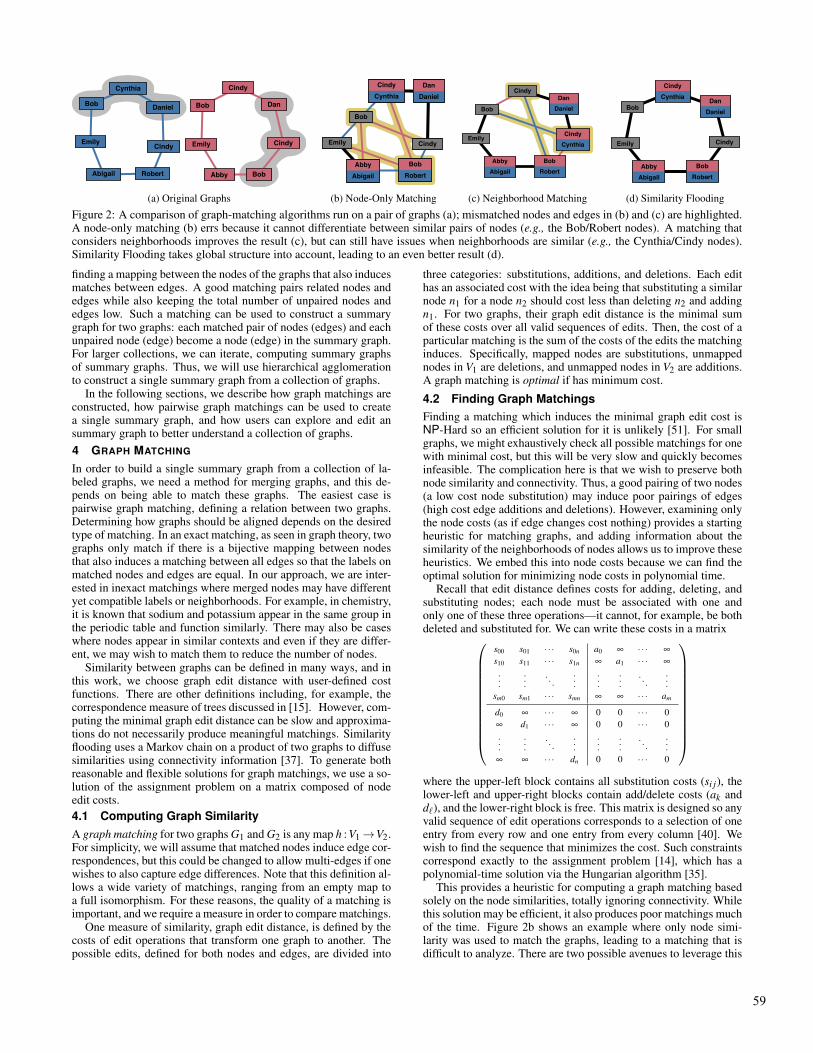
Figure 2: A comparison of graph-matching algorithms run on a pair of graphs (a); mismatched nodes and edges in (b) and (c) are highlighted.A node-only matching (b) errs because it cannot differentiate between similar pairs of nodes (e.g., the Bob/Robert nodes). A matching thatconsiders neighborhoods improves the result (c), but can still have issues when neighborhoods are similar (e.g., the Cynthia/Cindy nodes).Similarity Flooding takes global structure into account, leading to an even better result (d).

finding a mapping between the nodes of the graphs that also inducesmatches between edges. A good matching pairs related nodes andedges while also keeping the total number of unpaired nodes andedges low. Such a matching can be used to construct a summarygraph for two graphs: each matched pair of nodes (edges) and eachunpaired node (edge) become a node (edge) in the summary graph.For larger collections, we can iterate, computing summary graphsof summary graphs. Thus, we will use hierarchical agglomerationto construct a single summary graph from a collection of graphs.

In the following sections, we describe how graph matchings areconstructed, how pairwise graph matchings can be used to createa single summary graph, and how users can explore and edit ansummary graph to better understand a collection of graphs.4 GRAPH MATCHING

In order to build a single summary graph from a collection of la-beled graphs, we need a method for merging graphs, and this de-pends on being able to match these graphs. The easiest case ispairwise graph matching, defining a relation between two graphs.Determining how graphs should be aligned depends on the desiredtype of matching. In an exact matching, as seen in graph theory, twographs only match if there is a bijective mapping between nodesthat also induces a matching between all edges so that the labels onmatched nodes and edges are equal. In our approach, we are inter-ested in inexact matchings where merged nodes may have differentyet compatible labels or neighborhoods. For example, in chemistry,it is known that sodium and potassium appear in the same group inthe periodic table and function similarly. There may also be caseswhere nodes appear in similar contexts and even if they are differ-ent, we may wish to match them to reduce the number of nodes.

Similarity between graphs can be defined in many ways, and inthis work, we choose graph edit distance with user-defined costfunctions. There are other definitions including, for example, thecorrespondence measure of trees discussed in [15]. However, com-puting the minimal graph edit distance can be slow and approxima-tions do not necessarily produce meaningful matchings. Similarityflooding uses a Markov chain on a product of two graphs to diffusesimilarities using connectivity information [37]. To generate bothreasonable and flexible solutions for graph matchings, we use a so-lution of the assignment problem on a matrix composed of nodeedit costs.4.1 Computing Graph SimilarityA graph matching for two graphs G1 and G2 is any map h : V1→V2.For simplicity, we will assume that matched nodes induce edge cor-respondences, but this could be changed to allow multi-edges if onewishes to also capture edge differences. Note that this definition al-lows a wide variety of matchings, ranging from an empty map toa full isomorphism. For these reasons, the quality of a matching isimportant, and we require a measure in order to compare matchings.

One measure of similarity, graph edit distance, is defined by thecosts of edit operations that transform one graph to another. Thepossible edits, defined for both nodes and edges, are divided into

three categories: substitutions, additions, and deletions. Each edithas an associated cost with the idea being that substituting a similarnode n1 for a node n2 should cost less than deleting n2 and addingn1. For two graphs, their graph edit distance is the minimal sumof these costs over all valid sequences of edits. Then, the cost of aparticular matching is the sum of the costs of the edits the matchinginduces. Specifically, mapped nodes are substitutions, unmappednodes in V1 are deletions, and unmapped nodes in V2 are additions.A graph matching is optimal if has minimum cost.

4.2 Finding Graph MatchingsFinding a matching which induces the minimal graph edit cost isNP-Hard so an efficient solution for it is unlikely [51]. For smallgraphs, we might exhaustively check all possible matchings for onewith minimal cost, but this will be very slow and quickly becomesinfeasible. The complication here is that we wish to preserve bothnode similarity and connectivity. Thus, a good pairing of two nodes(a low cost node substitution) may induce poor pairings of edges(high cost edge additions and deletions). However, examining onlythe node costs (as if edge changes cost nothing) provides a startingheuristic for matching graphs, and adding information about thesimilarity of the neighborhoods of nodes allows us to improve theseheuristics. We embed this into node costs because we can find theoptimal solution for minimizing node costs in polynomial time.

Recall that edit distance defines costs for adding, deleting, andsubstituting nodes; each node must be associated with one andonly one of these three operations—it cannot, for example, be bothdeleted and substituted for. We can write these costs in a matrix

s00 s01 · · · s0n a0 ∞ · · · ∞

s10 s11 · · · s1n ∞ a1 · · · ∞

......

. . ....

......

. . ....

sm0 sm1 · · · smn ∞ ∞ · · · am

d0 ∞ · · · ∞ 0 0 · · · 0∞ d1 · · · ∞ 0 0 · · · 0...

.... . .

......

.... . .

...∞ ∞ · · · dn 0 0 · · · 0

where the upper-left block contains all substitution costs (si j), thelower-left and upper-right blocks contain add/delete costs (ak andd`), and the lower-right block is free. This matrix is designed so anyvalid sequence of edit operations corresponds to a selection of oneentry from every row and one entry from every column [40]. Wewish to find the sequence that minimizes the cost. Such constraintscorrespond exactly to the assignment problem [14], which has apolynomial-time solution via the Hungarian algorithm [35].

This provides a heuristic for computing a graph matching basedsolely on the node similarities, totally ignoring connectivity. Whilethis solution may be efficient, it also produces poor matchings muchof the time. Figure 2b shows an example where only node simi-larity was used to match the graphs, leading to a matching that isdifficult to analyze. There are two possible avenues to leverage this

59

heuristic: either use it to guide a search algorithm or try to encodeconnectivity information into the matrix.Finding Low-Cost Matchings. Our goal is to find a matching withlow cost. There are a number of search algorithms that serve toexplore the space of all possible matchings. One of the most well-known search algorithms is A∗ which is a best-first search strategythat uses estimates of costs to guide exploration to an optimal so-lution [30]. Beam search uses similar estimates but unlike A∗, itis a breadth-first search; at each step, each potential solution is ex-tended by adding one new node substitution and calculating the costof each new partial solution (both the known cost based on the editdistance costs and the remaining cost estimated from the node-onlyheuristic described above). Then, only the k partial solutions withthe least cost are kept; the rest are discarded. At the end, we willhave the lowest-cost solution among those that were not pruned, butnote that because our node-based heuristic underestimates costs, itis possible that an optimal solution was pruned.Using Neighborhood Information. We can also improve match-ings by encoding connectivity and neighborhood information intothe matrix our heuristic algorithm uses. Riesen et al. propose en-coding the best case edge substitution, deletion, and addition costsinto the node costs [40]. For example, a substitution v1→ v2 meansthat our best case scenario is that all edges connecting to v1 willmatch those edges connecting to v2 at minimal cost. We can calcu-late the cost of this scenario by adding the costs of these substitu-tions to the costs of adding or deleting the remaining edges. Thiscould also be extended to include matching the nodes on the otherside of the edge. Figure 2c shows the result of including neighborinformation in the heuristic; note that it still produces a sub-optimalsolution because it only considers the immediate neighborhood.Similarity Flooding. In order to better globally align graphs, weneed to include more information about the full neighborhoods ofeach node into substitution costs. Similarity flooding [37] is an it-erative process that propagates individual similarities between pairsof nodes across the entire graph. It works by using a direct productgraph whose nodes are the possible pairs of nodes from the inputgraphs and whose edges indicate positive correlations between pairsof nodes. Unlike a Cartesian product graph, a direct product graphonly includes an edge when both input graphs contain it.

The algorithm works by, at each step, calculating a new cost foreach node in the product graph G based on its current cost and thecosts of its neighbors. In this way, the cost of a given product nodecan eventually influence all of the other nodes it could be alignedwith (some nodes will be incompatible). More formally, if we letπk be the normalized vector of product node costs at the kth step,A(G) be the adjacency matrix of the product graph, and c(G) be theinitial costs expanded as a vector, we can write the iteration as:

πk+1 = αA(G)πk +(1−α)c(G)

where α is a parameter that controls the balance between diffusionand the initial costs [42]. This corresponds to the power method foreigenvector computation, and thus, this process will converge to π∞

which can then be used as our improved node substitution costs.With this solution, we can proceed to obtain a matching via the

Hungarian algorithm as before. Because of the diffusion, the newmatrix contains scores that better incorporate connectivity informa-tion. Figure 2d shows that this approach allows us to compute a bet-ter match than a node-only or neighborhood-based matching. Ourtool allows the use of both beam search and similarity flooding tocompute pairwise matchings.

5 SUMMARY GRAPH CONSTRUCTION

A summary graph of two graphs is generated from a graph matchingin a straightforward manner. If nodes are matched, we create a newcompound node; if not, we create individual nodes representing theunmatched nodes. More formally, given a graph matching h : V →V ′ for graphs G1,G2, we can create a summary graph G by defining

PythonSource

vtkDataSetReader

vtkDataSetMapper

vtkActorvtkLODActor

vtkRenderer

VTKCell

vtkScalarBarActor

vtkColorTransferFunctionvtkLookupTable

vtkImageClipvtkImageDataGeometryFilter

vtkImageResamplevtkImageReslicevtkWarpScalar

PythonSourcevtkElevationFiltervtkOutlineFilter

vtkPolyDataMapper

vtkActor

vtkProperty

vtkCubeAxesActor2D

vtkCamera

File

vtkPolyDataNormals

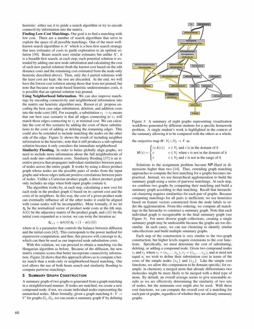
Figure 3: A summary of eight graphs representing visualizationworkflows generated by different students for a specific homeworkproblem. A single student’s work is highlighted in the context ofthe summary allowing it to be compared with the others as a whole.

the surjective map M : V1∪V2→ V as

M(v) =

(v,h(v)) v ∈V1 and v is in the domain of hv v ∈V1 when v is not in the domain of hv v ∈V2 and v is not in the range of h

Solutions to the assignment problem become NP-Hard in di-mensions higher than two [14]. Thus, extending graph matchingapproaches to compute the best matching for n graphs becomes im-practical. Instead, we use hierarchical agglomeration to build thesummary graph using a series of pairwise matchings. At each step,we combine two graphs by computing their matching and build asummary graph according to that matching. Recall that hierarchi-cal clustering requires similarities for each pair of graphs. Becausecomputing matchings for all pairs is inefficient, we use heuristicsbased on feature vectors constructed from the node labels to or-der the agglomeration. From this ordering, we compute all match-ings in the hierarchy to construct a summary graph. Note that eachindividual graph is recognizable in the final summary graph (seeFigure 3). For more diverse graph collections, creating a singlesummary graph may be undesirable because the graphs are too dis-similar. In such cases, we can use clustering to identify similarsubcollections and build multiple summary graphs.

Each step of the construction is very similar to the two-graphconstruction, but higher levels require extensions to the cost func-tions. Specifically, we must determine the cost of substituting,deleting, or adding a compound node. Given two compound nodesvi and v j where vi = (vi1 , . . .vim), v j = (v j1 , . . .v jn), and m need notequal n, we wish to define their substitution cost in terms of thecosts of the simple nodes {vik} and {v j`}. Like the simple costfunctions, we allow this computation to be domain-specific; for ex-ample, in chemistry a merged atom that already differentiates twomolecules might be more likely to be merged with a third type ofatom. By default, an overall average seems to give reasonable re-sults as we are effectively determining the similarity of two setsof nodes, but the minimum cost might also be used. With thesecost functions, we can compute the overall cost of a matching foreach pair of graphs, regardless of whether they are already summarygraphs.

60

N

C

C

C

N

H

(a) Original Graph

N

C

H C

N

C

C

N

(b) Broken Nodes

C

C

CN

N

CN

H

(c) Joined Nodes

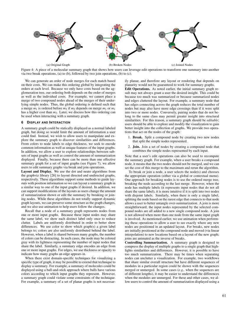
Figure 4: A piece of a molecular summary graph that shows how users can leverage edit operations to transform one summary into anothervia two break operations, (a) to (b), followed by two join operations, (b) to (c).

We can generate an order of node merges for each match basedon their costs. We can make this ordering global by integrating theorders at each level. Because we only have costs based on the ag-glomeration tree, our ordering both depends on the order of mergesas well as the individual costs. For example, we cannot place amerge of two compound nodes ahead of the merges of their under-lying simple nodes. Thus, the global ordering is defined such thata merge m1 is ordered before m2 if m2 depends on merge m1 or m1has a higher cost than m2. Later, we discuss how this ordering canbe used when interacting with a summary graph.

6 DISPLAY AND INTERACTION

A summary graph could be statically displayed as a normal labeledgraph, but doing so would limit the amount of information a usercould find. Instead, we wish to allow users to manipulate and ex-plore the summary graph to discover similarities and differences.From colors to node labels to edge thickness, we seek to encodecommon information as well as unique features of the input graphs.In addition, we allow a user to explore relationships between sub-sets of input graphs as well as control the amount of summarizationdisplayed. Finally, because there can be more than one effectivesummary graph for a set of input graphs (see Figure 7), we allowusers to edit summary graphs via break and join operations.Layout and Display. We use the dot and neato algorithms fromthe graphviz library [26] to layout directed and undirected graphs,respectively. These algorithms support some methods to guide lay-outs with position information so we can layout a summary graph ina similar way to one of the input graphs if desired. In addition, wecan support modifications of the layouts as users change the amountof summarization shown or edit the summary by breaking or join-ing nodes. While these algorithms do not totally support dynamicgraph layouts, we can preserve some structure as the graph changes,and we also use animation to help users follow the changes.

Recall that a node of a summary graph represents nodes fromone or more input graphs. Because these input nodes may sharethe same label, we show each distinct label only once to reduceclutter. Labels are uniformly distributed in order to better showdifferences. We use color to show which graph(s) a given labelbelongs to; colors are also uniformly distributed behind the label.However, when a label is shared between many graphs, the numberof colors can be distracting. In such cases, the node may be coloredgray with its lightness representing the number of input nodes thatshare the label. Similarly, a summary edge encodes an edge fromone or more input graphs. For edges, we use thickness or opacity toindicate how many graphs an edge appears in.

When there exist domain-specific techniques for visualizing aspecific type of graph, it may be possible to extend that technique todisplay a summary. For example, a summary of molecules could bedisplayed using a ball-and-stick approach where balls have variouscolors according to which input graphs they represent. However,a summary graph could violate some constraints of the technique.For example, a summary of a set of planar graphs is not necessar-

ily planar, and therefore any layout or rendering that depends onplanarity would not be guaranteed to work for summary graphs.Edit Operations. As noted earlier, the initial summary graph re-sult may not always grant a user the desired insight. This could bebecause too much was summarized or because summarized nodesand edges cluttered the layout. For example, a summary node thathas edges connecting across the graph reduces the total number ofnodes but may also have more edge crossings than if it were splitinto two or more nodes. Conversely, pairing nodes that do not be-long to the same class may permit greater insight into structuralsimilarities. For this reason, a summary graph should be editable;users should be able to explore and modify the visualization to gainbetter insight into the collection of graphs. We provide two opera-tions that act on the nodes of the graph:

1. Break. Split a compound node by creating two new nodesthat split the simple nodes represented.

2. Join. Join a set of nodes by creating a compound node thatcombines the simple nodes represented by each input.

Note that a user’s edit operations can also be used to recomputethe summary graph. For example, when a user breaks a compoundnode, it means that the two nodes should not be merged, and we canset the cost of this merge to the maximum and rerun the algorithm.

To break or join a node, a user selects the node(s) and choosesthe appropriate operation (either via a global or contextual menu).One approach for breaking nodes is to use the ordered merge tree,breaking the node according to the last merge. However, when thenode has multiple labels (it represents input nodes that do not allshare the same label), it is more intuitive if it is split into two nodeswith disjoint labels. Similarly, when there is only a single label,splitting the node based on the rarest edge that connects to that nodeallows a user to better untangle over-summarization. A join is morestraightforward; the input nodes represented by the selected com-pound nodes are all added to a new single compound node. A joinis not allowed when more than one node from the same input graphis involved. As mentioned earlier, we use animation when perform-ing these operations to allow a user to see exactly where any newnodes are positioned in an updated layout. For breaks, new nodesare initially positioned at the compound node and moved (via linearinterpolation) to new locations based on a layout of the new graph;joins are animated as the inverse of breaks.Controlling Summarization. A summary graph is designed tocompress the display of multiple graphs to a single graph that high-lights similarities and differences. However, it is possible to havetoo much summarization. There may be times when separatingnodes can unclutter a visualization. For example, two workflowsthat share similar overall structure but have different sequences ofmodules in a particular region could be shown with the sequencesmerged or unmerged. In some cases (e.g., when the sequences areof different lengths), it may be easier to understand the differenceswhen the modules are unmerged. For these and other cases, we al-low users to control the amount of summarization displayed using a

61

1.8.1.4

1.2.4.21.2.7.3

1.2.4.2

2.3.1.61

6.2.1.46.2.1.46.2.1.5

1.1.1.42

1.1.1.41

1.1.1.42

2.3.3.84.1.3.6

1.3.5.11.3.99.1

4.2.1.2

4.2.1.3

4.2.1.3

2.3.3.1

1.1.1.37

6.4.1.1

1.2.4.1

1.2.4.1

1.8.1.4

2.3.1.12

4.1.1.324.1.1.49

1.2.7.1

Nematode

Fruit Fly

E. Coli

Human

Maize

Castor Bean

Budding Yeast

H. pylori

(a) All Colors

1.8.1.4

1.2.4.21.2.7.3

1.2.4.2

2.3.1.61

6.2.1.46.2.1.46.2.1.5

1.1.1.42

1.1.1.41

1.1.1.42

2.3.3.84.1.3.6

1.3.5.11.3.99.1

4.2.1.2

4.2.1.3

4.2.1.3

2.3.3.1

1.1.1.37

6.4.1.1

1.2.4.1

1.2.4.1

1.8.1.4

2.3.1.12

4.1.1.324.1.1.49

1.2.7.1

(b) Highlighting

1.8.1.4

1.2.4.2

1.2.4.2

2.3.1.61

6.2.1.46.2.1.46.2.1.5

1.1.1.42

1.1.1.41

1.1.1.42

2.3.3.84.1.3.6

1.3.5.11.3.99.1

4.2.1.2

4.2.1.3

4.2.1.3

2.3.3.1

1.1.1.37

1.2.4.1

1.2.4.1

1.8.1.4

2.3.1.12

4.1.1.49

(c) Hiding Graphs

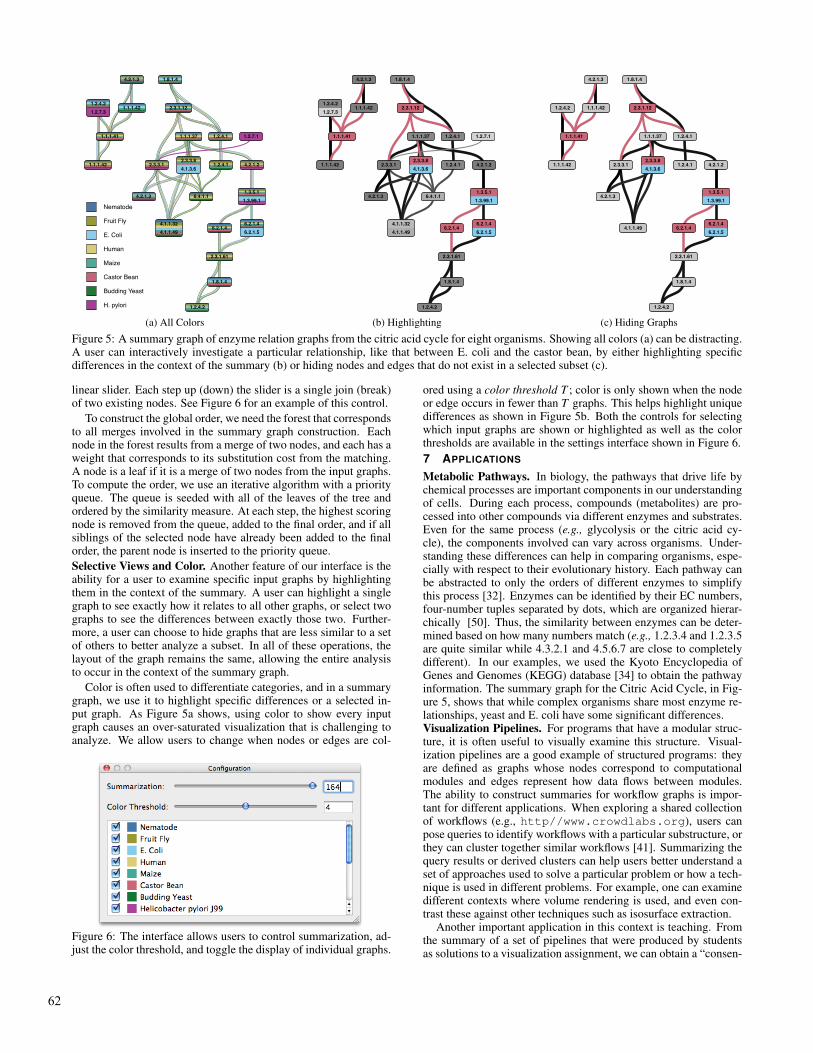
Figure 5: A summary graph of enzyme relation graphs from the citric acid cycle for eight organisms. Showing all colors (a) can be distracting.A user can interactively investigate a particular relationship, like that between E. coli and the castor bean, by either highlighting specificdifferences in the context of the summary (b) or hiding nodes and edges that do not exist in a selected subset (c).

linear slider. Each step up (down) the slider is a single join (break)of two existing nodes. See Figure 6 for an example of this control.

To construct the global order, we need the forest that correspondsto all merges involved in the summary graph construction. Eachnode in the forest results from a merge of two nodes, and each has aweight that corresponds to its substitution cost from the matching.A node is a leaf if it is a merge of two nodes from the input graphs.To compute the order, we use an iterative algorithm with a priorityqueue. The queue is seeded with all of the leaves of the tree andordered by the similarity measure. At each step, the highest scoringnode is removed from the queue, added to the final order, and if allsiblings of the selected node have already been added to the finalorder, the parent node is inserted to the priority queue.Selective Views and Color. Another feature of our interface is theability for a user to examine specific input graphs by highlightingthem in the context of the summary. A user can highlight a singlegraph to see exactly how it relates to all other graphs, or select twographs to see the differences between exactly those two. Further-more, a user can choose to hide graphs that are less similar to a setof others to better analyze a subset. In all of these operations, thelayout of the graph remains the same, allowing the entire analysisto occur in the context of the summary graph.

Color is often used to differentiate categories, and in a summarygraph, we use it to highlight specific differences or a selected in-put graph. As Figure 5a shows, using color to show every inputgraph causes an over-saturated visualization that is challenging toanalyze. We allow users to change when nodes or edges are col-

Figure 6: The interface allows users to control summarization, ad-just the color threshold, and toggle the display of individual graphs.

ored using a color threshold T ; color is only shown when the nodeor edge occurs in fewer than T graphs. This helps highlight uniquedifferences as shown in Figure 5b. Both the controls for selectingwhich input graphs are shown or highlighted as well as the colorthresholds are available in the settings interface shown in Figure 6.7 APPLICATIONS

Metabolic Pathways. In biology, the pathways that drive life bychemical processes are important components in our understandingof cells. During each process, compounds (metabolites) are pro-cessed into other compounds via different enzymes and substrates.Even for the same process (e.g., glycolysis or the citric acid cy-cle), the components involved can vary across organisms. Under-standing these differences can help in comparing organisms, espe-cially with respect to their evolutionary history. Each pathway canbe abstracted to only the orders of different enzymes to simplifythis process [32]. Enzymes can be identified by their EC numbers,four-number tuples separated by dots, which are organized hierar-chically [50]. Thus, the similarity between enzymes can be deter-mined based on how many numbers match (e.g., 1.2.3.4 and 1.2.3.5are quite similar while 4.3.2.1 and 4.5.6.7 are close to completelydifferent). In our examples, we used the Kyoto Encyclopedia ofGenes and Genomes (KEGG) database [34] to obtain the pathwayinformation. The summary graph for the Citric Acid Cycle, in Fig-ure 5, shows that while complex organisms share most enzyme re-lationships, yeast and E. coli have some significant differences.Visualization Pipelines. For programs that have a modular struc-ture, it is often useful to visually examine this structure. Visual-ization pipelines are a good example of structured programs: theyare defined as graphs whose nodes correspond to computationalmodules and edges represent how data flows between modules.The ability to construct summaries for workflow graphs is impor-tant for different applications. When exploring a shared collectionof workflows (e.g., http//www.crowdlabs.org), users canpose queries to identify workflows with a particular substructure, orthey can cluster together similar workflows [41]. Summarizing thequery results or derived clusters can help users better understand aset of approaches used to solve a particular problem or how a tech-nique is used in different problems. For example, one can examinedifferent contexts where volume rendering is used, and even con-trast these against other techniques such as isosurface extraction.

Another important application in this context is teaching. Fromthe summary of a set of pipelines that were produced by studentsas solutions to a visualization assignment, we can obtain a “consen-

62

OS

C

C

N

C

N

CN

CN

NC

H

H

H

H

NS

H

S

C

C

N

C

N

C

N

N

C

H

H

H

H

N H

H

O

N

H

S

C

H

H

S

C

C

N

C

N

CN

N

C

H

H

H

H

N

H

O

S

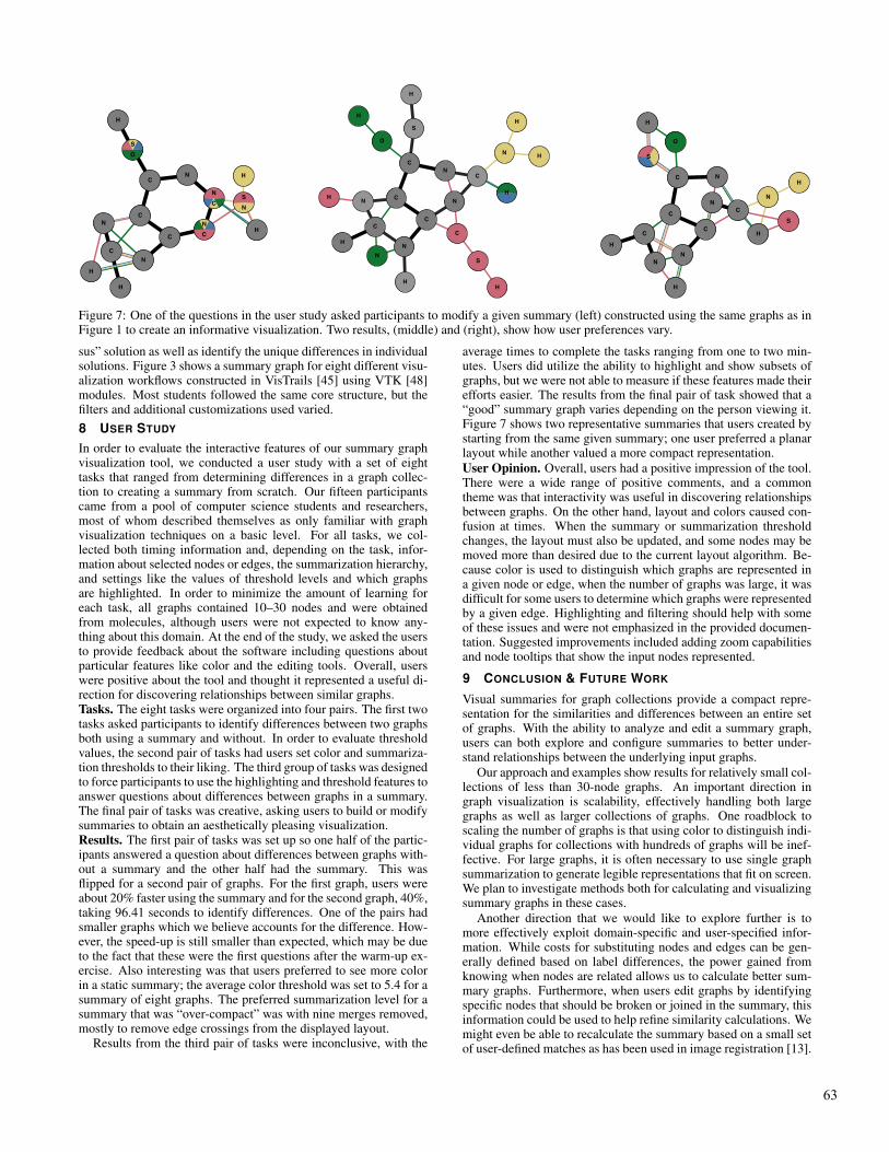
Figure 7: One of the questions in the user study asked participants to modify a given summary (left) constructed using the same graphs as inFigure 1 to create an informative visualization. Two results, (middle) and (right), show how user preferences vary.

sus” solution as well as identify the unique differences in individualsolutions. Figure 3 shows a summary graph for eight different visu-alization workflows constructed in VisTrails [45] using VTK [48]modules. Most students followed the same core structure, but thefilters and additional customizations used varied.8 USER STUDY

In order to evaluate the interactive features of our summary graphvisualization tool, we conducted a user study with a set of eighttasks that ranged from determining differences in a graph collec-tion to creating a summary from scratch. Our fifteen participantscame from a pool of computer science students and researchers,most of whom described themselves as only familiar with graphvisualization techniques on a basic level. For all tasks, we col-lected both timing information and, depending on the task, infor-mation about selected nodes or edges, the summarization hierarchy,and settings like the values of threshold levels and which graphsare highlighted. In order to minimize the amount of learning foreach task, all graphs contained 10–30 nodes and were obtainedfrom molecules, although users were not expected to know any-thing about this domain. At the end of the study, we asked the usersto provide feedback about the software including questions aboutparticular features like color and the editing tools. Overall, userswere positive about the tool and thought it represented a useful di-rection for discovering relationships between similar graphs.Tasks. The eight tasks were organized into four pairs. The first twotasks asked participants to identify differences between two graphsboth using a summary and without. In order to evaluate thresholdvalues, the second pair of tasks had users set color and summariza-tion thresholds to their liking. The third group of tasks was designedto force participants to use the highlighting and threshold features toanswer questions about differences between graphs in a summary.The final pair of tasks was creative, asking users to build or modifysummaries to obtain an aesthetically pleasing visualization.Results. The first pair of tasks was set up so one half of the partic-ipants answered a question about differences between graphs with-out a summary and the other half had the summary. This wasflipped for a second pair of graphs. For the first graph, users wereabout 20% faster using the summary and for the second graph, 40%,taking 96.41 seconds to identify differences. One of the pairs hadsmaller graphs which we believe accounts for the difference. How-ever, the speed-up is still smaller than expected, which may be dueto the fact that these were the first questions after the warm-up ex-ercise. Also interesting was that users preferred to see more colorin a static summary; the average color threshold was set to 5.4 for asummary of eight graphs. The preferred summarization level for asummary that was “over-compact” was with nine merges removed,mostly to remove edge crossings from the displayed layout.

Results from the third pair of tasks were inconclusive, with the

average times to complete the tasks ranging from one to two min-utes. Users did utilize the ability to highlight and show subsets ofgraphs, but we were not able to measure if these features made theirefforts easier. The results from the final pair of task showed that a“good” summary graph varies depending on the person viewing it.Figure 7 shows two representative summaries that users created bystarting from the same given summary; one user preferred a planarlayout while another valued a more compact representation.User Opinion. Overall, users had a positive impression of the tool.There were a wide range of positive comments, and a commontheme was that interactivity was useful in discovering relationshipsbetween graphs. On the other hand, layout and colors caused con-fusion at times. When the summary or summarization thresholdchanges, the layout must also be updated, and some nodes may bemoved more than desired due to the current layout algorithm. Be-cause color is used to distinguish which graphs are represented ina given node or edge, when the number of graphs was large, it wasdifficult for some users to determine which graphs were representedby a given edge. Highlighting and filtering should help with someof these issues and were not emphasized in the provided documen-tation. Suggested improvements included adding zoom capabilitiesand node tooltips that show the input nodes represented.

9 CONCLUSION & FUTURE WORK

Visual summaries for graph collections provide a compact repre-sentation for the similarities and differences between an entire setof graphs. With the ability to analyze and edit a summary graph,users can both explore and configure summaries to better under-stand relationships between the underlying input graphs.

Our approach and examples show results for relatively small col-lections of less than 30-node graphs. An important direction ingraph visualization is scalability, effectively handling both largegraphs as well as larger collections of graphs. One roadblock toscaling the number of graphs is that using color to distinguish indi-vidual graphs for collections with hundreds of graphs will be inef-fective. For large graphs, it is often necessary to use single graphsummarization to generate legible representations that fit on screen.We plan to investigate methods both for calculating and visualizingsummary graphs in these cases.

Another direction that we would like to explore further is tomore effectively exploit domain-specific and user-specified infor-mation. While costs for substituting nodes and edges can be gen-erally defined based on label differences, the power gained fromknowing when nodes are related allows us to calculate better sum-mary graphs. Furthermore, when users edit graphs by identifyingspecific nodes that should be broken or joined in the summary, thisinformation could be used to help refine similarity calculations. Wemight even be able to recalculate the summary based on a small setof user-defined matches as has been used in image registration [13].

63

REFERENCES

[1] E. N. Adams, III. Consensus techniques and the comparison of taxo-nomic trees. Systematic Zoology, 21(4):390–397, 1972.

[2] D. Archambault. Structural differences between two graphs throughhierarchies. In Proc. of Graphics Interface 2009, pages 87–94. Cana-dian Information Processing Society, 2009.

[3] D. Archambault, T. Munzner, and D. Auber. Topolayout: Multi-level graph layout by topological features. IEEE Trans. Vis. Comput.Graph., 13(2):305–317, 2007.

[4] D. Archambault, H. C. Purchase, and B. Pinaud. Difference map read-ability for dynamic graphs. In Proc. 18th Int’l Conf. Graph Drawing,pages 50–61. Springer-Verlag, 2011.

[5] M. Balzer and O. Deussen. Level-of-detail visualization of clusteredgraph layouts. In Proc. Asia-Pacific Symp. Vis., pages 133–140, 2007.

[6] Z. Bao, S. Cohen-Boulakia, S. Davidson, and P. Girard. PDiffView:Viewing the difference in provenance of workflow results. PVLDB,2(2):1638–1641, 2009.

[7] F. Beck, M. Burch, and S. Diehl. Towards an aesthetic dimensionsframework for dynamic graph visualisations. In Proc. IEEE InfoVis2009, pages 592–597, 2009.

[8] F. Beck and S. Diehl. Visual comparison of software architectures. InProc. 5th Int’l Symp. Software Vis., pages 183–192. ACM, 2010.

[9] T. Blasius, S. G. Kobourov, and I. Rutter. Simultaneous embedding ofplanar graphs. CoRR, abs/1204.5853, 2012.

[10] R. Bourqui and F. Jourdan. Revealing subnetwork roles using contex-tual visualization: Comparison of metabolic networks. In Proc. IEEEInfoVis 2008, pages 638–643, 2008.

[11] U. Brandes, J. Lerner, M. Lubbers, C. McCarty, and J. Molina. Visualstatistics for collections of clustered graphs. In IEEE Pacific Visual-ization Symposium, 2008, pages 47–54, 2008.

[12] S. Bremm, T. von Landesberger, M. Hess, T. Schreck, P. Weil, andK. Hamacher. Interactive visual comparison of multiple trees. In Proc.IEEE VAST 2011, pages 31–40, 2011.

[13] L. G. Brown. A survey of image registration techniques. ACM Com-put. Surv., 24(4):325–376, 1992.

[14] R. E. Burkard, M. Dell’Amico, and S. Martello. Assignment Prob-lems. SIAM, 2009.

[15] F. Chevalier, D. Auber, and A. Telea. Structural analysis and visualiza-tion of C++ code evolution using syntax trees. In 9th Int’l Workshopon Principles of Software Evolution, pages 90–97, 2007.

[16] C. Collberg, S. Kobourov, J. Nagra, J. Pitts, and K. Wampler. A systemfor graph-based visualization of the evolution of software. In Proc.ACM Symp. on Software Vis., pages 77–86. ACM, 2003.

[17] E. Di Giacomo, W. Didimo, M. van Kreveld, G. Liotta, and B. Speck-mann. Matched drawings of planar graphs. In Proc. 15th Int’l Conf.Graph Drawing, pages 183–194. Springer-Verlag, 2008.

[18] S. Diehl and C. Gorg. Graphs, they are changing. In Proc. 10th Int’lSymp. Graph Drawing, pages 23–30. Springer-Verlag, 2002.

[19] P. Eades and Q.-W. Feng. Multilevel visualization of clustered graphs.In S. North, editor, Graph Drawing, volume 1190 of Lecture Notes inComputer Science, pages 101–112. Springer, 1997.

[20] N. Elmqvist and J.-D. Fekete. Hierarchical aggregation for informa-tion visualization: Overview, techniques, and design guidelines. IEEETrans. Vis. Comput. Graph., 16:439–454, 2010.

[21] C. Erten, S. G. Kobourov, V. Le, and A. Navabi. Simultaneous graphdrawing: Layout algorithms and visualization schemes. Journal ofGraph Algortihms and Applications, 9(1):165–182, 2005.

[22] J. Freire, C. Silva, S. Callahan, E. Santos, C. Scheidegger, and H. Vo.Managing rapidly-evolving scientific workflows. In Int’l Provenanceand Annotation Workshop, LNCS 4145, pages 10–18. Springer, 2006.

[23] M. Freire, C. Plaisant, B. Shneiderman, and J. Golbeck. Manynets:an interface for multiple network analysis and visualization. In Proc.SIGCHI 2010, pages 213–222. ACM, 2010.

[24] G. W. Furnas and J. Zacks. Multitrees: enriching and reusing hierar-chical structure. In Proc. SIGCHI 1994, pages 330–336, 1994.

[25] E. Gansner, Y. Koren, and S. North. Topological fisheye views for vi-sualizing large graphs. IEEE Trans. Vis. Comput. Graph., 11(4):457–468, 2005.

[26] E. R. Gansner and S. C. North. An open graph visualization sys-

tem and its applications to software engineering. Softw. Pract. Exper.,30:1203–1233, 2000.

[27] M. R. Garey, D. S. Johnson, and L. Stockmeyer. Some simplified np-complete problems. In Proc. of ACM Symp. on Theory of Computing,pages 47–63, New York, NY, USA, 1974. ACM.

[28] M. Graham and J. Kennedy. Exploring multiple trees through DAGrepresentations. IEEE Trans. Vis. Comput. Graph., 13:1294–1301,2007.

[29] M. Graham and J. B. Kennedy. A survey of multiple tree visualisation.Information Visualization, 9(4):235–252, 2010.

[30] P. Hart, N. Nilsson, and B. Raphael. A formal basis for the heuris-tic determination of minimum cost paths. IEEE Trans. Syst. Sci. andCybern., 4(2):100–107, 1968.

[31] I. Herman, G. Melancon, and M. Marshall. Graph visualization andnavigation in information visualization: A survey. IEEE Trans. Vis.Comput. Graph., 6(1):24–43, 2000.

[32] M. Heymans and A. K. Singh. Deriving phylogenetic trees from thesimilarity analysis of metabolic pathways. In ISMB (Supplement ofBioinformatics), pages 138–146, 2003.

[33] D. Holten. Hierarchical edge bundles: Visualization of adjacency rela-tions in hierarchical data. IEEE Trans. Vis. Comput. Graph., 12:741–748, 2006.

[34] M. Kanehisa and S. Goto. KEGG: Kyoto Encyclopedia of Genes andGenomes. Nucleic Acids Research, 28(1):27–30, 2000.

[35] H. W. Kuhn. The hungarian method for the assignment problem.Naval Research Logistics Quarterly, 2(1-2):83–97, 1955.

[36] E. A. Leicht, P. Holme, and M. E. J. Newman. Vertex similarity innetworks. Phys. Rev. E, 73:026120, 2006.

[37] S. Melnik, H. Garcia-Molina, and E. Rahm. Similarity flooding:A versatile graph matching algorithm and its application to schemamatching. In Proc. 18th Int’l Conf. Data Eng., pages 117–128, 2002.

[38] T. Munzner, F. Guimbretiere, S. Tasiran, L. Zhang, and Y. Zhou. Tree-juxtaposer: scalable tree comparison using focus+context with guar-anteed visibility. ACM Trans. Graph., 22:453–462, 2003.

[39] C. Plaisant, J.-D. Fekete, and G. Grinstein. Promoting insight-basedevaluation of visualizations: From contest to benchmark repository.IEEE Trans. Vis. Comput. Graph., 14(1):120–134, 2008.

[40] K. Riesen and H. Bunke. Approximate graph edit distance compu-tation by means of bipartite graph matching. Image Vision Comput.,27:950–959, 2009.

[41] E. Santos, L. Lins, J. P. Ahrens, J. Freire, and C. T. Silva. A firststudy on clustering collections of workflow graphs. In IPAW, pages160–173, 2008.

[42] C. E. Scheidegger, H. T. Vo, D. Koop, J. Freire, and C. T. Silva. Query-ing and creating visualizations by analogy. IEEE Trans. Vis. Comput.Graph., 13(6):1560–1567, 2007.

[43] K. Thiel and M. R. Berthold. Node similarities from spreading activa-tion. IEEE Int’l Conf. on Data Mining, pages 1085–1090, 2010.

[44] S. Vilar, R. Harpaz, E. Uriarte, L. Santana, R. Rabadan, and C. Fried-man. Drug–drug interaction through molecular structure similarityanalysis. J. Am. Med. Inform. Assoc., 2012.

[45] VisTrails. http://www.vistrails.org.[46] T. von Landesberger, M. Gorner, and T. Schreck. Visual analysis of

graphs with multiple connected components. In Proc. IEEE VAST2009, pages 155–162, 2009.

[47] T. von Landesberger, A. Kuijper, T. Schreck, J. Kohlhammer, J. vanWijk, J.-D. Fekete, and D. Fellner. Visual analysis of large graphs:State-of-the-art and future research challenges. Computer GraphicsForum, 30(6):1719–1749, 2011.

[48] VTK. http://www.vtk.org.[49] M. Wattenberg. Visual exploration of multivariate graphs. In Proc.

SIGCHI 2006, pages 811–819. ACM, 2006.[50] E. C. Webb. Enzyme nomenclature 1992. Recommendations of the

Nomenclature Committee of the Int’l Union of Biochemistry andMolecular Biology on the Nomenclature and Classification of En-zymes. Academic Press, 1992.

[51] Z. Zeng, A. K. H. Tung, J. Wang, J. Feng, and L. Zhou. Comparingstars: on approximating graph edit distance. PVLDB, 2:25–36, 2009.

64