Visual saliency detection: a Kalman filter based … · Visual saliency detection: a Kalman filter based ... which is based on self-information maximization of any region ... The

Visual saliency detection: a Kalman filter based approach

Sourya Roy1,* and Pabitra Mitra2

1Department of Instrumentation and Electronics Engineering,Jadavpur University, Kolkata-700032,India2Department of Computer Science and Engineering ,Indian Institute of Technology, Kharagpur -721302, India*[email protected]

Abstract: In this paper we propose a Kalman filter aided saliency detection model which is basedon the conjecture that salient regions are considerably different from our ”visual expectation” orthey are ”visually surprising” in nature. In this work, we have structured our model with an im-mediate objective to predict saliency in static images. However, the proposed model can be easilyextended for space-time saliency prediction. Our approach was evaluated using two publicly avail-able benchmark data sets and results have been compared with other existing saliency models. Theresults clearly illustrate the superior performance of the proposed model over other approaches.

1. Introduction

Saccadic eye movement is one of most significant feature of human visual system which helps usto scan a scene with incredible celerity and robustness. During saccadic eye movement humaneyes rapidly moves from one point to another while simultaneously detecting interesting regions.Modelling and automatic detection of these salient regions which essentially seek attention of hu-man visual system, is currently a problem of considerable interest. It should be apparent that earlydetection of salient regions have numerous important applications. From scene understanding torapid target detection, more or less every computer vision task can be aided by saliency predic-tion. Previous approaches for saliency mapping can be divided into two groups: bottom up andtop down. Bottom up approaches relies on processing of inherent features (like contrast, edgesetc.)of the image and do not depend on any priori information, while top down hierarchy inspiredmethods assume that past experience and knowledge plays an important role in driving attention.

Bottom up saliency detection methods are generally termed as low level methods as they mostlyutilizes low level features of the image. These group of methods can be further classified intobiologically inspired approaches, purely computational techniques or methods which lies more orless in the middle-ground. Inspired from the feature integration theory [1]. the saliency modelproposed by Itti et al [2] is undoubtedly the most influential and significant work from the firstcategory. This biologically inspired model segregates the input image into several simple featuremaps and calculates center-surround difference for each map and finally combines them in a linearmanner to produce the master saliency map. Bruce and Tsotsos [16] proposed a saliency modelwhich is based on self-information maximization of any region relative to its surrounding. . Seoand Milanfar [3] also compared the center and surround using a self-resemblance measure.Murrayet. al [17] proposed a method which utilizes a low level vision model of color perception. Zhang

1

arX

iv:1

604.

0482

5v1

[cs

.CV

] 1

7 A

pr 2

016

Fig. 1. (a)Input image, (b) Saliency map using proposed method (with 3 feature channels),(c)Saliency map using proposed method (with 7 feature channels), (d) Human fixation densitymap

et al [4] computed saliency as a probability of target availability in a region. In 2005, Itti andBaldi [18] proposed a Bayesiansurprise based method defines saliency as a measure of surprise.Completely or partially computational approaches are also common in past literatures .

In this paper we propose a kalman filter based saliency detection mechanism which is motivatedby two much-discussed biological phenomena: 1) deviation from visual expectation or visual sur-prise [5] [6] [18] [9] and saccadic eye movement [7] [8]. Our algorithm does share the generalizednotion of surprise presented in a previous work [18] [9] by Itti and Baldi where they have proposeda method for video saliency detection, however using one of the most commonly used estimationtechnique i.e. Kalman filter, we have developed a more compact and flexible method for calcu-lating surprise based saliency in a static image and our model can be easily extended for videocase. Our algorithm has three main stages. First the color input image is split into low-level visualfeature channels. Based on the choice of feature channels, we have implemented two variants ofour model. The first one uses only three opponent color channels and the other one uses sevenfeatures channels [as in Itti-Koch model]. Then for each channel individual saliency map is gen-erated using Kalman filter algorithm and lastly all of them are combined to produce the final map.To employ kalman filter model for saliency mapping we have assumed that the input image is anoise corrupted measurement (perceived) signal and the true signal is an expected image which ourvisual system generates. So to produce the saliency map corresponding to a feature channel, wefirst estimate the expected counterpart of that specific channel using kalman filter. Then we simplycalculate the difference between the expected and perceived feature channel and define saliency asthe magnitude of difference. The main contributions of our work are as follows:

1) A definition of visual surprise in static image.2) A bottom-up saliency model based on Kalman filter.3) Evaluation of the proposed model on two popular benchmark data sets.

2. KALMAN FILTER BASED SALIENCY DETECTION

In this section we will describe our model thoroughly along with details of implementation. Thebasic architecture of the proposed algorithm has been shown in Fig. 2.

2

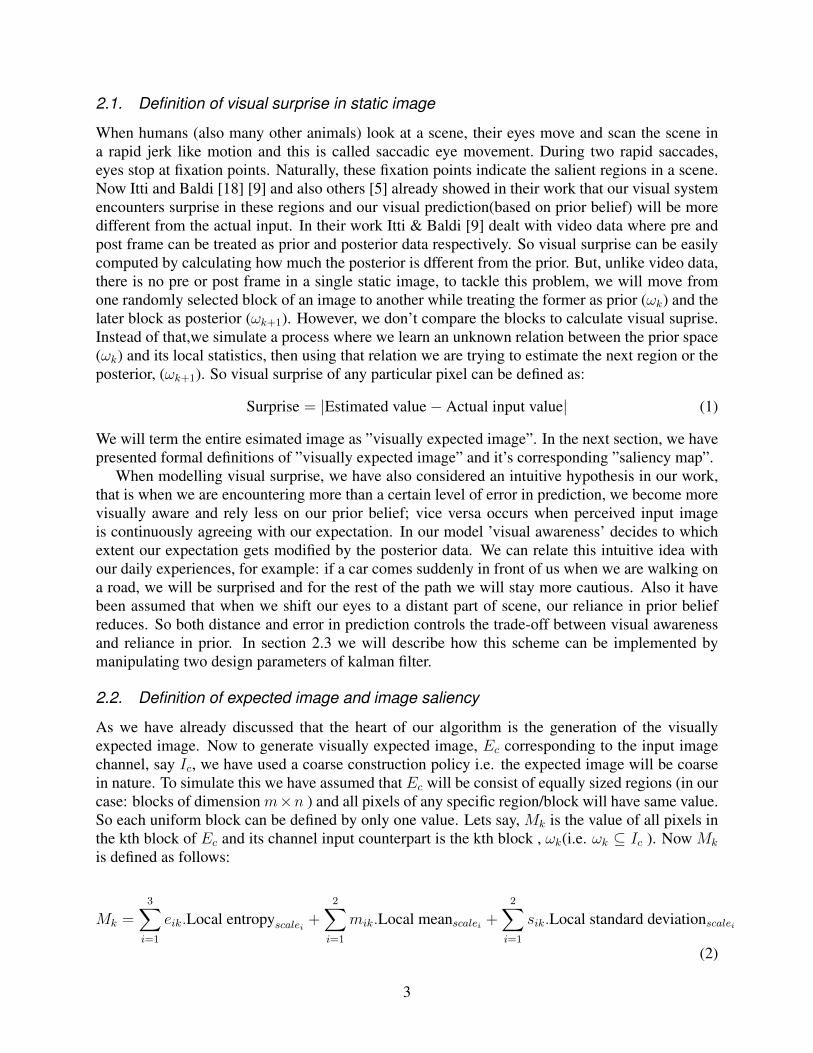
2.1. Definition of visual surprise in static image

When humans (also many other animals) look at a scene, their eyes move and scan the scene ina rapid jerk like motion and this is called saccadic eye movement. During two rapid saccades,eyes stop at fixation points. Naturally, these fixation points indicate the salient regions in a scene.Now Itti and Baldi [18] [9] and also others [5] already showed in their work that our visual systemencounters surprise in these regions and our visual prediction(based on prior belief) will be moredifferent from the actual input. In their work Itti & Baldi [9] dealt with video data where pre andpost frame can be treated as prior and posterior data respectively. So visual surprise can be easilycomputed by calculating how much the posterior is dfferent from the prior. But, unlike video data,there is no pre or post frame in a single static image, to tackle this problem, we will move fromone randomly selected block of an image to another while treating the former as prior (ωk) and thelater block as posterior (ωk+1). However, we don’t compare the blocks to calculate visual suprise.Instead of that,we simulate a process where we learn an unknown relation between the prior space(ωk) and its local statistics, then using that relation we are trying to estimate the next region or theposterior, (ωk+1). So visual surprise of any particular pixel can be defined as:

Surprise = |Estimated value− Actual input value| (1)

We will term the entire esimated image as ”visually expected image”. In the next section, we havepresented formal definitions of ”visually expected image” and it’s corresponding ”saliency map”.

When modelling visual surprise, we have also considered an intuitive hypothesis in our work,that is when we are encountering more than a certain level of error in prediction, we become morevisually aware and rely less on our prior belief; vice versa occurs when perceived input imageis continuously agreeing with our expectation. In our model ’visual awareness’ decides to whichextent our expectation gets modified by the posterior data. We can relate this intuitive idea withour daily experiences, for example: if a car comes suddenly in front of us when we are walking ona road, we will be surprised and for the rest of the path we will stay more cautious. Also it havebeen assumed that when we shift our eyes to a distant part of scene, our reliance in prior beliefreduces. So both distance and error in prediction controls the trade-off between visual awarenessand reliance in prior. In section 2.3 we will describe how this scheme can be implemented bymanipulating two design parameters of kalman filter.

2.2. Definition of expected image and image saliency

As we have already discussed that the heart of our algorithm is the generation of the visuallyexpected image. Now to generate visually expected image, Ec corresponding to the input imagechannel, say Ic, we have used a coarse construction policy i.e. the expected image will be coarsein nature. To simulate this we have assumed that Ec will be consist of equally sized regions (in ourcase: blocks of dimension m×n ) and all pixels of any specific region/block will have same value.So each uniform block can be defined by only one value. Lets say, Mk is the value of all pixels inthe kth block of Ec and its channel input counterpart is the kth block , ωk(i.e. ωk ⊆ Ic ). Now Mk

is defined as follows:

Mk =3∑

i=1

eik.Local entropyscalei+

2∑i=1

mik.Local meanscalei +2∑

i=1

sik.Local standard deviationscalei

(2)

3

Fig. 2. Flow diagram of the proposed model. This diagram represents the first variant of theproposed model which initially splits the input image into three opponent color maps and uses themas feature channel for saliency detection. The second variant follows exactly same framework asthis, but uses seven feature channels (one intensity, two color and four orientation channels).

Where Mk is a linear combination of local statistics. Our first task is to estimate the values ofthe coefficients (i.e. ei ,mi, si) of Mk and using that we will construct the coarse expected image,Ec. For this estimation purpose we have used Kalman filter. After constructing expected image Ec

associated with Ic, the saliency map Sc corresponding to Ic, can be computed as follows:

Sc = |Ic − Ec| (3)

After computing saliency map for each channel we combine them and apply center bias togenerate the final saliency map. However, before combining these channel saliency maps, weenhance them individually via contrast stretching to make the salient regions more conspicuous.

Though we have definedMk as a linear combination of statistics, our model doesn’t impose anyrestriction on the choice of Mk. Mk could have been more simpler or more thoughtfully craftednonlinear combination of features.

2.3. Kalman filter algorithm

In our work we have assumed that the input image is the measurement signal and the predictedimage by our visual system is the true signal. So using the Kalman filter algorithm [24] [25] [26]we will estimate the true signal using block to block random traversal policy which has beenalready described in previous section. Kalman filter is a very well-known estimator so we will justdescribe the main stages of the algorithm step by step below: The state variable form of the states(in our case the coefficients) can be described as :

xk+1 = Fkxk + wk (4)

where, xk =[x1k x2k x3k x4k x5k x6k x7k

]T is the state vector at kth instant. The statesare the coefficients of Mk (i.e. x1k = e1k, x2k = e2k, x3k = e3k, x4k = m1k, x5k = m2k, x6k =s1k, x7k = s2k).

Fk = I7 (identity matrix of size 7), is the state transition matrixwk is process noise(zero mean white Gaussian type)The observation signal can be represented using the following linear equation :

zk = Hkxk + vk (5)

4

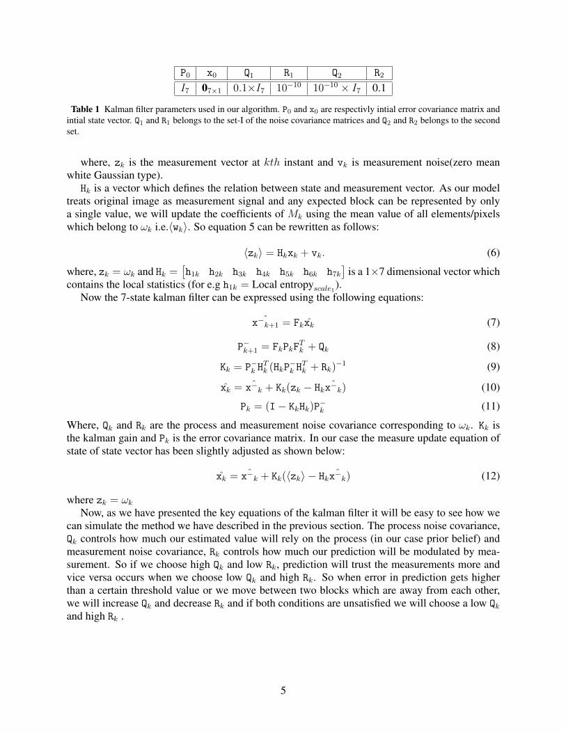
P0 x0 Q1 R1 Q2 R2

I7 07×1 0.1×I7 10−10 10−10 × I7 0.1

Table 1 Kalman filter parameters used in our algorithm. P0 and x0 are respectivly intial error covariance matrix andintial state vector. Q1 and R1 belongs to the set-I of the noise covariance matrices and Q2 and R2 belongs to the secondset.

where, zk is the measurement vector at kth instant and vk is measurement noise(zero meanwhite Gaussian type).

Hk is a vector which defines the relation between state and measurement vector. As our modeltreats original image as measurement signal and any expected block can be represented by onlya single value, we will update the coefficients of Mk using the mean value of all elements/pixelswhich belong to ωk i.e.〈wk〉. So equation 5 can be rewritten as follows:

〈zk〉 = Hkxk + vk. (6)

where, zk = ωk and Hk =[h1k h2k h3k h4k h5k h6k h7k

]is a 1×7 dimensional vector which

contains the local statistics (for e.g h1k = Local entropyscale1).

Now the 7-state kalman filter can be expressed using the following equations:

ˆx−k+1 = Fkx̂k (7)

P−k+1 = FkPkFTk + Qk (8)

Kk = P−k HTk (HkP

−k H

Tk + Rk)

−1 (9)

x̂k = ˆx−k + Kk(zk − Hk ˆx−k) (10)

Pk = (I− KkHk)P−k (11)

Where, Qk and Rk are the process and measurement noise covariance corresponding to ωk. Kk isthe kalman gain and Pk is the error covariance matrix. In our case the measure update equation ofstate of state vector has been slightly adjusted as shown below:

x̂k = ˆx−k + Kk(〈zk〉 − Hk ˆx−k) (12)

where zk = ωk

Now, as we have presented the key equations of the kalman filter it will be easy to see how wecan simulate the method we have described in the previous section. The process noise covariance,Qk controls how much our estimated value will rely on the process (in our case prior belief) andmeasurement noise covariance, Rk controls how much our prediction will be modulated by mea-surement. So if we choose high Qk and low Rk, prediction will trust the measurements more andvice versa occurs when we choose low Qk and high Rk. So when error in prediction gets higherthan a certain threshold value or we move between two blocks which are away from each other,we will increase Qk and decrease Rk and if both conditions are unsatisfied we will choose a low Qkand high Rk .

5

Fig. 3. Sample results of our model along with human fixation density maps and results fromother reference models. Column 1: Original input image, Column 2: Human fixation density map,Column 3: SUN [4] , Column 4: CIWM [17], Column 5: SR [3] ,Column 6: AIM [16], Column 7:RCSS [12], Column 8: saliency maps from our proposed KS-7

2.4. Implementation details

The first parameter we need to specify for our algorithm is the size of the blocks. To generateour results we have used blocks of size 25 x 25 (this has been selected empirically) and in all ofour simulations, where we initially down-sampled the input image to 400×300, this size providessatisfactory performance.

We already have shown that function Mk incorporates three local statistics at different scales.To employ this, initially we calculated two local standard deviation maps (considering 3x3 and5x5 neighborhood), two local mean maps (3x3 and 5x5 neighborhood) and three local entropymaps (5x5, 7x7 and 9x9 neighborhood) associated with the input image. Then when calculatingMk for the kth block we simply taken mean of the values from this feature maps, over only theregion which kth block specifies. Therefore the measurement vector Hk contains the seven valuescorresponding to ωk from these seven maps. Usually, tuning of kalman filter parameters is achallenging task but in our case tuning is not necessary as we are interested in coarse estimationof expected image. Furthermore, as expected image is a hypothetical signal and there is no precisedefinition of it, we cannot evaluate error in its estimation. Table 1 contains the values of kalmanfilter parameters which we have used. As we have said earlier we will oscillate between two sets of

6

values of Rk and Qk. When error between Mk and 〈ωk〉 goes above a certain threshold error or wemove from a block to another which does not belong to the neighborhood of the former (assuming4-connectivity), we will use the values from set-I (Q1 and R1); otherwise we will use set-II (Q2 andR2). The error between Mk and ωk can be defined as follows:

Errork = |Mk − 〈ωk〉 | (13)

The random traversal strategy is not critical for our algorithm, we could traverse among theblocks in any manner. But if we move from one block to another only in a nearest neighbor(alongany direction) sense, this can sometime slightly reduce the performance. Probabaly this is becausecontinuously navigating along similar region can lead to almost no changes in coefficient valuesfor a long time and then if a region even with little difference is introduced , it will produce moreerror. However in our algorithm we use large block size and avail a coarse construction strategy,so performance get negligibly affected by traversal strategy. Now if we don’t move in nearestneighbor manner, distance between blocks will also decide how much our current expectation willbe modulated by the prior belief.

For multi-scale implementation, along with the initially scaled input, we also produced saliencymaps corresponding to the half and quarter resolution images and then get the master saliency mapcombining these three saliency maps generated at three scales.

3. Experimental results

We have evaluated our proposed algorithm against two benchmark datasets: 1) Toronto dataset [10]and 2) MIT-300 dataset [27]. The Toronto human fixation dataset, collected by Bruce and Tsot-sos [10], is a well know benchmark dataset for visual saliency detection task which contains 120color images of equal dimensions (681 x 511) and eye fixation records from 20 human observers.MIT-300 is a relatively new dataset which contains 300 benchmark images of varying dimensions.It has been already stated that, in this work we have implented two different variants of our model.We will term the first implementation, which uses only three color channels, as ”KS-3” and theother one as ”KS-7” which utilizes seven feature channels.

Model AUC-Judd AUC-Borji CC SIM NSSAIM [16] 0.79 0.77 0.33 0.38 0.83SUN [4] 0.69 0.68 0.26 0.36 0.76SR [3] 0.77 0.76 0.40 0.41 1.10CIWM [17] 0 .75 0.74 0.35 0.38 0.96RCSS [12] 0.78 0.76 0.43 0.44 1.16KS-3 (proposed) 0.79 0.78 0.44 0.42 1.20KS-7 (proposed) 0.83 0.82 0.53 0.44 1.42

Table 2 Quantitative comparison between the proposed Kalman filter based method and other methods whenpredicting human eye fixations on Toronto data set [10].

3.1. Evaluation metrics

For quantitative evaluation we have used five standard metrics, namely AUC-Judd [27] [19], AUC-Borji [19], Correlation Coefficient (CC) [19], Similarity measure (SIM) [27] [19] and Normal-

7

ized Scanpath Saliency (NSS) [11] [19]. AUC-Judd and AUC-Borji are both area under theROC(Receiver operating characteristic) curve based metrics which convert the saliency maps intobinary maps and treat them as classifiers. The third metric CC or correlation coefficient is a linearmeasure which can be calculated as below:

CC =cov(S, F )

σS ∗ σF(14)

where S and F are saliency map and human fixation map respectively.The output range of CC metric is between -1 to +1. |CC output| = 1 denotes there is perfect

linear relationship exists between the ground fixation density map and saliency map. The simi-larity metric (SIM) compares fixation map and saliency map when they are viewed as normalizeddistributions. The similarity measure between normalized distributions,Sn and Fn can be given by:

SIM =N∑

x=1

min(Sn(x), Fn(x)) (15)

where,∑N

x=1 Sn(x) = 1 and∑N

x=1 Fn(x) = 1A similarity score of 1 denotes that the two distributions are identical. The last metric we used

for evaluation is Normalized Scanpath Saliency or NSS. This quantitative measure was proposedby Peteers and Itti [11] in 2005. The overall NSS score of a saliency map can be given by:

NSS =1

N

N∑x=1

Sn(x) (16)

where Sn and N denote normalized saliency map and the total number of human eye fixationsrespectively.

3.2. Performance on Toronto data set

On Toronto dataset, We have compared our results with five other saliency models which are: 1)SUN [4] 2) Information maximization model(AIM) [16] 3) Self resemblance model(SR) [3] and 4)Chromatic Induction wavelet model(CIWM) [17] and 5) Random Center Surround Model(RCSS) [12].Performances have been compared with the other methods both quantitatively (Table 2) and visu-ally (Fig.3). From Table 2, we can easily see that the 7 channel variant(KS-7) of the proposedapproach outperformed the other models against all metrics by a wide margin. Only Random Cen-ter Surround Saliency model gave similar performance in terms of similarity score. The 3 channelvariant of our algorithm, KS-3 also achieved state of the art performance on all metrics. As we cansee from the example images, our method is less susceptible to the edges than Zhang et al(SUN)and Bruce& Tsotsos(AIM). Though, CIWM and Self resemblance model(SR) sometimes demon-strated better edge suppression, these models tended to include large non-salient regions. Whencontrast between salient region and background is relatively low (e.g. sample image 7 in Figure3), only Bruce-Tsotos and Our model performed well. Zhang’s method(SUN) mainly highlightededges for most of the images.From visual inspection, it seems that RCSS model is more appro-priate for salient object detection rather than eye fixation prediction. RCSS also gave very poorperformance for both high entropy images and low contrast images. Qualitative comparison amongresults from different models also suggests that a large part of our success can be attributed to thesignificant reduction in false detection.

8

Fig. 4. ROC curves from both of the versions of our model, CIWM [17] and RCSS model [12]

In Figure 4, we have demonstrated the ROC (Receiver operating characteristic) curves forCIWM [17], RCSS [12] and the proposed method. As we can see from the plots, KS-7 demon-strates greater efficacy than the other models. ROC curves of RCSS and KS-3 are close to eachother while performance of CIWM is inferior to the other 3 models.

3.3. Performance on MIT-300 data set

As the ground fixation maps for MIT-300 images are not publicly available, we compared ourmodel only quantitatively with the other approaches on this dataset. In addition to the 5 modelsused for comparison on Toronto dataset, we have assessed our models performance on MIT-300against 7 other state of the art methods which are: CNN-VLM [20], Multiple Kernel Learningmodel (MKL) [21], Context Aware Saliency (CAS) [13], Generalized Nonlocal Mean Saliency(GNMS) [14], NARFI saliency (NARFI) [15], Sampled Template Collation (STC) [22] and LGSmodel [23]. In table 3, we have presented quantitative performance of various models on MIT-300 data set and these results from MIT-300 clearly demonstrates the superiority of our kalmanbased method which outperformed all other approaches against AUC-Judd, AUC-Borji and CCmetric. On SIM and NSS metric also the proposed approach(KS-7) achieved top scores along withRCSS and CNN-VLM model. Despite being a completely low level model our method performedbetter in an overall manner than the two learning based approaches: CNN-VLM and MKL. Theproposed approach also gave significantly better saliency predictions than Context Aware Saliencymodel(CAS) which uses higher level feature detectors (such as face detector) as well as low leveldetectors.

4. Conclusion

In this paper we have presented a Kalman filter based saliency detection method which generatesa visually expected scene and based on that builds a saliency map. We have developed our modelaround the notion of visual surprise and it can be extended easily for video data, where instead

9

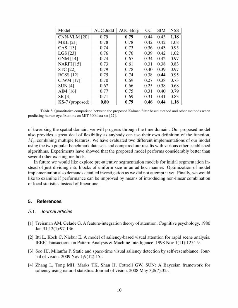
Model AUC-Judd AUC-Borji CC SIM NSSCNN-VLM [20] 0.79 0.79 0.44 0.43 1.18MKL [21] 0.78 0.78 0.42 0.42 1.08CAS [13] 0.74 0.73 0.36 0.43 0.95LGS [23] 0.76 0.76 0.39 0.42 1.02GNM [14] 0.74 0.67 0.34 0.42 0.97NARFI [15] 0.73 0.61 0.31 0.38 0.83STC [22] 0.79 0.78 0.40 0.39 0.97RCSS [12] 0.75 0.74 0.38 0.44 0.95CIWM [17] 0.70 0.69 0.27 0.38 0.73SUN [4] 0.67 0.66 0.25 0.38 0.68AIM [16] 0.77 0.75 0.31 0.40 0.79SR [3] 0.71 0.69 0.31 0.41 0.83KS-7 (proposed) 0.80 0.79 0.46 0.44 1.18

Table 3 Quantitative comparison between the proposed Kalman filter based method and other methods whenpredicting human eye fixations on MIT-300 data set [27].

of traversing the spatial domain, we will progress through the time domain. Our proposed modelalso provides a great deal of flexibility as anybody can use their own definition of the function,Mk, combining multiple features. We have evaluated two different implementations of our modelusing the two popular benchmark data sets and compared our results with various other establishedalgorithms. Experiments have showed that the proposed model performs considerably better thanseveral other existing methods.

In future we would like explore pre-attentive segmentation models for initial segmentation in-stead of just dividing into blocks of uniform size in an ad hoc manner. Optimization of modelimplementation also demands detailed investigation as we did not attempt it yet. Finally, we wouldlike to examine if performance can be improved by means of introducing non-linear combinationof local statistics instead of linear one.

5. References

5.1. Journal articles

[1] Treisman AM, Gelade G. A feature-integration theory of attention. Cognitive psychology. 1980Jan 31;12(1):97-136.

[2] Itti L, Koch C, Niebur E. A model of saliency-based visual attention for rapid scene analysis.IEEE Transactions on Pattern Analysis & Machine Intelligence. 1998 Nov 1(11):1254-9.

[3] Seo HJ, Milanfar P. Static and space-time visual saliency detection by self-resemblance. Jour-nal of vision. 2009 Nov 1;9(12):15-.

[4] Zhang L, Tong MH, Marks TK, Shan H, Cottrell GW. SUN: A Bayesian framework forsaliency using natural statistics. Journal of vision. 2008 May 3;8(7):32-.

10

[5] Summerfield C, Egner T. Expectation (and attention) in visual cognition. Trends in cognitivesciences. 2009 Sep 30;13(9):403-9.

[6] Jiang J, Summerfield C, Egner T. Attention sharpens the distinction between expectedand unexpected percepts in the visual brain. The Journal of Neuroscience. 2013 Nov20;33(47):18438-47.

[7] Kowler E, Anderson E, Dosher B, Blaser E. The role of attention in the programming of sac-cades. Vision research. 1995 Jul 31;35(13):1897-916.

[8] Fischer B, Breitmeyer B. Mechanisms of visual attention revealed by saccadic eye movements.Neuropsychologia. 1987 Dec 31;25(1):73-83.

[9] Itti L, Baldi P. Bayesian surprise attracts human attention. Vision research. 2009 Jun2;49(10):1295-306.

[10] Bruce N, Tsotsos J. Attention based on information maximization. Journal of Vision. 2007Jun 1;7(9):950-.

[11] Peters RJ, Iyer A, Itti L, Koch C. Components of bottom-up gaze allocation in natural images.Vision research. 2005 Aug 31;45(18):2397-416.

[12] Vikram TN, Tscherepanow M, Wrede B. A saliency map based on sampling an image intorandom rectangular regions of interest. Pattern Recognition. 2012 Sep 30;45(9):3114-24.

[13] Goferman S, Zelnik-Manor L, Tal A. Context-aware saliency detection. Pattern Analysis andMachine Intelligence, IEEE Transactions on. 2012 Oct;34(10):1915-26.

[14] Zhong G, Liu R, Cao J, Su Z. A generalized nonlocal mean framework with object-level cuesfor saliency detection. The Visual Computer. 2015:1-3.

[15] Chen JJ, Cao H, Ju Z, Qin L, Su ST. Non-attention region first initialisation of k-meansclustering for saliency detection. Electronics Letters. 2013 Oct 24;49(22):1384-6.

5.2. Conference Paper

[16] Bruce N, Tsotsos J. Saliency based on information maximization. In Advances in neuralinformation processing systems 2005 (pp. 155-162).

[17] Murray N, Vanrell M, Otazu X, Parraga CA. Saliency estimation using a non-parametric low-level vision model. InComputer Vision and Pattern Recognition (CVPR), 2011 IEEE Confer-ence on 2011 Jun 20 (pp. 433-440). IEEE.

[18] Itti L, Baldi PF. Bayesian surprise attracts human attention. InAdvances in neural informationprocessing systems 2005 (pp. 547-554).

[19] Riche N, Duvinage M, Mancas M, Gosselin B, Dutoit T. Saliency and human fixations: state-of-the-art and study of comparison metrics. InProceedings of the IEEE International Confer-ence on Computer Vision 2013 (pp. 1153-1160).

[20] Kato H, Harada T. Visual Language Modeling on CNN Image Representations. arXiv preprintarXiv:1511.02872. 2015 Nov 9.

11

[21] Kavak Y, Erdem E, Erdem A. Visual saliency estimation by integrating features using multiplekernel learning. arXiv preprint arXiv:1307.5693. 2013 Jul 22.

[22] Holzbach A, Cheng G. A scalable and efficient method for salient region detection usingsampled template collation. InImage Processing (ICIP), 2014 IEEE International Conferenceon 2014 Oct 27 (pp. 1110-1114). IEEE.

[23] Borji A, Itti L. Exploiting local and global patch rarities for saliency detection. InComputerVision and Pattern Recognition (CVPR), 2012 IEEE Conference on 2012 Jun 16 (pp. 478-485).IEEE.

5.3. Book, book chapter and manual

[24] Simon D. Optimal state estimation: Kalman, H infinity, and nonlinear approaches. John Wiley& Sons; 2006 Jun 19.

[25] Zarchan P. Progress In Astronautics and Aeronautics: Fundamentals of Kalman Filtering: APractical Approach. Aiaa; 2005.

[26] Brown RG. Introduction to random signal analysis and Kalman filtering. John Wiley & Sons;1983 Jun 1.

5.4. Report

[27] Judd T, Durand F, Torralba A. A benchmark of computational models of saliency to predicthuman fixations.,2012.

12