© Schlumberger Water Services Visual MODFLOW 2011.1 User’s Manual For Professional Applications in Three-Dimensional Groundwater Flow and Contaminant Transport Modeling Images created using Visual MODFLOW Premium

Welcome message from author
This document is posted to help you gain knowledge. Please leave a comment to let me know what you think about it! Share it to your friends and learn new things together.
Transcript
© Schlumberger Water Services
Visual MODFLOW 2011.1 User’s Manual
For Professional Applications in Three-Dimensional Groundwater Flow and Contaminant Transport Modeling
Images created using Visual MODFLOW Premium


PrefaceSchlumberger Water Services (SWS) is a recognized leader in the development and application of innovative groundwater technologies in addition to offering expert services and professional training to meet the advancing technological requirements of today’s groundwater and environmental professionals.
Schlumberger Water Services software consists of a complete suite of environmental software applications engineered for data management and analysis, modeling and simulation, visualization, and reporting. Schlumberger Water Services software is currently developed by SWS and sold globally as a suite of desktop solutions.
For over 18 years, our products and services have been used by firms, regulatory agencies, and educational institutions around the world. We develop each product to maximize productivity and minimize the complexities associated with groundwater and environmental projects. To date, we have over 14,000 registered software installations in more than 85 countries!
Need more information?If you would like to contact us with comments or suggestions, you can reach us at:
Schlumberger Water Services72 Victoria St. S. - Suite 202
Kitchener, Ontario, CANADA, N2G 4Y9
Phone: +1 (519) 746-1798Fax: +1 (519) 885-5262
General Inquiries: [email protected]
Web: www.swstechnology.com, www.water.slb.com
Obtaining Technical SupportTo help us handle your technical support questions as quickly as possible, please have the following information ready before you call, or include it in a detailed technical support e-mail:
• A complete description of the problem including a summary of key strokes and program event (or a screen capture showing the error message, where applicable)
• Product name and version number
• Product serial number
• Computer make and model number
• Operating system and version number
• Total free RAM
i

• Number of free bytes on your hard disk
• Software installation directory
• Directory location for your current project files
You may send us your questions via e-mail, fax, or call one of our technical support specialists. Please allow up to two business days for a response. Technical support is available 8:00 am to 5:00 pm EST Monday to Friday (excluding Canadian holidays).
Phone: +1 (519) 746-1798Fax: +1 (519) 885-5262
E-mail: [email protected]
Training and Consulting ServicesSchlumberger Water Services offers numerous, high quality training courses globally. Our courses are designed to provide a rapid introduction to essential knowledge and skills, and create a basis for further professional development and real-world practice. Open enrollment courses are offered worldwide each year. For the current schedule of courses, visit: www.swstechnology.com/training or e-mail us at: [email protected].
Schlumberger Water Services also offers expert consulting and peer reviewing services for data management, groundwater modeling, aqueous geochemical analysis, and pumping test analysis. For further information, please contact [email protected].
Schlumberger Water Services Software We also develop and distribute a number of other useful software products for the groundwater professionals, all designed to increase your efficiency and enhance your technical capability, including:
• Visual MODFLOW Premium*
• Hydro GeoBuilder*
• Hydro GeoAnalyst*
• Aquifer Test Pro*
• AquaChem*
• GW Contour*
• UnSat Suite Plus*
• Visual HELP*
• Visual PEST-ASP
ii

Visual MODFLOW PremiumVisual MODFLOW Premium is a three-dimensional groundwater flow and contaminant transport modeling application that integrates MODFLOW-2000, SEAWAT, MODPATH, MT3DMS, MT3D99, RT3D, VMOD 3D-Explorer, WinPEST, Stream Routing Package, Zone Budget, MGO, SAMG, and PHT3D. Applications include well head capture zone delineation, pumping well optimization, aquifer storage and recovery, groundwater remediation design, simulating natural attenuation, and saltwater intrusion.
Hydro GeoBuilderHydro GeoBuilder is the new generation in dynamic conceptual model building. Featuring a powerful multi-format object/data import tool and tested to work within the latest version of the Visual MODFLOW modeling environment, Hydro GeoBuilder enables you to build impressive representations of your groundwater system within a single modeling environment. This means you save hours when building your numerical model.
Hydro GeoAnalystHydro GeoAnalyst is an information management system for managing groundwater and environmental data. Hydro GeoAnalyst combines numerous pre and post processing components into a single program. Components include, Project Wizard, Universal Data Transfer System, Template Manager, Materials Specification Editor, Query Builder, QA/QC Reporter, Map Manager, Cross-Section Editor, HGA 3D-Explorer, Borehole Log Plotter, and Report Editor. The seamless integration of these tools provide the means for compiling and normalizing field data, analyzing and reporting subsurface data, mapping and assessing spatial information, and reporting site data.
AquiferTest ProAquiferTest Pro, designed for graphical analysis and reporting of pumping test and slug test data, offers the tools necessary to calculate an aquifer's hydraulic properties such as hydraulic conductivity, transmissivity, and storativity. AquiferTest Pro is versatile enough to consider confined aquifers, unconfined aquifers, leaky aquifers, and fractured rock aquifers conditions. Analysis results are displayed in report format, or may be exported into graphical formats for use in presentations. AquiferTest Pro also provides the tools for trends corrections, and graphical contouring water table drawdown around the pumping well.
AquaChemAquaChem is designed for the management, analysis, and reporting of water quality data. AquaChem’s analysis capabilities cover a wide range of functions and calculations frequently used for analyzing, interpreting and comparing water quality data. AquaChem includes a comprehensive selection of commonly used plotting techniques to represent the chemical characteristics of aqueous geochemical and water quality data, as well includes PHREEQC - a powerful geochemical reaction model.
iii
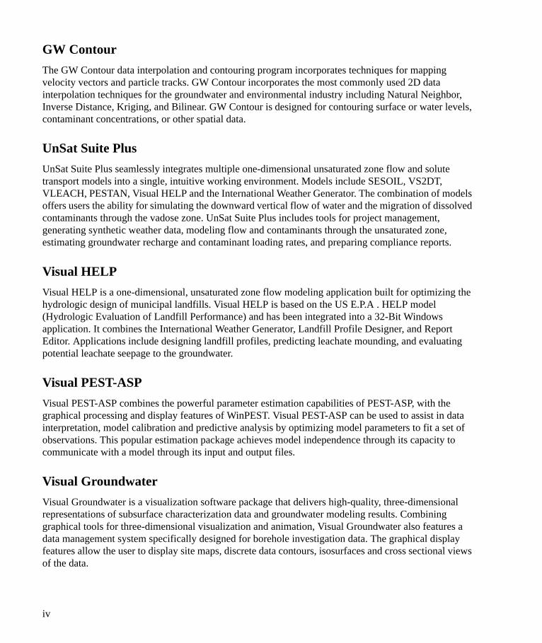
GW ContourThe GW Contour data interpolation and contouring program incorporates techniques for mapping velocity vectors and particle tracks. GW Contour incorporates the most commonly used 2D data interpolation techniques for the groundwater and environmental industry including Natural Neighbor, Inverse Distance, Kriging, and Bilinear. GW Contour is designed for contouring surface or water levels, contaminant concentrations, or other spatial data.
UnSat Suite PlusUnSat Suite Plus seamlessly integrates multiple one-dimensional unsaturated zone flow and solute transport models into a single, intuitive working environment. Models include SESOIL, VS2DT, VLEACH, PESTAN, Visual HELP and the International Weather Generator. The combination of models offers users the ability for simulating the downward vertical flow of water and the migration of dissolved contaminants through the vadose zone. UnSat Suite Plus includes tools for project management, generating synthetic weather data, modeling flow and contaminants through the unsaturated zone, estimating groundwater recharge and contaminant loading rates, and preparing compliance reports.
Visual HELPVisual HELP is a one-dimensional, unsaturated zone flow modeling application built for optimizing the hydrologic design of municipal landfills. Visual HELP is based on the US E.P.A . HELP model (Hydrologic Evaluation of Landfill Performance) and has been integrated into a 32-Bit Windows application. It combines the International Weather Generator, Landfill Profile Designer, and Report Editor. Applications include designing landfill profiles, predicting leachate mounding, and evaluating potential leachate seepage to the groundwater.
Visual PEST-ASPVisual PEST-ASP combines the powerful parameter estimation capabilities of PEST-ASP, with the graphical processing and display features of WinPEST. Visual PEST-ASP can be used to assist in data interpretation, model calibration and predictive analysis by optimizing model parameters to fit a set of observations. This popular estimation package achieves model independence through its capacity to communicate with a model through its input and output files.
Visual GroundwaterVisual Groundwater is a visualization software package that delivers high-quality, three-dimensional representations of subsurface characterization data and groundwater modeling results. Combining graphical tools for three-dimensional visualization and animation, Visual Groundwater also features a data management system specifically designed for borehole investigation data. The graphical display features allow the user to display site maps, discrete data contours, isosurfaces and cross sectional views of the data.
iv

Groundwater InstrumentationDiver-NETZDiver-NETZ is an all-inclusive groundwater monitoring network system that integrates high-quality field instrumentation with the industries latest communications and data management technologies. All of the Diver-NETZ components are designed to optimize your project workflow from collecting and recording groundwater data in the field - to project delivery in the office.
*Mark of Schlumberger
v

vi

Table of Contents vii
Table of Contents
1. Introduction to Visual MODFLOW ........................................... 1What’s New in Visual MODFLOW ............................................................................. 1
New Features in Visual MODFLOW 2011.1................................................................................... 2New Features in Visual MODFLOW 2010.1................................................................................... 3
Visual MODFLOW Installation ...................................................................................... 4Hardware Requirements ............................................................................................... 4
Installing Visual MODFLOW.......................................................................................................... 4Starting Visual MODFLOW ............................................................................................................ 5Un-installing Visual MODFLOW.................................................................................................... 5
Visual MODFLOW Features........................................................................................ 5
About the Interface ........................................................................................................... 6Getting Around In Visual MODFLOW ........................................................................................... 7Screen Layout ................................................................................................................................... 9
Visual MODFLOW Project Files .................................................................................. 11
Visual MODFLOW On-Line Help ................................................................................ 12
Software Maintenance and Technical Support............................................................ 14
2. Getting Started ............................................................................ 15Opening Older Visual MODFLOW Models ................................................................ 15
Importing MODFLOW Data Sets................................................................................. 15Using the MF96to2K.exe conversion tool .................................................................. 16Importing a MODFLOW 2000 data set ...................................................................... 19Determining Property Values for Confining Bed Layers ........................................... 23Calculating Kz Values Using VCONT....................................................................... 24Importing Same Cell Boundary Conditions................................................................ 26Importing Initial Heads from a MODFLOW model................................................... 26Limitations of MODFLOW data import..................................................................... 27Importing MODFLOW Packages ............................................................................... 27
Creating a New Model .................................................................................................... 29Selecting the Model Region ........................................................................................................... 40
Entering the Model Data ................................................................................................ 43
viii Table of Contents
3. Global Operations....................................................................... 45Saving the Model............................................................................................................. 45
Changing your Model Preferences................................................................................ 45
Three-Dimensional Visualization .................................................................................. 47
Importing Site Maps....................................................................................................... 47Georeferencing a Graphics File .................................................................................. 47
Adding Georeference Points ........................................................................................................... 49Deleting Georeference Points ......................................................................................................... 49Loading a New Map File ................................................................................................................ 49
Modifying Site Map Images ....................................................................................... 50Dual Co-ordinate Systems .......................................................................................... 50
Changing Measurement Units and Model Start Time ................................................ 51
Overlay Control Options................................................................................................ 52Overlay Groups ............................................................................................................................... 52Overlay Display Settings ................................................................................................................ 53
Printing the Model Display Area................................................................................... 59Page Setup................................................................................................................... 61
Page Layout .................................................................................................................................... 61Plot Description .............................................................................................................................. 63Project Name................................................................................................................................... 63Company Name .............................................................................................................................. 64
Print............................................................................................................................. 65Print Preview............................................................................................................... 65Save as graphics file ................................................................................................... 66Copy to Clipboard....................................................................................................... 66Show Legend .............................................................................................................. 66
Edit Legend..................................................................................................................................... 66Show Color Legend .................................................................................................... 67Annotate...................................................................................................................... 67Image Editor Help....................................................................................................... 68Image Title.................................................................................................................. 68Printing Methods......................................................................................................... 68
Selecting Numeric Engines............................................................................................. 69Groundwater Flow Numeric Engines ......................................................................... 69Mass Transport Numeric Engine ................................................................................ 70
Defining Flow Engines and Transport Variants ............................................................................. 71
Export Options................................................................................................................ 77
Table of Contents ix
Exporting Graphics Image Files ................................................................................. 77Exporting Data Files ................................................................................................... 79Exporting GIS Files .................................................................................................... 81
4. Model Input Data........................................................................ 83General Input .................................................................................................................. 84
The File Menu ................................................................................................................. 85
Grid Design...................................................................................................................... 86Assigning Inactive/Active Regions ............................................................................ 87Gridlines (Rows and Columns) .................................................................................. 88Grid Layers ................................................................................................................ 90Model Extents ............................................................................................................ 92Grid Smoothing .......................................................................................................... 93
Fixing Gridlines.............................................................................................................................. 96Importing Surfaces...................................................................................................... 97
As is ................................................................................................................................................ 99Import data...................................................................................................................................... 99Specified Elevation....................................................................................................................... 106Specified Thickness...................................................................................................................... 107Constant Slope.............................................................................................................................. 108
Previewing the Layer Elevations to be Imported...................................................... 110Assign Elevations .................................................................................................... 119
A note about Zero Thickness Cells: ............................................................................................. 120Single............................................................................................................................................ 123Line............................................................................................................................................... 123Polygon......................................................................................................................................... 124Window ........................................................................................................................................ 124Database ....................................................................................................................................... 125
Contouring ............................................................................................................... 126
Wells ............................................................................................................................... 127Pumping Wells.......................................................................................................... 127
Well Table .................................................................................................................................... 136Well Screen Intervals ................................................................................................................... 137Pumping Well Schedule ............................................................................................................... 139Importing Pumping Well Data ..................................................................................................... 142Graphing Pumping Well Schedules.............................................................................................. 146Multi-Node Wells (MNW) Package............................................................................................. 147
Head and Concentration Observation Wells............................................................. 152Observation Points........................................................................................................................ 155Observations ................................................................................................................................. 156Importing Observation Well Locations ........................................................................................ 158Observation Groups...................................................................................................................... 165
x Table of Contents
Properties....................................................................................................................... 167Constant Value Property Zones .................................................................................................... 168Distributed Value Property Zones ................................................................................................ 168
Tools for Assigning and Editing Properties.............................................................. 170Importing Distributed Property Data ............................................................................................ 171Assigning Property Zones............................................................................................................. 187Copying Property Zones ............................................................................................................... 188Editing the Property Database ...................................................................................................... 189Contouring Property Data ............................................................................................................ 191
Conductivity.............................................................................................................. 191Storage ...................................................................................................................... 195Initial Heads.............................................................................................................. 197Vadose Zone ............................................................................................................. 197
Sample Index of Soil Hydraulic Properties* ................................................................................ 198Vadose Zone Properties Settings .................................................................................................. 200
Bulk Density ............................................................................................................. 202Species Parameters ................................................................................................... 204Edit Constant Parameters.......................................................................................... 206Initial Concentration ................................................................................................. 207
Importing Initial Concentrations................................................................................................... 208Assigning Inactive Transport Zones ............................................................................................. 209
Dispersion ................................................................................................................. 210
Boundary Conditions.................................................................................................... 211Tools for Assigning and Editing Boundary Conditions............................................ 213
Importing Boundary Conditions ................................................................................................... 214Flow Boundary Conditions....................................................................................... 217
Importing Transient Boundary Condition Data ............................................................................ 226Constant Head (CHD) Boundary Conditions ............................................................................... 234River (RIV) Boundary Conditions................................................................................................ 237Stream (STR) Boundary Conditions ............................................................................................. 240General-Head (GHB) Boundary Conditions................................................................................. 246Lake (LAK) Boundary Conditions ............................................................................................... 250Drain (DRN) Boundary Conditions .............................................................................................. 252Wall (HFB) Boundary Conditions ................................................................................................ 255Recharge (RCH) Boundary Conditions ........................................................................................ 258Evapotranspiration Boundary Conditions..................................................................................... 266Using the Evapotranspiration Segments Package (ETS1) ............................................................ 271
Mass Transport Boundary Conditions ...................................................................... 274Constant Concentration Boundary Conditions ............................................................................. 274Recharge Concentration Boundary Conditions ............................................................................ 276Evapotranspiration Concentration Boundary Conditions ............................................................. 278Point Source Boundary Conditions............................................................................................... 280Import MIKE 11 River Network................................................................................................... 281
Particles (MODPATH)................................................................................................. 283
Table of Contents xi
Particle Release Time ................................................................................................................... 285Particle Discharge Options ........................................................................................................... 286
Zone Budget................................................................................................................... 286Flow Observations........................................................................................................................ 288
Tools ............................................................................................................................... 290Cell Inspector ............................................................................................................ 291Annotate.................................................................................................................... 292
Editing Text Settings .................................................................................................................... 293Units Converter......................................................................................................... 294Copy Image to Clipboard.......................................................................................... 294Enviro-Base Pro ........................................................................................................ 295
5. Run Section - Model Run Settings........................................... 297File .................................................................................................................................. 298
MODFLOW Run Settings............................................................................................ 298Time Steps ................................................................................................................ 299Initial Heads .............................................................................................................. 305
Calculating VCONT Values......................................................................................................... 306Importing Initial Heads................................................................................................................. 306
Solver Settings .......................................................................................................... 307Preconditioned Conjugate-Gradient Package (PCG2) ................................................................ 308Strongly Implicit Procedure Package (SIP) ................................................................................. 310Slice-Successive Overrelaxation Package (SOR) ....................................................................... 312WHS Solver for Visual MODFLOW (WHS) ............................................................................. 313Algebraic Multigrid Methods for Systems (SAMG) and Algebraic Multigrid Solver (AMG) ... 315Preconditioned Conjugate-Gradient Package (PCG4) ................................................................. 318Preconditioned Conjugate-Gradient Package (PCG5) ................................................................. 320Geometric Multigrid Solver (GMG) ............................................................................................ 321MODFLOW-NWT....................................................................................................................... 324
Recharge Settings ..................................................................................................... 328Evapotranspiration Settings ...................................................................................... 329Surface Water Leakage Settings ............................................................................... 330Layer Type Settings .................................................................................................. 332Re-wetting Settings................................................................................................... 335Anisotropy Settings................................................................................................... 338Output Control Settings ............................................................................................ 338List File Options ...................................................................................................... 340Engine Settings ......................................................................................................... 341
MODPATH Run Settings............................................................................................. 342Discharge Options..................................................................................................... 342
xii Table of Contents
Reference Time Settings........................................................................................... 343
MT3D/RT3D/PHT3D Run Settings ............................................................................ 344Solution Method ....................................................................................................... 345
Solution Method Settings.............................................................................................................. 347A Technical discussion of the MT3D Solution Methods.............................................................. 348Particle Options............................................................................................................................. 352Implicit Generalized Conjugate Gradient (GCG) Solver Settings................................................ 355Particle-Based Methods ................................................................................................................ 357Finite Difference Methods ............................................................................................................ 358TVD Method................................................................................................................................. 359A Technical Note on the Generalized Conjugate Gradient Solver ............................................... 360
Output/Time Steps Settings ...................................................................................... 361Calculating Transport Timestep Sizes ......................................................................................... 362
Initial Concentrations Settings.................................................................................. 363Importing Initial Concentrations................................................................................................... 364
Concentration Import file Conversion and Viewing Utility ..................................... 366Parallel Processing.................................................................................................... 367PHT3D Run Settings ................................................................................................ 368
General .......................................................................................................................................... 369Aqueous Components ................................................................................................................... 370Minerals ........................................................................................................................................ 371Equilibrium Gas Phases ................................................................................................................ 373Exchange Species.......................................................................................................................... 374
SEAWAT Run Settings ................................................................................................ 374Simulation Scenario.................................................................................................. 375
VDF Settings................................................................................................................................. 375VSC Settings................................................................................................................................. 377Flow Settings ................................................................................................................................ 381Transport Settings ......................................................................................................................... 382
SEAWAT Flow......................................................................................................... 382SEAWAT Transport ................................................................................................. 383
Optimization Settings ................................................................................................... 383
6. Running your Model - VMEngines ......................................... 385Advanced MODFLOW Run Settings ....................................................................... 387Advanced Zone Budget Run Settings....................................................................... 389Advanced MT3D Run Settings................................................................................. 390
VM Engine..................................................................................................................... 391Running the Model(s) ............................................................................................... 393MODFLOW Display Options................................................................................... 395MODPATH Display Options.................................................................................... 397
Table of Contents xiii
Zone Budget Options ................................................................................................ 398MT3D Display Options ............................................................................................ 399
7. Parameter Optimization: PEST and Predictive Analysis ..... 401Getting Started.............................................................................................................. 402
Selecting Model Parameters ........................................................................................ 403Selecting Parameters................................................................................................. 403Clearing Selected Parameters ................................................................................... 404Resetting Parameter Selections................................................................................. 404Saving Parameter Selections..................................................................................... 404Defining Parameter Settings ..................................................................................... 404
Description of Parameter Settings ................................................................................................ 405Parameter Groups ......................................................................................................................... 408
Prior Information ......................................................................................................... 410Adding Prior Information ......................................................................................... 411Deleting Prior Information........................................................................................ 412Editing Prior Information.......................................................................................... 413Resetting Prior Information ...................................................................................... 413Saving Prior Information .......................................................................................... 413
Assigning the Objective Function................................................................................ 413Selecting the Observation Data Type(s) ................................................................... 414Selecting the Observation Groups ............................................................................ 415
Filtering the Observation Groups List .......................................................................................... 415Editing User-Defined Observation Groups .................................................................................. 415
PEST Controls............................................................................................................... 416PEST Control Parameters ......................................................................................... 417
PESTMODE................................................................................................................................. 417Marquardt Lambda Settings ......................................................................................................... 417Parameter Change Constraints ..................................................................................................... 419Method Separation Value - PHIREDSWH .................................................................................. 421Precision - PRECIS ...................................................................................................................... 422Termination Criteria ..................................................................................................................... 422Output Control - ICOV, ICOR, IEIG ........................................................................................... 423Enable Restart - RSTFLE............................................................................................................. 423
Predictive Analysis Settings ......................................................................................... 424Prediction Data ......................................................................................................... 425
Analysis Mode - NPREDMAXMIN ............................................................................................ 426Data Type ..................................................................................................................................... 426Location........................................................................................................................................ 426Obs. Point ..................................................................................................................................... 426
xiv Table of Contents
Obs. Time...................................................................................................................................... 426Objective Function Criteria ...................................................................................... 426
Inside Limit - PD0 ........................................................................................................................ 426Outside Limit - PD1...................................................................................................................... 427Threshold - PD2............................................................................................................................ 427
Iteration Change Criteria .......................................................................................... 427Relative Change - RELPREDLAM .............................................................................................. 427Absolute Change - ABSPREDLAM............................................................................................. 428
Derivation Calculation Switch.................................................................................. 428Relative Change - RELPREDSWH .............................................................................................. 428Absolute Change - ABSPREDSWH............................................................................................. 428
Line Search ............................................................................................................... 428Maximum Model Runs - NSEARCH ........................................................................................... 429Initial Search Factor - INITSCHFAC ........................................................................................... 429Multiplication Factor - MULSCHFAC......................................................................................... 429
Termination Criteria ................................................................................................. 429Optimization Attempts - NPREDNORED.................................................................................... 429Number of Best Predictions - NPREDSTP................................................................................... 429Relative Distance - RELPREDSTP .............................................................................................. 430Absolute Distance - ABSPREDSTP............................................................................................. 430
Running the Parameter Estimation Simulation......................................................... 430Loading PEST Input Files......................................................................................... 432Validating PEST Input Files ..................................................................................... 432Starting the PEST Simulation ................................................................................... 433Interacting with the PEST Simulation ...................................................................... 433Displaying Reports and Graphs ................................................................................ 433Updating your Model................................................................................................ 447
8. Well Optimization..................................................................... 449Introduction............................................................................................................... 449Assumptions and Limitations of Well Optimization ................................................ 450
Well Optimization Settings .......................................................................................... 451Management.............................................................................................................. 452
Decision Variables ........................................................................................................................ 452Decision Variable Groups............................................................................................................. 455
Constraints ................................................................................................................ 457Global Constraints ........................................................................................................................ 458Pumping Balance Constraints ....................................................................................................... 459State Variable Constraints............................................................................................................. 461
Objectives ................................................................................................................. 463Controls..................................................................................................................... 464
Optimization Solver Options ........................................................................................................ 465
Table of Contents xv
Solution Options........................................................................................................................... 469Output Control Options ................................................................................................................ 470
Running Well Optimization......................................................................................... 470
Interpreting and Utilizing Well Optimization Results .............................................. 471
9. Output Section - Displaying Model Results............................ 475File Options ................................................................................................................... 477
Maps............................................................................................................................... 478Calibration Residual Maps........................................................................................ 478
Calibration Residual Display Options .......................................................................................... 479Contour Maps ........................................................................................................... 482
Contour Map Display Options...................................................................................................... 483Color Map Display Options.......................................................................................................... 486Removing Contour Maps ............................................................................................................. 487Selecting Output Times ................................................................................................................ 487Selecting Chemical Species.......................................................................................................... 488Selecting Observation Points........................................................................................................ 488Exporting Contour Data ............................................................................................................... 489
Pathline Maps ........................................................................................................... 489Pathline Display Options.............................................................................................................. 490Removing the Pathlines Map........................................................................................................ 491Exporting Pathlines ...................................................................................................................... 491
Velocity Vectors Maps ............................................................................................. 492Velocity Vectors Display Options................................................................................................ 492Selecting Output Times ................................................................................................................ 493Removing the Velocity Vectors Map ........................................................................................... 494Exporting Flow Velocity Data...................................................................................................... 494
Zone Budget Maps.................................................................................................... 495Zone Budget Listing ..................................................................................................................... 495Mass Balance Report .................................................................................................................... 496
Graphs............................................................................................................................ 497Calibration Graphs .................................................................................................... 498
Calculated vs. Observed Scatter Graphs ...................................................................................... 504Calibration Residuals Histogram.................................................................................................. 509
Time-Series Graphs .................................................................................................. 510Head or Concentration vs. Time Graphs ...................................................................................... 514Drawdown vs. Time Graphs......................................................................................................... 515Saturation vs. Time Graphs .......................................................................................................... 517Calibration Statistics vs. Time Graphs ......................................................................................... 518
Mass Balance Graphs................................................................................................ 519Flow Mass Balance Graphs .......................................................................................................... 519Transport Mass Balance Graphs................................................................................................... 521
xvi Table of Contents
Zone Budget Graphs ................................................................................................. 523Flow Zone Budget Graphs ............................................................................................................ 523Transport Zone Budget Graphs..................................................................................................... 525
Lake Budget Graphs ................................................................................................. 527
Tools ............................................................................................................................... 527Cell Inspector............................................................................................................ 528Annotate.................................................................................................................... 528Units Converter......................................................................................................... 528Copy Image to Clipboard.......................................................................................... 528Enviro-Base Pro........................................................................................................ 528
10. IChart - Graphing and Mapping Component...................... 529Toolbar Icons................................................................................................................. 530
Graph Properties .......................................................................................................... 531Save and Load Settings ................................................................................................................. 531
Axis Settings ............................................................................................................. 532Titles Settings ........................................................................................................... 533Series Settings........................................................................................................... 533Legends Settings ....................................................................................................... 535Operations Settings ................................................................................................... 536General Settings........................................................................................................ 537Info Settings.............................................................................................................. 539
Map Properties.............................................................................................................. 540Contour Settings ....................................................................................................... 541Color Map Settings ................................................................................................... 542
Annotation Tools........................................................................................................... 542
Printing Options............................................................................................................ 543Page Setup................................................................................................................. 544Plot Description ........................................................................................................ 545Project Name............................................................................................................. 546Company Name ........................................................................................................ 547
Exporting Data.............................................................................................................. 548Saving to a Graphics File.......................................................................................... 549
11. Visual MODFLOW 3D-Explorer .......................................... 551Getting Started.............................................................................................................. 552
Opening VMOD 3D-Explorer ...................................................................................................... 552
Table of Contents xvii
Closing VMOD 3D-Explorer ....................................................................................................... 552VMOD 3D-Explorer Data Files ................................................................................................... 553VMOD 3D-Explorer On-Line Help ............................................................................................. 553Software Performance Considerations ......................................................................................... 554OpenGL Settings .......................................................................................................................... 554
About the Interface ................................................................................................... 555Positioning the Panels................................................................................................................... 556Exaggeration................................................................................................................................. 5573D Navigation Tools .................................................................................................................... 557
Model Elements and Display Settings ......................................................................... 561Default Settings ............................................................................................................................ 562VMOD Project Display Settings .................................................................................................. 565Axis Properties ............................................................................................................................. 565Sitemaps Display Settings ............................................................................................................ 566
Input Model Elements............................................................................................... 566Domain Display Settings.............................................................................................................. 567Grid Display Settings ................................................................................................................... 567Wells Display Settings ................................................................................................................. 568Properties Display Settings........................................................................................................... 569Boundaries Display Settings......................................................................................................... 571
Output Model Elements ............................................................................................ 572Heads Display Settings................................................................................................................. 572Drawdowns Display Settings ....................................................................................................... 575Concentrations Display Settings................................................................................................... 576Pathlines ....................................................................................................................................... 577
Isosurfaces ................................................................................................................ 578Creating Isosurfaces ..................................................................................................................... 578Isosurface Display Properties ....................................................................................................... 580
Color Maps ............................................................................................................... 580Creating a Color Map ................................................................................................................... 580Color Map Display Settings ......................................................................................................... 581
Contour Maps ........................................................................................................... 582Creating Contour Maps ................................................................................................................ 582Contour Map Display Settings ..................................................................................................... 583
Color Fields............................................................................................................... 585Color Field Display Settings ........................................................................................................ 586
The Color Palette ...................................................................................................... 586The Color Legend ..................................................................................................... 588
Creating Slices and Cross-Sections ............................................................................. 588Creating a Vertical Slice ........................................................................................... 589Creating a Horizontal Slice....................................................................................... 590Creating a Vertical Cross-Section............................................................................. 591Deleting a Slice ......................................................................................................... 592Moving a Slice .......................................................................................................... 592
xviii Table of Contents
Creating Cut-aways ...................................................................................................... 593Creating an Animation.............................................................................................. 594
Scene Configurations.................................................................................................... 596
Saving to a Graphics File ............................................................................................. 597
Printing the 3D Image .................................................................................................. 598Page Setup................................................................................................................. 600
Page Layout .................................................................................................................................. 600Plot Description ............................................................................................................................ 601Project Name................................................................................................................................. 602Company Name ............................................................................................................................ 603
Print........................................................................................................................... 604Print Preview............................................................................................................. 604Save as graphics file ................................................................................................. 605Copy to Clipboard..................................................................................................... 605Show Legend ............................................................................................................ 605
Edit Legend................................................................................................................................... 605Show Color Legend .................................................................................................. 606Annotate.................................................................................................................... 606Image Editor Help..................................................................................................... 607Image Title................................................................................................................ 607Select......................................................................................................................... 607Zoom......................................................................................................................... 607Printing Methods....................................................................................................... 607
12. Appendix A: Visual MODFLOW Data Files ....................... 613Model Data Files ........................................................................................................... 614
Visual MODFLOW Data Files ................................................................................. 614General Files ................................................................................................................................. 614MODFLOW.................................................................................................................................. 614MODPATH................................................................................................................................... 614MT3D/RT3D................................................................................................................................. 614Zone Budget.................................................................................................................................. 615
Numerical Model Input Files.................................................................................... 615MODFLOW.................................................................................................................................. 615MODPATH................................................................................................................................... 616MT3Dxx/RT3D............................................................................................................................. 616Zone Budget.................................................................................................................................. 616
Output Files............................................................................................................... 616MODFLOW.................................................................................................................................. 616MODPATH................................................................................................................................... 617MT3Dxx/RT3D............................................................................................................................. 617

Table of Contents xix
PEST............................................................................................................................................. 618Zone Budget ................................................................................................................................. 618
Visual MODFLOW Input Data Formats ................................................................... 619VMA - Particle File Format...................................................................................... 619VMB - Flow Boundary Conditions File Format....................................................... 620VMG - Grid File Format........................................................................................... 622VMO - Heads Observation File Format ................................................................... 624VMP - Flow Property File Format............................................................................ 625VMW - Pumping Well File Format .......................................................................... 627VMZ - Zone Budget File Format.............................................................................. 627
13. Appendix B: Interpolation Method Settings ........................ 629Inverse Distance ............................................................................................................ 629
Kriging ........................................................................................................................... 631
Natural Neighbors......................................................................................................... 635
14. Appendix C: Numeric Engines .............................................. 639Groundwater Flow Numeric Engines ......................................................................... 640
MODFLOW-96 ........................................................................................................ 640MODFLOW-2000 .................................................................................................... 640MODFLOW-2005 .................................................................................................... 641MODFLOW-SURFACT .......................................................................................... 641SEAWAT.................................................................................................................. 642
Mass Transport Numeric Engines............................................................................... 643MT3Dv1.5................................................................................................................. 645MT3D96 (not available for new projects/variants)................................................... 646MT3DMS.................................................................................................................. 646MT3D99.................................................................................................................... 647SEAWAT.................................................................................................................. 647RT3D ........................................................................................................................ 647RT3D 2.5 .................................................................................................................. 651PHT3D 1.46 .............................................................................................................. 652
Sample Applications..................................................................................................................... 653Pre-Defined Reaction Modules .................................................................................................... 653Reaction Modules......................................................................................................................... 655Limitations.................................................................................................................................... 656References .................................................................................................................................... 657
15. Index......................................................................................... 659

xx Table of Contents
1
1Introduction to Visual MODFLOW
Visual MODFLOW is the most complete, and user-friendly, modeling environment for practical applications in three-dimensional groundwater flow and contaminant transport simulation. This fully-integrated package combines powerful analytical tools with a logical menu structure. Easy-to-use graphical tools allow you to:
• quickly dimension the model domain and select units • conveniently assign model properties and boundary conditions • run model simulations for flow and contaminant transport• calibrate the model using ma7nual or automated techniques• optimize pumping and remediation well rates and locations, and • visualize the results using 2D or 3D graphics.
The model input parameters and results can be visualized in 2D (cross-section and plan view) or 3D at any time during the development of the model or the displaying of the results. For complete three-dimensional groundwater flow and contaminant transport modeling, Visual MODFLOW is the best software package available.
When you purchase Visual MODFLOW, or any Schlumberger Water Services software product, you not only get the best software in the industry, you also gain the reputation of the company behind the product, and professional technical support for the software from our team of qualified groundwater modeling professionals. Schlumberger Water Services has been developing groundwater software since 1989, and our software is recognized, accepted, and used by more than 10,000 groundwater professionals in over 90 different countries around the world. This type of recognition is invaluable in establishing the credibility of your modeling software to clients and regulatory agencies. Visual MODFLOW is continually being upgraded with new features to fulfill our clients needs and requests.
1.0.1 What’s New in Visual MODFLOWThe main interface for Visual MODFLOW has much of the same user-friendly look and feel as previous versions of Visual MODFLOW, but what’s “under the hood” has been dramatically improved to give you more powerful tools for entering, modifying, analyzing, and presenting your groundwater modeling data. Some of the more
2 Chapter 1: Introduction to Visual MODFLOW
significant upgrade features in the latest versions of Visual MODFLOW are described below.
New Features in Visual MODFLOW 2011.1
Support for MODFLOW-NWT
A new version of MODFLOW provides enhanced capabilities for solving problems involving drying and rewetting non-linearities of hte unconfined groundwater flow equation.
For more information on MODFLOW-NWT, please refer to the following USGS publication: MODFLOW-NWT, A Newton Formulation for MODFLOW-2005. (Techniques and Methods 6-A37)
Support for 64-bit MODFLOW Engines
If you are running 64-bit version of Windows, you can leverage the power of 64-bit versions of the MODFLOW engines during running of your models. Available for MODFLOW-2000, 2005, MODFLOW-NWT, and SEAWAT.
Parallel Processing - Flow and Transport Engines
If your computer contains multiple processors, or dual core processors, you can leverage the power of parallel processing for your flow and transport simulations. Flow simulations using PCG, WHS, or SAMG* solvers can be solved over multiple processors reducing the simulation run time. Transport simulations that contain multiple species can benefit from parallel transport runs. These include MT3DMS, MT3D99, RT3D, SEAWAT, and PHT3D.
Support for SAMG v.2
The latest version of the SAMG solver* is dramatically faster than its predecessor, and is ideally suited for multi-layered models with heterogeneous properties.
*Available with the Premium version only.
Improved Evapotranspiration Options
Similar to Recharge, Evapotranspiration can now be applied to different layers during the simulation:
• To the top layer• To a specified layer• To the top-most active layer
3
Extended Lake Capabilities
• When defining a lake boundary condition, there is now an option to define horizontal leakance explicitly; this is important when there is both horizontal and vertical flow between the lake and aquifer, which is common in quarries or mine tailing ponds that have steep walls.
• In the Output, there is a new Lake Budget option for Graphs that allow for showing time series plots of the lake parameters: stage, precipitation, evaporation, runoff, volume changes. You can chart results from a single model or load multiple model results on the same plot, for comparing different model scenarios.
New Features in Visual MODFLOW 2010.1
Support for Lake Package (LAK3)
Simulate Lake-Aquifer interactions in transient or steady-state flow conditions using the MODFLOW Lake Package (LAK3). The LAK3 package is supported in the following engines: MODFLOW 2000, MODFLOW 2005, SEAWAT and MODFLOW-SURFACT.
For more information on the LAK3 package, please refer to the following USGS publication: Documentation of a Computer Program to Simulate Lake-Aquifer Interaction Using the MODFLOW Ground-Water Flow Model and the MOC3D Solute-Transport Model.
Support for the Evapotranspiration Segments Package (ETS1)
Simulate evapotranspiration by defining a multi-segment function that relates evapotranspiration rate to hydraulic head. This capability provides a degree of flexibility not supported by the original EVT Package, which by contrast, simulates evapotranspiration with a single linear function.
Import MODFLOW Packages into Existing Projects
MODFLOW packages can now be directly imported into any existing Visual MODFLOW project.
Supported packages include: HFB1, HFB6, DRN, CHD, RIV, GHB, LAK, WEL and Zone Budget
More Options for Importing and Exporting Data
Visual MODFLOW now provides more flexibility for importing and exporting data to/from your Visual MODFLOW project. The following options are now available:
• Import and export grid and property zones in layer, row and column format
4 Chapter 1: Introduction to Visual MODFLOW
(IJK) • Import and export boundary conditions in layer, row and column format for the
following packages: Constant Head (CHD), Drain (DRN), River (RIV), General Head (GHB), Wall (HFB) and Lake (LAK).
Support for Windows 7
Visual MODFLOW is now supported on Windows 7 operating systems, including Professional, Enterprise and Ultimate editions.
1.1 Visual MODFLOW Installation
1.1.1 Hardware RequirementsPlease refer to the Visual MODFLOW Getting Started Guide for details on the system requirements.
If you have any problems with your particular system configuration, please make sure that you followed the installation instructions precisely (see below under Installing Visual MODFLOW). If the problem is still unresolved, contact your hardware experts. Finally, if you are still having difficulties, see the section in the Preface on How to Contact SWS.
Installing Visual MODFLOWVisual MODFLOW must be installed on your local hard disk to run. Please read the section on hardware requirements at the beginning of this chapter to ensure that your system meets the requirements before performing the installation.
The installation procedure is outlined in the Visual MODFLOW Getting Started Guide documents provided with your Visual MODFLOW package. The installation procedure is also outlined in the files located on the Visual MODFLOW Installation media in the Installation Guide folder. Please refer to one of these documents before proceeding with the installation.
NOTE: You can install Visual MODFLOW from your media, or by downloading it from the SWS FTP site (ftp://ftp.flowpath.com). Please contact us for more details.
Note: Once the installation of Visual MODFLOW is completed, there will be a number of files in the program folder, plus several subfolders containing additional files. Please do NOT delete any files or subfolders in the Visual MODFLOW program folder, as all files are

Visual MODFLOW Installation 5
important to the function of the software.
The installation instructions for MODFLOW-SURFACT are provided with the MODFLOW-SURFACT Installation media in the Installation Guide folder.
Starting Visual MODFLOWOnce Visual MODFLOW has been installed on your computer, simply double-click on the Visual MODFLOW shortcut icon or click on Start/Programs/SWS Software/Visual MODFLOW 2011.1/Visual MODFLOW 2011.1.
Un-installing Visual MODFLOWTo uninstall Visual MODFLOW please follow the steps below:
• Make sure the Visual MODFLOW program is closed.• From your Windows operating system desktop, click Start-Settings-Control
Panel-Add/Remove Programs, and remove Visual MODFLOW from the list.
Note: When you uninstall Visual MODFLOW, the serial number information remains intact. So, when you reinstall Visual MODFLOW, the serial number is automatically detected on your computer, and you do not need to re-enter it.
1.1.2 Visual MODFLOW FeaturesWhen you purchased your Visual MODFLOW software, you selected a particular feature-set. Please see the following chart, which indicates which features are included with each version type. If there are features you require that are not included in the software you purchased, you may contact our Sales department at [email protected] for upgrade pricing information.
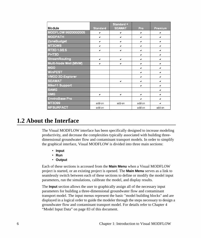
6 Chapter 1: Introduction to Visual MODFLOW
1.2 About the InterfaceThe Visual MODFLOW interface has been specifically designed to increase modeling productivity, and decrease the complexities typically associated with building three-dimensional groundwater flow and contaminant transport models. In order to simplify the graphical interface, Visual MODFLOW is divided into three main sections:
• Input• Run • Output
Each of these sections is accessed from the Main Menu when a Visual MODFLOW project is started, or an existing project is opened. The Main Menu serves as a link to seamlessly switch between each of these sections to define or modify the model input parameters, run the simulations, calibrate the model, and display results.
The Input section allows the user to graphically assign all of the necessary input parameters for building a three-dimensional groundwater flow and contaminant transport model. The input menus represent the basic "model building blocks" and are displayed in a logical order to guide the modeler through the steps necessary to design a groundwater flow and contaminant transport model. For details refer to Chapter 4 “Model Input Data” on page 83 of this document.
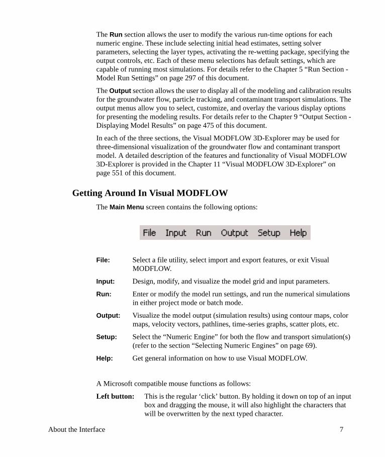
About the Interface 7
The Run section allows the user to modify the various run-time options for each numeric engine. These include selecting initial head estimates, setting solver parameters, selecting the layer types, activating the re-wetting package, specifying the output controls, etc. Each of these menu selections has default settings, which are capable of running most simulations. For details refer to the Chapter 5 “Run Section - Model Run Settings” on page 297 of this document.
The Output section allows the user to display all of the modeling and calibration results for the groundwater flow, particle tracking, and contaminant transport simulations. The output menus allow you to select, customize, and overlay the various display options for presenting the modeling results. For details refer to the Chapter 9 “Output Section - Displaying Model Results” on page 475 of this document.
In each of the three sections, the Visual MODFLOW 3D-Explorer may be used for three-dimensional visualization of the groundwater flow and contaminant transport model. A detailed description of the features and functionality of Visual MODFLOW 3D-Explorer is provided in the Chapter 11 “Visual MODFLOW 3D-Explorer” on page 551 of this document.
Getting Around In Visual MODFLOWThe Main Menu screen contains the following options:
File: Select a file utility, select import and export features, or exit Visual MODFLOW.
Input: Design, modify, and visualize the model grid and input parameters.
Run: Enter or modify the model run settings, and run the numerical simulations in either project mode or batch mode.
Output: Visualize the model output (simulation results) using contour maps, color maps, velocity vectors, pathlines, time-series graphs, scatter plots, etc.
Setup: Select the “Numeric Engine” for both the flow and transport simulation(s) (refer to the section “Selecting Numeric Engines” on page 69).
Help: Get general information on how to use Visual MODFLOW.
A Microsoft compatible mouse functions as follows:
Left button: This is the regular ‘click’ button. By holding it down on top of an input box and dragging the mouse, it will also highlight the characters that will be overwritten by the next typed character.

8 Chapter 1: Introduction to Visual MODFLOW
Right button: This button has different functions depending on the context. For example, it closes polygons or ends a line during the assignment of properties, boundaries, etc. During grid design, it also locates grid rows or columns on precise co-ordinates. Using the right button opens a sub-menu to copy, paste, delete etc.
The <Alt> shortcut keys can be used to access toolbar items and to select many buttons and can be used anytime an item or button text has an underlined letter. Simply press the <Alt> key and the letter key at the same time to access the item or select the button. The number and letter keys are active only when numerical or text input is required; all other keys are ignored by Visual MODFLOW.
The File menu options are described below.
Open... Opens an existing Visual MODFLOW data set.New: Creates a new Visual MODFLOW data set (for more details see
“Creating a New Model” on page 29)Save As: Saves the current model to a different filename.Close: Closes the current model.Import MODFLOW:Imports an existing set of USGS MODFLOW data files (for more
details see “Importing MODFLOW Data Sets” on page 15).Import MODFLOW Packages: Imports MODFLOW packages into an existing
project (for more details see “Importing MODFLOW Packages” on page 27)
Export... Exports the model image or data to a variety of file types.Change Units... Allows the user to change the model units. Changing the model
units only changes the unit labels. Model parameter values are NOT automatically converted to the new unit settings (for more details, see “Changing Measurement Units and Model Start Time” on page 51).
Preferences... Controls font size settings for labels and names of pumping and observation wells, axis, shapes, and contours. It also controls the Color settings for the Screen Background and the Axis labels.
Project Details... Allows the user to enter a Project Title, Description, Project Num-ber, Client name, Project Type, and Model Area Location, for use in print output.
Print: Prints the model display area to the selected printer (with or with-out a description of the image). For more details see “Printing the Model Display Area” on page 59.
eXit: Closes the project and shut-down Visual MODFLOW.
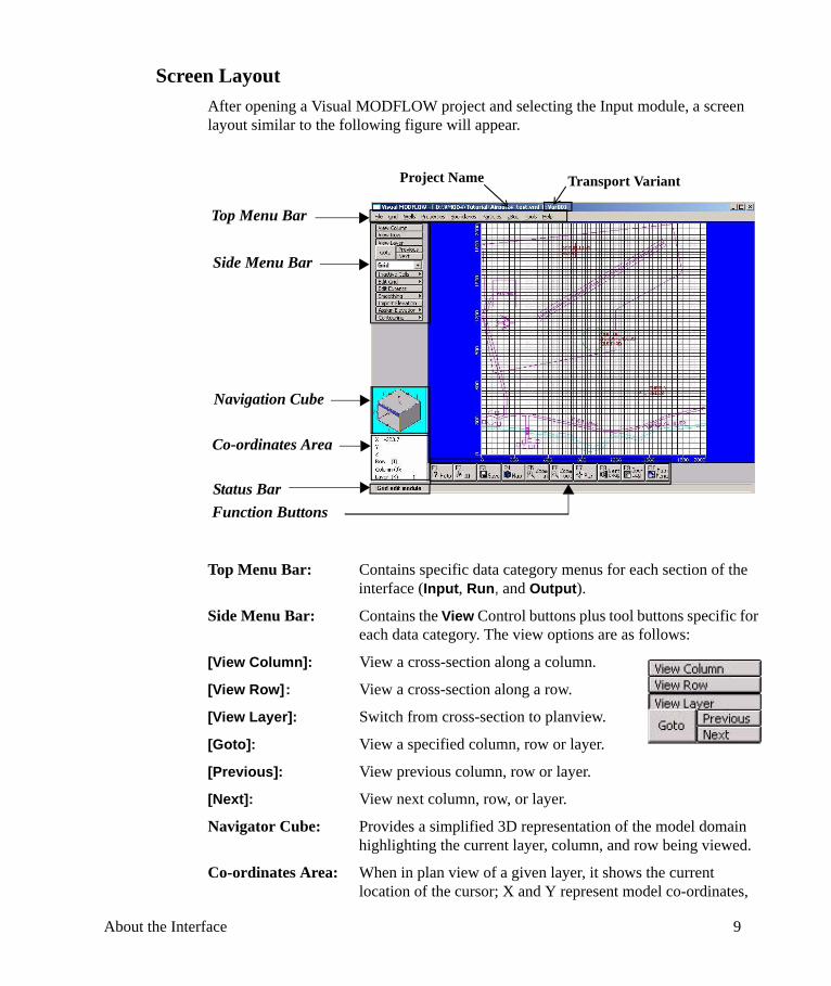
About the Interface 9
Screen LayoutAfter opening a Visual MODFLOW project and selecting the Input module, a screen layout similar to the following figure will appear.
Top Menu Bar: Contains specific data category menus for each section of the interface (Input, Run, and Output).
Side Menu Bar: Contains the View Control buttons plus tool buttons specific for each data category. The view options are as follows:
[View Column]: View a cross-section along a column.
[View Row]: View a cross-section along a row.
[View Layer]: Switch from cross-section to planview.
[Goto]: View a specified column, row or layer.
[Previous]: View previous column, row or layer.
[Next]: View next column, row, or layer.
Navigator Cube: Provides a simplified 3D representation of the model domain highlighting the current layer, column, and row being viewed.
Co-ordinates Area: When in plan view of a given layer, it shows the current location of the cursor; X and Y represent model co-ordinates,
Top Menu Bar
Side Menu Bar
Navigation Cube
Co-ordinates Area
Function ButtonsStatus Bar
Transport VariantProject Name
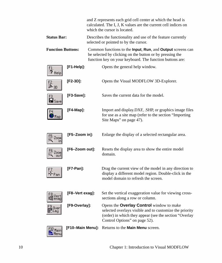
10 Chapter 1: Introduction to Visual MODFLOW
and Z represents each grid cell center at which the head is calculated. The I, J, K values are the current cell indices on which the cursor is located.
Status Bar: Describes the functionality and use of the feature currently selected or pointed to by the cursor.
Function Buttons: Common functions to the Input, Run, and Output screens can be selected by clicking on the button or by pressing the function key on your keyboard. The function buttons are:
[F1-Help]: Opens the general help window.
[F2-3D]: Opens the Visual MODFLOW 3D-Explorer.
[F3-Save]: Saves the current data for the model.
[F4-Map]: Import and display.DXF, .SHP, or graphics image files for use as a site map (refer to the section “Importing Site Maps” on page 47).
[F5–Zoom in]: Enlarge the display of a selected rectangular area.
[F6–Zoom out]: Resets the display area to show the entire model domain.
[F7-Pan]: Drag the current view of the model in any direction to display a different model region. Double-click in the model domain to refresh the screen.
[F8–Vert exag]: Set the vertical exaggeration value for viewing cross-sections along a row or column.
[F9-Overlay]: Opens the Overlay Control window to make selected overlays visible and to customize the priority (order) in which they appear (see the section “Overlay Control Options” on page 52).
[F10–Main Menu]: Returns to the Main Menu screen.
Visual MODFLOW Project Files 11
The interface features described above are consistent throughout the Visual MODFLOW program. The tool buttons and options available on the Side Menu Bar (see “Screen Layout” on page 9) will change depending on the active data category in the Input and Output screen. For example, the tool buttons shown on the Side Menu bar in the figure pertain to the Grid module, for designing and modifying the finite difference model grid. The tool buttons available for the Properties module are completely different. The options available for each Input and Output data category are described in the appropriate sections of this document, and instructions for using some of these options is described in the tutorial exercise document (Tutorial.pdf) provided on your installation media.
1.3 Visual MODFLOW Project FilesEach Visual MODFLOW project consists of many different data files, each pertaining to a specific component of the model (e.g. model setup, grid data, flow boundary conditions, flow properties, particle locations, etc.), whereby each data file is distinguished by its file extension. For example:
• projectname.VMF - general model information• projectname.VMG - model grid information• projectname.VMP - flow model properties information• projectname.VMB - flow model boundary condition information• projectname.VMW - flow model pumping/injection well information• projectname.VMO - flow model observation well information• projectname.VMA - flow model particle locations (for MODPATH)
A detailed listing of each Visual MODFLOW project file is provided in Appendix A on page 613 along with a description of the data structure for each file.
Although the data files associated with each Visual MODFLOW project are easily distinguished by the project name prefix, it is strongly recommended that the user create a separate folder for each modeling project to make it more practical to manage any map files or external data files associated with the project.
Although most of the data files associated with a Visual MODFLOW project are stored in ASCII format, it is not recommended to manually modify or manipulate the data in these files. Visual MODFLOW will not be able to successfully open a project if it encounters any unexpected or incorrect file formats in any of the data files related to the project.
That being said, the reason these files are stored in ASCII format, and the reason the data structures are explained in Appendix A, is to allow advanced users to generate their own Visual MODFLOW data sets using their own specialized programs and utilities. If this is attempted, it is strongly recommended to backup the original data files generated by Visual MODFLOW before replacing or manually modifying them.

12 Chapter 1: Introduction to Visual MODFLOW
1.4 Visual MODFLOW On-Line HelpVisual MODFLOW On-Line Help includes full color screen captures and illustrations which are otherwise black and white in the Visual MODFLOW User’s Manual. The information of interest can be viewed at all stages of the modeling project.
On-Line Help can be accessed either by selecting Help/General Help on the top menu bar, or by clicking the [F1-Help] button from lower tool bar, or by pressing the <F1> button on your keyboard. A Visual MODFLOW Help window will appear, as shown in the following figure. This window is divided into three main areas:
• A Navigation Frame on the left displays the Contents, Index, Search, and Favorites tabs.
• A Toolbar across the top displays a set of buttons to move around in the Visual MODFLOW Help system.
• A Topic Frame on the right displays the actual Help topics included in the On-Line Help.
The tabs in the Navigation Frame provide the core navigational features as described below.
Navigation Frame Toolbar Topic Frame

Visual MODFLOW On-Line Help 13
Contents
The Contents tab displays the entries in the “Table of Contents” in the form of an expandable/collapsible tree view. Closed book icons represent Table of Contents entries that have subentries.
Index
The Index tab displays the entries from the Table of Contents. You can scroll to find the index entry you want, or you can type in the first few letters of the Keywords in the text box, and the index will scroll automatically as you type. Double-click an index entry to display the corresponding Help topic. Alternately, you may select an index entry and then click the Display button to open the Help topic.
Search
The Search tab is used to search the On-Line Help documents for a word or phrase you are interested in. Simply type the word or phrase to search for, and then press <Enter> or click the Display button.
Favorites
You can add frequently accessed Help topics to a personal list of favorites, which is displayed on the Favorites tab. Once you have added a topic to your list of favorites, you can access the topic by double-clicking it. Click Add to add the currently displayed topic to your favorites list. Select a favorite and then click Remove to delete a topic from your favorites list.
The functionality of the main buttons displayed in the Toolbar are described below:
The Hide button hides the Navigation Frame, so only the Toolbar and the Topic Frame are visible. This allows more space on the screen to enlarge the Topic Frame for better viewing of the application.
The Show button displays all areas, the Navigation Frame, the Toolbar, and the Topic Frame.
Clicking the Forward button displays the next Help topic in sequence.
Clicking the Back button displays the previous Help topic in sequence.
Clicking the Home button returns to the Introduction section.

14 Chapter 1: Introduction to Visual MODFLOW
The Print button prints the currently displayed Help topic.
1.5 Software Maintenance and Technical SupportYour purchase of a new license of Visual MODFLOW software includes 1 (one) year of free Maintenance. If you have purchased an upgrade to Visual MODFLOW, please refer to your invoice or contact Schlumberger Water Services’ Sales department to confirm the length of your maintenance contract.
Maintenance for your software consists of upgrades to new versions of your software, updates to the current version, and technical support via phone, email, or fax. You have the option, at any time, to purchase a Maintenance Contract that extends your entitlement to free upgrades, updates, and technical support, in one year increments. A detailed summary of the Annual Maintenance Benefits is provided below:
• Free Major Software Upgrades, and Updates to the Current Version• Notification of Free Updates/Upgrades Available for your Software• Unlimited Telephone Support• Unlimited Email Support• Priority Response to Error Reports• Direct Bug Fix Updates• Documentation Updates• On-Demand FTP Downloads• Showcase Your Projects in SWS E-News• Option to Beta Test New Products
For more information about Annual Maintenance Contracts, contact our Sales department via e-mail at [email protected], or via phone at:
+1 519-746-1798.
Opening Older Visual MODFLOW Models 15
2Getting Started
This chapter presents information on:
• Importing MODFLOW Data Sets• Creating a New Model• Entering the Model Data
2.1 Opening Older Visual MODFLOW ModelsVisual MODFLOW is capable of directly opening any model created in 4.x (by simply clicking on File-Open, and selecting the appropriate VMF file). You will be asked whether you would like to make a backup copy of the model before it is converted to the new format.
Note: Although the direct opening of Visual MODFLOW 3.x and older models is not explicitly supported, due to the possibility of differences between the original project and the converted project, in most cases there should be no issues experienced when directly opening an older Visual MODFLOW project in Version 2011.1. However, SWS recommends that you carefully check your Input and Run parameters after converting to Version 2011.1 format, before continuing to work with the project. If you experience difficulties with the direct opening of an older Visual MODFLOW project, please try importing the translated MODFLOW files instead, as described in the next section.
2.2 Importing MODFLOW Data SetsIn some situations it may be necessary to import an existing MODFLOW data set into Visual MODFLOW in order to review the model, or evaluate different scenarios. Visual MODFLOW can import existing MODFLOW data sets provided they are in MODFLOW-2000 or MODFLOW-2005 format.
Note: Visual MODFLOW currently imports MODFLOW-2000 and
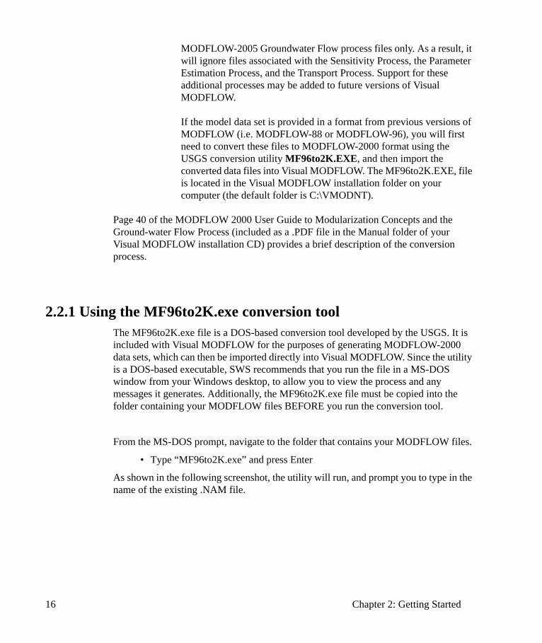
16 Chapter 2: Getting Started
MODFLOW-2005 Groundwater Flow process files only. As a result, it will ignore files associated with the Sensitivity Process, the Parameter Estimation Process, and the Transport Process. Support for these additional processes may be added to future versions of Visual MODFLOW.
If the model data set is provided in a format from previous versions of MODFLOW (i.e. MODFLOW-88 or MODFLOW-96), you will first need to convert these files to MODFLOW-2000 format using the USGS conversion utility MF96to2K.EXE, and then import the converted data files into Visual MODFLOW. The MF96to2K.EXE, file is located in the Visual MODFLOW installation folder on your computer (the default folder is C:\VMODNT).
Page 40 of the MODFLOW 2000 User Guide to Modularization Concepts and the Ground-water Flow Process (included as a .PDF file in the Manual folder of your Visual MODFLOW installation CD) provides a brief description of the conversion process.
2.2.1 Using the MF96to2K.exe conversion toolThe MF96to2K.exe file is a DOS-based conversion tool developed by the USGS. It is included with Visual MODFLOW for the purposes of generating MODFLOW-2000 data sets, which can then be imported directly into Visual MODFLOW. Since the utility is a DOS-based executable, SWS recommends that you run the file in a MS-DOS window from your Windows desktop, to allow you to view the process and any messages it generates. Additionally, the MF96to2K.exe file must be copied into the folder containing your MODFLOW files BEFORE you run the conversion tool.
From the MS-DOS prompt, navigate to the folder that contains your MODFLOW files.
• Type “MF96to2K.exe” and press Enter
As shown in the following screenshot, the utility will run, and prompt you to type in the name of the existing .NAM file.
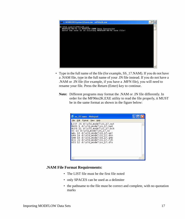
Importing MODFLOW Data Sets 17
• Type in the full name of the file (for example, SS_17.NAM). If you do not have a .NAM file, type in the full name of your .IN file instead. If you do not have a .NAM or .IN file (for example, if you have a .MFN file), you will need to rename your file. Press the Return (Enter) key to continue.
Note: Different programs may format the .NAM or .IN file differently. In order for the MF96to2K.EXE utility to read the file properly, it MUST be in the same format as shown in the figure below:
.NAM File Format Requirements:• The LIST file must be the first file noted
• only SPACES can be used as a delimiter
• the pathname to the file must be correct and complete, with no quotation marks
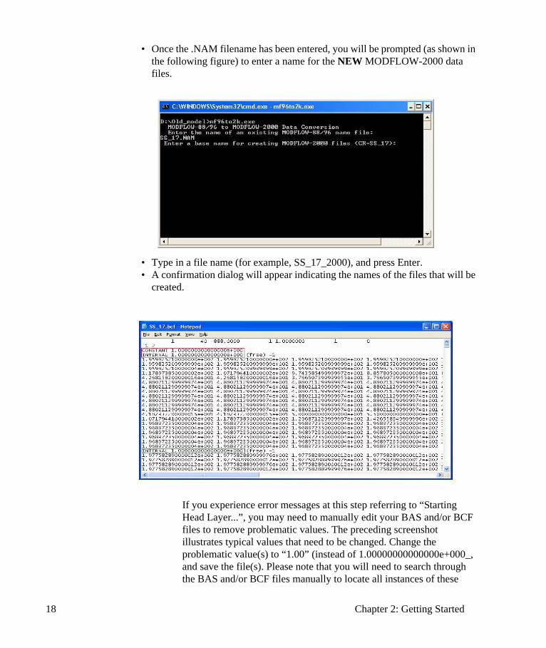
18 Chapter 2: Getting Started
• Once the .NAM filename has been entered, you will be prompted (as shown in the following figure) to enter a name for the NEW MODFLOW-2000 data files.
• Type in a file name (for example, SS_17_2000), and press Enter.• A confirmation dialog will appear indicating the names of the files that will be
created.
If you experience error messages at this step referring to “Starting Head Layer...”, you may need to manually edit your BAS and/or BCF files to remove problematic values. The preceding screenshot illustrates typical values that need to be changed. Change the problematic value(s) to “1.00” (instead of 1.00000000000000e+000_, and save the file(s). Please note that you will need to search through the BAS and/or BCF files manually to locate all instances of these
Importing MODFLOW Data Sets 19
values. Searching for the terms “Internal” and “Constant” in the .BCF file, and “Internal” in the .BAS file, should locate all of these values.
• If no error messages are created, you will be asked “Is there a quasi 3-D confining bed below layer 1?” Type YES or NO, then press Enter.
• You will then be prompted to enter a constant value for the Top of Layer 1.
Note: The conversion utility provides you with the range of Bottom elevations of Layer 1. Please refer to these numbers before entering an elevation for the Top of layer 1, to avoid creating cells with a thickness of 0. We recommend that you enter a “compatible value”, even if it is not realistic, during this process, and then edit your layer elevation values from the Visual MODFLOW Input screen.
• Type an elevation value, then press Enter.• You will be asked to repeat this process for the remaining layers in your model.
Negative elevation values can be entered.
The process should finish by returning to a DOS prompt. At this point, your MODFLOW-2000 data set has been created, and you are ready to use the Visual MODFLOW Import process to create a model from your MODFLOW data.
2.2.2 Importing a MODFLOW 2000 data setTo import a MODFLOW-2000 model data set, select File/ Import MODFLOW from the top menu bar, and then choose the .NAM (or .MODFLOW.IN) file of the model data set.
Note: The .NAM file (or .MODFLOW.IN file) is an ASCII file containing a list of the input and output data files for the model, and their location (folder and pathname) on the computer. If the model files have been moved to a new location, the file must be manually updated to reflect the new file location(s). See ".NAM File Format Requirements:" on page 17 for details.
Once you have selected the desired model data file, click on the [Open] button to continue.
Next, you will be asked to enter a name for the Visual MODFLOW model data files. It is recommend that you choose a name that is slightly different than the original model name, so you do not overwrite any of the original files. You may also want to save the Visual MODFLOW model in a separate folder. Once you have entered the desired name for the Visual MODFLOW model, press the [Save] button to continue.
The model data file selection window will appear, as shown in the following figure:
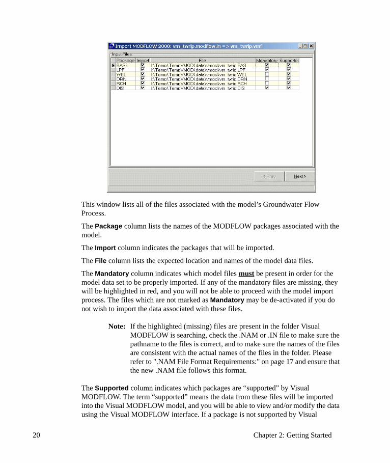
20 Chapter 2: Getting Started
This window lists all of the files associated with the model’s Groundwater Flow Process.
The Package column lists the names of the MODFLOW packages associated with the model.
The Import column indicates the packages that will be imported.
The File column lists the expected location and names of the model data files.
The Mandatory column indicates which model files must be present in order for the model data set to be properly imported. If any of the mandatory files are missing, they will be highlighted in red, and you will not be able to proceed with the model import process. The files which are not marked as Mandatory may be de-activated if you do not wish to import the data associated with these files.
Note: If the highlighted (missing) files are present in the folder Visual MODFLOW is searching, check the .NAM or .IN file to make sure the pathname to the files is correct, and to make sure the names of the files are consistent with the actual names of the files in the folder. Please refer to ".NAM File Format Requirements:" on page 17 and ensure that the new .NAM file follows this format.
The Supported column indicates which packages are “supported” by Visual MODFLOW. The term “supported” means the data from these files will be imported into the Visual MODFLOW model, and you will be able to view and/or modify the data using the Visual MODFLOW interface. If a package is not supported by Visual
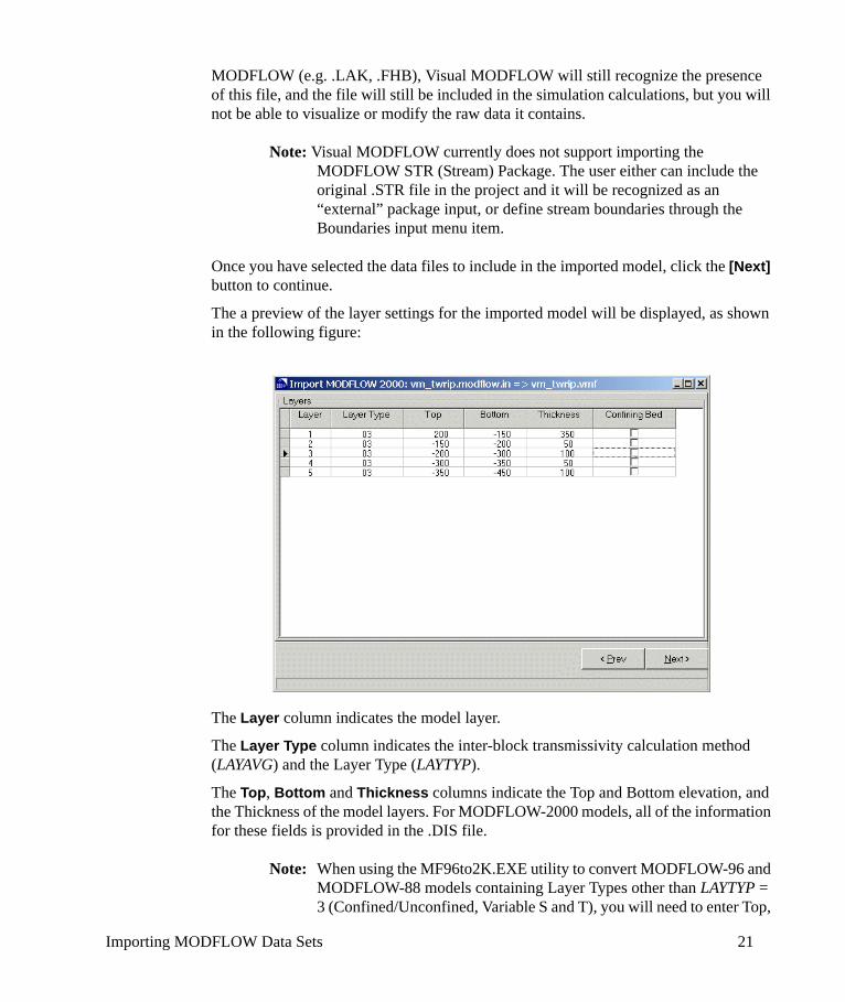
Importing MODFLOW Data Sets 21
MODFLOW (e.g. .LAK, .FHB), Visual MODFLOW will still recognize the presence of this file, and the file will still be included in the simulation calculations, but you will not be able to visualize or modify the raw data it contains.
Note: Visual MODFLOW currently does not support importing the MODFLOW STR (Stream) Package. The user either can include the original .STR file in the project and it will be recognized as an “external” package input, or define stream boundaries through the Boundaries input menu item.
Once you have selected the data files to include in the imported model, click the [Next] button to continue.
The a preview of the layer settings for the imported model will be displayed, as shown in the following figure:
The Layer column indicates the model layer.
The Layer Type column indicates the inter-block transmissivity calculation method (LAYAVG) and the Layer Type (LAYTYP).
The Top, Bottom and Thickness columns indicate the Top and Bottom elevation, and the Thickness of the model layers. For MODFLOW-2000 models, all of the information for these fields is provided in the .DIS file.
Note: When using the MF96to2K.EXE utility to convert MODFLOW-96 and MODFLOW-88 models containing Layer Types other than LAYTYP = 3 (Confined/Unconfined, Variable S and T), you will need to enter Top,
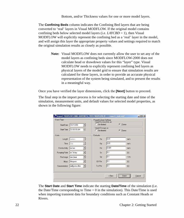
22 Chapter 2: Getting Started
Bottom, and/or Thickness values for one or more model layers.
The Confining Beds column indicates the Confining Bed layers that are being converted to ‘real’ layers in Visual MODFLOW. If the original model contains confining beds below selected model layers (i.e. LAYCBD = 1), then Visual MODFLOW will explicitly represent the confining bed as a ‘real’ layer in the model, and will assign this layer the appropriate property values and settings required to match the original simulation results as closely as possible.
Note: Visual MODFLOW does not currently allow the user to set any of the model layers as confining beds since MODFLOW-2000 does not calculate head or drawdown values for this “layer” type. Visual MODFLOW needs to explicitly represent confining bed layers as physical layers of the model grid to ensure that simulation results are calculated for these layers, in order to provide an accurate physical representation of the system being simulated, and to present the results in a meaningful way.
Once you have verified the layer dimensions, click the [Next] button to proceed.
The final step in the import process is for selecting the starting date and time of the simulation, measurement units, and default values for selected model properties, as shown in the following figure:
The Start Date and Start Time indicate the starting Date/Time of the simulation (i.e. the Date/Time corresponding to Time = 0 in the simulation). This Date/Time is used when importing transient data for boundary conditions such as Constant Heads or Rivers.

Importing MODFLOW Data Sets 23
The Length and Time units of the original model data set may not be modified, and will be used in the Visual MODFLOW model, but the remaining measurement units may be customized to suit your preferences. If no Time or Length units are specified in the original data files, you will be prompted to select them.
The Property Zone Settings frame indicates how the Conductivity and Storage property zones will be imported. The Distributed option will create a single property zone that is linked to a distribution array containing the actual cell-by-cell property values. The Zones option will create as many individual property zones as required to maintain a unique combination of parameter values (e.g. Kx, Ky, and Kz) in each property zone. For information on determining property values for confining bed layers, please see "Determining Property Values for Confining Bed Layers" on page 23
The Defaults frame indicates the default values for each imported property value. These values are only required when the imported model does not include all required data (for example, if the model being imported is a steady-state model, it will not have Ss or Sy values).
Click the [Finish] button to complete the import process. A confirmation will appear if the model was created successfully. You may then open the newly imported model by clicking on File/Open from the top menu bar of Visual MODFLOW program window.
2.2.3 Determining Property Values for Confining Bed LayersVisual MODFLOW requires all of the aquifer material properties (Kx, Ky, Kz, Ss, Sy, Eff. Por, Tot. Por) to be assigned to each grid cell in the model. However, the confining bed layers in MODFLOW-2000 only contain information about the vertical hydraulic conductivity, Kv (since it is assumed that groundwater only flows vertically through these confining layers). Therefore, the confining bed layer(s) are assigned default values for Ss, Sy, Eff. Por, and Tot. Por, as discussed in the following section. The layer type (LAYTYP) of a confining bed layer will be set to the same as the overlying layer. This layer type setting may be modified in the Run section of the Visual MODFLOW interface (see "Layer Type Settings" on page 332) after the data has been imported.
If the imported model uses the LPF Package, then the vertical hydraulic conductivity (Kv) is already defined using the VKCB variable. In this case, Visual MODFLOW assumes a horizontal anisotropy factor of 1 (CHANI = 1), and the hydraulic conductivity values will be calculated as follows:
Kx = Ky = Kz = VKCB
If the imported model uses the BCF package, Visual MODFLOW must use the VCONT values to calculate the vertical hydraulic conductivity values, as discussed in Calculating Kz Values Using VCONT.
24 Chapter 2: Getting Started
2.2.4 Calculating Kz Values Using VCONTOne of the biggest challenges when importing existing MODFLOW data sets is to back calculate the vertical hydraulic conductivity values for each layer, as required by Visual MODFLOW, using the VCONT values that MODFLOW requires to determine the vertical exchange of flow between layers.
Since its creation, Visual MODFLOW has always approached groundwater model development as a fully three-dimensional process, requiring each hydrogeologic unit (layer) to be explicitly represented in the model. In addition, Visual MODFLOW has focused on making the data requirements for modeling as easy to understand as possible for hydrogeologists who may not always be intimately familiar with the inner workings of a modeling program. As an example, Visual MODFLOW requires the user to enter a vertical hydraulic conductivity (Kz) value for each cell, rather than specifying a vertical conductance (VCONT) value between layers (as required by BCF-based MODFLOW models). Visual MODFLOW then automatically calculates the required VCONT values, as described in "Calculating VCONT Values" on page 306.
Although this approach has been widely praised by hydrogeologists and modelers for making the groundwater modeling process much easier to understand and visualize, it has created some problems and limitations when trying to import existing BCF-based MODFLOW data sets into Visual MODFLOW. The biggest problem lies in the fact that Visual MODFLOW requires Kz values for each layer of the model, whereas MODFLOW only provides VCONT values for each layer interface. As a result, you need to calculate NL unknown parameters using NL-1 known parameters, where NL is the number of model layers.
Note: For MODFLOW-88 and MODFLOW-96 models, this problem was further aggravated by the fact that MODFLOW did not require layer elevations to be explicitly defined for all model layers. This encouraged the use of quasi-3D models, where confining beds between aquifers were omitted from the model grid and were simulated using equivalent VCONT values. However, MODFLOW-2000 has alleviated these problems by requiring layer elevation data for ALL layers of the model, including confining beds.
In order to work around this limitation, Visual MODFLOW starts with the bottom layer of the model, and calculates a Kz value for each cell by assuming a horizontal to vertical anisotropy value (Kx/Kz) of 10 for each cell. This Kz value of the bottom layer is then used as a “seed” to calculate the Kz value of the overlying layer, using the following calculation:
Kvi,j,k = 0.5*THICKi,j,k/[DELR*DELC/VCONT – 0.5*THICKi,j,k+1/Kvi,j,k+1]
Where:
• Kvi,j,k is the vertical hydraulic conductivity of the grid cell in the upper layer
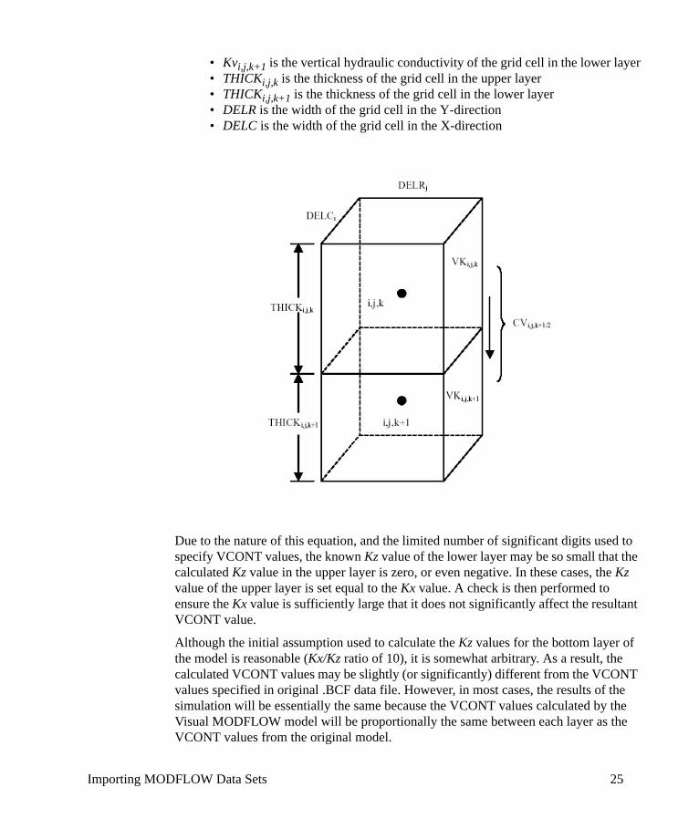
Importing MODFLOW Data Sets 25
• Kvi,j,k+1 is the vertical hydraulic conductivity of the grid cell in the lower layer• THICKi,j,k is the thickness of the grid cell in the upper layer• THICKi,j,k+1 is the thickness of the grid cell in the lower layer• DELR is the width of the grid cell in the Y-direction• DELC is the width of the grid cell in the X-direction
Due to the nature of this equation, and the limited number of significant digits used to specify VCONT values, the known Kz value of the lower layer may be so small that the calculated Kz value in the upper layer is zero, or even negative. In these cases, the Kz value of the upper layer is set equal to the Kx value. A check is then performed to ensure the Kx value is sufficiently large that it does not significantly affect the resultant VCONT value.
Although the initial assumption used to calculate the Kz values for the bottom layer of the model is reasonable (Kx/Kz ratio of 10), it is somewhat arbitrary. As a result, the calculated VCONT values may be slightly (or significantly) different from the VCONT values specified in original .BCF data file. However, in most cases, the results of the simulation will be essentially the same because the VCONT values calculated by the Visual MODFLOW model will be proportionally the same between each layer as the VCONT values from the original model.
26 Chapter 2: Getting Started
2.2.5 Importing Same Cell Boundary ConditionsFor certain boundary conditions, MODFLOW accepts multiple cell entries for the same boundary condition, in the same stress period (e.g. general head, rivers, and drains). For the General Head boundary condition, MODFLOW calculates the flux in a cell using the equation:
where
• Q = flux in the grid cell• Ci = ith conductance term in the grid cell• h = calculated head in the grid cell• hi = ith reference head in the grid cell
Although Visual MODFLOW does not allow the user to assign separate boundary condition values for the same boundary condition in the same cell, it does allow you to import this information from a MODFLOW data set. For example, with the General Head boundary condition, Visual MODFLOW will calculate the representative conductance and reference head values using the following formulas:
Note: This process has not yet been implemented at the time of printing. Currently, Visual MODFLOW will use the LAST boundary condition value ONLY. This feature will be added in the near future.
2.2.6 Importing Initial Heads from a MODFLOW modelWhen Visual MODFLOW imports a MODFLOW data set, the Initial Heads array is not automatically read into the Initial Heads property array. Instead, an .HDS file is created using the filename format [projectname].VMP.HDS. The user may specify this Initial Head file from the Run Menu, under MODFLOW-Initial Heads. Please see "Initial Heads" on page 305 for more information on using the Previous Visual MODFLOW Run option.
Q ΣCi h hi–( )=
C̃ ΣCi=
h̃ ΣCiHiΣCi
----------------=
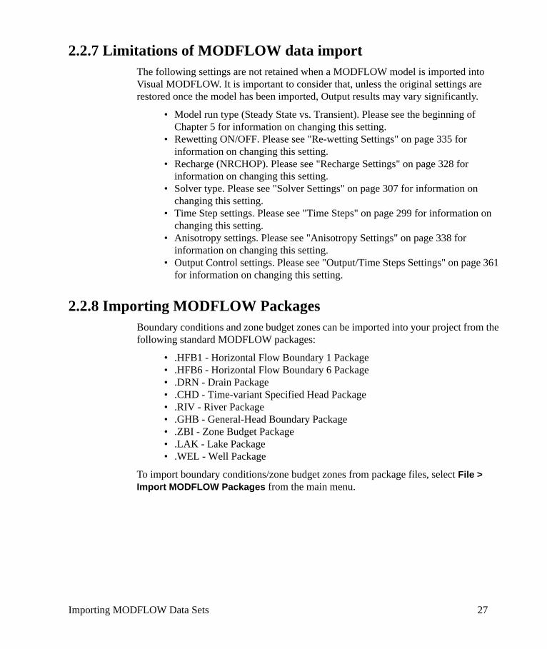
Importing MODFLOW Data Sets 27
2.2.7 Limitations of MODFLOW data importThe following settings are not retained when a MODFLOW model is imported into Visual MODFLOW. It is important to consider that, unless the original settings are restored once the model has been imported, Output results may vary significantly.
• Model run type (Steady State vs. Transient). Please see the beginning of Chapter 5 for information on changing this setting.
• Rewetting ON/OFF. Please see "Re-wetting Settings" on page 335 for information on changing this setting.
• Recharge (NRCHOP). Please see "Recharge Settings" on page 328 for information on changing this setting.
• Solver type. Please see "Solver Settings" on page 307 for information on changing this setting.
• Time Step settings. Please see "Time Steps" on page 299 for information on changing this setting.
• Anisotropy settings. Please see "Anisotropy Settings" on page 338 for information on changing this setting.
• Output Control settings. Please see "Output/Time Steps Settings" on page 361 for information on changing this setting.
2.2.8 Importing MODFLOW PackagesBoundary conditions and zone budget zones can be imported into your project from the following standard MODFLOW packages:
• .HFB1 - Horizontal Flow Boundary 1 Package• .HFB6 - Horizontal Flow Boundary 6 Package• .DRN - Drain Package• .CHD - Time-variant Specified Head Package• .RIV - River Package• .GHB - General-Head Boundary Package• .ZBI - Zone Budget Package• .LAK - Lake Package• .WEL - Well Package
To import boundary conditions/zone budget zones from package files, select File > Import MODFLOW Packages from the main menu.
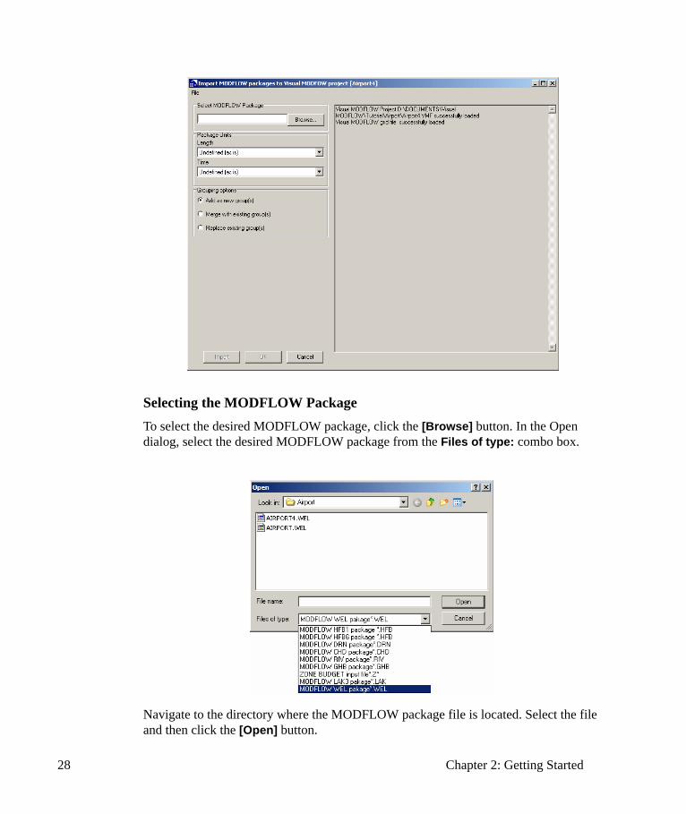
28 Chapter 2: Getting Started
Selecting the MODFLOW PackageTo select the desired MODFLOW package, click the [Browse] button. In the Open dialog, select the desired MODFLOW package from the Files of type: combo box.
Navigate to the directory where the MODFLOW package file is located. Select the file and then click the [Open] button.
Creating a New Model 29
Another Open window will appear on your screen. This time, select the corresponding MODFLOW discretization file (*.DIS). Click the [Open] button.
The discretization file is required to import information about the stress periods in the model. If you do not have a .DIS file you can manually create a text file that contains the length of the different stress periods in the model. Simply list the lengths line by line and save the file as a .TXT. This file can be selected in lieu of a .DIS file.
Package UnitsIf the selected package contains unit (length and time) information, Visual MODFLOW will read this information and automatically convert values to your default project units upon import. If there is no unit information in the selected package (e.g., the unit status is undefined), you must manually select the appropriate units from the Length and Time combo boxes. Furthermore, if you are importing stress periods using a user-defined .TXT file (instead of using a .DIS file), you must manually specify the units in the Length and Time combo boxes.
Grouping OptionsThe Add as new group(s) option will create a new group for the boundary condition being imported. The Replace existing group(s) option will completely replace all existing boundary conditions of the type being imported.
Importing the PackageSelect the Import button to import the package into your project. The logging information shown in the right side of the dialog will indicate whether or not the import was successful.
The import could be unsuccessful for any of the following reasons:
• The source file format has been changed or is corrupted• The grid dimensions of the source data exceeds the grid dimensions of the
model domain in the existing project.• For zone budget imports, the source grid dimensions must be identical to the
grid dimensions of the existing project.
2.3 Creating a New ModelIf you are new to groundwater modeling, we recommend that you follow the tutorial included with your Visual MODFLOW software. The tutorial .PDF guide can be accessed directly from the Visual MODFLOW installation CD, or you can open the VMOD_demo.PDF file from the Tutorials subfolder of the CD. The tutorial model files are installed in the Tutorial subfolder of your Visual MODFLOW program folder on your computer. If you would like to learn more about how to use your Visual
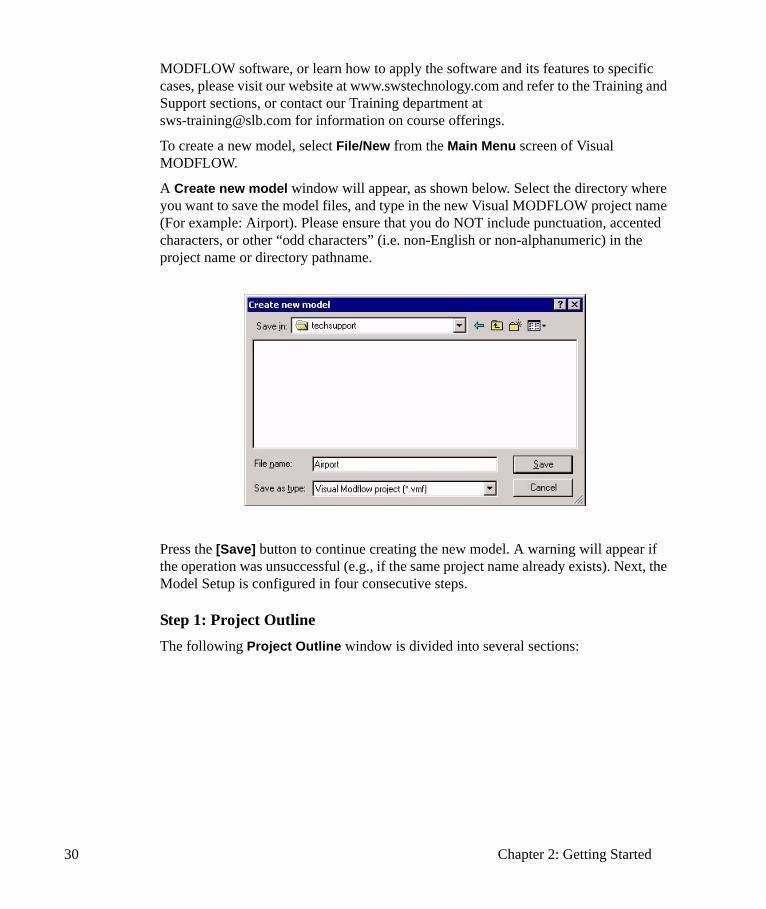
30 Chapter 2: Getting Started
MODFLOW software, or learn how to apply the software and its features to specific cases, please visit our website at www.swstechnology.com and refer to the Training and Support sections, or contact our Training department at [email protected] for information on course offerings.
To create a new model, select File/New from the Main Menu screen of Visual MODFLOW.
A Create new model window will appear, as shown below. Select the directory where you want to save the model files, and type in the new Visual MODFLOW project name (For example: Airport). Please ensure that you do NOT include punctuation, accented characters, or other “odd characters” (i.e. non-English or non-alphanumeric) in the project name or directory pathname.
Press the [Save] button to continue creating the new model. A warning will appear if the operation was unsuccessful (e.g., if the same project name already exists). Next, the Model Setup is configured in four consecutive steps.
Step 1: Project OutlineThe following Project Outline window is divided into several sections:

Creating a New Model 31
• The Project Information frame allows you to enter an optional Project Title, a project Description, and detailed project information by clicking on the Details button.
• The Flow Simulation frame allows you to select the Flow Type for your project using the picklist, and the appropriate Flow Numeric Engine and Simulation Type using the pull-down menus (if available).
• The Transport Simulation frame allows you to select whether Transport will be simulated (using the Yes/No picklist), and select the appropriate Transport Numeric Engine using the pull-down menu (if available)
• The Units frame allows you to select the desired units for each variable using the pull-down menus
Project DescriptionClicking on the Details button will open the Project Details window, allowing you to input optional information about your specific project, as shown in the following screenshot:
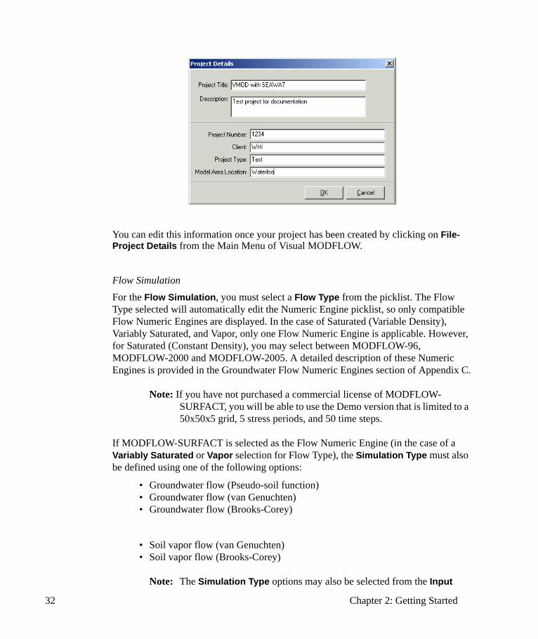
32 Chapter 2: Getting Started
You can edit this information once your project has been created by clicking on File-Project Details from the Main Menu of Visual MODFLOW.
Flow SimulationFor the Flow Simulation, you must select a Flow Type from the picklist. The Flow Type selected will automatically edit the Numeric Engine picklist, so only compatible Flow Numeric Engines are displayed. In the case of Saturated (Variable Density), Variably Saturated, and Vapor, only one Flow Numeric Engine is applicable. However, for Saturated (Constant Density), you may select between MODFLOW-96, MODFLOW-2000 and MODFLOW-2005. A detailed description of these Numeric Engines is provided in the Groundwater Flow Numeric Engines section of Appendix C.
Note: If you have not purchased a commercial license of MODFLOW-SURFACT, you will be able to use the Demo version that is limited to a 50x50x5 grid, 5 stress periods, and 50 time steps.
If MODFLOW-SURFACT is selected as the Flow Numeric Engine (in the case of a Variably Saturated or Vapor selection for Flow Type), the Simulation Type must also be defined using one of the following options:
• Groundwater flow (Pseudo-soil function)• Groundwater flow (van Genuchten)• Groundwater flow (Brooks-Corey)
• Soil vapor flow (van Genuchten)• Soil vapor flow (Brooks-Corey)
Note: The Simulation Type options may also be selected from the Input
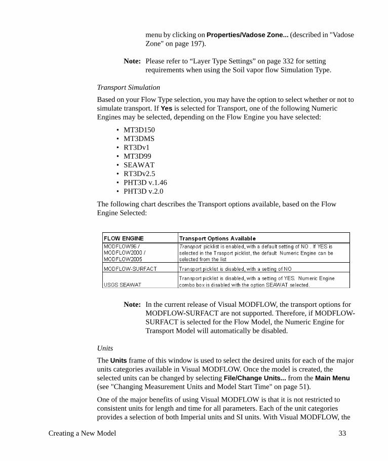
Creating a New Model 33
menu by clicking on Properties/Vadose Zone... (described in "Vadose Zone" on page 197).
Note: Please refer to “Layer Type Settings” on page 332 for setting requirements when using the Soil vapor flow Simulation Type.
Transport SimulationBased on your Flow Type selection, you may have the option to select whether or not to simulate transport. If Yes is selected for Transport, one of the following Numeric Engines may be selected, depending on the Flow Engine you have selected:
• MT3D150• MT3DMS• RT3Dv1• MT3D99• SEAWAT• RT3Dv2.5• PHT3D v.1.46• PHT3D v.2.0
The following chart describes the Transport options available, based on the Flow Engine Selected:
Note: In the current release of Visual MODFLOW, the transport options for MODFLOW-SURFACT are not supported. Therefore, if MODFLOW-SURFACT is selected for the Flow Model, the Numeric Engine for Transport Model will automatically be disabled.
UnitsThe Units frame of this window is used to select the desired units for each of the major units categories available in Visual MODFLOW. Once the model is created, the selected units can be changed by selecting File/Change Units... from the Main Menu (see "Changing Measurement Units and Model Start Time" on page 51).
One of the major benefits of using Visual MODFLOW is that it is not restricted to consistent units for length and time for all parameters. Each of the unit categories provides a selection of both Imperial units and SI units. With Visual MODFLOW, the
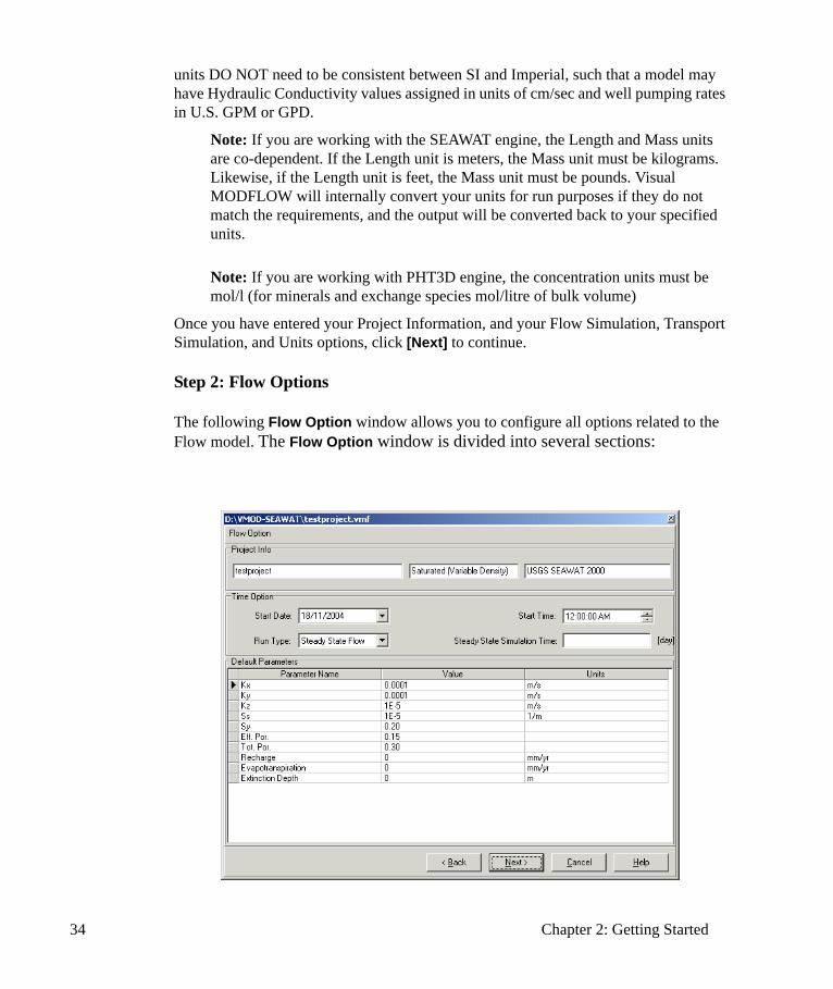
34 Chapter 2: Getting Started
units DO NOT need to be consistent between SI and Imperial, such that a model may have Hydraulic Conductivity values assigned in units of cm/sec and well pumping rates in U.S. GPM or GPD.
Note: If you are working with the SEAWAT engine, the Length and Mass units are co-dependent. If the Length unit is meters, the Mass unit must be kilograms. Likewise, if the Length unit is feet, the Mass unit must be pounds. Visual MODFLOW will internally convert your units for run purposes if they do not match the requirements, and the output will be converted back to your specified units.
Note: If you are working with PHT3D engine, the concentration units must be mol/l (for minerals and exchange species mol/litre of bulk volume)
Once you have entered your Project Information, and your Flow Simulation, Transport Simulation, and Units options, click [Next] to continue.
Step 2: Flow Options
The following Flow Option window allows you to configure all options related to the Flow model. The Flow Option window is divided into several sections:
Creating a New Model 35
• The Project Info frame is a Read-Only frame containing information about your project (which you defined previously)
• The Time Option frame allows you to set Date, Time, and Run information• The Default Parameters frame allows you to set the default flow parameters
for your model
Time OptionThe Start Date of the model is the date corresponding to the beginning of the simulation. Currently, this date is relevant only for transient flow simulations where recorded field data may be imported for defining time schedules for selected boundary conditions (Constant Head, River, General Head and Drain). Once the model is created, the Start Date can be modified by selecting File/Change Units... from the Main Menu (see "Changing Measurement Units and Model Start Time" on page 51).
The Start Time of the model is the time corresponding to the beginning of the simulation. Currently, this time is relevant only for transient flow simulations where recorded field data may be imported for defining time schedules for selected boundary conditions (Constant Head, River, General Head and Drain). Once the model is created, the Start Time can be modified by selecting File/Change Units... from the Main Menu (see "Changing Measurement Units and Model Start Time" on page 51).
The Run Type allows you to select between Steady State Flow and Transient Flow conditions.
If the Steady State Flow option is selected, Visual MODFLOW will prepare the data set for a steady-state flow simulation, and will automatically use the data from the first stress period of each boundary condition and pumping well defined in your project.
If the Transient Flow option is selected, Visual MODFLOW will prepare the data set for a transient flow simulation. During this process, Visual MODFLOW will automatically merge all of the different time period data defined for each pumping well and boundary condition into the stress period format required by the different versions of MODFLOW.
Note: If you are creating a Variable Density (SEAWAT) flow model, the flow type must be Transient Flow.If you have selected PHT3D for your Transport Engine, you may only select the Transient Flow Run Type, or Transient Flow with steady-state stress periods.
The Steady State Simulation Time is required for Steady State Flow simulations. You must enter a valid number (1 is acceptable if you do not have a preference) before proceeding. This parameter is not used if you have selected Transient Flow, however a number must still be entered. Although the simulation will always be run to the same equilibrium solution in Steady State, the total amount of water passing through
36 Chapter 2: Getting Started
boundary conditions (i.e. the cumulative value of the solution) depends on the amount of time simulated. For example, Zone Budget analysis of a Steady State solution would be affected by the simulation time, whereas regional head values would not. Additionally, this number would be important if you were performing a Well Optimization on your project.
The Steady State Simulation Time is linked to the Transport Simulation Time (see “Output/Time Steps Settings” on page 361), and changing one value will automatically update the other.
Default ParametersThe default parameter values are considered reasonable values to be assigned as initial estimates of the material properties in the model. If these values are different from the field measured values, the Default parameter values can be modified in this window, or by going to the Input menu of Visual MODFLOW. Please NOTE that once you have created the model, you will be able to enter new parameter values, and create varying parameter zones. The Default Parameters are simply “starting points” for the model when it is first created.
Once you have edited the variables in the Flow Option window, click [Next] to proceed.
Step 3: Transport OptionsIf you chose (in Step 1) to run a Transport simulation, or if the Flow Engine you selected requires a Transport simulation, the Transport Option window will appear similar to the following screen capture. Please NOTE that if you did not choose to run a Transport simulation, the Transport Option window will not be displayed. If you decide at a later date to add a Transport simulation to your project, you may do so by clicking on Setup-Edit Engines from the Main Menu.
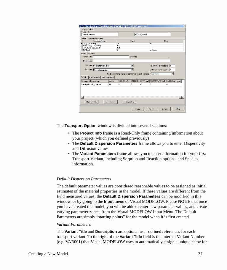
Creating a New Model 37
The Transport Option window is divided into several sections:
• The Project Info frame is a Read-Only frame containing information about your project (which you defined previously)
• The Default Dispersion Parameters frame allows you to enter Dispersivity and Diffusion values
• The Variant Parameters frame allows you to enter information for your first Transport Variant, including Sorption and Reaction options, and Species information.
Default Dispersion ParametersThe default parameter values are considered reasonable values to be assigned as initial estimates of the material properties in the model. If these values are different from the field measured values, the Default Dispersion Parameters can be modified in this window, or by going to the Input menu of Visual MODFLOW. Please NOTE that once you have created the model, you will be able to enter new parameter values, and create varying parameter zones, from the Visual MODFLOW Input Menu. The Default Parameters are simply “starting points” for the model when it is first created.
Variant ParametersThe Variant Title and Description are optional user-defined references for each transport variant. To the right of the Variant Title field is the internal Variant Number (e.g. VAR001) that Visual MODFLOW uses to automatically assign a unique name for
38 Chapter 2: Getting Started
each variant (for example, if you choose not to enter Variant Titles for your variants, or enter a duplicate Variant Title).
Depending upon the selected Transport Engine, you will also have the option of choosing from a number of available Sorption methods and Reactions. A complete description of each Transport Engine and the available options is provided in the Mass Transport Numeric Engines section of Appendix C.
The Total Number of Species and Number of Mobile Species fields are Read-Only values that are automatically updated based on the Species parameters you assign.
The Are the reaction parameters constant or spatially variable? field will be disabled (with a default setting of Constant) unless you have selected an RT3D transport engine. If you are using an RT3D transport engine, you will have the option to select between Constant, and Spatially Variable, reaction parameters.
The Species, Model Params, and Species Params tabs allow you to modify specific settings for each species, and for your Transport simulation. These parameters may also be edited from the Visual MODFLOW Input menu. Detailed information regarding these settings is contained in the MT3D/PHT3D/RT3D/SEAWAT User’s Manual PDF files, located in the Manual folder of your Visual MODFLOW installation media.
The New Species and Delete Species buttons allow you to add and remove species to your Transport simulation. This option is available only for certain transport engines.
Note: If you are creating a SEAWAT project, by default the first species created is “Salt”, and this Density controlling species may not be deleted, although you may edit the Density controlling species parameters.
Note: If you are using the PHT3D mass transport engine, it is possible to set components as active/inactive, in order to create customized reaction modules; non-active components will not be included in the reaction module. The definition of such user-defined reaction networks requires some basic understanding of geochemical processes and concepts as well as some knowledge of the geochemical code PHREEQC. For more details on the reaction modules that offer this capability, please refer to “PHT3D 1.46” on page 652 in the Appendix.
The Temperature button allows you to add a temperature species to your transport simulation. This option is available only for SEAWAT.
Once you have edited the variables in the Transport Option window, click [Next] to proceed.
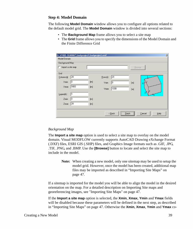
Creating a New Model 39
Step 4: Model DomainThe following Model Domain window allows you to configure all options related to the default model grid. The Model Domain window is divided into several sections:
• The Background Map frame allows you to select a site map• The Grid frame allows you to specify the dimensions of the Model Domain and
the Finite Difference Grid
Background MapThe Import a site map option is used to select a site map to overlay on the model domain. Visual MODFLOW currently supports AutoCAD Drawing eXchange Format (.DXF) files, ESRI GIS (.SHP) files, and Graphics Image formats such as .GIF, .JPG, .TIF, .PNG, and .BMP. Use the [Browse] button to locate and select the site map to include in the model.
Note: When creating a new model, only one sitemap may be used to setup the model grid. However, once the model has been created, additional map files may be imported as described in “Importing Site Maps” on page 47.
If a sitemap is imported for the model you will be able to align the model in the desired orientation on the map. For a detailed description on Importing Site maps and georeferencing images, see "Importing Site Maps" on page 47.
If the Import a site map option is selected, the Xmin, Xmax, Ymin and Ymax fields will be disabled because these parameters will be defined in the next step, as described in “Importing Site Maps” on page 47. Otherwise the Xmin, Xmax, Ymin and Ymax co-

40 Chapter 2: Getting Started
ordinates must be entered. Visual MODFLOW generates a uniform grid based on these dimensions. The uniform grid spacing may be customized in the Input menu of Visual MODFLOW (see "Gridlines (Rows and Columns)" on page 88).
If the Import a site map option is NOT selected, the new model data files will be generated, and the Visual MODFLOW Main Menu will display the model domain. Instructions on refining the finite difference grid and assigning the model properties and boundary conditions are provided in Chapter 4.
GridThe Grid frame contains options for the model dimensions and initial grid discretization. The initial grid will have uniform grid cell sizes throughout the entire model, but all grid spacing and elevations are customizable through the Visual MODFLOW interface. Visual MODFLOW by default allows up to 500 rows x 500 columns x 200 layers. If your project requires a grid larger than the default limits, you may contact the Technical Support department at [email protected] to request a custom-build for your software.
• Columns is the number of uniformly spaced columns in the model grid• Xmin is the minimum X co-ordinate for the model grid• Xmax is the maximum X co-ordinate for the model grid• Rows is the number of uniformly spaced rows in the model grid• Ymin is the minimum Y co-ordinate for the model grid• Ymax is the maximum Y co-ordinate for the model grid• Layers is the number of uniformly spaced layers in the model grid• Zmin is the minimum Z co-ordinate (elevation) for the model grid• Zmax is the maximum Z co-ordinate (elevation) for the model grid
After inputting the desired Grid parameters for the model, clicking on [Finish] saves the Flow and Transport options, creates the model grid, and opens either the Visual MODFLOW Input/Grid menu (if you did not Import a Site Map), or the Select Model Region window described below (if you did Import a Site Map).
Selecting the Model RegionSelecting a model region involves the following tasks:
• orienting the model grid along the principal direction of groundwater flow• selecting the overall size of the model domain from a large area
The Select Model Region window (shown in the following figure) provides tools for accomplishing all of these tasks.
In the Select Model Region window, the model domain is represented by an outline of a box with circular nodes at each corner and with arrows pointing along the X and Y

Creating a New Model 41
axes (see following figure). The model domain box can be shifted, expanded, and rotated to any alignment on the site map using the toolbar options described below. These options are also available under the View menu item.
Typically, the model domain is aligned along the principal direction of groundwater flow and the domain is large enough to accommodate reasonable boundary conditions for the model. In situations where the model domain is rotated, the model will use a dual co-ordinate system whereby locations in the model may be expressed in either world co-ordinates or model co-ordinates (see "Dual Co-ordinate Systems" on page 50).
Zoom in: Click-and-drag the mouse to select the zoom area.
Zoom out: View the entire map display area.
Resize Region: Click-and-drag a corner of the model domain box to stretch or shrink the size of the model domain. Double clicking on the model region will switch the mode between Resize Region and Rotate Region.

42 Chapter 2: Getting Started
Rotate Region: Click-and-drag a corner of the model domain box to rotate and align the model domain. Double clicking on the model region will switch the mode between Rotate Region and Resize Region.
Align Rectangle: Align the model domain with the x-axis.
Maximize: Enlarge the model domain to the full extents of the base map.
New Map: Load a new file for the site map.
If an AutoCAD .DXF file or an ESRI .SHP file is used for the site map, the top right-hand section will contain the Display Area co-ordinates where (X1, Y1) is the map co-ordinate in the lower left-hand corner and (X2, Y2) is the map co-ordinate in the top right-hand corner. These values are automatically read from the map file and may be modified to expand or shrink the available ‘real estate’ for defining the model region.
If a graphics file is used for the site map, the top right-hand section will contain the co-ordinates of the two Georeference Points. These values cannot be modified unless one of the georeference points is deleted and a different georeference point is assigned.
The Angle is the degree angle of rotation of the model region from the world co-ordinate axes.
The Model Origin is the X and Y world co-ordinate location of the bottom left-hand corner of the model domain.
The Model Corners are the model co-ordinates of the bottom left-hand corner (X1, Y1) and the top right-hand corner (X2, Y2) of the model domain. If the Angle is 0.0 and (X1, Y1) is the same as the Model Origin, then the model co-ordinate system will coincide with the world co-ordinate system. However, if the model domain is rotated from the world co-ordinate axes, then the model will use a dual co-ordinate systems.
The NRows and NColumns fields contain the number of finite difference rows and columns, respectively, for the model grid. The Show Grid switch is used to show/hide the model grid inside the model domain.
Note: In some situations (e.g. with large scale regional models), the georeferenced graphics image may be slightly distorted in scale, particularly when the model domain has been rotated over the site map. In these cases, the attributes of the graphics image will not be aligned with similar attributes from a .DXF map or a .SHP map files. This
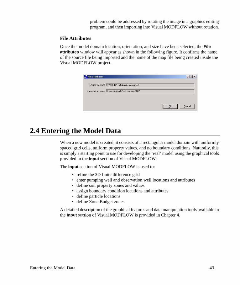
Entering the Model Data 43
problem could be addressed by rotating the image in a graphics editing program, and then importing into Visual MODFLOW without rotation.
File AttributesOnce the model domain location, orientation, and size have been selected, the File attributes window will appear as shown in the following figure. It confirms the name of the source file being imported and the name of the map file being created inside the Visual MODFLOW project.
2.4 Entering the Model DataWhen a new model is created, it consists of a rectangular model domain with uniformly spaced grid cells, uniform property values, and no boundary conditions. Naturally, this is simply a starting point to use for developing the ‘real’ model using the graphical tools provided in the Input section of Visual MODFLOW.
The Input section of Visual MODFLOW is used to:
• refine the 3D finite difference grid • enter pumping well and observation well locations and attributes• define soil property zones and values• assign boundary condition locations and attributes• define particle locations• define Zone Budget zones
A detailed description of the graphical features and data manipulation tools available in the Input section of Visual MODFLOW is provided in Chapter 4.

44 Chapter 2: Getting Started
Saving the Model 45
3Global Operations
This chapter presents information on:
• Changing your model preferences• Working with site maps• Modifying the images displayed by Visual MODFLOW• Printing the model display area• Selecting the numeric flow and transport engines• Exporting your model data
3.1 Saving the ModelThe current data and display settings for the model can be saved at any time by selecting File/Save from the top menu, or by clicking the [F3 - Save] button. In addition, as you navigate through the steps of assigning and editing the model input data, Visual MODFLOW will prompt you to save the most recent data each time you switch data categories. For example, when you switch from assigning Properties to assigning Boundary Conditions, you will be prompted to save the recent changes to the Property data.
3.2 Changing your Model PreferencesThe model Preferences can be accessed by clicking on File/Preferences from the top menu bar. The Preferences window will open, and shown in the following figure:
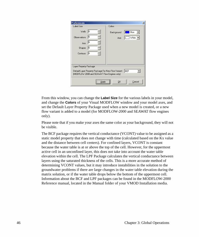
46 Chapter 3: Global Operations
From this window, you can change the Label Size for the various labels in your model, and change the Colors of your Visual MODFLOW window and your model axes, and set the Default Layer Property Package used when a new model is created, or a new flow variant is added to a model (for MODFLOW-2000 and SEAWAT flow engines only).
Please note that if you make your axes the same color as your background, they will not be visible.
The BCF package requires the vertical conductance (VCONT) value to be assigned as a static model property that does not change with time (calculated based on the Kx value and the distance between cell centers). For confined layers, VCONT is constant because the water table is at or above the top of the cell. However, for the uppermost active cell in an unconfined layer, this does not take into account the water table elevation within the cell. The LPF Package calculates the vertical conductance between layers using the saturated thickness of the cells. This is a more accurate method of determining VCONT values, but it may introduce instabilities in the solution to the groundwater problems if there are large changes in the water table elevation during the matrix solution, or if the water table drops below the bottom of the uppermost cell. Information about the BCF and LPF packages can be found in the MODFLOW-2000 Reference manual, located in the Manual folder of your VMOD Installation media.

Three-Dimensional Visualization 47
3.3 Three-Dimensional VisualizationIf you are using Visual MODFLOW Pro, or if you have purchased a license for Visual MODFLOW 3D-Explorer, you may visualize the model input data, and output results, at any time, from any module within Visual MODFLOW, by clicking the [F2 - 3D] button. A detailed description of the features and functionality of Visual MODFLOW 3D-Explorer is provided in Chapter 11 on page 551.
3.4 Importing Site MapsA site map (or base map) of the model region is often useful for gaining a perspective of the dimensions of the model, and for locating important characteristics of the model. The base map does not contain any specific data used in the calculations, and the presence of a base map does not influence the results of the simulation, but it is helpful for enhancing visualization of the model. Visual MODFLOW supports the use of site maps in AutoCAD .DXF, ESRI .SHP, and .JPG, .GIF, .TIF, .PNG, and .BMP graphics image file formats.
If a graphics file is being used as a site map, then the image must first be georeferenced by entering the X-Y world co-ordinates of two known locations on the image. Once the image is georeferenced, it is inserted as an Overlay item in the Visual MODFLOW project. The model grid, with reference to newly added image, can then be previewed. Note that this preview does not allow the user to rotate, move, or modify the grid location or dimension. The georeferencing procedure is described in the following section.
If an AutoCAD file (.DXF) or an ESRI Shape (.SHP) file is being used as the model site map, refer to "Selecting the Model Region" on page 40.
Once the model has been created, additional site maps can be added to the model using the [F4 - Maps] button in the lower toolbar of the Visual MODFLOW interface. The map(s) will be inserted as an additional Overlay item in the Visual MODFLOW project. Site maps can be viewed simultaneously, and graphics files (.JPG, .GIF, .TIF, .PNG, .BMP) may be modified using the Image Smoothing and Transparency options described in the "Modifying Site Map Images" on page 50.
3.4.1 Georeferencing a Graphics FileIf a graphics file (.JPG, .GIF, .TIF, .PNG, .BMP) is selected for the site map, then a Select Model Region window will appear as shown in the following figure.
Graphics files do not contain any co-ordinate information in their internal file format. Therefore, in order to use a graphics file as a site map, it must be manually georeferenced to map a co-ordinate system to the pixels of the image.

48 Chapter 3: Global Operations
The following Georeference Hints window will appear with some guidance on how to georeference the graphics file.
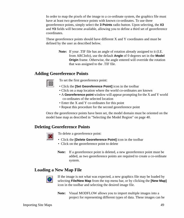
Importing Site Maps 49
In order to map the pixels of the image to a co-ordinate system, the graphics file must have at least two georeference points with known co-ordinates. To use three georeference points, simply select the 3 Points radio button. Upon selecting, the X3 and Y3 fields will become available, allowing you to define a third set of georeference coordinates.
These georeference points should have different X and Y coordinates and must be defined by the user as described below.
Note: If your .TIF file has an angle of rotation already assigned to it (I.E. from ARCInfo), use the default Angle of 0 degrees set in the Model Origin frame. Otherwise, the angle entered will override the rotation that was assigned to the .TIF file.
Adding Georeference PointsTo set the first georeference point:
• Click the [Set Georeference Point] icon in the toolbar• Click on a map location where the world co-ordinates are known• A Georeference point window will appear prompting for the X and Y world
co-ordinates of the selected location• Enter the X and Y co-ordinates for this point• Repeat this procedure for the second georeference point
Once the georeference points have been set, the model domain must be oriented on the model base map as described in "Selecting the Model Region" on page 40.
Deleting Georeference PointsTo delete a georeference point:
• Click the [Delete Georeference Point] icon in the toolbar• Click on the georeference point to delete
Note: If a georeference point is deleted, a new georeference point must be added, as two georeference points are required to create a co-ordinate system.
Loading a New Map FileIf the image is not what was expected, a new graphics file may be loaded by selecting File/New Map from the top menu bar, or by clicking the [New Map] icon in the toolbar and selecting the desired image file.
Note: Visual MODFLOW allows you to import multiple images into a project for representing different types of data. These images can be

50 Chapter 3: Global Operations
georeferenced after the project has been initially created. Graphics files can also be used in combination with ESRI GIS (.SHP) files and AutoCAD (.DXF) files.
3.4.2 Modifying Site Map ImagesOnce a graphics file has been loaded into your Visual MODFLOW project, you may access the Overlay Settings by clicking on the [F9-Overlay Function] button. Please see "Modifying the Display Settings of Selected
Overlays" on page 55 for details.
3.4.3 Dual Co-ordinate SystemsVisual MODFLOW uses two co-ordinate systems, world co-ordinates and model co-ordinates. This allows the model to be rotated on the site map while maintaining a UTM based co-ordinate system.
Transforming World Co-ordinates to Model Co-ordinatesTo transform world co-ordinates to model co-ordinates, use the following formulas. There is no transformation for the Z co-ordinates of the model.
Transforming Model Co-ordinates to World Co-ordinates
where
Xmodel = displayed X model co-ordinate
Xmodel-origin = model X start point (bottom left corner)
Xmodel Xworld Xworld origin––( ) θcos⋅ Yworld Yworld origin––( ) θsin⋅ Xmodel origin–+ +=
Ymodel Xworld Xworld origin––( ) θsin⋅ Yworld Yworld origin––( ) θcos⋅ Ymodel origin–+ +=
Xworld Xmodel Xmodel origin––( ) θcos⋅ Ymodel Ymodel origin––( )– θsin⋅ Xworld origin–+=
Yworld Xmodel Xmodel origin––( )– θsin⋅ Ymodel Ymodel origin––( ) θcos⋅ Yworld origin–+ +=
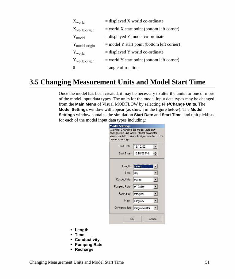
Changing Measurement Units and Model Start Time 51
Xworld = displayed X world co-ordinate
Xworld-origin = world X start point (bottom left corner)
Ymodel = displayed Y model co-ordinate
Ymodel-origin = model Y start point (bottom left corner)
Yworld = displayed Y world co-ordinate
Yworld-origin = world Y start point (bottom left corner)
θ = angle of rotation
3.5 Changing Measurement Units and Model Start TimeOnce the model has been created, it may be necessary to alter the units for one or more of the model input data types. The units for the model input data types may be changed from the Main Menu of Visual MODFLOW by selecting File/Change Units. The Model Settings window will appear (as shown in the figure below). The Model Settings window contains the simulation Start Date and Start Time, and unit picklists for each of the model input data types including:
• Length• Time• Conductivity• Pumping Rate• Recharge

52 Chapter 3: Global Operations
• Mass• Concentration
When modifying the units for selected data types, it is important to remember that Visual MODFLOW does NOT contain a unit conversion program. It will NOT transform the values already in the project to their equivalent values in the new system of units.
For example, if the length unit was in meters and it was changed to feet, any head values entered as 10 metres would now be read as 10 feet (i.e. they would not be converted to a value of 32.81 feet).
Therefore, if the units for any model data types are modified in the middle of developing the model, it is strongly recommended that ALL model input parameters be carefully and thoroughly reviewed to ensure they ‘make sense’.
Note: If you are working with the SEAWAT engine, the Length and Mass units are co-dependent. If the Length unit is meters, the Mass unit must be kilograms. Likewise, if the Length unit is feet, the Mass unit must be pounds. Visual MODFLOW will internally convert your units for run purposes if they do not match the requirements, and the output will be converted back to your specified units.If you are working with PHT3D engine, the concentration units must be mol/l (for minerals and exchange species mol/litre of bulk volume).
3.6 Overlay Control OptionsThe Input, Run and Output menus in Visual MODFLOW can be used to assign, edit, or display specific characteristics of the model. The display of the different model characteristics such as grid lines, maps, property zones, observations, boundary conditions, and contour lines are organized as a series of separate “Overlays”.
Overlay GroupsDue to the sheer number of different Overlays available in Visual MODFLOW, the Overlays were divided into different groups to make it easier to manage the Overlay list. The Overlay Group Names and Short Names are as follows:
Group Name Short Name Description
Boundary Conditions BC[F] Flow Boundary Conditions
BC[T] Transport Boundary Conditions
Contours (Input) C[I] Contour maps of Input parameters
Contours (Output) C[O] Contour maps of model Output
Calibration Cal Calibration data
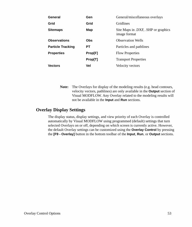
Overlay Control Options 53
General Gen General/miscellaneous overlays
Grid Grid Gridlines
Sitemaps Map Site Maps in .DXF, .SHP or graphics image format
Observations Obs Observation Wells
Particle Tracking PT Particles and pathlines
Properties Prop[F] Flow Properties
Prop[T] Transport Properties
Vectors Vel Velocity vectors
Note: The Overlays for display of the modeling results (e.g. head contours, velocity vectors, pathlines) are only available in the Output section of Visual MODFLOW. Any Overlay related to the modeling results will not be available in the Input and Run sections.
Overlay Display SettingsThe display status, display settings, and view priority of each Overlay is controlled automatically by Visual MODFLOW using programmed (default) settings that turn selected Overlays on or off, depending on which screen is currently active. However, the default Overlay settings can be customized using the Overlay Control by pressing the [F9 - Overlay] button in the bottom toolbar of the Input, Run, or Output sections.
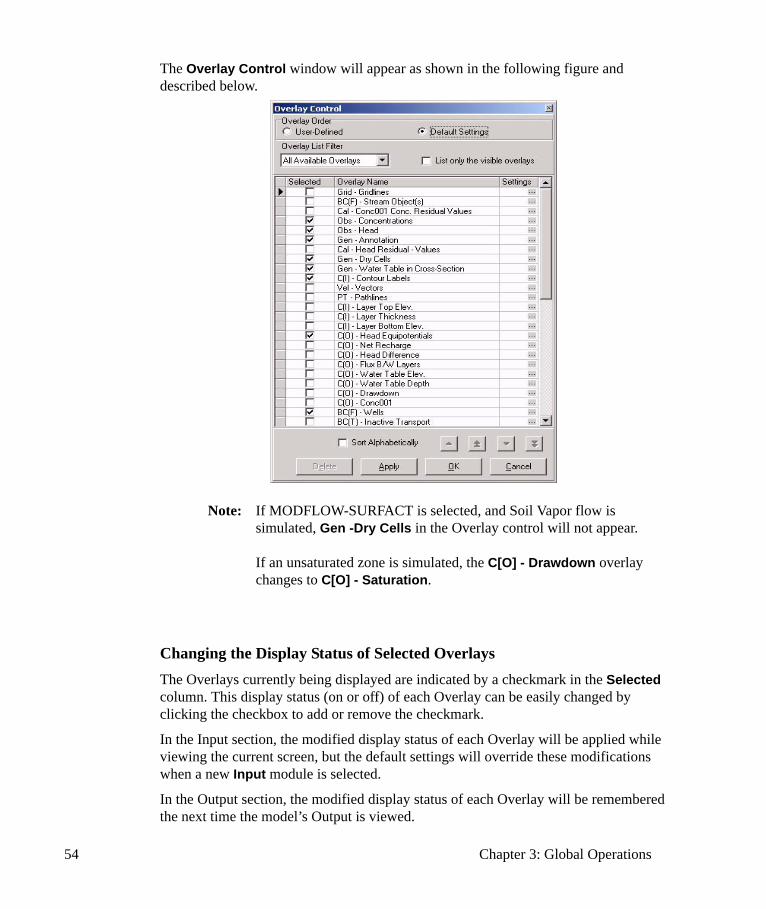
54 Chapter 3: Global Operations
The Overlay Control window will appear as shown in the following figure and described below.
Note: If MODFLOW-SURFACT is selected, and Soil Vapor flow is simulated, Gen -Dry Cells in the Overlay control will not appear.
If an unsaturated zone is simulated, the C[O] - Drawdown overlay changes to C[O] - Saturation.
Changing the Display Status of Selected OverlaysThe Overlays currently being displayed are indicated by a checkmark in the Selected column. This display status (on or off) of each Overlay can be easily changed by clicking the checkbox to add or remove the checkmark.
In the Input section, the modified display status of each Overlay will be applied while viewing the current screen, but the default settings will override these modifications when a new Input module is selected.
In the Output section, the modified display status of each Overlay will be remembered the next time the model’s Output is viewed.
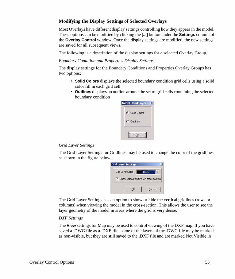
Overlay Control Options 55
Modifying the Display Settings of Selected OverlaysMost Overlays have different display settings controlling how they appear in the model. These options can be modified by clicking the [...] button under the Settings column of the Overlay Control window. Once the display settings are modified, the new settings are saved for all subsequent views.
The following is a description of the display settings for a selected Overlay Group.
Boundary Condition and Properties Display SettingsThe display settings for the Boundary Conditions and Properties Overlay Groups has two options:
• Solid Colors displays the selected boundary condition grid cells using a solid color fill in each grid cell
• Outlines displays an outline around the set of grid cells containing the selected boundary condition
Grid Layer SettingsThe Grid Layer Settings for Gridlines may be used to change the color of the gridlines as shown in the figure below:
The Grid Layer Settings has an option to show or hide the vertical gridlines (rows or columns) when viewing the model in the cross-section. This allows the user to see the layer geometry of the model in areas where the grid is very dense.
DXF SettingsThe View settings for Map may be used to control viewing of the DXF map. If you have saved a .DWG file as a .DXF file, some of the layers of the .DWG file may be marked as non-visible, but they are still saved to the .DXF file and are marked Not Visible in
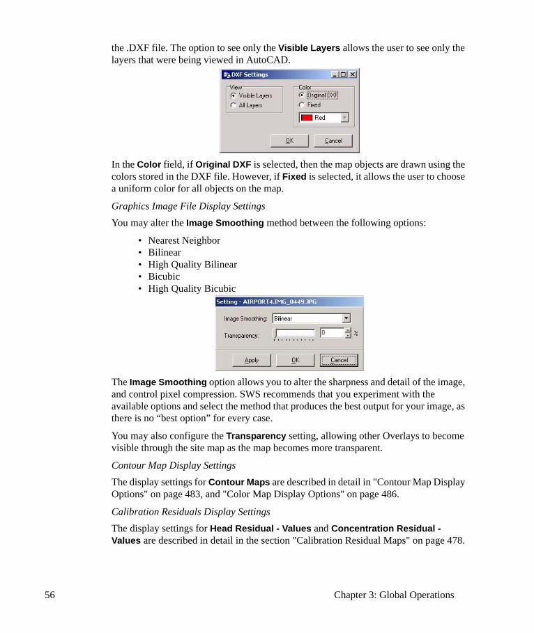
56 Chapter 3: Global Operations
the .DXF file. The option to see only the Visible Layers allows the user to see only the layers that were being viewed in AutoCAD.
In the Color field, if Original DXF is selected, then the map objects are drawn using the colors stored in the DXF file. However, if Fixed is selected, it allows the user to choose a uniform color for all objects on the map.
Graphics Image File Display SettingsYou may alter the Image Smoothing method between the following options:
• Nearest Neighbor• Bilinear• High Quality Bilinear• Bicubic• High Quality Bicubic
The Image Smoothing option allows you to alter the sharpness and detail of the image, and control pixel compression. SWS recommends that you experiment with the available options and select the method that produces the best output for your image, as there is no “best option” for every case.
You may also configure the Transparency setting, allowing other Overlays to become visible through the site map as the map becomes more transparent.
Contour Map Display SettingsThe display settings for Contour Maps are described in detail in "Contour Map Display Options" on page 483, and "Color Map Display Options" on page 486.
Calibration Residuals Display Settings The display settings for Head Residual - Values and Concentration Residual - Values are described in detail in the section "Calibration Residual Maps" on page 478.
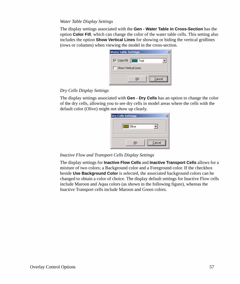
Overlay Control Options 57
Water Table Display SettingsThe display settings associated with the Gen - Water Table in Cross-Section has the option Color Fill, which can change the color of the water table cells. This setting also includes the option Show Vertical Lines for showing or hiding the vertical gridlines (rows or columns) when viewing the model in the cross-section.
Dry Cells Display SettingsThe display settings associated with Gen - Dry Cells has an option to change the color of the dry cells, allowing you to see dry cells in model areas where the cells with the default color (Olive) might not show up clearly.
Inactive Flow and Transport Cells Display SettingsThe display settings for Inactive Flow Cells and Inactive Transport Cells allows for a mixture of two colors; a Background color and a Foreground color. If the checkbox beside Use Background Color is selected, the associated background colors can be changed to obtain a color of choice. The display default settings for Inactive Flow cells include Maroon and Aqua colors (as shown in the following figure), whereas the Inactive Transport cells include Maroon and Green colors.

58 Chapter 3: Global Operations
Well Symbol Size and Color Display SettingsThe display settings associated with BC[F] - Wells (Pumping Wells), Obs - Head (Head Observation Wells) and Obs - Concentrations (Concentration Observation Wells) have the options to change the size and color of their Labels and Symbols. This setting also includes the option for showing or hiding the Well Labels.
The Normal color controls how the well symbol normally appears in the model. The Selected color is used for indicating wells that have been “selected” in the output mode for calibration evaluation. Calibration residual data can be displayed for “selected” wells, and only the “selected” wells will be included in the calibration graphs.
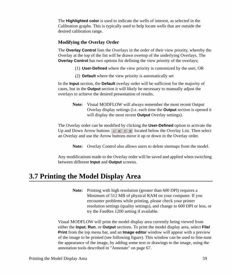
Printing the Model Display Area 59
The Highlighted color is used to indicate the wells of interest, as selected in the Calibration graphs. This is typically used to help locate wells that are outside the desired calibration range.
Modifying the Overlay OrderThe Overlay Control lists the Overlays in the order of their view priority, whereby the Overlay at the top of the list will be drawn overtop of the underlying Overlays. The Overlay Control has two options for defining the view priority of the overlays;
(1) User-Defined where the view priority is customized by the user, OR
(2) Default where the view priority is automatically set
In the Input section, the Default overlay order will be sufficient for the majority of cases, but in the Output section it will likely be necessary to manually adjust the overlays to achieve the desired presentation of results.
Note: Visual MODFLOW will always remember the most recent Output Overlay display settings (i.e. each time the Output section is opened it will display the most recent Output Overlay settings).
The Overlay order can be modified by clicking the User-Defined option to activate the Up and Down Arrow buttons located below the Overlay List. Then select an Overlay and use the Arrow buttons move it up or down in the Overlay order.
Note: Overlay Control also allows users to delete sitemaps from the model.
Any modifications made to the Overlay order will be saved and applied when switching between different Input and Output screens.
3.7 Printing the Model Display Area
Note: Printing with high resolution (greater than 600 DPI) requires a Minimum of 512 MB of physical RAM on your computer. If you encounter problems while printing, please check your printer resolution settings (quality settings), and change to 600 DPI or less, or try the FastRes 1200 setting if available.
Visual MODFLOW will print the model display area currently being viewed from either the Input, Run, or Output sections. To print the model display area, select File/Print from the top menu bar, and an Image editor window will appear with a preview of the image to be printed (see following figure). This window can be used to fine-tune the appearance of the image, by adding some text or drawings to the image, using the annotation tools described in "Annotate" on page 67.
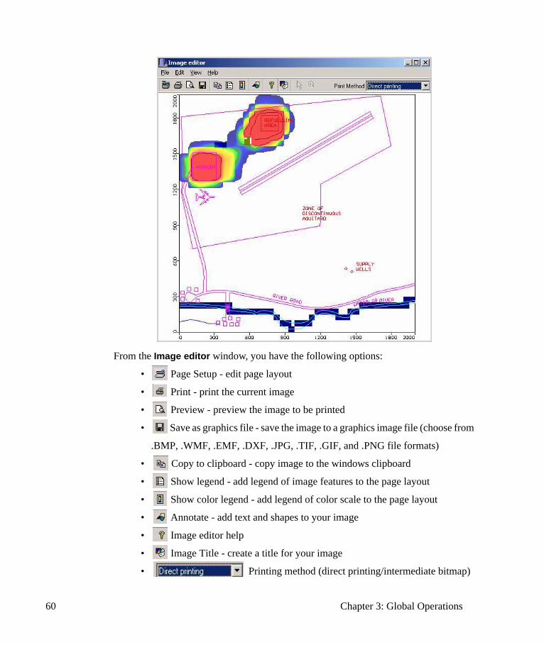
60 Chapter 3: Global Operations
From the Image editor window, you have the following options:
• Page Setup - edit page layout
• Print - print the current image
• Preview - preview the image to be printed
• Save as graphics file - save the image to a graphics image file (choose from
.BMP, .WMF, .EMF, .DXF, .JPG, .TIF, .GIF, and .PNG file formats)
• Copy to clipboard - copy image to the windows clipboard
• Show legend - add legend of image features to the page layout
• Show color legend - add legend of color scale to the page layout
• Annotate - add text and shapes to your image
• Image editor help
• Image Title - create a title for your image
• Printing method (direct printing/intermediate bitmap)
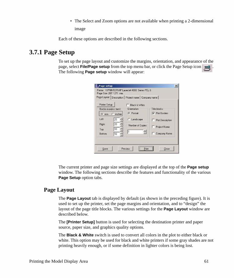
Printing the Model Display Area 61
• The Select and Zoom options are not available when printing a 2-dimensional
image
Each of these options are described in the following sections.
3.7.1 Page SetupTo set up the page layout and customize the margins, orientation, and appearance of the page, select File/Page setup from the top menu bar, or click the Page Setup icon . The following Page setup window will appear:
The current printer and page size settings are displayed at the top of the Page setup window. The following sections describe the features and functionality of the various Page Setup option tabs.
Page LayoutThe Page Layout tab is displayed by default (as shown in the preceding figure). It is used to set up the printer, set the page margins and orientation, and to “design” the layout of the page title blocks. The various settings for the Page Layout window are described below.
The [Printer Setup] button is used for selecting the destination printer and paper source, paper size, and graphics quality options.
The Black & White switch is used to convert all colors in the plot to either black or white. This option may be used for black and white printers if some gray shades are not printing heavily enough, or if some definition in lighter colors is being lost.

62 Chapter 3: Global Operations
The Border Margins options are used to set the size of the margins on each side of the selected page size.
The Orientation option is used to select the orientation of the plot on the printed page.
The Number of Copies option is used to set the number of copies of the page to print.
The Title blocks options are used to customize the appearance of the page layout, as shown in the following figure (the actual arrangement and size of the title blocks on the page will vary depending on the number of title blocks selected).
• Plot Borders will plot an outline along the page margins• Plot Description will add a title block to display a description of the plot (see
"Plot Description" on page 63).• Project Name will add a title block to display the Project Name and an optional
bitmap image of a logo (see "Project Name" on page 63).• Company Name will add a title block to display the company name and an
optional bitmap image of a logo (see "Company Name" on page 64).
Note: You will NOT be able to enter Description, Project Name, or Company Name information in their respective tabs unless you have Checked these options FIRST in the Title Blocks frame.
The [Save] button is used to save the Print settings including the Description, Project Name, and Company Name.
The [Preview] button is used to show a preview of the page as it will appear when it is printed. Please Note that the Plot Description, Company Name, and Project Name will only appear in the Preview window.
The [Print] button will print the page and close the Page Setup window.
The [Close] button will close the Page Setup window.

Printing the Model Display Area 63
Plot DescriptionIf the Plot Description option is selected in the Page Layout tab, the Description tab will become active in the Page Setup window, as shown in the following figure:
To enter the Description of the plot, click in the text box and start typing (or editing the current Description). A preview of the Description title will appear in the space below the Description text box.
The font button is used to select the desired font, size, style, and color for the Description text.
The Align option is used to align the Description in the Left, Center, or Right of the Description title block.
The Description information can be saved for subsequent printing by clicking the [Save] button.
Project NameIf the Project Name option is selected, the Project name tab will become active in the Page Setup window, as shown in the following figure:
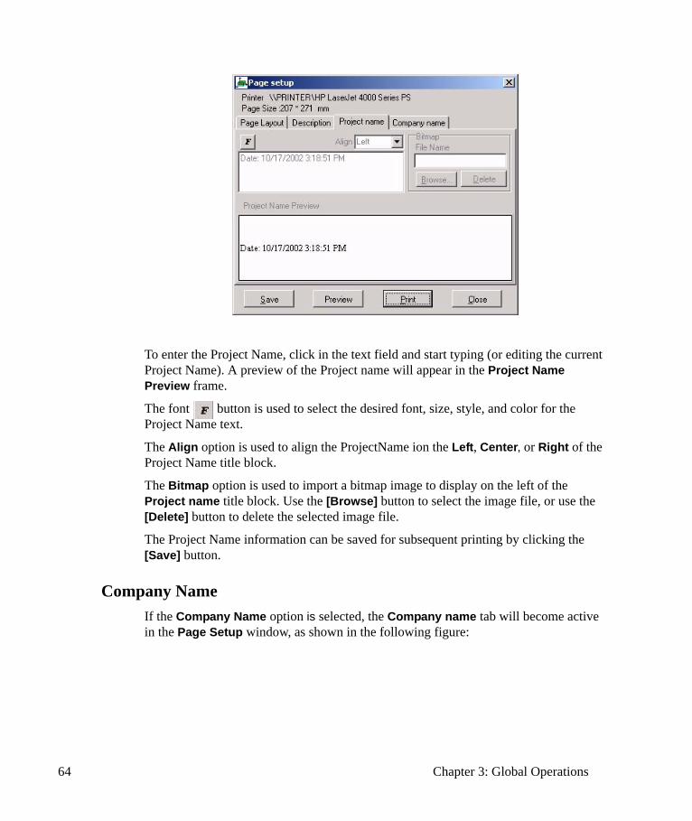
64 Chapter 3: Global Operations
To enter the Project Name, click in the text field and start typing (or editing the current Project Name). A preview of the Project name will appear in the Project Name Preview frame.
The font button is used to select the desired font, size, style, and color for the Project Name text.
The Align option is used to align the ProjectName ion the Left, Center, or Right of the Project Name title block.
The Bitmap option is used to import a bitmap image to display on the left of the Project name title block. Use the [Browse] button to select the image file, or use the [Delete] button to delete the selected image file.
The Project Name information can be saved for subsequent printing by clicking the [Save] button.
Company NameIf the Company Name option is selected, the Company name tab will become active in the Page Setup window, as shown in the following figure:
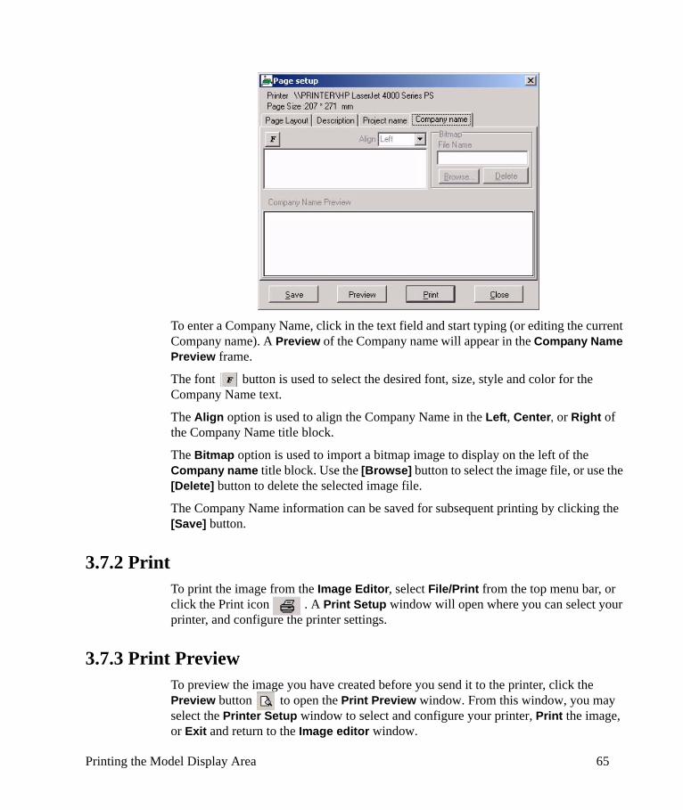
Printing the Model Display Area 65
To enter a Company Name, click in the text field and start typing (or editing the current Company name). A Preview of the Company name will appear in the Company Name Preview frame.
The font button is used to select the desired font, size, style and color for the Company Name text.
The Align option is used to align the Company Name in the Left, Center, or Right of the Company Name title block.
The Bitmap option is used to import a bitmap image to display on the left of the Company name title block. Use the [Browse] button to select the image file, or use the [Delete] button to delete the selected image file.
The Company Name information can be saved for subsequent printing by clicking the [Save] button.
3.7.2 PrintTo print the image from the Image Editor, select File/Print from the top menu bar, or click the Print icon . A Print Setup window will open where you can select your printer, and configure the printer settings.
3.7.3 Print PreviewTo preview the image you have created before you send it to the printer, click the Preview button to open the Print Preview window. From this window, you may select the Printer Setup window to select and configure your printer, Print the image, or Exit and return to the Image editor window.
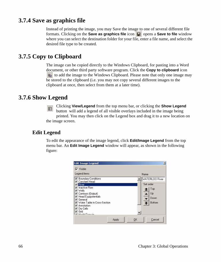
66 Chapter 3: Global Operations
3.7.4 Save as graphics fileInstead of printing the image, you may Save the image to one of several different file formats. Clicking on the Save as graphics file icon opens a Save to file window where you can select the destination folder for your file, enter a file name, and select the desired file type to be created.
3.7.5 Copy to ClipboardThe image can be copied directly to the Windows Clipboard, for pasting into a Word document, or other third party software program. Click the Copy to clipboard icon
to add the image to the Windows Clipboard. Please note that only one image may be stored to the clipboard (i.e. you may not copy several different images to the clipboard at once, then select from them at a later time).
3.7.6 Show LegendClicking View/Legend from the top menu bar, or clicking the Show Legend button will add a legend of all visible overlays included in the image being printed. You may then click on the Legend box and drag it to a new location on
the image screen.
Edit LegendTo edit the appearance of the image legend, click Edit/Image Legend from the top menu bar. An Edit Image Legend window will appear, as shown in the following figure:
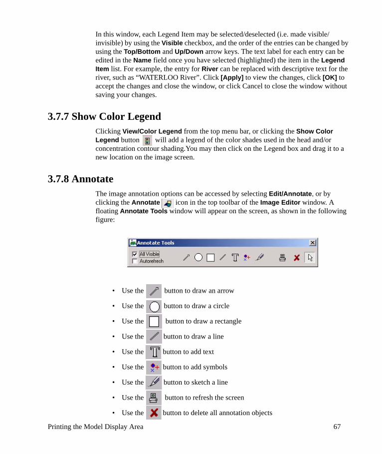
Printing the Model Display Area 67
In this window, each Legend Item may be selected/deselected (i.e. made visible/invisible) by using the Visible checkbox, and the order of the entries can be changed by using the Top/Bottom and Up/Down arrow keys. The text label for each entry can be edited in the Name field once you have selected (highlighted) the item in the Legend Item list. For example, the entry for River can be replaced with descriptive text for the river, such as “WATERLOO River”. Click [Apply] to view the changes, click [OK] to accept the changes and close the window, or click Cancel to close the window without saving your changes.
3.7.7 Show Color LegendClicking View/Color Legend from the top menu bar, or clicking the Show Color Legend button will add a legend of the color shades used in the head and/or concentration contour shading.You may then click on the Legend box and drag it to a new location on the image screen.
3.7.8 AnnotateThe image annotation options can be accessed by selecting Edit/Annotate, or by clicking the Annotate icon in the top toolbar of the Image Editor window. A floating Annotate Tools window will appear on the screen, as shown in the following figure:
• Use the button to draw an arrow
• Use the button to draw a circle
• Use the button to draw a rectangle
• Use the button to draw a line
• Use the button to add text
• Use the button to add symbols
• Use the button to sketch a line
• Use the button to refresh the screen
• Use the button to delete all annotation objects

68 Chapter 3: Global Operations
• Use the button to select, re-size, and move the annotation objects
Note: For details on printing a graph or bar chart, please refer to Chapter 10, "Graph Properties" on page 531.
3.7.9 Image Editor HelpYou can open the Online Help references to the Image Editor directly by clicking the Image Editor Help button .
3.7.10 Image TitleA Title can be added to the image by selecting Edit/Title from the top menu bar, or clicking the Image Title button . In the Properties window that opens, you can type your title text in the Title frame, use the Visible checkbox to add or remove the title to the image, Align the title along the left or right margins, or centre the title, and add a Shadow to the title and position the shadow above or below the title text.The font
button is used to select the desired font, size, style and color for the Image Title text.
3.7.11 Printing MethodsThere are two methods for printing:
Direct Printing- sends the image directly to the printer. This may not be ideal for images containing transparency, as the transparency may not show up. If the transparency does not show up, then try the second printing option. Additionally, if you are using a PostScript printer driver, the transparency settings may not show up. In this case, install the appropriate PCL driver for your printer, or use the Intermediate bitmap method of printing.
Intermediate bitmap- creates a temporary bitmap image in the memory, then sends the bitmap to the printer. This requires slightly more system memory, however it may provide a more suitable alternative to option 1.
Note: If you are printing an image that contains color shading (e.g. shaded head contours or concentration contours), direct printing will often result in a very large file being sent to your printer. If you are experiencing “out of memory” errors, or are not receiving output from your printer, please try the Intermediate bitmap method of printing. While the bitmap takes a few moments to create, it results in a much smaller file being sent to your printer, and facilitates image printing especially with older printers, or printers with low amounts of RAM.

Selecting Numeric Engines 69
Note: If you encounter problems when using a specific printer model, please check to see that you have the most recent Manufacturer-supplied driver installed. If installing a new driver does not resolve your printing issue, and you have tried both Printing Methods, you may use the last option, which is to save a graphics image file (as described in "Save as graphics file" on page 66), and print the file from another application.
3.8 Selecting Numeric EnginesVisual MODFLOW supports all of the most recent public domain and proprietary versions of MODFLOW and MT3D for simulating groundwater flow and mass transport. In Visual MODFLOW, these programs are referred to as Numeric Engines because they perform the numeric calculations required to solve the finite difference equations of groundwater flow and mass transport.
Although the most recent versions of these engines will be used most often, the reason for continuing to support the legacy codes is to provide the user the opportunity to reproduce simulation results from older model data sets using exactly the same simulation programs.
Note: The versions of MODPATH and Zone Budget included in Visual MODFLOW are the latest U.S.Geological Survey versions, compiled and optimized to run as 32 bit native Windows applications.
When creating a new model, the Flow and Transport Numeric Engines are selected. These Numeric Engines can be changed from the Main Menu of Visual MODFLOW by clicking Setup/Edit Engines from the top menu bar.
3.8.1 Groundwater Flow Numeric EnginesVisual MODFLOW provides a selection of Numeric Engines for simulating groundwater flow:
• MODFLOW-96 (Public Domain, U.S. Geological Survey)• MODFLOW-2000 (Public Domain, U.S. Geological Survey)• MODFLOW-2005 (Public Domain, U.S. Geological Survey)• MODFLOW-SURFACT (Proprietary, HydroGeoLogic, Inc.)• SEAWAT (Public Domain, U.S. Geological Survey)
A brief description of the differences between these Groundwater Flow Numeric Engines is provided in Appendix C, while a more detailed explanation of the differences can be found in their respective Reference Manuals, provided in the Manual folder on the Visual MODFLOW installation media.

70 Chapter 3: Global Operations
In terms of the Visual MODFLOW interface, the differences between the MODFLOW-96 and MODFLOW-2000 numeric engines are very subtle, with the exception that MODFLOW-2000 has built-in parameter estimation capabilities (not yet supported by Visual MODFLOW).
MODFLOW-SURFACT is designed to simulate unconfined saturated-unsaturated moisture movement, with some additional capabilities including surface ponding, adaptive time stepping, and air flow simulation. A brief description of the MODFLOW-SURFACT capabilities is provided in Appendix C.
SEAWAT is designed to simulate variable-density flow and transport conditions (for example, a salt water/fresh water interface). Please NOTE that SEAWAT automatically uses its own Transport Engine, based on MT3DMS. A brief description of the SEAWAT capabilities is provided in Appendix C.
3.8.2 Mass Transport Numeric EngineVisual MODFLOW currently provides a selection of numeric engines to use for the mass transport model, as listed below:
• MT3DMS (Public Domain, U.S. Army Corp of Engineers)• RT3D 1.0 (Public Domain, Battelle Northwest Laboratories)• RT3D 2.5 (Public Domain, Battelle Northwest Laboratories)• PHT3D 1.46 (Public Domain, www.pht3d.org)• MT3D96 (not available for new projects/variants) (Proprietary, S.S.
Papadopulos & Associates, Inc.)• MT3D99 (Proprietary, S.S. Papadopulos & Associates, Inc.)• SEAWAT (Public Domain, U.S. Geological Survey)
In the current version of Visual MODFLOW, the Transport Engine is assigned to a Transport Variant. Transport Variants are linked to compatible Flow Engines, meaning that depending on the Flow Engine selected, only existing Transport Variants using compatible Transport Engines will be displayed. If a new Transport Variant is created, only engines compatible with the selected Flow Engine will be available.
The SEAWAT transport engine (based on MT3DMS) can only be used with the SEAWAT flow engine, and it is automatically selected if a SEAWAT flow simulation is created.
The differences between the various Transport Numeric Engines are primarily rooted in the options for specifying sorption, reactions, and solvers. A brief description of the different options available for each of the available Mass Transport Numeric Engines is provided in Appendix C.
A more detailed description of the analysis capabilities for each program can be found in the reference manuals, provided in the Manual folder of the Visual MODFLOW installation media.
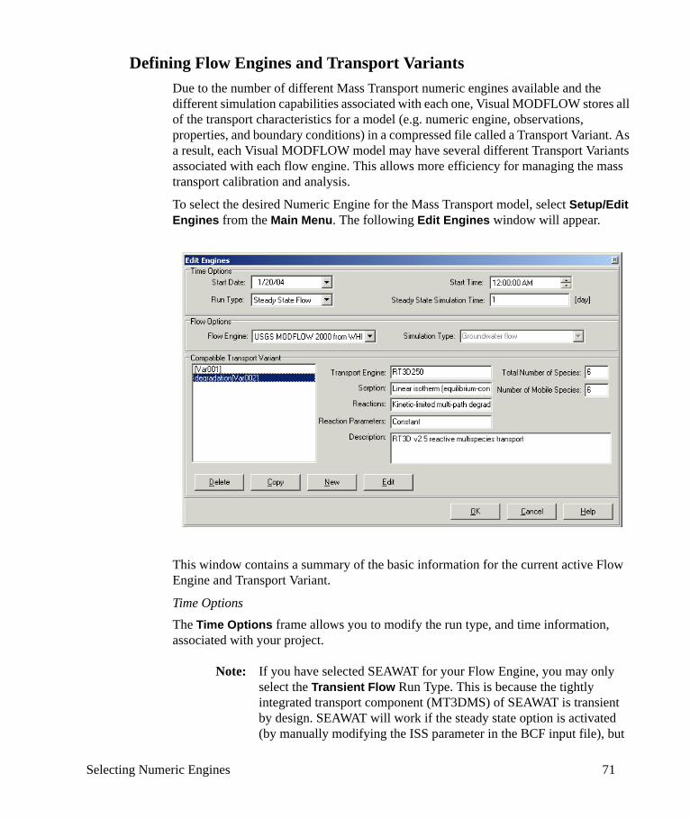
Selecting Numeric Engines 71
Defining Flow Engines and Transport VariantsDue to the number of different Mass Transport numeric engines available and the different simulation capabilities associated with each one, Visual MODFLOW stores all of the transport characteristics for a model (e.g. numeric engine, observations, properties, and boundary conditions) in a compressed file called a Transport Variant. As a result, each Visual MODFLOW model may have several different Transport Variants associated with each flow engine. This allows more efficiency for managing the mass transport calibration and analysis.
To select the desired Numeric Engine for the Mass Transport model, select Setup/Edit Engines from the Main Menu. The following Edit Engines window will appear.
This window contains a summary of the basic information for the current active Flow Engine and Transport Variant.
Time OptionsThe Time Options frame allows you to modify the run type, and time information, associated with your project.
Note: If you have selected SEAWAT for your Flow Engine, you may only select the Transient Flow Run Type. This is because the tightly integrated transport component (MT3DMS) of SEAWAT is transient by design. SEAWAT will work if the steady state option is activated (by manually modifying the ISS parameter in the BCF input file), but
72 Chapter 3: Global Operations
in some cases, the flow portion of the model will not converge. If you have selected PHT3D for your Transport Engine, you may only select the Transient Flow Run Type, or Transient Flow with steady-state stress periods.
Flow OptionsThe Flow Options frame allows you to select the desired Flow Engine to use for your project simulation, and the Simulation Type (if MODFLOW-SURFACT is selected).
Compatible Transport VariantA different Transport Variant may be selected from the Compatible Transport Variant field, or a new Transport Variant created. If multiple variants exist, the highlighted variant is the active variant that will be used in your simulation. If no variants compatible with the currently selected Flow Engine exist, you can create a New variant.
Note: If you switch to the SEAWAT Flow engine, and no transport variant has been defined for SEAWAT, you will be required to create at least one transport variant in order to work with the SEAWAT engine.
Note: If you originally created a project with no Transport simulation (e.g. a MODFLOW-2000 flow project), Var001 was “reserved” by Visual MODFLOW. This means that if you switch Flow Engines (e.g. to SEAWAT) and create a Transport Variant, the first “available” variant number would be Var002. This does not affect the variants themselves in any way, as the variant numbers are only internal reference numbers.
Note: If you are using the MODFLOW-SURFACT Flow Engine, you may not create a Transport Variant, or run a Transport simulation. The Compatible Transport Variant frame will be inactive.
Information about the selected Transport Variant is displayed in the fields to the right of the Compatible Transport Variant list. The buttons along the bottom of the window function as follows:
[Delete] Delete the selected variant.
[Copy] Create a new variant using the current variant settings (parameter changes cannot be made during the Copy process).
[New] Create a new variant with default settings.
[Edit] Modify the selected variant (see "Modifying a Transport Variant" on page 74).
[OK] Accept the selected variant and return to the Main Menu.
Selecting Numeric Engines 73
[Cancel] Return to the Main Menu, discarding ALL changes made in the Edit Engines window. It is important to note that ALL changes are discarded, not just the most recent change. If you have created/modified several variants, then made a change you want to undo, we recommend saving all changes, then returning to the Edit Engines window and undoing the change manually. A Confirm window will appear asking you if you are sure you want to undo all changes you have made. Click Yes to undo all changes, or No to return to the Edit Engines window.
In Visual MODFLOW the Transport Variant information is saved in the project.vmf file. For each variant a file called project.var### is saved to the working directory, where ### is the variant number (e.g. var001). When entering species-specific information in the Input section, the files containing the transport information are created in the working directory. When a new variant is created, the current information from the Input Module is compressed and saved to the project.var### file. All species-specific information in the Input menu will be reset for the new variant to the default values entered in the Transport Engine Options window. As you switch between variants, the input and output for the variants is compressed and uncompressed to and from the variant storage files.
The reason for this data structure is to allow multiple scenarios for contaminant transport using the same flow model. For example, this allows different remediation alternatives to be examined given an identical set of flow conditions.
Creating a new Transport VariantTo create a new Transport Variant compatible with the currently selected Flow Engine, click the New button. The Variant Parameters window will appear, similar to the following image:
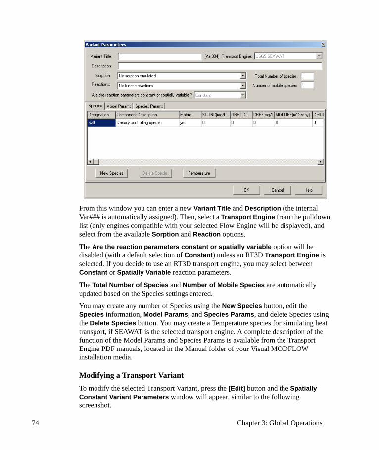
74 Chapter 3: Global Operations
From this window you can enter a new Variant Title and Description (the internal Var### is automatically assigned). Then, select a Transport Engine from the pulldown list (only engines compatible with your selected Flow Engine will be displayed), and select from the available Sorption and Reaction options.
The Are the reaction parameters constant or spatially variable option will be disabled (with a default selection of Constant) unless an RT3D Transport Engine is selected. If you decide to use an RT3D transport engine, you may select between Constant or Spatially Variable reaction parameters.
The Total Number of Species and Number of Mobile Species are automatically updated based on the Species settings entered.
You may create any number of Species using the New Species button, edit the Species information, Model Params, and Species Params, and delete Species using the Delete Species button. You may create a Temperature species for simulating heat transport, if SEAWAT is the selected transport engine. A complete description of the function of the Model Params and Species Params is available from the Transport Engine PDF manuals, located in the Manual folder of your Visual MODFLOW installation media.
Modifying a Transport VariantTo modify the selected Transport Variant, press the [Edit] button and the Spatially Constant Variant Parameters window will appear, similar to the following screenshot.
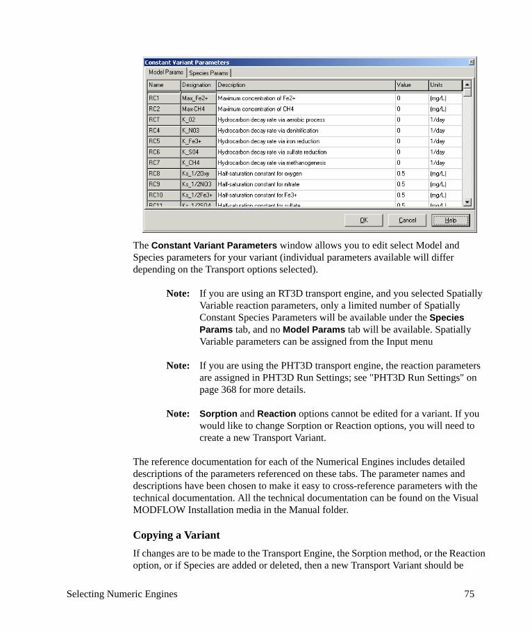
Selecting Numeric Engines 75
The Constant Variant Parameters window allows you to edit select Model and Species parameters for your variant (individual parameters available will differ depending on the Transport options selected).
Note: If you are using an RT3D transport engine, and you selected Spatially Variable reaction parameters, only a limited number of Spatially Constant Species Parameters will be available under the Species Params tab, and no Model Params tab will be available. Spatially Variable parameters can be assigned from the Input menu
Note: If you are using the PHT3D transport engine, the reaction parameters are assigned in PHT3D Run Settings; see "PHT3D Run Settings" on page 368 for more details.
Note: Sorption and Reaction options cannot be edited for a variant. If you would like to change Sorption or Reaction options, you will need to create a new Transport Variant.
The reference documentation for each of the Numerical Engines includes detailed descriptions of the parameters referenced on these tabs. The parameter names and descriptions have been chosen to make it easy to cross-reference parameters with the technical documentation. All the technical documentation can be found on the Visual MODFLOW Installation media in the Manual folder.
Copying a VariantIf changes are to be made to the Transport Engine, the Sorption method, or the Reaction option, or if Species are added or deleted, then a new Transport Variant should be
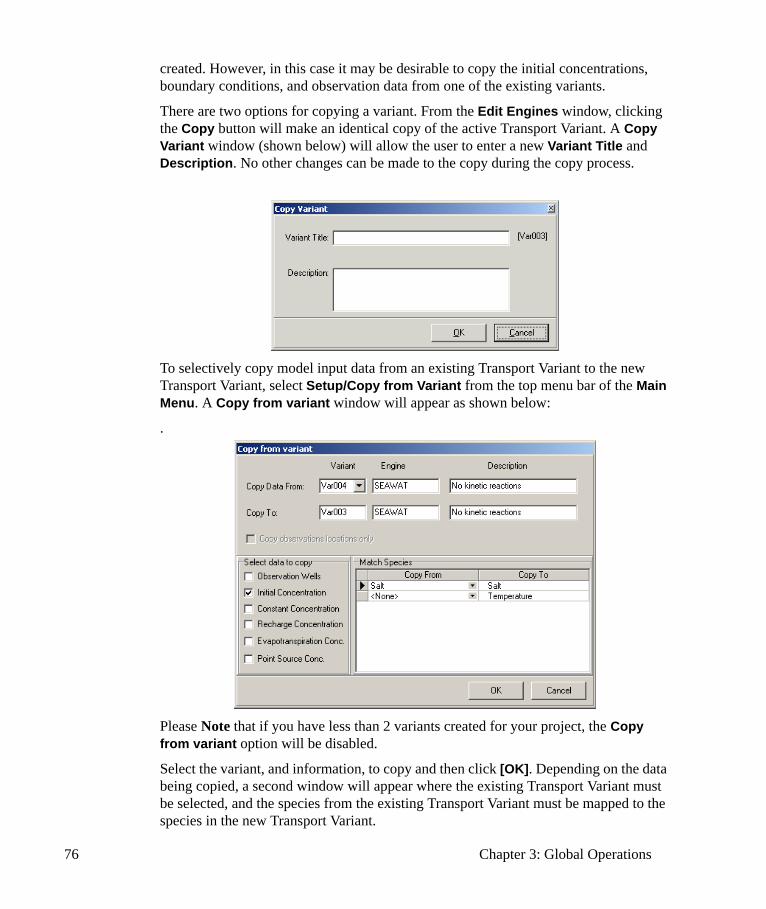
76 Chapter 3: Global Operations
created. However, in this case it may be desirable to copy the initial concentrations, boundary conditions, and observation data from one of the existing variants.
There are two options for copying a variant. From the Edit Engines window, clicking the Copy button will make an identical copy of the active Transport Variant. A Copy Variant window (shown below) will allow the user to enter a new Variant Title and Description. No other changes can be made to the copy during the copy process.
To selectively copy model input data from an existing Transport Variant to the new Transport Variant, select Setup/Copy from Variant from the top menu bar of the Main Menu. A Copy from variant window will appear as shown below:
.
Please Note that if you have less than 2 variants created for your project, the Copy from variant option will be disabled.
Select the variant, and information, to copy and then click [OK]. Depending on the data being copied, a second window will appear where the existing Transport Variant must be selected, and the species from the existing Transport Variant must be mapped to the species in the new Transport Variant.
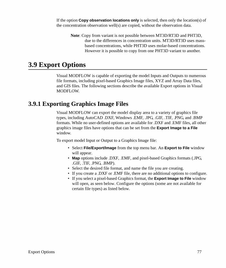
Export Options 77
If the option Copy observation locations only is selected, then only the location(s) of the concentration observation well(s) are copied, without the observation data.
Note: Copy from variant is not possible between MT3D/RT3D and PHT3D, due to the differences in concentration units. MT3D/RT3D uses mass-based concentrations, while PHT3D uses molar-based concentrations. However it is possible to copy from one PHT3D variant to another.
3.9 Export OptionsVisual MODFLOW is capable of exporting the model Inputs and Outputs to numerous file formats, including pixel-based Graphics Image files, XYZ and Array Data files, and GIS files. The following sections describe the available Export options in Visual MODFLOW.
3.9.1 Exporting Graphics Image FilesVisual MODFLOW can export the model display area to a variety of graphics file types, including AutoCAD .DXF, Windows .EMF, .JPG, .GIF, .TIF, .PNG, and .BMP formats. While no user-defined options are available for .DXF and .EMF files, all other graphics image files have options that can be set from the Export Image to a File window.
To export model Input or Output to a Graphics Image file:
• Select File/Export/Image from the top menu bar. An Export to File window will appear.
• Map options include .DXF, .EMF, and pixel-based Graphics formats (.JPG, .GIF, .TIF, .PNG, .BMP).
• Select the desired file format, and name the file you are creating.• If you create a .DXF or .EMF file, there are no additional options to configure.• If you select a pixel-based Graphics format, the Export Image to File window
will open, as seen below. Configure the options (some are not available for certain file types) as listed below.
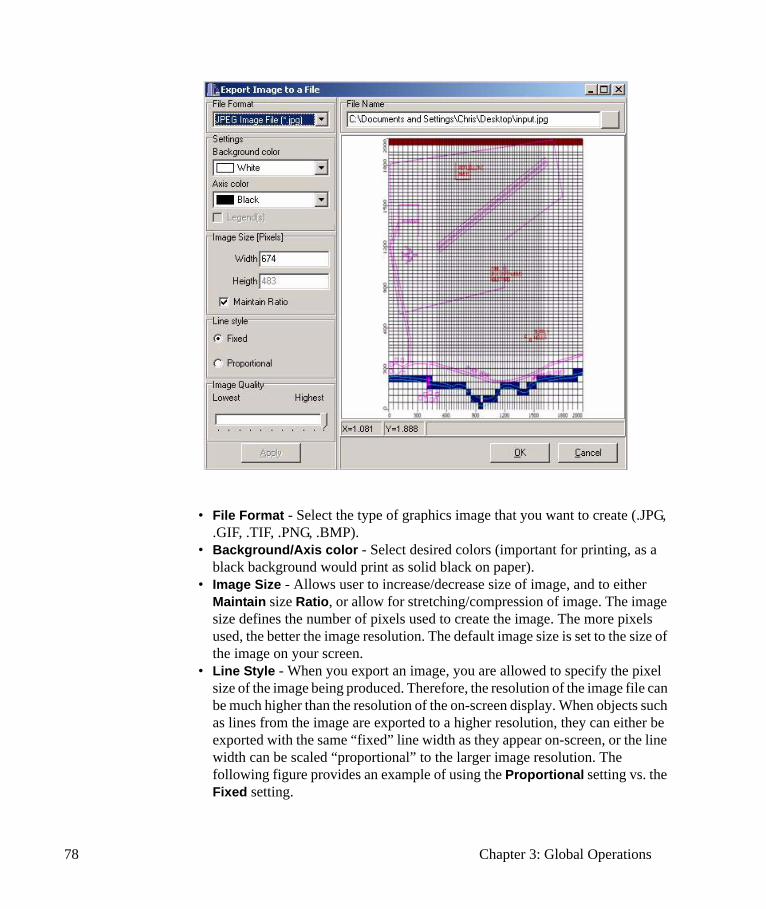
78 Chapter 3: Global Operations
• File Format - Select the type of graphics image that you want to create (.JPG, .GIF, .TIF, .PNG, .BMP).
• Background/Axis color - Select desired colors (important for printing, as a black background would print as solid black on paper).
• Image Size - Allows user to increase/decrease size of image, and to either Maintain size Ratio, or allow for stretching/compression of image. The image size defines the number of pixels used to create the image. The more pixels used, the better the image resolution. The default image size is set to the size of the image on your screen.
• Line Style - When you export an image, you are allowed to specify the pixel size of the image being produced. Therefore, the resolution of the image file can be much higher than the resolution of the on-screen display. When objects such as lines from the image are exported to a higher resolution, they can either be exported with the same “fixed” line width as they appear on-screen, or the line width can be scaled “proportional” to the larger image resolution. The following figure provides an example of using the Proportional setting vs. the Fixed setting.
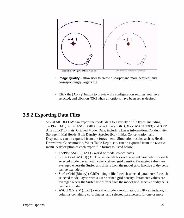
Export Options 79
• Image Quality - allow user to create a sharper and more detailed (and correspondingly larger) file.
• Click the [Apply] button to preview the configuration settings you have selected, and click on [OK] when all options have been set as desired.
3.9.2 Exporting Data FilesVisual MODFLOW can export the model data to a variety of file types, including TecPlot .DAT, Surfer ASCII .GRD, Surfer Binary .GRD, XYZ ASCII .TXT, and XYZ Array .TXT formats. Gridded Model Data, including Layer information, Conductivity, Storage, Initial Heads, Bulk Density, Species (Kd), Initial Concentration, and Dispersion, can be exported from the Input menu. Simulation results such as Heads, Drawdown, Concentration, Water Table Depth, etc. can be exported from the Output menu. A description of each export file format is listed below.
• TecPlot ASCII (.DAT) - world or model co-ordinates.• Surfer Grid (ASCII) (.GRD) - single file for each selected parameter, for each
selected model layer, with a user-defined grid density. Parameter values are averaged where the Surfer grid differs from the model grid. Inactive or dry cells can be excluded.
• Surfer Grid (Binary) (.GRD) - single file for each selected parameter, for each selected model layer, with a user-defined grid density. Parameter values are averaged where the Surfer grid differs from the model grid. Inactive or dry cells can be excluded.
• ASCII X,Y,Z,V (.TXT) - world or model co-ordinates, or IJK cell indexes, in columns containing co-ordinates, and selected parameters, for one or more
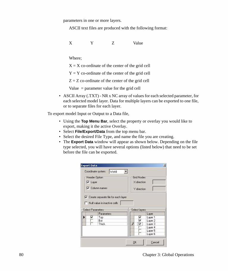
80 Chapter 3: Global Operations
parameters in one or more layers.
ASCII text files are produced with the following format:
X Y Z Value
Where;
X = X co-ordinate of the center of the grid cell
Y = Y co-ordinate of the center of the grid cell
Z = Z co-ordinate of the center of the grid cell
Value = parameter value for the grid cell
• ASCII Array (.TXT) - NR x NC array of values for each selected parameter, for each selected model layer. Data for multiple layers can be exported to one file, or to separate files for each layer.
To export model Input or Output to a Data file,
• Using the Top Menu Bar, select the property or overlay you would like to export, making it the active Overlay.
• Select File/Export/Data from the top menu bar.• Select the desired File Type, and name the file you are creating.• The Export Data window will appear as shown below. Depending on the file
type selected, you will have several options (listed below) that need to be set before the file can be exported.
Export Options 81
• Co-ordinate System - Select either World or Model co-ordinates for your output file.
• Header Option - Determines whether columns of data will be labeled.• Grid Nodes - Determines how many columns and rows of data will be output
to the file (applicable only for Surfer files)
Note: Surfer .GRD files contain a uniform grid spacing, so depending on the number of nodes you specify vs. the density of the original model grid, you may lose some resolution in your data, and the resultant file may not exactly represent the model data.
• Create separate file for each layer - If multiple layers are being exported, normally a single file will be created containing information for all layers (starting with the lowest layer). This option allows individual files to be created for each layer being exported.
• Null Value in Inactive Cells - Numerical value assigned to cells that are inactive or dry.
• Select Parameters - Allows some or all parameters for a particular Overlay to be exported.
• Select Layers - Allows some or all layers of the model to be exported.
• Click [OK] when all options have been set as desired.
3.9.3 Exporting GIS FilesVisual MODFLOW can also export contour lines of simulation results, and pathlines of particles, to an ESRI line shape .SHP file.
To export model OUTPUT to a .SHP file,
• Using the Top Menu Bar, select the desired Contour Map data type, or Pathline item, making it the active (current) Overlay.
• Select File/Export/GIS from the top menu bar.• Select the desired File Type (as noted above, the ESRI .SHP file option is only
available for OUTPUT Contour Maps and Pathlines), and name the file you are creating.
There are no other options to configure for .SHP files. A file will be created for the active layer only.

82 Chapter 3: Global Operations
83
4Model Input Data
This chapter presents information on:
• Assigning data in a new Visual MODFLOW model, and• Editing data in an existing Visual MODFLOW model.
Visual MODFLOW stores all of the data for the flow, pathline, and contaminant transport model components in a set of files having formats and data structures which are quite different than the model input data files required by MODFLOW, MODPATH, MODFLOW-SURFACT, and MT3D. There are many reasons for these differences, but the primary reasons are:
• Visual MODFLOW does not require consistent units for length and time. Instead, Visual MODFLOW allows mixed units for different model parameters (e.g. length in metres, pumping rate in US GPM, Recharge rate in mm/yr)
• Visual MODFLOW does not require boundary conditions to be defined in terms of stress periods. Instead, Visual MODFLOW allows each boundary condition to be defined using real time values and raw field data.
These differences are two of the key elements that make Visual MODFLOW so practical and user-friendly. However, these differences also require Visual MODFLOW to store data in a different format, and then translate these data files to the required format prior to running the models (e.g. MODFLOW, MODPATH, MODFLOW-SURFACT, MT3D, PEST).
Most of input files are stored in ASCII text format (see Appendix A for details on the data formats for selected Visual MODFLOW input data files). As a result, the input files can be manipulated using a text editor, or even generated using a FORTRAN or Visual Basic program, rather than using Visual MODFLOW's graphical user interface. However, if the files are externally manipulated or generated, the useful data validation and formatting checks performed by Visual MODFLOW will not be available. As a result, special care must be taken so the data structure for these files is not corrupted. It is not recommended - other than in special situations - to externally edit or manipulate the data files using a text editor.
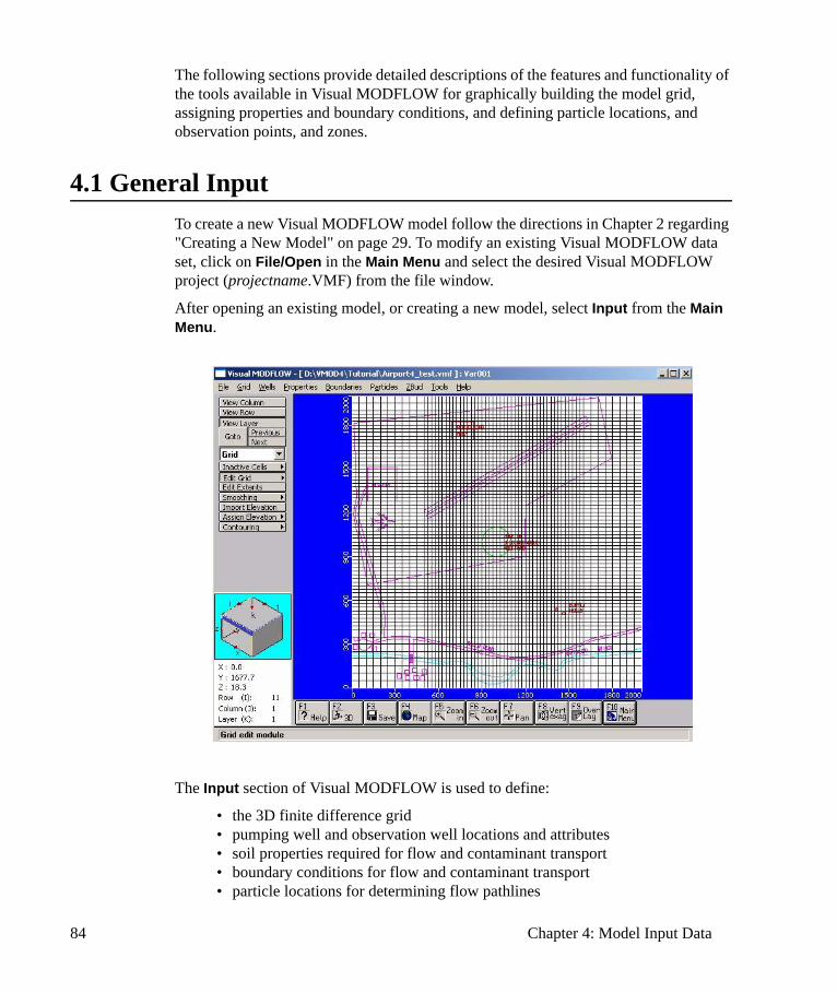
84 Chapter 4: Model Input Data
The following sections provide detailed descriptions of the features and functionality of the tools available in Visual MODFLOW for graphically building the model grid, assigning properties and boundary conditions, and defining particle locations, and observation points, and zones.
4.1 General InputTo create a new Visual MODFLOW model follow the directions in Chapter 2 regarding "Creating a New Model" on page 29. To modify an existing Visual MODFLOW data set, click on File/Open in the Main Menu and select the desired Visual MODFLOW project (projectname.VMF) from the file window.
After opening an existing model, or creating a new model, select Input from the Main Menu.
The Input section of Visual MODFLOW is used to define:
• the 3D finite difference grid• pumping well and observation well locations and attributes• soil properties required for flow and contaminant transport• boundary conditions for flow and contaminant transport• particle locations for determining flow pathlines

The File Menu 85
• observation zones for determining flow and mass budgets
The top menu bar of the [Input] section contains the following menu items:
File: Save the model, export, print, or return to the Main Menu.
Grid: Create and modify the grid (this is the active mode when entering the Input section).
Wells: Insert, modify, or delete pumping and observation wells. Visual MODFLOW imports Pumping Well data, and Head and Concentration Well data, from a variety of file formats including ASCII .TXT, .SHP, .XLS and .MDB.
Properties: Add or modify hydraulic conductivities, storage properties, initial heads, initial concentrations, dispersion properties, and chemical reaction properties. The Vadose Zone option is active only if MODFLOW-SURFACT is selected.
Boundaries: Input or modify flow and transport boundary conditions.
Particles: Add or modify particle locations for particle tracking.
Zbud: Input or modify zones used to calculate Zone Budget data.
Tools: Opens the Cell Inspector to view cell-by-cell parameter values, opens the Annotate screen to add lines, shapes, and text in the model domain, and opens the Units Converter.
Help: Obtain general help and version information.
4.2 The File MenuThe File item in the top menu bar has the following menu options:
Save: Save the data set.

86 Chapter 4: Model Input Data
Export: Export a Graphics Image, Data, or GIS file.
Preferences: Control font size settings for labels and names of pumping and observation wells, axes, shapes, and contours. It also controls the Color settings for the Screen Background and the Axis labels.
Print: Print the screen image, and select the printing device.
Main Menu: Return to the main program window.
4.3 Grid DesignThe Grid module allows the user to define and discretize the modeling domain. The user can add or delete gridlines, change cell or layer elevations, or remove cells from the computations.
When the Grid option is selected in the Input section, the tools along the left-hand menu bar will reflect grid specific options:
[Inactive Cells]: Define inactive zones (no-flow cells) within the model domain.
[Edit Grid]: Select from Edit Rows, Edit Columns, or Edit Layers to add, delete, move, refine, or coarsen the model grid.
[Edit Extents]: Expand or reduce the X and Y limits of the model grid.
[Smoothing]: Smooth the grid spacing transition in the X and Y directions.
[Import Elevation]: Import and interpolate layer surface elevations from discrete data point files, or set layer surface elevations using specified elevations, specified thickness, or with a constant slope. The layer-wise imported data set and interpolated surface layers can be previewed in two or three dimensions.
[Export Elevation]: Export surface elevations from model layers to various file formats.
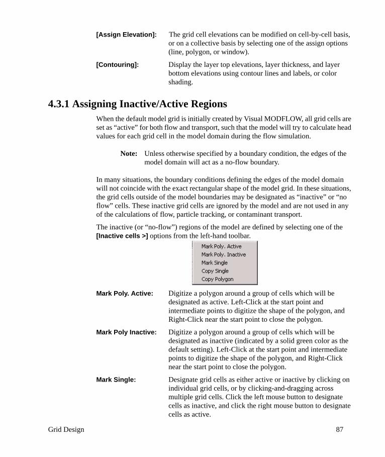
Grid Design 87
[Assign Elevation]: The grid cell elevations can be modified on cell-by-cell basis, or on a collective basis by selecting one of the assign options (line, polygon, or window).
[Contouring]: Display the layer top elevations, layer thickness, and layer bottom elevations using contour lines and labels, or color shading.
4.3.1 Assigning Inactive/Active RegionsWhen the default model grid is initially created by Visual MODFLOW, all grid cells are set as “active” for both flow and transport, such that the model will try to calculate head values for each grid cell in the model domain during the flow simulation.
Note: Unless otherwise specified by a boundary condition, the edges of the model domain will act as a no-flow boundary.
In many situations, the boundary conditions defining the edges of the model domain will not coincide with the exact rectangular shape of the model grid. In these situations, the grid cells outside of the model boundaries may be designated as “inactive” or “no flow” cells. These inactive grid cells are ignored by the model and are not used in any of the calculations of flow, particle tracking, or contaminant transport.
The inactive (or “no-flow”) regions of the model are defined by selecting one of the [Inactive cells >] options from the left-hand toolbar.
Mark Poly. Active: Digitize a polygon around a group of cells which will be designated as active. Left-Click at the start point and intermediate points to digitize the shape of the polygon, and Right-Click near the start point to close the polygon.
Mark Poly Inactive: Digitize a polygon around a group of cells which will be designated as inactive (indicated by a solid green color as the default setting). Left-Click at the start point and intermediate points to digitize the shape of the polygon, and Right-Click near the start point to close the polygon.
Mark Single: Designate grid cells as either active or inactive by clicking on individual grid cells, or by clicking-and-dragging across multiple grid cells. Click the left mouse button to designate cells as inactive, and click the right mouse button to designate cells as active.
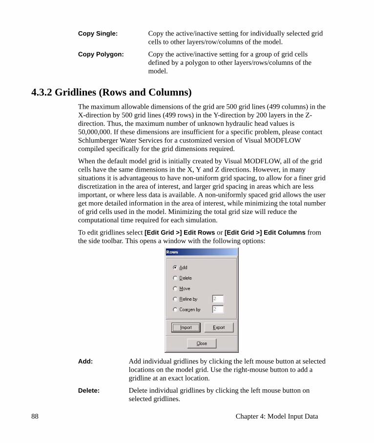
88 Chapter 4: Model Input Data
Copy Single: Copy the active/inactive setting for individually selected grid cells to other layers/row/columns of the model.
Copy Polygon: Copy the active/inactive setting for a group of grid cells defined by a polygon to other layers/rows/columns of the model.
4.3.2 Gridlines (Rows and Columns) The maximum allowable dimensions of the grid are 500 grid lines (499 columns) in the X-direction by 500 grid lines (499 rows) in the Y-direction by 200 layers in the Z-direction. Thus, the maximum number of unknown hydraulic head values is 50,000,000. If these dimensions are insufficient for a specific problem, please contact Schlumberger Water Services for a customized version of Visual MODFLOW compiled specifically for the grid dimensions required.
When the default model grid is initially created by Visual MODFLOW, all of the grid cells have the same dimensions in the X, Y and Z directions. However, in many situations it is advantageous to have non-uniform grid spacing, to allow for a finer grid discretization in the area of interest, and larger grid spacing in areas which are less important, or where less data is available. A non-uniformly spaced grid allows the user get more detailed information in the area of interest, while minimizing the total number of grid cells used in the model. Minimizing the total grid size will reduce the computational time required for each simulation.
To edit gridlines select [Edit Grid >] Edit Rows or [Edit Grid >] Edit Columns from the side toolbar. This opens a window with the following options:
Add: Add individual gridlines by clicking the left mouse button at selected locations on the model grid. Use the right-mouse button to add a gridline at an exact location.
Delete: Delete individual gridlines by clicking the left mouse button on selected gridlines.
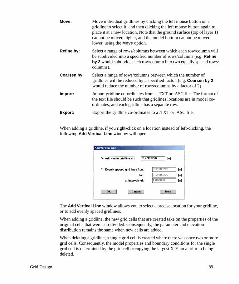
Grid Design 89
Move: Move individual gridlines by clicking the left mouse button on a gridline to select it, and then clicking the left mouse button again to place it at a new location. Note that the ground surface (top of layer 1) cannot be moved higher, and the model bottom cannot be moved lower, using the Move option.
Refine by: Select a range of rows/columns between which each row/column will be subdivided into a specified number of rows/columns (e.g. Refine by 2 would subdivide each row/column into two equally spaced rows/columns).
Coarsen by: Select a range of rows/columns between which the number of gridlines will be reduced by a specified factor. (e.g. Coarsen by 2 would reduce the number of rows/columns by a factor of 2).
Import: Import gridline co-ordinates from a .TXT or .ASC file. The format of the text file should be such that gridlines locations are in model co-ordinates, and each gridline has a separate row.
Export: Export the gridline co-ordinates to a .TXT or .ASC file.
When adding a gridline, if you right-click on a location instead of left-clicking, the following Add Vertical Line window will open:
The Add Vertical Line window allows you to select a precise location for your gridline, or to add evenly spaced gridlines.
When adding a gridline, the new grid cells that are created take on the properties of the original cells that were sub-divided. Consequently, the parameter and elevation distribution remains the same when new cells are added.
When deleting a gridline, a single grid cell is created where there was once two or more grid cells. Consequently, the model properties and boundary conditions for the single grid cell is determined by the grid cell occupying the largest X-Y area prior to being deleted.
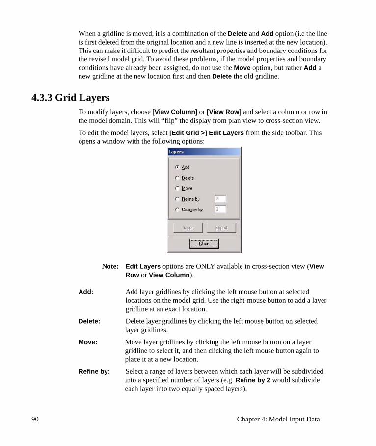
90 Chapter 4: Model Input Data
When a gridline is moved, it is a combination of the Delete and Add option (i.e the line is first deleted from the original location and a new line is inserted at the new location). This can make it difficult to predict the resultant properties and boundary conditions for the revised model grid. To avoid these problems, if the model properties and boundary conditions have already been assigned, do not use the Move option, but rather Add a new gridline at the new location first and then Delete the old gridline.
4.3.3 Grid Layers To modify layers, choose [View Column] or [View Row] and select a column or row in the model domain. This will “flip” the display from plan view to cross-section view.
To edit the model layers, select [Edit Grid >] Edit Layers from the side toolbar. This opens a window with the following options:
Note: Edit Layers options are ONLY available in cross-section view (View Row or View Column).
Add: Add layer gridlines by clicking the left mouse button at selected locations on the model grid. Use the right-mouse button to add a layer gridline at an exact location.
Delete: Delete layer gridlines by clicking the left mouse button on selected layer gridlines.
Move: Move layer gridlines by clicking the left mouse button on a layer gridline to select it, and then clicking the left mouse button again to place it at a new location.
Refine by: Select a range of layers between which each layer will be subdivided into a specified number of layers (e.g. Refine by 2 would subdivide each layer into two equally spaced layers).
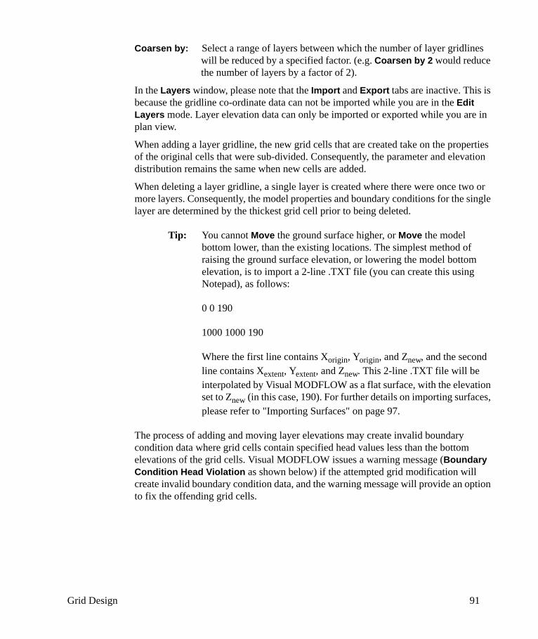
Grid Design 91
Coarsen by: Select a range of layers between which the number of layer gridlines will be reduced by a specified factor. (e.g. Coarsen by 2 would reduce the number of layers by a factor of 2).
In the Layers window, please note that the Import and Export tabs are inactive. This is because the gridline co-ordinate data can not be imported while you are in the Edit Layers mode. Layer elevation data can only be imported or exported while you are in plan view.
When adding a layer gridline, the new grid cells that are created take on the properties of the original cells that were sub-divided. Consequently, the parameter and elevation distribution remains the same when new cells are added.
When deleting a layer gridline, a single layer is created where there were once two or more layers. Consequently, the model properties and boundary conditions for the single layer are determined by the thickest grid cell prior to being deleted.
Tip: You cannot Move the ground surface higher, or Move the model bottom lower, than the existing locations. The simplest method of raising the ground surface elevation, or lowering the model bottom elevation, is to import a 2-line .TXT file (you can create this using Notepad), as follows:
0 0 190
1000 1000 190
Where the first line contains Xorigin, Yorigin, and Znew, and the second line contains Xextent, Yextent, and Znew. This 2-line .TXT file will be interpolated by Visual MODFLOW as a flat surface, with the elevation set to Znew (in this case, 190). For further details on importing surfaces, please refer to "Importing Surfaces" on page 97.
The process of adding and moving layer elevations may create invalid boundary condition data where grid cells contain specified head values less than the bottom elevations of the grid cells. Visual MODFLOW issues a warning message (Boundary Condition Head Violation as shown below) if the attempted grid modification will create invalid boundary condition data, and the warning message will provide an option to fix the offending grid cells.
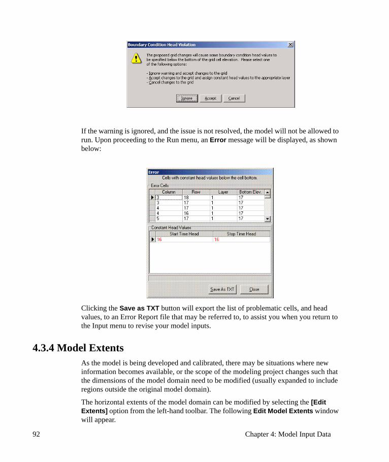
92 Chapter 4: Model Input Data
If the warning is ignored, and the issue is not resolved, the model will not be allowed to run. Upon proceeding to the Run menu, an Error message will be displayed, as shown below:
Clicking the Save as TXT button will export the list of problematic cells, and head values, to an Error Report file that may be referred to, to assist you when you return to the Input menu to revise your model inputs.
4.3.4 Model Extents As the model is being developed and calibrated, there may be situations where new information becomes available, or the scope of the modeling project changes such that the dimensions of the model domain need to be modified (usually expanded to include regions outside the original model domain).
The horizontal extents of the model domain can be modified by selecting the [Edit Extents] option from the left-hand toolbar. The following Edit Model Extents window will appear.

Grid Design 93
The Edit Model Extents window is used to change the location of the outer-most column or row gridlines.
The X-Extents indicate the Minimum and Maximum X-co-ordinate for the model domain.
The Y-Extents indicate the Minimum and Maximum Y-co-ordinate for the model domain.
The model domain can be enlarged by entering a lower Minimum value (even a negative value) and/or a larger Maximum value for the X-Extents and Y-Extents.
The model domain can be decreased by entering a larger Minimum value and/or a smaller Maximum value for the X-Extents and Y-Extents.
Note: The extents cannot be adjusted such that the outside row or column is less than 0.01 length units.
Note: The model extents cannot be reduced if the new size would result in rows or columns being “cut off”. In this case, simply delete the “extra” gridlines first, then reduce your model size.
Click [OK] when all the values are entered. If the values are not valid a message will appear stating the limits of the extents. The new model domain will span from the minimum locations entered to the maximum locations entered.
4.3.5 Grid Smoothing The computational efficiency of the MODFLOW solvers has been enhanced by implementing a grid-smoothing algorithm that optimizes discretization in non-uniform grids. Grid smoothing minimizes the possibility of poorly structured matrix equations, which can lead to convergence problems. In order to address this problem, an algorithm

94 Chapter 4: Model Input Data
was developed by Schlumberger Water Services to smooth a selected region of an arbitrary, non-uniform grid and then integrate the smoothed section back into the model without introducing additional irregularities into the grid.
The smoothing algorithm was developed using a parabolic equation proportional to the second derivative of the grid spacing. Smoothing the grid discretization, by generating a new grid using a mathematical transformation of a uniform grid, creates a grid discretization that is no longer discontinuous. Grid smoothing maximizes the effectiveness of the grid and expedites complex grid discretization. Improvements to the accuracy of contaminant transport models have been achieved, as well as greater numerical stability and faster convergence for complex flow problems. The grid smoothing function facilitates minor grid improvements that may turn an oscillatory flow solution into a stable converging one.
A compromise must be reached between the accuracy of the model, and the available computer resources, when designing a finite-difference grid. Usually, only selected portions of the model domain - such as well fields - are refined, leaving the rest of the grid more coarsely discretized. In this case, stability is the trade-off. Models that rely on a uniform grid are more stable and theoretically more accurate than non-uniform grids (Pinder and Gray, 1984). However, a sufficiently discretized uniform grid will result in extended simulation times.
A finer grid will normally give more precise results, especially in areas of steep hydraulic gradients. For best results, the grid spacing should change gradually. A “rule of thumb” is that the grid spacing should not increase by more than 50 percent between adjacent cells. An aspect ratio must also be respected; a grid cell should not be more than 10 times bigger in one direction than in the other.
It is recommended that smoothing of the grid spacing take place before adding the model layers and boundary conditions.
To smooth the gridlines, select [Smoothing >] from the left-hand toolbar and then either X - direction or Y - direction. Depending on the selection, an X grid smoothing window or a Y grid smoothing window will appear as shown in the following figure.
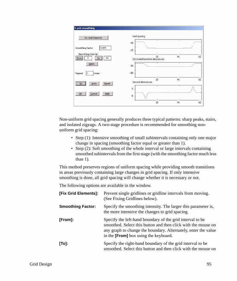
Grid Design 95
Non-uniform grid spacing generally produces three typical patterns: sharp peaks, stairs, and isolated zigzags. A two-stage procedure is recommended for smoothing non-uniform grid spacing:
• Step (1): Intensive smoothing of small subintervals containing only one major change in spacing (smoothing factor equal or greater than 1).
• Step (2): Soft smoothing of the whole interval or large intervals containing smoothed subintervals from the first stage (with the smoothing factor much less than 1).
This method preserves regions of uniform spacing while providing smooth transitions in areas previously containing large changes in grid spacing. If only intensive smoothing is done, all grid spacing will change whether it is necessary or not.
The following options are available in the window.
[Fix Grid Elements]: Prevent single gridlines or gridline intervals from moving. (See Fixing Gridlines below).
Smoothing Factor: Specify the smoothing intensity. The larger this parameter is, the more intensive the changes to grid spacing.
[From]: Specify the left-hand boundary of the grid interval to be smoothed. Select this button and then click with the mouse on any graph to change the boundary. Alternately, enter the value in the [From] box using the keyboard.
[To]: Specify the right-hand boundary of the grid interval to be smoothed. Select this button and then click with the mouse on
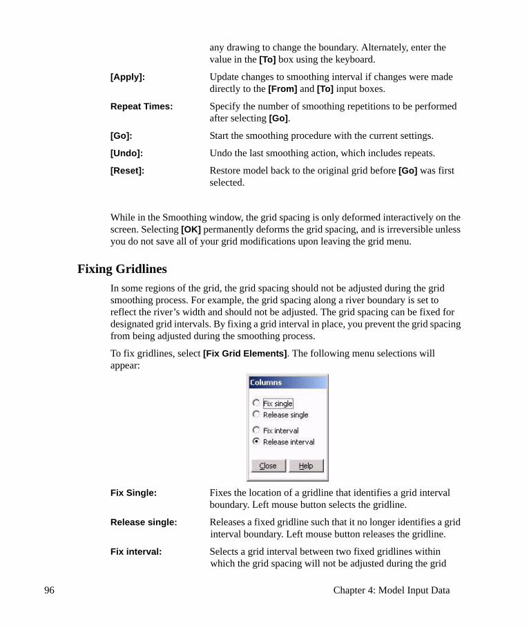
96 Chapter 4: Model Input Data
any drawing to change the boundary. Alternately, enter the value in the [To] box using the keyboard.
[Apply]: Update changes to smoothing interval if changes were made directly to the [From] and [To] input boxes.
Repeat Times: Specify the number of smoothing repetitions to be performed after selecting [Go].
[Go]: Start the smoothing procedure with the current settings.
[Undo]: Undo the last smoothing action, which includes repeats.
[Reset]: Restore model back to the original grid before [Go] was first selected.
While in the Smoothing window, the grid spacing is only deformed interactively on the screen. Selecting [OK] permanently deforms the grid spacing, and is irreversible unless you do not save all of your grid modifications upon leaving the grid menu.
Fixing GridlinesIn some regions of the grid, the grid spacing should not be adjusted during the grid smoothing process. For example, the grid spacing along a river boundary is set to reflect the river’s width and should not be adjusted. The grid spacing can be fixed for designated grid intervals. By fixing a grid interval in place, you prevent the grid spacing from being adjusted during the smoothing process.
To fix gridlines, select [Fix Grid Elements]. The following menu selections will appear:
Fix Single: Fixes the location of a gridline that identifies a grid interval boundary. Left mouse button selects the gridline.
Release single: Releases a fixed gridline such that it no longer identifies a grid interval boundary. Left mouse button releases the gridline.
Fix interval: Selects a grid interval between two fixed gridlines within which the grid spacing will not be adjusted during the grid
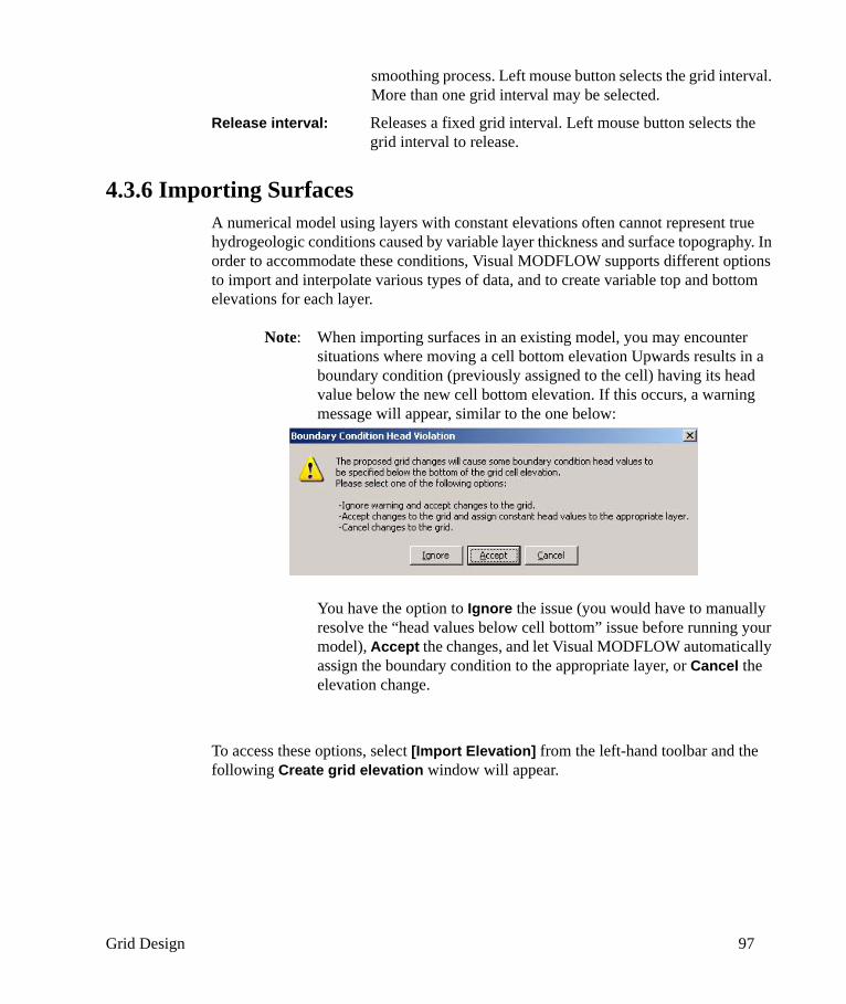
Grid Design 97
smoothing process. Left mouse button selects the grid interval. More than one grid interval may be selected.
Release interval: Releases a fixed grid interval. Left mouse button selects the grid interval to release.
4.3.6 Importing Surfaces A numerical model using layers with constant elevations often cannot represent true hydrogeologic conditions caused by variable layer thickness and surface topography. In order to accommodate these conditions, Visual MODFLOW supports different options to import and interpolate various types of data, and to create variable top and bottom elevations for each layer.
Note: When importing surfaces in an existing model, you may encounter situations where moving a cell bottom elevation Upwards results in a boundary condition (previously assigned to the cell) having its head value below the new cell bottom elevation. If this occurs, a warning message will appear, similar to the one below:
You have the option to Ignore the issue (you would have to manually resolve the “head values below cell bottom” issue before running your model), Accept the changes, and let Visual MODFLOW automatically assign the boundary condition to the appropriate layer, or Cancel the elevation change.
To access these options, select [Import Elevation] from the left-hand toolbar and the following Create grid elevation window will appear.
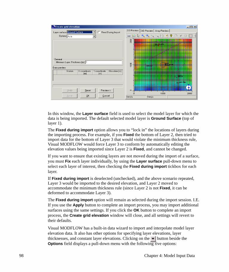
98 Chapter 4: Model Input Data
In this window, the Layer surface field is used to select the model layer for which the data is being imported. The default selected model layer is Ground Surface (top of layer 1).The Fixed during import option allows you to “lock in” the locations of layers during the importing process. For example, if you Fixed the bottom of Layer 2, then tried to import data for the bottom of Layer 3 that would violate the minimum thickness rule, Visual MODFLOW would force Layer 3 to conform by automatically editing the elevation values being imported since Layer 2 is Fixed, and cannot be changed.If you want to ensure that existing layers are not moved during the import of a surface, you must Fix each layer individually, by using the Layer surface pull-down menu to select each layer of interest, then checking the Fixed during import tickbox for each layer.If Fixed during import is deselected (unchecked), and the above scenario repeated, Layer 3 would be imported to the desired elevation, and Layer 2 moved to accommodate the minimum thickness rule (since Layer 2 is not Fixed, it can be deformed to accommodate Layer 3).The Fixed during import option will remain as selected during the import session. I.E. If you use the Apply button to complete an import process, you may import additional surfaces using the same settings. If you click the OK button to complete an import process, the Create grid elevation window will close, and all settings will revert to their defaults.
Visual MODFLOW has a built-in data wizard to import and interpolate model layer elevation data. It also has other options for specifying layer elevations, layer thicknesses, and constant layer elevations. Clicking on the button beside the Options field displays a pull-down menu with the following five options:
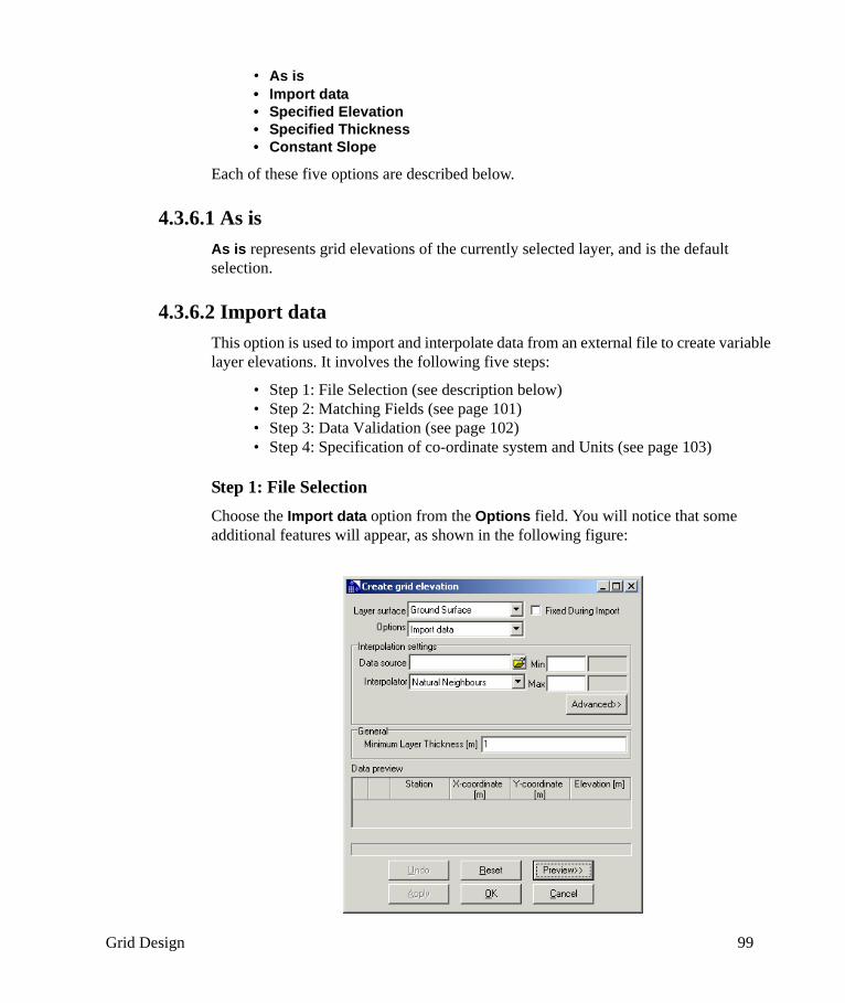
Grid Design 99
• As is• Import data• Specified Elevation • Specified Thickness• Constant Slope
Each of these five options are described below.
4.3.6.1 As is As is represents grid elevations of the currently selected layer, and is the default selection.
4.3.6.2 Import dataThis option is used to import and interpolate data from an external file to create variable layer elevations. It involves the following five steps:
• Step 1: File Selection (see description below)• Step 2: Matching Fields (see page 101)• Step 3: Data Validation (see page 102)• Step 4: Specification of co-ordinate system and Units (see page 103)
Step 1: File SelectionChoose the Import data option from the Options field. You will notice that some additional features will appear, as shown in the following figure:

100 Chapter 4: Model Input Data
The Interpolator field (in the newly created Interpolation settings frame) provides a selection of three popular data interpolation schemes:
• Inverse Distance• Kriging• Natural Neighbors
The default setting is Natural Neighbors.
The Min and Max fields with grey background display the minimum and the maximum elevation data values in the file that is being imported. The Min and Max fields with white background allow the user to control the lower and upper bounds of the data values by the interpolation schemes.
The [Advanced] button opens an Interpolator Options window with advanced settings for the selected interpolation method. A general description of each interpolation method, and a detailed description of the advanced settings for each of these methods, is provided in Appendix B.
The Minimum layer thickness field in the General frame defines the minimum distance between two adjacent layer surfaces. This minimum thickness overrides the interpolated elevation of a surface when two adjacent layer surfaces intersect. The top layer does not move, therefore the imported layer will shift to accommodate the minimum layer thickness. The default thickness is 1 m.
To select a Data source file, click on the Choose File Name button associated with the Data source field in the Interpolation settings frame. An Open window will appear (as shown below) to select the file, and file type being imported. In this example, an .XLS data file is selected.

Grid Design 101
The data file formats currently supported by Visual MODFLOW for importing and interpolating elevations data include:
• Grid - ASCII text files (.TXT, .DAT, .TAB, .CSV)• Grid - ESRI Grid file (.TXT, .ASC, .HDR)• Grid - MapInfo Grid file (.TXT)• Grid - Surfer Grid file (.GRD)• Grid - USGS DEM file (.DEM)• Gird - Row/Column/Layer files (*.TXT, *.CSV)• Points - Access Database file (.MDB)• Points - ASCII XYZ file (.TXT, .DAT, .TAB, .CSV)• Points - ESRI Shape file (.SHP)• Point - Excel Spreadsheet file (.XLS)
Once a data file has been selected, click the [Open] button to advance to the next step.
Step 2: Match FieldsThis step involves matching the columns from the source data file to the data fields required by the Visual MODFLOW to import and interpolate the elevation values. The following Match Fields window will appear once a data file has been selected.
The Required Data column lists the fields that need to be matched to a column of data from the source file. The elevation data includes three fields: X-co-ordinate, Y-co-ordinate, and Elevation. The Station field is optional (and does not need to be matched to a column of import data) as it is typically used for storing the station No. information.
The Match to column number… column is used to identify the column numbers from the source file corresponding to each required field. If a data source does not contain values for each of the required fields, the unmatched fields may either be left blank, or entered as “n/a” (not applicable).
For example, as shown in the following figure, the Match to column number... column is matched to the columns of imported data.
• Column #1 is matched to the X-co-ordinate, • Column #2 is matched to the Y-co-ordinate, and • Column #3 is matched to the Elevation.
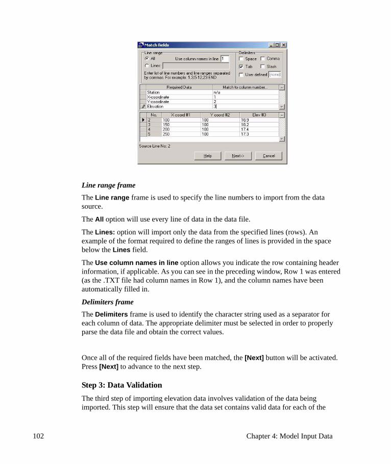
102 Chapter 4: Model Input Data
Line range frameThe Line range frame is used to specify the line numbers to import from the data source.
The All option will use every line of data in the data file.
The Lines: option will import only the data from the specified lines (rows). An example of the format required to define the ranges of lines is provided in the space below the Lines field.
The Use column names in line option allows you indicate the row containing header information, if applicable. As you can see in the preceding window, Row 1 was entered (as the .TXT file had column names in Row 1), and the column names have been automatically filled in.
Delimiters frameThe Delimiters frame is used to identify the character string used as a separator for each column of data. The appropriate delimiter must be selected in order to properly parse the data file and obtain the correct values.
Once all of the required fields have been matched, the [Next] button will be activated. Press [Next] to advance to the next step.
Step 3: Data ValidationThe third step of importing elevation data involves validation of the data being imported. This step will ensure that the data set contains valid data for each of the
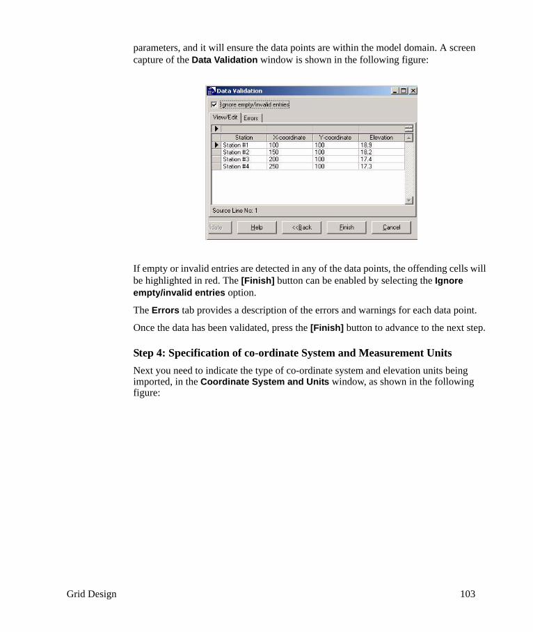
Grid Design 103
parameters, and it will ensure the data points are within the model domain. A screen capture of the Data Validation window is shown in the following figure:
If empty or invalid entries are detected in any of the data points, the offending cells will be highlighted in red. The [Finish] button can be enabled by selecting the Ignore empty/invalid entries option.
The Errors tab provides a description of the errors and warnings for each data point.
Once the data has been validated, press the [Finish] button to advance to the next step.
Step 4: Specification of co-ordinate System and Measurement UnitsNext you need to indicate the type of co-ordinate system and elevation units being imported, in the Coordinate System and Units window, as shown in the following figure:
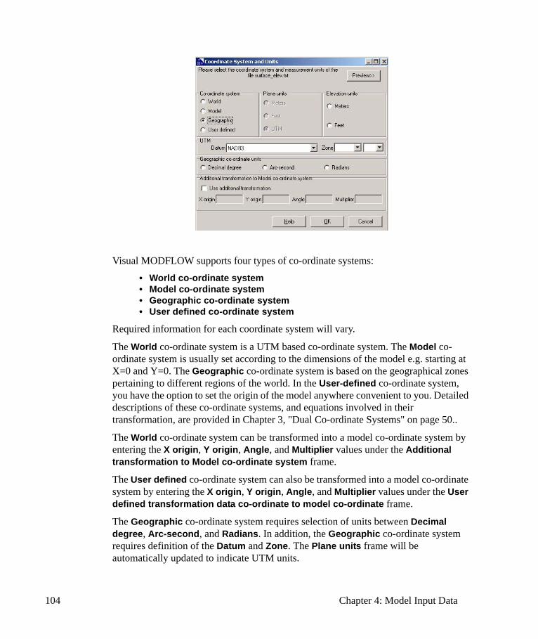
104 Chapter 4: Model Input Data
Visual MODFLOW supports four types of co-ordinate systems:
• World co-ordinate system• Model co-ordinate system• Geographic co-ordinate system• User defined co-ordinate system
Required information for each coordinate system will vary.
The World co-ordinate system is a UTM based co-ordinate system. The Model co-ordinate system is usually set according to the dimensions of the model e.g. starting at X=0 and Y=0. The Geographic co-ordinate system is based on the geographical zones pertaining to different regions of the world. In the User-defined co-ordinate system, you have the option to set the origin of the model anywhere convenient to you. Detailed descriptions of these co-ordinate systems, and equations involved in their transformation, are provided in Chapter 3, "Dual Co-ordinate Systems" on page 50..
The World co-ordinate system can be transformed into a model co-ordinate system by entering the X origin, Y origin, Angle, and Multiplier values under the Additional transformation to Model co-ordinate system frame.
The User defined co-ordinate system can also be transformed into a model co-ordinate system by entering the X origin, Y origin, Angle, and Multiplier values under the User defined transformation data co-ordinate to model co-ordinate frame.
The Geographic co-ordinate system requires selection of units between Decimal degree, Arc-second, and Radians. In addition, the Geographic co-ordinate system requires definition of the Datum and Zone. The Plane units frame will be automatically updated to indicate UTM units.

Grid Design 105
Definition of Elevation units (along the vertical direction of the model) is necessary for all co-ordinate systems.
The Plane units are not user-selectable, and are only required for the Geographic co-ordinate system.
Once the co-ordinate system and units have been selected, click [OK] to proceed and the following Create grid elevation window will appear. Note that the station-wise X co-ordinate, Y co-ordinate, and Elevations imported into the model are previewed under the Data Preview field. Individual points can be deselected by clicking in the checkbox beside the undesired point to remove the checkmark.
Click [Apply] to execute the interpolation of the imported elevation data. You may use the Preview button to view your elevation data being imported, in either plan view, or cross sectional view. Please see "Previewing the Layer Elevations to be Imported" on page 110 for an explanation of the Preview option buttons available in this preview window (please note that not all Preview features are available from the Coordinate System and Units Preview window). Clicking on the Preview button again will close the Preview window.
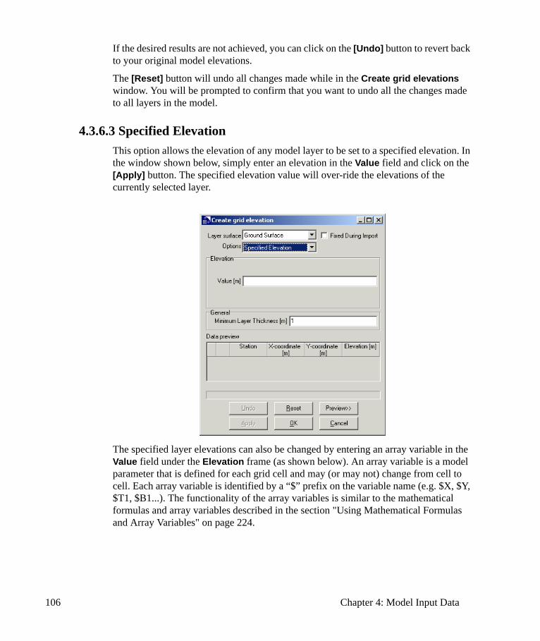
106 Chapter 4: Model Input Data
If the desired results are not achieved, you can click on the [Undo] button to revert back to your original model elevations.
The [Reset] button will undo all changes made while in the Create grid elevations window. You will be prompted to confirm that you want to undo all the changes made to all layers in the model.
4.3.6.3 Specified Elevation This option allows the elevation of any model layer to be set to a specified elevation. In the window shown below, simply enter an elevation in the Value field and click on the [Apply] button. The specified elevation value will over-ride the elevations of the currently selected layer.
The specified layer elevations can also be changed by entering an array variable in the Value field under the Elevation frame (as shown below). An array variable is a model parameter that is defined for each grid cell and may (or may not) change from cell to cell. Each array variable is identified by a “$” prefix on the variable name (e.g. $X, $Y, $T1, $B1...). The functionality of the array variables is similar to the mathematical formulas and array variables described in the section "Using Mathematical Formulas and Array Variables" on page 224.
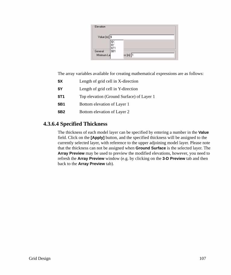
Grid Design 107
The array variables available for creating mathematical expressions are as follows:
$X Length of grid cell in X-direction
$Y Length of grid cell in Y-direction
$T1 Top elevation (Ground Surface) of Layer 1
$B1 Bottom elevation of Layer 1
$B2 Bottom elevation of Layer 2
4.3.6.4 Specified Thickness The thickness of each model layer can be specified by entering a number in the Value field. Click on the [Apply] button, and the specified thickness will be assigned to the currently selected layer, with reference to the upper adjoining model layer. Please note that the thickness can not be assigned when Ground Surface is the selected layer. The Array Preview may be used to preview the modified elevations, however, you need to refresh the Array Preview window (e.g. by clicking on the 3-D Preview tab and then back to the Array Preview tab).
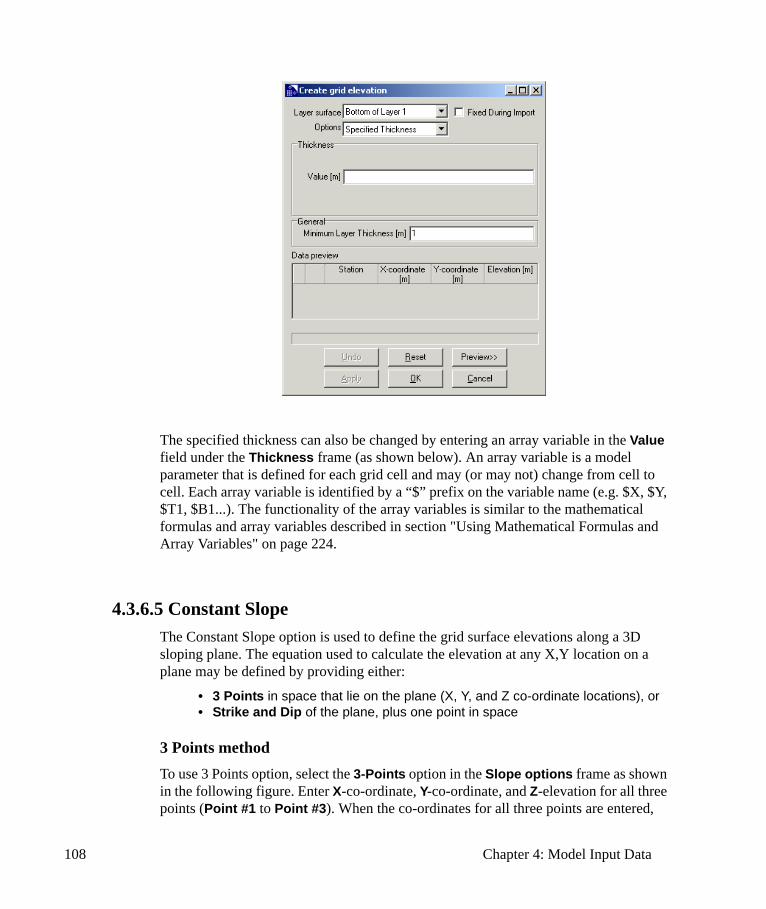
108 Chapter 4: Model Input Data
The specified thickness can also be changed by entering an array variable in the Value field under the Thickness frame (as shown below). An array variable is a model parameter that is defined for each grid cell and may (or may not) change from cell to cell. Each array variable is identified by a “$” prefix on the variable name (e.g. $X, $Y, $T1, $B1...). The functionality of the array variables is similar to the mathematical formulas and array variables described in section "Using Mathematical Formulas and Array Variables" on page 224.
4.3.6.5 Constant Slope The Constant Slope option is used to define the grid surface elevations along a 3D sloping plane. The equation used to calculate the elevation at any X,Y location on a plane may be defined by providing either:
• 3 Points in space that lie on the plane (X, Y, and Z co-ordinate locations), or• Strike and Dip of the plane, plus one point in space
3 Points methodTo use 3 Points option, select the 3-Points option in the Slope options frame as shown in the following figure. Enter X-co-ordinate, Y-co-ordinate, and Z-elevation for all three points (Point #1 to Point #3). When the co-ordinates for all three points are entered,

Grid Design 109
click the [Apply] button at the bottom of the window to calculate the grid cell elevations for the current layer surface.
Note: When the locations of the 3 points are not logical (e.g all located in a straight line) an error message will appear as shown in the following figure:
Strike and Dip methodWhen a bed is not horizontal, it has dip and strike. Strike and dip are geologic terms used to describe the slope direction and inclination (orientation) of the plane. These measurements define the direction and angle that rocks tilt into the earth’s surface.
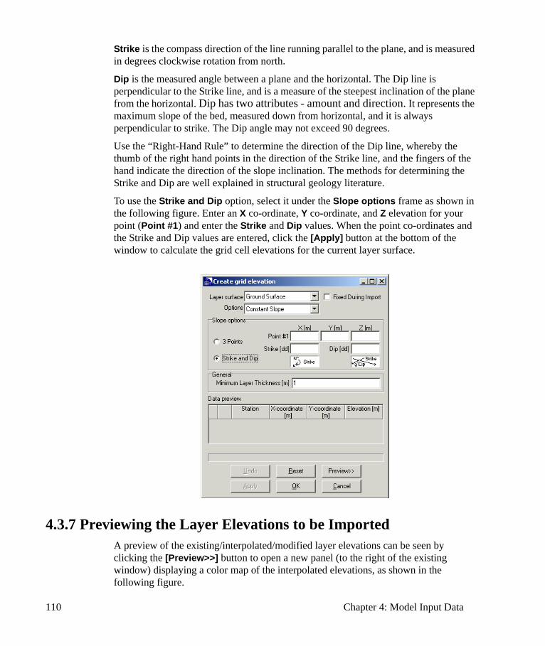
110 Chapter 4: Model Input Data
Strike is the compass direction of the line running parallel to the plane, and is measured in degrees clockwise rotation from north.
Dip is the measured angle between a plane and the horizontal. The Dip line is perpendicular to the Strike line, and is a measure of the steepest inclination of the plane from the horizontal. Dip has two attributes - amount and direction. It represents the maximum slope of the bed, measured down from horizontal, and it is always perpendicular to strike. The Dip angle may not exceed 90 degrees.
Use the “Right-Hand Rule” to determine the direction of the Dip line, whereby the thumb of the right hand points in the direction of the Strike line, and the fingers of the hand indicate the direction of the slope inclination. The methods for determining the Strike and Dip are well explained in structural geology literature.
To use the Strike and Dip option, select it under the Slope options frame as shown in the following figure. Enter an X co-ordinate, Y co-ordinate, and Z elevation for your point (Point #1) and enter the Strike and Dip values. When the point co-ordinates and the Strike and Dip values are entered, click the [Apply] button at the bottom of the window to calculate the grid cell elevations for the current layer surface.
4.3.7 Previewing the Layer Elevations to be ImportedA preview of the existing/interpolated/modified layer elevations can be seen by clicking the [Preview>>] button to open a new panel (to the right of the existing window) displaying a color map of the interpolated elevations, as shown in the following figure.
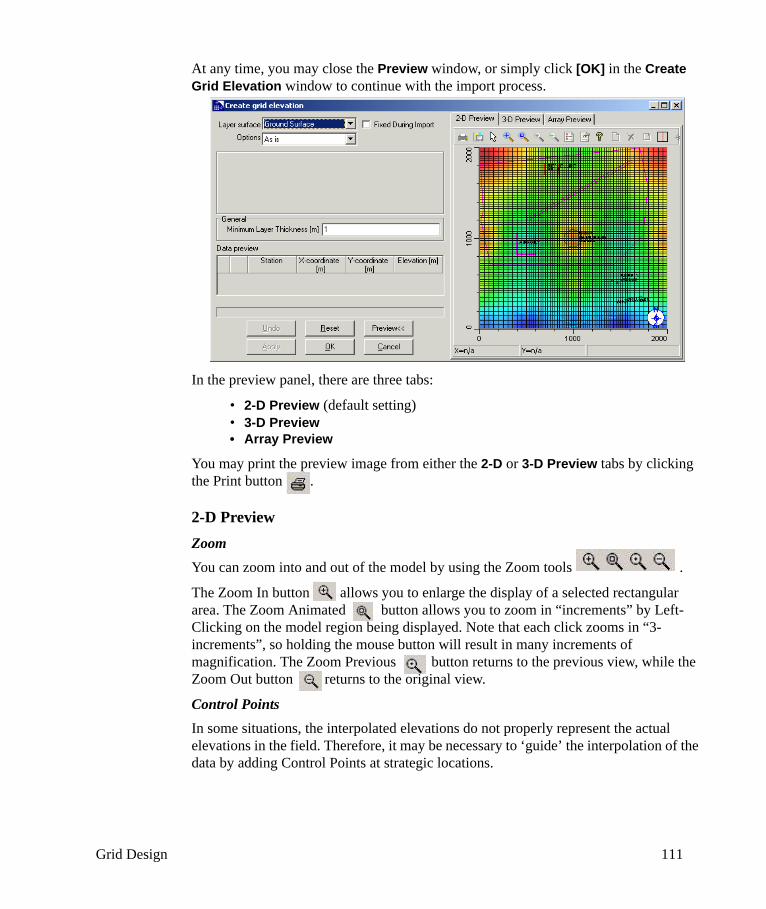
Grid Design 111
At any time, you may close the Preview window, or simply click [OK] in the Create Grid Elevation window to continue with the import process.
In the preview panel, there are three tabs:
• 2-D Preview (default setting)• 3-D Preview• Array Preview
You may print the preview image from either the 2-D or 3-D Preview tabs by clicking the Print button .
2-D PreviewZoomYou can zoom into and out of the model by using the Zoom tools .
The Zoom In button allows you to enlarge the display of a selected rectangular area. The Zoom Animated button allows you to zoom in “increments” by Left-Clicking on the model region being displayed. Note that each click zooms in “3-increments”, so holding the mouse button will result in many increments of magnification. The Zoom Previous button returns to the previous view, while the Zoom Out button returns to the original view.
Control PointsIn some situations, the interpolated elevations do not properly represent the actual elevations in the field. Therefore, it may be necessary to ‘guide’ the interpolation of the data by adding Control Points at strategic locations.
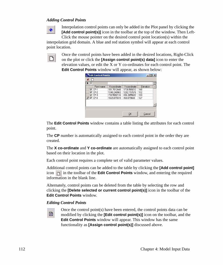
112 Chapter 4: Model Input Data
Adding Control PointsInterpolation control points can only be added in the Plot panel by clicking the [Add control point(s)] icon in the toolbar at the top of the window. Then Left-Click the mouse pointer on the desired control point location(s) within the
interpolation grid domain. A blue and red station symbol will appear at each control point location.
Once the control points have been added in the desired locations, Right-Click on the plot or click the [Assign control point(s) data] icon to enter the elevation values, or edit the X or Y co-ordinates for each control point. The Edit Control Points window will appear, as shown below:
The Edit Control Points window contains a table listing the attributes for each control point.
The CP number is automatically assigned to each control point in the order they are created.
The X co-ordinate and Y co-ordinate are automatically assigned to each control point based on their location in the plot.
Each control point requires a complete set of valid parameter values.
Additional control points can be added to the table by clicking the [Add control point] icon in the toolbar of the Edit Control Points window, and entering the required information in the blank line.
Alternately, control points can be deleted from the table by selecting the row and clicking the [Delete selected or current control point(s)] icon in the toolbar of the Edit Control Points window.
Editing Control PointsOnce the control point(s) have been entered, the control points data can be modified by clicking the [Edit control point(s)] icon on the toolbar, and the Edit Control Points window will appear. This window has the same functionality as [Assign control point(s)] discussed above.
Grid Design 113
Saving Control Points DataThe colored map of the interpolated elevations can be saved to a .BMP, .WMF, .EMF, or .DXF file by clicking the [Save As] icon on the top toolbar.
Deleting Control PointsControl points can be deleted by clicking the [Delete control point(s)] icon in the top toolbar, and clicking the mouse pointer on the control points to delete.
Legend on/offTo add or remove a map legend, click the [Show legend on/off] icon in the top toolbar. Ensure that you have selected a Legend type from the Graph Properties window, under the Legends tab, and made it visible.
Graph PropertiesThe appearance properties of the interpolated elevations map can be modified by Right-Clicking on the display area of the map and choosing the Properties option, or by clicking the [Graph Properties] icon from the toolbar. The
Graph Properties are similar to the Graph Properties described in detail on page 531.
X Cross sections To view a cross section along X axis.
Y Cross sections To view a cross section along Y axis.
3-D PreviewThe 3-D Preview is designed to visualize the interpolated three-dimensional grid elevations, to ensure that the imported data for each layer will be correctly defined in the model. This feature may prove very useful at the conceptualization stage of a model, especially when a model involves a number of layers, or very complex natural physical conditions.
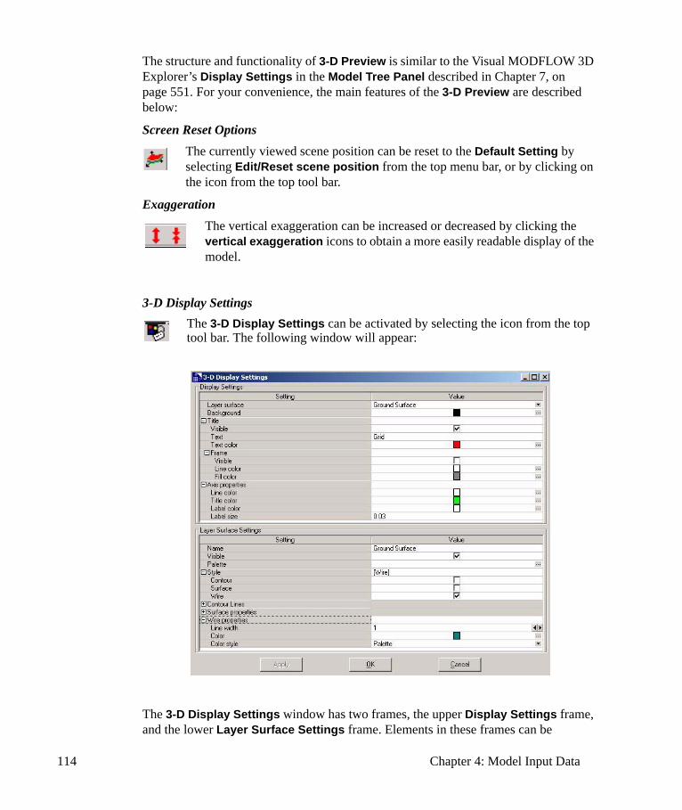
114 Chapter 4: Model Input Data
The structure and functionality of 3-D Preview is similar to the Visual MODFLOW 3D Explorer’s Display Settings in the Model Tree Panel described in Chapter 7, on page 551. For your convenience, the main features of the 3-D Preview are described below:
Screen Reset OptionsThe currently viewed scene position can be reset to the Default Setting by selecting Edit/Reset scene position from the top menu bar, or by clicking on the icon from the top tool bar.
Exaggeration The vertical exaggeration can be increased or decreased by clicking the vertical exaggeration icons to obtain a more easily readable display of the model.
3-D Display SettingsThe 3-D Display Settings can be activated by selecting the icon from the top tool bar. The following window will appear:
The 3-D Display Settings window has two frames, the upper Display Settings frame, and the lower Layer Surface Settings frame. Elements in these frames can be
Grid Design 115
expanded by clicking on the “+” symbol. The default settings can be modified and saved, and applied to the project by pressing the [Apply] button located at the bottom of the window.
Display SettingsThe Display Settings frame is used to define your preferences for the general project display. The Display Settings frame options include:
Layer SurfaceDisplays the name of the currently selected layer of the model. Click to select the other available model layers.
BackgroundThis option sets the display screen color. By default, the Background color of the display screen is black.
Title
Visible allows you to show or hide the title
Text allows you to enter the text to be displayed
Text Color sets the color of the title
Axis Properties Line Color sets the color of the axis lines (X, Y, Z axis).
Title Color sets the color of the axis names.
Label Color sets the color of the numerical axis labels.
Label Size sets the size of the numerical axis labels.
Layer Surface SettingsThe Layer Surface Settings frame is used to define your preferences for the display of specific model layers. Please Note that some options will be greyed out, depending on the Style that has been selected. Selecting a Style will activate the appropriate option. The Layer Surface Settings frame options include:
NameDisplays the name of the currently selected layer of the model.
VisibleAllows you to show or hide the currently selected layer.

116 Chapter 4: Model Input Data
PalettePalette controls the property-variable color scale used for all display elements. A description of thePalette is provided in "The Color Palette" on page 586. The color scheme for layers can be set to either a single color (Mono), or to be colored from the Palette.
Style The Style option lists the available display types for surfaces (Contour, Surface, Wire). This feature allows the user to selectively activate/de-active these elements and alter their properties. More than one Style may be combined for a particular layer.
Contour displays layer elevation contours.
Surface displays a solid (or semitransparent) layer surface.
Wire displays a gridded layer surface.
Contour Lines lists the layer elevation contours options.Line Style allows selection of the type of contour line to be displayed (Solid, Dotted, Dashed, or DashDot.
Line Width allows selection of the width of contour lines.
Color allows selection of contour line color if Mono is selected for the Color Style.
Color style allows the use of a single color (Mono), or coloring from the Palette.
Labels Color style allows the use of a single color (Mono) or coloring from the Palette.
Color sets the color for contour labels if Mono is selected for the Color Style.Number of Zones Based on the vertical variation in layer elevation, the number of zones differentiated by contour intervals is automatically set by the interpolator. However, it may be more practical for interpolation purposes to visualize such variations by changing their scale through an increase or decrease in the number of zones. The number of zones can simply be changed by typing in a new number in this field to obtain a more desirable contour interval and distribution of grid elevations.
Font name sets the font name used for contour labels.
Font type sets the font type used for contour labels.
Size sets the font size used for contour labels.
Visible allows labels to be shown or hidden.
Surface Properties lists the options available for the display of a solid (or
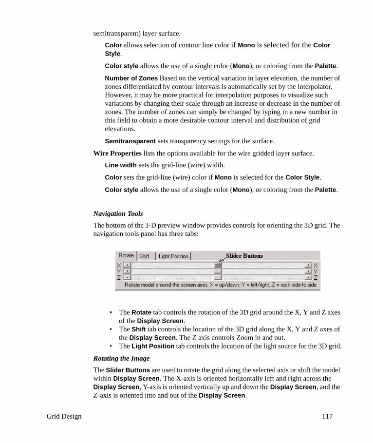
Grid Design 117
semitransparent) layer surface.Color allows selection of contour line color if Mono is selected for the Color Style.
Color style allows the use of a single color (Mono), or coloring from the Palette.
Number of Zones Based on the vertical variation in layer elevation, the number of zones differentiated by contour intervals is automatically set by the interpolator. However, it may be more practical for interpolation purposes to visualize such variations by changing their scale through an increase or decrease in the number of zones. The number of zones can simply be changed by typing in a new number in this field to obtain a more desirable contour interval and distribution of grid elevations.
Semitransparent sets transparency settings for the surface.
Wire Properties lists the options available for the wire gridded layer surface.Line width sets the grid-line (wire) width.
Color sets the grid-line (wire) color if Mono is selected for the Color Style.Color style allows the use of a single color (Mono), or coloring from the Palette.
Navigation ToolsThe bottom of the 3-D preview window provides controls for orienting the 3D grid. The navigation tools panel has three tabs:
• The Rotate tab controls the rotation of the 3D grid around the X, Y and Z axes of the Display Screen.
• The Shift tab controls the location of the 3D grid along the X, Y and Z axes of the Display Screen. The Z axis controls Zoom in and out.
• The Light Position tab controls the location of the light source for the 3D grid.
Rotating the ImageThe Slider Buttons are used to rotate the grid along the selected axis or shift the model within Display Screen. The X-axis is oriented horizontally left and right across the Display Screen, Y-axis is oriented vertically up and down the Display Screen, and the Z-axis is oriented into and out of the Display Screen.
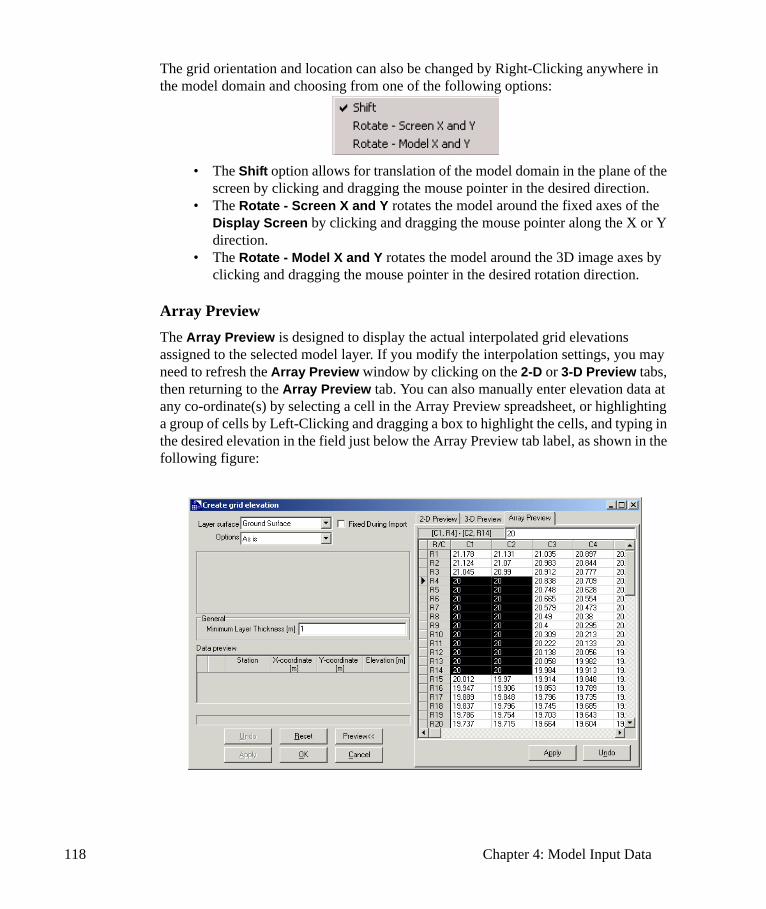
118 Chapter 4: Model Input Data
The grid orientation and location can also be changed by Right-Clicking anywhere in the model domain and choosing from one of the following options:
• The Shift option allows for translation of the model domain in the plane of the screen by clicking and dragging the mouse pointer in the desired direction.
• The Rotate - Screen X and Y rotates the model around the fixed axes of the Display Screen by clicking and dragging the mouse pointer along the X or Y direction.
• The Rotate - Model X and Y rotates the model around the 3D image axes by clicking and dragging the mouse pointer in the desired rotation direction.
Array PreviewThe Array Preview is designed to display the actual interpolated grid elevations assigned to the selected model layer. If you modify the interpolation settings, you may need to refresh the Array Preview window by clicking on the 2-D or 3-D Preview tabs, then returning to the Array Preview tab. You can also manually enter elevation data at any co-ordinate(s) by selecting a cell in the Array Preview spreadsheet, or highlighting a group of cells by Left-Clicking and dragging a box to highlight the cells, and typing in the desired elevation in the field just below the Array Preview tab label, as shown in the following figure:
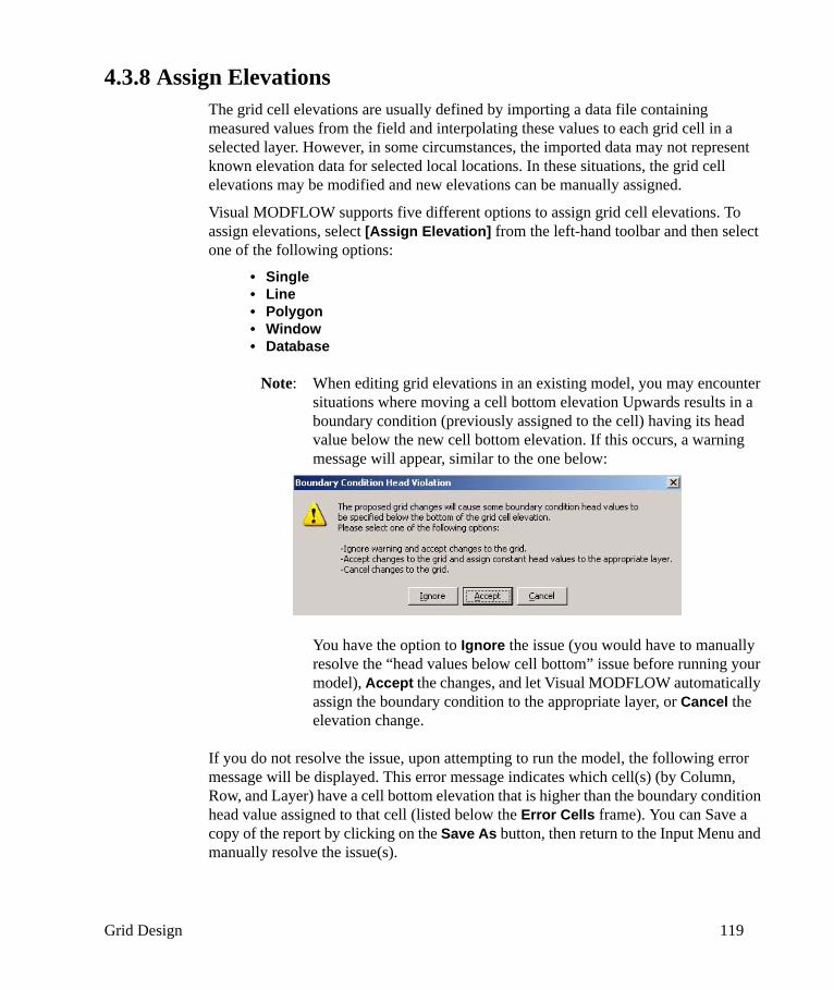
Grid Design 119
4.3.8 Assign Elevations The grid cell elevations are usually defined by importing a data file containing measured values from the field and interpolating these values to each grid cell in a selected layer. However, in some circumstances, the imported data may not represent known elevation data for selected local locations. In these situations, the grid cell elevations may be modified and new elevations can be manually assigned.
Visual MODFLOW supports five different options to assign grid cell elevations. To assign elevations, select [Assign Elevation] from the left-hand toolbar and then select one of the following options:
• Single• Line• Polygon• Window• Database
Note: When editing grid elevations in an existing model, you may encounter situations where moving a cell bottom elevation Upwards results in a boundary condition (previously assigned to the cell) having its head value below the new cell bottom elevation. If this occurs, a warning message will appear, similar to the one below:
You have the option to Ignore the issue (you would have to manually resolve the “head values below cell bottom” issue before running your model), Accept the changes, and let Visual MODFLOW automatically assign the boundary condition to the appropriate layer, or Cancel the elevation change.
If you do not resolve the issue, upon attempting to run the model, the following error message will be displayed. This error message indicates which cell(s) (by Column, Row, and Layer) have a cell bottom elevation that is higher than the boundary condition head value assigned to that cell (listed below the Error Cells frame). You can Save a copy of the report by clicking on the Save As button, then return to the Input Menu and manually resolve the issue(s).
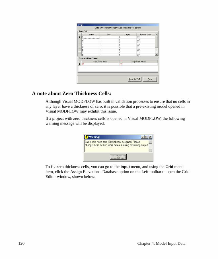
120 Chapter 4: Model Input Data
A note about Zero Thickness Cells:Although Visual MODFLOW has built in validation processes to ensure that no cells in any layer have a thickness of zero, it is possible that a pre-existing model opened in Visual MODFLOW may exhibit this issue.
If a project with zero thickness cells is opened in Visual MODFLOW, the following warning message will be displayed:
To fix zero thickness cells, you can go to the Input menu, and using the Grid menu item, click the Assign Elevation - Database option on the Left toolbar to open the Grid Editor window, shown below:
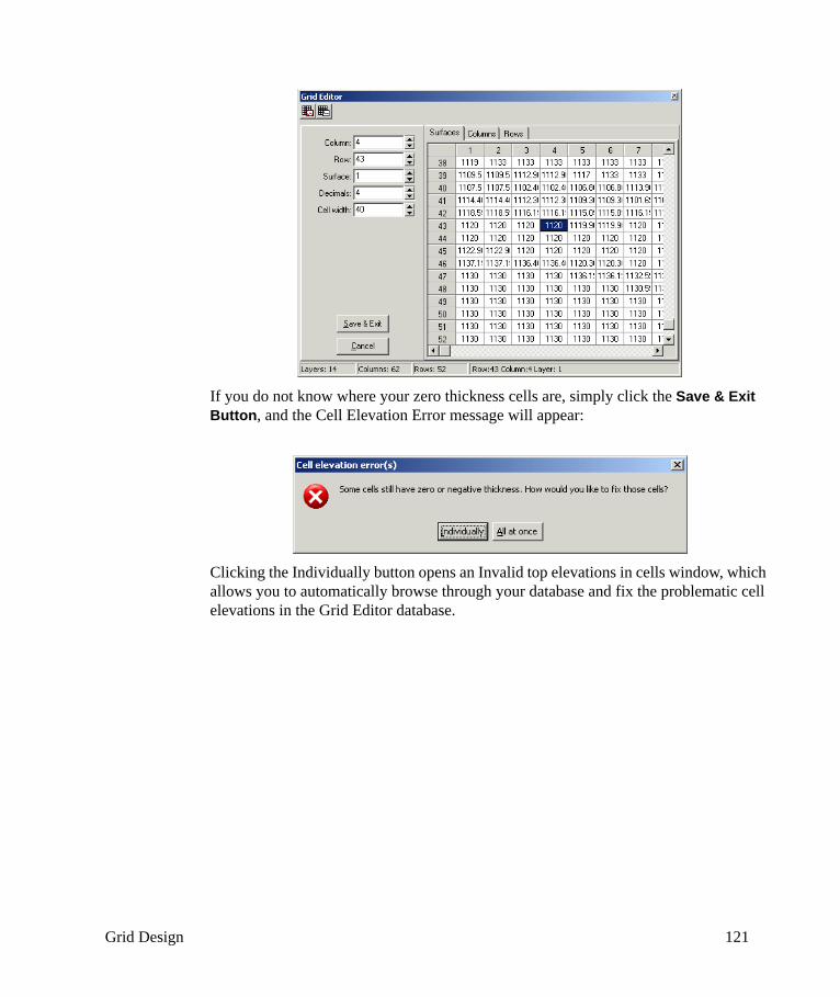
Grid Design 121
If you do not know where your zero thickness cells are, simply click the Save & Exit Button, and the Cell Elevation Error message will appear:
Clicking the Individually button opens an Invalid top elevations in cells window, which allows you to automatically browse through your database and fix the problematic cell elevations in the Grid Editor database.
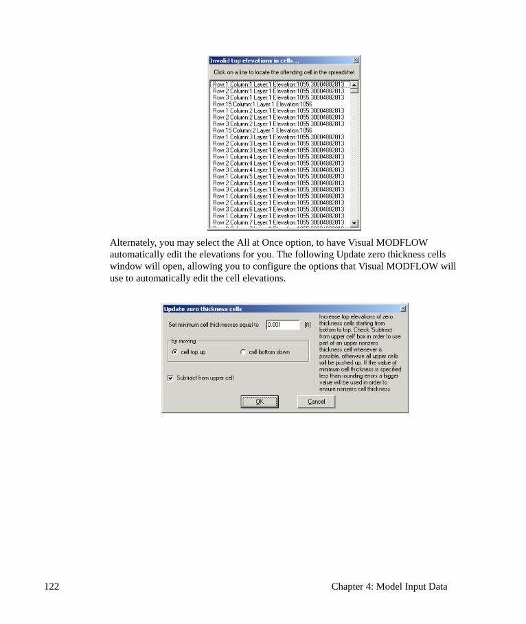
122 Chapter 4: Model Input Data
Alternately, you may select the All at Once option, to have Visual MODFLOW automatically edit the elevations for you. The following Update zero thickness cells window will open, allowing you to configure the options that Visual MODFLOW will use to automatically edit the cell elevations.
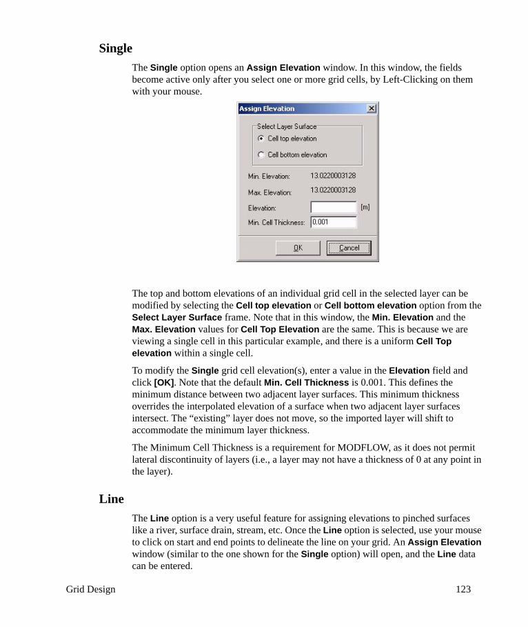
Grid Design 123
SingleThe Single option opens an Assign Elevation window. In this window, the fields become active only after you select one or more grid cells, by Left-Clicking on them with your mouse.
The top and bottom elevations of an individual grid cell in the selected layer can be modified by selecting the Cell top elevation or Cell bottom elevation option from the Select Layer Surface frame. Note that in this window, the Min. Elevation and the Max. Elevation values for Cell Top Elevation are the same. This is because we are viewing a single cell in this particular example, and there is a uniform Cell Top elevation within a single cell.
To modify the Single grid cell elevation(s), enter a value in the Elevation field and click [OK]. Note that the default Min. Cell Thickness is 0.001. This defines the minimum distance between two adjacent layer surfaces. This minimum thickness overrides the interpolated elevation of a surface when two adjacent layer surfaces intersect. The “existing” layer does not move, so the imported layer will shift to accommodate the minimum layer thickness.
The Minimum Cell Thickness is a requirement for MODFLOW, as it does not permit lateral discontinuity of layers (i.e., a layer may not have a thickness of 0 at any point in the layer).
LineThe Line option is a very useful feature for assigning elevations to pinched surfaces like a river, surface drain, stream, etc. Once the Line option is selected, use your mouse to click on start and end points to delineate the line on your grid. An Assign Elevation window (similar to the one shown for the Single option) will open, and the Line data can be entered.
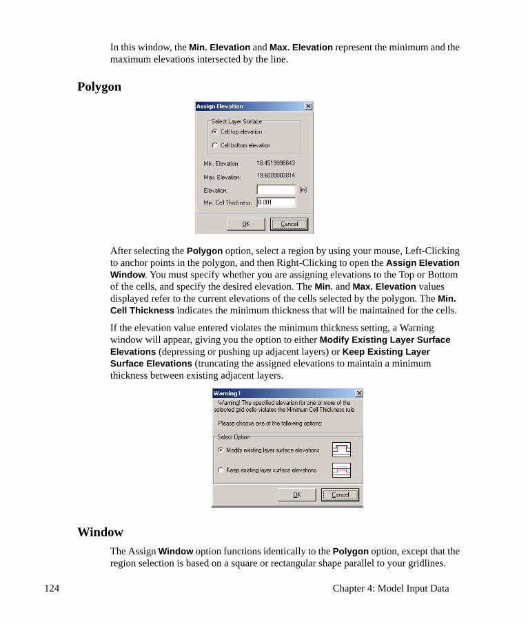
124 Chapter 4: Model Input Data
In this window, the Min. Elevation and Max. Elevation represent the minimum and the maximum elevations intersected by the line.
Polygon
After selecting the Polygon option, select a region by using your mouse, Left-Clicking to anchor points in the polygon, and then Right-Clicking to open the Assign Elevation Window. You must specify whether you are assigning elevations to the Top or Bottom of the cells, and specify the desired elevation. The Min. and Max. Elevation values displayed refer to the current elevations of the cells selected by the polygon. The Min. Cell Thickness indicates the minimum thickness that will be maintained for the cells.
If the elevation value entered violates the minimum thickness setting, a Warning window will appear, giving you the option to either Modify Existing Layer Surface Elevations (depressing or pushing up adjacent layers) or Keep Existing Layer Surface Elevations (truncating the assigned elevations to maintain a minimum thickness between existing adjacent layers.
Window The Assign Window option functions identically to the Polygon option, except that the region selection is based on a square or rectangular shape parallel to your gridlines.
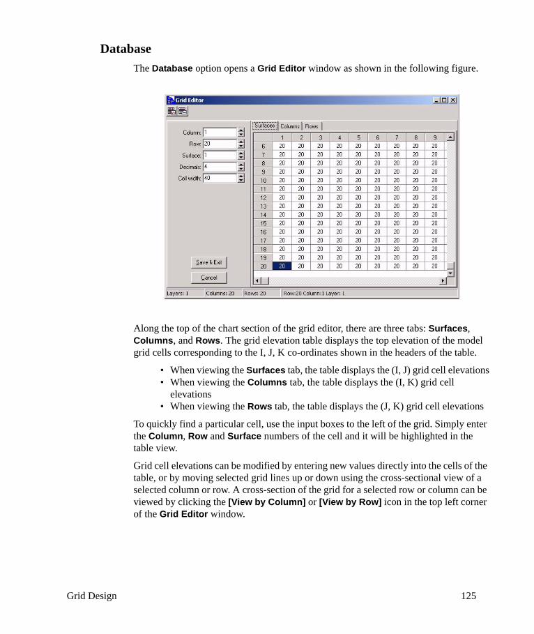
Grid Design 125
DatabaseThe Database option opens a Grid Editor window as shown in the following figure.
Along the top of the chart section of the grid editor, there are three tabs: Surfaces, Columns, and Rows. The grid elevation table displays the top elevation of the model grid cells corresponding to the I, J, K co-ordinates shown in the headers of the table.
• When viewing the Surfaces tab, the table displays the (I, J) grid cell elevations• When viewing the Columns tab, the table displays the (I, K) grid cell
elevations• When viewing the Rows tab, the table displays the (J, K) grid cell elevations
To quickly find a particular cell, use the input boxes to the left of the grid. Simply enter the Column, Row and Surface numbers of the cell and it will be highlighted in the table view.
Grid cell elevations can be modified by entering new values directly into the cells of the table, or by moving selected grid lines up or down using the cross-sectional view of a selected column or row. A cross-section of the grid for a selected row or column can be viewed by clicking the [View by Column] or [View by Row] icon in the top left corner of the Grid Editor window.
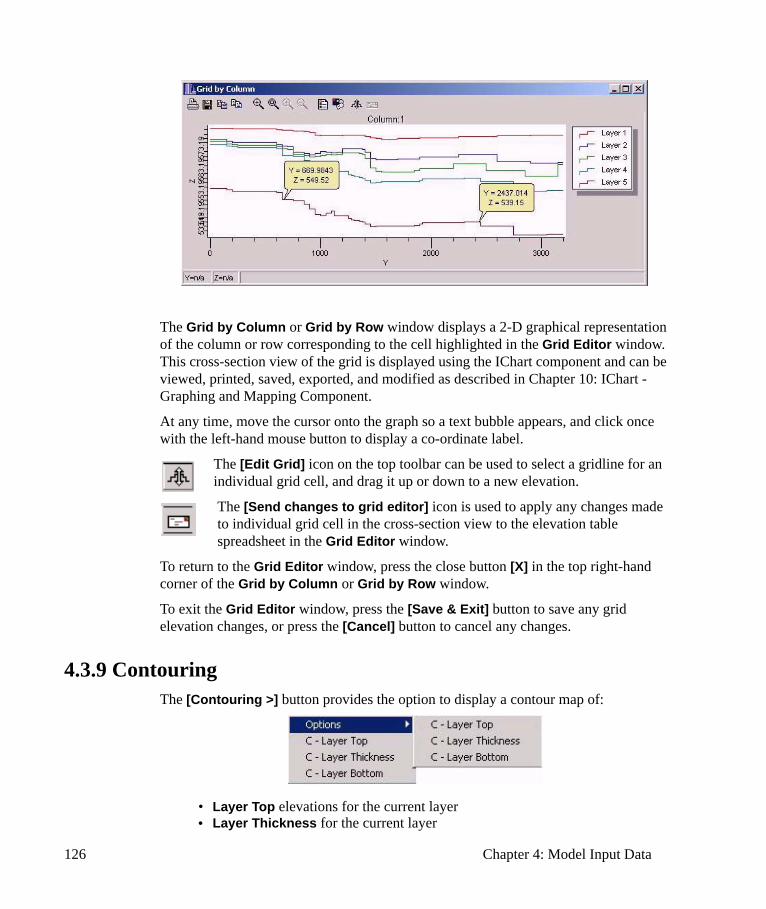
126 Chapter 4: Model Input Data
The Grid by Column or Grid by Row window displays a 2-D graphical representation of the column or row corresponding to the cell highlighted in the Grid Editor window. This cross-section view of the grid is displayed using the IChart component and can be viewed, printed, saved, exported, and modified as described in Chapter 10: IChart - Graphing and Mapping Component.
At any time, move the cursor onto the graph so a text bubble appears, and click once with the left-hand mouse button to display a co-ordinate label.
The [Edit Grid] icon on the top toolbar can be used to select a gridline for an individual grid cell, and drag it up or down to a new elevation.
The [Send changes to grid editor] icon is used to apply any changes made to individual grid cell in the cross-section view to the elevation table spreadsheet in the Grid Editor window.
To return to the Grid Editor window, press the close button [X] in the top right-hand corner of the Grid by Column or Grid by Row window.
To exit the Grid Editor window, press the [Save & Exit] button to save any grid elevation changes, or press the [Cancel] button to cancel any changes.
4.3.9 Contouring The [Contouring >] button provides the option to display a contour map of:
• Layer Top elevations for the current layer• Layer Thickness for the current layer

Wells 127
• Layer Bottom elevations for the current layer
The Options item provides access to the contour options for each of these Contouring overlays. A detailed description of the Contouring options is provided in the Contour Map Display Options section on page 483, and the Color Map Display Options section on page 486.
4.4 WellsThe Wells item in the top menu bar of the Input section is used to add, import, delete, move, and edit three different types of wells:
• Pumping Wells• Head and Concentration Observation Wells
The features and functionality of the graphical tools available for each type of well are described in the following sections.
4.4.1 Pumping WellsPumping well data can be added to the model by selecting Wells/Pumping Wells from the top menu bar of the Input section. The Pumping Wells screen provides the following graphical options in the left-hand toolbar.
Note: The maximum number of pumping and injection wells is limited only by the amount of RAM available.
[Import Wells]: Import pumping well data from a variety of file formats including ASCII .TXT, ESRI .SHP, .XLS, or .MDB.
[Add Well]: Add a pumping well by clicking the mouse on the desired well location in the model.
[Delete Well]: Delete pumping well(s) by selecting Single, Window, Polygon, All Wells, All Inactive, orAll Outside XY-Domain (as shown in the following figure).
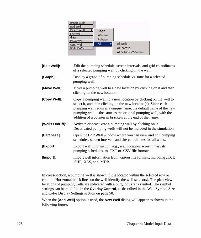
128 Chapter 4: Model Input Data
[Edit Well]: Edit the pumping schedule, screen intervals, and grid co-ordinates of a selected pumping well by clicking on the well.
[Graph]: Display a graph of pumping schedule vs. time for a selected pumping well.
[Move Well]: Move a pumping well to a new location by clicking on it and then clicking on the new location.
[Copy Well]: Copy a pumping well to a new location by clicking on the well to select it, and then clicking on the new location(s). Since each pumping well requires a unique name, the default name of the new pumping well is the same as the original pumping well, with the addition of a counter in brackets at the end of the name.
[Wells On/Off]: Activate or deactivate a pumping well by clicking on it. Deactivated pumping wells will not be included in the simulation.
[Database]: Open the Edit Well window where you can view and edit pumping schedules, screen intervals and site coordinates for all wells.
[Export]: Export well information, e.g., well location, screen intervals, pumping schedules, to .TXT or .CSV file formats.
[Import]: Import well information from various file formats, including .TXT, .SHP, .XLS, and .MDB.
In cross-section, a pumping well is shown if it is located within the selected row or column. Horizontal black lines on the well identify the well screen(s). The plan-view locations of pumping wells are indicated with a burgundy (red) symbol. The symbol settings can be modified in the Overlay Control, as described in the Well Symbol Size and Color Display Settings section on page 58.
When the [Add Well] option is used, the New Well dialog will appear as shown in the following figure:
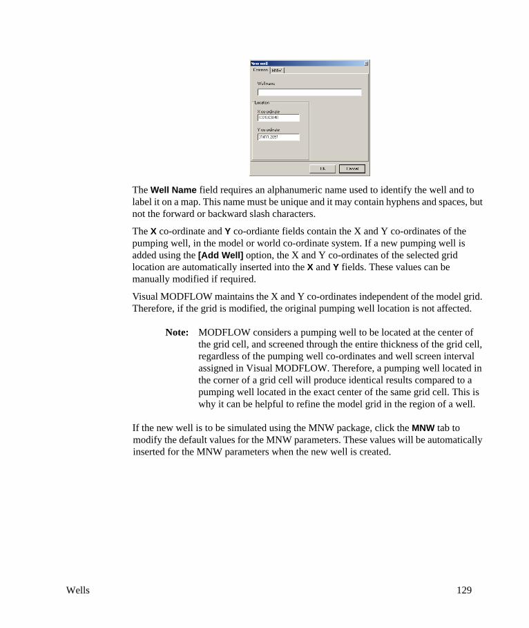
Wells 129
The Well Name field requires an alphanumeric name used to identify the well and to label it on a map. This name must be unique and it may contain hyphens and spaces, but not the forward or backward slash characters.
The X co-ordinate and Y co-ordiante fields contain the X and Y co-ordinates of the pumping well, in the model or world co-ordinate system. If a new pumping well is added using the [Add Well] option, the X and Y co-ordinates of the selected grid location are automatically inserted into the X and Y fields. These values can be manually modified if required.
Visual MODFLOW maintains the X and Y co-ordinates independent of the model grid. Therefore, if the grid is modified, the original pumping well location is not affected.
Note: MODFLOW considers a pumping well to be located at the center of the grid cell, and screened through the entire thickness of the grid cell, regardless of the pumping well co-ordinates and well screen interval assigned in Visual MODFLOW. Therefore, a pumping well located in the corner of a grid cell will produce identical results compared to a pumping well located in the exact center of the same grid cell. This is why it can be helpful to refine the model grid in the region of a well.
If the new well is to be simulated using the MNW package, click the MNW tab to modify the default values for the MNW parameters. These values will be automatically inserted for the MNW parameters when the new well is created.
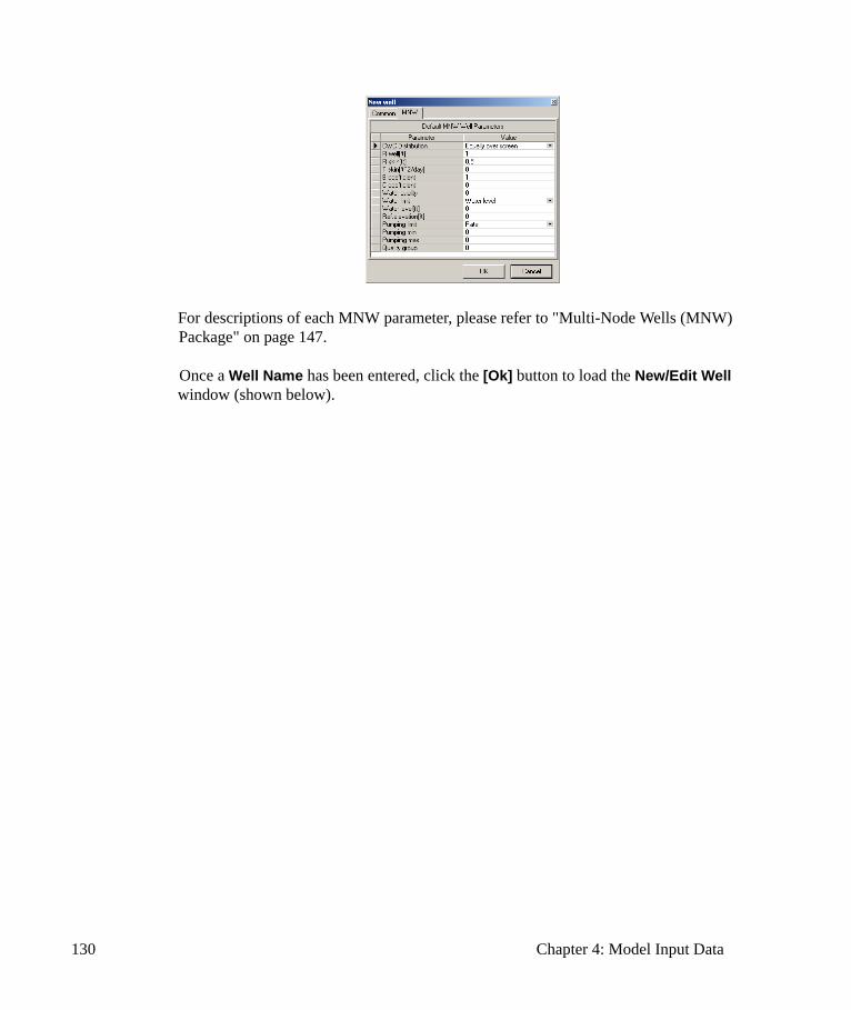
130 Chapter 4: Model Input Data
For descriptions of each MNW parameter, please refer to "Multi-Node Wells (MNW) Package" on page 147.
Once a Well Name has been entered, click the [Ok] button to load the New/Edit Well window (shown below).
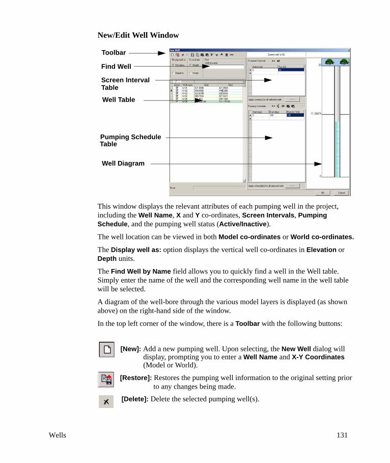
Wells 131
New/Edit Well Window
This window displays the relevant attributes of each pumping well in the project, including the Well Name, X and Y co-ordinates, Screen Intervals, Pumping Schedule, and the pumping well status (Active/Inactive).
The well location can be viewed in both Model co-ordinates or World co-ordinates.
The Display well as: option displays the vertical well co-ordinates in Elevation or Depth units.
The Find Well by Name field allows you to quickly find a well in the Well table. Simply enter the name of the well and the corresponding well name in the well table will be selected.
A diagram of the well-bore through the various model layers is displayed (as shown above) on the right-hand side of the window.
In the top left corner of the window, there is a Toolbar with the following buttons:
[New]: Add a new pumping well. Upon selecting, the New Well dialog will display, prompting you to enter a Well Name and X-Y Coordinates (Model or World).
[Restore]: Restores the pumping well information to the original setting prior to any changes being made.
[Delete]: Delete the selected pumping well(s).
Toolbar
Well Table
Screen Interval
Pumping Schedule
Well Diagram
Find Well
Table
Table

132 Chapter 4: Model Input Data
[Undelete]: Restore a well that has been deleted. Please note that once the New / Edit Well dialog is closed, the deleted well can no longer be restored.
[Well(s) Legend]: Displays the Rows Color Legend for the well table .
Each well (row) in the well table is assigned a color based on its current status. For example, if a well contains invalid data, its row will appear pink in the well table. Each color and its corresponding well status is displayed in the Rows Color Legend. Each item in the legend is described below:
Loaded Well: A saved well
New Well: A well that has been recently added to the wells table
Restored Well:A well that has been recently restored to previous well information (using the Restore button)
Undeleted Well: A well that has been recently undeleted
Invalid Well: A well that is missing information, i.e, pumping schedule, screen interval(s), or contains invalid attribute values
[Copy to Clipboard]: Copy selected well table data to the Windows clipboard.
[Load]: Import data into the Wells Table from a ASCII file. Upon selecting, the following dialog will display:
In the Import wells from file dialog, navigate to the folder and select the desired file. Once selected, click the [Open] button. The following dialog will display:
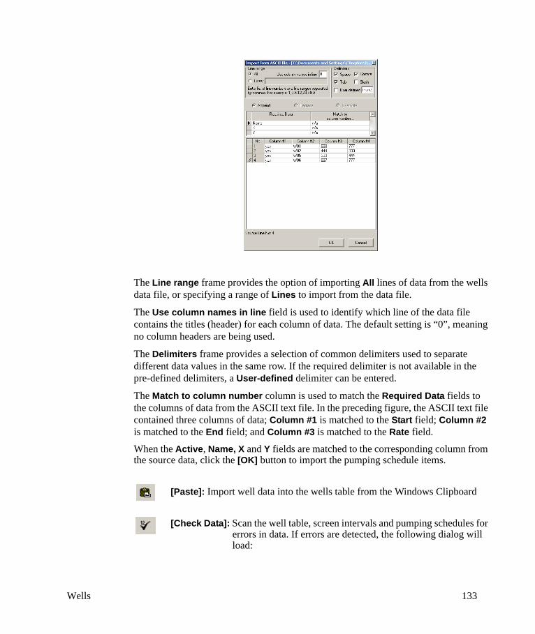
Wells 133
The Line range frame provides the option of importing All lines of data from the wells data file, or specifying a range of Lines to import from the data file.
The Use column names in line field is used to identify which line of the data file contains the titles (header) for each column of data. The default setting is “0”, meaning no column headers are being used.
The Delimiters frame provides a selection of common delimiters used to separate different data values in the same row. If the required delimiter is not available in the pre-defined delimiters, a User-defined delimiter can be entered.
The Match to column number column is used to match the Required Data fields to the columns of data from the ASCII text file. In the preceding figure, the ASCII text file contained three columns of data; Column #1 is matched to the Start field; Column #2 is matched to the End field; and Column #3 is matched to the Rate field.
When the Active, Name, X and Y fields are matched to the corresponding column from the source data, click the [OK] button to import the pumping schedule items.
[Paste]: Import well data into the wells table from the Windows Clipboard
[Check Data]: Scan the well table, screen intervals and pumping schedules for errors in data. If errors are detected, the following dialog will load:
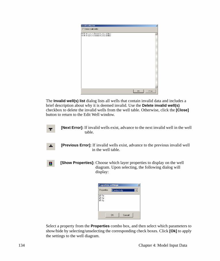
134 Chapter 4: Model Input Data
The Invalid well(s) list dialog lists all wells that contain invalid data and includes a brief description about why it is deemed invalid. Use the Delete invalid well(s) checkbox to delete the invalid wells from the well table. Otherwise, click the [Close] button to return to the Edit Well window.
[Next Error]: If invalid wells exist, advance to the next invalid well in the well table.
[Previous Error]: If invalid wells exist, advance to the previous invalid well in the well table.
[Show Properties]: Choose which layer properties to display on the well diagram. Upon selecting, the following dialog will display:
Select a property from the Properties combo box, and then select which parameters to show/hide by selecting/unselecting the corresponding check boxes. Click [Ok] to apply the settings to the well diagram.
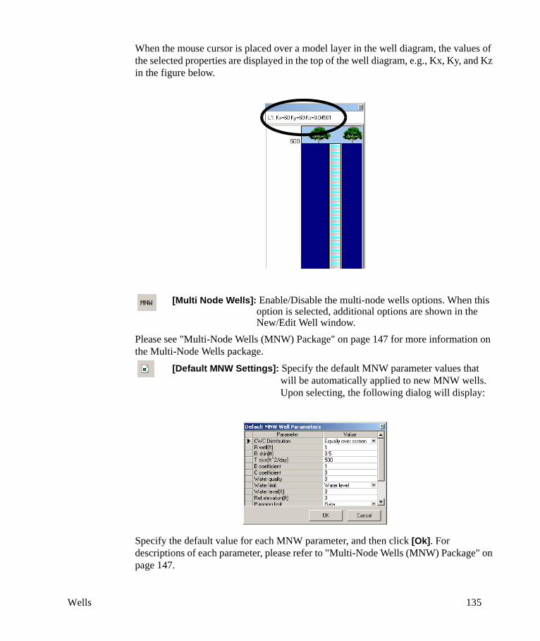
Wells 135
When the mouse cursor is placed over a model layer in the well diagram, the values of the selected properties are displayed in the top of the well diagram, e.g., Kx, Ky, and Kz in the figure below.
[Multi Node Wells]: Enable/Disable the multi-node wells options. When this option is selected, additional options are shown in the New/Edit Well window.
Please see "Multi-Node Wells (MNW) Package" on page 147 for more information on the Multi-Node Wells package.
[Default MNW Settings]: Specify the default MNW parameter values that will be automatically applied to new MNW wells. Upon selecting, the following dialog will display:
Specify the default value for each MNW parameter, and then click [Ok]. For descriptions of each parameter, please refer to "Multi-Node Wells (MNW) Package" on page 147.
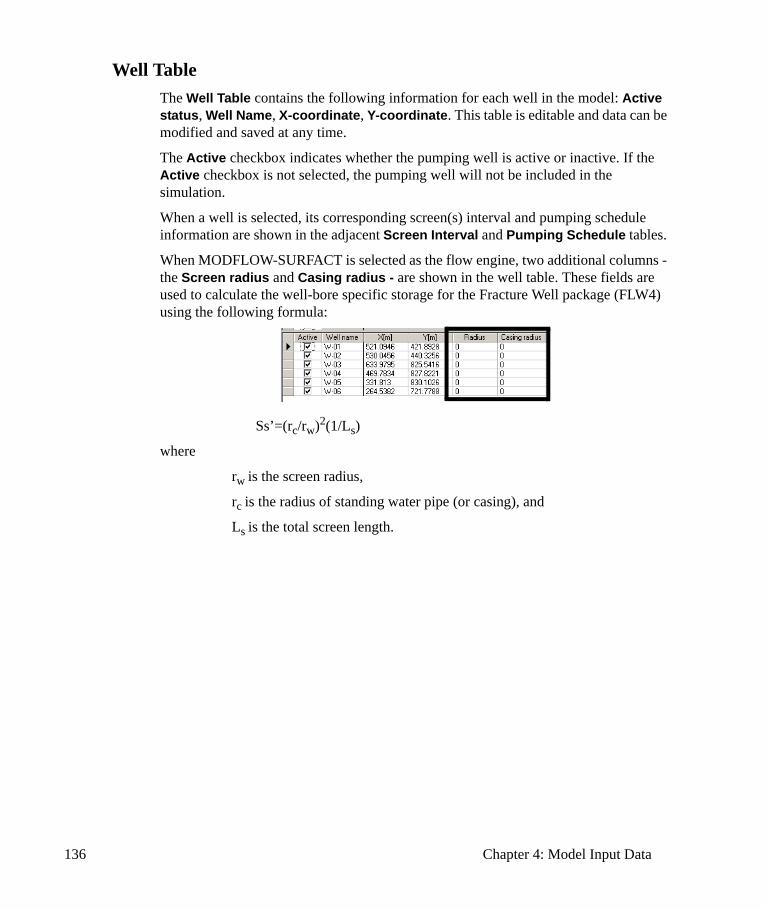
136 Chapter 4: Model Input Data
Well TableThe Well Table contains the following information for each well in the model: Active status, Well Name, X-coordinate, Y-coordinate. This table is editable and data can be modified and saved at any time.
The Active checkbox indicates whether the pumping well is active or inactive. If the Active checkbox is not selected, the pumping well will not be included in the simulation.
When a well is selected, its corresponding screen(s) interval and pumping schedule information are shown in the adjacent Screen Interval and Pumping Schedule tables.
When MODFLOW-SURFACT is selected as the flow engine, two additional columns - the Screen radius and Casing radius - are shown in the well table. These fields are used to calculate the well-bore specific storage for the Fracture Well package (FLW4) using the following formula:
Ss’=(rc/rw)2(1/Ls)
where
rw is the screen radius,
rc is the radius of standing water pipe (or casing), and
Ls is the total screen length.
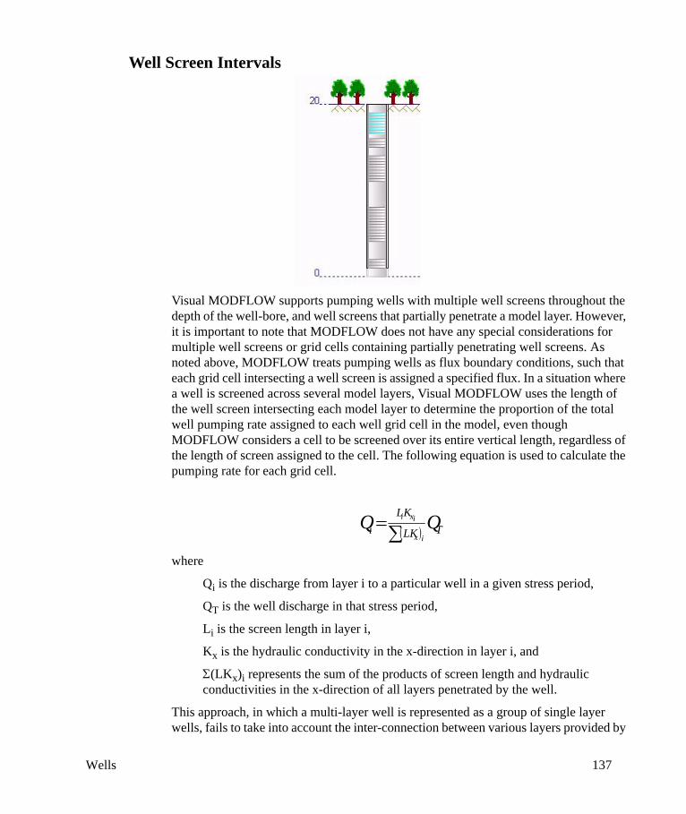
Wells 137
Well Screen Intervals
Visual MODFLOW supports pumping wells with multiple well screens throughout the depth of the well-bore, and well screens that partially penetrate a model layer. However, it is important to note that MODFLOW does not have any special considerations for multiple well screens or grid cells containing partially penetrating well screens. As noted above, MODFLOW treats pumping wells as flux boundary conditions, such that each grid cell intersecting a well screen is assigned a specified flux. In a situation where a well is screened across several model layers, Visual MODFLOW uses the length of the well screen intersecting each model layer to determine the proportion of the total well pumping rate assigned to each well grid cell in the model, even though MODFLOW considers a cell to be screened over its entire vertical length, regardless of the length of screen assigned to the cell. The following equation is used to calculate the pumping rate for each grid cell.
where
Qi is the discharge from layer i to a particular well in a given stress period,
QT is the well discharge in that stress period,
Li is the screen length in layer i,
Kx is the hydraulic conductivity in the x-direction in layer i, and
Σ(LKx)i represents the sum of the products of screen length and hydraulic conductivities in the x-direction of all layers penetrated by the well.
This approach, in which a multi-layer well is represented as a group of single layer wells, fails to take into account the inter-connection between various layers provided by
( ) TLK
KLi QQ
ix
ixi
∑=

138 Chapter 4: Model Input Data
the well. One of the most significant problems related to this approach is that well grid cells are essentially shut off when the water table drops below the bottom of the grid cell (i.e. when the grid cell becomes dry). This automatically reduces the total pumping rate of the well, and may cause the water table to “rebound” and re-activate the well grid cell. This type of on-again-off-again behavior for the pumping well(s) causes the solution to oscillate, and may prevent the model from converging to a solution. In the event the model does converge to a solution, the model results may be misleading if one or more pumping wells have lower than expected total pumping rates.
Alternately, a multi-layer well can sometimes be simulated by means of a vertical column of high permeability cells with a screen at the bottom of the column. In this case, if the top part of the model becomes dry, the total pumping rate is unaffected. This also takes into account the vertical inter-connection between layers. The downside of this approach is that the conductivity contrasts can lead to convergence problems.
This issue can also be addressed by selecting the MODFLOW-SURFACT engine for flow. In contrast to the standard MODFLOW engines, MODFLOW-SURFACT is able to redistribute pumping rates to the remaining active grid cells if one or more cells in the screened interval goes dry, thereby more accurately simulating the real-world effects of partial overpumping of a well screened over multiple layers.
Adding Well Screen IntervalsA well screen interval can be added graphically by right-clicking on the well-bore diagram and selecting the Add Screen option. Then click-and-drag the mouse from the start point of the well screen to the end point of the well screen.
The actual top and bottom elevations of each well screen interval are shown in the Screened Intervals table under the Screen Top and Screen Bottom columns, respectively. These values may be manually modified if required.
Well screen data can also be directly entered by clicking the [Add Screen] icon above the Screened Intervals table and entering the Screen Bottom and Screen Top elevations in the appropriate fields.
Each well screen interval requires data for the Screen Bottom elevation and the Screen Top elevation. If an additional well screen was accidentally added, and does not contain any data for the Screen Bottom and/or Screen Top, this interval must be deleted from the Screen Intervals table before closing the Edit Well window.
A well screen interval can be added over an entire layer thickness by right-clicking on the well-bore diagram and selecting Add Screen In Layer... option. Upon selecting, the following dialog will display:
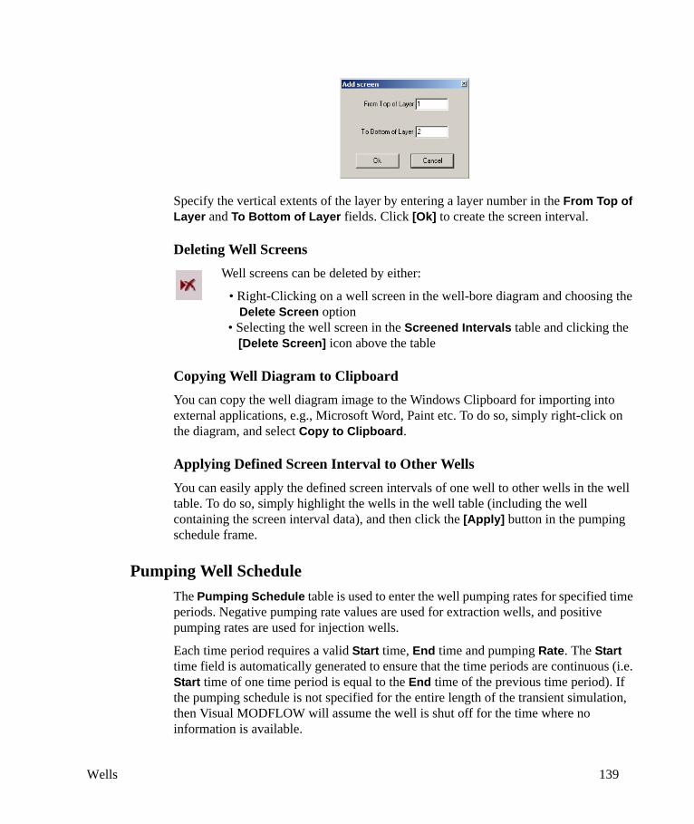
Wells 139
Specify the vertical extents of the layer by entering a layer number in the From Top of Layer and To Bottom of Layer fields. Click [Ok] to create the screen interval.
Deleting Well ScreensWell screens can be deleted by either:
• Right-Clicking on a well screen in the well-bore diagram and choosing the Delete Screen option
• Selecting the well screen in the Screened Intervals table and clicking the [Delete Screen] icon above the table
Copying Well Diagram to ClipboardYou can copy the well diagram image to the Windows Clipboard for importing into external applications, e.g., Microsoft Word, Paint etc. To do so, simply right-click on the diagram, and select Copy to Clipboard.
Applying Defined Screen Interval to Other Wells You can easily apply the defined screen intervals of one well to other wells in the well table. To do so, simply highlight the wells in the well table (including the well containing the screen interval data), and then click the [Apply] button in the pumping schedule frame.
Pumping Well ScheduleThe Pumping Schedule table is used to enter the well pumping rates for specified time periods. Negative pumping rate values are used for extraction wells, and positive pumping rates are used for injection wells.
Each time period requires a valid Start time, End time and pumping Rate. The Start time field is automatically generated to ensure that the time periods are continuous (i.e. Start time of one time period is equal to the End time of the previous time period). If the pumping schedule is not specified for the entire length of the transient simulation, then Visual MODFLOW will assume the well is shut off for the time where no information is available.
140 Chapter 4: Model Input Data
For steady-state simulations, the pumping rate for the first time period will be used as the steady-state pumping rate.
Adding Pumping Schedule ItemsTo add an item to the Pumping Schedule table,
• Click the [Append Schedule Item] icon above the table to add a schedule item, or simply click in the first row of the table.
• Enter an End time value and press the <Tab> key to advance to the Rate field
• Enter a pumping Rate value (remember to use a negative value for extraction wells)
• Press the <Tab> key again to create a new schedule item, or click the [OK] button to accept the pumping well data.
Each pumping schedule item is required to be completed with a valid End time and pumping Rate. If a pumping schedule item has been accidentally added without any data, it must be deleted before the Edit Well window can be closed.
Deleting Pumping Schedule ItemsTo delete an item from the Pumping Schedule table,
• Click on the item to delete in the Pumping Schedule table• Click on the [Delete Schedule Item] icon above the table
Inserting a Pumping Schedule ItemTo insert an item in the Pumping Schedule table,
• Click the time period where the new item will be inserted• Click the [Insert Schedule Item at Current Cursor Position] icon
above the table• Enter the End time for the new time period and press the <Tab> key to
advance to the Rate column• Enter the Rate value
Importing the Pumping Well ScheduleIn situations where well pumping schedules have been recorded at regular intervals over a long period of time, the process of manually entering each schedule item can be tedious and time-consuming. For these situations Visual MODFLOW can import the well pumping schedule from an ASCII text file, or from the Windows clipboard.
In either case, the data is required to be stored in the following format (see example below):
• At least three columns of data (Start time, End time and pumping Rate)

Wells 141
• Each schedule item must be stored in a different row• The time periods must be continuous
Start Time, Stop Time, Pumping Rate
Example:
0 200 -500
200 400 -200
400 600 -100
600 800 -300
To import the schedule items from an ASCII text file, click the [Load Schedule Items from ASCII File] icon and select the data file. The Import from ASCII file window will appear as shown in the following figure.
To paste the schedule items into the Pumping Schedule table from the Windows clipboard click the [Paste Schedule Items from Clipboard As Is] icon and the Import from Clipboard window will appear. This option has the same functionality as the Import from ASCII file window described below.
The Line range frame provides the option of importing All lines of data from the well pumping schedule data file, or specifying a range of Lines to import from the data file.
142 Chapter 4: Model Input Data
The Use column names in line field is used to identify which line of the data file contains the titles (header) for each column of data. The default setting is “0”, meaning no column headers are being used.
The Delimiters frame provides a selection of common delimiters used to separate different data values in the same row. If the required delimiter is not available in the pre-defined delimiters, a User-defined delimiter can be entered.
The Append option will append the imported data to the end of the current Pumping Schedule.
The Replace option will replace the current Pumping Schedule data with the imported data.
The Overwrite option will overwrite the Pumping Schedule data with the imported data for only those time periods for which the current Pumping Schedule is available.
The Match to column number column is used to match the Required Data fields to the columns of data from the ASCII text file. In the preceding figure, the ASCII text file contained three columns of data; Column #1 is matched to the Start field; Column #2 is matched to the End field; and Column #3 is matched to the Rate field.
When the Start, End and Rate fields are matched to the corresponding column from the source data, click the [OK] button to import the pumping schedule items.
Applying Defined Parameters to Other Wells You can easily apply the defined pumping schedule of one well to other wells in the well table. To do so, simply highlight the wells in the well table (including the well containing the pumping schedule data), and then click the [Apply] button in the pumping schedule frame.
Importing Pumping Well DataAlthough individual pumping wells may be easily added to the model using the [Add Well] option, this procedure may become tiresome and/or tedious for models containing tens or even hundreds of pumping wells. In these situations Visual MODFLOW allows you to import pumping well data comprising well locations, screen intervals, and pumping schedules. The data file formats currently supported by Visual MODFLOW for importing pumping wells include:
• ASCII text files (.TXT)• Excel spreadsheets (.XLS)• MS Access database files (.MDB)• GIS shape files (.SHP, point and multi-point line formats only)
The pumping well parameters required by Visual MODFLOW include:
• Well Name – unique alphanumeric identifier for each well• X co-ordinate – in model or world co-ordinate system
Wells 143
• Y co-ordinate – in model or world co-ordinate system• Screen ID – sequential screen number if multiple well screens are used• Top of Screen – elevation of the top of the well screen• Bottom of Screen – elevation of the bottom of the well screen• Screen Radius – radius of the well screen • Casing Radius – radius of the well casing• Stop Time – time when pumping rate is applicable• Pumping Rate – pumping rate (injection is positive, extraction is negative).
Of the above pumping well parameters required by Visual MODFLOW, only the Well Name, X co-ordinate and Y co-ordinate are required to be present in the source data file. The other parameters may be assigned constant values for all wells being imported.
For steady-state simulations, the Stop Time field may be assigned a constant value for all wells. For transient simulations containing variable pumping rates, a separate row of data is required for each well whenever the pumping rate changes.
If all pumping wells contain only a single well screen, the Screen ID may be set equal to 1 for all wells. If the well has multiple well screens, then a new set of parameters (a new row of data) is required for each well screen.
The Screen Radius and Casing Radius fields are only applicable:
• If MODFLOW-SURFACT is being used to solve the flow simulation, • If the Fractured Well Package (FLW4) is being used, and • If the well-bore specific storage is being calculated for each well (refer to
page 136).
Otherwise, the Screen radius and Casing radius fields are not used, and may be disregarded.
To import the pumping well data using an .XLS file, select [Import Wells] from the left-hand menu bar, and the Import Pumping Well Data window will appear as shown below.
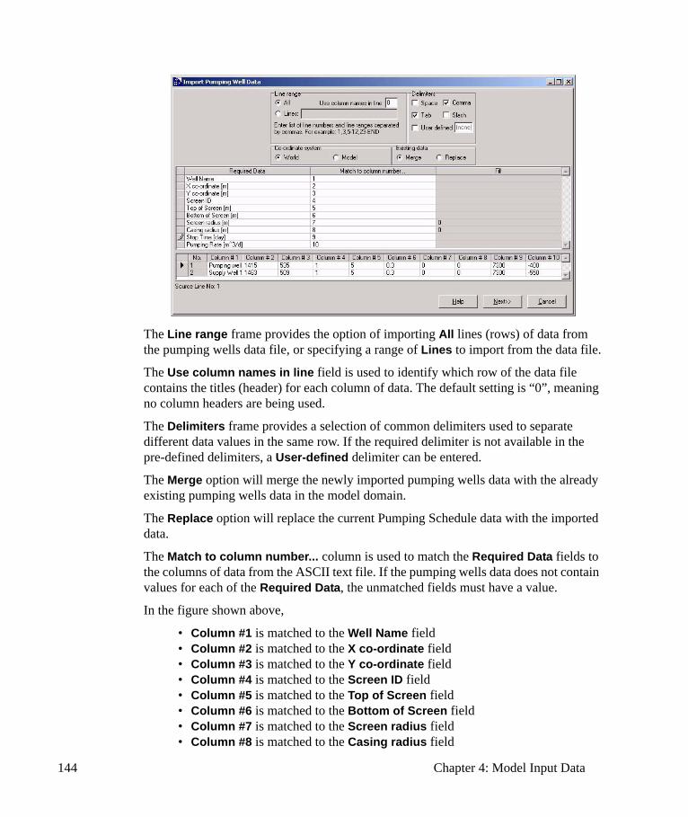
144 Chapter 4: Model Input Data
The Line range frame provides the option of importing All lines (rows) of data from the pumping wells data file, or specifying a range of Lines to import from the data file.
The Use column names in line field is used to identify which row of the data file contains the titles (header) for each column of data. The default setting is “0”, meaning no column headers are being used.
The Delimiters frame provides a selection of common delimiters used to separate different data values in the same row. If the required delimiter is not available in the pre-defined delimiters, a User-defined delimiter can be entered.
The Merge option will merge the newly imported pumping wells data with the already existing pumping wells data in the model domain.
The Replace option will replace the current Pumping Schedule data with the imported data.
The Match to column number... column is used to match the Required Data fields to the columns of data from the ASCII text file. If the pumping wells data does not contain values for each of the Required Data, the unmatched fields must have a value.
In the figure shown above,
• Column #1 is matched to the Well Name field • Column #2 is matched to the X co-ordinate field • Column #3 is matched to the Y co-ordinate field • Column #4 is matched to the Screen ID field • Column #5 is matched to the Top of Screen field • Column #6 is matched to the Bottom of Screen field • Column #7 is matched to the Screen radius field • Column #8 is matched to the Casing radius field
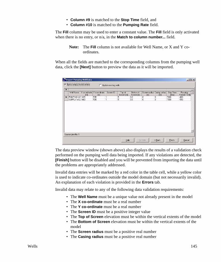
Wells 145
• Column #9 is matched to the Stop Time field, and • Column #10 is matched to the Pumping Rate field.
The Fill column may be used to enter a constant value. The Fill field is only activated when there is no entry, or n/a, in the Match to column number... field.
Note: The Fill column is not available for Well Name, or X and Y co-ordinates.
When all the fields are matched to the corresponding columns from the pumping well data, click the [Next] button to preview the data as it will be imported.
The data preview window (shown above) also displays the results of a validation check performed on the pumping well data being imported. If any violations are detected, the [Finish] button will be disabled and you will be prevented from importing the data until the problems are appropriately addressed.
Invalid data entries will be marked by a red color in the table cell, while a yellow color is used to indicate co-ordinates outside the model domain (but not necessarily invalid). An explanation of each violation is provided in the Errors tab.
Invalid data may relate to any of the following data validation requirements:
• The Well Name must be a unique value not already present in the model• The X co-ordinate must be a real number• The Y co-ordinate must be a real number• The Screen ID must be a positive integer value• The Top of Screen elevation must be within the vertical extents of the model• The Bottom of Screen elevation must be within the vertical extents of the
model• The Screen radius must be a positive real number• The Casing radius must be a positive real number
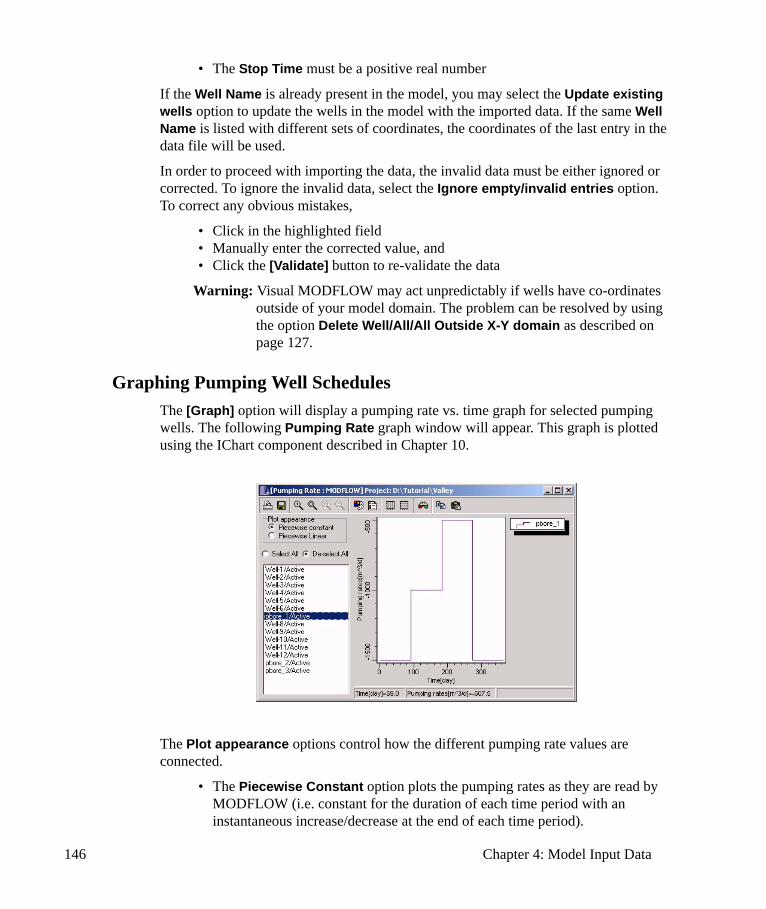
146 Chapter 4: Model Input Data
• The Stop Time must be a positive real number
If the Well Name is already present in the model, you may select the Update existing wells option to update the wells in the model with the imported data. If the same Well Name is listed with different sets of coordinates, the coordinates of the last entry in the data file will be used.
In order to proceed with importing the data, the invalid data must be either ignored or corrected. To ignore the invalid data, select the Ignore empty/invalid entries option. To correct any obvious mistakes,
• Click in the highlighted field • Manually enter the corrected value, and • Click the [Validate] button to re-validate the data
Warning: Visual MODFLOW may act unpredictably if wells have co-ordinates outside of your model domain. The problem can be resolved by using the option Delete Well/All/All Outside X-Y domain as described on page 127.
Graphing Pumping Well SchedulesThe [Graph] option will display a pumping rate vs. time graph for selected pumping wells. The following Pumping Rate graph window will appear. This graph is plotted using the IChart component described in Chapter 10.
The Plot appearance options control how the different pumping rate values are connected.
• The Piecewise Constant option plots the pumping rates as they are read by MODFLOW (i.e. constant for the duration of each time period with an instantaneous increase/decrease at the end of each time period).
Wells 147
• The Piecewise Linear option uses a single line to connect the pumping rates at the end of each time period.
Click the Select All option to view all of the pumping wells, click the De-select All option to remove all pumping wells from the graph.
Multi-Node Wells (MNW) Package Previous simulation capability of wells in Visual MODFLOW was limited to withdrawal at specified rates from individual cells. However, pumpage from aquifer systems commonly is complex. For example, heads in aquifers that surround a well are likely to vary along the length of a screen that pentetrates multiple aquifers or has a long horizontal extent. When pumping, recharge, or no user-specified inflow or outflow occurs in wells that are screened across multiple aquifers or in a single aquifer, there can be significant hydraulic effects on the ground-water flow system. The Multi-Node Well (MNW) package has been integrated in Visual MODFLOW to help simulate intraborehole flow occurring in wells with screens that span multiple layers.
Note: The MNW package cannot be used with MODFLOW SURFACT flow model.
Reference: User Guide For The Drawdown-Limited, Multi-Node Well (MNW) package for the U.S Geological Survey’s Modular Three-Dimensional Finite-Difference Ground-Water Flow Model, Versions MODFLOW-96 and MODFLOW-2000 by K.J Halford and R.T. Hanson.
The MNW options are accessible through the toolbar in the Visual MODFLOW New/Edit Well Window.
When the MNW button is selected from the toolbar, the MNW options will become available (shown in the image below):
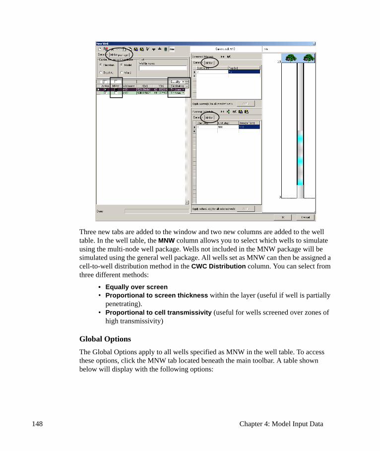
148 Chapter 4: Model Input Data
Three new tabs are added to the window and two new columns are added to the well table. In the well table, the MNW column allows you to select which wells to simulate using the multi-node well package. Wells not included in the MNW package will be simulated using the general well package. All wells set as MNW can then be assigned a cell-to-well distribution method in the CWC Distribution column. You can select from three different methods:
• Equally over screen• Proportional to screen thickness within the layer (useful if well is partially
penetrating). • Proportional to cell transmissivity (useful for wells screened over zones of
high transmissivity)
Global OptionsThe Global Options apply to all wells specified as MNW in the well table. To access these options, click the MNW tab located beneath the main toolbar. A table shown below will display with the following options:

Wells 149
Here you can define the well loss settings for all MNW wells.
Loss Type: If loss type is set to Skin, head loss is defined with skin. The model is linear and you must specify values for Tskin or Rskin.
If loss type is set to Linear, head loss is defined with coefficient B
If loss type is set to Nonlinear, head loss is defined with coefficients B and C.
Note: The Skin factor formula assumes full well penetration.
Reference SP: The set of water levels in the HNEW matrix at the beginning of the Reference SP (stress period) that will be used as default reference values for calculating drawdown. The default for this setting is 1.
P Loss: Power of the nonlinear discharge component of well loss that usually varies between 1.5 and 3.5 (Rorabaugh, 1953). By default this value is set to 1.
Screened Interval OptionsThe MNW screen options can be accessed by clicking the MNW tab in the Screen Interval frame (shown below).
In this table, specify R well (well radius) for the specified screen interval.
NOTE: Wells simulated using the MNW package can only have one screen interval.

150 Chapter 4: Model Input Data
Pumping Schedule OptionsThe MNW pumping schedule options can be accessed by clicking the MNW tab in the Pumping Schedule frame. Upon selecting, the following table is displayed:
The above table allows you to define well parameters, pumping/water level constraints and water quality options for each specified stress period. Please note that the required well parameters will change depending on the well loss type specified in the global MNW options. For example, if the well loss type is set to Skin, only Rskin and Tskin will be required (as shown in the image above). If the well loss type is set to Linear, only the B coefficient is required.
For each specified stress period, you can define the following settings:Rskin (Skin): Radius of the skin Tskin (Skin): Transmissivity of the skinB Coefficient (Linear/Nonlinear): B coefficient of the general well-loss equation as modified by Roabaugh (1953) (shown below) which defines the head loss from flow through formation damaged during well drilling, the gravel pack, and the well screen. (Earlougher, 1977; Cooley and Cunningham, 1979).
Where:hwell is the head in the well (L).hn is the head in the nth cell (L).Qn is the flow between the nth cell and the well (L3 / T)
hwell hn– AQn BQn CQnP+ +=
Wells 151
A is the linear aquifer-loss coefficient (T / L2)B is the linear well-loss coefficient (T / L2)C is nonlinear well-loss coefficient (Tp / L(3P-1)) and P is power of the nonlinear discharge component of well loss that usually
varies between 1.5 and 3.5 (Rorabaugh, 1953)C Coefficient (Nonlinear): C coefficient of well-loss equation (see above) as modified by Roabaugh which defines head loss from any turbulent flow near the well. (Rorabaugh, 1953).Water Limit Type: Set the limiting water-level to be expressed as either Drawdown or Water Level with respect to a specified reference elevation.Limiting Water Level: Specify the limiting water-level (or drawdown, depending on the Water Limit Type). Reference Elevation: Specify the reference elevation. If this value is greater than the maximum water level from the HNEW matrix at the beginning of the stress period (Reference SP), it is set to the simulated water level at the location of the drawdown-limited well.Pumping Limit Type: Express the pumping limits as the percentage of the specified pumping rate (Percent of Rate) or as a pumping rate (Rate) (L3 / T).Minimum Pumping: The minimum pumping rate that a well must exceed to remain active.Maximum Pumping: The minimum potential pumping rate that must be exceeded to reactivate an inactive well.Water Quality: The water-quality value that is to be flow-rate averaged amongst wells in the same Water Quality Group.Water Quality Group: Specify a water-quality group identifier value. Flow-rate averaged water-quality values are reported for each group of wells with the same identifier.Note: Water Quality output is not supported in this version of Visual MODFLOW. However, you can view the output results by opening the output MNW files (described below) in a text editor.
Applying Defined Parameters to Other Wells You can easily apply the defined pumping schedule parameters of one well to other MNW wells in the well table. To do so, simply highlight the wells in the well table (including the well containing the parameter data), and then click the [Apply] button in the pumping schedule frame.
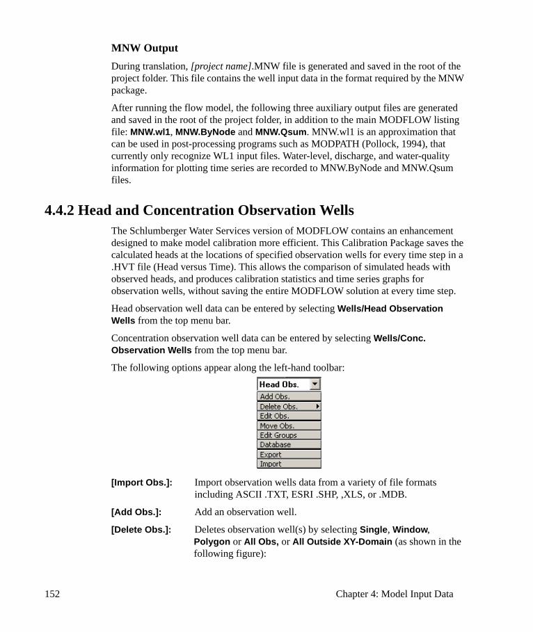
152 Chapter 4: Model Input Data
MNW OutputDuring translation, [project name].MNW file is generated and saved in the root of the project folder. This file contains the well input data in the format required by the MNW package.
After running the flow model, the following three auxiliary output files are generated and saved in the root of the project folder, in addition to the main MODFLOW listing file: MNW.wl1, MNW.ByNode and MNW.Qsum. MNW.wl1 is an approximation that can be used in post-processing programs such as MODPATH (Pollock, 1994), that currently only recognize WL1 input files. Water-level, discharge, and water-quality information for plotting time series are recorded to MNW.ByNode and MNW.Qsum files.
4.4.2 Head and Concentration Observation WellsThe Schlumberger Water Services version of MODFLOW contains an enhancement designed to make model calibration more efficient. This Calibration Package saves the calculated heads at the locations of specified observation wells for every time step in a .HVT file (Head versus Time). This allows the comparison of simulated heads with observed heads, and produces calibration statistics and time series graphs for observation wells, without saving the entire MODFLOW solution at every time step.
Head observation well data can be entered by selecting Wells/Head Observation Wells from the top menu bar.
Concentration observation well data can be entered by selecting Wells/Conc. Observation Wells from the top menu bar.
The following options appear along the left-hand toolbar:
[Import Obs.]: Import observation wells data from a variety of file formats including ASCII .TXT, ESRI .SHP, ,XLS, or .MDB.
[Add Obs.]: Add an observation well.
[Delete Obs.]: Deletes observation well(s) by selecting Single, Window, Polygon or All Obs, or All Outside XY-Domain (as shown in the following figure):

Wells 153
[Edit Obs.]: This feature allows you to edit the observation data associated with a selected observation well.
[Move Obs.]: This feature allows you to move the observation well to a new position in the domain, while maintaining the observation data.
[Edit Groups]: Create and edit groups of observation points to be used in the Run section and Output Module.
[Database]: Open the Edit Well window where you can view and edit observations, observation points and site coordinates for all wells in the current project.
[Export]: Export well information, e.g., well location, screen intervals, pumping schedules, to the .TXT file format.
In cross-section, observation wells are shown if they are located within the selected row or column. A red line on the well identifies the location of the observation point. The plan-view locations of observation wells are indicated with a green marker.
If the [Add Obs.] or the [Edit Obs.] options are used to assign an observation well, a New/Edit Well window will appear as shown in the following figure and described below.
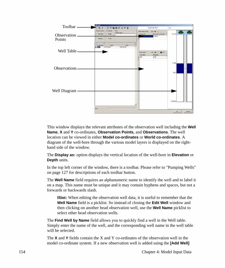
154 Chapter 4: Model Input Data
This window displays the relevant attributes of the observation well including the Well Name, X and Y co-ordinates, Observation Points, and Observations. The well location can be viewed in either Model co-ordinates or World co-ordinates. A diagram of the well-bore through the various model layers is displayed on the right-hand side of the window.
The Display as: option displays the vertical location of the well-bore in Elevation or Depth units.
In the top left corner of the window, there is a toolbar. Please refer to "Pumping Wells" on page 127 for descriptions of each toolbar button.
The Well Name field requires an alphanumeric name to identify the well and to label it on a map. This name must be unique and it may contain hyphens and spaces, but not a forwards or backwards slash.
Hint: When editing the observation well data, it is useful to remember that the Well Name field is a picklist. So instead of closing the Edit Well window and then clicking on another head observation well, use the Well Name picklist to select other head observation wells.
The Find Well by Name field allows you to quickly find a well in the Well table. Simply enter the name of the well, and the corresponding well name in the well table will be selected.
The X and Y fields contain the X and Y co-ordinates of the observation well in the model co-ordinate system. If a new observation well is added using the [Add Well]
Toolbar
Observation Points
Well Table
Observations
Well Diagram
Wells 155
option, the X and Y co-ordinates of the clicked location are automatically inserted in the X and Y fields. These values can be modified if data is available.
Visual MODFLOW maintains the X and Y co-ordinates independent of the model grid. Therefore, if the grid is modified, the original observation well location is not affected.
The Species Name field is present only for concentration observation wells. This field is a picklist used to select from the pre-defined list of dissolved species being simulated by the transport model.
Observation PointsThe Observation Points are the elevations at which the Observations were recorded. Each observation point requires a point ID and elevation. Although most monitoring or observation wells are installed with a well screen spanning a known interval of the aquifer, Visual MODFLOW requires a single observation point Elevation to be defined instead of a well screen interval. The reason for using Observation Points as opposed to a well screen interval is because a well screen may span several vertical grid cells (layers) of the model, and it would be impossible for Visual MODFLOW to “instinctively know” which grid cell to use for comparing observed values vs. calculated values. Therefore, a single observation point is used in order to eliminate any ambiguity regarding which model grid cell to use. Typically, the observation point elevation corresponds to the mid-point elevation of the well screen interval. However, for calibration purposes it is important to note that Visual MODFLOW simply compares the Observations for each observation point to the value calculated in the grid cell where the observation point is located. Visual MODFLOW does not make any special adjustments to account for Observation Points which do not exactly correspond to the center of the grid cell.
Visual MODFLOW supports Head and Concentration observation wells with multiple Observation Points throughout the length of the well-bore. For multi-level observation wells, the individual observation points from the same well may be turned on or off.
Adding Observation PointsAn observation point can be added graphically by Right-Clicking on the well-bore diagram and selecting the Add Observation Point option. A horizontal red line will appear in the well-bore diagram indicating the location of the observation point. Drag the observation point to the desired location within the well-bore.
The elevation of each observation point is shown in the Observation Points table. These values may be manually modified if required.
Observation point data can also directly entered by clicking the [Add Observation Point] icon above the Observation Points table, and entering the Screen Elevation value.
156 Chapter 4: Model Input Data
Each observation point requires data for the Screen Elevation. If an additional observation point was accidentally added and does not contain any data for the Screen Elevation, this observation point entry must be deleted from the table before closing the Edit Well window.
Deleting Observation PointsObservation Points can be deleted by either:
• Right-Clicking on an observation point in the well-bore diagram and choosing the Delete Observation Point option,
• Selecting the observation point in the Observation Points table and clicking the [Delete Observation Point] icon above the table.
ObservationsThe Observations table is used to enter the observed values at specified times.
Adding ObservationsTo add an item to the Observations table:
• Click the [Add Observation Values] icon above the table, or simply click in the first row of table
• Enter an Time value and press the <Tab> key to advance to the Head/Conc. field
• Enter an observation value• Press the <Tab> key again to create a new schedule item, or click the [OK]
button to accept the Observations data and close the Edit Well window
Each Observations table entry must be completed with a valid Time and observation value. If an Observations item has been accidentally added without any data, it must be deleted before the Edit Well window can be closed.
Deleting ObservationsTo delete an item from the Observations table:
• Click on the item to delete in the Observations table• Click on the [Delete Observation Value] icon above the table
Importing ObservationsIn situations where observations have been recorded/collected at regular intervals over a long period of time, the process of manually entering each observation item can be tedious and time-consuming. In these situations Visual MODFLOW can import the observation data from an ASCII text file, or from the Windows clipboard.
In either case, the data must be organized in the following format (see example below):
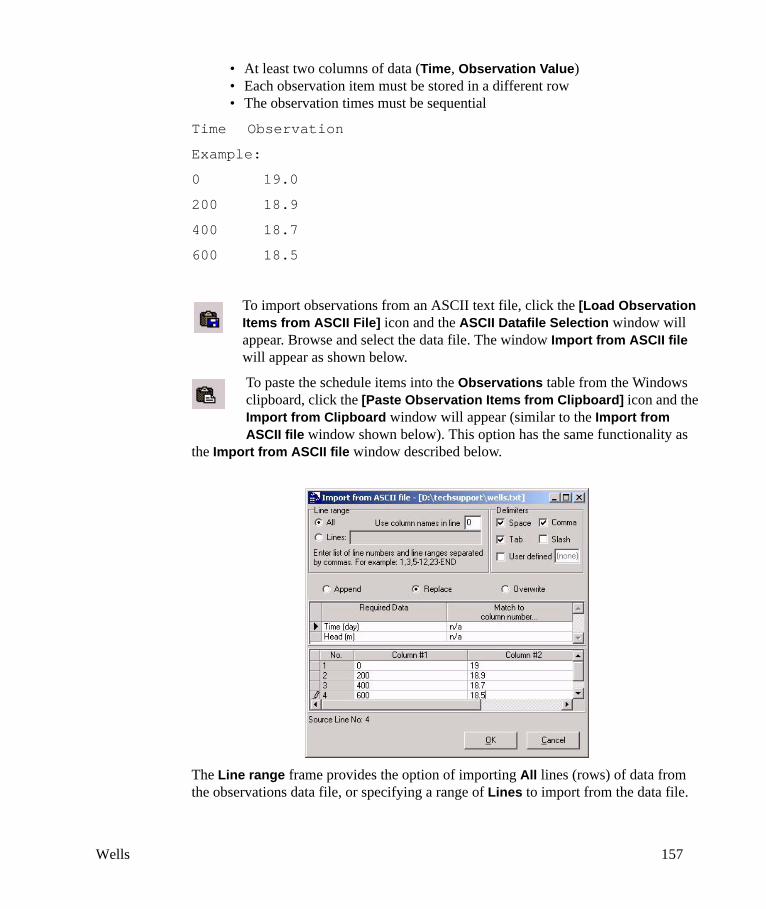
Wells 157
• At least two columns of data (Time, Observation Value)• Each observation item must be stored in a different row• The observation times must be sequential
Time Observation
Example:
0 19.0
200 18.9
400 18.7
600 18.5
To import observations from an ASCII text file, click the [Load Observation Items from ASCII File] icon and the ASCII Datafile Selection window will appear. Browse and select the data file. The window Import from ASCII file will appear as shown below.
To paste the schedule items into the Observations table from the Windows clipboard, click the [Paste Observation Items from Clipboard] icon and the Import from Clipboard window will appear (similar to the Import from ASCII file window shown below). This option has the same functionality as
the Import from ASCII file window described below.
The Line range frame provides the option of importing All lines (rows) of data from the observations data file, or specifying a range of Lines to import from the data file.
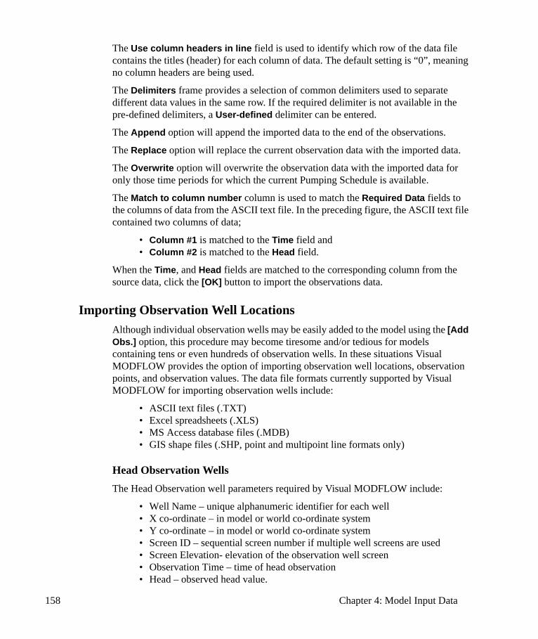
158 Chapter 4: Model Input Data
The Use column headers in line field is used to identify which row of the data file contains the titles (header) for each column of data. The default setting is “0”, meaning no column headers are being used.
The Delimiters frame provides a selection of common delimiters used to separate different data values in the same row. If the required delimiter is not available in the pre-defined delimiters, a User-defined delimiter can be entered.
The Append option will append the imported data to the end of the observations.
The Replace option will replace the current observation data with the imported data.
The Overwrite option will overwrite the observation data with the imported data for only those time periods for which the current Pumping Schedule is available.
The Match to column number column is used to match the Required Data fields to the columns of data from the ASCII text file. In the preceding figure, the ASCII text file contained two columns of data;
• Column #1 is matched to the Time field and • Column #2 is matched to the Head field.
When the Time, and Head fields are matched to the corresponding column from the source data, click the [OK] button to import the observations data.
Importing Observation Well LocationsAlthough individual observation wells may be easily added to the model using the [Add Obs.] option, this procedure may become tiresome and/or tedious for models containing tens or even hundreds of observation wells. In these situations Visual MODFLOW provides the option of importing observation well locations, observation points, and observation values. The data file formats currently supported by Visual MODFLOW for importing observation wells include:
• ASCII text files (.TXT)• Excel spreadsheets (.XLS)• MS Access database files (.MDB)• GIS shape files (.SHP, point and multipoint line formats only)
Head Observation WellsThe Head Observation well parameters required by Visual MODFLOW include:
• Well Name – unique alphanumeric identifier for each well• X co-ordinate – in model or world co-ordinate system• Y co-ordinate – in model or world co-ordinate system• Screen ID – sequential screen number if multiple well screens are used• Screen Elevation- elevation of the observation well screen• Observation Time – time of head observation• Head – observed head value.
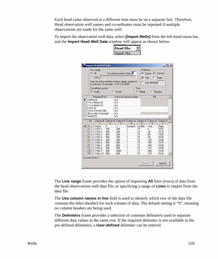
Wells 159
Each head value observed at a different time must be on a separate line. Therefore, Head observation well names and co-ordinates must be repeated if multiple observations are made for the same well.
To import the observation well data, select [Import Wells] from the left-hand menu bar, and the Import Head Well Data window will appear as shown below.
The Line range frame provides the option of importing All lines (rows) of data from the head observations well data file, or specifying a range of Lines to import from the data file.
The Use column names in line field is used to identify which row of the data file contains the titles (header) for each column of data. The default setting is “0”, meaning no column headers are being used.
The Delimiters frame provides a selection of common delimiters used to separate different data values in the same row. If the required delimiter is not available in the pre-defined delimiters, a User-defined delimiter can be entered.
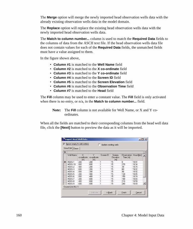
160 Chapter 4: Model Input Data
The Merge option will merge the newly imported head observation wells data with the already existing observation wells data in the model domain.
The Replace option will replace the existing head observation wells data with the newly imported head observation wells data.
The Match to column number... column is used to match the Required Data fields to the columns of data from the ASCII text file. If the head observation wells data file does not contain values for each of the Required Data fields, the unmatched fields must have a value assigned to them.
In the figure shown above,
• Column #1 is matched to the Well Name field • Column #2 is matched to the X co-ordinate field • Column #3 is matched to the Y co-ordinate field • Column #4 is matched to the Screen ID field • Column #5 is matched to the Screen Elevation field • Column #6 is matched to the Observation Time field • Column #7 is matched to the Head field
The Fill column may be used to enter a constant value. The Fill field is only activated when there is no entry, or n/a, in the Match to column number... field.
Note: The Fill column is not available for Well Name, or X and Y co-ordinates.
When all the fields are matched to their corresponding columns from the head well data file, click the [Next] button to preview the data as it will be imported.
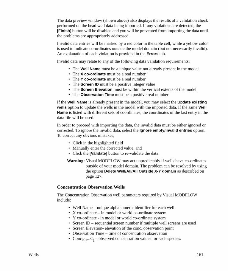
Wells 161
The data preview window (shown above) also displays the results of a validation check performed on the head well data being imported. If any violations are detected, the [Finish] button will be disabled and you will be prevented from importing the data until the problems are appropriately addressed.
Invalid data entries will be marked by a red color in the table cell, while a yellow color is used to indicate co-ordinates outside the model domain (but not necessarily invalid). An explanation of each violation is provided in the Errors tab.
Invalid data may relate to any of the following data validation requirements:
• The Well Name must be a unique value not already present in the model• The X co-ordinate must be a real number• The Y co-ordinate must be a real number• The Screen ID must be a positive integer value• The Screen Elevation must be within the vertical extents of the model• The Observation Time must be a positive real number
If the Well Name is already present in the model, you may select the Update existing wells option to update the wells in the model with the imported data. If the same Well Name is listed with different sets of coordinates, the coordinates of the last entry in the data file will be used.
In order to proceed with importing the data, the invalid data must be either ignored or corrected. To ignore the invalid data, select the Ignore empty/invalid entries option. To correct any obvious mistakes,
• Click in the highlighted field • Manually enter the corrected value, and • Click the [Validate] button to re-validate the data
Warning: Visual MODFLOW may act unpredictably if wells have co-ordinates outside of your model domain. The problem can be resolved by using the option Delete Well/All/All Outside X-Y domain as described on page 127.
Concentration Observation WellsThe Concentration Observation well parameters required by Visual MODFLOW include:
• Well Name – unique alphanumeric identifier for each well• X co-ordinate – in model or world co-ordinate system• Y co-ordinate - in model or world co-ordinate system• Screen ID – sequential screen number if multiple well screens are used• Screen Elevation- elevation of the conc. observation point • Observation Time – time of concentration observation• Conc001...Cj – observed concentration values for each species.
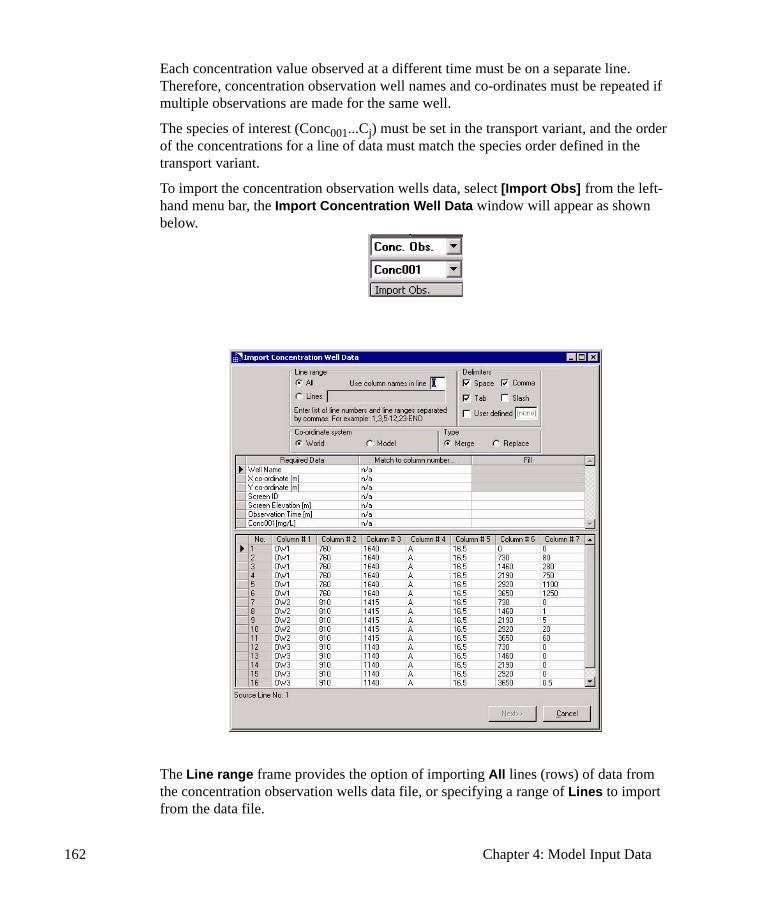
162 Chapter 4: Model Input Data
Each concentration value observed at a different time must be on a separate line. Therefore, concentration observation well names and co-ordinates must be repeated if multiple observations are made for the same well.
The species of interest (Conc001...Cj) must be set in the transport variant, and the order of the concentrations for a line of data must match the species order defined in the transport variant.
To import the concentration observation wells data, select [Import Obs] from the left-hand menu bar, the Import Concentration Well Data window will appear as shown below.
The Line range frame provides the option of importing All lines (rows) of data from the concentration observation wells data file, or specifying a range of Lines to import from the data file.

Wells 163
The Use column names in line field is used to identify which row of the data file contains the titles (header) for each column of data. The default setting is “0”, meaning no column headers are being used.
The Delimiters frame provides a selection of common delimiters used to separate different data values in the same row. If the required delimiter is not available in the pre-defined delimiters, a User-defined delimiter can be entered.
The Merge option will merge the newly imported concentration observation well data with the already existing observation well data in the model domain.
The Replace option will replace the existing concentration observation well data with the newly imported observation wells data.
The Match to column number... column is used to match the Required Data fields to the columns of data from the ASCII text file. If the concentration observation well data does not contain values for each of the Required Data, the unmatched fields must be assigned a value.
In the preceding figure,
• Column #1 is matched to the Well Name field• Column #2 is matched to the X co-ordinate field• Column #3 is matched to the Y co-ordinate field• Column #4 is matched to the Screen ID field • Column #5 is matched to the Screen Elevation field • Column #6 is matched to the Observation Time field, and • Column #7 is matched to the Conc. field.
The Fill column may be used to enter a constant value. The Fill field is only activated when there is no entry, or n/a, in the Match to column number... field.
Note: The Fill column is not available for Well Name, or X and Y co-ordinates.
When all the fields are matched to the corresponding columns from the concentration observation well data, click the [Next] button to preview the data as it will be imported.
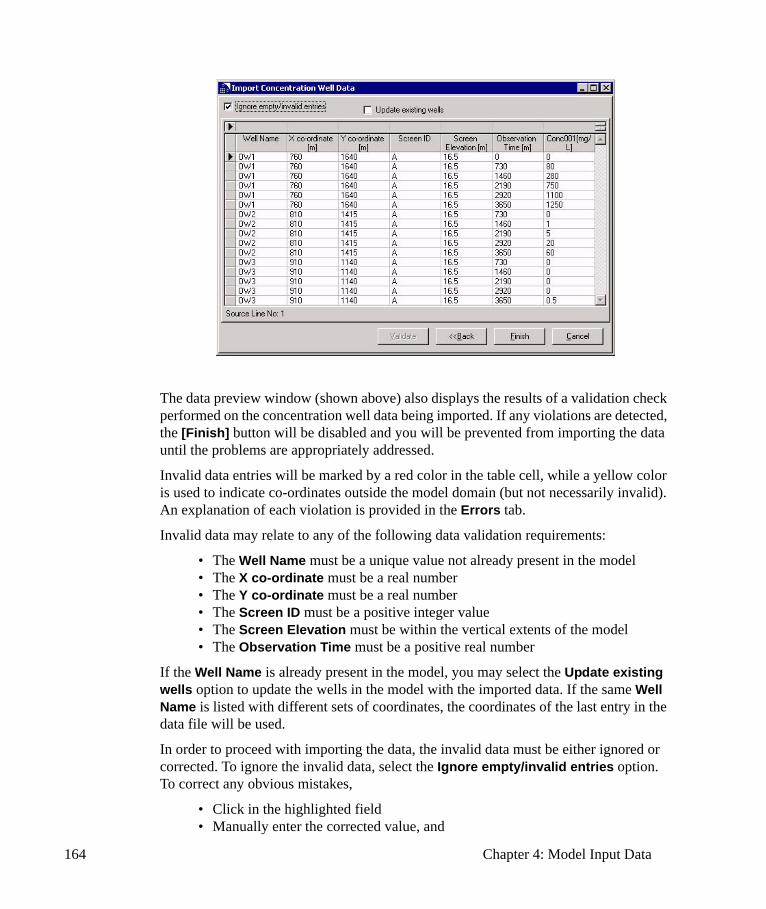
164 Chapter 4: Model Input Data
The data preview window (shown above) also displays the results of a validation check performed on the concentration well data being imported. If any violations are detected, the [Finish] button will be disabled and you will be prevented from importing the data until the problems are appropriately addressed.
Invalid data entries will be marked by a red color in the table cell, while a yellow color is used to indicate co-ordinates outside the model domain (but not necessarily invalid). An explanation of each violation is provided in the Errors tab.
Invalid data may relate to any of the following data validation requirements:
• The Well Name must be a unique value not already present in the model• The X co-ordinate must be a real number• The Y co-ordinate must be a real number• The Screen ID must be a positive integer value• The Screen Elevation must be within the vertical extents of the model• The Observation Time must be a positive real number
If the Well Name is already present in the model, you may select the Update existing wells option to update the wells in the model with the imported data. If the same Well Name is listed with different sets of coordinates, the coordinates of the last entry in the data file will be used.
In order to proceed with importing the data, the invalid data must be either ignored or corrected. To ignore the invalid data, select the Ignore empty/invalid entries option. To correct any obvious mistakes,
• Click in the highlighted field • Manually enter the corrected value, and
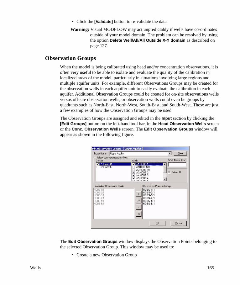
Wells 165
• Click the [Validate] button to re-validate the data
Warning: Visual MODFLOW may act unpredictably if wells have co-ordinates outside of your model domain. The problem can be resolved by using the option Delete Well/All/All Outside X-Y domain as described on page 127.
Observation GroupsWhen the model is being calibrated using head and/or concentration observations, it is often very useful to be able to isolate and evaluate the quality of the calibration in localized areas of the model, particularly in situations involving large regions and multiple aquifer units. For example, different Observations Groups may be created for the observation wells in each aquifer unit to easily evaluate the calibration in each aquifer. Additional Observation Groups could be created for on-site observations wells versus off-site observation wells, or observation wells could even be groups by quadrants such as North-East, North-West, South-East, and South-West. These are just a few examples of how the Observation Groups may be used.
The Observation Groups are assigned and edited in the Input section by clicking the [Edit Groups] button on the left-hand tool bar, in the Head Observation Wells screen or the Conc. Observation Wells screen. The Edit Observation Groups window will appear as shown in the following figure.
The Edit Observation Groups window displays the Observation Points belonging to the selected Observation Group. This window may be used to:
• Create a new Observation Group

166 Chapter 4: Model Input Data
• Add Observation Points to the selected Observation Group• Remove Observation Points from the selected Observation Group
The Group Name field displays the name of the current Observation Group, and contains a list of all available Observation Groups. A new Observation Group may be created by pressing the [New] button and entering a description in the Group Name field.
The Groups field contains a list of each layer in the model containing Observation Points. Selecting one or more of these Layer Groups will add the associated Observation Points to the Available Observation Points list.
The Wells list contains a list of all Observation Wells in the model. When a well in this list is selected, the Observation Points associated with the selected well are added to the Available Observation Points list.
Once all of the desired Observation Points are included in the list of Available Observation Points, use the arrow buttons to add/remove individual Observation Points to/from the list of Observation Points in Group.
Properties 167
4.5 PropertiesA groundwater flow and contaminant transport model requires many different types of data to simulate the hydrogeological and hydrogeochemical processes influencing the flow of groundwater and migration of dissolved contaminants. In Visual MODFLOW, the hydrogeological and hydrogeochemical characteristics of the model are classified into the following input properties:
Flow Properties• Conductivity (Kx, Ky, Kz)• Storage (Ss, Sy, Peff, Ptot)• Initial Heads• Vadose Zone
Note: The Vadose Zone menu item will be available only if MODFLOW-SURFACT is the selected flow engine.
Transport Properties • Bulk Density• Species Parameters (Spatially Variable)• Edit Constant Parameters• Initial Concentration• Dispersion (Dl, Dt, Dv, Diffusion)
Note: If no transport variant has been selected, the Transport Properties options will be disabled.
As noted in the list above, some of these model properties require data for several different parameters (e.g. Conductivity requires values for Kx, Ky, and Kz). These model properties, and their associated sets of parameters, are assigned using different input screens for each property. The active Properties screen will always be displayed in the Current Overlay field on the side menu bar.
A flow model requires Conductivity, Storage, and Initial Heads property values for each active grid cell in order to run a flow simulation. Similarly, a transport model requires transport parameter values for each active grid cell in order to run a transport simulation. Upon creating a Visual MODFLOW project, the default flow and transport parameter values are assigned to every grid cell in the model domain. This will ensure the model has the minimum data required to run a simulation. However, in most situations, the flow and transport properties will not be uniform throughout the entire model domain, and it will be necessary to assign different property values to different areas of the model.
168 Chapter 4: Model Input Data
Heterogeneous model property values are supported by Visual MODFLOW using either Constant Value Property Zones, or Distributed Value Property Zones. These two different approaches are described below.
Constant Value Property ZonesThe Constant Value Property Zones approach is the most simple and straight forward, and can be used for all model properties supported by Visual MODFLOW. Different model properties are accommodated by grouping grid cells sharing the same property values into “property zones”. Each property zone will (normally) contain a unique set of property values, and is represented by a different grid cell color.
The Constant Value Property Zones approach requires the development of a conceptual model, whereby each hydrostratigraphic unit of the model is assigned a uniform set of property values. For example, consider an aquifer where there is pumping test data and slug test data indicating a range of horizontal conductivity values from 1x10⁻⁴ cm/s to 5x10⁻⁴ cm/s at different locations within the aquifer. The conceptual approach would assign a uniform Kx and Ky value of 2.5x10⁻⁴ cm/s to the entire aquifer. This value would be adjusted up or down for calibration purposes within the range of values reported. If a reasonable calibration cannot be achieved using this conceptual model, it may be necessary to sub-divide this region into several zones to accommodate local irregularities in the flow pattern. However, almost all modeling textbooks strongly recommend to start out simple first and get as close a solution as possible, and then make the model more complex if necessary.
Distributed Value Property ZonesThe Distributed Value Property Zones approach is currently only available for Conductivity, Storage, Initial Heads, Initial Concentrations, and Dispersivity properties. This approach is a little more complicated because it involves linking a property zone to one or more parameter distribution arrays containing data interpolated from scattered observation points. When a property zone is linked to distribution array, the property values assigned to each grid cell within that zone are calculated by multiplying the zone parameter value with the corresponding value from the parameter distribution array. If the grid spacing from the model does not match the grid spacing from the distribution array, a bivariate interpolation scheme is used to calculate the appropriate parameter value at the center of the model grid cell using the four nearest data nodes in the parameter distribution array.
For example, consider a model with 5 rows, 5 columns, 1 layer and 3 different Conductivity zones. The attributes of each conductivity zone are described in the following table:

Properties 169
The arrangement of Conductivity property zones on the model grid is described in Table 3.2a, the Kx Distribution Array is described in Table 3.2b, and the resultant Kx values are shown in Table 3.2c.
Table 3.1Zone Parameter Va lues Linked to
Zone # Kx (cm/s) Ky (cm/s) Kz (cm/s) Distribution Array1 0.001 0.001 0.0001 No2 0.005 0.005 0.005 No3 1 1 1 Yes
Table 3.2a: Conductivity Zones On The Model Grid
Columns1 2 3 4 5
1 1 1 1 2 32 1 1 2 3 3
Rows 3 1 2 2 3 34 2 2 3 3 35 2 2 3 3 3
Table 3.2b: Interpolated Kx Values from a 5x5 Distribution Array
Columns1 2 3 4 5
1 0.0011 0.0012 0.0014 0.0016 0.00192 0.0013 0.0014 0.0016 0.0017 0.0021
Rows 3 0.0015 0.0016 0.0018 0.0018 0.00224 0.0012 0.0013 0.0019 0.0021 0.00255 0.0011 0.0011 0.0015 0.0019 0.0021
Table 3.2c: Model Kx Values
Columns1 2 3 4 5
1 0.001 0.001 0.001 0.005 0.00192 0.001 0.001 0.005 0.0017 0.0021
Rows 3 0.001 0.005 0.005 0.0018 0.00224 0.005 0.005 0.0019 0.0021 0.00255 0.005 0.005 0.0015 0.0019 0.0021

170 Chapter 4: Model Input Data
In Table 3.1, only Property Zone #3 is linked to a distribution array. Therefore, only the model grid cells assigned to Property Zone #3 are calculated using the Kx distribution array. The grid cells containing Property Zone #1 and #2 retain the Kx values specified for each zone.
As shown in the above example, both Constant Property Value Zones and Distributed Property Value Zones can co-exist in the same model, and in the same layer, such that some zones contain constant values and other zones contain distributed values interpolated from external data points.
When the Distributed Property Value Zones are initially imported into Visual MODFLOW, they are each assigned zone parameter values of 1.0. This zone parameter value is used as a multiplier for modifying the distributed property values within this zone during the model calibration process.
4.5.1 Tools for Assigning and Editing PropertiesThe different property zones are assigned and modified in Visual MODFLOW using an assortment of graphical tools appearing on the side menu bar of each Properties screen.
[Import]: Import and interpolate property data from discrete data points (currently only available for Conductivities, Storage, Initial Heads, Initial Concentrations, Dispersion, Recharge, and Evapotranspiration).
[Assign]: Assign a selected property zone to a Single grid cell, a Polygon of grid cells, or a rectangular Window of grid cells (see description on page 187).
[Copy]: Copy a single property zone from a selected grid cell to other grid cells, or copy all property zones from the current Layer/Column/Row to one or more model layers/columns/rows (see description on page 188).
[Database]: View and edit the property zone values.
[Contouring]: View contour maps and/or color maps of the property value distributions and modify the contour map and color appearance Options.
Each of these tools are described in the following sections.

Properties 171
Importing Distributed Property DataVisual MODFLOW has a built-in Property Data Import Wizard to import and interpolate model property values (Conductivities, Storage, Initial Heads, Initial Concentrations, and Dispersion) from discrete data points using a selection of three popular data interpolation schemes:
• Inverse Distance• Kriging• Natural Neighbors
The data file formats currently supported by Visual MODFLOW for importing and interpolating model property data include:
• ASCII text files (.TXT)• Excel spreadsheets (.XLS)• Surfer grid files (.GRD)• MS Access database files (.MDB)• ESRI Shapefiles (.SHP, point and line formats )• ESRI Polygon Shapefiles, see page 185.
The Property Data Import Wizard generates a distribution of model property values for either an entire layer(s) of the model, or within a specified region of the model defined by an existing model property zone(s).
When a data file is interpolated using the Property Data Import Wizard, Visual MODFLOW creates a distribution array for each of the required property parameters (e.g. Conductivity requires separate distribution arrays for Kx, Ky and Kz). Each distribution array consists of a two-dimensional grid of data with uniform spacing in the X and Y directions. These distribution arrays are “linked” to selected property zones within the model. If a property zone is linked to a distribution array, the parameter value for each grid cell in this zone is calculated by multiplying the parameter value for this zone by the corresponding interpolated value from the distribution array. When the model grid spacing does not correspond to the grid dimension of the distribution array, a bivariate interpolation scheme is used to calculate the property value for each model grid cell.
The Data Import Wizard involves the following five steps:
• Step 1: File Selection (see description below) • Step 2: Matching Fields (see description on page 173)• Step 3: Data Validation (see description on page 175)• Step 4: Interpolation Options (see description on page 176)• Step 5: Create/Select Property Zones (see description on page 182/184)
To import and interpolate a set of data for a model property, click the [Import] button on the left-hand menu bar of the property module screen to start the five step Property Data Import Wizard. Each of the five steps is described below, using an example of importing data for Conductivity. Please note that the various options available in each

172 Chapter 4: Model Input Data
frame of each window may vary slightly, depending on the Property being imported. Steps specific to .SHP file importing are noted separately on page 185.
Step 1: File SelectionThe first step of the Property Data Import Wizard is selecting the source data file. As mentioned above, Property Data Import Wizard supports three different data formats including ASCII text files, Excel spreadsheets, and GIS shape files (points and lines). If the source data is stored in a different format, but is in a tabular format, it can be copied-and-pasted from the Windows clipboard.
The following figure is a screen capture of the first screen of the Property Data Import Wizard, followed by descriptions of the fields and functionality of this screen.
Importing data for: indicates the model property data type. This field is determined by the active Properties screen in Visual MODFLOW and cannot be modified.
Source origin: indicates whether the data is being read from a data file, or from the Windows Clipboard. The default setting is to read the data from a file.
Source file: indicates the name of the source data file being imported. Use the [Browse] button to select the file type (.TXT, .XLS, or .SHP) and navigate to the location of the source data file. If the data is being copied from the Windows clipboard, the Source file: field is disabled and the [Browse] button becomes a [Load] button to load the data from the Windows clipboard.
The X-Y co-ordinate system indicates the co-ordinate system of the data points being imported. World co-ordinates are typically referenced to a standard national or regional co-ordinate system such as UTM, while Model co-ordinates are referenced to
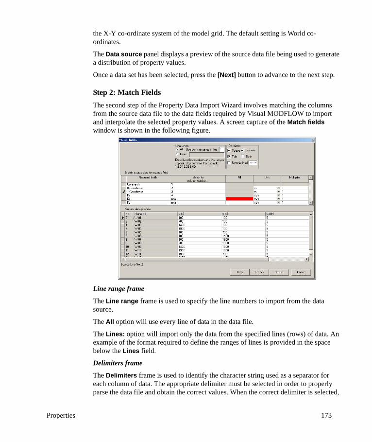
Properties 173
the X-Y co-ordinate system of the model grid. The default setting is World co-ordinates.
The Data source panel displays a preview of the source data file being used to generate a distribution of property values.
Once a data set has been selected, press the [Next] button to advance to the next step.
Step 2: Match FieldsThe second step of the Property Data Import Wizard involves matching the columns from the source data file to the data fields required by Visual MODFLOW to import and interpolate the selected property values. A screen capture of the Match fields window is shown in the following figure.
Line range frame
The Line range frame is used to specify the line numbers to import from the data source.
The All option will use every line of data in the data file.
The Lines: option will import only the data from the specified lines (rows) of data. An example of the format required to define the ranges of lines is provided in the space below the Lines field.
Delimiters frame
The Delimiters frame is used to identify the character string used as a separator for each column of data. The appropriate delimiter must be selected in order to properly parse the data file and obtain the correct values. When the correct delimiter is selected,
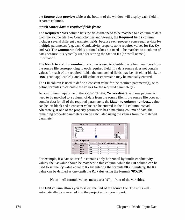
174 Chapter 4: Model Input Data
the Source data preview table at the bottom of the window will display each field in separate columns.
Match source data to required fields frame
The Required fields column lists the fields that need to be matched to a column of data from the source file. For Conductivities and Storage, the Required fields column includes several different parameter fields, because each property zone requires data for multiple parameters (e.g. each Conductivity property zone requires values for Kx, Ky, and Kz). The Comments field is optional (does not need to be matched to a column of data) because it is typically used for storing the Station ID (or “well name”) information.
The Match to column number… column is used to identify the column numbers from the source file corresponding to each required field. If a data source does not contain values for each of the required fields, the unmatched fields may be left either blank, or “n/a” (“not applicable”), and a fill value or expression may be manually entered.
The Fill column is used to define a constant value for the required parameter(s), or to define formulas to calculate the values for the required parameter(s).
As a minimum requirement, the X-co-ordinate, Y-co-ordinate, and one parameter need to be matched to a column of data from the source file. If the source file does not contain data for all of the required parameters, the Match to column number... value can be left blank and a constant value can be entered in the Fill column instead. Alternately, if one of the property parameters has a matching column of data, the remaining property parameters can be calculated using the values from the matched parameter.
For example, if a data source file contains only horizontal hydraulic conductivity values, the Kx value should be matched to this column, while the Fill column can be used to set the Ky value equal to Kx by entering the formula $KX. Similarly, the Kz value can be defined as one-tenth the Kx value using the formula $KX/10.
Note: All formula values must use a “$” in front of the variables.
The Unit column allows you to select the unit of the source file. The units will automatically be converted into the project units upon import.
Properties 175
The Multiplier column allows you to select a multiplier for the coordinate system (associated with the Region ID row when importing Recharge/Evapotranspiration), and enter a custom conversion value if the Custom Unit type is selected.
Source data preview frame
The Source data preview table shows a preview of the data points which will be interpolated to create the distributed value property zone(s). Each column header is labelled as Column #n, where “n” is the column number in order from left to right. If the Use column names in line option is used, the default column header will be replaced with the text from the specified line (row) number, but the column number remains.
Once all of the required fields have been matched, press the [Next] button to advance to the next step.
Step 3: Data ValidationThe third step of the Property Data Import Wizard involves validation of the data being imported. This step will ensure that the data set contains valid data for each of the parameters, and it will ensure the data points are within the model domain. The data validation rules for each model parameter are as follows:
Conductivity
• X-co-ordinate [Real Number] • Y-co-ordinate [Real Number] • Kx [Positive Real Number]• Kx/Ky [Positive Real Number]• Kx/Kz [Positive Real Number]
Storage
• X-co-ordinate [Real Number] • Y-co-ordinate [Real Number] • Ss [Positive Real Number]• Sy [Positive Real Number, less than TotPor]• EffPor [Positive Real Number, less than TotPor]• TotPor [Positive Real Number, less than one]
A screen capture of the Data Validation window is shown in the following figure, and the functionality and options for this step are described below.
The Preview tab provides a listing of the data points and parameter values which will be interpolated to create the distributed value property zone(s). Invalid data or empty data values will be highlighted in red, while data points located outside the model domain will be highlighted in yellow.

176 Chapter 4: Model Input Data
If empty or invalid entries are detected in any of the data points, the offending cells will be highlighted in red and the [Next] button will be disabled. The [Next] button can be enabled by selecting the Ignore empty/invalid entries option.
Data points outside the model domain can be either included in the interpolation, or they can be ignored. To include these data points, select the Include points outside of model domain option.
The Errors tab provides a description of the errors and warnings for each data point.
Once the data has been validated, press the [Next] button to advance to the next step.
Step 4: Interpolation OptionsThe Interpolation Options step involves:
• choosing the destination of the interpolated property data within the model domain
• selecting the interpolation method and settings• interpolating the data and creating a distribution array for each parameter
A screen capture of the Interpolation Options screen is shown in the following figure, and a description of the features and functionality is provided below.
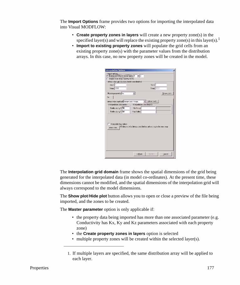
Properties 177
The Import Options frame provides two options for importing the interpolated data into Visual MODFLOW:
• Create property zones in layers will create a new property zone(s) in the specified layer(s) and will replace the existing property zone(s) in this layer(s).1
• Import to existing property zones will populate the grid cells from an existing property zone(s) with the parameter values from the distribution arrays. In this case, no new property zones will be created in the model.
The Interpolation grid domain frame shows the spatial dimensions of the grid being generated for the interpolated data (in model co-ordinates). At the present time, these dimensions cannot be modified, and the spatial dimensions of the interpolation grid will always correspond to the model dimensions.
The Show plot/Hide plot button allows you to open or close a preview of the file being imported, and the zones to be created.
The Master parameter option is only applicable if:
• the property data being imported has more than one associated parameter (e.g. Conductivity has Kx, Ky and Kz parameters associated with each property zone)
• the Create property zones in layers option is selected• multiple property zones will be created within the selected layer(s).
1. If multiple layers are specified, the same distribution array will be applied to each layer.
178 Chapter 4: Model Input Data
For presentation purposes, each model property zone is represented by a different color. This makes it easier to identify different soil types within the model domain. However, some of the model property zones require data for multiple parameters (e.g. a Conductivity zone requires values for Kx, Ky and Kz). As a result, when data is being imported for a model property containing more than one parameter, it is necessary to select the Master parameter used for defining the range of values associated with each property zone created for the different distribution arrays.
For example, if Conductivity data is imported using separate data points for both Kx and Kz, the distribution of Kx values in the Kx distribution array will be different than the distribution of Kz values in the Kz distribution array. However, both parameters belong to the same set of property zones. The Master parameter defines which distribution array will be used to define the range of values assigned to each property zones. If only one property zone is created for the entire distribution array, then the Master parameter is not relevant.
This concept will become more clear in the next step of the Interpolation Wizard.
Interpolation OptionsA distribution array must be created for each parameter described by the model property by interpolating the parameter data from the source data file. A separate interpolation options tab is created for each parameter being imported because separate distribution arrays are generated for each parameter.
Note: If a Fill value is used to define a parameter, no interpolation is required for this parameter because the distribution array consists of a constant value or a formula applied to a related distribution array.
The Interpolation Method field provides a selection of three popular methods of interpolating the data:
• Inverse Distance• Kriging• Natural Neighbors
The default setting is Natural Neighbors because this is a very robust and versatile interpolation method. However, Kriging is also a very popular interpolation method for geoscience applications.
The [Advanced] button opens the Interpolator Options window with access to more advanced settings for the selected interpolation method. A general description of each method and a detailed description of the advanced settings for each of these methods is provided in Appendix B.
Interpolation data nodesThe Interpolation data nodes frame describes the number of nodes in the X and Y direction for the interpolation grid used to create the distribution array. It is important to note that the interpolation grid density is NOT dependent on the model grid spacing,
Properties 179
but rather on the density of the data points. If the data points are very closely spaced in a particular region of the model, the grid spacing should be small, and the number of grid nodes should be large. However, if the data points are well distributed and relatively well-spaced, then the grid spacing can be large, and the number of grid nodes should be small.
Obviously, large interpolation grids create large data files, and take longer to process. Therefore, the number of interpolation data nodes should be as low as possible.
Interpolation data boundsThe Interpolation data bounds frame describes the minimum and maximum values for the interpolated data, and allows for user-defined minimum and maximum values. The reason these fields are required is to avoid importing invalid data that can be created when interpolating field data points. For example, a data set for hydraulic conductivities may contain all positive values, but a spatially decreasing trend may cause the interpolation scheme to “predict” negative conductivity values in a certain region of the model domain. The Minimum value and Maximum value fields allow the user to control the lower and upper bounds of the data values used by the interpolation scheme. If a value is predicted below the Minimum value, it is assigned equal to the Minimum value.
The Interpolate log values option will interpolate the log values of the data points and then invert the log value distribution. This option is commonly used for interpolating data with a high degree of variance such as hydraulic conductivities and initial concentrations.
The [Interpolate] button is used to start the interpolation process and create the distribution array for the selected parameter. A preview of the distribution array can be seen by clicking the [Show Plot >>] button to open a new panel showing color map of the distribution array, as shown in the following figure.
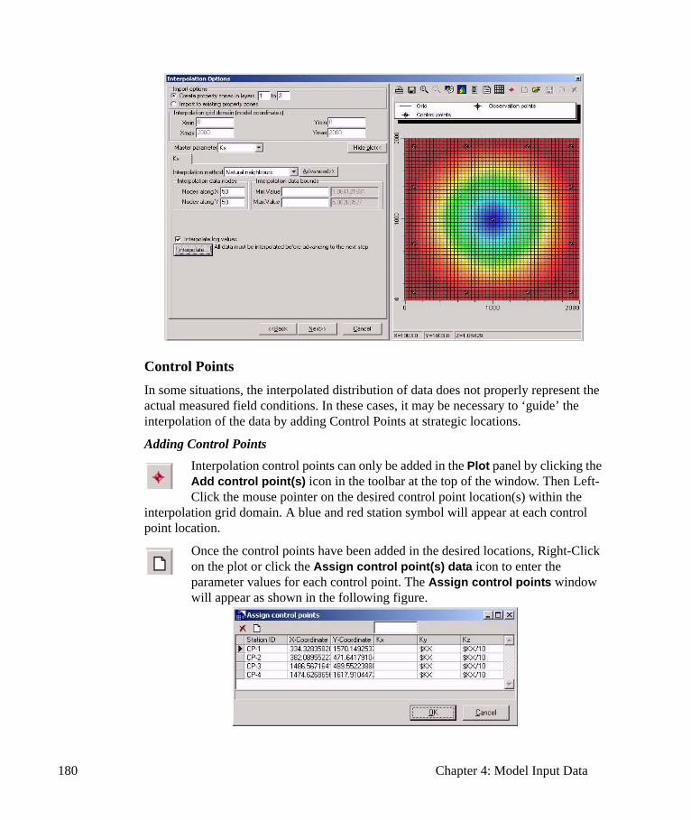
180 Chapter 4: Model Input Data
Control PointsIn some situations, the interpolated distribution of data does not properly represent the actual measured field conditions. In these cases, it may be necessary to ‘guide’ the interpolation of the data by adding Control Points at strategic locations.
Adding Control PointsInterpolation control points can only be added in the Plot panel by clicking the Add control point(s) icon in the toolbar at the top of the window. Then Left-Click the mouse pointer on the desired control point location(s) within the
interpolation grid domain. A blue and red station symbol will appear at each control point location.
Once the control points have been added in the desired locations, Right-Click on the plot or click the Assign control point(s) data icon to enter the parameter values for each control point. The Assign control points window will appear as shown in the following figure.
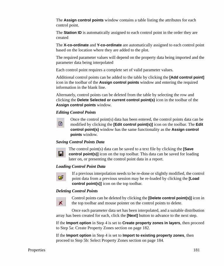
Properties 181
The Assign control points window contains a table listing the attributes for each control point.
The Station ID is automatically assigned to each control point in the order they are created
The X-co-ordinate and Y-co-ordinate are automatically assigned to each control point based on the location where they are added to the plot.
The required parameter values will depend on the property data being imported and the parameter data being interpolated
Each control point requires a complete set of valid parameter values.
Additional control points can be added to the table by clicking the [Add control point] icon in the toolbar of the Assign control points window and entering the required information in the blank line.
Alternately, control points can be deleted from the table by selecting the row and clicking the Delete Selected or current control point(s) icon in the toolbar of the Assign control points window.
Editing Control PointsOnce the control point(s) data has been entered, the control points data can be modified by clicking the [Edit control point(s)] icon on the toolbar. The Edit control point(s) window has the same functionality as the Assign control points window.
Saving Control Points DataThe control point(s) data can be saved to a text file by clicking the [Save control point(s)] icon on the top toolbar. This data can be saved for loading later on, or presenting the control point data in a report.
Loading Control Point DataIf a previous interpolation needs to be re-done or slightly modified, the control point data from a previous session may be re-loaded by clicking the [Load control point(s)] icon on the top toolbar.
Deleting Control PointsControl points can be deleted by clicking the [Delete control point(s)] icon in the top toolbar and mouse pointer on the control points to delete.
Once each parameter data set has been interpolated, and a suitable distribution array has been created for each, click the [Next] button to advance to the next step.
If the Import option in Step 4 is set to Create property zones in layers, then proceed to Step 5a: Create Property Zones section on page 182.
If the Import option in Step 4 is set to Import to existing property zones, then proceed to Step 5b: Select Property Zones section on page 184.
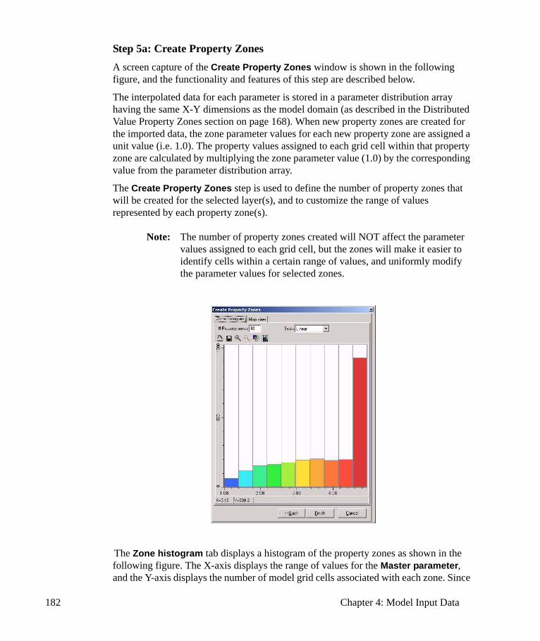
182 Chapter 4: Model Input Data
Step 5a: Create Property ZonesA screen capture of the Create Property Zones window is shown in the following figure, and the functionality and features of this step are described below.
The interpolated data for each parameter is stored in a parameter distribution array having the same X-Y dimensions as the model domain (as described in the Distributed Value Property Zones section on page 168). When new property zones are created for the imported data, the zone parameter values for each new property zone are assigned a unit value (i.e. 1.0). The property values assigned to each grid cell within that property zone are calculated by multiplying the zone parameter value (1.0) by the corresponding value from the parameter distribution array.
The Create Property Zones step is used to define the number of property zones that will be created for the selected layer(s), and to customize the range of values represented by each property zone(s).
Note: The number of property zones created will NOT affect the parameter values assigned to each grid cell, but the zones will make it easier to identify cells within a certain range of values, and uniformly modify the parameter values for selected zones.
The Zone histogram tab displays a histogram of the property zones as shown in the following figure. The X-axis displays the range of values for the Master parameter, and the Y-axis displays the number of model grid cells associated with each zone. Since

Properties 183
each property zone may contain data for several different parameters, the Master parameter (defined in Step 4: Interpolation Options section on page 176) is used to determine the range of values represented by each zone. The default setting creates 10 different property zones, each with the same increment value along the x-axis.
The # Property zones field indicates the number of property zones to create. This field can be customized to create just one property zone, or hundreds of property zones.
In many situations it will be sufficient to create only a single property zone representing the entire range of property values for the entire layer or set of layers. This will make it easy to uniformly increase or decrease the property values for the entire layer during the calibration process. However, if there is a specific region of the model where higher or lower ranges of property values make it more sensitive, then it may be useful to create several different property zones to effectively ‘isolate’ the more sensitive regions.
Setting the Scale for the Zone Values AxisThe Scale option controls the scale of the zone value axis (the X-axis) on the Zone histogram. The default setting is Linear. However, if the Master parameter ranges over several orders of magnitude, it may be easier or more appropriate to delineate the range of values associated with each property zone using a Log scale.
Customizing the Range of Values for Each Property ZoneWhen the # Property zones value is entered, the default setting is to create uniform increments for each property zone. However, this does not always yield the desired distribution of property zones. The range of values for each property zone can be customized by clicking-and-dragging the vertical line bounding each bar on the histogram to a new position along the x-axis.
Customizing the Zone ColorsThe default display setting for the histogram shows a rainbow color scale for the bars representing the property zones. Unfortunately, this rainbow color scale does not match the property zone colors that will be used in the Visual MODFLOW model grid. The current version of Visual MODFLOW does
not allow customized property zone colors, but the actual property zone colors for each zone can be displayed by clicking the [Zone colors] icon in the toolbar above the histogram.
Mapping Zones to the Model GridThe Map view tab displays a preview of the property zone distribution in the model domain as shown in the following figure. The default display settings show the distribution array grid using a rainbow color gradient for the zones.
The property zone colors, as they will appear in Visual MODFLOW, can be displayed by clicking the Visual MODFLOW colors icon in the toolbar above the map.

184 Chapter 4: Model Input Data
The property zone distribution on the actual model grid can be displayed by clicking the [Model grid] icon in the toolbar above the map.
Once the desired property distribution has been achieved, press the [Finish] button to import the new property zone data into the Visual MODFLOW model.
Hint: If several property zones were created for this data set, it is a good idea to print the Zone histogram before pressing the [Finish] button. The Zone histogram provides a reference for the range of values represented by each zone.
Upon returning to the Visual MODFLOW screen, a message will appear asking “Remove unused property entries?”. If the new property zone(s) created for the specified layer(s) of the model will be replacing an existing zone(s), the previous zone(s) will be removed from the list of zones if it is no longer being used anywhere else in the model.
Step 5b: Select Property ZonesThe Import to existing property zones options effectively “links” the selected property zones to the associated parameter distribution arrays. In doing so, the original zone parameter value is replaced by a unit parameter value (1.0). The property values assigned to each grid cell within that property zone are calculated by multiplying the zone parameter value (1.0) with the corresponding value from the parameter distribution array.
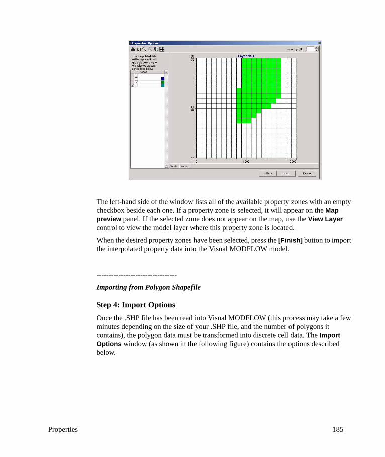
Properties 185
The left-hand side of the window lists all of the available property zones with an empty checkbox beside each one. If a property zone is selected, it will appear on the Map preview panel. If the selected zone does not appear on the map, use the View Layer control to view the model layer where this property zone is located.
When the desired property zones have been selected, press the [Finish] button to import the interpolated property data into the Visual MODFLOW model.
---------------------------------
Importing from Polygon Shapefile
Step 4: Import OptionsOnce the .SHP file has been read into Visual MODFLOW (this process may take a few minutes depending on the size of your .SHP file, and the number of polygons it contains), the polygon data must be transformed into discrete cell data. The Import Options window (as shown in the following figure) contains the options described below.
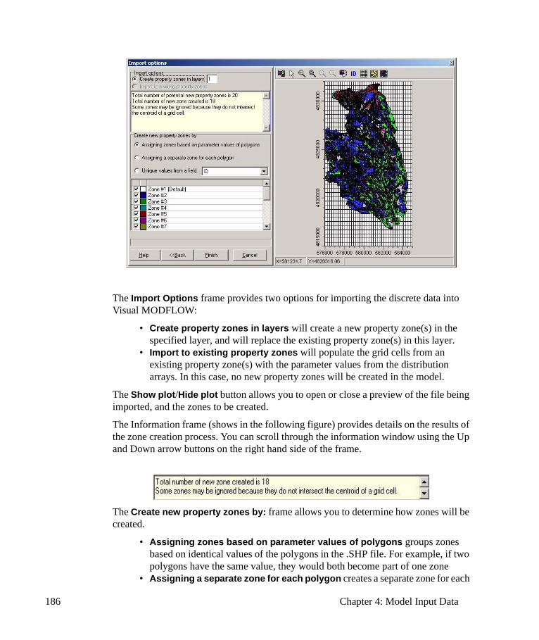
186 Chapter 4: Model Input Data
The Import Options frame provides two options for importing the discrete data into Visual MODFLOW:
• Create property zones in layers will create a new property zone(s) in the specified layer, and will replace the existing property zone(s) in this layer.
• Import to existing property zones will populate the grid cells from an existing property zone(s) with the parameter values from the distribution arrays. In this case, no new property zones will be created in the model.
The Show plot/Hide plot button allows you to open or close a preview of the file being imported, and the zones to be created.
The Information frame (shows in the following figure) provides details on the results of the zone creation process. You can scroll through the information window using the Up and Down arrow buttons on the right hand side of the frame.
The Create new property zones by: frame allows you to determine how zones will be created.
• Assigning zones based on parameter values of polygons groups zones based on identical values of the polygons in the .SHP file. For example, if two polygons have the same value, they would both become part of one zone
• Assigning a separate zone for each polygon creates a separate zone for each

Properties 187
polygon, even if some polygons have the same value• Unique values from a field: creates zones based on one of the columns of data
in your import file
You may see the results of your changes to the previously described options in the Plot window, if not already visible, by clicking on the Show Plot >> button. The Plot window includes the following options:
Print- You may print the preview image from either the 2-D or 3-D Preview tabs by clicking the Print button . The printing options are described in "Page Setup" on page 61.
Save As- The colored map of the interpolated elevations can be saved to a .BMP, .WMF, .EMF, or .DXF file by clicking the [Save As] icon on the top toolbar.
Zoom- You can zoom into and out of the model by using the Zoom tools . The Zoom In button allows you to enlarge the display of a
selected rectangular area. The Zoom Animated button allows you to zoom in “increments” by Left-Clicking on the model region being displayed. Note that each click zooms in “3-increments”, so holding the mouse button will result in many increments of magnification. The Zoom Previous button returns to the previous view, while the Zoom Out button returns to the original view.
Graph Properties- The appearance properties of the interpolated elevations map can be modified by Right-Clicking on the display area of the map and choosing the Properties option, or by clicking the [Graph Properties] icon from the toolbar. The Graph Properties are similar to the Graph Properties described in detail on page 531.
ID- You can display or hide the Region ID’s (from the .SHP file) on the map of polygons by clicking the ID button . Note that if you have a large number of regions, the labels may overlap and be difficult to read unless you are zoomed in to a small region. Alternately, you can click on an individual Region to see the Region number, as well as the parameter values for that region.
Grid- Show or hide the model grid by clicking the Show/Hide Grid button .
Map- Show the .GRD map of polygons by clicking the Show Map button .
Zones- Show the zones to be created by clicking the Show Zones button .
When the desired property zone distribution has been selected, press the [Finish] button to import the property data into the Visual MODFLOW model.
Assigning Property ZonesAs discussed on page 168, the Constant Value Property Zone approach is the fastest and easiest way to define the model properties. Although Visual MODFLOW supports an unlimited number of property zones, the usual practice is to develop a simplified
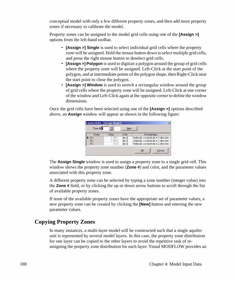
188 Chapter 4: Model Input Data
conceptual model with only a few different property zones, and then add more property zones if necessary to calibrate the model.
Property zones can be assigned to the model grid cells using one of the [Assign >] options from the left-hand toolbar.
• [Assign >] Single is used to select individual grid cells where the property zone will be assigned. Hold the mouse button down to select multiple grid cells, and press the right mouse button to deselect grid cells.
• [Assign >] Polygon is used to digitize a polygon around the group of grid cells where the property zone will be assigned. Left-Click at the start point of the polygon, and at intermediate points of the polygon shape, then Right-Click near the start point to close the polygon.
• [Assign >] Window is used to stretch a rectangular window around the group of grid cells where the property zone will be assigned. Left-Click at one corner of the window and Left-Click again at the opposite corner to define the window dimensions.
Once the grid cells have been selected using one of the [Assign >] options described above, an Assign window will appear as shown in the following figure:
The Assign Single window is used to assign a property zone to a single grid cell. This window shows the property zone number (Zone #) and color, and the parameter values associated with this property zone.
A different property zone can be selected by typing a zone number (integer value) into the Zone # field, or by clicking the up or down arrow buttons to scroll through the list of available property zones.
If none of the available property zones have the appropriate set of parameter values, a new property zone can be created by clicking the [New] button and entering the new parameter values.
Copying Property ZonesIn many instances, a multi-layer model will be constructed such that a single aquifer unit is represented by several model layers. In this case, the property zone distribution for one layer can be copied to the other layers to avoid the repetitive task of re-assigning the property zone distribution for each layer. Visual MODFLOW provides an
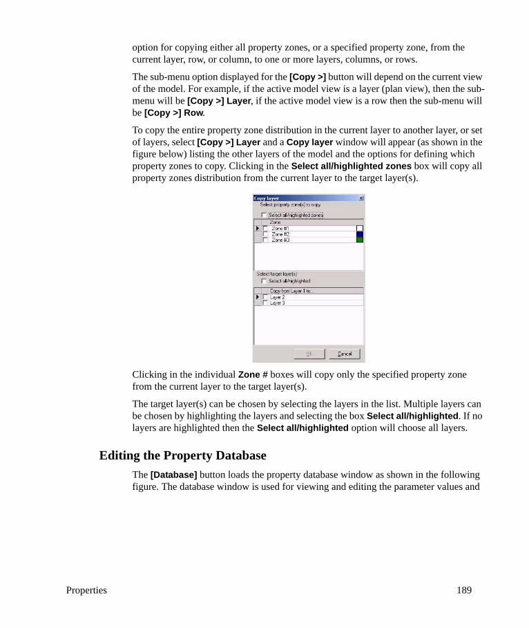
Properties 189
option for copying either all property zones, or a specified property zone, from the current layer, row, or column, to one or more layers, columns, or rows.
The sub-menu option displayed for the [Copy >] button will depend on the current view of the model. For example, if the active model view is a layer (plan view), then the sub-menu will be [Copy >] Layer, if the active model view is a row then the sub-menu will be [Copy >] Row.
To copy the entire property zone distribution in the current layer to another layer, or set of layers, select [Copy >] Layer and a Copy layer window will appear (as shown in the figure below) listing the other layers of the model and the options for defining which property zones to copy. Clicking in the Select all/highlighted zones box will copy all property zones distribution from the current layer to the target layer(s).
Clicking in the individual Zone # boxes will copy only the specified property zone from the current layer to the target layer(s).
The target layer(s) can be chosen by selecting the layers in the list. Multiple layers can be chosen by highlighting the layers and selecting the box Select all/highlighted. If no layers are highlighted then the Select all/highlighted option will choose all layers.
Editing the Property DatabaseThe [Database] button loads the property database window as shown in the following figure. The database window is used for viewing and editing the parameter values and

190 Chapter 4: Model Input Data
settings for all property zones in the model. The functionality and settings for the property zones are described below.
Each row of the property database table contains information about each of the model property zones including:
• Zone number and associated color• Zone parameter values• Active setting• Distribution Array link setting
The status bar below the table panel displays information about each zone parameter value by simply clicking the cursor on the zone parameter of interest.
The Zone numbers and colors are read-only data and cannot be modified.
The zone parameter values can be modified by simply entering a new value in the desired field.
The Active setting indicates whether the zone is active or inactive. An inactive zone is not assigned to any grid cells in the model, and may be removed without affecting the model results. Inactive zones can be removed using the [Clean Up] button.
The Distribution Array setting can be turned ON or OFF.
If the Distribution Array setting is ON, the zone parameter values from the database will be multiplied by the values from the associated distribution array to calculate the property values assigned to each grid cell as explained under Distributed Value Property Zones on page 168.
If the Distribution Array setting is OFF, the zone parameter values from the Property Database will be assigned to each grid cell associated with this property zone.
The [Clean Up] button is used to remove unused property zones from the database and to re-index the property zones in ascending order. This cleanup will likely cause some changes in the appearance of the property zone distributions because the zone colors are linked to the zone numbers. However, it will not affect the model results because the property values assigned to each grid cell do not change.
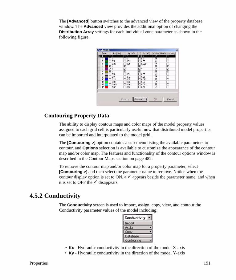
Properties 191
The [Advanced] button switches to the advanced view of the property database window. The Advanced view provides the additional option of changing the Distribution Array settings for each individual zone parameter as shown in the following figure.
Contouring Property Data The ability to display contour maps and color maps of the model property values assigned to each grid cell is particularly useful now that distributed model properties can be imported and interpolated to the model grid.
The [Contouring >] option contains a sub-menu listing the available parameters to contour, and Options selection is available to customize the appearance of the contour map and/or color map. The features and functionality of the contour options window is described in the Contour Maps section on page 482.
To remove the contour map and/or color map for a property parameter, select [Contouring >] and then select the parameter name to remove. Notice when the contour display option is set to ON, a appears beside the parameter name, and when it is set to OFF the disappears.
4.5.2 ConductivityThe Conductivity screen is used to import, assign, copy, view, and contour the Conductivity parameter values of the model including:
• Kx - Hydraulic conductivity in the direction of the model X-axis• Ky - Hydraulic conductivity in the direction of the model Y-axis
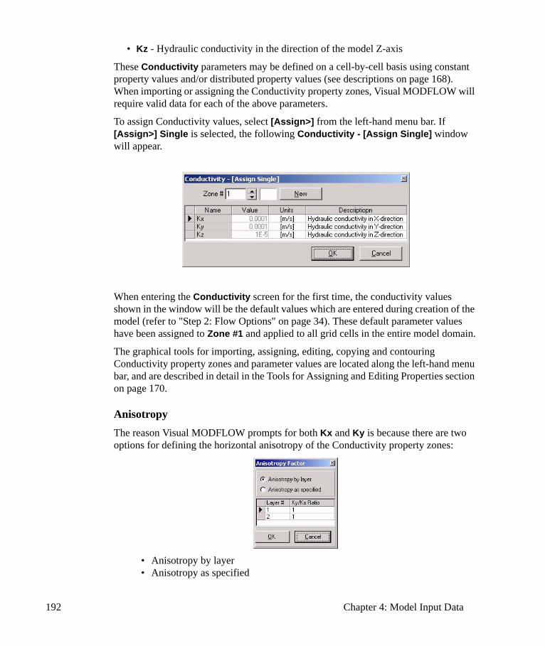
192 Chapter 4: Model Input Data
• Kz - Hydraulic conductivity in the direction of the model Z-axis
These Conductivity parameters may be defined on a cell-by-cell basis using constant property values and/or distributed property values (see descriptions on page 168). When importing or assigning the Conductivity property zones, Visual MODFLOW will require valid data for each of the above parameters.
To assign Conductivity values, select [Assign>] from the left-hand menu bar. If [Assign>] Single is selected, the following Conductivity - [Assign Single] window will appear.
When entering the Conductivity screen for the first time, the conductivity values shown in the window will be the default values which are entered during creation of the model (refer to "Step 2: Flow Options" on page 34). These default parameter values have been assigned to Zone #1 and applied to all grid cells in the entire model domain.
The graphical tools for importing, assigning, editing, copying and contouring Conductivity property zones and parameter values are located along the left-hand menu bar, and are described in detail in the Tools for Assigning and Editing Properties section on page 170.
AnisotropyThe reason Visual MODFLOW prompts for both Kx and Ky is because there are two options for defining the horizontal anisotropy of the Conductivity property zones:
• Anisotropy by layer• Anisotropy as specified
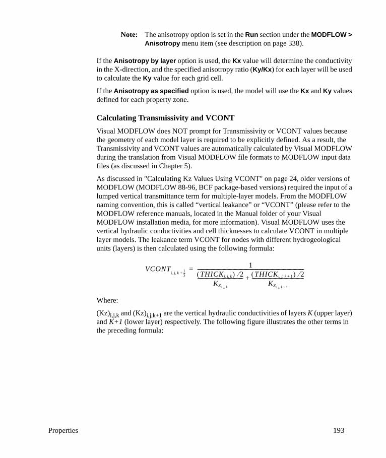
Properties 193
Note: The anisotropy option is set in the Run section under the MODFLOW > Anisotropy menu item (see description on page 338).
If the Anisotropy by layer option is used, the Kx value will determine the conductivity in the X-direction, and the specified anisotropy ratio (Ky/Kx) for each layer will be used to calculate the Ky value for each grid cell.
If the Anisotropy as specified option is used, the model will use the Kx and Ky values defined for each property zone.
Calculating Transmissivity and VCONTVisual MODFLOW does NOT prompt for Transmissivity or VCONT values because the geometry of each model layer is required to be explicitly defined. As a result, the Transmissivity and VCONT values are automatically calculated by Visual MODFLOW during the translation from Visual MODFLOW file formats to MODFLOW input data files (as discussed in Chapter 5).
As discussed in "Calculating Kz Values Using VCONT" on page 24, older versions of MODFLOW (MODFLOW 88-96, BCF package-based versions) required the input of a lumped vertical transmittance term for multiple-layer models. From the MODFLOW naming convention, this is called “vertical leakance” or “VCONT” (please refer to the MODFLOW reference manuals, located in the Manual folder of your Visual MODFLOW installation media, for more information). Visual MODFLOW uses the vertical hydraulic conductivities and cell thicknesses to calculate VCONT in multiple layer models. The leakance term VCONT for nodes with different hydrogeological units (layers) is then calculated using the following formula:
Where:
(Kz)i,j,k and (Kz)i,j,k+1 are the vertical hydraulic conductivities of layers K (upper layer) and K+1 (lower layer) respectively. The following figure illustrates the other terms in the preceding formula:
VCONTi j k 1
2---+, ,
1THICKi j k, ,( ) 2⁄
KZi j k, ,
------------------------------------- THICKi j k 1+, ,( ) 2⁄KZi j k 1+, ,
------------------------------------------+---------------------------------------------------------------------------------------=
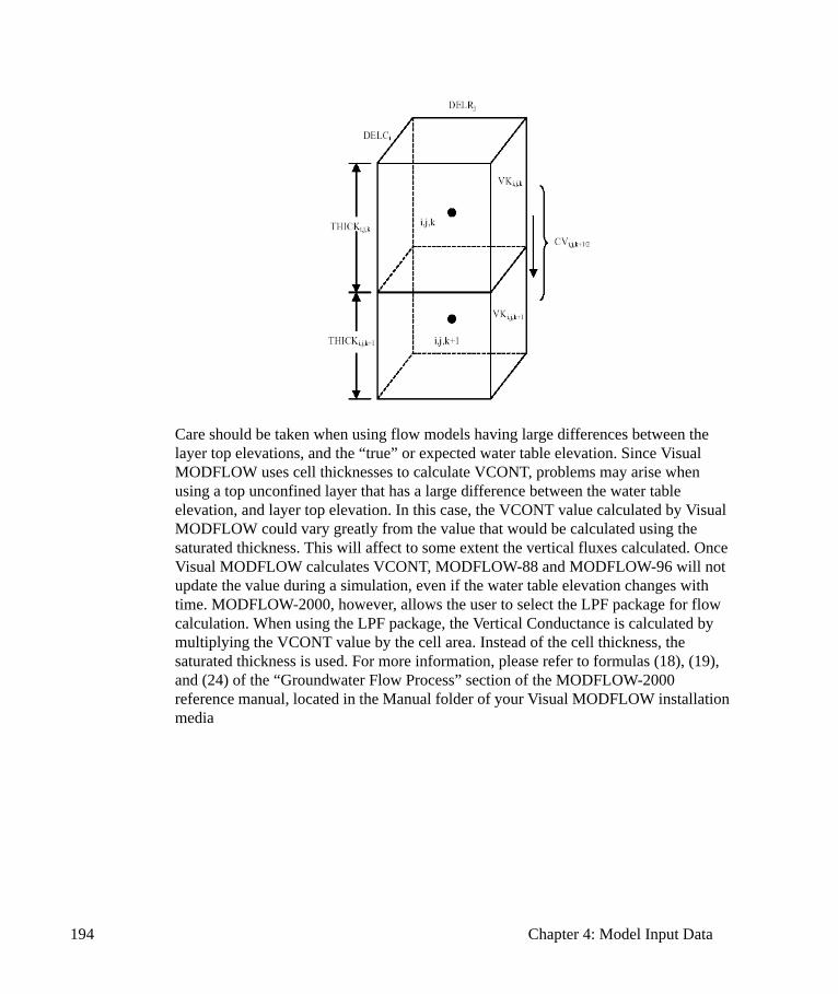
194 Chapter 4: Model Input Data
Care should be taken when using flow models having large differences between the layer top elevations, and the “true” or expected water table elevation. Since Visual MODFLOW uses cell thicknesses to calculate VCONT, problems may arise when using a top unconfined layer that has a large difference between the water table elevation, and layer top elevation. In this case, the VCONT value calculated by Visual MODFLOW could vary greatly from the value that would be calculated using the saturated thickness. This will affect to some extent the vertical fluxes calculated. Once Visual MODFLOW calculates VCONT, MODFLOW-88 and MODFLOW-96 will not update the value during a simulation, even if the water table elevation changes with time. MODFLOW-2000, however, allows the user to select the LPF package for flow calculation. When using the LPF package, the Vertical Conductance is calculated by multiplying the VCONT value by the cell area. Instead of the cell thickness, the saturated thickness is used. For more information, please refer to formulas (18), (19), and (24) of the “Groundwater Flow Process” section of the MODFLOW-2000 reference manual, located in the Manual folder of your Visual MODFLOW installation media
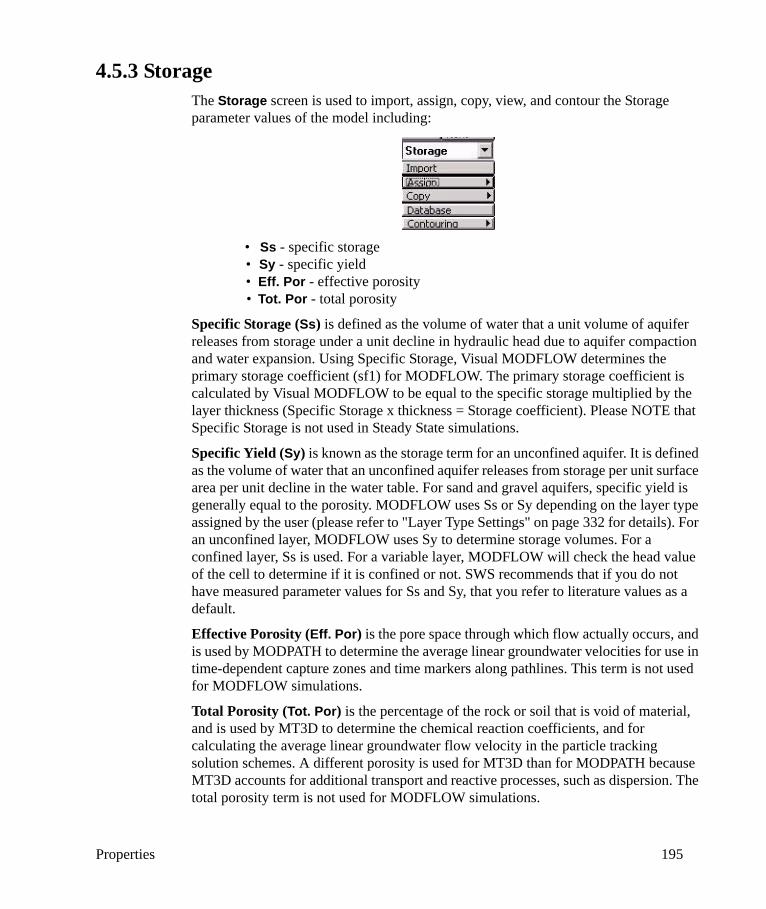
Properties 195
4.5.3 StorageThe Storage screen is used to import, assign, copy, view, and contour the Storage parameter values of the model including:
• Ss - specific storage• Sy - specific yield• Eff. Por - effective porosity• Tot. Por - total porosity
Specific Storage (Ss) is defined as the volume of water that a unit volume of aquifer releases from storage under a unit decline in hydraulic head due to aquifer compaction and water expansion. Using Specific Storage, Visual MODFLOW determines the primary storage coefficient (sf1) for MODFLOW. The primary storage coefficient is calculated by Visual MODFLOW to be equal to the specific storage multiplied by the layer thickness (Specific Storage x thickness = Storage coefficient). Please NOTE that Specific Storage is not used in Steady State simulations.
Specific Yield (Sy) is known as the storage term for an unconfined aquifer. It is defined as the volume of water that an unconfined aquifer releases from storage per unit surface area per unit decline in the water table. For sand and gravel aquifers, specific yield is generally equal to the porosity. MODFLOW uses Ss or Sy depending on the layer type assigned by the user (please refer to "Layer Type Settings" on page 332 for details). For an unconfined layer, MODFLOW uses Sy to determine storage volumes. For a confined layer, Ss is used. For a variable layer, MODFLOW will check the head value of the cell to determine if it is confined or not. SWS recommends that if you do not have measured parameter values for Ss and Sy, that you refer to literature values as a default.
Effective Porosity (Eff. Por) is the pore space through which flow actually occurs, and is used by MODPATH to determine the average linear groundwater velocities for use in time-dependent capture zones and time markers along pathlines. This term is not used for MODFLOW simulations.
Total Porosity (Tot. Por) is the percentage of the rock or soil that is void of material, and is used by MT3D to determine the chemical reaction coefficients, and for calculating the average linear groundwater flow velocity in the particle tracking solution schemes. A different porosity is used for MT3D than for MODPATH because MT3D accounts for additional transport and reactive processes, such as dispersion. The total porosity term is not used for MODFLOW simulations.

196 Chapter 4: Model Input Data
These Storage parameters may be defined on a cell-by-cell basis using constant property values and/or distributed property values (see descriptions on page 168). When importing or assigning the Storage property zones, Visual MODFLOW will require valid data for each of the above parameters.
To assign Storage values, select [Assign>] from the left-hand menu bar. If [Assign>] Single is selected, the following Storage - [Assign Single] window will appear.
When entering the Storage screen for the first time, the Storage parameter values shown in the window will be the default values which were entered during creation of the model (refer to "Step 2: Flow Options" on page 34). These default parameter values have been assigned to Zone #1, and applied to all grid cells in the entire model domain.
The graphical tools for importing, assigning, editing, copying and contouring Storage zones and parameter values are located along the left-hand menu bar, and are described in detail in the Tools for Assigning and Editing Properties section on page 170.
Copying the Conductivity Zone DistributionIn most situations, the spatial distribution of storage zones will be identical to the spatial distribution of conductivity zones. As a result, Visual MODFLOW provides the option of copying the Conductivity property zone distribution to the Storage input screen. This avoids the tedious task of trying to manually duplicate the Conductivity property zone arrangement with the Storage property zones.
To copy the Conductivity zones distribution, select [Copy >] Distrib from the side menu bar and the Storage property zones will automatically be created for every hydraulic conductivity zone (the values of the storage parameters for all new storage zones will be automatically set to the default Storage parameter values). Upon re-selecting [Copy >], a window Copy Distribution Warning! will appear informing that “Storage Properties Exist!” Continuing will reassign storage properties.
Next, select the [Database] button from the side menu bar and modify the storage values for each zone as required.
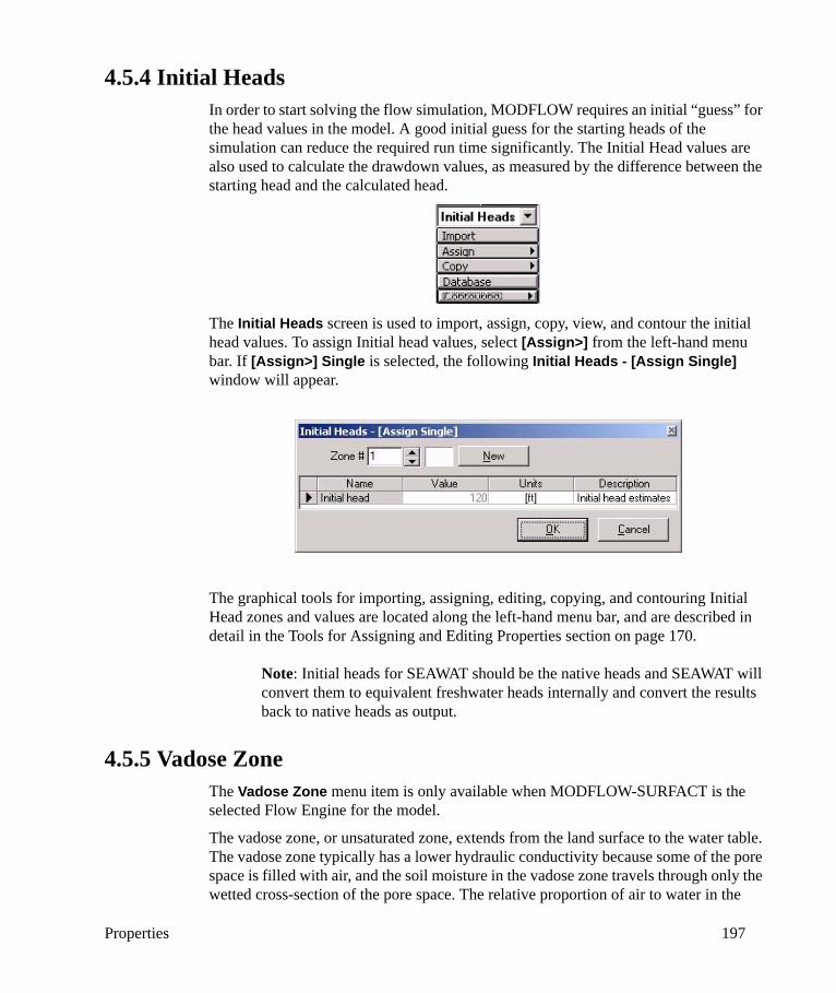
Properties 197
4.5.4 Initial HeadsIn order to start solving the flow simulation, MODFLOW requires an initial “guess” for the head values in the model. A good initial guess for the starting heads of the simulation can reduce the required run time significantly. The Initial Head values are also used to calculate the drawdown values, as measured by the difference between the starting head and the calculated head.
The Initial Heads screen is used to import, assign, copy, view, and contour the initial head values. To assign Initial head values, select [Assign>] from the left-hand menu bar. If [Assign>] Single is selected, the following Initial Heads - [Assign Single] window will appear.
The graphical tools for importing, assigning, editing, copying, and contouring Initial Head zones and values are located along the left-hand menu bar, and are described in detail in the Tools for Assigning and Editing Properties section on page 170.
Note: Initial heads for SEAWAT should be the native heads and SEAWAT will convert them to equivalent freshwater heads internally and convert the results back to native heads as output.
4.5.5 Vadose ZoneThe Vadose Zone menu item is only available when MODFLOW-SURFACT is the selected Flow Engine for the model.
The vadose zone, or unsaturated zone, extends from the land surface to the water table. The vadose zone typically has a lower hydraulic conductivity because some of the pore space is filled with air, and the soil moisture in the vadose zone travels through only the wetted cross-section of the pore space. The relative proportion of air to water in the

198 Chapter 4: Model Input Data
pores can vary, and consequently the hydraulic properties of the porous media can also vary.
In general, soil moisture in the vadose zone is under tension, and it travels through the vadose zone due to total soil-moisture potential (the sum of the elevation potential, and the pressure head). The pressure head is a function of the volumetric water content of the soil, and depends upon whether the soil has previously undergone wetting or drying. The relationship between pressure head and volumetric water content for a particular soil is known as a soil-water characteristic curve. Using the experimental soil-water characteristic curve and the soil hydrologic parameters, the movement of water in the vadose zone can be determined using the BCF4 package in MODFLOW-SURFACT. A sample index of soil properties is given below:
Sample Index of Soil Hydraulic Properties*
*Source is “Average hydraulic conductivity properties of ARS soil texture classes, “draft dated February, 2000 by J. Schaake. This expanded the work of others and included a total of 2128 soil samples. Wilting point is the fractional water content at 15 bar tension; field capacity is the fractional water content at 1/3 bar tension.
**It is used in Campbell’s equation. ref: Coby et al., A Statistical exploration of the relationship of soil moisture characteristics to the physical properties of soils, Water Resources Research 20(6): 682-690, 1984.
***Average values of the van Genuchten soil parameters obtained by experimental means (Carsel and Parrish, 1988) and also reported on page 180 in Contaminant Hydrogeology book by C. W. Fetter (1999).
Soil Type
Sand
%
Clay
%
Bulk Density
g/cm3
Field Capacity
cm3/cm3
Wilting point
cm3/cm3
Porosityfraction
Saturated Hydraulic Conducti-vity cm/s
Slope of Retention Curve (in log space)**
Alpha
parameter
(cm-1)***
s 94.83 2.27 1.49 0.08 0.03 0.43 0.0107 4.1 0.145
ls 85.23 6.53 1.52 0.15 0.06 0.42 0.0030 3.99 0.124
sl 69.28 12.48 1.57 0.21 0.09 0.4 0.0015 4.84 0.075
sil 19.28 17.11 1.42 0.32 0.12 0.46 0.0011 3.79 0.020
si 4.50 8.3 1.28 0.28 0.08 0.52 0.0023 3.05 0.016
l 41.00 20.69 1.49 0.29 0.14 0.43 0.0005 5.3 0.036
scl 60.97 26.33 1.6 0.27 0.17 0.39 0.0007 8.66 0.059
sicl 9.04 33.05 1.38 0.36 0.21 0.48 0.0015 7.48 0.010
cl 30.08 33.46 1.43 0.34 0.21 0.46 0.0005 8.02 0.019
sc 50.32 39.3 1.57 0.31 0.23 0.41 0.0003 13 0.027
sic 8.18 44.58 1.35 0.37 0.25 0.49 0.0008 9.76 0.005
c 24.71 52.46 1.39 0.36 0.27 0.47 0.0009 12.28
α
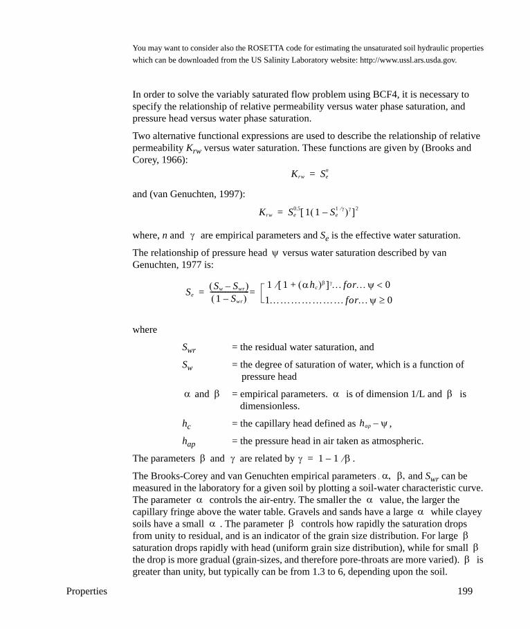
Properties 199
You may want to consider also the ROSETTA code for estimating the unsaturated soil hydraulic properties which can be downloaded from the US Salinity Laboratory website: http://www.ussl.ars.usda.gov.
In order to solve the variably saturated flow problem using BCF4, it is necessary to specify the relationship of relative permeability versus water phase saturation, and pressure head versus water phase saturation.
Two alternative functional expressions are used to describe the relationship of relative permeability Krw versus water saturation. These functions are given by (Brooks and Corey, 1966):
and (van Genuchten, 1997):
where, n and are empirical parameters and Se is the effective water saturation.
The relationship of pressure head versus water saturation described by van Genuchten, 1977 is:
where
Swr = the residual water saturation, and
Sw = the degree of saturation of water, which is a function of pressure head
and = empirical parameters. is of dimension 1/L and is dimensionless.
hc = the capillary head defined as ,
hap = the pressure head in air taken as atmospheric.
The parameters and are related by .
The Brooks-Corey and van Genuchten empirical parameters and Swr can be measured in the laboratory for a given soil by plotting a soil-water characteristic curve. The parameter controls the air-entry. The smaller the value, the larger the capillary fringe above the water table. Gravels and sands have a large while clayey soils have a small . The parameter controls how rapidly the saturation drops from unity to residual, and is an indicator of the grain size distribution. For large saturation drops rapidly with head (uniform grain size distribution), while for small the drop is more gradual (grain-sizes, and therefore pore-throats are more varied). is greater than unity, but typically can be from 1.3 to 6, depending upon the soil.
Krw Sen=
Krw Se0.5 1 1 Se
1 γ⁄–( )γ[ ]2=
γ
ψ
SeSw Swr–( )1 Swr–( )
----------------------- 1 1 αhc( )β+[ ]γ…for…ψ 0<⁄1…………………for…ψ 0≥
==
α β α β
hap ψ–
β γ γ 1 1 β⁄–=
α, , β,
α αα
α βββ
β
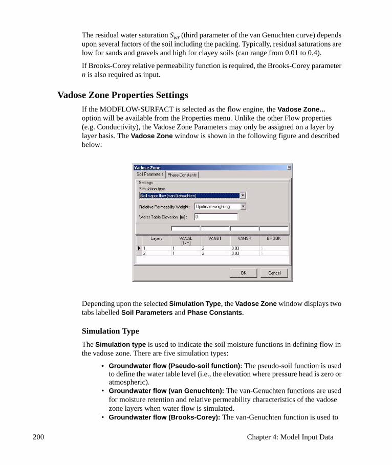
200 Chapter 4: Model Input Data
The residual water saturation Swr (third parameter of the van Genuchten curve) depends upon several factors of the soil including the packing. Typically, residual saturations are low for sands and gravels and high for clayey soils (can range from 0.01 to 0.4).
If Brooks-Corey relative permeability function is required, the Brooks-Corey parameter n is also required as input.
Vadose Zone Properties Settings If the MODFLOW-SURFACT is selected as the flow engine, the Vadose Zone... option will be available from the Properties menu. Unlike the other Flow properties (e.g. Conductivity), the Vadose Zone Parameters may only be assigned on a layer by layer basis. The Vadose Zone window is shown in the following figure and described below:
Depending upon the selected Simulation Type, the Vadose Zone window displays two tabs labelled Soil Parameters and Phase Constants.
Simulation TypeThe Simulation type is used to indicate the soil moisture functions in defining flow in the vadose zone. There are five simulation types:
• Groundwater flow (Pseudo-soil function): The pseudo-soil function is used to define the water table level (i.e., the elevation where pressure head is zero or atmospheric).
• Groundwater flow (van Genuchten): The van-Genuchten functions are used for moisture retention and relative permeability characteristics of the vadose zone layers when water flow is simulated.
• Groundwater flow (Brooks-Corey): The van-Genuchten function is used to
Properties 201
determine the moisture retention, and Brooks-Corey function is used to determine the relative permeability characteristics of the vadose zone layers when water flow is simulated.
• Soil vapor flow (van Genuchten): The van-Genuchten functions are used for retention and relative permeability characteristics of the vadose zone layers when air flow is simulated.
• Soil vapor flow (Brooks-Corey): The van-Genuchten function is used to determine the moisture retention, and Brooks-Corey function is used to determine the relative permeability characteristics of the vadose zone layers when air flow is simulated.
The default Simulation Type is set to Groundwater flow (Pseudo-soil function).For Relative Permeability Weight, there are two options to indicate weighting of the relative permeability term: Upstream weighting and Mid-point weighting.
In the five columns under the Water Table Elevation field, the values for the vadose zone parameters for each model layer are defined:
• Layers - is the model layer number. • VANAL - van Genuchten alpha parameter for specified layer number, must
be a positive non-zero value (default 1.0 m). It controls the air-entry, and is of dimension 1/L. The smaller the VANAL value, the larger is the capillary fringe above the water table. Gravel and sands have large alpha values (can be 1 to 5) while clayey soils have small alpha values (can be as small as 0.01 m).
• VANBT - van Genuchten beta parameter , must be a positive value greater than 1 (default value is 2). It controls how rapidly the saturation drops from unity to residual, and is an indicator of the grain-size distribution. For large VANBT, saturation drops rapidly with head (uniform grain-size distribution), while for a small VANBT value, the drop is more gradual (variable grain-size distribution, and therefore pore-throats are more varied). VANBT is greater than unity, but typically can be from 1.3 to 6, depending upon the soil type.
• VANSR - residual saturation level (Swr). It must be a positive value less than 1 (default value 0.03). It depends upon several factors of the soil, including the packing. Typically, residual saturations are low for sands and gravels and high for clayey soils (can range from 0.01 to 0.4).
• BROOK - is the Brooks-Corey exponent (n). It must be greater than zero (default value is 0.5).
If the Simulation Type is set to either of the Soil vapor flow options, the Water Table Elevation field becomes active, and a second tab labelled Phase Constants is enabled (as shown in the preceding Vadose Zone window). Water Table Elevation is required when air phase flow is simulated in the vadose zone. Visual MODFLOW will activate the Water Table Elevation field to define the water table elevation. If no Water Table Elevation data is available, upon closing Vadose Zone window a message will appear with the warning “Water Table Elevation data is required to run the Soil vapor flow simulation. Please return to Input section and enter the Water Table Elevation data
α( )
β( )
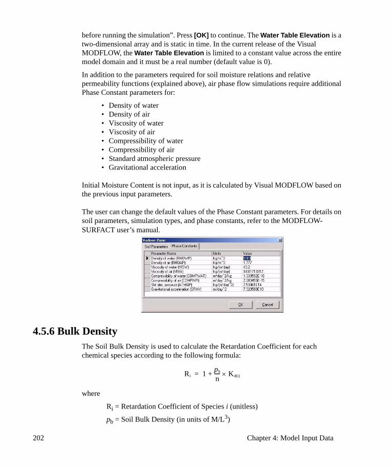
202 Chapter 4: Model Input Data
before running the simulation”. Press [OK] to continue. The Water Table Elevation is a two-dimensional array and is static in time. In the current release of the Visual MODFLOW, the Water Table Elevation is limited to a constant value across the entire model domain and it must be a real number (default value is 0).
In addition to the parameters required for soil moisture relations and relative permeability functions (explained above), air phase flow simulations require additional Phase Constant parameters for:
• Density of water • Density of air • Viscosity of water• Viscosity of air• Compressibility of water• Compressibility of air• Standard atmospheric pressure• Gravitational acceleration
Initial Moisture Content is not input, as it is calculated by Visual MODFLOW based on the previous input parameters.
The user can change the default values of the Phase Constant parameters. For details on soil parameters, simulation types, and phase constants, refer to the MODFLOW-SURFACT user’s manual.
4.5.6 Bulk DensityThe Soil Bulk Density is used to calculate the Retardation Coefficient for each chemical species according to the following formula:
where
Ri = Retardation Coefficient of Species i (unitless)
pb = Soil Bulk Density (in units of M/L3)
Ri 1 pb
n---- Kd(i)×+=
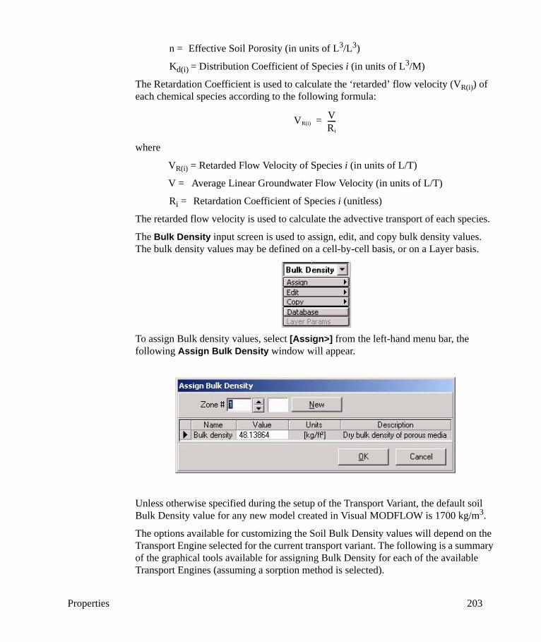
Properties 203
n = Effective Soil Porosity (in units of L3/L3)
Kd(i) = Distribution Coefficient of Species i (in units of L3/M)
The Retardation Coefficient is used to calculate the ‘retarded’ flow velocity (VR(i)) of each chemical species according to the following formula:
where
VR(i) = Retarded Flow Velocity of Species i (in units of L/T)
V = Average Linear Groundwater Flow Velocity (in units of L/T)
Ri = Retardation Coefficient of Species i (unitless)
The retarded flow velocity is used to calculate the advective transport of each species.
The Bulk Density input screen is used to assign, edit, and copy bulk density values. The bulk density values may be defined on a cell-by-cell basis, or on a Layer basis.
To assign Bulk density values, select [Assign>] from the left-hand menu bar, the following Assign Bulk Density window will appear.
Unless otherwise specified during the setup of the Transport Variant, the default soil Bulk Density value for any new model created in Visual MODFLOW is 1700 kg/m3.
The options available for customizing the Soil Bulk Density values will depend on the Transport Engine selected for the current transport variant. The following is a summary of the graphical tools available for assigning Bulk Density for each of the available Transport Engines (assuming a sorption method is selected).
VR(i)VRi-----=
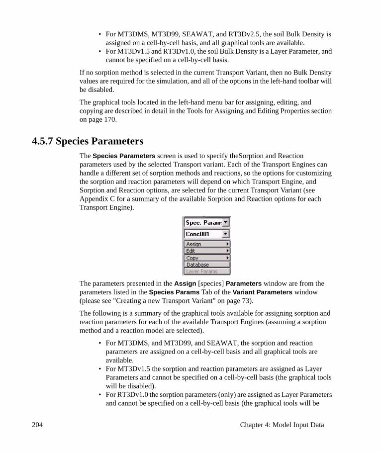
204 Chapter 4: Model Input Data
• For MT3DMS, MT3D99, SEAWAT, and RT3Dv2.5, the soil Bulk Density is assigned on a cell-by-cell basis, and all graphical tools are available.
• For MT3Dv1.5 and RT3Dv1.0, the soil Bulk Density is a Layer Parameter, and cannot be specified on a cell-by-cell basis.
If no sorption method is selected in the current Transport Variant, then no Bulk Density values are required for the simulation, and all of the options in the left-hand toolbar will be disabled.
The graphical tools located in the left-hand menu bar for assigning, editing, and copying are described in detail in the Tools for Assigning and Editing Properties section on page 170.
4.5.7 Species ParametersThe Species Parameters screen is used to specify theSorption and Reaction parameters used by the selected Transport variant. Each of the Transport Engines can handle a different set of sorption methods and reactions, so the options for customizing the sorption and reaction parameters will depend on which Transport Engine, and Sorption and Reaction options, are selected for the current Transport Variant (see Appendix C for a summary of the available Sorption and Reaction options for each Transport Engine).
The parameters presented in the Assign [species] Parameters window are from the parameters listed in the Species Params Tab of the Variant Parameters window (please see "Creating a new Transport Variant" on page 73).
The following is a summary of the graphical tools available for assigning sorption and reaction parameters for each of the available Transport Engines (assuming a sorption method and a reaction model are selected).
• For MT3DMS, and MT3D99, and SEAWAT, the sorption and reaction parameters are assigned on a cell-by-cell basis and all graphical tools are available.
• For MT3Dv1.5 the sorption and reaction parameters are assigned as Layer Parameters and cannot be specified on a cell-by-cell basis (the graphical tools will be disabled).
• For RT3Dv1.0 the sorption parameters (only) are assigned as Layer Parameters and cannot be specified on a cell-by-cell basis (the graphical tools will be

Properties 205
disabled except for Layer Params).• For RT3Dv2.5 the sorption parameters (only) are assigned on a cell-by-cell
basis and all the graphical tools are available.• For PHT3D, Bulk density and sorption parameters can be assigned on a cell-
by-cell basis. Reaction parameters in PHT3D are spatially constant and only can be assigned in PHT3D settings dialog. Finally, PHT3D currently does not allow nonlinear sorption.
To assign Species Parameters values, select [Assign>] from the left-hand menu bar, select a cell or group of cells in your model, and the Assign [species] Parameters window will appear, similar to the following figure:
If no sorption or reactions are selected in the current Transport Variant, then no sorption or reaction parameters are required for the simulation, and all of the options in the left-hand toolbar will be disabled.
Kd is expressed in units of 1/(mass/volume), and is derived as follows
First order reaction coefficients can be derived from a Half Life value as follows:
Where:
Ct is the concentration at time t, in units of mass/volume
Kd solidphase[ ]aqueousphase[ ]
------------------------------------------
massmass-------------⎝ ⎠⎛ ⎞
massvolume-------------------⎝ ⎠⎛ ⎞------------------------ 1
massvolume--------------------------------------= = =
Ct C0e kt–=
206 Chapter 4: Model Input Data
C0 is the initial concentration, in units of mass/volume
k is the first order decay rate, in units of 1/time
t is the time t
For a Half-life calculation, the equation can be rewritten as follows:
Where:
k is the first order decay rate, in units of 1/time
t1/2 is the Half Life value
The graphical tools for assigning, editing, copying, and contouring the Reaction model parameters located along the left-hand menu bar are described in detail in the Tools for Assigning and Editing Properties section on page 170.
4.5.8 Edit Constant ParametersThe Edit Constant Parameters option allows select parameters to be modified. The options available will be the same as those listed in the Spatially Constant Variant Parameters window (see "Modifying a Transport Variant" on page 74). Depending on the Transport Engine and Reaction Parameter options you have selected, there may or may not be Constant Parameters available for editing. If no Constant Parameters are available for editing, a message will appear as shown below.
k 0.5ln( ) t12---
–( )⁄=
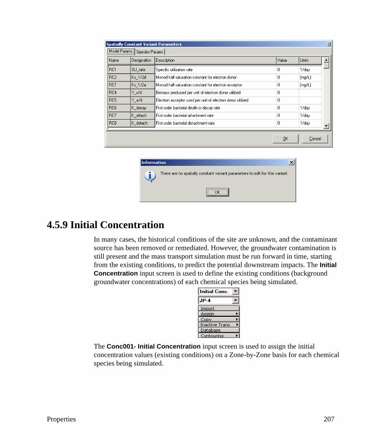
Properties 207
4.5.9 Initial ConcentrationIn many cases, the historical conditions of the site are unknown, and the contaminant source has been removed or remediated. However, the groundwater contamination is still present and the mass transport simulation must be run forward in time, starting from the existing conditions, to predict the potential downstream impacts. The Initial Concentration input screen is used to define the existing conditions (background groundwater concentrations) of each chemical species being simulated.
The Conc001- Initial Concentration input screen is used to assign the initial concentration values (existing conditions) on a Zone-by-Zone basis for each chemical species being simulated.
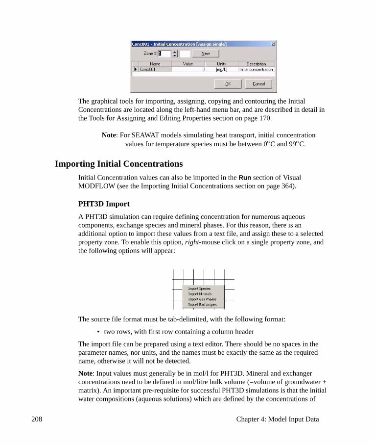
208 Chapter 4: Model Input Data
The graphical tools for importing, assigning, copying and contouring the Initial Concentrations are located along the left-hand menu bar, and are described in detail in the Tools for Assigning and Editing Properties section on page 170.
Note: For SEAWAT models simulating heat transport, initial concentration values for temperature species must be between 0°C and 99°C.
Importing Initial ConcentrationsInitial Concentration values can also be imported in the Run section of Visual MODFLOW (see the Importing Initial Concentrations section on page 364).
PHT3D ImportA PHT3D simulation can require defining concentration for numerous aqueous components, exchange species and mineral phases. For this reason, there is an additional option to import these values from a text file, and assign these to a selected property zone. To enable this option, right-mouse click on a single property zone, and the following options will appear:
The source file format must be tab-delimited, with the following format:
• two rows, with first row containing a column header
The import file can be prepared using a text editor. There should be no spaces in the parameter names, nor units, and the names must be exactly the same as the required name, otherwise it will not be detected.
Note: Input values must generally be in mol/l for PHT3D. Mineral and exchanger concentrations need to be defined in mol/litre bulk volume (=volume of groundwater + matrix). An important pre-requisite for successful PHT3D simulations is that the initial water compositions (aqueous solutions) which are defined by the concentrations of

Properties 209
aqueous species/components are charge-balanced. Other constraints exist on the entry of redox species and alkalinity, for example:
• for iron, the species ferric and ferrous iron needs to be entered rather than the total iron
• for carbonate, species must be expressed as total inorganic carbon rather than alkalinity
Calculating adequate values for the various components in your reaction simulation can therefore be a challenge. This can be made easy by using AquaChem to generate the PHT3D-ready input. AquaChem allows you to:
• Run a PHREEQC simulation using your solutions, to achieve charge-balanced• aqueous solutions and exchanger site compositions that are in equilibrium with
their corresponding aqueous solutions• Convert mass-based concentrations into molar-based concentrations.
For more details on AquaChem or to download a demo or trial version, please contact our sales department.
Assigning Inactive Transport ZonesIn many cases, the area of interest for the mass transport simulation will occupy only a small subregion of the model domain. As a result, it is not necessary to include the entire model domain and all of the associated grid cells in the mass transport model calculations. Visual MODFLOW provides an option for graphically assigning regions of the model outside the zone of interest as Inactive For Transport. MT3D does not simulate contaminant transport through cells defined to be Inactive For Transport.
The Inactive For Transport regions of the model are defined by selecting one of the [Inactive Trans.] options from the left-hand toolbar.
Mark Poly. Active: Digitize a polygon around a group of cells which will be designated as active. Left-Click at the start point of the polygon to start digitizing the shape of the polygon and Right-Click near the start point to close the polygon.
Mark Inactive: Digitize a polygon around a group of cells which will be designated as inactive (indicated by a dark yellow color). Left-Click at the start point of the polygon to start digitizing the shape of the polygon, and Right-Click near the start point to close the polygon.
Mark Single: Designate grid cells as either active or inactive by clicking on individual grid cells, or by clicking-and-dragging across multiple grid cells. Click the left mouse button to designate cells as inactive, and click the right mouse button to designate cells as active.
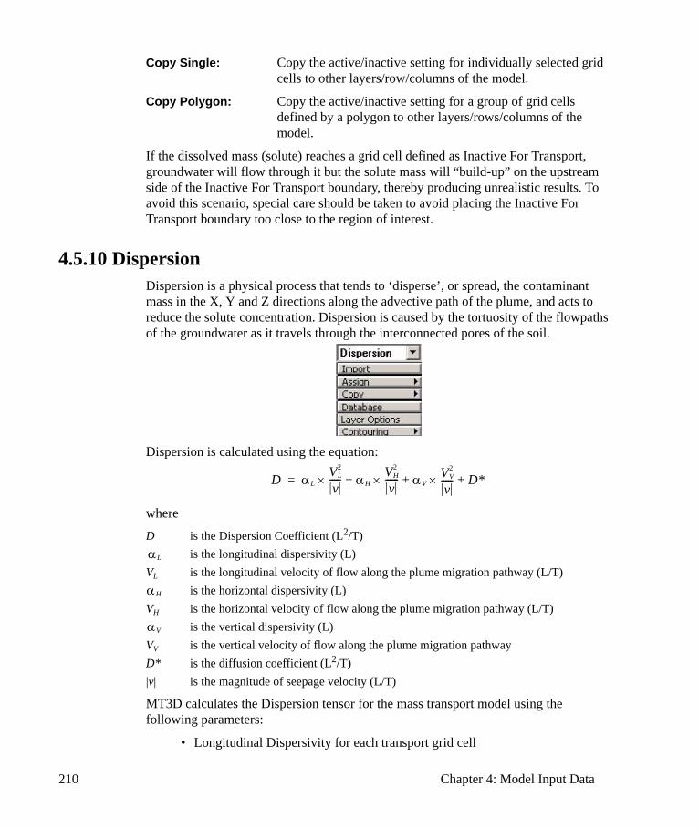
210 Chapter 4: Model Input Data
Copy Single: Copy the active/inactive setting for individually selected grid cells to other layers/row/columns of the model.
Copy Polygon: Copy the active/inactive setting for a group of grid cells defined by a polygon to other layers/rows/columns of the model.
If the dissolved mass (solute) reaches a grid cell defined as Inactive For Transport, groundwater will flow through it but the solute mass will “build-up” on the upstream side of the Inactive For Transport boundary, thereby producing unrealistic results. To avoid this scenario, special care should be taken to avoid placing the Inactive For Transport boundary too close to the region of interest.
4.5.10 DispersionDispersion is a physical process that tends to ‘disperse’, or spread, the contaminant mass in the X, Y and Z directions along the advective path of the plume, and acts to reduce the solute concentration. Dispersion is caused by the tortuosity of the flowpaths of the groundwater as it travels through the interconnected pores of the soil.
Dispersion is calculated using the equation:
where
D is the Dispersion Coefficient (L2/T)is the longitudinal dispersivity (L)
VL is the longitudinal velocity of flow along the plume migration pathway (L/T)is the horizontal dispersivity (L)
VH is the horizontal velocity of flow along the plume migration pathway (L/T)is the vertical dispersivity (L)
VV is the vertical velocity of flow along the plume migration pathwayD* is the diffusion coefficient (L2/T)|v| is the magnitude of seepage velocity (L/T)
MT3D calculates the Dispersion tensor for the mass transport model using the following parameters:
• Longitudinal Dispersivity for each transport grid cell
D αLVL
2
v-----× αH
VH2
v------× αV
VV2
v----- D*+×+ +=
αL
αH
αV
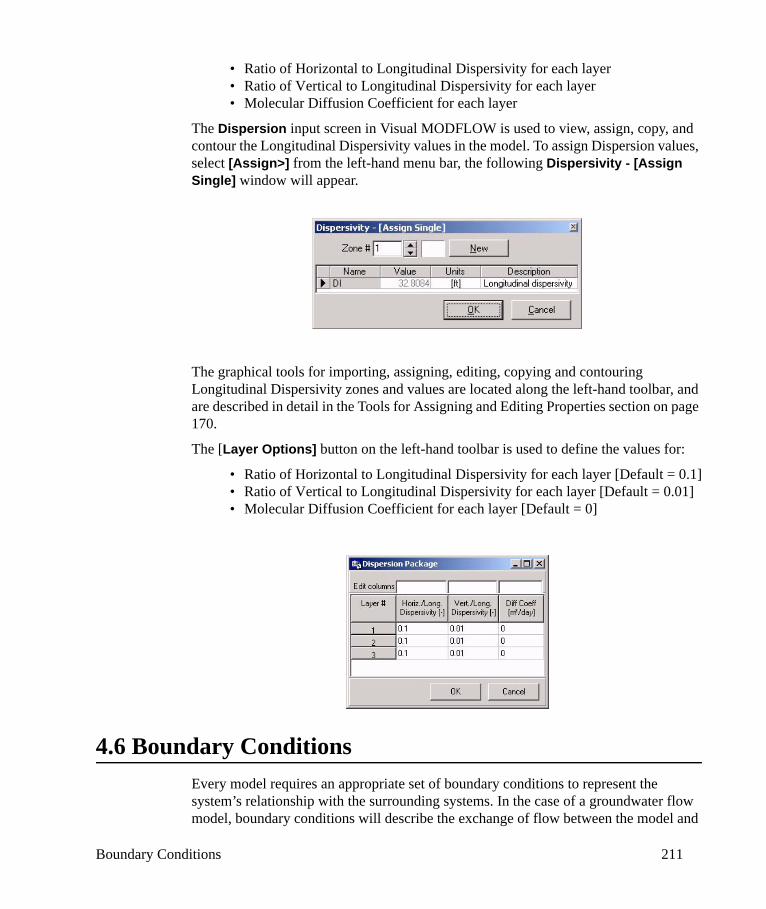
Boundary Conditions 211
• Ratio of Horizontal to Longitudinal Dispersivity for each layer• Ratio of Vertical to Longitudinal Dispersivity for each layer• Molecular Diffusion Coefficient for each layer
The Dispersion input screen in Visual MODFLOW is used to view, assign, copy, and contour the Longitudinal Dispersivity values in the model. To assign Dispersion values, select [Assign>] from the left-hand menu bar, the following Dispersivity - [Assign Single] window will appear.
The graphical tools for importing, assigning, editing, copying and contouring Longitudinal Dispersivity zones and values are located along the left-hand toolbar, and are described in detail in the Tools for Assigning and Editing Properties section on page 170.
The [Layer Options] button on the left-hand toolbar is used to define the values for:
• Ratio of Horizontal to Longitudinal Dispersivity for each layer [Default = 0.1]• Ratio of Vertical to Longitudinal Dispersivity for each layer [Default = 0.01]• Molecular Diffusion Coefficient for each layer [Default = 0]
4.6 Boundary ConditionsEvery model requires an appropriate set of boundary conditions to represent the system’s relationship with the surrounding systems. In the case of a groundwater flow model, boundary conditions will describe the exchange of flow between the model and
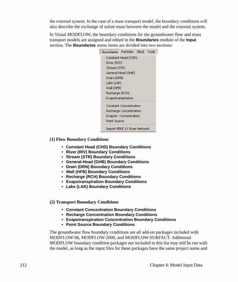
212 Chapter 4: Model Input Data
the external system. In the case of a mass transport model, the boundary conditions will also describe the exchange of solute mass between the model and the external system.
In Visual MODFLOW, the boundary conditions for the groundwater flow and mass transport models are assigned and edited in the Boundaries module of the Input section. The Boundaries menu items are divided into two sections:
(1) Flow Boundary Conditions
• Constant Head (CHD) Boundary Conditions• River (RIV) Boundary Conditions• Stream (STR) Boundary Conditions• General-Head (GHB) Boundary Conditions• Drain (DRN) Boundary Conditions• Wall (HFB) Boundary Conditions• Recharge (RCH) Boundary Conditions• Evapotranspiration Boundary Conditions• Lake (LAK) Boundary Conditions
(2) Transport Boundary Conditions
• Constant Concentration Boundary Conditions• Recharge Concentration Boundary Conditions• Evapotranspiration Concentration Boundary Conditions• Point Source Boundary Conditions
The groundwater flow boundary conditions are all add-on packages included with MODFLOW-96, MODFLOW-2000, and MODFLOW-SURFACT. Additional MODFLOW boundary condition packages not included in this list may still be run with the model, as long as the input files for these packages have the same project name and

Boundary Conditions 213
are located in the same project directory (see the Running Input Files From Unsupported Packages section on page 389 for details).
The mass transport boundary conditions are supported by the various mass transport codes included with Visual MODFLOW (e.g. MT3Dv.1.5, MT3D96 (not available for new projects/variants), MT3DMS, MT3D99, SEAWAT, RT3Dv.1, RT3Dv.2.5, and PHT3D).
Note: If no transport variant has been selected, the Transport Boundary conditions will be disabled
4.6.1 Tools for Assigning and Editing Boundary ConditionsIn general, each boundary conditions has the same set of graphical tools on the left-hand toolbar for assigning, editing, erasing, and copying the model boundary conditions. The following is a description of how to use these options. For specific descriptions of the data requirements and data entry options, refer to the sections describing each boundary condition type.
[Assign >]
• [Assign >] Single is used to select individual grid cells where the boundary condition will be assigned. Hold the mouse button down to select multiple grid cells, or click the right mouse button to deselect grid cells.
• [Assign >] Line is used to digitize a line along the grid cells where the boundary condition will be assigned. Left-Click at the start point of the line and continue to Left-Click at each node of the line. Right-Click at the end point of the line.
• [Assign >] Polygon is used to digitize a polygon around the group of grid cells where the boundary condition will be assigned. Left-Click at the start point of the polygon to begin digitizing the shape of the polygon and Right-Click near the start point to close the polygon.
• [Assign >] Window is used to stretch a Window (rectangle) around the group of grid cells where the boundary condition will be assigned. Left-Click at one corner of the window, and Left-Click again at the opposite corner to define the window dimensions.
[Edit >]
• [Edit >] Single is used to edit one or more grid cells belonging to the same group of boundary condition cells.
• [Edit >] Group is used to edit all of the grid cells belonging to the selected group of boundary condition cells.
• [Edit >] Property is used to edit the parameter values associated with a boundary condition zone.
[Erase >]
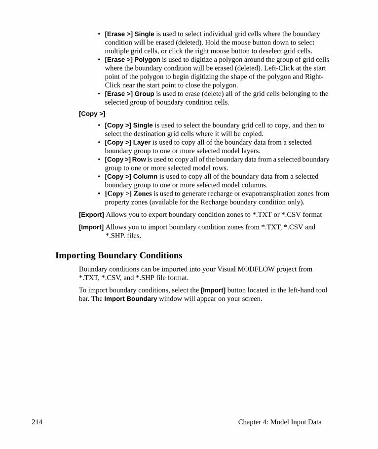
214 Chapter 4: Model Input Data
• [Erase >] Single is used to select individual grid cells where the boundary condition will be erased (deleted). Hold the mouse button down to select multiple grid cells, or click the right mouse button to deselect grid cells.
• [Erase >] Polygon is used to digitize a polygon around the group of grid cells where the boundary condition will be erased (deleted). Left-Click at the start point of the polygon to begin digitizing the shape of the polygon and Right-Click near the start point to close the polygon.
• [Erase >] Group is used to erase (delete) all of the grid cells belonging to the selected group of boundary condition cells.
[Copy >]
• [Copy >] Single is used to select the boundary grid cell to copy, and then to select the destination grid cells where it will be copied.
• [Copy >] Layer is used to copy all of the boundary data from a selected boundary group to one or more selected model layers.
• [Copy >] Row is used to copy all of the boundary data from a selected boundary group to one or more selected model rows.
• [Copy >] Column is used to copy all of the boundary data from a selected boundary group to one or more selected model columns.
• [Copy >] Zones is used to generate recharge or evapotranspiration zones from property zones (available for the Recharge boundary condition only).
[Export] Allows you to export boundary condition zones to *.TXT or *.CSV format
[Import] Allows you to import boundary condition zones from *.TXT, *.CSV and *.SHP. files.
Importing Boundary ConditionsBoundary conditions can be imported into your Visual MODFLOW project from *.TXT, *.CSV, and *.SHP file format.
To import boundary conditions, select the [Import] button located in the left-hand tool bar. The Import Boundary window will appear on your screen.
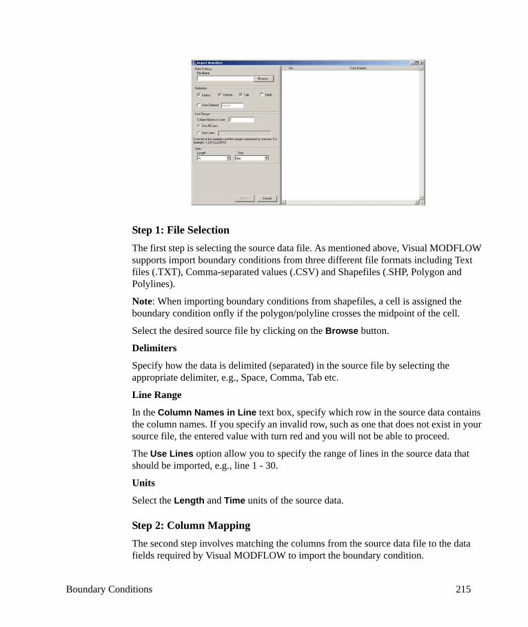
Boundary Conditions 215
Step 1: File SelectionThe first step is selecting the source data file. As mentioned above, Visual MODFLOW supports import boundary conditions from three different file formats including Text files (.TXT), Comma-separated values (.CSV) and Shapefiles (.SHP, Polygon and Polylines).
Note: When importing boundary conditions from shapefiles, a cell is assigned the boundary condition onfly if the polygon/polyline crosses the midpoint of the cell.
Select the desired source file by clicking on the Browse button.
Delimiters
Specify how the data is delimited (separated) in the source file by selecting the appropriate delimiter, e.g., Space, Comma, Tab etc.
Line Range
In the Column Names in Line text box, specify which row in the source data contains the column names. If you specify an invalid row, such as one that does not exist in your source file, the entered value with turn red and you will not be able to proceed.
The Use Lines option allow you to specify the range of lines in the source data that should be imported, e.g., line 1 - 30.
Units
Select the Length and Time units of the source data.
Step 2: Column MappingThe second step involves matching the columns from the source data file to the data fields required by Visual MODFLOW to import the boundary condition.

216 Chapter 4: Model Input Data
Co-ordinate Column Mapping Specify which columns in the source file represent the Row, Column and Layer data. If you wish to import the boundary condition to the layer currently being viewed, specify a value of 0 in the Layer field.
Time Column Mapping
Specify the columns in the source data that represent Start Time and End Time. If you wish to override the start time and end time in the source file, you can specify a constant values in the Default Start Time and Default Stop Time fields.
Grouping Code Column Mapping Specify the column in the source data that represents the grouping code.
Step 3: Mapping Boundary Condition ParametersThe next step involves mapping the boundary condition parameters in the source data to the field required by Visual MODFLOW.
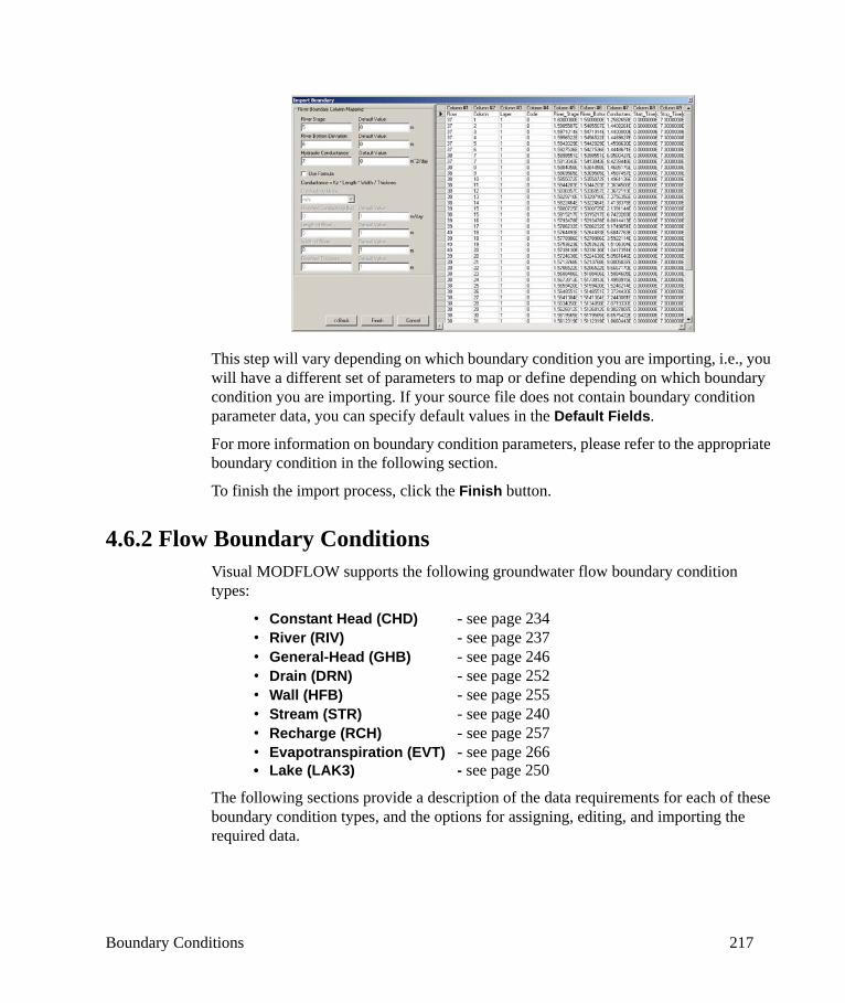
Boundary Conditions 217
This step will vary depending on which boundary condition you are importing, i.e., you will have a different set of parameters to map or define depending on which boundary condition you are importing. If your source file does not contain boundary condition parameter data, you can specify default values in the Default Fields.
For more information on boundary condition parameters, please refer to the appropriate boundary condition in the following section.
To finish the import process, click the Finish button.
4.6.2 Flow Boundary ConditionsVisual MODFLOW supports the following groundwater flow boundary condition types:
• Constant Head (CHD) - see page 234• River (RIV) - see page 237• General-Head (GHB) - see page 246• Drain (DRN) - see page 252• Wall (HFB) - see page 255• Stream (STR) - see page 240• Recharge (RCH) - see page 257• Evapotranspiration (EVT) - see page 266• Lake (LAK3) - see page 250
The following sections provide a description of the data requirements for each of these boundary condition types, and the options for assigning, editing, and importing the required data.
218 Chapter 4: Model Input Data
Steady-State vs. Transient Flow Boundary ConditionsFor transient simulations, MODFLOW requires the time element of the boundary conditions to be defined using Stress Period “counters” as opposed to using “real” times. As a result, each time interval for a transient model must be determined in terms of Stress Periods before any boundary condition data is defined. Unfortunately, accommodating this format is quite tedious because the data collected for rainfall and groundwater recharge doesn’t always follow the same time schedules as data collected for other boundary conditions like well pumping rates and surface water levels. This approach also makes it difficult to utilize raw field data collected and recorded in terms of real times.
In Visual MODFLOW, a Time Period is similar to a Stress Period, but with two important exceptions:
• A Time Period is defined using real times and real time units, and • Each boundary condition grid cell may contain different Time Periods
The advantage of this approach is the ability to clearly see the magnitude of time for each Time Period (as opposed to interpreting data such as “from Stress Period 1 to Stress Period 2”), and it facilitates more convenient methods for importing raw data from different boundary condition types.
Each group of boundary condition grid cells requires a minimum of one Time Period of data containing a Start Time, a Stop Time, and a complete set of data for the selected boundary condition type (the required data for each boundary condition type are described later in this section). For steady-state simulations, Visual MODFLOW requires data for only a single Time Period, while for transient simulations, Visual MODFLOW can accommodate an unlimited number of Time Periods.
For steady-state simulations the Stop Time value is irrelevant because the term “steady-state” indicates that the model results are not changing with time. Therefore, a Stop Time value of 1 time unit is commonly used. However, if the model is going to be used to evaluate a transient simulation in the future, it is probably a better idea to give it a more realistic value corresponding to the potential time frame of interest.
If a steady-state simulation is run using a model containing transient boundary condition data, only the data from the first Time Period of each grid cell will be used for the steady-state conditions.
If a transient model is run for 10 years, and a boundary condition is defined only for a period up to 7 years, Visual MODFLOW will assume this boundary condition does not exist for the remaining 3 years of the simulation. The exception to this rule are the Constant Head and Constant Concentration Boundaries, which must be defined for the entire simulation.
Note: For a steady-state simulation, a minimum of one active grid cell in the model MUST contain a head-dependent boundary condition type. Otherwise, the model is indeterminate and the solution will not
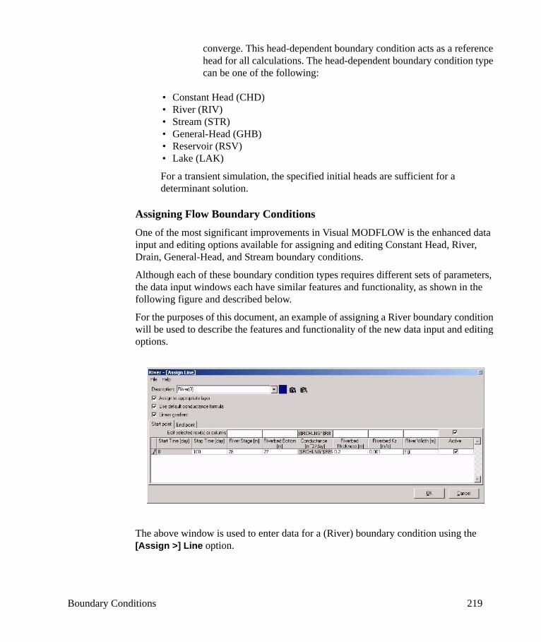
Boundary Conditions 219
converge. This head-dependent boundary condition acts as a reference head for all calculations. The head-dependent boundary condition type can be one of the following:
• Constant Head (CHD)• River (RIV)• Stream (STR)• General-Head (GHB)• Reservoir (RSV)• Lake (LAK)
For a transient simulation, the specified initial heads are sufficient for a determinant solution.
Assigning Flow Boundary ConditionsOne of the most significant improvements in Visual MODFLOW is the enhanced data input and editing options available for assigning and editing Constant Head, River, Drain, General-Head, and Stream boundary conditions.
Although each of these boundary condition types requires different sets of parameters, the data input windows each have similar features and functionality, as shown in the following figure and described below.
For the purposes of this document, an example of assigning a River boundary condition will be used to describe the features and functionality of the new data input and editing options.
The above window is used to enter data for a (River) boundary condition using the [Assign >] Line option.
220 Chapter 4: Model Input Data
DescriptionThe Description is an alphanumeric description for the selected group of model grid cells. This Description is used to identify this group of grid cells for the purpose of editing the boundary condition attributes for the entire group of cells at a later time (see the Editing Flow Boundary Conditions section on page 230).
Assign to appropriate layerThe Assign to appropriate layer option is used to automatically assign the boundary condition being entered to the grid cell in the ‘appropriate’ layer, where the appropriate grid cell is located in the layer corresponding to the head-related value being assigned to the selected grid cell.
For Constant Head, River, and Stream boundary conditions, MODFLOW does not allow the head-related values (Head, River Stage and Stream Stage, respectively) to be less than the bottom elevation of the grid cell in which the boundary condition is assigned. If the head-related value assigned to the selected grid cell is lower than the grid cell bottom elevation, this option will essentially ‘push’ the boundary condition down from the selected grid cell to the next lowest grid cell, where the head-related value is not below the grid cell bottom elevation.
Consider a model with the following dimensions:
• 0 – 1000 m in the X-Direction• 0 – 1000 m in the Y-Direction• 0 – 100 m in the Z-Direction• 10 rows x 10 columns x 5 layers of equal thicknesses
If a Constant Head boundary condition of 70 m is assigned along the west boundary in Layer 1, Visual MODFLOW will not accept it because 70 m is below the bottom elevation (80 m) of Layer 1. However, if the Assign to appropriate layer option is selected, Visual MODFLOW will accept this data and automatically assigns the Constant Head boundary condition to the same cells in Layer 2 instead.
Use default conductance formulaThe Use default conductance formula option is used to calculate the Conductance value for River, Stream, Drain and General Head boundary conditions using a mathematical expression containing array variables (see the Using Mathematical Formulas and Array Variables section on page 224). If the Use default conductance formula option is selected (as shown in the preceding figure) the conductance value will be calculated using a default formula associated with each boundary condition type. If the Use default conductance formula option is not selected, a conductance value will need to be entered manually.
The advantage of using the default conductance formula to calculate the conductance values for the group of grid cells is that each grid cell will be assigned a conductance value proportional to the size of the grid cell.
Boundary Conditions 221
Note: If the [Assign >] Line option is used to select the grid cells, then the default conductance formula will use the length of the line passing through each cell to calculate the conductance. If the [Assign >] Single or [Assign >] Polygon options are used to select the grid cells, then the default conductance formula will use the cell dimensions to calculate the conductance.
Linear gradientThe Linear gradient option is only available when [Assign > Line] is used to select the boundary condition grid cells. If the Linear gradient option is not selected, then the Assign Line data entry window will require a single set of attributes to be assigned to each grid cell intersected by the line. If the Linear gradient option is selected (as shown in the preceding figure) then the Assign Line window will prompt for two sets of boundary condition data; one set for the grid cell at the Start Point of the line, and one set for the grid cell at the End Point of the line. The boundary condition data for the grid cells between the Start Point grid cell and the End Point grid cell will be linearly interpolated between these two points using the formula below.
where
$Xi is the boundary condition parameter value at the ith grid cell along the line
$XSP is the boundary condition parameter value at the Start Point of the line
$XEP is the boundary condition parameter value at the End Point of the line
$TVAR1, i is the cumulative length of the line at the ith grid cell along the line, as measured from the center of the Start Point grid cell through the center of each successive grid cell along the line (see following figure).
$LENGTH is the total length of the line, as measured from the center of the Start Point grid cell through to the center of the End Point grid cell (see following figure).
When the line is digitized from the Start Point to the End Point, each grid cell is numbered in sequence according to the order in which the line passes through each cell. If the line passes through the same grid cell twice, the grid cell will be numbered twice as seen for grid cell “4” and “6” in the following figure. As a result, the parameter value calculated for “grid cell #6” will over-write the parameter value calculated for “grid cell #4”.
$Xi $XSP $XSP $XEP–( )$TVAR1 i,$LENGTH----------------------------×+=
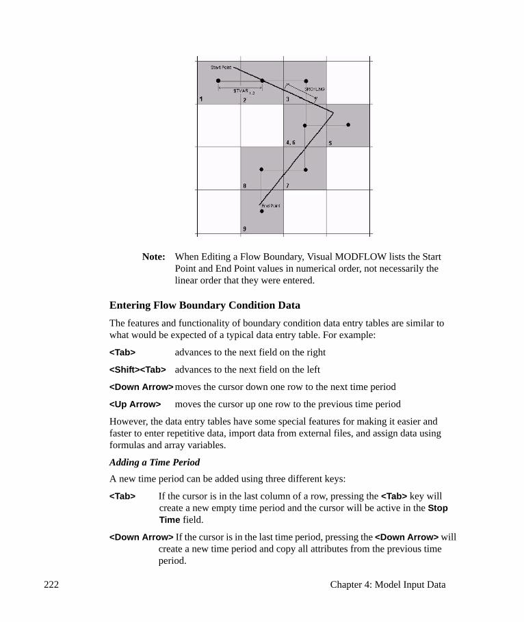
222 Chapter 4: Model Input Data
Note: When Editing a Flow Boundary, Visual MODFLOW lists the Start Point and End Point values in numerical order, not necessarily the linear order that they were entered.
Entering Flow Boundary Condition DataThe features and functionality of boundary condition data entry tables are similar to what would be expected of a typical data entry table. For example:
<Tab> advances to the next field on the right
<Shift><Tab> advances to the next field on the left
<Down Arrow> moves the cursor down one row to the next time period
<Up Arrow> moves the cursor up one row to the previous time period
However, the data entry tables have some special features for making it easier and faster to enter repetitive data, import data from external files, and assign data using formulas and array variables.
Adding a Time PeriodA new time period can be added using three different keys:
<Tab> If the cursor is in the last column of a row, pressing the <Tab> key will create a new empty time period and the cursor will be active in the Stop Time field.
<Down Arrow> If the cursor is in the last time period, pressing the <Down Arrow> will create a new time period and copy all attributes from the previous time period.

Boundary Conditions 223
<Enter> If the cursor is in the last time period, pressing the <Enter> key will create a new empty time period.
Deleting a Time PeriodUnwanted time periods can be deleted by Right-Clicking the mouse in the far left field of the time period and choosing the Delete selected row(s) option.
Inserting a Time PeriodA time period can be inserted into an existing schedule by Right-Clicking the mouse in the far left field of the time period immediately following (below) the time to be inserted and selecting the Insert row option.
Specifying Active/Inactive Time PeriodsFor River, Drain, General-Head, Stream, and Recharge boundary conditions, you can disable the selected Time Periods by removing the check marks from the Active column, which “turns off” the boundary condition for that particular Time Period. However, for Constant Head and Constant Concentration boundary condition, MODFLOW requires the boundary to be present (i.e. active) for all Time Periods throughout the entire simulation, and therefore no Time Period can be disabled.
Copying Repetitive DataIn many cases with transient simulations, there will only be a single parameter for each boundary condition type that changes with time (usually the head-related parameter). For example, with a River boundary, the River Stage value will change with time, but the River Bottom and the Conductance are usually static regardless of the season. However, MODFLOW requires that each attribute of a boundary condition must be defined for each time period. In order to make this data entry more convenient, the data from the current time period can be copied to the next time period by pressing the <Down Arrow> key to create a new time period. Alternately, pressing the <Tab> key in an empty field of the new time period will automatically copy the attribute value from the previous time period.
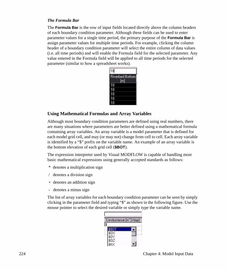
224 Chapter 4: Model Input Data
The Formula BarThe Formula Bar is the row of input fields located directly above the column headers of each boundary condition parameter. Although these fields can be used to enter parameter values for a single time period, the primary purpose of the Formula Bar is assign parameter values for multiple time periods. For example, clicking the column header of a boundary condition parameter will select the entire column of data values (i.e. all time periods) and will enable the Formula field for the selected parameter. Any value entered in the Formula field will be applied to all time periods for the selected parameter (similar to how a spreadsheet works).
Using Mathematical Formulas and Array VariablesAlthough most boundary condition parameters are defined using real numbers, there are many situations where parameters are better defined using a mathematical formula containing array variables. An array variable is a model parameter that is defined for each model grid cell, and may (or may not) change from cell to cell. Each array variable is identified by a “$” prefix on the variable name. An example of an array variable is the bottom elevation of each grid cell ($BOT).
The expression interpreter used by Visual MODFLOW is capable of handling most basic mathematical expressions using generally accepted standards as follows:
* denotes a multiplication sign
/ denotes a division sign
+ denotes an addition sign
- denotes a minus sign
The list of array variables for each boundary condition parameter can be seen by simply clicking in the parameter field and typing “$” as shown in the following figure. Use the mouse pointer to select the desired variable or simply type the variable name.

Boundary Conditions 225
Note: If a variable name is manually entered without the “$” prefix, it will not be recognized by Visual MODFLOW and a “Syntax error” message will be issued upon trying to close the data entry window.
The array variables available for creating mathematical expressions are as follows:
$BOT: Bottom elevation of grid cell [L]
$DX: Length of grid cell in X-direction [L]
$DY: Length of grid cell in Y-direction [L]
$DZ: Length (thickness) of grid cell in Z-direction [L]
$KX: Hydraulic conductivity in the X-direction [L/T]
$KY: Hydraulic conductivity in the Y-direction [L/T]
$KZ: Hydraulic conductivity in the Z-direction [L/T]
$MBOT: Model bottom elevation for the X-Y location of the grid cell [L]
$UCTOCOND: Unit conversion factor for converting the length and time units used for hydraulic conductivity to the length and time units used for Conductance
$RCHLNG: Length of line passing through each grid cell (in units of length)1
$LENGTH: Total length of the line as measured through the center of each grid cell (in units of length)1
$TVAR: Cumulative length of line as measured through the center of each grid cell (in units of length)1
Additional array variables are available for specific boundary condition types depending on the parameters required.
A common example of where a mathematical expression containing array variables is useful would be for defining the Conductance values for grid cells containing a River boundary condition (see the River (RIV) Boundary Conditions section on page 237). In this example, the Conductance for the River boundary condition in each grid cell is calculated using the following formula:
where
1. $RCHLNG, $LENGTH and $TVAR variables are only available when the [Assign >] Line option has been used to select the grid cells.
$COND $RCHLNG $RBWIDTH× $K×$RBTHICK
----------------------------------------------------------------------------------⎝ ⎠⎛ ⎞ $UCTOCOND×=
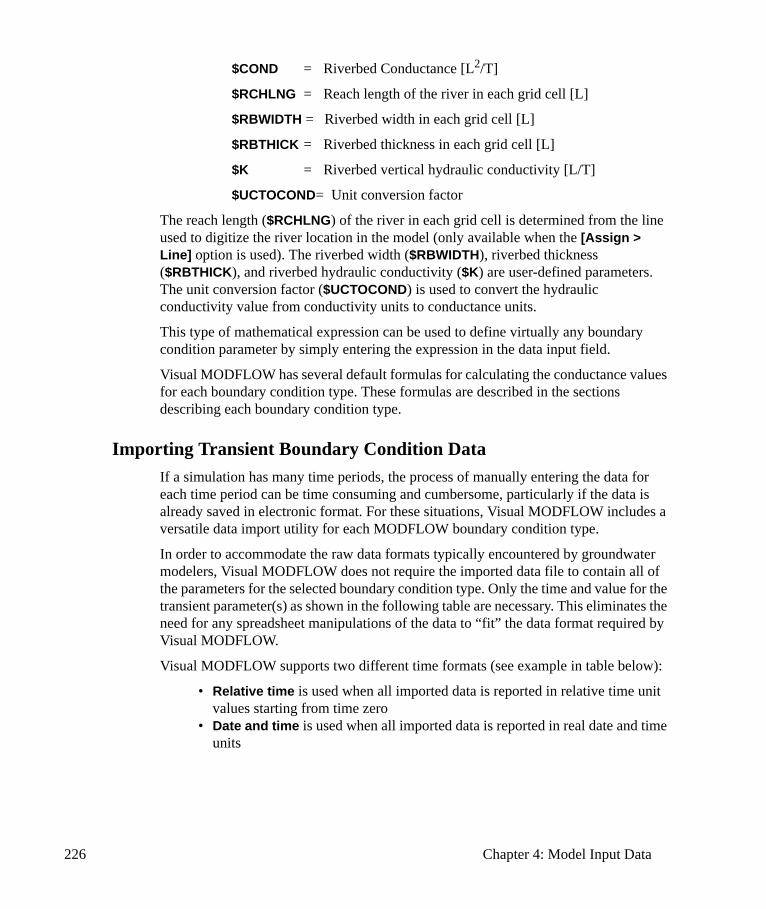
226 Chapter 4: Model Input Data
$COND = Riverbed Conductance [L2/T]
$RCHLNG = Reach length of the river in each grid cell [L]
$RBWIDTH = Riverbed width in each grid cell [L]
$RBTHICK = Riverbed thickness in each grid cell [L]
$K = Riverbed vertical hydraulic conductivity [L/T]
$UCTOCOND= Unit conversion factor
The reach length ($RCHLNG) of the river in each grid cell is determined from the line used to digitize the river location in the model (only available when the [Assign > Line] option is used). The riverbed width ($RBWIDTH), riverbed thickness ($RBTHICK), and riverbed hydraulic conductivity ($K) are user-defined parameters. The unit conversion factor ($UCTOCOND) is used to convert the hydraulic conductivity value from conductivity units to conductance units.
This type of mathematical expression can be used to define virtually any boundary condition parameter by simply entering the expression in the data input field.
Visual MODFLOW has several default formulas for calculating the conductance values for each boundary condition type. These formulas are described in the sections describing each boundary condition type.
Importing Transient Boundary Condition DataIf a simulation has many time periods, the process of manually entering the data for each time period can be time consuming and cumbersome, particularly if the data is already saved in electronic format. For these situations, Visual MODFLOW includes a versatile data import utility for each MODFLOW boundary condition type.
In order to accommodate the raw data formats typically encountered by groundwater modelers, Visual MODFLOW does not require the imported data file to contain all of the parameters for the selected boundary condition type. Only the time and value for the transient parameter(s) as shown in the following table are necessary. This eliminates the need for any spreadsheet manipulations of the data to “fit” the data format required by Visual MODFLOW.
Visual MODFLOW supports two different time formats (see example in table below):
• Relative time is used when all imported data is reported in relative time unit values starting from time zero
• Date and time is used when all imported data is reported in real date and time units
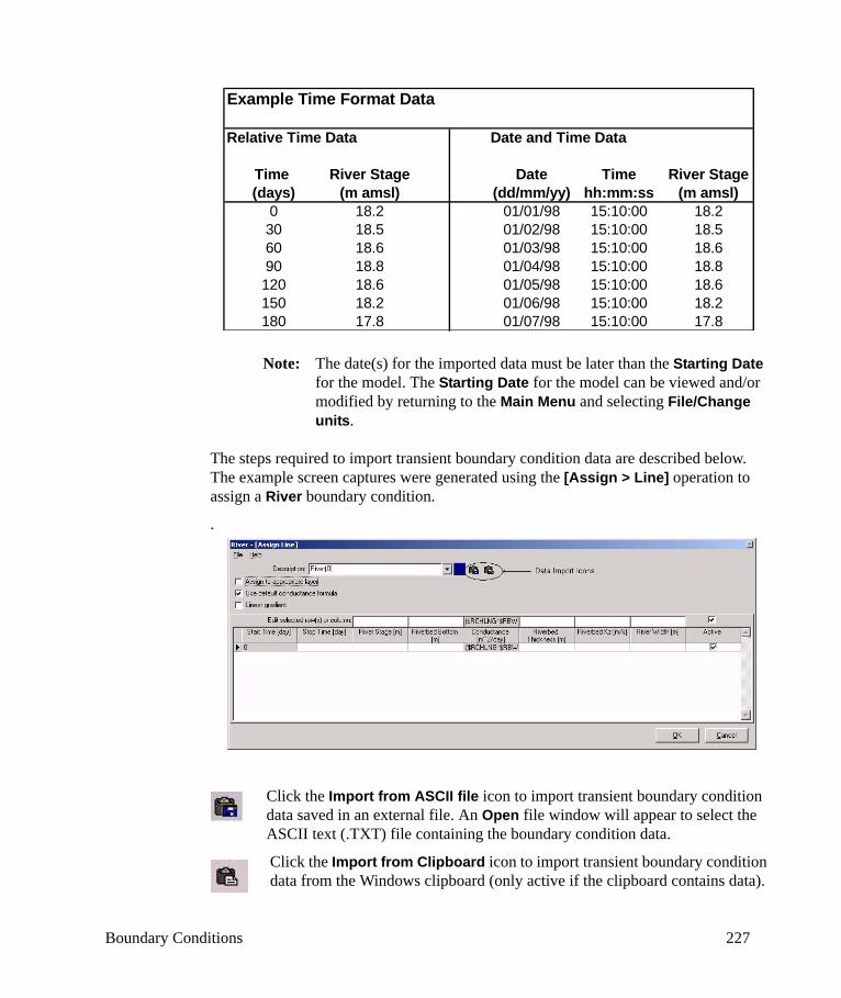
Boundary Conditions 227
Note: The date(s) for the imported data must be later than the Starting Date for the model. The Starting Date for the model can be viewed and/or modified by returning to the Main Menu and selecting File/Change units.
The steps required to import transient boundary condition data are described below. The example screen captures were generated using the [Assign > Line] operation to assign a River boundary condition.
.
Click the Import from ASCII file icon to import transient boundary condition data saved in an external file. An Open file window will appear to select the ASCII text (.TXT) file containing the boundary condition data.
Click the Import from Clipboard icon to import transient boundary condition data from the Windows clipboard (only active if the clipboard contains data).
Example Time Format Data
Relative Time Data Date and Time Data
Time River Stage Date Time River Stage(days) (m amsl) (dd/mm/yy) hh:mm:ss (m amsl)
0 18.2 01/01/98 15:10:00 18.230 18.5 01/02/98 15:10:00 18.560 18.6 01/03/98 15:10:00 18.690 18.8 01/04/98 15:10:00 18.8120 18.6 01/05/98 15:10:00 18.6150 18.2 01/06/98 15:10:00 18.2180 17.8 01/07/98 15:10:00 17.8

228 Chapter 4: Model Input Data
Alternately, Import from ASCII file or Import from Clipboard options (as shown on the right hand side) can be activated by clicking on File from the menu bar.
Once the data file is selected, the following Import window will appear.
Note: The Import from ASCII file window shown above has the same functionality as the Import from Clipboard option.
The Options menu lists six different options corresponding to the icons listed in the toolbar:
Load new data file Loads a different ASCII data file
Paste data from clipboard Replaces the existing data with data from the Windows clipboard (only active if the clipboard contains data).
Reload source data file Reloads the source data file after changes have been made
Boundary Conditions 229
Edit source data file Open and edit the source data file
Preview imported data Previews the imported data set as it will appear in the boundary condition data entry table
Preview data file Previews the data being imported in the data preview tableThe Delimiters frame provides a selection of common delimiters used to sepa-rate different data values in the same row. If the required delimiter is not avail-
able in the pre-defined delimiters, a User-defined delimiter can be entered.
The Use column names in line field is used to identify which line of the data file contains the titles (header) for each column of data. The default setting is “0”.
The Number of lines to skip field is used to identify the number of lines of data to skip. This is used if some redundant or unreliable data occurs at the start of the data file. The default setting is “0”, indicating that the first line of the data file will be read.
The Number of lines to read field is used to identify how many lines of data will be imported. This is used if some redundant or unreliable data occurs at the end of the data file. The default setting is “0” indicating that all data after the starting point will be imported.
The Time schedule in field contains a selection of two time formats: Relative time and Date and time (see "Importing Transient Boundary Condition Data" on page 226).
The Date format field is used to select the appropriate date format for the ASCII data file. This field is only available when Date and Time are selected in the Time Schedule field.
The Time format field is used to select the appropriate time format for the ASCII data file. This field is only available when Date and Time are selected in the Time Schedule field.
The Interpolation method field is used to select the appropriate interpolation method to use for creating the time schedules containing Start Time and Stop Time for each time period. The time interpolation method selected will determine how the data from the data files are manipulated to fit the required format. There are four time interpolation methods available:
• Piece-wise backward• Piece-wise middle• Piece-wise forward• Linear Gradient (only available for Constant Head boundary condition)
The Browse [...] button shows a graphical description of each interpolation method, and indicates how the raw data is interpreted and manipulated by Visual MODFLOW to fit the required time period format.
230 Chapter 4: Model Input Data
Note: It is important to consider how the Interpolation method selected will affect the data being imported into your model. You may need to add an extra line to your input file at the start, or the end, of the file to accommodate the Interpolation method you have selected.
The Required Data column lists the parameters required by the selected boundary condition type. In the example above, the Required Data column lists the parameters required by the River boundary condition.
The Match to column number column is used to match the Required Data fields to the columns of data from the ASCII text file. In the preceding example, the ASCII text file contained only two columns of data; (1) Time, and (2) River Stage. As a result:
• Column #1 is matched to the Relative time field, and • Column #2 is matched to the River Stage field.
The remaining Required Data fields may be left as “n/a” (not available) or as blank entries, and not assigned any values during the data import process.
Editing Flow Boundary ConditionsExisting boundary condition data can be modified by selecting either [Edit > Single], or [Edit > Group] from the toolbar on the left-hand side of the Visual MODFLOW window.
• The [Edit > Single] option can be used to select one or more grid cells belonging to the same group of boundary condition cells.
• The [Edit > Group] option can be used to select all of the grid cells belonging to the selected group of boundary condition cells.
Once the desired grid cells are selected, a Boundary Condition - Edit window will appear as shown in the following figure. This window will have different parameters depending on the selected boundary condition type (e.g. River in this case), but the functionality of this window is similar for most MODFLOW boundary conditions.
The Boundary Condition - Edit window has a very similar appearance, and much of the same functionality, as the [Boundary Condition] - Assign window (discussed on page 219), but there are some important differences to be aware of:
• The parameter value entry fields in the table are disabled, meaning that no values can be entered directly into these fields
• The [Boundary Condition] - Edit window contains only MODFLOW-related parameters
• The parameter fields may contain ranges of values
Note: The reason for these differences is explained at the end of this section, but it will become apparent as the functionality of this window is explained.
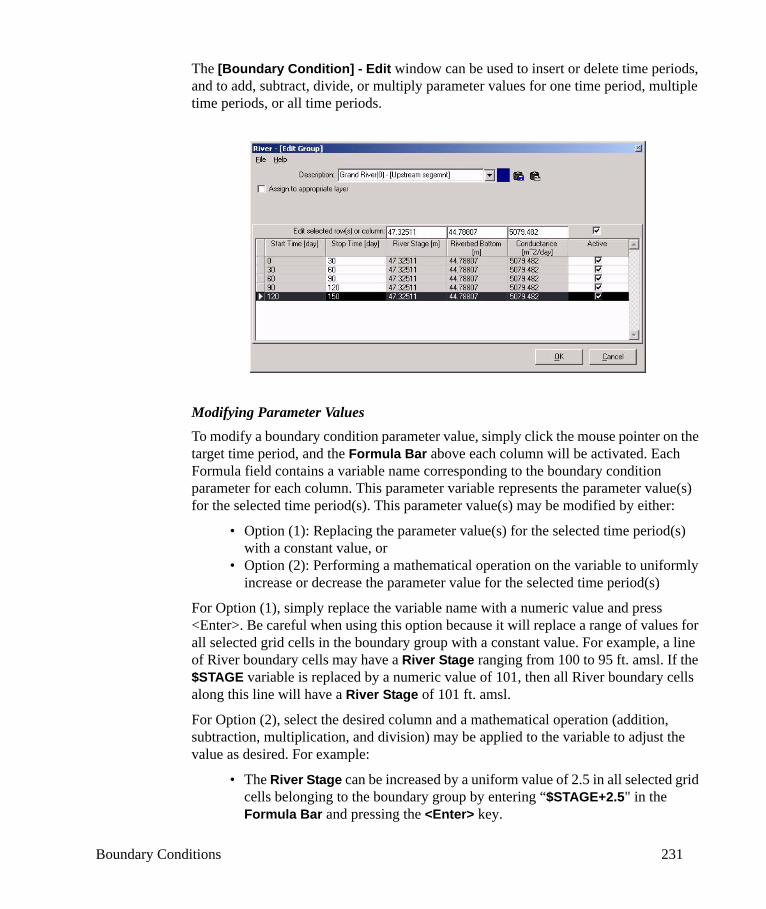
Boundary Conditions 231
The [Boundary Condition] - Edit window can be used to insert or delete time periods, and to add, subtract, divide, or multiply parameter values for one time period, multiple time periods, or all time periods.
Modifying Parameter ValuesTo modify a boundary condition parameter value, simply click the mouse pointer on the target time period, and the Formula Bar above each column will be activated. Each Formula field contains a variable name corresponding to the boundary condition parameter for each column. This parameter variable represents the parameter value(s) for the selected time period(s). This parameter value(s) may be modified by either:
• Option (1): Replacing the parameter value(s) for the selected time period(s) with a constant value, or
• Option (2): Performing a mathematical operation on the variable to uniformly increase or decrease the parameter value for the selected time period(s)
For Option (1), simply replace the variable name with a numeric value and press <Enter>. Be careful when using this option because it will replace a range of values for all selected grid cells in the boundary group with a constant value. For example, a line of River boundary cells may have a River Stage ranging from 100 to 95 ft. amsl. If the $STAGE variable is replaced by a numeric value of 101, then all River boundary cells along this line will have a River Stage of 101 ft. amsl.
For Option (2), select the desired column and a mathematical operation (addition, subtraction, multiplication, and division) may be applied to the variable to adjust the value as desired. For example:
• The River Stage can be increased by a uniform value of 2.5 in all selected grid cells belonging to the boundary group by entering “$STAGE+2.5" in the Formula Bar and pressing the <Enter> key.

232 Chapter 4: Model Input Data
• The River Stage can be multiplied by a uniform value of 1.1 in all selected grid cells belonging to the boundary group by entering “$STAGE*1.1" in the Formula Bar and pressing the <Enter> key.
• The River Stage can be decreased by a uniform value of 1.5 in all selected grid cells belonging to the boundary group by entering “$STAGE-1.5" in the Formula Bar and pressing the <Enter> key.
• The River Stage can be divided by a uniform value of 1.2 in all selected grid cells belonging to the boundary group by entering “$STAGE/1.2" in the Formula Bar and pressing the <Enter> key.
Additional array variables are also available for including in the parameter expressions, and can be viewed by simply typing "$" in the formula field. For example the River Stage may be set equal to 1.0 ft. below the top of the grid cell elevation in all grid cells by entering the following expression in the River Stage formula cell:
$BOT+$DZ-1.0
where
$BOT is the elevation of the bottom of the grid cell, and
$DZ is the length (thickness) of the grid cell in the Z-direction
Selecting Time PeriodsTo select the time period of interest, simply click the mouse pointer on the time period containing the parameter value(s) that need to be modified. To simultaneously modify multiple time periods, click on the left-most column of the starting time period and drag the mouse to the ending time period, or hold down the <Ctrl> key and click on individual time periods. To simultaneously modify a parameter for all time periods, click the mouse pointer in the column header of the parameter.
Inserting a Time PeriodTo insert a time period in the time schedule, Right-Click the mouse pointer in the time period that should be sub-divided, and select the Insert row option. A new time period will be created containing the data from the previous time period and with a blank Stop Time value. The Stop Time value entered will be automatically copied to the Start Time of the following time period.
Deleting a Time PeriodTo delete a time period from the time schedule, Right-Click the mouse pointer in the time period that should be removed and choose the Delete selected row(s) option. The selected time period and the associated data will be deleted from the time schedule, and the Start Time from the following time period will automatically be adjusted to match the Stop Time from the prior time period.
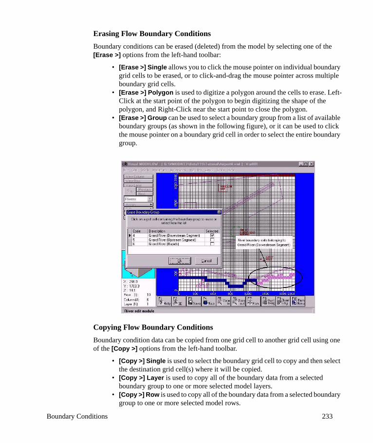
Boundary Conditions 233
Erasing Flow Boundary ConditionsBoundary conditions can be erased (deleted) from the model by selecting one of the [Erase >] options from the left-hand toolbar:
• [Erase >] Single allows you to click the mouse pointer on individual boundary grid cells to be erased, or to click-and-drag the mouse pointer across multiple boundary grid cells.
• [Erase >] Polygon is used to digitize a polygon around the cells to erase. Left-Click at the start point of the polygon to begin digitizing the shape of the polygon, and Right-Click near the start point to close the polygon.
• [Erase >] Group can be used to select a boundary group from a list of available boundary groups (as shown in the following figure), or it can be used to click the mouse pointer on a boundary grid cell in order to select the entire boundary group.
Copying Flow Boundary ConditionsBoundary condition data can be copied from one grid cell to another grid cell using one of the [Copy >] options from the left-hand toolbar.
• [Copy >] Single is used to select the boundary grid cell to copy and then select the destination grid cell(s) where it will be copied.
• [Copy >] Layer is used to copy all of the boundary data from a selected boundary group to one or more selected model layers.
• [Copy >] Row is used to copy all of the boundary data from a selected boundary group to one or more selected model rows.

234 Chapter 4: Model Input Data
• [Copy >] Column is used to copy all of the boundary data from a selected boundary group to one or more selected model columns.
Constant Head (CHD) Boundary ConditionsVisual MODFLOW supports the Time-Variant Specified-Head Package included with MODFLOW. The Visual MODFLOW input data for Constant Head grid cells is stored in the projectname.VMB file (see Appendix A), while the MODFLOW input data for Constant Head grid cells is stored in the projectname.CHD file (see the MODFLOW-2000 Reference Manual .PDF file provided with the Visual MODFLOW installation media, in the Manual folder).
The Constant Head boundary condition is used to fix the head value in selected grid cells regardless of the system conditions in the surrounding grid cells, thus acting as an infinite source of water entering the system, or as an infinite sink for water leaving the system. Therefore, Constant Head boundary conditions can have a significant influence on the results of a simulation, and may lead to unrealistic predictions, particularly when used in locations close to the area of interest.
Unlike most other transient MODFLOW boundary condition packages, the CHD package allows the specified heads to be linearly interpolated in time between the beginning and end of each stress period, such that the specified head for a grid cell may change at each time step of a given stress period. The CHD package requires the following information for each Constant Head grid cell for each stress period:
• Start Head: Specified head value at the beginning of the stress period• Stop Head: Specified head value at the end of the stress period
Constant Head boundary conditions can be assigned by selecting Boundaries/Constant Head (CHD) from the Input section of Visual MODFLOW and using any of the [Assign >] options from the left-hand toolbar (described in the Tools for Assigning and Editing Boundary Conditions section on page 213). Once the model grid cells are selected, a data input window will appear as shown in the following figure.
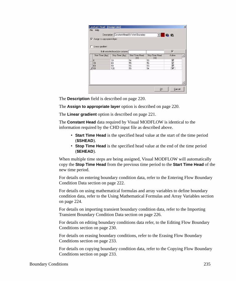
Boundary Conditions 235
The Description field is described on page 220.
The Assign to appropriate layer option is described on page 220.
The Linear gradient option is described on page 221.
The Constant Head data required by Visual MODFLOW is identical to the information required by the CHD input file as described above.
• Start Time Head is the specified head value at the start of the time period ($SHEAD).
• Stop Time Head is the specified head value at the end of the time period ($EHEAD).
When multiple time steps are being assigned, Visual MODFLOW will automatically copy the Stop Time Head from the previous time period to the Start Time Head of the new time period.
For details on entering boundary condition data, refer to the Entering Flow Boundary Condition Data section on page 222.
For details on using mathematical formulas and array variables to define boundary condition data, refer to the Using Mathematical Formulas and Array Variables section on page 224.
For details on importing transient boundary condition data, refer to the Importing Transient Boundary Condition Data section on page 226.
For details on editing boundary conditions data refer, to the Editing Flow Boundary Conditions section on page 230.
For details on erasing boundary conditions, refer to the Erasing Flow Boundary Conditions section on page 233.
For details on copying boundary condition data, refer to the Copying Flow Boundary Conditions section on page 233.
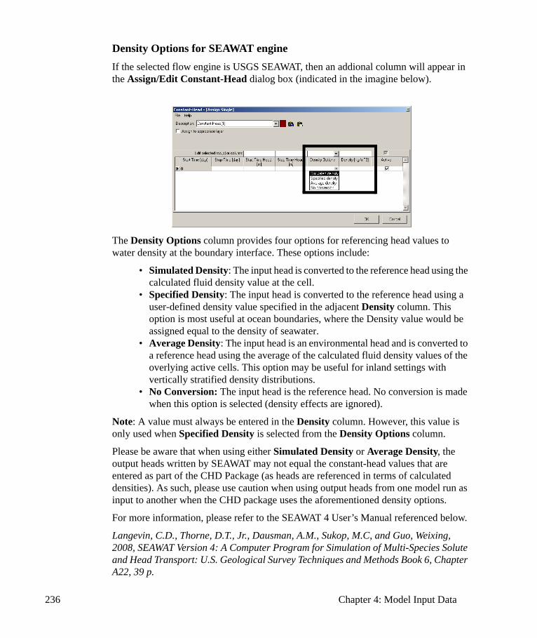
236 Chapter 4: Model Input Data
Density Options for SEAWAT engineIf the selected flow engine is USGS SEAWAT, then an addional column will appear in the Assign/Edit Constant-Head dialog box (indicated in the imagine below).
The Density Options column provides four options for referencing head values to water density at the boundary interface. These options include:
• Simulated Density: The input head is converted to the reference head using the calculated fluid density value at the cell.
• Specified Density: The input head is converted to the reference head using a user-defined density value specified in the adjacent Density column. This option is most useful at ocean boundaries, where the Density value would be assigned equal to the density of seawater.
• Average Density: The input head is an environmental head and is converted to a reference head using the average of the calculated fluid density values of the overlying active cells. This option may be useful for inland settings with vertically stratified density distributions.
• No Conversion: The input head is the reference head. No conversion is made when this option is selected (density effects are ignored).
Note: A value must always be entered in the Density column. However, this value is only used when Specified Density is selected from the Density Options column.
Please be aware that when using either Simulated Density or Average Density, the output heads written by SEAWAT may not equal the constant-head values that are entered as part of the CHD Package (as heads are referenced in terms of calculated densities). As such, please use caution when using output heads from one model run as input to another when the CHD package uses the aforementioned density options.
For more information, please refer to the SEAWAT 4 User’s Manual referenced below.
Langevin, C.D., Thorne, D.T., Jr., Dausman, A.M., Sukop, M.C, and Guo, Weixing, 2008, SEAWAT Version 4: A Computer Program for Simulation of Multi-Species Solute and Head Transport: U.S. Geological Survey Techniques and Methods Book 6, Chapter A22, 39 p.
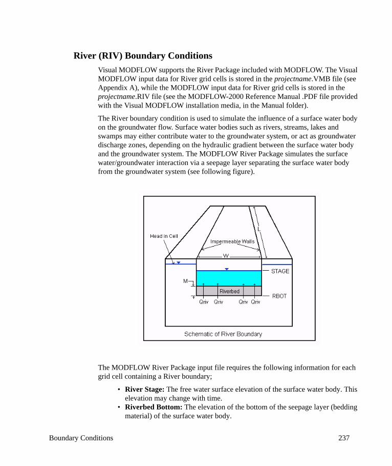
Boundary Conditions 237
River (RIV) Boundary ConditionsVisual MODFLOW supports the River Package included with MODFLOW. The Visual MODFLOW input data for River grid cells is stored in the projectname.VMB file (see Appendix A), while the MODFLOW input data for River grid cells is stored in the projectname.RIV file (see the MODFLOW-2000 Reference Manual .PDF file provided with the Visual MODFLOW installation media, in the Manual folder).
The River boundary condition is used to simulate the influence of a surface water body on the groundwater flow. Surface water bodies such as rivers, streams, lakes and swamps may either contribute water to the groundwater system, or act as groundwater discharge zones, depending on the hydraulic gradient between the surface water body and the groundwater system. The MODFLOW River Package simulates the surface water/groundwater interaction via a seepage layer separating the surface water body from the groundwater system (see following figure).
The MODFLOW River Package input file requires the following information for each grid cell containing a River boundary;
• River Stage: The free water surface elevation of the surface water body. This elevation may change with time.
• Riverbed Bottom: The elevation of the bottom of the seepage layer (bedding material) of the surface water body.
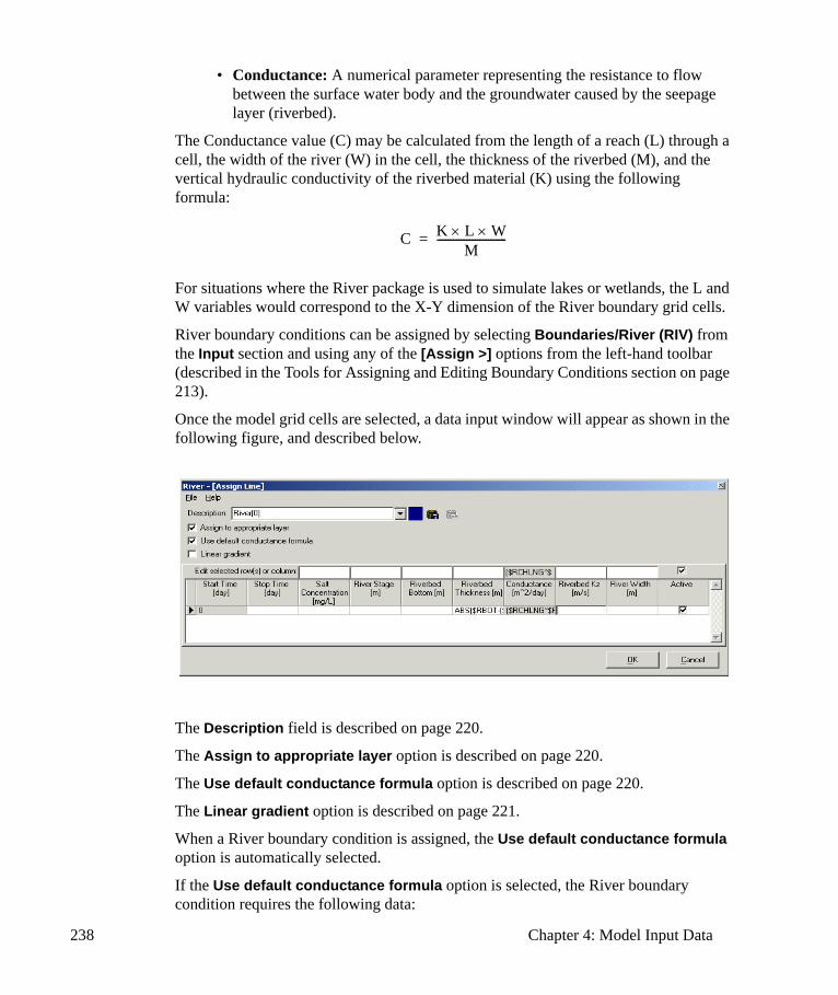
238 Chapter 4: Model Input Data
• Conductance: A numerical parameter representing the resistance to flow between the surface water body and the groundwater caused by the seepage layer (riverbed).
The Conductance value (C) may be calculated from the length of a reach (L) through a cell, the width of the river (W) in the cell, the thickness of the riverbed (M), and the vertical hydraulic conductivity of the riverbed material (K) using the following formula:
For situations where the River package is used to simulate lakes or wetlands, the L and W variables would correspond to the X-Y dimension of the River boundary grid cells.
River boundary conditions can be assigned by selecting Boundaries/River (RIV) from the Input section and using any of the [Assign >] options from the left-hand toolbar (described in the Tools for Assigning and Editing Boundary Conditions section on page 213).
Once the model grid cells are selected, a data input window will appear as shown in the following figure, and described below.
The Description field is described on page 220.
The Assign to appropriate layer option is described on page 220.
The Use default conductance formula option is described on page 220.
The Linear gradient option is described on page 221.
When a River boundary condition is assigned, the Use default conductance formula option is automatically selected.
If the Use default conductance formula option is selected, the River boundary condition requires the following data:
C K L× W×M
--------------------------=

Boundary Conditions 239
• Salt Concentration: The concentration of salt in the boundary condition (available only for SEAWAT simulations).
• River Stage: The free water surface elevation of the surface water body.• Riverbed Bottom: The elevation of the bottom of the seepage layer (bedding
material) of the surface water body. • Riverbed Thickness: Thickness of the riverbed (seepage layer). This
parameter is required by SEAWAT only (Guo and Langevin, 2002).• Conductance: A numerical parameter representing the resistance to flow
between the surface water body and the aquifer (this field is read-only and is calculated using the formula described below).
• Riverbed Kz: Vertical hydraulic conductivity of the riverbed material.• River Width: Width of the river.
If the grid cells were selected using the [Assign >] Line option, the default conductance formula is as follows:
If the grid cells were selected using [Assign >] Single, [Assign >] Polygon, or [Assign >] Window, the default conductance formula is as follows:
where
$COND: is the Conductance
$RCHLNG: is the reach length of the river line in each grid cell
$WIDTH: is the River Width in each grid cell
$K: is the Riverbed Kz
$UCTOCOND: is the conversion factor for converting the $K value to the same L and T units used by $COND
$RBTHICK:is the Riverbed Thickness
$DX: is the length of each grid cell in the X-direction
$DY: is the length of each grid cell in the Y-direction
If the Use default conductance formula option is turned off, the fields used for calculating the River Conductance value (Riverbed Thickness, Riverbed Kz, and River Width) are removed from the table, and the Conductance field becomes a writeable field where a value, or alternate formula, may be entered.
Note: When Conductance values (or any other parameters) are calculated using a formula, the array variables and formulas are not saved
$COND $RCHLNG $WIDTH× $K $UCTOCOND××$RBTHICK
----------------------------------------------------------------------------------------------------------------------=
$COND $DX $DY× $K $UCTOCOND××$RBTHICK
-----------------------------------------------------------------------------------------=
240 Chapter 4: Model Input Data
together with the River boundary data, and cannot be recalled or modified at a later time. Visual MODFLOW only stores the River Stage, River Bottom and Conductance values for each grid cell.
For details on entering boundary condition data, refer to the Entering Flow Boundary Condition Data section on page 222.
For details on using mathematical formulas and array variable to define boundary condition data, refer to the Using Mathematical Formulas and Array Variables section on page 224.
For details on importing transient boundary condition data, refer to the Importing Transient Boundary Condition Data section on page 226.
For details on editing boundary conditions data, refer to the Editing Flow Boundary Conditions section on page 230.
For details on erasing boundary conditions, refer to the Erasing Flow Boundary Conditions section on page 233.
For details on copying boundary condition data, refer to the Copying Flow Boundary Conditions section on page 233.
Stream (STR) Boundary ConditionsVisual MODFLOW supports the Streamflow-Routing Package STR1 (MODFLOW-96) and STR6 (MODFLOW-2000, MODFLOW-2005). The MODFLOW input data for Stream grid cells is stored in the projectname.STR file (see STR6 Package.pdf file, provided in the Manual folder of the Visual MODFLOW installation media).
Note: The Stream Boundary, and the associated Boundary Objects, are not supported by the SEAWAT Numeric Engine. You will not be able to assign Stream Boundary cells to a SEAWAT model, and existing Stream Boundary cells will be ignored during SEAWAT translation and running (i.e. if you change the Flow Engine of an existing model that already has Stream Boundary cells assigned).
The function of the Streamflow-Routing Package is to account for the amount of flow in-stream, and to simulate the interaction between surface streams and groundwater. Streams are divided into segments and reaches. Each reach corresponds to individual grid cells, while segments consist of a group of grid cells connected in downstream order. Streamflow is accounted for by specifying a stream inflow for the first reach in each segment, and then calculating the stream flow to adjacent downstream reaches in each segment as equal to inflow in the upstream reach plus/minus leakage from/to the aquifer in the upstream reach.
Stream flow into a segment that is formed from tributary streams is calculated by adding the outflows from the last reach in each of the specified tributary segments. If a
Boundary Conditions 241
segment is a diversion, then the specified flow into the first reach of the diversion segment is subtracted from the flow in the main stream. However, if the specified flow of the diversion is greater than the flow in the main stream, then no flow is diverted.
The Streamflow-Routing Package requires the following information for each reach of the Stream (each Stream grid cell):
• Stream Inflow: Inflow rate to the first reach of a stream segment, in units of length cubed per time. Use a value of -1 to indicate that the Stream Inflow will be calculated using the outflow from the last reach(es) of the upstream segment(s).
• Stream Stage: The free water surface elevation of the surface water body.• Streambed Top: The elevation of the top of the seepage layer (bedding
material) for the surface water body.• Streambed Bottom: The elevation of the bottom of the seepage layer (bedding
material) for the surface water body.• Conductance: A numerical parameter representing the resistance to flow
between the surface water body and the groundwater caused by the seepage layer (streambed).
• Width: The width of the stream channel in units of length.• Slope: The slope of the stream channel in units of length per length.• Roughness: Manning’s roughness coefficient for the stream channel.
The Width, Slope, and Roughness values are not required unless the Stream Stage is being calculated using Manning’s equation for open channel flow (Ozbilgin and Dickerman, 1984). If the Stream Stage is being calculated then the specified Stream Stage value is ignored.
Note: The method for specifying the Stream Stage value is a global setting. The Stream Stage must either be specified for ALL reaches in ALL Segments, or it must be calculated for ALL reaches in ALL segments. The Stream Stage cannot be specified for some reaches and then calculated for others.
The Conductance value (C) may be calculated from the length of a reach (L) through a cell, the width of the stream channel (W) in the cell, the thickness of the streambed (M), and the vertical hydraulic conductivity (K) of the streambed material using the following formula:
Assigning Stream SegmentsDue to the more complicated data requirements for the Streamflow-Routing Package, the Stream boundary condition in Visual MODFLOW is implemented using grid-independent line objects to represent each stream segment. The attributes for each
C K L× W×M
--------------------------=
242 Chapter 4: Model Input Data
stream segment are linked to the individual line objects instead of being assigned to a specific model grid cell. As a result, the grid may be modified at any time without adversely affecting the stream data.
Stream boundary conditions can be assigned by selecting Boundaries/Stream (STR) from the Input section and using any of the left-hand toolbar options described below:
[Add Segment]: Add a stream segment by digitizing a line along the stream in the downstream direction. Click the mouse pointer at the furthest upstream location of the segment, and then digitize the line in the downstream direction along the length of the stream channel. Right-Click at the location where the stream segment ends.
[Delete Segment]: Delete one or more selected stream segments by clicking on the segments to delete.
[Move Segment]: Move individual nodes of a stream segment, or move the entire stream segment, to a new location. Select a stream segment to highlight the nodes and then click-and-drag the node/segment to a new location.
[Edit Segment]: Edit or assign the attributes for one or more stream segments.
The recommended process for assigning the Stream boundaries is to first assign the main stream channel(s) segment and then add the stream attributes for this channel. Then assign the tributaries and diversions as necessary and add the stream attributes for these segments. Keep in mind that each stream segment MUST be digitized in the downstream direction to ensure proper sequential numbering of the segments and the reaches within each segment. The data for each stream segment can be entered immediately after each stream segment is added, or the data can be entered after the entire network of stream segments has been defined.
Adding a New Segment to an Existing Segment• Click [Add Segment] from the left-hand toolbar• Start digitizing the new segment by clicking the mouse pointer on the end node
of an existing segment.• A message will appear asking ‘Snap to the nearest node?’. Choose [Yes]. • The new segment will be joined to the existing segment at the selected node
location.• Digitize a line along the new segment to the furthest downstream location• Right-Click the mouse pointer at the end point of the new segment.
Joining a Tributary Segment to an Existing Stream SegmentA tributary segment contributes flow to a main segment. A downstream segment can receive contributions from multiple tributary segments at the same location.
• Click [Add Segment] from the left-hand toolbar.
Boundary Conditions 243
• Digitize a line along the tributary segment, starting from the furthest upstream location, down to the point where it will join an existing segment.
• Right-Click to end the tributary segment near a node from the existing segment. • A message will appear asking ‘Snap to the nearest node?’. Choose [Yes]. • The tributary segment will be joined to the existing segment at this node
location, and the existing segment will be split into two separate segments, an upstream segment and a downstream segment.
• If the existing segment already has data assigned to it, the end point values for the upstream segment and the start point values for the downstream segment will automatically be interpolated from the original data.
Adding Diversion SegmentsA diversion segment is used to divert a specified flow from the main segment. Multiple diversions can be specified at the same location, but if the diverted flow is larger than the actual flow, the diverted flow will be set to zero.
• Click [Add Segment] from the left-hand toolbar.• Start digitizing the diversion segment by clicking the mouse pointer on a node
from an existing segment where the stream flow will be diverted.• A message will appear asking ‘Snap to the nearest node?’. Choose [Yes]. • The diversion segment will be joined to the existing segment at this node
location, and the existing segment will be split into two separate segments, an upstream segment and a downstream segment.
• If the existing segment already has data assigned to it, the end point values for the upstream segment and the start point values for the downstream segment will automatically be interpolated from the original data.
• Digitize a line along the diversion segment to the furthest downstream location• Right-Click the mouse pointer at the end point of the diversion segment.
Adding a Node to a Segment• Click [Move Segment] from the left-hand toolbar• Click the segment to make it active• Right-Click on the new node location• Select the Add node option
Entering Stream DataOnce the stream segments are added to the model, the Stream data for each stream segment must be assigned. To assign Stream data to one or more segments:
• Click the [Edit Segment] button.• A Select Segment to Edit window will appear with a list of available stream
segments (a green dot indicates the corresponding segment contains all of the required data, while a red dot indicates the corresponding segment still requires data).
• Choose the desired segment by clicking in the corresponding checkbox.
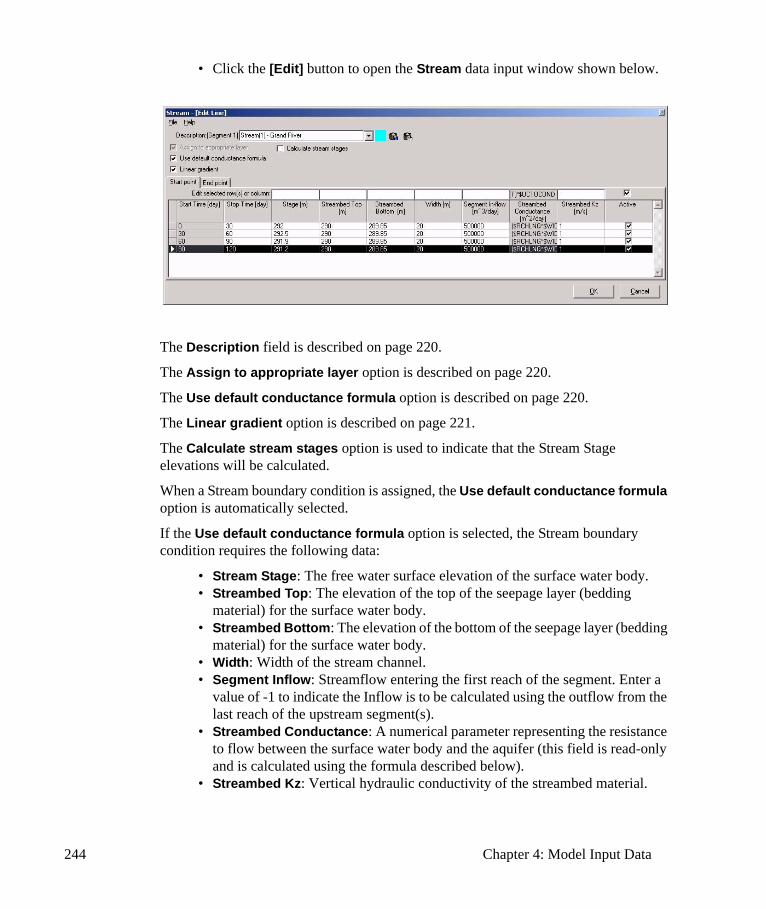
244 Chapter 4: Model Input Data
• Click the [Edit] button to open the Stream data input window shown below.
The Description field is described on page 220.
The Assign to appropriate layer option is described on page 220.
The Use default conductance formula option is described on page 220.
The Linear gradient option is described on page 221.
The Calculate stream stages option is used to indicate that the Stream Stage elevations will be calculated.
When a Stream boundary condition is assigned, the Use default conductance formula option is automatically selected.
If the Use default conductance formula option is selected, the Stream boundary condition requires the following data:
• Stream Stage: The free water surface elevation of the surface water body.• Streambed Top: The elevation of the top of the seepage layer (bedding
material) for the surface water body.• Streambed Bottom: The elevation of the bottom of the seepage layer (bedding
material) for the surface water body.• Width: Width of the stream channel.• Segment Inflow: Streamflow entering the first reach of the segment. Enter a
value of -1 to indicate the Inflow is to be calculated using the outflow from the last reach of the upstream segment(s).
• Streambed Conductance: A numerical parameter representing the resistance to flow between the surface water body and the aquifer (this field is read-only and is calculated using the formula described below).
• Streambed Kz: Vertical hydraulic conductivity of the streambed material.

Boundary Conditions 245
The default conductance formula is as follows:
where
$COND: is the Streambed Conductance
$RCHLNG: is the reach length of the Stream line in each grid cell
$WIDTH: is the Stream Width in each grid cell
$K: is the Streambed Kz
$UCTOCOND: is the conversion factor for converting the $K value to the same L and T units used by $COND
$STOP: is the Streambed Top elevation
$SBOT: is the Streambed Bottom elevation
If the Use default conductance formula option is turned off, the fields used for calculating the Streambed Conductance value (Width and Streambed Kz) are removed from the table and the Streambed Conductance field becomes a read/write field where any value or alternate formula may be entered.
If the Calculate stream stages option is selected, the Stream data input window will also prompt for the Roughness (Manning’s roughness coefficient) of the stream channel. The Slope of the stream channel is not entered because it is automatically calculated using the change in the Streambed Top elevation from one grid cell to the next.
For details on entering boundary condition data, refer to the Entering Flow Boundary Condition Data section on page 222.
For details on using mathematical formulas and array variable to define boundary condition data, refer to the Using Mathematical Formulas and Array Variables section on page 224.
For details on importing transient boundary condition data, refer to the Importing Transient Boundary Condition Data section on page 226.
For details on erasing boundary conditions, refer to the Erasing Flow Boundary Conditions section on page 233.
For details on copying boundary condition data, refer to the Copying Flow Boundary Conditions section on page 233.
Generating Streamflow DataThe Streamflow-Routing Package produces the following Streamflow data:
• Flow INTO the stream reach
$COND $RCHLNG $WIDTH× × $K × $UCTOCOND$STOP $SBOT–
---------------------------------------------------------------------------------------------------------------------------------=
246 Chapter 4: Model Input Data
• Flow INTO the aquifer• Flow OUT of the stream reach
This information can be written to the model listing file (.LST). In order to generate this data, you must set the Flow Terms (FTerms) to write to the .LST file, rather than being written to the .FLO file (which is the default setting). This setting can be changed in the MODFLOW Output Control options located in the Run section of Visual MODFLOW. Please see the Output Control Settings section on page 338 for further details.
To read the Stream Outflow data once the model has been run, open the .LST file using Notepad or another text editor, and search for the phrase “FLOW INTO”.
Note: You cannot generate the Stream Outflow data if you are running MODPATH, as the Output Control settings for MODFLOW will be overwritten to create the .FLO file that is required for MODPATH.
General-Head (GHB) Boundary ConditionsVisual MODFLOW supports the General-Head Boundary Package included with MODFLOW. The Visual MODFLOW input data for General-Head grid cells is stored in the projectname.VMB file (see Appendix A), while the MODFLOW input data for General-Head grid cells is stored in the projectname.GHB file (see MODFLOW-2000 Reference Manual .PDF file, provided in the Manual folder of the Visual MODFLOW installation media).
The function of the General-Head Boundary (GHB) Package is mathematically similar to that of the River, Drain, and ET Packages. Flow into or out of a cell from an external source is provided in proportion to the difference between the head in the cell and the reference head assigned to the external source. The application of this boundary condition is intended to be general, as indicated by its name, but the typical application of this boundary conditions is to represent heads in a model that are influenced by a large surface water body outside the model domain with a known water elevation. The purpose of using this boundary condition is to avoid unnecessarily extending the model domain outward to meet the element influencing the head in the model. As a result, the General Head boundary condition is usually assigned along the outside edges of the model domain. This scenario is illustrated in the following figure.
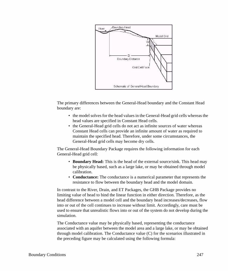
Boundary Conditions 247
The primary differences between the General-Head boundary and the Constant Head boundary are:
• the model solves for the head values in the General-Head grid cells whereas the head values are specified in Constant Head cells.
• the General-Head grid cells do not act as infinite sources of water whereas Constant Head cells can provide an infinite amount of water as required to maintain the specified head. Therefore, under some circumstances, the General-Head grid cells may become dry cells.
The General-Head Boundary Package requires the following information for each General-Head grid cell:
• Boundary Head: This is the head of the external source/sink. This head may be physically based, such as a large lake, or may be obtained through model calibration.
• Conductance: The conductance is a numerical parameter that represents the resistance to flow between the boundary head and the model domain.
In contrast to the River, Drain, and ET Packages, the GHB Package provides no limiting value of head to bind the linear function in either direction. Therefore, as the head difference between a model cell and the boundary head increases/decreases, flow into or out of the cell continues to increase without limit. Accordingly, care must be used to ensure that unrealistic flows into or out of the system do not develop during the simulation.
The Conductance value may be physically based, representing the conductance associated with an aquifer between the model area and a large lake, or may be obtained through model calibration. The Conductance value (C) for the scenarios illustrated in the preceding figure may be calculated using the following formula:
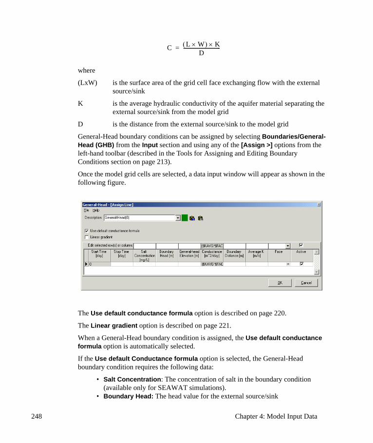
248 Chapter 4: Model Input Data
where
(LxW) is the surface area of the grid cell face exchanging flow with the external source/sink
K is the average hydraulic conductivity of the aquifer material separating the external source/sink from the model grid
D is the distance from the external source/sink to the model grid
General-Head boundary conditions can be assigned by selecting Boundaries/General-Head (GHB) from the Input section and using any of the [Assign >] options from the left-hand toolbar (described in the Tools for Assigning and Editing Boundary Conditions section on page 213).
Once the model grid cells are selected, a data input window will appear as shown in the following figure.
The Use default conductance formula option is described on page 220.
The Linear gradient option is described on page 221.
When a General-Head boundary condition is assigned, the Use default conductance formula option is automatically selected.
If the Use default Conductance formula option is selected, the General-Head boundary condition requires the following data:
• Salt Concentration: The concentration of salt in the boundary condition (available only for SEAWAT simulations).
• Boundary Head: The head value for the external source/sink
C L W×( ) K×D
-------------------------------=
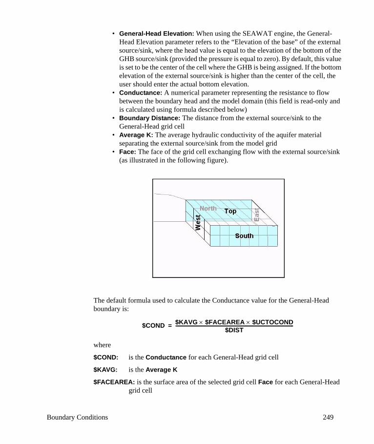
Boundary Conditions 249
• General-Head Elevation: When using the SEAWAT engine, the General-Head Elevation parameter refers to the “Elevation of the base” of the external source/sink, where the head value is equal to the elevation of the bottom of the GHB source/sink (provided the pressure is equal to zero). By default, this value is set to be the center of the cell where the GHB is being assigned. If the bottom elevation of the external source/sink is higher than the center of the cell, the user should enter the actual bottom elevation.
• Conductance: A numerical parameter representing the resistance to flow between the boundary head and the model domain (this field is read-only and is calculated using formula described below)
• Boundary Distance: The distance from the external source/sink to the General-Head grid cell
• Average K: The average hydraulic conductivity of the aquifer material separating the external source/sink from the model grid
• Face: The face of the grid cell exchanging flow with the external source/sink (as illustrated in the following figure).
The default formula used to calculate the Conductance value for the General-Head boundary is:
where
$COND: is the Conductance for each General-Head grid cell
$KAVG: is the Average K
$FACEAREA: is the surface area of the selected grid cell Face for each General-Head grid cell
$COND $KAVG $FACEAREA× $UCTOCOND×$DIST
-------------------------------------------------------------------------------------------------------------=

250 Chapter 4: Model Input Data
$UCTOCOND: is the conversion factor for converting the $K value to the same Length (L) and Time (T) units used by $COND
$DIST: is the Boundary Distance
If the Use default conductance formula option is not selected, the fields used for calculating the General-Head Conductance value (Boundary Distance, Average K, and Face) are removed from the table, and the Conductance field becomes a writeable field where a value, or alternate formula, may be entered.
Note: When Conductance values (or any other parameters) are calculated using a formula, the array variables and formulas are not saved together with the General-Head boundary data and cannot be recalled or modified at a later time. Visual MODFLOW only stores the Boundary Head and Conductance values for each grid cell.
For details on entering boundary condition data, refer to the Entering Flow Boundary Condition Data section on page 222.
For details on using mathematical formulas and array variable to define boundary condition data, refer to the Using Mathematical Formulas and Array Variables section on page 224.
For details on importing transient boundary condition data, refer to the Importing Transient Boundary Condition Data section on page 226.
For details on editing boundary conditions data, refer to the Editing Flow Boundary Conditions section on page 230.
For details on erasing boundary conditions, refer to the Erasing Flow Boundary Conditions section on page 233.
For details on copying boundary condition data, refer to the Copying Flow Boundary Conditions section on page 233.
Lake (LAK) Boundary ConditionsVisual MODFLOW supports the Lake (LAK3) package for MODFLOW. After translation, the Lake input data for MODFLOW is stored in the projectname.LAK file.
The lake boundary condition can be used to simulate the effects of stationary surface-water bodies such as lakes and reservoirs on an aquifer. The lake boundary is an alternative to the traditional approach of using the general head boundary condition. The main difference in the lake boundary is that the lake stage is calculated automatically based on the water budget, which is a function of inflow, outflow, recharge, evaporation, and anthropogenic inflow and discharge. The Lake package can be used for either steady state or transient simulations.
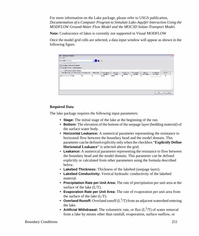
Boundary Conditions 251
For more information on the Lake package, please refer to USGS publication, Documentation of a Computer Program to Simulate Lake-Aquifer Interaction Using the MODFLOW Ground-Water Flow Model and the MOC3D Solute-Transport Model.
Note: Coalescence of lakes is currently not supported in Visual MODFLOW
Once the model grid cells are selected, a data input window will appear as shown in the following figure.
Required Data
The lake package requires the following input parameters:
• Stage: The initial stage of the lake at the beginning of the run.• Bottom: The elevation of the bottom of the seepage layer (bedding material) of
the surface water body. • Horizontal Leakance: A numerical parameter representing the resistance to
horizontal flow between the boundary head and the model domain. This parameter can be defined explicitly only when the checkbox “Explicitly Define Horizontal Leakance” is selected above the grid.
• Leakance: A numerical parameter representing the resistance to flow between the boundary head and the model domain. This parameter can be defined explicitly or calculated from other parameters using the formula described below.
• Lakebed Thickness: Thickness of the lakebed (seepage layer).• Lakebed Conductivity: Vertical hydraulic conductivity of the lakebed
material.• Precipitation Rate per Unit Area: The rate of precipitation per unit area at the
surface of the lake (L/T).• Evaporation Rate per Unit Area: The rate of evaporation per unit area from
the surface of the lake (L/T).• Overland Runoff: Overland runoff (L3/T) from an adjacent watershed entering
the lake. • Artificial Withdrawal: The volumetric rate, or flux (L3/T) of water removal
from a lake by means other than rainfall, evaporation, surface outflow, or

252 Chapter 4: Model Input Data
ground-water seepage. Normally, this would be used to specify the rate of artificial withdrawal from a lake for human water use, or if negative, artificial augmentation of a lake volume for esthetic or recreational purposes.
The default leakance formula is as follows:
where
$COND: is the Leakance
$K: is the Lakebed Kz
$UCTOCOND: is the conversion factor for converting the $K value to the same L and T units used by $COND
$RBTHICK:is the Lakebed Thickness
$DX: is the length of each grid cell in the X-direction
$DY: is the length of each grid cell in the Y-direction
If the Use default Leakance option is turned off, the fields used for calculating the River Conductance value (Lakebed Thickness, Lakebed Kz) are removed from the table, and the Leakance field becomes a writable field where a value may be entered.
Drain (DRN) Boundary ConditionsVisual MODFLOW supports the standard Drain Boundary Package included with MODFLOW. The Visual MODFLOW input data for Drain grid cells is stored in the projectname.VMB file (see Appendix A), while the MODFLOW input data for Drain grid cells is stored in the projectname.DRN file (see the MODFLOW-2000 Reference Manual .PDF file, provided in the Manual folder of the Visual MODFLOW installation media).
MODFLOW's Drain Package is designed to simulate the effects of features such as agricultural drains, which remove water from the aquifer at a rate proportional to the difference between the head in the aquifer and some fixed head or elevation. The Drain package assumes the drain has no effect if the head in the aquifer falls below the fixed head of the drain.
The Drain Package requires the following information as input for each cell containing this boundary condition:
• Head Elevation: The drain elevation, or drain head of the free surface of water within the drain. The drain is assumed to run only partially full, so that the head
$COND $DX $DY× $K $UCTOCOND××$RBTHICK
-----------------------------------------------------------------------------------------=
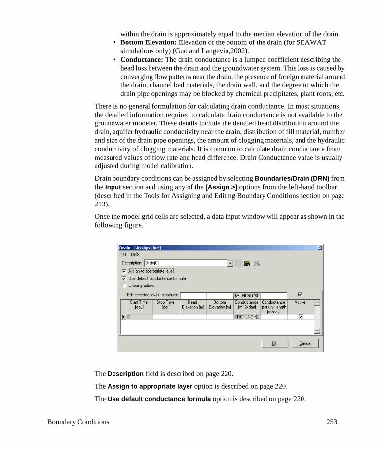
Boundary Conditions 253
within the drain is approximately equal to the median elevation of the drain. • Bottom Elevation: Elevation of the bottom of the drain (for SEAWAT
simulations only) (Guo and Langevin,2002).• Conductance: The drain conductance is a lumped coefficient describing the
head loss between the drain and the groundwater system. This loss is caused by converging flow patterns near the drain, the presence of foreign material around the drain, channel bed materials, the drain wall, and the degree to which the drain pipe openings may be blocked by chemical precipitates, plant roots, etc.
There is no general formulation for calculating drain conductance. In most situations, the detailed information required to calculate drain conductance is not available to the groundwater modeler. These details include the detailed head distribution around the drain, aquifer hydraulic conductivity near the drain, distribution of fill material, number and size of the drain pipe openings, the amount of clogging materials, and the hydraulic conductivity of clogging materials. It is common to calculate drain conductance from measured values of flow rate and head difference. Drain Conductance value is usually adjusted during model calibration.
Drain boundary conditions can be assigned by selecting Boundaries/Drain (DRN) from the Input section and using any of the [Assign >] options from the left-hand toolbar (described in the Tools for Assigning and Editing Boundary Conditions section on page 213).
Once the model grid cells are selected, a data input window will appear as shown in the following figure.
The Description field is described on page 220.
The Assign to appropriate layer option is described on page 220.
The Use default conductance formula option is described on page 220.

254 Chapter 4: Model Input Data
The Linear gradient option is described on page 221.
When a Drain boundary condition is assigned, the Use default conductance formula option is automatically selected.
If the Use default Conductance formula option is selected, the Drain boundary condition requires the following data:
• Head Elevation: The head value for the internal sink.• Bottom Elevation: The elevation of the bottom of the drain (for SEAWAT
simulations only).• Conductance: A numerical parameter representing the resistance to flow
between the boundary head and the model domain (this field is read-only and is calculated using formula described below).
• Conductance per unit length or area: The Conductance value per unit length/area of the Drain grid cells
If the grid cells were selected using the [Assign >] Line option, the default formula for the Drain Conductance is as follows:
If the grid cells were selected using [Assign >] Single, [Assign >] Polygon, or [Assign >] Window, the default conductance formula is as follows:
where
$COND: is the Conductance
$RCHLNG: is the reach length of the drain in each grid cell
$LCOND: is the Conductance per unit length of the drain in each grid cell
$SCOND: is the Conductance per unit area of the drain in each grid cell
$DX: is the length of each grid cell in the X-direction
$DY: is the length of each grid cell in the Y-direction
If the Use default conductance formula option is turned off, the fields used for calculating the Drain Conductance value (Conductance per unit length or area) are removed from the table and the Conductance field becomes a read/write field where any value or alternate formula may be entered.
Note: When Conductance values (or any other parameters) are calculated using a formula, the array variables and formulas are not saved together with the Drain boundary data, and cannot be recalled or modified at a later time. Visual MODFLOW only stores the Drain
$COND $RCHLNG $LCOND×=
$COND $DX $DY× $SCOND×=

Boundary Conditions 255
Elevation and Conductance values for each grid cell.
For details on entering boundary condition data, refer to the Entering Flow Boundary Condition Data section on page 222.
For details on using mathematical formulas and array variable to define boundary condition data, refer to the Using Mathematical Formulas and Array Variables section on page 224.
For details on importing transient boundary condition data, refer to the Importing Transient Boundary Condition Data section on page 226.
For details on editing boundary conditions data, refer to the Editing Flow Boundary Conditions section on page 230.
For details on erasing boundary conditions refer to the Erasing Flow Boundary Conditions section on page 233.
For details on copying boundary condition data, refer to the Copying Flow Boundary Conditions section on page 233.
Using Drains for a Seepage FaceIn many cases, the Drain boundary condition is used to simulate a seepage face where groundwater discharges to the surface of the model. Typically, this situation is encountered along steep slopes or escarpments and the Drain boundary is assigned to the top layer of grid cells along the side of the slope such that the Drain Elevation corresponds to the ground surface elevation (or just slightly below ground surface). When the water level reaches the ground surface elevation it is removed by the drain boundary.
This type of scenario can be easily accommodated in Visual MODFLOW by using the [Assign >] Polygon option to select the grid cells along the seepage face, and then entering a Drain Elevation value of:
$BOT + $DZ - 0.1
Where $BOT is the bottom elevation of each Drain grid cell and $DZ is the thickness of each Drain grid cell. This formula will assign a Drain Elevation value corresponding to 0.1 ft. below the top elevation of each Drain grid cell.
Wall (HFB) Boundary ConditionsVisual MODFLOW supports the Horizontal Flow Barrier (HFB) Package included with MODFLOW. The Visual MODFLOW input data for HFB grid cells is stored in the projectname.VMB file (see Appendix A), while the MODFLOW input data for HFB grid cells is stored in the projectname.HFB file (see MODFLOW-2000 Reference Manual .PDF file, provided in the Manual folder of the Visual MODFLOW installation media).
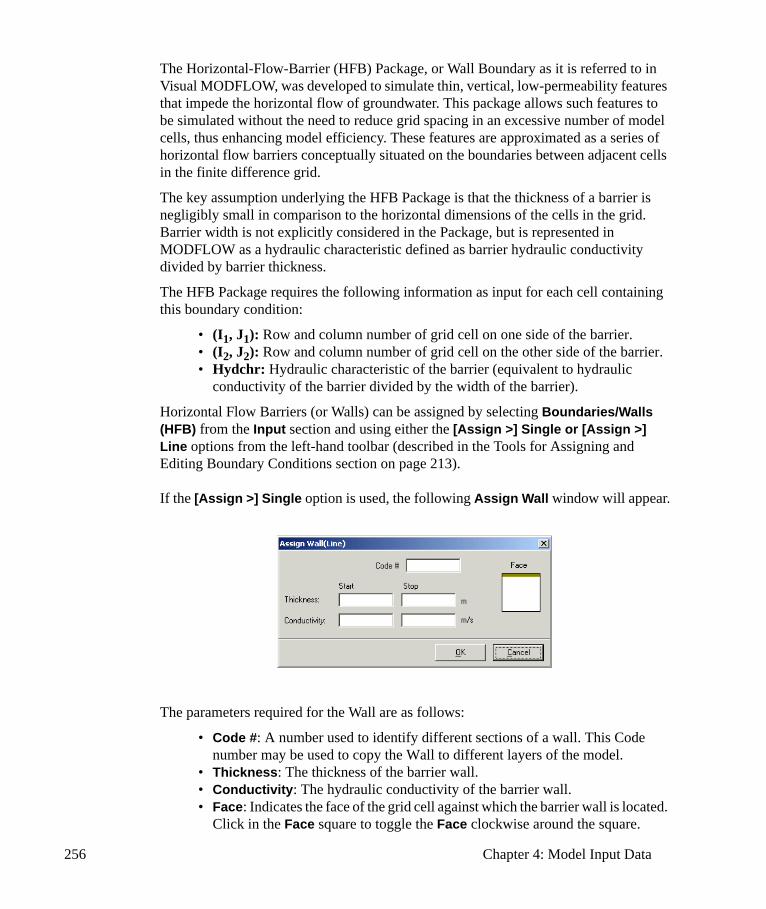
256 Chapter 4: Model Input Data
The Horizontal-Flow-Barrier (HFB) Package, or Wall Boundary as it is referred to in Visual MODFLOW, was developed to simulate thin, vertical, low-permeability features that impede the horizontal flow of groundwater. This package allows such features to be simulated without the need to reduce grid spacing in an excessive number of model cells, thus enhancing model efficiency. These features are approximated as a series of horizontal flow barriers conceptually situated on the boundaries between adjacent cells in the finite difference grid.
The key assumption underlying the HFB Package is that the thickness of a barrier is negligibly small in comparison to the horizontal dimensions of the cells in the grid. Barrier width is not explicitly considered in the Package, but is represented in MODFLOW as a hydraulic characteristic defined as barrier hydraulic conductivity divided by barrier thickness.
The HFB Package requires the following information as input for each cell containing this boundary condition:
• (I1, J1): Row and column number of grid cell on one side of the barrier.• (I2, J2): Row and column number of grid cell on the other side of the barrier.• Hydchr: Hydraulic characteristic of the barrier (equivalent to hydraulic
conductivity of the barrier divided by the width of the barrier).
Horizontal Flow Barriers (or Walls) can be assigned by selecting Boundaries/Walls (HFB) from the Input section and using either the [Assign >] Single or [Assign >] Line options from the left-hand toolbar (described in the Tools for Assigning and Editing Boundary Conditions section on page 213).
If the [Assign >] Single option is used, the following Assign Wall window will appear.
The parameters required for the Wall are as follows:
• Code #: A number used to identify different sections of a wall. This Code number may be used to copy the Wall to different layers of the model.
• Thickness: The thickness of the barrier wall.• Conductivity: The hydraulic conductivity of the barrier wall.• Face: Indicates the face of the grid cell against which the barrier wall is located.
Click in the Face square to toggle the Face clockwise around the square.
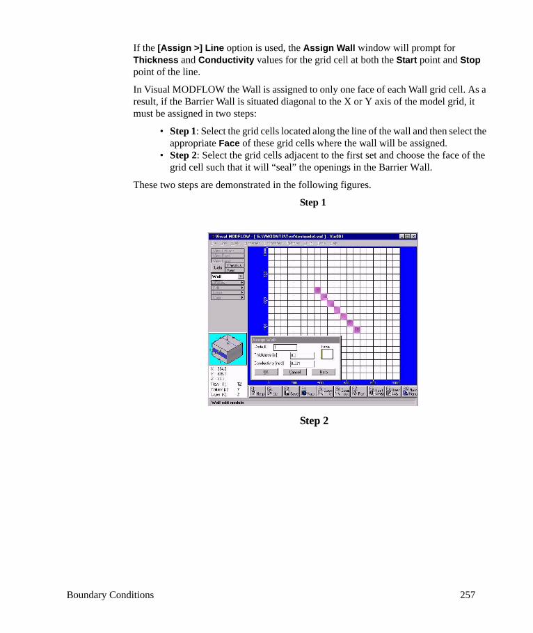
Boundary Conditions 257
If the [Assign >] Line option is used, the Assign Wall window will prompt for Thickness and Conductivity values for the grid cell at both the Start point and Stop point of the line.
In Visual MODFLOW the Wall is assigned to only one face of each Wall grid cell. As a result, if the Barrier Wall is situated diagonal to the X or Y axis of the model grid, it must be assigned in two steps:
• Step 1: Select the grid cells located along the line of the wall and then select the appropriate Face of these grid cells where the wall will be assigned.
• Step 2: Select the grid cells adjacent to the first set and choose the face of the grid cell such that it will “seal” the openings in the Barrier Wall.
These two steps are demonstrated in the following figures.
Step 1
Step 2
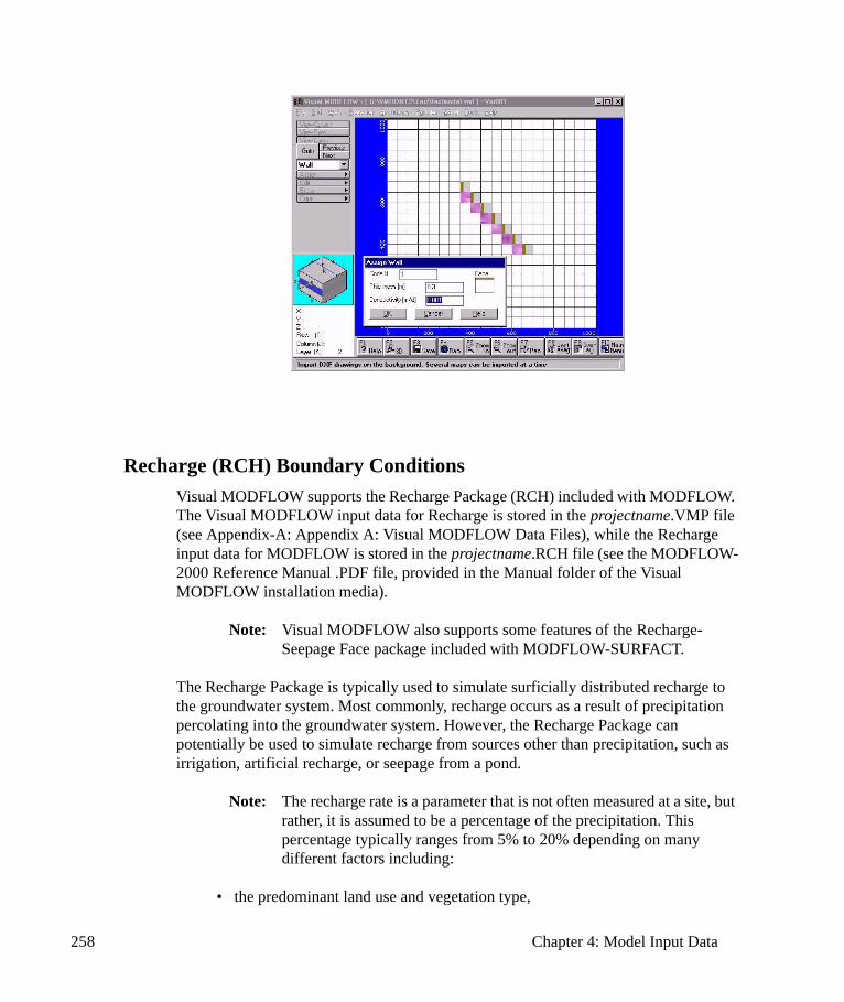
258 Chapter 4: Model Input Data
Recharge (RCH) Boundary ConditionsVisual MODFLOW supports the Recharge Package (RCH) included with MODFLOW. The Visual MODFLOW input data for Recharge is stored in the projectname.VMP file (see Appendix-A: Appendix A: Visual MODFLOW Data Files), while the Recharge input data for MODFLOW is stored in the projectname.RCH file (see the MODFLOW-2000 Reference Manual .PDF file, provided in the Manual folder of the Visual MODFLOW installation media).
Note: Visual MODFLOW also supports some features of the Recharge-Seepage Face package included with MODFLOW-SURFACT.
The Recharge Package is typically used to simulate surficially distributed recharge to the groundwater system. Most commonly, recharge occurs as a result of precipitation percolating into the groundwater system. However, the Recharge Package can potentially be used to simulate recharge from sources other than precipitation, such as irrigation, artificial recharge, or seepage from a pond.
Note: The recharge rate is a parameter that is not often measured at a site, but rather, it is assumed to be a percentage of the precipitation. This percentage typically ranges from 5% to 20% depending on many different factors including:
• the predominant land use and vegetation type,
Boundary Conditions 259
• the surface topography (slope), and • the soil cover material
The U.S. EPA’s HELP model is often used to estimate recharge rates for different zones within the model domain. Schlumberger Water Services’ Visual HELP program is a graphical interface for the HELP model, and it includes data from more than 3000 weather stations around the world. Contact a Schlumberger Water Services representative for more information about Visual HELP and how it can be used to estimate recharge rates for groundwater modeling applications.
The Recharge Package requires a two-dimensional array of recharge values for each grid cell in the horizontal plane, and an optional two-dimensional array of the layer numbers where the recharge will be applied for each grid cell in the horizontal plane.
Since natural recharge enters the groundwater system at the ground surface, Visual MODFLOW only allows recharge values to be assigned to Layer 1 while in View Layer mode. This allows all recharge zones to be visible at the same time in the same layer. By default, Visual MODFLOW will set the recharge to be applied to the upper-most active (wet) layer of the model for each vertical column of grid cell. However, Visual MODFLOW allows the user to specify that the recharge be applied to any of the model layers. For assigning recharge to specified layers refer to the section Assigning Recharge Zones below. The Recharge setting in the Run section under the MODFLOW/Recharge menu will also need to be modified (see the Recharge Settings section on page 328) so that Recharge is applied to the Specified Layer.
If MODFLOW-SURFACT is the selected numeric engine for the flow simulation, then you will also have the option of assigning a Ponding depth value at each time period in addition to the recharge value. The Ponding depth is the depth of the water above the ground surface. If the water table exceeds the ponding elevation then MODFLOW-SURFACT will remove the excess water from the system to prevent excessive build-up of head above the ground surface. It is worth noting that the excess recharge is NOT routed to any other locations as overland flow, but it is simply removed from the system. Please refer to the MODFLOW-SURFACT User’s Manual for more details.
Assigning Recharge ZonesThe Recharge boundary condition can be assigned by selecting Boundaries/Recharge (RCH) from the Input section. Upon creating a new model, a default Recharge value and time schedule is defined. This default time schedule is used to initially populate the two-dimensional array of Recharge values throughout the model. Once the default values are entered, spatially variable Recharge zones may be assigned.
Recharge zones can be assigned using the [Assign >] options from the left-hand toolbar (described in the Tools for Assigning and Editing Boundary Conditions section on page 213). The Recharge boundary conditions are assigned to the model using different colored zones to represent different Recharge values. Visual MODFLOW supports an unlimited number of Recharge zones.
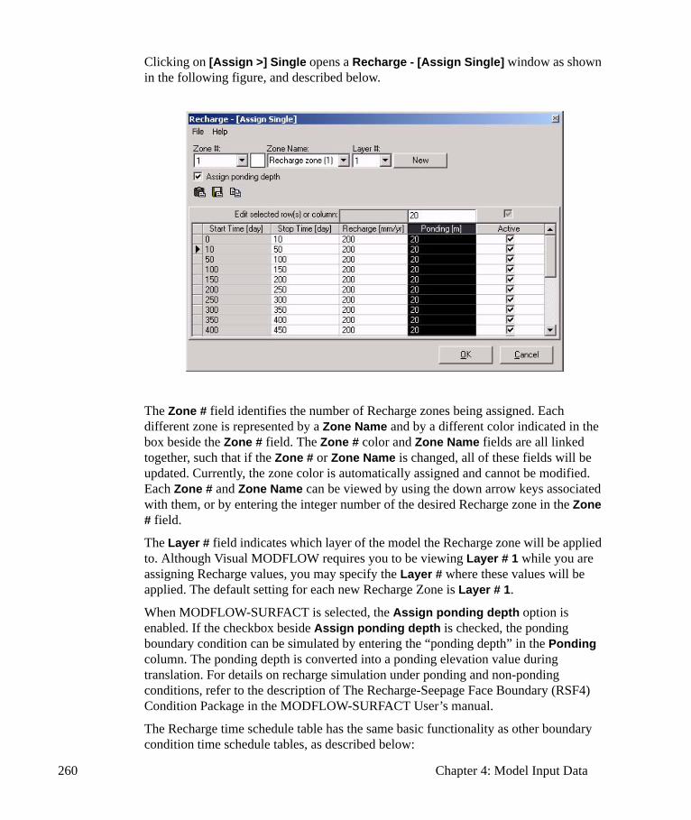
260 Chapter 4: Model Input Data
Clicking on [Assign >] Single opens a Recharge - [Assign Single] window as shown in the following figure, and described below.
The Zone # field identifies the number of Recharge zones being assigned. Each different zone is represented by a Zone Name and by a different color indicated in the box beside the Zone # field. The Zone # color and Zone Name fields are all linked together, such that if the Zone # or Zone Name is changed, all of these fields will be updated. Currently, the zone color is automatically assigned and cannot be modified. Each Zone # and Zone Name can be viewed by using the down arrow keys associated with them, or by entering the integer number of the desired Recharge zone in the Zone # field.
The Layer # field indicates which layer of the model the Recharge zone will be applied to. Although Visual MODFLOW requires you to be viewing Layer # 1 while you are assigning Recharge values, you may specify the Layer # where these values will be applied. The default setting for each new Recharge Zone is Layer # 1.
When MODFLOW-SURFACT is selected, the Assign ponding depth option is enabled. If the checkbox beside Assign ponding depth is checked, the ponding boundary condition can be simulated by entering the “ponding depth” in the Ponding column. The ponding depth is converted into a ponding elevation value during translation. For details on recharge simulation under ponding and non-ponding conditions, refer to the description of The Recharge-Seepage Face Boundary (RSF4) Condition Package in the MODFLOW-SURFACT User’s manual.
The Recharge time schedule table has the same basic functionality as other boundary condition time schedule tables, as described below:
Boundary Conditions 261
• Pressing the <Tab> or <Enter> key advances to the next cell on the right, and goes to the Stop Time field of the next time period if pressed while in the last column.
• If <Tab> or <Enter> is pressed from the last column of the last time period, it will create a new time period with the Start Time equal to the Stop Time of the previous time period, and with blank entries for all remaining parameters.
• If <Tab> or <Enter> is pressed from a blank data field in the last time period, it will copy the data from the previous time period.
• Pressing the <Shift> <Tab> keys advances to the next cell on the left, and goes to the Active field of the previous time period if the cursor is in the Stop Time field.
<Down Arrow>• Pressing the <Down Arrow> key will move the cursor to the next time period.• Pressing the <Down Arrow> key from the last time period will create a new time
period and will copy all parameter values from the previous time period (the Stop Time is not considered a parameter).
<Formula Bar>
• Any values entered in the Formula Bar fields will be applied to the selected cells in that parameter field column.
Creating a New Recharge ZoneTo create a new Recharge zone:
• Click the [Assign >] button in the left menu bar and choose Single, Line, Polygon or Window to select the desired grid cells where the new zone will be assigned.
• When the respective Assign Recharge window appears, press the [New] button.
• The Zone # automatically increments, and a new Zone Name is created with an empty time schedule.
• Enter the Stop Time and Recharge values for the first time period.• Press the <Enter> key to create a new time period, or click the [OK] button to
accept this value.
Importing Recharge Zones from Polygon ShapefilesPlease see Importing from Polygon Shapefile page 193 for more details.
Importing Transient Recharge ValuesEach Recharge time period for each Recharge Zone requires a Start time, Stop time, and Recharge value. Transient recharge data can be imported for a selected Recharge Zone using one of the three options described below:
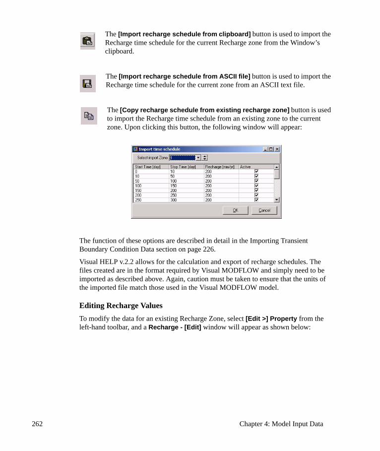
262 Chapter 4: Model Input Data
The [Import recharge schedule from clipboard] button is used to import the Recharge time schedule for the current Recharge zone from the Window’s clipboard.
The [Import recharge schedule from ASCII file] button is used to import the Recharge time schedule for the current zone from an ASCII text file.
The [Copy recharge schedule from existing recharge zone] button is used to import the Recharge time schedule from an existing zone to the current zone. Upon clicking this button, the following window will appear:
The function of these options are described in detail in the Importing Transient Boundary Condition Data section on page 226.
Visual HELP v.2.2 allows for the calculation and export of recharge schedules. The files created are in the format required by Visual MODFLOW and simply need to be imported as described above. Again, caution must be taken to ensure that the units of the imported file match those used in the Visual MODFLOW model.
Editing Recharge ValuesTo modify the data for an existing Recharge Zone, select [Edit >] Property from the left-hand toolbar, and a Recharge - [Edit] window will appear as shown below:
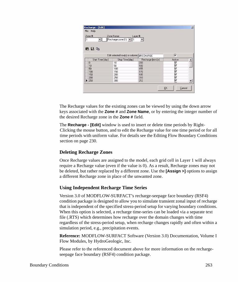
Boundary Conditions 263
The Recharge values for the existing zones can be viewed by using the down arrow keys associated with the Zone # and Zone Name, or by entering the integer number of the desired Recharge zone in the Zone # field.
The Recharge - [Edit] window is used to insert or delete time periods by Right-Clicking the mouse button, and to edit the Recharge value for one time period or for all time periods with uniform value. For details see the Editing Flow Boundary Conditions section on page 230.
Deleting Recharge Zones Once Recharge values are assigned to the model, each grid cell in Layer 1 will always require a Recharge value (even if the value is 0). As a result, Recharge zones may not be deleted, but rather replaced by a different zone. Use the [Assign >] options to assign a different Recharge zone in place of the unwanted zone.
Using Independent Recharge Time SeriesVersion 3.0 of MODFLOW-SURFACT’s recharge-seepage face boundary (RSF4) condition package is designed to allow you to simulate transient zonal input of recharge that is independent of the specified stress-period setup for varying boundary conditions. When this option is selected, a recharge time-series can be loaded via a separate text file (.RTS) which determines how recharge over the domain changes with time regardless of the stress-period setup, when recharge changes rapidly and often within a simulation period, e.g., precipitation events.
Reference: MODFLOW-SURFACT Software (Version 3.0) Documentation, Volume I Flow Modules, by HydroGeologic, Inc.
Please refer to the referenced document above for more information on the recharge-seepage face boundary (RSF4) condition package.
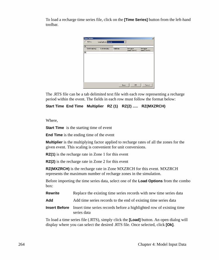
264 Chapter 4: Model Input Data
To load a recharge time series file, click on the [Time Series] button from the left-hand toolbar.
The .RTS file can be a tab delimited text file with each row representing a recharge period within the event. The fields in each row must follow the format below:
Start Time End Time Multiplier RZ (1) RZ(2) ..... RZ(MXZRCH)
Where,
Start Time is the starting time of event
End Time is the ending time of the event
Multiplier is the multiplying factor applied to recharge rates of all the zones for the given event. This scaling is convenient for unit conversions.
RZ(1) is the recharge rate in Zone 1 for this event
RZ(2) is the recharge rate in Zone 2 for this event
RZ(MXZRCH) is the recharge rate in Zone MXZRCH for this event. MXZRCH represents the maximum number of recharge zones in the simulation.
Before importing the time series data, select one of the Load Options from the combo box:
Rewrite Replace the existing time series records with new time series data
Add Add time series records to the end of existing time series data
Insert Before Insert time series records before a highlighted row of existing time series data
To load a time series file (.RTS), simply click the [Load] button. An open dialog will display where you can select the desired .RTS file. Once selected, click [Ok].
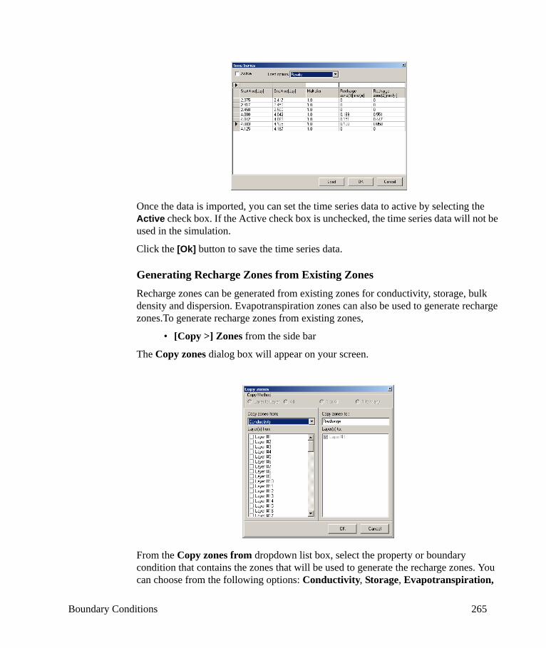
Boundary Conditions 265
Once the data is imported, you can set the time series data to active by selecting the Active check box. If the Active check box is unchecked, the time series data will not be used in the simulation.
Click the [Ok] button to save the time series data.
Generating Recharge Zones from Existing ZonesRecharge zones can be generated from existing zones for conductivity, storage, bulk density and dispersion. Evapotranspiration zones can also be used to generate recharge zones.To generate recharge zones from existing zones,
• [Copy >] Zones from the side bar
The Copy zones dialog box will appear on your screen.
From the Copy zones from dropdown list box, select the property or boundary condition that contains the zones that will be used to generate the recharge zones. You can choose from the following options: Conductivity, Storage, Evapotranspiration,

266 Chapter 4: Model Input Data
Bulk Density and Dispersion. Below, select the layer(s) that contains the zones. You will notice that these zones can only be used to generate recharge zones in Layer #1. This is because recharge boundary conditions can only be assigned to the top layer of the model. Click the [OK] button to generate the recharge zones.
Evapotranspiration Boundary ConditionsVisual MODFLOW supports both the Evapotranspiration Package (EVT) and the Evapotranspiration Segments Package (ETS1). The Visual MODFLOW input data for Evapotranspiration is stored in the projectname.VMP file (see Appendix A), while the Evapotranspiration input data for MODFLOW is stored in the projectname.EVT file (see the MODFLOW-2000 Reference Manual .PDF file, provided in the Manual folder of the Visual MODFLOW installation media).
The Evapotranspiration Package simulates the effects of plant transpiration, direct evaporation, and seepage at the ground surface by removing water from the saturated groundwater regime.
The Evapotranspiration Package requires the following information:
• Evapotranspiration rate: The rate of evapotranspiration as it occurs when the water table elevation is equal to the top of the grid cell elevation.
• Extinction Depth: The depth below the top of grid cell elevation where the evapotranspiration rate is negligible.
The Evapotranspiration Package approach is based on the following assumptions:
• When the water table is at or above the ground surface (top of layer 1), evapotranspiration loss from the water table occurs at the maximum rate specified by the user.
• When the elevation of the water table is below the ‘extinction depth’, or is beneath layer 1, evapotranspiration from the water table is negligible.
• Between these limits, evapotranspiration from the water table varies linearly with water table elevation.
Since evapotranspiration from the groundwater system usually occurs at or near the ground surface, Visual MODFLOW only allows Evapotranspiration values to be assigned to Layer 1 while in View Layer mode. This allows all Evapotranspiration zones to be visible at the same time in the same layer.
Assigning Evapotranspiration ZonesThe Evapotranspiration boundary condition can be assigned by selecting Boundaries/Evapotranspiration (EVT) from the Input section. Upon entering the Evapotranspiration screen for the first time, a pop-up window will require a default time schedule of Evapotranspiration values. This default time schedule is used to initially populate the two-dimensional array of Evapotranspiration values. Once the
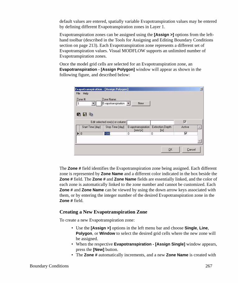
Boundary Conditions 267
default values are entered, spatially variable Evapotranspiration values may be entered by defining different Evapotranspiration zones in Layer 1.
Evapotranspiration zones can be assigned using the [Assign >] options from the left-hand toolbar (described in the Tools for Assigning and Editing Boundary Conditions section on page 213). Each Evapotranspiration zone represents a different set of Evapotranspiration values. Visual MODFLOW supports an unlimited number of Evapotranspiration zones.
Once the model grid cells are selected for an Evapotranspiration zone, an Evapotranspiration - [Assign Polygon] window will appear as shown in the following figure, and described below:
The Zone # field identifies the Evapotranspiration zone being assigned. Each different zone is represented by Zone Name and a different color indicated in the box beside the Zone # field. The Zone # and Zone Name fields are essentially linked, and the color of each zone is automatically linked to the zone number and cannot be customized. Each Zone # and Zone Name can be viewed by using the down arrow keys associated with them, or by entering the integer number of the desired Evapotranspiration zone in the Zone # field.
Creating a New Evapotranspiration ZoneTo create a new Evapotranspiration zone:
• Use the [Assign >] options in the left menu bar and choose Single, Line, Polygon, or Window to select the desired grid cells where the new zone will be assigned.
• When the respective Evapotranspiration - [Assign Single] window appears, press the [New] button.
• The Zone # automatically increments, and a new Zone Name is created with
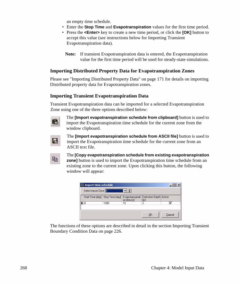
268 Chapter 4: Model Input Data
an empty time schedule. • Enter the Stop Time and Evapotranspiration values for the first time period.• Press the <Enter> key to create a new time period, or click the [OK] button to
accept this value (see instructions below for Importing Transient Evapotranspiration data).
Note: If transient Evapotranspiration data is entered, the Evapotranspiration value for the first time period will be used for steady-state simulations.
Importing Distributed Property Data for Evapotranspiration ZonesPlease see "Importing Distributed Property Data" on page 171 for details on importing Distributed property data for Evapotranspiration zones.
Importing Transient Evapotranspiration Data Transient Evapotranspiration data can be imported for a selected Evapotranspiration Zone using one of the three options described below:
The [Import evapotranspiration schedule from clipboard] button is used to import the Evapotranspiration time schedule for the current zone from the window clipboard.
The [Import evapotranspiration schedule from ASCII file] button is used to import the Evapotranspiration time schedule for the current zone from an ASCII text file.
The [Copy evapotranspiration schedule from existing evapotranspiration zone] button is used to import the Evapotranspiration time schedule from an existing zone to the current zone. Upon clicking this button, the following window will appear:
The functions of these options are described in detail in the section Importing Transient Boundary Condition Data on page 226.
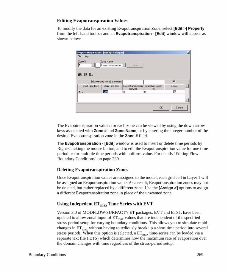
Boundary Conditions 269
Editing Evapotranspiration ValuesTo modify the data for an existing Evapotranspiration Zone, select [Edit >] Property from the left-hand toolbar and an Evapotranspiration - [Edit] window will appear as shown below:
The Evapotranspiration values for each zone can be viewed by using the down arrow keys associated with Zone # and Zone Name, or by entering the integer number of the desired Evapotranspiration zone in the Zone # field.
The Evapotranspiration - [Edit] window is used to insert or delete time periods by Right-Clicking the mouse button, and to edit the Evapotranspiration value for one time period or for multiple time periods with uniform value. For details "Editing Flow Boundary Conditions" on page 230.
Deleting Evapotranspiration Zones Once Evapotranspiration values are assigned to the model, each grid cell in Layer 1 will be assigned an Evapotranspiration value. As a result, Evapotranspiration zones may not be deleted, but rather replaced by a different zone. Use the [Assign >] options to assign a different Evapotranspiration zone in place of the unwanted zone.
Using Indepedent ETmax Time Series with EVT
Version 3.0 of MODFLOW-SURFACT’s ET packages, EVT and ETS1, have been updated to allow zonal input of ETmax values that are independent of the specified stress-period setup for varying boundary conditions. This allows you to simulate rapid changes in ETmax without having to tediously break up a short time period into several stress periods. When this option is selected, a ETmax time-series can be loaded via a separate text file (.ETS) which determines how the maximum rate of evaporation over the domain changes with time regardless of the stress-period setup.
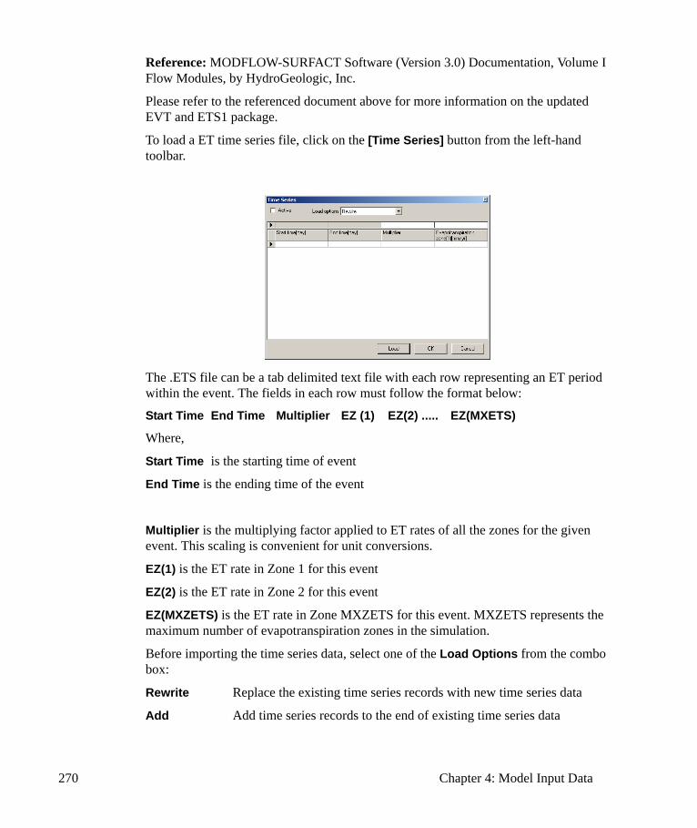
270 Chapter 4: Model Input Data
Reference: MODFLOW-SURFACT Software (Version 3.0) Documentation, Volume I Flow Modules, by HydroGeologic, Inc.
Please refer to the referenced document above for more information on the updated EVT and ETS1 package.
To load a ET time series file, click on the [Time Series] button from the left-hand toolbar.
The .ETS file can be a tab delimited text file with each row representing an ET period within the event. The fields in each row must follow the format below:
Start Time End Time Multiplier EZ (1) EZ(2) ..... EZ(MXETS)
Where,
Start Time is the starting time of event
End Time is the ending time of the event
Multiplier is the multiplying factor applied to ET rates of all the zones for the given event. This scaling is convenient for unit conversions.
EZ(1) is the ET rate in Zone 1 for this event
EZ(2) is the ET rate in Zone 2 for this event
EZ(MXZETS) is the ET rate in Zone MXZETS for this event. MXZETS represents the maximum number of evapotranspiration zones in the simulation.
Before importing the time series data, select one of the Load Options from the combo box:
Rewrite Replace the existing time series records with new time series data
Add Add time series records to the end of existing time series data
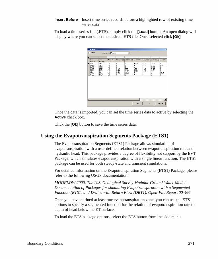
Boundary Conditions 271
Insert Before Insert time series records before a highlighted row of existing time series data
To load a time series file (.ETS), simply click the [Load] button. An open dialog will display where you can select the desired .ETS file. Once selected click [Ok].
Once the data is imported, you can set the time series data to active by selecting the Active check box.
Click the [Ok] button to save the time series data.
Using the Evapotranspiration Segments Package (ETS1)The Evapotranspiration Segments (ETS1) Package allows simulation of evapotranspiration with a user-defined relation between evapotranspiration rate and hydraulic head. This package provides a degree of flexibility not support by the EVT Package, which simulates evapotranspiration with a single linear function. The ETS1 package can be used for both steady-state and transient simulations.
For detailed information on the Evapotranspiration Segments (ETS1) Package, please refer to the following USGS documentation:
MODFLOW-2000, The U.S. Geological Survey Modular Ground-Water Model - Documentation of Packages for simulating Evapotranspiration with a Segmented Function (ETS1) and Drains with Return Flow (DRT1). Open-File Report 00-466.
Once you have defined at least one evapotranspiration zone, you can use the ETS1 options to specify a segmented function for the relation of evapotranspiration rate to depth of head below the ET surface.
To load the ETS package options, select the ETS button from the side menu.

272 Chapter 4: Model Input Data
The Evapotranspiration Segments Package dialog will appear on your screen.
Choosing the Desired Evapotranspiration PackageThe Use ETS Package check box allows you to choose between the ETS1 package and the EVT package (linear evapotranspiration). If this option is checked, the ETS1 package will be used to simulate evapotranspiration. If this option is unchecked, the EVT package will be used, and all specified ETS1 segments will be ignored.
Boundary Conditions 273
Specifying Evapotranspiration SegmentsFor transient simulations, different segments can be assigned to different time intervals. Select the desired time interval from the Time Interval combo box. If you wish to apply the same segments to al the time intervals, select the Use segments for all time intervals checkbox. Steady-state simulations only have one time interval.
Next, specify the desired number of segments (0 -1000) in the Number of Segments field, and then click the Generate Default Segments button.
Note: All defined evapotranspiration zones must have the same number of segments.
Visual MODFLOW will automatically generate default values for Depth% and Rate% at segment end-points in the table. The segments will also be displayed graphically in the adjacent graph.
The default segment end-point values can be modified to represent the desired evapotranspiration rate to depth relationship. Depth(%) and Rate(%) values must be entered as percentages (0-100) of the total Extinction Depth and Evapotranspiration rate, respectively. After entering a new value in the table, press the Enter key on your keyboard to the view the changes in the adjacent graph.
Adding/Removing Segment to/from a CurveTo add or remove segments from an exiting curve, enter the desired number of segments in the Number of Segments field, and press the Enter key on your keyboard (do not click the Generate Default Segments button). If the number of segments is greater than the current number of segments, new segments will be added alone the existing curve. If the specified number of segments is less than the current number of segments, segments will be removed from the curve.
Saving ETS Option Once the desired curve is created, click the OK button to save the settings.
274 Chapter 4: Model Input Data
4.6.3 Mass Transport Boundary ConditionsThe solution of the governing equation for mass transport requires the specification of boundary conditions. For the mass transport model supported by Visual MODFLOW there are four options for specifying transport boundary conditions:
• Constant Concentration - see page 274• Recharge Concentration - see page 276• Evapotranspiration Concentration - see page 278• Point Source - see page 280
The following sections provide a description of the data requirements for each of these boundary condition types, and the options for assigning, editing, and importing the required data.
Note: For SEAWAT models that simulate heat transport, all transport boundary conditions for the temperature species must have values between 0°C and 99°C.
Constant Concentration Boundary ConditionsVisual MODFLOW input data for the Constant Concentration boundary condition is stored in the projectname.MTN file (see Appendix A), while the Constant Concentration input data for MT3Dxx/RT3D is stored in the projectname.SSM file (see the MT3Dxx/RT3D Reference Manual .PDF file, provided in the Manual folder of the Visual MODFLOW installation media).
The Constant Concentration boundary condition acts as a contaminant source providing solute mass to the model domain in the form of a known concentration. An example of such a boundary condition is a spill that provides dissolved phase contamination at a fixed concentration for a relatively long period of time.
Note: In some cases, the Constant Concentration boundary condition may also act as a sink by taking mass out of the model domain (i.e. if the Constant Concentration value is lower than the value of the surrounding cells).
Assigning Constant Concentration ZonesConstant Concentration boundary conditions can be assigned by selecting Boundaries/Constant Concentration from the top menu bar and using the [Assign >] options from the left-hand toolbar (described in the Tools for Assigning and Editing Boundary Conditions section on page 213). Once the model grid cells are selected, the Assign Constant Concentration window will appear as shown below.
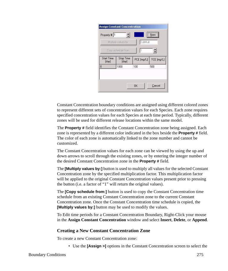
Boundary Conditions 275
Constant Concentration boundary conditions are assigned using different colored zones to represent different sets of concentration values for each Species. Each zone requires specified concentration values for each Species at each time period. Typically, different zones will be used for different release locations within the same model.
The Property # field identifies the Constant Concentration zone being assigned. Each zone is represented by a different color indicated in the box beside the Property # field. The color of each zone is automatically linked to the zone number and cannot be customized.
The Constant Concentration values for each zone can be viewed by using the up and down arrows to scroll through the existing zones, or by entering the integer number of the desired Constant Concentration zone in the Property # field.
The [Multiply values by:] button is used to multiply all values for the selected Constant Concentration zone by the specified multiplication factor. This multiplication factor will be applied to the original Constant Concentration values present prior to pressing the button (i.e. a factor of “1” will return the original values).
The [Copy schedule from:] button is used to copy the Constant Concentration time schedule from an existing Constant Concentration zone to the current Constant Concentration zone. Once the Constant Concentration time schedule is copied, the [Multiply values by:] button may be used to modify the values.
To Edit time periods for a Constant Concentration Boundary, Right-Click your mouse in the Assign Constant Concentration window and select Insert, Delete, or Append.
Creating a New Constant Concentration ZoneTo create a new Constant Concentration zone:
• Use the [Assign >] options in the Constant Concentration screen to select the

276 Chapter 4: Model Input Data
desired grid cells where the zone will be located.• When the Assign Constant Concentration window appears, press the [New]
button.• The Property # automatically increments and a new Constant Concentration
zone is created with an empty time schedule. • Enter the Stop Time and Concentration values for the first time period.• Press the <Enter> key to create a new time period, or click the [OK] button to
accept this value.
Note: If the simulation time is longer than the time specified for the Constant Concentrations, Visual MODFLOW assumes the Constant Concentration is maintained at the value set by the last Time Period for the duration of the simulation. If you manually assign a 0 value for a Constant Concentration boundary, the boundary cells may then become sinks, as they will be trying to maintain a 0 concentration value during the remainder of the simulation. If you need to model a concentration source that does not exist for the entire simulation, you might consider using the Recharge Concentration boundary condition, a Point Source boundary condition assigned to a well, or building a second model, and using the output from the first model (run until the contaminant source is removed) as the Initial Concentration for the second model. If you require assistance with the design of your model, please contact our Technical Support department to learn about Schlumberger Water Services’ Extended Modeling Support services. For more details, refer to the MT3DMS Reference manual, p. 6-34.
Editing Constant Concentration ValuesTo modify the data for an existing Constant Concentration zone, select [Edit >] Property from the left-hand toolbar, and an Edit Constant Concentration window will appear. This window has the same appearance and functionality as the Assign Constant Concentration window described above.
The concentration data for each Constant Concentration zone can be viewed by using the up and down arrows to scroll through the existing zones, or by entering the integer number of the desired zone in the Property # field.
Recharge Concentration Boundary ConditionsThe Visual MODFLOW input data for Recharge Concentration boundary conditions is stored in the projectname.MTH file (see Appendix A), while the Recharge Concentration input data for MT3Dxx/RT3D is stored in the projectname.SSM file (see the MT3Dxx/RT3D Reference Manual .PDF file provided in the Manual folder of the Visual MODFLOW installation media).
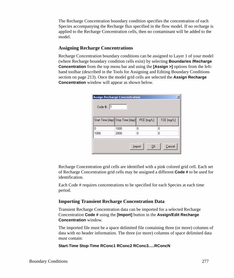
Boundary Conditions 277
The Recharge Concentration boundary condition specifies the concentration of each Species accompanying the Recharge flux specified in the flow model. If no recharge is applied to the Recharge Concentration cells, then no contaminant will be added to the model.
Assigning Recharge ConcentrationsRecharge Concentration boundary conditions can be assigned to Layer 1 of your model (where Recharge boundary condition cells exist) by selecting Boundaries /Recharge Concentration from the top menu bar and using the [Assign >] options from the left-hand toolbar (described in the Tools for Assigning and Editing Boundary Conditions section on page 213). Once the model grid cells are selected the Assign Recharge Concentration window will appear as shown below.
Recharge Concentration grid cells are identified with a pink colored grid cell. Each set of Recharge Concentration grid cells may be assigned a different Code # to be used for identification.
Each Code # requires concentrations to be specified for each Species at each time period.
Importing Transient Recharge Concentration DataTransient Recharge Concentration data can be imported for a selected Recharge Concentration Code # using the [Import] button in the Assign/Edit Recharge Concentration window.
The imported file must be a space delimited file containing three (or more) columns of data with no header information. The three (or more) columns of space delimited data must contain:
Start-Time Stop-Time RConc1 RConc2 RConc3.....RConcN
278 Chapter 4: Model Input Data
Where RConcN is the Recharge Concentration for the Nth Species being simulated by the model. The Stop Time for each time period must always coincide with the Start Time for the next time period, and a concentration value must be available for each Species in the model. In addition, the units of the imported data must match those set during the model’s creation.
SWS’ UnSat Suite v.2.2 and AquaChem software allows for the calculation and export of recharge concentration schedules. The files created are in the format required by Visual MODFLOW and simply need to be imported as described above. Again, caution must be taken to ensure that the units of the imported file match those used in the Visual MODFLOW model.
Note: When applying Recharge Concentration to layers below the ground surface, it is important to note that the associated Recharge boundary condition in layer 1 must be applied to the correct layer (using the Layer # option, as described in Recharge (RCH) Boundary Conditions section on page 258), since the Recharge Concentration boundary condition specifies the concentration of each Species accompanying the Recharge flux specified in the flow model. Additionally, the Recharge options for the MODFLOW engine must be configured (in the RUN menu, click on MODFLOW-Recharge) so that Recharge is applied to the Specified Layer.
Evapotranspiration Concentration Boundary ConditionsThe Visual MODFLOW input data for Evapotranspiration Concentration boundary conditions is stored in the projectname.MTV file (see Appendix A), while the Evapotranspiration Concentration input data for MT3Dxx/RT3D is stored in the projectname.SSM file (see the MT3Dxx/RT3D Reference Manual .PDF file, provided in the Manual folder of the Visual MODFLOW installation media).
The Evapotranspiration Concentration boundary condition specifies the concentration of each Species accompanying the Evapotranspiration flux specified in the corresponding flow model.
Assigning Evapotranspiration ConcentrationsEvapotranspiration Concentration boundary conditions can be assigned by selecting Boundaries/Evapotr. Concentration from the top menu bar and using the [Assign >] options from the left-hand toolbar (described in the Tools for Assigning and Editing Boundary Conditions section on page 213). Once the model grid cells are selected, the Assign Evapotranspiration Concentration window will appear as shown below.
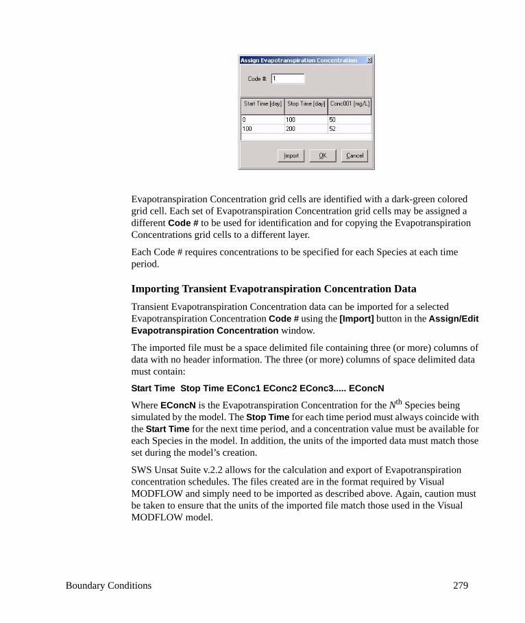
Boundary Conditions 279
Evapotranspiration Concentration grid cells are identified with a dark-green colored grid cell. Each set of Evapotranspiration Concentration grid cells may be assigned a different Code # to be used for identification and for copying the Evapotranspiration Concentrations grid cells to a different layer.
Each Code # requires concentrations to be specified for each Species at each time period.
Importing Transient Evapotranspiration Concentration DataTransient Evapotranspiration Concentration data can be imported for a selected Evapotranspiration Concentration Code # using the [Import] button in the Assign/Edit Evapotranspiration Concentration window.
The imported file must be a space delimited file containing three (or more) columns of data with no header information. The three (or more) columns of space delimited data must contain:
Start Time Stop Time EConc1 EConc2 EConc3..... EConcN
Where EConcN is the Evapotranspiration Concentration for the Nth Species being simulated by the model. The Stop Time for each time period must always coincide with the Start Time for the next time period, and a concentration value must be available for each Species in the model. In addition, the units of the imported data must match those set during the model’s creation.
SWS Unsat Suite v.2.2 allows for the calculation and export of Evapotranspiration concentration schedules. The files created are in the format required by Visual MODFLOW and simply need to be imported as described above. Again, caution must be taken to ensure that the units of the imported file match those used in the Visual MODFLOW model.

280 Chapter 4: Model Input Data
Point Source Boundary ConditionsThe Visual MODFLOW input data for Point Source boundary conditions is stored in the projectname.MTS file (see Appendix A), while the Point Source input data for MT3Dxx/RT3D is stored in the projectname.SSM file (see the MT3Dxx/RT3D Reference Manual .PDF file, provided in the Manual folder of the Visual MODFLOW installation media).
The Point Source boundary condition specifies the concentration of each Species entering or leaving the model through a flow boundary condition grid cell specified in the flow model.
Assigning Point SourcesPoint Source boundary conditions can be assigned by selecting Boundaries/Point Source from the top menu bar and using the [Assign >] options from the left-hand toolbar (described in the Tools for Assigning and Editing Boundary Conditions section on page 213).
The Point Source boundary condition may ONLY be assigned in grid cells containing a flow boundary condition (e.g. C.H.B., River, G.H.B., Stream, Pumping Well). If a Point Source is assigned to a Pumping Well, and the pump rate is set to 0, the point source will not add contaminant to the model. Once the model grid cells are selected, the Assign Point Source window will appear as shown below:
Point Source grid cells are identified with a yellow colored grid cell. Each set of Point Source grid cells may be assigned a different Code # to be used for identification.
The Time Schedule frame has two options for defining the time schedule for the Point Source:
• Copy from flow copies the time schedule from the existing flow boundary

Boundary Conditions 281
conditions• Define new allows for a new time schedule to be entered
Each Code # requires concentrations to be specified for each Species at each time period.
Note: If a flow boundary condition is deleted from the flow model, the associated Point Source boundary condition cell will also be deleted from the model.
When the Define new option is selected, the [Import] button will become available. This button allows you to load a PHT3D variant time series schedule from an ASCII text file. This can be particularly useful if your concentration data contains multiple species, and was prepared and exported using SWS’ AquaChem software.
The imported file must be a space delimited file containing three (or more) columns of data with no header information. The three (or more) columns of space delimited data must contain:
Start-Time Stop-Time RConc1 RConc2 RConc3.....RConcN
Where RConcN is the Point Source Concentration for the Nth Species being simulated by the model. The Stop Time for each time period must always coincide with the Start Time for the next time period, and a concentration value must be available for each Species in the model. In addition, the units of the imported data must match those set during the model’s creation.
NOTE: AquaChem automatically exports PHT3D concentration files in the correct format.
Import MIKE 11 River Network
BackgroundUsing OpenMI technology, Visual MODFLOW now supports combined river channel-groundwater modeling, through integration of DHI’s MIKE 11 software package. OpenMI stands for Open Modeling Interface and Environment. It aims to deliver standardized way to link water related computational models (and other data sources) that run parallel. For more details, please see http://www.openmi.org/
Note: Visual MODFLOW currently supports the basic river network/channel modeling capabilities of MIKE 11.
How it WorksMIKE 11 is integrated into Visual MODFLOW as a new boundary condition: Surface Leakage Boundary (SLB). The SLB package is a modified version of the FHB (Flow
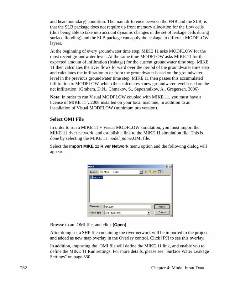
282 Chapter 4: Model Input Data
and head boundary) condition. The main difference between the FHB and the SLB, is that the SLB package does not require up front memory allocation for the flow cells (thus being able to take into account dynamic changes in the set of leakage cells during surface flooding) and the SLB package can apply the leakage to different MODFLOW layers.
At the beginning of every groundwater time step, MIKE 11 asks MODFLOW for the most recent groundwater level. At the same time MODFLOW asks MIKE 11 for the expected amount of infiltration (leakage) for the current groundwater time step. MIKE 11 then calculates the river flows forward over the period of the groundwater time step and calculates the infiltration to or from the groundwater based on the groundwater level in the previous groundwater time step. MIKE 11 then passes this accumulated infiltration to MODFLOW, which then calculates a new groundwater level based on the net infiltration. (Graham, D.N., Chmakov, S., Sapozhnikov, A., Gregersen, 2006)
Note: In order to run Visual MODFLOW coupled with MIKE 11, you must have a license of MIKE 11 v.2008 installed on your local machine, in addition to an installation of Visual MODFLOW (minimum pro version).
Select OMI FileIn order to run a MIKE 11 + Visual MODFLOW simulation, you must import the MIKE 11 river network, and establish a link to the MIKE 11 simulation file. This is done by selecting the MIKE 11 model_name.OMI file.
Select the Import MIKE 11 River Network menu option and the following dialog will appear:
Browse to an .OMI file, and click [Open].
After doing so, a SHP file containing the river network will be imported to the project, and added as new map overlay in the Overlay control. Click [F9] to see this overlay.
In addition, importing the .OMI file will define the MIKE 11 link, and enable you to define the MIKE 11 Run settings. For more details, please see "Surface Water Leakage Settings" on page 330.
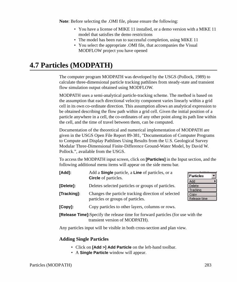
Particles (MODPATH) 283
Note: Before selecting the .OMI file, please ensure the following:
• You have a license of MIKE 11 installed, or a demo version with a MIKE 11 model that satisfies the demo restrictions
• The model has been run to successful completion, using MIKE 11• You select the appropriate .OMI file, that accompanies the Visual
MODFLOW project you have opened
4.7 Particles (MODPATH)The computer program MODPATH was developed by the USGS (Pollock, 1989) to calculate three-dimensional particle tracking pathlines from steady-state and transient flow simulation output obtained using MODFLOW.
MODPATH uses a semi-analytical particle-tracking scheme. The method is based on the assumption that each directional velocity component varies linearly within a grid cell in its own co-ordinate direction. This assumption allows an analytical expression to be obtained describing the flow path within a grid cell. Given the initial position of a particle anywhere in a cell, the co-ordinates of any other point along its path line within the cell, and the time of travel between them, can be computed.
Documentation of the theoretical and numerical implementation of MODPATH are given in the USGS Open File Report 89-381, "Documentation of Computer Programs to Compute and Display Pathlines Using Results from the U.S. Geological Survey Modular Three-Dimensional Finite-Difference Ground-Water Model, by David W. Pollock.”, available from the USGS.
To access the MODPATH input screen, click on [Particles] in the Input section, and the following additional menu items will appear on the side menu bar.
[Add]: Add a Single particle, a Line of particles, or a Circle of particles.
[Delete]: Deletes selected particles or groups of particles.
[Tracking]: Changes the particle tracking direction of selected particles or groups of particles.
[Copy]: Copy particles to other layers, columns or rows.
[Release Time]:Specify the release time for forward particles (for use with the transient version of MODPATH).
Any particles input will be visible in both cross-section and plan view.
Adding Single Particles• Click on [Add >] Add Particle on the left-hand toolbar. • A Single Particle window will appear.
284 Chapter 4: Model Input Data
• Select the tracking direction for the particles and then click on the desired particle locations in the model grid.
• Click [OK] when all particle locations have been assigned.
Adding a Line of Particles• Click on [Add >] Add Line on the left-hand toolbar. • Move the mouse pointer to the starting point of the line.• Left-Click to anchor the starting location of the line, and then Left-Click again
on the end point of the line.• A Line Particle window will appear.• Select the particle tracking direction and the number of particles along the line. .• Click [OK] to assign the line of particles.
If a line of particles is assigned across a variable surface, the particles along the line will be assigned at an elevation equal to the mid-point of the grid cell.
Adding a Circle of ParticlesA circle of backward tracking particles are typically assigned around a pumping well in order to determine the capture zone for that well.
• Click on [Add >] Add Circle on the left-hand toolbar. • Move the mouse pointer to the center of the circle.• Left-Click to anchor the center location of the circle, and then Left-Click again
at the desired radius of the circle.• A Circle Particle window will appear.• Select the particle tracking direction and the number of particles around the
circle.• Click [OK] to assign the circle of particles.
Deleting Particles• Click the [Delete] button on the left-hand toolbar. • A Delete Particle window will appear. • Use the mouse pointer to select the particles or groups of particles to delete• Click [OK] to delete the selected particles.
Changing the Particle Tracking DirectionOnce particle are assigned to the model the tracking direction may be changed at any time without re-assigning the particles.
• Click the [Tracking] button on the left-hand toolbar.• Use the mouse pointer to set the tracking direction of selected particles or
groups of particles. Left-Click to set to forward tracking (green colored particles), or Right-Click to set to backward tracking (red colored particles).
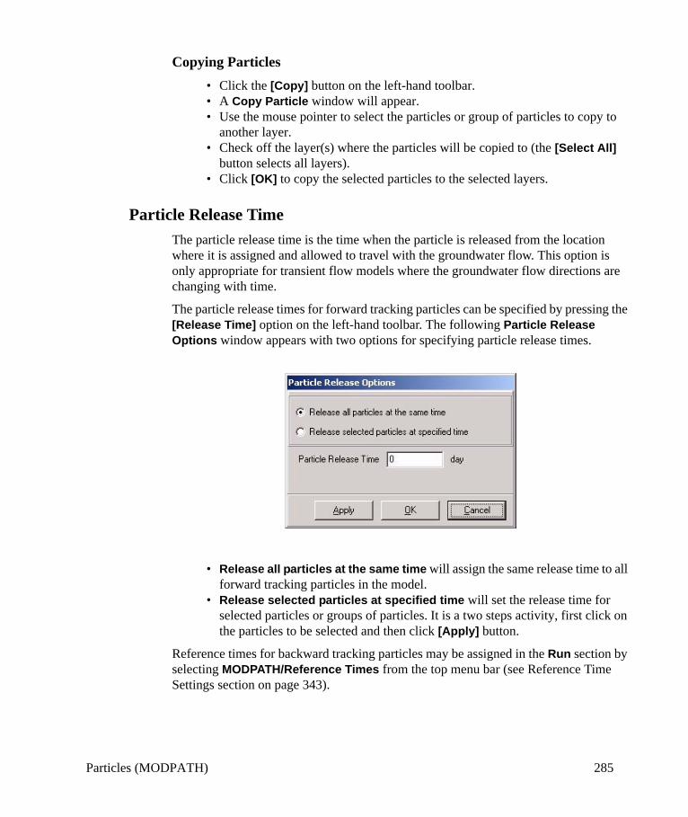
Particles (MODPATH) 285
Copying Particles• Click the [Copy] button on the left-hand toolbar.• A Copy Particle window will appear. • Use the mouse pointer to select the particles or group of particles to copy to
another layer.• Check off the layer(s) where the particles will be copied to (the [Select All]
button selects all layers).• Click [OK] to copy the selected particles to the selected layers.
Particle Release TimeThe particle release time is the time when the particle is released from the location where it is assigned and allowed to travel with the groundwater flow. This option is only appropriate for transient flow models where the groundwater flow directions are changing with time.
The particle release times for forward tracking particles can be specified by pressing the [Release Time] option on the left-hand toolbar. The following Particle Release Options window appears with two options for specifying particle release times.
• Release all particles at the same time will assign the same release time to all forward tracking particles in the model.
• Release selected particles at specified time will set the release time for selected particles or groups of particles. It is a two steps activity, first click on the particles to be selected and then click [Apply] button.
Reference times for backward tracking particles may be assigned in the Run section by selecting MODPATH/Reference Times from the top menu bar (see Reference Time Settings section on page 343).

286 Chapter 4: Model Input Data
Particle Discharge OptionsThe particle discharge options for MODPATH are available in the Run section of Visual MODFLOW under the MODPATH/Discharge Options in the top menu bar. These options are explained in the Discharge Options section on page 342.
4.8 Zone BudgetZone Budget calculates sub-regional water budgets using results from steady-state or transient MODFLOW simulations. Zone Budget calculates budgets by tabulating the budget data that MODFLOW produces using the cell-by-cell flow option. The user simply specifies the sub-regions for which budgets will be calculated. These sub-regions are entered as 'zones' analogous to the way that properties, such as hydraulic conductivity, are entered. Following a simulation, Zone Budget results can be read in the Output section under the Graphs item in the top menu bar.
The theoretical and numerical implementation of Zone Budget is described in the USGS Report "A Computer Program for Calculating Subregional Water Budgets Using Results from the U.S. Geological Survey Modular Three-Dimensional Finite-Difference Groundwater Flow Model, by Arlen W. Harbaugh", which is included in the MODFLOW Packages Reference Manual on your Visual MODFLOW media, in the Manual folder.
After selecting [Zbud] from the top menu bar the following additional side menu items appear:
[Assign >]: Assign user-defined water budget zones to Single grid cells, by digitizing a Polygon around a group of grid cells, or by stretching a rectangular Window around a group of grid cells.
[Copy >]: [Layer] Copy selected water budget zones from one layer to another layer.
[from Property] Create zone budget zones from property zones.
[from Boundary] Create zone budget zones from boundary condition groups.
[Database]: Display a list of all defined water budget zones, with colors corresponding to the zone number.
[Observations]: Enter flow observations for selected zones in the model.
Assigning ZonesZone Budget Zones can be assigned by selecting Zbud from the top menu bar of the Input section, and using any of the [Assign >] options described below:
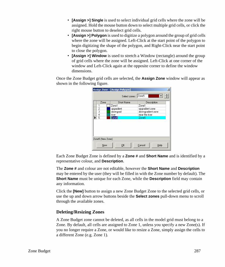
Zone Budget 287
• [Assign >] Single is used to select individual grid cells where the zone will be assigned. Hold the mouse button down to select multiple grid cells, or click the right mouse button to deselect grid cells.
• [Assign >] Polygon is used to digitize a polygon around the group of grid cells where the zone will be assigned. Left-Click at the start point of the polygon to begin digitizing the shape of the polygon, and Right-Click near the start point to close the polygon.
• [Assign >] Window is used to stretch a Window (rectangle) around the group of grid cells where the zone will be assigned. Left-Click at one corner of the window and Left-Click again at the opposite corner to define the window dimensions.
Once the Zone Budget grid cells are selected, the Assign Zone window will appear as shown in the following figure.
Each Zone Budget Zone is defined by a Zone # and Short Name and is identified by a representative colour, and Description.
The Zone # and colour are not editable, however the Short Name and Description may be entered by the user (they will be filled in with the Zone number by default). The Short Name must be unique for each Zone, while the Description field may contain any information.
Click the [New] button to assign a new Zone Budget Zone to the selected grid cells, or use the up and down arrow buttons beside the Select zones pull-down menu to scroll through the available zones.
Deleting/Resizing ZonesA Zone Budget zone cannot be deleted, as all cells in the model grid must belong to a Zone. By default, all cells are assigned to Zone 1, unless you specify a new Zone(s). If you no longer require a Zone, or would like to resize a Zone, simply assign the cells to a different Zone (e.g. Zone 1).
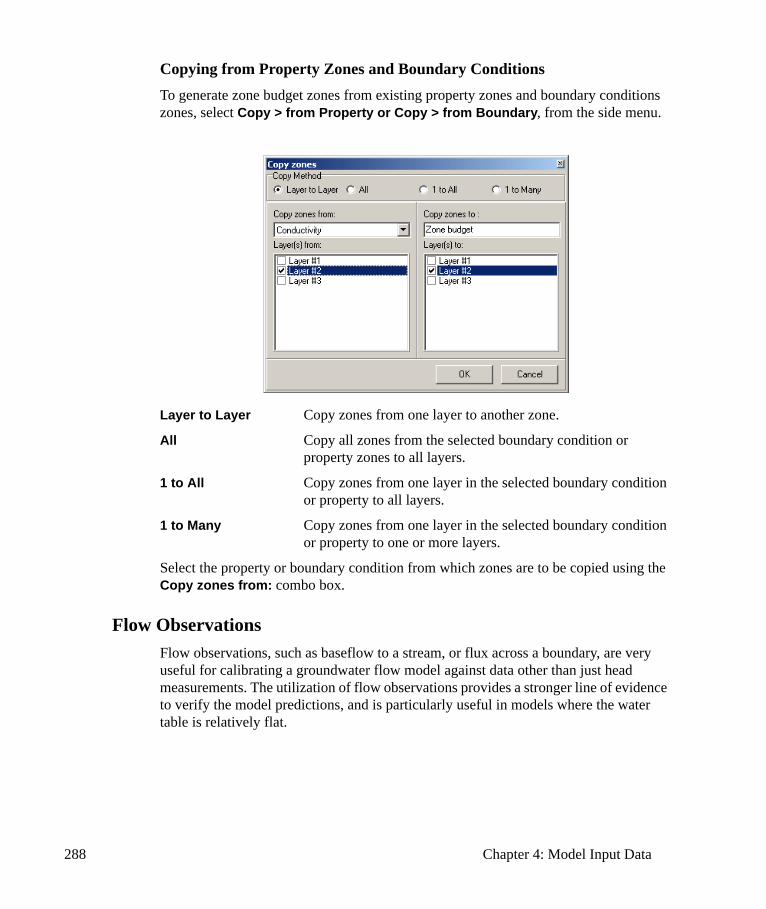
288 Chapter 4: Model Input Data
Copying from Property Zones and Boundary ConditionsTo generate zone budget zones from existing property zones and boundary conditions zones, select Copy > from Property or Copy > from Boundary, from the side menu.
Layer to Layer Copy zones from one layer to another zone.
All Copy all zones from the selected boundary condition or property zones to all layers.
1 to All Copy zones from one layer in the selected boundary condition or property to all layers.
1 to Many Copy zones from one layer in the selected boundary condition or property to one or more layers.
Select the property or boundary condition from which zones are to be copied using the Copy zones from: combo box.
Flow ObservationsFlow observations, such as baseflow to a stream, or flux across a boundary, are very useful for calibrating a groundwater flow model against data other than just head measurements. The utilization of flow observations provides a stronger line of evidence to verify the model predictions, and is particularly useful in models where the water table is relatively flat.
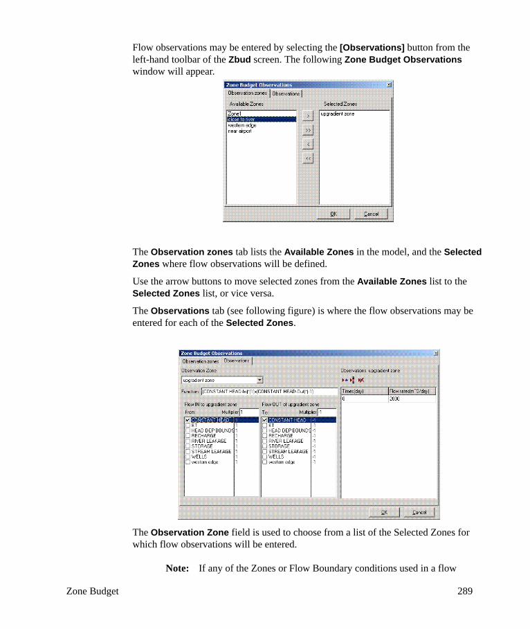
Zone Budget 289
Flow observations may be entered by selecting the [Observations] button from the left-hand toolbar of the Zbud screen. The following Zone Budget Observations window will appear.
The Observation zones tab lists the Available Zones in the model, and the Selected Zones where flow observations will be defined.
Use the arrow buttons to move selected zones from the Available Zones list to the Selected Zones list, or vice versa.
The Observations tab (see following figure) is where the flow observations may be entered for each of the Selected Zones.
The Observation Zone field is used to choose from a list of the Selected Zones for which flow observations will be entered.
Note: If any of the Zones or Flow Boundary conditions used in a flow
290 Chapter 4: Model Input Data
observation and deleted from the model, Visual MODFLOW will NOT automatically update the associated flow observations. As a result, some problems may occur if WinPEST is being used to calibrate the model using these ‘invalid’ flow observations.
The Function field lists the equation used in PEST to describe the different sources of flow contributing to the flow observation. This field is automatically filled depending on the flow sources selected for the flow observation.
The Flow IN and Flow OUT lists contain all of the different sources of flow going IN to or OUT of the Selected Zone, respectively. For the example above, the flow observation is defined for the Rivers zone (all grid cells where a River boundary condition is defined). The flow observations indicate flow is entering the Rivers zone through River leakage.
The Multiplier field is used to indicate the relative contribution of each source of flow to the Selected zone.
Occasionally, the way Zone Budget calculates flows may not correspond to the way the flows were measured in the field. To address this, the Observation table contains a means of summing the Zone Budget output such that the sum corresponds to the way the data was measured. Thus, each zone that you select from one of the lists, the zone and its weight are added to the function line. Then PEST adds the Zone Budget output values according to the defined function prior to comparing the Zone Budget output to the observations.
4.9 ToolsThe Tools menu item has the following options:
Cell Inspector: Displays the cell values and units for selected model parameters including grid co-ordinates, Kx, Ky, Kz, Ss, Sy, Head, Velocities, Concentration, and other Input and Output parameters.
Annotate: Add lines, shapes, and text to the display screen.
Units Converter: Converts the units of the selected parameters.
Copy Image to Clipboard: Copies screen image to the Windows clipboard
Enviro-Base Pro: Database containing references property values

Tools 291
4.9.1 Cell InspectorThe Cell Inspector is used to inspect selected model parameter values on a cell-by-cell basis using the mouse to select the grid cell of interest. The model parameters that may be viewed in the Cell Inspector include:
• Grid Position (Row, Column, Layer numbers of grid cell)• Model Position (X, Y, Z model co-ordinate values, Cell Top Elevation, Cell
Bottom Elevation and Cell Thickness)• World Position (X, Y, Z world co-ordinate values)• Properties (Kx, Ky, Kz, Specific Yield, Specific Storage, Effective Porosity,
Initial Head, and Initial Concentration values)• Boundary Conditions (Boundary Type, Specified Head, Concentrations,
Conductance, Recharge Rate, Evapotranspiration Rate and Extinction Depth values)
• Output (Head, Concentration, Species name, Velocity values: Vx, Vy, Vz, Vtotal values)
Note: The Output data can only be viewed from the Output section.
The Cell Inspector can be opened by selecting Tools/Cell Inspector from the top menu bar of either the Input or Output sections. The first time it is used in a model, the Cell Inspector window will be blank except for a message, as shown in figure below.
The Cell Inspector window has two tabs:
• The Options tab is used to select the model parameters to view• The Cell Values tab displays the grid cell values of the selected parameters
The Cell Values tab is initially blank is because it can be configured to display only the information of interest, and at this point no information has been selected.
There are two ways to select the model parameters to display in the Cell Inspector:
• Click the Options tab and select the model parameters from the parameter groups. A colored cross-hair will appear in the magnifying glass icon next to selected parameters as shown in the following figure. Alternately, clicking the All On button selects all the available parameter groups and All Off button deselects all the available parameter groups.
• While in the Cell Values tab, Right-Click on any of the model parameters (e.g. Row, Model X...) listed in the “Property” column, and choose from the
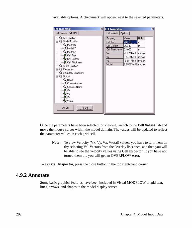
292 Chapter 4: Model Input Data
available options. A checkmark will appear next to the selected parameters.
Once the parameters have been selected for viewing, switch to the Cell Values tab and move the mouse cursor within the model domain. The values will be updated to reflect the parameter values in each grid cell.
Note: To view Velocity (Vx, Vy, Vz, Vtotal) values, you have to turn them on (by selecting Vel-Vectors from the Overlay list) once, and then you will be able to see the velocity values using Cell Inspector. If you have not turned them on, you will get an OVERFLOW error.
To exit Cell Inspector, press the close button in the top right-hand corner.
4.9.2 AnnotateSome basic graphics features have been included in Visual MODFLOW to add text, lines, arrows, and shapes to the model display screen.
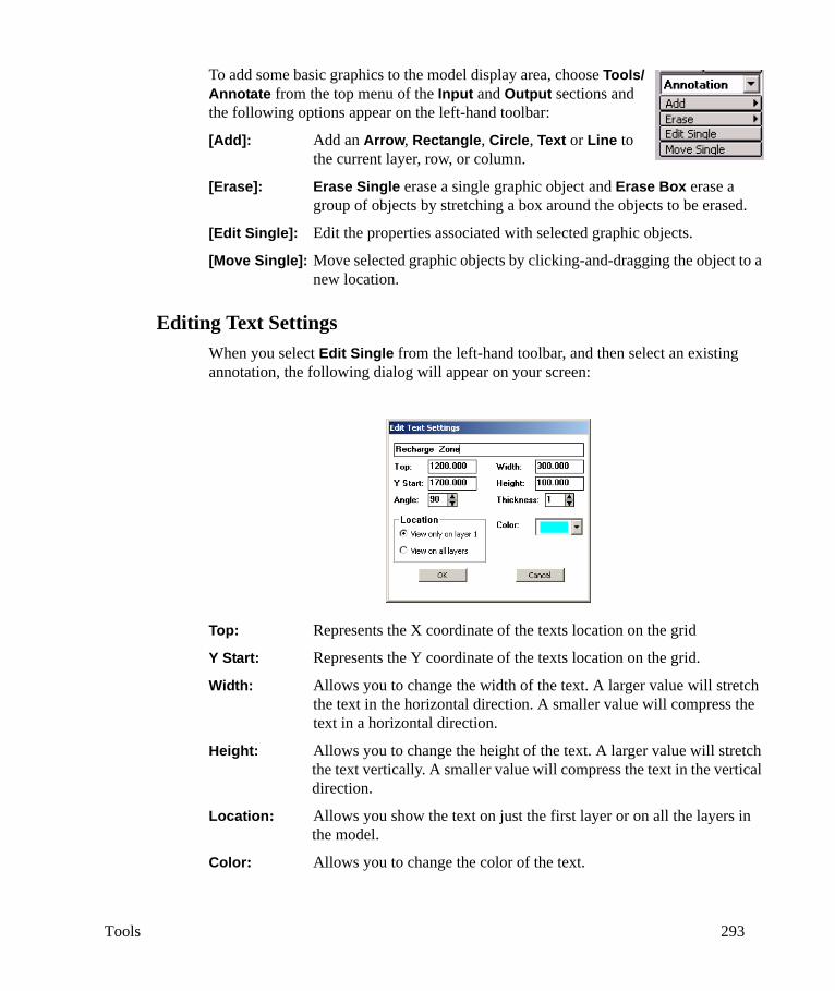
Tools 293
To add some basic graphics to the model display area, choose Tools/Annotate from the top menu of the Input and Output sections and the following options appear on the left-hand toolbar:
[Add]: Add an Arrow, Rectangle, Circle, Text or Line to the current layer, row, or column.
[Erase]: Erase Single erase a single graphic object and Erase Box erase a group of objects by stretching a box around the objects to be erased.
[Edit Single]: Edit the properties associated with selected graphic objects.
[Move Single]: Move selected graphic objects by clicking-and-dragging the object to a new location.
Editing Text SettingsWhen you select Edit Single from the left-hand toolbar, and then select an existing annotation, the following dialog will appear on your screen:
Top: Represents the X coordinate of the texts location on the grid
Y Start: Represents the Y coordinate of the texts location on the grid.
Width: Allows you to change the width of the text. A larger value will stretch the text in the horizontal direction. A smaller value will compress the text in a horizontal direction.
Height: Allows you to change the height of the text. A larger value will stretch the text vertically. A smaller value will compress the text in the vertical direction.
Location: Allows you show the text on just the first layer or on all the layers in the model.
Color: Allows you to change the color of the text.
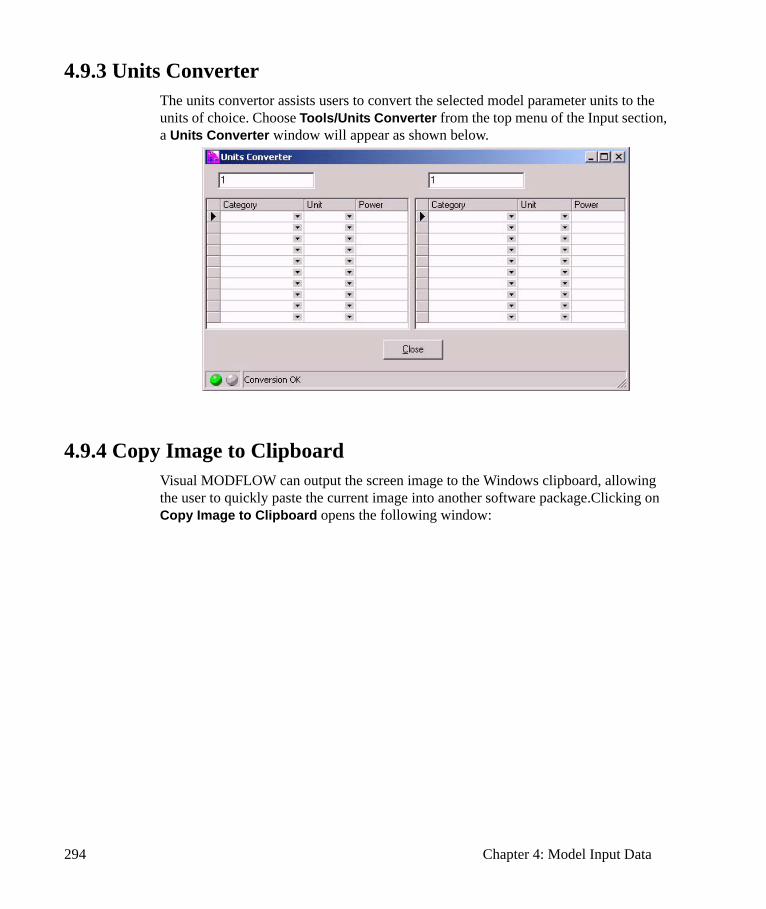
294 Chapter 4: Model Input Data
4.9.3 Units ConverterThe units convertor assists users to convert the selected model parameter units to the units of choice. Choose Tools/Units Converter from the top menu of the Input section, a Units Converter window will appear as shown below.
4.9.4 Copy Image to ClipboardVisual MODFLOW can output the screen image to the Windows clipboard, allowing the user to quickly paste the current image into another software package.Clicking on Copy Image to Clipboard opens the following window:
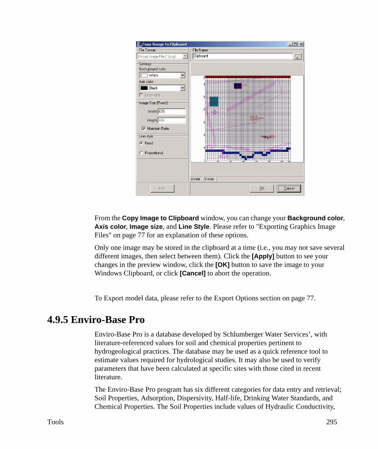
Tools 295
From the Copy Image to Clipboard window, you can change your Background color, Axis color, Image size, and Line Style. Please refer to "Exporting Graphics Image Files" on page 77 for an explanation of these options.
Only one image may be stored in the clipboard at a time (i.e., you may not save several different images, then select between them). Click the [Apply] button to see your changes in the preview window, click the [OK] button to save the image to your Windows Clipboard, or click [Cancel] to abort the operation.
To Export model data, please refer to the Export Options section on page 77.
4.9.5 Enviro-Base ProEnviro-Base Pro is a database developed by Schlumberger Water Services’, with literature-referenced values for soil and chemical properties pertinent to hydrogeological practices. The database may be used as a quick reference tool to estimate values required for hydrological studies. It may also be used to verify parameters that have been calculated at specific sites with those cited in recent literature.
The Enviro-Base Pro program has six different categories for data entry and retrieval; Soil Properties, Adsorption, Dispersivity, Half-life, Drinking Water Standards, and Chemical Properties. The Soil Properties include values of Hydraulic Conductivity,

296 Chapter 4: Model Input Data
Porosity, Specific Yield, and Specific Storage. The Chemical Properties include Viscosity, Henry's Coefficient, Vapour Pressure, Log Kow, Density, and Solubility. There are also editor windows for Material Type, Chemical Type, and References. Additionally, Enviro-Base Pro includes the option to calculate the arithmetic, geometric or logarithmic average value for parameters, and the user may convert an individual value or an average value into another unit.
Please consult the Online Help, or the PDF Manual included in the Manual folder of your Visual MODFLOW media, for a detailed explanation of the features contained in Enviro-Base Pro.

297
5Run Section - Model Run Settings
This chapter describes the features, functionality, and options in the Run section of the Visual MODFLOW interface. The Run section is where the model simulations are ‘launched’ (started), and it provides access to the run settings for the numeric engines chosen for flow, particle tracking, contaminant transport, and parameter estimation simulations.
The top menu bar of the Run section contains the following menu items:
• File• MODFLOW*• MODPATH• MT3D**• Optimization• Run• Tools• Help
* Depending on the numeric engine selected for running the flow simulation, the MODFLOW menu item may appear as MODFLOW-96, MODFLOW-2000, MODFLOW-2005, MODFLOW-NWT, SEAWAT, or MODFLOW-SURFACT (see the "Groundwater Flow Numeric Engines" section on page 69).
* If your model is using the SEAWAT engine, your top menu bar will have one entry for SEAWAT (flow and transport). The SEAWAT-specific run settings are described starting on page 374.
** Depending on the numeric engine selected for running the contaminant transport simulation, the MT3D menu item may appear as MT3D1.5, MT3DMS, MT3D99, RT3D, RT3Dv2.5, or PHT3D
Run Type: Steady-State or Transient
298 Chapter 5: Run Section - Model Run Settings
To switch between Steady State Flow and Transient Flow run types, you must return to the Main Menu, then click on Setup-Edit Engines. From the Edit Engines window, you may select the appropriate Run Type, and enter a Steady State Simulation Time (if applicable).
If the Steady-State Flow option is selected, Visual MODFLOW will prepare the data set for a steady-state flow simulation, and will automatically use the data from the first time period (only) of each boundary condition and pumping well defined in Visual MODFLOW to run the model to achieve flow equilibrium (i.e. a time-independent solution since all inputs are constant).
If the Transient Flow option is selected, Visual MODFLOW will prepare the data set for a transient flow simulation. During this process, Visual MODFLOW will automatically merge all of the different time period data defined for each pumping well and boundary condition into the stress period format required by the different versions of MODFLOW. This creates a time-dependent flow solution, as the model is being run with different inputs at different times
Note: If SEAWAT is the selected flow engine, only the Transient Flow option is available.
5.1 FileThe File menu item is used for the following operations:
Save: Save the current run settings.
Preferences: Control font size settings for labels and names of pumping and observation wells, axis, shapes, and contours. It also controls the Color settings for the Screen Background and the Axis labels.
Export… Export the model display to a Graphics Image file (.BMP, .GIF, .JPG, .PNG, .TIF), an AutoCAD (.DXF) file, or an Enhanced Windows MetaFile (.EMF).
Main Menu: Return to the Main Menu of Visual MODFLOW.
5.2 MODFLOW Run SettingsThe MODFLOW menu item may appear as MODFLOW-96, MODFLOW-2000, MODFLOW-2005, MODFLOW-NWT, SEAWAT, or MODFLOW-SURFACT depending on which numeric engine has been selected to solve the flow simulation. MODFLOW-2000 is the default selection for any new Visual MODFLOW model. The run settings available for all MODFLOW engines are as follows:

MODFLOW Run Settings 299
Time Steps: Define the number of time steps and the time-step multiplier for each stress period (Please NOTE that the Time Steps option is only available when the Transient Flow run type option is selected).
Initial Heads: Define the starting values for the initial head estimate (this can also be done from the Input menu, see the "Initial Heads" section on page 197).
Solver: Choose a MODFLOW solver package.
Recharge: Set recharge to be applied to either the top or the specified model layer, or to the uppermost active cells.
Layers: Specify the layer types in the model, as described in the MODFLOW reference manuals included with your Visual MODFLOW media, in the Manual folder.
Rewetting: Activate the wetting option of the BCF package and specify the rewetting variables.
Anisotropy: Assign the anisotropy factor by layer.
Output Control:Specify the times to save results and the formats.
List File Opts. Specify the information and format to be written to the .LST file.
The differences in the settings for each of the MODFLOW programs (MODFLOW-96, MODFLOW-2000, MODFLOW-2005, MODFLOW-NWT, SEAWAT, and MODFLOW-SURFACT) are described in the following sections.
5.2.1 Time Steps The Time Steps option is only available when you are running a transient model (i.e. when Transient Flow run type is selected). For transient flow simulations, Visual MODFLOW will automatically merge all of the different time periods defined for all of the different pumping wells and boundary conditions into the uniform stress period format required by MODFLOW. A stress period is defined as a time period in which all the stresses (boundary conditions, pumping rates, etc.) on the system are constant. Unfortunately, the data collected for each modeling site is rarely synchronized in terms of stress periods, so Visual MODFLOW merges the time schedules for all pumping wells and boundary conditions to determine the length of each stress period for a transient simulation. As a result, the user cannot directly modify the number of stress periods or the length of each stress period.
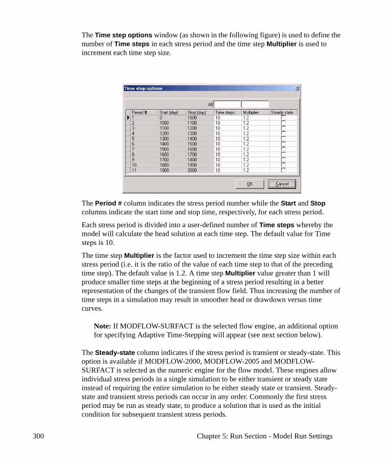
300 Chapter 5: Run Section - Model Run Settings
The Time step options window (as shown in the following figure) is used to define the number of Time steps in each stress period and the time step Multiplier is used to increment each time step size.
The Period # column indicates the stress period number while the Start and Stop columns indicate the start time and stop time, respectively, for each stress period.
Each stress period is divided into a user-defined number of Time steps whereby the model will calculate the head solution at each time step. The default value for Time steps is 10.
The time step Multiplier is the factor used to increment the time step size within each stress period (i.e. it is the ratio of the value of each time step to that of the preceding time step). The default value is 1.2. A time step Multiplier value greater than 1 will produce smaller time steps at the beginning of a stress period resulting in a better representation of the changes of the transient flow field. Thus increasing the number of time steps in a simulation may result in smoother head or drawdown versus time curves.
Note: If MODFLOW-SURFACT is the selected flow engine, an additional option for specifying Adaptive Time-Stepping will appear (see next section below).
The Steady-state column indicates if the stress period is transient or steady-state. This option is available if MODFLOW-2000, MODFLOW-2005 and MODFLOW-SURFACT is selected as the numeric engine for the flow model. These engines allow individual stress periods in a single simulation to be either transient or steady state instead of requiring the entire simulation to be either steady state or transient. Steady-state and transient stress periods can occur in any order. Commonly the first stress period may be run as steady state, to produce a solution that is used as the initial condition for subsequent transient stress periods.
MODFLOW Run Settings 301
Note: Currently, MODPATH and MT3D/RT3D do not support the use of mixed Steady-state and Transient stress periods. Therefore, all transient models must be run with all Transient stress periods while using MODPATH and/or MT3D/RT3D.
If MODFLOW-SURFACT is the selected flow engine, an additional Reset-Drawdown column will appear. Use this column to define a flag in the BAS file to reset reference head for calculating drawdowns.
Adaptive Time-Stepping In MODFLOW-SURFACT, the adaptive time-stepping and output package, ATO4, provides great robustness and efficiency in transient flow simulations, and provides improved organization and control of simulation output. Activating adaptive time stepping scheme permits the user to specify an initial time step size, a minimum and maximum time step size, a time step multiplier, and a time step reduction factor for each stress period. With these parameters, automatic generation of time steps take place and the time steps are dynamically determined during the iterations by cutting the time step size when the simulation becomes difficult, and increasing it when the difficulty passes.
The initial time step size is used for the first time-step of the stress period. If convergence is achieved within 35% of the maximum number of iterations, the time step size is increased by the multiplying factor. For a convergence rate between 35% and 65% of the maximum iterations, the time-step size is unaltered from the previous initial time step size, and the convergence behavior of the system is considered optimal for this value of initial time step size. If, however, the number of iterations required to achieve convergence exceeds 65% of the maximum iterations, the time step size is reduced by a time step reduction factor.
If the convergence is not achieved for a particular time step, the time step size is reduced by a factor of 5.0 and computations are redone for the smaller time step size. In addition, if a print time (i.e. the target time value at which the output printing/saving is required) is reached, the time step size is selected to include the print time value.
If the value of the initial time step size is reduced to be smaller than the minimum time step size, the simulation is aborted. This technique provides a means of exiting the program simulation if severe difficulties are encountered. Finally, the value of the initial time step size is constrained to be less than or equal to the maximum time step size. This constraint is significant for accuracy of time discretization, even when the non-linearities are mild or insignificant.
Time values of simulation results are not known a priori for an automatic time stepping scheme. Therefore, the ATO4 package automatically recognizes the specified time values in a particular stress period for output, and adjusts the time step size to perform computations at the selected save or print times. It functions similar to the output control options in MT3D.
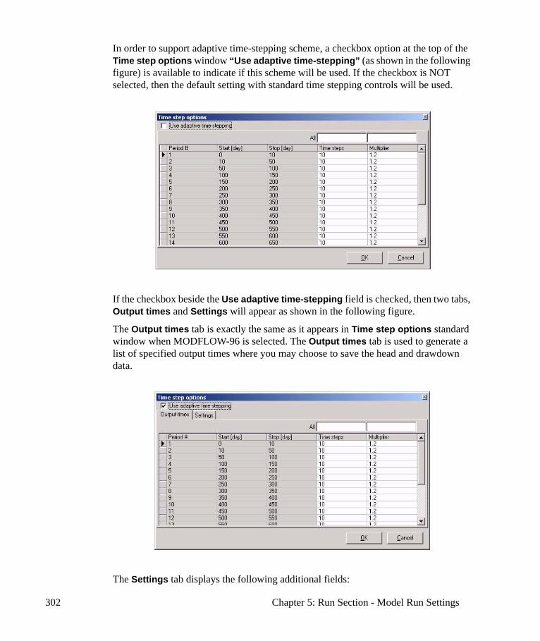
302 Chapter 5: Run Section - Model Run Settings
In order to support adaptive time-stepping scheme, a checkbox option at the top of the Time step options window “Use adaptive time-stepping” (as shown in the following figure) is available to indicate if this scheme will be used. If the checkbox is NOT selected, then the default setting with standard time stepping controls will be used.
If the checkbox beside the Use adaptive time-stepping field is checked, then two tabs, Output times and Settings will appear as shown in the following figure.
The Output times tab is exactly the same as it appears in Time step options standard window when MODFLOW-96 is selected. The Output times tab is used to generate a list of specified output times where you may choose to save the head and drawdown data.
The Settings tab displays the following additional fields:
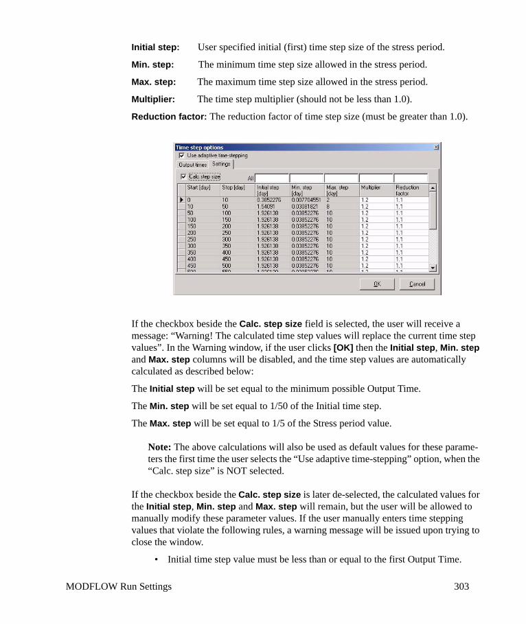
MODFLOW Run Settings 303
Initial step: User specified initial (first) time step size of the stress period.
Min. step: The minimum time step size allowed in the stress period.
Max. step: The maximum time step size allowed in the stress period.
Multiplier: The time step multiplier (should not be less than 1.0).
Reduction factor: The reduction factor of time step size (must be greater than 1.0).
If the checkbox beside the Calc. step size field is selected, the user will receive a message: “Warning! The calculated time step values will replace the current time step values”. In the Warning window, if the user clicks [OK] then the Initial step, Min. step and Max. step columns will be disabled, and the time step values are automatically calculated as described below:
The Initial step will be set equal to the minimum possible Output Time.
The Min. step will be set equal to 1/50 of the Initial time step.
The Max. step will be set equal to 1/5 of the Stress period value.
Note: The above calculations will also be used as default values for these parame-ters the first time the user selects the “Use adaptive time-stepping” option, when the “Calc. step size” is NOT selected.
If the checkbox beside the Calc. step size is later de-selected, the calculated values for the Initial step, Min. step and Max. step will remain, but the user will be allowed to manually modify these parameter values. If the user manually enters time stepping values that violate the following rules, a warning message will be issued upon trying to close the window.
• Initial time step value must be less than or equal to the first Output Time.
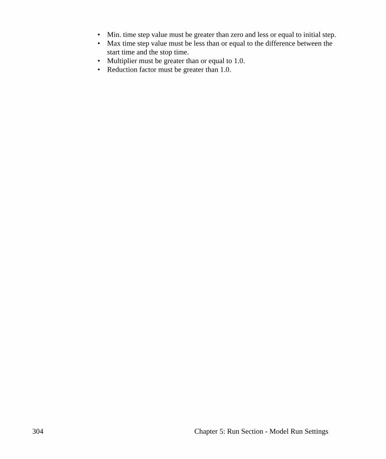
304 Chapter 5: Run Section - Model Run Settings
• Min. time step value must be greater than zero and less or equal to initial step. • Max time step value must be less than or equal to the difference between the
start time and the stop time.• Multiplier must be greater than or equal to 1.0.• Reduction factor must be greater than 1.0.
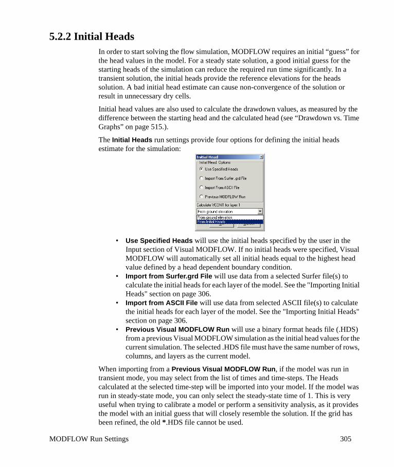
MODFLOW Run Settings 305
5.2.2 Initial HeadsIn order to start solving the flow simulation, MODFLOW requires an initial “guess” for the head values in the model. For a steady state solution, a good initial guess for the starting heads of the simulation can reduce the required run time significantly. In a transient solution, the initial heads provide the reference elevations for the heads solution. A bad initial head estimate can cause non-convergence of the solution or result in unnecessary dry cells.
Initial head values are also used to calculate the drawdown values, as measured by the difference between the starting head and the calculated head (see “Drawdown vs. Time Graphs” on page 515.).
The Initial Heads run settings provide four options for defining the initial heads estimate for the simulation:
• Use Specified Heads will use the initial heads specified by the user in the Input section of Visual MODFLOW. If no initial heads were specified, Visual MODFLOW will automatically set all initial heads equal to the highest head value defined by a head dependent boundary condition.
• Import from Surfer.grd File will use data from a selected Surfer file(s) to calculate the initial heads for each layer of the model. See the "Importing Initial Heads" section on page 306.
• Import from ASCII File will use data from selected ASCII file(s) to calculate the initial heads for each layer of the model. See the "Importing Initial Heads" section on page 306.
• Previous Visual MODFLOW Run will use a binary format heads file (.HDS) from a previous Visual MODFLOW simulation as the initial head values for the current simulation. The selected .HDS file must have the same number of rows, columns, and layers as the current model.
When importing from a Previous Visual MODFLOW Run, if the model was run in transient mode, you may select from the list of times and time-steps. The Heads calculated at the selected time-step will be imported into your model. If the model was run in steady-state mode, you can only select the steady-state time of 1. This is very useful when trying to calibrate a model or perform a sensitivity analysis, as it provides the model with an initial guess that will closely resemble the solution. If the grid has been refined, the old *.HDS file cannot be used.

306 Chapter 5: Run Section - Model Run Settings
Calculating VCONT ValuesWhen using the Layer Property Flow (LPF) package (or another Layer Property Package), the VCONT term is not required and the parameter is disabled. However, when using the Block Centered Flow (BCF) package, VCONT is defined for the interface between layers at the beginning of the simulation. Visual MODFLOW allows the VCONT value to be defined based on Ground Elevation values (i.e. cell top), or based on Initial Head values.
Note: If Layer 1 has been defined with Layer Type=0, VCONT will always be defined based on Ground Elevation values, and the option to change to Initial Heads will be greyed out.
Note: If your Initial Heads file (i.e. if imported from a previous run) contains dry cells, the VCONT calculation formula will use a 0 value for the dry layer(s).
Importing Initial HeadsInitial heads can be imported in both the Input and the Run sections of Visual MODFLOW (please see the "Initial Heads" section on page 197 for details on importing Initial Heads from the Input section). As discussed in Chapter 4, the advantage to importing the initial heads in the Run section is that the values are exact, because it is not necessary to calculate values for the constant value initial head property zones. The disadvantage to importing in the Run section is that you are unable to view the distribution of initial head values before running the model.
In the Run section, Visual MODFLOW can import initial heads data from:
• ASCII files (.TXT) in world or model co-ordinates system• Surfer files (.GRD) in world or model co-ordinates system
The ASCII file (.TXT) must be saved in Space or tab-delimited format with the following data structure:
X-co-ordinate, Y-co-ordinate, Initial Head Value
Example:
1120 2352 34
3392 4491 36
2892 2531 29
3590 1803 32
No header information or column titles are allowed, and the co-ordinate locations for the data points must be within the model domain. If different initial head values are required for different sets of layers in the model, then separate ASCII text files must be prepared for each model layer.

MODFLOW Run Settings 307
The Surfer Grid files must be saved in binary format, and the majority of the grid domain must correspond with the model domain. If different initial head values are required for different sets of layers in the model, then separate Surfer Grid files must be prepared for each model layer.
Visual MODFLOW uses an inverse distance interpolation method to calculate the head values for the center of each grid cell.
To import initial heads from an ASCII file or a Surfer file,
• Choose the source file type from the Initial Heads window and click [OK].• Select the source file for the first layer of the model and click [Open].• An Import Initial Head window will appear with the selected source file
applied to each layer of the model (see following figure).• To use a different source file for different layers, click in the target layer and
use the [Choose File] button to select the appropriate file for each layer.• Enter the appropriate number of Nearest Neighbors (nearest data points) to be
used during the interpolation procedure for each layer of the model.• Click [OK] to interpolate the initial heads data to the model grid and import the
array into Visual MODFLOW.
5.2.3 Solver SettingsVisual MODFLOW comes with a choice of different solvers to use in solving the numerical equations for the flow simulation:
• Preconditioned Conjugate-Gradient Package (PCG2)• Strongly Implicit Procedure Package (SIP)• Slice-Successive Overrelaxation Package (SOR)• WHS Solver for Visual MODFLOW (WHS)• Geometric Multigrid Solver (GMG)
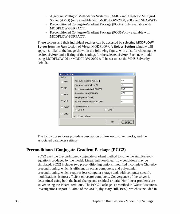
308 Chapter 5: Run Section - Model Run Settings
• Algebraic Multigrid Methods for Systems (SAMG) and Algebraic Multigrid Solver (AMG) (only available with MODFLOW-2000, 2005, and SEAWAT)
• Preconditioned Conjugate-Gradient Package (PCG4) (only available with MODFLOW-SURFACT).
• Preconditioned Conjugate-Gradient Package (PCG5)(only available with MODFLOW-SURFACT).
These solvers and their individual settings can be accessed by selecting MODFLOW/Solver from the Run section of Visual MODFLOW. A Solver Setting window will appear, similar to the image shown in the following figure, with a list for choosing the desired Solver and a listing of the settings for the selected Solver. Each new model using MODFLOW-96 or MODFLOW-2000 will be set to use the WHS Solver by default.
The following sections provide a description of how each solver works, and the associated parameter settings.
Preconditioned Conjugate-Gradient Package (PCG2) PCG2 uses the preconditioned conjugate-gradient method to solve the simultaneous equations produced by the model. Linear and non-linear flow conditions may be simulated. PCG2 includes two preconditioning options: modified incomplete Cholesky preconditioning, which is efficient on scalar computers; and polynomial preconditioning, which requires less computer storage and, with computer specific modifications, is most efficient on vector computers. Convergence of the solver is determined using both the head-change and residual criteria. Non-linear problems are solved using the Picard iterations. The PCG2 Package is described in Water-Resources Investigations Report 90-4048 of the USGS, (by Mary Hill, 1997), which is included in
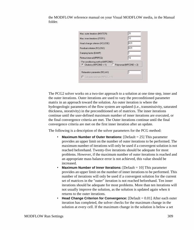
MODFLOW Run Settings 309
the MODFLOW reference manual on your Visual MODFLOW media, in the Manual folder.
The PCG2 solver works on a two-tier approach to a solution at one time step, inner and the outer iterations. Outer iterations are used to vary the preconditioned parameter matrix in an approach toward the solution. An outer iteration is where the hydrogeologic parameters of the flow system are updated (i.e., transmissivity, saturated thickness, storativity) in the preconditioned set of matrices. The inner iterations continue until the user-defined maximum number of inner iterations are executed, or the final convergence criteria are met. The Outer iterations continue until the final convergence criteria are met on the first inner iteration after an update.
The following is a description of the solver parameters for the PCG method:
• Maximum Number of Outer Iterations: [Default = 25] This parameter provides an upper limit on the number of outer iterations to be performed. The maximum number of iterations will only be used if a convergent solution is not reached beforehand. Twenty-five iterations should be adequate for most problems. However, if the maximum number of outer iterations is reached and an appropriate mass balance error is not achieved, this value should be increased.
• Maximum Number of Inner Iterations: [Default = 10] This parameter provides an upper limit on the number of inner iterations to be performed. This number of iterations will only be used if a convergent solution for the current set of matrices in the "outer" iteration is not reached beforehand. Ten inner iterations should be adequate for most problems. More than ten iterations will not usually improve the solution, as the solution is updated again when it returns to the outer iterations.
• Head Change Criterion for Convergence: [Default = 0.01] After each outer iteration has completed, the solver checks for the maximum change in the solution at every cell. If the maximum change in the solution is below a set
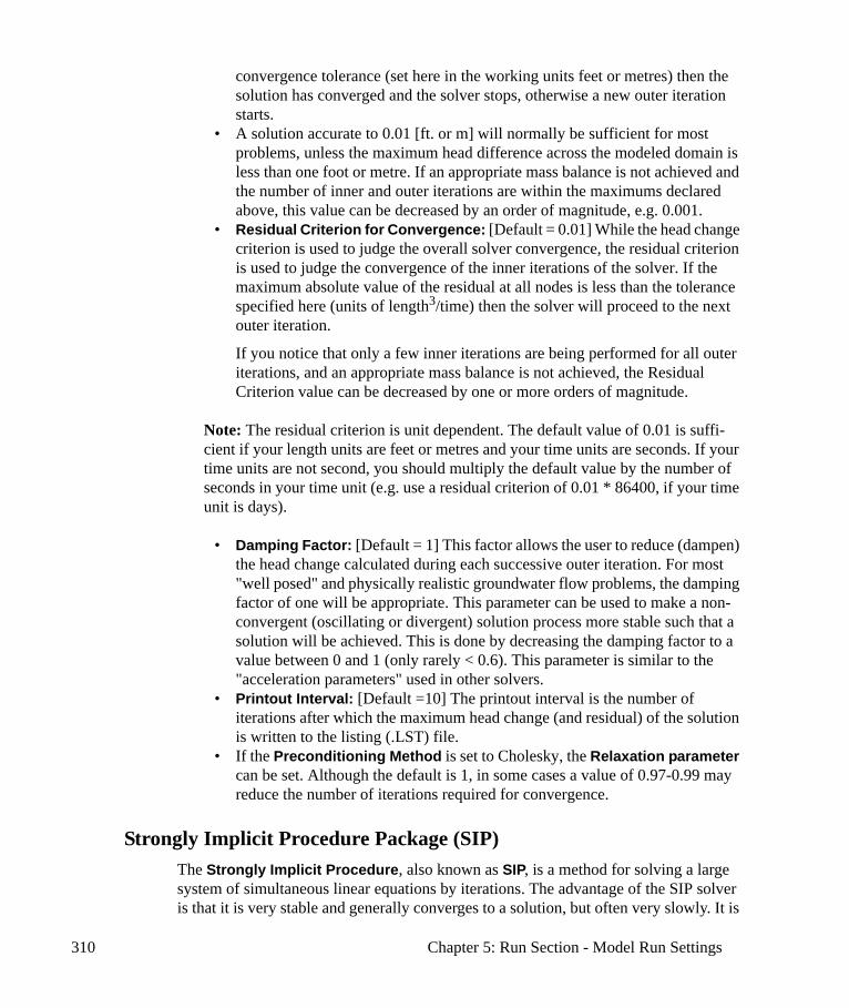
310 Chapter 5: Run Section - Model Run Settings
convergence tolerance (set here in the working units feet or metres) then the solution has converged and the solver stops, otherwise a new outer iteration starts.
• A solution accurate to 0.01 [ft. or m] will normally be sufficient for most problems, unless the maximum head difference across the modeled domain is less than one foot or metre. If an appropriate mass balance is not achieved and the number of inner and outer iterations are within the maximums declared above, this value can be decreased by an order of magnitude, e.g. 0.001.
• Residual Criterion for Convergence: [Default = 0.01] While the head change criterion is used to judge the overall solver convergence, the residual criterion is used to judge the convergence of the inner iterations of the solver. If the maximum absolute value of the residual at all nodes is less than the tolerance specified here (units of length3/time) then the solver will proceed to the next outer iteration.
If you notice that only a few inner iterations are being performed for all outer iterations, and an appropriate mass balance is not achieved, the Residual Criterion value can be decreased by one or more orders of magnitude.
Note: The residual criterion is unit dependent. The default value of 0.01 is suffi-cient if your length units are feet or metres and your time units are seconds. If your time units are not second, you should multiply the default value by the number of seconds in your time unit (e.g. use a residual criterion of 0.01 * 86400, if your time unit is days).
• Damping Factor: [Default = 1] This factor allows the user to reduce (dampen) the head change calculated during each successive outer iteration. For most "well posed" and physically realistic groundwater flow problems, the damping factor of one will be appropriate. This parameter can be used to make a non-convergent (oscillating or divergent) solution process more stable such that a solution will be achieved. This is done by decreasing the damping factor to a value between 0 and 1 (only rarely < 0.6). This parameter is similar to the "acceleration parameters" used in other solvers.
• Printout Interval: [Default =10] The printout interval is the number of iterations after which the maximum head change (and residual) of the solution is written to the listing (.LST) file.
• If the Preconditioning Method is set to Cholesky, the Relaxation parameter can be set. Although the default is 1, in some cases a value of 0.97-0.99 may reduce the number of iterations required for convergence.
Strongly Implicit Procedure Package (SIP) The Strongly Implicit Procedure, also known as SIP, is a method for solving a large system of simultaneous linear equations by iterations. The advantage of the SIP solver is that it is very stable and generally converges to a solution, but often very slowly. It is
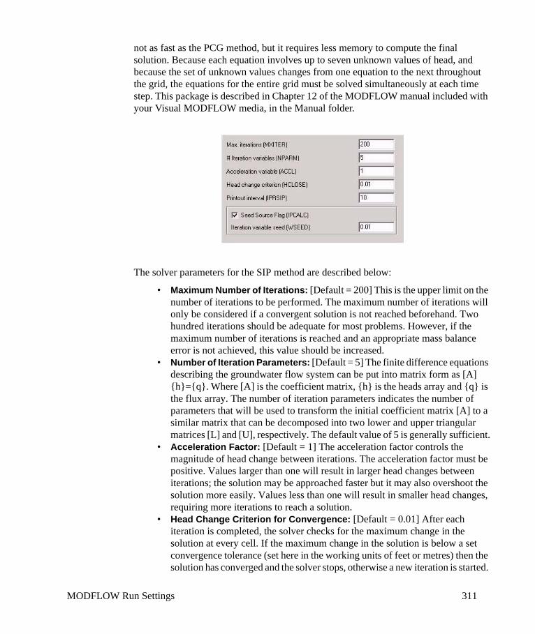
MODFLOW Run Settings 311
not as fast as the PCG method, but it requires less memory to compute the final solution. Because each equation involves up to seven unknown values of head, and because the set of unknown values changes from one equation to the next throughout the grid, the equations for the entire grid must be solved simultaneously at each time step. This package is described in Chapter 12 of the MODFLOW manual included with your Visual MODFLOW media, in the Manual folder.
The solver parameters for the SIP method are described below:
• Maximum Number of Iterations: [Default = 200] This is the upper limit on the number of iterations to be performed. The maximum number of iterations will only be considered if a convergent solution is not reached beforehand. Two hundred iterations should be adequate for most problems. However, if the maximum number of iterations is reached and an appropriate mass balance error is not achieved, this value should be increased.
• Number of Iteration Parameters: [Default = 5] The finite difference equations describing the groundwater flow system can be put into matrix form as [A] {h}={q}. Where [A] is the coefficient matrix, {h} is the heads array and {q} is the flux array. The number of iteration parameters indicates the number of parameters that will be used to transform the initial coefficient matrix [A] to a similar matrix that can be decomposed into two lower and upper triangular matrices [L] and [U], respectively. The default value of 5 is generally sufficient.
• Acceleration Factor: [Default = 1] The acceleration factor controls the magnitude of head change between iterations. The acceleration factor must be positive. Values larger than one will result in larger head changes between iterations; the solution may be approached faster but it may also overshoot the solution more easily. Values less than one will result in smaller head changes, requiring more iterations to reach a solution.
• Head Change Criterion for Convergence: [Default = 0.01] After each iteration is completed, the solver checks for the maximum change in the solution at every cell. If the maximum change in the solution is below a set convergence tolerance (set here in the working units of feet or metres) then the solution has converged and the solver stops, otherwise a new iteration is started.
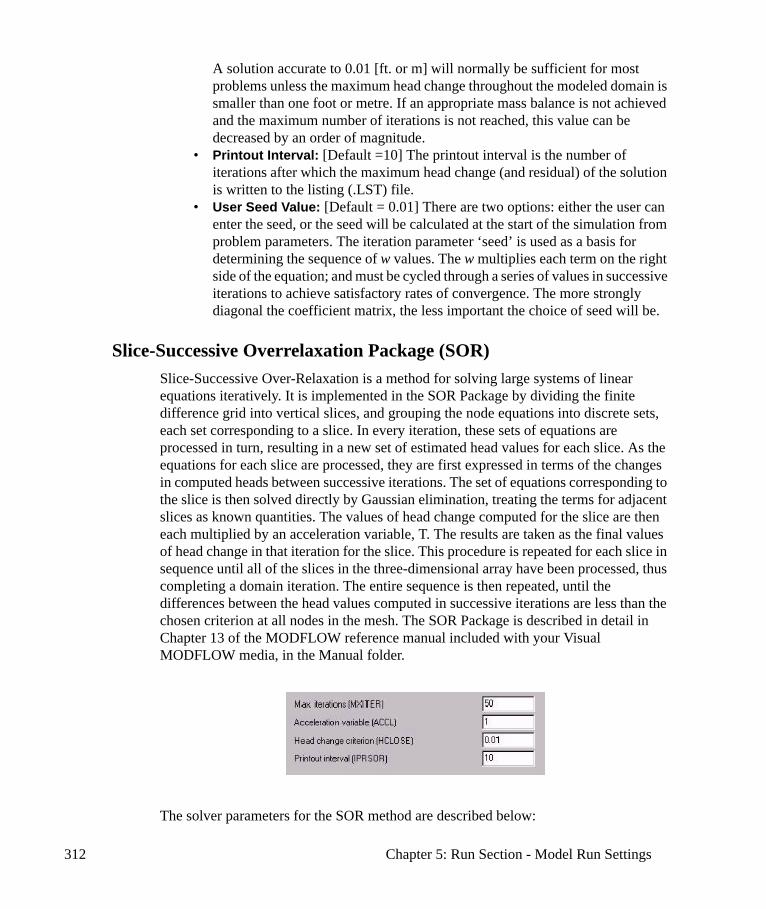
312 Chapter 5: Run Section - Model Run Settings
A solution accurate to 0.01 [ft. or m] will normally be sufficient for most problems unless the maximum head change throughout the modeled domain is smaller than one foot or metre. If an appropriate mass balance is not achieved and the maximum number of iterations is not reached, this value can be decreased by an order of magnitude.
• Printout Interval: [Default =10] The printout interval is the number of iterations after which the maximum head change (and residual) of the solution is written to the listing (.LST) file.
• User Seed Value: [Default = 0.01] There are two options: either the user can enter the seed, or the seed will be calculated at the start of the simulation from problem parameters. The iteration parameter ‘seed’ is used as a basis for determining the sequence of w values. The w multiplies each term on the right side of the equation; and must be cycled through a series of values in successive iterations to achieve satisfactory rates of convergence. The more strongly diagonal the coefficient matrix, the less important the choice of seed will be.
Slice-Successive Overrelaxation Package (SOR) Slice-Successive Over-Relaxation is a method for solving large systems of linear equations iteratively. It is implemented in the SOR Package by dividing the finite difference grid into vertical slices, and grouping the node equations into discrete sets, each set corresponding to a slice. In every iteration, these sets of equations are processed in turn, resulting in a new set of estimated head values for each slice. As the equations for each slice are processed, they are first expressed in terms of the changes in computed heads between successive iterations. The set of equations corresponding to the slice is then solved directly by Gaussian elimination, treating the terms for adjacent slices as known quantities. The values of head change computed for the slice are then each multiplied by an acceleration variable, T. The results are taken as the final values of head change in that iteration for the slice. This procedure is repeated for each slice in sequence until all of the slices in the three-dimensional array have been processed, thus completing a domain iteration. The entire sequence is then repeated, until the differences between the head values computed in successive iterations are less than the chosen criterion at all nodes in the mesh. The SOR Package is described in detail in Chapter 13 of the MODFLOW reference manual included with your Visual MODFLOW media, in the Manual folder.
The solver parameters for the SOR method are described below:
MODFLOW Run Settings 313
• Maximum Number of Iterations: [Default = 50] This parameter provides an upper limit on the number of iterations to be performed. The maximum number of iterations will only be used if a convergent solution is not reached beforehand. 50 iterations should be adequate for most problems. However, if the maximum number of outer iterations is reached and an appropriate mass balance error is not achieved, this value should be increased.
• Acceleration Factor: [Default = 1] The acceleration factor controls the magnitude of head changes between iterations. The acceleration factor must be positive. Values larger than one will result in larger head changes between iterations; the solution may be approached faster but it may also overshoot the solution more easily. Values less than one will result in smaller head changes, thus, requiring more iterations to reach a solution.
• Head Change Criterion for Convergence: [Default = 0.01] After each iteration is completed, the solver checks for the maximum change in the solution at every cell. If the maximum change in the solution is below a set convergence tolerance (set here in the working units of feet or metres), then the solution has converged and the solver stops, otherwise a new iteration is started. A solution accurate to 0.01 [ft. or m] will normally be sufficient for most problems unless the maximum head change throughout the model domain is less than 1 foot or metre. If an appropriate mass balance is not achieved and the number of iterations is less than the maximum, this value can be decreased by an order of magnitude.
• Printout Interval: [Default =10] The printout interval is the number of iterations after which the maximum head change (and residual) of the solution is written to the listing (.LST) file.
WHS Solver for Visual MODFLOW (WHS) The WHS Solver uses a Bi-Conjugate Gradient Stabilized (Bi-CGSTAB) acceleration routine implemented with Stone incomplete decomposition for preconditioning of the groundwater flow partial differential equations. This solver, as all iterative solvers, approaches the solution of a large set of partial differential equations iteratively through an approximate solution. Because the matrix equation for groundwater flow is initially "ill-conditioned", effective pre-conditioning of these matrices is necessary for an efficient solution.
The WHS solver works on a two-tier approach to a solution at one time step. Outer iterations are used to vary the factorized parameter matrix in an approach toward the solution. An outer iteration is where the hydrogeologic parameters of the flow system are updated (i.e., transmissivity, saturated thickness, storativity) in the factorized set of matrices. Different levels of factorization allow these matrices to be initialized differently to increase the efficiency of solution and model stability. Inner iterations are used to iteratively solve the matrices created in the outer iterations.
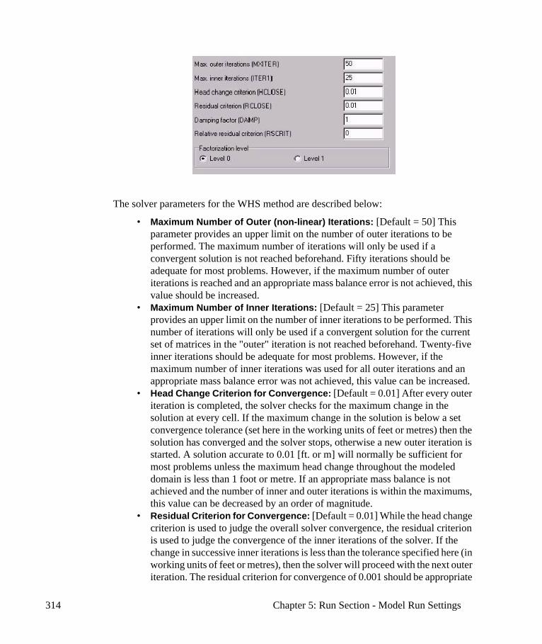
314 Chapter 5: Run Section - Model Run Settings
The solver parameters for the WHS method are described below:
• Maximum Number of Outer (non-linear) Iterations: [Default = 50] This parameter provides an upper limit on the number of outer iterations to be performed. The maximum number of iterations will only be used if a convergent solution is not reached beforehand. Fifty iterations should be adequate for most problems. However, if the maximum number of outer iterations is reached and an appropriate mass balance error is not achieved, this value should be increased.
• Maximum Number of Inner Iterations: [Default = 25] This parameter provides an upper limit on the number of inner iterations to be performed. This number of iterations will only be used if a convergent solution for the current set of matrices in the "outer" iteration is not reached beforehand. Twenty-five inner iterations should be adequate for most problems. However, if the maximum number of inner iterations was used for all outer iterations and an appropriate mass balance error was not achieved, this value can be increased.
• Head Change Criterion for Convergence: [Default = 0.01] After every outer iteration is completed, the solver checks for the maximum change in the solution at every cell. If the maximum change in the solution is below a set convergence tolerance (set here in the working units of feet or metres) then the solution has converged and the solver stops, otherwise a new outer iteration is started. A solution accurate to 0.01 [ft. or m] will normally be sufficient for most problems unless the maximum head change throughout the modeled domain is less than 1 foot or metre. If an appropriate mass balance is not achieved and the number of inner and outer iterations is within the maximums, this value can be decreased by an order of magnitude.
• Residual Criterion for Convergence: [Default = 0.01] While the head change criterion is used to judge the overall solver convergence, the residual criterion is used to judge the convergence of the inner iterations of the solver. If the change in successive inner iterations is less than the tolerance specified here (in working units of feet or metres), then the solver will proceed with the next outer iteration. The residual criterion for convergence of 0.001 should be appropriate
MODFLOW Run Settings 315
for most problems. However, if you notice that only a few inner iterations are being performed for every outer iteration and an appropriate mass balance is not achieved, this parameter value can be decreased by one or more orders of magnitude.
• Damping Factor for the Outer Iterations: [Default = 1] This factor allows the user to reduce (dampen) the head change calculated during each successive outer iteration. For most "well posed" and physically realistic groundwater flow problems, the dampening factor of one will be appropriate. This parameter can be used to make a non-convergent (oscillating or divergent) solution process more stable such that a solution will be achieved. This is done by decreasing the damping factor to a value between 0 and 1 (only rarely < 0.6). This parameter is similar to "acceleration parameters" used in other solvers.
• Relative Residual Criterion: [Default = 0] This parameter provides another method of checking for convergence of the inner iteration. This method compares the residual from the most recent inner iteration to the residual from the initial inner iteration. Once the most recent inner iteration residual is below the initial inner iteration residual times the relative residual criterion, the current outer iteration is completed and a new outer iteration will be started.
• Factorization Level: [Default = 0] There are two “levels” of factorization available with the WHS solver, 0 and 1. Level 0 requires more outer iterations but less memory. Level 1 requires fewer outer iterations but more memory. While convergence of the solver requires fewer iterations with a factorization level of 1, the memory required to run the solver increases with this factorization level. Also, the work per iteration increases with the level 1 factorization such that the total solution time may not be less than the solution time using level 0 factorization.
Algebraic Multigrid Methods for Systems (SAMG) and Algebraic Multigrid Solver (AMG)
Visual MODFLOW supports the Algebraic Multigrid Methods for Systems Solver (SAMG) Package developed by the Fraunhofer Institute for Algorithms and Scientific Computing (FhG-SCAI). Please note that the SAMG solver is only available with the SEAWAT, MODFLOW-2000,2005 flow engine.
The Algebraic Multigrid (AMG) Package solver may be obtained from the Fraunhofer Institute for Algorithms and Scientific Computing (FhG-SCAI) for research purposes only. Although most users will not have any difficulty running Visual MODFLOW with the AMG solver, Schlumberger Water Services unfortunately cannot provide technical support for users who choose to manually add the AMG solver to their Visual MODFLOW software.
The SAMG solver package is a complete multi-level framework, designed to overcome the high memory requirements of previous AMG-based solvers, while maintaining the
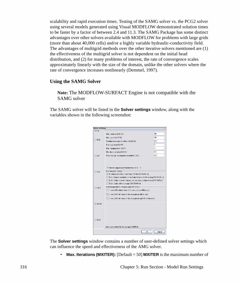
316 Chapter 5: Run Section - Model Run Settings
scalability and rapid execution times. Testing of the SAMG solver vs. the PCG2 solver using several models generated using Visual MODFLOW demonstrated solution times to be faster by a factor of between 2.4 and 11.3. The SAMG Package has some distinct advantages over other solvers available with MODFLOW for problems with large grids (more than about 40,000 cells) and/or a highly variable hydraulic-conductivity field. The advantages of multigrid methods over the other iterative solvers mentioned are (1) the effectiveness of the multigrid solver is not dependent on the initial head distribution, and (2) for many problems of interest, the rate of convergence scales approximately linearly with the size of the domain, unlike the other solvers where the rate of convergence increases nonlinearly (Demmel, 1997).
Using the SAMG Solver
Note: The MODFLOW-SURFACT Engine is not compatible with the SAMG solver
The SAMG solver will be listed in the Solver settings window, along with the variables shown in the following screenshot:
The Solver settings window contains a number of user-defined solver settings which can influence the speed and effectiveness of the AMG solver.
• Max. Iterations (MXITER): [Default = 50] MXITER is the maximum number of
MODFLOW Run Settings 317
times that the AMG routines will be called to obtain a solution. MXITER is never less than 2, and rarely more than 50. MXITER often equals 2 when the problem is linear (all layers are confined, and no boundary conditions are nonlinear; the Evapotranspiration, Drain, and River Packages, for example, produce nonlinear boundary conditions). For nonlinear problems, MXITER generally is 50 or less; however values near 50 and sometimes even larger are needed for more severely nonlinear problems.
• Max. Cycles (MXCYC): [Default = 50] For each call to the solver, AMG cycles through one or more sequences of coarsening and refinement. The solver is limited to a maximum of MXCYC cycles per call to the solver. For most problems, convergence for each iteration is achieved in less than 50 cycles, so that generally MXCYC can be less than 50. For highly nonlinear problems, however, better performance may be achieved by limiting the solver to a small number of cycles, and increasing the maximum number of iterations (MXITER). This prevents the solver from needlessly finding very accurate solutions at early iterations of these highly nonlinear problems.
• Residual Convergence Criterion (RCLOSE) for the inner iteration. Typically RCLOSE is set to the same value as HCLOSE. If RCLOSE is set too high, then additional outer iterations may be required due to the linear equation not being solved with sufficient accuracy. Likewise, a too restrictive setting for RCLOSE for nonlinear problems may force an unnecessarily accurate linear solution. This may be alleviated with the MXCYC parameter or with damping. NOTE: In the new SAMG package, RCLOSE and HCLOSE replace BCLOSE
• Damping Factor (DAMP): [Default = 1] The damping factor can be used to restrict the head change from one iteration to the next, which commonly is useful in very nonlinear problems. DAMP makes the solution change slowly, thus avoiding spurious deviations prompted by nonlinear effects at intermediate solutions. Values of DAMP less than 1.0 restrict the head change (under-relaxation), while values greater than 1.0 accelerate the head change (over-relaxation). For linear problems, no damping is necessary, and DAMP should be set equal to 1.0. For non-linear problems, restricting the head change (DAMP < 1.0) may be necessary to achieve convergence, and values of DAMP between 0.5 and 1.0 are generally sufficient.
For some nonlinear problems, imposing a fixed value of DAMP for every iteration can hinder convergence. One remedy for this condition is to adjust the amount of damping depending on how the head solution progresses. The AMG Package provides two adaptive damping strategies; (1) Cooley’s method with Huyakorn’s modification, and (2) the relative reduced residual method. These methods are described in detail in the U.S. Geological Open-File Report 01-177. A DAMP value of -1 will utilize the first method, and a DAMP value of -2 will utilize the second method.
• Max. Damping Factor (DUP): [Default = 1] The upper limit for DAMP when an adaptive damping strategy is used.
• Min. Damping Factor (DLOW): [Default = 0.2] The lower limit for DAMP
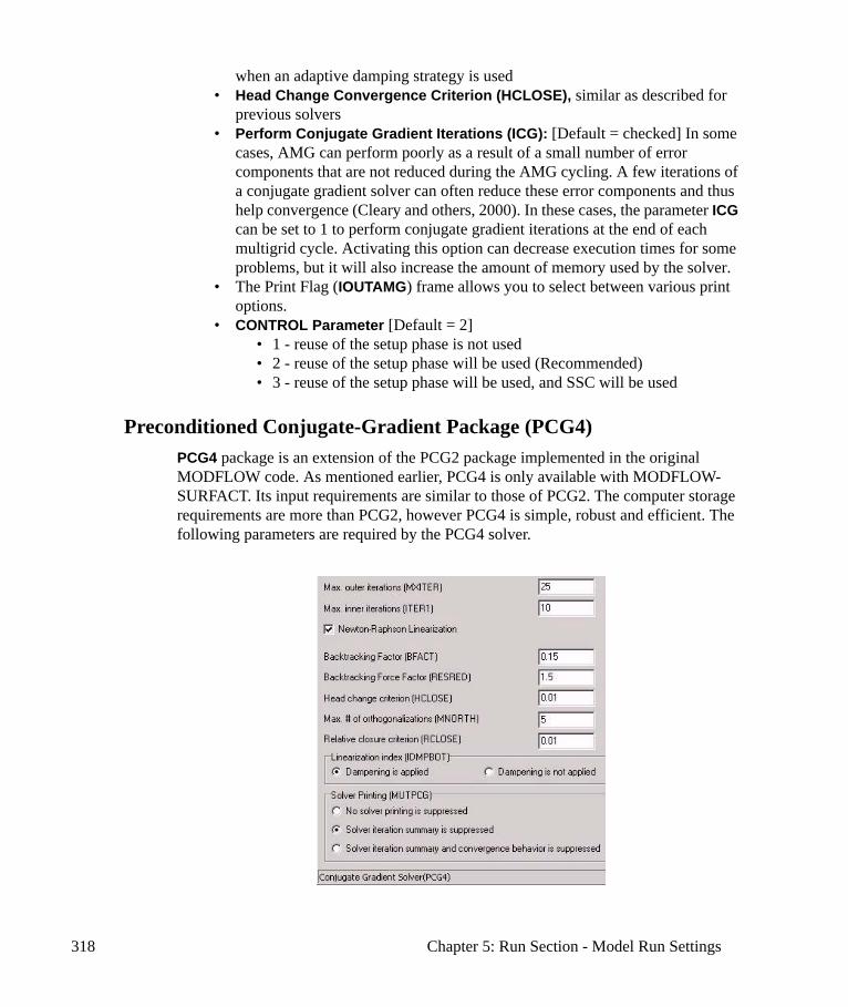
318 Chapter 5: Run Section - Model Run Settings
when an adaptive damping strategy is used• Head Change Convergence Criterion (HCLOSE), similar as described for
previous solvers• Perform Conjugate Gradient Iterations (ICG): [Default = checked] In some
cases, AMG can perform poorly as a result of a small number of error components that are not reduced during the AMG cycling. A few iterations of a conjugate gradient solver can often reduce these error components and thus help convergence (Cleary and others, 2000). In these cases, the parameter ICG can be set to 1 to perform conjugate gradient iterations at the end of each multigrid cycle. Activating this option can decrease execution times for some problems, but it will also increase the amount of memory used by the solver.
• The Print Flag (IOUTAMG) frame allows you to select between various print options.
• CONTROL Parameter [Default = 2]• 1 - reuse of the setup phase is not used• 2 - reuse of the setup phase will be used (Recommended)• 3 - reuse of the setup phase will be used, and SSC will be used
Preconditioned Conjugate-Gradient Package (PCG4) PCG4 package is an extension of the PCG2 package implemented in the original MODFLOW code. As mentioned earlier, PCG4 is only available with MODFLOW-SURFACT. Its input requirements are similar to those of PCG2. The computer storage requirements are more than PCG2, however PCG4 is simple, robust and efficient. The following parameters are required by the PCG4 solver.
MODFLOW Run Settings 319
• Maximum Number of Outer Iterations (MXITER): [Default = 25] This parameter provides an upper limit on the number of outer iterations to be performed. The maximum number of iterations will only be used if a convergent solution is not reached beforehand. Twenty-five iterations should be adequate for most problems. However, if the maximum number of outer iterations is reached and an appropriate mass balance error is not achieved, this value should be increased, generally to less than 100.
• Maximum Number of Inner Iterations (ITER1): [Default = 10] This parameter provides an upper limit on the number of inner iterations to be performed. This number of iterations will only be used if a convergent solution for the current set of matrices in the "outer" iteration is not reached beforehand. For non-linear problems, ITER1 usually ranges from 6 to 600, depending on the problem, and may be set at 600 with closure controlled by the tolerance limits.
• Newton-Raphson Linearization Index (INEWT): Newton-Raphson Linearization will be performed if the checkbox beside the Newton-Raphson Linearization is checked. A Newton-Raphson scheme providing quadratic convergence can greatly alleviate convergence difficulties for typically highly nonlinear unsaturated zone flow simulations with water and air as the active phases. The formulation of this scheme is designed to be compatible with the current MODFLOW schemes of solving for heads at all nodes at every iteration. This method integrates a backtracking algorithm to control step size into MODFLOW for use with nonlinear situations. The backtracking scheme limits the increase in residuals at any iteration, while an unrelaxation technique assists with oscillatory behavior of the solution between iterations.
• Backtracking Factor (BFACT): [Default = 0.15] This is a factor by which backtracking is performed if the residual reduction criterion is not met. BFACT must be greater than zero and less than one.
• Backtracking Force Factor (RESRED): [Default = 1.5] This is residual reduction factor to force backtracking. RESRED must be greater than zero. If RESRED is less than one, the backtracking algorithm forces a residual reduction at every Newton iteration. For RESRED greater than unity, increases in the residual are allowed by the prescribed factor to allow the Newton algorithm to move easily out of local minima. As RESRED increases, there are less chances for backtracking. The user should determine which value of this parameter gives optimal convergence for the particular problem.
• NOTE: BFACT and RESRED are required only when Newton-Raphson Linearization (INEWT) is selected.
• Head Change Criterion (HCLOSE): [Default = 0.01] When the maximum absolute value of the head change at all nodes during an iteration is less than or equal to HCLOSE, the nonlinear iterations are terminated.
• Maximum Number of Orthogonalizations (MNORTH): [Default = 5] This is the maximum number of orthogonalizations allowed for the Orthomin solver to solve the transport matrix equation. A suggested value of MNORTH ranges from 5 to 10, but lower values may be used to conserve array space. Smaller
320 Chapter 5: Run Section - Model Run Settings
MNORTH may, however, weaken the solver’s performance. MNORTH larger than 10 may help the solver to handle difficult problems but, in general, diminishing returns are expected for MNORTH much larger than 10.
• Relative Closure Criterion (RCLOSE): [Default = 0.01] The relative closure criterion for convergence is a parameter used for convergence of the inner iterations, when the relative head change is less than the prescribed value. Note that HCLOSE is also used to check for inner iteration convergence, and convergence is achieved when either RCLOSE or HCLOSE values have been met by the respective changes at any iteration. Note: If RCLOSE is set to zero, its value is taken as HCLOSE*10-3.
• Linearization Index (IDMPBOT): This is an index for using aquifer geometry to dampen head oscillations between iterations. If it is selected then the damping is applied, otherwise the damping is not applied. By default it is selected.
• Note: This dampening may be effective in achieving convergence for aquifer systems with highly irregular layering geometries that otherwise have difficulties converging, as a result of heads within any iteration falling significantly below the bottom of the modeled system.
• Solver Printing (MUTPCG): This is a flag which controls printing from the solver. It includes three options: i) No solver printing is suppressed, ii) Solver iteration summary is suppressed, and iii) Solver iteration summary and convergence behavior is suppressed. Usually this flag should be set to 1 or 2 to prevent lengthy outputs. Solver convergence behavior at each iteration needs to be examined only if the solver fails and the convergence is stalling.
Preconditioned Conjugate-Gradient Package (PCG5)As mentioned earlier, PCG5 is only available with MODFLOW-SURFACT. Its input requirements are similar to those in PCG4, however the PCG5 solver provides for additional levels of fill during ILU decomposition (the PCG4 solver only accommodates a fill level of zero). Moreover, it includes red-black ordering schemes and the ORTHOMIN acceleration scheme to make this package more robust and efficient than the PCG4 package. Experience has shown that PCG5 can be 20 times faster than the PCG4 package in solving typical flow and transport problems. The required parameters that are PCG5 specific are described below. All other parameters are also required by the PCG4 solver and are described in the PCG4 section above.
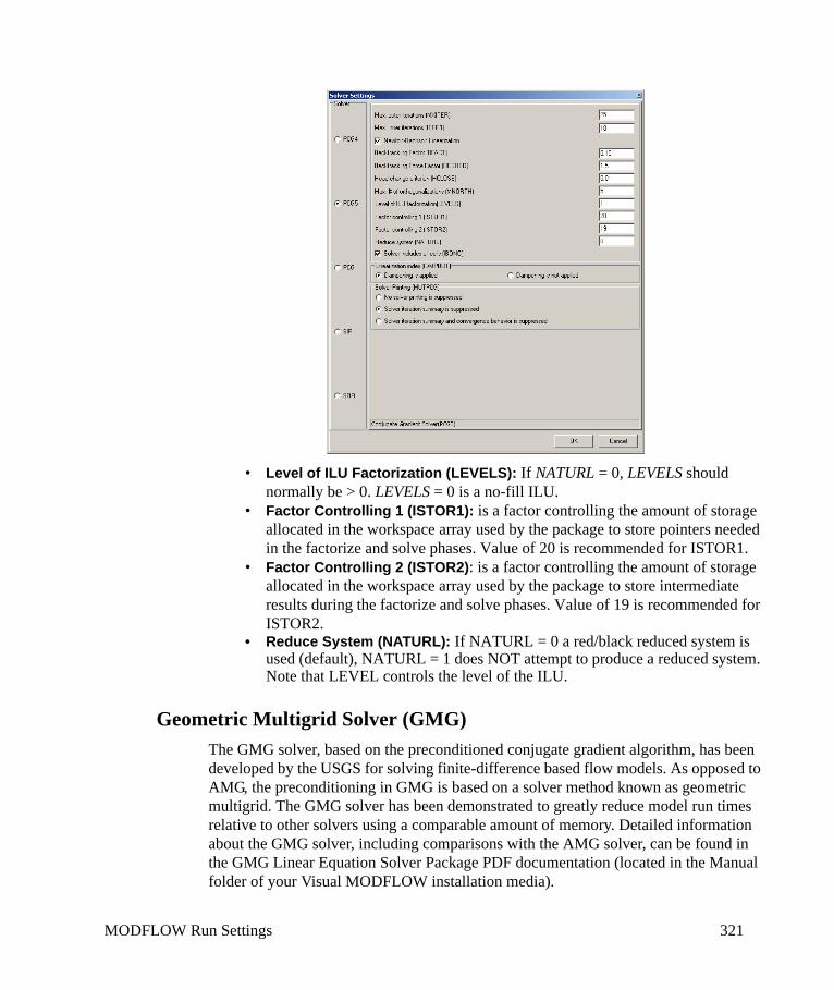
MODFLOW Run Settings 321
• Level of ILU Factorization (LEVELS): If NATURL = 0, LEVELS should normally be > 0. LEVELS = 0 is a no-fill ILU.
• Factor Controlling 1 (ISTOR1): is a factor controlling the amount of storage allocated in the workspace array used by the package to store pointers needed in the factorize and solve phases. Value of 20 is recommended for ISTOR1.
• Factor Controlling 2 (ISTOR2): is a factor controlling the amount of storage allocated in the workspace array used by the package to store intermediate results during the factorize and solve phases. Value of 19 is recommended for ISTOR2.
• Reduce System (NATURL): If NATURL = 0 a red/black reduced system is used (default), NATURL = 1 does NOT attempt to produce a reduced system. Note that LEVEL controls the level of the ILU.
Geometric Multigrid Solver (GMG)The GMG solver, based on the preconditioned conjugate gradient algorithm, has been developed by the USGS for solving finite-difference based flow models. As opposed to AMG, the preconditioning in GMG is based on a solver method known as geometric multigrid. The GMG solver has been demonstrated to greatly reduce model run times relative to other solvers using a comparable amount of memory. Detailed information about the GMG solver, including comparisons with the AMG solver, can be found in the GMG Linear Equation Solver Package PDF documentation (located in the Manual folder of your Visual MODFLOW installation media).

322 Chapter 5: Run Section - Model Run Settings
The solver parameters for the Geometric Multigrid Solver are described below using excerpts from the GMG Linear Equation Solver Package PDF documentation (located in the Manual folder of your Visual MODFLOW installation media):
• Max. outer iterations (MXITER): The maximum number of outer iterations. For linear problems, MXITER can be set to 1. For nonlinear problems, MXITER needs to be larger, but rarely more than 100. The maximum number of iterations will only be used if a convergent solution is not reached beforehand.
• Max. inner iterations (IITER): The maximum number of PCG iterations for each linear solution. A value of 100 is typically sufficient. It is frequently useful to specify a smaller number for nonlinear problems so as to prevent an excessive number of inner iterations. This number of iterations will only be used if a convergent solution for the current set of matrices in the "outer" iteration is not reached beforehand.
• Adaptive Damping Control (IADAMP): IADAMP is a flag that controls adaptive damping. If IADAMP = 0, then the value assigned to DAMP is used as a constant damping parameter. If IADAMP = 0, then the value of DAMP is used for the first nonlinear iteration. The damping parameter is adaptively varied on the basis of the head change, using Cooley’s method for subsequent iterations.
MODFLOW Run Settings 323
• Head change criterion (HCLOSE): After every outer iteration is completed, the solver checks for the maximum change in the solution at every cell. If the maximum change in the solution is below a set convergence tolerance (set here in the working units of feet or metres) then the solution has converged and the solver stops, otherwise a new outer iteration is started. A solution accurate to 0.01 [ft. or m] will normally be sufficient for most problems unless the maximum head change throughout the modeled domain is less than 1 foot or metre. If an appropriate mass balance is not achieved and the number of inner and outer iterations is within the maximums, this value can be decreased by an order of magnitude.
• Residual criterion (RCLOSE): RCLOSE is the residual convergence criterion for the inner iteration. The PCG algorithm computes the l2-norm of the residual and compares it against RCLOSE Typically, RCLOSE is set to the same value as HCLOSE (see below). If RCLOSE is set too high, then additional outer iterations may be required due to the linear equation not being solved with sufficient accuracy. On the other hand, a too restrictive setting for RCLOSE for nonlinear problems may force an unnecessarily accurate linear solution. This may be alleviated with the IITER parameter or with damping.
• Relaxation parameter (RELAX): The RELAX parameter can be used to improve the spectral condition number of the ILU preconditioned system. The value of RELAX should be approximately one. However, the relaxation parameter can cause the factorization to break down. If this happens, then the GMG solver will report an assembly error and a value smaller than one for RELAX should be tried. This item is read only if ISC = 4.
• Upper bound of estimate (NPBOL): IOUTGMG is a flag that controls the output of the GMG solver. The possible values of IOUTGMG and their meanings are as follows: If IOUTGMG = 0, then only the solver inputs are printed. If IOUTGMG = 1, then for each linear solve, the number of PCG iterations, the value of the damping parameter, the l2-norm of the residual, and the max-norm of the head change and its location (column, row, layer) are printed. At the end of a time/stress period, the total number of GMG calls, PCG iterations, and a running total of PCG iterations for all time/stress periods are printed. If IOUTGMG = 2, then the convergence history of the PCG iteration is printed, showing the l2-norm of the residual and the convergence factor for each iteration. IOUTGMG = 3 is the same as IOUTGMG = 1 except output is sent to the terminal instead of the MF2K LIST output file. IOUTGMG = 4 is the same as IOUTGMG = 2 except output is sent to the terminal instead of the MF2K LIST output file.
• Multigrid Preconditioner (ISM): ISM is a flag that controls the type of smoother used in the multigrid preconditioner. The possible values for ISM and their meanings are as follows: If ISM = 0, then ILU(0) smoothing is implemented in the multigrid preconditioner. This smoothing requires an additional vector on each multigrid level to store the pivots in the ILU factorization. If ISM = 1, then Symmetric Gauss Seidel (SGS) smoothing is implemented in the multigrid preconditioner. No additional storage is required
324 Chapter 5: Run Section - Model Run Settings
for this smoother; users may want to use this option if available memory is exceeded or nearly exceeded when using ISM = 0. Using SGS smoothing is not as robust as ILU smoothing; additional iterations are likely to be required in reducing the residuals. In extreme cases, the solver may fail to converge as the residuals cannot be reduced sufficiently.
• Semicoarsening Control in the Multigrid Preconditioner (ISC): A flag that controls semicoarsening in the multigrid preconditioner. The possible values of ISC and their meanings are given as follows: If ISC = 0, then the rows, columns and layers are all coarsened. If ISC = 1, then the rows and columns are coarsened, but the layers are not. If ISC = 2, then the columns and layers are coarsened, but the rows are not. If ISC = 3, then the rows and layers are coarsened, but the columns are not. If ISC = 4, then there is no coarsening. Typically, the value of ISC should be 0 or 1. In the case that there are large vertical variations in the hydraulic conductivities, then a value of 1 should be used. If no coarsening is implemented (ISC = 4), then the GMG solver is comparable to the PCG2 ILU(0) solver described in Hill (1990) and uses the least amount of memory.
• Damping factor (DAMP): This factor allows the user to reduce (dampen) the head change calculated during each successive outer iteration. For most "well posed" and physically realistic groundwater flow problems, the dampening factor of one will be appropriate. This parameter can be used to make a non-convergent (oscillating or divergent) solution process more stable such that a solution will be achieved. This is done by decreasing the damping factor to a value between 0 and 1 (only rarely < 0.6). This parameter is similar to "acceleration parameters" used in other solvers
MODFLOW-NWTThe NWT Solver parameters are shown in the image below. Detailed information about MODFLOW-NWT can be found in the Package PDF documentation (located in the Manual folder of your Visual MODFLOW installation disc).
NOTE: MODFLOW-NWT includes an upstream-weighting (UPW) intercell conductance package as a replacement internal flow package to those provided by the BCF, LPF, and HUF Packages. When MODFLOW-NWT is selected as the flow engine, the UPW property package will be generated during translation and used in the model run.

MODFLOW Run Settings 325
The following is a description of the NWT parameters (excerpt from the package documentation)
General
• OPTIONS—Automate Solver Options - MODFLOW-NWT provides flexibility to specify the values for each of the parameters, or to choose from one of the pre-defined solver “schemes”. When you select one of the pre-defined schemes, then the solver parameters are fixed and cannot be modified (all fields will be visible but disabled)
• SPECIFIED indicates that the optional solver input values listed for items 1 and 2 will be specified in the NWT input file by the user.
• SIMPLE indicates that default solver input values will be defined that work well for nearly linear models. This would be used for models that do not include nonlinear stress packages, and models that are either confined or consist of a single unconfined layer that is thick enough to contain the water table within a single layer. (See Table 2 of package documentation for the solver input values that will be used for this
326 Chapter 5: Run Section - Model Run Settings
option.)• MODERATE indicates that default solver input values will be defined
that work well for moderately nonlinear models. This would be used for models that include nonlinear stress packages, and models that consist of one or more unconfined layers. The “MODERATE” option should be used when the “SIMPLE” option does not result in successful convergence. (See Table 2 of package documentation for the solver input values that will be used for this option.)
• COMPLEX indicates that default solver input values will be defined that work well for highly nonlinear models. This would be used for models that include nonlinear stress packages, and models that consist of one or more unconfined layers representing complex geology and surface water/groundwater interaction. The “COMPLEX” option should be used when the “MODERATE” option does not result in successful convergence. (See Table 2 of package documentation for the solver input values that will be used for this option.)
• HEADTOL (units of length)—is the maximum head change between outer iterations for solution of the nonlinear problem.
• FLUXTOL (units of length cubed per time)—is the maximum root-mean-squared flux difference between outer iterations for solution of the nonlinear problem.
• MAXITEROUT is the maximum number of iterations to be allowed for solution of the outer (nonlinear) problem.
• THICKFACT is the portion of the cell thickness (length) used for smoothly adjusting storage and conductance coefficients to zero.
• LINMETH is a flag that determines which matrix solver will be used. • 1 = GMRES will be used• 2 = xMD will be used
• IBOTAV is a flag that indicates whether corrections will be made to groundwater head relative to the cell-bottom altitude if the cell is surrounded by dewatered cells. Checked = a correction will be made; Not-checked = no correction will be made. This input variable is problem specific and both options (IBOTAV selected/not-selected) should be tested.
Optional
• DBDTHETA is a coefficient used to reduce the weight applied to the head change between nonlinear iterations. DBDTHETA is used to control oscillations in head. Values range between 0.0 and 1.0, and larger values increase the weight (decrease under-relaxation) applied to the head change
• DBDKAPPA is a coefficient used to increase the weight applied to the head change between nonlinear iterations. DBDKAPPA is used to control oscillations in head. Values range between 0.0 and 1.0, and larger values increase the weight applied to the head change.
• DBDGAMMA is a factor used to weight the head change for iterations n–1 and

MODFLOW Run Settings 327
n. Values range between 0.0 and 1.0, and greater values apply more weight to the head change calculated during iteration n.
• MOMFACT is the momentum coefficient m and ranges between 0.0 and 1.0. Greater values apply more weight to the head change for iteration n.
Residual Control
• MAXBACKITER is the maximum number of reductions (backtracks) in the head change between nonlinear iterations. A value between 10 and 50 works well.
• BACKTOL is the proportional decrease in the root-mean-squared error of the groundwater-flow equation used to determine if residual control is required at the end of a nonlinear iteration.
• BACKREDUCE is a reduction factor used for residual control that reduces the head change between nonlinear iterations. Values should be between 0.0 and 1.0, where smaller values result in smaller head-change values.
• BACKFLAG is a flag used to specify whether residual control will be used. Checked = residual control is active; Not-checked = residual control is inactive.
GMRES Solver Options
If LINMETH = 1 (GMRES), then the following options will appear:
• MAXITINNER is the maximum number of iterations for the linear solution.• ILUMETHOD is the index for selection of the method for incomplete
factorization (ILU) used as a preconditioner.• ILUMETHOD=1—ILU with drop tolerance and fill limit. Fill-in terms
less than drop tolerance times the diagonal are discarded. The number of fill-in terms in each row of L and U is limited to the fill limit. The fill-limit largest elements are kept in the L and U factors.
• ILUMETHOD=2 — ILU(k), Order k incomplete LU factorization. Fill-in terms of higher order than k in the factorization are discarded.
• LEVFILL is the fill limit for ILUMETHOD = 1 and is the level of fill for ILUMETHOD = 2. Recommended values: 5-10 for method 1, 0-2 for method 2.
• STOPTOL is the tolerance for convergence of the linear solver. This is the residual of the linear equations scaled by the norm of the root mean squared error. Usually 10-8 to 10-12 works well.
• MSDR is the number of iterations between restarts of the GMRES Solver.
xMD Solver Options
If LINMETH = 2 (xMD), then the following options will appear:
• IACL is a flag for the acceleration method: • 0 = conjugate gradient;• 1 = ORTHOMIN;• 2 = Bi-CGSTAB.
• NORDER is a flag for the scheme of ordering the unknowns:
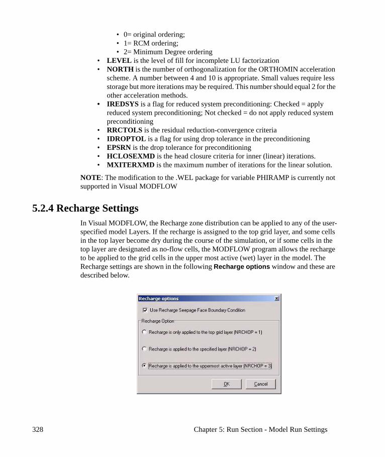
328 Chapter 5: Run Section - Model Run Settings
• 0= original ordering; • 1= RCM ordering; • 2= Minimum Degree ordering
• LEVEL is the level of fill for incomplete LU factorization• NORTH is the number of orthogonalization for the ORTHOMIN acceleration
scheme. A number between 4 and 10 is appropriate. Small values require less storage but more iterations may be required. This number should equal 2 for the other acceleration methods.
• IREDSYS is a flag for reduced system preconditioning: Checked = apply reduced system preconditioning; Not checked = do not apply reduced system preconditioning
• RRCTOLS is the residual reduction-convergence criteria• IDROPTOL is a flag for using drop tolerance in the preconditioning• EPSRN is the drop tolerance for preconditioning• HCLOSEXMD is the head closure criteria for inner (linear) iterations.• MXITERXMD is the maximum number of iterations for the linear solution.
NOTE: The modification to the .WEL package for variable PHIRAMP is currently not supported in Visual MODFLOW
5.2.4 Recharge SettingsIn Visual MODFLOW, the Recharge zone distribution can be applied to any of the user-specified model Layers. If the recharge is assigned to the top grid layer, and some cells in the top layer become dry during the course of the simulation, or if some cells in the top layer are designated as no-flow cells, the MODFLOW program allows the recharge to be applied to the grid cells in the upper most active (wet) layer in the model. The Recharge settings are shown in the following Recharge options window and these are described below.
MODFLOW Run Settings 329
• Recharge is only applied to the top grid layer: If any grid cells in Layer 1 are dry, or if they are designated as no-flow cells, the recharge values assigned to these grid cells will NOT be carried down to the underlying active (wet) grid cells. In this case, the inactive or dry cells act like an impermeable barrier to the recharge.
• Recharge is applied to the specified layer: It allows the user to assign the recharge values to any of the specified model layer (see “Assigning Recharge Zones” section on page 259 for details on how recharge is assigned to the specified layers).
• Recharge is applied to the uppermost active layer: If any grid cells in Layer 1 are dry, or if they are designated as no-flow cells, the recharge values assigned to these grid cells will be carried down to the upper most active (wet) grid cell in the same vertical column of grid cells.
Note: A constant head boundary condition always intercepts recharge and pre-vents deeper infiltration.
If MODFLOW-SURFACT is selected as the Flow Numeric Engine, then a checkbox beside the field “Use Recharge Seepage Face Boundary Condition” will be available. If the checkbox is selected ( ) the “Recharge is applied until water table reaches the user specified ponding elevation” (refer to the section “Evapotranspiration Boundary Conditions” section on page 266). If the checkbox is not selected, then the “Recharge is always applied as in the confined case” with heads continually rising. For more details on the Recharge-Seepage Face Boundary the user is encouraged to refer to Chapter 4 of MODFLOW-SURFACT User’s manual.
5.2.5 Evapotranspiration SettingsIn Visual MODFLOW, the Evapotranspiration distribution can be applied to any of the user-specified model Layers. If assigned to the top grid layer, and some cells in the top layer become dry during the course of the simulation, or if some cells in the top layer are designated as no-flow cells, the MODFLOW program allows the Evapotranspiration to be applied to the grid cells in the upper most active (wet) layer in the model. The Evapotranspiration settings are shown in the following Evapotranspiration Options window and these are described below.

330 Chapter 5: Run Section - Model Run Settings
• Evapotranspiration is only applied to the top grid layer: If any grid cells in Layer 1 are dry, or if they are designated as no-flow cells, the Evapotranspiration values assigned to these grid cells will NOT be carried down to the underlying active (wet) grid cells. In this case, the inactive or dry cells act like an impermeable barrier to the Evapotranspiration.
• Evapotranspiration is applied to the specified layer: It allows the user to assign the Evapotranspiration values to any of the specified model layers.
• Evapotranspiration is applied to the uppermost active layer: If any grid cells in Layer 1 are dry, or if they are designated as no-flow cells, the evapotranspiration values assigned to these grid cells will be carried down to the upper most active (wet) grid cell in the same vertical column of grid cells.
5.2.6 Surface Water Leakage SettingsUse these settings to define the MODFLOW+MIKE 11 Run settings, and synchronize your Visual MODFLOW model to the MIKE 11 model.
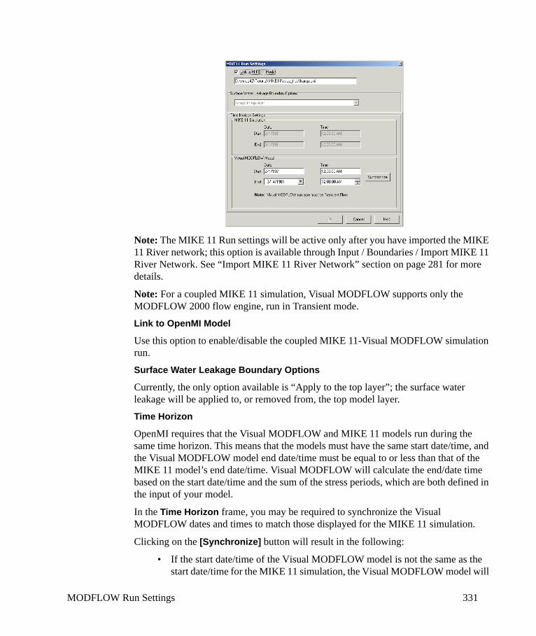
MODFLOW Run Settings 331
Note: The MIKE 11 Run settings will be active only after you have imported the MIKE 11 River network; this option is available through Input / Boundaries / Import MIKE 11 River Network. See “Import MIKE 11 River Network” section on page 281 for more details.
Note: For a coupled MIKE 11 simulation, Visual MODFLOW supports only the MODFLOW 2000 flow engine, run in Transient mode.
Link to OpenMI Model
Use this option to enable/disable the coupled MIKE 11-Visual MODFLOW simulation run.
Surface Water Leakage Boundary Options
Currently, the only option available is “Apply to the top layer”; the surface water leakage will be applied to, or removed from, the top model layer.
Time Horizon
OpenMI requires that the Visual MODFLOW and MIKE 11 models run during the same time horizon. This means that the models must have the same start date/time, and the Visual MODFLOW model end date/time must be equal to or less than that of the MIKE 11 model’s end date/time. Visual MODFLOW will calculate the end/date time based on the start date/time and the sum of the stress periods, which are both defined in the input of your model.
In the Time Horizon frame, you may be required to synchronize the Visual MODFLOW dates and times to match those displayed for the MIKE 11 simulation.
Clicking on the [Synchronize] button will result in the following:
• If the start date/time of the Visual MODFLOW model is not the same as the start date/time for the MIKE 11 simulation, the Visual MODFLOW model will

332 Chapter 5: Run Section - Model Run Settings
assume the MIKE 11 start date/time.• If the end date/time of the Visual MODFLOW model is greater than the end
date/time for the MIKE 11 simulation, the Visual MODFLOW model will assume the MIKE 11 end date/time. As a result, this will also shorten the Visual MODFLOW simulation length.
• If the end date/time of the Visual MODFLOW model is less than the end date/time for the MIKE 11 model, there will be no change; it is not possible to extend the end date/time, since these are both calculated from the stress periods. In this scenario, the MIKE 11+Visual MODFLOW simulation will run only to the displayed Visual MODFLOW end date/time. In order to extend the Visual MODFLOW model simulation length, return to the input and add more stress periods, or extend the time length of existing stress periods.
After running MODFLOW + MIKE 11, a new term “Surface Water Leakage” will be added to the .LST file, and as a result, displayed in the Mass Balance Report.
Note: If discharge from the groundwater model to the MIKE 11 model is high, and there is a significant difference in the time step length between the two models, you may encounter non-physical results and/or numerical instabilities. Try increasing the number of time steps in Visual MODFLOW to minimize this effect.
5.2.7 Layer Type SettingsThe Layer Type Settings window is used to set the LAYCON value and the LAYAVG variables required by the MODFLOW numeric engine.
The LAYCON value is the layer-type index array recognized by MODFLOW. MODFLOW has four different Layer Types to choose for LAYCON values as described below:
• Type 0 - Confined: Transmissivity and storage coefficients of the layer are constant for the entire simulation.
• Type 1 - Unconfined: Transmissivity of the layer varies and is calculated from the saturated thickness and hydraulic conductivity. The storage coefficient is constant; valid only for Layer 1.
• Type 2 - Confined/Unconfined: Transmissivity of the layer is constant. The storage coefficient may alternate between confined and unconfined values.
• Type 3 - Confined/Unconfined: [Default setting] Transmissivity of the layer varies. It is calculated from the saturated thickness and hydraulic conductivity. The storage coefficient may alternate between confined and unconfined values. Vertical leakage from above is limited if the aquifer becomes desaturated.
The LAYAVG value determines the method of computing interblock transmissivity.
Following are the five methods used in assigning the LAYAVG value.
• 0 - Harmonic mean interblock transmissivity [Default setting for MODFLOW-96 and MODFLOW-2000].
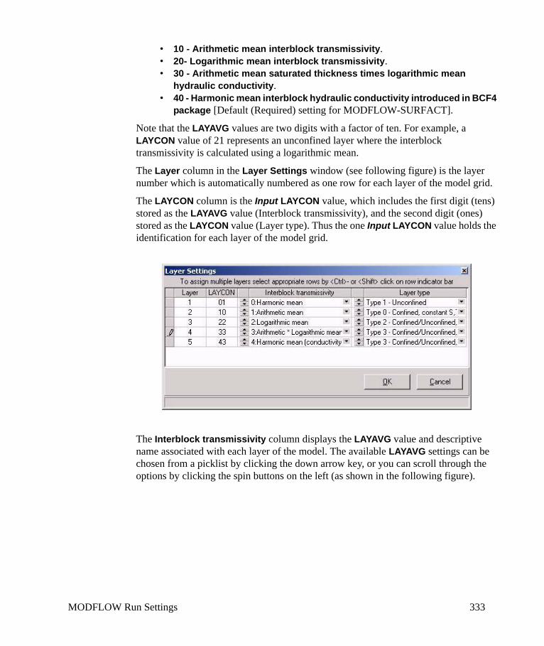
MODFLOW Run Settings 333
• 10 - Arithmetic mean interblock transmissivity.• 20- Logarithmic mean interblock transmissivity. • 30 - Arithmetic mean saturated thickness times logarithmic mean
hydraulic conductivity.• 40 - Harmonic mean interblock hydraulic conductivity introduced in BCF4
package [Default (Required) setting for MODFLOW-SURFACT].
Note that the LAYAVG values are two digits with a factor of ten. For example, a LAYCON value of 21 represents an unconfined layer where the interblock transmissivity is calculated using a logarithmic mean.
The Layer column in the Layer Settings window (see following figure) is the layer number which is automatically numbered as one row for each layer of the model grid.
The LAYCON column is the Input LAYCON value, which includes the first digit (tens) stored as the LAYAVG value (Interblock transmissivity), and the second digit (ones) stored as the LAYCON value (Layer type). Thus the one Input LAYCON value holds the identification for each layer of the model grid.
The Interblock transmissivity column displays the LAYAVG value and descriptive name associated with each layer of the model. The available LAYAVG settings can be chosen from a picklist by clicking the down arrow key, or you can scroll through the options by clicking the spin buttons on the left (as shown in the following figure).
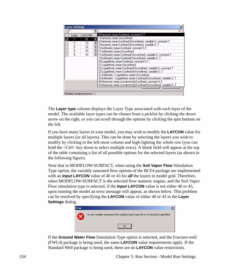
334 Chapter 5: Run Section - Model Run Settings
The Layer type column displays the Layer Type associated with each layer of the model. The available layer types can be chosen from a picklist by clicking the down arrow on the right, or you can scroll through the options by clicking the spin buttons on the left.
If you have many layers in your model, you may wish to modify the LAYCON value for multiple layers (or all layers). This can be done by selecting the layers you wish to modify by clicking in the left-most column and high-lighting the whole row (you can hold the <Ctrl> key down to select multiple rows). A blank field will appear at the top of the table containing a list of all possible options for the selected layers (as shown in the following figure).
Note that in MODFLOW-SURFACT, when using the Soil Vapor Flow Simulation Type option, the variably saturated flow options of the BCF4 package are implemented with an Input LAYCON value of 40 or 43 for all the layers in model grid. Therefore, when MODFLOW-SURFACT is the selected flow numeric engine, and the Soil Vapor Flow simulation type is selected, if the Input LAYCON value is not either 40 or 43, upon running the model an error message will appear, as shown below. This problem can be resolved by specifying the LAYCON value of either 40 or 43 in the Layer Settings dialog.
If the Ground Water Flow Simulation Type option is selected, and the Fracture-well (FWL4) package is being used, the same LAYCON value requirements apply. If the Standard Well package is being used, there are no LAYCON value restrictions.
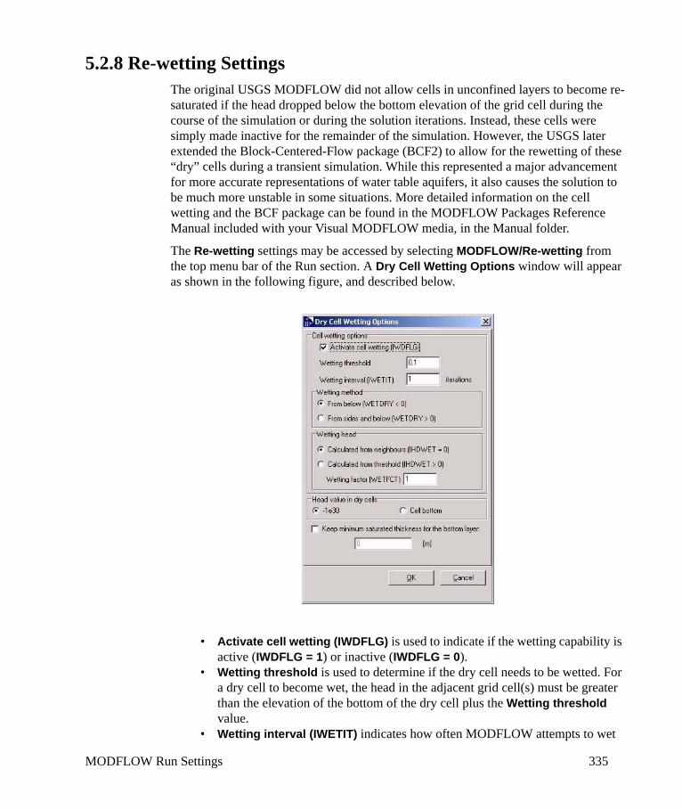
MODFLOW Run Settings 335
5.2.8 Re-wetting SettingsThe original USGS MODFLOW did not allow cells in unconfined layers to become re-saturated if the head dropped below the bottom elevation of the grid cell during the course of the simulation or during the solution iterations. Instead, these cells were simply made inactive for the remainder of the simulation. However, the USGS later extended the Block-Centered-Flow package (BCF2) to allow for the rewetting of these “dry” cells during a transient simulation. While this represented a major advancement for more accurate representations of water table aquifers, it also causes the solution to be much more unstable in some situations. More detailed information on the cell wetting and the BCF package can be found in the MODFLOW Packages Reference Manual included with your Visual MODFLOW media, in the Manual folder.
The Re-wetting settings may be accessed by selecting MODFLOW/Re-wetting from the top menu bar of the Run section. A Dry Cell Wetting Options window will appear as shown in the following figure, and described below.
• Activate cell wetting (IWDFLG) is used to indicate if the wetting capability is active (IWDFLG = 1) or inactive (IWDFLG = 0).
• Wetting threshold is used to determine if the dry cell needs to be wetted. For a dry cell to become wet, the head in the adjacent grid cell(s) must be greater than the elevation of the bottom of the dry cell plus the Wetting threshold value.
• Wetting interval (IWETIT) indicates how often MODFLOW attempts to wet
336 Chapter 5: Run Section - Model Run Settings
the dry cells detected during the course of the solution iterations. For example, if IWETIT = 2, cell wetting would be attempted at every second iteration. If a model with dry cells is having problems converging to a solution, it may be a result of oscillations due to drying and re-wetting of grid cells in sensitive regions of the model. Setting a larger cell wetting interval value may help the solution to converge, by allowing the heads in neighboring cells to get closer to a better solution before wetting the dry cells.
Wetting MethodsThe wetting of a dry cell is triggered by the head values in adjacent grid cells (see Wetting threshold above). The Wetting method frame has two options for determining the adjacent grid cells to use for determining whether the dry cell should be wetted.
• From below (WETDRY < 0) will use only the head in the grid cell directly below the dry cell to determine if the dry cell should be wetted. This option is generally more stable, and is particularly good when the adjacent horizontal cells are poor indicators of whether a cell should become wet (e.g. areas with steep vertical gradients and variable bottom elevations).
• Wet cells from side and below (WETDRY > 0) will used the head in all four adjacent grid cells and the grid cell directly below the dry cell to determine if the dry cell should be wetted. This option is useful in situations where a dry cell is located above a no-flow cell, such that it cannot be re-wet from below. It is also applicable for one-layer models where there are no cells below. However, this method can cause some problems in multi-layer models where inactive cells occur beneath wet cells.
Wetting HeadWhen a dry cell is wetted, the new head may be calculated using one of two methods:
• Calculated from neighbors
Head = Zbot + Wetting factor * (Neighboring head – Zbot)
• Calculated from threshold
Head = Zbot + Wetting factor * Wetting threshold
Where Zbot is the elevation of the bottom of the current cell.
Generally, the first equation is thought to be more reasonable, since the cell’s new head is varied according to the head in the neighboring cell, which caused it to become wet. However, in situations where MODFLOW is over-estimating head changes during iterations, this equation may cause non-convergence. The second equation can then be used to attempt a more stable solution.
MODFLOW Run Settings 337
Setting Head Values in Dry CellsEach dry cell is assigned a default head value as a flag to indicate it is dry. This value is typically a very large negative number (e.g. -1.0e30). However, the presence of large negative head values in dry cells may cause problems for parameter estimation simulations because this large negative value may be used to calculate the calibration residual (calculated head - observed head) at a grid cell that has become dry during one of the PEST iterations. In this case, it is more appropriate to assign the head value in dry cells equal to the cell bottom elevation to avoid this problem.
Setting Minimum Saturated Thickness When PEST runs with varied model parameters, some of these runs may produce dry cells, and as a result MODFLOW assigns head values equal to -1.0e30 to all the dry cells. This can cause the objective function to be skewed, and the subsequent model runs to fail to converge. If the “Keep minimum saturated thickness for the bottom layer” option is activated by assigning an appropriate head value to the bottom cell, MODFLOW will keep the bottom cell saturated. It prevents the column from drying out, ensures that PEST will continue running even though the calculated head is actually below the bottom layer of the model, and helps with model convergence. It is recommended to not activate this option in the first run of a model because it is important to know if the dry cells exist or not, and by preventing the column from drying out, the model results could be misleading.
Hints For Using Dry Cell WettingCell re-wetting often promotes a non-converging or unstable solution, which may be indicated by cells cycling between wet and dry. If this happens, we recommend you try the following:
• Make inactive any cells that you know should never become wet. • Increase the Wetting threshold value. This makes it more difficult for a cell to
be wetted, and therefore helps stop MODFLOW from repeatedly turning a cell on and then off again. However, the solution may become less accurate since cells that should become wet might stay dry.
• Modify the Wetting factor value. This will increase or decrease the new head in cells which are wetted.
• Change the Wetting method that controls cell wetting.• Change the Wetting head option that calculates the new head in the wetted cell.• Try using the SIP or PCG solver, and modifying the solver parameters.• For steady-state solutions, start with good initial head estimates. This will
provide good indications of which cells should be wet and dry, and therefore conversions of cells between wet and dry will be minimized.
NOTE: Re-wetting is not available for MODFLOW-NWT.
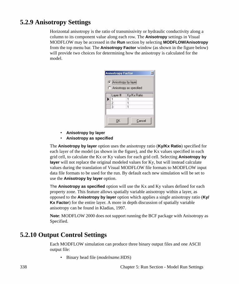
338 Chapter 5: Run Section - Model Run Settings
5.2.9 Anisotropy SettingsHorizontal anisotropy is the ratio of transmissivity or hydraulic conductivity along a column to its component value along each row. The Anisotropy settings in Visual MODFLOW may be accessed in the Run section by selecting MODFLOW/Anisotropy from the top menu bar. The Anisotropy Factor window (as shown in the figure below) will provide two choices for determining how the anisotropy is calculated for the model.
• Anisotropy by layer• Anisotropy as specified
The Anisotropy by layer option uses the anisotropy ratio (Ky/Kx Ratio) specified for each layer of the model (as shown in the figure), and the Kx values specified in each grid cell, to calculate the Kx or Ky values for each grid cell. Selecting Anisotropy by layer will not replace the original modeled values for Ky, but will instead calculate values during the translation of Visual MODFLOW file formats to MODFLOW input data file formats to be used for the run. By default each new simulation will be set to use the Anisotropy by layer option.
The Anisotropy as specified option will use the Kx and Ky values defined for each property zone. This feature allows spatially variable anisotropy within a layer, as opposed to the Anisotropy by layer option which applies a single anisotropy ratio (Ky/Kx Factor) for the entire layer. A more in depth discussion of spatially variable anisotropy can be found in Kladias, 1997.
Note: MODFLOW 2000 does not support running the BCF package with Anisotropy as Specified.
5.2.10 Output Control SettingsEach MODFLOW simulation can produce three binary output files and one ASCII output file:
• Binary head file (modelname.HDS)
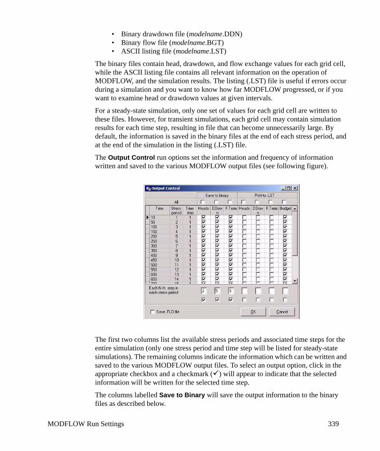
MODFLOW Run Settings 339
• Binary drawdown file (modelname.DDN)• Binary flow file (modelname.BGT)• ASCII listing file (modelname.LST)
The binary files contain head, drawdown, and flow exchange values for each grid cell, while the ASCII listing file contains all relevant information on the operation of MODFLOW, and the simulation results. The listing (.LST) file is useful if errors occur during a simulation and you want to know how far MODFLOW progressed, or if you want to examine head or drawdown values at given intervals.
For a steady-state simulation, only one set of values for each grid cell are written to these files. However, for transient simulations, each grid cell may contain simulation results for each time step, resulting in file that can become unnecessarily large. By default, the information is saved in the binary files at the end of each stress period, and at the end of the simulation in the listing (.LST) file.
The Output Control run options set the information and frequency of information written and saved to the various MODFLOW output files (see following figure).
The first two columns list the available stress periods and associated time steps for the entire simulation (only one stress period and time step will be listed for steady-state simulations). The remaining columns indicate the information which can be written and saved to the various MODFLOW output files. To select an output option, click in the appropriate checkbox and a checkmark ( ) will appear to indicate that the selected information will be written for the selected time step.
The columns labelled Save to Binary will save the output information to the binary files as described below.

340 Chapter 5: Run Section - Model Run Settings
Heads: Saves the heads in the binary heads file (.HDS).
DDown: Saves the drawdown in the binary drawdown file (.DDN).
F.Term: Saves the cell-by-cell flow terms in the binary budget (.BGT) file.
Note: The Zone Budget program uses the.BGT file for calculating the flow between zones. Therefore, to change the frequency at which the Zone Budget infor-mation is saved, select the desired F.Term intervals.
The columns labelled Print to .LST will save the output information to the listing file as described below.
Heads: Saves the heads in the listing file.
DDown: Saves the drawdown in the listing file.
F.Term: Saves the flux terms (cell by cell flow terms) in the listing file.
Budget: Saves the budget information in the listing file.
Note: MODFLOW only allows the flow terms (F.Term) to be stored once, in either the binary budget file (.BGT) or the listing file (.LST). Be aware that this setting can be lost if MODFLOW is being run together with MODPATH, because MOD-PATH requires the flow terms to be written to the .BGT file, and not to the .LST file.
The checkbox labelled Save.FLO file will save the cell-by-cell flow terms required by MT3D, when MT3D is not being run at the same time as MODFLOW.
Saving Output Every Nth Time StepFor simulations with many stress periods and time steps, it can be very tedious to manually select the desired output time step intervals. The row of fields underneath the Output Control table are used to specify regular time step intervals for saving files during Each N-th step in each stress period. The first text box is where the N value is entered. To apply this value to the column, click the underlying checkbox.
If MODPATH is run with the MODFLOW simulation, Visual MODFLOW will save the flow terms for all time steps
5.2.11 List File Options The List file print options window, as shown below, allows you to specify which information will be written to the listing file (.LST), as well as the format of this information.

MODFLOW Run Settings 341
5.2.12 Engine SettingsThe Flow Engine Settings window, as shown below, allows you to specify which version of the flow engines you wish to run, along with specifying Single or Double Precision.
NOTES:
• 64-bit versions of the Engines are only available if you are running a 64-bit version of Windows
• Use All Available CPU’s is only available for PCG, WHS and SAMG solvers, with MODFLOW-2000, 2005, and SEAWAT
• Run time solver control settings in the VMEngines window are not available when 64-bit Engine or “Parallel Processing” mode is selected; this means you will not have the ability to pause a simulation, adjust the controls, and re-start.
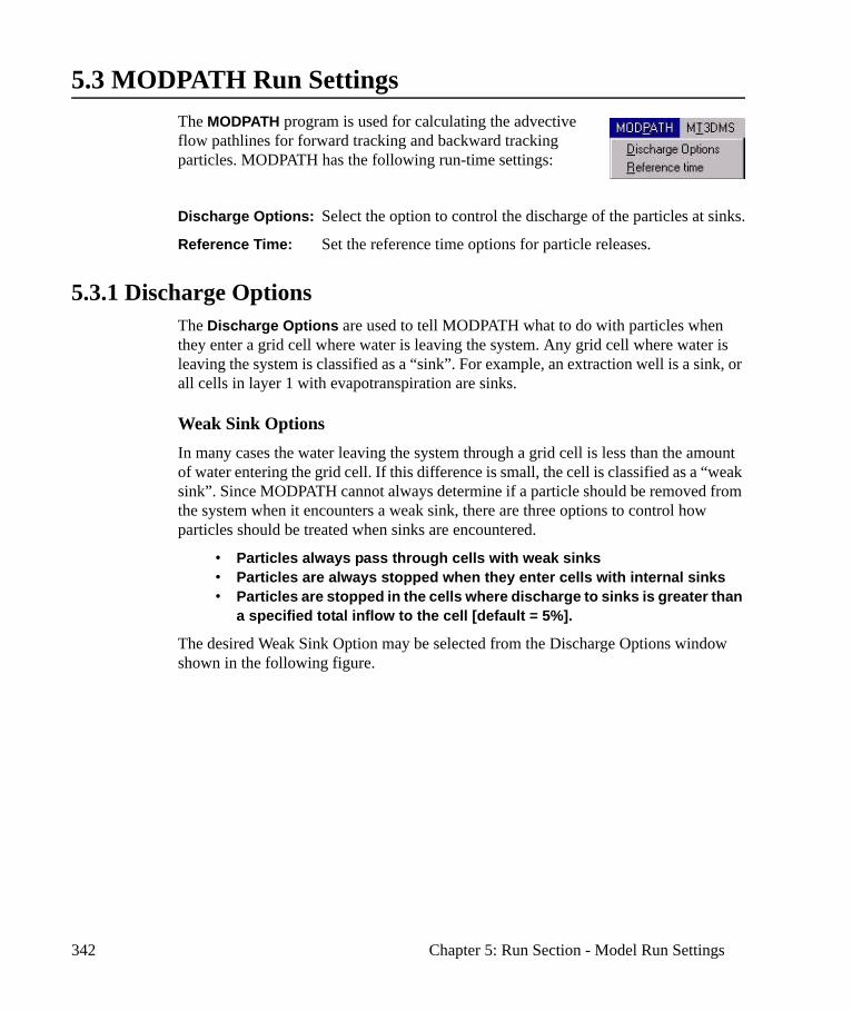
342 Chapter 5: Run Section - Model Run Settings
5.3 MODPATH Run SettingsThe MODPATH program is used for calculating the advective flow pathlines for forward tracking and backward tracking particles. MODPATH has the following run-time settings:
Discharge Options: Select the option to control the discharge of the particles at sinks.
Reference Time: Set the reference time options for particle releases.
5.3.1 Discharge OptionsThe Discharge Options are used to tell MODPATH what to do with particles when they enter a grid cell where water is leaving the system. Any grid cell where water is leaving the system is classified as a “sink”. For example, an extraction well is a sink, or all cells in layer 1 with evapotranspiration are sinks.
Weak Sink OptionsIn many cases the water leaving the system through a grid cell is less than the amount of water entering the grid cell. If this difference is small, the cell is classified as a “weak sink”. Since MODPATH cannot always determine if a particle should be removed from the system when it encounters a weak sink, there are three options to control how particles should be treated when sinks are encountered.
• Particles always pass through cells with weak sinks• Particles are always stopped when they enter cells with internal sinks • Particles are stopped in the cells where discharge to sinks is greater than
a specified total inflow to the cell [default = 5%].
The desired Weak Sink Option may be selected from the Discharge Options window shown in the following figure.
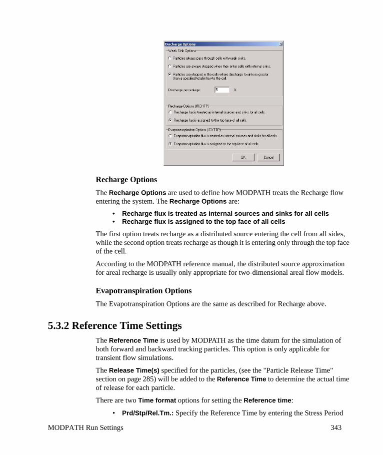
MODPATH Run Settings 343
Recharge OptionsThe Recharge Options are used to define how MODPATH treats the Recharge flow entering the system. The Recharge Options are:
• Recharge flux is treated as internal sources and sinks for all cells• Recharge flux is assigned to the top face of all cells
The first option treats recharge as a distributed source entering the cell from all sides, while the second option treats recharge as though it is entering only through the top face of the cell.
According to the MODPATH reference manual, the distributed source approximation for areal recharge is usually only appropriate for two-dimensional areal flow models.
Evapotranspiration OptionsThe Evapotranspiration Options are the same as described for Recharge above.
5.3.2 Reference Time SettingsThe Reference Time is used by MODPATH as the time datum for the simulation of both forward and backward tracking particles. This option is only applicable for transient flow simulations.
The Release Time(s) specified for the particles, (see the "Particle Release Time" section on page 285) will be added to the Reference Time to determine the actual time of release for each particle.
There are two Time format options for setting the Reference time:
• Prd/Stp/Rel.Tm.: Specify the Reference Time by entering the Stress Period
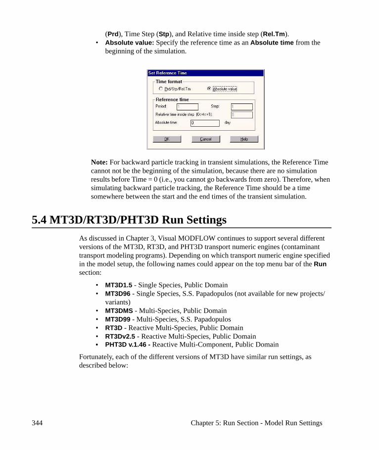
344 Chapter 5: Run Section - Model Run Settings
(Prd), Time Step (Stp), and Relative time inside step (Rel.Tm).• Absolute value: Specify the reference time as an Absolute time from the
beginning of the simulation.
Note: For backward particle tracking in transient simulations, the Reference Time cannot not be the beginning of the simulation, because there are no simulation results before Time = 0 (i.e., you cannot go backwards from zero). Therefore, when simulating backward particle tracking, the Reference Time should be a time somewhere between the start and the end times of the transient simulation.
5.4 MT3D/RT3D/PHT3D Run SettingsAs discussed in Chapter 3, Visual MODFLOW continues to support several different versions of the MT3D, RT3D, and PHT3D transport numeric engines (contaminant transport modeling programs). Depending on which transport numeric engine specified in the model setup, the following names could appear on the top menu bar of the Run section:
• MT3D1.5 - Single Species, Public Domain• MT3D96 - Single Species, S.S. Papadopulos (not available for new projects/
variants)• MT3DMS - Multi-Species, Public Domain• MT3D99 - Multi-Species, S.S. Papadopulos• RT3D - Reactive Multi-Species, Public Domain• RT3Dv2.5 - Reactive Multi-Species, Public Domain• PHT3D v.1.46 - Reactive Multi-Component, Public Domain
Fortunately, each of the different versions of MT3D have similar run settings, as described below:
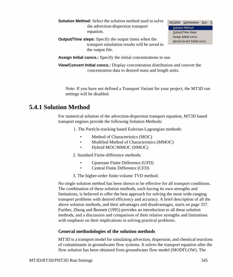
MT3D/RT3D/PHT3D Run Settings 345
Solution Method: Select the solution method used to solve the advection-dispersion transport equation.
Output/Time steps: Specify the output times when the transport simulation results will be saved to the output file.
Assign Initial concs.: Specify the initial concentrations to use.
View/Convert Initial concs.: Display concentration distribution and convert the concentration data to desired mass and length units.
Note: If you have not defined a Transport Variant for your project, the MT3D run settings will be disabled.
5.4.1 Solution MethodFor numerical solution of the advection-dispersion transport equation, MT3D based transport engines provide the following Solution Methods:
1. The Particle-tracking based Eulerian-Lagrangian methods:
• Method of Characteristics (MOC)• Modified Method of Characteristics (MMOC) • Hybrid MOC/MMOC (HMOC)
2. Standard Finite-difference methods:
• Upstream Finite Difference (UFD)• Central Finite Difference (CFD)
3. The higher-order finite-volume TVD method.
No single solution method has been shown to be effective for all transport conditions. The combination of these solution methods, each having its own strengths and limitations, is believed to offer the best approach for solving the most wide-ranging transport problems with desired efficiency and accuracy. A brief description of all the above solution methods, and their advantages and disadvantages, starts on page 357. Further, Zheng and Bennett (1995) provides an introduction to all these solution methods, and a discussion and comparison of their relative strengths and limitations with emphasis on their implications in solving practical problems.
General methodologies of the solution methodsMT3D is a transport model for simulating advection, dispersion, and chemical reactions of contaminants in groundwater flow systems. It solves the transport equation after the flow solution has been obtained from groundwater flow model (MODFLOW). The
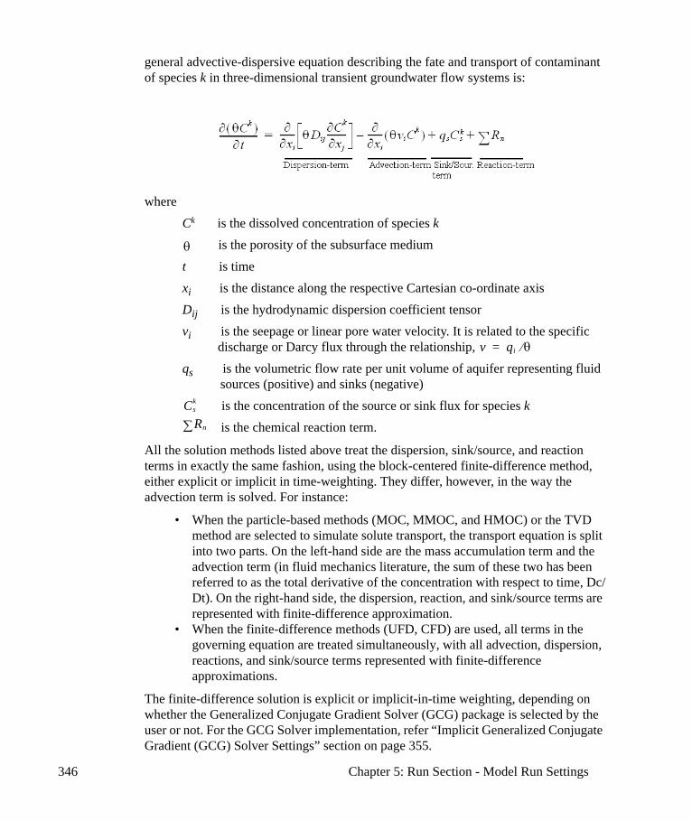
346 Chapter 5: Run Section - Model Run Settings
general advective-dispersive equation describing the fate and transport of contaminant of species k in three-dimensional transient groundwater flow systems is:
whereCk is the dissolved concentration of species k
is the porosity of the subsurface mediumt is timexi is the distance along the respective Cartesian co-ordinate axisDij is the hydrodynamic dispersion coefficient tensorvi is the seepage or linear pore water velocity. It is related to the specific
discharge or Darcy flux through the relationship, qs is the volumetric flow rate per unit volume of aquifer representing fluid
sources (positive) and sinks (negative)is the concentration of the source or sink flux for species k
is the chemical reaction term.
All the solution methods listed above treat the dispersion, sink/source, and reaction terms in exactly the same fashion, using the block-centered finite-difference method, either explicit or implicit in time-weighting. They differ, however, in the way the advection term is solved. For instance:
• When the particle-based methods (MOC, MMOC, and HMOC) or the TVD method are selected to simulate solute transport, the transport equation is split into two parts. On the left-hand side are the mass accumulation term and the advection term (in fluid mechanics literature, the sum of these two has been referred to as the total derivative of the concentration with respect to time, Dc/Dt). On the right-hand side, the dispersion, reaction, and sink/source terms are represented with finite-difference approximation.
• When the finite-difference methods (UFD, CFD) are used, all terms in the governing equation are treated simultaneously, with all advection, dispersion, reactions, and sink/source terms represented with finite-difference approximations.
The finite-difference solution is explicit or implicit-in-time weighting, depending on whether the Generalized Conjugate Gradient Solver (GCG) package is selected by the user or not. For the GCG Solver implementation, refer “Implicit Generalized Conjugate Gradient (GCG) Solver Settings” section on page 355.
θ
v qi θ⁄=
Csk
Rn∑

MT3D/RT3D/PHT3D Run Settings 347
Using the GCG SolverWhen the GCG Solver Package is specified to be included in a simulation, MT3D will do the following:
• When the particle-based methods (MOC, MMOC and HMOC) or the TVD method are used to simulate solute transport, the terms on the right-hand side are represented with implicit-in-time weighted finite-difference approximations.
Note: The TVD algorithm implemented in MT3D is explicit-in-time. This means that even if the GCG Package is used, the time steps in the TVD run will still be subject to a time constraint - but only the advection term.
• When the finite-difference methods (UFD, CFD) are used, all terms in the governing equation are represented with implicit-in-time weighted finite-difference approximations.
If the user does not specify the use of the GCG package, then all terms are represented with explicit-in-time weighted finite-difference approximations. For more details about how the GCG solver works, please refer to the section “A Technical Note on the Generalized Conjugate Gradient Solver” section on page 360.
Solution Method SettingsBy selecting MT3D.../Solution Method from the top menu bar, a Solution Method window will appear, as shown in the following figure. This is used to select the solution method to solve the general transport equation, and to customize the settings for the selected method. Although there are some subtle differences in the solution method settings for different MT3D transport engines, the majority of the settings are similar. The following figure pertains to the solution method for MT3DMS which is set as the default transport engine. Therefore, for ease of reference, in the following sections the variable names used within the MT3DMS manual are placed in brackets beside each parameter.
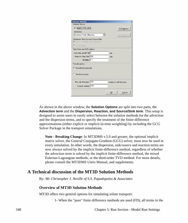
348 Chapter 5: Run Section - Model Run Settings
As shown in the above window, the Solution Options are split into two parts, the Advection term and the Dispersion, Reaction, and Source/Sink term. This setup is designed to assist users to easily select between the solution methods for the advection and the dispersion terms, and to specify the treatment of the finite-difference approximations (either explicit or implicit-in-time weighting) by including the GCG Solver Package in the transport simulations.
Note - Breaking Change: In MT3DMS v.5.0 and greater, the optional implicit matrix solver, the General Conjugate-Gradient (GCG) solver, must now be used in every simulation. In other words, the dispersion, sink/source and reaction terms are now always solved by the implicit finite-difference method, regardless of whether the advection term is solved by the implicit finite-difference method, the mixed Eulerian-Lagrangian methods, or the third-order TVD method. For more details, please consult the MT3DMS Users Manual, and supplements.
A Technical discussion of the MT3D Solution MethodsBy: Mr. Christopher J. Neville of S.S. Papadopulos & Associates
Overview of MT3D Solution MethodsMT3D offers two general options for simulating solute transport:
1- When the "pure" finite difference methods are used (FD), all terms in the
MT3D/RT3D/PHT3D Run Settings 349
governing equation are treated simultaneously, with advection, dispersion, reactions, and source-sink mixing terms represented with finite-difference approximations.2- When the operator-splitting methods are used to simulate solute transport, the governing equation is split into two parts. On the left-hand side are the mass accumulation term and the advection term (in the fluid mechanics literature, the sum of these two is referred to as the total derivative of the concentration with respect to time, Dc/Dt). On the right-hand side, the dispersion, reactions, and source-sink mixing terms are represented with finite-difference approximations. The operator-splitting techniques implemented in MT3D are the particle-based methods (MOC, MMOC and HMOC) and a 3rd-order TVD method.
Treatment of the transport terms with respect to timeMT3D offers the user two options for evaluating the terms in the finite-difference approximations, explicit or implicit-in-time weighting:
1- Explicit-in-time weighting. With explicit-in-time, or forward-in-time weighting (FIT), the terms in the finite-difference approximations are evaluated at the previous time step. This was the only option available in versions of MT3D from v.1.1 to MT3D96. Explicit-in-time weighting has the advantage of not requiring the assembly, storage, and solution of a matrix. It requires the least amount of RAM of all feasible methods. In particular, it requires no additional RAM with respect to the corresponding MODFLOW model. This was an important requirement for the development of MT3D, since the code was developed on a PC, for implementation on PCs. We now live in a world in which RAM is inexpensive. However, when MT3D was developed in 1987-1988, additional RAM over 640 KB was very limited and very expensive. Explicit-in-time weighting has the disadvantage of not being stable unless tight restrictions on the size of time steps are satisfied. In many cases, the size of the time steps can be relatively small - and may only get smaller as the spatial resolution of a model was increased. Furthermore, in versions of MT3D preceding MT3D96, the calculation of the overall maximum allowable step size was not correct, and a model could still experience severe problems although it seemed that all stability criteria were being satisfied. In theory, the maximum Courant number may be 1.0. However, because the stability requirements were not calculated correctly, in practice users often had to specify maximum Courant numbers significantly smaller than 1.0 to ensure stability.2- Implicit-in-time weighting. With implicit-in-time, or backward-in-time weighting (BIT), the terms in the finite-difference approximations are evaluated at the current time step. This option was added with the
350 Chapter 5: Run Section - Model Run Settings
introduction of MT3DMS and MT3D99. Implicit-in-time weighting has the advantage of being unconditional stable, and allows the use of relatively large time steps. The option requires the assembly, storage, and solution of a matrix, but these requirements are not as onerous as they were, both because additional RAM is relatively inexpensive, and because accurate and efficient matrix solvers are now widely available. The disadvantage of the method is that it is now possible to create transport models that require much more storage than the corresponding MODFLOW model. Although implicit-in-time weighting is unconditionally stable, its accuracy is not assured if the time steps are too large. In order to guarantee the accuracy, the maximum Courant number may be limited to 1.0. As a simulation proceeds and the concentration gradients diminish, this requirement may be relaxed.
Time-weighting options with the particular MT3D solution methods
1- When the "pure" finite difference methods are used (FD), all terms in the governing equation may be represented with either explicit or implicit-in-time weighted finite-difference approximations.2- When the particle-based methods (MOC, MMOC and HMOC) and the TVD method are used to simulate solute transport, the terms on the right-hand side (the dispersion, reactions, and source-sink mixing) may be represented with either explicit or implicit-in-time weighted finite-difference approximations.
A potential source of confusion to MT3D users is the apparent absence of a switch for specifying explicit or implicit time weighting. It turns out that this switch is 'implied'. When the user specifies that the GCG Solver Package is to be included in a simulation, the user is telling MT3D to do the following:
• When the "pure" finite difference methods are used (FD), all terms in the governing equation are represented with implicit-in-time weighted finite-difference approximations.
• When the particle-based methods (MOC, MMOC and HMOC) and the TVD method are used to simulate solute transport, the terms on the right-hand side are represented with implicit-in-time weighted finite-difference approximations. At the risk of confusing the issue, I should add at this point that the TVD algorithm implemented in MT3D is explicit-in-time. This means that even if the GCG Package is used, the times steps in TVD run will be still be subject to a time constraint - but only the advection term.

MT3D/RT3D/PHT3D Run Settings 351
If the user does not specify the use of the GCG package, then all terms are represented with explicit-in-time weighted finite-difference.
Solving the Advection Term When any of the particle-based methods (MOC, MMOC, HMOC) are selected to solve the Advection term, they require definition of the particle tracking method and the particle parameters. The [Particle Options] button (to the right of the Advection term, as shown in the above window) opens the Particle Parameters window. For a description of this window, refer to the section “Particle Options” section on page 352.
When the Advection term is solved using a Finite-difference method (UFD or CFD), the user has the option to solve the finite-difference equations explicitly (the default setting), or implicitly using the Implicit GCG solver. If the Implicit GCG solver is used to solve the finite difference equations, the [GCG Options] button (to the right of the Advection term) can be used to customize the GCG solver settings. For a description of this window, refer to the section “Implicit Generalized Conjugate Gradient (GCG) Solver Settings” section on page 355.
Note: In MT3D1.5, MT3D96 (not available for new projects/variants), and RT3Dv1.0, the Implicit GCG solver is not available, and the finite difference method will always be solved explicitly.
Solving the Dispersion and Reaction Terms The finite-difference approximations for the Dispersion and reaction terms can be solved using either the Implicit GCG Solver, or the Explicit finite-difference method. The [GCG Options] button (in the upper-right corner) opens the Implicit GCG Solver Settings window. For a description of this window, please refer to “Implicit Generalized Conjugate Gradient (GCG) Solver Settings” section on page 355.
Time Steps and GCG optionsThe parameters in this frame are duplicated in the Implicit GCG Solver Settings window. For a description of these parameters, please refer to “Implicit Generalized Conjugate Gradient (GCG) Solver Settings” section on page 355.
Porosity OptionsThe Porosity options are used to select which porosity measurement to use for the transport solution. For advection dominated transport, the best choice is to apply the Use effective porosity option, then the diffusion into and out of dead-end pore spaces can be considered negligible. For diffusion dominated transport, the best choice is to
352 Chapter 5: Run Section - Model Run Settings
select the Use total porosity option to account for mass transfer to and from dead-end pore spaces.
Courant NumberThe Courant number represents the number of cells a particle will be allowed to move through in any direction, in one transport step, when the MOC, MMOC and HMOC methods are used. Generally, the Courant Number is between 0.5 and 1.0, however, values in excess of 1.0 can be used with caution. If the upstream finite-difference method is used, the Courant Number must not exceed 1.0. Since the flow terms in all cells in the entire grid are checked when determining the maximum allowable step size for particle tracking, there may be some cells outside the area of interest with high flow rates. The high flow rates in these cells will control the time step calculation in MT3D. In this situation, setting the Courant Number greater than 1 will not affect the accuracy of the simulation. For discussion on the importance of the Courant number in the explicit or implicit finite-difference approximations, refer to “A Technical Note on the Generalized Conjugate Gradient Solver” section on page 360.
Minimum Saturated Thickness as a Fraction of Cell ThicknessThe Min. sat. thickness... fraction of cell thickness parameter is used to set a value for the minimum thickness of the saturated layer for each cell. This option is particularly important when active cells are running dry. This variable will be in the units specified for length during the initial setup of the model.
Particle OptionsThere are three different Particle Tracking Methods available (as shown in the following figure):
• First-order Euler algorithm, • Fourth-order Runge-Kutta algorithm, and • Fourth-order Runge-Kutta for sinks and sources; Euler, elsewhere
Traditionally, the First-order Euler algorithm is used for particle tracking. A uniform step size is used for all moving particles during each transport step in the particle tracking calculations. For particles located in areas of relatively uniform velocity, the First-order Euler algorithm may be sufficiently accurate. However, for particles in areas of strongly converging or diverging flows (for example, near sources or sinks), a higher order algorithm such as the Fourth-order Runge-Kutta algorithm may provide a more accurate solution. Although the Fourth-order Runge-Kutta algorithm is more accurate and permits the use of larger tracking steps, the computational requirements are high for problems with a large number of particles.
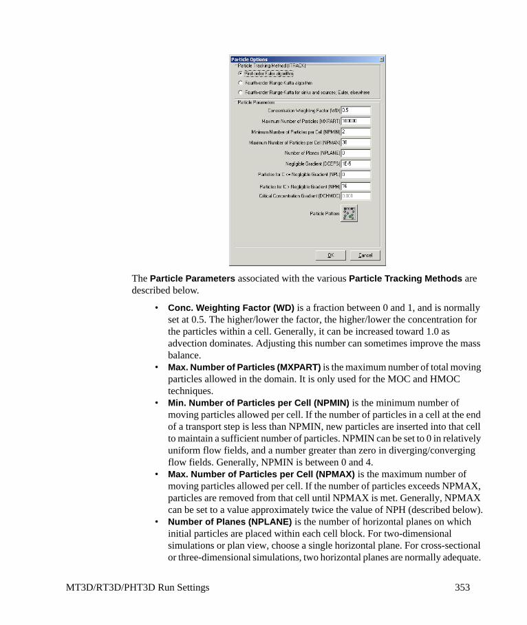
MT3D/RT3D/PHT3D Run Settings 353
The Particle Parameters associated with the various Particle Tracking Methods are described below.
• Conc. Weighting Factor (WD) is a fraction between 0 and 1, and is normally set at 0.5. The higher/lower the factor, the higher/lower the concentration for the particles within a cell. Generally, it can be increased toward 1.0 as advection dominates. Adjusting this number can sometimes improve the mass balance.
• Max. Number of Particles (MXPART) is the maximum number of total moving particles allowed in the domain. It is only used for the MOC and HMOC techniques.
• Min. Number of Particles per Cell (NPMIN) is the minimum number of moving particles allowed per cell. If the number of particles in a cell at the end of a transport step is less than NPMIN, new particles are inserted into that cell to maintain a sufficient number of particles. NPMIN can be set to 0 in relatively uniform flow fields, and a number greater than zero in diverging/converging flow fields. Generally, NPMIN is between 0 and 4.
• Max. Number of Particles per Cell (NPMAX) is the maximum number of moving particles allowed per cell. If the number of particles exceeds NPMAX, particles are removed from that cell until NPMAX is met. Generally, NPMAX can be set to a value approximately twice the value of NPH (described below).
• Number of Planes (NPLANE) is the number of horizontal planes on which initial particles are placed within each cell block. For two-dimensional simulations or plan view, choose a single horizontal plane. For cross-sectional or three-dimensional simulations, two horizontal planes are normally adequate.
354 Chapter 5: Run Section - Model Run Settings
Additional horizontal planes may be added if more resolution in the vertical direction is required.
• Negligible Gradient (DCEPS) is used to improve the computational efficiency of the MOC procedure. A higher number of particles are placed in cells involving advection calculations, and a lower number of particles are placed in cells not involved in advection calculations. If the calculated relative concentration gradient between adjacent cells is greater than DCEPS, NPMAX particles are placed in the cell. If the calculated relative concentration gradient is less than DCEPS, NPMIN particles are placed in the cell. A very small value such as 10-5 is generally used.
• Particles for C <= Negligible Gradient (NPL) is the number of initial particles per cell to be placed at cells where the calculated concentration gradient is less than or equal to DCEPS. Generally, this number can be set to 0. Setting NPL equal to NPH causes a uniform number of particles to be placed in every cell over the entire grid.
• Particles for C > Negligible Gradient (NPH) is the number of initial particles to be placed at cells where the concentration gradient in the cell (DCCELL) is greater than DCEPS. In relatively uniform flow fields, use a smaller NPH and increase NPH as the non-uniformity of the flow field increases. Values exceeding 16 in two-dimensional flow, or 32 in three-dimensional flow, are rarely necessary.
• Critical Conc. Gradient (DCHMOC): is the relative concentration gradient between the cell being considered and its neighboring cells, and is used to evaluate the sharpness of the concentration front. If the HMOC scheme is being used, and the calculated relative concentration gradient is greater than DCHMOC, then the MOC scheme is used, otherwise the MMOC scheme will be used. The DCHMOC criterion is empirical, but values between 0.001 and 0.01 have been found to be adequate for most problems.
• Particle Pattern (NLSINK) sets the number of particles per horizontal plane. The fixed pattern option distributes a fixed number of particles over the cell in the pattern shown in the pattern box. The total number of particles in the cell is multiplied by NPLANE. This option works well for relatively uniform flow fields.
Note: The random pattern option distributes the particles randomly in both the hor-izontal and vertical directions. The number of particles is entered under NPH. If the flow field is non-uniform, this option may capture the essence of the flow field bet-ter than the fixed pattern. The random distribution also leads to smaller mass bal-ance discrepancy in non-uniform or diverging/converging flow fields.
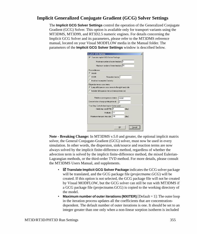
MT3D/RT3D/PHT3D Run Settings 355
Implicit Generalized Conjugate Gradient (GCG) Solver Settings The Implicit GCG Solver Settings control the operation of the Generalized Conjugate Gradient (GCG) Solver. This option is available only for transport variants using the MT3DMS, MT3D99, and RT3D2.5 numeric engines. For details concerning the Implicit GCG Solver and its parameters, please refer to the MT3DMS reference manual, located on your Visual MODFLOW media in the Manual folder. The parameters of the Implicit GCG Solver Settings window is described below.
Note - Breaking Change: In MT3DMS v.5.0 and greater, the optional implicit matrix solver, the General Conjugate-Gradient (GCG) solver, must now be used in every simulation. In other words, the dispersion, sink/source and reaction terms are now always solved by the implicit finite-difference method, regardless of whether the advection term is solved by the implicit finite-difference method, the mixed Eulerian-Lagrangian methods, or the third-order TVD method. For more details, please consult the MT3DMS Users Manual, and supplements.
• Translate Implicit GCG Solver Package indicates the GCG solver package will be translated, and the GCG package file (projectname.GCG) will be created. If this option is not selected, the GCG package file will not be created by Visual MODFLOW, but the GCG solver can still be run with MT3DMS if a GCG package file (projectname.GCG) is copied to the working directory of the model.
• Maximum number of outer iterations (MXITER) [Default = 1]: The outer loop in the iteration process updates all the coefficients that are concentration-dependent. The default number of outer iterations is one. It should be set to an integer greater than one only when a non-linear sorption isotherm is included
356 Chapter 5: Run Section - Model Run Settings
in simulation. For further detail please refer to page 4-19 in the MT3DMS Documentation and User’s Guide, located on your Visual MODFLOW media in the Manual folder.
• Maximum number of inner iterations (ITER1) [Default = 50]: The inner loop in the iteration process continues to iterate toward the solution until the convergence criterion is obtained or the maximum number of inner iterations is reached. During these iterations, the coefficient matrix and the right hand side vector matrix remain unchanged. The default number of inner iterations is fifty. A maximum value of thirty to fifty inner iterations should be sufficient for most problems. For further details please refer to page 4-19 in the MT3DMS Documentation and User’s Guide.
Preconditioning MethodsThe GCG Solver implicitly solves the non-advective terms in the transport equation using a two-iteration loop process and the choice between three pre-conditioning options:
• Jacobi (ISOLVE=1)• SSOR (ISOLVE=2)• Modified Incomplete Cholesky (ISOLVE=3)
The Modified Incomplete Cholesky method usually converges faster than the other two method options, but it requires significantly more memory.
Dispersion Tensor Cross TermsThe GCG Solver has two options for dealing the cross-derivative terms of the dispersion tensor:
• Lump all dispersion cross terms to the right hand side (NCRS=0) will place all the dispersion tensor cross terms to the right hand side of the matrix equation and consider them as known values. This method approximates the equation (the loss of accuracy is generally insignificant) but is highly efficient (reduces the memory requirement by nearly two thirds) since there are significantly less unknown terms to be solved. For further detail please refer to the MT3DMS Documentation and User’s Guide, located on your Visual MODFLOW media in the Manual folder.
• Include full dispersion tensor (NCRS=1) will keep all the dispersion tensor cross terms on the left-hand side of the matrix equation and consider them as unknown terms. This method gives the exact matrix equation but is memory intensive since there are significantly more unknown terms to be solved. For details, refer to the MT3DMS Documentation and User’s Guide.
The Relative convergence criterion (CCLOSE) [Default = 10-4]: is used to judge the convergence, in terms of relative concentration, of the inner iterations of the solver. The default value is 10-4. A value between 10-4 and 10-6 is generally adequate.
MT3D/RT3D/PHT3D Run Settings 357
The Concentration change printing interval (IPRGCG) [Default = 0]: is the interval for printing the maximum concentration changes of each iteration. The default is 0 for printing at the end of each stress period.
Time Steps• Initial Step Size (DT0): [Default = 0]: The Initial Step Size is used to override
the automatically calculated initial time step. The user can assign a value to be used for the first iteration of the solution. The default value of 0 means that the MT3D calculated value will be used.
If one of the particle-based methods is used, the maximum timestep size calculated by MT3D will be used unless this value is smaller.
If the implicit solver is not selected, then this value will be ignored and the value for DT0 will be taken from the Output/Time Step Control dialog.
• Multiplier (TTSMULT) [Default = 1]: This is the multiplier used to calculate the size of the next transport time step when the finite difference method is used with the implicit GCG solver. A value between 1 and 2 is generally adequate. Using a time step multiplier will degrade the solution at later times when the timestep becomes large, but can significantly decrease the amount of time needed for the solution. If one of the particle-based methods or the TVD method is used, this value will be ignored.
• Maximum transport step size (TTSMAX) [Default = 0]: This value is the maximum time step size allowed when a multiplier greater than 1 is used. Setting this equal to zero imposes no maximum limit.
Particle-Based Methods
Method of Characteristics (MOC)The MOC method is available in all versions of MT3D. The MOC method uses a conventional particle tracking technique based on a mixed Eulerian-Lagrangian method for solving the advection term. The dispersion, sink/source mixing and chemical reaction terms are solved with the finite difference method. The MOC technique tracks a large number of moving particles forward in time, and keeps track of the concentration and position of each particle.
The main advantage of the MOC technique is that it is virtually free of numerical dispersion. However, the drawback of the MOC technique is that it can be slow, and can require a large amount of computer memory.
Modified Method of Characteristics (MMOC)The MMOC method is available in all versions of MT3D. The MMOC was developed to improve computational efficiency of the MOC technique. Unlike the MOC
358 Chapter 5: Run Section - Model Run Settings
technique, which tracks the position and concentration of a large number of moving particles, the MMOC technique places a particle at the mid-point of each cell at each new time level. The particle is tracked backward to find its position at the old time level and the concentration associated with the old time level is used to approximate the concentration at the new time level.
The MMOC method is both faster and requires less computer memory than the MOC method. However, with the lower-order interpolation scheme available with MT3D, the MMOC method introduces some numerical dispersion.
Hybrid Method of Characteristics (HMOC)The HMOC method is available in all versions of MT3D. The HMOC method combines the strengths of the MOC and the MMOC methods by using an automatic adaptive scheme that uses the MOC technique at sharp concentration fronts, and the MMOC method away from the fronts. By selecting an appropriate criterion for controlling the switch between the MOC and MMOC techniques, the HMOC scheme can provide accurate solutions for both sharp and non-sharp front problems.
Finite Difference Methods
Upstream Finite Difference Method (UFD)The Upstream Finite Difference method is available in all MT3D versions. Since, the finite-difference method does not involve particle tracking or concentration interpolations, it is normally more computationally efficient than the Method of Characteristics (MOC). In addition, the finite difference method normally has very small mass balance errors because it is based on the principle of mass conservation. However, the Upstream Finite-Difference method can lead to significant numerical dispersion for problems having sharp concentration fronts.
Central Finite Difference Method (CFD)The Central Finite Difference method is only available in MT3DMS, MT3D99, and RT3Dv.2.5. The central finite difference method does not exhibit the numerical dispersion problems like the Upstream Finite Difference method, but is susceptible to excessive artificial oscillations in advection dominated problems.
Note: Unlike the finite-difference method, the mixed Eulerian-Lagrangian schemes (MOC, MMOC, and HMOC) are not entirely based on the principle of mass con-servation. Due to the discrete nature of the moving particles, the solution does not guarantee that the mass entering a cell will equal the mass exiting a cell. The result-ant mass balance error can be significant at early times, but usually decreases at later times. Various Particle Parameters, such as the number and initial distribution pattern of moving particles, the particle tracking scheme, and the step size, can be adjusted to minimize the mass balance discrepancy.
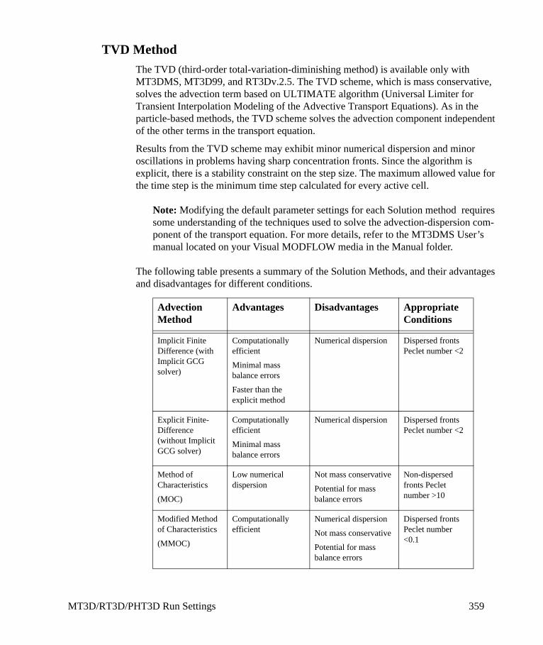
MT3D/RT3D/PHT3D Run Settings 359
TVD MethodThe TVD (third-order total-variation-diminishing method) is available only with MT3DMS, MT3D99, and RT3Dv.2.5. The TVD scheme, which is mass conservative, solves the advection term based on ULTIMATE algorithm (Universal Limiter for Transient Interpolation Modeling of the Advective Transport Equations). As in the particle-based methods, the TVD scheme solves the advection component independent of the other terms in the transport equation.
Results from the TVD scheme may exhibit minor numerical dispersion and minor oscillations in problems having sharp concentration fronts. Since the algorithm is explicit, there is a stability constraint on the step size. The maximum allowed value for the time step is the minimum time step calculated for every active cell.
Note: Modifying the default parameter settings for each Solution method requires some understanding of the techniques used to solve the advection-dispersion com-ponent of the transport equation. For more details, refer to the MT3DMS User’s manual located on your Visual MODFLOW media in the Manual folder.
The following table presents a summary of the Solution Methods, and their advantages and disadvantages for different conditions.
Advection Method
Advantages Disadvantages Appropriate Conditions
Implicit Finite Difference (with Implicit GCG solver)
Computationally efficient
Minimal mass balance errors
Faster than the explicit method
Numerical dispersion Dispersed fronts Peclet number <2
Explicit Finite- Difference (without Implicit GCG solver)
Computationally efficient
Minimal mass balance errors
Numerical dispersion Dispersed fronts Peclet number <2
Method of Characteristics
(MOC)
Low numerical dispersion
Not mass conservative
Potential for mass balance errors
Non-dispersed fronts Peclet number >10
Modified Method of Characteristics
(MMOC)
Computationally efficient
Numerical dispersion
Not mass conservative
Potential for mass balance errors
Dispersed fronts Peclet number <0.1

360 Chapter 5: Run Section - Model Run Settings
A Technical Note on the Generalized Conjugate Gradient SolverBy: Mr. Christopher J. Neville of S.S. Papadopulos & Associates
A new implicit Generalized Conjugate Gradient (GCG) solver is available for MT3DMS, MT3D99 and RT3Dv2.5. This solver is general-purpose iterative solver based on the generalized conjugate gradient method, and is implemented in a new package called the Generalized Conjugate Gradient (GCG) Package. The GCG solver is usually faster than the explicit finite-difference method because there are no time step constraints. However, it requires significantly more memory than the explicit solution method.
The explicit method, on the other hand, is simple and requires much less memory than the implicit method. It is also computationally efficient for certain advection-dominated problems in which the transport step size is not limited by stability constraints but rather by accuracy considerations. However, for transport problems with fine grid spacing, large dispersion coefficients, strongly non-linear sorption, or strong sink/source terms, the stability constraints can lead to exceedingly small transport steps when the explicit method is used.
Treatment of the transport terms with respect to timeMT3D offers the user two options for evaluating the terms in the finite-difference approximations: explicit or implicit-in-time weighting.
I. For explicit-in-time, or forward-in-time weighting (FIT), the terms in the finite-difference approximations are evaluated at the previous time step. This was the only option available in versions of MT3D from v.1.1 to MT3D96. Explicit-in-time weighting has the advantage of not requiring the assembly, storage, and solution of a matrix. It requires the least amount of RAM of all feasible methods. In particular, it requires no additional RAM with respect to the corresponding MODFLOW model. This was an important requirement for the development of MT3D, since the code was developed on a PC, for implementation on PCs. We now live in a world in which RAM is inexpensive. However, when MT3D was developed in 1987-1988, additional RAM over 640 KB was very limited and very expensive. Explicit-in-time weighting has the disadvantage of not being stable unless tight restrictions on the size of time steps are satisfied. In many cases, the size of the time steps could be very small - and would only get smaller as the spatial resolution of a model was increased. Furthermore, in versions of MT3D
Hybrid Method of Characteristics
(HMOC)
Computationally efficient
Low numerical dispersion
Must select adaptive criterion
Not mass conservative
Potential for mass balance errors
All conditions
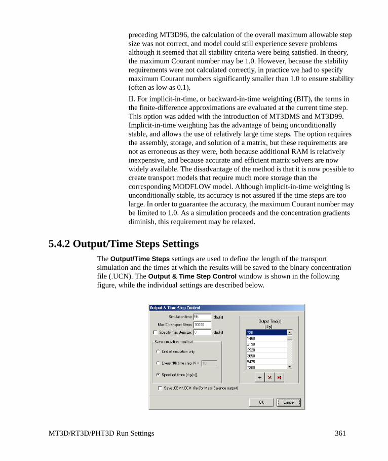
MT3D/RT3D/PHT3D Run Settings 361
preceding MT3D96, the calculation of the overall maximum allowable step size was not correct, and model could still experience severe problems although it seemed that all stability criteria were being satisfied. In theory, the maximum Courant number may be 1.0. However, because the stability requirements were not calculated correctly, in practice we had to specify maximum Courant numbers significantly smaller than 1.0 to ensure stability (often as low as 0.1).II. For implicit-in-time, or backward-in-time weighting (BIT), the terms in the finite-difference approximations are evaluated at the current time step. This option was added with the introduction of MT3DMS and MT3D99. Implicit-in-time weighting has the advantage of being unconditionally stable, and allows the use of relatively large time steps. The option requires the assembly, storage, and solution of a matrix, but these requirements are not as erroneous as they were, both because additional RAM is relatively inexpensive, and because accurate and efficient matrix solvers are now widely available. The disadvantage of the method is that it is now possible to create transport models that require much more storage than the corresponding MODFLOW model. Although implicit-in-time weighting is unconditionally stable, its accuracy is not assured if the time steps are too large. In order to guarantee the accuracy, the maximum Courant number may be limited to 1.0. As a simulation proceeds and the concentration gradients diminish, this requirement may be relaxed.
5.4.2 Output/Time Steps SettingsThe Output/Time Steps settings are used to define the length of the transport simulation and the times at which the results will be saved to the binary concentration file (.UCN). The Output & Time Step Control window is shown in the following figure, while the individual settings are described below.

362 Chapter 5: Run Section - Model Run Settings
• Simulation time is the total length of the transport simulation in the specified time units. This must be greater than zero.
• Max # of transport steps is the maximum number of transport steps for the simulation. Once the simulation has run through the specified Max # of transport steps the model will stop. This parameter is primarily used to limit the size of the output files generated.
• Specify max stepsize Sets the maximum step size to use for each transport time step. MT3D will use the smaller of: the internally calculated maximum timestep size based on the courant number, or the maximum timestep size specified here. If the implicit GCG solver is used, this value is ignored and the value found in the Solver options is used instead.
• Save simulation results at End of simulation only will save the simulation results at the end of the simulation only, and will not save any intermediate results. If more output data is desired, the solute concentrations can instead be saved at either regular time step intervals (Every Nth time step) or at manually entered times by checking the Specified times option, and then adding to the Output Times list. The simulation results are saved in the MT3D output *.OT file.
• Save concentration at observation point for every Nth time step allows to filter the amount of observation data that is saved to the .OBS file; ideal for transient runs with large output files
• Save one-line summary of mass budget for every Nth time step allows to filter the amount of mass budget data that is saved to the .MAS file; ideal for transient runs with large output files
• The Save .CBM/.CCM file option must be checked if you want Mass Balance output to be saved (for example, to generate Zone Budget-Transport data in the Output menu). By default, all new models are created with this option enabled, however older models may need to have this option manually enabled.
Calculating Transport Timestep Sizes MT3D calculates the transport timestep size for the particle-based methods (MOC, MMOC, HMOC) and the explicit finite-difference methods. The explicit finite difference methods and the particle-based methods use a uniform timestep size for all transport timesteps, which is calculated based on the following three numerical criteria.
The Courant Condition:
(Eq. 4.8, MT3D Reference Manual) ⎟⎟⎠
⎞⎜⎜⎝
⎛ ∆∆∆≤∆
zyxminc v
zv
yv
xRt ,,γ
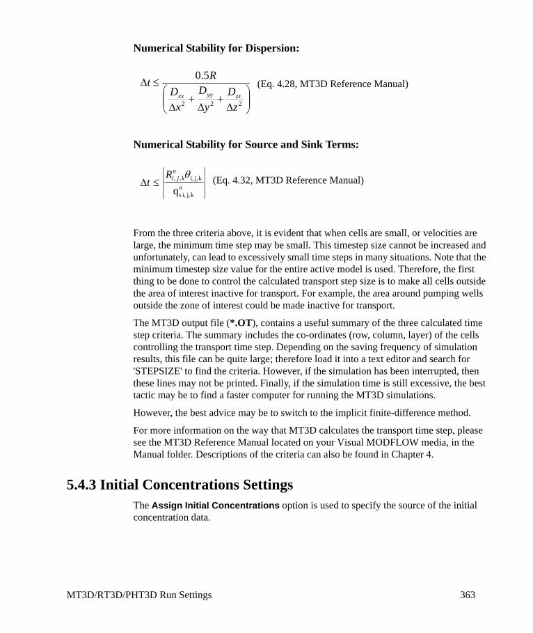
MT3D/RT3D/PHT3D Run Settings 363
Numerical Stability for Dispersion:
(Eq. 4.28, MT3D Reference Manual)
Numerical Stability for Source and Sink Terms:
(Eq. 4.32, MT3D Reference Manual)
From the three criteria above, it is evident that when cells are small, or velocities are large, the minimum time step may be small. This timestep size cannot be increased and unfortunately, can lead to excessively small time steps in many situations. Note that the minimum timestep size value for the entire active model is used. Therefore, the first thing to be done to control the calculated transport step size is to make all cells outside the area of interest inactive for transport. For example, the area around pumping wells outside the zone of interest could be made inactive for transport.
The MT3D output file (*.OT), contains a useful summary of the three calculated time step criteria. The summary includes the co-ordinates (row, column, layer) of the cells controlling the transport time step. Depending on the saving frequency of simulation results, this file can be quite large; therefore load it into a text editor and search for 'STEPSIZE' to find the criteria. However, if the simulation has been interrupted, then these lines may not be printed. Finally, if the simulation time is still excessive, the best tactic may be to find a faster computer for running the MT3D simulations.
However, the best advice may be to switch to the implicit finite-difference method.
For more information on the way that MT3D calculates the transport time step, please see the MT3D Reference Manual located on your Visual MODFLOW media, in the Manual folder. Descriptions of the criteria can also be found in Chapter 4.
5.4.3 Initial Concentrations SettingsThe Assign Initial Concentrations option is used to specify the source of the initial concentration data.
⎟⎟⎠
⎞⎜⎜⎝
⎛∆
+∆
+∆
≤∆
222
5.0
zD
yD
xD
Rtzzyyxx
nkj,i, s
kj,i,,,
qθn
kjiRt ≤∆

364 Chapter 5: Run Section - Model Run Settings
If the model is simulating contaminant migration immediately following a contamination event, then the initial concentrations of all contaminant species in the background groundwater will likely be zero. However, if the model is simulating reactive transport of chemicals, the initial concentrations of species such as dissolved oxygen (O2), sulphate (SO4), nitrate (NO3) and ferrous iron (Fe3) will need to be set equal to measured (or estimated) background concentrations.
As with the Initial Heads run settings, there are four options for defining the initial concentrations in the model (as shown in the preceding figure).
• Use Specified Concentrations will use the initial concentrations specified in the Input/Properties/Initial Concentration section of Visual MODFLOW. If no initial concentrations were specified for a given solute, Visual MODFLOW will automatically set the initial concentration equal to zero.
• Import from Surfer.grd File will use data from a selected Surfer file(s) to assign the initial concentrations of each species for each layer of the model. See the Importing Initial Concentrations section below.
• Import from ASCII File will use data from a selected ASCII file(s) to calculate the initial concentrations of each species for each layer of the model. See the Importing Initial Concentrations section below.
• Import from previous transport model will use the binary format concentrations file (.UCN) from a previous MT3D model simulation as the initial concentrations for the current simulation. The selected. UCN file must have the same number of rows, columns, and layers as the current model.
Importing Initial ConcentrationsVisual MODFLOW can import initial concentration data from either ASCII (.TXT) or Surfer (.GRD) files in world or model co-ordinate systems.
The ASCII files must be Space or Tab-delimited with the following format:
X-co-ordinate, Y-co-ordinate, Concentration value
Example:
1120 2352 0.023
3392 4491 0.008
2892 2531 1.500
3590 1803 0.532
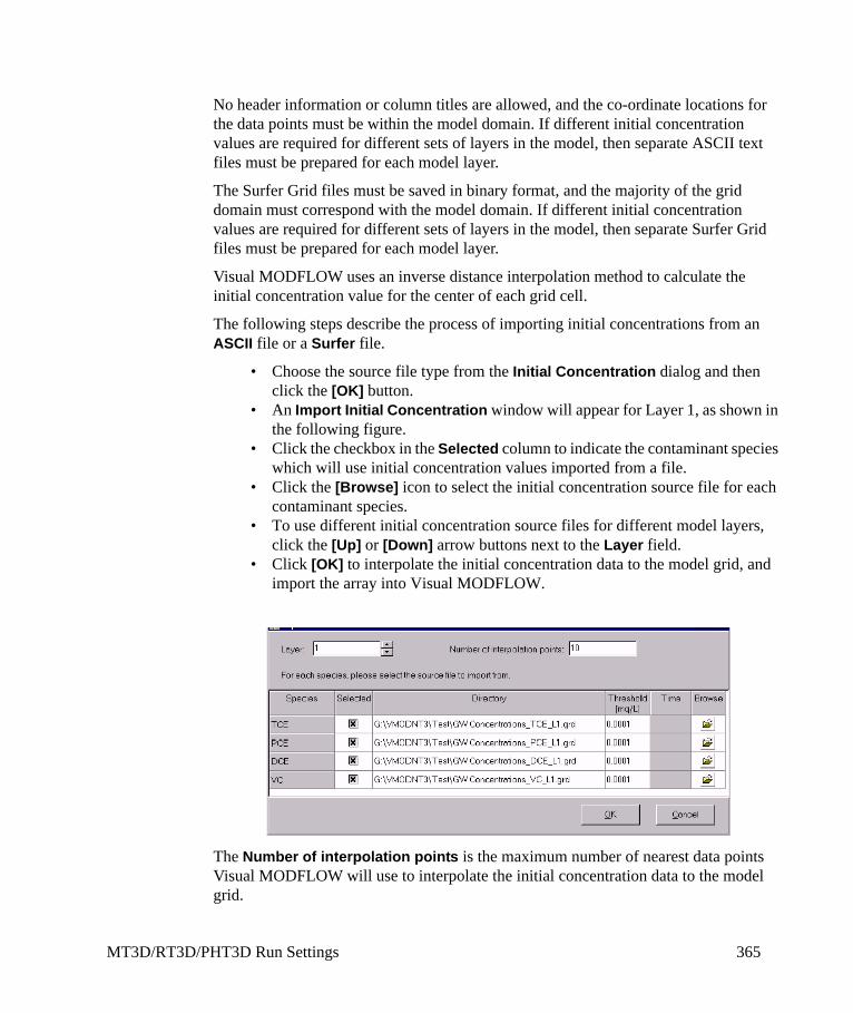
MT3D/RT3D/PHT3D Run Settings 365
No header information or column titles are allowed, and the co-ordinate locations for the data points must be within the model domain. If different initial concentration values are required for different sets of layers in the model, then separate ASCII text files must be prepared for each model layer.
The Surfer Grid files must be saved in binary format, and the majority of the grid domain must correspond with the model domain. If different initial concentration values are required for different sets of layers in the model, then separate Surfer Grid files must be prepared for each model layer.
Visual MODFLOW uses an inverse distance interpolation method to calculate the initial concentration value for the center of each grid cell.
The following steps describe the process of importing initial concentrations from an ASCII file or a Surfer file.
• Choose the source file type from the Initial Concentration dialog and then click the [OK] button.
• An Import Initial Concentration window will appear for Layer 1, as shown in the following figure.
• Click the checkbox in the Selected column to indicate the contaminant species which will use initial concentration values imported from a file.
• Click the [Browse] icon to select the initial concentration source file for each contaminant species.
• To use different initial concentration source files for different model layers, click the [Up] or [Down] arrow buttons next to the Layer field.
• Click [OK] to interpolate the initial concentration data to the model grid, and import the array into Visual MODFLOW.
The Number of interpolation points is the maximum number of nearest data points Visual MODFLOW will use to interpolate the initial concentration data to the model grid.
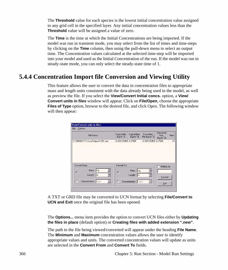
366 Chapter 5: Run Section - Model Run Settings
The Threshold value for each species is the lowest initial concentration value assigned to any grid cell in the specified layer. Any initial concentration values less than the Threshold value will be assigned a value of zero.
The Time is the time at which the Initial Concentrations are being imported. If the model was run in transient mode, you may select from the list of times and time-steps by clicking on the Time column, then using the pull-down menu to select an output time. The Concentration values calculated at the selected time-step will be imported into your model and used as the Initial Concentration of the run. If the model was run in steady-state mode, you can only select the steady-state time of 1.
5.4.4 Concentration Import file Conversion and Viewing UtilityThis feature allows the user to convert the data in concentration files to appropriate mass and length units consistent with the data already being used in the model, as well as preview the file. If you select the View/Convert Initial concs. option, a View/Convert units in files window will appear. Click on File/Open, choose the appropriate Files of Type option, browse to the desired file, and click Open. The following window will then appear:
A TXT or GRD file may be converted to UCN format by selecting File/Convert to UCN and Exit once the original file has been opened.
The Options... menu item provides the option to convert UCN files either by Updating the files in place (default option) or Creating files with added extension “.new”.
The path to the file being viewed/converted will appear under the heading File Name. The Minimum and Maximum concentration values allows the user to identify appropriate values and units. The converted concentration values will update as units are selected in the Convert From and Convert To fields.
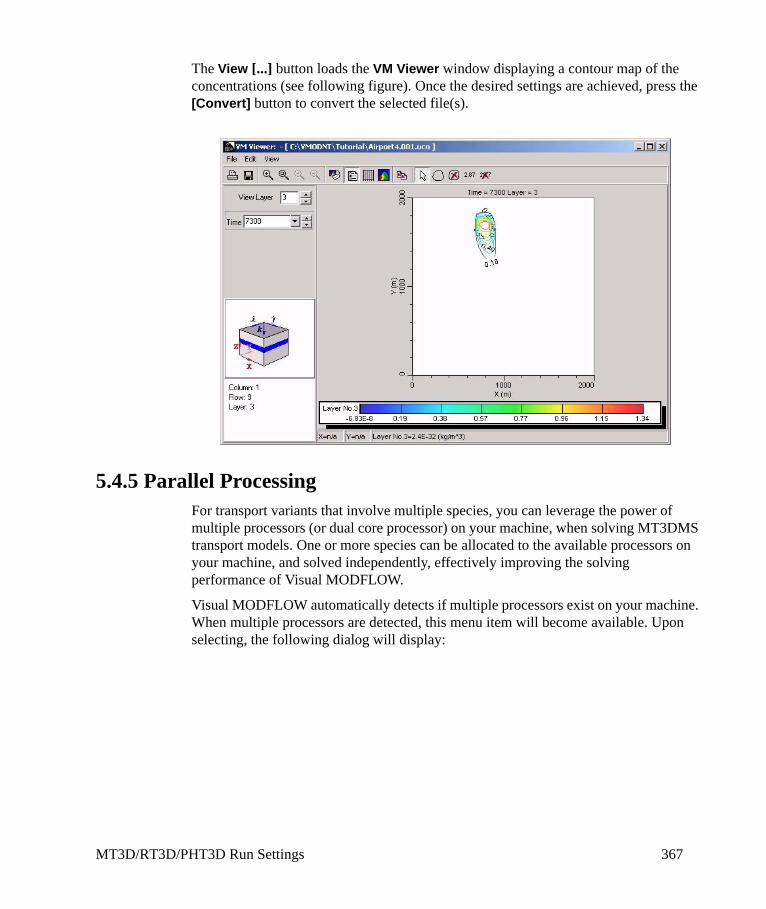
MT3D/RT3D/PHT3D Run Settings 367
The View [...] button loads the VM Viewer window displaying a contour map of the concentrations (see following figure). Once the desired settings are achieved, press the [Convert] button to convert the selected file(s).
5.4.5 Parallel ProcessingFor transport variants that involve multiple species, you can leverage the power of multiple processors (or dual core processor) on your machine, when solving MT3DMS transport models. One or more species can be allocated to the available processors on your machine, and solved independently, effectively improving the solving performance of Visual MODFLOW.
Visual MODFLOW automatically detects if multiple processors exist on your machine. When multiple processors are detected, this menu item will become available. Upon selecting, the following dialog will display:

368 Chapter 5: Run Section - Model Run Settings
In the Parallel Process Options dialog you can select either Single process or Multi Process. If you choose multi-process, enter the number of processes to use in the Number of processes field. NOTE: This value cannot exceed the total number of processors on your machine.
Click the [Ok] button to save the settings.
5.4.6 PHT3D Run SettingsA PHT3D simulation requires additional parameters and run-time settings to be defined. The following dialog will appear (for PHT3D transport variants only).
Note: Before applying PHT3D, users are encouraged to familiarize themselves with PHREEQC-2, MT3DMS, and geochemistry concepts.
For a list of some of the Limitations of PHT3D, please see “PHT3D 1.46” on page 652.

MT3D/RT3D/PHT3D Run Settings 369
General
Simulation Options
• Reaction Module - displays a preview of the reaction that was selected in the Transport Variant settings (Read-only).
• Enable PHREEQC-MT3DMS Reactions - is a flag to disable/enable reactions. This can be useful for calculating the net reaction effects.
• Redox Mode - is a flag that defines whether the starting values in the PHREEQC reaction step for pH and pe are variable, i.e., taken from the previous timestep, or if they are fixed. The latter is usually only required in special cases of non-redox sensitive problems where no numerical solution can be achieved otherwise. Select from:
• Variable pe and pH (Default)• Fixed pe and Variable pH• Fixed pe and pH
• Temperature of the Aqueous Solution - is the temperature used in chemical reactions for which a temperature dependence is defined within the database file. The value defines a homogeneous temperature within the model domain. Temperature (i.e. heat) is generally not simulated, unless indicated otherwise for selected reaction modules.
PHREEQC Execution Threshold Values
• Sum of changes in Aqueous Solution - The threshold value for executing PHREEQC defines a critical value (sum of concentration changes for all aqueous components) below which PHREEQC will be temporally deactivated at locations within the model domain where no geochemical changes are expected to occur. If the value is set to 0 PHREEQC will never be deactivated. If the value is set too high this might result in an inaccurate numerical solution.
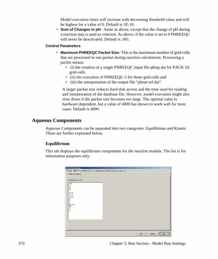
370 Chapter 5: Run Section - Model Run Settings
Model execution times will increase with decreasing threshold value and will be highest for a value of 0. Default is 1E-10.
• Sum of Changes in pH - Same as above, except that the change of pH during a reaction step is used as criterion. As above, if the value is set to 0 PHREEQC will never be deactivated. Default is .001.
Control Parameters
• Maximum PHREEQC Packet Size- This is the maximum number of grid-cells that are processed in one packet during reaction calculations. Processing a packet means:
• (i) the creation of a single PHREEQC input file phinp.dat for PACK SZ grid-cells
• (ii) the execution of PHREEQC-2 for those grid-cells and • (iii) the interpretation of the output file “phout sel.dat”.
A larger packet size reduces hard disk access and the time used for reading and interpretation of the database file. However, model execution might also slow down if the packet size becomes too large. The optimal value is hardware dependent, but a value of 4000 has shown to work well for most cases. Default is 4000.
Aqueous ComponentsAqueous Components can be separated into two categories: Equilibrium and Kinetic. These are further explained below.
EquilibriumThis tab displays the equilibrium components for the reaction module. The list is for information purposes only.
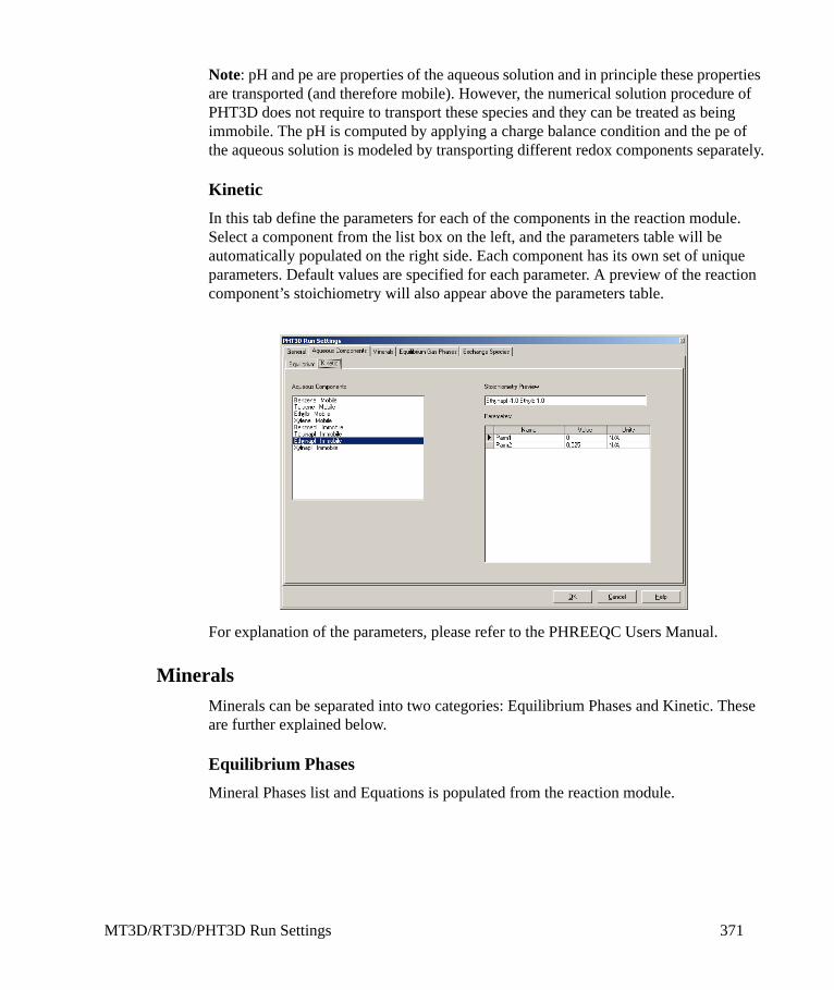
MT3D/RT3D/PHT3D Run Settings 371
Note: pH and pe are properties of the aqueous solution and in principle these properties are transported (and therefore mobile). However, the numerical solution procedure of PHT3D does not require to transport these species and they can be treated as being immobile. The pH is computed by applying a charge balance condition and the pe of the aqueous solution is modeled by transporting different redox components separately.
KineticIn this tab define the parameters for each of the components in the reaction module. Select a component from the list box on the left, and the parameters table will be automatically populated on the right side. Each component has its own set of unique parameters. Default values are specified for each parameter. A preview of the reaction component’s stoichiometry will also appear above the parameters table.
For explanation of the parameters, please refer to the PHREEQC Users Manual.
MineralsMinerals can be separated into two categories: Equilibrium Phases and Kinetic. These are further explained below.
Equilibrium PhasesMineral Phases list and Equations is populated from the reaction module.
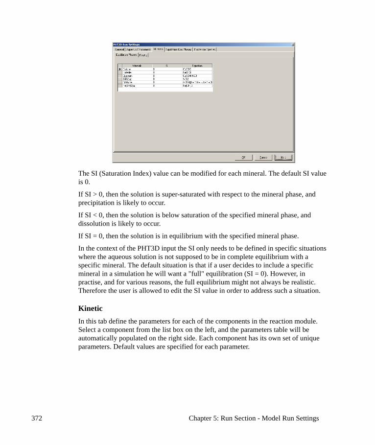
372 Chapter 5: Run Section - Model Run Settings
The SI (Saturation Index) value can be modified for each mineral. The default SI value is 0.
If SI > 0, then the solution is super-saturated with respect to the mineral phase, and precipitation is likely to occur.
If SI < 0, then the solution is below saturation of the specified mineral phase, and dissolution is likely to occur.
If SI = 0, then the solution is in equilibrium with the specified mineral phase.
In the context of the PHT3D input the SI only needs to be defined in specific situations where the aqueous solution is not supposed to be in complete equilibrium with a specific mineral. The default situation is that if a user decides to include a specific mineral in a simulation he will want a "full" equilibration (SI = 0). However, in practise, and for various reasons, the full equilibrium might not always be realistic. Therefore the user is allowed to edit the SI value in order to address such a situation.
KineticIn this tab define the parameters for each of the components in the reaction module. Select a component from the list box on the left, and the parameters table will be automatically populated on the right side. Each component has its own set of unique parameters. Default values are specified for each parameter.
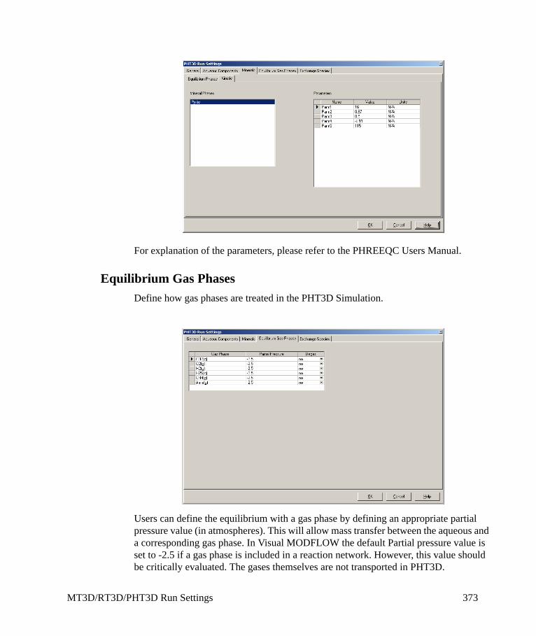
MT3D/RT3D/PHT3D Run Settings 373
For explanation of the parameters, please refer to the PHREEQC Users Manual.
Equilibrium Gas PhasesDefine how gas phases are treated in the PHT3D Simulation.
Users can define the equilibrium with a gas phase by defining an appropriate partial pressure value (in atmospheres). This will allow mass transfer between the aqueous and a corresponding gas phase. In Visual MODFLOW the default Partial pressure value is set to -2.5 if a gas phase is included in a reaction network. However, this value should be critically evaluated. The gases themselves are not transported in PHT3D.

374 Chapter 5: Run Section - Model Run Settings
Mass is transferred to the gas phase once over-saturation occurs (once the pressure of the system exceeds the user-defined partial pressure). In this situation, gas potentially accumulates and in principle the mass could be transferred back into the aqueous solution once the corresponding aqueous solution becomes undersaturated again.
To prevent this (if desired) a "degas" option is included in PHT3D. If this option is selected it will constantly remove the mass in the gas phase by resetting the gas concentration within grid cells to 0 before any reaction step. In Visual MODFLOW users can edit the Degas option (Yes/No) from the picklist. The default is No.
Note: Partial pressure values should be entered as the log of the partial pressure. For example, if the value for Phase is set to -1.0 it corresponds to log10(partial pressure) = 0.1 bar PCO2.
Exchange SpeciesThis tabs displays a preview of the Exchange Species involved in the reaction module. The list is for information purposes only.
5.5 SEAWAT Run SettingsIf SEAWAT has been selected for the Flow and Transport engine, the top menu bar will appear slightly different. There will be one menu for SEAWAT, which contains submenu items for Simulation Scenario, Flow, and Transport.
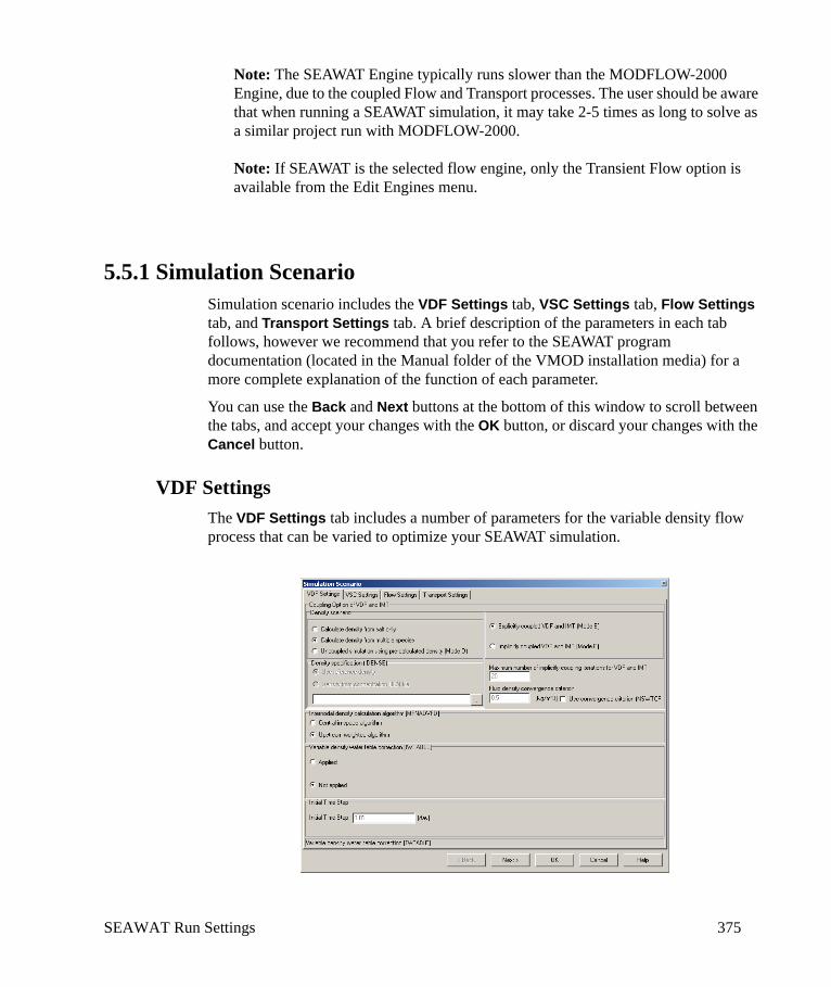
SEAWAT Run Settings 375
Note: The SEAWAT Engine typically runs slower than the MODFLOW-2000 Engine, due to the coupled Flow and Transport processes. The user should be aware that when running a SEAWAT simulation, it may take 2-5 times as long to solve as a similar project run with MODFLOW-2000.
Note: If SEAWAT is the selected flow engine, only the Transient Flow option is available from the Edit Engines menu.
5.5.1 Simulation ScenarioSimulation scenario includes the VDF Settings tab, VSC Settings tab, Flow Settings tab, and Transport Settings tab. A brief description of the parameters in each tab follows, however we recommend that you refer to the SEAWAT program documentation (located in the Manual folder of the VMOD installation media) for a more complete explanation of the function of each parameter.
You can use the Back and Next buttons at the bottom of this window to scroll between the tabs, and accept your changes with the OK button, or discard your changes with the Cancel button.
VDF SettingsThe VDF Settings tab includes a number of parameters for the variable density flow process that can be varied to optimize your SEAWAT simulation.
376 Chapter 5: Run Section - Model Run Settings
Coupling Option of VDF and IMTFor variable-density simulations involving coupled flow and transport, SEAWAT contains explicit and implicit options for solving the flow and transport equations. The Explicitly coupled VDF and IMT (Mode E) option, also referred to as a “one time step lag”, is the default option. With the explicit approach, the flow equation is formulated using fluid densities from the previous transport time step. For simulation with rapidly changing solute concentrations, the Implicitly coupled VDF and IMT (Mode E) option may provide a more accurate solution than the explicit option. With the implicit option, the flow and transport equations are solved repeatedly for each transport time step until consecutive differences in the calculated fluid densities are less than a user-specified value.
The Use Convergence Criterion (NSWTCPL) option can be used to control how often the flow field is updated. This option can only be used with the Explicitly coupled VDF and IMT (Mode E) option and can substantially reduce runtimes for simulations in which a new flow solution is not necessarily required for each transport timestep. When the check box is selected, the adjacent field will become available allowing you to specify a value for the maximum change in fluid density. If the maximum change in fluid density (between the present transport timestep and the last transport timestep for which the flow field was updated) is less than the specified value, SEAWAT will not update the flow field. SEAWAT only solves for the flow field:
• If the density change since the last flow field update exceeds the specified value at one or more cells,
• For the first transport timestep of the flow timestep, • For the last transport timestep of the flow timestep.
You can choose how many species to include in the equation of state to calculate fluid density. Select the Calculate Density from Salt Only to just include the Salt species. To include multiple species in the equation of state for fluid density, select the Calculate Density from Multiple Species option.
An uncoupled flow with transport simulation can be performed with a single species that does not affect fluid density. This method is particularly useful if you want to run a simulation using species concentrations generated in a previous MT3DMS simulation. To run SEAWAT with uncoupled flow, select the Uncoupled simulation using pre-calculated density (MODE D) option. When this option is selected, you can select from two options.
• Select Use Reference Density option to use the fluid density at the reference concentration, temperature, and pressure. These reference values are defined in the Constant Variant Parameters dialog in the Input section (Properties\Edit Constant Parameters...).
• Use the [...] button located below the Density Concentration from UCN file field to locate and specify the desired MT3DMS concentration file (*.UCN) to be used.
SEAWAT Run Settings 377
The Maximum number of implicitly coupling iterations for VDF and IMT parameter is only enabled if the “Implicitly coupled...” option is selected. The default value for this parameter is 20.
The Fluid density convergence criterion is only enabled if the “Implicitly coupled...” option is selected. The default value for this parameter is 1e-4.
Internodal Density Calculation Algorithm (MFNADVFD)This setting determines how the internodal density values used to conserve fluid mass will be calculated. One option is Central-in-space algorithm in which the density values are weighted based on adjacent cell lengths. Another is Upstream-weight algorithm in which the density value is selected based on the flow direction during that particular iteration. Results from variable-density simulations do not appear to be sensitive to the option selected; however users may want to experiment with both options.
The default option for this parameter is the Central-in-space algorithm.
Variable Density Water Table CorrectionThis setting is used to activate the variable-density water table correction. A detailed explanation of this parameter can be found in the “User’s Guide to SEAWAT” PDF document (located in the Manual folder of the VMOD installation media) by Guo and Langevin, 2002, equation 82. Since the variable density water table correction adds nonlinearity to the flow equation, the solvers may not converge for complicated water-table conditions. The user, therefore, has the option to run SEAWAT with or without the corrections.
The default option for this parameter is Not applied.
Initial Time StepThe default Initial Time Step is 0.001. The Time Step unit is automatically updated from the project settings. If the Time unit is changed (see “Changing Measurement Units and Model Start Time” section on page 51), the Initial Time Step value itself is not recalculated.
Note: In SEAWAT documentation, the inital time step is called FIRSTDT. It is used only at the beginning of a SEAWAT simulation.
VSC SettingsThe VSC Settings tab contains various settings for the SEAWAT Viscosity (VSC) package.

378 Chapter 5: Run Section - Model Run Settings
Please note that the VSC package is ONLY works with the Layer Property Flow (LPF) package and is not compatible with the BCF or HUF2 packages.
Viscosity OptionsThe first two options allow you to specify the number of species to use in the equation to calculate fluid viscosity. Select Calculate viscosity from single (salt only) species, no temperature dependence to calculate viscosity as a function of the salt species only. Select the Calculate viscosity from temperature and multiple species to calculate viscosity as a function of temperature and all MT3DMS species.
Viscosity can also be defined explicitly by selecting the User specified viscosity distribution option. When this option is selected, you can then choose from the following options located under Specified Viscosity Options (INVISC).
When the first option is selected, the values for the viscosity array are reused from the previous stress period. If it is the first stress period, values for the VISC array will be set to the fluid viscosity at the reference concentration and reference temperature (defined in the Constant Variant Parameters dialog in the Input section).
The Read specified viscosity from UCN file option allows you to specify a UCN file from which viscosity distributions are read. Click the [...] button under the Viscosity UCN file name field to locate the appropriate UCN file.
The Read concentration from UCN file and convert to viscosity using linear expression option allows you to specify a UCN file from which solute concentrations are read, and then converted into viscosity values using a linear expression. Click the [...] button under the Concentration UCN file name field to locate the appropriate UCN file.

SEAWAT Run Settings 379
Viscosity Temperature Dependence OptionsSEAWAT provides several options for representing dynamic viscosity as a function of temperature.
Simple Linear EquationWhen this option is selected, the following equation is used to calculate dynamic viscosity:
Where,
µ is dynamic viscosity
µ0 is the reference viscosity
Ck is the concentration for species k
C0k is the reference concentration
T is temperature
T0 is reference temperature
NS is number of species
For the remaining options, an alternative equation is used, with each option consisting of a different temperature term. Each temperature term is based on viscosity and temperature relations encountered in literature. The full viscosity equation is as follows:
Where,
µ = µT (T) is the temperature term, representing one of the following equations:Note: The default constant values for the following equation are defined in the Constant Variant Parameters dialog in the Input section of Visual MODFLOW. These values can also be defined when creating a new transport variant.

380 Chapter 5: Run Section - Model Run Settings
Voss (1984) ParametrizationWhen this option is selected, the following equation is used to calculate the temperature term:
Where,
A1 is 2.394 x 10⁵
A2 is 10
A3 is 248.37
A4 is 133.15
Pawlowski(1991) ParametrizationWhen this option is selected, the following equation is used to calculate the temperature term:
Where,
A1 is 1 x 10³
A2 is 1
A3 is 1.5512 x 10⁻²
A4 is -20
A5 is -1.572
Guo and Zhao (2005) ParametrizationThe following equation relates oil viscosity as a function of temperature and is therefore not applicable to water.
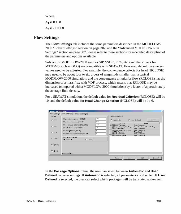
SEAWAT Run Settings 381
Where,
A1 is 0.168
A2 is -1.0868
Flow SettingsThe Flow Settings tab includes the same parameters described in the MODFLOW-2000 “Solver Settings” section on page 307, and the “Advanced MODFLOW Run Settings” section on page 387. Please refer to these sections for a detailed description of the parameters and options available.
Solvers for MODFLOW-2000 such as SIP, SSOR, PCG, etc. (and the solvers for MT3DMS such as GCG) are compatible with SEAWAT. However, default parameters values need to be adjusted. For example, the convergence criteria for head (HCLOSE) may need to be about four to six orders of magnitude smaller than a typical MODFLOW-2000 simulation; and the convergence criteria for flow (RCLOSE) has the dimension of a mass flux with VDF process, which means that RCLOSE may be increased (compared with a MODFLOW-2000 simulation) by a factor of approximately the average fluid density.
For a SEAWAT simulation, the default value for Residual Criterion (RCLOSE) will be 10, and the default value for Head Change Criterion (HCLOSE) will be 1e-6.
In the Package Options frame, the user can select between Automatic and User Defined package settings. If Automatic is selected, all parameters are disabled. If User Defined is selected, the user can select which packages will be translated and/or run.
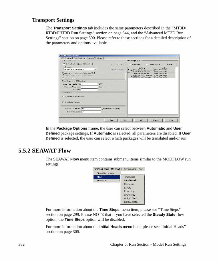
382 Chapter 5: Run Section - Model Run Settings
Transport SettingsThe Transport Settings tab includes the same parameters described in the “MT3D/RT3D/PHT3D Run Settings” section on page 344, and the “Advanced MT3D Run Settings” section on page 390. Please refer to these sections for a detailed description of the parameters and options available.
In the Package Options frame, the user can select between Automatic and User Defined package settings. If Automatic is selected, all parameters are disabled. If User Defined is selected, the user can select which packages will be translated and/or run.
5.5.2 SEAWAT FlowThe SEAWAT Flow menu item contains submenu items similar to the MODFLOW run settings.
For more information about the Time Steps menu item, please see “Time Steps” section on page 299. Please NOTE that if you have selected the Steady State flow option, the Time Steps option will be disabled.
For more information about the Initial Heads menu item, please see “Initial Heads” section on page 305.
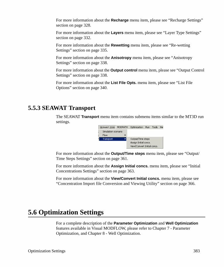
Optimization Settings 383
For more information about the Recharge menu item, please see “Recharge Settings” section on page 328.
For more information about the Layers menu item, please see “Layer Type Settings” section on page 332.
For more information about the Rewetting menu item, please see “Re-wetting Settings” section on page 335.
For more information about the Anisotropy menu item, please see “Anisotropy Settings” section on page 338.
For more information about the Output control menu item, please see “Output Control Settings” section on page 338.
For more information about the List File Opts. menu item, please see “List File Options” section on page 340.
5.5.3 SEAWAT TransportThe SEAWAT Transport menu item contains submenu items similar to the MT3D run settings.
For more information about the Output/Time steps menu item, please see “Output/Time Steps Settings” section on page 361.
For more information about the Assign Initial concs. menu item, please see “Initial Concentrations Settings” section on page 363.
For more information about the View/Convert Initial concs. menu item, please see “Concentration Import file Conversion and Viewing Utility” section on page 366.
5.6 Optimization SettingsFor a complete description of the Parameter Optimization and Well Optimization features available in Visual MODFLOW, please refer to Chapter 7 - Parameter Optimization, and Chapter 8 - Well Optimization.
384 Chapter 5: Run Section - Model Run Settings
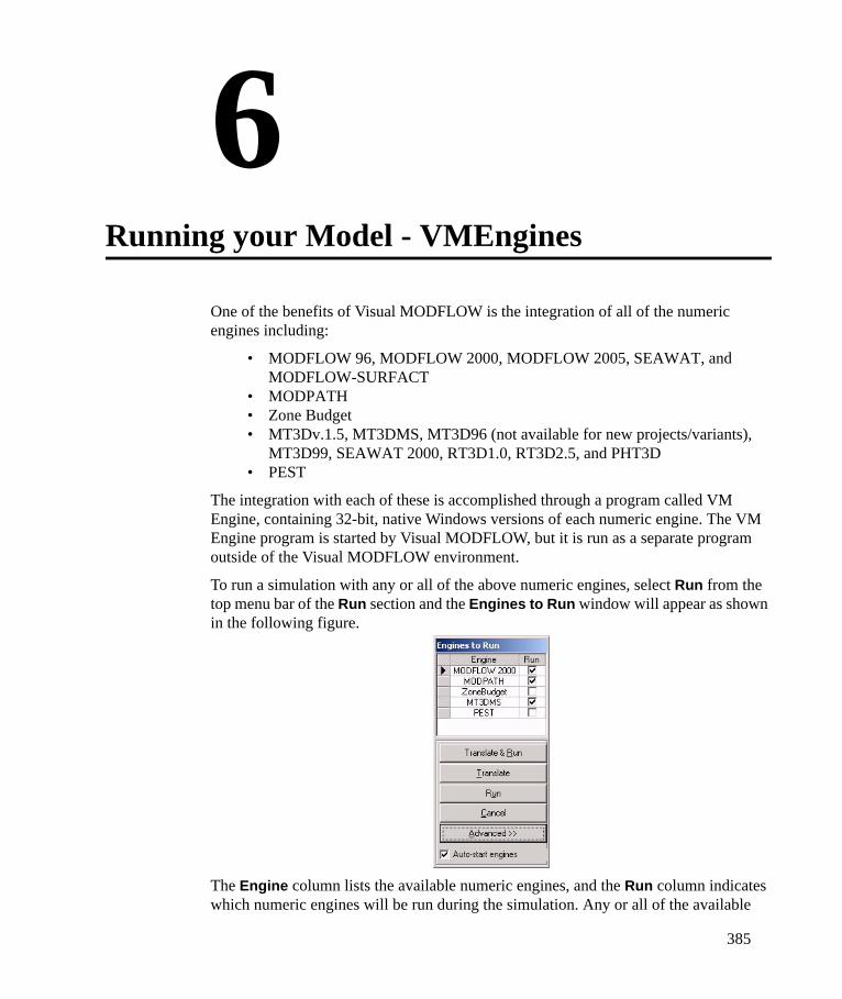
385
6Running your Model - VMEngines
One of the benefits of Visual MODFLOW is the integration of all of the numeric engines including:
• MODFLOW 96, MODFLOW 2000, MODFLOW 2005, SEAWAT, and MODFLOW-SURFACT
• MODPATH• Zone Budget• MT3Dv.1.5, MT3DMS, MT3D96 (not available for new projects/variants),
MT3D99, SEAWAT 2000, RT3D1.0, RT3D2.5, and PHT3D• PEST
The integration with each of these is accomplished through a program called VM Engine, containing 32-bit, native Windows versions of each numeric engine. The VM Engine program is started by Visual MODFLOW, but it is run as a separate program outside of the Visual MODFLOW environment.
To run a simulation with any or all of the above numeric engines, select Run from the top menu bar of the Run section and the Engines to Run window will appear as shown in the following figure.
The Engine column lists the available numeric engines, and the Run column indicates which numeric engines will be run during the simulation. Any or all of the available

386 Chapter 6: Running your Model - VMEngines
numeric engines can be run for the simulation provided the required data files are present in the model project folder.
The MODFLOW engine can be run by itself without any requirements from any of the other engines.
The MODPATH engine requires a valid .BGT file to be present in the project folder. This file will be automatically created if MODFLOW and MODPATH are mutually selected.
The Zone Budget engine requires a valid .BGT file to be present in the project folder. This file will be automatically created if MODFLOW and Zone Budget are mutually selected.
The MT3D engine requires a valid .FLO file to be present in the project folder. This file will be automatically created if MODFLOW and MT3D are mutually selected.
The PEST engine must be run with MODFLOW, and can optionally be run with MT3D.
The [Translate & Run] button will translate the model input data from Visual MODFLOW file formats to the data files required for the selected numeric engines (see Appendix A), and then start the VM Engine program to run the simulations.
The [Translate] button will translate the model input data from Visual MODFLOW file formats to the data files required for the selected numeric engines (see Appendix A).
The [Run] button will start the VM Engine program and run the selected numeric engines using the required (translated) data files already present in the project folder. If the required files are not present in the project folder, the numeric engines will not run. A warning message will appear indicating that the Visual MODFLOW files will not be translated prior to running the model. Press the [OK] button to start the simulation.
The [Cancel] button will close the Engines to Run window without translating or running any model files.
The [Advanced] button will expand the Engines to Run window to include a Settings column indicating either an Automatic or User Defined setting, as shown in the following figure. These settings are primarily used to control the Translate and Run options for the individual data sets associated with the Flow, Zone Budget and Transport engines.
The Auto-Start Engines option indicates whether the selected numeric engines will automatically start running the simulation when the [Translate & Run] button is selected or when the [Run] button is selected. If this option is selected, then VM Engines will automatically start running the simulation when it opens. If this option is not selected, VM Engines will open with the current simulation loaded, but it will not
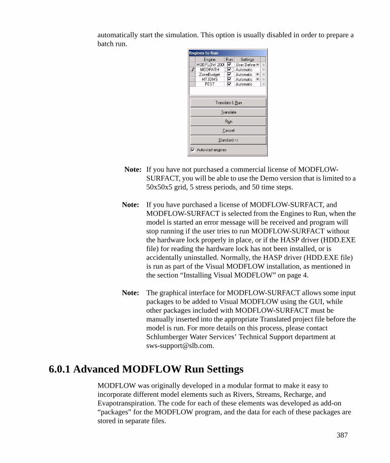
387
automatically start the simulation. This option is usually disabled in order to prepare a batch run.
Note: If you have not purchased a commercial license of MODFLOW-SURFACT, you will be able to use the Demo version that is limited to a 50x50x5 grid, 5 stress periods, and 50 time steps.
Note: If you have purchased a license of MODFLOW-SURFACT, and MODFLOW-SURFACT is selected from the Engines to Run, when the model is started an error message will be received and program will stop running if the user tries to run MODFLOW-SURFACT without the hardware lock properly in place, or if the HASP driver (HDD.EXE file) for reading the hardware lock has not been installed, or is accidentally uninstalled. Normally, the HASP driver (HDD.EXE file) is run as part of the Visual MODFLOW installation, as mentioned in the section “Installing Visual MODFLOW” on page 4.
Note: The graphical interface for MODFLOW-SURFACT allows some input packages to be added to Visual MODFLOW using the GUI, while other packages included with MODFLOW-SURFACT must be manually inserted into the appropriate Translated project file before the model is run. For more details on this process, please contact Schlumberger Water Services’ Technical Support department at [email protected].
6.0.1 Advanced MODFLOW Run SettingsMODFLOW was originally developed in a modular format to make it easy to incorporate different model elements such as Rivers, Streams, Recharge, and Evapotranspiration. The code for each of these elements was developed as add-on “packages” for the MODFLOW program, and the data for each of these packages are stored in separate files.
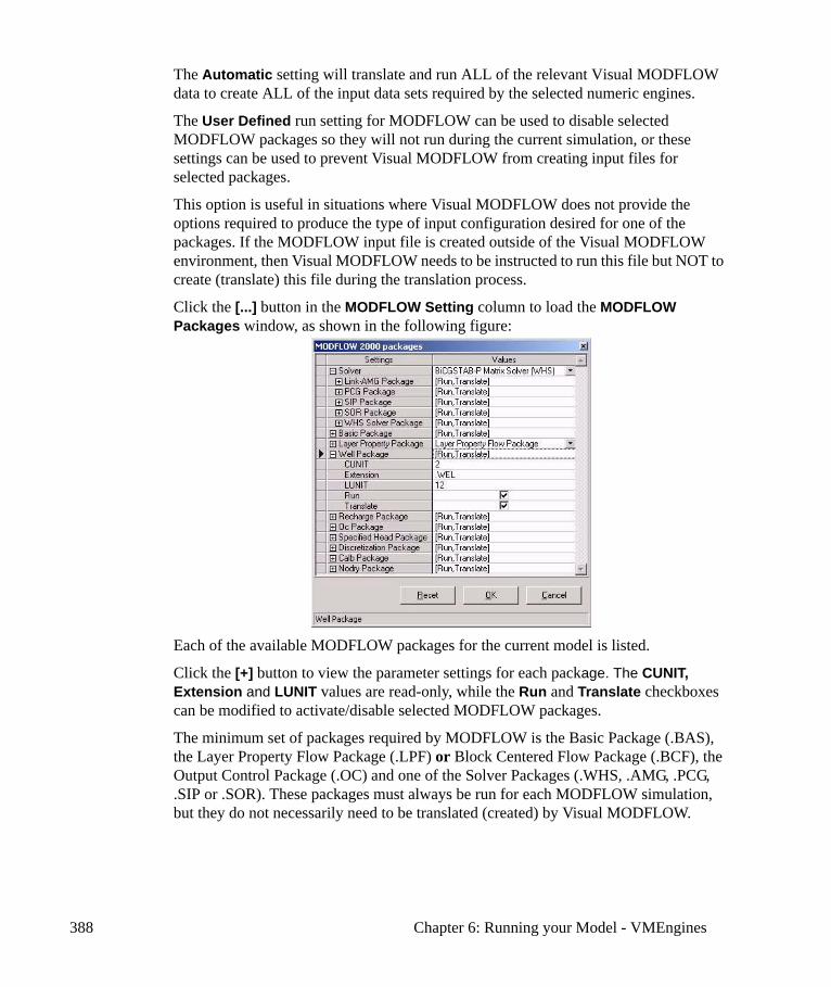
388 Chapter 6: Running your Model - VMEngines
The Automatic setting will translate and run ALL of the relevant Visual MODFLOW data to create ALL of the input data sets required by the selected numeric engines.
The User Defined run setting for MODFLOW can be used to disable selected MODFLOW packages so they will not run during the current simulation, or these settings can be used to prevent Visual MODFLOW from creating input files for selected packages.
This option is useful in situations where Visual MODFLOW does not provide the options required to produce the type of input configuration desired for one of the packages. If the MODFLOW input file is created outside of the Visual MODFLOW environment, then Visual MODFLOW needs to be instructed to run this file but NOT to create (translate) this file during the translation process.
Click the [...] button in the MODFLOW Setting column to load the MODFLOW Packages window, as shown in the following figure:
Each of the available MODFLOW packages for the current model is listed.
Click the [+] button to view the parameter settings for each package. The CUNIT, Extension and LUNIT values are read-only, while the Run and Translate checkboxes can be modified to activate/disable selected MODFLOW packages.
The minimum set of packages required by MODFLOW is the Basic Package (.BAS), the Layer Property Flow Package (.LPF) or Block Centered Flow Package (.BCF), the Output Control Package (.OC) and one of the Solver Packages (.WHS, .AMG, .PCG, .SIP or .SOR). These packages must always be run for each MODFLOW simulation, but they do not necessarily need to be translated (created) by Visual MODFLOW.
389
Running Input Files From Unsupported PackagesWhen the MODFLOW packages window is opened, Visual MODFLOW checks the project directory for model input data files from MODFLOW packages not currently supported by the Visual MODFLOW graphical interface. These files include:
• projectname.ETS (Evapotranspiration with a segmented function)• projectname.DRT (Drains with a return flow)• projectname.LAK (Lakes - Lake3 package only)• projectname.FHB (Flux and Head)• projectname.RES (Reservoir)• projectname.DAF (Diffusion Analogy Surface-Water Flow Model)• projectname.DAFG (DAFLOW-MODFLOW Link)• projectname.KDEP (Hydraulic-Conductivity Depth-Dependence)• projectname.SUB (Subsistence and Aquifer-System Compaction)• projectname.SFR (Stream Flow Routing)• projectname.DTOB (Observations: Drain Return)• projectname.HYD (Time Series Extraction)• projectname.SFOB (Observations: Stream Flow Routing)
If one of these MODFLOW input files are detected in the Visual MODFLOW project directory, it will be listed in the MODFLOW packages window and the default Setting for the package(s) will be to Run this input file with the model simulation.
Substituting Input FilesIn some circumstances Visual MODFLOW may not have all of the appropriate graphical or data manipulation tools required to produce the desired distribution of data. In these circumstances it may be necessary to write a FORTRAN or Visual Basic program to manipulate or create the required MODFLOW input files. Visual MODFLOW can still run these input files but the Translate option needs to be disabled for the selected MODFLOW Package input files being generated outside of Visual MODFLOW. This will prevent Visual MODFLOW from creating this input file, but if the Run option is still selected, the model will use the externally generated input file as long as it is located in the same directory as the Visual MODFLOW model.
6.0.2 Advanced Zone Budget Run SettingsThe ZoneBudget program reads the MODFLOW output and calculates a water budget between user-defined zones and other zones automatically identified by Visual MODFLOW.
Typically, water budget zones are defined in order to aid in the calibration of the model (e.g. determine how much water is exiting the model through a constant head boundary). Visual MODFLOW automatically creates zone budget zones for the various conductivity zones and boundary conditions. The Advanced Zone Budget settings can

390 Chapter 6: Running your Model - VMEngines
be used to activate or deactivate selected user defined zones, as shown in the following screenshot:
6.0.3 Advanced MT3D Run SettingsSimilar to MODFLOW, MT3D was also developed in a modular format to incorporate different model elements including source terms and reactions. The code for these elements was developed as add-on “packages” for the MT3D program, and the data for each of these packages are stored in separate files.
The User Defined run setting for MT3D can be used to disable selected MT3D packages so they will not run during the current simulation, or these settings can be used to prevent Visual MODFLOW from creating input files for the selected packages.
This setting is useful in situation where Visual MODFLOW does not provide the options required to produce the type of input configuration desired for one of the packages. If the MT3D input file is created outside of the Visual MODFLOW environment, then Visual MODFLOW needs to be instructed to run this file but NOT to create (translate) this file during the translation process.
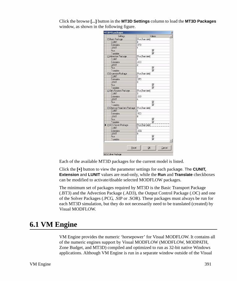
VM Engine 391
Click the browse [...] button in the MT3D Settings column to load the MT3D Packages window, as shown in the following figure.
Each of the available MT3D packages for the current model is listed.
Click the [+] button to view the parameter settings for each package. The CUNIT, Extension and LUNIT values are read-only, while the Run and Translate checkboxes can be modified to activate/disable selected MODFLOW packages.
The minimum set of packages required by MT3D is the Basic Transport Package (.BT3) and the Advection Package (.AD3), the Output Control Package (.OC) and one of the Solver Packages (.PCG, .SIP or .SOR). These packages must always be run for each MT3D simulation, but they do not necessarily need to be translated (created) by Visual MODFLOW.
6.1 VM EngineVM Engine provides the numeric ‘horsepower’ for Visual MODFLOW. It contains all of the numeric engines support by Visual MODFLOW (MODFLOW, MODPATH, Zone Budget, and MT3D) compiled and optimized to run as 32-bit native Windows applications. Although VM Engine is run in a separate window outside of the Visual
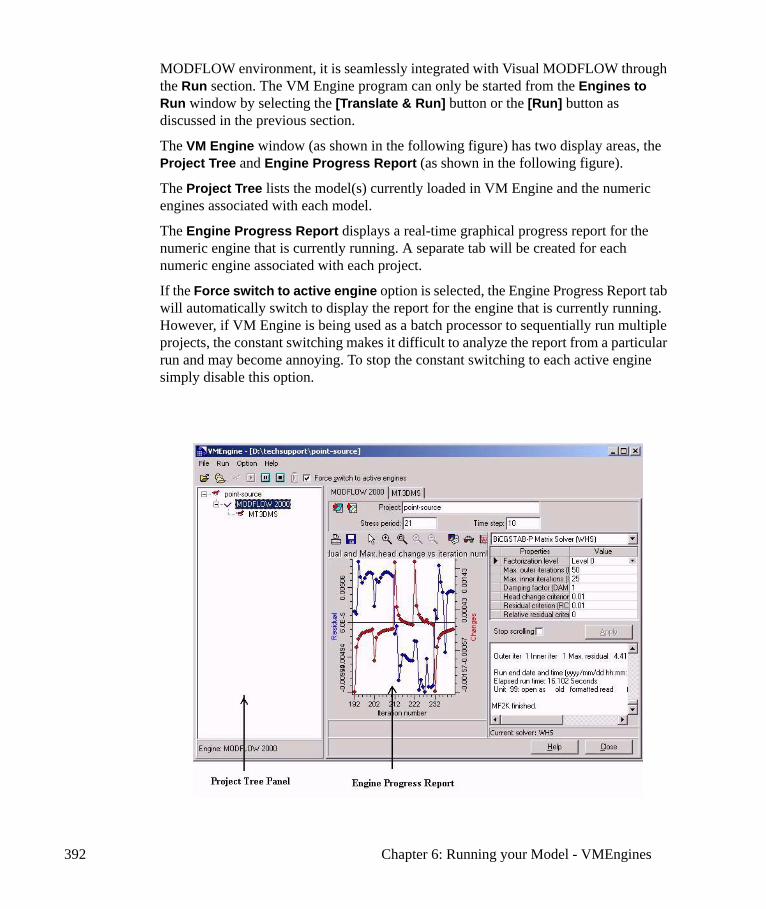
392 Chapter 6: Running your Model - VMEngines
MODFLOW environment, it is seamlessly integrated with Visual MODFLOW through the Run section. The VM Engine program can only be started from the Engines to Run window by selecting the [Translate & Run] button or the [Run] button as discussed in the previous section.
The VM Engine window (as shown in the following figure) has two display areas, the Project Tree and Engine Progress Report (as shown in the following figure).
The Project Tree lists the model(s) currently loaded in VM Engine and the numeric engines associated with each model.
The Engine Progress Report displays a real-time graphical progress report for the numeric engine that is currently running. A separate tab will be created for each numeric engine associated with each project.
If the Force switch to active engine option is selected, the Engine Progress Report tab will automatically switch to display the report for the engine that is currently running. However, if VM Engine is being used as a batch processor to sequentially run multiple projects, the constant switching makes it difficult to analyze the report from a particular run and may become annoying. To stop the constant switching to each active engine simply disable this option.
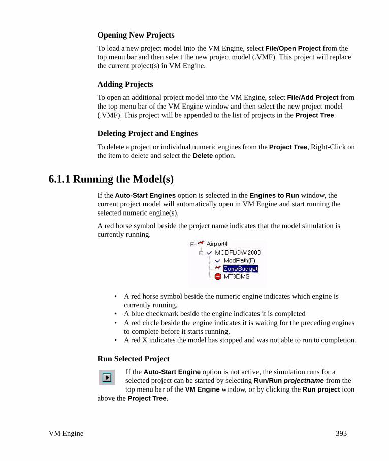
VM Engine 393
Opening New ProjectsTo load a new project model into the VM Engine, select File/Open Project from the top menu bar and then select the new project model (.VMF). This project will replace the current project(s) in VM Engine.
Adding ProjectsTo open an additional project model into the VM Engine, select File/Add Project from the top menu bar of the VM Engine window and then select the new project model (.VMF). This project will be appended to the list of projects in the Project Tree.
Deleting Project and EnginesTo delete a project or individual numeric engines from the Project Tree, Right-Click on the item to delete and select the Delete option.
6.1.1 Running the Model(s)If the Auto-Start Engines option is selected in the Engines to Run window, the current project model will automatically open in VM Engine and start running the selected numeric engine(s).
A red horse symbol beside the project name indicates that the model simulation is currently running.
• A red horse symbol beside the numeric engine indicates which engine is currently running,
• A blue checkmark beside the engine indicates it is completed • A red circle beside the engine indicates it is waiting for the preceding engines
to complete before it starts running,• A red X indicates the model has stopped and was not able to run to completion.
Run Selected ProjectIf the Auto-Start Engine option is not active, the simulation runs for a selected project can be started by selecting Run/Run projectname from the top menu bar of the VM Engine window, or by clicking the Run project icon
above the Project Tree.

394 Chapter 6: Running your Model - VMEngines
Run All ProjectsIf more than one project is loaded into VM Engine, all of the projects can be run in succession by selecting Run/Run All Projects from the top menu bar of the VM Engine window, or by clicking the Run All Projects icon above the
Project Tree.
Pausing the Running EngineThe numeric engine currently running in VM Engines can be paused by selecting Run/Pause from the top menu bar of the VM Engine window, or by clicking the Pause icons above the Project Tree. To restart the simulation, press the Resume by selecting Run from the top menu bar.
Stopping the Project RunThe current simulation can be terminated by selecting Run/Terminate from the top menu bar of the VM Engines window, or by clicking the Stop icon above the Project Tree Panel.
Batch Run SimulationsMultiple modeling projects can be loaded into VM Engines for the purpose of starting a batch run of simulations. To add a project to VM Engines select File/Add Project from the top menu bar of the VM Engine window and then select the project model file (projectname.VMF). This project will be appended to the list of projects in the Project Tree.
The numeric engine(s) available for the batch run will correspond to the last individual run of that model. If you would like to run additional engines that are not listed, you would need to open the model separately, go to the Run menu, select the Engines to run from the dialog, then select Translate. Once the model has been translated, you can close it, then open it for a batch run.

VM Engine 395
When running a batch of simulations, it is recommended to disable the VMEngines Auto start feature (from the Engines to Run window), and to disable the Force switch to active Engine feature.
You have the option to either run all simulations (in batch mode) by clicking on the Start all Projects icon, or run the currently selected project in the Project Tree by clicking on the Run project icon.
Note: If a model fails to converge, user input will be required to clear any error messages before the batch run can continue.
You can manually delete engines from a project run by right-clicking on the engine and selecting Delete.
Note: The Visual MODFLOW project files selected must be created by the most recent version of Visual MODFLOW before they can be added to the Project Tree.
6.1.2 MODFLOW Display OptionsThe Engine Progress Panel for MODFLOW provides the following functionality:
• display the current stress period and time step for the simulation• display a graphical progress report of the solution convergence data (maximum
residual head vs. number of iterations)• display the current solver being used and the associated parameters• on-the-fly modification of the solver and solver parameters• display a text-based report of the solution progress for each solver iteration• display a preview of contour maps and color maps of the head and drawdown
distributions with grid added or not.
The appearance of the graphical display of the residuals graph can be modified using the toolbar above the graph. The display options and properties of this graph are described in Chapter 10.
Modifying Solver ParametersThe selected solver and associated convergence criteria are displayed on the right hand side of the MODFLOW Engine Progress Panel. These settings were defined in the Run section of Visual MODFLOW prior to running the simulation. However, if the solution is encountering some difficulties in converging (as is often the case with complex multi-layered models) it may be necessary to adjust the convergence criteria during certain times of the simulation, or perhaps to even switch solvers.
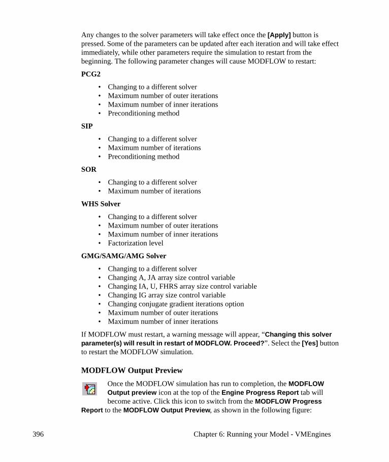
396 Chapter 6: Running your Model - VMEngines
Any changes to the solver parameters will take effect once the [Apply] button is pressed. Some of the parameters can be updated after each iteration and will take effect immediately, while other parameters require the simulation to restart from the beginning. The following parameter changes will cause MODFLOW to restart:
PCG2
• Changing to a different solver• Maximum number of outer iterations• Maximum number of inner iterations• Preconditioning method
SIP
• Changing to a different solver• Maximum number of iterations• Preconditioning method
SOR
• Changing to a different solver• Maximum number of iterations
WHS Solver
• Changing to a different solver• Maximum number of outer iterations• Maximum number of inner iterations• Factorization level
GMG/SAMG/AMG Solver
• Changing to a different solver• Changing A, JA array size control variable• Changing IA, U, FHRS array size control variable• Changing IG array size control variable• Changing conjugate gradient iterations option• Maximum number of outer iterations• Maximum number of inner iterations
If MODFLOW must restart, a warning message will appear, “Changing this solver parameter(s) will result in restart of MODFLOW. Proceed?”. Select the [Yes] button to restart the MODFLOW simulation.
MODFLOW Output PreviewOnce the MODFLOW simulation has run to completion, the MODFLOW Output preview icon at the top of the Engine Progress Report tab will become active. Click this icon to switch from the MODFLOW Progress
Report to the MODFLOW Output Preview, as shown in the following figure:
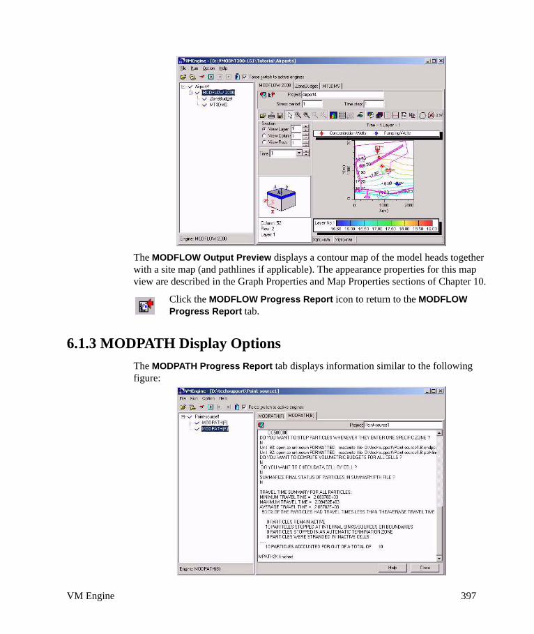
VM Engine 397
The MODFLOW Output Preview displays a contour map of the model heads together with a site map (and pathlines if applicable). The appearance properties for this map view are described in the Graph Properties and Map Properties sections of Chapter 10.
Click the MODFLOW Progress Report icon to return to the MODFLOW Progress Report tab.
6.1.3 MODPATH Display OptionsThe MODPATH Progress Report tab displays information similar to the following figure:

398 Chapter 6: Running your Model - VMEngines
This window displays the results and progress of the MODPATH calculations. It also provides a travel time summary for all particles and an explanation of where each particle became inactive or stopped in the simulation.
Click the Open Summary File icon to select, and display, a .PTH file containing detailed particle travel data.
MODPATH Output PreviewOnce the MODFLOW simulation has run to completion, the MODFLOW Output preview icon (as described above) will become active. Click this icon to switch from the MODFLOW Progress Report to the MODFLOW Output
Preview, and then click on the Animate Pathlines Only icon to animate the particle pathlines.
Click the MODPATH Progress Report tab to return to the MODPATH Progress Report.
6.1.4 Zone Budget OptionsThe Zone Budget Progress Report provides a real-time graphical display of the Zone Budget results as they are calculated.
It includes the project name of the model and the current stress period and time step being displayed on the chart. The chart may display either cumulative flows into or out of the aquifer or it may display individual flow rates (constant heads, rivers, etc.). The appearance settings for the graph are described in Chapter 11.
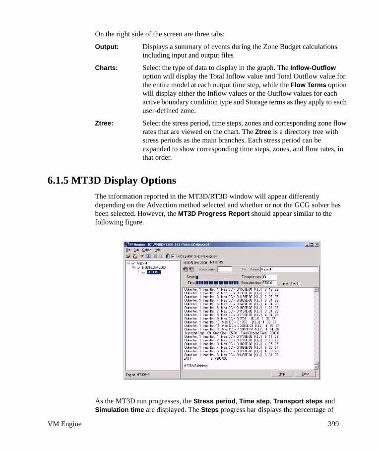
VM Engine 399
On the right side of the screen are three tabs:
Output: Displays a summary of events during the Zone Budget calculations including input and output files
Charts: Select the type of data to display in the graph. The Inflow-Outflow option will display the Total Inflow value and Total Outflow value for the entire model at each output time step, while the Flow Terms option will display either the Inflow values or the Outflow values for each active boundary condition type and Storage terms as they apply to each user-defined zone.
Ztree: Select the stress period, time steps, zones and corresponding zone flow rates that are viewed on the chart. The Ztree is a directory tree with stress periods as the main branches. Each stress period can be expanded to show corresponding time steps, zones, and flow rates, in that order.
6.1.5 MT3D Display OptionsThe information reported in the MT3D/RT3D window will appear differently depending on the Advection method selected and whether or not the GCG solver has been selected. However, the MT3D Progress Report should appear similar to the following figure.
As the MT3D run progresses, the Stress period, Time step, Transport steps and Simulation time are displayed. The Steps progress bar displays the percentage of

400 Chapter 6: Running your Model - VMEngines
transport steps, used so far out of the maximum allowable number of transport steps. The Time progress bar indicates how much of the total simulation time has been simulated.
MT3D Output PreviewIn many cases the computations required for a single contaminant transport simulation can take hours or even days to run to completion. This is a long time to wait just to discover something was obviously wrong with the simulation, particularly when this could have been detected during one of the early output times. This is why VM Engine provides the ability to preview the MT3D simulation results after each output time.
Once the first output time has been calculated, click the MT3D Output Preview button in the MT3D Progress Report Panel to switch to the MT3D Output Preview Panel.
The MT3D Output Preview Panel (similar to the MODFLOW Output Preview described on page 396) displays a concentration contour map for the first species listed in the model. If the simulation contains multiple species, Right-Click on the graph to choose which species to display. The appearance properties for this map view are described in the Graph Properties and Map Properties sections of Chapter 10.
Click the MT3D Progress Report icon to return to the MT3D Progress Report Panel.

7Parameter Optimization: PEST and Predictive Analysis
Parameter optimization is a discipline that provides tools for the efficient use of data to aid in mathematical modeling, and the estimation of the constants used in these models. It can be visualized as a study of inverse problems, as described below:
• Interpretation. An experiment is set up to introduce a controlled disturbance to the system of interest, in order to estimate some property of a system (e.g. a pumping test is used to estimate the transmissivity of an aquifer system). The model is then used to relate the disturbance and system properties to values that can be measured (e.g. piezometer measurements). The measured data may then be interpreted based on the premise that, for a known disturbance, it is possible to estimate the system properties from the measurement set.
• Calibration. If a system is disturbed, and this disturbance is simulated in a model, it should be possible to adjust the model’s parameters until the model output corresponds to field measurements taken during the disturbance. If so, we often conclude that the model will represent the system's behavior in response to other disturbances - disturbances which we may not be prepared to do in practice. A model is said to be "calibrated" when its parameters have been adjusted in this fashion.
• Predictive Analysis. Once a parameter set has been determined for which the model behavior matches the observed system behavior, it is then reasonable to ask whether another parameter set exists which also results in reasonable simulation by the model of the system under study. If this is the case, an even more pertinent question is whether predictions made by the model with the new parameter set are different.
For the purposes of groundwater modeling, the Calibration and Predictive Analysis applications of Parameter Optimization are the most relevant.
401
7.1 Getting StartedVisual MODFLOW provides a seamless interface to the popular parameter estimation and predictive analysis program PEST-ASP, developed by Dr. John Doherty of Watermark Computing. This chapter provides instructions on using Visual MODFLOW to setup, run, and interpret a Parameter Estimation/Predictive Analysis simulation. In addition, this chapter provides a brief description of the input parameters and settings required by PEST-ASP. A detailed description of the algorithms, parameters, input files, and other options for PEST-ASP may be obtained from the PEST-ASP User’s Manual .PDF file, located in the Manual folder of your Visual MODFLOW installation media.
Note: The Parameter Estimation component is included with the Pro version of Visual MODFLOW, or it may be purchased as an add-on package. If you do not have the Parameter Estimation component included with your software, please contact SWS’ Sales department for information on upgrading your software.
Visual MODFLOW supports both the Calibration and Predictive Analysis capabilities of the PEST-ASP program, and it allows you to run parameter estimation using results from both groundwater flow and contaminant transport simulations (i.e. observations can consist of heads, concentrations, and groundwater flux).
Before attempting to run a parameter estimation simulation, make sure your model meets the following two requirements:
[1] The model runs successfully and produces meaningful results. Parameter estimation is as much an art as it is a science, and therefore, it should only be used to complement your own efforts in understanding the system.
[2] The model has one or more (preferably many more) observations against which to compare the calculated results. Observations can be in the form of measured or estimated values of head or concentration at discrete points in the model, or in the form of measured or estimated groundwater fluxes into (or out of) one or more grid cells. Instructions for assigning flow observations, and observed head and concentration values, are described in detail later in this chapter.
Note: It is strongly advised that you familiarize yourself with the WINPEST and PEST-ASP User’s Manuals (located in the Manual folder of the Visual MODFLOW installation media) prior to attempting a parameter estimation simulation. The time spent on this will make your experience with parameter estimation much more productive, and will likely help you to overcome any difficulties you may experience the first time you run a simulation.
402 Chapter 7: Parameter Optimization: PEST and Predictive Analysis
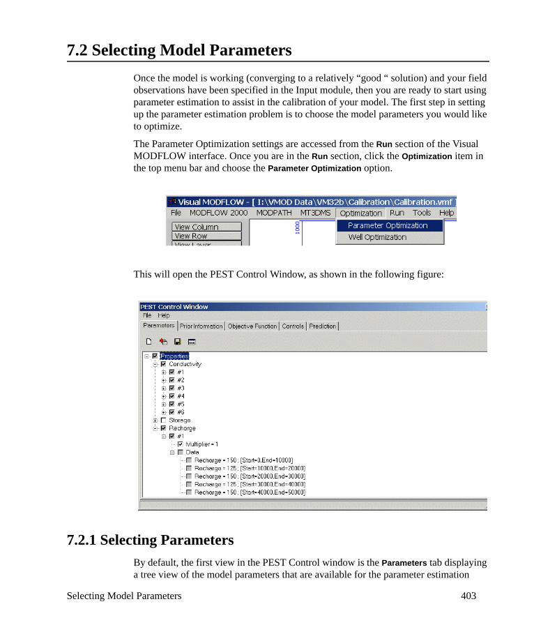
7.2 Selecting Model ParametersOnce the model is working (converging to a relatively “good “ solution) and your field observations have been specified in the Input module, then you are ready to start using parameter estimation to assist in the calibration of your model. The first step in setting up the parameter estimation problem is to choose the model parameters you would like to optimize.
The Parameter Optimization settings are accessed from the Run section of the Visual MODFLOW interface. Once you are in the Run section, click the Optimization item in the top menu bar and choose the Parameter Optimization option.
This will open the PEST Control Window, as shown in the following figure:
7.2.1 Selecting ParametersBy default, the first view in the PEST Control window is the Parameters tab displaying a tree view of the model parameters that are available for the parameter estimation
Selecting Model Parameters 403
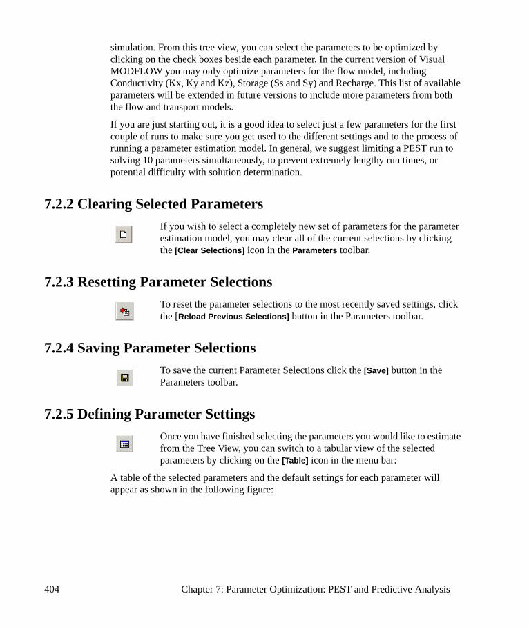
simulation. From this tree view, you can select the parameters to be optimized by clicking on the check boxes beside each parameter. In the current version of Visual MODFLOW you may only optimize parameters for the flow model, including Conductivity (Kx, Ky and Kz), Storage (Ss and Sy) and Recharge. This list of available parameters will be extended in future versions to include more parameters from both the flow and transport models.
If you are just starting out, it is a good idea to select just a few parameters for the first couple of runs to make sure you get used to the different settings and to the process of running a parameter estimation model. In general, we suggest limiting a PEST run to solving 10 parameters simultaneously, to prevent extremely lengthy run times, or potential difficulty with solution determination.
7.2.2 Clearing Selected ParametersIf you wish to select a completely new set of parameters for the parameter estimation model, you may clear all of the current selections by clicking the [Clear Selections] icon in the Parameters toolbar.
7.2.3 Resetting Parameter SelectionsTo reset the parameter selections to the most recently saved settings, click the [Reload Previous Selections] button in the Parameters toolbar.
7.2.4 Saving Parameter SelectionsTo save the current Parameter Selections click the [Save] button in the Parameters toolbar.
7.2.5 Defining Parameter SettingsOnce you have finished selecting the parameters you would like to estimate from the Tree View, you can switch to a tabular view of the selected parameters by clicking on the [Table] icon in the menu bar:
A table of the selected parameters and the default settings for each parameter will appear as shown in the following figure:
404 Chapter 7: Parameter Optimization: PEST and Predictive Analysis

This view contains two separate tables of data. The Parameters table contains the individual parameter settings required for each of the parameters you have selected to be used in the parameter estimation process. The Parameter Groups table contains the settings for each group of parameters selected to be used in the parameter estimation process. The following sections provide a short description of the Parameter settings and the Parameter Group settings. The PEST variable name associated with the fields is shown in uppercase (capital letters). A more detailed description of these settings is provided in the PEST-ASP User’s Manual, located in the Manual folder of the Visual MODFLOW installation media.
Description of Parameter Settings
Parameter The default name assigned by Visual MODFLOW to the selected parameters.
PEST Name - PARNMEParameter label used in the PEST input and output files.
Transformation - PARTRANS and IsTiedToThe parameter Transformation field controls how the parameter value will be transformed during the optimization process. There are four transformation options:
• None: No transformation takes place (i.e. the ‘real’ parameter value is
Selecting Model Parameters 405
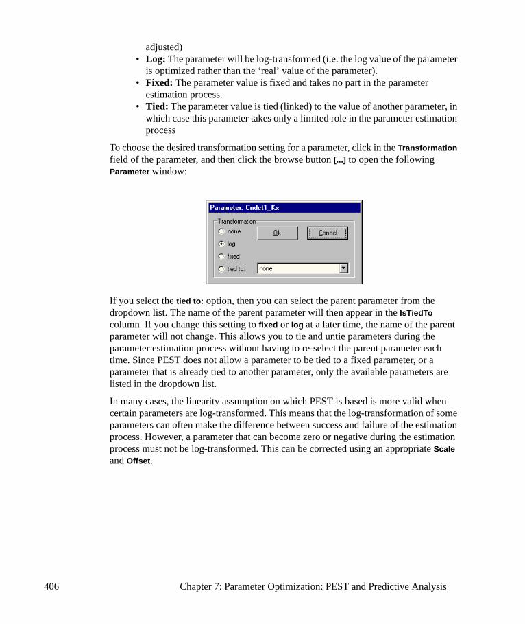
adjusted)• Log: The parameter will be log-transformed (i.e. the log value of the parameter
is optimized rather than the ‘real’ value of the parameter).• Fixed: The parameter value is fixed and takes no part in the parameter
estimation process.• Tied: The parameter value is tied (linked) to the value of another parameter, in
which case this parameter takes only a limited role in the parameter estimation process
To choose the desired transformation setting for a parameter, click in the Transformation field of the parameter, and then click the browse button [...] to open the following Parameter window:
If you select the tied to: option, then you can select the parent parameter from the dropdown list. The name of the parent parameter will then appear in the IsTiedTo column. If you change this setting to fixed or log at a later time, the name of the parent parameter will not change. This allows you to tie and untie parameters during the parameter estimation process without having to re-select the parent parameter each time. Since PEST does not allow a parameter to be tied to a fixed parameter, or a parameter that is already tied to another parameter, only the available parameters are listed in the dropdown list.
In many cases, the linearity assumption on which PEST is based is more valid when certain parameters are log-transformed. This means that the log-transformation of some parameters can often make the difference between success and failure of the estimation process. However, a parameter that can become zero or negative during the estimation process must not be log-transformed. This can be corrected using an appropriate Scale and Offset.
406 Chapter 7: Parameter Optimization: PEST and Predictive Analysis
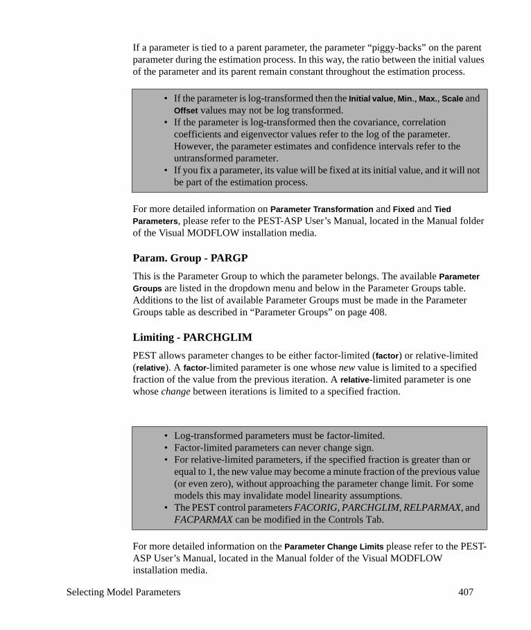
If a parameter is tied to a parent parameter, the parameter “piggy-backs” on the parent parameter during the estimation process. In this way, the ratio between the initial values of the parameter and its parent remain constant throughout the estimation process.
For more detailed information on Parameter Transformation and Fixed and Tied Parameters, please refer to the PEST-ASP User’s Manual, located in the Manual folder of the Visual MODFLOW installation media.
Param. Group - PARGPThis is the Parameter Group to which the parameter belongs. The available Parameter Groups are listed in the dropdown menu and below in the Parameter Groups table. Additions to the list of available Parameter Groups must be made in the Parameter Groups table as described in “Parameter Groups” on page 408.
Limiting - PARCHGLIMPEST allows parameter changes to be either factor-limited (factor) or relative-limited (relative). A factor-limited parameter is one whose new value is limited to a specified fraction of the value from the previous iteration. A relative-limited parameter is one whose change between iterations is limited to a specified fraction.
For more detailed information on the Parameter Change Limits please refer to the PEST-ASP User’s Manual, located in the Manual folder of the Visual MODFLOW installation media.
• If the parameter is log-transformed then the Initial value, Min., Max., Scale and Offset values may not be log transformed.
• If the parameter is log-transformed then the covariance, correlation coefficients and eigenvector values refer to the log of the parameter. However, the parameter estimates and confidence intervals refer to the untransformed parameter.
• If you fix a parameter, its value will be fixed at its initial value, and it will not be part of the estimation process.
• Log-transformed parameters must be factor-limited.• Factor-limited parameters can never change sign.• For relative-limited parameters, if the specified fraction is greater than or
equal to 1, the new value may become a minute fraction of the previous value (or even zero), without approaching the parameter change limit. For some models this may invalidate model linearity assumptions.
• The PEST control parameters FACORIG, PARCHGLIM, RELPARMAX, and FACPARMAX can be modified in the Controls Tab.
Selecting Model Parameters 407
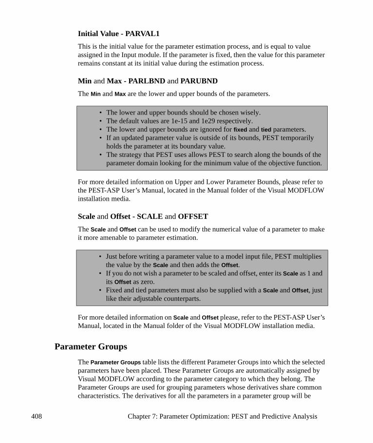
Initial Value - PARVAL1This is the initial value for the parameter estimation process, and is equal to value assigned in the Input module. If the parameter is fixed, then the value for this parameter remains constant at its initial value during the estimation process.
Min and Max - PARLBND and PARUBNDThe Min and Max are the lower and upper bounds of the parameters.
For more detailed information on Upper and Lower Parameter Bounds, please refer to the PEST-ASP User’s Manual, located in the Manual folder of the Visual MODFLOW installation media.
Scale and Offset - SCALE and OFFSETThe Scale and Offset can be used to modify the numerical value of a parameter to make it more amenable to parameter estimation.
For more detailed information on Scale and Offset please, refer to the PEST-ASP User’s Manual, located in the Manual folder of the Visual MODFLOW installation media.
Parameter Groups
The Parameter Groups table lists the different Parameter Groups into which the selected parameters have been placed. These Parameter Groups are automatically assigned by Visual MODFLOW according to the parameter category to which they belong. The Parameter Groups are used for grouping parameters whose derivatives share common characteristics. The derivatives for all the parameters in a parameter group will be
• The lower and upper bounds should be chosen wisely. • The default values are 1e-15 and 1e29 respectively. • The lower and upper bounds are ignored for fixed and tied parameters. • If an updated parameter value is outside of its bounds, PEST temporarily
holds the parameter at its boundary value.• The strategy that PEST uses allows PEST to search along the bounds of the
parameter domain looking for the minimum value of the objective function.
• Just before writing a parameter value to a model input file, PEST multiplies the value by the Scale and then adds the Offset.
• If you do not wish a parameter to be scaled and offset, enter its Scale as 1 and its Offset as zero.
• Fixed and tied parameters must also be supplied with a Scale and Offset, just like their adjustable counterparts.
408 Chapter 7: Parameter Optimization: PEST and Predictive Analysis
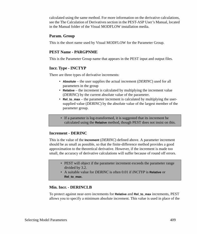
calculated using the same method. For more information on the derivative calculations, see the The Calculation of Derivatives section in the PEST-ASP User’s Manual, located in the Manual folder of the Visual MODFLOW installation media.
Param. GroupThis is the short name used by Visual MODFLOW for the Parameter Group.
PEST Name - PARGPNMEThis is the Parameter Group name that appears in the PEST input and output files.
Incr. Type - INCTYPThere are three types of derivative increments:
• Absolute – the user supplies the actual increment (DERINC) used for all parameters in the group
• Relative – the increment is calculated by multiplying the increment value (DERINC) by the current absolute value of the parameter.
• Rel_to_max – the parameter increment is calculated by multiplying the user-supplied value (DERINC) by the absolute value of the largest member of the parameter group.
Increment - DERINCThis is the value of the Increment (DERINC) defined above. A parameter increment should be as small as possible, so that the finite-difference method provides a good approximation to the theoretical derivative. However, if the increment is made too small, the accuracy of derivative calculations will suffer because of round off errors.
Min. Incr. - DERINCLBTo protect against near-zero increments for Relative and Rel_to_max increments, PEST allows you to specify a minimum absolute increment. This value is used in place of the
• If a parameter is log-transformed, it is suggested that its increment be calculated using the Relative method, though PEST does not insist on this.
• PEST will object if the parameter increment exceeds the parameter range divided by 3.2.
• A suitable value for DERINC is often 0.01 if INCTYP is Relative or Rel_to_max.
Selecting Model Parameters 409
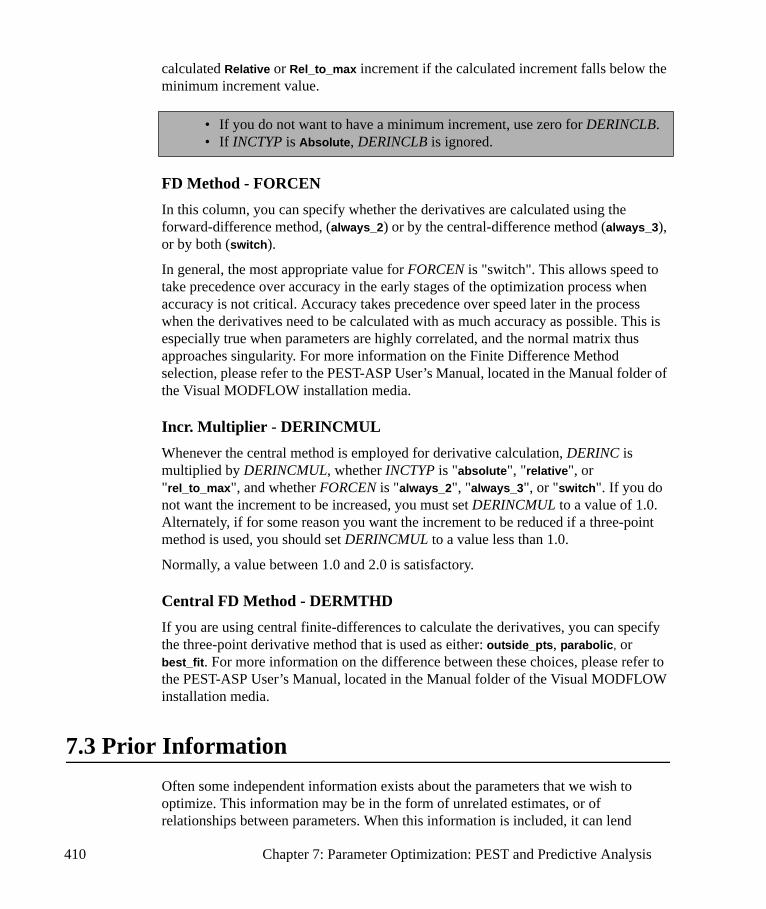
calculated Relative or Rel_to_max increment if the calculated increment falls below the minimum increment value.
FD Method - FORCENIn this column, you can specify whether the derivatives are calculated using the forward-difference method, (always_2) or by the central-difference method (always_3), or by both (switch).
In general, the most appropriate value for FORCEN is "switch". This allows speed to take precedence over accuracy in the early stages of the optimization process when accuracy is not critical. Accuracy takes precedence over speed later in the process when the derivatives need to be calculated with as much accuracy as possible. This is especially true when parameters are highly correlated, and the normal matrix thus approaches singularity. For more information on the Finite Difference Method selection, please refer to the PEST-ASP User’s Manual, located in the Manual folder of the Visual MODFLOW installation media.
Incr. Multiplier - DERINCMULWhenever the central method is employed for derivative calculation, DERINC is multiplied by DERINCMUL, whether INCTYP is "absolute", "relative", or "rel_to_max", and whether FORCEN is "always_2", "always_3", or "switch". If you do not want the increment to be increased, you must set DERINCMUL to a value of 1.0. Alternately, if for some reason you want the increment to be reduced if a three-point method is used, you should set DERINCMUL to a value less than 1.0.
Normally, a value between 1.0 and 2.0 is satisfactory.
Central FD Method - DERMTHDIf you are using central finite-differences to calculate the derivatives, you can specify the three-point derivative method that is used as either: outside_pts, parabolic, or best_fit. For more information on the difference between these choices, please refer to the PEST-ASP User’s Manual, located in the Manual folder of the Visual MODFLOW installation media.
7.3 Prior InformationOften some independent information exists about the parameters that we wish to optimize. This information may be in the form of unrelated estimates, or of relationships between parameters. When this information is included, it can lend
• If you do not want to have a minimum increment, use zero for DERINCLB.• If INCTYP is Absolute, DERINCLB is ignored.
410 Chapter 7: Parameter Optimization: PEST and Predictive Analysis

stability to the parameter estimation process, especially when parameters are highly correlated. Correlated parameters can lead to non-unique parameter estimates because varying them in certain linear combinations may cause very little change in the objective function. In some cases, this non-uniqueness can even lead to numerical instability and failure of the estimation process. If something is known about at least one of the members of such a troublesome set of parameters, this information, if included in the estimation process, may remove the non-uniqueness and provide stability.
For a detailed description of how prior information is incorporated into the PEST algorithm, please refer to the PEST-ASP User’s Manual, located in the Manual folder of the Visual MODFLOW installation media.
The Prior Information tab appears as shown in the following figure. Prior Information must be of a suitable type to be included. Both simple equality and linear relationships are acceptable. A Weight must be included with each article of Prior Information. In theory, this weight should be inversely proportional to the standard deviation of the right hand side of the Prior Information equation. In practice, however, the user simply assigns the weights according to the extent to which he/she wishes each article of prior information to influence the parameter estimation process.
7.3.1 Adding Prior InformationA new Prior Information article (equation) can be created by selecting the [Add New Prior Information Article] button in the Prior Information toolbar.
You will then be asked to enter a Name for the new Prior Information Article. Enter a name, then press the [Create] button.
Next, the Primary Information Editor window will appear as shown in the following figure. This window allows you to create a simple linear equation describing the Prior Information article.
Prior Information 411
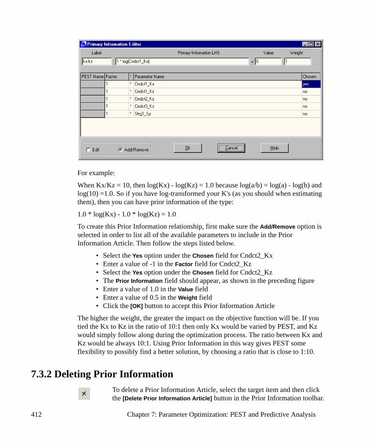
For example:
When Kx/Kz = 10, then log(Kx) - log(Kz) = 1.0 because log(a/b) = log(a) - log(b) and log(10) =1.0. So if you have log-transformed your K's (as you should when estimating them), then you can have prior information of the type:
1.0 * log(Kx) - 1.0 * log(Kz) = 1.0
To create this Prior Information relationship, first make sure the Add/Remove option is selected in order to list all of the available parameters to include in the Prior Information Article. Then follow the steps listed below.
• Select the Yes option under the Chosen field for Cndct2_Kx • Enter a value of -1 in the Factor field for Cndct2_Kz • Select the Yes option under the Chosen field for Cndct2_Kz• The Prior Information field should appear, as shown in the preceding figure• Enter a value of 1.0 in the Value field • Enter a value of 0.5 in the Weight field• Click the [OK] button to accept this Prior Information Article
The higher the weight, the greater the impact on the objective function will be. If you tied the Kx to Kz in the ratio of 10:1 then only Kx would be varied by PEST, and Kz would simply follow along during the optimization process. The ratio between Kx and Kz would be always 10:1. Using Prior Information in this way gives PEST some flexibility to possibly find a better solution, by choosing a ratio that is close to 1:10.
7.3.2 Deleting Prior InformationTo delete a Prior Information Article, select the target item and then click the [Delete Prior Information Article] button in the Prior Information toolbar.
412 Chapter 7: Parameter Optimization: PEST and Predictive Analysis

7.3.3 Editing Prior InformationTo edit a Prior Information Article, select the target item and then click the [Edit Prior Information Article] button in the Prior Information toolbar.
The Prior Information Editor window will appear as described in “Adding Prior Information” on page 411.
7.3.4 Resetting Prior InformationTo reset the Prior Information to the most recently saved settings, click the [Reload Previous Selections] button in the Prior Information toolbar.
7.3.5 Saving Prior InformationTo save the current Prior Information settings, click the [Save] button in the Prior Information toolbar.
7.4 Assigning the Objective FunctionWhen parameter estimation is used to assist in the calibration of a model, it is asked to minimize an objective function comprised of the sum of the weighted squared deviations between the calculated and observed system responses. In the case of a groundwater model, these system responses are typically head at a point in space, concentration at a point in space, or groundwater flow to a specified zone. Selecting the Objective Function tab will give you a list of all your available head, concentration, or flow observations as shown in the following figure:
Assigning the Objective Function 413
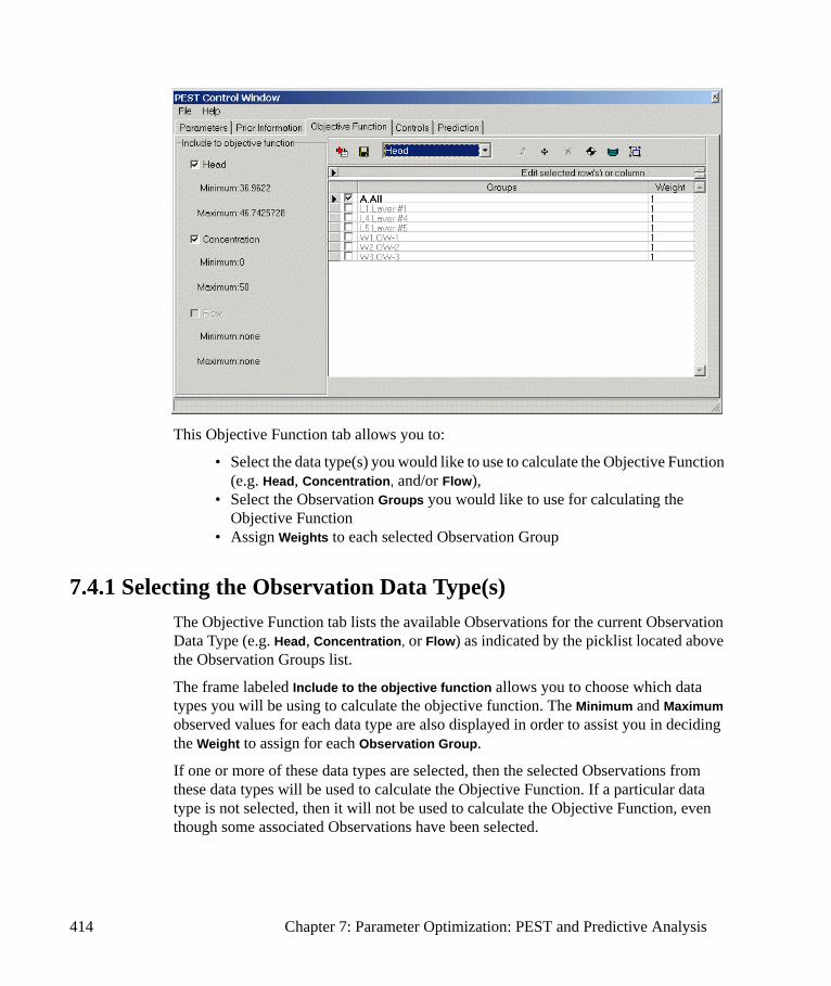
This Objective Function tab allows you to:
• Select the data type(s) you would like to use to calculate the Objective Function (e.g. Head, Concentration, and/or Flow),
• Select the Observation Groups you would like to use for calculating the Objective Function
• Assign Weights to each selected Observation Group
7.4.1 Selecting the Observation Data Type(s)The Objective Function tab lists the available Observations for the current Observation Data Type (e.g. Head, Concentration, or Flow) as indicated by the picklist located above the Observation Groups list.
The frame labeled Include to the objective function allows you to choose which data types you will be using to calculate the objective function. The Minimum and Maximum observed values for each data type are also displayed in order to assist you in deciding the Weight to assign for each Observation Group.
If one or more of these data types are selected, then the selected Observations from these data types will be used to calculate the Objective Function. If a particular data type is not selected, then it will not be used to calculate the Objective Function, even though some associated Observations have been selected.
414 Chapter 7: Parameter Optimization: PEST and Predictive Analysis
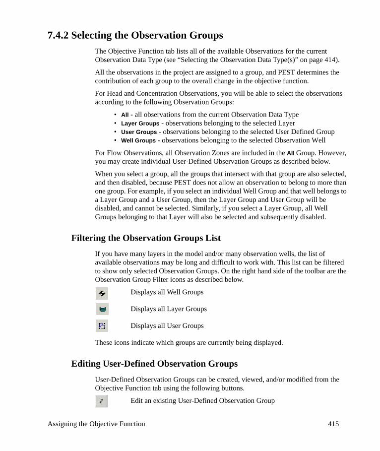
7.4.2 Selecting the Observation GroupsThe Objective Function tab lists all of the available Observations for the current Observation Data Type (see “Selecting the Observation Data Type(s)” on page 414).
All the observations in the project are assigned to a group, and PEST determines the contribution of each group to the overall change in the objective function.
For Head and Concentration Observations, you will be able to select the observations according to the following Observation Groups:
• All - all observations from the current Observation Data Type• Layer Groups - observations belonging to the selected Layer• User Groups - observations belonging to the selected User Defined Group• Well Groups - observations belonging to the selected Observation Well
For Flow Observations, all Observation Zones are included in the All Group. However, you may create individual User-Defined Observation Groups as described below.
When you select a group, all the groups that intersect with that group are also selected, and then disabled, because PEST does not allow an observation to belong to more than one group. For example, if you select an individual Well Group and that well belongs to a Layer Group and a User Group, then the Layer Group and User Group will be disabled, and cannot be selected. Similarly, if you select a Layer Group, all Well Groups belonging to that Layer will also be selected and subsequently disabled.
Filtering the Observation Groups List
If you have many layers in the model and/or many observation wells, the list of available observations may be long and difficult to work with. This list can be filtered to show only selected Observation Groups. On the right hand side of the toolbar are the Observation Group Filter icons as described below.
Displays all Well Groups
Displays all Layer Groups
Displays all User Groups
These icons indicate which groups are currently being displayed.
Editing User-Defined Observation Groups
User-Defined Observation Groups can be created, viewed, and/or modified from the Objective Function tab using the following buttons.
Edit an existing User-Defined Observation Group
Assigning the Objective Function 415
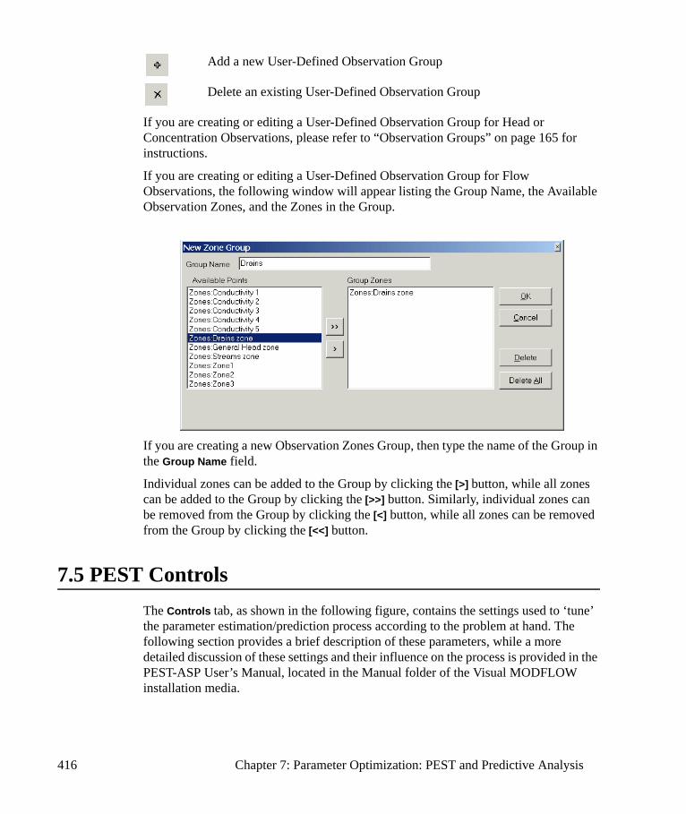
Add a new User-Defined Observation Group
Delete an existing User-Defined Observation Group
If you are creating or editing a User-Defined Observation Group for Head or Concentration Observations, please refer to “Observation Groups” on page 165 for instructions.
If you are creating or editing a User-Defined Observation Group for Flow Observations, the following window will appear listing the Group Name, the Available Observation Zones, and the Zones in the Group.
If you are creating a new Observation Zones Group, then type the name of the Group in the Group Name field.
Individual zones can be added to the Group by clicking the [>] button, while all zones can be added to the Group by clicking the [>>] button. Similarly, individual zones can be removed from the Group by clicking the [<] button, while all zones can be removed from the Group by clicking the [<<] button.
7.5 PEST ControlsThe Controls tab, as shown in the following figure, contains the settings used to ‘tune’ the parameter estimation/prediction process according to the problem at hand. The following section provides a brief description of these parameters, while a more detailed discussion of these settings and their influence on the process is provided in the PEST-ASP User’s Manual, located in the Manual folder of the Visual MODFLOW installation media.
416 Chapter 7: Parameter Optimization: PEST and Predictive Analysis

7.5.1 PEST Control Parameters
PESTMODE
The PESTMODE setting is used to indicate whether PEST is running in Estimation Mode or Prediction Mode. Estimation Mode is used to estimate the selected parameter values required to optimize (minimize) the objective function (i.e. to calibrate the model). Prediction Mode is used to estimate the selected parameter values required to either Minimize or Maximize the system response at a selected location, while maintaining an acceptable objective function value. If Prediction Mode is chosen, the Prediction tab is activated to allow definition of the Predictive Analysis settings.
Marquardt Lambda Settings
As outlined in the PEST-ASP User’s Manual, located in the Manual folder of the Visual MODFLOW installation media, PEST attempts parameter improvement using a number of different Marquardt Lambdas during any one optimization iteration. However, in the course of the overall parameter estimation process, the Marquardt Lambda generally gets smaller.
For high values of the Marquardt parameter (and therefore the Marquardt Lambda) the parameter estimation process approximates the gradient method of optimization. While the latter method is inefficient and slow if used for the entirety of the optimization
PEST Controls 417

process, it often helps in getting the process started, especially if initial parameter estimates are poor.
Initial Lambda - RLAMBDA1This is the initial real-value of the Marquardt Lambda. An initial value between 1 and 10 is usually appropriate, though if PEST complains that the normal matrix is not positive definite, you will need to provide a higher initial Marquardt Lambda.
Adjustment Factor - RLAMFACThis is the real factor by which the Marquardt Lambda is adjusted. It must be greater than 1.0. When PEST reduces Lambda, it divides by RLAMFAC. When it increases Lambda, it multiplies by RLAMFAC. PEST reduces Lambda if it can. However, if the normal matrix is not positive definite, or if a reduction in Lambda does not lower the objective function, PEST has no choice but to increase Lambda.
Sufficient Phi Ratio - PHIRATSUFDuring any one optimization iteration, PEST first lowers Lambda and, if this does not lower the objective function, it then raises Lambda. If it calculates an objective function, which is a fraction PHIRATSUF or less of the starting objective function for that iteration, PEST moves on to the next optimization iteration.
PHIRATSUF (which stands for "phi ratio sufficient") is a real variable for which a value of 0.3 is often appropriate. If it is set too low, model runs may be wasted in search of an objective function reduction which it is not possible to achieve, given the linear approximation on which the optimization equations of Chapter 2 are based. If it is set too high, PEST may not be able to set Lambda such that its value continues to be optimal as the parameter estimation process progresses.
Limiting Relative Phi Reduction - PHIREDLAMIf a new/old objective function ratio of PHIRATSUF or less is not achieved as different Marquardt Lambdas are tested, PEST must use some other criterion in deciding when it should move on to the next optimization iteration. This criterion is partly provided by the real variable PHIREDLAM.
If the relative reduction in the objective function between two consecutive Lambdas is less than PHIREDLAM, PEST takes this as an indication that it is probably more efficient to begin the next optimization iteration than to continue testing the effect of new Marquardt Lambdas.
A suitable value for PHIREDLAM is often around 0.01. If it is set too large, the criterion for moving on to the next optimization iteration is too easily met, and PEST is not given the opportunity of adjusting Lambda to find its optimal value. On the other hand, if PHIREDLAM is set too low, PEST will test too many Marquardt Lambdas on each optimization iteration when it would be better off starting a new iteration.
418 Chapter 7: Parameter Optimization: PEST and Predictive Analysis

Maximum Trial Lambdas - NUMLAMThis integer variable places an upper limit on the number of Lambdas that PEST can test during any one optimization iteration. It should normally be set between 5 and 10. For cases where parameters are being adjusted near their upper or lower limits, and for which some parameters are consequently being frozen, experience has shown that a value closer to 10 may be more appropriate than one closer to 5. This gives PEST more opportunity to adjust to the reduction in the number of parameters during the process.
Parameter Change Constraints
If there is no limit on the amount by which parameter values may change, parameter adjustments could regularly "overshoot" their optimal values, causing a prolongation of the estimation process at best, and instability with consequential estimation failure at worst. The concerns are greatest for highly non-linear problems.
In order to avoid this type of problem, PEST allows you to define the Max. Relative Change (RELPARMAX) and a Max. Factor Change (FACPARMAX) to limit parameter adjustments. Any particular parameter can be subject to only one of these constraints (i.e. a particular parameter must be either “relative-limited”, or “factor-limited”, in its adjustments).
Whether a parameter should be relative-limited or factor-limited depends on the parameter. However, you should note that a parameter can be reduced from its current value right down to zero for a relative change of only 1. If you wish to limit the extent of its downward movement during any one iteration to less than this, you may wish to set RELPARMAX to a value of 0.5. However, this may unduly restrict its upward movement. It may be better to declare the parameter as factor-limited. If so, a FACPARMAX value of 5.0 would limit its downward movement on any one iteration to 20 percent of its value at the start of the iteration, and its upward movement to 5 times its starting value. This may be a more sensible approach for many parameters.
It is important to note that a factor limit will not allow a parameter to change sign. Therefore, if a parameter must be free to change sign in the course of the optimization process, it must be relative-limited. Furthermore, RELPARMAX must be set at greater than unity, or the change of sign will be impossible. You must not declare a parameter as factor-limited, or as relative-limited with the relative limit of less than 1, if its upper and lower bounds are of opposite sign. Similarly, if a parameter's upper or lower bound is zero, it cannot be factor-limited and RELPARMAX must be at least unity.
Suitable values for RELPARMAX and FACPARMAX can vary enormously between cases. For highly non-linear problems, these values are best set low. If they are set too low, however, the estimation process can be very slow. An inspection of the PEST run record will often reveal whether you have set these values too low, as PEST records the maximum parameter factor and relative changes in this file at the end of each optimization iteration. If these changes are always at their upper limits and the
PEST Controls 419
estimation process is showing no signs of instability, it is quite possible that RELPARMAX and/or FACPARMAX could be increased.
If RELPARMAX and FACPARMAX are set too high, the estimation process may struggle. If PEST seems to be making no progress in lowering the objective function, and an inspection of the PEST run record reveals that some or all parameters are undergoing large changes at every optimization iteration, then it would be a good idea to reduce RELPARMAX and/or FACPARMAX. Another sign that these variables may need to be reduced is if PEST rapidly adjusts one or a number of parameters to their upper or lower bounds, and the latter are set far higher or lower than what you would expect the optimal parameter values to be. A further sign is if, rather than lowering the objective function, PEST estimates parameter values for which the objective function is incredibly high.
If you are unsure of how to set these parameters, a value of 5 for each of them is often suitable. In cases of extreme non-linearity, be prepared to set them much lower. Note, however, that FACPARMAX can never be less than 1. RELPARMAX can be less than 1 as long as no parameter's upper and lower bounds are of opposite sign. (If necessary use the OFFSET to shift the parameter domain so that it does not include zero.)
Max. relative parameter change - RELPARMAXRELPARMAX is the maximum relative change that a parameter is allowed to undergo between optimization iterations
The relative change in parameter b between optimization iterations i-1 and i is defined as
(bi-1 - bi)/(bi-1)
If parameter b is relative-limited, the absolute value of this relative change must be less than RELPARMAX. If a parameter upgrade vector is calculated such that the relative adjustment for one or more relative-limited parameters is greater than RELPARMAX, the magnitude of the upgrade vector is reduced such that this no longer occurs.
Max factor parameter change - FACPARMAXFACPARMAX is the maximum factor change that a parameter is allowed to undergo.
The factor change for parameter b between optimization iterations i-1 and i is defined as
bi-1/bi if | bi-1 | > | bi |, or
bi / bi-1 if | bi | > | bi-1 |
If parameter b is factor-limited, this factor change (which either equals or exceeds unity according to the above equation) must be less than FACPARMAX. If a parameter upgrade vector is calculated such that the factor adjustment for one or more factor-
420 Chapter 7: Parameter Optimization: PEST and Predictive Analysis
limited parameters is greater than FACPARMAX, the magnitude of the upgrade vector is reduced such that this no longer occurs.
Use-if-less Fraction - FACORIGIf, during the estimation process, a parameter becomes very small, the relative or factor limit to subsequent adjustment of this parameter may severely slow its return to larger values. Furthermore, for the case of relative-limited parameters which are permitted to change sign, it is possible that the denominator of the relative-limited equation above could become zero.
If the absolute value of a parameter falls below FACORIG multiplied by its original value, then FACORIG multiplied by its original value is substituted for the denominator of the equations above.
Therefore, the constraints that apply to a growth in absolute value of a parameter are lifted when its absolute value has become less than FACORIG multiplied by its original absolute value. However, where PEST wishes to reduce the parameter's absolute value even further, factor-limitations are not lifted. Relative limitations are not lifted if RELPARMAX is less than 1. FACORIG is not used to adjust limits for log-transformed parameters.
FACORIG must be greater than zero. A value of 0.001 is often suitable.
Method Separation Value - PHIREDSWH
The derivatives of observations with respect to parameters can be calculated using either forward differences (involving two parameter-observation pairs) or one of the variants of the central method (involving three parameter-observation pairs) described in the PEST-ASP User’s manual, located in the Manual folder of the Visual MODFLOW installation media. You must inform PEST through the group variables FORCEN and DERMTHD which method to use for the parameters belonging to each parameter group. If you allow PEST to switch between forward and central-difference methods, the variable PHIRREDSWH tells PEST when to switch.
If the relative reduction in the objective function between successive optimization iterations is less than PHIREDSWH, PEST will make the switch to three-point derivatives calculations for those parameter groups for which the character variable FORCEN has the value "switch".
A value of 0.1 is often suitable for PHIREDSWH. If it is set too high, PEST may make the switch to three-point derivatives calculations before it needs to. The result will be that more model runs will be required to fill the Jacobian matrix than are really needed at that stage of the estimation process. If PHIREDSWH is set too low, PEST may waste an optimization iteration or two in lowering the objective function to a smaller extent than would have been possible if it had made an earlier switch to central derivatives calculations. Note that PHIREDSWH should be set considerably higher than the input
PEST Controls 421
variable PHIREDSTP, which sets one of the termination criteria on the basis of the relative objective function reduction between optimization iterations.
Precision - PRECIS
PRECIS is a character variable which must be either "single" or "double". If it is supplied to PEST as "single", PEST writes parameters to model input files using single precision protocol. For example, parameter values will never be greater than 13 characters in length (even if the parameter space allows for a greater length) and the exponentiation character is "e". If PRECIS is supplied as "double", parameter values are written to model input files using double precision protocol. The maximum parameter value length is 23 characters and the exponentiation symbol is "d".
Termination Criteria
In addition to the termination controls available in this dialog, PEST will terminate if one or more of the following occur:
• the objective function goes to zero• the gradient of the objective function with respect to all parameters equals zero• the parameter upgrade vector equals zero• all parameters are at their limits and the upgrade vector points out of bounds.
For more detailed information on the Termination Criteria, please refer to the PEST-ASP User’s Manual, located in the Manual folder of the Visual MODFLOW installation media.
Overall Iteration Limit - NOPTMAXThis is the maximum number of iterations.
Negligible Reduction - PHIREDSTPIf the objective function does not change by more than this amount for NPHISTP iterations, PEST will stop. A suitable value for PHIREDSTP is 0.01, for most cases.
Max “No reduction” Iterations - NPHISTPThis is the maximum number of iterations that PEST will perform, if the objective function has not changed by at least PHIREDSTP.
For many cases, 3 is a suitable value NPHISTP. However, you must be careful not to set NPHISTP too low if the optimal values for some parameters are near or at their upper or lower bounds. In this case, it is possible that the magnitude of the parameter upgrade vector may be curtailed over one or a number of optimization iterations to ensure that no parameter value overshoots its bound. The result may be smaller reductions in the
422 Chapter 7: Parameter Optimization: PEST and Predictive Analysis

objective function than would otherwise occur. It would be incorrect if these reduced reductions were mistaken for the onset of parameter convergence to the optimal set.
Max Unsuccessful Iterations - NPHINOREDIf there is no reduction in the objective function, below its current minimum value, for this number of “unsuccessful” iterations, PEST will stop.
NPHINORED is an integer variable, where a value of 3 is often suitable
Negligible Relative Change - RELPARSTPIf the largest relative parameter change for all variables over NRELPAR iterations is less than this amount, PEST will stop.
All adjustable parameters, whether they are relative-limited or factor-limited, are involved in the calculation of the maximum relative parameter change.
RELPARSTP is a real variable for which a value of 0.01 is often suitable.
Max “No change” Iterations - NRELPARThis is the maximum number of iterations PEST will perform if the largest relative parameter change for all variables is below RELPARSTP.
NRELPAR is an integer variable. A value of 2 or 3 is normally adequate.
Output Control - ICOV, ICOR, IEIG
After the optimization process is complete, PEST writes some information concerning the optimized parameter set to its run record file. It tabulates the optimal values and the 95% confidence intervals pertaining to all adjustable parameters. It also tabulates the model-calculated observation set based on these parameters, together with the residuals (i.e. the differences between measured and model-calculated observations).
If you wish, PEST will write the parameter covariance matrix, the parameter correlation coefficient matrix, and the matrix of normalized eigenvectors of the covariance matrix to the run record file.
The integer variables ICOV, ICOR and IEIG determine whether PEST will output the covariance, correlation coefficient, and eigenvector matrixes respectively. If the relevant integer variable is checked (set to 1), the pertinent matrix will be written to the run record file. If it is not checked (set to 0), it will not be written.
Enable Restart - RSTFLE
This character variable is set by means of a check box. If it is checked, then “restart” is written to the control file. If it is unchecked, the value “norestart” is written.
PEST Controls 423
If restart is selected, PEST will dump the contents of many of its data arrays to a binary file (projectname.RST) at the beginning of each optimization iteration. This allows PEST to be restarted later, if execution is prematurely terminated. PEST will also dump the Jacobian matrix to another binary file (projectname.JAC) every time this matrix is filled.
If restart is not selected, PEST will not intermittently dump its array or Jacobian data, and later re-commencement of the optimization will not be possible.
7.6 Predictive Analysis SettingsPredictive Analysis is the process of estimating a set of parameter values required to minimize or maximize a system response at a selected location, while maintaining an acceptable Objective Function value.
Under more typical applications, parameter estimation is used to assist in the calibration of the model by estimating parameter values that minimize the Objective Function. In many cases, the shape of the Objective Function in parameter space is not comprised of a discrete bowl-shaped depression with the Objective Function lying neatly at the bottom of that depression. Rather, the Objective Function lies at the bottom of a long and narrow valley of almost equal depth along its length. Any parameters for which the objective function lies with the valley can be considered to calibrate the model. However, the predictive results of these different parameter sets may be quite different.
If the model was to be used for predictive purposes, then a sensitivity analysis would typically be run on the various sets of parameters that fall within this narrow band of parameter space in order to provide a reasonable range of possible outcomes.
The role of Predictive Analysis is to identify the set of parameter values that produce a ‘critical’ system response while maintaining a reasonable calibration. Predictive Analysis allows you to answer questions such as:
• What is the maximum water table drawdown caused by pumping?• What is the maximum concentration at a receptor?• What is the maximum leakage from a river or stream caused by pumping?
Before using Predictive Analysis, you should first run the model in Estimation Mode to make sure the model has achieved a minimum Objective Function (OBJmin). This value is important because it will be used to define the acceptable Objective Function value for Predictive Analysis purposes.
424 Chapter 7: Parameter Optimization: PEST and Predictive Analysis
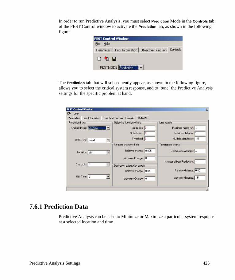
In order to run Predictive Analysis, you must select Prediction Mode in the Controls tab of the PEST Control window to activate the Prediction tab, as shown in the following figure:
The Prediction tab that will subsequently appear, as shown in the following figure, allows you to select the critical system response, and to ‘tune’ the Predictive Analysis settings for the specific problem at hand.
7.6.1 Prediction DataPredictive Analysis can be used to Minimize or Maximize a particular system response at a selected location and time.
Predictive Analysis Settings 425
Analysis Mode - NPREDMAXMIN
When PEST is used in Prediction Mode, it can be used to Minimize or Maximize the critical model prediction, while maintaining the objective function at or below an acceptable value.
Data Type
The critical model prediction may be either a Head value, a Concentration value or a Flow value.
Location
If the Data Type is a Head or Concentration value, the Location field will list all of the available Head or Concentration Observation Wells. If the Data Type is a Flow value, the Location field will list all of the available Flow Observation Zones.
Obs. Point
If the Data Type is a Head or Concentration value, the Obs. Point field will list all of the available Observation Points belonging to the selected Observation Well. If there is only one Observation Point belonging to the selected Observation Well, this Obs. Point field will be disabled.
Obs. Time
The Obs. Time field is used to select the time for the critical model prediction. This field will contain a list of the observation times for the selected Location.
If the Data Type is Flow, and the model is steady-state, the Obs. Time field will be disabled.
7.6.2 Objective Function Criteria
Inside Limit - PD0
PD0 is a value for the Objective Function which, under calibration conditions, is considered sufficient to ‘just calibrate’ the model, and is usually slightly larger than the minimum Objective Function obtained from running PEST in Estimation Mode.
426 Chapter 7: Parameter Optimization: PEST and Predictive Analysis
Outside Limit - PD1
The procedure by which PEST calculates the location of the critical point in parameter space is a complex one. If PEST is asked to maximize (or minimize) a certain model prediction while constrained to keep the Objective Function as close as possible to PD0, it will inevitably wander into and out of the ‘allowed parameter space’. The value of PD1 is a value slightly higher than PD0, which PEST will consider to be close enough when approaching the allowed parameter space from the outside.
Thus, PD0 is the Objective Function value PEST must aim for when maximizing (or minimizing) the model prediction, while PD1 is the Objective Function value it will accept.
Threshold - PD2
When PEST is run in Prediction Mode, as the Objective Function approaches PD0, the relative change in the Objective Function (OBJ) between Marquardt Lambdas may be small. However, the relative reduction in (OBJ - PD0) may be sufficient to warrant testing the efficacy of another Marquardt Lambda. The Threshold (PD2) is the Objective Function value at which PEST stops testing for a relative Objective Function reduction, and begins testing for a relative reduction in (OBJ - PD0).
7.6.3 Iteration Change CriteriaDuring each iteration, after it has filled the Jacobian matrix, PEST tests the ability of a number of different values of the Marquardt Lambda to achieve its objective. Its exact objective depends on the current value of the Objective Function. If the Objective Function is above PD1, then PEST’s highest priority is to lower the Objective Function. If the Objective Function is less than PD1, PEST’s highest priority is to raise or lower the model prediction. In either case, PEST is constantly faced with the decision of whether to test more Lambdas, or move onto the next iteration.
If the Objective Function is below PD1, and successive Marquardt Lambdas have not produced a model prediction with a significant Relative Change (RELPREDLAM) or a significant Absolute Change (ABSPREDLAM), then PEST will move on to the next optimization iteration.
Relative Change - RELPREDLAM
The Relative Change in the model prediction is the difference between the model prediction from previous Marquardt Lambda, and the model prediction from the current Marquardt Lambda, divided by the model prediction from the previous Marquardt Lambda.
Predictive Analysis Settings 427
Absolute Change - ABSPREDLAM
The Absolute Change in the model prediction is the difference between the model prediction from previous Marquardt Lambda and the model prediction from the current Marquardt Lambda.
7.6.4 Derivation Calculation SwitchIn the Parameter Groups section of the PEST Control file, the user informs PEST whether the derivatives of the model outcomes, with respect to the members of each parameter group, are to be calculated using two point, three point, or two points at first and then switch to three points if it fails to lower the Objective Function by a relative amount equal to PHIREDWSH between successive optimization iterations.
When used in Prediction Mode, the role of PHIREDSWH doesn’t change if the current Objective Function is above PD1. However, if it is below PD1, PEST’s decision to switch from two point to three point derivatives calculation is based on improvements to the model prediction. If, between two successive optimization iterations, the model prediction is not raised (or lowered) by a specified Relative change (RELPREDSWH), or by a specified Absolute change (ABSPREDSWH), PEST makes the switch to three point derivatives calculation.
Relative Change - RELPREDSWH
The Relative Change in the model prediction is the difference between the model prediction from the previous iteration, and the model prediction from the current iteration, divided by the model prediction from the previous Marquardt Lambda. A Relative Change setting of 0.05 is generally appropriate for most models. Enter a value of 0.0 if you do not want Relative Change to have an effect on the optimization process.
Absolute Change - ABSPREDSWH
The Absolute Change in the model prediction is the difference between the model prediction from previous iteration, and the model prediction from the current iteration. Due to the highly variable nature of the model predictions, there is no recommended value for the Absolute Change. Enter a value of 0.0 if you do not want Absolute Change to have an effect on the optimization process.
7.6.5 Line SearchWhen running in Prediction Mode, PEST calculates a parameter upgrade vector. However, it has been found from experience that the critical point in parameter space can be found more efficiently using a line search along the direction of its calculated
428 Chapter 7: Parameter Optimization: PEST and Predictive Analysis
parameter upgrade vector each time it calculates such a vector, in order to find the exact point of intersection of this vector with the PD0 parameter space.
Maximum Model Runs - NSEARCH
A line search is undertaken for each trial value of the Marquardt Lambda. The value of the Maximum Model Runs (NSEARCH) field represents the Maximum number of model runs that PEST will devote to this line search for any value of Lambda. In most situations you should conduct a line search using a value of 8 for the Maximum Model Runs. Set this value equal to 1 if you wish that no line search be undertaken.
Initial Search Factor - INITSCHFAC
When undertaking a line search, the initial model run is undertaken at that point along the parameter upgrade vector which is a specified factor along the line of the distance that PEST would have chosen. This is the Initial Search Factor (INITSCHFAC) and, unless there is a good reason to do otherwise, a value of 1.0 is usually appropriate.
Multiplication Factor - MULSCHFAC
Once the line search begins, PEST will move along the parameter upgrade vector, increasing or decreasing the distance along this vector by a specified Multiplication Factor (MULSCHFAC). A value of 1.5 to 2.0 is suitable in most cases.
7.6.6 Termination CriteriaWhen PEST is used in Prediction Mode, then the success of the Predictive Analysis process is based on the improvements to the model prediction, rather than on the improvements to the Objective Function. The Predictive Analysis process will terminate once the model prediction is no longer being improved by a significant amount.
Optimization Attempts - NPREDNORED
This is the maximum number of optimization attempts PEST will undertake without successfully improving the model prediction. A good setting for this field is 4.
Number of Best Predictions - NPREDSTP
This is the number of highest (or lowest) model predictions used to indicate that a better solution is will not likely be found. If the specified Number of Best Predictions are within a specified Relative Distance, or are within a specified Absolute Distance of
Predictive Analysis Settings 429

each other, then the Predictive Analysis process terminates. A good value for the Number of Best Predictions is 4.
Relative Distance - RELPREDSTP
The Relative Distance of the best model predictions is the difference between the highest model prediction and the lowest model prediction, divided by the highest model prediction. A good value for the Relative Distance is 0.05 for most cases. Enter a value of 0.0 if you do not want Relative Distance to have an effect on the optimization process.
Absolute Distance - ABSPREDSTP
The Absolute Distance of the best model predictions is the difference between the highest model prediction and the lowest model prediction. Enter a value of 0.0 if you do not want Absolute Distance to have an effect on the optimization process.
7.7 Running the Parameter Estimation SimulationThe WinPEST program is accessed from the Visual MODFLOW RUN menu.
To run WinPEST, you must select it from the list of available Engines to Run. You must also select all of the numeric engines that you want PEST to run during the parameter estimation process. Although PEST can only estimate flow parameter values, you must also run MT3D and/or Zone Budget if you are using concentration and/or flux observations to calculate the Objective Function. Please NOTE that if you are NOT using concentration and/or flux observations for your objective function, you should not run MT3D and/or ZoneBudget during the PEST run.
430 Chapter 7: Parameter Optimization: PEST and Predictive Analysis
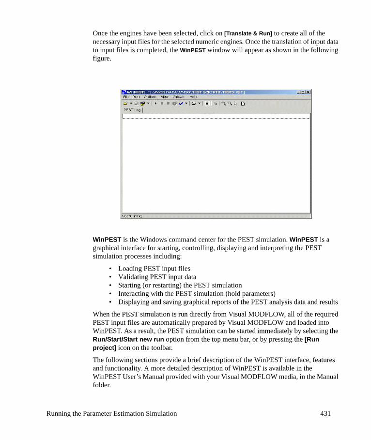
Once the engines have been selected, click on [Translate & Run] to create all of the necessary input files for the selected numeric engines. Once the translation of input data to input files is completed, the WinPEST window will appear as shown in the following figure.
WinPEST is the Windows command center for the PEST simulation. WinPEST is a graphical interface for starting, controlling, displaying and interpreting the PEST simulation processes including:
• Loading PEST input files• Validating PEST input data• Starting (or restarting) the PEST simulation• Interacting with the PEST simulation (hold parameters)• Displaying and saving graphical reports of the PEST analysis data and results
When the PEST simulation is run directly from Visual MODFLOW, all of the required PEST input files are automatically prepared by Visual MODFLOW and loaded into WinPEST. As a result, the PEST simulation can be started immediately by selecting the Run/Start/Start new run option from the top menu bar, or by pressing the [Run project] icon on the toolbar.
The following sections provide a brief description of the WinPEST interface, features and functionality. A more detailed description of WinPEST is available in the WinPEST User’s Manual provided with your Visual MODFLOW media, in the Manual folder.
Running the Parameter Estimation Simulation 431
7.7.1 Loading PEST Input FilesAs mentioned previously, if PEST is run directly from Visual MODFLOW, all of the PEST input files are automatically prepared and loaded into WinPEST. However, alternate PEST input files may also be loaded and run if they are prepared using the proper formats.
To load a PEST Control file for the current project, select File/Open/Project from the top menu bar or click the Open PEST control file icon from the toolbar.
To load a completely new project and all associated PEST input files, select File/Open/File and open one each of the following PEST input files: Control file (*.PST), Parameter Hold file (*.HLD), Template file (*.TPL), Parameter file (*.PAR), and Instruction file (*.INS).
To load the graphs from the results of a previous PEST simulation, select File/Load graphs from the top menu bar, and choose either Current plot or All plots.
7.7.2 Validating PEST Input FilesPEST comes with a built-in set of handy data validation utilities, called PESTCHECK, for checking the entire PEST data set (including template and instruction files cited in the PEST control file) for consistency and correctness. Although the chance of creating invalid data input files is greatly reduced by using Visual MODFLOW, it is a good idea to run the data validation checks prior to running the PEST simulation, just to avoid any unnecessary complications.
The Validations can be run by selecting Validate from the top menu bar (or by clicking the Check icon in the toolbar) and choosing one of the options described below. If any problems are encountered, PEST will issue error
messages to the PEST log screen.
The Validate/Check all option will run a check on all of the PEST input files to ensure they have the proper formats and information.
The Validate/Instructions option will run a check on the PEST Instructions file (.INS)
The Validate/Template option will run a check on the PEST Template file (.TPL)
If any errors are found, the offending file is opened in the window, where it can be inspected and edited if necessary. If you edit a file, remember to save your changes. Alternately, WinPEST can be closed and the error corrected in the Run or Input section as appropriate.
432 Chapter 7: Parameter Optimization: PEST and Predictive Analysis
7.7.3 Starting the PEST SimulationOnce the PEST input files are all loaded and validated, the PEST simulation can be started by selecting Run/Start/Start new run from the top menu bar or by clicking the Run project icon in the toolbar.
A command line window will open to indicate PEST is running. Do not close this window. If this command line window is closed, the PEST simulation will be terminated. PEST runs a “model” that is actually comprised of two models. These are MODFLOW and MODBORE. MODBORE is a program that spatially and temporally interpolates from the MODFLOW finite-difference grid and time step times to the locations and times of the observations. Through these two programs, the “model” produces numbers that can be directly compared to field observations.
7.7.4 Interacting with the PEST SimulationOnce the PEST run has started, there are a number of tools available for interacting with simulations.
The PEST simulation can be paused by selecting Run/Pause from the top menu bar, or by clicking the Pause icon in the toolbar.
The PEST simulation can be stopped by selecting Run/Stop from the top menu bar, or by clicking the Stop icon in the toolbar. You can restart PEST at the same point later by selecting Options/Run Restart.
Insensitive parameters may be ‘held’ (frozen) at the current value by selecting View/Hold Parameter(s) from the top menu bar, or by clicking the Hold parameter(s) icon in the toolbar. A Hold Status window will appear with a
graph of the available parameters. Select the parameter(s) to hold from the graph and then make any other necessary changes to these parameter groups or settings.
7.7.5 Displaying Reports and GraphsWhen the PEST simulation starts running, the simulation progress can be viewed using a variety of reporting and graphing formats. The View option in the top menu bar of WinPEST may be used to select the desired reports and graphs to display.
The reports include the PEST Log and the Run Record. The data is written and appended to these reports as the simulation progresses, and the reports will automatically scroll down to the bottom to display the most recently added
text. The Autoscroll option may be disabled by clicking the Autoscroll icon in the toolbar.
During PEST execution, you can view a number of useful pieces of information for displaying and interpreting the PEST simulation results, many of them in real-time graphical form. The displayed graphs will be updated “on the fly” after each PEST
Running the Parameter Estimation Simulation 433
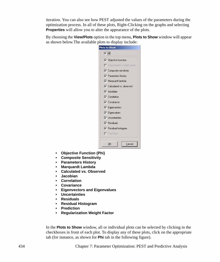
iteration. You can also see how PEST adjusted the values of the parameters during the optimization process. In all of these plots, Right-Clicking on the graphs and selecting Properties will allow you to alter the appearance of the plots.
By choosing the View/Plots option in the top menu, Plots to Show window will appear as shown below.The available plots to display include:
• Objective Function (Phi)• Composite Sensitivity• Parameters History• Marquardt Lambda• Calculated vs. Observed• Jacobian• Correlation• Covariance• Eigenvectors and Eigenvalues• Uncertainties• Residuals• Residual Histogram• Prediction• Regularization Weight Factor
In the Plots to Show window, all or individual plots can be selected by clicking in the checkboxes in front of each plot. To display any of these plots, click on the appropriate tab (for instance, as shown for Phi tab in the following figure).
434 Chapter 7: Parameter Optimization: PEST and Predictive Analysis
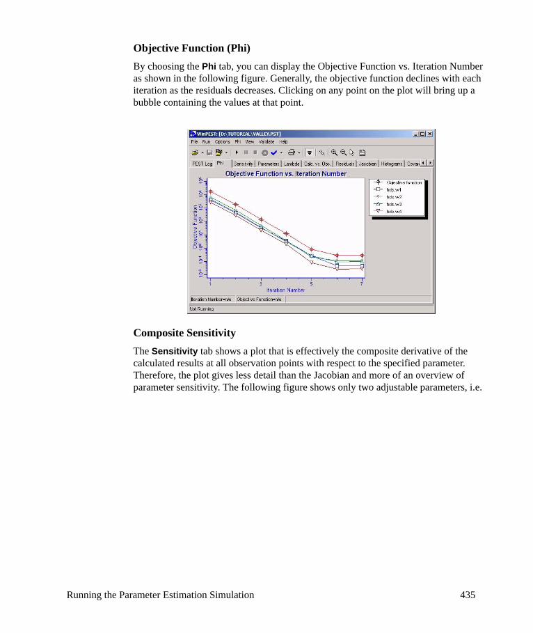
Objective Function (Phi)By choosing the Phi tab, you can display the Objective Function vs. Iteration Number as shown in the following figure. Generally, the objective function declines with each iteration as the residuals decreases. Clicking on any point on the plot will bring up a bubble containing the values at that point.
Composite SensitivityThe Sensitivity tab shows a plot that is effectively the composite derivative of the calculated results at all observation points with respect to the specified parameter. Therefore, the plot gives less detail than the Jacobian and more of an overview of parameter sensitivity. The following figure shows only two adjustable parameters, i.e.
Running the Parameter Estimation Simulation 435
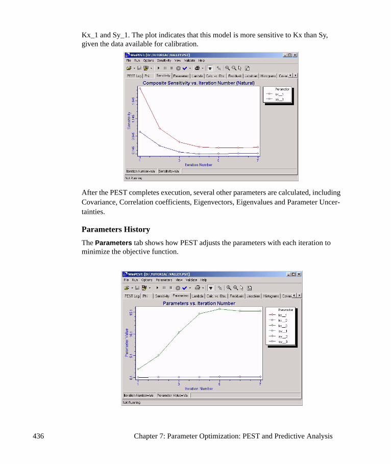
Kx_1 and Sy_1. The plot indicates that this model is more sensitive to Kx than Sy, given the data available for calibration.
After the PEST completes execution, several other parameters are calculated, including Covariance, Correlation coefficients, Eigenvectors, Eigenvalues and Parameter Uncer-tainties.
Parameters HistoryThe Parameters tab shows how PEST adjusts the parameters with each iteration to minimize the objective function.
436 Chapter 7: Parameter Optimization: PEST and Predictive Analysis
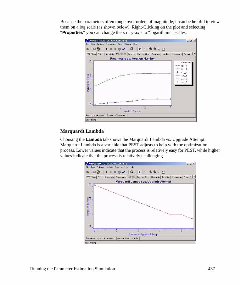
Because the parameters often range over orders of magnitude, it can be helpful to view them on a log scale (as shown below). Right-Clicking on the plot and selecting “Properties” you can change the x or y-axis to “logarithmic” scales.
Marquardt LambdaChoosing the Lambda tab shows the Marquardt Lambda vs. Upgrade Attempt. Marquardt Lambda is a variable that PEST adjusts to help with the optimization process. Lower values indicate that the process is relatively easy for PEST, while higher values indicate that the process is relatively challenging.
Running the Parameter Estimation Simulation 437
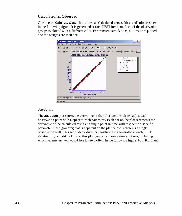
Calculated vs. ObservedClicking on Calc. vs. Obs. tab displays a “Calculated versus Observed” plot as shown in the following figure. It is generated at each PEST iteration. Each of the observation groups is plotted with a different color. For transient simulations, all times are plotted and the weights are included.
Jacobian The Jacobian plot shows the derivative of the calculated result (Head) at each observation point with respect to each parameter. Each bar on the plot represents the derivative of the calculated result at a single point in time with respect to a specific parameter. Each grouping that is apparent on the plot below represents a single observation well. This set of derivatives or sensitivities is generated at each PEST iteration. By Right-Clicking on this plot you can choose various options, including which parameters you would like to see plotted. In the following figure, both Kx_1 and
438 Chapter 7: Parameter Optimization: PEST and Predictive Analysis

Sy_1 are shown. This plot is useful for determining parameter sensitivities at specific locations (i.e. the observation points) within the model domain.
Correlation The correlation coefficient matrix under the Correlation tab is derived from the covariance matrix, and is easier to interpret. The diagonal terms are always 1. Off-diagonal terms will range from -1 to 1, depending on the degree of correlation. Values near zero are desirable because they indicate absence of correlation. Values close to 1 or –1 are less desirable because they indicate the parameters are strongly correlated. Correlated parameters are parameters that can be that are varied in pairs or groups with little effect on model output and therefore have little effect on the objective function. Hence while each parameter may be individually sensitive, the group of correlated parameters is insensitive, thus making it hard to estimate each parameter individually. Examination of parameter correlation is at least as important as examining individual parameter sensitivities. If PEST is having difficulty in reducing the objective function in one of your models, check the degree of parameter correlation. If you find that parameters are strongly correlated, PEST is proving valuable feedback on your observation data that may not have been noticed otherwise. It may specifically provide the suggestion that additional observations are required to resolve the non-uniqueness.
Running the Parameter Estimation Simulation 439
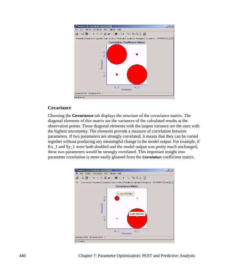
CovarianceChoosing the Covariance tab displays the structure of the covariance matrix. The diagonal elements of this matrix are the variances of the calculated results at the observation points. Those diagonal elements with the largest variance are the ones with the highest uncertainty. The elements provide a measure of correlation between parameters. If two parameters are strongly correlated, it means that they can be varied together without producing any meaningful change in the model output. For example, if Kx_1 and Sy_1 were both doubled and the model output was pretty much unchanged, these two parameters would be strongly correlated. This important insight into parameter correlation is more easily gleaned from the Correlation coefficient matrix.
440 Chapter 7: Parameter Optimization: PEST and Predictive Analysis

Eigenvectors and EigenvaluesThe information content of insights gleaned from the correlation coefficient matrix can also be derived through an inspection of the eigenvectors and eigenvalues. These terms sound quite fancy, but the concepts are not too difficult. Inspection of eigenvectors and eigenvalues has the added advantage of revealing correlations between more than two parameters. Eigenvectors simply define the semi-axes of the ellipsoids of probability of parameters, as inferred through the calibration process, as illustrated in the following figure:
This diagram shows two parameters, but eigenvectors will be defined for models with more than two parameters, which is when they become particularly useful. While this may sound a little complicated, Eigenvectors are an easy way to learn about parameter correlation between more than two parameters and gain some important information concerning estimated parameters.
To see how this works, click on the Eigenvalues tab. You will see that the eigenvectors are ordered from left to right in order of increasing Eigenvalue.
Running the Parameter Estimation Simulation 441
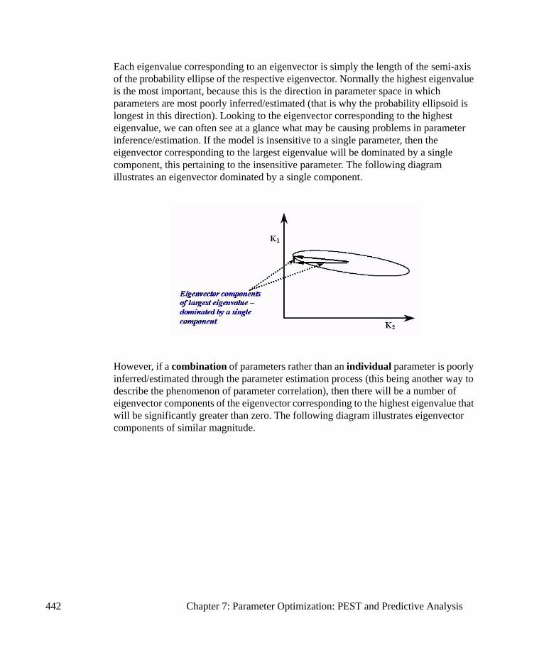
Each eigenvalue corresponding to an eigenvector is simply the length of the semi-axis of the probability ellipse of the respective eigenvector. Normally the highest eigenvalue is the most important, because this is the direction in parameter space in which parameters are most poorly inferred/estimated (that is why the probability ellipsoid is longest in this direction). Looking to the eigenvector corresponding to the highest eigenvalue, we can often see at a glance what may be causing problems in parameter inference/estimation. If the model is insensitive to a single parameter, then the eigenvector corresponding to the largest eigenvalue will be dominated by a single component, this pertaining to the insensitive parameter. The following diagram illustrates an eigenvector dominated by a single component.
However, if a combination of parameters rather than an individual parameter is poorly inferred/estimated through the parameter estimation process (this being another way to describe the phenomenon of parameter correlation), then there will be a number of eigenvector components of the eigenvector corresponding to the highest eigenvalue that will be significantly greater than zero. The following diagram illustrates eigenvector components of similar magnitude.
442 Chapter 7: Parameter Optimization: PEST and Predictive Analysis
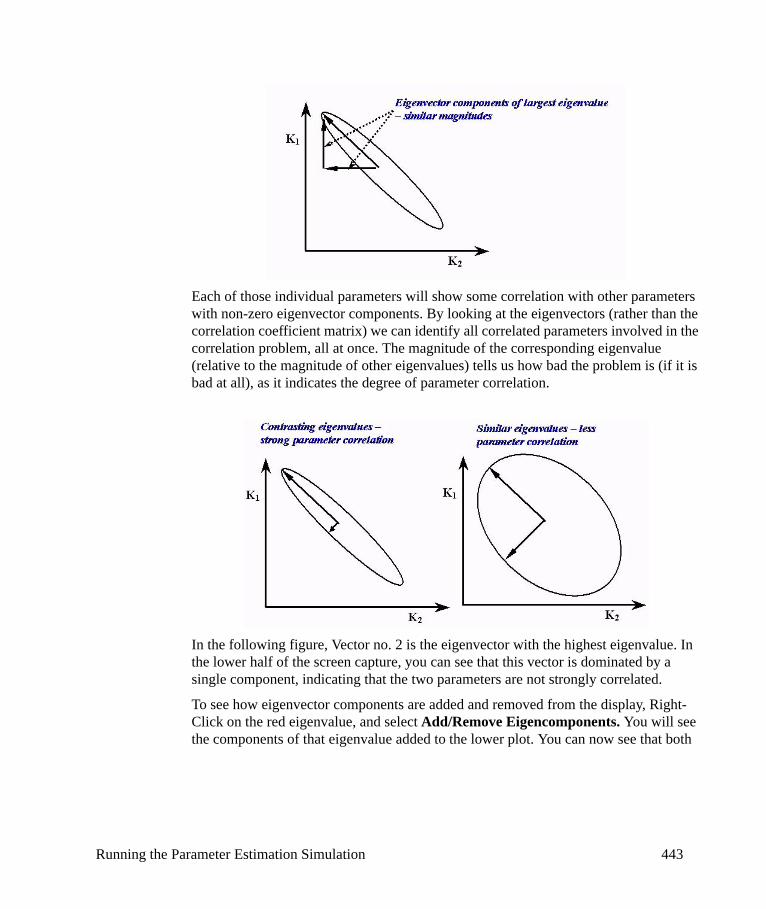
Each of those individual parameters will show some correlation with other parameters with non-zero eigenvector components. By looking at the eigenvectors (rather than the correlation coefficient matrix) we can identify all correlated parameters involved in the correlation problem, all at once. The magnitude of the corresponding eigenvalue (relative to the magnitude of other eigenvalues) tells us how bad the problem is (if it is bad at all), as it indicates the degree of parameter correlation.
In the following figure, Vector no. 2 is the eigenvector with the highest eigenvalue. In the lower half of the screen capture, you can see that this vector is dominated by a single component, indicating that the two parameters are not strongly correlated.
To see how eigenvector components are added and removed from the display, Right-Click on the red eigenvalue, and select Add/Remove Eigencomponents. You will see the components of that eigenvalue added to the lower plot. You can now see that both
Running the Parameter Estimation Simulation 443

eigenvectors are dominated by a single component, confirming that parameter correlation is not an issue in this model.
UncertaintiesUnder the Uncertainties tab, the standard deviation is displayed. These standard deviations are a linearized estimate of the uncertainty associated with a parameter (note the warning qualifier that pops up). This plot is perhaps most appropriately used for assessing relative uncertainties in parameters of the same type, rather than for assessing absolute uncertainties.
444 Chapter 7: Parameter Optimization: PEST and Predictive Analysis
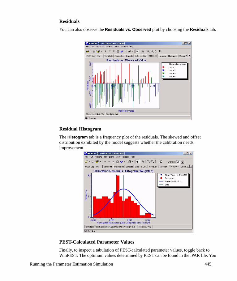
Residuals You can also observe the Residuals vs. Observed plot by choosing the Residuals tab.
Residual HistogramThe Histogram tab is a frequency plot of the residuals. The skewed and offset distribution exhibited by the model suggests whether the calibration needs improvement.
PEST-Calculated Parameter ValuesFinally, to inspect a tabulation of PEST-calculated parameter values, toggle back to WinPEST. The optimum values determined by PEST can be found in the .PAR file. You
Running the Parameter Estimation Simulation 445

can open and view this file by selecting File/Open/File from the top menu, and choosing the project file. The parameter values are displayed as shown in the following figure:
After inspecting the run time plots and optimized parameter values generated by PEST, return to the PEST log. This log summarizes the history of the optimization process. A more detailed history of the optimization process can be found in the [Projectname].REC (the PEST “run record) file, which is displayed by WinPEST after PEST has finished execution.
Head vs. TimeWhen PEST has stopped running, you can view the plot of modeled and observed heads for the last parameter combination to verify whether the calculated values and observed values show good agreement. This can be done by re-opening Visual MODFLOW from the task bar at the bottom of your screen.
Note: If the lowest objective function value has been obtained before the last PEST iteration, you would run MODFLOW with the optimum parameters before inspecting the output. If the lowest objective-function value is obtained in the last PEST iteration, then you do not need to perform an extra MODFLOW run.
Once the PEST simulation is completed, the graphs can be saved either as bitmap images to include in a report, or as configuration files to load at a later time. To save the PEST simulation analysis graphs, select File/Save graphs from the top menu bar and choose either:
• As picture to save each plot to a graphics file• Current plot to save only the plot currently being displayed• All plots to save all plots currently being displayed
446 Chapter 7: Parameter Optimization: PEST and Predictive Analysis
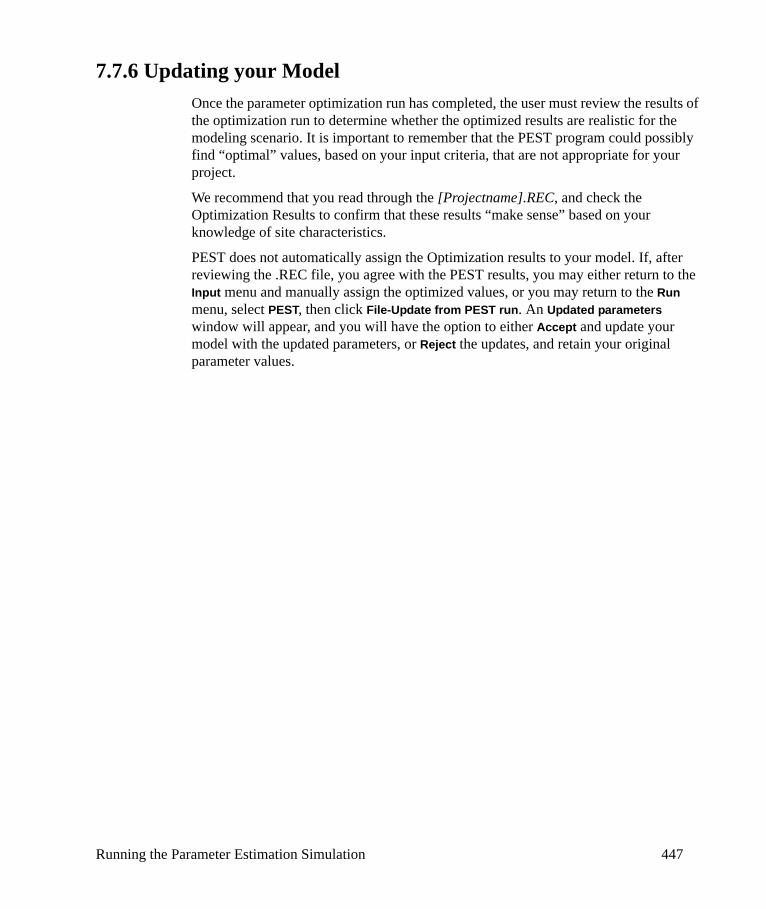
7.7.6 Updating your ModelOnce the parameter optimization run has completed, the user must review the results of the optimization run to determine whether the optimized results are realistic for the modeling scenario. It is important to remember that the PEST program could possibly find “optimal” values, based on your input criteria, that are not appropriate for your project.
We recommend that you read through the [Projectname].REC, and check the Optimization Results to confirm that these results “make sense” based on your knowledge of site characteristics.
PEST does not automatically assign the Optimization results to your model. If, after reviewing the .REC file, you agree with the PEST results, you may either return to the Input menu and manually assign the optimized values, or you may return to the Run menu, select PEST, then click File-Update from PEST run. An Updated parameters window will appear, and you will have the option to either Accept and update your model with the updated parameters, or Reject the updates, and retain your original parameter values.
Running the Parameter Estimation Simulation 447
448 Chapter 7: Parameter Optimization: PEST and Predictive Analysis
449
8Well Optimization
8.0.1 IntroductionPumping well optimization technology is used to determine the ideal pumping well locations, and ideal pumping rates at these locations, in order to minimize or maximize a specified criteria. Typically, pumping well optimization is used in the following applications:
• Groundwater remediation system design: Pumping well optimization is used to estimate the most cost-effective pump-and-treat groundwater remediation system by minimizing factors such as the number of pumping wells, and total pumping rates, while maintaining capture of the contaminated groundwater plume.
• Site dewatering system design: Pumping well optimization is used to estimate the most cost-effective pumping system design by minimizing factors such as the number of pumping wells, and total pumping rates, while maintaining the required water table drawdown.
• Water Resources Management: Pumping well optimization is used to estimate the maximum yield of a water supply pumping well, while maintaining a required water level in the aquifer.
These are just a few common examples of the many possible applications for pumping well optimization.
Visual MODFLOW currently supports the well optimization codes Modular Groundwater Optimizer (MGO) program, (public domain version). MGO is developed by Dr. Chunmiao Zheng and P. Patrick Wang from the University of Alabama, in cooperation with Groundwater Systems Research Ltd. Detailed documentation about the optimization algorithms and capabilities of MGO are provided in the MGO Documentation and User's Guide (Zheng and Wang, 2003). An electronic copy of this document is included on the Visual MODFLOW installation media, in the Manual folder.
This chapter describes how to set up and run a Pumping Well Optimization simulation using Visual MODFLOW. Although some details of the required inputs and parameters

450 Chapter 8: Well Optimization
will be provided in this chapter, you are encouraged to read the MGO Documentation and User's Guide in order to better understand the benefits and limitations of Pumping Well Optimization using MGO.
8.0.2 Assumptions and Limitations of Well OptimizationIn Visual MODFLOW, pumping well optimization may only be used under the following conditions:
• MODFLOW 96 flow engine, with PCG2, SIP, or SOR solver; • MT3DMS transport engine; • Steady-State Flow
To change your flow or transport engines, refer to “Selecting Numeric Engines” on page 69 for details. To change your solver settings, please refer to “Solver Settings” on page 307 for details.
In the current implementation, Visual MODFLOW with MGO supports only steady state simulations and optimizations. This means that only a single pumping rate may be optimized for each well.
MGO will only recognize pumping wells selected as active in the Visual MODFLOW input; inactive wells will be ignored. Additionally, the version of MGO provided with Visual MODFLOW will only support one pumping well per grid cell.
Wells screened in multiple layers are supported; the well-screen in the upper-most layer is used as the candidate well, and the underlying well-screens are treated as dependent variables. In MGO, there is no well block concept. The Optimization translation considers only one cell as a parameter list in the MGO input file, and treats other cells as dependent parameters. For more details, please refer to the MGO user's manual included in the Manual folder of your Visual MODFLOW installation media.
Dry cells pose a common problem in MODFLOW simulations, and can also become a problem during well optimization simulations. If a decision parameter is located on a dry cell, it will be turned off automatically. To prevent dry cells from occurring, you can set the minimum saturated thickness of any cell. See Solution settings for more details.
Dry Cells can be avoided by entering a minimum saturated thickness [thkmin] value, into the input file. You may add the following data block into the MGO.ini file:
&modflowthkmin = 0.5&end
Where [thkmin] is the minimum saturated thickness allowed. This will prevent cells from going dry, but the approach should be used with caution as it can lead to instability.
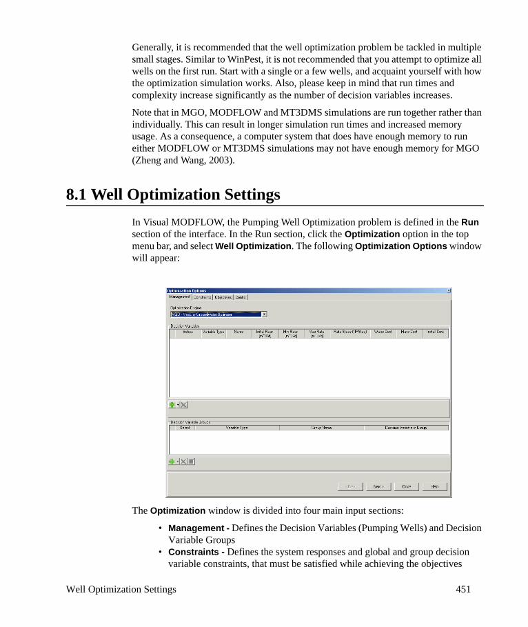
Well Optimization Settings 451
Generally, it is recommended that the well optimization problem be tackled in multiple small stages. Similar to WinPest, it is not recommended that you attempt to optimize all wells on the first run. Start with a single or a few wells, and acquaint yourself with how the optimization simulation works. Also, please keep in mind that run times and complexity increase significantly as the number of decision variables increases.
Note that in MGO, MODFLOW and MT3DMS simulations are run together rather than individually. This can result in longer simulation run times and increased memory usage. As a consequence, a computer system that does have enough memory to run either MODFLOW or MT3DMS simulations may not have enough memory for MGO (Zheng and Wang, 2003).
8.1 Well Optimization SettingsIn Visual MODFLOW, the Pumping Well Optimization problem is defined in the Run section of the interface. In the Run section, click the Optimization option in the top menu bar, and select Well Optimization. The following Optimization Options window will appear:
The Optimization window is divided into four main input sections:
• Management - Defines the Decision Variables (Pumping Wells) and Decision Variable Groups
• Constraints - Defines the system responses and global and group decision variable constraints, that must be satisfied while achieving the objectives
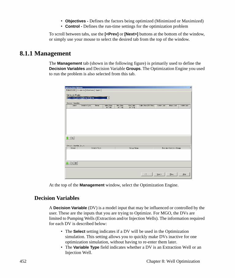
452 Chapter 8: Well Optimization
• Objectives - Defines the factors being optimized (Minimized or Maximized)• Control - Defines the run-time settings for the optimization problem
To scroll between tabs, use the [<Prev] or [Next>] buttons at the bottom of the window, or simply use your mouse to select the desired tab from the top of the window.
8.1.1 ManagementThe Management tab (shown in the following figure) is primarily used to define the Decision Variables and Decision Variable Groups. The Optimization Engine you used to run the problem is also selected from this tab.
At the top of the Management window, select the Optimization Engine.
Decision Variables
A Decision Variable (DV) is a model input that may be influenced or controlled by the user. These are the inputs that you are trying to Optimize. For MGO, the DVs are limited to Pumping Wells (Extraction and/or Injection Wells). The information required for each DV is described below:
• The Select setting indicates if a DV will be used in the Optimization simulation. This setting allows you to quickly make DVs inactive for one optimization simulation, without having to re-enter them later.
• The Variable Type field indicates whether a DV is an Extraction Well or an Injection Well.
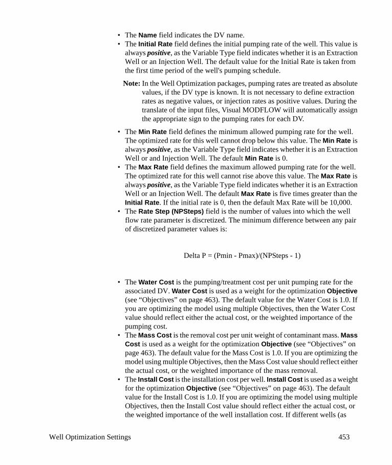
Well Optimization Settings 453
• The Name field indicates the DV name.• The Initial Rate field defines the initial pumping rate of the well. This value is
always positive, as the Variable Type field indicates whether it is an Extraction Well or an Injection Well. The default value for the Initial Rate is taken from the first time period of the well's pumping schedule.
Note: In the Well Optimization packages, pumping rates are treated as absolute values, if the DV type is known. It is not necessary to define extraction rates as negative values, or injection rates as positive values. During the translate of the input files, Visual MODFLOW will automatically assign the appropriate sign to the pumping rates for each DV.
• The Min Rate field defines the minimum allowed pumping rate for the well. The optimized rate for this well cannot drop below this value. The Min Rate is always positive, as the Variable Type field indicates whether it is an Extraction Well or and Injection Well. The default Min Rate is 0.
• The Max Rate field defines the maximum allowed pumping rate for the well. The optimized rate for this well cannot rise above this value. The Max Rate is always positive, as the Variable Type field indicates whether it is an Extraction Well or an Injection Well. The default Max Rate is five times greater than the Initial Rate. If the initial rate is 0, then the default Max Rate will be 10,000.
• The Rate Step (NPSteps) field is the number of values into which the well flow rate parameter is discretized. The minimum difference between any pair of discretized parameter values is:
Delta P = (Pmin - Pmax)/(NPSteps - 1)
• The Water Cost is the pumping/treatment cost per unit pumping rate for the associated DV. Water Cost is used as a weight for the optimization Objective (see “Objectives” on page 463). The default value for the Water Cost is 1.0. If you are optimizing the model using multiple Objectives, then the Water Cost value should reflect either the actual cost, or the weighted importance of the pumping cost.
• The Mass Cost is the removal cost per unit weight of contaminant mass. Mass Cost is used as a weight for the optimization Objective (see “Objectives” on page 463). The default value for the Mass Cost is 1.0. If you are optimizing the model using multiple Objectives, then the Mass Cost value should reflect either the actual cost, or the weighted importance of the mass removal.
• The Install Cost is the installation cost per well. Install Cost is used as a weight for the optimization Objective (see “Objectives” on page 463). The default value for the Install Cost is 1.0. If you are optimizing the model using multiple Objectives, then the Install Cost value should reflect either the actual cost, or the weighted importance of the well installation cost. If different wells (as
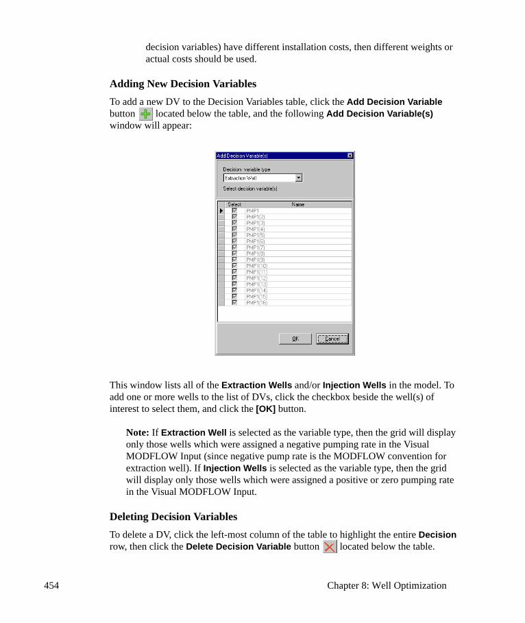
454 Chapter 8: Well Optimization
decision variables) have different installation costs, then different weights or actual costs should be used.
Adding New Decision VariablesTo add a new DV to the Decision Variables table, click the Add Decision Variable button located below the table, and the following Add Decision Variable(s) window will appear:
This window lists all of the Extraction Wells and/or Injection Wells in the model. To add one or more wells to the list of DVs, click the checkbox beside the well(s) of interest to select them, and click the [OK] button.
Note: If Extraction Well is selected as the variable type, then the grid will display only those wells which were assigned a negative pumping rate in the Visual MODFLOW Input (since negative pump rate is the MODFLOW convention for extraction well). If Injection Wells is selected as the variable type, then the grid will display only those wells which were assigned a positive or zero pumping rate in the Visual MODFLOW Input.
Deleting Decision VariablesTo delete a DV, click the left-most column of the table to highlight the entire Decision row, then click the Delete Decision Variable button located below the table.

Well Optimization Settings 455
Multiple DVs can be selected by dragging the pointer across several rows, or by holding down the <Ctrl> key as you select the rows using your mouse.
Note: If a deleted Decision Variable is part of an active Decision Variable Group, then there will be a prompt to remove the deleted Decision Variable from the associated Decision Variable Group.
Deactivating Decision VariablesIf you would like to run an optimization simulation without one or more of the currently selected Decision Variables, you may choose to deactivate the Decision Variables rather than deleting them. To deactivate a DV, click the Select checkbox next to the DV(s) you would like to ignore, so that the checkmark disappears. The benefit of deactivating a DV is that you may re-activate it at a later time by simply clicking the checkbox again to reselect it.
Note: If a deactivated Decision Variable is involved in an active Decision Variable Group, the deactivated Decision Variable will not be included in the associated Decision Variable Group.
Note: Deactivating a DV does not deactivate the pumping well from the input of Visual MODFLOW.
Updating Decision Variables from the ModelWhen a well is first added to the Decision Variables table, the fields such as Initial Rate and Max Rate for each well are estimated, using the pumping rate in the first time period. Once the well is added, the Optimization program is not 'aware' of changes to the model data. Therefore, changes to wells from the Input section of Visual MODFLOW will not be automatically updated. If one or more wells are deleted or renamed from the model, you will be asked to remove these wells from the list of DVs prior to running the Optimization.
Decision Variable Groups
A Decision Variable Group (DV Group) is a collection of individual DVs which may have similar 'interests'. These DV Groups are used for different purposes depending on which optimization engine is selected. When using MGO, a DV Group may only be used to define Balance Constraints (see “Pumping Balance Constraints” on page 459).
A DV Group must contain a minimum of one active DV. If a DV belonging to a Group is deleted, there will be a prompt to remove it from the associated DV Group to which it belonged. If a DV is deactivated, it is no longer an active member of the DV Group to which it belongs. If all DVs belonging to a DV Group are deactivated or deleted, the

456 Chapter 8: Well Optimization
DV Group will become invalid, and you will be required to either deactivate or delete the DV Group.
Adding Decision Variable GroupsTo add a new DV Group, click the Add Decision Variable Group button located below the table, and the following Edit Group window will appear:
A default name is generated for the new Group, and a list all of the current DVs is displayed. Each DV may only be added to one DV Group. To add one or more DVs to the new DV Group, click the checkbox beside the DV(s) of interest, and click the [OK] button. The new DV Group will appear in the table.
Deleting Decision Variable GroupsTo delete a DV Group, click the left-most column of the table to highlight the entire row, then click the Delete Decision Variable Group button located below the table. Multiple DV Groups can be selected by dragging the pointer across several rows, or by holding down the <Ctrl> key as you select the rows using your mouse.
Note: If a deleted DV Group is involved in any constraints, the associated constraints will become invalid, and need to be removed.
Deactivating Decision Variable GroupsIf you would like to run an optimization simulation without one or more of the Decision Variable Groups, you may choose to deactivate the DV Groups rather than deleting them. To deactivate a DV Group, click the Select checkbox next to the DV Group(s) you would like to ignore, so that the checkmark disappears. The benefit of deactivating

Well Optimization Settings 457
a DV Group is that you may re-activate it at a later time, by simply clicking the checkbox again to reselect it.
Note: If a deactivated DV Group is involved in any constraints, the associated constraints will become invalid, and need to be deleted or deactivated.
Editing Decision Variable GroupsDV Groups may be edited in order to change their name, or the DVs belonging to the Group. To edit a DV Group, click the left-most column of the row belonging to the DV Group you are interested in, then click the Edit Decision Variable Group button located below the Decision Variable Group table. The Edit Group window (as shown in “Adding Decision Variable Groups” on page 456) will appear. Use this window to change the Name of the DV Group, or to select/deselect DVs.
8.1.2 ConstraintsThe management objectives must be achieved within a set of constraints, which may be derived from technical, economic, legal, or political conditions associated with the project. There may be constraints on decision variables and state variables, and they may take the form of either equalities or inequalities. Constraints on the decision variables include the number of candidate wells, the upper and lower bounds for pumping/injection rates, and the candidate well locations. Constraints on the state variables might include the requirement that hydraulic heads be maintained above or below a certain level, or that contaminant concentrations not exceed regulatory standards at specified compliance points (Zheng and Wang, 2003).
The Constraints tab for MGO (see following figure) is used to define the Constraints for the optimization problem.
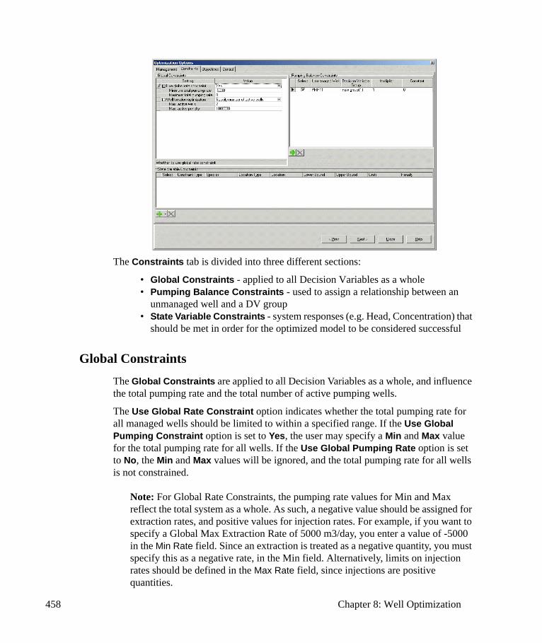
458 Chapter 8: Well Optimization
The Constraints tab is divided into three different sections:
• Global Constraints - applied to all Decision Variables as a whole • Pumping Balance Constraints - used to assign a relationship between an
unmanaged well and a DV group• State Variable Constraints - system responses (e.g. Head, Concentration) that
should be met in order for the optimized model to be considered successful
Global Constraints
The Global Constraints are applied to all Decision Variables as a whole, and influence the total pumping rate and the total number of active pumping wells.
The Use Global Rate Constraint option indicates whether the total pumping rate for all managed wells should be limited to within a specified range. If the Use Global Pumping Constraint option is set to Yes, the user may specify a Min and Max value for the total pumping rate for all wells. If the Use Global Pumping Rate option is set to No, the Min and Max values will be ignored, and the total pumping rate for all wells is not constrained.
Note: For Global Rate Constraints, the pumping rate values for Min and Max reflect the total system as a whole. As such, a negative value should be assigned for extraction rates, and positive values for injection rates. For example, if you want to specify a Global Max Extraction Rate of 5000 m3/day, you enter a value of -5000 in the Min Rate field. Since an extraction is treated as a negative quantity, you must specify this as a negative rate, in the Min field. Alternatively, limits on injection rates should be defined in the Max Rate field, since injections are positive quantities.
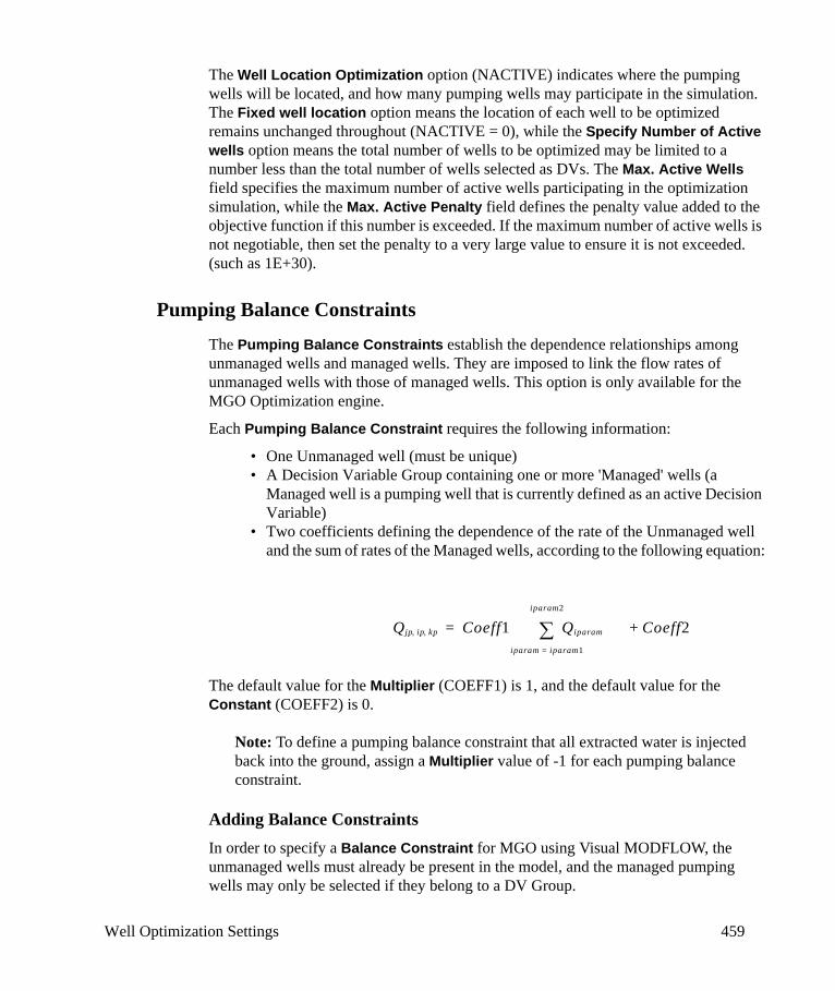
Well Optimization Settings 459
The Well Location Optimization option (NACTIVE) indicates where the pumping wells will be located, and how many pumping wells may participate in the simulation. The Fixed well location option means the location of each well to be optimized remains unchanged throughout (NACTIVE = 0), while the Specify Number of Active wells option means the total number of wells to be optimized may be limited to a number less than the total number of wells selected as DVs. The Max. Active Wells field specifies the maximum number of active wells participating in the optimization simulation, while the Max. Active Penalty field defines the penalty value added to the objective function if this number is exceeded. If the maximum number of active wells is not negotiable, then set the penalty to a very large value to ensure it is not exceeded. (such as 1E+30).
Pumping Balance Constraints
The Pumping Balance Constraints establish the dependence relationships among unmanaged wells and managed wells. They are imposed to link the flow rates of unmanaged wells with those of managed wells. This option is only available for the MGO Optimization engine.
Each Pumping Balance Constraint requires the following information:
• One Unmanaged well (must be unique)• A Decision Variable Group containing one or more 'Managed' wells (a
Managed well is a pumping well that is currently defined as an active Decision Variable)
• Two coefficients defining the dependence of the rate of the Unmanaged well and the sum of rates of the Managed wells, according to the following equation:
The default value for the Multiplier (COEFF1) is 1, and the default value for the Constant (COEFF2) is 0.
Note: To define a pumping balance constraint that all extracted water is injected back into the ground, assign a Multiplier value of -1 for each pumping balance constraint.
Adding Balance ConstraintsIn order to specify a Balance Constraint for MGO using Visual MODFLOW, the unmanaged wells must already be present in the model, and the managed pumping wells may only be selected if they belong to a DV Group.
Qjp ip kp, , Coeff1 Qiparam
iparam iparam1=
iparam2
∑ Coeff2+=

460 Chapter 8: Well Optimization
To add a new Balance Constraint, click the Add Balance Constraint button located below the table. The following Add Balance Constraint(s) window will appear:
Select the DV Group containing the 'managed' pumping wells you would like to balance, from the picklist at the top of the dialog. Then, select the unmanaged pumping wells to balance them against, from the grid. Each unmanaged pumping well may only be added to one Balance Constraint. To add one or more unmanaged pumping wells to a Balance Constraint, click the checkbox beside the pumping well(s) of interest, then click the [OK] button. A new Balance Constraint will be added to the Balance Constraint table.
Deleting Balance ConstraintsTo delete a Balance Constraint, click the left-most column of the table to highlight the entire row, and then click the Delete Balance Constraint button located below the table. Multiple Balance Constraints can be selected by dragging the pointer across several rows, or by holding down the <Ctrl> key as you select the rows using your mouse.
Deactivating Balance ConstraintsIf you would like to run an optimization simulation without one or more of the Balance Constraints, you may choose to deactivate the Balance Constraints rather than deleting them. To deactivate a Balance Constraint, click the Select checkbox next to the Balance Constraint(s) you would like to ignore, so that the checkmark disappears. The
Well Optimization Settings 461
benefit of deactivating a Balance Constraints is that you may reactivate it at a later time, by clicking the checkbox again to reselect it.
State Variable Constraints
The State Variable Constraints are constraints based on system responses to the stresses introduced by the Decision Variables. These typically include constraints such as minimum and maximum allowed values of head, or concentration, at a selected location. The information required to define a State Variable Constraint is described below:
• Select - Checkbox indicating if the State Variable Constraint will be used in the current Optimization simulation
• Constraint Type - Indicates the type of State Variable Constraint. For MGO, the choices are Head Bounds, or Concentration Bounds.
Note: In the current implementation of MGO in Visual MODFLOW, the Head Difference constraint type is not supported. However, a Head Difference constraint may be simulated by defining multiple zones in Visual MODFLOW, then creating a separate state variable for each zone, and assigning the appropriate head value (Lower or Upper Bound) for each zone.
• Species - Indicates the chemical species to which the Constraint is being applied. This field is only applicable if the Constraint Type involves chemical concentration or chemical mass, otherwise it becomes a read-only field with a value of N/A.
• Location Type - Indicates whether the Location of the Constraint being applied is defined by a Group of Observation Points, or by a group of grid cells within a Zone. The available Observation Groups correspond to the Observation Groups specified in the model, and the Zones correspond to the Zone Budget zones specified in the Input section of Visual MODFLOW. Please refer to “Zone Budget” on page 286 for more details.
Note: In the current version of Visual MODFLOW, only Zones are supported. Support for Observation Groups will be added in future versions.
• Location - Indicates the Name/ID of the selected Location item (either the name of an Observation Group, or the name of a Zone).
Note: In the current version, only Zones are supported. Support for Observation Groups will be added in future versions.
• Lower Bound - Indicates the Lower Bound of the State Variable Constraint in the selected Location. This field is editable, and must contain a real number.
• Upper Bound - Indicates the Upper Bound of the State Variable in the

462 Chapter 8: Well Optimization
selected Location. This field is editable, and must contain a real number greater than or equal to the value of the Lower Bound.
• Units - Indicates the unit type for the selected constraint (i.e. head or concentration). This is not an editable value, as the information is read from the Input files of the Visual MODFLOW model.
• Penalty - Indicates the Penalty value associated with violating the Upper or Lower Bound of the State Variable Constraint. This field is editable, and must contain a real number. If you want no violations of the constraint, set the penalty value to a very high value such as 1E+30. If you want to disable the constraint, set the penalty value = 0.
Note: MGO only allows for a uniform Penalty value for each Constraint Type. Therefore, if a Penalty value is modified for one State Variable Constraint entry, then the Penalty value for all Constraints of the same Type will also be changed.
Adding State Variable ConstraintsTo add a new State Variable Constraint, click the Add State Variable Constraint button located below the table. The following Add State Variable window will appear:
This window allows selection of the State Variable Type, Species name, and the Zones where the constraint will be applied (the Species name is only required if the State Variable Type is Concentration). Each Constraint may be applied to one or more Zones, and each Zone may be comprised of one or more grid cells. However, each Zone may only participate in one Constraint type at a time, and one Species at a time. (If there are no zones listed in this table, please return to the Input section of Visual MODFLOW, click on Zone Budget from the top menu bar, and assign Zones at the appropriate locations). Click the [OK] button to accept the selections, and then enter the
Well Optimization Settings 463
appropriate Lower Bound, Upper Bound, and Penalty values in the State Variable Constraints table.
Note: Zone budget in Visual MODFLOW does not allow a cell to be shared between multiple zones. As such, please take this into consideration when assigning state variable constraints. It may be necessary to assign one state variable to multiple zones.
Deleting State Variable ConstraintsTo delete a State Variable Constraint, click the left-most column of the table to highlight the entire row, and click the Delete State Variable Constraint button located below the table. Multiple State Variable Constraints can be selected by dragging the pointer across several rows, or by holding down the <Ctrl> key as you select the rows using your mouse
Deactivating State Variable ConstraintsIf you would like to run an optimization simulation without one or more of the State Variable Constraints, you may choose to deactivate the State Variable Constraints rather than deleting them. To deactivate a State Variable Constraint, click the Select checkbox next to the State Variable Constraint(s) you would like to ignore, so that the check mark disappears. The benefit of deactivating the State Variable Constraints is that you may reactivate them for another optimization run by clicking the checkbox again to reselect them.
8.1.3 ObjectivesThe objectives for an optimization problem can be defined as the net present value of the management costs, taken over an engineering planning horizon. The costs can include the capital costs associated with well drilling and installation, and operation costs associated with pumping and/or treatment over the lifetime of the project. Other forms of the objective function are also possible. For example, for a long-term contamination containment system, the objective function can be defined simply in terms of the total pumping volume, since the one-time drilling and installation costs may be negligible compared to the cumulative pumping and treatment costs. The exact form of the objective function depends on the nature of each individual problem.
The Objectives tab for MGO (see following figure) is used to define the optimization objectives.
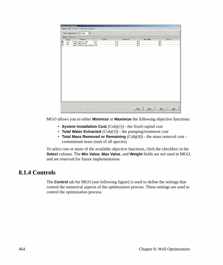
464 Chapter 8: Well Optimization
MGO allows you to either Minimize or Maximize the following objective functions:
• System Installation Cost (Cobj(1)) - the fixed capital cost• Total Water Extracted (Cobj(3)) - the pumping/treatment cost• Total Mass Removed or Remaining (Cobj(4)) - the mass removal cost -
contaminant mass (sum of all species)
To select one or more of the available objective functions, click the checkbox in the Select column. The Min Value, Max Value, and Weight fields are not used in MGO, and are reserved for future implementation.
8.1.4 ControlsThe Control tab for MGO (see following figure) is used to define the settings that control the numerical aspects of the optimization process. These settings are used to control the optimization process.

Well Optimization Settings 465
The Controls tab is divided into three sections:
• The Solver section is used to select the optimization Solver, and define the settings for the selected solver
• The Solution section is used to define the settings that control the model numerical engines
• The Output section is used to define the settings that control the output of the results from the simulation and optimization process
Optimization Solver Options
MGO supports three different solvers for the Optimization process:
• Genetic Algorithm (GA)• Simulated Annealing (SA)• Tabu Search (TS)
The following sections provide a brief overview of the solvers and their various settings. Detailed theoretical descriptions of the methods and settings used by each solver are provided in the MGO Reference Manual (Zheng and Wang, 2003). A .PDF copy of the document can be found on the Visual MODFLOW installation media, in the Manual folder.
Genetic AlgorithmGenetic algorithms (GA) are a family of combinatorial methods that search for solutions to complex problems, using an analogy between optimization and natural selection (Goldberg, 1989; Holland, 1992). GA mimics biological evolution based on
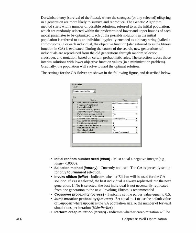
466 Chapter 8: Well Optimization
Darwinist theory (survival of the fittest), where the strongest (or any selected) offspring in a generation are more likely to survive and reproduce. The Genetic Algorithm method starts with a number of possible solutions, referred to as the initial population, which are randomly selected within the predetermined lower and upper bounds of each model parameter to be optimized. Each of the possible solutions in the initial population is referred to as an individual, typically encoded as a binary string (called a chromosome). For each individual, the objective function (also referred to as the fitness function in GA) is evaluated. During the course of the search, new generations of individuals are reproduced from the old generations through random selection, crossover, and mutation, based on certain probabilistic rules. The selection favors those interim solutions with lower objective function values (in a minimization problem). Gradually, the population will evolve toward the optimal solution.
The settings for the GA Solver are shown in the following figure, and described below.
• Initial random number seed (idum) - Must equal a negative integer (e.g. idum= -10000).
• Selection method (itourny) - Currently not used. The GA is presently set up for only tournament selection.
• Invoke elitism (ielite) - Indicates whether Elitism will be used for the GA solution. If Yes is selected, the best individual is always replicated into the next generation. If No is selected, the best individual is not necessarily replicated from one generation to the next. Invoking Elitism is recommended.
• Crossover probability (pcross) - Typically set the pcross value equal to 0.5.• Jump mutation probability (pmutate) - Set equal to -1 to use the default value
of 1/npopsiz where npopsiz is the GA population size, or the number of forward simulations per iteration (NsimPerIter).
• Perform creep mutation (icreep) - Indicates whether creep mutation will be
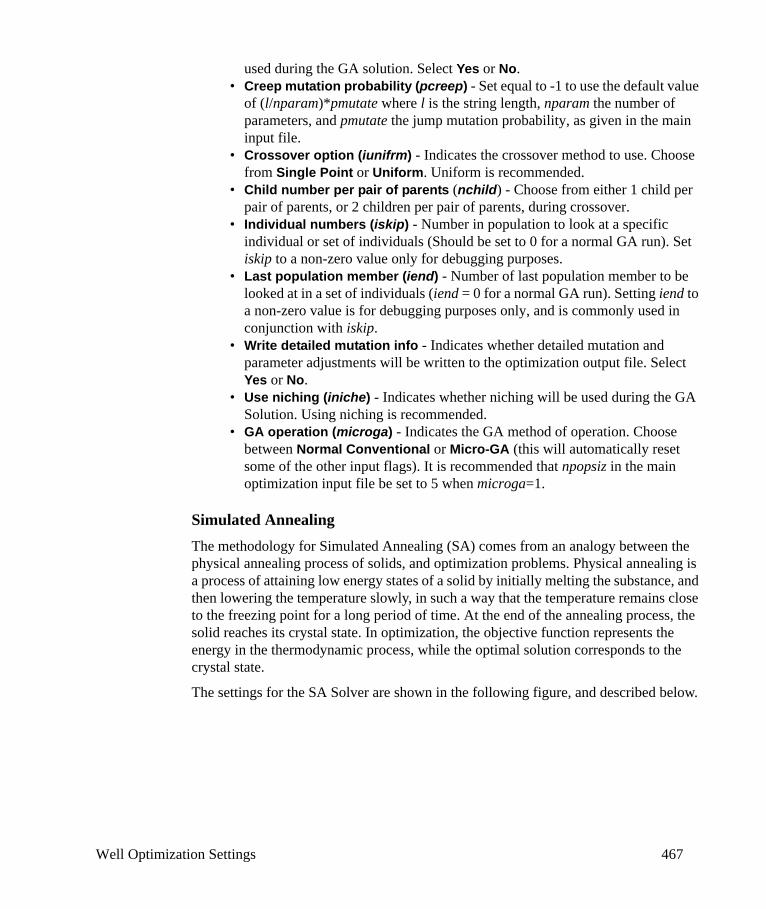
Well Optimization Settings 467
used during the GA solution. Select Yes or No.• Creep mutation probability (pcreep) - Set equal to -1 to use the default value
of (l/nparam)*pmutate where l is the string length, nparam the number of parameters, and pmutate the jump mutation probability, as given in the main input file.
• Crossover option (iunifrm) - Indicates the crossover method to use. Choose from Single Point or Uniform. Uniform is recommended.
• Child number per pair of parents (nchild) - Choose from either 1 child per pair of parents, or 2 children per pair of parents, during crossover.
• Individual numbers (iskip) - Number in population to look at a specific individual or set of individuals (Should be set to 0 for a normal GA run). Set iskip to a non-zero value only for debugging purposes.
• Last population member (iend) - Number of last population member to be looked at in a set of individuals (iend = 0 for a normal GA run). Setting iend to a non-zero value is for debugging purposes only, and is commonly used in conjunction with iskip.
• Write detailed mutation info - Indicates whether detailed mutation and parameter adjustments will be written to the optimization output file. Select Yes or No.
• Use niching (iniche) - Indicates whether niching will be used during the GA Solution. Using niching is recommended.
• GA operation (microga) - Indicates the GA method of operation. Choose between Normal Conventional or Micro-GA (this will automatically reset some of the other input flags). It is recommended that npopsiz in the main optimization input file be set to 5 when microga=1.
Simulated AnnealingThe methodology for Simulated Annealing (SA) comes from an analogy between the physical annealing process of solids, and optimization problems. Physical annealing is a process of attaining low energy states of a solid by initially melting the substance, and then lowering the temperature slowly, in such a way that the temperature remains close to the freezing point for a long period of time. At the end of the annealing process, the solid reaches its crystal state. In optimization, the objective function represents the energy in the thermodynamic process, while the optimal solution corresponds to the crystal state.
The settings for the SA Solver are shown in the following figure, and described below.

468 Chapter 8: Well Optimization
• Initial random number seed (idum) - Must equal a negative integer (e.g. idum= -10000).
• Starting temperature (temp) - Indicates the starting temperature.• Temperature reduction factor (redf) - Indicates the temperature reduction
factor; it must be a real number between 0 and 1.• Iteration restart number (nrestart) - Indicates the number of iterations after
which SA starts searching at a new point if the objective function does not have any improvement.
• Neighborhood step size (nstepsize) - Indicates the step size in selecting neighborhood solutions.
Tabu SearchTabu search (TS) is another heuristic algorithm for global optimization; the "natural" system on which TS is based is the human memory process. The modern form of TS derives from Glover (1986 and 1989). Like the previously described algorithms (GA and SA), TS has the ability to find the globally optimal solution. The underlying strategy of TS is a local search scheme, and a number of heuristic rules such as short-term memory and long-term memory. One important component is the short-term memory, which is referred to as the tabu list. The purpose of the tabu list is to force the search away from solutions that are selected in recent iterations, so that it will not become trapped in local minima. New solutions are rejected if they satisfy conditions given by the tabu list.
The settings for the TS Solver are shown in the following figure, and described below.
Well Optimization Settings 469
• Initial step size (nsize0) - Indicates the initial size of the short-term tabu list; must be a positive integer.
• Increment (inc) - Indicates the increment of the short-term tabu list, and must be a positive integer. TS increases the tabu size when a cycle is detected.
• Maximum cycle period (maxcycle) - Indicates the maximum cycle period the sample path may have.
• Number of iterations (nsample) - Indicates the number of iterations that TS checks cycling.
• Number of iterations to restart (nrestart) - Indicates the number of iterations after which TS starts searching at a new point if the objective function does not have any improvement.
• Neighborhood stepsize (nstepsize) - Indicate the step size in selecting neighborhood solutions; must be an integer.
Solution Options
The MGO Solution options are described below.
• Max number of iterations (MaxIter): Maximum number of iterations for the current optimization run
• Number of forward simulations (NsimPerIter): Number of forward simulations per iteration
• Total iterations (NTOL): Number of iterations after which the optimization run is terminated if the objective function is not improving
• Pumping rates scaling factor (PScale): Multiplier for all parameters to be optimized
• Restart previous run (iReStart): Flag indicating if the optimization will restart

470 Chapter 8: Well Optimization
from a previous run. Select No to begin a new optimization run.• Run final simulation (iFinalSim): Run final simulation with the optimized
parameters
Output Control Options
The Output control options are described below.
• Response Option (iResponse): Option to save intermediate results to the response database.
• Debugging level (iDebug): Option to save or view intermediate results of MODFLOW and MT3DMS. Choose Not Saved, Display Summary on Screen, or Save.
• Load results into VMOD input: Final simulation results will be read back to Visual MODFLOW, and can be viewed from the output mode.
8.2 Running Well OptimizationThe executable program of MGO was compiled using a Lahey FORTRAN 95 compiler (LF95) v. 5.7 to run on personal computers equipped with an Intel-compatible Pentium processor or higher, in the command prompt mode of Microsoft Windows 9x/2000/NT/XP. The minimum RAM required to run MGO is 128 MB. The minimum free hard drive space for installing MGO is 30 MB. Before running MGO, make sure that the MODFLOW and/or MT3DMS models have been properly constructed and calibrated as needed. (Zheng and Wang, 2003)
Once you are satisfied with the input settings and options for the Well Optimization, browse to the Simulation tab, and click the [Run] button at the bottom of the window.
This will launch the MGO engine, automatically translate the Visual MODFLOW and MGO input files, and launch the necessary numeric engines (MODFLOW 96 and MT3DMS (if applicable). There is no need to launch these engines through the Run menu in Visual MODFLOW. The MGO engine will run in a DOS window, as shown in the following figure:
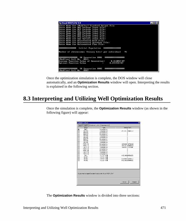
Interpreting and Utilizing Well Optimization Results 471
Once the optimization simulation is complete, the DOS window will close automatically, and an Optimization Results window will open. Interpreting the results is explained in the following section.
8.3 Interpreting and Utilizing Well Optimization ResultsOnce the simulation is complete, the Optimization Results window (as shown in the following figure) will appear:
The Optimization Results window is divided into three sections:

472 Chapter 8: Well Optimization
• Decision Variables - Displays the optimized values for each decision variable.• Objective Function - Displays a plot of the objective function at each iteration
of the simulation• MGO Output file (.MGO) - Displays the MGO simulation input file and output
file.
To import the simulation results into Visual MODFLOW, click the [Import] button.

Interpreting and Utilizing Well Optimization Results 473
Note: Importing the optimized pumping rates will overwrite the pumping rates that were defined in the Visual MODFLOW input.
To export the objective function graph, right-click on the graph and select Save-As, then Save the graph to your desired file type.
Otherwise, click [Close]. Once this dialog is closed, the Visual MODFLOW Output will load, and will display the Optimization simulation results.
The results will be saved to a separate “MGO” sub-folder, created in the model project folder. The MGO folder will contain the following files, which may provide helpful information.
• [modelname].mgo - displays MGO input and output• MGO.obf - objective function values• MGO.wel - optimized well rates• MGO.csn - constraint information

474 Chapter 8: Well Optimization

475
9Output Section - Displaying Model Results
The Output section of Visual MODFLOW allows the user to visualize, print, and export the simulation results. This chapter provides instructions on displaying, interpreting, customizing, and printing the groundwater flow, pathline, and contaminant transport modeling results using a variety of mapping and graphing presentation formats including:
Map type Data type
• Calibration Residual Maps Head and Concentration• Contour Maps Head, Drawdown, Concentration, Water
Table Elevation, Water Table Depth, Head Difference, Flux between Layers, Layer Elevation, and Net Recharge
• Pathline Maps• Velocity Vectors Maps• Zone Budget Maps
Graph type Data type
• Calibration Graphs Head, Concentration• Time-Series Graphs Head, Drawdown, and Concentration• Mass Balance Graphs Flow and Transport• Zone Budget Graphs Flow and Transport
The Output section of Visual MODFLOW is opened by selecting Output from the top menu bar of the Main Menu. Upon entering the Output section, Visual MODFLOW will automatically load the available Output files for Head (.HDS), Drawdown (.DDN) and Concentration (.UCN) for all output times. Once these data files are loaded, the Output screen will appear with the following items in the top menu bar.
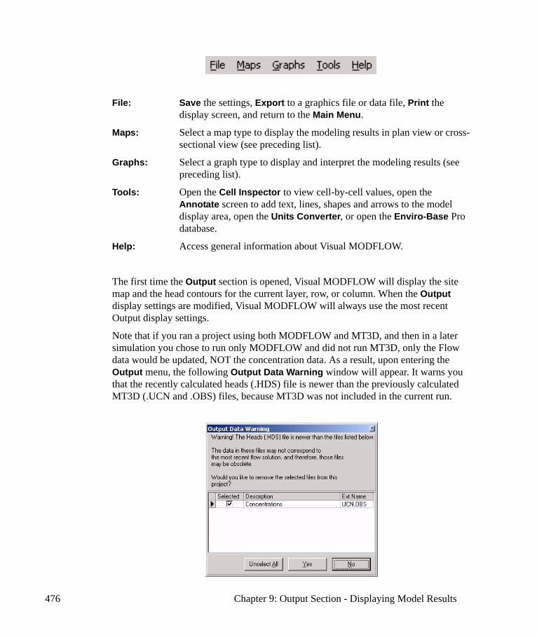
476 Chapter 9: Output Section - Displaying Model Results
File: Save the settings, Export to a graphics file or data file, Print the display screen, and return to the Main Menu.
Maps: Select a map type to display the modeling results in plan view or cross-sectional view (see preceding list).
Graphs: Select a graph type to display and interpret the modeling results (see preceding list).
Tools: Open the Cell Inspector to view cell-by-cell values, open the Annotate screen to add text, lines, shapes and arrows to the model display area, open the Units Converter, or open the Enviro-Base Pro database.
Help: Access general information about Visual MODFLOW.
The first time the Output section is opened, Visual MODFLOW will display the site map and the head contours for the current layer, row, or column. When the Output display settings are modified, Visual MODFLOW will always use the most recent Output display settings.
Note that if you ran a project using both MODFLOW and MT3D, and then in a later simulation you chose to run only MODFLOW and did not run MT3D, only the Flow data would be updated, NOT the concentration data. As a result, upon entering the Output menu, the following Output Data Warning window will appear. It warns you that the recently calculated heads (.HDS) file is newer than the previously calculated MT3D (.UCN and .OBS) files, because MT3D was not included in the current run.

File Options 477
Similarly, a warning message will appear if the recently calculated heads (.HDS) file is newer than the previously calculated ZoneBudget (.ZOT) file.
To proceed further, you are provided with three options:
Select [No] if you do not want to remove the selected files from the project (i.e. view the Output of the older files).
Select [Yes] if you want to remove the selected files from the project.
If you choose [Unselect All], then all the files will be removed from the project.
9.1 File OptionsThe File menu options are described as follows:
Save: Save the Output settings.
Export: Export the model display area to a graphics image file, data file, or GIS file. For more details, please refer to “Export Options” on page 77.
Preferences: Control font size settings for labels and names of pumping and observation wells, axes, shapes, and contours. This option also controls the Color settings for the Screen Background and the Axis labels.
Print: Print the screen image, and select the printer. For more details, please refer to “Printing the Model Display Area” on page 59.
Main Menu: Close the Output section and return to the Main Menu.
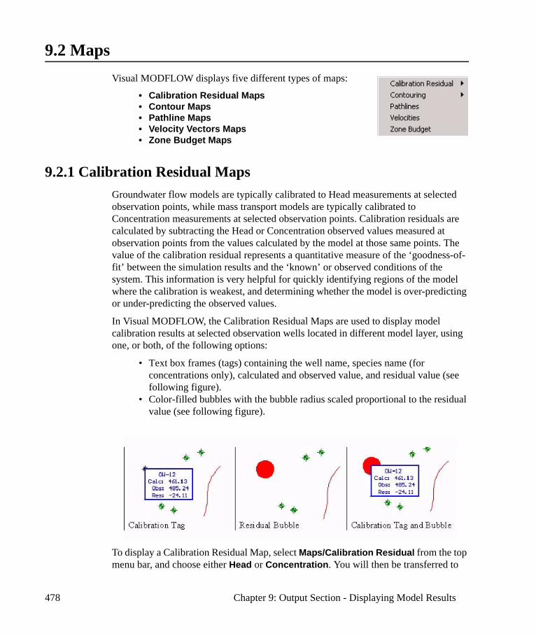
478 Chapter 9: Output Section - Displaying Model Results
9.2 MapsVisual MODFLOW displays five different types of maps:
• Calibration Residual Maps• Contour Maps• Pathline Maps• Velocity Vectors Maps• Zone Budget Maps
9.2.1 Calibration Residual Maps Groundwater flow models are typically calibrated to Head measurements at selected observation points, while mass transport models are typically calibrated to Concentration measurements at selected observation points. Calibration residuals are calculated by subtracting the Head or Concentration observed values measured at observation points from the values calculated by the model at those same points. The value of the calibration residual represents a quantitative measure of the ‘goodness-of-fit’ between the simulation results and the ‘known’ or observed conditions of the system. This information is very helpful for quickly identifying regions of the model where the calibration is weakest, and determining whether the model is over-predicting or under-predicting the observed values.
In Visual MODFLOW, the Calibration Residual Maps are used to display model calibration results at selected observation wells located in different model layer, using one, or both, of the following options:
• Text box frames (tags) containing the well name, species name (for concentrations only), calculated and observed value, and residual value (see following figure).
• Color-filled bubbles with the bubble radius scaled proportional to the residual value (see following figure).
To display a Calibration Residual Map, select Maps/Calibration Residual from the top menu bar, and choose either Head or Concentration. You will then be transferred to
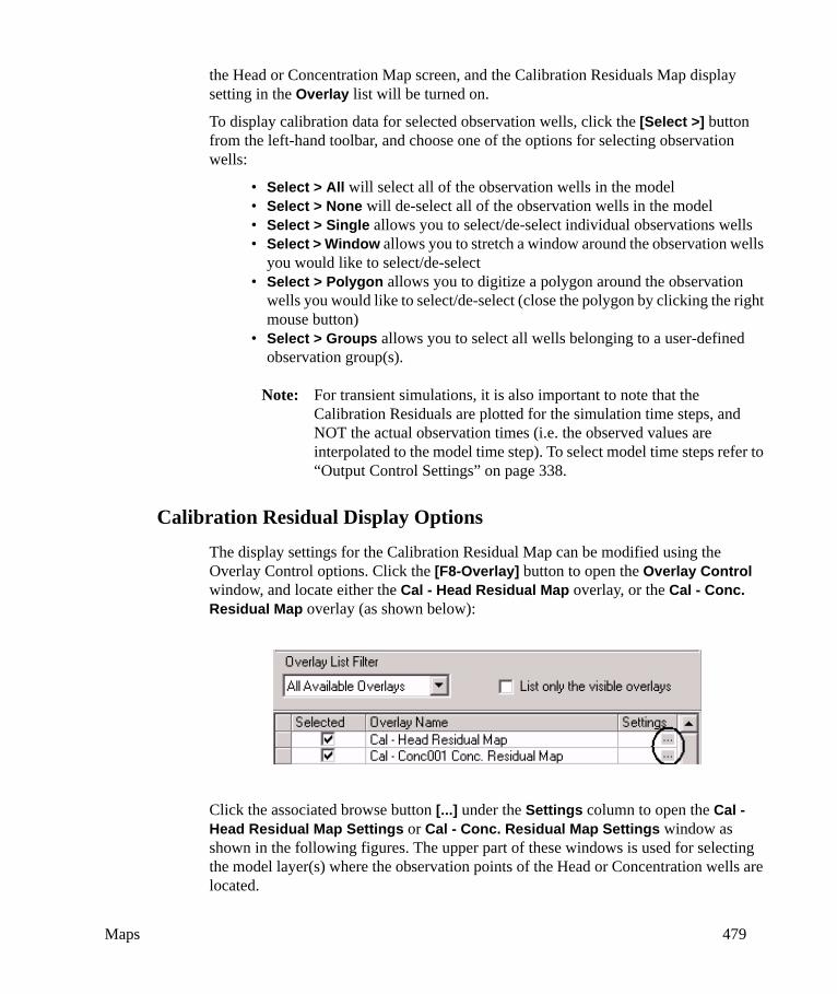
Maps 479
the Head or Concentration Map screen, and the Calibration Residuals Map display setting in the Overlay list will be turned on.
To display calibration data for selected observation wells, click the [Select >] button from the left-hand toolbar, and choose one of the options for selecting observation wells:
• Select > All will select all of the observation wells in the model• Select > None will de-select all of the observation wells in the model• Select > Single allows you to select/de-select individual observations wells• Select > Window allows you to stretch a window around the observation wells
you would like to select/de-select• Select > Polygon allows you to digitize a polygon around the observation
wells you would like to select/de-select (close the polygon by clicking the right mouse button)
• Select > Groups allows you to select all wells belonging to a user-defined observation group(s).
Note: For transient simulations, it is also important to note that the Calibration Residuals are plotted for the simulation time steps, and NOT the actual observation times (i.e. the observed values are interpolated to the model time step). To select model time steps refer to “Output Control Settings” on page 338.
Calibration Residual Display Options
The display settings for the Calibration Residual Map can be modified using the Overlay Control options. Click the [F8-Overlay] button to open the Overlay Control window, and locate either the Cal - Head Residual Map overlay, or the Cal - Conc. Residual Map overlay (as shown below):
Click the associated browse button [...] under the Settings column to open the Cal - Head Residual Map Settings or Cal - Conc. Residual Map Settings window as shown in the following figures. The upper part of these windows is used for selecting the model layer(s) where the observation points of the Head or Concentration wells are located.
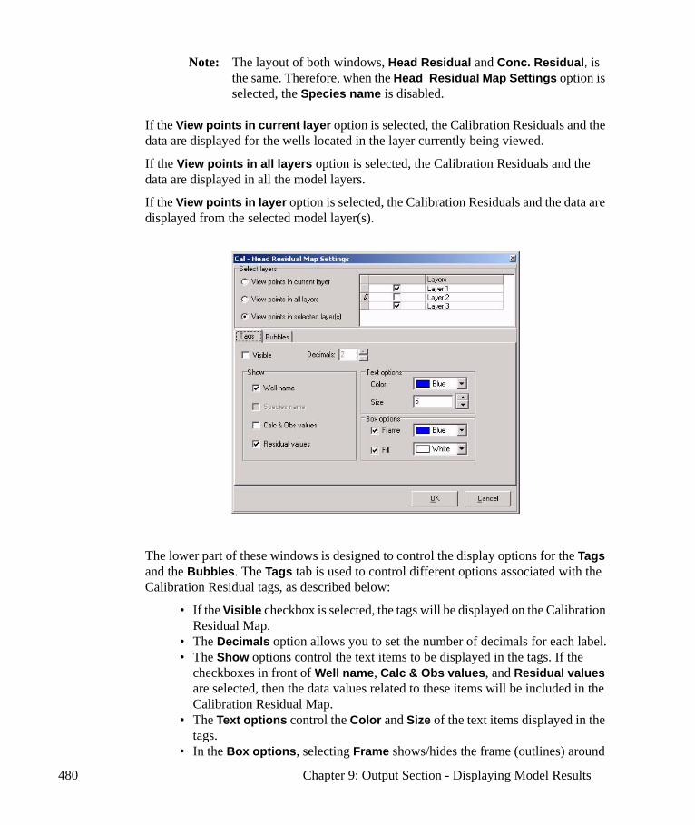
480 Chapter 9: Output Section - Displaying Model Results
Note: The layout of both windows, Head Residual and Conc. Residual, is the same. Therefore, when the Head Residual Map Settings option is selected, the Species name is disabled.
If the View points in current layer option is selected, the Calibration Residuals and the data are displayed for the wells located in the layer currently being viewed.
If the View points in all layers option is selected, the Calibration Residuals and the data are displayed in all the model layers.
If the View points in layer option is selected, the Calibration Residuals and the data are displayed from the selected model layer(s).
The lower part of these windows is designed to control the display options for the Tags and the Bubbles. The Tags tab is used to control different options associated with the Calibration Residual tags, as described below:
• If the Visible checkbox is selected, the tags will be displayed on the Calibration Residual Map.
• The Decimals option allows you to set the number of decimals for each label.• The Show options control the text items to be displayed in the tags. If the
checkboxes in front of Well name, Calc & Obs values, and Residual values are selected, then the data values related to these items will be included in the Calibration Residual Map.
• The Text options control the Color and Size of the text items displayed in the tags.
• In the Box options, selecting Frame shows/hides the frame (outlines) around

Maps 481
the tags, and controls the frame color (default color is blue). The Fill option may be selected to modify the background color in the tags (default color is white).
The Bubbles tab is used to control different options associated with bubbles, shown in the following figure, and described below.
• If the Visible checkbox is selected, the bubbles will be displayed on the Calibration Residual Map.
• The Color option controls the colors of the calibration residual bubbles. A positive value Calibration Residual bubble will be plotted using the selected color in the Positive value field (default color is red), while the negative value Calibration Residual bubbles will be displayed using the selected Negative value color (default color is blue).
• The Size option is used to set the Min. size and Max. size of the bubble radii which are associated with the Min. absolute value and the Max. absolute value of the Calibration Residuals.
The following Calibration Residual Map shows both the Head and the Concentration Residuals with negative and positive values.
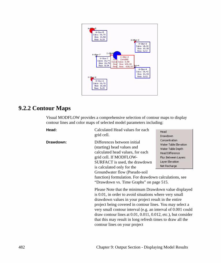
482 Chapter 9: Output Section - Displaying Model Results
9.2.2 Contour MapsVisual MODFLOW provides a comprehensive selection of contour maps to display contour lines and color maps of selected model parameters including:
Head: Calculated Head values for each grid cell.
Drawdown: Differences between initial (starting) head values and calculated head values, for each grid cell. If MODFLOW-SURFACT is used, the drawdown is calculated only for the Groundwater flow (Pseudo-soil function) formulation. For drawdown calculations, see “Drawdown vs. Time Graphs” on page 515.
Please Note that the minimum Drawdown value displayed is 0.01, in order to avoid situations where very small drawdown values in your project result in the entire project being covered in contour lines. You may select a very small contour interval (e.g. an interval of 0.001 could draw contour lines at 0.01, 0.011, 0.012, etc.), but consider that this may result in long refresh times to draw all the contour lines on your project
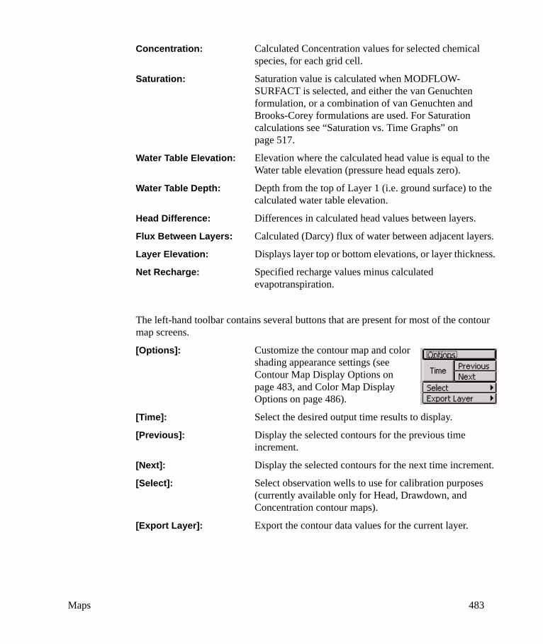
Maps 483
Concentration: Calculated Concentration values for selected chemical species, for each grid cell.
Saturation: Saturation value is calculated when MODFLOW-SURFACT is selected, and either the van Genuchten formulation, or a combination of van Genuchten and Brooks-Corey formulations are used. For Saturation calculations see “Saturation vs. Time Graphs” on page 517.
Water Table Elevation: Elevation where the calculated head value is equal to the Water table elevation (pressure head equals zero).
Water Table Depth: Depth from the top of Layer 1 (i.e. ground surface) to the calculated water table elevation.
Head Difference: Differences in calculated head values between layers.
Flux Between Layers: Calculated (Darcy) flux of water between adjacent layers.
Layer Elevation: Displays layer top or bottom elevations, or layer thickness.
Net Recharge: Specified recharge values minus calculated evapotranspiration.
The left-hand toolbar contains several buttons that are present for most of the contour map screens.
[Options]: Customize the contour map and color shading appearance settings (see Contour Map Display Options on page 483, and Color Map Display Options on page 486).
[Time]: Select the desired output time results to display.
[Previous]: Display the selected contours for the previous time increment.
[Next]: Display the selected contours for the next time increment.
[Select]: Select observation wells to use for calibration purposes (currently available only for Head, Drawdown, and Concentration contour maps).
[Export Layer]: Export the contour data values for the current layer.

484 Chapter 9: Output Section - Displaying Model Results
Contour Map Display Options
The contour map appearance may be customized by selecting the [Options] button from the left-hand toolbar. Depending on the contour map being displayed, a contour options window will appear, similar to the following figure, with options described below.
• Automatic reset min, max and interval values calculates the default values for the minimum and maximum contour values, and the contour interval, each time the view is changed (new layer/row/column or output time).
• Minimum sets the minimum contour value, below which no contour lines will be plotted. This setting is ignored if the Automatic contour levels option is not selected.
• Maximum sets the maximum contour value, above which no contour lines will be plotted. This setting is ignored if the Automatic contour levels option is not selected.
• Interval sets the contour increment value, starting from the Minimum value. This setting is ignored if the Automatic contour levels option is not selected.
• Color sets the color of the contour lines.• Width sets the width (thickness) of the contour lines.• Contour Labels options are used to hide/show the contour labels, and to set the
number of Decimals to plot for each contour line label. • Size and Width of contour labels can be set by clicking the down/up arrow

Maps 485
keys, or by entering desired values in the boxes.• Automatic contour levels shows/hides the contour line values generated for
the Minimum, Maximum and Interval values.• Custom contour levels shows/hides the user-defined contour values indicated
in the list.• Contouring resolution/speed provides a selection of five levels of contour
resolution; each level with a corresponding contouring speed (as resolution increases, speed decreases). The Highest/Slowest setting uses all grid cells to calculate the contour line location. The High/Slow setting takes a representative value from each group of four grid cells. The Medium/Medium setting takes a representative value from each group of eight grid cells.
Adding Contour LinesContour lines may be added at custom contour levels by selecting the [Options] button on the left-hand toolbar, and entering the desired Custom contour levels, or by Right-Clicking the mouse pointer on the model domain, choosing the Add contour(s) option, and then clicking the mouse pointer at the desired location(s) of the contour line(s). A contour line will be plotted at each location, corresponding to the data value at the selected location(s). The values of these contour lines will be added to the Custom contour levels table in the Contour options tab.
Right-Click the mouse pointer on the model domain again to stop adding custom contour lines.
Deleting Contour LinesCustom contour lines can be deleted by selecting the [Options] button on the left-hand toolbar, and deleting the values from the Custom contour levels table, or by Right-Clicking the mouse pointer on the model domain, choosing the Delete contour(s) option, and then clicking the mouse pointer on the custom contour line(s) to delete.
Right-Click the mouse pointer on the model domain again to stop deleting custom contour lines.
Alternately, to delete all custom contour lines, Right-Click on the model domain and select the Delete all custom option.
Adding Contour LabelsLabels can be added to any contour line at any location by Right-Clicking on the model domain and selecting the Add Label(s) option, then Left-Clicking on a contour line where a label should be added. If labels are not being added, make sure the desired contour map is set as the current overlay, and that Labels are turned on in the Overlay settings. See Overlay Display Settings on page 53 for details.
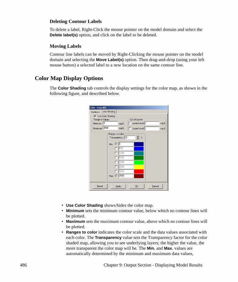
486 Chapter 9: Output Section - Displaying Model Results
Deleting Contour LabelsTo delete a label, Right-Click the mouse pointer on the model domain and select the Delete label(s) option, and click on the label to be deleted.
Moving LabelsContour line labels can be moved by Right-Clicking the mouse pointer on the model domain and selecting the Move Label(s) option. Then drag-and-drop (using your left mouse button) a selected label to a new location on the same contour line.
Color Map Display Options
The Color Shading tab controls the display settings for the color map, as shown in the following figure, and described below.
• Use Color Shading shows/hides the color map.• Minimum sets the minimum contour value, below which no contour lines will
be plotted. • Maximum sets the maximum contour value, above which no contour lines will
be plotted. • Ranges to color indicates the color scale and the data values associated with
each color. The Transparency value sets the Transparency factor for the color shaded map, allowing you to see underlying layers; the higher the value, the more transparent the color map will be. The Min. and Max. values are automatically determined by the minimum and maximum data values,

Maps 487
respectively, for the selected layer/row/column or output time. The intermediate values are linearly interpolated to each color, but may be customized by clicking the checkbox beside the color, and entering a new value (the new value must be less than the Max. value and greater than the Min. value).
• Cut off Levels specify the Upper and Lower limits of the color shading. Any values above or below the Upper and Lower limits, respectively, will not be shaded on the model domain. To change these values, click the checkbox beside the field and type the desired value into the corresponding data entry field.
Removing Contour Maps
Once a Contour Map has been selected and displayed in the Output section, it can only be removed using the Overlay Control, as described below:
• Press the [F9 - Overlay] button in the toolbar along the bottom of the Visual MODFLOW screen to load the Overlay Control window.
• Click the List only the visible overlays option (this reduces the list of Overlays and makes it easier to locate the Contour Map overlay).
• Locate the Contour Map overlay (looks like “C(O) - MapName”) and click the checkbox to remove the checkmark.
• Click the [OK] or [Apply] button to redraw the model display screen with the new Overlay settings.
Selecting Output Times
Visual MODFLOW runs both steady-state and transient simulations. For steady-state simulations, there is only one set of results for each contour map. However, for transient simulations, there may be tens, hundreds, or even thousands of output times generated for Head, Drawdown, and Concentration results.
To select the output time to display for the current contour map, click the [Time] button on the left-hand toolbar and choose the desired output time. Alternately, the output time displayed may be increased or decreased by pressing the [Next] or [Previous] button, respectively, located beside the [Time] button.
If a Head Contour Map and a Concentration Contour Map are being displayed simultaneously, it is important to remember that the Output times for these two data types are not synchronized. As a result, the Output time for the Head Contour Map may be completely different than the Output time for the Concentration Contour Map. Similarly, the Head and Drawdown Output times may also be different.
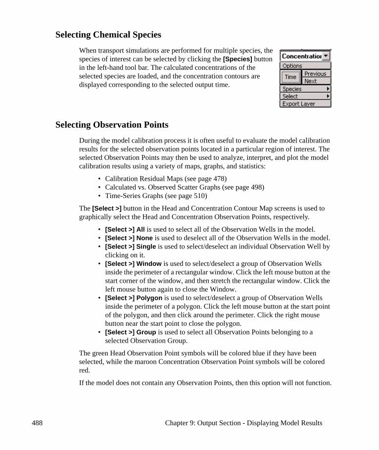
488 Chapter 9: Output Section - Displaying Model Results
Selecting Chemical Species
When transport simulations are performed for multiple species, the species of interest can be selected by clicking the [Species] button in the left-hand tool bar. The calculated concentrations of the selected species are loaded, and the concentration contours are displayed corresponding to the selected output time.
Selecting Observation Points
During the model calibration process it is often useful to evaluate the model calibration results for the selected observation points located in a particular region of interest. The selected Observation Points may then be used to analyze, interpret, and plot the model calibration results using a variety of maps, graphs, and statistics:
• Calibration Residual Maps (see page 478)• Calculated vs. Observed Scatter Graphs (see page 498)• Time-Series Graphs (see page 510)
The [Select >] button in the Head and Concentration Contour Map screens is used to graphically select the Head and Concentration Observation Points, respectively.
• [Select >] All is used to select all of the Observation Wells in the model.• [Select >] None is used to deselect all of the Observation Wells in the model.• [Select >] Single is used to select/deselect an individual Observation Well by
clicking on it.• [Select >] Window is used to select/deselect a group of Observation Wells
inside the perimeter of a rectangular window. Click the left mouse button at the start corner of the window, and then stretch the rectangular window. Click the left mouse button again to close the Window.
• [Select >] Polygon is used to select/deselect a group of Observation Wells inside the perimeter of a polygon. Click the left mouse button at the start point of the polygon, and then click around the perimeter. Click the right mouse button near the start point to close the polygon.
• [Select >] Group is used to select all Observation Points belonging to a selected Observation Group.
The green Head Observation Point symbols will be colored blue if they have been selected, while the maroon Concentration Observation Point symbols will be colored red.
If the model does not contain any Observation Points, then this option will not function.

Maps 489
Exporting Contour Data
The modeling results for a selected Output time can be exported to a tab-delimited ASCII data file for viewing, or post-processing using a third-party graphics software package. For additional exporting options, refer to Export Options on page 77.
Exporting Data For Current LayerThe contour data for the current layer may be exported to a text file by selecting the [Export Layer >] button from the left-hand toolbar, and choosing either:
• All Cells to export values for each cell in the current layer (inactive cells and dry cells are assigned head values of 1.0e30 and -1.0e30, respectively), OR
• Active Only to export data for the active cells (only) in the current layer
The data for the selected layer may be exported to either:
• Tab-delimited ASCII text files containing three columns of data {X, Y, Value} where X and Y are the X co-ordinate and Y co-ordinate for the center of each grid cell in either the World or Model co-ordinate system, OR
• TecPlot ASCII data files in either the World or Model co-ordinate system
If the model is currently being viewed by row or column (cross-section view), then the [Export Layer] option can not be used.
Exporting Data For All LayersTo export the contour data for the selected Output time to a text file, refer to Exporting Data Files on page 79.
9.2.3 Pathline MapsThe Pathlines Map can be displayed by selecting Maps/Pathlines from the Output section. The pathlines delineate the flow path and travel time of groundwater particles due to advective groundwater flow (as calculated by MODPATH).
The Pathlines Map is a little different from the other map types because it does not simply represent a “snap-shot” in time. Pathlines represent a historical travel log of the groundwater particles. Forward tracking pathlines are used to predict where groundwater is flowing, and how long it will take to reach a given location if it starts from a known location at a known time. Backward tracking pathlines are used to predict where groundwater at a given location and time is coming from, and how long it took to get there.
Visual MODFLOW provides a variety of display options for customizing the Pathlines map. These options are available from the left-hand toolbar, and are described below:
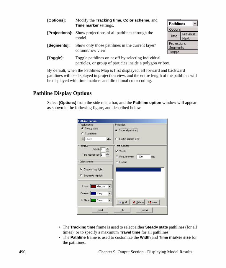
490 Chapter 9: Output Section - Displaying Model Results
[Options]: Modify the Tracking time, Color scheme, and Time marker settings.
[Projections]: Show projections of all pathlines through the model.
[Segments]: Show only those pathlines in the current layer/column/row view.
[Toggle]: Toggle pathlines on or off by selecting individual particles, or group of particles inside a polygon or box.
By default, when the Pathlines Map is first displayed, all forward and backward pathlines will be displayed in projection view, and the entire length of the pathlines will be displayed with time markers and directional color coding.
Pathline Display Options
Select [Options] from the side menu bar, and the Pathline option window will appear as shown in the following figure, and described below.
• The Tracking time frame is used to select either Steady state pathlines (for all times), or to specify a maximum Travel time for all pathlines.
• The Pathline frame is used to customize the Width and Time marker size for the pathlines.
Maps 491
• The Color scheme frame is used to select either Direction highlight, where the color of the pathlines are determined by the flow direction relative to the current plane, or Segments highlight where the color of the pathlines are determined by their location relative to the current layer. When Segments highlight is selected, the colors correspond to pathlines Above, Below, and In Plane. When Direction highlight is selected, the colors correspond to pathlines travelling Inward, Outward, and In Plane.
• The Projection frame allows the option to either Show all pathlines, displaying all the pathlines in all layers/row/columns, or to Start in current layer, displaying only pathlines for particles originating in the current layer/row/column.
• The Time markers frame is used to hide/show the pathline time markers (using the Visible checkbox), and to select the time intervals for each time marker. The Time markers can be plotted at Regular time intervals, or at Custom intervals selected by the user.
If forward tracking pathlines do not appear for some particles, check to make sure the particles are not assigned above the water table elevation, or in dry cells.
If backward tracking pathlines appear to ‘skim’ along the surface of the water table instead of exiting through recharge, check the MODPATH Discharge Options in the Run section to make sure the recharge flux is being assigned to the top face of all cells instead of being treated as an internal source/sink.
Removing the Pathlines Map
Once the Pathlines Map has been selected and displayed in the Output section, it can only be removed using the Overlay Control as described below:
• Press the [F9 - Overlay] button in the toolbar along the bottom of the Visual MODFLOW screen to load the Overlay Control window.
• Click the List only the visible overlays option (this reduces the list of Overlays and makes it easier to locate the Pathlines Map overlay).
• Locate the PT - Pathlines overlay and click the checkbox to remove the checkmark.
• Click the [OK] or [Apply] button to redraw the model display screen with the new Overlay settings.
Exporting Pathlines
For information on exporting Pathlines, please see Export Options on page 77. Pathlines may be exported to Graphics Image files, AutoCAD DXF files, Enhanced Windows Metafiles, or ESRI Shape files.
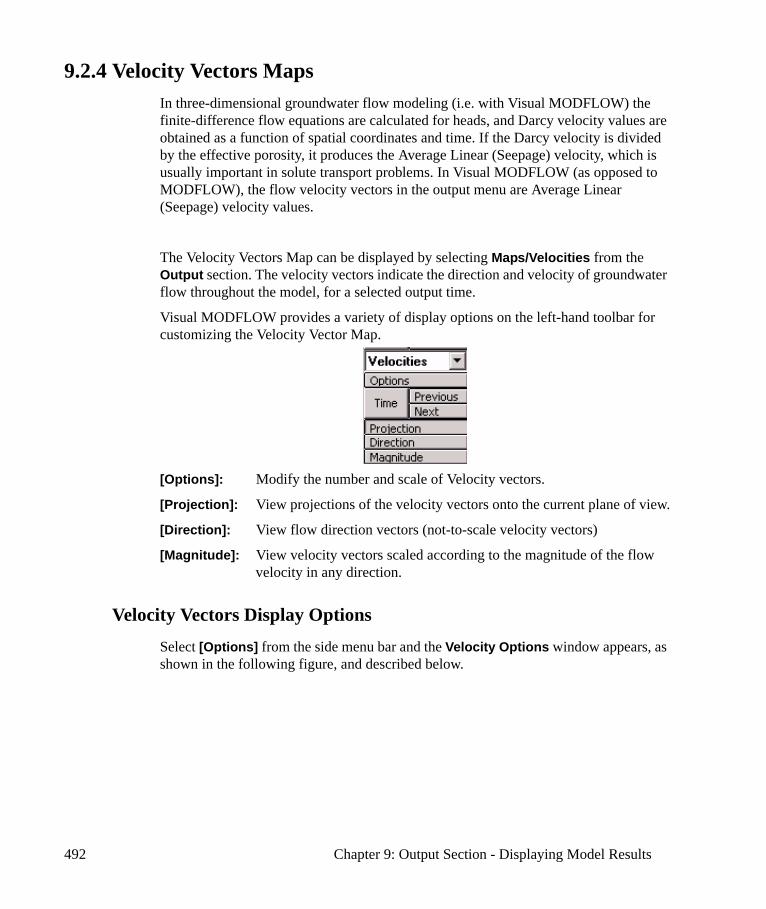
492 Chapter 9: Output Section - Displaying Model Results
9.2.4 Velocity Vectors MapsIn three-dimensional groundwater flow modeling (i.e. with Visual MODFLOW) the finite-difference flow equations are calculated for heads, and Darcy velocity values are obtained as a function of spatial coordinates and time. If the Darcy velocity is divided by the effective porosity, it produces the Average Linear (Seepage) velocity, which is usually important in solute transport problems. In Visual MODFLOW (as opposed to MODFLOW), the flow velocity vectors in the output menu are Average Linear (Seepage) velocity values.
The Velocity Vectors Map can be displayed by selecting Maps/Velocities from the Output section. The velocity vectors indicate the direction and velocity of groundwater flow throughout the model, for a selected output time.
Visual MODFLOW provides a variety of display options on the left-hand toolbar for customizing the Velocity Vector Map.
[Options]: Modify the number and scale of Velocity vectors.
[Projection]: View projections of the velocity vectors onto the current plane of view.
[Direction]: View flow direction vectors (not-to-scale velocity vectors)
[Magnitude]: View velocity vectors scaled according to the magnitude of the flow velocity in any direction.
Velocity Vectors Display Options
Select [Options] from the side menu bar and the Velocity Options window appears, as shown in the following figure, and described below.
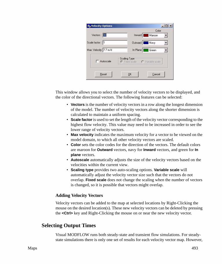
Maps 493
This window allows you to select the number of velocity vectors to be displayed, and the color of the directional vectors. The following features can be selected:
• Vectors is the number of velocity vectors in a row along the longest dimension of the model. The number of velocity vectors along the shorter dimension is calculated to maintain a uniform spacing.
• Scale factor is used to set the length of the velocity vector corresponding to the highest flow velocity. This value may need to be increased in order to see the lower range of velocity vectors.
• Max velocity indicates the maximum velocity for a vector to be viewed on the model domain, to which all other velocity vectors are scaled.
• Color sets the color codes for the direction of the vectors. The default colors are maroon for Outward vectors, navy for Inward vectors, and green for In plane vectors.
• Autoscale automatically adjusts the size of the velocity vectors based on the velocities within the current view.
• Scaling type provides two auto-scaling options. Variable scale will automatically adjust the velocity vector size such that the vectors do not overlap. Fixed scale does not change the scaling when the number of vectors is changed, so it is possible that vectors might overlap.
Adding Velocity VectorsVelocity vectors can be added to the map at selected locations by Right-Clicking the mouse on the desired location(s). These new velocity vectors can be deleted by pressing the <Ctrl> key and Right-Clicking the mouse on or near the new velocity vector.
Selecting Output Times
Visual MODFLOW runs both steady-state and transient flow simulations. For steady-state simulations there is only one set of results for each velocity vector map. However,

494 Chapter 9: Output Section - Displaying Model Results
for transient simulations, there may be tens, hundreds, or even thousands of output times generated for the flow simulation results.
To select the output time to display for the current velocity vectors map, click the [Time] button on the left-hand toolbar and choose the desired output time. Alternately, the output time displayed may be increased or decreased by pressing the [Next] or [Previous] button, respectively, located beside the [Time] button.
If a Head Contour Map and a Velocity Vector Map are being displayed simultaneously, the Output times for these two data types will be synchronized because the velocity values are directly dependent on the head values. However, the Velocity Vector Map is not synchronized with the Concentration Contour Maps.
Note: Cell-by-cell velocity values (Vx, Vy, Vz, and Vtotal) can be viewed using Cell Inspector. For details on using the Cell Inspector tool, refer to “Cell Inspector” on page 291.
Removing the Velocity Vectors Map
Once the Velocity Vectors Map has been selected and displayed in the Output section, it can only be removed using the Overlay Control as described below:
• Press the [F9 - Overlay] button in the toolbar along the bottom of the Visual MODLFOW screen to load the Overlay Control window.
• Click the List only the visible overlays option (this reduces the list of Overlays and makes it easier to locate the Velocity Vector Map overlay).
• Locate the Vel - Vectors overlay and click the checkbox to remove the checkmark.
• Click the [OK] or [Apply] button to redraw the model display screen with the new Overlay settings.
Exporting Flow Velocity Data
For information on exporting Velocity Vector data, please see Export Options on page 77. Velocity data may be exported to Graphics Image files, AutoCAD DXF files, Enhanced Windows Metafiles, XYZ ASCII .TXT files, Array ASCII .TXT files, Tecplot .DAT files, SURFER ASCII .GRD files, or SURFER Binary .GRD files.
When Velocity data is exported (or shown using the Cell Inspector), negative velocity values indicate movement in the opposite direction of positive velocity values. For example, a positive Vx indicates movement to the right, while a negative Vx indicates movement to the left (when looking at a Plan View of your model). A positive Vy indicates movement upwards, while a negative Vy indicates movement downwards (when looking at a Plan View of your model). A positive Vz indicates movement upwards through the model layers, while a negative Vz indicates movement downwards through the model layers.
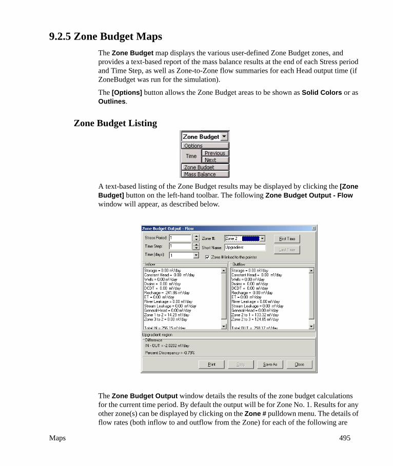
Maps 495
9.2.5 Zone Budget MapsThe Zone Budget map displays the various user-defined Zone Budget zones, and provides a text-based report of the mass balance results at the end of each Stress period and Time Step, as well as Zone-to-Zone flow summaries for each Head output time (if ZoneBudget was run for the simulation).
The [Options] button allows the Zone Budget areas to be shown as Solid Colors or as Outlines.
Zone Budget Listing
A text-based listing of the Zone Budget results may be displayed by clicking the [Zone Budget] button on the left-hand toolbar. The following Zone Budget Output - Flow window will appear, as described below.
The Zone Budget Output window details the results of the zone budget calculations for the current time period. By default the output will be for Zone No. 1. Results for any other zone(s) can be displayed by clicking on the Zone # pulldown menu. The details of flow rates (both inflow to and outflow from the Zone) for each of the following are
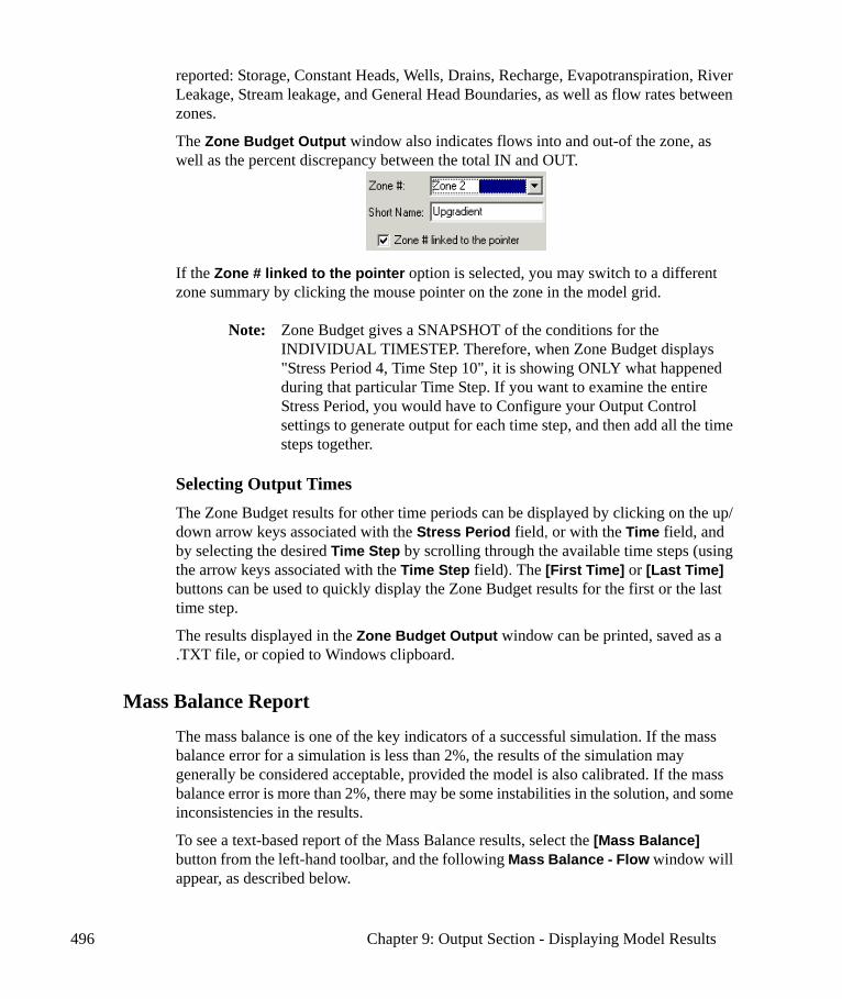
496 Chapter 9: Output Section - Displaying Model Results
reported: Storage, Constant Heads, Wells, Drains, Recharge, Evapotranspiration, River Leakage, Stream leakage, and General Head Boundaries, as well as flow rates between zones.
The Zone Budget Output window also indicates flows into and out-of the zone, as well as the percent discrepancy between the total IN and OUT.
If the Zone # linked to the pointer option is selected, you may switch to a different zone summary by clicking the mouse pointer on the zone in the model grid.
Note: Zone Budget gives a SNAPSHOT of the conditions for the INDIVIDUAL TIMESTEP. Therefore, when Zone Budget displays "Stress Period 4, Time Step 10", it is showing ONLY what happened during that particular Time Step. If you want to examine the entire Stress Period, you would have to Configure your Output Control settings to generate output for each time step, and then add all the time steps together.
Selecting Output TimesThe Zone Budget results for other time periods can be displayed by clicking on the up/down arrow keys associated with the Stress Period field, or with the Time field, and by selecting the desired Time Step by scrolling through the available time steps (using the arrow keys associated with the Time Step field). The [First Time] or [Last Time] buttons can be used to quickly display the Zone Budget results for the first or the last time step.
The results displayed in the Zone Budget Output window can be printed, saved as a .TXT file, or copied to Windows clipboard.
Mass Balance Report
The mass balance is one of the key indicators of a successful simulation. If the mass balance error for a simulation is less than 2%, the results of the simulation may generally be considered acceptable, provided the model is also calibrated. If the mass balance error is more than 2%, there may be some instabilities in the solution, and some inconsistencies in the results.
To see a text-based report of the Mass Balance results, select the [Mass Balance] button from the left-hand toolbar, and the following Mass Balance - Flow window will appear, as described below.

Graphs 497
The Mass Balance window details information about the entire model domain. Flow rates (cumulative inflows (IN to the model) and outflows (OUT of the model), and a percent discrepancy) are given for the same boundaries and properties as shown in Mass Balance Output window.
Removing the Zone Budget MapsOnce the Zone Budget Map has been selected and displayed in the Output section, it can only be removed using the Overlay Control as described below:
• Press the [F9 - Overlay] button in the toolbar along the bottom of the Visual MODFLOW screen to load the Overlay Control window.
• Click the List only the visible overlays option (this reduces the list of Overlays and makes it easier to locate the Zone Budget Map overlay).
• Locate the Gen - Zone Budget overlay and click the checkbox to remove the checkmark.
• Click the [OK] or [Apply] button to redraw the model display screen with the new Overlay settings.
9.3 GraphsVisual MODFLOW displays various types of graphs:
• Calibration Graphs• Time-Series Graphs• Mass Balance Graphs
498 Chapter 9: Output Section - Displaying Model Results
• Zone Budget Graphs• Lake Budget Graphs
Each of these graph types, and their associated display options, are presented in the following sections.
9.3.1 Calibration GraphsModel calibration is the process whereby selected model input parameters are adjusted within reasonable limits to produce simulation results that best match the known or measured values. Model calibration is the most critical process in building the groundwater flow and contaminant transport model, because the quality of the calibration inevitably determines the reliability of any conclusions and recommendations made using the simulation results.
The acceptability of a model’s calibration is usually a subjective measure, as each model has different objectives, and must be calibrated to different conditions. However, there are some generally accepted methods of evaluating and interpreting the model calibration using both qualitative and quantitative measures.
Visual MODFLOW provides a comprehensive selection of model calibration analysis tools for evaluating, interpreting, and presenting the model calibration, including:
• Calculated vs. Observed Scatter Graphs• Calibration Residuals Histograms• Calculated and Observed Values vs. Time• Calibration Statistics vs. Time
Calibration Graphs may be displayed in the Output section by selecting Graphs/Calibration from the top menu bar, and choosing either Head or Concentration. The default Calibration Graph is a scatter plot of Calculated vs. Observed values for the selected Observation Well(s), which are displayed with different symbol shapes and colors. The Calibration Plots window is the ‘Command Center’ for the four different types of Calibration Graphs. When the Calibration Plots window (shown below) is first opened, it will display a Calculated vs. Observed Scatter Graph of the Observation Points selected in the Visual MODFLOW screen (see Selecting Observation Points on page 488).
As shown in the following figure, the data points in the Calibration Plots are displayed according to the model layers where the observation wells are located. Further, the data points in the Calibration Plots can be linked to the map view in the main Visual MODFLOW window. This information is very useful in order to determine the vertical location of the observation points. In addition, the observation wells associated with the selected data point(s) will be highlighted in the map view in the main Visual MODFLOW window. To select the data points in the graph, please refer to Display Settings on page 503. This feature allows the user to quickly identify the location of the wells, and to check the magnitude of error associated with the individual data points.
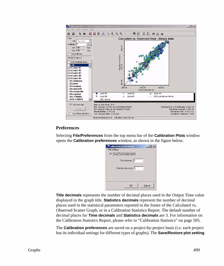
Graphs 499
PreferencesSelecting File/Preferences from the top menu bar of the Calibration Plots window opens the Calibration preferences window, as shown in the figure below.
Title decimals represents the number of decimal places used in the Output Time value displayed in the graph title. Statistics decimals represent the number of decimal places used in the statistical parameters reported in the footer of the Calculated vs. Observed Scatter Graph, or in a Calibration Statistics Report. The default number of decimal places for Time decimals and Statistics decimals are 3. For information on the Calibration Statistics Report, please refer to “Calibration Statistics” on page 505.
The Calibration preferences are saved on a project-by-project basis (i.e. each project has its individual settings for different types of graphs). The Save/Restore plot setting
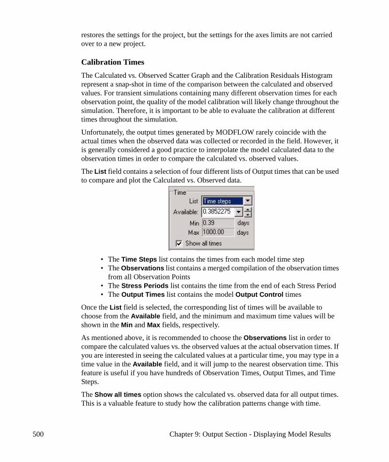
500 Chapter 9: Output Section - Displaying Model Results
restores the settings for the project, but the settings for the axes limits are not carried over to a new project.
Calibration TimesThe Calculated vs. Observed Scatter Graph and the Calibration Residuals Histogram represent a snap-shot in time of the comparison between the calculated and observed values. For transient simulations containing many different observation times for each observation point, the quality of the model calibration will likely change throughout the simulation. Therefore, it is important to be able to evaluate the calibration at different times throughout the simulation.
Unfortunately, the output times generated by MODFLOW rarely coincide with the actual times when the observed data was collected or recorded in the field. However, it is generally considered a good practice to interpolate the model calculated data to the observation times in order to compare the calculated vs. observed values.
The List field contains a selection of four different lists of Output times that can be used to compare and plot the Calculated vs. Observed data.
• The Time Steps list contains the times from each model time step• The Observations list contains a merged compilation of the observation times
from all Observation Points• The Stress Periods list contains the time from the end of each Stress Period • The Output Times list contains the model Output Control times
Once the List field is selected, the corresponding list of times will be available to choose from the Available field, and the minimum and maximum time values will be shown in the Min and Max fields, respectively.
As mentioned above, it is recommended to choose the Observations list in order to compare the calculated values vs. the observed values at the actual observation times. If you are interested in seeing the calculated values at a particular time, you may type in a time value in the Available field, and it will jump to the nearest observation time. This feature is useful if you have hundreds of Observation Times, Output Times, and Time Steps.
The Show all times option shows the calculated vs. observed data for all output times. This is a valuable feature to study how the calibration patterns change with time.
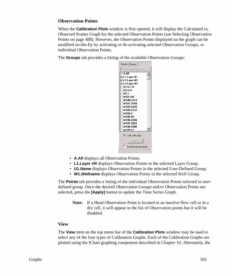
Graphs 501
Observation PointsWhen the Calibration Plots window is first opened, it will display the Calculated vs. Observed Scatter Graph for the selected Observation Points (see Selecting Observation Points on page 488). However, the Observation Points displayed on the graph can be modified on-the-fly by activating or de-activating selected Observation Groups, or individual Observation Points.
The Groups tab provides a listing of the available Observation Groups:
• A.All displays all Observation Points.• L1.Layer #N displays Observation Points in the selected Layer Group.• U1.Name displays Observation Points in the selected User-Defined Group.• W1.Wellname displays Observation Points in the selected Well Group.
The Points tab provides a listing of the individual Observation Points selected in user-defined group. Once the desired Observation Groups and/or Observation Points are selected, press the [Apply] button to update the Time Series Graph.
Note: If a Head Observation Point is located in an inactive flow cell or in a dry cell, it will appear in the list of Observation points but it will be disabled.
ViewThe View item on the top menu bar of the Calibration Plots window may be used to select any of the four types of Calibration Graphs. Each of the Calibration Graphs are plotted using the IChart graphing component described in Chapter 10. Alternately, the
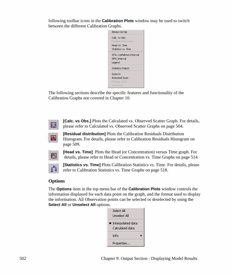
502 Chapter 9: Output Section - Displaying Model Results
following toolbar icons in the Calibration Plots window may be used to switch between the different Calibration Graphs.
The following sections describe the specific features and functionality of the Calibration Graphs not covered in Chapter 10.
[Calc. vs Obs.] Plots the Calculated vs. Observed Scatter Graph. For details, please refer to Calculated vs. Observed Scatter Graphs on page 504.
[Residual distribution] Plots the Calibration Residuals Distribution Histogram. For details, please refer to Calibration Residuals Histogram on page 509.
[Head vs. Time] Plots the Head (or Concentration) versus Time graph. For details, please refer to Head or Concentration vs. Time Graphs on page 514.
[Statistics vs. Time] Plots Calibration Statistics vs. Time. For details, please refer to Calibration Statistics vs. Time Graphs on page 518.
OptionsThe Options item in the top menu bar of the Calibration Plots window controls the information displayed for each data point on the graph, and the format used to display the information. All Observation points can be selected or deselected by using the Select All or Unselect All options.
Graphs 503
The Interpolated data option will compare the value calculated at the observation point against the value observed at the observation point. The value calculated at the observation point is obtained by interpolating calculated values from surrounding cells to the observation point location. The Calculated data option will compare the value calculated at the cell center against the value observed at the observation point.
Specific information about a data point on a graph may be obtained by simply clicking on the data point to display an Info bubble, or by clicking the Info option in the dropdown menu bar.
Display SettingsThe Time-Series Graphs (Head, Drawdown, and Concentration) are plotted using the IChart graphing component described in Chapter 10. Properties... opens the IChart graphing component (Display Settings). Please refer to IChart - Graphing and Mapping Component on page 529 for a detailed description of the display settings available for customizing the appearance of the graph, and for instructions on preparing and printing the graph.
Using the Select window icon in the Calibration plot, specific information about the data points may be obtained by plotting a polygon around the data points of interest, as shown in the following figure. The data points selected on
this graph are highlighted on the map, and change their color from dark green to light green. Clicking on individual symbols in the calculated vs. observed graphs also selects the data points highlighted on the map. The selected data points may be included in a group by creating a new group, using Edit/Create Observation Group from the graph menu bar. The Create Observation Group option can also be accessed by Right-Clicking on the graph.

504 Chapter 9: Output Section - Displaying Model Results
Calculated vs. Observed Scatter Graphs
The Scatter Graph of Calculated vs. Observed Values is the default Calibration Graph. This graph represents a snap-shot in time of the comparison between the values calculated by the model (Y-axis), and the values observed or measured in the field (X-axis). In the figure shown on page 498, all of the data points intersect the 45 degree line on the graph where X=Y. This represents an ideal calibration scenario, but it is not likely to happen in many real-life situations.
If the data points appear above the X=Y line, then the calculated values are larger than the observed values, and the Calibration Residual is positive, indicating that the model is over-predicting. If the data points are under the X=Y line, then the calculated values are less than the observed values, and the Calibration Residuals are negative, indicating that the model is under-predicting.
Interpolated and Extrapolated Data PointsAs discussed in Calibration Times on page 500, the output times from the model will rarely coincide with the actual observation times when the data was measured in the field. As a result, the calculated data must be interpolated to the observation times in order to calculate the Calibration Residual for a specific snap-shot in time (or vice-versa).
• Interpolated Calculated data points represent calculated values at observation times where the observation time is between two model output times.
• Extrapolated Calculated data points represent calculated values at observation
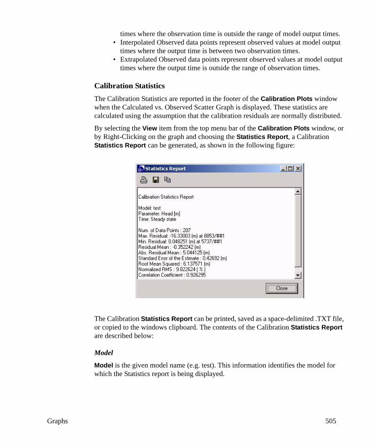
Graphs 505
times where the observation time is outside the range of model output times. • Interpolated Observed data points represent observed values at model output
times where the output time is between two observation times.• Extrapolated Observed data points represent observed values at model output
times where the output time is outside the range of observation times.
Calibration StatisticsThe Calibration Statistics are reported in the footer of the Calibration Plots window when the Calculated vs. Observed Scatter Graph is displayed. These statistics are calculated using the assumption that the calibration residuals are normally distributed.
By selecting the View item from the top menu bar of the Calibration Plots window, or by Right-Clicking on the graph and choosing the Statistics Report, a Calibration Statistics Report can be generated, as shown in the following figure:
The Calibration Statistics Report can be printed, saved as a space-delimited .TXT file, or copied to the windows clipboard. The contents of the Calibration Statistics Report are described below:
Model
Model is the given model name (e.g. test). This information identifies the model for which the Statistics report is being displayed.
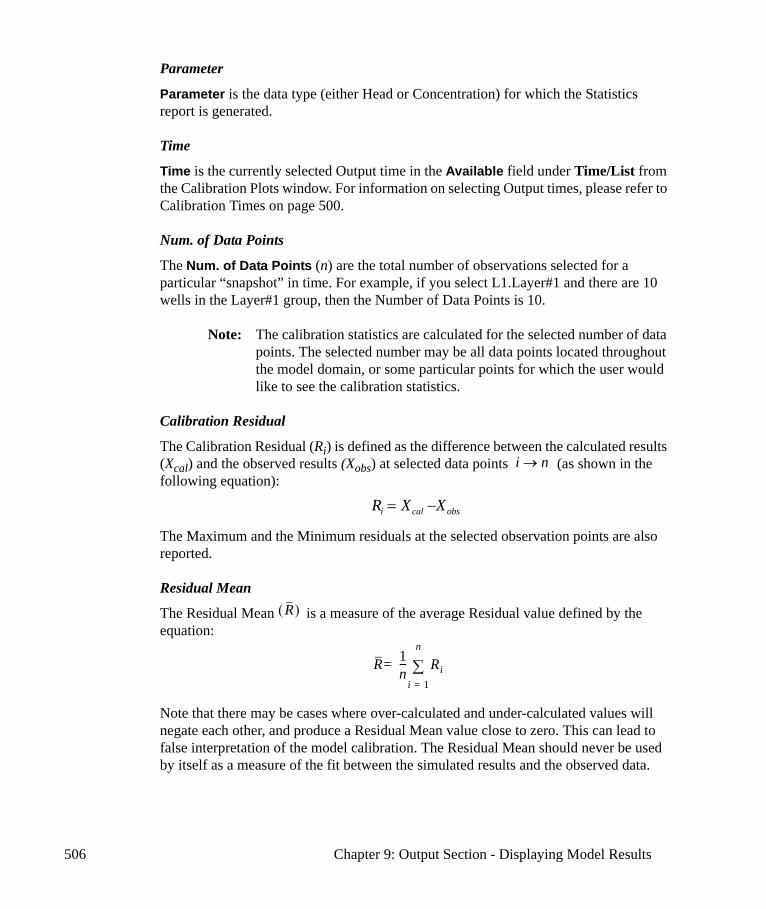
506 Chapter 9: Output Section - Displaying Model Results
Parameter
Parameter is the data type (either Head or Concentration) for which the Statistics report is generated.
Time
Time is the currently selected Output time in the Available field under Time/List from the Calibration Plots window. For information on selecting Output times, please refer to Calibration Times on page 500.
Num. of Data Points
The Num. of Data Points (n) are the total number of observations selected for a particular “snapshot” in time. For example, if you select L1.Layer#1 and there are 10 wells in the Layer#1 group, then the Number of Data Points is 10.
Note: The calibration statistics are calculated for the selected number of data points. The selected number may be all data points located throughout the model domain, or some particular points for which the user would like to see the calibration statistics.
Calibration Residual
The Calibration Residual (Ri) is defined as the difference between the calculated results (Xcal) and the observed results (Xobs) at selected data points (as shown in the following equation):
The Maximum and the Minimum residuals at the selected observation points are also reported.
Residual Mean
The Residual Mean is a measure of the average Residual value defined by the equation:
Note that there may be cases where over-calculated and under-calculated values will negate each other, and produce a Residual Mean value close to zero. This can lead to false interpretation of the model calibration. The Residual Mean should never be used by itself as a measure of the fit between the simulated results and the observed data.
i n→
obscali XXR −=
R( )
R 1n--- Ri
i 1=
n
∑=
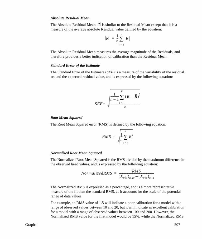
Graphs 507
Absolute Residual Mean
The Absolute Residual Mean is similar to the Residual Mean except that it is a measure of the average absolute Residual value defined by the equation:
The Absolute Residual Mean measures the average magnitude of the Residuals, and therefore provides a better indication of calibration than the Residual Mean.
Standard Error of the Estimate
The Standard Error of the Estimate (SEE) is a measure of the variability of the residual around the expected residual value, and is expressed by the following equation:
Root Mean Squared
The Root Mean Squared error (RMS) is defined by the following equation:
Normalized Root Mean Squared
The Normalized Root Mean Squared is the RMS divided by the maximum difference in the observed head values, and is expressed by the following equation:
The Normalized RMS is expressed as a percentage, and is a more representative measure of the fit than the standard RMS, as it accounts for the scale of the potential range of data values.
For example, an RMS value of 1.5 will indicate a poor calibration for a model with a range of observed values between 10 and 20, but it will indicate an excellent calibration for a model with a range of observed values between 100 and 200. However, the Normalized RMS value for the first model would be 15%, while the Normalized RMS
R
R 1n--- Ri
i 1=
n
∑=
SEE
1n 1–------------ Ri R–( )2
i 1=
n
∑
n-------------------------------------------=
RMS 1n--- Ri
2
i 1=
n
∑=
NormalizedRMS RMSXobs( )max Xobs( )min–
--------------------------------------------------=
508 Chapter 9: Output Section - Displaying Model Results
for the second model would be 1.5%. In this situation, the Normalized RMS values clearly indicates the second model provides a good fit between the calculated and observed values.
Correlation Coefficient
The Correlation Coefficient (Cor) is calculated as the covariance (Cov) between the calculated results (Xcal) and the observed results (Xobs) at selected data points divided by the product of their standard deviations. The correlation coefficient is calculated using the following equation:
The covariance is calculated using the following equation:
Where and are the mean values of calculated and observed results,
respectively.
The standard deviations are calculated by the equations:
Correlation Coefficients range in value from -1.0 to 1.0. The Correlation Coefficient determines whether two ranges of data move together - i.e. whether large values of one data set are associated with large values of the other data set (positive correlation), whether small values of one data set are associated with large values of the other data set (negative correlation), or whether values in both sets are unrelated (correlation near zero).
Cor Xcal Xobs,( )Cov Xcal Xobs,( )
σcal σ• obs--------------------------------------=
Cov Xcal Xobs,( ) 1n--- Xi µcal–( ) Xi µobs–( )
i 1=
n
∑=
µcal µobs
µcal1n--- Xcal
i 1=
n
∑=
µobs1n--- Xobs
i 1=
n
∑=
σcal1n--- Xcal µcal–( )2
i 1=
n
∑=
σobs1n--- Xobs µobs–( )2
i 1=
n
∑=
Graphs 509
Evaluating Uncertainty The uncertainty with which the heads are simulated can be evaluated using confidence intervals.
A confidence interval is an interval within which a hypothesis is considered tenable at a given significance level . For model calibration purposes, the hypothesis is that any given Residual is equal to the mean Residual. So, with the confidence interval, a lower and upper limit (range) for the mean are generated which gives us an indication of how much uncertainty is involved in our estimate of the true mean. The narrower the interval, the more precise is our estimate.
The % confidence interval is calculated using the following equation:
Where, X is the sample mean, s is sample standard deviation, n is the number of observations, and Z is the value of standard normal variable that puts percent in each tail of the Student-t distribution.
95% Confidence Interval
A 95% confidence interval allows the user to visualize a range of calculated values for each observed value with 95 percent confidence that the simulation results will be acceptable for a given observed value. The goal for model calibration should be to have the 45 degree line where X=Y fall within the 95% confidence interval lines.
95% Interval
The 95% interval is the interval where 95% of the total number of data points are expected to occur.
Calibration Residuals Histogram
To display a Calibration Residuals Histogram:
• Select Graphs/Calibration from the top menu bar of the Output section and choose either Head or Concentration.
• A Calibration Plots window will appear with a Calculated vs. Observed Scatter Graph.
• Select View/Residual Distribution from the top menu bar of the Calibration Plots window to switch to the Calibration Residuals Histogram.
The Calibration Residuals Histogram displays the Population, Frequency, or Relative Frequency of observations, for specified intervals of the Normalized Calibration Residual values. The Normalized Calibration Residual values are calculated using the above mentioned formulas for each data series.
α
1 α–( )100
Range X Z sn
-------±=
α 2⁄

510 Chapter 9: Output Section - Displaying Model Results
The number of groups of observation points or channels is specified in the top menu bar using the Channels property box. The default number of Channels is 20. This value can be increased or decreased using the up and down arrow buttons.
The Normal Distribution curve is a two-tailed p-value of a Z-test. This curve can be used to determine the likelihood an observation lies in a particular population.
The Residual Distribution Histogram provides a qualitative comparison of the distribution of the normalized calibration residual values against the student distribution curve. Ideally, the distribution of the calibration residuals for a large number of observation points would be similar to that of the student distribution curve, with most of the residuals groups clustered around the value of zero.
9.3.2 Time-Series GraphsA Time-Series graph plots the change in a selected variable(s) with time. In groundwater flow and contaminant transport modeling, time-series graphs are used to evaluate and compare temporal trends in the calculated Head, Drawdown, and Concentration at selected Observation Points. To plot a Time-Series Graph in Visual MODFLOW, select Graph/Time-Series option from the top menu bar of the Output section and choose either Head, Drawdown, or Concentration. A Time-Series Graph window will appear plotting both the calculated and observed values for the selected Observation Points, as shown in the following figure (for information on selecting Observation Points, please refer to Selecting Observation Points on page 488).
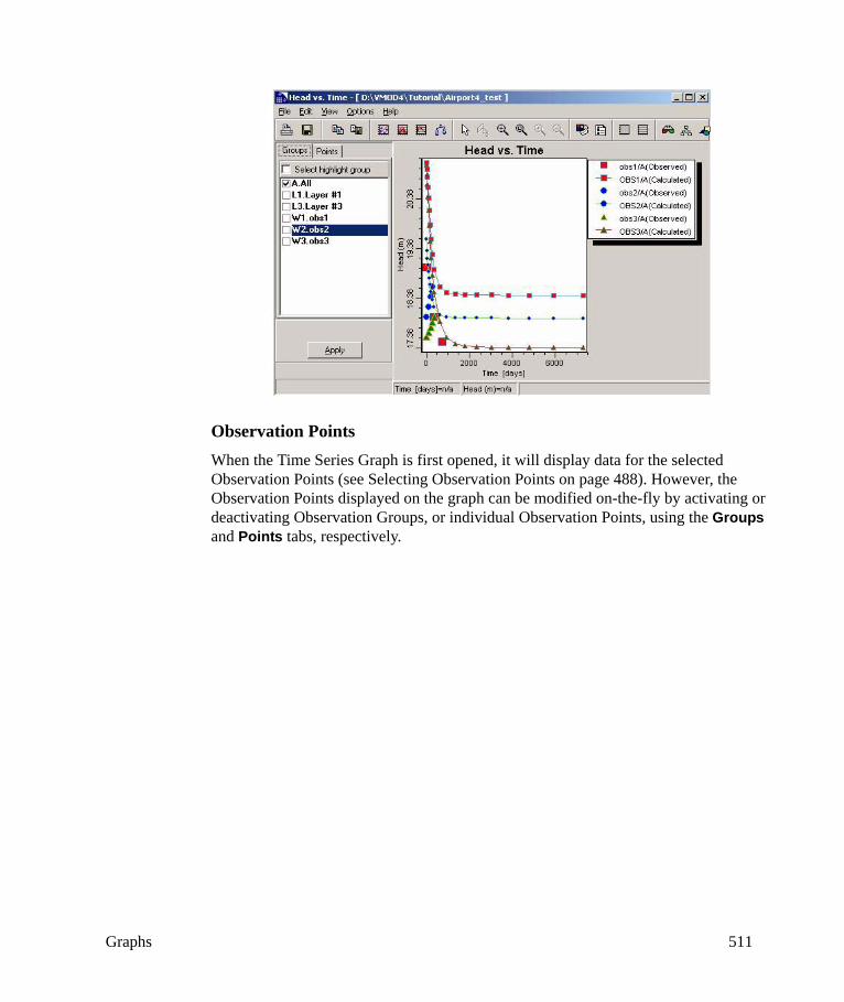
Graphs 511
Observation PointsWhen the Time Series Graph is first opened, it will display data for the selected Observation Points (see Selecting Observation Points on page 488). However, the Observation Points displayed on the graph can be modified on-the-fly by activating or deactivating Observation Groups, or individual Observation Points, using the Groups and Points tabs, respectively.
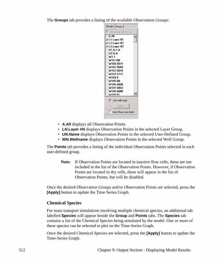
512 Chapter 9: Output Section - Displaying Model Results
The Groups tab provides a listing of the available Observation Groups:
• A.All displays all Observation Points.• LN.Layer #N displays Observation Points in the selected Layer Group.• UN.Name displays Observation Points in the selected User-Defined Group.• WN.Wellname displays Observation Points in the selected Well Group.
The Points tab provides a listing of the individual Observation Points selected in each user-defined group.
Note: If Observation Points are located in inactive flow cells, these are not included in the list of the Observation Points. However, if Observation Points are located in dry cells, these will appear in the list of Observation Points, but will be disabled.
Once the desired Observation Groups and/or Observation Points are selected, press the [Apply] button to update the Time Series Graph.
Chemical SpeciesFor mass transport simulations involving multiple chemical species, an additional tab labelled Species will appear beside the Group and Points tabs. The Species tab contains a list of the Chemical Species being simulated by the model. One or more of these species can be selected to plot on the Time-Series Graph.
Once the desired Chemical Species are selected, press the [Apply] button to update the Time-Series Graph.
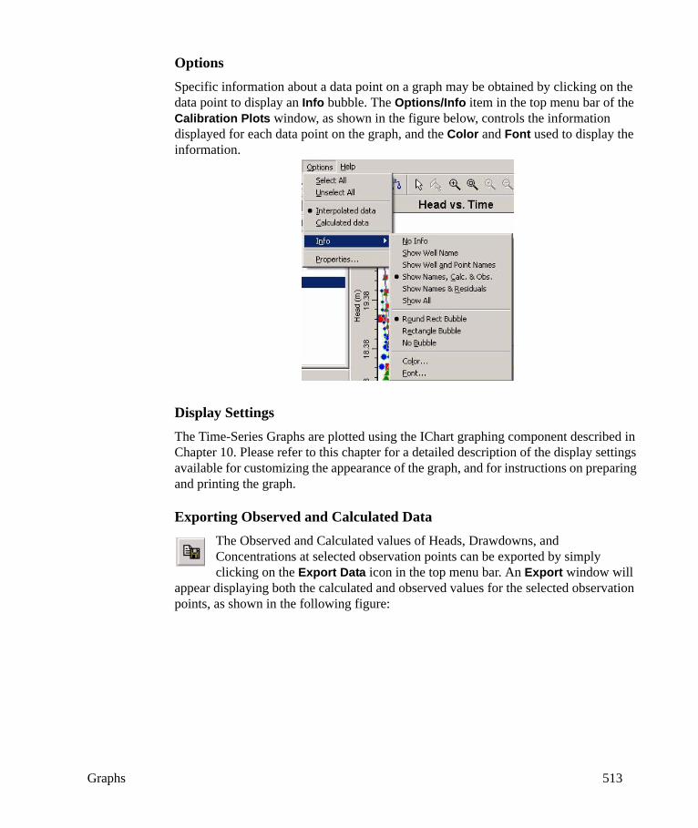
Graphs 513
OptionsSpecific information about a data point on a graph may be obtained by clicking on the data point to display an Info bubble. The Options/Info item in the top menu bar of the Calibration Plots window, as shown in the figure below, controls the information displayed for each data point on the graph, and the Color and Font used to display the information.
Display SettingsThe Time-Series Graphs are plotted using the IChart graphing component described in Chapter 10. Please refer to this chapter for a detailed description of the display settings available for customizing the appearance of the graph, and for instructions on preparing and printing the graph.
Exporting Observed and Calculated DataThe Observed and Calculated values of Heads, Drawdowns, and Concentrations at selected observation points can be exported by simply clicking on the Export Data icon in the top menu bar. An Export window will
appear displaying both the calculated and observed values for the selected observation points, as shown in the following figure:
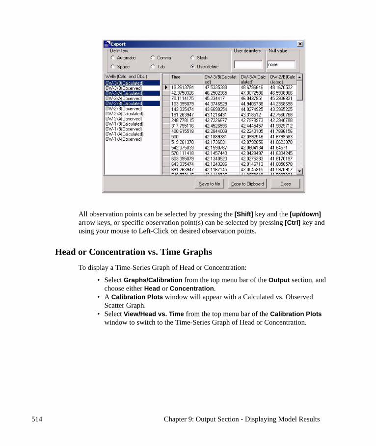
514 Chapter 9: Output Section - Displaying Model Results
All observation points can be selected by pressing the [Shift] key and the [up/down] arrow keys, or specific observation point(s) can be selected by pressing [Ctrl] key and using your mouse to Left-Click on desired observation points.
Head or Concentration vs. Time Graphs
To display a Time-Series Graph of Head or Concentration:
• Select Graphs/Calibration from the top menu bar of the Output section, and choose either Head or Concentration.
• A Calibration Plots window will appear with a Calculated vs. Observed Scatter Graph.
• Select View/Head vs. Time from the top menu bar of the Calibration Plots window to switch to the Time-Series Graph of Head or Concentration.
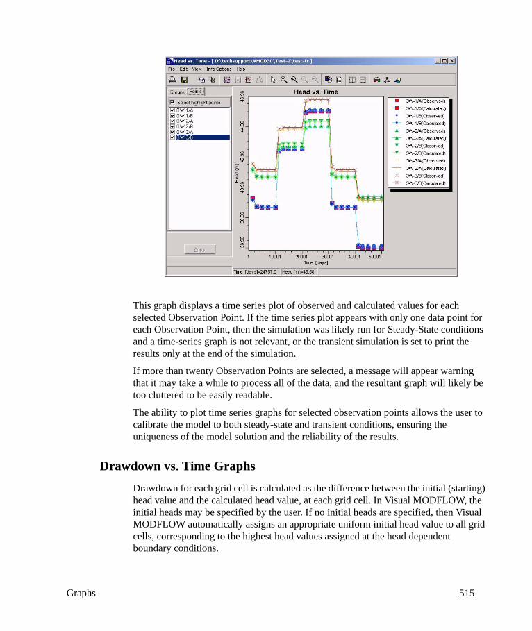
Graphs 515
This graph displays a time series plot of observed and calculated values for each selected Observation Point. If the time series plot appears with only one data point for each Observation Point, then the simulation was likely run for Steady-State conditions and a time-series graph is not relevant, or the transient simulation is set to print the results only at the end of the simulation.
If more than twenty Observation Points are selected, a message will appear warning that it may take a while to process all of the data, and the resultant graph will likely be too cluttered to be easily readable.
The ability to plot time series graphs for selected observation points allows the user to calibrate the model to both steady-state and transient conditions, ensuring the uniqueness of the model solution and the reliability of the results.
Drawdown vs. Time Graphs
Drawdown for each grid cell is calculated as the difference between the initial (starting) head value and the calculated head value, at each grid cell. In Visual MODFLOW, the initial heads may be specified by the user. If no initial heads are specified, then Visual MODFLOW automatically assigns an appropriate uniform initial head value to all grid cells, corresponding to the highest head values assigned at the head dependent boundary conditions.
516 Chapter 9: Output Section - Displaying Model Results
Drawdown Calculations at Observation points
Drawdown at an observation point is calculated using an initial (starting) head value and a calculated head value. If the initial observed head value at the observation point is not available, then the drawdown value at the observation point is calculated using the formula:
S = Hi - Hc
where
S = Drawdown at the observation point
Hi = Initial head at the observation point*
Hc = Calculated head at observation point*
If the observation point has an observed head value at Time=0, then the drawdown value at the observation point is calculated based on the observed head value using the following formula, rather than using the interpolated initial head values at the location of the observation point.
S = Ho - Hc
where
S = Drawdown at the observation point
Ho = Observed head at the observation point at time T=0
Hc = Calculated head at the observation point*
* The calculated head and initial head values at the observation points are horizontally interpolated from the grid cell centers to the actual location of the observation point.
Note: If MODFLOW-SURFACT is selected, the drawdown is calculated only when the simulation type is Groundwater flow (Pseudo-soil function). If simulation types are either van Genuchten, or a combination of van Genuchten and Brooks-Corey, then Saturation values are calculated (for more detail see “Saturation vs. Time Graphs” on page 517).
The following figure displays a Drawdown vs. Time Graph for three different Observation Points selected in the main Visual MODFLOW screen. By default, each Observation Point will be plotted using different symbols, and the calculated and the observed values for each Observation Point are differentiated by the symbol size, whereby the symbol for the Observed data series is larger than the symbol for the calculated data series. In addition, the data series for the calculated values are plotted using lines to join each data point, whereas the data series for the observed values are
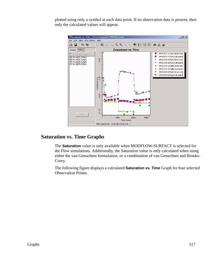
Graphs 517
plotted using only a symbol at each data point. If no observation data is present, then only the calculated values will appear.
Saturation vs. Time Graphs
The Saturation value is only available when MODFLOW-SURFACT is selected for the Flow simulations. Additionally, the Saturation value is only calculated when using either the van Genuchten formulation, or a combination of van Genuchten and Brooks-Corey.
The following figure displays a calculated Saturation vs. Time Graph for four selected Observation Points.

518 Chapter 9: Output Section - Displaying Model Results
Calibration Statistics vs. Time Graphs
To display a Time-Series Graph of Calibration Statistics:
• Select Graphs/Calibration from the top menu bar of the Output section, and choose either Head or Concentration.
• A Calibration Plots window will appear with a Calculated vs. Observed Scatter Graph.
• Select View/Statistics vs. Time from the top menu bar of the Calibration Plots window to switch to the Time-Series Graph of Calibration Statistics.
Graphs 519
The Calibration Statistics vs. Time Graph displays the various statistical measures of the model calibration throughout the entire simulation. The available calibration statistics include:
• Normalized RMS• Residuals• Normalized Residuals• Errors
These different graphs can be displayed by selecting the desired graph type from the View item in the top menu bar.
In the graph shown above, the Normalized RMS is increasing with time, indicating the quality of the model calibration is deteriorating towards the end of the simulation.
9.3.3 Mass Balance GraphsThe finite difference formulation of both the groundwater flow equation, and the mass transport equation, are based on conservation of mass, such that the mass of water or chemicals entering the system through various sources should equal the mass of water or chemicals leaving the system through the various sinks. The Mass Balance Graphs provide graphical representations of the mass of water or chemicals entering and leaving the system through the various sources and sinks.
Flow Mass Balance Graphs
The Flow Mass Balance Graphs plot the volume and rates of water entering and leaving the system through the flow boundary conditions, and from aquifer storage at the end of each stress period.
To plot the Flow Mass Balance Graphs, select Graphs/Mass Balance/Flow from the top menu bar of the Output section, and a Mass Balance: MODFLOW window will appear as shown below.
There are four different Flow Mass Balance Graphs:
• Percent Discrepancy plots the temporal changes in the Flow Mass Balance (total flow IN minus total flow OUT) expressed as a percentage of the total flow.
• IN - OUT plots the temporal change in the Flow Mass Balance (total flow IN minus the total flow OUT).
• Time Series plots the temporal flows IN and OUT of the system through the individual sources and sinks (flow boundary conditions and storage).
• Time step plots a bar chart of the flow IN to the system and the flow OUT of the system through the individual sources and sinks (flow boundary conditions and storage) for selected Output Times.

520 Chapter 9: Output Section - Displaying Model Results
Note: With both the Time Steps and the Time Series graphs, it is important to remember that these graphs present the cumulative mass at a point in time, and not the mass loading rate at a point in time.
As mentioned above, the Flow Mass Balance Graphs can be used to plot the flow volume or flow rates of water coming IN and going OUT of the system. By default, the Mass Balance: MODFLOW window plots the flow volume mass balance.
Use the View option in the top menu bar to select either Volume or Rates, or click the [Cumulative volume] or [Rate] icon in the toolbar.
Sources and Sinks On the left-hand side of the Mass Balance: MODFLOW window is a list of all potential sources and sinks for the current flow model (boundary conditions not included in the model will not be listed). These sources and sinks are included in both the IN list and the OUT list. The IN list contains a summary of the flow coming into the system from each individual source term, while the OUT list contains a summary of the flow going out of the system through each individual sink term.
These controls can be used to add or remove the individual source and sink terms from either the Time Series graph or the Time step graph.
The Percent Discrepancy graph and the IN-OUT graph consider only the total flow into and out-of the entire system as a whole. As a result, the settings for the individual IN and OUT terms do not influence the results and appearance of these graphs.
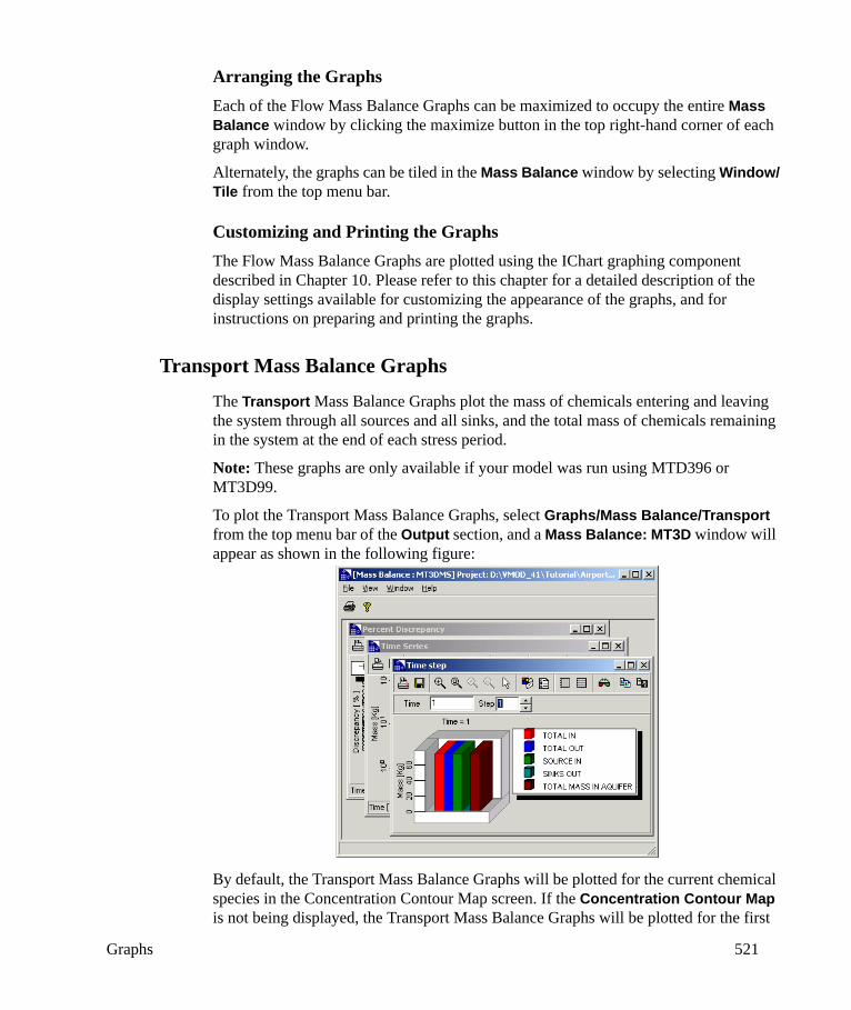
Graphs 521
Arranging the GraphsEach of the Flow Mass Balance Graphs can be maximized to occupy the entire Mass Balance window by clicking the maximize button in the top right-hand corner of each graph window.
Alternately, the graphs can be tiled in the Mass Balance window by selecting Window/Tile from the top menu bar.
Customizing and Printing the GraphsThe Flow Mass Balance Graphs are plotted using the IChart graphing component described in Chapter 10. Please refer to this chapter for a detailed description of the display settings available for customizing the appearance of the graphs, and for instructions on preparing and printing the graphs.
Transport Mass Balance Graphs
The Transport Mass Balance Graphs plot the mass of chemicals entering and leaving the system through all sources and all sinks, and the total mass of chemicals remaining in the system at the end of each stress period.
Note: These graphs are only available if your model was run using MTD396 or MT3D99.
To plot the Transport Mass Balance Graphs, select Graphs/Mass Balance/Transport from the top menu bar of the Output section, and a Mass Balance: MT3D window will appear as shown in the following figure:
By default, the Transport Mass Balance Graphs will be plotted for the current chemical species in the Concentration Contour Map screen. If the Concentration Contour Map is not being displayed, the Transport Mass Balance Graphs will be plotted for the first

522 Chapter 9: Output Section - Displaying Model Results
chemical species in the list. To plot the Transport Mass Balance Graphs for a different chemical species, open the Concentration Contour Map and use the [Species] button to select a new Chemical Species.
There are three different Transport Mass Balance Graphs:
• Percent Discrepancy plots the temporal changes in the Transport Mass Balance (cumulative mass IN minus cumulative mass OUT) expressed as a percentage of the cumulative mass IN.
• Time Series plots the temporal changes in the cumulative mass entering, remaining, and leaving the system (where; SOURCE IN is the mass entering through sources; SINKS OUT is the mass leaving the system through sinks; TOTAL MASS IN AQUIFER is the mass remaining; TOTAL IN is the mass added to the system through sources, and reduction in mass storage; and TOTAL OUT is mass removed from the system through sources, and increase in mass storage).
• Time step plots a bar chart of the cumulative mass that has entered, mass that remains, and mass that has left the system, at a specified Output Time.
Note: With both the Time Steps and the Time Series graphs, it is important to remember that these graphs present the cumulative mass at a point in time, and not the mass loading rate at a point in time.
Arranging the GraphsEach of the Transport Mass Balance Graphs can be maximized to occupy the entire Mass Balance window by clicking the maximize button in the top right-hand corner of each graph window.
Alternately, the graphs can be tiled in the Mass Balance window by selecting Window/Tile from the top menu bar.
Customizing and Printing the GraphsThe Transport Mass Balance Graphs are all plotted using the IChart graphing component described in Chapter 10. Please refer to this chapter for a detailed description of the display options available for customizing the appearance of the graphs, and for instructions on preparing and printing the graphs.
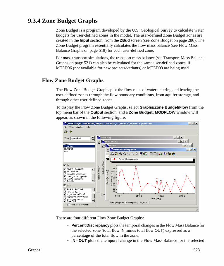
Graphs 523
9.3.4 Zone Budget GraphsZone Budget is a program developed by the U.S. Geological Survey to calculate water budgets for user-defined zones in the model. The user-defined Zone Budget zones are created in the Input section, from the ZBud screen (see Zone Budget on page 286). The Zone Budget program essentially calculates the flow mass balance (see Flow Mass Balance Graphs on page 519) for each user-defined zone.
For mass transport simulations, the transport mass balance (see Transport Mass Balance Graphs on page 521) can also be calculated for the same user-defined zones, if MT3D96 (not available for new projects/variants) or MT3D99 are being used.
Flow Zone Budget Graphs
The Flow Zone Budget Graphs plot the flow rates of water entering and leaving the user-defined zones through the flow boundary conditions, from aquifer storage, and through other user-defined zones.
To display the Flow Zone Budget Graphs, select Graphs/Zone Budget/Flow from the top menu bar of the Output section, and a Zone Budget: MODFLOW window will appear, as shown in the following figure:
There are four different Flow Zone Budget Graphs:
• Percent Discrepancy plots the temporal changes in the Flow Mass Balance for the selected zone (total flow IN minus total flow OUT) expressed as a percentage of the total flow in the zone.
• IN - OUT plots the temporal change in the Flow Mass Balance for the selected
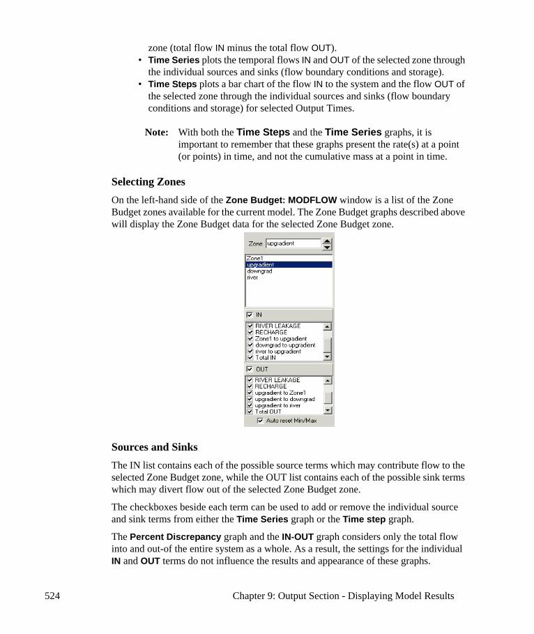
524 Chapter 9: Output Section - Displaying Model Results
zone (total flow IN minus the total flow OUT).• Time Series plots the temporal flows IN and OUT of the selected zone through
the individual sources and sinks (flow boundary conditions and storage).• Time Steps plots a bar chart of the flow IN to the system and the flow OUT of
the selected zone through the individual sources and sinks (flow boundary conditions and storage) for selected Output Times.
Note: With both the Time Steps and the Time Series graphs, it is important to remember that these graphs present the rate(s) at a point (or points) in time, and not the cumulative mass at a point in time.
Selecting ZonesOn the left-hand side of the Zone Budget: MODFLOW window is a list of the Zone Budget zones available for the current model. The Zone Budget graphs described above will display the Zone Budget data for the selected Zone Budget zone.
Sources and Sinks The IN list contains each of the possible source terms which may contribute flow to the selected Zone Budget zone, while the OUT list contains each of the possible sink terms which may divert flow out of the selected Zone Budget zone.
The checkboxes beside each term can be used to add or remove the individual source and sink terms from either the Time Series graph or the Time step graph.
The Percent Discrepancy graph and the IN-OUT graph considers only the total flow into and out-of the entire system as a whole. As a result, the settings for the individual IN and OUT terms do not influence the results and appearance of these graphs.
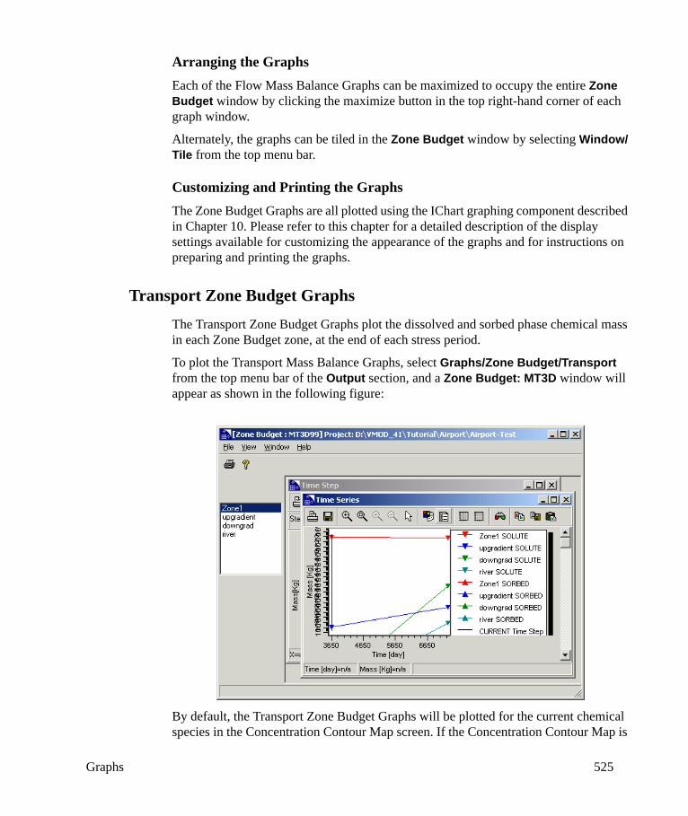
Graphs 525
Arranging the GraphsEach of the Flow Mass Balance Graphs can be maximized to occupy the entire Zone Budget window by clicking the maximize button in the top right-hand corner of each graph window.
Alternately, the graphs can be tiled in the Zone Budget window by selecting Window/Tile from the top menu bar.
Customizing and Printing the GraphsThe Zone Budget Graphs are all plotted using the IChart graphing component described in Chapter 10. Please refer to this chapter for a detailed description of the display settings available for customizing the appearance of the graphs and for instructions on preparing and printing the graphs.
Transport Zone Budget Graphs
The Transport Zone Budget Graphs plot the dissolved and sorbed phase chemical mass in each Zone Budget zone, at the end of each stress period.
To plot the Transport Mass Balance Graphs, select Graphs/Zone Budget/Transport from the top menu bar of the Output section, and a Zone Budget: MT3D window will appear as shown in the following figure:
By default, the Transport Zone Budget Graphs will be plotted for the current chemical species in the Concentration Contour Map screen. If the Concentration Contour Map is
526 Chapter 9: Output Section - Displaying Model Results
not being displayed, the Transport Zone Budget Graphs will be plotted for the first chemical in the species list. To select a different chemical species, open the Concentration Contour Map and use the [Species] button to select a new Chemical Species.
There are two different Transport Zone Budget Graphs:
Time Series: Plots the cumulative chemical mass dissolved (SOLUTE) and sorbed (SORBED) in each Zone Budget zone.
Time Step: Plots a bar chart of the cumulative mass dissolved (SOLUTE) and sorbed (SORBED) in each Zone Budget zone for selected Output Times.
Note: With both the Time Steps and the Time Series graphs, it is important to remember that these graphs present the rate(s) at a point (or points) in time, and not the cumulative mass at a point in time.
Note: Transport Zone Budget graphs are only available when the MT3D96 (not available for new projects/variants) or MT3D99 transport engines are used.
Arranging the GraphsThe Transport Zone Budget Graphs can be maximized to occupy the entire Zone Budget window by clicking the maximize button in the top right-hand corner of each graph window.
Alternately, the graphs can be tiled in the Zone Budget window by selecting Window/Tile from the top menu bar.
Customizing and Printing the GraphsThe Transport Zone Budget Graphs are all plotted using the IChart graphing component described in Chapter 10. Please refer to this chapter for a detailed description of the display options available for customizing the appearance of the graphs, and for instructions on preparing and printing the graphs.
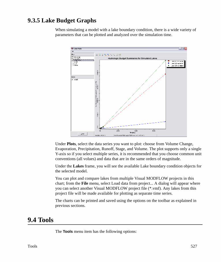
Tools 527
9.3.5 Lake Budget GraphsWhen simulating a model with a lake boundary condition, there is a wide variety of parameters that can be plotted and analyzed over the simulation time.
Under Plots, select the data series you want to plot: choose from Volume Change, Evaporation, Precipitation, Runoff, Stage, and Volume. The plot supports only a single Y-axis so if you select multiple series, it is recommended that you choose common unit conventions (all volues) and data that are in the same orders of magnitude.
Under the Lakes frame, you will see the available Lake boundary condition objects for the selected model.
You can plot and compare lakes from multiple Visual MODFLOW projects in this chart; from the File menu, select Load data from project... A dialog will appear where you can select another Visual MODFLOW project file (*.vmf). Any lakes from this project file will be made available for plotting as separate time series.
The charts can be printed and saved using the options on the toolbar as explained in previous sections.
9.4 ToolsThe Tools menu item has the following options:

528 Chapter 9: Output Section - Displaying Model Results
Cell Inspector: Displays the cell values and units for selected model parameters including grid co-ordinates, Kx, Ky, Kz, Ss, Sy, Head, Velocities, Concentration, and other Input and Output parameters.
Annotate: Add lines, shapes, and text to the display screen.
Units Converter: Converts the units of the selected parameters.
Copy Image to Clipboard: Copies screen image to the Windows clipboard
Enviro-Base Pro: Database containing references property values
9.4.1 Cell InspectorThe Cell Inspector feature is described in Chapter 4, “Cell Inspector” on page 291.
9.4.2 AnnotateThe Annotate feature is described in Chapter 4, “Annotate” on page 292.
9.4.3 Units ConverterThe Units Converter feature is described in Chapter 4, “Units Converter” on page 294.
9.4.4 Copy Image to ClipboardThe Copy Image to Clipboard feature is described in Chapter 4, “Copy Image to Clipboard” on page 294.
9.4.5 Enviro-Base ProThe Enviro-Base feature is described in Chapter 4, “Enviro-Base Pro” on page 295.

529
10IChart - Graphing and Mapping Component
IChart is a charting and plotting component developed by Schlumberger Water Services for the purpose of displaying and printing a variety of graph and map formats including:
• X-Y scatter graphs (multiple data series)• Time-series graphs (multiple data series)• Bar charts (multiple data series)• Contour maps (for MODFLOW/MT3D Output Previews)• Color maps (for MODFLOW/MT3D Output Previews)• Particle animation (for MODPATH Output Previews)
The IChart component is used throughout Visual MODFLOW for displaying and presenting the plot types listed above. This chapter describes the features and functionality of IChart under the following topic headings:
• Toolbar Icons• Graph Properties
• Axis Settings• Titles Settings• Series Settings• Legends Settings• Operations Settings• General Settings• Info Settings
• Map Properties• Contour Settings• Color Map Settings
• Annotation Tools• Printing Options• Exporting Data
• Saving to a Graphics File
Any of the “Settings” listed above may be accessed by Right-Clicking mouse anywhere on the display area of the graph.

530 Chapter 10: IChart - Graphing and Mapping Component
10.1 Toolbar IconsThis section describes the functionality of the toolbar icons available from the various IChart plots. The icons are described in the usual order of their appearance (from left to right) in the toolbar. Please note that the available icons are not the same for each type of plot being displayed, so some of the icons described below may not be available (or appropriate) for the current plot being displayed.
Print graphic: Opens the Print options window described on page 543.
Save As... Saves plot to a graphics files (.BMP, .EMF, or .WMF)
Copy to clipboard: Copies a bitmap image of the plot to the clipboard.
Export Data: Exports selected data series to an ASCII text file as described on page 548.
Pointer: Click on a plot to display info for a selected data point, or a selected location on the plot.
Zoom in: Zoom in on a selected region of the plot.
Animated zoom: Animated zoom in to a selected location.
Zoom previous: Zoom out to the previous zoom setting.
Zoom Out: Zoom out to view the entire plot area.
Graph Properties: Opens the Graph Properties window, as described in“Graph Properties” on page 531
Show legend: Shows/hides the legend for the plot.
Vertical grid: Displays vertical grid lines at each major tick on the X-axis.
Horizontal grid: Displays horizontal grid lines at each major tick on theY-axis.
3D-view: Creates a 3D view of the graph axes and data series.
Refresh: Refreshes the display of the graph.
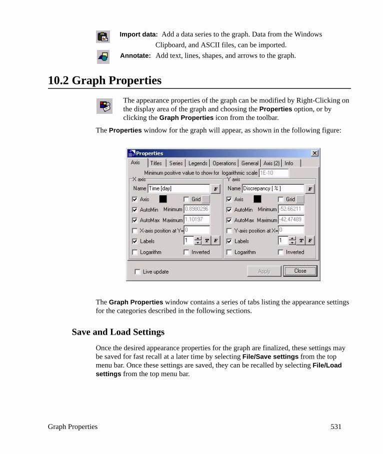
Graph Properties 531
Import data: Add a data series to the graph. Data from the Windows Clipboard, and ASCII files, can be imported.
Annotate: Add text, lines, shapes, and arrows to the graph.
10.2 Graph PropertiesThe appearance properties of the graph can be modified by Right-Clicking on the display area of the graph and choosing the Properties option, or by clicking the Graph Properties icon from the toolbar.
The Properties window for the graph will appear, as shown in the following figure:
The Graph Properties window contains a series of tabs listing the appearance settings for the categories described in the following sections.
Save and Load Settings
Once the desired appearance properties for the graph are finalized, these settings may be saved for fast recall at a later time by selecting File/Save settings from the top menu bar. Once these settings are saved, they can be recalled by selecting File/Load settings from the top menu bar.

532 Chapter 10: IChart - Graphing and Mapping Component
10.2.1 Axis SettingsThe Axis settings tab (see preceding figure) controls the appearance of the X and Y axes on the graph, including the axis title, minimum and maximum axis values, tick mark labels, and scale.
The Axis switch shows/hides the axis line, ticks and labels. The color box beside the Axis switch is used to select the color of the axis line.
The Grid switch hides/shows the grid lines for each tick along the axis. The color box beside the Grid switch is used to select the color of the grid lines.
The Minimum positive value to show for logarithmic scale is used when switching either axis from a normal scale to a logarithmic scale. This value is used as a default minimum value for the axis if the normal scale minimum is negative or zero.
The Name field is the label for the axis. This value will be plotted under the X-axis, and to the left of the Y-axis. The [F] button beside the Name field is used to select the font, size and color of the text.
The AutoMin and AutoMax options will automatically determine the minimum and maximum values, respectively, to plot on the axis. These values are displayed in the Minimum and Maximum fields. If the AutoMin and AutoMax fields are not selected, then user-defined Minimum and Maximum values may be entered.
The X-axis position option defines the Y value where the X-axis will be plotted through the graph. The default setting is to plot the X-axis corresponding the Minimum value of the Y-axis.
The Labels option defines the frequency of tick labels. A value of 1 will label each major tick mark along the axis. A value of 2 will label every 2nd major tick mark. The [T] button opens a Tick Properties window for setting the display options for the Major Ticks and Minor Ticks.
The Logarithm switch changes the axis scale from a normal scale to a logarithmic scale.
The Inverted switch changes the location of the Minimum and Maximum values on the axis. The default axis setting is for the Y-axis to increase from bottom to top, and the X-
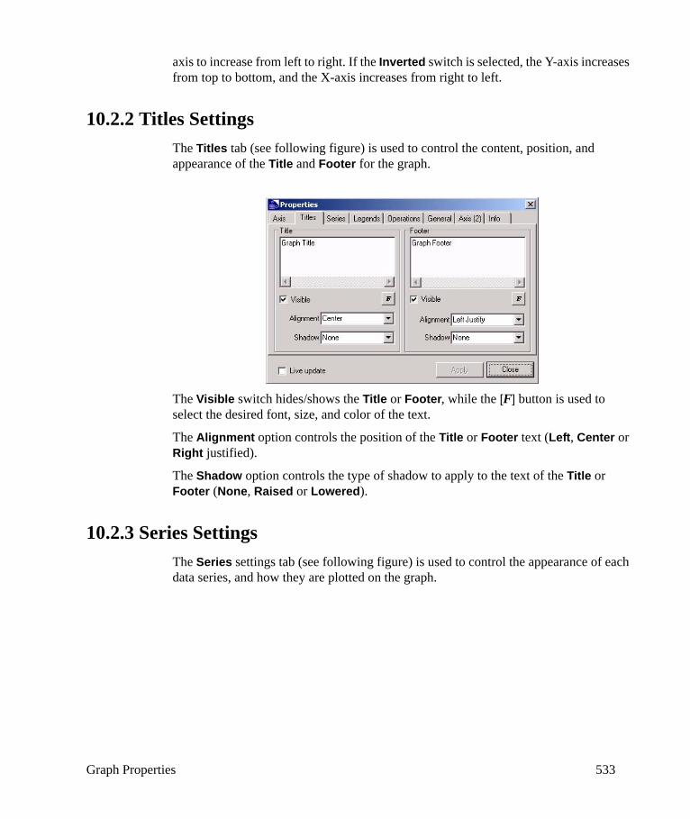
Graph Properties 533
axis to increase from left to right. If the Inverted switch is selected, the Y-axis increases from top to bottom, and the X-axis increases from right to left.
10.2.2 Titles SettingsThe Titles tab (see following figure) is used to control the content, position, and appearance of the Title and Footer for the graph.
The Visible switch hides/shows the Title or Footer, while the [F] button is used to select the desired font, size, and color of the text.
The Alignment option controls the position of the Title or Footer text (Left, Center or Right justified).
The Shadow option controls the type of shadow to apply to the text of the Title or Footer (None, Raised or Lowered).
10.2.3 Series SettingsThe Series settings tab (see following figure) is used to control the appearance of each data series, and how they are plotted on the graph.
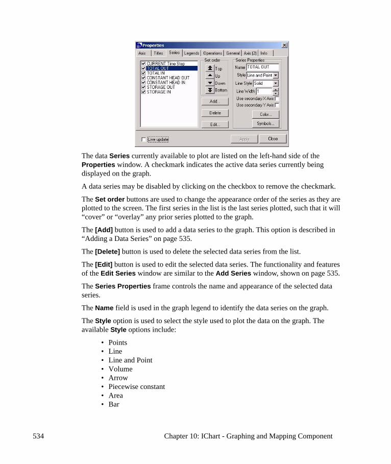
534 Chapter 10: IChart - Graphing and Mapping Component
The data Series currently available to plot are listed on the left-hand side of the Properties window. A checkmark indicates the active data series currently being displayed on the graph.
A data series may be disabled by clicking on the checkbox to remove the checkmark.
The Set order buttons are used to change the appearance order of the series as they are plotted to the screen. The first series in the list is the last series plotted, such that it will “cover” or “overlay” any prior series plotted to the graph.
The [Add] button is used to add a data series to the graph. This option is described in “Adding a Data Series” on page 535.
The [Delete] button is used to delete the selected data series from the list.
The [Edit] button is used to edit the selected data series. The functionality and features of the Edit Series window are similar to the Add Series window, shown on page 535.
The Series Properties frame controls the name and appearance of the selected data series.
The Name field is used in the graph legend to identify the data series on the graph.
The Style option is used to select the style used to plot the data on the graph. The available Style options include:
• Points• Line• Line and Point• Volume• Arrow• Piecewise constant• Area• Bar
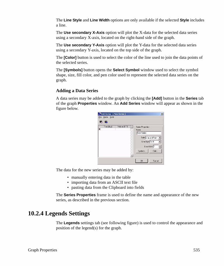
Graph Properties 535
The Line Style and Line Width options are only available if the selected Style includes a line.
The Use secondary X-Axis option will plot the X-data for the selected data series using a secondary X-axis, located on the right-hand side of the graph.
The Use secondary Y-Axis option will plot the Y-data for the selected data series using a secondary Y-axis, located on the top side of the graph.
The [Color] button is used to select the color of the line used to join the data points of the selected series.
The [Symbols] button opens the Select Symbol window used to select the symbol shape, size, fill color, and pen color used to represent the selected data series on the graph.
Adding a Data SeriesA data series may be added to the graph by clicking the [Add] button in the Series tab of the graph Properties window. An Add Series window will appear as shown in the figure below.
The data for the new series may be added by:
• manually entering data in the table• importing data from an ASCII text file• pasting data from the Clipboard into fields
The Series Properties frame is used to define the name and appearance of the new series, as described in the previous section.
10.2.4 Legends SettingsThe Legends settings tab (see following figure) is used to control the appearance and position of the legend(s) for the graph.
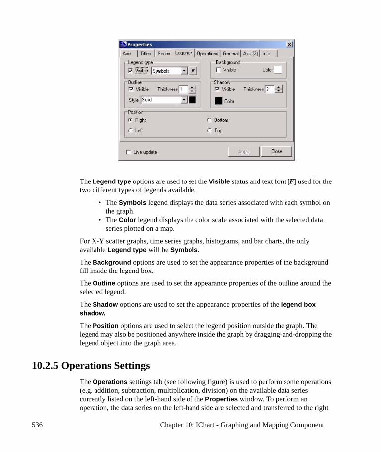
536 Chapter 10: IChart - Graphing and Mapping Component
The Legend type options are used to set the Visible status and text font [F] used for the two different types of legends available.
• The Symbols legend displays the data series associated with each symbol on the graph.
• The Color legend displays the color scale associated with the selected data series plotted on a map.
For X-Y scatter graphs, time series graphs, histograms, and bar charts, the only available Legend type will be Symbols.
The Background options are used to set the appearance properties of the background fill inside the legend box.
The Outline options are used to set the appearance properties of the outline around the selected legend.
The Shadow options are used to set the appearance properties of the legend box shadow.
The Position options are used to select the legend position outside the graph. The legend may also be positioned anywhere inside the graph by dragging-and-dropping the legend object into the graph area.
10.2.5 Operations SettingsThe Operations settings tab (see following figure) is used to perform some operations (e.g. addition, subtraction, multiplication, division) on the available data series currently listed on the left-hand side of the Properties window. To perform an operation, the data series on the left-hand side are selected and transferred to the right
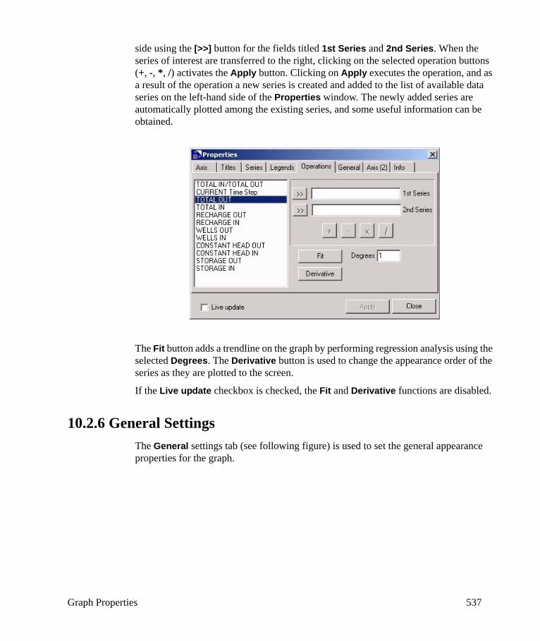
Graph Properties 537
side using the [>>] button for the fields titled 1st Series and 2nd Series. When the series of interest are transferred to the right, clicking on the selected operation buttons (+, -, *, /) activates the Apply button. Clicking on Apply executes the operation, and as a result of the operation a new series is created and added to the list of available data series on the left-hand side of the Properties window. The newly added series are automatically plotted among the existing series, and some useful information can be obtained.
The Fit button adds a trendline on the graph by performing regression analysis using the selected Degrees. The Derivative button is used to change the appearance order of the series as they are plotted to the screen.
If the Live update checkbox is checked, the Fit and Derivative functions are disabled.
10.2.6 General SettingsThe General settings tab (see following figure) is used to set the general appearance properties for the graph.
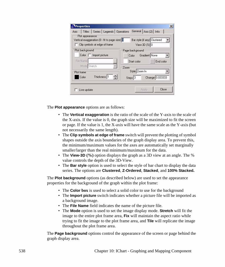
538 Chapter 10: IChart - Graphing and Mapping Component
The Plot appearance options are as follows:
• The Vertical exaggeration is the ratio of the scale of the Y-axis to the scale of the X-axis. If the value is 0, the graph size will be maximized to fit the screen or page. If the value is 1, the X-axis will have the same scale as the Y-axis (but not necessarily the same length).
• The Clip symbols at edge of frame switch will prevent the plotting of symbol shapes outside the axis boundaries of the graph display area. To prevent this, the minimum/maximum values for the axes are automatically set marginally smaller/larger than the real minimum/maximum for the data.
• The View-3D (%) option displays the graph as a 3D view at an angle. The % value controls the depth of the 3D-View.
• The Bar style option is used to select the style of bar chart to display the data series. The options are Clustered, Z-Ordered, Stacked, and 100% Stacked.
The Plot background options (as described below) are used to set the appearance properties for the background of the graph within the plot frame:
• The Color box is used to select a solid color to use for the background• The Import picture switch indicates whether a picture file will be imported as
a background image.• The File Name field indicates the name of the picture file.• The Mode option is used to set the image display mode. Stretch will fit the
image to the entire plot frame area, Fix will maintain the aspect ratio while trying to fit the image to the plot frame area, and Tile will replicate the image throughout the plot frame area.
The Page background options control the appearance of the screen or page behind the graph display area.

Graph Properties 539
• The Color box is used to select a solid color (only applicable if Gradient = None).
• The Gradient option is used to select the direction of the color gradient (options are either None, Left-Right or Top-Bottom).
• The Start color box is used to select the starting gradient color.• The End color box is used to select the end gradient color.
The Plot frame options are used to set the appearance properties of the outline around the plot frame.
The Zoom options control the operation of the animated Zoom In and Zoom Out features.
10.2.7 Info SettingsThe Info settings tab (see following figure) is used to set the appearance properties for the information tags of selected data points. These tags can be displayed by clicking on a data point in the graph.
The Tag Settings options are used to set the appearance properties of the information tags on selected data point.
The Style option is used to select from a list of shapes for each tag (options include Rectangle, Round Rectangle, and No Bubble).
The Position option is used to select the preferred position of the label relative to the data point (options include Right Top, Top Center, Right Bottom, Left Top, Bottom Center and Left Bottom).
The [Color] button is used to select the fill color for the selected label shape.
The [Font] button is used to select the font, size, and color of the label text.
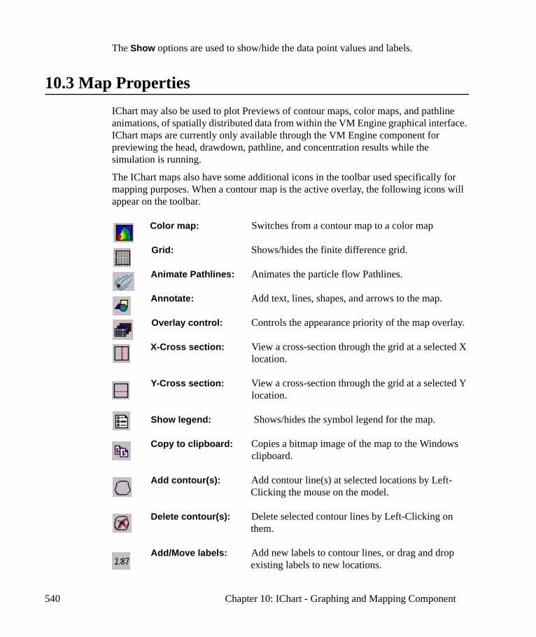
540 Chapter 10: IChart - Graphing and Mapping Component
The Show options are used to show/hide the data point values and labels.
10.3 Map PropertiesIChart may also be used to plot Previews of contour maps, color maps, and pathline animations, of spatially distributed data from within the VM Engine graphical interface. IChart maps are currently only available through the VM Engine component for previewing the head, drawdown, pathline, and concentration results while the simulation is running.
The IChart maps also have some additional icons in the toolbar used specifically for mapping purposes. When a contour map is the active overlay, the following icons will appear on the toolbar.
Color map: Switches from a contour map to a color map
Grid: Shows/hides the finite difference grid.
Animate Pathlines: Animates the particle flow Pathlines.
Annotate: Add text, lines, shapes, and arrows to the map.
Overlay control: Controls the appearance priority of the map overlay.
X-Cross section: View a cross-section through the grid at a selected X location.
Y-Cross section: View a cross-section through the grid at a selected Y location.
Show legend: Shows/hides the symbol legend for the map.
Copy to clipboard: Copies a bitmap image of the map to the Windows clipboard.
Add contour(s): Add contour line(s) at selected locations by Left-Clicking the mouse on the model.
Delete contour(s): Delete selected contour lines by Left-Clicking on them.
Add/Move labels: Add new labels to contour lines, or drag and drop existing labels to new locations.

Map Properties 541
10.3.1 Contour SettingsThe Contour settings tab is used to set the appearance properties for the contour lines and labels.
The Range of values options are used to set the minimum and maximum contour line values. If the Auto switch is selected, the Minimum/Maximum value for the first contour line will be automatically determined from the Real Min./Real Max. values.
The Lines options are used to select the increment method used to automatically calculate the contour line values to plot on the map.
• The Automatic intervals switch will show/hide the automatic contour line values.
• The Number of intervals option will plot a fixed number (N) of contour lines equivalent to the number of intervals. The increment value is calculated taking the different between the Minimum and Maximum contour values and dividing the result by (N-2).
• The Interval value option specifies the contour increment value.• The Color option is used to set the color of the contour lines. The Mono Color
option will color all contour lines the same color, while the Color Shading option will plot the contour lines using colors which are scaled according to the contour value.
The Labels option is used to set the appearance properties of the contour line labels.
• The Visible switch shows/hides labels.• The font [F] button is used to select the font, size, and color of the labels.• The Decimal places option defines the number of decimal places for each label.• The Labels Interval option labels every Nth contour line.
The Manual Levels table is used to enter custom contour line values.
• The Visible checkbox displays/hides the custom contour values.

542 Chapter 10: IChart - Graphing and Mapping Component
10.3.2 Color Map SettingsThe Color Map settings tab (see following figure) is used to set the appearance properties for the color map.
The Transparent switch will set the color map to be semi-transparent, such that other features of the model will be visible through the color map.
The Zebra switch will remove the gradation between the different colored zones, to display seven distinct colored zones.
The Quality options are used to select the quality of the color map. High Quality looks the best, but it takes longer to render and print.
The Palette options are used to select the colors for the map.
The Range of values option is used to define the minimum and maximum limits of the values plotted. Any values outside of this range will be “clipped” (removed) from the map display.
10.4 Annotation ToolsThe image annotation options can be accessed by selecting the Annotate icon from the top toolbar of different graphs in the output section. A floating Annotate Tools window will appear on the screen, as shown in the following figure:
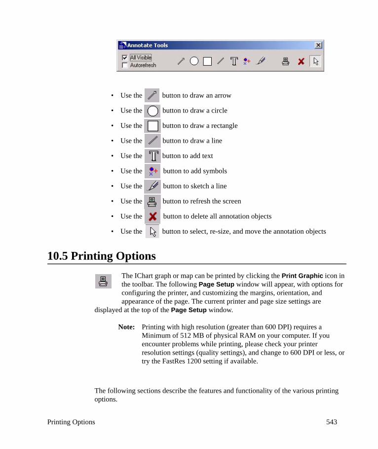
Printing Options 543
• Use the button to draw an arrow
• Use the button to draw a circle
• Use the button to draw a rectangle
• Use the button to draw a line
• Use the button to add text
• Use the button to add symbols
• Use the button to sketch a line
• Use the button to refresh the screen
• Use the button to delete all annotation objects
• Use the button to select, re-size, and move the annotation objects
10.5 Printing OptionsThe IChart graph or map can be printed by clicking the Print Graphic icon in the toolbar. The following Page Setup window will appear, with options for configuring the printer, and customizing the margins, orientation, and appearance of the page. The current printer and page size settings are
displayed at the top of the Page Setup window.
Note: Printing with high resolution (greater than 600 DPI) requires a Minimum of 512 MB of physical RAM on your computer. If you encounter problems while printing, please check your printer resolution settings (quality settings), and change to 600 DPI or less, or try the FastRes 1200 setting if available.
The following sections describe the features and functionality of the various printing options.
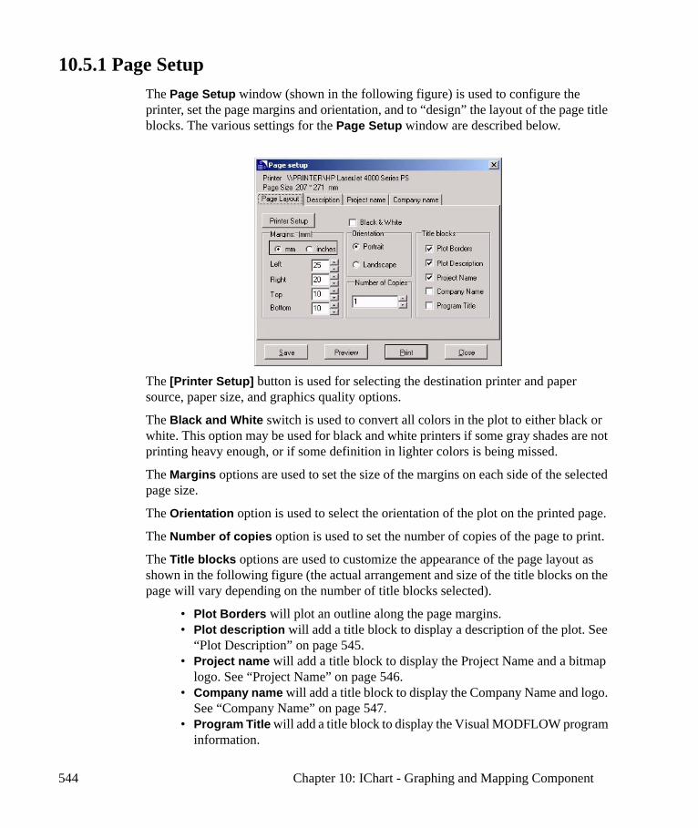
544 Chapter 10: IChart - Graphing and Mapping Component
10.5.1 Page SetupThe Page Setup window (shown in the following figure) is used to configure the printer, set the page margins and orientation, and to “design” the layout of the page title blocks. The various settings for the Page Setup window are described below.
The [Printer Setup] button is used for selecting the destination printer and paper source, paper size, and graphics quality options.
The Black and White switch is used to convert all colors in the plot to either black or white. This option may be used for black and white printers if some gray shades are not printing heavy enough, or if some definition in lighter colors is being missed.
The Margins options are used to set the size of the margins on each side of the selected page size.
The Orientation option is used to select the orientation of the plot on the printed page.
The Number of copies option is used to set the number of copies of the page to print.
The Title blocks options are used to customize the appearance of the page layout as shown in the following figure (the actual arrangement and size of the title blocks on the page will vary depending on the number of title blocks selected).
• Plot Borders will plot an outline along the page margins.• Plot description will add a title block to display a description of the plot. See
“Plot Description” on page 545.• Project name will add a title block to display the Project Name and a bitmap
logo. See “Project Name” on page 546.• Company name will add a title block to display the Company Name and logo.
See “Company Name” on page 547.• Program Title will add a title block to display the Visual MODFLOW program
information.
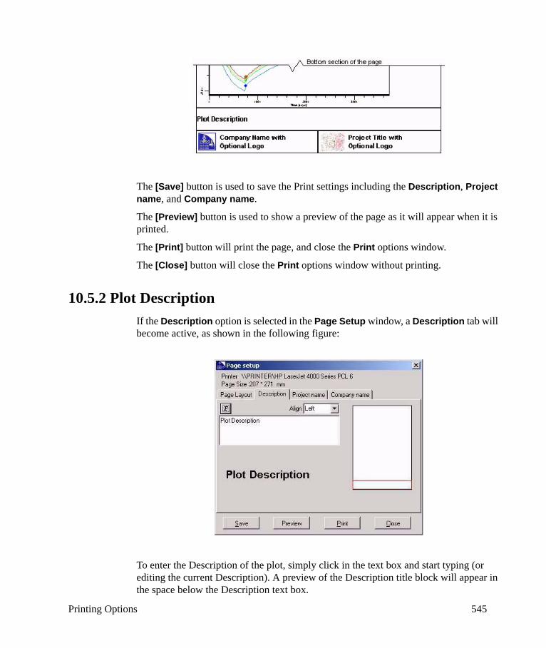
Printing Options 545
The [Save] button is used to save the Print settings including the Description, Project name, and Company name.
The [Preview] button is used to show a preview of the page as it will appear when it is printed.
The [Print] button will print the page, and close the Print options window.
The [Close] button will close the Print options window without printing.
10.5.2 Plot DescriptionIf the Description option is selected in the Page Setup window, a Description tab will become active, as shown in the following figure:
To enter the Description of the plot, simply click in the text box and start typing (or editing the current Description). A preview of the Description title block will appear in the space below the Description text box.
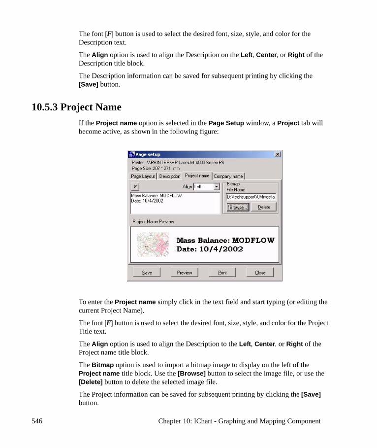
546 Chapter 10: IChart - Graphing and Mapping Component
The font [F] button is used to select the desired font, size, style, and color for the Description text.
The Align option is used to align the Description on the Left, Center, or Right of the Description title block.
The Description information can be saved for subsequent printing by clicking the [Save] button.
10.5.3 Project NameIf the Project name option is selected in the Page Setup window, a Project tab will become active, as shown in the following figure:
To enter the Project name simply click in the text field and start typing (or editing the current Project Name).
The font [F] button is used to select the desired font, size, style, and color for the Project Title text.
The Align option is used to align the Description to the Left, Center, or Right of the Project name title block.
The Bitmap option is used to import a bitmap image to display on the left of the Project name title block. Use the [Browse] button to select the image file, or use the [Delete] button to delete the selected image file.
The Project information can be saved for subsequent printing by clicking the [Save] button.
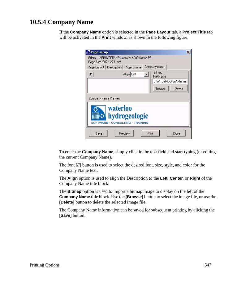
Printing Options 547
10.5.4 Company NameIf the Company Name option is selected in the Page Layout tab, a Project Title tab will be activated in the Print window, as shown in the following figure:
To enter the Company Name, simply click in the text field and start typing (or editing the current Company Name).
The font [F] button is used to select the desired font, size, style, and color for the Company Name text.
The Align option is used to align the Description to the Left, Center, or Right of the Company Name title block.
The Bitmap option is used to import a bitmap image to display on the left of the Company Name title block. Use the [Browse] button to select the image file, or use the [Delete] button to delete the selected image file.
The Company Name information can be saved for subsequent printing by clicking the [Save] button.
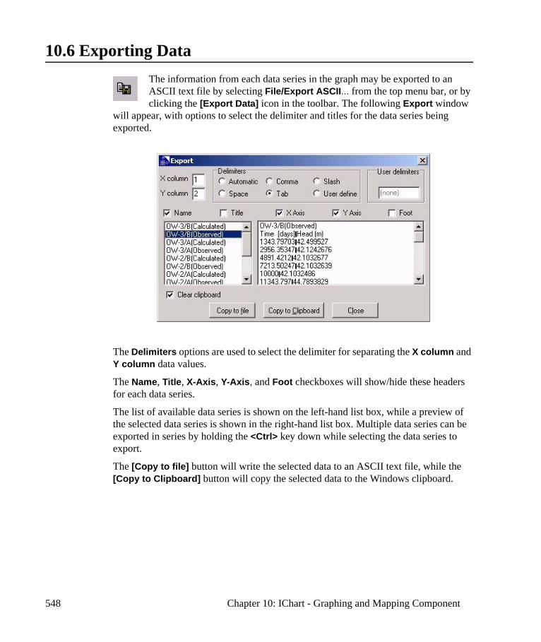
548 Chapter 10: IChart - Graphing and Mapping Component
10.6 Exporting DataThe information from each data series in the graph may be exported to an ASCII text file by selecting File/Export ASCII... from the top menu bar, or by clicking the [Export Data] icon in the toolbar. The following Export window
will appear, with options to select the delimiter and titles for the data series being exported.
The Delimiters options are used to select the delimiter for separating the X column and Y column data values.
The Name, Title, X-Axis, Y-Axis, and Foot checkboxes will show/hide these headers for each data series.
The list of available data series is shown on the left-hand list box, while a preview of the selected data series is shown in the right-hand list box. Multiple data series can be exported in series by holding the <Ctrl> key down while selecting the data series to export.
The [Copy to file] button will write the selected data to an ASCII text file, while the [Copy to Clipboard] button will copy the selected data to the Windows clipboard.
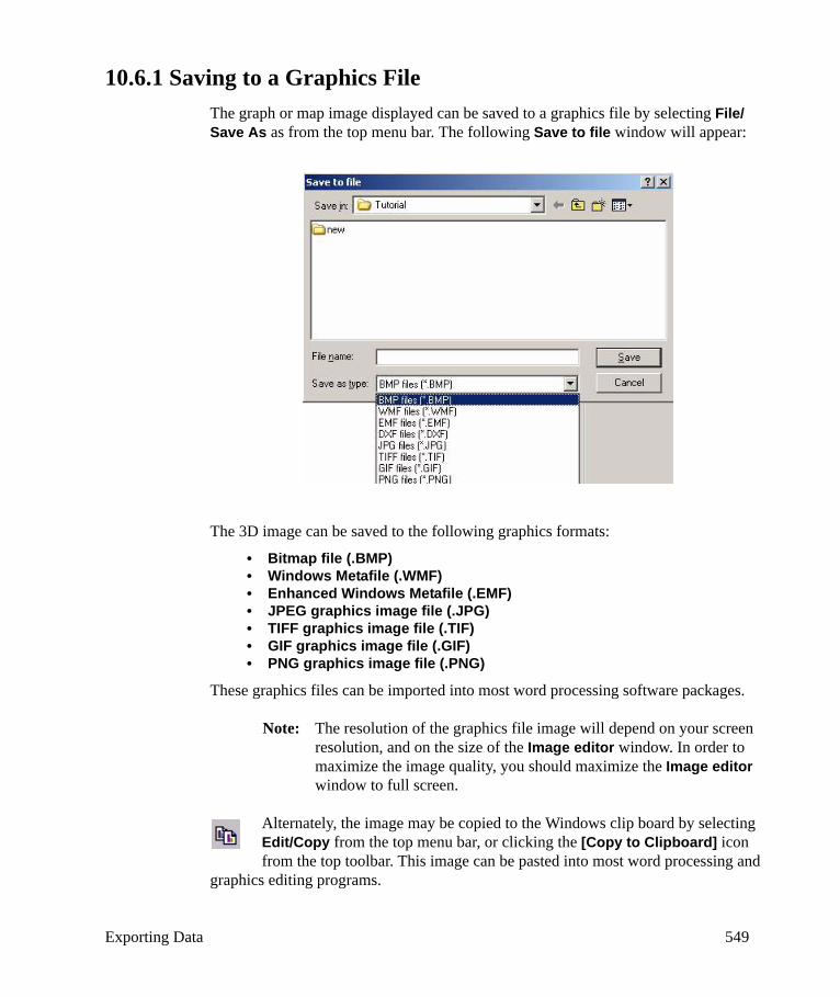
Exporting Data 549
10.6.1 Saving to a Graphics FileThe graph or map image displayed can be saved to a graphics file by selecting File/Save As as from the top menu bar. The following Save to file window will appear:
The 3D image can be saved to the following graphics formats:
• Bitmap file (.BMP)• Windows Metafile (.WMF)• Enhanced Windows Metafile (.EMF)• JPEG graphics image file (.JPG)• TIFF graphics image file (.TIF)• GIF graphics image file (.GIF)• PNG graphics image file (.PNG)
These graphics files can be imported into most word processing software packages.
Note: The resolution of the graphics file image will depend on your screen resolution, and on the size of the Image editor window. In order to maximize the image quality, you should maximize the Image editor window to full screen.
Alternately, the image may be copied to the Windows clip board by selecting Edit/Copy from the top menu bar, or clicking the [Copy to Clipboard] icon from the top toolbar. This image can be pasted into most word processing and
graphics editing programs.

550 Chapter 10: IChart - Graphing and Mapping Component
551
11Visual MODFLOW 3D-Explorer
Visual MODFLOW 3D-Explorer is an advanced three-dimensional visualization and animation component for displaying and presenting groundwater flow, pathlines, and contaminant transport modeling data, using a variety of three-dimensional graphical formats. The data structure is similar to that used by Visual MODFLOW. The graphical tools and presentation formats available are specifically designed for groundwater modeling applications. Visual MODFLOW 3D-Explorer uses state-of-the-art 3D graphics technology to display your model data and simulation results, using a complete selection of graphical formats including:
• 2D and 3D views of the model grid• Colored shapes for each grid cell• Bitmap overlays on surfaces• Enhanced contour label positioning and controls• 3D volumetric shapes for representing model property zones, boundary
conditions, and contamination plumes• Output times are synchronized to animate the combined transient flow and
transport results• 3D cutaway views• Multiple horizontal slices, vertical slices, and irregular cross-sections for
plotting contour line maps, and color maps of modeling results and model properties (heads, concentrations, water table, conductivity values, etc.)
• Concentration plumes are automatically clipped above the water table surface• Line elements for representing groundwater flow pathlines• Light source position control• Transparent objects• Animation sequence pausing, looping, and recording to an AVI file• Auto-rotate tools continuously rotate the model image around the X, Y, Z axis• and much more
This chapter provides a detailed description of the features and functionality of the various options for preparing and customizing a three-dimensional presentation of groundwater modeling data. The sections of this chapter are presented as follows:
552 Chapter 11: Visual MODFLOW 3D-Explorer
• Getting Started - see page 552• Model Elements and Display Settings - see page 561• Creating Slices and Cross-Sections - see page 588• Creating Cut-aways - see page 593• Creating an Animation - see page 594• Saving Scene Configurations - see page 596• Printing Options - see page 598• Saving to Graphics Files - see page 597
11.1 Getting StartedVisual MODFLOW 3D-Explorer (VMOD 3D-Explorer) is designed for the 3D visualization and animation of Visual MODFLOW projects. VMOD 3D-Explorer can be started directly from within the Visual MODFLOW environment, or as a “stand alone” application without Visual MODFLOW running.
Note: The 3D-Explorer component is included with the Pro and Premium versions of Visual MODFLOW. If you do not have the 3D-Explorer component included with your software, please contact SWS’ Sales department for information on upgrading your software.
Opening VMOD 3D-ExplorerTo start VMOD 3D-Explorer directly from Visual MODFLOW, click the [F2-3D] button located on the lower toolbar of the Visual MODFLOW interface. This will open VMOD 3D-Explorer in a separate window, and will load the active Visual MODFLOW project.
To start VMOD 3D-Explorer as a stand-alone application running outside of Visual MODFLOW, navigate through the Windows Start menu by selecting Start/Programs/SWS Software/Visual MODFLOW/ Visual MODFLOW 3D-Explorer. This will start VMOD 3D-Explorer without any project loaded.
To load a project, select File/Open from the top menu bar and navigate to a directory where the desired Visual MODFLOW project (projectname.vmf) is located, or click the [Open project] icon from the top tool bar.
Closing VMOD 3D-ExplorerIf VMOD 3D-Explorer was started directly from Visual MODFLOW, then it should be closed by returning to the Visual MODFLOW interface and clicking the [F2-3D] button again to close the 3D-Explorer window.
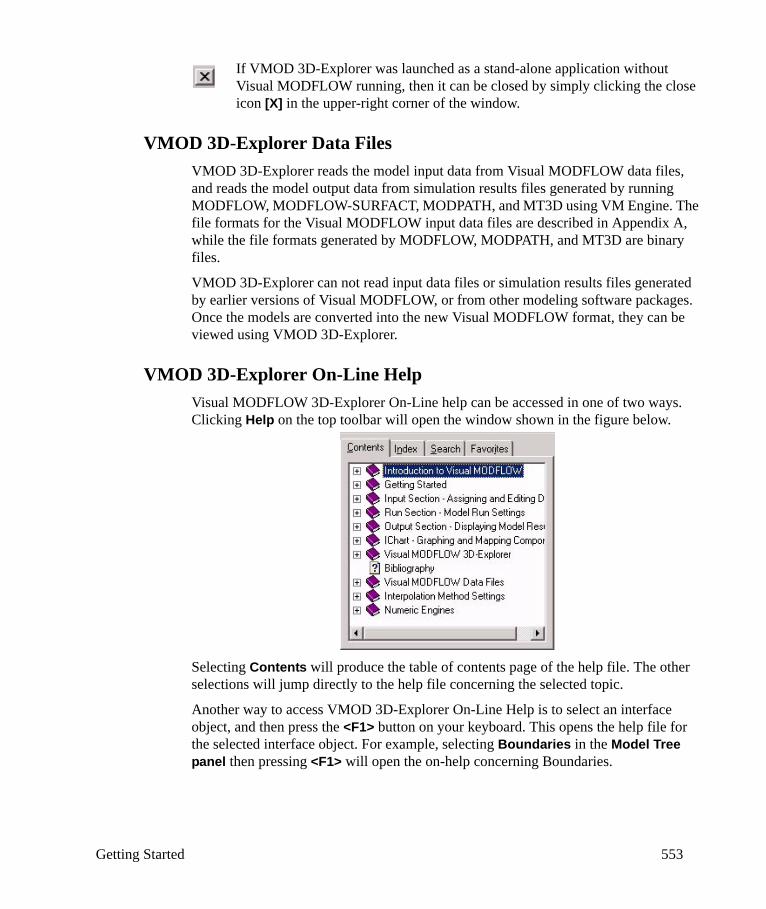
Getting Started 553
If VMOD 3D-Explorer was launched as a stand-alone application without Visual MODFLOW running, then it can be closed by simply clicking the close icon [X] in the upper-right corner of the window.
VMOD 3D-Explorer Data FilesVMOD 3D-Explorer reads the model input data from Visual MODFLOW data files, and reads the model output data from simulation results files generated by running MODFLOW, MODFLOW-SURFACT, MODPATH, and MT3D using VM Engine. The file formats for the Visual MODFLOW input data files are described in Appendix A, while the file formats generated by MODFLOW, MODPATH, and MT3D are binary files.
VMOD 3D-Explorer can not read input data files or simulation results files generated by earlier versions of Visual MODFLOW, or from other modeling software packages. Once the models are converted into the new Visual MODFLOW format, they can be viewed using VMOD 3D-Explorer.
VMOD 3D-Explorer On-Line HelpVisual MODFLOW 3D-Explorer On-Line help can be accessed in one of two ways. Clicking Help on the top toolbar will open the window shown in the figure below.
Selecting Contents will produce the table of contents page of the help file. The other selections will jump directly to the help file concerning the selected topic.
Another way to access VMOD 3D-Explorer On-Line Help is to select an interface object, and then press the <F1> button on your keyboard. This opens the help file for the selected interface object. For example, selecting Boundaries in the Model Tree panel then pressing <F1> will open the on-help concerning Boundaries.
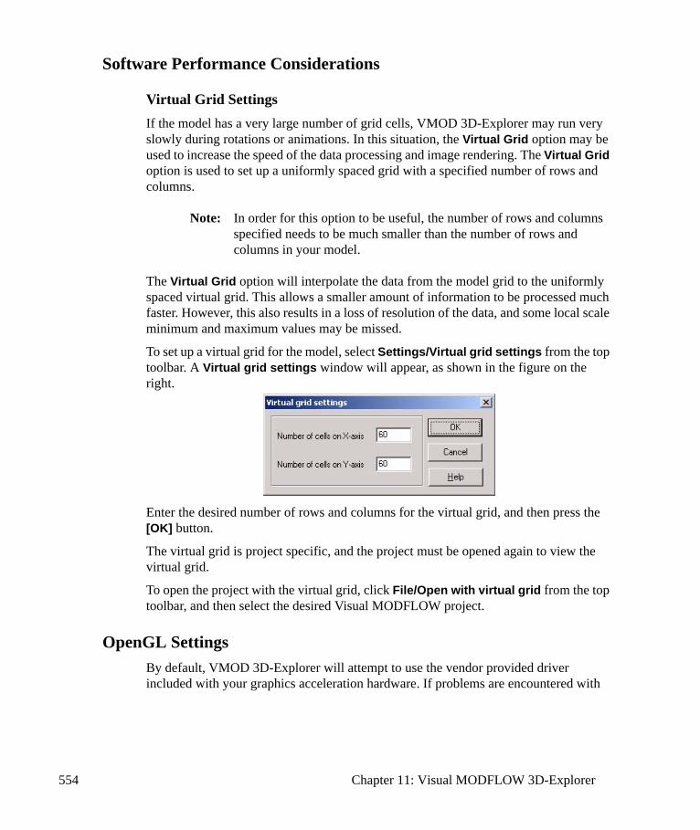
554 Chapter 11: Visual MODFLOW 3D-Explorer
Software Performance Considerations
Virtual Grid SettingsIf the model has a very large number of grid cells, VMOD 3D-Explorer may run very slowly during rotations or animations. In this situation, the Virtual Grid option may be used to increase the speed of the data processing and image rendering. The Virtual Grid option is used to set up a uniformly spaced grid with a specified number of rows and columns.
Note: In order for this option to be useful, the number of rows and columns specified needs to be much smaller than the number of rows and columns in your model.
The Virtual Grid option will interpolate the data from the model grid to the uniformly spaced virtual grid. This allows a smaller amount of information to be processed much faster. However, this also results in a loss of resolution of the data, and some local scale minimum and maximum values may be missed.
To set up a virtual grid for the model, select Settings/Virtual grid settings from the top toolbar. A Virtual grid settings window will appear, as shown in the figure on the right.
Enter the desired number of rows and columns for the virtual grid, and then press the [OK] button.
The virtual grid is project specific, and the project must be opened again to view the virtual grid.
To open the project with the virtual grid, click File/Open with virtual grid from the top toolbar, and then select the desired Visual MODFLOW project.
OpenGL SettingsBy default, VMOD 3D-Explorer will attempt to use the vendor provided driver included with your graphics acceleration hardware. If problems are encountered with
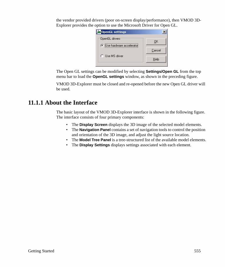
Getting Started 555
the vendor provided drivers (poor on-screen display/performance), then VMOD 3D-Explorer provides the option to use the Microsoft Driver for Open GL.
The Open GL settings can be modified by selecting Settings/Open GL from the top menu bar to load the OpenGL settings window, as shown in the preceding figure.
VMOD 3D-Explorer must be closed and re-opened before the new Open GL driver will be used.
11.1.1 About the InterfaceThe basic layout of the VMOD 3D-Explorer interface is shown in the following figure. The interface consists of four primary components:
• The Display Screen displays the 3D image of the selected model elements.• The Navigation Panel contains a set of navigation tools to control the position
and orientation of the 3D image, and adjust the light source location.• The Model Tree Panel is a tree-structured list of the available model elements.• The Display Settings displays settings associated with each element.
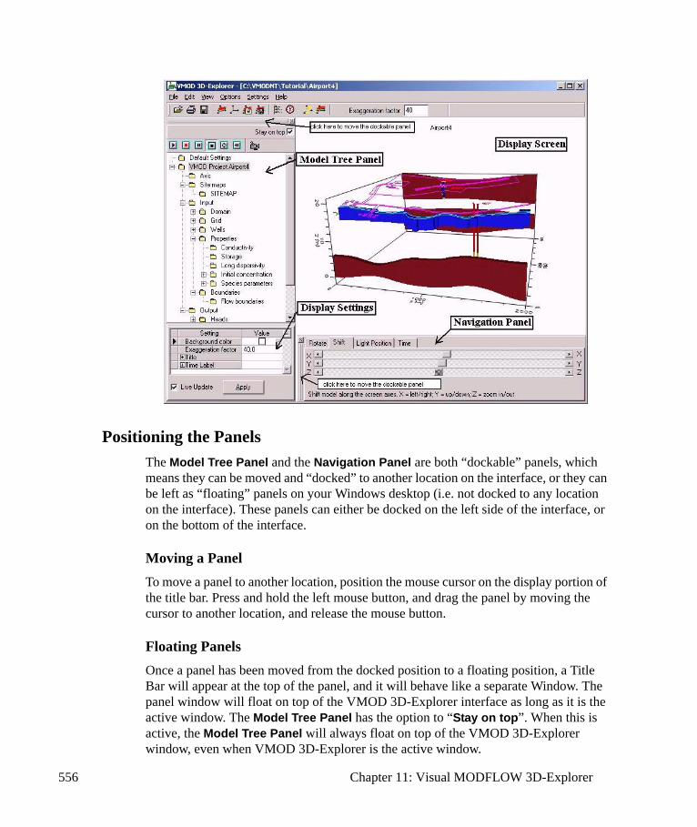
556 Chapter 11: Visual MODFLOW 3D-Explorer
Positioning the PanelsThe Model Tree Panel and the Navigation Panel are both “dockable” panels, which means they can be moved and “docked” to another location on the interface, or they can be left as “floating” panels on your Windows desktop (i.e. not docked to any location on the interface). These panels can either be docked on the left side of the interface, or on the bottom of the interface.
Moving a PanelTo move a panel to another location, position the mouse cursor on the display portion of the title bar. Press and hold the left mouse button, and drag the panel by moving the cursor to another location, and release the mouse button.
Floating PanelsOnce a panel has been moved from the docked position to a floating position, a Title Bar will appear at the top of the panel, and it will behave like a separate Window. The panel window will float on top of the VMOD 3D-Explorer interface as long as it is the active window. The Model Tree Panel has the option to “Stay on top”. When this is active, the Model Tree Panel will always float on top of the VMOD 3D-Explorer window, even when VMOD 3D-Explorer is the active window.

Getting Started 557
Docking PanelsFloating panels can be docked again by clicking the mouse pointer on the panel Title Bar, and dragging it to the left or bottom edge of the VMOD 3D-Explorer window. A grey outline will appear when the mouse pointer is in the proper location and the panel is dockable. Release the mouse button to dock the panel at the desired docking area.
Closing PanelsPanels may be removed from the VMOD 3D-Explorer interface by clicking the close icon. Panels can be re-opened using the View options from the top menu bar.
Exaggeration In Visual MODFLOW, the vertical exaggeration factor is set for viewing cross sections along a row or column. On opening VMOD 3D-Explorer, the exaggeration factor value is read directly from the Visual MODFLOW project, and displayed in the top toolbar of the VMOD 3D-Explorer window, as shown in the following figure:
In VMOD 3D-Explorer, the exaggeration factor can be changed at any time to obtain a more desirable vertical exaggeration of the model.
3D Navigation ToolsThe Navigation Panel should appear on your screen as shown in the following figure. If the Navigation Panel does not appear on the screen, click View/Navigation tools from the top menu bar, and the Navigation Panel should appear on the bottom docking area of the VMOD 3D-Explorer window:
Alternately, the Navigation Panel can be opened by clicking the [Navigation tools] icon located on the top toolbar.
The Navigation tools panel has four tabs:
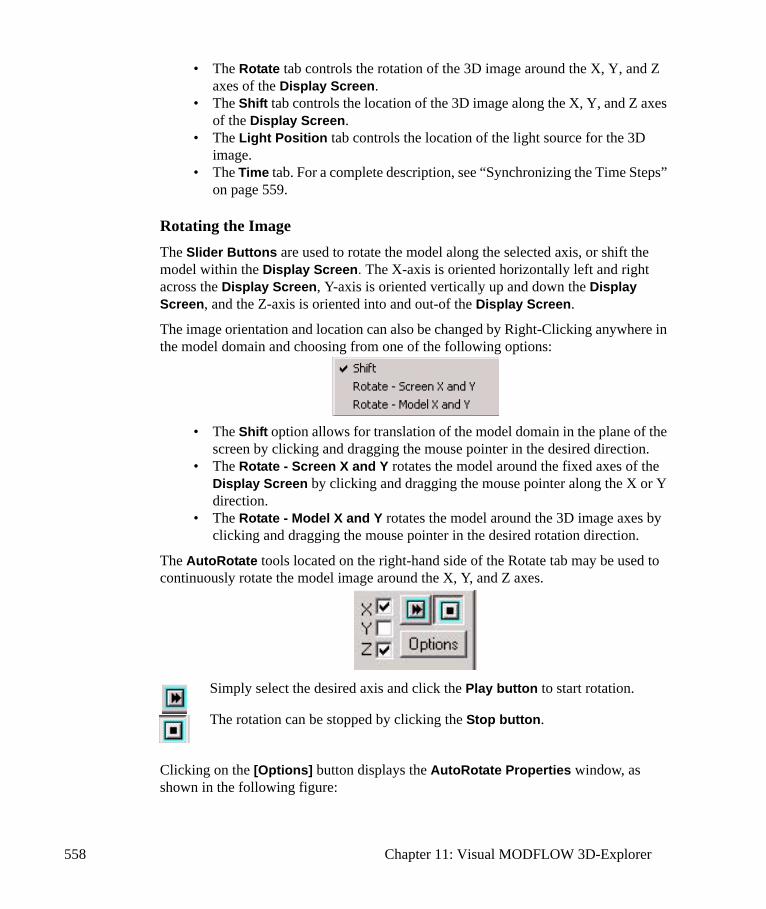
558 Chapter 11: Visual MODFLOW 3D-Explorer
• The Rotate tab controls the rotation of the 3D image around the X, Y, and Z axes of the Display Screen.
• The Shift tab controls the location of the 3D image along the X, Y, and Z axes of the Display Screen.
• The Light Position tab controls the location of the light source for the 3D image.
• The Time tab. For a complete description, see “Synchronizing the Time Steps” on page 559.
Rotating the ImageThe Slider Buttons are used to rotate the model along the selected axis, or shift the model within the Display Screen. The X-axis is oriented horizontally left and right across the Display Screen, Y-axis is oriented vertically up and down the Display Screen, and the Z-axis is oriented into and out-of the Display Screen.
The image orientation and location can also be changed by Right-Clicking anywhere in the model domain and choosing from one of the following options:
• The Shift option allows for translation of the model domain in the plane of the screen by clicking and dragging the mouse pointer in the desired direction.
• The Rotate - Screen X and Y rotates the model around the fixed axes of the Display Screen by clicking and dragging the mouse pointer along the X or Y direction.
• The Rotate - Model X and Y rotates the model around the 3D image axes by clicking and dragging the mouse pointer in the desired rotation direction.
The AutoRotate tools located on the right-hand side of the Rotate tab may be used to continuously rotate the model image around the X, Y, and Z axes.
Simply select the desired axis and click the Play button to start rotation.
The rotation can be stopped by clicking the Stop button.
Clicking on the [Options] button displays the AutoRotate Properties window, as shown in the following figure:

Getting Started 559
Automatic rotation can be performed around the Screen Axes or the Model Axes. The AutoRotate speed may be adjusted by pressing and holding the left mouse button on the Slider Button and setting it to the desired level.
Synchronizing the Time StepsThe Time tab is applicable only for transient flow and transport simulations. It is used to synchronize the Head, Drawdown, and Concentration data for animation purposes.
Most transient flow and transport models will have different output times for the flow simulation results vs. the transport simulation results. Therefore, it is necessary to synchronize these data sets in order to animate the combined flow and transport simulation results.
When the Time tab is selected, the following window appears.
Clicking in the Synchronize time steps checkbox automatically synchronizes the flow and transport data sets, and some additional options will appear:
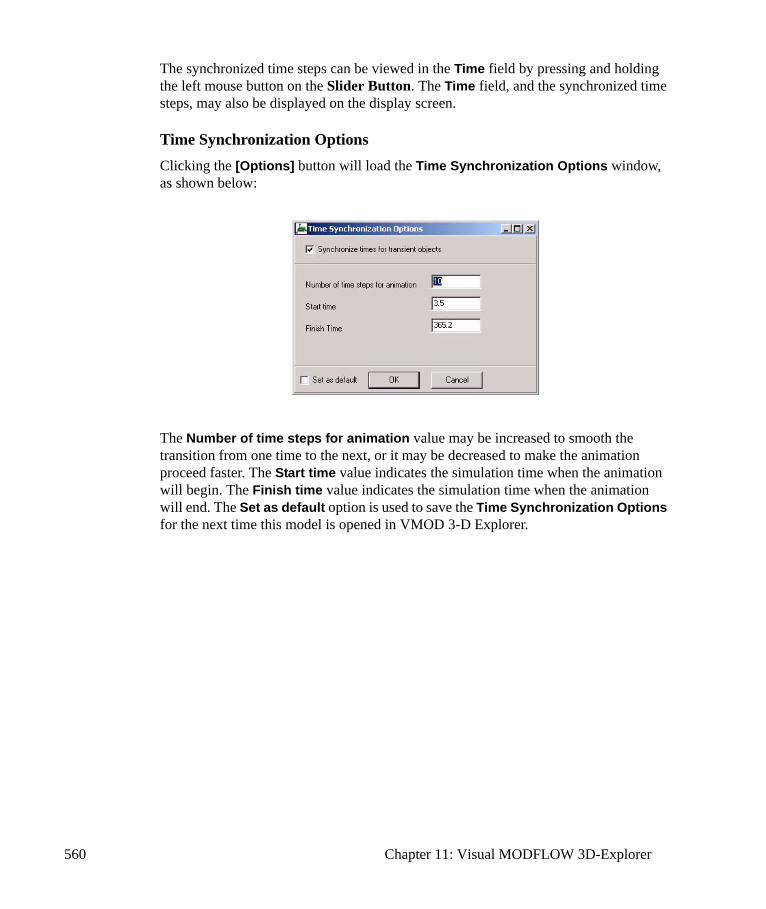
560 Chapter 11: Visual MODFLOW 3D-Explorer
The synchronized time steps can be viewed in the Time field by pressing and holding the left mouse button on the Slider Button. The Time field, and the synchronized time steps, may also be displayed on the display screen.
Time Synchronization OptionsClicking the [Options] button will load the Time Synchronization Options window, as shown below:
The Number of time steps for animation value may be increased to smooth the transition from one time to the next, or it may be decreased to make the animation proceed faster. The Start time value indicates the simulation time when the animation will begin. The Finish time value indicates the simulation time when the animation will end. The Set as default option is used to save the Time Synchronization Options for the next time this model is opened in VMOD 3-D Explorer.
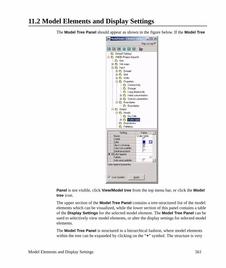
Model Elements and Display Settings 561
11.2 Model Elements and Display SettingsThe Model Tree Panel should appear as shown in the figure below. If the Model Tree
Panel is not visible, click View/Model tree from the top menu bar, or click the Model tree icon.
The upper section of the Model Tree Panel contains a tree-structured list of the model elements which can be visualized, while the lower section of this panel contains a table of the Display Settings for the selected model element. The Model Tree Panel can be used to selectively view model elements, or alter the display settings for selected model elements.
The Model Tree Panel is structured in a hierarchical fashion, where model elements within the tree can be expanded by clicking on the “+” symbol. The structure is very
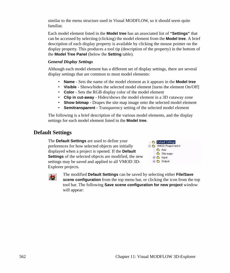
562 Chapter 11: Visual MODFLOW 3D-Explorer
similar to the menu structure used in Visual MODFLOW, so it should seem quite familiar.
Each model element listed in the Model tree has an associated list of “Settings” that can be accessed by selecting (clicking) the model element from the Model tree. A brief description of each display property is available by clicking the mouse pointer on the display property. This produces a tool tip (description of the property) in the bottom of the Model Tree Panel (below the Setting table).
General Display SettingsAlthough each model element has a different set of display settings, there are several display settings that are common to most model elements:
• Name - Sets the name of the model element as it appears in the Model tree• Visible - Shows/hides the selected model element [turns the element On/Off]• Color - Sets the RGB display color of the model element• Clip in cut-away - Hides/shows the model element in a 3D cutaway zone• Show bitmap - Drapes the site map image onto the selected model element• Semitransparent - Transparency setting of the selected model element
The following is a brief description of the various model elements, and the display settings for each model element listed in the Model tree.
Default SettingsThe Default Settings are used to define your preferences for how selected objects are initially displayed when a project is opened. If the Default Settings of the selected objects are modified, the new settings may be saved and applied to all VMOD 3D-Explorer projects.
The modified Default Settings can be saved by selecting either File/Save scene configuration from the top menu bar, or clicking the icon from the top tool bar. The following Save scene configuration for new project window will appear:
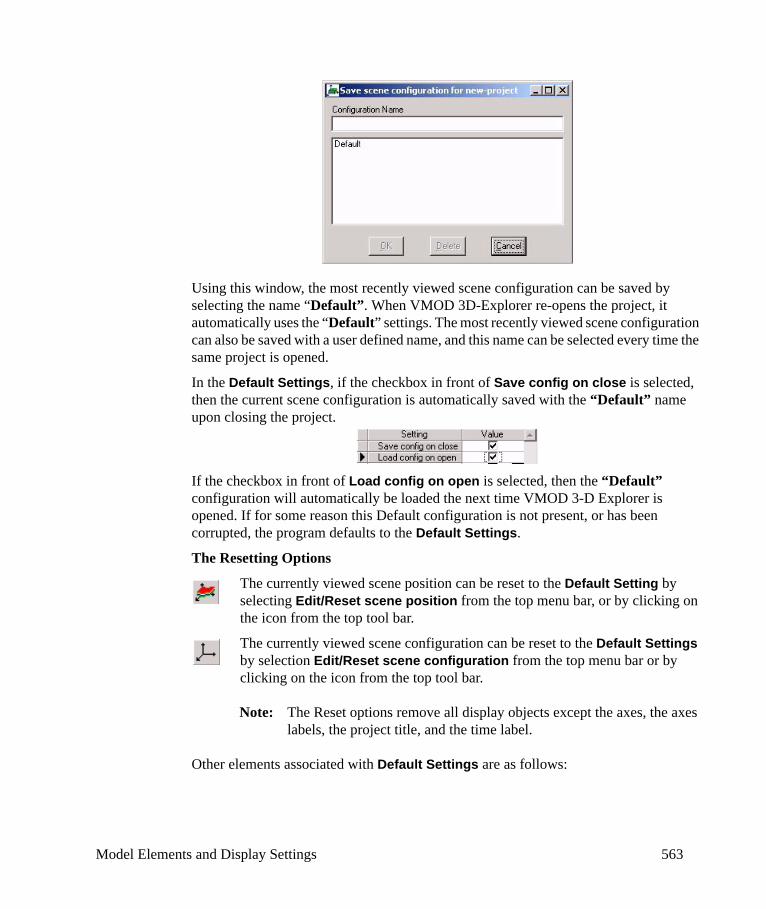
Model Elements and Display Settings 563
Using this window, the most recently viewed scene configuration can be saved by selecting the name “Default”. When VMOD 3D-Explorer re-opens the project, it automatically uses the “Default” settings. The most recently viewed scene configuration can also be saved with a user defined name, and this name can be selected every time the same project is opened.
In the Default Settings, if the checkbox in front of Save config on close is selected, then the current scene configuration is automatically saved with the “Default” name upon closing the project.
If the checkbox in front of Load config on open is selected, then the “Default” configuration will automatically be loaded the next time VMOD 3-D Explorer is opened. If for some reason this Default configuration is not present, or has been corrupted, the program defaults to the Default Settings.
The Resetting Options
The currently viewed scene position can be reset to the Default Setting by selecting Edit/Reset scene position from the top menu bar, or by clicking on the icon from the top tool bar.
The currently viewed scene configuration can be reset to the Default Settings by selection Edit/Reset scene configuration from the top menu bar or by clicking on the icon from the top tool bar.
Note: The Reset options remove all display objects except the axes, the axes labels, the project title, and the time label.
Other elements associated with Default Settings are as follows:

564 Chapter 11: Visual MODFLOW 3D-Explorer
Background color sets the image background color. By default, the Background color of the display screen is black.
Title
Text color sets the color of the Project title text. By default this is white.
Text size sets the size of the Project title text as a fraction of the screen size. By default this is 0.02.
Time Label
Text color sets the color of the Time label text. By default this is white.
Text size sets the size of the Time Label text Project title text as a fraction of the total screen size. By default this is 0.02.
Line color sets the color of the axes lines By default this is white.
Axis
Text color sets the color of the Title text. By default this is white.
Text size sets the size of the axes labels as a fraction of the total screen size. By default this is 0.02.
Line color sets the color of the axes lines. By default this is white.
Legends
Text color sets the color of the Legend text. By default this is white.
Inactive flow zone
Visible if selected, this option shows/hides the inactive flow cells.

Model Elements and Display Settings 565
Wells
Pumping/Label color sets the color of the Pumping Well label text.
Head observations/Label color sets the color of the Head Observation Well label text.
Concentration observations/Label color sets the color of the Concentration observation well label text.
VMOD Project Display SettingsThe VMOD Project element consists of general project settings, as shown in the following figure. By default, the project Title is given the same name as the model, and appears at the top of the Display Screen. This can be moved to any location within the Display Screen by clicking on the Title, and dragging it to a new location.
Axis PropertiesThe Axis model element controls the appearance of the lines and labels for the X, Y, and Z axes. The axes are primarily used to indicate the total dimensions (size) of the 3D image, and to orient the image when it has been rotated.
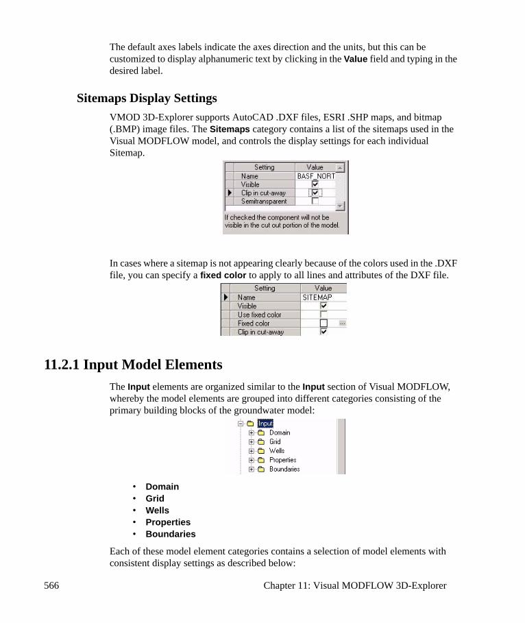
566 Chapter 11: Visual MODFLOW 3D-Explorer
The default axes labels indicate the axes direction and the units, but this can be customized to display alphanumeric text by clicking in the Value field and typing in the desired label.
Sitemaps Display SettingsVMOD 3D-Explorer supports AutoCAD .DXF files, ESRI .SHP maps, and bitmap (.BMP) image files. The Sitemaps category contains a list of the sitemaps used in the Visual MODFLOW model, and controls the display settings for each individual Sitemap.
In cases where a sitemap is not appearing clearly because of the colors used in the .DXF file, you can specify a fixed color to apply to all lines and attributes of the DXF file.
11.2.1 Input Model ElementsThe Input elements are organized similar to the Input section of Visual MODFLOW, whereby the model elements are grouped into different categories consisting of the primary building blocks of the groundwater model:
• Domain• Grid• Wells• Properties• Boundaries
Each of these model element categories contains a selection of model elements with consistent display settings as described below:
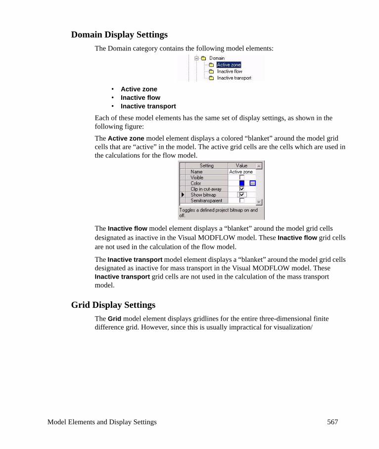
Model Elements and Display Settings 567
Domain Display SettingsThe Domain category contains the following model elements:
• Active zone• Inactive flow• Inactive transport
Each of these model elements has the same set of display settings, as shown in the following figure: The Active zone model element displays a colored “blanket” around the model grid cells that are “active” in the model. The active grid cells are the cells which are used in the calculations for the flow model.
The Inactive flow model element displays a “blanket” around the model grid cells designated as inactive in the Visual MODFLOW model. These Inactive flow grid cells are not used in the calculation of the flow model.
The Inactive transport model element displays a “blanket” around the model grid cells designated as inactive for mass transport in the Visual MODFLOW model. These Inactive transport grid cells are not used in the calculation of the mass transport model.
Grid Display SettingsThe Grid model element displays gridlines for the entire three-dimensional finite difference grid. However, since this is usually impractical for visualization/
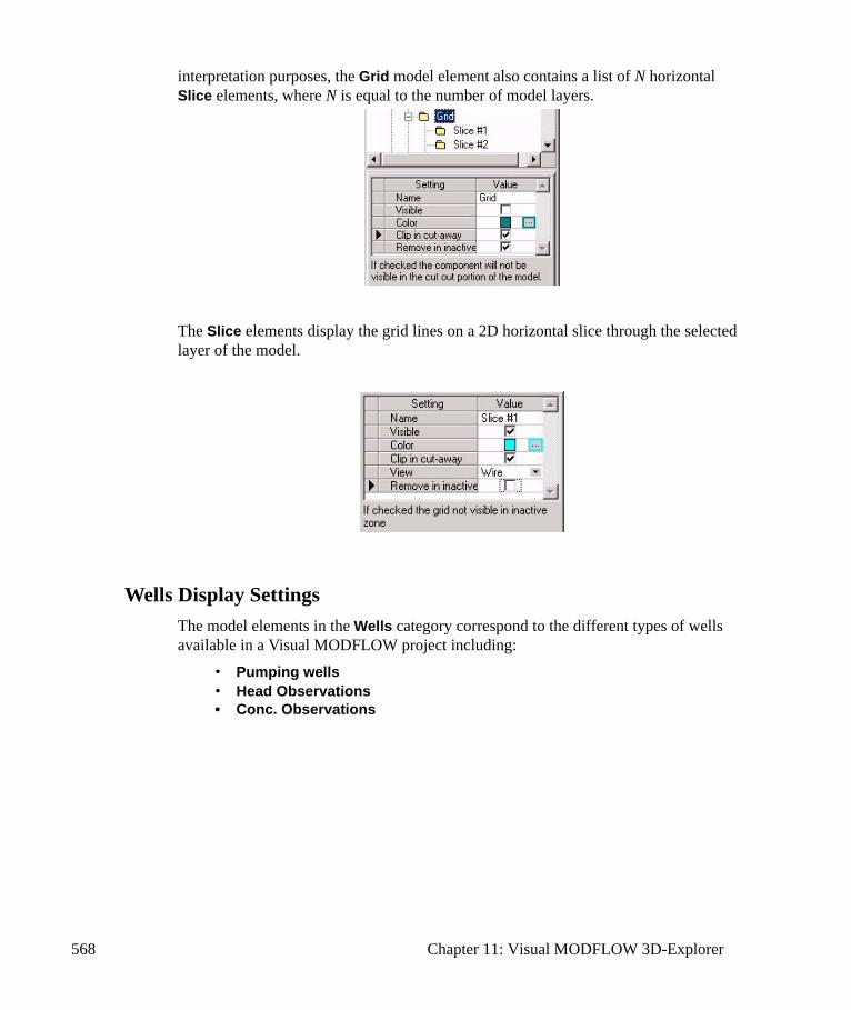
568 Chapter 11: Visual MODFLOW 3D-Explorer
interpretation purposes, the Grid model element also contains a list of N horizontal Slice elements, where N is equal to the number of model layers.
The Slice elements display the grid lines on a 2D horizontal slice through the selected layer of the model.
Wells Display SettingsThe model elements in the Wells category correspond to the different types of wells available in a Visual MODFLOW project including:
• Pumping wells• Head Observations• Conc. Observations
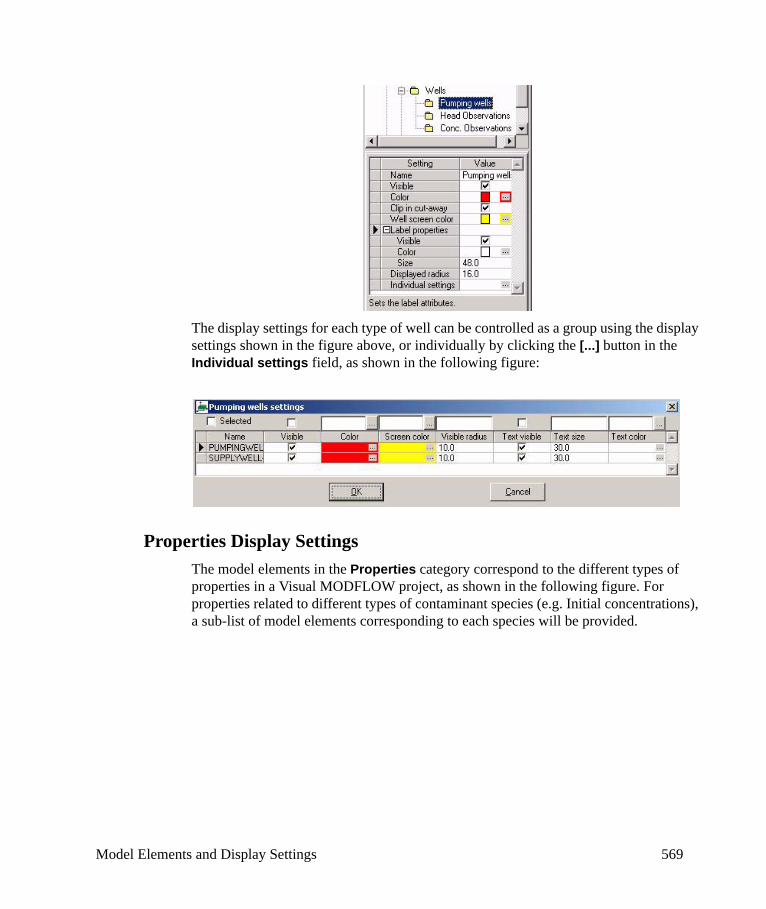
Model Elements and Display Settings 569
The display settings for each type of well can be controlled as a group using the display settings shown in the figure above, or individually by clicking the [...] button in the Individual settings field, as shown in the following figure:
Properties Display SettingsThe model elements in the Properties category correspond to the different types of properties in a Visual MODFLOW project, as shown in the following figure. For properties related to different types of contaminant species (e.g. Initial concentrations), a sub-list of model elements corresponding to each species will be provided.
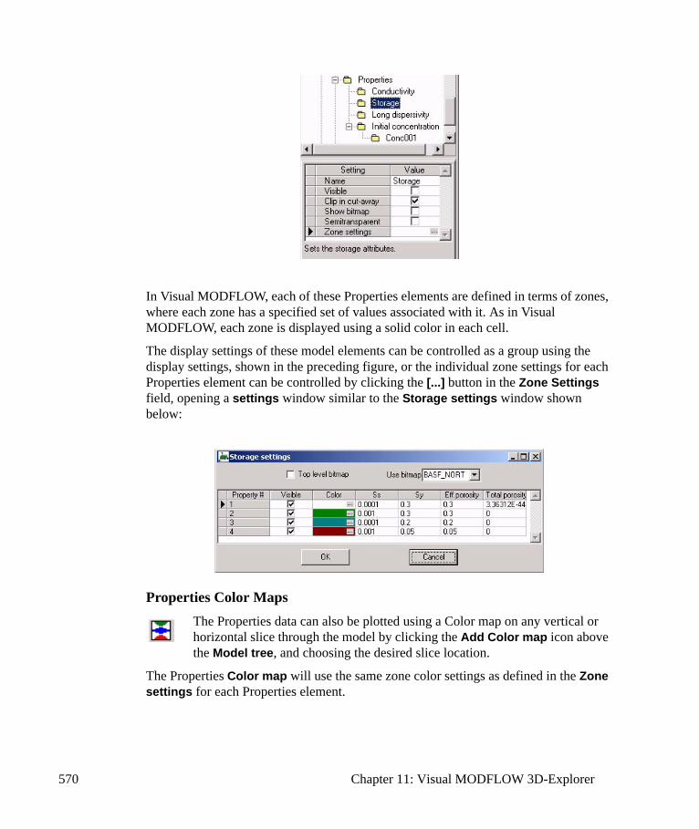
570 Chapter 11: Visual MODFLOW 3D-Explorer
In Visual MODFLOW, each of these Properties elements are defined in terms of zones, where each zone has a specified set of values associated with it. As in Visual MODFLOW, each zone is displayed using a solid color in each cell.
The display settings of these model elements can be controlled as a group using the display settings, shown in the preceding figure, or the individual zone settings for each Properties element can be controlled by clicking the [...] button in the Zone Settings field, opening a settings window similar to the Storage settings window shown below:
Properties Color MapsThe Properties data can also be plotted using a Color map on any vertical or horizontal slice through the model by clicking the Add Color map icon above the Model tree, and choosing the desired slice location.
The Properties Color map will use the same zone color settings as defined in the Zone settings for each Properties element.
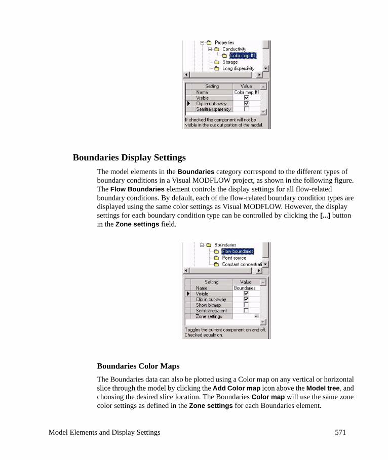
Model Elements and Display Settings 571
Boundaries Display SettingsThe model elements in the Boundaries category correspond to the different types of boundary conditions in a Visual MODFLOW project, as shown in the following figure. The Flow Boundaries element controls the display settings for all flow-related boundary conditions. By default, each of the flow-related boundary condition types are displayed using the same color settings as Visual MODFLOW. However, the display settings for each boundary condition type can be controlled by clicking the [...] button in the Zone settings field.
Boundaries Color MapsThe Boundaries data can also be plotted using a Color map on any vertical or horizontal slice through the model by clicking the Add Color map icon above the Model tree, and choosing the desired slice location. The Boundaries Color map will use the same zone color settings as defined in the Zone settings for each Boundaries element.
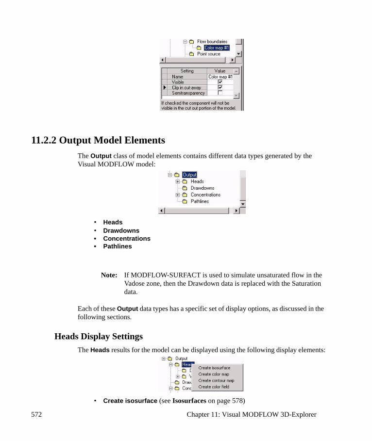
572 Chapter 11: Visual MODFLOW 3D-Explorer
11.2.2 Output Model ElementsThe Output class of model elements contains different data types generated by the Visual MODFLOW model:
• Heads• Drawdowns• Concentrations• Pathlines
Note: If MODFLOW-SURFACT is used to simulate unsaturated flow in the Vadose zone, then the Drawdown data is replaced with the Saturation data.
Each of these Output data types has a specific set of display options, as discussed in the following sections.
Heads Display SettingsThe Heads results for the model can be displayed using the following display elements:
• Create isosurface (see Isosurfaces on page 578)
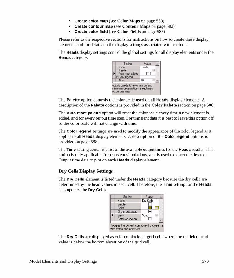
Model Elements and Display Settings 573
• Create color map (see Color Maps on page 580)• Create contour map (see Contour Maps on page 582)• Create color field (see Color Fields on page 585)
Please refer to the respective sections for instructions on how to create these display elements, and for details on the display settings associated with each one.
The Heads display settings control the global settings for all display elements under the Heads category.
The Palette option controls the color scale used on all Heads display elements. A description of the Palette options is provided in the Color Palette section on page 586.
The Auto reset palette option will reset the color scale every time a new element is added, and for every output time step. For transient data it is best to leave this option off so the color scale will not change with time.
The Color legend settings are used to modify the appearance of the color legend as it applies to all Heads display elements. A description of the Color legend options is provided on page 588.
The Time setting contains a list of the available output times for the Heads results. This option is only applicable for transient simulations, and is used to select the desired Output time data to plot on each Heads display element.
Dry Cells Display SettingsThe Dry Cells element is listed under the Heads category because the dry cells are determined by the head values in each cell. Therefore, the Time setting for the Heads also updates the Dry Cells.
The Dry Cells are displayed as colored blocks in grid cells where the modeled head value is below the bottom elevation of the grid cell.
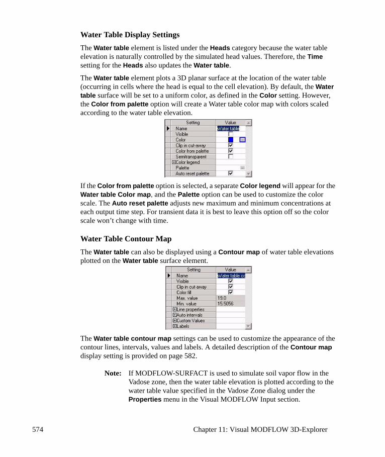
574 Chapter 11: Visual MODFLOW 3D-Explorer
Water Table Display SettingsThe Water table element is listed under the Heads category because the water table elevation is naturally controlled by the simulated head values. Therefore, the Time setting for the Heads also updates the Water table.
The Water table element plots a 3D planar surface at the location of the water table (occurring in cells where the head is equal to the cell elevation). By default, the Water table surface will be set to a uniform color, as defined in the Color setting. However, the Color from palette option will create a Water table color map with colors scaled according to the water table elevation.
If the Color from palette option is selected, a separate Color legend will appear for the Water table Color map, and the Palette option can be used to customize the color scale. The Auto reset palette adjusts new maximum and minimum concentrations at each output time step. For transient data it is best to leave this option off so the color scale won’t change with time.
Water Table Contour MapThe Water table can also be displayed using a Contour map of water table elevations plotted on the Water table surface element.
The Water table contour map settings can be used to customize the appearance of the contour lines, intervals, values and labels. A detailed description of the Contour map display setting is provided on page 582.
Note: If MODFLOW-SURFACT is used to simulate soil vapor flow in the Vadose zone, then the water table elevation is plotted according to the water table value specified in the Vadose Zone dialog under the Properties menu in the Visual MODFLOW Input section.
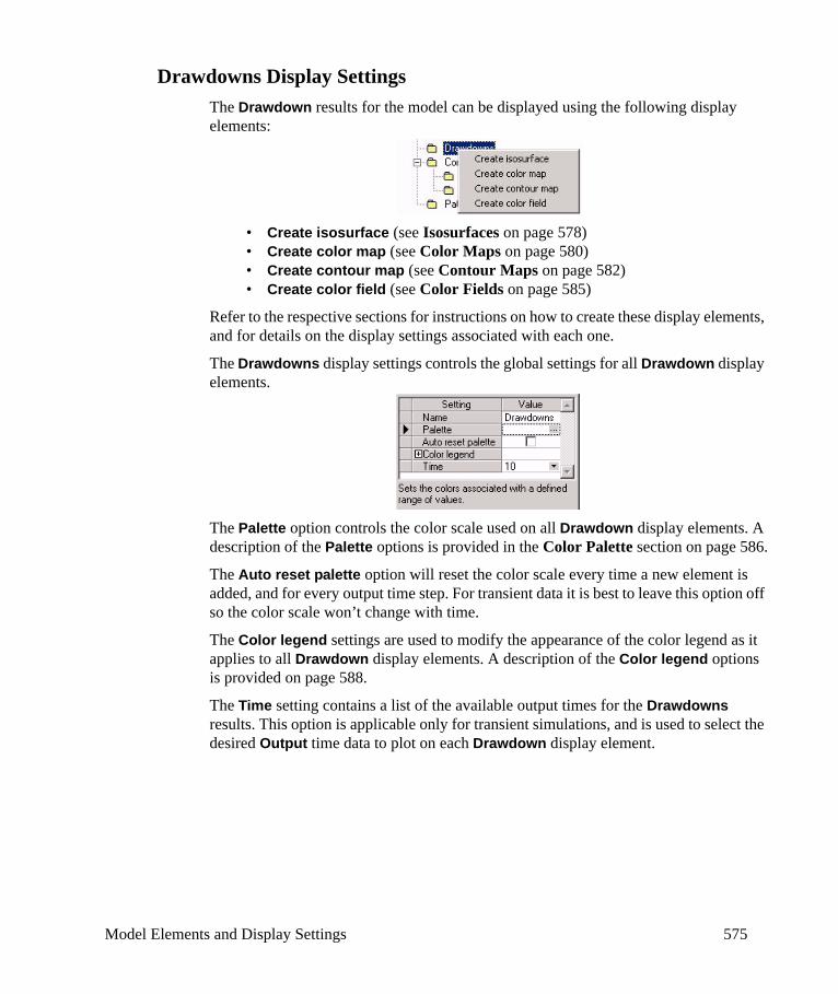
Model Elements and Display Settings 575
Drawdowns Display SettingsThe Drawdown results for the model can be displayed using the following display elements:
• Create isosurface (see Isosurfaces on page 578)• Create color map (see Color Maps on page 580)• Create contour map (see Contour Maps on page 582)• Create color field (see Color Fields on page 585)
Refer to the respective sections for instructions on how to create these display elements, and for details on the display settings associated with each one.
The Drawdowns display settings controls the global settings for all Drawdown display elements.
The Palette option controls the color scale used on all Drawdown display elements. A description of the Palette options is provided in the Color Palette section on page 586.
The Auto reset palette option will reset the color scale every time a new element is added, and for every output time step. For transient data it is best to leave this option off so the color scale won’t change with time.
The Color legend settings are used to modify the appearance of the color legend as it applies to all Drawdown display elements. A description of the Color legend options is provided on page 588.
The Time setting contains a list of the available output times for the Drawdowns results. This option is applicable only for transient simulations, and is used to select the desired Output time data to plot on each Drawdown display element.

576 Chapter 11: Visual MODFLOW 3D-Explorer
Concentrations Display SettingsThe Concentrations data category contains of a list of each species from the model. The transport results for each species can be displayed using the following display elements:
• Create isosurface (see Isosurfaces on page 578)• Create color map (see Color Maps on page 580)• Create contour map (see Contour Maps on page 582)• Create color field (see Color Fields on page 585)
Refer to the respective sections for instructions on how to create these display elements, and for details on the display settings associated with each one.
The Concentrations display settings for each species controls the global settings for all Concentrations display elements.
The Palette option controls the color scale used on all Concentrations display elements. A description of the Palette options is provided in the Color Palette section on page 586.
The Auto reset palette option will reset the color scale every time a new element is added and for every output time step. For transient data it is best to leave this option off so the color scale won’t change with time.
The Color legend settings are used to modify the appearance of the color legend as it applies to all Concentrations display elements. A description of the Color legend options is provided on page 588.
The Time setting contains a list of the available output times for the Concentrations results. This option is applicable only for transient simulations, and is used to select the desired Output time data to plot on each Concentration display element.
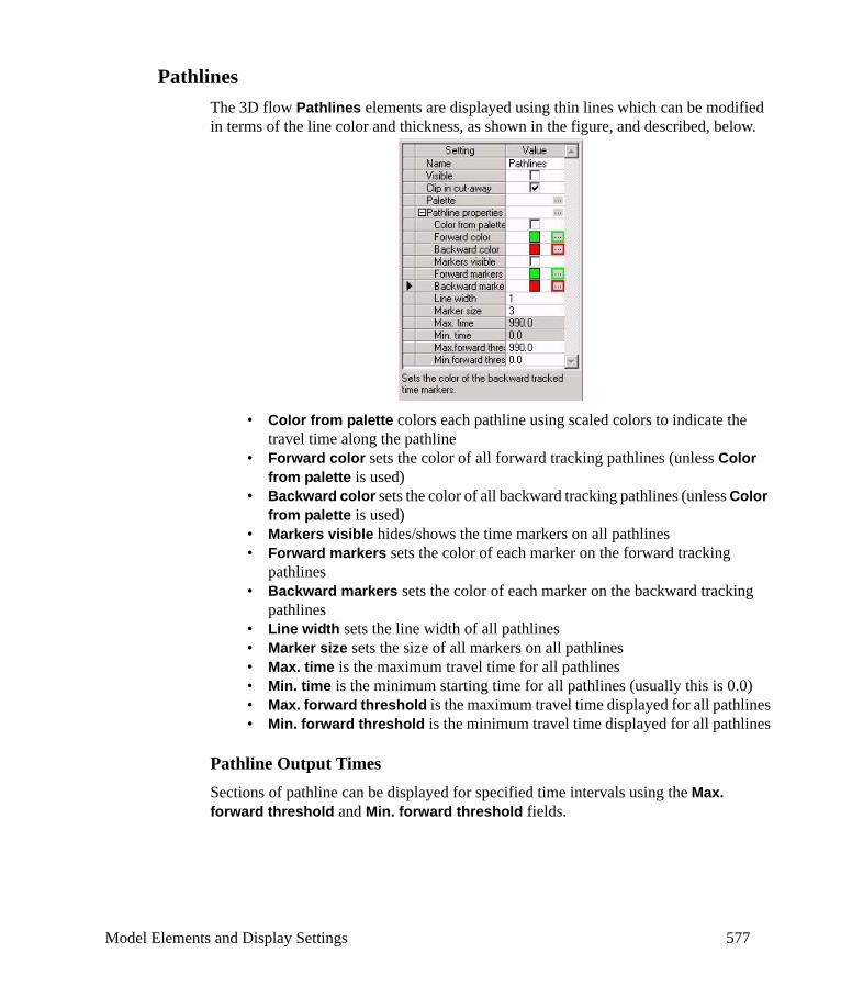
Model Elements and Display Settings 577
PathlinesThe 3D flow Pathlines elements are displayed using thin lines which can be modified in terms of the line color and thickness, as shown in the figure, and described, below.
• Color from palette colors each pathline using scaled colors to indicate the travel time along the pathline
• Forward color sets the color of all forward tracking pathlines (unless Color from palette is used)
• Backward color sets the color of all backward tracking pathlines (unless Color from palette is used)
• Markers visible hides/shows the time markers on all pathlines• Forward markers sets the color of each marker on the forward tracking
pathlines• Backward markers sets the color of each marker on the backward tracking
pathlines• Line width sets the line width of all pathlines• Marker size sets the size of all markers on all pathlines• Max. time is the maximum travel time for all pathlines• Min. time is the minimum starting time for all pathlines (usually this is 0.0)• Max. forward threshold is the maximum travel time displayed for all pathlines• Min. forward threshold is the minimum travel time displayed for all pathlines
Pathline Output TimesSections of pathline can be displayed for specified time intervals using the Max. forward threshold and Min. forward threshold fields.
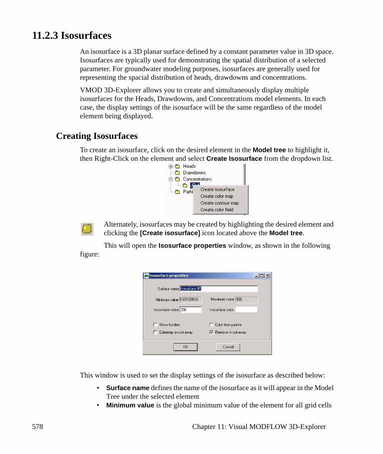
578 Chapter 11: Visual MODFLOW 3D-Explorer
11.2.3 IsosurfacesAn isosurface is a 3D planar surface defined by a constant parameter value in 3D space. Isosurfaces are typically used for demonstrating the spatial distribution of a selected parameter. For groundwater modeling purposes, isosurfaces are generally used for representing the spacial distribution of heads, drawdowns and concentrations.
VMOD 3D-Explorer allows you to create and simultaneously display multiple isosurfaces for the Heads, Drawdowns, and Concentrations model elements. In each case, the display settings of the isosurface will be the same regardless of the model element being displayed.
Creating IsosurfacesTo create an isosurface, click on the desired element in the Model tree to highlight it, then Right-Click on the element and select Create Isosurface from the dropdown list.
Alternately, isosurfaces may be created by highlighting the desired element and clicking the [Create isosurface] icon located above the Model tree.
This will open the Isosurface properties window, as shown in the following figure:
This window is used to set the display settings of the isosurface as described below:
• Surface name defines the name of the isosurface as it will appear in the Model Tree under the selected element
• Minimum value is the global minimum value of the element for all grid cells
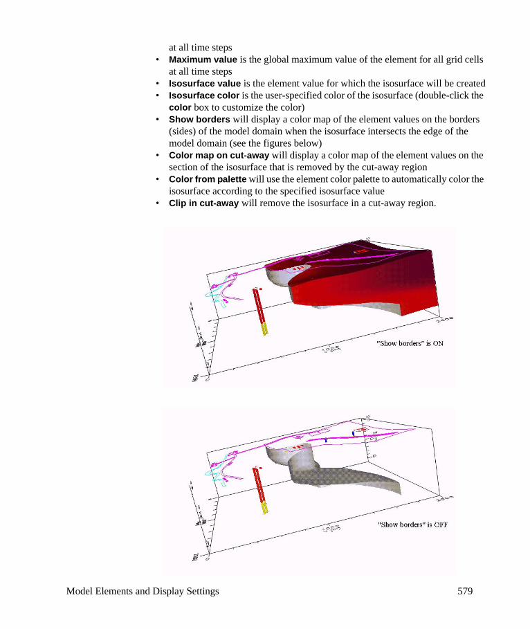
Model Elements and Display Settings 579
at all time steps• Maximum value is the global maximum value of the element for all grid cells
at all time steps• Isosurface value is the element value for which the isosurface will be created• Isosurface color is the user-specified color of the isosurface (double-click the
color box to customize the color)• Show borders will display a color map of the element values on the borders
(sides) of the model domain when the isosurface intersects the edge of the model domain (see the figures below)
• Color map on cut-away will display a color map of the element values on the section of the isosurface that is removed by the cut-away region
• Color from palette will use the element color palette to automatically color the isosurface according to the specified isosurface value
• Clip in cut-away will remove the isosurface in a cut-away region.
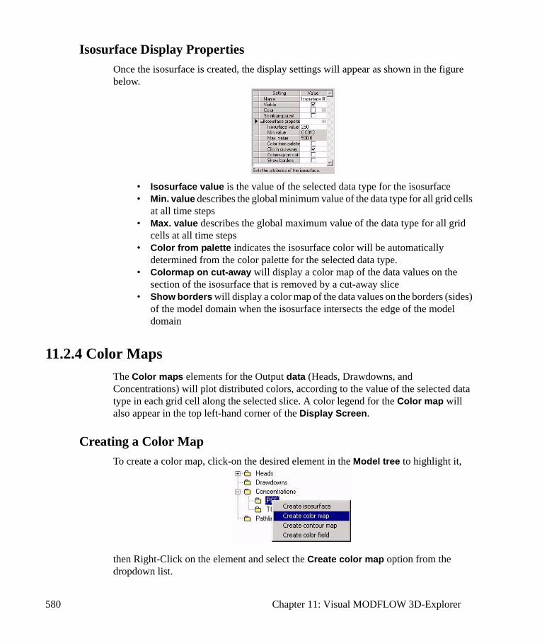
580 Chapter 11: Visual MODFLOW 3D-Explorer
Isosurface Display PropertiesOnce the isosurface is created, the display settings will appear as shown in the figure below.
• Isosurface value is the value of the selected data type for the isosurface• Min. value describes the global minimum value of the data type for all grid cells
at all time steps• Max. value describes the global maximum value of the data type for all grid
cells at all time steps• Color from palette indicates the isosurface color will be automatically
determined from the color palette for the selected data type. • Colormap on cut-away will display a color map of the data values on the
section of the isosurface that is removed by a cut-away slice• Show borders will display a color map of the data values on the borders (sides)
of the model domain when the isosurface intersects the edge of the model domain
11.2.4 Color MapsThe Color maps elements for the Output data (Heads, Drawdowns, and Concentrations) will plot distributed colors, according to the value of the selected data type in each grid cell along the selected slice. A color legend for the Color map will also appear in the top left-hand corner of the Display Screen.
Creating a Color MapTo create a color map, click-on the desired element in the Model tree to highlight it,
then Right-Click on the element and select the Create color map option from the dropdown list.
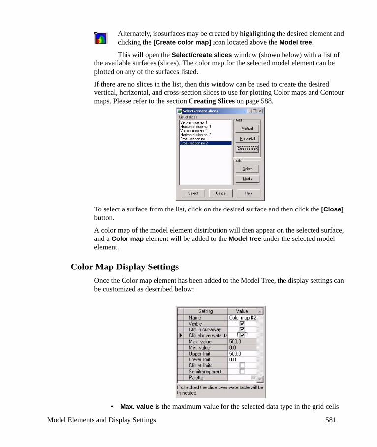
Model Elements and Display Settings 581
Alternately, isosurfaces may be created by highlighting the desired element and clicking the [Create color map] icon located above the Model tree.
This will open the Select/create slices window (shown below) with a list of the available surfaces (slices). The color map for the selected model element can be plotted on any of the surfaces listed.
If there are no slices in the list, then this window can be used to create the desired vertical, horizontal, and cross-section slices to use for plotting Color maps and Contour maps. Please refer to the section Creating Slices on page 588.
To select a surface from the list, click on the desired surface and then click the [Close] button.
A color map of the model element distribution will then appear on the selected surface, and a Color map element will be added to the Model tree under the selected model element.
Color Map Display SettingsOnce the Color map element has been added to the Model Tree, the display settings can be customized as described below:
• Max. value is the maximum value for the selected data type in the grid cells

582 Chapter 11: Visual MODFLOW 3D-Explorer
corresponding to the selected slice.• Min. value is the minimum value for the selected data type in the grid cells
corresponding to the selected slice.• Upper limit is the data value above which the color map may be clipped out
(not displayed).• Lower limit is the data value below which the color map may be clipped out
(not displayed).• Clip at limits indicates whether the color map will clipped above the Upper
limit and below the Lower limit.• Palette is used to customize the data values associated with each color. Any
changes made to the color palette for the selected data type will be applied to all color-scaled elements for the selected data type. This ensures that each element uses a consistent color scheme (and a correct color legend) for each data type throughout the model. The color palette options are discussed in more detail in “The Color Palette” on page 586.
11.2.5 Contour MapsContour maps are a set of lines plotted on a surface, whereby each line is connected by a set of points having equal values of a given data type.
Creating Contour MapsTo create a Contour map, click-on the desired element in the Model tree, and then Right-Click on the element and select the Create contour map option from the dropdown list.
Alternately, contour lines may be created by highlighting the desired element and clicking the [Create contour map] icon located above the Model tree.
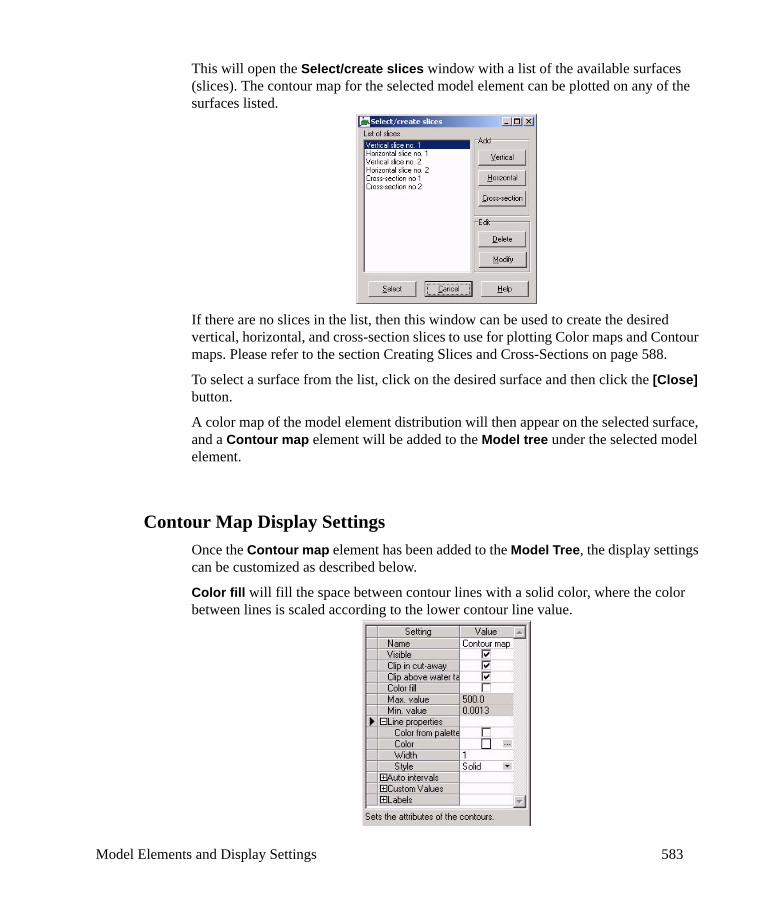
Model Elements and Display Settings 583
This will open the Select/create slices window with a list of the available surfaces (slices). The contour map for the selected model element can be plotted on any of the surfaces listed.
If there are no slices in the list, then this window can be used to create the desired vertical, horizontal, and cross-section slices to use for plotting Color maps and Contour maps. Please refer to the section Creating Slices and Cross-Sections on page 588.
To select a surface from the list, click on the desired surface and then click the [Close] button.
A color map of the model element distribution will then appear on the selected surface, and a Contour map element will be added to the Model tree under the selected model element.
Contour Map Display SettingsOnce the Contour map element has been added to the Model Tree, the display settings can be customized as described below.
Color fill will fill the space between contour lines with a solid color, where the color between lines is scaled according to the lower contour line value.
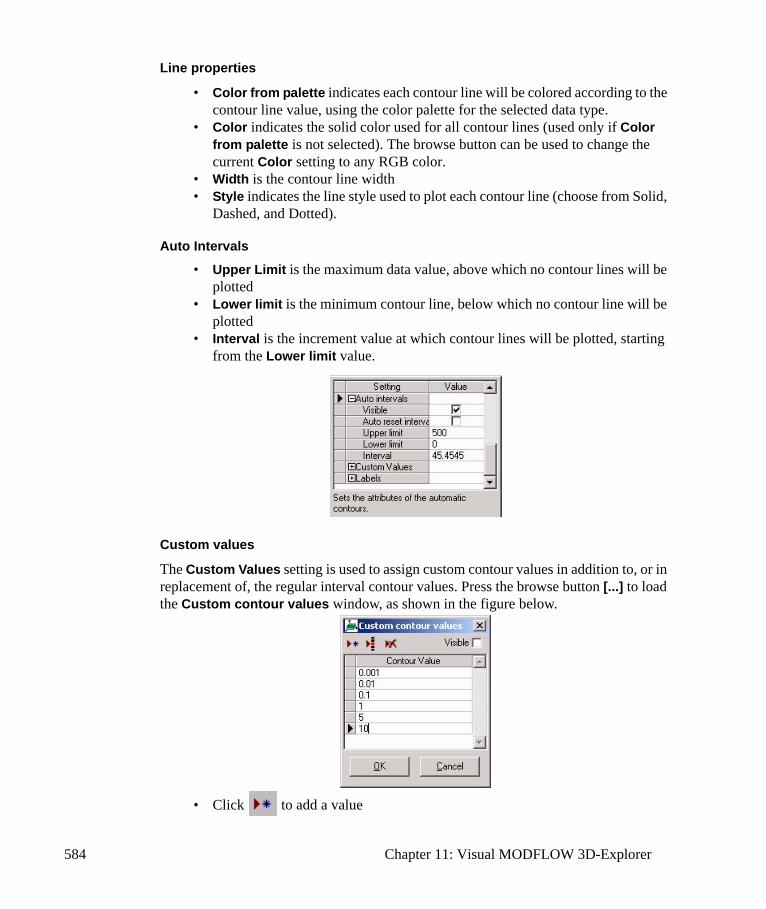
584 Chapter 11: Visual MODFLOW 3D-Explorer
Line properties
• Color from palette indicates each contour line will be colored according to the contour line value, using the color palette for the selected data type.
• Color indicates the solid color used for all contour lines (used only if Color from palette is not selected). The browse button can be used to change the current Color setting to any RGB color.
• Width is the contour line width• Style indicates the line style used to plot each contour line (choose from Solid,
Dashed, and Dotted).
Auto Intervals
• Upper Limit is the maximum data value, above which no contour lines will be plotted
• Lower limit is the minimum contour line, below which no contour line will be plotted
• Interval is the increment value at which contour lines will be plotted, starting from the Lower limit value.
Custom values
The Custom Values setting is used to assign custom contour values in addition to, or in replacement of, the regular interval contour values. Press the browse button [...] to load the Custom contour values window, as shown in the figure below.
• Click to add a value

Model Elements and Display Settings 585
• Click to insert a value
• Click to delete a value
This setting is commonly used to set logarithmic contour interval values for concentration data.
Labels
The Labels setting is used customize the appearance of the contour labels.
• Decimals is the number of decimals used for each label value• Text color is the color of each label• Text size is the size of each label
The labels are plotted on the top and bottom surface of a flat 3D rectangular box. The size of the box will be automatically adjusted to fit the text size, but the Box color and Box depth can be customized.
In situations where the 3D planar surface is highly variable in shape, some of the isoline labels may be difficult to read. This is a limitation of the current version of VMOD 3D-Explorer, but it is a feature that will be improved in later versions.
11.2.6 Color FieldsThe Color fields display format creates a 3D field of colored points on a user-specified grid. Each point is colored according to the value of the selected model element at each
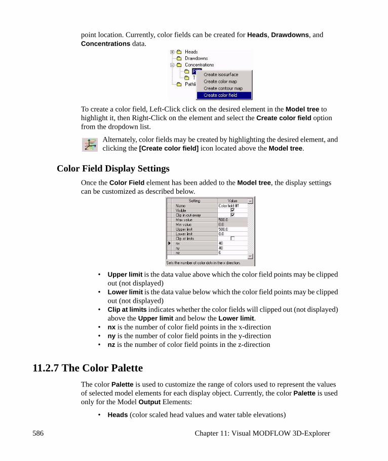
586 Chapter 11: Visual MODFLOW 3D-Explorer
point location. Currently, color fields can be created for Heads, Drawdowns, and Concentrations data.
To create a color field, Left-Click click on the desired element in the Model tree to highlight it, then Right-Click on the element and select the Create color field option from the dropdown list.
Alternately, color fields may be created by highlighting the desired element, and clicking the [Create color field] icon located above the Model tree.
Color Field Display SettingsOnce the Color Field element has been added to the Model tree, the display settings can be customized as described below.
• Upper limit is the data value above which the color field points may be clipped out (not displayed)
• Lower limit is the data value below which the color field points may be clipped out (not displayed)
• Clip at limits indicates whether the color fields will clipped out (not displayed) above the Upper limit and below the Lower limit.
• nx is the number of color field points in the x-direction• ny is the number of color field points in the y-direction• nz is the number of color field points in the z-direction
11.2.7 The Color PaletteThe color Palette is used to customize the range of colors used to represent the values of selected model elements for each display object. Currently, the color Palette is used only for the Model Output Elements:
• Heads (color scaled head values and water table elevations)
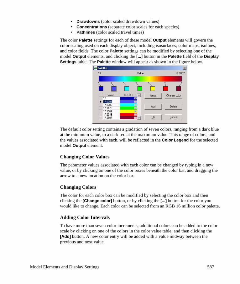
Model Elements and Display Settings 587
• Drawdowns (color scaled drawdown values)• Concentrations (separate color scales for each species)• Pathlines (color scaled travel times)
The color Palette settings for each of these model Output elements will govern the color scaling used on each display object, including isosurfaces, color maps, isolines, and color fields. The color Palette settings can be modified by selecting one of the model Output elements, and clicking the [...] button in the Palette field of the Display Settings table. The Palette window will appear as shown in the figure below.
The default color setting contains a gradation of seven colors, ranging from a dark blue at the minimum value, to a dark red at the maximum value. This range of colors, and the values associated with each, will be reflected in the Color Legend for the selected model Output element.
Changing Color ValuesThe parameter values associated with each color can be changed by typing in a new value, or by clicking on one of the color boxes beneath the color bar, and dragging the arrow to a new location on the color bar.
Changing ColorsThe color for each color box can be modified by selecting the color box and then clicking the [Change color] button, or by clicking the [...] button for the color you would like to change. Each color can be selected from an RGB 16 million color palette.
Adding Color IntervalsTo have more than seven color increments, additional colors can be added to the color scale by clicking on one of the colors in the color value table, and then clicking the [Add] button. A new color entry will be added with a value midway between the previous and next value.

588 Chapter 11: Visual MODFLOW 3D-Explorer
Deleting a colorTo have fewer color increments, simply remove a color by selecting the color from the Color Value table, and then clicking the [Delete] button.
Resetting the Color PaletteThe color settings can be reset to the initial default values by clicking the [Reset] button.
11.2.8 The Color LegendThe Color Legend is a scale of the element values associated with each color. The values and colors shown in the Color Legend are defined by the Color Palette settings for the selected data type element (see previous section).
Other display settings, including Title, Text size, Text color, and Frame color, can be customized using the display settings options, shown in the figure below.
The color legend will automatically appear in the top left-hand corner of the Display Screen whenever a display object using the color palette is plotted (e.g. color map). It can be moved to any other location in the Display Screen by dragging-and-dropping it at the desired location.
11.3 Creating Slices and Cross-SectionsA slice is defined as a 3D planar surface extending horizontally or vertically through the model domain. There are three types of slice objects available:
• Vertical slices along the XZ or YZ plane of the model extending through the entire depth of the model.
• Horizontal slices along the XY plane of the model• Cross-section slices along a straight line, or an irregular polyline, through the
entire depth of the model
These slice objects define the locations where color maps and contour maps can be plotted for selected model elements including Properties, Heads, Drawdowns and Concentrations. Slices can also be used to define Cut-away regions.
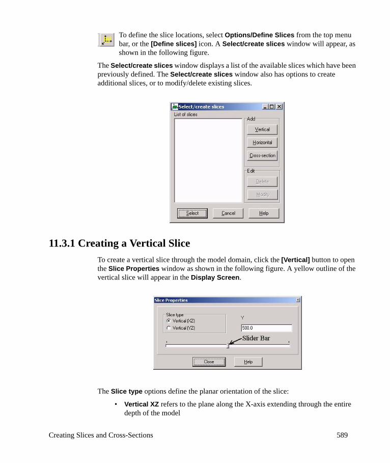
Creating Slices and Cross-Sections 589
To define the slice locations, select Options/Define Slices from the top menu bar, or the [Define slices] icon. A Select/create slices window will appear, as shown in the following figure.
The Select/create slices window displays a list of the available slices which have been previously defined. The Select/create slices window also has options to create additional slices, or to modify/delete existing slices.
11.3.1 Creating a Vertical SliceTo create a vertical slice through the model domain, click the [Vertical] button to open the Slice Properties window as shown in the following figure. A yellow outline of the vertical slice will appear in the Display Screen.
The Slice type options define the planar orientation of the slice:
• Vertical XZ refers to the plane along the X-axis extending through the entire depth of the model
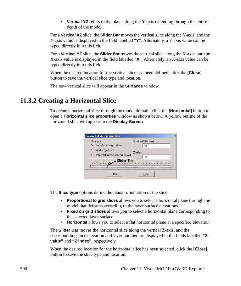
590 Chapter 11: Visual MODFLOW 3D-Explorer
• Vertical YZ refers to the plane along the Y-axis extending through the entire depth of the model
For a Vertical XZ slice, the Slider Bar moves the vertical slice along the Y-axis, and the Y-axis value is displayed in the field labelled “Y”. Alternately, a Y-axis value can be typed directly into this field.
For a Vertical YZ slice, the Slider Bar moves the vertical slice along the X-axis, and the X-axis value is displayed in the field labelled “X”. Alternately, an X-axis value can be typed directly into this field.
When the desired location for the vertical slice has been defined, click the [Close] button to save the vertical slice type and location.
The new vertical slice will appear in the Surfaces window.
11.3.2 Creating a Horizontal SliceTo create a horizontal slice through the model domain, click the [Horizontal] button to open a Horizontal slice properties window as shown below. A yellow outline of the horizontal slice will appear in the Display Screen.
The Slice type options define the planar orientation of the slice:
• Proportional to grid slices allows you to select a horizontal plane through the model that deforms according to the layer surface elevations
• Fixed on grid slices allows you to select a horizontal plane corresponding to the selected layer surface
• Horizontal allows you to select a flat horizontal plane at a specified elevation
The Slider Bar moves the horizontal slice along the vertical Z-axis, and the corresponding slice elevation and layer number are displayed in the fields labelled “Z value” and “Z index”, respectively.
When the desired location for the horizontal slice has been selected, click the [Close] button to save the slice type and location.
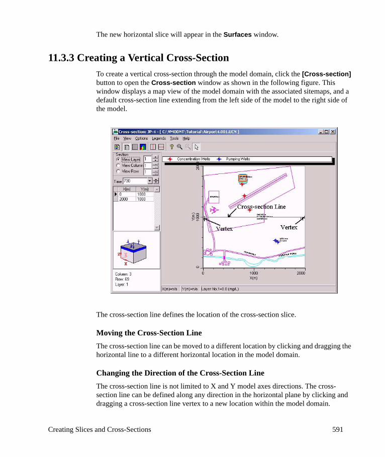
Creating Slices and Cross-Sections 591
The new horizontal slice will appear in the Surfaces window.
11.3.3 Creating a Vertical Cross-SectionTo create a vertical cross-section through the model domain, click the [Cross-section] button to open the Cross-section window as shown in the following figure. This window displays a map view of the model domain with the associated sitemaps, and a default cross-section line extending from the left side of the model to the right side of the model.
The cross-section line defines the location of the cross-section slice.
Moving the Cross-Section LineThe cross-section line can be moved to a different location by clicking and dragging the horizontal line to a different horizontal location in the model domain.
Changing the Direction of the Cross-Section LineThe cross-section line is not limited to X and Y model axes directions. The cross-section line can be defined along any direction in the horizontal plane by clicking and dragging a cross-section line vertex to a new location within the model domain.
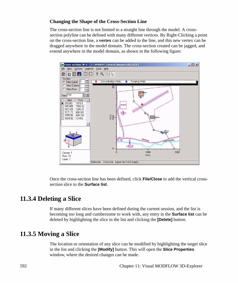
592 Chapter 11: Visual MODFLOW 3D-Explorer
Changing the Shape of the Cross-Section LineThe cross-section line is not limited to a straight line through the model. A cross-section polyline can be defined with many different vertices. By Right-Clicking a point on the cross-section line, a vertex can be added to the line, and this new vertex can be dragged anywhere in the model domain. The cross-section created can be jagged, and extend anywhere in the model domain, as shown in the following figure:
Once the cross-section line has been defined, click File/Close to add the vertical cross-section slice to the Surface list.
11.3.4 Deleting a SliceIf many different slices have been defined during the current session, and the list is becoming too long and cumbersome to work with, any entry in the Surface list can be deleted by highlighting the slice in the list and clicking the [Delete] button.
11.3.5 Moving a Slice The location or orientation of any slice can be modified by highlighting the target slice in the list and clicking the [Modify] button. This will open the Slice Properties window, where the desired changes can be made.
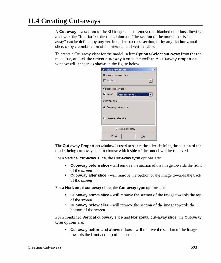
Creating Cut-aways 593
11.4 Creating Cut-awaysA Cut-away is a section of the 3D image that is removed or blanked out, thus allowing a view of the “interior” of the model domain. The section of the model that is “cut-away” can be defined by any vertical slice or cross-section, or by any flat horizontal slice, or by a combination of a horizontal and vertical slice.
To create a Cut-away view for the model, select Options/Select cut-away from the top menu bar, or click the Select cut-away icon in the toolbar. A Cut-away Properties window will appear, as shown in the figure below.
The Cut-away Properties window is used to select the slice defining the section of the model being cut-away, and to choose which side of the model will be removed.
For a Vertical cut-away slice, the Cut-away type options are:
• Cut-away before slice - will remove the section of the image towards the front of the screen
• Cut-away after slice - will remove the section of the image towards the back of the screen
For a Horizontal cut-away slice, the Cut-away type options are:
• Cut-away above slice - will remove the section of the image towards the top of the screen
• Cut-away below slice - will remove the section of the image towards the bottom of the screen
For a combined Vertical cut-away slice and Horizontal cut-away slice, the Cut-away type options are:
• Cut-away before and above slices - will remove the section of the image towards the front and top of the screen

594 Chapter 11: Visual MODFLOW 3D-Explorer
• Cut-away before and below slices - will remove the section of the image towards the front and bottom of the screen
• Cut-away after and above slices - will remove the section of the image towards the back and top of the screen
• Cut-away after and below slices - will remove the section of the image towards the back and bottom of the screen
The checkboxes beside the Vertical cut-away slice field and the Horizontal cut-away slice field will automatically be set to ON when a slice has been selected. If the active checkbox is set to OFF, the cut-away will not be applied to the image.
11.4.1 Creating an AnimationVMOD 3D-Explorer allows time-varying modeling results to be animated in order to show the changes in heads, drawdown, and concentration with time. The animation tool shows a sequential progression of the model data from the available output times for each data set. This animation can be saved to an .AVI file for convenient demonstrations using a compatible .AVI file player.
The Animation tools can be activated by highlighting the desired data type (Heads, Drawdowns or Concentrations) in the Model Tree. The following toolbar will appear above the Model Tree.
The Play button starts animating the results for the selected data type, starting from the current time step.
The Pause button pauses the animation at the current time step.
The Stop button stops the animation at the current time step.
The Loop button will continuously loop through all of the time steps.
The Rewind button will set the time back to the first time step.
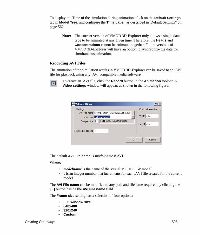
Creating Cut-aways 595
To display the Time of the simulation during animation, click on the Default Settings tab in Model Tree, and configure the Time Label, as described in“Default Settings” on page 562.
Note: The current version of VMOD 3D-Explorer only allows a single data type to be animated at any given time. Therefore, the Heads and Concentrations cannot be animated together. Future versions of VMOD 3D-Explorer will have an option to synchronize the data for simultaneous animation.
Recording AVI FilesThe animation of the simulation results in VMOD 3D-Explorer can be saved to an .AVI file for playback using any .AVI compatible media software.
To create an .AVI file, click the Record button in the Animation toolbar. A Video settings window will appear, as shown in the following figure:
The default AVI File name is modelname.#.AVI
Where:
• modelname is the name of the Visual MODFLOW model• # is an integer number that increments for each .AVI file created for the current
model
The AVI File name can be modified to any path and filename required by clicking the [...] button beside the AVI File name field.
The Frame size setting has a selection of four options:
• Full window size• 640x480• 320x240• Custom
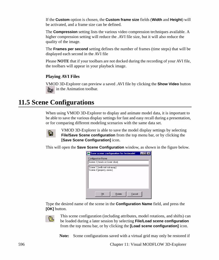
596 Chapter 11: Visual MODFLOW 3D-Explorer
If the Custom option is chosen, the Custom frame size fields (Width and Height) will be activated, and a frame size can be defined.
The Compression setting lists the various video compression techniques available. A higher compression setting will reduce the .AVI file size, but it will also reduce the quality of the image.
The Frames per second setting defines the number of frames (time steps) that will be displayed each second in the AVI file
Please NOTE that if your toolbars are not docked during the recording of your AVI file, the toolbars will appear in your playback image.
Playing AVI FilesVMOD 3D-Explorer can preview a saved .AVI file by clicking the Show Video button
in the Animation toolbar.
11.5 Scene ConfigurationsWhen using VMOD 3D-Explorer to display and animate model data, it is important to be able to save the various display settings for fast and easy recall during a presentation, or for comparing different modeling scenarios with the same data set.
VMOD 3D-Explorer is able to save the model display settings by selecting File/Save Scene configuration from the top menu bar, or by clicking the [Save Scene Configuration] icon.
This will open the Save Scene Configuration window, as shown in the figure below.
Type the desired name of the scene in the Configuration Name field, and press the [OK] button.
This scene configuration (including attributes, model rotations, and shifts) can be loaded during a later session by selecting File/Load scene configuration from the top menu bar, or by clicking the [Load scene configuration] icon.
Note: Scene configurations saved with a virtual grid may only be restored if
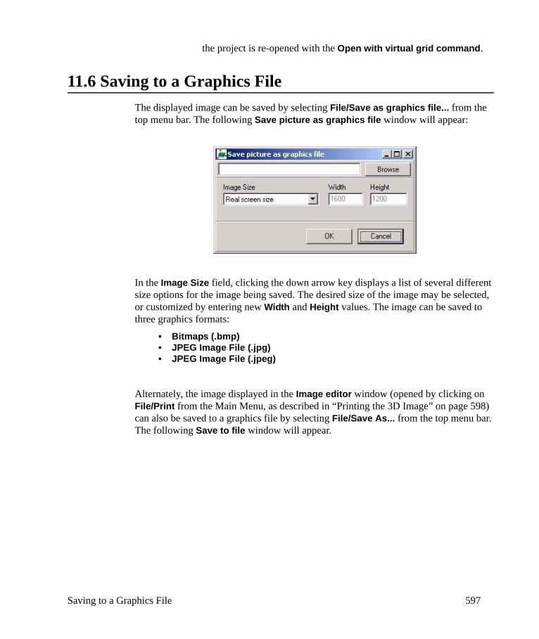
Saving to a Graphics File 597
the project is re-opened with the Open with virtual grid command.
11.6 Saving to a Graphics FileThe displayed image can be saved by selecting File/Save as graphics file... from the top menu bar. The following Save picture as graphics file window will appear:
In the Image Size field, clicking the down arrow key displays a list of several different size options for the image being saved. The desired size of the image may be selected, or customized by entering new Width and Height values. The image can be saved to three graphics formats:
• Bitmaps (.bmp)• JPEG Image File (.jpg)• JPEG Image File (.jpeg)
Alternately, the image displayed in the Image editor window (opened by clicking on File/Print from the Main Menu, as described in “Printing the 3D Image” on page 598) can also be saved to a graphics file by selecting File/Save As... from the top menu bar. The following Save to file window will appear.
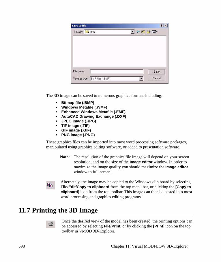
598 Chapter 11: Visual MODFLOW 3D-Explorer
The 3D image can be saved to numerous graphics formats including:
• Bitmap file (.BMP)• Windows Metafile (.WMF)• Enhanced Windows Metafile (.EMF)• AutoCAD Drawing Exchange (.DXF)• JPEG image (.JPG)• TIF image (.TIF)• GIF image (.GIF)• PNG image (.PNG)
These graphics files can be imported into most word processing software packages, manipulated using graphics editing software, or added to presentation software.
Note: The resolution of the graphics file image will depend on your screen resolution, and on the size of the Image editor window. In order to maximize the image quality you should maximize the Image editor window to full screen.
Alternately, the image may be copied to the Windows clip board by selecting File/Edit/Copy to clipboard from the top menu bar, or clicking the [Copy to clipboard] icon from the top toolbar. This image can then be pasted into most word processing and graphics editing programs.
11.7 Printing the 3D ImageOnce the desired view of the model has been created, the printing options can be accessed by selecting File/Print, or by clicking the [Print] icon on the top toolbar in VMOD 3D-Explorer.

Printing the 3D Image 599
An Image editor window will appear with a preview of the 3D image to be printed (see following figure). This window can be used to fine-tune the appearance of the image, by adding some text or drawings to the image, using the annotation tools described in “Annotate” on page 606.
From the Image editor window, you have the following options:
• Page Setup - edit page layout
• Print - print the current image
• Preview - preview the image to be printed
• Save as graphics file - save the image to a graphics image file (choose from
.BMP, .WMF, .EMF, .DXF, .JPG, .TIF, .GIF, and .PNG file formats)
• Copy to clipboard - copy image to the windows clipboard
• Show legend - add legend of image features to the page layout
• Show color legend - add legend of color scale to the page layout
• Annotate - add text and shapes to your image
• Image editor help
• Image Title - create a title for your image
• Printing method (direct printing/intermediate bitmap)
• Select - return your cursor to its normal function after zooming
• Zoom into or out of a section of the 3D image
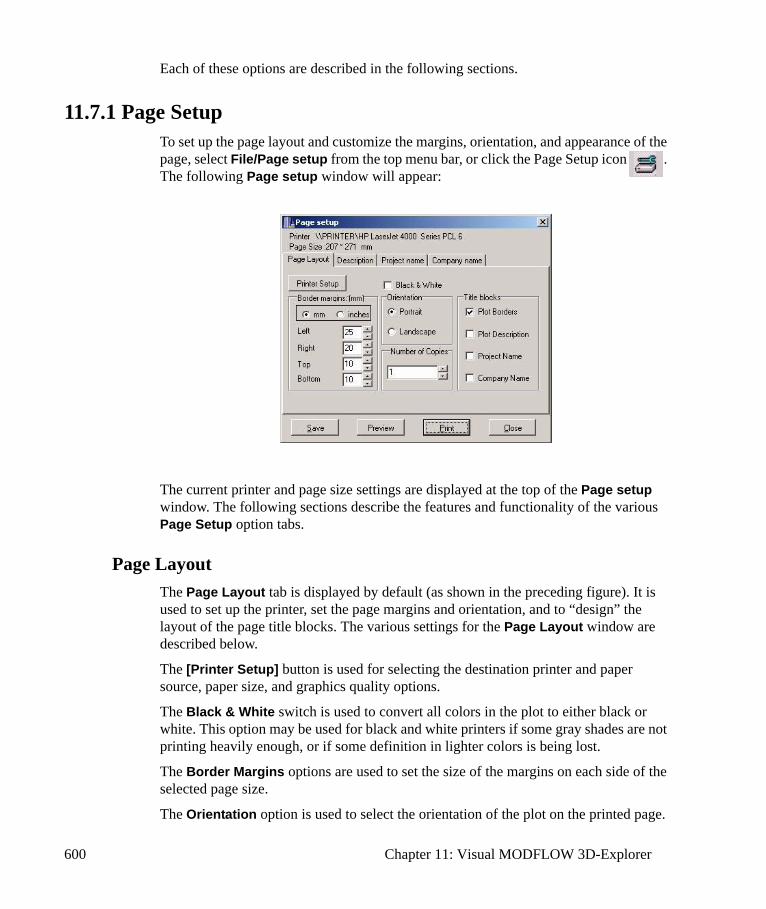
600 Chapter 11: Visual MODFLOW 3D-Explorer
Each of these options are described in the following sections.
11.7.1 Page SetupTo set up the page layout and customize the margins, orientation, and appearance of the page, select File/Page setup from the top menu bar, or click the Page Setup icon . The following Page setup window will appear:
The current printer and page size settings are displayed at the top of the Page setup window. The following sections describe the features and functionality of the various Page Setup option tabs.
Page LayoutThe Page Layout tab is displayed by default (as shown in the preceding figure). It is used to set up the printer, set the page margins and orientation, and to “design” the layout of the page title blocks. The various settings for the Page Layout window are described below.
The [Printer Setup] button is used for selecting the destination printer and paper source, paper size, and graphics quality options.
The Black & White switch is used to convert all colors in the plot to either black or white. This option may be used for black and white printers if some gray shades are not printing heavily enough, or if some definition in lighter colors is being lost.
The Border Margins options are used to set the size of the margins on each side of the selected page size.
The Orientation option is used to select the orientation of the plot on the printed page.

Printing the 3D Image 601
The Number of Copies option is used to set the number of copies of the page to print.
The Title blocks options are used to customize the appearance of the page layout, as shown in the following figure (the actual arrangement and size of the title blocks on the page will vary depending on the number of title blocks selected).
• Plot Borders will plot an outline along the page margins• Plot Description will add a title block to display a description of the plot (see
“Plot Description” on page 601).• Project Name will add a title block to display the Project Name and an optional
bitmap image of a logo (see “Project Name” on page 602).• Company Name will add a title block to display the company name and an
optional bitmap image of a logo (see “Company Name” on page 603).
Note: You will NOT be able to enter Description, Project Name, or Company Name information in their respective tabs unless you have Checked these options FIRST in the Title Blocks frame.
The [Save] button is used to save the Print settings including the Description, Project Name, and Company Name.
The [Preview] button is used to show a preview of the page as it will appear when it is printed.
The [Print] button will print the page and close the Page Setup window.
The [Close] button will close the Page Setup window.
Plot DescriptionIf the Plot Description option is selected in the Page Layout tab, the Description tab will become active in the Page Setup window, as shown in the following figure:
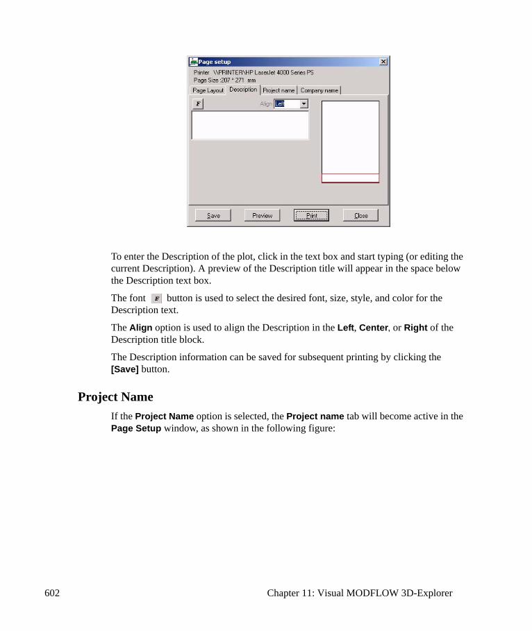
602 Chapter 11: Visual MODFLOW 3D-Explorer
To enter the Description of the plot, click in the text box and start typing (or editing the current Description). A preview of the Description title will appear in the space below the Description text box.
The font button is used to select the desired font, size, style, and color for the Description text.
The Align option is used to align the Description in the Left, Center, or Right of the Description title block.
The Description information can be saved for subsequent printing by clicking the [Save] button.
Project NameIf the Project Name option is selected, the Project name tab will become active in the Page Setup window, as shown in the following figure:
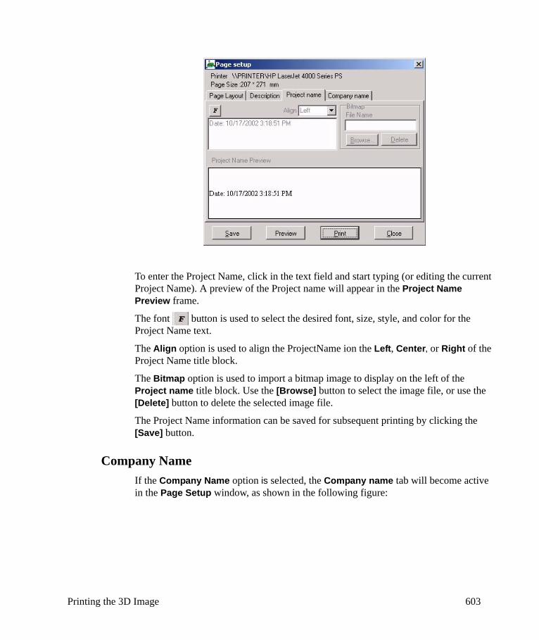
Printing the 3D Image 603
To enter the Project Name, click in the text field and start typing (or editing the current Project Name). A preview of the Project name will appear in the Project Name Preview frame.
The font button is used to select the desired font, size, style, and color for the Project Name text.
The Align option is used to align the ProjectName ion the Left, Center, or Right of the Project Name title block.
The Bitmap option is used to import a bitmap image to display on the left of the Project name title block. Use the [Browse] button to select the image file, or use the [Delete] button to delete the selected image file.
The Project Name information can be saved for subsequent printing by clicking the [Save] button.
Company NameIf the Company Name option is selected, the Company name tab will become active in the Page Setup window, as shown in the following figure:
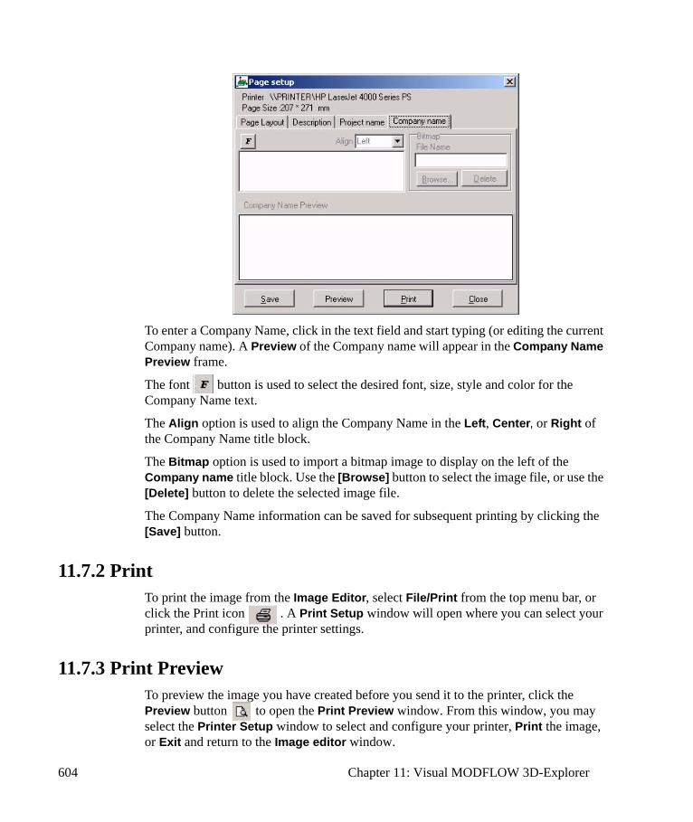
604 Chapter 11: Visual MODFLOW 3D-Explorer
To enter a Company Name, click in the text field and start typing (or editing the current Company name). A Preview of the Company name will appear in the Company Name Preview frame.
The font button is used to select the desired font, size, style and color for the Company Name text.
The Align option is used to align the Company Name in the Left, Center, or Right of the Company Name title block.
The Bitmap option is used to import a bitmap image to display on the left of the Company name title block. Use the [Browse] button to select the image file, or use the [Delete] button to delete the selected image file.
The Company Name information can be saved for subsequent printing by clicking the [Save] button.
11.7.2 PrintTo print the image from the Image Editor, select File/Print from the top menu bar, or click the Print icon . A Print Setup window will open where you can select your printer, and configure the printer settings.
11.7.3 Print PreviewTo preview the image you have created before you send it to the printer, click the Preview button to open the Print Preview window. From this window, you may select the Printer Setup window to select and configure your printer, Print the image, or Exit and return to the Image editor window.
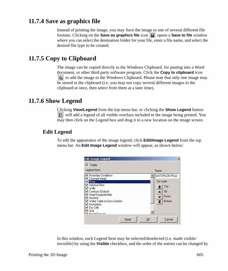
Printing the 3D Image 605
11.7.4 Save as graphics fileInstead of printing the image, you may Save the image to one of several different file formats. Clicking on the Save as graphics file icon opens a Save to file window where you can select the destination folder for your file, enter a file name, and select the desired file type to be created.
11.7.5 Copy to ClipboardThe image can be copied directly to the Windows Clipboard, for pasting into a Word document, or other third party software program. Click the Copy to clipboard icon
to add the image to the Windows Clipboard. Please note that only one image may be stored to the clipboard (i.e. you may not copy several different images to the clipboard at once, then select from them at a later time).
11.7.6 Show LegendClicking View/Legend from the top menu bar, or clicking the Show Legend button
will add a legend of all visible overlays included in the image being printed. You may then click on the Legend box and drag it to a new location on the image screen.
Edit LegendTo edit the appearance of the image legend, click Edit/Image Legend from the top menu bar. An Edit Image Legend window will appear, as shown below:
In this window, each Legend Item may be selected/deselected (i.e. made visible/invisible) by using the Visible checkbox, and the order of the entries can be changed by

606 Chapter 11: Visual MODFLOW 3D-Explorer
using the Top/Bottom and Up/Down arrow keys. The text label for each entry can be edited in the Name field once you have selected (highlighted) the item in the Legend Item list. For example, the entry for River can be replaced with descriptive text for the river, such as “WATERLOO River”. Click [Apply] to view the changes, click [OK] to accept the changes and close the window, or click Cancel to close the window without saving your changes.
11.7.7 Show Color LegendClicking View/Color Legend from the top menu bar, or clicking the Show Color Legend button will add a legend of the color shades used in the head and/or concentration contour shading.You may then click on the Legend box and drag it to a new location on the image screen.
11.7.8 AnnotateThe image annotation options can be accessed by selecting Edit/Annotate, or by clicking the Annotate icon in the top toolbar of the Image Editor window. A floating Annotate Tools window will appear on the screen, as shown in the following figure:
• Use the button to draw an arrow
• Use the button to draw a circle
• Use the button to draw a rectangle
• Use the button to draw a line
• Use the button to add text
• Use the button to add symbols
• Use the button to sketch a line
• Use the button to refresh the screen
• Use the button to delete all annotation objects
• Use the button to select, re-size, and move the annotation objects

Printing the 3D Image 607
Note: For details on printing a graph or bar chart, please refer to Chapter 10, section Graph Properties on page 531.
Note: Printing with high resolution (greater than 600 DPI) requires a Minimum of 512 MB of physical RAM on your computer. If you encounter problems while printing, please check your printer resolution settings (quality settings), and change to 600 DPI or less, or try the FastRes 1200 setting if available.
11.7.9 Image Editor HelpYou can open the Online Help references to the Image Editor directly by clicking the Image Editor Help button .
11.7.10 Image TitleA Title can be added to the image by selecting Edit/Title from the top menu bar, or clicking the Image Title button . In the Properties window that opens, you can type your title text in the Title frame, use the Visible checkbox to add or remove the title to the image, Align the title along the left or right margins, or centre the title, and add a Shadow to the title and position the shadow above or below the title text.The font
button is used to select the desired font, size, style and color for the Image Title text.
11.7.11 SelectIf you are using the Zoom feature, your cursor will remain in Zoom mode until you click the Select button, which reverts your cursor to normal mode.
11.7.12 ZoomYou may use the Zoom features to focus on a particular regions of the 3D model, which may then be printed. Select Zoom In , then left click your mouse and create a box around the area you would like to zoom into. The Zoom Previous button returns to the previous zoom selection, while Zoom Out returns to the regional 3D view.
11.7.13 Printing MethodsThere are two methods for printing:
Direct Printing- sends the image directly to the printer. This may not be ideal for images containing transparency, as the transparency may not show up. If the transparency does not show up, then try the second printing option. Additionally, if
608 Chapter 11: Visual MODFLOW 3D-Explorer
you are using a PostScript printer driver, the transparency settings may not show up. In this case, install the appropriate PCL driver for your printer, or use the Intermediate bitmap method of printing.
Intermediate bitmap- creates a temporary bitmap image in the memory, then sends the bitmap to the printer. This requires slightly more system memory, however it may provide a more suitable alternative to option 1.
Note: If you are printing an image that contains color shading (e.g. shaded head contours or concentration contours), direct printing will often result in a very large file being sent to your printer. If you are experiencing “out of memory” errors, or are not receiving output from your printer, please try the Intermediate bitmap method of printing. While the bitmap takes a few moments to create, it results in a much smaller file being sent to your printer, and facilitates image printing especially with older printers, or printers with low amounts of RAM.
Note: If you encounter problems when using a specific printer model, please check to see that you have the most recent Manufacturer-supplied driver installed. If installing a new driver does not resolve your printing issue, and you have tried both Printing Methods, you may use the last option, which is to save a graphics image file (as described in section Save as graphics file on page 605), and print the file from another application.
609
BibliographyAnderson, M. P. and Woessner, W.W., 1992: Applied Groundwater Modeling:
Simulation of Flow and Advective Transport. Academic Press Inc. San Diego, CA. 381 pp.
ASTM. 1996: ASTM Standards on Analysis of Hydrologic Parameters and Ground Water Modeling. Publication Code Number (PCN): 03-418096-38. West Conshohocken, PA. Ph: 610/8329585. 146 pp.
Bard, J., 1974: Nonlinear parameter estimation. Academic Press. NY. 341 pp.
Bear, J., 1979: Hydraulics of Groundwater. McGraw-Hill. New York, NY. 567 pp.
Brooks, R. H. and Corey, A. T., 1966: Properties of porous media affecting fluid flow. ASCE J. Irrig. Drain. Div., 92 (IR2): p. 61-88
Carsel, R. F., and Parrish, R. S., 1988: Developing joint probability distribution of soil water retention characteristics. Water Resour. Res. 24, p. 755-769.
D. N. Graham, S. Chmakov, A. Sapozhnikov, and J.B. Gregersen. OpenMI Coupling of MODFLOW and MIKE 11. “MODFLOW and More 2006. Managing Ground Water Systems. Conference Proceedings” May 21-24, v2, p727-731.
Cleary, A.J., Falgout, R.D., Henson, V.E., Jones, J.E., Manteuffel, T.A., McCormick, S.F., Miranda, G.N., and Ruge, J.W., 2000: Robustness and scalability of algebraic multigrid: SIAM Journal on Scientific Computing, v. 21, no. 5, p. 1886-1908.
Clement, T. P.,: RT3D v1.0 (1997), RT3D v2.5 (2001), A Modular Computer code for Simulating Reactive Multi-species Transport in 3-Dimensional groundwater systems. Pacific Northwest National Laboratory, Rihland, WA 99352, USA, PNNL-SA-11720, Found on-line at http://bioprocess.pnl.gov/rt3d.htm.
Cooley, R. L., 1983: Some new procedures for numerical solution of variably saturated flow problems. Water Resources Research, v19, no. 5. p. 1271-1285.
Demmel, J.W., 1997: Applied Numerical linear algebra: Philadelphia, Society for Industrial and Applied Mathematics, 419 p.
Domenico, P.A., and Schwartz, F. W., 1990: Physical and Chemical Hydrogeology. John Wiley and Sons Inc. New York, NY. 824 pp.
Driscoll, F.G., 1986: Groundwater and Wells, 2nd Edition. Johnson Division. St. Paul, Minnesota. 1089 pp.
Deutsch, C.V. and Journel, A.G., 1998: GSLIB Geostatistical Software Library and User’s Guide. Oxford University Press. N.Y. 369 pp.
610
Fetter, C.W., 1993: Contaminant Hydrogeology. Macmillan Publishing Co. New York, NY. 458 pp.
Fetter, C.W., 1994: Applied Hydrogeology, 3rd Edition. Macmillan Publishing Co. New York, NY. 691 pp.
Fetter, C.W., 1999: Contaminant Hydrogeology. 2nd Edition. Prentice-Hall Inc., New Jersey 500 pp.
Freeze, R.A., and Cherry, J.A., 1979: Groundwater. Prentice-Hall Inc. Englewood Cliffs, New Jersey. 604 pp.
Glover, F., 1986: Future paths for integer programming and links to artificial intelligence. Comp. and Operations Res., 5, p. 533-549.
Glover, F., 1989: Tabu Search - Part I, ORSA. J. Comp. 1(3), 190-206.
Graham, D.N., Chmakov, S., Sapozhnikov, A., Gregersen, J.B. OpenMI Coupling of MODFLOW and MIKE 11. “MODFLOW and More 2006. Managing Ground Water Systems. Conference Proceedings” May 21-24, v2, p727-731.
Harbaugh, A.W. 1990. A computer program for calculating subregional water budgets using results from the USGS Modular Three-Dimensional finite-difference groundwater flow model. U.S. Geological Survey Open-File Report 90-392.
Henry, R.M., 1995: A Critical Comparison of Some Commonly Used Groundwater Modeling Codes, M.Sc. Thesis. University of Waterloo, Department of Earth Sciences. Waterloo, Ontario. 115 pp.
Hill, M. C., 1997: Preconditioned Conjugate-Gradient 2 (PCG2), A Computer Program for Solving Groundwater Flow equations. USGS Water-Resources Investigations Report 90-4048.
Hill, M. C., 1992: A Computer Program (MODFLOWP) for Estimating Parameters of a Transient, Three-Dimensional, Ground-Water Flow Model using Nonlinear Regression. U. S. Geological Survey Open-File Report 91-484.
Huyakorn, P.S. and Pinder, G.F., 1983: Computational Methods in Subsurface Flow. Academic Press. New York, NY. 473 pp.
HydroGeoLogic, Inc., 1996: MODFLOW-SURFACT ver. 2.2 User’s manual. A three dimensional fully integrated finite difference code for simulating Fluid flow and Transport of contaminant in saturated-unsaturated porous media. Herndon, VA 20170, USA.
Doherty, J., 1998: Visual PEST: Graphical Model Independent Parameter Estimation. Watermark Computing and Waterloo Hydrogeologic Inc.
Kladias, M. P., and Ruskauff, G. J., 1997: Implementing Spatially Variable Anisotropy in MODFLOW. Ground Water, v35, no.2. p. 368-370
611
Koch, K., 1988: Parameter Estimation and Hypothesis Testing in Linear Models. Springer-Verlag, Berlin. 377 pp.
Levenberg, K., 1944: A method for the solution of certain non-linear problems in least squares. Q. Appl. Math., v2. 164-168 pp.
MacDonald, M. G. and Harbaugh, A. W., 1988: MODFLOW, A Modular three dimensional finite- difference groundwater flow model: U. S. Geological Survey Techniques of Water-Resources Investigations, Book 6, Chapter A1, 586 pp.
MacDonald, M.G. and A.W. Harbaugh. 1996. User’s Documentation: MODFLOW-96, An update to the USGS Modular three-dimensional finite–difference groundwater flow model. U.S. Geological Survey Open File Report 96-485.
Marquardt, D. W., 1963: An algorithm for least-squares estimation of nonlinear parameters. Journal of the Society of Industrial and Applied Mathematics, v11, no. 2. 431-441 pp.
Mehl, S.W., and Hill, M.C., 2001: MODFLOW-2000, The U.S. Geological Survey Modular Ground-Water Model - User Guide To The Link-AMG (LMG) Package For Solving Matrix Equations Using An Algebraic Multigrid Solver. U.S. Geological Survey Open-File Report 01-177.
Mikhail, E. M., 1976: Observations and Least Squares. IEP. NY. 497 pp.
Nash, J. C. and Walker-Smith, M., 1987: Nonlinear Parameter Estimation; an Integrated System in Basic. Marcel Dekker Inc. Monticello, NY. 493 pp.
National Ground Water Association, 1985, 1987, 1989, 1992... Practical Applications of Groundwater Models. Proceedings published by NGWA. Dublin, OH.
Nielsen, D.M. (editor). 1991: Practical Handbook of Ground Water Monitoring. Lewis Publishers. Chelsea, MI. 717 pp.
Ozbilgin, M.M. and Dickerman, D.C., 1984: A Modification of the Finite Difference Model for Simulation of a Two-Dimensional Ground-Water Flow to Include Surface-Ground Water Relationships: U.S. Geological Survey Water-Resources Investigations Report 83-4251, 98 pp.
Peaceman, D.W., 1983: Interpretation of Well-Block Pressures in Numerical Reservoir Simulation with Nonsquare Grid Blocks and Anisotropic Permeability. Society of Petroleum Engineers Journal, v. 23, no. 3. p. 531-543
Poeter, E., Zheng, C., and Hill, M., (editors) 1998: MODFLOW’98. Colorado School of Mines. Golden, Colorado.
Pollock, D.W., 1994: User’s Guide for MODPATH/MODPATH-PLOT version 3: A particle tracking post-processing package for MODFLOW, the USGS
612
finite-difference groundwater flow model. U.S. Geological Survey Open-File Report 94-464.
Pollock, David W., 1998: MODPATH, Documentation of Computer Programs to compute and display pathlines using results from U.S. Geological Survey modular three-dimensional finite difference groundwater flow model, U. S. Geological Survey Open Report 89-381, 188 pp.
Prommer, H., Barry, D.A., and C. Zheng, C., 2003. PHT3D - A MODFLOW/MT3DMS based reactive multi-component transport model. GroundWater, 42(2), 247-257.
Prudic, D.E., 1989: Documentation of a Computer Program to Simulate Stream-Aquifer Relations using a Modular, Finite-Difference, Ground-Water Flow Model. U. S. Geological Survey, Open-file report 88-729, 113 pp.
van Genuchten, M. Th., and Wierenga, P. J., 1977: Mass transfer studies in sorbing porous media: II. Experimental evaluation with Tritium (3H2O). Soil Sci. Soc. Am. J. 41 p. 272-278.
Zheng, C., 1993: Extension of the Method of Characteristics for Simulation of Solute Transport in Three Dimensions. Ground Water, vol 31(3). 456-465 pp.
Zheng, C., and Bennett, G. D., 1995: Applied Contaminant Transport Modeling: Theory and Practice, Van Nostrand Reinhold, New York.
Zheng, C., and Wang, P., 1999: MT3DMS, A Modular Three-Dimensional Multi- species Transport Model for Simulation of Advection, Dispersion, and Chemical Reactions of Contaminants in Groundwater Systems: Documentation and User’s Guide. U. S. Army Corps of Engineers, U. S. Army Engineer Research and Development Center, Vicksburg, Mississippi, SERDP-99-1.
Zheng, C. and Wang, P., 2003: MGO Modular Groundwater Optimizer Incorporating MODFLOW/MT3DMS: Documentation and User’s Guide. The University of Alabama, in cooperation with Groundwater Systems Research Ltd.
Zheng, C., 1999: User’s Guide. MT3D99 A modular 3D Multi-species transport simulator. S.S. Papadopulos & Associates.
613
AAppendix A: Visual MODFLOW Data Files
Visual MODFLOW stores all of the data for the flow, pathline, and contaminant transport model in a set of files having formats and data structures which are quite different than the model input data files required by MODFLOW, MODPATH, and MT3D. There are many reasons for these differences, but the primary reasons are:
• Visual MODFLOW does not require consistent units for length and time. Instead, Visual MODFLOW allows mixed units for different model parameters (e.g. length in metres, pumping rate in US GPM, Recharge rate in mm/yr)
• Visual MODFLOW does not require boundary conditions to be defined in terms of stress periods. Instead, Visual MODFLOW allows each boundary condition to be defined in using real time values and raw field data.
These differences are two of the key elements that make Visual MODFLOW so practical and user-friendly. However, these differences also require Visual MODFLOW to store the data in a different format, and then translate these data files to the required format(s) prior to running the models.
The following sections lists the various input and output data files generated by Visual MODFLOW, and describe the data formats for some of the more important data files.
Most input files are stored in ASCII text format, whereas most of the output files are stored in binary format. As a result, the input files can be manipulated using a text editor, or even generated using a FORTRAN or Visual Basic program, rather than using Visual MODFLOW's graphical user interface. However, if the files are externally manipulated or generated, the useful data validation and formatting checks performed by Visual MODFLOW will not be available. As a result, special care must be taken so the data structure for these files is not corrupted. It is not recommended - other than in special situations - to externally edit or manipulate the data files using a text editor.
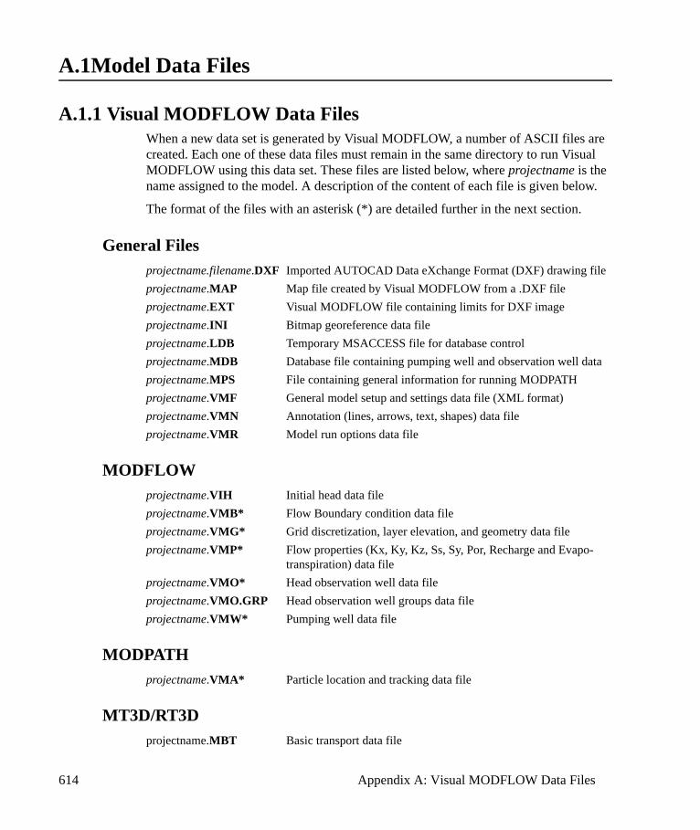
614 Appendix A: Visual MODFLOW Data Files
A.1Model Data Files
A.1.1 Visual MODFLOW Data FilesWhen a new data set is generated by Visual MODFLOW, a number of ASCII files are created. Each one of these data files must remain in the same directory to run Visual MODFLOW using this data set. These files are listed below, where projectname is the name assigned to the model. A description of the content of each file is given below.
The format of the files with an asterisk (*) are detailed further in the next section.
General Filesprojectname.filename.DXF Imported AUTOCAD Data eXchange Format (DXF) drawing fileprojectname.MAP Map file created by Visual MODFLOW from a .DXF fileprojectname.EXT Visual MODFLOW file containing limits for DXF imageprojectname.INI Bitmap georeference data fileprojectname.LDB Temporary MSACCESS file for database controlprojectname.MDB Database file containing pumping well and observation well dataprojectname.MPS File containing general information for running MODPATHprojectname.VMF General model setup and settings data file (XML format)projectname.VMN Annotation (lines, arrows, text, shapes) data fileprojectname.VMR Model run options data file
MODFLOWprojectname.VIH Initial head data fileprojectname.VMB* Flow Boundary condition data fileprojectname.VMG* Grid discretization, layer elevation, and geometry data fileprojectname.VMP* Flow properties (Kx, Ky, Kz, Ss, Sy, Por, Recharge and Evapo-
transpiration) data fileprojectname.VMO* Head observation well data fileprojectname.VMO.GRP Head observation well groups data fileprojectname.VMW* Pumping well data file
MODPATHprojectname.VMA* Particle location and tracking data file
MT3D/RT3Dprojectname.MBT Basic transport data file
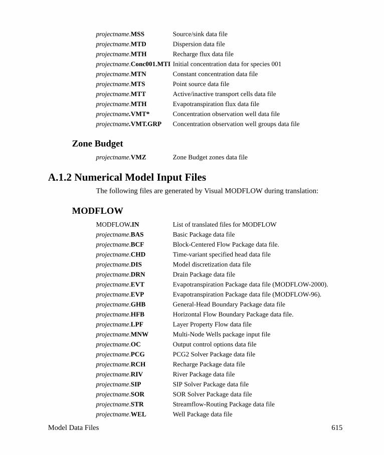
Model Data Files 615
projectname.MSS Source/sink data fileprojectname.MTD Dispersion data fileprojectname.MTH Recharge flux data fileprojectname.Conc001.MTI Initial concentration data for species 001projectname.MTN Constant concentration data fileprojectname.MTS Point source data fileprojectname.MTT Active/inactive transport cells data fileprojectname.MTH Evapotranspiration flux data fileprojectname.VMT* Concentration observation well data fileprojectname.VMT.GRP Concentration observation well groups data file
Zone Budgetprojectname.VMZ Zone Budget zones data file
A.1.2 Numerical Model Input FilesThe following files are generated by Visual MODFLOW during translation:
MODFLOWMODFLOW.IN List of translated files for MODFLOWprojectname.BAS Basic Package data file projectname.BCF Block-Centered Flow Package data file.projectname.CHD Time-variant specified head data fileprojectname.DIS Model discretization data fileprojectname.DRN Drain Package data file projectname.EVT Evapotranspiration Package data file (MODFLOW-2000).projectname.EVP Evapotranspiration Package data file (MODFLOW-96).projectname.GHB General-Head Boundary Package data fileprojectname.HFB Horizontal Flow Boundary Package data file.projectname.LPF Layer Property Flow data fileprojectname.MNW Multi-Node Wells package input fileprojectname.OC Output control options data fileprojectname.PCG PCG2 Solver Package data fileprojectname.RCH Recharge Package data fileprojectname.RIV River Package data fileprojectname.SIP SIP Solver Package data fileprojectname.SOR SOR Solver Package data fileprojectname.STR Streamflow-Routing Package data fileprojectname.WEL Well Package data file

616 Appendix A: Visual MODFLOW Data Files
projectname.WHS WHS Solver data file
MODPATHBACKWARD.IN Backward tracking particle locations data fileBACKWARD.PTH Backward tracking run options data fileFORWARD.IN Forward tracking particle locations data fileFORWARD.PTH Forward tracking run options data fileprojectname.MPT Main MODPATH input data fileMODPATH.IN List of MODPATH input files
MT3Dxx/RT3D projectname.AD3 Advection data fileprojectname.BT3 Basic Transport data fileprojectname.DP3 Dispersion data fileprojectname.GCG Transport Solver data fileprojectname.RC3 Chemical Reaction data fileprojectname.SS3 Source / Sink Mixing data fileMT3D.IN List of MT3D input files
Zone Budget projectname.ZBI Zone Budget data fileZONEBUD.IN List of Zone Budget input files
A.1.3 Output FilesAfter running the model, a number of results files will be generated. Some of the files generated by Visual MODFLOW can get very large (more than 100 Mbytes!). These files are typically in ASCII format, but some are in binary format to save disk space. The output files are described below.
Note:
* The files marked with an asterisk can get quite large for transient simulations.
MODFLOWprojectname.BGT* MODFLOW file containing water budget data used by MODPATH
(Binary format)
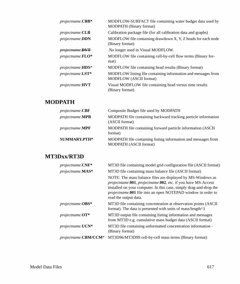
Model Data Files 617
projectname.CBB* MODFLOW-SURFACT file containing water budget data used by MODPATH (Binary format)
projectname.CLB Calibration package file (for all calibration data and graphs)projectname.DDN MODFLOW file containing drawdown X, Y, Z heads for each node
(Binary format)projectname.DVT No longer used in Visual MODFLOW. projectname.FLO* MODFLOW file containing cell-by-cell flow terms (Binary for-
mat)projectname.HDS* MODFLOW file containing head results (Binary format)projectname.LST* MODFLOW listing file containing information and messages from
MODFLOW (ASCII format)projectname.HVT Visual MODFLOW file containing head versus time results
(Binary format)
MODPATHprojectname.CBF Composite Budget file used by MODPATHprojectname.MPB MODPATH file containing backward tracking particle information
(ASCII format)projectname.MPF MODPATH file containing forward particle information (ASCII
format)SUMMARY.PTH* MODPATH file containing listing information and messages from
MODPATH (ASCII format)
MT3Dxx/RT3Dprojectname.CNF* MT3D file containing model grid configuration file (ASCII format)projectname.MAS* MT3D file containing mass balance file (ASCII format)
NOTE: The mass balance files are displayed by MS-Windows as projectname.001, projectname.002, etc. if you have MS-Access installed on your computer. In this case, simply drag-and-drop the projectname.001 file into an open NOTEPAD window in order to read the output data.
projectname.OBS* MT3D file containing concentration at observation points (ASCII format). The data is presented with units of mass/length^3
projectname.OT* MT3D output file containing listing information and messages from MT3D e.g. cumulative mass budget data (ASCII format)
projectname.UCN* MT3D file containing unformatted concentration information - (Binary format)
projectname.CBM/CCM* MT3D96/MT3D99 cell-by-cell mass terms (Binary format)

618 Appendix A: Visual MODFLOW Data Files
PESTprojectname.NDC Allows WINPEST to continue to run even if one calibration
attempt does not convergeprojectname.REC PEST results file (ASCII format)projectname.PLT loadable file (ASCII format)
Zone Budgetprojectname.ZOT Zone Budget file containing water balance data (ASCII format).
Visual MODFLOW Input Data Formats 619
A.2 Visual MODFLOW Input Data FormatsIn the following sections, the formats of the Visual MODFLOW input data files are documented. This information is included for the experienced user only. It is not necessary to directly edit the data files. It is strongly recommended to always use the Visual MODFLOW graphical user interface to create and modify these files, since this is the only way to ensure the data files have the required format, and valid data.
The information in the following files is written from the bottom layer to the top (ground surface). This is done to be consistent with MODFLOW. All input data files are written in free ASCII format ( i.e. there is at least one blank space between the numbers in each line). Real numbers require a decimal point, and can be expressed in either fixed or scientific notation (e.g., 104.0 or 1.04E2). Integer numbers, however, MUST NOT contain a decimal point.
Note: Spaces are the only delimiters accepted; commas are not accepted by Visual MODFLOW as delimiters.
A.2.1 VMA - Particle File FormatParticle data are stored as objects. Visual MODFLOW keeps on reading the objects until the end of the file is reached. The three types of particle objects are Single, Line and Circle particle objects.
For a Single particle object the format is:
0
1
Tracking (0 = Backward , 1 = Forward)
X Y Z Release_Time
For a Line particle object the format is:
1
N
Tracking (0 = Backward , 1 = Forward)
XSTART YSTART ZSTART Release_Time
XEND YEND ZEND Release_Time
For a Circle particle object the format is:
2
N
Tracking (0 = Backward , 1 = Forward)
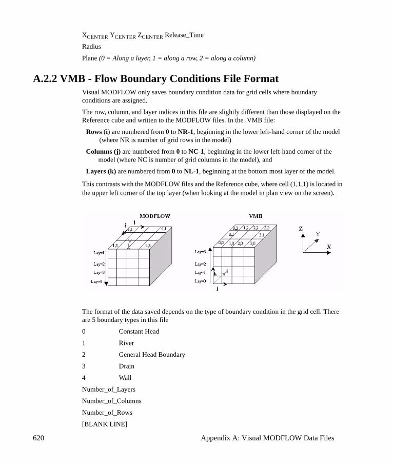
620 Appendix A: Visual MODFLOW Data Files
XCENTER YCENTER ZCENTER Release_Time
Radius
Plane (0 = Along a layer, 1 = along a row, 2 = along a column)
A.2.2 VMB - Flow Boundary Conditions File FormatVisual MODFLOW only saves boundary condition data for grid cells where boundary conditions are assigned.
The row, column, and layer indices in this file are slightly different than those displayed on the Reference cube and written to the MODFLOW files. In the .VMB file:
Rows (i) are numbered from 0 to NR-1, beginning in the lower left-hand corner of the model (where NR is number of grid rows in the model)
Columns (j) are numbered from 0 to NC-1, beginning in the lower left-hand corner of the model (where NC is number of grid columns in the model), and
Layers (k) are numbered from 0 to NL-1, beginning at the bottom most layer of the model.
This contrasts with the MODFLOW files and the Reference cube, where cell (1,1,1) is located in the upper left corner of the top layer (when looking at the model in plan view on the screen).
The format of the data saved depends on the type of boundary condition in the grid cell. There are 5 boundary types in this file
0 Constant Head
1 River
2 General Head Boundary
3 Drain
4 Wall
Number_of_Layers
Number_of_Columns
Number_of_Rows
[BLANK LINE]

Visual MODFLOW Input Data Formats 621
For each Constant Head boundary grid cell:
Layer
Column
Row
0 (Code for Constant Head boundary type)
Code_Number
Number_of_Time_Entries
Start_Time1 Stop_Time1 Start_Time_Head1 Stop_Time_Head1 Active/Inactive
.
Start_TimeNE Stop_TimeNE Start_Time_HeadNE Stop_Time_HeadNE Active/Inactive
For each River boundary grid cell:
Layer
Column
Row
1 (Code for River Boundary type)
Code_Number
Number_of_Time_Entries
Start_Time1 Stop_Time1 River_Stage1 River_Bottom1 Conductance1 Active/Inactive
.
Start_TimeNE Stop_timeNE River_StageNE River_BottomNE ConductanceNE Active/Inactive
For each General Head boundary grid cell:
Layer
Column
Row
2 (Code for GHB Boundary type)
Code_Number
Number_of_Time_Entries
Start_Time1 Stop_Time1 General_Head1 Conductance1 Active/Inactive
.
Start_TimeNE Stop_TimeNE General_HeadNE ConductanceNE Active/Inactive
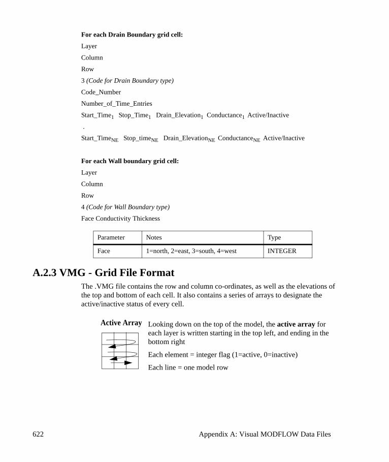
622 Appendix A: Visual MODFLOW Data Files
For each Drain Boundary grid cell:
Layer
Column
Row
3 (Code for Drain Boundary type)
Code_Number
Number_of_Time_Entries
Start_Time1 Stop_Time1 Drain_Elevation1 Conductance1 Active/Inactive
.
Start_TimeNE Stop_timeNE Drain_ElevationNE ConductanceNE Active/Inactive
For each Wall boundary grid cell:
Layer
Column
Row
4 (Code for Wall Boundary type)
Face Conductivity Thickness
A.2.3 VMG - Grid File FormatThe .VMG file contains the row and column co-ordinates, as well as the elevations of the top and bottom of each cell. It also contains a series of arrays to designate the active/inactive status of every cell.
Parameter Notes Type
Face 1=north, 2=east, 3=south, 4=west INTEGER
Looking down on the top of the model, the active array for each layer is written starting in the top left, and ending in the bottom right
Each element = integer flag (1=active, 0=inactive)
Each line = one model row
Active Array
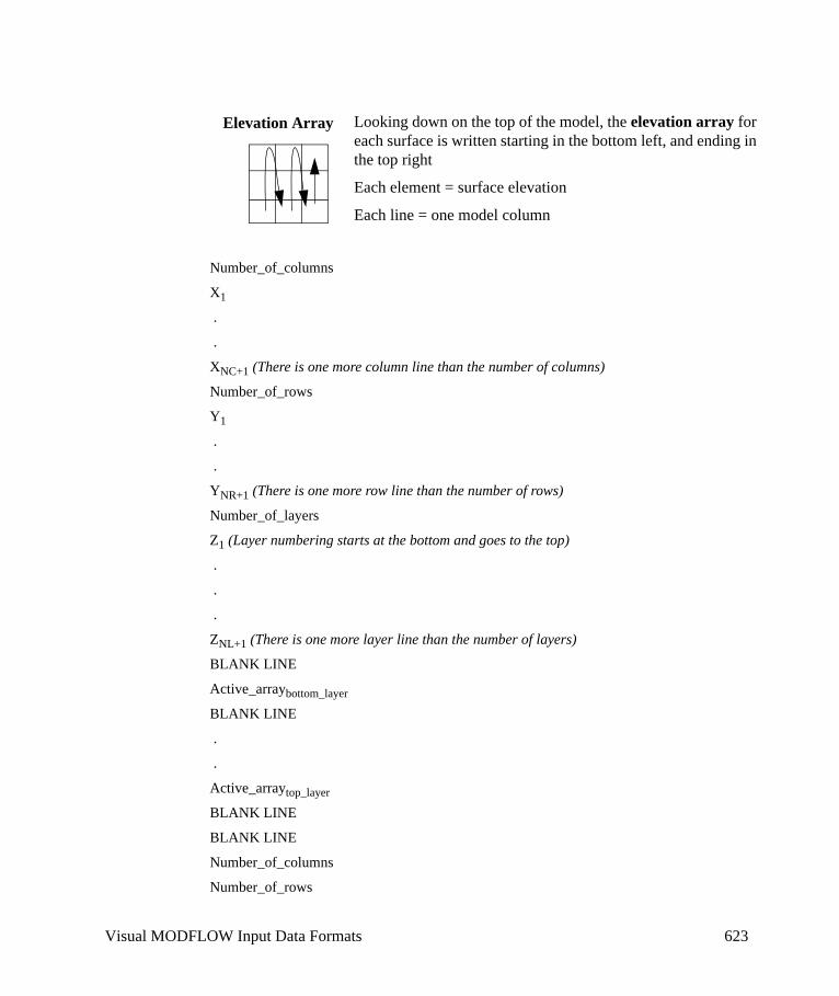
Visual MODFLOW Input Data Formats 623
Number_of_columns
X1
.
.
XNC+1 (There is one more column line than the number of columns)
Number_of_rows
Y1
.
.
YNR+1 (There is one more row line than the number of rows)
Number_of_layers
Z1 (Layer numbering starts at the bottom and goes to the top)
.
.
.
ZNL+1 (There is one more layer line than the number of layers)
BLANK LINE
Active_arraybottom_layer
BLANK LINE
.
.
Active_arraytop_layer
BLANK LINE
BLANK LINE
Number_of_columns
Number_of_rows
Looking down on the top of the model, the elevation array for each surface is written starting in the bottom left, and ending in the top right
Each element = surface elevation
Each line = one model column
Elevation Array
624 Appendix A: Visual MODFLOW Data Files
Number_of_layers
BLANK LINE
Elevation_arraybottom_surface
.
.
.
Elevation_arraytop_surface
A.2.4 VMO - Heads Observation File FormatThe .VMO and the .VMT files contain a two-line header followed by one entry for each head or concentration observation well.
Version='X.X.X.xxx' VMOD version numberWellCount=32 total number of observation wells in the file
for each observation well:Well='Obs-1' well nameX= 403.2258065 x - co-ordinate
Y= 608.8709677 y - co-ordinate Min_Z= 0 bottom of model at observation location Max_Z= 25 top of model at observation location Radius= 0 well radius - not currently used ScreenCount=0 not currently used for observation wells Screens not currently used for observation wells end Screens not currently used for observation wells ScheduleCount=0 not currently used for observation wells Schedule not currently used for observation wells end Schedule not currently used for observation wells PointCount=1 number of observation points in the well
for each observation point: Point='A' name of observation point Z= 12.5 elevation of observation point SpeciesCount=1 number of species in the model (for heads
observation wells this is always 1) Species='Head' for head observation wells this value is always
equal to “Head”; for concentration observation wells this is the species name
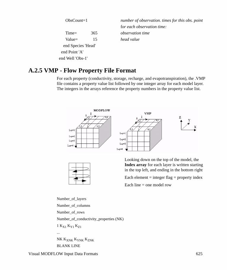
Visual MODFLOW Input Data Formats 625
ObsCount=1 number of observation. times for this obs. pointfor each observation time:
Time= 365 observation time Value= 15 head value end Species 'Head' end Point 'A' end Well 'Obs-1'
A.2.5 VMP - Flow Property File FormatFor each property (conductivity, storage, recharge, and evapotranspiration), the .VMP file contains a property value list followed by one integer array for each model layer. The integers in the arrays reference the property numbers in the property value list.
Number_of_layers
Number_of_columns
Number_of_rows
Number_of_conductivity_properties (NK)
1 KX1 KY1 KZ1
...
NK KXNK KYNK KZNK
BLANK LINE
Looking down on the top of the model, the Index array for each layer is written starting in the top left, and ending in the bottom right
Each element = integer flag = property index
Each line = one model row

626 Appendix A: Visual MODFLOW Data Files
Conductivity_Index_ArrayBottom_layer
BLANK LINE
...
Conductivity_Index_ArrayTop_layer
BLANK LINE
Number_of_storage_properties (NS)
1 SS1 SY1 Effective_porosity1 Total_Porosity1
...
NS SSNS SYNS Effective_PorosityNS Total_PorosityNS
BLANK LINE
Storage_Index_ArrayBottom_layer
BLANK LINE
...
Storage_Index_ArrayTop_layer
BLANK LINE
Number_of_recharge_properties (NR)
for each recharge property
Property_number Recharge_multiplier Index
Number_of_recharge_timesteps rchr entries
Property_number Recharge_value1 Start_time1 Stop_time1
Property_number Recharge_value2 Start_time2 Stop_time2
...
Property_number Recharge_valuensteps Start_timensteps Stop_timensteps
BLANK LINE
Recharge_Index_ArrayBottom_layer
BLANK LINE
...
Recharge_Index_ArrayTop_layer
BLANK LINE
Number_of_evapotranspiration_properties (NE)
for each evapotranspiration property
Property_number Evapo_multiplier Index
Number_of_evapo_timesteps evap entries
Property_number Evapo_value1 Evapo_depth1 Start_time1 Stop_time1
Visual MODFLOW Input Data Formats 627
Property_number Evapo_value2 Evapo_depth2 Start_time2 Stop_time2
...
Property_number Evapo_valuensteps Evapo_depthnsteps Start_timensteps Stop_timensteps
BLANK LINE
Evapo_Index_ArrayBottom_layer
BLANK LINE
...
Evapo_Index_ArrayTop_layer
A.2.6 VMW - Pumping Well File Format
NW, Coord Number_of_wells, co-ordinate System (0=model, 1=world)
For each well (i = 1 to NW)
ActiveFlag Active_flag (1 = active, 0 = inactive)
WELLi, OBSiName of pumping well and associated head observation well
Xi X-coord
Yi Y-coord
ZMINi Bottom elevation of model grid at (X, Y) location
ZMAXi, Ri Top elevation of model grid at (X, Y) location, Well Radius
NSi Number of well screen intervals
For each screened interval (j = 1 to NS)
BOTij Bottom elevation of Screen
TOPij Top elevation of Screen
NTi Number of pumping time periods
For each pumping time period (k = 1 to NT)
STARTik Start time of time period
STOPik Stop time of time period
RATEik Pumping rate for time period
A.2.7 VMZ - Zone Budget File FormatThe .VMZ file contains a cell-by-cell array for each layer, with the zone number of each cell. The first array is for the bottom layer and the last array is for the top layer. Each cell can belong to only one user-specified zone.
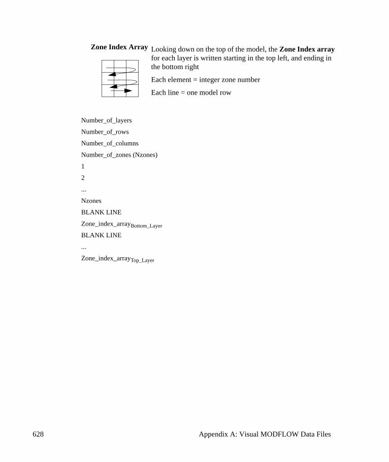
628 Appendix A: Visual MODFLOW Data Files
Number_of_layers
Number_of_rows
Number_of_columns
Number_of_zones (Nzones)
1
2
...
Nzones
BLANK LINE
Zone_index_arrayBottom_Layer
BLANK LINE
...
Zone_index_arrayTop_Layer
Looking down on the top of the model, the Zone Index array for each layer is written starting in the top left, and ending in the bottom right
Each element = integer zone number
Each line = one model row
Zone Index Array
Inverse Distance 629
BAppendix B: Interpolation Method Settings
Visual MODFLOW utilizes a built-in data interpolation, gridding, and contouring component to import and interpolate field data. This component has been developed by Schlumberger Water Services for the purpose of interpolating random data points to create a uniform grid of data, for visualization and interpretation and utilization in Visual MODFLOW.
The interpolation methods currently supported by the Interpolation component include:
• Inverse Distance• Kriging• Natural Neighbors
The following sections describe the methodology and the available settings for each of these interpolation methods. The method descriptions provided below are taken from the GSLIB Geostatistical Software Library and User’s Guide (Deutsch and Journel, 1998).
B.1 Inverse DistanceThe Inverse Distance Squared method is a very fast and efficient, weighted average interpolation method. The weighting factor applied to the data depends on the distance of the point from the grid cell, and is inversely proportional to the distance squared. Consequently, the greater the distance the data point is from the grid node, the smaller the influence it has on the calculated value.
The Inverse Distance Squared method for interpolation may generate patterns similar to a “bull’s-eye” surrounding points of observations. Selecting a larger number of nearest neighboring data points may smooth this effect, but if the bull’s eye pattern is undesirable, then other methods of interpolation, like Natural Neighbor and Kriging, are recommended.
The Interpolator Options window for the Inverse Distance Squared method is shown in the following figure, while each of the settings parameters is described below.
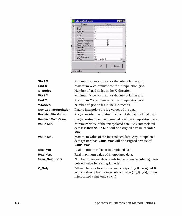
630 Appendix B: Interpolation Method Settings
Start X Minimum X co-ordinate for the interpolation grid.End X Maximum X co-ordinate for the interpolation grid.X_Nodes Number of grid nodes in the X-direction.Start Y Minimum Y co-ordinate for the interpolation grid.End Y Maximum Y co-ordinate for the interpolation grid.Y-Nodes Number of grid nodes in the Y-direction.Use Log Interpolation Flag to interpolate the log values of the data.Restrict Min Value Flag to restrict the minimum value of the interpolated data.Restrict Max Value Flag to restrict the maximum value of the interpolation data.Value Min Minimum value of the interpolated data. Any interpolated
data less than Value Min will be assigned a value of Value Min.
Value Max Maximum value of the interpolated data. Any interpolated data greater than Value Max will be assigned a value of Value Max.
Real Min Real minimum value of interpolated data.Real Max Real maximum value of interpolated data.Num_Neighbors Number of nearest data points to use when calculating inter-
polated value for each grid node.Z_Only Allows the user to select between outputting the original X
and Y values, plus the interpolated value (x,y,f(x,y)), or the interpolated value only (f(x,y)).
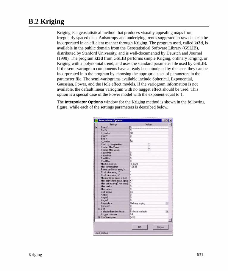
Kriging 631
B.2 KrigingKriging is a geostatistical method that produces visually appealing maps from irregularly spaced data. Anisotropy and underlying trends suggested in raw data can be incorporated in an efficient manner through Kriging. The program used, called kt3d, is available in the public domain from the Geostatistical Software Library (GSLIB), distributed by Stanford University, and is well-documented by Deustch and Journel (1998). The program kt3d from GSLIB performs simple Kriging, ordinary Kriging, or Kriging with a polynomial trend, and uses the standard parameter file used by GSLIB. If the semi-variogram components have already been modeled by the user, they can be incorporated into the program by choosing the appropriate set of parameters in the parameter file. The semi-variograms available include Spherical, Exponential, Gaussian, Power, and the Hole effect models. If the variogram information is not available, the default linear variogram with no nugget effect should be used. This option is a special case of the Power model with the exponent equal to 1.
The Interpolator Options window for the Kriging method is shown in the following figure, while each of the settings parameters is described below.
632 Appendix B: Interpolation Method Settings
Start X Minimum X co-ordinate for the interpolation grid.End X Maximum X co-ordinate for the interpolation grid.X_Nodes Number of grid nodes in the X-direction.Start Y Minimum Y co-ordinate for the interpolation grid.End Y Maximum Y co-ordinate for the interpolation grid.Y-Nodes Number of grid nodes in the Y-direction.Use Log Interpolation Flag to interpolate the log values of the data.Restrict Min. Value Flag to restrict the minimum value of the interpolated data.Restrict Max. Value Flag to restrict the maximum value of the interpolation data.Value Min. Minimum value of the interpolated data. Any interpolated
data less than Value Min. will be assigned a value of Value Min.
Value Max. Maximum value of the interpolated data. Any interpolated data greater than Value Max. will be assigned a value of Value Max.
Real Min. Real minimum value of interpolated data.Real Max. Real maximum value of interpolated data.Min. Trimming Limit Minimum bound for the interpolated data if the Restrict Min.
Value option is not selected by the user.Max. Trimming Limit Maximum bound for the interpolated data if the Restrict
Max. Value option is not selected by the user.
The Points per block along X, Points per block along Y, and Points per block along Z values allow the user to choose Block Kriging used for interpolation, as compared to Point Kriging. Block Kriging is based on the premise that since Kriging is a linear algorithm, direct estimation of the block average is possible for user-defined blocks. The default values for these parameters are 1, and in this case the default method is Point Kriging. If Block Kriging is being used, the user needs to enter the Min. points for block Kriging and Max. points for block Kriging.
The Octant Search option is an exhaustive search option available to make sure that data are taken on all sides of the point being estimated, and is especially recommended for 3D data. If the user specifies Max. points per octant to be greater than 0, an Octant Search is employed to find the neighborhood of points for interpolation.
The Max. radius and Min. radius defines the search distances, in user specified units, in the maximum horizontal direction and the minimum horizontal direction for determining the neighborhood of points for interpolation. For isotropic data, the two radii are the same. Enter the Vertical Radius value if 3D Kriging is to be performed. If the total number of points in the data is large (>200), computation time for Kriging may be reduced by specifying a smaller radius for the search.
The Angle1, Angle2, and Angle3 parameters define the search ellipsoid for situations in which anisotropy is present in the data.
Kriging 633
The Kriging type options are
• Stationary simple Kriging with SK mean• Ordinary Kriging• Nonstationary simple Kriging with means from an external file• Kriging with external drift
The following guidelines are recommended for selecting the type of Kriging.
Choose Stationary simple Kriging with SK mean, if the mean value is known and is constant throughout the area.
Select Ordinary Kriging if the mean is not constant everywhere, and needs to be recalculated dependent on the location of the neighborhood.
Choose Nonstationary simple Kriging with means from an external file if the mean is not constant and has to be read from an external file.
Select Kriging with an external drift when only the trend component needs to be estimated, and not the residual component, where the variable is assumed to be the sum of the trend and the residual component. This option is also referred to as Universal Kriging.
For most situations, Ordinary Kriging is recommended and is the default option.
The SK Mean defines the global mean of the data if Stationary simple Kriging is performed.
The Drift term defines the drift components if Kriging with external drift is performed. Nine drift components are possible:
• X = linear drift in x • Y = linear drift in y • Z = linear drift in z • Xq = quadratic drift in x • Yq = quadratic drift in y • Zq = quadratic drift in z • XY = cross quadratic drift in xy • XZ = cross quadratic drift in xz • YZ = cross quadratic drift in yz
The Variable/Trend Estimate allows the user to choose between estimating the variable or the trend. The default is Estimate variable.
The Nugget constant quantifies the sampling and assaying errors in the data. In a Variogram plot the nugget constant is the y-intercept value.
The Use variograms option allows the user to select the type of variogram to be used. The Variogram models available include:
Spherical model defined by an actual range a and positive variance contribution or sill value c.
634 Appendix B: Interpolation Method Settings
if h <= aif h >= a
Exponential model defined by an effect range a (integral range a/3) and positive variance contribution value c.
Gaussian model defined by an effective range a and positive variance contribution value c.
Power model defined by a power 0 < w < 2 and positive slope c.
The distance h may be anisotropic in 2D or 3D.
Hole Effect model defined by a length a to the first peak (size of the underlying cyclic features) and positive variance contribution value c.
If the variogram information is not available, the default linear variogram with no nugget effect should be used. This option is a special case of the Power model with the exponent equal to 1.
γ h( ) c Sph ha---⎝ ⎠⎛ ⎞⋅
c 1.5ha--- 0.5 h
a---⎝ ⎠⎛ ⎞
3
–⋅
c⎩⎪⎨⎪⎧
= =
γ h( ) c Exp ha---⎝ ⎠⎛ ⎞⋅ c 1 3h–
a---------⎝ ⎠⎛ ⎞exp–⋅= =
γ h( ) c 1 3h( )2
a2-------------–⎝ ⎠
⎛ ⎞exp–⋅=
γ h( ) c hw⋅=
γ h( ) c 1.0 ha--- π⋅⎝ ⎠⎛ ⎞cos–⋅=

Natural Neighbors 635
B.3 Natural Neighbors The Natural Neighbor method (Watson, 1994) is based on the Thiessen polygon method used for interpolating rainfall data. The grid node for interpolation is considered a new point, or target, to the existing data set. With the addition of this point, the Thiessen polygons based on the existing points are modified to include the new point. The polygons reduce in area to include the new points, and the area that is taken out from the existing polygons is called the “borrowed area”. The interpolation algorithm calculates the interpolated value as the weighted average of the neighboring observations where the weights are proportional to the borrowed areas. The Natural Neighbor method is valid only with the convex hull of the Thiessen polygon formed by the data points, and values outside the hull extrapolation should be used with caution.
The Natural Neighbor interpolation scheme may be visualized as a taut rubber sheet stretched to satisfy all the data points. The interpolated value at any location is a linear combination of all Natural Neighbors of that location, and the resulting surface is continuous with a slope that is also continuous. Combining the gradients or slopes with the linear interpolation provides results that are more smooth, and may anticipate the peaks and valleys between data. Singularities and other undesirable effects may be lessened by incorporating the gradient factor.
The gradient influence on the results can be manipulated by two tautness parameters that the user can enter. These parameters allow the interpolated surface to vary from purely linear interpolation to one which is well rounded and has the gradient factor. In all cases the slope discontinuities are removed and the resulting surface has slope continuity everywhere.
The Interpolator Options window for the Natural Neighbor method is shown in the following figure, while each of the settings parameters is described below.
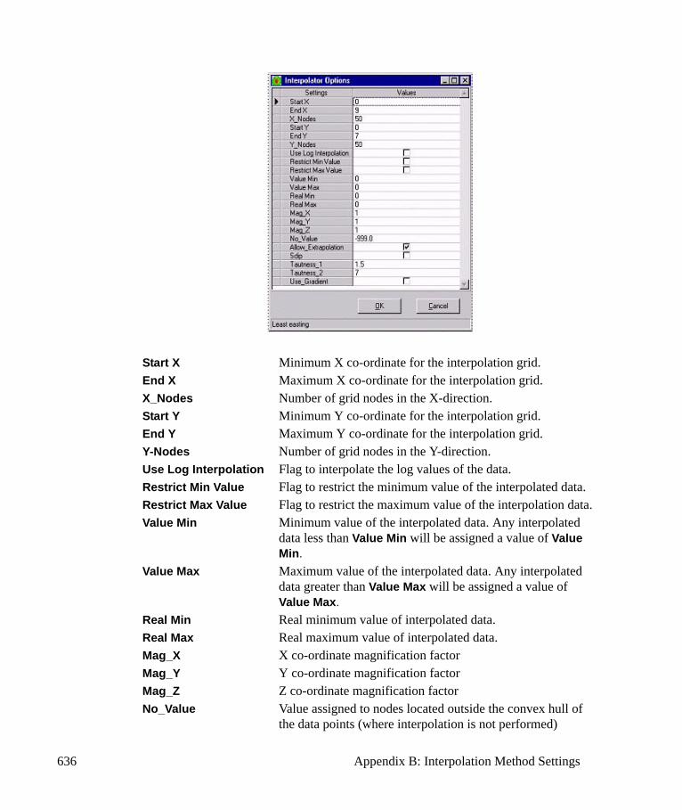
636 Appendix B: Interpolation Method Settings
Start X Minimum X co-ordinate for the interpolation grid.End X Maximum X co-ordinate for the interpolation grid.X_Nodes Number of grid nodes in the X-direction.Start Y Minimum Y co-ordinate for the interpolation grid.End Y Maximum Y co-ordinate for the interpolation grid.Y-Nodes Number of grid nodes in the Y-direction.Use Log Interpolation Flag to interpolate the log values of the data.Restrict Min Value Flag to restrict the minimum value of the interpolated data.Restrict Max Value Flag to restrict the maximum value of the interpolation data.Value Min Minimum value of the interpolated data. Any interpolated
data less than Value Min will be assigned a value of Value Min.
Value Max Maximum value of the interpolated data. Any interpolated data greater than Value Max will be assigned a value of Value Max.
Real Min Real minimum value of interpolated data.Real Max Real maximum value of interpolated data.Mag_X X co-ordinate magnification factorMag_Y Y co-ordinate magnification factorMag_Z Z co-ordinate magnification factorNo_Value Value assigned to nodes located outside the convex hull of
the data points (where interpolation is not performed)
Natural Neighbors 637
Allow_Extrapolation Is a flag to use extrapolation for nodes outside the convex hull of the polygon formed by the data points. In this case linear regression is used to fit a plane through the data set and calculate the interpolated value. This should be used with caution since extrapolation is less reliable than interpolation.
Sdip Calculate the aspect and slope at each grid node. This can be used to augment the elevation information. The aspect is measured in degrees or radians clockwise from north, and the slope is measured positively below the horizontal plane in degrees or radians.
Tautness_1 Controls the influence of the gradient on the results and may be used to smooth the interpolated surface.
Tautness_2 Controls the influence of the gradient on the results and may be used to smooth the interpolated surface.
Use_Gradient Blends the gradient calculation and the linear interpolation calculation to produce a smoother surface.

638 Appendix B: Interpolation Method Settings
639
CAppendix C: Numeric Engines
Visual MODFLOW supports all of the most recent public domain and proprietary versions of MODFLOW and MT3D for simulating groundwater flow modeling and mass transport modeling, respectively. In Visual MODFLOW, these programs are referred to as Numeric Engines because they perform the numeric calculations required to solve the finite difference equations of groundwater flow and mass transport. The numeric engines supported by Visual MODFLOW include:
Groundwater Flow
• MODFLOW-96 (Public Domain, U.S. Geological Survey)• MODFLOW-2000 (Public Domain, U.S. Geological Survey)• SEAWAT (Public Domain, U.S. Geological Survey)• MODFLOW-SURFACT (HydroGeoLogic, Inc.)
Mass Transport
• MT3D96 (not available for new projects/variants) (Proprietary, S.S. Papadopulos & Associates, Inc.)
• MT3DMS (Public Domain, U.S. Army Corp of Engineers)• MT3D99 (Proprietary, S.S. Papadopulos & Associates, Inc.)• RT3Dv1.0 (Public Domain, Battelle Northwest Laboratories)• RT3D 2.5 (Public Domain, Battelle Northwest Laboratories)• PHT3D v.1.46 (Public Domain, www.pht3d.org)• SEAWAT (Public Domain, U.S. Geological Survey)
Although the most recent versions of the MT3D programs will be used the majority of the time, the reason for continuing to support the legacy codes is to give the user the opportunity to reproduce simulation results from older model data sets, using exactly the same simulation programs.
Note: The MODPATH and Zone Budget versions included in Visual MODFLOW are the latest U.S.Geological Survey versions, compiled and optimized to run as 32 bit native Windows applications.
The following sections provide a brief overview of each Flow and Transport Numeric Engine, and offer some insight into the differences between them.
640 Appendix C: Numeric Engines
C.1 Groundwater Flow Numeric EnginesMODFLOW is a three-dimensional MODular finite-difference groundwater FLOW model, originally developed by the U.S. Geological Survey and released to the public domain in 1983. This version was referred to as MODFLOW-83. This code was eventually updated to conform to the Fortran 77 programming language in McDonald and Harbaugh (1988). The revised program was referred to as MODFLOW-88 and was also released to the public domain.
Included with your Visual MODFLOW Installation media is an electronic copy of the original MODFLOW-88 Reference Manual (MODFLOW-88 Manual.pdf), found in the Manual folder on the Installation CD.
C.1.1 MODFLOW-96MODFLOW-96 was released by the U.S. Geological Survey in 1996 to address several perceived needs of the program, most notably the ability to convert dry cells to variable head cells, and the ability to calculate alternate interblock transmissivities.
Included with your Visual MODFLOW Installation media is an electronic copy of the original MODFLOW-96 Reference Manual (MODFLOW-96 Manual.pdf), found in the Manual folder on the Installation CD.
C.1.2 MODFLOW-2000MODFLOW-2000 was released by the U.S. Geological Survey in 2000, and introduced a new process-based approach to the MODFLOW program structure, together with built-in parameter estimation capabilities. The process-based approach and built-in parameter estimation required some radical changes to input file structures and data requirements, the most significant being:
• The Block-Centered Flow (BCF) Package was replaced by the Layer Property Flow (LPF) Package as the default package
• When the LPF Package is used, the top and bottom elevations of each grid cell must be explicitly defined
• The boundary conditions values and property values may be defined in terms of parameter values and multiplier arrays
Visual MODFLOW supports and includes both MODFLOW-96 and MODFLOW-2000 to run the groundwater flow simulation. Ideally, these programs should produce identical results. However, MODFLOW-2000 may produce some subtle differences when running MODFLOW-96 models if specified VCONT values were used to simulate leakage from an aquitard.
Included with your Visual MODFLOW Installation media is an electronic copy of the original MODFLOW-2000 Reference Manual (MODFLOW-2000 Manual.pdf), found in the Manual folder on the Installation CD.
Groundwater Flow Numeric Engines 641
C.1.3 MODFLOW-2005MODFLOW-2005 was released by the U.S Geological Survey in 2006 and is very similar in design to MODFLOW-2000. The primary change in MODFLOW-2005 is the incorporation of a different approach in managing internal data. The main reason in the new approach is to facilitate the local-grid refinement (LGR) capability, which allows a subregion of the model grid to be simulated with a finer grid.
For more information on the MODFLOW-2005 flow engine, please refer to the electronic copy of the original MODFLOW-2005 Reference Manual (MODFLOW-2005 Manual.pdf) found in the Manual folder on the Installation CD.
C.1.4 MODFLOW-SURFACT One of the most important features in the Visual MODFLOW is the support for MODFLOW-SURFACT, developed by HydroGeoLogic, Inc. (HGL). MODFLOW-SURFACT is a fully integrated groundwater flow and solute transport package based on the USGS MODFLOW code (McDonald and Harbaugh, 1988). The modular structure of the original MODFLOW code is maintained, and modules for the enhanced features are called from the main program. MODFLOW-SURFACT constitutes additional modules, and extends the physical applicability of the MODFLOW code to handle complex field problems. In the current release of the Visual MODFLOW, only the flow packages of MODFLOW-SURFACT are supported.
The MODFLOW-SURFACT flow packages have the capability of modeling unsaturated moisture and air movement, and contain simultaneous solution techniques (e.g. Newton-Raphson linearization) that rigorously couple the surface-water and groundwater flow regimes. Three-dimensional variably saturated flow formulation can reduce the unsaturated flow problems (e.g. drying of cells near the water table), accurately delineate the water table elevations, and capture delayed yield response of an unconfined system to pumping and recharge. It includes adaptive time-stepping schemes with automatic generation and control of time steps. For a detailed description of the groundwater flow and solute transport modules, the user is encouraged to refer volumes 1 and 2 of the MODFLOW-SURFACT documentation.
“SURFACT” is an acronym for:
S- Schemes for robust and efficient modeling
U- rigorous treatment of Unsaturated flow
R- non-ponding Recharge and seepage face boundaries
F- Fracture well representation to provide rigorous treatment of well conditions
ACT- Analysis of Contaminant Transport.
The Flow packages are generally referred to as “SURF” and the Solute transport packages as “ACT”.
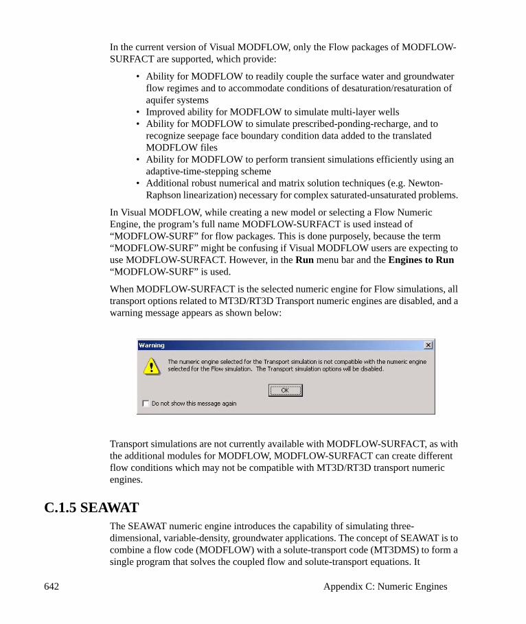
642 Appendix C: Numeric Engines
In the current version of Visual MODFLOW, only the Flow packages of MODFLOW-SURFACT are supported, which provide:
• Ability for MODFLOW to readily couple the surface water and groundwater flow regimes and to accommodate conditions of desaturation/resaturation of aquifer systems
• Improved ability for MODFLOW to simulate multi-layer wells• Ability for MODFLOW to simulate prescribed-ponding-recharge, and to
recognize seepage face boundary condition data added to the translated MODFLOW files
• Ability for MODFLOW to perform transient simulations efficiently using an adaptive-time-stepping scheme
• Additional robust numerical and matrix solution techniques (e.g. Newton-Raphson linearization) necessary for complex saturated-unsaturated problems.
In Visual MODFLOW, while creating a new model or selecting a Flow Numeric Engine, the program’s full name MODFLOW-SURFACT is used instead of “MODFLOW-SURF” for flow packages. This is done purposely, because the term “MODFLOW-SURF” might be confusing if Visual MODFLOW users are expecting to use MODFLOW-SURFACT. However, in the Run menu bar and the Engines to Run “MODFLOW-SURF” is used.
When MODFLOW-SURFACT is the selected numeric engine for Flow simulations, all transport options related to MT3D/RT3D Transport numeric engines are disabled, and a warning message appears as shown below:
Transport simulations are not currently available with MODFLOW-SURFACT, as with the additional modules for MODFLOW, MODFLOW-SURFACT can create different flow conditions which may not be compatible with MT3D/RT3D transport numeric engines.
C.1.5 SEAWATThe SEAWAT numeric engine introduces the capability of simulating three-dimensional, variable-density, groundwater applications. The concept of SEAWAT is to combine a flow code (MODFLOW) with a solute-transport code (MT3DMS) to form a single program that solves the coupled flow and solute-transport equations. It
Mass Transport Numeric Engines 643
formulates the flow equation using mass conservative instead of volume conservative like MODFLOW-2000.
SEAWAT derives the governing equation for variable-density groundwater flow in terms of equivalent freshwater head. Equivalent freshwater head is a very important terminology in variable-density groundwater flow.
There are no noticeable significances between MODFLOW-2000/MT3DMS code in Visual MODFLOW, and SEAWAT. The version of MODFLOW-2000 used in SEAWAT is version 1.18.00, which is the same version used in Visual MODFLOW 4.3. The version of MT3DMS in SEAWAT is version 5.2. The MT3DMS used in Visual MODFLOW is also version 5.2.
The input and output of SEAWAT is entered and displayed in terms of the head in the aquifer, rather than equivalent freshwater head. Other fluid related inputs such as hydraulic conductivity, primary storage coefficient, and secondary storage coefficient are using freshwater equivalent values, though differences are negligible.
Solvers for MODFLOW-2000 are compatible with SEAWAT, however default parameters values need to be adjusted. For example, convergence criteria for head (HCLOSE) may need to be about four to six orders of magnitude smaller than typical values, and convergence criteria for flow (RCLOSE) has the dimension of a mass flux with VDF process, which means that RCLOSE may be increased by approximately a factor of the average fluid density
Additionally, SEAWAT contains explicit and implicit options for solving the flow and transport equations. However, the implicit coupling option can only be used when a MT3DMS finite-difference method (as opposed to particle-based method) is used to solve the solute-transport equation.
C.2 Mass Transport Numeric EnginesAll of the different mass transport programs supported by Visual MODFLOW have evolved from essentially the same version of MT3D (Modular 3-Dimensional Transport model) first developed by Chunmiao Zheng in 1990 at S.S. Papadopulos & Associates, Inc. with partial support from the U.S. Environmental Protection Agency (USEPA).
MT3D uses either a mixed Eulerian-Lagrangian approach, or the finite-difference method, to solve the three-dimensional advective-dispersive-reactive equation. It is based on a modular structure to permit simulation of transport components independently or jointly. MT3D interfaces directly with the U.S. Geological Survey finite-difference groundwater flow model, MODFLOW, for the head solution, and supports most hydrologic and discretization features of MODFLOW.
MT3D was released as a public domain code in 1990, and since then has been widely accepted by practitioners and researchers around the world. Since the first release, there
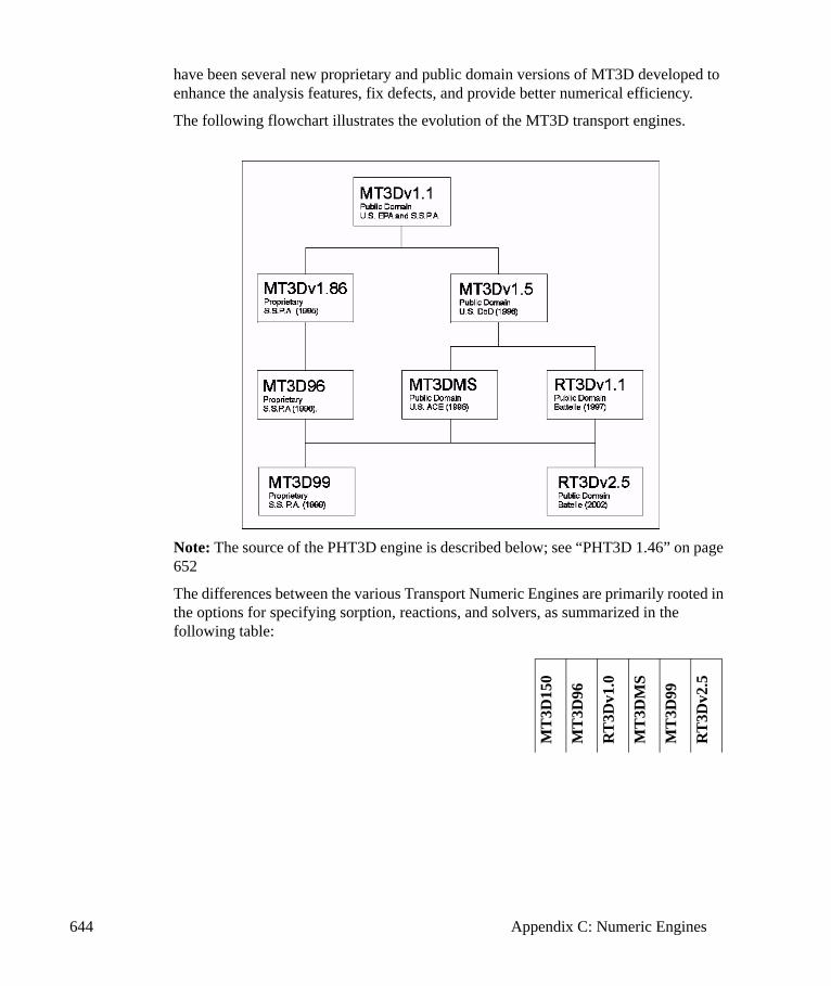
644 Appendix C: Numeric Engines
have been several new proprietary and public domain versions of MT3D developed to enhance the analysis features, fix defects, and provide better numerical efficiency.
The following flowchart illustrates the evolution of the MT3D transport engines.
Note: The source of the PHT3D engine is described below; see “PHT3D 1.46” on page 652
The differences between the various Transport Numeric Engines are primarily rooted in the options for specifying sorption, reactions, and solvers, as summarized in the following table:
MT
3D15
0
MT
3D96
RT
3Dv1
.0
MT
3DM
S
MT
3D99
RT
3Dv2
.5

Mass Transport Numeric Engines 645
Note: For the list of supported PHT3D reactions, see “PHT3D 1.46” on page 652 below.
C.2.1 MT3Dv1.5MT3D is a modular three-dimensional transport model for simulation of advection, dispersion, and chemical reaction of contaminants in groundwater systems. C. Zheng developed this transport model in 1996 while working at S.S. Papadopulos. The U.S. Environmental Protection Agency paid for the development of the documentation and, in return, a limited public domain version was made available. C. Zheng further
Sorp
tion
Opt
ions
No Sorption is simulated
Linear Isotherm (equilibrium-controlled)
Freundlich Isotherm (equilibrium-controlled)
Langmuir Isotherm (equilibrium-controlled)
First-order kinetic sorption (non-equilibrium)
First-order kinetic dual-domain mass transferR
eact
ions
Opt
ions
No kinetic reaction
First-order irreversible decay
Zeroth-order irreversible decay
Monod kinetics
First-order parent-daughter chain reaction
Instantaneous reactions among species
Instantaneous aerobic decay of BTEX
Instantaneous multi-path degradation of BTEX
Kinetic limited multi-path degradation of BTEX
Rate-limited sorption reactions
Double-Monod degradation model
Sequential decay reactions
Aerobic/anaerobic model for PCE/TCE degrad.
Solv
er
MOC, MMOC, HMOC and Upstream FD
Total-Variation Diminishing (TVD)
Generalized Conjugate Gradient (GCG)
646 Appendix C: Numeric Engines
developed MT3D at the University of Alabama with a grant from the Department of Defense.
Included with your Visual MODFLOW Installation media is an electronic copy of the original MT3D 1.1 Reference Manual. This is also the manual for MT3Dv1.5. The name of this file is MT3D1.1 manual.pdf and it can be found in the Manual folder on the Installation CD.
C.2.2 MT3D96 (not available for new projects/variants)C. Zheng developed this upgrade to the MT3D 1.5 code in 1996 for S.S. Papadopulos & Associates, Inc. The major modifications and enhancements from MT3D 1.5 include:
• improved Eulerian-Lagrangian solutions• improved finite-difference solution• improved treatment of heterogeneous porosity and transient flow problems• expanded mass accounting• more flexible input for chemical reactions• time-varying constant-concentration boundary conditions• improved interface with MODFLOW• full backward compatibility with previous versions of MT3D
At the time of its release, MT3D96 was a proprietary program sold by S.S. Papadopulos & Associates, Inc. and was not available in the public domain. The MT3D96 program was replaced by MT3D99, and is now considered to be obsolete.
However, Visual MODFLOW continues to support MT3D96 to ensure historical modeling results may be reproduced using exactly the same simulation codes. MT3D99 may be purchased as an add-on package to Visual MODFLOW.
C.2.3 MT3DMSMT3DMS is a modular three-dimensional multi-species transport model for simulation of advection, dispersion, and chemical reactions of contaminants in groundwater systems. Zheng and Wang developed this multi-species transport model in June 1998 for the US Army Corps of Engineers. This model includes the addition of:
• a third-order total-variation-diminishing scheme for solving the advection term, an iterative solver based on generalized conjugate gradient methods and the Lanczos/ORTHOMIN acceleration scheme,
• options for accommodating non-equilibrium sorption and dual-domain advection-diffusion mass transport, and
• a multi-component program structure to accommodate add-on reaction packages.
Included with your Visual MODFLOW Installation media is a document file of the MT3DMS Reference Manual. The name of this file is MT3DMS manual.pdf and it can
Mass Transport Numeric Engines 647
be found in the Manual folder of the Installation CD. Please refer to this document for a detailed description of the sorption options, reaction packages, and solvers available.
C.2.4 MT3D99MT3D99 is the successor to MT3D96, and incorporates many of the same functions as MT3DMS together with some additional modifications and enhancements including:
• zero-order and mixed-order Monod kinetic reactions;• a reaction package to handle BIOPLUME-type aerobic and anaerobic reactions
between hydrocarbon contaminants and any user-specified electron acceptors and parent-daughter chain reactions for inorganic and organic compounds;
• automatic restart option; and• detailed cell-by-cell mass budgets.
MT3D99 is a proprietary program developed by C. Zheng under contract to S.S. Papadopulos & Associates, Inc. and must be purchased as an add-on package to Visual MODFLOW.
Included with your Visual MODFLOW Installation media is an electronic copy of the MT3D99 Reference Manual, in the Manual folder of the Installation CD. Please refer to this manual for a detailed description of the sorption options, reaction packages, and solvers available.
C.2.5 SEAWATPlease see section C.1.5 on page 642
C.2.6 RT3DRT3D is a program for simulating reactive multi-species mass transport in three-dimensional groundwater aquifers. RT3Dv1.0 was first developed by P.T. Clement in 1997 for the Battelle Memorial Institute, Pacific Northwest National Laboratory, and was subsequently released into the public domain and quickly became an accepted standard for reactive transport modeling. Unfortunately, the code was based on MT3Dv1.5 and did not include many of the new solver technology implemented in MT3DMS. As a result, the application of RT3D was always hampered by excessively slow run-times.
RT3D 2.5 was released to the public domain in 2002, and now includes the same solver options as MT3DMS.
Included with your Visual MODFLOW Installation media is an electronic copy of the original RT3D Reference Manual (RT3D V1.0 manual.pdf) together with the RT3D v2.5 Update Document (RT3D V2.5 Update.pdf). These files can be found in the Manual folder of the Installation CD.

648 Appendix C: Numeric Engines
RT3D Pre-Programmed general Reaction PackagesThe RT3D Transport Numeric Engine contains the following reaction packages:
• Instantaneous aerobic decay of BTEX• Instantaneous multi-path degradation of BTEX• Kinetic limited multi-path degradation of BTEX• Rate-limited sorption reactions• Double-Monod degradation model• Sequential decay reactions• Aerobic/anaerobic model for PCE/TCE degradation
The reaction mechanisms for these packages are built-in to RT3D as a convenience for the user. The key parameters (i.e. reaction rates) have default values based on data reported in the literature. However, the user can adjust these parameters to better fit with data from a specific site. See the RT3D User’s Manual PNNL-11720 for details of the reaction mechanisms and adjustable parameters for these pre-programmed modules.
The following sections, taken from the RT3D Manual, briefly outline each of the reaction packages. For more information on appropriate values for the reaction constants, please see the RT3D Reference Manual.
For each RT3D reaction model, it is the user’s responsibility to obtain a detailed understanding of the limitations of the reaction model by refering to the RT3D Reference Manual, and obtaining copies of the referenced research papers before using the model for professional purposes.
Note: Stoichiometric ratios and yield coefficients in RT3D are assumed to be massbased rather than molar based. Concentrations in Visual MODFLOW for RT3D based models are in the concentration units specified by the user.
Model 1 - Instantaneous Aerobic Decay of BTEXModel 1 simulates the instantaneous biodegradation of fuel hydrocarbons under aerobic conditions. At each time step, the reaction algorithm models removal rates by reducing either hydrocarbons or oxygen to zero within each grid cell.
Model 1 has two components, BTEX and Oxygen, both of which are mobile and one reaction constant, the Stoichiometric ratio of Oxygen to BTEX (Default = 3.14).
Model 2 - Instantaneous Degradation of BTEX using Multiple Electron AcceptorsModel 2 is similar to the previous package except that it uses five degradation pathways (aerobic respiration, denitrification, iron reduction, sulfate reduction, and methanogenesis) to simulate biodegradation of BTEX compounds.
Model 2 includes six mobile components, BTEX, Oxygen, Nitrate, Fe2+, Sulfate, and Methane and the following reaction constants:
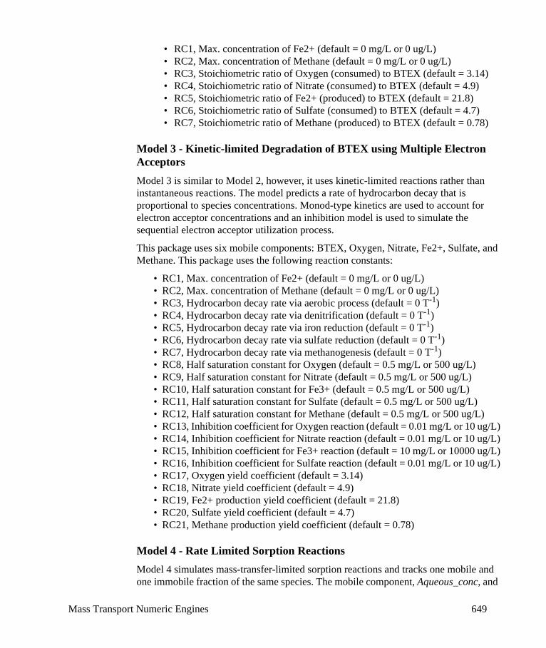
Mass Transport Numeric Engines 649
• RC1, Max. concentration of Fe2+ (default = 0 mg/L or 0 ug/L)• RC2, Max. concentration of Methane (default = 0 mg/L or 0 ug/L)• RC3, Stoichiometric ratio of Oxygen (consumed) to BTEX (default = 3.14)• RC4, Stoichiometric ratio of Nitrate (consumed) to BTEX (default = 4.9)• RC5, Stoichiometric ratio of Fe2+ (produced) to BTEX (default = 21.8)• RC6, Stoichiometric ratio of Sulfate (consumed) to BTEX (default = 4.7)• RC7, Stoichiometric ratio of Methane (produced) to BTEX (default = 0.78)
Model 3 - Kinetic-limited Degradation of BTEX using Multiple Electron AcceptorsModel 3 is similar to Model 2, however, it uses kinetic-limited reactions rather than instantaneous reactions. The model predicts a rate of hydrocarbon decay that is proportional to species concentrations. Monod-type kinetics are used to account for electron acceptor concentrations and an inhibition model is used to simulate the sequential electron acceptor utilization process.
This package uses six mobile components: BTEX, Oxygen, Nitrate, Fe2+, Sulfate, and Methane. This package uses the following reaction constants:
• RC1, Max. concentration of Fe2+ (default = 0 mg/L or 0 ug/L)• RC2, Max. concentration of Methane (default = 0 mg/L or 0 ug/L)• RC3, Hydrocarbon decay rate via aerobic process (default = 0 T-1)• RC4, Hydrocarbon decay rate via denitrification (default = 0 T-1)• RC5, Hydrocarbon decay rate via iron reduction (default = 0 T-1)• RC6, Hydrocarbon decay rate via sulfate reduction (default = 0 T-1)• RC7, Hydrocarbon decay rate via methanogenesis (default = 0 T-1)• RC8, Half saturation constant for Oxygen (default = 0.5 mg/L or 500 ug/L)• RC9, Half saturation constant for Nitrate (default = 0.5 mg/L or 500 ug/L)• RC10, Half saturation constant for Fe3+ (default = 0.5 mg/L or 500 ug/L)• RC11, Half saturation constant for Sulfate (default = 0.5 mg/L or 500 ug/L)• RC12, Half saturation constant for Methane (default = 0.5 mg/L or 500 ug/L)• RC13, Inhibition coefficient for Oxygen reaction (default = 0.01 mg/L or 10 ug/L)• RC14, Inhibition coefficient for Nitrate reaction (default = 0.01 mg/L or 10 ug/L)• RC15, Inhibition coefficient for Fe3+ reaction (default = 10 mg/L or 10000 ug/L)• RC16, Inhibition coefficient for Sulfate reaction (default = 0.01 mg/L or 10 ug/L)• RC17, Oxygen yield coefficient (default = 3.14)• RC18, Nitrate yield coefficient (default = 4.9)• RC19, Fe2+ production yield coefficient (default = 21.8)• RC20, Sulfate yield coefficient (default = 4.7)• RC21, Methane production yield coefficient (default = 0.78)
Model 4 - Rate Limited Sorption ReactionsModel 4 simulates mass-transfer-limited sorption reactions and tracks one mobile and one immobile fraction of the same species. The mobile component, Aqueous_conc, and
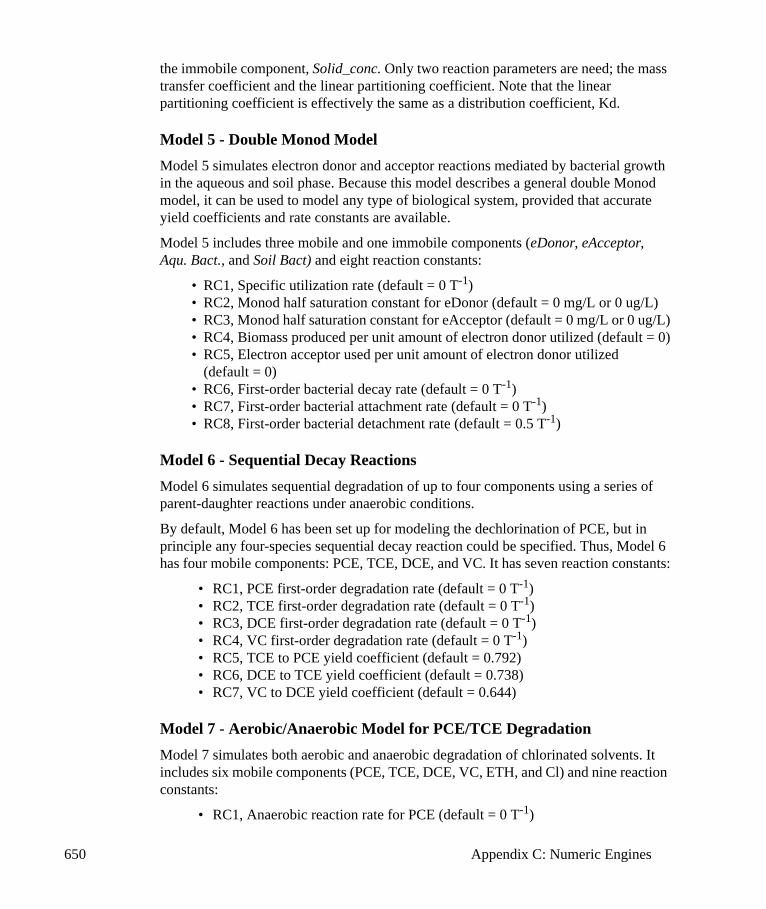
650 Appendix C: Numeric Engines
the immobile component, Solid_conc. Only two reaction parameters are need; the mass transfer coefficient and the linear partitioning coefficient. Note that the linear partitioning coefficient is effectively the same as a distribution coefficient, Kd.
Model 5 - Double Monod ModelModel 5 simulates electron donor and acceptor reactions mediated by bacterial growth in the aqueous and soil phase. Because this model describes a general double Monod model, it can be used to model any type of biological system, provided that accurate yield coefficients and rate constants are available.
Model 5 includes three mobile and one immobile components (eDonor, eAcceptor, Aqu. Bact., and Soil Bact) and eight reaction constants:
• RC1, Specific utilization rate (default = 0 T-1)• RC2, Monod half saturation constant for eDonor (default = 0 mg/L or 0 ug/L)• RC3, Monod half saturation constant for eAcceptor (default = 0 mg/L or 0 ug/L)• RC4, Biomass produced per unit amount of electron donor utilized (default = 0)• RC5, Electron acceptor used per unit amount of electron donor utilized
(default = 0)• RC6, First-order bacterial decay rate (default = 0 T-1)• RC7, First-order bacterial attachment rate (default = 0 T-1)• RC8, First-order bacterial detachment rate (default = 0.5 T-1)
Model 6 - Sequential Decay ReactionsModel 6 simulates sequential degradation of up to four components using a series of parent-daughter reactions under anaerobic conditions.
By default, Model 6 has been set up for modeling the dechlorination of PCE, but in principle any four-species sequential decay reaction could be specified. Thus, Model 6 has four mobile components: PCE, TCE, DCE, and VC. It has seven reaction constants:
• RC1, PCE first-order degradation rate (default = 0 T-1)• RC2, TCE first-order degradation rate (default = 0 T-1)• RC3, DCE first-order degradation rate (default = 0 T-1)• RC4, VC first-order degradation rate (default = 0 T-1)• RC5, TCE to PCE yield coefficient (default = 0.792)• RC6, DCE to TCE yield coefficient (default = 0.738)• RC7, VC to DCE yield coefficient (default = 0.644)
Model 7 - Aerobic/Anaerobic Model for PCE/TCE DegradationModel 7 simulates both aerobic and anaerobic degradation of chlorinated solvents. It includes six mobile components (PCE, TCE, DCE, VC, ETH, and Cl) and nine reaction constants:
• RC1, Anaerobic reaction rate for PCE (default = 0 T-1)
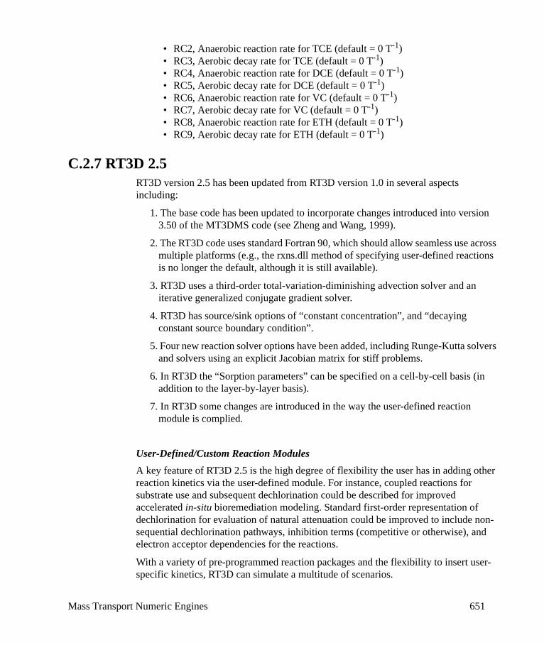
Mass Transport Numeric Engines 651
• RC2, Anaerobic reaction rate for TCE (default = 0 T-1)• RC3, Aerobic decay rate for TCE (default = 0 T-1)• RC4, Anaerobic reaction rate for DCE (default = 0 T-1)• RC5, Aerobic decay rate for DCE (default = 0 T-1)• RC6, Anaerobic reaction rate for VC (default = 0 T-1)• RC7, Aerobic decay rate for VC (default = 0 T-1)• RC8, Anaerobic reaction rate for ETH (default = 0 T-1)• RC9, Aerobic decay rate for ETH (default = 0 T-1)
C.2.7 RT3D 2.5RT3D version 2.5 has been updated from RT3D version 1.0 in several aspects including:
1. The base code has been updated to incorporate changes introduced into version 3.50 of the MT3DMS code (see Zheng and Wang, 1999).
2. The RT3D code uses standard Fortran 90, which should allow seamless use across multiple platforms (e.g., the rxns.dll method of specifying user-defined reactions is no longer the default, although it is still available).
3. RT3D uses a third-order total-variation-diminishing advection solver and an iterative generalized conjugate gradient solver.
4. RT3D has source/sink options of “constant concentration”, and “decaying constant source boundary condition”.
5. Four new reaction solver options have been added, including Runge-Kutta solvers and solvers using an explicit Jacobian matrix for stiff problems.
6. In RT3D the “Sorption parameters” can be specified on a cell-by-cell basis (in addition to the layer-by-layer basis).
7. In RT3D some changes are introduced in the way the user-defined reaction module is complied.
User-Defined/Custom Reaction Modules A key feature of RT3D 2.5 is the high degree of flexibility the user has in adding other reaction kinetics via the user-defined module. For instance, coupled reactions for substrate use and subsequent dechlorination could be described for improved accelerated in-situ bioremediation modeling. Standard first-order representation of dechlorination for evaluation of natural attenuation could be improved to include non-sequential dechlorination pathways, inhibition terms (competitive or otherwise), and electron acceptor dependencies for the reactions.
With a variety of pre-programmed reaction packages and the flexibility to insert user-specific kinetics, RT3D can simulate a multitude of scenarios.
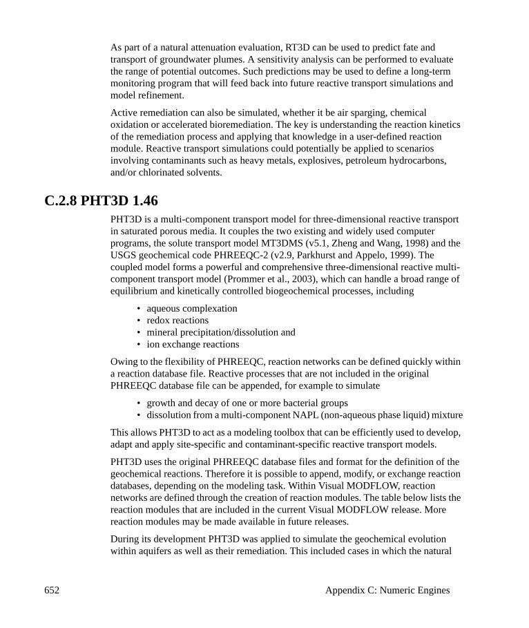
652 Appendix C: Numeric Engines
As part of a natural attenuation evaluation, RT3D can be used to predict fate and transport of groundwater plumes. A sensitivity analysis can be performed to evaluate the range of potential outcomes. Such predictions may be used to define a long-term monitoring program that will feed back into future reactive transport simulations and model refinement.
Active remediation can also be simulated, whether it be air sparging, chemical oxidation or accelerated bioremediation. The key is understanding the reaction kinetics of the remediation process and applying that knowledge in a user-defined reaction module. Reactive transport simulations could potentially be applied to scenarios involving contaminants such as heavy metals, explosives, petroleum hydrocarbons, and/or chlorinated solvents.
C.2.8 PHT3D 1.46PHT3D is a multi-component transport model for three-dimensional reactive transport in saturated porous media. It couples the two existing and widely used computer programs, the solute transport model MT3DMS (v5.1, Zheng and Wang, 1998) and the USGS geochemical code PHREEQC-2 (v2.9, Parkhurst and Appelo, 1999). The coupled model forms a powerful and comprehensive three-dimensional reactive multi-component transport model (Prommer et al., 2003), which can handle a broad range of equilibrium and kinetically controlled biogeochemical processes, including
• aqueous complexation• redox reactions• mineral precipitation/dissolution and • ion exchange reactions
Owing to the flexibility of PHREEQC, reaction networks can be defined quickly within a reaction database file. Reactive processes that are not included in the original PHREEQC database file can be appended, for example to simulate
• growth and decay of one or more bacterial groups• dissolution from a multi-component NAPL (non-aqueous phase liquid) mixture
This allows PHT3D to act as a modeling toolbox that can be efficiently used to develop, adapt and apply site-specific and contaminant-specific reactive transport models.
PHT3D uses the original PHREEQC database files and format for the definition of the geochemical reactions. Therefore it is possible to append, modify, or exchange reaction databases, depending on the modeling task. Within Visual MODFLOW, reaction networks are defined through the creation of reaction modules. The table below lists the reaction modules that are included in the current Visual MODFLOW release. More reaction modules may be made available in future releases.
During its development PHT3D was applied to simulate the geochemical evolution within aquifers as well as their remediation. This included cases in which the natural

Mass Transport Numeric Engines 653
and enhanced attenuation/remediation of organic contaminants is assessed, but also cases where the fate of inorganic pollutants is studied.
Sample ApplicationsPHT3D has been in modeling applications to study:
• the biogeochemistry of landfill leachate plumes• aromatic and chlorinated hydrocarbon spills • the fate of pesticides and the resulting isotopic fractionation• trace metal remediation by in-situ reactive zones• the fate of an ammoniacal liquor contamination• an emplaced creosote source experiment• the isotopic fractionation during natural attenuation of chlorinated ethenes• the geochemical evolution under islands in the Okavango Delta, Botswana • biogeochemical changes during ASR (aquifer storage and recovery) of
reclaimed water• temperature-dependent pyrite oxidation during a deep-well injection
experiment• the fate of a pharmaceutical residue during artificial recharge of groundwater • remediation of acid mine drainage by permeable reactive barriers• the reactive transport of chlorinated solvents in a permeable Fe(0)-filled
reactive barriers• the role of transverse dispersion on reactive contaminant transport• the geochemical evolution of the capture zone of drinking water supply wells
Modeling projects involving PHT3D are normally carried out in successive stages of increasing complexity and typically start with preliminary, batch-type model simulations using PHREEQC and flow/non-reactive solute transport modeling with MODFLOW and MT3DMS, respectively. Measured chloride concentrations and/or temperature data might serve as constraints to calibrate the model parameters influencing physical transport processes (see e.g., Prommer and Stuyfzand, 2005; Greskowiak et al., 2005, Prommer et al., 2006). The combination of the results from the calibrated conservative transport model and from the batch-type PHREEQC models form the base for the application of PHT3D.
Included with your Visual MODFLOW Installation media is an electronic copy of the original PHT3D Reference Manual (PHT3D manual v.1.0.pdf). This file can be found in the Manual folder of the Installation CD.
Note: Before applying PHT3D, users are encouraged to familiarize themselves with PHREEQC-2, MT3DMS, and geochemistry concepts.
Pre-Defined Reaction ModulesThe PHT3D Transport Numeric Engine contains a number of pre-defined reaction packages; these are reaction packages where the reaction network is hard-coded (the
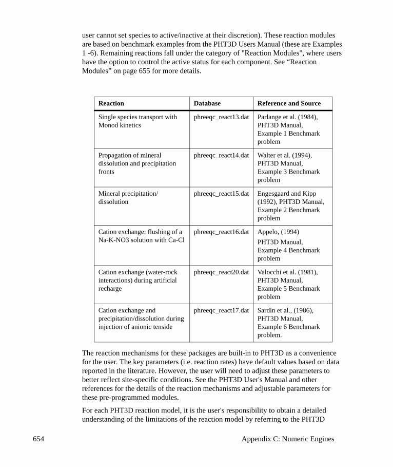
654 Appendix C: Numeric Engines
user cannot set species to active/inactive at their discretion). These reaction modules are based on benchmark examples from the PHT3D Users Manual (these are Examples 1 -6). Remaining reactions fall under the category of "Reaction Modules", where users have the option to control the active status for each component. See “Reaction Modules” on page 655 for more details.
The reaction mechanisms for these packages are built-in to PHT3D as a convenience for the user. The key parameters (i.e. reaction rates) have default values based on data reported in the literature. However, the user will need to adjust these parameters to better reflect site-specific conditions. See the PHT3D User's Manual and other references for the details of the reaction mechanisms and adjustable parameters for these pre-programmed modules.
For each PHT3D reaction model, it is the user's responsibility to obtain a detailed understanding of the limitations of the reaction model by referring to the PHT3D
Reaction Database Reference and Source
Single species transport with Monod kinetics
phreeqc_react13.dat Parlange et al. (1984), PHT3D Manual, Example 1 Benchmark problem
Propagation of mineral dissolution and precipitation fronts
phreeqc_react14.dat Walter et al. (1994), PHT3D Manual, Example 3 Benchmark problem
Mineral precipitation/dissolution
phreeqc_react15.dat Engesgaard and Kipp (1992), PHT3D Manual, Example 2 Benchmark problem
Cation exchange: flushing of a Na-K-NO3 solution with Ca-Cl
phreeqc_react16.dat Appelo, (1994)PHT3D Manual, Example 4 Benchmark problem
Cation exchange (water-rock interactions) during artificial recharge
phreeqc_react20.dat Valocchi et al. (1981), PHT3D Manual, Example 5 Benchmark problem
Cation exchange and precipitation/dissolution during injection of anionic tenside
phreeqc_react17.dat Sardin et al., (1986), PHT3D Manual, Example 6 Benchmark problem.
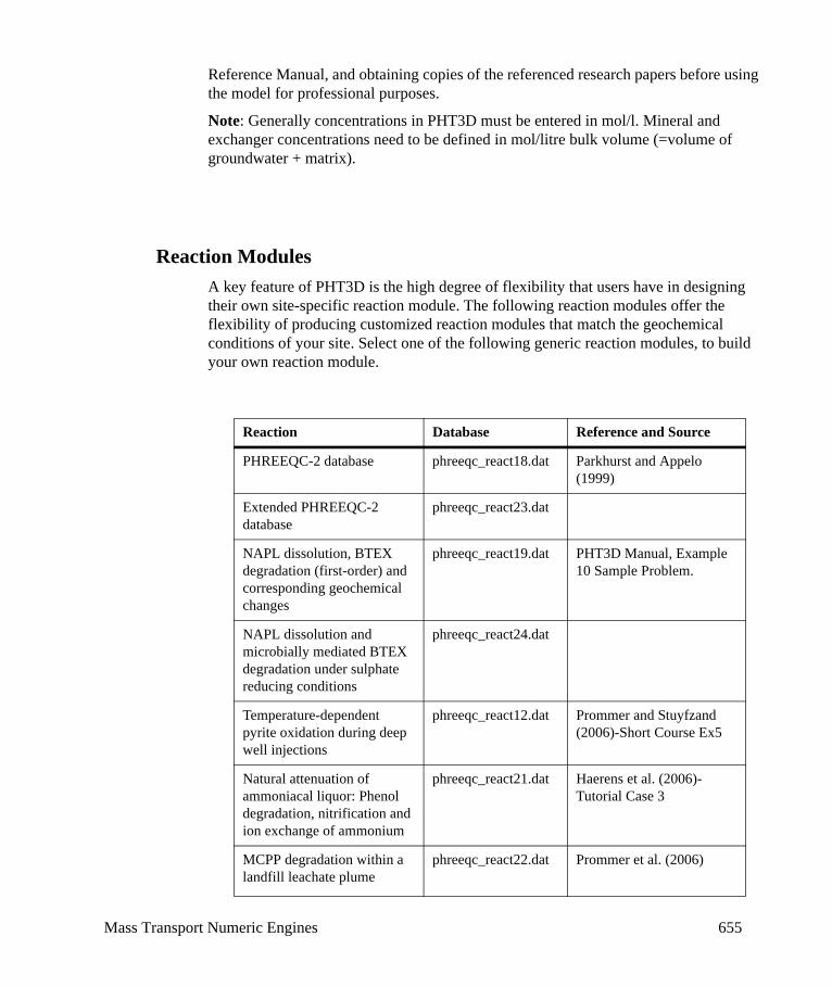
Mass Transport Numeric Engines 655
Reference Manual, and obtaining copies of the referenced research papers before using the model for professional purposes.
Note: Generally concentrations in PHT3D must be entered in mol/l. Mineral and exchanger concentrations need to be defined in mol/litre bulk volume (=volume of groundwater + matrix).
Reaction ModulesA key feature of PHT3D is the high degree of flexibility that users have in designing their own site-specific reaction module. The following reaction modules offer the flexibility of producing customized reaction modules that match the geochemical conditions of your site. Select one of the following generic reaction modules, to build your own reaction module.
Reaction Database Reference and Source
PHREEQC-2 database phreeqc_react18.dat Parkhurst and Appelo (1999)
Extended PHREEQC-2 database
phreeqc_react23.dat
NAPL dissolution, BTEX degradation (first-order) and corresponding geochemical changes
phreeqc_react19.dat PHT3D Manual, Example 10 Sample Problem.
NAPL dissolution and microbially mediated BTEX degradation under sulphate reducing conditions
phreeqc_react24.dat
Temperature-dependent pyrite oxidation during deep well injections
phreeqc_react12.dat Prommer and Stuyfzand (2006)-Short Course Ex5
Natural attenuation of ammoniacal liquor: Phenol degradation, nitrification and ion exchange of ammonium
phreeqc_react21.dat Haerens et al. (2006)-Tutorial Case 3
MCPP degradation within a landfill leachate plume
phreeqc_react22.dat Prommer et al. (2006)

656 Appendix C: Numeric Engines
When you select any of these reactions, the Active status of the component (yes/no) can be set; this allows the user the flexibility to add or remove components to the reaction. Non-active components will not be included in the reaction module. An example is shown below:
LimitationsSome other important notes for PHT3D:
• Initial and other water compositions at boundaries, e.g., recharge water composition and the water composition within injection wells MUST be charge-balanced.
• The operator-splitting between advective-dispersive transport (MT3DMS) and chemical reactions (PHREEQC) is controlled by the user through the "Time Steps" definition in the MODFLOW Run Time Settings.
• If a redox-sensitive component is included in a simulation, all other redox states of this component should also be activated (e.g., Fe(2) AND Fe(3), S(6) AND S(-2), etc.
• Bulk density and sorption parameters can be assigned on a cell-by-cell basis• Reaction parameters in PHT3D are spatially constant and can only be assigned
in PHT3D Run Settings dialog• PHT3D currently does not allow non-linear sorption

Mass Transport Numeric Engines 657
ReferencesAppelo, C.A.J., 1994. Cation and proton exchange, pH variations, and
carbonate reactions in a freshening aquifer. Water Resour. Res. 30, 2793-2805.
Engesgaard, P., and K.L. Kipp, 1992. A geochemical transport model for redox-controlled movement of mineral fronts in groundwater flow systems: A case of nitrate removal by oxidation of pyrite. Water Resour. Res. 28, 2829-2843.
Guo, W. and C.D. Langevin, 2002. User’s Guide to SEAWAT: A Computer Program for Simulation of Three-Deimensional Variable-Density Groundwater Flow, U.S. Geological Survey, Techniques of Water-Resources Unvestigations of the U.S Geological Survey, Book 6 Chapter A7,Tallahassee, Florida, 77p.
Greskowiak, J., Prommer, H., Vanderzalm, J., Pavelic, P., and P. Dillon, 2005. Modelling of carbon cycling and biogeochemical changes during a wastewater injection and recovery experiment at Bolivar/South Australia. Water Resour. Res., 41, doi:10.1029/2005WR004095.
Haerens, B., Prommer, H., Lerner, D.N., and A. Dassargues, 2006. Reactive transport modeling of a groundwater contamination by ammoniacal liquor. In MODFLOW and More 2006: Managing Ground-Water Systems. (Proc. International Ground Water Modeling Conference, Golden, Colorado USA, 22-24 May 2006).
Langevin, C.D., Thorne, D.T., Jr., Dausman, A.M., Sukop, M.C., and Guo, Weixing, 2008, SEAWAT Version 4: A Computer Program for Simulation of Multi-Species Solute and Heat Transport: U.S. Geological Survey Techniques and Methods Book 6, Chapter A22, 39 p.
Parkhurst, D.L., and C.A.J.Appelo, 1999. User's guide to PHREEQC (Version 2)-A computer program for speciation, batch-reaction, one-dimensional transport, and inverse geochemical calculations: U.S. Geological Survey Water-Resources Investigations Report 99-4259, 312 p.
Parlange, J.-Y., Starr, J. L., Barry, D.A., and R.D Braddock, 1984. Some approximate solutions of the transport equation with irreversible reactions. Sci. Soc. Am. J. 137, 434-442.
Pollak, D.W. 1994. User’s Guide for MODPATH/MODPATH-PLOT, Version 3: A Particle tracking post-processing package for MODFLOW, the U.S. Geological Survey finite-difference ground-water flow model: US Geological Survey Open-File Report 94-464, 6ch.
Prommer, H., Barry, D.A., and C. Zheng, C., 2003. PHT3D - A MODFLOW/MT3DMS based reactive multi-component transport model. Ground Water, 42(2), 247-257.
Prommer, H., Tuxen, N., and P.L. Bjerg, 2006. Fringe-controlled natural attenuation of phenoxy acids in a landfill plume: Integration of field-scale processes by

658 Appendix C: Numeric Engines
reactive-transport modelling. Submitted to Environmental Science and Technology (accepted for publication).
Prommer, H., and P.J. Stuyfzand, 2005. Identification of temperature-dependent water quality changes during a deep well injection experiment in a pyritic aquifer. Environmental Science and Technology, 39, 2200-2209.
Sardin, M., Krebs, R., and D. Schweich, 1986. Transient mass-transport in the presence of non-linear physico-chemical interaction laws: Progressive modelling and appropriate experimental procedures. Geoderma 38, 115-130.
Valocchi, A.J., Street, R.L., and P.V. Roberts. 1981. Transport of ion-exchanging solutes in groundwater: Chromatographic theory and field simulation, Water Resour. Res. 17, 1517-1527, 1981.
Walter, A.L., Frind, E.O., Blowes, D.W., Ptacek, C.J., and J.W. Molson, 1994. Modeling of multicomponent reactive transport in groundwater. 1. Model development and evaluation. Water Resour. Res. 30, 3137-3148.
Zheng, C., and P.P. Wang, 1999. MT3DMS: A modular three-dimensional multispecies model for simulation of advection, dispersion and chemical reactions of contaminants in groundwater systems; Documentation and User's Guide, Contract Report SERDP-99-1, U.S. Army Engineer Research and Development Center, Vicksburg, MS.
Index 659
IndexAAbout the Interface 6Absolute 409Absolute Change 427, 428Absolute change 428Absolute Distance 430ABSPREDLAM 427ABSPREDSTP 430ABSPREDSWH 428Active Zone 567Active Zone Display Properties 567Add contour(s) 540Add/Move labels 540Adding a Data Series 535Adjustment Factor 418Advection
Advection Method (MIXELM) 347Concentration Weighting Factor 353Critical Concentration Gradient 354Initial Particles (Negligible Concentration Gradient) 354Initial Particles (Random Pattern) 354Maximum Particles 353Maximum Particles per Cell 353Minimum Particles per Cell 353Negligible Gradient 354Number of Planes 353Particle Options 352Particle Pattern 354Particle Tracking Method (ITRACK) 355Particles Parameters 353
Advection method comparisons 359Advection Methods 347Advection Type 347
Hybrid Method of Characteristics 358Method of Characteristics 357, 358Modified Method of Characteristics 357
Analysis Mode 426Animate Pathlines 540Animated zoom 530Anisotropy 338Annotate 292, 527, 528
Add 293Edit Single 293Erase 293Move Single 293
Artificial Withdrawal 251Assign to appropriate layer 220Assigning Hydraulic Conductivity Zones 191Assigning Property Zones 187Assigning Stream Segments 241
BBackground 536Background color 564
Backward particle tracking 343Bar charts 529Bibliography 609Boundaries 211
Constant Concentration 274Constant Head 234Drains 252Evapotranspiration 266Evapotranspiration Concentration 278General Head 246Recharge 258Recharge Concentration 276
Boundary File (.VMB) Format 620Bulk Density 167
CCalibration Graphs 498Calibration Residuals Histogram 498Cell Inspector 291, 528Central FD Method 410Changing slices 592Check 432Check all 432Chemical Reactions See Species Parameters190
Cleanup 190Clear Selections 404Clip symbols 538Closing the VMOD 3D-Explorer 552Code description 220Color Legend 588Color Map Settings 542Color maps 529Colormaps 588Conc. Weighting Factor (WD) 353Concentration 482Conductance 241Conductivity 191Configuration Name 596Constant Concentration 274, 276, 278, 280Constant Head 234Contour maps 529Contour Settings 541Contouring
Next Time Button 483Options 483Previous Time Button 483Time 483
ContoursGeneral 478Options 483
Co-ordinatesDual Co-ordinate System 50Transforming Model to World 50
660 Index
Transforming World To Model 50Co-ordinates Area 9Copy to Clipboard 549, 598Copying a Variant 75Courant Condition 362Courant Number 352Creating a New Model 29Creating a slice 588Creating Isosurfaces 592Creating isosurfaces 592
Isosurface properties 578, 581, 583Critical Concentration Gradient (DCHMOC) 354Cross-section 591
Vertex 592cross-section line 591cross-section slice 591Cube Navigator 9Cut off Color Shading 542Cut-away 593Cutaway 588Cut-away Properties 593Cut-away slices
Slice properties 589, 590Vertical slices 589
DData Files 613, 629, 639Data Structure of Input Data Files 619Data Type 426Define Slices 589Define slices 589Delete contour(s) 540Deleting Boundary Conditions 233Deleting boundary conditions 233Deleting Slices 592Discharge Options 342Dispersion 210display properties 562Display Properties Table 562display settings 596Distribution Array 190dockable panels 556Domain Display Properties 567Drag Bar 556Drains 252
Conductance 253Drain Elevation 252
Drawdown 482Drawdowns 575DT0 with implicit solver 357
EEdit
Elevations 87, 119Extents 86, 92Grid 86Layers 90
Effective Porosity 195
Enable Restart 423End color 539Erasing Boundary Conditions 233Estimation Mode 417ETS1 271Eulerian-Lagrangian 358Evaporation Rate per Unit Area 251Evapotranspiration 266Evapotranspiration Concentration 278Export
DXF File 77EMF File 77Windows Metafile 77
FF2-3D icon 552FACPARMAX 419FD Method 410File 298, 477
Input Module 85Files
general 614Fixing Gridlines 96floating panels 556flow pathlines 577Force switch to active engine 392Formula Bar 224Formulas and Array Variables 224Forward particle tracking 343forward threshold 577Function Buttons 10
F1 - Help 10F10 – Main Menu 10F2 10F3 - Save 10F4 - Map 10F5 – Zoom In 10F6 – Zoom Out 10F7 – Pan 10F8 – Vert Exag 10F9 - Overlay 10
GGCG solver 360GCG Solver Settings 355General Features 15General Head 246, 247
Conductance 247Generalized Conjugate Gradient Solver 360Getting Around Visual MODFLOW 7Gradient 539Graph Editor 598Graph Properties 531Graph properties 530Graphs 497
95% Confidence Interval 508, 509Grid
Contouring 87
Index 661
Contouring Option 126Edit 86Edit Elevations 87, 119Edit Extents 86, 92Edit Layers 90Smoothing 86
Grid Display Properties 567Grid Editor 119Grid File (.VMG) Format 622Grid Properties 567Grid Smoothing 93
Fixing Gridlines 96Guo and Zhao (2005) Parametrization 380
HHardware Requirements 4Head Difference 483Head Flux 483Head Observation Wells 152
Add 152Delete 152Edit 153Edit Groups 153Move 153
Head Output Times 575Histogram of Calibration Residuals 498Holding parameters 433Hybrid Method of Characteristics (HMOC) 358Hydraulic Conductivity 191Hydraulic ConductivitySee Conductivity 191
IImperial units 33Import
Existing MODFLOW Models 15Import Elevation 86, 97Importing Transient Boundary Condition Data 226Inactive Flow Display Properties 567Inactive Transport
Defining Boundary Geometry 209Inactive/Active Cells 86
Copy Polygon 88, 210Copy Single 88, 210Defining 87, 88Mark Inactive 87, 209Mark Polygon Active 87, 209Mark Single 87, 209
Incr. Multiplier 410Incr. Type 409Increment 409Initial Concentration - output 363Initial Heads 197
Import 208, 305, 306, 363, 364Import from Previous MODFLOW Run 305, 364
Initial Lambda 418Initial Search Factor 429Initial Time Step 357Initial Value 408
INITSCHFAC 429Injection WellsSee Pumping Wells 127Input files
Visual MODFLOW 614Input Model Elements 566Input Module 6
Boundaries 211File 85General Input 84Grid 86Particles 283Properties 167Tools 290Zone Budget 286
Inside Limit 426Instability
PEST 411Installation
Visual MODFLOW 4Interface 83, 613Introduction 1Inverted 532Isoline maps 588Isosurface color 579, 580Isosurface value 579, 580
LLabels 532Lakebed Conductivity 251Lakebed Thickness 251Layers 332
Type 0 Confined 332Type 1 Unconfined 332, 333Type 2 Confined/Unconfined 332, 333Type 3 Confined/Unconfined 332, 333
legend position 536Legend type 536Limiting 407Limiting Relative Phi Reduction 418Line Search 428Linear gradient 221List File Options. 340, 341Load scene configuration 596Location 426Logarithm 532
MMajor Ticks 532Manning’s Roughness Coefficient 241Marquardt Lambda 417Mass Transport Boundary Conditions 274Max “No change” Iterations 423Max “No reduction” Iterations 422Max factor parameter change 420Max Particles/Cell (NPMAX) 353Max Unsuccessful Iterations 423Max. Factor Change 419Max. forward threshold 577
662 Index
Max. Relative Change 419Max. relative parameter change 420Maximum Model Runs 429Maximum Number of Particles (MXPART) 353Maximum time step with particle-based methods 357Maximum Trial Lambdas 419Method of Characteristics (MOC) 357Method Separation Value 421MIKE 11 Run Settings 331Min Particles/Cell (NPMIN) 353Min. forward threshold 577Min. Incr. 409Minimum saturated thickness 352Minor Ticks 532Model tree 561
Tool tip 562MODFLOW 298
Anisotropy 299, 338Layers 299, 332List File Options 299, 340, 341Output Control 299, 338Recharge 299, 328, 329Rewetting 299, 335Solver 299, 303Solvers 307Time Steps 299
MODFLOW-NWT 324MODFLOW-SURFACT
Adaptive Time Stepping 301Drawdown 482, 516Engines to Run dialog 387Flow Engine 641Flow Simulation Type 32PCG4 package 318PCG5 package 320Ponding Depth 259Recharge Seepage Face Boundary Condition 329Saturation 517Soil Vapor Flow option 334Transport 33Vadose Zone 197, 200Wells 136, 143
Modified Method of Characteristics (MMOC) 357Modifying Slices 592MODPATH 283, 342
Discharge Options 342Reference Time 342, 343
MODPATH Run-Time Settings 342MT3D
Advection 345Initial Concentration 345Initial Concentration - output 363MT3D1.5 344MT3D99 344MT3DMS 344Output/Time Steps 345Parallel Processing 367RT3D 344
MT3D96 Run-Time Settings 344MT3D99 Run-Time Settings 344MT3DMS 297MT3DMS Run-Time Settings 344MULSCHFAC 429Multiplication Factor 429Multi-Well Node (MNW) Package 147
NNavigate panel
Changing views 557Rotate 117, 558Shift 117, 558
Negligible Gradient (DCEPS) 354Negligible Reduction 422Negligible Relative Change 423Net Recharge 483NPREDMAXMIN 426NPREDNORED 429NPREDSTP 429NSEARCH 429Number of Best Predictions 429Number of Initial Particles for Random Pattern (NPH) 354Number of Initial Particles in Cells with Negligible
Concentration Gradient (NPL) 354Number of Particle Planes (NPLANE) 353Numerical Stability
Dispersion 363Source and Sink Terms 363
OObjective Function 413Objective Function Criteria 426Objects 589Obs. Point 426Obs. Time 426Observation Groups 165Observation Points for Flow See Head Observation
Wells 152Observation Well Data File (.VMO) Format 624Observation Zones Group 416Offset 408Open GL 554Optimization Attempts 429Outline 536Output Control 338, 423
Print to List File 340Output files
MODFLOW 616MODPATH 617, 618MT3D 617Visual MODFLOW 616Zone Budget 618
Output Module 6, 7, 475Annotate 527Contours 476, 478File 476, 477Help 476
Index 663
Tools 476Velocities 476
Output/Time StepsMaximum Transport Steps 362Simulation Time 362
Outside Limit 427Overall Iteration Limit 422Overland Runoff 251
PPage background 538Param. Group 407, 409Parameter Change Constraints 419Parameter Groups 408parameter Transformation 405Parameters 403Particle File (.VMA) Format 619Particle Pattern (NLSINK) 354Particle Release Options 285particle release times 285Particles 283
Add 283Add, Circle 284Add, Line 284Add, Single 283Copy 283, 285Delete 283, 284Release at Same Time 285Release at Various Times 285Release Time 283, 285Tracking 283, 284
Pathline Output Times 577Pathlines 577
Options 490Projections 490Segments 490Toggle 490
Pawlowski(1991) Parametrization 380PD0 426PD1 427PD2 427PEST 383
Calibration 401derivative method - always_2 410derivative method - always_3 410derivative method - best_fit 410derivative method - outside_pts 410derivative method - parabolic 410derivative method - switch 410Forward derivatives 410In Visual MODFLOW 401Interpretation 401Logarithmic transformation 409Marquardt Parameter 417Nonuniqueness 411Objective function 413Prior Information 410Round-off errors 409
Running PEST 416, 430Scale and Offset 408Termination Criteria 422Weights 411
PEST Control Window 403PEST Controls 416PEST Name 409PEST Parameters
Change Limits 407, 408Correlation 411Fixed and Tied 405Parameter Optimization 403Upper and Lower Bounds 408
PEST VariablesDERINC 409DERINCLB 409DERINCMUL 410DERMTHD 410FACORIG 407, 421FACPARMAX 407, 420FORCEN 410ICOR 423ICOV 423IEIG 423INCTYP 409NOPTMAX 422NPHINORED 423NPHISTP 422NRELPAR 423NUMLAM 419OFFSET 408PARCHGLIM 407PARGP 407PARGPNME 409PARLBND 408PARNME 405PARTRANS 405PARUBND 408PARVAL1 408PHIREDLAM 418PHIREDSTP 422PHIREDSWH 421PRECIS 422RELPARMAX 407, 420RELPARSTP 423RHIRATSUF 418RLAMBDA1 418RLAMFAC 418RSTFLE 423SCALE 408
PEST-ASP 402PESTMODE 417PHIREDWSH 428PHT3D
Limitations 656Reaction Modules 653Run Settings 368
Plot appearance 538

664 Index
Plot background 538Plot frame 539Positioning the Panels 556Precipitation Rate per Unit Area 251Precision 422Preconditioned Conjugate-Gradient Package (PCG2) 308Preconditioners
Modified Incomplete Cholesky 308Polynomial 308
Prediction Data 425Prediction Mode 417Predictive Analysis 401Predictive Analysis Settings 424Print graphic 530Print to LST 340Printing 59
To DXF File 77To EMF File 77To Windows Metafile 77
Printing Options 598project.var001 file 73Properties 167
Assign 170, 187Contouring 191Copy 170, 189Database 170Dispersion 210Hydraulic Conductivity 191Initial Concentration 207Initial Heads 197Storage 195
Property File (.VMP) Format 625Pumping Wells 127
Add 127, 128, 152Copy 128Delete 127Edit 128Graph 128, 146Import 142, 158Move 128Wells On/Off 128
RRange of values 541Recharge 258, 328, 329Recharge Concentration 276Reference Time 343Relative 409Relative Change 427, 428Relative change 428Relative Distance 430RELPARMAX 419RELPREDLAM 427RELPREDSTP 430RELPREDSWH 428Rewetting 335
Cell Wetting Control 336Solution Convergence 337
Wet/Dry Threshold 336Rivers
Conductance 238, 241River Bottom Elevation 237, 241River Stage Elevation 241
Rotate - Model X and Y 118, 558Rotate - Screen X and Y 118, 558Rotate tab 117, 558Rows Color Legend 132RT3D 647, 651, 652RT3D Reactions
Aerobic/Anaerobic Model for PCE/TCE Degradation 650Double Monod Model 650Instantaneous Aerobic Decay of BTEX 648Instantaneous Degradation of BTEX using Multiple
Electron Acceptors 648Kinetic-limited Degradation of BTEX using Multiple
Electron Acceptors 649Rate Limited Sorption Reactions 649Sequential Decay Reactions 650
RunMODPATH 397MT3D 399Zone Budget 398
Run Module 6, 7, 297File 298Menu 297MODFLOW 298MODPATH 342MT3Dxx / RT3D 344PEST 383
Run project 433
SSave .FLO file 340Save scene configuration 596Save to Binary 339Scale 408Scene Configurations 596Screen Layout 9SEAWAT
Bottom Elevation 253, 254Density Controlling Species 38Length and Mass units 34, 52Numeric Engine 642Run Settings 374Run Times 375Salt Concentration 239Simulation Scenario 375Stream Boundary 240Transient Flow 35Transport Variant 72Uncoupling Flow with Transport 376
Selecting Model Parameters 403Selecting Parameters 403Shift tab 117, 558Show all times 500Show borders 579, 580

Index 665
SI units 33Side Option Bar 9
Goto 9Next 9Previous 9View Column Button 9View Layer Button 9View Row Button 9
Simple Linear Equation (Viscosity) 379Sitemaps Display Properties 566Slice 588slice objects 588Slices 588Slice-Successive Overrelaxation Package (SOR) 312Software Performance 554Solver Parameters 355Solvers 307
Preconditioned Conjugate-Gradient Package 308Slice-Successive Overrelaxation Package 312Strongly Implicit Procedure Package 310WHS Solver 313
Species Parameters 204Specific Storage 195Specific Yield 195Start color 539Starting the PEST Simulation 433Starting Visual MODFLOW 5Status Line 10Storage 195
Distributing Zones 196Effective Porosity 195Specific Storage 195Specific Yield 195Total Porosity 195
Stream (STR) 240Stream boundary conditions 242Stream channel slope 241Stream Inflow 241Stream Stage 241Streambed Bottom 241Streambed Top 241Streamflow-Routing Package 240Strongly Implicit Procedure Package (SIP) 310
Parameters 311Sufficient Phi Ratio 418Surface dialog 589Surface name 578, 580
TTermination Criteria 422, 429The Color Palette 586, 588Threshold 427Time Step Multiplier 357Time Steps 299Time-series graphs 529Tool tip 562Toolbar Icons 530Tools 290
Annotate 292, 528Cell Inspector 291, 528
Top Menu Bar 9Total Porosity 195Transformation 405Translate GCG Package 355Translated input files 615Transparent 542Transport Stepsizes Calculated by MT3D 362TVD 359
UUCN Conversion and Creation Utility 366Units 33Use default conductance formula 220Use Specified Concentrations 364Use-if-less Fraction 421User-Defined Observation Groups 415
VValidate 432Validating PEST Input Files 432Variants
Copying 75Velocities
Direction 492Magnitude 492, 526Options 492Projection 492Vector Scaling 493
Vertical exaggeration 538Vertical Slices 589Vertical XZ slice 590Vertical YZ slice 590View
column 9layer 9row 9
View-3D 538Viewing options 561Virtual Grid 554
Open with virtual grid 554Virtual grid settings 554Viscosity Options 378Voss (1984) Parametrization 380VSC Settings 377
WWalls 255Water Table 483Well File (.VMW) Format 627Wells 127Wells Also See Pumping Wells, Head Observation Wells,
Concentration Observation Wells 127WHS Solver (WHS) 313WinPEST 430World Co-ordinates 50
666 Index
XX-axis position 532X-Y scatter graphs 529
YY-axis position 532
ZZebra 542Zero Thickness Cells 120Zone Budget 286
Assign Zones 286Copy 286Database 286Mass Balance 496Observations 286, 288Output 495
Zone Budget Data File (.VMZ) Format 627Zoom in 530Zoom options 539Zoom out 530Zoom previous 530
Related Documents