Visible near infra-red (VisNIR) spectroscopy for predicting soil organic carbon in Ethiopia

Vol. 6(3), pp. 126-139, March 2014 DOI: 10.5897/JENE2013.0374 ISSN 2006-9847 ©2014 Academic Journals http://www.academicjournals.org/JENE

Journal of Ecology and the Natural Environment

Full Length Research Paper

Visible near infra-red (VisNIR) spectroscopy for predicting soil organic carbon in Ethiopia

Abebe Shiferaw1,2* and Christian Hergarten2

1International Livestock Research Institute (ILRI), Addis Abeba, Ethiopia.

2University of Bern, Hochschulstrasse 4, 3012 Bern, Switzerland.

Accepted 27 January, 2014

Over the past few decades, the advantages of the visible-near infra-red (VisNIR) diffuse reflectance spectrometer (DRS) method have enabled prediction of soil organic carbon (SOC). In this study, SOC was predicted using regression models for samples taken from three sites (Gununo, Maybar and Anjeni) in Ethiopia. SOC was characterized in laboratory using conventional wet chemistry and VisNIR-DRS methods. Principal component analysis (PCA), principal component regression (PCR) and partial least square regression (PLS) models were developed using Unscrambler X 10.2. PCA results show that the first two components accounted for a minimum of 96% variation which increased for individual sites and with data treatments. Correlation (r), coefficient of determination (R2) and residual prediction deviation (RPD) were used to rate four models built. PLS model (r, R2, RPD) values for Anjeni were 0.9, 0.9 and 3.6; for Gununo values 0.6, 0.3 and 1.2; for Maybar values 0.6, 0.3 and 0.9, and for the three sites values 0.7, 0.6 and 1.5, respectively. PCR model values (r, R2, RPD) for Anjeni were 0.9, 0.8 and 2.7; for Gununo values 0.5, 0.3 and 1; for Maybar values 0.5, 0.1 and 0.7, and for the three sites values 0.7, 0.5 and 1.2, respectively. Comparison and testing of models shows superior performance of PLS to PCR. Models were rated as very poor (Maybar), poor (Gununo and three sites) and excellent (Anjeni). A robust model, Anjeni, is recommended for prediction of SOC in Ethiopia. Key words: Prediction, soil organic carbon, visible near infra-red, spectrometer, Ethiopia.

INTRODUCTION Concerns about global warming have resulted in an international agreement on reducing the emission of greenhouse gases (Kandel et al., 2011). The concern created a renewed interest in determination of soil orga-nic carbon (SOC) content (Brunet et al., 2007). SOC represents one of the major pools in the global C cycle. Therefore, small changes in SOC stocks cause an impor-tant CO2 fluxes between terrestrial ecosystems and the atmosphere (Stevens et al., 2006). Determination of SOC content is an important part of research to examine the fluxes.Current technologies to determine SOC depend on

two categories of technologies often described as “intensive” and “non-intensive” (McCarty et al., 2002).

To quantify SOC, “intensive technology”, uses several different techniques of fractionation and chemical extrac-tions procedures. The intensive technologies include dry combustion for total carbon, calcimeter method for inorganic carbon and wet oxidation for SOC (Janik et al., 1998; Sankey et al., 2008; Walkley and Black, 1934). “Intensive technologies” are conventional and standard procedures but are time-consuming, laborious and ex-pensive. The existence of several deviations in analytical

*Corresponding author. E-mail: [email protected]. Tel: +251911482350. Abbreviations: SOC, Soil organic carbon; VisNIR, visible near infra-red; DRS, diffuse reflectance spectrometer; NIRS, near infra-red spectrometer; GUN, Gununo; ANJ, Anjeni; MAY, Maybar; 3 SITES, all sites.

procedures among the standard methods makes them more complex (McCarty et al., 2010).

In recent years, the “non-intensive technology” method is used as an alternative method because of its multiple advantages. Attention is given for such an alternative method as Visible near infrared reflectance (VisNIR) using diffuse reflectance spectroscopy (DRS) (Brunet et al., 2007). VisNIR-DRS methods are new, rapid, simple, non-destructive, reproducible, cost effective and some times more accurate than conventional analytical methods (Chang et al., 2001; Brown et al., 2005; Gomez et al., 2008; Cecillon et al., 2009; McCarty et al., 2010).

It is well-known fact that infrared predicted data can never be better than the original laboratory values. VisNIR-DRS method is less accurate than conventional laboratory methods such as wet oxidation and dry com-bustion (Stevens et al., 2006). If the sources of laboratory error can be identified, however; the VisNIR method may in fact be a better tool for interpretation than the ‘appro-priate’ chemical analysis (Janik et al., 1998). A compre-hensive review on advantages and disadvantages of VisNIR Spectrometer exist in Blanco and Villarroya (2002). VisNIR Spectrometer methods have also a limita-tion associated with instrumentation, data transferability, variation in study scale (Mouazen et al., 2010). In spite of these limitations, progress has shown the potential of Visible-Near Infra-Red Reflectance (VisNIR) for soil analysis (Janik et al., 1998).

In predicting SOC various types of spectrometers (DRS) are used (Blanco and Villarroya, 2002). The most common types of spectrometers are described as diffuse reflectance (DR), Mid Infrared (MIR) and Near Infrared (VisNIR). In this study, VisNIR spectrometer was used with range from 700 to 2,500 nm wavelength (Viscarra Rossel et al., 2006; Viscarra Rossel and McBratney, 2008). DRS has been used in soil science research since the 1950s (Viscarra Rossel and McBratney, 2008), how-ever, characterizing soil using VisNIR-DRS dates back to the 1960s (Brown et al., 2005). Over the past 40 years, VisNIR-DRS methods have been developed as tool to predict SOC (Kang, 2006). Today the wide application of VisNIR-DRS methods has resulted in a modern techni-que for landscape modeling (Brown et al., 2005) pre-cision agriculture (He and Song, 2006; Brown et al., 2005) digital soil mapping (Viscarra Rossel and McBratney, 2008) and soil C monitoring (Brown et al., 2005; Ge et al, 2011) for use in carbon sequestration studies and carbon finance.

VisNIR-DRS method involves analytical correlation of spectral data for predicting soil physical and chemical properties (He and Song, 2006; Chang et al., 2001; Genot et al., 2011) including SOC (Brown et al., 2005; Brown et al., 2005; Kang, 2006; Reeves et al., 2006; Gomez et al., 2008; Ge et al., 2011). The method has been reported as an accurate way of predicting SOC in laboratory (Gomez et al., 2008; McCarty et al., 2002; Stevens et al., 2006). Existing challenges limiting use of

Shiferaw and Hergarten 127 VisNIR-DRS includes finding suitable data treatment and calibration strategies (Chang et al., 2001). As soil organic matter is complex, spectra results are not directly infor-mative (Brunet et al., 2007). There is complexity of spec-tra and overlapping bands associated with its soil organic matter component (Kang, 2006; Sankey et al., 2008). The VisNIR spectra for SOC have not been well described so far, perhaps due to the complexity of material (Brown et al., 2005). Moreover, soil constituents various materials other than organic matter, which interact in a complex way to produce a given spectrum. So, direct quantitative prediction of soil characteristics is impossible (Cecillon et al., 2009; Chang et al., 2001). It is good to note that soils are more diverse in composition compared with tradi-tional VisNIR products like grains or forages (Ge et al., 2011). It is therefore rather possible to calibrate model to predict soil organic carbon.

Simple equations involving pedo-transfer functions are used for predicting soil properties (Janik et al., 1998). Likewise, over the past decades, both physical and che-mical properties of soils have been predicted from soils spectral data using multivariate equations (Kang, 2006; Cecillon et al., 2009). The prediction is successful for soil organic carbon. Multivariate analysis is used to construct models capable of accurately predicting properties of unknown samples. Multivariate calibration methods such as multiple linear-regression (MLR), principal components regression (PCR), Boosted Regression Trees (BRT), Arti-ficial Neutral Networks (ANN), Locally Weighted Regres-sion (LWR) and partial least squares regression (PLSR) has been applied to all spectroscopic studies (quanti-tative analysis) with variable degrees of success (Kang, 2006; Chang et al., 2001; Genot et al.,2011). PLS, PCR, MLR are good where there is linear relationship while ANN and others can be used where there is no linear relationship (Blanco and Villarroya, 2002). None of the above models are universally accepted and there are variously proposed calibration techniques (Chang et al., 2001; Genot et al., 2011).

Regression techniques involve relating the soil spectral data measured using VisNIR-DRS to laboratory mea-sured soil properties (Ge et al., 2011). In this study, spec-tral data was related with SOC determined using analy-tical (Walkley and Black) method using multivariate re-gression models. Models built are tested using full predic-tion method and checked for accuracy using statistical parameters (Chang et al., 2001; Kandel et al., 2011).

This study makes use of three models: PCA, PLS and PCR. These models were selected for three reasons. First, they are full spectrum data compression techniques (Viscarra Rossel and McBratney, 2008; Naes et al., 2002). Second, the models can handle co-linearity. Third, they are most widely used and successful in SOC predic-tions (Blanco and Villarroya, 2002; Ge et al., 2011). As reviewed by Stevens et al. (2006), PLS and PCR are more frequently used than other models. MLR model was not used in this study because of its limitation in leverage

128 J. Ecol. Nat. Environ. correction and handling co-linearity (Stevens et al., 2006; CAMO, 2012).

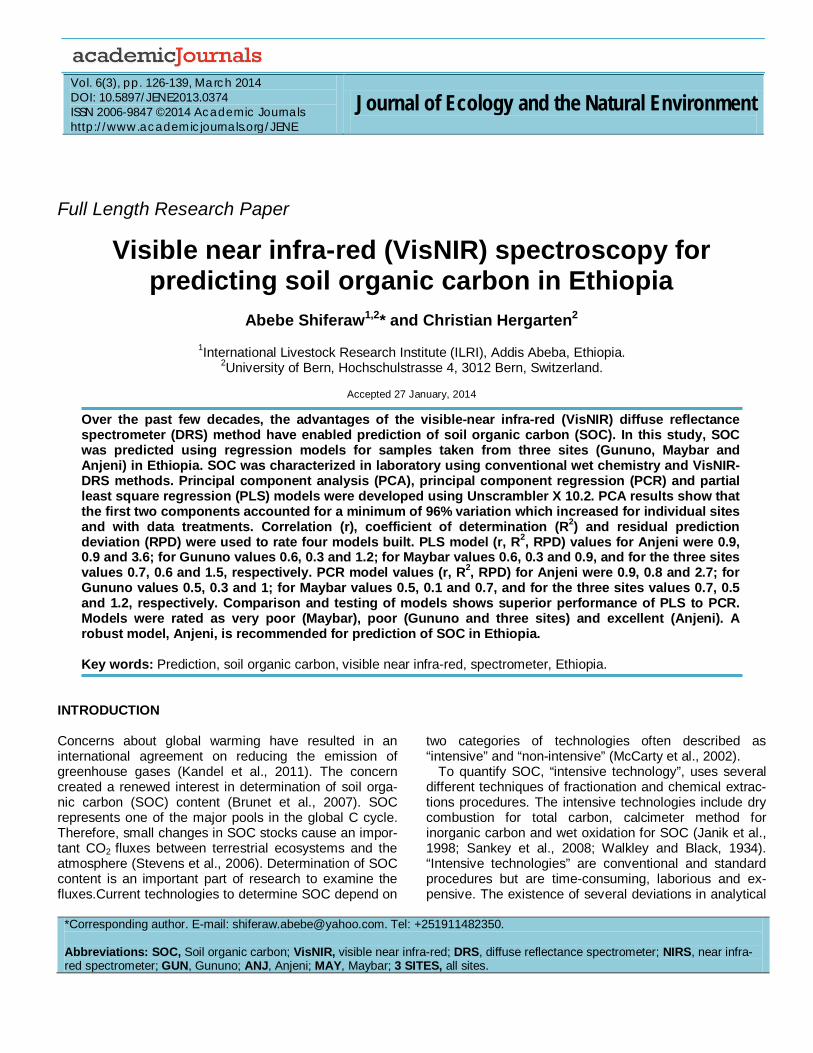
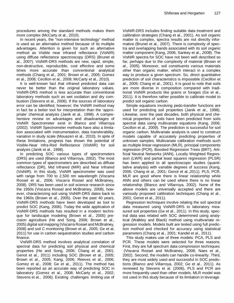
As reviewed by Brown et al. (2005), soil properties were predicted using VisNIR Spectrometer in a wide range of scale representing soil variability from local, regional to global libraries. Regional libraries refer to a greater geographic extent than local libraries while global libraries are based on major soil taxa from multiple con-tinents (Sankey et al., 2008; Brown et al., 2005). A com-parison of results by Sankey et al. (2008) and review by Chang et al., (2001) and Stevens et al., (2006) shows that local libraries have better calibration accuracy com-pared with regional and global libraries. This study attempts to build four models (for individual 3 sites and all three sites) and recommends the most robust model for prediction of SOC in Ethiopia. Until recently, VisNIR-DRS has not been used as a tool to predict soil properties in Ethiopia. The paper specifically attempts to show the effect of data treatment on models, model testing and selection. MATERIALS AND METHODS The study area The study areas are located in the Ethio-Swiss Soil Conservation Program (SCRP) sites established in 1980s. The sites are Gununo in South, Maybar in North-Eastern and Anjeni in North-Western Ethiopia. Gununo site is situated in Wolayita Zone, at 16 km WNW of Sodo town at 37° 38’ E /6° 56 ‘N (SCRP, 2000, b) in Damote-Sore district. Maybar site is situated in South Wello Zone, 14 km SSE of Desse town at 39° 40’ E /11 00 ‘N (SCRP, 2000d) in Albulko district. Anjeni site is situated in West Gojam Zone,Dembecha district at 15 Km North of Demecha at 37° 31’ E /10° 40 ‘N(SCRP, 2000c) (Figure 1). Methods An equivalent mass depth soil sampling method was used as suggested for soil carbon study by Stolbovoy et al. (2002). Soil samples were taken from 64 soil profiles in three sites. Although the study sites are small in size, there are different types of soil types in the areas (Table 1) resulted in an intensive sampling. Depending on profile depth, samples were taken from 0-10, 10-30, 30-50, 50-100 cm depths. Although SOC distribution decrease with soil depth, its concenteration is visible up to 1 meter (Allen et al., 2010). Thus, deep sampling protocol is suggested for SOC study (Baker et al., 2007). Total soil samples are 96 from Gununo, 98 from Anjeni and 81 from Maybar. As recommended by Brunet et al. (2007) and Knadel et al. (2011) soil samples were grinded and sieved through 0.2 mm for better carbon prediction as used in this study.

A field spectroscopy (VisNIR-DRS) by Analytical Spectral Device (ASD) Incorporation was used for measurement of 275 samples taken from three sites. SOC was measured in laboratory using standard procedure for wet oxidation method as described in Walkley and Black (1934). Scanning procedures are as described in Brown et al. (2005) with detail protocols as indicated in Viscarra Rossel (2009). Reflectance spectra were measured on petri dishes, twice for each sample using a mug light. Spectra wavelength ranges from 350 to 2500 nm. Data reduction methods are needed in VisNIR Spectrometer study (Blanco and Villarroya, 2002). Following spectra data transposing for pre-processing, data was

reduced using average (for replicate sample spectra measurement). Then every 10th of the wavelength was selected.

There also seems to be lack of clarity on pre-processing to optimize spectral data (Brunet et al., 2007). Proper data pre-treatment help develop accurate calibration (Reeves et al., 2006; Blanco and Villarroya, 2002). Having tested various data pre-treatment procedures, Multiplicative scatter correction (MSC) and Detrending (DT) were selected to get best calibration and validation result. Steps used in developing multivariate models are as described in Blanco and Villarroya (2002) and CAMO (2012).

Unscrambler X 10.2 (CAMO Software, Analytical Spectral Device {ASD}, Oslo, Norway) (CAMO, 2012) was used for data pre-treatment, model calibration, validation and testing. Using test set validation method; principal component analysis (PCA) was used to examine hidden structure of data, to visualize relationship (similarity and difference) between soil samples and spectral wavelength (variables). PCA was used mainly to describe sample effect on models. PCA was used as descriptive tool while PCR and PLS were used as predictive tool. SOC content was regressed against soil spectra using PLS and PCR.

All model calibration involves selecting 10 components (factors), testing regression coefficients at *P < 0.05% significance level with test set validation. A total of 4 models were built for three individual sites independently and for all the three sites (altogether). To develop model for the three sites, data (n=275) was divided in to validation (30%, n=82) and calibration (70%, n=193) set. In developing each site models, validation and calibration samples are 28 and 68 for Gununo, 29 and 69 for Anjeni and 24 and 57 for Maybar, respectively.

The regression models were compared to examine accuracy and predictive ability using correlation coefficient (r), slope, coefficient of determination (R2), root mean error of calibration (RMEC) and prediction (RMEP). Ratings of the models in this study were based on combining two parameters. The first parameter was based on R2 values rate as suggested by Viscarra Rossel and McBratney (2008). The second parameter was based on RPD value rate as suggested by Mouazen et al. (2010). The accuracy of developed models were tested using full prediction by examining (predicted and reference plot) which shows the difference between measured and predicted values. RESULTS AND DISCUSSION Soil organic carbon (SOC) analytic result The soil of the study sites were described and classified by the Ethio-Swiss Soil Conservation Program (SCRP) (Kejela, 1995; Weigel, 1986,a, Weigel, 1986,b). Altitude of the study area varies from 1982 to 2858 meter above sea level (m.a.s.l). Traditional agro-ecology of the sites varies from Moist WeynaDega to Wet WeynaDega.

SOC samples of the three sites (n= 275) have 2.5 mode and 1.9(g/Kg) median. SOC data is skewed positively (0.8, standard error of skewness = 0.14) with first quartile (Q1) = 1.0 and third quartile (Q3) = 2.6 values.

Previous soil studies in the area, SOC was also determined using Walkley and Black method (though sampling procedure varies). Anjeni was described as soils with low organic carbon (Zeleke, 2000; SCRP, 2000, c). Kejela (1995) found OC variation with maximum values with Phaeozem surface layers with 4.6% and mini- mmum with sub soils of (Gleysol-Fluvisol) with 0.05. SOC % in Zeleke (2000) and SCRP (2000c) varied from 1.1

Shiferaw and Hergarten 129

Figure 1. Location of study sites in Ethiopia.

Table 1. Description of soils of the study sites. Name of research site Gununo (GUN) Maybar (MAY) Anjeni (ANJ) Climate (Thornthwaite classification) *± Temperate , humid Temperate , Sub-humid Temperate , Sub-humid

Parent materials*,± Trapp series of tertiary volcanic eruptions, ignimbrites,rhyolite , trachites and tuffs

Volcanic Trapp series with alkali-olivine basalts

Basaltic Trapp series of the tertiary volcanic eruption, tuff

Major soil Types (FAO-UNESCO)

Nitosols, Acrisols, Phaeozems, Fluvisols

Phaeozems , Lithosols, Gleysols

Alisols, NitosolsCambisols

Size of study area (ha) 166.8* 519.7* 918.4*

*Based on SCRP, 2000a; SCRP, 2000b; SCRP, 2000c; SCRP, 2000d; ± Kejela (1995), Weigel (1986a), Weigel (1986b). to 3.9% mainly because survey area was smaller compared with Kejela (1995). Weigel (1986a) indicated

that high percentage of OC is available in Gununo with some soil units of Humic Acrisols and Nitisols. Organic

130 J. Ecol. Nat. Environ.

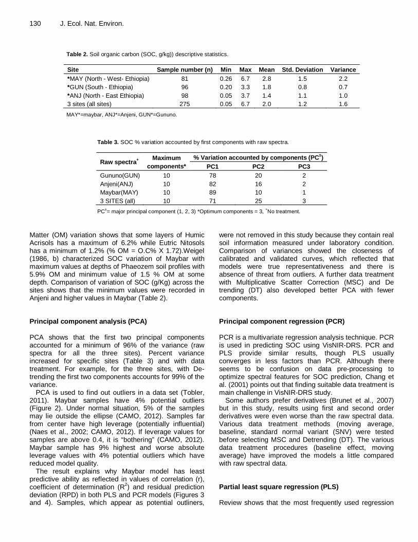
Table 2. Soil organic carbon (SOC, g/kg)) descriptive statistics. Site Sample number (n) Min Max Mean Std. Deviation Variance *MAY (North - West- Ethiopia) 81 0.26 6.7 2.8 1.5 2.2 *GUN (South - Ethiopia) 96 0.20 3.3 1.8 0.8 0.7 *ANJ (North - East Ethiopia) 98 0.05 3.7 1.4 1.1 1.0 3 sites (all sites) 275 0.05 6.7 2.0 1.2 1.6

MAY*=maybar, ANJ*=Anjeni, GUN*=Gununo.

Table 3. SOC % variation accounted by first components with raw spectra.

Raw spectra+ Maximum components*

% Variation accounted by components (PC±) PC1 PC2 PC3

Gununo(GUN) 10 78 20 2 Anjeni(ANJ) 10 82 16 2 Maybar(MAY) 10 89 10 1 3 SITES (all) 10 71 25 3

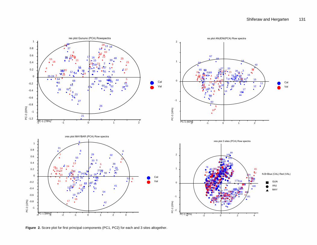
PC±= major principal component (1, 2, 3) *Optimum components = 3, +No treatment. Matter (OM) variation shows that some layers of Humic Acrisols has a maximum of 6.2% while Eutric Nitosols has a minimum of 1.2% (% OM = O.C% X 1.72).Weigel (1986, b) characterized SOC variation of Maybar with maximum values at depths of Phaeozem soil profiles with 5.9% OM and minimum value of 1.5 % OM at some depth. Comparison of variation of SOC (g/Kg) across the sites shows that the minimum values were recorded in Anjeni and higher values in Maybar (Table 2). Principal component analysis (PCA) PCA shows that the first two principal components accounted for a minimum of 96% of the variance (raw spectra for all the three sites). Percent variance increased for specific sites (Table 3) and with data treatment. For example, for the three sites, with De-trending the first two components accounts for 99% of the variance.

PCA is used to find out outliers in a data set (Tobler, 2011). Maybar samples have 4% potential outliers (Figure 2). Under normal situation, 5% of the samples may lie outside the ellipse (CAMO, 2012). Samples far from center have high leverage (potentially influential) (Naes et al., 2002; CAMO, 2012). If leverage values for samples are above 0.4, it is “bothering” (CAMO, 2012). Maybar sample has 9% highest and worse absolute leverage values with 4% potential outliers which have reduced model quality.

The result explains why Maybar model has least predictive ability as reflected in values of correlation (r), coefficient of determination (R2) and residual prediction deviation (RPD) in both PLS and PCR models (Figures 3 and 4). Samples, which appear as potential outliners,

were not removed in this study because they contain real soil information measured under laboratory condition. Comparison of variances showed the closeness of calibrated and validated curves, which reflected that models were true representativeness and there is absence of threat from outliers. A further data treatment with Multiplicative Scatter Correction (MSC) and De trending (DT) also developed better PCA with fewer components. Principal component regression (PCR) PCR is a multivariate regression analysis technique. PCR is used in predicting SOC using VisNIR-DRS. PCR and PLS provide similar results, though PLS usually converges in less factors than PCR. Although there seems to be confusion on data pre-processing to optimize spectral features for SOC prediction, Chang et al. (2001) points out that finding suitable data treatment is main challenge in VisNIR-DRS study.

Some authors prefer derivatives (Brunet et al., 2007) but in this study, results using first and second order derivatives were even worse than the raw spectral data. Various data treatment methods (moving average, baseline, standard normal variant (SNV) were tested before selecting MSC and Detrending (DT). The various data treatment procedures (baseline effect, moving average) have improved the models a little compared with raw spectral data. Partial least square regression (PLS) Review shows that the most frequently used regression


Figure 2. Score plot for first principal components (PC1, PC2) for each and 3 sites altogether.

Cal

Val

PC-1 (78%)-2 -1 0 1 2

PC-2

(20%

)

-1.2

-1

-0.8

-0.6

-0.4

-0.2

0

0.2

0.4

0.6

0.8

1Figure - - Scores plot Gununo (PCA) Rowspectra

1

23

45

6

7

8

91011

12

1314

151617

18

19

20

21

22

23

2425

26

27

28

29

30

31

32

3334

3536

3738

39

4041

42

43

444546

47

48

49

5051

52

5354

5556

5758

59

60

61

6263

64

65

6667

68

1

2

3

4

5

6

7

8

9

10

11

1213

14

1516

17

18

1920

21

22

23

24

25

26

2728

Cal

Val

PC-1 (82%)-2 -1 0 1 2

PC-2

(16%

)

-1

0

1

2Figure - - Scores plot ANJENI(PCA) Row spectra

1

2

3

4

56

7

8910

1112

1314

15

16

1718

19

20

21

22

23

2425

262728 2930

3132

3334

35363738

39

40

41

4243 444546

4748495051

5253

54

5556

57

58

59

60

6162

63

64

65

66

6768

69 12

34

5

6

7

89

10

11

12 131415

16

171819

2021

22 23242526

27

28

29

Cal

Val

PC-1 (89%)-4 -3 -2 -1 0 1 2 3

PC-2

(10%

)

-1

-0.8

-0.6

-0.4

-0.2

0

0.2

0.4

0.6

0.8

1

Figure- Scores plot MAYBAR (PCA) Row spectra

1

2

3

45

6

7

8

9

10

111213

14

15

16

17

1819

2021

22232425

2627

28

29

31

32

3334

35

36

37

38

39

40

41

42

43

44 45

46474849

505152

53

54

55

56

571

2

34

5

6

7

8

9

10

11

12

13

1415

1617

18192021

22

23

24

N.B=Blue (CAL) Red (VAL)

GUN

ANJ

MAY

PC-1 (71%)-4 -2 0 2 4

PC-2

(25%

)

-2

-1

0

1

2

Figure- - Scores plot 3 sites (PCA) Row spectra

1

2345

6

7

8

9

1011

12

13

141516

17

1819

20

21

222324

25

26272829

30

3132

33

34

35

36

37

383940

4142

4344

45

46

474849

5051

52

53

54

55

5657

5859

60

61626364

65

66676869

70

71

72737475

76

7778

79

80 81

8283

84

858687

88

8990

91

92

9394

959697

98

99100

101

102

103104105

106

107

108

109110

111112113

114115

116117

118

119120

121

122123124125

126127

128

129

130

131132

133134

135

136

137138

139140141

143

144

145146

147

148149150151

152153

154

155

156

157158

159

160161

162

163

164165

166

167168

169170

171

172

173

174

175176

177

178

179180

181182

183184185186

187188

189190

192193

12

3

4

56

7

8

9

10

111213

14

15

1617

181920

21

2223

24

25 26

27

282930

313233

34

35

36

3738

39

404142

43 44

45

4647

4849

50

51

52

53545557

585960

61

62

6364

65

66

6768

69

70

71

72

7374

75

76

777879 8081

82


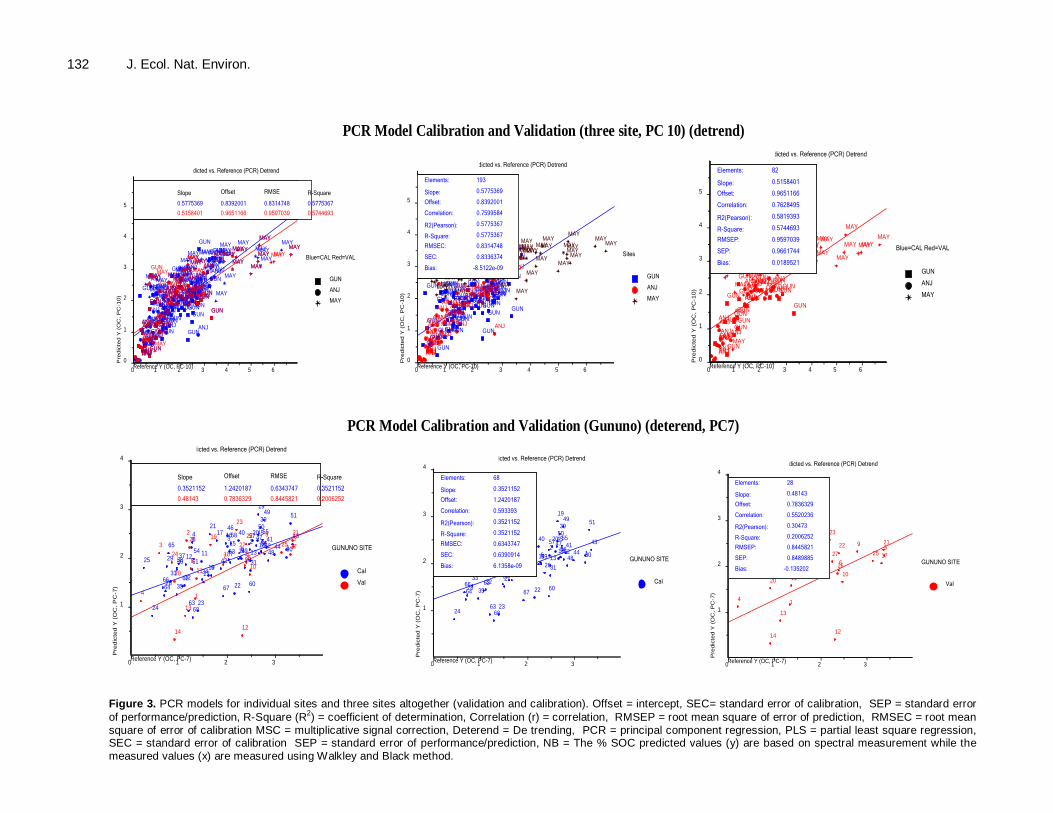
Figure 3. PCR models for individual sites and three sites altogether (validation and calibration). Offset = intercept, SEC= standard error of calibration, SEP = standard error of performance/prediction, R-Square (R2) = coefficient of determination, Correlation (r) = correlation, RMSEP = root mean square of error of prediction, RMSEC = root mean square of error of calibration MSC = multiplicative signal correction, Deterend = De trending, PCR = principal component regression, PLS = partial least square regression, SEC = standard error of calibration SEP = standard error of performance/prediction, NB = The % SOC predicted values (y) are based on spectral measurement while the measured values (x) are measured using Walkley and Black method.

PCR Model Calibration and Validation (three site, PC 10) (detrend)

PCR Model Calibration and Validation (Gununo) (deterend, PC7)

Blue=CAL Red=VAL

GUN

ANJ

MAY

Reference Y (OC, PC-10)0 1 2 3 4 5 6

Pre

dict

ed Y

(O

C, P

C-1

0)

0

1

2

3

4

5

Figure (a) Predicted vs. Reference (PCR) Detrend

GUN

GUN

GUN

GUN

GUNGUN

GUN

GUN

GUN

GUN

GUN

GUN

GUN

GUN

GUN

GUN

GUN

GUN

GUN

GUNGUN

GUNGUN

GUNGUN

GUNGUNGUN

GUN GUNGUNGUN GUN

GUN

GUN

GUN

GUN

GUN

GUN

GUN

GUN

GUN

GUN

GUNGUN

GUN

GUN

GUN

GUNGUNGUN

GUNGUN

GUNGUN

GUN

GUN

GUN

GUNGUN

GUNGUNGUNGUN

GUNGUN

GUN

GUN

GUN

GUNGUN GUN

GUN

ANJ

ANJANJ

ANJ

ANJ ANJ

ANJ

ANJANJANJ

ANJANJANJANJ

ANJ

ANJANJ

ANJ

ANJANJ

ANJ

ANJ

ANJANJ

ANJ

ANJ

ANJ

ANJANJ

ANJ

ANJ

ANJANJ

ANJANJANJANJ

ANJ

ANJANJ

ANJANJ

ANJANJANJ

ANJANJANJ

ANJ

ANJ

ANJ

ANJANJ

ANJ

ANJANJ

ANJANJANJ

ANJ

ANJ

MAYMAYMAY

MAY

MAY

MAY

MAYMAY

MAYMAY

MAYMAYMAYMAY

MAY

MAYMAY

MAY MAY

MAY

MAY

MAYMAYMAYMAYMAYMAY

MAY

MAYMAY

MAY

MAY

MAY

MAY

MAY

MAYMAYMAYMAY

MAYMAY MAYMAYMAY

MAYMAYMAYMAY

MAYMAYMAYMAY

MAYMAYMAY

GUN

GUN

GUN

GUNGUN

GUNGUN

GUN

GUN

GUN

GUNGUN

GUN

GUN

GUN

GUN

GUN

GUN

GUN

GUNANJANJ

ANJ

ANJ

ANJ

ANJ

ANJ

ANJ

ANJ

ANJANJANJANJ

ANJ

ANJANJ

ANJANJ

ANJANJ

ANJ ANJANJANJANJ

ANJANJANJANJ

ANJ

MAYMAYMAY

MAY

MAY MAY

MAY

MAYMAY

MAY

MAYMAY

MAYMAY MAYMAY

MAY

MAY

MAY

MAYMAYMAYMAY

MAY

MAY

MAYMAY

MAYMAY

MAY

Slope Offset RMSE R-Square

0.5158401 0.9651166 0.9597039 0.57446930.5775369 0.8392001 0.8314748 0.5775367

Slope Offset RMSE

0.5158401 0.9651166 0.95970390.5775369 0.8392001 0.8314748

Sites

GUN

ANJ

MAY

Reference Y (OC, PC-10)0 1 2 3 4 5 6

Pre

dict

ed Y

(O

C, P

C-1

0)

0

1

2

3

4

5

Figure (b) Predicted vs. Reference (PCR) Detrend

GUN

GUN

GUN

GUN

GUNGUN

GUN

GUN

GUN

GUN

GUN

GUN

GUN

GUN

GUN

GUN

GUN

GUN

GUN

GUNGUN

GUNGUN

GUNGUN

GUNGUNGUN

GUN GUNGUNGUN GUN

GUN

GUN

GUN

GUN

GUN

GUN

GUN

GUN

GUN

GUN

GUNGUN

GUN

GUN

GUN

GUNGUNGUN

GUNGUN

GUNGUN

GUN

GUN

GUN

GUNGUN

GUNGUNGUNGUN

GUNGUN

GUN

GUN

GUN

GUNGUN GUN

GUN

ANJ

ANJANJ

ANJ

ANJ ANJ

ANJ

ANJANJANJ

ANJANJANJANJ

ANJ

ANJANJ

ANJ

ANJANJ

ANJ

ANJ

ANJANJ

ANJ

ANJ

ANJ

ANJANJ

ANJ

ANJ

ANJANJ

ANJ ANJANJANJ

ANJ

ANJANJ

ANJANJ

ANJANJANJ

ANJANJ

ANJ

ANJ

ANJ

ANJ

ANJANJ

ANJ

ANJANJ

ANJANJ

ANJ

ANJ

ANJ

MAYMAYMAY

MAY

MAY

MAY

MAYMAY

MAYMAY

MAYMAYMAYMAY

MAY

MAYMAY

MAY MAY

MAY

MAY

MAYMAYMAYMAYMAYMAY

MAY

MAYMAY

MAY

MAY

MAY

MAY

MAY

MAYMAYMAYMAY

MAYMAY MAYMAYMAY

MAYMAYMAYMAY

MAYMAYMAYMAY

MAYMAYMAY

Elements:

Slope:Offset:

Correlation:

R2(Pearson):

R-Square:RMSEC:

SEC:

Bias:

193

0.5775369

0.8392001

0.7599584

0.5775367

0.5775367

0.8314748

0.8336374

-8.5122e-09

Elements:

Slope:Offset:

Correlation:

R2(Pearson):

R-Square:RMSEC:

SEC:

Bias:

193

0.5775369

0.8392001

0.7599584

0.5775367

0.5775367

0.8314748

0.8336374

-8.5122e-09

Blue=CAL Red=VAL

GUN

ANJ

MAY

Reference Y (OC, PC-10)0 1 2 3 4 5 6

Pre

dict

ed Y

(O

C, P

C-1

0)

0

1

2

3

4

5

Figure (c) Predicted vs. Reference (PCR) Detrend

GUN

GUN

GUN

GUNGUN

GUNGUN

GUN

GUN

GUN

GUNGUN

GUN

GUN

GUN

GUN

GUN

GUN

GUN

GUNANJANJ

ANJ

ANJ

ANJ

ANJ

ANJ

ANJ

ANJ

ANJANJANJANJ

ANJ

ANJANJ

ANJANJ

ANJANJ

ANJ ANJANJANJANJ

ANJANJANJANJ

ANJ

MAYMAYMAY

MAY

MAY MAY

MAY

MAYMAY

MAY

MAYMAY

MAYMAY MAYMAY

MAY

MAY

MAY

MAYMAYMAYMAY

MAY

MAY

MAYMAY

MAYMAY

MAY

Elements:

Slope:Offset:

Correlation:

R2(Pearson):

R-Square:RMSEP:

SEP:

Bias:

82

0.5158401

0.9651166

0.7628495

0.5819393

0.5744693

0.9597039

0.9661744

0.0189521

Elements:

Slope:Offset:

Correlation:

R2(Pearson):

R-Square:RMSEP:

SEP:

Bias:

82

0.5158401

0.9651166

0.7628495

0.5819393

0.5744693

0.9597039

0.9661744

0.0189521

GUNUNO SITE

Cal

Val

Reference Y (OC, PC-7)0 1 2 3

Pre

dict

ed Y

(O

C, P

C-7

)

1

2

3

4Figure (a) Predicted vs. Reference (PCR) Detrend

1234

56

7

8

910

1112 131415

1617

18

19

2021

22

2324

25 26

2728

2930

31

3233 34

35

363738

39

4041

42

4344

4546

47

48

49

50

51

525354

55

565758

59

60

61

62

63

64

65

6667

68

1

2

3

4

5

678

9

1011

12

13

14

1718

19

20

2122

23

2425

26

2728


0.48143 0.7836329 0.8445821 0.20062520.3521152 1.2420187 0.6343747 0.3521152

Slope Offset RMSE R-

0.48143 0.7836329 0.8445821 0.20.3521152 1.2420187 0.6343747 0.3

GUNUNO SITE

Cal


Pre

dict

ed Y

(O

C, P

C-7

)

1

2

3

4Figure (b) Predicted vs. Reference (PCR) Detrend

1234

56

7

8

910

1112 131415

1617

18

19

2021

22

2324

25 26

2728

2930

31

3233 34

35

363738

39

4041

42

4344

4546

47

48

49

50

51

525354

55

565758

59

60

61

62

63

64

65

6667

68

Elements:

Slope:Offset:

Correlation:

R2(Pearson):

R-Square:RMSEC:

SEC:

Bias:

68

0.3521152

1.2420187

0.593393

0.3521152

0.3521152

0.6343747

0.6390914

6.1358e-09

Elements:

Slope:Offset:

Correlation:

R2(Pearson):

R-Square:RMSEC:

SEC:

Bias:

68

0.3521152

1.2420187

0.593393

0.3521152

0.3521152

0.6343747

0.6390914

6.1358e-09 GUNUNO SITE

Val


Pre

dict

ed Y

(O

C, P

C-7

)

1

2

3

4Figure (b) Predicted vs. Reference (PCR) Detrend

1

2

3

4

5

678

9

1011

12

13

14

1718

19

20

2122

23

2425

26

2728

Elements:

Slope:Offset:

Correlation:

R2(Pearson):

R-Square:RMSEP:

SEP:

Bias:

28

0.48143

0.7836329

0.5520236

0.30473

0.2006252

0.8445821

0.8489885

-0.135202

Elements:

Slope:Offset:

Correlation:

R2(Pearson):

R-Square:RMSEP:

SEP:

Bias:

28

0.48143

0.7836329

0.5520236

0.30473

0.2006252

0.8445821

0.8489885

-0.135202


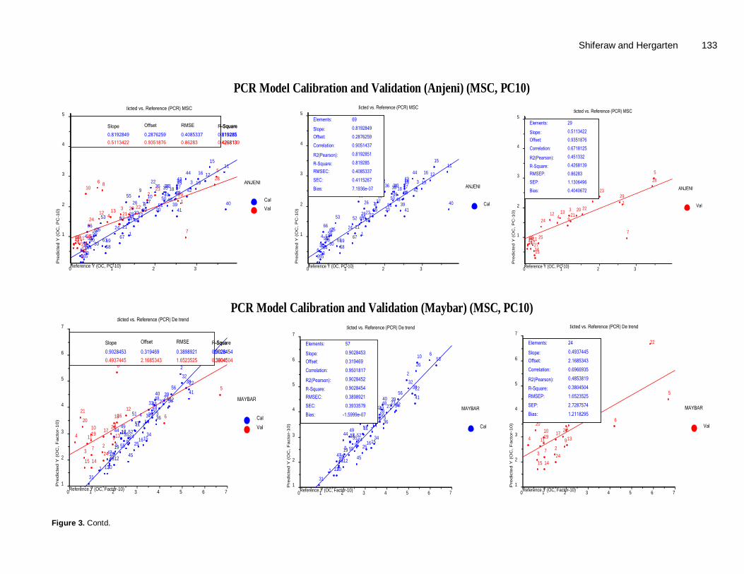
Figure 3. Contd.

PCR Model Calibration and Validation (Anjeni) (MSC, PC10)

PCR Model Calibration and Validation (Maybar) (MSC, PC10)

ANJENI

Cal

Val


Pre

dict

ed Y

(O

C, P

C-1

0)

1

2

3

4

5Figure (a) Predicted vs. Reference (PCR) MSC

1

2

3

4

6

78

910

11

12

13

14

15

16

171819

20

21

22

23

2425

26

272829

30313233

343536

37

38

39 4041

42

4344

4546

4748

4950

51

5253

54

55

56

58

5960 61

62

63

64

65

66

67

68

69

12

34

5

6

7

8

9

10

11

12 13

1415

1617

1819

2021

22

23

24

2526 27

28

29


0.5113422 0.9351876 0.86283 0.42681390.8192849 0.2876259 0.4085337 0.819285


0.5113422 0.9351876 0.86283 0.42681390.8192849 0.2876259 0.4085337 0.819285

ANJENI

Cal


Pre

dic

ted Y

(O

C, P

C-1

0)

1

2

3

4

5Figure (b) Predicted vs. Reference (PCR) MSC

1

2

3

4

6

78

910

11

12

13

14

15

16

171819

20

21

22

23

2425

26

272829

30313233

343536

37

38

39 4041

42

4344

4546

4748

4950

51

5253

54

55

56

58

5960 61

62

63

64

65

66

67

68

69

Elements:

Slope:Offset:

Correlation:

R2(Pearson):

R-Square:RMSEC:

SEC:

Bias:

69

0.8192849

0.2876259

0.9051437

0.8192851

0.819285

0.4085337

0.4115267

7.1936e-07

Elements:

Slope:Offset:

Correlation:

R2(Pearson):

R-Square:RMSEC:

SEC:

Bias:

69

0.8192849

0.2876259

0.9051437

0.8192851

0.819285

0.4085337

0.4115267

7.1936e-07 ANJENI

Val


Pre

dic

ted Y

(O

C, P

C-1

0)

1

2

3

4

5Figure (c) Predicted vs. Reference (PCR) MSC

12

34

5

6

7

8

9

10

11

12 13

1415

1617

1819

2021

22

23

24

2526 27

28

29

Elements:

Slope:Offset:

Correlation:

R2(Pearson):

R-Square:RMSEP:

SEP:

Bias:

29

0.5113422

0.9351876

0.6718125

0.451332

0.4268139

0.86283

1.1306496

0.4040672

Elements:

Slope:Offset:

Correlation:

R2(Pearson):

R-Square:RMSEP:

SEP:

Bias:

29

0.5113422

0.9351876

0.6718125

0.451332

0.4268139

0.86283

1.1306496

0.4040672

MAYBAR

Cal

Val

Reference Y (OC, Factor-10)0 1 2 3 4 5 6 7

Pre

dic

ted

Y (

OC

, F

act

or-

10

)

1

2

3

4

5

6

7Figure (a) Predicted vs. Reference (PCR) De trend

1

2

34

5

6

7

89

10

11

1213

14

15161718

192021

22

23

2425

26

2728

29

30

31

32

33

3435

3637

38

3940 4142

43

44

454647

48

49

5051

52

53

54

55

56

571

23

4

5

6

7

8

9

10

11

12

13

1415

16

17

18

19

20

21

22

23

24


0.4937445 2.1685343 1.6523525 0.38045040.9028453 0.319469 0.3898921 0.9028454

Slope Offset RMSE R-Squar

0.4937445 2.1685343 1.6523525 0.380450.9028453 0.319469 0.3898921 0.90284

MAYBAR

Cal


Pre

dic

ted Y

(O

C, F

act

or-

10)

1

2

3

4

5

6

7Figure (b) Predicted vs. Reference (PCR) De trend

1

2

34

5

6

7

89

10

11

1213

14

15161718

192021

22

23

2425

26

2728

29

30

31

32

33

3435

3637

38

3940 4142

43

44

454647

48

49

5051

52

53

54

55

56

57

Elements:

Slope:Offset:

Correlation:

R2(Pearson):

R-Square:RMSEC:

SEC:

Bias:

57

0.9028453

0.319469

0.9501817

0.9028452

0.9028454

0.3898921

0.3933579

-1.5999e-07

Elements:

Slope:Offset:

Correlation:

R2(Pearson):

R-Square:RMSEC:

SEC:

Bias:

57

0.9028453

0.319469

0.9501817

0.9028452

0.9028454

0.3898921

0.3933579

-1.5999e-07MAYBAR

Val


Pre

dic

ted Y

(O

C, F

act

or-

10)

1

2

3

4

5

6

7Figure (c) Predicted vs. Reference (PCR) De trend

1

23

4

5

6

7

8

9

10

11

12

13

1415

16

17

18

19

20

21

22

23

24

Elements:

Slope:Offset:

Correlation:

R2(Pearson):

R-Square:RMSEP:

SEP:

Bias:

24

0.4937445

2.1685343

0.6966935

0.4853819

0.3804504

1.6523525

2.7287574

1.2118295

Elements:

Slope:Offset:

Correlation:

R2(Pearson):

R-Square:RMSEP:

SEP:

Bias:

24

0.4937445

2.1685343

0.6966935

0.4853819

0.3804504

1.6523525

2.7287574

1.2118295


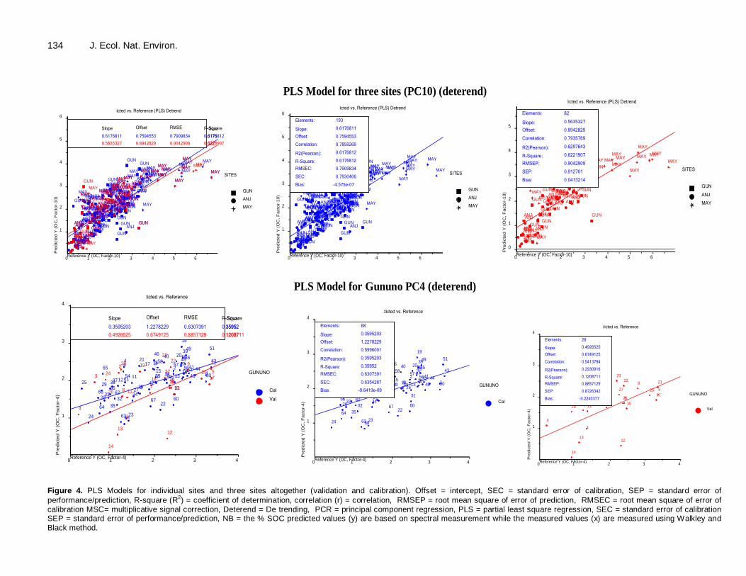
Figure 4. PLS Models for individual sites and three sites altogether (validation and calibration). Offset = intercept, SEC = standard error of calibration, SEP = standard error of performance/prediction, R-square (R2) = coefficient of determination, correlation (r) = correlation, RMSEP = root mean square of error of prediction, RMSEC = root mean square of error of calibration MSC= multiplicative signal correction, Deterend = De trending, PCR = principal component regression, PLS = partial least square regression, SEC = standard error of calibration SEP = standard error of performance/prediction, NB = the % SOC predicted values (y) are based on spectral measurement while the measured values (x) are measured using Walkley and Black method.

PLS Model for three sites (PC10) (deterend)

PLS Model for Gununo PC4 (deterend)

SITES

GUN

ANJ

MAY

Reference Y (OC, Factor-10)0 1 2 3 4 5 6

Pre

dict

ed Y

(OC

, Fac

tor-

10)

1

2

3

4

5

6Figure (a)Predicted vs. Reference (PLS) Detrend

GUN

GUN

GUN

GUN

GUNGUN

GUN

GUN

GUN

GUNGUN

GUN

GUN

GUN

GUN

GUN

GUN

GUN

GUN

GUN

GUN

GUNGUN

GUNGUN

GUNGUN

GUNGUN

GUNGUNGUN GUN

GUN

GUN

GUN

GUN

GUN

GUN

GUN

GUN

GUN

GUN

GUNGUN

GUN

GUN

GUN

GUNGUNGUN

GUNGUN

GUNGUN

GUN

GUN

GUN

GUNGUN

GUNGUNGUNGUN

GUNGUN

GUN

GUN

GUN

GUNGUNGUNGUN

ANJ

ANJANJ

ANJ

ANJANJ

ANJ

ANJANJANJ

ANJANJ

ANJ

ANJANJ

ANJ

ANJANJ

ANJ

ANJ

ANJ

ANJ

ANJ

ANJ

ANJANJ

ANJ

ANJ

ANJ

ANJANJANJ

ANJANJANJ

ANJ

ANJ

ANJANJ

ANJ

ANJANJANJ

ANJ

ANJ

ANJ

ANJ

ANJ

ANJ

ANJANJ

ANJ

ANJANJ

ANJANJ

ANJ

ANJ

ANJ

MAYMAY

MAY

MAY

MAY

MAY

MAYMAY

MAYMAY

MAYMAYMAY

MAY

MAY

MAY

MAY

MAYMAY

MAY

MAY

MAYMAYMAYMAYMAY

MAYMAY

MAYMAY

MAY

MAY

MAY

MAY

MAY

MAYMAY

MAYMAYMAYMAY

MAYMAYMAY

MAY

MAYMAYMAY

MAYMAYMAYMAY

MAY

MAYMAY

GUNGUN

GUN

GUNGUN

GUNGUN

GUN GUN

GUN

GUNGUN

GUN

GUN

GUN

GUN

GUN

GUN

GUN

GUN

ANJANJ

ANJ

ANJ

ANJ ANJ

ANJ

ANJ

ANJ

ANJANJ

ANJ

ANJ

ANJ

ANJANJ

ANJANJ

ANJANJ

ANJANJ

ANJANJ

ANJ

ANJANJANJ

ANJ

ANJ

MAYMAY

MAY

MAY

MAY MAY

MAY

MAYMAY

MAY

MAYMAY

MAY

MAY

MAYMAY

MAY

MAY

MAY

MAYMAY

MAYMAYMAY

MAYMAYMAY

MAYMAY

MAY


0.5635327 0.8942829 0.9042909 0.62219070.6176811 0.7594553 0.7909834 0.6176812

Slope Offset RMSE R-Squa

0.5635327 0.8942829 0.9042909 0.622190.6176811 0.7594553 0.7909834 0.61768

SITES

GUN

ANJ

MAY


Pre

dict

ed Y

(OC

, Fac

tor-

10)

1

2

3

4

5

6Figure (b)Predicted vs. Reference (PLS) Detrend

GUN

GUN

GUN

GUN

GUNGUN

GUN

GUN

GUN

GUNGUN

GUN

GUN

GUN

GUN

GUN

GUN

GUN

GUN

GUN

GUN

GUNGUN

GUNGUN

GUNGUN

GUNGUN

GUNGUNGUN GUN

GUN

GUN

GUN

GUN

GUN

GUN

GUN

GUN

GUN

GUN

GUNGUN

GUN

GUN

GUN

GUNGUNGUN

GUNGUN

GUNGUN

GUN

GUN

GUN

GUNGUN

GUNGUNGUNGUN

GUNGUN

GUN

GUN

GUN

GUNGUNGUNGUN

ANJ

ANJANJ

ANJ

ANJANJ

ANJ

ANJANJANJ

ANJANJ

ANJ

ANJANJ

ANJ

ANJANJ

ANJ

ANJ

ANJ

ANJ

ANJ

ANJ

ANJANJ

ANJ

ANJ

ANJ

ANJANJANJ

ANJANJANJ

ANJ

ANJ

ANJANJ

ANJ

ANJANJANJ

ANJ

ANJ

ANJ

ANJ

ANJ

ANJ

ANJANJ

ANJ

ANJANJ

ANJANJ

ANJ

ANJ

ANJ

MAYMAY

MAY

MAY

MAY

MAY

MAYMAY

MAYMAY

MAYMAYMAY

MAY

MAY

MAY

MAY

MAYMAY

MAY

MAY

MAYMAYMAYMAYMAY

MAYMAY

MAYMAY

MAY

MAY

MAY

MAY

MAY

MAYMAY

MAYMAYMAYMAY

MAYMAYMAY

MAY

MAYMAYMAY

MAYMAYMAYMAY

MAY

MAYMAY

Elements:

Slope:Offset:

Correlation:

R2(Pearson):

R-Square:RMSEC:

SEC:

Bias:

193

0.6176811

0.7594553

0.7859269

0.6176812

0.6176812

0.7909834

0.7930406

-4.575e-07

Elements:

Slope:Offset:

Correlation:

R2(Pearson):

R-Square:RMSEC:

SEC:

Bias:

193

0.6176811

0.7594553

0.7859269

0.6176812

0.6176812

0.7909834

0.7930406

-4.575e-07

SITES

GUN

ANJ

MAY


Pre

dict

ed Y

(OC

, Fac

tor-

10)

0

1

2

3

4

5

Figure (c)Predicted vs. Reference (PLS) Detrend

GUNGUN

GUN

GUNGUN

GUNGUN

GUN GUN

GUN

GUNGUN

GUN

GUN

GUN

GUN

GUN

GUN

GUN

GUN

ANJANJ

ANJ

ANJ

ANJ ANJ

ANJ

ANJ

ANJ

ANJ

ANJ

ANJ

ANJ

ANJ

ANJANJ

ANJANJ

ANJANJ

ANJANJ

ANJANJ

ANJ

ANJANJANJ

ANJ

ANJ

MAYMAY

MAY

MAY

MAY MAY

MAY

MAYMAY

MAY

MAYMAY

MAY

MAY

MAYMAY

MAY

MAY

MAY

MAYMAY

MAYMAYMAY

MAYMAYMAY

MAYMAY

MAY

Elements:

Slope:Offset:

Correlation:

R2(Pearson):

R-Square:RMSEP:

SEP:

Bias:

82

0.5635327

0.8942829

0.7935769

0.6297643

0.6221907

0.9042909

0.912701

0.0413214

Elements:

Slope:Offset:

Correlation:

R2(Pearson):

R-Square:RMSEP:

SEP:

Bias:

82

0.5635327

0.8942829

0.7935769

0.6297643

0.6221907

0.9042909

0.912701

0.0413214

GUNUNO

Cal

Val

Reference Y (OC, Factor-4)0 1 2 3 4

Pre

dict

ed Y

(OC

, Fac

tor-

4)

1

2

3

4Figure (a) Predicted vs. Reference

12

34

567

8

910

1112131415

161718

19

2021

22

2324

25 26

2728

29

30

31

3233 34

35

363738

3940

41

42

4344

4546

47

48

4950

51

525354

55

565758

59

60

61

62

63

64

65

6667

681

2

3

4

5

678

9

1011

1213

14

1718

19

20

212223

24 25

26

2728


0.4926525 0.6749125 0.8857129 0.12087110.3595203 1.2278229 0.6307391 0.35952


0.4926525 0.6749125 0.8857129 0.120870.3595203 1.2278229 0.6307391 0.35952

GUNUNO

Cal


Pre

dict

ed Y

(OC

, Fac

tor-

4)

1

2

3

4Figure (b) Predicted vs. Reference

12

34

567

8

910

1112131415

161718

19

2021

22

2324

25 26

2728

29

30

31

3233 34

35

363738

3940

41

42

4344

4546

47

48

4950

51

525354

55

565758

59

60

61

62

63

64

65

6667

68

Elements:

Slope:Offset:

Correlation:

R2(Pearson):

R-Square:RMSEC:

SEC:

Bias:

68

0.3595203

1.2278229

0.5996001

0.3595203

0.35952

0.6307391

0.6354287

-9.6419e-09

Elements:

Slope:Offset:

Correlation:

R2(Pearson):

R-Square:RMSEC:

SEC:

Bias:

68

0.3595203

1.2278229

0.5996001

0.3595203

0.35952

0.6307391

0.6354287

-9.6419e-09GUNUNO

Val


Pre

dict

ed Y

(OC

, Fac

tor-

4)

1

2

3

4Figure (c) Predicted vs. Reference

1

2

3

4

5

678

9

1011

1213

14

1718

19

20

212223

24 25

26

2728

Elements:

Slope:Offset:

Correlation:

R2(Pearson):

R-Square:RMSEP:

SEP:

Bias:

28

0.4926525

0.6749125

0.5413794

0.2930916

0.1208711

0.8857129

0.8726342

-0.2240377

Elements:

Slope:Offset:

Correlation:

R2(Pearson):

R-Square:RMSEP:

SEP:

Bias:

28

0.4926525

0.6749125

0.5413794

0.2930916

0.1208711

0.8857129

0.8726342

-0.2240377


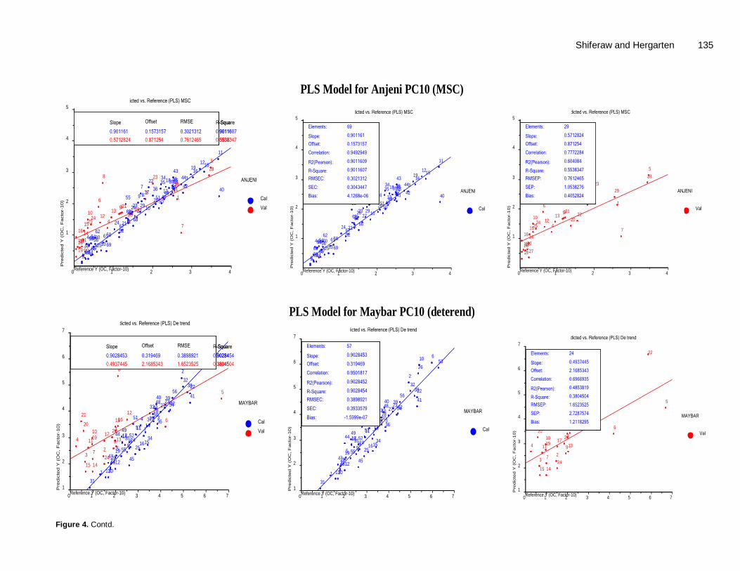
Figure 4. Contd.

PLS Model for Anjeni PC10 (MSC)

PLS Model for Maybar PC10 (deterend)

ANJENI

Cal

Val


Pre

dic

ted Y

(O

C, F

act

or-

10)

1

2

3

4

5Figure (a) Predicted vs. Reference (PLS) MSC

1

3

4

56

789

10

11

12

13

14

1516

1718

19

20

21

22

23

24

25

26 272829

30

3132

3435

3637

38394041 42

43444546

4748

4950

51

52

5354

55

5657

5859

60

6162

63

6465

66

6768

69

12

3

4

5

6

7

8

910

11

1213

14

1516

1718

19

2021 22

23

2425

2627

28

29


0.5712824 0.871254 0.7612465 0.55383470.901161 0.1573157 0.3021312 0.9011607


0.5712824 0.871254 0.7612465 0.553830.901161 0.1573157 0.3021312 0.90116

ANJENI

Cal


Pre

dic

ted

Y (

OC

, F

act

or-

10

)

1

2

3

4

5Figure (b) Predicted vs. Reference (PLS) MSC

1

3

4

56

789

10

11

12

13

14

1516

1718

19

20

21

22

23

24

25

26 272829

30

3132

3435

3637

38394041 42

43444546

4748

4950

51

52

5354

55

5657

5859

60

6162

63

6465

66

6768

69

Elements:

Slope:Offset:

Correlation:

R2(Pearson):

R-Square:RMSEC:

SEC:

Bias:

69

0.901161

0.1573157

0.9492949

0.9011609

0.9011607

0.3021312

0.3043447

4.1268e-06

Elements:

Slope:Offset:

Correlation:

R2(Pearson):

R-Square:RMSEC:

SEC:

Bias:

69

0.901161

0.1573157

0.9492949

0.9011609

0.9011607

0.3021312

0.3043447

4.1268e-06ANJENI

Val


Pre

dic

ted Y

(O

C, F

act

or-

10)

1

2

3

4

5Figure (c) Predicted vs. Reference (PLS) MSC

12

3

4

5

6

7

8

910

11

1213

14

1516

1718

19

2021 22

23

2425

2627

28

29

Elements:

Slope:Offset:

Correlation:

R2(Pearson):

R-Square:RMSEP:

SEP:

Bias:

29

0.5712824

0.871254

0.7772284

0.604084

0.5538347

0.7612465

1.0538276

0.4052824

Elements:

Slope:Offset:

Correlation:

R2(Pearson):

R-Square:RMSEP:

SEP:

Bias:

29

0.5712824

0.871254

0.7772284

0.604084

0.5538347

0.7612465

1.0538276

0.4052824

MAYBAR

Cal

Val


Pre

dic

ted

Y (

OC

, F

act

or-

10

)

1

2

3

4

5

6

7Figure (a) Predicted vs. Reference (PLS) De trend

1

2

34

5

6

7

89

10

11

1213

14

15161718

192021

22

23

2425

26

2728

29

30

31

32

33

3435

3637

38

3940 4142

43

44

454647

48

49

5051

52

53

54

55

56

571

23

4

5

6

7

8

9

10

11

12

13

1415

16

17

18

19

20

21

22

23

24


0.4937445 2.1685343 1.6523525 0.38045040.9028453 0.319469 0.3898921 0.9028454


0.4937445 2.1685343 1.6523525 0.380450.9028453 0.319469 0.3898921 0.90284

MAYBAR

Cal


Pre

dic

ted Y

(O

C, F

act

or-

10)

1

2

3

4

5

6

7Figure (b) Predicted vs. Reference (PLS) De trend

1

2

34

5

6

7

89

10

11

1213

14

15161718

192021

22

23

2425

26

2728

29

30

31

32

33

3435

3637

38

3940 4142

43

44

454647

48

49

5051

52

53

54

55

56

57

Elements:

Slope:Offset:

Correlation:

R2(Pearson):

R-Square:RMSEC:

SEC:

Bias:

57

0.9028453

0.319469

0.9501817

0.9028452

0.9028454

0.3898921

0.3933579

-1.5999e-07

Elements:

Slope:Offset:

Correlation:

R2(Pearson):

R-Square:RMSEC:

SEC:

Bias:

57

0.9028453

0.319469

0.9501817

0.9028452

0.9028454

0.3898921

0.3933579

-1.5999e-07 MAYBAR

Val


Pre

dic

ted

Y (

OC

, F

act

or-

10

)

1

2

3

4

5

6

7Figure (c) Predicted vs. Reference (PLS) De trend

1

23

4

5

6

7

8

9

10

11

12

13

1415

16

17

18

19

20

21

22

23

24

Elements:

Slope:Offset:

Correlation:

R2(Pearson):

R-Square:RMSEP:

SEP:

Bias:

24

0.4937445

2.1685343

0.6966935

0.4853819

0.3804504

1.6523525

2.7287574

1.2118295

Elements:

Slope:Offset:

Correlation:

R2(Pearson):

R-Square:RMSEP:

SEP:

Bias:

24

0.4937445

2.1685343

0.6966935

0.4853819

0.3804504

1.6523525

2.7287574

1.2118295

136 J. Ecol. Nat. Environ. Partial least square regression (PLS) Review shows that the most frequently used regression models in VisNIR-DRS are PCR and PLS (Blanco and Villarroya, 2002; Viscarra Rossel et al., 2006). Both PCR and PLS can cope with data containing large numbers of predictor variables that are highly collinear (Viscarra Rossel and McBratney, 2008). PLS is the most preferred and popular method to predict SOC (Kang, 2006; Viscarra Rossel et al., 2006; Viscarra Rossel and McBratney, 2008). PLS is used for accurate prediction of site-specific data sets to establish local spectral library (Sankey et al., 2008). SOC measured with Walkley-Black method have been predicted from local to global spectral level using PLS in VisNIR-DRS. Review of past studies on SOC by He and Song (2006) found correlation of 0.9 for soil organic matter (n= 30) RMSEP = 0.12, RMSEC=0.058. Brown et al. (2005) predicted SOC (n= 3793) with correlation of 0.82, Slope =0.76, RMSD=0.9% (with first derivative, D1). McCarty et al., (2002) predicted SOC for different set of sample (n=177- 257) with correlation of 0.82-0.98, RMSD =5.5-7.9. Kang (2006) found correlation of 0.9 for soil samples (n=26) to predict SOC using PLS regression model (r = 0.9) with RMSEC = 0.07 and RMSEP = 0.12. Testing and comparison of models for SOC prediction Using full prediction test, the minimum and maximum deviation values were compared for PLS and PCR models. PLS model for Anjeni is the best while PCR model for Maybar is the worst. PLS as a whole has better performance compared with PCR (Table 6). This agrees with findings of Kang (2006), Viscarra Rossel et al. (2006) and Viscarra Rossel and McBratney (2008).

To compare models, accuracy indices are used (Chang et al., 2001; Brunet et al., 2007; He and Song 2006; Ge et al., 2011, Kandel et al., 2011; Stevens et al., 2006). These indices are statistical parameters based on high value (close to 1) correlation coefficient (r2), coefficient of determination (R2) and slope values. Moreover, values of residual predictive deviation (RPD), root mean square error (RMSE), standard of error of calibration (SEC) and standard error of performance or prediction (SEP) also assesses model quality (Chang et al., 2001; Brunet et al., 2007; He and Song, 2006; Mouazen et al., 2010; Ge et al., 2011; CAMO, 2012). In this study (Tables 4 and 5) accuracy indices are better for PLS than PCR.

Root mean square error of predication (RMSEP) is expressed in the same units than the variable of analyses (soil organic carbon, g kg-1). Standard error of prediction/performance (SEP) assesses the ability of the model to predict SOC. Standard error of calibration (SEC) is the standard deviations of all the points from the reference values in the calibration set (Stevens et al.,

2006). Best model has lowest SEP. That means, SEP indicates variation in the precision of predictions (Mouazen et al., 2010; CAMO, 2012). In this study (Table 4 and 5) SEP values are better for PLS than PCR.

R2 values for prediction of soil properties are rated as very good (>0.81), good (0.61-0.8), fair (0.41-0.6) and poor (<0.4) (Viscarra Rossel and McBratney, 2008). The value of R2 varies from 0.1 (Maybar) which is rated as poor to 0.9 (Anjeni) which is rated as very good (Tables 4 and 5). R2 values reflect that Anjeni has good predictive ability for SOC while the three site model has is fair. But, Maybar and Gununo models are too poor to be used for prediction.

Ratio of standard deviation to RMSEP or RMSEC is RPD (Chang et al., 2001; Stevens et al., 2006; Mouazen et al., 2010; Kandel et al., 2011; Ge et al., 2011). RPD is used as indicator of predictive ability of models. Genot et al., (2011) indicated that RPD is used to compare samples from diverse variability. Rating shows that RPD< 1 is very poor model, RPD from 1 to 1.4 is poor model, RPD from 1.4 to 1.8 is fair model, RPD from 1.8 to 2 is good model, RPD from 2 to 2.5 is very good model and PRD >2.5 is excellent model (Mouazen et al., 2010). The value of RPD in this study varies from 0.7 (Maybar) to 3.6 (Anjeni).

Values of r2, R2, slope and RPD (Tables 4 and 5) shows that PLS has better predictive capacity compared with PCR. Finding in this study agrees with PLS better performance over PCR as indicated by Mouazen et al. (2010) and Viscarra Rossel et al. (2006).PCR and PLS are related techniques and in most situations prediction errors will be similar (Viscarra Rossel and McBratney, 2008), though PLS has comparatively lower predication error. As a whole, taking in to account the two rating methods based on R2 values as suggested by Viscarra Rossel and McBratney (2008) and RPD value as suggested by Mouazen et al., (2010), Anjeni model is excellent while Gununo and Maybar models are poor. Maybar model has least predictive capacity and rated as very poor based on the above two rating parameters. Conclusions Visible-near infrared reflectance (VisNIR) diffuse reflectance spectrometer (DRS) method was used to predict SOC in Ethiopia. Analytical data shows that SOC (g/Kg) from three sites (n=275) has a mean value of 2.0 with 1.2 standard deviation. Most frequent value of SOC is 2.5 g/Kg with a minimum of 0.05 and maximum of 6.7.

PCA score plot shows first two components accounts for a minimum of 96% variation. The closeness of the samples in score plot shows samples similarity with respect to the first principal components.

Although performance of PLS is superior to PCR, in both cases Anjeni model is the best while Maybar the worst. The poor performance of Maybar model might be

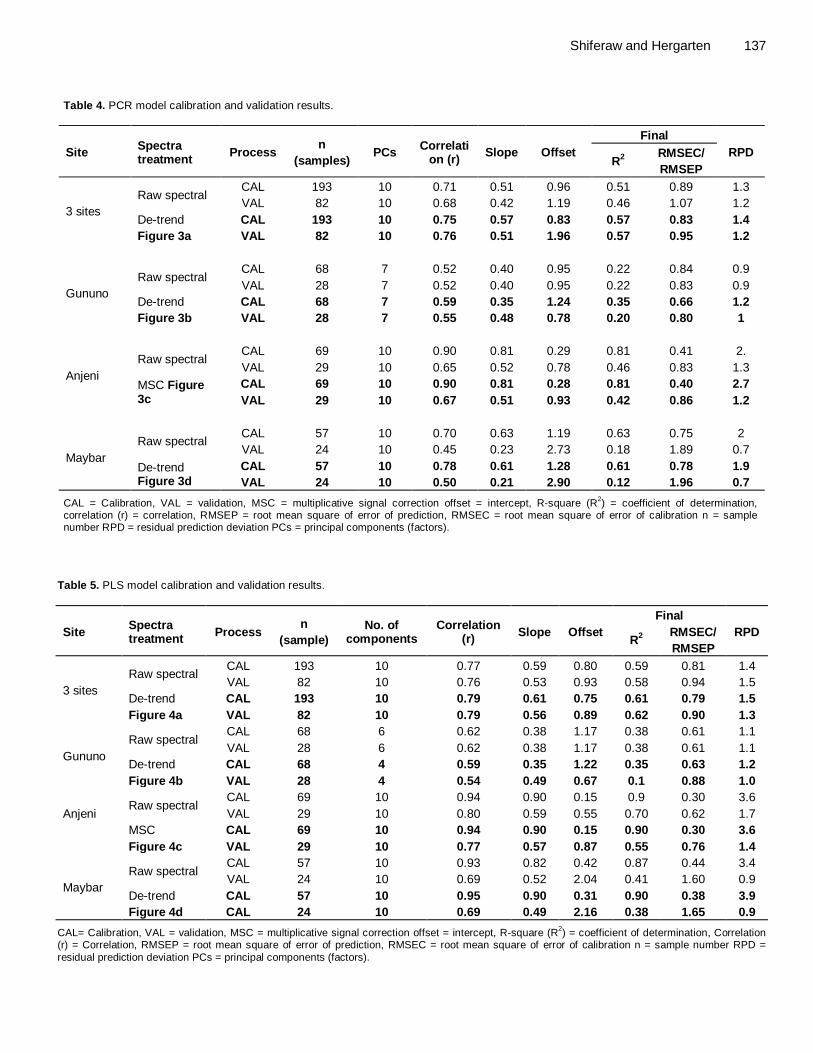
Shiferaw and Hergarten 137 Table 4. PCR model calibration and validation results.

Site Spectra treatment Process n

(samples) PCs Correlation (r) Slope Offset

Final RPD

R2 RMSEC/ RMSEP

3 sites Raw spectral

CAL 193 10 0.71 0.51 0.96 0.51 0.89 1.3 VAL 82 10 0.68 0.42 1.19 0.46 1.07 1.2

De-trend Figure 3a

CAL 193 10 0.75 0.57 0.83 0.57 0.83 1.4 VAL 82 10 0.76 0.51 1.96 0.57 0.95 1.2

Gununo Raw spectral

CAL 68 7 0.52 0.40 0.95 0.22 0.84 0.9 VAL 28 7 0.52 0.40 0.95 0.22 0.83 0.9

De-trend Figure 3b

CAL 68 7 0.59 0.35 1.24 0.35 0.66 1.2 VAL 28 7 0.55 0.48 0.78 0.20 0.80 1

Anjeni Raw spectral

CAL 69 10 0.90 0.81 0.29 0.81 0.41 2. VAL 29 10 0.65 0.52 0.78 0.46 0.83 1.3

MSC Figure 3c

CAL 69 10 0.90 0.81 0.28 0.81 0.40 2.7 VAL 29 10 0.67 0.51 0.93 0.42 0.86 1.2

Maybar Raw spectral CAL 57 10 0.70 0.63 1.19 0.63 0.75 2

VAL 24 10 0.45 0.23 2.73 0.18 1.89 0.7 De-trend Figure 3d

CAL 57 10 0.78 0.61 1.28 0.61 0.78 1.9 VAL 24 10 0.50 0.21 2.90 0.12 1.96 0.7

CAL = Calibration, VAL = validation, MSC = multiplicative signal correction offset = intercept, R-square (R2) = coefficient of determination, correlation (r) = correlation, RMSEP = root mean square of error of prediction, RMSEC = root mean square of error of calibration n = sample number RPD = residual prediction deviation PCs = principal components (factors).

Table 5. PLS model calibration and validation results.

Site Spectra treatment Process n

(sample) No. of

components Correlation

(r) Slope Offset Final

RPD R2 RMSEC/ RMSEP

3 sites Raw spectral CAL 193 10 0.77 0.59 0.80 0.59 0.81 1.4

VAL 82 10 0.76 0.53 0.93 0.58 0.94 1.5 De-trend Figure 4a

CAL 193 10 0.79 0.61 0.75 0.61 0.79 1.5 VAL 82 10 0.79 0.56 0.89 0.62 0.90 1.3

Gununo Raw spectral

CAL 68 6 0.62 0.38 1.17 0.38 0.61 1.1 VAL 28 6 0.62 0.38 1.17 0.38 0.61 1.1

De-trend Figure 4b

CAL 68 4 0.59 0.35 1.22 0.35 0.63 1.2 VAL 28 4 0.54 0.49 0.67 0.1 0.88 1.0

Anjeni

Raw spectral CAL 69 10 0.94 0.90 0.15 0.9 0.30 3.6 VAL 29 10 0.80 0.59 0.55 0.70 0.62 1.7

MSC Figure 4c

CAL 69 10 0.94 0.90 0.15 0.90 0.30 3.6 VAL 29 10 0.77 0.57 0.87 0.55 0.76 1.4

Maybar Raw spectral

CAL 57 10 0.93 0.82 0.42 0.87 0.44 3.4 VAL 24 10 0.69 0.52 2.04 0.41 1.60 0.9

De-trend Figure 4d

CAL 57 10 0.95 0.90 0.31 0.90 0.38 3.9 CAL 24 10 0.69 0.49 2.16 0.38 1.65 0.9

CAL= Calibration, VAL = validation, MSC = multiplicative signal correction offset = intercept, R-square (R2) = coefficient of determination, Correlation (r) = Correlation, RMSEP = root mean square of error of prediction, RMSEC = root mean square of error of calibration n = sample number RPD = residual prediction deviation PCs = principal components (factors).


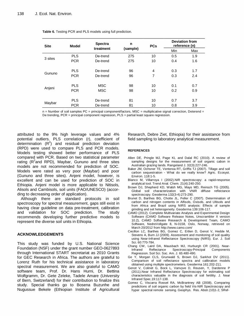
Table 6. Testing PCR and PLS models using full prediction.

Site Model Spectra treatment

n (sample) PCs

Deviation from reference (n)

Min Max

3 sites PLS De-trend 275 10 0.5 1.9 PCR De-trend 275 10 0.4 1.6

Gununo PLS De-trend 96 4 0.3 1.7 PCR De-trend 96 7 0.3 2.4

Anjeni PLS MSC 98 10 0.1 0.7 PCR MSC 98 10 0.2 0.9

Maybar PLS De-trend 81 10 0.7 3.7 PCR De-trend 81 10 0.8 3.9

n = Number of soil samples PC = principal component/factors, MSC = multiplicative signal correction, Deterend = De trending, PCR = principal component regression, PLS = partial least square regression.

attributed to the 9% high leverage values and 4% potential outliers. PLS correlation (r), coefficient of determination (R2) and residual prediction deviation (RPD) were used to compare PLS and PCR models. Models testing showed better performance of PLS compared with PCR. Based on two statistical parameter rating (R2and RPD), Maybar, Gununo and three sites models are not recommended for prediction of SOC. Models were rated as very poor (Maybar) and poor (Gununo and three sites). Anjeni model, however, is excellent and can be used for prediction of SOC in Ethiopia. Anjeni model is more applicable to Nitisols, Alisols and Cambisols, soil units (FAO/UNESCO) (accor-ding to decreasing order of application).

Although there are standard protocols in soil spectroscopy for spectral measurement, gaps still exist in having clear guideline on data pre-treatment, calibration and validation for SOC prediction. The study recommends developing further predictive models to represent the diverse soil units in Ethiopia. ACKNOWLEDGEMENTS This study was funded by U.S. National Science Foundation (NSF) under the grant number GEO-0627893 through International START secretariat as 2010 Grants for GEC Research in Africa. The authors are grateful to Lorenz Ruth for his technical assistance in laboratory spectral measurement. We are also grateful to CAMO software team, Prof. Dr. Hans Hurni, Dr. Bettina Wolfgramm, Dr. Gete Zeleke, Tadele Amare (University of Bern, Switzerland) for their contribution to finalize this study. Special thanks go to Bosena Buzunhe and Nugussue Bekele (Ethiopian Institute of Agricultural

Research, Debre Ziet, Ethiopia) for their assistance from field sampling to laboratory analytical measurement. REFERENCES Allen DE, Pringle MJ, Page KL and Dalal RC (2010). A review of

sampling designs for the measurement of soil organic cabon in Australian grazing lands. Rangeland J. 32(3):227-246.

Baker JM, Ochsner TE, Venterea RT, Griffis TJ (2007). Tillage and soil carbon sequestration - What do we really know? Agric. Ecosyst. Environ. 118:1-5.

Blanco M, Villarroya I (2002).NIR spectroscopy: a rapid-response analytical tool. Trend Anal. Chem. 21(4):240-250.

Brown DJ, Shepherd KD, Walsh MG, Mays MD, Reinsch TG (2005). Global soil characterization with VNIR diffuse reflectance spectroscopy. Geoderma 132(3-4):273-290.

Brunet D, Barthes BG, Chotte JL, Feller C (2007). Determination of carbon and nitrogen contents in Alfisols, Oxisols, and Ultisols and from Africa and Brazil using NIRS analysis: Effects of sample grinding and set heterogeneity. Geoderma 139:106-117.

CAMO (2012). Complete Multivariate Analysis and Experimental Design Software (CAMO Software Release Notes, Unscrambler X version 10.2), CAMO Software Research & Development Team, CAMO Software, NedreVollgate 8, N-0158, Oslo, Norway, retrieved on March 20/2012 from http://www.camo.com/

Cecillon LC, Barthes BG, Gomez C, Ertlen D, Genot V, Hedde M, Stevens A, Burn JJ (2009). Assessment and monitoring of soil quality using Near-Infrared Reflectance Spectroscopy (NIRS). Eur. J. Soil Sci. 60:770-784.

Chang CW, Laird DA, Mausbach MJ, Hurburgh CR (2001). Near-Infrared Reflectance Spectroscopy-Principal Components Regression. Soil Sci. Soc. Am. J. 65:480-490.

Ge Y, Morgan CLS, Grunwald S, Brown DJ, Sarkhot DV (2011). Comparison of soil reflectance spectra and calibration models obtained using multiple spectrometers. Geoderma 161:202-211.

Genot V, Colinet G, Bock L, Vanvyve D, Reusen, Y, Dardenne P (2011).Near Infrared Reflectance Spectroscopy for estimating soil characteristics valuable in the diagnosis of soil fertility. J. Near Infrared Spec.19:117-138.

Gomez C, Viscarra Rossel RA, McBrantney AB (2008), Comparing predictions of soil organic carbon by field Vis-NIR Spectroscopy and hyper spectral remote sensing. Geophys. Res. Abstr.(10)1-2, SRef-

http://www.camo.com/

ID:1607-7962/gra/EGU2008-A-00317. He Y, Song H (2006). Prediction of soil content using near-infrared

spectroscopy, SPINE news room. The international Society for Optical Engineering. DOI: 10.1117/2.1200604.0164

Janik LJ, Merry RH, Skjemstand JO(1998).Can mid infrared diffuse reflectance analysis replace soil extractions?. Aust. J Exp. Agric. 38:681-96.

Kang M (2006). Quantification of soil organic carbon using mid and near Diffuse Reflectance Infrared Fourier Transform spectroscopy, M.Sc thesis, Texas A&M University, Department of Geology and Geophysics Department. Accessible at <geoweb.tamu.edu/Faculty/Herbert/docs/02KangMSThesis.pdf>

Kejela K (1995). Soils of the Anjeni Area-Gojam Research Unit, Ethiopia. Soil Conservation Research Program (SCRP), Center for Development and Environment (CDE), University of Bern, Switzerland, Research Report 27.

Knadel M, Thomsen A, Greve MH (2011). Multi-sensor On -The -Go Mapping of Soil Organic Carbon Content. Soil Sci. Soc. Am. J. 75:1799-1806.

McCarty GW, Reeves JB, Follett RF, Kimble JM (2002). Mid-Infrared and Near Infrared Diffuse Reflectance Spectroscopy for Soil Carbon Measurement. Soil Sci. Soc. Am. J. 66:640-646.

McCarty GW, Reeves JB,.Yost R, Doraiswamny PC, Doumbia M (2010).Evaluation of methods for measuring soil organic carbon in West African soils. Afr. J Agric. Res. 5(16):2169-2177.

Mouazen AM, Kuang B, DeBeardemaeker J, Ramon H(2010). Comparison among principal components, partial least square and back propagation neutral network analyses for accuracy of measurement of selected soil properties with visible and near infrared spectroscopy. Geoderma 158:23-31.

Naes T, Isaksson T, Fearn T, Davies T (2002). A User-Friendly Guide to Multivariate Calibration and Classification, NIR publications, Chichester, UK, p. 344.

Reeves JB, Follett RF, McCarty GW, Kimble JM (2006). Can Near or Mid-Infrared Diffuse Reflectance Spectroscopy Be Used to Determine Soil Carbon Pools?. Commun. Soil Sci. Plan. 37:2307-2325.

Sankey JB, Brown DJ, Bernard ML, Lawrence RL (2008). Comparing local vs. global visible Near-Infrared (VisNIR) diffuse reflectance spectroscopy (DRS) calibrations for the prediction of soil clay, organic C and inorganic C. Geoderma 148:149-158.

SCRP (2000a). Concept and Methodology: Long-term Monitoring of the Agricultural Environment in Six Research Stations in Ethiopia. Soil Conservation Research Program (SCRP), Center for Development and Environment (CDE), University of Bern, Switzerland.

SCRP (2000b). Area of Gununo, Sidamo, Ethiopia: Long Term Monitoring of the Agricultural Environment (1981-1994). Soil Conservation Research Program (SCRP), Center for Development and Environment (CDE), University of Bern, Switzerland.

SCRP (2000c). Area of Anjeni, Gojam: Long-term Monitoring of the Agricultural Environment 1984-1994. Soil Erosion and Conservation Database, Soil Conservation Research Program (SCRP), Center for Development and Environment (CDE), University of Bern, Switzerland.

Shiferaw and Hergarten 139 SCRP (2000d). Area of Mayber, Wello: Long-term Monitoring of the

Agricultural Environment 1984-1994. Soil Erosion and Conservation Database, Soil Conservation Research Program (SCRP), Center for Development and Environment (CDE), University of Bern, Switzerland.

Stevens A, Wesemael B, Vandenschrick G, Toure S, Tychon B (2006). Detection of Carbon Stock Change in Agricultural Soils Using Spectroscopic Techniques. Soil Sci. Soc. Am. J. 70:844-850.

Stolbovoy V, Montanarella L, Filippi N, Jones A, Gallego J, Grassi G (2002). Soil Sampling Protocol to Certify the Changes of Organic Carbon Stock in Mineral Soil of The European Union, Version 2 , EUR 21576 EN/2, 56 pp. EC(European Commission), Office for official Publication of the European Communities, Institute for Environment and Sustainability, Luxembourg.

Tobler M (2011)Assessment of dominant land-uses systems in the Tajik Pamiron on the basis of a soil spectral library , Master Thesis, Federal Institute of Technology (ETH) Zurich, Center for Development and Environment (CDE) Bern and Swiss Federal Institute for Forest, Snow and Landscape Research (WSL), 90 pp. Available at <www.ehs.unu.edu/palm/file/get/8662>

Viscarra Rossel RA (2009).The Soil Spectroscopy Group and the development of a global soil spectral library. Geophys. Res. Abstr. 11:1-2, EGU2009-14021.

Viscarra Rossel RA, Walvoort DJJ, McBratney AB, Janik LJ, Skjemstad JO (2006).Visible near infrared, mid infrared or combined diffuse reflectance spectroscopy for simultaneous assessment of various soil properties. Geoderma 131:59-75.

Viscarra Rossel RA, McBratney AB (2008). Diffuse Reflectance Spectroscopy as a Tool for Digital Soil Mapping, In: Digital Soil Mapping with Limited Data (eds. Hartemink et.al ) Springer Science Business Media B.V. Chapter 13, pp. 165-172.

Walkley A, Black IA (1934). An examination of the degtjareff method for determining soil organic matter and a proposed modification of the chromic acid titration method. Soil Sci.37: 29-38.

Weigel G (1986a). Soils of the Gununo Area-Sidamo Research Unit, Ethiopia. Soil Conservation Research Program (SCRP), Center for Development and Environment (CDE), University of Bern, Switzerland, Research Report 8.

Weigel G (1986b). Soils of the Maybar Area, Wello Area: their potential and constraints for agricultural development, Volume A4., a case study in the Ethiopian Highlands, African Studies Series, Geographica Bernensia, University of Berne, Switzerland.

Zeleke G (2000). Landscape Dynamics and Soil Erosion Process Modeling in the North-western Ethiopian Highlands. African Studies Series 16. Berne: Geographica Bernensia.

Visible near infra-red (VisNIR) spectroscopy for predicting soil organic carbon in Ethiopia

Documents