Visible Light Communication-Based Indoor Localization Using ...

Visible Light Communication-based Indoor Localization using

Gaussian Process

Kejie Qiu

The Hong Kong University

of Science and Technology

[email protected]

Fangyi Zhang

Queensland University of Technology

[email protected]

Ming Liu

City University of Hong Kong

[email protected]

Abstract—For mobile robots and position-based services, suchas healthcare service, precise localization is the most fundamentalcapability while low-cost localization solutions are with increasingneed and potentially have a wide market. A low-cost localizationsolution based on a novel Visible Light Communication (VLC)system for indoor environments is proposed in this paper.A number of modulated LED lights are used as beacons toaid indoor localization additional to illumination. A GaussianProcess(GP) is used to model the intensity distributions of thelight sources. A Bayesian localization framework is constructedusing the results of the GP, leading to precise localization. Path-planning is hereby feasible by only using the GP variance field,rather than using a metric map. Dijkstra’s algorithm-based path-planner is adopted to cope with the practical situations. Wedemonstrate our localization system by real-time experimentsperformed on a tablet PC in an indoor environment.

I. INTRODUCTION

A. Motivation

Precise localization is the fundamental capacity of many

robotic applications and healthcare services, because it is not

only the basis for navigation, also it can be an important

information source for further big data applications. It is also

one of the most essential data shared in a cloud robotic system

[1]. The indoor localization problem is especially challeng-

ing, where localization cannot be achieved by GPS due to

the satellite signal being greatly attenuated. Although many

methods are available such as WiFi-based [2] and visual indoor

topological localization [3], they require dense coverage of

WiFi access points or expensive sensors like high-performance

cameras to guarantee the localization accuracy.

We propose to achieve robust and precise localization by

using modulated visible light as stable global references. The

possibility of achieving accurate localization using a single

photonic sensor has been discussed in our previous work

earlier last year [4]. We introduced a Gaussian Process-based

sensor modeling technique and supplied a low-cost solution for

personal localization services, considering a photonic sensor

is common on most consumer electronic devices. As a key

This work is supported by National Natural Science Foundation of ChinaNo. 6140021318; partially by the Research Grant Council of Hong Kong SARGovernment, China, under project No. 16206014 and No. 16212815 awardedto Prof. Ming Liu.

to realize global localization, the details of asynchronous

decomposition of the light signal has been discussed in another

previous work late last year [5]. Given the sensor modeling

framework and light signal decomposition results, the intensity

distributions of the signal components could be modeled for

further probabilistic localization. Thus, by fusing these two

existing work, the complete implementation of the localization

system using VLC will be discussed in this paper.

The overall structure of the proposed approach is shown

in Fig. 1. The mixed modulated light signal is captured by

a photonic sensor, which is decomposed using an ad-hoc

blind signal decomposition algorithm. The signal intensity

of each light source is further used for both environment

modeling process and Bayesian filter-based localization. The

environment model is represented by the mean fields and

variance fields of the observed components. Note that path-

planning could be thus realized based on the variance fields.

SignalDecomposition

Gaussian ProcessModeling

BayesianLocalization

Localizationfrom Robot

IntensityDistribution Map

(Mean & Variance)

PositionEstimation

ModulatedLight SignalGaussian Process

ModelingBayesian Filter

Localization

Fig. 1. The overall structure of the proposed solution for indoor localization

B. Contribution

• We realize a data-driven environment modeling scheme

based on Gaussian Process Regression using the scalar

2015 IEEE/RSJ International Conference on Intelligent Robots and Systems (IROS)Congress Center HamburgSept 28 - Oct 2, 2015. Hamburg, Germany

978-1-4799-9994-1/15/$31.00 ©2015 IEEE 3125

output from a photonic sensor, such that no prior knowl-

edge is required on the light distribution and indoor

circumstance arrangement.

• We design a low-cost and precise indoor localization

system with the support of a Bayesian framework by only

using the modulated LEDs based on the GP results. We

do realize the actual implementation and show the demo

in a laboratory while many state-of-the-art VLC-based

solutions only consider the simulation.

C. Organization

Section II of this paper introduces different localization

solutions in the robotic areas. In section III, we briefly

introduce the key LED tubes we use for localization reference

and a typical working environment for the localization system.

Section IV shows the scheme and implementation of the VLC-

based indoor localization algorithm. Section V gives out the

validation and experiment results, the implementation of path-

planning is also introduced. Finally, we make a conclusion of

our work and envision future work.

II. RELATED WORK

Robotic localization is a well-discussed problem. Local-

ization using 3G networks [6] is a practical solution based

on existing infrastructures, but it requires large-scale cover-

age of the expensive base stations. Localization via ultra-

wideband(UWB) radios is another practical localization solu-

tion based on sensor network [7], the bandwidth used in this

kind of system is more than 500 MHz. The dedicated hardware

has to be well designed and distributed even though it allows

centimeter accuracy in ranging. Efficient visual localization

methods using omnidirectional cameras were introduced in our

previous works [8], [9], [10], [11].

VLC is a type of wireless communication technique, which

makes use of visible light as the transmission medium of

information. A key advantage of VLC is that it can be simulta-

neously used for illumination and communication. XW Ng et

al. proposed a medical healthcare information system based on

VLC, mainly considering the disturbance of electromagnetic

waves to medical instruments [12]. Also, VLC could be used

as a communication channel for autonomous control and

remote manipulation [13], [14].

VLC-based positioning systems have also been discussed in

literature [15]. However, most of these systems require several

types of sensors to work together, such as the high-accuracy

positioning system based on VLC proposed by M. Yoshino et

al. [16], [17]. Kim et al. tried to overcome this disadvantage

by using an intensity modulation/direct detection and radio

frequency carrier allocation method [18], but the transmission

channel consumption is relatively high in this case. Zhou Zhou

et al. achieved 0.5mm simulation localization accuracy [19]

by studying the ideal Lambertian transmission models of the

LED sources. The mentioned accuracy is also calculated inside

an ideal simulation situation without considering the complex

light reflection in the real world. All of these methods re-

quire geometrical computation, rather than sensor data-driven

modeling which has been proved to be sufficient for precise

localization in our previous work [4]. We further realize a

practical localization implementation in the real world based

on the previous work in this paper, filling the gap between the

ideal model and reality.

III. HARDWARE AND SYSTEM SETUP

A typical setup is described as follows: in an indoor

environment, several modulated LED tubes are distributed

arbitrarily. Each LED has a unique modulation waveform,

which is carefully selected to ensure high auto-correlation and

low cross-correlation responses between every two tubes. Our

demo VLC system is based on the previously proposed LED

tube as shown in Fig. 2 [4]. According to the latest standard,

the LED driver is already contained in the LED tube, so the

micro-controller is the only additional cost to a common tube.

Since the base working frequency used in our system is as

low as 1 kHz, the most basic micro-controller could meet the

need, which ensures the low modification cost to the regular

illumination LED tubes.

120cm

30.3cm

13.4cm

Fig. 2. VLC light sources used in this paper

It emits white visible light using LEDs at a high frequency.

A typical test environment using 12 modulated LEDs is shown

in Fig. 3, which replaces the original illumination condition.

In real situations, a device connected with a photonic sensor

will be used inside this environment, which receives all the

lights from different LED beacons at the same time. A large

amount of noise will be introduced due to asynchronism

and the existence of environment light. These noises will

affect the accuracy of decomposition results or even make

the decomposition results totally wrong. Thus in order to get

relatively precise intensity of each beacon code, the extracted

intensity will be corrected by minimizing the error between

decomposed signals and original signals [5].

IV. LOCALIZATION

A. Model Construction

Firstly we need to model the luminous distribution of

a certain room so that the specific location of each LED

3126

Src #1Src #5

Src #2

Src #6Src #8

Src #3 Src #9

Src #4,7,10,11,12 are outside the FOV

Fig. 3. A typical setup for the light sources of the VLC system

beacon is no longer needed once the indoor environment

is determined, in other words, the localization works in a

data-driven mode. Therefore, a data collection process is a

prerequisite, which should be carefully arranged and cover all

the possible operating area since the accurate localization and

path-planning are only possible where the sensor has been in

the data collection phase.

There are two ways to model the mapping from decomposed

light intensity vector to location using Gaussian Process Re-

gression:

• The first one is similar to the existing WifiSLAM [20],

where a direct mapping from signal to location is mod-

eled. For example, if twelve light sources are presented,

a mapping function from light component intensity s ={s1 . . . s12} to 2-D location x(x, y)

x = g(s) : R12 → R2 (1)

needs to be estimated.

• The second way is to solve the dual problem, where the

inverse mapping

s = g(x) : R2 → R12 (2)

is estimated. After that the Bayesian rule is adopted to

calculate a posterior for localization.

In both cases, the independent variables of the GP are,

however, unknown. A mobile robot with SLAM capability

is adopted to provide this latent information with Gaussian

noise. We can see that despite that the second way has higher

computational complexity, it has higher robustness because the

training of the model is much more lightweight and easier to

converge, considering the low dimensionality. Besides this, the

likelihood P (g(x) | x) is usually a product of independent ob-

servations as discussed later in the next subsection. Therefore,

even with partially sheltered light signal, it will not greatly

affect the location of the likelihood maximal.

As for the Gaussian Process model, we follow the function-

space definition described by Rasmussen [21]. Let D =(x1, y1), (x2, y2), ..., (xn, yn) be a set of training samples

drawn from a noisy process

yi = f(xi) + ε (3)

where each xi is an input sample in Rd and each yi is an

observation result in R. ε is zero mean, additive Gaussian

noise with known variance σ2

n. In practice, xi denotes the

2D position and yi denotes a component of the received

signal. For notational convenience, we aggregate the n input

vectors xi into a d × n matrix X, and the target values

yi into the vector denoted y. A Gaussian Process estimates

posterior distributions over functions f from training data

D. These distributions are represented non-parametrically by

using training samples. The key idea underlying GPs is the

requirement that the function values at different positions are

correlated, where the covariance between two function values,

f(xp) and f(xq) are dependent on the input values xp,xq .

This dependency can be specified via an arbitrary covariance

function, or so-called kernel k(xp, xq). The choice of the

kernel function is typically left to the user, the most widely

used being the squared exponential, or Gaussian kernel:

k(xp, xq) = σ2

fexp(−1

2l2)|xp − xq|

2 (4)

where σ2

f is the signal variance and l is the length scale

that determines how strongly the correlation between points

maintains. Both parameters control the smoothness of the

functions estimated by a GP. The variance between function

values decreases with the distance between their corresponding

input vales.

Since we do not have direct access to the function values

but only noisy observations, it is necessary to represent the

corresponding covariance function for noisy observations:

cov(yp, yq) = k(xp, xq) + σ2

nδpq (5)

where σ2

n is the Gaussian observation noise and δpq is one if

p = q and zero otherwise. For an entire set for input values X ,

the covariance over the corresponding observation y becomes

cov(y) = K + σ2

nI (6)

where K is the n ∗ n covariance matrix of the input values,

that is, K[p, q] = k(xp, xq).Note that for any set of values X , one can generate the

matrix K and then sample a set of corresponding targets y that

have the desired covariance. The sampled values are jointly

Gaussian with y ∼ N(0,K + σ2

nI). Additionally, it is the

posterior distribution over functions given training data X , y.

From Eq. 4 it follows that the posterior over function values

is Gaussianly distributed:

p(f(x∗)|x∗, X, y) = N(f(x∗);µx∗ , σ2

x∗) (7)

whereµx∗ = kT

∗(K + σ2

nI)−1y

σ2

x∗= k(x∗, x∗)− kT

∗(K + σ2

nI)−1k∗

(8)

Here k∗ is an n-dimensional column vector, describing the

covariances between x∗ and the n training inputs X , and K is

3127

the covariance matrix of the inputs X . After that the Bayesian

rule is adopted the optimal localization can be represented as

that:

x = argmaxx∗

p(f(x∗) | x∗) (9)

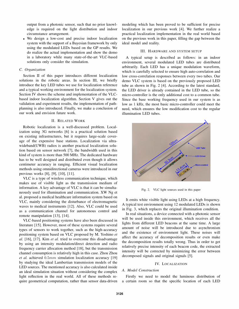
At the end of the modeling step, we get several intensity

distribution maps including the mean maps and the corre-

sponding variance maps, regarding each LED light source. A

pair of example results is shown in Fig. 4. The regression mean

represents the expected light signal observation; the variance

field represents the observation likelihood. The “shape” of the

variance field roughly represents the traversable areas, since

the observations over these areas are with higher confidence

and thus low variance values.

(a) The mean field of light 6 (b) The variance field of light 6

Fig. 4. A typical example of the Gaussian Process results

B. Bayesian Localization

An intuitive graph model of Bayesian dynamic filtering is

shown in figure 5, where the standard plate representation

is adopted to show the relation among random variables

in time series. The goal of localization is to estimate the

Fig. 5. Bayesian filtering graph model

current position xt by knowing history estimations x0:t−1 and

observations y0:t−1 [22], namely:

P (xt|y0:t,u0:t)

∝P (yt|xt)×∑

xt−1

P (xt|xt−1,ut−1)P (xt−1|y0:t−1,u0:t−1)

(10)

where

• P (yt|xt): the observation model learnt by GP;

• P (xt|xt−1,ut−1): motion model. In this case, a zero-

mean Gaussian is used, since no motion estimation is

introduced, i.e. N (0, σ2), where σ is a tunable parameter.

Here we empirically choose σ = 0.033m, considering the

average maximal walking speed of a human is 1.0m/sand the algorithm refreshing rate is 30Hz. We can actu-

ally adjust this parameter according to the real working

speed.

• P (xt−1|y0:t−1,u0:t−1): previous position estimate.

The localization prior is initialized by a uniform distribution.

The product of the individually observed light components

represents the observation model, because the observation of

light sources is theoretically independent, namely:

p(yt|xt) =

S∏

s=1

p(yst |xt) (11)

where s represents the index of the observed light sources.

V. EXPERIMENTAL RESULTS

We conducted experiments in a 4.7 m × 8.6 m indoor

environment with 12 modulated LED lights. Note that neither

larger size of the environment nor larger number of the light

sources will deteriorate the localization accuracy thanks to

the global localization nature. All the functions are realized

on a Tablet connected with a photonic sensor. The details

of experimental data collection is introduced in another work

[23].

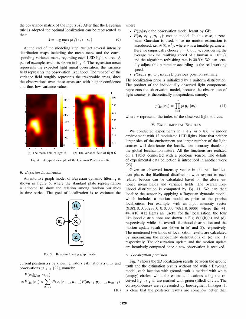
Given an observed intensity vector in the real localiza-

tion phase, the likelihood distribution with respect to each

related beacon can be calculated based on the aforemen-

tioned mean fields and variance fields. The overall like-

lihood distribution is computed by Eq. 11. We can then

localize the sensor by applying a Bayesian dynamic model,

which includes a motion model as prior to the precise

localization. For example, with an input intensity vector

(9183, 0, 0, 30298, 0, 0, 0, 0, 0, 7681, 0, 6966) where the #1,

#4, #10, #12 lights are useful for the localization, the four

likelihood distributions are shown in Fig. 6(a)(b)(c) and (d),

respectively, while the overall likelihood distribution and the

motion update result are shown in (e) and (f), respectively.

The mentioned two kinds of localization results are calculated

by maximizing the probability distributions of (e) and (f)

respectively. The observation update and the motion update

are iteratively computed once a new observation is received.

A. Localization precision

Fig. 7 shows the 2D localization results between the ground

truth and the estimation results without and with a Bayesian

model, each location with ground-truth is marked with white

(empty) circles, while the estimated locations using the re-

ceived light signal are marked with green (filled) circles. The

correspondences are represented by line-segment linkages. It

is clear that the posterior results are somehow better than

3128

(a) #1 (b) #4

0

0.5

1

(c) #10

(d) #12 (e) perception update

0

0.5

1

(f) motion update

Fig. 6. Normalized probability distributions of the four independent like-lihoods, the overall likelihood (perception update) and the posterior (motionupdate)

(a) Localization results using maxi-mum likelihood

(b) Localization results using maxi-mum posterior

Fig. 7. Comparison of the localization results (green, filled circles) andground-truths (white, empty circles)

the direct output using maximum likelihood. The “clustered”

appearance of the posterior distribution is due to the static

motion model.

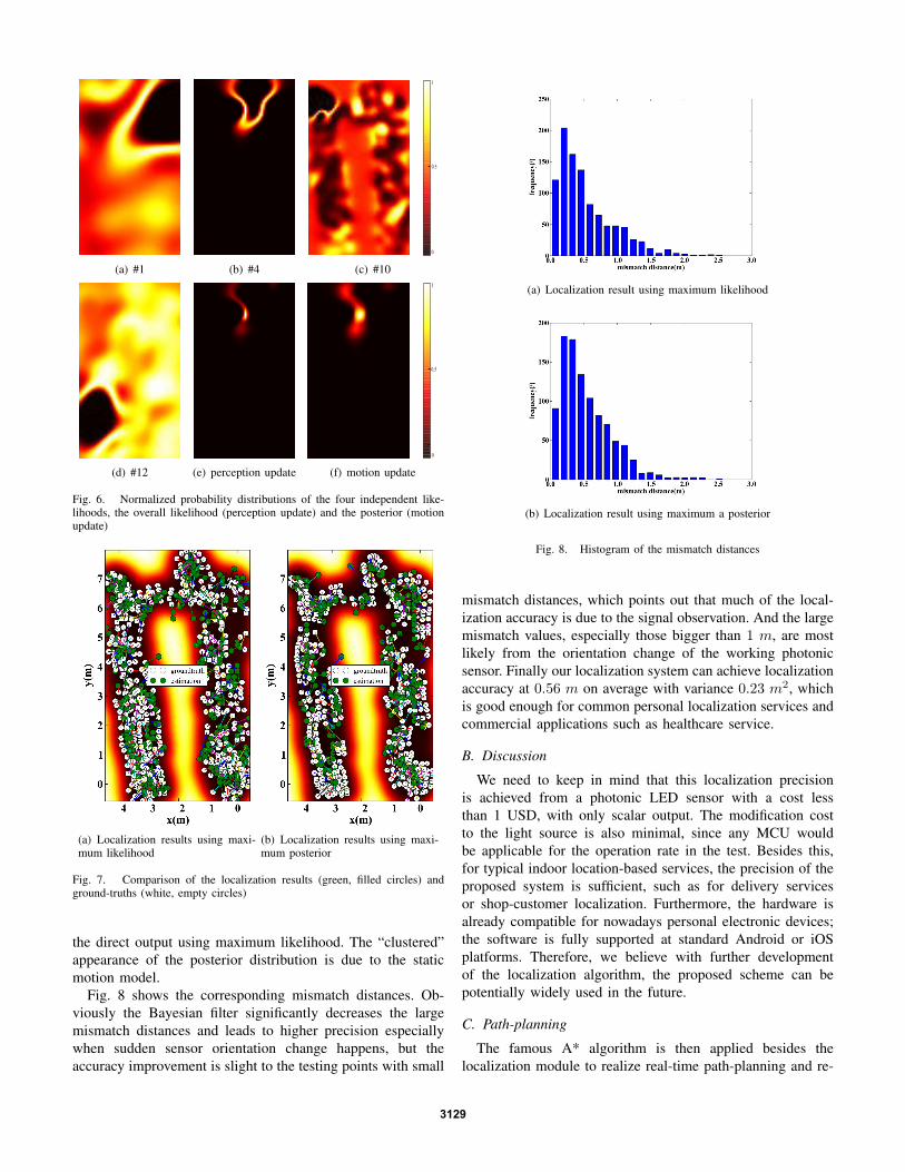
Fig. 8 shows the corresponding mismatch distances. Ob-

viously the Bayesian filter significantly decreases the large

mismatch distances and leads to higher precision especially

when sudden sensor orientation change happens, but the

accuracy improvement is slight to the testing points with small

(a) Localization result using maximum likelihood

(b) Localization result using maximum a posterior

Fig. 8. Histogram of the mismatch distances

mismatch distances, which points out that much of the local-

ization accuracy is due to the signal observation. And the large

mismatch values, especially those bigger than 1 m, are most

likely from the orientation change of the working photonic

sensor. Finally our localization system can achieve localization

accuracy at 0.56 m on average with variance 0.23 m2, which

is good enough for common personal localization services and

commercial applications such as healthcare service.

B. Discussion

We need to keep in mind that this localization precision

is achieved from a photonic LED sensor with a cost less

than 1 USD, with only scalar output. The modification cost

to the light source is also minimal, since any MCU would

be applicable for the operation rate in the test. Besides this,

for typical indoor location-based services, the precision of the

proposed system is sufficient, such as for delivery services

or shop-customer localization. Furthermore, the hardware is

already compatible for nowadays personal electronic devices;

the software is fully supported at standard Android or iOS

platforms. Therefore, we believe with further development

of the localization algorithm, the proposed scheme can be

potentially widely used in the future.

C. Path-planning

The famous A* algorithm is then applied besides the

localization module to realize real-time path-planning and re-

3129

planning. The specific path-planning algorithm could be re-

placed by other advanced searching algorithms such as A*[24],

D*[25], etc. To construct the cost-map used in the graph-

based searching algorithms, the map made by SLAM robot

is naturally the first choice. It means we can use the metric

map created during the data-gathering phase to guide the path-

planning. However, in several situations, the map calculated

by the laser scanner has a noisy boundary. More importantly

it is coupled with dynamic objects in the mapping process.

This means a pre-denoising step is needed. Comparatively, the

variance field computed by the Gaussian Process is a better

choice since it naturally provides references regarding the trust

to the original data. The details of this part are introduced in

our another work [26].

VI. CONCLUSION

In this paper, we proposed a low-cost solution for indoor

localization using a VLC-based system. We integrated signal

decomposition, Gaussian Process regression, Bayesian model

to solve the localization problem. The results showed the

accuracy and practicality of our system, which tends to be a

better solution for indoor localization with minor cost, for both

robotic applications and positioning of human users. In the

future, we want to further improve the accuracy and robustness

of the system in terms of the pattern selection method of the

modulated LEDs, and the training method of the Gaussian

Process. Also, we’d like to validate our localization system in

a large-scale indoor environment and do more research on the

situation with salient sensor orientation change.

VIDEO SUPPLEMENT

The attached video shows the dynamic localization and real-

time path-planning results. Note that we mimic an environment

of a big shopping mall and demonstrate our indoor localization

and path-planning system. Different regions in the map are

decorated with commercial brands to vividly demonstrate the

idea for indoor positioning-based services. The user is moving

in the test environment with a hand-held tablet. The screen-

shots for the localization and path-planning results and two

real views are simultaneously presented. The real-time demo

shows the localization accuracy is still acceptable even thought

the operating height and orientation are not stable(hand-held

case).

REFERENCES

[1] L. Wang, M. Liu, and M. Q.-H. Meng, “Real-time multisensor data re-trieval for cloud robotic systems,” Automation Science and Engineering,

IEEE Transactions on, vol. 12, no. 2, pp. 507–518, 2015.

[2] Y. X. Sun, M. Liu, and Q.-H. Meng., “Wifi signal strength-based robotindoor localization,” in IEEE International Conference on Information

and Automation, 2014.

[3] M. Liu and R. Siegwart, “Dp-fact: Towards topological mapping andscene recognition with color for omnidirectional camera,” in Robotics

and Automation (ICRA), 2012 IEEE International Conference on, may2012, pp. 3503 –3508.

[4] M. Liu, K. Qiu, S. Li, F. Che, L. Wu, and C. P. Yue, “Towards indoorlocalization using visible light communication for consumer electronicdevices,” in Proceedings of the IEEE/RSJ International Conference on

Intelligent Robots and Systems (IROS), Chicago, the USA, 2014.

[5] F. Zhang, K. Qiu, and M. Liu, “Asynchronous blind signal decom-position using tiny-length code for visible light communication-basedindoor localization,” in Robotics and Automation (ICRA), 2015 IEEE

International Conference on. IEEE, 2015, pp. 2800–2805.[6] Q. Xu, A. Gerber, Z. M. Mao, and J. Pang, “Acculoc: practical localiza-

tion of performance measurements in 3g networks,” in Proceedings of

the 9th international conference on Mobile systems, applications, and

services. ACM, 2011, pp. 183–196.[7] S. Gezici, Z. Tian, G. B. Giannakis, H. Kobayashi, A. F. Molisch, H. V.

Poor, and Z. Sahinoglu, “Localization via ultra-wideband radios: a lookat positioning aspects for future sensor networks,” Signal Processing

Magazine, IEEE, vol. 22, no. 4, pp. 70–84, 2005.[8] M. Liu and R. Siegwart, “Dp-fact: Towards topological mapping and

scene recognition with color for omnidirectional camera,” in Robotics

and Automation (ICRA), 2012 IEEE International Conference on. IEEE,2012, pp. 3503–3508.

[9] M. Liu, C. Pradalier, F. Pomerleau, and R. Siegwart, “Scale-only visualhoming from an omnidirectional camera,” in Robotics and Automation

(ICRA), 2012 IEEE International Conference on. IEEE, 2012, pp.3944–3949.

[10] M. Liu, C. Pradalier, and R. Siegwart, “Visual homing from scale withan uncalibrated omnidirectional camera,” Robotics, IEEE Transactions

on, vol. 29, no. 6, pp. 1353–1365, 2013.[11] M. Liu, D. Scaramuzza, C. Pradalier, R. Siegwart, and Q. Chen, “Scene

recognition with omnidirectional vision for topological map usinglightweight adaptive descriptors,” in Intelligent Robots and Systems,

2009. IROS 2009. IEEE/RSJ International Conference on. IEEE, 2009,pp. 116–121.

[12] X.-W. Ng and W.-Y. Chung, “Vlc-based medical healthcare informationsystem,” Biomedical Engineering: Applications, Basis and Communica-

tions, vol. 24, no. 02, pp. 155–163, 2012.[13] M. Abualhoul, M. Marouf, O. Shagdar, F. Nashashibi et al., “Platoon

control using vlc: A feasibility study.” 2013.[14] E. Poves, G. del Campo-Jimenez, and F. Lopez-Hernandez, “Vlc-

based light-weight portable user interface for in-house applications,” inConsumer Communications and Networking Conference (CCNC), 2011

IEEE. IEEE, 2011, pp. 365–367.[15] G. del Campo-Jimenez, J. M. Perandones, and F. Lopez-Hernandez, “A

vlc-based beacon location system for mobile applications,” in Localiza-

tion and GNSS (ICL-GNSS), 2013 International Conference on. IEEE,2013, pp. 1–4.

[16] T. Tanaka and S. Haruyama, “New position detection method usingimage sensor and visible light leds,” in Machine Vision, 2009. ICMV’09.

Second International Conference on. IEEE, 2009, pp. 150–153.[17] M. Yoshino, S. Haruyama, and M. Nakagawa, “High-accuracy position-

ing system using visible led lights and image sensor,” in Radio and

Wireless Symposium, 2008 IEEE. IEEE, 2008, pp. 439–442.[18] H.-S. Kim, D.-R. Kim, S.-H. Yang, Y.-H. Son, and S.-K. Han, “An

indoor visible light communication positioning system using a rf carrierallocation technique,” Journal of Lightwave Technology, vol. 31, no. 1,pp. 134–144, 2013.

[19] Z. Zhou, M. Kavehrad, and P. Deng, “Indoor positioning algorithm usinglight-emitting diode visible light communications,” Optical Engineering,vol. 51, no. 8, pp. 085 009–1, 2012.

[20] B. Ferris, D. Fox, and N. D. Lawrence, “Wifi-slam using gaussianprocess latent variable models.” in IJCAI, vol. 7, 2007, pp. 2480–2485.

[21] C. E. Rasmussen, “Gaussian processes for machine learning,” 2006.[22] C. M. Bishop, Pattern recognition and machine learning. springer,

2006.[23] M. L. Kejie Qiu, Fangyi Zhang, “Environment modeling-based indoor

localization using visible light communication,” in IEEE International

Conference on Real-time Computing and Robotics (RCAR), Changsha,China, 2015.

[24] P. E. Hart, N. J. Nilsson, and B. Raphael, “A formal basis for theheuristic determination of minimum cost paths,” Systems Science and

Cybernetics, IEEE Transactions on, vol. 4, no. 2, pp. 100–107, 1968.[25] A. Stentz, “Optimal and efficient path planning for partially-known

environments,” in Robotics and Automation, 1994. Proceedings., 1994

IEEE International Conference on. IEEE, 1994, pp. 3310–3317.[26] M. L. Kejie Qiu, Fangyi Zhang, “Visible light communication-based in-

door environment modeling and metric-free path planning,” in IEEE In-

ternational Conference on Automation Science and Engineering (CASE),Gothenburg, Sweden, 2015.

3130