RICE UNIVERSITY Viscosity Evaluation of Heavy Oils from NMR Well Logging by Zheng Yang A THESIS SUBMITTED IN PARTIAL FULFILLMENT OF THE REQUIREMENTS FOR THE DEGREE Doctor of Philosophy APPROVED, THESIS COMMITTEE George J. Hirasaki, A.J. Harstook Professor, Chair Chemical and Biomolecular Engineering Walter G. Chapman, William W. Akers Professor Chemical and Biomolecular Engineering Andreas Lüttge, Professor Earth Science and Chemistry HOUSTON, TEXAS APRIL, 2011

Welcome message from author
This document is posted to help you gain knowledge. Please leave a comment to let me know what you think about it! Share it to your friends and learn new things together.
Transcript
RICE UNIVERSITY
Viscosity Evaluation of Heavy Oils from NMR Well Logging
by
Zheng Yang
A THESIS SUBMITTED
IN PARTIAL FULFILLMENT OF THE
REQUIREMENTS FOR THE DEGREE
Doctor of Philosophy
APPROVED, THESIS COMMITTEE
George J. Hirasaki, A.J. Harstook Professor, Chair
Chemical and Biomolecular Engineering
Walter G. Chapman, William W. Akers Professor
Chemical and Biomolecular Engineering
Andreas Lüttge, Professor
Earth Science and Chemistry
HOUSTON, TEXAS
APRIL, 2011
Abstract
Viscosity Evaluation of Heavy Oils from NMR Well Logging
by
Zheng Yang
Heavy oil is characterized by its high viscosity, which is a major obstacle to both
logging and recovery. Due to the loss of T2 information shorter than the echo spacing
(TE), estimation of heavy oil properties from NMR T2 measurements is usually
problematic. In this work, a new method has been developed to overcome the echo
spacing restriction of NMR spectrometer during the measurement of heavy oil. A FID
measurement supplemented the CPMG in an effort to recover the lost T2 data.
Constrained by the initial magnetization (M0) estimated from the FID and Curie’s law
and assuming lognormal distribution for bitumen, the corrected T2 of bitumen can be
obtained. This new method successfully overcomes the TE restriction of the NMR
spectrometer and is nearly independent on the TE applied in the measurement. This
method was applied in the measurement of systems at elevated temperatures (8 ~ 90 oC)
and some important petrophysical properties of Athabasca bitumen, such as hydrogen
index (HI), fluid content and viscosity were evaluated by using the corrected T2.
Well log NMR T2 measurements of bitumen appear to be significantly longer than
the laboratory results. This is likely due to the dissolved gas in bitumen. The T2
distribution depends on oil viscosity and dissolved gas concentration, which can vary
throughout the field. In this work, the viscosity and laboratory NMR measurements were
made on the recombined live bitumen sample and the synthetic Brookfield oil as a
function of dissolved gas concentrations. The effects of CH4, CO2, and C2H6 on the
viscosity and T2 response of these two heavy oils at different saturation pressures were
investigated.
The investigations on live oil viscosity show that, regardless of the gas type used
for saturation, the live oil T2 correlates with viscosity/temperature ratio on a log-log scale.
More importantly, the changes of T2 and viscosity/temperature ratio caused by solution
gas follows the same trend of those caused by temperature variations on the dead oil. This
conclusion holds for both the bitumen and the synthetic Brookfield oil. This finding on
the relationship between the oil T2 and its corresponding viscosity/temperature ratio
creates a way for in-situ viscosity evaluation of heavy oil through NMR well logging.

Acknowledgements
First of all, I wish to express my sincere gratitude to my thesis advisor Dr. George
J. Hirasaki for his enlightening guidance and generous support throughout my Ph.D.
thesis research. Special thanks go to Dr. Walter G. Chapman, who not only serves in my
thesis committee, but also provided many helpful discussions and suggestions about my
research with great patience. I also greatly appreciate Dr. Andreas Lüttge at Department
of Earth Science, who serves in my thesis committee.
I am very grateful to Dr. Harold Vinegar, Dr. Matthias Appel, Dr. Daniel Reed
and Dr. Sean Zou at Shell E&P Company for their invaluable guidance and ideas about
my research. Thank Dr. Maura Puerto for her generous help in the design and setup of the
experimental equipments. Thank Dr. M. Robert Willcott at Rice University for his
interesting NMR class and insightful discussion on the NMR measurement of bitumen.
Thank Dr. Gersh Zvi Taicher at Echo Medical Systems for the 20-MHz NMR
measurements. Many thanks go to my colleagues in this group, especially Michael
Rauschhuber, Arjun Kurup, Robert Li, Neeraj Rohilla, Jose Lopez and Tianmin Jiang, for
their spiritual and academic help throughout my thesis research.
I want to acknowledge Shell E&P Company and Rice Consortium of Processes in
Porous Media for the financial support.
Most of all, I wish to thank my wife Qing Zhu and my family for their constant
love, support and understanding, and for all the sacrifices that they have made.
Table of Contents
Abstract .............................................................................................................................. ii
Acknowledgements .......................................................................................................... iv
List of Figures .................................................................................................................. vii
List of Tables ................................................................................................................... xv
Chapter 1 Introduction ................................................................................................. 1
Chapter 2 NMR Measurement of Bitumen at Different Temperatures ................ 11
2.1 Introduction ........................................................................................................ 11
2.2 Equipment and Experimental Procedures .......................................................... 12
2.3 Results ................................................................................................................ 14
2.3.1 Regular CPMG Measurement on Bitumen Sample .................................... 14
2.3.2 Improved Experimental Scheme for Correcting T2 of Bitumen ................. 16
2.3.3 Improved Interpretation Method for Correcting T2 of Bitumen ................. 18
2.3.4 Interpretation of CPMG Raw Data at 30 oC with New Model ................... 20
2.3.5 Application at Different Sample Temperature ............................................ 23
2.4 Conclusions ........................................................................................................ 39
Chapter 3 NMR Measurement and Viscosity Evaluation of Live Brookfield Oil. 40
3.1 Introduction ........................................................................................................ 40
3.2 Equipment and Experimental Procedures .......................................................... 41
3.3 Results ................................................................................................................ 42
3.3.1 Characterization of Brookfield Oil at Different Temperatures ................... 42
3.3.2 Investigations on Recombined Live Brookfield Oil ................................... 50
3.4 Conclusions ........................................................................................................ 88
Chapter 4 NMR Measurement and Viscosity Evaluation of Live Bitumen .......... 90
4.1 Introduction ........................................................................................................ 90
4.2 Equipment and Experimental Procedures .......................................................... 91
4.3 Results ................................................................................................................ 91
4.3.1 Characterization of Bitumen #10-19 at Different Temperatures ................ 91
4.3.2 Investigations on Recombined Live Bitumen ........................................... 101
4.4 Conclusions ...................................................................................................... 157

vi
Chapter 5 Conclusions and Future Work ............................................................... 159
5.1 Conclusions of This Study ............................................................................... 159
5.2 Future Work ..................................................................................................... 162
References ...................................................................................................................... 164
Appendix A .................................................................................................................... 168
Appendix B .................................................................................................................... 171
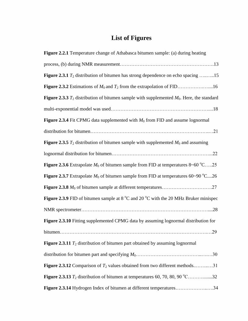
List of Figures
Figure 2.2.1 Temperature change of Athabasca bitumen sample: (a) during heating
process, (b) during NMR measurement………………………………………………….13
Figure 2.3.1 T2 distribution of bitumen has strong dependence on echo spacing …..…..15
Figure 2.3.2 Estimations of M0 and T2 from the extrapolation of FID…………….…....16
Figure 2.3.3 T2 distribution of bitumen sample with supplemented M0. Here, the standard
multi-exponential model was used……………………………………………………....18
Figure 2.3.4 Fit CPMG data supplemented with M0 from FID and assume lognormal
distribution for bitumen……………………………………………………………….…21
Figure 2.3.5 T2 distribution of bitumen sample with supplemented M0 and assuming
lognormal distribution for bitumen……………………………………………………...22
Figure 2.3.6 Extrapolate M0 of bitumen sample from FID at temperatures 8~60 oC…..25
Figure 2.3.7 Extrapolate M0 of bitumen sample from FID at temperatures 60~90 oC....26
Figure 2.3.8 M0 of bitumen sample at different temperatures………………………….27
Figure 2.3.9 FID of bitumen sample at 8 oC and 20
oC with the 20 MHz Bruker minispec
NMR spectrometer……………………………………………………………………....28
Figure 2.3.10 Fitting supplemented CPMG data by assuming lognormal distribution for
bitumen……………………………………………………………………………….…29
Figure 2.3.11 T2 distribution of bitumen part obtained by assuming lognormal
distribution for bitumen part and specifying M0…………………………………..….…30
Figure 2.3.12 Comparison of T2 values obtained from two different methods..……..…31
Figure 2.3.13 T2 distribution of bitumen at temperatures 60, 70, 80, 90 oC………........32
Figure 2.3.14 Hydrogen Index of bitumen at different temperatures………………..….34
viii
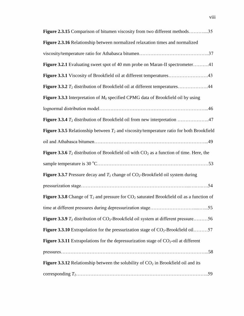
Figure 2.3.15 Comparison of bitumen viscosity from two different methods………....35
Figure 2.3.16 Relationship between normalized relaxation times and normalized
viscosity/temperature ratio for Athabasca bitumen……………………………………..37
Figure 3.2.1 Evaluating sweet spot of 40 mm probe on Maran-II spectrometer……….41
Figure 3.3.1 Viscosity of Brookfield oil at different temperatures…………………….43
Figure 3.3.2 T2 distribution of Brookfield oil at different temperatures……………….44
Figure 3.3.3 Interpretation of M0 specified CPMG data of Brookfield oil by using
lognormal distribution model…………………………………………………………...46
Figure 3.3.4 T2 distribution of Brookfield oil from new interpretation ………………..47
Figure 3.3.5 Relationship between T2 and viscosity/temperature ratio for both Brookfield
oil and Athabasca bitumen……………………………………………………………...49
Figure 3.3.6 T2 distribution of Brookfield oil with CO2 as a function of time. Here, the
sample temperature is 30 oC………………………………………………….…………53
Figure 3.3.7 Pressure decay and T2 change of CO2-Brookfield oil system during
pressurization stage…………………………………………………………...….….….54
Figure 3.3.8 Change of T2 and pressure for CO2 saturated Brookfield oil as a function of
time at different pressures during depressurization stage……………………….....…...55
Figure 3.3.9 T2 distribution of CO2-Brookfield oil system at different pressure………56
Figure 3.3.10 Extrapolation for the pressurization stage of CO2-Brookfield oil………57
Figure 3.3.11 Extrapolations for the depressurization stage of CO2-oil at different
pressures………………………………………………………………………………...58
Figure 3.3.12 Relationship between the solubility of CO2 in Brookfield oil and its
corresponding T2………………………………………………………………………..59
ix
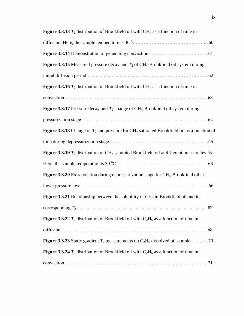
Figure 3.3.13 T2 distribution of Brookfield oil with CH4 as a function of time in
diffusion. Here, the sample temperature is 30 oC……………………………….……....60
Figure 3.3.14 Demonstration of generating convection………………………………..61
Figure 3.3.15 Measured pressure decay and T2 of CH4-Brookfield oil system during
initial diffusion period…………………………………………………………………..62
Figure 3.3.16 T2 distribution of Brookfield oil with CH4 as a function of time in
convection……………………………………………………………………………....63
Figure 3.3.17 Pressure decay and T2 change of CH4-Brookfield oil system during
pressurization stage……………………………………………………………………..64
Figure 3.3.18 Change of T2 and pressure for CH4 saturated Brookfield oil as a function of
time during depressurization stage……………………………………………..…….…65
Figure 3.3.19 T2 distribution of CH4 saturated Brookfield oil at different pressure levels.
Here, the sample temperature is 30 oC…………………………………………….……66
Figure 3.3.20 Extrapolation during depressurization stage for CH4-Brookfield oil at
lower pressure level……………………………………………………………………..66
Figure 3.3.21 Relationship between the solubility of CH4 in Brookfield oil and its
corresponding T2..............................................................................................................67
Figure 3.3.22 T2 distribution of Brookfield oil with C2H6 as a function of time in
diffusion……………………………………………………………………...…………68
Figure 3.3.23 Static gradient T2 measurements on C2H6 dissolved oil sample……...…70
Figure 3.3.24 T2 distribution of Brookfield oil with C2H6 as a function of time in
convection………………………………………………………………………………71

x
Figure 3.3.25 Pressure decay and T2 change of C2H6-Brookfield oil system during
pressurization stage……………………………………………………………….……..72
Figure 3.3.26 Changes of T2 and pressure for C2H6 saturated Brookfield oil as a function
of time at different pressures during depressurization stage………………………….…73
Figure 3.3.27 T2 distribution of C2H6 saturated Brookfield oil at different pressure levels.
Here, the sample temperature is 30 oC………………………………………….….……74
Figure 3.3.28 Extrapolation during pressurization stage for C2H6-oil…………….…....75
Figure 3.3.29 Extrapolations for the depressurization stage of C2H6-oil at different
pressures…………………………………………………………………………….…...76
Figure 3.3.30 Relationship between the solubility of C2H6 in Brookfield oil and its
corresponding T2………………………………………………………………………...77
Figure 3.3.31 Relationship between equilibrium pressure and the corresponding live oil
T2 for different gases……………………………………………………………….……78
Figure 3.3.32 Relationship between the gas concentration in Brookfield oil and the
equilibrated pressures…………………………………………………………………....79
Figure 3.3.33 Relationship between the gas concentration in Brookfield oil and its
corresponding T2…………………………………………………………………….…..81
Figure 3.3.34 Analysis of compressibility factor z of CO2 for adjusting the calculated
solubility of CO2 in Brookfield oil to follow Henry’s law.………………………….…..82
Figure 3.3.35 Setup of capillary viscometer……………………………………….…....85
Figure 3.3.36 Relationship between the T2 of Brookfield oil and the
viscosity/temperature ratio………………………………………………………….…...87

xi
Figure 3.3.37 Relationship between normalized relaxation times and normalized
viscosity/temperature ratio for Brookfield oil……………………………………….…..88
Figure 4.3.1 Viscosity of bitumen #10-19 at different temperatures…………….……..92
Figure 4.3.2 T2 distribution of bitumen #10-19 at different temperatures………….…..94
Figure 4.3.3 FID of bitumen #10-19 at different temperatures…………………….…...95
Figure 4.3.4 M0 of the bitumen #10-19 at different temperatures estimated by using
different methods………………………………………………………………………..96
Figure 4.3.5 Fitting of M0 specified CPMG data of bitumen #10-19 by using lognormal
distribution model……………………………………………………………………….97
Figure 4.3.6 T2 distribution of bitumen #10-19 from the new interpretation……….…..98
Figure 4.3.7 Comparison on bitumen T2 obtained before and after the correction via
lognormal distribution model……………………………………………………………99
Figure 4.3.8 Relationship between T2 and viscosity/temperature ratio for bitumen #10-
19……………………………………………………………………………………….100
Figure 4.3.9 Recorded pressure change during diffusion in the case of C2H6-bitumen.103
Figure 4.3.10 Pressure and T2 change of C2H6- bitumen system………………………104
Figure 4.3.11 T2 distribution of bitumen #10-19 with dissolved C2H6 during
pressurization stage………………………………………………………………….....105
Figure 4.3.12 Change of T2 and pressure for C2H6 saturated bitumen as a function of time
at different pressure………………………………………………………………….....107
Figure 4.3.13 T2 distribution of C2H6 saturated bitumen at different pressures…….....108
Figure 4.3.14 Interpretation of M0 specified CPMG data of C2H6-bitumen by using
lognormal distribution model……………………………………………………...…...111

xii
Figure 4.3.15 T2 distribution of C2H6 saturated bitumen from new interpretation as a
function of the equilibrium pressure…………………………………………….....…...112
Figure 4.3.16 Comparison of C2H6 saturated bitumen T2 at different pressure obtained
before and after correction via lognormal distribution model……………………….…113
Figure 4.3.17 T2 of C2H6 saturated bitumen at different pressure levels………………114
Figure 4.3.18 Extrapolation for the pressurization stage of C2H6-bitumen…………...115
Figure 4.3.19 Extrapolations for the depressurization stage of C2H6- bitumen at different
pressures………………………………………………………………………………..116
Figure 4.3.20 Relationship between the C2H6 solubility in bitumen and its corresponding
live T2…………………………………………………………………………………..118
Figure 4.3.21 Relationship between the concentration of C2H6 in bitumen and
equilibrated pressure……………………………………………………………………119
Figure 4.3.22 Recorded pressure change during diffusion in case of CO2- bitumen….121
Figure 4.3.23 Pressure and T2 change of CO2- bitumen system……………………….122
Figure 4.3.24 T2 distribution of bitumen #10-19 with dissolved CO2 during
pressurization stage…………………………………………………………………….123
Figure 4.3.25 Change of T2 and pressure for CO2 saturated bitumen as a function of time
at different pressure…………………………………………………………………….125
Figure 4.3.26 T2 distribution of CO2 saturated bitumen at different pressure level...…126
Figure 4.3.27 Interpretation of M0 specified CPMG data of CO2-bitumen by using
lognormal distribution model…………………………………………………………..127
Figure 4.3.28 T2 distribution of CO2 saturated bitumen from new interpretation as a
function of the equilibrium pressure……………………………………………………128
xiii
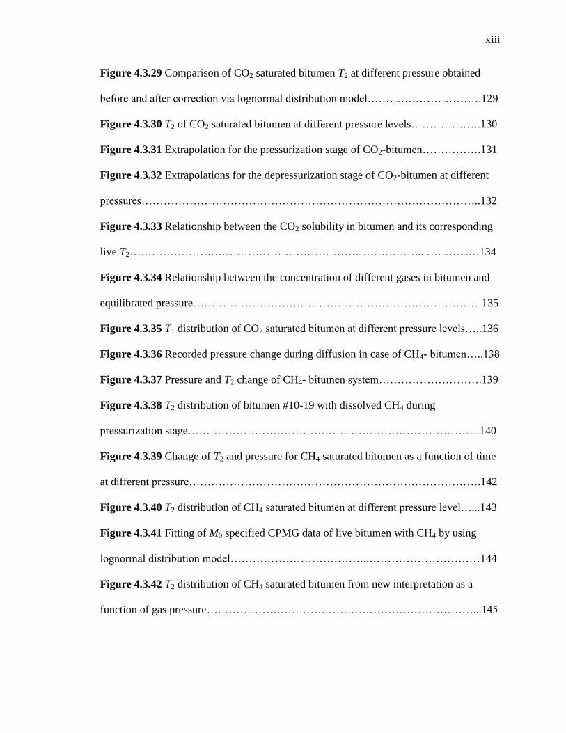
Figure 4.3.29 Comparison of CO2 saturated bitumen T2 at different pressure obtained
before and after correction via lognormal distribution model………………………….129
Figure 4.3.30 T2 of CO2 saturated bitumen at different pressure levels……………….130
Figure 4.3.31 Extrapolation for the pressurization stage of CO2-bitumen…………….131
Figure 4.3.32 Extrapolations for the depressurization stage of CO2-bitumen at different
pressures………………………………………………………………………………..132
Figure 4.3.33 Relationship between the CO2 solubility in bitumen and its corresponding
live T2……………………………………………………………………...………...…134
Figure 4.3.34 Relationship between the concentration of different gases in bitumen and
equilibrated pressure……………………………………………………………………135
Figure 4.3.35 T1 distribution of CO2 saturated bitumen at different pressure levels…..136
Figure 4.3.36 Recorded pressure change during diffusion in case of CH4- bitumen…..138
Figure 4.3.37 Pressure and T2 change of CH4- bitumen system……………………….139
Figure 4.3.38 T2 distribution of bitumen #10-19 with dissolved CH4 during
pressurization stage…………………………………………………………………….140
Figure 4.3.39 Change of T2 and pressure for CH4 saturated bitumen as a function of time
at different pressure…………………………………………………………………….142
Figure 4.3.40 T2 distribution of CH4 saturated bitumen at different pressure level…...143
Figure 4.3.41 Fitting of M0 specified CPMG data of live bitumen with CH4 by using
lognormal distribution model………………………………..…………………………144
Figure 4.3.42 T2 distribution of CH4 saturated bitumen from new interpretation as a
function of gas pressure………………………………………………………………...145
xiv
Figure 4.3.43 Comparison of bitumen T2 at different pressure obtained before and after
correction of lognormal distribution model…………………………………………….146
Figure 4.3.44 Live bitumen T2 saturated by three different gases at different pressure
levels………………………………………………………………………………..…..147
Figure 4.3.45 Extrapolation for the pressurization stage of CH4-bitumen…………….148
Figure 4.3.46 Extrapolations for the depressurization stage of CH4-bitumen at different
pressures………………………………………………………………………………..149
Figure 4.3.47 Relationship between the gas concentration in bitumen and equilibrated
pressure…………………………………………………………………………………151
Figure 4.3.48 Relationship between the gas solubility in bitumen and its corresponding
live T2 ………………………………………………………………………..………....152
Figure 4.3.49 Analysis of compressibility factor z of CO2 for adjusting the calculated
solubility of CO2 in bitumen #10-19 to follow Henry’s law.……………………….….153
Figure 4.3.50 Relationship between the live bitumen T2 and the viscosity/temperature
ratio for all three gases………………………………………………………………....156
Figure 4.3.51 Relationship between the normalized relaxation time and the normalized
viscosity/temperature ratio for bitumen #10-19 and other oil samples………………...157
List of Tables
Table 2.3.1: NMR response of bitumen sample in regular CPMG .……………………16
Table 3.3.1: T2 of Brookfield oil obtained from two different interpretations ...…….…48
Table 3.3.2: Measured viscosity of Live Brookfield oil via capillary viscometer......…..86
Table 4.3.1: Extrapolated pressure values for C2H6- bitumen …………...……………117
Table 4.3.2: Extrapolated pressure value and solubility of CO2 in the bitumen ………133
Table 4.3.3: Extrapolated pressure value and solubility of CH4 in the bitumen ………150
Table 4.3.4: Measured viscosity and T2 for bitumen under different conditions …...…155
1
Chapter 1 Introduction
Nuclear magnetic resonance (NMR) refers to the response of atomic nuclei to
magnetic fields. In the presence of an external magnetic field, an atomic nucleus
processes around the direction of the external field in much the same way a gyroscope
processes around the earth’s gravitational field. Measurable signals can be produced
when these spinning magnetic nuclei interact with the external magnetic fields (Cowan
1997).
With the invention of NMR logging tools that use permanent magnets and pulsed
radio frequency signals, the application of sophisticated laboratory techniques to
determine formation properties in situ in recently drilled or while drilling well has been
possible from the early 1990s (Coates, Xiao and Prammer 1999), (Dunn, Bergman and
Latorraca 2002). Rather than placing the sample at the center of the instrument, the NMR
logging tools turns the laboratory NMR equipment inside-out and places itself in a well
bore, and is surrounded by the formation to be analyzed. A permanent magnet is placed
inside the NMR logging tool to produce a magnetic field that polarizes the formation
materials, and an antenna is incorporated to surround this magnet, which is used to
perturb the spins and then “listen” for the decaying echo signal from those protons that
are in resonance with the field from the permanent magnet.
Theoretically, NMR measurements can be made on any nucleus that has an odd
number of protons or neutrons or both, such as the nucleus of hydrogen (1H), carbon
(13
C), and sodium (23
Na). For most of the elements found in earth formations, the nuclear
magnetic signal induced by external magnetic fields is too small to be detected with a

2
borehole NMR logging tool. However, hydrogen, which has only one proton and no
neutrons, is abundant in both water and hydrocarbons, has a relatively large gyromagnetic
ratio, and produces strong signals. To date, almost all NMR logging and NMR rock
studies are based on responses of the nucleus of the hydrogen atom.
Since the relationship between the proton resonance frequency and the strength of
the permanent magnetic field is linear, the frequency of the transmitted and received
energy can be tuned to investigate regions at different distance from an NMR logging
tool. This tuning of an NMR probe to be sensitive to a specific frequency allows the
magnetic resonance instruments to image narrow slices of either a hospital patient or a
rock formation.
The NMR tool is characterized to be exclusively visible to fluids (Vinegar 1986).
Consequently, the matrix materials do not contribute to the porosity measured by an
NMR logging tool so that the calibration to formation lithology is not necessary. This
response characteristic makes the NMR well logging tool fundamentally different from
other conventional logging tools.
The major shortcoming for those conventional neutron, bulk-density, and
acoustic-travel-time porosity-logging tools is that it can be influenced by all the
components of a reservoir rock (Hearst and Nelson 1985), (Bassiouni 1994). It is well
known that the reservoir rocks typically have more rock framework than fluid-filled
space, therefore, these conventional tools tend to be much more sensitive to the matrix
materials than to the pore fluids.
The conventional resistivity-logging tools are designed to be extremely sensitive
to the fluid-filled space and traditionally are used to estimate the amount of water present
3
in reservoir rocks. However, they cannot be considered as the true fluid-logging devices.
These tools are strongly influenced by the presence of conductive minerals and, for the
proper interpretation of these tools, a detailed knowledge of the properties of both the
formation and the water in the pore space is required (Coates, Xiao and Prammer 1999).
Due to the special physical principles on which NMR logging is based, the NMR
logging tools are particularly powerful at providing the following information: a)
quantities of the fluids in the rock; b) properties of the fluids in the rock; c) sizes of the
pores that contain fluids.
Fluid quantities can be estimated by measuring the density of hydrogen nuclei in
reservoir fluids with NMR logging tool. Since the density of hydrogen nuclei present in
water is known and that of oils is similar, data from the NMR tool can be easily
converted to an apparent water-filled porosity. Moreover, this conversion can be done
without any knowledge of the minerals that make up the solid fraction of the rock.
NMR well logging technology relies on the ability to link specific rock conditions
or fluid properties within a thin zone a few inches from the borehole wall in the reservoir
to different NMR behavior. The NMR tools can determine the presence and quantities of
different fluids (Coates, Xiao and Prammer 1999), (Dunn, Bergman and Latorraca 2002),
as well as some of the specific properties of the fluids, such as viscosity (Morris et al
1994), (LaTorraca, Stonard, et al. 1999), (Lo, et al. 2002). Specific pulse-sequence
settings can be run by the NMR logging tools to enhance their ability to detect particular
fluid conditions.
As a result of differences in the NMR behavior between a fluid in the pore space
of a reservoir rock and the fluid in bulk form (Huang 1997), enough pore-size
4
information can be extracted from NMR logging data to remarkably improve the
estimation of some key petrophysical properties, such as permeability (Curwen and
Molaro 1995) and the volume of capillary-bound water (Prammer 1994).
As mentioned in previous paragraphs, the NMR porosity is essentially matrix-
independent and the NMR logging tools are only sensitive to the pore fluids. The
sensitive volumes of the NMR logging tools are well defined (Coates, Xiao and Prammer
1999), and the difference in various NMR properties, such as relaxation times and
diffusivity of various fluids, makes it possible to identify immobile water, movable water,
gas, light oil, medium-viscosity oil, and heavy oil (Dunn, Bergman and Latorraca 2002).
The superiority of NMR logging tools at providing the above valuable
petrophysical information makes these tools stand out among logging devices. In recent
years, the developments of the NMR logging technology and the applications of NMR to
core analysis and formation evaluation have been very rapid and widespread (Dunn,
Bergman and Latorraca 2002). Currently, NMR logging tools are extensively used for
determining reservoir porosity and permeability (Mirotchnik, et al. 2001), and for the
real-time analysis of bottom-hole sampling of reservoir fluids (Bouton, et al. 2001),
(Masak, et al. 2002).
As the conventional oil reserves in the world continue to decline and the
worldwide demand for oil keeps increasing, the heavy oil and bitumen deposits attract
great attention from the industry, and are considered to be a very important part for the
world energy security in the future. Numerous companies have invested billions of
dollars in oil sands surface mining and in situ recovery projects for heavy oil.
Furthermore, as the oil price keeps going higher, the exploration of bitumen in deeper
5
formations is drawing more and more interest. Many in-situ bitumen recovery options
have been designed and commercialized for recovering oil in the deeper formations
(Bryan, Mai, et al. 2005). Therefore, being able to predict heavy oil properties and fluid
saturation in situ and optimize the process of bitumen extraction process is of
considerable value to the industry.
Heavy oil and bitumen are characterized by their high viscosities, which are the
major obstacles to their recovery and properties investigations. As the most important
petrophysical property, viscosity of heavy oil determines both the economics and the
technical chance of success for the chosen recovery scheme and is often directly related
to the recoverable reserves estimates (Miller and Erno 1995). As a result, in-situ oil
viscosity measurement techniques would be of significant benefit to the industry.
Because of the unique operational mechanism of nuclear magnetic resonance
(Coates, Xiao and Prammer 1999), the low-field NMR shows great potential as a logging
tool for assessing reservoir-fluid viscosities. However, due to the loss of T2 information
shorter than echo spacing (TE), estimation of heavy oil viscosity from NMR T2 is often
problematic. In order to eventually extend the use of NMR logging tools to the competent
estimation of the heavy oil viscosity in the field through logs, the development of both
NMR measurement scheme and data interpretation method are required.
On the other hand, in past years, many NMR-based oil-viscosity correlations were
presented in literatures to relate viscosity to different NMR parameters. Correlations were
observed between oil viscosity and the mean NMR relaxation time of the oil (Kleinberg
and Vinegar 1996), (Straley, et al. 1997), (Morriss, et al. 1997), (LaTorraca, Stonard, et
al. 1999), and between viscosity and the apparent signal strength of the oil (Galford and
6
Marschall 2000), (Mirotchnik, et al. 2001). Previous work in our group focused on the
development of a viscosity correlation derived from T1 of alkanes (Lo, et al. 2002) and
was tested with various crude oils in later work (Y. Zhang 2002), (Hirasaki, Lo and
Zhang 2003). Unfortunately, while these correlations did a good job for predicting
viscosities of conventional oils, none of them were successful when it comes to the
highly viscous heavy oil and bitumen.
Another property of great importance to the recovery of heavy oil is reservoir
fluid content. There are several areas in oil sands development operations where it is
critical to have an estimate of the oil, water, and solids content of a given sample. During
initial characterization of reservoir, determining oil and water content with depth and
location in the reservoir is necessary. Fluid content determination with logging tools
would be beneficial for all reservoir characterization investigations. In mining operations,
obtaining enough information on the fluid and solids content of the mined oil sand ore
will allow the extraction process to be better optimized and controlled.
Currently, the industry standard for accurately measuring fluid content is the
Dean-Stark extraction method, which is costly and time consuming. Centrifuge
technology is often used for speeding up the process, but this can cause inaccuracy
because of the similar fluid densities and the presence of emulsions (Bryan and Kantzas
2005). Although, the conventional resistivity-logging tools are also traditionally used to
estimate the amount of water present in reservoir rocks, they are strongly influenced by
the presence of conductive minerals. Moreover, in order to properly interpreted device
responses, a detailed knowledge of the properties of both the formation and the water in
the pore space is also needed (Coates, Xiao and Prammer 1999).

7
Due to the lithology-independent and quick-response features, low-field NMR has
been used as an improved method for making estimations of oil and water content in ore
and froth samples. The application of this technology for heavy oil reservoirs and oil
sands characterization is of particular interest.
However, NMR logging has not been very successful in characterizing heavy oil
and bitumen (viscosity > 100,000 cp). The high oil viscosity still causes challenging
problems for the NMR logging tools. The combination of the echo spacing (TE)
limitation of applied NMR logging instrument and the fast relaxation of heavy oil
resulting from its high viscosity inevitably result in the loss of NMR information (T2)
during measurement (Kleinberg and Vinegar 1996), (Morriss, et al. 1997), (LaTorraca,
Dunn, et al. 1998), (LaTorraca, Stonard, et al. 1999), (Lo, et al. 2002), (Hirasaki, Lo and
Zhang 2003), (Bryan and Kantzas 2005), (Bryan, Mai, et al. 2006) and (Bryan, Kantzas
and Badry, et al. 2006). Consequently, estimation of bitumen properties, such as
hydrogen index (HI), fluid content and viscosity, based on the captured NMR response is
problematic and generally has incorrect TE or sample temperature dependence.
Kleinberg and Vinegar (Kleinberg and Vinegar 1996) reported an apparent
hydrogen index (HIapp) decrease among NMR measurements on some heavy crude oil
samples (API gravity < 17o) and attributed it to the oil components decaying faster than 1
msec. LaTorraca, et al. (LaTorraca, Stonard, et al. 1999) investigated on the effects of
varying TE on the T2 distributions and incorporated TE as a parameter into the Vinegar
equation (Kleinberg and Vinegar 1996) to relate the signal loss (HIapp or apparent
logarithmic mean T2, T2,app) to the viscosity for heavy oils (>1000 cp).
8
However, this particular method, which is based on the signal loss in NMR
measurement on heavy oils, inevitably has a dependence on the value of TE used by the
NMR logging tools and consequently needs adjustment according to various TE applied.
Furthermore, the use of these signal-loss-based correlations rely on supplemental
information from other logging tools, such as the use of resistivity and density logs for
porosity and oil saturation, and estimates of the degree of invasion. The influences of
high noise levels on any of these logging tools introduce error into the estimates. More
importantly, the essential use of the “apparent” NMR values (HIapp or T2,app) in this
method makes it impossible to develop the ultimate theory-based correlations for oil
properties, which undoubtedly depend on the “real” values. Therefore, the development
of a new method to correct the T2 values of the heavy oils from an incomplete T2
distribution and overcome the echo spacing limitation of NMR spectrometer is of great
necessity.
Another problem in the NMR well logging of heavy oil and bitumen is that, well
log NMR T2 measurements of the heavy oil (bitumen) appear to be significantly longer
than the laboratory results. This is likely due to the dissolved gas in bitumen in the
reservoir. The T2 distribution depends on oil viscosity and dissolved gas concentration,
which may vary throughout the field. Therefore, a method to determine the solution gas
and the in-situ viscosity from NMR logs would be very useful in heavy oil and bitumen
reservoir development.
The objectives of this study are to solve these two problems in the NMR well
logging of heavy oils.
9
An improved NMR measurement scheme, combining FID and CPMG is
developed in the investigation on Athabasca bitumen. A new method for the
interpretation of NMR data, which uses the lognormal distribution model to fit the CPMG
data supplemented with the specified initial magnetization M0, successfully overcomes
the echo spacing restriction of NMR tools in the application for viscous heavy oils. By
using the corrected T2 information, improved estimates for viscosity, fluid content and
hydrogen index of bitumen were achieved.
In the second part of this study, the viscosity and laboratory NMR measurements
on a recombined live bitumen sample and the Brookfield oil standard (synthetic oil,
100% PAO) as a function of dissolved gas concentrations were performed. The effects of
three major reservoir gases (CH4, CO2, and C2H6) on the viscosity and T2 response of the
two different oil samples at a series of saturation pressures were investigated. The
correlations between the saturation pressure, gas solubility, NMR T2 and live oil viscosity
are established to resolve the differences between the NMR log and laboratory data. The
findings create a way for in-situ viscosity evaluation of heavy oil through NMR well
logging.
A brief introduction of the chapters in this thesis is as follows:
Chapter 1 is for problem statement and subject introduction. The relevant
literature reviews is also included in this chapter.
Chapter 2 describes the investigations performed on the Canadian Athabasca
bitumen. A new NMR measurement scheme and data interpretation method were
developed to successfully overcome the echo spacing restrictions during the NMR
measurements on heavy oils.
10
Chapter 3 illustrates the work performed on the synthetic Brookfield oil. In this
chapter, the facilities and procedures for the high pressure experiments are designed. The
viscosity and NMR measurements were performed at various pressure levels. The
dissolving behaviors of three different reservoir gases were observed and the solubility of
each gas in this synthetic oil was evaluated via PVT measurements.
Chapter 4 investigates the changes of viscosity and the NMR response of the
recombined live bitumen sample with three different reservoir gases. Comparisons were
drawn between the results from the live bitumen and live Brookfield oil. Correlations are
established to resolve the differences between the NMR log and laboratory data.
Chapter 5 is devoted to the conclusion of this study and suggestions for the future
work in this research area.
11
Chapter 2 NMR Measurement of Bitumen at Different
Temperatures
2.1 Introduction
Heavy oil and bitumen is characterized by its high viscosity and density, and
represent a worldwide known oil reserve of 6 trillion barrels (Galford 2000) and
(Deleersnyder 2004). As the conventional oil reserves of the world continue to decline
and the exploration and production technologies keep improving, the heavy oil and
bitumen deposits have attracted great attention from both the government and the
industry, and will be the future of the world oil industry for years to come.
Low field NMR has displayed great potential in many heavy oil well logging
cases (California, Venezuela, China) (Deleersnyder 2004). However, the echo spacing
(TE) limitation of applied NMR logging tools and the fast relaxation of heavy oil
resulting from its high viscosity have combined to make the NMR information (T2)
inevitably lost during measurements. Consequently, estimation of heavy oil properties,
such as hydrogen index (HI), fluid content and viscosity, based on the captured NMR
response is problematic and generally has incorrect TE or sample temperature
dependence.
In this chapter, new methods for both NMR measurement and subsequent raw
data interpretation are developed to correct the T2 relaxation times of heavy oil (bitumen).
The new methods can overcome the echo spacing limitation of NMR spectrometer and
have only minor TE dependence. Further improvement was also made to eliminate the
12
incorrect temperature dependence during the application of the new methods at different
sample temperatures (8 ~ 90 oC). The petrophysical properties, such as hydrogen index,
fluid saturation and viscosity can be directly estimated from the corrected relaxation
times.
2.2 Equipment and Experimental Procedures
The major nuclear magnetic resonance (NMR) spectrometer used in this work is a
low field Maran-II spectrometer (Maran-SS), which is operating at a proton resonance
frequency of 2.0 MHz. The effective vertical height of the magnetic field is around 5 cm.
The temperature of magnetic field system is controlled at 30 oC with an error of ± 0.1
oC.
The heavy oil sample used in this work is froth separated Athabasca bitumen from
Alberta, Canada. It consists of bitumen, water and a small amount of clay. The bitumen
sample used for the measurements with Maran-II is contained in a glass tube (I.D. 4.66
cm) with a sample height of 3.60 cm. The sample tube was carefully sealed and stored at
room temperature.
The NMR measurements were performed at different sample temperatures from 8
to 90 oC. The temperature of magnet was kept at 30
oC for all measurements. Before each
measurement, the bitumen sample was placed in a thermal water bath at the desired
temperature for over 4 hours to reach the sample temperature equilibrium. The sample
tube was wrapped with four-layer paper insulation during the measurement. A single
measurement took less than 1 min. The measurement at each temperature was repeated at
least three times to ensure the data reliability.
13
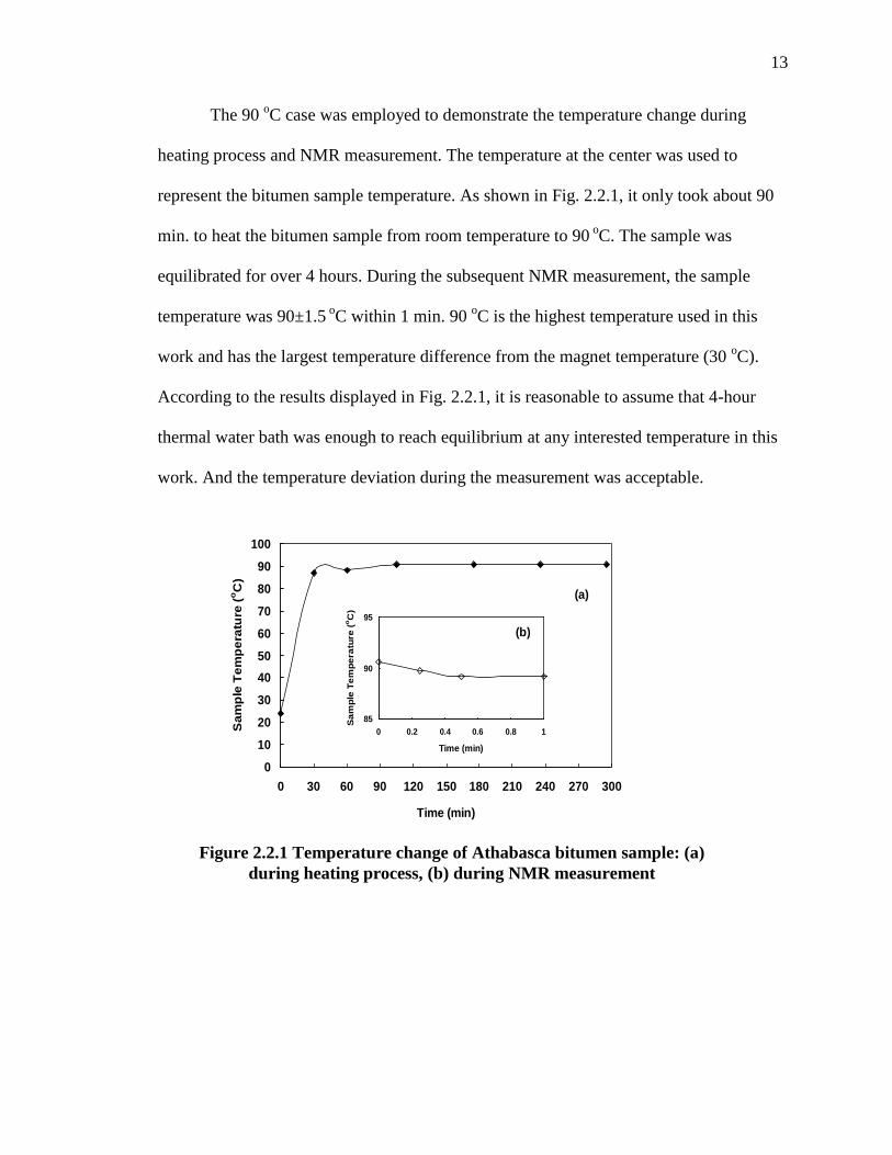
The 90 oC case was employed to demonstrate the temperature change during
heating process and NMR measurement. The temperature at the center was used to
represent the bitumen sample temperature. As shown in Fig. 2.2.1, it only took about 90
min. to heat the bitumen sample from room temperature to 90 oC. The sample was
equilibrated for over 4 hours. During the subsequent NMR measurement, the sample
temperature was 90±1.5 o
C within 1 min. 90 oC is the highest temperature used in this
work and has the largest temperature difference from the magnet temperature (30 oC).
According to the results displayed in Fig. 2.2.1, it is reasonable to assume that 4-hour
thermal water bath was enough to reach equilibrium at any interested temperature in this
work. And the temperature deviation during the measurement was acceptable.
0
10
20
30
40
50
60
70
80
90
100
0 30 60 90 120 150 180 210 240 270 300
Time (min)
Sa
mp
le T
em
pe
ratu
re (
oC
)
(a)
85
90
95
0 0.2 0.4 0.6 0.8 1
Time (min)
Sa
mp
le T
em
pe
ratu
re (
oC
)
(b)
Figure 2.2.1 Temperature change of Athabasca bitumen sample: (a)
during heating process, (b) during NMR measurement
14
2.3 Results
2.3.1 Regular CPMG Measurement on Bitumen Sample
Regular CPMG measurements were performed on the Athabasca bitumen sample
of 30 oC with the Maran-II spectrometer. For the bitumen sample, the applied width of
π/2 pulse was 9.45 sec and that of π pulse was 16.60 sec. Three different echo spacings
(TE) 0.4 msec, 0.8 msec and 1.2 msec were applied respectively. The CPMG raw data
were fitted to the standard multi-exponential decay model as follows (Dunn, LaTorraca,
et al. 1994):
i
T
t
i
ieftM ,2)( (2.1)
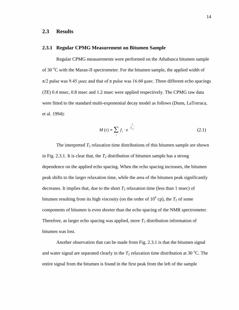
The interpreted T2 relaxation time distributions of this bitumen sample are shown
in Fig. 2.3.1. It is clear that, the T2 distribution of bitumen sample has a strong
dependence on the applied echo spacing. When the echo spacing increases, the bitumen
peak shifts to the larger relaxation time, while the area of the bitumen peak significantly
decreases. It implies that, due to the short T2 relaxation time (less than 1 msec) of
bitumen resulting from its high viscosity (on the order of 106 cp), the T2 of some
components of bitumen is even shorter than the echo spacing of the NMR spectrometer.
Therefore, as larger echo spacing was applied, more T2 distribution information of
bitumen was lost.
Another observation that can be made from Fig. 2.3.1 is that the bitumen signal
and water signal are separated clearly in the T2 relaxation time distribution at 30 oC. The
entire signal from the bitumen is found in the first peak from the left of the sample
15
spectra (Bryan, Mai, et al. 2006). Thus, in this case, the local minimum after the bitumen
peak was employed as the cut-off between oil and water peaks.
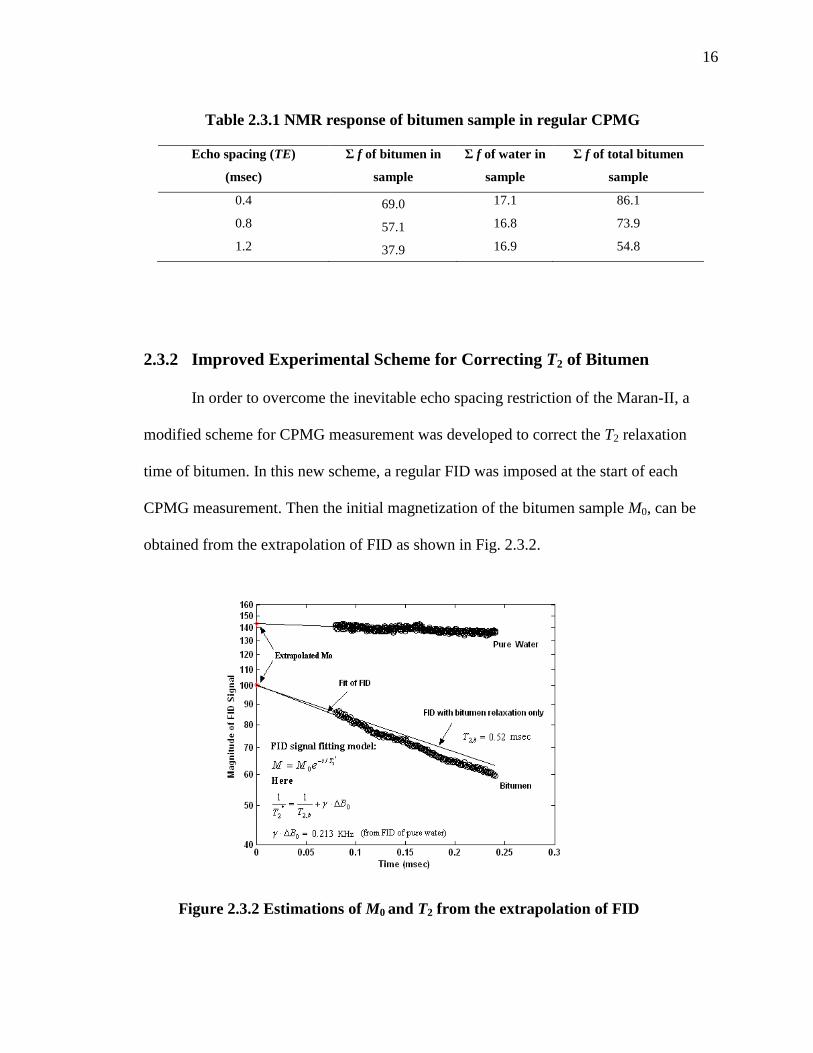
The NMR responses (amplitude f) from water and bitumen in the sample are
calculated respectively and shown in Table 2.3.1. We can easily find that, due to the loss
of T2 information shorter than the applied echo spacing, the summation of amplitude from
bitumen keeps deceasing when the applied echo spacing increases. On the other hand, the
summation of amplitudes from the water response, which can be taken as the indication
of area covered by water peaks, only has very slight changes. This implies insensitive
response of water to the applied echo spacing, which results from its significantly lower
viscosity and larger T2 relaxation time. Here, the water relaxation time is less than the
value of bulk water because of surface relaxation due to interaction with bitumen and
clay solids.
Figure 2.3.1 T2 distribution of bitumen has strong dependence on echo spacing
0
1
2
3
4
5
6
7
8
9
10
0.1 1 10 100 1000 10000
T 2 Relaxation Time Distribution (msec)
Am
plitu
de
f
TE = 0.4 msec TE = 0.8 msec TE = 1.2 msec
0.4 ms
0.8 ms
1.2 ms
0
20
40
60
80
100
0.1 1 10 100 1000 10000
T 2 Relaxation Time Distribution (msec)
Cu
mu
lati
ve f
16
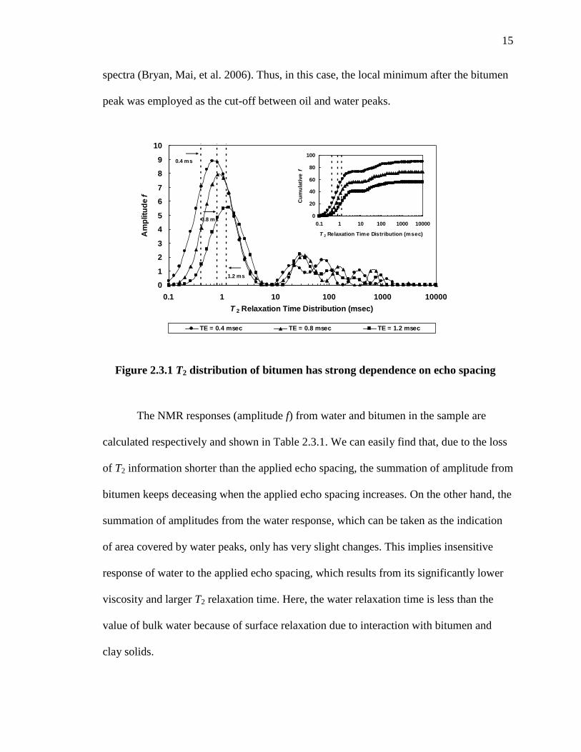
2.3.2 Improved Experimental Scheme for Correcting T2 of Bitumen
In order to overcome the inevitable echo spacing restriction of the Maran-II, a
modified scheme for CPMG measurement was developed to correct the T2 relaxation
time of bitumen. In this new scheme, a regular FID was imposed at the start of each
CPMG measurement. Then the initial magnetization of the bitumen sample M0, can be
obtained from the extrapolation of FID as shown in Fig. 2.3.2.
Echo spacing (TE)
(msec)
Σ f of bitumen in
sample
Σ f of water in
sample
Σ f of total bitumen
sample
0.4 69.0 17.1 86.1
0.8 57.1 16.8 73.9
1.2 37.9 16.9 54.8
Figure 2.3.2 Estimations of M0 and T2 from the extrapolation of FID
Table 2.3.1 NMR response of bitumen sample in regular CPMG
17
The transverse relaxation of the measured FID signal follows a first order rate
process with a characteristic time constant T2* (Coates, Xiao and Prammer 1999):
*2
0)(
T
t
eMtM . (2.2)
Here, M0 is the initial magnetization of the sample. The constant T2* is called
transverse relaxation time and is affected by the inhomogeneity of the static magnetic
field. The time constant describing the decay of the transverse magnetization due to both
the spin-spin relaxation of bulk sample (T2) and the inhomogeneity of the static field is
given as:
0
,2
*
2
11B
TT b
. (2.3)
where T2,b is the intrinsic transverse relaxation time of bitumen, 0B is the
inhomogeneity of the static field in unit, KHz.
From the Eq. [2.2] and Eq. [2.3], we can see that in order to determine the
inhomogeneity of magnetic field, a sample with the property that T2* « T2,b must be used.
The pure water (deionized), which has a T2,b relaxation time of around 2.9 sec, serves this
purpose well. Then, the inhomogeneity 0B of the applied magnetic field in this work
can be estimated, which is 0.213 KHz as shown in Fig. 2.3.2.
Due to the high viscosity of bitumen, the T2,b of bitumen is small and comparable
to the inhomogeneity of magnetic field. Therefore, both terms on the right side of Eq.
[2.3] count for the single exponential fitting. Given the inhomogeneity obtained from the
FID of pure water (Fig. 2.3.2), the estimated T2 of bitumen is 0.52 msec.
18
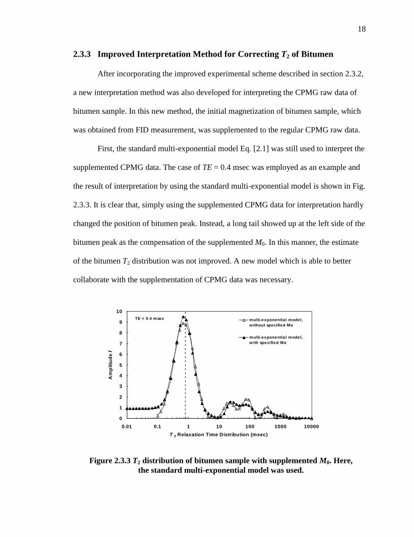
2.3.3 Improved Interpretation Method for Correcting T2 of Bitumen
After incorporating the improved experimental scheme described in section 2.3.2,
a new interpretation method was also developed for interpreting the CPMG raw data of
bitumen sample. In this new method, the initial magnetization of bitumen sample, which
was obtained from FID measurement, was supplemented to the regular CPMG raw data.
First, the standard multi-exponential model Eq. [2.1] was still used to interpret the
supplemented CPMG data. The case of TE = 0.4 msec was employed as an example and
the result of interpretation by using the standard multi-exponential model is shown in Fig.
2.3.3. It is clear that, simply using the supplemented CPMG data for interpretation hardly
changed the position of bitumen peak. Instead, a long tail showed up at the left side of the
bitumen peak as the compensation of the supplemented M0. In this manner, the estimate
of the bitumen T2 distribution was not improved. A new model which is able to better
collaborate with the supplementation of CPMG data was necessary.
Figure 2.3.3 T2 distribution of bitumen sample with supplemented M0. Here,
the standard multi-exponential model was used.
0
1
2
3
4
5
6
7
8
9
10
0.01 0.1 1 10 100 1000 10000
T 2 Relaxation Time Distribution (msec)
Am
plitu
de
f
multi-exponentia l model,
w ithout specified Mo
multi-exponentia l model,
w ith specified Mo
TE = 0.4 msec
19
The bitumen peaks shown in Fig. 2.3.1 are quite symmetric on the semi-
logarithmic scale. Furthermore, the logarithmic mean of T2 is more commonly used in
different property correlations. Based on these two points, instead of the standard multi-
exponential model, a lognormal distribution model was assumed to represent the T2
distribution of bitumen. The derivation of this lognormal distribution based model is
shown as below:
The multi-exponential model is expressed by Eq. [2.1]. Since it consists of two
parts, bitumen and water, it can also be expressed as Eq. [2.4]:
k
T
t
kw
j
T
t
jbwb
kj efeftMtMtM ,2,2
,,)()()( (2.4)
On the right side of Eq. [2.4], the first term is for bitumen and the second term is
for water part in the bitumen sample. Here, we assume the interpretation for water part is
correct from standard multi-exponential model and replace the bitumen part in Eq. [2.4]
with a lognormal distribution model. Then, the )(tMb in Eq. [2.4] becomes:
j
T
t
jbbb
jegftM ,2
,0,)( (2.5)
In Eq. [2.5], j
g follows lognormal distribution, as shown in Eq. [2.6]:
)ln(2
1,2
2
)ln(
,
2
2,2
j
T
jbTeg
j
(2.6)
Where 11
,
j
jbg (2.7)
It’s clear that, in this lognormal distribution model, there are two unknowns, the
log mean T2 of bitumen, , and the standard deviation, . In order to optimize the
20
fitting computation, the )ln(,2 j
T was chosen at , 2 , , 23 , 2 ,
25 . Then, the T2 distribution of bitumen could be represented by using eleven
points with a lognormal distribution. Thus, in Eq. [2.6]:
2)ln(
,2 jT (2.8)
Here, we assume that only bitumen and water in the bitumen sample give NMR response.
Therefore, the total response of bitumen 0,b
f is equal to the difference between the initial
magnetization M0 of bitumen sample and the total NMR response of water part. Then, the
0,bf in Eq. [2.5] can be expressed as:
k
kwbfMf
,00, (2.9)
Finally, the new model, which combines the original multi-exponential model for water
part and a lognormal distribution model for bitumen part, can be expressed as below:
k
T
t
kw
j
T
t
jbb
kj efegftM ,2,2
,,0,)( (2.10)
2.3.4 Interpretation of CPMG Raw Data at 30 oC with New Model
The M0 obtained from the FID supplemented the CPMG data. The newly
developed model as shown by Eq. [2.10] was employed to fit the augmented CPMG data
at 30 oC. The Matlab code used for the lognormal distribution fitting is displayed in
Appendix A. The supplemented CPMG data is input by a file named “t_and_g.dat” and
the data of fitted result is saved in a file named “t_and_h_fitting_result.dat”.
21
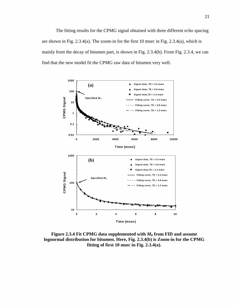
The fitting results for the CPMG signal obtained with three different echo spacing
are shown in Fig. 2.3.4(a). The zoom-in for the first 10 msec in Fig. 2.3.4(a), which is
mainly from the decay of bitumen part, is shown in Fig. 2.3.4(b). From Fig. 2.3.4, we can
find that the new model fit the CPMG raw data of bitumen very well.
Figure 2.3.4 Fit CPMG data supplemented with M0 from FID and assume
lognormal distribution for bitumen. Here, Fig. 2.3.4(b) is Zoom-in for the CPMG
fitting of first 10 msec in Fig. 2.3.4(a).
0.01
0.1
1
10
100
1000
0 2000 4000 6000 8000 10000
Time (msec)
CP
MG
Sig
na
l
Signal data, TE = 0.4 msec
Signal data, TE = 0.8 msec
Signal data,TE = 1.2 msec
Fitting curve, TE = 0.4 msec
Fitting curve, TE = 0.8 msec
Fitting curve, TE = 1.2 msec
Specified M 0
(a)
10
100
1000
0 2 4 6 8 10
T ime (msec)
CP
MG
Sig
na
l
Signal data, TE = 0.4 msec
Signal data, TE = 0.8 msec
Signal data,TE = 1.2 msec
Fitting curve, TE = 0.4 msec
Fitting curve, TE = 0.8 msec
Fitting curve, TE = 1.2 msec
Specified M 0
(b)

22
The interpretations of CPMG data are shown in Fig. 2.3.5. The T2 distributions of
bitumen sample obtained from the standard multi-exponential model without specified
M0 are compared with the results from the new model. As displayed in Fig. 2.3.5, the T2
of bitumen estimated by specifying M0 in CPMG data and assuming lognormal
distribution for bitumen are 0.58, 0.56 and 0.54 msec for TE = 0.4, 0.8 and 1.2 msec,
respectively. However, the corresponding T2 obtained from the regular CPMG
interpretation are 0.74, 0.83, 1.33 msec, respectively. Apparently, the T2 of bitumen
obtained by using the new model are remarkably shorter. More importantly, the corrected
T2 of bitumen has little dependence on echo spacing and is close to the T2 estimated from
FID (0.52 msec).
0
2
4
6
8
10
12
14
16
18
0.01 0.1 1 10 100 1000 10000
T 2 Relaxation Time Distribution (msec)
Am
plitu
de
f
TE = 0.4 msec, w/ specified Mo TE = 0.4 msec, w/o specified Mo
TE = 0.8 msec, w/ specified Mo TE = 0.8 msec, w/o specified Mo
TE = 1.2 msec, w/ specified Mo TE = 1.2 msec, w/o specified Mo
0
1020
30
40
5060
70
80
90100
110
0.01 1 100 10000
T 2 Relaxation Time Distribution (msec)
Cu
mu
lati
ve
f
Figure 2.3.5 T2 distribution of bitumen sample with supplemented M0 and
assuming lognormal distribution for bitumen.
23
As shown in the cumulative T2 distribution in Fig. 2.3.5, the area of the bitumen
peak is significantly increased by using the new interpretation method. This is due to the
compensation for the loss of T2 information shorter than echo spacing in regular CPMG
measurements.
2.3.5 Application at Different Sample Temperature
It is well known that the temperature of the environment for well logging varies
with each application. Therefore, after the successful application in 30 oC case, this new
method was also applied for the measurements at different sample temperatures. The
temperature range in this work is from 8 oC to 90
oC, which is adequate for the Canadian
bitumen logging. Some important properties of bitumen at different temperatures were
evaluated by using its T2 obtained from the new method.
2.3.5.1 Calculation Method of HI and Saturation at Different Temperatures
The hydrogen index (HI) of a fluid is defined as the proton density of the fluid at
any given temperature and pressure divided by the proton density of pure water in
standard conditions. It can be expressed as below (Dunn, Bergman and Latorraca 2002):
WaterPure of volumeequalan in Hydrogen ofAmount
Samplein Hydrogen ofAmount HI (2.11)
The hydrogen index should be a quantity independent of measurement methods.
In this work, the hydrogen index of bitumen can be expressed as Eq. [2.12].
condition standardat ,0intereststandard
interest of conditionsat //
/tw
wbbwbb
bVMTT
VfHI (2.12)
24
Here,
wbbf
/, sum of f of bitumen part in the bitumen sample;
wbwf
/, sum of f of water part in the bitumen sample;
wM
,0, initial magnetization of pure water;
wbbV
/ , volume of bitumen part in the bitumen sample;
wbwV
/ , volume of water part in the bitumen sample;
tV , total volume of bitumen sample and volume of pure water standard;
standardT , standard temperature of pure water sample;
interestT , interested temperature of pure water sample;
In this work, the total volume of bitumen sample is equal to the volume of pure
water as standard, thus the volumes of water and bitumen in the mixture sample can be
estimated by Eq. [2.13] and Eq. [2.14] respectively:
condition standardat ,0intereststandard
interest of conditionsat /
//
w
wbw
twbwMTT
fVV (2.13)
wbwtwbbVVV
// (2.14)
Another assumption, which was necessary for the investigation on bitumen
sample at different temperature, is that the difference of sample volume within our
interested temperature range is negligible. Consequently, Eq. [2.12] becomes,
condition standardat ,0intereststandard
interest of conditionsat ,0/
/
/
1
tw
wwbw
wbb
bVMTT
Mf
f
HI (2.15)
25
The equation for calculating water saturation wS can be derived from Eq. [2.13]
and expressed as:
condition standardat ,0intereststandard
interest of conditionsat //
/w
wbw
t
wbw
wMTT
f
V
VS (2.16)
2.3.5.2 Investigation on Bitumen Sample at Different Temperatures
Besides 30 oC, the bitumen sample was also measured at 8, 20, 40, 50, 60, 70, 80,
90 oC, respectively. The same interpretation method as used in 30
oC case was employed.
The HI and viscosity of bitumen as well as the water saturation in the sample were
estimated by using the T2 of bitumen obtained from the new method.
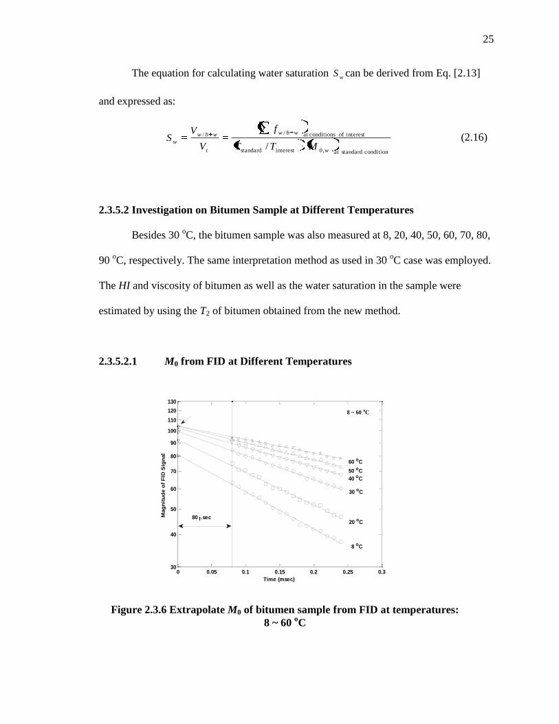
2.3.5.2.1 M0 from FID at Different Temperatures
Figure 2.3.6 Extrapolate M0 of bitumen sample from FID at temperatures:
8 ~ 60 oC
0 0.05 0.1 0.15 0.2 0.25 0.330
40
50
60
70
80
90
100
110
120
130
Mag
nit
ud
e o
f F
ID S
ign
al
Time (msec)
20 C 20 C
8 ~ 60 oC
20 oC
30 oC
40 oC
50 oC
60 oC
8 oC
80 sec
26
Fig. 2.3.6 displays the initial magnetization of bitumen sample at 8, 20, 30, 40, 50,
60 oC, which were estimated from extrapolation of FID. According to the Curie’s Law
(Cowan 1997), when temperature increases, the M0 of sample should decreases
correspondingly. However, within the range from 8 to 60 oC, the extrapolated M0 of
bitumen increases as temperature rises, which is opposite to the Curie’s Law’s prediction.
Moreover, when the temperature is over 40 oC, the extrapolated M0 becomes very close to
each other (indicated by the arrow). The flatter attenuation trend of FID signal at higher
temperature is indicative of the significant decrease in sample viscosity when the
temperature increases.
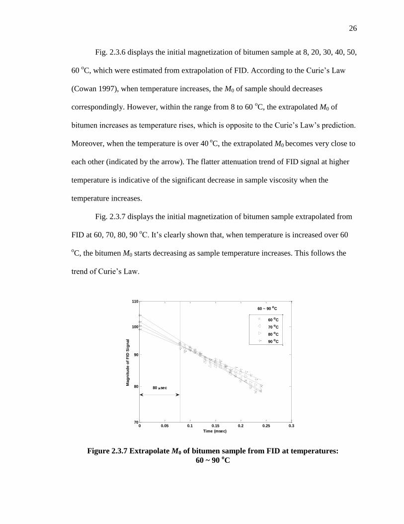
Fig. 2.3.7 displays the initial magnetization of bitumen sample extrapolated from
FID at 60, 70, 80, 90 oC. It’s clearly shown that, when temperature is increased over 60
oC, the bitumen M0 starts decreasing as sample temperature increases. This follows the
trend of Curie’s Law.
Figure 2.3.7 Extrapolate M0 of bitumen sample from FID at temperatures:
60 ~ 90 oC
0 0.05 0.1 0.15 0.2 0.25 0.370
80
90
100
110
Mag
nit
ud
e o
f F
ID S
ign
al
Time (msec)
60 oC
70 oC
80 oC
90 oC
60 ~ 90 oC
80 sec
27
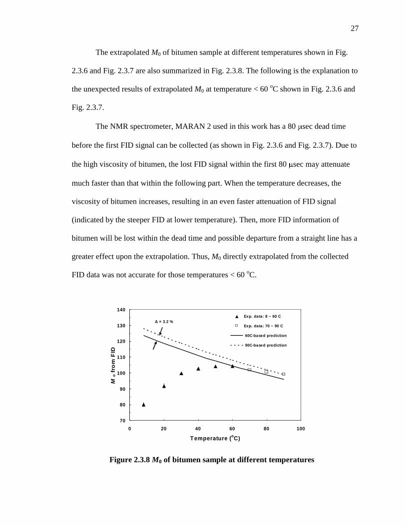
The extrapolated M0 of bitumen sample at different temperatures shown in Fig.
2.3.6 and Fig. 2.3.7 are also summarized in Fig. 2.3.8. The following is the explanation to
the unexpected results of extrapolated M0 at temperature < 60 oC shown in Fig. 2.3.6 and
Fig. 2.3.7.
The NMR spectrometer, MARAN 2 used in this work has a 80 sec dead time
before the first FID signal can be collected (as shown in Fig. 2.3.6 and Fig. 2.3.7). Due to
the high viscosity of bitumen, the lost FID signal within the first 80 sec may attenuate
much faster than that within the following part. When the temperature decreases, the
viscosity of bitumen increases, resulting in an even faster attenuation of FID signal
(indicated by the steeper FID at lower temperature). Then, more FID information of
bitumen will be lost within the dead time and possible departure from a straight line has a
greater effect upon the extrapolation. Thus, M0 directly extrapolated from the collected
FID data was not accurate for those temperatures < 60 oC.
Figure 2.3.8 M0 of bitumen sample at different temperatures
70
80
90
100
110
120
130
140
0 20 40 60 80 100
Temperature (oC)
Mo f
rom
FID
Exp. data: 8 ~ 60 C
Exp. data: 70 ~ 90 C
60C-based prediction
90C-based prediction
Δ = 3.2 %

28
This proposed explanation was supported by the results from the measurement
with 20 MHz Bruker minispec spectrometer, which had a dead time of 50 sec rather
than the 80 sec of the 2 MHz Maran-II. Fig. 2.3.9 displays the Bruker FID signal
measured on the same Athabasca bitumen but smaller sample size at 8 oC and 20
oC. As
we expected that, the faster attenuations of bitumen FID signal are observed before 80
sec especially at the lower temperature (8 oC).
The underestimation of the extrapolated M0 at low temperatures (< 60 oC) can be
corrected by the Curie’s Law. Given a real M0 value at certain temperature, the M0 of the
same sample at any other temperatures can be predicted by using Curie’s Law. When the
temperature of bitumen is over 60 oC, the sample viscosity is low enough that complete
0 0.05 0.1 0.1520
30
40
50
60
70
80
Mag
nit
ud
e o
f F
ID S
ign
al
Time (msec)
20 C 20 C
Larmor Frequency = 20 MHz
8 oC
80 sec
50 sec
20 oC
Figure 2.3.9 FID of bitumen sample at 8 oC and 20
oC with the 20 MHz Bruker
minispec NMR spectrometer. Here, the 20 MHz Bruker minispec has a dead
time of 50 sec. Dashed lines are extrapolation from data 50 ~ 80 sec. Solid
lines are extrapolation from data ≥ 80 sec.

29
FID information is assumed to be collected and the extrapolated M0 decreases with
increasing temperature as expected. Therefore, the extrapolated M0 value at temperature
≥ 60 oC can be assumed to be the real values and used as the basis for the Curie’s Law
correction. As shown in Fig. 2.3.8, the difference between the 60 oC-based prediction
(solid line) and the 90 oC-based prediction (dashed line) is 3.2 %. In this work, the 60
oC-
based prediction of M0 were employed for all the following calculations.
2.3.5.2.2 Interpretation of CPMG at Different Temperatures
Supplementing the Curie’s Law corrected M0 into the regular CPMG raw data, the
experimental data with specified M0 at each temperature were fitted to the lognormal
distribution based model and the fitting results are shown in Fig. 2.3.10. The
correspondingly interpreted T2 distribution of bitumen is shown in Fig. 2.3.11 (a).
0
10
20
30
40
50
60
70
80
90
100
110
120
130
140
0 2 4 6 8 10
T ime (msec)
CP
MG
Sig
na
l
Signal data, T = 8 C
Signal data, T = 20 C
Signal data, T = 30 C
Signal data, T = 40 C
Signal data, T = 50 C
Signal data, T = 60 C
Signal data, T = 70 C
Signal data, T = 80 C
Signal data, T = 90 C
Fitting curve
Specified Mo
Curie's Law corrected M 0
Figure 2.3.10 Fitting supplemented CPMG data by assuming lognormal
distribution for bitumen. Here, the specified M0 is corrected by Curie’s Law
30
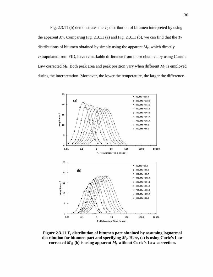
Fig. 2.3.11 (b) demonstrates the T2 distribution of bitumen interpreted by using
the apparent M0. Comparing Fig. 2.3.11 (a) and Fig. 2.3.11 (b), we can find that the T2
distributions of bitumen obtained by simply using the apparent M0, which directly
extrapolated from FID, have remarkable difference from those obtained by using Curie’s
Law corrected M0. Both peak area and peak position vary when different M0 is employed
during the interpretation. Moreover, the lower the temperature, the larger the difference.
Figure 2.3.11 T2 distribution of bitumen part obtained by assuming lognormal
distribution for bitumen part and specifying M0. Here, (a) is using Curie’s Law
corrected M0; (b) is using apparent M0 without Curie’s Law correction.
0
5
10
15
20
25
0.01 0.1 1 10 100 1000 10000
T 2 Relaxation T ime (msec)
Am
pli
tud
e f
8C, Mo = 80.0
20C, Mo = 91.8
30C, Mo = 99.7
40C, Mo = 102.7
50C, Mo = 104.1
60C, Mo = 104.4
70C, Mo = 101.9
80C, Mo = 100.4
90C, Mo = 99.0
(b)
0
5
10
15
20
25
0.01 0.1 1 10 100 1000 10000
T 2 Relaxation T ime (msec)
Am
pli
tud
e f
8C, Mo = 123.7
20C, Mo = 118.7
30C, Mo = 114.7
40C, Mo = 111.1
50C, Mo = 107.6
60C, Mo = 104.4
70C, Mo = 101.4
80C, Mo = 98.5
90C, Mo = 95.8
(a)
31
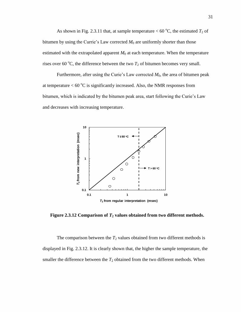
As shown in Fig. 2.3.11 that, at sample temperature < 60 oC, the estimated T2 of
bitumen by using the Currie’s Law corrected M0 are uniformly shorter than those
estimated with the extrapolated apparent M0 at each temperature. When the temperature
rises over 60 oC, the difference between the two T2 of bitumen becomes very small.
Furthermore, after using the Curie’s Law corrected M0, the area of bitumen peak
at temperature < 60 oC is significantly increased. Also, the NMR responses from
bitumen, which is indicated by the bitumen peak area, start following the Curie’s Law
and decreases with increasing temperature.
The comparison between the T2 values obtained from two different methods is
displayed in Fig. 2.3.12. It is clearly shown that, the higher the sample temperature, the
smaller the difference between the T2 obtained from the two different methods. When
0.1
1
10
0.1 1 10
T2 fr
om
new
in
terp
reta
tio
n (
msec)
T2 from regular interpretation (msec)
T ≤ 60 oC
T > 60 oC
Figure 2.3.12 Comparison of T2 values obtained from two different methods.
32
sample temperature was raised to be above 60 oC, almost no difference was observed for
the Athabasca bitumen T2 values from different methods.
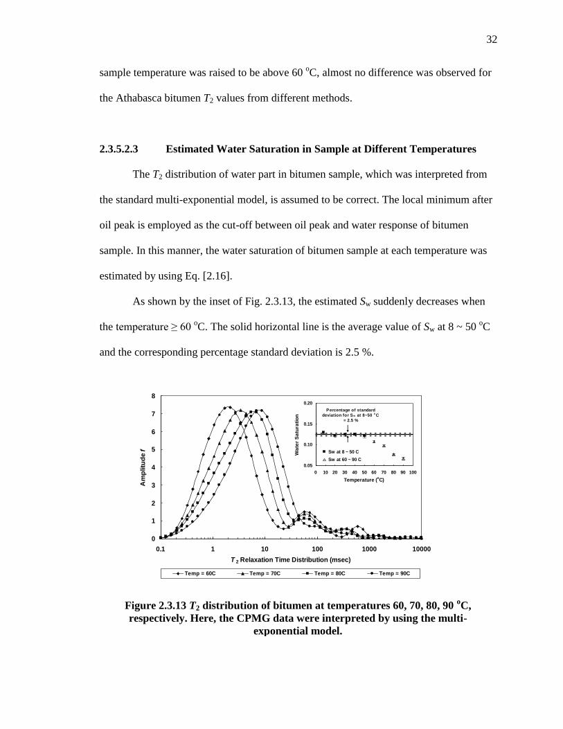
2.3.5.2.3 Estimated Water Saturation in Sample at Different Temperatures
The T2 distribution of water part in bitumen sample, which was interpreted from
the standard multi-exponential model, is assumed to be correct. The local minimum after
oil peak is employed as the cut-off between oil peak and water response of bitumen
sample. In this manner, the water saturation of bitumen sample at each temperature was
estimated by using Eq. [2.16].
As shown by the inset of Fig. 2.3.13, the estimated Sw suddenly decreases when
the temperature ≥ 60 oC. The solid horizontal line is the average value of Sw at 8 ~ 50
oC
and the corresponding percentage standard deviation is 2.5 %.
0
1
2
3
4
5
6
7
8
0.1 1 10 100 1000 10000
T 2 Relaxation Time Distribution (msec)
Am
plitu
de
f
Temp = 60C Temp = 70C Temp = 80C Temp = 90C
0.05
0.10
0.15
0.20
0 10 20 30 40 50 60 70 80 90 100
Temperature (oC)
Wa
ter
Sa
tura
tio
n
Sw at 8 ~ 50 C
Sw at 60 ~ 90 C
Percentage of standard
deviation for Sw at 8~50 oC
= 2.5 %
Figure 2.3.13 T2 distribution of bitumen at temperatures 60, 70, 80, 90 oC,
respectively. Here, the CPMG data were interpreted by using the multi-
exponential model.
33
A proposed explanation to the sudden decrease of Sw at temperature ≥ 60 oC is
that the cut-off we used in this work to distinguish oil peak and water peaks is not proper
in those high temperature cases. When the sample temperature is lower than 60 oC, the
bitumen peak is clearly separated from the water peaks. We can simply use the local
minimum after the bitumen peak as the cut-off. However, when the sample temperature is
raised over 60 o
C, due to the comparable T2 of emulsified water and bitumen, the water
peaks run into the bitumen peak, as shown in Fig. 2.3.13. Using the local minimum as the
cut-off may not be proper under these conditions.
A more sophisticated oil-water cut-off is necessary in the research on bitumen at
high temperatures. In this work, the sample tube was well-sealed. We purposely shuffled
the experiment sequence to avoid any unexpected temperature-sequence-dependent
results. For example, the 20 oC measurement was performed after the 90
oC one. Based
on the experimental data of water saturation shown in Fig. 2.3.13, it’s reasonable to
assume that the real water saturation of bitumen sample does not change within the
temperature range of this work.
Therefore, we may be able to use the water saturation data at low temperatures (8
~ 50 oC) to calibrate the cut-off at high temperatures (60 ~ 90
oC) in the following
research. On the other hand, due to the significant difference between the diffusivities of
bitumen and water, we may also use Diffusion Editing measurement (Hürlimann,
Venkataramanan and Flaum 2002) to evaluate the NMR response of emulsified water in
bitumen samples.
2.3.5.2.4 Estimated HI of Bitumen at Different Temperatures

34
The hydrogen index (HI) of bitumen at different temperature can be calculated by
using Eq. [2.15] and the results are shown in Fig. 2.3.14. It is clear that, when the
extrapolated M0 from FID is not corrected by Curie’s Law, the apparent HI of bitumen
has a temperature-dependence. This is due to the underestimation of apparent M0 (as
shown in Fig. 2.3.6 and Fig. 2.3.8) when sample temperature < 60 oC, and the inaccurate
cut-off for calculating the water saturation (as shown in Fig. 2.3.13) at temperature ≥ 60
oC.
However, after the correction for M0, the incorrect temperature dependence is
eliminated and the bitumen HI stays constant at different temperature. The average value
is 0.82 and the percentage standard deviation is only 0.6 %.
2.3.5.2.5 Estimated Viscosity of Bitumen at Different Temperatures
Figure 2.3.14 Hydrogen Index of bitumen at different temperatures
0.40
0.50
0.60
0.70
0.80
0.90
1.00
0 20 40 60 80 100
Temperature (oC)
Hy
dro
ge
n I
nd
ex
of
Bit
um
en
Curie 's law corrected HI at 8 ~ 50 C
Curie 's law corrected HI at 60 ~ 90 C
Apparent HI w ithout Curie 's law
correction
Percentage standard deviation for
corrected HI at 8 ~ 90 oC = 0.6 %
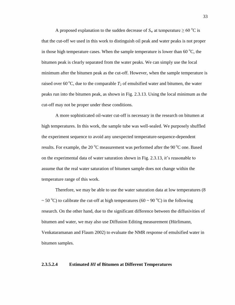
35
A correlation of log-mean T2 with the ratio of viscosity and temperature, which
was derived from alkanes T1, was developed in previous work of our group (Lo, et al.
2002) and (Hirasaki, Lo and Zhang 2003). As displayed in Fig. 2.3.15, given the
corrected T2, the viscosities of bitumen at different temperatures were estimated by using
the alkane correlation.
It is clearly shown in Fig. 2.3.15 that the viscosity of bitumen estimated from the
alkane correlation has significant discrepancy from the experimental value measured by
viscometer at low temperatures. As the sample temperature increases, the viscosity of
bitumen decreases and the difference between the two viscosity values keeps decreasing.
When it reaches 90 oC, the calculated value becomes equal to the experimental value.
This means that the alkane correlation, as many other NMR Relaxation Time vs.
0.1
1
10
1.E+02
1.E+03
1.E+04
1.E+05
1.E+06
1.E+07
0 20 40 60 80 100
T2
of B
itum
en
(ms
ec
)
Vis
co
sit
y (c
P)
Temperature (oC)
T2 from Lognormal Fitting
Viscosity from Alkane Correlation
Viscosity from Viscometer
Figure 2.3.15 Comparison of bitumen viscosity from two different methods
36
Viscosity correlations (Kleinberg and Vinegar 1996), (Morriss, et al. 1997), (Straley, et al.
1997) and (LaTorraca, Stonard, et al. 1999), is only good for the oil with relatively low
viscosity, but not suitable for those with extremely high viscosity like bitumen. In order
to find out the reason responsible for the discrepancy, we need to start from the
theoretical basis on highly viscous oil relaxation.
Dead crude oils relax mainly by intramolecular dipole-dipole interactions (Zhang,
PhD Thesis 2002). By normalizing the relaxation time, viscosity and
viscosity/temperature ratio with respect to 2 MHz as shown in Eq. [2.17] and Eq. [2.18]:
2,1
0
2,1
2TT
N (2.17)
2
0
N (2.18)
The intramolecular dipole-dipole interaction model for a rigid spherical molecule can be
expressed as follows (Hirasaki, Lo and Zhang 2003) and (Zhang, PhD Thesis 2002):
22
N
2
1N
21
3/8
1
3/2
2
1
NNT
ST
ST
SW
T (2.19)
22
N
2
2N
21
3/2
1
3/51
2
1
NNT
ST
ST
SW
T (2.20)
k
aS
3
83
. (2.21)
The experimental results between normalized T1 or T2 relaxation times and
normalized viscosity/temperature ratio are shown in Fig. 2.3.16. Also, some literature
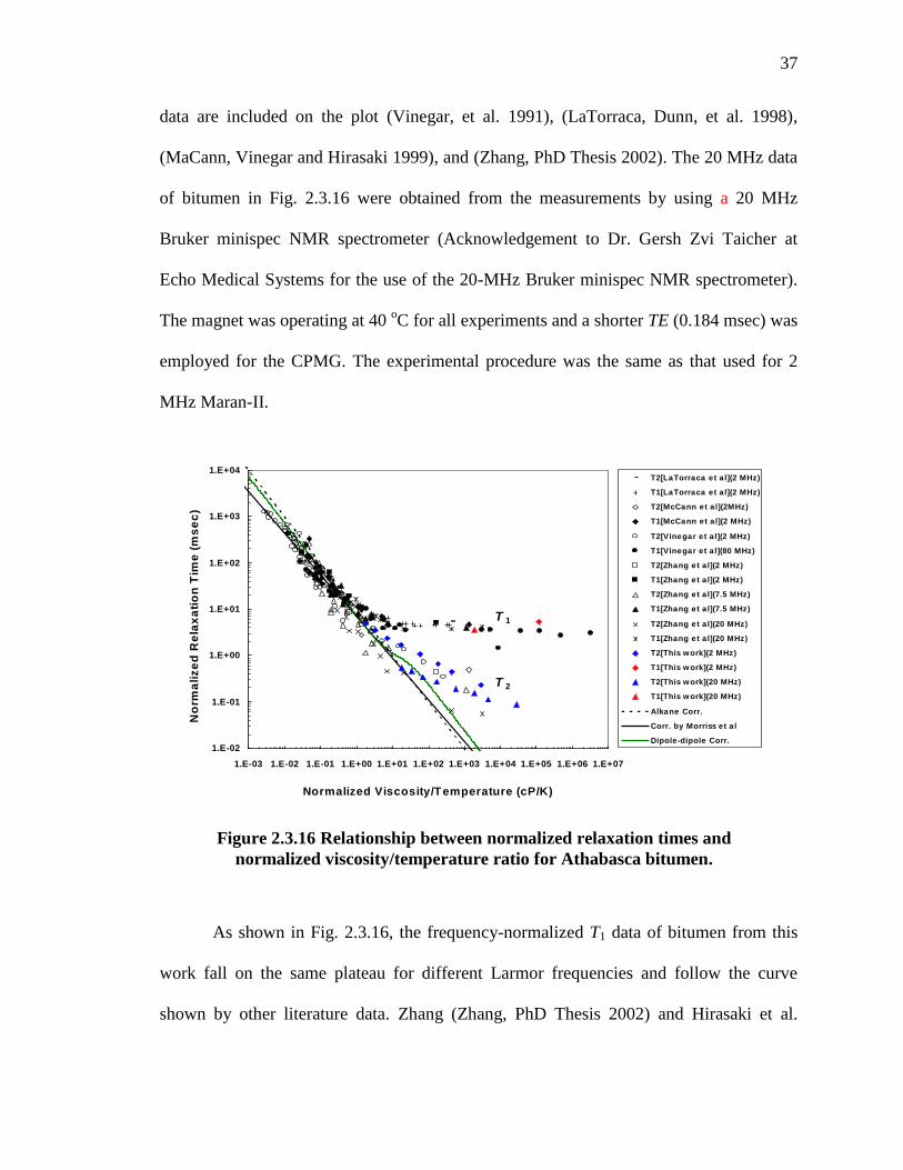
37
data are included on the plot (Vinegar, et al. 1991), (LaTorraca, Dunn, et al. 1998),
(MaCann, Vinegar and Hirasaki 1999), and (Zhang, PhD Thesis 2002). The 20 MHz data
of bitumen in Fig. 2.3.16 were obtained from the measurements by using a 20 MHz
Bruker minispec NMR spectrometer (Acknowledgement to Dr. Gersh Zvi Taicher at
Echo Medical Systems for the use of the 20-MHz Bruker minispec NMR spectrometer).
The magnet was operating at 40 oC for all experiments and a shorter TE (0.184 msec) was
employed for the CPMG. The experimental procedure was the same as that used for 2
MHz Maran-II.
As shown in Fig. 2.3.16, the frequency-normalized T1 data of bitumen from this
work fall on the same plateau for different Larmor frequencies and follow the curve
shown by other literature data. Zhang (Zhang, PhD Thesis 2002) and Hirasaki et al.
1.E-02
1.E-01
1.E+00
1.E+01
1.E+02
1.E+03
1.E+04
1.E-03 1.E-02 1.E-01 1.E+00 1.E+01 1.E+02 1.E+03 1.E+04 1.E+05 1.E+06 1.E+07
Normalized Viscosity/Temperature (cP/K)
No
rma
liz
ed
Re
lax
ati
on
Tim
e (
ms
ec
)
T2[LaTorraca et a l](2 MHz)
T1[LaTorraca et a l](2 MHz)
T2[McCann et a l](2MHz)
T1[McCann et a l](2 MHz)
T2[Vinegar et a l](2 MHz)
T1[Vinegar et a l](80 MHz)
T2[Zhang et a l](2 MHz)
T1[Zhang et a l](2 MHz)
T2[Zhang et a l](7.5 MHz)
T1[Zhang et a l](7.5 MHz)
T2[Zhang et a l](20 MHz)
T1[Zhang et a l](20 MHz)
T2[This w ork](2 MHz)
T1[This w ork](2 MHz)
T2[This w ork](20 MHz)
T1[This w ork](20 MHz)
Alkane Corr.
Corr. by Morriss et a l
Dipole-dipole Corr.
T 1
T 2
Figure 2.3.16 Relationship between normalized relaxation times and
normalized viscosity/temperature ratio for Athabasca bitumen.
38
(Hirasaki, Lo and Zhang 2003) reported in their work that, the measured T1 for viscous
samples do not follow the theoretical trend, which predicted by the intramolecular dipole-
dipole interaction model. The experimental T1 levels off at high viscosity and reaches a
plateau for normalized viscosity/temperature greater than 1 cP/K.
The experimental T2 continues to shorten with increasing viscosity. Moreover, T2
is considerably less than T1 in all cases for heavy oils. As shown in Fig. 2.3.16, the
measured bitumen normalized T2 at either Larmor frequency in this work follows the
trend of previous literature data. The black solid line in Fig. 2.3.16 is from the T2
correlation by Morriss et al. (Morriss, et al. 1997) and the dashed line is from the Alkane
correlation (Hirasaki, Lo and Zhang 2003). Although the viscosity predictions from the
two correlations have difference for light oils, they are quite similar at high viscosities.
Viscosity prediction is adaptable for relatively low viscosity crude oils. However, highly
viscous samples significantly depart from both of two correlations.
The correlation derived from the intramolecular dipole-dipole interactions model
(expressed by Eq. [2.20]) was also employed to fit the experimental data. The only
variable in Eq. [2.20] is S and its estimated value in this case is 0.082. The fitted results
are plotted as the green solid line in Fig. 2.3.16. It is clear that the experimental data of
heavy oils also have great departure from the dipole-dipole correlation.
In this manner, further work is undergoing and a new correlation will be
developed to better correlate T2 relaxation time and heavy oil viscosity.
39
2.4 Conclusions
The echo spacing restriction of regular CPMG measurement on highly viscous
bitumen can be overcome by specifying the M0 in CPMG raw data and assuming
lognormal distribution for bitumen during the interpretation.
Apparent M0 of bitumen from FID at low temperatures (< 60 oC) has incorrect
dependence on temperature due to the loss of FID signal within the initial decay period.
This incorrect temperature dependence can be corrected by the Curie’s Law. Given a
correct M0 value at certain temperature, the M0 of the same sample at any other
temperatures can be predicted by using the equation of Curie’s Law.
Given Curie’s Law corrected M0 and proper cut-off between oil and water, the
hydrogen index (HI) and water saturation (Sw) of bitumen sample can be evaluated by
using the method in this work. The estimated HI of Athabasca bitumen is 0.82.
The T1 and T2 of Athabasca bitumen follow the trend of previous literature data.
The existing T2 vs. viscosity correlations, which are good for the oil with relatively low
viscosity, are not suitable for the samples with extremely high viscosity like Canadian
bitumen.
40
Chapter 3 NMR Measurement and Viscosity Evaluation of Live
Brookfield Oil
3.1 Introduction
The laboratory NMR measurements have shown that the laboratory results of the
Canadian bitumen sample appear to be remarkably shorter than the corresponding well
log NMR T2. This is likely due to the dissolved gas in the bitumen. The T2 distribution
depends on oil viscosity and dissolved gas concentration, which may vary throughout the
heavy oil field. Thus, a method to determine the gas solubility and the in-situ viscosity
from NMR logs would be very useful in heavy oil and bitumen reservoir development.
In this chapter, the viscosity and laboratory NMR measurements on the
recombined live Brookfield oil sample as a function of dissolved gas concentrations were
performed. The effects of three different gases (CH4, CO2, and C2H6) on the viscosity of
Brookfield oil at a series of saturation pressures were investigated. The correlations
among the saturation pressure, gas solubility, NMR T2 and live oil viscosity are
established to resolve the differences between the NMR log and laboratory data. The
findings create a way for in-situ viscosity evaluation of heavy oil through NMR well
logging.
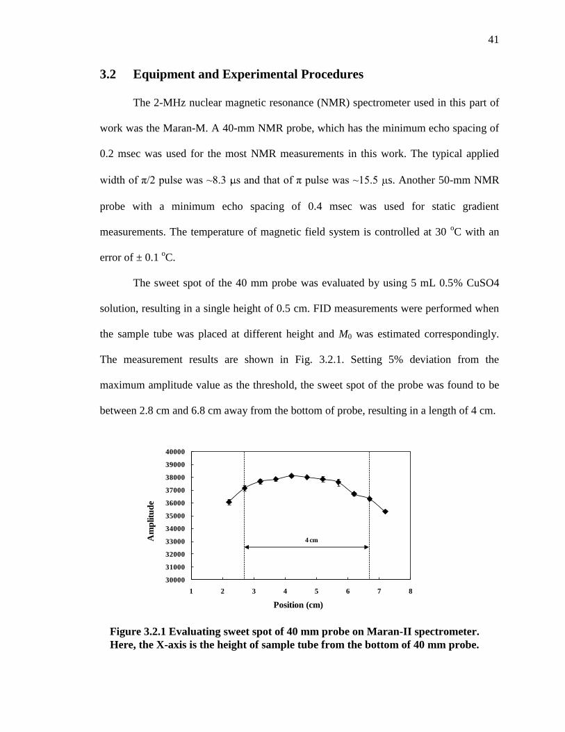
41
3.2 Equipment and Experimental Procedures
The 2-MHz nuclear magnetic resonance (NMR) spectrometer used in this part of
work was the Maran-M. A 40-mm NMR probe, which has the minimum echo spacing of
0.2 msec was used for the most NMR measurements in this work. The typical applied
width of π/2 pulse was ~8.3 s and that of π pulse was ~15.5 s. Another 50-mm NMR
probe with a minimum echo spacing of 0.4 msec was used for static gradient
measurements. The temperature of magnetic field system is controlled at 30 oC with an
error of ± 0.1 oC.
The sweet spot of the 40 mm probe was evaluated by using 5 mL 0.5% CuSO4
solution, resulting in a single height of 0.5 cm. FID measurements were performed when
the sample tube was placed at different height and M0 was estimated correspondingly.
The measurement results are shown in Fig. 3.2.1. Setting 5% deviation from the
maximum amplitude value as the threshold, the sweet spot of the probe was found to be
between 2.8 cm and 6.8 cm away from the bottom of probe, resulting in a length of 4 cm.
30000
31000
32000
33000
34000
35000
36000
37000
38000
39000
40000
1 2 3 4 5 6 7 8
Am
plitu
de
Position (cm)
4 cm
Figure 3.2.1 Evaluating sweet spot of 40 mm probe on Maran-II spectrometer.
Here, the X-axis is the height of sample tube from the bottom of 40 mm probe.
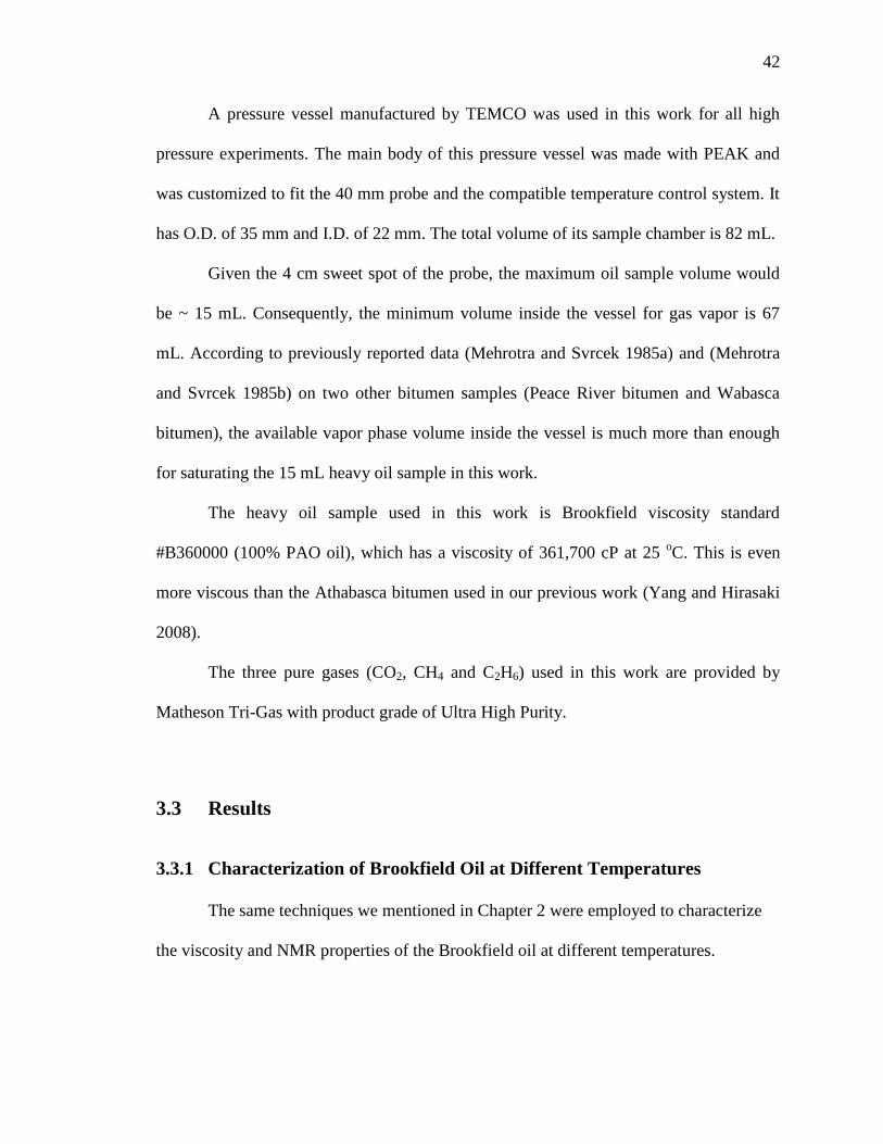
42
A pressure vessel manufactured by TEMCO was used in this work for all high
pressure experiments. The main body of this pressure vessel was made with PEAK and
was customized to fit the 40 mm probe and the compatible temperature control system. It
has O.D. of 35 mm and I.D. of 22 mm. The total volume of its sample chamber is 82 mL.
Given the 4 cm sweet spot of the probe, the maximum oil sample volume would
be ~ 15 mL. Consequently, the minimum volume inside the vessel for gas vapor is 67
mL. According to previously reported data (Mehrotra and Svrcek 1985a) and (Mehrotra
and Svrcek 1985b) on two other bitumen samples (Peace River bitumen and Wabasca
bitumen), the available vapor phase volume inside the vessel is much more than enough
for saturating the 15 mL heavy oil sample in this work.
The heavy oil sample used in this work is Brookfield viscosity standard
#B360000 (100% PAO oil), which has a viscosity of 361,700 cP at 25 oC. This is even
more viscous than the Athabasca bitumen used in our previous work (Yang and Hirasaki
2008).
The three pure gases (CO2, CH4 and C2H6) used in this work are provided by
Matheson Tri-Gas with product grade of Ultra High Purity.
3.3 Results
3.3.1 Characterization of Brookfield Oil at Different Temperatures
The same techniques we mentioned in Chapter 2 were employed to characterize
the viscosity and NMR properties of the Brookfield oil at different temperatures.
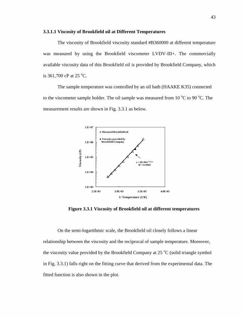
43
3.3.1.1 Viscosity of Brookfield oil at Different Temperatures
The viscosity of Brookfield viscosity standard #B360000 at different temperature
was measured by using the Brookfield viscometer LVDV-III+. The commercially
available viscosity data of this Brookfield oil is provided by Brookfield Company, which
is 361,700 cP at 25 oC.
The sample temperature was controlled by an oil bath (HAAKE K35) connected
to the viscometer sample holder. The oil sample was measured from 10 oC to 90
oC. The
measurement results are shown in Fig. 3.3.1 as below.
On the semi-logarithmic scale, the Brookfield oil closely follows a linear
relationship between the viscosity and the reciprocal of sample temperature. Moreover,
the viscosity value provided by the Brookfield Company at 25 oC (solid triangle symbol
in Fig. 3.3.1) falls right on the fitting curve that derived from the experimental data. The
fitted function is also shown in the plot.
y = 4E-06e7518.5x
R² = 0.9985
1.E+03
1.E+04
1.E+05
1.E+06
1.E+07
2.5E-03 3.0E-03 3.5E-03 4.0E-03
Vis
co
sity
(cP
)
1/ Temperature (1/K)
Measured Brookfield oil
Viscosity provided by Brookfield Company
Figure 3.3.1 Viscosity of Brookfield oil at different temperatures
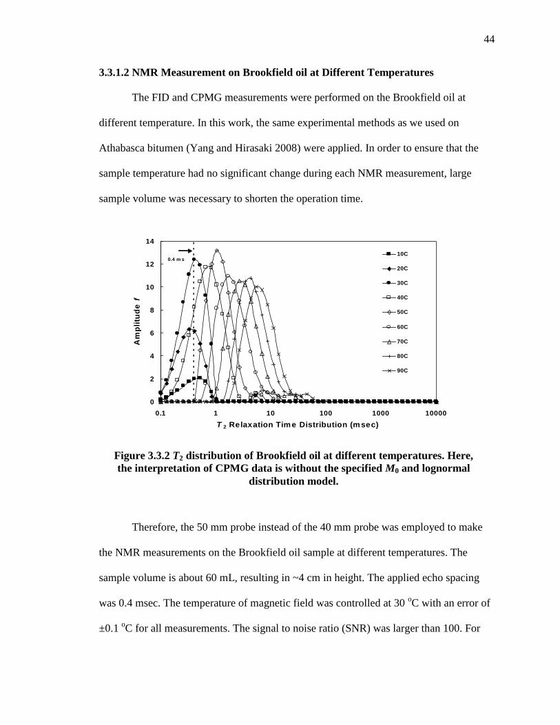
44
3.3.1.2 NMR Measurement on Brookfield oil at Different Temperatures
The FID and CPMG measurements were performed on the Brookfield oil at
different temperature. In this work, the same experimental methods as we used on
Athabasca bitumen (Yang and Hirasaki 2008) were applied. In order to ensure that the
sample temperature had no significant change during each NMR measurement, large
sample volume was necessary to shorten the operation time.
Therefore, the 50 mm probe instead of the 40 mm probe was employed to make
the NMR measurements on the Brookfield oil sample at different temperatures. The
sample volume is about 60 mL, resulting in ~4 cm in height. The applied echo spacing
was 0.4 msec. The temperature of magnetic field was controlled at 30 oC with an error of
±0.1 oC for all measurements. The signal to noise ratio (SNR) was larger than 100. For
0
2
4
6
8
10
12
14
0.1 1 10 100 1000 10000
T 2 Relaxation Tim e Distribution (m sec)
Am
pli
tud
e f
10C
20C
30C
40C
50C
60C
70C
80C
90C
0.4 m s
Figure 3.3.2 T2 distribution of Brookfield oil at different temperatures. Here,
the interpretation of CPMG data is without the specified M0 and lognormal
distribution model.

45
the Brookfield oil sample, the applied width of π/2 pulse was 8.6 s and that of π pulse
was 15.82 s.
The NMR measurements (CPMG and FID) were performed on the Brookfield oil
sample at temperature from 10 oC to 90
oC and were conducted with an interval of 10
oC
at a time within the temperature range. At each temperature, the measurement was
repeated for three times to ensure the reliability of experimental data.
The T2 distribution of Brookfield oil at different temperature, which was
interpreted from the regular CPMG data without specified M0 and lognormal distribution
model, is shown in Fig. 3.3.2. The 0.4 msec echo spacing is indicated by the vertical
dashed line in the plot.
As shown in Fig. 3.3.2, the T2 distribution of Brookfield oil is not entirely longer
than the applied echo spacing until the sample temperature ≥ 50 oC. Therefore, for the
cases at 10 oC to 40
oC, the M0 obtained from the FID measurement at each temperature
was imposed into the regular CPMG data and the lognormal distribution model (Yang
and Hirasaki 2008) was employed to re-interpret the M0 specified data as shown in Fig.
3.3.3.
Fig. 3.3.3(a) shows the extrapolated M0 of Brookfield oil from FID at different
temperatures. It is clear that, the extrapolated values closely follow the Curie’s law
(calculation based on M0 from FID at 50 oC) within the entire temperature range. This is
different from the results observed in the work on Athabasca bitumen (Chapter 2). This
may be due to the much simpler composition of this synthetic oil sample. The Brookfield
oil is a commercially available viscosity standard from Brookfield Company, which is
made by 100% PAO, is much more pure than the crude Athabasca bitumen. Therefore, it

46
does not have many extremely fast relaxing components, which will result in significant
FID information loss within dead time at low temperatures (Yang and Hirasaki 2008).
Figure 3.3.3 Interpretation of M0 specified CPMG data of Brookfield oil by
using lognormal distribution model. Here, (a) M0 extrapolated from FID at
different temperature; (b) fitting the supplemented CPMG data via lognormal
distribution model
0
10
20
30
40
50
60
70
80
90
100
0 2 4 6 8 10
Time (msec)
CP
MG
Sig
na
l
Signal data, T = 10 C
Signal data, T = 20 C
Signal data, T = 30 C
Signal data, T = 40 C
Signal data, T = 50 C
Fitting curve
Specified Mo
Specified M 0
60
70
80
90
100
0 20 40 60 80 100
M0
fro
m F
ID
Temperature (oC)
Experimental data from FID at 10~90 C
Fitted curve by Curie's law
(a)
(b)
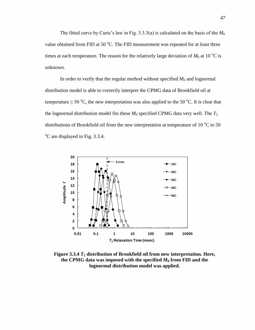
47
The fitted curve by Curie’s law in Fig. 3.3.3(a) is calculated on the basis of the M0
value obtained from FID at 50 oC. The FID measurement was repeated for at least three
times at each temperature. The reason for the relatively large deviation of M0 at 10 oC is
unknown.
In order to verify that the regular method without specified M0 and lognormal
distribution model is able to correctly interpret the CPMG data of Brookfield oil at
temperature ≥ 50 oC, the new interpretation was also applied to the 50
oC. It is clear that
the lognormal distribution model fits these M0 specified CPMG data very well. The T2
distributions of Brookfield oil from the new interpretation at temperature of 10 oC to 50
oC are displayed in Fig. 3.3.4.
0
2
4
6
8
10
12
14
16
18
20
0.01 0.1 1 10 100 1000 10000
Am
pli
tud
e f
T2 Relaxation Time (msec)
10C
20C
30C
40C
50C
0.4 ms
Figure 3.3.4 T2 distribution of Brookfield oil from new interpretation. Here,
the CPMG data was imposed with the specified M0 from FID and the
lognormal distribution model was applied.
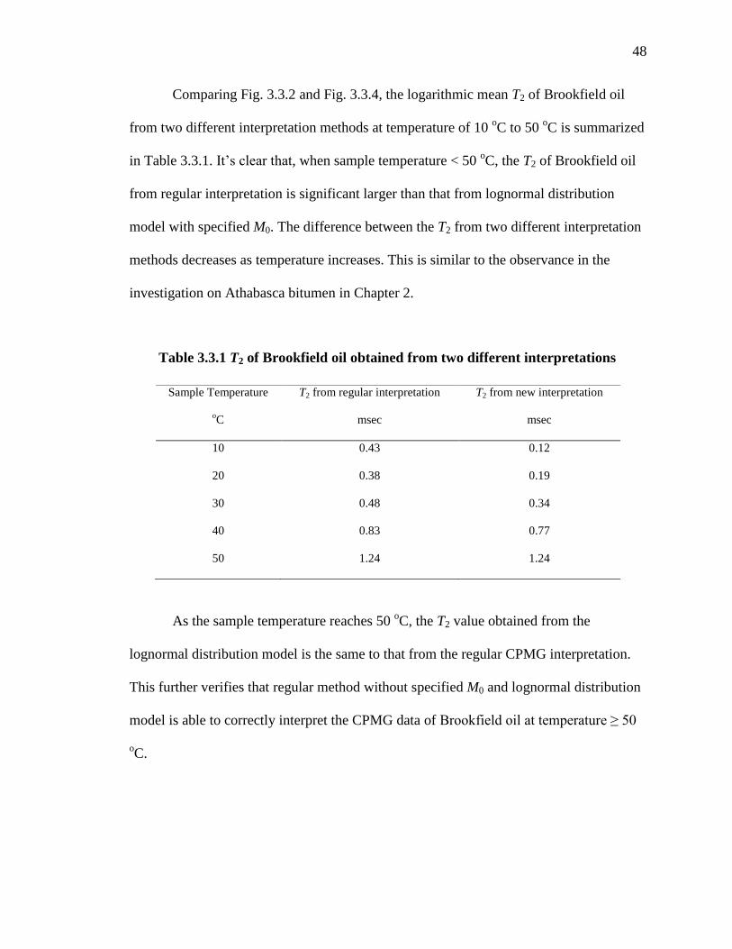
48
Comparing Fig. 3.3.2 and Fig. 3.3.4, the logarithmic mean T2 of Brookfield oil
from two different interpretation methods at temperature of 10 oC to 50
oC is summarized
in Table 3.3.1. It’s clear that, when sample temperature < 50 oC, the T2 of Brookfield oil
from regular interpretation is significant larger than that from lognormal distribution
model with specified M0. The difference between the T2 from two different interpretation
methods decreases as temperature increases. This is similar to the observance in the
investigation on Athabasca bitumen in Chapter 2.
As the sample temperature reaches 50 oC, the T2 value obtained from the
lognormal distribution model is the same to that from the regular CPMG interpretation.
This further verifies that regular method without specified M0 and lognormal distribution
model is able to correctly interpret the CPMG data of Brookfield oil at temperature ≥ 50
oC.
Sample Temperature
oC
T2 from regular interpretation
msec
T2 from new interpretation
msec
10 0.43 0.12
20 0.38 0.19
30 0.48 0.34
40 0.83 0.77
50 1.24 1.24
Table 3.3.1 T2 of Brookfield oil obtained from two different interpretations
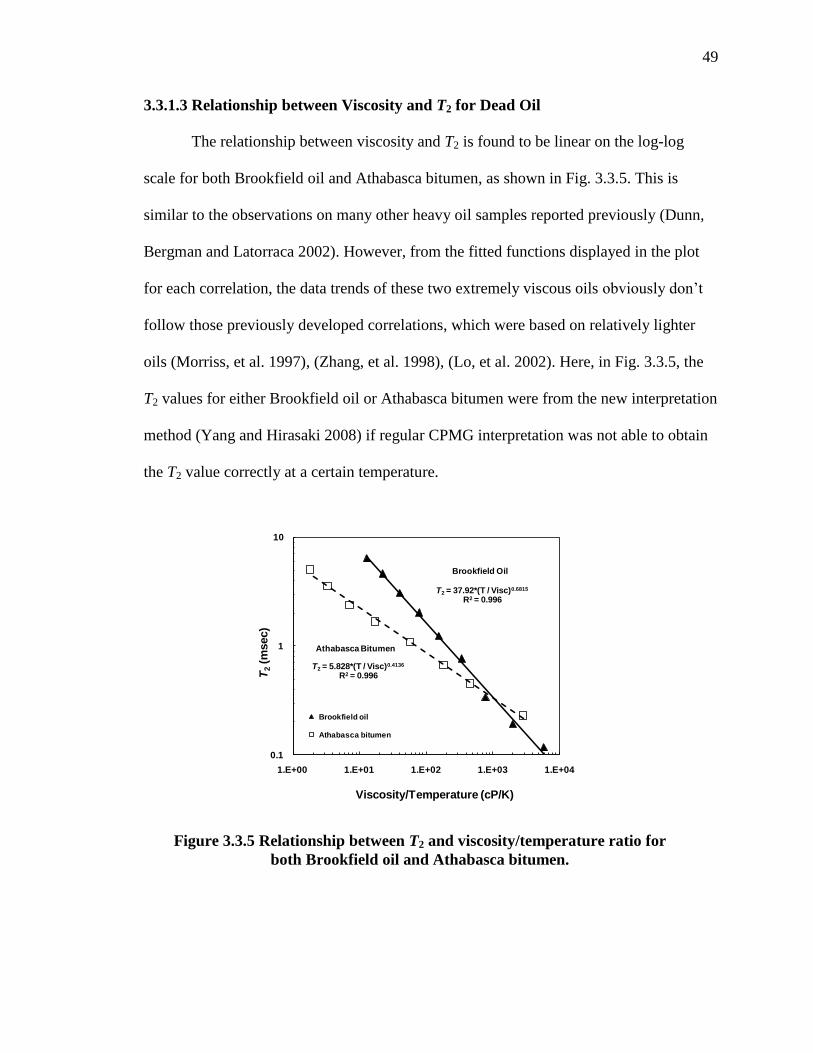
49
3.3.1.3 Relationship between Viscosity and T2 for Dead Oil
The relationship between viscosity and T2 is found to be linear on the log-log
scale for both Brookfield oil and Athabasca bitumen, as shown in Fig. 3.3.5. This is
similar to the observations on many other heavy oil samples reported previously (Dunn,
Bergman and Latorraca 2002). However, from the fitted functions displayed in the plot
for each correlation, the data trends of these two extremely viscous oils obviously don’t
follow those previously developed correlations, which were based on relatively lighter
oils (Morriss, et al. 1997), (Zhang, et al. 1998), (Lo, et al. 2002). Here, in Fig. 3.3.5, the
T2 values for either Brookfield oil or Athabasca bitumen were from the new interpretation
method (Yang and Hirasaki 2008) if regular CPMG interpretation was not able to obtain
the T2 value correctly at a certain temperature.
0.1
1
10
1.E+00 1.E+01 1.E+02 1.E+03 1.E+04
T2
(msec)
Viscosity/Temperature (cP/K)
Brookfield oil
Athabasca bitumen
Brookfield Oil
T2 = 37.92*(T / Visc)0.6815
R2 = 0.996
Athabasca Bitumen
T2 = 5.828*(T / Visc)0.4136
R2 = 0.996
Figure 3.3.5 Relationship between T2 and viscosity/temperature ratio for
both Brookfield oil and Athabasca bitumen.

50
3.3.2 Investigations on Recombined Live Brookfield Oil
The investigations on the recombined live Brookfield oil were performed with
three different reservoir gases, CO2, CH4, and C2H6. In each case, the measurements were
conducted at different pressure levels.
During the experiments with each gas, the procedure was dived into two stages
generally, the pressurization stage and the depressurization stage. First, the highly
pressurized gas was introduced into the closed pressure vessel with certain amount of oil
at bottom. After the gas-oil system reached equilibrium at the highest pressure level, the
system pressure would be depressurized to several lower levels, step by step. At each
lower pressure, the equilibrium was achieved as well.
During the entire process, NMR measurements were performed periodically to
track the T2 change. Proper number of scans (NS) was chosen to make the signal to noise
ratio (SNR) equal to 100. Each measurement was repeated 6 times to ensure the
reliability of experimental data. The system pressure inside the vessel was monitored by
using a Senso-Metrics pressure transducer (Model 602008, Max. 5,000 psig).
3.3.2.1 Method for Calculating Gas Solubility at Different Pressures
The solubility of each gas in Brookfield oil needs to be calculated at different
pressure levels in this work. The method for calculating the gas solubility from pressure
data is described as follows:
(I) Pressurization Stage:
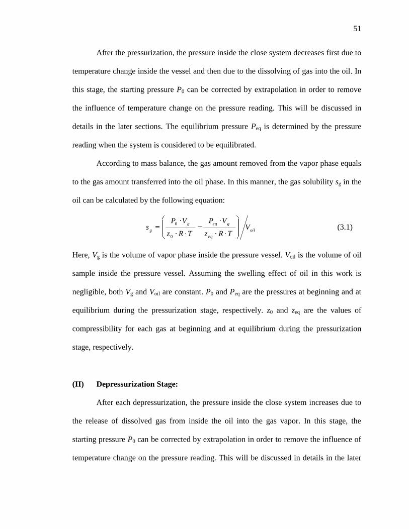
51
After the pressurization, the pressure inside the close system decreases first due to
temperature change inside the vessel and then due to the dissolving of gas into the oil. In
this stage, the starting pressure P0 can be corrected by extrapolation in order to remove
the influence of temperature change on the pressure reading. This will be discussed in
details in the later sections. The equilibrium pressure Peq is determined by the pressure
reading when the system is considered to be equilibrated.
According to mass balance, the gas amount removed from the vapor phase equals
to the gas amount transferred into the oil phase. In this manner, the gas solubility sg in the
oil can be calculated by the following equation:
oil
eq
geqg
gV
TRz
VP
TRz
VPs
0
0 (3.1)
Here, Vg is the volume of vapor phase inside the pressure vessel. Voil is the volume of oil
sample inside the pressure vessel. Assuming the swelling effect of oil in this work is
negligible, both Vg and Voil are constant. P0 and Peq are the pressures at beginning and at
equilibrium during the pressurization stage, respectively. z0 and zeq are the values of
compressibility for each gas at beginning and at equilibrium during the pressurization
stage, respectively.
(II) Depressurization Stage:
After each depressurization, the pressure inside the close system increases due to
the release of dissolved gas from inside the oil into the gas vapor. In this stage, the
starting pressure P0 can be corrected by extrapolation in order to remove the influence of
temperature change on the pressure reading. This will be discussed in details in the later
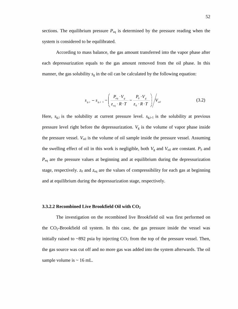
52
sections. The equilibrium pressure Peq is determined by the pressure reading when the
system is considered to be equilibrated.
According to mass balance, the gas amount transferred into the vapor phase after
each depressurization equals to the gas amount removed from the oil phase. In this
manner, the gas solubility sg in the oil can be calculated by the following equation:
oil
g
eq
geq
igigV
TRz
VP
TRz
VPss
0
0
1,, (3.2)
Here, sg,i is the solubility at current pressure level. sg,i-1 is the solubility at previous
pressure level right before the depressurization. Vg is the volume of vapor phase inside
the pressure vessel. Voil is the volume of oil sample inside the pressure vessel. Assuming
the swelling effect of oil in this work is negligible, both Vg and Voil are constant. P0 and
Peq are the pressure values at beginning and at equilibrium during the depressurization
stage, respectively. z0 and zeq are the values of compressibility for each gas at beginning
and at equilibrium during the depressurization stage, respectively.
3.3.2.2 Recombined Live Brookfield Oil with CO2
The investigation on the recombined live Brookfield oil was first performed on
the CO2-Brookfield oil system. In this case, the gas pressure inside the vessel was
initially raised to ~892 psia by injecting CO2 from the top of the pressure vessel. Then,
the gas source was cut off and no more gas was added into the system afterwards. The oil
sample volume is ~ 16 mL.
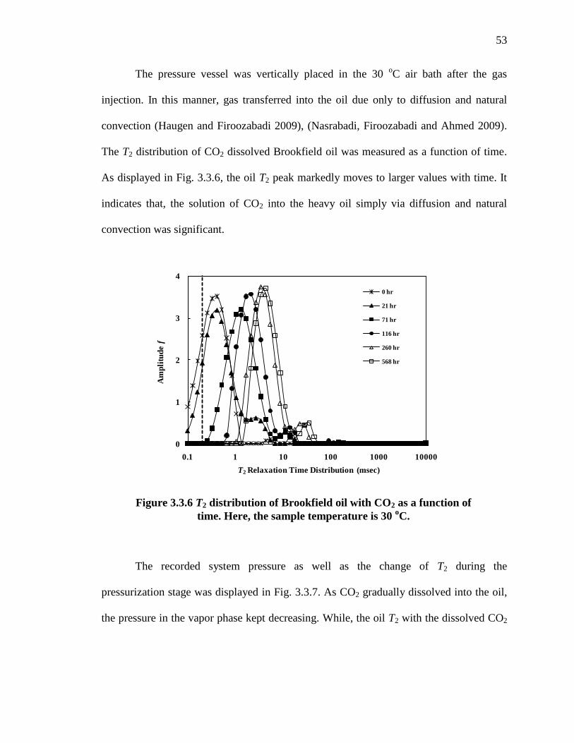
53
The pressure vessel was vertically placed in the 30 oC air bath after the gas
injection. In this manner, gas transferred into the oil due only to diffusion and natural
convection (Haugen and Firoozabadi 2009), (Nasrabadi, Firoozabadi and Ahmed 2009).
The T2 distribution of CO2 dissolved Brookfield oil was measured as a function of time.
As displayed in Fig. 3.3.6, the oil T2 peak markedly moves to larger values with time. It
indicates that, the solution of CO2 into the heavy oil simply via diffusion and natural
convection was significant.
The recorded system pressure as well as the change of T2 during the
pressurization stage was displayed in Fig. 3.3.7. As CO2 gradually dissolved into the oil,
the pressure in the vapor phase kept decreasing. While, the oil T2 with the dissolved CO2
0
1
2
3
4
0.1 1 10 100 1000 10000
Am
pli
tud
e f
T2 Relaxation Time Distribution (msec)
0 hr
21 hr
71 hr
116 hr
260 hr
568 hr
Figure 3.3.6 T2 distribution of Brookfield oil with CO2 as a function of
time. Here, the sample temperature is 30 oC.
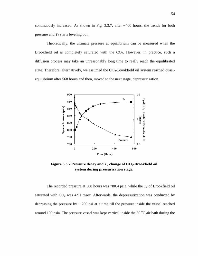
54
continuously increased. As shown in Fig. 3.3.7, after ~400 hours, the trends for both
pressure and T2 starts leveling out.
Theoretically, the ultimate pressure at equilibrium can be measured when the
Brookfield oil is completely saturated with the CO2. However, in practice, such a
diffusion process may take an unreasonably long time to really reach the equilibrated
state. Therefore, alternatively, we assumed the CO2-Brookfield oil system reached quasi-
equilibrium after 568 hours and then, moved to the next stage, depressurization.
The recorded pressure at 568 hours was 780.4 psia, while the T2 of Brookfield oil
saturated with CO2 was 4.91 msec. Afterwards, the depressurization was conducted by
decreasing the pressure by ~ 200 psi at a time till the pressure inside the vessel reached
around 100 psia. The pressure vessel was kept vertical inside the 30 oC air bath during the
0.1
1
10
760
780
800
820
840
860
880
900
0 200 400 600
T2
of C
O2
Disso
lved
Bro
ok
field
Oil
(mse
c)
Sy
stem
Press
ure (
psi
a)
Time (Hour)
Pressure
T2
Figure 3.3.7 Pressure decay and T2 change of CO2-Brookfield oil
system during pressurization stage.
55
entire depressurization process. The changes of pressure and live oil T2 were monitored in
the similar way as we did during the pressurization
The NMR measurements and pressure recording lasted for at least extra two days
after the CO2 saturated oil first reached its equilibrated value at each pressure level. In
this manner, the reliability of measured values for both T2 and pressure at equilibrium can
be ensured.
The change of T2 and gas pressure for the CO2 saturated Brookfield oil as a
function of time at four different lower pressure levels are displayed in Fig. 3.3.8. The
values of pressure and live oil T2 at equilibrium are shown in each subplot, respectively.
The time for the CO2 saturated oil first reached its equilibrated value at each pressure
level was indicated by the vertical dashed lines.
600
700
1
10
0 50 100 150 200
Pressu
re (p
sia)
T2
of
Bro
ok
field
Oil
(m
sec)
Time (Hour)
T2 Pressure
Peq = 638.1 psiaT2 = 3.06 msec
60
160
0.1
1
0 50 100 150
Pressu
re (p
sia)
T2
of
Bro
ok
field
Oil
(m
sec)
Time (Hour)
T2 Pressure
Peq = 121.8 psiaT2 = 0.59 msec
400
500
1
10
0 50 100 150 200
Pressu
re (p
sia)
T2
of
Bro
ok
field
Oil
(m
sec)
Time (Hour)
T2 Pressure
Peq = 451.8 psiaT2 = 1.72 msec
200
300
0.1
1
10
0 20 40 60 80
Pressu
re (p
sia)
T2
of
Bro
ok
field
Oil
(m
sec)
Time (Hour)
T2 Pressure
Peq = 273.2 psiaT2 = 0.98 msec
Figure 3.3.8 Change of T2 and pressure for CO2 saturated Brookfield oil
as a function of time at different pressures during depressurization stage.
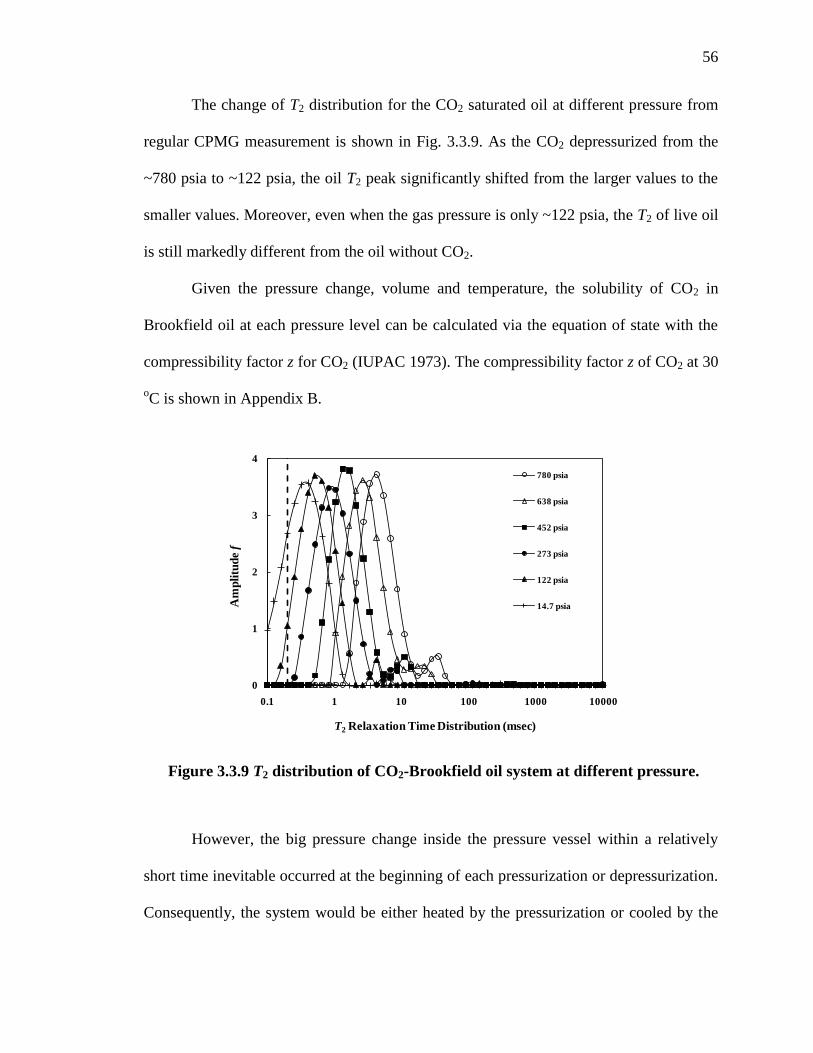
56
The change of T2 distribution for the CO2 saturated oil at different pressure from
regular CPMG measurement is shown in Fig. 3.3.9. As the CO2 depressurized from the
~780 psia to ~122 psia, the oil T2 peak significantly shifted from the larger values to the
smaller values. Moreover, even when the gas pressure is only ~122 psia, the T2 of live oil
is still markedly different from the oil without CO2.
Given the pressure change, volume and temperature, the solubility of CO2 in
Brookfield oil at each pressure level can be calculated via the equation of state with the
compressibility factor z for CO2 (IUPAC 1973). The compressibility factor z of CO2 at 30
oC is shown in Appendix B.
However, the big pressure change inside the pressure vessel within a relatively
short time inevitable occurred at the beginning of each pressurization or depressurization.
Consequently, the system would be either heated by the pressurization or cooled by the
Figure 3.3.9 T2 distribution of CO2-Brookfield oil system at different pressure.
0
1
2
3
4
0.1 1 10 100 1000 10000
Am
pli
tud
e f
T2 Relaxation Time Distribution (msec)
780 psia
638 psia
452 psia
273 psia
122 psia
14.7 psia
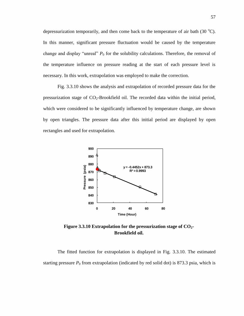
57
depressurization temporarily, and then come back to the temperature of air bath (30 oC).
In this manner, significant pressure fluctuation would be caused by the temperature
change and display “unreal” P0 for the solubility calculations. Therefore, the removal of
the temperature influence on pressure reading at the start of each pressure level is
necessary. In this work, extrapolation was employed to make the correction.
Fig. 3.3.10 shows the analysis and extrapolation of recorded pressure data for the
pressurization stage of CO2-Brookfield oil. The recorded data within the initial period,
which were considered to be significantly influenced by temperature change, are shown
by open triangles. The pressure data after this initial period are displayed by open
rectangles and used for extrapolation.
The fitted function for extrapolation is displayed in Fig. 3.3.10. The estimated
starting pressure P0 from extrapolation (indicated by red solid dot) is 873.3 psia, which is
y = -0.4452x + 873.3R² = 0.9993
830
840
850
860
870
880
890
900
0 20 40 60 80
Pre
ssu
re (
psia
)
Time (Hour)
Figure 3.3.10 Extrapolation for the pressurization stage of CO2-
Brookfield oil.

58
19 psi lower than the recorded pressure data right after the introduction of high pressure
CO2 (892.3 psia).
The similar analysis and extrapolation were also performed on the pressure data
recorded in the stage of depressurization and shown in Fig. 3.3.11. The extrapolation is
shown by solid line and the extrapolated value at each pressure level is highlighted by red
solid dot in each subplot. The points excluded from extrapolation are indicated by arrows
in each plot. The fitted functions and the R2 values are also displayed.
It is clearly shown that, with the additional effect of temperature rise-up after each
rapid depressurization, the pressure within the initial period (open triangles) increases
significantly faster than those thereafter (open rectangles).
y = 5.3975x + 616.1R² = 0.9852
600
610
620
630
640
0 5 10 15 20
Press
ure (
psi
a)
Time (Hour)
Peq = 638 psia
Excluded from extrapolation
y = 5.9202x + 420.3R² = 0.9969
410
420
430
440
450
460
0 5 10 15 20
Press
ure (
psi
a)
Time (Hour)
Peq = 452 psia
Excluded from extrapolation
y = 4.0857x + 97.8R² = 0.9793
80
90
100
110
120
130
0 5 10 15 20 25
Press
ure (
psi
a)
Time (Hour)
Peq = 122 psia
Excluded from extrapolation
y = 3.592x + 240.5R² = 0.9748
230
240
250
260
270
280
0 5 10 15 20
Press
ure (
psi
a)
Time (Hour)
Peq = 273 psia
Excluded from extrapolation
Figure 3.3.11 Extrapolations for the depressurization stage of CO2-oil at
different pressures
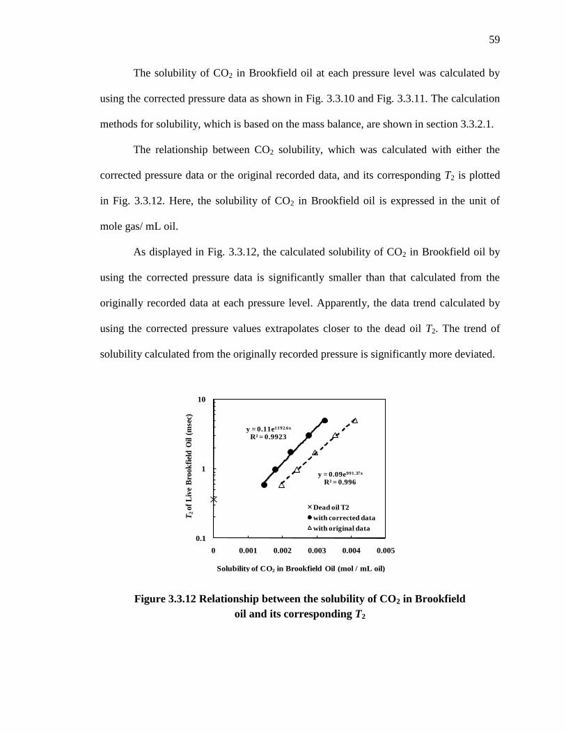
59
The solubility of CO2 in Brookfield oil at each pressure level was calculated by
using the corrected pressure data as shown in Fig. 3.3.10 and Fig. 3.3.11. The calculation
methods for solubility, which is based on the mass balance, are shown in section 3.3.2.1.
The relationship between CO2 solubility, which was calculated with either the
corrected pressure data or the original recorded data, and its corresponding T2 is plotted
in Fig. 3.3.12. Here, the solubility of CO2 in Brookfield oil is expressed in the unit of
mole gas/ mL oil.
As displayed in Fig. 3.3.12, the calculated solubility of CO2 in Brookfield oil by
using the corrected pressure data is significantly smaller than that calculated from the
originally recorded data at each pressure level. Apparently, the data trend calculated by
using the corrected pressure values extrapolates closer to the dead oil T2. The trend of
solubility calculated from the originally recorded pressure is significantly more deviated.
y = 0.11e1192.6x
R² = 0.9923
y = 0.09e991.37x
R² = 0.996
0.1
1
10
0 0.001 0.002 0.003 0.004 0.005
T2of
Liv
e B
rook
fiel
d O
il (
mse
c)
Solubility of CO2 in Brookfield Oil (mol / mL oil)
Dead oil T2
with corrected data
with original data
Figure 3.3.12 Relationship between the solubility of CO2 in Brookfield
oil and its corresponding T2

60
3.3.2.3 Recombined Live Brookfield Oil with CH4
In the case of CH4-Brookfield oil, the gas pressure inside the vessel was initially
raised to ~896 psia by injecting CH4 from the top of the pressure vessel. Then, the gas
source was cut off and no more gas was added into the system afterwards. The oil sample
volume was ~ 15 mL.
The pressure vessel was vertically placed in the 30 oC air bath after the
introduction of pressurized CH4. In this manner, only diffusion occurred between the gas
and oil. The T2 distribution of Brookfield oil with CH4 was measured as a function of
time and the results are displayed in Fig. 3.3.13.
As shown in Fig. 3.3.13, the position of live Brookfield oil peak does not
significantly change during the entire measurement for 168 hours. The extremely slow
dissolving of CH4 is due to the small diffusivity of CH4 into heavy oil (Zhang, Hyndman
0.0
0.5
1.0
1.5
2.0
2.5
3.0
3.5
4.0
4.5
0.1 1 10 100 1000 10000
Am
pli
tud
e f
T2 Relaxation Time Distribution (msec)
0hr
4hr
19hr
42hr
101hr
168hr
Figure 3.3.13 T2 distribution of Brookfield oil with CH4 as a function of
time in diffusion. Here, the sample temperature is 30 oC.
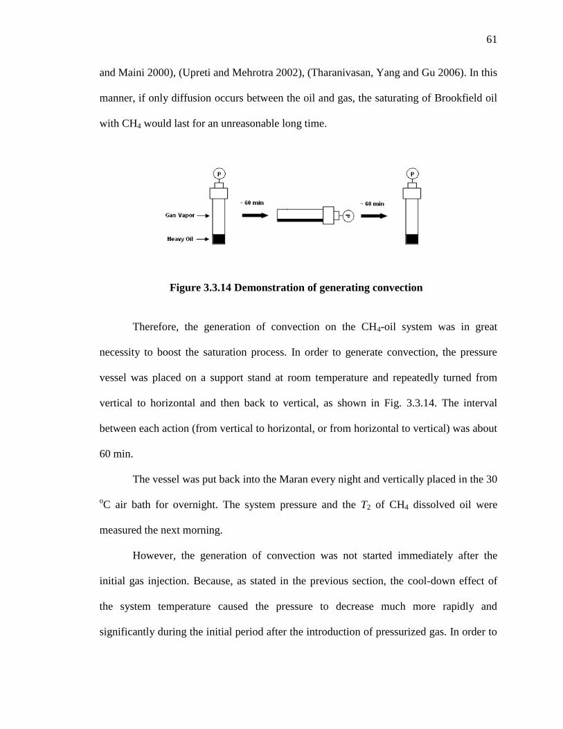
61
and Maini 2000), (Upreti and Mehrotra 2002), (Tharanivasan, Yang and Gu 2006). In this
manner, if only diffusion occurs between the oil and gas, the saturating of Brookfield oil
with CH4 would last for an unreasonable long time.
Therefore, the generation of convection on the CH4-oil system was in great
necessity to boost the saturation process. In order to generate convection, the pressure
vessel was placed on a support stand at room temperature and repeatedly turned from
vertical to horizontal and then back to vertical, as shown in Fig. 3.3.14. The interval
between each action (from vertical to horizontal, or from horizontal to vertical) was about
60 min.
The vessel was put back into the Maran every night and vertically placed in the 30
oC air bath for overnight. The system pressure and the T2 of CH4 dissolved oil were
measured the next morning.
However, the generation of convection was not started immediately after the
initial gas injection. Because, as stated in the previous section, the cool-down effect of
the system temperature caused the pressure to decrease much more rapidly and
significantly during the initial period after the introduction of pressurized gas. In order to
Figure 3.3.14 Demonstration of generating convection
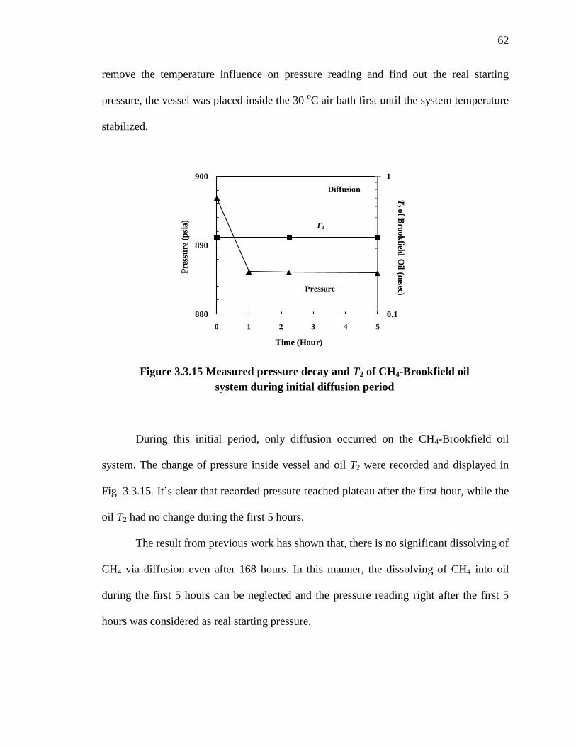
62
remove the temperature influence on pressure reading and find out the real starting
pressure, the vessel was placed inside the 30 oC air bath first until the system temperature
stabilized.
During this initial period, only diffusion occurred on the CH4-Brookfield oil
system. The change of pressure inside vessel and oil T2 were recorded and displayed in
Fig. 3.3.15. It’s clear that recorded pressure reached plateau after the first hour, while the
oil T2 had no change during the first 5 hours.
The result from previous work has shown that, there is no significant dissolving of
CH4 via diffusion even after 168 hours. In this manner, the dissolving of CH4 into oil
during the first 5 hours can be neglected and the pressure reading right after the first 5
hours was considered as real starting pressure.
0.1
1
880
890
900
0 1 2 3 4 5
T2
of B
roo
kfield
Oil (m
sec)P
ress
ure
(p
sia
)
Time (Hour)
Pressure
T2
Diffusion
Figure 3.3.15 Measured pressure decay and T2 of CH4-Brookfield oil
system during initial diffusion period
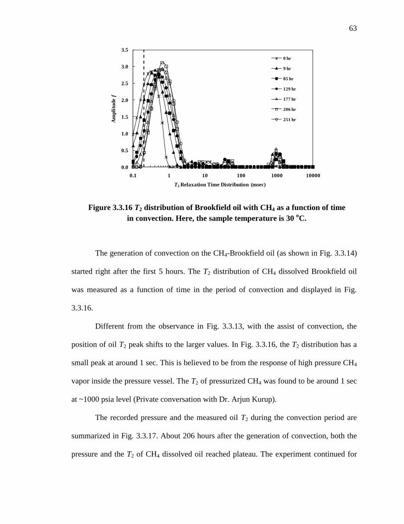
63
The generation of convection on the CH4-Brookfield oil (as shown in Fig. 3.3.14)
started right after the first 5 hours. The T2 distribution of CH4 dissolved Brookfield oil
was measured as a function of time in the period of convection and displayed in Fig.
3.3.16.
Different from the observance in Fig. 3.3.13, with the assist of convection, the
position of oil T2 peak shifts to the larger values. In Fig. 3.3.16, the T2 distribution has a
small peak at around 1 sec. This is believed to be from the response of high pressure CH4
vapor inside the pressure vessel. The T2 of pressurized CH4 was found to be around 1 sec
at ~1000 psia level (Private conversation with Dr. Arjun Kurup).
The recorded pressure and the measured oil T2 during the convection period are
summarized in Fig. 3.3.17. About 206 hours after the generation of convection, both the
pressure and the T2 of CH4 dissolved oil reached plateau. The experiment continued for
0.0
0.5
1.0
1.5
2.0
2.5
3.0
3.5
0.1 1 10 100 1000 10000
Am
pli
tud
e f
T2 Relaxation Time Distribution (msec)
0 hr
9 hr
85 hr
129 hr
177 hr
206 hr
251 hr
Figure 3.3.16 T2 distribution of Brookfield oil with CH4 as a function of time
in convection. Here, the sample temperature is 30 oC.
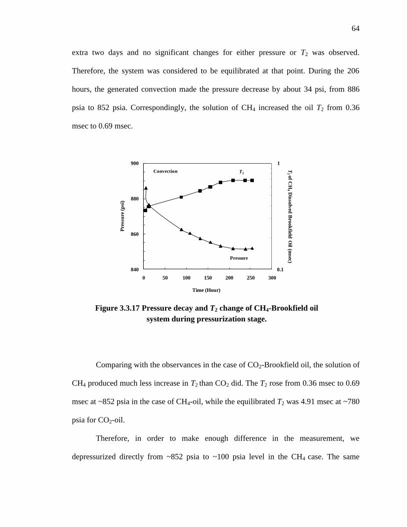
64
extra two days and no significant changes for either pressure or T2 was observed.
Therefore, the system was considered to be equilibrated at that point. During the 206
hours, the generated convection made the pressure decrease by about 34 psi, from 886
psia to 852 psia. Correspondingly, the solution of CH4 increased the oil T2 from 0.36
msec to 0.69 msec.
Comparing with the observances in the case of CO2-Brookfield oil, the solution of
CH4 produced much less increase in T2 than CO2 did. The T2 rose from 0.36 msec to 0.69
msec at ~852 psia in the case of CH4-oil, while the equilibrated T2 was 4.91 msec at ~780
psia for CO2-oil.
Therefore, in order to make enough difference in the measurement, we
depressurized directly from ~852 psia to ~100 psia level in the CH4 case. The same
0.1
1
840
860
880
900
0 50 100 150 200 250 300
T2
of C
H4
Disso
lved
Bro
ok
field O
il (msec)
Pre
ssu
re (
psi
)
Time (Hour)
Pressure
T2Convection
Figure 3.3.17 Pressure decay and T2 change of CH4-Brookfield oil
system during pressurization stage.
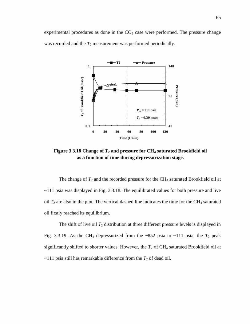
65
experimental procedures as done in the CO2 case were performed. The pressure change
was recorded and the T2 measurement was performed periodically.
The change of T2 and the recorded pressure for the CH4 saturated Brookfield oil at
~111 psia was displayed in Fig. 3.3.18. The equilibrated values for both pressure and live
oil T2 are also in the plot. The vertical dashed line indicates the time for the CH4 saturated
oil firstly reached its equilibrium.
The shift of live oil T2 distribution at three different pressure levels is displayed in
Fig. 3.3.19. As the CH4 depressurized from the ~852 psia to ~111 psia, the T2 peak
significantly shifted to shorter values. However, the T2 of CH4 saturated Brookfield oil at
~111 psia still has remarkable difference from the T2 of dead oil.
40
90
140
0.1
1
0 20 40 60 80 100 120
Pressu
re (p
sia)
T2
of
Bro
ok
field
Oil
(m
sec)
Time (Hour)
T2 Pressure
Peq = 111 psia
T2 = 0.39 msec
Figure 3.3.18 Change of T2 and pressure for CH4 saturated Brookfield oil
as a function of time during depressurization stage.
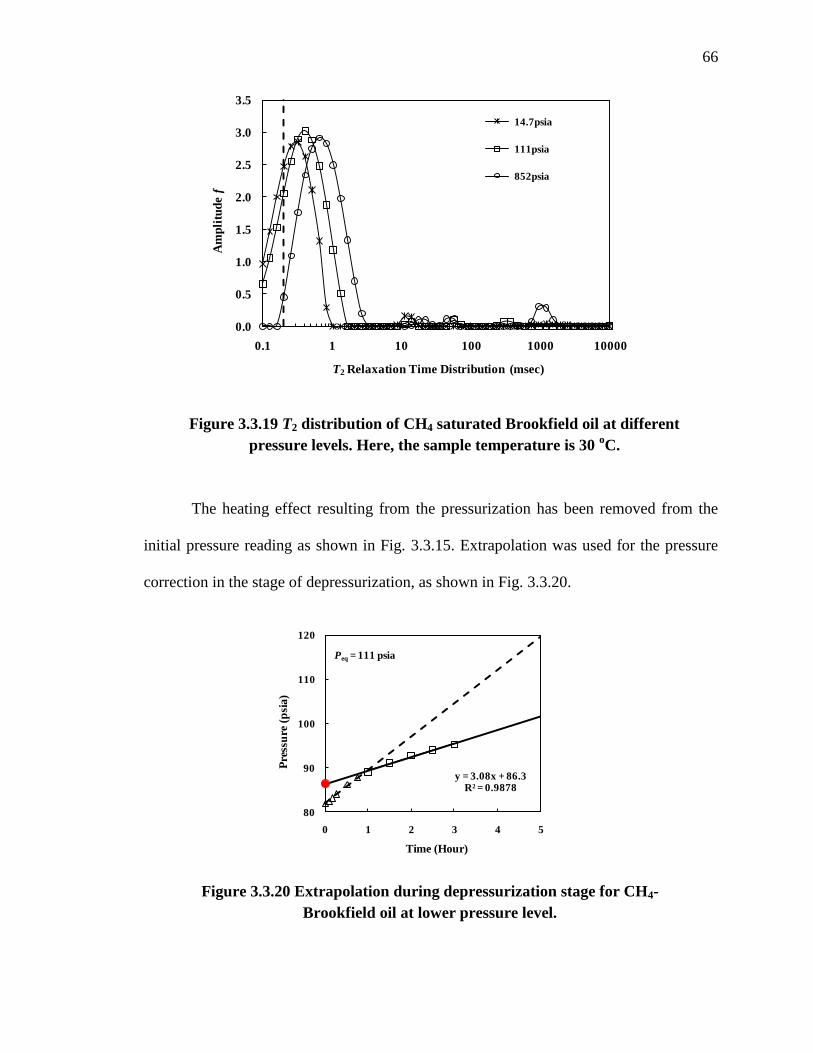
66
The heating effect resulting from the pressurization has been removed from the
initial pressure reading as shown in Fig. 3.3.15. Extrapolation was used for the pressure
correction in the stage of depressurization, as shown in Fig. 3.3.20.
y = 3.08x + 86.3R² = 0.9878
80
90
100
110
120
0 1 2 3 4 5
Pre
ssu
re (
psi
a)
Time (Hour)
Peq = 111 psia
Figure 3.3.20 Extrapolation during depressurization stage for CH4-
Brookfield oil at lower pressure level.
0.0
0.5
1.0
1.5
2.0
2.5
3.0
3.5
0.1 1 10 100 1000 10000
Am
pli
tud
e f
T2 Relaxation Time Distribution (msec)
14.7psia
111psia
852psia
Figure 3.3.19 T2 distribution of CH4 saturated Brookfield oil at different
pressure levels. Here, the sample temperature is 30 oC.
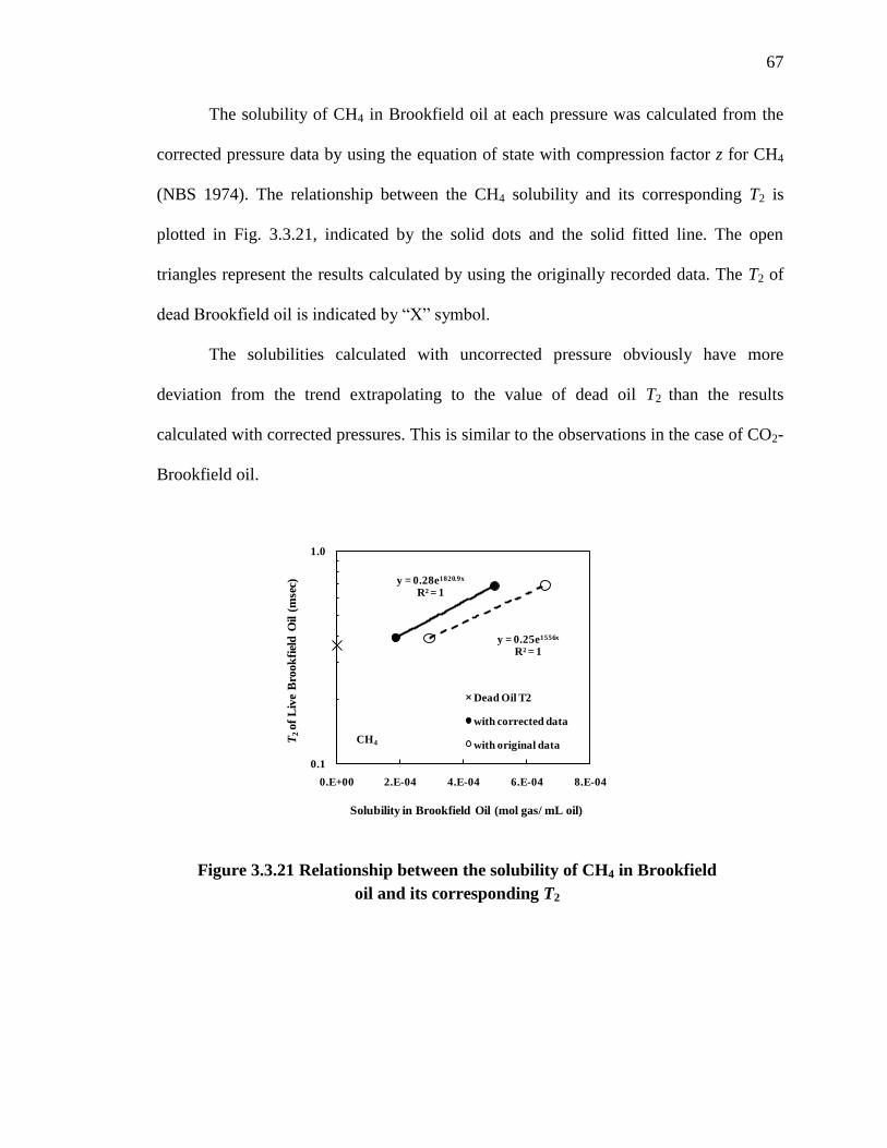
67
The solubility of CH4 in Brookfield oil at each pressure was calculated from the
corrected pressure data by using the equation of state with compression factor z for CH4
(NBS 1974). The relationship between the CH4 solubility and its corresponding T2 is
plotted in Fig. 3.3.21, indicated by the solid dots and the solid fitted line. The open
triangles represent the results calculated by using the originally recorded data. The T2 of
dead Brookfield oil is indicated by “X” symbol.
The solubilities calculated with uncorrected pressure obviously have more
deviation from the trend extrapolating to the value of dead oil T2 than the results
calculated with corrected pressures. This is similar to the observations in the case of CO2-
Brookfield oil.
y = 0.28e1820.9x
R² = 1
y = 0.25e1556x
R² = 1
0.1
1.0
0.E+00 2.E-04 4.E-04 6.E-04 8.E-04
T2
of
Liv
e B
roo
kfi
eld
Oil (
mse
c)
Solubility in Brookfield Oil (mol gas/ mL oil)
Dead Oil T2
with corrected data
with original dataCH4
Figure 3.3.21 Relationship between the solubility of CH4 in Brookfield
oil and its corresponding T2
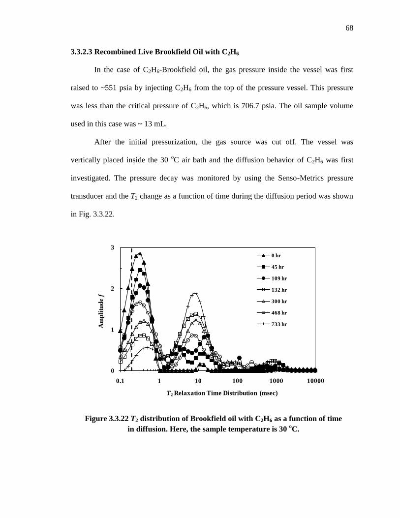
68
3.3.2.3 Recombined Live Brookfield Oil with C2H6
In the case of C2H6-Brookfield oil, the gas pressure inside the vessel was first
raised to ~551 psia by injecting C2H6 from the top of the pressure vessel. This pressure
was less than the critical pressure of C2H6, which is 706.7 psia. The oil sample volume
used in this case was ~ 13 mL.
After the initial pressurization, the gas source was cut off. The vessel was
vertically placed inside the 30 oC air bath and the diffusion behavior of C2H6 was first
investigated. The pressure decay was monitored by using the Senso-Metrics pressure
transducer and the T2 change as a function of time during the diffusion period was shown
in Fig. 3.3.22.
0
1
2
3
0.1 1 10 100 1000 10000
Am
pli
tud
e f
T2 Relaxation Time Distribution (msec)
0 hr
45 hr
109 hr
132 hr
300 hr
468 hr
733 hr
Figure 3.3.22 T2 distribution of Brookfield oil with C2H6 as a function of time
in diffusion. Here, the sample temperature is 30 oC.
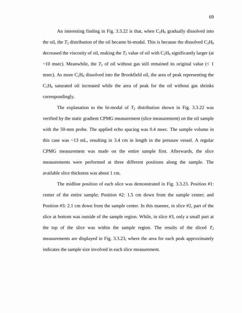
69
An interesting finding in Fig. 3.3.22 is that, when C2H6 gradually dissolved into
the oil, the T2 distribution of the oil became bi-modal. This is because the dissolved C2H6
decreased the viscosity of oil, making the T2 value of oil with C2H6 significantly larger (at
~10 msec). Meanwhile, the T2 of oil without gas still remained its original value (< 1
msec). As more C2H6 dissolved into the Brookfield oil, the area of peak representing the
C2H6 saturated oil increased while the area of peak for the oil without gas shrinks
correspondingly.
The explanation to the bi-modal of T2 distribution shown in Fig. 3.3.22 was
verified by the static gradient CPMG measurement (slice measurement) on the oil sample
with the 50-mm probe. The applied echo spacing was 0.4 msec. The sample volume in
this case was ~13 mL, resulting in 3.4 cm in length in the pressure vessel. A regular
CPMG measurement was made on the entire sample first. Afterwards, the slice
measurements were performed at three different positions along the sample. The
available slice thickness was about 1 cm.
The midline position of each slice was demonstrated in Fig. 3.3.23. Position #1:
center of the entire sample; Position #2: 1.5 cm down from the sample center; and
Position #3: 2.1 cm down from the sample center. In this manner, in slice #2, part of the
slice at bottom was outside of the sample region. While, in slice #3, only a small part at
the top of the slice was within the sample region. The results of the sliced T2
measurements are displayed in Fig. 3.3.23, where the area for each peak approximately
indicates the sample size involved in each slice measurement.
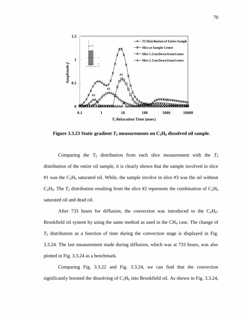
70
Comparing the T2 distribution from each slice measurement with the T2
distribution of the entire oil sample, it is clearly shown that the sample involved in slice
#1 was the C2H6 saturated oil. While, the sample involve in slice #3 was the oil without
C2H6. The T2 distribution resulting from the slice #2 represents the combination of C2H6
saturated oil and dead oil.
After 733 hours for diffusion, the convection was introduced to the C2H6-
Brookfield oil system by using the same method as used in the CH4 case. The change of
T2 distribution as a function of time during the convection stage is displayed in Fig.
3.3.24. The last measurement made during diffusion, which was at 733 hours, was also
plotted in Fig. 3.3.24 as a benchmark.
Comparing Fig. 3.3.22 and Fig. 3.3.24, we can find that the convection
significantly boosted the dissolving of C2H6 into Brookfield oil. As shown in Fig. 3.3.24,
Figure 3.3.23 Static gradient T2 measurements on C2H6 dissolved oil sample.
0
0.5
1
1.5
0.1 1 10 100 1000 10000
Am
pli
tud
e f
T2 Relaxation Time (msec)
T2 Distribution of Entire Sample
Slice at Sample Center
Slice 1.5cm Down from Center
Slice 2.1cm Down from Center
#2
#1
#3
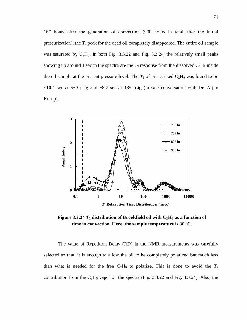
71
167 hours after the generation of convection (900 hours in total after the initial
pressurization), the T2 peak for the dead oil completely disappeared. The entire oil sample
was saturated by C2H6. In both Fig. 3.3.22 and Fig. 3.3.24, the relatively small peaks
showing up around 1 sec in the spectra are the T2 response from the dissolved C2H6 inside
the oil sample at the present pressure level. The T2 of pressurized C2H6 was found to be
~10.4 sec at 560 psig and ~8.7 sec at 485 psig (private conversation with Dr. Arjun
Kurup).
The value of Repetition Delay (RD) in the NMR measurements was carefully
selected so that, it is enough to allow the oil to be completely polarized but much less
than what is needed for the free C2H6 to polarize. This is done to avoid the T2
contribution from the C2H6 vapor on the spectra (Fig. 3.3.22 and Fig. 3.3.24). Also, the
0
1
2
3
0.1 1 10 100 1000 10000
Am
pli
tud
e f
T2 Relaxation Time Distribution (msec)
733 hr
757 hr
805 hr
900 hr
Figure 3.3.24 T2 distribution of Brookfield oil with C2H6 as a function of
time in convection. Here, the sample temperature is 30 oC.
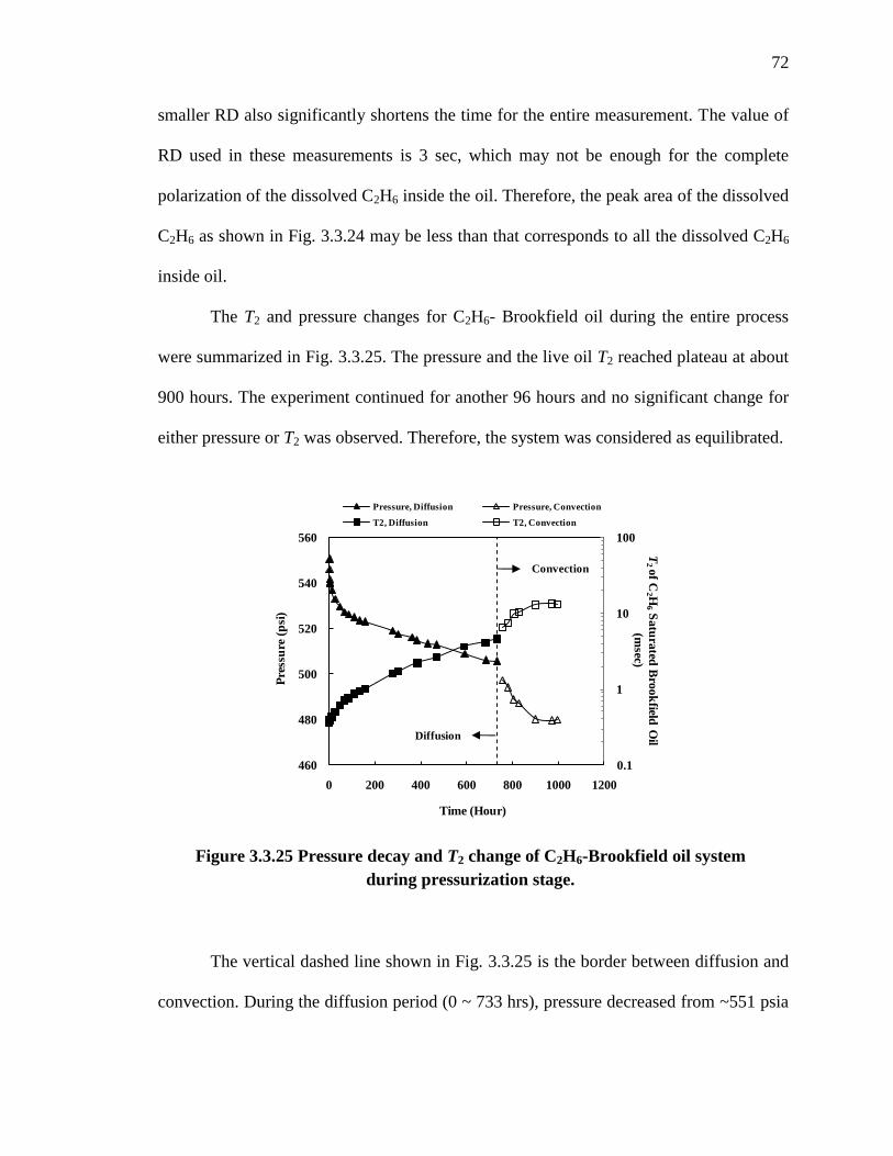
72
smaller RD also significantly shortens the time for the entire measurement. The value of
RD used in these measurements is 3 sec, which may not be enough for the complete
polarization of the dissolved C2H6 inside the oil. Therefore, the peak area of the dissolved
C2H6 as shown in Fig. 3.3.24 may be less than that corresponds to all the dissolved C2H6
inside oil.
The T2 and pressure changes for C2H6- Brookfield oil during the entire process
were summarized in Fig. 3.3.25. The pressure and the live oil T2 reached plateau at about
900 hours. The experiment continued for another 96 hours and no significant change for
either pressure or T2 was observed. Therefore, the system was considered as equilibrated.
The vertical dashed line shown in Fig. 3.3.25 is the border between diffusion and
convection. During the diffusion period (0 ~ 733 hrs), pressure decreased from ~551 psia
0.1
1
10
100
460
480
500
520
540
560
0 200 400 600 800 1000 1200
T2of C
2 H6
Sa
tura
ted B
roo
kfield
Oil
(msec)
Pre
ssu
re (
psi
)
Time (Hour)
Pressure, Diffusion Pressure, Convection
T2, Diffusion T2, Convection
Diffusion
Convection
Figure 3.3.25 Pressure decay and T2 change of C2H6-Brookfield oil system
during pressurization stage.
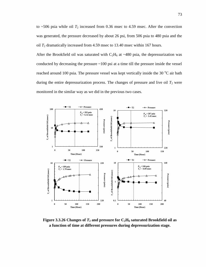
73
to ~506 psia while oil T2 increased from 0.36 msec to 4.59 msec. After the convection
was generated, the pressure decreased by about 26 psi, from 506 psia to 480 psia and the
oil T2 dramatically increased from 4.59 msec to 13.40 msec within 167 hours.
After the Brookfield oil was saturated with C2H6 at ~480 psia, the depressurization was
conducted by decreasing the pressure ~100 psi at a time till the pressure inside the vessel
reached around 100 psia. The pressure vessel was kept vertically inside the 30 oC air bath
during the entire depressurization process. The changes of pressure and live oil T2 were
monitored in the similar way as we did in the previous two cases.
220
320
1
10
0 50 100 150
Pressu
re (p
sia)
T2
of
Bro
ok
field
Oil
(m
sec)
Time (Hour)
T2 Pressure
Peq = 287 psiaT2 = 3.45 msec
330
430
1
10
100
0 50 100 150
Pressu
re (p
sia)
T2
of
Bro
ok
field
Oil
(m
sec)
Time (Hour)
T2 Pressure
Peq = 393 psiaT2 = 6.32 msec
120
220
1
10
0 50 100 150 200
Pressu
re (p
sia)
T2
of
Bro
ok
field
Oil
(m
sec)
Time (Hour)
T2 Pressure
Peq = 189 psiaT2 = 1.70 msec
40
140
0.1
1
10
0 50 100 150 200
Pressu
re (p
sia)
T2
of
Bro
ok
field
Oil
(m
sec)
Time (Hour)
T2 Pressure
Peq = 106 psiaT2 = 0.89 msec
Figure 3.3.26 Changes of T2 and pressure for C2H6 saturated Brookfield oil as
a function of time at different pressures during depressurization stage.

74
The measured T2 and recorded pressure change as a function of time for the C2H6
saturated Brookfield oil at four lower pressure levels were displayed in Fig. 3.3.26. The
equilibrated values for both pressure and live oil T2 at each pressure level are displayed in
each subplot, respectively. The vertical dashed lines in Fig. 3.3.26 indicate the time for
the C2H6 saturated oil firstly reached its equilibrium at each pressure level.
The T2 peak shift of C2H6 saturated oil at different pressures is clearly shown in
Fig. 3.3.27. As the C2H6 depressurized from the ~480 psia to ~106 psia, the T2 peak
significantly decreased. However, even when the equilibrium pressure was only ~106
psia, the C2H6 saturated Brookfield oil still had a T2 value of 0.89 msec, which is
markedly larger than the T2 of dead oil (0.36 msec).
0
1
2
3
0.1 1 10 100 1000 10000
Am
pli
tud
e f
T2 Relaxation Time Distribution (msec)
14.7 psia
106 psia
189 psia
287 psia
393 psia
480 psia
Figure 3.3.27 T2 distribution of C2H6 saturated Brookfield oil at different
pressure levels. Here, the sample temperature is 30 oC.

75
The T2 peak from the response of dissolved C2H6, which is around 1 sec at ~480
psia, shifted to the smaller values as equilibrium pressure decreases (as shown in Fig.
3.3.27). Meanwhile, the area of the dissolved C2H6 T2 peak shrinks as well, indicating the
decrease of dissolved amount of C2H6 inside oil sample.
The initial pressure P0 at each pressure level was corrected by extrapolation. The
analysis and extrapolation of recorded pressure data for C2H6-Brookfield oil during
pressurization stage is shown in Fig. 3.3.28. The similar extrapolations for the pressure
correction during depressurization stage are shown in Fig. 3.3.29. As shown in Fig.
3.3.28 and Fig. 3.3.29, the difference between the trend of pressure data within the initial
period (open triangles) and the later part (open rectangles) is marked for both
pressurization and depressurization. Due to the additional effect from temperature
variation, the pressure within the initial period changes significantly faster than that
thereafter.
y = -0.3244x + 540.5R² = 0.9951
520
530
540
550
560
0 5 10 15 20 25
Pre
ssu
re (
psi
a)
Time (Hour)
Figure 3.3.28 Extrapolation during pressurization stage for C2H6-oil.
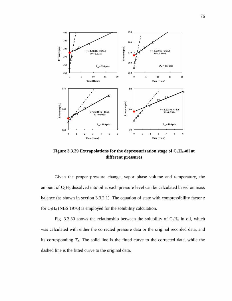
76
Given the proper pressure change, vapor phase volume and temperature, the
amount of C2H6 dissolved into oil at each pressure level can be calculated based on mass
balance (as shown in section 3.3.2.1). The equation of state with compressibility factor z
for C2H6 (NBS 1976) is employed for the solubility calculation.
Fig. 3.3.30 shows the relationship between the solubility of C2H6 in oil, which
was calculated with either the corrected pressure data or the original recorded data, and
its corresponding T2. The solid line is the fitted curve to the corrected data, while the
dashed line is the fitted curve to the original data.
y = 2.2414x + 155.5R² = 0.9955
150
160
170
0 1 2 3 4 5 6
Press
ure (
psi
a)
Time (Hour)
Peq = 189 psia
y = 1.6257x + 78.9R² = 0.9514
70
80
90
0 1 2 3 4 5 6
Press
ure (
psi
a)
Time (Hour)
Peq = 106 psia
y = 1.6301x + 267.2R² = 0.9608
250
260
270
280
290
0 5 10 15 20
Press
ure (
psi
a)
Time (Hour)
Peq = 287 psia
y = 1.3881x + 374.9R² = 0.9257
350
360
370
380
390
400
0 5 10 15 20
Press
ure (
psi
a)
Time (Hour)
Peq = 393 psia
Figure 3.3.29 Extrapolations for the depressurization stage of C2H6-oil at
different pressures
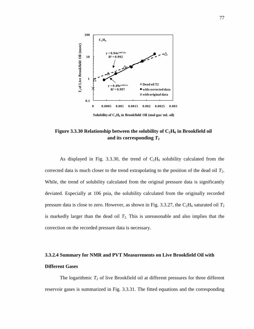
77
As displayed in Fig. 3.3.30, the trend of C2H6 solubility calculated from the
corrected data is much closer to the trend extrapolating to the position of the dead oil T2.
While, the trend of solubility calculated from the original pressure data is significantly
deviated. Especially at 106 psia, the solubility calculated from the originally recorded
pressure data is close to zero. However, as shown in Fig. 3.3.27, the C2H6 saturated oil T2
is markedly larger than the dead oil T2. This is unreasonable and also implies that the
correction on the recorded pressure data is necessary.
3.3.2.4 Summary for NMR and PVT Measurements on Live Brookfield Oil with
Different Gases
The logarithmic T2 of live Brookfield oil at different pressures for three different
reservoir gases is summarized in Fig. 3.3.31. The fitted equations and the corresponding
y = 0.49e1404.3x
R² = 0.997
y = 0.94e1007.8x
R² = 0.992
0.1
1
10
100
0 0.0005 0.001 0.0015 0.002 0.0025 0.003
T2
of
Liv
e B
rook
fiel
d O
il (
mse
c)
Solubility of C2H6 in Brookfield Oil (mol gas/ mL oil)
Dead oil T2
with corrected data
with original data
C2H6
Figure 3.3.30 Relationship between the solubility of C2H6 in Brookfield oil
and its corresponding T2
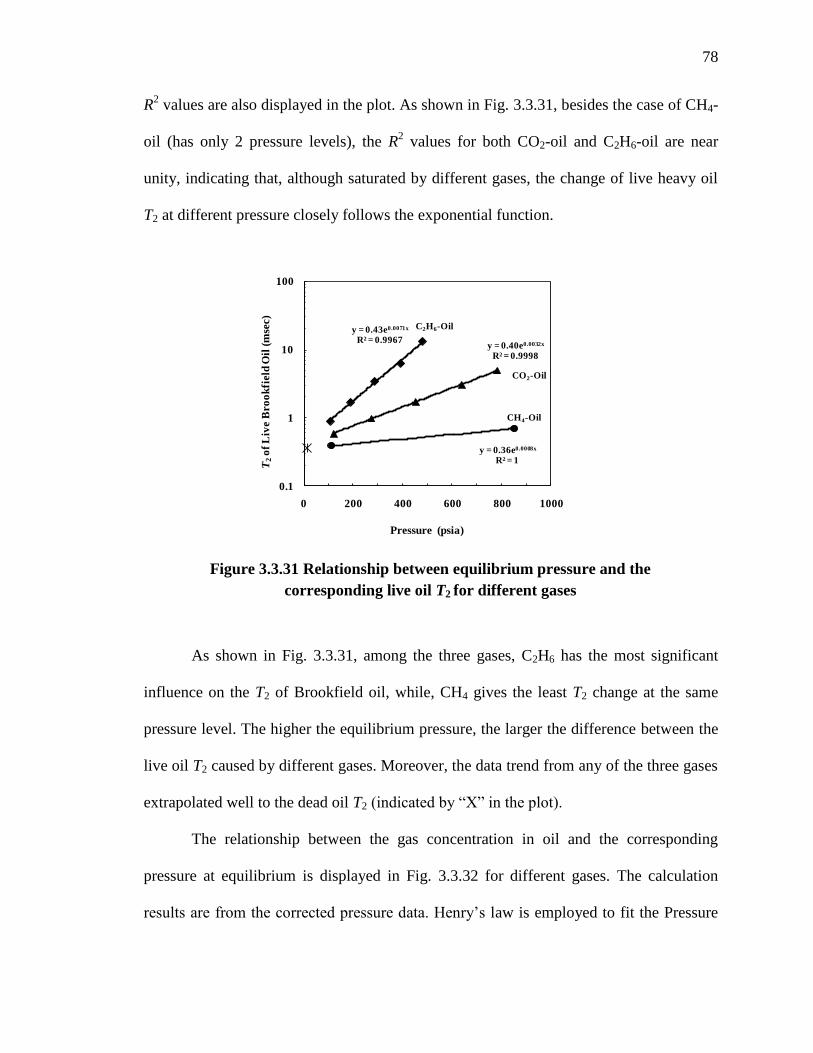
78
R2 values are also displayed in the plot. As shown in Fig. 3.3.31, besides the case of CH4-
oil (has only 2 pressure levels), the R2 values for both CO2-oil and C2H6-oil are near
unity, indicating that, although saturated by different gases, the change of live heavy oil
T2 at different pressure closely follows the exponential function.
As shown in Fig. 3.3.31, among the three gases, C2H6 has the most significant
influence on the T2 of Brookfield oil, while, CH4 gives the least T2 change at the same
pressure level. The higher the equilibrium pressure, the larger the difference between the
live oil T2 caused by different gases. Moreover, the data trend from any of the three gases
extrapolated well to the dead oil T2 (indicated by “X” in the plot).
The relationship between the gas concentration in oil and the corresponding
pressure at equilibrium is displayed in Fig. 3.3.32 for different gases. The calculation
results are from the corrected pressure data. Henry’s law is employed to fit the Pressure
y = 0.43e0.0071x
R² = 0.9967y = 0.40e0.0032x
R² = 0.9998
y = 0.36e0.0008x
R² = 1
0.1
1
10
100
0 200 400 600 800 1000
T2
of
Liv
e B
ro
ok
field
Oil
(m
sec)
Pressure (psia)
CO2-Oil
CH4-Oil
C2H6-Oil
Figure 3.3.31 Relationship between equilibrium pressure and the
corresponding live oil T2 for different gases

79
vs. Gas Concentration data and the estimated Henry’s constant for each gas in the
Brookfield oil is displayed by the corresponding fitted function in the plot.
As shown in Fig. 3.3.32(a), the calculated solubility values in the cases of C2H6-
oil and CH4-oil follow the Henry’s law well. However, the originally calculated solubility
of CO2 is significantly deviated. The extrapolation of the CO2 data does not pass the
origin. Instead, at x-axis (y = 0), it has an intercept of 0.00109 mol gas/mL oil (indicated
by the red solid dot).
The proposed explanation for this phenomenon is that, during the pressurization
stage in the case of CO2-oil (~800 psia at 30 oC), besides the original two phases (vapor
CO2 and liquid oil), a third phase, which is CO2-rich liquid with presence of heavy-
hydrocarbon components, may be formed inside the CO2-heavy oil system. The L-L-V
three-phase-equilibrium has been observed in both CO2/Alkane system (Orr, Yu and Lien
C2H6-Oily = 209478xR² = 0.9916
0
100
200
300
400
500
600
700
800
900
0.E+00 1.E-03 2.E-03 3.E-03 4.E-03
Pre
ssu
re
at
Eq
uilib
riu
m (
pis
a)
Gas Concentration in Brookfield Oil (mol gas/ mL oil)
CH4-Oil
C2H6-Oil
CO2-Oil
Intercept
CH4-Oily = 1568119x
R2 = 0.86
CO2-Oily = 373435x - 407.24
R2 = 0.9931
C2H6-Oily = 209478x
R² = 0.9916
0
100
200
300
400
500
600
700
800
900
0.E+00 1.E-03 2.E-03 3.E-03 4.E-03
Pre
ssu
re
at
Eq
uilib
riu
m (
pis
a)
Gas Concentration in Brookfield Oil (mol gas/ mL oil)
CH4-Oil
C2H6-Oil
Corrected CO2-Oil
CH4-Oily = 1568119x
R2 = 0.86
Corrected CO2-Oily = 373435xR2 = 0.9931
(a) (b)
Figure 3.3.32 Relationship between the gas concentration in Brookfield oil and the
equilibrated pressures. Here, (a) solubility data in the case of CO2-Oil is deviated from
Henry’s law; (b) solubility data for CO2-Oil is corrected to follow Henry’s law.
80
1981), (Enick, Holder and Morsi 1985) and CO2/Crude oil system (Orr, Yu and Lien
1981) (Syegh, et al. 1990) at near-critical condition. The extraction of heavy hydrocarbon
components (as heavy as C24) into CO2-rich phase was reported by Orr et al. (Orr, Yu and
Lien 1981). More importantly, the three phases coexisting was found to be able to form
more easily with heavier component in the CO2/oil binary mixture (Orr, Yu and Lien
1981).
During the pressurization stage of CO2-oil system in this study, after the injection
of the pressurized CO2 was ceased, the stripping of hydrocarbons from the oil by CO2 and
the dissolving of CO2 into oil occurred simultaneously. As more heavy-hydrocarbon
components present in the CO2 vapor phase, a CO2-rich liquid phase could have
gradually formed inside the pressure vessel. However, simply by monitoring the pressure
change in vapor phase, we cannot tell the difference between the pressure decay from the
dissolving of CO2 into oil and the pressure decay caused by the condensation of CO2 into
the CO2-rich liquid phase.
The recorded pressure decay due to the condensation of CO2 in the second liquid
phase was mistaken as that caused by the solution of CO2 into the oil phase. As a result,
the calculated solubility of CO2 at the highest pressure level could be significantly larger
than its “true” value.
Subsequently, as the pressure decreases, the CO2-oil system moved away from the
three phases coexisting region, and the data for the pressure difference at each lower
pressure level could be obtained properly. However, based on the method for solubility
calculation in this work (as shown in section 3.3.2.1), any impact on the solubility at the
highest pressure will uniformly affect the calculation of solubility at each lower pressure.
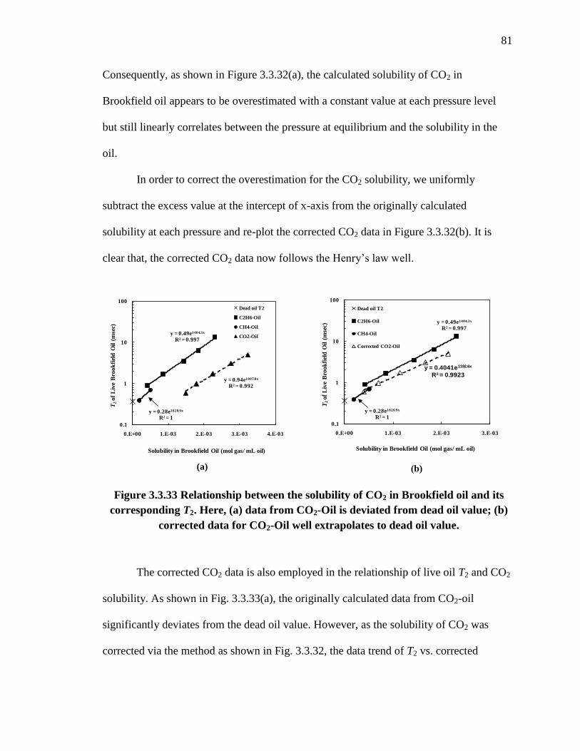
81
Consequently, as shown in Figure 3.3.32(a), the calculated solubility of CO2 in
Brookfield oil appears to be overestimated with a constant value at each pressure level
but still linearly correlates between the pressure at equilibrium and the solubility in the
oil.
In order to correct the overestimation for the CO2 solubility, we uniformly
subtract the excess value at the intercept of x-axis from the originally calculated
solubility at each pressure and re-plot the corrected CO2 data in Figure 3.3.32(b). It is
clear that, the corrected CO2 data now follows the Henry’s law well.
The corrected CO2 data is also employed in the relationship of live oil T2 and CO2
solubility. As shown in Fig. 3.3.33(a), the originally calculated data from CO2-oil
significantly deviates from the dead oil value. However, as the solubility of CO2 was
corrected via the method as shown in Fig. 3.3.32, the data trend of T2 vs. corrected
Figure 3.3.33 Relationship between the solubility of CO2 in Brookfield oil and its
corresponding T2. Here, (a) data from CO2-Oil is deviated from dead oil value; (b)
corrected data for CO2-Oil well extrapolates to dead oil value.
y = 0.49e1404.3x
R² = 0.997
y = 0.28e1820.9x
R² = 1
y = 0.94e1007.8x
R² = 0.992
0.1
1
10
100
0.E+00 1.E-03 2.E-03 3.E-03 4.E-03
T2
of
Liv
e B
roo
kfi
eld
Oil (
mse
c)
Solubility in Brookfield Oil (mol gas/ mL oil)
Dead oil T2
C2H6-Oil
CH4-Oil
CO2-Oil
y = 0.49e1404.3x
R² = 0.997
y = 0.28e1820.9x
R² = 1
y = 0.4041e1192.6x
R² = 0.9923
0.1
1
10
100
0.E+00 1.E-03 2.E-03 3.E-03
T2
of
Liv
e B
roo
kfi
eld
Oil (
mse
c)
Solubility in Brookfield Oil (mol gas/ mL oil)
Dead oil T2
C2H6-Oil
CH4-Oil
Corrected CO2-Oil
(a) (b)
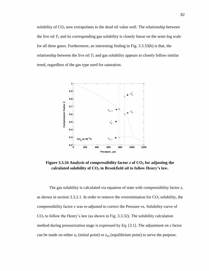
82
solubility of CO2 now extrapolates to the dead oil value well. The relationship between
the live oil T2 and its corresponding gas solubility is closely linear on the semi-log scale
for all three gases. Furthermore, an interesting finding in Fig. 3.3.33(b) is that, the
relationship between the live oil T2 and gas solubility appears to closely follow similar
trend, regardless of the gas type used for saturation.
The gas solubility is calculated via equation of state with compressibility factor z,
as shown in section 3.3.2.1. In order to remove the overestimation for CO2 solubility, the
compressibility factor z was re-adjusted to correct the Pressure vs. Solubility curve of
CO2 to follow the Henry’s law (as shown in Fig. 3.3.32). The solubility calculation
method during pressurization stage is expressed by Eq. [3.1]. The adjustment on z factor
can be made on either z0 (initial point) or zeq (equilibrium point) to serve the purpose.
0 200 400 600 800 1000 12000.2
0.3
0.4
0.5
0.6
0.7
0.8
0.9
1
Pressure, psi
Co
mp
ressio
n F
acto
r Z
z0
z0*
ze*
CO2 at 30 oC z
e, l
ze,
v
Figure 3.3.34 Analysis of compressibility factor z of CO2 for adjusting the
calculated solubility of CO2 in Brookfield oil to follow Henry’s law.
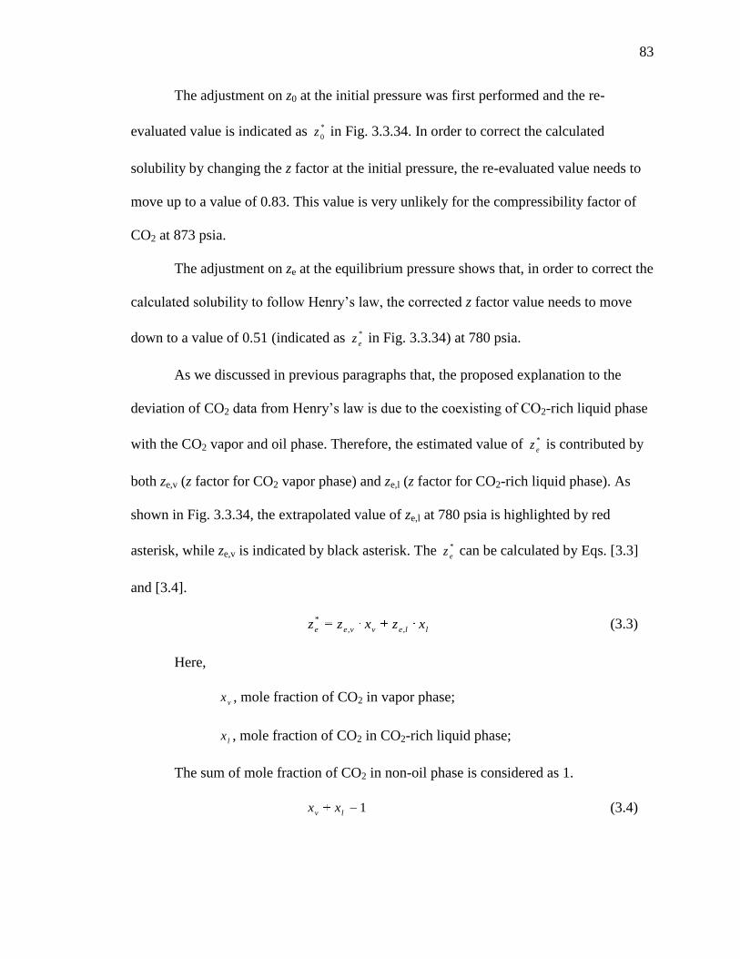
83
The adjustment on z0 at the initial pressure was first performed and the re-
evaluated value is indicated as *
0z in Fig. 3.3.34. In order to correct the calculated
solubility by changing the z factor at the initial pressure, the re-evaluated value needs to
move up to a value of 0.83. This value is very unlikely for the compressibility factor of
CO2 at 873 psia.
The adjustment on ze at the equilibrium pressure shows that, in order to correct the
calculated solubility to follow Henry’s law, the corrected z factor value needs to move
down to a value of 0.51 (indicated as *
ez in Fig. 3.3.34) at 780 psia.
As we discussed in previous paragraphs that, the proposed explanation to the
deviation of CO2 data from Henry’s law is due to the coexisting of CO2-rich liquid phase
with the CO2 vapor and oil phase. Therefore, the estimated value of *
ez is contributed by
both ze,v (z factor for CO2 vapor phase) and ze,l (z factor for CO2-rich liquid phase). As
shown in Fig. 3.3.34, the extrapolated value of ze,l at 780 psia is highlighted by red
asterisk, while ze,v is indicated by black asterisk. The *
ez can be calculated by Eqs. [3.3]
and [3.4].
llevveexzxzz
,,
* (3.3)
Here,
vx , mole fraction of CO2 in vapor phase;
lx , mole fraction of CO2 in CO2-rich liquid phase;
The sum of mole fraction of CO2 in non-oil phase is considered as 1.
1lv
xx (3.4)

84
Given the values for all three z factors shown in Eq. [3.3] and combining Eq. [3.3]
and Eq. [3.4], the mole fraction of CO2 in vapor phase and CO2 in CO2-rich liquid phase
can be calculated. The calculated mole fraction of CO2 in vapor phase is 0.58,
correspondingly, the mole fraction in CO2-rich liquid phase is 0.42.
Here, on basis of the available data in the reference book (IUPAC 1973), the
estimated density for CO2 vapor is ~0.1431 g/mL and the density for CO2-rich liquid is
~0.5421 g/mL. In this manner, the volume fraction of CO2 in either vapor phase or CO2-
rich liquid phase is calculated to be 0.84 and 0.16, respectively.
3.3.2.5 Viscosity Measurements on Live Brookfield Oil
The viscosity of live Brookfield oil with different gases was measured at different
pressures by using the capillary viscometer. All the measurements on the live oil were
performed at room temperature (22 oC). The relationship between fluid viscosity and the
flow rate, measured pressure drop and the tube dimension is governed by the Hagen-
Poiseuille equation as below:
LQ
RPPL
8
)(4
0 (3.5)
Here, is oil viscosity, Q is flow rate, L is length of tube, R is inner radius of the tube.
The setup of the capillary viscometer used in this work is demonstrated in Fig.
3.3.35. The tubing used for measuring the viscosity is the Swagelok 1/8” stainless tubing,
which has 14.9 cm in length and 0.175 cm in I.D. The transfer vessel at the bottom in the
setup shown in Fig. 3.3.35 was manufactured by TEMCO. The ISCO pump was
85
employed to drive the fluid to flow. The pressure rating of the transducer used in this case
is 200 psi
The capillary viscometer was first tested with dead Brookfield oil at four different
flow rates. The average value obtained by using the capillary viscometer was 468,996 cP
at room temperature. Meanwhile, the viscosity measured by Brookfield viscometer at the
same temperature was 481,000 cP, which had only ~2.5% difference from the average
value from the capillary viscometer.
The viscosity of live Brookfield oil saturated by C2H6 was measured at five
different pressure levels. Meanwhile, in the case of either CO2-oil or CH4 oil, the live oil
viscosity measurement was performed at one pressure level for each. The measured
viscosity values of Brookfield oil under different conditions are summarized in Table
3.3.2.
Figure 3.3.35 Setup of capillary viscometer.
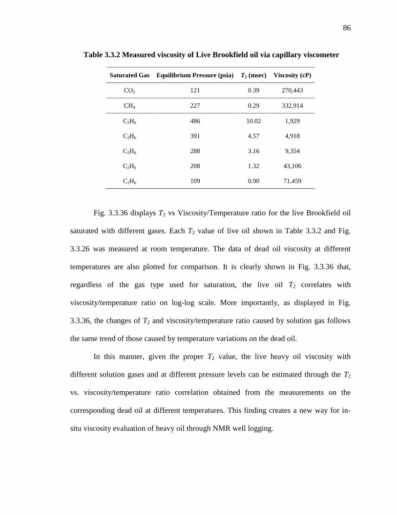
86
Fig. 3.3.36 displays T2 vs Viscosity/Temperature ratio for the live Brookfield oil
saturated with different gases. Each T2 value of live oil shown in Table 3.3.2 and Fig.
3.3.26 was measured at room temperature. The data of dead oil viscosity at different
temperatures are also plotted for comparison. It is clearly shown in Fig. 3.3.36 that,
regardless of the gas type used for saturation, the live oil T2 correlates with
viscosity/temperature ratio on log-log scale. More importantly, as displayed in Fig.
3.3.36, the changes of T2 and viscosity/temperature ratio caused by solution gas follows
the same trend of those caused by temperature variations on the dead oil.
In this manner, given the proper T2 value, the live heavy oil viscosity with
different solution gases and at different pressure levels can be estimated through the T2
vs. viscosity/temperature ratio correlation obtained from the measurements on the
corresponding dead oil at different temperatures. This finding creates a new way for in-
situ viscosity evaluation of heavy oil through NMR well logging.
Saturated Gas Equilibrium Pressure (psia) T2 (msec) Viscosity (cP)
CO2 121 0.39 270,443
CH4 227 0.29 332,914
C2H6 486 10.02 1,929
C2H6 391 4.57 4,918
C2H6 288 3.16 9,354
C2H6 208 1.32 43,106
C2H6 109 0.90 71,459
Table 3.3.2 Measured viscosity of Live Brookfield oil via capillary viscometer
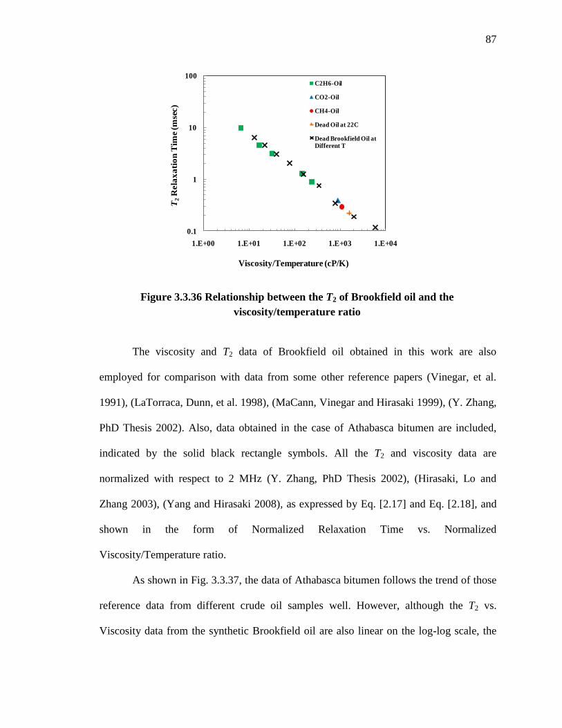
87
The viscosity and T2 data of Brookfield oil obtained in this work are also
employed for comparison with data from some other reference papers (Vinegar, et al.
1991), (LaTorraca, Dunn, et al. 1998), (MaCann, Vinegar and Hirasaki 1999), (Y. Zhang,
PhD Thesis 2002). Also, data obtained in the case of Athabasca bitumen are included,
indicated by the solid black rectangle symbols. All the T2 and viscosity data are
normalized with respect to 2 MHz (Y. Zhang, PhD Thesis 2002), (Hirasaki, Lo and
Zhang 2003), (Yang and Hirasaki 2008), as expressed by Eq. [2.17] and Eq. [2.18], and
shown in the form of Normalized Relaxation Time vs. Normalized
Viscosity/Temperature ratio.
As shown in Fig. 3.3.37, the data of Athabasca bitumen follows the trend of those
reference data from different crude oil samples well. However, although the T2 vs.
Viscosity data from the synthetic Brookfield oil are also linear on the log-log scale, the
0.1
1
10
100
1.E+00 1.E+01 1.E+02 1.E+03 1.E+04
T2
Rela
xa
tio
n T
ime
(mse
c)
Viscosity/Temperature (cP/K)
C2H6-Oil
CO2-Oil
CH4-Oil
Dead Oil at 22C
Dead Brookfield Oil at Different T
Figure 3.3.36 Relationship between the T2 of Brookfield oil and the
viscosity/temperature ratio
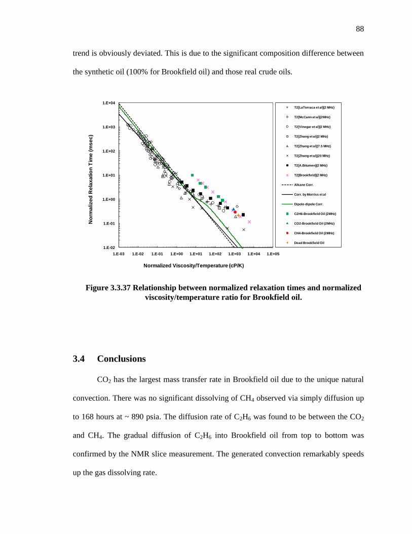
88
trend is obviously deviated. This is due to the significant composition difference between
the synthetic oil (100% for Brookfield oil) and those real crude oils.
3.4 Conclusions
CO2 has the largest mass transfer rate in Brookfield oil due to the unique natural
convection. There was no significant dissolving of CH4 observed via simply diffusion up
to 168 hours at ~ 890 psia. The diffusion rate of C2H6 was found to be between the CO2
and CH4. The gradual diffusion of C2H6 into Brookfield oil from top to bottom was
confirmed by the NMR slice measurement. The generated convection remarkably speeds
up the gas dissolving rate.
1.E-02
1.E-01
1.E+00
1.E+01
1.E+02
1.E+03
1.E+04
1.E-03 1.E-02 1.E-01 1.E+00 1.E+01 1.E+02 1.E+03 1.E+04 1.E+05
No
rma
lize
d R
ela
xa
tio
n T
ime
(m
se
c)
Normalized Viscosity/Temperature (cP/K)
T2[LaTorraca et al](2 MHz)
T2[McCann et al](2MHz)
T2[Vinegar et al](2 MHz)
T2[Zhang et al](2 MHz)
T2[Zhang et al](7.5 MHz)
T2[Zhang et al](20 MHz)
T2[A.Bitumen](2 MHz)
T2[Brookfield](2 MHz)
Alkane Corr.
Corr. by Morriss et al
Dipole-dipole Corr.
C2H6-Brookfield Oil (2MHz)
CO2-Brookfield Oil (2MHz)
CH4-Brookfield Oil (2MHz)
Dead Brookfield Oil
Figure 3.3.37 Relationship between normalized relaxation times and normalized
viscosity/temperature ratio for Brookfield oil.
89
The live oil T2 is significantly larger than T2 of dead oil, even at the lowest
pressure level in this work (~100 psia). The relationship between the equilibrium pressure
and the live oil T2 is found to be closely linear on semi-log scale for all three reservoir
gases.
The originally recorded pressure data for all the three gases (CO2, CH4 and C2H6)
were analyzed. In order to remove the temperature influence on pressure reading and
estimate the real starting pressure, extrapolation was employed to correct the recorded
pressure data within the initial period after each pressurization or depressurization.
The solubility in Brookfield oil for all the three gases (CO2, CH4 and C2H6) were
calculated by using the corrected pressure data. The dissolving of both CH4 and C2H6 in
Brookfield oil is found to follow the Henry’s law well. However, the observed dissolving
behavior of CO2 in Brookfield oil is significantly deviated.
The relationship between the calculated gas solubility and the corresponding live
oil T2 is found to be closely linear on a semi-log scale for all three reservoir gases.
Regardless of the gas type used for saturation, the live oil T2 correlates with
viscosity/temperature ratio on log-log scale. Moreover, the changes of T2 and
viscosity/temperature ratio caused by solution gas follows the same trend of those caused
by temperature variations on the dead oil. This creates a new way for in-situ viscosity
evaluation of heavy oil through NMR well logging.

90
Chapter 4 NMR Measurement and Viscosity Evaluation of Live
Bitumen
4.1 Introduction
The viscosity evaluation and the laboratory NMR measurements of the
recombined live Brookfield oil have been discussed in Chapter 3. The effects of three
major reservoir gases (CH4, CO2, and C2H6) on the changes of viscosity and T2 of this
synthetic oil were investigated under a series of saturation pressures. However, at the end
of Chapter 3, Fig. 3.3.35 showed the deviation of the synthetic Brookfield oil data from
the trend of those crude oil data due to the composition difference.
In this chapter, a new crude bitumen sample #10-19, provided by Shell E&P
Company, was employed for all the investigations. Similar experimental procedures as
mentioned in Chapter 3 were used for all the NMR, PVT and viscosity measurements on
the bitumen #10-19 sample. The correlations among the saturation pressure, gas
solubility, NMR T2 and live bitumen viscosity for the bitumen are established in this
chapter. Comparisons will be made between the data obtained from the investigations on
bitumen sample and the results shown in the case of Brookfield oil.

91
4.2 Equipment and Experimental Procedures
The nuclear magnetic resonance (NMR) spectrometer (Maran-M), the NMR
probes and the pressure vessel used in this work on bitumen #10-19 were the same as
those employed for the Brookfield oil in Chapter 3.
The heavy oil sample used in this part of work is the bitumen sample #10-19,
provided by the Shell Oil Company. The properties of this crude bitumen sample will be
discussed in the following sections.
The three reservoir gases (CO2, CH4 and C2H6) used in this case are provided by
Matheson Tri-Gas with product grade of Ultra High Purity.
4.3 Results
4.3.1 Characterization of Bitumen #10-19 at Different Temperatures
The same techniques we mentioned in Chapter 2 and Chapter 3 were employed to
characterize the viscosity and NMR properties of the bitumen #10-19 sample at different
temperatures.
4.3.1.1 Viscosity of Bitumen #10-19 at Different Temperatures
The viscosity of the bitumen #10-19 at different temperature was measured by
using the Brookfield viscometer LVDV-III+. The sample temperature was controlled by
an oil bath (HAAKE K35) connected to the viscometer sample holder. The oil sample
was measured from 10 oC to 90
oC. The viscosity changes with temperature of Athabasca

92
bitumen and Brookfield oil are used to compare with the results from bitumen #10-19.
The measurement results are shown in Fig. 4.3.1 as below.
As shown in Fig. 4.3.1, on the semi-logarithmic scale, all the three heavy oils
closely follow linear relationship between viscosity and reciprocal of sample temperature.
The viscosity of bitumen #10-19 (indicated by solid dots) is generally higher than that of
Athabasca bitumen at each temperature. The correlation equation for the result of
bitumen #10-19 is displayed in the plot. It is clearly shown that, as crude oils, the
experimental results of bitumen #10-19 and Athabasca bitumen follow the similar trend,
while the results from Brookfield oil are apparently deviated.
Due to the limit of Brookfield viscometer LVDV-III+, the lowest temperature that
the viscosity measurement can be performed on bitumen #10-19 was 20 oC. When the
sample temperature was further lowered to 10 oC, the viscosity of the bitumen was
y = 5E-12e11805x
R² = 0.9946
1.E+02
1.E+03
1.E+04
1.E+05
1.E+06
1.E+07
2.5E-03 3.0E-03 3.5E-03 4.0E-03
Vis
co
sity
(cP
)
1/ Temperature (1/K)
Bitumen #10-19
Athabasca bitumen
Brookfield oil
Figure 4.3.1 Viscosity of bitumen #10-19 at different temperatures
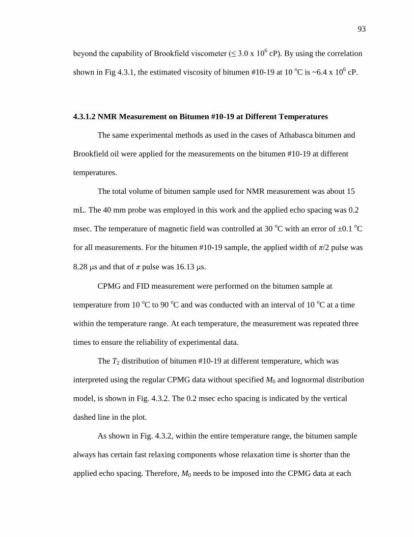
93
beyond the capability of Brookfield viscometer (≤ 3.0 x 10⁶ cP). By using the correlation
shown in Fig 4.3.1, the estimated viscosity of bitumen #10-19 at 10 oC is ~6.4 x 10
6 cP.
4.3.1.2 NMR Measurement on Bitumen #10-19 at Different Temperatures
The same experimental methods as used in the cases of Athabasca bitumen and
Brookfield oil were applied for the measurements on the bitumen #10-19 at different
temperatures.
The total volume of bitumen sample used for NMR measurement was about 15
mL. The 40 mm probe was employed in this work and the applied echo spacing was 0.2
msec. The temperature of magnetic field was controlled at 30 oC with an error of ±0.1
oC
for all measurements. For the bitumen #10-19 sample, the applied width of π/2 pulse was
8.28 s and that of π pulse was 16.13 s.
CPMG and FID measurement were performed on the bitumen sample at
temperature from 10 oC to 90
oC and was conducted with an interval of 10
oC at a time
within the temperature range. At each temperature, the measurement was repeated three
times to ensure the reliability of experimental data.
The T2 distribution of bitumen #10-19 at different temperature, which was
interpreted using the regular CPMG data without specified M0 and lognormal distribution
model, is shown in Fig. 4.3.2. The 0.2 msec echo spacing is indicated by the vertical
dashed line in the plot.
As shown in Fig. 4.3.2, within the entire temperature range, the bitumen sample
always has certain fast relaxing components whose relaxation time is shorter than the
applied echo spacing. Therefore, M0 needs to be imposed into the CPMG data at each
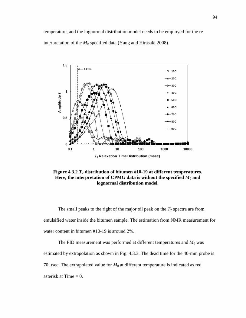
94
temperature, and the lognormal distribution model needs to be employed for the re-
interpretation of the M0 specified data (Yang and Hirasaki 2008).
The small peaks to the right of the major oil peak on the T2 spectra are from
emulsified water inside the bitumen sample. The estimation from NMR measurement for
water content in bitumen #10-19 is around 2%.
The FID measurement was performed at different temperatures and M0 was
estimated by extrapolation as shown in Fig. 4.3.3. The dead time for the 40-mm probe is
70 sec. The extrapolated value for M0 at different temperature is indicated as red
asterisk at Time = 0.
0
0.5
1
1.5
0.1 1 10 100 1000 10000
Am
plitu
de
f
T2 Relaxation Time Distribution (msec)
10C
20C
30C
40C
50C
60C
70C
80C
90C
0.2 ms
Figure 4.3.2 T2 distribution of bitumen #10-19 at different temperatures.
Here, the interpretation of CPMG data is without the specified M0 and
lognormal distribution model.
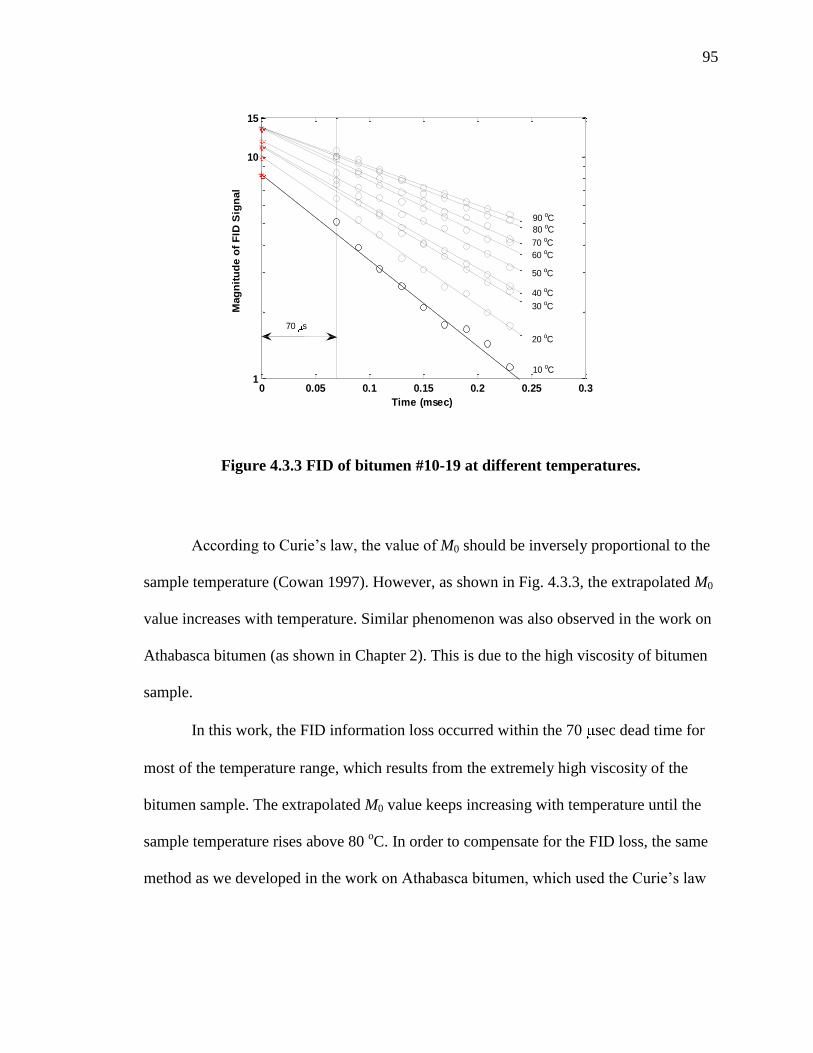
95
According to Curie’s law, the value of M0 should be inversely proportional to the
sample temperature (Cowan 1997). However, as shown in Fig. 4.3.3, the extrapolated M0
value increases with temperature. Similar phenomenon was also observed in the work on
Athabasca bitumen (as shown in Chapter 2). This is due to the high viscosity of bitumen
sample.
In this work, the FID information loss occurred within the 70 sec dead time for
most of the temperature range, which results from the extremely high viscosity of the
bitumen sample. The extrapolated M0 value keeps increasing with temperature until the
sample temperature rises above 80 oC. In order to compensate for the FID loss, the same
method as we developed in the work on Athabasca bitumen, which used the Curie’s law
0 0.05 0.1 0.15 0.2 0.25 0.31
10
15
Mag
nit
ud
e o
f F
ID S
ign
al
Time (msec)
10 oC
20 oC
30 oC
40 oC
50 oC
60 oC
70 oC
80 oC
90 oC
70 s
Figure 4.3.3 FID of bitumen #10-19 at different temperatures.
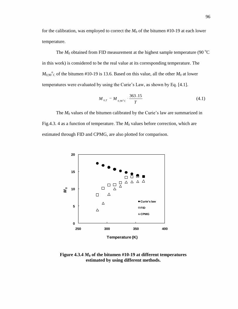
96
for the calibration, was employed to correct the M0 of the bitumen #10-19 at each lower
temperature.
The M0 obtained from FID measurement at the highest sample temperature (90 oC
in this work) is considered to be the real value at its corresponding temperature. The
M0,90oC of the bitumen #10-19 is 13.6. Based on this value, all the other M0 at lower
temperatures were evaluated by using the Curie’s Law, as shown by Eq. [4.1].
TMM
CT o
15.36390,0,0
(4.1)
The M0 values of the bitumen calibrated by the Curie’s law are summarized in
Fig.4.3. 4 as a function of temperature. The M0 values before correction, which are
estimated through FID and CPMG, are also plotted for comparison.
0
5
10
15
20
250 300 350 400
M 0
Temperature (K)
Curie's law
FID
CPMG
Figure 4.3.4 M0 of the bitumen #10-19 at different temperatures
estimated by using different methods.
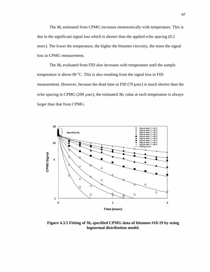
97
The M0 estimated from CPMG increases monotonically with temperature. This is
due to the significant signal loss which is shorter than the applied echo spacing (0.2
msec). The lower the temperature, the higher the bitumen viscosity, the more the signal
loss in CPMG measurement.
The M0 evaluated from FID also increases with temperature until the sample
temperature is above 80 oC. This is also resulting from the signal loss in FID
measurement. However, because the dead time in FID (70 sec) is much shorter than the
echo spacing in CPMG (200 sec), the estimated M0 value at each temperature is always
larger than that from CPMG.
1
10
0 1 2
CP
MG
Sig
na
l
Time (msec)
Signal data, T = 10 CSignal data, T = 20 CSignal data, T = 30 CSignal data, T = 40 CSignal data, T = 50 CSignal data, T = 60 CSignal data, T = 70 CSignal data, T = 80 CSignal data, T = 90 CFitting curve
Specified M0
5
20
Figure 4.3.5 Fitting of M0 specified CPMG data of bitumen #10-19 by using
lognormal distribution model.
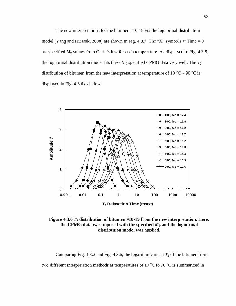
98
The new interpretations for the bitumen #10-19 via the lognormal distribution
model (Yang and Hirasaki 2008) are shown in Fig. 4.3.5. The “X” symbols at Time = 0
are specified M0 values from Curie’s law for each temperature. As displayed in Fig. 4.3.5,
the lognormal distribution model fits these M0 specified CPMG data very well. The T2
distribution of bitumen from the new interpretation at temperature of 10 oC ~ 90
oC is
displayed in Fig. 4.3.6 as below.
Comparing Fig. 4.3.2 and Fig. 4.3.6, the logarithmic mean T2 of the bitumen from
two different interpretation methods at temperatures of 10 oC to 90
oC is summarized in
0
1
2
3
4
0.001 0.01 0.1 1 10 100 1000 10000
Am
plitu
de f
T2 Relaxation Time (msec)
10C, Mo = 17.4
20C, Mo = 16.8
30C, Mo = 16.2
40C, Mo = 15.7
50C, Mo = 15.2
60C, Mo = 14.8
70C, Mo = 14.3
80C, Mo = 13.9
90C, Mo = 13.6
Figure 4.3.6 T2 distribution of bitumen #10-19 from the new interpretation. Here,
the CPMG data was imposed with the specified M0 and the lognormal
distribution model was applied.
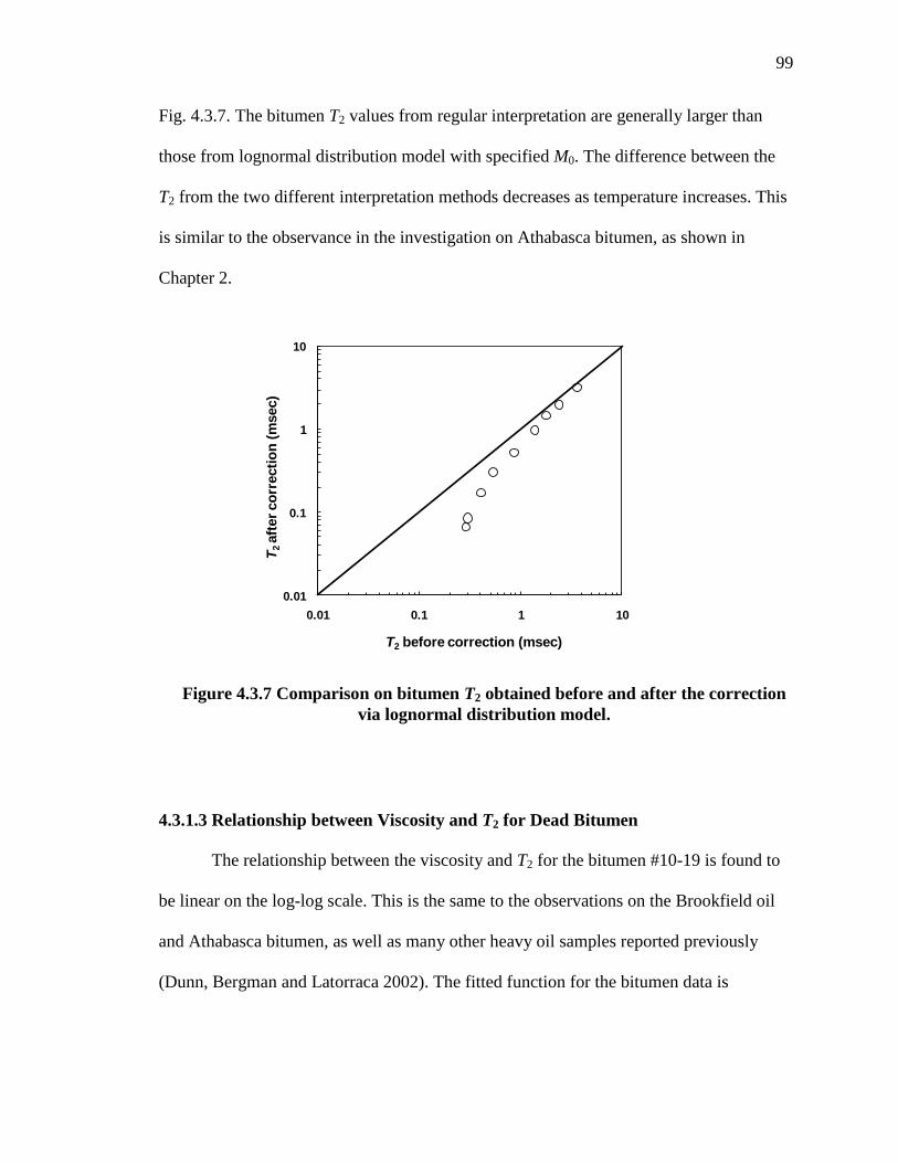
99
Fig. 4.3.7. The bitumen T2 values from regular interpretation are generally larger than
those from lognormal distribution model with specified M0. The difference between the
T2 from the two different interpretation methods decreases as temperature increases. This
is similar to the observance in the investigation on Athabasca bitumen, as shown in
Chapter 2.
4.3.1.3 Relationship between Viscosity and T2 for Dead Bitumen
The relationship between the viscosity and T2 for the bitumen #10-19 is found to
be linear on the log-log scale. This is the same to the observations on the Brookfield oil
and Athabasca bitumen, as well as many other heavy oil samples reported previously
(Dunn, Bergman and Latorraca 2002). The fitted function for the bitumen data is
0.01
0.1
1
10
0.01 0.1 1 10
T2
aft
er
co
rrecti
on
(msec)
T2 before correction (msec)
Figure 4.3.7 Comparison on bitumen T2 obtained before and after the correction
via lognormal distribution model.
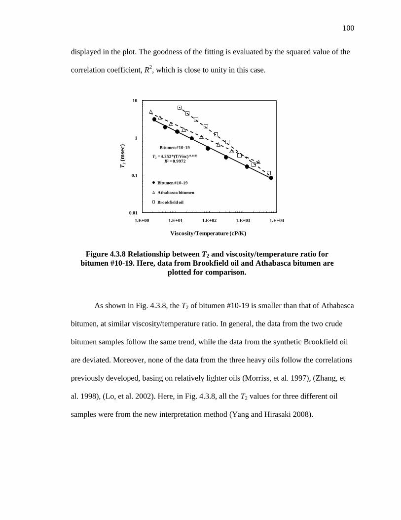
100
displayed in the plot. The goodness of the fitting is evaluated by the squared value of the
correlation coefficient, R2, which is close to unity in this case.
As shown in Fig. 4.3.8, the T2 of bitumen #10-19 is smaller than that of Athabasca
bitumen, at similar viscosity/temperature ratio. In general, the data from the two crude
bitumen samples follow the same trend, while the data from the synthetic Brookfield oil
are deviated. Moreover, none of the data from the three heavy oils follow the correlations
previously developed, basing on relatively lighter oils (Morriss, et al. 1997), (Zhang, et
al. 1998), (Lo, et al. 2002). Here, in Fig. 4.3.8, all the T2 values for three different oil
samples were from the new interpretation method (Yang and Hirasaki 2008).
0.01
0.1
1
10
1.E+00 1.E+01 1.E+02 1.E+03 1.E+04
T2
(mse
c)
Viscosity/Temperature (cP/K)
Bitumen #10-19
Athabasca bitumen
Brookfield oil
Bitumen #10-19
T2 = 4.252*(T/Visc) 0.4493
R2 = 0.9972
Figure 4.3.8 Relationship between T2 and viscosity/temperature ratio for
bitumen #10-19. Here, data from Brookfield oil and Athabasca bitumen are
plotted for comparison.

101
4.3.2 Investigations on Recombined Live Bitumen
The investigations on the recombined live bitumen were performed with three
different reservoir gases, CO2, CH4, and C2H6. The measurements were conducted at
different pressure levels for each gas.
The experimental procedures used in the work on bitumen are the same as those
used in the case of Brookfield oil. For each gas, the procedure was divided into two
stages, the pressurization stage and the depressurization stage. The highly pressurized gas
was first introduced into the closed pressure vessel with bitumen at the bottom. After the
gas-bitumen system reached equilibrium at the highest pressure level, the system pressure
would be depressurized to a series of lower pressures. At each lower pressure, the
equilibrium was achieved and the NMR measurements were performed.
During the NMR measurements in the work on bitumen, the number of scans
(NS) was chosen to make the signal to noise ratio (SNR) equal to 100 in each case. Each
measurement was repeated for 6 times so that the reliability of experimental data can be
ensured. During the entire process, the system pressure inside the vessel was recorded as
a function of time.
4.3.2.1 Calculation of Gas Solubility in Bitumen
The solubility of each gas in the bitumen #10-19 was calculated via the same
method as mentioned in the work on Brookfield oil (section 3.3.2.1). Given the proper
pressure data, the solubility can be calculated by using the equation of state with
compression factor z for each gas.
102
4.3.2.2 Recombined Live Bitumen with C2H6
The investigation on the recombined bitumen was first performed with C2H6. The
total dead bitumen sample volume used in this case was ~13 mL. The C2H6 was injected
into the pressure vessel from the top. The gas pressure inside the vessel was monitored by
using Senso-Metrics pressure transducer.
The total sample chamber volume of the pressure vessel is about 82 mL.
Subtracting 13 mL for oil sample, the total space for gas is about 69 mL. The
investigation on the estimation of pressure and gas volume for saturating the heavy oil in
previous work shows that, for 13 mL heavy oil sample, the gas volume needed for
saturation is about 28.6 mL at target pressure and temperature. Therefore, the total
available gas is much more than enough for saturating the oil.
The critical temperature and pressure of C2H6 is 32.2 oC and 706.7 psia,
respectively. The operation temperature in this work is 30 oC, which is close to the
critical temperature of C2H6. Therefore, the highest pressure we can use for this C2H6-
bitumen system should be lower than its critical pressure value.
In this manner, the gas pressure inside the vessel was first raised to ~531 psia.
Right after the introduction of pressurized C2H6, the gas source was cut off and no more
gas was added into the system afterwards. Due to the dissolving of C2H6 into the
bitumen, the pressure inside the vessel will keep decreasing until it finally reaches the
equilibrium.
4.3.2.2.1 Pressurization Stage of C2H6-Bitumen
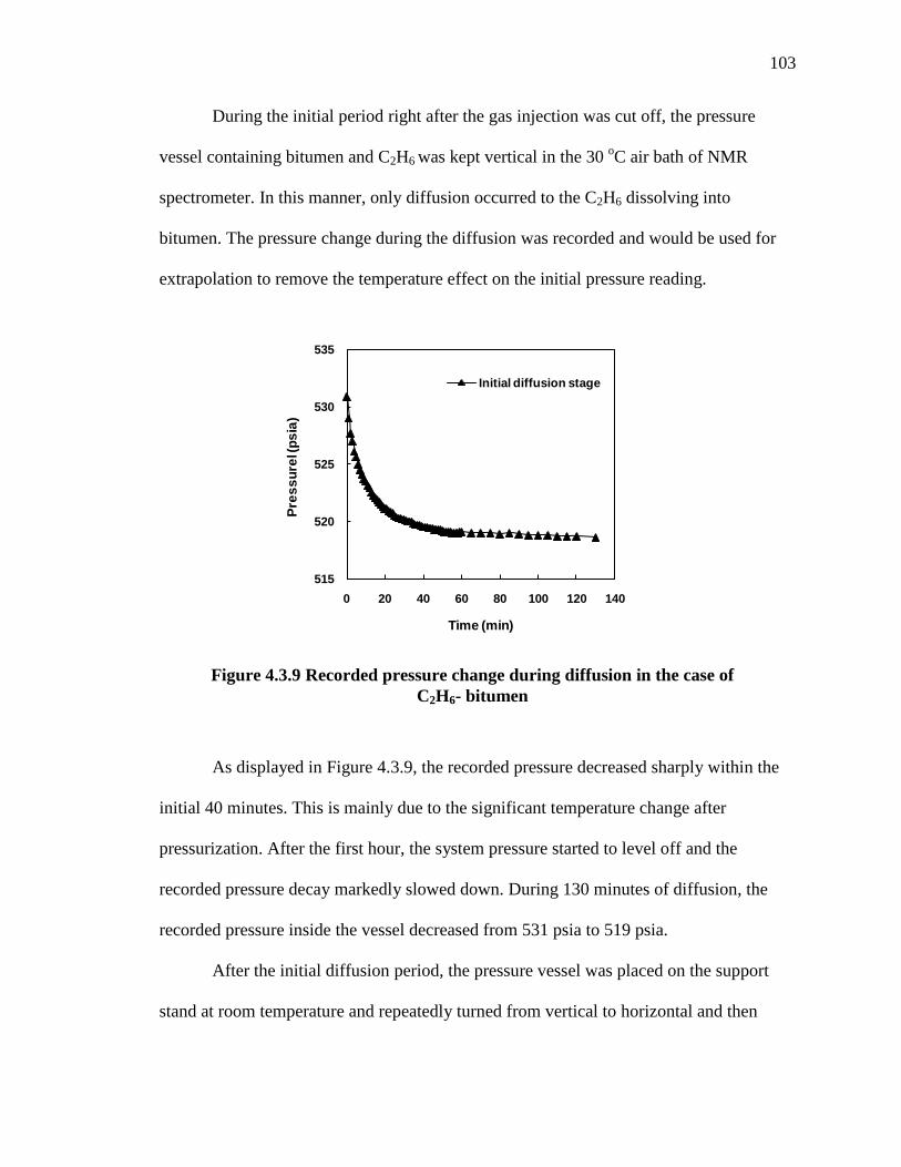
103
During the initial period right after the gas injection was cut off, the pressure
vessel containing bitumen and C2H6 was kept vertical in the 30 oC air bath of NMR
spectrometer. In this manner, only diffusion occurred to the C2H6 dissolving into
bitumen. The pressure change during the diffusion was recorded and would be used for
extrapolation to remove the temperature effect on the initial pressure reading.
As displayed in Figure 4.3.9, the recorded pressure decreased sharply within the
initial 40 minutes. This is mainly due to the significant temperature change after
pressurization. After the first hour, the system pressure started to level off and the
recorded pressure decay markedly slowed down. During 130 minutes of diffusion, the
recorded pressure inside the vessel decreased from 531 psia to 519 psia.
After the initial diffusion period, the pressure vessel was placed on the support
stand at room temperature and repeatedly turned from vertical to horizontal and then
515
520
525
530
535
0 20 40 60 80 100 120 140
Pre
ss
ure
l (p
sia
)
Time (min)
Initial diffusion stage
Figure 4.3.9 Recorded pressure change during diffusion in the case of
C2H6- bitumen
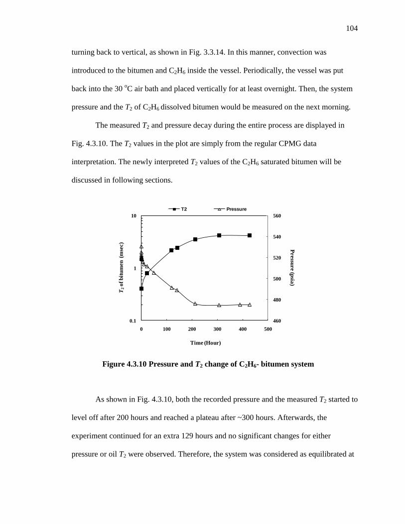
104
turning back to vertical, as shown in Fig. 3.3.14. In this manner, convection was
introduced to the bitumen and C2H6 inside the vessel. Periodically, the vessel was put
back into the 30 oC air bath and placed vertically for at least overnight. Then, the system
pressure and the T2 of C2H6 dissolved bitumen would be measured on the next morning.
The measured T2 and pressure decay during the entire process are displayed in
Fig. 4.3.10. The T2 values in the plot are simply from the regular CPMG data
interpretation. The newly interpreted T2 values of the C2H6 saturated bitumen will be
discussed in following sections.
As shown in Fig. 4.3.10, both the recorded pressure and the measured T2 started to
level off after 200 hours and reached a plateau after ~300 hours. Afterwards, the
experiment continued for an extra 129 hours and no significant changes for either
pressure or oil T2 were observed. Therefore, the system was considered as equilibrated at
460
480
500
520
540
560
0.1
1
10
0 100 200 300 400 500
Pressu
re (p
sia)
T2
of
bit
um
en
(m
sec)
Time (Hour)
T2 Pressure
Figure 4.3.10 Pressure and T2 change of C2H6- bitumen system
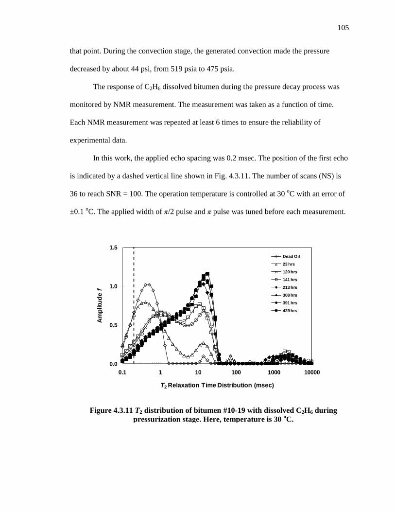
105
that point. During the convection stage, the generated convection made the pressure
decreased by about 44 psi, from 519 psia to 475 psia.
The response of C2H6 dissolved bitumen during the pressure decay process was
monitored by NMR measurement. The measurement was taken as a function of time.
Each NMR measurement was repeated at least 6 times to ensure the reliability of
experimental data.
In this work, the applied echo spacing was 0.2 msec. The position of the first echo
is indicated by a dashed vertical line shown in Fig. 4.3.11. The number of scans (NS) is
36 to reach SNR = 100. The operation temperature is controlled at 30 oC with an error of
±0.1 oC. The applied width of π/2 pulse and π pulse was tuned before each measurement.
0.0
0.5
1.0
1.5
0.1 1 10 100 1000 10000
Am
plitu
de
f
T2 Relaxation Time Distribution (msec)
Dead Oil
23 hrs
120 hrs
141 hrs
213 hrs
308 hrs
391 hrs
429 hrs
Figure 4.3.11 T2 distribution of bitumen #10-19 with dissolved C2H6 during
pressurization stage. Here, temperature is 30 oC.
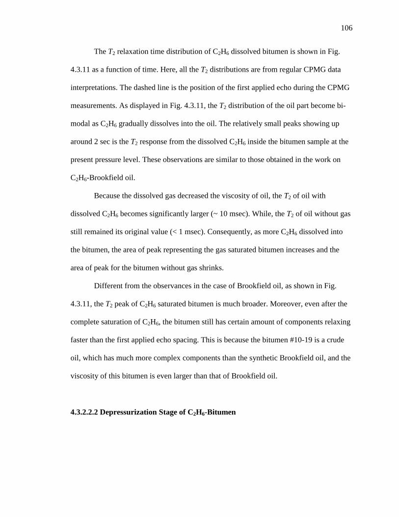
106
The T2 relaxation time distribution of C2H6 dissolved bitumen is shown in Fig.
4.3.11 as a function of time. Here, all the T2 distributions are from regular CPMG data
interpretations. The dashed line is the position of the first applied echo during the CPMG
measurements. As displayed in Fig. 4.3.11, the T2 distribution of the oil part become bi-
modal as C2H6 gradually dissolves into the oil. The relatively small peaks showing up
around 2 sec is the T2 response from the dissolved C2H6 inside the bitumen sample at the
present pressure level. These observations are similar to those obtained in the work on
C2H6-Brookfield oil.
Because the dissolved gas decreased the viscosity of oil, the T2 of oil with
dissolved C2H6 becomes significantly larger (~ 10 msec). While, the T2 of oil without gas
still remained its original value (< 1 msec). Consequently, as more C2H6 dissolved into
the bitumen, the area of peak representing the gas saturated bitumen increases and the
area of peak for the bitumen without gas shrinks.
Different from the observances in the case of Brookfield oil, as shown in Fig.
4.3.11, the T2 peak of C2H6 saturated bitumen is much broader. Moreover, even after the
complete saturation of C2H6, the bitumen still has certain amount of components relaxing
faster than the first applied echo spacing. This is because the bitumen #10-19 is a crude
oil, which has much more complex components than the synthetic Brookfield oil, and the
viscosity of this bitumen is even larger than that of Brookfield oil.
4.3.2.2.2 Depressurization Stage of C2H6-Bitumen
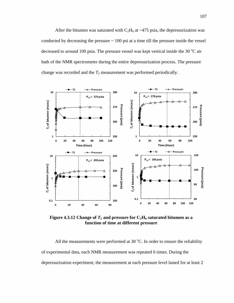
107
After the bitumen was saturated with C2H6 at ~475 psia, the depressurization was
conducted by decreasing the pressure ~ 100 psi at a time till the pressure inside the vessel
decreased to around 100 psia. The pressure vessel was kept vertical inside the 30 oC air
bath of the NMR spectrometer during the entire depressurization process. The pressure
change was recorded and the T2 measurement was performed periodically.
All the measurements were performed at 30 oC. In order to ensure the reliability
of experimental data, each NMR measurement was repeated 6 times. During the
depressurization experiment, the measurement at each pressure level lasted for at least 2
330
350
370
390
1
10
0 20 40 60 80 100 120
Pre
ss
ure
(ps
ia)
T2
of
bit
um
en
(m
se
c)
Time (Hour)
T2 Pressure
Peq = 370 psia
160
180
200
220
0.1
1
10
0 20 40 60 80
Pre
ss
ure
(ps
ia)
T2
of
bit
um
en
(m
se
c)
Time (Hour)
T2 Pressure
Peq = 200 psia
60
80
100
120
0.1
1
10
0 20 40 60 80 100 120
Pre
ss
ure
(ps
ia)
T2
of
bit
um
en
(m
se
c)
Time (Hour)
T2 Pressure
Peq = 106 psia
230
250
270
290
1
10
0 20 40 60 80 100
Pre
ss
ure
(ps
ia)
T2
of
bit
um
en
(m
se
c)
Time (Hour)
T2 Pressure
Peq = 278 psia
Figure 4.3.12 Change of T2 and pressure for C2H6 saturated bitumen as a
function of time at different pressure
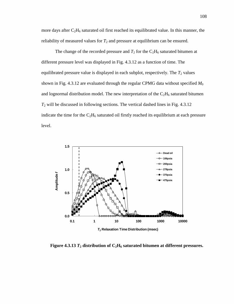
108
more days after C2H6 saturated oil first reached its equilibrated value. In this manner, the
reliability of measured values for T2 and pressure at equilibrium can be ensured.
The change of the recorded pressure and T2 for the C2H6 saturated bitumen at
different pressure level was displayed in Fig. 4.3.12 as a function of time. The
equilibrated pressure value is displayed in each subplot, respectively. The T2 values
shown in Fig. 4.3.12 are evaluated through the regular CPMG data without specified M0
and lognormal distribution model. The new interpretation of the C2H6 saturated bitumen
T2 will be discussed in following sections. The vertical dashed lines in Fig. 4.3.12
indicate the time for the C2H6 saturated oil firstly reached its equilibrium at each pressure
level.
0.0
0.5
1.0
1.5
0.1 1 10 100 1000 10000
Am
plitu
de f
T2 Relaxation Time Distribution (msec)
Dead oil
106psia
200psia
278psia
370psia
475psia
Figure 4.3.13 T2 distribution of C2H6 saturated bitumen at different pressures.
109
The T2 distributions of C2H6 saturated bitumen at different pressure levels are
displayed in Fig. 4.3.13. Here, all the distributions in the plot are from the regular CPMG
data interpretations. The major oil peaks on the T2 spectra are much broader than those
observed on synthetic Brookfield oil. This is because the bitumen is crude oil and has
various components, which result in a broad range of T2 responses. As mentioned in the
case of C2H6-Brookfield oil in section 3.3.2.3, due to the specific selection of the RD
value in this work, the small peaks around 2 sec as shown in Fig. 4.3.13 is not correctly
proportional to the gas concentration in the bitumen.
4.3.2.2.3 New Interpretations of T2 Distributions
As shown in Fig. 4.3.13, even saturated by C2H6 at the highest pressure level, the
bitumen sample still has certain fast relaxing components whose relaxation time is shorter
than the applied echo spacing. Therefore, M0 needs to be imposed into the CPMG data at
each equilibrated pressure level and the lognormal distribution model was employed to
re-interpret the M0 specified data (Yang and Hirasaki 2008).
As discussed in section 4.3.1.2, due to the extremely high viscosity of the bitumen
sample, the value of M0 directly extrapolated from FID has incorrect temperature
dependence and needs to be corrected via Curie’s law on the basis of the M0 value
obtained from FID at the highest temperature (90 oC). However, this technique for the M0
estimation cannot be used on the bitumen sample inside the pressure vessel because the
temperature rating of the vessel is only 40 oC.
Therefore, the M0 of the dead bitumen sample inside the pressure vessel was
estimated by the ratio of M0 values obtained from regular CPMG measurements on the
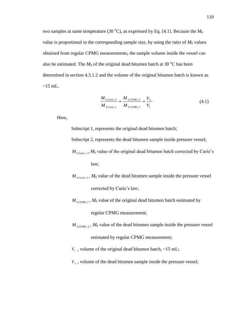
110
two samples at same temperature (30 oC), as expressed by Eq. [4.1]. Because the M0
value is proportional to the corresponding sample size, by using the ratio of M0 values
obtained from regular CPMG measurements, the sample volume inside the vessel can
also be estimated. The M0 of the original dead bitumen batch at 30 oC has been
determined in section 4.3.1.2 and the volume of the original bitumen batch is known as
~15 mL.
1
2
1,,0
2,,0
1,,0
2,,0
V
V
M
M
M
M
CPMG
CPMG
Curie
Curie (4.1)
Here,
Subscript 1, represents the original dead bitumen batch;
Subscript 2, represents the dead bitumen sample inside pressure vessel;
1,,0 CurieM , M0 value of the original dead bitumen batch corrected by Curie’s
law;
2,,0 CurieM , M0 value of the dead bitumen sample inside the pressure vessel
corrected by Curie’s law;
1,,0 CPMGM , M0 value of the original dead bitumen batch estimated by
regular CPMG measurement;
2,,0 CPMGM , M0 value of the dead bitumen sample inside the pressure vessel
estimated by regular CPMG measurement;
1V , volume of the original dead bitumen batch, ~15 mL;
2V , volume of the dead bitumen sample inside the pressure vessel;
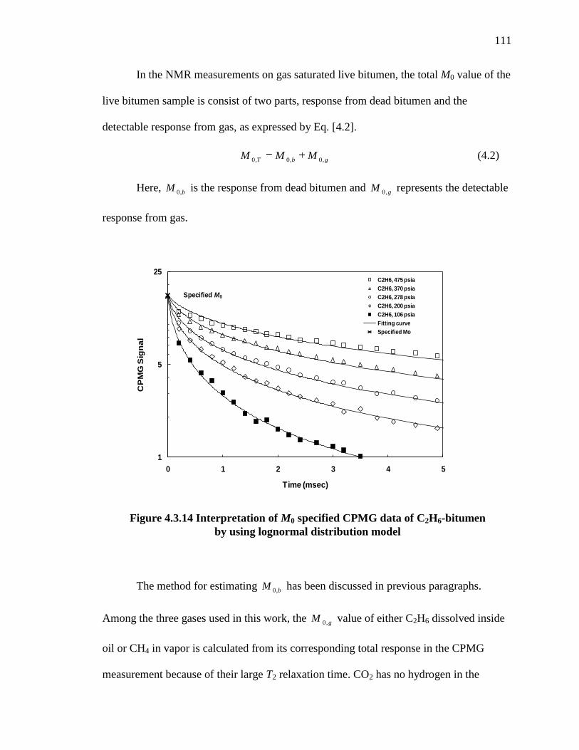
111
In the NMR measurements on gas saturated live bitumen, the total M0 value of the
live bitumen sample is consist of two parts, response from dead bitumen and the
detectable response from gas, as expressed by Eq. [4.2].
gbTMMM
,0,0,0 (4.2)
Here, b
M,0
is the response from dead bitumen and g
M,0
represents the detectable
response from gas.
The method for estimating bM
,0 has been discussed in previous paragraphs.
Among the three gases used in this work, the gM
,0 value of either C2H6 dissolved inside
oil or CH4 in vapor is calculated from its corresponding total response in the CPMG
measurement because of their large T2 relaxation time. CO2 has no hydrogen in the
1
5
25
0 1 2 3 4 5
CP
MG
Sig
na
l
Time (msec)
C2H6, 475 psia
C2H6, 370 psia
C2H6, 278 psia
C2H6, 200 psia
C2H6, 106 psia
Fitting curve
Specified Mo
Specified M0
Figure 4.3.14 Interpretation of M0 specified CPMG data of C2H6-bitumen
by using lognormal distribution model

112
molecule thus, does not give response in the Maran spectrometer used in this work.
Therefore, in the case of CO2-bitumen, g
M,0
is 0.
The new interpretations for the C2H6-bitumen are displayed in Fig. 4.3.14. As
shown in Fig. 4.3.14, the lognormal distribution model fits these M0 specified CPMG
data well. Note that the “X” at Time = 0, which represents the specified M0, is not single
value actually. The M0 has different value at different pressure due to the change of g
M,0
. However, in the case of C2H6-bitumen, the change of g
M,0
is at different pressure is not
big enough to make significant difference for the total M0 value on the logarithmic scale
in Fig. 4.3.14.
0
1
2
3
4
0.001 0.01 0.1 1 10 100 1000 10000
Am
plitu
de f
T2 Relaxation Time (msec)
106 psia
200 psia
278 psia
370 psia
475 psia
Figure 4.3.15 T2 distribution of C2H6 saturated bitumen from new interpretation
as a function of the equilibrium pressure

113
The T2 distribution of C2H6 saturated bitumen from the new interpretation at each
pressure level is displayed in Fig. 4.3.15. As the C2H6 depressurized from the ~475 psia
to ~106 psia, the T2 peak significantly shifted from the larger values to the smaller values.
The logarithmic mean T2 of the C2H6 saturated bitumen from two different
interpretation methods are compared in Fig. 4.3.16. The T2 values of the live bitumen
from regular interpretation are generally larger than those from lognormal distribution
model with specified M0. The difference between the T2 values from two different
interpretation methods decreases as saturation pressure increases.
The T2 changes of C2H6 saturated oil as a function of the equilibrated pressure are
displayed in Fig. 4.3.17. The rectangle symbols in Fig. 4.3.17 are the T2 data obtained
from regular interpretation at each pressure. The triangle symbols are the T2 data obtained
0.1
1
10
0.1 1 10
T2
fro
m n
ew
inte
rpre
tati
on
(m
sec)
T2 from regular interpretation (msec)
Figure 4.3.16 Comparison of C2H6 saturated bitumen T2 at different pressure
obtained before and after correction via lognormal distribution model.

114
from the new interpretation with lognormal distribution model. The solid lines are the
fitted curves to the experimental data. The fitted functions are also shown in the plot.
An interesting finding from Fig. 4.3.17 is that, although the T2 values from two
different interpretations have significant discrepancy, the trends for them are both closely
linear on the semi-log scale. Moreover, both of the two trends extrapolate well to their
corresponding dead oil values, respectively. This proves that the T2 differences between
two interpretations are systematic, caused by the restriction of the applied echo spacing in
this work.
As shown in Fig. 4.3.17, the R2 value for two fitting curves are both near unity,
indicating that the change of C2H6 saturated oil T2 at different pressure closely follows
the exponential function. This is similar to our observations in the work on gas-
Brookfield oil systems.
y = 0.414e0.0049x
R² = 0.9975
y = 0.1369e0.0065x
R² = 0.9984
0.1
1
10
0 100 200 300 400 500
T2
of
Liv
e B
itu
men
(m
sec)
Pressure (psia)
Dead bitumen, regular interpretation
C2H6-bitumen, regular interpretation
Dead bitumen, new interpretation
C2H6-bitumen, new interpretation
Figure 4.3.17 T2 of C2H6 saturated bitumen at different pressure levels
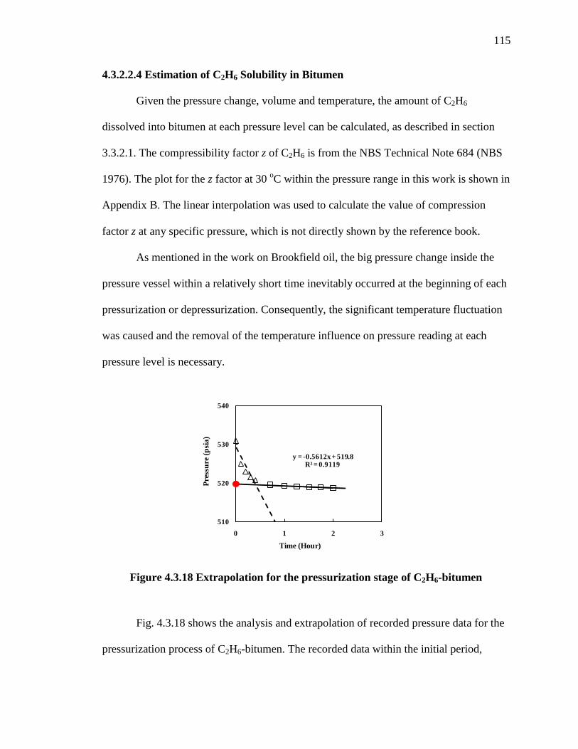
115
4.3.2.2.4 Estimation of C2H6 Solubility in Bitumen
Given the pressure change, volume and temperature, the amount of C2H6
dissolved into bitumen at each pressure level can be calculated, as described in section
3.3.2.1. The compressibility factor z of C2H6 is from the NBS Technical Note 684 (NBS
1976). The plot for the z factor at 30 oC within the pressure range in this work is shown in
Appendix B. The linear interpolation was used to calculate the value of compression
factor z at any specific pressure, which is not directly shown by the reference book.
As mentioned in the work on Brookfield oil, the big pressure change inside the
pressure vessel within a relatively short time inevitably occurred at the beginning of each
pressurization or depressurization. Consequently, the significant temperature fluctuation
was caused and the removal of the temperature influence on pressure reading at each
pressure level is necessary.
Fig. 4.3.18 shows the analysis and extrapolation of recorded pressure data for the
pressurization process of C2H6-bitumen. The recorded data within the initial period,
y = -0.5612x + 519.8R² = 0.9119
510
520
530
540
0 1 2 3
Pre
ssu
re (
psi
a)
Time (Hour)
Figure 4.3.18 Extrapolation for the pressurization stage of C2H6-bitumen
116
which were considered to be markedly influenced by temperature change, are shown by
open triangles. The pressure data after this initial period are displayed by open rectangles
and are used for extrapolation.
The extrapolation is indicated by solid line in Fig. 4.3.18. The estimated starting
pressure P0 from extrapolation is 519.8 psia, which is 11.1 psi lower than the recorded
pressure data right after the introduction of high pressure C2H6 (530.9 psia). The similar
work for depressurization is shown in Fig. 4.3.19.
In each subplot of Fig. 4.3.19, the extrapolation is shown by solid line and the
extrapolated value at each pressure level is indicated by solid dot. The fitted functions
and the R2 values are also displayed.
y = 2.3371x + 187.32R² = 0.9611
170
180
190
200
0 1 2 3 4
Pre
ss
ure
(p
sia
)
Time (Hour)
Peq = 200 psia
y = 3.2532x + 358.2R² = 0.9752
330
340
350
360
370
380
0 1 2 3 4
Pre
ss
ure
(p
sia
)
Time (Hour)
Peq = 370 psia
y = 3.8106x + 261.8R² = 0.9614
250
260
270
280
0 1 2 3
Pre
ss
ure
(p
sia
)
Time (Hour)
Peq = 278 psia
y = 3.6265x + 90.548R² = 0.9827
80
90
100
110
0 1 2 3 4
Pre
ss
ure
(p
sia
)
Time (Hour)
Peq = 106 psia
Figure 4.3.19 Extrapolations for the depressurization stage of C2H6- bitumen at
different pressures
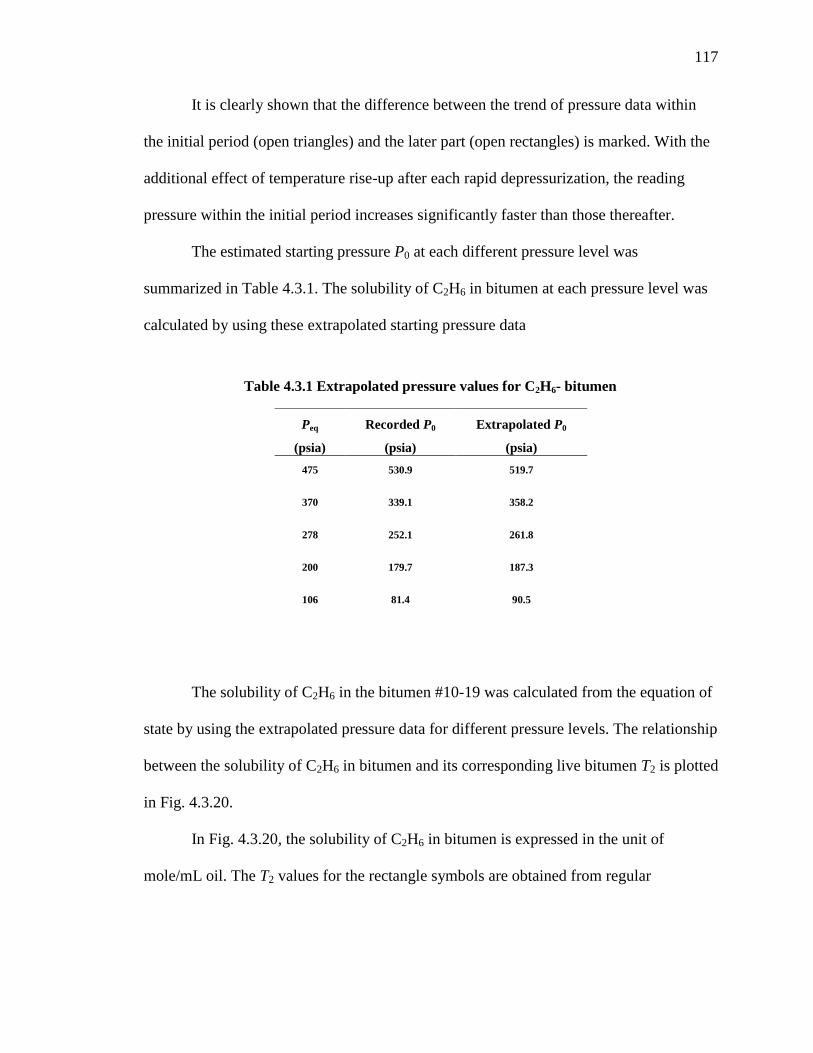
117
It is clearly shown that the difference between the trend of pressure data within
the initial period (open triangles) and the later part (open rectangles) is marked. With the
additional effect of temperature rise-up after each rapid depressurization, the reading
pressure within the initial period increases significantly faster than those thereafter.
The estimated starting pressure P0 at each different pressure level was
summarized in Table 4.3.1. The solubility of C2H6 in bitumen at each pressure level was
calculated by using these extrapolated starting pressure data
The solubility of C2H6 in the bitumen #10-19 was calculated from the equation of
state by using the extrapolated pressure data for different pressure levels. The relationship
between the solubility of C2H6 in bitumen and its corresponding live bitumen T2 is plotted
in Fig. 4.3.20.
In Fig. 4.3.20, the solubility of C2H6 in bitumen is expressed in the unit of
mole/mL oil. The T2 values for the rectangle symbols are obtained from regular
Peq
(psia)
Recorded P0
(psia)
Extrapolated P0
(psia)
475 530.9 519.7
370 339.1 358.2
278 252.1 261.8
200 179.7 187.3
106 81.4 90.5
Table 4.3.1 Extrapolated pressure values for C2H6- bitumen
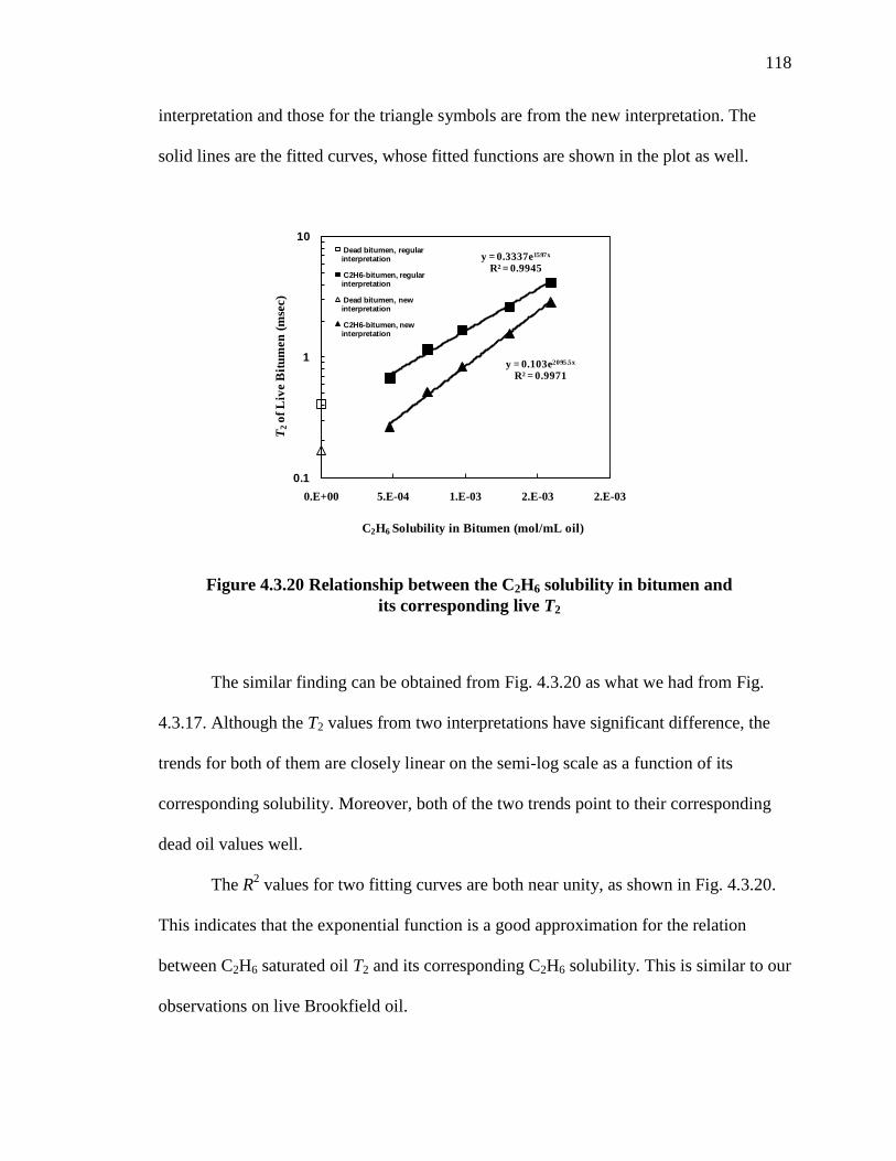
118
interpretation and those for the triangle symbols are from the new interpretation. The
solid lines are the fitted curves, whose fitted functions are shown in the plot as well.
The similar finding can be obtained from Fig. 4.3.20 as what we had from Fig.
4.3.17. Although the T2 values from two interpretations have significant difference, the
trends for both of them are closely linear on the semi-log scale as a function of its
corresponding solubility. Moreover, both of the two trends point to their corresponding
dead oil values well.
The R2 values for two fitting curves are both near unity, as shown in Fig. 4.3.20.
This indicates that the exponential function is a good approximation for the relation
between C2H6 saturated oil T2 and its corresponding C2H6 solubility. This is similar to our
observations on live Brookfield oil.
y = 0.3337e1597x
R² = 0.9945
y = 0.103e2095.5x
R² = 0.9971
0.1
1
10
0.E+00 5.E-04 1.E-03 2.E-03 2.E-03
T2
of
Liv
e B
itu
men
(m
sec)
C2H6 Solubility in Bitumen (mol/mL oil)
Dead bitumen, regular interpretation
C2H6-bitumen, regular interpretation
Dead bitumen, new interpretation
C2H6-bitumen, new interpretation
Figure 4.3.20 Relationship between the C2H6 solubility in bitumen and
its corresponding live T2
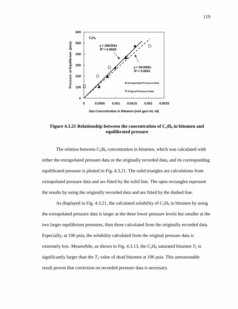
119
The relation between C2H6 concentration in bitumen, which was calculated with
either the extrapolated pressure data or the originally recorded data, and its corresponding
equilibrated pressure is plotted in Fig. 4.3.21. The solid triangles are calculations from
extrapolated pressure data and are fitted by the solid line. The open rectangles represent
the results by using the originally recorded data and are fitted by the dashed line.
As displayed in Fig. 4.3.21, the calculated solubility of C2H6 in bitumen by using
the extrapolated pressure data is larger at the three lower pressure levels but smaller at the
two larger equilibrium pressures, than those calculated from the originally recorded data.
Especially, at 106 psia, the solubility calculated from the original pressure data is
extremely low. Meanwhile, as shown in Fig. 4.3.13, the C2H6 saturated bitumen T2 is
significantly larger than the T2 value of dead bitumen at 106 psia. This unreasonable
result proves that correction on recorded pressure data is necessary.
y = 286359xR² = 0.9826
y = 261968xR² = 0.6661
0
100
200
300
400
500
600
0 0.0005 0.001 0.0015 0.002 0.0025
Pre
ss
ure
at
Eq
uilib
riu
m (p
isa
)
Gas Concentration in Bitumen (mol gas/ mL oil)
Extrapolated Pressure Data
Original Pressure Data
C2H6
Figure 4.3.21 Relationship between the concentration of C2H6 in bitumen and
equilibrated pressure
120
Henry’s law is employed to fit the Pressure vs. Gas Concentration data. The solid
line is the fitted curve to the extrapolated data, while the dashed line is the fitted curve to
the original data. The fitted functions for both two cases are displayed in the plot. As
shown in Fig. 4.3.21, the calculated Pressure vs. Gas Concentration values with
extrapolated pressure data closely follows the Henry’s law. However, the calculation
from the original data is badly deviated. The Henry’s law constant of C2H6 in the bitumen
#10-19 evaluated from the corrected pressure data is about 2.86 x 10⁵ mL·psi/mol.
4.3.2.3 Recombined Live Bitumen with CO2
The investigation on the CO2 saturated bitumen was conducted with a total
sample volume of ~9.5 mL. The total sample chamber volume of the pressure vessel is
about 82 mL. Subtracting 9.5 mL for oil sample, the total space for gas is about 72.5 mL.
The gas pressure inside the vessel was first raised to ~760 psia by injecting CO2
from the top of the pressure vessel. Then, the gas source was cut off and no more gas was
added into the system afterwards. The gas pressure inside the vessel was monitored by
using Senso-Metrics pressure transducer. Due to the dissolving of CO2 into the bitumen,
the pressure inside the vessel will keep decreasing until it finally reaches the equilibrium.
4.3.2.3.1 Pressurization Stage of CO2-Bitumen
During the initial period right after the gas injection was cut off, the pressure
vessel containing bitumen and CO2 was kept vertical in the 30 oC air bath of NMR
spectrometer. In this manner, only diffusion occurred to the CO2 dissolving into bitumen.

121
The pressure change during the diffusion was recorded and would be used for
extrapolation to remove the temperature effect on the initial pressure reading.
As displayed in Figure 4.3.22, the recorded pressure decreased sharply within the
initial 30 minutes. This is mainly due to the significant temperature change after the
injection of the pressurized CO2. After the first hour, the system pressure started to
obviously slow down. The diffusion lasted for 6 hours (360 minutes), in which the
pressure inside the vessel decreased from ~760 psia to ~738 psia.
After the initial diffusion period, the pressure vessel was placed on the support
stand at room temperature and repeatedly turned from vertical to horizontal and then back
to vertical, as shown in Fig.3.3.14. In this manner, convection was generated on the
bitumen and CO2 mixture inside the vessel. Periodically, the vessel was put back into the
730
740
750
760
770
0 50 100 150 200 250 300 350 400
Pre
ss
ure
l (p
sia
)
Time (min)
Initial stage
Figure 4.3.22 Recorded pressure change during diffusion in the case of
CO2- bitumen
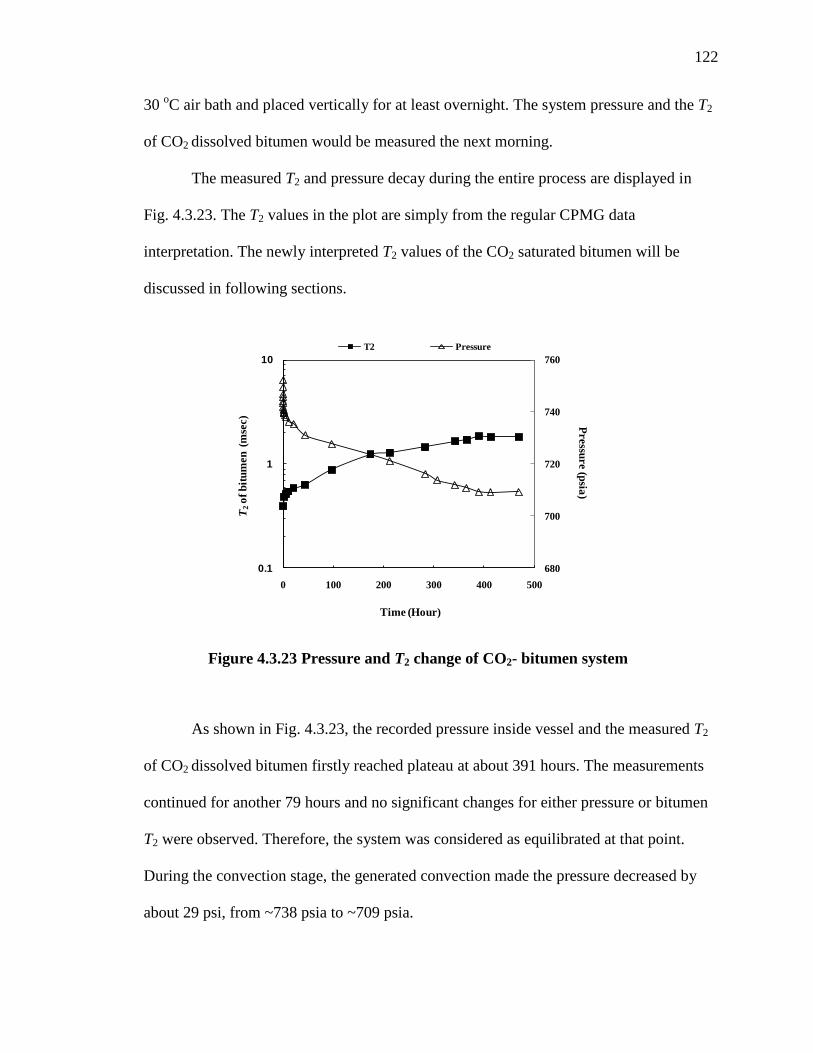
122
30 oC air bath and placed vertically for at least overnight. The system pressure and the T2
of CO2 dissolved bitumen would be measured the next morning.
The measured T2 and pressure decay during the entire process are displayed in
Fig. 4.3.23. The T2 values in the plot are simply from the regular CPMG data
interpretation. The newly interpreted T2 values of the CO2 saturated bitumen will be
discussed in following sections.
As shown in Fig. 4.3.23, the recorded pressure inside vessel and the measured T2
of CO2 dissolved bitumen firstly reached plateau at about 391 hours. The measurements
continued for another 79 hours and no significant changes for either pressure or bitumen
T2 were observed. Therefore, the system was considered as equilibrated at that point.
During the convection stage, the generated convection made the pressure decreased by
about 29 psi, from ~738 psia to ~709 psia.
680
700
720
740
760
0.1
1
10
0 100 200 300 400 500
Pressu
re (p
sia)
T2
of
bit
um
en
(m
sec)
Time (Hour)
T2 Pressure
Figure 4.3.23 Pressure and T2 change of CO2- bitumen system

123
The response of CO2 dissolved bitumen during the pressure decay process was
monitored by NMR measurement as a function of time. Each NMR measurement was
repeated for at least 6 times so that the reliability of experimental data can be ensured.
In this work, the applied echo spacing was 0.2 msec. The position of the first echo
is indicated by a dashed vertical line shown in Fig. 4.3.24. The number of scans (NS) is
adjusted accordingly to reach an SNR = 100. The operation temperature is controlled at
30 oC with an error of ±0.1
oC. The applied width of π/2 pulse and π pulse was tuned
before each measurement.
The T2 relaxation time distribution of CO2 dissolved bitumen #10-19 is shown in
Fig. 4.3.24 as a function of time. Here, all the T2 distributions are from regular CPMG
0.0
0.2
0.4
0.6
0.8
1.0
0.1 1 10 100 1000 10000
Am
plitu
de
f
T2 Relaxation Time Distribution (msec)
Dead Oil
21 hrs
97 hrs
174 hrs
284 hrs
391 hrs
470 hrs
Figure 4.3.24 T2 distribution of bitumen #10-19 with dissolved CO2 during
pressurization stage. Here, temperature is 30 oC.
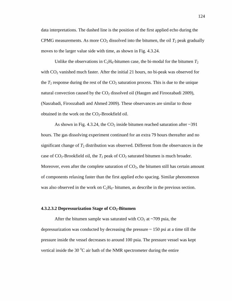
124
data interpretations. The dashed line is the position of the first applied echo during the
CPMG measurements. As more CO2 dissolved into the bitumen, the oil T2 peak gradually
moves to the larger value side with time, as shown in Fig. 4.3.24.
Unlike the observations in C2H6-bitumen case, the bi-modal for the bitumen T2
with CO2 vanished much faster. After the initial 21 hours, no bi-peak was observed for
the T2 response during the rest of the CO2 saturation process. This is due to the unique
natural convection caused by the CO2 dissolved oil (Haugen and Firoozabadi 2009),
(Nasrabadi, Firoozabadi and Ahmed 2009). These observances are similar to those
obtained in the work on the CO2-Brookfield oil.
As shown in Fig. 4.3.24, the CO2 inside bitumen reached saturation after ~391
hours. The gas dissolving experiment continued for an extra 79 hours thereafter and no
significant change of T2 distribution was observed. Different from the observances in the
case of CO2-Brookfield oil, the T2 peak of CO2 saturated bitumen is much broader.
Moreover, even after the complete saturation of CO2, the bitumen still has certain amount
of components relaxing faster than the first applied echo spacing. Similar phenomenon
was also observed in the work on C2H6- bitumen, as describe in the previous section.
4.3.2.3.2 Depressurization Stage of CO2-Bitumen
After the bitumen sample was saturated with CO2 at ~709 psia, the
depressurization was conducted by decreasing the pressure ~ 150 psi at a time till the
pressure inside the vessel decreases to around 100 psia. The pressure vessel was kept
vertical inside the 30 oC air bath of the NMR spectrometer during the entire
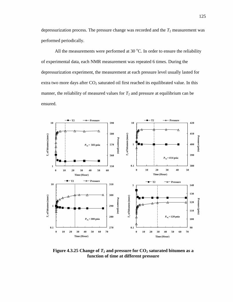
125
depressurization process. The pressure change was recorded and the T2 measurement was
performed periodically.
All the measurements were performed at 30 oC. In order to ensure the reliability
of experimental data, each NMR measurement was repeated 6 times. During the
depressurization experiment, the measurement at each pressure level usually lasted for
extra two more days after CO2 saturated oil first reached its equilibrated value. In this
manner, the reliability of measured values for T2 and pressure at equilibrium can be
ensured.
380
390
400
410
420
0.1
1
10
0 10 20 30 40 50
Pressu
re (p
sia)
T2
of
bit
um
en
(m
sec)
Time (Hour)
T2 Pressure
Peq = 414 psia
90
100
110
120
130
140
0.1
1
0 10 20 30 40 50 60 70
Pressu
re (p
sia)
T2
of
bit
um
en
(m
sec)
Time (Hour)
T2 Pressure
Peq = 120 psia
270
280
290
300
310
0.1
1
10
0 10 20 30 40 50 60 70
Pressu
re (p
sia)
T2
of
bit
um
en
(m
sec)
Time (Hour)
T2 Pressure
Peq = 300 psia
550
560
570
580
590
1
10
0 10 20 30 40 50 60
Pressu
re (p
sia)
T2
of
bit
um
en
(m
sec)
Time (Hour)
T2 Pressure
Peq = 583 psia
Figure 4.3.25 Change of T2 and pressure for CO2 saturated bitumen as a
function of time at different pressure
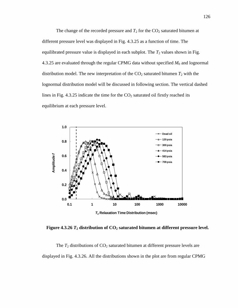
126
The change of the recorded pressure and T2 for the CO2 saturated bitumen at
different pressure level was displayed in Fig. 4.3.25 as a function of time. The
equilibrated pressure value is displayed in each subplot. The T2 values shown in Fig.
4.3.25 are evaluated through the regular CPMG data without specified M0 and lognormal
distribution model. The new interpretation of the CO2 saturated bitumen T2 with the
lognormal distribution model will be discussed in following section. The vertical dashed
lines in Fig. 4.3.25 indicate the time for the CO2 saturated oil firstly reached its
equilibrium at each pressure level.
The T2 distributions of CO2 saturated bitumen at different pressure levels are
displayed in Fig. 4.3.26. All the distributions shown in the plot are from regular CPMG
0.0
0.2
0.4
0.6
0.8
1.0
0.1 1 10 100 1000 10000
Am
plitu
de f
T2 Relaxation Time Distribution (msec)
Dead oil
120 psia
300 psia
414 psia
583 psia
709 psia
Figure 4.3.26 T2 distribution of CO2 saturated bitumen at different pressure level.
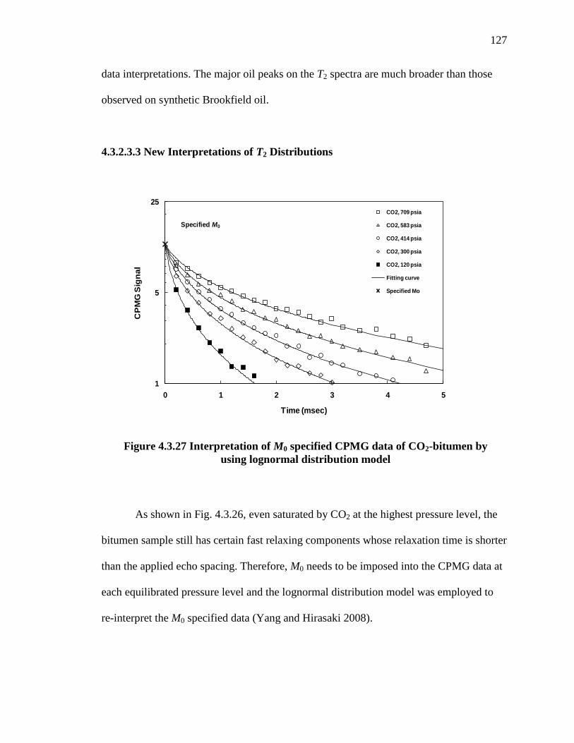
127
data interpretations. The major oil peaks on the T2 spectra are much broader than those
observed on synthetic Brookfield oil.
4.3.2.3.3 New Interpretations of T2 Distributions
As shown in Fig. 4.3.26, even saturated by CO2 at the highest pressure level, the
bitumen sample still has certain fast relaxing components whose relaxation time is shorter
than the applied echo spacing. Therefore, M0 needs to be imposed into the CPMG data at
each equilibrated pressure level and the lognormal distribution model was employed to
re-interpret the M0 specified data (Yang and Hirasaki 2008).
1
5
25
0 1 2 3 4 5
CP
MG
Sig
na
l
Time (msec)
CO2, 709 psia
CO2, 583 psia
CO2, 414 psia
CO2, 300 psia
CO2, 120 psia
Fitting curve
Specified Mo
Specified M0
Figure 4.3.27 Interpretation of M0 specified CPMG data of CO2-bitumen by
using lognormal distribution model
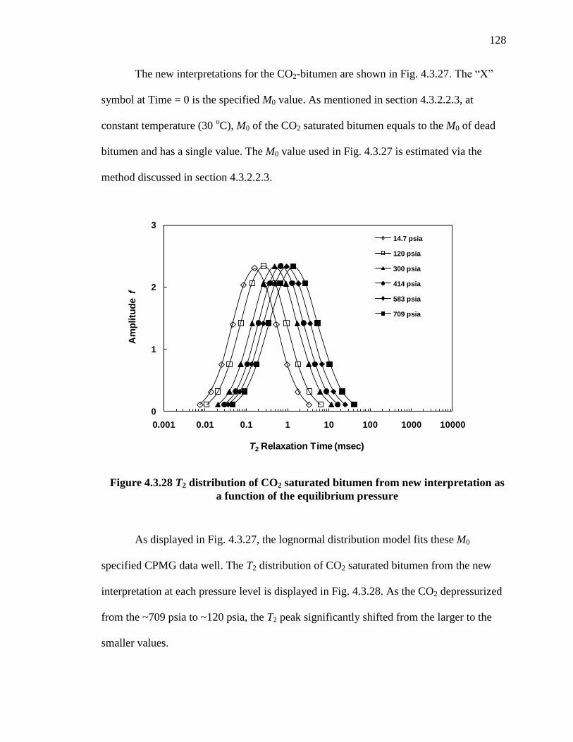
128
The new interpretations for the CO2-bitumen are shown in Fig. 4.3.27. The “X”
symbol at Time = 0 is the specified M0 value. As mentioned in section 4.3.2.2.3, at
constant temperature (30 oC), M0 of the CO2 saturated bitumen equals to the M0 of dead
bitumen and has a single value. The M0 value used in Fig. 4.3.27 is estimated via the
method discussed in section 4.3.2.2.3.
As displayed in Fig. 4.3.27, the lognormal distribution model fits these M0
specified CPMG data well. The T2 distribution of CO2 saturated bitumen from the new
interpretation at each pressure level is displayed in Fig. 4.3.28. As the CO2 depressurized
from the ~709 psia to ~120 psia, the T2 peak significantly shifted from the larger to the
smaller values.
0
1
2
3
0.001 0.01 0.1 1 10 100 1000 10000
Am
plitu
de f
T2 Relaxation Time (msec)
14.7 psia
120 psia
300 psia
414 psia
583 psia
709 psia
Figure 4.3.28 T2 distribution of CO2 saturated bitumen from new interpretation as
a function of the equilibrium pressure
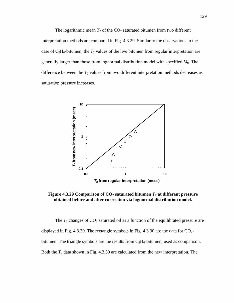
129
The logarithmic mean T2 of the CO2 saturated bitumen from two different
interpretation methods are compared in Fig. 4.3.29. Similar to the observations in the
case of C2H6-bitumen, the T2 values of the live bitumen from regular interpretation are
generally larger than those from lognormal distribution model with specified M0. The
difference between the T2 values from two different interpretation methods decreases as
saturation pressure increases.
The T2 changes of CO2 saturated oil as a function of the equilibrated pressure are
displayed in Fig. 4.3.30. The rectangle symbols in Fig. 4.3.30 are the data for CO2-
bitumen. The triangle symbols are the results from C2H6-bitumen, used as comparison.
Both the T2 data shown in Fig. 4.3.30 are calculated from the new interpretation. The
0.1
1
10
0.1 1 10
T2
fro
m n
ew
inte
rpre
tati
on
(m
sec)
T2 from regular interpretation (msec)
Figure 4.3.29 Comparison of CO2 saturated bitumen T2 at different pressure
obtained before and after correction via lognormal distribution model.

130
solid lines are the fitted curves to the experimental data. The fitted functions are also
shown in the plot.
It clearly shows that at the same pressure level, the T2 change caused by C2H6 is
generally larger than that caused by CO2. Moreover, the higher the pressure level, the
larger the difference in T2 changes. As displayed in Fig. 4.3.30, the changes of T2 data
caused by two different gases are both closely linear on the semi-log scale and the two
trends also well extrapolate to the dead bitumen value (indicated by “X”). The R2 value
for two fitting curves are both near unity, indicating that the live bitumen T2 change
caused by either C2H6 or CO2 at different pressure closely follows the exponential
function.
y = 0.1369e0.0065x
R² = 0.9984
y = 0.2064e0.0027x
R² = 0.9887
0.1
1
10
0 200 400 600 800
T2
of
Liv
e B
itu
men
(m
sec)
Pressure (psia)
C2H6-Bitumen, new interpretation
CO2-Bitumen, new interpretation
Dead Bitumen, new interpretation
Figure 4.3.30 T2 of CO2 saturated bitumen at different pressure levels

131
4.3.2.3.4 Estimation of CO2 Solubility in Bitumen
Given the pressure change, volume and temperature, the amount of CO2 dissolved
into bitumen at each pressure level can be calculated, as described in section 3.3.2.1. In
this case, the reference data for compression factor z of CO2 is from the IUPAC
International Thermodynamic Tables (IUPAC 1973). The linear interpolation was used to
calculate the value of compression factor z at any specific pressure, which is not directly
shown by the reference book.
In order to remove the temperature effects on the initial pressure reading,
extrapolations were employed for the correction. Fig. 4.3.31 shows the analysis and
extrapolation of recorded pressure data for CO2-bitumen during the pressurization stage.
The recorded data within the initial period, which were considered to be markedly
influenced by temperature change, are shown by open triangles. The pressure data after
this initial period are displayed by open rectangles and used for extrapolation.
y = -3.24x + 744.7R² = 0.9179
730
740
750
760
770
0 0.5 1 1.5 2
Pre
ssu
re (
psi
a)
Time (Hour)
Figure 4.3.31 Extrapolation for the pressurization stage of CO2-bitumen
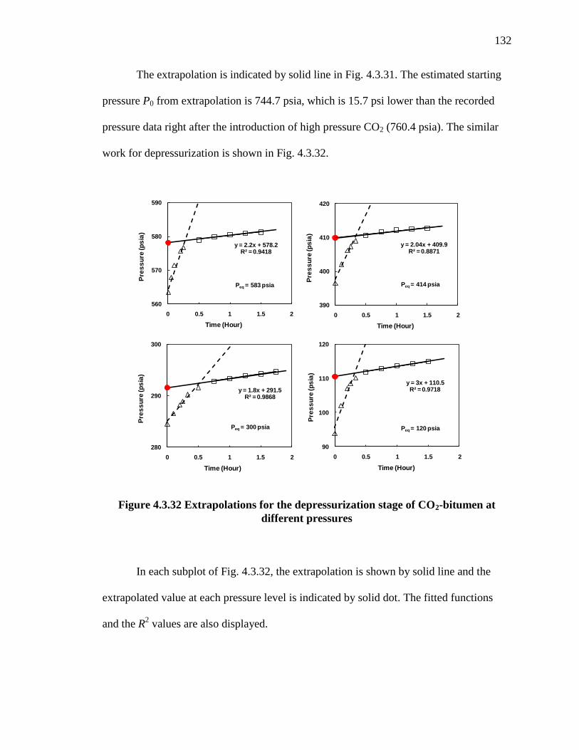
132
The extrapolation is indicated by solid line in Fig. 4.3.31. The estimated starting
pressure P0 from extrapolation is 744.7 psia, which is 15.7 psi lower than the recorded
pressure data right after the introduction of high pressure CO2 (760.4 psia). The similar
work for depressurization is shown in Fig. 4.3.32.
In each subplot of Fig. 4.3.32, the extrapolation is shown by solid line and the
extrapolated value at each pressure level is indicated by solid dot. The fitted functions
and the R2 values are also displayed.
y = 2.2x + 578.2R² = 0.9418
560
570
580
590
0 0.5 1 1.5 2
Pre
ss
ure
(p
sia
)
Time (Hour)
Peq = 583 psia
y = 2.04x + 409.9R² = 0.8871
390
400
410
420
0 0.5 1 1.5 2P
res
su
re (p
sia
)
Time (Hour)
Peq = 414 psia
y = 1.8x + 291.5R² = 0.9868
280
290
300
0 0.5 1 1.5 2
Pre
ss
ure
(p
sia
)
Time (Hour)
Peq = 300 psia
y = 3x + 110.5R² = 0.9718
90
100
110
120
0 0.5 1 1.5 2
Pre
ss
ure
(p
sia
)
Time (Hour)
Peq = 120 psia
Figure 4.3.32 Extrapolations for the depressurization stage of CO2-bitumen at
different pressures
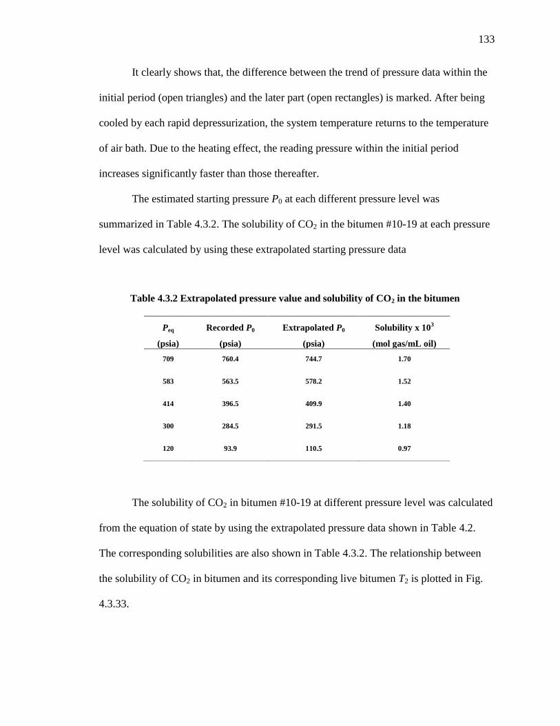
133
It clearly shows that, the difference between the trend of pressure data within the
initial period (open triangles) and the later part (open rectangles) is marked. After being
cooled by each rapid depressurization, the system temperature returns to the temperature
of air bath. Due to the heating effect, the reading pressure within the initial period
increases significantly faster than those thereafter.
The estimated starting pressure P0 at each different pressure level was
summarized in Table 4.3.2. The solubility of CO2 in the bitumen #10-19 at each pressure
level was calculated by using these extrapolated starting pressure data
The solubility of CO2 in bitumen #10-19 at different pressure level was calculated
from the equation of state by using the extrapolated pressure data shown in Table 4.2.
The corresponding solubilities are also shown in Table 4.3.2. The relationship between
the solubility of CO2 in bitumen and its corresponding live bitumen T2 is plotted in Fig.
4.3.33.
Peq
(psia)
Recorded P0
(psia)
Extrapolated P0
(psia)
Solubility x 103
(mol gas/mL oil)
709 760.4 744.7 1.70
583 563.5 578.2 1.52
414 396.5 409.9 1.40
300 284.5 291.5 1.18
120 93.9 110.5 0.97
Table 4.3.2 Extrapolated pressure value and solubility of CO2 in the bitumen
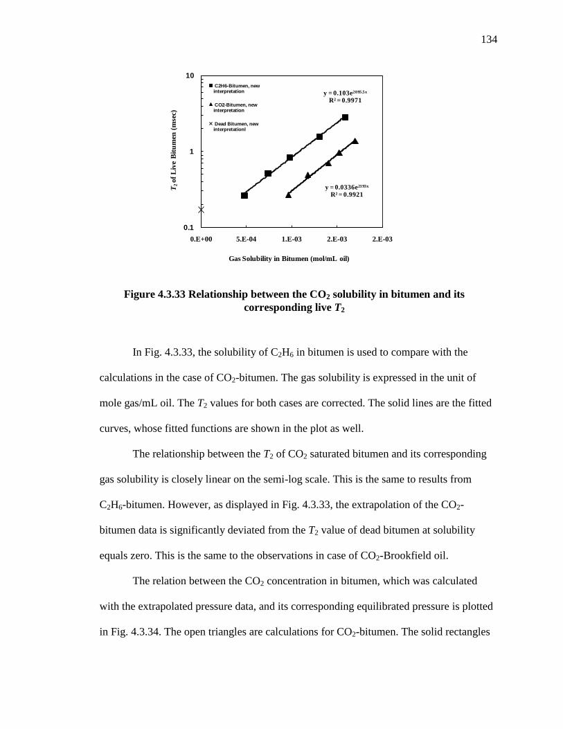
134
In Fig. 4.3.33, the solubility of C2H6 in bitumen is used to compare with the
calculations in the case of CO2-bitumen. The gas solubility is expressed in the unit of
mole gas/mL oil. The T2 values for both cases are corrected. The solid lines are the fitted
curves, whose fitted functions are shown in the plot as well.
The relationship between the T2 of CO2 saturated bitumen and its corresponding
gas solubility is closely linear on the semi-log scale. This is the same to results from
C2H6-bitumen. However, as displayed in Fig. 4.3.33, the extrapolation of the CO2-
bitumen data is significantly deviated from the T2 value of dead bitumen at solubility
equals zero. This is the same to the observations in case of CO2-Brookfield oil.
The relation between the CO2 concentration in bitumen, which was calculated
with the extrapolated pressure data, and its corresponding equilibrated pressure is plotted
in Fig. 4.3.34. The open triangles are calculations for CO2-bitumen. The solid rectangles
y = 0.103e2095.5x
R² = 0.9971
y = 0.0336e2193x
R² = 0.9921
0.1
1
10
0.E+00 5.E-04 1.E-03 2.E-03 2.E-03
T2o
f L
ive
Bit
um
en (
mse
c)
Gas Solubility in Bitumen (mol/mL oil)
C2H6-Bitumen, new interpretation
CO2-Bitumen, new interpretation
Dead Bitumen, new interpretationl
Figure 4.3.33 Relationship between the CO2 solubility in bitumen and its
corresponding live T2
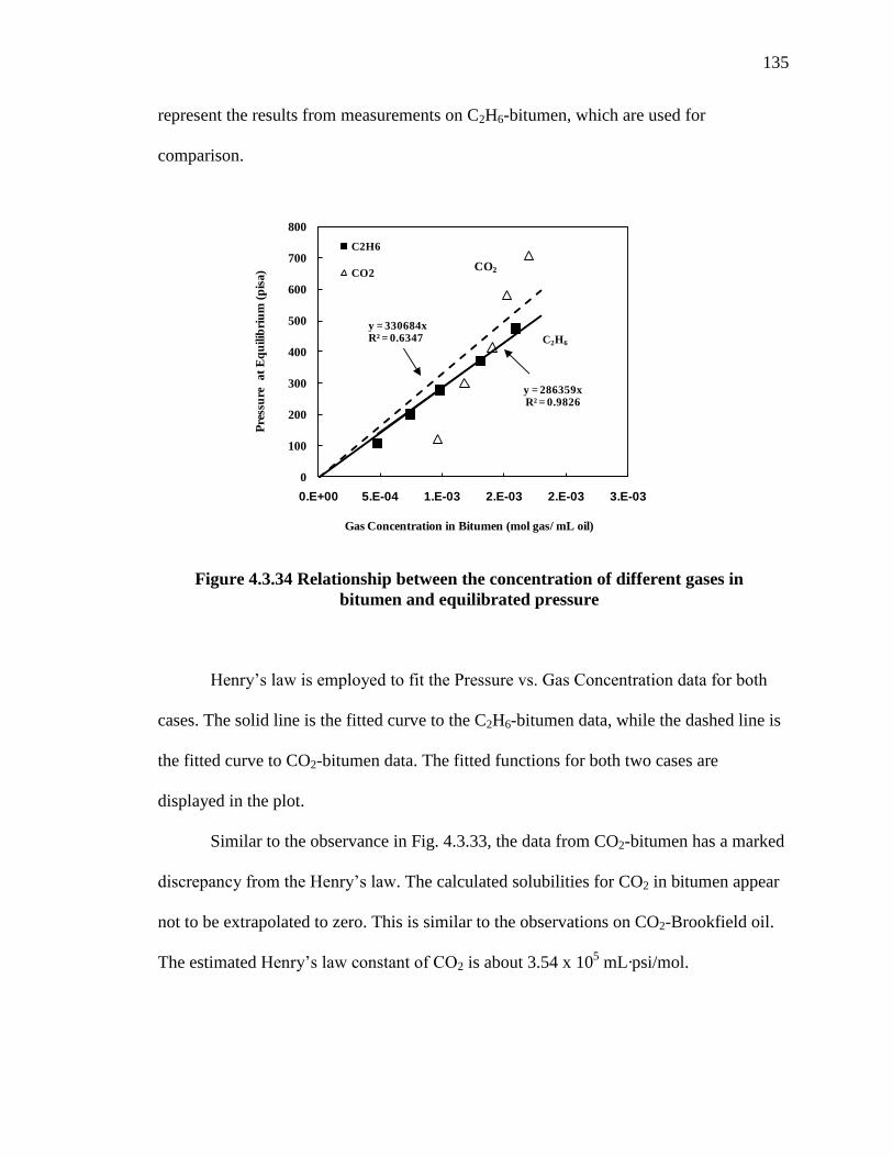
135
represent the results from measurements on C2H6-bitumen, which are used for
comparison.
Henry’s law is employed to fit the Pressure vs. Gas Concentration data for both
cases. The solid line is the fitted curve to the C2H6-bitumen data, while the dashed line is
the fitted curve to CO2-bitumen data. The fitted functions for both two cases are
displayed in the plot.
Similar to the observance in Fig. 4.3.33, the data from CO2-bitumen has a marked
discrepancy from the Henry’s law. The calculated solubilities for CO2 in bitumen appear
not to be extrapolated to zero. This is similar to the observations on CO2-Brookfield oil.
The estimated Henry’s law constant of CO2 is about 3.54 x 10⁵ mL·psi/mol.
y = 286359xR² = 0.9826
0
100
200
300
400
500
600
700
800
0.E+00 5.E-04 1.E-03 2.E-03 2.E-03 3.E-03
Pre
ssu
re
at
Eq
uilib
riu
m (
pis
a)
Gas Concentration in Bitumen (mol gas/ mL oil)
C2H6
CO2CO2
C2H6
y = 330684xR² = 0.6347
Figure 4.3.34 Relationship between the concentration of different gases in
bitumen and equilibrated pressure

136
4.3.2.3.5 T1 Measurements of CO2 Saturated Bitumen
T1 measurements were performed on the CO2 saturated bitumen at each
corresponding pressure shown in Fig. 4.3.26. The Inversion Recovery sequence with 20
different recovery times logarithmically spaced between 30 sec and 5 sec was
employed. The interpreted T1 distributions for the live bitumen at each equilibrated
pressure level are displayed in Fig. 4.3.35.
The change of T1 distribution with pressure is much less significant, comparing to
the corresponding T2 change of live bitumen as shown in Fig. 4.3.26. In other words, the
change of bitumen viscosity (caused by the change of CO2 solubility at different
pressure) has much more effect on the T2 response rather than T1. This observance
accords the results obtained by our group in previous work on other heavy oil samples
0
0.2
0.4
0.6
0.8
1
0.1 1 10 100 1000 10000
Am
plitu
de f
Relaxation Time (msec)
T1 at 709 psia
T1 at 583 psia
T1 at 414 psia
T1 at 300 psia
T1 at 120 psia
Figure 4.3.35 T1 distribution of CO2 saturated bitumen at different pressure levels
137
(Hirasaki, Lo and Zhang 2003) and the results recently reported by some other
researchers (Zielinski, et al. 2010).
4.3.2.4 Recombined Live Bitumen with CH4
Due to the extremely high viscosity of bitumen, the sample volume was inevitably
lost during the previous measurements. In the investigation on the CH4-bitumen, the total
volume of bitumen was ~7.6 mL. The total sample chamber volume of the pressure
vessel is about 82 mL. Subtracting 9.5 mL for oil sample, the total space for gas is about
74.4 mL.
The gas pressure inside the vessel was firstly raised to ~946 psia by injecting CH4
from the top of the pressure vessel. Then, the gas source was cut off and no more gas was
added into the system afterwards. The gas pressure inside the vessel was monitored by
using Senso-Metrics pressure transducer during the entire process until the gas-bitumen
system finally reached equilibrium.
4.3.2.4.1 Pressurization Stage of CH4-Bitumen
During the initial period right after the gas injection was cut off, the pressure
vessel containing bitumen and CH4 was kept vertical in the 30 oC air bath of NMR
spectrometer. In this manner, only diffusion occurred to the CH4 dissolving into bitumen.
The pressure change during the diffusion was recorded and would be used for
extrapolation to remove the temperature effect on the initial pressure reading.
Unlike the observation in the case of CH4-Brookfield oil, the methane was found
to be easier to dissolve into the bitumen than the Brookfield oil simply via diffusion. The
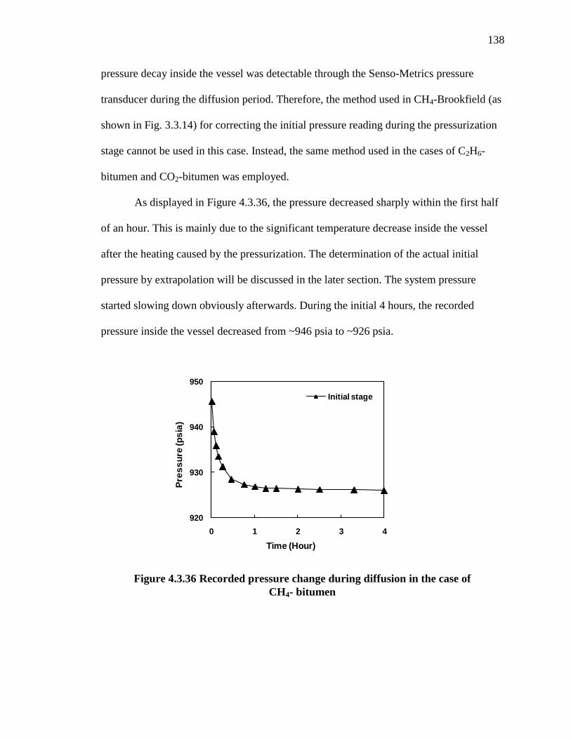
138
pressure decay inside the vessel was detectable through the Senso-Metrics pressure
transducer during the diffusion period. Therefore, the method used in CH4-Brookfield (as
shown in Fig. 3.3.14) for correcting the initial pressure reading during the pressurization
stage cannot be used in this case. Instead, the same method used in the cases of C2H6-
bitumen and CO2-bitumen was employed.
As displayed in Figure 4.3.36, the pressure decreased sharply within the first half
of an hour. This is mainly due to the significant temperature decrease inside the vessel
after the heating caused by the pressurization. The determination of the actual initial
pressure by extrapolation will be discussed in the later section. The system pressure
started slowing down obviously afterwards. During the initial 4 hours, the recorded
pressure inside the vessel decreased from ~946 psia to ~926 psia.
920
930
940
950
0 1 2 3 4
Pre
ss
ure
(p
sia
)
Time (Hour)
Initial stage
Figure 4.3.36 Recorded pressure change during diffusion in the case of
CH4- bitumen

139
After the initial diffusion period, the pressure vessel was placed on the support
stand at room temperature and repeatedly turned from vertical to horizontal and then
turning back to vertical, as shown in Fig. 3.3.14. In this manner, convection was
introduced to the bitumen and CH4 mixture inside the vessel. Periodically, the vessel was
put back into the 30 oC air bath and placed vertically for at least overnight. The system
pressure and the T2 of C2H6 dissolved bitumen would be measured the next morning.
The measured T2 and pressure decay during the entire process are displayed in
Fig. 4.3.37. The T2 values in the plot are simply from the regular CPMG data
interpretation. The newly interpreted T2 values of the C2H6 saturated bitumen will be
discussed in following sections.
As shown in Fig. 4.3.37, the recorded pressure inside vessel and the measured T2
of CH4 dissolved bitumen firstly reached plateau after ~331 hours. The measurements
910
920
930
940
950
0.1
1
0 100 200 300 400 500
Pressu
re (p
sia)
T2
of
bit
um
en
(m
sec)
Time (Hour)
T2 Pressure
30 oC
Figure 4.3.37 Pressure and T2 change of CH4- bitumen system
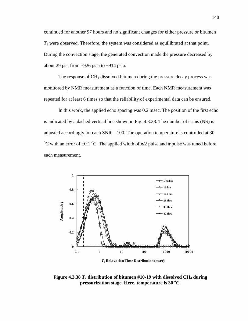
140
continued for another 97 hours and no significant changes for either pressure or bitumen
T2 were observed. Therefore, the system was considered as equilibrated at that point.
During the convection stage, the generated convection made the pressure decreased by
about 29 psi, from ~926 psia to ~914 psia.
The response of CH4 dissolved bitumen during the pressure decay process was
monitored by NMR measurement as a function of time. Each NMR measurement was
repeated for at least 6 times so that the reliability of experimental data can be ensured.
In this work, the applied echo spacing was 0.2 msec. The position of the first echo
is indicated by a dashed vertical line shown in Fig. 4.3.38. The number of scans (NS) is
adjusted accordingly to reach SNR = 100. The operation temperature is controlled at 30
oC with an error of ±0.1
oC. The applied width of π/2 pulse and π pulse was tuned before
each measurement.
0
0.2
0.4
0.6
0.8
1
0.1 1 10 100 1000 10000
Am
pli
tud
e f
T2 Relaxation Time Distribution (msec)
Dead oil
19 hrs
141 hrs
263hrs
331hrs
428hrs
Figure 4.3.38 T2 distribution of bitumen #10-19 with dissolved CH4 during
pressurization stage. Here, temperature is 30 oC.
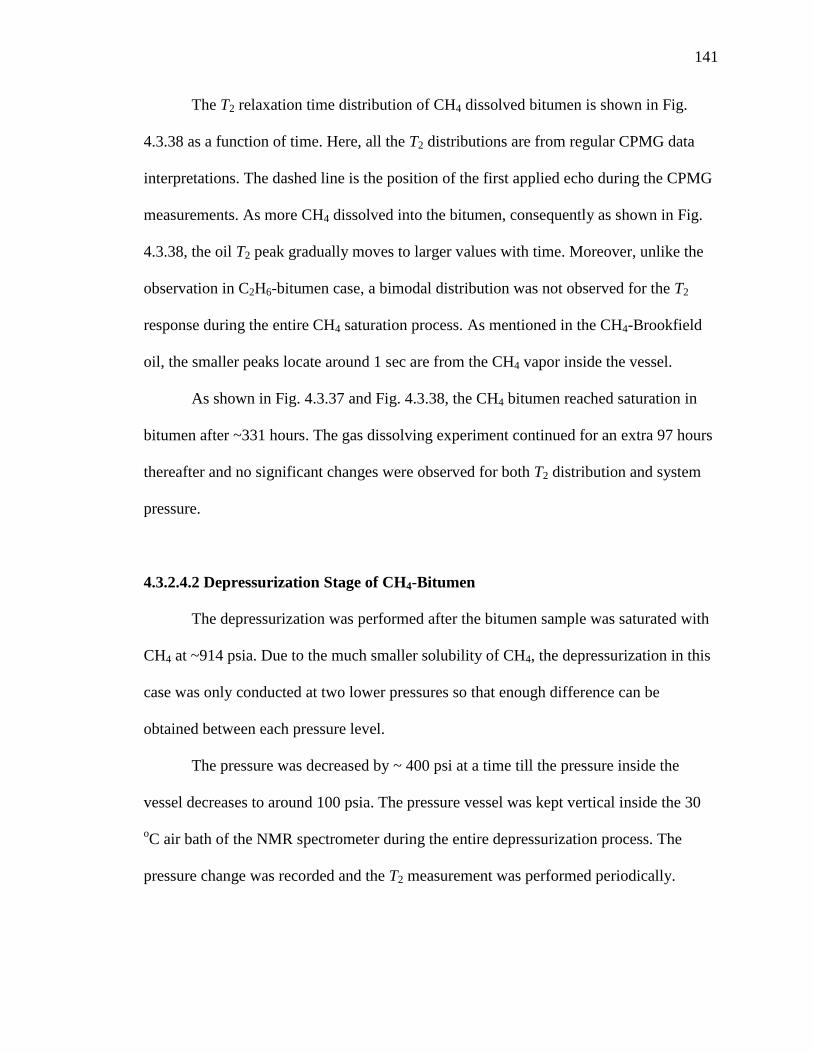
141
The T2 relaxation time distribution of CH4 dissolved bitumen is shown in Fig.
4.3.38 as a function of time. Here, all the T2 distributions are from regular CPMG data
interpretations. The dashed line is the position of the first applied echo during the CPMG
measurements. As more CH4 dissolved into the bitumen, consequently as shown in Fig.
4.3.38, the oil T2 peak gradually moves to larger values with time. Moreover, unlike the
observation in C2H6-bitumen case, a bimodal distribution was not observed for the T2
response during the entire CH4 saturation process. As mentioned in the CH4-Brookfield
oil, the smaller peaks locate around 1 sec are from the CH4 vapor inside the vessel.
As shown in Fig. 4.3.37 and Fig. 4.3.38, the CH4 bitumen reached saturation in
bitumen after ~331 hours. The gas dissolving experiment continued for an extra 97 hours
thereafter and no significant changes were observed for both T2 distribution and system
pressure.
4.3.2.4.2 Depressurization Stage of CH4-Bitumen
The depressurization was performed after the bitumen sample was saturated with
CH4 at ~914 psia. Due to the much smaller solubility of CH4, the depressurization in this
case was only conducted at two lower pressures so that enough difference can be
obtained between each pressure level.
The pressure was decreased by ~ 400 psi at a time till the pressure inside the
vessel decreases to around 100 psia. The pressure vessel was kept vertical inside the 30
oC air bath of the NMR spectrometer during the entire depressurization process. The
pressure change was recorded and the T2 measurement was performed periodically.

142
All the measurements were performed at 30 oC. In order to ensure the reliability
of experimental data, each NMR measurement was repeated 6 times. During the
depressurization experiment, the measurement at each pressure level usually lasted for
extra two more days after CH4 saturated oil first reached its equilibrated value. In this
manner, the reliability of measured values for T2 and pressure at equilibrium can be
ensured.
In order to ensure the reliability of experimental data, each NMR measurement
was repeated for 6 times. During the depressurization experiment, the measurement at
each pressure level usually lasted for at least extra two more days after CH4 saturated oil
first reached its equilibrated value. In this manner, the reliability of measured values for
T2 and pressure at equilibrium can be ensured.
The change of the recorded pressure and T2 for the CH4 saturated bitumen at
different pressure level was displayed in Fig. 4.3.39 as a function of time. The
490
500
510
520
530
540
0.1
1
0 20 40 60 80
Pressu
re (p
sia)
T2
of
bit
um
en (
mse
c)
Time (Hour)
T2 Pressure
Peq = 517 psia
110
120
130
140
150
0.1
1
0 20 40 60 80
Pressu
re (p
sia)
T2
of
bit
um
en
(m
sec)
Time (Hour)
T2 Pressure
Peq = 131 psia
Figure 4.3.39 Change of T2 and pressure for CH4 saturated bitumen as a
function of time at different pressure
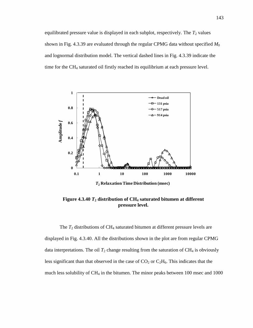
143
equilibrated pressure value is displayed in each subplot, respectively. The T2 values
shown in Fig. 4.3.39 are evaluated through the regular CPMG data without specified M0
and lognormal distribution model. The vertical dashed lines in Fig. 4.3.39 indicate the
time for the CH4 saturated oil firstly reached its equilibrium at each pressure level.
The T2 distributions of CH4 saturated bitumen at different pressure levels are
displayed in Fig. 4.3.40. All the distributions shown in the plot are from regular CPMG
data interpretations. The oil T2 change resulting from the saturation of CH4 is obviously
less significant than that observed in the case of CO2 or C2H6. This indicates that the
much less solubility of CH4 in the bitumen. The minor peaks between 100 msec and 1000
0
0.2
0.4
0.6
0.8
1
0.1 1 10 100 1000 10000
Am
pli
tud
ef
T2 Relaxation Time Distribution (msec)
Dead oil
131 psia
517 psia
914 psia
Figure 4.3.40 T2 distribution of CH4 saturated bitumen at different
pressure level.

144
msec in Fig. 4.3.40 are from free CH4 in the vapor phase. As the system pressure
decreases, the gas peak moves to the smaller values and peak area shrinks.
4.3.2.4.3 New Interpretations of T2 Distributions
As shown in Fig. 4.3.40, even saturated by CH4 at the highest pressure level, the
bitumen sample still has certain fast relaxing components whose relaxation time is shorter
than the applied echo spacing. Therefore, the M0 need to be imposed into the CPMG data
at each equilibrated pressure level and the lognormal distribution model was employed to
re-interpret the M0 specified data (Yang and Hirasaki 2008).
1
5
25
0 1 2 3 4 5
CP
MG
Sig
na
l
Time (msec)
CH4, 914 psia
CH4, 517 psia
CH4, 131 psia
Fitting curve
Specified Mo
Specified M0
Figure 4.3.41 Fitting of M0 specified CPMG data of live bitumen with CH4
by using lognormal distribution model
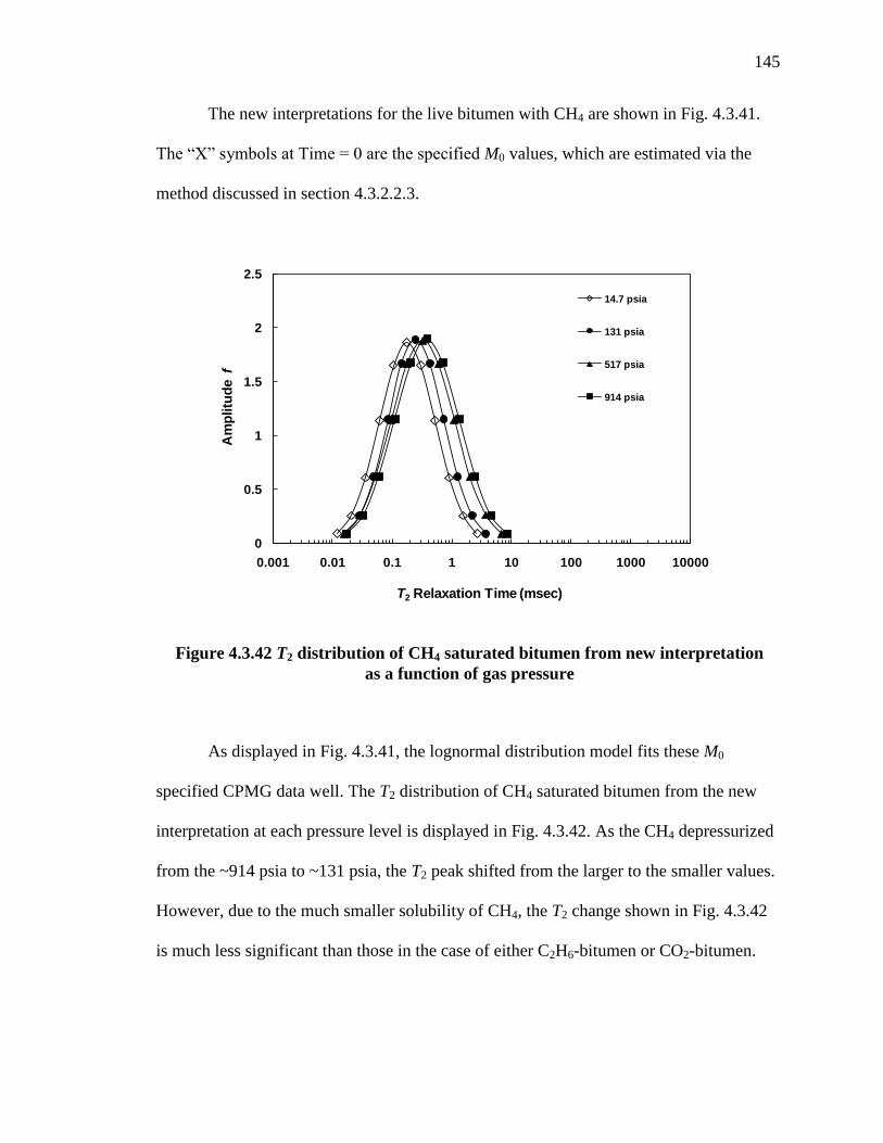
145
The new interpretations for the live bitumen with CH4 are shown in Fig. 4.3.41.
The “X” symbols at Time = 0 are the specified M0 values, which are estimated via the
method discussed in section 4.3.2.2.3.
As displayed in Fig. 4.3.41, the lognormal distribution model fits these M0
specified CPMG data well. The T2 distribution of CH4 saturated bitumen from the new
interpretation at each pressure level is displayed in Fig. 4.3.42. As the CH4 depressurized
from the ~914 psia to ~131 psia, the T2 peak shifted from the larger to the smaller values.
However, due to the much smaller solubility of CH4, the T2 change shown in Fig. 4.3.42
is much less significant than those in the case of either C2H6-bitumen or CO2-bitumen.
0
0.5
1
1.5
2
2.5
0.001 0.01 0.1 1 10 100 1000 10000
Am
plitu
de f
T2 Relaxation Time (msec)
14.7 psia
131 psia
517 psia
914 psia
Figure 4.3.42 T2 distribution of CH4 saturated bitumen from new interpretation
as a function of gas pressure
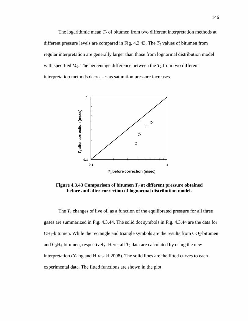
146
The logarithmic mean T2 of bitumen from two different interpretation methods at
different pressure levels are compared in Fig. 4.3.43. The T2 values of bitumen from
regular interpretation are generally larger than those from lognormal distribution model
with specified M0. The percentage difference between the T2 from two different
interpretation methods decreases as saturation pressure increases.
The T2 changes of live oil as a function of the equilibrated pressure for all three
gases are summarized in Fig. 4.3.44. The solid dot symbols in Fig. 4.3.44 are the data for
CH4-bitumen. While the rectangle and triangle symbols are the results from CO2-bitumen
and C2H6-bitumen, respectively. Here, all T2 data are calculated by using the new
interpretation (Yang and Hirasaki 2008). The solid lines are the fitted curves to each
experimental data. The fitted functions are shown in the plot.
0.1
1
0.1 1
T2
aft
er
co
rrecti
on
(m
sec)
T2 before correction (msec)
Figure 4.3.43 Comparison of bitumen T2 at different pressure obtained
before and after correction of lognormal distribution model.
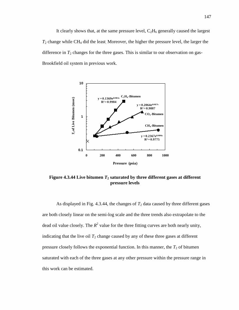
147
It clearly shows that, at the same pressure level, C2H6 generally caused the largest
T2 change while CH4 did the least. Moreover, the higher the pressure level, the larger the
difference in T2 changes for the three gases. This is similar to our observation on gas-
Brookfield oil system in previous work.
As displayed in Fig. 4.3.44, the changes of T2 data caused by three different gases
are both closely linear on the semi-log scale and the three trends also extrapolate to the
dead oil value closely. The R2 value for the three fitting curves are both nearly unity,
indicating that the live oil T2 change caused by any of these three gases at different
pressure closely follows the exponential function. In this manner, the T2 of bitumen
saturated with each of the three gases at any other pressure within the pressure range in
this work can be estimated.
y = 0.1369e0.0065x
R² = 0.9984y = 0.2064e0.0027x
R² = 0.9887
y = 0.2367e0.0006x
R² = 0.9775
0.1
1
10
0 200 400 600 800 1000
T2
of
Liv
e B
itu
men
(m
sec)
Pressure (psia)
CO2-Bitumen
CH4-Bitumen
C2H6-Bitumen
Figure 4.3.44 Live bitumen T2 saturated by three different gases at different
pressure levels
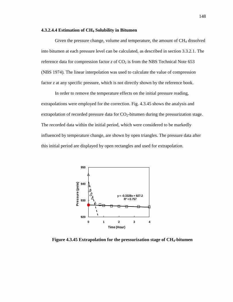
148
4.3.2.4.4 Estimation of CH4 Solubility in Bitumen
Given the pressure change, volume and temperature, the amount of CH4 dissolved
into bitumen at each pressure level can be calculated, as described in section 3.3.2.1. The
reference data for compression factor z of CO2 is from the NBS Technical Note 653
(NBS 1974). The linear interpolation was used to calculate the value of compression
factor z at any specific pressure, which is not directly shown by the reference book.
In order to remove the temperature effects on the initial pressure reading,
extrapolations were employed for the correction. Fig. 4.3.45 shows the analysis and
extrapolation of recorded pressure data for CO2-bitumen during the pressurization stage.
The recorded data within the initial period, which were considered to be markedly
influenced by temperature change, are shown by open triangles. The pressure data after
this initial period are displayed by open rectangles and used for extrapolation.
y = -0.3328x + 927.2R² = 0.757
920
930
940
950
0 1 2 3 4
Pre
ss
ure
(p
sia
)
Time (Hour)
Figure 4.3.45 Extrapolation for the pressurization stage of CH4-bitumen
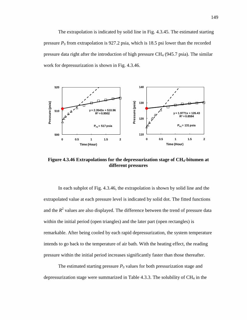
149
The extrapolation is indicated by solid line in Fig. 4.3.45. The estimated starting
pressure P0 from extrapolation is 927.2 psia, which is 18.5 psi lower than the recorded
pressure data right after the introduction of high pressure CH4 (945.7 psia). The similar
work for depressurization is shown in Fig. 4.3.46.
In each subplot of Fig. 4.3.46, the extrapolation is shown by solid line and the
extrapolated value at each pressure level is indicated by solid dot. The fitted functions
and the R2 values are also displayed. The difference between the trend of pressure data
within the initial period (open triangles) and the later part (open rectangles) is
remarkable. After being cooled by each rapid depressurization, the system temperature
intends to go back to the temperature of air bath. With the heating effect, the reading
pressure within the initial period increases significantly faster than those thereafter.
The estimated starting pressure P0 values for both pressurization stage and
depressurization stage were summarized in Table 4.3.3. The solubility of CH4 in the
y = 2.3543x + 510.96R² = 0.9502
500
510
520
0 0.5 1 1.5 2
Pre
ss
ure
(p
sia
)
Time (Hour)
Peq = 517 psia
y = 1.9771x + 126.43R² = 0.8594
110
120
130
140
0 0.5 1 1.5 2
Pre
ss
ure
(p
sia
)
Time (Hour)
Peq = 131 psia
Figure 4.3.46 Extrapolations for the depressurization stage of CH4-bitumen at
different pressures
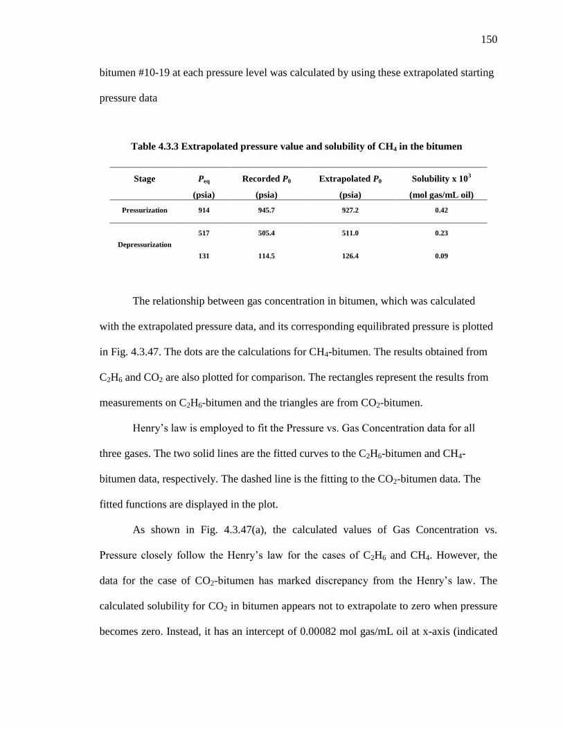
150
bitumen #10-19 at each pressure level was calculated by using these extrapolated starting
pressure data
The relationship between gas concentration in bitumen, which was calculated
with the extrapolated pressure data, and its corresponding equilibrated pressure is plotted
in Fig. 4.3.47. The dots are the calculations for CH4-bitumen. The results obtained from
C2H6 and CO2 are also plotted for comparison. The rectangles represent the results from
measurements on C2H6-bitumen and the triangles are from CO2-bitumen.
Henry’s law is employed to fit the Pressure vs. Gas Concentration data for all
three gases. The two solid lines are the fitted curves to the C2H6-bitumen and CH4-
bitumen data, respectively. The dashed line is the fitting to the CO2-bitumen data. The
fitted functions are displayed in the plot.
As shown in Fig. 4.3.47(a), the calculated values of Gas Concentration vs.
Pressure closely follow the Henry’s law for the cases of C2H6 and CH4. However, the
data for the case of CO2-bitumen has marked discrepancy from the Henry’s law. The
calculated solubility for CO2 in bitumen appears not to extrapolate to zero when pressure
becomes zero. Instead, it has an intercept of 0.00082 mol gas/mL oil at x-axis (indicated
Stage Peq
(psia)
Recorded P0
(psia)
Extrapolated P0
(psia)
Solubility x 103
(mol gas/mL oil)
Pressurization 914 945.7 927.2 0.42
Depressurization
517 505.4 511.0 0.23
131 114.5 126.4 0.09
Table 4.3.3 Extrapolated pressure value and solubility of CH4 in the bitumen
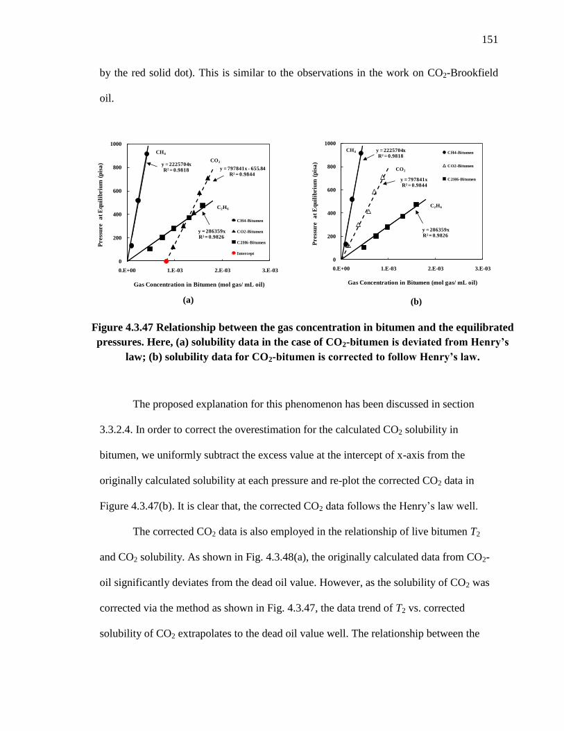
151
by the red solid dot). This is similar to the observations in the work on CO2-Brookfield
oil.
The proposed explanation for this phenomenon has been discussed in section
3.3.2.4. In order to correct the overestimation for the calculated CO2 solubility in
bitumen, we uniformly subtract the excess value at the intercept of x-axis from the
originally calculated solubility at each pressure and re-plot the corrected CO2 data in
Figure 4.3.47(b). It is clear that, the corrected CO2 data follows the Henry’s law well.
The corrected CO2 data is also employed in the relationship of live bitumen T2
and CO2 solubility. As shown in Fig. 4.3.48(a), the originally calculated data from CO2-
oil significantly deviates from the dead oil value. However, as the solubility of CO2 was
corrected via the method as shown in Fig. 4.3.47, the data trend of T2 vs. corrected
solubility of CO2 extrapolates to the dead oil value well. The relationship between the
y = 2225704xR² = 0.9818
y = 286359xR² = 0.9826
0
200
400
600
800
1000
0.E+00 1.E-03 2.E-03 3.E-03
Press
ure
at
Eq
uil
ibriu
m (
pis
a)
Gas Concentration in Bitumen (mol gas/ mL oil)
CH4-Bitumen
CO2-Bitumen
C2H6-Bitumen
Intercept
C2H6
CH4
y = 797841x - 655.84R² = 0.9844
CO2
y = 2225704xR² = 0.9818
y = 286359xR² = 0.9826
0
200
400
600
800
1000
0.E+00 1.E-03 2.E-03 3.E-03
Press
ure
at
Eq
uil
ibriu
m (
pis
a)
Gas Concentration in Bitumen (mol gas/ mL oil)
CH4-Bitumen
CO2-Bitumen
C2H6-Bitumen
C2H6
CH4
y = 797841x R² = 0.9844
CO2
(a) (b)
Figure 4.3.47 Relationship between the gas concentration in bitumen and the equilibrated
pressures. Here, (a) solubility data in the case of CO2-bitumen is deviated from Henry’s
law; (b) solubility data for CO2-bitumen is corrected to follow Henry’s law.
152
live bitumen T2 and its corresponding gas solubility is closely linear on the semi-log scale
for all three gases. Furthermore, similar to the observations in CO2-Brookfield oil, the
relationship between the live oil T2 and gas solubility shown in Fig. 4.3.48(b) appears to
closely follow similar trend, regardless of the gas type used for saturation.
The gas solubility is calculated via equation of state with compressibility factor z,
as shown in section 3.3.2.1. In order to remove the overestimation for CO2 solubility, the
compressibility factor z was re-adjusted to correct the Pressure vs. Solubility curve of
CO2 to follow the Henry’s law (as shown in Fig. 4.3.47). The solubility calculation
method during pressurization stage is expressed by Eq. [3.1]. The adjustment on z factor
can be made on either z0 (initial point) or zeq (equilibrium point) to serve the purpose.
Figure 4.3.48 Relationship between the gas solubility in bitumen and its corresponding
T2. Here, (a) data from CO2-bitumen is deviated from dead oil value; (b) corrected data
for CO2-bitumen well extrapolates to dead oil value.
y = 0.2288e1341.9x
R² = 0.9432
y = 0.103e2095.5x
R² = 0.9971
y = 0.0336e2193x
R² = 0.9921
0.1
1
10
0.E+00 1.E-03 2.E-03
T2
of
Liv
e B
itu
men
(m
sec)
Gas Solubility in Bitumen (mol/mL oil)
CH4-Bitumen
C2H6-Bitumen
CO2-Bitumen
Dead Bitumen
C2H6
CH4
CO2
y = 0.2288e1341.9x
R² = 0.9432
y = 0.103e2095.5x
R² = 0.9971
y = 0.2041e2193x
R² = 0.9921
0.1
1
10
0.E+00 1.E-03 2.E-03
T2
of
Liv
e B
itu
men
(m
sec)
Gas Solubility in Bitumen (mol/mL oil)
CH4-Bitumen
C2H6-Bitumen
CO2-Bitumen
Dead Bitumen
C2H6
CH4
CO2
(a) (b)
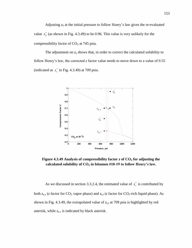
153
Adjusting z0 at the initial pressure to follow Henry’s law gives the re-evaluated
value *
0z (as shown in Fig. 4.3.49) to be 0.96. This value is very unlikely for the
compressibility factor of CO2 at 745 psia.
The adjustment on ze shows that, in order to correct the calculated solubility to
follow Henry’s law, the corrected z factor value needs to move down to a value of 0.55
(indicated as *
ez in Fig. 4.3.49) at 709 psia.
As we discussed in section 3.3.2.4, the estimated value of *
ez is contributed by
both ze,v (z factor for CO2 vapor phase) and ze,l (z factor for CO2-rich liquid phase). As
shown in Fig. 4.3.49, the extrapolated value of ze,l at 709 psia is highlighted by red
asterisk, while ze,v is indicated by black asterisk.
0 200 400 600 800 1000 12000.2
0.3
0.4
0.5
0.6
0.7
0.8
0.9
1
Pressure, psi
Co
mp
ressio
n F
acto
r Z
CO2 at 30 oC
ze,
v
ze*
z0
z0*
ze,
l
Figure 4.3.49 Analysis of compressibility factor z of CO2 for adjusting the
calculated solubility of CO2 in bitumen #10-19 to follow Henry’s law.
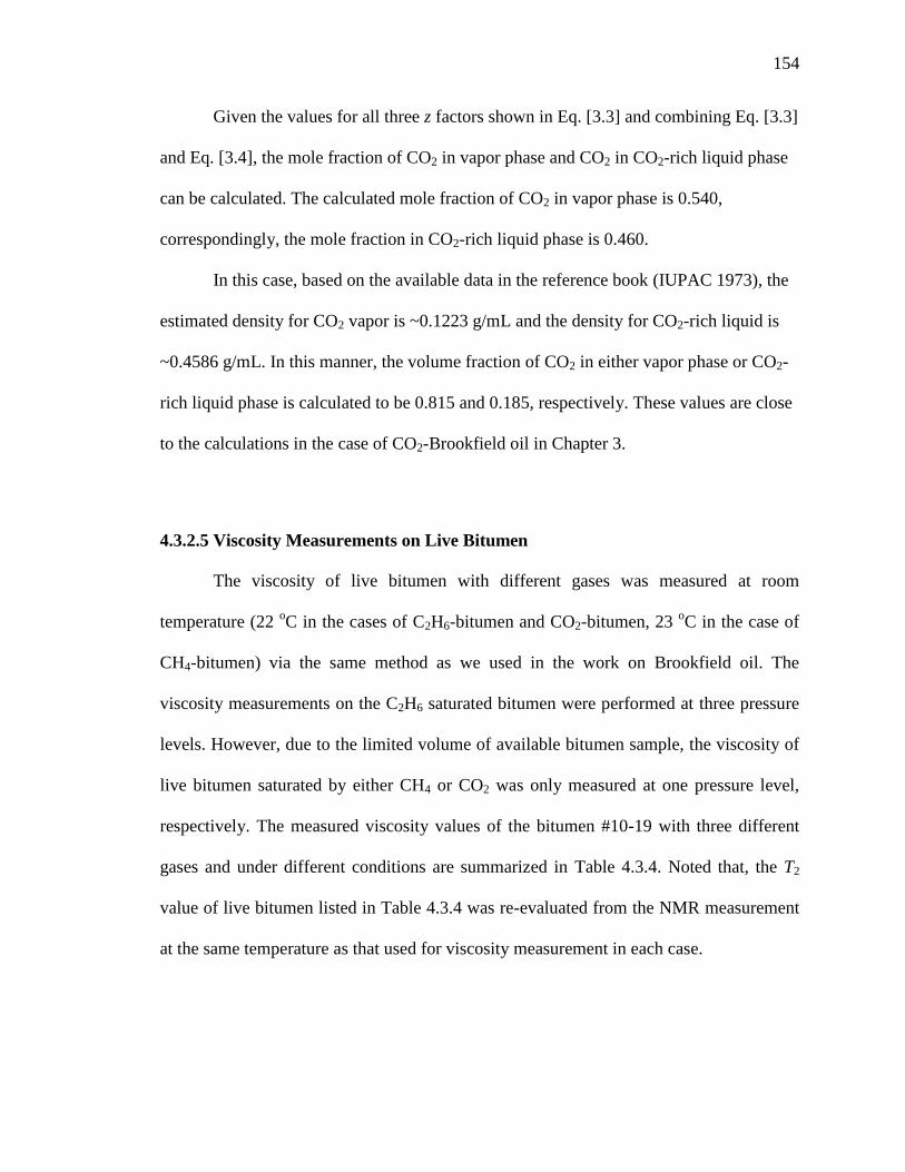
154
Given the values for all three z factors shown in Eq. [3.3] and combining Eq. [3.3]
and Eq. [3.4], the mole fraction of CO2 in vapor phase and CO2 in CO2-rich liquid phase
can be calculated. The calculated mole fraction of CO2 in vapor phase is 0.540,
correspondingly, the mole fraction in CO2-rich liquid phase is 0.460.
In this case, based on the available data in the reference book (IUPAC 1973), the
estimated density for CO2 vapor is ~0.1223 g/mL and the density for CO2-rich liquid is
~0.4586 g/mL. In this manner, the volume fraction of CO2 in either vapor phase or CO2-
rich liquid phase is calculated to be 0.815 and 0.185, respectively. These values are close
to the calculations in the case of CO2-Brookfield oil in Chapter 3.
4.3.2.5 Viscosity Measurements on Live Bitumen
The viscosity of live bitumen with different gases was measured at room
temperature (22 oC in the cases of C2H6-bitumen and CO2-bitumen, 23
oC in the case of
CH4-bitumen) via the same method as we used in the work on Brookfield oil. The
viscosity measurements on the C2H6 saturated bitumen were performed at three pressure
levels. However, due to the limited volume of available bitumen sample, the viscosity of
live bitumen saturated by either CH4 or CO2 was only measured at one pressure level,
respectively. The measured viscosity values of the bitumen #10-19 with three different
gases and under different conditions are summarized in Table 4.3.4. Noted that, the T2
value of live bitumen listed in Table 4.3.4 was re-evaluated from the NMR measurement
at the same temperature as that used for viscosity measurement in each case.
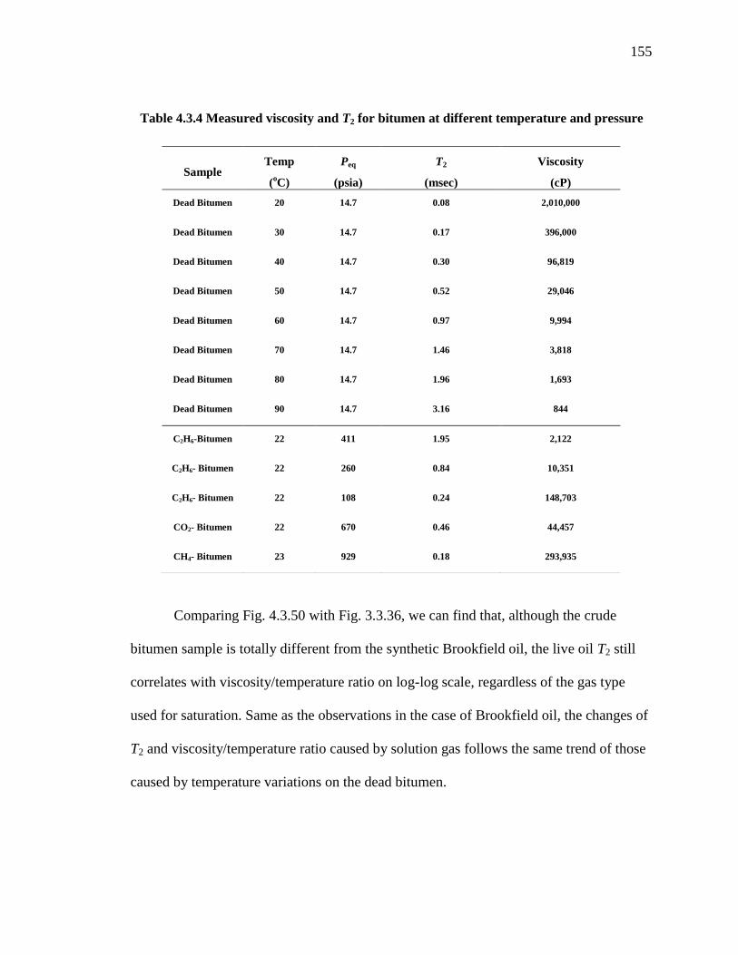
155
Comparing Fig. 4.3.50 with Fig. 3.3.36, we can find that, although the crude
bitumen sample is totally different from the synthetic Brookfield oil, the live oil T2 still
correlates with viscosity/temperature ratio on log-log scale, regardless of the gas type
used for saturation. Same as the observations in the case of Brookfield oil, the changes of
T2 and viscosity/temperature ratio caused by solution gas follows the same trend of those
caused by temperature variations on the dead bitumen.
Sample Temp
(oC)
Peq
(psia)
T2
(msec)
Viscosity
(cP)
Dead Bitumen 20 14.7 0.08 2,010,000
Dead Bitumen 30 14.7 0.17 396,000
Dead Bitumen 40 14.7 0.30 96,819
Dead Bitumen 50 14.7 0.52 29,046
Dead Bitumen 60 14.7 0.97 9,994
Dead Bitumen 70 14.7 1.46 3,818
Dead Bitumen 80 14.7 1.96 1,693
Dead Bitumen 90 14.7 3.16 844
C2H6-Bitumen 22 411 1.95 2,122
C2H6- Bitumen 22 260 0.84 10,351
C2H6- Bitumen 22 108 0.24 148,703
CO2- Bitumen 22 670 0.46 44,457
CH4- Bitumen 23 929 0.18 293,935
Table 4.3.4 Measured viscosity and T2 for bitumen at different temperature and pressure

156
In this manner, given the proper T2 value, the live bitumen viscosity with different
solution gases and at different pressure levels can be estimated through the T2 vs.
viscosity/temperature ratio correlation obtained from the investigation on dead
bitumen(as shown in Fig. 4.3.8). Data from other reference papers (Vinegar, et al. 1991),
(LaTorraca, Dunn, et al. 1998), (McCann, Vinegar and Hirasaki 1999), (Y. Zhang, PhD
Thesis 2002) are employed to compare with the bitumen and Brookfield oil data obtained
in this work and shown in Fig. 4.3.51. Here, the relaxation time and viscosity/temperature
ratio are normalized with respect to 2 MHz, as expressed by Eq. [2.17] and Eq. [2.18].
As displayed in Fig. 4.3.51, all the results of bitumen are highlighted in red.
While, the data obtained from Brookfield oil are highlighted in blue. As shown in Figure
18, although the data trend of synthetic Brookfield oil is deviated from others, both T2
0.01
0.1
1
10
1.E+00 1.E+01 1.E+02 1.E+03 1.E+04
T2
Rela
xa
tio
n T
ime (
mse
c)
Viscosity/Temperature (cP/K)
C2H6-Bitumenl
CO2-Bitumenl
CH4-Bitumen
Dead Bitumen at Different T
Figure 4.3.50 Relationship between the live bitumen T2 and the
viscosity/temperature ratio for all three gases
157
and T1 data obtained in the work on bitumen #10-19 well follow the trend of reference
data from other crude oils, respectively.
4.4 Conclusions
The T2 of live bitumen is significantly larger than the T2 of dead bitumen, even at
the lowest pressure level in this work (~100 psia). The relationship between the
equilibrium pressure and the live oil T2 of the bitumen sample is found to be closely
linear on semi-log scale for all three reservoir gases. C2H6 has the most significant
influence on the T2, while, CH4 gives the least T2 change at the same pressure level.
1.E-02
1.E-01
1.E+00
1.E+01
1.E+02
1.E+03
1.E-02 1.E-01 1.E+00 1.E+01 1.E+02 1.E+03 1.E+04 1.E+05
No
rma
lize
d R
ela
xa
tio
n T
ime
(mse
c)
Normalized Viscosity/Temperature (cP/K)
T2[LaTorraca et al](2 MHz)
T1[LaTorraca et al](2 MHz)
T2[McCann et al](2MHz)
T1[McCann et al](2 MHz)
T2[Vinegar et al](2 MHz)
T1[Vinegar et al](80 MHz)
T2[Zhang et al](2 MHz)
T1[Zhang et al](2 MHz)
T2[Zhang et al](7.5 MHz)
T1[Zhang et al](7.5 MHz)
T2[Zhang et al](20 MHz)
T1[Zhang et al](20 MHz)
Corr. by Morriss et al
Dipole-dipole Corr.
T2[Bitumen, Dead](2 MHz)
T2[Bitumen, Live](2 MHz)
T1[Bitumen, Live](2 MHz)
T2[Brookfield, Dead](2 MHz)
T2[Brookfield, Live](2 MHz)
T1
T2
Figure 4.3.51 Relationship between the normalized relaxation time and the
normalized viscosity/temperature ratio for bitumen #10-19 and other oil samples

158
Moreover, the data trend from any of the three gases extrapolated well to the dead
bitumen T2. All these findings are similar to the observations in the work on Brookfield
oil.
The dissolving of both CH4 and C2H6 in the bitumen sample follows the Henry’s
law well. However, the behavior of CO2 significantly deviates from Henry’s Law.
Similar results were also noticed in the case of CO2-Brookfield oil. The relationship
between the calculated gas solubility and the corresponding live oil T2 is found to be
closely linear on a semi-log scale for all three gases. Deviation was also found for CO2.
The deviations in the case of CO2 are possibly due to unexpected phase behavior
temporarily occurring at the highest pressure level in this work, resulting in the
overestimation of the pressure difference data used in the calculation of solubility. This
proposed explanation needs to be verified in the future work.
In the viscosity measurements, we found that, regardless of the gas type used for
saturation, the live bitumen T2 correlates with the viscosity/temperature ratio on log-log
scale. Moreover, both the T2 and T1 data obtained from the measurements on bitumen
follow the trend of reference data from other crude oils. Furthermore, changes of T2 and
the viscosity/temperature ratio caused by solution gas follow the same trend of those
caused by temperature variations on the dead oil and holds true for both crude bitumen
and synthetic Brookfield oil. This creates a new way for in-situ viscosity evaluation of
heavy oil through NMR well logging.
159
Chapter 5 Conclusions and Future Work
5.1 Conclusions of This Study
The echo spacing restriction of regular CPMG measurement on highly viscous
bitumen can be overcome by specifying the initial magnetization M0 in CPMG raw data
and assuming lognormal distribution for bitumen during the interpretation.
The apparent M0 of Athabasca bitumen from FID at low temperatures (< 60 oC)
has incorrect dependence on temperature due to the loss of FID signal within the
instrument’s dead time. This incorrect temperature dependence can be corrected by
applying the Curie’s Law. Given a correct M0 value at a certain temperature, the M0 of
the same sample at any other temperatures can be predicted by the Curie’s Law.
As discussed in Chapter 2, given the Curie’s Law corrected M0 and proper cut-off
between oil and water, the hydrogen index (HI) and water saturation (Sw) of bitumen
sample can be evaluated by applying the method introduced in this work. The estimated
HI of Athabasca bitumen is 0.82.
The T1 and T2 of Athabasca bitumen follow the trend of previous literature data in
the relationship between the normalized relaxation time and the normalized
viscosity/temperature ratio. The existing T2 vs. viscosity correlations, which are good for
the oil with relatively low viscosity, are not suitable for the samples with extremely high
viscosity like Canadian bitumen.
In Chapter 3, the measurements performed on the live Brookfield oil illustrate
that, CO2 has the largest mass transfer rate in the Brookfield oil due to the unique natural

160
convection. There was no significant dissolving of CH4 observed simply via diffusion up
to 168 hours at ~ 890 psia. The diffusion rate of C2H6 was found to be between the CO2
and CH4. The gradual diffusion of C2H6 into Brookfield oil from top to bottom was
confirmed by the NMR slice measurement. The convection generated by changing the
orientation of the pressure vessel markedly boosts the gas dissolving rate.
The live oil T2 is significantly larger than the T2 value of dead oil, even at the
lowest pressure level in this work (~100 psia). The relationship between the equilibrium
pressure and the live oil T2 is found to be closely linear on semi-log scale for all three
reservoir gases (CO2, CH4 and C2H6).
Based on the mass balance of gas inside the closed pressure vessel, the equation
of state with compression factor z was employed to calculate the gas solubility. However,
large pressure changes inside the pressure vessel within a relatively short time inevitably
occurred at the beginning of each pressurization or depressurization. Consequently, the
system would be temporarily heated by the pressurization or cooled by the
depressurization, and then return to the temperature of air bath (30 oC). In this manner,
significant pressure fluctuation would be caused by the temperature change and display
inaccurate P0 for the solubility calculations. Therefore, in order to remove the
temperature influence on the pressure reading and estimate the real starting pressure,
extrapolation was employed to correct the recorded pressure data within the initial period
after each pressurization or depressurization.
The originally recorded pressure data for all the three gases (CO2, CH4 and C2H6)
were analyzed. The solubility of each gas in Brookfield oil was calculated by using the
extrapolated pressure data. The dissolving behaviors of both CH4 and C2H6 in Brookfield
161
oil are found to follow the Henry’s law well. However, the observed dissolving behavior
of CO2 in Brookfield oil significantly deviates. Consequently, in the relationship between
the calculated gas solubility and the corresponding live oil T2, deviations were also found
in the CO2 case, while the data trends for the other two gases can extrapolate well to the
dead oil value and are closely linear on a semi-log scale.
The investigations on the live bitumen are illustrated in Chapter 4. The
measurements show that, the difference in the T2 distribution between the bitumen with
gas solute and the dead bitumen is significant for all three gases, even at the lowest
pressure level (~100 psia). The relationship between the equilibrium pressure and the live
bitumen T2 is found to be closely linear on semi-log scale for each reservoir gas. C2H6
has the most significant influence on the T2, while, CH4 gives the least T2 change at the
same pressure level. Moreover, the data trend from any of the three gases extrapolated
well to the dead bitumen T2. All these findings are similar to the observations in the work
on Brookfield oil.
The dissolving of both CH4 and C2H6 in the bitumen sample follows the Henry’s
law well. However, the behavior of CO2 is significantly different. This is the same
finding obtained in the case of CO2-Brookfield oil. The relationship between the
calculated gas solubility and the corresponding live T2 of bitumen sample is found to be
closely linear on a semi-log scale for all three gases. Deviation was again noted for CO2.
The deviations in the case of CO2 are possibly due to unexpected phase behavior
temporarily occurring at the highest pressure level in this work, resulting in the
overestimation of the pressure difference data used in the calculation of solubility. This
proposed explanation needs to be verified in the future work.

162
During the viscosity evaluations of these two heavy oil samples under different
conditions, we found that, regardless of the gas type used for saturation, the live oil T2
correlates with viscosity/temperature ratio on log-log scale. Although the data for the
Brookfield oil deviate from the trend of crude oils, both the T2 and T1 data obtained from
the measurements on bitumen follow the trend of reference data from other crude oils.
More importantly, the changes of T2 and viscosity/temperature ratio caused by solution
gas follows the same trend of those caused by temperature variations on the dead oil.
These findings hold for both crude bitumen and synthetic Brookfield oil, and create a
way for in-situ viscosity evaluation of heavy oil through NMR well logging.
5.2 Future Work
On the basis of the work that has been done in this study, the following future
work is suggested:
1. Further work needs to be done to better distinguish the T2 signal of heavy oil from
the emulsified water inside the heavy oil. In this manner, the oil saturation can be
calculated more accurately.
2. Identification of the phase behavior of CO2 at the temperature and the highest
pressure level used in this work via windowed cell tests to verify the proposed
explanation for the deviation of calculated solubilities observed in the CO2 cases
in this study.
3. Investigation of the T2 response and viscosity change of live heavy oils saturated
with gas mixture at various pressures.

163
4. Study of combining NMR and other logging tools to better characterized the
petrophysical properties of various heavy oils.

164
References
Bassiouni, Z. Theory, Measurement, and Interpretation of Well Logs. SPE Textbook
Series, v.4., 1994.
Bouton, J., M.G. Prammer, P. Masak, and S. Menger. "Assessment of Sample
Contamination by Down-Hole NMR Fluid Analysis." 2001 SPE Annual Technical
Conference and Exhibition Proceedings. 2001.
Bryan, J., A. Kantzas, R. Badry, J. Emmerson, and T. Hancsicsak. "In-situ Viscosity of
Heavy Oil: Core and Log Calibrations." 7th Canadian International Petroleum
Conference. Alberta, Canada, 2006. Paper 2006-116.
Bryan, J., A. Mai, F. Hum, and A. Kantzas. "Oil- and Water-Content Measurements in
Bitumen Ore and Froth Samples Using Low-Field NMR." SPE Reservoir
Evaluation & Engineering, 2006, 9: 654-663.
Bryan, J., and A. Kantzas. "Oil-Viscosity Predictions from Low-Field NMR
Measurements." SPE Reservoir Evaluation & Engineering, 2005: 8: 44-52.
Coates, G.R., L. Xiao, and M.G. Prammer. NMR Logging: Principles of Applications.
Houston, TX: Halliburton Energy Service, 1999.
Cowan, B. Nuclear Magnetic Resonance and Relaxation. Cambridge, UK: Cambridge
University Press, 1997.
Curwen, D. W., and C. Molaro. "Permeability fomr Magnetic Resonance Imaging Logs."
SPWLA 36th Annual Logging Symposium Proceedings. Society of Petrophysicists
& Well Log Analysts, 1995. 1995-GG.
Deleersnyder, M. "In-Situ Heavy-Oils Viscosity Determination Using NMR and
Conventional Logs: Application to a Real Example." SPE International Thermal
Operations and Heavy Oil Symposium and Western Regional Meeting. Bakersfield,
CA: Society of Petroleum Engineers, 2004. Paper SPE 86939.
Dunn, K.J., D.J. Bergman, and C.A. Latorraca. Nuclear Magnetic Resonance
Petrophysical and Logging Applications. New York: Pergramon, 2002.
Dunn, K.J., G.A. LaTorraca, J.L. Warner, and D.J. Bergman. "On the Calculation and
Interpretation of NMR Relaxation Time Distributions ." 69th SPE Annual
Technical Conference and Exhibition. New Orleans, LA: Society of Petroleum
Engineers, 1994. SPE 28367.
165
Enick, R., G.D. Holder, and B.I. Morsi. "Critical and Three Phase Behavior in the Carbon
Dioxide/Tridecane System." Fluid Phase Equilibria, 1985, 22: 209-224.
Galford, J.E. "Combining NMR and conventional Logs to Determine Fluid Volumes and
Oil Viscosity in Heavy-Oil Reservoirs." 2000 SPE Annual Technical Conference
and Exhibition. Dallas, TX: Society of Petroleum Engineers, 2000. Paper SPE
63257.
Galford, J.E., and D.M. Marschall. "Combining NMR and Conventional Logs to
Determine Fluid Volumes and Oil Viscosity in Heavy Oil Reservoirs." 2000 SPE
Annual Technical Conference and Exhibition Proceedings. SPE, 2000.
Haugen, K.B., and A. Firoozabadi. "Mixing of Two Binary Nonequilibrium Phases in
One Dimension." AICHE Journal, 2009, 55: 1930-1936.
Hearst, J.R., and P.H. Nelson. Well Logging for Physical Properties. New York:
McGraw-Hill Book Company, 1985.
Hirasaki, G.J., S.W. Lo, and Y. Zhang. " NMR properties of petroleum reservoir fluids."
Magnetic Resonance Imaging, 2003, 21: 269-277.
Huang, C.-C. Master Thesis. Houston, TX: Rice University, 1997.
Hürlimann, M.D., L. Venkataramanan, and C. Flaum. "The diffusion–spin relaxation
time distribution function as an experimental probe to characterize fluid mixtures in
porous media." Journal of Chemical Physics, 2002, 117: 10223-10232.
IUPAC. International Thermodynamic Tables of the Fluid State Carbon Dioxide.
London, UK: Pergamon Press, 1973.
Kleinberg, R., and H.J. Vinegar. "NMR Properties of Reservoir Fluids." The Log
Analyst, 1996, 37: 20-32.
LaTorraca, G.A., K.J. Dunn, P.R. Webber, and R.M. Carlson. "Low-Field NMR
Determinations of the Properties of Heavy Oils and Water-in-Oil Emulsions."
Magnetic Resonance Imaging, 1998, 16: 659-662.
LaTorraca, G.A., S.W. Stonard, P.R. Webber, R.M. Carlson, and K.J. Dunn. "Heavy Oil
Viscosity Determination using NMR Logs." 40th SPWLA Annual Logging
Symposium. Oslo, Norway: SPWLA, 1999. paper PPP.
Lo, S.W., G.J. Hirasaki, W.V. House, and R. Kobayashi. "Mixing Rules and Correlations
of NMR Relaxation Time with Viscosity, Diffusivity and Gas/Oil Ratio of
Methane/Hydrocarbon Mixtures." SPE Journal, 2002, March: 24-34.
166
MaCann, K.E., A. Vinegar, and G.J. Hirasaki. "NMR Analysis of Crude Oil and Pure
Hydrocarbon Fluids." private communication, 1999.
Masak, P.C., et al. "Field Test Results and Applications of the Down-Hole Magnetic
Resonance Fluid Analyzer." 43rd SPWLA Annual Logging Symposium
Transactions. SPWLA, 2002.
Miller, K., and B. Erno. "Use and Misuse of Heavy Oil and Bitumen Viscosity Data."
1995 Annual Technical Meeting of the Petroleum Society of CIM. 1995. 14-17.
Mirotchnik, K., K. Allsopp, A. Kantzas, D. Curwen, and R. Badry. "Low-Field NMR
Method for Bitumen Sands Characterization: A New Approach." SPE Reservoir
Evaluation & Engineering (SPE), 2001, 4(2): 88-96.
Morriss, C.E., R. Freedman, C. Straley, M. Johnston, H.J. Vinegar, and P.N. Tutunjian.
"Hydrocarbon Saturation and Viscosity Estimation from NMR Logging in the
Belridge Diatomite." The Log Analyst, 1997, 38: 44-59.
Nasrabadi, H., A. Firoozabadi, and T. Ahmed. "Complex Flow and Composition Path in
CO2 Injection Schemes From Density Effects in 2 and 3D." SPE Annual Technical
Conference and Exhibition. New Orleans, Louisiana: Society of Petroleum
Engineers, 2009. 124803-PP.
NBS. The Thermophysical Properties of Ethane, from 90 to 600K at Pressures to 700 bar.
Boulder, Colorado: NBS Technical Note 684, 1976.
Orr, F.M. Jr., A.D. Yu, and C.L. Lien. "Phase Behavior of CO2 and Crude Oil in Low-
Temperature Reservoirs." Society of Petroleum Engineers Journal, 1981: 480-492.
Prammer, M.G. "NMR pore size distributions and permeability at the well site." 1994
SPE Annual Technical Conference and Exhibition Proceedings. SPE, 1994: 55-64.
Syegh, S.G., D.N. Rao, S. Kokal, and J. Najman. "Phase Behaviour and Physical
Properties of Lindbergh Heavy Oil/CO2 Mixtures." Journal of Canadian Petroleum
Technology, 1990, 29: 31-39.
Straley, C., D. Rossini, A. Vinegar, P.N. Tutunjian, and C.E. Morriss. "Core Analysis by
Low-Field NMR." The Log Analyst, 1997, 38: 84-94.
Tharanivasan, A.K., C. Yang, and Y. Gu. "Measurements of Molecular Diffusion
Coefficients of Carbon Dioxide, Methane, and Propane in Heavy Oil under
Reservoir Conditions." Energy & Fuels, 2006, 20: 2509-2517.
Upreti, S.R., and A.K. Mehrotra. "Diffusivity of CO2, CH4, C2H6, and N2 in Athabasca
Bitumen." Canadian Journal of Chemical Engineering, 2002, 80: 116-125.
167
Vinegar, H.J. "X-ray CT and NMR imaging of rocks." Journal of Petroleum Technology,
1986, 38:115-117.
Vinegar, H.J., P.N. Tutunjian, W.A. Edelstein, and P.B. Roemer. "Whole Core Analysis
by 13C NMR." SPE Formation Evaluation, 1991, 183-189.
Yang, Z., and G.J. Hirasaki. "NMR measurement of bitumen at different temperatures."
Journal of Magnetic Resonance, 2008, 192(2): 280-293.
Zhang, Q., S.-W. Lo, C.C. Huang, G.J. Hirasaki, R. Kobayashi, and W.V. House. "Some
Exceptions to Default NMR Rock and Fluid Properties." SPWLA 39th Annual
Logging Symposium. Keystone, Colorado: SPWLA, 1998. Paper FF.
Zhang, Y. PhD Thesis. Houston, TX: Rice University, 2002.
Zhang, Y.P., C.L. Hyndman, and B.B. Maini. "Measurement of gas diffusivity in heavy
oils." Journal of Petroleum Science and Engineering, 2000, 25: 37-47.
168
Appendix A
Main Code:
% Lognormal Distribution Fitting for Bitumen, by Elton Yang
clear
clc
clf
load t_and_g.dat
x = t_and_g(2:end,1);
y = t_and_g(2:end,2);
y = abs(y);
Mo = t_and_g(1,2);
a0 = [2,0]; % initial guess
options = optimset ('TolX', 0.000001);
options.Display = 'off';
a = fminsearch ('lognorm', a0, options, x, y);
% For plotting
load t2_and_f_water.txt
t2_wat = t2_and_f_water(:,1);
f_wat = t2_and_f_water(:,2);
n = length(x); % number of CPMG signal points for fitting
f0 = Mo - sum(f_wat); % Sum of f for bitumen part
S = a(1); % Sigma in lognormal distribution
M = a(2); % Mu in lognormal distribution
Ln_t2_bit(1) = M-2.5*S;
% Lognormal distribution fitting
for i = 2:11
Ln_t2_bit(i) = Ln_t2_bit(i-1)+S/2;
g(i) = 1./(S*sqrt(2*pi)).*exp(-(Ln_t2_bit(i)-M).^2/(2*S^2))*abs(S/2);
t2_bit(i) = exp(Ln_t2_bit(i));
end
g = g';
t2_bit = t2_bit';
% generate new x for plotting
spacing = t_and_g(3,1);
add_x = x(1):0.01:x(round(3/spacing));
x_plot = [add_x'; x((round(3/spacing)+1):end)];
n = length(x_plot);
169
for j = 1:n
% bitumen part
for k = 1:length(t2_bit)
amp_bit(k) = f0*g(k)*exp(-x_plot(j)/(t2_bit(k)+eps));
end
sig_bit = sum(amp_bit);
% water part
for kk = 1:length(t2_wat)
amp_wat(kk) = f_wat(kk)*exp(-x_plot(j)/t2_wat(kk));
end
sig_wat = sum(amp_wat);
% CPMG signal = bitumen part + water part
h(j,1) = sig_bit + sig_wat;
end
E = lognorm(a, x, y)
semilogx(x,y,'b+');
hold on
semilogx(x_plot,h, 'r');
axis ([0,20,0,20])
xlabel 'Time (msec)'
ylabel 'Fitting Curve'
fit_dat = [x_plot h];
save t_and_h_fitting_result.dat fit_dat -ascii
Subroutine Code for Function “Lognorm”:
function E = lognorm(a,x,y)
% sum of square residual during log normal nonlinear regression
load t2_and_f_water.txt
load t_and_g.dat
t2_wat = t2_and_f_water(:,1);
f_wat = t2_and_f_water(:,2);
Mo = t_and_g(1,2);
n = length(x); % number of CPMG signal points for fitting
f0 = Mo - sum(f_wat); % Sum of f for bitumen part
S = a(1); % Sigma in lognormal distribution
M = a(2); % Mu in lognormal distribution
Ln_t2_bit(1) = M-2.5*S;
170
% Lognormal distribution fitting
for i = 2:11
Ln_t2_bit(i) = Ln_t2_bit(i-1)+S/2;
g(i) = 1/((S+eps)*sqrt(2*pi))*exp(-(Ln_t2_bit(i)-M)^2/(2*(S+eps)^2))*abs(S/2);
t2_bit(i) = exp(Ln_t2_bit(i));
end
g = g';
t2_bit = t2_bit';
for j = 1:n
% bitumen part
for k = 1:length(t2_bit)
amp_bit(k) = f0*g(k)*exp(-x(j)/(t2_bit(k)+eps));
end
sig_bit = sum(amp_bit);
% water part
for kk = 1:length(t2_wat)
amp_wat(kk) = f_wat(kk)*exp(-x(j)/t2_wat(kk));
end
sig_wat = sum(amp_wat);
% CPMG signal = bitumen part + water part
h(j,1) = sig_bit + sig_wat;
end
E = sum((y - h).^2);
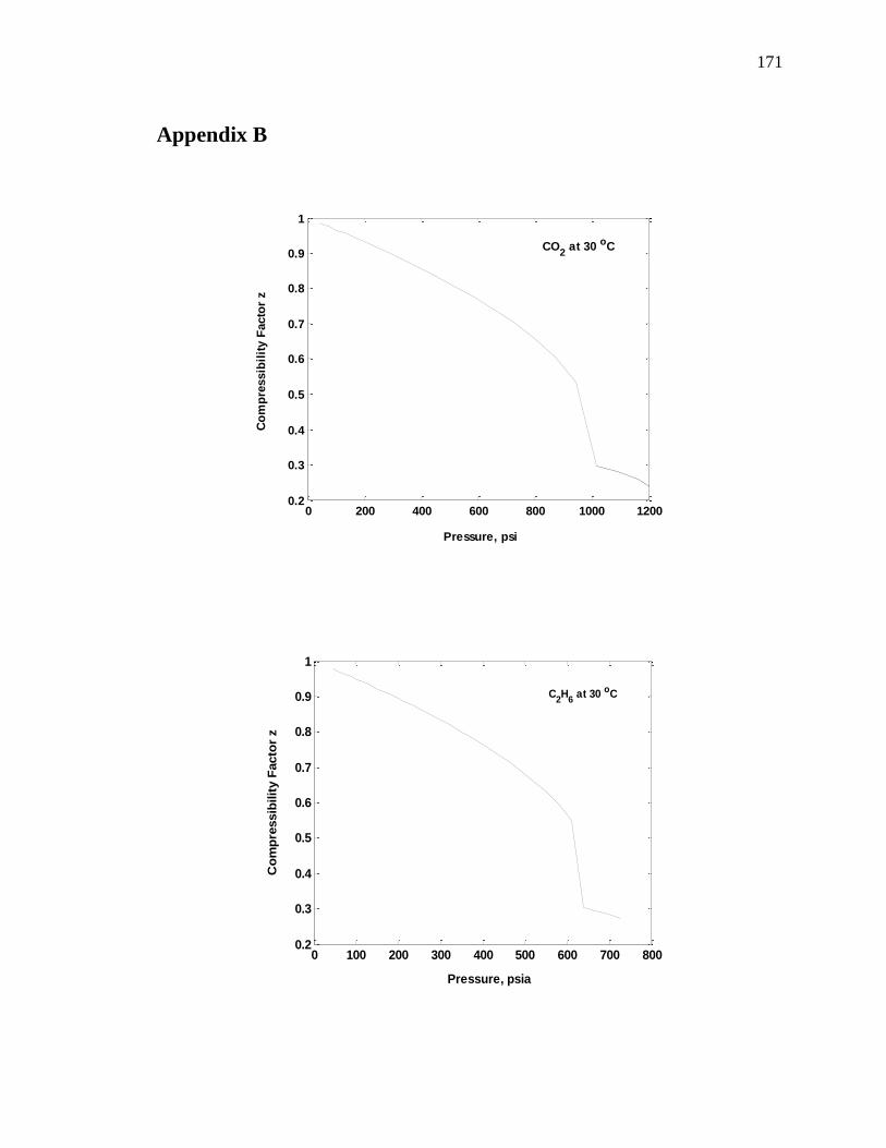
171
Appendix B
0 200 400 600 800 1000 12000.2
0.3
0.4
0.5
0.6
0.7
0.8
0.9
1
Pressure, psi
Co
mp
ressib
ilit
y F
acto
r z
CO2 at 30 oC
0 100 200 300 400 500 600 700 8000.2
0.3
0.4
0.5
0.6
0.7
0.8
0.9
1
Pressure, psia
Co
mp
ressib
ilit
y F
acto
r z
C2H
6 at 30 oC
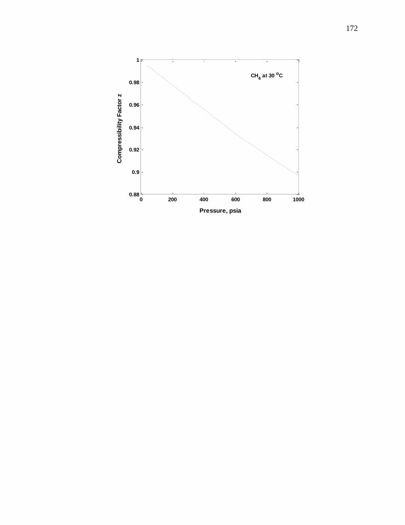
172
0 200 400 600 800 10000.88
0.9
0.92
0.94
0.96
0.98
1
Pressure, psia
Co
mp
ressib
ilit
y F
acto
r z
CH4 at 30 oC
Related Documents