Viscoelastic Model of Waterhammer in Single Pipeline

Archives of Hydro-Engineering and Environmental MechanicsVol. 53 (2006), No. 4, pp. 331–351© IBW PAN, ISSN 1231–3726

Viscoelastic Model of Waterhammer in Single Pipeline –Problems and Questions

Katarzyna Weinerowska-Bords

Gdańsk University of Technology, Faculty of Civil and Environmental Engineering,ul. Narutowicza 11/12, 80-952 Gdańsk, Poland, e-mail: [email protected]

(Received June 14, 2006; revised December 05, 2006)

AbstractIn the paper, viscoelastic model of waterhammer in a single polymer pipeline is analysed.The theoretical background of viscoelastic behaviour of the structure is shown and themathematical model of waterhammer in a polymer pipeline is presented. The main problemsconnected with applying the model are discussed. The main emphasis is on the question ofparameter estimation. Important aspects of wave speed calibration are presented. Estimationof a second group of parameters – retardation time and creep compliance values – wasanalysed. Problems and questions connected with the number of parameters, methods ofestimation, potential non-uniqueness of the solution and accuracy of obtained calculationswere discussed.

Key words: waterhammer, viscoelasticity, wave speed, relaxation time, creep compliance

Notations

a – wave speed,A – cross section area,c1 – constant dependent on the pipe fastening,D – internal pipe diameter,e – thickness of the pipe walls,E – Young’s modulus,E0 – instantaneous tensile modulus,Ei – tensile modulus of i-th Kelvin-Voigt element,E∗ – complex tensile modulus,g – acceleration due to gravity,H – water head,J – tensile compliance of the spring; creep function,K – liquid bulk modulus of elasticity,N – number of elements in viscoelastic model of the structure,p – pressure,

332 K. Weinerowska-Bords

Q – discharge,r – internal radius of the pipe,t – time,T – oscillation period,v – average in cross-section velocity of the stream,x – distance,ε – strain; unitary elongation of the internal circumference of the pipe,η – viscosity coefficient,θ, ψ – parameters in four-point scheme,λ – linear friction factor,ρ – density of liquid,σ – stress,τ – time of retardation,ω – circular frequency.

1. Introduction. Viscoelastic Behaviour of the Structure

The behaviour of polymers, understood as a strain reaction for applied stress, isthe consequence of their characteristic structure. In this specific construction eachof the molecules has the form of flexible thread and may ceaselessly change theshape of its contour, curling and twisting with change of energy (Ferry 1965). Suchcomplex structure determines viscoelastic effects in which each macroscopic strainis accompanied with complicated strains in molecular structure. In consequence,the reaction of polymers to the applied load is totally different from the behaviourof elastic materials, e.g. steel.

The description of viscoelastic behaviour of the body is usually developed onthe basis of one of two approaches (Aklonis et al 1972). The first is connectedwith so-called “mechanical analogues”. The group of models basing on this kindof approach refer to the combinations of mechanical elements, usually springs anddashpots, which more or less faithfully reproduce the viscoelastic response of realsystems. The behaviour of the body is then predicted on the basis of mechanicalparameters of these elements.

The second group of models is developed on the basis of molecular theories andthe motion of the representative form of molecules in viscous medium is deducted(Aklonis et al 1972). In this case, the behaviour of the structure is predicted on thebasis of molecular parameters. As the authors prove, the two approaches, at leastin the case when polymer structure is analysed, are equivalent.

The model of waterhammer in the pipeline of the walls made of material ofviscoelastic type is developed according to the approach of the first type. Theresponse of the polymer pipeline walls during waterhammer refers to the behaviourof a combination of springs and dashpots and the analysis is based on the mechan-ical properties of these elements, described by mechanical parameters and basic

Viscoelastic Model of Waterhammer in Single Pipeline – Problems and Questions 333

equations governing stress-strain relations. The springs in the model are treated aspure Hookean elements responsible for the elastic behaviour of the structure, andare described by the equation:

σ = Eε, (1)

where σ represents stress, ε – strain and E is Young’s modulus.The linear viscous response of the structure, characteristic for liquids, is repre-

sented by the behaviour of dashpots (pistons in cylinders), each one described byNewton’s law:

σ = η∂ε

∂t, (2)

where t is time and η a viscosity coefficient.On the basis of these elements several viscoelastic models may be derived,

according to the assumed combination of elements. The most basic models includeMaxwells model and the Voigt model.

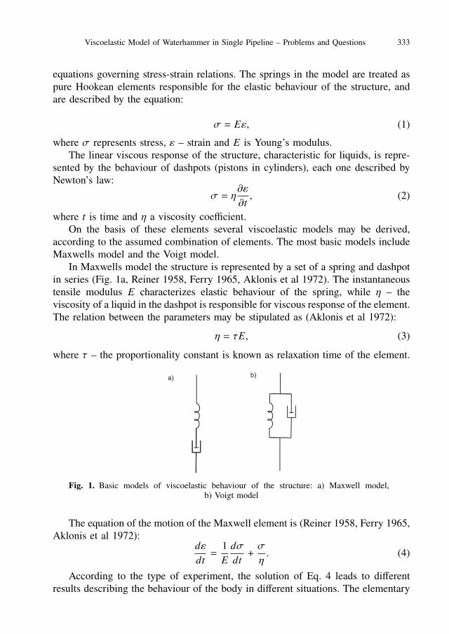
In Maxwells model the structure is represented by a set of a spring and dashpotin series (Fig. 1a, Reiner 1958, Ferry 1965, Aklonis et al 1972). The instantaneoustensile modulus E characterizes elastic behaviour of the spring, while η – theviscosity of a liquid in the dashpot is responsible for viscous response of the element.The relation between the parameters may be stipulated as (Aklonis et al 1972):

η = τE, (3)

where τ – the proportionality constant is known as relaxation time of the element.

Fig. 1. Basic models of viscoelastic behaviour of the structure: a) Maxwell model,b) Voigt model

The equation of the motion of the Maxwell element is (Reiner 1958, Ferry 1965,Aklonis et al 1972):

dεdt=

1E

dσdt+σ

η. (4)

According to the type of experiment, the solution of Eq. 4 leads to differentresults describing the behaviour of the body in different situations. The elementary


tests are carried out with the assumption that the stress varies sinusoidally withangular frequency f (ω = 2π f = 2π/T, where T is oscillation period), and can bedecomposed on two components – real, which is in phase with strain, and imaginary,which is π/2 out of phase with strain. The typical test results are shown in Tab. 1.

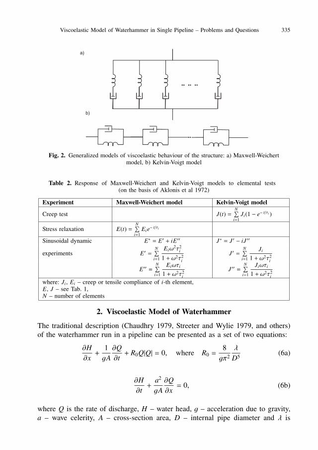
Table 1. Response of Maxwell and Voigt models to elemental tests (on the basis of Akloniset al 1972)

Experiment Maxwell element Voigt elementCreep test J(t) = J + t/η J(t) = J(1 − et/τ)Stress relaxation E(t) = E e−t/τ E(t) = ESinusoidal dynamic J∗= J ′ − iJ ′′ J∗ = J ′ − iJ ′′

experiments J ′ = J J ′ =J

1 + ω2τ2

J ′′ =1ωη

J ′′ =Jωτ

1 + ω2τ2

E∗ = E′ + iE′′ E∗ = E′ + iE′′

E′ =Eω2τ2

1 + ω2τ2 E′ = E

E′′ =Eωτ

1 + ω2τ2 E′′ = ωη

where: J = 1/ E – tensile compliance of the spring (Aklonis et al 1972),creep function (Covas et al 2004)J∗ – complex tensile creep compliance;E∗ – complex tensile modulusJ ′, E′ – real components of J∗ and E∗J ′′, E′′ – imaginary components of J∗ and E∗

Contrary to the Maxwell element, the Voigt model is based on parallel structureof spring and dashpot (Fig. 1b). The stress then is the sum of stresses of twoindividual elements and the fundamental equation is:

σ(t) = ε(t)E + ηdε(t)

dt. (5)

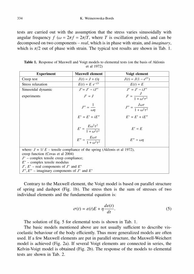
The solution of Eq. 5 for elemental tests is shown in Tab. 1.The basic models mentioned above are not usually sufficient to describe vis-

coelastic behaviour of the body efficiently. Thus more generalized models are oftenused. If a few Maxwell elements are put in parallel structure, the Maxwell-Weichertmodel is achieved (Fig. 2a). If several Voigt elements are connected in series, theKelvin-Voigt model is obtained (Fig. 2b). The response of the models to elementaltests are shown in Tab. 2.


Fig. 2. Generalized models of viscoelastic behaviour of the structure: a) Maxwell-Weichertmodel, b) Kelvin-Voigt model

Table 2. Response of Maxwell-Weichert and Kelvin-Voigt models to elemental tests(on the basis of Aklonis et al 1972)

Experiment Maxwell-Weichert model Kelvin-Voigt model

Creep test J(t) =N∑

i=1Ji(1 − e− t/τi )

Stress relaxation E(t) =N∑

i=1Eie− t/τi

Sinusoidal dynamic E∗ = E′ + iE′′ J∗ = J ′ − iJ ′′

experiments E′ =N∑

i=1

Eiω2τ2

i

1 + ω2τ2i

J ′ =N∑

i=1

Ji

1 + ω2τ2i

E′′ =N∑

i=1

Eiωτi

1 + ω2τ2i

J ′′ =N∑

i=1

Jiωτi

1 + ω2τ2i

where: Ji , Ei – creep or tensile compliance of i-th element,E, J – see Tab. 1,N – number of elements

2. Viscoelastic Model of Waterhammer

The traditional description (Chaudhry 1979, Streeter and Wylie 1979, and others)of the waterhammer run in a pipeline can be presented as a set of two equations:

∂H∂x+

1gA

∂Q∂t+ R0Q|Q| = 0, where R0 =

8gπ2

λ

D5 (6a)

∂H∂t+

a2

gA∂Q∂x= 0, (6b)

where Q is the rate of discharge, H – water head, g – acceleration due to gravity,a – wave celerity, A – cross-section area, D – internal pipe diameter and λ is


the linear friction factor. However, thanks to the appreciable improvement of mea-suring techniques and rapid progress in mathematical modelling, comparison ofobserved characteristics of waterhammer run (mainly pressure changes during thephenomenon) with results of calculation on the basis of Eq. (6a, b) was possible.Such comparison proved significant differences in both types of characteristics –measured and calculated, which in consequence led to the conclusion that traditionaldescription of waterhammer is not complete and adequate. As a result, the set ofequations (6a, b) was often replaced by more complicated description, in which themain emphasis was on the modification of friction term in momentum equation.One can find many different approaches of such modification, from the simplest ideaof multiplying it by some constant (even up to 10 and more), to more complicatedones. The results obtained by calculations became closer to observations, howeverthe problem was still not solved to a satisfactory degree.

The difference in calculations and observations is particularly clear for pipesmade of polymers. The reason for this fact is the viscoelastic behaviour of thismaterial as the reaction on stress. The equations (6a, b) describing the elasticmodel may be applied for steel pipes and preliminary calculations for plastic pipes.If more accurate calculations are needed, it is necessary to develop the form ofmathematical description taking into account viscoelastic character of pipe walldeformations (Brunone et al 2000, Covas et al 2004).

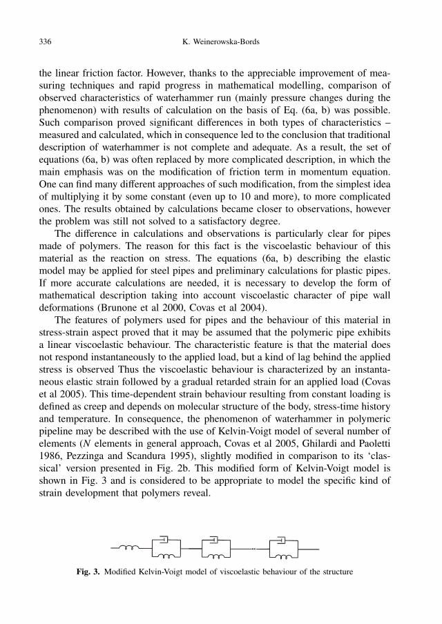
The features of polymers used for pipes and the behaviour of this material instress-strain aspect proved that it may be assumed that the polymeric pipe exhibitsa linear viscoelastic behaviour. The characteristic feature is that the material doesnot respond instantaneously to the applied load, but a kind of lag behind the appliedstress is observed Thus the viscoelastic behaviour is characterized by an instanta-neous elastic strain followed by a gradual retarded strain for an applied load (Covaset al 2005). This time-dependent strain behaviour resulting from constant loading isdefined as creep and depends on molecular structure of the body, stress-time historyand temperature. In consequence, the phenomenon of waterhammer in polymericpipeline may be described with the use of Kelvin-Voigt model of several number ofelements (N elements in general approach, Covas et al 2005, Ghilardi and Paoletti1986, Pezzinga and Scandura 1995), slightly modified in comparison to its ‘clas-sical’ version presented in Fig. 2b. This modified form of Kelvin-Voigt model isshown in Fig. 3 and is considered to be appropriate to model the specific kind ofstrain development that polymers reveal.

Fig. 3. Modified Kelvin-Voigt model of viscoelastic behaviour of the structure


The strain of the polymer pipe during waterhammer is understood as unitaryelongation of the internal circumference of the pipe, which can be defined as (Ghi-lardi and Paoletti 1986):

dε =drr, (7)

where r is the internal radius of the pipe.The total strain ε of the material described by the model shown in Fig. 3 can

be expressed then as a sum of instantaneous and retarded components, ε0 and εrrespectively:

ε = ε0 + εr , (8)

where εr represents the total retarded strain resulting from behaviour of each ele-ment i:

εr =

N∑i=1

εi. (9)

The instantaneous strain component in Eq. (8) is calculated as in the elasticmodel, where E0 is Young’s modulus, thus:

ε0 =σ

E0, (10)

while retarded components εi in Eq. (9) represent the viscous behaviour of eachKelvin-Voigt element (i = 1 . . .N). Thus, on the basis of Eq. (5), for each elementi one can write

σ = Eiεi + ηidεi

dt(11)

and – in consequence:

dεi

dt=

1τi

(σ

Ei− εi

), (12)

where Ei and τi are the tensile modulus and retardation time for i-th Kelvin-Voigtelement.

Now, assuming that the material of the pipe is homogenetic and isotropic, forwhich the Poisson modulus is constant and all the shear stresses and inertia effectsmay be neglected, the stress for the pipe subjected to the internal pressure p canbe expressed as (e.g. Wylie and Streeter 1983):

σ =pDc1

2e, (13)


where D is the internal diameter of pipe, e is its wall thickness and c1 is a constantdependent on the pipe fastening. Introducing Eq. (13) to (12), one can write:

dεi

dt=

1τi

(pD c1

2eEi− εi

). (14)

The Eq. (14) put into (9) defines the retarded component of the strain, whichintroduced to Eq. (8) both with instantaneous component (10) describe the totalstrain of viscoelastic material.

The last step of creating the viscoelastic model of waterhammer is introducingthe viscoelastic behaviour into unsteady flow equations. The analysis of the influenceof viscoelasticity is easier if the following form of the continuity equation is used(Ghilardi and Paoletti 1986):

∂

∂t(ρA) +

∂

∂x(ρvA) = 0, (15)

which can be expanded to:

ρ∂A∂t+ A

∂ρ

∂t+ ρA

∂v

∂x+ ρv

∂A∂x+ vA

∂ρ

∂x= 0, (16)

where ρ is water density and v is average in the cross-section velocity of the stream.Taking into account the definition of ε expressed by (7), one can write:

∂A∂t=∂A∂ε

∂ε

∂t= 2A

∂ε

∂t, (17a)

∂A∂x=∂A∂ε

∂ε

∂x= 2A

∂ε

∂x. (17b)

What is more, the relation between density ρ and pressure p can be expressed bystate equation for water (with the assumption of neglecting the entropy variation):

∂ρ

∂p=ρ

K, (18)

where K is the liquid bulk modulus of elasticity.Introducing Eqs. (17a, b) and (18) to continuity equation (16), after transforma-

tion, leads to:

∂p∂t+ v

∂p∂x+ 2K

(∂ε

∂t+ v

∂ε

∂x

)+ K

∂v

∂x= 0. (19)

In consequence, after introducing linear viscous behaviour described by theKelvin-Voigt model into Eq. (19), one obtains:


∂p∂t+ v

∂p∂x+ ρa2 ∂v

∂x+ 2ρa2 dεr

dt= 0, (20)

where wave speed a can be defined as:

a =

√√√√√√√√√√ Kρ

1 + c1KDE0

e. (21)

If the terms v(∂p/∂x) and v(∂εr /∂x) in Eq. (20) are neglected and if the dependentvariables Q and H are taken into account (instead of v and p), the final set ofequations for waterhammer in a viscoelastic pipe can be written as:

∂H∂x+

1gA

∂Q∂t+ R0Q|Q| = 0, where R0 =

8gπ2

λ

D5 , (22a)

∂H∂t+

a2

gA∂Q∂x+

2a2

g

N∑i=1

∂εi

∂t= 0, (22b)

where:

∂εi

∂t=

1τi

(pD c1

2eEi− εi

). (22c)

The set of equations (22a–c) is the equivalent of (6a, b) for viscoelastic materialof the pipe.

In conclusion it can be said that viscous behaviour influences only the continuityequation, in which the additional term connected with viscoelastic behaviour of thematerial appears.

The consequence of viscoelastic behaviour of pipeline material is the increase ofwave dispersion which results in change of wave frequency (and so – also oscillationperiod) and additional dumping of the surge (visibly stronger than in the case ofelastic material, e.g. steel), resulting in faster attenuation of the oscillations andshorter time of phenomenon run. As the maximal pressure increases and the timeof phenomenon duration are much lower than in case of elastic material – from thepractical point of view polymer pipes are much safer for the pipeline systems thanelastic ones.

Applying viscoelastic model for the solution of waterhammer problem in poly-meric pipelines improves the result, making it more consistent with measured pres-sure characteristics. The example of application of the model is presented in Fig. 4.


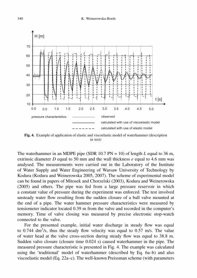
Fig. 4. Example of application of elastic and viscoelastic model of waterhammer (descriptionin text)

The waterhammer in an MDPE pipe (SDR 10.7 PN = 10) of length L equal to 36 m,extrinsic diameter D equal to 50 mm and the wall thickness e equal to 4.6 mm wasanalysed. The measurements were carried out in the Laboratory of the Instituteof Water Supply and Water Engineering of Warsaw University of Technology byKodura (Kodura and Weinerowska 2005, 2007). The scheme of experimental modelcan be found in papers of Mitosek and Chorzelski (2003), Kodura and Weinerowska(2005) and others. The pipe was fed from a large pressure reservoir in whicha constant value of pressure during the experiment was enforced. The test involvedunsteady water flow resulting from the sudden closure of a ball valve mounted atthe end of a pipe. The water hammer pressure characteristics were measured bytensiometer indicator located 0.39 m from the valve and recorded in the computer’smemory. Time of valve closing was measured by precise electronic stop-watchconnected to the valve.

For the presented example, initial water discharge in steady flow was equalto 0.744 dm3/s, thus the steady flow velocity was equal to 0.57 m/s. The valueof water head at the valve cross-section during steady flow was equal to 38.8 m.Sudden valve closure (closure time 0.024 s) caused waterhammer in the pipe. Themeasured pressure characteristic is presented in Fig. 4. The example was calculatedusing the ‘traditional’ model of waterhammer (described by Eq. 6a–b) and alsoviscoelastic model (Eq. 22a–c). The well-known Preissman scheme (with parameters


θ = ψ = 0.5) was used to solve the equations in both cases. The pressure wave speedwas determined on the basis of such measurements as a = 423 m/s. The presentedsolutions were obtained for space step ∆x = 1 m and time step enabling to obtainCourant number equal to unity (∆t = 0.00236 s). Linear friction coefficient wascalculated for assumed pipe roughness 0.004 mm from simplified Colebrook-Whiteformula. In viscoelastic approach the easiest model of one Kelvin-Voigt elementwas used and the best solution obtained for the values of τ = 0.0541 s and J =1/E = 0.9E − 10 Pa−1 was shown in Fig. 4.

In the figure, the results of calculations and measurements are compared. Asit can be seen, viscoelastic model of waterhammer enables the obtaining of a sat-isfactory solution, while the classical approach (elastic model) is not sufficientlyaccurate in the case of polymer pipe. Even if different attempts with increasingthe friction factor are applied, it is not possible to obtain a satisfactory solutionfor an elastic model, as not only amplitudes of oscillations but also frequency andperiod of oscillations are incorrectly modelled. Thus one can notice the significantincrease of accuracy of the solution if viscoelastic model is applied.

However, despite such “good” examples as the one presented above, there arestill several problems that have not been sufficiently recognized so far. Many authorspresent different examples of successful implementation of this method, however –the way of obtaining such result is not “general” but individually found for eachcase separately. This means that the solution may not be of a universal character andthus there is still a problem with finding some global approach to this question. Theproblems that very strongly determine such a situation may be divided into somegroups, from which the most important seem to be those connected with modelparameters estimation and the ones connected with numerical aspects.

The second group of problems – numerical aspects – boils down mainly tothe question of a choice of numerical scheme applied to solve the set of equations(22a–c) and choice of numerical parameters such as space and time step in calcula-tions (in consequence also the value of Courant number) and numerical coefficientsif they appear in a chosen numerical scheme. This question has been widely anal-ysed in literature (e.g. Szymkiewicz 2006). It is known that numerical effects maysignificantly change the solution, not only as to the numerical quantities but – whatis more important – the character of the phenomenon. The waterhammer is a distinctexample of a problem in which it is particularly easy to lose the physical realityof the process and interpret numerical effects as physical ones. The amplitude andfrequency of pressure oscillations are the essential elements of the phenomenon andthe values obtained in the solution may be the resultant effect of both – physicalcharacter of waterhammer and numerical dispersion and dissipation. Thus it isvery important to realize the influence of the numerical parameter values and toset these values clearly when the solution example is presented. Some authors paygreat attention to this question and apply numerical schemes of a high accuracy andpresent the values of numerical parameters (coefficients, time and space steps etc.)


to enable the solution to be interpreted correctly (e.g. Covas et al 2005). However,there are still examples presented in different papers in which the authors do notshow numerical details of the solution, making it impossible to repeat and interpretin the right way.

Even if problems of the kind given above are successfully solved – the chosenscheme is accurate and the parameters are chosen properly, there is still one veryimportant question, which is in the presented problem of an essential matter. It isconnected with model parameters, their estimation and sensitivity of the model tothe values of these parameters. Some of these questions will be analysed in a moredetailed way below.

3. Viscoelastic Model Parameters

General Remarks

One of the important group of problems connected with model parameters concernsthe friction term. It is a question vivid not only in the case of polymeric pipes but forall types of pipelines. Thus it is not connected strictly with elastic or viscoelasticbehaviour of the material and may be treated as a separate problem. The termconnected with friction appears in momentum equation, no matter whether viscousfeatures of the material are taken into account or not. The way of representingfriction in this equation is important and influences the result very strongly. Theapproaches applied in this question are of various types – from the easiest, wherethe friction factor λ is calculated like a steady flow or – its modified version –the value of λ is multiplied (even 10 times or more) to take into account higherenergy losses in unsteady conditions – to much more sophisticated approaches inwhich friction depends also on time and space derivatives of velocity and otherfactors. However, no matter which concept is considered – the problem of frictionin waterhammer is a separate question. As it does not deplete the list of difficultiesduring waterhammer problems solution, and – even if solved in a very accurate way– does not guarantee the proper solution – it will not be considered in the paper.

The essential question of the viscoelastic model of waterhammer is connectedwith main parameters that must be estimated – wave speed a, numbers of elementsin Kelvin-Voigt model, values of retardation time τι and values of creep complianceJi (where Ji =1/Ei and Ei is modulus of elasticity for a spring of i-th element) foreach element i (i=1. . . N). As will be discussed further, most of these parametersare very difficult or even impossible to estimate theoretically. There are problemsof different nature, one of the most important is connected with the fact, that –as the springs and dashpots are only hypothetical, conceptual elements used tomodel the phenomenon – most parameters are of a ‘mathematical’ character, withno strict attitude to the physical side of waterhammer. It makes identification muchmore difficult. If also taken into account that in some examples the number ofelements in the Kelvin-Voigt model reaches even the value of 5 – the total number


of parameters goes up to 11, which may make the solution not unique and difficultto interpret. Obtaining the solution is usually not so difficult as regards calcula-tion, as the possibility exists to estimate parameters on the basis of optimizationprocedures, but the interpretation and obtaining of consistency of the model withphysical features of the phenomenon is questionable. There may be a problem withthe influence of the method of optimization and choice of objective function onsolution and usually such parameters have only mathematical meaning, with nophysical relation. What is more – such approach is possible only if there are mea-surements for waterhammer in the considered pipeline, which affords the possibilityof applying optimization techniques. If the pipeline is being designed and there areno possibilities of verification – there are no clear rules as to how to estimateparameters to be able to carry out rough calculations of waterhammer modelling.

Wave Celerity

One of the most important questions is proper wave celerity estimation. In manyexamples authors take into account the value of wave speed calculated on the basisof the formula (21), (Chaudhry 1979, Wylie and Streeter 1993). Such approachbrings many problems of different natures.

The first aspect concerning this question is proper E0 choice. It is known thatthe value of Young modulus depends on the material of the pipeline. However, thevalue of E0 is not strictly fixed for each material A big variety of polymers used forpipe walls is observed and for each type of polymer there are several modifications(Saechtling 2000). For example, from a big family of polyethylene pipes one candistinguish HDPE, MDPE, LDPE, HPPE and for each type the producers give therange of the values that Young modulus can take. If the values are taken fromhandbooks of polymers the range of values can also differ slightly. What is more,the ranges for different types of polymers can partly interpenetrate, which meansthat the limits of values for different materials are not strict. E.g. the modulus ofelasticity for MDPE takes the values 0.6–0.8 GPa, while for HDPE one can findthe values of Young’s modulus of a range 0.7–1.0 GPa (Covas et al 2004) or even0.6–1.4 GPa (Saechtling 2000). In consequence, the values of a calculated on thebasis of Eq. (21) may differ significantly. For example, for the pipeline of innerdiameter D equal to 50.6 mm and wall thickness e equal to 3 mm, for K = 2.19GPa and c1 = 1, the wave speed calculated according to Eq. (21) may vary from197.8 m/s (for E0 = 0.6 GPa) to 298 m/s (for E0 = 1.4 GPa) which makes thedifference of about 100 m/s depending only on the assumed value of E0. Whatis more, the viscoelastic features of polymers that result in rheological behaviourhave considerable influence on mechanical performance of the material (Ferry 1965,Aklonis et al 1972, Covas et al 2004), which results in that short-term modulus ofelasticity being higher than long-term modulus of elasticity (Janson 1995, Covaset al 2004). The factors given above cause that the value of a – if one tries to


estimate it theoretically – may be significantly different. That consequently makesa significant difference in the oscillation period and values of pressure amplitudes.If the velocity of steady flow in the pipeline was 1 m/s, the theoretical pressureincrease may differ from 19.7 m to 29 m for the extreme values of E0 given above,which is a difference of 0.1 MPa.

What makes this question even more complicated, is that the essential aspect– as observed – was that the real value of wave celerity in waterhammer differsfrom that obtained in Eq. (21). Experiments proved that the observed values of aare much higher that those calculated for Young modulus for elastic behaviour. Andalso, as was observed, the maximal pressure amplitude calculated on the basis ofthe formula:

∆p = ρa∆v, (23)

(where ρ is water density and ∆v is the difference between the values of velocity insteady state v0 and final velocity v1 near the valve after the rapid change; usually v1equal to zero) as the values of a presented above is also lower than observed, andthe difference may be up to about 10–25%. The phenomenon is recognized as linepacking effect (Wylie and Streeter 1993, Covas et al 2004). Thus the two valuesof empirical wave speed and theoretical wave speed (for elastic model, calculatedfrom Eq. (21)) must be distinguished. For the purpose of this paper this secondwave speed (theoretical) will further be denoted as a0.

What is more, the variation of wave speed value during the phenomenon run isobserved (Covas et al 2004). This value changes both in time (decreases during thephenomenon) and in space (differs along the pipeline). These values can changee.g. from 423 m/s at the beginning of the phenomenon to about 380 m/s in furtherphase (Covas et al 2004), which is about 40 m/s (about 10%). Thus for the purposeof the viscoelastic model of waterhammer expressed by Eq. (22a–c) only somekind of average value may be assumed. This average value may be estimated onthe basis of measurements, by observing the oscillation period, which seems to bethe best way to fit this value to the analysed phenomenon run. However, it cannotusually be done in sufficiently accurate way, and even so – it is valid only forthe considered case of waterhammer in a particular pipeline. Thus there are alsoattempts to express the viscoelastic model of the phenomenon in a different way.

Instead of influencing the additional term in mass equation (22b) which isa consequence of approach shown in Eqs. (7–14), there is an alternative way oftaking into account rheological behaviour of the material. In this approach the vari-able during phenomenon wave speed a is considered and introduced to continuityequation (Covas et al 2005, Meißner and Franke 1977, Mitosek and Chorzelski2003 and others). This is a concept of frequency-dependent wave speed and alsotime-dependent behaviour of the pipe-wall, that can be described in terms of an-gular frequency (ω = π/T ). This approach was analysed among others by Meißnerand Franke (1977), Rieutford (1982), Franke and Seyler (1983) and Mitosek and


Chorzelski (2003). By considering creep compliance function and introducing it tomomentum and continuity equations, Meißner and Franke (1977) derived a complexformula, enabling to calculate the velocity for pressure wave propagation. As theypresented, the value of wave celerity a depended not only on fluid density, internaldiameter of the pipe, liquid bulk modulus of elasticity and pipe wall thickness,but also the frequency of pressure oscillations ω, the storage and loss compliancesof the wall material J ′ and J ′′ (defined as in Tab. 1 and Tab. 2) and so-calledlinearized friction factor. If the influence of the friction on wave speed is neglected,the formula for thin-walled viscoelastic pipes can be written as follows (Meißnerand Franke 1977, Mitosek and Chorzelski 2003):

a =

√√√√√√√√√√√√√√2ρ√(

1K+ J ′

De

)2

+

(J ′′

De

)2

+1K+ J ′

De

. (24)

This alternative approach also affords some problems, one of which is properJ ′ and J ′′ estimation. Some authors present the equations on the basis of which onecan determine the values of the storage and loss compliances J ′ and J ′′. Schwarzl(1970) and Mitosek and Chorzelski (2003) present the formulas in which J ′ andJ ′′ are the functions of creep compliance J(t) and circular frequency ω. However,to calculate J ′ and J ′′, the explicit formula of J(t) must be known. This, as isknown, is not an easy problem, as the form of this function depends on specificfeatures of the material and should be determined for each material separately,experimentally. Although some authors present some formulas for J(t), they arevalid only for the analysed case of a pipe of particular diameter, wall thickness and– what makes things even worse – for the particular temperature of the stream. Insuch situation proper determination of wave speed a in this way is very difficult, andin most practical cases almost impossible, as the formulas for J(t), which are of anempirical character, for most of the pipes are not known and difficult to determine.

The second way of taking into account frequency-variable wave speed a is theapproach presented by Lisheng and Wylie (1990). They proposed to apply the knownformula for pressure wave velocity (21), but with use of complex Young modulusE∗ (defined as in Tab. 1 and Tab. 2) instead of Young modulus E0. As E∗(ω)is a complex function of wave frequency, in consequence, wave speed a is alsofrequency-variable. As it is easy to guess, the problem is how to determine E∗(ω).The best way is to get such data from material tests in rheo-vibration apparatus.However, it is not easy to carry out such tests and for many practical cases theyare inaccessible. What is more, some authors prove (Lisheng and Wylie 1990) thatthe value of E∗ so obtained can be even 40% smaller than the true physical value


of the dynamic modulus. Thus one can see that this kind of approach also leads tomany problems of practical use of the mentioned formulas.

However, the approaches presented above show explicitly that pressure wavespeed a is frequency depended. In a consequence – it depends on period of oscil-lations T . Taking into account that:

a =2LT, (25)

it can be proved that a also depends on the length of the pipe. Mitosek and Chorzel-ski (2003) presented a study in which they examined the relationship betweenobserved a (for pipes of the same material, diameter and wall thickness) and thelength of the pipe which varied in different experiments. The diagrams showing thea(ω), a(L) and E∗(ω) dependences for the analysed cases were presented and theempirical formulas for a(L) functions for the analysed materials were determined.Such formulas may be helpful in the determining of a. The problem in application ofthis method is that the formulas are valid only for the pipes examined experimentallythus for the pipes of the same material, diameter and wall thickness as those usedin tests. As we also know, the value of pressure wave speed is influenced by manydifferent factors and thus the empirical formulas do not have a ‘general’ character.

To sum up the previous considerations, there is no firm formula enabling a esti-mation if there are no measurements. One way may be increasing the value of a0 byabout 10–25% (Covas et al 2004) or even more as the author’s experiments proved,however the question is which value of E0 to calculate a0 should be chosen, andsecond – how much it should be increased (which value of the range presented aboveto chose). The answers to these questions may influence the solution significantly.The second way of estimating a may be comparing to previously analysed examplesfor which the observations were accessible and trying to find some rule for eachtype of material separately. However it seems that there is no objective method toestimate a value in a proper way.

Thus one can notice that the basic problem of waterhammer – wave celerity– is not a trivial one, and seemingly unimportant factors influence the solution toa significant degree. Even if the problem of waterhammer is considered only fromthe practical point of view and the proper simulation of the whole phenomenonrun is not particularly important, proper estimation of the highest amplitude is ofsignificant meaning.

Kelvin-Voigt Element Parameters

Although, as we have already presented, there are attempts to apply frequency--dependent wave speed in waterhammer model, the approach leading to modifiedwaterhammer equations (22a–c) is more popular. In such an approach, next, aneven more difficult problem, is the estimation of Ji and τi for each element in


the Kelvin-Voigt model. As already mentioned, the springs and dashpots are onlyconceptual elements of the model, with no physical equivalent and thus the estima-tion of Ji and τi is hindered as the parameters have no physical interpretation. Thevalues of the parameters are strongly related to the assumed number of elements inKelvin-Voigt model. The higher number of a priori assumed elements, the betterpotential coincidence between calculations and observations. However, the only wayof estimating such high numbers of parameters is optimization and the results ofsuch estimation are valid for the particular, analysed case only. For a different pipeof the same material or for a different discharge rate or number of elements – theset of parameters has different values. Thus it is very difficult to find any global,general relation or formula or at least procedure as to how to deal with such casesor how to predict the pressure characteristics during waterhammer for a pipeline forwhich there are no measurements (e.g. during the stage of planning and designing).As far as is known – there are no objective procedures for finding the “optimal”number of elements N in Kelvin-Voigt model nor any relations enabling estimationof retardation time for each dashpot and creep compliance for each spring in themodel. The usual way is to assume the number of elements – usually from 1 to 5.Covas et al (2004) state that increasing the number of parameters above 5 does notresult in solution improvement. If the number of elements is low – 1 or 2, retardationtime and the related values of creep compliance are usually estimated on the basisof trial and error method or with the use of optimization procedures (e.g. Pezzingaand Scandura 1995). If the number of elements is greater (e.g. 4 or 5) the valuesof τi are assumed and the values of creep compliance are estimated on the basisof optimization (Covas et al 2004). As a result the least square error of calculatedvalues of water head related to observed is very low (even down to 0.05 m2), butthe chosen values of parameters (retardation time and creep compliances) are validonly for this particular case. Thus it would be important to find some more globalrelation between the parameters and some kind of more general procedure enablingpredicting waterhammer runs also for pipelines for which the observations are notpossible. That is particularly important, as it should be considered that in practicethere are many much more complicated cases. The optimization procedures withsuch big numbers of parameters may be possible for a single pipeline, but if thenetwork of pipelines is considered – there are much more factors influencing thesolution and it would be important to be able to predict at least approximate valuesof parameters on the basis of more a physically-related method than optimizationprocedure.

On the other hand, finding any global approach, based more on theoreticalconsiderations or examination of different experiments, and trying to find any regu-larity occurs to be difficult. Covas et al (2004) present a wide range of experimentsleading to creep characterization and estimation of values of creep compliance Jfor pipes made of PE. In tests presented the creep compliance function was esti-


mated by running creep tests in longitudinal samples of pipe. In addition, dynamicmechanical tests were carried out.

The creep compliance values for each temperature change in time (increase).The obtained values varied from about 0.08 E-8 Pa−1 to 0.25 E-8 Pa−1. The dynamictests let real and imaginary components of complex modulus of E∗ be examined(see Tab. 1 and Tab. 2). In conclusion authors state that in none of the tests was itpossible to obtain a good definition of creep function for a very short time (2–3 s),nor exact value of the elastic creep component J0. What is more, the authors provedthat the values obtained in tests do not correspond exactly with the exact creepfunction of PE integrated in pipe systems, and the creep compliance for existingpipe systems should be estimated on the basis of calibration procedures.

The numerical tests carried out by the same authors (Covas et al 2005) fordifferent cases, different numbers of Kelvin-Voigt elements and for assumed timesof retardation led to optimal creep compliance values varying from about 9E-11 to2E-10 Pa−1, which is considerably different from the values obtained in creep tests.Thus the optimization procedures seem to be the best way of determining modelparameters, however, one should remember that each set of obtained values is validonly for the analysed case and also for assumed times of retardation.

Optimization procedure cannot be applied if measurements are not accessible.Thus numerous cases (e.g. designing of pipelines, existing pipeline systems whereit is impossible to carry out the measurements etc.) cannot be solved using sucha means of calibration. Evaluation of retardation time and creep compliance in suchcase still seems to be an open question.

4. Final Remarks and Conclusions

The considerations presented constitute the kind of discussion on the question ofviscoelastic model application. The main aspects of theoretical background of theviscoelastic behaviour of the structure were presented and main problems connectedwith viscoelastic model application were discussed. The general conclusions maybe summarized as below:

• For polymer pipelines it is necessary to apply viscoelastic models of waterham-mer as the traditional approach valid for elastic materials (e.g. steel), leads toconsiderable discrepancy between calculated and observed values of pressure.Some authors present calculations for polymeric pipelines without consideringthe viscoelastic model of waterhammer, however the viscoelastic effects of ma-terial behaviour are then ‘hidden’ in values of other parameters (e.g. numerical)or other terms (e.g. friction term in momentum equation), giving a similar effectof additional damping of oscillations. However, such approach seems not to besuitable as the physical side of the phenomenon is not modelled in a properway which makes interpretation of the solution difficult and may lead to wrongconclusions.


• Application of a viscoelastic model is connected with many problems of differentnatures, of which very important is parameter estimation.

• The choice of a the method of parameter estimation and accuracy of obtainedresults depend, among other things, on the assumed approach to consideringviscoelasticity of the material. If the approach of frequency-dependent pressurewave speed is taken into account, most of the parameters should be estimatedon the basis of material tests, which makes this approach difficult in practicalcases.

• If the Kelvin-Voigt model of viscoelastic behaviour is taken into account (insteadof frequency-dependent pressure wave speed introduction to the ‘traditional’waterhammer model equations), the important question of parameter estimationis the number of parameters. The number of viscoelastic model parametersdepends on the assumed number of Kelvin-Voigt elements. For each elementtwo parameters – retardation time and creep compliance must be found. Inaddition, the waterhammer wave speed must be estimated. The bigger numberof parameters gives the potential possibility of obtaining higher accordance be-tween observations and calculations. However, there is a limit of Kelvin-Voigtelement number (Covas et al 2005 give the value of 4 or 5) above which no im-provement in measurement-calculations coincidence is observed. What is more,the greater number of parameters causes the higher possibility of non-uniquesolution obtaining and bigger problems with interpretation of the influence ofthe parameters in the result.

• Wave speed may be estimated in different ways. The most proper seems to bethe estimation on the basis of observations. However, such an approach has alsodisadvantages. First, it requires the results of measurements, thus it is valid forexisting systems for which experiments may be carried out. Second – water-hammer wave speed changes both in space and time during the phenomenonrun and, moreover, it depends on many factors, e.g. frequency of oscillationsand temperature of the liquid. Thus the value that is introduced to the modeldescribed by Eqs. (22a–c) may be only a kind of average wave speed.

• The other way of wave speed estimation takes into account the theoretical valueof a0 calculated according to Eq. (21). This approach also gives rise to twomain problems. First, there is the problem with proper estimation of modulusof elasticity which can vary for considered material in a relatively wide range,leading to vivid results in obtained waterhammer pressure characteristics. Sec-ond – it was proved that real values of a differ from the theoretical value of a0significantly (10–20%) or even more. Thus in consequence such approach maylead to results far from those observed.

• There is a serious problem to estimate a when there is no possibility of carryingout the experiments. In such a situation the approach presented above seems


to be very helpful, however, it may give only a rough estimation. The secondsolution may be comparing the analysed case to previously examined, and tryingto conclude on the basis of some kind of analogy. However, this may also bedifficult.

• Parameters connected with Kelvin-Voigt element – retardation time and creepcompliance are very difficult to estimate, as they are of a mathematical characteronly, with no attitude to technical parameters of the system. If the number ofelements in a Kelvin-Voigt model is small (1 or 2), usually all parameters areestimated on the basis of optimization procedures. If the number is higher, usu-ally retardation times are assumed and responding creep compliance values areoptimized. As proved (Covas et al 2004), the values obtained due to optimiza-tion procedures differ from those obtained from creep tests. It suggests that theonly way of estimating these parameters is optimization, which is possible onlywhen measurements are accessible. Thus the problem arises, what to do if thepipeline is analysed on design stage or for any other reason experiments are notpossible. It seems there has been no general way to estimate creep compliancein such situations, so far. One should also remember that even if measurementsare accessible and optimization procedure can be carried out – the parametervalues obtained in such a way are valid for this particular case only and willbe different not only if a different pipeline is considered, but also for the samepipeline if a different number of Kelvin-Voigt elements is taken into account orif different values of retardation times are assumed. Thus, such values do nothave any global character.

• For many of the reasons mentioned above, especially for cases where measure-ments are not accessible, it seems to be very important to try to find a moreeffective approach of relatively global character, more vivid regularity in param-eter estimation, to be able to better model those cases for which an experimentis not possible. It seems to be particularly important when one takes into con-sideration that the problems presented above concerned only the easiest exampleof simple pipeline of constant diameter. In real systems there is often a need forcarrying out calculations for more complicated systems, e.g. pipeline networks.Thus it seems reasonable that in such cases one will tend to decrease the numberof parameters for each pipeline, to enable calibration of the whole system. Thussome kind of regularity may be essential for such complicated cases.

References

Aklonis J. J., McKnight W. J., Shen M. (1972), Introduction to Polymer Viscoelasticity, John Wiley& Sons, Inc, New York.

Axworthy D. H., Ghidaoui M. S., McInnis D. (2000), Extended thermodynamics derivation of energydissipation in unsteady pipe flow, J. of Hydr. Eng., Vol. 126, No. 4, 276–287.


Brunone B., Karney B. W., Micarelli M., Ferrante M. (2000), Velocity profiles and unsteady pipefriction in transient flow, J. of Water Res. Planning and Managm., Vol. 126, No. 4, 236–244.

Chaudhry M. H. (1979), Applied Hydraulic Transients, Van Nostrand Reinhold Company, New York.Covas D., Stoianov I., Mano J. F., Ramos H., Graham N., Maksimovic C. (2004), The dynamic effect

of pipe-wall viscoelasticity in hydraulic transients, Part I – experimental analysis and creepcharacterization, J. of Hydraul. Res., Vol. 42, No. 5, 516–530.

Covas D., Stoianov I., Mano J. F., Ramos H., Graham N., Maksimovic C. (2005), The dynamic effectof pipe-wall viscoelasticity in hydraulic transients, Part II – model development, calibration andverification, J. of Hydraul. Res., Vol. 43, No. 1, 56–70.

Ferry J. D. (1965), Viscoelastic Properties of Polymers, WN-T, Warszawa (in Polish).Franke G., Seyler F. (1983), Computation of unsteady pipe flow with respect to viscoelastic material

properties, J. Hydraul. Res., IAHR, 21(5), 345–353.Ghilardi P., Paoletti A. (1986), Additional viscoelastic pipes as pressure surges suppressors, Proc.

of 5th International Conference on Pressure Surges, Hannover, Germany, 22–24 September,113–121.

Janson L.-E. (1995), Plastic Pipes for Water Supply and Sewage Disposal, Borealis, Stockholm.Kodura A., Weinerowska K. (2005), The influence of the local pipe leak on the properties of the

water hammer, Proc. of 2nd Congress of Env. Eng., Vol. 1, (Monografie KIŚ, Vol. 32), PAN,Lublin, 399–407 (in Polish).

Kodura A., Weinerowska K. (2007), The influence of the local pipe leak on water hammer prop-erties, Environmental Engineering. Proc. of the Second National Congress of EnvironmentalEngineering, Lublin, Poland. Taylor & Francis, London, 239–244.

Lisheng S., Wylie E. B. (1990), Complex wavespeed and hydraulic transients in viscoelastic pipes,Jour. of Fluid Eng., Vol. 112, No. 12, 496–500.

Meißner E., Franke G. (1977), Influence of pipe material on the dampening of waterhammer, Proc.of the 17thCongress of int. Assoc. for Hydr. Res. IAHR, Baden-Baden, Germany.

Mitosek M. Chorzelski M. (2003), Influence of Visco-Elasticity on Pressure Wave Velocity inPolyethylene MDPE Pipe, Archives of Hydro-Engineering and Environmental Mechanics, Vol.50, No. 2, 127–140.

Pezzinga G., Scandura P. (1995), Unsteady flow in instalations with polymeric additional pipe, J. ofHydr. Eng., Vol. 121. No. 11, 802–811.

Ramos H., Covas D., Borga A., Loureiro D. (2004), Surge damping analysis in pipe systems: mod-elling and experiments, J. of Hydraul. Res., Vol. 42, No. 4, 413–425.

Reiner M. (1958). Theoretical Rheology, PWN, Warszawa (in Polish),Rieutford E. (1982), Transients Response of Fluid Viscoelastic Lines, J. Fluid Engng., ASME 104,

335–341.Saechtling H. (2000), Handbook of Polymers, Wydawnictwa Naukowo-Techniczne, Warszawa (in

Polish).Schwarzl F. R. (1970), On the interconversion between visco-elastic material functions, Pure and

Applied Chemistry, Vol. 23, No. 2/3, 219–234.Streeter V. L., Wylie E. B. (1979), Hydraulic Transients, New York, McGraw-Hill Book Co.Szymkiewicz R. (2006), The Method of the Analysis of Numerical Dissipation and Dispersion in the

Solution of the Equations of Hydrodynamics, Wyd. Politechniki Gdańskiej (in Polish).Wylie E. B., Streeter V. L. (1983), Fluid Transients, FEB Press, Ann Arbor, Michigan.Wylie E. B., Streeter V. L. (1993), Fluid Transients in Systems, Prentice Hall, Englewood Cliffts, NT.Zhao M., Ghidaoui M. S. (2003), Efficient quasi-two-dimensional model for water hammer problems,

J. of Hydr. Eng., Vol. 129, No. 12, 1007–1013.

Viscoelastic Model of Waterhammer in Single Pipeline

Documents