Universiteit Gent Faculteit Economie en Bedrijfskunde Vakgroep Beleidsinformatica en Operationeel Beheer Multi-Mode Resource-Constrained Project Scheduling Problem Metaheuristic Solution Procedures and Extensions Vincent Van Peteghem Proefschrift tot het bekomen van de graad van Doctor in de Toegepaste Economische Wetenschappen: Handelsingenieur Academiejaar 2009-2010

Welcome message from author
This document is posted to help you gain knowledge. Please leave a comment to let me know what you think about it! Share it to your friends and learn new things together.
Transcript

Universiteit GentFaculteit Economie en Bedrijfskunde
Vakgroep Beleidsinformatica en Operationeel Beheer
Multi-Mode Resource-Constrained ProjectScheduling ProblemMetaheuristic Solution Procedures and Extensions
Vincent Van Peteghem
Proefschrift tot het bekomen van de graad vanDoctor in de Toegepaste Economische Wetenschappen: Handelsingenieur
Academiejaar 2009-2010


Universiteit GentFaculteit Economie en Bedrijfskunde
Vakgroep Beleidsinformatica en Operationeel Beheer
PromotorProf. dr. Mario Vanhoucke
Doctoral juryProf. dr. Marc De Clercq - DeanProf. dr. Patrick Van Kenhove - Academic SecretaryProf. dr. Erik Demeulemeester - Katholieke Universiteit LeuvenProf. dr. Luc Chalmet - Universiteit Gent/Universiteit AntwerpenProf. dr. Rainer Kolisch - Technische Universitat Munchen - GermanyProf. dr. Francisco Ballestin - Public University of Navarra - Spain
Universiteit GentFaculteit Economie en Bedrijfskunde
Vakgroep Beleidsinformatica en Operationeel BeheerTweekerkenstraat 2B-9000 Gent, Belgie
Tel.: +32-9-264.35.17Fax.: +32-9-264.42.86
Proefschrift tot het bekomen van de graad vanDoctor in de Toegepaste Economische Wetenschappen: Handelsingenieur
Academiejaar 2009-2010


Dankwoord
Our greatest weakness lies in giving up. The most certain way tosucceed is always to try just one more time.
Thomas Alva Edison
Hier ligt het dan. Mijn doctoraat. Mijn dagen schrijven van papers. Mijnweken zoeken naar dat halve procentje verbetering. Mijn maanden van ploeteren incode. En toch, nu alles neergeschreven, gelezen en herlezen is en het geheel netjesis ingebonden, blijven vooral tientallen herinneringen over die niets - of slechts vanveraf - met het onderwerp van mijn doctoraat te maken hebben. De Brug. MISTA.Ierland. Mails. Personeelscompetitie. Vlerick. Verloffiche. 12urenloop. Schriftje.Seminariewerk. Deadlines. Apple. Restaurant zoeken. Assistants4Life. Poitiers.Lesgeven. Weer Poitiers. Tubingen. Nog eentje. Fiona. Bowlingkampioenschap.9 mei 2007. Stukje taart. In order to. Tours. En vooral: nooit opgeven.
Toch zou dit doctoraat - en alle bijhorende herinneringen - er nooit geweest zijnzonder de hulp van velen. Met dit dankwoord hoop ik dan ook allen die betrokkenzijn geweest bij dit doctoraat te bedanken.
Vooreerst een heel bijzonder woord van dank aan mijn promotor, prof. dr.Mario Vanhoucke. Mario, het was voor mij een ongelofelijke eer om de afgelopenjaren samen te werken met jou. Je deur stond altijd open om iets te vragen envele uren hebben we samen gespendeerd aan je ronde tafel. Je nooit aflatendeenthousiasme voor onderzoek trok me telkens opnieuw mee in die - toch wel -wondere wereld van project management. We hebben even moeten zoeken hoe wemijn onderzoek moesten aanpakken, maar telkens hebben we een nieuwe pogingondernomen en doorgezet. Het gesprek dat we in Tubingen hebben gehad heefter ongetwijfeld voor gezorgd dat dit document hier vandaag ligt. Mario, bedanktvoor je steun, je hulp en de kansen die ik kreeg.
Ook een woord van dank aan prof. dr. Luc Chalmet. Luc, de afgelopen jarenhebben we intensief samengewerkt aan de cursus Productie- en Logistiek beleid.We hebben dit steeds aangepakt in onderlinge samenspraak en steeds kreeg ikhierbij van jou alle kansen. Het deed me dan ook enorm veel plezier toen je lidwou worden van mijn doctoraatsjury. Luc, bedankt voor de vlotte en aangenamesamenwerking de afgelopen jaren.
Ook een woord van dank aan de andere leden van mijn examenjury, prof. dr.Erik Demeulemeester, prof. dr. Rainer Kolisch en prof. dr. Francisco Ballestin.Erik, net zoals vele anderen hier op onze onderzoeksgroep heb ik de basisknepen

ii
van operationeel onderzoek meegekregen tijdens je lessen in Leuven. Ze hebbenmee de basis gelegd voor dit doctoraat. Bedankt voor alle opmerkingen, feedbacken ondersteuning. Rainer, you are one of the persons cited the most in my dis-sertation, so it meant a lot to me that you became a member of my doctoral jury.Moreover, your very detailed and elaborate list of feedback significantly improvedthe quality of my work. My sincere thanks to you. Francisco, thank you for cri-tically revising my dissertation and for your insightful comments and suggestionsto increase the quality of this work.
Ook nog een woord van dank aan prof. dr. Johan Christiaens voor de kansdie hij mij vele jaren geleden geboden heeft om als assistent te starten aan dezefaculteit. Ondanks de korte periode dat we samengewerkt hebben, hou ik velefijne herinneringen over aan onze samenwerking.
Een stimulerende onderzoeksomgeving begint natuurlijk bij een goede werk-omgeving. En daarom vooreerst een woord van dank aan de Universiteit Gent.Meer dan tien jaar na mijn eerste les ben ik nog steeds ongelofelijk trots om aandeze instelling te mogen studeren en werken. Het is voor mij in ieder geval eengrote eer geweest om deel uit te maken van deze universiteitsgemeenschap en ikben blij dat ik met dit doctoraat een beperkte bijdrage heb kunnen leveren aan deverdere uitbouw van onze universiteit.
Graag wil ik dan ook alle collega’s aan onze vakgroep en faculteit van hartebedanken voor de vele fijne en ontspannende momenten. Een speciaal woord vandank aan mijn bureaugenoten Christophe, Jeroen, Thomas en Veronique. Hoewelwe soms de ’stille bureau’ genoemd worden, zorgden onze korte gesprekken steedsvoor de nodige afleiding. Ook mijn oude bureaugenoten en collega’s bij de vak-groep accountancy wil ik graag bedanken voor de leuke tijd. Een speciaal woordvan dank ook aan mijn (ex-)collega’s Peter, Arne, Dieter, Frederik en Broos. Alsik het even niet meer zag zitten, eens goed wou klagen of gewoon zin had in eengesprek of een grap, kon ik steeds bij jullie terecht. Bedankt. Ook een heel grootwoord van dank aan het ondersteunend personeel: de mensen van het secretariaat(Martine en Ann), het decanaat en het onderhoudspersoneel.
Dit doctoraat zou er ook niet gekomen zijn door (af en toe) te ontspannen.Een van mijn meest dierbare ontspanningen is ongetwijfeld De Pinte Leeft! Peter,Lieven, Matthijs, Guy, Dieter en Peter, samen hebben we de afgelopen jaren heelwat uit de grond gestampt. Ik hoop dat we ook in de toekomst onze doelstellingkunnen blijven waarmaken, maar met een Pintenaer in de hand zal dit ongetwijfeldlukken. Ook mijn collega-volleyballers wil ik bedanken. Aangezien onderzoekdikwijls eenzaam is, heb ik altijd enorm genoten van de sfeer in onze ploeg, vande punten tijdens de wedstrijd en de pinten erna...
Daarnaast zijn er een aantal mensen die ik heel bijzonder wil bedanken voorhun onvoorwaardelijke steun de afgelopen jaren. Als ik belde, hen tegenkwam ofbij hen langsging, kon ik steeds alles tegen hen kwijt. Dus daarom een hele grotedank-je-wel aan Matthijs, Wim, Jeroen, Helen, Nele, Peter en Stefaan.
Ook een bijzonder woord van dank aan Philippe en Luce. Het was leuk om opelk moment welkom te zijn. Steeds mocht ik mee aanschuiven aan tafel en leefdenjullie mee met de vorderingen van mijn doctoraat. Bedankt!

iii
Ook mijn familie wil ik danken voor de steun en in het bijzonder mijn grootou-ders. Grootouders zijn met hun financiele beloningssysteem dikwijls de grootstemotivator voor goede studieprestaties, maar dat waren hun interesse en meele-ven evenzeer. De strenge, maar goedkeurende blik van pepe, de korte bezoekjesbij oma net voor ik naar een examen vertrok en de steeds terugkerende vragenvan Bobo, elk zorgden ze voor de nodige stimulans. Ook mijn allerliefste zusjesmogen niet ontbreken in dit dankwoord. Julie en Elisa, hoewel ik mij het waar-schijnlijk nog vaak zal beklagen, ik kan alleen maar zeggen dat ik mij geen beterezussen kan indenken. Steeds stonden jullie klaar om mij te helpen, af en toe metvolle goesting, maar ongetwijfeld vaak tegen jullie zin. Toch kon ik steeds op jullierekenen. Bedankt Jules en Lizie, ook voor het nalezen van dit doctoraat.
Tot slot wil ik zeker mijn papa en mama bedanken. Ik was waarschijnlijk nietaltijd de gemakkelijkste. Ik vertelde nooit waar ik mee bezig was of gaf enkel mijnstandaardantwoord ’een beetje’ als jullie vroegen ’vlot het een beetje?’. Toch hoopik dat dit doctoraat ook voor jullie een bekroning is voor de manier waarop jullieme al die jaren steunden en ondersteunden. Ik ben jullie in ieder geval ontzettenddankbaar voor alles.
Save the best for last! Evelyn, wie had dit ooit gedacht toen we elkaar iets meerdan drie jaar geleden voor de eerste keer kruisten. We hebben sindsdien samen alheel wat beleefd, genoten en afgelachen. Je steun heeft me de afgelopen maandengeholpen om te blijven doorgaan. Bedankt om er steeds te zijn voor mij. Laten weelkaar nog lang gelukkig maken!
Gent, 28 mei 2010Vincent Van Peteghem


Table of Contents
Dankwoord i
Nederlandse samenvatting xix
English summary xxiii
1 Introduction 1
I Metaheuristics for the MRCPSP 5
2 The Multi-mode Resource-constrained Project Scheduling Problem 72.1 Introduction . . . . . . . . . . . . . . . . . . . . . . . . . . . . . 72.2 Problem formulation . . . . . . . . . . . . . . . . . . . . . . . . 82.3 Example . . . . . . . . . . . . . . . . . . . . . . . . . . . . . . . 102.4 Definitions . . . . . . . . . . . . . . . . . . . . . . . . . . . . . . 102.5 Literature overview . . . . . . . . . . . . . . . . . . . . . . . . . 18
2.5.1 Exact solution procedures . . . . . . . . . . . . . . . . . 182.5.2 Heuristic solution procedures . . . . . . . . . . . . . . . 192.5.3 Metaheuristic solution procedures . . . . . . . . . . . . . 19
2.5.3.1 Classification criteria . . . . . . . . . . . . . . 192.5.3.2 Metaheuristic solution procedures . . . . . . . . 20
2.6 Conclusions . . . . . . . . . . . . . . . . . . . . . . . . . . . . . 25
3 Metaheuristic Solution Procedures for the MRCPSP 273.1 Introduction . . . . . . . . . . . . . . . . . . . . . . . . . . . . . 273.2 Classification . . . . . . . . . . . . . . . . . . . . . . . . . . . . 29
3.2.1 Classification criteria . . . . . . . . . . . . . . . . . . . . 293.2.2 Classification of the proposed metaheuristics . . . . . . . 31
3.3 Genetic algorithm . . . . . . . . . . . . . . . . . . . . . . . . . . 333.3.1 Introduction . . . . . . . . . . . . . . . . . . . . . . . . . 333.3.2 Representation . . . . . . . . . . . . . . . . . . . . . . . 343.3.3 Extended generation scheme . . . . . . . . . . . . . . . . 353.3.4 Details of the genetic algorithm . . . . . . . . . . . . . . 37
3.3.4.1 Initial population . . . . . . . . . . . . . . . . 373.3.4.2 Evaluation . . . . . . . . . . . . . . . . . . . . 38

vi
3.3.4.3 Parent selection . . . . . . . . . . . . . . . . . 403.3.4.4 Crossover . . . . . . . . . . . . . . . . . . . . 403.3.4.5 Mutation . . . . . . . . . . . . . . . . . . . . . 403.3.4.6 Update . . . . . . . . . . . . . . . . . . . . . . 41
3.3.5 Computational results . . . . . . . . . . . . . . . . . . . 413.3.6 Conclusions . . . . . . . . . . . . . . . . . . . . . . . . . 42
3.4 Artificial Immune System . . . . . . . . . . . . . . . . . . . . . . 443.4.1 Introduction . . . . . . . . . . . . . . . . . . . . . . . . . 443.4.2 AIS algorithm for the MRCPSP . . . . . . . . . . . . . . 44
3.4.2.1 Initial population . . . . . . . . . . . . . . . . 453.4.2.2 Clonal selection process . . . . . . . . . . . . . 473.4.2.3 Affinity maturation . . . . . . . . . . . . . . . 48
3.4.3 Computational results . . . . . . . . . . . . . . . . . . . 493.4.4 Conclusions . . . . . . . . . . . . . . . . . . . . . . . . . 50
3.5 Scatter Search . . . . . . . . . . . . . . . . . . . . . . . . . . . . 503.5.1 Introduction . . . . . . . . . . . . . . . . . . . . . . . . . 503.5.2 Resource scarceness matrix . . . . . . . . . . . . . . . . 513.5.3 Scatter search . . . . . . . . . . . . . . . . . . . . . . . . 53
3.5.3.1 The Diversification Generation Method . . . . . 543.5.3.2 The Subset Generation Method . . . . . . . . . 563.5.3.3 The Solution Combination Method . . . . . . . 563.5.3.4 The Improvement Method . . . . . . . . . . . . 563.5.3.5 The Reference Set Update Method . . . . . . . 583.5.3.6 Local searches . . . . . . . . . . . . . . . . . . 58
3.5.4 Computational results . . . . . . . . . . . . . . . . . . . 603.5.4.1 Dataset generation . . . . . . . . . . . . . . . . 603.5.4.2 Impact of the algorithmic parameters . . . . . . 613.5.4.3 Influence of the improvement method . . . . . . 613.5.4.4 Introduction of local searches . . . . . . . . . . 643.5.4.5 An integrated solution procedure for the MRCPSP 64
3.5.5 Conclusions . . . . . . . . . . . . . . . . . . . . . . . . . 653.6 Conclusions . . . . . . . . . . . . . . . . . . . . . . . . . . . . . 65
4 New Dataset for the MRCPSP 674.1 Introduction . . . . . . . . . . . . . . . . . . . . . . . . . . . . . 674.2 Analysis of the current benchmark datasets . . . . . . . . . . . . 684.3 A New Dataset for the MRCPSP . . . . . . . . . . . . . . . . . . 70
4.3.1 Generation conditions . . . . . . . . . . . . . . . . . . . 704.3.2 Dataset generation . . . . . . . . . . . . . . . . . . . . . 714.3.3 Dataset characteristics . . . . . . . . . . . . . . . . . . . 714.3.4 Download . . . . . . . . . . . . . . . . . . . . . . . . . . 72
4.4 Conclusions . . . . . . . . . . . . . . . . . . . . . . . . . . . . . 73

vii
5 Comparative Results for the MRCPSP 755.1 Introduction . . . . . . . . . . . . . . . . . . . . . . . . . . . . . 755.2 Methodology . . . . . . . . . . . . . . . . . . . . . . . . . . . . 765.3 Computational comparison . . . . . . . . . . . . . . . . . . . . . 76
5.3.1 Test design . . . . . . . . . . . . . . . . . . . . . . . . . 765.3.2 Experimental results . . . . . . . . . . . . . . . . . . . . 78
5.3.2.1 Results of the PSPLIB and Boctor dataset . . . 785.3.2.2 MMLIB* and MMLIB+ . . . . . . . . . . . . . 79
5.4 Discussion and conclusions . . . . . . . . . . . . . . . . . . . . . 81
II Extensions to the MRCPSP 89
6 Preemption 916.1 Introduction . . . . . . . . . . . . . . . . . . . . . . . . . . . . . 916.2 Problem formulation . . . . . . . . . . . . . . . . . . . . . . . . 926.3 Solution procedure . . . . . . . . . . . . . . . . . . . . . . . . . 936.4 Computational results . . . . . . . . . . . . . . . . . . . . . . . . 946.5 Conclusions . . . . . . . . . . . . . . . . . . . . . . . . . . . . . 96
7 Introduction of Learning Effects 997.1 Introduction . . . . . . . . . . . . . . . . . . . . . . . . . . . . . 99
7.1.1 Literature overview . . . . . . . . . . . . . . . . . . . . . 1007.1.2 Modeling . . . . . . . . . . . . . . . . . . . . . . . . . . 102
7.2 DTRTP . . . . . . . . . . . . . . . . . . . . . . . . . . . . . . . 1047.2.1 Problem formulation . . . . . . . . . . . . . . . . . . . . 1047.2.2 Learning effects in the DTRTP . . . . . . . . . . . . . . . 106
7.3 Solution approach . . . . . . . . . . . . . . . . . . . . . . . . . . 1087.3.1 Solution procedure . . . . . . . . . . . . . . . . . . . . . 1087.3.2 Results . . . . . . . . . . . . . . . . . . . . . . . . . . . 109
7.4 Experimental design . . . . . . . . . . . . . . . . . . . . . . . . 1107.4.1 Schedule generation . . . . . . . . . . . . . . . . . . . . 1107.4.2 Research design . . . . . . . . . . . . . . . . . . . . . . 1117.4.3 Dataset . . . . . . . . . . . . . . . . . . . . . . . . . . . 113
7.5 Computational results . . . . . . . . . . . . . . . . . . . . . . . . 1147.5.1 Impact of learning on the project baseline schedule . . . . 1147.5.2 Margin of error during project progress . . . . . . . . . . 1167.5.3 Benefits of early knowledge of learning effects . . . . . . 117
7.6 Conclusions . . . . . . . . . . . . . . . . . . . . . . . . . . . . . 119
8 Case Study: Audit Scheduling 1218.1 Introduction . . . . . . . . . . . . . . . . . . . . . . . . . . . . . 1218.2 Audit scheduling problem . . . . . . . . . . . . . . . . . . . . . . 122
8.2.1 Description . . . . . . . . . . . . . . . . . . . . . . . . . 1228.2.2 Example project . . . . . . . . . . . . . . . . . . . . . . 125
viii
8.2.3 Mathematical formulation . . . . . . . . . . . . . . . . . 1288.3 Solution approach . . . . . . . . . . . . . . . . . . . . . . . . . . 132
8.3.1 Representation . . . . . . . . . . . . . . . . . . . . . . . 1328.3.2 Schedule generation scheme with dynamic priority rules . 1338.3.3 Algorithmic details . . . . . . . . . . . . . . . . . . . . . 134
8.4 Computational results . . . . . . . . . . . . . . . . . . . . . . . . 1348.4.1 Audit firm . . . . . . . . . . . . . . . . . . . . . . . . . . 1358.4.2 Analysis . . . . . . . . . . . . . . . . . . . . . . . . . . 135
8.4.2.1 Scenario 1 . . . . . . . . . . . . . . . . . . . . 1368.4.2.2 Scenario 2 . . . . . . . . . . . . . . . . . . . . 1368.4.2.3 Scenario 3 . . . . . . . . . . . . . . . . . . . . 137
8.5 Conclusions . . . . . . . . . . . . . . . . . . . . . . . . . . . . . 138
9 Conclusions and Future Research 1419.1 Introduction . . . . . . . . . . . . . . . . . . . . . . . . . . . . . 1419.2 Metaheuristic procedures for the MRCPSP . . . . . . . . . . . . . 1429.3 Extensions for the MRCPSP . . . . . . . . . . . . . . . . . . . . 1449.4 General reflections . . . . . . . . . . . . . . . . . . . . . . . . . 146

List of Figures
2.1 Network of the example project . . . . . . . . . . . . . . . . . . . 102.2 Schedules of the example project . . . . . . . . . . . . . . . . . . 142.3 Schedules of the example project . . . . . . . . . . . . . . . . . . 16
3.1 Procedure of the bi-population genetic algorithm . . . . . . . . . 333.2 Schedule of the example project . . . . . . . . . . . . . . . . . . 343.3 Mode improvement of activity 4 . . . . . . . . . . . . . . . . . . 373.4 Mode improvement of activity 7 . . . . . . . . . . . . . . . . . . 373.5 Optimal solution . . . . . . . . . . . . . . . . . . . . . . . . . . 383.6 Artificial Immune System: procedure . . . . . . . . . . . . . . . 453.7 Relationship between makespan and value of the mode assignment
characteristic . . . . . . . . . . . . . . . . . . . . . . . . . . . . 463.8 The resource scarceness matrix . . . . . . . . . . . . . . . . . . . 533.9 A conceptual overview of the scatter search procedure . . . . . . . 553.10 Solution improvement methods . . . . . . . . . . . . . . . . . . . 593.11 Distribution of the most effective improvement methods over the
resource scarceness matrix . . . . . . . . . . . . . . . . . . . . . 623.12 Influence of the local searches on the resource scarceness matrix . 65
4.1 Frequency table for the project instance characteristics . . . . . . 70
5.1 Computational performance on MMLIB50 . . . . . . . . . . . . . 865.2 Computational performance on MMLIB100 . . . . . . . . . . . . 875.3 Computational performance on MMLIB+ . . . . . . . . . . . . . 88
6.1 Feasible schedule P-MRCPSP . . . . . . . . . . . . . . . . . . . 936.2 Optimal solution for the example project for the P-MRCPSP . . . 94
7.1 Mathematical modeling of average and real efficiency curves andthe number of working days and man-days with and without learning105
7.2 Efficiency curve of example project . . . . . . . . . . . . . . . . 1077.3 Different schedules for the example project . . . . . . . . . . . . 1127.4 Mode and schedule information for the example project . . . . . . 1127.5 Research design: 3 comparative schedules . . . . . . . . . . . . . 113
8.1 Influence of the setup time on audit team switches . . . . . . . . . 125

x
8.2 Audit scheduling example: a feasible solution . . . . . . . . . . . 1288.3 Multiple project scheduling problem . . . . . . . . . . . . . . . . 1338.4 Influence of the setup time on audit team switches . . . . . . . . . 1378.5 Objective function values for different values of the setup time . . 138
List of Tables
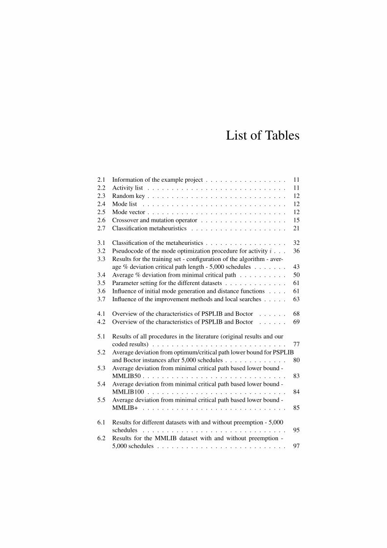
2.1 Information of the example project . . . . . . . . . . . . . . . . . 112.2 Activity list . . . . . . . . . . . . . . . . . . . . . . . . . . . . . 112.3 Random key . . . . . . . . . . . . . . . . . . . . . . . . . . . . . 122.4 Mode list . . . . . . . . . . . . . . . . . . . . . . . . . . . . . . 122.5 Mode vector . . . . . . . . . . . . . . . . . . . . . . . . . . . . . 122.6 Crossover and mutation operator . . . . . . . . . . . . . . . . . . 152.7 Classification metaheuristics . . . . . . . . . . . . . . . . . . . . 21
3.1 Classification of the metaheuristics . . . . . . . . . . . . . . . . . 323.2 Pseudocode of the mode optimization procedure for activity i . . . 363.3 Results for the training set - configuration of the algorithm - aver-
age % deviation critical path length - 5,000 schedules . . . . . . . 433.4 Average % deviation from minimal critical path . . . . . . . . . . 503.5 Parameter setting for the different datasets . . . . . . . . . . . . . 613.6 Influence of initial mode generation and distance functions . . . . 613.7 Influence of the improvement methods and local searches . . . . . 63
4.1 Overview of the characteristics of PSPLIB and Boctor . . . . . . 684.2 Overview of the characteristics of PSPLIB and Boctor . . . . . . 69
5.1 Results of all procedures in the literature (original results and ourcoded results) . . . . . . . . . . . . . . . . . . . . . . . . . . . . 77
5.2 Average deviation from optimum/critical path lower bound for PSPLIBand Boctor instances after 5,000 schedules . . . . . . . . . . . . . 80
5.3 Average deviation from minimal critical path based lower bound -MMLIB50 . . . . . . . . . . . . . . . . . . . . . . . . . . . . . . 83
5.4 Average deviation from minimal critical path based lower bound -MMLIB100 . . . . . . . . . . . . . . . . . . . . . . . . . . . . . 84
5.5 Average deviation from minimal critical path based lower bound -MMLIB+ . . . . . . . . . . . . . . . . . . . . . . . . . . . . . . 85
6.1 Results for different datasets with and without preemption - 5,000schedules . . . . . . . . . . . . . . . . . . . . . . . . . . . . . . 95
6.2 Results for the MMLIB dataset with and without preemption -5,000 schedules . . . . . . . . . . . . . . . . . . . . . . . . . . . 97
xii
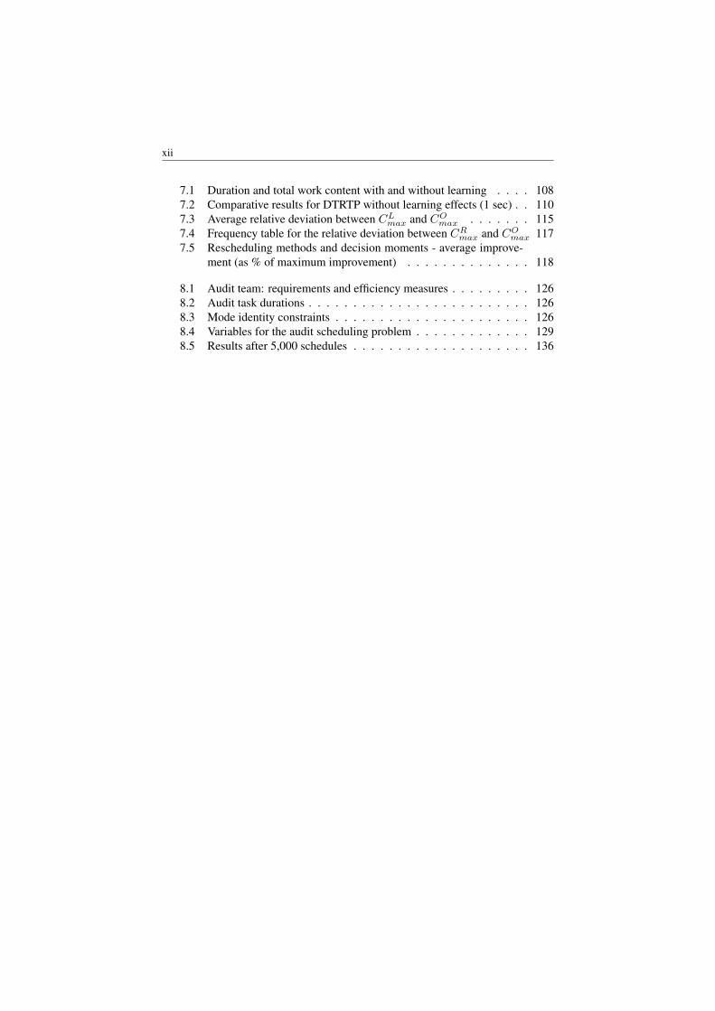
7.1 Duration and total work content with and without learning . . . . 1087.2 Comparative results for DTRTP without learning effects (1 sec) . . 1107.3 Average relative deviation between CLmax and COmax . . . . . . . 1157.4 Frequency table for the relative deviation between CRmax and COmax 1177.5 Rescheduling methods and decision moments - average improve-
ment (as % of maximum improvement) . . . . . . . . . . . . . . 118
8.1 Audit team: requirements and efficiency measures . . . . . . . . . 1268.2 Audit task durations . . . . . . . . . . . . . . . . . . . . . . . . . 1268.3 Mode identity constraints . . . . . . . . . . . . . . . . . . . . . . 1268.4 Variables for the audit scheduling problem . . . . . . . . . . . . . 1298.5 Results after 5,000 schedules . . . . . . . . . . . . . . . . . . . . 136

List of Acronyms
A
AIS Artificial Immune SystemAL Activity list
B
BPGA Bi-Population Genetic Algorithm
C
CNC Coefficient of Network ComplexityCP Critical PathCPIM Critical Path Improvement MethodCPU Computer Processing UnitCSLB Critical Sequence Lower Bound
D
DTRTP Discrete Time/Resource Tradeoff Problem
E
ERR Excess of Resource Request

xiv
F
FIM Feasibility Improvement Method
G
GA Genetic Algorithm
L
LB Lower BoundLFT Latest Finish TimeLST Latest Start Time
M
MAP Mode Assignment ProblemMASSP Medium-term Audit-staff Scheduling ProblemML Mode ListMMLIB Multi-mode LibraryMRCPSP Multi-mode Resource-constrained Project Scheduling
ProblemMRCPSP/R Multi-mode Resource-constrained Project Scheduling
Problem with Renewable resourcesMV Mode Vector
N
NP Non-deterministic Polynomial-time

xv
O
OS Order Strength
P
PMBOK Project Management Body Of KnowledgePS Particle SwarmPSPLIB Project scheduling problem libraryP-MRCPSP Preempted Multi-mode Resource-Constrained Project
Scheduling Problem
R
R Renewable resourcesRC Resource constrainednessRCPSP Resource-constrained Project Scheduling ProblemRF Resource FactorRK Random keyRNR Renewable and Nonrenewable resourcesRS Resource StrengthRWK Remaining Work Content
S
SA Simulated AnnealingSGS Schedule Generation SchemeSLK SlackSS Scatter searchSUM Sum of durations
T
TO Topological ordering

xvi
TS Tabu SearchTWC Total Work Content
W
WC Work ContentWCIM Work Content Improvement Method


Nederlandse samenvatting
Operations research (OR) heeft als doel processen binnen organisaties te verbete-ren of te optimaliseren met behulp van hiervoor ontwikkelde technieken en mo-dellen. De discipline kende zijn oorsprong tijdens WOII, toen aan de hand vanwiskundige modellen de logistieke bevoorrading van militair materiaal en goede-ren werd gepland. In de jaren na de oorlog ontwikkelde OR zich ten volle en tot opvandaag worden technieken en procedures ontwikkeld om complexe problemen inde bedrijfswereld, de maatschappij en de industrie te analyseren en te optimalise-ren.
Een van de onderzoeksdomeinen waarbinnen OR actief is, is project mana-gement. Project management kan omschreven worden als het geheel van kennis,vaardigheden, tools en technieken om een project zo te plannen dat het aan alleprojecteisen voldoet. Een project kan gedefinieerd worden als een tijdelijke in-spanning met als doel het creeren van een uniek product of een unieke service(PMBOK). De bouw van piramides in Egypte, de ontwikkeling van een iPhone-applicatie, het schrijven van een doctoraat, de organisatie van een verkiezingscam-pagne of het bouwen van een huis zijn allemaal typische voorbeelden van projec-ten.
De voorbije jaren is het belang van project management enorm toegenomen.Tientallen boeken over project management zijn verschenen en project softwarepakketten zijn ontwikkeld of uitgebreid met nieuwe planningsmogelijkheden. Bo-vendien zijn verschillende planningsproblemen reeds uitvoerig bestudeerd in deacademische literatuur en zijn talloze exacte, heuristische of metaheuristische op-lossingsmethodes voorgesteld.
Een van die planningsproblemen is het zogenaamde ’multi-mode resource-constrained project scheduling probleem’, waarbij getracht wordt een project ineen zo kort mogelijke duurtijd te plannen, rekening houdend met de volgordere-laties tussen de verschillende activiteiten en met de beschikbare hernieuwbare enniet-hernieuwbare middelen. Voor elk van de activiteiten zijn er bovendien meer-dere uitvoeringsmogelijkheden.
Dit doctoraat is opgedeeld in twee delen. In een eerste deel worden drie meta-heuristische oplossingsprocedures en een nieuwe dataset voorgesteld, terwijl inhet tweede deel verschillende meer praktische concepten worden geıntroduceerd.Dit werk wordt afgesloten met een algemene conclusie en enkele suggesties voorverder onderzoek.
Deel I van dit doctoraat start met een introductie van het multi-mode resource-constrained project scheduling probleem en een overzicht van de beschikbare li-
xx NEDERLANDSE SAMENVATTING
teratuur. Aan de hand van een voorbeeld worden enkele veelgebruikte termen inde project planning literatuur voorgesteld. Vervolgens worden drie oplossingsme-thodes ontwikkeld: een genetisch algoritme (GA), een artificieel immuun systeemalgoritme (AIS) en een scatter search algoritme (SS).
Het voorgestelde genetisch algoritme verschilt van andere genetische oplos-singsmethodes aangezien het gebruik maakt van twee populaties, een met left-justified schedules (waarbij alle activiteiten zo vroeg mogelijk gepland worden)en een met right-justified schedules (waarbij alle activiteiten zo laat mogelijk ge-pland worden). Het algoritme maakt ook gebruik van een generatieschema dat isuitgebreid met een methode die de gekozen mode van een activiteit tracht te opti-maliseren door te kiezen voor de mode die resulteert in de laagst mogelijke eindtijdvoor die activiteit.
De AIS procedure is gebaseerd op de principes van het menselijke immuunsysteem. Wanneer ziektekiemen het menselijke lichaam binnendringen zullen deantigenen die in staat zijn om de ziektekiemen te bestrijden, zich vermenigvuldigenom op die manier zo snel mogelijk de ziekte te doen verdwijnen. Ditzelfde principewordt toegepast in deze oplossingsmethode, die bovendien een procedure bevat omop een gecontroleerde manier de initiele populatie te genereren. Deze procedureis gebaseerd op experimentele resultaten die een link aantonen tussen bepaaldeeigenschappen van de gekozen modes en de uiteindelijke duurtijd van het project.
Een laatste algoritme is een scatter search algoritme. Deze procedure maakt ge-bruik van verschillende verbeteringsmethodes die elk aangepast zijn aan de speci-fieke eigenschappen van de verschillende hernieuwbare en niet-hernieuwbare mid-delen. Aan de hand van parameters die de beperktheid van de middelen aangeeft,wordt de procedure gestuurd in de richting van de meest efficiente verbeterings-methode en op die manier wordt een zo optimaal mogelijke oplossing gezocht.
Elk van de voorgestelde procedures behaalde uitstekende resultaten op de be-staande benchmark datasets. Deze sets vertonen evenwel enkele beperkingen ge-zien de huidige evolutie in de ontwikkeling van metaheuristische oplossingsme-thodes. Om die reden werd een nieuwe, verbeterde dataset ontwikkeld, die on-derzoekers in staat moet stellen om hun oplossingen te vergelijken met andereprocedures.
Om een vergelijking te kunnen maken tussen alle bestaande oplossingsmetho-des hebben we elk algoritme dat beschikbaar is in de literatuur gecodeerd en getestop de bestaande en nieuwe datasets. Door alle testen uit te voeren op eenzelfdecomputer en met eenzelfde stopcriterium zijn we in staat geweest een duidelijkeen faire vergelijking te maken. Onze voorgestelde algoritmes presteren bovendienuitstekend.
In het tweede deel van dit doctoraat worden een aantal uitbreidingen onder deloep genomen. Zo wordt in het eerste hoofdstuk van dit tweede deel de invloednagegaan van het onderbreken van activiteiten: activiteiten kunnen dan op elketijdstip stopgezet worden om later, zonder bijkomende kost, herstart te worden. Deintroductie van deze uitbreiding leidt tot een significante daling van de gemiddeldeduurtijd van een project vergeleken met de situatie waarin geen onderbrekingentoegelaten worden.

SUMMARY IN DUTCH xxi
Een andere uitbreiding is de introductie van leereffecten in een projectomge-ving. Hierbij wordt verondersteld dat een persoon efficienter wordt naarmate hijof zij langer aan een activiteit werkt. Dit leerconcept wordt vanuit drie verschil-lende hoeken bekeken. Ten eerste wordt nagegaan wat de invloed is van de in-troductie van het leerconcept op de totale duurtijd van een project en worden deverschillende parameters die hierop een invloed hebben geanalyseerd. Ten tweedebekijken we welke foutenmarge er moet aangenomen worden wanneer men geenrekening houdt met het leerconcept en tot slot achterhalen we dat door het tijdigincorporeren van de leereffecten significante verbeteringen kunnen gerealiseerdworden.
In het laatste deel van dit doctoraat wordt het genetisch algoritme uit deel Igebruikt om de planning van een audit kantoor te optimaliseren. In deze plan-ning dienen audit teams toegewezen te worden aan verschillende audit taken. Erkan duidelijk aangetoond worden dat met het gebruik van optimalisatietechniekensignificante verbeteringen kunnen gemaakt worden in de planning van de auditteams.
De bijdrage van dit doctoraat is drievoudig. Ten eerste werden drie state-of-the-art algoritmes gepresenteerd die in staat zijn om het multi-mode resource-constrained project scheduling probleem op een heel efficiente manier op te lossen.Bovendien werd telkens specifieke project informatie gebruikt om de efficientievan de procedure te verhogen. Ten tweede werden verschillende stappen onder-nomen om dit probleem uit te breiden naar meer realistische planningsproblemen.Het toelaten van het onderbreken van activiteiten en de introductie van leereffec-ten leidden tot nieuwe inzichten in het onderzoek van project planning. Tot slotworden met de ontwikkeling van een nieuwe dataset onderzoekers aangemoedigdom hun resultaten te vergelijken met die van andere procedures. Met deze nieuwedataset is tevens de basis gelegd voor verder onderzoek van dit interessante plan-ningsprobleem.

English summary
In the literature, a project is often described as a temporary endeavor undertakento create a unique product or service. The management of those projects is accom-plished through the use of the process of initiating, planning, executing, control-ling and closing (PMBOK). To guide projects to success, it is important to con-struct feasible and cost-efficient schedules. Different research fields within projectscheduling have been explored during recent years and a large set of exact, heuris-tic and metaheuristic solution procedures have been designed in order to tackle awide variety of project scheduling problems.
In this work, we study the multi-mode resource-constrained project schedulingproblem, which is a generalization of the resource-constrained project schedul-ing problem. Each activity in the project can be performed in different sets ofmodes, with specific activity durations and resource requirements. The objectiveof the MRCPSP is to find a mode and a start time for each activity such that themakespan is minimized and the schedule is feasible with respect to the precedenceand renewable and nonrenewable resource constraints.
The work consists of two main parts. In the first part, three metaheuristicsolution procedures are presented and a new benchmark dataset is proposed. Inthe second part, several practical concepts are introduced in order to take stepstowards real-life scheduling problems. This work is concluded with an overallconclusion and several suggestions for further research.
Part I starts with an introduction of the problem under study. An overviewof the available metaheuristic solution procedures is given and several conceptsand definitions used in this work are explained and illustrated with an example.Furthermore, three new metaheuristic solution procedures are presented, i.e. agenetic algorithm, an artificial immune system and a scatter search procedure.
The genetic algorithm makes use of two separate populations and extends theserial schedule generation scheme by introducing a mode improvement procedure.This procedure improves the mode selection by choosing the feasible mode of acertain activity that minimizes the finish time of the activity. The artificial immunesystem algorithm makes use of mechanisms inspired by the vertebrate immunesystem, such as hypermutation and proliferation. A controlled mode assignmentprocedure is set up in order to generate the initial population. This procedure isbased on experimental results which reveal a link between predefined mode listcharacteristics and the project makespan. Finally, the scatter search is executedwith different improvement methods, each tailored to the specific characteristicsof different renewable and nonrenewable resource scarceness values. These re-
xxiv ENGLISH SUMMARY
source parameters have been introduced in project scheduling literature to measurea project instance’s resource scarceness and are incorporated in the search processof the scatter search procedure.
All procedures proved to be very successful on the currently available bench-mark datasets, the PSPLIB dataset (Kolisch et al., 1995) and the dataset proposedby Boctor (1993). However, these datasets show some shortcomings given therecent evolution in the development of metaheuristic search procedures. We there-fore propose a new benchmark dataset MMLIB to overcome the disadvantagesof the current datasets. This new dataset can be used by researchers to comparethe results of their solution procedures with other procedures. In order to make afair comparison between all metaheuristic solution procedures on the same com-puter and for the same stop criteria, we also code each algorithm available in theliterature and test their performance on each of the three benchmark datasets.
In Part II of this work, we introduce several practical concepts in order totake steps towards real-life scheduling procedures. One of these practical conceptsis preemption, in which is it possible to preempt an activity at any integer timeinstance and restart it later on at no additional cost. In order to allow activity pre-emption, the original activity network is converted into a new network, in whicheach activity is split into subactivities with a unit duration of 1. The introduc-tion of preemption leads to a significant decrease in the average project makespancompared to the non-preempted case.
Another concept deals with the assumption that productivity and efficiencychanges can occur during project execution due to the effect of learning, the pro-cess of acquiring experience while performing an activity. This concept of activity-specific learning, in which the resources become more efficient the longer they stayon the job, is examined from various angles. The concept is introduced in the dis-crete time/resource trade-off problem, in which each activity contains a specificwork content in terms of working days, instead of a fixed duration and resourcerequirement. For each activity, a set of execution modes can be specified by us-ing different combinations of durations and resource requirements, as long as thespecified work content is met. Computational tests find a significant influenceof the introduction of learning effects in project scheduling and reveal the mainproject drivers that affect the project makespan when learning effects are intro-duced. Moreover, the margin of error made by ignoring learning during scheduleconstruction is measured. Finally, it is shown that timely incorporating learningduring the project progress leads to significant makespan improvements.
In the last chapter of this work, an attempt is made to use the genetic algorithmdesigned for the MRCPSP to solve a real-life audit scheduling problem, whichconsists of generating an appropriate audit team schedule for a small Belgian auditfirm. Although the algorithm is applied on a simplification of a practical planningproblem, the introduction of optimization techniques significantly improves theefficiency of the audit team schedule.
The contribution of this dissertation is threefold. First, three state-of-the-artsmetaheuristics are presented to solve the MRCPSP. Our genetic algorithm, arti-ficial immune system and scatter search procedure generated excellent results.

ENGLISH SUMMARY xxv
Moreover, the use of problem specific information in the local search process,such as the use of resource scarceness parameters in the scatter search procedure,increased the efficiency of the procedure significantly. Second, several efforts weremade to include practical concepts in order to take steps towards real-life schedul-ing problems. The introduction of preemption and learning led to new interestinginsights in project scheduling research. Finally, the new dataset will facilitate andmotivate researchers to investigate and develop new ideas and techniques to solvethe MRCPSP. Researchers are encouraged to use this dataset to compare the re-sults of their solution procedures with other procedures. The generation of thisnew dataset makes room for further research on this interesting and challengingresearch topic.


1Introduction
As a formal discipline, Operations Research originated as the mathematical sched-uling of a massive project logistically supplying Europe with military equipmentand goods during WWII (Jozefowska and Weglarz, 2006). In the decades after thewar, the discipline expanded into a field widely used to solve, analyze and optimizecomplex problems in business, society and industry. The developed techniques andprocedures were and are applied in industries ranging from petrochemistry to air-lines, finance, logistics and government, and operations research has become anarea of active academic and industrial research (Hillier and Lieberman, 2005).
One of the research fields on which operational research techniques are ap-plied is project management. Project management is the application of knowl-edge, skills, tools, and techniques to project activities to meet project requirements.Project management is accomplished through the use of the process of initiating,planning, executing, controlling and closing (PMBOK, 2004). A project can bedefined as a set of activities with a defined start point and defined end state, whichpursues a defined goal and uses a defined set of resources (Slack et al., 2009).The examples of projects are countless. The construction of the Burj Khalifa (thetallest man-made structure ever built), the development of an iPhone application,the building of the pyramids in Egypt, the construction of the wind park on theThorntonbank, the organization of an electoral campaign or the construction of ahouse are all examples of projects.
During the past decades, the importance of project management continues to
2 INTRODUCTION
grow rapidly. Many books on project management have been published1, newproject management software is developed, software packages have been expandedwith new scheduling capabilities and new techniques for measuring project pro-gress have been developed. The gap between the theory and practice is reduceddue to the popularization of project management research. In other words, projectmanagement is booming.
Project scheduling has also been an attractive research topic during the pastdecades. Project scheduling stems from machine scheduling, in which a groupof tasks should be assigned to a machine or resource. Different research fieldswithin project scheduling have been explored during recent years and a large setof exact, heuristic and metaheuristic solution procedures have been designed inorder to tackle a wide variety of project scheduling problems.
In this work, we study the multi-mode resource-constrained project sched-uling problem (MRCPSP), which is a generalization of the resource-constrainedproject scheduling problem (RCPSP). Due to the resource constraints, this prob-lem is known to be NP-hard (Blazewicz et al., 1983), meaning that optimal solu-tion procedures can only be used for relatively simple problem instances, while(meta)heuristic procedures will be needed for large-sized projects.
For the MRCPSP, many exact, heuristic and metaheuristic solution proceduresare proposed in recent years. Each of these procedures is tested on different setsof instances for different stop criteria which makes it difficult to present a faircomparison between the different procedures. The aim of this dissertation is toconstruct new state-of-the-art metaheuristic solution procedures for the MRCPSPand to make a fair comparison between the different metaheuristic solution proce-dures available in the literature. Moreover, the current benchmark datasets, whichare used to test the efficiency and performance of the solution procedures, showsome shortcomings given the recent evolution in the development of metaheuristicsearch procedures. We therefore propose a new dataset, which aims to overcomethe drawbacks of these datasets.
We also introduce several practical concepts in order to take steps towardsreal-life scheduling procedures. One of these practical concepts is preemption, inwhich it is possible to preempt an activity at any time and restart it later on atno additional cost. Another concept deals with the assumption that productivityand efficiency changes can occur during project execution due to the effect oflearning, which indicates the process of acquiring experience while performing anactivity. The introduction of these concepts leads to new interesting insights inproject scheduling research. In a case study, we apply one of our metaheuristicapproaches on a real-life audit scheduling problem, which consists of generatingan appropriate audit team schedule for a small Belgian audit firm.
The remainder of this work is structured as follows. Part I starts with the for-
1We refer the interested reader to Vanhoucke (2010), amongst many others.
INTRODUCTION 3
mulation of the MRCPSP (chapter 2). In chapter 3, three metaheuristic solutionprocedures for the MRCPSP are proposed, while in chapter 4 a new dataset forthe MRCPSP is proposed. In chapter 5, a fair comparison of the different solu-tion procedures is made which gives an indication of the performance of our ownprocedures and classifies all procedures according to similar stop criteria.
In part II, two extensions on the MRCPSP are presented. In chapter 6, theintroduction of preemption is discussed, while in chapter 7, the influence of theintroduction of learning effects on the project makespan is investigated. In chapter8, a model for an audit scheduling problem with sequence-dependent setup timesand different audit team efficiencies is proposed and the results for a real-life auditoffice scheduling problem are presented. In the last chapter, overall conclusionsand suggestions for future research are presented.
Publications
Parts of this dissertation have already been presented at international conferencesor have been published in international journals.
Publications in international journals
• Van Peteghem, V. and Vanhoucke, M., 2009, ”An Artificial Immune Systemfor the Multi-mode Resource-Constrained Project Scheduling Problem”, Lec-ture Notes in Computer Science, 5482, 85-96.
• Van Peteghem, V. and Vanhoucke, M., 2010, ”A Genetic Algorithm for thePreemptive and Non-preemptive Multi-mode Resource-Constrained ProjectScheduling Problem”, European Journal of Operational Research, 201, 409-418.
Unpublished working papers
• Van Peteghem, V. and Vanhoucke, M., 2009, ”Using Resource ScarcenessCharacteristics to Solve the Multi-Mode Resource-Constrained Project Sche-duling Problem”, Working paper 09/595
• Van Peteghem, V. and Vanhoucke, M., 2010, ”Introducing Learning Effectsin Resource-Constrained Project Scheduling”, Working paper 10/633
• Van Peteghem, V. and Vanhoucke, M., 2010, ”An Experimental Investi-gation of Metaheuristics for the Multi-Mode Resource-Constrained ProjectScheduling on New Dataset Instances”, Working paper

4 INTRODUCTION
Presentations at conferences
• Van Peteghem, V. and Vanhoucke, M., 2007, ”A Genetic Algorithm for theMulti-Mode Resource-constrained Project Scheduling Problem”, Paper pre-sented at the 22nd European Conference on Operational Research – Prague(Czech Republic)
• Van Peteghem, V. and Vanhoucke, M., 2008, ”A Comparison of VariousPopulation-based Meta-heuristics to Solve the MRCPSP”, Paper presentatedat the 11th International Workshop on Project Management and Scheduling– Istanbul (Turkey)
• Van Peteghem, V. and Vanhoucke, M., 2009, ”An Artificial Immune Systemfor the Multi-mode Resource-Constrained Project Scheduling Problem”, Pa-per presented at the 9th European Conference on Evolutionary Computationin Combinatorial Optimization – Tubingen (Germany)
• Van Peteghem, V. and Vanhoucke, M., 2009, ”Introduction of Learning Ef-fects in Resource-constrained Projects”, Paper presented at the 23th Euro-pean Conference on Operational Research – Bonn (Germany)
• Van Peteghem, V. and Vanhoucke, M., 2010, ”Learning Effects under Dif-ferent Project Settings”, Paper presented at the 12th International Workshopon Project Management and Scheduling – Tours (France)
• Van Peteghem, V. and Vanhoucke, M., 2010, ”An Experimental Investi-gation of Meta-heuristics for the Multi-mode Resource-constrained ProjectScheduling on new Dataset Instances”, Paper presented at the 24th EuropeanConference on Operational Research – Lisbon (Portugal)
• Van Peteghem, V. and Vanhoucke, M., 2010, ”Audit-staff Scheduling withAlternative Audit Teams and Setup Times”, Paper presented at the 24th Eu-ropean Conference on Operational Research – Lisbon (Portugal)

Part I
Metaheuristics for theMRCPSP

2The Multi-mode Resource-constrained
Project Scheduling Problem
2.1 Introduction
Resource-constrained project scheduling has been a research topic for many dec-ades, resulting in a wide variety of optimization procedures. The main focus onproject lead time minimization has led to the development of various exact and(meta)heuristic procedures for scheduling projects with tight resource constraintsunder a wide variety of assumptions. The basic problem type in project schedul-ing is the well-known resource-constrained project scheduling problem (RCPSP).This problem type aims at minimizing the total duration or makespan of a projectsubject to precedence relations between the activities and the limited renewableresource availabilities, and is known to be NP-hard (Blazewicz et al., 1983).
The multi-mode RCPSP (MRCPSP) is a generalized version of the RCPSP,where each activity can be performed in different sets of modes, with a specific ac-tivity duration and resource requirements. Three different categories of resourcescan be distinguished (Slowinski et al., 1994): renewable resources, which are lim-ited per time-unit (e.g. manpower, machines), nonrenewable resources, which arelimited for the entire project (e.g. budget) and doubly constrained resources, whichare limited both per time-unit and for the total project duration (e.g. cash-flow pertime-unit). Since doubly constrained resources can be considered as a combinationof renewable and nonrenewable resources, we do not consider them explicitly. Theobjective of the MRCPSP is to find a mode and a start time for each activity such
8 THE MULTI-MODE RESOURCE-CONSTRAINED PROJECT SCHEDULING PROBLEM
that the makespan is minimized and the schedule is feasible with respect to theprecedence and renewable and nonrenewable resource constraints. As this prob-lem is a generalization of the RCPSP, the MRCPSP is also NP-hard. Moreover, ifthere is more than one nonrenewable resource, the problem of finding a feasiblesolution for the MRCPSP is NP-complete (Kolisch and Drexl, 1997). The prob-lem is denoted as m, 1T |cpm, disc,mu|Cmax using the classification scheme ofHerroelen and De Reyck (1999) and is denoted as MPS|prec|Cmax by Bruckeret al. (1999).
In this chapter, an overview is given of the MRCPSP. In section 2.2, a generalformulation of the problem is described. In section 2.3, an example project is pre-sented which is used to explain the concepts and terminology which are presentedin section 2.4. This chapter concludes with an extended overview of the currentliterature on the MRCPSP.
2.2 Problem formulation
The MRCPSP can be stated as follows. The project is represented as an activity-on-the-node network G(N,A), where N is the set of activities and A is the setof pairs of activities between which a finish-start precedence relationship with aminimal time lag of 0 exists. A set of activities, numbered from 1 to |N | witha dummy start node 0 and a dummy end node |N | + 1, is to be scheduled on aset Rρ of renewable and Rν of nonrenewable resource types. Each activity i ∈N is performed in a mode mi, which is chosen out of a set of |Mi| differentexecution modes Mi = {1, ..., |Mi|}. The duration of activity i, when executedin mode mi, is dimi . Each mode mi requires rρimik renewable resource units(k ∈ Rρ). For each renewable resource k ∈ Rρ, the availability aρk is constantthroughout the project horizon. Activity i, executed in mode mi, will also userνimil nonrenewable resource units (l ∈ Rν) of the total available nonrenewableresource aνl . A schedule S is defined by a vector of activity start times si and avector denoting its corresponding execution modes mi. A schedule is said to befeasible if all precedence and renewable and nonrenewable resource constraintsare satisfied. The objective of the MRCPSP is to minimize the makespan of theproject.
The MRCPSP can be conceptually formulated as follows:
Min. s|N |+1 (2.1)

CHAPTER 2 9
s.t.
si + dimi ≤ sj ∀(i, j) ∈ A (2.2)∑i∈S(t)
rρimik ≤ aρk ∀k ∈ Rρ,∀mi ∈Mi (2.3)
|N |∑i=1
rνimil ≤ aνl ∀l ∈ Rν ,∀mi ∈Mi (2.4)
mi ∈Mi ∀i ∈ N (2.5)
s0 = 0 (2.6)
si ∈ int+ ∀i ∈ N (2.7)
where S(t) denotes the set of activities in progress in period [t − 1, t[, t ∈{1, ..., s|N |+1}. The objective function 2.1 minimizes the total makespan of theproject. Constraint set 2.2 takes the finish-start precedence relations with a mini-mal time lag of 0 into account. Constraints 2.3 and 2.4 take care of the renewableand nonrenewable resource limitations, respectively. Each activity i has to be per-formed in exactly one mode mi (constraint 2.5). Constraint 2.6 forces the projectto start at time instance 0 and constraint 2.7 ensures that the activity start timesassume nonnegative integer values. A schedule which fulfills all the constraints2.1 to 2.7, is called optimal.
The MRCPSP can be divided into two subproblems: a first subproblem canbe referred to as the Mode Assignment Problem (MAP), whose aim is to find afeasible mode assignment. A mode assignment which uses more nonrenewableresources than available is called infeasible, otherwise the mode assignment iscalled feasible.
The number of requested nonrenewable resource units that exceeds the capac-ity aνl , l ∈ Rν , is defined as the excess of resource request ERR. The formula ofthe ERR can be stated as follows:
ERR =
l∑j=1
(max(0,
|N |∑i=1
(rνimij)− aνj )) l ∈ Rν (2.8)
An ERR=0 means that the solution is feasible. If ERR is larger than 0, thesolution is infeasible.
In a second subproblem, the order in which the activities need to be scheduledmust be determined. Given the duration and the resource consumptions of thedifferent activities, the aim of the scheduling problem is to minimize the makespanof the project.
10 THE MULTI-MODE RESOURCE-CONSTRAINED PROJECT SCHEDULING PROBLEM
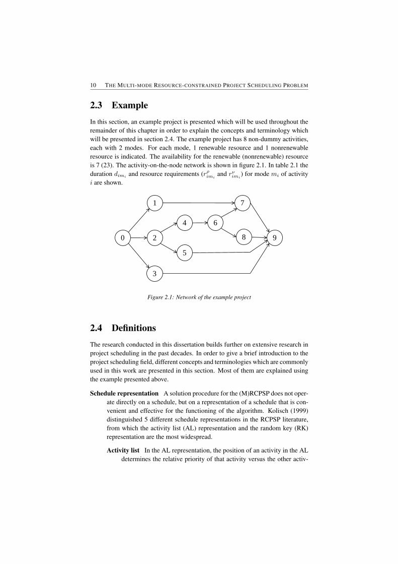
2.3 ExampleIn this section, an example project is presented which will be used throughout theremainder of this chapter in order to explain the concepts and terminology whichwill be presented in section 2.4. The example project has 8 non-dummy activities,each with 2 modes. For each mode, 1 renewable resource and 1 nonrenewableresource is indicated. The availability for the renewable (nonrenewable) resourceis 7 (23). The activity-on-the-node network is shown in figure 2.1. In table 2.1 theduration dimi and resource requirements (rρimi and rνimi ) for mode mi of activityi are shown.
20
4
7
6
1
8
5
3
9
Figure 2.1: Network of the example project
2.4 DefinitionsThe research conducted in this dissertation builds further on extensive research inproject scheduling in the past decades. In order to give a brief introduction to theproject scheduling field, different concepts and terminologies which are commonlyused in this work are presented in this section. Most of them are explained usingthe example presented above.
Schedule representation A solution procedure for the (M)RCPSP does not oper-ate directly on a schedule, but on a representation of a schedule that is con-venient and effective for the functioning of the algorithm. Kolisch (1999)distinguished 5 different schedule representations in the RCPSP literature,from which the activity list (AL) representation and the random key (RK)representation are the most widespread.
Activity list In the AL representation, the position of an activity in the ALdetermines the relative priority of that activity versus the other activ-

CHAPTER 2 11
act i mode mi dimi rρimi rνimi0 1 0 0 01 1 4 3 3
2 5 2 42 1 1 3 4
2 2 2 33 1 1 2 3
2 2 1 14 1 2 5 4
2 3 4 35 1 2 4 6
2 5 3 26 1 1 1 4
2 3 1 37 1 1 3 3
2 3 2 28 1 2 3 4
2 2 3 39 1 0 0 0
Available 7 23
Table 2.1: Information of the example project
ities. In table 2.2, an example of an activity list is given. In order toavoid infeasible solutions, the activity list is always precedence feasi-ble, which means that the precedence relations between the differentactivities are met.
Random Key In the RK representation, the sequence in which the activi-ties are scheduled is based on the priority value attributed to each ac-tivity. It is assumed in this work that a low RK value corresponds to ahigh priority. In table 2.3, three random key representations are given,which will all result in the same project schedule.
place 1 2 3 4 5 6 7 8AL 1 2 3 4 6 7 5 8
Table 2.2: Activity list
Mode representation Next to the schedule representation, the mode representa-tion determines the execution mode of each activity. Once a mode is as-signed to an activity, the duration and the resource consumption of each

12 THE MULTI-MODE RESOURCE-CONSTRAINED PROJECT SCHEDULING PROBLEM
activity 1 2 3 4 5 6 7 8RK1 12 16 19 25 21 18 12 28RK2 1 2 3 5 4 6 7 8RK3 0.21 0.25 0.98 1.15 1.02 2.21 0.24 0.25
Table 2.3: Random key
resource type can be determined. Two mode representations can be distin-guished: the mode list and the mode vector.
Mode list In the mode list representation, the list represents the executionmodes of the activities in ascending order, i.e. the first number in thelist indicates the mode in which the first activity will be executed, thesecond number the execution mode of the second activity, etc. In table2.4, an example of a mode list is given. Activity 7, for example, isexecuted in mode 1.
Mode vector In the mode vector representation, the mode indicated in theith position of the mode vector represents the execution mode of theactivity placed in the ith position of the activity list. A mode vector isalways represented in combination with an activity list. In table 2.5,an example of a mode vector is given, together with the activity list asrepresented in table 2.2. As can be seen, the same modes are chosenfor each activity as in the mode list example.
activity 1 2 3 4 5 6 7 8mode list 2 1 2 1 2 1 1 2
Table 2.4: Mode list
place 1 2 3 4 5 6 7 8AL 1 2 3 4 6 7 5 8MV 2 1 2 1 1 1 2 2
Table 2.5: Mode vector
Mode reduction Before the mode lists are generated, the mode reduction proce-dure of Sprecher et al. (1997) can be applied. This procedure excludes thosemodes which are inefficient or non-executable and those resources whichare redundant.

CHAPTER 2 13
– A mode is called inefficient if there is another mode of the same activitywith the same or smaller duration and no more requirements for allresources.
– A mode is called non-executable if its execution would violate the re-newable or nonrenewable resource constraints in any schedule.
– A nonrenewable resource is called redundant if the sum of the maximalrequests for that nonrenewable resource does not exceed its availabi-lity.
Excluding these modes or nonrenewable resources does not affect the set offeasible or optimal schedules.
Consider the example project instance given in section 2.3. Mode 1 of ac-tivity 8 can be called inefficient because both its duration and its resourcerequirements are equal or larger than those of mode 2. Also mode 1 of ac-tivity 5 can be excluded, because this mode is non-executable with respectto the nonrenewable resource. If it were executed, the project would requireat least 24 nonrenewable resource units, while only 23 are available. Themode can therefore be deleted.
Schedule generation scheme A schedule generation scheme (SGS) translates theschedule representation into a schedule. Two different types of SGSs existin the literature: the serial SGS (Kelley Jr., 1963) and the parallel SGS (Bed-worth and Bailey, 1982).
Serial SGS The serial scheduling scheme sequentially adds activities tothe schedule one-at-a-time. In each iteration, the next activity in thepriority list (activity list or random key) is chosen and that activity isassigned to the schedule as soon as possible within the precedence andresource constraints.
Parallel SGS In contrast to the serial SGS, the parallel scheduling schemeiterates over the different schedule times ts in which activities can beadded to the schedule. These schedule times correspond to the com-pletion times of already scheduled activities. At each time ts, theunscheduled activities whose predecessors have been completed, areconsidered in the order of the priority list and are scheduled on thecondition that no resource conflict originates at that time instant.
Figure 2.2(a) depicts a schedule which is based on the activity list as pro-posed in table 2.2 and the mode list as proposed in table 2.4. The schedule has amakespan of 9 days and is generated by using a serial schedule generation scheme.In figure 2.2(b), the schedule based on the same activity and mode list is shownusing a parallel SGS. This schedule results in a makespan of 11 days. However,
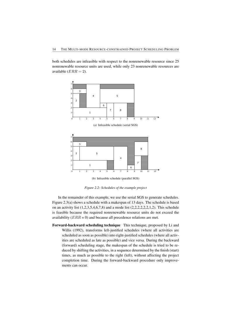
14 THE MULTI-MODE RESOURCE-CONSTRAINED PROJECT SCHEDULING PROBLEM
both schedules are infeasible with respect to the nonrenewable resource since 25nonrenewable resource units are used, while only 23 nonrenewable resources areavailable (ERR = 2).
12
1
2
3
4
6
7 8
5
6 7 8 9 10 110 1 2 3 4 5
3
2
1
7
6
5
4
(a) Infeasible schedule (serial SGS)
7
4
63
5
5
24
3
7
8
2
116
0 1 2 3 4 5 126 7 8 9 10 11
(b) Infeasible schedule (parallel SGS)
Figure 2.2: Schedules of the example project
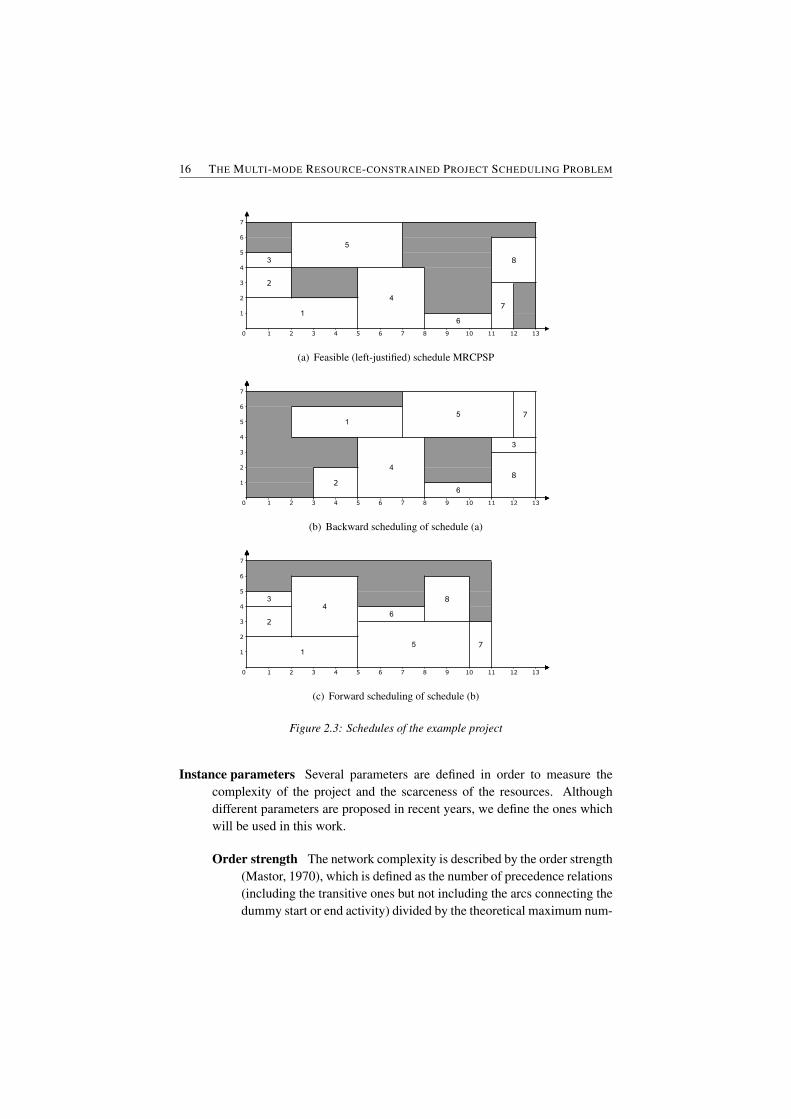
In the remainder of this example, we use the serial SGS to generate schedules.Figure 2.3(a) shows a schedule with a makespan of 13 days. The schedule is basedon an activity list (1,2,3,5,4,6,7,8) and a mode list (2,2,2,2,2,2,1,2). This scheduleis feasible because the required nonrenewable resource units do not exceed theavailability (ERR = 0) and because all precedence relations are met.
Forward-backward scheduling technique This technique, proposed by Li andWillis (1992), transforms left-justified schedules (where all activities arescheduled as soon as possible) into right-justified schedules (where all activ-ities are scheduled as late as possible) and vice versa. During the backward(forward) scheduling stage, the makespan of the schedule is tried to be re-duced by shifting the activities, in a sequence determined by the finish (start)times, as much as possible to the right (left), without affecting the projectcompletion time. During the forward-backward procedure only improve-ments can occur.

CHAPTER 2 15
On the schedule presented in figure 2.3(a), the backward scheduling techniqueis applied. Activities 8 cannot be scheduled later, while activity 7 can be shifted (1time unit) to start at time instant 12. Activities 6 and 4 cannot be scheduled later.Activity 5 can be right-shifted to start at time 7. Since the right shift of activity5 has made some additional resources available, activity 1 can be shifted 2 timeunits to start at time instant 2. Activity 3 can also be shifted to its latest start time11. In this way, we obtain the schedule of figure 2.3(b) with a makespan of 11units. Further improvements of the schedule are possible by shifting activities asmuch as possible to the left (forward scheduling). However, the total makespan ofthe schedule remains 11, as can be seen in figure 2.3(c).
Crossover During a crossover operation, information of two solution vectors iscombined in order to generate a new solution vector. The one- and two-pointcrossover are the most used crossovers.
One-point crossover In a one-point crossover, a single crossover point isselected and all data beyond that point in either string are swappedbetween the two parents.
Two-point crossover In a two-point crossover operation, two crossoverpoints are selected on the parent strings and everything between thesetwo crossover points is swapped.
Mutation The mutation operator is applied in order to introduce lost genetic ma-terial into the population and creates variation in the different individuals.
In table 2.6, an example of a one-point crossover is presented. Two activitylists (AL1 and AL2) are used to create a new activity list ALcross. The crossoverpoint is chosen randomly and is equal to 3, which means that the first 3 activitiesare chosen out of activity listAL1 and the last 5 are selected from activity listAL2,i.e. the activities which are not selected yet from AL1 are scheduled following thesequence in AL2. The new activity list ALcross is presented below. On this newactivity list, a mutation operation is applied. The activities 3 and 5 from the activitylist ALcross are swapped. This results in the activity list ALmut.
place 1 2 3 4 5 6 7 8AL1 1 2 4 5 6 3 7 8AL2 2 1 3 4 6 5 8 7
ALcross 1 2 4 3 6 5 8 7ALmut 1 2 4 5 6 3 8 7
Table 2.6: Crossover and mutation operator
16 THE MULTI-MODE RESOURCE-CONSTRAINED PROJECT SCHEDULING PROBLEM
3
7
6
5
1
5
4
5
4
3
2
1
2
7 8 9 10 110 1 2 3 4 12 136
6
7
8
(a) Feasible (left-justified) schedule MRCPSP
5
8
3
2
4
71
6
7
6
5
4
3
2
1
0 1 2 3 4 5 12 136 7 8 9 10 11
(b) Backward scheduling of schedule (a)
4 5 12 136 7 8 9 10 11
1
0 1 2 3
7
6
5
4
3
25
17
4
2
83
6
(c) Forward scheduling of schedule (b)
Figure 2.3: Schedules of the example project
Instance parameters Several parameters are defined in order to measure thecomplexity of the project and the scarceness of the resources. Althoughdifferent parameters are proposed in recent years, we define the ones whichwill be used in this work.
Order strength The network complexity is described by the order strength(Mastor, 1970), which is defined as the number of precedence relations(including the transitive ones but not including the arcs connecting thedummy start or end activity) divided by the theoretical maximum num-

CHAPTER 2 17
ber of precedence relations (|N |(|N | − 1)/2). The resource strengthOS varies between 0 and 1. An OS close to 0 indicates a parallelnetwork, while an OS close to 1 implies a serial network. The orderstrength of our example project is equal to 0.39.
Resource strength In the literature, two of the most used parameters tocalculate the scarceness of the resources for single-mode projects arethe Resource Strength (RS), introduced by Cooper (1976) and lateron redefined by Alvarez-Valdes and Tamarit (1989) and Kolisch et al.(1995), and the Resource Constrainedness (RC), proposed by Patter-son (1976). Since no formula is known for the resource constrained-ness as a resource parameter for multi-mode resource-constrained pro-jects, we will use in this work the resource strength as a parameter tocalculate the scarceness of the renewable and nonrenewable resources.Kolisch et al. (1995) and Demeulemeester et al. (2003) defined the re-source strength for multi-mode projects as follows:
RSk =ak − rmink
rmaxk − rmink
(2.9)
where ak denotes the total availability of renewable resource type k,rmink is formulated as maxi=1,...,|N |;mi=1,...,|Mi|r
ρikmi
and rmaxk de-notes the peak demand of renewable resource type k in the prece-dence preserving the earliest start schedule, where each activity hasa duration which corresponds to a maximum allocation of resources(Demeulemeester et al., 2003). The resource strength RS varies be-tween 0 and 1. A RS close to 0 indicates that the scarceness ofthe resource is high, while a RS close to 1 implies that the resourceis hardly restrictive. In the example project, the renewable resourcestrength RSρ is equal to 0.29. Kolisch et al. (1995) defined rmink asmaxi=1,...,|N |
{minmi=1,...,|Mi|r
ρikmi
}. However, for low values of
RSk, the use of this definition will lead to different non-executablemodes, which means that its execution would violate the renewable (ornonrenewable) resource constraints in any schedule (Sprecher, 2000).
For the nonrenewable resources the minimum and maximum consump-tion can be obtained by cumulating the consumptions obtained whenperforming each activity in the mode having minimum and maximumconsumptions. In the example project, the value of the nonrenewableresource strength RSν is equal to 0.25.
Resource factor The resource factor (RF) indicates the percentage of re-sources that are required per activity. The renewable resource factorRF ρ of resource k can be calculated as follows:

18 THE MULTI-MODE RESOURCE-CONSTRAINED PROJECT SCHEDULING PROBLEM
RF ρk =1
|N |
|N |∑i=1
1
|Mi|
|Mi|∑mi=1
{1 if rρimik > 00 otherwise
(2.10)
The nonrenewable resource factor RF ν can be calculated similarly. Inthe example project, both the renewable and nonrenewable resourcefactor is equal to 1.
In this section, different different concepts and terminologies which are com-monly used in the project scheduling field are presented. In the following section,an overview is given of the solutions procedures for the MRCPSP currently avail-able in the literature.
2.5 Literature overview
Several exact and heuristic approaches to solve the MRCPSP have been proposedin recent years. In section 2.5.1, an overview is given of the exact solution proce-dures. In section 2.5.2, we discuss the heuristic solution procedures and in section2.5.3, we describe the metaheuristic solution procedures. In this last section, eachsolution procedure is also described in detail, since the computational results ofthese algorithms will be compared with the metaheuristic solution procedures pro-posed in this work.
Although the solution procedures that tackle the MRCPSP/max, in which min-imal and maximal time lags are incorporated, show many similarities with theprocedures proposed for the MRCPSP, we refer in this section only to the solutionprocedures for the classical MRCPSP. The interested reader is referred to the pa-per of Barrios et al. (2009) for an overview of the available metaheuristics for theMRCPSP/max.
2.5.1 Exact solution procedures
The first solution method for the multi-mode problem can be found in Slowinski(1980), who presented a one-stage and two-stage linear programming approach.Talbot (1982) and Patterson et al. (1989) presented an enumeration scheme-basedprocedure. Speranza and Vercellis (1993) proposed a depth-first branch-and-boundalgorithm, but Hartmann and Sprecher (1996) have shown that this algorithm maybe unable to find the optimal solution for instances with two or more renewable re-sources. More recently, Sprecher et al. (1997), Hartmann and Drexl (1998) andSprecher and Drexl (1998) presented branch-and-bound algorithms, while Zhuet al. (2006) proposed a branch-and-cut algorithm. However, none of these proce-dures can be used for solving large-sized realistic projects, since they are unable

CHAPTER 2 19
to find an optimal solution in a reasonable computation time. Therefore, differentsingle-pass heuristic and metaheuristic procedures are presented.
2.5.2 Heuristic solution procedures
Talbot (1982) and Sprecher and Drexl (1998) proposed to impose a time limiton their exact branch-and-bound procedure. Boctor (1993) tested 21 heuristicscheduling rules and suggested a combination of 5 heuristics which have a highprobability of giving the best solution. Drexl and Grunewald (1993) proposed abiased random sampling approach, while Ozdamar and Ulusoy (1994) proposed alocal constraint based analysis approach. Boctor (1996) presented a heuristic al-gorithm based on the Critical Path Method computation, Kolisch and Drexl (1997)suggested a local search method with a single neighborhood search, Knotts et al.(2000) evaluated different agent-based algorithms and Lova et al. (2006) designedseveral multi-pass heuristics based on priority rules for solving the MRCPSP.
2.5.3 Metaheuristic solution procedures
This section gives an overview of the current available metaheuristics from theliterature. In section 2.5.3.1 an overview of the different classification criteria, asmentioned in Kolisch and Hartmann (1999), is given and the available algorithmsare classified according to these criteria. In section 2.5.3.2 an extensive and de-tailed overview of all the metaheuristics is presented.
2.5.3.1 Classification criteria
In order to make a classification of the available metaheuristics, the procedures aresorted based on three classification criteria as proposed by Kolisch and Hartmann(1999): the metaheuristic strategy, the schedule representation, the mode repre-sentation and the schedule generation scheme. In what follows we briefly examineeach of these criteria.
Metaheuristic strategy Several metaheuristic strategies to solve a schedulingproblem are available. For an overview of these metaheuristic strategies werefer to Glover and Kochenberger (2003). For the MRCPSP the followingsix strategies were used: genetic algorithm (GA), scatter search (SS), sim-ulated annealing (SA), particle swarm (PS), tabu search (TS) and artificialimmune system (AIS).
Schedule representation Kolisch (1999) distinguished 5 different schedule rep-resentations in the RCPSP literature, from which the activity list (AL) repre-sentation and the random key (RK) representation are the most widespread.

20 THE MULTI-MODE RESOURCE-CONSTRAINED PROJECT SCHEDULING PROBLEM
Mode representation Two mode representations can be distinguished in the lit-erature: the mode vector (MV) and the mode list (ML).
Schedule generation scheme A schedule generation scheme (SGS) translates theschedule representation into a schedule. Two different types of SGSs existin the literature: the serial SGS (Kelley, 1963) and the parallel SGS (Bed-worth and Bailey, 1982). Kolisch (1996b) has shown that it is sometimesimpossible to reach an optimal solution with the parallel SGS. Nevertheless,both schemes are used in the solution procedures currently available in theliterature.
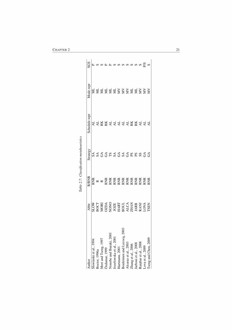
In table 2.7 an overview of the different metaheuristic algorithms is given. Foreach solution procedure, the name of the author(s) and the abbreviation used inthis work to refer to the procedure is given. The indication R or RNR in the thirdcolumn indicates if the procedure is applicable on datasets with only renewableresources (R) or with both renewable and nonrenewable (RNR) resources. Theinformation in the fourth, fifth, sixth and seventh column indicates the metaheuris-tic strategy, the schedule representation, the mode representation and the schedulegeneration scheme used to solve the problem instances, respectively.
2.5.3.2 Metaheuristic solution procedures
In this section, an overview is given of the different procedures available in theliterature according to their metaheuristic strategy: genetic algorithm, simulatedannealing, tabu search, scatter search and particle swarm.
Genetic algorithms Introduced by Holland (1975), genetic algorithms (GAs)use techniques and procedures inspired by evolutionary biology to solve complexoptimization problems. Several selection mechanisms, such as natural selection,crossover and mutation, are applied in order to recombine existing solutions sothat new ones are obtained and an optimal solution is found.
Mori and Tseng (1997) were the first to develop a genetic algorithm for theMRCPSP/R. The algorithm is based on the priority list representation, where thechromosome provides information about the scheduling order and the executionmode for each activity. The scheduling order is the priority of the activity in theschedule and lies between its forward and backward scheduling order (see Tavares,1990). The crossover operator is a one-point crossover, which randomly choosesan activity for which the start time is lower, and is applied on both the schedulingorder and mode list, while the mutation operator randomly adapts the mode listof a randomly chosen schedule. The population of a new generation is generatedby duplicating the best offspring schedules, by producing new schedules using thecrossover and mutation operator and by generating new random schedules.
CHAPTER 2 21
Tabl
e2.
7:C
lass
ifica
tion
met
aheu
rist
ics
Aut
hor
Abb
rR
/RN
RSt
rate
gySc
hedu
lere
prM
ode
repr
SGS
Slow
insk
ieta
l.,19
94SL
OW
RN
RSA
AL
ML
PB
octo
r,19
96a
BO
CT
RSA
AL
ML
SM
oria
ndT
seng
,199
7M
OR
IR
GA
RK
ML
SO
zdam
ar,1
999
OZ
DA
RN
RG
AR
KM
LP
Non
obe
and
Ibar
aki,
2001
NO
NO
RN
RT
SA
LM
LP
Joze
fow
ska
etal
.,20
01JO
ZE
RN
RSA
AL
ML
SH
artm
ann,
2001
HA
RT
RN
RG
AA
LM
VS
Bou
leim
enan
dL
ecoc
q,20
03B
OU
LR
NR
SAA
LM
VS
Alc
araz
etal
.,20
03A
LC
AR
NR
GA
AL
MV
SZ
hang
etal
.,20
06Z
HA
NR
NR
PSR
KM
LS
Jarb
ouie
tal.,
2008
JAR
BR
NR
PSR
KM
LS
Ran
jbar
etal
.,20
08R
AN
JR
NR
SSA
LM
VS
Lov
aet
al.,
2009
LO
VAR
NR
GA
AL
MV
P/S
Tse
ngan
dC
hen,
2009
TSE
NR
NR
GA
AL
MV
S
22 THE MULTI-MODE RESOURCE-CONSTRAINED PROJECT SCHEDULING PROBLEM
Ozdamar (1999) presented a hybrid genetic algorithm which makes use of thepriority list representation and a parallel SGS that performs exactly two iterations,one forward and one backward on each chromosome. A chromosome is repre-sented by two lists: a mode assignment list and a priority assignment list, whichindicates the priority rule used to select the candidate activity in the nth position.For each chromosome a crossover probability is calculated which is dependenton both the chromosome’s makespan and the population’s makespan and whichdetermines the probability of the chromosome to be recombined in the next ge-neration. A similar calculation is made to determine the probability to apply themutation operator. In order to generate the population of a new generation, eachchromosome is reproduced a number of times proportional to its objective functionvalue.
Hartmann (2001) developed a genetic algorithm based on the activity list rep-resentation and a serial SGS, which only generates forward schedules. A two-pointcrossover operator and a mutation operator are applied with a certain probabilityin order to create new genes. The ranking method is used as selection operator.The algorithm is extended with two local search procedures to improve the sched-ules. The single-pass improvement procedure checks for every activity whether amulti-mode left shift can be performed. A multi-mode left shift of an activity j isan operation on a given schedule which reduces the finish time of activity j with-out changing the modes or finish times of the other activities and without violatingthe precedence and resource constraints. The multi-pass improvement procedurerepeats the single-pass procedure until no further improvements can be detected.However, computational results have shown that the single-pass improvement pro-cedure performs the best.
Alcaraz et al. (2003) developed a genetic algorithm based on the activity listrepresentation and the serial SGS. An additional gene decides whether a forwardor backward scheduling is employed when computing a schedule from an activityand mode list. The two-point forward-backward crossover operator as designed byAlcaraz and Maroto (2001) is extended to the multi-mode version. A two-phasemutation operator is applied, which firstly modifies the activity list and secondlyalters the mode assignment.
Lova et al. (2009) proposed a hybrid genetic algorithm, with an activity listrepresentation and a serial and parallel SGS, which generates forward and back-ward schedules. Two extra genes decide whether a forward or backward sched-uling is employed and whether the serial or parallel SGS is executed. The two-point crossover operator and mutation are applied and the two-tournament selec-tion is applied to reproduce the new population. The authors also introduced amulti-mode forward-backward improvement method, which is an extension of theforward-backward improvement method described by Tormos and Lova (2001)and which can change the execution mode if a better position for an activity can

CHAPTER 2 23
be found.Tseng and Chen (2009) presented a two-phased genetic local search algorithm,
with an activity list representation and a serial SGS, which generates forward andbackward schedules. During the first phase, a set of elite solutions is searchedby the genetic algorithm, using a modified two-point crossover operator and amutation operator, based on the critical path activities in the schedule. This eliteset is utilized to construct the initial population of the second phase. A mutationoperator and a forward-backward local search is applied on this elite set, in orderto search more thoroughly in the promising areas of the solution space.
Simulated annealing The simulated annealing method is based on the physicalannealing process and has been introduced for the first time by Metropolis et al.(1953). In this method, all improvements are accepted, while inferior solutions arerejected or accepted with a certain probability, which decreases with the value ofthe difference in costs of the current and neighbor solution. The method has beenused several times to solve the MRCPSP.
Boctor (1996) was the first to present a simulated annealing procedure andpresented a procedure with an activity list representation and a serial SGS for theRCPSP and MRCPSP/R. The procedure started with an initial solution, gener-ated by the minimum slack/shortest feasible mode heuristic as proposed in Boctor(1993). To generate neighbor solutions, a random chosen activity is moved to an-other position in the precedence feasible activity list. To determine the executionmode, the mode resulting in the earliest finish time taking into account the prece-dence and renewable resource constraints is chosen. Several heating, reheatingand cooling phases are proposed.
Slowinski et al. (1994) proposed a simulated annealing procedure with an ac-tivity list representation and a parallel SGS. The initial starting solution is the bestsolution among a set of parallel priority heuristics. A neighborhood solution isaccepted with a probability of exp(-ρ/T ), where T is the control parameter, de-termined by the acceptable deterioration rate, and ρ the actual deterioration of thesolution vector.
Bouleimen and Lecocq (2003) proposed a simulated annealing procedure withan activity list representation and a serial SGS. The authors used two separate ex-ploration techniques in a two-stage procedure. In the first stage only a mode neigh-borhood exploration is performed, while in the second stage an activity neighbor-hood exploration is performed in order to further improve the solution. However,the second stage is only applied if a smaller makespan is found in the first stage.The initial value of the procedure is generated randomly. In the first explorationphase, no probabilistic acceptance criteria were used and only neighbors with asmaller makespan were accepted. In the second phase, fixed control parameterswere used in order to fully explore the search space.

24 THE MULTI-MODE RESOURCE-CONSTRAINED PROJECT SCHEDULING PROBLEM
Jozefowska et al. (2001) proposed a simulated annealing procedure with an ac-tivity list representation and a serial SGS, which makes use of the adaptive coolingscheme of Aarts and Korst (1989). In this work, the value of the control parameteris variable since the value depends on the search path. This involves the absenceof a reheating phase, as used in the papers of Boctor (1996) and Bouleimen andLecocq (2003). The initial solution can be obtained by setting all activities on theactivity list in an ascending order that follows from the ordering of nodes in theprecedence relation graph, and by executing all jobs in their first modes. The ge-neration of a neighborhood is generated by using one of the following operators:a neighborhood shift which operates only on the list of activities, a mode changewhich operates only on the mode list or a combined move.
Tabu search Tabu Search (TS) is a local search method, designed to drive thesearch away from local optima by accepting non-improving solutions. An intelli-gent use of memory is employed to help in exploiting the characteristics of previ-ous solution runs. The structure of the method is extremely malleable and hence itis often used to guide other constructive heuristics in order to avoid being trappedinto a poor local optimum.
Nonobe and Ibaraki (2002) presented a tabu search procedure for the RCPSPand the MRCPSP with an activity list representation and a parallel SGS. In theinitial part of the tabu search procedure, solutions are randomly generated in orderto find a feasible solution. Afterwards, this solution is repeatedly replaced by itsbest non-tabu neighbor until the stop criterion is achieved. Three types of neigh-borhood moves are proposed: a mode shift change mod(i,m′i), which changesthe mode of activity i to mode m′i; an activity shift shift aft(i, j), which shiftsactivity i immediately after activity j and an activity shift shift bef(i, j), whichmodifies the position of activity j to the position before i. The tabu list prohibits allmoves executed in the τ recent iterations, where τ is a program parameter calledtabu tenure.
Scatter search Scatter search is a population-based metaheuristic, proposed byGlover et al. (2000), in which solutions are intelligently combined to yield bet-ter solutions. The scatter search method makes use of deterministic proceduresthat can include problem specific knowledge (Pinol and Beasley, 2006) and cantherefore be implemented in a variety of ways and degrees of sophistication. Foran overview of the basic and advanced features of the scatter-search, we refer toGlover et al. (2000) and Marti et al. (2006).
Ranjbar et al. (2009) presented a scatter search algorithm with an activity listrepresentation and a serial SGS. In order to start with a diverse initial populationof solutions, the biased random sampling using frequency memory is employed.The solutions are combined using the path relinking method (Glover et al., 2000).
CHAPTER 2 25
This approach generates new solutions by exploring trajectories connecting high-quality solutions. Finally, a local search procedure, which changes with a certainprobability the mode mi of an activity i to mi − 1 and mi + 1 while the otheractivities remained unchanged, is applied to each generated schedule.
Particle Swarm Particle Swarm optimization (PS) was introduced by Kennedyand Eberhart (1995) and simulates the swarming behavior of animals to reach thepromising areas. Just like a population-based metaheuristic, PS conducts a searchusing a population (called swarm) of individuals (called particles) that is updatedfrom iteration to iteration, using formulas for each particle’s position and velocity.Two authors have used the principles of particle swarm to solve the MRCPSP.
The PS algorithm of Zhang et al. (2006) makes use of the priority list rep-resentation and a serial SGS. The initial population and the initial velocities aregenerated randomly. The formulas of Kennedy and Eberhart (1995) are used toupdate the population. In order to adjust infeasible particle solutions, a solutionprocedure is proposed to change the infeasibility of the current solution based onthe activity’s priority value. However, one can prove that endless loops can occurdue to the randomness of the mode selection part.
Jarboui et al. (2008) proposed a combinatorial PS algorithm with a priority listrepresentation and a serial SGS. The generation of the initial mode lists is gener-ated according to a certain probability (per mode) which increases for decreasingrenewable resource consumption of that mode. Once a mode list is generated, alocal search optimization procedure is applied on the list to optimize the sequencein which the activities should be scheduled. The activities are scheduled accordingto a probability which is determined by its number of successors. Feasible swapsare then performed in order to obtain improvements in the best solution.
2.6 ConclusionsIn this chapter, an introduction is given to the MRCPSP. We described the gen-eral formulation of the problem and presented an example project which is used toexplain the most important concepts and terminology used in project schedulingliterature. This chapter concluded with an overview of the available literature onthe MRCPSP and an introduction to each available metaheuristic solution proce-dure.

3Metaheuristic Solution Procedures for
the MRCPSP
3.1 Introduction
During the past decades, different metaheuristic solution procedures were usedto solve a wide set of combinatorial optimization problems. Each of these meta-heuristics is composed of different techniques, which are not dedicated to the so-lution of a particular problem, but are designed with the aim to be flexible enoughto handle a wide range of combinatorial problems. A metaheuristic can thereforebe considered as a conceptual framework which can be adapted with a few modi-fications to fit a specific optimization problem. Metaheuristic strategies guide andmodify the operations of subordinate heuristics and explore the search space inorder to find (near-)optimal solutions (Osman and Laporte, 1996).
The advantage of metaheuristic algorithms is the interaction between local im-provement procedures and higher level strategies to create a process capable ofescaping from local optima and performing a robust search of a solution space(Glover and Kochenberger, 2003). Local improvement methods attempt to ex-plore intensively the promising regions in the neighborhood of the current solution,while the search strategies of the different metaheuristic philosophies are designedto exploit the entire solution space. This balance between intensification and di-versification is very important for finding the near-optimal solution efficiently. Onthe one hand, the search process should quickly identify these regions in the searchspace where high quality solutions can be found, while on the other hand, the al-
28 CHAPTER 3
gorithm should not waste too much time in regions that are either already exploredor do not provide high quality solutions (Blum and Roli, 2003). Since metaheuris-tics are not problem-specific and are composed out of a set of basic concepts, it isoften necessary to include problem specific adaptions to these methods in order toobtain an effective metaheuristic solution procedure.
There are different metaheuristic solution procedures available in the literature.In the previous chapter, the genetic algorithm, the scatter search, the simulated an-nealing, the particle swarm and tabu search procedures were already presented,but many others are available (Glover and Kochenberger, 2003). According toBlum and Roli (2003), metaheuristic philosophies can be classified and describedin different ways: nature-inspired versus non-nature inspired, one versus variousneighborhood structure, memory usage versus memory-less methods and single-point versus population-based. This last classification is based on the characteris-tic of the number of solutions used at the same time. Algorithms working on onesingle solution are called trajectory methods and encompass metaheuristics liketabu search, iterated local search and variable neighborhood search. Population-based metaheuristics, on the contrary, perform search processes that describe theevolution of a set of points in the search space.
Osman (1995) makes another division and classifies the family of metaheuris-tics into three categories. The first is that of construction-based metaheuristics,which include greedy random adaptive search methods, guided construction meth-ods and ant colony systems. These metaheuristics tackle an optimization problemby exploring the search space using a so-called search tree. Each path from theroot node of the search tree to one of the leaves corresponds to the process of con-structing a candidate solution. The metaheuristics gradually build a solution bysampling the search space in every iteration. The second category is that of local-search-based metaheuristics, which include simulated annealing, noisy methods,guided local search methods, iterated local search, neural networks, tabu search,threshold accepting and variable neighborhood search. These methods includeintelligent extensions of local search algorithms in order to escape from local min-ima to proceed with the exploration of the search space. The third category is thatof population-based metaheuristics, which include evolutionary methods (geneticalgorithms, memetic algorithms, artificial immune systems, ...), path-relinking andscatter search. Since this type of metaheuristics deals with a population of solu-tions, population-based algorithms provide an intrinsic way for the exploration ofthe search space.
In this chapter, three different population-based metaheuristic solution proce-dures for the MRCPSP are proposed, i.e. a genetic algorithm, an artificial immunesystem and a scatter search. Before the metaheuristics are described in detail, eachof the solution procedures is classified based on different classification criteria insection 3.2. Next, in section 3.3, a bi-population genetic algorithm is described,
METAHEURISTIC SOLUTION PROCEDURES FOR THE MRCPSP 29
which makes use of two separate populations and extends the serial schedule ge-neration scheme by introducing a mode improvement procedure. In section 3.4,an artificial immune system algorithm is presented. This algorithm makes use ofmechanisms which are inspired by the vertebrate immune system, such as hyper-mutation and proliferation. The initial population set is generated with a controlledmode assignment procedure, based on experimental results which reveal a link be-tween predefined mode list characteristics and the project makespan. Finally, insection 3.5, a scatter search algorithm is proposed, which is executed with differentimprovement methods, each tailored to the specific characteristics of different re-newable and nonrenewable resource scarceness values. These resource parametershave been introduced in project scheduling literature to measure the scarceness ofresources of a project instance and are incorporated in the search process of thescatter search procedure.
Each section describes the different metaheuristics in detail and provides somecomputational results for the configuration of the solution procedure. In chapter5, a comparison is made between the different metaheuristic solution procedures.Computational tests are therefore performed on three datasets: the PSPLIB dataset(proposed by Kolisch et al., 1995), the dataset set by Boctor (1993) (hereaftercalled the Boctor dataset) and the MMLIB dataset, which is the new benchmarkdataset presented in chapter 4.
3.2 ClassificationIn order to give an extensive overview of the different components which will beused in the three metaheuristics, each solution procedure is classified accordingto nine metaheuristic classification criteria. Some of these criteria are inherent tothe metaheuristic solution procedure (e.g. the number of populations in a scat-ter search procedure), some are straightforward (e.g. the metaheuristic strategy),while the performance of some are tested during the computational experiments(e.g. the penalty function). In section 3.2.1, an overview of the classification cri-teria is given, while in section 3.2.2, the classification for the three metaheuristicsis made and discussed.
3.2.1 Classification criteria
The classification for each of the metaheuristic procedures is based on the follow-ing nine criteria. For the first three classification criteria, we also refer to section2.5.3.1.
Metaheuristic strategy Three metaheuristic procedures are proposed in this chap-ter: a genetic algorithm, an artificial immune system procedure and a scattersearch procedure. A genetic algorithm uses several mechanisms, such as
30 CHAPTER 3
natural selection, crossover and mutation in order to recombine existing so-lutions so that new ones are obtained. The scatter search algorithm contrastswith the genetic algorithm by focusing not only on the quality of the solu-tion, but also on the diversity of a solution. The use of diversification andimprovement methods leads to a more efficient exploration of the solutionspace. The artificial immune system finally makes use of mechanisms, suchas the clonal selection process, hypermutation and receptor editing, whichare inspired by the vertebrate immune system.
Schedule representation Two schedule representations are used: the activity list(AL) representation, where the position of an activity in the AL is deter-mined by the relative priority of that activity versus the other activities, andthe random key (RK) representation, where the sequence in which the activ-ities are scheduled is based on the priority value attributed to each activity.
Schedule generation scheme A schedule representation can be translated into aschedule by a serial SGS or by a parallel SGS. Since Kolisch (1996b) hasshown that it is sometimes impossible to reach an optimal solution with theparallel SGS, we use in our metaheuristic solution procedures only the serialSGS.
Penalty function As infeasible solutions can be included in the population, in-feasible schedules must be penalized. Therefore, several penalty functionsare available in the literature: the penalty function of Hartmann (2001), thepenalty function of Alcaraz et al. (2003), the penalty function of Jarbouiet al. (2008) and the penalty function of Lova et al. (2009).
Initial population Since the three proposed solution procedures are population-based metaheuristics, the algorithm needs an initial population on whichthe algorithmic techniques can be applied. This initial population can begenerated randomly or can be generated by the controlled mode assignmentprocedure, which will be proposed in section 3.4.
Local improvement methods Local improvement methods attempt to intensi-vely explore the promising regions in the neighborhood of the current solu-tion. Jozefowska et al. (2001), Bouleimen and Lecocq (2003), Kolisch andDrexl (1997) and Hartmann (2001) already proposed several local searchprocedures for the MRCPSP, which will be referred to as ’Local search lit-erature’. In section 3.3, a mode improvement method will be described anda combined local improvement method, which is composed out of three im-provement methods, will be presented in section 3.5.
Number of populations Population-based algorithm traditionally use 1 popula-tion on which different procedures are applied. However, in this work, we

METAHEURISTIC SOLUTION PROCEDURES FOR THE MRCPSP 31
will propose algorithms which make use of 2 populations.
Crossover Although different crossover operators are proposed in the literature,tests revealed that the one-point and two-point crossover obtained the bestresults in our algorithms.
Mutation In one procedure no mutation operator is applied. Two classificationitems are therefore considered: mutation or no mutation.
3.2.2 Classification of the proposed metaheuristics
In table 3.1, an overview of the different classification criteria is given. For eachof the developed metaheuristic solution procedures, it is indicated if and how thisclassification criterion is used in the proposed algorithm (’x’ means the componentis applied and/or tested in this solution procedure).
During the computational experiments of the genetic algorithm (section 3.3),the performance of the different penalty functions, the number of populations andthe local improvement methods from the literature are tested. During the com-putational experiments of the AIS (section 3.4), the initial population generationmethods (controlled versus random) are tested. The scatter search algorithm makesuse of a combination of the best performing local improvement methods from theliterature, the mode improvement method and the combined improvement method.This is tested in section 3.5.
In the remainder of this chapter, a detailed description of each metaheuristicsolution procedure is given.
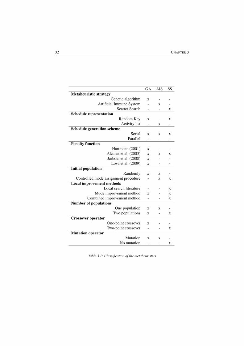
32 CHAPTER 3
GA AIS SSMetaheuristic strategy
Genetic algorithm x - -Artificial Immune System - x -
Scatter Search - - xSchedule representation
Random Key x - xActivity list - x -
Schedule generation schemeSerial x x x
Parallel - - -Penalty function
Hartmann (2001) x - -Alcaraz et al. (2003) x x xJarboui et al. (2008) x - -
Lova et al. (2009) x - -Initial population
Randomly x x -Controlled mode assignment procedure - x x
Local improvement methodsLocal search literature - - x
Mode improvement method x - xCombined improvement method - - x
Number of populationsOne population x x -
Two populations x - xCrossover operator
One-point crossover x - -Two-point crossover - - x
Mutation operatorMutation x x -
No mutation - - x
Table 3.1: Classification of the metaheuristics
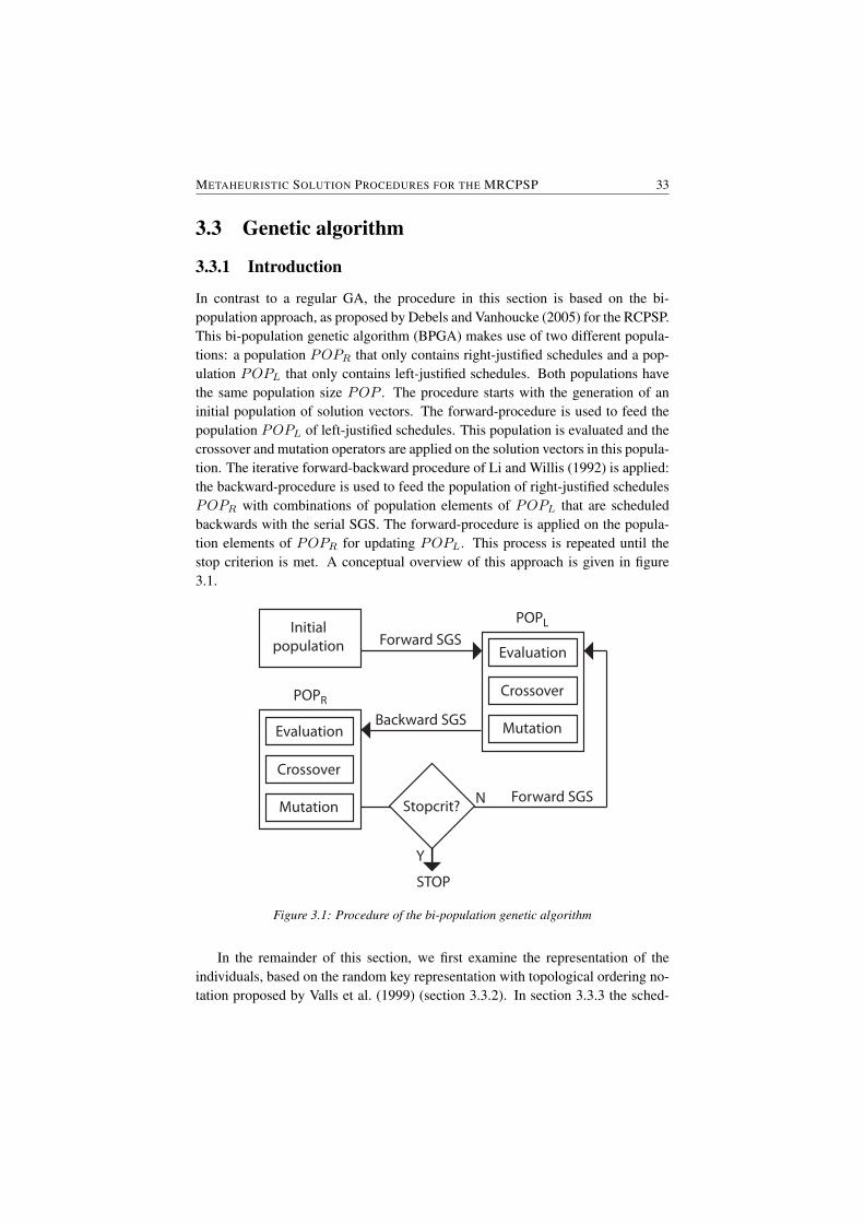
METAHEURISTIC SOLUTION PROCEDURES FOR THE MRCPSP 33
3.3 Genetic algorithm
3.3.1 Introduction
In contrast to a regular GA, the procedure in this section is based on the bi-population approach, as proposed by Debels and Vanhoucke (2005) for the RCPSP.This bi-population genetic algorithm (BPGA) makes use of two different popula-tions: a population POPR that only contains right-justified schedules and a pop-ulation POPL that only contains left-justified schedules. Both populations havethe same population size POP . The procedure starts with the generation of aninitial population of solution vectors. The forward-procedure is used to feed thepopulation POPL of left-justified schedules. This population is evaluated and thecrossover and mutation operators are applied on the solution vectors in this popula-tion. The iterative forward-backward procedure of Li and Willis (1992) is applied:the backward-procedure is used to feed the population of right-justified schedulesPOPR with combinations of population elements of POPL that are scheduledbackwards with the serial SGS. The forward-procedure is applied on the popula-tion elements of POPR for updating POPL. This process is repeated until thestop criterion is met. A conceptual overview of this approach is given in figure3.1.
Initial population Evaluation
Crossover
MutationEvaluation
Crossover
Mutation
POPL
POPR
Forward SGS
Forward SGS
Backward SGS
Stopcrit? N
Y
STOP
Figure 3.1: Procedure of the bi-population genetic algorithm
In the remainder of this section, we first examine the representation of theindividuals, based on the random key representation with topological ordering no-tation proposed by Valls et al. (1999) (section 3.3.2). In section 3.3.3 the sched-
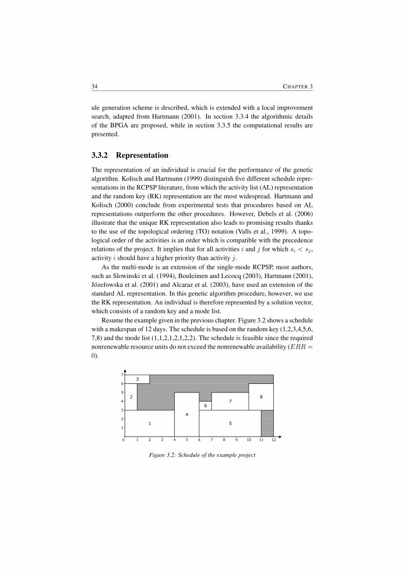
34 CHAPTER 3
ule generation scheme is described, which is extended with a local improvementsearch, adapted from Hartmann (2001). In section 3.3.4 the algorithmic detailsof the BPGA are proposed, while in section 3.3.5 the computational results arepresented.
3.3.2 Representation
The representation of an individual is crucial for the performance of the geneticalgorithm. Kolisch and Hartmann (1999) distinguish five different schedule repre-sentations in the RCPSP literature, from which the activity list (AL) representationand the random key (RK) representation are the most widespread. Hartmann andKolisch (2000) conclude from experimental tests that procedures based on ALrepresentations outperform the other procedures. However, Debels et al. (2006)illustrate that the unique RK representation also leads to promising results thanksto the use of the topological ordering (TO) notation (Valls et al., 1999). A topo-logical order of the activities is an order which is compatible with the precedencerelations of the project. It implies that for all activities i and j for which si < sj ,activity i should have a higher priority than activity j.
As the multi-mode is an extension of the single-mode RCPSP, most authors,such as Slowinski et al. (1994), Bouleimen and Lecocq (2003), Hartmann (2001),Jozefowska et al. (2001) and Alcaraz et al. (2003), have used an extension of thestandard AL representation. In this genetic algorithm procedure, however, we usethe RK representation. An individual is therefore represented by a solution vector,which consists of a random key and a mode list.
Resume the example given in the previous chapter. Figure 3.2 shows a schedulewith a makespan of 12 days. The schedule is based on the random key (1,2,3,4,5,6,7,8) and the mode list (1,1,2,1,2,1,2,2). The schedule is feasible since the requirednonrenewable resource units do not exceed the nonrenewable availability (ERR =
0).
4
5
6
82
7
3
126 7 8 9 10 110 1 2 3 4 5
2
1
1
7
6
5
4
3
Figure 3.2: Schedule of the example project
METAHEURISTIC SOLUTION PROCEDURES FOR THE MRCPSP 35
3.3.3 Extended generation scheme
A schedule generation scheme (SGS) translates the solution vector into a scheduleS. As already stated in section 3.2.1, we use in this work the serial SGS. However,we have extended the serial SGS with the following two elements.
First, our procedure makes use of the forward/backward scheduling technique,a well-known local search technique for RCPSP metaheuristics. The idea of sched-uling activities in backward and forward direction has been introduced by Li andWillis (1992) and then used as improving method by Tormos and Lova (2001).Afterwards several authors, such as Alcaraz and Maroto (2001), Valls et al. (2005)and Debels et al. (2006) amongst others, have used similar procedures. The for-ward (backward) procedure is applied on the population POPR (POPL) of right-justified (left-justified) schedules and is used to build the left-justified (right-justi-fied) schedules which are stored in the population POPL (POPR). To embedthe TO condition in the random key representation, the start (finish) times of theactivities of the schedules in POPL (POPR) are used as the priority values ofthe random key. The sequence of the activities is made by sorting the activities in(reverse) chronological order of their start (finish) times (Debels and Vanhoucke,2007).
Second, our serial generation scheme is extended with a procedure to improvethe mode selection. For every activity i ∈ {1, ..., |N |} that will be scheduled, bothin the forward and in the backward procedure, there is a probability of Pmodimpthat the mode improvement procedure will be executed. We use mi to refer tothe current mode of activity i. The mode improvement procedure evaluates foreach activity i whether a new mode selection m′i leads to an improvement in theERR′. Consequently, this procedure evaluates all possible mode assignments k =
1, ..., |Mi| of an activity i and calculates for each new mode list the correspondingexcess of resource request ERR′. If the ERR′ is equal or smaller than the currentERR, the procedure checks if an improvement can be made in the finish timeof that activity. The mode m′i with the lowest finish time f ′i , which does notincrease the ERR, is chosen. If no improvement can be made, the mode selectionis retained.
The pseudocode for the mode improvement procedure for an activity i of aproject with an excess resource request of ERR is shown in table 3.2.
This mode improvement procedure is a combination of a mode selection rule ofLova et al. (2006) on the one hand and the single-pass improvement local search ofHartmann (2001) on the other hand. Lova et al. (2006) extend the serial generationscheme using the ’Earliest Feasible Finish Time’ as a mode selection rule. Duringthe generation of the schedule, this rule selects for each activity the executionmode so that it is scheduled with the smallest feasible finish time possible. Thelocal search of Hartmann (2001) is based on the multi-mode left shift of Sprecher(1994). For each completely generated feasible schedule, the procedure checks for

36 CHAPTER 3
FOR k=1,...,|Mi|{
Set new mode m′i = k and create a new mode vectorCompute ERR′
IF (ERR′)≤ ERR)Compute f ′iIF(f ′i < fi)
fi = f ′imi = m′iERR = ERR′
}
Table 3.2: Pseudocode of the mode optimization procedure for activity i
every activity whether a multi-mode left shift can be performed. A multi-modeleft shift of an activity j is an operation on a given schedule which reduces thefinish time of activity j without changing the modes or finish times of the otheractivities and without violating the constraints. Unlike the procedure of Hartmann,our procedure tries to improve the makespan during the generation of the schedule.
One could think that the mode improvement procedure will always chose themode with the lowest duration. However, a mode with a shorter duration oftenrequires more nonrenewable resource units and gives cause to an increase of theERR and the infeasibility of the schedule. In addition, a mode with a longer dura-tion requires less resource units, both renewable and nonrenewable. The procedurewill therefore be able to schedule the activity more easily in parallel with other ac-tivities, because - due to the lower resource requirements - less resource conflictswill occur. Retake the schedule presented in figure 3.2. Suppose that activities 4and 7 are subject to the mode improvement procedure. After scheduling activities1, 2 and 3 (without applying the procedure), the mode improvement procedure isused for activity 4. With the current mode for activity 4 (mode 1), the schedulehas an ERR of 0. The finish time of mode 1 is 6 (see Fig 3.3(a)). When changingthe mode of activity 4 to 2, the ERR remains equal, because the required nonre-newable resource units (22) are smaller than the available ones (23). Although theduration of mode 2 is larger than mode 1, the required renewable resource unitsalso decrease and the activity can be scheduled in parallel with activity 1. The fin-ish time for mode 2 is now 5 (see Fig 3.3(b)). Because mode 2 has a lower finishtime and the ERR does not deteriorate, the mode list is adapted. After schedulingactivities 5 and 6, the mode improvement is applied on activity 7. For activity7, mode 2 is currently selected and when inserting the activity in the current par-
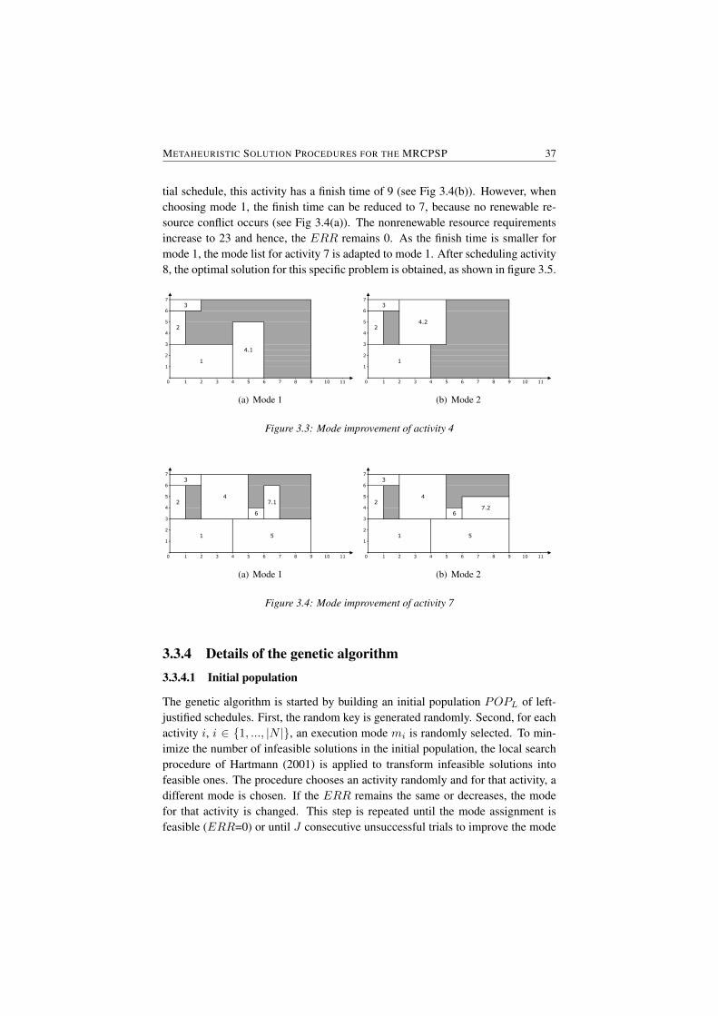
METAHEURISTIC SOLUTION PROCEDURES FOR THE MRCPSP 37
tial schedule, this activity has a finish time of 9 (see Fig 3.4(b)). However, whenchoosing mode 1, the finish time can be reduced to 7, because no renewable re-source conflict occurs (see Fig 3.4(a)). The nonrenewable resource requirementsincrease to 23 and hence, the ERR remains 0. As the finish time is smaller formode 1, the mode list for activity 7 is adapted to mode 1. After scheduling activity8, the optimal solution for this specific problem is obtained, as shown in figure 3.5.
10 11
4.1
4 5 6 7 8 9
1
0 1 2 3
7
36
2
5
4
3
1
2
(a) Mode 1
6 7 8 9 10 110 1 2 3 4 5
5
4
3
1
2
1
7
3
4.2
6
2
(b) Mode 2
Figure 3.3: Mode improvement of activity 4
3
4
7.1
6
6 7 8 9 10 110 1 2 3 4 5
3
1
2
1
2
5
7
6
5
4
(a) Mode 1
6
5
7.2
3
2
4
6 7 8 9 10 110 1 2 3 4 5
7
6
5
4
3
1
2
1
(b) Mode 2
Figure 3.4: Mode improvement of activity 7
3.3.4 Details of the genetic algorithm3.3.4.1 Initial population
The genetic algorithm is started by building an initial population POPL of left-justified schedules. First, the random key is generated randomly. Second, for eachactivity i, i ∈ {1, ..., |N |}, an execution mode mi is randomly selected. To min-imize the number of infeasible solutions in the initial population, the local searchprocedure of Hartmann (2001) is applied to transform infeasible solutions intofeasible ones. The procedure chooses an activity randomly and for that activity, adifferent mode is chosen. If the ERR remains the same or decreases, the modefor that activity is changed. This step is repeated until the mode assignment isfeasible (ERR=0) or until J consecutive unsuccessful trials to improve the mode
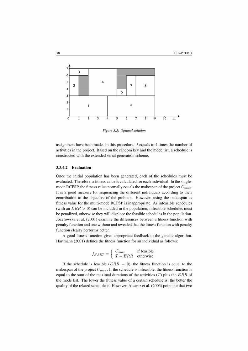
38 CHAPTER 3
7
10
7
3
4
6
2
5
8
5
4
63
1 5
2
1
6 7 8 9 110 1 2 3 4
Figure 3.5: Optimal solution
assignment have been made. In this procedure, J equals to 4 times the number ofactivities in the project. Based on the random key and the mode list, a schedule isconstructed with the extended serial generation scheme.
3.3.4.2 Evaluation
Once the initial population has been generated, each of the schedules must beevaluated. Therefore, a fitness value is calculated for each individual. In the single-mode RCPSP, the fitness value normally equals the makespan of the project Cmax.It is a good measure for sequencing the different individuals according to theircontribution to the objective of the problem. However, using the makespan asfitness value for the multi-mode RCPSP is inappropriate. As infeasible schedules(with an ERR > 0) can be included in the population, infeasible schedules mustbe penalized, otherwise they will displace the feasible schedules in the population.Jozefowska et al. (2001) examine the differences between a fitness function withpenalty function and one without and revealed that the fitness function with penaltyfunction clearly performs better.
A good fitness function gives appropriate feedback to the genetic algorithm.Hartmann (2001) defines the fitness function for an individual as follows:
fHART =
{Cmax if feasibleT + ERR otherwise
If the schedule is feasible (ERR = 0), the fitness function is equal to themakespan of the project Cmax. If the schedule is infeasible, the fitness function isequal to the sum of the maximal durations of the activities (T ) plus the ERR ofthe mode list. The lower the fitness value of a certain schedule is, the better thequality of the related schedule is. However, Alcaraz et al. (2003) point out that two

METAHEURISTIC SOLUTION PROCEDURES FOR THE MRCPSP 39
different individuals with the same excess of resource request but with a differentmakespan have the same fitness value. They also mention that the upper boundT is a poor bound and indicate that the probability of the infeasible solutions tosurvive will be near 0. Therefore, they define a new fitness function that can bepresented as follows:
fALC =
{Cmax if feasibleCmax +max feas Cmax − CPmin + ERR otherwise
wheremax feas Cmax gives the maximal makespan of the feasible schedulesrelated to individuals of the current generation andCPmin is the critical path usingthe minimal duration of each activity. According to Alcaraz et al. (2003), thisfitness computation reveals better results than the one of Hartmann (2001).
Lova et al. (2009) also state that the fitness function of Alcaraz et al. (2003)is built by adding units of time from the makespan and units of resources fromthe excess of nonrenewable resources and conclude that the magnitude of bothaspects of the solution can disturb the meaning of the fitness function. Therefore,they propose a new fitness function where both aspects of the solution are jointlyconsidered but normalized in order to eliminate their magnitudes. This fitnessfunction can be presented as follows:
fLOV A =
1− max feas Cmax−Cmaxmax feas Cmax
if feasible
1 + Cmax−CPminCmax
+∑l∈Rν max(0,
∑|N|i=1 r
νimil−aνl
aνl) otherwise
The individual with the greatest feasible makespan will have a fitness valueequal to 1 while the individual with the best feasible makespan will have a fitnessvalue close to 0. The fitness function of a non-feasible individual is always greaterthan 1, so feasible solutions will always have a smaller fitness value than infeasiblesolutions. Moreover, the sum of the normalized deviation of the makespan fromthe minimal critical path and the normalized excess of nonrenewable resources areadded. According to Lova et al. (2009), this fitness function solves the cited weakpoints of the fitness computation of Alcaraz et al. (2003). In addition, computa-tional tests in their paper reveal superior performance of this fitness function.
Finally, also Jarboui et al. (2008) propose a fitness function, which measuresthe degree of infeasibility and transforms this into a penalty function which growsin proportion to the infeasibility level, thus guiding the search toward the feasiblesolution space. The fitness function is given as:
fJARB =
{Cmax if feasibleCmax +
∑|Rν |l=1 δmax(0,
∑|N |i=1(rνimil)− a
νl ) otherwise
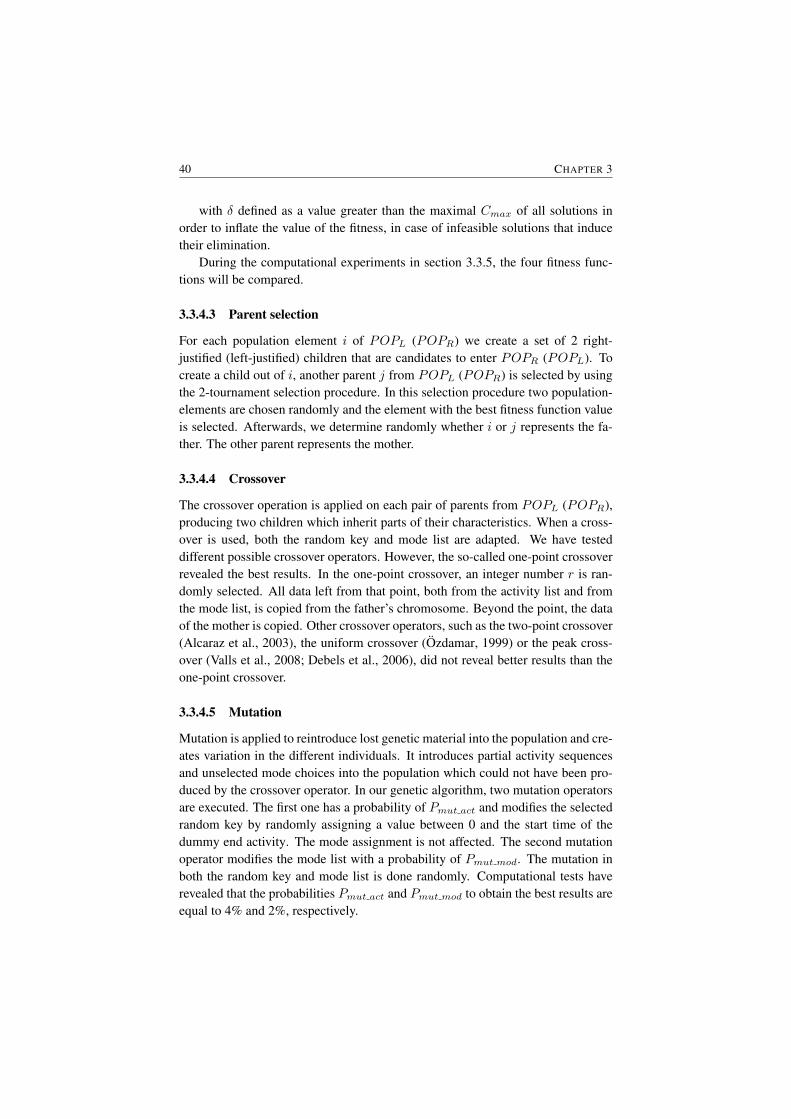
40 CHAPTER 3
with δ defined as a value greater than the maximal Cmax of all solutions inorder to inflate the value of the fitness, in case of infeasible solutions that inducetheir elimination.
During the computational experiments in section 3.3.5, the four fitness func-tions will be compared.
3.3.4.3 Parent selection
For each population element i of POPL (POPR) we create a set of 2 right-justified (left-justified) children that are candidates to enter POPR (POPL). Tocreate a child out of i, another parent j from POPL (POPR) is selected by usingthe 2-tournament selection procedure. In this selection procedure two population-elements are chosen randomly and the element with the best fitness function valueis selected. Afterwards, we determine randomly whether i or j represents the fa-ther. The other parent represents the mother.
3.3.4.4 Crossover
The crossover operation is applied on each pair of parents from POPL (POPR),producing two children which inherit parts of their characteristics. When a cross-over is used, both the random key and mode list are adapted. We have testeddifferent possible crossover operators. However, the so-called one-point crossoverrevealed the best results. In the one-point crossover, an integer number r is ran-domly selected. All data left from that point, both from the activity list and fromthe mode list, is copied from the father’s chromosome. Beyond the point, the dataof the mother is copied. Other crossover operators, such as the two-point crossover(Alcaraz et al., 2003), the uniform crossover (Ozdamar, 1999) or the peak cross-over (Valls et al., 2008; Debels et al., 2006), did not reveal better results than theone-point crossover.
3.3.4.5 Mutation
Mutation is applied to reintroduce lost genetic material into the population and cre-ates variation in the different individuals. It introduces partial activity sequencesand unselected mode choices into the population which could not have been pro-duced by the crossover operator. In our genetic algorithm, two mutation operatorsare executed. The first one has a probability of Pmut act and modifies the selectedrandom key by randomly assigning a value between 0 and the start time of thedummy end activity. The mode assignment is not affected. The second mutationoperator modifies the mode list with a probability of Pmut mod. The mutation inboth the random key and mode list is done randomly. Computational tests haverevealed that the probabilities Pmut act and Pmut mod to obtain the best results areequal to 4% and 2%, respectively.
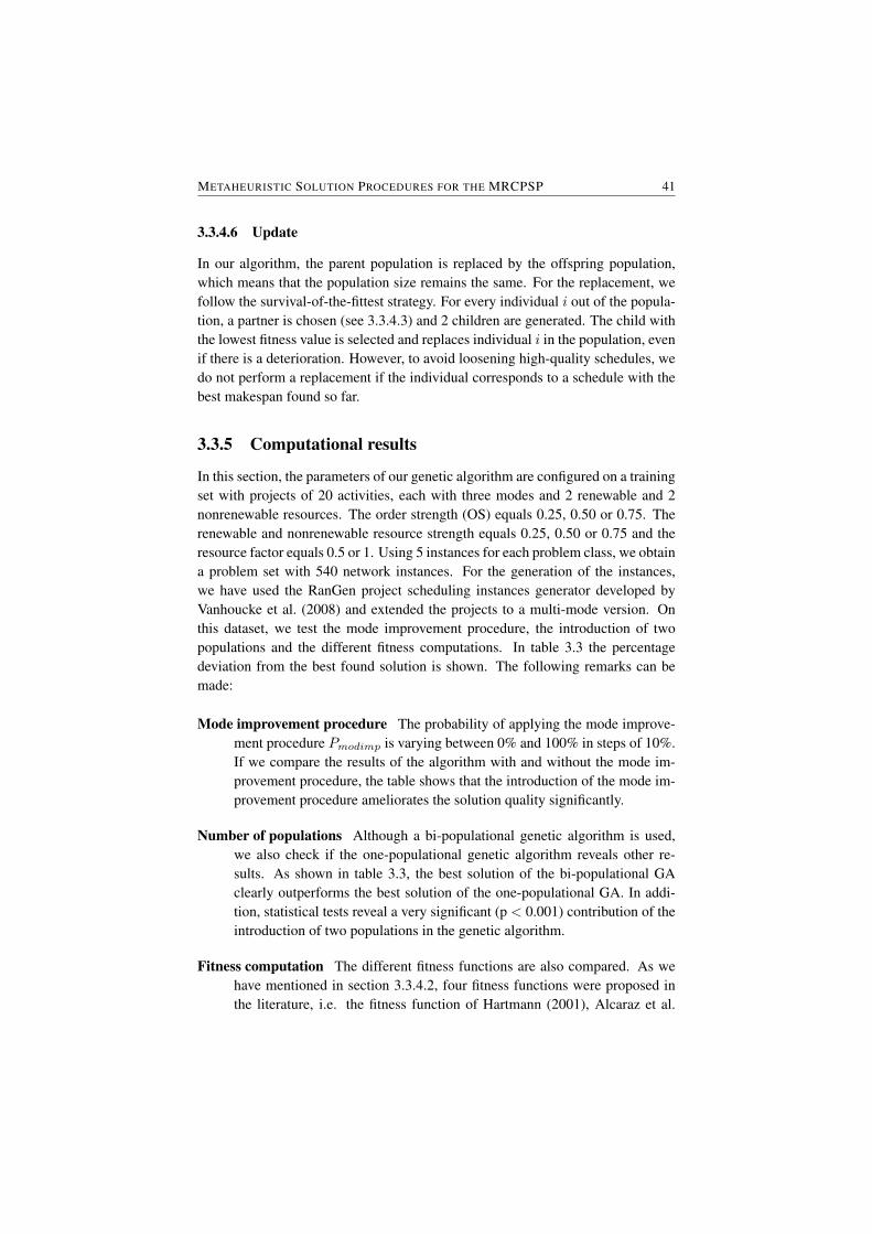
METAHEURISTIC SOLUTION PROCEDURES FOR THE MRCPSP 41
3.3.4.6 Update
In our algorithm, the parent population is replaced by the offspring population,which means that the population size remains the same. For the replacement, wefollow the survival-of-the-fittest strategy. For every individual i out of the popula-tion, a partner is chosen (see 3.3.4.3) and 2 children are generated. The child withthe lowest fitness value is selected and replaces individual i in the population, evenif there is a deterioration. However, to avoid loosening high-quality schedules, wedo not perform a replacement if the individual corresponds to a schedule with thebest makespan found so far.
3.3.5 Computational results
In this section, the parameters of our genetic algorithm are configured on a trainingset with projects of 20 activities, each with three modes and 2 renewable and 2nonrenewable resources. The order strength (OS) equals 0.25, 0.50 or 0.75. Therenewable and nonrenewable resource strength equals 0.25, 0.50 or 0.75 and theresource factor equals 0.5 or 1. Using 5 instances for each problem class, we obtaina problem set with 540 network instances. For the generation of the instances,we have used the RanGen project scheduling instances generator developed byVanhoucke et al. (2008) and extended the projects to a multi-mode version. Onthis dataset, we test the mode improvement procedure, the introduction of twopopulations and the different fitness computations. In table 3.3 the percentagedeviation from the best found solution is shown. The following remarks can bemade:
Mode improvement procedure The probability of applying the mode improve-ment procedure Pmodimp is varying between 0% and 100% in steps of 10%.If we compare the results of the algorithm with and without the mode im-provement procedure, the table shows that the introduction of the mode im-provement procedure ameliorates the solution quality significantly.
Number of populations Although a bi-populational genetic algorithm is used,we also check if the one-populational genetic algorithm reveals other re-sults. As shown in table 3.3, the best solution of the bi-populational GAclearly outperforms the best solution of the one-populational GA. In addi-tion, statistical tests reveal a very significant (p < 0.001) contribution of theintroduction of two populations in the genetic algorithm.
Fitness computation The different fitness functions are also compared. As wehave mentioned in section 3.3.4.2, four fitness functions were proposed inthe literature, i.e. the fitness function of Hartmann (2001), Alcaraz et al.
42 CHAPTER 3
(2003), Lova et al. (2009) and Jarboui et al. (2008). Looking for the best re-sults for both fitness computations, the fitness value of Alcaraz et al. (2003)reveals better results than the other fitness functions.
We thus conclude that the best results are obtained by using two populations,the fitness function according to Alcaraz et al. (2003) and setting the probabilityof applying the mode improvement procedure, Pmodimp, equal to 30%.
When configuring the algorithm, we have noticed that the population size hasan influence on the performance of the algorithm. We examined that the populationsize is negatively related to the number of activities. Similar results were found inDebels and Vanhoucke (2005), Hartmann (2001) and Alcaraz and Maroto (2001),amongst others. Tests were performed on different datasets with a different numberof activities. For each dataset, the optimal population size was determined. Thenumber of generated schedules was held constant at 5,000 schedules. A nonlinearleast squares regression based on the best population size values for the differentnumber of activities revealed a negative relationship between the population size(POP ) and the number of activities (|N |) which can be defined as follows:
POP = e3.551+22.72|N|
A large population size avoids homogeneity of the population and this becomesmore important for small problem instances. However, when the population sizebecomes too large, only few generations can be computed within the time limitand the advantages of the genetic algorithm cannot be fully exploited.
3.3.6 Conclusions
In this section, a genetic algorithm for the MRCPSP has been proposed. For thisalgorithm we have used two populations, one with left-justified schedules and onewith right-justified schedules. Computational tests have shown that this methodperforms better than the regular GA with one population. In addition, an extendedserial schedule generation scheme is introduced, which improves the mode selec-tion by choosing the feasible mode of a certain activity that minimizes the finishtime of the activity. Finally, tests revealed that the fitness function of Alcaraz et al.(2003) performed better than the other ones available in the literature. The perfor-mance of this metaheuristic solution procedure on the current benchmark datasetswill be shown in chapter 5.

METAHEURISTIC SOLUTION PROCEDURES FOR THE MRCPSP 43
Tabl
e3.
3:R
esul
tsfo
rth
etr
aini
ngse
t-co
nfigu
ratio
nof
the
algo
rith
m-a
vera
ge%
devi
atio
ncr
itica
lpat
hle
ngth
-5,0
00sc
hedu
les
Pmodimp
#po
pula
tions
Fitn
ess
com
p.0%
10%
20%
30%
40%
50%
60%
70%
80%
90%
100%
1po
pula
tion
Har
tman
n8.
22%
1.83
%1.
53%
1.49
%1.
42%
1.50
%1.
48%
1.56
%1.
62%
1.59
%2.
00%
Alc
araz
7.93
%1.
78%
1.51
%1.
49%
1.42
%1.
60%
1.43
%1.
49%
1.50
%1.
71%
2.04
%L
ova
8.19
%1.
83%
1.53
%1.
49%
1.42
%1.
50%
1.48
%1.
56%
1.62
%1.
58%
1.98
%Ja
rbou
i7.
23%
1.91
%1.
68%
1.46
%1.
48%
1.57
%1.
70%
1.85
%1.
81%
2.06
%2.
53%
2po
pula
tions
Har
tman
n1.
03%
0.13
%0.
07%
0.09
%0.
06%
0.03
%0.
170.
09%
0.09
%0.
040.
08%
Alc
araz
1.06
%0.
13%
0.02
%0.
00%
0.11
%0.
06%
0.03
%0.
11%
0.06
%0.
01%
0.15
%L
ova
2.07
%0.
49%
0.41
%0.
38%
0.27
%0.
35%
0.16
%0.
28%
0.17
%0.
22%
0.26
%Ja
rbou
i5.
22%
2.03
%1.
18%
0.94
%0.
75%
0.51
%0.
43%
0.40
%0.
39%
0.35
%0.
31%
44 CHAPTER 3
3.4 Artificial Immune System
3.4.1 Introduction
An Artificial Immune System (AIS) is a computational algorithm proposed byDe Castro and Timmis (2002) and inspired by theories and components of the ver-tebrate immune system. The vertebrate immune system is able to identify and killdisease-causing elements, called antigens, by the use of immune cells, of which theB-cells are the most common ones. These immune cells have receptor moleculeson their surfaces (also called antibodies), whose aim it is to recognize and bind topattern-specific antigens.
Since the antibodies on the B-cells are able to kill this specific type of antigens(antibodies and antigens whose shapes are complementary will rivet together), theB-cells will be stimulated to proliferate and to mature into non-dividing antibodysecreting cells (plasma cells), according to the principles of clonal selection. Thedegree of proliferation is directly proportional to the recognizing degree of the anti-gen and the proliferation is succeeded by cell divisions and results in a populationof clones which are copies from each other (De Castro and Timmis, 2002).
To better recognize the antigens, a whole mutation and selection process, whichis called the affinity maturation, is applied on the cloned cells. A first mechanismis the hypermutation, a process in which random changes take place in the vari-able region of the antibody molecules. The degree of hypermutation is inverselyproportional to the affinity of the antibody to the antigen: the higher the affinity,the lower the mutation rate and vice versa. However, a large proportion of thesemutated antibodies will be of inferior quality and will be non-functional in theimmune system. Those cells are eliminated from the population and replaced bynewly developed receptors in a process called receptor editing.
The remainder of this section is organized as follows: the algorithmic detailsof the AIS algorithm will be presented in section 3.4.2. In section 3.4.3 somecomputational experiments will be executed, while in section 3.4.4 the conclusionsare presented.
3.4.2 AIS algorithm for the MRCPSP
The efficient mechanisms of an immune system make artificial immune systemsuseful for scheduling problems. AIS is used for solving job-shop (Coello et al.,2003; Hart et al., 1998), flow-shop (Engin and Doyen, 2004) and resource-con-strained project scheduling problems (Agarwal et al., 2007). In this section, aproblem-solving technique for the MRCPSP based on the principles of the verte-brate immune system is presented. The different generic steps in our AIS algorithmare presented in figure 3.6 and will be discussed along the following subsections.
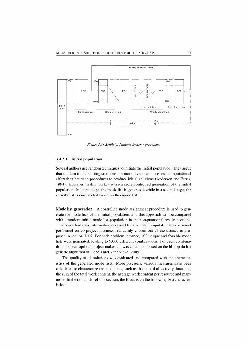
METAHEURISTIC SOLUTION PROCEDURES FOR THE MRCPSP 45
POP POP
LOWLOW
HIGH
Clonal selectionInitial population
HIGH
RAND
POP
POP POP POP
EV
AL
UA
TIO
N
LOW
MU
TA
TIO
N
till stop condition is met
selection Affinity Maturation
Hypermutation Receptor editing
EV
AL
UA
TIO
N
HIGH
MU
TA
TIO
N
SEED
Figure 3.6: Artificial Immune System: procedure
3.4.2.1 Initial population
Several authors use random techniques to initiate the initial population. They arguethat random initial starting solutions are more diverse and use less computationaleffort than heuristic procedures to produce initial solutions (Anderson and Ferris,1994). However, in this work, we use a more controlled generation of the initialpopulation. In a first stage, the mode list is generated, while in a second stage, theactivity list is constructed based on this mode list.
Mode list generation A controlled mode assignment procedure is used to gen-erate the mode lists of the initial population, and this approach will be comparedwith a random initial mode list population in the computational results sections.This procedure uses information obtained by a simple computational experimentperformed on 90 project instances, randomly chosen out of the dataset as pro-posed in section 3.3.5. For each problem instance, 100 unique and feasible modelists were generated, leading to 9,000 different combinations. For each combina-tion, the near-optimal project makespan was calculated based on the bi-populationgenetic algorithm of Debels and Vanhoucke (2005).
The quality of all solutions was evaluated and compared with the character-istics of the generated mode lists. More precisely, various measures have beencalculated to characterize the mode lists, such as the sum of all activity durations,the sum of the total work content, the average work content per resource and manymore. In the remainder of this section, the focus is on the following two character-istics:
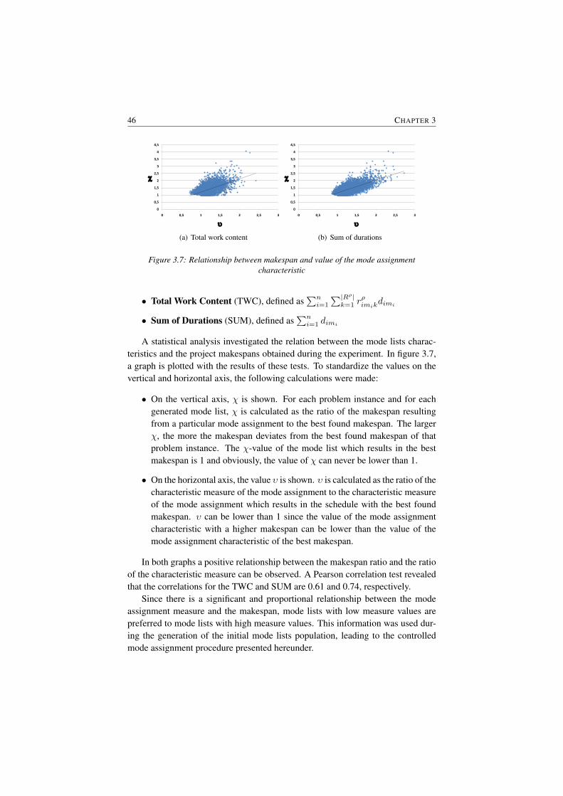
46 CHAPTER 3
0
0,5
1
1,5
2
2,5
3
3,5
4
4,5
0 0,5 1 1,5 2 2,5 3
c
u
(a) Total work content
0
0,5
1
1,5
2
2,5
3
3,5
4
4,5
0 0,5 1 1,5 2 2,5 3
c
u
(b) Sum of durations
Figure 3.7: Relationship between makespan and value of the mode assignmentcharacteristic
• Total Work Content (TWC), defined as∑ni=1
∑|Rρ|k=1 r
ρimik
dimi
• Sum of Durations (SUM), defined as∑ni=1 dimi
A statistical analysis investigated the relation between the mode lists charac-teristics and the project makespans obtained during the experiment. In figure 3.7,a graph is plotted with the results of these tests. To standardize the values on thevertical and horizontal axis, the following calculations were made:
• On the vertical axis, χ is shown. For each problem instance and for eachgenerated mode list, χ is calculated as the ratio of the makespan resultingfrom a particular mode assignment to the best found makespan. The largerχ, the more the makespan deviates from the best found makespan of thatproblem instance. The χ-value of the mode list which results in the bestmakespan is 1 and obviously, the value of χ can never be lower than 1.
• On the horizontal axis, the value υ is shown. υ is calculated as the ratio of thecharacteristic measure of the mode assignment to the characteristic measureof the mode assignment which results in the schedule with the best foundmakespan. υ can be lower than 1 since the value of the mode assignmentcharacteristic with a higher makespan can be lower than the value of themode assignment characteristic of the best makespan.
In both graphs a positive relationship between the makespan ratio and the ratioof the characteristic measure can be observed. A Pearson correlation test revealedthat the correlations for the TWC and SUM are 0.61 and 0.74, respectively.
Since there is a significant and proportional relationship between the modeassignment measure and the makespan, mode lists with low measure values arepreferred to mode lists with high measure values. This information was used dur-ing the generation of the initial mode lists population, leading to the controlledmode assignment procedure presented hereunder.

METAHEURISTIC SOLUTION PROCEDURES FOR THE MRCPSP 47
A controlled mode assignment procedure can be formulated in the three fol-lowing steps:
1. A start population of mode lists, called RANDPOP , is created, with alarge number of randomly generated feasible mode lists (|RANDPOP | isequal to 4 times the number of populations elements POP ).
2. Each mode list has a characteristic measure value, which is likely to lead tosmaller project makespans.
3. The POP mode lists with the lowest values are selected for entrance in theinitial population.
Once the mode lists are generated, a duration and resource consumption isset to each activity for each population element. Based on this information, theactivity list can be generated.
Activity list generation In the second stage, the activity list is generated. Sev-eral heuristics available in the literature make use of well-performing priority rulesto generate the sequence in which the activities should be scheduled. Some of thebest performing priority rules are the Latest Finish Time (LFT), the Latest StartTime (LST), the Minimum Slack (SLK) and the Maximum Remaining Work (RWK).More information about these priority rules can be found in Kolisch (1996a) andBoctor (1993).
For each mode list, an activity list is generated using one of the proposed prior-ity rules. Since different mode lists are generated, also a diverse set of activity listswill be generated. If two or more equal mode lists occur in the initial population,different priority rules are applied on the mode lists to avoid equal solution vectorsin the initial population.
After the generation of the activity list and the mode list, a schedule is built foreach of the POP population elements in the initial population.
3.4.2.2 Clonal selection process
A population of POP solution vectors is generated and for each solution vector themakespan is determined. Only the best Pclonal% solution vectors will be availablefor proliferation. For these solution vectors, the corresponding affinity value isdetermined as follows:
Aff(V ) =1
makespan(V )− bestmakespan+ 1(3.1)
where makespan(V) refers to the makespan of solution vector V and best-makespan refers to the best makespan found so far. The number of clones of a
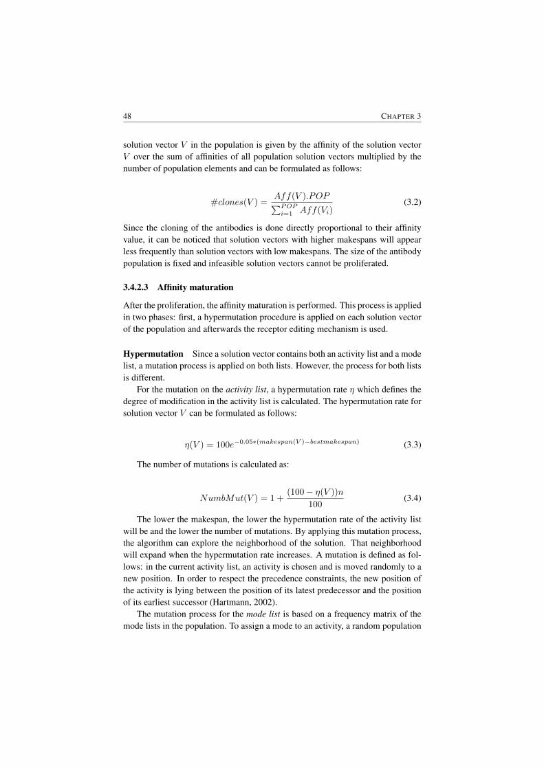
48 CHAPTER 3
solution vector V in the population is given by the affinity of the solution vectorV over the sum of affinities of all population solution vectors multiplied by thenumber of population elements and can be formulated as follows:
#clones(V ) =Aff(V ).POP∑POPi=1 Aff(Vi)
(3.2)
Since the cloning of the antibodies is done directly proportional to their affinityvalue, it can be noticed that solution vectors with higher makespans will appearless frequently than solution vectors with low makespans. The size of the antibodypopulation is fixed and infeasible solution vectors cannot be proliferated.
3.4.2.3 Affinity maturation
After the proliferation, the affinity maturation is performed. This process is appliedin two phases: first, a hypermutation procedure is applied on each solution vectorof the population and afterwards the receptor editing mechanism is used.
Hypermutation Since a solution vector contains both an activity list and a modelist, a mutation process is applied on both lists. However, the process for both listsis different.
For the mutation on the activity list, a hypermutation rate η which defines thedegree of modification in the activity list is calculated. The hypermutation rate forsolution vector V can be formulated as follows:
η(V ) = 100e−0.05∗(makespan(V )−bestmakespan) (3.3)
The number of mutations is calculated as:
NumbMut(V ) = 1 +(100− η(V ))n
100(3.4)
The lower the makespan, the lower the hypermutation rate of the activity listwill be and the lower the number of mutations. By applying this mutation process,the algorithm can explore the neighborhood of the solution. That neighborhoodwill expand when the hypermutation rate increases. A mutation is defined as fol-lows: in the current activity list, an activity is chosen and is moved randomly to anew position. In order to respect the precedence constraints, the new position ofthe activity is lying between the position of its latest predecessor and the positionof its earliest successor (Hartmann, 2002).
The mutation process for the mode list is based on a frequency matrix of themode lists in the population. To assign a mode to an activity, a random population
METAHEURISTIC SOLUTION PROCEDURES FOR THE MRCPSP 49
element is chosen and the mode for that population element activity is assignedto the cloned element activity. Modes that occur more in the population of goodsolutions will therefore occur more. This procedure shows similarities with theHarmony Search procedure (Geem et al., 2001). In case the mode list becomesinfeasible, a feasibility procedure is applied so that the mode list becomes feasibleby changing mode assignments and the modes with the lowest mode characteristics(as defined in the previous section) are chosen first. After the mutation process,every new feasible solution vector is evaluated.
Receptor Editing After the cloning and mutation process, a new population ofantibodies is generated. Only the best Pediting% antibodies are preserved in thepopulation. The other elements are eliminated and to preserve POP elementsin the population, the population is seeded with high quality mode lists from thestart population RANDPOP . In that way, schedules with a low makespan stayincorporated in the antibody population and antibodies evolving to inferior searchregions are deleted. The newly generated population is the start population for anew generation process. This process continues until the stop condition is met.
3.4.3 Computational results
In order to prove the efficiency of our algorithm, the AIS solution procedure istested on the test set as proposed in section 3.3.5. The impact of the differentalgorithmic parameters, such as Pclonal, Pediting and the population size POP , istested and the efficiency of our initial population generation method is proven.
Extensive testing revealed that the optimal values for the different algorithmicparameters are Pclonal = 25%, Pediting = 20% and POP = 450. Table 3.4 showsthe average deviation from the minimal critical path after the initial populationgeneration ofPOP population elements and after 5,000 schedules. The 2 differentmode characteristics (TWC and SUM) and the 4 different priority rules (LFT, LST,SLK and RWK) are compared to the result of the solutions in which a randomgenerated initial population is used (i.e. random generation of the activity list andrandom choice of the mode assignment).
A paired-samples T-test revealed a very significant (p<0.001) influence onthe quality of the schedules when using a controlled initial population generationmethod instead of a random generation method: the difference between the aver-age deviation from the critical path for the random generated solutions (48.23%)and the average deviation for the controlled generated elements (LST/SUM withan average deviation of 37.17%) is 11.06%, which corresponds with an averagedecrease of 2.2 working days on an average makespan of 28 days (information notavailable in table 3.4).
Regardless of which priority rule is used, the combination in which SUM
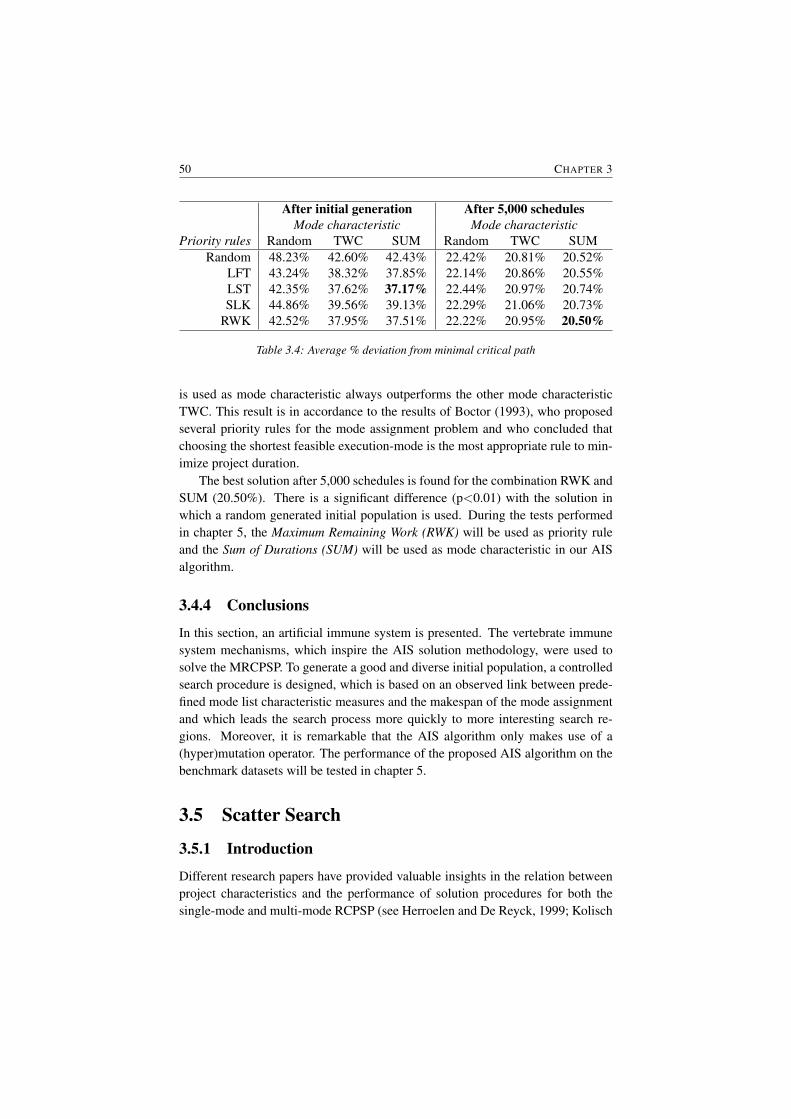
50 CHAPTER 3
After initial generation After 5,000 schedulesMode characteristic Mode characteristic
Priority rules Random TWC SUM Random TWC SUMRandom 48.23% 42.60% 42.43% 22.42% 20.81% 20.52%
LFT 43.24% 38.32% 37.85% 22.14% 20.86% 20.55%LST 42.35% 37.62% 37.17% 22.44% 20.97% 20.74%SLK 44.86% 39.56% 39.13% 22.29% 21.06% 20.73%
RWK 42.52% 37.95% 37.51% 22.22% 20.95% 20.50%
Table 3.4: Average % deviation from minimal critical path
is used as mode characteristic always outperforms the other mode characteristicTWC. This result is in accordance to the results of Boctor (1993), who proposedseveral priority rules for the mode assignment problem and who concluded thatchoosing the shortest feasible execution-mode is the most appropriate rule to min-imize project duration.
The best solution after 5,000 schedules is found for the combination RWK andSUM (20.50%). There is a significant difference (p<0.01) with the solution inwhich a random generated initial population is used. During the tests performedin chapter 5, the Maximum Remaining Work (RWK) will be used as priority ruleand the Sum of Durations (SUM) will be used as mode characteristic in our AISalgorithm.
3.4.4 Conclusions
In this section, an artificial immune system is presented. The vertebrate immunesystem mechanisms, which inspire the AIS solution methodology, were used tosolve the MRCPSP. To generate a good and diverse initial population, a controlledsearch procedure is designed, which is based on an observed link between prede-fined mode list characteristic measures and the makespan of the mode assignmentand which leads the search process more quickly to more interesting search re-gions. Moreover, it is remarkable that the AIS algorithm only makes use of a(hyper)mutation operator. The performance of the proposed AIS algorithm on thebenchmark datasets will be tested in chapter 5.
3.5 Scatter Search
3.5.1 Introduction
Different research papers have provided valuable insights in the relation betweenproject characteristics and the performance of solution procedures for both thesingle-mode and multi-mode RCPSP (see Herroelen and De Reyck, 1999; Kolisch
METAHEURISTIC SOLUTION PROCEDURES FOR THE MRCPSP 51
et al., 1995). To the best of our knowledge, for the multi-mode RCPSP only onepaper has used project characteristics to steer the algorithmic procedures towardspromising solution areas. Buddhakulsomsiri and Kim (2007) propose the movingresource strength, which helps the priority rule-based heuristic for the MRCPSPwith activity splitting and resource vacation in order to identify in which projectsituations activity splitting is likely to be beneficial during scheduling.
The main contribution of the solution procedure is threefold: first, a scattersearch procedure to solve the scheduling problem is proposed. While a scattersearch is proven to be successful in dealing with combinatorial problems, to thebest of our knowledge, it has not been used before to solve the MRCPSP. Sec-ond, three different solution improvement methods are developed, each based onthe information obtained from the renewable and nonrenewable resource charac-teristics. Third, the proposed algorithm provides state-of-the-art results for theavailable benchmark datasets.
The outline of this section is as follows. In section 3.5.2, a resource scarce-ness matrix is presented which gives insight into the influence of the scarceness ofthe renewable and nonrenewable resources on the search focus of the algorithm.Section 3.5.3 proposes a scatter search for the MRCPSP, for which different solu-tion improvement methods tailored to the resource scarceness characteristics of aproject, are presented. In section 3.5.4, computational results for the configurationof the scatter search are given and the influence of the resource scarceness on thesolution quality is tested. Finally, in the last section, overall conclusions of thissolution procedure are presented.
3.5.2 Resource scarceness matrix
Several resource parameters have been introduced in the past decades to measurethe scarceness of resources of a project instance. These parameters are determinedby the resource consumption and the resource availability. For a constant resourceavailability, the scarceness will increase for an increasing resource consumption.Moreover, the more restrictive a resource type becomes, the higher the makespanof the project will be.
Since the resource scarceness can be applied on both the renewable and nonre-newable resources, a brief description for both resource types is given.
– Renewable resources
When the scarceness of the renewable resources is low, the project is hardlyrestricted by its resources. The makespan of the project will mainly be de-termined by the precedence relations of the project and each activity willbe scheduled at or close to its critical path start time. When, however, thescarceness of renewable resources is high, the influence of the resource con-straints will overrule the precedence constraints. Due to the relatively low
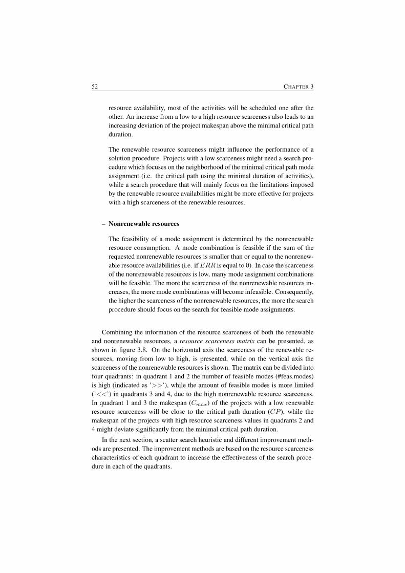
52 CHAPTER 3
resource availability, most of the activities will be scheduled one after theother. An increase from a low to a high resource scarceness also leads to anincreasing deviation of the project makespan above the minimal critical pathduration.
The renewable resource scarceness might influence the performance of asolution procedure. Projects with a low scarceness might need a search pro-cedure which focuses on the neighborhood of the minimal critical path modeassignment (i.e. the critical path using the minimal duration of activities),while a search procedure that will mainly focus on the limitations imposedby the renewable resource availabilities might be more effective for projectswith a high scarceness of the renewable resources.
– Nonrenewable resources
The feasibility of a mode assignment is determined by the nonrenewableresource consumption. A mode combination is feasible if the sum of therequested nonrenewable resources is smaller than or equal to the nonrenew-able resource availabilities (i.e. ifERR is equal to 0). In case the scarcenessof the nonrenewable resources is low, many mode assignment combinationswill be feasible. The more the scarceness of the nonrenewable resources in-creases, the more mode combinations will become infeasible. Consequently,the higher the scarceness of the nonrenewable resources, the more the searchprocedure should focus on the search for feasible mode assignments.
Combining the information of the resource scarceness of both the renewableand nonrenewable resources, a resource scarceness matrix can be presented, asshown in figure 3.8. On the horizontal axis the scarceness of the renewable re-sources, moving from low to high, is presented, while on the vertical axis thescarceness of the nonrenewable resources is shown. The matrix can be divided intofour quadrants: in quadrant 1 and 2 the number of feasible modes (#feas.modes)is high (indicated as ’>>’), while the amount of feasible modes is more limited(’<<’) in quadrants 3 and 4, due to the high nonrenewable resource scarceness.In quadrant 1 and 3 the makespan (Cmax) of the projects with a low renewableresource scarceness will be close to the critical path duration (CP ), while themakespan of the projects with high resource scarceness values in quadrants 2 and4 might deviate significantly from the minimal critical path duration.
In the next section, a scatter search heuristic and different improvement meth-ods are presented. The improvement methods are based on the resource scarcenesscharacteristics of each quadrant to increase the effectiveness of the search proce-dure in each of the quadrants.
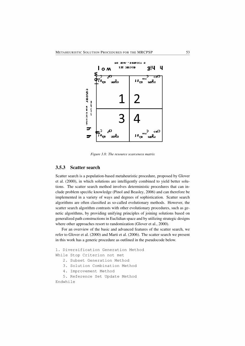
METAHEURISTIC SOLUTION PROCEDURES FOR THE MRCPSP 53� �� � �� �� � � �� � � �� � � �� �� ��� � ���� � � ��
� � � ��� �� �� ��� ! �"#$ � � �% & � ' ��( ( ��� ) ) �"#$ � � �% & � ' ��( (� ��� � * +� ��+� � ,- ., ��� ! �"#$ � � �% & � ' ��/ / ��� ) ) �"# $ � � �% & � ' ��/ /
Figure 3.8: The resource scarceness matrix
3.5.3 Scatter search
Scatter search is a population-based metaheuristic procedure, proposed by Gloveret al. (2000), in which solutions are intelligently combined to yield better solu-tions. The scatter search method involves deterministic procedures that can in-clude problem specific knowledge (Pinol and Beasley, 2006) and can therefore beimplemented in a variety of ways and degrees of sophistication. Scatter searchalgorithms are often classified as so-called evolutionary methods. However, thescatter search algorithm contrasts with other evolutionary procedures, such as ge-netic algorithms, by providing unifying principles of joining solutions based ongeneralized path constructions in Euclidian space and by utilizing strategic designswhere other approaches resort to randomization (Glover et al., 2000).
For an overview of the basic and advanced features of the scatter search, werefer to Glover et al. (2000) and Marti et al. (2006). The scatter search we presentin this work has a generic procedure as outlined in the pseudocode below.
1. Diversification Generation MethodWhile Stop Criterion not met
2. Subset Generation Method3. Solution Combination Method4. Improvement Method5. Reference Set Update Method
Endwhile

54 CHAPTER 3
In figure 3.9, a conceptual overview of the different steps in our scatter searchprocedure is shown. In the remainder of this section, each of these different stepsis explained in detail.
3.5.3.1 The Diversification Generation Method
Initial population In this first step, a pool P of POP solution vectors is gener-ated.
The controlled mode assignment procedure, as proposed in section 3.4.2.1, isused to generate the mode lists. Once the mode lists are generated, a duration andresource consumption can be assigned to each activity for each population element.Since Kolisch and Drexl (1997) mention that finding a feasible solution for theMRCPSP is a NP-complete problem if at least two nonrenewable resources aregiven, infeasible solutions are accepted in the initial population, but are penalizedwith the penalty function of Alcaraz et al. (2003). The activity lists are generatedrandomly, assigning a priority value to each activity.
Reference sets After the generation of POP population elements and the eval-uation of the solution vectors with the serial schedule generation scheme (SGS),which translates the solution vector into a schedule, two diverse populations areconstructed from P : a set B1, with the b1 best solutions of the solution set P anda set B2, with b2 diverse solutions. For the subset B1, a threshold t1 on the min-imal distance between the elements is imposed in pursuit of diversity. The subsetB2 contains the b2 best solutions from P\B1 that are sufficiently distant from theelements of B1. The diversity in B2 is achieved by a threshold t2 on the smallestdistance to any element in B1 with t2 > t1. The distance between two solutions isa measure for diversity and is calculated according to the following two distancefunctions. The first distance function, dsp1,p2 , calculates the distance as the sum ofthe differences between the start times of the activities and can be formulated asfollows:
dsp1,p2 =
|N |∑i=1
|sp2i − sp1i |
with p1 and p2 two population elements and sp1 and sp2 their according starttimes. The second distance function, dmp1,p2 , calculates the distance based on thedifference in mode assignments and is formulated as follows:
dmp1,p2 =
|N |∑i=1
{0 if mp1
i = mp2i
1 otherwise
In the computational results section both distance functions are compared andthe optimal values for the thresholds are determined.
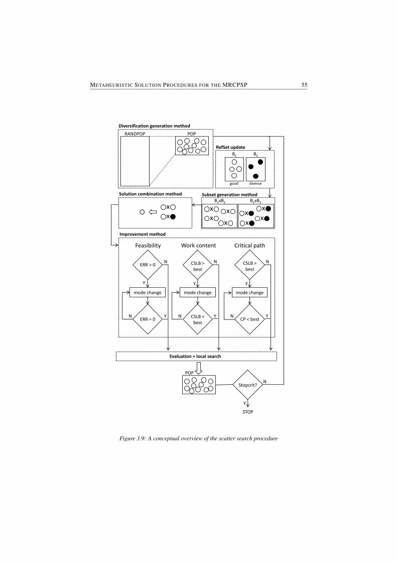
METAHEURISTIC SOLUTION PROCEDURES FOR THE MRCPSP 55
YY Y
Feasibility Work content Critical path
mode change
ERR > 0
ERR = 0N
mode change
CSLB > best
CSLB < best
N
mode change
CSLB > best
CP < bestN
Y
NN N
Improvement method
Y Y
Subset generation method
xx
x
x
xx
x
xB1xB1 B1xB2
Solution combination method
xx
Diversification generation method
RANDPOP
B1 B2
RefSet update
POP
POP
Evaluation + local search
Stopcrit?
Y
N
STOP
good diverse
Figure 3.9: A conceptual overview of the scatter search procedure

56 CHAPTER 3
If there are less solutions in B2 than the predefined number b2, the set B2 isfilled up with randomly generated schedules.
3.5.3.2 The Subset Generation Method
After the initialization phase, a new pool of solutions is created by combiningpairs of reference solutions in a controlled way. New solutions are created fromall two-element subsets. First, all pairs in B1 containing at least one new solutioncompared to the previous generation are considered. From each such pair, twochildren are produced. Second, from each combination of one element from B1
and one from B2 two offsprings are constructed. Choosing the two reference solu-tions out of the same cluster stimulates intensification, while choosing them fromdifferent clusters stimulates diversification.
3.5.3.3 The Solution Combination Method
In the solution combination phase, the two selected population elements produce anew offspring which inherits parts of their parents’ characteristics. Several cross-over operators were tested and tests revealed that the two-point crossover methodclearly outperforms other crossover operators. In the two-point crossover scheme,two crossover points are randomly chosen and the characteristics between themare exchanged. As the procedure works on both the activity list and the mode list,the crossover considers start times and modes simultaneously (i.e. using the samecrossover points).
3.5.3.4 The Improvement Method
In this section, we propose different solution improvement methods, which are ap-plied on the solution vectors that are generated in the solution combination method.Every new solution vector consists of a new generated activity list and a new gen-erated mode list. Since the mode list determines the duration and the renewableand nonrenewable resource requirements for each activity, quick tests can be usedto indicate whether the solution vector has potential to improve the current bestsolution found so far, without actually using the schedule generation scheme. Thetwo quick tests are:
Feasibility test This test is related to the nonrenewable resources and checkswhether the mode assignment is feasible or not. If the test reveals an in-feasible solution vector (ERR > 0), the feasibility improvement method isperformed.
Lower bound This test is related to the renewable resources and checks whethera new generated mode assignment (i.e. a duration and renewable resources)
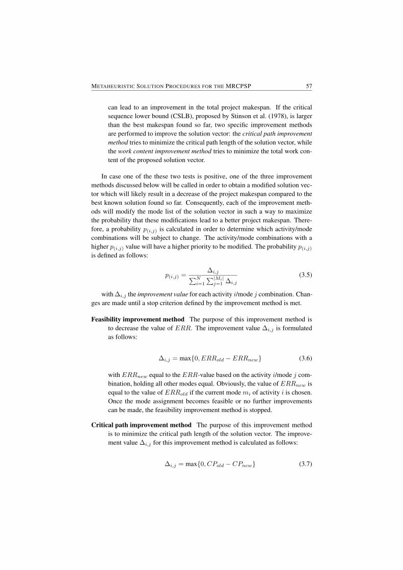
METAHEURISTIC SOLUTION PROCEDURES FOR THE MRCPSP 57
can lead to an improvement in the total project makespan. If the criticalsequence lower bound (CSLB), proposed by Stinson et al. (1978), is largerthan the best makespan found so far, two specific improvement methodsare performed to improve the solution vector: the critical path improvementmethod tries to minimize the critical path length of the solution vector, whilethe work content improvement method tries to minimize the total work con-tent of the proposed solution vector.
In case one of the these two tests is positive, one of the three improvementmethods discussed below will be called in order to obtain a modified solution vec-tor which will likely result in a decrease of the project makespan compared to thebest known solution found so far. Consequently, each of the improvement meth-ods will modify the mode list of the solution vector in such a way to maximizethe probability that these modifications lead to a better project makespan. There-fore, a probability p(i,j) is calculated in order to determine which activity/modecombinations will be subject to change. The activity/mode combinations with ahigher p(i,j) value will have a higher priority to be modified. The probability p(i,j)is defined as follows:
p(i,j) =∆i,j∑N
i=1
∑|Mi|j=1 ∆i,j
(3.5)
with ∆i,j the improvement value for each activity i/mode j combination. Chan-ges are made until a stop criterion defined by the improvement method is met.
Feasibility improvement method The purpose of this improvement method isto decrease the value of ERR. The improvement value ∆i,j is formulatedas follows:
∆i,j = max{0, ERRold − ERRnew} (3.6)
with ERRnew equal to the ERR-value based on the activity i/mode j com-bination, holding all other modes equal. Obviously, the value ofERRnew isequal to the value of ERRold if the current mode mi of activity i is chosen.Once the mode assignment becomes feasible or no further improvementscan be made, the feasibility improvement method is stopped.
Critical path improvement method The purpose of this improvement methodis to minimize the critical path length of the solution vector. The improve-ment value ∆i,j for this improvement method is calculated as follows:
∆i,j = max{0, CPold − CPnew} (3.7)
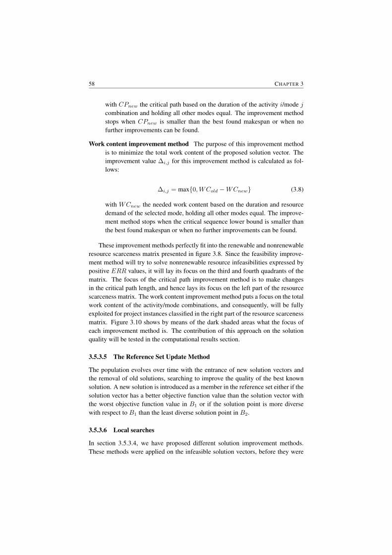
58 CHAPTER 3
with CPnew the critical path based on the duration of the activity i/mode jcombination and holding all other modes equal. The improvement methodstops when CPnew is smaller than the best found makespan or when nofurther improvements can be found.
Work content improvement method The purpose of this improvement methodis to minimize the total work content of the proposed solution vector. Theimprovement value ∆i,j for this improvement method is calculated as fol-lows:
∆i,j = max{0,WCold −WCnew} (3.8)
with WCnew the needed work content based on the duration and resourcedemand of the selected mode, holding all other modes equal. The improve-ment method stops when the critical sequence lower bound is smaller thanthe best found makespan or when no further improvements can be found.
These improvement methods perfectly fit into the renewable and nonrenewableresource scarceness matrix presented in figure 3.8. Since the feasibility improve-ment method will try to solve nonrenewable resource infeasibilities expressed bypositive ERR values, it will lay its focus on the third and fourth quadrants of thematrix. The focus of the critical path improvement method is to make changesin the critical path length, and hence lays its focus on the left part of the resourcescarceness matrix. The work content improvement method puts a focus on the totalwork content of the activity/mode combinations, and consequently, will be fullyexploited for project instances classified in the right part of the resource scarcenessmatrix. Figure 3.10 shows by means of the dark shaded areas what the focus ofeach improvement method is. The contribution of this approach on the solutionquality will be tested in the computational results section.
3.5.3.5 The Reference Set Update Method
The population evolves over time with the entrance of new solution vectors andthe removal of old solutions, searching to improve the quality of the best knownsolution. A new solution is introduced as a member in the reference set either if thesolution vector has a better objective function value than the solution vector withthe worst objective function value in B1 or if the solution point is more diversewith respect to B1 than the least diverse solution point in B2.
3.5.3.6 Local searches
In section 3.5.3.4, we have proposed different solution improvement methods.These methods were applied on the infeasible solution vectors, before they were
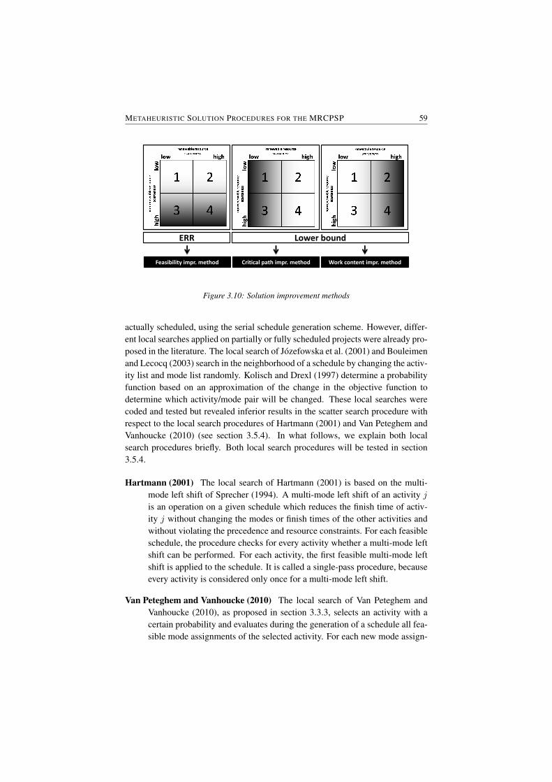
METAHEURISTIC SOLUTION PROCEDURES FOR THE MRCPSP 59
ERR Lower bound
Feasibility impr. method Critical path impr. method Work content impr. method
Figure 3.10: Solution improvement methods
actually scheduled, using the serial schedule generation scheme. However, differ-ent local searches applied on partially or fully scheduled projects were already pro-posed in the literature. The local search of Jozefowska et al. (2001) and Bouleimenand Lecocq (2003) search in the neighborhood of a schedule by changing the activ-ity list and mode list randomly. Kolisch and Drexl (1997) determine a probabilityfunction based on an approximation of the change in the objective function todetermine which activity/mode pair will be changed. These local searches werecoded and tested but revealed inferior results in the scatter search procedure withrespect to the local search procedures of Hartmann (2001) and Van Peteghem andVanhoucke (2010) (see section 3.5.4). In what follows, we explain both localsearch procedures briefly. Both local search procedures will be tested in section3.5.4.
Hartmann (2001) The local search of Hartmann (2001) is based on the multi-mode left shift of Sprecher (1994). A multi-mode left shift of an activity jis an operation on a given schedule which reduces the finish time of activ-ity j without changing the modes or finish times of the other activities andwithout violating the precedence and resource constraints. For each feasibleschedule, the procedure checks for every activity whether a multi-mode leftshift can be performed. For each activity, the first feasible multi-mode leftshift is applied to the schedule. It is called a single-pass procedure, becauseevery activity is considered only once for a multi-mode left shift.
Van Peteghem and Vanhoucke (2010) The local search of Van Peteghem andVanhoucke (2010), as proposed in section 3.3.3, selects an activity with acertain probability and evaluates during the generation of a schedule all fea-sible mode assignments of the selected activity. For each new mode assign-
60 CHAPTER 3
ment the ERR is calculated. If the ERR is equal to or smaller than thecurrent one, the local search checks if an improvement can be made in thefinish time of that activity. The mode with the lowest finish time that doesnot increase the ERR is chosen.
3.5.4 Computational results
In this section, we configure the algorithm and evaluate its performance. In section3.5.4.1 we present two datasets which are generated for this research and whichwill be used to test and configure the algorithmic parameter settings in section3.5.4.2. The influence of the improvement methods on the different quadrants inthe resource scarceness matrix is tested in section 3.5.4.3. The analysis of the localsearches is presented in section 3.5.4.4, while the introduction of an integratedsolution procedure is presented in section 3.5.4.5.
3.5.4.1 Dataset generation
In this section, two datasets are proposed, each containing a large set of data in-stances based on different complexity project parameters. A first dataset is used toconfigure the proposed scatter search algorithm, the other dataset is used to analyzethe influence of the improvement methods and the local searches on the resourcescarceness matrix.
For the generation of the instances of both datasets, we have used the RanGenproject scheduling instances generator developed by Vanhoucke et al. (2008) andextended the projects to a multi-mode version. Each instance contains 50 activi-ties, with three modes, two renewable resources and two nonrenewable resources.Dataset 1 is used in section 3.5.4.2 for the configuration of the algorithmic param-eters, while dataset 2 is used in sections 3.5.4.3, 3.5.4.4 and 3.5.4.5 to analyze theperformance of the improvement methods and local searches.
The following network and resource parameters were used for the two datasets.The values for each of these project characteristics are presented in table 3.5.
1. The network complexity is described by the order strength. In both datasets,the value of the OS is set at 0.25, 0.50 or 0.75.
2. In dataset 1, the resource strength is set at 0.25, 0.50 or 0.75, while in theother dataset, the parameter varies between 0 and 1 in steps of 0.10. Thesame parameter values are used for the nonrenewable resource strength inboth datasets.
3. The resource factor (RF ) indicates the percentage of resources required peractivity and is set at 0.50 or 1.
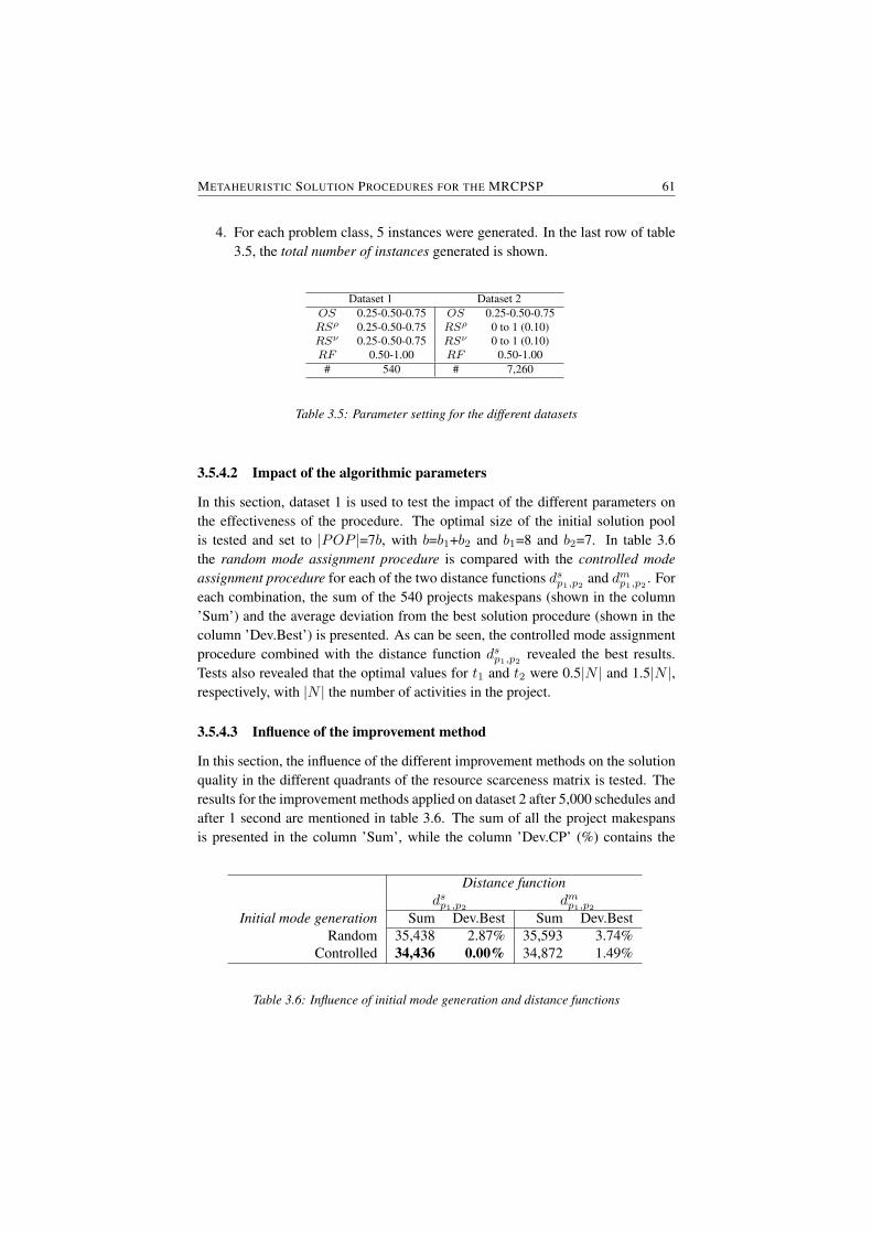
METAHEURISTIC SOLUTION PROCEDURES FOR THE MRCPSP 61
4. For each problem class, 5 instances were generated. In the last row of table3.5, the total number of instances generated is shown.
Dataset 1 Dataset 2OS 0.25-0.50-0.75 OS 0.25-0.50-0.75RSρ 0.25-0.50-0.75 RSρ 0 to 1 (0.10)RSν 0.25-0.50-0.75 RSν 0 to 1 (0.10)RF 0.50-1.00 RF 0.50-1.00
# 540 # 7,260
Table 3.5: Parameter setting for the different datasets
3.5.4.2 Impact of the algorithmic parameters
In this section, dataset 1 is used to test the impact of the different parameters onthe effectiveness of the procedure. The optimal size of the initial solution poolis tested and set to |POP |=7b, with b=b1+b2 and b1=8 and b2=7. In table 3.6the random mode assignment procedure is compared with the controlled modeassignment procedure for each of the two distance functions dsp1,p2 and dmp1,p2 . Foreach combination, the sum of the 540 projects makespans (shown in the column’Sum’) and the average deviation from the best solution procedure (shown in thecolumn ’Dev.Best’) is presented. As can be seen, the controlled mode assignmentprocedure combined with the distance function dsp1,p2 revealed the best results.Tests also revealed that the optimal values for t1 and t2 were 0.5|N | and 1.5|N |,respectively, with |N | the number of activities in the project.
3.5.4.3 Influence of the improvement method
In this section, the influence of the different improvement methods on the solutionquality in the different quadrants of the resource scarceness matrix is tested. Theresults for the improvement methods applied on dataset 2 after 5,000 schedules andafter 1 second are mentioned in table 3.6. The sum of all the project makespansis presented in the column ’Sum’, while the column ’Dev.CP’ (%) contains the
Distance functiondsp1,p2 dmp1,p2
Initial mode generation Sum Dev.Best Sum Dev.BestRandom 35,438 2.87% 35,593 3.74%
Controlled 34,436 0.00% 34,872 1.49%
Table 3.6: Influence of initial mode generation and distance functions
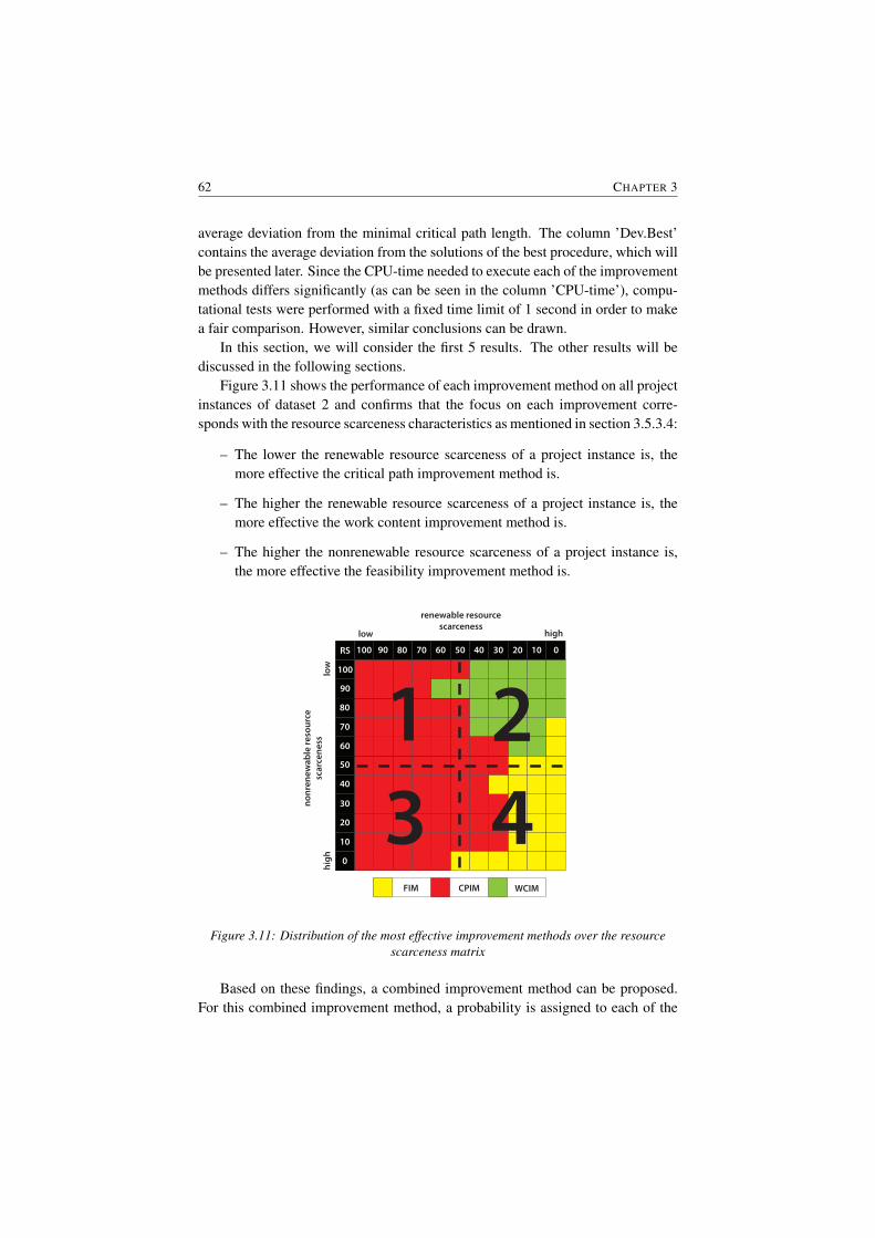
62 CHAPTER 3
average deviation from the minimal critical path length. The column ’Dev.Best’contains the average deviation from the solutions of the best procedure, which willbe presented later. Since the CPU-time needed to execute each of the improvementmethods differs significantly (as can be seen in the column ’CPU-time’), compu-tational tests were performed with a fixed time limit of 1 second in order to makea fair comparison. However, similar conclusions can be drawn.
In this section, we will consider the first 5 results. The other results will bediscussed in the following sections.
Figure 3.11 shows the performance of each improvement method on all projectinstances of dataset 2 and confirms that the focus on each improvement corre-sponds with the resource scarceness characteristics as mentioned in section 3.5.3.4:
– The lower the renewable resource scarceness of a project instance is, themore effective the critical path improvement method is.
– The higher the renewable resource scarceness of a project instance is, themore effective the work content improvement method is.
– The higher the nonrenewable resource scarceness of a project instance is,the more effective the feasibility improvement method is.
100 90 80 70 60 50 40 30 20 10 0
100
90
80
70
60
50
40
30
20
10
0
RS
low high
low
high
nonr
enew
able
reso
urce
sc
arce
ness
renewable resource scarceness
FIM CPIM WCIM
1 243
Figure 3.11: Distribution of the most effective improvement methods over the resourcescarceness matrix
Based on these findings, a combined improvement method can be proposed.For this combined improvement method, a probability is assigned to each of the
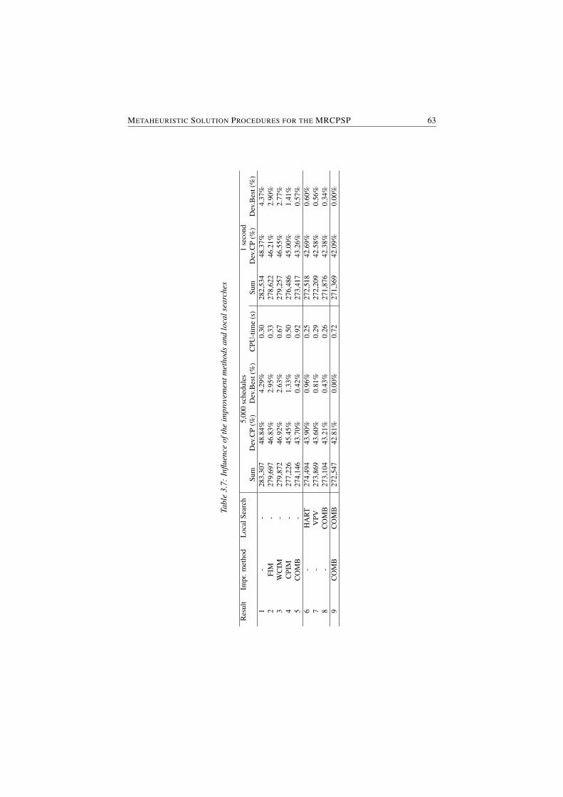
METAHEURISTIC SOLUTION PROCEDURES FOR THE MRCPSP 63
Tabl
e3.
7:In
fluen
ceof
the
impr
ovem
entm
etho
dsan
dlo
cals
earc
hes
Res
ult
Impr
.met
hod
Loc
alSe
arch
5,00
0sc
hedu
les
1se
cond
Sum
Dev
.CP
(%)
Dev
.Bes
t(%
)C
PU-t
ime
(s)
Sum
Dev
.CP
(%)
Dev
.Bes
t(%
)1
--
283,
307
48.8
4%4.
29%
0.30
282,
534
48.3
7%4.
37%
2FI
M-
279,
697
46.8
3%2.
95%
0.33
278,
622
46.2
1%2.
90%
3W
CIM
-27
9,87
246
.92%
2.63
%0.
6727
9,25
746
.55%
2.77
%4
CPI
M-
277,
226
45.4
5%1.
33%
0.50
276,
486
45.0
0%1.
41%
5C
OM
B-
274,
146
43.7
0%0.
42%
0.92
273,
417
43.2
6%0.
57%
6-
HA
RT
274,
494
43.9
0%0.
96%
0.25
272,
518
42.6
9%0.
60%
7-
VPV
273,
869
43.6
0%0.
81%
0.29
272,
209
42.5
8%0.
56%
8-
CO
MB
273,
104
43.2
1%0.
43%
0.26
271,
876
42.3
8%0.
34%
9C
OM
BC
OM
B27
2,54
742
.81%
0.00
%0.
7227
1,36
942
.09%
0.00
%
64 CHAPTER 3
improvement methods, based on the value U which is assigned according to thefollowing formula:
UCPIM = RSρ
UFIM = 100−RSν
UWCIM = 100−RSρ
with RSρ the value of the renewable resource strength and RSν the valueof the nonrenewable resource strength. The probability P that an improvementmethod q (q = CPIM , FIM or WCIM ) is chosen is equal to:
Pq =Uq
UCPIM + UFIM + UWCIM
If the improvement is selected and finds an improvement in the solution vector,the value U is increased so that the probability of selection in a next iteration isincreased. In doing so, this probability selection method aims at selecting theimprovement methods that fit best with the project under study given the renewableand nonrenewable resource characteristics as shown in the resource scarcenessmatrix. Table 3.7 shows that this method results in the best performing resultsfound (result 5).
3.5.4.4 Introduction of local searches
Results 6 and 7 in table 3.7 show the impact on the solution quality for the two localsearches described in section 3.5.3.6, i.e. the local search of Hartmann (HART )and the local search of Van Peteghem and Vanhoucke (V PV ). The table shows thatthe local of search of Van Peteghem and Vanhoucke outperforms on average thesolutions of Hartmann. However, looking to the specificRSν−RSρ-combinationsin the resource scarceness matrix, a distinction can be made: in (parts of) quadrants2 and 3 the local search of Hartmann (HART ) outperforms the local search ofVan Peteghem and Vanhoucke (V PV ), while in the other two quadrants, the latterseems more effective than the former (see fig. 3.12). Based on these findings,a controlled local search procedure is proposed (result 8), where in the specificregions of quadrant 2 and 3 the local search of Hartmann is used, while in theother situations, the local search of Van Peteghem and Vanhoucke is performed.
3.5.4.5 An integrated solution procedure for the MRCPSP
An integrated procedure is developed by integrating the combined local search andthe combined improvement method in our scatter search algorithm. The results forthe overall procedure are mentioned in table 3.7 (result 9). In the following sec-tion, tests will be performed on the PSPLIB dataset using this integrated solutionprocedure.
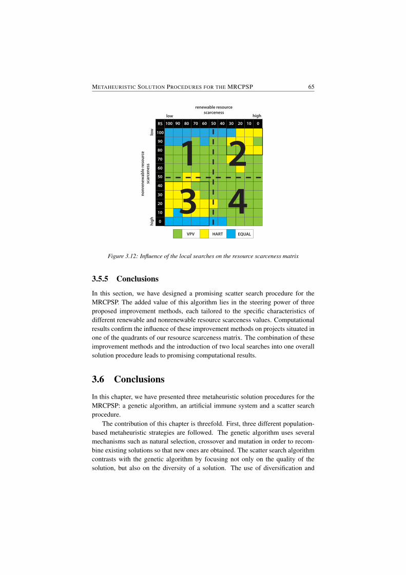
METAHEURISTIC SOLUTION PROCEDURES FOR THE MRCPSP 65
100 90 80 70 60 50 40 30 20 10 0
100
90
80
70
60
50
40
30
20
10
0
RS
low high
low
high
nonr
enew
able
reso
urce
sc
arce
ness
renewable resource scarceness
VPV HART EQUAL
1 243
Figure 3.12: Influence of the local searches on the resource scarceness matrix
3.5.5 Conclusions
In this section, we have designed a promising scatter search procedure for theMRCPSP. The added value of this algorithm lies in the steering power of threeproposed improvement methods, each tailored to the specific characteristics ofdifferent renewable and nonrenewable resource scarceness values. Computationalresults confirm the influence of these improvement methods on projects situated inone of the quadrants of our resource scarceness matrix. The combination of theseimprovement methods and the introduction of two local searches into one overallsolution procedure leads to promising computational results.
3.6 Conclusions
In this chapter, we have presented three metaheuristic solution procedures for theMRCPSP: a genetic algorithm, an artificial immune system and a scatter searchprocedure.
The contribution of this chapter is threefold. First, three different population-based metaheuristic strategies are followed. The genetic algorithm uses severalmechanisms such as natural selection, crossover and mutation in order to recom-bine existing solutions so that new ones are obtained. The scatter search algorithmcontrasts with the genetic algorithm by focusing not only on the quality of thesolution, but also on the diversity of a solution. The use of diversification and
66 CHAPTER 3
improvement methods leads to a more efficient exploration of the solution space.The artificial immune system finally makes use of mechanisms, such as the clonalselection process, hypermutation and receptor editing, which are inspired by thevertebrate immune system. The artificial immune system differs from the geneticalgorithm by the fact that new solutions are only generated by applying a (hy-per)mutation operator. Second, problem-specific techniques and local searchesare added to each of the metaheuristic solution procedures in order to solve theMRCPSP efficiently: the extended generation scheme with mode improvementmethod in the genetic algorithm, the controlled mode assignment procedure togenerate a good and diverse initial population in the artificial immune system pro-cedure and the three improvement methods, each tailored to the specific renewableand nonrenewable scarceness characteristics in the scatter search procedure. Theintroduction of these methods significantly increases the performance of the proce-dures. Third, in the recent literature different penalty functions and local searcheswere proposed. An overview of these penalty functions and local searches is givenand tested during computational experiments. The results give an indication of theeffectiveness of each of these procedures and functions and emphasize the needfor solution methods and procedures tailored to the specific characteristics of themulti-mode scheduling problem.
In this chapter, an overview is given of the algorithmic features of the differentmetaheuristic solution procedures. These procedures are tested on specific datasetsto optimize the different algorithmic parameters, however, no comparison is madebetween the metaheuristics on a standard benchmark dataset. In order to make thisfair comparison between the three procedures and the other metaheuristics avail-able in the literature, computational tests are performed on the benchmark datasetsPSPLIB and Boctor. The results of this comparison are presented in chapter 5.Moreover, results are also provided for tests performed on the new benchmarkdataset MMLIB, which is presented in the next chapter.
4New Dataset for the MRCPSP
4.1 Introduction
In order to make a fair comparison between different solution procedures for spe-cific optimization problems, standard benchmark sets are available to test the ef-ficiency and performance of the proposed algorithm. Examples are the PSPLIBdataset for the RCPSP (Kolisch et al., 1995), the MPSPLIB for multi-projectscheduling problems (Homberger, 2007) and the dataset for the machine sched-uling problem, proposed by Sels and Vanhoucke (2009).
For the MRCPSP, the PSPLIB dataset (Kolisch et al., 1995) and the Boctordataset (Boctor, 1993) are available. Most authors make use of these datasets totest the performance of their procedures in order to compare them to other algo-rithms available in the literature. However, the two datasets show some impor-tant shortcomings given the recent evolution in the development of metaheuristicsearch procedures. Therefore, we propose in this chapter a new benchmark datasetwhich overcomes the disadvantages of the current datasets and which can be usedas a benchmark dataset for further research. In section 4.2, we make an analysisof the current benchmark datasets and explain their shortcomings, while in section4.3 we propose the indicators of the newly developed and generated benchmarkdataset.
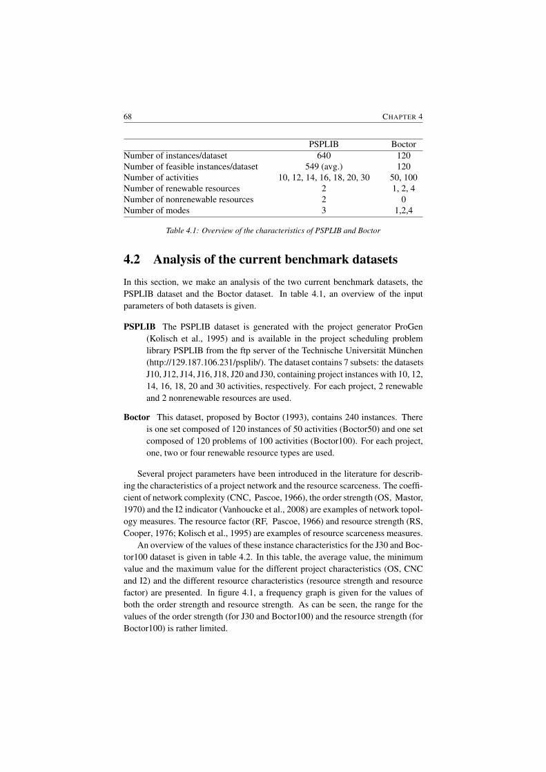
68 CHAPTER 4
PSPLIB BoctorNumber of instances/dataset 640 120Number of feasible instances/dataset 549 (avg.) 120Number of activities 10, 12, 14, 16, 18, 20, 30 50, 100Number of renewable resources 2 1, 2, 4Number of nonrenewable resources 2 0Number of modes 3 1,2,4
Table 4.1: Overview of the characteristics of PSPLIB and Boctor
4.2 Analysis of the current benchmark datasetsIn this section, we make an analysis of the two current benchmark datasets, thePSPLIB dataset and the Boctor dataset. In table 4.1, an overview of the inputparameters of both datasets is given.
PSPLIB The PSPLIB dataset is generated with the project generator ProGen(Kolisch et al., 1995) and is available in the project scheduling problemlibrary PSPLIB from the ftp server of the Technische Universitat Munchen(http://129.187.106.231/psplib/). The dataset contains 7 subsets: the datasetsJ10, J12, J14, J16, J18, J20 and J30, containing project instances with 10, 12,14, 16, 18, 20 and 30 activities, respectively. For each project, 2 renewableand 2 nonrenewable resources are used.
Boctor This dataset, proposed by Boctor (1993), contains 240 instances. Thereis one set composed of 120 instances of 50 activities (Boctor50) and one setcomposed of 120 problems of 100 activities (Boctor100). For each project,one, two or four renewable resource types are used.
Several project parameters have been introduced in the literature for describ-ing the characteristics of a project network and the resource scarceness. The coeffi-cient of network complexity (CNC, Pascoe, 1966), the order strength (OS, Mastor,1970) and the I2 indicator (Vanhoucke et al., 2008) are examples of network topol-ogy measures. The resource factor (RF, Pascoe, 1966) and resource strength (RS,Cooper, 1976; Kolisch et al., 1995) are examples of resource scarceness measures.
An overview of the values of these instance characteristics for the J30 and Boc-tor100 dataset is given in table 4.2. In this table, the average value, the minimumvalue and the maximum value for the different project characteristics (OS, CNCand I2) and the different resource characteristics (resource strength and resourcefactor) are presented. In figure 4.1, a frequency graph is given for the values ofboth the order strength and resource strength. As can be seen, the range for thevalues of the order strength (for J30 and Boctor100) and the resource strength (forBoctor100) is rather limited.
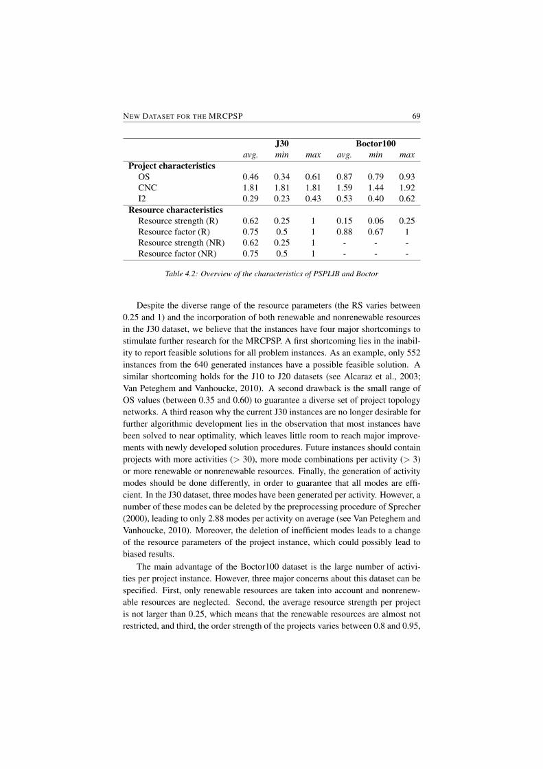
NEW DATASET FOR THE MRCPSP 69
J30 Boctor100avg. min max avg. min max
Project characteristicsOS 0.46 0.34 0.61 0.87 0.79 0.93CNC 1.81 1.81 1.81 1.59 1.44 1.92I2 0.29 0.23 0.43 0.53 0.40 0.62
Resource characteristicsResource strength (R) 0.62 0.25 1 0.15 0.06 0.25Resource factor (R) 0.75 0.5 1 0.88 0.67 1Resource strength (NR) 0.62 0.25 1 - - -Resource factor (NR) 0.75 0.5 1 - - -
Table 4.2: Overview of the characteristics of PSPLIB and Boctor
Despite the diverse range of the resource parameters (the RS varies between0.25 and 1) and the incorporation of both renewable and nonrenewable resourcesin the J30 dataset, we believe that the instances have four major shortcomings tostimulate further research for the MRCPSP. A first shortcoming lies in the inabil-ity to report feasible solutions for all problem instances. As an example, only 552instances from the 640 generated instances have a possible feasible solution. Asimilar shortcoming holds for the J10 to J20 datasets (see Alcaraz et al., 2003;Van Peteghem and Vanhoucke, 2010). A second drawback is the small range ofOS values (between 0.35 and 0.60) to guarantee a diverse set of project topologynetworks. A third reason why the current J30 instances are no longer desirable forfurther algorithmic development lies in the observation that most instances havebeen solved to near optimality, which leaves little room to reach major improve-ments with newly developed solution procedures. Future instances should containprojects with more activities (> 30), more mode combinations per activity (> 3)or more renewable or nonrenewable resources. Finally, the generation of activitymodes should be done differently, in order to guarantee that all modes are effi-cient. In the J30 dataset, three modes have been generated per activity. However, anumber of these modes can be deleted by the preprocessing procedure of Sprecher(2000), leading to only 2.88 modes per activity on average (see Van Peteghem andVanhoucke, 2010). Moreover, the deletion of inefficient modes leads to a changeof the resource parameters of the project instance, which could possibly lead tobiased results.
The main advantage of the Boctor100 dataset is the large number of activi-ties per project instance. However, three major concerns about this dataset can bespecified. First, only renewable resources are taken into account and nonrenew-able resources are neglected. Second, the average resource strength per projectis not larger than 0.25, which means that the renewable resources are almost notrestricted, and third, the order strength of the projects varies between 0.8 and 0.95,

70 CHAPTER 4
0%
10%
20%
30%
40%
50%
60%
0.02
5
0.07
5
0.12
5
0.17
5
0.22
5
0.27
5
0.32
5
0.37
5
0.42
5
0.47
5
0.52
5
0.57
5
0.62
5
0.67
5
0.72
5
0.77
5
0.82
5
0.87
5
0.92
5
0.97
5 1
PSPLIB-J30 Boctor-100
(a) Order strength
0%
10%
20%
30%
40%
50%
60%
0.02
5
0.07
5
0.12
5
0.17
5
0.22
5
0.27
5
0.32
5
0.37
5
0.42
5
0.47
5
0.52
5
0.57
5
0.62
5
0.67
5
0.72
5
0.77
5
0.82
5
0.87
5
0.92
5
0.97
5 1
PSPLIB-J30 Boctor-100
(b) Resource strength
Figure 4.1: Frequency table for the project instance characteristics
which means that the projects are mainly serial.In the next section, we will present three new datasets, which will cover most
of the shortcomings mentioned in this section and are suggested to be used as anew benchmark dataset for the MRCPSP.
4.3 A New Dataset for the MRCPSP
4.3.1 Generation conditions
In order to overcome the shortcomings of the PSPLIB and Boctor datasets, thefollowing conditions were taken into account while generating the dataset:
1. The generated project is diverse with respect to the project (OS) and resourcecharacteristics (RS and RF).
2. Every instance has at least 1 feasible solution.
3. No modes can be excluded.
4. Both renewable and nonrenewable resources are taken into account.
NEW DATASET FOR THE MRCPSP 71
4.3.2 Dataset generation
For the generation of the instances, we have used the RanGen project schedulinginstances generator developed by Vanhoucke et al. (2008) and extended to projectswith multiple modes. In order to meet the conditions mentioned in the previ-ous section, two repair functions are used during the generation of the differentdatasets.
1. For projects with low values of the nonrenewable resource strength (RSν =0.25), many infeasible projects were generated. This problem was also citedby Demeulemeester et al. (2003). If the resource strength of a nonrenew-able resource is low, this results in a low value of the availability aν . Sincethe generation of the projects occurs randomly, only in a limited number ofcases a feasible project is generated. Therefore, a repair function is used toavoid this problem. A large set of small projects (10 activities) is generatedwith a RSν = 0.25 and a RF ν = 0.50. All feasible projects are selectedfrom this large set. During the generation of the projects with a large num-ber of activities (e.g. 50 or 100), a random combination is selected from thegenerated small subset of feasible projects and the nonrenewable resourceinformation is randomly assigned to one of the new project’s activities. Toobtain the overall availability, the sum of all nonrenewable resource avail-abilities of the chosen small projects is made. This process can be executedsince, based on the mathematical formulation of the nonrenewable resourcestrength, the combination of two feasible projects always leads to a feasibleproject.
2. Many inefficient modes were generated during the data generation process.Modes are labelled as inefficient if there is another mode of the same ac-tivity with the same or smaller duration and no more requirements for allresources. Since all projects are generated randomly, it is straightforwardthat inefficient modes are generated. Therefore, a repair function is used inorder to deal with the problem of inefficient modes. If an inefficient mode isdetected, the resource requirement of one of the nonrenewable resources isset to a value lower than the original nonrenewable resource demand. This isonly possible if the resource demand is not 0 or if the nonrenewable resourcedemand is not the minimal resource demand for that activity (otherwise thenonrenewable resource strength will be affected). In the case no changescan be performed, a new project is generated.
4.3.3 Dataset characteristics
The dataset generation resulted in the design of two datasets: the MMLIB* dataset,which has project characteristics similar to the PSPLIB dataset and takes the short-

72 CHAPTER 4
comings mentioned in the previous section into account, and the MMLIB+ dataset,which also takes more resources and more modes into account. The motivationto generate both datasets comes from the idea that the complexity of the currentbenchmark datasets should be increased. The MMLIB* is generated to increase thecomplexity of the scheduling problem (i.e. more activities), the MMLIB+ datasetis generated to increase the complexity of both the scheduling problem (i.e. moreactivities) and the mode assignment problem (i.e. more possible nonrenewablemode combinations).
MMLIB* The MMLIB* dataset is a dataset with two subsets: MMLIB50 andMMLIB100 with 50 and 100 activities, respectively. Each project activityhas 2 renewable and 2 nonrenewable resources and for each activity, 3 modeswere defined. The order strength is set at 0.25, 0.50 or 0.75. The resourcestrength of both the renewable and nonrenewable resource strength is setat 0.25, 0.50 or 0.75 and the resource factor is set at 0.50 or 1 for bothrenewable and nonrenewable resources. Using 5 instances for each problemclass, each MMLIB* dataset contains 540 instances. The MMLIB* datasetscan be considered as similar to the PSPLIB datasets, however, the orderstrength is more diverse and projects with a resource strength equal to 1have not been included in the set. Moreover, all the instances have a feasiblesolution and no modes can be deleted during the preprocessing procedure.
MMLIB+ The MMLIB+ dataset contains projects with 50 and 100 activities.Each project activity has 2 or 4 renewable and nonrenewable resources. Foreach activity, 3, 6 or 9 modes are defined. The order strength is set at 0.25,0.50 or 0.75. The resource strength of both the renewable and nonrenewableresource strength is set at 0.25, 0.50 or 0.75. In order to keep the numberof instances to a reasonable level, the renewable and nonrenewable resourcefactor is set at 1. Using 5 instances for each problem class, the MMLIB+dataset contains 3,240 instances.
4.3.4 Download
The problem instances, as well as the solution files, can be downloaded from thewebsite http://www.projectmanagement.UGent.be/mrcpsp.htm, under the namesMMLIB50.zip, MMLIB100.zip and MMLIB+.zip.
The solution files contain the best individual solution of each problem instance(without a given stop criterion). The website will be updated regularly, and wecall upon researchers to report the solutions of their procedures when this leads toan improvement (with a stop criterion of 1,000, 5,000 and 50,000 schedules andwithout any stop criterion).

NEW DATASET FOR THE MRCPSP 73
4.4 ConclusionsIn this chapter, a new dataset for the MRCPSP is proposed which deals with themajor shortcomings of the existing benchmark datasets and which will contributeto the search of new and better solutions in the future. In the next chapter, anobjective comparison of various metaheuristic procedures on this new dataset willbe presented.

5Comparative Results for the MRCPSP
5.1 Introduction
The increasing interest in operations research for metaheuristics during the recentyears has resulted in the development of several metaheuristic solution proceduresfor the MRCPSP. A wide variety of metaheuristic strategies, solution represen-tations and schedule generation schemes were used to develop the most efficientalgorithm. Since the methods are tested on different benchmark datasets using dif-ferent stop criteria, a fair comparison between each of these procedures is difficult.
In this chapter, we compare all metaheuristic solution procedures available inthe literature. We have coded all procedures as described in our literature overviewpresented in section 2.5.3 and compared their performance with the performanceof our proposed solution procedures. This comparison gives an indication of theperformance of our own procedures and classifies all procedures according to sim-ilar stop criteria. The tests are performed on the benchmark datasets PSPLIB andBoctor, as well as on the newly developed dataset MMLIB.
The remainder of this chapter is organized as follows. In section 5.2, anoverview of the followed methodology to obtain the comparative results for thedifferent metaheuristics is described. In section 5.3, the computational compari-son is given, with a description of the test design and the results for the PPLIP,Boctor and MMLIB dataset. In the last section, overall conclusions and sugges-tions for future research are presented.
76 CHAPTER 5
5.2 Methodology
In order to compare each of the procedures on the same computer and for the samestop criteria, each algorithm presented in section 2.5.3 has been coded1. In thissection, we will explain the methodology that has been followed in order to obtaina fair and realistic reproduction of the original codes.
Each paper is studied by two undergraduate students and one PhD student. Foreach procedure three independently coded programs were available, each reviewedby a PhD student, who reviewed the code to look if the structure corresponded tothe steps presented in the original paper. In case the content of the paper wasinsufficient to interpret the algorithm, other papers and solution procedures of theauthor were analyzed. The best program was selected and submitted to a secondcontrol phase.
If necessary, the following two adaptations were made. First, since not allalgorithms included the preprocessing method of Sprecher et al. (1997), the pre-processing procedure was added to each solution procedure in order to make a faircomparison based on the same solution space. Second, procedures which are onlyapplicable on datasets with renewable resources (in casu BOCT and MORI),are transferred to a version in which nonrenewable resources are incorporated. Inorder to deal with possible infeasible solutions, the penalty function as introducedby Alcaraz et al. (2003) is used in the code.
To emphasize the efficiency of all procedures, an overview of the differentsolution procedures is given in table 5.1. For every procedure, the dataset and stopcriterion is mentioned. The results in the paper are also indicated, as well as theresults obtained by our own coded versions. As can be seen, all the proceduresobtain equivalent or slightly better results than the results shown in the originalpapers. This can be due to randomness, the incorporation of the preprocessingprocess or the competitive nature of the coding process. The different procedureswere tested on the available datasets as well as on the new dataset MMLIB.
5.3 Computational comparison
5.3.1 Test design
This section gives a comparison of all the metaheuristics presented in table 2.7and the designed metaheuristic solution procedures proposed in chapter 3. Testsare executed on two subsets: a first subset with the existing datasets PSPLIB andBoctor (J10, J20, J30 and Boctor) and a second subset with the newly generateddatasets MMLIB* and MMLIB+.
1This overview contains all metaheuristic solution procedures published in international peer re-viewed journals before August 1, 2009.
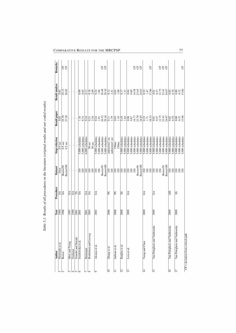
COMPARATIVE RESULTS FOR THE MRCPSP 77
Tabl
e5.
1:R
esul
tsof
allp
roce
dure
sin
the
liter
atur
e(o
rigi
nalr
esul
tsan
dou
rco
ded
resu
lts)
Aut
hor
Year
Proc
edur
eD
atas
etSt
opcr
iteri
onR
esul
tpap
erR
esul
tana
lyse
Rem
arks
1Sl
owin
skie
tal.
1994
SAO
wn
0.5
sec
0.02
0.02
2B
octo
r19
96SA
Boc
tor5
00.
5se
c25
.70
25.1
3C
PB
octo
r100
0.5
sec
27.2
026
.82
CP
3M
oria
ndT
seng
1997
GA
--
--
4O
zdam
ar19
99G
A-
--
-5
Non
obe
and
Ibar
aki
2001
TS
--
--
6Jo
zefo
wsk
aet
al.
2001
SAJ1
05,
000
sche
dule
s1.
160.
99J2
05,
000
sche
dule
s6.
746.
657
Har
tman
n20
01G
AJ1
06,
000
sche
dule
s0.
100.
138
Bou
leim
enan
dL
ecoc
q20
03SA
J10
50se
c0.
210.
18J2
050
sec
2.10
2.09
9A
lcar
azet
al.
2003
GA
J10
5,00
0sc
hedu
les
0.24
0.24
J20
5,00
0sc
hedu
les
1.91
1.96
Boc
tor5
05,
000
sche
dule
s26
.52
26.4
8C
PB
octo
r100
5,00
0sc
hedu
les
29.1
629
.10
CP
10Z
hang
etal
.20
06PS
J10
unkn
own/
1se
c0.
110.
12J2
0un
know
n/1
sec
1.79
2.41
11Ja
rbou
ieta
l.20
08PS
J10
150m
s0.
030.
03J2
015
0ms
1.10
1.08
12R
anjb
aret
al.
2008
SSJ1
05,
000
sche
dule
s0.
180.
17J2
05,
000
sche
dule
s1.
641.
3113
Lov
aet
al.
2009
GA
J10
5,00
0sc
hedu
les
0.06
0.04
J20
5,00
0sc
hedu
les
0.87
0.89
J30
5,00
0sc
hedu
les
14.7
714
.58
CP
Boc
tor5
05,
000
sche
dule
s23
.70
23.6
5C
PB
octo
r100
5,00
0sc
hedu
les
24.8
524
.63
CP
14T
seng
and
Che
n20
09G
AJ1
05,
000
sche
dule
s0.
330.
32J2
05,
000
sche
dule
s1.
711.
47J3
05,
000
sche
dule
s18
.33
17.0
6C
P15
Van
Pete
ghem
and
Van
houc
ke20
09G
AJ1
05,
000
sche
dule
s0.
010.
01J2
05,
000
sche
dule
s0.
570.
57J3
05,
000
sche
dule
s13
.75
13.7
5C
PB
octo
r50
5,00
0sc
hedu
les
23.4
123
.41
CP
Boc
tor1
005,
000
sche
dule
s24
.67
24.6
7C
P16
Van
Pete
ghem
and
Van
houc
ke20
09A
ISJ1
05,
000
sche
dule
s0.
020.
02J2
05,
000
sche
dule
s0.
700.
7017
Van
Pete
ghem
and
Van
houc
ke20
09SS
J10
5,00
0sc
hedu
les
0.00
0.00
J20
5,00
0sc
hedu
les
0.32
0.32
J30
5,00
0sc
hedu
les
13.6
613
.66
CP
CP
=de
viat
ion
from
criti
calp
ath
78 CHAPTER 5
Since it is assumed that the computational effort for constructing one scheduleis similar in most heuristics and in order to make a fair comparison, the evaluationis stopped after a predefined number of generated schedules. The evaluation ofthe first subset is stopped after 5,000 schedules. For the second dataset, the stopcriterion is set at 1,000, 5,000 and 50,000 schedules.
According to Kolisch and Hartmann (2006) the advantage of the number ofschedules as stop criterion is twofold: first, it is platform independent and second,future studies can easily make use of the benchmark results by applying the samestop criterion. However, the stop criterion also has a few shortcomings: first, itcannot be applied to all different heuristic strategies. Second, the required time tocompute one schedule might differ between metaheuristics. Nevertheless, Kolischand Hartmann (2006) conclude that limiting the number of schedules is the bestcriterion available for a broad comparison, which motivated us to use this stopcriterion in all computational experiments.
To measure the number of schedules, the definition of one schedule should bedefined. In their RCPSP review paper, Kolisch and Hartmann (2006) state thatone schedule corresponds to (at most) one start time assignment per activity, asdone by a SGS. However, measuring the number of schedules according to thisrule means that for every mode change in a local search procedure a new scheduleshould be counted. Therefore, Lova et al. (2009) define the number of generatedschedules as the sum of times each activity of the project has obtained a feasiblestart time divided by the number of activities of the project. Assume a projectwith eight activities, each with three modes. Suppose that the SGS generates aschedule based on a activity and mode list (8 start times are assigned) and that alocal search procedure has also analyzed the two other (feasible) modes for three ofthe activities. This means that the procedure has generated and analyzed (8+2x3)/8= 1,75 schedules. In the remainder of this paper, the last definition is used to definethe number of schedules.
5.3.2 Experimental results
5.3.2.1 Results of the PSPLIB and Boctor dataset
The results for the first subset obtained after 5,000 schedules can be found in table5.2. For the J10 and J20 set, the average deviation from the optimal solution isgiven. For the J30 and Boctor dataset, the deviation from the minimal criticalpath-based lower bound is reported. If a solution procedure was not able to obtaina feasible solution for all project instances, the percentage of instances for whicha feasible solution was found is indicated between brackets. As can be seen inthe table, not all heuristics were able to obtain a feasible solution for all projectinstances.
The metaheuristics are sorted with respect to decreasing average deviations for
COMPARATIVE RESULTS FOR THE MRCPSP 79
the Boctor100 dataset, except for schedules which were not able to obtain feasibleresults for all datasets. The best results for a specific dataset are displayed in bold.In order to determine the best heuristic, the concept of dominance as defined inKolisch and Hartmann (2006) is used: a heuristic a is dominated by a heuristic b ifa has for at least one instance set a higher deviation than bwithout having for any ofthe other combinations a lower average deviation. Table 5.2 reveals that the scattersearch and genetic algorithm (as proposed in chapter 3) and the procedure of Lovaet al. (2009) are not dominated by other heuristics. For the PSPLIB dataset, ourscatter search procedure dominates all other metaheuristics.
As the most recent metaheuristics available in the literature obtain near-optimalresults for the PSPLIB dataset, the use of this dataset is not longer recommendedto evaluate the performance of new solution procedures. Therefore, the use ofthe MMLIB50, MMLIB100 and MMLIB+ is encouraged to compare the resultsof new solution procedures with the existing methods. The results of the existingmethods are presented in the next section.
5.3.2.2 MMLIB* and MMLIB+
The results of the computational tests on the MMLIB50, MMLIB100 and MM-LIB* are given in the tables 5.3 to 5.5. In these tables, performance measures forthe three stop criteria (1,000, 5,000 and 50,000 schedules, respectively) are shown.For every stop criterion, three measures are indicated. First, the percentage of in-stances for which a feasible solution is found. Second, the average deviation fromthe minimal critical path based lower bound is given and finally the maximumdeviation is shown. The metaheuristics are sorted with respect to the results for50,000 schedules, except for schedules which were not able to obtain feasible re-sults for all project instances.
Not all metaheuristic solution procedures succeed to obtain a feasible schedulefor all project instances. This is mainly due to the fact that these metaheuristicshave not included a search procedure to enhance the feasibility of an infeasiblesolution vector. The procedure of Boctor (1996) and Mori and Tseng (1997) weredesigned to solve the MRCPSP/R, while the procedures of Bouleimen and Lecocq(2003) and Ranjbar et al. (2009) were also designed to solve other schedulingproblems, such as the RCPSP and the DTRTP.
In figures 5.1 to 5.3, a graphic representation is given of three performancemeasures for the three datasets for each of the three stop criteria and for eachmetaheuristic. The white part of each bar indicates the percentage of infeasiblesolutions, while the black part of the bar indicates the percentage of best solutionsfound. The grey part indicates the feasible solutions for which no best solutioncould be found. The algorithms are sorted on their percentage of best results foundafter 50,000 schedules for each of the three datasets.
Based on the obtained results, the following conclusions can be drawn. First,

80 CHAPTER 5
Author
Repr
SGS
J10J20
J30B
octor50B
octor100Slow
inskietal.(SA)
AL
P2.01
(44.96)2.51
(50.18)6.13
(48.55)31.70
38.14B
octor(SA)
AL
S0.27
11.66(99.10)
29.58(93.66)
25.1326.82
Bouleim
en&
Lecocq
(SA)
AL
S2.65
10.26(99.64)
33.60(99.64)
28.5331.49
Nonobe
andIbaraki(T
S)A
LP
5.829.02
26.4348.61
56.91M
ori&T
seng(G
A)
PLS
2.6813.55
24.9941.28
53.81O
zdamar(G
A)
PLP
0.706.05
27.3837.81
47.21Jarbouietal.(PS)
PLS
0.222.44
18.1430.31
37.82Z
hangetal.(PS)
PLS
0.313.17
18.6328.97
32.83V
anPeteghem
&V
anhoucke(A
IS)A
LS
0.020.70
14.1825.83
30.12A
lcarazetal.(G
A)
AL
S0.24
1.9621.83
26.4829.10
Tseng
andC
hen(G
A)
AL
S0.32
1.4717.06
26.6027.12
Hartm
ann(G
A)
AL
S0.20
1.6115.96
24.7326.47
Ranjbaretal.(SS)
AL
S0.17
1.3116.21
24.1025.84
Jozefowska
etal.(SA)
AL
S0.99
6.6518.64
24.4425.70
Van
Peteghem&
Vanhoucke
(SS)PL
S0.00
0.3213.66
23.7925.11
Van
Peteghem&
Vanhoucke
(GA
)PL
S0.01
0.5713.75
23.4124.67
Lova
etal.(GA
)A
LP/S
0.040.89
14.5823.65
24.63
Table5.2:
Averagedeviation
fromoptim
um/criticalpath
lower
boundfor
PSP
LIBand
Boctor
instancesafter
5,000schedules
COMPARATIVE RESULTS FOR THE MRCPSP 81
although several solution procedures (Alcaraz et al., 2003; Zhang et al., 2006;Tseng and Chen, 2009) find feasible solutions for all project instances, they do notfind any (or a small part) of the best solutions. On the other hand, more thanone third of the solutions found by Slowinski et al. (1994) for the MMLIB50and MMLIB100 dataset is also the best known solution. Second, the infeasibil-ity rate of some procedures clearly decreases for an increasing number of sched-ules evaluated (Bouleimen and Lecocq, 2003; Mori and Tseng, 1997), while othermetaheuristic solution procedures do not succeed to increase this rate significantly(Slowinski et al., 1994; Boctor, 1996; Ranjbar et al., 2009). It is conjectured thatthis is mainly due to the restricted feasibility improvement methods which are in-corporated in the algorithms. Finally, based on these results, it can be stated thatour scatter search procedure dominates all other metaheuristics. This is mainlydue to the advanced improvement methods which are designed to search for thebest performing mode assignment in the search space and to the ’intelligent’ so-lution combination method using resource scarceness characteristics to steer thealgorithm to the most promising solution regions. We believe that this objectivecomparison of various metaheuristic procedures and the creation of new datasetswill contribute to the search of new and better solutions in the future.
5.4 Discussion and conclusions
This research has given an overview of the metaheuristic solution procedures avail-able in the literature to solve the multi-mode resource-constrained project schedul-ing problem and has made a fair comparison between these procedures. Moreover,a new benchmark dataset is proposed. Researchers are encouraged to use thisdataset to compare the results of their solution procedures with other procedures.
Based on the results, the following conclusions can be made. First, the multi-mode RCPSP can be divided into two subproblems: the mode assignment problem,whose aim it is to generate a feasible mode assignment list, and a scheduling prob-lem, whose aim it is to minimize the makespan of the problem. Some proceduresemphasized too much the scheduling problem, by which these procedures were notable to generate feasible solutions for all project instances. Moreover, proceduresusing a clever mode assignment procedure to generate the initial population, suchas the minimum normalized resources procedure of Lova et al. (2009) or the con-trolled mode assignment procedure as presented in chapter 3, have an advantagecompared to other methods, especially when the number of generated schedules islow. Future research will have to focus on this mode assignment problem, sincefor an increasing number of activities and an increasing number of modes the com-plexity of this problem also increases.
Second, the good performance of some solution procedures is mainly due tothe applied MRCPSP-specific local search procedures rather than to the followed

82 CHAPTER 5
metaheuristic search strategy. This conclusion is supported by computational testsexecuted by several authors comparing the effectiveness of both their algorithmand a similar solution procedure without the proposed local search method. Lovaet al. (2009) prove that their hybrid genetic algorithm with efficient improve-ment method clearly outperforms a simple genetic algorithm. Similar results arefound by Hartmann (2001), who shows that the use of the single-pass improve-ment method clearly improves the performance of the proposed genetic algorithm.Moreover, the use of problem specific information in the local search process,such as the use of resource scarceness parameters in the scatter search procedure,increases the efficiency of the procedure significantly.
Finally, we hope to have contributed in making a fair comparison between thedifferent available datasets. We believe that the introduction of three new datasetsopens the possibility to compare new solution procedures with the currently avail-able methods. Although the use of standard datasets often motivates researchers toimprove merely the benchmark results rather than to investigate in new promisingmethodologies, we hope that the introduction of this new dataset will also stimu-late the development of new ideas and techniques to tackle the MRCPSP.

COMPARATIVE RESULTS FOR THE MRCPSP 83
Aut
hors
1,00
0sc
hedu
les
5,00
0sc
hedu
les
50,0
00sc
hedu
les
Feas
ible
Av.
Dev
.M
ax.D
ev.
Feas
ible
Av.
Dev
.M
ax.D
ev.
Feas
ible
Av.
Dev
.M
ax.D
ev.
Slow
insk
ieta
l.(S
A)
21.8
5-
137.
5023
.52
-12
5.00
25.0
0-
121.
43B
octo
r(SA
)67
.59
-17
1.43
69.6
3-
171.
4378
.52
-21
3.33
Bou
leim
en&
Lec
ocq
(SA
)72
.96
-23
4.62
77.7
8-
280.
0082
.78
-25
3.33
Ozd
amar
(GA
)83
.15
-21
3.33
83.3
3-
213.
3383
.33
-20
6.67
Ran
jbar
etal
.(SS
)85
.19
-20
6.90
87.0
4-
190.
0089
.65
-18
0.73
Mor
i&T
seng
(GA
)72
.22
-23
0.77
83.5
2-
240.
0010
0.00
46.9
131
5.38
Alc
araz
etal
.(G
A)
100.
0056
.06
300.
0010
0.00
43.0
531
5.38
100.
0040
.69
315.
38N
onob
ean
dIb
arak
i(T
S)10
0.00
43.3
528
4.62
100.
0041
.10
276.
9210
0.00
38.9
826
1.54
Jarb
ouie
tal.
(PS)
100.
0049
.98
323.
0810
0.00
38.8
628
4.62
100.
0032
.01
253.
85Z
hang
etal
.(PS
)10
0.00
49.2
526
9.23
100.
0035
.94
253.
8510
0.00
30.2
323
8.46
Tse
ngan
dC
hen
(GA
)10
0.00
65.1
730
7.69
100.
0040
.99
261.
5410
0.00
29.4
424
6.15
Joze
fow
ska
etal
.(SA
)10
0.00
49.0
627
6.92
100.
0033
.81
261.
5410
0.00
27.8
124
6.15
Har
tman
n(G
A)
100.
0035
.40
253.
8510
0.00
30.6
124
6.15
100.
0026
.81
230.
77L
ova
etal
.(G
A)
100.
0034
.16
253.
8510
0.00
28.5
923
3.08
100.
0026
.69
215.
38V
anPe
tegh
em&
Van
houc
ke(A
IS)
100.
0031
.52
223.
0810
0.00
27.4
522
3.08
100.
0025
.26
223.
08V
anPe
tegh
em&
Van
houc
ke(G
A)
100.
0034
.07
246.
1510
0.00
27.1
221
5.38
100.
0024
.93
215.
38V
anPe
tegh
em&
Van
houc
ke(S
S)10
0.00
28.1
723
0.77
100.
0025
.45
223.
0810
0.00
23.7
921
5.38
Tabl
e5.
3:Av
erag
ede
viat
ion
from
min
imal
criti
calp
ath
base
dlo
wer
boun
d-M
MLI
B50

84 CHAPTER 5
Authors
1,000schedules
5,000schedules
50,000schedules
FeasibleA
v.Dev.
Max.D
ev.Feasible
Av.D
ev.M
ax.Dev.
FeasibleA
v.Dev.
Max.D
ev.Slow
inskietal.(SA)
18.89-
168.1819.81
-141.94
21.48-
140.91B
octor(SA)
66.67-
203.5766.67
-156.25
66.67-
150.00B
ouleimen
&L
ecocq(SA
)66.67
-200.00
67.04-
203.5767.41
-192.86
Ozdam
ar(GA
)66.67
-221.43
67.59-
192.8667.59
-192.86
Mori&
Tseng
(GA
)67.04
-221.43
69.63-
247.0683.33
-257.14
Ranjbaretal.(SS)
83.33-
185.7183.33
-171.43
83.33-
169.14A
lcarazetal.(G
A)
100.0061.80
252.63100.00
52.67252.63
100.0046.68
245.16N
onobeand
Ibaraki(TS)
100.0049.32
238.10100.00
47.03236.84
100.0045.04
236.84Jarbouietal.(PS)
91.85-
300.00100.00
49.41247.62
100.0040.23
231.58T
sengand
Chen
(GA
)100.00
72.95257.89
100.0066.04
257.89100.00
37.04226.32
Zhang
etal.(PS)100.00
57.42233.33
100.0044.05
215.79100.00
35.35205.26
Jozefowska
etal.(SA)
100.0053.97
258.06100.00
39.05238.71
100.0030.27
205.26H
artmann
(GA
)100.00
39.96221.05
100.0033.98
200.00100.00
29.04194.74
Van
Peteghem&
Vanhoucke
(AIS)
100.0036.68
189.47100.00
31.75184.21
100.0028.09
184.21L
ovaetal.(G
A)
100.0036.29
216.13100.00
31.01200.00
100.0027.89
194.74V
anPeteghem
&V
anhoucke(G
A)
100.0037.58
215.79100.00
29.55194.74
100.0025.63
178.95V
anPeteghem
&V
anhoucke(SS)
100.0029.77
194.74100.00
26.51184.21
100.0024.02
178.95
Table5.4:
Averagedeviation
fromm
inimalcriticalpath
basedlow
erbound
-MM
LIB100

COMPARATIVE RESULTS FOR THE MRCPSP 85
Aut
hors
5,00
0sc
hedu
les
50,0
00sc
hedu
les
Feas
ible
Av.
Dev
.M
ax.D
ev.
Feas
ible
Av.
Dev
.M
ax.D
ev.
Slow
insk
ieta
l.(S
A)
4.78
-30
7.32
4.78
-30
7.32
Boc
tor(
SA)
54.4
8-
427.
7865
.77
-49
0.63
Ozd
amar
(GA
)68
.64
-52
8.13
68.7
7-
500.
00B
oule
imen
&L
ecoc
q(S
A)
67.9
6-
606.
2570
.59
-59
0.63
Ran
jbar
etal
.(SS
)70
.66
-80
5.05
73.6
5-
623.
15Jo
zefo
wsk
aet
al.(
SA)
75.0
0-
810.
3475
.00
-72
1.88
Mor
i&T
seng
(GA
)72
.59
-70
2.70
97.2
2-
1057
.69
Van
Pete
ghem
&V
anho
ucke
(GA
)97
.59
-79
3.10
97.5
9-
775.
86Z
hang
etal
.(PS
)99
.81
-86
5.52
99.8
5-
848.
28A
lcar
azet
al.(
GA
)10
0.00
177.
5510
00.0
010
0.00
164.
8799
6.55
Tse
ngan
dC
hen
(GA
)10
0.00
183.
0299
6.55
100.
0014
2.14
917.
24N
onob
ean
dIb
arak
i(T
S)10
0.00
148.
0292
0.69
100.
0014
3.66
910.
34Ja
rbou
ieta
l.(P
S)94
.29
-99
3.10
100.
0013
7.99
913.
79H
artm
ann
(GA
)10
0.00
132.
0187
2.41
100.
0011
1.45
793.
10L
ova
etal
.(G
A)
100.
0011
4.07
748.
2810
0.00
102.
7370
0.00
Van
Pete
ghem
&V
anho
ucke
(AIS
)10
0.00
112.
8277
5.17
100.
0010
1.95
700.
00V
anPe
tegh
em&
Van
houc
ke(S
S)10
0.00
101.
4573
4.48
100.
0092
.76
679.
31
Tabl
e5.
5:Av
erag
ede
viat
ion
from
min
imal
criti
calp
ath
base
dlo
wer
boun
d-M
MLI
B+
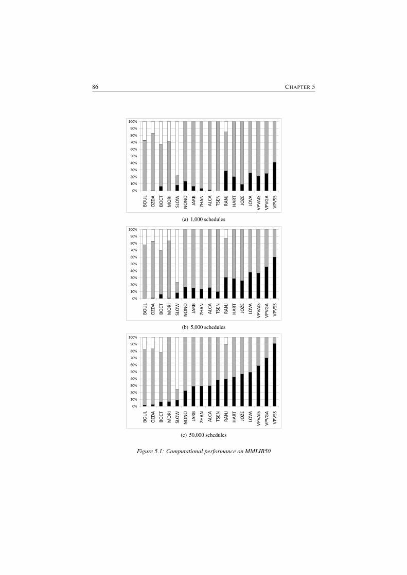
86 CHAPTER 5
0%
10%
20%
30%
40%
50%
60%
70%
80%
90%
100%
BOUL
OZD
A
BOCT
MORI
SLOW
NONO
JARB
ZHAN
ALCA
TSEN
RANJ
HART
JOZE
LOVA
VPVAIS
VPVGA
VPVSS
(a) 1,000 schedules
0%
10%
20%
30%
40%
50%
60%
70%
80%
90%
100%
BOUL
OZD
A
BOCT
MORI
SLOW
NONO
JARB
ZHAN
ALCA
TSEN
RANJ
HART
JOZE
LOVA
VPVAIS
VPVGA
VPVSS
(b) 5,000 schedules
0%
10%
20%
30%
40%
50%
60%
70%
80%
90%
100%
BOUL
OZD
A
BOCT
MORI
SLOW
NONO
JARB
ZHAN
ALCA
TSEN
RANJ
HART
JOZE
LOVA
VPVAIS
VPVGA
VPVSS
(c) 50,000 schedules
Figure 5.1: Computational performance on MMLIB50
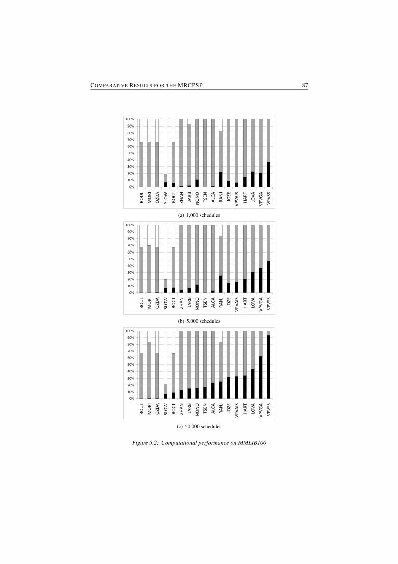
COMPARATIVE RESULTS FOR THE MRCPSP 87
0%
10%
20%
30%
40%
50%
60%
70%
80%
90%
100%
BOUL
MORI
OZD
A
SLOW
BOCT
ZHAN
JARB
NONO
TSEN
ALCA
RANJ
JOZE
VPVAIS
HART
LOVA
VPVGA
VPVSS
(a) 1,000 schedules
0%
10%
20%
30%
40%
50%
60%
70%
80%
90%
100%
BOUL
MORI
OZD
A
SLOW
BOCT
ZHAN
JARB
NONO
TSEN
ALCA
RANJ
JOZE
VPVAIS
HART
LOVA
VPVGA
VPVSS
(b) 5,000 schedules
0%
10%
20%
30%
40%
50%
60%
70%
80%
90%
100%
BOUL
MORI
OZD
A
SLOW
BOCT
ZHAN
JARB
NONO
TSEN
ALCA
RANJ
JOZE
VPVAIS
HART
LOVA
VPVGA
VPVSS
(c) 50,000 schedules
Figure 5.2: Computational performance on MMLIB100
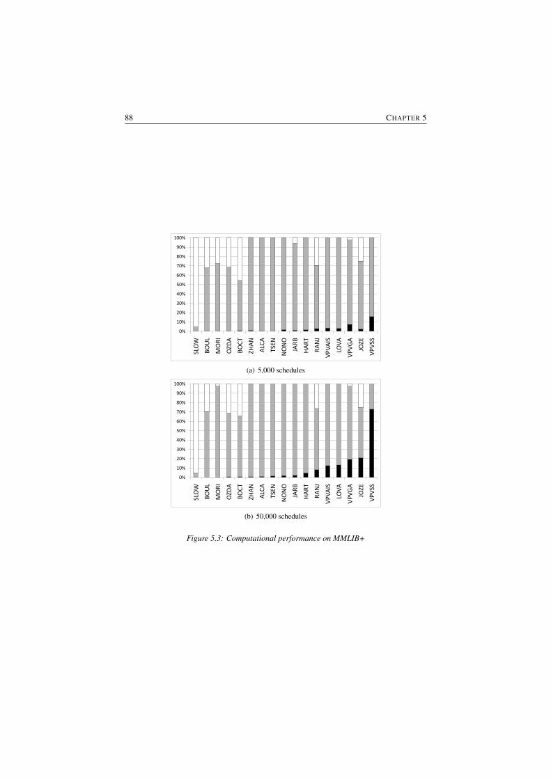
88 CHAPTER 5
0%
10%
20%
30%
40%
50%
60%
70%
80%
90%
100%
SLOW
BOUL
MORI
OZD
A
BOCT
ZHAN
ALCA
TSEN
NONO
JARB
HART
RANJ
VPVAIS
LOVA
VPVGA
JOZE
VPVSS
(a) 5,000 schedules
0%
10%
20%
30%
40%
50%
60%
70%
80%
90%
100%
SLOW
BOUL
MORI
OZD
A
BOCT
ZHAN
ALCA
TSEN
NONO
JARB
HART
RANJ
VPVAIS
LOVA
VPVGA
JOZE
VPVSS
(b) 50,000 schedules
Figure 5.3: Computational performance on MMLIB+

Part II
Extensions to the MRCPSP

6Preemption
6.1 Introduction
The basic RCPSP and MRCPSP assume that each activity, once started, will beexecuted until its completion. The extension to the preemptive multi-mode ver-sion (P-MRCPSP) allows activities to be preempted at any integer time instanceand restarted later on at no additional cost. For the single-mode case, Kaplan(1988), Demeulemeester and Herroelen (1996) and Vanhoucke and Debels (2008)present exact algorithms, while Damay et al. (2007) propose a linear programmingbased algorithm. Ballestin et al. (2008) reveal the benefits of allowing only 1 in-terruption per activity and prove the effectiveness of justification in the presenceof preemption. Ballestin et al. (2009) investigate the effect of interruption on theproject makespan in more general cases and analyze the usefulness of preemp-tion in the presence of due dates. For the multi-mode case, Buddhakulsomsiri andKim (2006) prove that preemption is very effective to improve the optimal projectmakespan in the presence of resource vacations and temporary resource unavail-ability and that the makespan improvement is dependent on the parameters thatimpact resource utilization. To the best of our knowledge, no further research hasbeen performed on the P-MRCPSP.
In this chapter, a genetic algorithm approach for solving the P-MRCPSP isintroduced. In section 6.2 the problem formulation of the P-MRCPSP is presented,while in section 6.3 the details of the solution procedure are described. In section6.4, the computational results for the MRCPSP with activity preemption executed
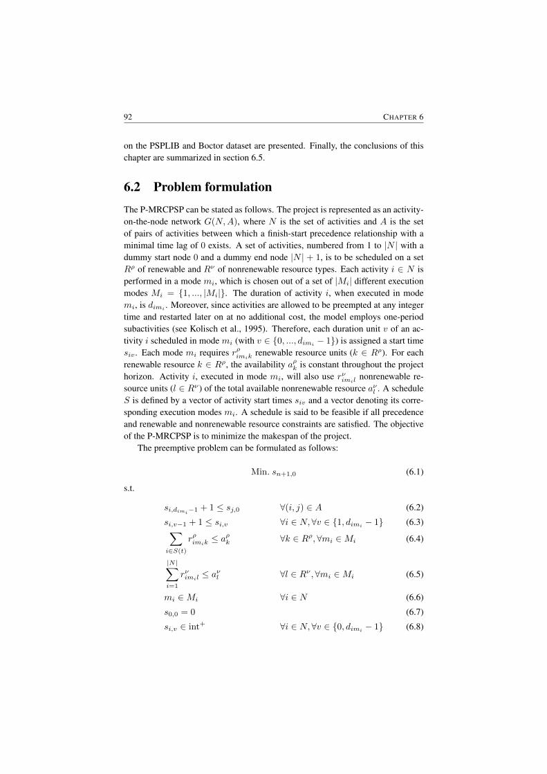
92 CHAPTER 6
on the PSPLIB and Boctor dataset are presented. Finally, the conclusions of thischapter are summarized in section 6.5.
6.2 Problem formulationThe P-MRCPSP can be stated as follows. The project is represented as an activity-on-the-node network G(N,A), where N is the set of activities and A is the setof pairs of activities between which a finish-start precedence relationship with aminimal time lag of 0 exists. A set of activities, numbered from 1 to |N | with adummy start node 0 and a dummy end node |N | + 1, is to be scheduled on a setRρ of renewable and Rν of nonrenewable resource types. Each activity i ∈ N isperformed in a mode mi, which is chosen out of a set of |Mi| different executionmodes Mi = {1, ..., |Mi|}. The duration of activity i, when executed in modemi, is dimi . Moreover, since activities are allowed to be preempted at any integertime and restarted later on at no additional cost, the model employs one-periodsubactivities (see Kolisch et al., 1995). Therefore, each duration unit v of an ac-tivity i scheduled in mode mi (with v ∈ {0, ..., dimi − 1}) is assigned a start timesiv . Each mode mi requires rρimik renewable resource units (k ∈ Rρ). For eachrenewable resource k ∈ Rρ, the availability aρk is constant throughout the projecthorizon. Activity i, executed in mode mi, will also use rνimil nonrenewable re-source units (l ∈ Rν) of the total available nonrenewable resource aνl . A scheduleS is defined by a vector of activity start times siv and a vector denoting its corre-sponding execution modes mi. A schedule is said to be feasible if all precedenceand renewable and nonrenewable resource constraints are satisfied. The objectiveof the P-MRCPSP is to minimize the makespan of the project.
The preemptive problem can be formulated as follows:
Min. sn+1,0 (6.1)
s.t.
si,dimi−1 + 1 ≤ sj,0 ∀(i, j) ∈ A (6.2)
si,v−1 + 1 ≤ si,v ∀i ∈ N, ∀v ∈ {1, dimi − 1} (6.3)∑i∈S(t)
rρimik ≤ aρk ∀k ∈ Rρ,∀mi ∈Mi (6.4)
|N |∑i=1
rνimil ≤ aνl ∀l ∈ Rν ,∀mi ∈Mi (6.5)
mi ∈Mi ∀i ∈ N (6.6)
s0,0 = 0 (6.7)
si,v ∈ int+ ∀i ∈ N, ∀v ∈ {0, dimi − 1} (6.8)
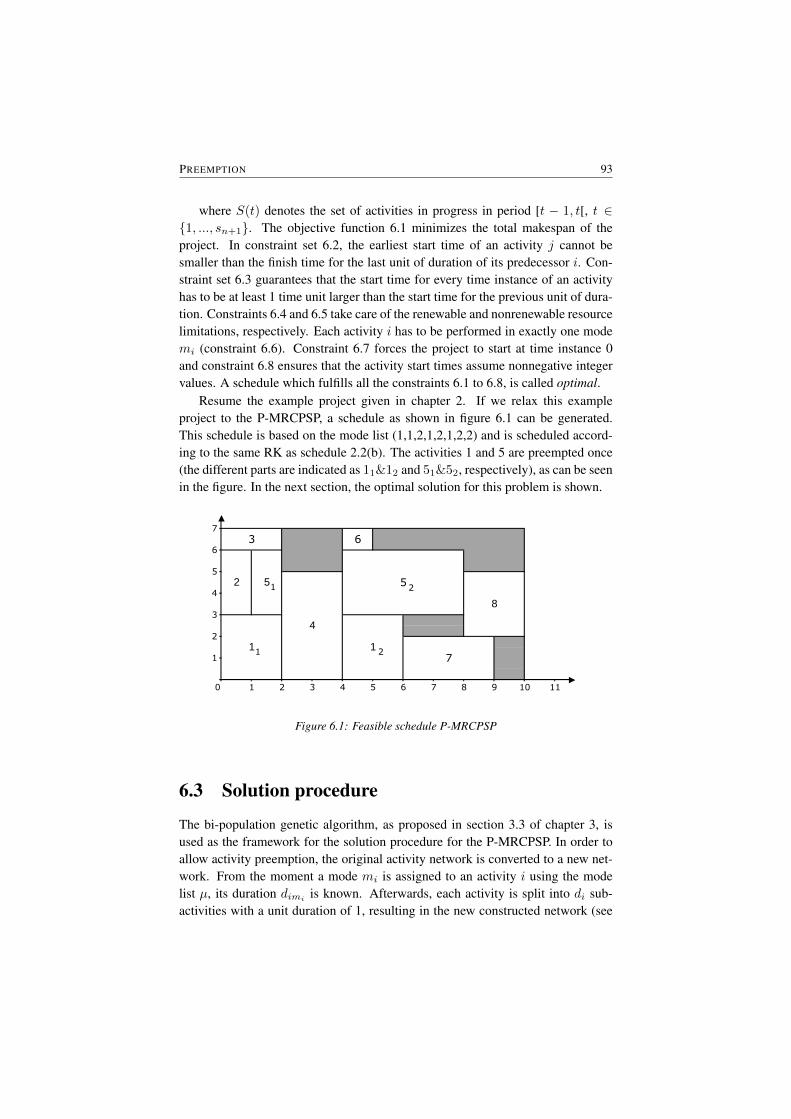
PREEMPTION 93
where S(t) denotes the set of activities in progress in period [t − 1, t[, t ∈{1, ..., sn+1}. The objective function 6.1 minimizes the total makespan of theproject. In constraint set 6.2, the earliest start time of an activity j cannot besmaller than the finish time for the last unit of duration of its predecessor i. Con-straint set 6.3 guarantees that the start time for every time instance of an activityhas to be at least 1 time unit larger than the start time for the previous unit of dura-tion. Constraints 6.4 and 6.5 take care of the renewable and nonrenewable resourcelimitations, respectively. Each activity i has to be performed in exactly one modemi (constraint 6.6). Constraint 6.7 forces the project to start at time instance 0and constraint 6.8 ensures that the activity start times assume nonnegative integervalues. A schedule which fulfills all the constraints 6.1 to 6.8, is called optimal.
Resume the example project given in chapter 2. If we relax this exampleproject to the P-MRCPSP, a schedule as shown in figure 6.1 can be generated.This schedule is based on the mode list (1,1,2,1,2,1,2,2) and is scheduled accord-ing to the same RK as schedule 2.2(b). The activities 1 and 5 are preempted once(the different parts are indicated as 11&12 and 51&52, respectively), as can be seenin the figure. In the next section, the optimal solution for this problem is shown.
6
7
8
4
7
6
3
5
4
3
2
1
1
2 5
110 1 2 3 4 5
1
5
6 7 8 9 10
1
1
2
2
Figure 6.1: Feasible schedule P-MRCPSP
6.3 Solution procedure
The bi-population genetic algorithm, as proposed in section 3.3 of chapter 3, isused as the framework for the solution procedure for the P-MRCPSP. In order toallow activity preemption, the original activity network is converted to a new net-work. From the moment a mode mi is assigned to an activity i using the modelist µ, its duration dimi is known. Afterwards, each activity is split into di sub-activities with a unit duration of 1, resulting in the new constructed network (see
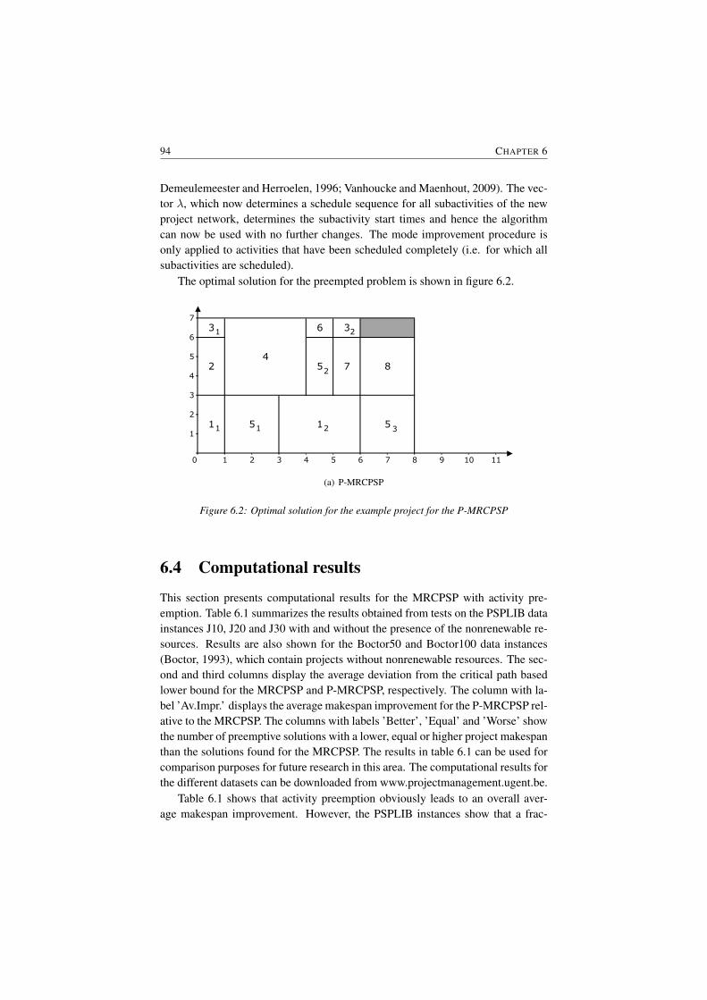
94 CHAPTER 6
Demeulemeester and Herroelen, 1996; Vanhoucke and Maenhout, 2009). The vec-tor λ, which now determines a schedule sequence for all subactivities of the newproject network, determines the subactivity start times and hence the algorithmcan now be used with no further changes. The mode improvement procedure isonly applied to activities that have been scheduled completely (i.e. for which allsubactivities are scheduled).
The optimal solution for the preempted problem is shown in figure 6.2.
2
3
10
7
6
2
5
4
3
9
1
0 1 2 3
7
4 5 6 7 8
5
8
11
1
3
5
4
1
5
61 2
1 1 2
2
3
(a) P-MRCPSP
Figure 6.2: Optimal solution for the example project for the P-MRCPSP
6.4 Computational results
This section presents computational results for the MRCPSP with activity pre-emption. Table 6.1 summarizes the results obtained from tests on the PSPLIB datainstances J10, J20 and J30 with and without the presence of the nonrenewable re-sources. Results are also shown for the Boctor50 and Boctor100 data instances(Boctor, 1993), which contain projects without nonrenewable resources. The sec-ond and third columns display the average deviation from the critical path basedlower bound for the MRCPSP and P-MRCPSP, respectively. The column with la-bel ’Av.Impr.’ displays the average makespan improvement for the P-MRCPSP rel-ative to the MRCPSP. The columns with labels ’Better’, ’Equal’ and ’Worse’ showthe number of preemptive solutions with a lower, equal or higher project makespanthan the solutions found for the MRCPSP. The results in table 6.1 can be used forcomparison purposes for future research in this area. The computational results forthe different datasets can be downloaded from www.projectmanagement.ugent.be.
Table 6.1 shows that activity preemption obviously leads to an overall aver-age makespan improvement. However, the PSPLIB instances show that a frac-
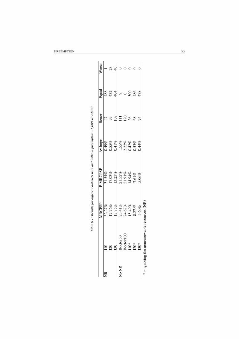
PREEMPTION 95
Tabl
e6.
1:R
esul
tsfo
rdi
ffere
ntda
tase
tsw
ithan
dw
ithou
tpre
empt
ion
-5,0
00sc
hedu
les
MR
CPS
PP-
MR
CPS
PA
v.Im
pr.
Bet
ter
Equ
alW
orse
NR
J10
32.2
7%31
.54%
0.49
%47
488
1J2
017
.76%
17.0
3%0.
55%
9943
223
J30
13.7
5%13
.23%
0.41
%10
840
440
No
NR
Boc
tor5
023
.41%
21.5
2%1.
55%
111
90
Boc
tor1
0024
.67%
21.9
1%2.
22%
120
00
J10*
15.4
9%14
.94%
0.42
%36
500
0J2
0*8.
27.%
7.61
%0.
53%
6848
60
J30*
5.60
%5.
06%
0.44
%74
478
0*
=ig
nori
ngth
eno
nren
ewab
lere
sour
ces
(NR
)
96 CHAPTER 6
tion of the projects shows a higher makespan with preemption compared to thebest found MRCPSP solution. Indeed, introducing activity preemption results in alarger project network, since each non-preempted activity needs to be splitted intosubactivities, leading to an increase of the random key size. This larger RK searchspace is responsible for the fraction of solutions displayed in the ’Worse’ column.
The table also shows that activity preemption always leads to better solutions(the column ’Worse’ is equal to 0) when no nonrenewable resources are taken intoaccount. In that case, infeasible mode assignments will never occur, leaving moreroom to the algorithm to select low duration modes. Obviously, when nonrenew-able resources are taken into account, the low durations correspond to relativelyhigh nonrenewable resource demand, leading to infeasible mode assignments. Weindeed observe that the best found solutions without nonrenewable resources con-tain many mode assignments with low activity durations, which is in line with thestudy of Boctor (1993) who has shown that the ’shortest feasible mode’ selectionrule performs best.
The results of the introduction of preemption on the new datasets MMLIB50and MMLIB100 are presented in table 6.2. The results are in line with the resultsobtained for the PSPLIB and Boctor dataset: in case nonrenewable resources aretaken into account, the procedure is not always able to find similar or better resultsthan in the non-preempted case. In case no nonrenewable resources are considered,no inferior results are obtained.
6.5 ConclusionsIn this chapter, we have designed an adapted version of the genetic algorithm forthe preemptive multi-mode resource-constrained project scheduling problem. Theresults of the computational tests performed on the PSPLIB dataset revealed thatthe introduction of preemption does significantly help in decreasing the averageproject makespan compared to the non-preempted case. If no nonrenewable re-sources are taken into account, the introduction of preemption always leads tobetter solutions.

PREEMPTION 97
Tabl
e6.
2:R
esul
tsfo
rth
eM
MLI
Bda
tase
twith
and
with
outp
reem
ptio
n-5
,000
sche
dule
s
MR
CPS
PP-
MR
CPS
PA
v.Im
pr.
Bet
ter
Equ
alW
orse
NR
MM
LIB
5020
,164
20,0
920.
30%
154
299
87M
ML
IB10
025
,623
25,5
570.
16%
169
249
122
No
NR
MM
LIB
50*
17,1
4917
,032
0.62
%94
446
0M
ML
IB10
0*21
,839
21,5
830.
98%
133
407
0*
=ig
nori
ngth
eno
nren
ewab
lere
sour
ces
(NR
)


7Introduction of Learning Effects
7.1 Introduction
Project scheduling has been a research topic for many decades, resulting in a widevariety of optimization procedures. The main focus on the project lead time min-imization has led to the development of various exact and (meta)heuristic pro-cedures for scheduling projects with tight resource constraints under a wide va-riety of assumptions. The basic problem type in project scheduling is the well-known resource-constrained project scheduling problem (RCPSP). This problemtype aims at minimizing the total duration or makespan of a project subject toprecedence relations between the activities and the limited renewable resourceavailabilities, and is known to be NP-hard (Blazewicz et al., 1983).
In most projects, human resources are a critical factor in the scheduling pro-cess. Not only their availability, but also their productivity will influence theproject duration. One of the reasons why the productivity of a human resourcevaries over time is the effect of learning (Wright, 1936), which indicates the pro-cess of acquiring experience while performing similar activities leading to an im-provement of the worker’s skill. As a measurable result of learning, the time re-quired to perform the next jobs decreases (Janiak and Rudek, 2007).
However, in the project scheduling literature, most models assume static andoften homogeneous efficiencies of resources (Heimerl and Kolisch, 2009). In thischapter, the effect of learning on the efficiency of human resources is studied forthe well-known discrete time/resource trade-off problem (DTRTP). In this sched-
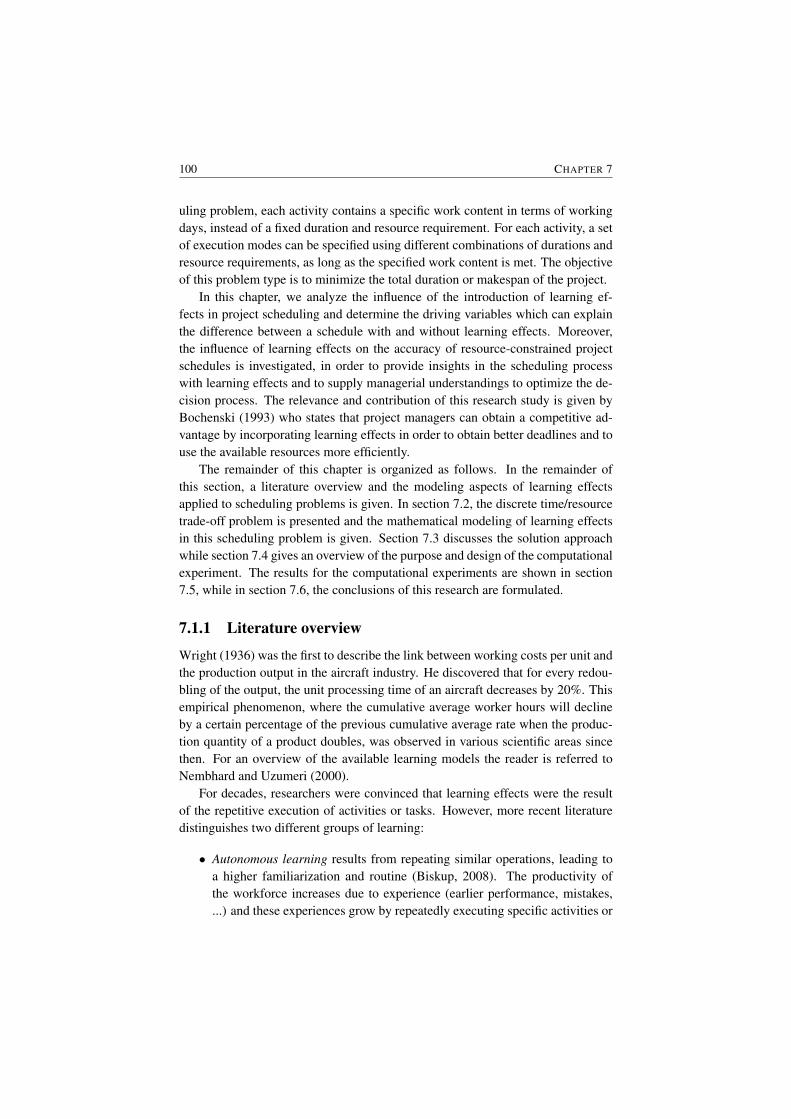
100 CHAPTER 7
uling problem, each activity contains a specific work content in terms of workingdays, instead of a fixed duration and resource requirement. For each activity, a setof execution modes can be specified using different combinations of durations andresource requirements, as long as the specified work content is met. The objectiveof this problem type is to minimize the total duration or makespan of the project.
In this chapter, we analyze the influence of the introduction of learning ef-fects in project scheduling and determine the driving variables which can explainthe difference between a schedule with and without learning effects. Moreover,the influence of learning effects on the accuracy of resource-constrained projectschedules is investigated, in order to provide insights in the scheduling processwith learning effects and to supply managerial understandings to optimize the de-cision process. The relevance and contribution of this research study is given byBochenski (1993) who states that project managers can obtain a competitive ad-vantage by incorporating learning effects in order to obtain better deadlines and touse the available resources more efficiently.
The remainder of this chapter is organized as follows. In the remainder ofthis section, a literature overview and the modeling aspects of learning effectsapplied to scheduling problems is given. In section 7.2, the discrete time/resourcetrade-off problem is presented and the mathematical modeling of learning effectsin this scheduling problem is given. Section 7.3 discusses the solution approachwhile section 7.4 gives an overview of the purpose and design of the computationalexperiment. The results for the computational experiments are shown in section7.5, while in section 7.6, the conclusions of this research are formulated.
7.1.1 Literature overview
Wright (1936) was the first to describe the link between working costs per unit andthe production output in the aircraft industry. He discovered that for every redou-bling of the output, the unit processing time of an aircraft decreases by 20%. Thisempirical phenomenon, where the cumulative average worker hours will declineby a certain percentage of the previous cumulative average rate when the produc-tion quantity of a product doubles, was observed in various scientific areas sincethen. For an overview of the available learning models the reader is referred toNembhard and Uzumeri (2000).
For decades, researchers were convinced that learning effects were the resultof the repetitive execution of activities or tasks. However, more recent literaturedistinguishes two different groups of learning:
• Autonomous learning results from repeating similar operations, leading toa higher familiarization and routine (Biskup, 2008). The productivity ofthe workforce increases due to experience (earlier performance, mistakes,...) and these experiences grow by repeatedly executing specific activities or

INTRODUCTION OF LEARNING EFFECTS 101
tasks. This type of learning is also referred to as learning-by-doing or theHorndal-effect.
• Induced learning is the result of management investing in the know-howand the productivity of the human resources (Adler and Clark, 1991; Uptonand Kim, 1998). Additional training, changes in the remuneration systemand production environment, innovative education or incentive schemes areexamples of management decisions that can influence the learning rate ofthe human resources. Important in this case is the determination of the opti-mal learning rate, since a reduction of the learning rate is usually related tohigher costs.
Learning effects have been discussed in the scheduling literature from variousangles.
In a review paper on the different learning models proposed in the machinescheduling literature, Biskup (2008) makes a distinction between position-basedlearning, where the learning is only affected by the number of tasks being pro-cessed, and the sum-of-processing-time learning, that takes into account the pro-cessing time of all jobs processed so far.
In the staff scheduling literature, several authors already modeled efficiency tocope with the effects of learning. Wu and Sun (2006) denote that the efficiencyof staff will improve by doing more. They develop a genetic algorithm to mini-mize the total outsourcing costs for a project with a fixed time horizon. Heimerland Kolisch (2009) present an optimization model to address the problem of as-signing project work to multi-skilled internal and external human resources whileconsidering learning, depreciation of knowledge and company skill level targets.
In multi-project scheduling, Shtub et al. (1996) and Amor and Teplitz (1998)develop heuristic and metaheuristic procedures for scheduling projects with a repet-itive nature under learning effects. Ash and Smith-Daniels (1999) present a heuris-tic for a multi-project scheduling problem where project preemption is allowed andlearning, forgetting and relearning effects are introduced. They state that, duringthe execution of an activity in development projects, people continuously learn andbecome more activity-efficient. They define learning as the increased productivityduring the course of each project activity (activity-specific learning).
The empirical evidence that learning takes place over time can be found inBrazel (1972) and Sahal (1979), who show that the same power function learn-ing model as the repetition-based learning model noted by Wright (1936) can beused. Hanakawa et al. (1998) reveal that learning effects exist in project settingsin general and software development settings in particular. They show that theproductivity of a developer will increase if he/she stays on the task longer. Thevariations of the productivity depend on the developer’s knowledge, experienceand learning curves. Another behavioral study of Hendriks et al. (1999) reveals

102 CHAPTER 7
that two factors can affect the staff allocation: the project scatter, which indicatesthat the team efficiency will increase if the number of team staff is larger thanneeded, and the resource dedication, which denotes that the dedication of a staffmember to a particular job can increase efficiency.
The focus of this work is on the introduction of autonomous and activity-specific learning curves in a multi-mode project scheduling environment.
7.1.2 Modeling
The introduction of the learning concepts in scheduling environments requires amathematical formulation. The following assumptions and definitions are formu-lated:
• The efficiency of a human resource is defined as the portion of work per-formed in one time unit by a human resource, assuming that the entire tasktakes one time unit for an employee working at a normal level (i.e. efficiency= 100%) (Gutjahr et al., 2008).
• A person working at a uniform efficiency level of 100% during one day, isperforming one working day.
• A man-day is defined as the period of time needed to execute the work per-formed on one working day by one person, taking into account its averageefficiency level.
• The work content of a specific activity is expressed in working days. Inproject scheduling environments without learning effects, the number ofworking days to execute an activity is equal to the number of man-days.When learning effects are considered, the number of man-days to executethe work content of an activity depends on the activity duration and the val-ues of the learning variables (i.e. efficiency).
• Throughout this chapter, it is assumed that every resource performing ac-tivity i has the same initial average efficiency level Ei1 and learning rateLi (denoted by E1 and L). This is in contrast with other authors (see e.g.Gutjahr et al., 2008) who assume that every employee possesses differentknowledge, education, skills, abilities, etc. in different fields.
The traditional learning curve is a downward sloping power function that rep-resents the amount of time spent to complete the next iteration of a single task andis frequently formalized by using the following formula:
Tn = T1n−b (7.1)

INTRODUCTION OF LEARNING EFFECTS 103
where Tn is the average processing time of the n-th unit of the cumulativeproduction quantity n, T1 the production time of the first unit and b = −log2Lthe learning index depending on the learning rate L, which indicates the learningachieved. Thus, the lower the learning rate L, the higher the effects from learningwill be.
Average efficiency Based on this traditional learning curve, Wu and Sun (2006)defined the average efficiency curve, representing the activity-specific knowledgeof a resource after a time period t for a specific activity i, as follows:
Eit = Ei1tbi (7.2)
where Ei1 indicates the initial efficiency curve of activity i and bi is the learn-ing index of activity i depending on the activity-specific learning rate Li. Thisformula indicates that when a human resource works longer on an activity, hisor her average activity-specific efficiency level and competency increases. Infigure 7.1(a), the average efficiency curve is shown for a human resource withan initial average efficiency E1 of 0.7 and a learning rate L of 0.85. Basedon the formulation, one can calculate that the average efficiency at time 10 is0.7 ∗ 10−log20.85 = 1.201.
Real efficiency The average efficiency curve only indicates the average of the(actual) efficiency values over the time period [0,t]. As shown, the average ef-ficiency at time 10 in the example is 1.201 and indicates the average of all theefficiencies over the period [0,10]. This leads to a total of 12.01 working daysexecuted during the first 10 days (1.201 * 1 day) (see also figure 7.1(a)). The sameresult is obtained by calculating the surface under the real efficiency curve, whichindicates the efficiency Eit of a resource i on a specific time instant t. The realefficiency Eit can be formulated as follows:
Eit = Ei1(1 + bi)tbi (7.3)
The efficiency curve is shown in figure 7.1(b). The efficiency at time 10 is1.483, which is obviously higher than the average efficiency at that time instant.The surface under the efficiency curve for the period [0,10] is 12.01 which is ob-viously equal to the surface of the rectangle in figure 7.1(a).
Number of man-days The formula of the efficiency curve will be used to calcu-late the number of man-days needed to execute a specific work content. Therefore,the number of working days performed by one human resource during T man-days(Dw
T ) is first calculated. Since the assumption is made that the work content is ex-pressed in working days, Dw
T can be calculated as:
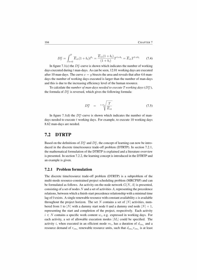
104 CHAPTER 7
DwT =
∫ T
t=0
Ei1(1 + bi)tbi =
Ei1(1 + bi)
(1 + bi)T 1+bi = Ei1T
1+bi (7.4)
In figure 7.1(c) the DwT -curve is shown which indicates the number of working
days executed during tman-days. As can be seen, 12.01 working days are executedafter 10 man-days. The curve x = y bisects the area and reveals that after 4.6 man-days the number of working days executed is larger than the number of man-daysand this is due to the increasing efficiency level of the human resource.
To calculate the number of man-days needed to execute T working days (DmT ),
the formula of DwT is reversed, which gives the following formula:
DmT = 1+bi
√T
Ei1(7.5)
In figure 7.1(d) the DmT -curve is shown which indicates the number of man-
days needed to execute t working days. For example, to execute 10 working days8.62 man-days are needed.
7.2 DTRTPBased on the definitions of Dm
T and DwT , the concept of learning can now be intro-
duced in the discrete time/resource trade-off problem (DTRTP). In section 7.2.1,the mathematical formulation of the DTRTP is explained and a literature overviewis presented. In section 7.2.2, the learning concept is introduced in the DTRTP andan example is given.
7.2.1 Problem formulation
The discrete time/resource trade-off problem (DTRTP) is a subproblem of themulti-mode resource-constrained project scheduling problem (MRCPSP) and canbe formulated as follows. An activity-on-the-node network G(N,A) is presented,consisting of a set of nodesN and a set of activitiesA, representing the precedencerelations, between which a finish-start precedence relationship with a minimal timelag of 0 exists. A single renewable resource with constant availability a is availablethroughout the project horizon. The set N contains a set of |N | activities, num-bered from 1 to |N | with a dummy start node 0 and a dummy end node |N | + 1,representing the start and completion of the project, respectively. Each activityi ∈ N contains a specific work content wi, e.g. expressed in working days. Foreach activity, a set of allowable execution modes |Mi| could be specified. Theactivity i, when executed in an efficient mode mi, has a duration of dimi and aresource demand of rimi renewable resource units, such that dimirimi is at least
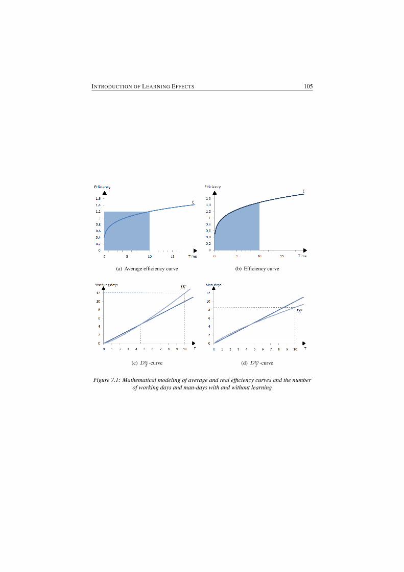
INTRODUCTION OF LEARNING EFFECTS 105
(a) Average efficiency curve
(b) Efficiency curve
(c) DwT -curve (d) DmT -curve
Figure 7.1: Mathematical modeling of average and real efficiency curves and the numberof working days and man-days with and without learning

106 CHAPTER 7
equal to and as close as possible to wi. A mode is called efficient if every othermode has either a strictly higher duration or a strictly higher resource demand.The objective is to schedule each activity in one of its execution modes, subject toboth the precedence and resource constraint, under the objective to minimize theproject makespan. The problem can be formulated as follows:
minimize fn (7.6)
subject to fi + djmj ≤ fj ∀(i, j) ∈ A (7.7)∑i∈S(t)
rimi ≤ a ∀mi ∈Mi,∀t (7.8)
mi ∈Mi ∀i ∈ N (7.9)
f0 = 0 (7.10)
fi ∈ int+ ∀i ∈ N (7.11)
where S(t) denotes the set of activities in progress in period ]t − 1, t] and fithe finish time of the ith activity.
Demeulemeester et al. (2000) present an efficient branch-and-bound approachto solve the DTRTP, while De Reyck et al. (1998) present several heuristic proce-dures, based on local search procedures and Tabu Search (TS). Recently, Ranjbarand Kianfar (2007) have developed a genetic algorithm and Ranjbar et al. (2009)presented a scatter search procedure. In this work, we will use an adapted versionof the bi-genetic algorithm of Van Peteghem and Vanhoucke (2010), who presentstate-of-the-art results for the multi-mode resource-constrained project schedulingproblem. The adaptions will be discussed in detail in section 7.3.1.
To incorporate the learning concept into this model, equation 7.11 should beremoved and equation 7.7 should be defined as
fi + 1+bj
√djmj
Ej1≤ fj ∀(i, j) ∈ A (7.12)
with bj the learning rate and Ej1 the initial efficiency. In case no learning
effects occur (i.e. Lj=100% and Ej1=100%), the value 1+bj
√djmjEj1
is equal to
djmj .
7.2.2 Learning effects in the DTRTP
For every activity in the DTRTP, the work content, expressed in working days, isknown in advance and based on this work content, several execution modes canbe determined. Consider an activity i with a work content of 12 working days.
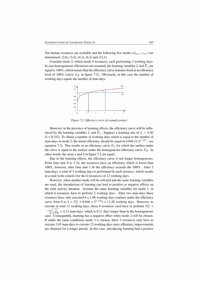
INTRODUCTION OF LEARNING EFFECTS 107
Ten human resources are available and the following five modes (dimi , rimi ) aredetermined: (2,6), (3,4), (4,3), (6,2) and (12,1).
Consider mode 2, which needs 4 resources, each performing 3 working days.In case homogeneous efficiencies are assumed, the learning variables L andE1 areequal to 100%, which means that the efficiency curve remains fixed at an efficiencylevel of 100% (curve EH in figure 7.2). Obviously, in this case the number ofworking days equals the number of man-days.
Figure 7.2: Efficiency curve of example project
However, in the presence of learning effects, the efficiency curve will be influ-enced by the learning variables L and E1. Suppose a learning rate of L = 0.90
(b = 0.152). To obtain a number of working days which is equal to the number ofman-days in mode 2, the initial efficiency should be equal to 0.846 (3/31.152 - seeequation 7.3). This results in an efficiency curve EL for which the surface underthe curve is equal to the surface under the homogeneous efficiency curve EH . Inother words, the areas a and b in figure 7.2 are equal.
Due to the learning effects, the efficiency curve is not longer homogeneous.From time unit 0 to 1.16, the resources have an efficiency which is lower than100%, however, after time unit 1.16 the efficiency exceeds the 100%. After 3man-days, a total of 3 working days is performed by each resource, which resultsin a total work content (for the 4 resources) of 12 working days.
However, when another mode will be selected and the same learning variablesare used, the introduction of learning can lead to positive or negative effects onthe total activity duration. Assume the same learning variables for mode 1, inwhich 6 resources have to perform 2 working days. After two man-days theseresources have only executed 6 x 1.88 working days (surface under the efficiencycurve from 0 to 2 = Dw
2 = 0.846 x 21.152) = 11.28 working days. However, toexecute in total 12 working days, these 6 resources each have to perform Dm
2 =1.152
√2
0.846 = 2.11 man-days, which is 0.11 days longer than in the homogeneouscase. Consequently, learning has a negative effect when mode 2 will be chosen.If under the same conditions mode 3 is chosen, these 3 resources only have toexecute 3.85 man-days to execute 12 working days since efficiency improvementsare obtained for a longer period. In this case, introducing learning had a positive

108 CHAPTER 7
effect on the duration of mode 3. An overview of the other execution modes canbe found in table 7.1.
mode dim rim wihomogeneous learning homogeneous learning
1 2 2.11 6 12 12.662 3 3 4 12 123 4 3.85 3 12 11.554 6 5.48 2 12 10.965 12 9.99 1 12 9.99
Table 7.1: Duration and total work content with and without learning
As can be seen in the table, the introduction of learning effects introduces a newtrade-off between the activity duration and the total work content. Since workinglonger on an activity will decrease the total work content expressed in man-days, itbecomes more interesting to execute the activity in a mode with a smaller resourcedemand since these resources will become more efficient when they work longeron the activity. However, shorter execution modes are in favor of the objective tominimize the total makespan of the project, although their total work content willbe larger.
7.3 Solution approachThis section briefly discusses the adaptations made on an existing solution proce-dure in order to take the learning effects into account, and shows that this proce-dure can compete with current state-of-the-art solution procedures for the DTRTPwithout learning effects.
7.3.1 Solution procedure
In order to test the impact of activity learning on the total project duration, anadapted version of the bi-population based genetic algorithm of Van Peteghem andVanhoucke (2010) has been used. This procedure has been originally developedto solve multi-mode resource-constrained project scheduling problems within thepresence of renewable and nonrenewable resource constraints. In order to incorpo-rate learning curves during the construction of a baseline schedule, the followingadaptions have been made:
• Since the introduction of the learning effect creates non-integer durationsfor each of the different modes, the schedule generation scheme has beenadapted to deal with these fractional durations.
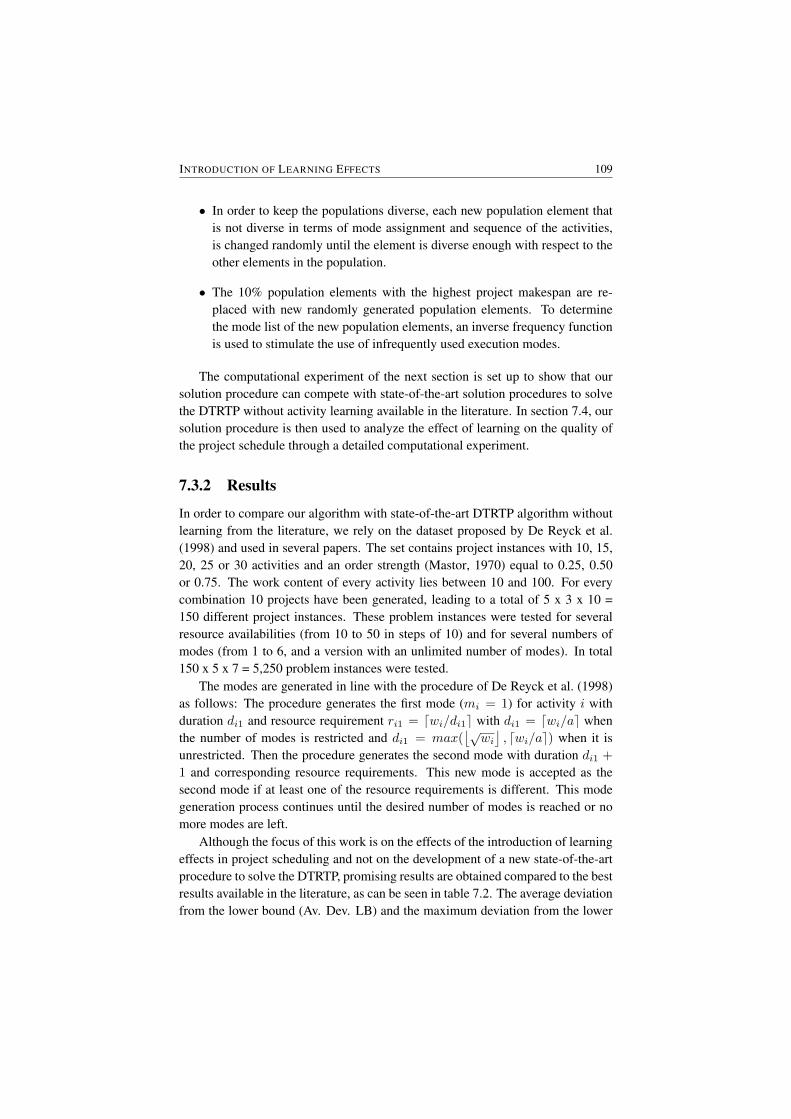
INTRODUCTION OF LEARNING EFFECTS 109
• In order to keep the populations diverse, each new population element thatis not diverse in terms of mode assignment and sequence of the activities,is changed randomly until the element is diverse enough with respect to theother elements in the population.
• The 10% population elements with the highest project makespan are re-placed with new randomly generated population elements. To determinethe mode list of the new population elements, an inverse frequency functionis used to stimulate the use of infrequently used execution modes.
The computational experiment of the next section is set up to show that oursolution procedure can compete with state-of-the-art solution procedures to solvethe DTRTP without activity learning available in the literature. In section 7.4, oursolution procedure is then used to analyze the effect of learning on the quality ofthe project schedule through a detailed computational experiment.
7.3.2 Results
In order to compare our algorithm with state-of-the-art DTRTP algorithm withoutlearning from the literature, we rely on the dataset proposed by De Reyck et al.(1998) and used in several papers. The set contains project instances with 10, 15,20, 25 or 30 activities and an order strength (Mastor, 1970) equal to 0.25, 0.50or 0.75. The work content of every activity lies between 10 and 100. For everycombination 10 projects have been generated, leading to a total of 5 x 3 x 10 =150 different project instances. These problem instances were tested for severalresource availabilities (from 10 to 50 in steps of 10) and for several numbers ofmodes (from 1 to 6, and a version with an unlimited number of modes). In total150 x 5 x 7 = 5,250 problem instances were tested.
The modes are generated in line with the procedure of De Reyck et al. (1998)as follows: The procedure generates the first mode (mi = 1) for activity i withduration di1 and resource requirement ri1 = dwi/di1e with di1 = dwi/ae whenthe number of modes is restricted and di1 = max(
⌊√wi⌋, dwi/ae) when it is
unrestricted. Then the procedure generates the second mode with duration di1 +
1 and corresponding resource requirements. This new mode is accepted as thesecond mode if at least one of the resource requirements is different. This modegeneration process continues until the desired number of modes is reached or nomore modes are left.
Although the focus of this work is on the effects of the introduction of learningeffects in project scheduling and not on the development of a new state-of-the-artprocedure to solve the DTRTP, promising results are obtained compared to the bestresults available in the literature, as can be seen in table 7.2. The average deviationfrom the lower bound (Av. Dev. LB) and the maximum deviation from the lower
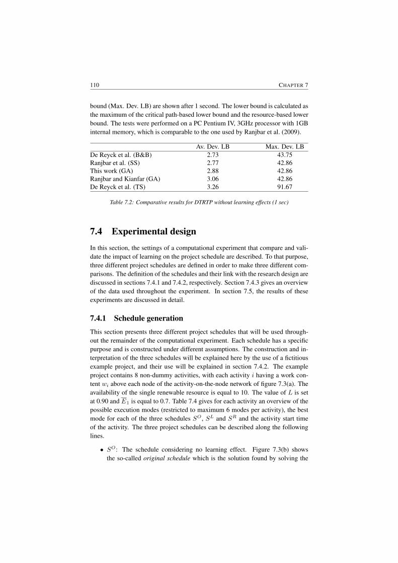
110 CHAPTER 7
bound (Max. Dev. LB) are shown after 1 second. The lower bound is calculated asthe maximum of the critical path-based lower bound and the resource-based lowerbound. The tests were performed on a PC Pentium IV, 3GHz processor with 1GBinternal memory, which is comparable to the one used by Ranjbar et al. (2009).
Av. Dev. LB Max. Dev. LBDe Reyck et al. (B&B) 2.73 43.75Ranjbar et al. (SS) 2.77 42.86This work (GA) 2.88 42.86Ranjbar and Kianfar (GA) 3.06 42.86De Reyck et al. (TS) 3.26 91.67
Table 7.2: Comparative results for DTRTP without learning effects (1 sec)
7.4 Experimental designIn this section, the settings of a computational experiment that compare and vali-date the impact of learning on the project schedule are described. To that purpose,three different project schedules are defined in order to make three different com-parisons. The definition of the schedules and their link with the research design arediscussed in sections 7.4.1 and 7.4.2, respectively. Section 7.4.3 gives an overviewof the data used throughout the experiment. In section 7.5, the results of theseexperiments are discussed in detail.
7.4.1 Schedule generation
This section presents three different project schedules that will be used through-out the remainder of the computational experiment. Each schedule has a specificpurpose and is constructed under different assumptions. The construction and in-terpretation of the three schedules will be explained here by the use of a fictitiousexample project, and their use will be explained in section 7.4.2. The exampleproject contains 8 non-dummy activities, with each activity i having a work con-tent wi above each node of the activity-on-the-node network of figure 7.3(a). Theavailability of the single renewable resource is equal to 10. The value of L is setat 0.90 and E1 is equal to 0.7. Table 7.4 gives for each activity an overview of thepossible execution modes (restricted to maximum 6 modes per activity), the bestmode for each of the three schedules SO, SL and SR and the activity start timeof the activity. The three project schedules can be described along the followinglines.
• SO: The schedule considering no learning effect. Figure 7.3(b) showsthe so-called original schedule which is the solution found by solving the
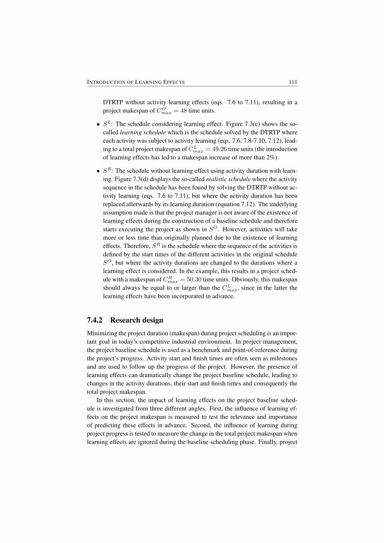
INTRODUCTION OF LEARNING EFFECTS 111
DTRTP without activity learning effects (eqs. 7.6 to 7.11), resulting in aproject makespan of COmax = 48 time units.
• SL: The schedule considering learning effect. Figure 7.3(c) shows the so-called learning schedule which is the schedule solved by the DTRTP whereeach activity was subject to activity learning (eqs. 7.6, 7.8-7.10, 7.12), lead-ing to a total project makespan ofCLmax = 49.26 time units (the introductionof learning effects has led to a makespan increase of more than 2%).
• SR: The schedule without learning effect using activity duration with learn-ing. Figure 7.3(d) displays the so-called realistic schedule where the activitysequence in the schedule has been found by solving the DTRTP without ac-tivity learning (eqs. 7.6 to 7.11), but where the activity duration has beenreplaced afterwards by its learning duration (equation 7.12). The underlyingassumption made is that the project manager is not aware of the existence oflearning effects during the construction of a baseline schedule and thereforestarts executing the project as shown in SO. However, activities will takemore or less time than originally planned due to the existence of learningeffects. Therefore, SR is the schedule where the sequence of the activities isdefined by the start times of the different activities in the original scheduleSO, but where the activity durations are changed to the durations where alearning effect is considered. In the example, this results in a project sched-ule with a makespan of CRmax = 50.30 time units. Obviously, this makespanshould always be equal to or larger than the CLmax, since in the latter thelearning effects have been incorporated in advance.
7.4.2 Research design
Minimizing the project duration (makespan) during project scheduling is an impor-tant goal in today’s competitive industrial environment. In project management,the project baseline schedule is used as a benchmark and point-of-reference duringthe project’s progress. Activity start and finish times are often seen as milestonesand are used to follow up the progress of the project. However, the presence oflearning effects can dramatically change the project baseline schedule, leading tochanges in the activity durations, their start and finish times and consequently thetotal project makespan.
In this section, the impact of learning effects on the project baseline sched-ule is investigated from three different angles. First, the influence of learning ef-fects on the project makespan is measured to test the relevance and importanceof predicting these effects in advance. Second, the influence of learning duringproject progress is tested to measure the change in the total project makespan whenlearning effects are ignored during the baseline scheduling phase. Finally, project
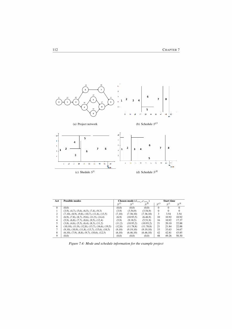
112 CHAPTER 7
54
6527
45
22
86
57
91
00
(a) Project network
(b) Schedule SO
(c) Shedule SL
(d) Schedule SR
Act Possible modes Chosen mode (dimi ,rimi ) Start timeSO SL SR SO SL SR
0 (0,0) (0,0) (0,0) (0,0) 0 0 01 (3,9), (4,7), (5,6), (6,5), (7,4), (9,3) (3,9) (3.54,9) (3.54,9) 0 0 02 (7,10), (8,9), (9,8), (10,7), (11,6), (13,5) (7,10) (7.38,10) (7.38,10) 3 3.54 3.543 (6,9), (7,8), (8,7), (9,6), (11,5), (14,4) (6,9) (10.93,5) (6.46,9) 10 10.92 10.924 (5,9), (6,8), (7,7), (8,6), (9,5), (12,4) (5,9) (9.18,5) (5.51,9) 16 10.92 17.375 (3,8), (4,6), (5,5), (6,4), (8,3), (11,2) (11,2) (10.93,2) (10.93,2) 21 20.10 22.886 (10,10), (11,9), (12,8), (13,7), (16,6), (19,5) (12,8) (11.78,8) (11.78,8) 21 21.84 22.887 (9,10), (10,9), (11,8), (13,7), (15,6), (18,5) (9,10) (9.19,10) (9.19,10) 33 33.63 34.678 (6,10), (7,9), (8,8), (9,7), (10,6), (12,5) (6,10) (6.46,10) (6.46,10) 42 42.81 43.859 (0,0) (0,0) (0,0) (0,0) 48 49.26 50.30
Figure 7.4: Mode and schedule information for the example project
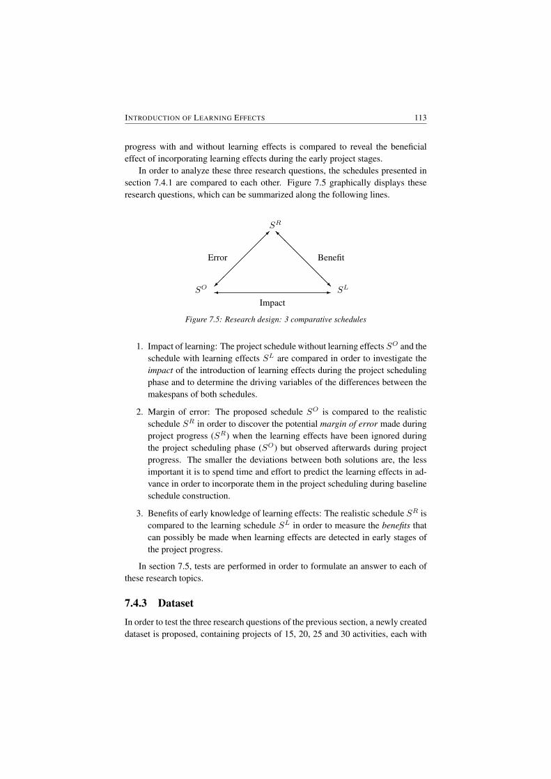
INTRODUCTION OF LEARNING EFFECTS 113
progress with and without learning effects is compared to reveal the beneficialeffect of incorporating learning effects during the early project stages.
In order to analyze these three research questions, the schedules presented insection 7.4.1 are compared to each other. Figure 7.5 graphically displays theseresearch questions, which can be summarized along the following lines.
SO SL
SR
Impact
Error Benefit
� -���������
���� @
@@
@@@I@@@@@@R
Figure 7.5: Research design: 3 comparative schedules
1. Impact of learning: The project schedule without learning effects SO and theschedule with learning effects SL are compared in order to investigate theimpact of the introduction of learning effects during the project schedulingphase and to determine the driving variables of the differences between themakespans of both schedules.
2. Margin of error: The proposed schedule SO is compared to the realisticschedule SR in order to discover the potential margin of error made duringproject progress (SR) when the learning effects have been ignored duringthe project scheduling phase (SO) but observed afterwards during projectprogress. The smaller the deviations between both solutions are, the lessimportant it is to spend time and effort to predict the learning effects in ad-vance in order to incorporate them in the project scheduling during baselineschedule construction.
3. Benefits of early knowledge of learning effects: The realistic schedule SR iscompared to the learning schedule SL in order to measure the benefits thatcan possibly be made when learning effects are detected in early stages ofthe project progress.
In section 7.5, tests are performed in order to formulate an answer to each ofthese research topics.
7.4.3 Dataset
In order to test the three research questions of the previous section, a newly createddataset is proposed, containing projects of 15, 20, 25 and 30 activities, each with

114 CHAPTER 7
a work content between 10 and 100. The order strength of the activities variesbetween 0.10 and 0.90, in steps of 0.10. For every combination 10 projects weregenerated. In total 4 x 9 x 10 = 360 different project instances were generated.
For the generation of the instances, we have used the RanGen project schedul-ing instances generator developed by Demeulemeester et al. (2003) and Vanhouckeet al. (2008) and extended the projects to a discrete time/resource trade-off version.The tests are performed with a limited number of modes (2, 3, 4, 5, 6, 7, 8, 9 and10) and an unlimited number of modes and are generated according to the modegeneration rules mentioned above. The resource availability for every renewableresource varies from 10 to 50 in steps of 10. In total, 360 x 10 x 5 = 18,000different projects were tested and evaluated.
7.5 Computational results
7.5.1 Impact of learning on the project baseline schedule
By making a comparison between the two schedules SO and SL, the impact oflearning effects on the project makespan can be analyzed and the driving variablescan be determined. In order to analyze the influence of the learning rate and the ini-tial efficiency independently, a computational analysis is made for different valuesof L and E1. Both the learning rate L and initial efficiency rate E1 varies between0.7 and 1 in steps of 0.1. For every combination, the CLmax is compared to COmax.Without loss of generality, it is still assumed that all the resources have the samelearning and efficiency values for all the different activities. In total, 18,000 x 4 x4 = 288,000 projects were analyzed.
Table 7.3 shows the relative deviations between the two schedules which havebeen measured as follows:
dev =CLmax − COmax
COmax. (7.13)
Next to the influence of the learning rate and the initial efficiency parameters,the influence of other project parameters have also been taken into account butnot reported in the table. The results of the tests can be summarized along thefollowing lines.
• Initial efficiency: The initial efficiency has an influence on the project make-span. The higher the initial efficiency, the smaller the makespan. The tableshows that for increasing initial efficiency values the average relative de-viation decreases from -1.65% to -27.58%, indicating that CLmax becomessmaller and smaller compared to the COmax and illustrating the beneficialeffect of high initial resource efficiencies on the project makespan.
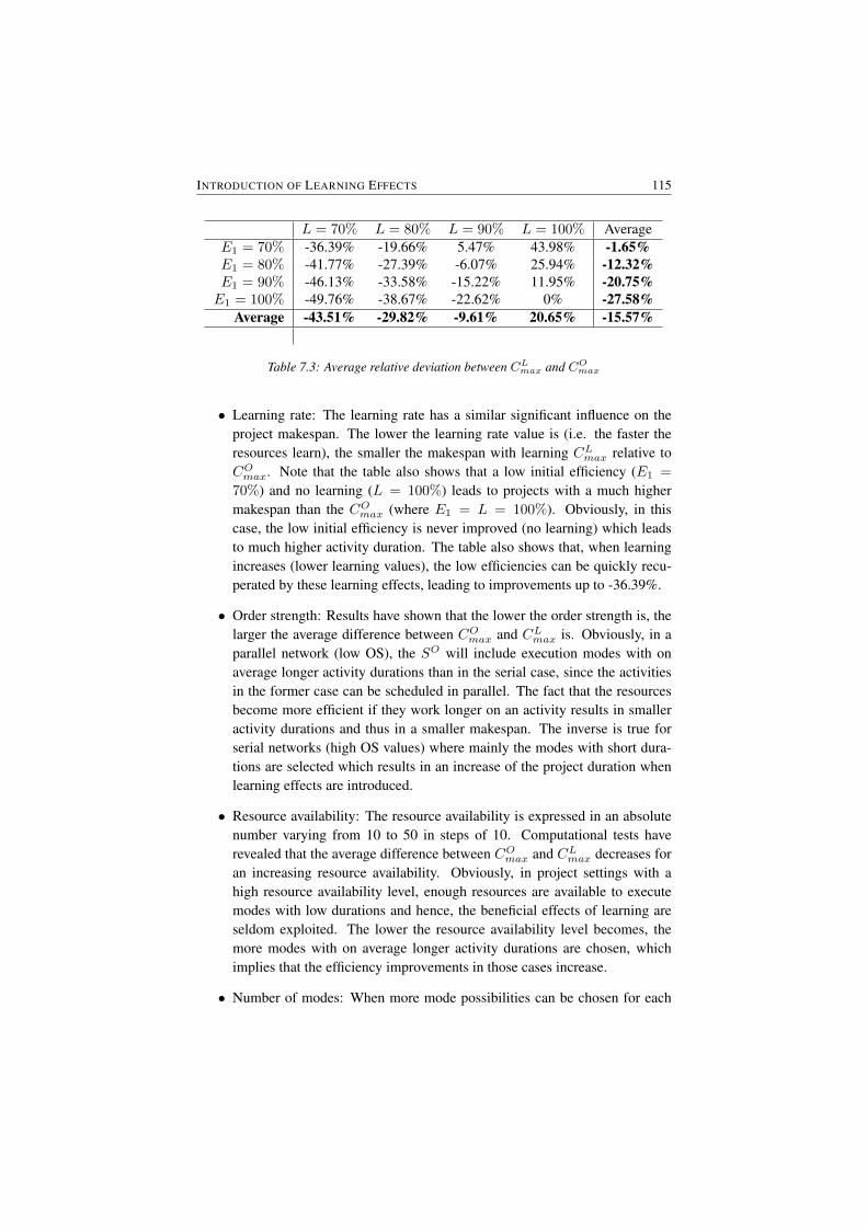
INTRODUCTION OF LEARNING EFFECTS 115
L = 70% L = 80% L = 90% L = 100% AverageE1 = 70% -36.39% -19.66% 5.47% 43.98% -1.65%E1 = 80% -41.77% -27.39% -6.07% 25.94% -12.32%E1 = 90% -46.13% -33.58% -15.22% 11.95% -20.75%E1 = 100% -49.76% -38.67% -22.62% 0% -27.58%
Average -43.51% -29.82% -9.61% 20.65% -15.57%
Table 7.3: Average relative deviation between CLmax and COmax
• Learning rate: The learning rate has a similar significant influence on theproject makespan. The lower the learning rate value is (i.e. the faster theresources learn), the smaller the makespan with learning CLmax relative toCOmax. Note that the table also shows that a low initial efficiency (E1 =
70%) and no learning (L = 100%) leads to projects with a much highermakespan than the COmax (where E1 = L = 100%). Obviously, in thiscase, the low initial efficiency is never improved (no learning) which leadsto much higher activity duration. The table also shows that, when learningincreases (lower learning values), the low efficiencies can be quickly recu-perated by these learning effects, leading to improvements up to -36.39%.
• Order strength: Results have shown that the lower the order strength is, thelarger the average difference between COmax and CLmax is. Obviously, in aparallel network (low OS), the SO will include execution modes with onaverage longer activity durations than in the serial case, since the activitiesin the former case can be scheduled in parallel. The fact that the resourcesbecome more efficient if they work longer on an activity results in smalleractivity durations and thus in a smaller makespan. The inverse is true forserial networks (high OS values) where mainly the modes with short dura-tions are selected which results in an increase of the project duration whenlearning effects are introduced.
• Resource availability: The resource availability is expressed in an absolutenumber varying from 10 to 50 in steps of 10. Computational tests haverevealed that the average difference between COmax and CLmax decreases foran increasing resource availability. Obviously, in project settings with ahigh resource availability level, enough resources are available to executemodes with low durations and hence, the beneficial effects of learning areseldom exploited. The lower the resource availability level becomes, themore modes with on average longer activity durations are chosen, whichimplies that the efficiency improvements in those cases increase.
• Number of modes: When more mode possibilities can be chosen for each

116 CHAPTER 7
activity, there is more flexibility and room for makespan improvement whenlearning effects are incorporated. Consequently, the higher the number ofmodes and activities, the larger the differences between COmax and CLmaxare.
• Average duration: The average duration gives an insight in the averagelength of an activity. It is calculated for the different mode durations when
no learning effects are assumed and can be formulated as∑Ni=1
∑Mij=1
dij
Mi
N .Similar to the number of modes, an increase in the average activity durationincreases the average difference between the two project schedules.
Statistical analysis indicates a strong significant influence (p<0.001) of theparameters L and E1 on the difference between COmax and CLmax. The other driv-ing variables have a smaller but still significant influence on the direction and themagnitude of the difference.
7.5.2 Margin of error during project progress
In this section, the accuracy of the project schedule SR is compared to the scheduleconsidering no learning effects (SO). This research will give insights in the marginof error which is made using the original schedule SO where learning effects areassumed to be unknown in advance. This project schedule is the baseline scheduleproposed to the client and/or is used to set milestones without being aware that thelearning effect will occur during project execution. However, efficiency improve-ments or deficiencies might occur during project progress which affect the activitydurations and the total project makespan.
Table 7.4 classifies the set of projects into different deviation classes where therelative deviations are measured as follows:
dev =CRmax − COmax
COmax. (7.14)
Consequently, the higher the deviations, the higher the margin of error is madeby ignoring the learning effects during schedule construction. The table shows thatonly 7.53% of the projects have an absolute deviation smaller than 1%. Most pro-jects (approximately 78%) have a deviation of more than 10%. These tests clearlyshow that the original baseline schedule SO is often not an accurate prediction ofthe real project progress since learning effects will often lead to high deviationsbetween the proposed makespan COmax and the observed makespan CRmax. Conse-quently, prior information about the learning effects during the scheduling phasewill often generate a competitive advantage in terms of the accuracy of the projectschedule and the project makespan promised to the client.
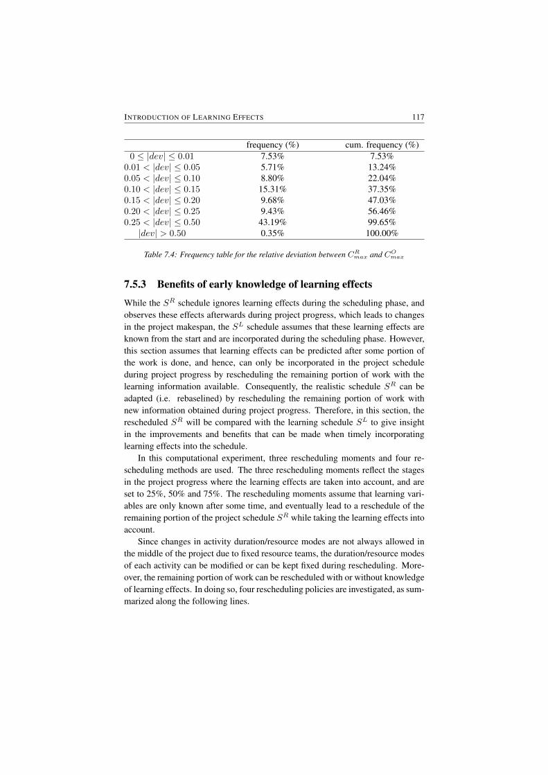
INTRODUCTION OF LEARNING EFFECTS 117
frequency (%) cum. frequency (%)0 ≤ |dev| ≤ 0.01 7.53% 7.53%
0.01 < |dev| ≤ 0.05 5.71% 13.24%0.05 < |dev| ≤ 0.10 8.80% 22.04%0.10 < |dev| ≤ 0.15 15.31% 37.35%0.15 < |dev| ≤ 0.20 9.68% 47.03%0.20 < |dev| ≤ 0.25 9.43% 56.46%0.25 < |dev| ≤ 0.50 43.19% 99.65%|dev| > 0.50 0.35% 100.00%
Table 7.4: Frequency table for the relative deviation between CRmax and COmax
7.5.3 Benefits of early knowledge of learning effects
While the SR schedule ignores learning effects during the scheduling phase, andobserves these effects afterwards during project progress, which leads to changesin the project makespan, the SL schedule assumes that these learning effects areknown from the start and are incorporated during the scheduling phase. However,this section assumes that learning effects can be predicted after some portion ofthe work is done, and hence, can only be incorporated in the project scheduleduring project progress by rescheduling the remaining portion of work with thelearning information available. Consequently, the realistic schedule SR can beadapted (i.e. rebaselined) by rescheduling the remaining portion of work withnew information obtained during project progress. Therefore, in this section, therescheduled SR will be compared with the learning schedule SL to give insightin the improvements and benefits that can be made when timely incorporatinglearning effects into the schedule.
In this computational experiment, three rescheduling moments and four re-scheduling methods are used. The three rescheduling moments reflect the stagesin the project progress where the learning effects are taken into account, and areset to 25%, 50% and 75%. The rescheduling moments assume that learning vari-ables are only known after some time, and eventually lead to a reschedule of theremaining portion of the project schedule SR while taking the learning effects intoaccount.
Since changes in activity duration/resource modes are not always allowed inthe middle of the project due to fixed resource teams, the duration/resource modesof each activity can be modified or can be kept fixed during rescheduling. More-over, the remaining portion of work can be rescheduled with or without knowledgeof learning effects. In doing so, four rescheduling policies are investigated, as sum-marized along the following lines.
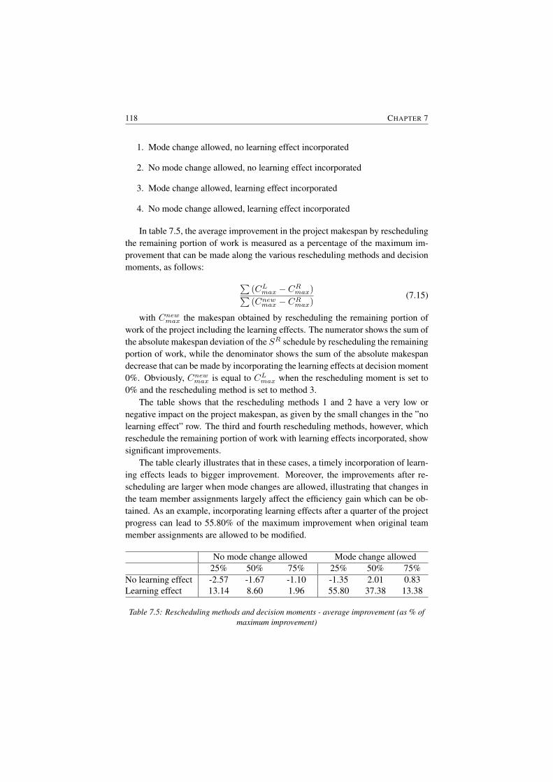
118 CHAPTER 7
1. Mode change allowed, no learning effect incorporated
2. No mode change allowed, no learning effect incorporated
3. Mode change allowed, learning effect incorporated
4. No mode change allowed, learning effect incorporated
In table 7.5, the average improvement in the project makespan by reschedulingthe remaining portion of work is measured as a percentage of the maximum im-provement that can be made along the various rescheduling methods and decisionmoments, as follows: ∑
(CLmax − CRmax)∑(Cnewmax − CRmax)
(7.15)
with Cnewmax the makespan obtained by rescheduling the remaining portion ofwork of the project including the learning effects. The numerator shows the sum ofthe absolute makespan deviation of the SR schedule by rescheduling the remainingportion of work, while the denominator shows the sum of the absolute makespandecrease that can be made by incorporating the learning effects at decision moment0%. Obviously, Cnewmax is equal to CLmax when the rescheduling moment is set to0% and the rescheduling method is set to method 3.
The table shows that the rescheduling methods 1 and 2 have a very low ornegative impact on the project makespan, as given by the small changes in the ”nolearning effect” row. The third and fourth rescheduling methods, however, whichreschedule the remaining portion of work with learning effects incorporated, showsignificant improvements.
The table clearly illustrates that in these cases, a timely incorporation of learn-ing effects leads to bigger improvement. Moreover, the improvements after re-scheduling are larger when mode changes are allowed, illustrating that changes inthe team member assignments largely affect the efficiency gain which can be ob-tained. As an example, incorporating learning effects after a quarter of the projectprogress can lead to 55.80% of the maximum improvement when original teammember assignments are allowed to be modified.
No mode change allowed Mode change allowed25% 50% 75% 25% 50% 75%
No learning effect -2.57 -1.67 -1.10 -1.35 2.01 0.83Learning effect 13.14 8.60 1.96 55.80 37.38 13.38
Table 7.5: Rescheduling methods and decision moments - average improvement (as % ofmaximum improvement)

INTRODUCTION OF LEARNING EFFECTS 119
7.6 ConclusionsAlthough empirical evidence is given that learning effects exist in project sched-uling environments, the concept is not yet widely applied in the current projectscheduling literature. In this chapter, the introduction of learning effects into thediscrete time/resource trade-off problem is investigated from various angles. Com-putational tests found a significant influence of the introduction of learning effectsin project scheduling and a practical impact of the concept on management de-cisions. Computational experiments have been set up to reveal the main projectdrivers that affect the project makespan when introducing learning effects, to mea-sure the margin of error made by ignoring learning during schedule constructionand to show that timely incorporation of learning effects when the project is inprogress can lead to significant makespan improvements.
Several future research directions can be suggested. In addition to learning,also forgetting is a natural phenomenon that occurs when a resource stops work-ing on a specific activity. The interruption of the activity obviously leads to thetermination of the activity-specific learning process and is extremely significantwhen activity splitting is allowed. Empirical research has also shown that workingwith insufficient or too many resources can result in an efficiency decrease due toan increasing loss of motivation and dedication. The introduction of team workwhere the efficiency of a single resource can influence the team efficiency and thedetermination of the optimal number of team members and its influence on theproject duration is also a topic for further research. Finally, in this research wehave focused on the autonomous learning concept. However, the acquired insightsin project scheduling with learning effects can be used to discuss and investigatethe induced learning concept, where learning is the result of management invest-ments in training and innovative technologies. The determination of the optimallearning rate per activity will be one of the key questions the learning effect re-search can introduce into the project management practice.


8Case Study: Audit Scheduling
8.1 Introduction
In this work, several metaheuristic solution procedures for the multi-mode resource-constrained project scheduling problem were proposed. These approaches wereapplied on theoretical project instances in order to optimize the efficiency of theprocedures and to compare the results with other metaheuristics available in theliterature. Although our procedures obtained state-of-the-art results on the bench-mark datasets, the ultimate goal of our research is to optimize real-life schedules,such that efficiency improvements, cost reductions or profit increases can be real-ized. In this chapter, we therefore apply one of our metaheuristic approaches ona real-life audit scheduling problem, which consists of generating an appropriateschedule for a small Belgian audit firm.
In audit scheduling, the assignment of a set of auditors to a set of audit tasks,with a predefined arrival time and due date, is optimized. The schedule shouldspecify the audit assignment start and finish time and indicate which auditor willprocess the task. Several authors have already discussed audit scheduling underdifferent constraints. Chan and Dodin (1986) present a decision support system foraudit-staff scheduling. They expand the loading model of Balachandran and Zolt-ners (1981) in order to deal with precedence constraints among audit tasks, duedates, arrival times, penalty costs for missing audit due dates and the constraintthat an auditor cannot process more than one audit task at a time. Furthermore,Dodin and Chan (1991) examine the impact of different objective functions for the
122 CHAPTER 8
audit scheduling problem, while Drexl (1991) presents a hybrid branch and bound-/dynamic programming algorithm to solve an audit scheduling problem in order tominimize the overall costs. Dodin and Elimam (1997) present a procedure foraudit scheduling with overlapping activities and sequence-dependent setup costs,such as travel time and cost, while Dodin et al. (1998) tackle this problem with atabu search procedure. Brucker and Schumacher (1999) also present a tabu searchprocedure for an audit scheduling problem with the following characteristics: eachauditor is only available during disjoint time periods and has a minimal and maxi-mal working time. Moreover, the task of an auditor can be preempted under certaincircumstances.
Salewski et al. (1997) state that the above solution procedures are single levelmodels which try to construct a direct assignment of auditors to tasks and periods.Based on a survey among the 200 biggest public accountant firms in Germany, theyformulate three levels within audit scheduling: the medium-term planning, whichassigns teams of auditors to the audit tasks and constructs a schedule by determin-ing the workload per auditor and per week over a planning horizon between threeand twelve months; the medium-to-short-term planning, which produces a sched-ule for each auditor that covers all engagements in which he/she is involved in theconsidered week on the basis of periods of four hours and the short-term planning,which assigns the auditors to an audit task in periods of one hour. Salewski et al.(1997) state that the medium-term audit-staff scheduling problem (MASSP) canbe formulated as a mode-identity resource-constrained project scheduling prob-lem and determine some priority rules to solve the MASSP. Drexl et al. (2006)propose a column generation method for this problem.
In the remainder of this chapter, an algorithm is presented for the medium-termaudit-staff scheduling problem, with sequence-dependent set-up times, varying au-ditors availability, alternative audit teams and variable audit team efficiencies. Thisalgorithm is applied on real-life data from a small Belgium audit firm, with 15 au-ditors and almost 250 audit tasks.
This chapter is organized as follows: in section 8.2 the problem formulation isdefined, while in section 8.3, a solution approach for this problem will be formu-lated. The results of a computational study will be discussed in section 8.4, whilethe conclusions of this chapter are drawn in section 8.5.
8.2 Audit scheduling problem
8.2.1 Description
An audit firm employs a number N of auditors, which have to execute a set Eof engagements within a given planning horizon. An engagement includes theexecution of a set of audit tasks A. Each audit task of an audit engagement can
CASE STUDY: AUDIT SCHEDULING 123
be performed by different audit teams (modes). The processing time dijmi foreach task j of engagement i will be different for each audit team mi and will beinfluenced by the qualification, industry experience and familiarity with the client’sbusiness of each audit team. The number of execution modes for each task withinthe same engagement is the same.
There may exist a precedence relationship between two audit tasks, whichmeans that the second audit task may not be processed before the first task of theengagement is carried out. Each audit engagement has a time window in which itshould be performed: each engagement has a release time, which is the contractualdate or any time thereafter when the engagement becomes ready for processing anda due date, which is the time when the audit engagement should be completed. Inmost cases this due date is strict, since the due date is a legal restriction of theduration of the audit engagement.
Several audit resource types are available (e.g. senior auditor, assistant au-ditor or junior auditor) and for each resource type several auditors are available.The availability of some auditors may be restricted in certain periods, e.g. due toholidays, vacations or training. Note that not all audit tasks within the same en-gagement should be executed by the same audit team. However, some of the tasksshould be processed by the same team, due to e.g. legal requirements, while otherscan be executed by other audit teams. This problem notation refers to the modeidentity constraints of Salewski et al. (1997).
We assume that the auditor teams work at a homogeneous efficiency level of100%. However, every new audit engagement is characterized by an introductionperiod, in which the audit team learns to know the company, finds out how the com-pany works, etc. This setup time is added to the total duration of the audit task. Theidea of setup time incorporation in scheduling is not new and is already studied inthe resource-constrained project scheduling (Kaplan, 1991; Kolisch, 1995; Debelsand Vanhoucke, 2006; Kruger and Scholl, 2009, 2010) and machine scheduling(Potts and Kovalyov, 2000; Allahverdi et al., 2008). In our problem statement, weassume an audit task-dependent setup time that needs to be added to the audit taskat the initial start of the audit engagement as well as for each time a new audit taskis performed by another audit team. The setup time can be seen as the loss of timedue to the audit team inefficiency at the beginning of a new audit task.
In order to calculate the setup time, we assume that during the introductionperiod, the auditor teams follow a learning curve, determined by the audit team’sinitial efficiencyE1 and learning rateL, until the 100% efficiency level is obtained.The learning variables L and E1 give an indication of the audit team’s skills: moreskilled audit teams have better learning variables (higher initial efficiency E1 andlower learning rate L) than less experienced audit teams.

124 CHAPTER 8
Based on equation 7.3, the time needed to obtain the 100% efficiency level(expressed in man-days) is equal to
ts = b
√100%
(1 + b)E1
with b = −log2L the learning index depending on the learning rate L. Itis assumed that each audit team has a specific learning rate and a specific initialefficiency, which depends on their mixture and level of skills.
The number of working days performed during the time period [0,ts] can becalculated based on equation 7.4 and is equal to
Dwts = Ei1t
1+bs
Dwts = Ei1( b
√100%
(1 + b)E1
)1+b
Consequently, due to the initial setup period where resources need to reachtheir 100% efficiency level, ts man-days will be necessary to performDw
ts workingdays (ts ≥ Dw
ts ). Hence, the total number of working days performed after dijmiman-days can be calculated as the sum of the following two values:
1. Dwts , which is the number of working days performed during the period
[0,ts] following the efficiency curve determined by the learning variablesL and E1.
2. dijmi−ts, which is the number of working days performed during the period]ts,dijmi ], since a homogeneous efficiency (L = E1 = 100%) is assumedduring this period. In this period, the number of working days is equal to thenumber of man-days.
The setup time s is defined as the additional time above the predefined dijmiman-days (where homogeneous efficiencies are assumed) due to the initial intro-duction period (in which no homogeneous efficiencies are considered). Hence, thetotal time is dijmi + s man-days. The setup time can be calculated as:
s = dijmi − [(dijmi − ts) +Dwts ]
s = ts −Dwts
Consider the example of an audit team with an initial efficiency E1 of 0.7 anda learning rate L of 0.85 (b = 0.234) executing an activity with a duration dijmiof 3 working days. Without setup time, the activity is executed in 3 man-days(due to the homogeneous efficiency), however, when setup times are considered,

CASE STUDY: AUDIT SCHEDULING 125
an introduction period is assumed in which the audit team follows the efficiencycurve, determined by the learning variables. It can be calculated that this introduc-tion period takes ts = 1.86 man-days during which Dw
ts = 1.51 working days areperformed (see figure 8.1). The additional duration due to the initial introductionperiod can be executed in ts − Dw
ts = 1.86 - 1.51 = 0.35 man-days. This is indi-cated by the grey area and is equal to the black area, which indicates the loss ofefficiency due to learning.
E
1 2 3 T
100%
E
1 2 31.86 3.31 T
100%
ts
Dtsw d -ijmi ts
d ijmi
1.86
=
Figure 8.1: Influence of the setup time on audit team switches
With respect to studies published earlier in this research field, some specificelements are not included in the audit scheduling model. First, the minimum andmaximum time lags between audit tasks are not taken into account. Second, nopreference values are assigned, which means that each execution mode has thesame chance to be chosen. Third, no travel times are considered, since we assumethat all audits took place at the same place.
8.2.2 Example project
In this section, we present an example for the audit scheduling problem. Anoverview of the different variables which are used in the remainder of this sectionis given in table 8.4. The values for the different variables used in this exampleproject are also mentioned in the column ’Example’.
Consider an example project with three audit engagements. Audit engagement1 and 3 contain 3 audit tasks, audit engagement 2 contains only 2 audit tasks. Eachaudit engagement has a release date (λ1 = 0, λ2 = 5, λ3 = 10) and a due date(δ1 = 10, δ2 = δ3 = 20). The planning horizon of the three audit engagements is20.
Each audit task can be executed in two modes. Each mode represents an auditorteam, composed out of one or more auditors. The audit office has in total 5 auditorsavailable, divided into two audit types (C = 2): 2 senior auditors and 3 junior
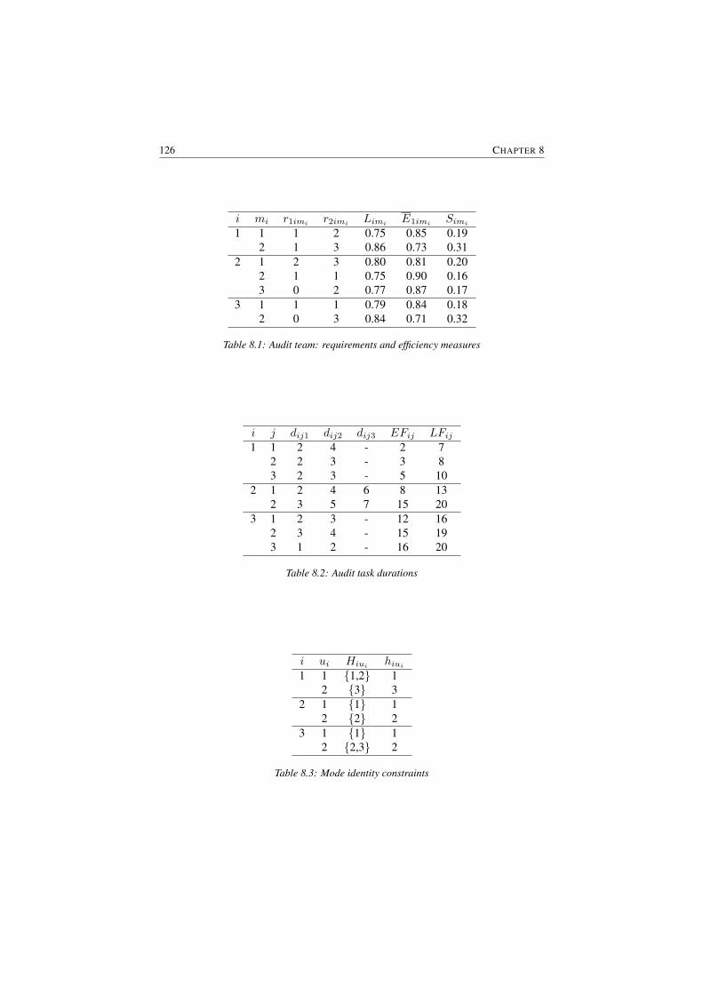
126 CHAPTER 8
i mi r1imi r2imi Limi E1imi Simi1 1 1 2 0.75 0.85 0.19
2 1 3 0.86 0.73 0.312 1 2 3 0.80 0.81 0.20
2 1 1 0.75 0.90 0.163 0 2 0.77 0.87 0.17
3 1 1 1 0.79 0.84 0.182 0 3 0.84 0.71 0.32
Table 8.1: Audit team: requirements and efficiency measures
i j dij1 dij2 dij3 EFij LFij1 1 2 4 - 2 7
2 2 3 - 3 83 2 3 - 5 10
2 1 2 4 6 8 132 3 5 7 15 20
3 1 2 3 - 12 162 3 4 - 15 193 1 2 - 16 20
Table 8.2: Audit task durations
i ui Hiui hiui1 1 {1,2} 1
2 {3} 32 1 {1} 1
2 {2} 23 1 {1} 1
2 {2,3} 2
Table 8.3: Mode identity constraints

CASE STUDY: AUDIT SCHEDULING 127
auditors. The cost of the former is 175 per day, while the cost for the latter is 100per day. The different audit team combinations are given in table 8.1, includingthe audit team learning variables L and E1. All auditors are available during thecomplete planning horizon. The duration of the different audit tasks executed bythe different audit teams is given in table 8.2. For example, the duration d122 oftask 2 of engagement 1 executed in mode 2 is 3. This task is executed by an auditteam which consists of 1 senior and 3 junior auditors (see mode 2 of engagement1 in table 8.1). We can also calculate the earliest finish time (EF ) and latest finishtime (LF ) for each audit task, based on the shortest duration for each audit task(without taking the setup time into account).
A mode identity constraint is set to audit engagement 1 and 3. Audit task 1and 2 of engagement 1 should be executed by the same audit team (i.e. the samemode). This means that if mode 1 is chosen for audit task 1 of engagement 1,also mode 1 has to be chosen for audit task 2 of the same engagement. The sameis true for the audit tasks 2 and 3 of engagement 3. In table 8.3, an overview ofthe different mode identity constraints for the example project is given. The set ofaudit tasks of each engagement is divided into ui different subsets and each subsetHiui contains one or more audit tasks which must be executed by the same auditteam. Each audit task is part of exactly one subset (
∑Uiui=1 |Hiui | = Ai,∀i).
The setup time of the different audit tasks is defined by the efficiency parame-ters of the audit team. An overview of the setup times Simi for the different modesis given in table 8.1. The setup time is applied if the previous audit task is notexecuted by the same audit team or if the audit task is the first task of the auditengagement. In these cases, the setup time sijmi of a specific audit task j of en-gagement i executed in modemi is equal to Simi . In all other cases, the setup timesijmi is equal to 0. For example, the setup time s111 = S11 = 0.19 if the task isexecuted by mode team 1, while the setup time s121 of audit task 2 of engagement1 is equal to 0 since the task should be executed in the same mode as audit task 1(see table 8.3).
A precedence relation is set between the different tasks of an audit engage-ment. The set of predecessors of audit task j of audit engagement i is given by thevariable Vij , which consists of elements (o, p), representing an audit task p of anaudit engagement o. For example, the element (3,1) is a predecessor of audit task2 of engagement 3. There is also a precedence relation between audit task 3 ofengagement 1 and audit task 1 of engagement 3, since the release time of engage-ment 3 is equal to the due date of engagement 1 (see also section 8.3.1). So, theelement (1, 3) ∈ V31.
In figure 8.2, a feasible solution for the problem is given, taking into accountthe mode identity constraints, the setup times and the due date restrictions. Thechosen audit teams are: team 1 for all tasks in engagement 1, team 1 for audit task1 and team 2 for audit task 2 of engagement 2 and team 1 for audit task 1 and team

128 CHAPTER 8
2 for audit task 2 and 3 of engagement 3. The setup times are indicated in grey.The finish time of engagement 1 is 9.20, the finish time of engagement 2 is 12.36and the finish time of engagement 3 is 18.68.
5 10 15 T20
5 10 15 T20
11 12
1321
22
11 12
31
133121
22
32 33
r1
r2team 1 team 1
team 1
team 1
team 2
team 1
team 1 team 1
team 1
team 1
team 1
team 2
team 2 team 2
Figure 8.2: Audit scheduling example: a feasible solution
8.2.3 Mathematical formulation
In this section, a mathematical formulation is defined for the audit scheduling prob-lem as defined in the previous section.
The following decision variable is defined:
xijmit =
{1 if team mi completes task j of engagement i at the time t0 otherwise
The model is given by the following equations:
optimize ψ (8.1)
Mi∑mi=1
LFihiui∑t=EFihiui
xifiuimit = 1 1 ≤ i ≤ E, 1 ≤ ui ≤ Ui (8.2)
LFihiui∑t=EFihiui
xihiuimit =
LFij∑t=EFij
xijmit
1 ≤ i ≤ E,∀j ∈ Hiui\{hiui}, 1 ≤ ui ≤ Ui, 1 ≤ mi ≤Mi (8.3)
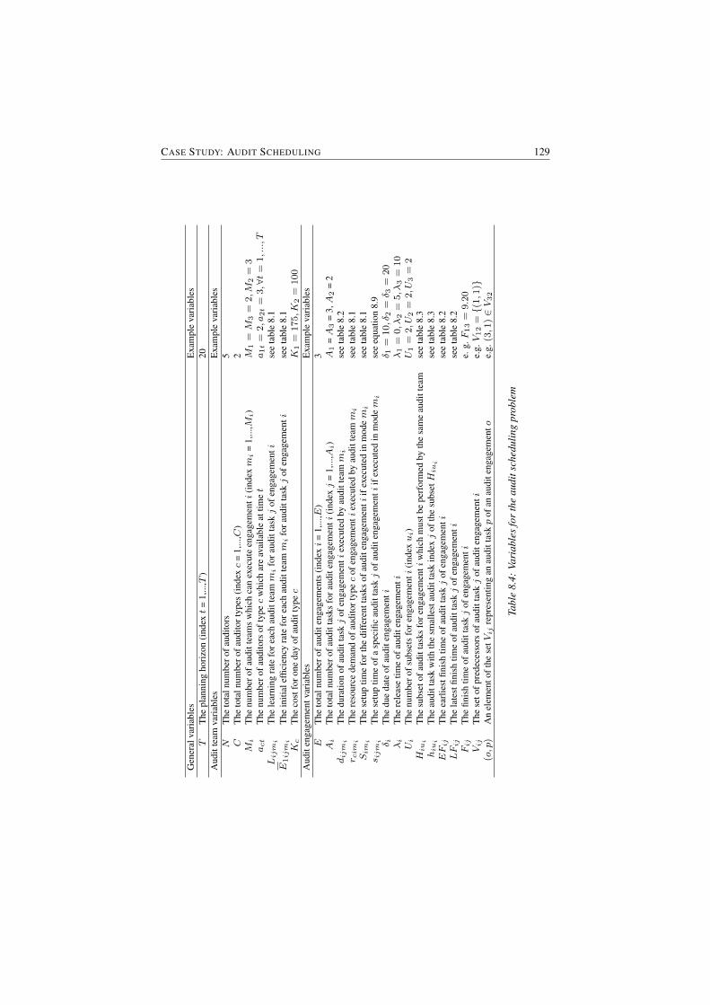
CASE STUDY: AUDIT SCHEDULING 129
Gen
eral
vari
able
sE
xam
ple
vari
able
sT
The
plan
ning
hori
zon
(ind
ext
=1,
...,T
)20
Aud
itte
amva
riab
les
Exa
mpl
eva
riab
les
NT
heto
taln
umbe
rofa
udito
rs5
CT
heto
taln
umbe
rofa
udito
rtyp
es(i
ndexc
=1,
...,C
)2
Mi
The
num
bero
faud
itte
ams
whi
chca
nex
ecut
een
gage
men
ti(i
ndexmi
=1,
...,M
i)
M1=M
3=
2,M
2=
3act
The
num
bero
faud
itors
ofty
pec
whi
char
eav
aila
ble
attim
et
a1t=
2,a
2t=
3,∀t=
1,...,T
Lijmi
The
lear
ning
rate
fore
ach
audi
ttea
mmi
fora
udit
taskj
ofen
gage
men
tise
eta
ble
8.1
E1ijmi
The
initi
alef
ficie
ncy
rate
fore
ach
audi
ttea
mmi
fora
udit
taskj
ofen
gage
men
tise
eta
ble
8.1
Kc
The
cost
foro
neda
yof
audi
ttyp
ec
K1=
175,K
2=
100
Aud
iten
gage
men
tvar
iabl
esE
xam
ple
vari
able
sE
The
tota
lnum
bero
faud
iten
gage
men
ts(i
ndexi
=1,
...,E
)3
Ai
The
tota
lnum
bero
faud
itta
sks
fora
udit
enga
gem
enti
(ind
exj
=1,
...,Ai)
A1
=A
3=
3,A
2=
2dijmi
The
dura
tion
ofau
ditt
askj
ofen
gage
men
tiex
ecut
edby
audi
ttea
mmi
see
tabl
e8.
2r cimi
The
reso
urce
dem
and
ofau
dito
rtyp
ec
ofen
gage
men
tiex
ecut
edby
audi
ttea
mmi
see
tabl
e8.
1Simi
The
setu
ptim
efo
rthe
diff
eren
ttas
ksof
audi
teng
agem
enti
ifex
ecut
edin
mod
emi
see
tabl
e8.
1s ijmi
The
setu
ptim
eof
asp
ecifi
cau
ditt
askj
ofau
dite
ngag
emen
tiif
exec
uted
inm
odemi
see
equa
tion
8.9
δ iT
hedu
eda
teof
audi
teng
agem
enti
δ 1=
10,δ
2=δ 3
=20
λi
The
rele
ase
time
ofau
dite
ngag
emen
tiλ1=
0,λ
2=
5,λ
3=
10
Ui
The
num
bero
fsub
sets
fore
ngag
emen
ti(i
ndexui)
U1=
2,U
2=
2,U
3=
2Hiui
The
subs
etof
audi
ttas
ksfo
reng
agem
enti
whi
chm
ustb
epe
rfor
med
byth
esa
me
audi
ttea
mse
eta
ble
8.3
hiui
The
audi
ttas
kw
ithth
esm
alle
stau
ditt
ask
inde
xj
ofth
esu
bsetHiui
see
tabl
e8.
3EFij
The
earl
iest
finis
htim
eof
audi
ttas
kj
ofen
gage
men
tise
eta
ble
8.2
LFij
The
late
stfin
ish
time
ofau
ditt
askj
ofen
gage
men
tise
eta
ble
8.2
Fij
The
finis
htim
eof
audi
ttas
kj
ofen
gage
men
tie.
g.F13=
9.20
Vij
The
seto
fpre
dece
ssor
sof
audi
ttas
kj
ofau
dite
ngag
emen
tie.
g.V12=
{(1,1
)}(o,p
)A
nel
emen
toft
hese
tVij
repr
esen
ting
anau
ditt
askp
ofan
audi
teng
agem
ento
e.g.
(3,1
)∈V32
Tabl
e8.
4:Va
riab
les
for
the
audi
tsch
edul
ing
prob
lem
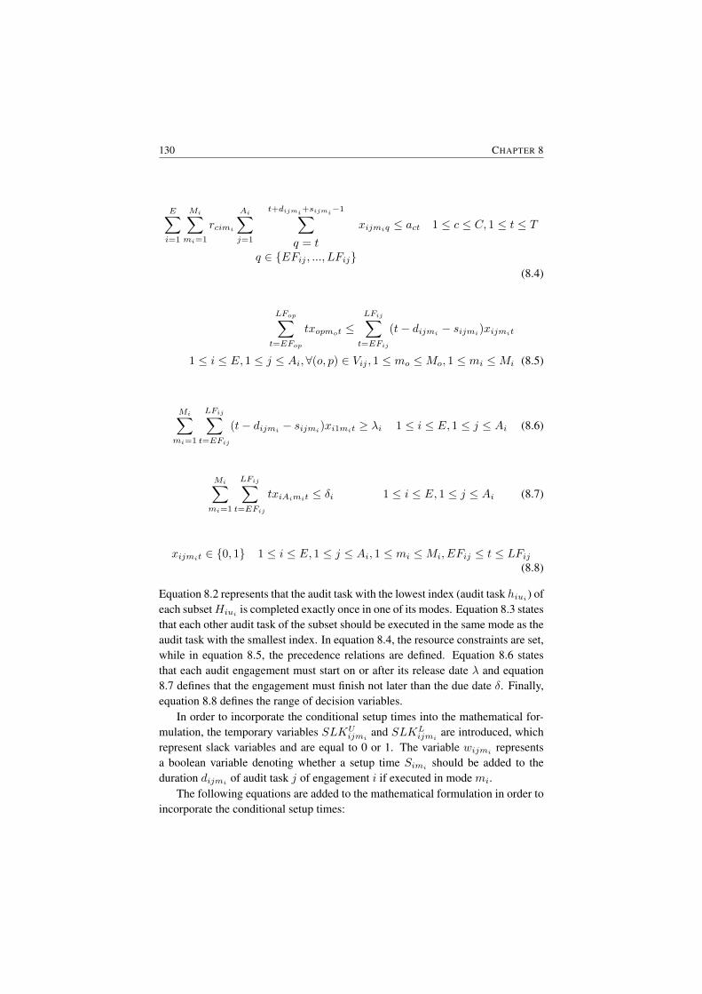
130 CHAPTER 8
E∑i=1
Mi∑mi=1
rcimi
Ai∑j=1
t+dijmi+sijmi−1∑q = t
q ∈ {EFij , ..., LFij}
xijmiq ≤ act 1 ≤ c ≤ C, 1 ≤ t ≤ T
(8.4)
LFop∑t=EFop
txopmot ≤LFij∑t=EFij
(t− dijmi − sijmi)xijmit
1 ≤ i ≤ E, 1 ≤ j ≤ Ai,∀(o, p) ∈ Vij , 1 ≤ mo ≤Mo, 1 ≤ mi ≤Mi (8.5)
Mi∑mi=1
LFij∑t=EFij
(t− dijmi − sijmi)xi1mit ≥ λi 1 ≤ i ≤ E, 1 ≤ j ≤ Ai (8.6)
Mi∑mi=1
LFij∑t=EFij
txiAimit ≤ δi 1 ≤ i ≤ E, 1 ≤ j ≤ Ai (8.7)
xijmit ∈ {0, 1} 1 ≤ i ≤ E, 1 ≤ j ≤ Ai, 1 ≤ mi ≤Mi, EFij ≤ t ≤ LFij(8.8)
Equation 8.2 represents that the audit task with the lowest index (audit task hiui ) ofeach subsetHiui is completed exactly once in one of its modes. Equation 8.3 statesthat each other audit task of the subset should be executed in the same mode as theaudit task with the smallest index. In equation 8.4, the resource constraints are set,while in equation 8.5, the precedence relations are defined. Equation 8.6 statesthat each audit engagement must start on or after its release date λ and equation8.7 defines that the engagement must finish not later than the due date δ. Finally,equation 8.8 defines the range of decision variables.
In order to incorporate the conditional setup times into the mathematical for-mulation, the temporary variables SLKU
ijmiand SLKL
ijmiare introduced, which
represent slack variables and are equal to 0 or 1. The variable wijmi representsa boolean variable denoting whether a setup time Simi should be added to theduration dijmi of audit task j of engagement i if executed in mode mi.
The following equations are added to the mathematical formulation in order toincorporate the conditional setup times:

CASE STUDY: AUDIT SCHEDULING 131
sijmi = wijmiSimi 1 ≤ i ≤ E, 1 ≤ j ≤ 1, 1 ≤ mi ≤Mi (8.9)
wi1mi = 1 1 ≤ i ≤ E, 1 ≤ mi ≤Mi (8.10)
LFij∑t=EFij
xijmit −LFij∑t=EFij
xij−1mit ≤ SLKUijmi 1 ≤ i ≤ E,∀j > 1, 1 ≤ mi ≤Mi
(8.11)
LFij∑t=EFij
xijmit −LFij∑t=EFij
xij−1mit ≤ SLKLijmi 1 ≤ i ≤ E,∀j > 1, 1 ≤ mi ≤Mi
(8.12)
wijmi = SLKLijmi + SLKU
ijmi 1 ≤ i ≤ E,∀j > 1, 1 ≤ mi ≤Mi (8.13)
Equation 8.9 defines the value of the setup time of audit task j of engagementi. The value of sijmi is equal to 0 or to Simi and depends on the value of wijmi .For the first task of all engagements the value of wijmi is equal to 1 (equation8.10). For all other audit tasks, the value of wijmi is equal to 0 if the previous taskis executed in the same mode as the current audit task and otherwise equal to 1(equations 8.11, 8.12 and 8.13).
Different objective functions can be defined. A first objective function mini-mizes the number of audit engagements finishing after the due date δ.
ψ1 = min
E∑i=1
{1 FiAi > δi0 otherwise
A second objective function assigns a penalty cost P to each day an auditengagement is finished after the proposed due date δ. If the previous objectivefunction is 0, the result of this objective function will obviously be 0. In this work,the penalty P is, without loss of generality, set at 1 per day.
ψ2 = min
E∑i=1
{P (FiAi − δi) FiAi > δi0 otherwise
Finally, a third objective function maximizes the value of the remaining re-source capacity. The function gives an indication of the resources which are avail-able for other audit engagements and is inspired by the audit office’s desire toobtain efficient audit team assignments. The function is calculated as follows:
132 CHAPTER 8
ψ3 = max
T∑t=0
C∑c=1
(act − act)Kc
with act equal to the number of resources of resource type c used at time t, asdefined in the left hand side of equation 8.4.
8.3 Solution approach
In this section, the solution approach for this audit scheduling problem will bepresented. Salewski et al. (1997) proved that the MASSP is a special case ofthe mode identity resource-constrained project scheduling problem (MIRCPSP).Several adaptations are presented such that the problem can be solved using thegenetic algorithm, as proposed in chapter 3. In section 8.3.1, the schedule andsolution representation are presented, while in section 8.3.2, a schedule generationscheme with dynamic priority rules is presented in which the mode improvementmethod is incorporated. Finally, in section 8.3.3, the algorithmic details of thegenetic solution procedure are presented.
8.3.1 Representation
Since the audit scheduling problem consists of a set of audit engagements, whichare divided in a set of audit tasks between which a precedence relation exists, theproblem can be seen as a multiple project scheduling problem, in which a set ofsingle-projects (the audit engagements) should be scheduled sharing the same setof available resource. This can be represented as the different projects shown infigure 8.3(a). However, projects can be bound together artificially into a singleproject by the addition of two dummy activities representing the start and end ofthe single aggregate project (Hans et al., 2007), as shown in figure 8.3(b).
Since each audit engagement i has a release date λi, before which the en-gagement cannot start, and a due date δi, before which the engagement should befinished due to legal restrictions, extra precedence constraints can be added to theproject, without violating the project characteristics. For each pair of engagements(i, j), for which δi ≤ λj is true, a precedence constraint is set between engage-ments i and j. This results in a project as shown in figure 8.3(c).
Using this representation, the genetic algorithm as proposed in chapter 3 canbe used to solve this problem. However, some adaptations are made in order todeal with the specific characteristics of the audit scheduling problem. In the nextsection, a schedule generation scheme with dynamic priority rules is presented.
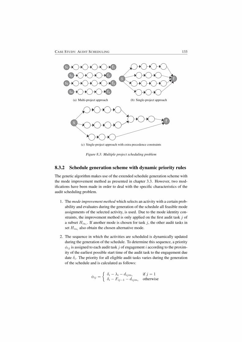
CASE STUDY: AUDIT SCHEDULING 133
s1 f1
s2 f2
s3 f3
s4 f4
(a) Multi-project approach
s f
(b) Single-project approach
s f
(c) Single-project approach with extra precedence constraints
Figure 8.3: Multiple project scheduling problem
8.3.2 Schedule generation scheme with dynamic priority rules
The genetic algorithm makes use of the extended schedule generation scheme withthe mode improvement method as presented in chapter 3.3. However, two mod-ifications have been made in order to deal with the specific characteristics of theaudit scheduling problem.
1. The mode improvement method which selects an activity with a certain prob-ability and evaluates during the generation of the schedule all feasible modeassignments of the selected activity, is used. Due to the mode identity con-straints, the improvement method is only applied on the first audit task j ofa subset Hiui . If another mode is chosen for task j, the other audit tasks inset Hiui also obtain the chosen alternative mode.
2. The sequence in which the activities are scheduled is dynamically updatedduring the generation of the schedule. To determine this sequence, a priorityφij is assigned to each audit task j of engagement i according to the proxim-ity of the earliest possible start time of the audit task to the engagement duedate δi. The priority for all eligible audit tasks varies during the generationof the schedule and is calculated as follows:
φij =
{δi − λi − dijmi if j = 1δi − Fij−1 − dijmi otherwise

134 CHAPTER 8
Audit tasks which approach their due dates have a higher chance to be sched-uled with respect to the other eligible activities. Moreover, audit tasks with alarger task duration are also preferred over audit tasks with shorter durations.
The incorporation of this scheduling generation scheme with dynamic priorityrules implies that the sequence in which the audit tasks are scheduled is updateddynamically during the generation of the schedule. This implies that the randomkey, as used in the genetic algorithm proposed in chapter 3 cannot be used. More-over, tests were also performed using the random key, however, this generationscheme revealed inferior results with respect to the proposed schedule generationscheme with dynamic priority rules.
8.3.3 Algorithmic details
In this section, some specific algorithmic details of the genetic algorithm are pre-sented.
Mode identity Due to the introduction of the mode identity constraint, the cross-over and mutation operators are adapted such that a change in mode alsoleads to the adaption of the mode of the other activities in the set Hiui .
Crossover As in the genetic algorithm presented in chapter 3, the best results areobtained by using a one-point crossover, which is applied on the mode listsof the population.
Mutation A mutation operator is applied to each mode list. The mutation ran-domly changes the mode of a randomly selected activity. The probability ofan activity to be mutated is equal to 5%.
In the following section, this genetic algorithm is applied on real-life data froma small Belgium audit firm, with 15 auditors and more than 250 audit engagementsper year.
8.4 Computational results
In this section, computational tests are performed to test the efficiency of our ge-netic algorithm, to analyze the influence of the setup costs, mode identity con-straints and objective functions and to compare our schedule with the originalschedule obtained from the audit firm. In section 8.4.1, the audit firm is presentedin detail, while in section 8.4.2, an analysis of three different scenarios is given.
CASE STUDY: AUDIT SCHEDULING 135
8.4.1 Audit firm
The data used is received from a local Belgian audit firm, which is part of an inter-national network of more than 600 independent offices, present in more than 100countries. Eight offices are located in Belgium. Each office works independently,but the offices support each other to resolve personnel shortage.
The office, from which the audit scheduling data of the year 2008 is obtained,has an audit department with 15 auditors, divided over 4 audit types: 3 partners,4 managers, 3 seniors and 5 junior assistants. It is assumed that all auditors ofthe same type are mutually interchangeable. For the year 2008, the audit firm hasobtained 237 audit engagements, each with a duration, a release and a due date.The average engagement duration is 2 weeks, with a minimum of 0.5 day anda maximum of 16 weeks. For each audit engagement, several execution modesare defined, which represent audit teams (composed of one or more auditors) anddetermine the duration, resource requirements and the audit team efficiency. Foreach audit engagement, a list of audit tasks which must be executed by the sameaudit team is available. Since the real cost for the different audit types may not begiven, a relative weight is assigned to each audit type. These weights are basedon the monetary costs of the different types of auditors. We rescaled the cost ofthe junior auditor to 100 and compared the cost of any other resource type withthis cost. The weight of the junior auditor is therefore set at 100, the weight of thesenior assistant is set at 127, the weight of a manager is set at 173 and the weightof a partner is set at 267. The information about the resource availability (holidays,training, ...) is given.
Currently, the audit department makes use of Microsoft Office Excel to man-ually schedule the audit engagements and tasks. In the remainder of this chapter,we refer to the original schedule as the one designed by the audit firm. However,compared to the real-life situation, the following assumptions are made. First,each auditor performs a forty-hour week. This assumption, however, will lead toactivities exceeding the engagement due date, although this is not in accordanceto the real-life situation in which overtime is used to solve these resource capacityproblems. Second, resource inavailability for short periods (e.g. one-day training)is not taken into account since the preemption of activities is not allowed by thealgorithm. Obviously, longer periods of unavailability are taken into account.
8.4.2 Analysis
In this section, an evaluation is made for three different scenarios. A first sce-nario assumes a situation without setup costs and mode identity constraints andis presented in section 8.4.2.1. A second scenario introduces the mode identityconstraint and is presented in section 8.4.2.2. Finally, in the third scenario, whichis presented in section 8.4.2.3, the setup costs are added to the problem.
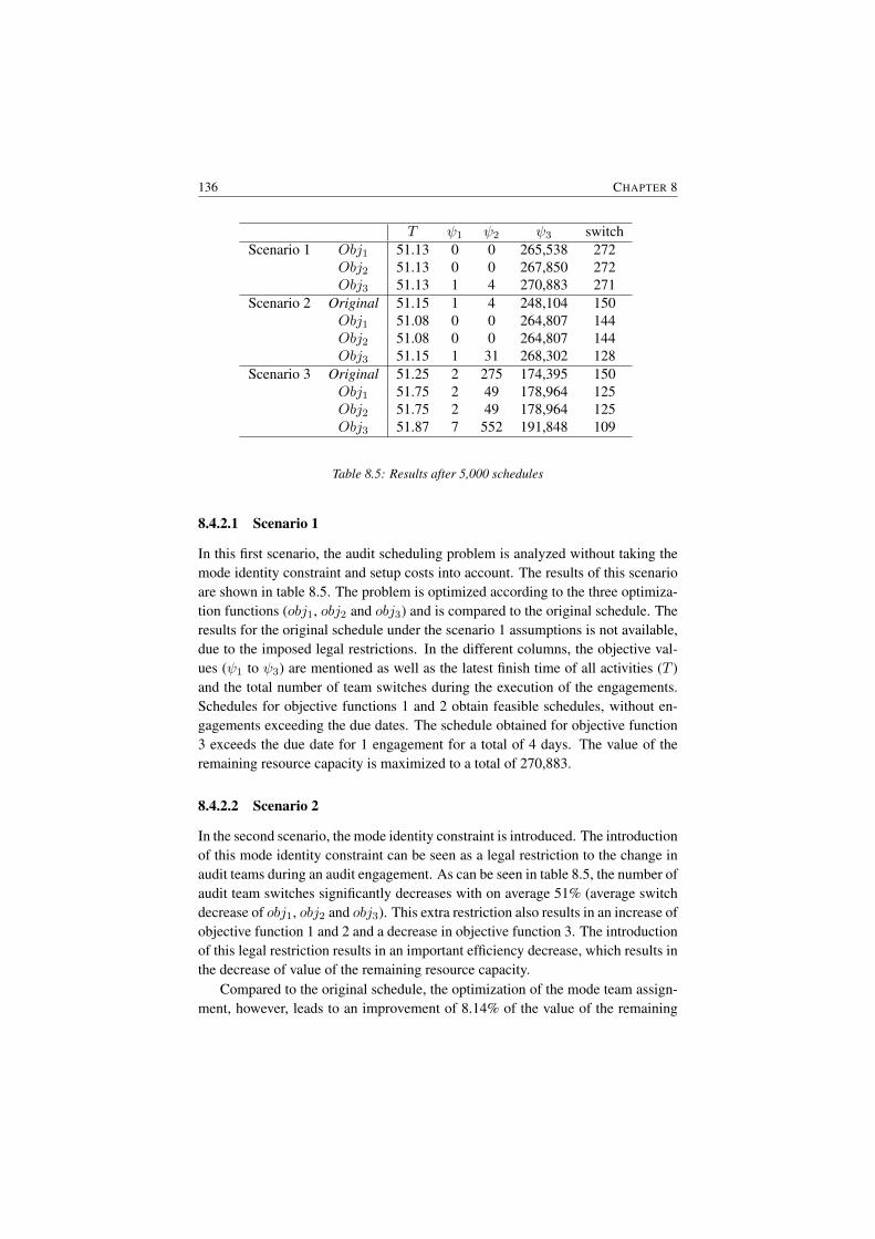
136 CHAPTER 8
T ψ1 ψ2 ψ3 switchScenario 1 Obj1 51.13 0 0 265,538 272
Obj2 51.13 0 0 267,850 272Obj3 51.13 1 4 270,883 271
Scenario 2 Original 51.15 1 4 248,104 150Obj1 51.08 0 0 264,807 144Obj2 51.08 0 0 264,807 144Obj3 51.15 1 31 268,302 128
Scenario 3 Original 51.25 2 275 174,395 150Obj1 51.75 2 49 178,964 125Obj2 51.75 2 49 178,964 125Obj3 51.87 7 552 191,848 109
Table 8.5: Results after 5,000 schedules
8.4.2.1 Scenario 1
In this first scenario, the audit scheduling problem is analyzed without taking themode identity constraint and setup costs into account. The results of this scenarioare shown in table 8.5. The problem is optimized according to the three optimiza-tion functions (obj1, obj2 and obj3) and is compared to the original schedule. Theresults for the original schedule under the scenario 1 assumptions is not available,due to the imposed legal restrictions. In the different columns, the objective val-ues (ψ1 to ψ3) are mentioned as well as the latest finish time of all activities (T )and the total number of team switches during the execution of the engagements.Schedules for objective functions 1 and 2 obtain feasible schedules, without en-gagements exceeding the due dates. The schedule obtained for objective function3 exceeds the due date for 1 engagement for a total of 4 days. The value of theremaining resource capacity is maximized to a total of 270,883.
8.4.2.2 Scenario 2
In the second scenario, the mode identity constraint is introduced. The introductionof this mode identity constraint can be seen as a legal restriction to the change inaudit teams during an audit engagement. As can be seen in table 8.5, the number ofaudit team switches significantly decreases with on average 51% (average switchdecrease of obj1, obj2 and obj3). This extra restriction also results in an increase ofobjective function 1 and 2 and a decrease in objective function 3. The introductionof this legal restriction results in an important efficiency decrease, which results inthe decrease of value of the remaining resource capacity.
Compared to the original schedule, the optimization of the mode team assign-ment, however, leads to an improvement of 8.14% of the value of the remaining
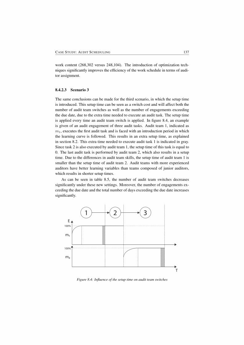
CASE STUDY: AUDIT SCHEDULING 137
work content (268,302 versus 248,104). The introduction of optimization tech-niques significantly improves the efficiency of the work schedule in terms of audi-tor assignment.
8.4.2.3 Scenario 3
The same conclusions can be made for the third scenario, in which the setup timeis introduced. This setup time can be seen as a switch cost and will affect both thenumber of audit team switches as well as the number of engagements exceedingthe due date, due to the extra time needed to execute an audit task. The setup timeis applied every time an audit team switch is applied. In figure 8.4, an exampleis given of an audit engagement of three audit tasks. Audit team 1, indicated asm1, executes the first audit task and is faced with an introduction period in whichthe learning curve is followed. This results in an extra setup time, as explainedin section 8.2. This extra time needed to execute audit task 1 is indicated in gray.Since task 2 is also executed by audit team 1, the setup time of this task is equal to0. The last audit task is performed by audit team 2, which also results in a setuptime. Due to the differences in audit team skills, the setup time of audit team 1 issmaller than the setup time of audit team 2. Audit teams with more experiencedauditors have better learning variables than teams composed of junior auditors,which results in shorter setup times.
As can be seen in table 8.5, the number of audit team switches decreasessignificantly under these new settings. Moreover, the number of engagements ex-ceeding the due date and the total number of days exceeding the due date increasessignificantly.
m1
m2
E
T
1 2 3
100%
100%
Figure 8.4: Influence of the setup time on audit team switches
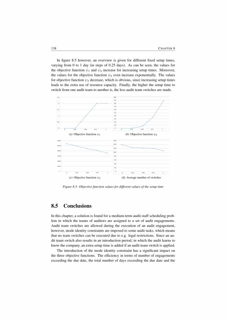
138 CHAPTER 8
In figure 8.5 however, an overview is given for different fixed setup times,varying from 0 to 1 day (in steps of 0.25 days). As can be seen, the values forthe objective function ψ1 and ψ2 increase for increasing setup times. Moreover,the values for the objective function ψ2 even increase exponentially. The valuesfor objective function ψ3 decrease, which is obvious, since increasing setup timesleads to the extra use of resource capacity. Finally, the higher the setup time toswitch from one audit team to another is, the less audit team switches are made.
0
0.5
1
1.5
2
2.5
0 0.25 0.50 0.75 1
(a) Objective function ψ1
0
10
20
30
40
50
60
70
80
90
100
0 0.25 0.50 0.75 1
(b) Objective function ψ2
300000
250000
200000
150000
100000
50000
00 0.25 0.50 0.75 1
(c) Objective function ψ3
0
20
40
60
80
100
120
140
160
0 0.25 0.50 0.75 1
(d) Average number of switches
Figure 8.5: Objective function values for different values of the setup time
8.5 Conclusions
In this chapter, a solution is found for a medium-term audit-staff scheduling prob-lem in which the teams of auditors are assigned to a set of audit engagements.Audit team switches are allowed during the execution of an audit engagement,however, mode identity constraints are imposed to some audit tasks, which meansthat no team switches can be executed due to e.g. legal restrictions. Since an au-dit team switch also results in an introduction period, in which the audit learns toknow the company, an extra setup time is added if an audit team switch is applied.
The introduction of the mode identity constraint has a significant impact onthe three objective functions. The efficiency in terms of number of engagementsexceeding the due date, the total number of days exceeding the due date and the

CASE STUDY: AUDIT SCHEDULING 139
total value of the remaining resource capacity decrease significantly. The introduc-tion of a setup time further decreases the efficiency, which results in a significantdecrease in the number of audit team switches. The same results are obtained foran increasing fixed setup time. The larger the setup time is, the less interesting itis to switch audit teams during audit engagement execution.
The algorithm is applied on real-life data from a small Belgium audit firm,with 15 auditors and almost 250 audit tasks per year. Compared with the optimalschedule obtained in the computational section (result scenario 2 - objective func-tion ψ3), an efficiency improvement is realized in the audit team assignment of8.14% in the value of the unassigned resource capacity (from 248,104 to 268,302),which corresponds with almost 200 working days of a junior assistant.
Although the algorithm is applied on a simplification of a practical planningsituation, the introduction of optimization techniques significantly improves theefficiency of the work schedule in terms of auditor assignment. As many auditoffices still use relatively simple programs to schedule their auditor teams, the useof advanced scheduling algorithms and techniques aims to generate high qualityschedules. Future research is needed to develop methods which can incorporateovertime and other real-life extensions and which can convert the obtained auditteam schedule into single auditor schedules efficiently.

9Conclusions and Future Research
In this chapter, an overview of the different research topics of this work is given,the main contribution of each algorithm is analyzed and different directions forfuture research are defined. Moreover, general reflections are expressed with re-spect to future research in project scheduling in general and multi-mode resource-constrained project scheduling in particular.
9.1 Introduction
In this work, we investigated the multi-mode resource-constrained project schedul-ing problem (MRCPSP), where each activity can be performed in different sets ofmodes, with a specific activity duration and resource requirements. The activitieshave to be scheduled within precedence constraints and (renewable and nonrenew-able) resource constraints, in order to minimize the makespan of the project.
The MRCPSP can be divided into two subproblems: a first subproblem is re-ferred to as the Mode Assignment Problem (MAP), whose aim it is to find a feasiblemode assignment. A mode assignment is called feasible if the nonrenewable re-source demand does not exceed the nonrenewable resource availability. If there ismore than one nonrenewable resource, the problem of finding a feasible solutionis NP-complete (Kolisch and Drexl, 1997). In a second subproblem, a start timeshould be assigned to each activity. Given the duration and the resource consump-tions of the different activities, the aim of this scheduling problem is to minimizethe makespan of the project.
142 CONCLUSIONS AND FUTURE RESEARCH
The resource-constrained project scheduling problem in general and its multi-mode extension in particular have been research topics for many decades, resultingin a wide variety of solution procedures. Different search strategies have been usedin order to solve the MRCPSP. An overview of the exact, heuristic and metaheuris-tic algorithms has been presented in chapter 2.
In Part I of this work, we proposed different population-based metaheuristics.Each of the search strategies has been tailored to the problem under study. Thesolution procedures have been tested on the PSPLIB dataset (Kolisch et al., 1995)and the dataset of Boctor (1993) and have been compared to other solution proce-dures available in the literature. Moreover, a new dataset MMLIB was generatedin order to deal with the major shortcomings of the current benchmark datasets,given the recent evolution in the development of metaheuristic search procedures.In Part II, we focused on some extensions of the MRCPSP. First, the MRCPSP wasextended to the preemptive multi-mode version in order to investigate the influenceof preemption on the project duration. Second, the concept of learning was incor-porated in the discrete time/resource trade-off problem in order to investigate theinfluence of the introduction of learning effects on the project makespan. Finally,an audit scheduling problem with sequence-dependent setup times and differentaudit team efficiencies is modeled as an MRCPSP and the results for a real-lifeaudit team scheduling problem were presented.
The remainder of this chapter is organized as follows. Section 9.2 briefly re-views part I in which three metaheuristic solution procedures for the MRCPSP areintroduced. In section 9.3, an overview is given of the two extensions and the casestudy which are discussed in Part II. Finally, some general reflections are presentedin section 9.4.
9.2 Metaheuristic procedures for the MRCPSP
Part I of this work investigated the potential of three different population-basedmetaheuristic solution procedures to solve the MRCPSP. In section 3.3, a bi-populational genetic algorithm was proposed, which makes use of two popula-tions, one with left-justified schedules and one with right-justified schedules. Alsoan extended serial schedule generation scheme was proposed, which improves themode selection by choosing the feasible mode of a certain activity that minimizesthe finish time of the activity. In section 3.4, we successfully explored the artifi-cial immune system solution methodology to tackle the MRCPSP. The algorithmmakes use of a controlled search procedure, which selects out of a large set of modelists those lists that have a larger probability to obtain better solutions. This proce-dure leads the search process more quickly to the more interesting search regions.Finally, the scatter search procedure was proposed in section 3.5. Unlike the othertwo metaheuristic procedures, the scatter search procedure uses strategic designs
CONCLUSIONS AND FUTURE RESEARCH 143
to artificially introduce diversity during the search process. The main contribu-tion of this procedure is the steering power of the three proposed improvementmethods, each tailored to the specific characteristics of different renewable andnonrenewable resource scarceness values. Moreover, by combining the differentimprovement methods and two local searches, an efficient combined solution pro-cedure could be designed, which leads to promising computational results. Whencomparing the performance of the different procedures (cf. chapter 5), we canconclude that the scatter search procedure outperforms the other procedures.
Concerning the design of metaheuristic procedures, we consider the focus onthe mode assignment problem and the use of problem specific information in thesearch process as important directions for future research. The new dataset whichhas been proposed in chapter 4 can facilitate and motivate researchers to investigateand develop new ideas and techniques to tackle the MRCPSP.
Focus on the mode assignment problem Algorithms using a clever mode as-signment procedure to generate the initial population have an advantage comparedto other methods. Their performance is better, especially when the number of gen-erated schedules is low. By focusing on the mode assignment problem, i.e. search-ing for a feasible mode combination, the procedure should be able to reduce thesearch space, not only in order to exclude infeasible mode assignments, but alsoto determine those mode combinations with the largest probability of obtainingthe optimal solution. Although the use of mode characteristics has already beenstudied in section 3.4, future research should focus on finding mode parameters orcharacteristics which influence the makespan of the project.
Use of problem specific information Regardless of the used search strategy, theperformance of a metaheuristic is mainly determined by local search proceduresused in the algorithm. Procedures which are best tailored to the project settingsoutperform other procedures. The use of problem specific information in theselocal search procedures significantly increases the efficiency of the procedure. Tothat purpose, the design of new local search procedures should be encouraged.
Even though the currently proposed procedures perform very well on the cre-ated instances of the benchmark datasets PSPLIB, Boctor and MMLIB, they willprobably perform less well on real project instances. Real-life problems will not fitin a specific group of project parameters. In order to provide project managers anefficient schedule, future research should focus on the influence and use of otherindicators, not only project specific parameters, but also environmental informa-tion and project progress information. A decision support system could provide alink between software packages and the real-life projects and would clearly reducethe gap between academic research and practice.
144 CONCLUSIONS AND FUTURE RESEARCH
New dataset for the MRCPSP Based on the disadvantages of the current bench-mark datasets PSPLIB and Boctor, we have developed a new dataset MMLIB thathas been used to test and validate the proposed metaheuristic solution proceduresand to compare the performance of the three algorithms with the metaheuristic so-lution procedures available in the literature. The introduction of this new datasetopens the possibility to compare new solution procedures with the currently avail-able methods. Researchers are encouraged to use this dataset to compare the re-sults of their solution procedures with other procedures.
9.3 Extensions for the MRCPSP
In part II of this work, we explored two extensions of the MRCPSP, namely theintroduction of preemption and the introduction of learning in the MRCPSP. Inchapter 6, the influence of preemption on the project duration was investigated.The extension to the preemptive multi-mode version allows activities to be pre-empted at any integer time instance and restarted later on at no additional cost.This is in contrast with the basic MRCPSP, in which it is assumed that each activ-ity, once started, will be executed until its completion. In order to allow activitypreemption, the original activity network is converted into a new network, in whicheach activity is split into subactivities with a unit duration of 1. The introductionof preemption leads to a significant decrease in the average project makespan com-pared to the non-preempted case. Nevertheless, it should be stated that it is moredifficult to find improvements if nonrenewable resources are taken into account.
In chapter 7, the influence of the introduction of learning effects was investi-gated. The concept of activity-specific learning, in which the resources becamemore efficient the longer they stay on the job, was examined from various an-gles. The concept was introduced in the discrete time/resource trade-off problem,in which each activity contains a specific work content in terms of working days,instead of a fixed duration and resource requirement. For each activity, a set ofexecution modes can be specified using different combinations of durations andresource requirements, as long as the specified work content is met. Computa-tional tests revealed a significant influence of the introduction of learning effectsin project scheduling. The main project drivers that affect the project makespanwhen introducing learning effects have been analyzed, the margin of error madeby ignoring learning during schedule construction has been measured and the im-portance of incorporating the learning effects timely (i.e. when the project is inprogress) has been proven, since this leads to significant makespan improvements.
Nevertheless, with respect to these two extensions, several future research di-rections can be suggested, as mentioned in the following paragraphs.
CONCLUSIONS AND FUTURE RESEARCH 145
Preemption If nonrenewable resources are taken into account, the proposedalgorithm was not always able to obtain better solutions compared to the non-preemptive case. This is mainly due to the larger project network, which is gener-ated by splitting the activities into subactivities with a unit duration of 1. New so-lution procedures must be able to decrease the number of inferior solutions. Futureresearch should therefore focus on an improved mode selection procedure, search-ing feasible mode assignments more quickly. Another possibility is to limit thenumber of interruptions allowed during project execution. This probably wouldhave an influence on the results since the search space (here determined as thenumber of (sub)activities) clearly decreases due to the restricted number of inter-ruptions. Moreover, this restriction proved to be successful in the procedure ofBallestin et al. (2008) for the preempted version of the RCPSP.
In most cases, it is assumed that activities can be preempted without any addi-tional cost. However, this assumption is difficult to maintain in real-life situations.Two types of penalization can be proposed and could be introduced in future re-search on this topic:
• Fixed setup time Every time a preempted activity is restarted, a fixed setuptime can be added to the duration of the activity. This penalization is alreadyintroduced in the paper of Vanhoucke (2008).
• Variable setup time Ash and Smith-Daniels (1999) have determined theimpact of learning, forgetting and relearning on the project completion timewhen preemption is allowed. When an activity is preempted, the efficiencylevel is interrupted and a period of forgetting is initialized. The variablesetup time is determined as the time needed to relearn and obtain the originalefficiency level. A similar approach to calculate the setup time is used inchapter 8.
Stochastic durations In chapter 7, the influence of the introduction of learningeffects is studied. The influence of learning on the activity durations is measureddeterministically. However, a more realistic view could be obtained by consideringthe learning effect in a stochastic way. The durations should therefore follow aprobabilistic distribution, using the formulas given in chapter 7 as the average ofthe durations. Future research should focus on this point.
In addition to learning, forgetting is also a natural phenomenon that occurswhen a resource stops working on a specific activity. The interruption of the activ-ity obviously leads to the termination of the activity-specific learning process andis beneficial when activity splitting is allowed. Empirical research has also shownthat working with insufficient or too many resources can result in an efficiencydecrease due to an increasing loss of motivation and dedication. The introduc-tion of team work where the efficiency of a single resource can influence the team
146 CONCLUSIONS AND FUTURE RESEARCH
efficiency and the determination of the optimal number of team members and itsinfluence on the project duration are also topics for further research. Finally, inthis research we have focused on the autonomous learning concept. However, theacquired insights in project scheduling with learning effects can be used to dis-cuss and investigate the induced learning concept, where learning is the result ofmanagement investments in training and innovative technologies. The determina-tion of the optimal learning rate per activity will be one of the key questions thelearning effect research can propose to the project management practice.
Other extensions The general MRCPSP imposes strict assumptions on the ac-tivities, which often might be violated in practice. The introduction of preemptionand the introduction of the learning concept were two extensions on the generalMRCPSP to relax these assumptions. However, other extensions still have to bestudied. We refer, amongst others, to the scheduling problem with discounted cashflows or the multi-mode resource availability cost problem. Moreover, also theoption to allow within-activity fast tracking should be considered, since this ex-tension proves to be successful in reducing the makespan of schedule (Vanhouckeand Debels, 2008).
Real-life situations In the last chapter of this work, the algorithms designedfor the MRCPSP are used to solve real-life scheduling problems, such as the au-dit team scheduling problem. Although the algorithm is applied on a simplifica-tion of a practical planning problem, the introduction of optimization techniquessignificantly improves the efficiency of the audit team schedule, as can be seenin the computational analysis. Future research, however, is needed to developmethods to incorporate overtime and other real-life extensions. Moreover, otherplanning problems could also be converted to the MRCPSP and could be solvedusing the available solution procedures. This will reduce the gap between aca-demic research and practice.
9.4 General reflections
In general, many project scheduling problems are still unexplored. In this work,we have covered the MRCPSP and some of its extensions. To conclude this work,we briefly overview the main contributions of this work.
Three state-of-the-art algorithms In the first part of this work, we have pre-sented three metaheuristic solution procedures. These procedures obtainstate-of-the-art results compared to the results of the algorithms available inthe literature. Moreover, the use of search strategies that have never beenused before to tackle the MRCPSP, such as the scatter search procedure and

CONCLUSIONS AND FUTURE RESEARCH 147
the artificial immune system method, have proven to be successful in findinghigh quality solutions.
Use of problem specific information The use of problem specific information inthe local search process, such as the use of resource scarceness parametersin the scatter search procedure, increased the efficiency of the proceduresignificantly.
New dataset The new dataset can facilitate and motivate researchers to inves-tigate and develop new ideas and techniques to tackle the MRCPSP. Re-searchers are encouraged to use this dataset to compare the results of theirsolution procedures with other procedures.
Introduction of learning With the introduction of the learning effect in a multi-mode project environment, a new trade-off is set between the duration of anactivity and the efficiency of a human resource. We have also learned thatthe efficiency of human resources influences the project duration. Moreover,the earlier the learning effect is taken into account, the larger the benefit withrespect to the original baseline schedule is.
Use for real-life problems The applicability and importance of the multi-moderesource-constrained project scheduling problem are illustrated by means ofa real-life audit team scheduling problem bridging the gap between sched-uling theory and practice.

References
Aarts, E. and Korst, J. (1989). Simulated Annealing and Boltzmann Machines:A Stochastic Approach to Combinatorial Optimization and Neural Computing.Wiley, Chichester.
Adler, P. S. and Clark, K. B. (1991). Behind the learning curve: A sketch of thelearning process. Management Science, 37(3):267–281.
Agarwal, R., Tiwari, M., and Mukherjee, S. (2007). Artificial immune systembased approach for solving resource constraint project scheduling problem. In-ternational Journal of Advanced Manufacturing Technology, 34:584–593.
Alcaraz, J. and Maroto, C. (2001). A robust genetic algorithm for resource alloca-tion in project scheduling. Annals of Operations Research, 102:83–109.
Alcaraz, J., Maroto, C., and Ruiz, R. (2003). Solving the multi-mode resource-constrained project scheduling problem with genetic algorithms. Journal of theOperational Research Society, 54:614–626.
Allahverdi, A., Ng, C., Cheng, T., and Kovalyov, M. (2008). A survey of sched-uling problems with setup times or costs. European Journal of OperationalResearch, 187:985–1032.
Alvarez-Valdes, R. and Tamarit, J. (1989). Heuristic algorithms for resource-constrained project scheduling: A review and emperical analysis. In Slowinski,R. and Weglarz, J., editors, Advances in Project Scheduling. Elsevier, Amster-dam.
Amor, J. and Teplitz, C. (1998). An efficient approximation procedure for projectcomposite learning curves. Project Management Journal, 29:28–42.
Anderson, E. and Ferris, M. (1994). Genetic algorithm for combinatorial optimi-sation: The assembly line balancing problem. ORSA Journal on Computing,6:161–173.
Ash, R. and Smith-Daniels, D. E. (1999). The effects of learning, forgetting, andrelearning on decision rule performance in multiproject scheduling. DecisionSciences, 30:47–82.

150 REFERENCES
Balachandran, B. and Zoltners, A. (1981). An interactive audit-staff schedulingdecision support system. The Accounting Review, 56:801–812.
Ballestin, F., Valls, V., and Quintanilla, S. (2008). Pre-emption in resource-constrained project scheduling. European Journal of Operational Research,189:1136–1152.
Ballestin, F., Valls, V., and Quintanilla, S. (2009). Scheduling projectswith limitednumber of preemptions. Computers and Operations Research, 36:2913–2925.
Barrios, A., Ballestin, F., and Valls, V. (2009). A double genetic algorithm for themrcpsp/max. doi:10.1016/j.cor.2009.09.019.
Bedworth, D. and Bailey, J. (1982). Integrated Production Control Systems - Man-agement, Analysis, Design. Wiley, New York.
Biskup, D. (2008). A state-of-the-art review on scheduling with learning effects.European Journal of Operational Research, 188:315–329.
Blazewicz, J., Lenstra, J., and Rinnooy Kan, A. (1983). Scheduling subject toresource constraints: Classification and complexity. Discrete Applied Mathe-matics, 5:11–24.
Blum, C. and Roli, A. (2003). Metaheuristics in combinatorial optimization:Overview and conceptual comparison. ACM Computing Surveys, 35(3):268–308.
Bochenski, B. (1993). Implementing Production-Quality Client/server Systems.John Wiley & Sons, Inc.
Boctor, F. (1993). Heuristics for scheduling projects with resource restrictions andseveral resource-duration modes. International Journal of Production Research,31:2547–2558.
Boctor, F. (1996). A new and efficient heuristic for scheduling projects with re-source restrictions and multiple execution modes. European Journal of Opera-tional Research, 90:349–361.
Bouleimen, K. and Lecocq, H. (2003). A new efficient simulated annealing algo-rithm for the resource-constrained project scheduling problem and its multiplemode version. European Journal of Operational Research, 149:268–281.
Brazel, Y. (1972). The rate of technical progress: The indianapolis 500. Journalof Economic Theory, 4:72–81.
REFERENCES 151
Brucker, P., Drexl, A., Mohring, R., Neumann, K., and Pesch, E. (1999). Resource-constrained project scheduling: notation, classification, models, and methods.European Journal of Operational Research, 112:3–41.
Brucker, P. and Schumacher, D. (1999). A new tabu search procedure for an audit-scheduling problem. Journal of Scheduling, 2(4):157–173.
Buddhakulsomsiri, J. and Kim, D. (2006). Properties of multi-mode resource-constrained project scheduling problems with resource vacations and activitysplitting. European Journal of Operational Research, 175:279–295.
Buddhakulsomsiri, J. and Kim, D. (2007). Priority rule-based heuristic for multi-mode resource-constrained project scheduling problems with resource vacationsand activity splitting. European Journal of Operational Research, 178:374–390.
Chan, K. and Dodin, B. (1986). A decision support system for audit-staff schedul-ing with precedence constraints and due dates. The Accounting Review, 61:726–734.
Coello, C. C., Rivera, D., and Cortes, N. (2003). Use of an artificial immunesystem for job shop scheduling. Lecture Notes in Computer Science, 2787:1–10.
Cooper, D. (1976). Heuristics for Scheduling Resource-constrained Projects: AnExperimental Investigation. Management Science, 22:1186–1194.
Damay, J., Quilliot, A., and Sanlaville, E. (2007). Linear programming basedalgorithms for preemptive and non-preemptive rcpsp. European Journal of Op-erational Research, 182:1012–1022.
De Castro, L. and Timmis, J. (2002). Artificial immune systems: a novel paradigmfor pattern recognition. In Alonso, L., Corchado, J., and Fyfe, C., editors, Arti-ficial Neural Networks in Pattern Recognition. University of Paisley.
De Reyck, B., Demeulemeester, E., and Herroelen, W. (1998). Local search meth-ods for the discrete time/resource trade-off problem in project networks. NavalResearch Logistics, 45:553–578.
Debels, D., De Reyck, B., Leus, R., and Vanhoucke, M. (2006). A hybrid scat-ter search/electromagnetism meta-heuristic for project scheduling. EuropeanJournal of Operational Research, 169:638–653.
Debels, D. and Vanhoucke, M. (2005). A bi-population based genetic algorithmfor the RCPSP. Lecture Notes in Computer Science, 3483:378–387.
Debels, D. and Vanhoucke, M. (2006). Pre-emptive resource-constrained projectscheduling with setup times. Technical report, Ghent University.
152 REFERENCES
Debels, D. and Vanhoucke, M. (2007). A decomposition-based genetic algorithmfor the resource-constrained project scheduling problem. Operations Research,55:457–469.
Demeulemeester, E., De Reyck, B., and Herroelen, W. (2000). Discrete time/re-source trade-off problem in project networks: A branch-and-bounded approach.IIE Transactions, 32:1059–1069.
Demeulemeester, E. and Herroelen, W. (1996). An efficient optimal solutionfor the preemptive resource-constrained project scheduling problem. EuropeanJournal of Operational Research, 90:334–348.
Demeulemeester, E., Vanhoucke, M., and Herroelen, W. (2003). A random net-work generator for activity-on-the-node networks. Journal of Scheduling, 6:13–34.
Dodin, B. and Chan, H. (1991). Application of production scheduling methodsto external and internal audit scheduling. European Journal of OperationalResearch, 52:267–279.
Dodin, B. and Elimam, A. (1997). Audit scheduling with overlapping activitiesand sequence-dependent setup costs. European Journal of Operational Re-search, 97:22–33.
Dodin, B., Elimam, A., and Rolland, E. (1998). Tabu search in audit scheduling.European Journal of Operational Research, 106:373–392.
Drexl, A. (1991). Scheduling of project networks by job assignment. ManagementScience, 37(12):1590–1602.
Drexl, A., Frahm, J., and Salewski, F. (2006). Audit-staff scheduling by columngeneration. In Morlock, M., Schwindt, C., Trautmann, N., and Zimmermann,J., editors, Perspectives on Operations Research. Gabler Edition Wissenschaft.
Drexl, A. and Grunewald, J. (1993). Nonpreemptive multi-mode resource-constrained project scheduling. IIE Transactions, 25:74–81.
Engin, O. and Doyen, A. (2004). A new approach to solve hybrid flow shopscheduling problems by artificial immune system. Future Generation ComputerSystems, 20:1083–1095.
Geem, Z., Kim, J., and Loganathan, G. (2001). A new heuristic optimizationalgorithm: Harmony search. Simulation, 76:60–68.
Glover, F. and Kochenberger, G. A. (2003). Handbook of Metaheuristics. KluwerAcademic Publishers.
REFERENCES 153
Glover, F., Laguna, M., and Marti, R. (2000). Fundamentals of scatter search andpath relinking. Control and Cybernetics, 29:653–684.
Gutjahr, W. J., Katzensteiner, S., Reiter, P., Stummer, C., and Denk, M. (2008).Competence-driven project portfolio selection, scheduling and staff assignment.Central European Journal of Operations Research, 16(3):281–306.
Hanakawa, N., Morisaki, S., and Matsumoto, K.-I. (1998). A learning curve basedsimulation model for software development. In 20th International Conferenceon Software Engineering (ICSE’98).
Hans, E., Herroelen, W., Leus, R., and Wullink, G. (2007). A hierarchical approachto multi-project planning under uncertainty. Omega The International Journalof Management Science, 35:563–577.
Hart, E., Ross, P., and Nelson, J. (1998). Producing robust schedules via an artifi-cial immune system. In Proceedings of the ICEC ’98.
Hartmann, S. (2001). Project scheduling with multiple modes: A genetic algo-rithm. Annals of Operations Research, 102:111–135.
Hartmann, S. (2002). A self-adapting genetic algorithm for project schedulingunder resource constraints. Naval Research Logistics, 49:433–448.
Hartmann, S. and Drexl, A. (1998). Project scheduling with multiple modes: Acomparison of exact algorithms. Networks, 32:283–297.
Hartmann, S. and Kolisch, R. (2000). Experimental evaluation of state-of-the-artheuristics for the resource-constrained project scheduling problem. EuropeanJournal of Operational Research, 127:394–407.
Hartmann, S. and Sprecher, A. (1996). A note on ”hierarchical models for multi-project planning and scheduling”. European Journal of Operational Research,94:377–383.
Heimerl, C. and Kolisch, R. (2009). Scheduling and staffing multiple projects witha multi-skilled workforce. Accepted for publication in OR Spectrum.
Hendriks, M., Voeten, B., and Kroep, L. (1999). Human resource allocation in amulti-project research and development environment. International Journal ofProject Management, 17:181–188.
Herroelen, W. and De Reyck, B. (1999). Phase transitions in project scheduling.Journal of the Operational Research Society, 50:148–156.
Hillier, F. S. and Lieberman, G. J. (2005). Introduction to Operations Research.McGraw-Hill: Boston (MA).

154 REFERENCES
Holland, J. (1975). Adaptation in natural and artificial systems. University ofMichigan Press, Ann Arbor.
Homberger, J. (2007). A multi-agent system for the decentralized resource-constrained multi-project scheduling problem. International Transactions inOperational Research, 14(6):565–589.
Janiak, A. and Rudek, R. (2007). The learning effect: Getting to the core of theproblem. Information Processing Letters, 103:183–187.
Jarboui, B., Damak, N., Siarry, P., and Rebai, A. (2008). A combinatorial par-ticle swarm optimization for solving multi-mode resource-constrained projectscheduling problems. Applied Mathematics and Computation, 195:299–308.
Jozefowska, J., Mika, M., Rozycki, R., Waligora, G., and Weglarz, J. (2001). Sim-ulated annealing for multi-mode resource-constrained project scheduling. An-nals of Operations Research, 102:137–155.
Jozefowska, J. and Weglarz, J. (2006). Perspectives in Modern Project Scheduling.Springer.
Kaplan, L. (1988). Resource-constrained project scheduling with preemption ofjobs. PhD thesis, University of Michigan.
Kaplan, L. (1991). Resource-constrained project scheduling with setuptimes. Technical report, Department of Management, University of Tenessee,Knoxville.
Kelley, J. (1963). The critical-path method: Resources planning and scheduling.Prentice-Hall, New Jersey.
Kennedy, J. and Eberhart, R. (1995). Particle swarm optimization. In Proceedingsof the IEEE Conference on Neural Networks.
Knotts, G., Dror, M., and Hartman, B. (2000). Agent-Based Project Scheduling.IIE Transactions, 32(5):387–401.
Kolisch, R. (1995). Project scheduling under resource constraints – Efficientheuristics for several problem classes. PhD thesis, Physica, Heidelberg.
Kolisch, R. (1996a). Efficient priority rules for the resource-constrained projectscheduling problem. Journal of Operations Management, 14:179–192.
Kolisch, R. (1996b). Serial and parallel resource-constrained project schedulingmethods revisited: Theory and computation. European Journal of OperationalResearch, 90:320–333.
REFERENCES 155
Kolisch, R. (1999). Resource allocation capabilities of commercial project man-agement software packages. Interfaces, 29:19–31.
Kolisch, R. and Drexl, A. (1997). Local search for nonpreemptive multi-moderesource-constrained project scheduling. IIE Transactions, 29:987–999.
Kolisch, R. and Hartmann, S. (1999). Heuristic algorithms for solving theresource-constrained project scheduling problem: Classification and compu-tational analysis. In Weglarz, J., editor, Project scheduling: Recent models,algorithms and applications. Kluwer Academic Publishers.
Kolisch, R. and Hartmann, S. (2006). Experimental investigation of heuristicsfor resource-constrained project scheduling: An update. European Journal ofOperational Research, 174:23–37.
Kolisch, R., Sprecher, A., and Drexl, A. (1995). Characterization and generationof a general class of resource-constrained project scheduling problems. Man-agement Science, 41:1693–1703.
Kruger, D. and Scholl, A. (2009). A heuristic solution framework for the resourceconstrained (multi-)project scheduling problem with sequence-dependent trans-fer times. European Journal of Operational Research, 197(2):492–508.
Kruger, D. and Scholl, A. (2010). Managing and modelling general resource trans-fers in (multi-)project scheduling. OR Spectrum, 32(2):369–394.
Li, K. and Willis, R. (1992). An iterative scheduling technique for resource-constrained project scheduling. European Journal of Operational Research,56:370–379.
Lova, A., Tormos, P., and Barber, F. (2006). Multi-Mode Resource ConstrainedProject Scheduling: Scheduling Schemes, Priority Rules and Mode SelectionRules. Inteligencia Artificial, 30:69–86.
Lova, A., Tormos, P., Cervantes, M., and Barber, F. (2009). An efficient hybridgenetic algorithm for scheduling projects with resource constraints and multipleexecution modes. International Journal of Production Economics, 117:302–316.
Marti, R., Laguna, M., and Glover, F. (2006). Principles of Scatter Search. Euro-pean Journal of Operational Research, 169:359–372.
Mastor, A. (1970). An experimental and comparative evaluation of production linebalancing techniques. Management Science, 16:728–746.

156 REFERENCES
Metropolis, N., Rosembluth, A., Rosenbluth, M., and Teller, A. (1953). Equationof state calculations by fast computing machines. Journal of Chemical Physics,21:1087–1092.
Mori, M. and Tseng, C. (1997). A genetic algorithm for the multi-mode resourceconstrained project scheduling problem. European Journal of Operational Re-search, 100:134–141.
Nembhard, D. and Uzumeri, M. (2000). An individual-based description of learn-ing within an organization. IEEE Transactions on Engineering Management,47(3):370 – 378.
Nonobe, K. and Ibaraki, T. (2002). Formulation and tabu search algorithm for theresource constrained project scheduling problem. In Ribeiro, C. and Hansen, P.,editors, Essays and Surveys in Metaheuristics. Kluwer Academic Publishers.
Osman, I. (1995). An introduction to meta-heuristics. In Lawrence, M. and Wils-don, C., editors, Operational Research Tutorial Papers. Operational ResearchSociety Press.
Osman, I. and Laporte, G. (1996). Metaheuristics: A bibliography. Annals ofOperations Research, 63:513–623.
Ozdamar, L. (1999). A genetic algorithm approach to a general category projectscheduling problem. IEEE Transactions on Systems, Management and Cyber-netics, 29:44–59.
Ozdamar, L. and Ulusoy, G. (1994). A local constraint based analysis approachto project scheduling under general resource constraints. European Journal ofOperational Research, 79:287–298.
Pascoe, T. (1966). Allocation of resources - CPM. Revue Francaise de RechercheOperationnelle, 38:31–38.
Patterson, J. (1976). Project scheduling: The effects of problem structure onheuristic scheduling. Naval Research Logistics, 23:95–123.
Patterson, J., Slowinski, R., Talbot, F., and Weglarz, J. (1989). An algorithm fora general class of precedence and resource constrained scheduling problem. InSlowinsky, R. and Weglarz, J., editors, Advances in Project Scheduling. Else-vier, Amsterdam.
Pinol, H. and Beasley, J. (2006). Scatter Search and Bionomic Algorithms forthe Aircraft Landing Problem. European Journal of Operational Research,171:439–462.

REFERENCES 157
PMBOK (2004). A Guide to the Project Management Body of Knowledge, ThirdEdition. Newtown Square, Pa.: Project Management Institute, Inc.
Potts, C. and Kovalyov, M. (2000). Scheduling with batching: A review. EuropeanJournal of Operational Research, 120:228–249.
Ranjbar, M., De Reyck, B., and Kianfar, F. (2009). A hybrid scatter-search forthe discrete time/resource trade-off problem in project scheduling. EuropeanJournal of Operational Research, 193:35–48.
Ranjbar, M. and Kianfar, F. (2007). Solving the discrete time/resource trade-off problem with genetic algorithms. Applied Mathematics and Computation,191:451–456.
Sahal, D. (1979). A theory of progress functions. AIIE Transactions, 11(1):23–29.
Salewski, F., Schirmer, A., and Drexl, A. (1997). Project scheduling under re-source and mode identity constraints: Model, complexity, methods and applica-tions. European Journal of Operational research, 102:88–110.
Sels, V. and Vanhoucke, M. (2009). A genetic algorithm for the single machinemaximum lateness problem. Technical report, Faculty of Economics and Busi-ness Administration, Ghent University.
Shtub, A., LeBlanc, L., and Cai, Z. (1996). Scheduling programs with repetitiveprojects: A comparison of a simulated annealing, a genetic and a pair-wise swapalgorithm. European Journal of Operational Research, 88:124–138.
Slack, N., Chambers, S., Johnston, R., and Betts, A. (2009). Operations andprocess management. Prentice-Hall, Inc: NJ.
Slowinski, R. (1980). Two approaches to problems of resource allocation amongproject activities - a comparative study. Journal of Operational Research Soci-ety, 8:711–723.
Slowinski, R., Soniewicki, B., and Weglarz, J. (1994). DSS for multi-objectiveproject scheduling subject to multiple-category resource constraints. EuropeanJournal of Operational Research, 79:220–229.
Speranza, M. and Vercellis, C. (1993). Hierarchical models for multi-project plan-ning and scheduling. European Journal of Operational Research, 64:312–325.
Sprecher, A. (1994). Resource-constrained project scheduling: Exact methods forthe multi-mode case. Lecture Notes in Economics and Mathematical Systems,Springer, Berlin.

158 REFERENCES
Sprecher, A. (2000). Scheduling resource-constrained projects competitively atmodest memory requirements. Management Science, 46:710–723.
Sprecher, A. and Drexl, A. (1998). Multi-mode resource-constrained projectscheduling with a simple, general and powerful sequencing algorithm. Euro-pean Journal of Operational Research, 107:431–450.
Sprecher, A., Hartmann, S., and Drexl, A. (1997). An exact algorithm for projectscheduling with multiple modes. OR Sprektrum, 19:195–203.
Stinson, J., Davis, E., and Khumawala, B. (1978). Multiple Resource-ConstrainedScheduling Using Branch-and-Bound. IIE Transactions, 10:252–259.
Talbot, F. (1982). Resource-constrained project scheduling problem with time-resource trade-offs: The nonpreemptive case. Management Science, 28:1197–1210.
Tavares (1990). A multi-stage non-deterministic model for project scheduling un-der resource constraints. European Journal of Operational Research, 49:92–101.
Tormos, P. and Lova, A. (2001). A competitive heuristic solution techniquefor resource-constrained project scheduling. Annals of Operations Research,102:65–81.
Tseng, L.-Y. and Chen, S.-C. (2009). Two-phase genetic local search algorithm forthe multimode resource-constrained project scheduling problem. IEEE Trans-actions on Evolutionary Computation, 13:848–857.
Upton, D. M. and Kim, B. (1998). Alternative methods of learning and processimprovement in manufacturing. Journal of Operations Management, 16:1–20.
Valls, V., Ballestin, F., and Quintanilla, S. (2005). Justification and RCPSP: Atechnique that pays. European Journal of Operational Research, 165 (2):375–386.
Valls, V., Ballestin, F., and Quintanilla, S. (2008). A hybrid genetic algorithmfor the resource constrained project scheduling problem. European Journal ofOperational Research, 185(2):495–508.
Valls, V., Laguna, M., Lino, P., Prez, A., and Quintanilla, S. (1999). Projectscheduling with stochastic activity interruptions. In Weglarz, J., editor, ProjectScheduling: Recent Models, Algorithms and Applications. Kluwer AcademicPublisher.

REFERENCES 159
Van Peteghem, V. and Vanhoucke, M. (2010). A genetic algorithm for the pre-emptive and non-preemptive multi-mode resource-constrained project schedul-ing problems. European Journal of Operational Research, 201:409–418.
Vanhoucke, M. (2008). Setup times and fast tracking in resource-constrainedproject scheduling. Computers and Industrial Engineering, 54:1062–1070.
Vanhoucke, M. (2010). Measuring Time - Improving Project Performance usingEarned Value Management. International Series in Operations Research andManagement Science. Springer.
Vanhoucke, M., Coelho, J., Debels, D., Maenhout, B., and Tavares, L. (2008). Anevaluation of the adequacy of project network generators with systematicallysampled networks. European Journal of Operational Research, 187:511–524.
Vanhoucke, M. and Debels, D. (2008). The impact of various activity assump-tions on the lead-time and resource utilization of resource-constrained projects.Computers and Industrial Engineering, 54:140–154.
Vanhoucke, M. and Maenhout, B. (2009). On the characterization and genera-tion of nurse scheduling problem instances. European Journal of OperationalResearch, 196:457–467.
Wright, T. (1936). Factors affecting the cost of airplanes. Journal of AeronauticalScience, 3:122–128.
Wu, M. and Sun, S. (2006). A project scheduling and staff assignment modelconsidering learning effect. International Journal of Advanced Manufacturingand Technology, 28:1190–1195.
Zhang, H., Tam, C., and Li. (2006). Multi-mode project scheduling based on parti-cle swarm optimization. Computer-Aided Civil and Infrastructure Engineering,21:93–103.
Zhu, G., Bard, J., and Tu, G. (2006). A Branch-and-Cut Procedure for the Multi-mode Resource-Constrained Project-Scheduling Problem. Journal on Comput-ing, 18(3):377–390.
Related Documents