d32ogoqmya1dw8.cloudfront.net · Web viewPopulation Dynamics—Bacterial Growth Curves Provide Data to Calculate Growth Rates and Carrying Capacity (Developed for The Mathematics

Population Dynamics—Bacterial Growth Curves Provide Data to Calculate Growth Rates and Carrying Capacity

(Developed for The Mathematics of Biology, MATH 236 at St. Olaf College by Anne Walter, Rebecca Sanft, Megan Campbell and Lansa Dawano)

I. Introduction

This lab is designed to study population growth by observing the growth of bacteria suspended in nutrient broth over an eight-hour period. Growth will be monitored with respect to initial population densities as our first variable. Other variables such as nutrient concentrations or compositions will be pursued subsequently. Our interests will be first, what is their growth behavior over time? And secondly, what effect, if any, these variables, initial population size and nutrient concentration, have on the population density or number of individuals/ml (pn), maximum intrinsic growth rate (r), and the maximal population size (K). Our approach will be to collect population density data over time and use a modified discrete logistic growth model to extract the parameters r and K.

Bacteria reproduce by the process called binary fission, in which a single cell divides into two identical cells, called daughter cells, each with identical DNA of the parent cell. Though they are not too picky, bacteria have their own favorable conditions. The Escherichia coli that we are studying grow well in a warm nutrient rich environment. Simple Nutrient Broth or Luria Broth (LB) are commonly used nutrient rich media for growing E. coli at an optimal temperature of 37oC. Some bacterial species growing in these conditions may divide every 20 minutes!

We will monitor population size by measuring the optical density (OD) or turbidity of the solution using a spectrophotometer or a plate reader. As the number of cells increases the solution will be more turbid due to light bouncing off of the cells so OD (or absorbance) is a simple indirect measure of the number of cells. Due to the time frame for bacterial cell division, we will need to sample our populations every 15 or 30 min for as long as 8 hours and then again ideally at about 16 hours (logistics below). The collection of OD values for each time point will be a data set that is a proxy for cell number vs. time or the pattern of growth for the bacterial population. In parallel, we will estimate the actual population size using plate counts at several time points so that OD can be converted to “number of individuals”. Finally, we will confirm our assumption that OD is a good way to assess population size measuring OD of a dilution series from a very concentrated bacterial stock solution.

By using mathematical formulations of models for logistic population growth, we can use the data to determine the parameters for the model, intrinsic growth rate (r) and the maximal population density or the carrying capacity (K). By plotting predicted values (calculated from our parameter estimates and model) for a range of times and comparing these to the actual data, we can evaluate the effectiveness of our model. For example, we can ask the question “do bacterial cells grow logistically under these conditions”? Mathematically, if the model does not fit, we can adjust our model using reasonable assumptions and test that against the data we have. The next experimental step would be to alter one growth parameter initial number of bacterial, temperature or nutrient concentration and ask if one or more aspects of the growth curve change.

Learning Goals:

Gain an understanding of population behavior and dependence on density

1

conditions Practice our lab skills including planning a multipart experiment and using

micropipetters, absorbance spectrophotometry, dilutions, plating bacteria. Plot raw data to see actual growth curve and test assumptions regarding OD and

population density. Work through the modeling process: mathematical formulation, parameter

estimation, model validation Use the mathematical model to predict population size at any given time &

compare the prediction with the actual experimental results Finally, use the outcomes (experimental and calculated) to refine questions,

experimental and mathematical design.

II. Modeling populations

Each biological population grows differently with independent rates and behaviors depending on competition for limited amounts of space and nutrients. We will assess whether initial bacterial population density has an effect on the growth behavior or limits of the growth of the population. Our populations of bacteria reproduce by binary fission, and so each individual doubles without the need of a sexual partner, threshold age or gender requirements.

When a population is provided with plenty of food, space to grow, and no threat from predators, it tends to grow at rate that is proportional to the population, i.e., in one unit of time, the population grows at a rate proportional to the number of individuals:

pn+1 = pn + r* pn,

where pn is the population at time step n, and r is called the intrinsic growth rate. If we rearrange this equation

(pn+1 + pn)/pn = r

the left side is called the per capita growth over the time interval defined. Note that the numerator is the growth rate (change in individuals per unit time). By dividing by the number of individuals, we obtain the per capita growth rate, which is the rate of growth per individual. In this model, the per capita growth rate is constant for any population size (see figure below). As the population gets larger, the change in population size per time step (Δpn = pn+1 - pn = r * pn,) increases. This results in exponential growth.

When the population is small and resources are abundant, it seems reasonable that the population could grow exponentially. However, as a population gets larger, it is typically constrained by limits on space and nutrients or accumulation of toxic waste. We would expect the per capita growth rate to decrease as the population increases. Graphically, we could assume the following:

2

This is the simplest relationship (a linear relationship) for a decrease in per capita growth rate (p/p) as the population increases. We assume the per capita growth rate is close to r (the intrinsic growth rate) when the population is small. As the population increases, the per capita growth rate decreases. Note that the per capita growth rate is positive when pn < K, negative when pn >K and zero when pn =K. We refer to K as the population’s carrying capacity, or the maximum possible value fort he number of individuals that can be sustained in a given environment.

Assuming the relationship above between per capita growth rate and population size, we can express this in mathematical form. The vertical intercept is r and the slope is –r/K. Therefore,

(pn+1 – pn)/pn = r – (r/K) * pn = r*(1 – (pn/K)

Rearranging this we have the following recursive equation: pn+1 = pn + r*pn* (1- pn/K)

This is called the logistic growth model.

**In your notebook, sketch population size versus time for the logistic growth model.**

Logistic growth curves exhibit the following phases: an exponential growth phase which starts with a slow increase over time there are very few individuals that rapidly increases in rate as the population size grows and a stationary phase when growth slows due to the fact that the population grows to or near capacity (K), conditions that decrease doubling times and increase death rates. Note that there are implicit assumptions in the logistic discrete-time model:

1. Per capita growth rate is density dependent. 2.Abiotic variables such as temperature will be held constant in the experiments. 3.Age structure is constant and random (bacteria don’t have complex life histories) 4.Biotic factors (nutrients, waste) will vary in these experiments. The mathematical

model is agnostic regarding these factors.

We will measure the growth of a population of the common gut bacterium, Escherichia coli, (E. coli) by changes in OD (Absorbance). To convert OD to numbers of bacteria, we will count them at a few points using a method to estimate colony forming units or CFU. We will confirm the working range of concentrations by checking OD vs. multiple dilutions of a bacterial culture. Assuming our model is valid, we will use the data to estimate our parameters r and K, then compare our model output to the data. We will then investigate the effect of varying initial population density and/or nutrient concentrations and modify our model.

III. The Experiment

We will initiate our experiment by inoculating a growth medium with a stock E. coli culture to set initial bacterial density conditions. We will measure population growth

3

(i.e changes in the number of individuals per ml of broth) by measuring the optical density of our test cultures using the spectrophotometer or plate reader at each time point. We will test the assumption that OD is linear dependent on bacterial concentration by a series of dilutions from a stock culture. (TWO sets of measurements one to yield growth data and the other test measurement assumptions.)

To convert OD to numbers of bacteria per ml, we will determine colony forming units, CFU by plate counts of serially diluted culture, a standardized method for counting the number of living bacteria on agar plates. Samples for the plate counts will be taken at three different times in parallel with the optical density measurements.

**What do you think will happen? Draw a graph predicting the change in population size vs. time.**

Preparation:

(NOTE to Instructors: The steps of this experiment may completed by different lab groups and the data combined or each lab group may do all steps required for complete data collection. The plate counts are messy and should be done by as many hands as possible for accurate data: alternatively, the literature reports that an OD600 = 1 (pathlength 1 cm) is about 8 x 108 cells/ml (Agilent Technologies) and our data suggest that OD600 = 0.1 represents 5.2 x 107

cells/ml and an OD600 = 1 is 5 x 108 cells/ml. )

1.Make a rough time-line of your experiment—the timing and order of work is critical! 2.Make a table to record optical density 3.Draw and label axes prior to lab so you can plot your raw (unprocessed) data as

you go along 4.Write down questions you might have before your experiment Materials:For measuring OD:• Spectrophotometer • Optical density 1 ml cuvettes • Timer Or 96 well plate reader with

Absorbance and shaking capability. Sterile 96-wll plates and covers

General supplies needed for plate counts and manipulating cultures: • P-1000 and P-200 Micropipettes • Sterile blue and yellow tips • 21 microcentrifuge tubes

• Tube racks • Sterile deionized water • Plates containing nutrient agar

medium (9 per group) • Parafilm • Ice buckets • Vortex • Waste Container • Tube of sterile broth culture • E. coli cultures in 50 ml of nutrient

media (in shaking incubator) • Sterile spreaders • 37oC shaking incubators • 37oC incubator for agar plates

A. Measuring growth rates by optical density – Spectrophotometer method (if using a plate reader, see below) 1. Initial culture– Prepared for you one hour before lab. 0.25, 1.0 or 4.0 ml of

“overnight culture” was pipetted into the 50ml of broth. It has been shaking at 37oC for about 1 hr. 1 ml of each initial dilution is at your place. Pick up your initial flask(s) in the shaker.

YOU START HERE

4

2.Reading optical density: Make sure your spectrophotometer is set to a wavelength of 600nm and establish your “blank” with 1ml of sterile broth in a cuvette (clear faces of the cuvette should be facing you): set this to read zero OD).

3.Swirl your bacterial culture and pipette 1ml into another cuvette and insert it into the cuvette holder and close the cover. Return flask to shaking incubator.

4.Read the absorbance value directly from the display and record it in your notebook.

5.Remove your sample. Repeat OD reading every 30 minutes for a period of 5+ hours.

6. Take a 0.2 ml sample of your culture into a sterile test tube for serial dilution (plate counts below) and place it on ice.

7. In the time intervals between growth samples, CHECK the validity of the OD readings as a proxy for bacterial density (number of individuals/ml, pn) by taking a 2ml aliquot of the overnight culture (prepared for you, at your place) and prepare dilutions of this sample to read in the spectrophotometer. For example, I would plan to read OD600 for 1 ml of the original “overnight” culture (very dense), and 1 ml of a 1:4, 1:9, 1:19, 1:49 and 1:99 dilutions. (How will you prepare these – write down each step!) Call the original concentration 1x and calculate the concentrations of the diluted samples: plot these values (x axis) vs. the values of OD600 measured (y-axis). Is the relationship linear? Why was this important to do?

OR Reading Optical Density -- Plate Reader Method:

1. Initial culture– Prepared for you one hour before lab. 0.25, 1.0 or 4.0 ml of “overnight culture” was pipetted into the 50ml of broth. It has been shaking at 37oC for about 1 hr. 1 ml of each initial dilution is at your place. Pick up your initial flask in the shaker.

YOU START HERE2. Each lab team will add samples to a 96-well plate to confirm the relationship

between OD and bacterial cell concentration. After this plate is read, each group will add initial cultures to be followed overnight.

3. To CHECK the validity of the OD readings as a proxy for bacterial density (number of individuals/ml, pn) by preparing dilutions from an aliquot of the overnight culture (prepared for you, at your place) to read in the spectrophotometer. For example, I would plan to read OD600 for 1 ml of the original “overnight” culture (very dense), and 1ml of a 1:4, 1:9, 1:19, 1:49 and 1:99 dilutions. Each group should prepare dilutions and hold them on ice until the plate is ready for you to load 200 µl of nutrient broth (blank) and each sample. The plate will be read and data shared with the class. Call the original concentration 1x and calculate the concentrations of the diluted samples: plot these values (x) vs. the values of OD600 measured. Is the relationship linear? Why was this important to do?

4. Prepare a plate for measuring growth rates by adding 200 µl of each of the diluted “initial cultures” (e.g., 1/4, 1 and 4x) into wells designated for your lab team. Include a well with only nutrient broth. Ideally each group should have duplicate or triplicate samples. Insert the plate into the plate reader set at 37oC, with periodic shaking and readings at 15 minute intervals for 8 hours.

B. Using serial dilution and plate count to convert OD to numbers of cells per ml.According to the American Society for Microbiology, the standardized plate count is a reliable method for enumerating live bacteria. To determine bacterial count, a set of serial dilutions is made and a sample of each dilution is plated onto an agar medium and incubated for 18 to 24 hours for the cells to grow and divide. We will count these later this week.

5

First we prepare a series set of serial dilutions of your initial culture (0 hr) to decrease the concentration of bacteria to a number we can actually count when each live bacterium grows into a colony on a plate. (Note typical concentrations are 107 or more cells/ml). These dilutions will then be plated onto an agar surface and incubated overnight for counting in the next lab period. We will repeat this at the 1.5 and 5 hrs (or a time of your choosing).

We must calculate the dilution factor for each tube in the dilution series. The dilution factor can be calculated by dividing the amount of original culture transferred into each tube by the total volume in the tube after the transfer (amount of original culture + amount of diluent already in the tube). Note: After the first tube, each tube is a dilution of the previous dilution tube. For example, if you take 0.1ml of culture into 0.9ml, first dilution factor is 10-1. If you now take 0.1 ml from the diluted tube it has 0.01ml of the original sample and the dilution factor of tube 2 is 10-2 i.e., dilution factors multiply.

Dilution Factor = the volume of original culture transferred /total volume in the tube

Serial Dilution Procedure1. Label all seven of the microcentrifuge tubes (10-1 10-2 10-3 etc.) as in the figure

below and keep the tubes on a rack to avoid getting them mixed up. 2. Label the bottom (the side with the agar) of the 3 nutrient agar plates found at

your bench with your name, date, and the dilution factor (write near the edge of the plate because you’ll have to count the colonies on these plates later on.

3. Using the P-1000 pipette, fill each of the 7 dilution tubes with 0.9ml (900 μl) of sterile distilled water (Make sure not to touch the portion of the tip that will go into the tubes for this may contaminate your culture)

4. Begin serial dilution by pipetting 0.1ml (100 μl) of the initial culture dispensing it into the first tube labeled 10-1 and eject the tip into the waste container. (Use a new tip each time you pipette during serial dilution)

5. Close the tube and vortex the tube at medium speed for 2-3 sec to mix thoroughly.

6. Pipette 0.1ml (100 μl) out of the same tube and dispense it into the next tube labeled 10-2, vortex again to mix thoroughly.

7. Repeat this process until the 7th tube (10-7)

Now you’re ready to plate your cultures. Because we want to count between 25 and 250 colonies per plate you will be plating the last three tubes containing your dilution tubes labeled (10-5 10-6 and 10-7).

6

1. Using new sterile tips, pipette 100 μl from the “10-5 tube”, open the plate and dispense it onto the surface of the corresponding plate labeled 10-5.

2. Using a sterile spreader, spread the culture all over the surface of the plate by gently spreading the agar surface three times turning the plate as you spread for an even distribution of your culture.

3. Repeat this process for the other two dilutions.4. When your plates are dry (the liquid has soaked in), use parafilm to seal your

plates so that the fan in the incubator doesn’t dry out your culture, and place your three plates in the incubator at 37oC with the lid side down to avoid condensation. We will count colonies next lab period.

Later this week-- Plate AnalysisTo get reasonable data, we will count only the plates with approximately 25-250 colonies because this is the range that is considered statistically significant.

1. Choose which plates to count, count all the colonies or colonies in one quadrant. Record the number of colonies and the dilution factor in your notebook

2. Use these two values to calculate the number of colony forming units on each plate The formula for calculating Colony Forming Units (CFU) per ml of original sample:

CFU/ml = # of colonies on plate / (dilution factor) x (volume put on the plate)

Tabulate OD600 and the corresponding CFU values: remember that CFU corresponds to live cells whereas OD600 is a proxy measure that reflects the number of particles/ml (live, dead, dust).

Sharing Data

We will enter the raw OD vs. time data sets into an Excel file on the Classes folder under “Student Shared” – see notes below to make it easier to use these data with R. In addition, as the CFU data are gathered, we will add those to an Excel file in a set of CFU vs. OD data.

IV. Data Analysis

Recall that our goal is to end up with a plot of the change in cell concentration at 30 (or 15) minute time intervals vs. time. If the logistic growth model is valid, we expect to see a linear relationship as in Figure 2. By fitting the data using a linear least squares model, we should derive the parameters r (the intrinsic growth rate) and K or the carrying capacity for each growth condition.

Record OD600 and time in Excel columns named so you can use them later with R commands: make sure there are no spaces between words; instead use “_” or “.”. Then save the file as a “.csv” file. After the absorbance column, make both a “Cells” and then a “Change.cells” column, in which we will use a conversion factor to calculate the number of bacterial cells in your population based on the OD600 value and then the population change over time.

Use everyone’s CFU vs. OD data to develop a standard curve so that you can convert OD600 to numbers of bacteria per ml, the population density. This will be messy but we only need two significant digits!

7

Calculate the number of cells per ml (pn) solution from your OD data column. For each 30 min interval use pn or number of cells/ml to calculate that change in the number of cells (pn+1 – pn).

NOTE ** When you calculate the change in the number of cells (i.e., pn+1 – pn), this expression assumes the change in time is a single unit (30 minutes in this case). Only calculate this change where the data are taken at two consecutive 30-min time steps. The r will be growth/30 min.

Once you have access to R, open a new script file. Install the package gdata, which allows you to read data from Excel into R:

>install.packages(“gdata”) >library(gdata)

Next, read the data into R.>data=read.csv("~/Classes/2013-14 Semester 2/math-236/Student Shared//bacterial_data.csv")

Make sure to replace “bacteria_data.xlsx” with whatever you named your file!! You can also replace the location with read.xls(file.choose()) to browse for your file.

Now run the command: >data

to see your data appear on your R interface. The headings of columns should be what you named them on Excel; however, if they for some reason are not, be sure to use

the headings that R gave them for the remaining commands or the calculations will be given an error designation. It should look something like this:

Plot the population versus time of your first sample with the command:

8

>plot(data$Time,data$Cells1,main="TITLE HERE")

And if you’re curious about the change in population over time, you could plot >plot(data$Time,data$change.Cells1,main=” TITLE HERE”)

Be sure to insert the title of your graph where it says TITLE HERE in quotations. The plot should appear on the right hand side of your RStudio interface on the bottom. To save this graph, click on the export button and save as an image. Be sure to save the image somewhere you can access it later!

In order to compare our model to the data, we must estimate the values of the parameters, r and K. Note that the model is nonlinear, but we can use linear regression if we consider the equation for per capita growth, (pn+1 - pn)/ pn = r* (1- pn/K). Now we can use the data set to estimate parameter values for our model. We need to manipulate the data in order to obtain a vector for (pn+1 - pn)/ pn . To do this, we can divide the column for change in cells by the column for total cells to obtain per capita bacterial growth:

>percap=(data$change.Cells1/data$Cells1)

This assigns values to “percap” and then allows us to call up these values later. Our model assumes there is a linear relationship between per capita growth and population. Let’s plot the data to see if it displays this trend: >plot(data$Cells1,percap,xlab=”Population in cells/mL”,ylab=”Per capita Growth Rate”)

To find estimates for r and K from this data, we can perform a linear regression in R by using the command lm. Naming the linear regression “params” allows us to late call up the estimated values for the slope and y-intercept.

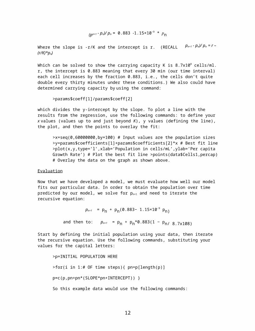
>params=lm(formula=percap~data$Cells1) >paramsThe y-intercept is given under (Intercept) and the slope is given under data$Cells1, so we can see that the y- intercept is 0.883 and the slope is -1.15×10-9. Therefore, our finite difference model can be written as:

(pn+1 - pn)/ pn = 0.883 -1.15×10-9 * 𝑝n

Where the slope is -r/K and the intercept is r. (RECALL pn+1 - pn)/ pn = r – (r/K)*pn)

0E+00. 2E+08. 4E+08. 6E+08. 8E+08.0.0

0.2

0.4

0.6

0.8

1.0

Population size (cells per ml)

Per

cap

ita

gro

wth

rat

e

9

Which can be solved to show the carrying capacity K is 8.7x108 cells/ml. r, the intercept is 0.883 meaning that every 30 min (our time interval) each cell increases by the fraction 0.883, i.e., the cells don’t quite double every thirty minutes under these conditions.) We also could have determined carrying capacity by using the command:

>params$coeff[1]/params$coeff[2]

which divides the y-intercept by the slope. To plot a line with the results from the regression, use the following commands: to define your x values (values up to and just beyond K), y values (defining the line), the plot, and then the points to overlay the fit:

>x=seq(0,60000000,by=100) # Input values are the population sizes >y=params$coefficients[1]+params$coefficients[2]*x # Best fit line >plot(x,y,type=’l’,xlab=’Population in cells/mL’,ylab=’Per capita Growth Rate’) # Plot the best fit line >points(data$Cells1,percap) # Overlay the data on the graph as shown above.

Evaluation

Now that we have developed a model, we must evaluate how well our model fits our particular data. In order to obtain the population over time predicted by our model, we solve for pn=1 and need to iterate the recursive equation:

pn+1 = pn + pn(0.883− 1.15×10-9 pn)

and then to: pn+1 = pn + pn*0.883(1 − pn/ 8.7x108)

Start by defining the initial population using your data, then iterate the recursive equation. Use the following commands, substituting your values for the capital letters:

>p=INITIAL POPULATION HERE

>for(i in 1:# OF time steps){ pn=p[length(p)]

p=c(p,pn+pn*(SLOPE*pn+INTERCEPT)) }

So this example data would use the following commands:

>p=10500000

>for(i in 1:30){ pn=p[length(p)]

p=c(p,pn+pn*(params$coefficients[2]*pn+params$coefficients[1])) }

Then compare the model to the data with the following:

>plot(p,type= ‘l’) >points(data$Time ,data$Cells1)

How well does your calculated model fit the data? Does it exhibit the general dynamics observed in the data? Was this a good model, or could another kind of model have fit the data better? Be sure to contemplate these

10

questions when doing your final analysis of the experiment.

Repeat this same process with the data from your additional samples. If you reuse R commands, be sure to go through carefully and replace all of the necessary terminology in order to obtain results that are from that new sample and not from your first sample again. Post the values of r and K for each initial bacteria concentration on a group spreadsheet on the Shared Drive, and bring those values to the next lab along with your graphs in order to discuss the results

Once you have collected all of your data and analyzed it in R to find both the growth rate and carrying capacity, share your group’s result with the class. Your professor or TA will have a copy of the Shared Drive chart of bacterial concentrations, growth rate R, and carrying capacity K, which you can in pairs then graph and analyze by hand. Determine if there is a relationship between any of those two quantities; do you see any correlation? Do any of the two variables graphed against each other create any sort of pattern?

FOR NEXT WEEK, please:

1) BRING YOUR ANALYZED DATA TO CLASS FOR DISCUSSION

2) SUBMIT THE MEDIA REQUIRED FOR YOUR EXPERIMENTS (SEE NEXT LAB) AT LEAST 2-DAYS AHEAD OF LAB.

Experiment Part 2: Effect of changing concentrations of nutrient media or supplementing growth media on growth curve for defined initial population.

Now you are the researcher! You and your partner must decide which bacterial concentration is the best to continue with other variables. Varying other conditions may cause r and K to either increase or decrease, so you might want to consider that accepted values for accurate results of OD lie between 0.1 and 1, so if your recorded absorbance values fall outside that range, they may not be so accurate.

You will be going through a very similar process as the previous lab day, but instead of varying the number of starting individuals, we will be varying the bacterial medium. What do you predict will happen with more or less concentrated food source? Or a different source? What is changing? NOTE: be sure to choose media to compare that differ by only ONE variable – e.g., glucose OR protein concentration or by ALL variables (e.g., does a more concentrated medium support more bacteria or higher growth rates?)

Proceed through the experiment as before, doing the same procedures and calculations. Think through the same kinds of questions. Do the growth curves differ? Are the parameters estimated different? If so, what is the basis for these differences?

More Questions1. What can you conclude about the relationship between initial population values

and growth? 2. What is the relationship between initial nutrient concentration and the

characteristics of logistic population growth? What happens to nutrient or other solute concentrations over time?

3. Did your population reach its carrying capacity? How do you know? Would you expect these samples to reach a steady state or an equilibrium condition?

4. Suppose we start with a particular number of bacteria and we’d like to maintain that same number of bacteria constantly over time. What would we have to do

11

in order to create that steady-state condition? 5. Is there a relationship between growth rate and bacterial concentration?

Nutrient concentration? 6. How does the carrying capacity of each population change/ stay constant

depending on changes in the growing conditions? Why do you think this happens?

7. How does the per capita growth rate change / stay constant as the growing conditions differ? Why?

8. How would the graphs change if carry capacity changes? or per capita growth rate changes?

9. What did you find in testing the glucose of the sample over time? What conclusions might you draw from that information? Is there a pattern?

10. Based on your data and knowledge of population behavior and nutrients, how do you think a curve reflecting the amount of nutrients present in the sample might behave? Draw an example.

11. Do you think another dimension of the model is necessary to create a model that is more precise, more general, or more realistic? Explain.

12