
Welcome message from author
This document is posted to help you gain knowledge. Please leave a comment to let me know what you think about it! Share it to your friends and learn new things together.
Transcript


THE SCIENCE AND INFORMATION ORGANIZATION
www.thesa i .o rg | in fo@thesa i .o rg

(IJACSA) International Journal of Advanced Computer Science and Applications, Vol. 4, No. 10, 2013
(i)
www.ijacsa.thesai.org
Editorial Preface
From the Desk of Managing Editor…
It is our pleasure to present to you the October 2013 Issue of International Journal of Advanced Computer Science and
Applications.
Today, it is incredible to consider that in 1969 men landed on the moon using a computer with a 32-kilobyte memory
that was only programmable by the use of punch cards. In 1973, Astronaut Alan Shepherd participated in the first
computer "hack" while orbiting the moon in his landing vehicle, as two programmers back on Earth attempted to "hack"
into the duplicate computer, to find a way for Shepherd to convince his computer that a catastrophe requiring a
mission abort was not happening; the successful hack took 45 minutes to accomplish, and Shepherd went on to hit his
golf ball on the moon. Today, the average computer sitting on the desk of a suburban home office has more
computing power than the entire U.S. space program that put humans on another world!!
Computer science has affected the human condition in many radical ways. Throughout its history, its developers have
striven to make calculation and computation easier, as well as to offer new means by which the other sciences can be
advanced. Modern massively-paralleled super-computers help scientists with previously unfeasible problems such as
fluid dynamics, complex function convergence, finite element analysis and real-time weather dynamics.
At IJACSA we believe in spreading the subject knowledge with effectiveness in all classes of audience. Nevertheless,
the promise of increased engagement requires that we consider how this might be accomplished, delivering up-to-
date and authoritative coverage of advanced computer science and applications.
Throughout our archives, new ideas and technologies have been welcomed, carefully critiqued, and discarded or
accepted by qualified reviewers and associate editors. Our efforts to improve the quality of the articles published and
expand their reach to the interested audience will continue, and these efforts will require critical minds and careful
consideration to assess the quality, relevance, and readability of individual articles.
To summarise, the journal has offered its readership thought provoking theoretical, philosophical, and empirical ideas
from some of the finest minds worldwide. We thank all our readers for their continued support and goodwill for IJACSA.
We will keep you posted on updates about the new programmes launched in collaboration.
Lastly, we would like to express our gratitude to all authors, whose research results have been published in our journal, as
well as our referees for their in-depth evaluations.
We hope that materials contained in this volume will satisfy your expectations and entice you to submit your own
contributions in upcoming issues of IJACSA
Thank you for Sharing Wisdom!
Managing Editor
IJACSA
Volume 4 Issue 10 October 2013
ISSN 2156-5570 (Online)
ISSN 2158-107X (Print)
©2013 The Science and Information (SAI) Organization

(IJACSA) International Journal of Advanced Computer Science and Applications, Vol. 4, No. 10, 2013
(ii)
www.ijacsa.thesai.org
Editorial Board
Dr. Kohei Arai – Editor-in-Chief
Saga University
Domains of Research: Human-Computer Interaction, Networking, Information Retrievals,
Optimization Theory, Modeling and Simulation, Satellite Remote Sensing, Computer
Vision, Decision Making Methodology
Dr. Ka Lok Man
Xi’an Jiaotong-Liverpool University (XJTLU)
Domain of Research: Computer Science and Microelectronics
Dr. Sasan Adibi
Research In Motion (RIM)
Domain of Research: Security of wireless systems, Quality of Service
Dr. Zuqing Zuh
University of Science and Technology of China
Domains of Research : Optical Communication Systems, Optical network architecture
and design, Next generation Internet, Signal processing, Broadband access network,
such as cable access (DOCSIS) networks, passive optical networks (PON), fiber to the
home (FTTH), Energy-efficient network and green technologies
Dr. Sikha Bagui
University of West Florida
Domain of Research: Database, database modeling, ER diagrams, XML data, web
databases, data mining, association rule mining, data preprocessing
Dr. T. V. Prasad
Lingaya's University
Domain of Research: Bioinformatics, Natural Language Processing, Image Processing,
Robotics, Knowledge Representation
Dr. Mohd Helmy Abd Wahab
Universiti Tun Hussein Onn Malaysia
Domain of Research: Data Mining, Database, Web-based Application, Mobile
Computing

(IJACSA) International Journal of Advanced Computer Science and Applications, Vol. 4, No. 10, 2013
(iii)
www.ijacsa.thesai.org
Reviewer Board Members
A Kathirvel
Karpaga Vinayaka College of Engineering and
Technology
A.V. Senthil Kumar
Hindusthan College of Arts and Science
Abbas Karimi
Islamic Azad University Arak Branch
Abdel-Hameed Badawy
Arkansas Tech University
Abdelghni Lakehal
Fsdm Sidi Mohammed Ben Abdellah University
Abdul Wahid
Gautam Buddha University
Abdul Hannan
Vivekanand College
Abdul Khader Jilani Saudagar
Al-Imam Muhammad Ibn Saud Islamic University
Abdur Rashid Khan
Gomal Unversity
Abeer Elkorny
Faculty of computers and information, Cairo
University
Ahmed Boutejdar
Dr. Ahmed Nabih Zaki Rashed
Menoufia University
Ajantha Herath
University of Fiji Aderemi A. Atayero
Covenant University
Ahmed Mahmood
Akbar Hossin
Akram Belghith
University Of California, San Diego
Albert Alexander
Kongu Engineering College
Alcinia Zita Sampaio
Technical University of Lisbon
Ali Ismail Awad
Luleå University of Technology
Amit Verma
Department in Rayat & Bahra Engineering
College
Amitava Biswas
Cisco Systems
Anand Nayyar
KCL Institute of Management and Technology,
Jalandhar
Andi Wahju Rahardjo Emanuel
Maranatha Christian University, INDONESIA
Anirban Sarkar
National Institute of Technology, Durgapur, India
Andrews Samraj
Mahendra Engineering College
Arash Habibi Lashakri
University Technology Malaysia (UTM)
Aris Skander
Constantine University
Ashraf Mohammed Iqbal
Dalhousie University and Capital Health
Ashok Matani
Ashraf Owis
Cairo University
Asoke Nath
St. Xaviers College
B R SARATH KUMAR
Lenora College of Engineering
Babatunde Opeoluwa Akinkunmi
University of Ibadan
Badre Bossoufi
University of Liege
Balakrushna Tripathy
VIT University
Basil Hamed
Islamic University of Gaza
Bharat Bhushan Agarwal
I.F.T.M.UNIVERSITY
Bharti Waman Gawali
Department of Computer Science &
information
Bhanu Prasad Pinnamaneni
Rajalakshmi Engineering College; Matrix Vision
GmbH
Bilian Song
Brahim Raouyane
INPT
Brij Gupta
University of New Brunswick

(IJACSA) International Journal of Advanced Computer Science and Applications, Vol. 4, No. 10, 2013
(iv)
www.ijacsa.thesai.org
Constantin Filote
Stefan cel Mare University of Suceava
Constantin Popescu
Department of Mathematics and Computer
Science, University of Oradea
Chandrashekhar Meshram
Chhattisgarh Swami Vivekananda Technical
University
Chao Wang
Chi-Hua Chen
National Chiao-Tung University
Ciprian Dobre
University Politehnica of Bucharest
Chien-Pheg Ho
Information and Communications Research
Laboratories, Industrial Technology Research
Institute of Taiwan
Prof. D. S. R. Murthy
Sreeneedhi
Dana PETCU
West University of Timisoara
Duck Hee Lee
Medical Engineering R&D Center/Asan Institute
for Life Sciences/Asan Medical Center
Deepak Garg
Thapar University.
Dong-Han Ham
Chonnam National University
Dr. Gunaseelan Devraj
Jazan University, Kingdom of Saudi Arabia
Dr. Bright Keswani
Associate Professor and Head, Department of
Computer Applications, Suresh Gyan Vihar
University, Jaipur (Rajasthan) INDIA
Dr. S Kumar
Anna University
Dragana Becejski-Vujaklija
University of Belgrade, Faculty of organizational
sciences
Driss EL OUADGHIRI
Dr. Omaima Al-Allaf
Asesstant Professor
Elena Camossi
Joint Research Centre
Eui Lee
Firkhan Ali Hamid Ali
UTHM
Fokrul Alom Mazarbhuiya
King Khalid University
Frank Ibikunle
Covenant University
Fu-Chien Kao
Da-Y eh University
G. Sreedhar
Rashtriya Sanskrit University
Ganesh Sahoo
RMRIMS
Gaurav Kumar
Manav Bharti University, Solan Himachal
Pradesh
Ghalem Belalem
University of Oran (Es Senia)
Gufran Ahmad Ansari
Qassim University
Giri Babu
Indian Space Research Organisation
Giacomo Veneri
University of Siena
Gerard Dumancas
Oklahoma Medical Research Foundation
Georgios Galatas
George Mastorakis
Technological Educational Institute of Crete
Gavril Grebenisan
University of Oradea
Hadj Hamma Tadjine
IAV GmbH
Hanumanthappaj
UNIVERSITY OF MYSORE
Hamid Alinejad-Rokny
University of Newcastle
Harco Leslie Hendric Spits Warnars
Budi LUhur University
Hardeep
Ferozaepur College of Engineering &
Technology, India
Hamez l. El Shekh Ahmed
Pure mathematics
Hesham Ibrahim
Chemical Engineering Department, Faculty of
Engineering, Al-Mergheb University
Dr. Himanshu Aggarwal
Punjabi University, India
Huda K. AL-Jobori
Ahlia University
Iwan Setyawan
Satya Wacana Christian University Dr. Jamaiah Haji Yahaya
Northern University of Malaysia (UUM), Malaysia
Jasvir Singh
Communication Signal Processing Research Lab

(IJACSA) International Journal of Advanced Computer Science and Applications, Vol. 4, No. 10, 2013
(v)
www.ijacsa.thesai.org
James Coleman
Edge Hill University
Jim Wang
The State University of New York at Buffalo,
Buffalo, NY
John Salin
George Washington University
Jyoti Chaudary
high performance computing research lab
Jatinderkumar R. Saini
S.P.College of Engineering, Gujarat
K Ramani
K.S.Rangasamy College of Technology,
Tiruchengode K V.L.N.Acharyulu
Bapatla Engineering college
Kanak Saxena
S.A.TECHNOLOGICAL INSTITUTE
Ka Lok Man
Xi’an Jiaotong-Liverpool University (XJTLU)
Kushal Doshi
IEEE Gujarat Section
Kashif Nisar
Universiti Utara Malaysia
Kavya Naveen
Kayhan Zrar Ghafoor
University Technology Malaysia
Kitimaporn Choochote
Prince of Songkla University, Phuket Campus
Kohei Arai
Saga University
Kunal Patel
Ingenuity Systems, USA
Krasimir Yordzhev
South-West University, Faculty of Mathematics
and Natural Sciences, Blagoevgrad, Bulgaria Labib Francis Gergis
Misr Academy for Engineering and Technology
Lai Khin Wee
Biomedical Engineering Department, University
Malaya
Latha Parthiban
SSN College of Engineering, Kalavakkam
Lazar Stosic
Collegefor professional studies educators
Aleksinac, Serbia
Lijian Sun
Chinese Academy of Surveying and Mapping,
China
Leandors Maglaras
Leon Abdillah
Bina Darma University
Ljubomir Jerinic
University of Novi Sad, Faculty of Sciences,
Department of Mathematics and Computer
Science
Lokesh Sharma
Indian Council of Medical Research
Long Chen
Qualcomm Incorporated
M. Reza Mashinchi
M. Tariq Banday
University of Kashmir
Mazin Al-Hakeem
Research and Development Directorate - Iraqi
Ministry of Higher Education and Research
Md Rana
University of Sydney
Miriampally Venkata Raghavendera
Adama Science & Technology University,
Ethiopia
Mirjana Popvic
School of Electrical Engineering, Belgrade
University
Manas deep
Masters in Cyber Law & Information Security
Manpreet Singh Manna
SLIET University, Govt. of India
Manuj Darbari
BBD University
Md. Zia Ur Rahman
Narasaraopeta Engg. College, Narasaraopeta
Messaouda AZZOUZI
Ziane AChour University of Djelfa
Dr. Michael Watts
University of Adelaide
Milena Bogdanovic
University of Nis, Teacher Training Faculty in
Vranje
Miroslav Baca
University of Zagreb, Faculty of organization and
informatics / Center for biomet
Mohamed Ali Mahjoub
Preparatory Institute of Engineer of Monastir
Mohamed El-Sayed
Faculty of Science, Fayoum University, Egypt.
Mohammad Yamin Mohammad Ali Badamchizadeh
University of Tabriz
Mohamed Najeh Lakhoua
ESTI, University of Carthage

(IJACSA) International Journal of Advanced Computer Science and Applications, Vol. 4, No. 10, 2013
(vi)
www.ijacsa.thesai.org
Mohammad Alomari
Applied Science University
Mohammad Kaiser
Institute of Information Technology
Mohammed Al-Shabi
Assisstant Prof.
Mohammed Sadgal
Mourad Amad
Laboratory LAMOS, Bejaia University Mohammed Ali Hussain
Sri Sai Madhavi Institute of Science &
Technology
Mohd Helmy Abd Wahab
Universiti Tun Hussein Onn Malaysia
Monji Kherallah
University of Sfax
Mostafa Ezziyyani
FSTT
Mueen Uddin
Universiti Teknologi Malaysia UTM
Mona Elshinawy
Howard University
N Ch.Sriman Narayana Iyengar
VIT University
Natarajan Subramanyam
PES Institute of Technology
Neeraj Bhargava
MDS University
Noura Aknin
University Abdelamlek Essaadi
Nidhi Arora
M.C.A. Institute, Ganpat University
Nazeeruddin Mohammad
Prince Mohammad Bin Fahd University
Najib Kofahi
Yarmouk University
Na Na
NA
Om Sangwan
Oliviu Matel
Technical University of Cluj-Napoca
Osama Omer
Aswan University
Ousmane Thiare
Associate Professor University Gaston Berger of
Saint-Louis SENEGAL
Pankaj Gupta
Microsoft Corporation
Paresh V Virparia
Sardar Patel University
Dr. Poonam Garg
Institute of Management Technology,
Ghaziabad
Prabhat K Mahanti
UNIVERSITY OF NEW BRUNSWICK
Qufeng Qiao
University of Virginia
Rachid Saadane
EE departement EHTP
Raghuraj Singh
Raj Gaurang Tiwari
AZAD Institute of Engineering and Technology
Rajesh Kumar
National University of Singapore
Rakesh Balabantaray
IIIT Bhubaneswar
RashadAl-Jawfi
Ibb university
Rashid Sheikh
Shri Venkteshwar Institute of Technology , Indore
Ravi Prakash
University of Mumbai
Rawya Rizk
Port Said University
Reshmy Krishnan
Muscat College affiliated to stirling University.U
Ricardo Vardasca
Faculty of Engineering of University of Porto
Ritaban Dutta
ISSL, CSIRO, Tasmaniia, Australia
Rowayda Sadek
Ruchika Malhotra
Delhi Technoogical University
Saadi Slami
University of Djelfa
Sachin Kumar Agrawal
University of Limerick
Dr.Sagarmay Deb
University Lecturer, Central Queensland
University, Australia
Said Ghoniemy
Taif University
Samarjeet Borah
Dept. of CSE, Sikkim Manipal University
University College of Applied Sciences UCAS-
Palestine
Santosh Kumar
Graphic Era University, India
Sasan Adibi
Research In Motion (RIM)
Saurabh Pal
VBS Purvanchal University, Jaunpur

(IJACSA) International Journal of Advanced Computer Science and Applications, Vol. 4, No. 10, 2013
(vii)
www.ijacsa.thesai.org
Saurabh Dutta
Dr. B. C. Roy Engineering College, Durgapur
Sebastian Marius Rosu
Special Telecommunications Service
Selem charfi
University of Valenciennes and Hainaut
Cambresis, France.
Sengottuvelan P
Anna University, Chennai
Senol Piskin
Istanbul Technical University, Informatics Institute
Seyed Hamidreza Mohades Kasaei
University of Isfahan
Shafiqul Abidin
G GS I P University
Shahanawaj Ahamad
The University of Al-Kharj
Shawkl Al-Dubaee
Assistant Professor
Shriram Vasudevan
Amrita University
Sherif Hussain
Mansoura University
Siddhartha Jonnalagadda
Mayo Clinic
Sivakumar Poruran
SKP ENGINEERING COLLEGE
Shikha Bagui
University of West Florida
Sim-Hui Tee
Multimedia University
Simon Ewedafe
Baze University
SUKUMAR SENTHILKUMAR
Universiti Sains Malaysia
Slim Ben Saoud
Sumit Goyal
Sumazly Sulaiman
Institute of Space Science (ANGKASA), Universiti
Kebangsaan Malaysia
Sohail Jabb
Bahria University
Suhas Manangi
Microsoft
Suresh Sankaranarayanan
Institut Teknologi Brunei
Susarla Sastry
J.N.T.U., Kakinada
Syed Ali
SMI University Karachi Pakistan
T C. Manjunath
HKBK College of Engg
T V Narayana Rao
Hyderabad Institute of Technology and
Management
T. V. Prasad
Lingaya's University
Taiwo Ayodele
Infonetmedia/University of Portsmouth
Tarek Gharib
THABET SLIMANI
College of Computer Science and Information
Technology
Totok R. Biyanto
Engineering Physics, ITS Surabaya
TOUATI YOUCEF
Computer sce Lab LIASD - University of Paris 8
Venkatesh Jaganathan
ANNA UNIVERSITY
VIJAY H MANKAR
VINAYAK BAIRAGI
Sinhgad Academy of engineering, Pune
Vishal Bhatnagar
AIACT&R, Govt. of NCT of Delhi
VISHNU MISHRA
SVNIT, Surat
Vitus S.W. Lam
The University of Hong Kong
Vuda Sreenivasarao
St. Mary’s College of Engineering & Technology
Wei Wei
Wichian Sittiprapaporn
Mahasarakham University
Xiaojing Xiang
AT&T Labs
Y Srinivas
GITAM University
YASSER ATTIA ALBAGORY
College of Computers and Information
Technology, Taif University, Saudi Arabia
YI FEI WANG
The University of British Columbia
Yilun Shang
University of Texas at San Antonio
YU QI
Mesh Capital LLC
ZAIRI ISMAEL RIZMAN
UiTM (Terengganu) Dungun Campus
ZENZO POLITE NCUBE
North West University
ZHAO ZHANG
Deptment of EE, City University of Hong Kong

(IJACSA) International Journal of Advanced Computer Science and Applications, Vol. 4, No. 10, 2013
(viii)
www.ijacsa.thesai.org
ZHEFU SHI
ZHIXIN CHEN
ILX Lightwave Corporation
ZLATKO STAPIC
University of Zagreb
ZUQING ZHU
University of Science and Technology of China
ZURAINI ISMAIL
Universiti Teknologi Malaysia

(IJACSA) International Journal of Advanced Computer Science and Applications, Vol. 4, No. 10, 2013
(vii)
www.ijacsa.thesai.org
CONTENTS
Paper 1: Identification of Employees Using RFID in IE-NTUA
Authors: Rashid Ahmed, John N. Avaritsiotis
PAGE 1 – 5
Paper 2: Smart Broadcast Technique for Improved Video Applications over Constrained Networks
Authors: U. Ukommi
PAGE 6 – 10
Paper 3: Automated Edge Detection Using Convolutional Neural Network
Authors: Mohamed A. El-Sayed, Yarub A. Estaitia, Mohamed A. Khafagy
PAGE 11 – 17
Paper 4: Hiding an Image inside another Image using Variable-Rate Steganography
Authors: Abdelfatah A. Tamimi, Ayman M. Abdalla, Omaima Al-Allaf
PAGE 18 – 21
Paper 5: Synthetic template: effective tool for target classification and machine vision
Authors: Kaveh Heidary
PAGE 22 – 31
Paper 6: Using Penalized Regression with Parallel Coordinates for Visualization of Significance in High Dimensional Data
Authors: Shengwen Wang, Yi Yang, Jih-Sheng Chang, Fang-Pang Lin
PAGE 32 – 38
Paper 7: Maturity Model for IT Service Outsourcing in Higher Education Institutions
Authors: Victoriano Valencia García, Dr. Eugenio J. Fernández Vicente, Dr. Luis Usero Aragonés
PAGE 39 – 45
Paper 8: A New Approach for Hiding Data Using B-box
Authors: Dr. Saad Abdual azize AL_ani, Bilal Sadeq Obaid Obaid
PAGE 46 – 48
Paper 9: Enhanced Link Redirection Interface for Secured Browsing using Web Browser Extensions
Authors: Mrinal Purohit Y, Kaushik Velusamy, Shriram K Vasudevan
PAGE 49 – 52
Paper 10: A Novel Location Determination Technique for Traffic Control and Surveillance using Stratospheric Platforms
Authors: Yasser Albagory, Mostafa Nofal, Said El-Zoghdy
PAGE 53 – 58
Paper 11: Overall Sensitivity Analysis Utilizing Bayesian Network for the Questionnaire Investigation on SNS
Authors: Tsuyoshi Aburai, Kazuhiro Takeyasu
PAGE 59 – 72
Paper 12: Risk Assessment of Network Security Based on Non-Optimum Characteristics Analysis
Authors: Ping He
PAGE 73 – 79

(IJACSA) International Journal of Advanced Computer Science and Applications, Vol. 4, No. 10, 2013
(viii)
www.ijacsa.thesai.org
Paper 13: An Architectural-model for Context aware Adaptive Delivery of Learning Material
Authors: Kalla. Madhu Sudhana, V. Cyril Raj, T.Ravi
PAGE 80 – 87
Paper 14: Hybrid Reasoning Model for Strengthening the problem solving capability of Expert Systems
Authors: Kapil Khandelwal, Durga Prasad Sharma
PAGE 88 – 94
Paper 15: Quaternionic Wigner-Ville distribution of analytical signal in hyperspectral imagery
Authors: Yang LIU, Robert GOUTTE
PAGE 95– 98
Paper 16: On the Practical Feasibility of Secure Multipath Communication
Authors: Stefan Rass, Benjamin Rainer, Stefan Schauer
PAGE 99 – 108
Paper 17: Optimizing the use of an SPI Flash PROM in Microblaze-Based Embedded Systems
Authors: Ahmed Hanafi, Mohammed Karim
PAGE 109 – 114
Paper 18: Design and Application of Queue-Buffer Communication Model in Pneumatic Conveying
Authors: Liping Zhang, Haomin Hu
PAGE 115 – 119
Paper 19: Thyroid Diagnosis based Technique on Rough Sets with Modified Similarity Relation
Authors: Elsayed Radwan, Adel M.A. Assiri
PAGE 120 – 126
Paper 20: Geo-visual Approach for Spatial Scan Statistics: An Analysis of Dengue Fever Outbreaks in Delhi
Authors: Shuchi Mala, Raja Sengupta
PAGE 127 – 137
Paper 21: Load Balancing with Neural Network
Authors: Nada M. Al Sallami, Ali Al daoud, Sarmad A. Al Alousi
PAGE 138 – 145
Paper 22: Acceptance of Web 2.0 in learning in higher education: a case study Nigeria
Authors: Razep Echeng, Abel Usoro, Grzegorz Majewski
PAGE 146 – 151
Paper 23: Mitigating Black Hole attack in MANET by Extending Network Knowledge
Authors: Hicham Zougagh, Ahmed Toumanari, Rachid Latif, Noureddine.Idboufker
PAGE 152 – 158
Paper 24: Determining Public Structure Crowd Evacuation Capacity
Authors: Pejman Kamkarian, Henry Hexmoor
PAGE 159 – 174
Paper 25: Terrain Coverage Ant Algorithms: The Random Kick Effect
Authors: M. Dervisi, O.B. Efremides, D.P. Iracleous
PAGE 175 – 178
(IJACSA) International Journal of Advanced Computer Science and Applications, Vol. 4, No. 10, 2013
1 | P a g e www.ijacsa.thesai.org
Identification of Employees Using RFID in IE-NTUA
Rashid Ahmed
National Technical University of Athens Engineering School of Electrical and Computer Engineering
9, Iroon Polytechniou St., 15773 Athens, Greece
John N. Avaritsiotis
National Technical University of Athens School of Electrical and Computer
9, Iroon Polytechniou St., 15773 Athens, Greece
Abstract—During the last decade with the rapid increase in
indoor wireless communications, location-aware services have
received a great deal of attention for commercial, public-safety,
and a military application, the greatest challenge associated with
indoor positioning methods is moving object data and
identification. Mobility tracking and localization are multifaceted
problems, which have been studied for a long time in different
contexts. Many potential applications in the domain of WSNs
require such capabilities. The mobility tracking needs inherent in
many surveillance, security and logistic applications. This paper
presents the identification of employees in National Technical
University in Athens (IE-NTUA), when the employees access to a
certain area of the building (enters and leaves to/from the
college), Radio Frequency Identification (RFID) applied for identification by offering special badges containing RFID-tags.
Keywords—RFID; Employees In National Technical
University; Global Positioning System; Non-Line of Site
I. INTRODUCTION
RECENT years have witnessed and enormous increase in moving object data from tag readings in supply chain operations, to toll and road sensor readings from vehicles on road networks. A big factor in the emergence of these data is the rapid adoption of Radio Frequency Identification (RFID) technology in industry and government. RFID is a technology that allows a sensor (RFID reader) to read from a distance and without line of sight (NLOS), a unique identifier that is provided (via a radio signal) by an “inexpensive” tag attached to an item. The technology has applications in many diverse areas, RFID offers an alternative to bar code identification that can be used in our system [1]. Generally, outdoor location estimation systems use one of two approaches: one based on the global positioning system (GPS), the other based on the cellular network system [2]. Although these approaches are convenient for positioning in outdoor environments, they do not provide accurate positioning for indoor applications because:1) the received GPS signals are too weak to provide the necessary information and, 2) the FCC Enhanced 911 [3] enables emergency services, and the localization accuracy which is within 50–300 m generally is inadequate. There is another approach for RADAR: An In-Building RF-based User location but RADAR operates by recording and processing signal strength information at multiple base stations positioned to provide overlapping coverage in the area of interest [4]. Thus, it is necessary to work other systems for indoor location-aware services to more accurately identify an indoor area. The objective of our research is to collect the data from special badges (containing RFID tags) and identify these tags to interact with NTUA information system to detect the employees that are entering and leaving the college.
This paper is organized as follows. In Section II, we describe the background of RFID technology and problems encountered RFID systems. Section III, presents the details of RFID identification in NTUA. Section IV, we present an identification case study and the data set description of RFID-tags, finally, Conclusions are given in section V.
II. RFID TECHNOLOGY
RFID is a technology that uses radio frequency communication to automatically identify, track and manage objects, people or animals. The devices are paired and able to "recognize" each other through the transmission of radio waves. Implementing RFID technology will ensure the basic rights of tracking, right location, right route ,right time in and right time out, by Positive employees’ identification which the standards of data exchange with confidentiality of employees’ information), RFID has some desirable features, such as contactless communications, high data rate and security, NLOS readability, compactness and low cost [5], NTUA stressing guidelines for tamperproof non-transferable special badges minimizing the risk of losing transferred data. The storage technology will allow data transfer to and from host system and data storage with large storage capacity and reading ranges, RFID tags will help increase processing speed compared to bar codes.
Unlike bar code, RFID-tags can be read through and around human body, clothing and non-metallic materials due to the system which utilizes radio waves provide a better approximation for location detection because of the ability of these waves to penetrate various materials. Instead of using differences in arrival times as in Ultrasound, this system utilizes signal strength to measure the location and identification [6].
A. Radio Link Budget in RFID Systems
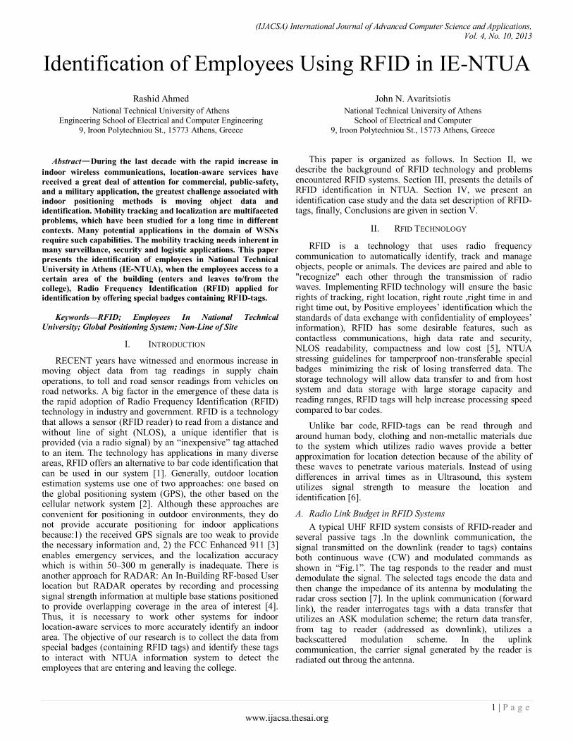
A typical UHF RFID system consists of RFID-reader and several passive tags .In the downlink communication, the signal transmitted on the downlink (reader to tags) contains both continuous wave (CW) and modulated commands as shown in “Fig.1”. The tag responds to the reader and must demodulate the signal. The selected tags encode the data and then change the impedance of its antenna by modulating the radar cross section [7]. In the uplink communication (forward link), the reader interrogates tags with a data transfer that utilizes an ASK modulation scheme; the return data transfer, from tag to reader (addressed as downlink), utilizes a backscattered modulation scheme. In the uplink communication, the carrier signal generated by the reader is radiated out throug the antenna.
(IJACSA) International Journal of Advanced Computer Science and Applications, Vol. 4, No. 10, 2013
2 | P a g e www.ijacsa.thesai.org
Fig. 1. Far-field modulated backscatter
The tag collects energy from the electromagnetic waves coming from the reader and converts it to DC supply for the chip. Once the tag is powered up, the reader sends the commands by modulating its carrier. After commands are completed, the reader sends an un-modulated continuous wave (CW) signal which is used to provide DC supply for the tag. More details on RFID system protocol and operation can be found [8],[9].
B. Problems Encounterd in Operating RFID System
Several potential issues must be solved successfully at the front end of the design process. Careful selection of a dynamic solution is important. In every case, a system design approach is required before implementing an RFID solution. The requirements for multiple tags, speed of operation, accuracy, cost and security must all be considered to provide the result demanded by the application [10]. Some of the common problems with generic RFID are:
1) Reader collision: One problem encountered with RFID
systems mainly longer range UHF systems is that the signal
from one reader can interfere with the signal from another
where coverage overlaps. This is called reader collision. This
can be avoided by using a technique named Time Division
Multiple Access (TDMA) which is a special anti-collision
scheme. The readers are instructed to read at altered times, rather
than both trying to read at the same time. By using this technique, RFID-reader does not interfere with each other. But by saying this, two readers that overlap each other in an area will read any RFID tag twice. Therefore the system has to be set up in such way that if one reader reads a tag, another reader does not read it again [11]. There are a lot of companies that point out how important it is that the reader collision software prevents the colliding readers from communicating with RFID tags in their respective reading zones. The Anti-Collision protocol allows the reading of large number of tagged objects at the same time and it ensures that each tag is read only once. The standard method in use is adapted by Auto-ID and it works like this; the reader asks tags to respond only if their first number of the identifier matches the number communicated by the reader. If more than one-tag responds, the reader asks for the next number in the identifier. It remains doing so until only one-tag responds. This phenomenon happens very quickly and RFID-reader can read 50 tags in less than a second. Different vendors have developed different systems for having the tags respond to the reader one at a time.
Since they can be read in milliseconds, it appears that all the tags are being read simultaneously, [12].
2)Interference: Like other technologies using radio waves
(garage door openers, remote control toys, pagers,etc.), RFID
systems are subject to interference from unwanted signals
electromagnetic noise. To protect against "misreads", tag data
contains bits that are encoded to provide error detection by the
reader to improve the reliability of the system.
3) Presence of metal: The presence of metal can block the performance of RFID readers and tags as well, which affects
read range. However, metal can also enhance or amplify the
read range of RFID with good system design.
4) Presence of water: The presence of water can also impede
the performance of RFID, but as with electricity and water,
good system design can overcome most limitations, [13].
III. THE PROCEDURE OF RFID IDENTIFICATION IN NTUA
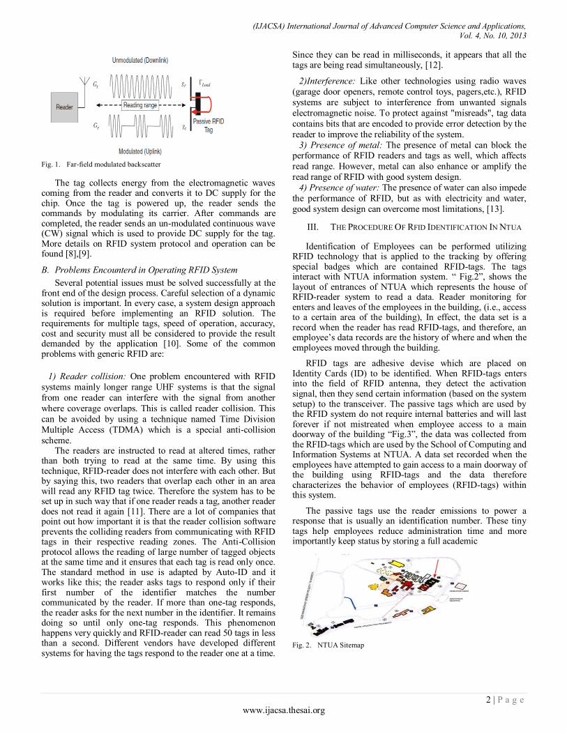
Identification of Employees can be performed utilizing RFID technology that is applied to the tracking by offering special badges which are contained RFID-tags. The tags interact with NTUA information system. “ Fig.2”, shows the layout of entrances of NTUA which represents the house of RFID-reader system to read a data. Reader monitoring for enters and leaves of the employees in the building, (i.e., access to a certain area of the building), In effect, the data set is a record when the reader has read RFID-tags, and therefore, an employee’s data records are the history of where and when the employees moved through the building.
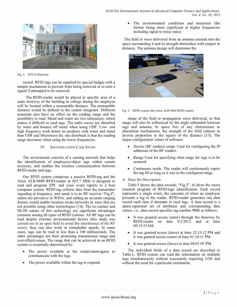
RFID tags are adhesive devise which are placed on Identity Cards (ID) to be identified. When RFID-tags enters into the field of RFID antenna, they detect the activation signal, then they send certain information (based on the system setup) to the transceiver. The passive tags which are used by the RFID system do not require internal batteries and will last forever if not mistreated when employee access to a main doorway of the building “Fig.3”, the data was collected from the RFID-tags which are used by the School of Computing and Information Systems at NTUA. A data set recorded when the employees have attempted to gain access to a main doorway of the building using RFID-tags and the data therefore characterizes the behavior of employees (RFID-tags) within this system.
The passive tags use the reader emissions to power a response that is usually an identification number. These tiny tags help employees reduce administration time and more importantly keep status by storing a full academic
Fig. 2. NTUA Sitemap
(IJACSA) International Journal of Advanced Computer Science and Applications, Vol. 4, No. 10, 2013
3 | P a g e www.ijacsa.thesai.org
Fig. 3. NTUA Doorway
record. RFID tags can be supplied by special badges with a tamper mechanism to prevent from being removed or to emit a signal if attempted to be removed.
The RFID-reader would be placed in specific area of a main doorway of the building in college during the employee will be located within a measurable distance. The measurable distance would be defined in the system integrator. Different materials also have an effect on the reading range and the possibility to read. Metal and water are two substances, which makes it difficult to read tags. The radio waves are absorbed by water and bounce off metal when using UHF. Low- and high frequency work better on products with water and metal than UHF and Microwave do, one drawback is that the reading range decreases when using the lower frequencies.
IV. IDENTIFICATION CASE STUDY
The environment consists of a sensing network that helps
the identification of employees/object tags within certain accuracy, and enables the wireless communication between RFID-reader and tags.
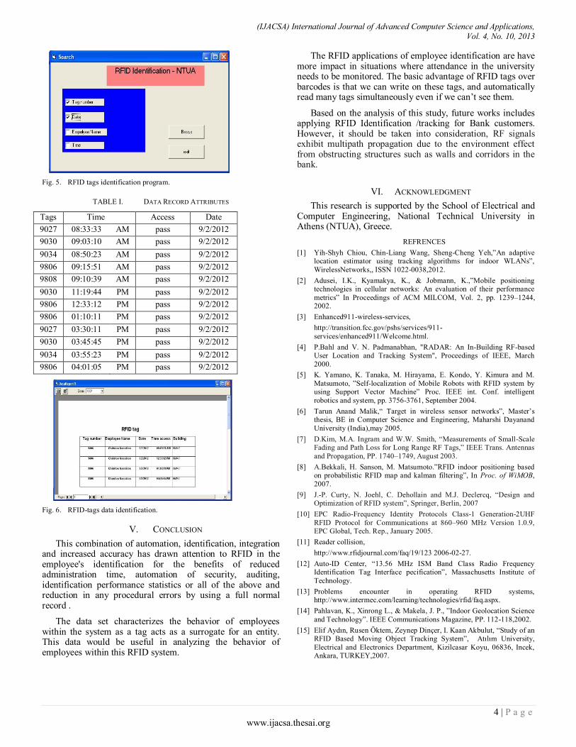
Our RFID system comprises a passive RFID-tag and the Alien ALR-8800 RFID-reader at 865.7 MHz is designed to read and program EPC and issue event reports to a host computer system. RFID-tag collects data from the transmitter signaling at frequency, and sends it to an RF receiver.“Fig.4”, radios are pervasive in WSNs, and adding an accurate ranging feature would enable location aware networks in ways that are not possible using other technologies [14]. The no contact and NLOS nature of this technology are significant advantages common among all types of RFID systems. All RF tags can be read despite extreme environmental factors (this study was carried out in an open field to avoid the interference of the RF noise), they can also work at remarkable speeds. In some cases, tags can be read in less than a 100 milliseconds. The other advantages are their promising transmission range and cost-effectiveness. The range that can be achieved in an RFID system is essentially determined by:
The power available at the reader/interrogator to communicate with the tags.
The power available within the tag to respond.
The environmental conditions and structures (the former being more significant at higher frequencies including signal to noise ratio).
The field or wave delivered from an antenna extends into the
space surrounding it and its strength diminishes with respect to
distance. The antenna design will determine the
Fig. 4. RFID system (the Alien ALR-8800 RFID reader)
shape of the field or propagation wave delivered, so that range will also be influenced by the angle subtended between tags and antenna. In space free of any obstructions or absorption mechanisms, the strength of the field reduces in inverse proportion to the square of the distance [15]. The major configuration values of software:
Device (RF readers) setup: Used for configuring the IP addresses of the RF readers.
Range Used for specifying what range for tags is to be scanned.
Continuous mode: The reader will continuously report the tag ID as long as it was in the configured range.
A. Data Set Description
Table I shows the data records, “Fig.5”, 6) show the menu research program of RFID-tags identification. Each record represents a single event; the outcome of when an employee presents a tag to the reader. RFID-reader generates one data record each time it attempts to read tags. A data record is a space-separated set of attributes and corresponding data values. i.e., data record specifies tag number 9806 as follows:
It was granted access (enter) through the doorway by RFID-reader on date 9/2/2012 and at time 09:15:51AM.
It was granted access (leave) at time 12:33:12 PM and it was granted access (enter) at time 01:10:11 PM.
It was granted access (leave) at time 04:01:05 PM.
The individual fields of a data record are described in Table.I., RFID system can read the information on multiple tags simultaneously without necessarily requiring LOS and without the need for a particular orientation.
(IJACSA) International Journal of Advanced Computer Science and Applications, Vol. 4, No. 10, 2013
4 | P a g e www.ijacsa.thesai.org
Fig. 5. RFID tags identification program.
TABLE I. DATA RECORD ATTRIBUTES
Tags Time Access Date
9027 08:33:33 AM pass 9/2/2012
9030 09:03:10 AM pass 9/2/2012
9034 08:50:23 AM pass 9/2/2012
9806 09:15:51 AM pass 9/2/2012
9808 09:10:39 AM pass 9/2/2012
9030 11:19:44 PM pass 9/2/2012
9806 12:33:12 PM pass 9/2/2012
9806 01:10:11 PM pass 9/2/2012
9027 03:30:11 PM pass 9/2/2012
9030 03:45:45 PM pass 9/2/2012
9034 03:55:23 PM pass 9/2/2012
9806 04:01:05 PM pass 9/2/2012
Fig. 6. RFID-tags data identification.
V. CONCLUSION
This combination of automation, identification, integration and increased accuracy has drawn attention to RFID in the employee's identification for the benefits of reduced administration time, automation of security, auditing, identification performance statistics or all of the above and reduction in any procedural errors by using a full normal record .
The data set characterizes the behavior of employees within the system as a tag acts as a surrogate for an entity. This data would be useful in analyzing the behavior of employees within this RFID system.
The RFID applications of employee identification are have more impact in situations where attendance in the university needs to be monitored. The basic advantage of RFID tags over barcodes is that we can write on these tags, and automatically read many tags simultaneously even if we can’t see them.
Based on the analysis of this study, future works includes applying RFID Identification /tracking for Bank customers. However, it should be taken into consideration, RF signals exhibit multipath propagation due to the environment effect from obstructing structures such as walls and corridors in the bank.
VI. ACKNOWLEDGMENT
This research is supported by the School of Electrical and Computer Engineering, National Technical University in Athens (NTUA), Greece.
REFRENCES
[1] Yih-Shyh Chiou, Chin-Liang Wang, Sheng-Cheng Yeh,”An adaptive location estimator using tracking algorithms for indoor WLANs”,
WirelessNetworks,, ISSN 1022-0038,2012.
[2] Adusei, I.K., Kyamakya, K., & Jobmann, K.,”Mobile positioning technologies in cellular networks: An evaluation of their performance
metrics” In Proceedings of ACM MILCOM, Vol. 2, pp. 1239–1244, 2002.
[3] Enhanced911-wireless-services,
http://transition.fcc.gov/pshs/services/911-
services/enhanced911/Welcome.html.
[4] P.Bahl and V. N. Padmanabhan, "RADAR: An In-Building RF-based User Location and Tracking System", Proceedings of IEEE, March
2000.
[5] K. Yamano, K. Tanaka, M. Hirayama, E. Kondo, Y. Kimura and M.
Matsumoto, ”Self-localization of Mobile Robots with RFID system by using Support Vector Machine” Proc. IEEE int. Conf. intelligent
robotics and system, pp. 3756-3761, September 2004.
[6] Tarun Anand Malik,“ Target in wireless sensor networks”, Master’s thesis, BE in Computer Science and Engineering, Maharshi Dayanand
University (India),may 2005.
[7] D.Kim, M.A. Ingram and W.W. Smith, “Measurements of Small-Scale Fading and Path Loss for Long Range RF Tags,” IEEE Trans. Antennas
and Propagation, PP. 1740–1749, August 2003.
[8] A.Bekkali, H. Sanson, M. Matsumoto.”RFID indoor positioning based on probabilistic RFID map and kalman filtering”, In Proc. of WiMOB,
2007.
[9] J.-P. Curty, N. Joehl, C. Dehollain and M.J. Declercq, “Design and Optimization of RFID system”, Springer, Berlin, 2007
[10] EPC Radio-Frequency Identity Protocols Class-1 Generation-2UHF
RFID Protocol for Communications at 860–960 MHz Version 1.0.9, EPC Global, Tech. Rep., January 2005.
[11] Reader collision,
http://www.rfidjournal.com/faq/19/123 2006-02-27.
[12] Auto-ID Center, “13.56 MHz ISM Band Class Radio Frequency Identification Tag Interface pecification”, Massachusetts Institute of
Technology.
[13] Problems encounter in operating RFID systems, http://www.intermec.com/learning/technologies/rfid/faq.aspx.
[14] Pahlavan, K., Xinrong L., & Makela, J. P., ”Indoor Geolocation Science
and Technology”. IEEE Communications Magazine, PP. 112-118,2002.
[15] Elif Aydın, Rusen Öktem, Zeynep Dinçer, I. Kaan Akbulut, “Study of an RFID Based Moving Object Tracking System”, Atılım University,
Electrical and Electronics Department, Kizilcasar Koyu, 06836, Incek, Ankara, TURKEY,2007.

(IJACSA) International Journal of Advanced Computer Science and Applications, Vol. 4, No. 10, 2013
5 | P a g e www.ijacsa.thesai.org
AUTHORS PROFILE
Rashid Ahmed is a Ph.D student in the School of Electrical and Computer Engineering, National Technical University of Athens, Greece, and is a student member of the IEEE. E-mail: [email protected].
John N. Avaritsiotis is a Professor of Microelectronics in the Department of Electrical and Computer Engineering of the National Technical University of Athens (NTUA). He has published over 80 technical articles in various scientific journals, and has presented more than 30 papers at
international conferences. His present research interests concern the development of surface micro-machining processes for the production of micromechanical sensors and design and prototyping of various types of multi-sensor systems for various applications. He is the Director of two R&D Laboratories: the Microelectronics Lab and the Electronic Sensors Lab of NTUA. He is the Co-Editor of the Journal Active and Passive Electronic Devices, Guest Editor of IEEE Transactions on Components, Packaging and manufacturing Technology, Senior Member of IEEE and Member of IOP and ISHM.

(IJACSA) International Journal of Advanced Computer Science and Applications, Vol. 4, No. 10, 2013
6 | P a g e www.ijacsa.thesai.org
Smart Broadcast Technique for Improved Video
Applications over Constrained Networks
U. Ukommi
Faculty of Engineering and Physical Sciences
University of Surrey
Guildford, Surrey, United Kingdom.
Abstract—improved wireless video communication is
challenging since video stream is vulnerable to channel
distortions. Hence, the need to investigate efficient scheme for
improved video communications. This research work investigated
broadcast schemes, and proposes smart broadcast technique as a
solution for improved video quality over constrained network
such as wireless network under tight constraints. The scheme
exploits the concept of video analysis and adaptation principles in
the optimization process. The experimental results obtained
under different channel conditions demonstrate the capability of
the proposed scheme in terms of improving the average received video quality performance over a constrained network.
Keywords—Video communication; broadcast; video quality;
wireless network
I. INTRODUCTION
Video communication over a wireless channel is more error-prone compared to that of a wired channel due to varying channel conditions and resource constraints. Demand for improved video services is rapidly growing in the society. A typical video communication system consists of video source, source encoder, channel encoder and receiving terminal for reception and display of the transmitted video signal. The video encoder such as H.264/AVC [1] performs video compression and support error resilience features [2] [3]. Wireless technology such as Mobile WiMAX provide delivery channel for video applications over wireless paltform. Mobile WiMAX uses Orthogonal Frequency Division Multiple Access (OFDMA) [4], which divides the available resources into a number of subchannels [5]. Modulation schemes such as Quadrature Phase Shift Keying (QPSK) and Quadrature Amplitude Modulation (QAM) are also supported in OFDMA with variable channel coding rates [6] [7] which offer channel protection for improved video communications. Factors such as Signal-to-Noise Ratio (SNR) determine the performance of a wireless transmission [8]. SNR takes the relative factors such as path loss, cable loss into account [9].
Wireless video communication is becoming indispensable means of communication in the society due to the mobility, flexibility and portability. It is capable of satisfying client demand anywhere at anytime. However, there are many challenges in wireless video communication channels such as resource constraints, varying network characteristics. These factors influence the quality performance of video services over challenging networks. Hence, this research report focuses on efficient scheme, utilizing content characterization to
maximize the received video quality performance under constrained networks.
II. RELATED WORK
Various schemes for video transmission have been discussed in the literature including Unequal Power Allocation for Scalable Video Transmission, where base layers of scalable video are allocated more error protection level compared to the enhancement layer [10]. An Unequal Error Protection Scheme for Object-based Video Communications, where different quantization parameters are allocated for coding of each object in the video sequence [11]. Self-organized Content and Routing in Intelligent Broadcast Environments (SCRIBE) is presented in [12] with the objective of minimizing the redundancy associated with convectional flooding broadcast scheme. SCRIBE achieves its objective by adaptively controlling the message path. Intelligent Broadcast System for Enhanced Personalized-services based on contents semantic is discussed in [13] where viewers satisfaction is increased by serving user preferences. In [14] multimedia adaptation is adopted in which based on the fact viewers are more interested in a certain region or clip. Based on this fact, different adaptation schemes have been proposed [15] [16]. These schemes aim to reduce the quality for regions that are little or no interest for the user and to increase the quality on the Region of Interest (ROI). The idea is based on human visual system that has different sensitivity to different visual areas [17]. In addition to the existing technologies, improving the quality of video applications over constrained network based on the characterization of video stream is proposed in the Smart Broadcast Technique (SBT). The rest of the paper is organized as follows. Section III describes the proposed scheme. Section IV presents the system architecture scheme. Section V describes the simulation methodology. Section VI presents the results and discussion of the research. Finally, the paper is concluded in Section VII with future work.
III. THE PROPOSED TECHNIQUE
The proposed Smart Broadcast Technique (SBT) for improved video broadcast applications is based on the dynamic nature of video content characterization. The main objective of SBT is to enhance transmission strategy in order to improve the received video performance over constrained network. In the scheme, video transmission parameters are adapted according to the characteristic of the video stream. The characterization process includes classification and
(IJACSA) International Journal of Advanced Computer Science and Applications, Vol. 4, No. 10, 2013
7 | P a g e www.ijacsa.thesai.org
prioritization of video streams based on their respective properties. Such property include content characteristic which is employed as an index in the adaptation process. The scheme is designed to analyze video streams with relative motion characteristic and improves its protection level against impact of channel errors. The proposed scheme aims at maximizing the average received video performance through intelligent adaptation of the limited transmission resources.
In the characterization process, optical flow algorithm of Lucas and Kanade [18] is used in the research to analyze video characteristics. Video contents are analyzed and the average motion activity in video scene is estimated. The motion activity estimation process is carried out by identification of significant feature points in the video scene. Feature point in this concept is defined as a point of the object in video scene that can be easily detected and tracked from frame to frame. Types of image features points include edges, blobs, ridges and corners [19]. In the measurement process, the object is first detected and analyzed to determine the changes in motion activity. Feature point relative difference in terms of pixel displacement between successive video frames quantifies motion vector of the feature point.
A typical video scene consists of objects characterized by spatial characteristics (number and shape of objects) and temporal characteristics. Changes in the motion characteristics between successive video scenes are mainly caused by object motion and global motion [20]. In the estimation of motion activity level of a video scene, the total average motion activity over a given video sequence is normalized by the spatial and temporal resolutions to maintain consistency across different video sequences. The mathematical model for the
estimation process is given by [21]:
, where
MS represents the motion activity level of the video sequence
over L number video frames. F is the motion activity level of a video frame. R and T are the spatial and temporal resolutions of the video sequence, respectively.
IV. SYSTEM ARCHITECTURE
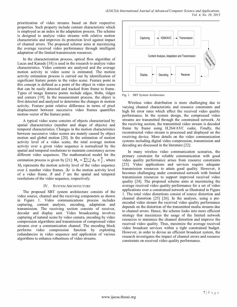
The proposed SBT system architecture consists of the video source, channel and the receiving components as shown in Figure 1. Video communications process includes capturing, content analysis, encoding, adaptation and transmission. The receiving section consists of receiver, decoder and display unit. Video broadcasting involves capturing of natural scene by video camera, encoding by video compression algorithms and transmission of compressed video streams over a communication channel. The encoding block performs video compression function by exploiting redundancies in video sequence and application of various algorithms to enhance robustness of video streams.
Constrained
network
TransmissionH264/AVCCapturing
Display Decoding Receiver
Content Analysis, Adaptation and Transmission
Fig. 1. SBT System Architecture
Wireless video distribution is more challenging due to varying channel characteristic and resource constraints and high bit error rates which affect the received video quality performance. In the system design, the compressed video streams are transmitted through the constrained network. At the receiving section, the transmitted video stream is decoded frame by frame using H.264/AVC codec. Finally, the reconstructed video stream is processed and displayed on the receiving device. More details on the video communication systems including digital video compression, transmission and decoding are discussed in the literature [22].
In many wireless video communication scenarios, the primary constraint for reliable communication with good video quality performance arises from resource constraints [23]. Video applications and services require adequate transmission resources to attain good quality. However, it becomes challenging under constrained network with limited transmission resources to support improved received video quality [24]. The proposed scheme aims at maximizing the average received video quality performance for a set of video applications over a constrained network as illustrated in Figure 1. The total video distortions consist of source distortion and channel distortion [25] [26]. In the analysis, using a pre-encoded video stream the received video quality performance depends on the distortion of the transmitted media streams due to channel errors. Hence, the scheme looks into more efficient strategy that maximizes the usage of the limited network resources to minimize the channel distortion and improve the received video quality. Thus, maximize the average received video broadcast services within a tight constrained budget. However, in order to devise an efficient broadcast system, the research investigates the impact of channel errors and resource constraints on received video quality performance.

(IJACSA) International Journal of Advanced Computer Science and Applications, Vol. 4, No. 10, 2013
8 | P a g e www.ijacsa.thesai.org
V. SIMULATION
The simulation process is performed using different standard test video sequences representing different content characterization, ranging from high motion characteristic (HP), to low motion content characteristic (LP). In the classification process, test video sequences are clustered into group based on the similarity of content characteristics, temporal and spatial resolution characterization.
H.264/AVC reference software, version 15.1 (JM 15.1) [27] is employed in pre-encoding of the test video sequences. The scheme is tested with standard sample test video sequences: Soccer, Foreman, Weather and Akiyo, all in Common Intermediate Format (CIF). The test video sequences are encoded at average bitrates of 0.768Mbps. The frame rate is fixed at 30 frames per second, and the Group of Picture (GOP) size of 8 was employed in the compression process for all the test video sequence. In each of the test video sequence, a total number of 300 frames were processed in IPPP… format (first frame of each sequence is intra-coded, followed by P-frames). Content Adaptive Binary Arithmetic Coding (CABAC) technique is adopted in the compression. The compressed video streams are segmented into slice. The slice [28] is encapsulated in RTP/UDP/IP [29] for transmission through the protocol stack of simulated broadcast system. At the Network Abstraction Layer (NAL), slice output of the VCL is placed in NALU [30] prior to transmission. For optimization of the payload header [31] and reduction of high loss probability the NALU length is fixed at 512 bytes for the test video sequences. RTP transport is augmented by a control protocol for monitoring of the data delivery and provision of feedback on the reception quality [32]. The compressed video streams are then transmitted through simulated wireless Chanel.
The channel conditions are simulated with error traces [33], generated from simulated wireless channel conditions for 16QAM, ½ Modulation and Coding Scheme (MCS), with a range of SNR levels. The error patterns are obtained by comparing the data bits within the original data slot to the transmitted data slot. If there is any bit error within the data slot, it is then declared as an error. The error traces with the similar SNR are used to corrupt the compressed video streams transmitted through the simulator. The SNR levels for the video streams are distributed using lookup tables. The look-up tables translate the bit error rate information into distortion levels, which are used in the distribution of the transmission resources among the video streams. The transmission parameters of the video streams are adjusted based on the content characterization of the compressed video streams. The resource distribution is carried out initially by equal allocation of transmit resources for all media streams, and then incremented based on the content characterization of the video streams. The uniqueness of the scheme can be recognized in terms of simplicity of the system model and resource allocation strategy. The experimental results were averaged over ten simulations carried out repeatedly in order to obtain stable results and evaluate the performance of the proposed scheme.
At the receiving section, the transmitted video streams are demodulated and decoded using H.264/AVC reference software version 15.1 (JM 15.1). The error concealment with frame copy mode is employed for concealment of corrupted video packets. When a packet is lost, the RTP sequence number enables the decoder to identify the lost packet such that the location of the corrupted packet in a frame is identified and concealed. Peak Signal-to-Noise Ratio (PSNR) [34] is used in estimating the received video quality performance.
As a measure of the objective function which can be defined as maximizing the average received video quality performance among a set of video streams over a constrained network, PSNR [35] is employed to measure the performance of the proposed system in terms of the average received video quality of the transmitted video streams. PSNR metric is widely employed in the field of video quality performance measurement, though do not have strong correlation with subjective experiment [36]. Table 1 presents the simulation conditions and input parameters.
TABLE I. PARAMETERS FOR SIMULATIONS
System Parameter
Test video sequence Soccer, Foreman, Weather, Akiyo
Source encoder H.264/AVC reference software
Frames format IPPP…
Spatial resolution CIF (352*288)
GOP 8.0
Frame rate 30 fps
Packet size 512 bytes
Channel Coding CTC
Permutation scheme PUSC
Path loss model ITU-R
Quality Measurement PSNR
VI. RESULT AND DISCUSSION
The average received video quality performances of tested video sequences are measured using PSNR algorithm. The simulations were carried out to assess the performance of the proposed scheme in terms of average received video quality performance over constrained network. Readings of the PSNR values were taken from the reconstructed video frames by comparing with the original video frames. The PSNR values represent the received video quality performance. The higher the PSNR values the better the received video quality performance. From Table 2, the video quality performance across the tested video sequences varies according to the video content characterization. The average received video quality performance of video content characterized with high motion (HP) recorded improvement when transmitted on SBT scheme. The enhancement in the received video quality performance is due to the fact that the proposed SBT system improves the protection level of the video streams with high motion characterization by improving the SNR level. The enhancement in the protection level mitigates the impact of channel errors on the reconstructed video quality.
(IJACSA) International Journal of Advanced Computer Science and Applications, Vol. 4, No. 10, 2013
9 | P a g e www.ijacsa.thesai.org
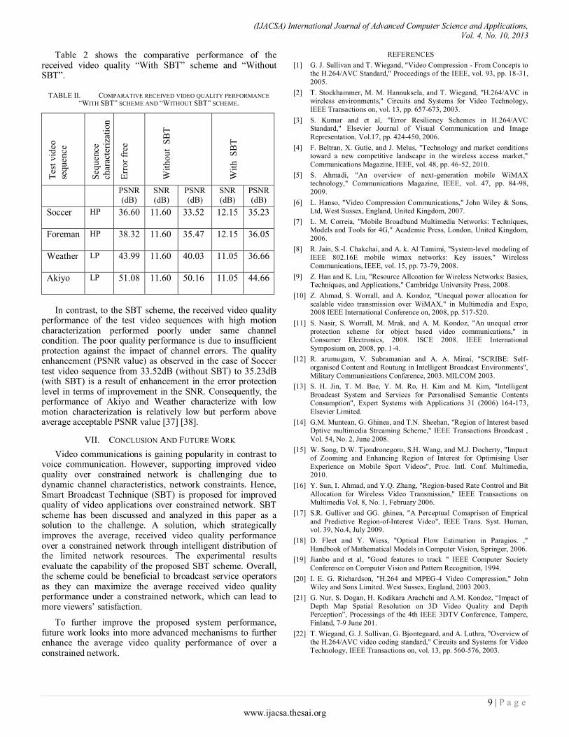
Table 2 shows the comparative performance of the received video quality “With SBT” scheme and “Without SBT”.
TABLE II. COMPARATIVE RECEIVED VIDEO QUALITY PERFORMANCE
“WITH SBT” SCHEME AND “WITHOUT SBT” SCHEME.
Tes
t vid
eo
sequen
ce
Seq
uen
ce
char
acte
riza
tion
Err
or
free
Wit
hout
SB
T
Wit
h
SB
T
PSNR (dB)
SNR (dB)
PSNR (dB)
SNR (dB)
PSNR (dB)
Soccer HP 36.60 11.60 33.52 12.15 35.23
Foreman HP 38.32 11.60 35.47 12.15 36.05
Weather LP 43.99 11.60 40.03 11.05 36.66
Akiyo LP 51.08 11.60 50.16 11.05 44.66
In contrast, to the SBT scheme, the received video quality
performance of the test video sequences with high motion characterization performed poorly under same channel condition. The poor quality performance is due to insufficient protection against the impact of channel errors. The quality enhancement (PSNR value) as observed in the case of Soccer test video sequence from 33.52dB (without SBT) to 35.23dB (with SBT) is a result of enhancement in the error protection level in terms of improvement in the SNR. Consequently, the performance of Akiyo and Weather characterize with low motion characterization is relatively low but perform above average acceptable PSNR value [37] [38].
VII. CONCLUSION AND FUTURE WORK
Video communications is gaining popularity in contrast to voice communication. However, supporting improved video quality over constrained network is challenging due to dynamic channel characteristics, network constraints. Hence, Smart Broadcast Technique (SBT) is proposed for improved quality of video applications over constrained network. SBT scheme has been discussed and analyzed in this paper as a solution to the challenge. A solution, which strategically improves the average, received video quality performance over a constrained network through intelligent distribution of the limited network resources. The experimental results evaluate the capability of the proposed SBT scheme. Overall, the scheme could be beneficial to broadcast service operators as they can maximize the average received video quality performance under a constrained network, which can lead to more viewers’ satisfaction.
To further improve the proposed system performance, future work looks into more advanced mechanisms to further enhance the average video quality performance of over a constrained network.
REFERENCES
[1] G. J. Sullivan and T. Wiegand, "Video Compression - From Concepts to the H.264/AVC Standard," Proceedings of the IEEE, vol. 93, pp. 18-31,
2005.
[2] T. Stockhammer, M. M. Hannuksela, and T. Wiegand, "H.264/AVC in wireless environments," Circuits and Systems for Video Technology,
IEEE Transactions on, vol. 13, pp. 657-673, 2003.
[3] S. Kumar and et al, "Error Resiliency Schemes in H.264/AVC Standard," Elsevier Journal of Visual Communication and Image
Representation, Vol.17, pp. 424-450, 2006.
[4] F. Beltran, X. Gutie, and J. Melus, "Technology and market conditions toward a new competitive landscape in the wireless access market,"
Communications Magazine, IEEE, vol. 48, pp. 46-52, 2010.
[5] S. Ahmadi, "An overview of next-generation mobile WiMAX technology," Communications Magazine, IEEE, vol. 47, pp. 84-98,
2009.
[6] L. Hanso, "Video Compression Communications," John Wiley & Sons, Ltd, West Sussex, England, United Kingdom, 2007.
[7] L. M. Correia, "Mobile Broadband Multimedia Networks: Techniques, Models and Tools for 4G," Academic Press, London, United Kingdom,
2006.
[8] R. Jain, S.-I. Chakchai, and A. k. Al Tamimi, "System-level modeling of IEEE 802.16E mobile wimax networks: Key issues," Wireless
Communications, IEEE, vol. 15, pp. 73-79, 2008.
[9] Z. Han and K. Liu, "Resource Allcoation for Wireless Networks: Basics, Techniques, and Applications," Cambridge University Press, 2008.
[10] Z. Ahmad, S. Worrall, and A. Kondoz, "Unequal power allocation for
scalable video transmission over WiMAX," in Multimedia and Expo, 2008 IEEE International Conference on, 2008, pp. 517-520.
[11] S. Nasir, S. Worrall, M. Mrak, and A. M. Kondoz, "An unequal error
protection scheme for object based video communications," in Consumer Electronics, 2008. ISCE 2008. IEEE International
Symposium on, 2008, pp. 1-4.
[12] R. arumugam, V. Subramanian and A. A. Minai, "SCRIBE: Self-organised Content and Routung in Intelligent Broadcast Environments",
Military Communications Conference, 2003. MILCOM 2003.
[13] S. H. Jin, T. M. Bae, Y. M. Ro, H. Kim and M. Kim, "Intelligent
Broadcast System and Services for Personalised Semantic Contents Consumption", Expert Systems with Applications 31 (2006) 164-173,
Elsevier Limited.
[14] G.M. Muntean, G. Ghinea, and T.N. Sheehan, "Region of Interest based Dptive multimedia Streaming Scheme," IEEE Transactions Broadcast ,
Vol. 54, No. 2, June 2008.
[15] W. Song, D.W. Tjondronegoro, S.H. Wang, and M.J. Docherty, "Impact of Zooming and Enhancing Region of Interest for Optimising User
Experience on Mobile Sport Videos", Proc. Intl. Conf. Multimedia, 2010.
[16] Y. Sun, I. Ahmad, and Y.Q. Zhang, "Region-based Rate Control and Bit
Allocation for Wireless Video Transmission," IEEE Transactions on Multimedia Vol. 8, No. 1, February 2006.
[17] S.R. Gulliver and GG. ghinea, "A Perceptual Comaprison of Emprical
and Predictive Region-of-Interest Video", IEEE Trans. Syst. Human, vol. 39, No.4, July 2009.
[18] D. Fleet and Y. Wiess, "Optical Flow Estimation in Paragios. ,"
Handbook of Mathematical Models in Computer Vision, Springer, 2006.
[19] Jianbo and et al, "Good features to track " IEEE Computer Society
Conference on Computer Vision and Pattern Recognition, 1994.
[20] I. E. G. Richardson, "H.264 and MPEG-4 Video Compression," John Wiley and Sons Limited. West Sussex, England, 2003 2003.
[21] G. Nur, S. Dogan, H. Kodikara Arachchi and A.M. Kondoz, “Impact of
Depth Map Spatial Resolution on 3D Video Quality and Depth Perception”, Processings of the 4th IEEE 3DTV Conference, Tampere,
Finland, 7-9 June 201.
[22] T. Wiegand, G. J. Sullivan, G. Bjontegaard, and A. Luthra, "Overview of the H.264/AVC video coding standard," Circuits and Systems for Video
Technology, IEEE Transactions on, vol. 13, pp. 560-576, 2003.

(IJACSA) International Journal of Advanced Computer Science and Applications, Vol. 4, No. 10, 2013
10 | P a g e www.ijacsa.thesai.org
[23] R.G. Gallager, "Energy Limited Channels: Coding, Multiacces and
Spread Spectrum", Tech. REP. MIT. LIDS-P-1714, Novermber 1987.
[24] O. Oyman, J. Foerster, T. Yong-joo, and L. Seong-Choon, "Toward
enhanced mobile video services over WiMAX and LTE [WiMAX/LTE Update]," Communications Magazine, IEEE, vol. 48, pp. 68-76, 2010.
[25] L. Ke-Ying, Y. Jar-Ferr, and S. Ming-Ting, "Rate-Distortion Cost
Estimation for H.264/AVC," Circuits and Systems for Video Technology, IEEE Transactions on, vol. 20, pp. 38-49, 2010.
[26] W. Yao, W. Zhenyu, and J. M. Boyce, "Modeling of transmission-loss-
induced distortion in decoded video," Circuits and Systems for Video Technology, IEEE Transactions on, vol. 16, pp. 716-732, 2006.
[27] A. M. Tourapis, "Joint Video Team (JVT) of ISO/IEC MPEG & ITU-T
VCEG (ISO/IEC JTC1/SC29/WG11 and ITU-T SG16 Q.6)," Geneva, http://iphome.hhi.de/suehring/tml/, February 2009.
[28] S. Wenger, "H.264/AVC over IP," Circuits and Systems for Video
Technology, IEEE Transactions on, vol. 13, pp. 645-656, 2003.
[29] S. Wenger, M. Hannuksela, T. Stockhammer, M. Westerland, and D. Singer, "RTP Payload Format for H.264 Video," IETF, RFC 3984,
February 2005.
[30] J. Ostermann, J. Bormans, P. List, D. Marpe, M. Narroschke, F. Pereira,
T. Stockhammer, and T. Wedi, "Video coding with H.264/AVC: tools, performance, and complexity," Circuits and Systems Magazine, IEEE,
vol. 4, pp. 7-28, 2004.
[31] S. Jung, "Effect of Robust Header Compression (ROHC) and Packet
Aggregation on Multi-hop Wireless Mesh Networks," IEEE 6th
International Conference on computer and Information Technology (CIT’06), 2006.
[32] S. C. H. Schulzrinne, R. Frederick, V. Jacobson, "RTP: A Transport Protocol for Real-Time Applications, RFC 3550 Internet-Draft," IETF
Network Working Group, July 2003.
[33] EU-1ST-FP6-Project, "Scalable Ultra-fast and Interoperable Interactive Television (SUIT)," http://suit.av.it.pt/, 2006.
[34] A.A. Atayero, O.I. Sheluhim, Y.A. Ivanov and A.A. Alatishe,
"Estimation of the Visual Quality of Video Streaming Under Desynchronisation Conditions", International Journal of Advanced
Computer Science and Aplications, Vol. 2, No. 12, 2011.
[35] M. Vranjes, S. Rimac-Drlje, and K. Grgic, "Locally averaged PSNR as a simple objective Video Quality Metric," in ELMAR, 2008. 50th
International Symposium, 2008, pp. 17-20.
[36] A. M. Kondoz, "Visual Media Coding and Transmission," John Wiley & Sons Ltd, United Kingdom, 2009.
[37] A.A. Atayero, O.I. Sheluhim, Y.A. Ivanov and J.O. Iruemi, "Wideband
Wireless Access Systems Interference Robustness: Its Effect on Quality of Video Streaming", International Journal of Advanced Computer
Science and Aplications, Vol. 3, No. 1, 2012.
[38] T. Zinner, O. Abboud, O. Hohlfeld, and P. Tran-Gia, “Toward QoE
Management for Scalable Video Streaming,” Proc. 21th ITC Specialist Seminar Multimedia Appl. Traffic, performance QoE, 2010.
(IJACSA) International Journal of Advanced Computer Science and Applications, Vol. 4, No. 10, 2013
11 | P a g e www.ijacsa.thesai.org
Automated Edge Detection Using Convolutional
Neural Network
Mohamed A. El-Sayed
Dept. of Math., Faculty of Science,
University of Fayoum, Egypt.
Assistant prof. of CS, Taif
University, KSA
Yarub A. Estaitia
Assistant prof. of Computer Science,
College of computers and IT,
Taif University, KSA
Mohamed A. Khafagy
Dept. of Mathematics, Faculty of
Science, Sohag University,
Egypt
Abstract—The edge detection on the images is so important
for image processing. It is used in a various fields of applications
ranging from real-time video surveillance and traffic
management to medical imaging applications. Currently, there is
not a single edge detector that has both efficiency and reliability.
Traditional differential filter-based algorithms have the
advantage of theoretical strictness, but require excessive post-
processing. Proposed CNN technique is used to realize edge
detection task it takes the advantage of momentum features
extraction, it can process any input image of any size with no
more training required, the results are very promising when
compared to both classical methods and other ANN based methods.
Keywords—Edge detection; Convolutional Neural Networks;
Max Pooling
I. INTRODUCTION
Computer vision aims to duplicate the effect of human vision by electronically perceiving and understanding an image. Giving computers the ability to see is not an easy task. Towards computer vision the role of edge detection is very crucial as it is the preliminary or fundamental stage in pattern recognition. Edges characterize object boundaries and are therefore useful for segmentation and identification of objects in a scene. The idea that the edge detection is the first step in vision processing has fueled a long term search for a good edge detection algorithm [1].
Edge detection is a crucial step towards the ultimate goal of computer vision, and is an intensively researched subject; an edge is defined by a discontinuity in gray level values. In other words, an edge is the boundary between an object and the background. The shape of edges in images depends on many parameters: The geometrical and optical properties of the object, the illumination conditions, and the noise level in the images. Edges include the most important information in the image, and can provide the information of the object’s position [2]. Edge detection is an important link in computer vision and other image processing, used in feature detection and texture analysis.
Edge detection is frequently used in image segmentation. In that case an image is seen as a combination of segments in which image data are more or less homogeneous. Two main alternatives exist to determine these segments:
1) Classification of all pixels that satisfy the criterion of
homogeneousness;
2) Detection of all pixels on the borders between different
homogeneous areas. Edges are quick changes on the image profile. These quick
changes on the image can be detected via traditional difference filters [3]. Also it can be also detected by using canny method [4] or Laplacian of Gaussian (LOG) method [5]. In these classic methods, firstly masks are moved around the image. The pixels which are the dimension of masks are processed. Then, new pixels values on the new image provide us necessary information about the edge. However, errors can be made due to the noise while mask is moved around the image [6]. The class of edge detection using entropy has been widely studied, and many of the paper , for examples [7],[8],[9].
Artificial neural network can be used as a very prevalent technology, instead of classic edge detection methods. Artificial neural network [10], is more as compared to classic method for edge detection, since it provides less operation load and has more advantageous for reducing the effect of the noise [11]. An artificial neural network is more useful, because multiple inputs and multiple outputs can be used during the stage of training [12], [13].
Many edge detection filters only detect edges in certain directions; therefore combinations of filters that detect edges in different directions are often used to obtain edge detectors that detect all edges.
This paper is organized as follows: Section 2 presents some fundamental concepts and we describe the proposed method used. In Section 3, we report the effectiveness of our method when applied to some real-world and some standard database set of images. At last Results, Discussion and Conclusion of this paper will be drawn in Section 4.
II. PIXEL BASED EDGE DETECTION
In digital image processing, we can write an image as a set
of pixels qpf ,
and an edge detection filter which detects edges
with direction as a (template) matrix with elements mnw ,
,
see Figure.1. We can then determine whether a pixel qpf ,
is
an edge pixel or not, by looking at the pixel’s neighborhood, see Figure 2, where the neighborhood has the same size as the
(IJACSA) International Journal of Advanced Computer Science and Applications, Vol. 4, No. 10, 2013
12 | P a g e www.ijacsa.thesai.org
edge detector template, say )12()12( MN . We then
calculate the discrete convolution.
mqnp
N
Nn
M
Mm
mnqp fwg
,,, (1)
where qpf ,
can be classified as an edge pixel if qpg ,
exceeds a certain threshold and is a local maximum in the
direction perpendicular to in the imageqpg ,.
MNMN
MNMN
ww
w
ww
,,
0,0
,,
...
..
.
..
...
Fig. 1. A )12()12( MN template mnw ,
.
Fig. 2. A )12()12( QP image with a )12()12( MN neighborhood
around qpf ,
.
Some examples of templates for edge detection are:
-1 -2 -1 1 1 1
0 0 0 0 0 0
1 2 1 -1 -1 -1
Sobel
,0°
Prewritt, 0°
The dependency on the edge direction is not very strong;
edges with a direction ± 45° will also activate the edge
detector [14].
III. CONVOLUTIONAL NEURAL NETWORKS
Typically convolutional layers are interspersed with sub-sampling layers to reduce computation time and to gradually build up further spatial and configurable invariance. A small sub-sampling factor is desirable however in order to maintain
specificity at the same time. Of course, this idea is not new, but the concept is both simple and powerful [15]. It combines three architectural ideas to ensure some degree of shift, scale and distortion invariance: local receptive fields, shared weights (or weights replications), and spatial or temporal sub-sampling [16].
Fig. 3. Convolutional Neural Networks structure.
The input plane receive images, each unit in a layer receives input from a set of units located in a small neighborhood in the previous layer. With local receptive fields, neurons can extract elementary visual features such as oriented edges, end points, corners (or other features such as speech spectrograms).These features are then combined by the subsequent layers in order to detect higher-order features.
IV. PROPOSED TECHNIQUE
Convolutional Neural Networks (Convolutiobal Neural Network) are variants of MLPs which are inspired from biology. From Hubel and Wiesel’s early work on the cat’s visual cortex , we know there exists a complex arrangement of cells within the visual cortex. These cells are sensitive to small sub-regions of the input space, called a receptive field, and are tiled in such a way as to cover the entire visual field. These filters are local in input space and are thus better suited to exploit the strong spatially local correlation present in natural images. Additionally, two basic cell types have been identified: simple cells (S) and complex cells (C). Simple cells (S) respond maximally to specific edge-like stimulus patterns within their receptive field. Complex cells (C) have larger receptive fields and are locally invariant to the exact position of the stimulus.
a) Sparse Connectivity:
Layer M+1
Layer M
Layer M-1
Fig. 4. A Sparse Connectivity template .
QPQP
MqNpMqNp
qp
MqNpMqNp
QPQP
ww
ff
f
ff
ff
,,
,,
,
,,
,,
...
...
...
...
..
...
...
.
...
...
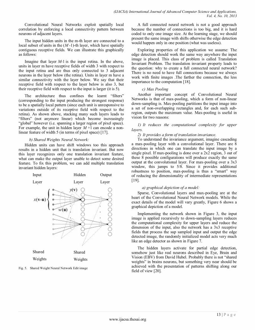
(IJACSA) International Journal of Advanced Computer Science and Applications, Vol. 4, No. 10, 2013
13 | P a g e www.ijacsa.thesai.org
Convolutional Neural Networks exploit spatially local correlation by enforcing a local connectivity pattern between neurons of adjacent layers.
The input hidden units in the m-th layer are connected to a local subset of units in the (M -1)-th layer, which have spatially contiguous receptive fields. We can illustrate this graphically as follows:
Imagine that layer M-1 is the input retina. In the above, units in layer m have receptive fields of width 3 with respect to the input retina and are thus only connected to 3 adjacent neurons in the layer below (the retina). Units in layer m have a similar connectivity with the layer below. We say that their receptive field with respect to the layer below is also 3, but their receptive field with respect to the input is larger (it is 5).
The architecture thus confines the learnt “filters” (corresponding to the input producing the strongest response) to be a spatially local pattern (since each unit is unresponsive to variations outside of its receptive field with respect to the retina). As shown above, stacking many such layers leads to “filters” (not anymore linear) which become increasingly “global” however (i.e. spanning a larger region of pixel space). For example, the unit in hidden layer M +1 can encode a non-linear feature of width 5 (in terms of pixel space) [17].
b) Shared Weights Neural Network:
Hidden units can have shift windows too this approach results in a hidden unit that is translation invariant. But now this layer recognizes only one translation invariant feature, what can make the output layer unable to detect some desired feature. To fix this problem, we can add multiple translation invariant hidden layers:
Input
Layer
Hidden
Layer
Output
Layer
Shared
Weights
Shared
Weights
Fig. 5. Shared Weight Neural Network Edit image
A full connected neural network is not a good approach because the number of connections is too big, and it is hard coded to only one image size. At the learning stage, we should present the same image with shifts otherwise the edge detection would happen only in one position (what was useless).
Exploring properties of this application we assume: The edge detection should work the same way anywhere the input image is placed. This class of problem is called Translation Invariant Problem. The translation invariant property leads to the question: why to create a full connected neural network? There is no need to have full connections because we always work with finite images .The farther the connection, the less importance to the computation [18].
c) Max Pooling
Another important concept of Convolutional Neural Networks is that of max-pooling, which a form of non-linear down-sampling is. Max-pooling partitions the input image into a set of non-overlapping rectangles and, for each such sub-region, outputs the maximum value. Max-pooling is useful in vision for two reasons:
1) It reduces the computational complexity for upper
layers.
2) It provides a form of translation invariance. To understand the invariance argument, imagine cascading
a max-pooling layer with a convolutional layer. There are 8 directions in which one can translate the input image by a single pixel. If max-pooling is done over a 2x2 region, 3 out of these 8 possible configurations will produce exactly the same output at the convolutional layer. For max-pooling over a 3x3 window, this jumps to 5/8. Since it provides additional robustness to position, max-pooling is thus a “smart” way of reducing the dimensionality of intermediate representations [19].
a) graphical depiction of a model:
Sparse, Convolutional layers and max-pooling are at the heart of the Convolutional Neural Network models. While the exact details of the model will vary greatly, Figure 6 shows a graphical depiction of a model.
Implementing the network shown in Figure 3, the input image is applied recursively to down-sampling layers reduces the computational complexity for upper layers and reduce the dimension of the input, also the network has a 3x3 receptive fields that process the sup sampled input and output the edge detected image, the randomly initialized model acts very much like an edge detector as shown in Figure 7.
The hidden layers activate for partial edge detection, somehow just like real neurons described in Eye, Brain and Vision (EBV) from David Hubel. Probably there is not “shared weights” in brains neurons, but something very near should be achieved with the presentation of patterns shifting along our field of view [20].
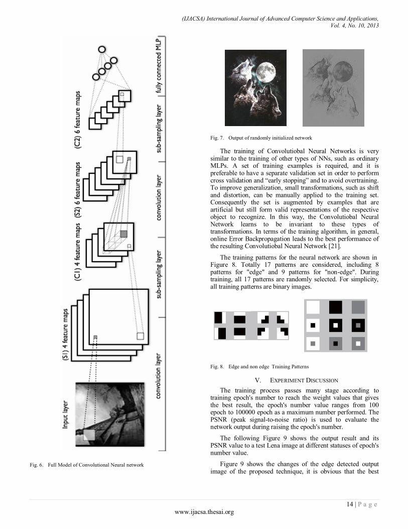
(IJACSA) International Journal of Advanced Computer Science and Applications, Vol. 4, No. 10, 2013
14 | P a g e www.ijacsa.thesai.org
Fig. 6. Full Model of Convolutional Neural network
Fig. 7. Output of randomly initialized network
The training of Convolutiobal Neural Networks is very similar to the training of other types of NNs, such as ordinary MLPs. A set of training examples is required, and it is preferable to have a separate validation set in order to perform cross validation and “early stopping” and to avoid overtraining. To improve generalization, small transformations, such as shift and distortion, can be manually applied to the training set. Consequently the set is augmented by examples that are artificial but still form valid representations of the respective object to recognize. In this way, the Convolutiobal Neural Network learns to be invariant to these types of transformations. In terms of the training algorithm, in general, online Error Backpropagation leads to the best performance of the resulting Convolutiobal Neural Network [21].
The training patterns for the neural network are shown in Figure 8. Totally 17 patterns are considered, including 8 patterns for "edge" and 9 patterns for "non-edge". During training, all 17 patterns are randomly selected. For simplicity, all training patterns are binary images.
Fig. 8. Edge and non edge Training Patterns
V. EXPERIMENT DISCUSSION
The training process passes many stage according to training epoch's number to reach the weight values that gives the best result, the epoch's number value ranges from 100 epoch to 100000 epoch as a maximum number performed. The PSNR (peak signal-to-noise ratio) is used to evaluate the network output during raising the epoch's number.
The following Figure 9 shows the output result and its PSNR value to a test Lena image at different statuses of epoch's number value.
Figure 9 shows the changes of the edge detected output image of the proposed technique, it is obvious that the best
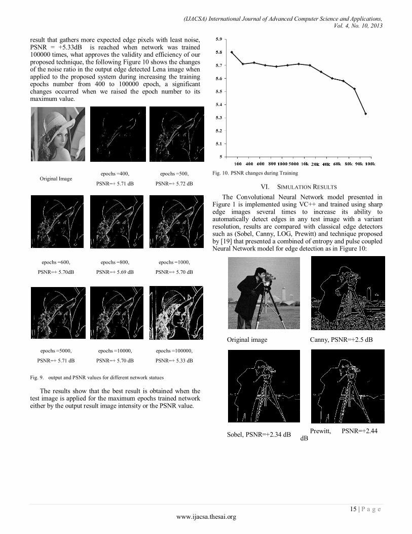
(IJACSA) International Journal of Advanced Computer Science and Applications, Vol. 4, No. 10, 2013
15 | P a g e www.ijacsa.thesai.org
result that gathers more expected edge pixels with least noise, PSNR = +5.33dB is reached when network was trained 100000 times, what approves the validity and efficiency of our proposed technique, the following Figure 10 shows the changes of the noise ratio in the output edge detected Lena image when applied to the proposed system during increasing the training epochs number from 400 to 100000 epoch, a significant changes occurred when we raised the epoch number to its maximum value.
Original Image epochs =400,
PSNR=+ 5.71 dB
epochs =500,
PSNR=+ 5.72 dB
epochs =600,
PSNR=+ 5.70dB
epochs =800,
PSNR=+ 5.69 dB
epochs =1000,
PSNR=+ 5.70 dB
epochs =5000,
PSNR=+ 5.71 dB
epochs =10000,
PSNR=+ 5.70 dB
epochs =100000,
PSNR=+ 5.33 dB
Fig. 9. output and PSNR values for different network statues
The results show that the best result is obtained when the test image is applied for the maximum epochs trained network either by the output result image intensity or the PSNR value.
Fig. 10. PSNR changes during Training
VI. SIMULATION RESULTS
The Convolutional Neural Network model presented in Figure 1 is implemented using VC++ and trained using sharp edge images several times to increase its ability to automatically detect edges in any test image with a variant resolution, results are compared with classical edge detectors such as (Sobel, Canny, LOG, Prewitt) and technique proposed by [19] that presented a combined of entropy and pulse coupled Neural Network model for edge detection as in Figure 10:
Original image Canny, PSNR=+2.5 dB
Sobel, PSNR=+2.34 dB Prewitt, PSNR=+2.44
dB

(IJACSA) International Journal of Advanced Computer Science and Applications, Vol. 4, No. 10, 2013
16 | P a g e www.ijacsa.thesai.org
LOG, PSNR=+2.34 dB Chen [17] ,
PSNR=+2.65 dB
Proposed, PSNR=+2.3 dB
Fig. 11. comparison of different techniques Vs proposed technique.
It is obvious to notice from Figure 11 that proposed technique achieves edge detection process efficiently compared with different known methods, where it gathers more expected edge pixels and left a little bit noise than other techniques as shown in Figure 12.
Fig. 12. PSNR values compared.
One of the main advantages of proposed technique it that it performs well when applied to high resolution and live images the following figure 12 shows the result for a modern house image with size 1024x711 pixels. This approach performs well with common standard images, high resolution size and live images.
Original image
Output result image with a 10000 epochs trained network
Output result image with a
100000 epochs trained network
Fig. 13. output result for modern house image
VII. CONCLUSION
The Convolutional Neural Network is used as an edge detection tool. It was trained with different edge and non edge patterns several times so that it is able to automatically detect edges in any test image efficiently.
The proposed technique applied for standard images such as Lena, and Cameraman, also live non standard images with different size, resolution, intensity, lighting effects and other conditions. The technique shows a good performance when applied on all test images.

(IJACSA) International Journal of Advanced Computer Science and Applications, Vol. 4, No. 10, 2013
17 | P a g e www.ijacsa.thesai.org
REFERENCES
[1] M. Norgaard, N.K. Poulsen, O. Ravn, “Advances in derivative-free state estimation for non-linear systems,” Technical Report IMM-REP-1998-
15 (revised edition), Technical University of Denmark, Denmark, April 2000.
[2] L. Canny, “A computational approach to edge detection”, IEEE Trans.
on Pattern Analysis and Machine Intelligence, vol. 8 no. 1, pp. 679-698, 1986.
[3] D. Marr, E. Hildreth, “Theory of edge detection”, Proc. of Royal Society
Landon, B(207): 187-217, 1980.
[4] R. Machuca,. “Finding edges in noisy scenes”, IEEE Trans. on Pattern Analysis and Machine Intelligence, 3: 103-111, 1981.
[5] F. Rosenblatt, “The Perceptron: A Probabilistic Model for Information
Storage and Organization in the Brain”, Cornell Aeronautical Laboratory, Psychological Review, v65, No. 6, pp. 386-408, 1958.
[6] A. J. Pinho, L. B. Almeida, “Edge detection filters based on artificial
neural networks”, Pro. of ICIAP'95, IEEE Computer Society Press, p.159-164, 1995.
[7] Mohamed A. El-Sayed and Mohamed A. Khafagy, “Using Renyi's Entropy For Edge Detection In Level Images”, International Journal of
Intelligent Computing and Information Science (IJICIS) Vol. 11, No.2, pp. 1-10, 2011.
[8] Mohamed A. El-Sayed , “Study of Edge Detection Based On 2D
Entropy”, International Journal of Computer Science Issues (IJCSI) ISSN : 1694-0814 , Vol. 10, Issue 3, No 1, pp. 1-8, 2013.
[9] Mohamed A. El-Sayed , S. F.Bahgat , and S. Abdel-Khalek “Novel
Approach of Edges Detection for Digital Images Based On Hybrid Types of Entropy”, International Appl. Math. Inf. Sci. 7, No. 5,
pp.1809-1817 , 2013.
[10] H.L. Wang, X.Q. Ye, W.K. Gu, “Training a NeuralNetwork for Moment Based Image Edge Detection” Journal of Zhejiang University
SCIENCE(ISSN 1009-3095, Monthly), Vol.1, No.4, pp. 398-401 CHINA, 2000.
[11] Y. Xueli, “Neural Network and Example”, Learning, Press of Railway of
China, Beijing, 1996.
[12] P.K. Sahoo, S. Soltani,A.K.C. Wong, Y.C. Chen,"A Survey of the
Thresholding Techniques", Computer Vision Graphics Image Process, 1988.
[13] Y. LeCun,L.Bottou,Y.Bengio, and P.Haffner.“Gradient-based learning applied to document recognition”, Proceedings of the IEEE, vol. 86, pp.
2278–2324, November 1998.
[14] Jake Bouvrie “Notes on Convolutional Neural Networks” Center for Biological and Computational Learning Department of Brain and
Cognitive Sciences Massachusetts Institute of Technology Cambridge, MA 02139, 2006.
[15] van der Zwaag, B.J. and Slump, C.H. and Spaanenburg , L, ”Analysis of
neural networks for edge detection”, In:13th Annual Workshop on Circuits Systems and Signal Processing (ProRISC), 28-29 November
2002.
[16] Honglak Lee; "Tutorial on Deep Learning and Applications", NIPS Workshop on Deep Learning and Unsupervised Feature Learni, 2010.
[17] Sumedha, Monika Jenna, "Morphological Shared Weight Neural
Network: A method to improve fault tolerance in Face"; International Journal of Advanced Research in Computer Engineering & Technology
Volume 1, Issue 1, March 2012.
[18] Jawad Nagi , Frederick Ducatelle , Gianni A. Di Caro , Dan Cires¸an , Ueli Meier , Alessandro Giusti ,Farrukh Nagi , Jurgen Schmidhuber ,
Luca Maria Gambardella; "Max-Pooling Convolutional Neural Networks for Vision-based Hand Gesture Recognition" International
conference on signal and image processing applications, 2011.
[19] ranzato; "Deep learning documentation: Convolutional Neural
Networks" Copyright 2008--2010, LISA lab. Last updated on Dec 03, 2012
[20] Stefan Duffner “Face Image Analysis With Convolutional Neural
Networks”, 2007.
[21] Jiansheng Chen, Jing Ping Heand Guangda Su, “Combining image entropy with the pulse coupled neural network in edge detection” , ICIP
2010.

(IJACSA) International Journal of Advanced Computer Science and Applications, Vol. 4, No. 10, 2013
18 | P a g e www.ijacsa.thesai.org
Hiding an Image inside another Image using
Variable-Rate Steganography
Abdelfatah A. Tamimi
Dept. of Computer Science
Faculty of Science & I.T.
Al-Zaytoonah University of Jordan
Amman, Jordan
Ayman M. Abdalla
Dept. of Multimedia Systems
Faculty of Science & I.T.
Al-Zaytoonah University of Jordan
Amman, Jordan
Omaima Al-Allaf
Dept. of C.I.S.
Faculty of Science & I.T.
Al-Zaytoonah University of Jordan
Amman, Jordan
Abstract—A new algorithm is presented for hiding a secret
image in the least significant bits of a cover image. The images
used may be color or grayscale images. The number of bits used
for hiding changes according to pixel neighborhood information
of the cover image. The exclusive-or (XOR) of a pixel’s neighbors
is used to determine the smoothness of the neighborhood. A
higher XOR value indicates less smoothness and leads to using
more bits for hiding without causing noticeable degradation to
the cover image. Experimental results are presented to show that
the algorithm generally hides images without significant changes
to the cover image, where the results are sensitive to the smoothness of the cover image.
Keywords—image steganography; information hiding; LSB
method
I. INTRODUCTION
Steganography is a method of hiding a secret message inside other information so that the existence of the hidden message is concealed. Cryptography, in contrast, is a method of scrambling hidden information so that unauthorized persons will not be able to recover it. The main advantage steganography has over cryptography is that it hides the actual existence of secret information, making it an unlikely target of spying attacks. To achieve higher security, a combination of steganography with cryptography may be used.
In this paper, a new algorithm is presented to hide information in the least significant bits (LSBs) of image pixels. The algorithm uses a variable number of hiding bits for each pixel, where the number of bits is chosen based on the amount of visible degradation they may cause to the pixel compared to its neighbors. The amount of visible degradation is expected to be higher for smooth areas, so the number of hiding bits is chosen to be proportional to the exclusive-or (XOR) of the pixel’s neighbors. Analysis showed effectiveness of the algorithm in minimizing degradation while it was sensitive to the smoothness of cover images.
II. BACKGROUND AND RELATED WORK
Surveys of different steganography techniques were presented in previous work, where secret information may be hidden in text, audio, image or video [1], [2], [3], [4], [5], [6], [7]. When an image is chosen to be used for hiding information, it is called a cover image. A cover image containing the secret information is called a stego image.
Hiding in LSBs of each pixel is desired since their modification will cause less distortion compared to other bits. The number of bits used should be variable and related to the stego image to minimize distortion [8], [9]. However, some applications, such as lossy compression, involve image alteration where some LSBs are lost. In such cases, more significant bits are used by transformation algorithms that utilize the special features of these applications. These techniques generally append coding information to the image with minimal or no change to the original pixels [10], [11].
Generally, the related previous work did not focus on hiding images inside other images. In addition, related image steganography research was usually limited to either grayscale or Red-Green-Blue images; not generalized to work for both image types. The new algorithm of this paper handles hiding different images inside other images of various types.
III. THE HIDING ALGORITHM
This algorithm uses a variable number of LSBs from each pixel of the cover image for hiding. A grayscale image consists of only one color matrix. A Red-Green-Blue (RGB) color image consists of three matrices representing the three colors. The number of bits chosen from each pixel color (red, green, and blue) is different. Images in other color formats may be converted to RGB matrices and converted back after the hiding process is done. The actual number of bits changes according to neighborhood information of each pixel color. When the resemblance between the neighbors of a pixel color entry is low, the pixel entry is located in a non-smooth area where change will not be detected easily. Therefore, the number of bits used for hiding is chosen to be proportional to the neighbors’ XOR value for each pixel color entry.
The pixels used in hiding are those located in every line and every other column of the cover image, as in the white squares of a chess board. Pixels on the borders are not used for hiding. This means that approximately 50% of the pixels are used for hiding, while the rest of the pixels are used in determining hiding values and hiding capacity. For RGB images, each color is treated separately. The hiding process starts with the Red matrix, followed by the Green, and then the Blue. The XOR is computed for the value of each one of these pixels’ four neighbors: left, right, above, and below. This comparison measures the smoothness of the pixel’s neighborhood so that the number of hiding bits can be determined.
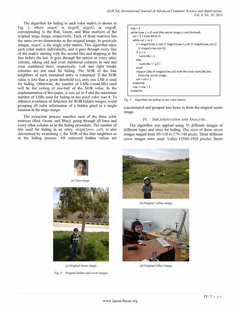
(IJACSA) International Journal of Advanced Computer Science and Applications, Vol. 4, No. 10, 2013
19 | P a g e www.ijacsa.thesai.org
The algorithm for hiding in each color matrix is shown in Fig. 1, where stegoC is stegoR, stegoG, or stegoB, corresponding to the Red, Green, and Blue matrices of the original stego image, respectively. Each of these matrices has
the same (nm) dimensions as the original image. In grayscale images, stegoC is the single color matrix. This algorithm takes each color matrix individually, and it goes through every line of the matrix starting with the second line and stopping at the line before the last. It goes through the entries in every other column, taking odd and even numbered columns in odd and even numbered lines, respectively. Left and right border columns are not used for hiding. The XOR of the four neighbors of each examined entry is computed. If the XOR
value is less than a given threshold (), only one LSB is used for hiding. Otherwise, the number of LSBs (numLSBs) used will be the ceiling of one-half of the XOR value. In the
implementation of this paper, was set to 9 and the maximum number of LSBs used for hiding in any pixel color was 4. To enhance avoidance of detection for RGB hidden images, avoid grouping all color information of a hidden pixel in a single location in the stego image.
The extraction process searches each of the three color matrices (Red, Green, and Blue), going through all lines and every other column as in the hiding procedure. The number of bits used for hiding in an entry, stegoC(row, col), is also determined by examining x; the XOR of the four neighbors as in the hiding process. All extracted hidden values are
concatenated and grouped into bytes to form the original secret image.
IV. IMPLEMENTATION AND ANALYSIS
The algorithm was applied using 35 different images of different types and sizes for hiding. The sizes of these secret
images ranged from 55110 to 175148 pixels. Three different
cover images were used: Valley (25601920 pixels), Street
Fig. 1. Algorithm for hiding in one color matrix.
row = 2
while (row n-2) and (the secret image is not finished) col = 2 + (row MOD 2)
while col m-2
x = stegoC(row-1,col) stegoC(row+1,col) stegoC(row,col-1)
stegoC(row,col+1))
if x numLSBs = 1 else
numLSBs = x/2 endif replace LSBs of stegoC(row,col) with the next numLSBs bits from the secret image col = col + 2
endwhile row = row + 1 endwhile
(a) Face image
(b) Original Valley image
(c) Original Street image (d) Original Office image
Fig. 2. Original hidden and cover images.
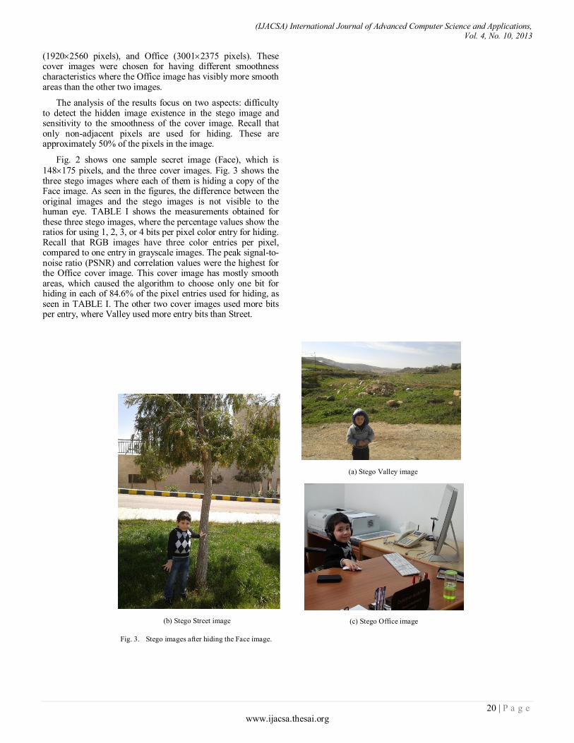
(IJACSA) International Journal of Advanced Computer Science and Applications, Vol. 4, No. 10, 2013
20 | P a g e www.ijacsa.thesai.org
(19202560 pixels), and Office (30012375 pixels). These cover images were chosen for having different smoothness characteristics where the Office image has visibly more smooth areas than the other two images.
The analysis of the results focus on two aspects: difficulty to detect the hidden image existence in the stego image and sensitivity to the smoothness of the cover image. Recall that only non-adjacent pixels are used for hiding. These are approximately 50% of the pixels in the image.
Fig. 2 shows one sample secret image (Face), which is
148175 pixels, and the three cover images. Fig. 3 shows the three stego images where each of them is hiding a copy of the Face image. As seen in the figures, the difference between the original images and the stego images is not visible to the human eye. TABLE I shows the measurements obtained for these three stego images, where the percentage values show the ratios for using 1, 2, 3, or 4 bits per pixel color entry for hiding. Recall that RGB images have three color entries per pixel, compared to one entry in grayscale images. The peak signal-to-noise ratio (PSNR) and correlation values were the highest for the Office cover image. This cover image has mostly smooth areas, which caused the algorithm to choose only one bit for hiding in each of 84.6% of the pixel entries used for hiding, as seen in TABLE I. The other two cover images used more bits per entry, where Valley used more entry bits than Street.
(a) Stego Valley image
(b) Stego Street image (c) Stego Office image
Fig. 3. Stego images after hiding the Face image.

(IJACSA) International Journal of Advanced Computer Science and Applications, Vol. 4, No. 10, 2013
21 | P a g e www.ijacsa.thesai.org
The average results for all 35 test images are shown in TABLE II. The average correlation value was taken for the absolute values of correlation for all images, where the original cover image was compared to each of its stego images to obtain the individual correlation values.
As TABLE II shows, the PSNR and correlation values were high, indicating low degradation of stego images and big difficulty for hidden image detection. The correlation and PSNR values were the highest for the Office cover image. This mostly-smooth cover image caused the algorithm, on average, to choose only one bit for hiding in each of 85.8% of the pixels used for hiding, as seen in TABLE II. The other two cover images used more bits per entry, where Valley used more bits than Street. This indicates that images with smoother areas are a poor choice for cover images since they must use fewer bits for hiding to avoid detection, consequently lowering their hiding capacity. The slight increase in PSNR and correlation values for such images may not be a feasible expense for the significant decrease of hiding capacity.
V. CONCLUSIONS
The new algorithm presented in this paper uses a variable number of LSBs from each color of each considered pixel for hiding a secret image, where approximately 50% of all pixels are considered for hiding. The actual number of hiding bits in a pixel is inversely proportional to the smoothness of its neighbors. The smoothness of a pixel area is determined by taking the XOR of the pixel's neighbors, where a high XOR value indicates less smoothness.
Test results showed that the new algorithm keeps the hidden image difficult to detect, as shown by the high PSNR and correlation values for stego images. The algorithm must hide less information in images containing more smooth areas to keep avoiding detection. This indicates that hiding in such images would be a poor choice.
VI. FUTURE WORK
The presented algorithm may be modified easily to work with video where each frame is regarded as a single image. However, the modification should be made more efficient by taking advantage of video properties, which differ according to video content and format. For example, frames with less smooth contents could be detected and chosen for hiding information. Another reason for considering video format properties is their effect on video sensitivity to modification. For example, some video formats use the similarities and differences within frame sequences to perform compression. Hiding information in such videos may cause a detectable change in video size unless the hiding algorithm works around the compression method.
REFERENCES
[1] A. Al-Othmani, A. Abdul Manaf and A. Zeki, “A survey on
steganography techniques in real time audio signals and evaluation,” Int. J. Comput. Sci. Issues, vol. 9, no. 1, p. 3037, 2012.
[2] R. Amirtharajan, J. Qin and J. Rayappan, “Random image
steganography and steganalysis: Present status and future direction,” Inf. Technol. J., vol. 11, no. 5, pp. 566-576, 2012.
[3] G. Chhajed, K. Deshmukh and T. Kulkarni, “Review on binary image
steganography and watermarking,” Int. J. Comput. Sci. & Eng., vol. 3, no. 11, pp. 3645-3651, 2011.
[4] A. Hmood, H. Jalab, Z. Kasirun, B. Zaidan and A. Zaidan, “On the
capacity and security of steganography approaches: An overview,” J. Appl. Sci., vol. 10, no. 16, pp. 1825-1833, 2010.
[5] P. Jayaram, H. Ranganatha and H. Anupama, “Information hiding using
audio steganography - A survey,” Int. J. Multimedia Appl., vol. 3, no. 3, pp. 86-96, 2011.
[6] V. Reddy, A. Subramanyam and P. Reddy, “Implementation of LSB steganography and its evaluation for various file formats,” Int. J. Adv.
Networking Appl., vol. 2, no. 5, pp. 868-872, 2011.
[7] I. Shoukat, K. Abu Bakar and M. Iftikhar, “A survey about the latest trends and research isuues of cryptographic elements,” Int. J. Comput.
Sci. Issues, vol. 8, no. 3:2, pp. 140-149, 2011.
[8] S. Janakiraman, R. Amirtharajan, K. Thenmozhi and J. Rayappan, “Pixel forefinger for gray in color: A layer by layer stego,” Inf. Technol.
J., vol. 11, no. 1, pp. 9-19, 2012.
[9] A. Pradhan, D. Sharma and G. Swain, “Variable rate steganography in digital images using two, three and four neighbor pixels,” Indian J.
Comput. Sci. & Eng., pp. 457-463, 2012.
[10] M. Al-Husainy, “A new image steganography based on decimal-digits representation,” Comput. & Inf. Sci., vol. 4, no. 6, pp. 38-47, 2011.
[11] O. Zanganeh and S. Ibrahim, “Adaptive image steganography based on
optimal embedding and robust against Chi-square attack,” Inf. Technol. J., vol. 10, no. 7, pp. 1285-1294, 2011.
TABLE II. AVERAGE RESULTS FOR 35 TEST IMAGES
Cover
Image Correlation
PSNR
(dB)
1 bit
%
2 bit
%
3 bit
%
4 bit
%
Valley 0.999993 62.300 45.4 30.3 21.3 3.0
Street 0.999994 60.775 65.7 18.9 11.1 4.3
Office 0.999997 66.072 85.8 10.5 2.7 0.9
TABLE I. RESULTS FOR THE FACE TEST IMAGE
Cover
Image Correlation
PSNR
(dB)
1 bit
%
2 bit
%
3 bit
%
4 bit
%
Valley 0.999988 59.174 36.9 32.0 27.1 4.0
Street 0.999986 57.731 56.3 23.0 15.3 5.4
Office 0.999994 62.701 84.6 11.3 2.9 1.2
(IJACSA) International Journal of Advanced Computer Science and Applications, Vol. 4, No. 10, 2013
22 | P a g e www.ijacsa.thesai.org
Synthetic template: effective tool for target
classification and machine vision
Kaveh Heidary
Department of Electrical Engineering and Computer Science
Alabama A&M University
Normal, Alabama 35762, USA
Abstract—A process for replacing a voluminous image
dictionary, which characterizes a certain target of interest in a
constrained zone of effectiveness representing controlled states
including scale and view angle, with a synthetic template has been
developed. Synthetic template (ST) is a spatial map (grayscale
image) obtained by combining the set of zone-specific training
images that are ascribed to the target of interest. It has been
shown that the solo-template ST correlation filter outperforms
filter banks comprised of multiple target-class training images. A
geometric interpretation of the basic ST concept is employed in order to further explain and substantiate its properties.
Keywords—machine vision; image procession; target
classification; correlation filter
I. INTRODUCTION
Machine vision involves the process of autonomous assessment of imagery data in a wide array of applications ranging from robotic navigation to biometrics and automatic detection and tracking of targets [1-5]. Computers are utilized to detect, identify and track objects of interest based on their electromagnetic or acoustic signatures, which may be expressed as two-dimensional data arrays obtained through an assortment of modalities including visible, infrared and synthetic aperture radar (SAR) imagery [6]. In the context of this paper a digital image is the result of spatial sampling and quantization of the filtered light energy emanating from the object and impinging on the focal plane of the optical sensor. Low level machine vision involves processing at the pixel level including image operations such as smoothing, enhancement and edge detection. Midlevel machine vision moves beyond pixels and involves larger abstractions such as shape, geometry and texture based classification, and high level vision involves context cognition including image understanding and interpretation [7-13]. This paper addresses a midlevel machine vision problem involving the development of a supervised learning algorithm for imagery based classification of objects. The goal is to develop a classifier that can determine the presence and location of the object of interest in arbitrary two-dimensional images. The classifier is constructed using a set of training images that represent the object of interest under assorted object states and viewing conditions that characterize the classifier's intended zone of effectiveness. The resultant classifier must be robust, in the sense of its ability to detect and locate with high reliability the object of interest under arbitrary view conditions within the
intended zone of effectiveness. It must also be computationally efficient in terms of its ability to operate on large image files with low latency, using readily available hardware platforms. The two requirements of locating ability and computational efficiency of the desired classifier point in the direction of Fourier filtering [14].
The optimal procedure for determination of the presence of a known signal in the input waveform generated by the sensor, whose output is potentially corrupted by an additive stationary noise process, is matched filtering [15-17]. The matched filter is the optimal linear signal processor in the sense of maximizing signal-to-noise ratio (SNR) at the detector output. Under special circumstances, where the power spectral density of the noise process is uniform (white noise), the impulse response of the matched filter is equivalent to the time/space-reversed version of the sought after signal. The optimal method for detecting the presence of a known signal in the input waveform which is corrupted by an additive white Gaussian noise (AWGN) process is therefore cross-correlating the waveform with a replica of the signal of interest.
Pattern matching, where a window containing an image of the sought after object (target) is slid over the image under test, is a conventional approach to locating targets of interest in the input image [18-20]. Generally, a typical target of interest is characterized by many windows comprising the target-class training set of images. Each window pertains to the target image under a specific view condition such as scale, pose, lighting, possible partial obscuration, view and illumination directions, etc. An actual target in real images can render countless patterns due to variations in range (scale), both in-plane and out-of-plane rotation (pose), environmental conditions including lighting, shadow and partial obscuration effects [21-27]. Any given object can cast infinitely may different projections upon the sensor's focal plane array and therefore can produce countless images. Object image variability may arise from intrinsic and extrinsic inconsistencies. Intrinsic effects include object deformation, articulation and pose, and extrinsic effects include range, view angle, lighting and obscuration.
One of the elements of any machine vision system is a target dictionary of images associated with each object of interest. In a robust system, a typical target dictionary consists of numerous windows (target images), and the sensor image must be tested against all the windows in order to establish the target's presence and potential locations or lack thereof in the input image. The sensor images must be tested against
* Partial sponsorship for K.H. was provided by Department of Defense
through US Army RDECOM W911NF-13-1-0136. * E-mail: [email protected], Telephone: +1 256 372 5587.
.
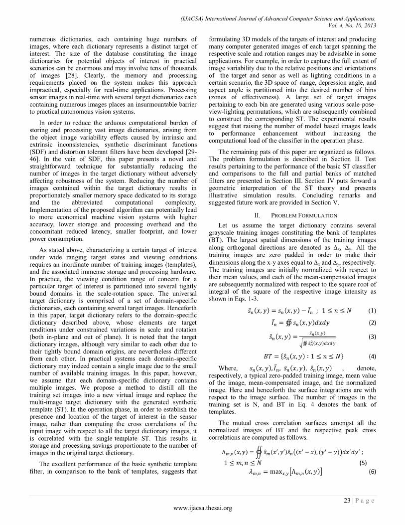
(IJACSA) International Journal of Advanced Computer Science and Applications, Vol. 4, No. 10, 2013
23 | P a g e www.ijacsa.thesai.org
numerous dictionaries, each containing huge numbers of images, where each dictionary represents a distinct target of interest. The size of the database constituting the image dictionaries for potential objects of interest in practical scenarios can be enormous and may involve tens of thousands of images [28]. Clearly, the memory and processing requirements placed on the system makes this approach impractical, especially for real-time applications. Processing sensor images in real-time with several target dictionaries each containing numerous images places an insurmountable barrier to practical autonomous vision systems.
In order to reduce the arduous computational burden of storing and processing vast image dictionaries, arising from the object image variability effects caused by intrinsic and extrinsic inconsistencies, synthetic discriminant functions (SDF) and distortion tolerant filters have been developed [29-46]. In the vein of SDF, this paper presents a novel and straightforward technique for substantially reducing the number of images in the target dictionary without adversely affecting robustness of the system. Reducing the number of images contained within the target dictionary results in proportionately smaller memory space dedicated to its storage and the abbreviated computational complexity. Implementation of the proposed algorithm can potentially lead to more economical machine vision systems with higher accuracy, lower storage and processing overhead and the concomitant reduced latency, smaller footprint, and lower power consumption.
As stated above, characterizing a certain target of interest under wide ranging target states and viewing conditions requires an inordinate number of training images (templates), and the associated immense storage and processing hardware. In practice, the viewing condition range of concern for a particular target of interest is partitioned into several tightly bound domains in the scale-rotation space. The universal target dictionary is comprised of a set of domain-specific dictionaries, each containing several target images. Henceforth in this paper, target dictionary refers to the domain-specific dictionary described above, whose elements are target renditions under constrained variations in scale and rotation (both in-plane and out of plane). It is noted that the target dictionary images, although very similar to each other due to their tightly bound domain origins, are nevertheless different from each other. In practical systems each domain-specific dictionary may indeed contain a single image due to the small number of available training images. In this paper, however, we assume that each domain-specific dictionary contains multiple images. We propose a method to distill all the training set images into a new virtual image and replace the multi-image target dictionary with the generated synthetic template (ST). In the operation phase, in order to establish the presence and location of the target of interest in the sensor image, rather than computing the cross correlations of the input image with respect to all the target dictionary images, it is correlated with the single-template ST. This results in storage and processing savings proportionate to the number of images in the original target dictionary.
The excellent performance of the basic synthetic template filter, in comparison to the bank of templates, suggests that
formulating 3D models of the targets of interest and producing many computer generated images of each target spanning the respective scale and rotation ranges may be advisable in some applications. For example, in order to capture the full extent of image variability due to the relative positions and orientations of the target and senor as well as lighting conditions in a certain scenario, the 3D space of range, depression angle, and aspect angle is partitioned into the desired number of bins (zones of effectiveness). A large set of target images pertaining to each bin are generated using various scale-pose-view-lighting permutations, which are subsequently combined to construct the corresponding ST. The experimental results suggest that raising the number of model based images leads to performance enhancement without increasing the computational load of the classifier in the operation phase.
The remaining pats of this paper are organized as follows. The problem formulation is described in Section II. Test results pertaining to the performance of the basic ST classifier and comparisons to the full and partial banks of matched filters are presented in Section III. Section IV puts forward a geometric interpretation of the ST theory and presents illustrative simulation results. Concluding remarks and suggested future work are provided in Section V.
II. PROBLEM FORMULATION
Let us assume the target dictionary contains several grayscale training images constituting the bank of templates (BT). The largest spatial dimensions of the training images
along orthogonal directions are denoted as x, y. All the training images are zero padded in order to make their
dimensions along the x-y axes equal to x and y, respectively. The training images are initially normalized with respect to their mean values, and each of the mean-compensated images are subsequently normalized with respect to the square root of integral of the square of the respective image intensity as shown in Eqs. 1-3.
(1)
(2)
(3)
(4)
Where, , denote, respectively, a typical zero-padded training image, mean value of the image, mean-compensated image, and the normalized image. Here and henceforth the surface integrations are with respect to the image surface. The number of images in the training set is N, and BT in Eq. 4 denotes the bank of templates.
The mutual cross correlation surfaces amongst all the normalized images of BT and the respective peak cross correlations are computed as follows.
(5)
(6)

(IJACSA) International Journal of Advanced Computer Science and Applications, Vol. 4, No. 10, 2013
24 | P a g e www.ijacsa.thesai.org
where, denote, respectively, the cross
correlation surface and the corresponding peak cross correlation between two BT images and . The function in Eq. 5 is periodically extended along both spatial directions.
One of the templates of BT which has the largest minimum peak cross correlation with respect to all the other images is declared the prototype template (PT) as shown below.
(7)
(8)
(9)
Where, denotes PT. If there are multiple images that satisfy the condition of Eq. 8, one is chosen randomly and is declared as PT.
All the BT images are spatially aligned with respect to PT. This is done by spatially shifting each image such that the peak of its cross correlation surface with respect to PT occurs at (0,0).
(10)
(11)
(12)
Where, is a typical spatially shifted and renormalized
target template, and denotes the bank of spatially shifted and aligned templates.
Summing all the spatially aligned target templates of Eq.12, and normalizing the resultant synthetic image such that the integral of its square is unity, one arrives at the synthetic template (ST).
(13)
(14)
(15)
Where, represents the ST.
As explained above, BT in Eq. 4 consists of the entire set of normalized training images, whereas PT in Eq. 9 contains only one of those images. PT is deemed the best representative of the training set in the sense that it has the largest minimum peak correlation with respect to all the trainers. A conceptual and geometric account of PT proceeds as follows: in the manifold of the training images within the image hyperspace, PT is closer to the center of gravity of the training manifold than any other BT image. Similar to PT, ST also consists of a
single template, however, it is none of the actual training images, and is synthesized by amalgamation of all the trainers. A conceptual and geometric account of ST proceeds as follows: in the manifold of the training images within the image hyperspace, ST is indeed the center of gravity of the training manifold. ST is the center of mass of the convex hall of the training images. The spatial dimensions of the constituent templates of BT, PT, and ST are identical, namely . The computational complexity of processing a typical sensor image with BT is therefore higher than processing the same image with PT and ST, by a factor equal to the number of training images N. In the operation phase, the correlation of the filter template is computed with respect to the input image, and if the correlation value exceeds the user-specified threshold, the presence of target is declared at the specified location of the input image.
It is noted that BT is the conventional matched filter bank under the white noise assumption. In the next section the performance of correlation filters based on the full bank of templates (BT) is compared to those based on two single-image templates, namely the prototype template (PT) and the synthetic template (ST). Also, the performance of the correlation filter based on the fractional bank of templates (FBT) is examined. The images comprising a typical FBT are obtained by random selection of a user-prescribed number of images from BT.
III. TEST RESULTS
In this section the performance of correlation filters based on BT, PT, ST, and FBT are examined using actual images for training and testing. The images used in the test scenarios presented here are obtained from the Amsterdam Library of Object Images (ALOI), details of which are provided in [47] and the actual image databases are found at [48]. Many tests were conducted, where designated image sets pertaining to certain user-specified objects were utilized as the target-class training set of images. The images of the chosen target-class object which were not employed in the training process as well as the images of other non-target objects were utilized as the test set of images. Four types of correlation filters were constructed, as described in Section II, using the sequestered training set of images. The correlation filters were subsequently used as binary classifiers in order to classify each of the images in the test set as either target-class or non-target-class. The performance of each type of filter is characterized in terms of its receiver operating characteristic (ROC), where the probability of detection PD is plotted in terms of the probability of false-alarm PFA. In the tests presented here, PD and PFA for a particular classification filter refer to the proportion of the test images that are, respectively, correctly labeled and mislabeled by the corresponding filter.
Target-class and non-target-class training and test images employed in the first experiment were the image masks pertaining to objects number - 2, 550, 700, 800, and 950, which denote, respectively, lab-keys, winny-the-pooh, daffy-duck, tea-can, and bananas in ALOI. The database contains 71 image masks for each object, all taken at the same range and at equally spaced view angles in . In this experiment, the target-class universe of images (TCUI)
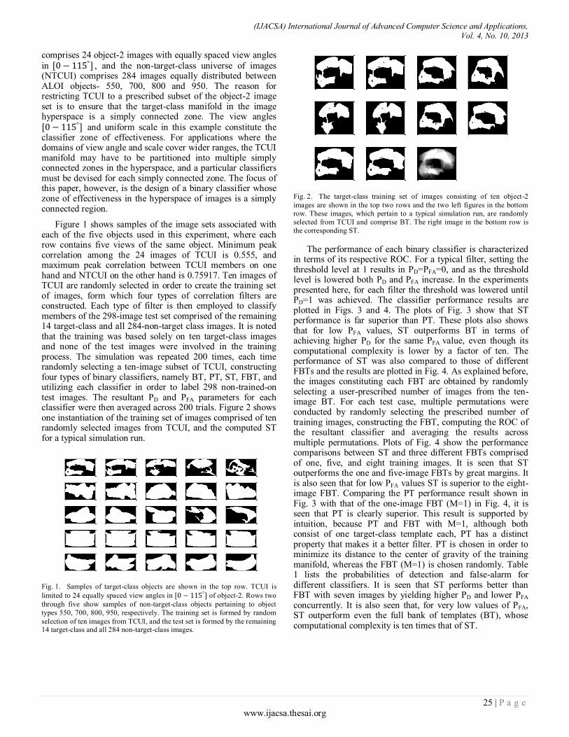
(IJACSA) International Journal of Advanced Computer Science and Applications, Vol. 4, No. 10, 2013
25 | P a g e www.ijacsa.thesai.org
comprises 24 object-2 images with equally spaced view angles
in , and the non-target-class universe of images (NTCUI) comprises 284 images equally distributed between ALOI objects- 550, 700, 800 and 950. The reason for restricting TCUI to a prescribed subset of the object-2 image set is to ensure that the target-class manifold in the image hyperspace is a simply connected zone. The view angles
and uniform scale in this example constitute the classifier zone of effectiveness. For applications where the domains of view angle and scale cover wider ranges, the TCUI manifold may have to be partitioned into multiple simply connected zones in the hyperspace, and a particular classifiers must be devised for each simply connected zone. The focus of this paper, however, is the design of a binary classifier whose zone of effectiveness in the hyperspace of images is a simply connected region.
Figure 1 shows samples of the image sets associated with each of the five objects used in this experiment, where each row contains five views of the same object. Minimum peak correlation among the 24 images of TCUI is 0.555, and maximum peak correlation between TCUI members on one hand and NTCUI on the other hand is 0.75917. Ten images of TCUI are randomly selected in order to create the training set of images, form which four types of correlation filters are constructed. Each type of filter is then employed to classify members of the 298-image test set comprised of the remaining 14 target-class and all 284-non-target class images. It is noted that the training was based solely on ten target-class images and none of the test images were involved in the training process. The simulation was repeated 200 times, each time randomly selecting a ten-image subset of TCUI, constructing four types of binary classifiers, namely BT, PT, ST, FBT, and utilizing each classifier in order to label 298 non-trained-on test images. The resultant PD and PFA parameters for each classifier were then averaged across 200 trials. Figure 2 shows one instantiation of the training set of images comprised of ten randomly selected images from TCUI, and the computed ST for a typical simulation run.
Fig. 1. Samples of target-class objects are shown in the top row. TCUI is
limited to 24 equally spaced view angles in of object-2. Rows two
through five show samples of non-target-class objects pertaining to object
types 550, 700, 800, 950, respectively. The training set is formed by random
selection of ten images from TCUI, and the test set is formed by the remaining 14 target-class and all 284 non-target-class images.
Fig. 2. The target-class training set of images consisting of ten object-2
images are shown in the top two rows and the two left figures in the bottom
row. These images, which pertain to a typical simulation run, are randomly
selected from TCUI and comprise BT. The right image in the bottom row is
the corresponding ST.
The performance of each binary classifier is characterized in terms of its respective ROC. For a typical filter, setting the threshold level at 1 results in PD=PFA=0, and as the threshold level is lowered both PD and PFA increase. In the experiments presented here, for each filter the threshold was lowered until PD=1 was achieved. The classifier performance results are plotted in Figs. 3 and 4. The plots of Fig. 3 show that ST performance is far superior than PT. These plots also shows that for low PFA values, ST outperforms BT in terms of achieving higher PD for the same PFA value, even though its computational complexity is lower by a factor of ten. The performance of ST was also compared to those of different FBTs and the results are plotted in Fig. 4. As explained before, the images constituting each FBT are obtained by randomly selecting a user-prescribed number of images from the ten-image BT. For each test case, multiple permutations were conducted by randomly selecting the prescribed number of training images, constructing the FBT, computing the ROC of the resultant classifier and averaging the results across multiple permutations. Plots of Fig. 4 show the performance comparisons between ST and three different FBTs comprised of one, five, and eight training images. It is seen that ST outperforms the one and five-image FBTs by great margins. It is also seen that for low PFA values ST is superior to the eight-image FBT. Comparing the PT performance result shown in Fig. 3 with that of the one-image FBT (M=1) in Fig. 4, it is seen that PT is clearly superior. This result is supported by intuition, because PT and FBT with M=1, although both consist of one target-class template each, PT has a distinct property that makes it a better filter. PT is chosen in order to minimize its distance to the center of gravity of the training manifold, whereas the FBT (M=1) is chosen randomly. Table 1 lists the probabilities of detection and false-alarm for different classifiers. It is seen that ST performs better than FBT with seven images by yielding higher PD and lower PFA concurrently. It is also seen that, for very low values of PFA, ST outperform even the full bank of templates (BT), whose computational complexity is ten times that of ST.
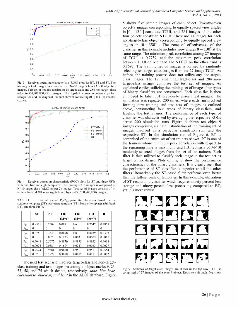
(IJACSA) International Journal of Advanced Computer Science and Applications, Vol. 4, No. 10, 2013
26 | P a g e www.ijacsa.thesai.org
Fig. 3. Receiver operating characteristic (ROC) plots for BT, PT and ST. The
training set of images is comprised of N=10 target-class (ALOI object-2)
images. Test set of images consists of 14 target-class and 284 non-target-class
(objects-550,700,800,950) images. The top-left corner represents perfect
recognition and the diagonal line (not shown) connecting (0,0) to (1,1) denotes chance.
Fig. 4. Receiver operating characteristic (ROC) plots for ST and three FBTs
with one, five and eight templates. The training set of images is comprised of
N=10 target-class (ALOI object-2) images. Test set of images consists of 14
target-class and 284 non-target-class (objects-550,700,800,950) images.
TABLE I. List of several PD-PFA pairs for classifiers based on the synthetic template (ST), prototype template (PT), bank of templates (full bank BT), and three FBTs.
ST PT FBT
(M=1)
FBT
(M=4)
FBT
(M=7)
BT
PD
PFA
0.8571
0
0.2609
0
0.087
0
0.6
0
0.7647
0
0.7857
0
PD
PFA
0.875
0
0.3533
0.007
0.8098
0.1233
0.8
0.003
0.8039
0.0003
0.8393
0.0011
PD
PFA
0.9048
0.0024
0.5072
0.038
0.8859
0.1604
0.8833
0.0247
0.8922
0.0033
0.9018
0.0027
PD
PFA
0.9524
0.02
0.9384
0.1879
0.9620
0.3098
0.95
0.0812
0.951
0.021
0.9554
0.0092
The next test scenario involves target-class and non-target-class training and test images pertaining to object masks 9, 23, 33, 58, and 75 which denote, respectively, shoe, blue-bear, chess-horse, blue-car, and boat in the ALOI database. Figure
5 shows five sample images of each object. Twenty-seven object-9 images corresponding to equally spaced view angles in constitute TCUI, and 284 images of the other four objects constitute NTCUI. There are 71 images for each non-target-class object corresponding to equally spaced view
angles in . The zone of effectiveness of the
classifier in this example includes view angles at the same range. The minimum peak correlation among 27 images of TCUI is 0.7739, and the maximum peak correlation between TCUI on one hand and NTCUI on the other hand is 0.8697. The training set of images is formed by randomly selecting ten target-class images from the 27-image TCUI. As before, the training process does not utilize any non-target-class images. The 17 remaining target-class and 284 non-target-class images comprise the test set of images. As explained earlier, utilizing the training set of images four types of binary classifiers are constructed. Each classifier is then employed to label 301 previously unseen test images. The simulation was repeated 200 times, where each run involved forming new training and test sets of images as outlined above, constructing four types of binary classifiers, and labeling the test images. The performance of each type of classifier was characterized by averaging the respective ROCs across 200 simulation runs. Figure 6 shows ten object-9 images comprising a single instantiation of the training set of images involved in a particular simulation run, and the respective ST. In the simulation run of Figure 6, BT is comprised of the entire set of ten trainers shown, PT is one of the trainers whose minimum peak correlation with respect to the remaining nine is maximum, and FBT consists of M<10 randomly selected images from the set of ten trainers. Each filter is then utilized to classify each image in the test set as target or non-target. Plots of Fig. 7 show the performance characteristics of the binary classifiers. It is clearly seen that the performance of ST classifier is superior to all the other filters. Remarkably the ST-based filter performs even better than the full-set bank of templates. In this example, utilization of ST results in a classifier which requires ninety-percent less storage and ninety-percent less processing compared to BT, yet it is more robust.
Fig. 5. Samples of target-class images are shown in the top row. TCUI is
comprised of 27 images of the type-9 object. Rows two through five show
0 0.01 0.02 0.03 0.04 0.05 0.06 0.07 0.08 0.09 0.10
0.1
0.2
0.3
0.4
0.5
0.6
0.7
0.8
0.9
1
PFA
PD
number of training images N=10
BT
PT
ST
0 0.02 0.04 0.06 0.08 0.1 0.12 0.14 0.16 0.18 0.20
0.1
0.2
0.3
0.4
0.5
0.6
0.7
0.8
0.9
1number of training images N=10
PD
PFA
FBT (M=1)
FBT (M=5)
FBT (M=8)
ST
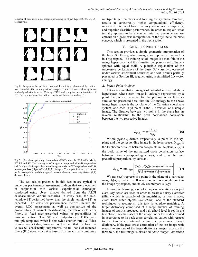
(IJACSA) International Journal of Advanced Computer Science and Applications, Vol. 4, No. 10, 2013
27 | P a g e www.ijacsa.thesai.org
samples of non-target-class images pertaining to object types 23, 33, 58, 75, respectively.
Fig. 6. Images in the top two rows and the left two columns of the bottom
row constitute the training set of images. These ten object-9 images are
randomly selected from the 27-image TCUI and comprise one instantiation of BT. The right image of the bottom row shows the corresponding ST.
Fig. 7. Receiver operating characteristic (ROC) plots for FBT with (M=5),
BT, PT and ST. The training set of images is comprised of N=10 target-class
(ALOI object-9) images. Test set of images consists of 17 target-class and 284
non-target-class (objects-23,33,58,75) images. The top-left corner represents
perfect recognition and the diagonal line (not shown) connecting (0,0) to (1,1) denotes chance.
The test results presented in this section are typical of numerous performance assessment findings that were obtained in conjunction with various experimental campaigns conducted using object images derived from the ALOI database under various scenarios. In every case, the solo-template ST performed better than the single-template PT, as expected. The classifier performance metrics include the overall ROC assessments as well as comparison of the probabilities of correct classification, for various classifier filters, at fixed user-prescribed values of probabilities of misclassification. The ST also outperformed FBTs with multiple templates, which is somewhat counter intuitive. What is most remarkable, however, is the fact that for low PFA values ST consistently outperforms the full bank of matched filters (BT) upon which it is based. This means that combining
multiple target templates and forming the synthetic template, results in concurrently higher computational efficiency, measured in terms of lower memory and reduced complexity, and superior classifier performance. In order to explain what initially appears to be a counter intuitive phenomenon, we embark on a geometric interpretation of the synthetic template concept, which is presented in the next section.
IV. GEOMETRIC INTERPRETATION
This section provides a simple geometric interpretation of the basic ST theory, where images are represented as vectors in a hyperspace. The training set of images is a manifold in the image hyperspace, and the classifier comprises a set of hyper-spheres with equal radii. A plausible explanation of the impressive performance of the basic ST classifier, observed under various assessment scenarios and test results partially presented in Section III, is given using a simplified 2D vector analogy.
A. Image-Point Analogy
Let us assume that all images of potential interest inhabit a hyperspace, where each image is uniquely represented by a point. Let us also assume, for the purpose of explanatory simulations presented here, that the 2D analogy to the above image hyperspace is the xy-plane of the Cartesian coordinate system, and each (x,y) point is the 2D version of a unique image. The distance between two points in the plane has an inverse relationship to the peak normalized correlation between the two respective images.
(16)
Where, and denote, respectively, a point in the xy-plane and the corresponding image in the hyperspace,
is
the Euclidean distance between two points in the plane, is
the peak value of the normalized cross correlation surface
between two corresponding images, and is the user prescribed proportionality constant.
(17)
Where, (u,v) represents a point in the plane of a particular image , which itself is represented as a single point in the image hyperspace, and its 2D counterpart is (x,y).
In machine learning, a set of images representing an object class, say chair, are used in order to create a binary classifier (filter) which is capable of distinguishing, in new images, chair from other objects (non-chair). one of the standard techniques to accomplish this task is template matching. A target dictionary comprised of a large number of training images of chair is produced, and a threshold level is set. In the test phase, the class label of the image under test is determined in accordance to its peak cross correlation values with respect to the templates contained within the prearranged target dictionary. If the peak cross correlation of the test image with respect to any one of the target dictionary images exceeds the threshold, the test image is classified chair (target), otherwise
0 0.005 0.01 0.015 0.02 0.025 0.03 0.035 0.040.5
0.55
0.6
0.65
0.7
0.75
0.8
0.85
0.9
0.95
1
PFA
PD
number of training images N=10
FBT (M=5)
BT
PT
ST
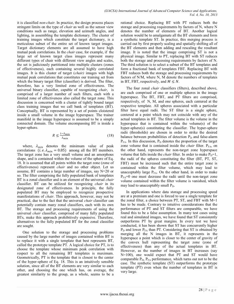
(IJACSA) International Journal of Advanced Computer Science and Applications, Vol. 4, No. 10, 2013
28 | P a g e www.ijacsa.thesai.org
it is classified non-chair. In practice, the design process places stringent limits on the type of chair as well as the sensor view conditions such as range, elevation and azimuth angles, and lighting, in assembling the template dictionary. The cluster of training images which constitute the target dictionary, is a meticulous subset of the entire set of known target images. Target dictionary elements are all assumed to have high mutual peak correlations. In the chair case, for example, if the large set of known target class images represent many different types of chair with different view angles and scales, the set is judiciously partitioned into multiple clusters (zones of effectiveness), each containing several highly correlated images. It is this cluster of target (chair) images with high mutual peak correlations that constitutes our training set from which the binary target filter (classifier) is derived. The filter, therefore, has a very limited zone of effectiveness. The universal binary classifier, capable of recognizing chair, is comprised of a larger number of such filters, each with a limited zone of effectiveness also called the target zone. This discussion is concerned with a cluster of tightly bound target class training images that we call bank of templates (BT). Conceptually, BT is represented by a set of points cloistered inside a small volume in the image hyperspace. The trainer manifold in the image hyperspace is assumed to be a simply connected domain. The volume encompassing BT is inside a hyper-sphere.
(18)
where, denotes the minimum value of peak correlations among all the BT members. The target zone has a very small volume and an amorphous shape, and is contained within the volume of the sphere of Eq. 18. It is assumed that all points within the target zone (zone of effectiveness) represent chair and no other object. Let us assume, BT contains a large number of images, say N=20 or so. The filter comprising the fully populated bank of templates BT is a zonal classifier and is an element of the universal chair classifier. BT can be utilized for recognizing chair in its designated zone of effectiveness. In principle, the fully populated BT may be employed to recognize prospective manifestations of chair. This approach, however, may not be practical, due to the fact that the universal chair classifier can potentially contain many zonal classifiers, each with its own BT. The storage and processing requirements of using the universal chair classifier, comprised of many fully populated BTs, make this approach prohibitively expensive. Therefore, alternatives to the fully populated BT for the zonal classifier are sought.
One solution to the storage and processing problems caused by the large number of images contained within BT is to replace it with a single template that best represents BT, called the prototype template PT. A logical choice for PT, is to choose the template whose minimum peak correlation with respect to all the remaining BT templates is maximum. Geometrically, PT is the template that is closest to the center of the hyper-sphere of Eq. 18. This is an intuitively sensible solution, since all of the BT elements are very similar to each other, and choosing the one which has, on average, the greatest similarity to the group, as a whole, seems to be a
rational choice. Replacing BT with PT reduces both the storage and processing requirements by factors of N, where N denotes the number of elements of BT. Another logical solution would be to amalgamate all the BT elements and form a synthetic template ST. In practice, this merging process is carried out by first properly scaling and spatially shifting all of the BT elements and then adding and rescaling the resultant image. It is noted that the image comprising ST is not a physical image. Similar to PT, replacing BT with ST reduces both the storage and processing requirements by factors of N. The third solution is to select a subset of the BT templates and form a fractional bank of templates FBT. Replacing BT with FBT reduces both the storage and processing requirements by factors of N/M, where N, M denote the numbers of templates in BT, FBT, respectively, and .
The four zonal chair classifiers (filters), described above,
are each comprised of one or multiple spheres in the image hyperspace. The BT, FBT, and PT filters are comprised,
respectively, of N, M, and one spheres, each centered at the
respective template. All spheres associated with a particular
filter have equal radii. The ST filter is a single sphere,
centered at a point which may not coincide with any of the
actual templates in BT. The filter volume is the volume in the
hyperspace that is contained within the volume(s) of the
hyper-sphere(s) constituting the classifier. The hyper-sphere
radii (thresholds) are chosen in order to strike the desired
balance between probabilities of detection PD and false-alarm
PFA. In this discussion, PD denotes the proportion of the target
zone volume that is contained inside the chair filter. PFA, on the other hand, represents the non-target zone hyperspace
volume that falls inside the chair filter. In order to make PD=1,
the radii of the spheres constituting the filter (BT, PT, ST,
FBT) must be increased such that the entire target zone is
contained within the filter volume, which may lead to
unacceptably large PFA. On the other hand, in order to make
PFA=0 one must decrease the radii until the non-target zone
volume contained within the filter volume is vanished, which
may lead to unacceptably small PD.
In applications where data storage and processing speed are at a premium and one is forced to use a single template for the zonal filter, a choice between PT, ST, and FBT with M=1 has to be made. Contrary to intuitive considerations that the performance of PT and ST filters are comparable, we have found this to be a false assumption. In many test cases using real and simulated images, we have found that ST consistently outperforms PT by great margins. In every test we have conducted, it has been shown that ST has concurrently higher PD and lower PFA than PT. Considering that ST is obtained by merging all the N images in BT, it represents in the hyperspace a point which is closer to the center of gravity of the convex hull representing the target zone (zone of effectiveness) than any of the actual templates in BT. However, as the number of images in BT increases (say N=100), one would expect that PT and ST would have comparable PD, PFA performance, which turns out not to be the case. The synthetic template (ST) outperforms the prototype template (PT) even when the number of templates in BT is very large.
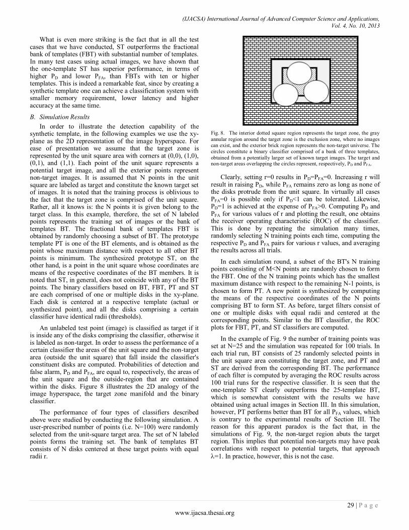
(IJACSA) International Journal of Advanced Computer Science and Applications, Vol. 4, No. 10, 2013
29 | P a g e www.ijacsa.thesai.org
What is even more striking is the fact that in all the test cases that we have conducted, ST outperforms the fractional bank of templates (FBT) with substantial number of templates. In many test cases using actual images, we have shown that the one-template ST has superior performance, in terms of higher PD and lower PFA, than FBTs with ten or higher templates. This is indeed a remarkable feat, since by creating a synthetic template one can achieve a classification system with smaller memory requirement, lower latency and higher accuracy at the same time.
B. Simulation Results
In order to illustrate the detection capability of the synthetic template, in the following examples we use the xy-plane as the 2D representation of the image hyperspace. For ease of presentation we assume that the target zone is represented by the unit square area with corners at (0,0), (1,0), (0,1), and (1,1). Each point of the unit square represents a potential target image, and all the exterior points represent non-target images. It is assumed that N points in the unit square are labeled as target and constitute the known target set of images. It is noted that the training process is oblivious to the fact that the target zone is comprised of the unit square. Rather, all it knows is: the N points it is given belong to the target class. In this example, therefore, the set of N labeled points represents the training set of images or the bank of templates BT. The fractional bank of templates FBT is obtained by randomly choosing a subset of BT. The prototype template PT is one of the BT elements, and is obtained as the point whose maximum distance with respect to all other BT points is minimum. The synthesized prototype ST, on the other hand, is a point in the unit square whose coordinates are means of the respective coordinates of the BT members. It is noted that ST, in general, does not coincide with any of the BT points. The binary classifiers based on BT, FBT, PT and ST are each comprised of one or multiple disks in the xy-plane. Each disk is centered at a respective template (actual or synthesized point), and all the disks comprising a certain classifier have identical radii (thresholds).
An unlabeled test point (image) is classified as target if it is inside any of the disks comprising the classifier, otherwise it is labeled as non-target. In order to assess the performance of a certain classifier the areas of the unit square and the non-target area (outside the unit square) that fall inside the classifier's constituent disks are computed. Probabilities of detection and false alarm, PD and PFA, are equal to, respectively, the areas of the unit square and the outside-region that are contained within the disks. Figure 8 illustrates the 2D analogy of the image hyperspace, the target zone manifold and the binary classifier.
The performance of four types of classifiers described above were studied by conducting the following simulation. A user-prescribed number of points (i.e. N=100) were randomly selected from the unit-square target area. The set of N labeled points forms the training set. The bank of templates BT consists of N disks centered at these target points with equal radii r.
Fig. 8. The interior dotted square region represents the target zone, the gray
annular region around the target zone is the exclusion zone, where no images
can exist, and the exterior brick region represents the non-target universe. The
circles constitute a binary classifier comprised of a bank of three templates,
obtained from a potentially larger set of known target images. The target and non-target areas overlapping the circles represent, respectively, PD and PFA.
Clearly, setting r=0 results in PD=PFA=0. Increasing r will result in raising PD, while PFA remains zero as long as none of the disks protrude from the unit square. In virtually all cases PFA=0 is possible only if PD<1 can be tolerated. Likewise, PD=1 is achieved at the expense of PFA>0. Computing PD and PFA for various values of r and plotting the result, one obtains the receiver operating characteristic (ROC) of the classifier. This is done by repeating the simulation many times, randomly selecting N training points each time, computing the respective PD and PFA pairs for various r values, and averaging the results across all trials.
In each simulation round, a subset of the BT's N training points consisting of M<N points are randomly chosen to form the FBT. One of the N training points which has the smallest maximum distance with respect to the remaining N-1 points, is chosen to form PT. A new point is synthesized by computing the means of the respective coordinates of the N points comprising BT to form ST. As before, target filters consist of one or multiple disks with equal radii and centered at the corresponding points. Similar to the BT classifier, the ROC plots for FBT, PT, and ST classifiers are computed.
In the example of Fig. 9 the number of training points was set at N=25 and the simulation was repeated for 100 trials. In each trial run, BT consists of 25 randomly selected points in the unit square area constituting the target zone, and PT and ST are derived from the corresponding BT. The performance of each filter is computed by averaging the ROC results across 100 trial runs for the respective classifier. It is seen that the one-template ST clearly outperforms the 25-template BT, which is somewhat consistent with the results we have obtained using actual images in Section III. In this simulation, however, PT performs better than BT for all PFA values, which is contrary to the experimental results of Section III. The reason for this apparent paradox is the fact that, in the simulations of Fig. 9, the non-target region abuts the target region. This implies that potential non-targets may have peak correlations with respect to potential targets, that approach
=1. In practice, however, this is not the case.
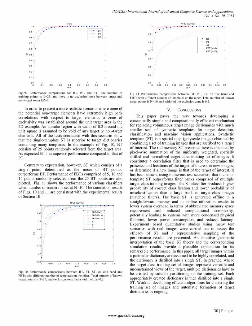
(IJACSA) International Journal of Advanced Computer Science and Applications, Vol. 4, No. 10, 2013
30 | P a g e www.ijacsa.thesai.org
Fig. 9. Performance comparisons for BT, PT, and ST. The number of
training points is N=25, and there is no exclusion zone between target and non-target zones EZ=0.
In order to present a more realistic scenario, where none of the potential non-target elements have extremely high peak correlations with respect to target elements, a zone of exclusivity was established around the unit target area in the 2D example. An annular region with width of 0.2 around the unit square is assumed to be void of any target or non-target elements. All of the tests conducted with this scenario show that the single-template ST is superior to target dictionaries containing many templates. In the example of Fig. 10, BT consists of 25 points randomly selected from the target area. As expected BT has superior performance compared to that of PT.
Contrary to expectation, however, ST which consists of a single point, determined as the mean of BT points, outperforms BT. Performance of FBTs comprised of 5, 10 and 15 points randomly selected from the 25 BT points are also plotted. Fig. 11 shows the performance of various classifiers when number of trainers is set at N=10. The simulation results of Figs. 10 and 11 are consistent with the experimental results of Section III.
Fig. 10. Performance comparisons between BT, PT, ST, on one hand and
FBTs with different number of templates on the other. Total number of known target points is N=25, and exclusion zone had a width of EZ=0.2.
Fig. 11. Performance comparisons between BT, PT, ST, on one hand and
FBTs with different number of templates on the other. Total number of known
target points is N=10, and width of the exclusion zone is 0.2.
V. CONCLUSIONS
This paper paves the way towards developing a conceptually simple and computationally efficient mechanism for replacing voluminous target image dictionaries with much smaller sets of synthetic templates for target detection, classification and machine vision applications. Synthetic template (ST) is a spatial map (grayscale image) obtained by combining a set of training images that are ascribed to a target of interest. The rudimentary ST presented here is obtained by pixel-wise summation of the uniformly weighted, spatially shifted and normalized target-class training set of images. It constitutes a correlation filter that is used to determine the presence and locations of the target of interest in new images, or determine if a new image is that of the target of interest. It has been shown, using numerous test scenarios, that the solo-template ST outperforms filter banks comprised of multiple target-class training images. The ST classifier produces higher probability of correct classification and lower probability of misclassification than a large bank of target-class images (matched filters). The basic ST is generated offline in a straightforward manner and its online utilization results in lower system overhead in terms of abbreviated memory space requirement and reduced computational complexity, potentially leading to systems with more condensed physical footprint, lower power consumption, and reduced latency. Experiment based quantitative studies using many test scenarios with real images were carried out to assess the efficacy of ST and a representative sampling of the performance results are presented. An intuitive geometric interpretation of the basic ST theory and the corresponding simulation results provide a plausible explanation for its remarkable performance. In this paper, all target images within a particular dictionary are assumed to be highly correlated, and the dictionary is distilled into a single ST. In practice, where the target-class training set of images represent versatile and unconstrained views of the target, multiple dictionaries have to be created by suitable partitioning of the training set. Each appropriately created dictionary is then distilled into a single ST. Work on developing efficient algorithms for clustering the training set of images and automatic formation of target dictionaries is ongoing.
0 0.1 0.2 0.3 0.4 0.5 0.6 0.7 0.80
0.1
0.2
0.3
0.4
0.5
0.6
0.7
0.8
0.9
1
PFA
PD
N=25
BT
PT
ST
0 0.05 0.1 0.15 0.2 0.25 0.3 0.35 0.40.65
0.7
0.75
0.8
0.85
0.9
0.95
1
PFA
PD
N=25 (EZ=0.2)
FBT (M=5)
FBT (M=10)
FBT (M=15)
BT
ST
PT
0 0.05 0.1 0.15 0.2 0.25 0.3 0.35 0.4 0.45 0.50.3
0.4
0.5
0.6
0.7
0.8
0.9
1N=10 (EZ=0.2)
PD
PFA
BT
PT
ST
FBT (M=1)
FBT (M=5)

(IJACSA) International Journal of Advanced Computer Science and Applications, Vol. 4, No. 10, 2013
31 | P a g e www.ijacsa.thesai.org
REFERENCES
[1] B. G. Batchelor (Editor), Machine Vision Handbook, Springer, 2012.
[2] C. Steger, M. Ulrich, C. Wiedemann, Machine Vision Algorithms and Applications, Wiley -VCH, 2007.
[3] E.R. Davies, Computer and Machine Vision: Theory, Algorithms,
Practicalities, Academic Press, 2012.
[4] R. C. Gonzalez, R. E. Woods, Digital Image Processing, Prentice Hall, 2007.
[5] T. Acharya, A. K. Ray, Image Processing - Principles and Applications,
Wiley, 2006.
[6] B. Bhanu, 'Automatic target recognition: State of the art survey,' IEEE Transactions on Aerospace and Electronic Systems, Vol. AES-22, No.
4, (1986) pp. 364-379.
[7] H. Kauppinen, T. Seppanen, M. Pietikainen, 'An experimental
comparison of autoregressive and Fourier-based descriptors in 2D shape classification,' IEEE Transactions on Pattern Analysis and Machine
Intelligence, Vol. 17, No. 2, (1995) pp. 201-207.
[8] S. Belongie, J. Malik, J. Puzicha, 'Shape matching and object recognition using shape contexts,' IEEE Transactions on Pattern Analysis and
Machine Intelligence, Vol. 24, No. 24, (2002) pp. 509-522.
[9] Y. Rui, T.S. Huang, S.F. Chang, 'Image Retrieval: Current Techniques, Promising Directions, and Open Issues,' Journal of Visual
Communication and Image Representation, Vol. 10, No. 1, (1999) pp. 39-62.
[10] A. Vailaya, M.A.T. Figueiredo, A.K. Jain, H.J. Zhang, 'Image
classification for content-based indexing,' IEEE Transactions on Image Processing, Vol. 10, No. 1, (2001) pp. 117-130.
[11] D. Zhang, G. Lu, 'Shape-based image retrieval using generic Fourier
descriptor,' Signal Processing: Image Communication, Vol. 17, No. 10, (2002) pp. 825-848.
[12] [12] M. Bober, 'MPEG-7 visual shape descriptors,' IEEE Transactions
on Circuits and Systems for Video Technology, Vol. 11, No. 6, (2001) 716–719.
[13] Y. Liu, D. Zhang, G. Lu, W.Y. Ma, 'A survey of content-based image retrieval with high-level semantics,' Pattern Recognition, Vol. 40, No. 1,
(2007) 262-282.
[14] A.B. Vander Lugt, 'Signal detection by complex filtering,' IEEE Transactions on Information Theory, Vol. 10, No. 2, (1964) pp. 139-145.
[15] G.L. Turin, 'An introduction to matched filters,' IRE Transactions on
Information Theory, Vol. 6, No. 3, (1960) 311-329.
[16] A, Papoulis, Signal Analysis, McGraw-Hill, 1977.
[17] H. L. Van Trees, Detection, Estimation, and Modulation Theory, Vol. 1, John Wiley & Sons, 2001.
[18] Q.S. Chen, M. Defrise, F. Deconinck, 'Symmetric phase-only matched
filtering of Fourier-Mellin transforms for image registration and recognition,' IEEE Transactions on Pattern Analysis and Machine
Intelligence, Vol. 16, No. 12, (1994) pp. 1156-1168.
[19] L.M. Novak, G.J. Owirka, C.M. Netishen, 'Radar Target Identification
using Spatial Matched Filters,' Pattern Recognition, Vol. 27, No. 4, (1994) pp. 607-617.
[20] A. Mahalanobis, A.V. Forman Jr., N. Day, M. Bower, R. Cherry, 'Multi-
class SAR using shift-invariant correlation filters,' Pattern Recognition, Vol. 27, No. 4, (1994) pp. 619-626.
[21] A.S. Georghiades, P.N. Belhumeur, D.J. Kriegman, 'From few to many:
Illumination cone models for face recognition under variable lighting and pose,' IEEE Transactions on Pattern Analysis and Machine Vision,
Vol. 23, No. 6, (2001) pp. 643-660.
[22] K.J. Dana, B.V. Ginneken, S.K. Nayar, and J.J. Koenderink, 'Reflectance and texture of real world surfaces,' ACM Transactions on
Graphics, Vol. 18, No. 1, (1999) pp. 1-34.
[23] P. N. Belhumeur, D. J. Kriegman, 'What is the set of images of an object under all possible illumination conditions?,' International Journal of
Computer Vision , Vol. 28, No. 3, (1998) pp. 1-16.
[24] P. Hallinan, A Deformable Model for Face Recognition Under Arbitrary Lighting Conditions, PhD thesis, Harvard University,1995.
[25] R.C. Hoover, A.A. Maciejewski, R.G. Roberts, 'Fast Eigenspace Decomposition of Images of Objects with Variation in Illumination and
Pose,' IEEE Transactions on Systems, Man, and Cybernetics, Vol. 41,
No. 2, (2011) pp. 318-329.
[26] R. Garg, D. Hao, S.M. Seitz, N. Snavely, 'The Dimensionality of Scene
Appearance,' Proceedings IEEE 12th International Conference on Computer Vision (2009) pp. 1917-1924.
[27] T.M. Caelli, Z.Q. Liu, 'On the minimum number of templates required
for shift, rotation and size invariant pattern recognition,' Pattern Recognition, Vol. 21, No. 3, (1988) 205-216.
[28] S. Landeau, T. Dagobert, 'Image database generation using image metric
constraints: an application within the CALADIOM project,' Proc. SPIE 623410, (2006) pp. 1-12.
[29] D. Casasent, D. Psaltis, 'Position, Rotation, and Scale Invariant Optical
Correlation,' Applied Optics, Vol. 15, No. 7, (1976) pp. 1795-1799.
[30] Y. N. Hsu, H.H. Arsenault, G. April, 'Rotation-invariant digital pattern recognition using circular harmonic expansion,' Applied Optics, Vol.
21, No. 22, (1982) pp. 4012-4015.
[31] D. Mendlovic, E. Marom, N. Konforti, 'Shift and scale invariant pattern recognition using Mellin radial harmonics,' Optics Communication, Vol.
67, No. 3, (1988) pp. 172-176.
[32] Y. Sheng, J. Duvernoy, 'Circular-Fourier-radial-Mellin transform
descriptors for pattern recognition,' JOSA A, Vol. 3, No. 6, (1986) pp. 885-888.
[33] H. J. Caulfield, M. H. Weinberg, 'Computer recognition of 2-D patterns
using generalized matched filters,' Applied Optics, Vol. 21, No. 9, (1982) pp. 1699-1704.
[34] B. V. K. Kumar, 'Minimum-variance synthetic discriminant functions,'
JOSA A, Vol. 3, No. 10, (1986) pp. 1579-1584.
[35] A. Mahalanobis, B.V.K. Kumar, D. Casasent, 'Minimum average correlation energy filters,' Applied Optics, Vol. 26, No. 17, (1987) pp.
3633-3640.
[36] D. Casasent, G. Ravichandran , S. Bollapragada, 'Gaussian-minimum average correlation energy filters,' Applied Optics, Vol. 30, No. 35,
(1991) pp. 5176-5181.
[37] D. Casasent, G. Ravichandran , 'Advanced distortion-invariant minimum average correlation energy (MACE) filters,' Applied Optics, Vol. 31, No.
8, (1992) pp. 1109-1116.
[38] M. Savvides, B.V.K.V. Kumar, 'Quad Phase Minimum Average
Correlation Energy Filters for Reduced Memory Illumination Tolerant Face Authentication,' Lecture Notes in Computer Science, Vol. 2688,
(2003) pp. 1056-1065.
[39] K. Heidary, H.J. Caulfield, 'Application of supergeneralized matched filters to target classification', Applied Optics Vol. 44 No. 1, (2005) pp.
47-54.
[40] K. Heidary, H.J. Caulfield, 'Nonlinear Fourier correlation,' Proceedings of SPIE Vol. 7340A, (2009) pp. 1-11.
[41] R. B. Johnson, K. Heidary, 'A unified approach for database analysis and
application to ATR performance metrics,' Proceedings of SPIE, Vol. 7696Z, (2011) pp. 1-20.
[42] A. Mahalanobis, R.R. Muise, S.R. Stanfill, A. Van Nevel, 'Design and
application of quadratic correlation filters for target detection,' IEEE Transactions on Aerospace and Electronic Systems, Vol. 40, No. 3,
(2004) pp. 837-850.
[43] J. Wright, A. Y. Yang, A. Ganesh, S. S. Sastry, M. Yi, 'Robust Face Recognition via Sparse Representation,' IEEE Transactions on Pattern
Analysis and Machine Intelligence, Vol. 31, No. 2, (2009) pp. 210-227.
[44] [44] K. Heidary, 'Distortion tolerant correlation filter design,' Applied
Optics, Vol. 52, No. 12, (2013) pp. 2570-2576.
[45] E. Perez, B. Javidi, 'Nonlinear distortion-tolerant filters for detection of road signs in background noise,' IEEE Transactions on Vehicular
Technology, Vol. 51, No. 3, (2002) pp.567-576.
[46] O. Arandjelovic, R. Cipolla, 'A methodology for rapid illumination-invariant face recognition using image processing filters,' Computer
Vision and Image Understanding, Volume 113, No. 2, (2009) 159-171.
[47] J. M. Geusebroek, G. J. Burghouts, A. W. M. Smeulders, The Amsterdam library of object images, Int. J. Comput. Vision, Vol. 61,
No. 1, (2005) pp. 103-112.
[48] http://staff.science.uva.nl/~aloi/ .
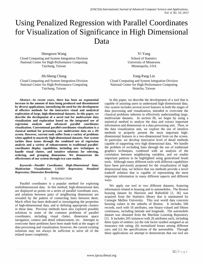
(IJACSA) International Journal of Advanced Computer Science and Applications,
Vol. 4, No. 10, 2013
32 | P a g e
www.ijacsa.thesai.org
Using Penalized Regression with Parallel Coordinates
for Visualization of Significance in High Dimensional
Data
Shengwen Wang
Cloud Computing and System Integration Division
National Center for High-Performance Computing
Taichung, Taiwan
Yi Yang
School of Statistics
University of Minnesota
Minneapolis, USA
Jih-Sheng Chang
Cloud Computing and System Integration Division
National Center for High-Performance Computing
Taichung, Taiwan
Fang-Pang Lin
Cloud Computing and System Integration Division
National Center for High-Performance Computing
Hsinchu, Taiwan
Abstract—In recent years, there has been an exponential
increase in the amount of data being produced and disseminated
by diverse applications, intensifying the need for the development
of effective methods for the interactive visual and analytical
exploration of large, high-dimensional datasets. In this paper, we
describe the development of a novel tool for multivariate data
visualization and exploration based on the integrated use of
regression analysis and advanced parallel coordinates
visualization. Conventional parallel-coordinates visualization is a
classical method for presenting raw multivariate data on a 2D
screen. However, current tools suffer from a variety of problems
when applied to massively high-dimensional datasets. Our system
tackles these issues through the combined use of regression
analysis and a variety of enhancements to traditional parallel-
coordinates display capabilities, including new techniques to
handle visual clutter, and intuitive solutions for selecting,
ordering, and grouping dimensions. We demonstrate the
effectiveness of our system through two case-studies.
Keywords—Parallel Coordinates; High-Dimensional Data;
Multivariate Visualization; LASSO Regression; Penalized
Regression; Dimension Reordering
I. INTRODUCTION
Parallel coordinates is a popular method for exploring multidimensional data. In this method, high-dimensional data are displayed as points on a series of parallel coordinate axes, and relations between pairs of neighboring dimensions are revealed by the pattern of connecting lines between them. Much effort has been dedicated to investigating the properties of high-dimensional data, and to defining appropriate clusters in these data. Previous methods have also explored possible solutions to some of the common problems of parallel coordinates, including visual clutter, dimension space navigation, context and detail enhancement, etc. Attempts to overcome these problems have been made both at the stages of data processing and visualization; however, the current existing solutions may not always be sufficient to solve all of the related issues completely.
In this paper, we describe the development of a tool that is capable of assisting users to understand high dimensional data. Our system includes several novel features in both the stages of data processing and visualization, intended to overcome the classical problems inherent in effectively understanding large, multivariate datasets. In section III, we begin by using a statistical method to analyze the data and extract important information and dimensions in a data processing unit. Then, in the data visualization unit, we explore the use of intuitive methods to properly present the most important high-dimensional features in a two-dimensional form on the screen. In particular, we develop innovative level of detail methods capable of supporting very high dimensional data. We handle the problem of occluding lines through the use of traditional graphics techniques, combined with an analysis of the correlation between neighboring variables, and we enable important patterns to be highlighted using generalized brush tools. Although many different tools with different capabilities have been previously proposed for the visualization of high dimensional data, we believe that our methods provide a novel tradeoff solution that is capable of representing the most important information in many different aspects and different ways.
We apply our tool to two different datasets, featuring information related to housing and to automobiles. The Boston housing dataset by Harrison and Rubinfeld [1, 36] was acquired from the Statistics library that is maintained by Carnegie Mellon University. This real world data concerns housing values in the suburbs of Boston. It includes 506 records, each with 16 attributes, one binary-valued and fifteen continuous, including latitude and longitude. The automobile dataset was obtained from the Machine Learning Repository [1]. It includes 205 instances with 26 attributes each, including three types of entities: (a) the risk factor symbol assigned as an insurance risk rating; (b) normalized losses among different cars; and (c) the specifications of the automobile. Through these applications we attempt to demonstrate that our tool are
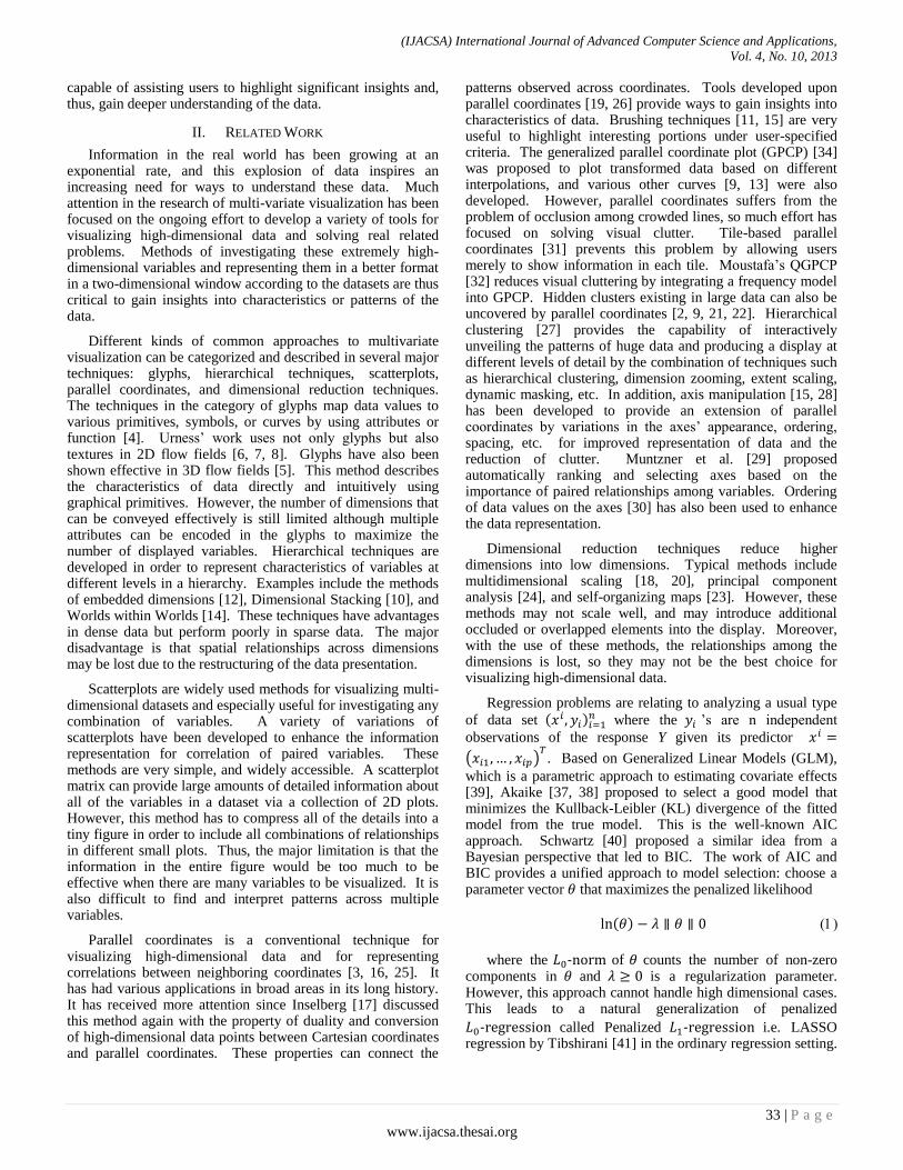
(IJACSA) International Journal of Advanced Computer Science and Applications,
Vol. 4, No. 10, 2013
33 | P a g e
www.ijacsa.thesai.org
capable of assisting users to highlight significant insights and, thus, gain deeper understanding of the data.
II. RELATED WORK
Information in the real world has been growing at an exponential rate, and this explosion of data inspires an increasing need for ways to understand these data. Much attention in the research of multi-variate visualization has been focused on the ongoing effort to develop a variety of tools for visualizing high-dimensional data and solving real related problems. Methods of investigating these extremely high-dimensional variables and representing them in a better format in a two-dimensional window according to the datasets are thus critical to gain insights into characteristics or patterns of the data.
Different kinds of common approaches to multivariate visualization can be categorized and described in several major techniques: glyphs, hierarchical techniques, scatterplots, parallel coordinates, and dimensional reduction techniques. The techniques in the category of glyphs map data values to various primitives, symbols, or curves by using attributes or function [4]. Urness’ work uses not only glyphs but also textures in 2D flow fields [6, 7, 8]. Glyphs have also been shown effective in 3D flow fields [5]. This method describes the characteristics of data directly and intuitively using graphical primitives. However, the number of dimensions that can be conveyed effectively is still limited although multiple attributes can be encoded in the glyphs to maximize the number of displayed variables. Hierarchical techniques are developed in order to represent characteristics of variables at different levels in a hierarchy. Examples include the methods of embedded dimensions [12], Dimensional Stacking [10], and Worlds within Worlds [14]. These techniques have advantages in dense data but perform poorly in sparse data. The major disadvantage is that spatial relationships across dimensions may be lost due to the restructuring of the data presentation.
Scatterplots are widely used methods for visualizing multi-dimensional datasets and especially useful for investigating any combination of variables. A variety of variations of scatterplots have been developed to enhance the information representation for correlation of paired variables. These methods are very simple, and widely accessible. A scatterplot matrix can provide large amounts of detailed information about all of the variables in a dataset via a collection of 2D plots. However, this method has to compress all of the details into a tiny figure in order to include all combinations of relationships in different small plots. Thus, the major limitation is that the information in the entire figure would be too much to be effective when there are many variables to be visualized. It is also difficult to find and interpret patterns across multiple variables.
Parallel coordinates is a conventional technique for visualizing high-dimensional data and for representing correlations between neighboring coordinates [3, 16, 25]. It has had various applications in broad areas in its long history. It has received more attention since Inselberg [17] discussed this method again with the property of duality and conversion of high-dimensional data points between Cartesian coordinates and parallel coordinates. These properties can connect the
patterns observed across coordinates. Tools developed upon parallel coordinates [19, 26] provide ways to gain insights into characteristics of data. Brushing techniques [11, 15] are very useful to highlight interesting portions under user-specified criteria. The generalized parallel coordinate plot (GPCP) [34] was proposed to plot transformed data based on different interpolations, and various other curves [9, 13] were also developed. However, parallel coordinates suffers from the problem of occlusion among crowded lines, so much effort has focused on solving visual clutter. Tile-based parallel coordinates [31] prevents this problem by allowing users merely to show information in each tile. Moustafa’s QGPCP [32] reduces visual cluttering by integrating a frequency model into GPCP. Hidden clusters existing in large data can also be uncovered by parallel coordinates [2, 9, 21, 22]. Hierarchical clustering [27] provides the capability of interactively unveiling the patterns of huge data and producing a display at different levels of detail by the combination of techniques such as hierarchical clustering, dimension zooming, extent scaling, dynamic masking, etc. In addition, axis manipulation [15, 28] has been developed to provide an extension of parallel coordinates by variations in the axes’ appearance, ordering, spacing, etc. for improved representation of data and the reduction of clutter. Muntzner et al. [29] proposed automatically ranking and selecting axes based on the importance of paired relationships among variables. Ordering of data values on the axes [30] has also been used to enhance the data representation.
Dimensional reduction techniques reduce higher dimensions into low dimensions. Typical methods include multidimensional scaling [18, 20], principal component analysis [24], and self-organizing maps [23]. However, these methods may not scale well, and may introduce additional occluded or overlapped elements into the display. Moreover, with the use of these methods, the relationships among the dimensions is lost, so they may not be the best choice for visualizing high-dimensional data.
Regression problems are relating to analyzing a usual type
of data set ( ) where the ’s are n independent
observations of the response Y given its predictor
( )
. Based on Generalized Linear Models (GLM),
which is a parametric approach to estimating covariate effects [39], Akaike [37, 38] proposed to select a good model that minimizes the Kullback-Leibler (KL) divergence of the fitted model from the true model. This is the well-known AIC approach. Schwartz [40] proposed a similar idea from a Bayesian perspective that led to BIC. The work of AIC and BIC provides a unified approach to model selection: choose a parameter vector that maximizes the penalized likelihood
( )
where the - of counts the number of non-zero components in and is a regularization parameter. However, this approach cannot handle high dimensional cases. This leads to a natural generalization of penalized
- called Penalized - i.e. LASSO regression by Tibshirani [41] in the ordinary regression setting.

(IJACSA) International Journal of Advanced Computer Science and Applications,
Vol. 4, No. 10, 2013
34 | P a g e
www.ijacsa.thesai.org
Later a linear combination of and penalties encourages some grouping effects. This is the elastic net proposed by Zou and Hastie [34].
III. OUR APPROACH
Parallel coordinates is widely used for applications of multivariate visualization, and a variety of its variations have been developed. However, little work has been done using regression problems as well to handle and represent high-dimensional data. In this section, we describe our algorithm of visualizing regression data in terms of two components, data processing and data visualization units, based on LASSO and advanced parallel coordinates.
A. Data Processing Unit
In many high dimensional problems we often want to find a smaller subset of input covariates that contribute
most to a specified output Y. Consider the high dimensional regression model
(2)
where is a random noise and ( )
is a p-
dimensional vector. The linear relation between Y and captured in is estimated using n pairs of training
data { } for where . Some traditional
regularization methods such as ridge regression [35, 36] are adopted for solving the problem when the number of explanatory variables is much larger than the number of observations, i.e. . Ridge regression is defined for minimizing the residual sum of squares, subject to a constraint on the -norm of the regression coefficients, ‖ ‖
, which is equivalent to an optimization problem with an penalty on the regression coefficients:
∑ ( )
‖ ‖
Ridge regression can nicely handle correlated predictors. If two predictors are highly correlated, ridge regression will equally scale each predictor. However, ridge regression cannot do variable selection, for it only proportionally shrinks the coefficients, but does not set any to exact zero. LASSO proposed by Tibshirani [41] successfully combines the shrinkage property and subset selection; LASSO is defined for minimizing the residual sum of squares, subject to a constraint on the -norm of the regression coefficients, equivalently:
∑ ( )
‖ ‖
The penalty in LASSO results in a variable selection property due to the singularity of function at zero. LASSO can exclude unimportant variables from the model by shrink their coefficients to be exact zero. However if two predictors are highly correlated, LASSO will select only one and completely dropped the other.
More recently Zou and Hastie [34] proposed the elastic net which combines the strengths of the previous two approaches, it is a mixture of the (lasso) and (ridge regression): to
maximize the likelihood subject to the constraint ( )‖ ‖
‖ ‖ , equivalently,
∑ ( )
( )‖ ‖
‖ ‖
when the problem reduces to the LASSO penalty. The advantages of elastic net are threefold. First of all, by the property of its constraint on parameter , making enough large will set some of the coefficients to be exactly zero, hence left us a smaller subset of input variables with nonzero associated estimates. Secondly, this model selection process is continuous hence very stable: when is sufficiently large all estimate are zero. While gradually decreasing will make variables that minimize the penalized residual sum of squares become nonzero. Thus predictors with strongest effect will enter the model first. Thirdly, the elastic net has a nice grouping effect, it can select groups of correlated variables, i.e. strongly correlated predictors tend to be in or out of the model simultaneously.
B. Data Visualization Unit
Parallel coordinates is the main visualization unit of our tool used for visualizing high dimensional data in this paper. We augment the traditional approach with a combination of techniques including axis manipulation, axis grouping, line and axis coloring, and region highlighting for enhancing multivariate visualization and investigating patterns in the data.
1) Axis Manipulation: Using regression analysis with high
dimensional data for model selection could provide important
information about the significance of variables, and it is very
handy to develop techniques by using axis manipulation to
visualize the information effectively. The techniques we use
include axis reordering, axis navigation, and axis flip. Different methods [15, 28] have been proposed for ordering
axes; however, the order we adopt from the model selection should be the most appropriate for regression problems. We apply elastic net regression to the high dimensional data to obtain a sequence of ordered variables and render the Y variable followed by a subset of subsequent ordered variables on a 2D screen. The number of variables that are displayed in a screen can be dynamically designated by the user according to the screen resolution, the dataset characteristics, and the user’s preference. Since the number of variables that can be displayed at one time in one screen is limited, our tool addresses a way for observing large numbers of different variables through the capability of navigating subsets of variables in distinct screens. These variables still appear in an ordered sequence but on different pages, in which the first coordinate remains the Y axis. We can not only focus on the most important data and their relationships in one screen by automatically ordering significant variables but we can also investigate all other variables by navigating among them. In addition, we enable the feature of axis flip, which provides the assist of better representation of line connection between neighboring coordinates. Parallel coordinates features a strong visualization of adjacent coordinates, whose correlation ranges from negative one to positive one. When the correlation between two variables is near positive one, lines connecting two variables of each record tend to be parallel. Otherwise,
(IJACSA) International Journal of Advanced Computer Science and Applications,
Vol. 4, No. 10, 2013
35 | P a g e
www.ijacsa.thesai.org
complex crossing of lines would appear. Flipping the axes properly according to the correlation of each pair of adjacent coordinates ensures the positive correlation between neighboring coordinates. The ability of switching between flip and non-flip statuses improves the observation of characteristics between two variables since human perception distinguishes the degree of parallel lines well. We design the axes to be of a certain width with a solid green triangle on the bottom edge or a solid red triangle on the top edge. The bottom and top of all of the axes are originally minimum and maximum values of corresponding variables respectively. Theses axes have solid green triangles on the bottom edges, representing their non-flipped state featuring increasing values from the bottom. Once an axis is flipped, its triangle is moved to the top and given the red color. All flipping can be performed automatically, and the icons provide effective hints for the status of the axes. Users can also decide to switch between statuses on their own.
2) Axis Grouping: Our tool not only arranges axes in an
ordered sequence with respect to variables’ significance but
also provides information of significance in different levels.
A series of grouped highly correlated variables are produced
in data processing stages and converted into advanced parallel
coordinates in a two-dimensional figure. Users can view the
figure embedded with an implicit hierarchical structure of
grouped variables and further observe relationships across
multiple variables with strong correlations. We apply techniques of different spacing, curves, and axes
to group of variables. Intuitively, variables in the same group have similar properties so they tend to be placed more closely. Thus, spacing of axes in a same group is given narrower. We further make the group tight in human perception by replacing axes from rectangle boxes to thick lines so that the groups can be perceived directly. An issue is raised while this design is developed. When we compress more information into groups with less spacing, lines between axes tend to become more cluttered and unclear. Flipping axes may alleviate this problem but it is not sufficiently effective in all situations. Therefore, we use curves to reduce the distance of line deviances in the group. Many possible splines could be used; we found that B-spline curves met our needs well. The curves are located within the convex hall of the control points, which are the values of variables in the record, and they show the trend of the lines. Degrading dramatically crossing lines into smooth curves alleviates unwanted crowding effects in narrower regions.
3) Line and Axis Color: Colors can be very effective for
conveying information. We can encode a variety of
information in the appearance of lines or axes by using
different coloring schemes. Originally, we had only mono-
colored lines in between coordinates; however, various
saturated colors can encode the degree of correlation of two
neighboring variables. We use the most saturated blue and red
colors to represent correlations of positive and negative one
respectively. The saturation of the color decreases as the
absolute correlation decreases. Dark or black colors imply
that the two adjacent variables are not correlated. When we
apply the axis flip, all correlations of two adjacent variables
will be positive and only blue and black colors of lines will be
seen. We can further encode values of Y into the colors of the
lines by using a rainbow color scale. The rainbow color scale
includes multiple hues, and we map these colors (excluding
the white portion in the scale) to the Y axis bar, which is the
first axis in each page. Each record is given the color
according to the color of the Y axis where it starts. The color
for each record is the same throughout all line segments
connecting variables’ values. In this way, we can easily
observe the corresponding Y value based on the line color of
each record. Our thick axis bars are capable of encoding line frequency,
deviances, or other values in patterns and colors on the bars. There are many records connecting two neighboring coordinates, many of which may coincide, leading to the loss of information about some records in the display. To avoid this, we develop frequency indicators by dividing our bar into twenty segments and filling in a color for each segment based on the line frequency ending at that segment. The more lines a segment ends with, the darker the color of that segment will be. If the color of a segment is white, then there are no lines connected to that segment. Our axis coloration scheme can also encode values like deviances by drawing a red color in a portion of a bar. If we consider a full red axis bar to be 100 percent and an empty bar to be 0 percent, all other deviances can be represented with a red partial axis bar according to its values. This bar can certainly encode different values, depending on which values users want to visualize.
Visual clutter is an intrinsic problem in parallel coordinates visualization when the number of records is high. By using the transparency capabilities of OpenGL on top of our line coloring methods, we can provide an adequate solution and appealing results. Where multiple lines occlude or coincide, the colors of the lines will tend to appear more saturated. Otherwise, they are less salient. Thus this method emphasizes the lines that appear with higher frequency, and those saturated lines tend to receive more attention automatically.
4) Region Highlight: Highlighting regions containing
groups of lines focuses attention on those lines and allows the
unveiling of insights into data in those regions. Showing the
relationships of variables among groups is important. We
paint the background with a light blue color within each
region of grouped coordinates. Coloring the regions of each
group brings users’ attention to these areas and emphasizes the
relations of the line connections. Highlighting lines or curves within some specified regions
enhances the capability of our tool for visualizing interesting data. Suppose that S is a set of n-dimensional data defined as
{ - } . is
an n-dimensional record defined as ( ).
We can define an interval [ ] of the axis i and an
axis restriction { } based on this interval .
A highlighted region between coordinates i and i+1 is thus defined as ( ) . Similarly, we have brush
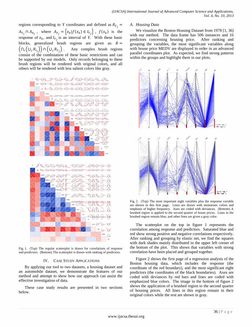
(IJACSA) International Journal of Advanced Computer Science and Applications,
Vol. 4, No. 10, 2013
36 | P a g e
www.ijacsa.thesai.org
regions corresponding to Y coordinates and defined as
, where { ( ) } , ( ) is the
response of , and is an interval of Y. With these basic
blocks, generalized brush regions are given as:
(⋂ (⋃ ) ) (⋃ ) . Any complex brush regions
consist of the combination of these basic restrictions and can be supported by our models. Only records belonging to these brush regions will be rendered with original colors, and all others will be rendered with less salient colors like gray.
Fig. 1. (Top) The regular scatterplot is drawn for correlations of response
and predictors. (Bottom) The scatterplot is drawn with ranking of predictors.
IV. CASE STUDY APPLICATIONS
By applying our tool to two datasets, a housing dataset and an automobile dataset, we demonstrate the features of our method and attempt to show how our approach can assist the effective investigation of data.
These case study results are presented in two sections below.
A. Housing Data
We visualize the Boston Housing Dataset from 1978 [1, 36] with our method. The data frame has 506 instances and 16 predictors concerning housing price. After ranking and grouping the variables, the most significant variables along with house price MEDV are displayed in order in an advanced parallel coordinates plot. As expected, we find strong patterns within the groups and highlight them in our plots.
Fig. 2. (Top) The most important eight variables plus the response variable
are shown in this first page. Lines are drawn with monotonic colors and emphasis of higher frequency. Axes are coded with deviances. (Bottom) A
brushed region is applied to the second quarter of house prices. Lines in the
brushed region remain blue, and other lines are given a gray color.
The scatterplot on the top in figure 1 represents the correlation among response and predictors. Saturated blue and red show strong positive and negative correlations respectively. After ranking and grouping by elastic net, we find the squares with dark shades mainly distributed in the upper left corner of the bottom of the plot. This shows that variables with strong correlation have been placed and grouped together.
Figure 2 shows the first page of a regression analysis of the Boston housing data, which includes the response (the coordinate of the red boundary), and the most significant eight predictors (the coordinates of the black boundaries). Axes are coded with deviances by red bars and lines are coded with emphasized blue colors. The image in the bottom of figure 2 shows the application of a brushed region to the second quarter of housing prices. All lines in this region remain in their original colors while the rest are shown in gray.
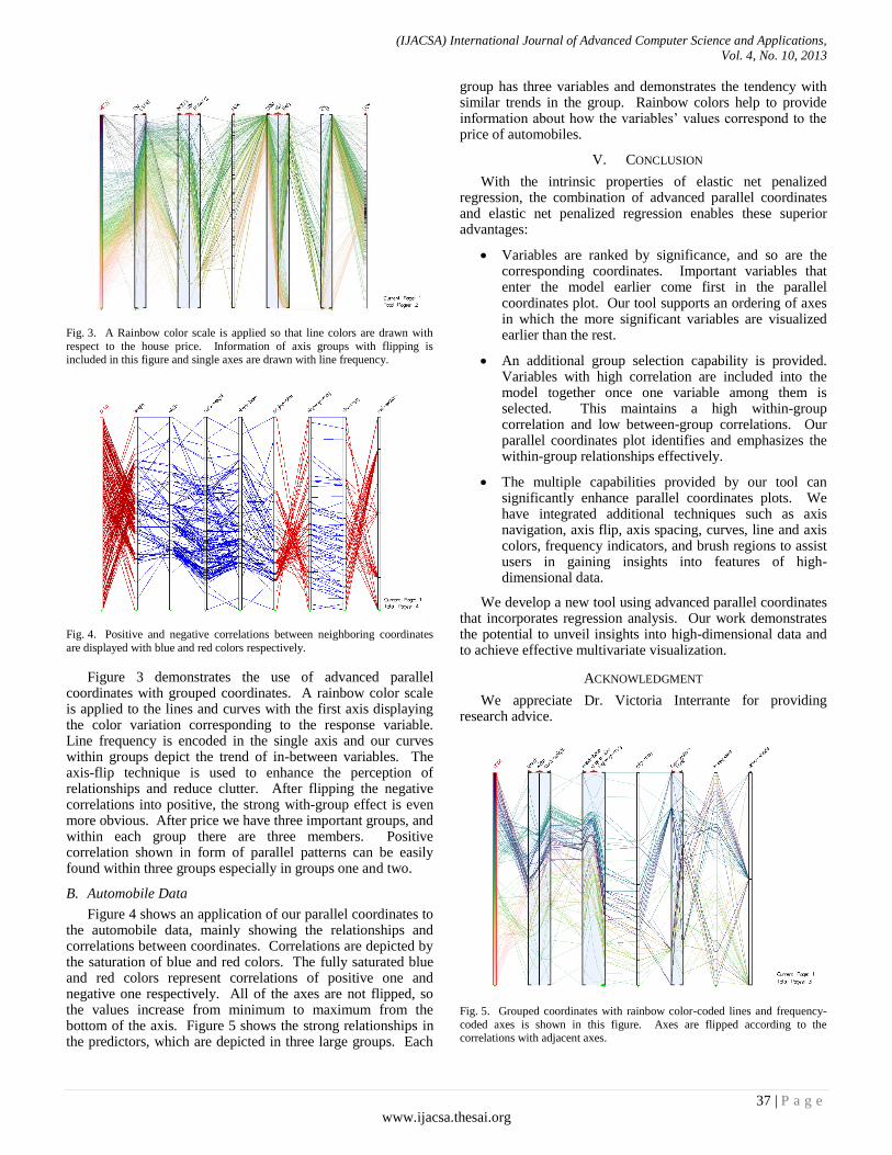
(IJACSA) International Journal of Advanced Computer Science and Applications,
Vol. 4, No. 10, 2013
37 | P a g e
www.ijacsa.thesai.org
Fig. 3. A Rainbow color scale is applied so that line colors are drawn with
respect to the house price. Information of axis groups with flipping is
included in this figure and single axes are drawn with line frequency.
Fig. 4. Positive and negative correlations between neighboring coordinates
are displayed with blue and red colors respectively.
Figure 3 demonstrates the use of advanced parallel coordinates with grouped coordinates. A rainbow color scale is applied to the lines and curves with the first axis displaying the color variation corresponding to the response variable. Line frequency is encoded in the single axis and our curves within groups depict the trend of in-between variables. The axis-flip technique is used to enhance the perception of relationships and reduce clutter. After flipping the negative correlations into positive, the strong with-group effect is even more obvious. After price we have three important groups, and within each group there are three members. Positive correlation shown in form of parallel patterns can be easily found within three groups especially in groups one and two.
B. Automobile Data
Figure 4 shows an application of our parallel coordinates to the automobile data, mainly showing the relationships and correlations between coordinates. Correlations are depicted by the saturation of blue and red colors. The fully saturated blue and red colors represent correlations of positive one and negative one respectively. All of the axes are not flipped, so the values increase from minimum to maximum from the bottom of the axis. Figure 5 shows the strong relationships in the predictors, which are depicted in three large groups. Each
group has three variables and demonstrates the tendency with similar trends in the group. Rainbow colors help to provide information about how the variables’ values correspond to the price of automobiles.
V. CONCLUSION
With the intrinsic properties of elastic net penalized regression, the combination of advanced parallel coordinates and elastic net penalized regression enables these superior advantages:
Variables are ranked by significance, and so are the corresponding coordinates. Important variables that enter the model earlier come first in the parallel coordinates plot. Our tool supports an ordering of axes in which the more significant variables are visualized earlier than the rest.
An additional group selection capability is provided. Variables with high correlation are included into the model together once one variable among them is selected. This maintains a high within-group correlation and low between-group correlations. Our parallel coordinates plot identifies and emphasizes the within-group relationships effectively.
The multiple capabilities provided by our tool can significantly enhance parallel coordinates plots. We have integrated additional techniques such as axis navigation, axis flip, axis spacing, curves, line and axis colors, frequency indicators, and brush regions to assist users in gaining insights into features of high-dimensional data.
We develop a new tool using advanced parallel coordinates that incorporates regression analysis. Our work demonstrates the potential to unveil insights into high-dimensional data and to achieve effective multivariate visualization.
ACKNOWLEDGMENT
We appreciate Dr. Victoria Interrante for providing research advice.
Fig. 5. Grouped coordinates with rainbow color-coded lines and frequency-
coded axes is shown in this figure. Axes are flipped according to the correlations with adjacent axes.
(IJACSA) International Journal of Advanced Computer Science and Applications,
Vol. 4, No. 10, 2013
38 | P a g e
www.ijacsa.thesai.org
REFERENCES
[1] C. L. Blake and C. J. Merz, UCI Repository of Machine Learning Databases, Department of Information and Computer Science, University of California, Irvine, 1998.
[2] J. Zhou, S. Konecni, K. Marx, and G. Grinstein, “A Visual Approach to Improve Clustering Based on Cluster Ensembles,” Proceedings of SPIE 7530, 2010.
[3] R. E. Moustafa and E. J. Wegman, “On Some Generalization to Parallel Coordinate Plots,” Seeing a Million, A Data Visualization Workshop, 2002.
[4] R. J. Littlefield, “Using the GLYPH concept to Create User-Definable Display Formats,” Proceedings NCGA ’83., pp. 697-706, June 1983.
[5] S. Wang, V. Interrante, and E. Longmire, “Multi-Variate Visualization of 3D Turbulent Flow Data,” Proceedings of SPIE The International Society for Optical Engineering, 7530, Jan. 2010.
[6] T. Urness and V. Interrante, “Streamline Visualization of Multiple 2D Vector Fields,” Proceedings of SPIE The International Society for Optical Engineering, 6809, Jan. 2008.
[7] T. Urness, V. Interrante, I. Marusic, E. Longmire, and B. Ganapathisubramani, “Effectively Visualizing Multi-Valued Flow Data Using Color and Texture,” Proceedings of IEEE Visualization 2003, pp. 16, 2003.
[8] T. Urness, V. Interrante, E. Longmire, I. Marusic, S. O’Neill, and T. W. Jones, “Strategies for the Visualization of Multiple 2D Vector Fields,” IEEE Computer Graphics and Applications, vol. 26, no. 4, pp. 74-82, 2006.
[9] K. T. McDonnell and K. Mueller, “Illustrative Parallel Coordinates,” Computer Graphics Forum, vol. 27, no. 3, pp. 1031-1038, 2008.
[10] J. LeBlanc, M. O. Ward, and N. Wittels, “Exploring N-dimensional Databases,” Proceedings of Visualization ’90, pp. 230-237, 1990.
[11] A. R. Martin and M. O. Ward, “High Dimensional Brushing for Interactive Exploration of Multivariate Data,” Proceedings of IEEE Visualization ’95, pp. 126, 1995.
[12] T. Mihalisin, E. Gawlinski, J. Timlin, and J. Schwegler, “Visualizing Multivariate Functions, Data, and Distributions,” IEEE Computer Graphics and Applications, vol. 11, pp. 28-37, 1991.
[13] M. Graham and J. Kennedy, “Using Curves to Enhance Parallel Coordinate Visualizations,” Proceedings Of Intl. Conf. on Information Visualization, pp. 10-16, 2006.
[14] C. Beshers and S. Feiner, “AutoVisual: Rule-Based Design of Interactive Multivariate Visualizations,” IEEE Computer Graphics and Applications, vol. 13, no. 4, pp. 41-49, 1993.
[15] H. Hauser, F. Ledermann, and H. Doleisch, “Angular Brushing of Extended Parallel Coordinates,” Proceedings of the IEEE Symposium on Information Visualization (InfoViz’02), pp. 127, 2002.
[16] E. J. Wegman, “Hyperdimensional Data Analysis Using Parallel Coordinates,” J. Am. Stat. Assn., vol. 85, no. 411, pp. 664-675, 1990.
[17] A. Inselberg, “The Plane with Parallel Coordinates,” Special Issue on Computational Geometry of the Visual Computer, vol. 1, no. 2, pp. 69-91, 1985.
[18] A. Mead, “Review of the Development of Multidimensional Scaling Methods,” The Statistician, vol. 33, pp. 27-35, 1992.
[19] D. Yang, E. A. Rundensteiner, and M. O. Ward, “Analysis Guided Visual Exploration of Multivariate Data” Proceedings of the 2007 IEEE Symposium on Visual Analytics Science and Technology, pp. 38-90, 2007.
[20] S. Weinberg, “An Introduction to Multidimensional Scaling,” Measurement and Evaluation in Counseling and Development, vol. 24 pp. 12-36, 1991.
[21] A. O. Artero, M. C. F. de Oliveira, and H. Levkowitz, “Uncovering Clusters in Crowded Parallel Coordinates Visualizations,” Proceedings of the IEEE Symposium on Information Visualization (InfoVis’04), pp. 81-88, 2004.
[22] H. Zhou, X. Yuan, H. Qu, W. Cui, and B. Chen, “Visual Clustering in Parallel Coordinates,” Computer Graphics Forum, vol. 27, no. 3, pp. 1047-1054, 2008.
[23] T. Kohonen, “The Self-Organizing Map,” Proceedings of IEEE, pp. 1464-80, 1978.
[24] J. Jolliffe, “Principal of Component Analysis,” Springer Verlag, 1986.
[25] A. Inselberg and B. Dimsdale, “Parallel Coordinates: A Tool for Visualizing Multidimensional Geometry,” Proceedings of IEEE Visualization ’90, pp. 361-378, 1990.
[26] M. O. Ward, “XmdvTool: Integrating Multiple Methods for Visualizing Multivariate Data,” Proceedings of IEEE Visualizatin ’94, pp. 326-333, 1994.
[27] Y.-H. Fua, M. O. Ward, and A. E. Rundensteiner, “Hierarchical Parallel Coordinates for Exploration of Large Datasets,” Proceedings of IEEE Visualizatin ’99, pp. 43-50, 1999.
[28] J. Yang, W. Peng, M. O. Ward, and E. A. Rundensteiner, “Interactive Hierarchical Dimension Ordering, Spacing and Filtering for Exploration of High Dimensional Datasets,” Proceedings of the IEEE Symposium on Information Visualization, pp. 105-112, 2003.
[29] H.-C. Hege, I. Hotz, and T. Muntzner, “Pairwise Axis Ranking for Parallel Coordinates of Large Multivariate Data,” Eurographics-IEEE TCVG Symposium on Visualization, vol. 28, no. 3, 2009.
[30] G. E. Rosario, E. A. Rundensteiner, D. C. Brown, M. O. Ward, and S. Huang, “Mapping Nominal Values to Numbers for Effective Visualization,” Proceedings of the IEEE Symposium on Information Visualization (InfoVis’04), vol. 3, no. 2, pp. 80-95, 2004.
[31] J. Alsakran, Y. Zhao, and X. Zhao, “Tile-Based Parallel Coordinates and its Application in Financial Visualization,” Proceedings of SPIE 7530, 2010.
[32] R. E. Moustafa, “QGPCP: Quantized Generalized Parallel Coordinate Plots for Large Multivariate Data Visualization,” J. Comput. Graph. Stat., vol. 18, no. 1, pp. 32-51, 2009.
[33] D. Harrison and D. L. Rubinfeld, “Hedonic Prices and the Demand for Clean Air,” Journal of Environmental Economics and Management, vol. 5, pp. 81-102, 1978.
[34] H. Zou and T. Hastie, “Regularization and Variable Selection via the Elastic Net,” J. Roy. Statist. Soc. Ser. B, vol. 67, pp. 301-320, 2005.
[35] N. R. Draper and H. Smith, Applied Regression Analysis. Wiley Series in Probability and Statistics, 3rd ed., John Wiley & Sons, New York, 1998.
[36] R. R. Hocking, Methods and Applications of Linear Models: Regression and the Analysis of Variance. Wiley Series in Probability and Statistics, John Wiley & Sons, New York, 1996.
[37] H. Akaike, “Information Theory and an Extension of the Maximum likelihood Principle,” Second International Symposium on Information Theory (Edited by B.N. Petrov and F. Csaki), Akademiai Kiado, Budapest, pp. 267-281, 1973.
[38] H. Akaike, “A New Look at the Statistical Model Identification,” IEEE Trans. Auto. Control, vol. 19, pp. 716-723, 1974.
[39] P. McCullagh and J. A. Nelder, “Generalized Linear Models,” Chapman and Hall, London, 1989.
[40] G. Schwartz, “Estimating the Dimension of a Model,” Ann. Statist., vol. 6, pp. 461-464, 1978.
[41] R. Tibshirani, “Regression Shrinkage and Selection via the LASSO,” J. Roy. Statist. Soc. Ser. B, vol. 58, pp. 267-288, 1996.

(IJACSA) International Journal of Advanced Computer Science and Applications, Vol. 4, No. 10, 2013
39 | P a g e www.ijacsa.thesai.org
Maturity Model for IT Service Outsourcing in Higher
Education Institutions
Victoriano Valencia García Computer Management Technician
and Researcher at Alcalá University
Madrid, Spain
Dr. Eugenio J. Fernández Vicente
Professor at Computer Science Dept.
Alcalá University
Madrid, Spain
Dr. Luis Usero Aragonés
Professor at Computer Science Dept. Alcalá University
Madrid, Spain
Abstract—The current success of organizations depends on
the successful implementation of Information and Comunication
Technologies (ICTs). Good governance and ICT management are
essential for delivering value, managing technological risks,
managing resources and performance measurement. In addition,
outsourcing is a strategic option which complements IT services provided internally in organizations.
This paper proposes the design of a new holistic maturity
model based on standards ISO/IEC 20000 and ISO/IEC 38500,
the frameworks and best practices of ITIL and COBIT, with a specific focus on IT outsourcing.
This model is validated by practices in the field of higher
education, using a questionnaire and a metrics table among other
measurement tools. Models, standards and guidelines are
proposed in the model for facilitating adaptation to universities
and achieving excellence in the outsourcing of IT services. The
applicability of the model allows an effective transition to a model
of good governance and management of outsourced IT services
which, aligned with the core business of universities (teaching,
research and innovation), affect the effectiveness and efficiency of its management, optimizes its value and minimizes risks.
Keywords— IT Governance; IT Management; Outsourcing; IT
Services; Maturity Models
I. INTRODUCTION
One thing to change about ICT at university level is the deeply rooted approach which exists, or which used to exist, called infrastructure management. This kind of management has evolved into a governance and management model more in line with the times, which is a professional management of services offered to the university community [6]. It is for this reason that in recent years a set of methodologies, best practices and standards, such as ITIL, ISO 20000, ISO 38500 and COBIT, have been developed to facilitate ICT governance and management in a more effective and efficient way.
These methodologies, which are appropriate and necessary to move from infrastructure management to service management, see a lack of academic research. For that reason it is inadvisable to use these frameworks on their own, and it is advisable to consider other existing frameworks in order to extract the best from each for university level [6].
ICT or IT services have implications for business and innovation processes and may be a determinant in their evolution. The organization of these services, their status
within the organization of the university, and their relationships with other management departments and new technologies is therefore vital. At present, the degree of involvement, the volume of services offered, and the participation or external alliances with partner companies through outsourcing are of special interest.
Currently, and in the years to come, organizations that achieve success are and will be those who recognize the benefits of information technology and make use of it to boost their core businesses in an effective strategic alignment, where delivery of value, technology, risk management, resource management, and performance measurement of resources are the pillars of success.
It is necessary to apply the above-mentioned practices through a framework and process to present the activities in a manageable and logical structure. Good practice should be more strongly focused on control and less on execution. They should help optimize IT investments and ensure optimal service delivery. IT best practices have become significant due to a number of factors, according to COBIT (www.itgi.org)[9]:
Business managers and boards demanding a better return from IT investments, i.e., the demand that IT delivers what the business needs to enhance stakeholder value;
Concern over the generally increasing level of IT expenditure;
The need to meet regulatory requirements for IT controls in areas such as privacy and financial reporting, and in specific sectors such as finance, pharmaceutical and healthcare;
The selection of service providers and the management of service outsourcing and acquisition;
Increasingly complex IT-related risks, such as network security;
IT governance initiatives that include the adoption of control frameworks and good practices to help monitor and improve critical IT activities to increase business value and reduce business risk;
The need to optimise costs by following, where possible, standardised, rather than specially developed, approaches;

(IJACSA) International Journal of Advanced Computer Science and Applications, Vol. 4, No. 10, 2013
40 | P a g e www.ijacsa.thesai.org
The growing maturity and consequent acceptance of well-regarded frameworks, such as COBIT, IT Infrastructure Library (ITIL), ISO 27000 series on information security-related standards, ISO 9001:2000 Quality Management Systems—Requirements Capability Maturity Model ® Integration (CMMI), Projects in Controlled Environments 2 (PRINCE2) and A Guide to the Project Management Body of Knowledge (PMBOK); and
The need for organizations to assess how they are performing against generally accepted standards and their peers (benchmarking)
It is clear that ICTs have become ubiquitous in almost all organizations, institutions and companies, regardless of the sector to which they belong. Hence, effective and efficient ICT management to facilitate optimal results is necessary essential.
Furthermore, in this environment of total ICT dependency in organizations using ICTs for the management, development and communication of intangible assets, such as information and knowledge [14], organizations become successful if these assets are reliable, accurate, safe and delivered to the right person at the right time and place [9].
In short, we propose that the proper administration of ICT will add value to the organization, regardless of its sector (whether social, economic or academic) and will assist it in achieving its objectives and minimizing risk [6].
Given the importance of proper management of ICT, the search for solutions to the alignment of ICT with the core business of organizations has accelerated in recent years. The use of suitable metrics or indicators for measurement and valuation, generate confidence in the management teams. This will ensure that investment in ICTs generates the corresponding business value with minimal risk [6].
The above solutions are models of good practice, metrics, standards and methodologies that enable organizations to properly manage ICTs. And public universities are not outside these organizations, though they are not ahead. In addition, interest in adopting models of governance and management of appropriate ICTs is not as high as it should be.
Two of the factors through which IT best practices have become important is, the selection of appropriate service providers and the management of outsourcing and procurement of IT services.
In addition, a maturity model is a method for judging whether the processes used, and the way they are used, are characteristic of a mature organization [4].
Models by phases or levels allow us to understand how IT management strategies based on computing evolve over time [10]. According to these models, organizations progress through a number of identifiable stages. Each stage or phase reflects a particular level of maturity in terms of IT use and management in the organization.
There are many maturity models in the literature, and they are applied to various fields, such as project management, data management, help desk, systems safety engineering. Most of
them refer to either Nolan’s original model [13] or the Capability Maturity Model of Software Engineering Institute (Carnegie Mellon Software Engineering Institute). The latter model describes the principles and practices underlying software processes and is intended to help software organizations evolve from ad-hoc, chaotic processes to mature, disciplined software processes.
Nolan was the first to design a descriptive stage theory for planning, organizing and controlling activities associated with managing the computational resources of organizations. His research was motivated by the theoretical need for the management and use of computers in organizations. From 1973 until today, technology and the way it is used has changed a lot, but Nolan’s original idea is still valid, and it will remain so as long as the quality of services provided internally in organizations, or by external suppliers, are essential.
II. LITERATURE REVIEW ON MATURITY MODELS FOR IT
OUTSOURCING AND COMPARISON CHART
Very few models or frameworks of IT outsourcing can be found in the literature, either from the point of view of the client or outsourcer. The few models or frameworks that exist are varied. After a thorough literature review, and taking into account the point of view of the customer, the following models have been found to be relevant:
[M1] Managing Complex IT Outsourcing – Partnerships (2002) [2] focuses on managing complex relationships with IT vendors taking into account the following aspects: IT strategy; information management; flexible contracts; contract management and accounts; and human resource availability.
[M2] Information Technology Outsourcing (ITO) Governance: An Examination of the Outsourcing Management Maturity Model (2004) [4] is an evolutionary model similar to CMM but it lacks metrics to measure the maturity level properly. The maturity model for IT outsourcing consists of 5 levels: level 1 (vendor management fundamentals); level 2 (defined service outcome); level 3 (measures); level 4 (trust); and level 5 (business value recognized).
[M3] A Unified Framework for Outsourcing Governance (2007) [5]: a unified framework on the governance of outsourcing from the combined perspectives of the customer and the provider. The framework focuses on three areas: governance processes; organizational structure of governance; and performance measurement.
[M4] IT Outsourcing Maturity Model (2004) [1]: this model identifies five maturity levels based on a literature review and interviews with the participants of outsourcing. It is a generalist, stage-maturity model where organizations rise gradually. The five stages or phases of the model are: insourcing; forming; storming; norming; and performing.
[M5] Outsourcing Management Framework Based on ITIL v3 Framework (2011) [11]: a framework based on ITIL v3 that it is composed of four phases to

(IJACSA) International Journal of Advanced Computer Science and Applications, Vol. 4, No. 10, 2013
41 | P a g e www.ijacsa.thesai.org
be met consecutively. The four phases are: phase 1 (incident and problem management); phase 2 (financial management, risk management and service level management); phase 3 (supplier management; change management; and security management); and phase 4 (service evaluation).
[M6] Multisourcing Maturity Model (2011) [8]: a multisourcing maturity model for large companies with federal IT organization. For that reason it is considered to be a very specific model. Model based on CMMI-ACQ, eSCM-CL and Gartner IT procurement, consisting of six levels: level 0 (multisourcing incomplete); level 1 (multisourcing prepared); level 2 (multisourcing engaged); level 3 (multisourcing established); level 4 (multisourcing managed); and level 5 (multisourcing optimized).
[M7] Maturity model for IT outsourcing relationships (2006) [7]: a maturity model based on organizational theories and practices in the relationships established in IT outsourcing. The model consists of three phases: cost; resources; and alliances.
[M8] IT Governance Maturity and IT Outsourcing Degree: An Exploratory Study (2007) [3]: the aim of this study is to shed light on whether the evaluation of IT governance maturity differs depending on whether clients outsource selectively or completely.
[M9] Global Multisourcing Strategy: Integrating Learning From Manufacturing Into IT Service Outsourcing (2011) [12]: a theoretical framework with a specific focus on economic and operational outsourcing, it omits many other determinants. It proposes two dimensions –width and depth– which analyze the compensation of a multisourcing strategy in detail from the perspective of the customer.
The following table shows the maturity models and frameworks above, along with the key areas or determinants that they are based on. All key areas shown in the Table I are the bases of the maturity model designed for IT service outsourcing.
Taking into account all key areas shown in Table I, a holistic maturity model (henceforth MM) has been designed with a specific focus on IT outsourcing governance and IT service management.
The model establishes where organizations involved in the study are in relation to the following control criteria and information requirements according to Cobit: effectiveness; efficiency; confidentiality; integrity; availability; compliance; and reliability. Other criteria, from the perspective of managing critical IT resources; included: applications; information; infrastructure; and people.
TABLE I. EXISTING MATURITY MODELS AND FRAMEWORKS ON IT
OUTSOURCING
Key areas or
determinants
Maturity models and frameworks about IT
outsourcing
M1 M2 M3 M4 M5 M6 M7 M8 M9
Formal
Agreement X
X
X X
X
Service
Measurement X X
X X
X
Quality
Management
X
X
Monitoring
and
Adjustments
X X X X
X
Alignment IT-
Business X X X
X
IT Governance
Structure X
X
X
Service Level
Agreement
(SLA)
X X
X X
X
IT Service
Registration
Incident and
Problem
Management
X X
Changes
X
Testing and
Deployment
Control of
External
Providers
X X
X X X X X
Business Risk
X X X
X
Financial
Management
X X X X X
Legislation X X
Demand and
Capacity
Management
Formal
Agreement
Management
X
X
Knowledge
Management X
X
X
Guidelines on
outsourcing an
IT service (life
cicle)
With regard to IT governance, standard ISO/IEC 38500:2008, published in 2008, aims to provide a framework of principles for directors of different organizations in order to manage, evaluate, and monitor the efficient, effective and acceptable use of information and communication technologies.

(IJACSA) International Journal of Advanced Computer Science and Applications, Vol. 4, No. 10, 2013
42 | P a g e www.ijacsa.thesai.org
The direction, according to ISO / IEC 38500, must govern IT in three main areas:
Management. Direct the preparation and implementation of strategic plans and policies, assigning responsibilities. Ensure smooth transition of projects to production, considering the impacts on the operation, the business and infrastructure. Foster a culture of good governance of IT in the organization.
Evaluation. Examine and judge the current and future use of IT, including strategies, proposals and supply agreements (both internal and external).
Monitoring. Monitor IT performance measuring systems in order to ensure that they fit as planned.
According to the results of the "IT Governance Study 2007" [15] [16], reasons compelling governments to create an IT structure in the university include: aligning IT objectives with strategic objectives; promoting institutional vision of IT; ensuring transparency in decision-making; cost reduction; increased efficiency; and regulation and compliance audits.
On service management, MM takes into account ISO/IEC 20000 and ITIL v3, but it is customized to integrate governance and management into a single model. The model moves towards an integration that facilitates the joint use of frameworks efficiently. Thus, the MM designed consists of five levels, with each level having a number of general and specific characteristics that define it. These are determined by the selection of general concepts that underpin the MM (see first column in Table I). The selection is always justified and countersigned by ISO 20000 and ISO 38500 standards and ITIL and COBIT best practice methodologies.
III. MATURITY MODEL PROPOSED
In order to design the proposed maturity model, we studied in detail every reference on the provision of IT services that there is in the ISO 20000 and ISO 38500 standards and ITIL v3 and COBIT methodologies. In addition, we investigated the relevant literature and failed to find any maturity model that brings together the previous methodologies with a specific focus on IT outsourcing. As a result, a number of concepts and subconcepts were categorized to form the basis of the maturity model.
The MM follows a stage structure and has two major components: maturity level and concept. Each maturity level is determined by a number of concepts common to all levels.
Each concept is defined by a number of features that specify the key practices which, when performed, can help organizations meet the objectives of a particular maturity level. These characteristics become indicators, which, when measured, determine the maturity level.
The MM defines five maturity levels: initial or improvised; repeatable or intuitive; defined; managed and measurable; and optimized.
The model proposes that organizations under study should ascend from one level of maturity to the next without skipping any intermediate level. In practice, organizations can
accomplish specific practices in upper levels. However, this does not mean they can skip levels, since optimum results are unlikely if practices in lower levels go unfulfilled.
The complete maturity model, with five levels and characteristics in each, is the subject of a paper selected to be published1.
IV. METRICS FOR MATURITY ASSESSMENT
We have designed an assessment tool along with the maturity model that allows independent validation and practical application of the model. Therefore, the maturity of an organization indicates how successfully all practices that characterize a certain maturity level have gone fulfilled. The questions used in the questionnaire consider the basis of the assessment instrument. They were extracted from each of the indicators defining each of the general concepts and key areas of the maturity model. These general concepts and defining characteristics have been extracted from the following standards and methodologies:
Standard ISO/IEC 20000 and methodology of good practices ITIL v3. Both provide a systematic approach to the provision and management of quality IT services.
Standard ISO/IEC 38500:2008 provides guiding principles for directors of different organizations to manage, evaluate, and monitor the use of information and communication technologies effectively and efficiently.
Cobit business-oriented methodology provides good practice through a series of domains and processes, as well as metrics and maturity models in order to measure the achievement of the objectives pursued.
In addition, new indicators have been developed based on the proposed model in order to assess appropriate aspects not reflected either in previous methodologies and standards or in the existing literature (e.g. the inclusion of service performance in the SLA and the use of user-satisfaction surveys in IT-business alignment).
To evaluate the maturity model of an organization using the model and the measurement instruments proposed, it is necessary to obtain a series of data resulting from the responses to the questionnaire based on the indicators that define the general concepts of our maturity model.
Table II shows one of the nineteen key areas or concepts that are the basis of the MM. The first column of the table shows the level or levels corresponding to the indicator located in the second column.
The second column shows the survey questions and indicators for each of the questions or part of the questions. Finally, the third column shows the source where the indicator or item has been extracted as a feature of the general concept or key area of the model.
1 Cf. Valencia, V., López, J., Holgado, J.C., & Usero, L., “Modelo de Madurez
para la Externalización de Servicios de TI”, Proceedings of the 8th
International Academic Conference on Government and Management of IT Service, King Juan Carlos University, Madrid, [forthcoming]

(IJACSA) International Journal of Advanced Computer Science and Applications, Vol. 4, No. 10, 2013
43 | P a g e www.ijacsa.thesai.org
TABLE II. METRICS TABLE AND QUESTIONNAIRE
Level Code – Indicator – Question of
Questionnaire
Source
Concept: Formal Agreement: contract, agreement or
similar (FA) ISO 20000,
Cobit, ITIL
v3
3 FA1 - Procedures and processes – Are there
clear documented procedures to facilitate the
control of outsourced IT services with clear
processes for negotiating with external
providers?
Cobit
FA2 - Elements of FA - Formal agreements
(contracts, agreements or the like) of every
outsourced IT service include:
ISO 20000,
ITIL, Cobit
3 FA2a - Scope of work
2 FA2b - Services / deliverables to be provided
3 FA2c - Timeline
2 FA2d - Service levels
2 FA2e - Costs
3 FA2f - Billing Agreements
2 FA2g - Responsibilities of the Parties
FA3 - Requirements of FAs - Formal
agreements meet the following requirements:
Cobit
3 FA3a - Legal (compliance with current
regulations)
3 FA3b - Operational (proper delivery and
management of services in operation)
3 FA3c - Control (for the measurement and
analysis of the services)
4 FA4 - Revision frequency of FAs - Formal
agreements are reviewed periodically at
predefined intervals
ISO 20000
3 FA5 - Penalties in FAs - There are penalties
for breach of formal agreements, including
termination of agreements
Self
developed
345 FA6 - Enforcement of penalties in FAs -
Degree of enforcement of penalties for breach
of agreements
Self
developed
Therefore, the maturity level of every higher education institution studied is measured by evaluating its development in each key area or concept, which is indicated by responses to items or indicators in Table II. In order to qualify for a specific maturity level, the university surveyed must carry out all key practices of that level successfully.
V. OBJECTIVES OF THE MATURITY MODEL
The main purpose of the model is to fulfill as many requirements of an ideal maturity model for IT outsourcing in the governance and management of outsourced IT services as possible. With the identification and definition of some key concepts and an assessment tool, the model allows a systematic and structured assessment of organizations. Although the assessment instrument has a lot of qualitative responses, it also has quantitative responses, such as the degree of compliance with certain characteristics that define the maturity model (e.g. the degree of influence of the KPIs and KGIs in the penalties for breach of agreements).
The identification of key areas and concepts specifying its characteristics to constitute the underlying structure of the MM, complements the necessity to refer to governance and
management concepts tested and backed by standards and methodologies.
Moreover, the model advocates continuous learning and improvements in governance in IT outsourcing and good management of outsourced IT services, even when organizations have reached the maximum level (5).
VI. CONCLUSIONS AND FUTURE RESEARCH
Both ISO 20000 and ISO 38500 standards, and ITIL v3 and COBIT methodologies of best practice in IT management and governance, are a good basis for the study and analysis of governance and management of the outsourced IT services in organizations. That is why they allow the design of a new maturity model that facilitates the achievement of an effective transition to a model of good governance and management of outsourced IT services that, aligned with the core business in organizations, impacts on the effectiveness and efficiency of its management, optimizes its value and minimizes risks.
A questionnaire (survey form) forms the basis of the quantitative study of the maturity model. The questionnaire is based on the attributes or indicators that define the different levels of the model. It contains standard and suitable questions, according to the nature of the research.
Questionnaire responses allow the obtaining or calculation of the level of maturity by applying the scale defined in the model. In addition, questionnaire responses, after being properly analysed, shed light on the current situation of the different organizations studied in governance and management of outsourced IT services.
This research will also provide specific case studies that will be carried out at some universities and will put the model into practice in order to draw conclusions. The questions used in the questionnaire, currently sent to some universities to be completed, bring the design of a proposed improvement plan (see Table III) to allow a sequential growth by stages. The growth occurs as a hierarchical progression that should not be reversed, for the aforementioned reasons, and involve a broad range of organizational activities in governance and management of IT outsourcing.
Table III shows one of the five levels (there are five tables, one for each level) of the MM with the key areas or concepts to be improved in order to allow a sequential growth by stages. The first column of the table shows the concepts. The second column of the table shows the objectives to achieve corresponding to the concept in the first column. Finally, the third column shows the actions to accomplish in order to achieve the objectives set in the second column.
Therefore, in the case studies, we will apply the established scales, which will rate the university surveyed and the object of study, at a level of maturity within the MM. Depending on the level of maturity in which the university is rated, improvement actions, according to the improvement plan, will be proposed to achieve a target level.
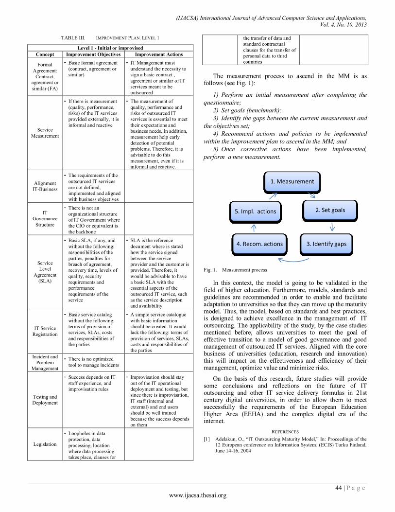
(IJACSA) International Journal of Advanced Computer Science and Applications, Vol. 4, No. 10, 2013
44 | P a g e www.ijacsa.thesai.org
TABLE III. IMPROVEMENT PLAN. LEVEL 1
Level 1 - Initial or improvised
Concept Improvement Objectives Improvement Actions
Formal
Agreement:
Contract,
agreement or
similar (FA)
- Basic formal agreement
(contract, agreement or
similar)
- IT Management must
understand the necessity to
sign a basic contract ,
agreement or similar of IT
services meant to be
outsourced
Service
Measurement
- If there is measurement
(quality, performance,
risks) of the IT services
provided externally, it is
informal and reactive
- The measurement of
quality, performance and
risks of outsourced IT
services is essential to meet
their expectations and
business needs. In addition,
measurement help early
detection of potential
problems. Therefore, it is
advisable to do this
measurement, even if it is
informal and reactive.
Alignment
IT-Business
- The requirements of the
outsourced IT services
are not defined,
implemented and aligned
with business objectives
IT
Governance
Structure
- There is not an
organizational structure
of IT Government where
the CIO or equivalent is
the backbone
Service
Level
Agreement
(SLA)
- Basic SLA, if any, and
without the following:
responsibilities of the
parties, penalties for
breach of agreement,
recovery time, levels of
quality, security
requirements and
performance
requirements of the
service
- SLA is the reference
document where is stated
how the service signed
between the service
provider and the customer is
provided. Therefore, it
would be advisable to have
a basic SLA with the
essential aspects of the
outsourced IT service, such
as the service description
and availability
IT Service
Registration
- Basic service catalog
without the following:
terms of provision of
services, SLAs, costs
and responsibilities of
the parties
- A simple service catalogue
with basic information
should be created. It would
lack the following: terms of
provision of services, SLAs,
costs and responsibilities of
the parties
Incident and
Problem
Management
- There is no optimized
tool to manage incidents
Testing and
Deployment
- Success depends on IT
staff experience, and
improvisation rules
- Improvisation should stay
out of the IT operational
deployment and testing, but
since there is improvisation,
IT staff (internal and
external) and end users
should be well trained
because the success depends
on them
Legislation
- Loopholes in data
protection, data
processing, location
where data processing
takes place, clauses for
the transfer of data and
standard contractual
clauses for the transfer of
personal data to third
countries
The measurement process to ascend in the MM is as follows (see Fig. 1):
1) Perform an initial measurement after completing the
questionnaire;
2) Set goals (benchmark);
3) Identify the gaps between the current measurement and
the objectives set;
4) Recommend actions and policies to be implemented
within the improvement plan to ascend in the MM; and
5) Once corrective actions have been implemented,
perform a new measurement.
Fig. 1. Measurement process
In this context, the model is going to be validated in the field of higher education. Furthermore, models, standards and guidelines are recommended in order to enable and facilitate adaptation to universities so that they can move up the maturity model. Thus, the model, based on standards and best practices, is designed to achieve excellence in the management of IT outsourcing. The applicability of the study, by the case studies mentioned before, allows universities to meet the goal of effective transition to a model of good governance and good management of outsourced IT services. Aligned with the core business of universities (education, research and innovation) this will impact on the effectiveness and efficiency of their management, optimize value and minimize risks.
On the basis of this research, future studies will provide some conclusions and reflections on the future of IT outsourcing and other IT service delivery formulas in 21st century digital universities, in order to allow them to meet successfully the requirements of the European Education Higher Area (EEHA) and the complex digital era of the internet.
REFERENCES
[1] Adelakun, O., “IT Outsourcing Maturity Model,” In: Proceedings of the 12 European conference on Information System, (ECIS) Turku Finland,
June 14-16, 2004
1. Measurement
2. Set goals
3. Identify gaps 4. Recom. actions
5. Impl. actions

(IJACSA) International Journal of Advanced Computer Science and Applications, Vol. 4, No. 10, 2013
45 | P a g e www.ijacsa.thesai.org
[2] Beulen, E., Ribbers, P., “Managing complex IT outsourcing-
partnerships,” System Sciences, 2002. HICSS. In: Proceedings of the 35th Annual Hawaii International Conference on , vol., no., pp.10 pp.,,
7-10 Jan 2002 doi: 10.1109/HICSS.2002.994424
[3] Dahlberg, T., Lahdelma, P., “IT Governance Maturity and IT
Outsourcing Degree: An Exploratory Study,” System Sciences, 2007. HICSS 2007. 40th Annual Hawaii International Conference on , vol.,
no., pp.236a,236a, Jan. 2007 doi: 10.1109/HICSS.2007.306
[4] Fairchild, A.M., “Information technology outsourcing (ITO) governance: an examination of the outsourcing management maturity
model,” System Sciences, 2004. In: Proceedings of the 37th Annual Hawaii International Conference on, vol., no., pp.8 pp., 5-8 Jan. 2004
doi: 10.1109/HICSS.2004.1265565
[5] Fan Jing Meng, Xiao Yang He, Yang, S.X. and Peng Ji, “A Unified Framework for Outsourcing Governance,” E-Commerce Technology
and the 4th IEEE International Conference on Enterprise Computing, E-Commerce, and E-Services, 2007, CEC/EEE 2007, The 9th IEEE
International Conference on , vol., no., pp.367,374, 23-26 July 2007 doi: 10.1109/CEC-EEE.2007.16
[6] Fernández, Eugenio, “UNiTIL: Gobierno y Gestión del TIC basado en
ITIL,” III Congreso Interacadémico 2008 / itSMF España. Last Access on 5th Sept 2011at
http://www.uc3m.es/portal/page/portal/congresos_jornadas/congreso_itsmf/UNiTIL%20Gobierno%20y%20Gestion%20de%20TIC%20basado%
20en%20ITIL.pdf
[7] Gottschalk, P, Solli-Sæther, Hans, “Maturity model for IT outsourcing relationships,” Industrial Management & Data Systems, Vol. 106 Iss: 2,
pp.200 – 212, 2006
[8] Herz, T.P., Hamel, F., Uebernickel, F. and Brenner, W., “Towards a
Multisourcing Maturity Model as an Instrument of IT Governance at a Multinational Enterprise,” System Sciences (HICSS), 2011 44th Hawaii
International Conference on , vol., no., pp.1,10, 4-7 Jan. 2011 doi: 10.1109/HICSS.2011.448
[9] ITGI. Last Access on 26th June 2012 at http://www.itgi.org/
[10] Lyytinen, K., “Penetration of information technology in organizations,” Scandinavian Journal of Information Systems, 3, 87–109, 1991
[11] Mobarhan, R.; Rahman, A.A.; Majidi, M., “Outsourcing management
framework based on ITIL v3 framework,” Information Technology in Asia (CITA 11), 2011 7th International Conference on , vol., no., pp.1,5,
12-13 July 2011 doi: 10.1109/CITA.2011.5999536
[12] Ning Su, Levina, N., “Global Multisourcing Strategy: Integrating Learning From Manufacturing Into IT Service Outsourcing,”
Engineering Management, IEEE Transactions on , vol.58, no.4, pp.717,729, Nov. 2011 doi: 10.1109/TEM.2010.2090733
[13] Nolan, R.L., “Managing the computer resource: a stage hypothesis,”
Communications of the ACM 16 (7). 399, 1973 doi: 10.1145/362280.362284
[14] Patel, Nandish., “Emergent Forms of IT Governance to Support Global
eBusiness Models,” Journal of Information Technology Theory and Application (JITTA), 4 (2), Article 5, 2002, Last access on 19th July
2011 at http://aisel.aisnet.org/jitta/vol4/iss2/5
[15] Yanosky, R., Borreson Caruso, J., “Process and Politics: IT Governance
in Higher Education,” ECAR Key Findings. EDUCASE, 2008, Last Access on 6th March 2012 at
http://net.educause.edu/ir/library/pdf/ekf/EKF0805.pdf
[16] Yanosky, R., McCredie, J., “IT Governance: Solid Structures and Practical Politics,” ECAR Symposium, Boca Ratón, Florida, 2007
(IJACSA) International Journal of Advanced Computer Science and Applications, Vol. 4, No. 10, 2013
46 | P a g e www.ijacsa.thesai.org
A New Approach for Hiding Data Using B-box
Dr. Saad Abdual azize AL_ani
Associate Prof. Computer Science Department
Al_Mamon University College
Baghdad, Iraq
Bilal Sadeq Obaid Obaid
Associated Researcher Computer Science (MSc)
Amman Arab University
Amman, Jordan
Abstract—Digital Images and video encryption play an
important role in today’s multimedia world. Many encryption
schemes have been proposed to provide a security for digital
images. This paper designs an efficient cryptosystem for video.
Our method can achieve two goals; the first goal is to design a
height security for hiding a data in video, the second goal is to design a computational complexity cryptosystem.
Keywords—ASCII; Binary; Cryptosystem; Decimal; Decryption;
Encryption; Image; Plaintext; Video
I. INTRODUCTION
The grand challenges of the data that is carried and stored over the network is making the data safe and disclosed to illegal users. The use of computer networks - especially during the last decade – has grown dramatically. For this reason, creating and developing the security systems and encryption techniques should take wide focus in the field of information security [2]. Parallel with the information transition evolution time, systems and techniques have big success against the threats, but still there are faults [1]. One of these techniques is using the image and multimedia encryption, because the digital image is becoming important carrier of information for people [3]. With the advance of information security requirement, the encryption technology of digital image is applied widely on multimedia communications. Conventional encryption arithmetic could be used to develop or initiate new techniques for best specification and satisfactions. Because some encryption algorithms still used where there there disadvantages and faults are included, such as the structure complexity, the secret key singleness and the encryption speed slowly, and it is difficult to satisfy the encryption requirement of the image that has lots of data. So using the conventional encryption solely is not enough [4]. Anarchic mapping idea could be applied into video to encrypt, because it has the sensitivity and big qualifications of initial values and the randomness [6]. The method which is adopting combined conventional encryption technology. Complex anarchic mapping can overcome the single conventional encryption’s disadvantage effectively. The pixels’ values in original image of video frames can be changed ultimately via encrypting, in order to realize the aim of encryption [5].
For powerful and advanced quality of encryption effectively, the method of position scrambling can be used before and during encrypting steps [5]. The classical algorithms are Arnold cat map, affine transformation, magic square transformation, and knight-tour transformation, etc. Through these transformations, the change of the image pixels’ position can be realized by keeping the secret of parameters and by normalizing heavy complex random boxes and
numbers and with iteration times to reach the aim of encryption. A method which based on Arnold cat map and S-DES has been proposed and developed strongly and efficiently in this paper by applying the particular character of logistic anarchic map. The key numbers of S-DES are increased and the key can be changed in real-time [7]. The experiments results have shown that the good methods that integrate encryption/decryption process on the image or video produce well security and fast executing with no visible contorting or reconstructing on the image
II. THE METHOD
The method of encryption process divides into two sections. First section is to encrypt the data. The second is to augment the encrypted data on a video file.
A. Encryption Algorithm
With first section step, we will initiate the input size of Plaintext such 8 – character and handle such a binary (0s, 1s).
1) Choose eight characters as Plaintext such one block.
2) Calculate the weight of the plaintext characters by
subtracting 64 from the ASCII code of each character
3) Convert the weights to binary mode with 6 bits. Here,
output includes 48 binary bits (8char * 6bits).
4) Build the B – Table, where B – table which consists of 4
rows and 15 columns. The table made up by generating a
particular function to generate the number 15 randomly from
1 to 15, where the function will be generated for four times.
5) For each 6 bits from the 48 bit that referred to the
selected Plaintext, consider first and last bits as row number
of the B – table that have been evaluated, and every 4 bits in
between is for the column number.
6) From B – table, take value of the cell that have been
matched by (Row no, Column no).
7) Convert it to its 4 bits of binary mode. Here, the result
will be changed and shrank from 48 bits to 32 bits.
8) Generate a particular function specialized for
generating random numbers to build P – table.
9) Broadcast the 32 bits in P – table, where P – table used
to reshape the sequence of the 32 bits depending on P – table
numbers, these numbers are the assumed new location of the
32 bits.
10) Write the output row by row to get new 32 bits. The
output is the encrypted data bits and the next steps for
augmenting the encrypted data into video file

(IJACSA) International Journal of Advanced Computer Science and Applications, Vol. 4, No. 10, 2013
47 | P a g e www.ijacsa.thesai.org
11) Initiate a free object of video file to prepare for
constructing a new video and giving the name of the object.
12) Define the video that should be encrypted.
13) Find the number of frames of the defined video.
14) Find the dimensions of video frames that defined.
15) Create a figure that would hold the video frames.
16) Configure the created figure shape, dimensions and
location to be adjusted with appearance of video frames
properties.
17) Generate a random number by applying a particular
algorithm, select random number from the interval [1, number
of the video frame that we have inputted].
18) Sequentially, read the data of video frame and save it
on the memory.
19) Present the frame data as image onto a special
figure.
20) Create frame by getting the data that is presented
onto the figure.
21) Find a frame which holds the random number of the
video frames.
22) Convert the frame data type to image data type.
23) Find the dimension of the converted image.
24) Hag the image array to sub - image arrays, where
each sub –image size is 8*8. With considering image is
colored, that mean it's three dimensions (R, G, B), so it's run
over the sub – image dimensions (8*8*3).
25) Record the location of each sub-image array
depending on the image.
26) Calculate the number of sub – images that have been
produced.
27) Apply the particular random number generator from
the interval [1, number of sub – image].
28) Pick-up the sub – image array that holds the random
number.
29) Calculate the values (minimum, mean, maximum) of
sub-image array pixels from arrays (red, green, blue)
respectively.
30) Conserve the locations of those values from sub-
image array.
31) Convert the values from decimal to binary mode.
32) Bring first three bits of encrypted data bits and put
them rather last three binary bits of minimum value, and next
three bits of encrypted data bits rather than last three binary
bits of mean value, and next three bits of encrypted data bits
key rather the last three binary bits of maximum.
33) Convert each changed binary back to decimal mode.
34) Carry each value as new pixels back to the origin
locations of the new values (locations of min, mean and max)
of sub-image array which is the converted image.
35) Convert the converted image back to frame data type.
36) Fulfill the video object file by adding frame by frame
to the video object file that has been constructed, respectively,
depending on the frame order from that came out of the
inputted video file.
37) Close the figure that prints the data of frames to
initiate the new figure to present the next frame to add them
onto video object file.
38) Generate special algorithm on the video file that is
done to remove – for some time – some delays or to increase
of video size that could occur. Here, the algorithm has finished encrypting the data and
hiding it inside a video file by a very strong algorithm that
aims to hide and save data or to maintain property rights.
B. Decrytion Algorithm
Now, the output is the encrypted video will be decrypted by the inverse algorithm to testify and return the original video – that has been encrypted - file back.
1) Define the video that should be decrypted.
2) Find the number of frames of the defined video.
3) Find the dimensions of video frames that defined.
4) Create a figure whose would hold the video frames.
5) Configure the shape of created figure, dimensions and
location to be adjusted with appearance of video frames
properties.
6) By applying a particular algorithm to generate a
random number, select random number from the interval [1,
number of the video frame that we have inputted].
7) Sequentially, read the data of video frame and save it in
the memory.
8) Present the frame data as image of a special figure.
9) Create frame by getting the data that presented onto the
figure.
10) Find a frame which holds the random number of the
video frames.
11) Convert the frame data type to image data type
12) Find the dimension of the converted image
13) Divide the image array to sub - image arrays, where
each sub –image size is 8*8. With considering image as
colored, that mean three dimensions (R, G, B), so it's run over
the sub – image dimensions (8*8*3).
14) Record the location of each sub-image array
depending on the image.
15) Calculate the number of sub – images that have been
produced.
16) Apply the particular random number of generator
from the interval [1, number of sub – image].
17) Pick-up the sub – image array that holds the random
number
18) Calculate the values (minimum, mean, maximum) of
sub-image array pixels from arrays (red, green, blue)
respectively.
19) Conserve the locations of those values from sub-
image array
20) Pickup each LSB from minimum, maximum, mean of
sub image.
21) Convert the values from binary mode to decimal.
22) Broadcasting the bits of decrypted data array on the
P-1 table, where the P-1 is evaluated by special generation
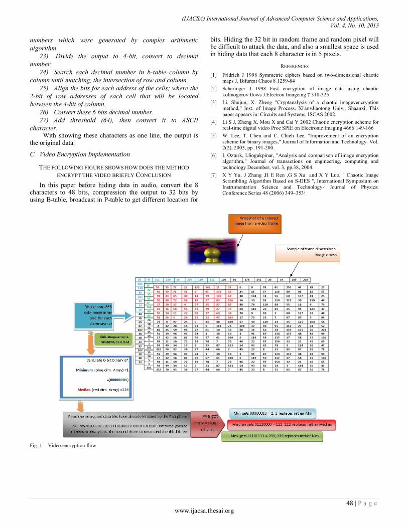
(IJACSA) International Journal of Advanced Computer Science and Applications, Vol. 4, No. 10, 2013
48 | P a g e www.ijacsa.thesai.org
numbers which were generated by complex arithmetic
algorithm.
23) Divide the output to 4-bit, convert to decimal
number.
24) Search each decimal number in b-table column by
column until matching, the intersection of row and column.
25) Align the bits for each address of the cells; where the
2-bit of row addresses of each cell that will be located
between the 4-bit of column.
26) Convert these 6 bits decimal number.
27) Add threshold (64), then convert it to ASCII
character. With showing these characters as one line, the output is
the original data.
C. Video Encryption Implementation
THE FOLLOWING FIGURE SHOWS HOW DOES THE METHOD
ENCRYPT THE VIDEO BRIEFLY CONCLUSION
In this paper before hiding data in audio, convert the 8 characters to 48 bits, compression the output to 32 bits by using B-table, broadcast in P-table to get different location for
bits. Hiding the 32 bit in random frame and random pixel will be difficult to attack the data, and also a smallest space is used in hiding data that each 8 character is in 5 pixels.
REFERENCES
[1] Fridrich J 1998 Symmetric ciphers based on two-dimensional chaotic maps J. Bifurcat Chaos 8 1259-84
[2] Scharinger J 1998 Fast encryption of image data using chaotic
kolmogorov flows J.Electron Imageing 7 318-325
[3] Li. Shujun, X. Zheng "Cryptanalysis of a chaotic imagevencryption method," Inst. of Image Process. Xi'anvJiaotong Univ., Shaanxi, This
paper appears in: Circuits and Systems, ISCAS 2002.
[4] Li S J, Zheng X, Mou X and Cai Y 2002 Chaotic encryption scheme for real-time digital video Proc SPIE on Electronic Imaging 4666 149-166
[5] W. Lee, T. Chen and C. Chieh Lee, "Improvement of an encryption
scheme for binary images," Journal of Information and Technology. Vol. 2(2), 2003, pp. 191-200.
[6] I. Ozturk, I.Sogukpinar, "Analysis and comparison of image encryption algorithm," Journal of transactions on engineering, computing and
technology December, vol. 3, pp.38, 2004.
[7] X Y Yu, J Zhang ,H E Ren ,G S Xu and X Y Luo, " Chaotic Image Scrambling Algorithm Based on S-DES ", International Symposium on
Instrumentation Science and Technology- Journal of Physics: Conference Series 48 (2006) 349–353\
Fig. 1. Video encryption flow
(IJACSA) International Journal of Advanced Computer Science and Applications, Vol. 4, No. 10, 2013
49 | P a g e www.ijacsa.thesai.org
Enhanced Link Redirection Interface for Secured
Browsing using Web Browser Extensions
Mrinal Purohit Y
Dept. Of Computer Science
Amrita University
Coimbatore, India
Kaushik Velusamy
Dept. Of Computer Science
Amrita University
Coimbatore, India
Shriram K Vasudevan
Dept. Of Computer Science
Amrita University
Coimbatore, India
Abstract—In the present world scenario where data is meant
to be protected from intruders and crackers, everyone has the
fear to keep their private data safe. As the data is stored on
servers accessed through websites by browsers, it’s the browsers,
which act as a medium between a user and the server to send or
receive data. As browsers send data in plain text, any data which
is sent could easily be intercepted and used against someone.
Hence this led to the use of Transport Layer Security (TLS) and
Secure Socket Layer (SSL), which are cryptographic protocols
designed to provide communication security over the Internet. A
layer on top of SSL/TLS, support an encrypted mode, also known
as HTTPS (HTTP Secure). Therefore, one of the main aspect of
security lies in the website supporting HTTPS. Most websites
have support for this encrypted mode and still we use an
unencrypted mode of websites because a common user is
unaware of the advancements in the field of technology. So to
help us, in browsers, we have extensions or plug-ins to ease our
life. This paper proposes the idea to implement the security measures in the web browsers.
Keywords—Browsers; HTTPS; SSL
I. INTRODUCTION
Now-a-days, the browsers are the common application which people use to obtain information and share the same with others. It has become a common sight to the eye. But it’s not just the information which matters; it is the person’s personal information which is at stake. Browsers are said to be secured when the data is sent from the browser, only based on what type of layer of security the website has used. If there is no layer of security, then the data is sent as a plain text. Few websites use HTTPS which makes the website secure by encrypting data using long term public and secret keys, before sending. Hence it depends on whether a website has this support for HTTPS or not. Currently most websites offer HTTPS versions of their simple websites which are only triggered when there is a data exchange between the user and server.
A browser extension is a computer program which extends a normal browser’s functionality. Browsers lack in few functionalities which are complemented by extensions. Extensions can be disabled but as they help a user in providing assistance, the user is forced to be dependent on them to make their work easier and make their browsing experience better. Different browsers have different requirements for an extension to be developed. Each browser have their own set of architecture and API’s which requires different code and skills for each extension. Extensions are developed using web
technologies like HTML, JavaScript, CSS and XML. Most famous browsers like Chrome and Firefox have their own web store for extensions which can be downloaded and used by anyone. Thus making it a very powerful tool for developers to make use of the browser’s robustness.
This paper combines secure web browsing using HTTPS focusing on website redirection using browser extension and spam filtering to save the user’s personal data and to make his browsing experience secure. The links which are classified as spam are stored in a vault for future references for spam and secure redirection.
II. LITERATURE SURVEY
Browsers being one of the main source of information retrieval from the Internet, have many vulnerabilities. Though they have private browsing feature in browsers like Chrome, Firefox and Internet Explorer they are still prone to attacks as stated in [9]. They describe the flaws existing in browsers even in the private mode, which the user imagines is secure. They describe attacks prone to a local attacker and a web attacker who can access personal data even if the user uses private browsing mode. The proposed flaw points the use of extensions leaving trace of websites visited, on the disk which can be accessed by an attacker. Hence even if a user makes use of private browsing, they are still not secure. But this gives an insight that web URL’s can be accessed in both normal and private mode of the browsers [9].
Each browser differs in its extensible architecture and working. Extensions depend on the architecture, whether they can be developed or not. For example, from the following list of browsers, Internet Explorer, Firefox, Chrome and Safari, only Safari doesn’t support extensions. [9]. An extension called BROWSERSPY was developed, which did not require any special privileges but still it managed to take complete control over the browser and observe all activity performed through the browser staying undetectable. Extensions can be harmful but at the same time helpful. An example is PwdHash [10] which hashes the plaintext data given by the user, data associated with the website and a private salt stored on the client machine. Therefore, there can be both security oriented and security hindering extensions existing in the extensions market [7].
Both the end users and administrators of various services on the Internet such as email systems use different anti-spam techniques. Some of these anti-spam techniques have been embedded in products, services and software to ease the burden

(IJACSA) International Journal of Advanced Computer Science and Applications, Vol. 4, No. 10, 2013
50 | P a g e www.ijacsa.thesai.org
on users and administrators, But there is a unique technique which serves as a complete solution to the spam problem for securing the browsing activities on the Internet and each has different trade-offs ranging between incorrectly rejecting legitimate links Vs. not rejecting any spam link.
Table.1 below describes security in Google Chrome, IE and Mozilla Firefox. The comparison considers metrics such as vulnerability report counts and URL blacklists [3]. This paper takes a fundamentally different approach, examining which security metrics are most effective in protecting end users who browse the Internet. The following graph shows the comparison of different browsers based on the analysis of the mentioned factors. It is seen that all the three major browsers don’t provide URL Blacklisting service. We have analyzed that neither Google’s Safe Browsing service nor Microsoft’s URS, appears to provide a fully comprehensive snapshot of all malware and spam web links in the wild at any given point in time [8]. This proves a strong support for the idea proposed in this paper.
The main concern of a browser extension is to secure the user from malicious links and safe guard the user’s private data that are shared on the Internet. Rather than discovering vulnerabilities, it is the need of the hour to protect a user in their browsing experience. Thus, this paper proposes the basic idea to use the browser extensions to prevent spam and make the fullest utilization of the browsers as well as the website’s fullest power which supports the HTTPS.
TABLE I. Comparison of factors leading to vulnerabilities in different web browsers.
Criteria Chrome Internet Explorer Firefox
Sandboxing Yes Implemented No
Plug-in Security Yes Implemented No
JIT Hardening Yes Yes No
ASLR Yes Yes Yes
DEP Yes Yes Yes
GS Yes Yes Yes
URL Blacklisting No No No
III. SPAM WEB LINKS
Most spam travels through blog networks. In order to get link redirections back to their sites or their client’s sites, members of fake blog owners are paid for posting the spam links for higher hits. Guest blogging and other forms of contributing content to legitimate sites is a much whiter tactic, but considering that as a strategy that relies heavily on low-quality advertisement. Guest blogging looks similar to a blog network spam.
Article marketing is another method to spread spam. This method provides one or two links with the anchor text of the user’s choice, and hence the ranking increases in search engines. Such articles are found to be easy, cheap and without creativity or mental effort. Most articles on the Internet are made for the sole purpose of getting huge hits for their links, and essentially all the followed links are self-generated rather
than endorsements. Due to its wide spread on the Internet these links with no weights come in and the links with no impact go out. They are persistent because of decent free template which is not filtered by Google.
Most links which the users don’t want to visit are embedded in a site wide link where the users are redirected to visit, so as to bring attention to their websites. Creating a piece of link and later replacing the content with something more beneficial and tricking the people to link to their desired content are examples of Link Bait Switching. Social Bookmarking and sharing sites carry many web links which don’t have any value. Profile spam and comment spam add to the above [1].
Spam web links are spam links which are spread on the Internet, and which take advantage of link based ranking algorithms which gives websites higher rankings the more highly ranked websites linked to it. It’s a trend on social networking sites to spread spam links [5]. Social sites with low spam control, stops getting visitors when being overrun by low quality external links. Handling spam is getting harder day by day as new technology emerges. Spam traps are often email addresses that were never valid or have been invalid for a long time, which were used to collect spams. They are found by pulling addresses off the hidden webpages. Spamcop, a blacklist directory uses spamtraps to catch spammers and blacklist them. Hence it gets tougher to track them out through web services [11].
Google bomb refers to the practice of creating a large number of links that cause the webpages to have high rankings in Google searches. It is mostly done for either business, political or pun purposes. Spam web links are the links which are spread on the Internet, and take advantage of link based ranking algorithms, which gives websites higher rankings. The more highly ranked websites are linked to it. It’s a trend on social networking sites to spread spam links [5
IV. PROPOSED METHODOLOGY
An extension for a browser is usually developed using web technologies like HTML, JavaScript, CSS and XML. Using these technologies, an extension to secure a user’s browsing experience has been implemented. The browser concentrated for this extension is Google Chrome. The basic idea is to redirect any URL to the HTTPS version based on its domain name and if the redirection falls back then the extension checks if the URL is a spam. So while checking if the link is a spam, the user is then redirected to a safe website with a message and the URL is stored in a safe vault and thus the link is safely redirected to the original URL.
Websites, even if they use HTTPS are a bit unsecure because every website has their own separate domain. And here the redirection is to that secure domain rather HTTPS. This is the reason why a particular rule cannot be used for every website by changing the HTTP in the URL to HTTPS. Because that would only mean the change of protocol, whereas in reality it means that we should redirect to the secure website which sends data in an encrypted mode.
Initially, It is mandatory to first determine the domain of the URL and then based on the predefined set of rules we
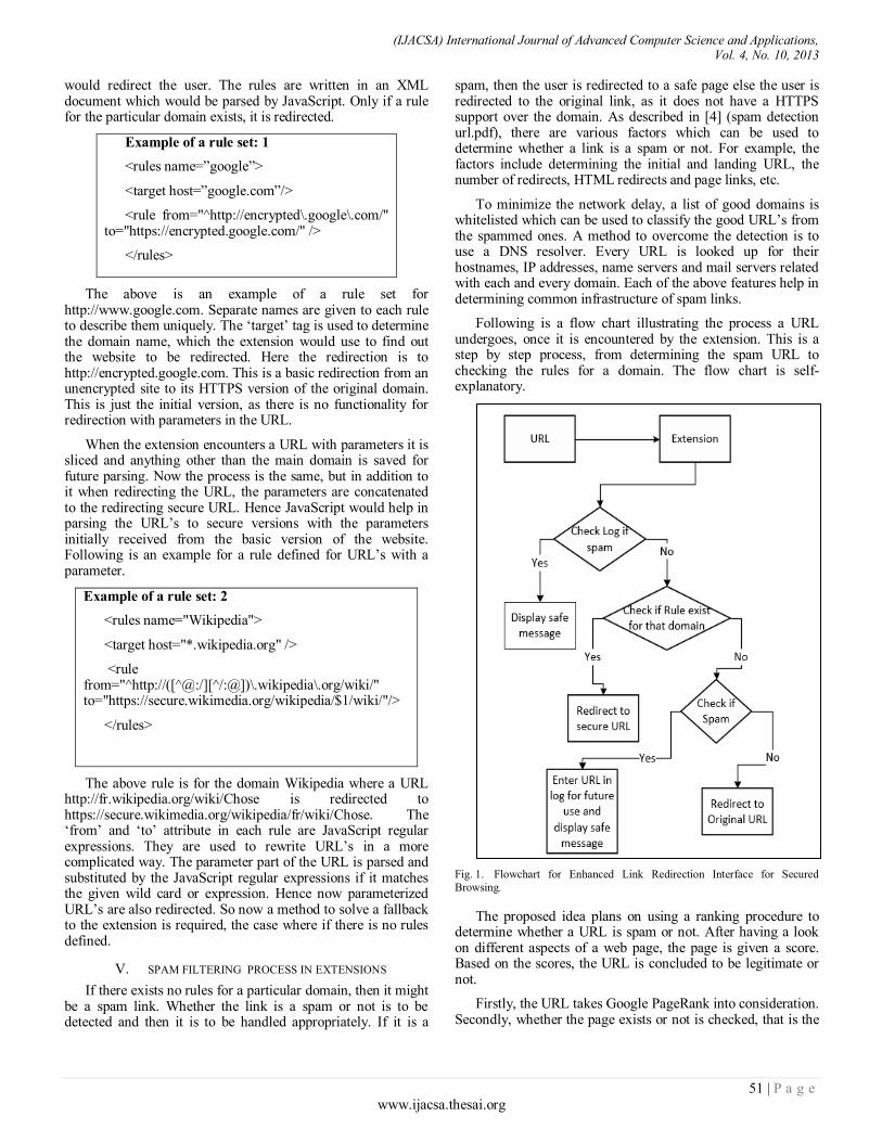
(IJACSA) International Journal of Advanced Computer Science and Applications, Vol. 4, No. 10, 2013
51 | P a g e www.ijacsa.thesai.org
would redirect the user. The rules are written in an XML document which would be parsed by JavaScript. Only if a rule for the particular domain exists, it is redirected.
Example of a rule set: 1
<rules name=”google”>
<target host=”google.com”/>
<rule from="^http://encrypted\.google\.com/" to="https://encrypted.google.com/" />
</rules>
The above is an example of a rule set for http://www.google.com. Separate names are given to each rule to describe them uniquely. The ‘target’ tag is used to determine the domain name, which the extension would use to find out the website to be redirected. Here the redirection is to http://encrypted.google.com. This is a basic redirection from an unencrypted site to its HTTPS version of the original domain. This is just the initial version, as there is no functionality for redirection with parameters in the URL.
When the extension encounters a URL with parameters it is sliced and anything other than the main domain is saved for future parsing. Now the process is the same, but in addition to it when redirecting the URL, the parameters are concatenated to the redirecting secure URL. Hence JavaScript would help in parsing the URL’s to secure versions with the parameters initially received from the basic version of the website. Following is an example for a rule defined for URL’s with a parameter.
Example of a rule set: 2
<rules name="Wikipedia">
<target host="*.wikipedia.org" />
<rule from="^http://([^@:/][^/:@])\.wikipedia\.org/wiki/" to="https://secure.wikimedia.org/wikipedia/$1/wiki/"/>
</rules>
The above rule is for the domain Wikipedia where a URL http://fr.wikipedia.org/wiki/Chose is redirected to https://secure.wikimedia.org/wikipedia/fr/wiki/Chose. The ‘from’ and ‘to’ attribute in each rule are JavaScript regular expressions. They are used to rewrite URL’s in a more complicated way. The parameter part of the URL is parsed and substituted by the JavaScript regular expressions if it matches the given wild card or expression. Hence now parameterized URL’s are also redirected. So now a method to solve a fallback to the extension is required, the case where if there is no rules defined.
V. SPAM FILTERING PROCESS IN EXTENSIONS
If there exists no rules for a particular domain, then it might be a spam link. Whether the link is a spam or not is to be detected and then it is to be handled appropriately. If it is a
spam, then the user is redirected to a safe page else the user is redirected to the original link, as it does not have a HTTPS support over the domain. As described in [4] (spam detection url.pdf), there are various factors which can be used to determine whether a link is a spam or not. For example, the factors include determining the initial and landing URL, the number of redirects, HTML redirects and page links, etc.
To minimize the network delay, a list of good domains is whitelisted which can be used to classify the good URL’s from the spammed ones. A method to overcome the detection is to use a DNS resolver. Every URL is looked up for their hostnames, IP addresses, name servers and mail servers related with each and every domain. Each of the above features help in determining common infrastructure of spam links.
Following is a flow chart illustrating the process a URL undergoes, once it is encountered by the extension. This is a step by step process, from determining the spam URL to checking the rules for a domain. The flow chart is self-explanatory.
Fig. 1. Flowchart for Enhanced Link Redirection Interface for Secured
Browsing.
The proposed idea plans on using a ranking procedure to determine whether a URL is spam or not. After having a look on different aspects of a web page, the page is given a score. Based on the scores, the URL is concluded to be legitimate or not.
Firstly, the URL takes Google PageRank into consideration. Secondly, whether the page exists or not is checked, that is the

(IJACSA) International Journal of Advanced Computer Science and Applications, Vol. 4, No. 10, 2013
52 | P a g e www.ijacsa.thesai.org
existence of PageRank, number of links on the page, links on the page are spam or of quality content, whether the page is indexed, the site is indexed and is the page dynamically loading and additionally if it is a RFC complied. Based on the characteristics, the scores are increased if there is a positive response from the web page and negative for any negative response. In the end if the scores lie between a particular low ranges, the link is declared spam and if it is not then it is declared legitimate.
The extension now determines the URL to be spam or not based on a set of scores. So if it is spam, the user is redirected to a safe website with a message conveyed that it was an unsafe website. Later, this link is added to the vault which is a log file for future references. Again if the same link is intercepted, there is no requirement to calculate the scores again but just to check the log file. And finally, if the link is not a spam but is a safe link with no support for HTTPS, the user is then redirected to the original link with no restrictions.
Very few websites don’t have support for HTTPS. And of the small set, are websites which don’t share user data or require user data. Hence these types of URL’s are redirected to the initial URL phase. These websites don’t have set of rules; hence they are tested for spam. Therefore, if they are legitimate links they are just redirected to the website.
Finally, among the many potential attacks that target Internet with spams or vulnerabilities in browsers, browsers which failed to protect the user from spams have received relatively little attention.
Hence using an extension to enhance the security of user data and their browsing experience would make a great impact in simplifying a user’s life rather than managing their data continuously [2].
VI. FUTURE WORKS
This extension looks only into the link-redirection and spam detection. But whenever there is a URL redirection, the domains for which the cookies are stored are lost. Hence before the user is redirected, the cookies have to be analysed. Based on the new domain, the old cookies should be deleted and new set of cookies have to be created. This cookie exchange is necessary because the usual cookies are stored on the HTTP version of the website whereas the secure version is HTTPS.
There is a change in protocols, hence in the cookie exchange. This could be a future enhancement. Installing extensions can be cumbersome for every user as they have to go to the Chrome Store every time.
So implementing the extension functionality directly into a browser is a possibility. This feature can be useful for users who possess very less knowledge about securing personal and private data. This can be implemented on open source browsers like Chromium.
VII. CONCLUSION
Extensions add specific abilities into browsers which helps the user in solving many problems which the user cannot solve on their own. As extensions are just simple programs complementing functions of browsers, they take a very small amount of space, and still cover various aspects of data storage and data security. This extension is one way, of how simple programs can secure a user from malicious links and web crackers.
ACKNOWLEDGMENT
We thank Amrita University, India for providing the opportunity and facilities in all possible ways for this research. We thank all the reviewers of this paper for their helpful comments and suggestions.
REFERENCES
[1] Ter Louw, Mike, Lim, JinSoon , Venkatakrishnan, V.N, “Extensible Web Browser Security”, detection of Intrusions and Malware, and
Vulnerability Assessment, Lecture Notes in Computer Science. Springer Berlin Heidelberg, 2007-01-01, Pages 1-19,
http://dx.doi.org/10.1007/978-3-540-73614-1_1, DOI: 10.1007/978-3-540-73614-1_1
[2] N. Jovanovic, C. Kruegel, and E. Kirda. Pixy: A static analysis tool for
detecting web application vulnerabilities (short paper). In Proceesings of the 2006 IEEE Symposium on Security and Privacy, pages 258–263,
2006.
[3] N. Freeman and R. S. Liverani. Exploiting cross context scripting vulnerabilities in Firefox, April 2010. http://www.security-
assessment.com/files/whitepapers/Exploiting_Cross_ Context_Scripting_vulnerabilities_in_Firefox.pdf.
[4] Kurt Thomas, Chris Grier, , Justin Ma, Vern Paxson Y, Dawn Song,
“Design and Evaluation of a Real-Time URL Spam Filtering Service”, University of California, Berkeley, International Computer Science
Institute. Proceedings of the IEEE Symposium on Security and Privacy, May 2011.
[5] Devdatta Akhawe and Adrienne Porter Felt, “Alice inWarningland:A
Large-Scale Field Study of Browser SecurityWarning Effectiveness”, University of California, Google, Inc. Usenix Security Symposium,
Washington DC, 2013.
[6] Mike Ter Louw, Jin Soon Lim, V. N. Venkatakrishnan, “Enhancing web browser security against malware extensions”. Journal in Computer
Virology 4(3): 179-195 (2008).
[7] ACCUVANT LABS security assessment and research, “Browser
Security Comparison – A Quantitative Approach”, Pages 140, Version 0.0, Revision Date: 12/6/2011.
[8] Nikhil Swamy, Benjamin Livshits, Arjun Guha, Matthew Fredrikson,
"Verified Security for Browser Extensions", Microsoft Research Technical Report, MSR-TR-2010-157.
[9] AGGARWAL, G., BURSZTEIN, E., JACKSON, C., AND BONEH, D.
An analysis of private browsing modes in modern browsers. In Proceedings of the 19th USENIX conference on Security (2010),
USENIX Security’10.
[10] Ross, B., et al.: Stronger password authentication using browser extensions. In: 14th USENIX Security Symposium (August 2005).
[11] Mark Felegyhazi, Christian Kreibich, and Vern Paxson. On the potential
of proactive domain blacklisting. In Proceedings of the Third USENIX Workshop on Large-scale Exploits and Emergent Threats (LEET), San
Jose, CA, USA, April 2010.
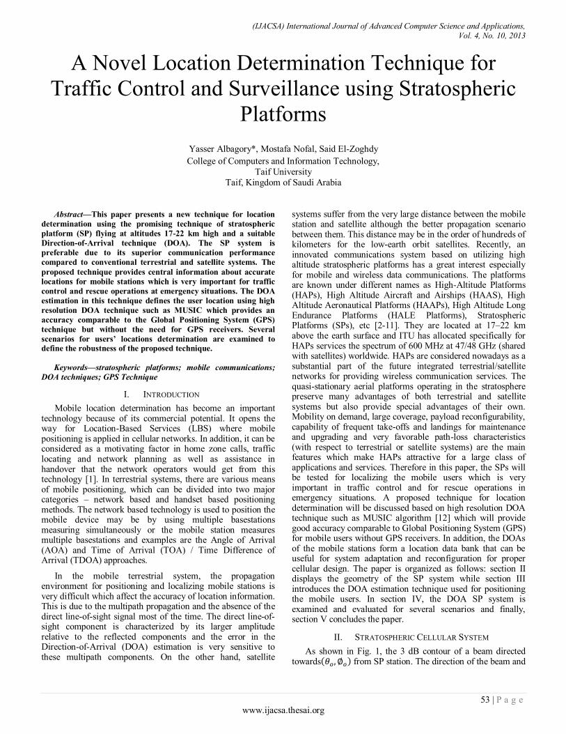
(IJACSA) International Journal of Advanced Computer Science and Applications, Vol. 4, No. 10, 2013
53 | P a g e www.ijacsa.thesai.org
A Novel Location Determination Technique for
Traffic Control and Surveillance using Stratospheric
Platforms
Yasser Albagory*, Mostafa Nofal, Said El-Zoghdy
College of Computers and Information Technology,
Taif University
Taif, Kingdom of Saudi Arabia
Abstract—This paper presents a new technique for location
determination using the promising technique of stratospheric
platform (SP) flying at altitudes 17-22 km high and a suitable
Direction-of-Arrival technique (DOA). The SP system is
preferable due to its superior communication performance
compared to conventional terrestrial and satellite systems. The
proposed technique provides central information about accurate
locations for mobile stations which is very important for traffic
control and rescue operations at emergency situations. The DOA
estimation in this technique defines the user location using high
resolution DOA technique such as MUSIC which provides an
accuracy comparable to the Global Positioning System (GPS)
technique but without the need for GPS receivers. Several
scenarios for users’ locations determination are examined to define the robustness of the proposed technique.
Keywords—stratospheric platforms; mobile communications;
DOA techniques; GPS Technique
I. INTRODUCTION
Mobile location determination has become an important technology because of its commercial potential. It opens the way for Location-Based Services (LBS) where mobile positioning is applied in cellular networks. In addition, it can be considered as a motivating factor in home zone calls, traffic locating and network planning as well as assistance in handover that the network operators would get from this technology [1]. In terrestrial systems, there are various means of mobile positioning, which can be divided into two major categories – network based and handset based positioning methods. The network based technology is used to position the mobile device may be by using multiple basestations measuring simultaneously or the mobile station measures multiple basestations and examples are the Angle of Arrival (AOA) and Time of Arrival (TOA) / Time Difference of Arrival (TDOA) approaches.
In the mobile terrestrial system, the propagation environment for positioning and localizing mobile stations is very difficult which affect the accuracy of location information. This is due to the multipath propagation and the absence of the direct line-of-sight signal most of the time. The direct line-of-sight component is characterized by its larger amplitude relative to the reflected components and the error in the Direction-of-Arrival (DOA) estimation is very sensitive to these multipath components. On the other hand, satellite
systems suffer from the very large distance between the mobile station and satellite although the better propagation scenario between them. This distance may be in the order of hundreds of kilometers for the low-earth orbit satellites. Recently, an innovated communications system based on utilizing high altitude stratospheric platforms has a great interest especially for mobile and wireless data communications. The platforms are known under different names as High-Altitude Platforms (HAPs), High Altitude Aircraft and Airships (HAAS), High Altitude Aeronautical Platforms (HAAPs), High Altitude Long Endurance Platforms (HALE Platforms), Stratospheric Platforms (SPs), etc [2-11]. They are located at 17–22 km above the earth surface and ITU has allocated specifically for HAPs services the spectrum of 600 MHz at 47/48 GHz (shared with satellites) worldwide. HAPs are considered nowadays as a substantial part of the future integrated terrestrial/satellite networks for providing wireless communication services. The quasi-stationary aerial platforms operating in the stratosphere preserve many advantages of both terrestrial and satellite systems but also provide special advantages of their own. Mobility on demand, large coverage, payload reconfigurability, capability of frequent take-offs and landings for maintenance and upgrading and very favorable path-loss characteristics (with respect to terrestrial or satellite systems) are the main features which make HAPs attractive for a large class of applications and services. Therefore in this paper, the SPs will be tested for localizing the mobile users which is very important in traffic control and for rescue operations in emergency situations. A proposed technique for location determination will be discussed based on high resolution DOA technique such as MUSIC algorithm [12] which will provide good accuracy comparable to Global Positioning System (GPS) for mobile users without GPS receivers. In addition, the DOAs of the mobile stations form a location data bank that can be useful for system adaptation and reconfiguration for proper cellular design. The paper is organized as follows: section II displays the geometry of the SP system while section III introduces the DOA estimation technique used for positioning the mobile users. In section IV, the DOA SP system is examined and evaluated for several scenarios and finally, section V concludes the paper.
II. STRATOSPHERIC CELLULAR SYSTEM
As shown in Fig. 1, the 3 dB contour of a beam directed towards from SP station. The direction of the beam and
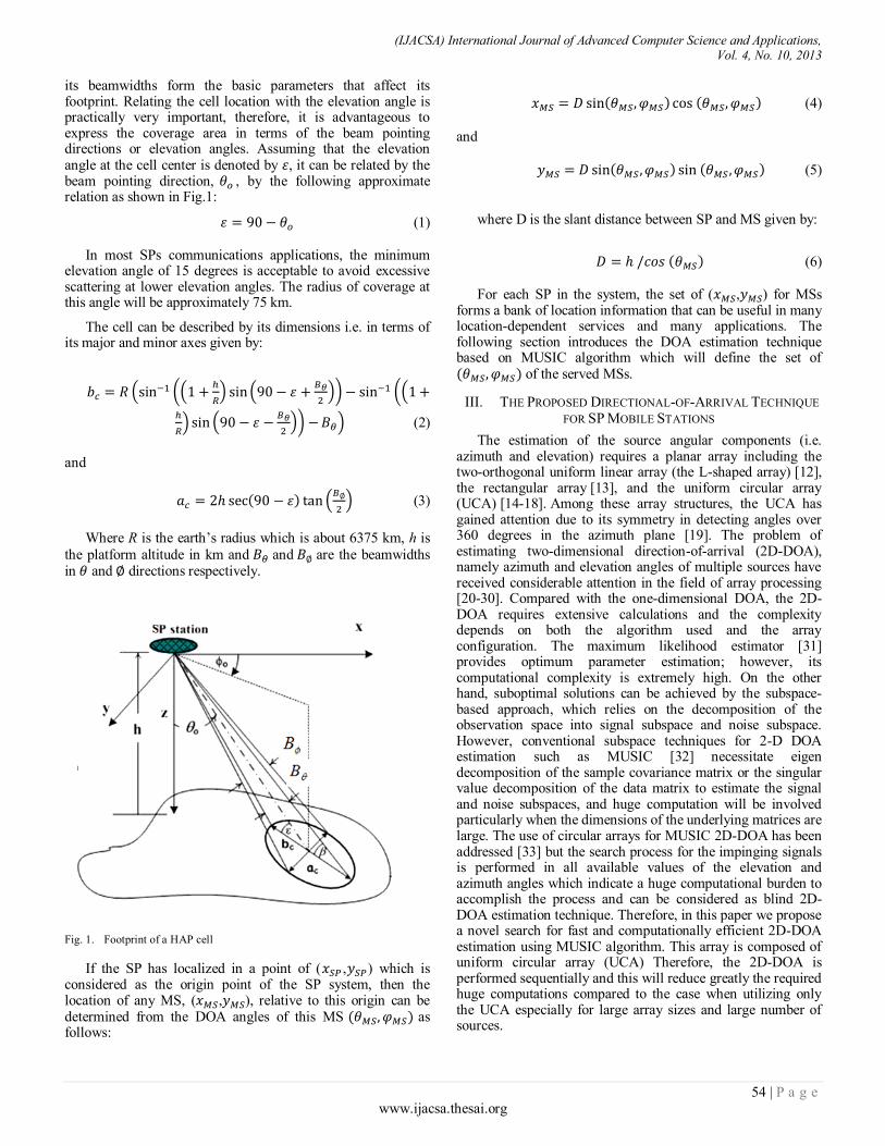
(IJACSA) International Journal of Advanced Computer Science and Applications, Vol. 4, No. 10, 2013
54 | P a g e www.ijacsa.thesai.org
its beamwidths form the basic parameters that affect its footprint. Relating the cell location with the elevation angle is practically very important, therefore, it is advantageous to express the coverage area in terms of the beam pointing directions or elevation angles. Assuming that the elevation angle at the cell center is denoted by , it can be related by the beam pointing direction, , by the following approximate relation as shown in Fig.1:
(1)
In most SPs communications applications, the minimum
elevation angle of 15 degrees is acceptable to avoid excessive scattering at lower elevation angles. The radius of coverage at this angle will be approximately 75 km.
The cell can be described by its dimensions i.e. in terms of its major and minor axes given by:
(2)
and
(3)
Where R is the earth’s radius which is about 6375 km, h is
the platform altitude in km and and are the beamwidths in and directions respectively.
Fig. 1. Footprint of a HAP cell
If the SP has localized in a point of ( , ) which is considered as the origin point of the SP system, then the location of any MS, ( , ), relative to this origin can be determined from the DOA angles of this MS as follows:
(4)
and
(5)
where D is the slant distance between SP and MS given by:
(6)
For each SP in the system, the set of ( , ) for MSs forms a bank of location information that can be useful in many location-dependent services and many applications. The following section introduces the DOA estimation technique based on MUSIC algorithm which will define the set of of the served MSs.
III. THE PROPOSED DIRECTIONAL-OF-ARRIVAL TECHNIQUE
FOR SP MOBILE STATIONS
The estimation of the source angular components (i.e. azimuth and elevation) requires a planar array including the two-orthogonal uniform linear array (the L-shaped array) [12], the rectangular array [13], and the uniform circular array (UCA) [14-18]. Among these array structures, the UCA has gained attention due to its symmetry in detecting angles over 360 degrees in the azimuth plane [19]. The problem of estimating two-dimensional direction-of-arrival (2D-DOA), namely azimuth and elevation angles of multiple sources have received considerable attention in the field of array processing [20-30]. Compared with the one-dimensional DOA, the 2D-DOA requires extensive calculations and the complexity depends on both the algorithm used and the array configuration. The maximum likelihood estimator [31] provides optimum parameter estimation; however, its computational complexity is extremely high. On the other hand, suboptimal solutions can be achieved by the subspace-based approach, which relies on the decomposition of the observation space into signal subspace and noise subspace. However, conventional subspace techniques for 2-D DOA estimation such as MUSIC [32] necessitate eigen decomposition of the sample covariance matrix or the singular value decomposition of the data matrix to estimate the signal and noise subspaces, and huge computation will be involved particularly when the dimensions of the underlying matrices are large. The use of circular arrays for MUSIC 2D-DOA has been addressed [33] but the search process for the impinging signals is performed in all available values of the elevation and azimuth angles which indicate a huge computational burden to accomplish the process and can be considered as blind 2D-DOA estimation technique. Therefore, in this paper we propose a novel search for fast and computationally efficient 2D-DOA estimation using MUSIC algorithm. This array is composed of uniform circular array (UCA) Therefore, the 2D-DOA is performed sequentially and this will reduce greatly the required huge computations compared to the case when utilizing only the UCA especially for large array sizes and large number of sources.
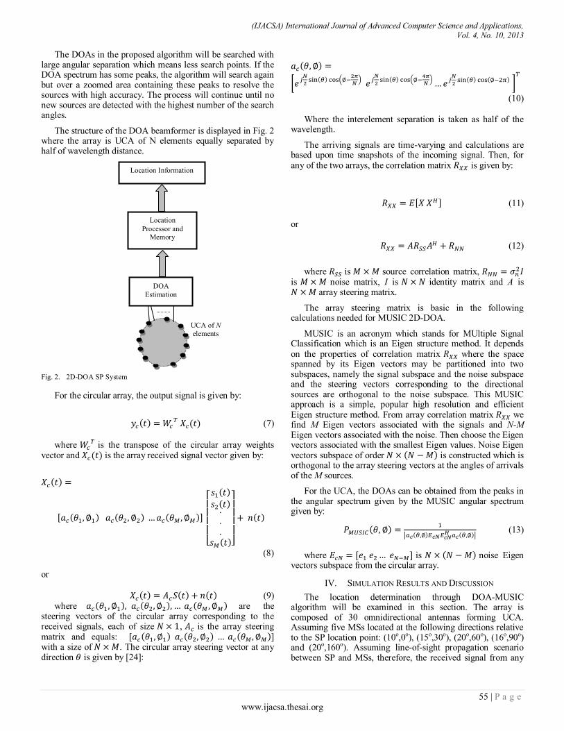
(IJACSA) International Journal of Advanced Computer Science and Applications, Vol. 4, No. 10, 2013
55 | P a g e www.ijacsa.thesai.org
The DOAs in the proposed algorithm will be searched with large angular separation which means less search points. If the DOA spectrum has some peaks, the algorithm will search again but over a zoomed area containing these peaks to resolve the sources with high accuracy. The process will continue until no new sources are detected with the highest number of the search angles.
The structure of the DOA beamformer is displayed in Fig. 2 where the array is UCA of N elements equally separated by half of wavelength distance.
Fig. 2. 2D-DOA SP System
For the circular array, the output signal is given by:
(7)
where is the transpose of the circular array weights
vector and is the array received signal vector given by:
(8)
or
(9) where are the
steering vectors of the circular array corresponding to the received signals, each of size , is the array steering matrix and equals: with a size of . The circular array steering vector at any direction is given by [24]:
(10)
Where the interelement separation is taken as half of the
wavelength.
The arriving signals are time-varying and calculations are based upon time snapshots of the incoming signal. Then, for any of the two arrays, the correlation matrix is given by:
(11)
or
(12)
where is source correlation matrix,
is noise matrix, I is identity matrix and A is array steering matrix.
The array steering matrix is basic in the following calculations needed for MUSIC 2D-DOA.
MUSIC is an acronym which stands for MUltiple Signal Classification which is an Eigen structure method. It depends on the properties of correlation matrix where the space spanned by its Eigen vectors may be partitioned into two subspaces, namely the signal subspace and the noise subspace and the steering vectors corresponding to the directional sources are orthogonal to the noise subspace. This MUSIC approach is a simple, popular high resolution and efficient Eigen structure method. From array correlation matrix we find M Eigen vectors associated with the signals and N-M Eigen vectors associated with the noise. Then choose the Eigen vectors associated with the smallest Eigen values. Noise Eigen vectors subspace of order is constructed which is orthogonal to the array steering vectors at the angles of arrivals of the M sources.
For the UCA, the DOAs can be obtained from the peaks in the angular spectrum given by the MUSIC angular spectrum given by:
(13)
where is noise Eigen
vectors subspace from the circular array.
IV. SIMULATION RESULTS AND DISCUSSION
The location determination through DOA-MUSIC algorithm will be examined in this section. The array is composed of 30 omnidirectional antennas forming UCA. Assuming five MSs located at the following directions relative to the SP location point: (10o,0o), (15o,30o), (20o,60o), (16o,90o) and (20o,160o). Assuming line-of-sight propagation scenario between SP and MSs, therefore, the received signal from any
UCA of N
elements
DOA
Estimation
Location Information
Location
Processor and Memory
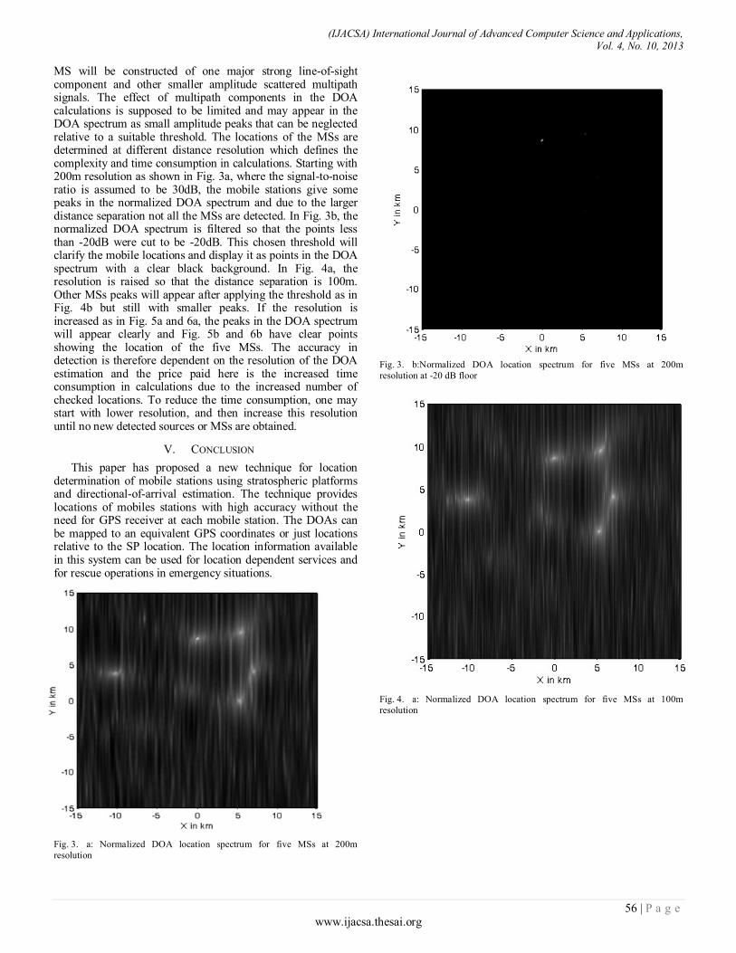
(IJACSA) International Journal of Advanced Computer Science and Applications, Vol. 4, No. 10, 2013
56 | P a g e www.ijacsa.thesai.org
MS will be constructed of one major strong line-of-sight component and other smaller amplitude scattered multipath signals. The effect of multipath components in the DOA calculations is supposed to be limited and may appear in the DOA spectrum as small amplitude peaks that can be neglected relative to a suitable threshold. The locations of the MSs are determined at different distance resolution which defines the complexity and time consumption in calculations. Starting with 200m resolution as shown in Fig. 3a, where the signal-to-noise ratio is assumed to be 30dB, the mobile stations give some peaks in the normalized DOA spectrum and due to the larger distance separation not all the MSs are detected. In Fig. 3b, the normalized DOA spectrum is filtered so that the points less than -20dB were cut to be -20dB. This chosen threshold will clarify the mobile locations and display it as points in the DOA spectrum with a clear black background. In Fig. 4a, the resolution is raised so that the distance separation is 100m. Other MSs peaks will appear after applying the threshold as in Fig. 4b but still with smaller peaks. If the resolution is increased as in Fig. 5a and 6a, the peaks in the DOA spectrum will appear clearly and Fig. 5b and 6b have clear points showing the location of the five MSs. The accuracy in detection is therefore dependent on the resolution of the DOA estimation and the price paid here is the increased time consumption in calculations due to the increased number of checked locations. To reduce the time consumption, one may start with lower resolution, and then increase this resolution until no new detected sources or MSs are obtained.
V. CONCLUSION
This paper has proposed a new technique for location determination of mobile stations using stratospheric platforms and directional-of-arrival estimation. The technique provides locations of mobiles stations with high accuracy without the need for GPS receiver at each mobile station. The DOAs can be mapped to an equivalent GPS coordinates or just locations relative to the SP location. The location information available in this system can be used for location dependent services and for rescue operations in emergency situations.
Fig. 3. a: Normalized DOA location spectrum for five MSs at 200m
resolution
Fig. 3. b:Normalized DOA location spectrum for five MSs at 200m
resolution at -20 dB floor
Fig. 4. a: Normalized DOA location spectrum for five MSs at 100m
resolution
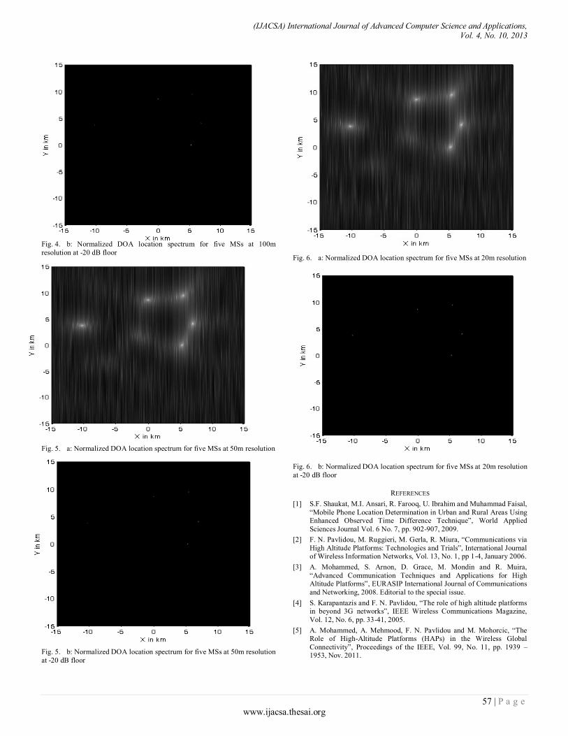
(IJACSA) International Journal of Advanced Computer Science and Applications, Vol. 4, No. 10, 2013
57 | P a g e www.ijacsa.thesai.org
Fig. 4. b: Normalized DOA location spectrum for five MSs at 100m
resolution at -20 dB floor
Fig. 5. a: Normalized DOA location spectrum for five MSs at 50m resolution
Fig. 5. b: Normalized DOA location spectrum for five MSs at 50m resolution
at -20 dB floor
Fig. 6. a: Normalized DOA location spectrum for five MSs at 20m resolution
Fig. 6. b: Normalized DOA location spectrum for five MSs at 20m resolution
at -20 dB floor
REFERENCES
[1] S.F. Shaukat, M.I. Ansari, R. Farooq, U. Ibrahim and Muhammad Faisal,
“Mobile Phone Location Determination in Urban and Rural Areas Using Enhanced Observed Time Difference Technique”, World Applied
Sciences Journal Vol. 6 No. 7, pp. 902-907, 2009.
[2] F. N. Pavlidou, M. Ruggieri, M. Gerla, R. Miura, “Communications via
High Altitude Platforms: Technologies and Trials”, International Journal of Wireless Information Networks, Vol. 13, No. 1, pp 1-4, January 2006.
[3] A. Mohammed, S. Arnon, D. Grace, M. Mondin and R. Muira,
“Advanced Communication Techniques and Applications for High Altitude Platforms”, EURASIP International Journal of Communications
and Networking, 2008. Editorial to the special issue.
[4] S. Karapantazis and F. N. Pavlidou, “The role of high altitude platforms in beyond 3G networks”, IEEE Wireless Communications Magazine,
Vol. 12, No. 6, pp. 33-41, 2005.
[5] A. Mohammed, A. Mehmood, F. N. Pavlidou and M. Mohorcic, “The Role of High-Altitude Platforms (HAPs) in the Wireless Global
Connectivity”, Proceedings of the IEEE, Vol. 99, No. 11, pp. 1939 – 1953, Nov. 2011.

(IJACSA) International Journal of Advanced Computer Science and Applications, Vol. 4, No. 10, 2013
58 | P a g e www.ijacsa.thesai.org
[6] J. Kim, D. Lee, J. Ahn, D. S. Ahn and B. J. Ku, “Is HAPS Viable for the
Next-Generation Telecommunication Platforms in Koria”, EURASIP Journal on Wireless Communications and Networking, Vol. 2008, doi:
1155/2008/596383, 2008.
[7] M. Dessouky, H. Sharshar, Y. Albagory, “Improving The Cellular
Coverage from A High Altitude Platform by Novel Tapered Beamforming Technique”, Journal of Electromagnetic Waves and
Applications, JEMWA, Vol.21, No.13, pp. 1721 –1731, 2007.
[8] S. Aljahdali, M. Nofal and Y. Albagory, “Geometrical Correction for Cell Deployment in Stratospheric Cellular Systems”, Progress In
Electromagnetics Research C, Vol. 29, pp. 83-96, 2012.
[9] M. Nofal, S. Aljahdali and Y. Albagory, “Tapered Beamforming for Concentric Ring Arrays”, AEU International Journal of Electronics and
Communications, Vol. 67, No. 1, pp. 58-63, 2013.
[10] Y. Albagory, M. Dessouky, H. Sharshar, “An Approach for Low Sidelobe Beamforming in Uniform Concentric Circular Arrays”,
International Journal of Wireless Personal Communications, Vol. 43, No. 4, pp. 1363-1368, 2007.
[11] P. Pace and G. Aloi, “Disaster Monitoring and Mitigation using
Aerospace Technologies and Integrated Telecommunication Networks”, IEEE Aerospace and Electronic Systems Magazine, Vol. 23, No. 4, pp.
3-9, April 2008.
[12] N.J. Li, J.F. Gu, P. Wei, “2-D DOA estimation via matrix partition and stacking technique”, EURASIP J Adv Signal Process 2009(53), 1–8
(2009).
[13] C.P. Mathews, M.D. Zoltowski, “Eigenstructure techniques for 2-D
angle estimation with uniform circular arrays”, IEEE Trans Signal Process 42(9), 2395–2407 (1994). Publisher Full Text
[14] M. Pesavento, J.F. Böhme, “Direction of arrival estimation in uniform
circular arrays composed of directional elements”, Proc Sensor Array and Multichannel Signal Processing Workshop, 503–507 (2002)
[15] R. Goossens, H. Rogier, “A hybrid UCA-RARE/Root-MUSIC approach
for 2-D direction of arrival estimation in uniform circular arrays in the presence of mutual coupling”, IEEE Trans Antennas Propag 55(3), 841–
849 (2007)
[16] T.T. Zhang, Y.L. Lu, H.T. Hui, “Compensation for the mutual coupling effect in uniform circular arrays for 2D DOA estimations employing the
maximum likelihood technique”, IEEE Trans Aerosp Electron Syst 44(3), 1215–1221 (2008)
[17] W. Buhong, H. Hontat, L. Mookseng, “Decoupled 2D direction of
arrival estimation using compact uniform circular arrays in the presence of elevation-dependent mutual coupling”, IEEE Trans Antennas
Propag 58(3), 747–755 (2010)
[18] J. Xie, Z. He, H. Li and J. Li, “2D DOA estimation with sparse uniform
circular arrays in the presence of mutual coupling”, EURASIP Journal on Advances in Signal Processing 2011, 2011:127.
[19] F. L. Liu, “Study on parameter estimation algorithms for mulitpath signals in wireless networks”, Doctoral Dissertation, Northeastern
University, Shenyang, China, 2005.
[20] Y. T. Wu, G. S. Liao and H. C. So, “A fast algorithm for 2-D direction-of-arrival estimation”, Signal Processing, vol.83, pp.1827-1831, 2003.
[21] T. Kuroda, N. Kikuma and N. Inagaki, “DOA estimation and pairing
method in 2D-ESPRIT using triangular antenna array”, Electronics and Communications, vol.86, no.6, pp.59-68, 2003.
[22] L. Wei, and Y. Hua, A further remark on the shifted cross array for
estimating 2-D directions of wave arrival, IEEE Transactions on Signal Processing, vol.40, no.1, pp.493-497, 1993.
[23] Y. M. Chen, J. H. Lee and C. C. Yeh, “Two-dimensional angle-of-
arrival estimation for uniform plannar arrays with sensor position errors”, IEE Proceedings, vol.140, no.2, pp.37-42, 1993.
[24] C. P. Mathews, and M. D. Zoltowski, “Eigenstructure techniques for 2-D
angle estimation with uniform circular arrays”, IEEE Transactions on Signal Processing, vol.42, no.9, pp.2395-2407, 1994.
[25] T. H. Liu, and J. M. Mendel, “Azimuth and elevation direction finding using arbitrary array geometries”, IEEE Transactions on Signal Process,
vol.46, no.7, pp.2061-2065, 1998.
[26] Y. Dong, Y. T. Wu and G. S. Liao, “A novel method for estimating 2-D DOA”, Journal of Xidian University, vol.30, no.5, pp.569-573, 2003.
[27] T. Kuroda, N. Kikuma and N. Inagaki, “DOA estimation and pairing
method in 2D-ESPRIT using triangular antenna array”, Electrons and Communications, vol.86, no.6, pp.1505-1513, 2003.
[28] A. J. Van der Veen, P. B. Ober and E. F. Deprettere, “Azimuth and
elevation computation in high resolution DOA estimation”, IEEE Transactions on Signal Processing, vol.40, no.7, pp.1828-1832, 1992.
[29] T. Filik and T. Engin Tuncer, “2-D Paired Direction-Of-Arrival Angle
Estimation With Two Parallel Uniform Linear Arrays”, International Journal of Innovative Computing, Information and Control Volume 7,
Number 6, pp. 3269-3279, June 2011
[30] Y. Hua, T.K. Sarkar, D.D. Weiner, “An L-shaped array for estimating 2-D directions of wave arrival”, IEEE Trans. Antennas Propagation 39 (2)
(1991) 143–146.
[31] Q. Cheng, Y. Hua, “Further study of the pencil-MUSIC algorithm”,
IEEE Trans. Aerospace Electronic Systems 32 (1) (1996) 284–299.
[32] Ping TAN, “Study of 2D DOA Estimation for Uniform Circular Array in Wireless Location System”, International Journal of Computer Network
and Information Security, 2010, 2, 54-60.
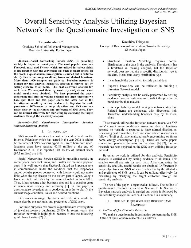
(IJACSA) International Journal of Advanced Computer Science and Applications, Vol. 4, No. 10, 2013
59 | P a g e www.ijacsa.thesai.org
Overall Sensitivity Analysis Utilizing Bayesian
Network for the Questionnaire Investigation on SNS
Tsuyoshi Aburai†
Graduate School of Policy and Management,
Doshisha University, Kyoto, Japan
Kazuhiro Takeyasu
College of Business Administration, Tokoha University,
Shizuoka, Japan
Abstract—Social Networking Service (SNS) is prevailing
rapidly in Japan in recent years. The most popular ones are
Facebook, mixi, and Twitter, which are utilized in various fields
of life together with the convenient tool such as smart-phone. In
this work, a questionnaire investigation is carried out in order to
clarify the current usage condition, issues and desired functions.
More than 1,000 samples are gathered. Bayesian network is
utilized for this analysis. Sensitivity analysis is carried out by
setting evidence to all items. This enables overall analysis for
each item. We analyzed them by sensitivity analysis and some
useful results were obtained. We have presented the paper
concerning this. But the volume becomes too large, therefore we
have split them and this paper shows the latter half of the
investigation result by setting evidence to Bayesian Network
parameters. Differences in usage objectives and SNS sites are
made clear by the attributes and preference of SNS users. They
can be utilized effectively for marketing by clarifying the target customer through the sensitivity analysis.
Keywords—SNS; Questionnaire Investigation; Bayesian
Network; Sensitivity Analysis
I. INTRODUCTION
SNS means the services to construct social network on the Internet. Friendster which has started in the year 2002 is said to be the father of SNS. Various typed SNS were born ever since. Japanese users have reached 42.89 million at the end of December 2011. It is reported that 45.1% of Internet users (95.1 million) use SNS.
Social Networking Service (SNS) is prevailing rapidly in recent years. Facebook, mixi, and Twitter are the most popular ones. It is well known that Facebook played an important role in communication under the condition that the telephones and/or cellular phones connected with Internet could not make links when the big disaster hit the eastern part of Japan. Google launched forth into SNS by the name Google+ in June 2011. Thus, it has become a hot business spot and it is exerting great influence upon society and economy [1]. In this paper, a questionnaire investigation is conducted in order to clarify the current usage condition, issues and desired functions.
Differences in usage objectives and SNS sites would be made clear by the attributes and preference of SNS users.
For these purposes, we created a questionnaire investigation of jewelry/accessory purchasing (SNS). In recent years, the Bayesian network is highlighted because it has the following good characteristics [2] [3].
Structural Equation Modeling requires normal distribution to the data in the analysis. Therefore, it has a limitation in making analysis, but the Bayesian network does not require a specific distribution type to the data. It can handle any distribution type.
It can handle the data which include partial data.
Expert’s know-how can be reflected in building a Bayesian Network model.
Sensitivity analysis can be easily performed by settling evidence. We can estimate and predict the prospective purchaser by that analysis.
It is a probability model having a network structure. Related items are connected with directional link. Therefore, understanding becomes easy by its visual chart.
This research utilizes the Bayesian network to analyze SNS users’ current usage conditions, issues and desired functions because no variable is required to have normal distribution. Reviewing past researches, there are some related researches as follows. Tsuji et al. have analyzed preference mining on future home energy consumption [4] [5]. There are some papers concerning purchase behavior in the shop [6] [7], but no research has been reported on the SNS users utilizing Bayesian network.
Bayesian network is utilized for this analysis. Sensitivity analysis is carried out by setting evidence to all items. This enables overall analysis for each item. After conducting the sensitivity analysis, useful results are obtained. Differences in usage objectives and SNS sites are made clear by the attributes and preference of SNS users. It can be utilized effectively for marketing by clarifying the target customer through the sensitivity analysis.
The rest of the paper is organized as follows. The outline of questionnaire research is stated in Section 2. In Section 3, Bayesian network analysis is carried out which is followed by the sensitivity analysis in Section 4. Section 5 is a summary.
II. OUTLINE OF QUESTIONNAIRE RESEARCH AND
EXAMINEES
A. Outline of Questionnaire Research
We make a questionnaire investigation concerning the SNS. Outline of questionnaire research is as follows.
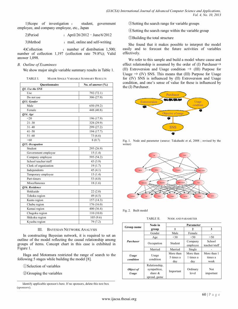
(IJACSA) International Journal of Advanced Computer Science and Applications, Vol. 4, No. 10, 2013
60 | P a g e www.ijacsa.thesai.org
1)Scope of investigation : student, government employee, and company employee, etc., Japan
2)Period :April/26/2012–June/6/2012
3)Method :mail, online and self-writing
4)Collection :number of distribution 1,500; number of collection 1,197 (collection rate 79.8%); Valid answer 1,098.
B. Outline of Examinees
We show major single variable summary results in Table 1.
TABLE I. MAJOR SINGLE VARIABLE SUMMARY RESULTS
Questionnaire No. of answer (%)
Q1. Use the SNS
Use 792 (72.1)
Do not use 306 (27.9)
Q13. Gender
Male 650 (59.2)
Female 448 (40.8)
Q14. Age
<20 196 (17.9)
21–30 328 (29.9)
31–40 299 (27.2)
41–50 194 (17.7)
51–60 73 (6.6)
>60 8 (0.7)
Q15. Occupation
Student 295 (26.9)
Government employee 15 (1.4)
Company employee 595 (54.2)
School teacher/staff 43 (3.9)
Clerk of organization 19 (1.7)
Independents 45 (4.1)
Temporary employee 15 (1.4)
Part-timers 53 (4.8)
Miscellaneous 18 (1.6)
Q16. Residence
Hokkaido 22 (2.0)
Tohoku region 49 (4.5)
Kanto region 157 (14.3)
Chubu region 176 (16.0)
Kansai region 400 (36.4)
Chugoku region 110 (10.0)
Shikoku region 105 (9.6)
Kyushu region 79 (7.2)
III. BAYESIAN NETWORK ANALYSIS
In constructing Bayesian network, it is required to set an outline of the model reflecting the causal relationship among groups of items. Concept chart in this case is exhibited in Figure 1.
Haga and Motomura restricted the range of search to the following 5 stages while building the model [8].
①Selection of variables
②Grouping the variables
③Setting the search range for variable groups
④Setting the search range within the variable group
⑤Building the total structure
She found that it makes possible to interpret the model easily and to forecast the future activities of variables effectively.
We refer to this sample and build a model where cause and
effect relationship is assumed by the order of (I) Purchaser⇒
(II) Extroversion and Usage condition ⇒ (III) Purpose for
Usage ⇒ (IV) SNS. This means that (III) Purpose for Usage for (IV) SNS is influenced by (II) Extroversion and Usage condition, and one’s sense of value for these is influenced by the (I) Purchaser.
Fig. 1. Node and parameter (source: Takahashi et al, 2008 ; revised by the writer)
Fig. 2. Built model
TABLE II. NODE AND PARAMETER
Group name Node in
group
Parameter
1 2 3
Purchaser
Gender Male Female -
Age <30 <50 >50
Occupation Student Company
employee
School
teacher/staff
Married Married Single -
Usage
condition
Usage
condition
More than
5 times a
day
More than
1 times a
day
More than 1
times a
week
Object of
Usage
Relationship,
sympathize,
share &
spread, game
Important Ordinary
level
Not
important
Identify applicable sponsor/s here. If no sponsors, delete this text box
(sponsors).

(IJACSA) International Journal of Advanced Computer Science and Applications, Vol. 4, No. 10, 2013
61 | P a g e www.ijacsa.thesai.org
Extroversion Holidays Outdoor Indoor
Cannot
choose
either
SNS
Facebook,
mixi, Twitter,
Google+,
YouTube,
Mobage,
Ameba
Use Do not
use -
Group
name Node in group
Parameter
4 5 6
Purchaser
Gender - - -
Age - - -
Occupation Independents Part-timers Others
Married - - -
Usage
condition
Usage
condition
Less than
that - -
Object of
Usage
Relationship,
sympathize,
share & spread,
game
- - -
Extroversion Holidays - - -
SNS
Facebook,
mixi, Twitter,
Google+,
YouTube,
Mobage,
Ameba
- - -
We used BAYONET software (http://www.msi.co.jp/BAYONET/). When plural nodes exist in the same group, the causal relationship is hard to set a priori. In that case, the BAYONET system sets the sequence automatically utilizing AIC standard. Node and parameter of Figure 2 are exhibited in Table 2.
IV. SENSITIVITY ANALYSIS
Now, posterior probability is calculated by setting evidence as, for example, 1.0. Comparing Prior probability and Posterior probability, we can seek the change and confirm the instruction for purchasing. We set evidence to all parameters. Therefore the analysis volume becomes too large.
In this paper, we pick up half of the total cases and make analysis. In this paper, detailed analysis is conducted for the objective of usage items, Extroversion items and SNS site items, where nodes we analyze here are “Relationship”, “Sympathize”, “Share & Spread”, “Game”, “Holidays” and “SNS site”. The first half part is analyzed in the previous paper.
As stated above, we set evidence for each parameter, and the calculated posterior probability is exhibited in Appendix Table A. The value of “Posterior probability – Prior probability” (we call this “Difference of probability” hereafter) is exhibited in Appendix Table B. The sensitivity analysis is executed by mainly using this table. It is well known that difference of probability becomes small as the node becomes distant [9].
Here, we pick up major parameters by the distance of node [9].
Node separated by 1 class: Select major parameter of which absolute value of difference of probability is more than 0.02
Node separated by 2 class: Select major parameter of which absolute value of difference of probability is more than 0.005
Node separated by 3 class: Select major parameter of which absolute value of difference of probability is more than 0.001
For the sensitivity analysis of SNS site, only “Use” is analyzed.
In order to assist the definite decision making for the marketing plan, “Less than that” in “Usage condition”, “Ordinary” in “Objective of usage” and “Cannot choose either” in “Extroversion” are deleted from the selection.
The larger one for the change of value is selected in “Objective of usage” by comparing “Important” and “Not”. Furthermore, when the volume of change in “Not use” of SNS is greater than those in “Use”, it is not selected.
In selecting parameters, negative value does not necessarily have distinct meaning, therefore we mainly pick up positive value in the case meaning is not clear.
Now we examine each case.
A. Sensitively Analysis for “Relationship”
1) Setting evidence to “Important”
①Node separated by 1 class.
Usage condition More than 5 times a day 0.055
②Node separated by 2 class
Occupation Student 0.007
③Node separated by 3 class
No corresponding data.
We can observe that “Those who put importance concerning, relationship are students who use more than 5 times a day”.
2) Setting evidence to “Not important”
① Node separated by 1 class
Usage condition More than 1 times a week 0.094
Extroversion Indoor 0.029
Google+ Use 0.102
Mobage Use 0.109
Ameba Use 0.086
②Node separated by 2 class
Gender Male 0.020
Female 0.023
Age ―50 0.027
50― 0.042

(IJACSA) International Journal of Advanced Computer Science and Applications, Vol. 4, No. 10, 2013
62 | P a g e www.ijacsa.thesai.org
Occupation Company Employee 0.019
School Teacher/Staff 0.036
Independents 0.019
Part-timers 0.037
Married Married 0.027
Single 0.016
Sympathize Not 0.025
Share & Spread Not 0.046
Game Not 0.019
③Node separated by 3 class
No corresponding data.
We can observe that “Those who do not put importance concerning relationship, are indoor typed Company Employer, School Teacher/Staff, Independents, Part-timers of married under 50 or over 50 or single Male/Female who use more than 1 times a week, do not esteem Sympathize, Share & Spread, Game, use Google+, Mobage and Ameba”.
B. Sensitivity Analysis for “Sympathize”
1) Setting Evidence to “Important”
①Node separated by 1 class
Usage condition More than 5 times a day 0.042
Extroversion Indoor 0.051
Google+ Use 0.046
Ameba Use 0.022
②Node separated by 2 class
Occupation Student 0.011
③Node separated by 3 class
No corresponding data. We can observe that “Those who put importance
concerning sympathize, are indoor typed students who use more than 5 times a day, use Google+ and Ameba”.
2) Setting evidence to “Not important”
①Node separated by 1 class
Usage condition More than 1 times a week 0.026
Extroversion Outdoor 0.062
Facebook Use 0.036
②Node separated by 2 class
Gender Male 0.006
Female 0.005
Age ―50 0.012
50― 0.021
Occupation Company Employee 0.006
School Teacher/Staff 0.016
Independents 0.008
Part-timers 0.016
Married Married 0.017
Relationship Not 0.015
Share & Spread Not 0.018
Game Not 0.008
③Node separated by 3 class
No corresponding data We can observe that “Those who do not put importance
concerning sympathize, are outdoor typed married Male/Female of Company Employee, School Teacher/Staff, Independents, Part-timers under 50 or over 50, do not esteem Relationship, Share & Spread, nor Game, use Facebook”.
C. Sensitivity Analysis for “Share & Spread”
1) Setting evidence to “Important”
①Node separated by 1 class
Usage condition More than 5 times a day 0.072
②Node separated by 2 class
Occupation Student 0.013
③Node separated by 3 class
No corresponding data. We can observe that “Those who put importance
concerning share & spread are students who use more than 5 times a day”.
2) Setting evidence to “Not important”
① Node separated by 1 class
Usage condition More than 1 times a week 0.064
Extroversion Outdoor 0.026
Indoor 0.026
Google+ Use 0.124
Mobage Use 0.128
Ameba Use 0.096
②Node separated by 2 class
Gender Male 0.022
Female 0.023
Age ―50 0.029
50― 0.056
Occupation Company Employee 0.020
School Teacher/Staff 0.053
Independents 0.020
Part-timers 0.038
Married Married 0.032
Relationship Not 0.062
Sympathize Not 0.030
Game Not 0.021
③Node separated by 3 class
No corresponding data. We can observe that “Those who do not put importance
concerning share & spread, are Outdoor/Indoor typed Company Employee, School Teacher/Staff, Independents, Part-timers of married Male/Female under 50 or over 50, do not esteem Relationship, Sympathize, nor Game, use Google+, Mobage and Ameba”.

(IJACSA) International Journal of Advanced Computer Science and Applications, Vol. 4, No. 10, 2013
63 | P a g e www.ijacsa.thesai.org
D. Sensitivity Analysis for “Game”
1) Setting evidence to “Important”
①Node separated by 1 class
Usage condition More than 5 times a day 0.085
Extroversion Indoor 0.078
Mobage Use 0.150
②Node separated by 2 class
Age ―30 0.014
Occupation Student 0.026
③Node separated by 3 class
No corresponding data. We can observe that “Those who put importance
concerning Game, are indoor typed students under 30 who use more than 5 times a day”.
2) Setting evidence to “Not important”
①Node separated by 1 class
Usage condition More than 1 times a day 0.042
Extroversion Outdoor 0.027
Facebook Use 0.052
②Node separated by 2 class
Occupation Company Employee 0.005
③Node separated by 3 class
No corresponding data We can observe that “Those who do not put importance
concerning Game, are outdoor typed Company Employee who use more than 1 times a day, use Facebook”.
E. Sensitivity Analysis for “Extroversion”
1) Setting evidence to “Outdoor”
①Node separated by 1 class
Married Married 0.074
Sympathize Not 0.054
Game Not 0.022
②Node separated by 2 class
Gender Male 0.005
Age ―50 0.031
50― 0.040
③Node separated by 3 class
Occupation Independents 0.027
Usage condition More than 1 times a week 0.011
We can observe that “Those who prefer outdoor concerning extroversion, are Independent Male over 50 or under 50 who use more than 1 times a week, esteem Sympathize and Game”.
2) Setting evidence to “Indoor”
①Node separated by 1 class
Married Single 0.060
Sympathize Important 0.051
Game Important 0.095
②Node separated by 2 class
Gender Female 0.010
Age ―30 0.041
Google+ Use 0.008
You tube Use 0.006
Mobage Use 0.026
Ameba Use 0.008
③Node separated by 3 class
Occupation Student 0.040
Usage condition More than 5 times a day 0.016
We can observe that “Those who prefer indoor concerning extroversion, are single students under 30 who use more than 5 times a day, esteem Sympathize and Game, use Google+, You tube, Mobage and Ameba”.
F. Sensitivity Analysis for “Facebook”
1) Setting evidence to “Use”
①Node separated by 1 class
Relationship Important 0.026
Sympathize Not 0.045
Share & Spread Important 0.031
Game Not 0.065
②Node separated by 2 class
Usage condition More than 1 times a day 0.006
③Node separated by 3 class
No corresponding data. We can observe that “Those who use Facebook, use more
than 1 times a day, esteem Relationship, and Share & Spread, while do not esteem Sympathize nor Game”.
G. Sensitivity Analysis for “mixi”
1) Setting evidence to “Use”
①Node separated by 1 class
Relationship Important 0.063
Sympathize Important 0.033
Share & Spread Important 0.023
Game Important 0.058
Extroversion Outdoor 0.032
Indoor 0.032
②Node separated by 2 class
Usage condition More than 5 times a day 0.048
More than 1 times a day 0.037
More than 1 times a week 0.016
Facebook Use 0.036
Twitter Use 0.037
You tube Use 0.033
③Node separated by 3 class
Gender Male 0.033
Female 0.032
Age ―30 0.038

(IJACSA) International Journal of Advanced Computer Science and Applications, Vol. 4, No. 10, 2013
64 | P a g e www.ijacsa.thesai.org
―50 0.031
50― 0.027
Occupation Student 0.040
Company Employee 0.033
School Teacher/Staff 0.028
Independents 0.033
Part-timers 0.028
Married Married 0.031
Single 0.034
We can observe that “Those who use mixi, are indoor/outdoor typed Married/Single with versatile occupations in the wide spread ages, esteem Relationship, Sympathize, Share & Spread and Game, use Facebook, Twitter and You tube”.
H. Sensitivity Analysis for “Twitter”
1) Setting evidence to “Use”
①Node separated by 1 class
Relationship Important 0.046
Sympathize Important 0.063
Share & Spread Important 0.021
Game Not 0.048
Extroversion Outdoor 0.030
Indoor 0.028
②Node separated by 2 class
Usage condition More than 5 times a day 0.038
More than 1 times a day 0.035
More than 1 times a week 0.022
Facebook Use 0.034
mixi Use 0.034
You tube Use 0.031
③Node separated by 3 class
Gender Male 0.031
Female 0.030
Age ―30 0.033
―50 0.030
50― 0.027
Occupation Student 0.034
Company Employee 0.031
School Teacher/Staff 0.027
Independents 0.031
Part-timers 0.028
Married Married 0.031
Single 0.034
We can observe that “Those who use Twitter, are indoor/outdoor typed Married/Single with versatile occupations in the wide spread ages, esteem Relationship, Sympathize and
Share & Spread, while do not esteem Game, use Facebook, mixi and You tube”.
I. Sensitivity Analysis for “Google+”
1) Setting evidence to “Use”
①Node separated by 1 class
Relationship Not 0.262
Sympathize Important 0.122
Share & Spread Not 0.213
Game Important 0.084
Extroversion Outdoor 0.075
Indoor 0.090
②Node separated by 2 class
Usage condition More than 5 times a day 0.053
More than 1 times a day 0.069
More than 1 times a week 0.105
Facebook Use 0.063
You tube Use 0.082
Mobage Use 0.133
Ameba Use 0.113
③Node separated by 3 class
Gender Male 0.080
Female 0.081
Age ―30 0.071
―50 0.083
50― 0.093
Occupation Student 0.068
Company Employee 0.079
School Teacher/Staff 0.091
Independents 0.080
Part-timers 0.088
Married Married 0.083
Single 0.078
We can observe that “Those who use Google+, are indoor/outdoor typed Married/Single with versatile occupations in the wide spread ages, esteem Sympathize and Game, while do not esteem Relationship nor Share & Spread, use Facebook, mixi and You tube”.
J. Sensitivity Analysis for “You tube”
1) Setting evidence to “Use”
①Node separated by 1 class
Sympathize Important 0.034
Game Important 0.021
②Node separated by 2 class
No corresponding data.
③Node separated by 3 class
No corresponding data. We can observe that “Those who use You tube, esteem
Sympathize and Game”.

(IJACSA) International Journal of Advanced Computer Science and Applications, Vol. 4, No. 10, 2013
65 | P a g e www.ijacsa.thesai.org
K. Sensitivity Analysis for “Mobage”
1) Setting evidence to “Use”
①Node separated by 1 class
Relationship Not 0.260
Sympathize Important 0.097
Share & Spread Not 0.210
Game Important 0.216
Extroversion Outdoor 0.076
Indoor 0.104
②Node separated by 2 class
Usage condition More than 5 times a day 0.070
More than 1 times a day 0.063
More than 1 times a week 0.105
Google+ Use 0.128
You tube Use 0.086
Ameba Use 0.119
③Node separated by 3 class
Gender Male 0.083
Female 0.083
Age ―30 0.076
―50 0.084
50― 0.094
Occupation Student 0.075
Company Employee 0.080
School Teacher/Staff 0.093
Independents 0.082
Part-timers 0.089
Married Married 0.084
Single 0.083
We can observe that “Those who use Mobage, are indoor/outdoor typed Married/Single with versatile occupations in the wide spread ages, esteem Sympathize and Game, while do not esteem Relationship, nor Share & Spread, use Google+, You tube and Ameba”.
L. Sensitivity Analysis for “Ameba”
1) Setting evidence to “Use”
①Node separated by 1 class
Relationship Not 0.244
Sympathize Important 0.113
Share & Spread Not 0.192
Game Important 0.112
Extroversion Outdoor 0.085
Indoor 0.095
②Node separated by 2 class
Usage condition More than 5 times a day 0.070
More than 1 times a day 0.076
More than 1 times a week 0.107
Google+ Use 0.122
You tube Use 0.089
Mobage Use 0.130
③Node separated by 3 class
Gender Male 0.087
Female 0.088
Age ―30 0.081
―50 0.089
50― 0.097
Occupation Student 0.079
Company Employee 0.086
School Teacher/Staff 0.095
Independents 0.087
Part-timers 0.093
Married Married 0.089
Single 0.086
We can observe that “Those who use Ameba, are indoor/outdoor typed Married/Single with versatile occupations in the wide spread ages, esteem Sympathize and Game, while do not esteem Relationship nor Share & Spread, use Google+, You tube and Mobage”.
V. REMARKS
Setting evidence to all parameters, we can obtain following findings.
If the model is spread toward lower level with branch, observation data tends to be small. Therefore ripple effect becomes small as it passes through node to node.
The change of differences of probability (ie.“Posterior probability - Prior probability”) decreases exponentially as a node is separated from the source node where evidence is set. To cope with this, such methods as Reinforcement Learning, transformation by logarithmic scale would be effective. As the depth of a model becomes deep, above phenomenon occurs, therefore model building of shallow depth is required.
1) We could confirm that those who esteem Relationship,
Sympathize, Share & Spread and Game are relatively young
and they use them frequently.
2) Those who esteem Sympathize have a tendency to use
Google+ and Ameba, while they do not use Facebook.
Google+ has a good characteristic in group function and
Ameba is often utilized as a diary. Users sympathize these
sites rather than Facebook, where it makes public the current
information. Furthermore users feel much more sympathy than
Facebook.
This may be because mixi has a good diary function.
3) These who do not esteem Game of outdoor typed
company employee often use Facebook.
4) Young people of indoor type use SNS frequently than
those of outdoor type.

(IJACSA) International Journal of Advanced Computer Science and Applications, Vol. 4, No. 10, 2013
66 | P a g e www.ijacsa.thesai.org
5) Correlation between usage objective and SNS site is
shown in Table 3. We can observe that the users of Facebook, mixi, Twitter
esteem Relationship and Share & Spread.
The users of Facebook and Twitter do not esteem Game.
As could be seem from the investigation results of the former half, users of Google+, Mobage, Ameba have the same usage objective and use them simultaneously.
TABLE III. CORRELATION BETWEEN USAGE OBJECTIVE AND SNS SITE
Relationship Sympathize Share &
Spread Game
Facebook ○ × ○ ×
mixi ○ ○ ○ ○
Twitter ○ ○ ○ ×
Google+ × ○ × ○
You Tube - ○ - ○
Mobage × ○ × ○
Ameba × ○ × ○
We could obtain the interesting insight by classifying the volume of change.
Further investigation should be executed hereafter.
VI. CONCLUSION
Social Networking Service (SNS) is prevailing rapidly in Japan in recent years. In this work, a questionnaire investigation was carried out in order to clarify the current usage condition, issues and desired functions. More than 1,000 samples are gathered. Bayesian network is utilized for this analysis. After conducting the sensitivity analysis, useful results are obtained. Differences in usage objectives and SNS sites were made clear by the attributes and preference of SNS users. We could observe that the users of Facebook, mixi,
Twitter esteemed Relationship and Share & Spread. While the users of Facebook and Twitter did not esteem Game.
They can be utilized effectively for marketing by clarifying the target customer through the sensitivity analysis. We could obtain the detailed results together with those of the former half.
VII. FUTURE WORKS
To confirm instructions and their results would be our next step investigation. Systematic research investigation for SNS is still on the beginning stage. Such research as this should be further developed with the increased case studies.
REFERENCES
[1] Kotler, P. and Keller, K., Brady, M., Goodman, M., and Hansen. T,
Marketing Management (2 ed.), Pearson, Harlow, UK, 2012.
[2] Neapolitan, R. E, Learning Bayesian Networks, Pearson Prentice Hall, Upper Saddle River, NJ, 2004.
[3] Neaplitan, R.E, Learning Bayesian Networks”, Artificial Intelligence,
Prentice Hall, 2008.
[4] Tsuji. H., Kojima, M., Takahashi, A., Nakano, M., Aoki, S., Inoue, S., Asari, K., and Mimura, E, Preference mining on future home energy
consumption, IEEE International Conference on Systems, Man and Cybernetics, Singapore, pp3697-3701, 2008.
[5] Takahashi. A., Aoki, S., Tsuji, H., and Inoue, S, Bayesian network for
future home energy consumption, Lecture Notes in Computer Science, 5243, pp372-379.R. Nicole, “Title of paper with only first word
capitalized,” J. Name Stand. Abbrev., in press, 2008.
[6] Tatsuoka, K., Yoshida, T., and Munemoto, J, Analysis on purchase behavior according to display way of merchandise by Bayesian network,
Journal of Architecture and Planning (Transactions of AIJ), 73(633), pp2349-2354, 2008.
[7] Tatsuoka, K., Yoshida, T., and Munemoto, J, Analysis on relationship between layout of display cases ad purchase behavior by Bayesian
network, Journal of Architecture and Planning (Transactions of AIJ), 73(634), pp2633-2638, 2008.
[8] Haga, M. and Motomura, Y, Marketing strategy and product
development using Bayesian networks, Jinko Chino Gakkai Jinko Chino Kihon Mondai Kenkyukai Shiryo, 2005, pp59-61.
[9] Takeyasu, K and Ishio, C, Questionnaire Investigation on Jewelry /
Accessory and its Analysis Utilizing Bayesian Network, Osaka Prefecture University 『Journal of Economics、Business and Law』Vol.56 No.1, pp 25-40, 2010.
APPENDIX: Table A
Name state Prior Gender Age Occupation
Male Female ―30 ―50 50― Student Company
Employee
School
Teacher/Staff Independents Part-timers
Gender Male 0.592 1.000 0.000 0.592 0.592 0.592 0.606 0.694 0.513 0.545 0.079
Female 0.408 0.000 1.000 0.408 0.408 0.408 0.394 0.306 0.487 0.455 0.921
Age
―30 0.477 0.477 0.477 1.000 0.000 0.000 0.978 0.327 0.251 0.062 0.260
―50 0.449 0.449 0.449 0.000 1.000 0.000 0.014 0.584 0.657 0.806 0.582
50― 0.075 0.074 0.074 0.000 0.000 1.000 0.008 0.090 0.092 0.133 0.158
Occupation
Student 0.267 0.276 0.260 0.553 0.008 0.028 1.000 0.000 0.000 0.000 0.000
Company Employee 0.542 0.604 0.386 0.353 0.670 0.621 0.000 1.000 0.000 0.000 0.000
School Teacher/Staff 0.040 0.037 0.051 0.022 0.062 0.052 0.000 0.000 1.000 0.000 0.000
Independents 0.042 0.043 0.052 0.006 0.084 0.083 0.000 0.000 0.000 1.000 0.000
Part-timers 0.049 0.008 0.133 0.032 0.076 0.125 0.000 0.000 0.000 0.000 1.000
Others 0.061 0.032 0.118 0.034 0.099 0.091 0.000 0.000 0.000 0.000 0.000
Married Married 0.424 0.464 0.351 0.133 0.667 0.734 0.146 0.512 0.528 0.635 0.467
Single 0.576 0.536 0.649 0.867 0.333 0.266 0.854 0.488 0.472 0.365 0.533

(IJACSA) International Journal of Advanced Computer Science and Applications, Vol. 4, No. 10, 2013
67 | P a g e www.ijacsa.thesai.org
Usage
condition
More than 5 times a
day 0.368 0.315 0.292 0.464 0.242 0.167 0.548 0.253 0.212 0.332 0.186
More than 1 times a
day 0.408 0.382 0.395 0.375 0.388 0.351 0.322 0.441 0.372 0.369 0.360
More than 1 times a
week 0.175 0.193 0.207 0.115 0.265 0.275 0.091 0.239 0.176 0.188 0.344
Less than that 0.049 0.110 0.107 0.046 0.105 0.207 0.040 0.067 0.240 0.111 0.111
Relationship
Important 0.824 0.788 0.785 0.822 0.775 0.743 0.832 0.789 0.753 0.790 0.757
Ordinary 0.102 0.118 0.119 0.100 0.124 0.141 0.094 0.118 0.138 0.117 0.132
Not 0.074 0.094 0.095 0.078 0.101 0.116 0.074 0.093 0.110 0.093 0.111
Sympathize
Important 0.385 0.368 0.368 0.389 0.358 0.345 0.396 0.365 0.353 0.367 0.353
Ordinary 0.311 0.322 0.323 0.312 0.327 0.331 0.308 0.325 0.327 0.321 0.331
Not 0.304 0.310 0.309 0.299 0.315 0.324 0.297 0.310 0.319 0.312 0.316
Share &
Spread
Important 0.614 0.582 0.580 0.616 0.573 0.538 0.627 0.584 0.541 0.584 0.561
Ordinary 0.255 0.265 0.266 0.257 0.267 0.274 0.254 0.265 0.275 0.264 0.270
Not 0.131 0.153 0.154 0.127 0.160 0.187 0.119 0.151 0.184 0.151 0.170
Game
Important 0.254 0.245 0.243 0.268 0.234 0.227 0.279 0.235 0.235 0.246 0.229
Ordinary 0.292 0.305 0.307 0.287 0.311 0.326 0.280 0.306 0.324 0.304 0.318
Not 0.454 0.449 0.450 0.445 0.455 0.447 0.441 0.459 0.441 0.450 0.453
Extroversion
Outdoor 0.311 0.316 0.301 0.274 0.342 0.350 0.275 0.322 0.324 0.338 0.316
Indoor 0.269 0.263 0.279 0.310 0.234 0.225 0.308 0.256 0.254 0.239 0.263
Cannot choose either 0.421 0.421 0.419 0.416 0.424 0.425 0.416 0.422 0.422 0.424 0.421
Facebook Use 0.634 0.619 0.619 0.625 0.619 0.610 0.626 0.622 0.610 0.620 0.614
Not 0.367 0.381 0.381 0.375 0.381 0.390 0.374 0.378 0.390 0.380 0.386
mixi Use 0.495 0.528 0.527 0.533 0.526 0.522 0.535 0.528 0.523 0.528 0.523
Not 0.505 0.472 0.473 0.467 0.474 0.478 0.465 0.472 0.477 0.472 0.477
Twitter Use 0.422 0.452 0.452 0.455 0.451 0.449 0.456 0.453 0.449 0.453 0.450
Not 0.578 0.548 0.548 0.545 0.549 0.551 0.544 0.547 0.551 0.547 0.550
Google+ Use 0.142 0.223 0.223 0.213 0.225 0.235 0.211 0.222 0.233 0.222 0.230
Not 0.858 0.777 0.777 0.787 0.775 0.765 0.789 0.778 0.767 0.778 0.770
You Tube Use 0.562 0.542 0.542 0.546 0.540 0.538 0.547 0.541 0.539 0.542 0.539
Not 0.438 0.458 0.458 0.454 0.460 0.462 0.453 0.459 0.461 0.458 0.461
Mobage Use 0.116 0.199 0.199 0.192 0.200 0.209 0.191 0.196 0.209 0.198 0.205
Not 0.884 0.801 0.801 0.808 0.800 0.791 0.809 0.804 0.791 0.802 0.795
Ameba Use 0.149 0.236 0.236 0.229 0.238 0.245 0.228 0.235 0.244 0.235 0.241
Not 0.851 0.764 0.764 0.771 0.762 0.755 0.772 0.765 0.756 0.765 0.759
Married Usage condition Relationship Sympathize Share & Spread Game
Married Single
More
than 5
times a
day
More
than 1
times a
day
More
than 1
times a
week
Important Ordinary Not Important Ordinary Not Important Ordinary Not Important Ordinary Not
0.657 0.545 0.609 0.589 0.573 0.593 0.586 0.584 0.592 0.591 0.5922 0.593 0.591 0.586 0.594 0.590 0.592
0.343 0.455 0.391 0.411 0.427 0.407 0.414 0.416 0.408 0.409 0.4078 0.407 0.409 0.414 0.406 0.410 0.408
0.152 0.709 0.677 0.470 0.305 0.493 0.425 0.415 0.499 0.466 0.462 0.497 0.467 0.421 0.512 0.456 0.472
0.717 0.257 0.283 0.460 0.591 0.436 0.487 0.494 0.431 0.458 0.460 0.433 0.456 0.489 0.419 0.464 0.453
0.131 0.034 0.040 0.070 0.105 0.071 0.088 0.090 0.070 0.077 0.078 0.069 0.077 0.089 0.068 0.079 0.074
0.094 0.394 0.430 0.225 0.146 0.277 0.245 0.241 0.283 0.262 0.263 0.279 0.265 0.245 0.297 0.259 0.262
0.636 0.437 0.409 0.598 0.593 0.516 0.512 0.508 0.510 0.520 0.517 0.516 0.515 0.509 0.494 0.517 0.525
0.054 0.034 0.027 0.043 0.041 0.041 0.049 0.049 0.041 0.043 0.044 0.040 0.044 0.050 0.040 0.045 0.042
0.071 0.029 0.029 0.038 0.067 0.044 0.055 0.058 0.044 0.048 0.048 0.044 0.048 0.056 0.044 0.049 0.046
0.065 0.051 0.033 0.052 0.096 0.056 0.069 0.072 0.056 0.061 0.061 0.055 0.061 0.069 0.055 0.062 0.059
0.080 0.055 0.072 0.045 0.055 0.066 0.070 0.072 0.067 0.067 0.068 0.066 0.068 0.071 0.070 0.068 0.065
1.000 0.000 0.310 0.420 0.509 0.410 0.442 0.446 0.399 0.423 0.433 0.407 0.422 0.447 0.390 0.429 0.424
0.000 1.000 0.690 0.580 0.491 0.590 0.558 0.554 0.601 0.577 0.567 0.593 0.578 0.553 0.610 0.571 0.576
0.247 0.366 1.000 0.000 0.000 0.344 0.160 0.179 0.358 0.270 0.283 0.364 0.274 0.147 0.424 0.245 0.284
0.383 0.376 0.000 1.000 0.000 0.398 0.342 0.236 0.375 0.384 0.368 0.383 0.378 0.347 0.298 0.379 0.416
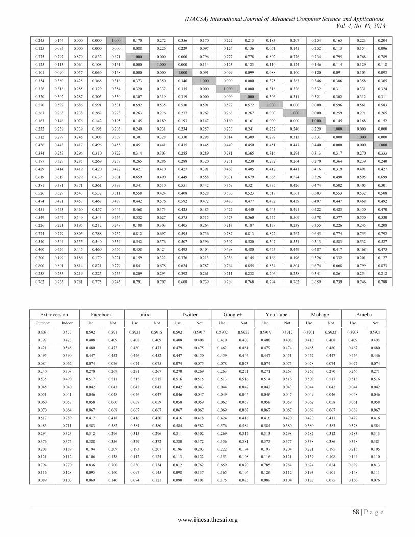
(IJACSA) International Journal of Advanced Computer Science and Applications, Vol. 4, No. 10, 2013
68 | P a g e www.ijacsa.thesai.org
0.245 0.164 0.000 0.000 1.000 0.170 0.272 0.356 0.170 0.222 0.213 0.183 0.207 0.254 0.165 0.223 0.204
0.125 0.095 0.000 0.000 0.000 0.088 0.226 0.229 0.097 0.124 0.136 0.071 0.141 0.252 0.113 0.154 0.096
0.775 0.797 0.879 0.832 0.671 1.000 0.000 0.000 0.796 0.777 0.778 0.802 0.776 0.734 0.795 0.768 0.789
0.125 0.113 0.064 0.108 0.161 0.000 1.000 0.000 0.114 0.123 0.123 0.110 0.124 0.146 0.114 0.129 0.118
0.101 0.090 0.057 0.060 0.168 0.000 0.000 1.000 0.091 0.099 0.099 0.088 0.100 0.120 0.091 0.103 0.093
0.354 0.380 0.428 0.368 0.316 0.373 0.350 0.346 1.000 0.000 0.000 0.375 0.363 0.346 0.386 0.358 0.365
0.326 0.318 0.285 0.329 0.354 0.320 0.332 0.335 0.000 1.000 0.000 0.318 0.326 0.332 0.311 0.331 0.324
0.320 0.302 0.287 0.303 0.330 0.307 0.319 0.319 0.000 0.000 1.000 0.306 0.311 0.321 0.302 0.312 0.311
0.570 0.592 0.686 0.591 0.531 0.592 0.535 0.530 0.591 0.572 0.572 1.000 0.000 0.000 0.596 0.561 0.583
0.267 0.263 0.238 0.267 0.273 0.263 0.276 0.277 0.262 0.268 0.267 0.000 1.000 0.000 0.259 0.271 0.265
0.163 0.146 0.076 0.142 0.195 0.145 0.189 0.193 0.147 0.160 0.161 0.000 0.000 1.000 0.145 0.168 0.152
0.232 0.258 0.339 0.195 0.205 0.249 0.231 0.234 0.257 0.236 0.241 0.252 0.240 0.229 1.000 0.000 0.000
0.312 0.299 0.245 0.308 0.339 0.301 0.328 0.330 0.298 0.314 0.309 0.297 0.313 0.331 0.000 1.000 0.000
0.456 0.443 0.417 0.496 0.455 0.451 0.441 0.435 0.445 0.449 0.450 0.451 0.447 0.440 0.000 0.000 1.000
0.384 0.257 0.296 0.310 0.322 0.314 0.303 0.285 0.289 0.281 0.365 0.316 0.294 0.313 0.317 0.270 0.333
0.187 0.329 0.285 0.269 0.257 0.265 0.286 0.288 0.320 0.251 0.230 0.272 0.264 0.270 0.364 0.239 0.240
0.429 0.414 0.419 0.420 0.422 0.421 0.410 0.427 0.391 0.468 0.405 0.412 0.441 0.416 0.319 0.491 0.427
0.619 0.619 0.629 0.639 0.601 0.659 0.490 0.449 0.558 0.631 0.679 0.665 0.574 0.526 0.498 0.595 0.699
0.381 0.381 0.371 0.361 0.399 0.341 0.510 0.551 0.442 0.369 0.321 0.335 0.426 0.474 0.502 0.405 0.301
0.526 0.529 0.543 0.532 0.511 0.558 0.424 0.408 0.528 0.530 0.523 0.518 0.561 0.503 0.553 0.532 0.508
0.474 0.471 0.457 0.468 0.489 0.442 0.576 0.592 0.472 0.470 0.477 0.482 0.439 0.497 0.447 0.468 0.492
0.451 0.453 0.460 0.457 0.444 0.468 0.373 0.425 0.485 0.427 0.440 0.443 0.491 0.422 0.423 0.450 0.470
0.549 0.547 0.540 0.543 0.556 0.532 0.627 0.575 0.515 0.573 0.560 0.557 0.509 0.578 0.577 0.550 0.530
0.226 0.221 0.195 0.212 0.248 0.188 0.303 0.405 0.264 0.213 0.187 0.178 0.238 0.355 0.226 0.245 0.208
0.774 0.779 0.805 0.788 0.752 0.812 0.697 0.595 0.736 0.787 0.813 0.822 0.762 0.645 0.774 0.755 0.792
0.540 0.544 0.555 0.540 0.534 0.542 0.576 0.507 0.596 0.502 0.520 0.547 0.551 0.513 0.583 0.532 0.527
0.460 0.456 0.445 0.460 0.466 0.458 0.424 0.493 0.404 0.498 0.480 0.453 0.449 0.487 0.417 0.468 0.473
0.200 0.199 0.186 0.179 0.221 0.159 0.322 0.376 0.213 0.236 0.145 0.166 0.196 0.326 0.332 0.201 0.127
0.800 0.801 0.814 0.821 0.779 0.841 0.678 0.624 0.787 0.764 0.855 0.834 0.804 0.674 0.668 0.799 0.873
0.238 0.235 0.219 0.225 0.255 0.209 0.293 0.392 0.261 0.211 0.232 0.206 0.238 0.341 0.261 0.254 0.212
0.762 0.765 0.781 0.775 0.745 0.791 0.707 0.608 0.739 0.789 0.768 0.794 0.762 0.659 0.739 0.746 0.788
Extroversion Facebook mixi Twitter Google+ You Tube Mobage Ameba
Outdoor Indoor Use Not Use Not Use Not Use Not Use Not Use Not Use Not
0.603 0.577 0.592 0.591 0.5921 0.5915 0.592 0.5917 0.5902 0.5922 0.5919 0.5917 0.5901 0.5922 0.5908 0.5921
0.397 0.423 0.408 0.409 0.408 0.409 0.408 0.408 0.410 0.408 0.408 0.408 0.410 0.408 0.409 0.408
0.421 0.548 0.480 0.472 0.480 0.473 0.479 0.475 0.462 0.481 0.479 0.474 0.465 0.480 0.467 0.480
0.495 0.390 0.447 0.452 0.446 0.452 0.447 0.450 0.459 0.446 0.447 0.451 0.457 0.447 0.456 0.446
0.084 0.062 0.074 0.076 0.074 0.075 0.074 0.075 0.078 0.073 0.074 0.075 0.078 0.074 0.077 0.074
0.240 0.308 0.270 0.269 0.271 0.267 0.270 0.269 0.263 0.271 0.271 0.268 0.267 0.270 0.266 0.271
0.535 0.490 0.517 0.511 0.515 0.515 0.516 0.515 0.513 0.516 0.514 0.516 0.509 0.517 0.513 0.516
0.045 0.040 0.042 0.043 0.042 0.043 0.042 0.043 0.044 0.042 0.042 0.043 0.044 0.042 0.044 0.042
0.051 0.041 0.046 0.048 0.046 0.047 0.046 0.047 0.049 0.046 0.046 0.047 0.049 0.046 0.048 0.046
0.060 0.057 0.058 0.060 0.058 0.059 0.058 0.059 0.062 0.058 0.058 0.059 0.062 0.058 0.061 0.058
0.070 0.064 0.067 0.068 0.067 0.067 0.067 0.067 0.069 0.067 0.067 0.067 0.069 0.067 0.068 0.067
0.517 0.289 0.417 0.418 0.416 0.420 0.416 0.418 0.424 0.416 0.416 0.420 0.420 0.417 0.422 0.416
0.483 0.711 0.583 0.582 0.584 0.580 0.584 0.582 0.576 0.584 0.584 0.580 0.580 0.583 0.578 0.584
0.294 0.323 0.312 0.296 0.315 0.296 0.311 0.302 0.269 0.317 0.313 0.298 0.282 0.312 0.283 0.313
0.376 0.375 0.388 0.356 0.379 0.372 0.380 0.372 0.356 0.381 0.375 0.377 0.338 0.386 0.358 0.381
0.208 0.189 0.194 0.209 0.193 0.207 0.196 0.203 0.222 0.194 0.197 0.204 0.221 0.195 0.215 0.195
0.121 0.112 0.106 0.138 0.112 0.124 0.113 0.122 0.153 0.108 0.116 0.121 0.159 0.108 0.144 0.110
0.794 0.770 0.836 0.700 0.830 0.734 0.812 0.762 0.659 0.820 0.785 0.784 0.624 0.824 0.692 0.813
0.116 0.128 0.095 0.160 0.097 0.145 0.098 0.137 0.165 0.106 0.126 0.112 0.193 0.101 0.148 0.111
0.089 0.103 0.069 0.140 0.074 0.121 0.090 0.101 0.175 0.073 0.089 0.104 0.183 0.075 0.160 0.076
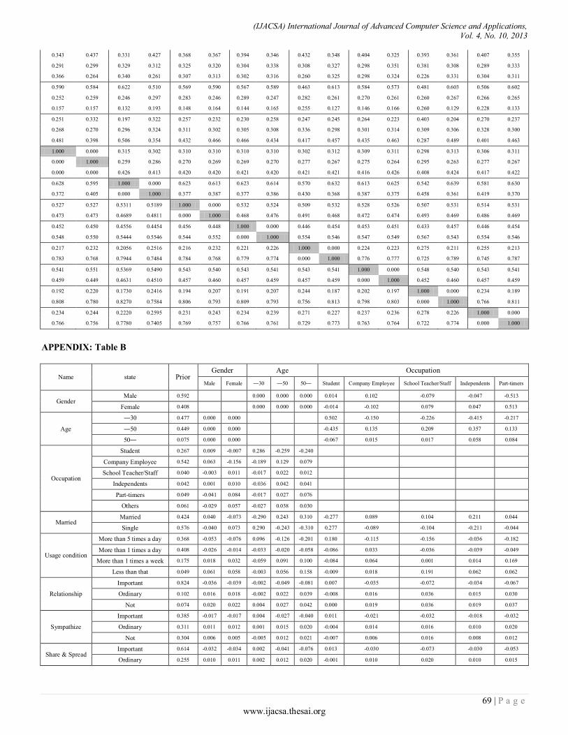
(IJACSA) International Journal of Advanced Computer Science and Applications, Vol. 4, No. 10, 2013
69 | P a g e www.ijacsa.thesai.org
0.343 0.437 0.331 0.427 0.368 0.367 0.394 0.346 0.432 0.348 0.404 0.325 0.393 0.361 0.407 0.355
0.291 0.299 0.329 0.312 0.325 0.320 0.304 0.338 0.308 0.327 0.298 0.351 0.381 0.308 0.289 0.333
0.366 0.264 0.340 0.261 0.307 0.313 0.302 0.316 0.260 0.325 0.298 0.324 0.226 0.331 0.304 0.311
0.590 0.584 0.622 0.510 0.569 0.590 0.567 0.589 0.463 0.613 0.584 0.573 0.481 0.603 0.506 0.602
0.252 0.259 0.246 0.297 0.283 0.246 0.289 0.247 0.282 0.261 0.270 0.261 0.260 0.267 0.266 0.265
0.157 0.157 0.132 0.193 0.148 0.164 0.144 0.165 0.255 0.127 0.146 0.166 0.260 0.129 0.228 0.133
0.251 0.332 0.197 0.322 0.257 0.232 0.230 0.258 0.247 0.245 0.264 0.223 0.403 0.204 0.270 0.237
0.268 0.270 0.296 0.324 0.311 0.302 0.305 0.308 0.336 0.298 0.301 0.314 0.309 0.306 0.328 0.300
0.481 0.398 0.506 0.354 0.432 0.466 0.466 0.434 0.417 0.457 0.435 0.463 0.287 0.489 0.401 0.463
1.000 0.000 0.315 0.302 0.310 0.310 0.310 0.310 0.302 0.312 0.309 0.311 0.298 0.313 0.306 0.311
0.000 1.000 0.259 0.286 0.270 0.269 0.269 0.270 0.277 0.267 0.275 0.264 0.295 0.263 0.277 0.267
0.000 0.000 0.426 0.413 0.420 0.420 0.421 0.420 0.421 0.421 0.416 0.426 0.408 0.424 0.417 0.422
0.628 0.595 1.000 0.000 0.623 0.613 0.623 0.614 0.570 0.632 0.613 0.625 0.542 0.639 0.581 0.630
0.372 0.405 0.000 1.000 0.377 0.387 0.377 0.386 0.430 0.368 0.387 0.375 0.458 0.361 0.419 0.370
0.527 0.527 0.5311 0.5189 1.000 0.000 0.532 0.524 0.509 0.532 0.528 0.526 0.507 0.531 0.514 0.531
0.473 0.473 0.4689 0.4811 0.000 1.000 0.468 0.476 0.491 0.468 0.472 0.474 0.493 0.469 0.486 0.469
0.452 0.450 0.4556 0.4454 0.456 0.448 1.000 0.000 0.446 0.454 0.453 0.451 0.433 0.457 0.446 0.454
0.548 0.550 0.5444 0.5546 0.544 0.552 0.000 1.000 0.554 0.546 0.547 0.549 0.567 0.543 0.554 0.546
0.217 0.232 0.2056 0.2516 0.216 0.232 0.221 0.226 1.000 0.000 0.224 0.223 0.275 0.211 0.255 0.213
0.783 0.768 0.7944 0.7484 0.784 0.768 0.779 0.774 0.000 1.000 0.776 0.777 0.725 0.789 0.745 0.787
0.541 0.551 0.5369 0.5490 0.543 0.540 0.543 0.541 0.543 0.541 1.000 0.000 0.548 0.540 0.543 0.541
0.459 0.449 0.4631 0.4510 0.457 0.460 0.457 0.459 0.457 0.459 0.000 1.000 0.452 0.460 0.457 0.459
0.192 0.220 0.1730 0.2416 0.194 0.207 0.191 0.207 0.244 0.187 0.202 0.197 1.000 0.000 0.234 0.189
0.808 0.780 0.8270 0.7584 0.806 0.793 0.809 0.793 0.756 0.813 0.798 0.803 0.000 1.000 0.766 0.811
0.234 0.244 0.2220 0.2595 0.231 0.243 0.234 0.239 0.271 0.227 0.237 0.236 0.278 0.226 1.000 0.000
0.766 0.756 0.7780 0.7405 0.769 0.757 0.766 0.761 0.729 0.773 0.763 0.764 0.722 0.774 0.000 1.000
APPENDIX: Table B
Name state Prior Gender Age Occupation
Male Female ―30 ―50 50― Student Company Employee School Teacher/Staff Independents Part-timers
Gender Male 0.592
0.000 0.000 0.000 0.014 0.102 -0.079 -0.047 -0.513
Female 0.408
0.000 0.000 0.000 -0.014 -0.102 0.079 0.047 0.513
Age
―30 0.477 0.000 0.000 0.502 -0.150 -0.226 -0.415 -0.217
―50 0.449 0.000 0.000
-0.435 0.135 0.209 0.357 0.133
50― 0.075 0.000 0.000 -0.067 0.015 0.017 0.058 0.084
Occupation
Student 0.267 0.009 -0.007 0.286 -0.259 -0.240
Company Employee 0.542 0.063 -0.156 -0.189 0.129 0.079
School Teacher/Staff 0.040 -0.003 0.011 -0.017 0.022 0.012
Independents 0.042 0.001 0.010 -0.036 0.042 0.041
Part-timers 0.049 -0.041 0.084 -0.017 0.027 0.076
Others 0.061 -0.029 0.057 -0.027 0.038 0.030
Married Married 0.424 0.040 -0.073 -0.290 0.243 0.310 -0.277 0.089 0.104 0.211 0.044
Single 0.576 -0.040 0.073 0.290 -0.243 -0.310 0.277 -0.089 -0.104 -0.211 -0.044
Usage condition
More than 5 times a day 0.368 -0.053 -0.076 0.096 -0.126 -0.201 0.180 -0.115 -0.156 -0.036 -0.182
More than 1 times a day 0.408 -0.026 -0.014 -0.033 -0.020 -0.058 -0.086 0.033 -0.036 -0.039 -0.049
More than 1 times a week 0.175 0.018 0.032 -0.059 0.091 0.100 -0.084 0.064 0.001 0.014 0.169
Less than that 0.049 0.061 0.058 -0.003 0.056 0.158 -0.009 0.018 0.191 0.062 0.062
Relationship
Important 0.824 -0.036 -0.039 -0.002 -0.049 -0.081 0.007 -0.035 -0.072 -0.034 -0.067
Ordinary 0.102 0.016 0.018 -0.002 0.022 0.039 -0.008 0.016 0.036 0.015 0.030
Not 0.074 0.020 0.022 0.004 0.027 0.042 0.000 0.019 0.036 0.019 0.037
Sympathize
Important 0.385 -0.017 -0.017 0.004 -0.027 -0.040 0.011 -0.021 -0.032 -0.018 -0.032
Ordinary 0.311 0.011 0.012 0.001 0.015 0.020 -0.004 0.014 0.016 0.010 0.020
Not 0.304 0.006 0.005 -0.005 0.012 0.021 -0.007 0.006 0.016 0.008 0.012
Share & Spread Important 0.614 -0.032 -0.034 0.002 -0.041 -0.076 0.013 -0.030 -0.073 -0.030 -0.053
Ordinary 0.255 0.010 0.011 0.002 0.012 0.020 -0.001 0.010 0.020 0.010 0.015

(IJACSA) International Journal of Advanced Computer Science and Applications, Vol. 4, No. 10, 2013
70 | P a g e www.ijacsa.thesai.org
Not 0.131 0.022 0.023 -0.004 0.029 0.056 -0.012 0.020 0.053 0.020 0.038
Game
Important 0.254 -0.008 -0.010 0.014 -0.020 -0.027 0.026 -0.019 -0.018 -0.008 -0.025
Ordinary 0.292 0.013 0.015 -0.005 0.019 0.034 -0.012 0.014 0.031 0.012 0.026
Not 0.454 -0.005 -0.004 -0.009 0.001 -0.007 -0.013 0.005 -0.013 -0.004 -0.001
Extroversion
Outdoor 0.311 0.005 -0.009 -0.037 0.031 0.040 -0.035 0.011 0.013 0.027 0.006
Indoor 0.269 -0.006 0.010 0.041 -0.035 -0.044 0.040 -0.013 -0.015 -0.030 -0.006
Cannot choose either 0.421 0.000 -0.001 -0.005 0.003 0.004 -0.004 0.001 0.001 0.003 0.000
Facebook Use 0.634 -0.014 -0.015 -0.009 -0.015 -0.024 -0.008 -0.011 -0.024 -0.013 -0.019
Not 0.367 0.014 0.015 0.009 0.015 0.024 0.008 0.011 0.024 0.013 0.019
mixi Use 0.495 0.033 0.032 0.038 0.031 0.027 0.040 0.033 0.028 0.033 0.028
Not 0.505 -0.033 -0.032 -0.038 -0.031 -0.027 -0.040 -0.033 -0.028 -0.033 -0.028
Twitter Use 0.422 0.031 0.030 0.033 0.030 0.027 0.034 0.031 0.027 0.031 0.028
Not 0.578 -0.031 -0.030 -0.033 -0.030 -0.027 -0.034 -0.031 -0.027 -0.031 -0.028
Google+ Use 0.142 0.080 0.081 0.071 0.083 0.093 0.068 0.079 0.091 0.080 0.088
Not 0.858 -0.080 -0.081 -0.071 -0.083 -0.093 -0.068 -0.079 -0.091 -0.080 -0.088
You Tube Use 0.562 -0.020 -0.020 -0.016 -0.022 -0.024 -0.015 -0.021 -0.022 -0.020 -0.023
Not 0.438 0.020 0.020 0.016 0.022 0.024 0.015 0.021 0.022 0.020 0.023
Mobage Use 0.116 0.083 0.083 0.076 0.084 0.094 0.075 0.080 0.093 0.082 0.089
Not 0.884 -0.083 -0.083 -0.076 -0.084 -0.094 -0.075 -0.080 -0.093 -0.082 -0.089
Ameba Use 0.149 0.087 0.088 0.081 0.089 0.097 0.079 0.086 0.095 0.087 0.093
Not 0.851 -0.087 -0.088 -0.081 -0.089 -0.097 -0.079 -0.086 -0.095 -0.087 -0.093
Married Usage condition Relationship Sympathize Share & Spread Game
Married Single
More
than 5
times a day
More
than 1
times a day
More
than 1
times a week
Important Ordinary Not Important Ordinary Not Important Ordinary Not Important Ordinary Not
0.065 -0.047 0.017 -0.003 -0.019 0.001 -0.006 -0.008 0.001 -0.001 0.000 0.002 -0.001 -0.006 0.002 -0.002 0.000
-0.065 0.047 -0.017 0.003 0.019 -0.001 0.006 0.008 -0.001 0.001 0.000 -0.002 0.001 0.006 -0.002 0.002 0.000
-0.324 0.233 0.200 -0.006 -0.172 0.016 -0.051 -0.061 0.023 -0.011 -0.014 0.021 -0.010 -0.055 0.035 -0.020 -0.005
0.268 -0.192 -0.165 0.011 0.142 -0.012 0.038 0.046 -0.018 0.009 0.011 -0.015 0.007 0.040 -0.029 0.016 0.005
0.056 -0.041 -0.035 -0.005 0.030 -0.004 0.013 0.016 -0.005 0.002 0.003 -0.005 0.003 0.015 -0.006 0.005 0.000
-0.173 0.127 0.162 -0.042 -0.121 0.010 -0.022 -0.027 0.016 -0.006 -0.005 0.011 -0.002 -0.022 0.030 -0.008 -0.005
0.095 -0.105 -0.133 0.056 0.052 -0.026 -0.029 -0.034 -0.032 -0.022 -0.025 -0.025 -0.027 -0.033 -0.048 -0.025 -0.016
0.014 -0.005 -0.013 0.003 0.002 0.001 0.009 0.009 0.001 0.003 0.004 0.000 0.004 0.011 0.000 0.005 0.002
0.029 -0.013 -0.013 -0.004 0.026 0.002 0.013 0.016 0.002 0.006 0.007 0.002 0.006 0.014 0.002 0.008 0.004
0.016 0.002 -0.015 0.003 0.047 0.007 0.020 0.024 0.007 0.012 0.012 0.006 0.012 0.021 0.006 0.013 0.010
0.019 -0.006 0.011 -0.016 -0.006 0.005 0.009 0.011 0.006 0.006 0.007 0.005 0.007 0.010 0.009 0.007 0.004
-0.114 -0.003 0.085 -0.014 0.019 0.023 -0.024 0.000 0.009 -0.017 -0.001 0.023 -0.033 0.005 0.001
0.114 0.003 -0.085 0.014 -0.019 -0.023 0.024 0.000 -0.009 0.017 0.001 -0.023 0.033 -0.005 -0.001
-0.121 -0.002 -0.024 -0.208 -0.189 -0.010 -0.098 -0.085 -0.004 -0.094 -0.221 0.056 -0.123 -0.083
-0.025 -0.033
-0.010 -0.066 -0.172 -0.033 -0.024 -0.041 -0.026 -0.031 -0.061 -0.110 -0.030 0.007
0.071 -0.010
-0.004 0.098 0.181 -0.005 0.047 0.039 0.008 0.032 0.079 -0.010 0.048 0.029
0.076 0.046 0.039 0.177 0.180 0.048 0.075 0.087 0.022 0.092 0.203 0.064 0.105 0.047
-0.049 -0.027 0.055 0.008 -0.153 -0.029 -0.047 -0.046 -0.022 -0.048 -0.090 -0.030 -0.056 -0.035
0.023 0.011 -0.038 0.006 0.059
0.012 0.021 0.021 0.008 0.023 0.045 0.012 0.027 0.016
0.027 0.016 -0.017 -0.014 0.094 0.017 0.025 0.025 0.014 0.026 0.046 0.018 0.029 0.019
-0.031 -0.005 0.042 -0.017 -0.069 -0.012 -0.036 -0.039
-0.010 -0.022 -0.039 0.001 -0.028 -0.020
0.014 0.007 -0.026 0.018 0.043 0.008 0.021 0.024
0.007 0.015 0.021 0.000 0.020 0.012
0.017 -0.002 -0.017 -0.001 0.026 0.004 0.015 0.015
0.003 0.007 0.018 -0.001 0.008 0.008
-0.044 -0.022 0.072 -0.023 -0.083 -0.022 -0.079 -0.084 -0.023 -0.042 -0.042 -0.018 -0.053 -0.031
0.012 0.008 -0.017 0.012 0.019 0.008 0.021 0.022 0.008 0.014 0.012
0.004 0.016 0.010
0.032 0.014 -0.055 0.011 0.064 0.014 0.058 0.062 0.015 0.029 0.030 0.014 0.037 0.021
-0.022 0.004 0.085 -0.058 -0.048 -0.005 -0.023 -0.020 0.004 -0.018 -0.013 -0.002 -0.014 -0.025
0.020 0.007 -0.048 0.016 0.047 0.009 0.036 0.038 0.006 0.022 0.017 0.005 0.021 0.039

(IJACSA) International Journal of Advanced Computer Science and Applications, Vol. 4, No. 10, 2013
71 | P a g e www.ijacsa.thesai.org
0.002 -0.011 -0.038 0.042 0.001 -0.003 -0.013 -0.019 -0.009 -0.005 -0.004 -0.003 -0.007 -0.014
0.074 -0.054 -0.014 0.000 0.011 0.003 -0.007 -0.025 -0.021 -0.030 0.054 0.005 -0.016 0.003 0.006 -0.040 0.022
-0.082 0.060 0.016 0.001 -0.012 -0.004 0.018 0.019 0.051 -0.018 -0.039 0.004 -0.005 0.002 0.095 -0.030 -0.029
0.008 -0.007 -0.002 0.000 0.001 0.000 -0.011 0.006 -0.030 0.047 -0.015 -0.009 0.021 -0.005 -0.101 0.070 0.007
-0.015 -0.015 -0.004 0.006 -0.033 0.026 -0.144 -0.185 -0.076 -0.002 0.045 0.031 -0.060 -0.107 -0.136 -0.038 0.065
0.015 0.015 0.004 -0.006 0.033 -0.026 0.144 0.185 0.076 0.002 -0.045 -0.031 0.060 0.107 0.136 0.038 -0.065
0.031 0.034 0.048 0.037 0.016 0.063 -0.071 -0.087 0.033 0.035 0.028 0.023 0.066 0.008 0.058 0.037 0.013
-0.031 -0.034 -0.048 -0.037 -0.016 -0.063 0.071 0.087 -0.033 -0.035 -0.028 -0.023 -0.066 -0.008 -0.058 -0.037 -0.013
0.029 0.031 0.038 0.035 0.022 0.046 -0.049 0.003 0.063 0.005 0.018 0.021 0.069 0.000 0.001 0.028 0.048
-0.029 -0.031 -0.038 -0.035 -0.022 -0.046 0.049 -0.003 -0.063 -0.005 -0.018 -0.021 -0.069 0.000 -0.001 -0.028 -0.048
0.083 0.078 0.053 0.069 0.105 0.046 0.161 0.262 0.122 0.071 0.045 0.036 0.096 0.213 0.084 0.103 0.066
-0.083 -0.078 -0.053 -0.069 -0.105 -0.046 -0.161 -0.262 -0.122 -0.071 -0.045 -0.036 -0.096 -0.213 -0.084 -0.103 -0.066
-0.022 -0.018 -0.007 -0.021 -0.028 -0.020 0.014 -0.055 0.034 -0.059 -0.042 -0.015 -0.011 -0.048 0.021 -0.030 -0.035
0.022 0.018 0.007 0.021 0.028 0.020 -0.014 0.055 -0.034 0.059 0.042 0.015 0.011 0.048 -0.021 0.030 0.035
0.084 0.083 0.070 0.063 0.105 0.043 0.206 0.260 0.097 0.120 0.030 0.050 0.080 0.210 0.216 0.086 0.011
-0.084 -0.083 -0.070 -0.063 -0.105 -0.043 -0.206 -0.260 -0.097 -0.120 -0.030 -0.050 -0.080 -0.210 -0.216 -0.086 -0.011
0.089 0.086 0.070 0.076 0.107 0.061 0.144 0.244 0.113 0.063 0.083 0.057 0.089 0.192 0.112 0.105 0.063
-0.089 -0.086 -0.070 -0.076 -0.107 -0.061 -0.144 -0.244 -0.113 -0.063 -0.083 -0.057 -0.089 -0.192 -0.112 -0.105 -0.063
Extroversion Facebook mixi Twitter Google+ You Tube Mobage Ameba
Outdoor Indoor Use Not Use Not Use Not Use Not Use Not Use Not Use Not
0.011 -0.014 0.000 -0.001 0.000 0.000 0.000 0.000 -0.002 0.000 0.000 0.000 -0.002 0.000 -0.001 0.000
-0.011 0.014 0.000 0.001 0.000 0.000 0.000 0.000 0.002 0.000 0.000 0.000 0.002 0.000 0.001 0.000
-0.056 0.072 0.003 -0.005 0.004 -0.004 0.002 -0.002 -0.014 0.004 0.003 -0.003 -0.012 0.003 -0.010 0.003
0.046 -0.059 -0.002 0.003 -0.003 0.003 -0.002 0.001 0.011 -0.003 -0.002 0.002 0.008 -0.002 0.007 -0.002
0.010 -0.012 -0.001 0.002 -0.001 0.001 -0.001 0.000 0.004 -0.001 -0.001 0.001 0.004 -0.001 0.003 -0.001
-0.028 0.041 0.003 0.002 0.004 0.000 0.003 0.002 -0.004 0.004 0.004 0.000 0.000 0.003 -0.001 0.003
-0.007 -0.051 -0.024 -0.030 -0.027 -0.026 -0.026 -0.027 -0.029 -0.026 -0.027 -0.026 -0.033 -0.025 -0.029 -0.026
0.005 0.000 0.002 0.004 0.002 0.003 0.002 0.003 0.005 0.002 0.002 0.003 0.005 0.002 0.004 0.002
0.009 -0.001 0.004 0.006 0.004 0.005 0.005 0.005 0.007 0.004 0.005 0.005 0.007 0.004 0.007 0.004
0.011 0.008 0.009 0.011 0.009 0.011 0.009 0.010 0.013 0.009 0.009 0.010 0.013 0.009 0.012 0.009
0.009 0.003 0.006 0.007 0.006 0.006 0.006 0.006 0.008 0.006 0.006 0.006 0.008 0.006 0.007 0.006
0.094 -0.135 -0.006 -0.006 -0.008 -0.004 -0.007 -0.005 0.000 -0.008 -0.008 -0.004 -0.003 -0.007 -0.002 -0.007
-0.094 0.135 0.006 0.006 0.008 0.004 0.007 0.005 0.000 0.008 0.008 0.004 0.003 0.007 0.002 0.007
-0.074 -0.045 -0.056 -0.072 -0.053 -0.071 -0.057 -0.066 -0.099 -0.051 -0.055 -0.070 -0.086 -0.056 -0.085 -0.055
-0.032 -0.033 -0.020 -0.052 -0.029 -0.036 -0.028 -0.036 -0.052 -0.027 -0.034 -0.031 -0.070 -0.023 -0.050 -0.027
0.034 0.015 0.020 0.035 0.019 0.033 0.022 0.029 0.047 0.019 0.022 0.030 0.047 0.020 0.041 0.021
0.072 0.063 0.057 0.089 0.063 0.075 0.064 0.073 0.104 0.059 0.067 0.072 0.110 0.059 0.095 0.061
-0.030 -0.054 0.012 -0.124 0.005 -0.090 -0.012 -0.062 -0.165 -0.004 -0.040 -0.040 -0.200 0.000 -0.132 -0.012
0.015 0.026 -0.007 0.058 -0.005 0.043 -0.004 0.036 0.064 0.005 0.025 0.010 0.091 0.000 0.046 0.009
0.015 0.029 -0.005 0.066 0.000 0.047 0.016 0.027 0.102 0.000 0.015 0.030 0.109 0.001 0.086 0.002
-0.043 0.051 -0.054 0.041 -0.017 -0.018 0.009 -0.039 0.046 -0.037 0.019 -0.061 0.008 -0.024 0.022 -0.030
-0.020 -0.012 0.018 0.001 0.014 0.009 -0.007 0.027 -0.003 0.016 -0.013 0.040 0.070 -0.003 -0.023 0.022
0.062 -0.040 0.036 -0.042 0.004 0.009 -0.001 0.013 -0.043 0.021 -0.006 0.021 -0.078 0.027 0.001 0.008
-0.024 -0.030 0.008 -0.104 -0.045 -0.024 -0.047 -0.025 -0.151 -0.001 -0.030 -0.041 -0.133 -0.011 -0.108 -0.012
-0.002 0.004 -0.009 0.042 0.028 -0.008 0.034 -0.008 0.027 0.006 0.015 0.006 0.005 0.012 0.012 0.010
0.026 0.026 0.001 0.062 0.017 0.032 0.013 0.033 0.124 -0.005 0.015 0.035 0.128 -0.002 0.096 0.002
-0.002 0.078 -0.057 0.068 0.003 -0.022 -0.024 0.004 -0.007 -0.009 0.010 -0.031 0.150 -0.049 0.017 -0.017
-0.024 -0.022 0.004 0.032 0.019 0.010 0.013 0.016 0.044 0.006 0.008 0.022 0.017 0.014 0.036 0.008
0.027 -0.056 0.052 -0.100 -0.022 0.012 0.012 -0.020 -0.037 0.003 -0.019 0.009 -0.167 0.035 -0.053 0.009
0.004 -0.009 -0.001 0.000 -0.001 -0.001 -0.009 0.002 -0.001 0.000 -0.013 0.002 -0.004 0.000
-0.009 0.017 0.001 0.001 0.000 0.002 0.008 -0.002 0.006 -0.005 0.026 -0.006 0.008 -0.002
0.005 -0.008 0.000 0.000 0.001 -0.001 0.000 0.000 -0.005 0.005 -0.013 0.004 -0.004 0.001
-0.005 -0.038 -0.010 -0.021 -0.010 -0.019 -0.064 -0.001 -0.021 -0.009 -0.091 0.005 -0.053 -0.003

(IJACSA) International Journal of Advanced Computer Science and Applications, Vol. 4, No. 10, 2013
72 | P a g e www.ijacsa.thesai.org
0.005 0.038 0.010 0.021 0.010 0.019 0.064 0.001 0.021 0.009 0.091 -0.005 0.053 0.003
0.032 0.032 0.036 0.024 0.037 0.029 0.014 0.037 0.033 0.031 0.012 0.036 0.019 0.036
-0.032 -0.032 -0.036 -0.024 -0.037 -0.029 -0.014 -0.037 -0.033 -0.031 -0.012 -0.036 -0.019 -0.036
0.030 0.028 0.034 0.023 0.034 0.026 0.024 0.032 0.031 0.029 0.012 0.035 0.024 0.032
-0.030 -0.028 -0.034 -0.023 -0.034 -0.026 -0.024 -0.032 -0.031 -0.029 -0.012 -0.035 -0.024 -0.032
0.075 0.090 0.063 0.109 0.074 0.089 0.078 0.084 0.082 0.081 0.133 0.069 0.113 0.071
-0.075 -0.090 -0.063 -0.109 -0.074 -0.089 -0.078 -0.084 -0.082 -0.081 -0.133 -0.069 -0.113 -0.071
-0.021 -0.010 -0.025 -0.013 -0.019 -0.021 -0.019 -0.021 -0.019 -0.020 -0.014 -0.021 -0.018 -0.021
0.021 0.010 0.025 0.013 0.019 0.021 0.019 0.021 0.019 0.020 0.014 0.021 0.018 0.021
0.076 0.104 0.057 0.126 0.078 0.091 0.075 0.091 0.128 0.071 0.086 0.081 0.119 0.073
-0.076 -0.104 -0.057 -0.126 -0.078 -0.091 -0.075 -0.091 -0.128 -0.071 -0.086 -0.081 -0.119 -0.073
0.085 0.095 0.073 0.111 0.083 0.094 0.085 0.091 0.122 0.078 0.089 0.087 0.130 0.078
-0.085 -0.095 -0.073 -0.111 -0.083 -0.094 -0.085 -0.091 -0.122 -0.078 -0.089 -0.087 -0.130 -0.078

(IJACSA) International Journal of Advanced Computer Science and Applications, Vol. 4, No. 10, 2013
73 | P a g e www.ijacsa.thesai.org
Risk Assessment of Network Security Based on Non-
Optimum Characteristics Analysis
Ping He
Liaoning Police Academy
No.260, Yingping Road, Dalian, China
Abstract—This paper discusses in detail the theory of non-
optimum analysis on network systems. It points out that the main
problem of exploring indefinite networks’ optimum lies in the
lack of non-optimum analysis on the network system. The paper
establishes the syndrome and empirical analysis based on the
non-optimum category of the network security. At the same time,
it also puts forward the non-optimum measurement of the
network security along with non-optimum tracing and self-
organization of the network systems. The formation of non-
optimum network serves as the basis for existence of optimum
network. Besides, the level of network security can be measured
from the non-optimum characteristics analysis of network
systems. By summing the practice, this paper has also come at the
minimum non-optimum principle of the network security
optimization, established the relationship between risk and non-
optimum, and put forward evaluation method about trust degree
of network security. Finally, according to the previous practice of
network security risk management, a kind of network security
optimization has been developed to approach the relationship of non-optimum and risk.
Keywords—network security; non-optimum analysis; risk
assessment; maximum and minimum limitation; ARS
I. INTRODUCTION
Network security, as a technology with the fastest rate of development and application in all branches of business, requires adequate protection to provide high security. The aim of the safety analysis applied on an information system is to identify and evaluate threats, vulnerabilities and safety characteristics. To cope up the mode of the network security management in the research and application field of computer science is still a challenge. Many literatures [1-4] research shows that the objective of network security management is optimized for network security. In fact, Optimization involves Operations Research techniques that have been used for years in designing networks, transportation system, and manufacturing systems also can be applied to optimizing network security. The objective of this problem is to minimize the Tost Cost of Ownership is the sum of capital and operating over the life of the network security assets [1].
One of motives of traditional optimization theory is to express mankind seek perfection of things. Practice has showed that people could not have an accurate judgment for the perfection. The previous system analysis committed that it is impossible to realize optimum under a limited condition of time and resources. At the same time, behind the optimum, there is definitely a series of hypotheses, middle-way decisions, and predigesting of data. Under most conditions, the
hypotheses of optimum do not exist. Although people have generalized this method to many fields, the results obtained can be only temporary, and sometimes cannot achieve the final goals [5]. Thus limitations of traditional optimization theory are to be reflected.
However due to the complexity of network’s practice, there are numbers of unknown and uncertain factors, longitudinal and transverse relationship of things, people’s networks behavior. Especially as the network systems heads to the orderly dynamic condition, some of the hidden troubles are not exposed, the achieved most optical modes are in unstable states. This implies that the recognition and practice of mankind is featured by the exploration and pursuit not only in an optimum category, but also, under many conditions, in a non-optimum category. That is to say when people are faced with urgent problems, they need not only to find out the most optimum mode or realize the most optimum aim, but also, more importantly, to get rid of the vicious influences of non-optimum accidents effectively as well as control the non-optimum factors of the network system.
The objective of this paper is to analyze the self-organization characteristic on the network system and to discuss a method for network security analysis based on measurement of non-optimum characteristics.
This paper is structured as follows: The second section introduces the non-optimum concepts of network systems and related research reviews theoretical principles relevant to network system like characteristics of non-optimum, analysis on technology acceptance model. The third section RAS architecture studies based on non-optimum analysis. Finally, conclusion puts forward the discoveries of this research and future research direction.
II. THEORY AND METHODS
A. A New System Self-organization Theory
In the research of the self-organization theory of systems, the transmission of order and non-order is a core question. The Theory of Dissipation Structure (I. Prigogine, 1977), Synergetic Theory (H. Haken, 1979) and Chaos Theory contribute a great deal to it. According to the theory of Dissipation Structure, as long as the system is open, the non-equilibrium state may become the source of ordered system. So non-optimum is the source of non-ordered system. Only when the system goes out of the non-optimum category, can it come into the ordered stage, where we are to seek the optimization.
(IJACSA) International Journal of Advanced Computer Science and Applications, Vol. 4, No. 10, 2013
74 | P a g e www.ijacsa.thesai.org
In fact, their individual theories include non-optimum theory of the system [6]. Because the major character of the self-organization of the system is to perfect the running of the system, develop its goals, they have to experience from non-optimum to optimum, and from optimum to non-optimum. If the system is not featured with this non-optimum, it doesn’t need self-organization either. Analysis shows that systems always stay on the transmission of optimum and non-optimum, and the aim of self-organization is to bring the system from the non-optimum to the optimum
System non-optimum analysis is one of the youngest branches of information science; it is not ten year s old. The date of its birth can, with certainty, be considered to be the appearance in 2003 of the by now classical work of He Ping [6]. In the following years, the research of systems’ non-optimum has developed very fast, both in theory and in practice, which involves non-optimum recognition of systems, evaluation of the optimum and non-optimum solutions, the non-optimum measurement of systems, the non-optimum differentiation and instruction of systems in the engineering areas. In reality, every system belongs to the non-optimum category. It meets the recognition and realization of mankind to analyze the causes of non-optimum system and the ways to reach optimum from the viewpoint of non-optimum category. This way of thinking is abbreviated as non-optimum tracing theory, and the theory of researching and tracing non-optimum is called non-optimum analysis theory of system.
Network security systems (NSS), a synthetic product of computer science and communication technology, came into being in the 1980's. It abstracts a security system of network into a model and searches for the most optical solution systematically under restrictions. However due to the complexity of network, there are numbers of unknown and uncertain factors, longitudinal and transverse relationship of networks, people’s networks behavior. Especially as the network heads to the orderly dynamic condition, some of the hidden troubles are not exposed, the achieved modes of the network security are in unstable states. This implies that the recognition and practice of network security is featured by the exploration and pursuit not only in known security mode, but also, under many conditions, in many unknown security mode. That is to say when network system are faced with urgent problems, they need not only to find out the trust mode or realize the most trust aim, but also, more importantly, to get rid of the vicious influences of non-trust accidents effectively as well as recognition the non-trust factors of the network system.
The groundwork of the security analysis theory of the network system is the systematic self-organization doctrine. For any network systems, whether it has entered the optimum category or gone out of non-optimum category are judged through self-organization theory. Because a network has to go through three attributes: dynamic, uncertainty and invented, it is characterized by the alternating occurrence of trust, non-optimum, optimum, and so on. In order to hold the network security in the optimum category under certain degree and stage, we have to recognize and control the non-optimum factors of the network through self-organization function. As we know, the self-organization system is not only dynamic, but also evaluative. In order to measure the degree of the evolution
of the system’s self-organization, the criteria of evolution have to be set up (self-organization criteria). Different schools have different choice of the criteria and different opinions have to be applied in different systems. Generally speaking, from the viewpoint of the inner structural organization of the network system, network entropy (NE) and relevant parameters can be used as criteria, e.g. entity of the NE, upper-entity of the NE, and negative NE. As is explained in the statistics of entropies, the value of the network entropy proves how much chaos there are in the network system and when the network system achieves the thermodynamic balance, the entropy reaches maximum. Therefore, the direction, where the entropy decreases is called, as the direction where the network security optimization. That is to say the decrease of the entropy, the difference of the entropy and the maximum entropy can be taken as the measurement of the organization (the measurement of the trust network). From the viewpoint of the relationship of the network and the outside, there exist criteria of capacity and function. For example, the order references of the network system can represent the organization within the network as well as the relationship between the network and its outside. Therefore, the order reference can be used as a characteristic reference of the evolution of the self-organizing system. Except for the above two criteria of the basic self-organization, different self-organization criteria can be chosen depending on the different natures of network action systems [7].
B. The Relationship of Risk and Non-optimum
The purpose of any risk analysis is providing decision-makers with the best possible information about the probability of loss. As a result, it is important that decision-makers accept the risk analysis method used, and that information resulting from the analysis should be in a useful form.
A system always functions within an environment of uncertainty to achieve its objectives. The uncertainty prevailing in the environment has the chance of something happening, and that happening may be optimum system or non-optimum system. In this situation, risk can be viewed as happening of something in non-optimum system, which has negative impact upon the objective of a system.
Risk universe is the overall non-optimum environment of system. The future is uncertain, therefore the future system is non-optimum, that is, and risk is prevailing everywhere. Especially, in the context of system, we can sort out some items or the risk universe based on empirical characteristics of non-optimum system, which includes the following:
Functioning risk of system. This type of risk arises due to functioning of system. In business system, the non-optimum impact of unwise pricing and distribution policy of product (where unwise pricing and distribution are two non-optimum factors) on the overall revenue of the business system can be cited as an example of the risk.
In the analysis of the business environment risks, three are the risks imposed by market scenario. The loss of market share due to introduction of new competitive forces and the functioning of illegal forces in market are all non-optimum factors of business environment risk.
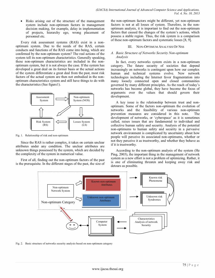
(IJACSA) International Journal of Advanced Computer Science and Applications, Vol. 4, No. 10, 2013
75 | P a g e www.ijacsa.thesai.org
Risks arising out of the structure of the management system include non-optimum factors in management decision making, for example, delay in implementation of projects, hierarchy ego, wrong placement of personnel etc.
Every risk assessment systems (RAS) exist in a non-optimum system. Due to the needs of the RAS, certain conducts and functions of the RAS come into being, which are confirmed by the non-optimum system? The real actions of the system tell its non-optimum characteristics. Generally speaking, these non-optimum characteristics are included in the non-optimum system, but it is not always the case. If the system has developed a great deal on its former basis or the actual actions of the system differentiate a great deal from the past, most risk factors of the actual system are then not embodied in the non-optimum characteristics system and still have things to do with the characteristics (See figure1).
Fig. 1. Relationship of risk and non-optimum
Since the RAS is rather complex, it takes on certain unclear attributes under any condition. The unclear attributes are unknown things possessed by the system, which are decided by the complexity of the system in numerical value.
First of all, finding out the non-optimum factors of the past is the prerequisite. In the different stages of the past, the size of
the non-optimum factors might be different, yet non-optimum factors is not at all losses of system. Therefore, in the non-optimum analysis, it is important to find out the non-optimum factors that caused the changes of the system’s actions, which possess a stable region. Thus, the risk system is a comparison of these non-optimum factors and systematic losses [8, 9].
III. NON-OPTIMUM ANALYSIS OF NSS
A. Basic Structure of Networks Security Non-optimum Analysis
In fact, every networks system exists in a non-optimum category. The future security of societies that depend increasingly on networks is contingent upon how our complex human and technical systems evolve. New network technologies including the Internet favor fragmentation into many loosely connected open and closed communities governed by many different principles. As the reach of today’s networks has become global, they have become the focus of arguments over the values that should govern their development.
A key issue is the relationship between trust and non-optimum. Some of the factors non-optimum the evolution of networks and the feasibility of various non-optimum prevention measures are considered in this note. The development of networks, or ‘cyberspace’ as it is sometimes called, raises issues that are fundamental to individual and collective human safety and security. Analysis of the potential non-optimums to human safety and security in a pervasive network environment is complicated by uncertainty about how people will perceive its associated non-optimums, whether or not they perceive it as trustworthy, and whether they behave as if it is trustworthy.
According to the non-optimum analysis of the system (He Ping, 2003), the important thing in the management of network system as a new effort is not a problem of optimizing. Rather, it is one of eliminating threaten and keeping away risk and detours as possible.
Non-optimum Category
Fig. 2. Basic structure of networks security analysis based on non-optimum category
Assessment
System
Non-optimum
System (NOS)
Losses System (LS)
Risk System (RS)
Known non-optimum
Attributes
Unknown non-optimum
Attributes
Non-optimum
Network System
Known risk Phenomena
Unknown risk Syndromes
Computer
System
Characteristics
Analysis of network
Security
(IJACSA) International Journal of Advanced Computer Science and Applications, Vol. 4, No. 10, 2013
76 | P a g e www.ijacsa.thesai.org
Even if some model of network management is considered optimum under the present circumstances, it is hard to be a stable one because it is in the midst of a dynamic process with quite a few hidden threats lurching and many horizontal or vertical relations between factors and their specific laws unknown. The so-called optimum model on network system is only at a system optimum state. So, if we try to set goals for the network system, make plans and take measures and advocate some optimum models simply following the optimum thinking methods out of blind subjective wish, we’ll be actually putting the network system on an unreliable and unrealistic basis.
So we say that the non-optimum thinking and the methods of system non-optimum measurement with risk-avoiding as its basic aim are based on the non-optimum facts with its special ways of thinking, network gathering, analyzing and processing, and with the setting up of non-optimum network system, these methods seek to eliminate threaten and risk, thus providing a new way of scientifically summarizing past lessons and making them lamppost for the future. Figure 1 shows the basic structure of networks security analysis based on non-optimum category [10].
The security of the network system emerges and develops in non-optimum category. Every security attributes exists in a non-optimum category, and the non-optimum characteristics of the real actions tell its risk attributes of networks systems. Generally speaking, these risk phenomena are included in the non-optimum category of network system, but since the network system is rather complex, it takes on certain unclear attributes under any condition. The unclear attributes are unknown things possessed by the risk system of network security, which are decided by the complexity of the risk system in numerical value. For example, the risk analysis of the network system is much more complicated than the physical system. Therefore the unknown things of a network system are much more than a physical system. These unclear attributes cause the risk factors of the network system.
The concept of non-optimum is quite comprehensive in network security system. From the viewpoint of networks system’ software, non-optimum means unfeasible and unreasonable; from the viewpoint of human’ network behavior, it means non-trust; from the viewpoint of networks’ capacity, it means ineffective and abnormal; from the viewpoint of networks’ change, it means obstacles, disturbance and influence. There exists a serious of non-optimum problem from the entity of the network system to the change of the network system, which causes non-optimum category. As to every kind of networks security problems, there is the individual non-optimum category as well as the common non-optimum category. The so-called individual non-optimum category is decided by the characters of the networks relationship system, while the common non-optimum category is an objective entity of networks behavior. At present, most security analysis is designed manually based on past experience of their networks behavior. Since the number of possible optimization model very large for realistic applications of reasonable complexity, security analysis modeling designed manually may not work well when applied in new problem instances. Further, there is no systematic method to evaluate the effectiveness of security designed manually. For these reasons, a “cooperative” method
for discovering the proper security decision for a particular application is very desirable. This leads to the development of our method for extensionality security model (ESM) of non-optimum category.
B. A Basic Theorem of Network Security Attributes Limitation
In network system, the factors of network security has optimum characteristics and optimum characteristics, as well as the evolution relationship between these characteristics, therefore, we can set up a state space of network security based on these characteristics and relationships [11].
Definition 3.1 Let )),(,,,( ooROOXS be a state space
of network security, where },,{ 1 LxxX be a set of the
network security factor,
},,{ 1 nooO be a set of optimum
characteristics of the network security factor, },,{ 1 mooO
be a set of non-optimum characteristics of the network security
factor, ),( ooR be a relationship between O and O , and
}|,{),( OoOoooooR .
Definition 3.2 Let )}(,),({)(1
xxxnOOO is the
optimum degree set ofO , )(( ]1,0[:) XxO and exist index
set of optimum degree in )),(,,( ooROOS ,
},,{ 1 l , then },0:)({ XxxO O
is called -optimum if there is a minimum limitation.
Definition 3.3 Let )}(,),({)(1
xxxmOOO
is the non-
optimum degree set of O ( ]0,1[:)( XxO
), and exist
index set of non-optimum degree in )),(,,( ooROOS ,
},,{ 1 l , then },0:|)({| UxxOO
or
},0:|)(|{ UxxOO
is called -non-optimum if
there is a maximum limitation.
Theorem 3.1 (Attributes Limitation Theory) Let X is a
closed set definition in metric space, effect function )(xO ,
)(xO
of optimum and non-optimum is homeomorphism
mapping in X for any Xx (network security factor), and there are maximum optimum degree and minimum non-
optimum degree to )(xO and |)(| xO
in X , then we have
)(RM is called network security optimization with minimum
risk model, that is
})()(
:|)(|min),(max{)(
11 XOOx
xxRM
OO
OO
Proof: Let )(xO and |)(| xO
have maximum and
minimum respectively in X :

(IJACSA) International Journal of Advanced Computer Science and Applications, Vol. 4, No. 10, 2013
77 | P a g e www.ijacsa.thesai.org
What is called the minimum risk analysis, in the can support range of risk analysis, is that if the maximum of corresponding to optimum characteristics values is chose from the minimum absolute value of non-optimum characteristics
values. Meanwhile if it has a corresponding value in O, there
exists the minimum risk value in the corresponding decision-making project. According to the known condensations, it exist
the minimum value to |)(| xO
in X , and the minimum
value is in O , then we will prove that it existed the minimum
risk analysis in O
According to the literature [11], we have the minimum
value of |)(| xO
, and },0:|)(|{ UxxOO
Suppose that it there exists a minimum value at least in O .
Let X be a closed set, according to the literature [11] Lemma1,
)(),( XOXO oo are all closed sets, we know OO , are
closed sets of OO, , respectively. )()( -11
OO OO,
, are
closed sets from Lemma 2 of literature [11], so
)()( 11
OO OO
is a closed set.
Suppose )(1
0 OxO
and |)(| xO
is a minimum
value in O,
the optimum attribute value )( 0xO is existed in
corresponding to the minimum |)(| xO
from Definition 1.
Assume that the minimum |)(| xO
have a sequence
)}({ nOx , )( Nn , satisfy )()( 0xx
OnO ,
)( n ; because 1
O is continuous, we obtain:
0
1 ))(( xxx nnOO = ))(( 0
1 xOO
.
As O is continuous, and has a corresponding sequence
)}({ nO x in O , satisfying )()( 0xx OnO , because
O is a closed set, we have OxO )( 0 , at the same time
O is a homeomorphism mapping, we obtain, )(1
0 Ox O
hence, x )()( 11
OO OO
, therefore, the minimum risk
model of network security optimization is as follows:
})()(
:)(min),(max{)(
11 XOOx
xxRM
OO
OO
C. Risk Assessment Method Based on )(RM
In fact, the )(RM is a relationship between optimum
attributes and non-optimum in network security, thus, this relationship can be represented by a table where each row
),,2,1( miXxi represents the factor of network
security, for instance, physical factor, software factor, management factor as well as man-made factor and so on. Every column represents a relationship of optimum attributes
and non-optimum for every network security factors (See table 1).
TABLE I. BASIC INFORMATION TABLE OF )(RM
11,oo 22 ,oo … nn oo ,
1x 1111,oo 1212,oo … nn oo 11 ,
2x 2121,oo 2222,oo … nn oo 22 ,
… … … … …
mx 11, mm oo 22 , mm oo … mnmn oo ,
Thus, we can be set up a method of network security optimization, which is risk assessment method based on Attributes Limitation Theory (ALT). According to basic principle of network security management [11], we have
Can be determined acceptable level value of every Xxi
If )min()( RiskRS [12].
))(),(min()(1
m
i
n
j
iojjo xxxRS
Subject to})()(
:)(min),(max{)(
11 XOOx
xxRM
OO
OO
Every network security problems exists in a non-optimum category. Due to the needs of the network security optimization, certain conducts and functions of the networks come into being, which are confirmed by the non-optimum category? The real behavior of the network tells its security problem. Generally speaking, these security problems are included in the non-optimum category, but it is not always the case. If the network has developed a great deal on its former basis or the actual actions of the network differentiate a great deal from the past, most network security factors of the actual network are then not embodied in the non-optimum attribute and still have things to do with the attribute.
IV. THE DESIGN OF RISK ASSESSMENT SYSTEM (RAS)
Since the network security is rather complex, it takes on certain unclear attributes under any condition. The unclear attributes are unknown things possessed by the network system, which are decided by the complexity of the network in numerical value. The key to analyze and research network security systems lies in how to build up non-optimum sets of the network system.
First of all, finding out the non-optimum category of the past is the prerequisite. In the different stages of the past, the size of the non-optimum set might be different, yet non-optimum set is not at all non-optimum characteristics. Therefore, in the non-optimum set, it is important to find out
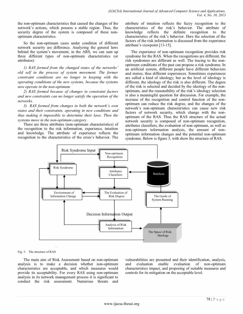
(IJACSA) International Journal of Advanced Computer Science and Applications, Vol. 4, No. 10, 2013
78 | P a g e www.ijacsa.thesai.org
the non-optimum characteristics that caused the changes of the network’s actions, which possess a stable region. Thus, the security degree of the system is composed of these non-optimum characteristics.
So the non-optimum cases under condition of different network security are difference. Analyzing the general laws behind the system’s movement, in the ARS, we can sum up three different types of non-optimum characteristics (or attributes):
1) RAS formed from the changed states of the networks’
old self in the process of system movement. The former
constraint conditions are no longer in keeping with the
operating conditions of the new systems, because the systems
now operate in the non-optimum.
2) RAS formed because of changes in constraint factors
and new constraints can no longer satisfy the operation of the
networks.
3) RAS formed from changes in both the network’s own
states and their constraints, operating in new conditions and
thus making it impossible to determine their laws. Then the
systems move in the non-optimum category. There are three attributes (non-optimum characteristics) of
the recognition to the risk information, experience, intuition and knowledge. The attribute of experience reflects the recognition to the characteristics of the crisis’s behavior. The
attribute of intuition reflects the fuzzy recognition to the characteristics of the risk’s behavior. The attribute of knowledge reflects the definite recognition to the characteristics of the risk’s behavior. Here the selection of the factors of the risk information is discussed from the experience attribute’s viewpoint [13-15].
The experience of non-optimum recognition provides risk syndrome for the RAS. When the recognitions are different, the risk syndromes are different as well. The tracing to the non-optimum conditions of the past can propose a risk syndrome. In an artificial system, different people have different behaviors and stories, thus different experiences. Sometimes experiences are called a kind of ideology; but as the level of ideology is different, the ideology of the risk is also different. The degree of the risk is selected and decided by the ideology of the non-optimum, and the reasonability of the risk’s ideology selection is also a meaningful question for discussion. For example, the increase of the recognition and control function of the non-optimum can reduce the risk degree, and the changes of the network’s non-optimum characteristics can cause new risk factors of network security, which change with the non-optimum of the RAS. Thus the RAS structure of the actual network security is composed of non-optimum recognition, attributes classifiers, the evaluation of non-optimum, as well as non-optimum information analysis, the amount of non-optimum information changes and the potential non-optimum syndrome. Below is figure 3, with show the structure of RAS.
Risk Syndrome Input
Decision Information Output
Fig. 3. The structure of RAS
The main aim of Risk Assessment based on non-optimum analysis is to make a decision whether non-optimum characteristics are acceptable, and which measures would provide its acceptability. For every RAS using non-optimum analysis in its network management process it is significant to conduct the risk assessment. Numerous threats and
vulnerabilities are presented and their identification, analysis, and evaluation enable evaluation of non-optimum characteristics impact, and proposing of suitable measures and controls for its mitigation on the acceptable level.
Non-optimum Recognition
Batebase
Attributes Classifiers
The Evaluation of Risk Degree
Analysis of Risk Information
The Guide of System Running
Environment of Information Change
Risk Syndrome
The Space of Risk Ideology

(IJACSA) International Journal of Advanced Computer Science and Applications, Vol. 4, No. 10, 2013
79 | P a g e www.ijacsa.thesai.org
V. CONCLUSIONS
The key issues of network security management are effective recognition and evaluation for non-optimum characteristics of the network system. Depending on all above studies, we can identify security attributes of network systems by using non-optimum analysis methods of systems. Thereby we can control the security of network system. Because there are various uncertainty attributes of information security. For example, the random of non-optimum occurrence, the fuzzy of behaviors judgments, the unascertained of security attributes. Due to the limit of space, the detailed algorithm and computer program, which is about recognition and evaluation system, will be introduced in another paper.
From the non-optimum analysis, it can be concluded that people need the controllable order of the system, and non-optimum can also be non-risk. From the risk reference system, the transit of the system from risk into non-risk as well as the requisites of the transit can be estimated. The Self-organization of Network Security System based on non-optimum analysis will be widely used in the decision sciences. It can often transform people’s experiences into scientific means and might set up reference models with behavior attributes in the control system. This kind of model can marry the experiences and the theories, and can make actual judges to the running path of the risk management.
There is profound potential for putting the non-optimum thinking into use in Chinas network security management, and in other country’s practice. Take the non-optimum guiding system for example; it can be employed in the network security management of the country’s macro policies, financial system as well as decision analysis. To be sure, the establishment of this non-optimum guiding system with computer as its means with information processing techniques as its foundation is no easy task.
ACKNOWLEDGMENT
The authors are grateful for the support given by National Natural Science Foundation of China (Grant No. 61272170). We also thank reviewers for insightful and helpful suggestions.
REFERENCES
[1] Prabhat Kumar Vishwakarma, Optimization and Analysing the Effectiveness of Security Hardening Measure Using Various
Optimization Techniques as well as Network Measurement Model Giving Special Emphasis to Attack Tree Model, International Journal of
Network Security & Its Applications, 2011, Vol.3, No.4, pp.100-109.
[2] Gupta, M., Rees, J., Chaturvedi, A., and Chi, J, Matching Information
Security Vulnerabilities to Organizational Security Policies: A Genetic Algorithm Approach, 2006, Decision Support Systems, vol.41, no.3, pp.
592-603.
[3] Jeremy Cicurel, Information Security Process Optimization: Efficient
Management of IT Security, Practice Director, CIO Advisory, 2012, www.kurtsalmon.com.
[4] He Ping, A Guiding System for Non-optimum Recognition, Control and
Decision, 1989, vol.6, no.3, pp.18-21.
[5] He Ping, Theories and Methods of Non-optimum Analysis on systems, Journal of China Engineering Science, 2003, vol.5, no.7, pp.47-54.
[6] Ping He, Characteristics Analysis of Network Non-Optimum Based on
Self-Organization Theory, Global Journal of Computer Science and Technology, 2010, Vol.10, no.9, pp. 67-72.
[7] Božo Nikolić, Ljiljana Ružić-Dimitrijević, Risk Assessment of
Information Technology Systems, Informing Science and Information Technology, 2009,Vol.6, pp.595-615.
[8] He Ping, The Method of Non-optimum Analysis on Risk Management
System,In: Bartel Van de Walle, ed, proc. of the Int’l conf ISCRAM, 2008, pp. 604-609.
[9] Zengtang Qu, Method of Non-optimum Analysis on Risk Control System, JOURNAL OF SOFTWARE, 2009, Vol. 4, no. 4, pp.374-381.
[10] Ping He, Maximum Sub-Optimum Decision-Making Based on Non-
Optimum Information Analysis, Advanced Science Letters, 2012, vol.5, no.1, pp.376-385.
[11] Arjen Lenstra, Tim Voss, Information Security Risk Assessment,
Aggregation, and Mitigation, ACISP 2004, LNCS 3108, pp. 391–401.
[12] Emil BURTESCU, The Network’s Data Security Risk Analysis, Revista Informatica Economică, 2008, Vol.48, No.4, pp. 51-53.
[13] Ping He, The Idea of Non-Optimum and It's Research Methods, 2011
International Conference on Agricultural and Natural Resources Engineering, Advances in Biomedical Engineering, 2011, Vol.3-5, 296-
301.
[14] Libo Hou, Approach of Non-optimum Analysis on Information Systems Security, IEEE Computer Society, IITA International Conference on
Control, Automation and Systems Engineering, 2009, pp.225-228.
[15] Ping He. The method of attribute analysis in non-optimum to optimum.
Journal of Liaoning Normal University.2008, Vol.31, no.1, pp. 29-33. (Chinese)
AUTHORS PROFILE
He Ping is a professor of the Department of Information at Liaoning Police Academy, P.R. China. He is currently Deputy Chairman of the Centre of Information Development at Management Science Academy of China. In 1986 He advance system non-optimum analysis and founded research institute. He has researched analysis of information system for more than 20 years. Since 1990 his work is optimization research
on management information system. He has published more than 200 papers and ten books, and is editor of several scientific journals. In 1992 awards Prize for the Outstanding Contribution Recipients of Special Government Allowances P. R. China.

(IJACSA) International Journal of Advanced Computer Science and Applications, Vol. 4, No. 10, 2013
80 | P a g e www.ijacsa.thesai.org
An Architectural-model for Context aware Adaptive
Delivery of Learning Material
Kalla. Madhu Sudhana
Ph.D. Scholar, Dept. of C. S. E,
St. Peter’s University,
Chennai, India.
V. Cyril Raj
Head, Dept. of Computer Science,
Dr. M.G.R University,
Chennai, India
T.Ravi
Principal,
Srinivasa Institute of Engg & Tech,
Chennai, India
Abstract—The web based learning has become more complex
to search required learning resources with continuously growing
digital learning contents which are entangled with structural and
semantic interrelationship. Meanwhile, the rapid development of
communication technology lead to heterogeneity of learning
devices than it was in the early stage. The context-aware adaptive
learning environment has become a promising solution to these
searching and presentation problems in educational domain. To
solve this context aware learning content delivery problem, we
proposed a novel architectural model based on MVC (Model–
View–Controller) design pattern, that is able to perform
personalized adaptive delivery of course content according to
learner contextual information such as learning style and
characteristics of the learning device using an ontological approach.
Keywords—MVC design pattern; context-aware adaptive
learning; architectural model; Usability Analysis
I. INTRODUCTION
In an adaptive e-learning environment, the system must respond harmoniously to changes of learner needs, learning style and context. The e-learning approach such as online learning is empowering the students for self-learning and to create personalized context aware adaptive learning approaches, through leveraging the huge digital learning resources that are available on internet.
The recent emerging mobile communication technology and the popularity of mobile solutions have geared the traditional PC based e-learning approach to increase their change to m-learning, but the divergence between these two types of environments based on their technical capabilities and characteristics has become a paradox to use existing digital learning contents and applications that are developed with the perspective of computers.
Therefore, various content adaptation (transcoding) techniques emerged to perform the adaptation of learning contents based on the characteristics of learning devices. These single-source adaptation techniques often lead to high complexity and cumbersome task to deliver the adapted contents dynamically as per the characteristics of client device, this need to develop multi-source authoring contents, where separate resources are maintained for each class of devices. In the proposed prototype implementation we are considering only two types of resources as compatible for PC and mobile environments.
Here, we proposed an architectural framework for context aware adaptive content delivery for course based e-learning environments. The novel feature of our architectural approach uses the recent MVC (Model–View–Controller [1]) architectural design pattern that provides the benefits such as: code reusability, upgradability and multiple views of the same data. Another important feature is ontology-based learner context model that helps in accessing the concepts that are contextually and conceptually suitable for learner needs.
II. RELATED RESEARCH WORK
Jane Yau [2] proposed context-aware and adaptive learning architecture, through dividing the dimensions of adaptation into two separate layers as: learning styles and knowledge level as learning preferences in adaptation layer and location and time as contextual features of adaptation layer. Yau [3] introduced the Context-aware and Adaptive Learning Schedule (CALS) framework, in which they considered learning activities, learner profile and learner schedule events as context dimensions. Through considering learner’s personal features, preferences and previous actions as contextual profile, Martin [4] presented an architecture of a system, based on modularization of the adaptation layer that supports context-based adaptation for m-learning. Agile e-learning system architecture proposed by Finke [5] with the features such as adaptability, reusability and changeability provides an opportunity for dynamic curriculum exposition.
The personalized multi-agent e-learning system architecture proposed by Baylari [6] uses an item response theory and artificial neural network to recommend appropriate learning materials to the learner through diagnosing learner’s learning activity. As quoted by He, Daqing [7], ontology can provide the visual presentation of conceptual structure about the course topics and Dicheva [8] stated that the conceptual structure of the course content helps in getting the orientation of learning task.
III. OBJECTIVES OF PROPOSED APPROACH
The main objective of proposed system is to improve learner’s knowledge and to facilitate the learner to review course contents at any moment of time. The development of new generation of e-learning applications has to leverage the technical advancements in digital learning devices to obtain potential benefits. Here, we noticed two important technical strategies that are to be considered while developing the new
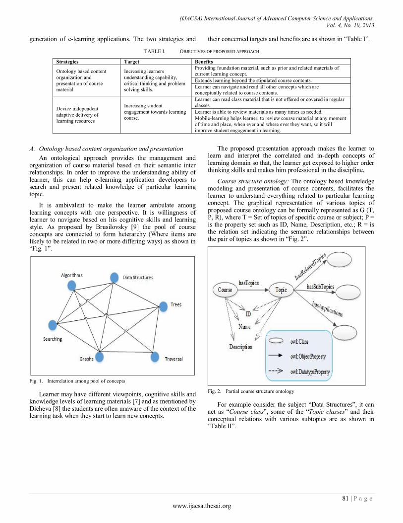
(IJACSA) International Journal of Advanced Computer Science and Applications, Vol. 4, No. 10, 2013
81 | P a g e www.ijacsa.thesai.org
generation of e-learning applications. The two strategies and their concerned targets and benefits are as shown in “Table I”.
TABLE I. OBJECTIVES OF PROPOSED APPROACH
Strategies Target Benefits
Ontology based content
organization and
presentation of course
material
Increasing learners
understanding capability,
critical thinking and problem
solving skills.
Providing foundation material, such as prior and related materials of
current learning concept.
Extends learning beyond the stipulated course contents.
Learner can navigate and read all other concepts which are
conceptually related to course contents.
Device independent
adaptive delivery of
learning resources
Increasing student
engagement towards learning
course.
Learner can read class material that is not offered or covered in regular
classes.
Learner is able to review materials as many times as needed.
Mobile-learning helps learner, to review course material at any moment
of time and place, when ever and where ever they want, so it will
improve student engagement in learning.
A. Ontology based content organization and presentation
An ontological approach provides the management and organization of course material based on their semantic inter relationships. In order to improve the understanding ability of learner, this can help e-learning application developers to search and present related knowledge of particular learning topic.
It is ambivalent to make the learner ambulate among learning concepts with one perspective. It is willingness of learner to navigate based on his cognitive skills and learning style. As proposed by Brusilovsky [9] the pool of course concepts are connected to form heterarchy (Where items are likely to be related in two or more differing ways) as shown in “Fig. 1”.
Fig. 1. Interrelation among pool of concepts
Learner may have different viewpoints, cognitive skills and knowledge levels of learning materials [7] and as mentioned by Dicheva [8] the students are often unaware of the context of the learning task when they start to learn new concepts.
The proposed presentation approach makes the learner to learn and interpret the correlated and in-depth concepts of learning domain so that, the learner get exposed to higher order thinking skills and makes him professional in the discipline.
Course structure ontology: The ontology based knowledge modeling and presentation of course contents, facilitates the learner to understand everything related to particular learning concept. The graphical representation of various topics of proposed course ontology can be formally represented as G (T, P, R), where T = Set of topics of specific course or subject; P = is the property set such as ID, Name, Description, etc.; R = is the relation set indicating the semantic relationships between the pair of topics as shown in “Fig. 2”.
Fig. 2. Partial course structure ontology
For example consider the subject “Data Structures”, it can act as “Course class”, some of the “Topic classes” and their conceptual relations with various subtopics are as shown in “Table II”.
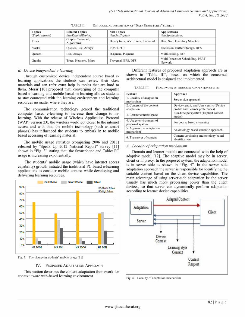
(IJACSA) International Journal of Advanced Computer Science and Applications, Vol. 4, No. 10, 2013
82 | P a g e www.ijacsa.thesai.org
TABLE II. ONTOLOGICAL DESCRIPTION OF “DATA STRUCTURES” SUBJECT
Topics
(Topic classes) Related Topics
(hasRelatedTopics) Sub Topics
(hasSubTopics) Applications
(hasApplications)
Trees Graphs, Traversal,
Algorithms Binary trees, AVL Trees, Traversal Heap Sort, Directory Structure
Stacks Queues, List, Arrays PUSH, POP Recursion, Buffer Storage, DFS
Queues List, Arrays D-Queue, P-Queue Multi-tasking, BFS
Graphs Trees, Network, Maps Traversal, BFS, DFS Multi Processor Scheduling, PERT-
Network
B. Device independent e-learning
Through customized device independent course based e-learning applications the students can review their class materials and can refer extra help in topics that are hard to them. Morar [10] proposed that, converging of the computer based e-learning and mobile based m-learning allows students to stay connected with the learning environment and learning resources no matter where they are.
The communication technology geared the traditional computer based e-learning to increase their change to m-learning. With the release of Wireless Application Protocol (WAP) version 2.0, the wireless world got closer to the internet access and with that, the mobile technology (such as smart phones) has influenced the students to embark in to mobile based accessing of learning material.
The mobile usage statistics (comparing 2006 and 2011) released by “Speak Up 2012 National Report” survey [11] shown in “Fig. 3” stating that, the Smartphone and Tablet PC usage is increasing exponentially.
The students’ mobile usage (which have internet access capability) growth initiated the traditional PC based e-learning applications to consider mobile context while developing and delivering learning resources.
Fig. 3. The change in students’ mobile usage [11]
IV. PROPOSED ADAPTATION APPROACH
This section describes the content adaptation framework for context aware web-based learning environment.
Different features of proposed adaptation approach are as shown in “Table III”, based on which the concerned architectural model is designed and implemented.
TABLE III. FRAMEWORK OF PROPOSED ADAPTATION SYSTEM
Feature Approach
1. Locality of adaptation
mechanism Server side approach
2. Content of the context
adaptation
Device centric and User centric (Device
profile and Learner preferences)
3. Learner context space Run-time perspective (Explicit context
model)
4. Usage environment of
proposed system For course based e-learning
5. Approach of adaptation
mechanism An ontology based semantic approach
6. The server of content Content versioning and ontology based
identification
A. Locality of adaptation mechanism
Domain and learner models are connected with the help of adaptive model [12]. The adaptive model may be in server, client or in proxy. In the proposed system, the adaptation model is in server side as shown in “Fig. 4”. In the server side adaptation approach the server is responsible for identifying the suitable content based on the client device capabilities. The main advantage of using server-side adaptation is: the server usually has much more processing power than the client devices, so that server can dynamically perform adaptation according to learner device capabilities.
Fig. 4. Locality of adaptation mechanism
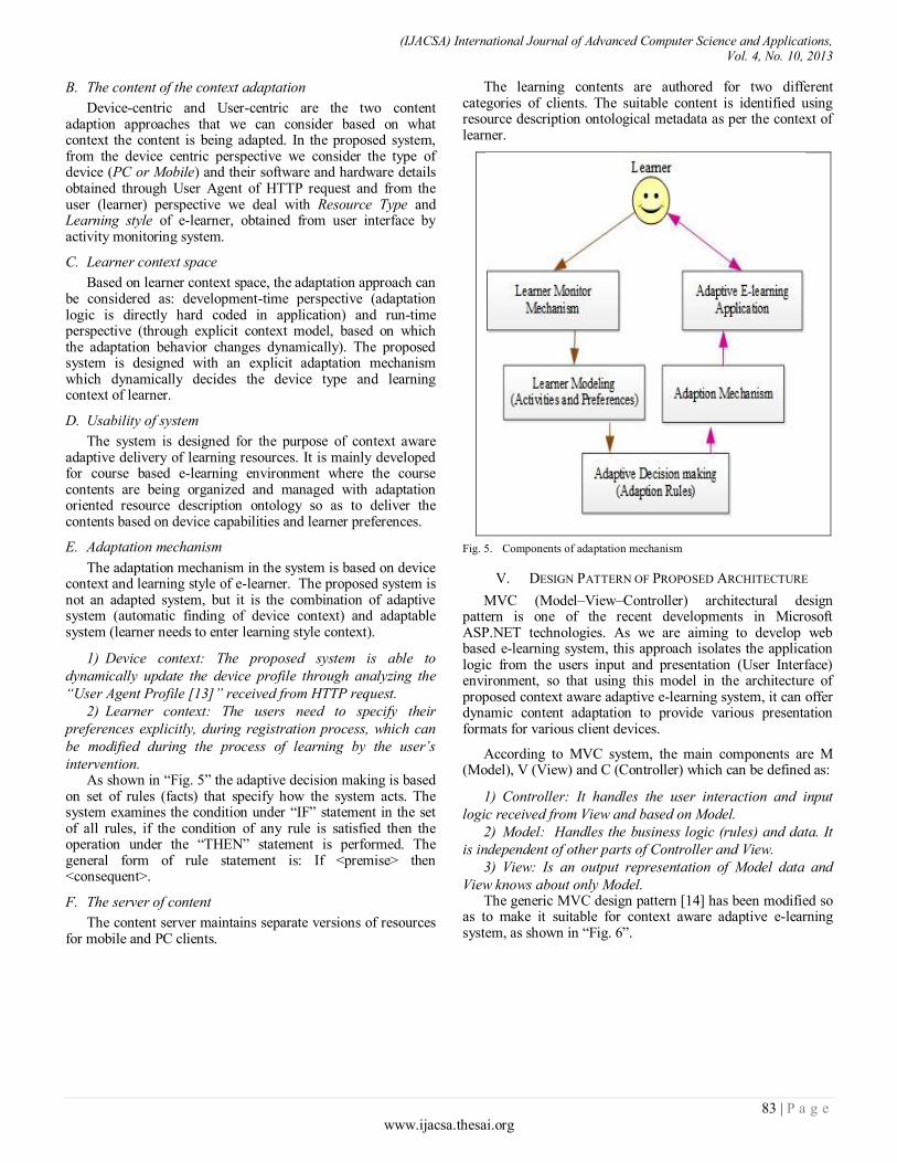
(IJACSA) International Journal of Advanced Computer Science and Applications, Vol. 4, No. 10, 2013
83 | P a g e www.ijacsa.thesai.org
B. The content of the context adaptation
Device-centric and User-centric are the two content adaption approaches that we can consider based on what context the content is being adapted. In the proposed system, from the device centric perspective we consider the type of device (PC or Mobile) and their software and hardware details obtained through User Agent of HTTP request and from the user (learner) perspective we deal with Resource Type and Learning style of e-learner, obtained from user interface by activity monitoring system.
C. Learner context space
Based on learner context space, the adaptation approach can be considered as: development-time perspective (adaptation logic is directly hard coded in application) and run-time perspective (through explicit context model, based on which the adaptation behavior changes dynamically). The proposed system is designed with an explicit adaptation mechanism which dynamically decides the device type and learning context of learner.
D. Usability of system
The system is designed for the purpose of context aware adaptive delivery of learning resources. It is mainly developed for course based e-learning environment where the course contents are being organized and managed with adaptation oriented resource description ontology so as to deliver the contents based on device capabilities and learner preferences.
E. Adaptation mechanism
The adaptation mechanism in the system is based on device context and learning style of e-learner. The proposed system is not an adapted system, but it is the combination of adaptive system (automatic finding of device context) and adaptable system (learner needs to enter learning style context).
1) Device context: The proposed system is able to
dynamically update the device profile through analyzing the
“User Agent Profile [13]” received from HTTP request.
2) Learner context: The users need to specify their
preferences explicitly, during registration process, which can
be modified during the process of learning by the user’s
intervention. As shown in “Fig. 5” the adaptive decision making is based
on set of rules (facts) that specify how the system acts. The system examines the condition under “IF” statement in the set of all rules, if the condition of any rule is satisfied then the operation under the “THEN” statement is performed. The general form of rule statement is: If <premise> then <consequent>.
F. The server of content
The content server maintains separate versions of resources for mobile and PC clients.
The learning contents are authored for two different categories of clients. The suitable content is identified using resource description ontological metadata as per the context of learner.
Fig. 5. Components of adaptation mechanism
V. DESIGN PATTERN OF PROPOSED ARCHITECTURE
MVC (Model–View–Controller) architectural design pattern is one of the recent developments in Microsoft ASP.NET technologies. As we are aiming to develop web based e-learning system, this approach isolates the application logic from the users input and presentation (User Interface) environment, so that using this model in the architecture of proposed context aware adaptive e-learning system, it can offer dynamic content adaptation to provide various presentation formats for various client devices.
According to MVC system, the main components are M (Model), V (View) and C (Controller) which can be defined as:
1) Controller: It handles the user interaction and input
logic received from View and based on Model.
2) Model: Handles the business logic (rules) and data. It
is independent of other parts of Controller and View.
3) View: Is an output representation of Model data and
View knows about only Model. The generic MVC design pattern [14] has been modified so
as to make it suitable for context aware adaptive e-learning system, as shown in “Fig. 6”.
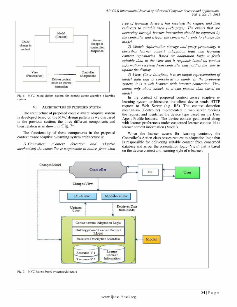
(IJACSA) International Journal of Advanced Computer Science and Applications, Vol. 4, No. 10, 2013
84 | P a g e www.ijacsa.thesai.org
Fig. 6. MVC based design pattern for context aware adaptive e-learning
system.
VI. ARCHITECTURE OF PROPOSED SYSTEM
The architecture of proposed context aware adaptive system is developed based on the MVC design pattern as we discussed in the previous section; the three different components and
their relation is as shown in “Fig. 7”.
The functionality of these components in the proposed context aware adaptive e-learning system architecture is:
1) Controller: (Context detection and adaptive
mechanism) the controller is responsible to notice, from what
type of learning device it has received the request and then
redirects to suitable view (web page). The events that are
occurring through learner interaction should be captured by
the controller and trigger the concerned events to change the
model.
2) Model: (Information storage and query processing) it
describes learner context, adaptation logic and learning
content repositories. Based on adaptation logic it feeds
suitable data to the view and it responds based on context
information received from controller and notifies the view to
update the display.
3) View: (User Interface) it is an output representation of
model data and is considered as dumb. In the proposed
system, it is a web browser with internet connection. View
knows only about model, so it can present data based on
model. In the context of proposed context aware adaptive e-
learning system architecture, the client device sends HTTP request to Web Server (e.g. IIS). The context detection mechanism (Controller) implemented in web server receives the request and identifies the device type based on the User Agent Profile headers. The device context gets stored along with learner preferences under concerned learner context-id as learner context information (Model).
When the learner access for learning contents, the Controller’s Action class passes request to adaptation logic that is responsible for delivering suitable content from concerned database and as per the presentation logic (View) that is based on the device context and learning style of e-learner.
Fig. 7. MVC Pattern based system architecture
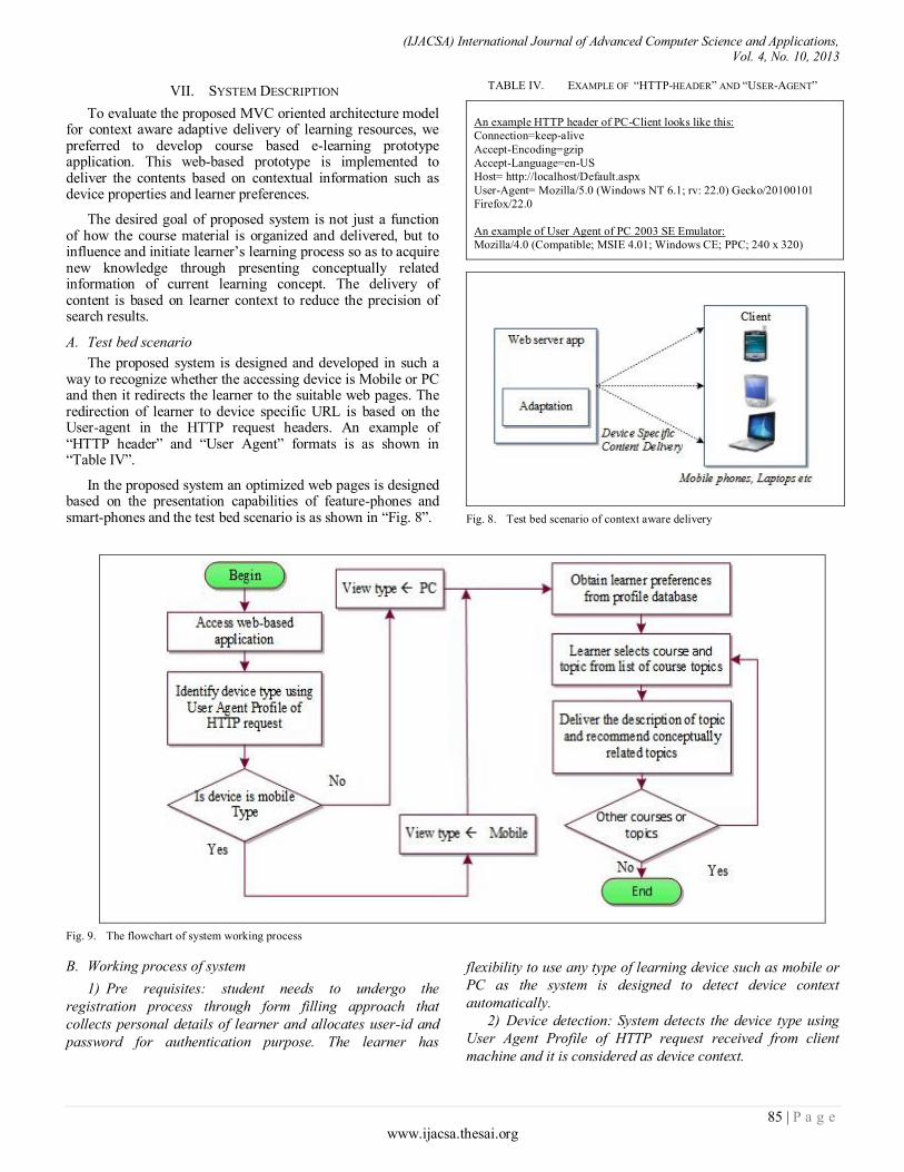
(IJACSA) International Journal of Advanced Computer Science and Applications, Vol. 4, No. 10, 2013
85 | P a g e www.ijacsa.thesai.org
VII. SYSTEM DESCRIPTION
To evaluate the proposed MVC oriented architecture model for context aware adaptive delivery of learning resources, we preferred to develop course based e-learning prototype application. This web-based prototype is implemented to deliver the contents based on contextual information such as device properties and learner preferences.
The desired goal of proposed system is not just a function of how the course material is organized and delivered, but to influence and initiate learner’s learning process so as to acquire new knowledge through presenting conceptually related information of current learning concept. The delivery of content is based on learner context to reduce the precision of search results.
A. Test bed scenario
The proposed system is designed and developed in such a way to recognize whether the accessing device is Mobile or PC and then it redirects the learner to the suitable web pages. The redirection of learner to device specific URL is based on the User-agent in the HTTP request headers. An example of “HTTP header” and “User Agent” formats is as shown in “Table IV”.
In the proposed system an optimized web pages is designed based on the presentation capabilities of feature-phones and smart-phones and the test bed scenario is as shown in “Fig. 8”.
TABLE IV. EXAMPLE OF “HTTP-HEADER” AND “USER-AGENT”
An example HTTP header of PC-Client looks like this:
Connection=keep-alive
Accept-Encoding=gzip
Accept-Language=en-US
Host= http://localhost/Default.aspx
User-Agent= Mozilla/5.0 (Windows NT 6.1; rv: 22.0) Gecko/20100101
Firefox/22.0
An example of User Agent of PC 2003 SE Emulator:
Mozilla/4.0 (Compatible; MSIE 4.01; Windows CE; PPC; 240 x 320)
Fig. 8. Test bed scenario of context aware delivery
Fig. 9. The flowchart of system working process
B. Working process of system
1) Pre requisites: student needs to undergo the
registration process through form filling approach that
collects personal details of learner and allocates user-id and
password for authentication purpose. The learner has
flexibility to use any type of learning device such as mobile or
PC as the system is designed to detect device context
automatically.
2) Device detection: System detects the device type using
User Agent Profile of HTTP request received from client
machine and it is considered as device context.
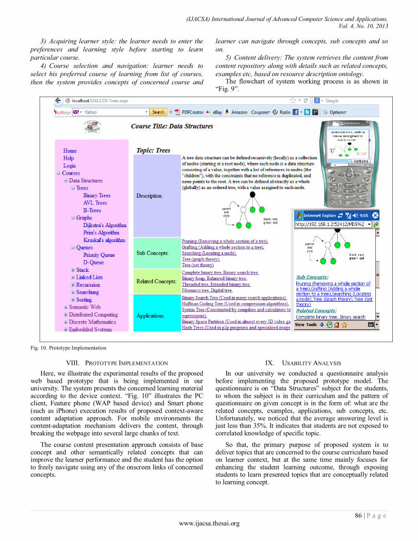
(IJACSA) International Journal of Advanced Computer Science and Applications, Vol. 4, No. 10, 2013
86 | P a g e www.ijacsa.thesai.org
3) Acquiring learner style: the learner needs to enter the
preferences and learning style before starting to learn
particular course.
4) Course selection and navigation: learner needs to
select his preferred course of learning from list of courses,
then the system provides concepts of concerned course and
learner can navigate through concepts, sub concepts and so
on.
5) Content delivery: The system retrieves the content from
content repository along with details such as related concepts,
examples etc, based on resource description ontology. The flowchart of system working process is as shown in
“Fig. 9”.
Fig. 10. Prototype Implementation
VIII. PROTOTYPE IMPLEMENTATION
Here, we illustrate the experimental results of the proposed web based prototype that is being implemented in our university. The system presents the concerned learning material according to the device context. “Fig. 10” illustrates the PC client, Feature phone (WAP based device) and Smart phone (such as iPhone) execution results of proposed context-aware content adaptation approach. For mobile environments the content-adaptation mechanism delivers the content, through breaking the webpage into several large chunks of text.
The course content presentation approach consists of base concept and other semantically related concepts that can improve the learner performance and the student has the option to freely navigate using any of the onscreen links of concerned concepts.
IX. USABILITY ANALYSIS
In our university we conducted a questionnaire analysis before implementing the proposed prototype model. The questionnaire is on “Data Structures” subject for the students, to whom the subject is in their curriculum and the pattern of questionnaire on given concept is in the form of: what are the related concepts, examples, applications, sub concepts, etc. Unfortunately, we noticed that the average answering level is just less than 35%. It indicates that students are not exposed to correlated knowledge of specific topic.
So that, the primary purpose of proposed system is to deliver topics that are concerned to the course curriculum based on learner context, but at the same time mainly focuses for enhancing the student learning outcome, through exposing students to learn presented topics that are conceptually related to learning concept.
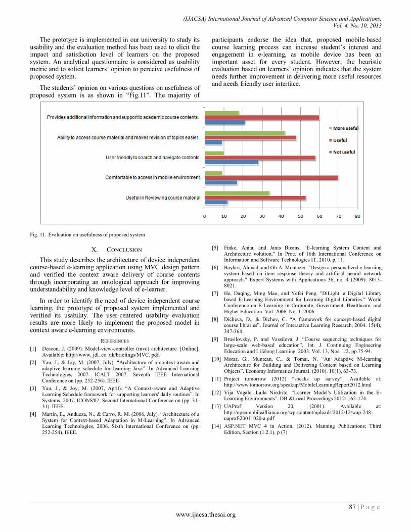
(IJACSA) International Journal of Advanced Computer Science and Applications, Vol. 4, No. 10, 2013
87 | P a g e www.ijacsa.thesai.org
The prototype is implemented in our university to study its usability and the evaluation method has been used to elicit the impact and satisfaction level of learners on the proposed system. An analytical questionnaire is considered as usability metric and to solicit learners’ opinion to perceive usefulness of proposed system.
The students’ opinion on various questions on usefulness of proposed system is as shown in “Fig.11”. The majority of
participants endorse the idea that, proposed mobile-based course learning process can increase student’s interest and engagement in e-learning, as mobile device has been an important asset for every student. However, the heuristic evaluation based on learners’ opinion indicates that the system needs further improvement in delivering more useful resources and needs friendly user interface.
Fig. 11. Evaluation on usefulness of proposed system
X. CONCLUSION
This study describes the architecture of device independent course-based e-learning application using MVC design pattern and verified the context aware delivery of course contents through incorporating an ontological approach for improving understandability and knowledge level of e-learner.
In order to identify the need of device independent course learning, the prototype of proposed system implemented and verified its usability. The user-centered usability evaluation results are more likely to implement the proposed model in context aware e-learning environments.
REFERENCES
[1] Deacon, J. (2009). Model-view-controller (mvc) architecture. [Online].
Available: http://www. jdl. co. uk/briefings/MVC. pdf.
[2] Yau, J., & Joy, M. (2007, July). “Architecture of a context-aware and
adaptive learning schedule for learning Java”. In Advanced Learning Technologies, 2007. ICALT 2007. Seventh IEEE International
Conference on (pp. 252-256). IEEE
[3] Yau, J., & Joy, M. (2007, April). “A Context-aware and Adaptive Learning Schedule framework for supporting learners' daily routines”. In
Systems, 2007. ICONS'07. Second International Conference on (pp. 31-31). IEEE.
[4] Martin, E., Andueza, N., & Carro, R. M. (2006, July). “Architecture of a
System for Context-based Adaptation in M-Learning”. In Advanced Learning Technologies, 2006. Sixth International Conference on (pp.
252-254). IEEE.
[5] Finke, Anita, and Janis Bicans. "E-learning System Content and
Architecture volution." In Proc. of 16th International Conference on Information and Software Technologies IT, 2010. p. 11.
[6] Baylari, Ahmad, and Gh A. Montazer. "Design a personalized e-learning system based on item response theory and artificial neural network
approach." Expert Systems with Applications 36, no. 4 (2009): 8013-8021.
[7] He, Daqing, Ming Mao, and Yefei Peng. "DiLight: a Digital Library
based E-Learning Environment for Learning Digital Libraries." World Conference on E-Learning in Corporate, Government, Healthcare, and
Higher Education. Vol. 2006. No. 1. 2006.
[8] Dicheva, D., & Dichev, C. “A framework for concept-based digital course libraries”. Journal of Interactive Learning Research, 2004. 15(4),
347-364.
[9] Brusilovsky, P. and Vassileva, J. “Course sequencing techniques for large-scale web-based education”, Int. J. Continuing Engineering
Education and Lifelong Learning. 2003. Vol. 13, Nos. 1/2, pp.75-94.
[10] Morar, G., Muntean, C., & Tomai, N. “An Adaptive M-learning Architecture for Building and Delivering Content based on Learning
Objects”. Economy Informatics Journal. (2010). 10(1), 63-73.
[11] Project tomorrow (2012) “speaks up survey”. Available at: http://www.tomorrow.org/speakup/MobileLearningReport2012.html
[12] Vija Vagale, Laila Niedrite. “Learner Model's Utilization in the E-Learning Environments”. DB &Local Proceedings 2012: 162-174.
[13] UAProf Version 20, (2001). Available at:
http://openmobilealliance.org/wp-content/uploads/2012/12/wap-248-uaprof-20011020-a.pdf
[14] ASP.NET MVC 4 in Action. (2012). Manning Publications; Third
Edition, Section (1.2.1), p (7)
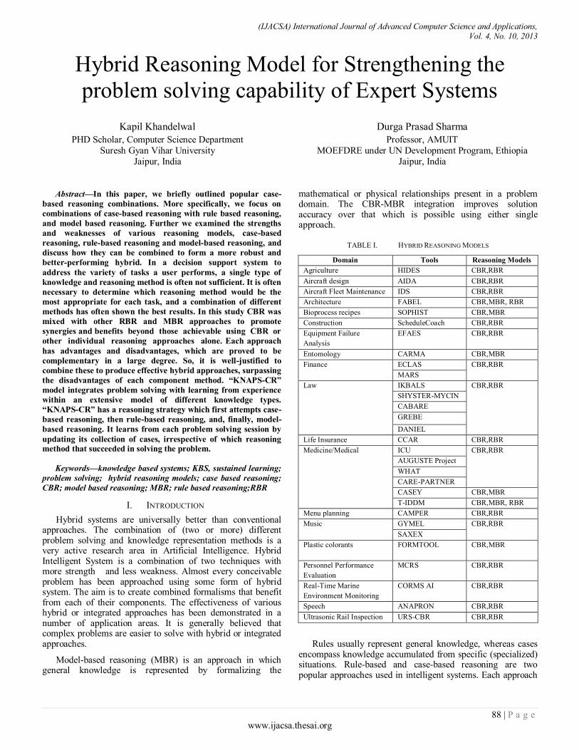
(IJACSA) International Journal of Advanced Computer Science and Applications, Vol. 4, No. 10, 2013
88 | P a g e www.ijacsa.thesai.org
Hybrid Reasoning Model for Strengthening the
problem solving capability of Expert Systems
Kapil Khandelwal
PHD Scholar, Computer Science Department
Suresh Gyan Vihar University
Jaipur, India
Durga Prasad Sharma
Professor, AMUIT
MOEFDRE under UN Development Program, Ethiopia
Jaipur, India
Abstract—In this paper, we briefly outlined popular case-
based reasoning combinations. More specifically, we focus on
combinations of case-based reasoning with rule based reasoning,
and model based reasoning. Further we examined the strengths
and weaknesses of various reasoning models, case-based
reasoning, rule-based reasoning and model-based reasoning, and
discuss how they can be combined to form a more robust and
better-performing hybrid. In a decision support system to
address the variety of tasks a user performs, a single type of
knowledge and reasoning method is often not sufficient. It is often
necessary to determine which reasoning method would be the
most appropriate for each task, and a combination of different
methods has often shown the best results. In this study CBR was
mixed with other RBR and MBR approaches to promote
synergies and benefits beyond those achievable using CBR or
other individual reasoning approaches alone. Each approach
has advantages and disadvantages, which are proved to be
complementary in a large degree. So, it is well-justified to
combine these to produce effective hybrid approaches, surpassing
the disadvantages of each component method. “KNAPS-CR”
model integrates problem solving with learning from experience
within an extensive model of different knowledge types.
“KNAPS-CR” has a reasoning strategy which first attempts case-
based reasoning, then rule-based reasoning, and, finally, model-
based reasoning. It learns from each problem solving session by
updating its collection of cases, irrespective of which reasoning method that succeeded in solving the problem.
Keywords—knowledge based systems; KBS, sustained learning;
problem solving; hybrid reasoning models; case based reasoning;
CBR; model based reasoning; MBR; rule based reasoning;RBR
I. INTRODUCTION
Hybrid systems are universally better than conventional approaches. The combination of (two or more) different problem solving and knowledge representation methods is a very active research area in Artificial Intelligence. Hybrid Intelligent System is a combination of two techniques with more strength and less weakness. Almost every conceivable problem has been approached using some form of hybrid system. The aim is to create combined formalisms that benefit from each of their components. The effectiveness of various hybrid or integrated approaches has been demonstrated in a number of application areas. It is generally believed that complex problems are easier to solve with hybrid or integrated approaches.
Model-based reasoning (MBR) is an approach in which general knowledge is represented by formalizing the
mathematical or physical relationships present in a problem domain. The CBR-MBR integration improves solution accuracy over that which is possible using either single approach.
TABLE I. HYBRID REASONING MODELS
Domain Tools Reasoning Models
Agriculture HIDES CBR,RBR
Aircraft design AIDA CBR,RBR
Aircraft Fleet Maintenance IDS CBR,RBR
Architecture FABEL CBR,MBR, RBR
Bioprocess recipes SOPHIST CBR,MBR
Construction ScheduleCoach CBR,RBR
Equipment Failure
Analysis
EFAES CBR,RBR
Entomology CARMA CBR,MBR
Finance ECLAS CBR,RBR
MARS
Law IKBALS CBR,RBR
SHYSTER-MYCIN
CABARE
GREBE
DANIEL
Life Insurance CCAR CBR,RBR
Medicine/Medical ICU CBR,RBR
AUGUSTE Project
WHAT
CARE-PARTNER
CASEY CBR,MBR
T-IDDM CBR,MBR, RBR
Menu planning CAMPER CBR,RBR
Music GYMEL CBR,RBR
SAXEX
Plastic colorants FORMTOOL
CBR,MBR
Personnel Performance
Evaluation
MCRS CBR,RBR
Real-Time Marine
Environment Monitoring
CORMS AI CBR,RBR
Speech ANAPRON CBR,RBR
Ultrasonic Rail Inspection URS-CBR CBR,RBR
Rules usually represent general knowledge, whereas cases encompass knowledge accumulated from specific (specialized) situations. Rule-based and case-based reasoning are two popular approaches used in intelligent systems. Each approach
(IJACSA) International Journal of Advanced Computer Science and Applications, Vol. 4, No. 10, 2013
89 | P a g e www.ijacsa.thesai.org
has advantages and disadvantages, which are proved to be complementary in a large degree. So, it is well-justified to combine rules and cases to produce effective hybrid approaches, surpassing the disadvantages of each component method [3] [9][10][11][12][13][15][17][18].
II. ADVANTAGES & DISADVANTAGES OF CBR, RBR, MBR
& HYBRID REASONING
A. Rule-based Reasoning
The advantages of a rule-based approach include:
1) The ability to use, in a very direct fashion, experiential
knowledge acquired from human experts. This is particularly
important in domains that rely heavily on heuristics to manage
complexity and/or missing information.
2) Rules map into state space search. Explanation
facilities support debugging.
3) The separation of knowledge from control simplifies
development of expert systems by enabling an iterative
development process where the knowledge engineer acquires,
implements, and tests individual rules.
4) Good performance is possible in limited domains.
Because of the large amounts of knowledge required for
intelligent problem solving, expert systems are limited to
narrow domains. However, there are many domains where
design of an appropriate system has proven extremely useful.
5) Good explanation facilities. Although the basic rule-
based framework supports flexible, problem-specific
explanations, it must be mentioned that the ultimate quality of
these explanations depends upon the structure and content of
the rules. Explanation facilities differ widely between data- and goal-
driven systems.
Disadvantages of rule-based reasoning include:
1) Often the rules obtained from human experts are highly
heuristic in nature, and do not capture functional or model-
based knowledge of the domain.
2) Heuristic rules tend to be “brittle” and can have
difficulty handling missing information or unexpected data
values.
3) Another aspect of the brittleness of rules is a tendency
to degrade rapidly near the “edges” of the domain knowledge.
Unlike humans, rule-based systems are usually unable to fall
back on first principles of reasoning when confronted with
novel problems.
4) Explanations function at the descriptive level only,
omitting theoretical explanations. This follows from the fact
that heuristic rules gain much of their power by directly
associating problem symptoms with solutions, without
requiring (or supporting) deeper reasoning.
5) The knowledge tends to be very task dependent.
Formalized domain knowledge tends to be very specific in its
applicability. Currently, knowledge representation languages
do not approach the flexibility of human reasoning [4][9][11].
B. Case-based Reasoning
The advantages of case-based reasoning include:
1) The ability to encode historical knowledge directly. In
many domains, cases can be obtained from existing case
histories, repair logs, or other sources, eliminating the need
for intensive knowledge acquisition with a human expert.
2) Allows shortcuts in reasoning. If an appropriate case
can be found, new problems can often be solved in much less
time than it would take to generate a solution from rules or
models and search.
3) It allows a system to avoid past errors and exploit past
successes. CBR provides a model of learning that is both
theoretically interesting and practical enough to apply to
complex problems.
4) Extensive analysis of domain knowledge is not
required. Unlike a rule-based system, where the knowledge
engineer must anticipate rule interactions, CBR allows a
simple additive model for knowledge acquisition. This requires
an appropriate representation for cases, a useful retrieval
index, and a case adaptation strategy.
5) Appropriate indexing strategies add insight and
problem-solving power. The ability to distinguish differences
in target problems and select an appropriate case is an
important source of a case-based reasoner’s power; often,
indexing algorithms can provide this functionality
automatically. The disadvantages of case-based reasoning include:
1) Cases do not often include deeper knowledge of the
domain. This handicaps explanation facilities, and in many
situations it allows the possibility that cases may be
misapplied, leading to poor quality or wrong advice.
2) A large case base can suffer problems from
store/compute trade-offs.
3) It is difficult to determine good criteria for indexing and
matching cases. Currently, retrieval vocabularies and
similarity matching algorithms must be carefully hand crafted;
this can offset many of the advantages CBR offers for
knowledge acquisition [1][2][4][7][8][14].
C. Model-based Reasoning
The advantages of model-based reasoning include:
1) The ability to use functional/structural knowledge of the
domain in problem solving. This increases the reasoner’s
ability to handle a variety of problems, including those that
may not have been anticipated by the system’s designers.
2) Model-based reasoners tend to be very robust. For the
same reasons that humans often retreat to first principles
when confronted with a novel problem, model based reasoners
tend to be thorough and flexible problem solvers.
3) Some knowledge is transferable between tasks. Model-
based reasoners are often built using scientific, theoretical
knowledge. Because science strives for generally applicable
theories, this generality often extends to model-based
reasoners.
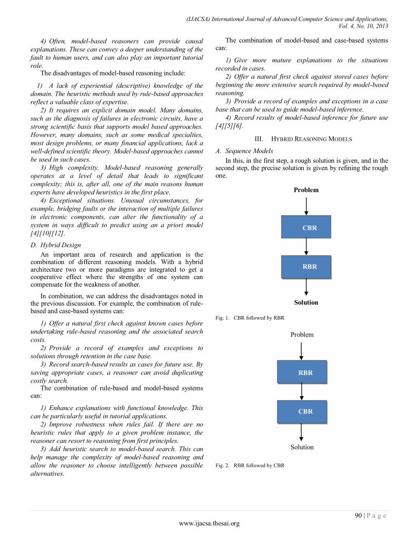
(IJACSA) International Journal of Advanced Computer Science and Applications, Vol. 4, No. 10, 2013
90 | P a g e www.ijacsa.thesai.org
4) Often, model-based reasoners can provide causal
explanations. These can convey a deeper understanding of the
fault to human users, and can also play an important tutorial
role. The disadvantages of model-based reasoning include:
1) A lack of experiential (descriptive) knowledge of the
domain. The heuristic methods used by rule-based approaches
reflect a valuable class of expertise.
2) It requires an explicit domain model. Many domains,
such as the diagnosis of failures in electronic circuits, have a
strong scientific basis that supports model based approaches.
However, many domains, such as some medical specialties,
most design problems, or many financial applications, lack a
well-defined scientific theory. Model-based approaches cannot
be used in such cases.
3) High complexity. Model-based reasoning generally
operates at a level of detail that leads to significant
complexity; this is, after all, one of the main reasons human
experts have developed heuristics in the first place.
4) Exceptional situations. Unusual circumstances, for
example, bridging faults or the interaction of multiple failures
in electronic components, can alter the functionality of a
system in ways difficult to predict using an a priori model
[4][10][12].
D. Hybrid Design
An important area of research and application is the combination of different reasoning models. With a hybrid architecture two or more paradigms are integrated to get a cooperative effect where the strengths of one system can compensate for the weakness of another.
In combination, we can address the disadvantages noted in the previous discussion. For example, the combination of rule-based and case-based systems can:
1) Offer a natural first check against known cases before
undertaking rule-based reasoning and the associated search
costs.
2) Provide a record of examples and exceptions to
solutions through retention in the case base.
3) Record search-based results as cases for future use. By
saving appropriate cases, a reasoner can avoid duplicating
costly search. The combination of rule-based and model-based systems
can:
1) Enhance explanations with functional knowledge. This
can be particularly useful in tutorial applications.
2) Improve robustness when rules fail. If there are no
heuristic rules that apply to a given problem instance, the
reasoner can resort to reasoning from first principles.
3) Add heuristic search to model-based search. This can
help manage the complexity of model-based reasoning and
allow the reasoner to choose intelligently between possible
alternatives.
The combination of model-based and case-based systems can:
1) Give more mature explanations to the situations
recorded in cases.
2) Offer a natural first check against stored cases before
beginning the more extensive search required by model-based
reasoning.
3) Provide a record of examples and exceptions in a case
base that can be used to guide model-based inference.
4) Record results of model-based inference for future use
[4][5][6].
III. HYBRID REASONING MODELS
A. Sequence Models
In this, in the first step, a rough solution is given, and in the second step, the precise solution is given by refining the rough one.
Fig. 1. CBR followed by RBR
Fig. 2. RBR followed by CBR
RBR
CBR
Problem
Solution
CBR
RBR
Problem
Solution
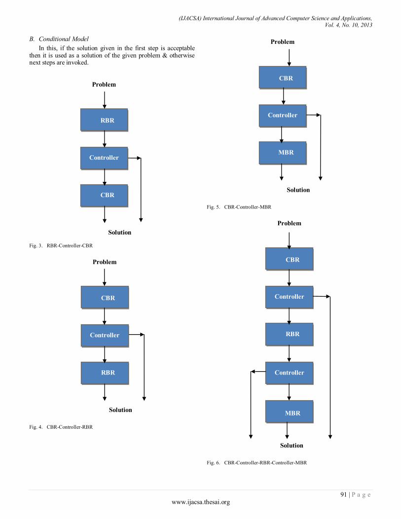
(IJACSA) International Journal of Advanced Computer Science and Applications, Vol. 4, No. 10, 2013
91 | P a g e www.ijacsa.thesai.org
B. Conditional Model
In this, if the solution given in the first step is acceptable then it is used as a solution of the given problem & otherwise next steps are invoked.
Fig. 3. RBR-Controller-CBR
Fig. 4. CBR-Controller-RBR
Fig. 5. CBR-Controller-MBR
Fig. 6. CBR-Controller-RBR-Controller-MBR
CBR
Controller CControll
Problem
Solution
RBR
Controller
MBR
CBR
Controller CControll
Problem
Solution
MBR
CBR
Controller CControll
Problem
Solution
RBR
RBR
Controller CControll
Problem
Solution
CBR
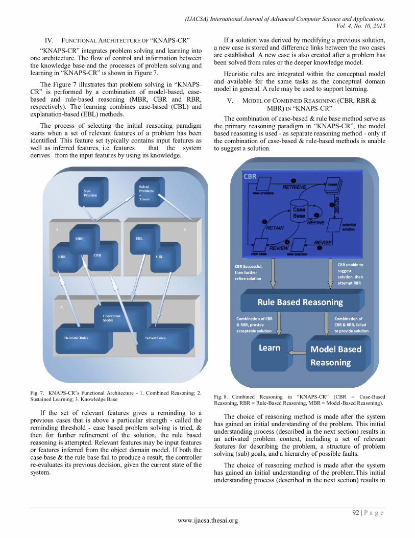
(IJACSA) International Journal of Advanced Computer Science and Applications, Vol. 4, No. 10, 2013
92 | P a g e www.ijacsa.thesai.org
IV. FUNCTIONAL ARCHITECTURE OF “KNAPS-CR”
“KNAPS-CR” integrates problem solving and learning into one architecture. The flow of control and information between the knowledge base and the processes of problem solving and learning in “KNAPS-CR” is shown in Figure 7.
The Figure 7 illustrates that problem solving in “KNAPS-CR” is performed by a combination of model-based, case-based and rule-based reasoning (MBR, CBR and RBR, respectively). The learning combines case-based (CBL) and explanation-based (EBL) methods.
The process of selecting the initial reasoning paradigm starts when a set of relevant features of a problem has been identified. This feature set typically contains input features as well as inferred features, i.e. features that the system derives from the input features by using its knowledge.
Fig. 7. KNAPS-CR’s Functional Architecture - 1. Combined Reasoning; 2.
Sustained Learning; 3. Knowledge Base
If the set of relevant features gives a reminding to a previous cases that is above a particular strength - called the reminding threshold - case based problem solving is tried, & then for further refinement of the solution, the rule based reasoning is attempted. Relevant features may be input features or features inferred from the object domain model. If both the case base & the rule base fail to produce a result, the controller re-evaluates its previous decision, given the current state of the system.
If a solution was derived by modifying a previous solution, a new case is stored and difference links between the two cases are established. A new case is also created after a problem has been solved from rules or the deeper knowledge model.
Heuristic rules are integrated within the conceptual model and available for the same tasks as the conceptual domain model in general. A rule may be used to support learning.
V. MODEL OF COMBINED REASONING (CBR, RBR &
MBR) IN “KNAPS-CR”
The combination of case-based & rule base method serve as the primary reasoning paradigm in “KNAPS-CR”, the model based reasoning is used - as separate reasoning method - only if the combination of case-based & rule-based methods is unable to suggest a solution.
Fig. 8. Combined Reasoning in “KNAPS-CR” (CBR = Case-Based
Reasoning, RBR = Rule-Based Reasoning, MBR = Model-Based Reasoning).
The choice of reasoning method is made after the system has gained an initial understanding of the problem. This initial understanding process (described in the next section) results in an activated problem context, including a set of relevant features for describing the problem, a structure of problem solving (sub) goals, and a hierarchy of possible faults.
The choice of reasoning method is made after the system has gained an initial understanding of the problem.This initial understanding process (described in the next section) results in
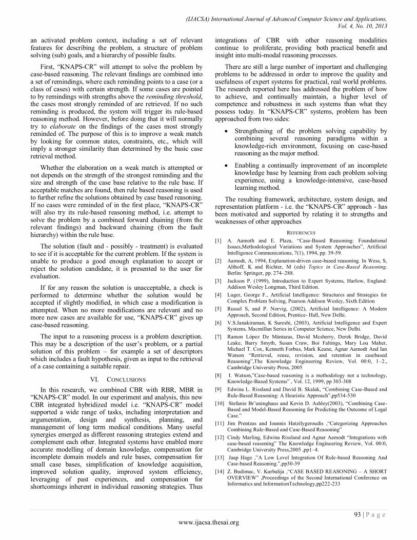
(IJACSA) International Journal of Advanced Computer Science and Applications, Vol. 4, No. 10, 2013
93 | P a g e www.ijacsa.thesai.org
an activated problem context, including a set of relevant features for describing the problem, a structure of problem solving (sub) goals, and a hierarchy of possible faults.
First, “KNAPS-CR” will attempt to solve the problem by case-based reasoning. The relevant findings are combined into a set of remindings, where each reminding points to a case (or a class of cases) with certain strength. If some cases are pointed to by remindings with strengths above the reminding threshold, the cases most strongly reminded of are retrieved. If no such reminding is produced, the system will trigger its rule-based reasoning method. However, before doing that it will normally try to elaborate on the findings of the cases most strongly reminded of. The purpose of this is to improve a weak match by looking for common states, constraints, etc., which will imply a stronger similarity than determined by the basic case retrieval method.
Whether the elaboration on a weak match is attempted or not depends on the strength of the strongest reminding and the size and strength of the case base relative to the rule base. If acceptable matches are found, then rule based reasoning is used to further refine the solutions obtained by case based reasoning. If no cases were reminded of in the first place, “KNAPS-CR” will also try its rule-based reasoning method, i.e. attempt to solve the problem by a combined forward chaining (from the relevant findings) and backward chaining (from the fault hierarchy) within the rule base.
The solution (fault and - possibly - treatment) is evaluated to see if it is acceptable for the current problem. If the system is unable to produce a good enough explanation to accept or reject the solution candidate, it is presented to the user for evaluation.
If for any reason the solution is unacceptable, a check is performed to determine whether the solution would be accepted if slightly modified, in which case a modification is attempted. When no more modifications are relevant and no more new cases are available for use, “KNAPS-CR” gives up case-based reasoning.
The input to a reasoning process is a problem description. This may be a description of the user’s problem, or a partial solution of this problem – for example a set of descriptors which includes a fault hypothesis, given as input to the retrieval of a case containing a suitable repair.
VI. CONCLUSIONS
In this research, we combined CBR with RBR, MBR in “KNAPS-CR” model. In our experiment and analysis, this new CBR integrated hybridized model i.e. “KNAPS-CR” model supported a wide range of tasks, including interpretation and argumentation, design and synthesis, planning, and management of long term medical conditions. Many useful synergies emerged as different reasoning strategies extend and complement each other. Integrated systems have enabled more accurate modelling of domain knowledge, compensation for incomplete domain models and rule bases, compensation for small case bases, simplification of knowledge acquisition, improved solution quality, improved system efficiency, leveraging of past experiences, and compensation for shortcomings inherent in individual reasoning strategies. Thus
integrations of CBR with other reasoning modalities continue to proliferate, providing both practical benefit and insight into multi-modal reasoning processes.
There are still a large number of important and challenging problems to be addressed in order to improve the quality and usefulness of expert systems for practical, real world problems. The research reported here has addressed the problem of how to achieve, and continually maintain, a higher level of competence and robustness in such systems than what they possess today. In “KNAPS-CR” systems, problem has been approached from two sides:
Strengthening of the problem solving capability by combining several reasoning paradigms within a knowledge-rich environment, focusing on case-based reasoning as the major method.
Enabling a continually improvement of an incomplete knowledge base by learning from each problem solving experience, using a knowledge-intensive, case-based learning method.
The resulting framework, architecture, system design, and representation platform - i.e. the “KNAPS-CR” approach - has been motivated and supported by relating it to strengths and weaknesses of other approaches
REFERENCES
[1] A. Aamoth and E. Plaza, “Case-Based Reasoning: Foundational Issues,Methodological Variations and System Approaches”, Artificial
Intelligence Communications, 7(1), 1994, pp. 39-59.
[2] Aamodt, A, 1994, Explanation-driven case-based reasoning. In Wess, S, Althoff, K and Richter, M (eds) Topics in Case-Based Reasoning.
Berlin: Springer, pp. 274–288.
[3] Jackson P. (1999), Introduction to Expert Systems, Harlow, England: Addison Wesley Longman, Third Edition.
[4] Luger, George F., Artificial Intelligence: Structures and Strategies for
Complex Problem Solving, Pearson Addison Wesley, Sixth Edition
[5] Russel S, and P. Norvig, (2002), Artificial Intelligence: A Modern
Approach, Second Edition, Prentice- Hall, New Delhi.
[6] V.S.Janakiraman, K Sureshi, (2003), Artificial Intelligence and Expert Systems, Macmillan Series in Computer Science, New Delhi.
[7] Ramon López De Mántaras, David Mcsherry, Derek Bridge, David
Leake, Barry Smyth, Susan Craw, Boi Faltings, Mary Lou Maher, Michael T. Cox, Kenneth Forbus, Mark Keane, Agnar Aamodt And Ian
Watson “Retrieval, reuse, revision, and retention in casebased Reasoning”,The Knowledge Engineering Review, Vol. 00:0, 1–2.,
Cambridge University Press, 2005
[8] I. Watson,”Case-based reasoning is a methodology not a technology, Knowledge-Based Systems” , Vol. 12, 1999, pp 303-308
[9] Edwina L. Rissland and David B. Skalak, “Combining Case-Based and
Rule-Based Reasoning: A Heuristic Approach”,pp534-530
[10] Stefanie Br¨uninghaus and Kevin D. Ashley(2003), “Combining Case-Based and Model-Based Reasoning for Predicting the Outcome of Legal
Case.”
[11] Jim Prentzas and Ioannis Hatzilygeroudis ,“Categorizing Approaches
Combining Rule-Based and Case-Based Reasoning”
[12] Cindy Marling, Edwina Rissland and Agnar Aamodt “Integrations with case-based reasoning” The Knowledge Engineering Review, Vol. 00:0,
Cambridge University Press,2005 ,pp1–4.
[13] Jaap Hage ,”A Low Level Integration Of Rule-based Reasoning And Case-based Reasoning.”,pp30-39
[14] Z. Budimac, V. Kurbalija ,“CASE BASED REASONING – A SHORT
OVERVIEW” ,Proceedings of the Second International Conference on Informatics and InformationTechnology,pp222-233

(IJACSA) International Journal of Advanced Computer Science and Applications, Vol. 4, No. 10, 2013
94 | P a g e www.ijacsa.thesai.org
[15] Bittencourt, I.I., M. Tadeu and E.B. Costa (2006) Combining AI
techniques into a legal agent-based intelligent tutoring system, in Proceedings of the Eighteenth International Conference on Software
Engineering and Knowledge Engineering (SEKE-2006), Skokie, IL: Knowledge Systems Institute, 35–40.
[16] Bogaerts, S., and Leake, D. 2005. A Framework for Rapid and Modular Case-Based Reasoning System Development. Technical Report TR 617,
Computer Science Department, Indiana University, Bloomington, IN.
[17] Hanemann, L. (2006) A hybrid rule-based/case-based reasoning approach for service fault diagnosis, in Proceedings of the 2006
International Symposium on Frontiers in Networking with Applications,
in conjunction with the Twentieth IEEE International Conference on Advanced Information Networking and Applications, Washington, DC:
IEEE, 734–740.
[18] K. Ashwin Kumar, Yashwardhan Singh, Sudip Sanyal, (2009) Hybrid
approach using case-based reasoning and rule-based reasoning for domain independent clinical decision support in ICU, Expert Systems
with Applications 36, 65–71.

(IJACSA) International Journal of Advanced Computer Science and Applications,
Vol. 4, No. 10, 2013
95 | P a g e
www.ijacsa.thesai.org
Quaternionic Wigner-Ville distribution of analytical
signal in hyperspectral imagery
Yang LIU
Shanghai Medical Instrumentation College
101 Yingkou Road, Yangpu.District 200093
Shanghai.China
Robert GOUTTE
University of Lyon,INSA, labo CREATIS
Umr Cnrs 5220,Inserm 1044 Lyon,France
Abstract—The 2D Quaternionic Fourier Transform (QFT),
applied to a real 2D image, produces an invertible quaternionic
spectrum. If we conserve uniquely the first quadrant of this
spectrum, it is possible, after inverse transformation, to obtain,
not the original image, but a 2D quaternion image, which
generalize in 2D the classical notion of 1D analytical image.
From this quaternion image, we compute the corresponding
correlation product, then, by applying the direct QFT, we obtain
the 4D Wigner-Ville distribution of this analytical signal. With
reference to the shift variables χ1 , χ2 used for the computation of
the correlation product, we obtain a local quaternion Wigner-
Ville distribution spectrum.
Keywords—Analytical; signal; hyperspectral imagery;
quaternionic distribution
I. INTRODUCTION
The most common method of analysis of the frequency content of an n-D real signal is the classical complex Fourier transform. The Fourier transforms have been widely used in signal and image processing. ever since the discovery of the Fast Fourier Transform in 1965 (Cooley-Tukey algorithm) which made the computation of Discrete Fourier Transform feasible using a computer.
Based on the concept of quaternion the quaternion Fourier transform (QFT) has been introduced by Ell (Ref 1) and implemented by Pei (Ref 2) with conventional 2D Fourier transform .
The analytic signal is a complex extension of a 1D signal that is based upon the Hilbert transform; it was introduced to signal theory by Gabor in 1946 (Ref 3).This representation gives access to the instantaneous amplitude and phase. Several attempts to generalize the analytic signal to two dimensions have been reported in the literature, based on the properties of Hilbert and Riesz transforms (Ref 4).
II. CONCEPT OF QUATERNION’S NUMBERS
The Quaternion, discovered by Hamilton (Ref 5) in 1843, also called hyper complex numbers, are the generalization of complex numbers. A complex number has two components: the real and the imaginary part.
The quaternion has four components:
and i, j, k obeys the rules as below:
We clearly observe that multiplication is associative and distributive, compared to addition, but not commutative.
When the real part is null, the corresponding number is called a pure quaternion. For a quaternion-valued function, we can define its magnitude as follow:
| | √
like its conjugate as: q∗=qr qii qjj qkk
III. 2D QUATERNIONIC FOURIER TRANSFORM (QFT)
The classic n-D complex Fourier transform is:
2
1
( ) ( ) exp i i
n
i nj u x n
c
i
F f x dx
u
The QFT is based on the quaternion’s concept, the quaternion Fourier Transform of a 2D real signal f(x, y) is defined as:
( ) ∫ ∫ ( )
This QFT, of type 1, is noted two-side. If the input f(x, y) is a quaternion function and not only a real function, we can decompose f(x, y) as:
( ) ( ) ( ) ( ) ( )
where fr(x, y), fi(x, y), fj(x, y) and fk(x, y) are real functions. We obtain ( ) ( ) ( ) ( ) ( )
The QFT is not identical to the 2D Clifford Fourier
Transform (Ref 6,7), since the signal f CF is sandwiched between the two exponential functions rather than standing on their left side. However the two transforms are identical for real 2D signals.
The QFT is invertible and its inverse is expressed as:
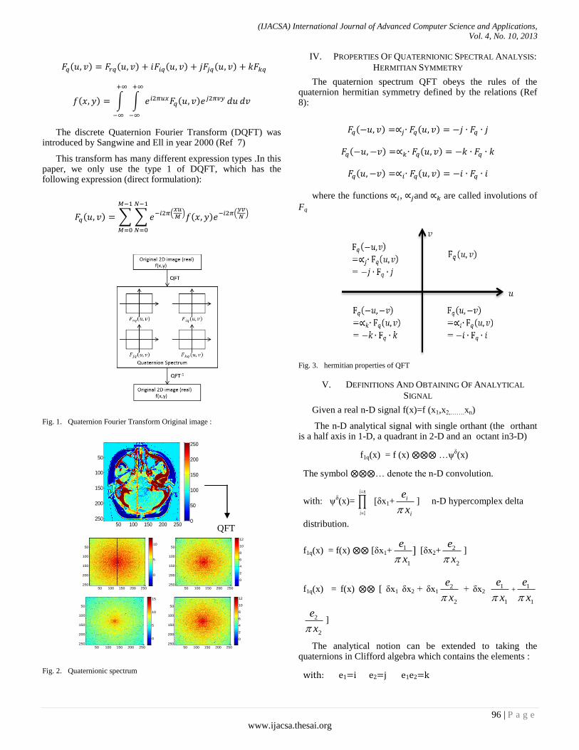
(IJACSA) International Journal of Advanced Computer Science and Applications,
Vol. 4, No. 10, 2013
96 | P a g e
www.ijacsa.thesai.org
( ) ( ) ( ) ( )
( ) ∫ ∫ ( )
The discrete Quaternion Fourier Transform (DQFT) was
introduced by Sangwine and Ell in year 2000 (Ref 7)
This transform has many different expression types .In this paper, we only use the type 1 of DQFT, which has the following expression (direct formulation):
( ) ∑ ∑ (
) ( ) (
)
Fig. 1. Quaternion Fourier Transform Original image :
QFT
Fig. 2. Quaternionic spectrum
IV. PROPERTIES OF QUATERNIONIC SPECTRAL ANALYSIS:
HERMITIAN SYMMETRY
The quaternion spectrum QFT obeys the rules of the quaternion hermitian symmetry defined by the relations (Ref 8):
( ) ( )
( ) ( )
( ) ( )
where the functions , and are called involutions of
Fq
Fig. 3. hermitian properties of QFT
V. DEFINITIONS AND OBTAINING OF ANALYTICAL
SIGNAL
Given a real n-D signal f(x)=f (x1,x2,…….xn)
The n-D analytical signal with single orthant (the orthant is a half axis in 1-D, a quadrant in 2-D and an octant in3-D)
f1q(x) = f (x) ⨂⨂⨂ …ψδ(x)
The symbol ⨂⨂⨂… denote the n-D convolution.
with: ψδ(x)=
1
i n
i
[δx1+i
i
e
x] n-D hypercomplex delta
distribution.
f1q(x) = f(x) ⨂⨂ [δx1+1
1
]e
x [δx2+
2
2
e
x]
f1q(x) = f(x) ⨂⨂ [ δx1 δx2 + δx12
2
e
x + δx2
1
1
e
x+
1
1
e
x
2
2
e
x]
The analytical notion can be extended to taking the quaternions in Clifford algebra which contains the elements :
with: e1=i e2=j e1e2=k
50 100 150 200 250
50
100
150
200
250 0
50
100
150
200
250
50 100 150 200 250
50
100
150
200
250
0
5
10
50 100 150 200 250
50
100
150
200
250
0
2
4
6
8
10
12
50 100 150 200 250
50
100
150
200
250
0
5
10
15
50 100 150 200 250
50
100
150
200
250
0
2
4
6
8
10
12
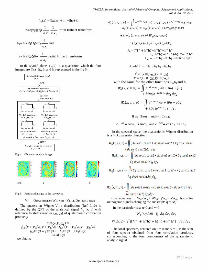
(IJACSA) International Journal of Advanced Computer Science and Applications,
Vol. 4, No. 10, 2013
97 | P a g e
www.ijacsa.thesai.org
f1q(x) =f(x1,x2) +ih1+jh2+kh
h f(x)⊗⊗
1
1
x 2
1
x total Hilbert transform
h1 f(x)⊗ ⊗δx2
1
1
xand
h2= f(x)⊗⊗δx1
2
1
xpartial Hilbert transforms
In the spatial plane f1q(x) is a quaternion which the four images are f(x) , h1, h2 and h ,represented in the fig 5.
Fig. 4. Obtaining analytic image
Real i j k
Fig. 5. Analytical images in the space plan
VI. QUATERNION WIGNER –VILLE DISTRIBUTION
The quaternion Wigner-Ville distribution (Ref 9,10) is defined by the QFT of the analytical signal f1q (x, y) with reference to shift variables (χ1, χ2) of quaternionic correlation product ρ
( ) ( ⁄ ⁄ )
∗( ⁄ ⁄ ) ( ) ( ) ( ) ( )
( ) we obtain:
( ) ∬ ( )
( ) ( ) ( )
( ) ( )
ρ (x,y,u,v)=Aq+iBq+jCq+kDq
Aq=f f + h
h +h
h +h h
Bq=h h f h
+h f h
h f h
h h +h
h +h f
=h f f h +h
h h
h
f
+ = f(x+0,5χ1),(y+0,5χ2)
f =f(x 0,5χ1),(y 0,5χ2)
with the same for the other functions h ,h and h.
( ) ∬ (
)
( ) ∬ (
)
If α1=2πuχ1 and α2=2πvχ2
= cosα1 i sinα1 and cos α2 s nα2
In the spectral space, the quaternionic Wigner distribution is a 4-D quaternion function :
(this equation : Wq=Wqr+ iWqi+ jWqj+ kWqk holds for monogenic signals changing the subscripts q to M)
In the particular case u=0 and v=0
Wqr(x,y,0,0)= ∬
Wqr(x,y)= ∬ f f h h
h h
h h
The local spectrum, centered on u = 0 and v = 0, is the sum of four spectra obtained from four correlation products, corresponding to the four components of the quaternionic analytic signal.
50 100 150 200 250
50
100
150
200
250 -400
-200
0
200
400
50 100 150 200 250
50
100
150
200
250-200
-100
0
100
200
300
400
50 100 150 200 250
50
100
150
200
250 -200
-100
0
100
200
300
400
50 100 150 200 250
50
100
150
200
250
-200
0
200
400

(IJACSA) International Journal of Advanced Computer Science and Applications,
Vol. 4, No. 10, 2013
98 | P a g e
www.ijacsa.thesai.org
VII. GENERALIZATION FOR 3-D REAL SIGNAL.
For n=3,the hypercomplex delta distribution ψδ (x)
become:
ψδ(x1,x2,x3)= δx1 δx2 δx3 +[δx1 +
1
1
e
x] [δx2+
2
2
e
x] [δx3+
3
3
e
x]
and with the rules of Cayley-Dickson (Ref 9,11)
ψδ(x1,x2,x3)= δx1 δx2 δx3 +e1
3
1
2x x
x
+ e2
31
2
x x
x
+
33 2
1 3
xe
x x
+ e4
1 2
3
x x
x
+ 2
5 2
1 3
xe
x x
+ 1
6 2
1 3
xe
x x
+
7 3
1 2 3
1e
x x x
which is a octonion structure
fCD(x1,x2,x3)= f (x1,x2,x3) ⊗ ⊗ ⊗ δx1 δx2 δx3 +e1 3
1
2x x
x
+ e2 31
2
x x
x
+ 3
3 2
1 3
xe
x x
+ e4 1 2
3
x x
x
+ 2
5 2
1 3
xe
x x
+
16 2
1 3
xe
x x
+
7 3
1 2 3
1e
x x x]
which corresponds to 8 images in the spectral plan: one real and seven imaginaries.
The process to obtain the Wigner-Ville distribution is the same as in the previous case n=2, but the computational complexity is increased by the passage, for the analytic signal, of an quaternionic structure to an octonion.
VIII. CONCLUSION
The use of the Fourier quaternionic transformation, associated at the convolution with the n-D delta distribution ,allows to obtain, from real image signal, a spatially hyper complex representation of the analytical signal (quaternion in 2D and octonion in 3D).From this approach , we can generalize the concept of the Wigner Ville distribution and obtain an analytical. tool with both a frequency selectivity and spatial localization.
Interesting applications can be envisaged in imagery, especially for the segmentation problems or in texture analysis (Ref 12).
REFERENCES
[1] T.A.ELL,Hypercomplex spectral transforms,PhD Thesis ,Université of Minnesota,1992.
[2] S.C.Pei,J.J.Ding,J.H.Chang,Efficient Implementation of quaternion Fourier transform,IEEE transactions on signal processing,2001,vol49,no11,p.2783-2797.
[3] D.Gabor, Theorie of communication :Inst Elec.Eng.London,vol.3,pp:429-457,1946.
[4] M.Unser, Hilbert-Riesz wavelet Transform, Seventh Workshop on Information Optics, Fr, June 1-5, 2008.
[5] W.R.Hamilton, On a new Species of imaginary quantities connected with a theory of Quaternion (1843),Meeting of the Royal Irish Academy.
[6] W.K.Clifford. Application of Grassmann’s extensive algebra,Am.J.Math,1,350-1878.
[7] P.R.Girard, .Delachartre,P.Clarysse,R.Goutte,Mise en oeuvre du signal analytique dans les algèbres de Clifford, Colloque 23éme Gretsi,5-8 sept 2011,Bordeaux.
[8] S.I.Sangwine and T.A.Tell, The discrete Fourier transform of a colour image,Image Processing,Math Methods,Algorithms and Applications,pp:430-441,Chichester,2000.
[9] S.L.Hahn,Multidimensional Complex Signals with Single Orthant,
Proceeding IEEE,vol80,pp1287-1300 August1992.
[10] S;L.Hahn,Wigner Quaternionic and Monogenic Signal ,IEEE Trans on Signal Processing,vol53,No 8,August 2005.
[11] K.M.Snopek,The study of properties of nD Analytic Signals,Radioengineering,vol 1,No1,April 2012.
[12] Y.Zhu,R.Goutte,M.Amiel,On the use of a two-dimensional Wigner Ville distribution for texture segmentation.Signal Proc.30,205-220,1993.
(IJACSA) International Journal of Advanced Computer Science and Applications, Vol. 4, No. 10, 2013
99 | P a g e www.ijacsa.thesai.org
On the Practical Feasibility of Secure Multipath
Communication
Stefan Rass and Benjamin Rainer
Technical Faculty, Universität Klagenfurt
Klagenfurt, Austria
Stefan Schauer
Austrian Institute of Technology (AIT)
Safety & Security Department
9020 Klagenfurt, Austria
Abstract—Secure multipath transmission (MPT) uses network
path redundancy to achieve privacy in the absence of public-key
encryption or any shared secrets for symmetric encryption. Since
this form of secret communication works without secret keys, the
risk of human failure in key management naturally vanishes,
leaving security to rest only on the network management.
Consequently, MPT allows for secure communication even under
hacker attacks, on condition that at least some parts of the
network remain intact (unconquered) at all times. This feature is,
however, bought at the price of high network connectivity
(densely meshed structures) that is hardly found in real life
networks. Based on a game-theoretic treatment of multipath
transmission, we present theoretical results for judging the
networks suitability for secure communication. In particular, as
MPT uses non-intersecting and reliable paths, we present
algorithms to compute these in a way that is especially suited for
subsequent secure and reliable communication. Our treatment
will use MPT as a motivating and illustrating example, however,
the results obtained are not limited to any particular application of multipath transmission or security.
Keywords—communication system security; multipath
channels; privacy; risk analysis; security by design
I. INTRODUCTION
Private communication is traditionally achieved by means of encryption based on pre-shared secrets or public-key cryptography. The latter is known to never ultimately resist cryptanalysis because of its intractability based fundament, and any symmetric scheme is perfectly secure if and only if it is somehow isomorphic to the one-time pad. For this reason, secure communication services usually require the user to properly manage certificates and cryptographic keys, which is an intricate and error prone process. Multipath transmission (MPT) offers an elegant yet somewhat expensive alternative, by exploiting network path redundancy to achieve security, besides increased reliability. In particular, MPT does not rely on shared secrets, but assumes the network to be sufficiently meshed to prevent an attacker from sniffing on the entirety of a transmission (for the same reason, failure of network components may not cause a complete breakdown, thus increasing reliability of the system at the same time). Under this hypothesis and suitable channel coding schemes, the portion of the information that escapes the adversary's eyes acts in the very same way as a secret key protects information through encryption. Throughout this work, we consider end-to-end communication between two (fixed) nodes in the network by means of MPT.
Communication by MPT, whenever applicable, offers some neat advantages: first, its security can be shown and retained under the assumption that whole parts of the network are fully under the attacker's control, including knowledge of all cryptographic keys and identity credentials. This threat model in particular covers situations in which software vulnerability exploits (e.g., buffer overflows, SQL-injections, etc.) give remote administrative permissions to an external attacker. Exploiting such vulnerabilities (possibly even zero-day attacks) in a whole set of components in the system is covered by the attacker model used in the sequel.
Second, MPT does not rest on any unproven mathematical conjectures or empirical indications, such as public-key and symmetric cryptography do. While both are considered highly trustworthy, insecurity due to human failure in the operation of the system remains a non-negligible threat. MPT naturally achieves risk diversion by removing duties of key-management, and thus somewhat limiting vulnerabilities by human error.
Network reference architectures (topologies) often have some redundancy for robustness against node failures, whose potential for secure communication, however, often remains hidden. Most theoretical treatments of MPT are explicitly devoted to perfectly secure transmission, which leads to very strong criteria on the network connectivity (cf. [1]). Whereas perfect privacy demands zero probability for an attacker to learn any of the communicated bits, the slightly weaker notion of arbitrarily secure transmission (introduced in III.E) asks for a way to communicate such that the attacker's chance to learn something from the transmission is bounded by some fixed (acceptably low) value .
Besides MPTs suitability for risk management and to gain some security against social engineering, there are also good reasons (cf. [2]) to theoretically study MPT, such as fault-tolerant distributed computing, verifiable secret sharing, secure multiparty computation (SMC) or simply the interest in information-theoretic security (like in quantum cryptography [3]). All of these areas at some stage rely on perfectly secure channels, which MPT can create. The need for high-security communication primitives is also motivated by the advent of new computing models like quantum- or DNA-computing. The whole field of post-quantum cryptography [4] accounts for such future security demands, and MPT is another theoretical yet hardly practical alternative.
(IJACSA) International Journal of Advanced Computer Science and Applications, Vol. 4, No. 10, 2013
100 | P a g e www.ijacsa.thesai.org
This work shall be a step towards making MPT more practical. To this end, we derive theoretical results on how MPT can be carried out over networks to get secure and reliable pairwise communication channels. We validate our results using a prototype implementation of the described methods, which works on hierarchically structured networks. That is, we consider communication not only within an enterprise network, but also across different administrative domains. The resulting network models are graphs that model wide area networks, connecting “black-box nodes” that are themselves local area networks (LANs). A security analysis towards secure communication across such a hierarchically structured infrastructure can be based on conventional graph-theoretic algorithms (shortest path and max-flow), which will be at the core of this work.
II. RELATED WORK
The authors of [5] and [6] discovered MPT as a necessity for perfectly confidential communication, and the work of [7] and [8] complemented this structural result with sharp lower bounds on the necessary communication overhead for such a transmission. Common to all these references are their strong hypotheses on the underlying network graph topology, which gave rise to the game-theoretic treatment in [9] attempting to apply these ideas in general rather than only strongly connected networks. Ever since then, the picture has been extended in various ways, such as by looking for lower bounds on the graph connectivity [8], [10]-[14] implications of synchrony and asynchrony in the transmission [15], [16] impossibility results [17], [18] or applications of MPT in ad hoc and wireless networks [19]-[23].
Multipath transmission is currently under standardization in the course of the Transmission Control Protocol (TCP), see [24]. Experimental simulations have been done towards resource pooling and multipath transmission with a focus on other protocols such as the Stream Control Transmission Protocol (SCTP) and the Multipath RTP (MPTP) with concurrent multipath transmission; see [25] and [26], respectively. Furthermore, [27] introduced an improvement to multipath TCP (MPTCP) where the idea is to introduce fountain code to MPTCP to reduce the impact of paths with lower transmission quality on the overall throughput. Especially in the light of these latest developments, looking at the theoretical possibility of MPT under a more practical environment seems more demanding than ever.
III. PRELIMINARIES
Let a network be modeled as an undirected graph with node set comprising all network devices (computers, routers, switches, etc.), and the edge set giving the (physical or logical) connections between them. Let the nodes be weighted by a security measure defined as The value can be set to either exclude a node from any attack (say, by organisational assumptions, non-cryptographic protections or contractual regulations if models the subnet of a transmission service provider), or to express the (pessimistic) assumption that zero-day exploits or other intrusions on the device may be expected. In that case, we may put , which can also be
done if the „probabilistic security“ of a node is difficult or impossible to obtain reliably. In other cases, assigning appropriate resilience to each node is left to probabilistic security models or general statistical approaches (e.g., beta-reputation [28], [29]). Note that it is not necessary to weight edges, as an edge with weight can be replaced by two unweighted edges to an artificial node with weight in between: .
We write to denote the vertex- and edge-sets of a graph . Moreover, given subsets , we write for the induced subgraph. The symbol denotes the power-set of .
The degree of a node is the number of edges that is part of. For two distinct nodes , hereafter representing the sender and receiver of a transmission, an - -path or wire in is a subgraph of nodes and edges, where and the degree of all nodes is two, and only and have degree one. That is, a path is a subgraph that forms a connection from to as a sequence of nodes and edges. The set of all - -paths is called the set of wires, and denoted by . This set again constitutes a subgraph of . Two - -paths are called (node-)disjoint, if .
Random variables are as well denoted by uppercase letters, as those will exclusively be set-valued (thus justifying the overloaded notation here). We write whenever the
distribution of is . The symbol denotes a random
draw from a set , according to the probability distribution (supported on ).
A. Adversary Model
Assuming that nodes in a network have common or similar security properties, say by running on the same firmware or residing in the same physical location, our attacker model is a family of subsets of that share common vulnerabilities. This models situations in which exploits on several machines create a path through the network towards the valuable data (an attack path). Formally, we model the attacker as a subset , where a set describes an attack scenario in which the adversary has gained full access and control over all nodes in (elsewhere called an adversary structure [30], [8]. As the attacker's behavior is unknown, let be a random variable supported on , whose realization corresponds to the mounting of an attack. We will need this later for our formalization in section III.C.
B. Abstract MPT and its Prerequisites
We write to denote a general MPT protocol that transmits a message over a network, taking random coins to make internal decisions. In particular, the random variable is assumed to steer the choices of transmission paths, besides other protocol-specific actions that use randomness. As our upcoming treatment of security will heavily rely on what paths are chosen for transmission, and what nodes have been attacked successfully (random variable ), let us write for the random variable that selects transmission paths. A particular transmission of a secret message from a sender to a receiver then works by selecting transmission

(IJACSA) International Journal of Advanced Computer Science and Applications, Vol. 4, No. 10, 2013
101 | P a g e www.ijacsa.thesai.org
paths by sampling from and running the MPT protocol over the chosen set of paths. This captures most of the theoretical work on MPT cited in section II, where the set of paths is always assumed to be fixed prior to the transmission, when some additional assumptions are adopted, which commonly appear implicitly throughout the MPT literature (e.g., [6]-[8] and others):
1) The network topology is reliably known, so that paths
can be selected. Here, we can allow only for partial
knowledge of the topology, treating all parts of the network
with unknown topologies as black boxes (and taking
advantage of the hierarchical graph modeling mentioned
above and detailed later).
2) Packets can be routed over fixed chosen paths.
Although such source routing is an existing yet mostly
disabled feature of the internet protocol (IP), such routing can
be over virtual LANs resembling the paths (network layer 2),
or using port routing on layer 3 (transport).
3) The routing is reliable in the sense that a packet does
not deviate from its designated transportation route. Although
we explicitly assume this here, one can relax this assumption
to a limited extent, while still retaining the possibility of
secure communication [31]. We do not explore this any
further here.
4) An exhaustive set of scenarios can be identified under
which an adversary can attack. This is usually the result of
topological vulnerability analysis (searching for attack paths
and attack graphs), the results of which make up the abstract
family of component sets that are vulnerable to a
specific attack. In section IV.B, we show how to derive an
approximation of from the anyway required computation of
node-disjoint paths. We stress that these assumptions exclude adversaries being
able to mimic a certain number of virtual nodes (Sybil attacks), which would mean that the network topology information is itself unreliable. It is subject of future work, yet outside the scope of this article, to consider adversaries with such power.
C. Simple MPT – An Example
To motivate the general treatment and show how secure MPT may work, we use an inefficient yet simple example protocol. Suppose that the network permits node-disjoint - -paths , where . Let the message be a bitstring , which the sender writes as , where is the bitwise XOR. This representation is immediately found by choosing random strings , and putting We call each a share to . From a cryptographic viewpoint, this is an -out-of- -sharing, as no subset of less than of the shares reveals any information on . This is easy to see, as any unknown share, say , acts as a one-time pad encryption of .
For the same reason, an attacker is required to get all shares in order to correctly recover . So, if each share travels over a distinct path , then no set with cardinality will suffice to disclose . Consequently, any attack on less than nodes will necessarily fail, and only those
attack scenarios will be successful (for the adversary), in which all paths are intercepted.1.
Recall that were random variables describing the (random) path choices and (unknown) compromised node sets. Let us introduce an (efficiently decidable) predicate that equals 1 if and only if attack fails under transmission scenario . Then is also a binary random variable, which measures the success rate of the (generic) protocol where is under the sender's control, and is coming from the adversary and thus unknown. The next section will define security in terms of the predicate , more precisely, its expectation.
D. Security Measures
It is common in cryptography to capture attack scenarios in abstract “games”. Security is then defined in terms of the likelihood for the attacker to win the game.
: Let be the message to be sent over
from to .
1) The (honest) sender chooses .
2) The adversary conquers a node-set .
3) The protocol is executed, resulting in either success ( ) or failure ( ).
4) Output as the game’s outcome.
The security of an MPT transmission is the attacker's advantage in winning the above game,
.
A widely unexploited feature of MPT is the degree of freedom to choose the paths (in particular, all prior research seems to keep the path choices fixed a priori in an attempt to guard against every scenario described by . We take a more general direction here, by using game-theory to optimize the honest party's behavior ( ) and the attacker's behavior ( ) simultaneously. This leads to the computation of a (Nash-)
equilibrium for
, which satisifes
(1)
for any distributions .
The appeal of imposing a zero-sum hypothesis on the competition between the sender and the attacker lies in the validity of the right of the above inequalities under any real behavior of the attacker. Put differently, if the advantage is
computed as the Nash-equilibrium solution
, then this value lower-bounds the success-rate of the MPT-protocol regardless of what the attacker actually does (see [9] and [32] for formal proofs), conditional on the only hypothesis that no attack outside is mounted (in which case, however, any security analysis would fail).
1 More general approaches (e.g. [6], [8]) replace this simple encoding by a
more robust and flexible polynomial secret sharing, or equivalently, a Reed-
Solomon encoding. This enjoys both, robustness against path failure, and
perfect secrecy against eavesdropping on a certain limited number of wires.

(IJACSA) International Journal of Advanced Computer Science and Applications, Vol. 4, No. 10, 2013
102 | P a g e www.ijacsa.thesai.org
The converse probability, called the vulnerability,
(2)
measures how many messages are discovered by the attacker, relative to the entire lot of transmitted information. This upper bounds the likelihood for an attack, which is why we can consistently use the same symbol as for the node-weights. The important difference here is that (2) refers to a whole transmission from to , rather than a single node.
E. Definitions
Since our adversary can control his advantage via clever choices about the compromised nodes, we extend the usual model of an adversary structure towards a probability distribution supported on an adversary structure.
Definition 1. Given a network , an adversary is described by a probability distribution supported on a family of possibly compromised nodes. Concerning semantics, we define . The attacker is computationally unconstrained regarding the processing of information in his possession.
Imposing no limit on the attacker's power is actually not unrealistic under our adversary model: by assumption, once the attacker has conquered a set of nodes, we assume full control over all nodes in , including full knowledge about the data residing in these nodes. Hence, the attacker can compute anything that the honest parties could compute too, thus precluding (and invalidating) all intractability assumptions that would otherwise establish security of conventional public-key and symmetric cryptography.
Nevertheless, to keep things practical, we need to impose bounds on the computational power of the honest parties (no transmission scheme can feasibly handle inputs of exponential size), and on the size of the adversary structure (to keep the running time of our algorithms within reasonable bounds).
Definition 2. [5] A transmission is called -private (for ), if for any two plain text messages, the corresponding random ciphertexts have distributions that are statistically indistinguishable (distant in the 1-norm) up to a difference of . A transmission is called -reliable for , if with probability at least , the delivery is correct. A transmission is -secure, if it is both, -private and -reliable, and it is called perfectly secure if . The transmission is called efficient, if its bit- and round-complexity is polynomial in the size of the network and the message, as well as and , wherever and/or .
The vulnerability definition (2) is naturally linked to the above security concepts by the following fact:
Theorem 1. [9] Assume a Nash-equilibrium behavior
for the honest parties in
, and let be computed as in (2) for a predicate . If indicates a successful confidential (not necessarily
correct) transmission using , then is - ri ate Alternatively, if indicates a successful correct (not
necessarily confidential) transmission using , then is
-reliable
This is a major difference to the treatment common in cryptography. As opposed to the abstract games serving for complexity-theoretic reduction arguments towards security proofs, for multipath transmission we explicitly attempt to execute the game in reality. The optimal way of doing this is determined by techniques of game-theory, whose details are not relevant here (see [9] for a full treatment). Theorem 1 is the permission to use the following as our security definition:
Definition 3. A protocol is called - , if there is some
such that for every distribution over
. The protocol is said to achieve arbitrarily secure message transmission (ASMT), if it is -secure for every . A 0-secure protocol is said to achieve perfectly secure message transmission (PSMT).
Notice that ASMT can achieve the same level of secrecy as any conventional encryption, if we set to be the likelihood of guessing the key (e.g., for a Bit AES key). However, and more generally than PSMT, the Nash-equilibrium based analysis of security is extensible towards multiple interdependent security goals in a consistent way [33]. Other concepts like Definition 2 are much more difficult to handle or extend.
Obviously, PSMT implies ASMT. The converse is not true, since ASMT allows for a strictly positive residual chance of disclosing the message, which PSMT explicitly rules out. The advantage of ASMT over PSMT, however, is that the former may be possible in cases where PSMT is ruled out by insufficient graph connectivity. The remainder of this work is dedicated to a discussion on how to set up the transmission
game
so that either ASMT is possible, or neither PSMT nor ASMT are achievable (provably).
Going through the literature on MPT (and also section III.C), one finds the idea of “by assing” the attacker by irtue of using multiple paths to be a common denominator among most (if not all) MPT protocols. The next definition captures this more explicitly.
Definition 4. Let a (directed) graph and a subset be given. For two distinct nodes , we define the (directed) residual - -capacity of w.r.t. , denoted as , as the number of - -paths that circumvent , i.e., the number of paths that do not go through any node in .
The residual capacity is important as it characterizes the possibility or impossibility of secure transmission based on whether a person-in-the-middle attack between and is possible (or the attacker can be circumvented).
Proposition 1. ASMT from to is possible against an active adversary , if and only if the residual capacity for all .
Proof. For the necessity, suppose that PSMT is possible then the likelihood of a message to circumvent any is 1. Then for every there exists at least one path that avoids , hence the residual capacity is . Conversely, if the residual capacity is , then the following protocol can do

(IJACSA) International Journal of Advanced Computer Science and Applications, Vol. 4, No. 10, 2013
103 | P a g e www.ijacsa.thesai.org
arbitrarily secure message transmission: put and observe that by hypothesis. Now (as described in section II.B), let us divide the message
by a -out-of- -sharing as , and transmit over another distinct path (exhausting the set of available paths). Let denote the probability of to bypass all compromised nodes. Furthermore, implies that (note that the distributions that control the choice of paths and compromised nodes can be omitted, since for any ). Since recovery of the message requires all shares (the predicate would thus be defined as 1 in this case only), the likelihood for all these getting caught is
as . So
for any given , if is chosen sufficiently large.
The rather simple transmission protocol used in the proof of Proposition 1 is clearly suboptimal in terms of communication overhead (yet its overhead is polynomial in , thus nevertheless being efficient in the sense of Definition 2). Its meaning for our investigation, is merely to prove that ASMT is possible based on a certain graph connectivity. Nevertheless, the security of multipath transmission is in any case determined by the likelihood to circumvent compromised nodes. Consequently, a larger number of paths to choose from will eventually maximize the chances of bypassing the adversary. Our algorithms for path enumeration given in section IV.A will therefore attempt to give a maximal number of such paths.
IV. SETTING UP THE MPT-GAME
Our main objective in the following is to practically
instantiate
for a given protocol , which for any MPT protocol requires two initial tasks: 1) enumerate a maximal set of paths to choose from, and 2) compute the most vulnerable points in the network (as those may be the most likely targets for an attack).
As an exhaustive enumeration of paths is infeasible (usually, there are exponentially many of them), and an exhaustive enumeration of attack strategies is also difficult, we
shall “a roximate” both ingredients to
,
and use the approximations and in place of and throughout the rest, where the goodness of this approximation will be in the center of attention now.
A. Enumerating Transmission Paths
A useful result from graph theory (Theorem 5.17 in [34]) equates the number of node-disjoint paths between any two nodes in to the cardinality of a minimal vertex cut between and , where an - -cut} in a graph is a set so that any - -path has . For the adversary, conquering a cut is equivalent to mounting a person-in-the-middle attack, which is the only way to effectively intercept an MPT transmission. The problem of finding a minimal vertex cuts is computationally simple and solvable by min-cut-max-flow techniques. The latter basically work by computing node-disjoint paths (cf. [35]), which we need anyway. So, the node-disjoint paths can be used to run MPT, while the graph cuts that are computed alongside can be used to identify neuralgic points in the network that potentially match attack strategies in (hence „approximate“ ).
So far, there is no real computational difficulty, whenever the number of paths is known and constant. Here is the problem: the number of paths is determined by the power of the adversary in terms of how many nodes can be corrupted at the same time. Moreover, even if this number is known, if any logical connection within the network would use the maximal number of paths, network congestions become highly likely and congestion control may randomly cause paths to intersect. Such congestions can be even due to the adversary; a scenario that has received attention in [31], where the reliability of routing was in the focus of interest. This shows another limitation of the aforementioned references in terms of practicability. Although [8] provides a sharp limit on the minimal required amount of bandwidth for MPT, and many results assuring perfectly private communication under certain graph connectivity assumptions are known, a network whose bandwidth and connectivity undercut the theoretical minimum requirements for PSMT may rule out the latter, yet still enable ASMT.
Let denote the set of all candidate paths, from which the protocol may select a subset for transmission. This is basically an approximation to the set , whose cardinality may be exponential (and thus infeasible to handle).
To set up , we compute the maximal number of node-disjoint - -paths by running a conventional edge-capacity based min-cut-max-flow algorithm on a transformed version of The transformation is well-known and detailed in [35] It basically substitutes each node in the graph by two connected nodes , setting the capacity of the internal (directed) edge to 1 so as to limit the flow through this node. All other undirected edges are replaced by two directed edges and , both of which have infinite capacity. The only exception to this rule are the sender's node , from which only outgoing edges are drawn, and the receiver's node , having only incoming edges.
It is easy to see that an integral maximal - -flow over a network with vertex capacities all set to 1 equals the number of node-disjoint - -paths. We can also permit intersections of paths in certain selected nodes, say in case that a node has zero vulnerability, and thus cannot be conquered in any scenario in . To let paths intersect at a node, we simply increase its internal edge weight from 1 to , so that any number of paths may pass this node.
Taking a closer look at the internals of the Ford-Fulkerson min-cut-max-flow algorithm, we see that the algorithm in each step increases the flow by searching for another flow-augmenting path through nodes with positive remaining capacity. On this residual network, we can construct a flow-augmenting ath by looking for the “most secure” - -path. This is easy by virtue of a shortest-path algorithm that takes the vertex security as the length of the internal edge from , taking all other edges (connecting different nodes to each other) with zero length. Observe that we now have two different weights assigned to each node, one of which is either 1 or to limit the number of paths through this node; while the other weight serves to compute another flow-augmenting path by taking the (next) most secure - -path.
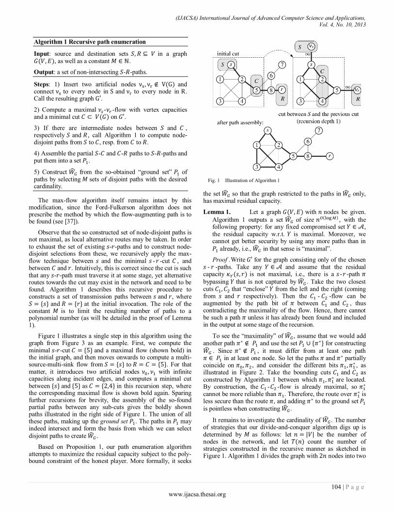
(IJACSA) International Journal of Advanced Computer Science and Applications, Vol. 4, No. 10, 2013
104 | P a g e www.ijacsa.thesai.org
Fig. 1 Illustration of Algorithm 1
Algorithm 1 Recursive path enumeration
Input: source and destination sets in a graph , as well as a constant .
Output: a set of non-intersecting - -paths.
Steps: 1) Insert two artificial nodes and connect to every node in and to every node in . Call the resulting graph .
2) Compute a maximal - -flow with vertex capacities and a minimal cut on .
3) If there are intermediate nodes between and , respectively and , call Algorithm 1 to compute node-disjoint paths from to , resp. from to .
4) Assemble the partial - and - paths to - -paths and put them into a set .
5) Construct from the so-obtained “ground set” of paths by selecting sets of disjoint paths with the desired cardinality.
Fig. 6. Alternative routes and bounding cuts
Fig. 5. Transmission routes and cuts
The max-flow algorithm itself remains intact by this modification, since the Ford-Fulkerson algorithm does not prescribe the method by which the flow-augmenting path is to be found (see [37]).
Observe that the so constructed set of node-disjoint paths is not maximal, as local alternative routes may be taken. In order to exhaust the set of existing - -paths and to construct node-disjoint selections from these, we recursively apply the max-flow technique between and the minimal - -cut , and between and . Intuitively, this is correct since the cut is such that any - -path must traverse it at some stage, yet alternative routes towards the cut may exist in the network and need to be found. Algorithm 1 describes this recursive procedure to constructs a set of transmission paths between and , where and at the initial invocation. The role of the constant is to limit the resulting number of paths to a polynomial number (as will be detailed in the proof of Lemma 1).
Figure 1 illustrates a single step in this algorithm using the graph from Figure 3 as an example. First, we compute the minimal - -cut and a maximal flow (shown bold) in the initial graph, and then moves onwards to compute a multi-source-multi-sink flow from to . For that matter, it introduces two artificial nodes with infinite capacities along incident edges, and computes a minimal cut between and as in this recursion step, where the corresponding maximal flow is shown bold again. Sparing further recursions for brevity, the assembly of the so-found partial paths between any sub-cuts gives the boldly shown paths illustrated in the right side of Figure 1. The union of all these paths, making up the ground set . The paths in may indeed intersect and form the basis from which we can select
disjoint paths to create .
Based on Proposition 1, our path enumeration algorithm attempts to maximize the residual capacity subject to the poly-bound constraint of the honest player. More formally, it seeks
the set so that the graph restricted to the paths in only, has maximal residual capacity.
Lemma 1. Let a graph with nodes be given.
Algorithm 1 outputs a set of size , with the following property: for any fixed compromised set , the residual capacity w.r.t. is maximal. Moreover, we cannot get better security by using any more paths than in
already, i.e., in that sense is “maximal”.
Proof .Write for the graph consisting only of the chosen - -paths. Take any and assume that the residual capacity is not maximal, i.e., there is a - -path
bypassing that is not captured by . Take the two closest cuts that “enclose” from the left and the right (coming from and respectively). Then the - -flow can be augmented by the path bit of between and , thus contradicting the maximality of the flow. Hence, there cannot be such a path unless it has already been found and included in the output at some stage of the recursion.
To see the “maximality” of , assume that we would add another path and use the set for constructing
. Since , it must differ from at least one path in at least one node. So let the paths and partially coincide on , and consider the different bits
, as illustrated in Figure 2. Take the bounding cuts and as constructed by Algorithm 1 between which
are located. By construction, the - -flow is already maximal, so
cannot be more reliable than . Therefore, the route over
is less secure than the route , and adding to the ground set
is pointless when constructing .
It remains to investigate the cardinality of . The number of strategies that our divide-and-conquer algorithm digs up is determined by as follows: let be the number of nodes in the network, and let count the number of strategies constructed in the recursive manner as sketched in Figure 1. Algorithm 1 divides the graph with nodes into two
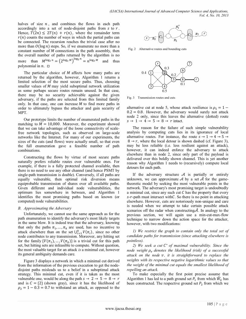
(IJACSA) International Journal of Advanced Computer Science and Applications, Vol. 4, No. 10, 2013
105 | P a g e www.ijacsa.thesai.org
Fig. 2 Alternative routes and bounding cuts
Fig. 3 Transmission routes and cuts
halves of size , and combines the flows in each path accordingly into a set of node-disjoint paths from to . Hence, , where the remainder term counts the number of ways in which the partial paths can be connected. The recursion reaches the trivial case after no more than steps. So, if we enumerate no more than a constant number of connections in the path assembly, then the overall number of paths returned by the algorithm is no
more than
and thus
polynomial in .
The particular choice of affects how many paths are returned by the algorithm, however, Algorithm 1 returns a limited selection of the most secure paths. Thus, choosing smaller values of may yield suboptimal network utilization as some perhaps secure routes remain unused. In that case, there may be no security achievable against the given adversary, if the paths are selected from this limited family only. In that case, one can increase to find more paths in order to ultimately bypass the attacker and gain security of MPT.
Our prototype limits the number of enumerated paths in the matching to . Moreover, the experiment showed that we can take advantage of the loose connectivity of scale-free network topologies, such as observed on large-scale networks like the Internet. For many of our experiments, the sizes of the cuts (and flows) were actually small, so that even the full enumeration gave a feasible number of path combinations.
Constructing the flows by virtue of most secure paths naturally prefers reliable routes over vulnerable ones. For example, if there is a fully protected channel available, then there is no need to use any other channel (and hence PSMT by single-path transmission is doable). Conversely, if all paths are equally vulnerable, then optimal risk diversion means equiprobable transmission of shares over all available paths. Given different and individual node vulnerabilities, the optimum lies somewhere in between, and Algorithm 1 identifies the most promising paths based on known (or computed) node vulnerabilities.
B. Approximating the Adversary
Unfortunately, we cannot use the same approach as for the path enumeration to identify the adversary's most likely targets in the same blow. It is indeed true that the adversary, knowing that only the paths are used, has no incentive to
attack elsewhere than on the set , since no other
node contributes to any transmission. Moreover, any hitting set for the family is a trivial cut for this path set, but hitting sets are infeasible to compute. Without question, the most valuable target for an attack is a minimal cut, however its general ambiguity demands care.
Figure 3 displays a network in which a minimal cut derived from the information of the previous execution to get the node-disjoint paths misleads us to a belief in a suboptimal attack strategy. This minimal cut, even if it is taken as the most vulnerable one, would be along the path and is (shown gray), since it has the likelihood of to withstand an attack, as opposed to the
alternative cut at node 5, whose attack resilience is . However, the adversary would surely not attack node 2 only, since this leaves the alternative (dotted) route intact.
The reason for the failure of such simple vulnerability analysis by computing cuts lies in its ignorance of local alternative routes. For instance, the route , where the local detour is shown dashed (cf. Figure 3), may be less reliable (i.e. less resilient against an attack), however, it can indeed enforce the adversary to attack elsewhere than in node 2, since only part of the payload is delivered over this boldly shown channel. This is yet another reason why Algorithm 1 needs to (recursively) compute local detours for each path.
If the adversary structure is partially or entirely
unknown, we can approximate by a set for the game-theoretic model by seeking the most vulnerable points in the network. The adversary's most promising target is undoubtedly a minimal cut, since any such cut has the property that every - -path must intersect with . So there is no point in attacking elsewhere. However, cuts are notoriously non-unique and care is needed when we attempt to take certain possible attack
scenarios off the radar when constructing . In analogy to the previous section, we will again use a min-cut-max-flow technique to narrow down the action space for the attacker, however, with two modifications:
1) We restrict the graph to contain only the total set of
candidate paths for transmission (since attacking elsewhere is
pointless).
2) We seek a cut of maximal vulnerability. Since the
node weight denotes the likelihood (risk) of a successful
attack on the node , it is straightforward to replace the
weights with its respective negative logarithmic values so that
the weight of the minimal cut equals the smallest likelihood of
repelling an attack. To make especially the first point precise assume that
Algorithm 1 has led to a path ground set from which has been constructed. The respective ground set from which we

(IJACSA) International Journal of Advanced Computer Science and Applications, Vol. 4, No. 10, 2013
106 | P a g e www.ijacsa.thesai.org
construct is then simply the union of all nodes that are used
by at least one path in , i.e., , and restrict
the graph to contain only the nodes in when we consider the adversary's attack strategies by seeking a cut whose weight (as determined by the negative logarithms of the node weights) is maximal. The goodness of the approximation of the
unknown adversary structure through the set is readily established, since
attack on attack on attack on attack on .
for every - -cut . Hence, the adversary is best off attacking nodes in , as these form the most vulnerable points in the system. The algorithmic details are unchanged, since the max-flow algorithm directly provides us with the sought cut as the most vulnerable point in the network. This is where we can
expect an attack with maximal probability, so that can be constructed as the family of subsets of . Specifically, if a set shall be compromised, then either is already a cut, in
which case contains a set of larger weight, i.e., better chance to fail under an attack, or is not a cut, in which case its chances to breach the security of the transmission is less than
for any cut, especially those contained in . We conclude these observations as
Proposition 2. (Approximation of the adversary ) Let be a set in the unknown adversary structure . Then the likelihood to attack the nodes in is no larger
than the likelihood to attack some set in .
V. HIERARCHIAL NETWORKS
Many practical networks are organized in a hierarchical manner, such as company networks can be scattered throughout a country with local area networks (LANs) that are interconnected subnets of a larger wide area network (WAN). For instance, if the sub-networks are hosted by some provider, then we can model the provider's network topology only to the extent to which it is known. If so, then we can use the techniques here to get a risk estimate for the provider's network . Otherwise, we can (subjectively or based on service level agreements) assign a trust level to the ro ider‘s network and treat it as a black box for the overall risk analysis. As another application scenario, think of a large enterprise network, in which we divide the whole network into local subnets (e.g. designated core-switches for different departments within the company) that are part of the larger network. This is modeled as the „WAN“ although it basically is a condensed view on a big LAN.
Suppose that we have a WAN , in which each subgraph node itself represents another LAN subnet , and each edge connects two “border-gateways” (these are the entry- and exit-points to the subnet) . Figure 4 shows an example. The analysis of the WAN and its subnets is based on the following two intuitions:
1) From the WAN perspective, each subnet is represented
as a single node, whose duty is only the delivery of payload
through it. For that matter, we must assume that a subnet is a
connected sub-graph, for otherwise, the WAN would contain
routes that are physically impossible by the subnet topology.
Depending on the particular internal structure of the subnet,
we must do an individual and specific vulnerability analysis
for the subnet and carry over this information as node-weight
to the WAN for the higher-level vulnerability analysis within
the WAN. All of these assessments are done using multipath
transmission games in the way as described in the previous
sections.
2) Each subnet delivers its payload using MPT, exactly
as the WAN does. Let be the border-
gateways within , then we set up and solve an MPT game
(yielding the equilibrium ) and get a vulnerability
estimate
for the connection - for
Within the super-graph the
representation of the subnet is a single node with a weight-
vector, and where the particular node-weight to set up the
game-matrix is determined according to the exact entry- and
exit-gateway when traversing the subnet . If the transmission
game
is played using the optimal choice
rule , then the value upper bounds the probability for a
f l atta k on th “nod ” by the properties of the
equilibrium distribution (see (1)). It can therefore be used
to analyze the WAN in the final step, by treating the game as
non-deterministic and taking the weights in the WAN.
To exemplify the treatment of subnets, especially the second of the above intuitions, consider a snippet of a WAN , showing a single subnet that is connected to three other nodes in Figure 4a sketches the full network. The condensed network , shown in Figure 4b, has reduced to a single node with a vector of three weights that represent the vulnerabilities for the channels , and through the subnet Now, consider the multipath game within , and a strategy that takes the (sub)route , then within this route, the node would receive the weight , since from , the payload enters through and leaves towards via the exit-gateway . Similarly, in the path , the “node” would have weight for the same reason. This simple trick extends our multipath transmission game setup to very large scale networks at a computationally efficient level.
VI. EXPERIMENTAL EVALUATION
For a practical evaluation, we implemented the described algorithms in a C++ prototype, and fed a total of 210 random networks with scale-free topology (sampled under the Barabási-Albert model [38]) with node counts ranging from 20 to 150 (in steps of 10).
For outlier robustness, we computed the median running time in seconds for 15 random testcases per network size. Figure 5 displays the growth of the running time dependent on the network size. All benchmarks were carried out on an Intel Core i7 3.4 GHz with four physical cores and four virtual cores (through hyper threading) with 8 GB of RAM and Windows 7 x64 installed.
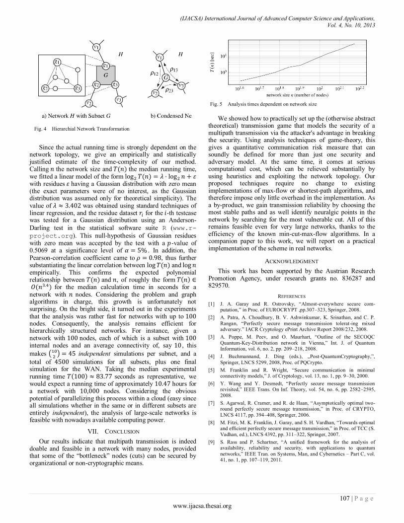
(IJACSA) International Journal of Advanced Computer Science and Applications, Vol. 4, No. 10, 2013
107 | P a g e www.ijacsa.thesai.org
Fig. 4 Hierarchial Network Transformation
Fig. 5 Analysis times dependent on network size
Since the actual running time is strongly dependent on the network topology, we give an empirically and statistically justified estimate of the time-complexity of our method. Calling the network size and the median running time, we fitted a linear model of the form with residues having a Gaussian distribution with zero mean (the exact parameters were of no interest, as the Gaussian distribution was assumed only for theoretical simplicity). The value of was obtained using standard techniques of linear regression, and the residue dataset for the -th testcase was tested for a Gaussian distribution using an Anderson-
Darling test in the statistical software suite R (www.r-
project.org). This null-hypothesis of Gaussian residues with zero mean was accepted by the test with a -value of 0.5069 at a significance level of . In addition, the Pearson-correlation coefficient came to , thus further substantiating the linear correlation between and empirically. This confirms the expected polynomial relationship between and , of roughly the form for the median calculation time in seconds for a network with nodes. Considering the problem and graph algorithms in charge, this growth is unfortunately not surprising. On the bright side, it turned out in the experiments that the analysis was rather fast for networks with up to nodes. Consequently, the analysis remains efficient for hierarchically structured networks. For instance, given a network with nodes, each of which is a subset with internal nodes and an average connectivity of, say , this
makes independent simulations per subnet, and a
total of simulations for all subsets, plus one final simulation for the WAN. Taking the median experimental running time seconds as representative, we would expect a running time of approximately hours for a network with nodes. Considering the obvious potential of parallelizing this process within a cloud (easy since all simulations whether in the same or in different subsets are entirely independent), the analysis of large-scale networks is feasible with nowadays available computing power.
VII. CONCLUSION
Our results indicate that multipath transmission is indeed doable and feasible in a network with many nodes, provided that some of the “bottleneck” nodes (cuts) can be secured by organizational or non-cryptographic means.
We showed how to practically set up the (otherwise abstract theoretical) transmission game that models the security of a multipath transmission via the attacker's advantage in breaking the security. Using analysis techniques of game-theory, this gives a quantitative communication risk measure that can soundly be defined for more than just one security and adversary model. At the same time, it comes at serious computational cost, which can be relieved substantially by using heuristics and exploiting the network topology. Our proposed techniques require no change to existing implementations of max-flow or shortest-path algorithms, and therefore impose only little overhead in the implementation. As a by-product, we gain transmission reliability by choosing the most stable paths and as well identify neuralgic points in the network by searching for the most vulnerable cut. All of this remains feasible even for very large networks, thanks to the efficiency of the known min-cut-max-flow algorithms. In a companion paper to this work, we will report on a practical implementation of the scheme in real networks.
ACKNOWLEDGMENT
This work has been supported by the Austrian Research Promotion Agency, under research grants no. 836287 and 829570.
REFERENCES
[1] J. A. Garay and R. Ostro sky, “Almost-everywhere secure com- utation,” in Proc. of EUROCRYPT , .307–323, Springer, 2008.
[2] A. Patra, A. Choudhury, B. V. Ashwinkumar, K. Srinathan, and C. P.
Rangan, “Perfectly secure message transmission tolerat-ing mixed ad ersary.” IACR Cry tology ePrint Archi e Re ort 2008/232, 2008.
[3] A. Po e, M. Pee , and O. Maurhart, “Outline of the SECOQC
Quantum-Key-Distribution network in Vienna,” Int. J. of Quantum Information, vol. 6, no. 2, pp. 209–218, 2008.
[4] J. Buchmannand, J. Ding (eds.), „Post-QuantumCryptography,”,
Springer, LNCS 5299, 2008, Proc. of PQCrypto.
[5] M. Franklin and R. Wright, “Secure communication in minimal connecti ity models,” J. of Cry tology, ol. 13, no. 1, . 9–30, 2000.
[6] Y. Wang and Y. Desmedt, “Perfectly secure message transmission re isited,” IEEE Trans. On Inf. Theory, vol. 54, no. 6, pp. 2582–2595,
2008.
[7] S. Agarwal, R. Cramer, and R. de Haan, “Asym totically o timal two-round erfectly secure message transmission,” in Proc. of CRYPTO,
LNCS 4117, pp. 394–408, Springer, 2006.
[8] M. Fitzi, M. K. Franklin, J. Garay, and S. H. Vardhan, “Towards o timal and efficient erfectly secure message transmission,” in Proc. of TCC (S.
Vadhan, ed.), LNCS 4392, pp. 311–322, Springer, 2007.
[9] S. Rass and P. Schartner, “A unified framework for the analysis of availability, reliability and security, with applications to quantum
networks,” IEEE Tran. on Systems, Man, and Cybernetics – Part C, vol. 41, no. 1, pp. 107–119, 2011.

(IJACSA) International Journal of Advanced Computer Science and Applications, Vol. 4, No. 10, 2013
108 | P a g e www.ijacsa.thesai.org
[10] M. Franklin and M. Yung, “Secure hy ergra hs: ri acy from artial
broadcast,” in Proc. of STOC, . 36–44, ACM, 1995.
[11] K. Srinathan, A. Narayanan, and C. Pandu Rangan, “O timal erfectly
secure message transmission,” in Proc. of CRYPTO, LNCS 3152, . 545–561, Springer, 2004.
[12] K. KurosawaandK.Suzuki,“Almost secure (1-round, n-channel) message
transmission scheme,” in Proc. of ICTIS (Y. Desmedt, ed.), . 99–112, Springer, 2007.
[13] K. Kurosawa and K. Suzuki, “Truly efficient 2-round perfectly secure
message transmission scheme,” in Proc. of EUROCRYPT, LNCS 4965, pp. 324–340, Springer, 2008.
[14] K. Kurosawa, “Round-efficient erfectly secure message trans-mission
scheme against general ad ersary,” Designs, Codes and Cry togra hy, vol. 63, no. 2, pp. 199–207, 2012.
[15] H. M. Sayeed and H. Abu-Amara, “Efficient erfectly secure message
transmission in synchronous networks,” Information and Com utation, vol. 126, no. 1, pp. 53–61, 1996.
[16] A. Choudhury and A. Patra, “On the communication complexity of
reliable and secure message transmission in asynchronous networks,” in Proc. of ICISC (H. Kim, ed.), LNCS 7259, pp. 450– 466, Springer,
2011.
[17] H. Shi, S. Jiang, R. Safavi-Naini, and M. Tuhin, “On o timal secure
message transmission by ublic discussion,” IEEE Trans. on Inf. Theory, vol.57,pp.572–585,jan.2011.
[18] J. Garay, C. Givens, and R. Ostro sky, “Secure message trans-mission
by ublic discussion: a brief sur ey,” in Proc. of IWCC, . 126–141, Springer, 2011.
[19] P. Kotzanikolaou, R. Ma ro odi, and C. Douligeris, “Secure multi ath
routingfor mobile adhoc networks,” in Proc. ofWONS, pp. 89–96, IEEE, 2005.
[20] Z. Li and Y.-K. Kwok, “A new multi ath routing a roach to enhancing
TCP security in ad hoc wireless networks,” in Proc. of ICPP Worksho s, pp. 372–379, IEEE, 2005.
[21] T. Zinner, K. Tutschku, A. Nakao, and P. Tran-Gia, “Performance
Evaluation of Packet Re-ordering on Concurrent Multipath Transmissions for Trans ort Virtualization,” Int. J. of Communication
Networks and Distributed Systems, May 2010.
[22] L. Zhao and J. Delgado-Frias, “Multi ath routing based secure data transmission in ad hoc networks,” Prof. of IWCMC, . 17– 23, 2006.
[23] N. Enomoto, H. Shimonishi, J. Higuchi, T. Yoshikawa, and A. Iwata, “High-speed, short-latency multipath ethernet transport for
interconnections,” in Proc. of HOTI, (Washington, DC, USA), . 75–84, IEEE, 2008.
[24] De artment of Com uter Science, Network Research Grou , “Multi ath
tc resources.” htt ://nrg.cs.ucl.ac.uk/m tc /, May 2012.
[25] T. Dreibholz, “E aluation and o timisation of multi ath trans ort using
the stream control transmission rotocol.” htt ://www.nbn-resolving.de/urn:nbn:de:hbz: 464-20120315-103208-1, March 2012.
Habilitation Treatise, University of Duisburg-Essen.
[26] V. Singh, S. Ahsan, and J. Ott, “MPRTP: Multi ath considerations for real-time media,” ACM Multimedia Systems Conference, . 190–201,
2013.
[27] Y. Cui, X. Wang, H. Wang, G. Pan, and Y. Wang, “FMTCP: a fountain code-based multi ath transmission control rotocol,” in Proc. of ICDCS,
pp. 366–375, IEEE, 2012.
[28] A. Jøsang and R. Ismail, “The beta re utation system,” in Proc. of the 15th Bled Electronic Commerce Conf., 2002.
[29] S. Rass and S. Kurowski,“On bayesian trust and risk forecasting for com ound systems,” in Proceedings Conf. on IT Security Incident Management & IT Forensics (IMF), pp. 69–82, IEEE Computer Society,
2013.
[30] M. Ashwin Kumar, P. R. Goundan, K. Srinathan, and C. Pandu Rangan, “On erfectly secure communication o er arbitrary networks,” in Proc.
of PODC, pp. 193–202, ACM, 2002.
[31] S. Rass and S. Konig, “Indirect eavesdropping in quantum networks,” in
Proc. of ICQNM,pp.83–88, Expert Publishing Services (XPS), 2011.
[32] T. Alpcan and T. Başar, “Network Security: A Decision and Game Theoretic Approach,” Cambridge University Press, 2010.
[33] S. Rass, “On game-theoretic network security ro isioning,” S ringer J.
of Network and Systems Management, vol. 21, no. 1, pp. 47–64, 2013.
[34] G. Chartrandand P. Zhang, “Introduction to Graph Theory,” Higher education, Boston: McGraw-Hill, 2005.
[35] A. Abbas, “A hybrid rotocol for identification of a maximal set of node
disjoint aths,” Int. Arab J. Of Information Technology (IAJIT), vol. 6, no. 4, pp. 344–358, 2009.
[36] S. Rass and S. Konig, “Turning quantum cry togra hy against itself:
How to avoid indirect eavesdropping in quantum networks by passive and acti e ad ersaries,” Int. J. on Advances in Systems and
Measurements, vol. 5, no. 1 & 2, pp. 22–33, 2012.
[37] L. Lovász and M. Plummer, “Matching Theory,” Amsterdam-New
York: North-Holland, 1986.
[38] A.-L. Barabási, R. Albert, and H. Jeong, “Scale-freecharacteristics of random networks: the topology of the world-wide web,” Physica A, vol.
281, no. 1–4, pp. 69–77, 2000.
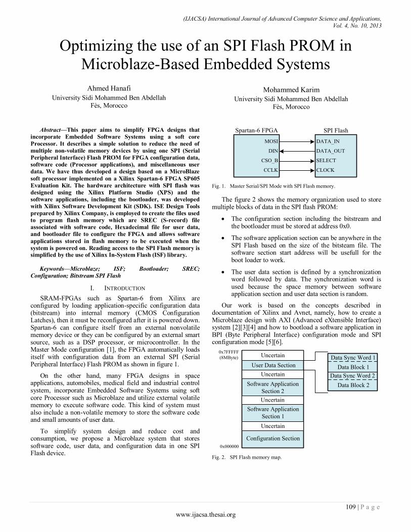
(IJACSA) International Journal of Advanced Computer Science and Applications, Vol. 4, No. 10, 2013
109 | P a g e www.ijacsa.thesai.org
Optimizing the use of an SPI Flash PROM in
Microblaze-Based Embedded Systems
Ahmed Hanafi
University Sidi Mohammed Ben Abdellah
Fès, Morocco
Mohammed Karim
University Sidi Mohammed Ben Abdellah
Fès, Morocco
Abstract—This paper aims to simplify FPGA designs that
incorporate Embedded Software Systems using a soft core
Processor. It describes a simple solution to reduce the need of
multiple non-volatile memory devices by using one SPI (Serial
Peripheral Interface) Flash PROM for FPGA configuration data,
software code (Processor applications), and miscellaneous user
data. We have thus developed a design based on a MicroBlaze
soft processor implemented on a Xilinx Spartan-6 FPGA SP605
Evaluation Kit. The hardware architecture with SPI flash was
designed using the Xilinx Platform Studio (XPS) and the
software applications, including the bootloader, was developed
with Xilinx Software Development Kit (SDK). ISE Design Tools
prepared by Xilinx Company, is employed to create the files used
to program flash memory which are SREC (S-record) file
associated with software code, Hexadecimal file for user data,
and bootloader file to configure the FPGA and allows software
applications stored in flash memory to be executed when the
system is powered on. Reading access to the SPI Flash memory is simplified by the use of Xilinx In-System Flash (ISF) library.
Keywords—Microblaze; ISF; Bootloader; SREC;
Configuration; Bitstream SPI Flash
I. INTRODUCTION
SRAM-FPGAs such as Spartan-6 from Xilinx are configured by loading application-specific configuration data (bitstream) into internal memory (CMOS Configuration Latches), then it must be reconfigured after it is powered down. Spartan-6 can configure itself from an external nonvolatile memory device or they can be configured by an external smart source, such as a DSP processor, or microcontroller. In the Master Mode configuration [1], the FPGA automatically loads itself with configuration data from an external SPI (Serial Peripheral Interface) Flash PROM as shown in figure 1.
On the other hand, many FPGA designs in space applications, automobiles, medical field and industrial control system, incorporate Embedded Software Systems using soft core Processor such as Microblaze and utilize external volatile memory to execute software code. This kind of system must also include a non-volatile memory to store the software code and small amounts of user data.
To simplify system design and reduce cost and consumption, we propose a Microblaze system that stores software code, user data, and configuration data in one SPI Flash device.
MOSI
DIN
CSO_B
CCLK
Spartan-6 FPGA
DATA_IN
DATA_OUT
SELECT
CLOCK
SPI Flash
Fig. 1. Master Serial/SPI Mode with SPI Flash memory.
The figure 2 shows the memory organization used to store multiple blocks of data in the SPI flash PROM:
The configuration section including the bitstream and the bootloader must be stored at address 0x0.
The software application section can be anywhere in the SPI Flash based on the size of the bitsteam file. The software section start address will be usefull for the boot loader to work.
The user data section is defined by a synchronization word followed by data. The synchronization word is used because the space memory between software application section and user data section is random.
Our work is based on the concepts described in documentation of Xilinx and Avnet, namely, how to create a Microblaze design with AXI (Advanced eXtensible Interface) system [2][3][4] and how to bootload a software application in BPI (Byte Peripheral Interface) configuration mode and SPI configuration mode [5][6].
0x000000
Configuration Section
User Data Section
Software Application
Section 1
Data Block 1
0x7FFFFF
(8MByte)
Software Application
Section 2
Uncertain
Uncertain
Uncertain
Uncertain
Data Sync Word 1
Data Sync Word 2
Data Block 2
Fig. 2. SPI Flash memory map.
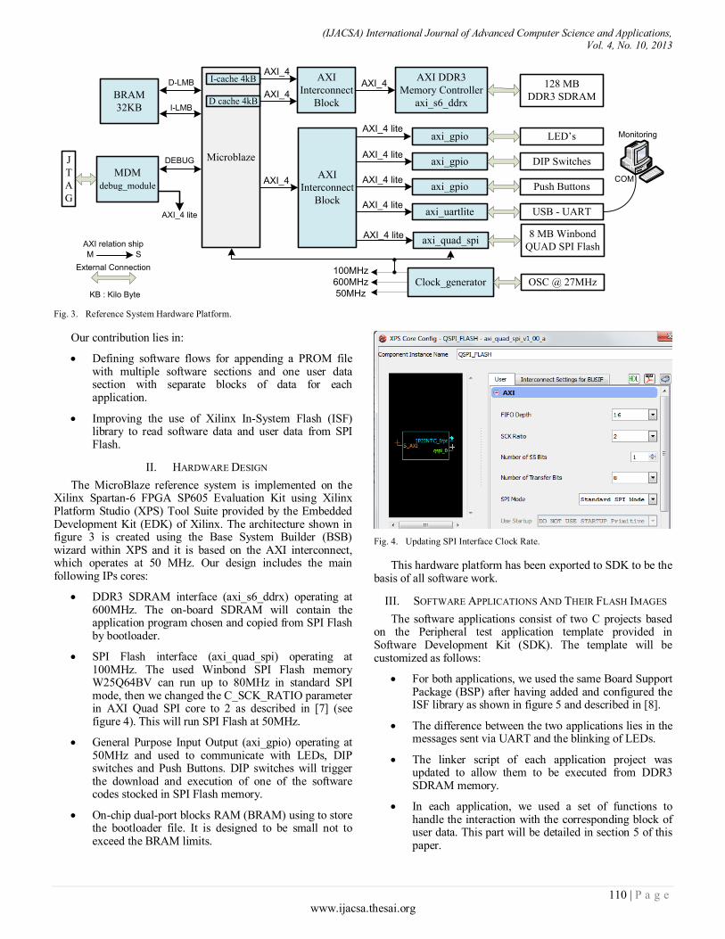
(IJACSA) International Journal of Advanced Computer Science and Applications, Vol. 4, No. 10, 2013
110 | P a g e www.ijacsa.thesai.org
128 MB
DDR3 SDRAM
8 MB Winbond
QUAD SPI Flash
LED’saxi_gpio
DIP Switches
Push Buttons
USB - UART
axi_gpio
axi_gpio
axi_uartlite
axi_quad_spi
AXI
Interconnect
Block
AXI DDR3
Memory Controller
axi_s6_ddrx
Microblaze
I-cache 4kB
D cache 4kBBRAM
32KB
AXI_4
AXI_4
AXI_4
AXI_4
AXI_4 lite
AXI
Interconnect
Block
AXI_4 lite
AXI_4 lite
AXI_4 lite
AXI_4 lite
D-LMB
I-LMB
External Connection
AXI relation ship
M S
Clock_generator OSC @ 27MHz100MHz
600MHz
50MHz
MDM
debug_module
DEBUG
AXI_4 lite
J
T
A
G
COM
Monitoring
KB : Kilo Byte
Fig. 3. Reference System Hardware Platform.
Our contribution lies in:
Defining software flows for appending a PROM file with multiple software sections and one user data section with separate blocks of data for each application.
Improving the use of Xilinx In-System Flash (ISF) library to read software data and user data from SPI Flash.
II. HARDWARE DESIGN
The MicroBlaze reference system is implemented on the Xilinx Spartan-6 FPGA SP605 Evaluation Kit using Xilinx Platform Studio (XPS) Tool Suite provided by the Embedded Development Kit (EDK) of Xilinx. The architecture shown in figure 3 is created using the Base System Builder (BSB) wizard within XPS and it is based on the AXI interconnect, which operates at 50 MHz. Our design includes the main following IPs cores:
DDR3 SDRAM interface (axi_s6_ddrx) operating at 600MHz. The on-board SDRAM will contain the application program chosen and copied from SPI Flash by bootloader.
SPI Flash interface (axi_quad_spi) operating at 100MHz. The used Winbond SPI Flash memory W25Q64BV can run up to 80MHz in standard SPI mode, then we changed the C_SCK_RATIO parameter in AXI Quad SPI core to 2 as described in [7] (see figure 4). This will run SPI Flash at 50MHz.
General Purpose Input Output (axi_gpio) operating at 50MHz and used to communicate with LEDs, DIP switches and Push Buttons. DIP switches will trigger the download and execution of one of the software codes stocked in SPI Flash memory.
On-chip dual-port blocks RAM (BRAM) using to store the bootloader file. It is designed to be small not to exceed the BRAM limits.
Fig. 4. Updating SPI Interface Clock Rate.
This hardware platform has been exported to SDK to be the basis of all software work.
III. SOFTWARE APPLICATIONS AND THEIR FLASH IMAGES
The software applications consist of two C projects based on the Peripheral test application template provided in Software Development Kit (SDK). The template will be customized as follows:
For both applications, we used the same Board Support Package (BSP) after having added and configured the ISF library as shown in figure 5 and described in [8].
The difference between the two applications lies in the messages sent via UART and the blinking of LEDs.
The linker script of each application project was updated to allow them to be executed from DDR3 SDRAM memory.
In each application, we used a set of functions to handle the interaction with the corresponding block of user data. This part will be detailed in section 5 of this paper.
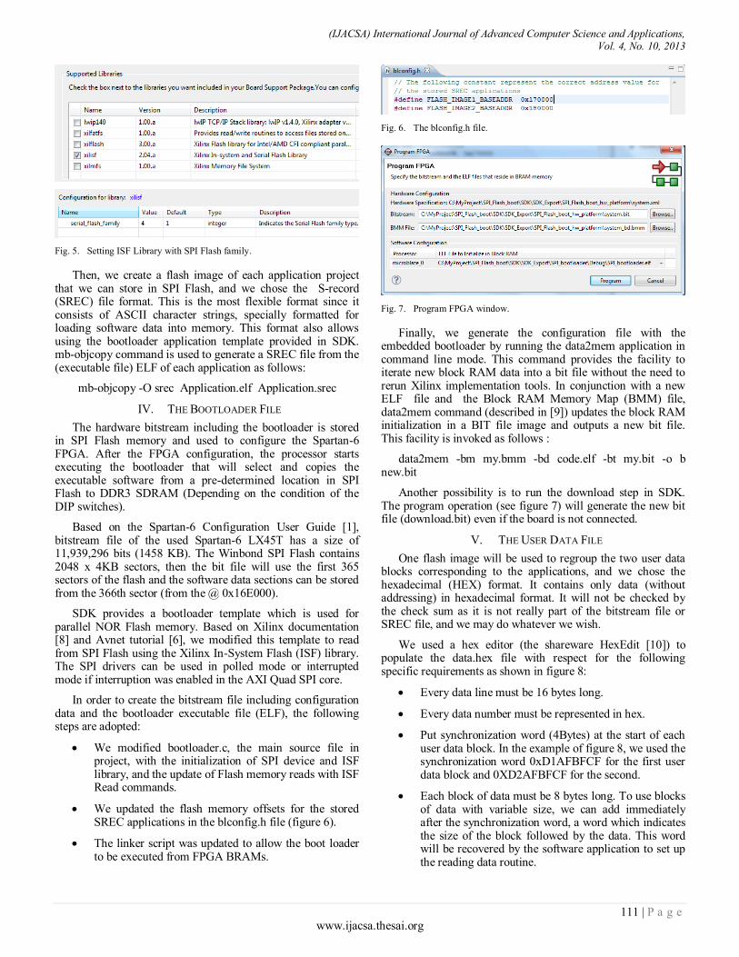
(IJACSA) International Journal of Advanced Computer Science and Applications, Vol. 4, No. 10, 2013
111 | P a g e www.ijacsa.thesai.org
Fig. 5. Setting ISF Library with SPI Flash family.
Then, we create a flash image of each application project that we can store in SPI Flash, and we chose the S-record (SREC) file format. This is the most flexible format since it consists of ASCII character strings, specially formatted for loading software data into memory. This format also allows using the bootloader application template provided in SDK. mb-objcopy command is used to generate a SREC file from the (executable file) ELF of each application as follows:
mb-objcopy -O srec Application.elf Application.srec
IV. THE BOOTLOADER FILE
The hardware bitstream including the bootloader is stored in SPI Flash memory and used to configure the Spartan-6 FPGA. After the FPGA configuration, the processor starts executing the bootloader that will select and copies the executable software from a pre-determined location in SPI Flash to DDR3 SDRAM (Depending on the condition of the DIP switches).
Based on the Spartan-6 Configuration User Guide [1], bitstream file of the used Spartan-6 LX45T has a size of 11,939,296 bits (1458 KB). The Winbond SPI Flash contains 2048 x 4KB sectors, then the bit file will use the first 365 sectors of the flash and the software data sections can be stored from the 366th sector (from the @ 0x16E000).
SDK provides a bootloader template which is used for parallel NOR Flash memory. Based on Xilinx documentation [8] and Avnet tutorial [6], we modified this template to read from SPI Flash using the Xilinx In-System Flash (ISF) library. The SPI drivers can be used in polled mode or interrupted mode if interruption was enabled in the AXI Quad SPI core.
In order to create the bitstream file including configuration data and the bootloader executable file (ELF), the following steps are adopted:
We modified bootloader.c, the main source file in project, with the initialization of SPI device and ISF library, and the update of Flash memory reads with ISF Read commands.
We updated the flash memory offsets for the stored SREC applications in the blconfig.h file (figure 6).
The linker script was updated to allow the boot loader to be executed from FPGA BRAMs.
Fig. 6. The blconfig.h file.
Fig. 7. Program FPGA window.
Finally, we generate the configuration file with the embedded bootloader by running the data2mem application in command line mode. This command provides the facility to iterate new block RAM data into a bit file without the need to rerun Xilinx implementation tools. In conjunction with a new ELF file and the Block RAM Memory Map (BMM) file, data2mem command (described in [9]) updates the block RAM initialization in a BIT file image and outputs a new bit file. This facility is invoked as follows :
data2mem -bm my.bmm -bd code.elf -bt my.bit -o b new.bit
Another possibility is to run the download step in SDK. The program operation (see figure 7) will generate the new bit file (download.bit) even if the board is not connected.
V. THE USER DATA FILE
One flash image will be used to regroup the two user data blocks corresponding to the applications, and we chose the hexadecimal (HEX) format. It contains only data (without addressing) in hexadecimal format. It will not be checked by the check sum as it is not really part of the bitstream file or SREC file, and we may do whatever we wish.
We used a hex editor (the shareware HexEdit [10]) to populate the data.hex file with respect for the following specific requirements as shown in figure 8:
Every data line must be 16 bytes long.
Every data number must be represented in hex.
Put synchronization word (4Bytes) at the start of each user data block. In the example of figure 8, we used the synchronization word 0xD1AFBFCF for the first user data block and 0XD2AFBFCF for the second.
Each block of data must be 8 bytes long. To use blocks of data with variable size, we can add immediately after the synchronization word, a word which indicates the size of the block followed by the data. This word will be recovered by the software application to set up the reading data routine.
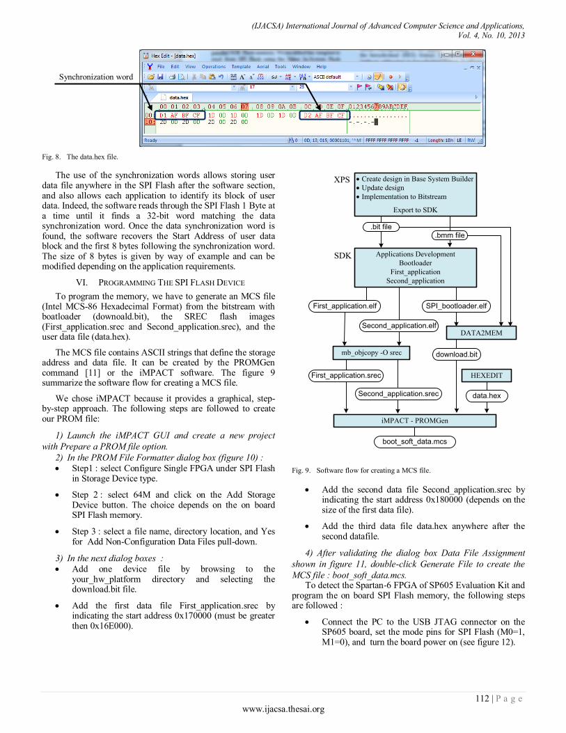
(IJACSA) International Journal of Advanced Computer Science and Applications, Vol. 4, No. 10, 2013
112 | P a g e www.ijacsa.thesai.org
Fig. 8. The data.hex file.
The use of the synchronization words allows storing user data file anywhere in the SPI Flash after the software section, and also allows each application to identify its block of user data. Indeed, the software reads through the SPI Flash 1 Byte at a time until it finds a 32-bit word matching the data synchronization word. Once the data synchronization word is found, the software recovers the Start Address of user data block and the first 8 bytes following the synchronization word. The size of 8 bytes is given by way of example and can be modified depending on the application requirements.
VI. PROGRAMMING THE SPI FLASH DEVICE
To program the memory, we have to generate an MCS file (Intel MCS-86 Hexadecimal Format) from the bitstream with boatloader (downoald.bit), the SREC flash images (First_application.srec and Second_application.srec), and the user data file (data.hex).
The MCS file contains ASCII strings that define the storage address and data file. It can be created by the PROMGen command [11] or the iMPACT software. The figure 9 summarize the software flow for creating a MCS file.
We chose iMPACT because it provides a graphical, step-by-step approach. The following steps are followed to create our PROM file:
1) Launch the iMPACT GUI and create a new project
with Prepare a PROM file option.
2) In the PROM File Formatter dialog box (figure 10) :
Step1 : select Configure Single FPGA under SPI Flash in Storage Device type.
Step 2 : select 64M and click on the Add Storage Device button. The choice depends on the on board SPI Flash memory.
Step 3 : select a file name, directory location, and Yes for Add Non-Configuration Data Files pull-down.
3) In the next dialog boxes :
Add one device file by browsing to the your_hw_platform directory and selecting the download.bit file.
Add the first data file First_application.srec by indicating the start address 0x170000 (must be greater then 0x16E000).
Create design in Base System Builder
Update design
Implementation to Bitstream
Export to SDK
XPS
SDK Applications Development
Bootloader
First_application
Second_application
.bit file.bmm file
SPI_bootloader.elf
DATA2MEM
First_application.elf
Second_application.elf
mb_objcopy -O srec download.bit
First_application.srec
Second_application.srec
iMPACT - PROMGen
boot_soft_data.mcs
data.hex
HEXEDIT
Fig. 9. Software flow for creating a MCS file.
Add the second data file Second_application.srec by indicating the start address 0x180000 (depends on the size of the first data file).
Add the third data file data.hex anywhere after the second datafile.
4) After validating the dialog box Data File Assignment
shown in figure 11, double-click Generate File to create the
MCS file : boot_soft_data.mcs. To detect the Spartan-6 FPGA of SP605 Evaluation Kit and
program the on board SPI Flash memory, the following steps are followed :
Connect the PC to the USB JTAG connector on the SP605 board, set the mode pins for SPI Flash (M0=1, M1=0), and turn the board power on (see figure 12).
Synchronization word
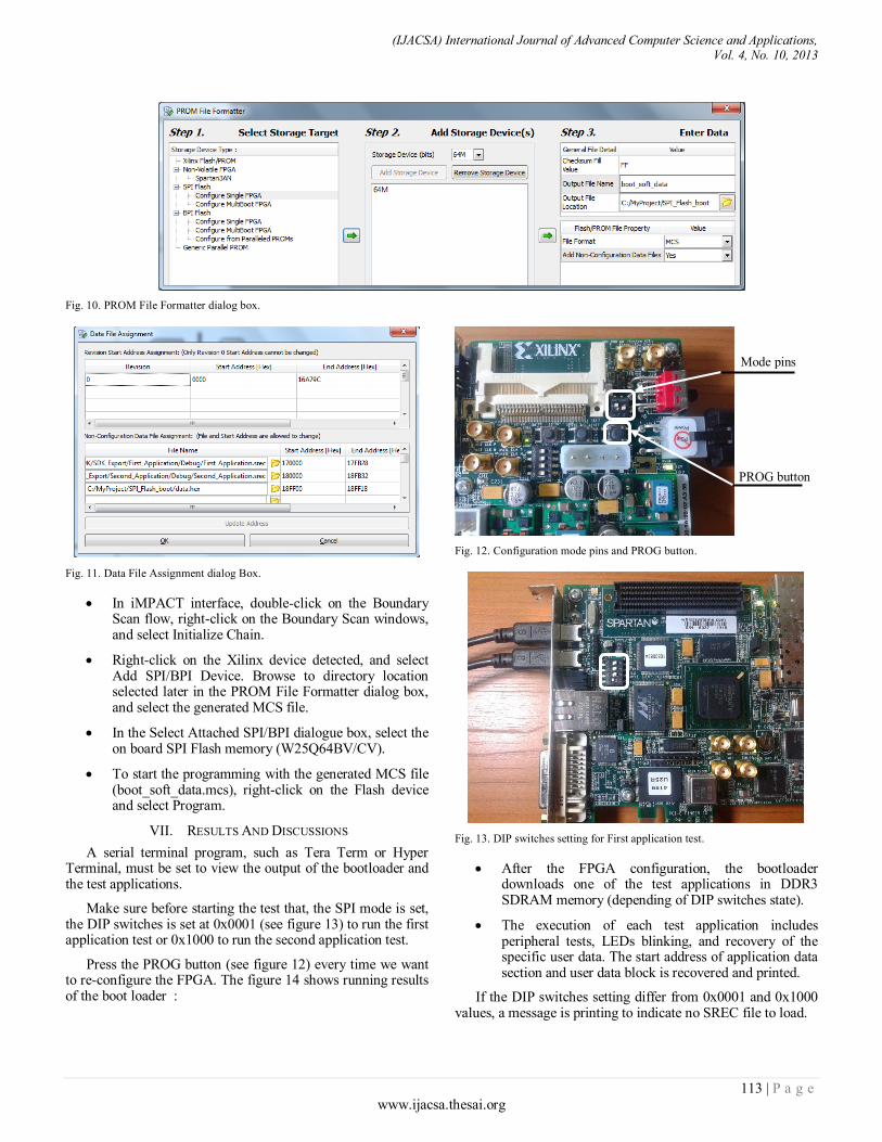
(IJACSA) International Journal of Advanced Computer Science and Applications, Vol. 4, No. 10, 2013
113 | P a g e www.ijacsa.thesai.org
Fig. 10. PROM File Formatter dialog box.
Fig. 11. Data File Assignment dialog Box.
In iMPACT interface, double-click on the Boundary Scan flow, right-click on the Boundary Scan windows, and select Initialize Chain.
Right-click on the Xilinx device detected, and select Add SPI/BPI Device. Browse to directory location selected later in the PROM File Formatter dialog box, and select the generated MCS file.
In the Select Attached SPI/BPI dialogue box, select the on board SPI Flash memory (W25Q64BV/CV).
To start the programming with the generated MCS file (boot_soft_data.mcs), right-click on the Flash device and select Program.
VII. RESULTS AND DISCUSSIONS
A serial terminal program, such as Tera Term or Hyper Terminal, must be set to view the output of the bootloader and the test applications.
Make sure before starting the test that, the SPI mode is set, the DIP switches is set at 0x0001 (see figure 13) to run the first application test or 0x1000 to run the second application test.
Press the PROG button (see figure 12) every time we want to re-configure the FPGA. The figure 14 shows running results of the boot loader :
Fig. 12. Configuration mode pins and PROG button.
Fig. 13. DIP switches setting for First application test.
After the FPGA configuration, the bootloader downloads one of the test applications in DDR3 SDRAM memory (depending of DIP switches state).
The execution of each test application includes peripheral tests, LEDs blinking, and recovery of the specific user data. The start address of application data section and user data block is recovered and printed.
If the DIP switches setting differ from 0x0001 and 0x1000 values, a message is printing to indicate no SREC file to load.
Mode pins
PROG button

(IJACSA) International Journal of Advanced Computer Science and Applications, Vol. 4, No. 10, 2013
114 | P a g e www.ijacsa.thesai.org
Fig. 14. Terminal Window showing test running
VIII. CONCLUSION AND FUTUR WORKS
This paper demonstrates a method concerning the optimization of the SPI flash memory in FPGA designs that incorporate Embedded Software Systems using Microblaze. It is simple to implement and can be used in any embedded system with limited memory resources.
Successful achievement of this work will encourage us to use an SPI Flash memory as mass memory of our on-board computer (for nano-satellite) that will take an SRAM-FPGA as central processor. The embedded platform can be enriched by proposing a fallback and multiboot technique to create a multiple embedded designed systems (multiple configuration sections), always by using a single SPI Flash memory.
REFERENCES
[1] Xilinx Company “Spartan-6 FPGA Configuration User Guide” UG380 (v2.5) January 23, 2013. [internet] Available at
http://www.xilinx.com/support/documentation/user_guides/ug380.pdf
[2] Xilinx Company “MicroBlaze Processor Reference Guide” UG081 (v13.4) January 18, 2012. [internet] Available at
http://www.xilinx.com/support/documentation/sw_manuals/xilinx13_4/
mb_ref_guide.pdf
[3] Xilinx Company “Spartan-6 Family Overview” DS160 (v2.0) October 25, 2011. [internet] Available at
http://www.xilinx.com/support/documentation/data_sheets/ds160.pdf
[4] Xilinx Company “Embedded System Tools Reference Manual EDK”
UG111 (v13.4) January 18, 2012. [internet] Available at
http://www.xilinx.com/support/documentation/sw_manuals/xilinx13_4/e
st_rm.pdf
[5] Casey Cain “FPGA Configuration from Flash PROMs on Spartan-3E 1600E Board” XAPP978 (v1.2) November 5, 2010.
[6] Avnet Reference Design "Creating a Microblaze SPI Flash Bootloader”
Version 13.2.01 September 22, 2011.
[7] Xilinx Company “LogiCORE IP AXI Quad Serial Peripheral Interface (AXI Quad SPI) V1.00a” DS843 October 19, 2011.
http://www.xilinx.com/support/documentation/ip_documentation/axi_qu
ad_spi/v1_00_a/ds843_axi_quad_spi.pdf
[8] Xilinx Company “OS and Libraries Document Collection” UG643 July 27, 2012. [internet] Available at
http://www.xilinx.com/support/documentation/sw_manuals/xilinx14_2/oslib_rm.pdf
[9] Xilinx Company “Data2MEM User Guide” UG437 (v2.0) April 04,
2007. [internet] Available at
http://www.xilinx.com/itp/xilinx10/books/docs/d2m/d2m.pdf
[10] http://www.hexedit.com/
[11] Xilinx Company “Command Line Tools User Guide” UG628 (v 13.4) January 18, 2012. [internet] Available at
http://www.xilinx.com/support/documentation/sw_manuals/xilinx14_1/
devref.pdf
(IJACSA) International Journal of Advanced Computer Science and Applications, Vol. 4, No. 10, 2013
115 | P a g e www.ijacsa.thesai.org
Design and Application of Queue-Buffer
Communication Model in Pneumatic Conveying
Liping Zhang
College of Electronic and Electrical Engineering
Shanghai University of Engineering Science Songjiang District, Shanghai 201620, China
Haomin Hu
College of Electronic and Electrical Engineering
Shanghai University of Engineering Science Songjiang District, Shanghai 201620, China
Abstract—In order to communicate with a PLC
(Programmable Logic Controller) flexibly and freely, a data
communication model based on the PLC's free port is designed.
In the structure of the model, a distributed data communication
environment is constructed by using Ethernet and serial
adapters. In the communication algorithm, a method of queue-
buffer for multi-threaded is used to improve the real-time of the
control. This communication model has good scalability and
portability because the realization of it is not restricted by the
number of PLC slave stations and the type of operating system of
the host computer. A corresponding communication algorithm is
applied to data collection and devices monitoring for a pipe
pneumatic conveying system. The practice shows that not only
the stability and reliability of the model can meet the needs of
automatic control but also the communication performance and efficiency of the model is outstanding.
Keywords—Queue-Buffer; Programmable Logic Controller;
Freeport Communication; Critical resource; Mutex
I. INTRODUCTION
PLC as the industrial automatic control equipment encompassing the automation technology, computer technology, control technology and communications technology, has been widely used in various fields of industrial automation [1]. In the control system, how to achieve stable, efficient and flexible communication between the host computer and the PLC has become an important research topic. At the same time, PLC manufacturers also offer a variety of communication methods for users to choose. Taking Siemens S7-200 series as an example, a control system consisting of this series PLC can generally use configuration software monitoring, third-party monitoring-software monitoring, touch screen monitoring and other monitoring methods [2]. Meanwhile, in order to improve the flexibility of automated control systems, many kinds of PLC provide a communication patterns named "free port", such as Siemens s7-200 series PLC, Mitsubishi FX2 series PLC, OMRON CJM1 series PLC and so on.
Freeport communication is a method of using serial communication hardware and relevant instructions for customizing communication protocols which are provided by the PLC to realize data communication by PLC programming. The literatures [3] and [4] have described the implementations of the Siemens PLC communication method on free port. Currently the discussion about the free port communication method of the PLC mainly focused on the "point-to-point"
technology, namely realizing the data acquisition and control of PLC through the serial communication of host computer. Literature [5] has described a method of using MSComm programming control for host computer to communicate with S7-200 series PLC. But in the field of industrial control, there will be many PLCs as slave stations, and not only the serial number of host computer is limited, but also the communication distance is restricted. This paper describes an approach which is based on Ethernet and serial adapters to achieve distributed data communication model through the PLC free port. This model has the advantage of being cross-platform and can be implemented in different operating systems. At the same time, in order to achieve the acquisition of data and the control of PLC efficiently and stably, the communication algorithm based on queue-buffer for multi-threaded is designed. Under the premise of ensuring real-time, this algorithm also improves the scalability of the number of communication nodes and the concurrency adaptability of archive database as far as possible.
In the following section, structure of the system and related communication model and algorithm are discussed.
II. SYSTEM STRUCTURE
In the design of control system for a variety of powder dense phase pneumatic conveying engineering, a lot of devices need to be monitored, such as exhausting valve, feeding valve, pre-closing valve, outlet valve, upper intake valve, down intake valve, pneumatic hammer of pump and pulse dust collector, pneumatic hammer, fan of hopper. It's easy to use PLCs as control sources to debug and maintain solenoid valves and indicator lights by electric relays. The control system needs to detect and monitor the working status of pump pressure transmitters, material high level switch, pneumatic valve position switch, air pressure gauge and thermal resistance, etc. Many brands of PLC can control these devices, and they also provide the free port for communication, although different PLCs vary in communication protocol, but many PLC provides a free port of communication. The number of devices which PLC can control is limited and PLCs should be added as monitoring stations when the device exceeds a certain number. At the same time, the number of serial interfaces of host computer is limited too and communication will be restricted by the number of interfaces when PLCs' number beyond it. In order to monitor the devices with good scalability, we designed a communication system whose structure is shown in Figure 1.
(IJACSA) International Journal of Advanced Computer Science and Applications, Vol. 4, No. 10, 2013
116 | P a g e www.ijacsa.thesai.org
Device 1
PLC
Ethernet /
Serial Adapter
RS-232/485
RJ-45
Device 2 Device m……
Ethernet
Control Computer
(host computer)
Device
m+1
PLC
Ethernet /
Serial Adapter
RS-232/485
RJ-45
Device
m+2
Device
n……
……
Fig. 1. system structure
A distributed data communication structure is used in Figure 1. Each PLC detects and controls a set of devices and the data collected by it is transferred to the Ethernet and serial adapters through serial port. The adapter converts the data into TCP datagram and delivers them to Ethernet. The communication between these nodes is TCP connection-oriented reliable data transmission. Although this architecture provides the system with a distributed processing environment, communication model and algorithm will largely affect the real-time of data acquisition. Therefore, the design of communications algorithm is also important.
III. COMMUNICATION MODEL DESIGN
A. Design Principles
For the industrial automatic control system, the real-time is very important. In the control system shown in Figure 1, the host computer sends instructions to PLCs via Ethernet and serial adapters, and PLCs control devices of system. If data collection is performed, PLCs transfer the data to host computer via the Ethernet and serial adapter. When the number of PLC and devices is large, it is difficult to guarantee real-time if polling communication is still used. Taking data collection as an example, the obstruction of any communication channel will interfere with sampling period and affect real-time. Although the real-time of data acquisition can be improved by using multiple threads concurrently, the scalability of system is unable to be ensured, if there is no reasonable synchronization scheduling mechanism. Queue-buffer communication model describes a way to achieve host computer communicating with PLCs in multi-threaded by synchronization and mutual exclusion of critical resources, and improve the real-time of system, the reliability of data acquisition and archiving as far as possible.
According to the Bernstein condition for concurrent execution [6], the following formula must be satisfied for process P1 and p2 can execute concurrently and has a reproducible operating environment.
211221 pWpWpWpRpWpR
Where R represents a set of resource which some process will read, and W represents a set of resource which some process will write. The following conclusion can be drawn. We
assume that T is a set of threads for communication in the host computer, if the following formula is established, the communication threads can execute concurrently.
jijiji ttTtTttt ,,,, , jiijji tWtWtWtRtWtR
In order to improve the concurrent performance of system, we used two kinds of independent thread (ie, communication thread and archive thread) to achieve the communication with PLCs and archive of collected data. Meanwhile, in order to reduce the critical region and competition of threads for critical resources, we used private queues and public queue for data buffer and buffering threads to schedule the data. Queue-Buffer communication model is shown in Figure 2:
Communication
Thread 1
...
Ethernet
wt wt wt
Buffering
Thread 1
rd rd rd
Public Queue
Private Queue
rear
Database
Server
front
Archiving
Threads
Communication
Thread 2
Communication
Thread n
Buffering
Thread 2
Buffering
Thread n
Fig. 2. Queue-Buffer Communication Model
B. Feasibility Analysis
In the communication model shown in Figure 2, each communication thread is assigned with a buffer queue for storing the data collected from the PLC. Because each thread has a buffer queue and the queue is not shared, so we call the queue a "private queue". In the private queue is not the full case, communication threads will not be blocked for delay of data saving. Concurrent operation can be guaranteed. Communication thread writes data to the private queue, and buffering thread reads data from the private queue. What they affect is the movement of the rd pointer and wt pointer, so synchronization will occur only when the private queue is empty or full. When the private queue is empty, the buffering thread will be blocked, but the communication thread will not be affected, and real-time can still be guaranteed. Only when the private queue is full, the communication will be blocked, and what causes this phenomenon is that the data archive is not fast enough. In addition to archiving the cycle too quickly, what impacts the speed of archive are the following two reasons. (1) The buffer size of private queue is too small, and the buffer overflows before the thread which is responsible for data archiving gets the time slice. (2) The concurrent processing capacity of database is not enough and a large number of connections is occupied, or archiving thread switches between connecting and disconnecting too frequently that degrades the performance. In the first case, we can resolve the problem by increasing the buffer size appropriately. But for the second case, the database concurrency is determined by the

(IJACSA) International Journal of Advanced Computer Science and Applications, Vol. 4, No. 10, 2013
117 | P a g e www.ijacsa.thesai.org
database performance, and therefore the number of connections can not be increased arbitrarily. To solve this problem, another queue buffer, namely the public queue, is added between the archiving thread and the buffering thread. The number of database connections is controlled by the archiving threads which maintain database connection stably to reduce the switch of connection state.
In the above communication model, the data of private queue is not archived in the database directly, but is stored into a public queue by buffering threads. So that not only data can be copied from private queues to public queue quickly that reduce the possibility of private queue to overflow, and the number of threads can be isolated and the database communication correlation between the degree of concurrency, but also the correlation between communication threads number and concurrency of database is isolated. Thus the competition for the database connection will be changed into the competition of buffering threads for rear pointer of public queue buffer, and the number of threads which access front pointer of public queue buffer can be determined according to the performance of the database. This scheme effectively improves the universality of database for archiving, and when a lot of concurrent operations are required, so a distributed database can be easily used.
C. Algorithm Description
An important step forward in this area of concurrent programming occurred when Edsger Dijkstra introduced the concept of the semaphore. A semaphore is a special variable that takes only whole positive numbers and upon which programs can only act atomically [7]. The following algorithm is described by primitive P and V. Because concurrency and synchronization between threads is happening in the queue for private queues and public queue, algorithm based on the type of queue buffer will be described separately. Read operation and write operation of private queues is described below:
int wt, rd, pvt_queue_len; // Initial values of wt and rd are 0, and value of pvt_queue_len equals to the length of private queue
sem_t pvt_queue_full, pvt_queue_empty; // Initial values for the two semaphores are 0 and pvt_queue_len respectively
struct data_item pvt_queue[pvt_queue_len]; // pvt_queue is private queue
write_pvt_queue() // Write collected data to private queue
{
P(pvt_queue_empty); // If private queue buffer is not full, then write the data, or block
Write data to pvt_queue(wt);
wt = (wt+1)% pvt_queue_len;// Move the write pointer of private queue backward
V(pvt_queue_full);
}
read_pvt_queue() // Read data from private queue
{
P(pvt_queue_full); // If buffer is not full, then read data, or block
dat = pvt_queue[rd]; //Save data to variable dat
rd = (rd+1) % pvt_queue_len;// Move the read pointer of private queue backward
V(pvt_queue_empty);
}
In the algorithm above, sem_t is a data type of semaphore in linux and struct data_item is a custom data type for the data item stored in queue buffer. On the other hand, In the read_pvt_queue() function which is to read data from private queue, the data is copied to a temporary storage, variable dat, in order to prevent the data from being overwritten by communication thread before it is saved into public queue buffer. Since each communication thread and buffering thread require the data members and functions above, the readability of the program can be improved by encapsulating them into a class.
Read operation and write operation of public queues is described below:
int front, rear, pub_queue_len; //Initial values of front and rear are 0, and pub_queue_len means the length of public queue
sem_t pub_queue_full, pub_queue_empty; // Initial values for the two semaphores are 0 and pub_queue_len respectively
struct data_item pub_queue[pub_queue_len]; // pub_queue is public queue
pthread_mutex_t mtx_front, mtx_rear; // Mutex operation for the front and rear of public queue, Initial values of them are 1
write_pub_queue() // Write data to public queue
{
P(pub_queue_empty); // If public queue buffer is not full, program continue, or block
P(mtx_rear);// Mutex operation for rear of public queue
Buffering thread write data into pub_queue[rear];
rear=(rear+1) % pub_queue_len;// Move the rear pointer of public queue backward
V(mtx_rear);
V(pub_queue_full);
}
read_pub_queue() // Read data from public queue, executed by archiving thread
{
P(pub_queue_full); // If public queue buffer is not empty, program continue, or block
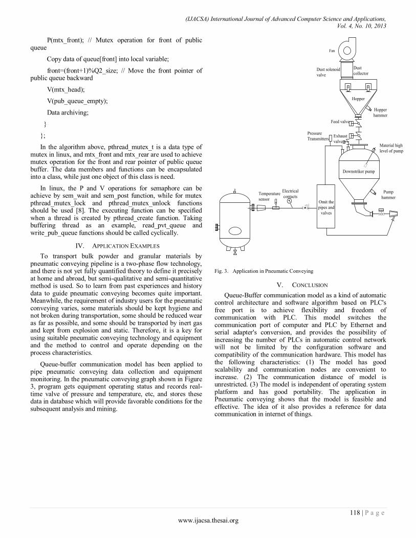
(IJACSA) International Journal of Advanced Computer Science and Applications, Vol. 4, No. 10, 2013
118 | P a g e www.ijacsa.thesai.org
P(mtx_front); // Mutex operation for front of public queue
Copy data of queue[front] into local variable;
front=(front+1)%Q2_size; // Move the front pointer of public queue backward
V(mtx_head);
V(pub_queue_empty);
Data archiving;
}
};
In the algorithm above, pthread_mutex_t is a data type of mutex in linux, and mtx_front and mtx_rear are used to achieve mutex operation for the front and rear pointer of public queue buffer. The data members and functions can be encapsulated into a class, while just one object of this class is need.
In linux, the P and V operations for semaphore can be achieve by sem_wait and sem_post function, while for mutex pthread_mutex_lock and pthread_mutex_unlock functions should be used [8]. The executing function can be specified when a thread is created by pthread_create function. Taking buffering thread as an example, read_pvt_queue and write_pub_queue functions should be called cyclically.
IV. APPLICATION EXAMPLES
To transport bulk powder and granular materials by pneumatic conveying pipeline is a two-phase flow technology, and there is not yet fully quantified theory to define it precisely at home and abroad, but semi-qualitative and semi-quantitative method is used. So to learn from past experiences and history data to guide pneumatic conveying becomes quite important. Meanwhile, the requirement of industry users for the pneumatic conveying varies, some materials should be kept hygiene and not broken during transportation, some should be reduced wear as far as possible, and some should be transported by inert gas and kept from explosion and static. Therefore, it is a key for using suitable pneumatic conveying technology and equipment and the method to control and operate depending on the process characteristics.
Queue-buffer communication model has been applied to pipe pneumatic conveying data collection and equipment monitoring. In the pneumatic conveying graph shown in Figure 3, program gets equipment operating status and records real-time valve of pressure and temperature, etc, and stores these data in database which will provide favorable conditions for the subsequent analysis and mining.
Fan
Downstriker pump
Material high
level of pump
Pump
hammer
Exhaust
valve
Pressure
Transmitters
Hopper
hammer
Hopper
Dust solenoid
valve
Dust
collector
Feed valve
Electrical
contactsTemperature
sensorOmit the
pipes and
valves
Fig. 3. Application in Pneumatic Conveying
V. CONCLUSION
Queue-Buffer communication model as a kind of automatic control architecture and software algorithm based on PLC's free port is to achieve flexibility and freedom of communication with PLC. This model switches the communication port of computer and PLC by Ethernet and serial adapter's conversion, and provides the possibility of increasing the number of PLCs in automatic control network will not be limited by the configuration software and compatibility of the communication hardware. This model has the following characteristics: (1) The model has good scalability and communication nodes are convenient to increase. (2) The communication distance of model is unrestricted. (3) The model is independent of operating system platform and has good portability. The application in Pneumatic conveying shows that the model is feasible and effective. The idea of it also provides a reference for data communication in internet of things.

(IJACSA) International Journal of Advanced Computer Science and Applications, Vol. 4, No. 10, 2013
119 | P a g e www.ijacsa.thesai.org
ACKNOWLEDGMENT
The projects have been supported by the Innovation Program of Shanghai Municipal Education Commission "Vehicle Collision Avoidance System based on Vehicle Wireless Communication" (No.12YZ151), and "Discipline Comprehension Construction on Control Science and Engineering" (No.13XKCZ07), and 'First Class Discipline Cultivation - Mechanical Engineering" (No.YLJX12-7).
Liping Zhang acknowledges the guidance & support of Cheng-Chew Lim of the University of Adelaide during her academic visit in 2013/2014.
REFERENCES
[1] Gong Yunxing, Zhao Houuu, Qi Benzhi, PLC technology and application – Based on Siemens s7-200 series. BeiJing: Tsinghua
University Press, 2009, pp.68–73.
[2] Liu Ning, Design and Implementation of the Control and Monitoring
subsystems in Small Scale Water Treatment Engineering. Jilin University [D] pp.12, April 2012.
[3] Xiang Xiaohan, Industrial Communication Tutorial for Siemens PLC Specialist. BeiJing: Chemical Industry Press, March 2013.
[4] Li Jiangquan, Yan Haijuan, Liu Jiaodi, Deng Hongtao, Application
Examples of Siemens PLC communication and Control Programming. BeiJing: China Electric Power Press, January 2012.
[5] Xu Qiyi, Wu Yuqiang, Jiang Xiuping, Li Kun, Communication between
S7-200 PLC and Computer under C++ Builder Environment. Process Automation Instrumentation, vol. 1, pp.57-60, 2007.
[6] Tang Xiaodan, Liang Hongbin, Zhe Fengping, Tang ZiYing, Computer
Operating System. ShangXi:Xi'an Electronic and Science University Press, August 2011.
[7] Neil Matthew, Richard Stones. Beginning Linux Programming 4th
Edition. Wrox, 2007, pp.578-580.
[8] Yang Zongde, Lu Guanghong, Liu Yong, Linux Advanced Programming, 3rd Edition. BeiJing: Posts & Telecommunications Press.
November 2012, pp.305-307.

(IJACSA) International Journal of Advanced Computer Science and Applications, Vol. 4, No. 10, 2013
120 | P a g e www.ijacsa.thesai.org
Thyroid Diagnosis based Technique on Rough Sets
with Modified Similarity Relation
Elsayed Radwan 1,3
1Computer Science Department P.O.Box: 715
3Institute of Scientific Research and Revival of Islamic
Heritage, Umm Al-Qura University, KSA
Adel M.A. Assiri 2,3
2Biochemistry Department,
Faculty of Medicine,Umm Al-Qura University, KSA 3Institute of Scientific Research and Revival of Islamic
Heritage, Umm Al-Qura University, KSA
Abstract—Because of the patient’s inconsistent data,
uncertain Thyroid Disease dataset is appeared in the learning
process: irrelevant, redundant, missing, and huge features. In
this paper, Rough sets theory is used in data discretization for
continuous attribute values, data reduction and rule induction.
Also, Rough sets try to cluster the Thyroid relation attributes in
the presence of missing attribute values and build the Modified
Similarity Relation that is dependent on the number of missing
values with respect to the number of the whole defined attributes
for each rule. The discernibility matrix has been constructed to
compute the minimal sets of reducts, which is used to extract the
minimal sets of decision rules that describe similarity relations among rules. Thus, the rule associated strength is measured.
Keywords— Thyroid Disease - Rough Sets - Data Discretization
– Knowledge Reduction; Modified Similarity Relation MSIM
I. INTRODUCTION
Hypothyroid is one of the most common diseases that frequently misunderstood and misdiagnosis. Thyroid is a small butterfly-shaped gland, located in the neck. The thyroid produces several hormones; two of them are important: triiodothyronine (T3) and thyroxin (T4). Each of them must be produced by thyroid in normal rang; to help cells convert oxygen and calories into energy [6,7,8]. It is based almost exclusively upon measuring the amount of thyroid hormone in the blood. So there are normal ranges for thyroid hormones which have been calculated by our application in this paper: T4, T3, TSH, TBG, T4U and FTI. Doctors faced many problems during dealing with patient’s data such as huge data needed from patients, misdiagnosis, missing data when applying patient history and the required human efforts.
According to the previous research, various neural network methods including Multi-Layer Perception with Back-Propagation method (MLP), Radial Basis Function (RBF) and adaptive Conic Section Function Neural Network (CSFNN) are used to help diagnosis of thyroid disease, their classification accuracies are separately 88.3%, 81.69% and 85.92% [7]. Also, five different methods including Linear Discriminant Analysis (LDA), C4.5 with default learning parameters (C4.5-1), C4.5 with parameter c equal to 5 (C4.5-2), C4.5 with parameter c equal to 95 (C4.5-3) and DIMLP with two hidden layers and default learning parameters(DIMLP) to perform classification, and the accuracies reached 81.34%, 93.26%, 92.81%, 92.94% and 94.86% respectively [8]. Moreover, an accuracy of 81% was obtained with the application of artificial immune
recognition system (AIRS) [7]. Furthermore, diagnosed thyroid diseases with an expert system that called ESTDD (expert system for thyroid disease diagnosis), whose accuracy was 95.33%[14]. Finally, swarm optimization optimized support vector machines with fisher score (FS-PSO-SVM) CAD system for thyroid disease, and the average accuracy of 97.49% was achieved.
As a result, all diagnosis algorithms currently in use depend on different kinds of heuristics where the resulting recodes contain missing bases due to the presence of gaps which may be misclassifying the diseases. Also, a continuous dataset due to the measuring range are discovered. Thus, a good and effective tool to deal with vagueness, missing and uncertainty of information is needed in the presence of continuous data which should be discretized. Rough sets [11,12] deals with the classificatory of data tables and focus on structural relationships in data sets. Rough Sets theory constitutes a framework for inducing minimal decision rules, these rules in turn can be used to perform a classification task. The main goal of the rough set analysis is to search large databases for meaningful decision rules and finally acquire new knowledge. Rough sets has been successfully applied in many different fields, particularly the medical field [2]. A rough set investigates structural relationship in data rather than probability distribution and produce decision table rather than trees [5].
In this paper Rough sets try to classify Thyroid in the presence of missing bases and build the Modified Similarity Relations that is dependent on the number of missing bases with respect to the number of the whole defined attributes for each rule [15]. The Thyroid relation attributes are converted to suitable representation for rough set analysis by discretizing and then constructing a matrix where each row corresponding to the similarity score between Thyroid attributes and each column corresponding to a defined attribute that describe the position of bases inside the rule. The discernibility matrix is used to discern similarity relation among rules in the presence of gaps and deduction of decision rules which describe Thyroid relation attributes with a minimal set of attributes.
According to the previous discussion, the paper is organized as follows; in section II a brief introduction of important field (rough set) is discussed. Section III describes the fundamentals of our method where the an approach of the supervised learning for incomplete Thyroid dataset using rough

(IJACSA) International Journal of Advanced Computer Science and Applications, Vol. 4, No. 10, 2013
121 | P a g e www.ijacsa.thesai.org
sets and its performance are given. Section IV examine the application and guide the user using it. Then we conclude with section V the purpose of that paper and its results.
II. PRELIMINARIES
This section briefs on the basic notions of rough sets that is used in this paper and the detailed definitions can be referred to some related papers [5, 11,12, 13].
A. Rough Set Theory
Rough set theory proposed by Pawlak [11] is an effective approach to imprecision, vagueness, and uncertainty. Rough set theory overlaps with many other theories such that fuzzy sets, evidence theory, and statistics. From a practical point of view, it is a good tool for data analysis. The main goal of the rough set analysis is to synthesize approximation of concepts from acquired data. The starting point of Rough set theory is an observation that the objects having the same description are indiscernible (similar) with respect to the available information. Determination of the similar objects with respect to the defined attributes values is very hard and sensible when some attribute values are missing. This problem must be handled very carefully. The indiscernibility relation is a fundamental concept of the rough set theory which used in the complete information systems. In order to process incomplete information systems, the indiscernibility relation needs to be extended to some equivalent relations.
The starting point of rough set theory which is based on
data analysis is a data set called an information system ( IS ).
IS is a data table, whose columns are labeled by attributes, rows are labeled by objects or cases, and the entire of the table
are the attribute values. Formally, ATUIS , , where U and
AT are nonempty finite sets called “the universe” and “the set of attributes,” respectively. Every attribute ATa , has a set
V a of its values called the “domain of a ”. If V acontains
missing values for at least one attribute, then S is called an incomplete information system, otherwise it is complete. Any information table defines a function that maps the direct
product ATU into the set of all values assigned to each attribute. The example of incomplete information system depicted in Table I where set of objects in the universe corresponding to set of instances and set of attributes corresponding to set of values inside each instance. The values of attributes are corresponding to the values of bases inside each object such as the value of instance1at attribute1is defined by ρ(instance1, attribute1) =[1,2].
TABLE I. EXAMPLE OF INCOMPLETE INFORMATION SYSTEM
attribute1 attribute2 attribute3
instance1 [1,2] 0 *
instance2 [1,3] 1 A
instance3 [3,4] 2 A
The concept of the indiscernibility relation is an essential concept in rough set theory which is used to distinguish objects described by a set of attributes in complete information
systems. Each subset A of AT defines an indiscernibility relation as follows:
}, ),( ),(: ),{()( ATAAaayaxUUyxAIND (1)
Obviously, )(AIND is an equivalence relation, the family of all
equivalence classes of )(AIND , for example, a partition
determined by A which is denoted by )(/ AINDU or AU /
[11]. Obviously )(AIND is an equivalence relation and:
AawhereaINDAIND )( )( (2)
A fundamental problem discussed in rough set is whether the whole knowledge extracted from data sets is always necessary to classify objects in the universe; this problem arises in many practical applications and will be referred to as knowledge reduction. The two fundamental concepts used in knowledge reduction are the core and reduct. Intuitively, a reduct of knowledge is its essential part, which suffices to define all basic classifications occurring in the considered knowledge, whereas the core is in a certain sense it’s most important part. Let A set of attributes and let Aa , the attribute a is dispensable in A if:
}){ ( )( aAINDAIND (3)
Otherwise a is indispensable attribute. The set of attributesB , where AB is called reduct of A if:
)( )( AINDBIND (4)
and A may have many reducts. The set of all indispensable attributes in A will be called the core of A , and will be
denoted as )( ACORE :
(A)REDACORE )( (5)
Recently, many researches have proposed to represent knowledge in a form of discernibility matrix [12]. This representation has many advantages because it enables simple computation of the core and reduct of knowledge.
Let ),( AUK be a knowledge representation system with
},...,,{ 21 xxx nU by a discernibility matrix of K denoted by
)(kM , which means nn matrix defined by:
.2,1 , ),( ),( : )( ....,njiforajxaixAacij (6)
Thus entry cij is the set of all attributes which discern
objects xi and x j .
The core can be defined now as the set of all single element entries of the discernibility matrix, i.e.
}. ij { i,jsomefor(a)cA:a(A)CORE (7)
It can be easily seen that AB is the reduct of A if B is
the minimal subset of A such that cB for any nonempty

(IJACSA) International Journal of Advanced Computer Science and Applications, Vol. 4, No. 10, 2013
122 | P a g e www.ijacsa.thesai.org
Input: Knowledge Representation System with n instance and f
feature , ),,( dAUK
Output: minimal sets of decision rules d x
For each continuous feature A. For j= 2 to a. Calculate the partition considering j equal interval then
define a set of Boolean variables . b. Create a new decision tabl by using the set of Boolean
variables in step a, where is called P-
discretization of . c. Treat the missing attribute values in the decision attribute
system
d. Compute the dependency measure
e. If(number of partitions OR
Stopping Criteria ( construct a new data matrix with
discrete values) B. Endfor j C. Divide the range of considering interval Endfor k.
entry ) ( cc in )(kM .In other words reduct is the minimal
subset of attributes that discerns all objects discernible by the
whole set of attributes. Let ADC , be two subsets of
attributes, called condition and decision attributes respectively. KR- system with distinguished condition and decision attributes will be called a decision table and will be denoted
),,,( DCAUT .Every Ux associate a function
Vd ax A: , such that ),()()( axxaad x , for every
DCa ; the function dx will be called a decision rule, and
x will be referred to as a label of the decision rule d x [5].
III. SUPERVISING LEARNING BASED ON ROUGH SETS WITH
MODIFIED RELATION
Transforming non categorical attributes in decision table into categorical ones is done by using Rough Sets Boolean Reasoning RSBR discretization Algorithm [1,3,9,10]. Using reduct algorithm to generate reducts and induce decision rules that associated from the discretized decision table with two factors strength and certainty factors. Moreover, the medical dataset suffers from missing attribute values that cause more complex problem. Thus , the similarity matrix is used to solve these problems, wherever the clustering process groups elementary sets, making the problem less complex than the original one.
A. Discretizing Continuous Features with Missing Values
Discretization means that a notion of “distance” between attribute values is not needed in contrast to many other machine learning techniques. Non-categorical attributes should be discretized as a preprocessing step. The discretization step thus determines how coarsely we want to view the world. In other words, Discretization is the process for transforming continuous feature into qualitative features [10]. For numerical attributes, this amounts to search for cut-off points that define intervals. In the medical domain, there are often values that are “natural” to use as cut-off points and that can be used to manually discretize variables. Such cut-off points may not be found in the literature, thus, the existed algorithms can be used to suggest them [12]. A given number could be considered as an upper bound for the number of cut point. In practice, is set to be much less than the number of instances, assuming no repetition of continuous values for a feature [3]. The number of decision rules is affected by the number of values of the attributes. If many attributes have many vales, the number of decision rules increases. Therefore the number of cut points has to be evaluated carefully in the discretization process.
Although there are effective methods of discretization of real-valued attributes like entropy, frequency binning, naïve, semi naïve, different results by using different discretization methods are obtained. The results of discretization affect directly the quality of the discovered rules. In this work rough sets theory can be applied to compute a dependency measure considering the partitioning generated by the cut points and the decisional feature in order to obtain a better set of cut points [1,9,10].
Unlike some of discretization methods that totally ignore the effect of the discretized attribute values on the performance
of the induction algorithm, Rough Set Boolean Reasoning, RSBR, combines discretization of real-valued attributes and classification. The basic concepts of the discretization based on the RSBR can be summarized as follows:
a) Sort the continuous values of the features to be
discretized
b) Discretization of a decision table, where is an interval of real values taken by attribute c; is a
searching process for a partition of for any satisfying some optimization criteria (depend only of the
computation of the dependency measure) while preserving
some discernibility constraints. Any partition of is defined by
a sequence of the so-called cuts from ;
c) Proposing an algorithm to do so using the Scott’s
formula to obtain a family of partitions which can be
identified with a set of cuts.
Unfortunately, the Thyroid dataset contains missing values, gaps. These gaps should be violated before measuring the rules’ dependencies. As the result, similarity measures are used to find similar pairs of objects. Besides the discretization approach [3] , the missing attribute value has simultaneously been solved during learning algorithm, as illustrated in Fig. 1.
Fig. 1. the discretization computing algorithm
The algorithm depends only on the computation of the dependency measure that needs to compute the complexity of missing attribute value algorithm. Thus, in the worst case the order of the algorithm is , where is the number of instance and is the number of attributes. To treat the missing values appeared in the Thyroid dataset, the second part of our approach consists of rough set analysis for discovering the gaps (missing attribute values).
The rough set approach used here is modified to deal with
Incomplete Information System, where (U, AT)IIS , where

(IJACSA) International Journal of Advanced Computer Science and Applications, Vol. 4, No. 10, 2013
123 | P a g e www.ijacsa.thesai.org
U and AT are nonempty finite sets called “the universe” and
“the set of attributes,” respectively. Every attribute ATa , has
a set of values called V a and this set contains missing values
for at least one attribute. In order to process Incomplete Information Systems )(IIS , the indiscernibility relation has
been extended to some equivalent relations, for example, tolerance relation, similarity relation, valued tolerance relation,
and so forth. Similarity relation )(ASIM denotes a binary
relation between objects that are possibly indiscernible in terms of values of attributes and in the case of missing values the modified relation is:
*}),( *),( ),(),(, ,),{()(
ayoraxorayaxAaUUyxASIM
(8)
}),(),(:{)( ATAASIMyxUyxSA (9)
SA(x) is the maximal set of objects which are possibly indiscernible by A with x.
The modified similarity relation )(MSIM can be defined as
follows[15]:
1) ),( xx )(AMSIM where , for all ;
2) (x, y) )(AMSIM where , if
and only if
a. a
y
a
x , a A where
a
x,
a
yare defined
values,
b. 2
N if N is even
c.
if N is odd (10)
Where = ),( a
y
a
xfor all a A, is the
number ofequal pairs for the attribute “a” for all a A for the
objects “x,” “y,” respectively, where ,
are defined values.
(10)
There are several kinds of reduct considering for decision tables. In this paper, Let be a decision system. The generalized decision in is the function which is defined by
, (11)
A decision system is called consistent, if for any otherwise is inconsistent. Any set consisting of all objects with the same generalized decision value is called the generalized decision class.
The decision relative reduct may be found from the
modified discernibility matrix , the elements in
the discernibility matrix can be defined as follows:
(12)
Where is computed by equation (6).
The minimal reducts for the Incomplete Information
System IIS are as follows: a set 'AB is reduct of IIS if and only if:
)'()(,,' AMSIMCMSIMBCAB (13)
Construction of the decision relative discernibilty function
from the discernibilty matrix shows that the prime implicants, DNF, of the Boolean function representation of
discernibility matrix. is a discernibility function for IIS if and only if:
ij ,),( , cUUxxc jiij (14)
These analyses try to cluster similar Thyroid attributes due to the presence of missing bases (gaps) inside it. The following algorithm is used to analysis the similarity of rules using rough sets:
Rough Sets Algorithm: Compute minimal sets of decision
rules
Input: The Decision Representation System AAdAUK '),,',( ( instance and attributes)
Output: minimal sets of decision rules d x
1. Compute )(' xS A for each object x in U
2. Compute )'(AMSIM for the set 'A of attributes
3. reductmin A
4. N reductmin
5. For 0i to 1N do
Remove the ith
attribute aifrom the set reductmin
If )(AMSIM ≠ MSIM ( reductmin)
reductmin reductmin ai
endif
endfor
6. Construct discernibility matrix
Aijc
7. Compute discernibility function
8. Describe sets of d x specified by
Fig. 2. the computation of gaps using MSIM
The complexity of the algorithm of missing attribute value computation should be of order . Then the whole algorithm should be of order .
B. Rule Generation
Decision algorithm is a finite set of “ ” decision rules. With every decision rule three coefficients are associated: the strength, the certainty and the coverage factors of the rule. The coefficients can be computed from the data or can be a subjective assessment. It is shown that these coefficients satisfy Bayes’ formula. Bayesian inference methodology consists in updating prior probabilities by means of data to posterior probabilities, which express updated knowledge when data become available. The strength, certainty

(IJACSA) International Journal of Advanced Computer Science and Applications, Vol. 4, No. 10, 2013
124 | P a g e www.ijacsa.thesai.org
and coverage factors can be interpreted either as probabilities (objective), or as a degree of truth. Moreover, they can be also interpreted as a deterministic flow distribution in flow graphs associated with decision algorithms. This leads to a new look on Bayes’ theorem and its applications in reasoning from data, without referring to its probabilistic character.
Rough set theory depend on philosophy of classifications so information system should be expressed by dividing non-empty finite set of attributes into two subsets condition attribute and decision attribute (this process is called supervised learning) and information system in this case called decision table
Where is a set of condition attributes and is decision attribute
A decision rule is an expression in the form, read “ ”, where and are logical formulas called condition and decision of the rule, respectively [5,11]. Let denote the set of all objects from the universe , having the property . If is a decision rule then =card (|C^D|) will be called the support of the decision rule and
(15)
will be referred to as the strength of the decision rule.
With every decision rule the certainty factor is interpreted as the frequency of objects having the property in the set of objects having the property
(16)
IV. THYROID EXPERIMENT USING ROUGH SETS
An experimental database of thyroid records obtained from the Garvan Institute of Medical Research [4]. Two files are used for this diagnosing application. The firs file is the names file that describes the attributes; about 30 attributes information are applying for each patient: age, sex, on thyroxine, query on thyroxine, on antithyroid medication, sick, pregnant, thyroid surgery, I131 treatment, query hypothyroid, query hyperthyroid, lithium, goitre, tumor, hypopituitary, psych, TSH measured, TSH, T3 measured, T3, TT4 measured, TT4, T4U measured, T4U, FTI measured, FTI, TBG measured, TBG , referral source. The second file, the application’s data file provides information on the cases for each patient. The entry for each case consists of one line that give the values for all explicitly defined attributes. If an attribute value is not known, it is replaced by ”*”
Our problem is the diagnosis of hypothyroidism. The idea is to measure blood levels of T4 and TSH [6,14]. It is based almost exclusively upon measuring the amount of thyroid hormone in the blood. So there are normal ranges for thyroid hormones which have been calculated by our application in this paper. We have four types of thyroid diagnosing: Hyperthyroid, Primary hypothyroid, Compensated
hypothyroid, Secondary hypothyroid. And negative. Hypothyroidism is treated by replacing the missing hormone, a hormone that is essential to the body’s key functions. Diagnosis of thyroid disease is a process that depends on: Clinical evaluation, blood tests, and imaging tests. In our application, we rely on the blood test which includes the following:
T4: Thyroxine
T3: Triiodothyronine
TSH: Thyroid Stimulating Hormone Test
TT4: Total T4/ Total Thyroxine
TBG: Thyroglobulin/Thyroid Binding Globulin.
T4U: Thyroxine utilization rates
FTI: Thyroid Function Tests.
The aim of the experiments is to provide some preliminary evidence on how effective the new method of feature selection is and compare the experiments after applying it. In order to evaluate the feature subset selection using Modified Similarity relation of Rough Sets, then run experiments on 2514 record of datasets.
Rough Sets classify the training Thyroid data and mostly instances were classified correctly and errors are decreased. Statistics are summarizing that accuracy is 97.49%. About 2451 instances are correctly classified. The discovered rules are described in table II.
TABLE II. THE DESCRIPTIONS OF THE RULES GENERATED FROM ROUGH
SETS LEARNING WITH MSIM METHODS
RULES DESCRIOTION
Rule 1 IF TSH <= 6 THEN Medication-diagnosis-of-Hypothyroid = Negative (supp=2246./cer=1.0)
Rule 2 IF TSH > 6 AND FTI <= 64 AND TSH-measured = Normal AND T4U-measured = Normal AND thyroid-surgery = FALSE THEN Medication-diagnosis-of-Hypothyroid = Primary-hypothyroid (supp=59.0/cer=1.0)
Rule 3 IF TSH > 6 AND FTI <= 64 AND on-thyroxine = FALSE AND TSH-measured = Normal AND thyroid-surgery = FALSE AND TT4 <= 150 AND TT4-measured = Normal AND TSH <= 47 THEN Medication-diagnosis-of-Hypothyroid = Compensated-hypothyroid (supp=126.0)
Rule 4 IF TSH > 6 AND FTI > 64 AND on-thyroxine = TRUE AND referral-source = other AND THEN Medication-diagnosis-of-Hypothyroid = Negative (supp= 31.02)
Rule 5 IF TSH > 6 AND FTI > 64 AND on-thyroxine = FALSE AND TSH-measured = Abnormal THEN Medication-diagnosis-of-Hypothyroid = Negative (supp=25.19)
Rule 6 IF TSH > 6 AND FTI > 64 AND on-thyroxine = FALSE AND TSH-measured = Normal AND thyroid-surgery = FALSE AND TT4 <=150 AND TT4-
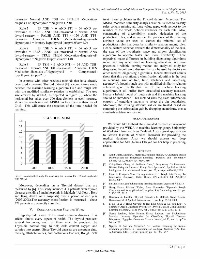
(IJACSA) International Journal of Advanced Computer Science and Applications, Vol. 4, No. 10, 2013
125 | P a g e www.ijacsa.thesai.org
measure= Normal AND TSH <= 39THEN Medication-diagnosis-of-Hypothyroid = Negative (15.0)
Rule 7 IF TSH > 6 AND FTI > 64 AND on-thyroxine = FALSE AND TSH-measured = Normal AND thyroid-surgery = FALSE AND TT4 <=150 AND TT4-measure= Abnormal THEN Medication-diagnosis-of-Hypothyroid = Primary-hypothyroid (supp=6.0/cer=1.0)
Rule 8 IF TSH > 6 AND FTI > 64 AND on-thyroxine = FALSE AND TSH-measured = Normal AND thyroid-surgery = TRUE THEN Medication-diagnosis-of-Hypothyroid = Negative (supp=3.0/cer= 1.0)
Rule 9 IF TSH > 6 AND FTI <= 64 AND TSH-measured = Normal AND T4U-measured = Abnormal THEN Medication-diagnosis-of-Hypothyroid = Compensated-hypothyroid (supp=2.0)
In contrast with other previous methods that have already been used in treating Thyroid dataset [8], a comparative study between the machine learning algorithm C4.5 and rough sets with the modified similarity relation is established. The tree size created by WEKA, as depicted in figure (3) where the horizontal bar taken over 500 data element in each measure, shows that rough sets with MSIM has less tree size than that of C4.5. This will cause the reduction of the time needed for learning.
Fig. 3. a comparative study for measuring the tree size for C4.5 and rough sets with MSIM
Moreover, depending on a Thyroid dataset that are measured by [6], This study included 414 patients with thyroid diseases attending 3 main hospitals in Makkah ( Al-Noor , Hera and King Abdul Aziz hospitals) over a period of one year (2007-2008).The accuracy classification is measured , about 371 patients are correctly classified.
V. CONCLUSIONS AND FEATURE WORK
Hypothyroid is one of the most common diseases. It is affects almost every aspect of health. The thyroid produces several hormones, each of them must be produced by Thyroidin normal rang; to help cells convert oxygen and calories into energy. Since Thyroid datasets are uncertain data, missing attribute values, and continuous features, Rough Sets
treat these problems in the Thyroid dataset. Moreover, The MSIM, modified similarity analysis relation, is used to classify rules contain missing attribute value, gaps, with respect to the number of the whole defined attributes for each rule. Also, constructing of discernibility matrix, deduction of the production rules, and reducts in the presence of the missing attribute value are used to extract the minimal set of productions rules that describe similarity relation among rules. Hence, feature selection reduces the dimensionality of the data, the size of the hypothesis space and allows classification algorithm to operate faster and more effectively. These objectives make difference in building diagnosing algorithms more than any other machine learning algorithm. We have presented a reliable learning method and analytical study for diagnosing hypothyroid disease that can be used by doctors in other medical diagnosing algorithms. Indeed statistical results show that this evolutionary classification algorithm is the best in reducing size of tree, time, attributes and increasing accuracy. Although rough sets with modified similarity relation achieved good results that that of the machine learning algorithms, it still suffer from unsatisfied accuracy measure. Hence a hybrid model of rough sets and the machine learning should be introduced. This method uses the class information entropy of candidate patients to select the bin boundaries. Moreover, the missing attribute values are treated based on computing the information gain by dropping an attribute, then a similarity relation is measured.
ACKNOWLEDGMENT
We would like to thank the simulated research environment provided by the WEKA to machine learning group, University of Waikato, Hamilton, New Zealand. Also, a great appreciation to Gravan Institute of Medical Research for providing the medical database. Also, we should express our deep appreciation for Mrs. Nesma Elsayed for her help in preparing results.
REFERENCES
[1] Ankit Gupta, Kishan G. Mehrotra,Chilukuri Mohan,”A Clustering-Based Discretization for Supervised Learning, ”Statistics and Probability
Letters, vol.80, pp.816-824, May 2010.
[2] Ching-Hsue Cheng & Jr-Shian Chen," Diagnosing Cardiovascular Disease Using an Enhanced Rough Sets Approach", Applied Artificial
Intelligence: An International Journal,vol. 23, no. 6,pp. 487-499, 2009.
[3] Frida R. Coaquira Nina, On Applications Of Rough Sets Theory To Knowledge Discovery, Ph.D. Thesis, UNIVERSITY OF PUERTO
RICO, 2007.
[4] ftp://ftp.ics.uci.edu/pub/machine-learning-databases.Accessed 9.8.2013
[5] Georg Peters, Richard Weber, Rene Nowatzke, "Dynamic Rough
Clustering and its Applications", Applied Soft Computing, vol. 12, pp. 3193-3207, 2012.
[6] Hawazen A. Lamfon, Thyroid Disorders In Makkah, Saudi Arabia,
Ozean Journal of Applied Sciences, vol. 1, no. 1,pp. 55-58, 2008.
[7] Li-Na Li & Ji-Hong Ouyang & Hui-Ling Chen & Da-You Liu," A Computer Aided Diagnosis System for Thyroid Disease Using Extreme
Learning Machine", J Med Syst, vol. 36 no. 5, pp. 3327-3337, 2012.
[8] Nesma Ibrahim, Taher Hamza, Elsayd Radwan, “An Evolutionary Machine Learning Algorithm for Classifying Thyroid Diseases
Diagnoses, “Egyptian Computer Science Journal,vol.35, no. 1, pp.73-86,Jan 2011.
[9] Nguyen H. Son and Skowron," A.: Boolean reasoning for feature
extraction problems, In: Foundations of Intelligent Systems (Z.W. Ras, A. Skowron, Eds.). | Berlin: Springer, pp.117-126, 1997.
0
2
4
6
8
10
12
14
16
500 1000 1500 2000
C4.5 RS+MSIM

(IJACSA) International Journal of Advanced Computer Science and Applications, Vol. 4, No. 10, 2013
126 | P a g e www.ijacsa.thesai.org
[10] Nguyen H. Son and Skowron A.: Quantization of real value attributes. |
Proc. Int. Workshop Rough Sets and Soft Computing at 2nd Joint Conf. Information Sciences (JCIS'95), Durham, NC, pp.34-37, (1995).
[11] Pawlak, Z., " Rough Sets- Theoretical Aspects of Reasoning about Data", Kluwer Academic, Dordrecht, 1991.
[12] Polkowski, L., Skowron, A.(Eds), Rough Sets in Knowledge Discovery,
Physica- Verlag, Heidelberg, vols: 1 and 2, 1998
[13] Roman, W. Swiniarski, Andrzej Skowron," Rough Set Methods in
Feature Selection and Recognition", Pattern Recognition Letters, vol. 24, pp. 833-849, 2003.
[14] Keles, A., "ESTDD: Expert System For Thyroid Diseases Diagnosis", Expert Syst. Appl. vol.34 no. 1,pp. 242–246, 2008.
[15] Sara El-Sayed El-Metwally, Elsayed Radwan, Taher Hamza, " Multiple
DNA Sequence Alignment using a Hybrid Model of GA and Rough Sets", Egyptian Computer Science Journal, vol. 34 no. 3, May 2010.

(IJACSA) International Journal of Advanced Computer Science and Applications, Vol. 4, No. 10, 2013
127 | P a g e www.ijacsa.thesai.org
Geo-visual Approach for Spatial Scan Statistics: An
Analysis of Dengue Fever Outbreaks in Delhi
Shuchi Mala, Raja Sengupta
Computer Science and Engineering
Indraprastha Institute of Information Technology Delhi
New Delhi, India
Abstract— There are very few surveillance systems being used
to detect disease outbreaks at present. In disease surveillance
system, data related to cases and various risk factors are collected
and then the collected data is transformed into meaningful
information for effective disease control using statistical analysis
tools. Disease outbreaks can be detected but for effective disease
control, a visualization approach is required. Without
appropriate visualization, it is very difficult to interpret the
results of analysis. In this work, a method has been developed for
geographical representation of the disease surveillance and
response system for early detection of disease outbreaks using
SaTScan and open source Geographic Information System
software. Maps that combine the geographical location of
diseases and clusters to enhance the understanding of results of
statistical analysis tool are developed using QGIS library which
provides many spatial algorithms and native GIS functions. This
library is accessed through PyQGIS and PyQt using Python.
Keywords—Disease Surveillance; p-value; clusters; statistically
significant; outbreaks and visualization
I. INTRODUCTION
Disease surveillance is a continuous process of collecting information, as well as organizing, analyzing and interpreting the information collected so that the disease outbreaks can be determined and effective actions in disease control may be taken. Outbreaks for diseases can be discovered by monitoring space-time trends of disease occurrences which can highlight changing patterns in risk and help to identify new risk factors. However surveillance datasets are mostly large in size.
Therefore, the availability and performance of software capable of analyzing space-time disease surveillance data on a continuous basis is essential for practical surveillance. At various places disease database for various diseases like cancer, dengue fever, malaria and many more are maintained. Number of new cases is typically added to a disease database daily, monthly or yearly, with the duration depending on the type of disease and the limit of database system.
A traditional disease surveillance mechanism involves reporting of diseases confirmed by labs to local or national organizations of health. This does not normally allow for early detection of new outbreaks. In new surveillance systems, it is easier to find out where the outbreaks will occur and what will be the geographical sizes of these outbreaks. In these systems, clustering is done which tells about number of cases of disease within study area.
Visualization of spatial distribution of the disease over a defined area helps user to analyze clusters easily and efficiently; and users can also detect unusual patterns of disease outbreaks. To study geographical variations of disease risk, the locations of cases are mostly proxies for residential addresses such as pin codes. If individual addresses are available, it is easy to plot the locations of cases on the map. The most common type of map for visualization is Choropleth maps for spatial distribution of disease in the well-defined geographical area using health indicators as occurrence, incidence rate and mortality rate. Choropleth maps usually use color or pattern combinations to show different levels of disease risk associated with each geographical area. These geographical areas are small areas usually defined for administrative purposes, such as counties, zones, wards, colonies, villages, towns and cities. For visualization, various geographical information systems can be used like QGIS which is a cross-platform free and open source desktop geographic information systems application.
In this paper, a method is developed to visualize the results obtained by SaTScan. The method provides an easier way to run SaTScan multiple times and add graphical output for analyzing results obtained by the developed application. This standalone package takes datasets or files of population, cases information, geographical coordinates of each location and optional controls as an input in a simple prescribed format and generates text files in SaTScan format and allows the user to choose SaTScan analysis options. It reads the results from SaTScan and creates geographical outputs, based on a separate map boundary file. The front end was developed using PyQt4, Qt4, PyQGIS and QGIS libraries, with Python as the interfacing programming language. Effectiveness of the user interface is demonstrated by a case study of dengue fever in Delhi, India from 2010-2012. This application is particularly useful to health Officials who do not have knowledge of GIS software in disease surveillance and disease control.
II. MATERIALS AND METHODS
A. Related work
Disease clustering can be classified as temporal clustering, spatial clustering or space time clustering. Temporal clustering observes whether cases are located close to each other in time, spatial clustering observes whether cases are located close to each other in space and space-time clustering observes whether cases are close in space as well as in time. For detection of disease cluster, various statistical methods have
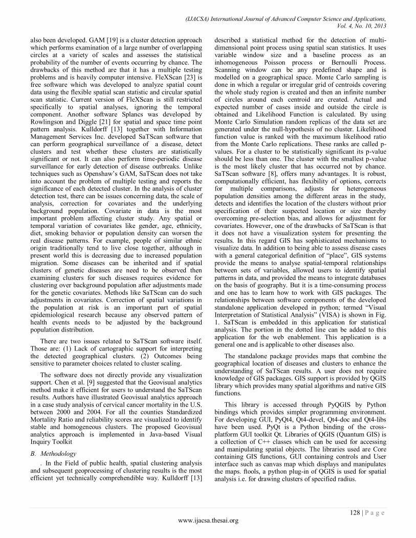
(IJACSA) International Journal of Advanced Computer Science and Applications, Vol. 4, No. 10, 2013
128 | P a g e www.ijacsa.thesai.org
also been developed. GAM [19] is a cluster detection approach which performs examination of a large number of overlapping circles at a variety of scales and assesses the statistical probability of the number of events occurring by chance. The drawbacks of this method are that it has a multiple testing problems and is heavily computer intensive. FleXScan [23] is free software which was developed to analyze spatial count data using the flexible spatial scan statistic and circular spatial scan statistic. Current version of FleXScan is still restricted specifically to spatial analyses, ignoring the temporal component. Another software Splancs was developed by Rowlingson and Diggle [21] for spatial and space time point pattern analysis. Kulldorff [13] together with Information Management Services Inc. developed SaTScan software that can perform geographical surveillance of a disease, detect clusters and test whether these clusters are statistically significant or not. It can also perform time-periodic disease surveillance for early detection of disease outbreaks. Unlike techniques such as Openshaw’s GAM, SaTScan does not take into account the problem of multiple testing and reports the significance of each detected cluster. In the analysis of cluster detection test, there can be issues concerning data, the scale of analysis, correction for covariates and the underlying background population. Covariate in data is the most important problem affecting cluster study. Any spatial or temporal variation of covariates like gender, age, ethnicity, diet, smoking behavior or population density can worsen the real disease patterns. For example, people of similar ethnic origin traditionally tend to live close together, although in present world this is decreasing due to increased population migration. Some diseases can be inherited and if spatial clusters of genetic diseases are need to be observed then examining clusters for such diseases requires evidence for clustering over background population after adjustments made for the genetic covariates. Methods like SaTScan can do such adjustments in covariates. Correction of spatial variations in the population at risk is an important part of spatial epidemiological research because any observed pattern of health events needs to be adjusted by the background population distribution.
There are two issues related to SaTScan software itself. Those are: (1) Lack of cartographic support for interpreting the detected geographical clusters. (2) Outcomes being sensitive to parameter choices related to cluster scaling.
The software does not directly provide any visualization support. Chen et al. [9] suggested that the Geovisual analytics method make it efficient for users to understand the SaTScan results. Authors have illustrated Geovisual analytics approach in a case study analysis of cervical cancer mortality in the U.S. between 2000 and 2004. For all the counties Standardized Mortality Ratio and reliability scores are visualized to identify stable and homogeneous clusters. The proposed Geovisual analytics approach is implemented in Java-based Visual Inquiry Toolkit
B. Methodology
. In the Field of public health, spatial clustering analysis and subsequent geoprocessing of clustering results is the most efficient yet technically comprehendible way. Kulldorff [13]
described a statistical method for the detection of multi-dimensional point process using spatial scan statistics. It uses variable window size and a baseline process as an inhomogeneous Poisson process or Bernoulli Process. Scanning window can be any predefined shape and is modelled on a geographical space. Monte Carlo sampling is done in which a regular or irregular grid of centroids covering the whole study region is created and then an infinite number of circles around each centroid are created. Actual and expected number of cases inside and outside the circle is obtained and Likelihood Function is calculated. By using Monte Carlo Simulation random replicas of the data set are generated under the null-hypothesis of no cluster. Likelihood function value is ranked with the maximum likelihood ratio from the Monte Carlo replications. These ranks are called p-values. For a cluster to be statistically significant its p-value should be less than one. The cluster with the smallest p-value is the most likely cluster that has occurred not by chance. SaTScan software [8], offers many advantages. It is robust, computationally efficient, has flexibility of options, corrects for multiple comparisons, adjusts for heterogeneous population densities among the different areas in the study, detects and identifies the location of the clusters without prior specification of their suspected location or size thereby overcoming pre-selection bias, and allows for adjustment for covariates. However, one of the drawbacks of SaTScan is that it does not have a visualization system for presenting the results. In this regard GIS has sophisticated mechanisms to visualize data. In addition to being able to assess disease cases with a general categorical definition of “place”, GIS systems provide the means to analyse spatial-temporal relationships between sets of variables, allowed users to identify spatial patterns in data, and provided the means to integrate databases on the basis of geography. But it is a time-consuming process and one has to learn how to work with GIS packages. The relationships between software components of the developed standalone application developed in python; termed “Visual Interpretation of Statistical Analysis” (VISA) is shown in Fig. 1. SaTScan is embedded in this application for statistical analysis. The portion in the dotted line can be added to this application for the web enablement. This application is a general one and is applicable to other diseases also.
The standalone package provides maps that combine the geographical location of diseases and clusters to enhance the understanding of SaTScan results. A user does not require knowledge of GIS packages. GIS support is provided by QGIS library which provides many spatial algorithms and native GIS functions.
This library is accessed through PyQGIS by Python bindings which provides simpler programming environment. For developing GUI, PyQt4, Qt4-devel, Qt4-doc and Qt4-libs have been used. PyQt is a Python binding of the cross-platform GUI toolkit Qt. Libraries of QGIS (Quantum GIS) is a collection of C++ classes which can be used for accessing and manipulating spatial objects. The libraries used are Core containing GIS functions, GUI containing controls and User interface such as canvas map which displays and manipulates the maps. ftools, a python plug-in of QGIS is used for spatial analysis i.e. for drawing clusters of specified radius.
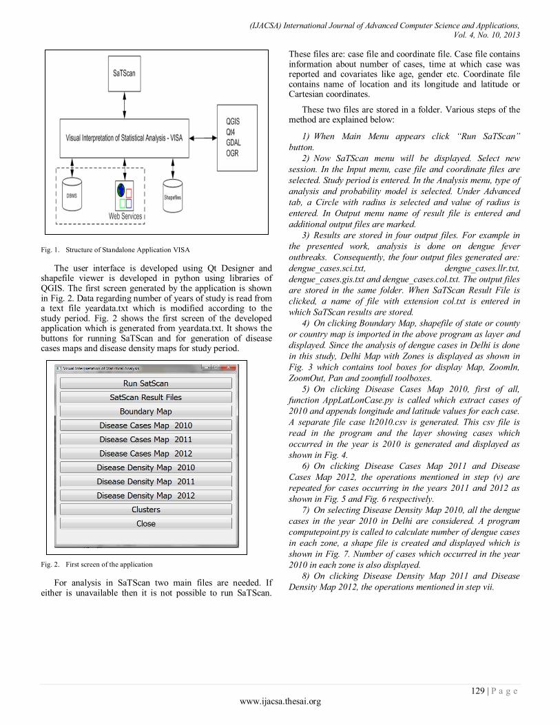
(IJACSA) International Journal of Advanced Computer Science and Applications, Vol. 4, No. 10, 2013
129 | P a g e www.ijacsa.thesai.org
Fig. 1. Structure of Standalone Application VISA
The user interface is developed using Qt Designer and shapefile viewer is developed in python using libraries of QGIS. The first screen generated by the application is shown in Fig. 2. Data regarding number of years of study is read from a text file yeardata.txt which is modified according to the study period. Fig. 2 shows the first screen of the developed application which is generated from yeardata.txt. It shows the buttons for running SaTScan and for generation of disease cases maps and disease density maps for study period.
Fig. 2. First screen of the application
For analysis in SaTScan two main files are needed. If either is unavailable then it is not possible to run SaTScan.
These files are: case file and coordinate file. Case file contains information about number of cases, time at which case was reported and covariates like age, gender etc. Coordinate file contains name of location and its longitude and latitude or Cartesian coordinates.
These two files are stored in a folder. Various steps of the method are explained below:
1) When Main Menu appears click “Run SaTScan”
button.
2) Now SaTScan menu will be displayed. Select new
session. In the Input menu, case file and coordinate files are
selected. Study period is entered. In the Analysis menu, type of
analysis and probability model is selected. Under Advanced
tab, a Circle with radius is selected and value of radius is
entered. In Output menu name of result file is entered and
additional output files are marked.
3) Results are stored in four output files. For example in
the presented work, analysis is done on dengue fever
outbreaks. Consequently, the four output files generated are:
dengue_cases.sci.txt, dengue_cases.llr.txt,
dengue_cases.gis.txt and dengue_cases.col.txt. The output files
are stored in the same folder. When SaTScan Result File is
clicked, a name of file with extension col.txt is entered in
which SaTScan results are stored.
4) On clicking Boundary Map, shapefile of state or county
or country map is imported in the above program as layer and
displayed. Since the analysis of dengue cases in Delhi is done
in this study, Delhi Map with Zones is displayed as shown in
Fig. 3 which contains tool boxes for display Map, ZoomIn,
ZoomOut, Pan and zoomfull toolboxes.
5) On clicking Disease Cases Map 2010, first of all,
function AppLatLonCase.py is called which extract cases of
2010 and appends longitude and latitude values for each case.
A separate file case lt2010.csv is generated. This csv file is
read in the program and the layer showing cases which
occurred in the year is 2010 is generated and displayed as
shown in Fig. 4.
6) On clicking Disease Cases Map 2011 and Disease
Cases Map 2012, the operations mentioned in step (v) are
repeated for cases occurring in the years 2011 and 2012 as
shown in Fig. 5 and Fig. 6 respectively.
7) On selecting Disease Density Map 2010, all the dengue
cases in the year 2010 in Delhi are considered. A program
computepoint.py is called to calculate number of dengue cases
in each zone, a shape file is created and displayed which is
shown in Fig. 7. Number of cases which occurred in the year
2010 in each zone is also displayed.
8) On clicking Disease Density Map 2011 and Disease
Density Map 2012, the operations mentioned in step vii.
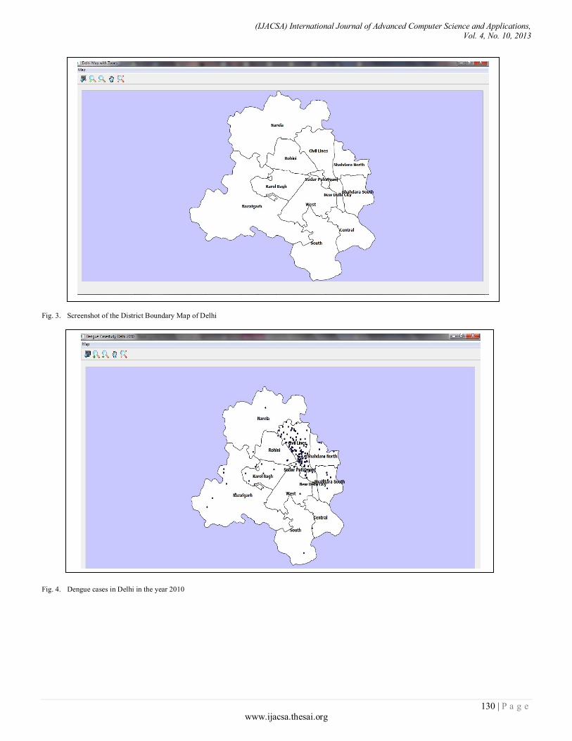
(IJACSA) International Journal of Advanced Computer Science and Applications, Vol. 4, No. 10, 2013
130 | P a g e www.ijacsa.thesai.org
Fig. 3. Screenshot of the District Boundary Map of Delhi
Fig. 4. Dengue cases in Delhi in the year 2010
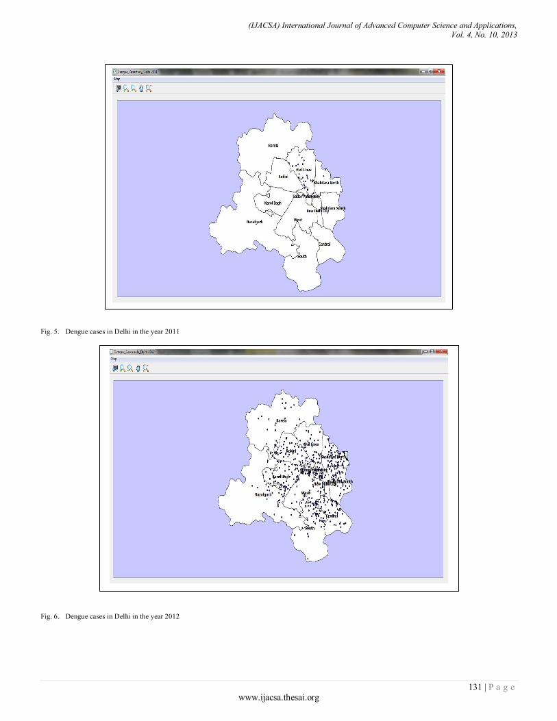
(IJACSA) International Journal of Advanced Computer Science and Applications, Vol. 4, No. 10, 2013
131 | P a g e www.ijacsa.thesai.org
Fig. 5. Dengue cases in Delhi in the year 2011
Fig. 6. Dengue cases in Delhi in the year 2012

(IJACSA) International Journal of Advanced Computer Science and Applications, Vol. 4, No. 10, 2013
132 | P a g e www.ijacsa.thesai.org
are repeated for cases occurring in the years 2011 and 2012 as shown in Fig. 8 and Fig. 9 respectively.
1) When Cluster button is clicked, the application reads
the SaTScan result file dengue_cases.col.txt and forms a file
cluster.csv which contains all clusters having p-value less than
a specified value. This csv file is read and a layer is created.
Using ftools plug-in, buffers of a specified radius are created.
The created layers are displayed which are shown in Fig. 10.
2) On clicking close, the application is terminated.
III. RESULTS AND DISCUSSION
In this section an analysis of dengue fever outbreaks in Delhi for past three years is presented as a sample case. In India 28,000 dengue cases were reported in 2010 and there is a significant rise in the incidence of dengue from 18,860 cases in the year 2011 to 49,606 cases in the year 2012 and 1,700 dengue cases were reported from Delhi due to the disease last year . If disease surveillance was done nation-wide for early detection of disease outbreaks, effective actions would have been taken and outbreaks would have been controlled. To perform disease surveillance statistical methods to detect disease clusters are required. It is equally important to have effective visualization approach. The presented work covers both the aspects of disease surveillance along with the surveillance results.
A. Data collection
To perform any type of analysis the most importance requirement is data. Data for analysis was collected from DHO Civil Lines Zone, Municipal Corporation of Delhi, Health Department. The data covering details on dengue cases in Delhi are available for the years 2010, 2011 and 2012 only. The details were taken from the Epidemiological Investigation form for the above mentioned years.
B. Data Pre-processing
The data collected is transformed in the format that is required to perform statistical analysis. The data is transformed into a comma separated file which contains information about the observed cases location name, case count, date of reported case, age of the case and gender. In this file age and gender are the covariates. Another comma separated value file is created for the coordinate information about the geographical location where case has occurred. In this file information about location name, latitude and longitude of the location of the case is stored.
C. Map Digitization
Georeferencing process is used to assign real-world coordinates to each pixel of the raster using QGIS. In the presented work, scanned map of Delhi is digitized by obtaining coordinates from the markings on the map image itself. Using these GCPs (Ground Control Points), the image is warped and it is made to fit within the chosen coordinate system [15].
D. Statistical Analysis
To detect clusters of disease outbreaks, statistical analysis is performed using SaTScan software which is embedded in the stand alone VISA application. To begin analysis, in the
GUI of the presented application, click on “Run SaTScan" button. On clicking the button, SaTScan window opens. In the input tab, import the created comma separated value file which contains the details about observed cases under case file option. This file is saved as dengue_cases.cas. The extension supported by SaTScan for case file is .cas. Under coordinate file option import the other comma separated file which contains latitude and longitude information about each location of the observed case. This file is saved as dengue_cases.geo. The extension supported by SaTScan for coordinate file is .geo. The study period is from 2010/1/1 to 2012/12/31 with time precision to be year and coordinates latitude/longitude. In the analysis, space-time analysis and space time permutation model are selected. Space time permutation model is used in the analysis because dengue fever has a relation with environmental variables as many cases are observed in months with warm and humid weather. Hence with geographical location time is also an important parameter to perform analysis. Adjustment for the maximum spatial cluster size is set at 2 kilometers. In the output tab, result file dengue cases.txt is saved and SaTScan software is executed.
E. Visualization results generated by VISA package
Delhi region is divided into 12 zones which are Narela, Rohini, Civil Lines, Shahdara North, Shahdara South, New Delhi City, Karol Bagh, Nazafgarh, central, west, Sadar Paharganj and south. On clicking Delhi Map button, the zone boundary map is generated as shown in Fig. 3. On Clicking Disease Cases Map 2010 button, dengue fever cases spread in year 2010 map are generated as shown in Fig. 4. High number of cases occurred in Sant Nagar (64), Jahangirpuri (47),Timarpuri (24) and Burari Village (22). On Clicking Disease Cases Map 2011 button, dengue fever cases reported year 2011 map are generated as shown in Fig. 5. Majority of cases occurred in Jahangirpuri (12), SantNagar (5), and Malkaganj (4). On Clicking Disease Cases Map2012 button, dengue fever spread in year 2012 map is generated as shown in Fig. 6. High number of cases occurred in Rajnagar-II (34), Mandawali (26) and SangamVihar (23). There are 8 locations in Delhi where cases were reported in 2010, 2011 as well as 2012 as TABLE 1. On clicking “No. of cases Map" button, Choropleth map is generated to show density of dengue cases with graduated colors. On the basis of zone, most cases are reported from Civil Lines Zone, Shahdara North Zone and Shahdara South Zone as shown in Fig. 6. On clicking Clusters button, clusters and buffer map are generated as shown in Fig. 7. There are seven detected clusters out of which one is most likely cluster and six are secondary clusters as shown in TABLE 2.
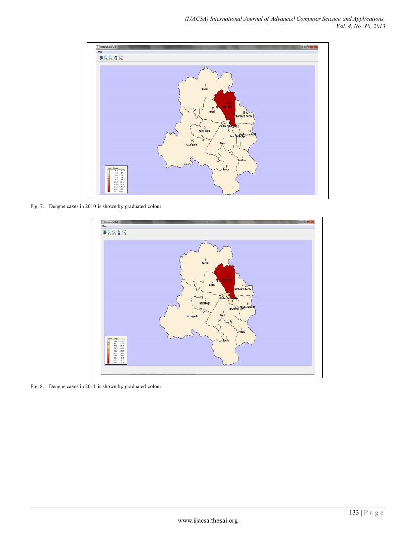
(IJACSA) International Journal of Advanced Computer Science and Applications, Vol. 4, No. 10, 2013
133 | P a g e www.ijacsa.thesai.org
Fig. 7. Dengue cases in 2010 is shown by graduated colour
Fig. 8. Dengue cases in 2011 is shown by graduated colour
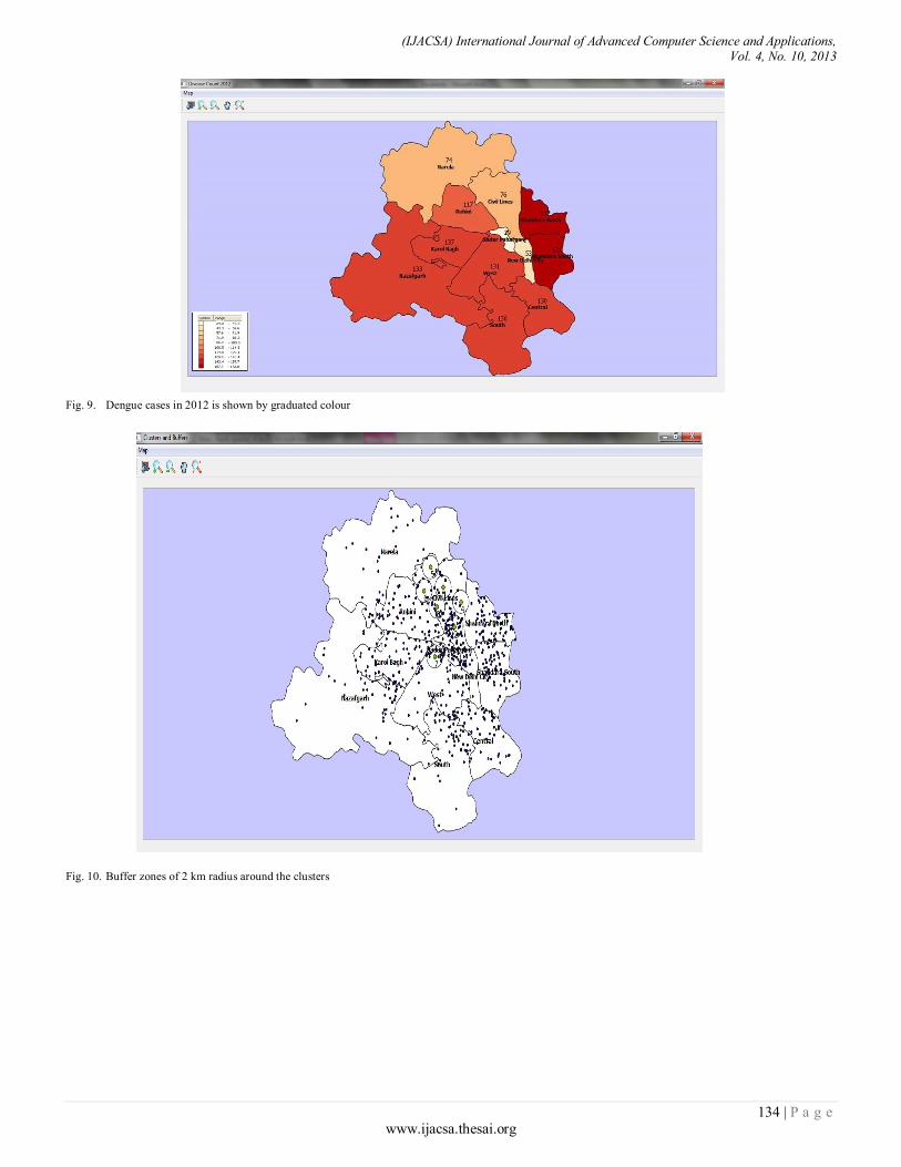
(IJACSA) International Journal of Advanced Computer Science and Applications, Vol. 4, No. 10, 2013
134 | P a g e www.ijacsa.thesai.org
Fig. 9. Dengue cases in 2012 is shown by graduated colour
Fig. 10. Buffer zones of 2 km radius around the clusters
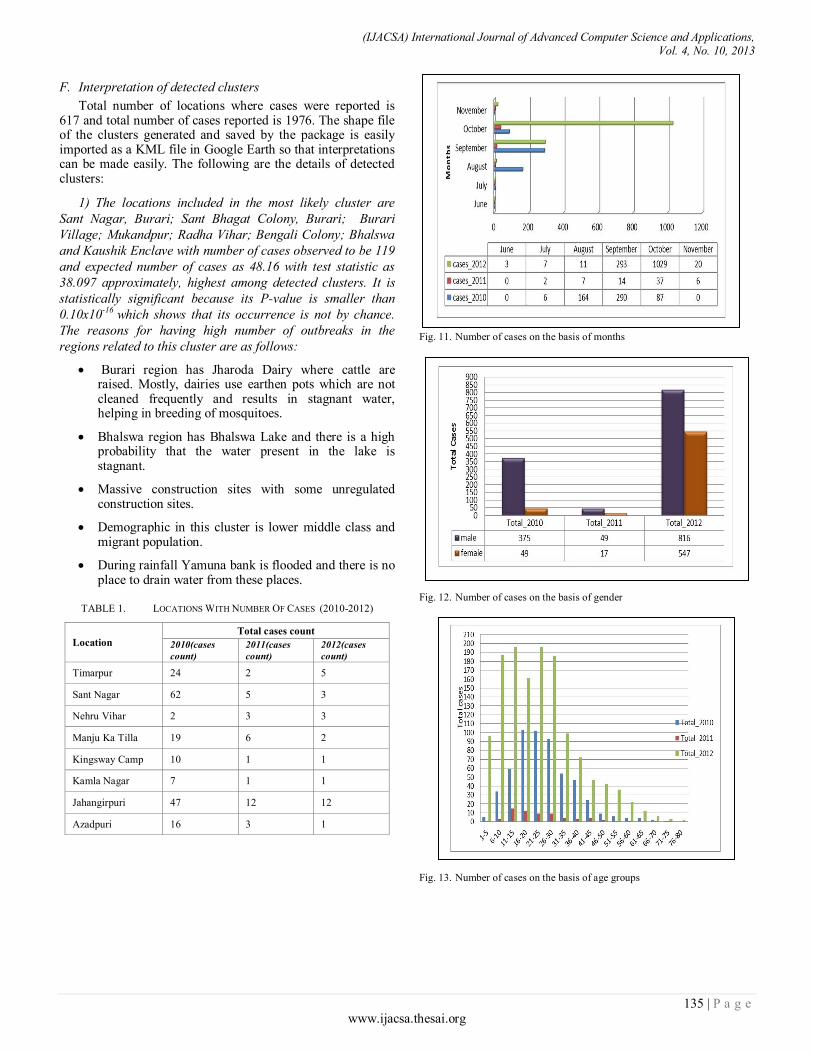
(IJACSA) International Journal of Advanced Computer Science and Applications, Vol. 4, No. 10, 2013
135 | P a g e www.ijacsa.thesai.org
F. Interpretation of detected clusters
Total number of locations where cases were reported is 617 and total number of cases reported is 1976. The shape file of the clusters generated and saved by the package is easily imported as a KML file in Google Earth so that interpretations can be made easily. The following are the details of detected clusters:
1) The locations included in the most likely cluster are
Sant Nagar, Burari; Sant Bhagat Colony, Burari; Burari
Village; Mukandpur; Radha Vihar; Bengali Colony; Bhalswa
and Kaushik Enclave with number of cases observed to be 119
and expected number of cases as 48.16 with test statistic as
38.097 approximately, highest among detected clusters. It is
statistically significant because its P-value is smaller than
0.10x10⁻¹⁶ which shows that its occurrence is not by chance.
The reasons for having high number of outbreaks in the
regions related to this cluster are as follows:
Burari region has Jharoda Dairy where cattle are raised. Mostly, dairies use earthen pots which are not cleaned frequently and results in stagnant water, helping in breeding of mosquitoes.
Bhalswa region has Bhalswa Lake and there is a high probability that the water present in the lake is stagnant.
Massive construction sites with some unregulated construction sites.
Demographic in this cluster is lower middle class and migrant population.
During rainfall Yamuna bank is flooded and there is no place to drain water from these places.
TABLE 1. LOCATIONS WITH NUMBER OF CASES (2010-2012)
Location Total cases count
2010(cases
count)
2011(cases
count)
2012(cases
count)
Timarpur 24 2 5
Sant Nagar 62 5 3
Nehru Vihar 2 3 3
Manju Ka Tilla 19 6 2
Kingsway Camp 10 1 1
Kamla Nagar 7 1 1
Jahangirpuri 47 12 12
Azadpuri 16 3 1
Fig. 11. Number of cases on the basis of months
Fig. 12. Number of cases on the basis of gender
Fig. 13. Number of cases on the basis of age groups

(IJACSA) International Journal of Advanced Computer Science and Applications, Vol. 4, No. 10, 2013
136 | P a g e www.ijacsa.thesai.org
TABLE 2. CLUSTERS WITH P-VALUE LESS THAN 0.55
Cluster
Number
Clusters Information
Central Location
ID
Latitude
Longitude
Cluster
Start Date
Cluster End
Date
Log
Likelihood
Ratio
P-value of
Cluster
Observed
Cases
Expected
Cases
Observed/
Expected
1 Sant Nagar
Burari
28.74544
77.190212
01-01-2010
31-12-2010
37.490136
1.00E-17
119
48.85
2.45
2 Delhi
University
28.7
77.213
01-01-2010
31-12-2010
30.182756
1.11E-16
142
69.66
2.04
3 Majlisparki
28.7
77.177633
01-01-2010
31-12-2010
24.49099
2.7E-13
100
45.94
2.18
4 Wazirabad
Village
28.7
77.226145
01-01-2010
31-12-2010
8.08196
0.0022
22
8.13
2.71
5 Kadi Village
28.8
77.164402
01-01-2010
31-12-2010
8.03457
0.0023
24
9.35
2.57
6 Badli
28.7
77.151392
01-01-2011
31-12-2010
5.921857
0.042
6
0.97
6.2
7 East Patel
Nagar
28.6
77.172961
01-01-2012
31-12-2010
3.848719
0.548
65
45.35
1.43
2) The locations included in the second cluster are Delhi
University, St. Stephen College, Patel Chest, Miranda House,
Ramjas College, Mall Road, Old Vidhan Sabha, Mourice
Nagar, Vijay Nagar, Khyber Pass, Hansraj College, Hakikat
Nagar, Old Chandrawal, Kamla Nagar, Rajpur Road, Old
Gupta Colony, New Chandrawal, Under Hill Road, IP College
Campus, Timarpur, Outram Lane, Aruna Nagar, Civil Line,
Out Ram Line, Kalyan Vihar, Malkaganj, Rajpur, Kingsway
Camp, Ghanta Ghar, Gur Mandi, GTB Hospital Campus, Ram
Kishore Marg, CC Colony, Kabir Basti, Ishwar Colony, Singh
Sabha Road, Indra Vihar, Rana Pratap Bagh, Mukherji
Nagar, West Mukherji Nagar, Shakti Nagar and Majnu Ka
Tilla with number of cases observed as 142 and expected
number of cases as 68.82 with test statistic to be 31.074
approximately, second highest among detected clusters. It is
statistically significant because its P-value is 0.11x10⁻¹⁵ which
shows that its occurrence is not by chance. The reasons for
having high number of outbreaks in the regions related to this
cluster are as follows:
Most of the areas are institutional and government office area. These are vulnerable due to lack of awareness.
There is no sense of ownership because of multiplicity of authorities.
There are large open areas near Rajpur Road where rain water is collected
Large student population and lack of awareness about prevention control of disease.
In months of July and August breeding of mosquitoes takes place and in months of September and October they become adults and thus large number of cases are observed in these two months as shown in Fig. 11.
On the basis of gender, infected male population was very high in 2010 and 2011 in comparison to female population but
in 2012 there was a high increase in the number of infected females as shown in Fig. 12.
On the basis of age group in the year 2010, most cases occurred in 16-20 years of age; in the year 2011 most of the cases occurred in the 11-15 years of age and in the year 2012 most of cases occurred in the 11-15 years and 20-25 years of age groups as shown in Fig. 13.
IV. CONCLUSION
The Geographical visualization approach developed in this paper facilitates the space-time cluster detection methods by providing an efficient representation of the results of statistical analysis in geographical space. Space-time analysis is performed by using space-time permutation model of SaTScan. The disease clusters are detected with the cluster radius as 2 kilometers. With the proposed visualization method maps are generated. These maps show spreading of cases, density of cases within each district or county and statistically significant clusters. With the help of presented work proactive actions can be taken to prevent disease outbreaks. It is also helpful in identifying the hot zone of an epidemic. Therefore on the basis of information gathered from statistical analysis and visualization the overall quality of health of the nation can be improved. This application is specifically useful to health Officials who do not have knowledge of GIS software. The standalone package is developed by using python, PyQGIS, QGIS, PyQT4, Qt Designer and SaTScan. Use of the proposed method is demonstrated to analyze the results of statistical analysis of dengue fever. The team of doctors in Municipal Corporation of Delhi found these results very informative; efficient and accurate and the interpretations related to the clusters were very similar to their interpretations.
FUTURE WORK
The present work will be extended to include a statistical interface for space-time analysis instead of integrating the developed application with SaTScan. This application will be

(IJACSA) International Journal of Advanced Computer Science and Applications, Vol. 4, No. 10, 2013
137 | P a g e www.ijacsa.thesai.org
made web-based and database containing diseases information will be integrated with it. With the facility of a database user can save data whenever required and can perform analysis at chosen time intervals such as on weekly basis or based on months or years from remote location.
ACKNOWLEDGMENT
We would like to thank Dr Ashok Rawat, Deputy Heath Officer, Civil Lines Zone, Municipal Corporation of Delhi and Dr. Sanjay Sinha, Senior Doctor, Health Department, Civil Lines Zone, Municipal Corporation of Delhi for providing us the data on dengue fever to perform analysis.
REFERENCES
[1] Agricola Odoi, S Wayne Martin, Pascal Michel, Dean Middleton, John Holt and JeffWilson, 2004, Investigation Of Clusters Of Giardiasis using
GIS And A Spatial Scan Statistic, International Journal of Health Geographics, Vol.3, No.11, pp 1-11.
[2] Allyson M Abrams and Ken P Kleinman, 2007, A SATSCAN Macro
Accessory For Cartography (Smac) Package Implemented With SAS Software, International Journal of Health Geographics, Vol. 6, No.6, pp.
1-8.
[3] Besag J.E. and Newell J., 1991, the detection of clusters in rare diseases, Journal of the Royal Statistical Society, Series a, 154, 143–155.
[4] Sabel E. Clive, Loytonen Markku, Maheswaran Ravi, Craglia Massimo,
2004, GIS in public health practice, CRC Press LLC.
[5] Tatlonghari Jayson A. Rick, 2009,GIS Manual using Quantum GIS, pp. 23-36.
[6] Dobias Martin, 2010, PyQGIS Developer Cookbook, created by sphinx-
quickstart.
[7] B. M. Harwani, 2011, Introduction to Python Programming and
Developing GUI Applications with PyQt, Cengage Learning, pp.2 01-416.
[8] Kulldorff M., 2011, SaTScan User Guide, pp. 4-107.
[9] Chen Jin, Roth E Robert, Naito T Adam, Lengerich J Eugene and
MacEachren MAlan, 2008,Geovisual analytics To Enhance Spatial Scan Statistic Interpretation: AnAnalysis Of U.S. Cervical Cancer Mortality,
International Journal of Health Geographics, Vol.7, No.57, pp. 1-18.
[10] Kulldorff M., 1998,Statistical methods for spatial epidemiology: tests forrandomness, In GIS and Health, pp. 49–62, London: Taylor &
Francis.
[11] Gail M., Krickeberg K., Samet J., Tsiatis A., Wong W., Tango. T, 2009,
Statistics for Biology and Health, springer.
[12] Jankowska Marta, Aldstadt Jared, Getis Arthur, Weeks John, Fraley
Grant, 2008,An Amoeba procedure For Visualizing Clusters, GIScience , Park City, UT.
[13] Kuldorff M., 1997, A Spatial Scan Statistic, Commun Statist Theory
Meth, Vol.26, No.6, pp. 1481-1495.
[14] Kulldorff M., 2001, Prospective Time Periodic Geographical Disease SurveillanceUsing A Scan Statistic, Royal Statistical Society, Vol. 164,
Part 1, pp. 61-72.
[15] Kulldorff M., Feuer J. Eric, Miller A. Barry and Freedman S. Laurence, 1997, Breast Cancer Clusters in the Northeast United States: A
Geographic Analysis, American Journal of Epidemiology, Vol. 146, No. 2, pp. 161-170.
[16] Kulldorff M., Huang L., Pickle L. and Duczmal L., 2006, An Elliptic
Spatial Scan Statistics, Wiley InterScience, Vol. 25, pp. 3929-3943.
[17] Kulldorff M., Heffernan Richard, Hartman Jessica, Assunc Renato, Mostashari Farzad,2005,A Space Time Permutation Scan Statistic For
Disease Outbreak Detection, plos journals, Vol.2, No.3, pp. 216-224.
[18] Kulldorff M., Athas F. William, Feuer J. Eric, Miller A. Barry and Key
R. Charles, 1998, Evaluating Cluster Alarms: A Space-Time Scan Statistic and Brain Cancer in Los Alamos, New Mexico, American
Journal of Public Health, 1998, Vol. 88, No.9, pp. 1377-1380.
[19] Openshaw, Charlton M, Wymer C, Craft A, 1987, A Mark 1 geographical analysis machine for the automated analysis of point data
sets, International Journal of Geographical Information Systems, Vol.1, pp. 335–358.
[20] Piarroux Renaud, Barrais Robert, Faucher Benot, Haus Rachel, Piarroux
Martine,Gaudart Jean, Magloire Roc, and Raoult Didier, 2011, Understanding The Cholera Epidemic, Haiti. Emerging Infectious
Diseases, Vol. 17, No. 7, pp. 1161-1167.
[21] Rowlingson B. and Diggle P., 1993, Splancs: spatial point pattern analysis code in SPlus, Computers and Geosciences, Vol. 19, pp. 627–
655.
[22] Sheehan TJ and DeChello LM, 2005, A Space-Time Analysis of the Proportion of Late Stage Breast Cancer in Massachusetts, 1988 to 1997,
International Journal of Health Geographics, Vol.4, No.15, pp. 1-9.
[23] Takahashi K., Yokoyama T., and Tango T., 2009, FleXScan: Software for the Flexible Spatial Scan Statistic. v3.0, National Institute of Public
Health, Japan.
[24] Tango T and Takahashi K,2005, A Flexibly Shaped Spatial Scan
Statistic for Detecting Clusters, International Journal of Health Geographics, Vol. 4, No. 11, pp. 1-15.

(IJACSA) International Journal of Advanced Computer Science and Applications, Vol. 4, No. 10, 2013
138 | P a g e www.ijacsa.thesai.org
Load Balancing with Neural Network
Nada M. Al Sallami
Associated Prof., CS Dept.
Faculty of Information Technology
& Science, Al Zaytoonah Private
University
Amman, Jordan
Ali Al daoud
Prof., CS Dept.
Faculty of Information Technology
& Science,Al Zaytoonah Private
University
Amman, Jordan
Sarmad A. Al Alousi
CIS Researcher
Amman, Jordan
Abstract—This paper discusses a proposed load balance
technique based on artificial neural network. It distributes
workload equally across all the nodes by using back propagation
learning algorithm to train feed forward Artificial Neural
Network (ANN). The proposed technique is simple and it can
work efficiently when effective training sets are used. ANN
predicts the demand and thus allocates resources according to
that demand. Thus, it always maintains the active servers
according to current demand, which results in low energy
consumption than the conservative approach of over-
provisioning. Furthermore, high utilization of server results in
more power consumption, server running at higher utilization
can process more workload with similar power usage. Finally the
existing load balancing techniques in cloud computing are
discussed and compared with the proposed technique based on
various parameters like performance, scalability, associated
overhead... etc. In addition energy consumption and carbon
emission perspective are also considered to satisfy green computing.
Keywords—Green Cloud Computing; Load Balancing;
Artificial Neural Networks
I. INTRODUCTION
Cloud computing can help business shift their focus to developing good business applications that will bring true business value [1]. Cloud computing can mainly provide four different service like: virtual server storage (Infrastructure as a service or IaaS) such as Amazon Web Services, software solution provider over the internet (Software as a Service or SaaS), software and product development tools (Platform as a Service or PaaS) such as Google Apps and Communication as a service or CaaS) [2][3]]. Clouds are deployed on physical infrastructure where Cloud middleware is implemented for delivering service to customers. Such an infrastructure and middleware differ in their services, administrative domain and access to users. Therefore, the Cloud deployments are classified mainly into three types: Public Cloud, Private Cloud and Hybrid Cloud. Due to the exponential growth of cloud computing, it has been widely adopted by the industry and there is a rapid expansion in data-centers. This expansion has caused the dramatic increase in energy use and its impact on the environment in terms of carbon footprints. The link between energy consumption and carbon emission has given rise to an energy management issue which is to improve energy-efficiency in cloud computing to achieve Green computing [4].This paper proposed a new algorithm to achieve Green computing in load balancing. The algorithm uses artificial neural network to solve load balancing in cloud, its
performance is discussed and compared with the existing load balancing techniques.
To deliver technical and economic advantage, cloud computing must be deployed, as well as implemented, successfully. Deployment supersedes implementation, because merely utilizing the services of a cloud vendor does not by itself differentiate an organization from its competitors. Competitors likewise can implement cloud services, imitating resulting IT efficiencies. Successful deployment denotes the realization of unique or valuable organizational benefits that are a source of differentiation and competitive advantage. IT-related success is described through three categories of derived benefit: strategic, economic, and technological. Strategic refers to an organization’s renewed focus on its core business activities that can accompany a move to cloud computing when its IT functions, whole or in part, are hosted and/or managed by a cloud vendor. Economic refers to an organization’s ability to tap the cloud vendor’s expertise and technological resources to reduce in-house IT expenses. Technological refers to an organization’s access to state-of-the-art technology and skilled personnel, eliminating the risk and cost of in-house technological obsolescence. Deployment is defined in terms of the strategic, economic and technological benefits realized through cloud computing, setting the organization apart from its competitors. Optimizing the strategic, economic, and technological benefits derived from cloud computing is a function of an organization’s ability to use its own IT-related resources and capabilities to leverage the resources of the vendor. Since cloud computing is generally characterized as an IT service (with the vendor providing and maintaining the software and hardware infrastructure), the ability of the client organization to integrate and utilize the vendor’s services determines the extent IT benefits are likely to be achieved. Organization- specific capabilities related to implementation, integration, and utilization of cloud services play a key role in deployment performance [3]. Organization-Specific capabilities that can be a source of competitive advantages are [3]:
Technical. IT resources giving the organization functionality, flexibility, and scalability.
Managerial. Human IT resources resulting from training, experience, and insight.
Relational. Ability to develop positive associations with IT providers characterized by trust.

(IJACSA) International Journal of Advanced Computer Science and Applications, Vol. 4, No. 10, 2013
139 | P a g e www.ijacsa.thesai.org
II. GREEN COMPUTING
“Green” has become a popular term for describing things that are good for the environment, generally healthful and, more recently, economically sensible. “Going Green” implies reducing your energy use and pollution footprint. The technology community, specifically computer users, have popularized the term “Green Computing,” which is the reduction of the pollution and energy footprint of computers. Green Computing, or Green IT, is the practice of implementing policies and procedures that improve the efficiency of computing resources in such a way as to reduce the energy consumption and environmental impact of their utilization. As High Performance Computing (HPC) is becoming popular in commercial and consumer IT applications, it needs the ability to gain rapid and scalable access to high end computing capabilities. This computing infrastructure is provided by cloud computing by making use of datacenters. It helps the HPC users in an on-demand and payable access to their applications and data, anywhere from a cloud [4][5][6]. Cloud computing data-centers have been enabled by high-speed computer networks that allow applications to run more efficiently on these remote, broadband computer networks, compared to local personal computers. These data-centers cost less for application hosting and operation than individual application software licenses running on clusters of on-site computer clusters [11]. However, the explosion of cloud computing networks and the growing demand drastically increases the energy consumption of data-centers, which has become a critical issue and a major concern for both industry and society [8]. This increase in energy consumption not only increases energy cost but also increases carbon-emission. High energy cost results in reducing cloud providers’ profit margin and high carbon emission is not good for the environment [7]. Hence, energy-efficient solutions that can address the high energy consumption, both from the perspective of the cloud provider and the environment are required. This is a dire need of cloud computing to achieve Green computing.
A. Features of Clouds enabling Green computing
The key driver technology for energy efficient Clouds is “Virtualization,” which allows significant improvement in energy efficiency of Cloud providers by leveraging the economies of scale associated with large number of organizations sharing the same infrastructure. Virtualization is the process of presenting a logical grouping or subset of computing resources so that they can be accessed in ways that give benefits over the original configuration. By consolidation of underutilized servers in the form of multiple virtual machines sharing same physical server at higher utilization, companies can gain high savings in the form of space, management, and energy. According to reference [9], there are following four key factors that have enabled the Cloud computing to lower energy usage and carbon emissions from ICT.
Dynamic Provisioning: In traditional setting there are two reasons for over-provisioning: first, it is very difficult to predict the demand at a time and second, to guarantee availability of services and to maintain certain level of service quality to end users. Cloud
providers monitor and predict the demand and thus allocate resources according to demand. Those applications that require less number of resources can be consolidated on the same server. Thus, datacenters always maintain the active servers according to current demand, which results in low energy consumption than the conservative approach of over-provisioning.
Multi-tenancy: The smaller fluctuation in demand results in better prediction and results in greater energy savings. Using multi-tenancy approach, Cloud computing infrastructure reduces overall energy usage and associated carbon emissions. The SaaS providers serve multiple companies on same infrastructure and software. This approach is obviously more energy efficient than multiple copies of software installed on different infrastructure.
Server Utilization: High utilization of server results in more power consumption, server running at higher utilization can process more workload with similar power usage. Using virtualization technologies, multiple applications can be hosted and executed on the same server in isolation, thus lead to utilization levels up to 70%.
Datacenter Efficiency: The Cloud datacenters are quite different from traditional hosting facilities. A cloud datacenter could comprise of many hundreds or thousands of networked computers with their corresponding storage and networking subsystems, power distribution and conditioning equipment, and cooling infrastructures. A data center hosts computational power, storage and applications required to support an enterprise business. A data center is central to modern IT infrastructure, as all enterprise content is sourced from or passes through it. There are two major and complementary methods [8] to build a green data center: first, utilize green elements in the design and building process of a data center. Second, Greenify the process of running and operating a data center in everyday usage.
B. Green Load Balancing
Load balancing can be one such energy-saving solution in cloud computing environment. Thus load balancing is required to achieve Green computing in clouds which can be done with the help of the following two factors [6]:
Reducing Energy Consumption - Load balancing helps in avoiding overheating by balancing the workload across all the nodes of a cloud, hence reducing the amount of energy consumed.
Reducing Carbon Emission - Energy consumption and carbon emission go hand in hand. The more the energy consumed, higher is the carbon footprint. As the energy consumption is reduced with the help of Load balancing, so is the carbon emission helping in achieving Green computing.
In addition, the existing load balancing techniques in clouds,
consider various parameters like:
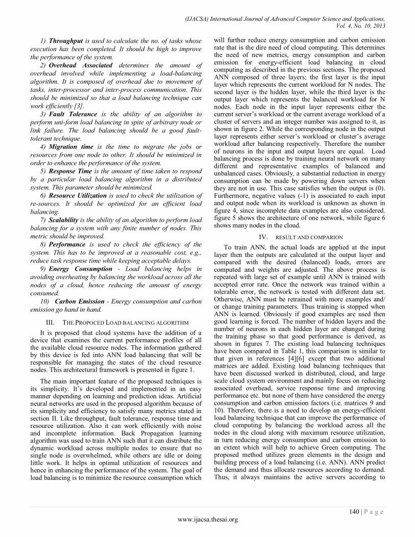
(IJACSA) International Journal of Advanced Computer Science and Applications, Vol. 4, No. 10, 2013
140 | P a g e www.ijacsa.thesai.org
1) Throughput is used to calculate the no. of tasks whose
execution has been completed. It should be high to improve
the performance of the system.
2) Overhead Associated determines the amount of
overhead involved while implementing a load-balancing
algorithm. It is composed of overhead due to movement of
tasks, inter-processor and inter-process communication. This
should be minimized so that a load balancing technique can
work efficiently [3].
3) Fault Tolerance is the ability of an algorithm to
perform uni-form load balancing in spite of arbitrary node or
link failure. The load balancing should be a good fault-
tolerant technique.
4) Migration time is the time to migrate the jobs or
resources from one node to other. It should be minimized in
order to enhance the performance of the system.
5) Response Time is the amount of time taken to respond
by a particular load balancing algorithm in a distributed
system. This parameter should be minimized.
6) Resource Utilization is used to check the utilization of
re-sources. It should be optimized for an efficient load
balancing.
7) Scalability is the ability of an algorithm to perform load
balancing for a system with any finite number of nodes. This
metric should be improved.
8) Performance is used to check the efficiency of the
system. This has to be improved at a reasonable cost, e.g.,
reduce task response time while keeping acceptable delays.
9) Energy Consumption - Load balancing helps in
avoiding overheating by balancing the workload across all the
nodes of a cloud, hence reducing the amount of energy
consumed.
10) Carbon Emission - Energy consumption and carbon
emission go hand in hand.
III. THE PROPOCED LOAD BALANCING ALGORITHM
It is proposed that cloud systems have the addition of a device that examines the current performance profiles of all the available cloud resource nodes. The information gathered by this device is fed into ANN load balancing that will be responsible for managing the states of the cloud resource nodes. This architectural framework is presented in figure 1.
The main important feature of the proposed techniques is its simplicity. It’s developed and implemented in an easy manner depending on learning and prediction ideas. Artificial neural networks are used in the proposed algorithm because of its simplicity and efficiency to satisfy many metrics stated in section II. Like throughput, fault tolerance, response time and resource utilization. Also it can work efficiently with noise and incomplete information. Back Propagation learning algorithm was used to train ANN such that it can distribute the dynamic workload across multiple nodes to ensure that no single node is overwhelmed, while others are idle or doing little work. It helps in optimal utilization of resources and hence in enhancing the performance of the system. The goal of load balancing is to minimize the resource consumption which
will further reduce energy consumption and carbon emission rate that is the dire need of cloud computing. This determines the need of new metrics, energy consumption and carbon emission for energy-efficient load balancing in cloud computing as described in the previous sections. The proposed ANN composed of three layers; the first layer is the input layer which represents the current workload for N nodes. The second layer is the hidden layer, while the third layer is the output layer which represents the balanced workload for N nodes. Each node in the input layer represents either the current server’s workload or the current average workload of a cluster of servers and an integer number was assigned to it, as shown in figure 2. While the corresponding node in the output layer represents either server’s workload or cluster’s average workload after balancing respectively. Therefore the number of neurons in the input and output layers are equal. Load balancing process is done by training neural network on many different and representative examples of balanced and unbalanced cases. Obviously, a substantial reduction in energy consumption can be made by powering down servers when they are not in use. This case satisfies when the output is (0). Furthermore, negative values (-1) is associated to each input and output node when its workload is unknown as shown in figure 4, since incomplete data examples are also considered. figure 5 shows the architecture of one network, while figure 6 shows many nodes in the cloud.
IV. RESULT AND COMPARION
To train ANN, the actual loads are applied at the input layer then the outputs are calculated at the output layer and compared with the desired (balanced) loads, errors are computed and weights are adjusted. The above process is repeated with large set of example until ANN is trained with accepted error rate. Once the network was trained within a tolerable error, the network is tested with different data set. Otherwise, ANN must be retrained with more examples and/ or change training parameters. Thus training is stopped when ANN is learned. Obviously if good examples are used then good learning is forced. The number of hidden layers and the number of neurons in each hidden layer are changed during the training phase so that good performance is derived, as shown in figures 7. The existing load balancing techniques have been compared in Table 1, this comparison is similar to that given in references [4][6] except that two additional matrices are added. Existing load balancing techniques that have been discussed worked in distributed, cloud, and large scale cloud system environment and mainly focus on reducing associated overhead, service response time and improving performance etc. but none of them have considered the energy consumption and carbon emission factors (i.e. matrices 9 and 10). Therefore, there is a need to develop an energy-efficient load balancing technique that can improve the performance of cloud computing by balancing the workload across all the nodes in the cloud along with maximum resource utilization, in turn reducing energy consumption and carbon emission to an extent which will help to achieve Green computing. The proposed method utilizes green elements in the design and building process of a load balancing (i.e. ANN). ANN predict the demand and thus allocate resources according to demand. Thus, it always maintains the active servers according to

(IJACSA) International Journal of Advanced Computer Science and Applications, Vol. 4, No. 10, 2013
141 | P a g e www.ijacsa.thesai.org
current demand, which results in low energy consumption than the conservative approach of over-provisioning. High utilization of server results in more power consumption, server running at higher utilization can process more workload with similar power usage.
V. CONCLUSION
The existing load balancing techniques have been compared in Table 1, this comparison is similar to that given in references [4][6] except that two additional matrices are added. Existing load balancing techniques that have been discussed worked in distributed, cloud, and large scale cloud system environment and mainly focus on reducing associated overhead, service response time and improving performance etc. but none of them have considered the energy consumption and carbon emission factors. Therefore, there is a need to develop an energy-efficient load balancing technique that can improve the performance of cloud computing by balancing the workload across all the nodes in the cloud along with maximum resource utilization, in turn reducing energy consumption and carbon emission to an extent which will help to achieve Green computing. The proposed method utilizes green elements in the design and building process of a load balancing (i.e. ANN). ANN predict the demand and thus allocate resources according to demand. Thus, it always maintains the active servers according to current demand, which results in low energy consumption than the conservative approach of over-provisioning. High utilization of server results in more power consumption, server running at higher utilization can process more workload with similar power usage.
REFERENCES
[1] Abdulaziz Aljabre, “ Cloud Computing for Increased Business Value”, International Journal of Business and Social Science, Vol. 3 No. 1;
January 2012
[2] K. Dinesh, G. Poornima, K.Kiruthika, " Efficient Resources Allocation for Different Jobs in Cloud", International Journal of Computer
Applications (0975 – 8887) Volume 56– No.10, October 2012
[3] Gary Garrison, Sanghyun Kim, and Robin L. Wakefield, " Success Factors for Deploying Cloud Computing", communications of the ACM
| September 2012 | vol. 55 | no. 9, doi:10.1145/2330667.2330685.
[4] Nidhi Jain Kansal and Inderveer Chana, “ Existing Load Balancing Techniques in Cloud Computing: A Systematic Re-View”, Journal of
Information Systems and Communication ISSN: 0976-8742, E-ISSN: 0976-8750, Volume 3, Issue 1, 2012, pp- 87-91. Available online at
http://www.bioinfo.in/contents.php?id=45
[5] Bhatt, G. and Grover, ”Types of information technology capabilities and
their role in competitive advantage: An empirical study”, Journal of Management Information Systems 22, 2 (2005), 253–277.
[6] Nidhi Jain Kansal1, Inderveer Chana2, “Cloud Load Balancing
Techniques : A Step Towards Green Computing “,IJCSI International Journal of Computer Science Issues, Vol. 9, Issue 1, No 1, January 2012
, ISSN (Online): 1694-0814, www.IJCSI.org.
[7] Al-Dahoud Ali and Mohamed A. Belal, (2007) “Multiple Ant Colonies Optimization for Load Balancing in DistributedSystems”, ICTA’07,
Hammamet, Tunisia.
[8] M. Mani B. Srivastava, IEEE, Anantha P. Chandrakasan, and F. and Robert W. Brodersen, IEEE, "Predictive System Shutdown and Other
Architectural Techniques for Energy Efficient Programmable Computation," IEEE Transactions on VLSI ystems, vol. 4, p. 15, March
1996.
[9] Truong Vinh Truong Duy, Yukinori Sato and Yasushi Inoguchi,”Performance Evaluation of a Green Scheduling Algorithm for
Energy Savings in Cloud Computing”, IEEE International Symposium
on Parallel & Distributed Processing, Workshops and Phd Forum
(IPDPSW), 2010 .
[10] H. Mehta, P. Kanungo, and M. Chandwani, “Decentralized content
aware load balancing algorithm for distributed computing environments”, Proceedings of the International Conference Workshop
on Emerging Trends in Technology (ICWET), February 2011, pages 370-375.
[11] A. M. Nakai, E. Madeira, and L. E. Buzato, “Load Balancing for Internet
Distributed Services Using Limited Redirection Rates”, 5th IEEE Latin-American Symposium on Dependable Computing (LADC), 2011, pages
156-165.
[12] Y. Lua, Q. Xiea, G. Kliotb, A. Gellerb, J. R. Larusb, and A. Greenber, “Join-Idle-Queue: A novel load balancing algorithm for dynamically
scalable web services”, An international Journal on Performance evaluation, In Press, Accepted Manuscript, Available online 3 August
2011.
[13] Xi. Liu, Lei. Pan, Chong-Jun. Wang, and Jun-Yuan. Xie, “A Lock-Free Solution for Load Balancing in Multi-Core Environment”, 3rd IEEE
International Workshop on Intelligent Systems and Applications (ISA), 2011, pages 1-4.
[14] J. Hu, J. Gu, G. Sun, and T. Zhao, “A Scheduling Strategy on Load
Balancing of Virtual Machine Resources in Cloud Computing Environment”, Third International Symposium on Parallel Architectures,
Algorithms and Programming (PAAP), 2010, pages 89-96.
[15] A. Bhadani, and S. Chaudhary, “Performance evaluation of web servers using central load balancing policy over virtual machines on cloud”,
Proceedings of the Third Annual ACM Bangalore Conference (COMPUTE), January 2010.
[16] H. Liu, S. Liu, X. Meng, C. Yang, and Y. Zhang, “LBVS: A Load Balancing Strategy for Virtual Storage”, International Conference on
Service Sciences (ICSS), IEEE, 2010, pages 257-262.
[17] Y. Fang, F. Wang, and J. Ge, “A Task Scheduling Algorithm Based on Load Balancing in Cloud Computing”, Web Information Systems and
Mining, Lecture Notes in Computer Science, Vol. 6318, 2010, pages 271-277.
[18] M. Randles, D. Lamb, and A. Taleb-Bendiab, “A Comparative Study
into Distributed Load Balancing Algorithms for Cloud Computing”, Proceedings of 24
th IEEE International Conference on Advanced
Information Networking and Applications Workshops, Perth, Australia, April 2010, pages 551-556.
[19] Z. Zhang, and X. Zhang, “A Load Balancing Mechanism Based on Ant
Colony and Complex Network Theory in Open Cloud Computing Federation”, Proceedings of 2
nd International Conference on Industrial
Mechatronics and Automation (ICIMA), Wuhan, China, May 2010, pages 240- 243.
[20] Al-Dahoud Ali, M.A. Belal and M. Belal Al-Zoubi, “Load Balancing of
Distributed Systems Based on Multiple Ant Colonies Optimization “, American Journal of Applied Sciences 7 (3): 428-433, 2010 , ISSN
1546-9239
[21] S. Wang, K. Yan, W. Liao, and S. Wang, “Towards a Load Balancing in a Three-level Cloud Computing Network”, Proceedings of the 3rd IEEE
International Conference on Computer Science and Information Technology (ICCSIT), Chengdu, China, September 2010, pages 108-113
[22] V. Nae, R. Prodan, and T. Fahringer, “Cost-Efficient Hosting and Load Balancing of Massively Multiplayer Online Games”, Proceedings of the
11th IEEE/ACM International Conference on Grid Computing (Grid), IEEE Computer Society, October 2010, pages 9-17.
[23] R. Stanojevic, and R. Shorten, “Load balancing vs. distributed rate
limiting: a unifying framework for cloud control”, Proceedings of IEEE ICC, Dresden, Germany, August 2009, pages 1-6,
[24] Y. Zhao, and W. Huang, “Adaptive Distributed Load Balancing
Algorithm based on Live Migration of Virtual Machines in Cloud”, Proceedings of 5th IEEE International Joint Conference on INC, IMS
and IDC, Seoul, Republic of Korea, August 2009, pages 170-175.
[25] A. Singh, M. Korupolu, and D. Mohapatra, “Server-storage virtualization: integration and load balancing in data centers”,
Proceedings of the ACM/IEEE conference on Supercomputing (SC), November 2008.
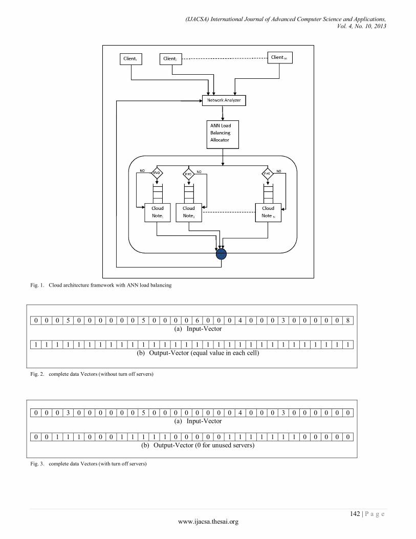
(IJACSA) International Journal of Advanced Computer Science and Applications, Vol. 4, No. 10, 2013
142 | P a g e www.ijacsa.thesai.org
Fig. 1. Cloud architecture framework with ANN load balancing
0 0 0 5 0 0 0 0 0 0 5 0 0 0 0 6 0 0 0 4 0 0 0 3 0 0 0 0 0 8
(a) Input-Vector
1 1 1 1 1 1 1 1 1 1 1 1 1 1 1 1 1 1 1 1 1 1 1 1 1 1 1 1 1 1
(b) Output-Vector (equal value in each cell)
Fig. 2. complete data Vectors (without turn off servers)
0 0 0 3 0 0 0 0 0 0 5 0 0 0 0 0 0 0 0 4 0 0 0 3 0 0 0 0 0 0
(a) Input-Vector
0 0 1 1 1 0 0 0 1 1 1 1 1 0 0 0 0 0 1 1 1 1 1 1 1 0 0 0 0 0
(b) Output-Vector (0 for unused servers)
Fig. 3. complete data Vectors (with turn off servers)
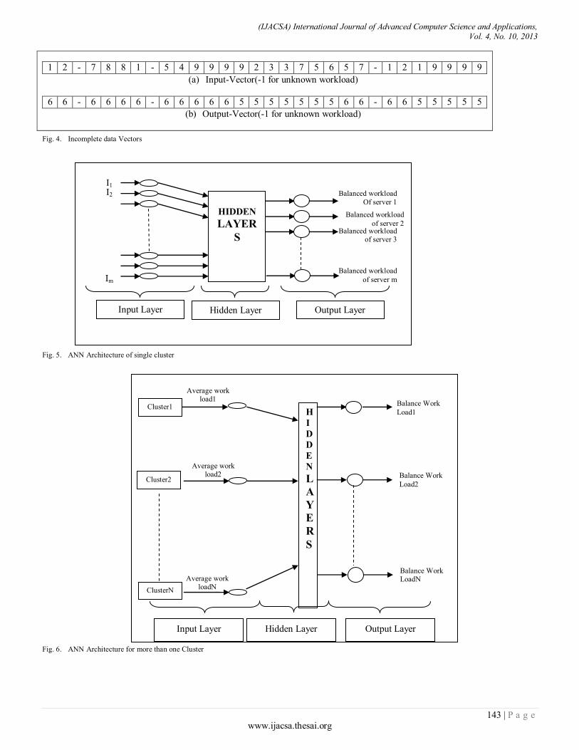
(IJACSA) International Journal of Advanced Computer Science and Applications, Vol. 4, No. 10, 2013
143 | P a g e www.ijacsa.thesai.org
1 2 - 7 8 8 1 - 5 4 9 9 9 9 2 3 3 7 5 6 5 7 - 1 2 1 9 9 9 9
(a) Input-Vector(-1 for unknown workload)
6 6 - 6 6 6 6 - 6 6 6 6 6 5 5 5 5 5 5 5 6 6 - 6 6 5 5 5 5 5
(b) Output-Vector(-1 for unknown workload)
Fig. 4. Incomplete data Vectors
Fig. 5. ANN Architecture of single cluster
Fig. 6. ANN Architecture for more than one Cluster
HIDDEN
LAYER
S
Balanced workload
Of server 1
Input Layer Hidden Layer Output Layer
I1 I2
Im
Balanced workload
of server 2 Balanced workload
of server 3
Balanced workload
of server m
H
I
D
D
E
N
L
A
Y
E
R
S
Input Layer Hidden Layer Output Layer
Cluster2
Average work load1
Average work load2
Average work loadN
Cluster1
ClusterN
Balance Work
Load1
Balance Work
Load2
Balance Work LoadN
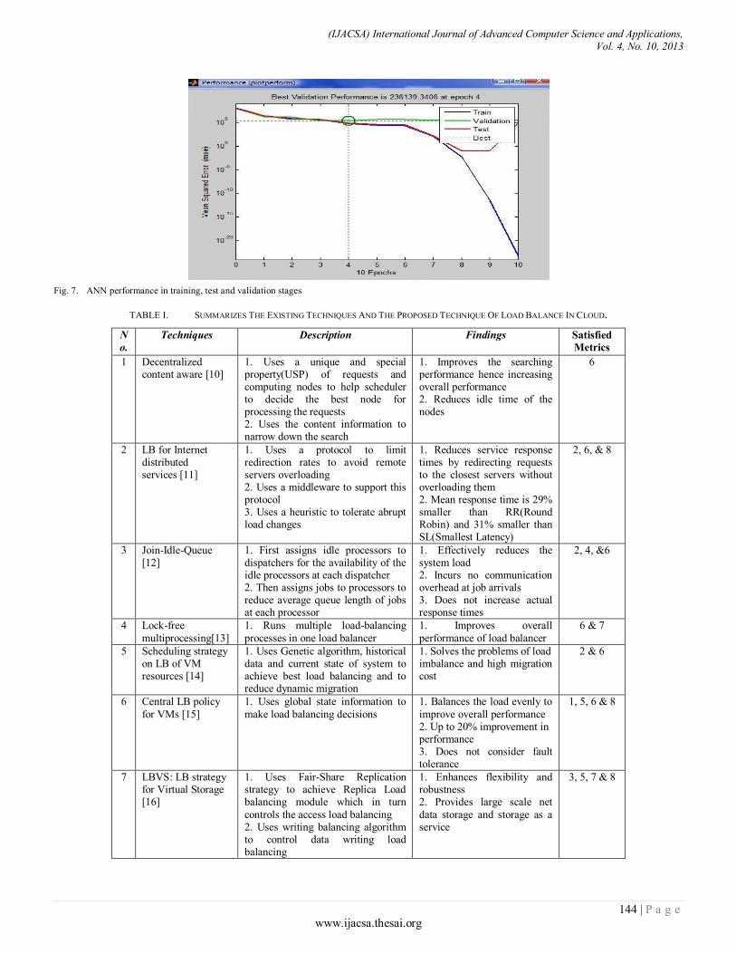
(IJACSA) International Journal of Advanced Computer Science and Applications, Vol. 4, No. 10, 2013
144 | P a g e www.ijacsa.thesai.org
Fig. 7. ANN performance in training, test and validation stages
TABLE I. SUMMARIZES THE EXISTING TECHNIQUES AND THE PROPOSED TECHNIQUE OF LOAD BALANCE IN CLOUD.
N
o.
Techniques Description Findings Satisfied
Metrics
1 Decentralized content aware [10]
1. Uses a unique and special property(USP) of requests and computing nodes to help scheduler to decide the best node for processing the requests 2. Uses the content information to narrow down the search
1. Improves the searching performance hence increasing overall performance 2. Reduces idle time of the nodes
6
2 LB for Internet distributed services [11]
1. Uses a protocol to limit redirection rates to avoid remote servers overloading 2. Uses a middleware to support this protocol 3. Uses a heuristic to tolerate abrupt load changes
1. Reduces service response times by redirecting requests to the closest servers without overloading them 2. Mean response time is 29% smaller than RR(Round Robin) and 31% smaller than SL(Smallest Latency)
2, 6, & 8
3 Join-Idle-Queue [12]
1. First assigns idle processors to dispatchers for the availability of the idle processors at each dispatcher 2. Then assigns jobs to processors to reduce average queue length of jobs at each processor
1. Effectively reduces the system load 2. Incurs no communication overhead at job arrivals 3. Does not increase actual response times
2, 4, &6
4 Lock-free
multiprocessing[13]
1. Runs multiple load-balancing
processes in one load balancer
1. Improves overall
performance of load balancer
6 & 7
5 Scheduling strategy on LB of VM resources [14]
1. Uses Genetic algorithm, historical data and current state of system to achieve best load balancing and to reduce dynamic migration
1. Solves the problems of load imbalance and high migration cost
2 & 6
6 Central LB policy
for VMs [15]
1. Uses global state information to
make load balancing decisions
1. Balances the load evenly to
improve overall performance 2. Up to 20% improvement in performance 3. Does not consider fault tolerance
1, 5, 6 & 8
7 LBVS: LB strategy for Virtual Storage [16]
1. Uses Fair-Share Replication strategy to achieve Replica Load balancing module which in turn
controls the access load balancing 2. Uses writing balancing algorithm to control data writing load balancing
1. Enhances flexibility and robustness 2. Provides large scale net
data storage and storage as a service
3, 5, 7 & 8

(IJACSA) International Journal of Advanced Computer Science and Applications, Vol. 4, No. 10, 2013
145 | P a g e www.ijacsa.thesai.org
8 Task Scheduling Based on LB [17]
1. First maps tasks to virtual machines and then virtual machines to host resources
1. Improves task response time 2. Improves resource utilization
5, 6 & 8
9 Honeybee Foraging Behavior [18]
1. Achieves global load balancing through local serve actions
1. Performs well as system diversity increases 2. Does not increase throughput as system size increases
1, 7 &8
10 Biased Random Sampling [18]
1. Achieves load balancing across all system nodes using random
sampling of the system domain
1. Performs better with high and similar population of
resources 2. Degrades as population diversity increases
1, 7 & 8
11 Active Clustering [18]
1. Optimizes job assignment by connecting similar services by local re-wiring
1. Performs better with high resources 2. Utilizes the increased system resources to increase
throughput 3. Degrades as system diversity increases
1, 7 & 8
12 ACCLB (Ant Colony and Complex Network Theory) [19][20]
1. Uses small-world and scale-free characteristics of complex network to achieve better load balancing
1. Overcomes heterogeneity 2. Adaptive to dynamic environments 3. Excellent in fault tolerance 4. Good scalability
3, 6, 7 & 8
13 Two-phase scheduling(OLB + LBMM) [21]
1. Uses OLB (Opportunistic Load Balancing) to keep each node busy and uses LBMM(Load Balance Min-Min) to achieve the minimum execution time of each task
1. Efficient utilization of resources 2. Enhances work efficiency
6 & 8
14 Event-driven [22] 1. Uses complete capacity event as input, analyzes its components and
generates the game session load balancing actions
1. Capable of scaling up and down a game session on
multiple resources according to the variable user load 2. Occasional QoS breaches as low as 0.66%
2, 5, 6, 7 & 8
15 Carton(LB + DRL) [23]
1. Uses Load Balancing to minimize the associated cost and uses Distributed Rate Limiting for fair
allocation of resources
1. Simple 2. Easy to implement 3.Very low computation and
communication overhead
5, 7 & 8
16 Compare and Balance [24]
1. Based on sampling 2. Uses adaptive live migration of virtual machines
1. Balances load amongst servers 2. Reaches equilibrium fast 3. Assures migration of VMs from high-cost physical hosts to low-cost host 4. Assumption of having
enough memory with each physical host
2, 5 & 8
17 VectorDot [25] 1. Uses dot product to distinguish node based on the item requirement
1. Handles hierarchical and multidimensional resource constraints 2. Removes overloads on server, switch and storage
1 & 8
18 The proposed ANN techniq
1. Use ANN to distribute the dynamic workload across multiple nodes to ensure that no single node is overwhelmed. Bp supervised neural networks are used
1. Optimal Balances load amongst servers.
.2. Adaptive to dynamic environments 3. Excellent in fault tolerance
4. Good scalability 5. unused server are turned off
3, 6, 7, 8, 9 & 10

(IJACSA) International Journal of Advanced Computer Science and Applications, Vol. 4, No. 10, 2013
146 | P a g e www.ijacsa.thesai.org
Acceptance of Web 2.0 in learning in higher
education: a case study Nigeria
Razep Echeng
School of Computing
University of the West of Scotland
Paisley, United Kingdom
Abel Usoro
School of Computing
University of the West of Scotland
Paisley, United Kingdom
Grzegorz Majewski
Faculty of Information Studies
Novo Mesto
Slovania
Abstracts—Technology acceptance has been studied in
different perspectives. Though a few empirical studies on
acceptance of Web 2.0 as a social networking tool in teaching and
learning exist, none of such studies exist in Nigeria which is the
focus of this study. This paper reports on a pilot study that
begins to fill this gap by investigating the perceptions, attitude
and acceptance of Web 2.0 in e-learning of this country. Based
on literature review and initial primary study, a conceptual
model of 9 variables and associated hypotheses was designed.
The model was operationalised into a questionnaire that was used
to collect data from 317 students from 5 universities. The
findings that came from data analysis indicate that all the
variables except motivation via learning management systems
which are not presently used in these universities affect intention
to use Web 2.0 in e-learning in Nigeria. Some of the validated
variables are perceived usefulness and prior knowledge. The
major conclusions and recommendations include the utilisation of
Web 2.0 facilities to stimulate participation in learning. This
work will contribute to the body of knowledge on acceptance of
Web 2.0 social networking tools in teaching and learning. It will
aid management decisions toward investing better on technology
so as to improve the educational sector. This research will also be
beneficial in the social development of individuals, local communities, national and international communities.
Keywords—Web 2.0; collaboration; active participation;
enhanced learning; Web 2.0 acceptance; learning; higher
education; technology based learning
I. BACKGROUND
The usefulness of Web 2.0 tools has been empirically studied by few researchers. For example, Xie et al. [1] studied blogs, Parker et al. [2] researched Twitter, Ajjan and Hortshorn [3] researched acceptance, and McKinney et al. [4] studied podcast. Research on the impacts of Web 2.0 tools in higher education is increasing by the day in developed and developing countries [5] [6] [7] [8] [9]. Few studies are beginning to emerge in developing countries on the use of Web 2.0 in higher institution, for example Anunobi & Ogbonna [10].
Web 2.0 provides social networks as a student support feature [11] [12] [13]. It enables the sharing of learning experiences, exchanging of information about the subjects being taught and assessment requirements, and provision of moral support. Web 2.0 technologies provide opportunities for students to construct and share knowledge with each other. Jucevičienė and Valinevičienė [13] concluded in their studies that there are four main factors that determine the adoption of
social network usage in higher education: academic service support; student support; social and cooperate learning; and achievement representation. This paper tests three models of acceptance and discusses the acceptance of Web 2.0 technologies in learning. The rest of this paper will present the need for Web 2.0 technologies in education, theoretical framework, method, findings and discussion, and summary and future work.
II. LITERATURE REVIEW
A. The Need for Web 2.0 technologies in education
In order to achieve a better learner centred approach, there is need for education and training institutions to adopt the 21st-century technologies that improve learner engagement among other benefits. Web 2.0 is such a technology and it provides very effective web-based collaborative systems. Being a relatively young technology, a number of issues are yet to be resolved. One of these is its acceptance and use in teaching and learning [6]. However, several studies, for example, Redecker [7] [14], have shown that Web 2.0 social computing tools and application in education and training enhances participatory learning, collaboration, knowledge and information sharing. Also research findings from Xia and Sharma [1] show that students’ thinking levels were increased as the students updated their blogs weekly. It also offers effective strategies for implementing what has been learnt by exploring other media.
Nevertheless, despite the opportunities offered by Web 2.0 technologies in learning, adoption is low [10] [15]. This research investigates this low adoption in Nigerian learning environment using an adapted technology acceptance model. The empirical work using this model examines attitudes and perceptions of users in order to predict their acceptance of Web 2.0 technologies for learning.
B. Theoretical framework
This research used, as underpinning theories, the technology acceptance model (TAM) and the unified theory of the use and acceptance of technology (UTAUT). The TAM theory which origin is from theory of reasoned action (TRA) [16] states that users’ behavioural intentions determine their acceptance of technology and their behaviour in turn influences their attitude [17]. Two variables, perceived ease of use and perceive usefulness, are the fundamental determinants of acceptance of technology [17]. TAM has been tested and validated in business settings with few validations in
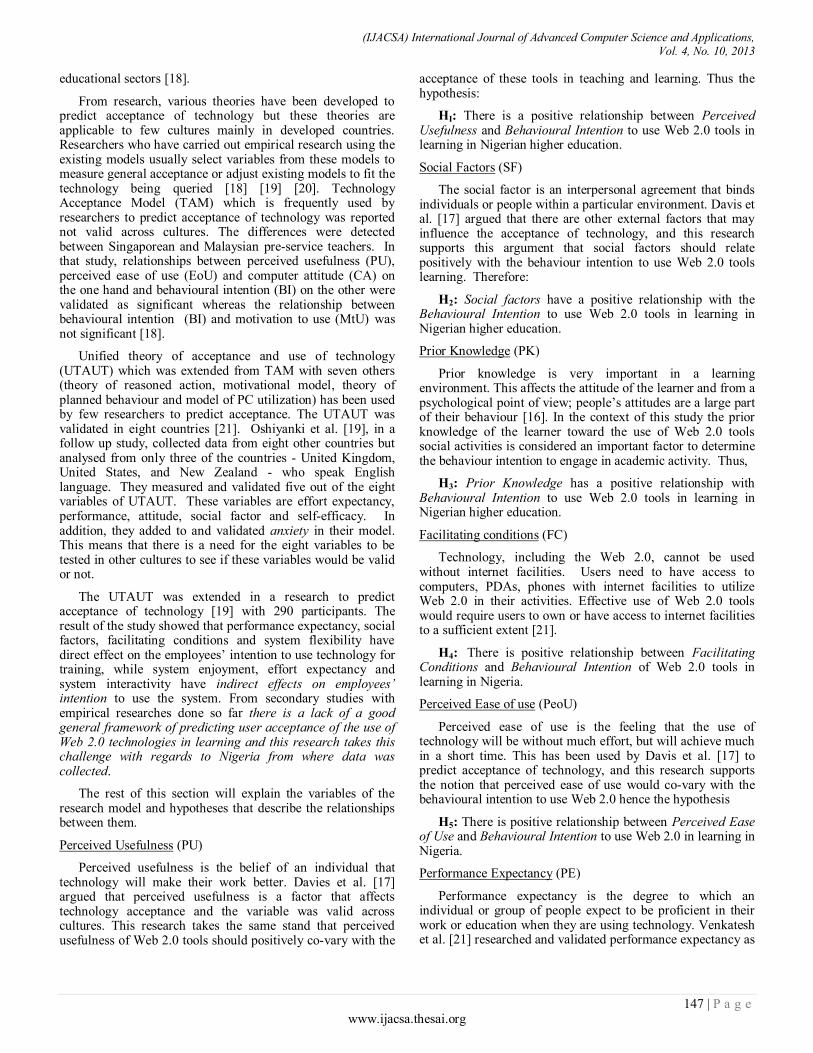
(IJACSA) International Journal of Advanced Computer Science and Applications, Vol. 4, No. 10, 2013
147 | P a g e www.ijacsa.thesai.org
educational sectors [18].
From research, various theories have been developed to predict acceptance of technology but these theories are applicable to few cultures mainly in developed countries. Researchers who have carried out empirical research using the existing models usually select variables from these models to measure general acceptance or adjust existing models to fit the technology being queried [18] [19] [20]. Technology Acceptance Model (TAM) which is frequently used by researchers to predict acceptance of technology was reported not valid across cultures. The differences were detected between Singaporean and Malaysian pre-service teachers. In that study, relationships between perceived usefulness (PU), perceived ease of use (EoU) and computer attitude (CA) on the one hand and behavioural intention (BI) on the other were validated as significant whereas the relationship between behavioural intention (BI) and motivation to use (MtU) was not significant [18].
Unified theory of acceptance and use of technology (UTAUT) which was extended from TAM with seven others (theory of reasoned action, motivational model, theory of planned behaviour and model of PC utilization) has been used by few researchers to predict acceptance. The UTAUT was validated in eight countries [21]. Oshiyanki et al. [19], in a follow up study, collected data from eight other countries but analysed from only three of the countries - United Kingdom, United States, and New Zealand - who speak English language. They measured and validated five out of the eight variables of UTAUT. These variables are effort expectancy, performance, attitude, social factor and self-efficacy. In addition, they added to and validated anxiety in their model. This means that there is a need for the eight variables to be tested in other cultures to see if these variables would be valid or not.
The UTAUT was extended in a research to predict acceptance of technology [19] with 290 participants. The result of the study showed that performance expectancy, social factors, facilitating conditions and system flexibility have direct effect on the employees’ intention to use technology for training, while system enjoyment, effort expectancy and system interactivity have indirect effects on employees’ intention to use the system. From secondary studies with empirical researches done so far there is a lack of a good general framework of predicting user acceptance of the use of Web 2.0 technologies in learning and this research takes this challenge with regards to Nigeria from where data was collected.
The rest of this section will explain the variables of the research model and hypotheses that describe the relationships between them.
Perceived Usefulness (PU)
Perceived usefulness is the belief of an individual that technology will make their work better. Davies et al. [17] argued that perceived usefulness is a factor that affects technology acceptance and the variable was valid across cultures. This research takes the same stand that perceived usefulness of Web 2.0 tools should positively co-vary with the
acceptance of these tools in teaching and learning. Thus the hypothesis:
HI: There is a positive relationship between Perceived Usefulness and Behavioural Intention to use Web 2.0 tools in learning in Nigerian higher education.
Social Factors (SF)
The social factor is an interpersonal agreement that binds individuals or people within a particular environment. Davis et al. [17] argued that there are other external factors that may influence the acceptance of technology, and this research supports this argument that social factors should relate positively with the behaviour intention to use Web 2.0 tools learning. Therefore:
H2: Social factors have a positive relationship with the Behavioural Intention to use Web 2.0 tools in learning in Nigerian higher education.
Prior Knowledge (PK)
Prior knowledge is very important in a learning environment. This affects the attitude of the learner and from a psychological point of view; people’s attitudes are a large part of their behaviour [16]. In the context of this study the prior knowledge of the learner toward the use of Web 2.0 tools social activities is considered an important factor to determine the behaviour intention to engage in academic activity. Thus,
H3: Prior Knowledge has a positive relationship with Behavioural Intention to use Web 2.0 tools in learning in Nigerian higher education.
Facilitating conditions (FC)
Technology, including the Web 2.0, cannot be used without internet facilities. Users need to have access to computers, PDAs, phones with internet facilities to utilize Web 2.0 in their activities. Effective use of Web 2.0 tools would require users to own or have access to internet facilities to a sufficient extent [21].
H4: There is positive relationship between Facilitating Conditions and Behavioural Intention of Web 2.0 tools in learning in Nigeria.
Perceived Ease of use (PeoU)
Perceived ease of use is the feeling that the use of technology will be without much effort, but will achieve much in a short time. This has been used by Davis et al. [17] to predict acceptance of technology, and this research supports the notion that perceived ease of use would co-vary with the behavioural intention to use Web 2.0 hence the hypothesis
H5: There is positive relationship between Perceived Ease of Use and Behavioural Intention to use Web 2.0 in learning in Nigeria.
Performance Expectancy (PE)
Performance expectancy is the degree to which an individual or group of people expect to be proficient in their work or education when they are using technology. Venkatesh et al. [21] researched and validated performance expectancy as
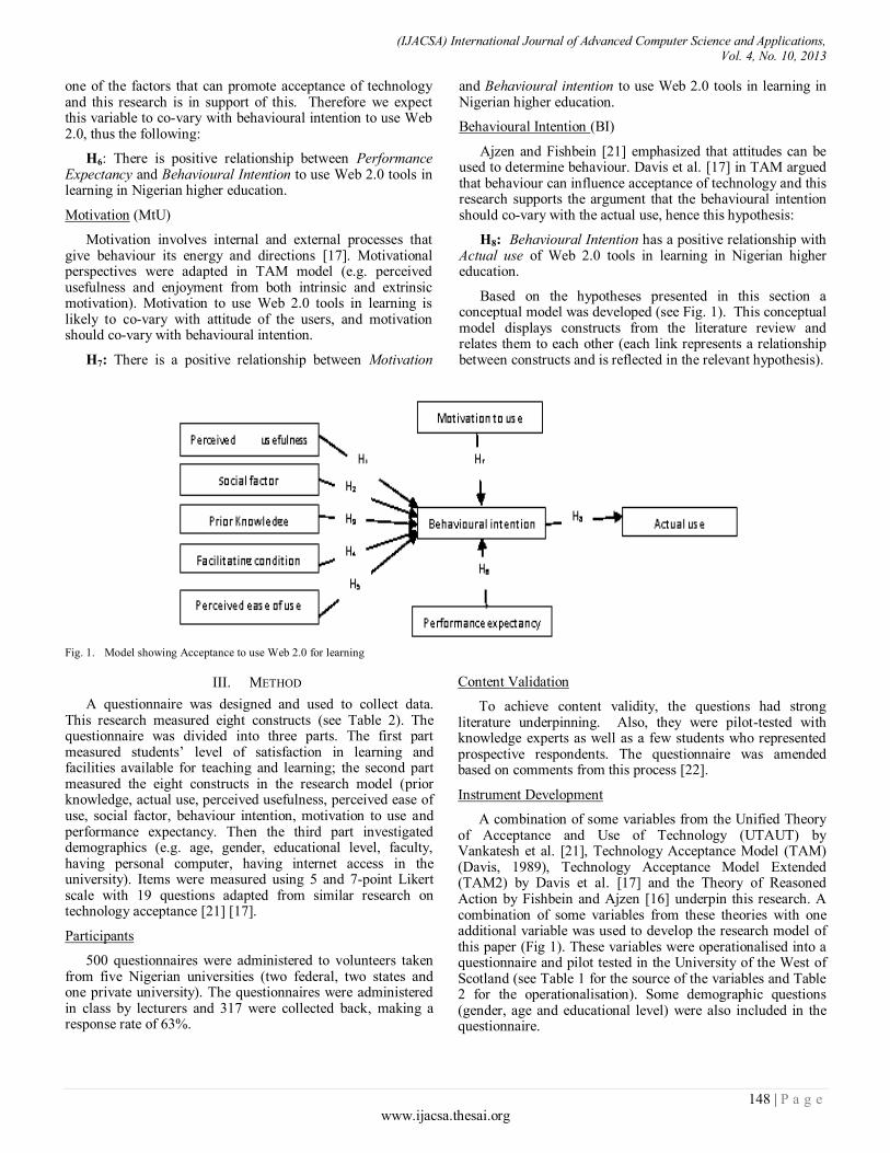
(IJACSA) International Journal of Advanced Computer Science and Applications, Vol. 4, No. 10, 2013
148 | P a g e www.ijacsa.thesai.org
one of the factors that can promote acceptance of technology and this research is in support of this. Therefore we expect this variable to co-vary with behavioural intention to use Web 2.0, thus the following:
H6: There is positive relationship between Performance Expectancy and Behavioural Intention to use Web 2.0 tools in learning in Nigerian higher education.
Motivation (MtU)
Motivation involves internal and external processes that give behaviour its energy and directions [17]. Motivational perspectives were adapted in TAM model (e.g. perceived usefulness and enjoyment from both intrinsic and extrinsic motivation). Motivation to use Web 2.0 tools in learning is likely to co-vary with attitude of the users, and motivation should co-vary with behavioural intention.
H7: There is a positive relationship between Motivation
and Behavioural intention to use Web 2.0 tools in learning in Nigerian higher education.
Behavioural Intention (BI)
Ajzen and Fishbein [21] emphasized that attitudes can be used to determine behaviour. Davis et al. [17] in TAM argued that behaviour can influence acceptance of technology and this research supports the argument that the behavioural intention should co-vary with the actual use, hence this hypothesis:
H8: Behavioural Intention has a positive relationship with Actual use of Web 2.0 tools in learning in Nigerian higher education.
Based on the hypotheses presented in this section a conceptual model was developed (see Fig. 1). This conceptual model displays constructs from the literature review and relates them to each other (each link represents a relationship between constructs and is reflected in the relevant hypothesis).
Fig. 1. Model showing Acceptance to use Web 2.0 for learning
III. METHOD
A questionnaire was designed and used to collect data. This research measured eight constructs (see Table 2). The questionnaire was divided into three parts. The first part measured students’ level of satisfaction in learning and facilities available for teaching and learning; the second part measured the eight constructs in the research model (prior knowledge, actual use, perceived usefulness, perceived ease of use, social factor, behaviour intention, motivation to use and performance expectancy. Then the third part investigated demographics (e.g. age, gender, educational level, faculty, having personal computer, having internet access in the university). Items were measured using 5 and 7-point Likert scale with 19 questions adapted from similar research on technology acceptance [21] [17].
Participants
500 questionnaires were administered to volunteers taken from five Nigerian universities (two federal, two states and one private university). The questionnaires were administered in class by lecturers and 317 were collected back, making a response rate of 63%.
Content Validation
To achieve content validity, the questions had strong literature underpinning. Also, they were pilot-tested with knowledge experts as well as a few students who represented prospective respondents. The questionnaire was amended based on comments from this process [22].
Instrument Development
A combination of some variables from the Unified Theory of Acceptance and Use of Technology (UTAUT) by Vankatesh et al. [21], Technology Acceptance Model (TAM) (Davis, 1989), Technology Acceptance Model Extended (TAM2) by Davis et al. [17] and the Theory of Reasoned Action by Fishbein and Ajzen [16] underpin this research. A combination of some variables from these theories with one additional variable was used to develop the research model of this paper (Fig 1). These variables were operationalised into a questionnaire and pilot tested in the University of the West of Scotland (see Table 1 for the source of the variables and Table 2 for the operationalisation). Some demographic questions (gender, age and educational level) were also included in the questionnaire.

(IJACSA) International Journal of Advanced Computer Science and Applications, Vol. 4, No. 10, 2013
149 | P a g e www.ijacsa.thesai.org
TABLE I. VARIABLES AND SOURCE
Variables Source
Prior knowledge (PK) Mine (new)
Social factors (SF) TAM, UTAUT
Perceived usefulness (PU) TAM
Performance expectancy (PE) UTAUT
Motivation MtU TRA
Perceived Ease of use (PEoU) TAM
Facilitating conditions (FC) UTAUT
Actual use (AU) TAM UTAUT
Behavior intention (BI) TAM UTAUT
TABLE II. OPERATIONALISATION
Constructs Questions Items
EoU How easy do you find using these Web 2.0 tools listed below to obtain the resources you need for your studies?
7
AtU How many times do you use Web 2.0 tools listed above for academic purposes per week? 5
MtU To what extent do you agree that social part of e-learning platforms (e.g. Module and Blackboard) motivate learner to a great extend to achieve learning objectives?
8
E-learning platforms enable you to send mails, download course materials upload assignments, read announcements, access the library material and discuss with other students, professionals and your lecturers. To what extent do you think such system would motivate you to achieve your learning objectives?
10
FC
Regarding facilities available for learning and teaching in the university, how satisfied are you? Add any necessary comments regarding technology and facilities available in your university
4
Do you own personal computers or phone with internet connection
PU To what extent do you agree that Web 2.0 tools would speed up acquisition of knowledge? 11
BI To what extent do you agree that social computing should be adopted in education and training for sharing of knowledge and information?
9
SF To what extent do you agree that Web 2.0 tools will encourage active participation? 11
AtU How many times do you use Web 2.0 per week? 6
PE To what extent do you agree that the use of Web 2.0 technology in education will help improve performance
14
Demographics Status Are you a student or lecturer? Gender Gender What is your gender?
Status
Field Field What is your field?
Age bracket
What is your gender?
Are you a student or lecturer?
What is your field?
What is your age bracket? Status Are you a student or lecturer? Field What is your field? Age bracket What is your age bracket?
16
1
19
17
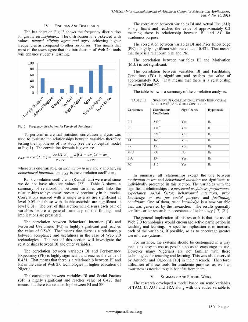
(IJACSA) International Journal of Advanced Computer Science and Applications, Vol. 4, No. 10, 2013
150 | P a g e www.ijacsa.thesai.org
IV. FINDINGS AND DISCUSSION
The bar chart on Fig. 2 shows the frequency distribution for perceived usefulness. The distribution is left-skewed with values: neutral, slightly agree and agree achieving higher frequencies as compared to other responses. This means that most of the users agree that the introduction of Web 2.0 tools will enhance students’ learning.
Fig. 2. Frequency distribution for Perceived Usefulness
To perform inferential statistics, correlation analysis was used to evaluate the relationships between variables therefore testing the hypotheses of this study (see the conceptual model at Fig. 1). The correlation formula is given as:
where x is one variable, eg motivation to use and y another, eg behavioural intention; and ρX,Y is the correlation coefficient.
Rank correlation coefficients (Kendall tau) were used since we do not have absolute values [22]. Table 3 shows a summary of relationships between variables and links the relationships to hypotheses presented previously in the model. Correlations marked with a single asterisk are significant at level 0.05 and those with double asterisks are significant at level 0.01. The rest of this section will discuss each pair of variables before a general summary of the findings and implications are presented.
The correlation between Behavioral Intention (BI) and Perceived Usefulness (PU) is highly significant and reaches the value of 0.549. That means that there is a relationship between acceptance and usefulness in the case of Web 2.0 technologies. The rest of this section will investigate the relationships between BI and other variables.
The correlation between variables BI and Performance Expectancy (PE) is highly significant and reaches the value of 0.431. That means that there is a relationship between BI and PE in the case of Web 2.0 technologies in higher education of Nigeria.
The correlation between variables BI and Social Factors (SF) is highly significant and reaches value of 0.423 that means that there is a relationship between BI and SF.
The correlation between variables BI and Actual Use (AU) is significant and reaches the value of approximately 0.2 meaning there is relationship between BI and AC for academics purpose.
The correlation between variables BI and Prior Knowledge (PK) is highly significant with the value of 0.431. That means that there is a relationship BI and PK.
The correlation between variables BI and Motivation (MtU) is not significant.
The correlation between variables BI and Facilitating Conditions (FC) is significant and reaches the value of approximately 0.3. That means that there is a relationship between BI and FC.
The table below is a summary of the correlation analyses.
TABLE III. SUMMARY OF CORRELATIONS BETWEEN BEHAVIOURAL
INTENTION (BI) AND OTHER CONSTRUCTS
Constructs Correlations
Coefficients Significance
Hypothesis
PU .549**
Yes H1
PE .431**
Yes H2
SF .520**
Yes H3
AU .169* Yes H4
PK .153* Yes H5
MtU .932 No H6
EoU .134* Yes H7
FC .115* Yes H8
In summary, all relationships except the one between motivation to use and behavioural intention are significant as individually presented in this section. The variables with the significant relationships are perceived usefulness, performance expectancy, social factor, behavioural intentions, prior knowledge or use for social purpose and facilitating conditions. One of them, prior knowledge is a new variable that was generated by the researcher. The results generally confirm earlier research in acceptance of technology [17] [21].
The general implication of this research is that the use of Web 2.0 technologies would encourage active participation in teaching and learning. A specific implication is to increase each of the variables, if possible, so as to encourage greater use of these systems.
For instance, the systems should be customised in a way that is as easy to use as possible so as to encourage its use. However many Nigerians are not familiar with these technologies for teaching and learning. This was also observed by Anunobi and Ogbonna [10] in their research. Therefore, utilisation of these tools for academic purposes as well as awareness is needed to gain benefits from them.
V. SUMMARY AND FUTURE WORK
The research developed a model based on some variables of TAM, UTAUT and TRA along with one added variable to
0
20
40
60
80
100

(IJACSA) International Journal of Advanced Computer Science and Applications, Vol. 4, No. 10, 2013
151 | P a g e www.ijacsa.thesai.org
examine the intention to adopt Web 2.0 in learning in Nigerian higher education. The results showed seven out of eight variables to significantly co-relate with behavioural intention. These variables include perceived usefulness, performance expectancy, social factor, and prior knowledge. The implications of the study include the need to make the tools available in the first place in Nigerian higher education; and to deploy them in an easy-to-use way so as contribute to learning and teaching in this environment.
As has been noted, motivation did not exhibit a significant influence on intention likely because the students were not using the any learning management systems (moodle or blackboard) whereas the question on motivation was emphasizing the use of Moodle or Blackboard platform enhancing learning activities. However previous research in United Kingdom [24] was significant probably because the students are familiar with Moodle. Therefore this variable will be tested again in the future after the students are exposed to LMS. A setting up of a LMS will also enable experiments that will engage the students and teachers in Web 2.0 technologies. Such experiments will produce useful qualitative data that will richly complement this quantitative study.
REFERENCE
[1] Y. Xie and P. Shama, “The effect of peer-interaction styles in team
blogging on students’ cognitive thinking and blog participation”, Journal of Educational Computing, vol. 42 no. 4, pp. 459-479, 2010.
[2] K. R. Parker and J. T. Chao, “Wiki as a Teaching Tool,
Interdisciplinary” Journal of knowledge and learning Objects, vol. 3, pp. 57-72, 2007.
[3] H. Ajjan and R Hartshorne, “Investigating faculty decisions to adopt
Web 2.0 technologies: Theory and empirical tests”, The Internet and Higher Education, vol. 11, no 2, pp. 71–80, 2008.
[4] D. McKinney, J. Dych, and E. Luber, “I-tunes University and the
Classroom: Can Podcasts replace Professor?” Computer & education journal, vol. 52, pp. 617-623, 2009.
[5] B. Alexander, “Web 2.0: A new wave of innovation for teaching and learning?” EDUCAUSE Review, vol. 41, no. 2, pp. 32-44, 2006.
[6] T. Franklin and M. Van Harmelen, Web 2.0 for content for learning and
teaching in higher education, London: Joint Information Systems Committee, 2007.
[7] C. Redecker, “Review of Learning 2.0 practices”, Study on the Impact of
Web 2.0 Innovations on Education and Training in Europe, 2009 Available online https://europa.eu/Publications/pub.cfm?id=2059
[Accessed: 25-11-2011].
[8] N. Vlahovic, “Web 2.0 and its Impact on Information Extraction Practices”, Proceedings of the International Conference on Applied
Computer Science, 2010.
[9] R. Echeng, The use of Web 2.0 in teaching and learning in Nigerian
higher institution, An MSc Thesis submitted to the School of Computing, University of the West of Scotland, 2011.
[10] C. Anunobi and A. Ogbonna, “Web 2.0 use by Librarians in a state in Nigeria”, Developing Country Studies, vol. 2, no. 5, pp. 7-66, 2012.
[11] N. Selwyn, “Faceworking: exploring students’ education–related use of
Facebook”, Learning, Media & Technology – Routledge, no. 2, vol. 34, pp. 157–174, 2009.
[12] C. Madge, J. Meek, J. Wellens and T. Hooley, “Facebook, social
integration and informal learning at university”, Learning, Media, & Technology – Routledge, vol. 2, issue 34, pp. 141–155, 2004.
[13] P. Jucevičienė, G. Valinevičienė, “A Conceptual Model of Social
Networking in Higher Education”, Electronics and Electrical Engineering – Kaunas: Technologija, vol. 6, no. 102, pp. 55–58, 2010.
[14] M. McLoughlin and J. Lee, "Social software and participatory learning:
Pedagogical choices with technology affordances in the Web 2.0 era", In the 8
th conference proceedings of Ascilite (2007).
[15] G. Olasina, "The use of Web 2.0 tools and social networking sites by
librarians, information professionals, and other professionals in workplaces in Nigeria" PNLA Quarterly, the official publication of the
Pacific Northwest Library Association, vol.75 no.3, pp.72-33, 2011.
[16] I. Ajzen and M. Fishbein, Understanding attitudes and predicting social
behavior, Englewood Cliff, NJ: Prentice Hall, 1980.
[17] F. Davis, R. Bagozzi, and P. Warshaw, "User acceptance of computer technology: a comparison of two theoretical models", Management
Science, vol. 35, pp. 982-2003, 1989.
[18] T. Teo, W. Su Luan, and C. Sing, "A cross-cultural examination of the intention to use technology between Singaporean and Malaysian pre-
service teachers: an application of the Technology Acceptance Model (TAM)", Educational Technology & Society, vol. 11, no. 4, 265–280,
2008.
[19] L. Oshiyanki, P. Cairns, P and H. Thimbleby, "Validating Unified theory of acceptance and use of Technology (UTAUT) tool cross- culturally",
British computer society Volume 2 proceeding of the 21st century BCS
group conference, 2007.
[20] A. Thamer, M. Alrawashdeh, Muhairat and S. Alqatawnah, Factors
affecting acceptance of web-based training system: using extended UTAUT and structural equation modeling, 2010.
[21] V. Venkatesh, M. Morris, G. Davis and F. Davis, “User acceptance of
information technology: Toward a unified view”, MIS Quarterly, vol. 27, no.3 pp. 425–478, 2003.
[22] G. Zikmund Business Research Methods, Mason, OH: Thomson/South Western, 2003.
[23] G. Yule and M. Kendall, An Introduction to the Theory of Statistics,
14th Edition (5th Impression 1968). Charles Griffin & Co., pp. 258–270, 1950.
[24] R. Echeng, A. Usoro and G. Majewski, "Acceptance of Web 2.0 in
Learning in higher education: an empirical study of a Scottish university", WBC July Conference Proceedings on E-learning, 2013.

(IJACSA) International Journal of Advanced Computer Science and Applications, Vol. 4, No. 10, 2013
152 | P a g e www.ijacsa.thesai.org
Mitigating Black Hole attack in MANET by
Extending Network Knowledge
Hicham Zougagh, Ahmed Toumanari, Rachid Latif
Laboratory ESSI,
National School of Applied sciences
Agadir, Morocco
Noureddine.Idboufker
Laboratory TIM
National School of Applied sciences
Marrakech, Morocco
Abstract—The Optimized Link State Routing Protocol is
developed for Mobile Ad Hoc Network. It operates as a table
driven, proactive protocol. The core of the OLSR protocol is the
selection of Multipoint Relays (MPRs), used as a flooding
mechanism for distributing control traffic messages in the
network, and reducing the redundancy in the flooding process. A
node in an OLSR network selects its MPR set so that all two hop
neighbor are reachable by the minimum number of MPR.
However, if an MPR misbehaves during the execution of the
protocol, the connectivity of the network is compromised. This
paper introduces a new algorithm for the selection of Multipoint
Relays (MPR) with additional coverage whose aims is to provide
each node to selects alternative paths to reach any destination
two hops away. This technique helps avoid the effect of malicious attacks and its easily to implement the corresponding algorithm.
Keywords—MANET; OLSR; Security; Routing Protocol; Black
Hole attack
I. INTRODUCTION
Today, mobile Ad-hoc networks (MANETs) are a major element of the business environment, allowing wireless devices such as cell phones, laptops, and PDAs to provide mobility to users and enable them to be in constant contact with others. Technically. Mobile Ad hoc Networks (MANET) are dynamic and self-organized networks that are able to operate without an dependability on fixed or pre-installed infrastructure, using only wireless devices that act both as hosts and routers, and thus cooperatively provide multi-hop communications [1]. Because of these characteristics, MANETs are much more vulnerable to several types of security attacks.
The communication in mobile ad hoc networks comprises two phases: the route discovery and the data transmission. In an adverse environment, both phases are vulnerable to a variety of attacks. First, rivals can disrupt the route discovery by impersonating the destination, and responding with stale or corrupted routing information, or by disseminating forged control traffic. This way, attackers can obstruct the propagation of legitimate route control traffic and adversely influence the topological knowledge of benign nodes.
However, adversaries can also disrupt the data transmission phase and, thus, cause significant data loss by fraudulently tampering, redirecting and dropping data or injecting forgets data packets. To provide comprehensive security, both phases of MANET communication must be safeguarded. It is noteworthy that secure routing protocols, which ensure the correctness of the discovered topology information cannot, by
themselves, ensure the secure and undisrupted delivery of transmitted data [2].
One way to secure a mobile ad hoc network at the network layer is to secure the routing protocols, in order to prevent possible attacks. In brief the task of the routing protocol is to discover the topology to ensure that each node is able to acquire a recent map of network topology so as to construct routes.
Routing in MANET can be classified into three categories: reactive protocol (e.g. AODV [3], DSR [4]), proactive protocol (e.g. optimized link state routing (OLSR) [5], TBRPF [6]), and hybrid protocol (e,g, ZRP [7]). Early works in MANET security research (e.g. ARAN [8], Aridane [9], SAODV [10,11], SEAD [12], [13–14]) have focused on providing preventive schemes to protect the routing protocol in MANET. Most of these schemes are based on key management or encryption techniques to prevent unauthorized nodes from joining the network.
However, these approaches cannot prevent attacks launched by a compromised node who owns a valid key. Therefore, intrusion detection and response system are required to counter the attack as a second line of protection. To design an effective and efficient intrusion detection and reaction system, in-depth understanding of how a compromised node can attack a MANET is indispensable.
The Optimized Link Stat Routing Protocol (OLSR) [5] is a proactive routing protocol for MANET, i.e. All nodes need to maintain a consistent view of the network topology. They are also vulnerable to a number of disruptive attacks in the presence of malicious nodes (identity spoofing, link withholding, link spoofing, miserly attack, wormhole attack and Black hole attack...). As a result, it is also necessary to provide security scheme for the OLSR protocol.
In this paper, we focus on the single black hole attack in which an intermediate node drops packets passing through it. The motivation of the dropper node is the preservation of its resources, such as its limited battery, while at the same time using the resources of others to deliver its data. In our approach, we present an improved MPR selection algorithm that can reduce the number of malicious nodes trying to be selected as Multipoint Relay by maintaining its Willingness fields equal to Will_always.
The rest of the paper is organized as follows. The next section provides a short overview on OLSR, followed by the

(IJACSA) International Journal of Advanced Computer Science and Applications, Vol. 4, No. 10, 2013
153 | P a g e www.ijacsa.thesai.org
description of Single black hole attack. Section IV summarizes the literature. In section V, we present our approach to secure OLSR protocol. In section VI we give an Illustration and an example. Section VII presents the result of simulations. Section VIII concludes the paper. In the end section XI present the futur work.
II. THE OLSR PROTOCOL
Optimized Link State Routing Protocol (OLSR) [5] is a routing protocol developed for mobile ad hoc networks (MANETs), it is a proactive routing protocol that employs an efficient link state packet forwarding a mechanism called Multipoint relaying. OLSR optimizes the pure link state routing protocol. Conceptually OLSR topology discovery involves tow phases: neighbor discovery and topology discovery. In the first phase, neighbor nodes are discovered by using Hello messages. The exchange of Hello messages in OLSR allows the selection of those MPR nodes. MPR nodes are responsible for broadcasting topology control (TC) message which would be flooded through the network in the second phase.
A. OLSR Control Traffic.
A node detects its one hop and two hop neighbors through link sensing which is accomplished though broadcasting periodic Hello messages containing neighbor link state (sym, asym, MPR or lost). Fig. 1 shows the basic information of a Hello message.
Originator Address
Link code Reserved Link message Size
Neighbor address
…...
Link Type Reserved Link message size
Neighbor address
…..
Fig. 1. OLSR Hello Message Format.
Originator Address
Advertized Neighbor sequence Number (ANSN)
Reserved
Advertized Neighbor (MPR Selector) address
.…….
Fig. 2. OLSR TC message Format
These messages are broadcast by all nodes heard only by immediate neighbors; they are never relayed any further. Upon the reception of Hello messages, other nodes can derive information concerning their one hop neighbor and two hop neighbors. They can also calculate a subset of one hop symmetric neighbor nodes as its MPR set. This MPR set is declared in its next Hello message broadcast. Furthermore, through receiving a Hello message, nodes can create or update their MPR selector set. That demonstrates nodes which have currently selected this node as their MPR.
A Topology Control (TC) message is periodically sent to the whole MANET by each MPR in the network to
respectively declare its MPR selector set. It is, then, used in the construction of routing tables in every MANET node. Fig. 2 shows the basic format of a TC message [5].
Thus, a TC message contains the list of neighbors that have selected the sender node as an MPR (MPR Selector Set), and an Advertized Neighbor Sequence Number (ANSN) is used by a receiving node to check if the information advertized in the TC messages is more recent.
Only MPR nodes are allowed to generate and forward TC messages. The information embedded in TC messages generated by an MPR includes at least the existing links between itself and its MPR selectors. The non-MPR nodes do receive TC messages from their MPRs and process them. However, non-MPR nodes do not forward the received TC messages. This feature of OLSR reduces the number of messages exchanged in topology discovery Fig 3.
B. Multi-Point Relays Selection.
Multi-Point Relays Selection is done in such a way that all the two-hop-neighbors are reachable from the MPR in terms of radio range. The two-hop-neighbor set found by the exchange of HELLO messages is used to calculate the MPR set and the nodes signal their MPRs selections through the same mechanism.
MPR calculation is based on willingness announced by neighbors using Hello messages. Willingness is one of the fields in a Hello message, which specifies the willingness of a node to carry and forward traffic on behalf of other nodes. According to the standard OLSR, willingness may be set to integer value between 0 and 7. The willingness value of WILL_NEVER (integer value of 0) means that a node does not wish to carry traffic to other nodes and it will not be included in the MPR set. The willingness value of WILL_ALWAYS (integer value of 7) means that a node is willing or has resources to forward traffic to other nodes. Therefore, for a given node. That all the neighbor nodes with willingness equal to WILL_ALWAYS will always be included in the set of MPRs [15].
The aim of Multi-Point Relays is to minimize the flooding of the network with broadcast packets by reducing duplicate retransmission in the same region. Each node of the network selects the smallest set (MPRs) of neighbor nodes that can reach all of its symmetric two hop neighbors which may forward its messages. The MPR selection algorithm proceeds in four steps:
Start with an MPR set made of all members of M with M_Willingness equal to Will_always.
A node M first selects as MPR the neighbors that have the one neighbor in the two hop node from M.
It then selects as MPR a neighbor that has the largest count of uncovered two-hop nodes. This step is repeated until all two-hop nodes are covered.
Finally, any MPR node N can be discarded since the MPR set covers all two hop neighbors without the MPR node N.
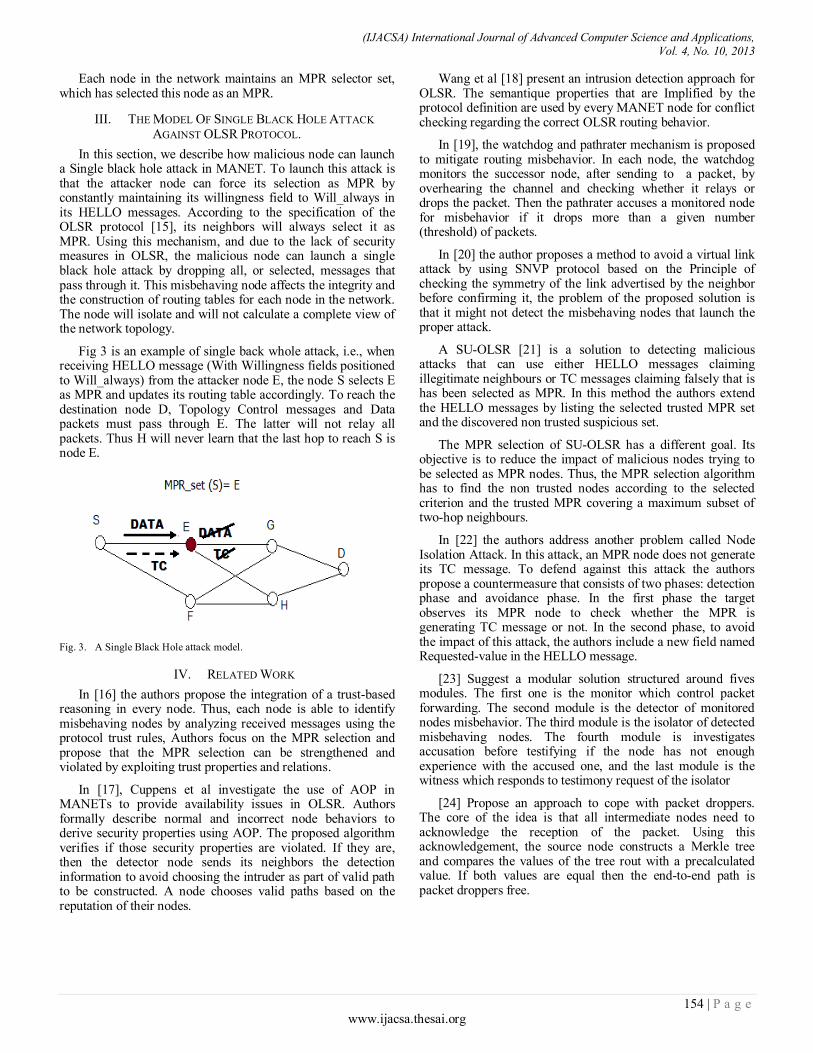
(IJACSA) International Journal of Advanced Computer Science and Applications, Vol. 4, No. 10, 2013
154 | P a g e www.ijacsa.thesai.org
Each node in the network maintains an MPR selector set, which has selected this node as an MPR.
III. THE MODEL OF SINGLE BLACK HOLE ATTACK
AGAINST OLSR PROTOCOL.
In this section, we describe how malicious node can launch a Single black hole attack in MANET. To launch this attack is that the attacker node can force its selection as MPR by constantly maintaining its willingness field to Will_always in its HELLO messages. According to the specification of the OLSR protocol [15], its neighbors will always select it as MPR. Using this mechanism, and due to the lack of security measures in OLSR, the malicious node can launch a single black hole attack by dropping all, or selected, messages that pass through it. This misbehaving node affects the integrity and the construction of routing tables for each node in the network. The node will isolate and will not calculate a complete view of the network topology.
Fig 3 is an example of single back whole attack, i.e., when receiving HELLO message (With Willingness fields positioned to Will_always) from the attacker node E, the node S selects E as MPR and updates its routing table accordingly. To reach the destination node D, Topology Control messages and Data packets must pass through E. The latter will not relay all packets. Thus H will never learn that the last hop to reach S is node E.
Fig. 3. A Single Black Hole attack model.
IV. RELATED WORK
In [16] the authors propose the integration of a trust-based reasoning in every node. Thus, each node is able to identify misbehaving nodes by analyzing received messages using the protocol trust rules, Authors focus on the MPR selection and propose that the MPR selection can be strengthened and violated by exploiting trust properties and relations.
In [17], Cuppens et al investigate the use of AOP in MANETs to provide availability issues in OLSR. Authors formally describe normal and incorrect node behaviors to derive security properties using AOP. The proposed algorithm verifies if those security properties are violated. If they are, then the detector node sends its neighbors the detection information to avoid choosing the intruder as part of valid path to be constructed. A node chooses valid paths based on the reputation of their nodes.
Wang et al [18] present an intrusion detection approach for OLSR. The semantique properties that are Implified by the protocol definition are used by every MANET node for conflict checking regarding the correct OLSR routing behavior.
In [19], the watchdog and pathrater mechanism is proposed to mitigate routing misbehavior. In each node, the watchdog monitors the successor node, after sending to a packet, by overhearing the channel and checking whether it relays or drops the packet. Then the pathrater accuses a monitored node for misbehavior if it drops more than a given number (threshold) of packets.
In [20] the author proposes a method to avoid a virtual link attack by using SNVP protocol based on the Principle of checking the symmetry of the link advertised by the neighbor before confirming it, the problem of the proposed solution is that it might not detect the misbehaving nodes that launch the proper attack.
A SU-OLSR [21] is a solution to detecting malicious attacks that can use either HELLO messages claiming illegitimate neighbours or TC messages claiming falsely that is has been selected as MPR. In this method the authors extend the HELLO messages by listing the selected trusted MPR set and the discovered non trusted suspicious set.
The MPR selection of SU-OLSR has a different goal. Its objective is to reduce the impact of malicious nodes trying to be selected as MPR nodes. Thus, the MPR selection algorithm has to find the non trusted nodes according to the selected criterion and the trusted MPR covering a maximum subset of two-hop neighbours.
In [22] the authors address another problem called Node Isolation Attack. In this attack, an MPR node does not generate its TC message. To defend against this attack the authors propose a countermeasure that consists of two phases: detection phase and avoidance phase. In the first phase the target observes its MPR node to check whether the MPR is generating TC message or not. In the second phase, to avoid the impact of this attack, the authors include a new field named Requested-value in the HELLO message.
[23] Suggest a modular solution structured around fives modules. The first one is the monitor which control packet forwarding. The second module is the detector of monitored nodes misbehavior. The third module is the isolator of detected misbehaving nodes. The fourth module is investigates accusation before testifying if the node has not enough experience with the accused one, and the last module is the witness which responds to testimony request of the isolator
[24] Propose an approach to cope with packet droppers. The core of the idea is that all intermediate nodes need to acknowledge the reception of the packet. Using this acknowledgement, the source node constructs a Merkle tree and compares the values of the tree rout with a precalculated value. If both values are equal then the end-to-end path is packet droppers free.

(IJACSA) International Journal of Advanced Computer Science and Applications, Vol. 4, No. 10, 2013
155 | P a g e www.ijacsa.thesai.org
V. THE PROPOSED SOLUTION
As previously mentioned, each node in the network has to select a set of one-hop neighbors MPR set, which is constructed by the smallest number of nodes that allow the MPR selector to cover every two-hop neighbor through, at least one of its MPRs.
To deal with a Single Black Hole attack, we propose an algorithm to select MPR with additional coverage without giving priority to nodes with higher willingness. The aim of this algorithm is to reduce the impact of malicious nodes trying to be selected as MPR nodes.
Our approach is a modified version of the RFC 3626 [1] MPR coverage parameter which allows increasing the number of nodes through which, the MPR selector can reach every two hop neighbor. For example, if MPR-Coverage is equal to K it means that, if possible every two-hop neighbor can be reached though at least K nodes (K=1, standard OLSR).
Before introducing this algorithm, some notations should be described first:
1HN_set(X): the set of node X’s one hop symmetric neighbors. It is created by the way of changing HELLO messages between nodes.
2HN_set(X): the set of node X’s two hop symmetric neighbors excluding any node in 1HN_set(X). It is also created by the way of changing HELLO messages.
MPR_set (E): the set of nodes selected as MPR by the node E. (MPR_set (E) ⊆ 1HN_set (E)).
MPRS_set (E): the set of symmetric neighbours which have selected the node E as MPR. (MPRS_set (E) ⊆ 1HN_set (E)).
Degree (X, Y): the degree of node X’s one hop neighbor; returns the number of nodes in 2HN_set(X) such that {2HN_set(X) ∩ 1HN_set(Y) ≠ Ø } assuming that Y ∈ 1HN_set(X).
Reachability (X,Y): the number of nodes in 2HN_set(X) which are not yet covered by at least one node in the MPR_set(X), and which are reachable through node Y.
Poorly_set: A subset of 2NH_set(X) which is covered by less than K nodes in 1NH_set(X).
The proposed heuristic for selecting MPRs is then as follows:
1) Calculate degree of each node in one hop neighbor of
X
2) Select as MPRs those nodes in one hop neighbor
which cover the poorly covered nodes in two hop neighbor.
3) We remove the poorly covered nodes from two hop
neighbor set for the rest of the computation. While there exist nodes in two hop neighbor which are not
covered by at least k nodes in the MPR set.
Calculate the reachability of each node in 1HN_set(X) not in MPR_set.
Select as MPR the node which provide reachability to the maximum number of nodes in 2HN_set(X) and maximum degree.
Eliminate all the nodes in 2HN_set(X) now covered by at least, K node in the MPR_set.
Algorithm 1: MPR Selection with K-Coverage
1HN*_set(X) ← 1HN_set(X)
2HN*_set(X) ← 2HN_set(X)
Poorly_set ← Ø
MPR_set (x) ← Ø
For all node Y ∈ 1HN_set(X) do
Degree(X, Y) ←│ 1HN_set(Y) \ 1HN_set(X) \ {X,Y}│
End.
For each Y ∈ 2HN*_set(X) do
If │1HN_set(Y) ∩ 1HN*_set(X) │ < K then
Poorly_set(X) ← Poorly_set(X) ∪{Y}
MPR_set(X) ← MPR_set(X) ∪ {1HN*_set(X) ∩ 1HN_set(Y) }
2HN*_set(X) ← 2HN*_set(X) \ {Y}
Endif
Endif
For each Z ∈ 2HN*_set(X) : │1HN_set(Z) ∩MPR_set(X)│> K do
2HN*_set(X) ← 2HN*_set(X) \ {Z}
End.
While (2HN*_set(X) ≠ Ø) do
For each Y ∈ 1HN*_set(X) do
Reachability (X, Y) ←│ {F / F ∈ 2HN*_set(X) ∩ 1HN_set(Y) and
MPR_set(X) ∩ 1HN_set(F) = Ø } │
End.
If Reachability (X,Y)= Max { Reachability (X,Y), Y ∈
1HN*_set(X)} and Degree(X,Y) = Max { Degree (X,Y), Y ∈
1HN*_set(X)} then
MPR_set(X) ← MPR_set(X) ∪ {Y}
2HN*_set(X) ← 2HN*_set(X) \ {1HN_set(Y) ∩ 2HN*_set(X)}
Endif
End.
Return MPR_set (X)
End
VI. ILLUSTRATIVE EXAMPLE
To understand the mechanism of our solution, we present a Schema which shows an example of MANET (Fig. 4). Table 1 represents the nodes in one hop neighbors of A and their Willingness.
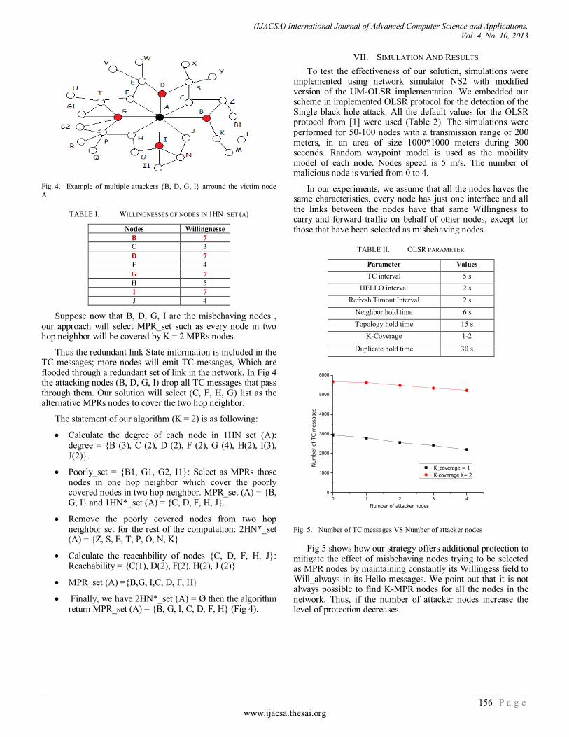
(IJACSA) International Journal of Advanced Computer Science and Applications, Vol. 4, No. 10, 2013
156 | P a g e www.ijacsa.thesai.org
Fig. 4. Example of multiple attackers {B, D, G, I} arround the victim node
A.
TABLE I. WILLINGNESSES OF NODES IN 1HN_SET (A)
Nodes Willingnesse
B 7
C 3
D 7
F 4
G 7
H 5
I 7
J 4
Suppose now that B, D, G, I are the misbehaving nodes , our approach will select MPR_set such as every node in two hop neighbor will be covered by K = 2 MPRs nodes.
Thus the redundant link State information is included in the TC messages; more nodes will emit TC-messages, Which are flooded through a redundant set of link in the network. In Fig 4 the attacking nodes (B, D, G, I) drop all TC messages that pass through them. Our solution will select (C, F, H, G) list as the alternative MPRs nodes to cover the two hop neighbor.
The statement of our algorithm (K = 2) is as following:
Calculate the degree of each node in 1HN_set (A): degree = {B (3), C (2), D (2), F (2), G (4), H(2), I(3), J(2)}.
Poorly_set = {B1, G1, G2, I1}: Select as MPRs those nodes in one hop neighbor which cover the poorly covered nodes in two hop neighbor. MPR_set (A) = {B, G, I} and 1HN*_set (A) = {C, D, F, H, J}.
Remove the poorly covered nodes from two hop neighbor set for the rest of the computation: 2HN*_set (A) = {Z, S, E, T, P, O, N, K}
Calculate the reacahbility of nodes {C, D, F, H, J}: Reachability = {C(1), D(2), F(2), H(2), J (2)}
MPR_set (A) ={B,G, I,C, D, F, H}
Finally, we have 2HN*_set (A) = Ø then the algorithm return MPR_set (A) = {B, G, I, C, D, F, H} (Fig 4).
VII. SIMULATION AND RESULTS
To test the effectiveness of our solution, simulations were implemented using network simulator NS2 with modified version of the UM-OLSR implementation. We embedded our scheme in implemented OLSR protocol for the detection of the Single black hole attack. All the default values for the OLSR protocol from [1] were used (Table 2). The simulations were performed for 50-100 nodes with a transmission range of 200 meters, in an area of size 1000*1000 meters during 300 seconds. Random waypoint model is used as the mobility model of each node. Nodes speed is 5 m/s. The number of malicious node is varied from 0 to 4.
In our experiments, we assume that all the nodes haves the same characteristics, every node has just one interface and all the links between the nodes have that same Willingness to carry and forward traffic on behalf of other nodes, except for those that have been selected as misbehaving nodes.
TABLE II. OLSR PARAMETER
Parameter Values
TC interval 5 s
HELLO interval 2 s
Refresh Timout Interval 2 s
Neighbor hold time 6 s
Topology hold time 15 s
K-Coverage 1-2
Duplicate hold time 30 s
0 1 2 3 4
0
1000
2000
3000
4000
5000
6000
Num
ber
of
TC m
ess
ages
Number of attacker nodes
K_coverage = 1
K-coverage K= 2
Fig. 5. Number of TC messages VS Number of attacker nodes
Fig 5 shows how our strategy offers additional protection to mitigate the effect of misbehaving nodes trying to be selected as MPR nodes by maintaining constantly its Willingess field to Will_always in its Hello messages. We point out that it is not always possible to find K-MPR nodes for all the nodes in the network. Thus, if the number of attacker nodes increase the level of protection decreases.
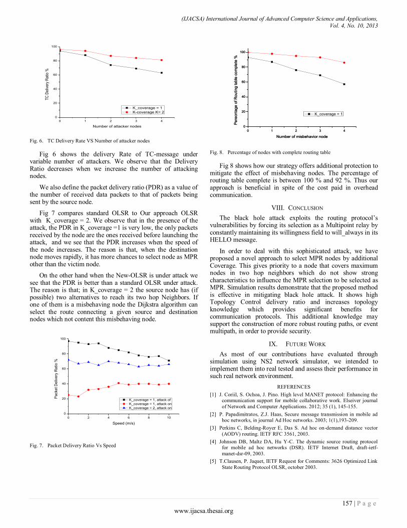
(IJACSA) International Journal of Advanced Computer Science and Applications, Vol. 4, No. 10, 2013
157 | P a g e www.ijacsa.thesai.org
0 1 2 3 4
0
20
40
60
80
100T
C D
eliv
ery
Rat
io %
Number of attacker nodes
K_coverage = 1
K-coverage K= 2
Fig. 6. TC Delivery Rate VS Number of attacker nodes
Fig 6 shows the delivery Rate of TC-message under variable number of attackers. We observe that the Delivery Ratio decreases when we increase the number of attacking nodes.
We also define the packet delivery ratio (PDR) as a value of the number of received data packets to that of packets being sent by the source node.
Fig 7 compares standard OLSR to Our approach OLSR with K_coverage = 2. We observe that in the presence of the attack, the PDR in K_coverage =1 is very low, the only packets received by the node are the ones received before launching the attack, and we see that the PDR increases when the speed of the node increases. The reason is that, when the destination node moves rapidly, it has more chances to select node as MPR other than the victim node.
On the other hand when the New-OLSR is under attack we see that the PDR is better than a standard OLSR under attack. The reason is that; in K_coverage = 2 the source node has (if possible) two alternatives to reach its two hop Neighbors. If one of them is a misbehaving node the Dijkstra algorithm can select the route connecting a given source and destination nodes which not content this misbehaving node.
0 2 4 6 8 10
0
20
40
60
80
100
Pa
cke
t D
eliv
ery
Ra
tio %
Speed (m/s)
K_coverage = 1, attack of
K_coverage = 1, attack on
K_coverage = 2, attack on
Fig. 7. Packet Delivery Ratio Vs Speed
0 1 2 3 4
0
20
40
60
80
100
0 1 2 3 4
0
20
40
60
80
100
Pe
recn
tag
e o
f R
ou
tin
g ta
ble
co
mp
lete
%
Number of misbehavior node
K_coverage = 2
Pe
recn
tag
e o
f R
ou
tin
g ta
ble
co
mp
lete
%
Number of misbehavior node
K_coverage = 1
Fig. 8. Percentage of nodes with complete routing table
Fig 8 shows how our strategy offers additional protection to mitigate the effect of misbehaving nodes. The percentage of routing table complete is between 100 % and 92 %. Thus our approach is beneficial in spite of the cost paid in overhead communication.
VIII. CONCLUSION
The black hole attack exploits the routing protocol’s vulnerabilities by forcing its selection as a Multipoint relay by constantly maintaining its willingness field to will_always in its HELLO message.
In order to deal with this sophisticated attack, we have proposed a novel approach to select MPR nodes by additional Coverage. This gives priority to a node that covers maximum nodes in two hop neighbors which do not show strong characteristics to influence the MPR selection to be selected as MPR. Simulation results demonstrate that the proposed method is effective in mitigating black hole attack. It shows high Topology Control delivery ratio and increases topology knowledge which provides significant benefits for communication protocols. This additional knowledge may support the construction of more robust routing paths, or event multipath, in order to provide security.
IX. FUTURE WORK
As most of our contributions have evaluated through simulation using NS2 network simulator, we intended to implement them into real tested and assess their performance in such real network environment.
REFERENCES
[1] J. Coriil, S. Ochoa, J. Pino. High level MANET protocol: Enhancing the communication support for mobile collaborative work. Elseiver journal
of Network and Computer Applications. 2012; 35 (1), 145-155.
[2] P. Papadimitratos, Z.J. Haas, Secure message transmission in mobile ad hoc networks, in journal Ad Hoc networks. 2003; 1(1),193-209.
[3] Perkins C, Belding-Royer E, Das S. Ad hoc on-demand distance vector
(AODV) routing. IETF RFC 3561, 2003.
[4] Johnson DB, Maltz DA, Hu Y-C. The dynamic source routing protocol for mobile ad hoc networks (DSR). IETF Internet Draft, draft-ietf-
manet-dsr-09, 2003.
[5] T.Clausen, P. Jaquet, IETF Request for Comments: 3626 Optimized Link
State Routing Protocol OLSR, october 2003.

(IJACSA) International Journal of Advanced Computer Science and Applications, Vol. 4, No. 10, 2013
158 | P a g e www.ijacsa.thesai.org
[6] Ogier R, Lewis M, Templin F. Topology dissemination based on reverse-
path forwarding (TBRPF). IETF Internet Draft, draft-ietf-manet-tbrpf-07.txt, 2003.
[7] J-H. Zygmunt : A new routing protocol for the recon_gurable wireless networks. In Proceedings of 6th IEEE International Conference on
Universal Personal Communications, IEEE ICUPC'97, October 12-16, 1997, San Diego, California, USA, volume 2, pages 562{566. IEEE,
IEEE, October 1997.
[8] Sanzgiri K, Dahill B, Levine BN, Shields C, Belding-Royer E. A secure routing protocol for ad hoc networks. Proceedings of 2002 IEEE
International Conference on Network Protocols (ICNP), Paris, France, November 2002.
[9] Hu Y-C, Perrig A, Johnson DB. Ariadne: a secure on-demand routing
protocol for ad hoc networks. Proceedings of the MobiCom 2002, Atlanta, Georgia, U.S.A., 23–28 September 2002.
[10] Zapata MG. Secure ad hoc on-demand distance vector routing. ACM
Mobile Computing and Communications Review (MC2R) 2002; 6(3):106–107.
[11] Zapata MG, Asokan N. Securing ad-hoc routing protocols. Proceedings
of the 2002 ACM Workshop on Wireless Security (WiSe 2002), Atlanta, GA, U.S.A., September 2002; 1–10.
[12] Hu Y-C, Johnson DB, Perrig A. SEAD: secure efficient distance vector
routing for mobile wireless ad hoc networks. Proceedings of the 4th IEEE Workshop on Mobile Computing Systems and Applications
(WMCSA 2002). IEEE: Calicoon, NY, June 2002; 3–13.
[13] Papadimitratos P, Haas Z. Secure routing for mobile ad hoc networks.
Proceedings of the SCS Communication Networks and Distributed Systems Modeling and Simulation Conference, San Antonio, TX, 27–31
January, 2002.
[14] Zhou L, Haas ZJ. Securing ad hoc networks. IEEE Networks Special Issue on Network Security, November/ December 1999; 24–30.
[15] C.Adjih, A.Laouiti, P.Minet, P.Muhlethan, A. Quayyum, L.Viennot. The
Optimized Routing Protocol for Mobile ad hoc Networks: Protocol
Specification. Projet HIPERCOM.INRIA research report N° 5145,
March 2004.
[16] A. Adnane, R.T. de Sousa Jr., C. Bidan, and L. Mé. Autonomic trust
reasoning enables misbehavior detection in OLSR. In ACM Symposium on Applied computing (SAC), pages 2006–2013, New York, USA,
2008.
[17] F. Cuppens, N. Cuppens-Boulahia, T. Ramard, and J. Thomas. Misbehaviors detection to ensure availability in OLSR. In Mobile Sensor
Networks (MSN), volume 4864 of Lecture Notes in Computer Science, pages 799–813. Springer, 2007.
[18] M. Wang, L. Lamont, P. Mason, M. Gorlatova, An effective intrusion
detection approach for OLSR MANET protocol, in: Proceedings of the First International Conference on Secure Network Protocols (NPSEC),
IEEE Computer Society, Washington, USA, 2005, pp. 55–60.
[19] Marti S, Giuli TJ, Kevin L, Mary B. Mitigating routing misbehavior in mobile ad hoc networks. In: Proceedings of the 6th annual international
conference on mobile computing and networking (MobiCom’00); 2000. p. 255–65.
[20] Soufian Djahel, Farid Nait Abslam, Avoiding virtual link attack in
wireless ad hoc networks, Proceeding of the 2008 IEEE/ACS Internetional conference of computer systems and application, p 355-
360. March 31 avril 04, 2008.
[21] Rachid abdellaoui and Jean Marc Robert. SU-OLSR : A new solution to thwart attacks against the olsr protocol. Mster thesis.Height school of
technology (ETS) Canada. 2009.
[22] Bounpadith Kannhavong , Hidehisa Nakayama , Nei Kato , Abbas
Jamalipour , Yoshiaki Nemoto, A study of a routing attack in OLSR-based mobile ad hoc networks, International Journal of Communication
Systems, 2007; 20 (11), p.1245-1261.
[23] D.Djenouri, N.badach, On eliminating packet droppers in MANET: A modular solution. Ad Hoc Networks 2009; 7(6): 1243-58.
[24] A. Badach, A. Belmehdi, Fighting against packet dropping misbehavior
in multi-hop wireless ad hoc network, Network and Computer Application 35(2012) 1130-1139.
Determining Public Structure Crowd Evacuation
Capacity
Pejman Kamkarian
Computer Engineering Department
Southern Illinois University
Carbondale, U.S.A
Henry Hexmoor
Computer Science Department
Southern Illinois University
Carbondale, U.S.A
Abstract— This paper explores a strategy for determining
public space safety. Due to varied purposes and locations, each
public space has architecture as well as facilities. A generalized
analysis of capacities for public spaces is essential. The method
we propose is to examine a public space with a given
architecture. We used Bayesian Belief Network to determine the
level of safety and identify points of weakness in public spaces.
Keywords— Networks of Bayesian Belief Revision, Public
Space Safety, Crowd Evacuation
I. INTRODUCTION
Access to geometrics features of a public space as well as
crowd specification is essential for exploring the safety of
structures. An emergency event requires evacuation of people
from indoor spaces. They need to evacuate in the safest
possible way within the least amount of time. In an evacuation,
the crowd will use spaces and pathways in unintended ways.
This stems from collective group behaviors that emerge from
an individual’s propensity to spend the least amount of effort
to vacate the premises. Resulting effects are unpredictable.
Although, in some cases, such as attempting to exit through
exit doors, minimizing distances to an exit is not a guiding
principle; minimizing travel time to reach an exit door might
be. Crowd density is important as the number of people in a
unit of indoor space, which is not homogenous. Our primary
objective is to determine universal factors that can cause
collapsing buildings. Secondarily, we wish to develop a model
using Bayesian Belief Networks to provide building architects
with the capability to examine a public space regarding its
capacities to transfer people. This will provide us a metric for
quantifying building safety. We hope that our model will be a
useful tool that will supplement guidelines for safer future
building design codes.
Although no design improvement can prevent disasters,
they can mitigate and significantly reduce frequency of
occurrence. Our approach is multipronged. We explore crowd
specifications as well as building and public space features to
suggest a methodology for the design and management of
indoor environments where crowds appear. In order to
systematically assess risk factors for a building, we must
investigate behavior of the crowd dynamics during various
situations, such as crowd distribution patterns. The crowd
speed of movement, crowd density, and also the space
utilization maps allow us to qualitatively and quantitatively
assess the safety of the public space. Some physical
specifications of indoor public spaces, such as the exit door
width or locations of installed ground facilities, are considered
as well. For example, the doorway widths should be increased
to make crossing through them easier without congestion.
Consideration should also be given to the potential usage of
interconnected gates called concourses by spectators at events
such as public transportation areas. Usage can be considerable
if the event spans multiple hours, if inclement weather
conditions are present, or if large numbers are in attendance.
Development of our pattern spans beyond our current project.
The crowd consists of many individuals. Each entity has the
capacity to react according to his internal parameters and the
specifications of the environment as the simulation proceeds.
The dynamics of the crowd are an emergent phenomenon that
is not programmed explicitly. A group of people at an indoor public space may move
randomly. Lack of first aid and emergency extinguisher tools will lead to potential disasters in evacuation. In some cases, such as smoke or derbies, the vision is diminished. People mostly try to look for any tools that can help them survive. First aid kits, fire extinguishers or axes, and glowing red exit lights are necessary tools that can expedite evacuation. In this paper we demonstrate the Bayesian Belief Networks as a significant solution to examine and assure the safety for the people. The Bayesian Belief Network performs this task by coalescing general specifications of the environment and the people’s behaviors. In section 2 we will describe salient attributes of a crowd. Section 2 outlines crowd attributes as well as physical properties of structures. Section 3 describes Bayesian belief network methodology in general and applies it to a specific building to support our concept. Concluding remarks in section 5 culminate our paper.
II. PERTINENT PROPERTIES
Shortcut exploitation is a fundamental human trait that is in effect for crowds. Another relevant property of crowds is competitive behavior, which will become important in egress and ingress conditions. In an evacuation, individuals will compete with one another in progressing towards exits, exploiting optimal available paths. Our tool will be a predictive device for discovering human characteristics affecting unsafe movement patterns in public spaces. Whereas guiding principles encode salient properties and behaviors, they can
(IJACSA) International Journal of Advanced Computer Science and Applications, Vol. 4, No. 10, 2013
159 | P a g e www.ijacsa.thesai.org
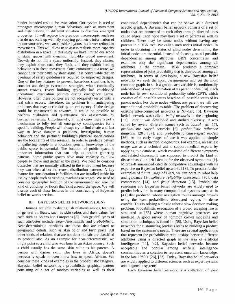
hinder intended results for evacuation. Our system is used to propagate microscopic human behaviors, such as movement and distributions, in different situation to discover emergent properties. It will replace the previous macroscopic analyses that do not scale up well. By studying geometric information of indoor structures, we can consider layouts that lower redundant movements. This will allow us to assess realistic room capacity distribution in a space. In this study we have limited our scope to static spaces with dynamic, fluid-like crowd movement. Crowds do not fill a space uniformly. Instead, they cluster; they exploit short cuts; they flock, and they exhibit herding behavior as in sheep movement. Once committed to a route, we cannot alter their paths by static signs. It is conceivable that an overhaul of safety guidelines is required for improved designs. One of the key features to prevent hazardous situations is to consider and design evacuation strategies, which continually attract crowds. Every building typically has established operational evacuation policies during emergency egress. However, often these policies are not adequately tested until a real crisis occurs. Therefore, the problem is in anticipating problems that may occur during an emergency. If the design could be constructed in advance, it would be possible to perform qualitative and quantitative risk assessments by destructive testing. Unfortunately, in most cases there is not a mechanism to fully test all emergency contingencies for a specific building. People will always try to find a safe and fast way to leave dangerous positions. Investigating human behaviors and the pertinent building’s physical specifications are the focal aims of this research. In order to predict a pattern of gathering people in a location, general knowledge of the public space is essential. The location of public space is important information that can help us predict gathering patterns. Some public spaces have more capacity to allow people to move and gather at the place. We need to consider obstacles that are normally affixed in the environment because they can often affect the crowd distribution patterns. A key feature for consideration is facilities that are installed inside for use by people such as vending machines or stages. We need to consider geographic location of the environment and also the kind of buildings or floors that exist around the space. We will discuss each of these features in the constructing of Bayesian belief networks section.
III. BAYESIAN BELIEF NETWORKS (BBN)
Humans are able to distinguish relations among features
of general attributes, such as skin colors and their values for
each such as Asians and Europeans [8]. Two general types of
such attributes include: near-deterministic and probabilistic.
Near-deterministic attributes are those that are related to
geographic details, such as skin color and birth place. All
other kinds of relations that are not deterministic are classified
as probabilistic. As an example for near-deterministic, we
might point to a child who was born in an Asian country. Such
a child usually has the same skin color as his parents. A
person with darker skin, who lives in Africa, doesn’t
necessarily speak or even know how to speak African. We
consider these kinds of examples in the probabilistic category.
Bayesian belief network is a probabilistic graphical pattern
consisting of a set of random variables as well as their
conditional dependencies that can be shown as a directed
acyclic graph. A Bayesian belief network consists of a set of
nodes that are connected to each other through directed lines
called edges. Each node may have a set of parents as well as
children. There may be some nodes without having any
parents in a BBN tree. We called such nodes initial nodes. In
order to obtaining the status of child nodes determining the
initial nodes are essential. Instead of focusing on all possible
dependencies among attributes, BBN concentrates and
examines only the significant dependencies among all
attributes in the domain. BBN produces a compact
representation of joint probability that is distributed among all
attributes. In terms of developing a new Bayesian belief
networks we seek the most parsimonious and yet the most
complete graph. In such a graph, each variable is conditionally
independent of any combination of its parent nodes [14]. Each
node has its own conditional probability table (CPT), which
consists of all possible states based on all possible states of its
parent nodes. For those nodes without any parent we will use
unconditional probabilities table. The problem of discovering
existing inter-connected networks is NP-hard [6]. Bayesian
belief network was called belief networks in the beginning
[32]. Later it was developed and studied diversely. It was
called by several different names such as causal nets [17],
probabilistic causal networks [5], probabilistic influence
diagrams [20], [37], and probabilistic cause-effect models
[36]. At the early stages of use it was applied to simple
methods, such as medical diagnostics. For example, an earliest
usage was as a technical aid to support medical experts by
applying to a database, which consisted of different symptoms
and related diseases. It was supposed to predict the kind of
disease based on brief details for the observed symptoms [1].
Microsoft announced cited its competitive advantages with its
expertise on Bayesian belief networks [18]. To present further
examples of future usage of BBN, we can point to robot help
and guidance [3], software reliability assessment [30], data
compression [14], and fraud detection [13]. Probabilistic
reasoning and Bayesian belief networks are widely used to
predict behaviors in many computational systems such as in
[41] that produced robotic navigation routes amongst crowds
using the least probabilistic obstructed regions in dense
crowds. This is solving a classic robotic slow decision making
problem. Probabilistic evacuation of a crowd escaping fire is
simulated in [35] where human cognitive processes are
modeled. A good survey of common crowd modeling and
simulation techniques is found in [38]. Using Bayesian belief
networks for customizing products leads to building a product
based on the customer’s needs. There are several applications
that represent the probabilistic relationships between different
attributes using a directed graph in the area of artificial
intelligence [11], [42]. Bayesian belief networks became
acceptable and popular among artificial intelligence
communities as a solution to represent uncertain knowledge,
in the late 1980’s [26], [33]. Today, Bayesian belief networks
are widely applied to different sciences such as expert systems
and diagnostic systems.
Each Bayesian belief network is a collection of joint
(IJACSA) International Journal of Advanced Computer Science and Applications, Vol. 4, No. 10, 2013
160 | P a g e www.ijacsa.thesai.org
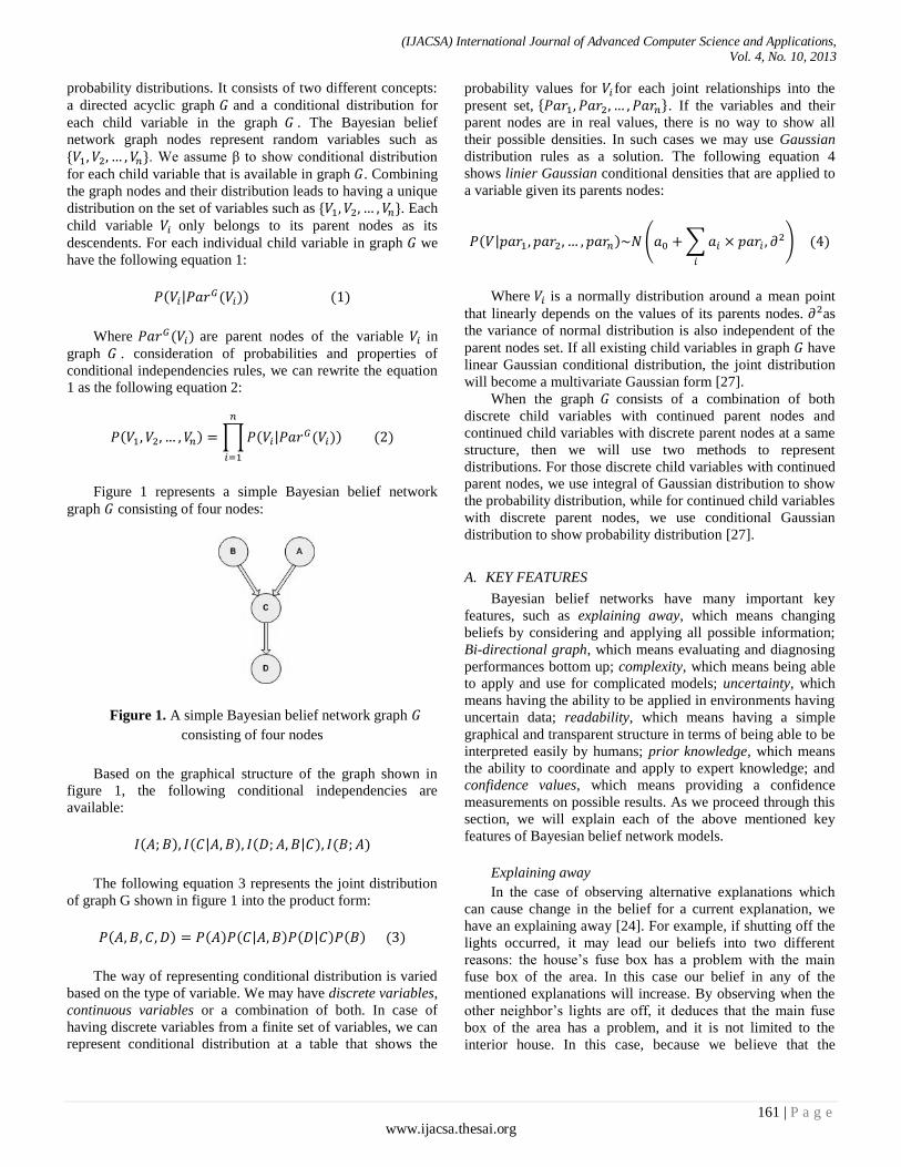
probability distributions. It consists of two different concepts:
a directed acyclic graph and a conditional distribution for
each child variable in the graph . The Bayesian belief
network graph nodes represent random variables such as
. We assume β to show conditional distribution
for each child variable that is available in graph . Combining
the graph nodes and their distribution leads to having a unique
distribution on the set of variables such as . Each
child variable only belongs to its parent nodes as its
descendents. For each individual child variable in graph we
have the following equation 1:
( | ( (
Where ( are parent nodes of the variable in
graph . consideration of probabilities and properties of
conditional independencies rules, we can rewrite the equation
1 as the following equation 2:
( ∏ ( | (
(
Figure 1 represents a simple Bayesian belief network
graph consisting of four nodes:
Figure 1. A simple Bayesian belief network graph
consisting of four nodes
Based on the graphical structure of the graph shown in
figure 1, the following conditional independencies are
available:
( ( | ( | (
The following equation 3 represents the joint distribution
of graph G shown in figure 1 into the product form:
( ( ( | ( | ( (
The way of representing conditional distribution is varied
based on the type of variable. We may have discrete variables,
continuous variables or a combination of both. In case of
having discrete variables from a finite set of variables, we can
represent conditional distribution at a table that shows the
probability values for for each joint relationships into the
present set, . If the variables and their
parent nodes are in real values, there is no way to show all
their possible densities. In such cases we may use Gaussian
distribution rules as a solution. The following equation 4
shows linier Gaussian conditional densities that are applied to
a variable given its parents nodes:
( | ( ∑
) (
Where is a normally distribution around a mean point
that linearly depends on the values of its parents nodes. as
the variance of normal distribution is also independent of the
parent nodes set. If all existing child variables in graph have
linear Gaussian conditional distribution, the joint distribution
will become a multivariate Gaussian form [27].
When the graph consists of a combination of both
discrete child variables with continued parent nodes and
continued child variables with discrete parent nodes at a same
structure, then we will use two methods to represent
distributions. For those discrete child variables with continued
parent nodes, we use integral of Gaussian distribution to show
the probability distribution, while for continued child variables
with discrete parent nodes, we use conditional Gaussian
distribution to show probability distribution [27].
A. KEY FEATURES
Bayesian belief networks have many important key
features, such as explaining away, which means changing
beliefs by considering and applying all possible information;
Bi-directional graph, which means evaluating and diagnosing
performances bottom up; complexity, which means being able
to apply and use for complicated models; uncertainty, which
means having the ability to be applied in environments having
uncertain data; readability, which means having a simple
graphical and transparent structure in terms of being able to be
interpreted easily by humans; prior knowledge, which means
the ability to coordinate and apply to expert knowledge; and
confidence values, which means providing a confidence
measurements on possible results. As we proceed through this
section, we will explain each of the above mentioned key
features of Bayesian belief network models.
Explaining away
In the case of observing alternative explanations which
can cause change in the belief for a current explanation, we
have an explaining away [24]. For example, if shutting off the
lights occurred, it may lead our beliefs into two different
reasons: the house’s fuse box has a problem with the main
fuse box of the area. In this case our belief in any of the
mentioned explanations will increase. By observing when the
other neighbor’s lights are off, it deduces that the main fuse
box of the area has a problem, and it is not limited to the
interior house. In this case, because we believe that the
(IJACSA) International Journal of Advanced Computer Science and Applications, Vol. 4, No. 10, 2013
161 | P a g e www.ijacsa.thesai.org

shutting off of the lights is because of a failure in the area,
there are no reasons to believe that a failure exists inside the
house, and hence we should retract that belief [21].
Bi-directional structure
Bi-directional is an ability to predict the inputs based on a
certain output. For example, in case of producing cars, a
Bayesian belief network is able to give us the features
necessary to produce each customized car. In other words, it is
able to show us the inputs based on a specific output. Such
ability isn’t available for many other intelligent systems, such
as fussy logic and feed forward neural networks. The
mentioned systems are called one-way models, or in other
words, from input to output only and hence trace the inputs
based on a certain output is impossible.
Complexity
Bayesian belief network consists of a set of nodes, and
arcs between nodes. Each node may have many children nodes
or parent nodes. Because the probability distribution of
attributes for each certain value depends only on its parents
nodes, estimation is possible based on fewer parameters. In
other words, because each node and its parents are separated
from the rest of model; we need fewer parameters in terms of
being able to predict the kind of relationships between
different variables.
Uncertainty
Assume having a group of people who are gathered at a
same place for a party. Predicting the time, the path, and the
next favorite location inside the environment for any available
individual at any certain time is almost impossible. Each
individual chooses his/her path, location and the time of
movement based on his/her needs. There are a variety of
reasons of existence uncertainty, such as distortion,
irrelevancy, and incompleteness [24]. In such cases in
Bayesian belief networks, we use probabilities, rather than
certain values such as true or false. This means Bayesian
belief networks are able to apply to cases where a combination
uncertainty is much more desirable.
Readability
As a main key feature of Bayesian belief networks, we
can point to readability. This means it has a simple and easy to
recognize model even for complicated problems. Having a
graphical structure pattern of Bayesian belief networks, using
simple meanings such as nodes and arcs between nodes, and
having a rational organizing and designing variables and the
relations between variables, make the Bayesian belief
networks a pleasant solution to apply complex problems that
are involved with many different relations and nodes. In other
words, applying Bayesian belief networks to a complex
problem consisting of a lot of different relations and nodes
won’t reduce its easy interpretability by humans because of its
graphical and rational structure.
Prior knowledge
In order to design each model, having basic values and
measurements are essential. In Bayesian belief networks, in
order to design the model, we need to have only formal initial
values rather than broad different values and limitations for
each one. Having such ability as another main key feature of
Bayesian belief networks makes it more meaningful to apply
to a variety of problems, especially on models for which we
don’t have broad initial values or prior data knowledge about.
Confidence values
In many intelligent systems such as neural networks, the
prediction results in a vector or scalar value which is not
suitable enough in case of needing to have a decision maker
system. Instead, in Bayesian belief networks, because of
having a probability distribution which is a boundary between
a law and high value, we are able to build a decision support
system more efficiently.
B. THEORY
In order to design a model of Bayesian belief networks,
we need to investigate three different areas: general structure
definition, parameters definition, and using the created model
to start predicting.
General structure definition
A Bayesian belief network generally consists of two
parts: nodes that represent values and bi-directed arcs that
show relations between nodes. The simplest case of Bayesian
belief networks consist of a node as child which has one
parent node and a bi-directed arc which is located between the
child node and the parent node. In the case of a real problem,
we may have a large group of nodes and bi-directed arcs as
relations between them. In such models, tracing and finding a
certain parameter among a large group of nodes and relations
may take a long time and will significantly reduce the
performance of the Bayesian belief network. As a solution to
this problem, we may use a search technique in order to
increase the quality and reduce the needed time to trace and
find any certain parameter. Many different search techniques
have the ability to apply a Bayesian belief networks models,
such as K2 methods that were proposed by Cooper and
Herskovits [7]. This algorithm is able to trace and find the
parameters for certain nodes based on a greedy search
algorithm; Generic algorithms may be used to ordering nodes
for using by K2. structural search of this algorithm is similar
to the travelling salesman problem [25], [12], and modified
Expectation Maximization (EM) method [15], which can learn
the available general structure and parameters in Bayesian
belief networks model and branch and bound method [29]. It
is able to limit the combinatorial explosion for example during
choosing a certain feature.
Parameters definition
(IJACSA) International Journal of Advanced Computer Science and Applications, Vol. 4, No. 10, 2013
162 | P a g e www.ijacsa.thesai.org

The next step to designing Bayesian belief networks
model is defining conditional probabilities for each node. In
other words, we need to determine the estimation of
occurrence for each node, where can be considered by a set of
nodes as well as their parent nodes. One way to estimate the
probability is to use the frequency of occurrence for each set
of variables among available data. If the number of times
observation increases, the frequency tends toward a true
probability distribution. In case of having a small set of data,
using an alternative approach is essential. Based on that we
need initially to assume a particular distribution such as
uniform and then update it in order of encapsulation the
information contained among available data. To achieve this
goal, we may use Expectation Maximization (EM) algorithm
[9], which can be combined with an equivalent sample size
[28].
Using the created model to start predicting
As the final step, we have to use the final model in terms of
making prediction. In case of observing some values of some
variables we are able to calculate the remaining variables. To
achieve this goal, we need to find the states of observations and
then propagating the beliefs around the available networks, and
continue this until all beliefs that are in the form of conditional
probabilities become consistent. Finally we can read the
favorite probability distribution directly from the Bayesian
belief networks.
IV. CONSTRUCTING OF BAYESIEN BELIEF
NETWORKS
In order to implement and demonstrate our Bayesian
belief network, we considered two separate work areas: indoor
public space specifications, including both indoor and some
outdoor, and the features of people who are presented on the
public space. We then applied both indoor public space and
the people features on a unit Bayesian belief networks pattern.
A. IMPLEMENTATION
Generally we have divided the employed factors of a
building safety crowd evacuation into two categories
including Physical public space specifications, and the Crowd
specifications itself.
Physical properties
Studding on physical properties, while investigating on
crowd safety evacuation is essential. Most of time, people are
located in a closed covered area when gathering for any
certain event. They share a common activity which is almost
related to the reason of gathering while forming a crowd. Of
all existing features that may directly or indirectly are related
to the geometric indoor space details, the following were more
interested with us to be considered:
Terrestrial sustainability: We considered on any natural
or other sources that can cause vibrating the indoor space as
an important factor. There are two general sources that can
affect a public space to be vibrating. In terms of determining
the safety of the building, considering to such sources is
essential. The first group of sources is natural and is related to
the area geometry specifications that a public space is built on;
such as the distance from any faults or volcanoes. The second
group of vibrating sources may create by human such as any
metro or train facilities. Beside the mentioned reasons,
considering the average weather status of the area is one other
key feature that can affect the rate of vibrating the
construction significantly. A public space located in a severe
area that has stormy weather most times a year is more expose
to be vibrated than the one which is located in an area with
having a stable weather.
Flow capacity: We divided this feature into two
categories: the flow capacity for interior public space and for
the building that the examined public space is located inside.
For indoor public space, we focused on obstacles in terms of
the number, installation positions and also the average size of
them. Each public space has a number of emergency exit
doors as well as normal entrances that should be taken into
account. To have an estimation of safety for general building
flow capacity, we considered on all existence obstacles that
are located somewhere between the indoor space and the main
entrances of the building. The number of such objects, as well
as the installation positions and the average size of them were
the factors that we considered for this category. As another
key feature, we investigated on the type of the building such
as a flat, an apartment, a tower and so on. In case of being
inside an apartment or a tower, considering the level that
public space is located leads having a better estimation for the
evacuation safety rate.
Overall exit capacity: Each door, based on its location,
and the width, has a different ability to allow passing a
number of people trough it at any moment. We considered this
feature for not only the examined public space, but for all
entrance that are located between indoor space and the main
building.
First Aid recovery capacity: In emergency cases, having a
proper distinguisher tools that are installed on a reasonable
locations can help people to stay alive and safe in a more
period of time before being able to evacuate from dangerous
situations. For example; in case of firing, using existing fire
distinguishers near the incident, help people to stay alive
inside the area of fire for longer time before evacuating while
a large group of people tend to across from entrances.
Structural integrity: To have a better building safety
estimation, considering the materials that public space is made
of as well as the year of build is essential.an old age building,
especially in case of using old materials may leads putting the
people inside at higher risk that a new building consisting a
new and better materials.
Space occupancy rate: This factor can be determined by
(IJACSA) International Journal of Advanced Computer Science and Applications, Vol. 4, No. 10, 2013
163 | P a g e www.ijacsa.thesai.org
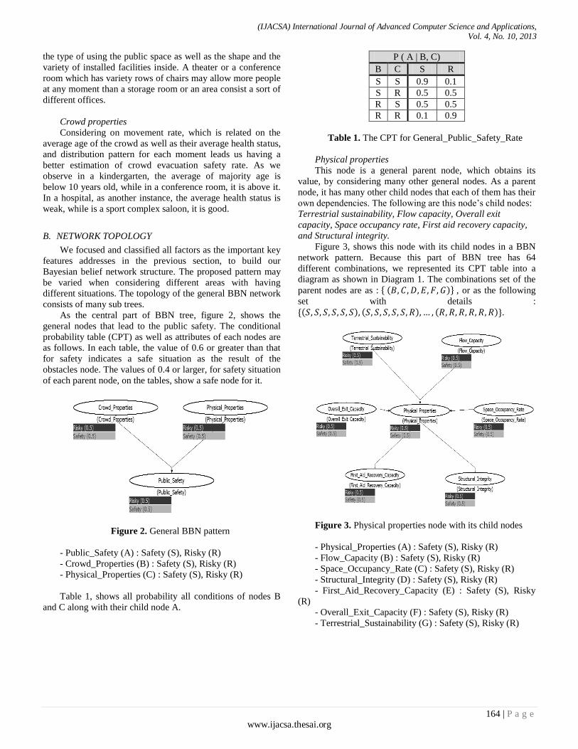
the type of using the public space as well as the shape and the
variety of installed facilities inside. A theater or a conference
room which has variety rows of chairs may allow more people
at any moment than a storage room or an area consist a sort of
different offices.
Crowd properties
Considering on movement rate, which is related on the
average age of the crowd as well as their average health status,
and distribution pattern for each moment leads us having a
better estimation of crowd evacuation safety rate. As we
observe in a kindergarten, the average of majority age is
below 10 years old, while in a conference room, it is above it.
In a hospital, as another instance, the average health status is
weak, while is a sport complex saloon, it is good.
B. NETWORK TOPOLOGY
We focused and classified all factors as the important key
features addresses in the previous section, to build our
Bayesian belief network structure. The proposed pattern may
be varied when considering different areas with having
different situations. The topology of the general BBN network
consists of many sub trees.
As the central part of BBN tree, figure 2, shows the
general nodes that lead to the public safety. The conditional
probability table (CPT) as well as attributes of each nodes are
as follows. In each table, the value of 0.6 or greater than that
for safety indicates a safe situation as the result of the
obstacles node. The values of 0.4 or larger, for safety situation
of each parent node, on the tables, show a safe node for it.
Figure 2. General BBN pattern
- Public_Safety (A) : Safety (S), Risky (R)
- Crowd_Properties (B) : Safety (S), Risky (R)
- Physical_Properties (C) : Safety (S), Risky (R)
Table 1, shows all probability all conditions of nodes B
and C along with their child node A.
P ( A | B, C)
B C S R
S S 0.9 0.1
S R 0.5 0.5
R S 0.5 0.5
R R 0.1 0.9
Table 1. The CPT for General_Public_Safety_Rate
Physical properties
This node is a general parent node, which obtains its
value, by considering many other general nodes. As a parent
node, it has many other child nodes that each of them has their
own dependencies. The following are this node’s child nodes:
Terrestrial sustainability, Flow capacity, Overall exit
capacity, Space occupancy rate, First aid recovery capacity,
and Structural integrity.
Figure 3, shows this node with its child nodes in a BBN
network pattern. Because this part of BBN tree has 64
different combinations, we represented its CPT table into a
diagram as shown in Diagram 1. The combinations set of the
parent nodes are as : ( , or as the following
set with details :
( ( ( .
Figure 3. Physical properties node with its child nodes
- Physical_Properties (A) : Safety (S), Risky (R)
- Flow_Capacity (B) : Safety (S), Risky (R)
- Space_Occupancy_Rate (C) : Safety (S), Risky (R)
- Structural_Integrity (D) : Safety (S), Risky (R)
- First_Aid_Recovery_Capacity (E) : Safety (S), Risky
(R)
- Overall_Exit_Capacity (F) : Safety (S), Risky (R)
- Terrestrial_Sustainability (G) : Safety (S), Risky (R)
(IJACSA) International Journal of Advanced Computer Science and Applications, Vol. 4, No. 10, 2013
164 | P a g e www.ijacsa.thesai.org
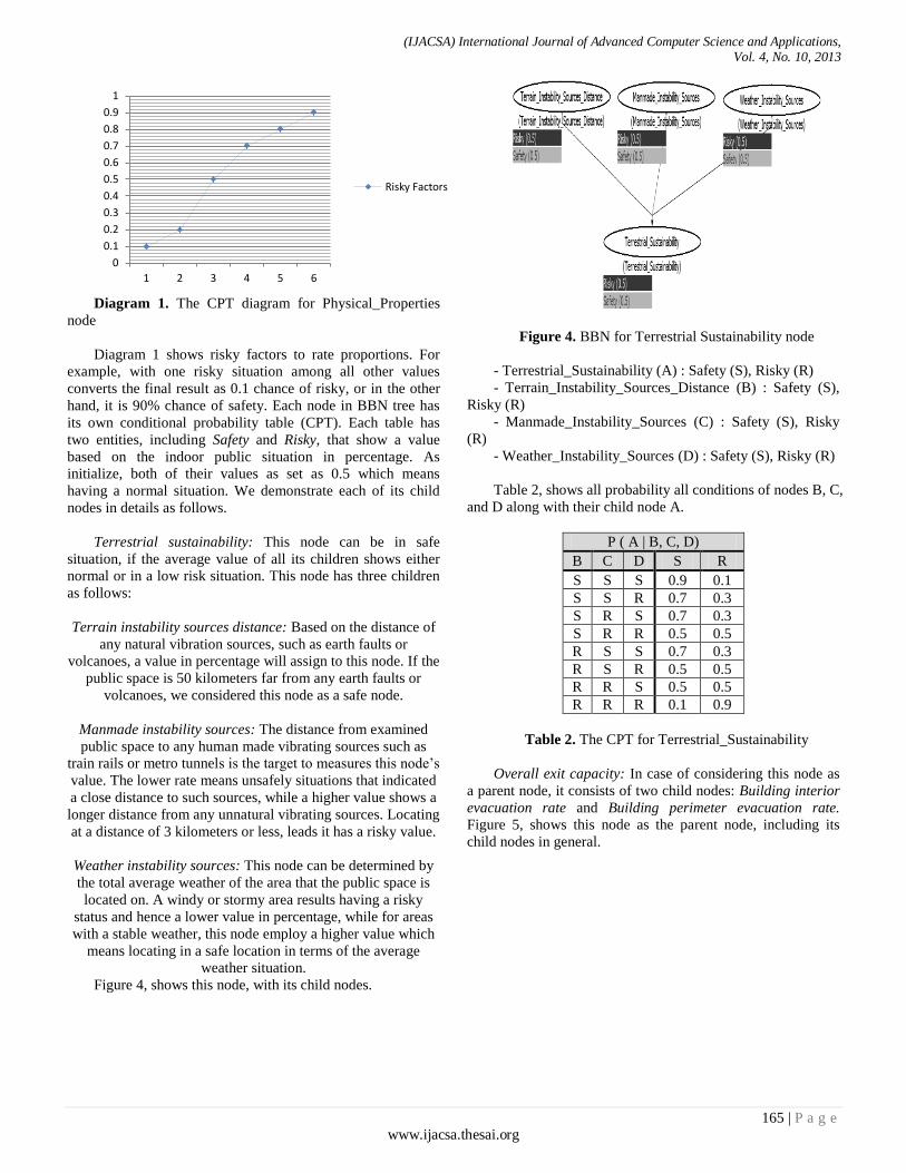
Diagram 1. The CPT diagram for Physical_Properties
node
Diagram 1 shows risky factors to rate proportions. For
example, with one risky situation among all other values
converts the final result as 0.1 chance of risky, or in the other
hand, it is 90% chance of safety. Each node in BBN tree has
its own conditional probability table (CPT). Each table has
two entities, including Safety and Risky, that show a value
based on the indoor public situation in percentage. As
initialize, both of their values as set as 0.5 which means
having a normal situation. We demonstrate each of its child
nodes in details as follows.
Terrestrial sustainability: This node can be in safe
situation, if the average value of all its children shows either
normal or in a low risk situation. This node has three children
as follows:
Terrain instability sources distance: Based on the distance of
any natural vibration sources, such as earth faults or
volcanoes, a value in percentage will assign to this node. If the
public space is 50 kilometers far from any earth faults or
volcanoes, we considered this node as a safe node.
Manmade instability sources: The distance from examined
public space to any human made vibrating sources such as
train rails or metro tunnels is the target to measures this node’s
value. The lower rate means unsafely situations that indicated
a close distance to such sources, while a higher value shows a
longer distance from any unnatural vibrating sources. Locating
at a distance of 3 kilometers or less, leads it has a risky value.
Weather instability sources: This node can be determined by
the total average weather of the area that the public space is
located on. A windy or stormy area results having a risky
status and hence a lower value in percentage, while for areas
with a stable weather, this node employ a higher value which
means locating in a safe location in terms of the average
weather situation.
Figure 4, shows this node, with its child nodes.
Figure 4. BBN for Terrestrial Sustainability node
- Terrestrial_Sustainability (A) : Safety (S), Risky (R)
- Terrain_Instability_Sources_Distance (B) : Safety (S),
Risky (R)
- Manmade_Instability_Sources (C) : Safety (S), Risky
(R)
- Weather_Instability_Sources (D) : Safety (S), Risky (R)
Table 2, shows all probability all conditions of nodes B, C,
and D along with their child node A.
P ( A | B, C, D)
B C D S R
S S S 0.9 0.1
S S R 0.7 0.3
S R S 0.7 0.3
S R R 0.5 0.5
R S S 0.7 0.3
R S R 0.5 0.5
R R S 0.5 0.5
R R R 0.1 0.9
Table 2. The CPT for Terrestrial_Sustainability
Overall exit capacity: In case of considering this node as
a parent node, it consists of two child nodes: Building interior
evacuation rate and Building perimeter evacuation rate.
Figure 5, shows this node as the parent node, including its
child nodes in general.
0
0.1
0.2
0.3
0.4
0.5
0.6
0.7
0.8
0.9
1
1 2 3 4 5 6
Risky Factors
(IJACSA) International Journal of Advanced Computer Science and Applications, Vol. 4, No. 10, 2013
165 | P a g e www.ijacsa.thesai.org
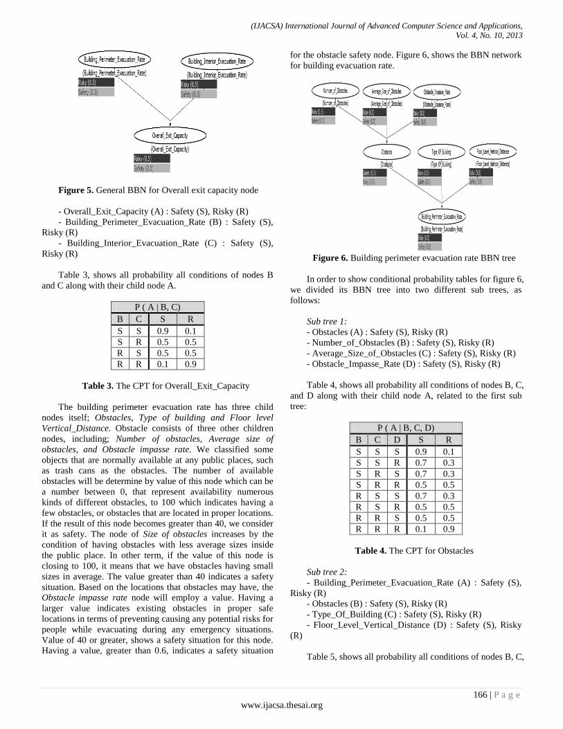
Figure 5. General BBN for Overall exit capacity node
- Overall_Exit_Capacity (A) : Safety (S), Risky (R)
- Building_Perimeter_Evacuation_Rate (B) : Safety (S),
Risky (R)
- Building_Interior_Evacuation_Rate (C) : Safety (S),
Risky (R)
Table 3, shows all probability all conditions of nodes B
and C along with their child node A.
P ( A | B, C)
B C S R
S S 0.9 0.1
S R 0.5 0.5
R S 0.5 0.5
R R 0.1 0.9
Table 3. The CPT for Overall_Exit_Capacity
The building perimeter evacuation rate has three child
nodes itself; Obstacles, Type of building and Floor level
Vertical_Distance. Obstacle consists of three other children
nodes, including; Number of obstacles, Average size of
obstacles, and Obstacle impasse rate. We classified some
objects that are normally available at any public places, such
as trash cans as the obstacles. The number of available
obstacles will be determine by value of this node which can be
a number between 0, that represent availability numerous
kinds of different obstacles, to 100 which indicates having a
few obstacles, or obstacles that are located in proper locations.
If the result of this node becomes greater than 40, we consider
it as safety. The node of Size of obstacles increases by the
condition of having obstacles with less average sizes inside
the public place. In other term, if the value of this node is
closing to 100, it means that we have obstacles having small
sizes in average. The value greater than 40 indicates a safety
situation. Based on the locations that obstacles may have, the
Obstacle impasse rate node will employ a value. Having a
larger value indicates existing obstacles in proper safe
locations in terms of preventing causing any potential risks for
people while evacuating during any emergency situations.
Value of 40 or greater, shows a safety situation for this node.
Having a value, greater than 0.6, indicates a safety situation
for the obstacle safety node. Figure 6, shows the BBN network
for building evacuation rate.
Figure 6. Building perimeter evacuation rate BBN tree
In order to show conditional probability tables for figure 6,
we divided its BBN tree into two different sub trees, as
follows:
Sub tree 1:
- Obstacles (A) : Safety (S), Risky (R)
- Number_of_Obstacles (B) : Safety (S), Risky (R)
- Average_Size_of_Obstacles (C) : Safety (S), Risky (R)
- Obstacle_Impasse_Rate (D) : Safety (S), Risky (R)
Table 4, shows all probability all conditions of nodes B, C,
and D along with their child node A, related to the first sub
tree:
P ( A | B, C, D)
B C D S R
S S S 0.9 0.1
S S R 0.7 0.3
S R S 0.7 0.3
S R R 0.5 0.5
R S S 0.7 0.3
R S R 0.5 0.5
R R S 0.5 0.5
R R R 0.1 0.9
Table 4. The CPT for Obstacles
Sub tree 2:
- Building_Perimeter_Evacuation_Rate (A) : Safety (S),
Risky (R)
- Obstacles (B) : Safety (S), Risky (R)
- Type_Of_Building (C) : Safety (S), Risky (R)
- Floor_Level_Vertical_Distance (D) : Safety (S), Risky
(R)
Table 5, shows all probability all conditions of nodes B, C,
(IJACSA) International Journal of Advanced Computer Science and Applications, Vol. 4, No. 10, 2013
166 | P a g e www.ijacsa.thesai.org
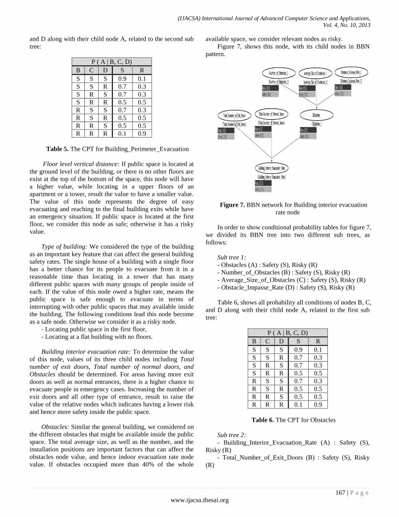
and D along with their child node A, related to the second sub
tree:
P ( A | B, C, D)
B C D S R
S S S 0.9 0.1
S S R 0.7 0.3
S R S 0.7 0.3
S R R 0.5 0.5
R S S 0.7 0.3
R S R 0.5 0.5
R R S 0.5 0.5
R R R 0.1 0.9
Table 5. The CPT for Building_Perimeter_Evacuation
Floor level vertical distance: If public space is located at
the ground level of the building, or there is no other floors are
exist at the top of the bottom of the space, this node will have
a higher value, while locating in a upper floors of an
apartment or a tower, result the value to have a smaller value.
The value of this node represents the degree of easy
evacuating and reaching to the final building exits while have
an emergency situation. If public space is located at the first
floor, we consider this node as safe; otherwise it has a risky
value.
Type of building: We considered the type of the building
as an important key feature that can affect the general building
safety rates. The single house of a building with a single floor
has a better chance for its people to evacuate from it in a
reasonable time than locating in a tower that has many
different public spaces with many groups of people inside of
each. If the value of this node owed a higher rate, means the
public space is safe enough to evacuate in terms of
interrupting with other public spaces that may available inside
the building. The following conditions lead this node become
as a safe node. Otherwise we consider it as a risky node.
- Locating public space in the first floor,
- Locating at a flat building with no floors.
Building interior evacuation rate: To determine the value
of this node, values of its three child nodes including Total
number of exit doors, Total number of normal doors, and
Obstacles should be determined. For areas having more exit
doors as well as normal entrances, there is a higher chance to
evacuate people in emergency cases. Increasing the number of
exit doors and all other type of entrance, result to raise the
value of the relative nodes which indicates having a lower risk
and hence more safety inside the public space.
Obstacles: Similar the general building, we considered on
the different obstacles that might be available inside the public
space. The total average size, as well as the number, and the
installation positions are important factors that can affect the
obstacles node value, and hence indoor evacuation rate node
value. If obstacles occupied more than 40% of the whole
available space, we consider relevant nodes as risky.
Figure 7, shows this node, with its child nodes in BBN
pattern.
Figure 7. BBN network for Building interior evacuation
rate node
In order to show conditional probability tables for figure 7,
we divided its BBN tree into two different sub trees, as
follows:
Sub tree 1:
- Obstacles (A) : Safety (S), Risky (R)
- Number_of_Obstacles (B) : Safety (S), Risky (R)
- Average_Size_of_Obstacles (C) : Safety (S), Risky (R)
- Obstacle_Impasse_Rate (D) : Safety (S), Risky (R)
Table 6, shows all probability all conditions of nodes B, C,
and D along with their child node A, related to the first sub
tree:
P ( A | B, C, D)
B C D S R
S S S 0.9 0.1
S S R 0.7 0.3
S R S 0.7 0.3
S R R 0.5 0.5
R S S 0.7 0.3
R S R 0.5 0.5
R R S 0.5 0.5
R R R 0.1 0.9
Table 6. The CPT for Obstacles
Sub tree 2:
- Building_Interior_Evacuation_Rate (A) : Safety (S),
Risky (R)
- Total_Number_of_Exit_Doors (B) : Safety (S), Risky
(R)
(IJACSA) International Journal of Advanced Computer Science and Applications, Vol. 4, No. 10, 2013
167 | P a g e www.ijacsa.thesai.org
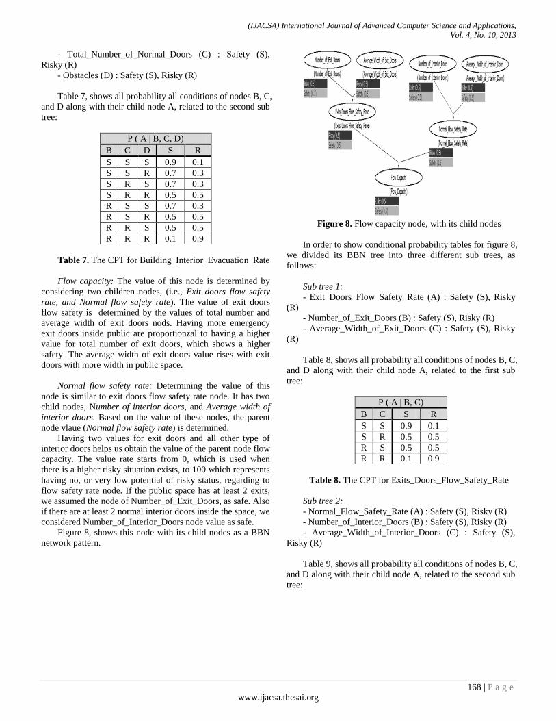
- Total_Number_of_Normal_Doors (C) : Safety (S),
Risky (R)
- Obstacles (D) : Safety (S), Risky (R)
Table 7, shows all probability all conditions of nodes B, C,
and D along with their child node A, related to the second sub
tree:
P ( A | B, C, D)
B C D S R
S S S 0.9 0.1
S S R 0.7 0.3
S R S 0.7 0.3
S R R 0.5 0.5
R S S 0.7 0.3
R S R 0.5 0.5
R R S 0.5 0.5
R R R 0.1 0.9
Table 7. The CPT for Building_Interior_Evacuation_Rate
Flow capacity: The value of this node is determined by
considering two children nodes, (i.e., Exit doors flow safety
rate, and Normal flow safety rate). The value of exit doors
flow safety is determined by the values of total number and
average width of exit doors nods. Having more emergency
exit doors inside public are proportionzal to having a higher
value for total number of exit doors, which shows a higher
safety. The average width of exit doors value rises with exit
doors with more width in public space.
Normal flow safety rate: Determining the value of this
node is similar to exit doors flow safety rate node. It has two
child nodes, Number of interior doors, and Average width of
interior doors. Based on the value of these nodes, the parent
node vlaue (Normal flow safety rate) is determined.
Having two values for exit doors and all other type of
interior doors helps us obtain the value of the parent node flow
capacity. The value rate starts from 0, which is used when
there is a higher risky situation exists, to 100 which represents
having no, or very low potential of risky status, regarding to
flow safety rate node. If the public space has at least 2 exits,
we assumed the node of Number_of_Exit_Doors, as safe. Also
if there are at least 2 normal interior doors inside the space, we
considered Number_of_Interior_Doors node value as safe.
Figure 8, shows this node with its child nodes as a BBN
network pattern.
Figure 8. Flow capacity node, with its child nodes
In order to show conditional probability tables for figure 8,
we divided its BBN tree into three different sub trees, as
follows:
Sub tree 1:
- Exit_Doors_Flow_Safety_Rate (A) : Safety (S), Risky
(R)
- Number_of_Exit_Doors (B) : Safety (S), Risky (R)
- Average_Width_of_Exit_Doors (C) : Safety (S), Risky
(R)
Table 8, shows all probability all conditions of nodes B, C,
and D along with their child node A, related to the first sub
tree:
P ( A | B, C)
B C S R
S S 0.9 0.1
S R 0.5 0.5
R S 0.5 0.5
R R 0.1 0.9
Table 8. The CPT for Exits_Doors_Flow_Safety_Rate
Sub tree 2:
- Normal_Flow_Safety_Rate (A) : Safety (S), Risky (R)
- Number_of_Interior_Doors (B) : Safety (S), Risky (R)
- Average_Width_of_Interior_Doors (C) : Safety (S),
Risky (R)
Table 9, shows all probability all conditions of nodes B, C,
and D along with their child node A, related to the second sub
tree:
(IJACSA) International Journal of Advanced Computer Science and Applications, Vol. 4, No. 10, 2013
168 | P a g e www.ijacsa.thesai.org
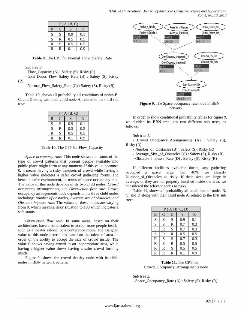
P ( A | B, C)
B C S R
S S 0.9 0.1
S R 0.5 0.5
R S 0.5 0.5
R R 0.1 0.9
Table 9. The CPT for Normal_Flow_Safety_Rate
Sub tree 3:
- Flow_Capacity (A) : Safety (S), Risky (R)
- Exit_Doors_Flow_Safety_Rate (B) : Safety (S), Risky
(R)
- Normal_Flow_Safety_Rate (C) : Safety (S), Risky (R)
Table 10, shows all probability all conditions of nodes B,
C, and D along with their child node A, related to the third sub
tree:
P ( A | B, C)
B C S R
S S 0.9 0.1
S R 0.5 0.5
R S 0.5 0.5
R R 0.1 0.9
Table 10. The CPT for Flow_Capacity
Space occupancy rate: This node shows the status of the
type of crowd patterns that present people available into
public place might form at any moment. If this value becomes
0, it means having a risky banquets of crowd while having a
higher value indicates a safer crowd gathering forms, and
hence a safer environment, in terms of space occupancy rate.
The value of this node depends of its two child nodes, Crowd
occupancy arrangements, and Obstruction flow rate. Crowd
occupancy arrangements node depends on its three child nodes
including: Number of obstacles, Average size of obstacles, and
Obstacle impasse rate. The values of these nodes are varying
from 0, which means a risky situation to 100 which indicates a
safe status.
Obstruction flow rate: In some areas, based on their
architecture, have a better talent to accept more people inside,
such as a theater saloon, or a conference room. The assigned
value to this node determines based on the talent of area, in
order of the ability to accept the size of crowd inside. The
value 0 shows having crowd in an inappropriate area, while
having a higher value shows having a safer crowd forming
inside.
Figure 9, shows the crowd density node with its child
nodes in BBN network pattern.
Figure 9. The Space occupancy rate node in BBN
network
In order to show conditional probability tables for figure 9,
we divided its BBN tree into two different sub trees, as
follows:
Sub tree 1:
- Crowd_Occupancy_Arrangements (A) : Safety (S),
Risky (R)
- Number_of_Obstacles (B) : Safety (S), Risky (R)
- Average_Size_of_Obstacles (C) : Safety (S), Risky (R)
- Obstacle_Impasse_Rate (D) : Safety (S), Risky (R)
If different facilities available during any gathering
occupied a space larger than 40%, we classify
Number_of_Obstacles as risky. If their sizes are large in
average, or they are not properly installed inside the area, we
considered the relevant nodes as risky.
Table 11, shows all probability all conditions of nodes B,
C, and D along with their child node A, related to the first sub
tree:
P ( A | B, C, D)
B C D S R
S S S 0.9 0.1
S S R 0.7 0.3
S R S 0.7 0.3
S R R 0.5 0.5
R S S 0.7 0.3
R S R 0.5 0.5
R R S 0.5 0.5
R R R 0.1 0.9
Table 11. The CPT for
Crowd_Occupancy_Arrangements node
Sub tree 2:
- Space_Occupancy_Rate (A) : Safety (S), Risky (R)
(IJACSA) International Journal of Advanced Computer Science and Applications, Vol. 4, No. 10, 2013
169 | P a g e www.ijacsa.thesai.org
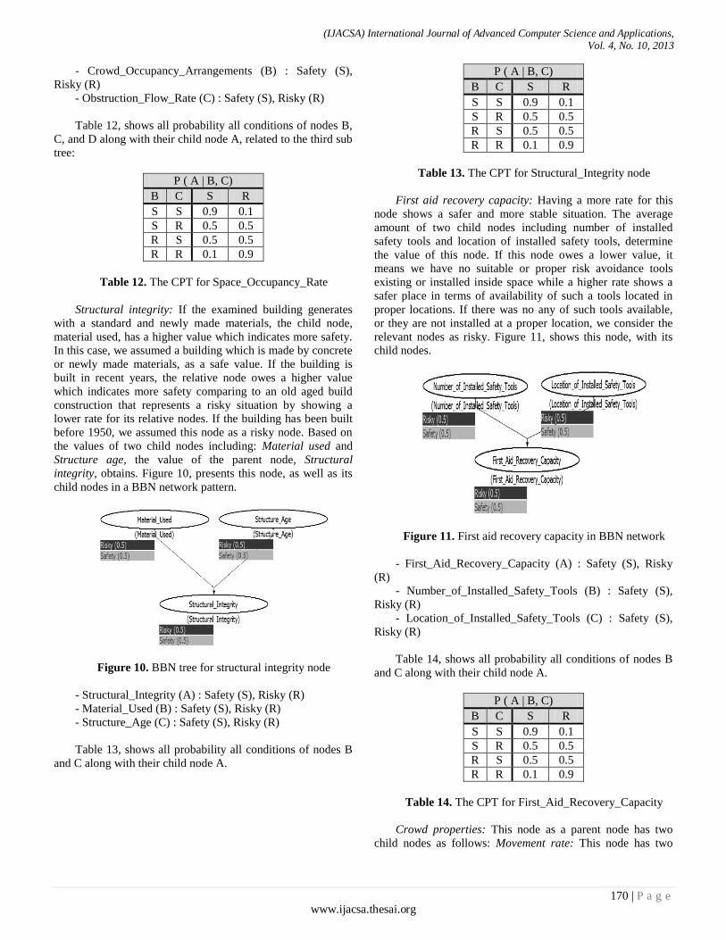
- Crowd_Occupancy_Arrangements (B) : Safety (S),
Risky (R)
- Obstruction_Flow_Rate (C) : Safety (S), Risky (R)
Table 12, shows all probability all conditions of nodes B,
C, and D along with their child node A, related to the third sub
tree:
P ( A | B, C)
B C S R
S S 0.9 0.1
S R 0.5 0.5
R S 0.5 0.5
R R 0.1 0.9
Table 12. The CPT for Space_Occupancy_Rate
Structural integrity: If the examined building generates
with a standard and newly made materials, the child node,
material used, has a higher value which indicates more safety.
In this case, we assumed a building which is made by concrete
or newly made materials, as a safe value. If the building is
built in recent years, the relative node owes a higher value
which indicates more safety comparing to an old aged build
construction that represents a risky situation by showing a
lower rate for its relative nodes. If the building has been built
before 1950, we assumed this node as a risky node. Based on
the values of two child nodes including: Material used and
Structure age, the value of the parent node, Structural
integrity, obtains. Figure 10, presents this node, as well as its
child nodes in a BBN network pattern.
Figure 10. BBN tree for structural integrity node
- Structural_Integrity (A) : Safety (S), Risky (R)
- Material_Used (B) : Safety (S), Risky (R)
- Structure_Age (C) : Safety (S), Risky (R)
Table 13, shows all probability all conditions of nodes B
and C along with their child node A.
P ( A | B, C)
B C S R
S S 0.9 0.1
S R 0.5 0.5
R S 0.5 0.5
R R 0.1 0.9
Table 13. The CPT for Structural_Integrity node
First aid recovery capacity: Having a more rate for this
node shows a safer and more stable situation. The average
amount of two child nodes including number of installed
safety tools and location of installed safety tools, determine
the value of this node. If this node owes a lower value, it
means we have no suitable or proper risk avoidance tools
existing or installed inside space while a higher rate shows a
safer place in terms of availability of such a tools located in
proper locations. If there was no any of such tools available,
or they are not installed at a proper location, we consider the
relevant nodes as risky. Figure 11, shows this node, with its
child nodes.
Figure 11. First aid recovery capacity in BBN network
- First_Aid_Recovery_Capacity (A) : Safety (S), Risky
(R)
- Number_of_Installed_Safety_Tools (B) : Safety (S),
Risky (R)
- Location_of_Installed_Safety_Tools (C) : Safety (S),
Risky (R)
Table 14, shows all probability all conditions of nodes B
and C along with their child node A.
P ( A | B, C)
B C S R
S S 0.9 0.1
S R 0.5 0.5
R S 0.5 0.5
R R 0.1 0.9
Table 14. The CPT for First_Aid_Recovery_Capacity
Crowd properties: This node as a parent node has two
child nodes as follows: Movement rate: This node has two
(IJACSA) International Journal of Advanced Computer Science and Applications, Vol. 4, No. 10, 2013
170 | P a g e www.ijacsa.thesai.org
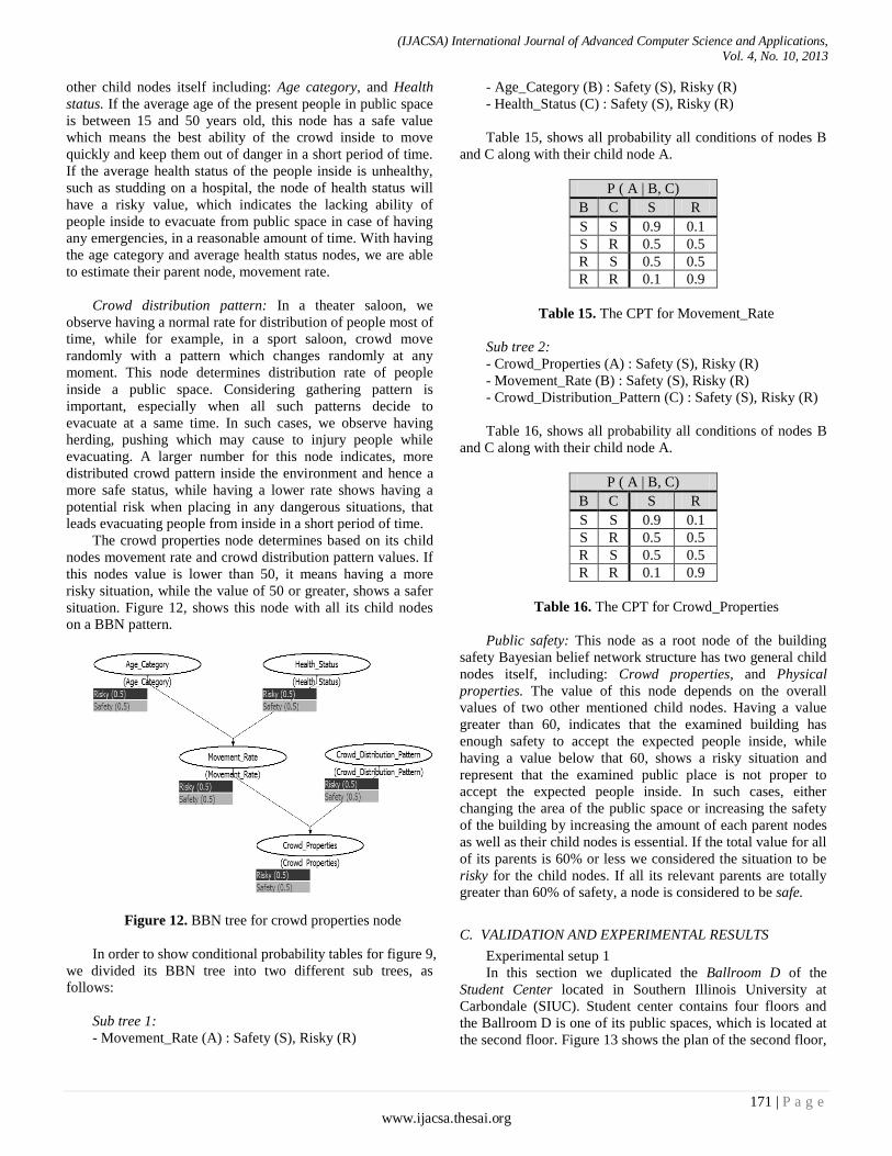
other child nodes itself including: Age category, and Health
status. If the average age of the present people in public space
is between 15 and 50 years old, this node has a safe value
which means the best ability of the crowd inside to move
quickly and keep them out of danger in a short period of time.
If the average health status of the people inside is unhealthy,
such as studding on a hospital, the node of health status will
have a risky value, which indicates the lacking ability of
people inside to evacuate from public space in case of having
any emergencies, in a reasonable amount of time. With having
the age category and average health status nodes, we are able
to estimate their parent node, movement rate.
Crowd distribution pattern: In a theater saloon, we
observe having a normal rate for distribution of people most of
time, while for example, in a sport saloon, crowd move
randomly with a pattern which changes randomly at any
moment. This node determines distribution rate of people
inside a public space. Considering gathering pattern is
important, especially when all such patterns decide to
evacuate at a same time. In such cases, we observe having
herding, pushing which may cause to injury people while
evacuating. A larger number for this node indicates, more
distributed crowd pattern inside the environment and hence a
more safe status, while having a lower rate shows having a
potential risk when placing in any dangerous situations, that
leads evacuating people from inside in a short period of time.
The crowd properties node determines based on its child
nodes movement rate and crowd distribution pattern values. If
this nodes value is lower than 50, it means having a more
risky situation, while the value of 50 or greater, shows a safer
situation. Figure 12, shows this node with all its child nodes
on a BBN pattern.
Figure 12. BBN tree for crowd properties node
In order to show conditional probability tables for figure 9,
we divided its BBN tree into two different sub trees, as
follows:
Sub tree 1:
- Movement_Rate (A) : Safety (S), Risky (R)
- Age_Category (B) : Safety (S), Risky (R)
- Health_Status (C) : Safety (S), Risky (R)
Table 15, shows all probability all conditions of nodes B
and C along with their child node A.
P ( A | B, C)
B C S R
S S 0.9 0.1
S R 0.5 0.5
R S 0.5 0.5
R R 0.1 0.9
Table 15. The CPT for Movement_Rate
Sub tree 2:
- Crowd_Properties (A) : Safety (S), Risky (R)
- Movement_Rate (B) : Safety (S), Risky (R)
- Crowd_Distribution_Pattern (C) : Safety (S), Risky (R)
Table 16, shows all probability all conditions of nodes B
and C along with their child node A.
P ( A | B, C)
B C S R
S S 0.9 0.1
S R 0.5 0.5
R S 0.5 0.5
R R 0.1 0.9
Table 16. The CPT for Crowd_Properties
Public safety: This node as a root node of the building
safety Bayesian belief network structure has two general child
nodes itself, including: Crowd properties, and Physical
properties. The value of this node depends on the overall
values of two other mentioned child nodes. Having a value
greater than 60, indicates that the examined building has
enough safety to accept the expected people inside, while
having a value below that 60, shows a risky situation and
represent that the examined public place is not proper to
accept the expected people inside. In such cases, either
changing the area of the public space or increasing the safety
of the building by increasing the amount of each parent nodes
as well as their child nodes is essential. If the total value for all
of its parents is 60% or less we considered the situation to be
risky for the child nodes. If all its relevant parents are totally
greater than 60% of safety, a node is considered to be safe.
C. VALIDATION AND EXPERIMENTAL RESULTS
Experimental setup 1
In this section we duplicated the Ballroom D of the
Student Center located in Southern Illinois University at
Carbondale (SIUC). Student center contains four floors and
the Ballroom D is one of its public spaces, which is located at
the second floor. Figure 13 shows the plan of the second floor,
(IJACSA) International Journal of Advanced Computer Science and Applications, Vol. 4, No. 10, 2013
171 | P a g e www.ijacsa.thesai.org
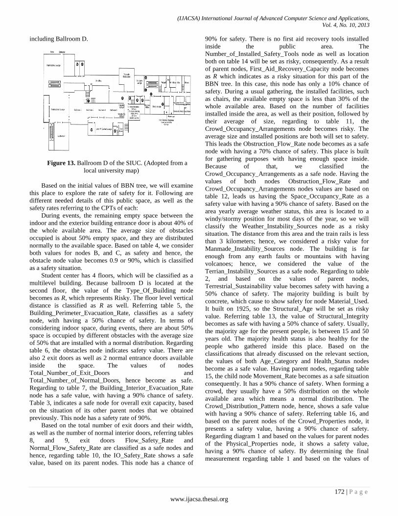
including Ballroom D.
Figure 13. Ballroom D of the SIUC. (Adopted from a
local university map)
Based on the initial values of BBN tree, we will examine
this place to explore the rate of safety for it. Following are
different needed details of this public space, as well as the
safety rates referring to the CPTs of each:
During events, the remaining empty space between the
indoor and the exterior building entrance door is about 40% of
the whole available area. The average size of obstacles
occupied is about 50% empty space, and they are distributed
normally to the available space. Based on table 4, we consider
both values for nodes B, and C, as safety and hence, the
obstacle node value becomes 0.9 or 90%, which is classified
as a safety situation.
Student center has 4 floors, which will be classified as a
multilevel building. Because ballroom D is located at the
second floor, the value of the Type_Of_Building node
becomes as R, which represents Risky. The floor level vertical
distance is classified as R as well. Referring table 5, the
Building_Perimeter_Evacuation_Rate, classifies as a safety
node, with having a 50% chance of safety. In terms of
considering indoor space, during events, there are about 50%
space is occupied by different obstacles with the average size
of 50% that are installed with a normal distribution. Regarding
table 6, the obstacles node indicates safety value. There are
also 2 exit doors as well as 2 normal entrance doors available
inside the space. The values of nodes
Total_Number_of_Exit_Doors and
Total_Number_of_Normal_Doors, hence become as safe.
Regarding to table 7, the Building_Interior_Evacuation_Rate
node has a safe value, with having a 90% chance of safety.
Table 3, indicates a safe node for overall exit capacity, based
on the situation of its other parent nodes that we obtained
previously. This node has a safety rate of 90%.
Based on the total number of exit doors and their width,
as well as the number of normal interior doors, referring tables
8, and 9, exit doors Flow_Safety_Rate and
Normal_Flow_Safety_Rate are classified as a safe nodes and
hence, regarding table 10, the IO_Safety_Rate shows a safe
value, based on its parent nodes. This node has a chance of
90% for safety. There is no first aid recovery tools installed
inside the public area. The
Number_of_Installed_Safety_Tools node as well as location
both on table 14 will be set as risky, consequently. As a result
of parent nodes, First_Aid_Recovery_Capacity node becomes
as R which indicates as a risky situation for this part of the
BBN tree. In this case, this node has only a 10% chance of
safety. During a usual gathering, the installed facilities, such
as chairs, the available empty space is less than 30% of the
whole available area. Based on the number of facilities
installed inside the area, as well as their position, followed by
their average of size, regarding to table 11, the
Crowd_Occupancy_Arrangements node becomes risky. The
average size and installed positions are both will set to safety.
This leads the Obstruction_Flow_Rate node becomes as a safe
node with having a 70% chance of safety. This place is built
for gathering purposes with having enough space inside.
Because of that, we classified the
Crowd_Occupancy_Arrangements as a safe node. Having the
values of both nodes Obstruction_Flow_Rate and
Crowd_Occupancy_Arrangements nodes values are based on
table 12, leads us having the Space_Occupancy_Rate as a
safety value with having a 90% chance of safety. Based on the
area yearly average weather status, this area is located to a
windy/stormy position for most days of the year, so we will
classify the Weather_Instability_Sources node as a risky
situation. The distance from this area and the train rails is less
than 3 kilometers; hence, we considered a risky value for
Manmade_Instability_Sources node. The building is far
enough from any earth faults or mountains with having
volcanoes; hence, we considered the value of the
Terrian_Instability_Sources as a safe node. Regarding to table
2, and based on the values of parent nodes,
Terrestrial_Sustainability value becomes safety with having a
50% chance of safety. The majority building is built by
concrete, which cause to show safety for node Material_Used.
It built on 1925, so the Structural_Age will be set as risky
value. Referring table 13, the value of Structural_Integrity
becomes as safe with having a 50% chance of safety. Usually,
the majority age for the present people, is between 15 and 50
years old. The majority health status is also healthy for the
people who gathered inside this place. Based on the
classifications that already discussed on the relevant section,
the values of both Age_Category and Health_Status nodes
become as a safe value. Having parent nodes, regarding table
15, the child node Movement_Rate becomes as a safe situation
consequently. It has a 90% chance of safety. When forming a
crowd, they usually have a 50% distribution on the whole
available area which means a normal distribution. The
Crowd_Distribution_Pattern node, hence, shows a safe value
with having a 90% chance of safety. Referring table 16, and
based on the parent nodes of the Crowd_Properties node, it
presents a safety value, having a 90% chance of safety.
Regarding diagram 1 and based on the values for parent nodes
of the Physical_Properties node, it shows a safety value,
having a 90% chance of safety. By determining the final
measurement regarding table 1 and based on the values of
(IJACSA) International Journal of Advanced Computer Science and Applications, Vol. 4, No. 10, 2013
172 | P a g e www.ijacsa.thesai.org

parent nodes Physica_Properties and Crowd_Properties, the
value of the child node Public_Safety node will be determine.
This node reflects a safety measure, having a 90% chance of
safety.
Experimental setup 2
In contrast to our first experiment, our second experiment
exhibits a contradictory instance for our protocol. We
considered the Hyatt regency walkway located in Hyatt
regency Kansas City in Kansas City, Missouri. In Kansas City
the walkway collapsed and fell two connected walkways while
they are occupied with a large group of attendance in the
lobby holding a tea dance area below. It caused over 114
people to lose their lives and more than 216 other people to be
injured. The incident occurred in July 17, 1981 and it was
known as the deadliest structural collapse in U.S. history until
2001, when the buildings of world trade center collapsed due
to the infamous 9/11 terrorist attacks. We applied our model to
the Hyatt building for the purpose of validating our model. It
demonstrates dangerous and unreliable situations for that
building based on available specifications related to it.
Considering people as obstacles since a large group of people
were attending that building most of the times. Therefore
obstacle nodes show a risky situation. The nodes of
Type_of_Building and Floor_Level are both risky based on
the building specification and hence
Building_Preimeter_Evacuation_Rate is determined to be
risky. The only way to reach the exit doors were located at
two sides if the hallways. Consequently,
Building_Interior_Evacuation_Rate which depends on
obstacles and total number of exit and normal doors is
considered risky. As a result, Overal_Exit_Capacity is risky.
The Flow_Capacity node shows a risky situation because all
its children nodes are indicating risky situations. The
Space_Occupancy_Rate is risky because of the large number
of people who were present in the building most of times.
Since the hallways were not equipped with proper numbers of
first aid recovery tools and hence the relevant nodes are risky.
Two nodes of Terrestrial_Sustainability and
Structural_Integrity exhibit safety because there were not
major sources of vibrating sources around the building and
also the building collapsed shortly after opening to the people.
Figure 14 shows the earthquakes status around Kansas City.
Figure 14. Earthquakes status around Kansas City
Adapted from www.greatdreams.com/madrid.htm
Regarding to diagram 1, since we have 4 risky and 2 safe
situations, the status for the Physical_Properties node becomes
risky with 70% chance of risky. The Age_Category node is
risky, however the Health_Status node is safe, and the
Movement_Rate node value becomes safety with 50% chance
of safety. The Crowd_Distribution_Pattern node is risky,
because there was no any particular arrang ement among the
people who were present at the hallways. The
Crowd_Properties node is safe with the 50% chance of safety.
In this case, because the other major node (i.e.,
Physical_Properties) has a 70% chance of lack of safety, the
final result of the building safety is determined to be risky.
V. CONSTRUCTING OF BAYESIEN BELIEF
NETWORKS
This paper employed Bayesian belief networks as the
computational mechanism for evaluating potential risks that
can be determined from unpredictable patterns of crowd
movements in a building. Using Bayesian belief network as a
tool we are able to predict the probability of building faults
from a large group of people. We focused on pertinent
attributes of the environment and the people contributing to
potential risks. It is essential to have such a mechanism
wherever a large group of people congregate in indoor public
spaces especially when the space is located on upper levels of
the building. This will help security personnel to determine
strategies for guiding people to safety. This can prevent
potential risk that can occur due to movements in emergencies
from damage from excess weight on structures.
REFERENCES
[1] Barnett, G. O., Famiglietti, K T., Kim, R. J., Hoffer, E. P., Feldman, M.J., 1998. DXplain on the Internet. In American Medical Informatics Association 1998 Annual Symposium.
[2] Bellomo, N., Dogbe, C., (2011), “On the Modeling of Traffic and Crowds: A Survey of Models, Speculations, and Perspectives”, In SIAM REVIEW c 2011 Society for Industrial and Applied Mathematics, Vol.
(IJACSA) International Journal of Advanced Computer Science and Applications, Vol. 4, No. 10, 2013
173 | P a g e www.ijacsa.thesai.org

53, No. 3, pp. 409–463, Society for Industrial and Applied Mathematics pub.
[3] Berler, A., Shimony, S.E., (1997), "Bayes Networks for Sonar Sensor Fusion", In Geiger, D, Shenoy, P (eds) 1997. Proceedings of the Thirteenth Conference on Uncertainty in Artificial Intelligence Morgan Kaufmann.
[4] Colombo, R., Goatin, P., Rosini, M., (2010), “A Macroscopic Model of Pedestrian Flows in Panic Situations”, In Current Advances in Nonlinear Analysis and Related Topics, pp.43–60, Mathematical Sciences and Applications, Gakuto Pub.
[5] Cooper, G.F., (1984), “NESTOR: A computer-based medical diagnostic aid that integrates causal and probabilistic knowledge”, In Ph.D. dissertation, Medical Information Sciences, Stanford University.
[6] Cooper, G.F., (1987), “Probabiistic inference using belief networks is NP-hard”, In Technical Report KSL-87-27, Medical Computer Science Group, Stanford University.
[7] Cooper, G.F., Herskovits, E., (1992), "A Bayesian Method for the Induction of Probabilistic Networks from Data", In Machine Learning Vol. 9 pp. 309-347.
[8] Davies, T.R., Russell, S.J., (1987), “A logical approach to reasoning by analogy”, In IJCAI 10 (pp. 264–270).
[9] Dempster, A.P., Laird, N.M., Rubin, D.B., (1977), "Maximum Likelihood from Incomplete Data via the EM Algorithm with discussion", In Journal of the Royal Statistical Society, Series B, Vol. 39 pp.1-38.
[10] Dogbe, C., (2010), “On the Cauchy problem for macroscopic model of pedestrian flows”, In J. Math. Anal. Appl. 372, (2010), 77-85, Elsevier pub.
[11] Duda, R.O., Hart, P.E., Nilsson, N.J., (1976), “Subjective Bayesian methods for rule-based inference systems”, In Proceedings of the 1976 National Computer Conference (AFIPS Press), pp. 1075-1082.
[12] Etxeberria, R., Larranaga, P., Pikaza, J.M., (1997), "Analysis of the behaviour of the genetic algorithms when searching Bayesian networks from data", In Pattern Recognition Letters Vol. 18 No 11-13 pp 1269-1273
[13] Ezawa, K.J., Schuermann, T., (1995), "Fraud/Uncollectible Debt Detection Using a Bayesian Network Based Learning System: A Rare Binary Outcome with Mixed Data Structures", In Besnard, P, Hanks, S (eds) Proceedings of the Eleventh Conference on Uncertainty in Artificial Intelligence Morgan Kaufmann.
[14] Frey, B.J., (1998), “Graphical Models for Machine Learning and Digital Communication”, In MIT Press.
[15] Friedman, N., (1998), "The Bayesian Structural EM Algorithm", In Cooper, GF, Moral, S (eds) Proceedings of the Fourteenth Conference on Uncertainty in Artificial Intelligence Morgan Kaufmann.
[16] Gawronski, P., Kulakowski, K., (2011), “Crowd dynamics - being stuck”, In Computer Physics Communications Vol. 182, No. 9, pp. 1924-1927.
[17] Good, I.J., (1961-62), “A causal calculus (I & II)”, In British Journal of the Philosophy of Science l1: 305-318 12: 43-51.
[18] Helm, L., (1996), " Improbable Inspiration", In Los Angeles Times, October 28, 1996.
[19] Henein, C., White, T., (2010), “Microscopic information processing and communication in crowd dynamics”, In Physica A(389), pp. 4636-4653, Elsevier Pub.
[20] Howard, R.A., Matheson, J.E., (1984), “Influence Diagrams”, In Howard, R.A. and Matheson, J.E. (eds.), The Principles and Applications of Decision Analysis, (Strategic Decisions Group, Menlo Park, CA), pp. 721-762.
[21] Jensen, F.V., (1996), “An Introduction to Bayesian Networks”, In UCL Press.
[22] Jiang, Y., Zhang, P., Wong, S.C., Liu, R., (2010), “A higher-order macroscopic model for pedestrian flow”, In Physica A: Statistical Mechanics and its Applications, Volume 389, Issue 21, 1 November 2010, Pages 4623-4635, Elsevier pub.
[23] Korhonen, T., Heliovaara, S., Hostikkaa, S., Ehtamo, H., (2010). “Counterflow Model for Agent-Based Simulation of Crowd Dynamics”, In Safety Science.
[24] Krause, P., Clark, D., (1993), “Representing Uncertain Knowledge: An Artificial Intelligence Approach”, In Intellect Books.
[25] Larranaga, P., Kuijpers, C.M.H., Murga, R.H., Yurramendi, Y., (1996), "Learning Bayesian network structures by searching for the best ordering with genetic algorithms", In IEEE Trans on Systems, Man and Cybernetics-A Vol. 26 No. 4 pp.487- 493.
[26] Lauritzen, S.L., Spiegelhalter, D.J., (1988), "Local computations with probabilities on graphical structures and their application to expert systems", In Journal of the Royal Statistical Society, Vol. 50 No. 2 pp.157-224.
[27] Lauritzen, S.L., Wermuth, N., (1989), “Graphical models for associations between variables, some of which are qualitative and some quantitative”, In Annals of Statistics 17, 31–57.
[28] Mitchell, T.M., (1997), “Machine Learning”, In McGraw-Hill.
[29] Narendra, P.M., Fukunaga, K., (1977), "A Branch and Bound Algorithm for Feature Subset Selection", In IEEE Transactions on Computers, Vol. 26, No. 9, pp. 917-922.
[30] Neil, M., Littlewood, B., Fenton, N., (1996), "Applying Bayesian Belief Networks to Systems Dependability Assessment", In Proceedings of Safety Critical Systems Club Symposium, Leeds, 6-8 February 1996 Springer-Verlag.
[31] Patil, S., Van den Berg, J., Curtis, S., Lin, M., Manocha, D., (2011), “Directing Crowd Simulations Using Navigation Fields”, In IEEE Transactions on Visualization and Computer Graphics, vol. 17(2), pp. 244-254, IEEE press.
[32] Pearl, J., (1986), “Fusion, propagation and structuring in belief networks”, In Artificial Intelligence 29 241-288.
[33] Pearl, J., (1988), “Probabilistic Reasoning in Intelligent Systems: networks of plausible inference”, In Morgan Kaufmann.
[34] Peacock, R.D., Kuligowski, E.D., Averill, J.D., (Eds), (2011), “Pedestrian and Evacuation Dynamics”, In Springer pub.
[35] Pires, T.T., 2005. An approach for modeling human cognitive behavior in evacuation models, In Fire Safety Journal, Vol. 40, No. 2, March 2005, Pages 177–189, Elsevier Pub.
[36] Rousseau, W.F., (1968), “A method for computing probabilities”, In complex situations, Technical Report 6252-2, Stanford University Center for Systems Research.
[37] Shachter, R.D., (1986), “Intelligence Probabilistic inference”, In Kanal, L.N., Lemmer, J.F. (eds.), Uncertainly in Artificial Intelligence (North-Holland, Amsterdam), pp. 371-382.
[38] Shendarkarb, A., Vasudevana, K., Leea, S., Son, Y., 2008. Crowd simulation for emergency response using BDI agents based on immersive virtual reality, Simulation Modeling Practice and Theory, Vol. 16, No. 9, Pages 1415–1429, Elsevier Pub.
[39] Shiwakoti, N., Sarvi, M., Rose, G., Burd, M., (2011), “Animal dynamics based approach for modeling pedestrian crowd egress under panic conditions”, In Transpostation Research B, pp. 1-17, Elsevier Pub.
[40] Steffen, B., Seyfried, A., (2010), “Methods for measuring pedestrian density, flow, speed and direction with minimal scatter”, In Physica A 389, pp. 1902-1910, Elsevier.
[41] Trautman, P., Krause, A., 2010. Unfreezing the Robot: Navigation in Dense, Interacting Crowds, IROS proceedings, pp. 797-803, IEEE press.
[42] Weiss, S.M., Kulikowski, C.A., Amarel, S., Safir, A., (1978), “A model-based method for computer-aided medical decision making”, In Artificial Intelligence l1 145-172.
[43] Zheng, X., Cheng, Y., (2011), “Modeling cooperative and competitive behaviors in emergency evacuation: A game-theoretical approach”, In Computers & Mathematics with Applications, Vol. 62, No. 12, p. 4627-4634, Elsevier.
(IJACSA) International Journal of Advanced Computer Science and Applications, Vol. 4, No. 10, 2013
174 | P a g e www.ijacsa.thesai.org
Terrain Coverage Ant Algorithms:The Random Kick Effect
M. DervisiComputer Science Department,
IST College Athens, Greecein collaboration with
University of Hertfordshire, UKE-mail: [email protected]
O.B. EfremidesComputer Science Department,
IST College Athens, Greecein collaboration with
University of Hertfordshire, UKE-mail: [email protected]
D.P. IracleousComputer Science Department,
IST College Athens, Greecein collaboration with
University of Hertfordshire, UKE-mail: [email protected]
Abstract—In this work the effect of random repositioningof ant robots/agents on the performance of terrain coveragealgorithms is investigated. A number of well-known terraincoverage algorithms are implemented and studied in a simulatedenvironment. We prove that agent repositioning imposes smallvariations on the performance of the algorithms when randomor controlled jumps occurred and evaporation and failures areallowed.
Keywords—Terrain coverage, ant agents, performance
I. INTRODUCTION
Terrain coverage algorithms using ant robots/agents [1],[2], [3] is under investigation in this work. We focus on thejump effect of agents during the execution of the algorithms.This effect can be defined as an unexpected fast move of theagent, from its current position to a new one, in a way thatis not defined by the terrain coverage algorithm. This is, forexample, the case that visitors of a museum accidentally kickthe surveillance ant robots.
Resulting functional algorithms can have applications ineveryday use, such as vacuum cleaning a large area [4], [5].Moreover, they can also be applied in critical emergency cases,like searching the terrain of a collapsed mine, patrolling asecure area, etc.
The key point in this work is that the executing algorithmshould be able to complete the assigned task, even if the terrainor the agents are abruptly affected by natural phenomena, thehuman factor, a sudden failure, the presence of obstacles in thearea etc. In any case, this should be as efficient as possible.
Throughout this work, jump is applied on well know terraincoverage algorithms [6], [7], various terrain types and initialagent positions. In all cases the objective is to examine theperformance of terrain coverage and how it is affected dueto jump and its combination with the simulation settings.The most important settings include, agent battery drain [3],the probability of agent failures [8] and the evaporation ofpheromone left by agents on the terrain [7], [8].
The algorithms studied in this work, have as their mainpurpose to visit each area or cell of the terrain, at least once[6], [7], [8]. Hence, it can be said that their goal is it toachieve the exploration of unknown areas. These include Node-counting, Recency, Alarm, Learning Real-Time A* (LRTA*),
Online Mapping Algorithms (OMA) and Wagner [9], [3],[10]. Such algorithms have found practical and inexpensiveimplementations in many real life problems [7]. Additionally,a brute force approach using Random walk was also studiedbut was excluded from the main comparisons found in theexperimental results section, as this implementation is of verylow performance. As each of the aforementioned algorithmsfollows a slightly differentiated strategy in the way terrainexploration is achieved, the effects of simulation settings areexamined for each algorithm in case.
This paper is organized as follows. In Section 2 the sixalgorithms under investigation are presented. The setting forthe experiments is given in Section 3 while the simulationresults are discussed in Section 4. Conclusions are drawn inSection 5.
II. THE ALGORITHMS
Six different algorithms are under investigations herein.Node counting:
The node-counting algorithm (also referred to as “count-ing“ later) approaches the terrain coverage in a deterministicmanner since it always chooses to move to the place with theleast number of visits. At each step, each agent moves fromits cell to an adjacent terrain cell, which is the one with thefewest number of visits (by all agents). In the case where thereare more than one cells that have the fewest visits, the ties canbe broken at random [7].
LRTA*: also referred to as “learning” later, is a determin-istic target location algorithm which updates the number ofvisits of the current cell during each step. In this method, thenumber of visits acts as a repellent for each agent [10]. Witheach movement of the ant, the value of the current cell isupdated by taking the number of visits of the adjacent cell (towhich the ant is about to move) and incrementing it by one.In the case where there are more than one cell that have thefewest visits, the ties can be broken at random [11].
Wagner’s: Wagner proposed a deterministic terrain cover-age method that updates the current cell value only if it is lessthan the value of the adjacent cell to which the ant is aboutto move. No update will occur to the current cell if the valueof the current cell is higher than the cell to which the antis moving to. This method is similar to both the LRTA* and
175 | P a g e www.ijacsa.thesai.org
(IJACSA) International Journal of Advanced Computer Science and Applications, Vol. 4, No. 10, 2013
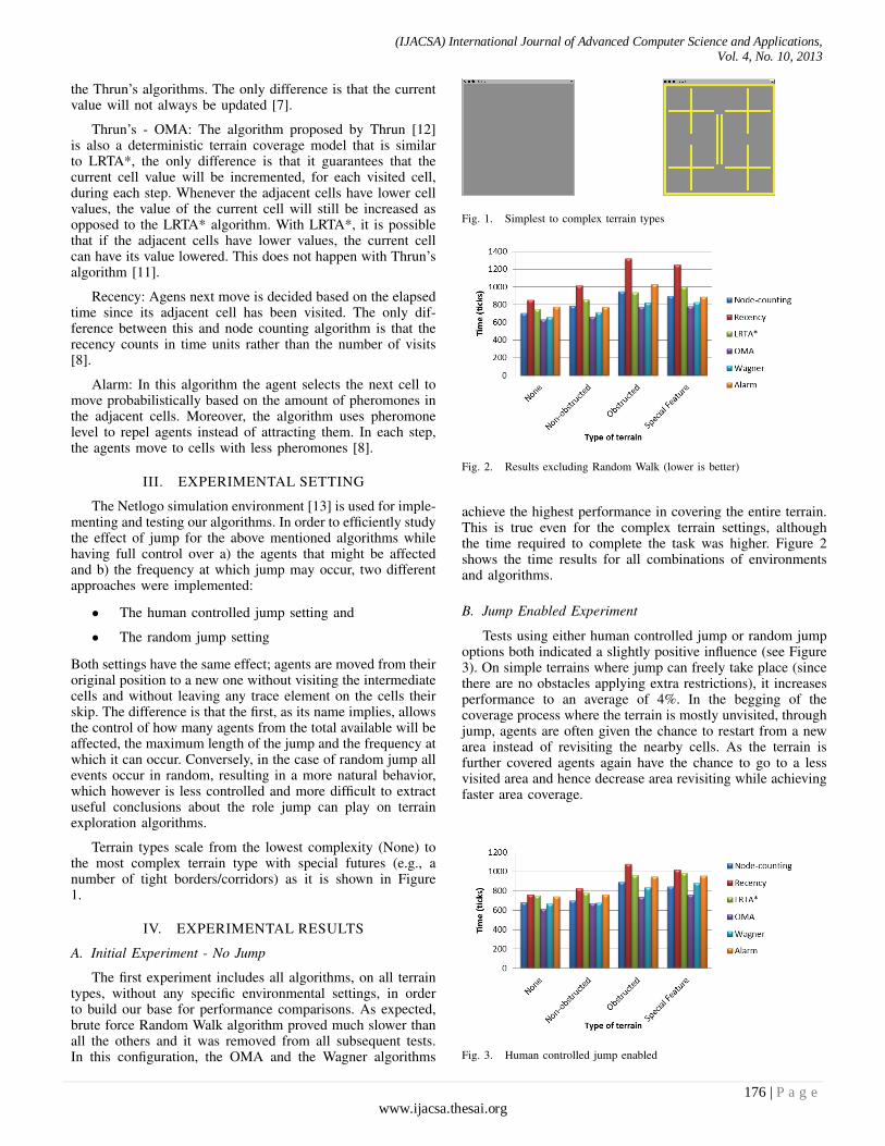
the Thrun’s algorithms. The only difference is that the currentvalue will not always be updated [7].
Thrun’s - OMA: The algorithm proposed by Thrun [12]is also a deterministic terrain coverage model that is similarto LRTA*, the only difference is that it guarantees that thecurrent cell value will be incremented, for each visited cell,during each step. Whenever the adjacent cells have lower cellvalues, the value of the current cell will still be increased asopposed to the LRTA* algorithm. With LRTA*, it is possiblethat if the adjacent cells have lower values, the current cellcan have its value lowered. This does not happen with Thrun’salgorithm [11].
Recency: Agens next move is decided based on the elapsedtime since its adjacent cell has been visited. The only dif-ference between this and node counting algorithm is that therecency counts in time units rather than the number of visits[8].
Alarm: In this algorithm the agent selects the next cell tomove probabilistically based on the amount of pheromones inthe adjacent cells. Moreover, the algorithm uses pheromonelevel to repel agents instead of attracting them. In each step,the agents move to cells with less pheromones [8].
III. EXPERIMENTAL SETTING
The Netlogo simulation environment [13] is used for imple-menting and testing our algorithms. In order to efficiently studythe effect of jump for the above mentioned algorithms whilehaving full control over a) the agents that might be affectedand b) the frequency at which jump may occur, two differentapproaches were implemented:
• The human controlled jump setting and
• The random jump setting
Both settings have the same effect; agents are moved from theiroriginal position to a new one without visiting the intermediatecells and without leaving any trace element on the cells theirskip. The difference is that the first, as its name implies, allowsthe control of how many agents from the total available will beaffected, the maximum length of the jump and the frequency atwhich it can occur. Conversely, in the case of random jump allevents occur in random, resulting in a more natural behavior,which however is less controlled and more difficult to extractuseful conclusions about the role jump can play on terrainexploration algorithms.
Terrain types scale from the lowest complexity (None) tothe most complex terrain type with special futures (e.g., anumber of tight borders/corridors) as it is shown in Figure1.
IV. EXPERIMENTAL RESULTS
A. Initial Experiment - No Jump
The first experiment includes all algorithms, on all terraintypes, without any specific environmental settings, in orderto build our base for performance comparisons. As expected,brute force Random Walk algorithm proved much slower thanall the others and it was removed from all subsequent tests.In this configuration, the OMA and the Wagner algorithms
Fig. 1. Simplest to complex terrain types
Fig. 2. Results excluding Random Walk (lower is better)
achieve the highest performance in covering the entire terrain.This is true even for the complex terrain settings, althoughthe time required to complete the task was higher. Figure 2shows the time results for all combinations of environmentsand algorithms.
B. Jump Enabled Experiment
Tests using either human controlled jump or random jumpoptions both indicated a slightly positive influence (see Figure3). On simple terrains where jump can freely take place (sincethere are no obstacles applying extra restrictions), it increasesperformance to an average of 4%. In the begging of thecoverage process where the terrain is mostly unvisited, throughjump, agents are often given the chance to restart from a newarea instead of revisiting the nearby cells. As the terrain isfurther covered agents again have the chance to go to a lessvisited area and hence decrease area revisiting while achievingfaster area coverage.
Fig. 3. Human controlled jump enabled
176 | P a g e www.ijacsa.thesai.org
(IJACSA) International Journal of Advanced Computer Science and Applications, Vol. 4, No. 10, 2013
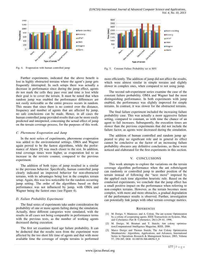
Fig. 4. Evaporation with human controlled jump
Further experiments, indicated that the above benefit islost in highly obstructed terrains where the agent’s jump getsfrequently interrupted. In such setups there was actually adecrease in performance since during the jump effect, agentsdo not mark the cells they pass over and time is lost whiletheir goal is to cover the terrain. It must be noted that whenrandom jump was enabled the performance differences arenot easily noticeable as the entire process occurs in random.This means that since there is no control over the distance,frequency and number of agents that are affected by jump,no safe conclusions can be made. Hence, in all cases thehuman controlled jump provided results that can be more easilypredicted and interpreted, concerning the actual effect of jumpon the terrain coverage process, for the purposes of this work.
C. Pheromone Evaporation and Jump
In the next series of experiments, pheromone evaporationwas added to the environmental settings. OMA and Wagneragain proved to be the fastest algorithms, while the perfor-mance of Alarm [9] was much closer to the rest. In addition,total coverage times were higher, as evaporation led to anincrease in the revisits counter, compared to the previousexperiment.
The addition of both types of jump resulted in a similarto the previous behavior. Specifically, human controlled jumpclearly indicated an improved behavior for non-obstructedterrains, with its advantages being lost in the complex terrainsetup. Again, this was less noticeable for the random occurringjump setting. The order of the algorithms based on theirperformance was not influenced by jump, with OMA andWagner being the fastest ones (see Figure 4).
D. Failure Probability Experiments
The final series of experiments take under consideration theprobability of one or more agents failing during the simulation.Actually, three different categories were simulated, with theresults in all cases not being comparable in performance termswith the previous tests, as the number of working agentsdecreased during execution.
The first set examines fixed age failure probability. It canbe deducted that the results seen from the experiment wereaffected by the too short life time of agents and that with moreavailable time the coverage of simple terrains is performed
Fig. 5. Constant Failure Probability set to 80%
more efficiently. The addition of jump did not affect the results,which were almost similar in simple terrains and slightlyslower in complex ones, when compared to not using jump.
The second sub-experiment series examine the case of theconstant failure probability. OMA and Wagner had the mostdistinguishing performance. In both experiments with jumpenabled, the performance was slightly improved for simpleterrains. In contrast, it was slower for the obstructed terrains.
The final failure experiment included the increasing failureprobability case. This was actually a more aggressive failuresetting, compared to constant, as with time the chance of anagent to fail increases. Subsequently, the execution times areslower than the previous experiments that did not include thefailure factor, as agents were decreased during the simulation.
The addition of human controlled and random jump ap-peared to play no significant role and in general its effectcannot be conclusive as the factor of an increasing failureprobability obscures any definitive conclusions, as these werenoticed and elaborated for the first experiments in this section.
V. CONCLUSIONS
This work attempts to explore the variations on the terraincoverage algorithm performance when the ant robots/agentcan randomly or controlled jump to another position of theterrain instead of following the “next move” imposed bythe applied each time algorithm heuristic rule. Based on theconducted experiments, we conclude that the jump effect hasa small positive impact on the performance when referring tonon-complex terrains. However, as the terrain becomes morecomplex, with more and more obstacles, a gradual degradationof the performance results is observed. Further, investigationcan potentially link jumps with other terrain coverage metrics.
REFERENCES
[1] M. Dorigo, V. Maniezzo, and A. Coloni, The ant system: Optimizationby a colony of cooperating agents. IEEE Transactions on Systems, Man,and Cybernetics Part B: Cybernetics, 26(1):29–41, 1996.
[2] M. Dorigo, M. Birattari and T. Stutzle, Ant colony optimiza-tion,Computational Intelligence Magazine, IEEE, 2006
[3] Marco Dorigo and Thomas Stutzle, The Ant Colony OptimizationMetaheuristic: Algorithms, Applications, and Advances, InternationalSeries in Operations Research & Management Science, 2003, Volume57, 250-285, DOI: 10.1007/0-306-48056-5 9
177 | P a g e www.ijacsa.thesai.org
(IJACSA) International Journal of Advanced Computer Science and Applications, Vol. 4, No. 10, 2013

[4] J. R. VanderHeide and N. S. V. Rao. Terrain coverage of an unknownroom by an autonomous mobile robot. Technical report, Oak RidgeNational Laboratory, Tennessee, United States, 1995.
[5] F. Adler and D. Gordon, Information collection and spread by networksof patrolling ants, The American Naturalist, 140(3):373–400, 1992
[6] Sven Knoenig and Yaxin Liu, Terrain Coverage with Ant Robots: ASimulation Study, College of Computing, Georgia Institute of Technol-ogy, Atlanta, GA 30332-0280, 2001
[7] Jonathan Mason and Ronaldo Menezes, Autonomous Algorithms forTerrain Coverage Metrics, Classification and Evaluation, IEEE Congresson Evolutionary Computation, 2008
[8] Robert Treverton and Ronaldo Menezes, Evaluating Failure in TerrainCoverage by Autonomous Agents, IEEE, 978-1-4244-2753-6, 2009
[9] C. Lloyd. The alarm pheromones of social insects: A review. Technicalreport, Colorado State University, 2003
[10] Eric Bonabeau , Marco Dorigo and Guy Theraulaz, Swarm intelligence:from natural to artificial systems, Oxford University Press, Inc., NewYork, NY, 1999
[11] S. Thrun, Efficient exploration in reinforcement learning. Technical Re-port CMU-CS-92-102, School of Computer Science, Carnegie MellonUniversity, 1992
[12] Howie Choset, Coverage for robotics – A survey of recent results,Annals of Mathematics and Artificial Intelligence Volume 31, Numbers1-4, 113-126, DOI: 10.1023/A:1016639210559
[13] U. Wilensky, Netlogo. Center for Connected Learning and Computer-Based Modeling, Evanston, 1999
178 | P a g e www.ijacsa.thesai.org
(IJACSA) International Journal of Advanced Computer Science and Applications, Vol. 4, No. 10, 2013
Related Documents


