Video Object Tracking using SIFT and Mean Shift Master Thesis in Communication Engineering ZHU CHAOYANG Department of Signals and Systems Signal Processing Group CHALMERS UNIVERSITY OF TECHNOLOGY Göteborg, Sweden, 2011 Report No. Ex005/2011

Welcome message from author
This document is posted to help you gain knowledge. Please leave a comment to let me know what you think about it! Share it to your friends and learn new things together.
Transcript
Video Object Tracking using SIFT and Mean Shift Master Thesis in Communication Engineering ZHU CHAOYANG Department of Signals and Systems Signal Processing Group CHALMERS UNIVERSITY OF TECHNOLOGY Göteborg, Sweden, 2011 Report No. Ex005/2011
Thesis for degree of Master of Science
Video Object Tracking using SIFT and Mean Shift
Chaoyang Zhu
Supervisor and Examinor: Professor Irene Gu
Department of Signal and System, Signal Processing Group, Chalmers University of Technology (CTH), Sweden (Report: Ex005/2011)
Gothenburg, 2011
I
Abstract
Visual object tracking for surveillance applications is an important task in computer vision. Many algorithms and technologies have been developed to automatically monitor pedestrians, traffic or other moving objects. One main difficulty in object tracking, among many others, is to choose suitable features and models for recognizing and tracking the target. Some common choices of features to characterize visual objects are: color, intensity, shape and feature points. In this thesis three methods are studied: mean shift tracking based on the color pdf, optical flow tracking based on the intensity and motion, SIFT and RANSAC tracking based on scale invariant local feature points. Mean shift is then combined with local feature points. Preliminary results from experiments have shown that the adopted method is able to track target with translation, rotation, partial occlusion and deformation.
II
Table of Contents
Abstract .............................................................................................................................. I Table of Contents ............................................................................................................. II Chapter 1. Introduction ..................................................................................................... 1
1.1 Concept of visual object tracking ....................................................................... 1 1.2 Applications of visual object tracking ................................................................ 2 1.3 Difficulties and algorithms ................................................................................. 2 1.4 The structure of this thesis .................................................................................. 3
Chapter 2. Feature Extraction Methods ............................................................................ 4 2.1 SIFT method ....................................................................................................... 4
2.1.1 Concept and features of SIFT .................................................................. 4 2.1.2 Scale-space extrema detection ................................................................. 5 2.1.3 Locating keypoints .................................................................................. 7 2.1.4 SIFT feature representation ..................................................................... 9 2.1.5 Orientation assignment ............................................................................ 9 2.1.6 Keypoint matching ................................................................................ 10
2.2 RANSAC method ............................................................................................. 11 2.2.1 Basics of RANSAC ............................................................................... 11 2.2.2 The RANSAC algorithm ....................................................................... 14 2.2.3 Results from RANSAC ......................................................................... 18
2.3 Mean Shift ........................................................................................................ 18 2.3.1 Basics of Mean Shift ............................................................................. 18 2.3.2 Mean shift algorithm ............................................................................. 20 2.3.3 Results of mean shift tracking ............................................................... 22
2.4 Optical flow method ......................................................................................... 23 2.4.1 Basics of optical flow ............................................................................ 23 2.4.2 Variants of optical flow ......................................................................... 26
Chapter 3. Combined Method ........................................................................................ 28 3.1 Description of the combined method ............................................................... 28 3.2 Algorithm of the combined method ................................................................. 29
Chapter 4. Experimental Results .................................................................................... 33 4.1 Results from SIFT and RANSAC .................................................................... 33 4.2 Results from Mean Shift ................................................................................... 34 4.3 Results from optical flow ................................................................................. 35 4.4 Results from the combined method .................................................................. 36
4.5.1. Discussion ............................................................................................. 38 4.5.2. Conclusion and future work ................................................................. 39
Acknowledgements ........................................................................................................ 42 References ...................................................................................................................... 43
1
Chapter 1. Introduction 1.1 Concept of visual object tracking
Visual object tracking is an important task within the field of computer vision. It aims at locating a moving object or several ones in time using a camera. An algorithm analyses the video frames and outputs the location of moving targets within the video frame. So it can be defined as the process of segmenting an object of interest from a video scene and keeping track of its motion, orientation, occlusion etc. in order to extract useful information by means of some algorithms. Its main task is to find and follow a moving object or several targets in image sequences.
The proliferation of high-powered computers and the increasing need for automated video analysis have generated a great deal of interest in visual object tracking algorithms. The use of visual object tracking is pertinent in the tasks of automated surveillance, traffic monitoring, vehicle navigation, human-computer interaction etc. Automated video surveillance deals with real time observation of people or vehicles in busy or restricted environments leading to tracking and activity analysis of the subjects in the field of view. There are three key steps in video surveillance: detection of interesting moving objects, tracking of such objects from frame to frame, and analysis of object tracks to recognize their behavior.
Visual object tracking follows the segmentation step and is more or less equivalent to the "recognition" step in the image processing. Detection of moving objects in video streams is the first relevant step of information extraction in many computer vision applications. There are basically three approaches in visual object tracking. Feature-based methods aim at extracting characteristics such as points, line segments from image sequences, tracking stage is then ensured by a matching procedure at every time instant. Differential methods are based on the optical flow computation, i.e. on the apparent motion in image sequences, under some regularization assumptions. The third class uses the correlation to measure interimage displacements. Selection of a particular approach largely depends on the domain of the problem.
The development and increased availability of video technology have in recent years inspired a large amount of work on object tracking in video sequences [1]. Many researchers have tried various approaches for object tracking. Nature of the technique used largely depends on the application domain. Some of the research work done in the field of visual object tracking includes, for example:
The block matching technique for object tracking in traffic scenes in [2 ]: A motionless airborne camera is used for video capturing. They have discussed the block matching technique for different resolutions and complexities.
Object tracking algorithm using a moving camera in [3]: The algorithm is based on domain knowledge and motion modeling. Displacement of each point is assigned a discreet probability distribution matrix. Based on the model, image registration step is carried out. The registered image is then compared with the background to track the moving object.
Video surveillance using multiple cameras and camera models in [4]: It uses object features gathered from two or more cameras situated at different locations. These features are then combined for location estimation in video surveillance systems.
Another simple feature based object tracking method is explained in [5]: The method first segments the image into foreground and background to find objects of interest. Then four types of features are gathered for each object of interest. Then for each consecutive frames the changes in features are calculated for various possible
2
directions of movement. The one that satisfies certain threshold conditions is selected as the position of the object in the next frame.
A feedback-based method for object tracking in presence of occlusions in [6]: In this method several performance evaluation measures for tracking are placed in a feedback loop to track non-rigid contours in a video sequence. 1.2 Applications of visual object tracking Visual object tracking has many applications. Some important applications are:
(1) Automated video surveillance: In these applications computer vision system is designed to monitor the movements in an area (shopping malls, car parks, etc.), identify the moving objects and report any doubtful situation. The system needs to discriminate between natural entities and humans, which require a good visual object tracking system.
(2) Robot vision: In robot navigation, the steering system needs to identify different obstacles in the path to avoid collision. If the obstacles themselves are other moving objects then it calls for a real-time visual object tracking system.
(3) Traffic monitoring: In some countries highway traffic is continuously monitored using cameras. Any vehicle that breaks the traffic rules or is involved in other illegal act can be tracked down easily if the surveillance system is supported by an object tracking system.
(4) Animation: Visual object tracking algorithm can also be extended for animation.
(5) Government or military establishments. To sum up, visual object tracking is applied to a wide range of fields nowadays, such as multimedia, video data compression, industry production, military affairs and so on. Accordingly, it is of great real significance and application value to investigate in visual object tracking.
The detection and tracking of motion object in real time image sequences is the important task in image processing, computer vision, mode identification etc. It flexibly combines the technologies of image processing, autocontrol and information science, forms a new technology of real time detection of motion object, extraction location information of the object and tracking of it. Furthermore, rapid progress in technologies of signal processing, sensor and new material provides reliable software and hardware for the capturing and processing of image in real time.
1.3 Difficulties and algorithms
In general, trackers can be subdivided into two categories [7]. First, there are generic trackers which use only a minimum amount of a priori information, e.g., the mean-shift approach by Comaniciu et al. [ 8 ] and the color-based particle filter developed by Perez et al. [9]. Secondly, there are trackers that use a very specific model of the object, like e.g. the spline representation of the contour by Isard et al. [10, 11].
The objects found in video trackers are often being tracked in "difficult" environments characterised by the variable visibility (e.g. shadows, occlusions) and the presence of spurious (e.g. similarly-coloured) objects and backgrounds. As a result, visual object tracking still suffers from a lack of robustness due to temporary occlusions, objects crossing, changing lighting conditions, specularities and out-of-plane rotations. The main difficulty in video tracking is to associate target locations in
3
consecutive video frames, especially when the objects are moving fast relative to the frame rate. Here, video tracking systems usually employ a motion model which describes how the image of the target might change for different possible motions of the object to track.
Many algorithms have been developed and implemented to solve the difficulties that arised from the video tracking process, such as SIFT ( Scale Invariant Feature Transform), KPSIFT (keypoint-preserving-SIFT), PDSIFT (partial-descriptor-SIFT), RANSAC(Random Sample Consensus), mean shift, optical flow, GDOH (gradient distance and orientation histogram) etc. The role of the tracking algorithm is to analyze the video frames in order to estimate the motion parameters. These parameters characterize the location of the target.
1.4 The structure of this thesis
The thesis consists of four chapters, the details are as follows:
In Chapter 1, we explain the concept of visual object tracking and introduce some of the research work done in the field, five aspects of its important applications, the difficulties in visual object tracking, and some algorithms dealing with these issues. The structure of this thesis is also described.
In Chapter 2, we review the current feature generation methods in the field of visual object tracking, including SIFT, RANSAC, mean shift and optical flow. An extensive survey of the concept, characteristics, detection stages, algorithms, experimental results of SIFT as well as advantages of SIFT features are presented. The concept, algorithm of RANSAC, experimental result of using RANSAC and basic affine transforms are dissertated. The basic theory and algorithm of mean shift, density gradient estimation and some experimental results of mean shift tracking are described. The basic theory of optical flow, two kinds of optical flow and experimental results of optical flow are given in the last part.
In Chapter 3, we present an enhanced SIFT and mean shift for object tracking.. The flowchart of algorithmic is included and some experimental results of the integration of mean shift and SIFT feature tracking are presented. Experiment results verified that the proposed method could produce better solutions in object tracking of different scenarios and is an effective visual object tracking algorithm.
In Chapter 4, we discuss the work done in this thesis. Several directions for further research are presented, including: Develop algorithms for tracking objects in unconstrained videos; Efficient algorithms for online estimation of discriminative feature sets; Further study on the online boosting methods for feature selection. Using semi-supervised learning techniques for modeling objects; Modeling the problem using Kalman filter more accurately; Improving the speed of the fitting algorithm in the active appearance model by using multi-resolution; Investigating the convergence property of the proposed framework.
4
Chapter 2. Feature Extraction Methods Visual object tracking is an important topic in multimedia technologies,
particularly in applications such as teleconferencing, surveillance and human–computer interface. The difficulty in visual object tracking process is to find and filter some features that are less sensitive to image translation, scaling, rotation, illumination changes, distortion and partially occlusion. The goal of object tracking is to determine the position of the object in images continuously and reliably against dynamic scenes. To achieve this target, a number of elegant methods have been established.
This thesis has studied several image feature generation methods, including SIFT, RANSAC, mean shift, optical flow. The feature points of SIFT is based on keypoints. RANSAC method is based on parameters of a mathematical model from a set of observed data, mean shift method is based on the kernel and density gradient function, optical flow is based on color or intensity changes.
2.1 SIFT method
2.1.1 Concept and features of SIFT Scale Invariant Feature Transform (SIFT) is an approach for detecting and
extracting local feature descriptors that are reasonably invariant to changes in illumination, scaling, rotation, image noise and small changes in viewpoint. This algorithm is first proposed by David Lowe in 1999, and then further developed and improved [12].
SIFT features have many advantages such as follows: (1) SIFT features are all natual features of images. They are favorably invariant
to image translation, scaling, rotation, illumination, viewpoint, noise etc. (2) Good speciality, rich in information, suitable for fast and exact matching in a
mass of feature database. (3) Fertility. Lots of SIFT features will be explored even if there are only a few
objects. (4) Relatively fast speed. the speed of SIFT even can satisfy real time process
after the SIFT algorithm is optimized. (5) Better expansibility. SIFT is vey convenient to combine with other
eigenvector, and generate much useful information. Detection stages for SIFT features are as follows:
(1) Scale-space extrema detection: The first stage of computation searches over all scales and image locations. It is implemented efficiently by means of a difference-of-Gaussian function to identify potential interest points that are invariant to orientation and scale.
5
(2) Keypoint localization: At each candidate location, a detailed model is fit to determine scale and location. Keypoints are selected on basis of measures of their stability.
(3) Orientation assignment: One or more orientations are assigned to each keypoint location on basis of local image gradient directions. All future operations are performed on image data that has been transformed relative to the assigned scale, orientation, and location for each feature, thereby providing invariance to these transformations.
(4) Generation of keypoint descriptors: The local image gradients are measured at the selected scale in the region around each keypoint. These gradients are transformed into a representation which admits significant levels of local change in illumination and shape distortion.
2.1.2 Scale-space extrema detection Interest points for SIFT features correspond to local extrema of difference-of-Gaussian filters at different scales.
Given a Gaussian-blurred image described as the formula
( , , ) ( , , ) ( , )L x y G x y I x yσ σ= ∗ (2-1)
Where 2 2
2
2
1( , , )2
x y
G x y e σσσ
+−
=Π
(2-2)
(2-2) is a variable scale Gaussian, whose result of convolving an image with a difference-of-Gaussian filter is given by
( , , ) ( , , ) ( , , )D x y L x y k L x yσ σ σ= − (2-3)
Which is just be different from the Gaussian-blurred images at scales and kσ σ .
6
Scale(first octave)
Scale(next octave)
Gaussian
difference-of-Gaussian(DOG)
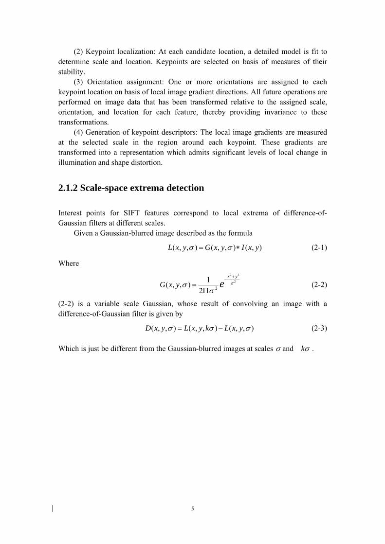
Fig. 2.1 Diagram showing the blurred images at different scales, and the computation of the difference-of-Gaussian images
The first step toward the detection of interest points is the convolution of the
image with Gaussian filters at different scales, and the generation of difference-of-Gaussian images from the difference of adjacent blurred images.
The rotated images are grouped by octave (an octave corresponds to doubling the value of σ), and the value of k is selected so that we can obtain a fixed number of blurred images per octave. This also ensures that we obtain the same figure of difference-of-Gaussian images per octave.
Scale
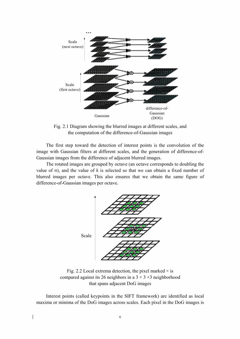
Fig. 2.2 Local extrema detection, the pixel marked × is
compared against its 26 neighbors in a 3 × 3 ×3 neighborhood that spans adjacent DoG images
Interest points (called keypoints in the SIFT framework) are identified as local
maxima or minima of the DoG images across scales. Each pixel in the DoG images is
7
compared to its 8 neighbors at the same scale, plus the 9 corresponding neighbors at neighboring scales. If the pixel is a local maximum or minimum, it is selected as a candidate keypoint. For each candidate keypoint:
(1) Interpolation of nearby data is used to accurately determine its position; (2) Keypoints with low contrast are removed; (3) Responses along edges are eliminated; (4) The keypoint is assigned an orientation.
To determine the keypoint orientation, a gradient orientation histogram is computed in the neighborhood of the keypoint (using the Gaussian image at the closest scale to the keypoint's scale). The contribution of each neighboring pixel is weighted by the gradient magnitude and a Gaussian window with a σ that is 1.5 times the scale of the keypoint.
Peaks in the histogram correspond to dominant orientations. A separate keypoint is reated for the direction corresponding to the histogram maximum, and any other direction within 80% of the maximum value.
All the properties of the keypoint are measured relative to the keypoint orientation, this provides invariance to rotation.
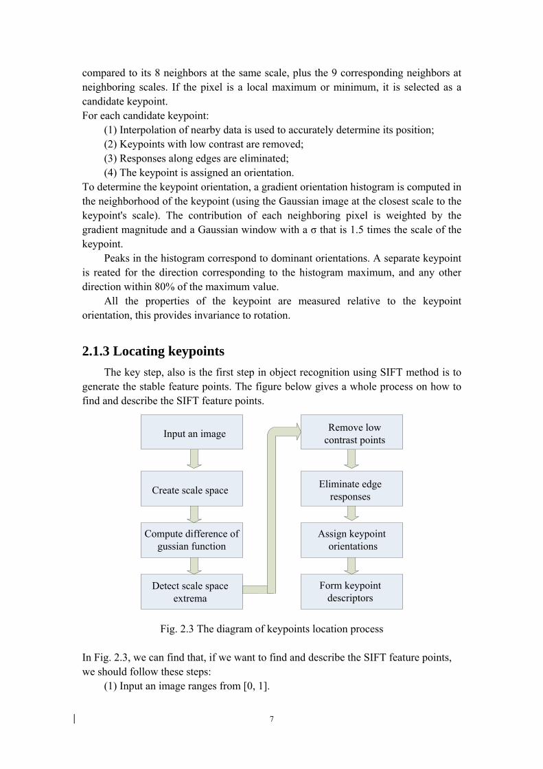
2.1.3 Locating keypoints The key step, also is the first step in object recognition using SIFT method is to
generate the stable feature points. The figure below gives a whole process on how to find and describe the SIFT feature points.
Input an image
Create scale space
Compute difference of gussian function
Detect scale space extrema
Remove low contrast points
Eliminate edge responses
Assign keypoint orientations
Form keypoint descriptors
Fig. 2.3 The diagram of keypoints location process
In Fig. 2.3, we can find that, if we want to find and describe the SIFT feature points, we should follow these steps:
(1) Input an image ranges from [0, 1].
8
(2) Use a variable-scale Gaussian kernel ),,( σyxG to create scale space
),,( σyxL .
(3) Calculate difference-of-Gaussian function as an appoximation to the normalized Laplacian.Because studies have shown that the normalized Laplacian is invariant to the scale change.
(4) Find the maxima or minima of difference-of-Gaussian function value by comparing one of the pixels to its above, current and below scales in 3 3× regions.
(5) Accurate the keypoint’s locations by discarding points below a predetermined value.
1( )2 x
ˆ ˆx xTDD D ∂
= +∂
(2-4)
In (2-4), x is calculated by setting the derivative ),,( σyxD to zero.
(6) The extremas of different-of-Gaussian have large principal curvatures along edges, it can be reduced by checking
rr
DetTr 22 )1(
)H()H( +
< (2-5)
Evidently, H in (2-5) is a 2 2× Hessian matrix, r is the ratio between the largest magitude and the smallest one.
(7) To achieve invariance to rotation, the gradient magnitude ),( yxm and
orientation ),( yxθ are precomputed as the following equations.
22 ))1,()1,(()),1(),1((),( −−++−−+= yxLyxLyxLyxLyxm (2-6)
)),1(),1()1,()1,((tan),( 1
yxLyxLyxLyxLyx−−+−−+
= −θ (2-7)
(8) Take a feature point and its 16×16 neighbours round it.Then divide them into 4 4× subregions, histogram every subregion with 8 bins.
9
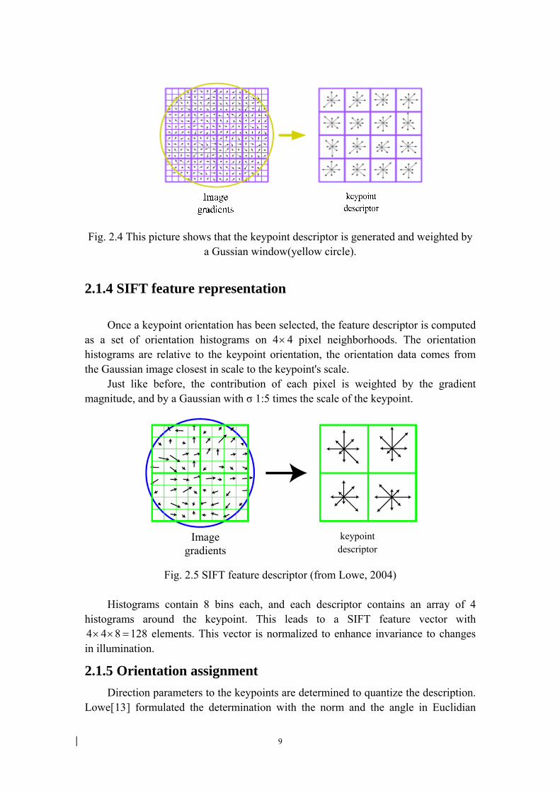
Fig. 2.4 This picture shows that the keypoint descriptor is generated and weighted by
a Gussian window(yellow circle).
2.1.4 SIFT feature representation
Once a keypoint orientation has been selected, the feature descriptor is computed as a set of orientation histograms on 4 4× pixel neighborhoods. The orientation histograms are relative to the keypoint orientation, the orientation data comes from the Gaussian image closest in scale to the keypoint's scale.
Just like before, the contribution of each pixel is weighted by the gradient magnitude, and by a Gaussian with σ 1:5 times the scale of the keypoint.
Image gradients
keypoint descriptor
Fig. 2.5 SIFT feature descriptor (from Lowe, 2004)
Histograms contain 8 bins each, and each descriptor contains an array of 4
histograms around the keypoint. This leads to a SIFT feature vector with 4 4 8 128× × = elements. This vector is normalized to enhance invariance to changes in illumination.
2.1.5 Orientation assignment
Direction parameters to the keypoints are determined to quantize the description. Lowe[13] formulated the determination with the norm and the angle in Euclidian
10
space, with the direction of key points used as normalized the gradient direction of the key point operator in the following step. After an image revolvement, the identical directions demanded can be worked out.
2.1.6 Keypoint matching
The next step is to apply these SIFT methods to video frame sequences for object tracking. SIFT features are extracted through the input video frame sequences and stored by their keypoints descriptors. Each key point assigns 4 parameters, which are 2D location (x coordinate and y coordinate ), orientation and scale. Each object is tracked in a new video frame sequences by separatelly comparing each feature point found from the new video frame sequences to those on the target object. The Euclidean distance is introduced as a similarity measurement of feature characters. The candidates can be preserved when the two feature’s Euclidean distance is larger than the threshold specified previous. So the best matches can be picked out by the the parameters value, in the other way, consistency of of their location, orientation and scale.
Each cluster of three or more features that agree on an object and its pose is then subject to further detailed model verification and subsequently outliers are throwed away. Finally the probability that a particular set of features indicates the presence of an object is computed, considering the accuracy of fit and number of probable false matches. Object matches that pass all of the above tests can be recognized as correct with high confidence.
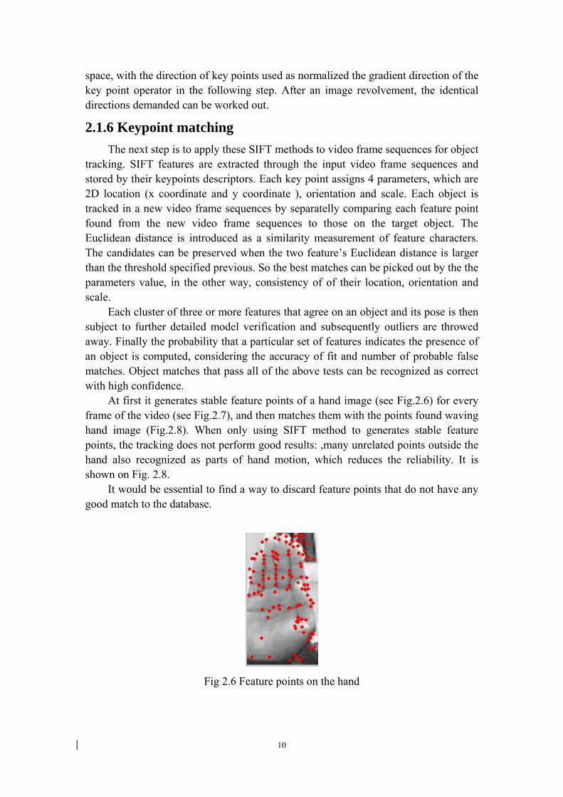
At first it generates stable feature points of a hand image (see Fig.2.6) for every frame of the video (see Fig.2.7), and then matches them with the points found waving hand image (Fig.2.8). When only using SIFT method to generates stable feature points, the tracking does not perform good results: ,many unrelated points outside the hand also recognized as parts of hand motion, which reduces the reliability. It is shown on Fig. 2.8.
It would be essential to find a way to discard feature points that do not have any good match to the database.
Fig 2.6 Feature points on the hand
11
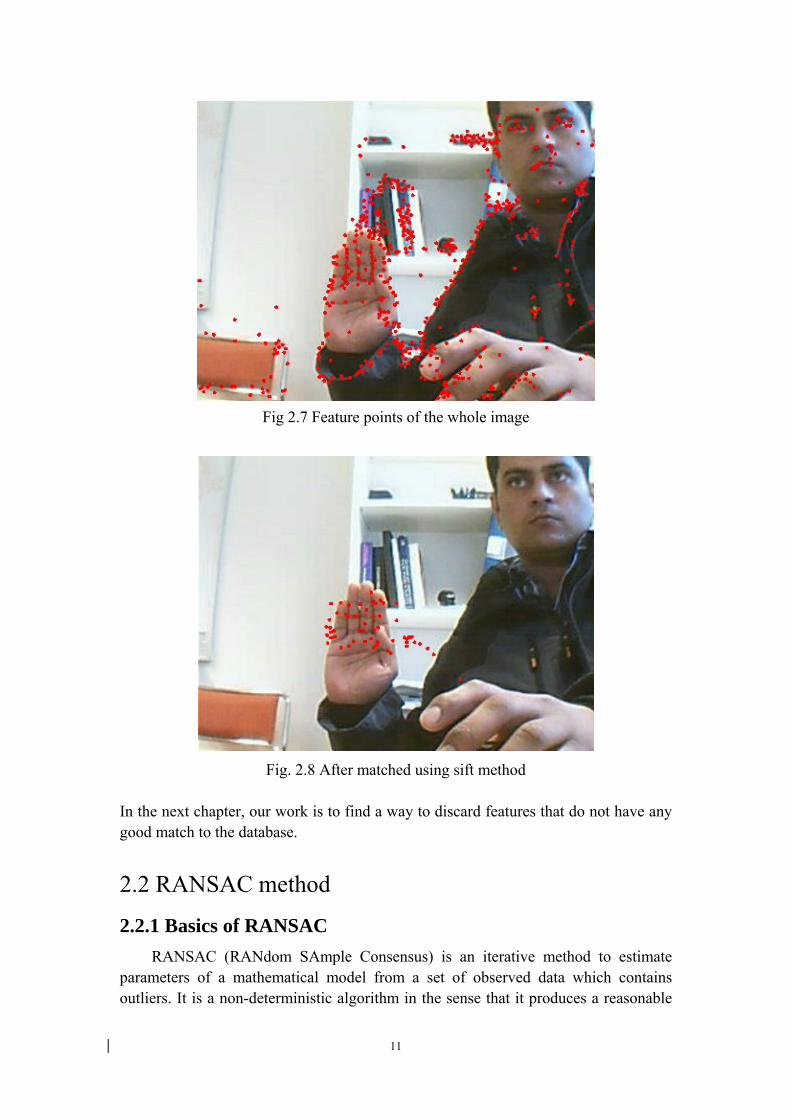
Fig 2.7 Feature points of the whole image
Fig. 2.8 After matched using sift method
In the next chapter, our work is to find a way to discard features that do not have any good match to the database.
2.2 RANSAC method
2.2.1 Basics of RANSAC
RANSAC (RANdom SAmple Consensus) is an iterative method to estimate parameters of a mathematical model from a set of observed data which contains outliers. It is a non-deterministic algorithm in the sense that it produces a reasonable
12
result only with a certain probability, with this probability increasing as more iterations are allowed. The algorithm was first published by Fischler and Bolles in 1981.
A basic assumption is that the data consists of "inliers", i.e., data whose distribution can be explained by some set of model parameters, and "outliers" which are data that do not fit the model. In addition to this, the data can be subject to noise. The outliers can come, e.g., from extreme values of the noise or from erroneous measurements or incorrect hypotheses about the interpretation of data. RANSAC also assumes that, given a (usually small) set of inliers, there exists a procedure which can estimate the parameters of a model that optimally explains or fits this data.
Because there are incorrect matches due to ambiguous features or confusing background information as object features, individual feature matches have a lower probability of correctness than a cluster of features. It has been found that at least three features of a cluster is possible to reach a reliable recognition.
RANSAC can be applied to check whether a cluster of points fits to a geometric model. From the matched points obtained by SIFT method, three pairs of points are randomly chosen to create a transform matrix that fits to a 2D plane. Then set a threshold, distance the true point position from the previous point position is calculated by the transform matrix. RANSAC achieves its goal by iteratively selecting a random subset of the original data. These data are hypothetical inliers. This hypothesis is then tested as follows:
(1) A model is fitted to the hypothetical inliers, i.e. all free parameters of the model are reconstructed from the data set.
(2) All other data are then tested against the fitted model. If a point fits well to the estimated model, it is also considered as a hypothetical inlier.
(3) The estimated model is reasonably good if sufficiently large number of points have been classified as hypothetical inliers.
(4) The model is re-estimated from all hypothetical inliers because the model has only been estimated from the initial set of hypothetical inliers.
(5) Finally, the model is evaluated by estimating the error of inliers relative to the model.
This procedure is repeated a fixed number of times, each time producing either a model which is rejected because too few points are classified as inliers, or a refined model together with a corresponding error measure. In the latter case, we keep the refined model if its error is lower than the last saved model.
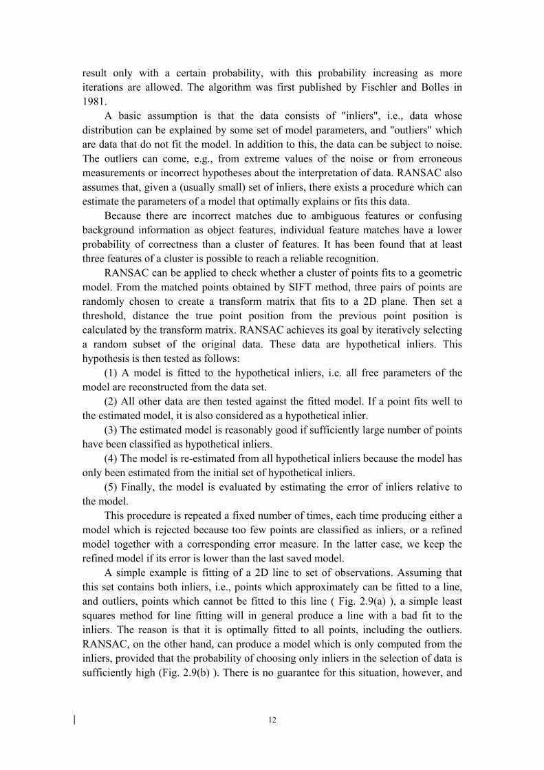
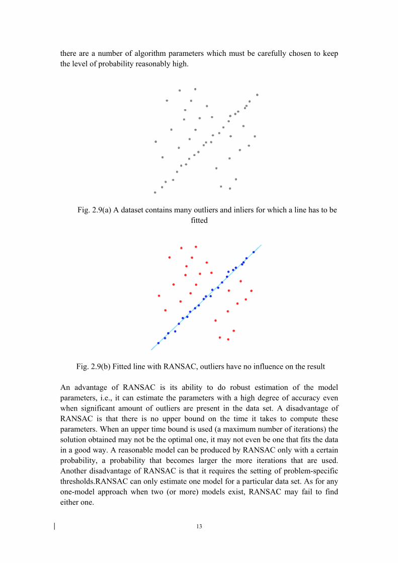
A simple example is fitting of a 2D line to set of observations. Assuming that this set contains both inliers, i.e., points which approximately can be fitted to a line, and outliers, points which cannot be fitted to this line ( Fig. 2.9(a) ), a simple least squares method for line fitting will in general produce a line with a bad fit to the inliers. The reason is that it is optimally fitted to all points, including the outliers. RANSAC, on the other hand, can produce a model which is only computed from the inliers, provided that the probability of choosing only inliers in the selection of data is sufficiently high (Fig. 2.9(b) ). There is no guarantee for this situation, however, and
13
there are a number of algorithm parameters which must be carefully chosen to keep the level of probability reasonably high.
Fig. 2.9(a) A dataset contains many outliers and inliers for which a line has to be
fitted
Fig. 2.9(b) Fitted line with RANSAC, outliers have no influence on the result
An advantage of RANSAC is its ability to do robust estimation of the model parameters, i.e., it can estimate the parameters with a high degree of accuracy even when significant amount of outliers are present in the data set. A disadvantage of RANSAC is that there is no upper bound on the time it takes to compute these parameters. When an upper time bound is used (a maximum number of iterations) the solution obtained may not be the optimal one, it may not even be one that fits the data in a good way. A reasonable model can be produced by RANSAC only with a certain probability, a probability that becomes larger the more iterations that are used. Another disadvantage of RANSAC is that it requires the setting of problem-specific thresholds.RANSAC can only estimate one model for a particular data set. As for any one-model approach when two (or more) models exist, RANSAC may fail to find either one.
14
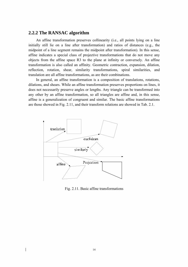
2.2.2 The RANSAC algorithm An affine transformation preserves collinearity (i.e., all points lying on a line
initially still lie on a line after transformation) and ratios of distances (e.g., the midpoint of a line segment remains the midpoint after transformation). In this sense, affine indicates a special class of projective transformations that do not move any objects from the affine space R3 to the plane at infinity or conversely. An affine transformation is also called an affinity. Geometric contraction, expansion, dilation, reflection, rotation, shear, similarity transformations, spiral similarities, and translation are all affine transformations, as are their combinations.
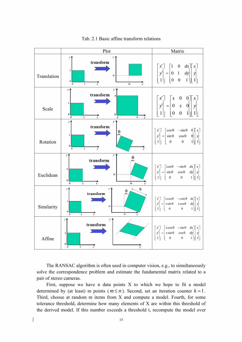
In general, an affine transformation is a composition of translations, rotations, dilations, and shears. While an affine transformation preserves proportions on lines, it does not necessarily preserve angles or lengths. Any triangle can be transformed into any other by an affine transformation, so all triangles are affine and, in this sense, affine is a generalization of congruent and similar. The basic affine transformations are those showed in Fig. 2.11, and their transform relations are showed in Tab. 2.1.
Fig. 2.11. Basic affine transformations
15
Tab. 2.1 Basic affine transform relations
Plot Matrix
Translation
⎥⎥⎥
⎦
⎤
⎢⎢⎢
⎣
⎡
⎥⎥⎥
⎦
⎤
⎢⎢⎢
⎣
⎡1001
=⎥⎥⎥
⎦
⎤
⎢⎢⎢
⎣
⎡′′
11001yx
dydx
yx
Scale
⎥⎥⎥
⎦
⎤
⎢⎢⎢
⎣
⎡
⎥⎥⎥
⎦
⎤
⎢⎢⎢
⎣
⎡=
⎥⎥⎥
⎦
⎤
⎢⎢⎢
⎣
⎡′′
11000000
1yx
ss
yx
Rotation
⎥⎥⎥
⎦
⎤
⎢⎢⎢
⎣
⎡
⎥⎥⎥
⎦
⎤
⎢⎢⎢
⎣
⎡θθθ−θ
=⎥⎥⎥
⎦
⎤
⎢⎢⎢
⎣
⎡′′
11000cossin0sincos
1yx
yx
Euclidean
⎥⎥⎥
⎦
⎤
⎢⎢⎢
⎣
⎡
⎥⎥⎥
⎦
⎤
⎢⎢⎢
⎣
⎡θθθ−θ
=⎥⎥⎥
⎦
⎤
⎢⎢⎢
⎣
⎡′′
1100cossinsincos
1yx
dydx
yx
Similarity
⎥⎥⎥
⎦
⎤
⎢⎢⎢
⎣
⎡
⎥⎥⎥
⎦
⎤
⎢⎢⎢
⎣
⎡θθθ−θ
=⎥⎥⎥
⎦
⎤
⎢⎢⎢
⎣
⎡′′
1100cossinsincos
1yx
dyssdxss
yx
Affine
cos sinsin cos
1 0 0 1 1
x s dx xy s dy y′ θ − θ⎡ ⎤ ⎡ ⎤ ⎡ ⎤
⎢ ⎥ ⎢ ⎥ ⎢ ⎥′ = θ θ⎢ ⎥ ⎢ ⎥ ⎢ ⎥⎢ ⎥ ⎢ ⎥ ⎢ ⎥⎣ ⎦ ⎣ ⎦ ⎣ ⎦
The RANSAC algorithm is often used in computer vision, e.g., to simultaneously
solve the correspondence problem and estimate the fundamental matrix related to a pair of stereo cameras.
First, suppose we have n data points X to which we hope to fit a model determined by (at least) m points ( m n≤ ). Second, set an iteration counter 1k = . Third, choose at random m items from X and compute a model. Fourth, for some tolerance threshold, determine how many elements of X are within this threshold of the derived model. If this number exceeds a threshold t, recompute the model over

16
this consensus set and halt. Finally, set 1k k= + , If k K< , for some predetermined K, go to the third step. Otherwise accept the model with the biggest consensus set so far, or fail.
In general, the RANSAC algorithm, in pseudocode, works as follows:
input: data - a set of observations model - a model that can be fitted to data n - the minimum number of data required to fit the model k - the maximum number of iterations allowed in the algorithm t - a threshold value for determining when a datum fits a model d - the number of close data values required to assert that a model fits well to the data
output: best_model - model parameters which best fit the data (or nil if no good model is
found) best_consensus_set - data point from which this model has been estimated best_error - the error of this model relative to the data
iterations = 0 best_model = nil best_consensus_set = nil best_error = infinity while iterations < k
maybe_inliers = n randomly selected values from data maybe_model = model parameters fitted to maybe_inliers consensus_set = maybe_inliers for every point in data not in maybe_inliers if point fits maybe_model with an error smaller than t add point to consensus_set if the number of elements in consensus_set is > d (this implies that we may have found a good model, now test how good it is) better_model = model parameters fitted to all points in consensus_set this_error = a measure of how well better_model fits these points if this_error < best_error (we have found a model which is better than any of the previous ones,
keep it until a better one is found) best_model = better_model best_consensus_set = consensus_set best_error = this_error increment iterations return: best_model, best_consensus_set, best_error
17
Possible variants of the RANSAC algorithm include: (1) Break the main loop if a sufficiently good model has been found, that is, one
with sufficiently small error. May save some computation time at the expense of an additional parameter.
(2) Compute this_error directly from maybe_model without re-estimating a model from the consensus set. May save some time at the expense of comparing errors related to models which are estimated from a small number of points and therefore more sensitive to noise. The values of parameters t and d have to be determined from specific requirements related to the application and the data set, possibly based on experimental evaluation. The parameter k (the number of iterations), however, can be determined from a theoretical result. Let p be the probability that the RANSAC algorithm in some iteration selects only inliers from the input data set when it chooses the n points from which the model parameters are estimated. When this happens, the resulting model is likely to be useful so p gives the probability that the algorithm produces a useful result. Let w be the probability of choosing an inlier each time a single point is selected, that is,
w = number of inliers in data / number of points in data
A common case is that w is not well known beforehand, but some rough value can be given. Assuming that the n points needed for estimating a model are selected
independently, nw is the probability that all n points are inliers, and 1 nw− is the
probability that at least one of the n points is an outlier, a case which implies that a bad model will be estimated from this point set. That probability to the power of k is the probability that the algorithm never selects a set of n points which all are inliers and this must be the same as 1-p. Consequently,
1 (1 )np w k− = − (2-8)
which, after taking the logarithm of both sides, leads to
log(1 )log(1 )n
pkw−
=−
(2-9)
It should be noted that this result assumes that the n data points are selected independently, that is, a point which has been selected once is replaced and can be selected again in the same iteration. This is often not a reasonable approach and the derived value for k should be taken as an upper limit in the case that the points are selected without replacement. For example, in the case of finding a line which fits the data set illustrated in the above Fig. 2.9, the RANSAC algorithm typically chooses 2 points in each iteration, and computes the model as the line between the points. It then decides the final inliers. .
To gain additional confidence, the standard deviation or multiples thereof can be added to k. The standard deviation of k is defined as
18
1( )n
n
wSD kw−
= (2-10)
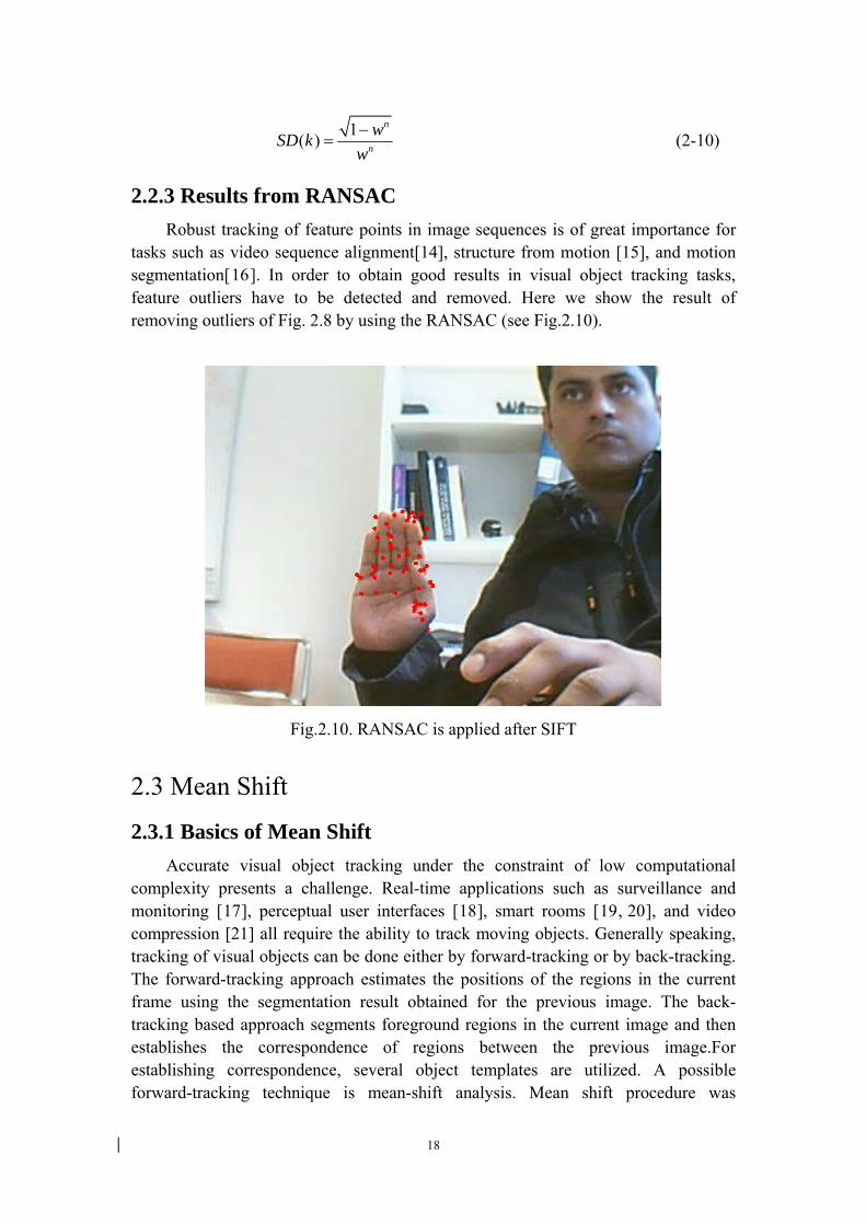
2.2.3 Results from RANSAC Robust tracking of feature points in image sequences is of great importance for
tasks such as video sequence alignment[14], structure from motion [15], and motion segmentation[16]. In order to obtain good results in visual object tracking tasks, feature outliers have to be detected and removed. Here we show the result of removing outliers of Fig. 2.8 by using the RANSAC (see Fig.2.10).
Fig.2.10. RANSAC is applied after SIFT
2.3 Mean Shift
2.3.1 Basics of Mean Shift Accurate visual object tracking under the constraint of low computational
complexity presents a challenge. Real-time applications such as surveillance and monitoring [17], perceptual user interfaces [18], smart rooms [19, 20], and video compression [21] all require the ability to track moving objects. Generally speaking, tracking of visual objects can be done either by forward-tracking or by back-tracking. The forward-tracking approach estimates the positions of the regions in the current frame using the segmentation result obtained for the previous image. The back-tracking based approach segments foreground regions in the current image and then establishes the correspondence of regions between the previous image.For establishing correspondence, several object templates are utilized. A possible forward-tracking technique is mean-shift analysis. Mean shift procedure was
19
originally introduced in 1975, but only after 20 years later in 1995, this method has been re-introduced by D. Fuiorea [22]. In his article, a kernel function is defined to calculate the distance between sample points and its mean shift, also a weight coefficient is inverse with the distance. The closer the distance is, the larger the weight coefficient is.
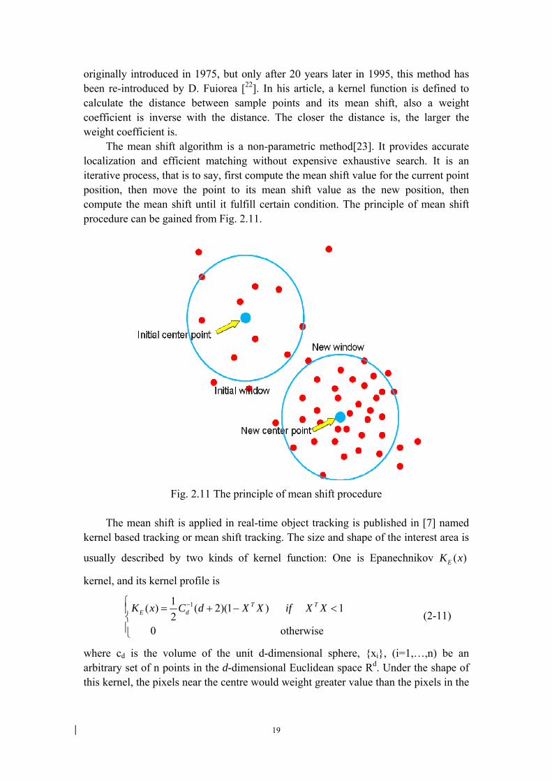
The mean shift algorithm is a non-parametric method[23]. It provides accurate localization and efficient matching without expensive exhaustive search. It is an iterative process, that is to say, first compute the mean shift value for the current point position, then move the point to its mean shift value as the new position, then compute the mean shift until it fulfill certain condition. The principle of mean shift procedure can be gained from Fig. 2.11.
Fig. 2.11 The principle of mean shift procedure
The mean shift is applied in real-time object tracking is published in [7] named
kernel based tracking or mean shift tracking. The size and shape of the interest area is
usually described by two kinds of kernel function: One is Epanechnikov ( )EK x
kernel, and its kernel profile is
11( ) ( 2)(1 ) 12
0 otherwise
T TE dK x C d X X if X X−⎧ = + − <⎪
⎨⎪⎩
(2-11)
where cd is the volume of the unit d-dimensional sphere, {xi}, (i=1,…,n) be an arbitrary set of n points in the d-dimensional Euclidean space Rd. Under the shape of this kernel, the pixels near the centre would weight greater value than the pixels in the
20
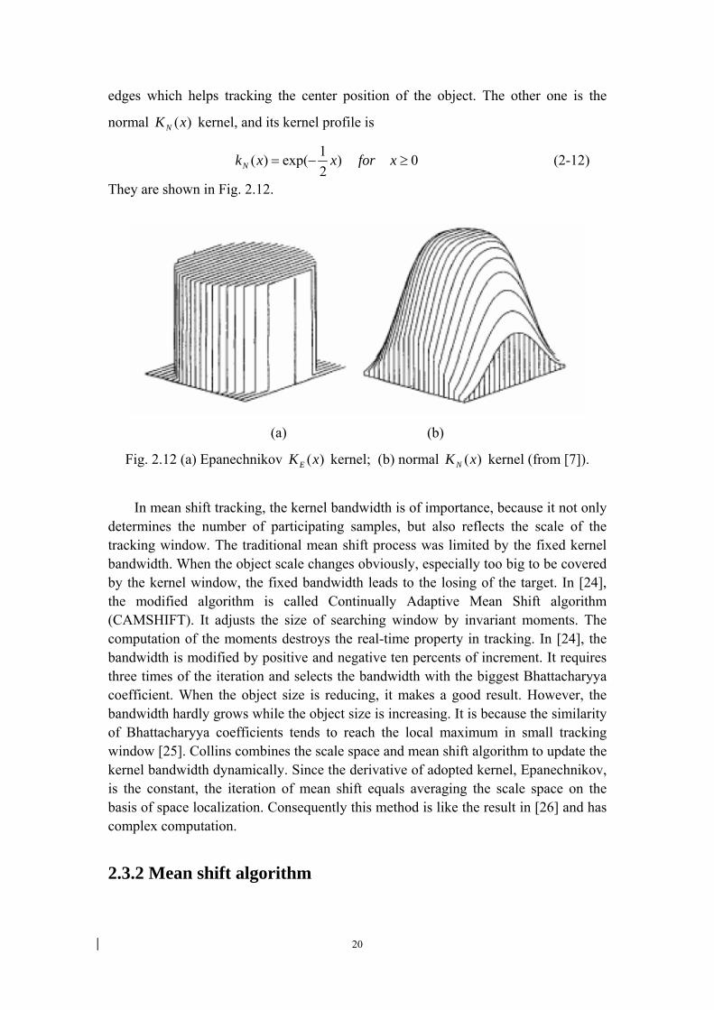
edges which helps tracking the center position of the object. The other one is the
normal )(xKN kernel, and its kernel profile is
0)21exp()( ≥−= xforxxkN (2-12)
They are shown in Fig. 2.12.
(a) (b)
Fig. 2.12 (a) Epanechnikov )(xKE kernel; (b) normal )(xKN kernel (from [7]).
In mean shift tracking, the kernel bandwidth is of importance, because it not only
determines the number of participating samples, but also reflects the scale of the tracking window. The traditional mean shift process was limited by the fixed kernel bandwidth. When the object scale changes obviously, especially too big to be covered by the kernel window, the fixed bandwidth leads to the losing of the target. In [24], the modified algorithm is called Continually Adaptive Mean Shift algorithm (CAMSHIFT). It adjusts the size of searching window by invariant moments. The computation of the moments destroys the real-time property in tracking. In [24], the bandwidth is modified by positive and negative ten percents of increment. It requires three times of the iteration and selects the bandwidth with the biggest Bhattacharyya coefficient. When the object size is reducing, it makes a good result. However, the bandwidth hardly grows while the object size is increasing. It is because the similarity of Bhattacharyya coefficients tends to reach the local maximum in small tracking window [25]. Collins combines the scale space and mean shift algorithm to update the kernel bandwidth dynamically. Since the derivative of adopted kernel, Epanechnikov, is the constant, the iteration of mean shift equals averaging the scale space on the basis of space localization. Consequently this method is like the result in [26] and has complex computation.
2.3.2 Mean shift algorithm
21
The kernel-based object tracking algorithm (mean shift algorithm) is as follows:
(1) The target model { uq }(u =1 2…m, m bins of histograms) is derived from an
elliptic region centered at 0y , to remove the influence of the target scale it is
normalized to a unit circle, its pixel coordinates{ *ix }.
∑
∑=
∗
=∗∗
−
−−=
n
i i
n
i iiu
x
uxbxq
1
21
2
)1(
))(()1(ˆ
δ (2-13)
where n is the number of pixels, δ is the Kronecker delta function:
⎩⎨⎧ =
=otherwise
xx
001
)(δ (2 -14)
(2) Use 0y from previous frame location as an initial position to estimate
{ )ˆ(ˆ 0ypu } in the new frame
∑∑
=
=
−
−−= n
i i
n
i iiu
hx
uxbhxyp
1
1
)1(
))(()1()(ˆ
δ (2-15)
In the equation above 2
hxyhx i
i−
= , 1}ˆ{1
=∑ =
m
u uq and 1}ˆ{1
=∑ =
m
u up .
Compute
[ ] ∑ ==
m
u uu qypqyp1 00 ˆ)ˆ(ˆˆ)ˆ(ˆρ (2-16)
(3) Derive weights for i=1,2,…,n according:
))(()ˆ(ˆ
ˆ
0
uxbyp
qw iu
ui −= δ (2-17)
(4) Determine the new location of the target candidate according to:
[ ),0)()( ∞∈′−= xforxkxg (2-18)
∑∑
=
== n
i ii
n
i iii
hxgw
hxgwxy
1
11
)(
)(ˆ (2-19)
(5) Compute the new likelihood value )}ˆ(ˆ{ 1ypu for u=1,2,…,m, and determine
[ ] ∑ ==
m
u uu qypqyp1 11 ˆ)ˆ(ˆˆ)ˆ(ˆρ (2-20)
(6) If the similarity between the new target region and the target region and the target mode is less than that between the old target region and the model
22
[ ] [ ]qypqyp ˆ)ˆ(ˆˆ)ˆ(ˆ 01 ρρ < (2-21)
Perform the remaining operations of this step – move the target region half way between the new and old locations,
)ˆˆ(21ˆ 101 yyy += (2-22)
and evaluate the similarity function in this new location
[ ]qyp ˆ)ˆ(ˆ 1ρ (2-23)
Return to the beginning of this step 6.
(7) If ε<− 01 ˆˆ yy , stop. Otherwise, use the current target location as a start for
the new location 10 ˆˆ yy = , and continue with step 3.
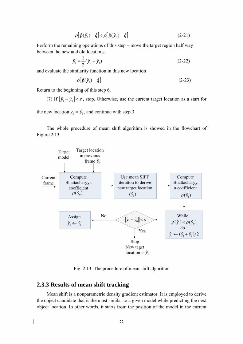
The whole procedure of mean shift algorithm is showed in the flowchart of
Figure 2.13.
While
0ˆ( )yρ
Compute Bhattacharyya
coefficient
Use mean SIFT iteratton to derive
new target location1ˆ( )y
1ˆ( )yρ
Compute Bhattacharyya coefficient
0 1ˆ ˆy y←Assign
1 0ˆ ˆy y ε− <1 0ˆ ˆ( ) ( )y yρ ρ<do
1 1 0ˆ ˆ ˆ( ) 2y y y← +
Target model
Target location in previous
frame 0y
Current frame
No
Stop New taget location is
Yes
1y
Fig. 2.13 The procedure of mean shift algorithm
2.3.3 Results of mean shift tracking
Mean shift is a nonparametric density gradient estimator. It is employed to derive the object candidate that is the most similar to a given model while predicting the next object location. In other words, it starts from the position of the model in the current
23
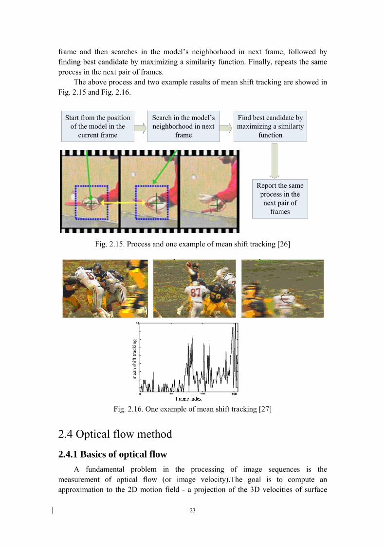
frame and then searches in the model’s neighborhood in next frame, followed by finding best candidate by maximizing a similarity function. Finally, repeats the same process in the next pair of frames.
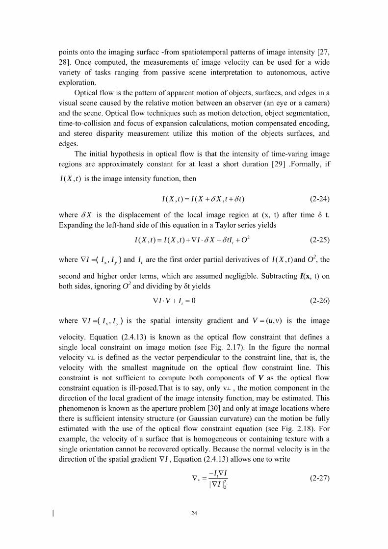
The above process and two example results of mean shift tracking are showed in Fig. 2.15 and Fig. 2.16.
Start from the position of the model in the
current frame
Search in the model’sneighborhood in next
frame
Find best candidate by maximizing a similarty
function
Report the same process in the next pair of
frames
Fig. 2.15. Process and one example of mean shift tracking [26]
mea
n sh
ift tr
acki
ng
Fig. 2.16. One example of mean shift tracking [27]
2.4 Optical flow method
2.4.1 Basics of optical flow
A fundamental problem in the processing of image sequences is the measurement of optical flow (or image velocity).The goal is to compute an approximation to the 2D motion field - a projection of the 3D velocities of surface
24
points onto the imaging surfacc -from spatiotemporal patterns of image intensity [27, 28]. Once computed, the measurements of image velocity can be used for a wide variety of tasks ranging from passive scene interpretation to autonomous, active exploration.
Optical flow is the pattern of apparent motion of objects, surfaces, and edges in a visual scene caused by the relative motion between an observer (an eye or a camera) and the scene. Optical flow techniques such as motion detection, object segmentation, time-to-collision and focus of expansion calculations, motion compensated encoding, and stereo disparity measurement utilize this motion of the objects surfaces, and edges.
The initial hypothesis in optical flow is that the intensity of time-varing image regions are approximately constant for at least a short duration [29] .Formally, if
( , )I X t is the image intensity function, then
( , ) ( , )I X t I X X t tδ δ= + + (2-24)
where Xδ is the displacement of the local image region at (x, t) after time δ t. Expanding the left-hand side of this equation in a Taylor series yields
2( , ) ( , ) tI X t I X t I X tI Oδ δ= +∇ ⋅ + + (2-25)
where x yI I I∇ =( , ) and tI are the first order partial derivatives of ( , )I X t and O2, the
second and higher order terms, which are assumed negligible. Subtracting I(x, t) on both sides, ignoring O2 and dividing by δt yields
0tI V I∇ ⋅ + = (2-26)
where x yI I I∇ =( , ) is the spatial intensity gradient and ( , )V u v= is the image
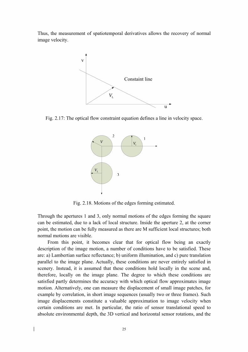
velocity. Equation (2.4.13) is known as the optical flow constraint that defines a single local constraint on image motion (see Fig. 2.17). In the figure the normal velocity v┴ is defined as the vector perpendicular to the constraint line, that is, the velocity with the smallest magnitude on the optical flow constraint line. This constraint is not sufficient to compute both components of V as the optical flow constraint equation is ill-posed.That is to say, only v┴ , the motion component in the direction of the local gradient of the image intensity function, may be estimated. This phenomenon is known as the aperture problem [30] and only at image locations where there is sufficient intensity structure (or Gaussian curvature) can the motion be fully estimated with the use of the optical flow constraint equation (see Fig. 2.18). For example, the velocity of a surface that is homogeneous or containing texture with a single orientation cannot be recovered optically. Because the normal velocity is in the direction of the spatial gradient I∇ , Equation (2.4.13) allows one to write
22| |
tI II°
− ∇∇ =
∇ (2-27)
25
Thus, the measurement of spatiotemporal derivatives allows the recovery of normal image velocity.
LV
Constaint line
u
v
Fig. 2.17: The optical flow constraint equation defines a line in velocity space.
V1V
LV
Fig. 2.18. Motions of the edges forming estimated.
Through the apertures 1 and 3, only normal motions of the edges forming the square can be estimated, due to a lack of local structure. Inside the aperture 2, at the corner point, the motion can be fully measured as there are M sufficient local structures; both normal motions are visible.
From this point, it becomes clear that for optical flow being an exactly description of the image motion, a number of conditions have to be satisfied. These are: a) Lambertian surface reflectance; b) uniform illumination, and c) pure translation parallel to the image plane. Actually, these conditions are never entirely satisfied in scenery. Instead, it is assumed that these conditions hold locally in the scene and, therefore, locally on the image plane. The degree to which these conditions are satisfied partly determines the accuracy with which optical flow approximates image motion. Alternatively, one can measure the displacement of small image patches, for example by correlation, in short image sequences (usually two or three frames). Such image displacements constitute a valuable approximation to image velocity when certain conditions are met. In particular, the ratio of sensor translational speed to absolute environmental depth, the 3D vertical and horizontal sensor rotations, and the
26
time interval between frames must be small quantities [31]. Optical flow may also be computed as the disparity field where, given two stereo images or two adjacent images in some sequence, features of interest in the images are extracted and matched via a correspondence process.
Essentially, performing 2D motion detection involves the processing of scenes where the sensor is moving within an environment containing both stationary and nonstationary objects. Furthermore, visual events such as occlusion, transparent motions, and nonrigid objects increase the inherent complexity of the measurement of optical flow.
2.4.2 Variants of optical flow In computer vision, optical flow is a velocity field associated with image
changes. This effect generally appears due to the relative movement between object and camera or by moving the light sources that illuminates the scene [32]. Most approaches to estimate optical flow are based on brighteness changes between two scenes. A color image corresponds to a multi-channel image where each pixel is associated to more than one value that represents color information and brightness intensity. Color information can be used in optical flow estimation.
2.4.2.1 Optical flow for grayscale images
Among the existing methods for optical flow estimation, gradient based techniques are often used. Such techniques are based on image brightness that changes in each pixel with an (x, y) coordinates. Considering that small displacements do not modify brightness intensity of a image point, a constrained optical flow equation can be defined as
0x y tI u I v I+ + = (2-28)
where u and v are the optical flow components in x and y directions for a
displacement ( , )x yd d d= , ,x yI I and tI are the partial derivatives of the image
brightness, ( , )I x y , with regard to the horizontal ( )x and vertical ( )y coordinates,
and time (t). The optical flow vector is defined by ( , )V u v= . Optical flow cannot be
estimated only from Equation (2-28) (Aperture Problem). Thus, some additional
constraint needs to be used to find a solution for the flow components, ,u v .
(1) Lucas and Kanade’s Method B. Lucas, T. Kanade [33] used a local constraint to solve the aperture problem.
This method considers that small regions in the image corresponds to the same object and have similar movement. The image is divided in windows of size N N× , each
27
one with 2p N= pixels. A local constraint of movement is used to form an
overconstrained system with p equations and 2 variables, as in (2-29) 1 1 1
2 2 2
0
0
0
x y t
x y t
xp yp tp
I u I v I
I u I v I
I u I v I
+ + =
+ + =
+ + =
(2-29)
(2) Bouguet’s Method Bouguet’s method [ 34 ] uses hierarchical processing applied to Lucas and
Kanade’s method. A justification for using of hierarchical processing is the necessity of better precision in measures of the obtained optical flow vectors. This method uses pyramidal representation of gray image frames. Bouguet algorithm consists of using down level estimations as initial guess of pyramidal top level. The estimation of pyramidal highest level is the estimated optical flow. (3) Eliete’s Method
Eliete’s method [35] is a variation of Lucas and Kanade’s method (Section 1). Eliete uses a bigger window for the brightness conservation model than the one considered by Lucas and Kanade. Only some pixels of each window are randomly chosen for the flow vector estimation. The overconstrained equation system is solved by the LMS method.
2.4.2.2 Optical flow for color images
Optical flow cannot be completely determined from a simple gray image sequence without introducing assumptions about movements in the image. Color image is an additional natural resource of information that can facilitate the problem resolution. Ohta [36] was the first one to consider a optical flow estimation method that does not use additional constraints about movements in the image. His method is based on multi-channel images (as color images) to obtain multiple constraints from a simple image pixel.
A multi-channel image consists of some associated images, making easy to obtain more information from a point of the scene [37]. The optical flow equation 1 can be applied to each image channel n. For color images with three channels (RGB, HSV, HSI, YUV) the system would result in (2.4.23)
1 1 1
2 2 2
3 3 3
0
0
0
x y t
x y t
x y t
I u I v I
I u I v I
I u I v I
+ + =
+ + =
+ + =
(2-30)
Another idea proposed by Golland [38] is the color conservation. Since that geometric component does not depend on light model, the color intensities can be represented by (2.4.24)
28
( , , )( , , )( , , )
r
r
b
R c CG c CB c C
ψ θ γψ θ γψ θ γ
===
(2-30)
where ( , , )c ψ θ γ is the geometric component related to the angles of incidence (φ),
observation (θ) and phase (γ), and the spectral component Ci is defined by: { }( ) ( ) ( ) , ,i iC I D d i r g bρ λ λ λ λ
Ω
= ∈∫ (2-31)
where ( )ρ λ represents the reflectivity function, ( )I λ is the incident light and
( )iD λ represents the light sensor detection function. The reflection geometry can
significantly change with the object movement (rotation, movement in camera direction, etc.). This way, the brightness intensity function will no more satisfy the
conservation assumption. The new iC functions given by Equation (2-31) remain
constant under any type of movement. Therefore it is not influenced by the reflection
geometry. Although it is impossible extracting the iC information from the (R,G,B)
values provided by a color image, the ratio of two components (R,G,B) corresponds to
the ratio of two iC components. Thus, some color models based on relations of R, G
and B functions can be used: normalized RGB, HSV, HSI and YUV. In recent years, improvement made on optical flow estimation by using color
information is used most in this way: Optical flow was estimated by using the methods of Lucas and Kanade, Bouguet
and Eliete. Invalid and null flow vectors are represented by dots in the estimated optical flow field, also called flow map. These above methods have been applied to two consecutive frames of an image sequence.
Lucas and Kanade’s method could be used with brightness conservation window of value which can be N=10. The obtained results, using only brightness information of two consecutive pictures are always valid. Eliete’s method could be also used with a window of size N =10. Only 1/8 randomly chosen pixels of the window have been used in flow estimation.
3. Combined Method 3.1 Description of the combined method
29
In this thesis the proposed tracking algorithm is an effective integration using of SIFT, RANSAC and mean shift feature tracking. The proposed approach will apply a similarity measurement between two neighboring frames in terms of color and SIFT correspondence. Technically, a track will be made if mean shift and SIFT feature tracking lead to approximate probability distributions (e.g., intensity and color) within the corresponding region in the next image frame (ideally the two probability distributions should be identical if the scenario does not change to much). An expectation–maximization algorithm is employed in order to pursue a maximum likelihood estimate using the measurements from SIFT, RANSAC and mean shift correspondence.
The main contributions of the combined method consist of: (1) A combinatorial theory of SIFT, RANSAC and mean shift feature matching is proposed for vidio object tracking. The combined method congregates the advantages of SIFT, RANSAC and mean shift method, and discards the advantages of the methods covered. (2) the process of combinatorial method is given in the paper in detail. It elicits a new way for vidio object tracking, which can be improved and developed by the later researchers. (3) The combinatorial method for object tracking can be assembled to a application package or application software to apply in the practice.the corresponding key codes and parameters is given in this thesis. (4) The tracking performance of the proposed strategy can be experimentally justified against that of only use one classical algorithms, i.e., just using mean shift tracking or just using SIFT tracking.
3.2 Algorithm of the combined method The intention of combined method is to concentrate the advantages of the classic methods used in vidio object tracking and apply it into practice. The process of combined method is to analyse the features of objects and chose one or several methods according to characters of tracking methods and the demands.
All of the combined method can be described in algorithmic and models, all of which will be recounted in this chapter.
The flowchart of the algorithm is summarized as follows:
(1) First, select a region of interest on the first frame as a reference object model. This reference model is described by its PDF (probability distributions function, PDF)
estimation which is a m-bin color histogram uq in a rectangular (or ellipse) region
centered at 0y and window size h .
11
=∑ =
m
u uq (2-32)
In which uq is the probability distribution of color u .
30
(2) Implement SIFT and RANSAC methods to the next frame. If there are many corresponding points between the reference object region and a candidate region, an affine matrix is estimated by applying the RANSAC. Picking up the four corners of the rectangle model in the first frame, the affine matrix is used to transform the location of the old four corners to new ones, averaging its new positions. This results
in a new center point SIFTy _1 . If there are not sufficient pairs of matched points
found in the second frame, just average these positions and obtain its SIFTy _1 . The
candidate region centered at SIFTy _1 is described by the color histogram
)_1( SIFTypu .
(3) Apply mean shift to the new frame in parallel. Calculate a new center
position of mean shift, MeanShifty _1 , and the corresponding color histogram
)_1( MeanShiftypu .
(4) Compare these two Bhattacharyya coefficients from the regions whose centers are estimated from the mean shift and SIFT respectively as follows:
∑=
=m
uuu qSIFTypSIFT
1
)_1(_ρ (2-33)
∑=
=m
uuu qMeanShiftypMeanShift
1
)_1(_ρ (2-34)
(5) The bounding box center that is associated with a large Bhattacharyya
coefficient is selected as the new box center 1y for the current frame.
1_ _ _1
1_y SIFT if SIFT MeanShift
yy MeanShift otherwise
ρ ρ≥⎧= ⎨⎩
(2-35)
(6) If the coefficient is larger than a threshold specified previous by application
requires ( that is T>ρ ), it is assumed that the target in the current frame is not
occluded. The region of interest is updated for SIFT matching process for the following frames.
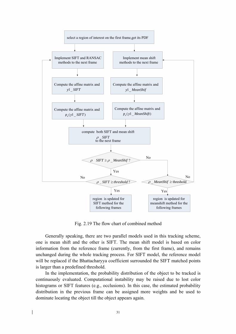
The flow chart of combined method progress advanced in this paper can be described as follows:
31
select a region of interest on the first frame,get its PDF
Implement SIFT and RANSAC methods to the next frame
Implement mean shiftmethods to the next frame
Compute the affine matrix and
region is updated for SIFT method for the
following frames
_ SIFTρcompute both SIFT and mean shift
to the next frame
Compute the affine matrix and( 1_ )up y SIFT
Compute the affine matrix and( 1_ )up y MeanShift
1_y SIFT
Yes
_ _ ?SIFT MeanShifρ ρ≥
_ thresholdMeanShifρ ≥_ ?SIFT thresholdρ ≥
region is updated for meanshift method for the
following frames
Compute the affine matrix and1_y MeanShif
Yes
Yes
No
No No
Fig. 2.19 The flow chart of combined method
Generally speaking, there are two parallel models used in this tracking scheme, one is mean shift and the other is SIFT. The mean shift model is based on color information from the reference frame (currently, from the first frame), and remains unchanged during the whole tracking process. For SIFT model, the reference model will be replaced if the Bhattacharyya coefficient surrounded the SIFT matched points is larger than a predefined threshold.
In the implementation, the probability distribution of the object to be tracked is continuously evaluated. Computational instability may be raised due to lost color histograms or SIFT features (e.g., occlusions). In this case, the estimated probability distribution in the previous frame can be assigned more weights and be used to dominate locating the object till the object appears again.

32
The new method can be used for tracking people in the room or on the street who
were occluded by different objects. The camera being fixed, additional geometric constraints and also background subtraction can be exploited to improve the tracking
process. The value of 1_y MeanShif and 1_y SIFT are worked out by refferd
algorithm (see Chaper 2). Two center points are compared. The center of the method of the lagest Bhattacharyya coefficient is accepted, and if the Bhattacharyya coefficient is larger than a threshold, it is deemed that the comared object can be updated.
33
Chapter 4. Experimental Results Several experiments had been done to evaluate the proposed tracking algorithms. These sequences used in experiments consist of indoors and outdoors testing environments so that the proposed scheme can be fully evaluated. For comparison purposes, conventional mean shift tracking [ 39 ], RANSAC, optical flow, and combined method are utilized. It must be pointed out that in this evaluation there is no intension to track multiple objects. On the contrary, a single object is detected in the first frame of each sequence, followed by continuous tracking to the remaining part of the sequence. In some sequences, there are more than one object in the scene. These scenarios are set up for evaluating the performance of a tracking system against interference in this "multiple candidate" circumstance.
First, the sequence "jam.avi" is tested. The video contains a moving face with 2D planer rotations. This sequence was utilized to evaluate the performance of the SIFT and RANSAC tracker in a poor lighting environment.
Secondly, to test the Mean Shift algorithm in complicated scenarios, we here employ a "pedestrian" sequence, where a walking person is intersected by another person during the course of walking. These two sequences mentioned since they are related to indoor and outdoor human activities. As another example, the performance of the optical flow tracking scheme is also evaluated in indoor environments.
The third sequence namely "duck" is investigated. Finally, the proposed SIFT-mean shift tracker is applied to test the two videos
"occlusion" and "woman", where the target of interest (a person) contains frequent change of his/her postures.
In this test, it is interesting to explore the characteristics of the proposed approach to the change of illumination and moving objects.
4.1 Results from SIFT and RANSAC First, SIFT features are obtained from the first frame using the algorithm
described in Section 2.1. The features are stored by their keypoints descriptors. Each keypoint specifies 4 parameters. The face is tracked in the second frame by individually comparing each feature point found from the second frame to those on the first frame. The Euclidean distance is worked out.The candidate can be preserved when the two features Euclidean distance is larger than a threshold. So the good matches are picked out by the consistency of their location, orientation and scale.
Tracking results on the example sequence "jam" are illustrated in Fig. 3.1. They represent the outcomes of the conventional SIFT and RANSAC tracker. Clearly, this tracker led to drifts in such a poor lighting situation. This is due to the fact that the background’s color is approximate to that of the human face, which deviates the track. The green points in Fig. 3.1 are the corresponding points located by contrast with the update object. The red points in Fig. 3.1 are the corresponding points located by

34
contrast with the first frame. It can be descried from the four images that the detected SIFT and RANSAC features correctlytracked on the face after the rotation of the image.
Fig. 3.1 Result on the ’jam.avi’ sequence. Frames 11,22,39,54
4.2 Results from Mean Shift Experiment was performed to assess the tracking performance of Mean Shift
approach. The mean shift based tracker proved to be robust to partial occlusion, clutter, distractors and camera motion. Since no motion model has been assumed, the tracker adapted well to the nonstationary character of the pedestrian's movements. it starts from the position of the model in the first frame and then searches in the model’s neighborhood in next frame, followed by finding best candidate by maximizing a similarity function. And then repeats the same process in the next pair of frames.
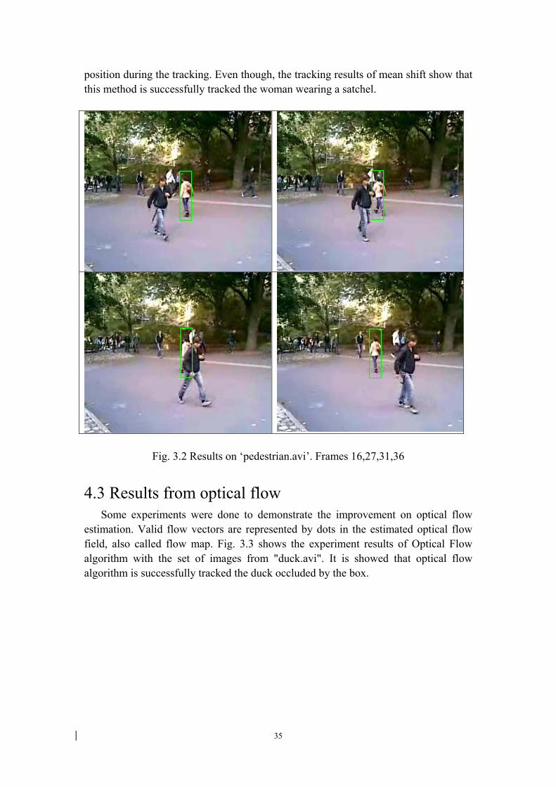
Fig. 3.2 shows four image examples of performance of Mean Shift in sequence "pedestrian". The challenge of this sequence is that a tracking system needs to effectively handle the situation where a female adult was occluded by the others when they crossed over. In this particular example, the aim is to locate the woman wearing a satchel, who was walk on the road. In addition, this person slowly changed her
35
position during the tracking. Even though, the tracking results of mean shift show that this method is successfully tracked the woman wearing a satchel.
Fig. 3.2 Results on ‘pedestrian.avi’. Frames 16,27,31,36
4.3 Results from optical flow Some experiments were done to demonstrate the improvement on optical flow
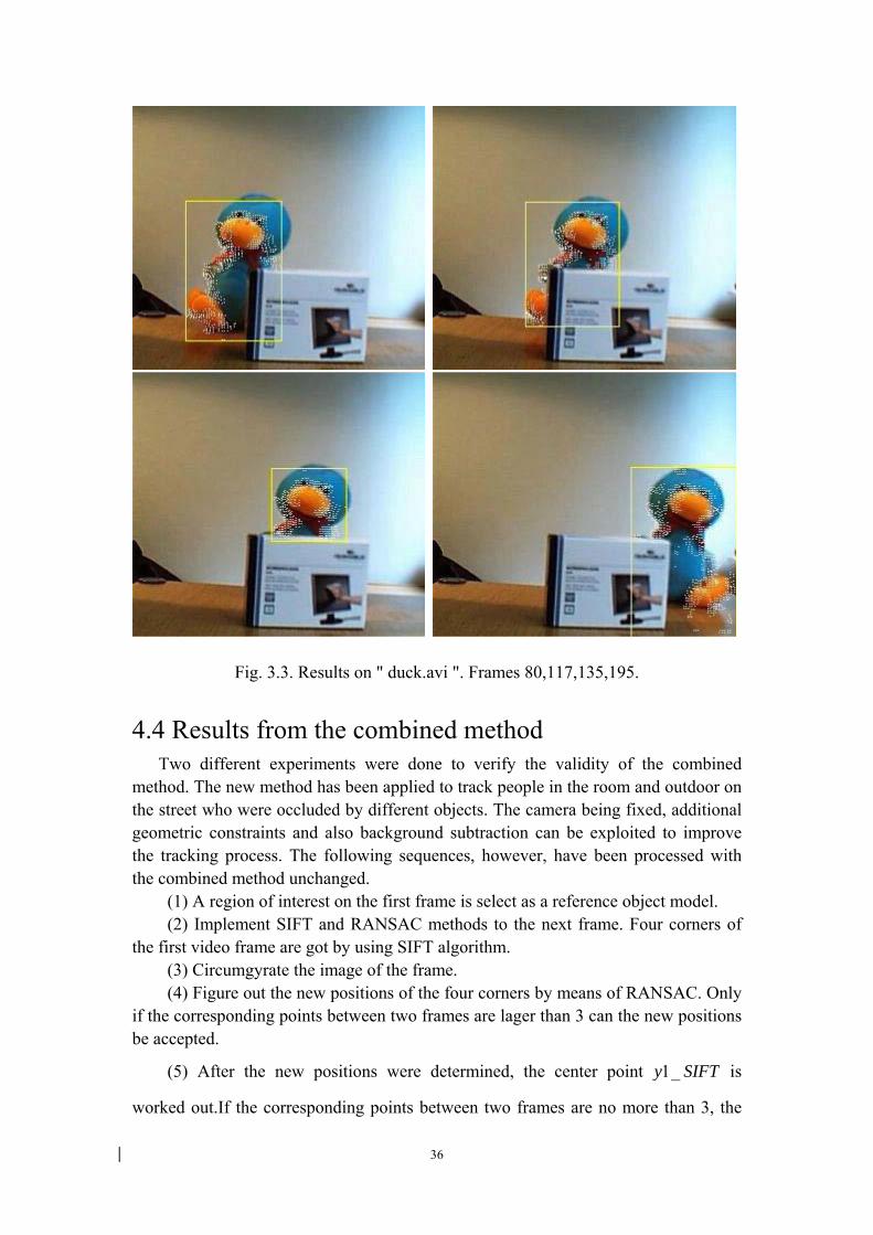
estimation. Valid flow vectors are represented by dots in the estimated optical flow field, also called flow map. Fig. 3.3 shows the experiment results of Optical Flow algorithm with the set of images from "duck.avi". It is showed that optical flow algorithm is successfully tracked the duck occluded by the box.
36
Fig. 3.3. Results on " duck.avi ". Frames 80,117,135,195.
4.4 Results from the combined method Two different experiments were done to verify the validity of the combined
method. The new method has been applied to track people in the room and outdoor on the street who were occluded by different objects. The camera being fixed, additional geometric constraints and also background subtraction can be exploited to improve the tracking process. The following sequences, however, have been processed with the combined method unchanged.
(1) A region of interest on the first frame is select as a reference object model. (2) Implement SIFT and RANSAC methods to the next frame. Four corners of
the first video frame are got by using SIFT algorithm. (3) Circumgyrate the image of the frame. (4) Figure out the new positions of the four corners by means of RANSAC. Only
if the corresponding points between two frames are lager than 3 can the new positions be accepted.
(5) After the new positions were determined, the center point 1_y SIFT is
worked out.If the corresponding points between two frames are no more than 3, the
37
mean of corresponding points is considered as the center point 1_y SIFT directly. at
the same time the value of 1_y MeanShift is worked out by meanshift algorithm,
which according to the meanshift algorithm, two center points are compared. (6) Work out the Bhattacharyya coefficients and the lagest one is singled out.
The center of the method of the lagest Bhattacharyya coefficient is accepted. And if the Bhattacharyya coefficient id larger than a threshold, it is deemed that the comared object can be updated.
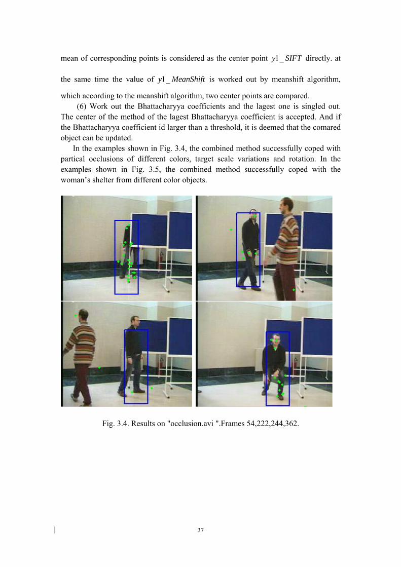
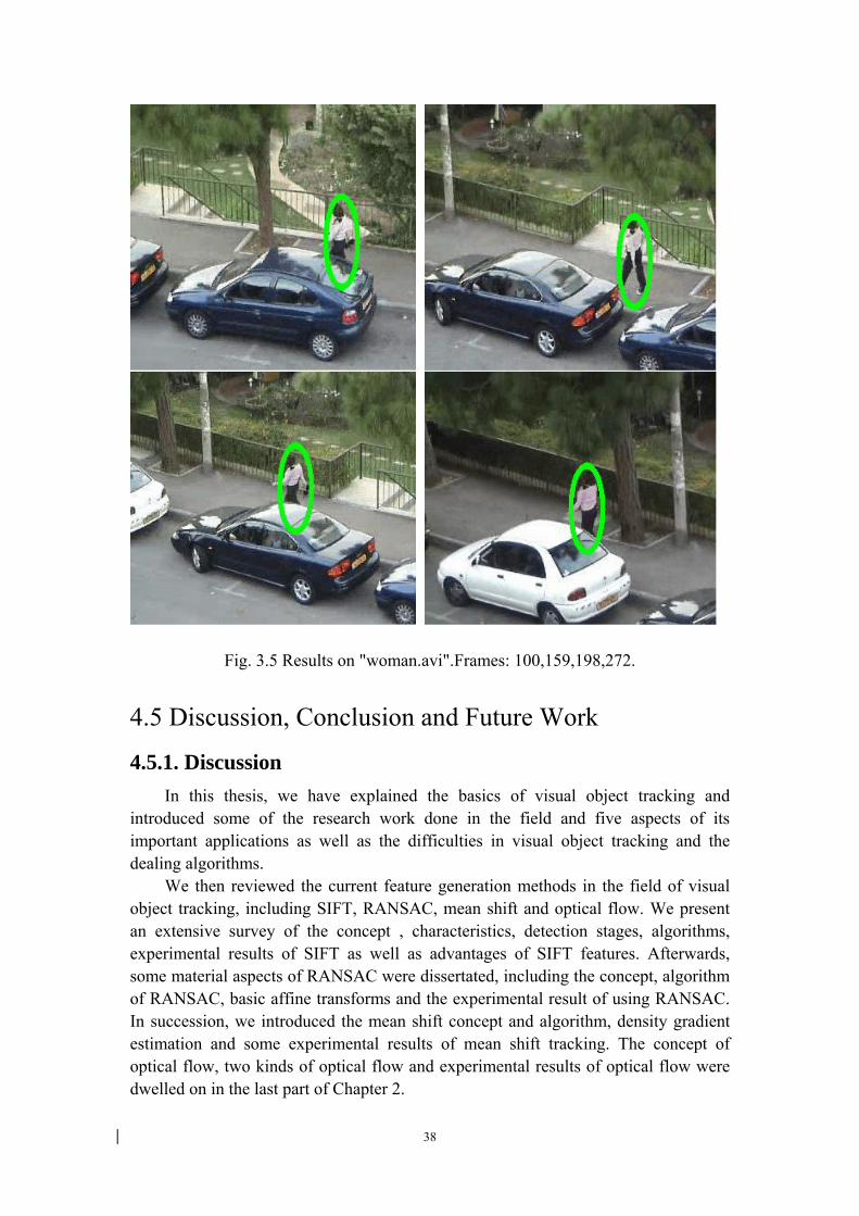
In the examples shown in Fig. 3.4, the combined method successfully coped with partical occlusions of different colors, target scale variations and rotation. In the examples shown in Fig. 3.5, the combined method successfully coped with the woman’s shelter from different color objects.
Fig. 3.4. Results on "occlusion.avi ".Frames 54,222,244,362.
38
Fig. 3.5 Results on "woman.avi".Frames: 100,159,198,272.
4.5 Discussion, Conclusion and Future Work
4.5.1. Discussion In this thesis, we have explained the basics of visual object tracking and
introduced some of the research work done in the field and five aspects of its important applications as well as the difficulties in visual object tracking and the dealing algorithms.
We then reviewed the current feature generation methods in the field of visual object tracking, including SIFT, RANSAC, mean shift and optical flow. We present an extensive survey of the concept , characteristics, detection stages, algorithms, experimental results of SIFT as well as advantages of SIFT features. Afterwards, some material aspects of RANSAC were dissertated, including the concept, algorithm of RANSAC, basic affine transforms and the experimental result of using RANSAC. In succession, we introduced the mean shift concept and algorithm, density gradient estimation and some experimental results of mean shift tracking. The concept of optical flow, two kinds of optical flow and experimental results of optical flow were dwelled on in the last part of Chapter 2.
39
SIFT features are reasonably invariant to rotation, scaling, and illumination changes. We can use them for matching and object recognition among other things. It is robust to occlusion, as long as we can see at least 3 features from the object we can compute the location and pose. Efficient on-line matching, recognition can be performed in close-to-real time (at least for small object databases). RANSAC can estimate the parameters with a high degree of accuracy even when significant amount of outliers are present in the data set. The mean shift algorithm is an alternative techniques which has recently received the attention of the image processing community. It tries to recursively compute the modes of the probability density function using an update equation similar to. The mean shift algorithm provides accurate localization and efficient matching without expensive exhaustive search. Optical flow is a fundamental problem in the processing of image sequences.
A solution to enhance the performance of classical SIFT and mean shift object tracking has been presented in this paper. This work integrated the outcomes of SIFT feature correspondence and mean shift tracking. The approach applied a similarity measurement between two neighboring frames in terms of color and SIFT correspondence. Finally, some experimental results of the integration of mean shift and SIFT feature tracking were presented. Experiment results verified that the proposed method could produce better solutions in object tracking of different scenarios and is an effective visual object tracking algorithm.
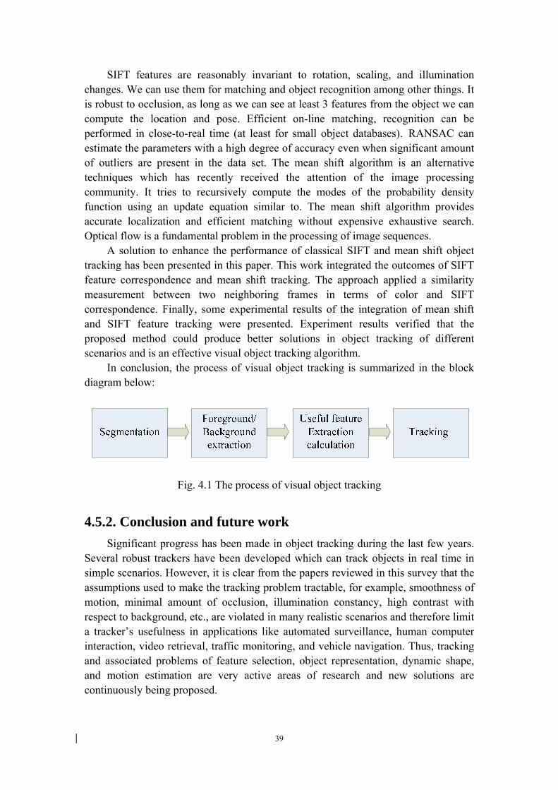
In conclusion, the process of visual object tracking is summarized in the block diagram below:
Fig. 4.1 The process of visual object tracking
4.5.2. Conclusion and future work Significant progress has been made in object tracking during the last few years.
Several robust trackers have been developed which can track objects in real time in simple scenarios. However, it is clear from the papers reviewed in this survey that the assumptions used to make the tracking problem tractable, for example, smoothness of motion, minimal amount of occlusion, illumination constancy, high contrast with respect to background, etc., are violated in many realistic scenarios and therefore limit a tracker’s usefulness in applications like automated surveillance, human computer interaction, video retrieval, traffic monitoring, and vehicle navigation. Thus, tracking and associated problems of feature selection, object representation, dynamic shape, and motion estimation are very active areas of research and new solutions are continuously being proposed.
40
One challenge in tracking is to develop algorithms for tracking objects in unconstrained videos, for example, videos obtained from broadcast news networks or home videos. These videos are noisy, compressed, unstructured, and typically contain edited clips acquired by moving cameras from multiple views. Another related video domain is of formal and informal meetings. These videos usually contain multiple people in a small field of view. Thus, there is severe occlusion, and people are only partially visible. One interesting solution is to employ audio in addition to video for object tracking. There are some methods being developed for estimating the point of location of audio source, for example, a person’s mouth, based on four or six microphones. This audio-based localization of the speaker provides additional information which then can be used in conjunction with a video-based tracker to solve problems like severe occlusion.
In general, an important issue that has been neglected in the development of tracking algorithms is integration of contextual information. For example, in a vehicle tracking application, the location of vehicles should be constrained to paths on the ground as opposed to vertical walls or the sky. Recent work in the area of object recognition[ 40 ] has shown that exploiting contextual information is helpful in recognition. In addition, advances in classifiers [41] have made accurate detection of scene context possible, for example, man made structures, paths of movement, class of objects, etc. A tracker that takes advantage of contextual information to incorporate general constraints on the shape and motion of objects will usually perform better than one that does not exploit this information. This is because a tracker designed to give the best average performance in a variety of scenarios can be less accurate for a particular scene than a tracker that is attuned (by exploiting context) to the characteristics of that scene.
The use of a particular feature set for tracking can also greatly affect the performance. Generally, the features that best discriminate between multiple objects and, between the object and background are also best for tracking the object. Many tracking algorithms use a weighted combination of multiple features assuming that a combination of preselected features will be discriminative. A wide range of feature selection algorithms have been investigated in the machine learning and pattern recognition communities. However, these algorithms require offline training information about the target and/or the background. Such information is not always available. Moreover, as the object appearance or background varies, the discriminative features also vary. Thus, there is a need for online selection of discriminative features. Some work has been done in this area for online selection of individual features [42]. However, the problem of efficient online estimation of discriminative feature sets remains unresolved. One promising direction to achieve this goal is the use of the online boosting methods [43] for feature selection.
In a similar way, most tracking algorithms use prespecified models for object representation. The capability to learn object models online will greatly increase the applicability of a tracker. Motion-based segmentation [ 44 ] and multibody factorization [45] methods have been used to learn models for multiple objects moving in a scene. However, these approaches assume rigid body motion.
41
Unsupervised learning of object models for multiple nonrigid moving objects from a single camera remains an unsolved problem. One interesting direction that has largely been unexplored is the use of semisupervised learning techniques for modeling objects. These techniques do not require prohibitive amounts of training data. Moreover, they can not only learn nonrigid shapes and/or appearance, but they can also encode the knowledge of the background in the form of negative training data.
Probabilistic state-space methods including Kalman Filters, JPDAFs, HMMs and Dynamic Bayesian Networks (DBNs) have been extensively used to estimate object motion parameters[46,47,48]. Among these methods, DBNs are probably the most general method for representation of conditional dependencies between multiple variables and/or image observations. They also provide a principled framework for fusing information from different sources. However, there is a need for more efficient solutions for inference before DBNs are more commonly used in tracking applications.
Overall, we believe that additional sources of information, in particular prior and contextual information, should be exploited whenever possible to attune the tracker to the particular scenario in which it is used. A principled approach to integrate these disparate sources of information will result in a general tracker that can be employed with success in a variety of applications.
In a word, there are many directions for further research in deriving invariant and distinctive image features. Those may include the work of the follows[49,50,51]:
• Develop algorithms for tracking objects in unconstrained videos; • Integration of contextual information tracking algorithms; • Efficient algorithm for online estimation of discriminative feature sets; • Further study on the online boosting methods for feature selection; •Using semisupervised learning techniques for modeling objects; • Model the problem for Kalman filter more accurately; • Improve the speed of the fitting algorithm in the active appearance model by
using multi-resolution; • Investigate the convergence property of the proposed framework. This
investigation may help enhance the proposed algorithm for efficiency purposes; • Further study of the proposed object tracking scheme to demonstrate the
improvement made; • Include the occlusion detection to improve the accuracy of the system. In addition, the proposed algorithm needs to be comprehensively evaluated in a
wider database. Currently, this paper suggests that, although the tracking results are promising in certain situations, further development and more evaluation is anticipated in severe image clutters and occlusions.

42
Acknowledgements The thesis was directed by my advisor, professor Gu. I would like to express my
gratitude to professor Gu for her generous support and supervision. It is her profound knowledge of extensive professional experience, invaluable guidance, and encouragement enrich my whole thesis study at the University of Chalmers,it is a most rewarding experience of my life.
I am also grateful to the other members of Peter, Tiesheng Wang, for their
valuable insight to the area of vedio object tracking.
References
1 P.J. Butt and et al. Object tracking with a moving camera. In Proc. 2nd Int.Conf. on
Computer Vision, pp. 2-12, 1989. 2 A. Gyaourova, C. Kamath, S. and C. Cheung. Block matching object tracking. LLNL
Technical report, October, pp. 22 -26, 2003. 3 Y. Rosenberg, M. Werman. Real-Time Object Tracking from a Moving Video Camera:
A software approach on PC. Applications of Computer Vision, WACV '98. Proceedings, pp.784-793,1998.
4 A. Turolla, L. Marchesotti and C.S. Regazzoni. Multiple camera object tracking in video surveillance applications. Applications of Computer Vision. pp. 132–135, 2001.
5 Y. Wang, J. Doherty and R. Van Dyck. Moving object tracking in video - Proc. Conference on Information Sciences and Systems, Princeton, NJ, pp.546-549, March 2000.
6 Çiˇgdem Eroˇglu Erdem and Bülent San - Video Object Tracking With Feedback of Performance Measures - IEEE Transactions on circuits and systems for video technology, vol. 13, no. 4, April 2003.
7 Probabilistic Object Tracking Using Multiple Features,David Serby, Esther-Koller-Meier, Luc Van Gool, Computer Vision Laboratory (BIWI), ETH Z¨urich, Switzerland,1998.
8 D. Comaniciu, V. Ramesh, and P. Meer, Real-time tracking of non-rigid objects using mean shift, CVPR, pp. 142–149, 2000.
9 P. Perez, C. Hue, J. Vermaak, and M. Gangnet, Color-based probabilistic tracking, ECCV, pp. 661–675, 2002.
10 M. Isard, and A. Blake. Condensation – conditional density propagation for visual tracking, IJCV, 29(1):5–28, 1998.
11 M. Isard, and A. Blake, ICondensation: Unifying low-level and high-level tracking in a stochastic framework, ECCV, pp. 893–908, 1998.
12 G. David Lowe. Object recognition from local scale-invariant features. Proceedings of the International Conference on Computer Vision. 2. pp. 1150–1157,1997.
13 G. David Lowe. Distinctive image features from scale-invariant keypoints. International Journal of Computer Vision, 60(2), pp, 91-110, 2004.
14 Y. Caspi and M. Irani, Alignment of non-overlapping sequences. Proc. Int. Conf. Computer Vision, 76-83, 2001.
15 C. Tomasi and T. Kanade, Shape and motion from image streams under orthography: A factorization method, Int. J. Computer Vision 9(2), 137-154, 1992.
16 P. Torr, Motion Segmentation and Outlier Detection, PhD thesis, Department of Engineering Science, University of Oxford, 1995.
17 Y. Cui, S. Samarasekera, Q. Huang. Indoor Monitoring Via the Collaboration Betweena Peripheral Senson and a Foveal Sensor, IEEE Work-shop on Visual Surveillance, Bomba y, India, 2-9, 1998.
18 G. R. Bradski, Computer Vision Face T racking as a Component of a Perceptual User Interface, IEEE Work. on Applic. Comp. Vis., Princeton, 214-219, 1998.
19 S.S. Intille, J.W. Davis, A.F. Bobick, Real-Time Closed-World T racking. IEEE Conf. on Comp. Vis. and Pat. Rec., Puerto Rico, 697-703, 1997.
20 C. Wren, A. Azarbayejani, T. Darrell, A. Pentland, Pfinder: Real-Time Tracking of the Human Body, IEEE Trans. Pattern Analysis Machine Intell, 19:780-785, 1997.
21 A. Eleftheriadis, A. Jacquin. Automatic Face Location Detection and Tracking for
Model-Assisted Coding of Video Teleconference Sequences at Low Bit Rates, Signal Processing- Image Communication, 7(3): 231-248, 1995.
22 D. Fuiorea, V. Gui, D. Pescaru, and C. Toma. Comparative study on RANSAC and Mean shift algorithm, International Symposium on Electronics and Telecommunications Edition 8. vol. 53(67) Sept. 2008, pp. 80-85.
23 Y.Cheng. Mean Shift, Mode Seeking, and Clustering, IEEE Trans. Pattern Analysis and Machine Intelligence, Vol. 17, No 8, 790-799,1995
24 G. R. Bradski. Computer Vision Face Tracking as a Component of a Perceptual User Interface. IEEE Work. On Applic. Comp. Vis., Princeton, pp. 214-219, 1998.
25 Collins RT. Mean-Shift blob tracking through scale space. In: Danielle M, ed. IEEE Int’l Conf. on Computer Vision and Pattern Recognition, Vol 2. Baltimore: Victor Graphics, pp.234-240, 2003
26 D. Comaniciu, V. Ramesh, and P. Meer, Real-time tracking of non-rigid objects using mean shift, CVPR, pp. 142–149, 2000.
27 Horn B.K.P. Robot Vision. MIT Press, Cambridge, 1986. 28 Verri A. and Poggio T. Against quantitative optical flow. Proc. IEEE ICCV, London,
pp.171-180, 1987. 29 B. K. Horn and B. G. Schunck. Determining optical flow. 1980. 30 S. Ullman. The interpretation of structure from motion. Proceedings of the Royal
Society, pp. 405–426, 1979. 31 B.F. Buxton and D.W. Murray. Optic flow segmentation as an ill-posed and
maximum likelihood problem. Image and Vis. pp. 163-169, 1985. 32 B. Lucas and T. Kanade. An iterative image registration technique with an application
to stereo vision. In IJCAI81, pp. 674–679, 1981. 33 B. Lucas, T. Kanade. An iterative image restoration technique with an application to
stereo vision, Proceedings of the DARPA Image Understanding Workshop, pp. 434–439, 1981.
34 J.-Y. Bouguet. Pyramidal implementation of the Lucas Kanade feature tracker. OpenCV Documentation, Intel Corporation, Microprocessor Research Lab, 1999.
35 Documentation, Intel Corporation, Microprocessor Research Lab, pp. 325–329, 1999. 36 N. Ohta. Optical flow detection by color images. IEEE International Conference On
Image Processing, pp. 801–805, Sept. 1989. 37 N. Ohta and S. Nishizawa. How much does color information help optical flow
computation? IEICE Transactions on Information and Systems – Oxford Journal, pp. 1759–1762, 2006.
38 P. Golland and A. M. Bruckstein. Motion from color. Computer Vision and Image Understanding: CVIU, 68(3), pp. 346–362, Dec. 1997.
39 D. Comaniciu, V. Ramesh, P. Meer, Real-time tracking of non-rigid objects using mean shift, in: IEEE International Conference on Computer Vision and Pattern Recognition (CVPR), South Carolina, pp. 142–149,2000.
40 K. Murphy, A. Torralba, and W. Freeman. Using the forest to see the trees: a graphical model relating features, objects and scenes. In Advances in Neural Info. Proc. Systems, pp. 323–331, 2003.
41 J. Friedman, T. Hastie, and R. Tibshirani. Additive logistic regression: a statistical view of boosting. Annals of statistics, 28(2):337–374, 2000.
42 A. Gelman, J. Carlin, H. Stern, and D. Rubin. Bayesian Data Analysis. Chapman and Hall, 1995.
43 M. Fink and P. Perona. Mutual boosting for contextual influence. In Advances in Neural Info. Proc. Systems, 2003.
44 M. Black and P. Rangarajan. On the unification of line processes, outlier rejection,
and robust statistics with applications in early vision. The International Journal of Computer Vision, 19(1):57–91, 1996.
45 Henry A. Rowley. Takeo Kanade. Human face detection in visual scenes. In Advances in Neural Info. Proc. Systems, volume 8, 1995.
46 A G Simith. Incremental estimation of Image flow using a Kalman filter In IEEE Proceedings of Workshop on VLsuul Motzon (Princeton, NJ, Oct.), pp. 36-43,1991.
47 Lowe, D.G. Local feature view clustering for 3D object recognition. IEEE Conference on Computer Vision and Pattern Recognition, Kauai, Hawaii, pp. 682-688, 2001.
48 W. Freeman and E. H. Adelson. The design and use of steerable filters. IEEE Transactions on Pattern Analysis and Machine Intelligence, pp. 891–906, 1991.
49 Ke, Y., and Sukthankar, R., PCA-SIFT: A More Distinctive Representation for Local Image Descriptors, Computer Vision and Pattern Recognition, pp. 238-243, 2004.
50 Lindeberg, Tony and Bretzner, Lars. Real-time scale selection in hybrid multi-scale representations. Proc. Scale-Space'03, Springer Lecture Notes in Computer Science pp. 148-163, 2003.
51 Scovanner, Paul; Ali, S; Shah, M. A 3-dimensional sift descriptor and its application to action recognition. Proceedings of the 15th International Conference on Multimedia. pp. 357-360,2007.
Related Documents