Video Game Pathfinding and Improvements to Discrete Search on Grid-based Maps by Bobby Anguelov Submitted in partial fulfillment of the requirements for the degree Master of Science in the Faculty of Engineering, Built Environment and Information Technology University of Pretoria Pretoria JUNE 2011

Welcome message from author
This document is posted to help you gain knowledge. Please leave a comment to let me know what you think about it! Share it to your friends and learn new things together.
Transcript

Video Game Pathfinding and Improvements to Discrete
Search on Grid-based Maps by
Bobby Anguelov
Submitted in partial fulfillment of the requirements for the degree
Master of Science
in the Faculty of Engineering, Built Environment and Information Technology
University of Pretoria
Pretoria
JUNE 2011

Publication Data: Bobby Anguelov. Video Game Pathfinding and Improvements to Discrete Search on Grid-based Maps. Master‘s dissertation, University of Pretoria, Department of Computer Science, Pretoria, South Africa, June 2011. Electronic, hyperlinked PDF versions of this dissertation are available online at: http://cirg.cs.up.ac.za/ http://upetd.up.ac.za/UPeTD.htm
Video Game Pathfinding and Improvements to Discrete Search on
Grid-based Maps
by
Bobby Anguelov
Email: [email protected]
Abstract
The most basic requirement for any computer controlled game agent in a video game is to be able to
successfully navigate the game environment. Pathfinding is an essential component of any agent
navigation system. Pathfinding is, at the simplest level, a search technique for finding a route
between two points in an environment. The real-time multi-agent nature of video games places
extremely tight constraints on the pathfinding problem. This study aims to provide the first
complete review of the current state of video game pathfinding both in regards to the graph search
algorithms employed as well as the implications of pathfinding within dynamic game environments.
Furthermore this thesis presents novel work in the form of a domain specific search algorithm for
use on grid-based game maps: the spatial grid A* algorithm which is shown to offer significant
improvements over A* within the intended domain.
Keywords: Games, Video Games, Artificial Intelligence, Pathfinding, Navigation, Graph Search,
Hierarchical Search Algorithms, Hierarchical Pathfinding, A*.
Supervisor: Prof. Andries P. Engelbrecht
Department: Department of Computer Science
Degree: Master of Science


―In theory, theory and practice are the same.
In practice, they are not.‖
- Albert Einstein


i
Acknowledgements
This work would not have been completed without the following people:
My supervisor, Prof. Andries Engelbrecht, for his crucial academic and financial support.
My dad, Prof. Roumen Anguelov, who first introduced me to the wonderful world of
computers and who has always been there to support me and motivate me through thick and
thin.
Alex Champandard for letting me bounce ideas off of him. These ideas would eventually
become the SGA* algorithm.
Neil Kirby, Tom Buscaglia and the IGDA Foundation for awarding me the 2011 ―Eric
Dybsand Memorial Scholarship for AI development‖.
Dave Mark for taking me under his wing at the 2011 Game Developers Conference and
introducing me to a whole bunch of game AI VIPs.
Jack Bogdan, Gordon Bellamy and Sheri Rubin for all their amazing work on the IGDA
Scholarships. This thesis would not have been completed as quickly without the IGDA
scholarship.
Chris Jurney, for taking the time to discuss my thesis topic all those years ago. His work on
the pathfinding for ―Company of Heroes‖ is the inspiration behind this thesis.
My friends and colleagues, for their support over the last few years and for putting up with
all my anxiety and neuroses.
This work has been partly supported by bursaries from:
The National Research Foundation (http://www.nrf.ac.za) through the Computational
Intelligence Research Group (http://cirg.cs.up.ac.za).
The University of Pretoria.

ii

iii
Contents
Acknowledgements ............................................................................................................................................. i
Contents ............................................................................................................................................................. iii
List of Figures ................................................................................................................................................... vii
List of Pseudocode Algorithms ....................................................................................................................... x
Chapter 1 Introduction ............................................................................................................................... 1
1.1 Problem Statement and Overview .................................................................................................. 1
1.2 Thesis Objectives .............................................................................................................................. 2
1.3 Thesis Contributions......................................................................................................................... 2
1.4 Thesis Outline .................................................................................................................................... 3
Chapter 2 Video Games and Artificial Intelligence ................................................................................ 5
2.1 Introduction to Video Games ......................................................................................................... 5
2.2 Video Game Artificial Intelligence ................................................................................................. 8
2.2.1 Human Level AI ..................................................................................................................... 10
2.2.2 Comparison to Academic and Industrial AI ....................................................................... 11
2.3 Game Engine Architecture ............................................................................................................ 13
2.3.1 The Game Engine ................................................................................................................... 13
2.3.2 Basic Engine Architecture and Components ...................................................................... 15
2.3.3 Game Engine Operation and the Game Loop ................................................................... 16
2.3.4 Performance Constraints ....................................................................................................... 18
2.3.5 Memory Constraints ............................................................................................................... 20
2.3.6 The Need for Concurrency ................................................................................................... 21
2.4 The Video Game Artificial Intelligence System.......................................................................... 21
2.4.1 Game Agent Architecture ...................................................................................................... 22
iv
2.4.2 The Game Agent Update....................................................................................................... 24
2.4.3 The AI System Architecture and Multi-Frame Distribution ............................................ 26
2.4.4 The Role of Pathfinding in a Game AI System .................................................................. 27
2.5 Summary ........................................................................................................................................... 29
Chapter 3 Graph Representations of Video Game Environments ................................................... 31
3.1 The Navigational Graph Abstraction ........................................................................................... 31
3.2 Waypoint Based Navigation Graphs ............................................................................................ 33
3.3 Mesh Based Navigational Graphs ................................................................................................. 34
3.4 Grid Based Navigational Graphs .................................................................................................. 37
3.5 Summary ........................................................................................................................................... 39
Chapter 4 The Requirements and Constraints of Video Game Pathfinding .................................... 41
4.1 The Pathfinding Search Problem .................................................................................................. 41
4.2 Pathfinding Search Problem Requirements................................................................................. 43
4.2.1 Path Optimality ....................................................................................................................... 43
4.2.2 Path Smoothing ....................................................................................................................... 44
4.3 Pathfinding Search Problem Constraints ..................................................................................... 45
4.3.1 Performance Constraints ....................................................................................................... 46
4.3.2 Memory Constraints ............................................................................................................... 48
4.4 Pathfinding in Dynamic Environments ....................................................................................... 49
4.5 Selecting a Suitable Search Algorithm .......................................................................................... 52
4.6 Summary ........................................................................................................................................... 53
Chapter 5 Discrete Search Algorithms ................................................................................................... 55
5.1 Discrete Search Algorithms ........................................................................................................... 55
5.2 Dijkstra‘s Algorithm ........................................................................................................................ 56
5.2.1 The Algorithm ......................................................................................................................... 56
5.2.2 Optimizations .......................................................................................................................... 59

v
5.2.3 A Point-to-Point Version of Dijkstra‘s Algorithm ............................................................ 61
5.3 The A* Algorithm ........................................................................................................................... 62
5.3.1 The Algorithm ......................................................................................................................... 63
5.3.2 The Heuristic Function .......................................................................................................... 66
5.3.3 Optimizations .......................................................................................................................... 68
5.4 Iterative Deepening A*................................................................................................................... 71
5.5 Simplified Memory-Bounded Algorithm ..................................................................................... 73
5.6 Fringe Search ................................................................................................................................... 75
5.7 Summary ........................................................................................................................................... 77
Chapter 6 Continuous Search Algorithms ............................................................................................. 79
6.1 Continuous Search Algorithms ..................................................................................................... 79
6.2 Incremental Search Algorithms ..................................................................................................... 81
6.2.1 Introduction ............................................................................................................................. 81
6.2.2 Lifelong Planning A* (LPA*) ................................................................................................ 82
6.2.3 Dynamic A* Lite (D* Lite) .................................................................................................... 85
6.3 Anytime Search Algorithms ........................................................................................................... 89
6.4 Real-Time Search Algorithms ........................................................................................................ 90
6.5 The Suitability of Continuous Search Algorithms for use in Dynamic Video Game
Environments ............................................................................................................................................... 92
6.6 Summary ........................................................................................................................................... 94
Chapter 7 Hierarchical Search Algorithms ............................................................................................ 97
7.1 Hierarchical Approaches ................................................................................................................ 97
7.1.1 Problem Sub-division ............................................................................................................. 97
7.1.2 The Abstraction Build Stage................................................................................................100
7.1.3 The Abstract Search Stage ...................................................................................................102
7.1.4 Path Refinement ....................................................................................................................102
vi
7.1.5 Considerations for Hierarchical Pathfinding ....................................................................104
7.2 Hierarchical Pathfinding A*.........................................................................................................105
7.3 Partial Refinement A* ...................................................................................................................109
7.4 Minimal Memory Abstractions....................................................................................................112
7.5 Summary .........................................................................................................................................115
Chapter 8 The Spatial Grid A* Algorithm ...........................................................................................117
8.1 The Domain Specificity of Video Game Pathfinding ..............................................................117
8.2 The Spatial Grid A* Algorithm ...................................................................................................120
8.2.1 Spatial Grid A* Variant 1 .....................................................................................................121
8.2.2 Spatial Grid A* Variant 2 .....................................................................................................131
8.2.3 Spatial Grid A* Variant 3 .....................................................................................................138
8.3 Experimental Results ....................................................................................................................141
8.3.1 Testing Procedures ...............................................................................................................141
8.3.2 Counter-Strike Maps.............................................................................................................142
8.3.3 Company of Heroes Maps ...................................................................................................147
8.3.4 Baldur‘s Gate Maps ..............................................................................................................150
8.3.5 Starcraft Maps ........................................................................................................................155
8.3.6 Pseudo Real Time Strategy Maps .......................................................................................159
8.4 Summary and Conclusion ............................................................................................................162
Chapter 9 Conclusions and Future Work ............................................................................................165
9.1 Conclusions ....................................................................................................................................165
9.2 Future Research .............................................................................................................................167
Bibliography ....................................................................................................................................................169

vii
List of Figures
Figure 2.1: A screenshot from "Need for Speed" (1994) ............................................................................. 7
Figure 2.2: A screenshot from "Gran Turismo 5" (2010) ............................................................................ 7
Figure 2.3: A screenshot from Namco‘s PACMAN (1980) ........................................................................ 9
Figure 2.4: A screenshot of id Software's "DOOM‖ (1993) ..................................................................... 14
Figure 2.5: A high level overview of the various game Engine Systems.................................................. 17
Figure 2.6: A generalized flowchart representing the runtime operation of a game engine. ................ 19
Figure 2.7: The general AI agent architecture. ............................................................................................. 23
Figure 2.8: The game agent update loop ...................................................................................................... 25
Figure 2.9: Performing agent updates atomically. ....................................................................................... 28
Figure 2.10: A naive approach to agent update scheduling. ...................................................................... 28
Figure 2.11: A robust scheduling approach for agent updates. ................................................................. 28
Figure 3.1: Waypoint based navigational graphs ......................................................................................... 33
Figure 3.2: Creating a mesh based navigational graph from a game environment................................. 35
Figure 3.3: The subdivision of a single triangle due to an environmental change.................................. 36
Figure 3.4: The most common grid cell connection geometries ............................................................... 37
Figure 3.5: A grid-based representation of a Game Environment ........................................................... 38
Figure 4.1: The effect of path smoothing on a generated path ................................................................. 45
Figure 4.2: An example of the level of Destructibility in ‗Company of Heroes‘ .................................... 50
Figure 4.3: The need for path replanning as a result of an environmental change ................................ 51
Figure 4.4: An environmental change requiring the replanning of the agent‘s path .............................. 51
Figure 5.1: The Dijkstra's algorithm‘s cost-so-far calculation and path generation ............................... 57
Figure 5.2: A comparison of search space exploration between Dijkstra‘s algorithm and A* ............. 64
Figure 5.3: The effects of inadmissible A* heuristics ................................................................................. 67
Figure 7.1: The subdivision of a large pathfinding problem into smaller sub-problems ....................100
Figure 7.2: A basic overview of a hierarchical search. ..............................................................................103
Figure 7.3: The HPA* graph abstraction cluster creation ........................................................................105
Figure 7.4: The HPA* graph inter-cluster and intra-cluster links ...........................................................106
Figure 7.5: The effects of the post-processing smoothing phase on path optimality ..........................108
Figure 7.6: The PRA* Abstraction ..............................................................................................................110
viii
Figure 7.7: The Minimal Memory Abstraction ..........................................................................................114
Figure 7.8: A comparison between the HPA* and MM* abstractions. (a). (b). ....................................114
Figure 7.9: Improving path sub-optimality through the trimming of sub-problem solutions ...........115
Figure 8.1: Sample map and resulting gridmap from the Company of Heroes RTS game ................118
Figure 8.2: Sample maps from various game genres.................................................................................118
Figure 8.3: SGA* sub-goal creation and refinement .................................................................................122
Figure 8.4: Search space comparison between A* and SGA* for a simple search problem...............124
Figure 8.5: The search space reduction of SGA* and effect of path smoothing on a SGA* path ....125
Figure 8.6: Invalid sub-goal creation ...........................................................................................................126
Figure 8.7: Disjoint region SGA* special case ...........................................................................................128
Figure 8.8: The need for path-smoothing for optimal paths ...................................................................131
Figure 8.9: Unnecessary SGA* variant 1 search space exploration due to naïve sub-goal selection .132
Figure 8.10: SGA* Variant 2 Search Space Exploration ..........................................................................134
Figure 8.11: The difference between the two refinement path trimming techniques ..........................135
Figure 8.12: The effect of the additional condition on refinement path trimming ..............................136
Figure 8.13: SGA* V2 Partial Pathfinding .................................................................................................138
Figure 8.14: Example maps from the ―Counter-Strike‖ test set .............................................................142
Figure 8.15: The cs_militia ―Counter-Strike‖ Map‖ .................................................................................143
Figure 8.16: Per-map SGA* performance results for the "Counter-Strike" test set ............................144
Figure 8.17: Search space exploration statistics for SGA* over A*........................................................145
Figure 8.18: Per-map SGA* path optimality measurements for the "Counter-Strike" test set ..........146
Figure 8.19: Overall SGA* results for the "Counter-Strike" test set ......................................................146
Figure 8.20: Example maps from the ―Company of Heroes‖ test set ...................................................147
Figure 8.21: Per-map SGA* performance results for the "Company of Heroes" test set ..................148
Figure 8.22: Per-map SGA* path optimality measurements for the "Company of Heroes" test set 149
Figure 8.23: Overall SGA* results for the "Company of Heroes" test set ............................................149
Figure 8.24: Example maps from the ―Baldur‘s Gate‖ test set ...............................................................150
Figure 8.25: Per-map SGA* performance results for the "Baldur‘s Gate" test set ..............................151
Figure 8.26: Per-map SGA* performance results for maps 29-43 of the ―Baldur‘s Gate‖ test set ...152
Figure 8.27: Per-map SGA* path optimality measurements for the "Baldur‘s Gate" test set ............153
Figure 8.28: Per-map SGA* path optimality measurements for maps 29 to 43 of the "Baldur‘s Gate"
test set ..............................................................................................................................................................154

ix
Figure 8.29: Map AR0400SR from the "Baldur's Gate" test set .............................................................154
Figure 8.30: Overall SGA* results for the "Baldur‘s Gate" test set ........................................................155
Figure 8.31: Example maps from the ―Starcraft‖ test set ........................................................................156
Figure 8.32: Per-map SGA* performance measurements for the "Starcraft" test set .........................157
Figure 8.33: Per-map SGA* path optimality measurements for the "Starcraft" test set .....................158
Figure 8.34: Overall SGA* results for the "Starcraft" test set .................................................................158
Figure 8.35: Example maps from the pseudo RTS test set .....................................................................159
Figure 8.36: Per-map SGA* performance measurements for the ―Pseudo RTS " test set .................160
Figure 8.37: Per-map SGA* path optimality measurements for the "Pseudo RTS" test set ..............161
Figure 8.38: Overall SGA* results for the "Pseudo RTS" test set ..........................................................161

x
List of Pseudocode Algorithms
Listing 5.1: Pseudocode for Dijkstra's Algorithm ....................................................................................... 59
Listing 5.2: Pseudocode for the point-to-point version of Dijkstra‘s algorithm .................................... 62
Listing 5.3: Pseudocode for the A* algorithm ............................................................................................. 66
Listing 5.4: Pseudocode for the IDA* Algorithm and depth first search................................................ 74
Listing 5.5: Pseudocode for the fringe search algorithm and TLFS ......................................................... 77
Listing 6.1: Pseudocode for the LPA* Algorithm ....................................................................................... 85
Listing 6.2: Pseudocode for the D* Lite algorithm ..................................................................................... 88
Listing 8.1: Pseudocode for SGA* variant 1 ..............................................................................................129
Listing 8.2: Pseudocode for SGA* variant 2 ..............................................................................................139
Listing 8.3: Pseudocode for SGA* variant 3 ..............................................................................................140

1
Chapter 1 Introduction
1.1 Problem Statement and Overview
The most basic requirement for any computer controlled game agent in a video game is to be able to
successfully navigate the game environment. The navigation problem is broken down into two
problems: locomotion and pathfinding [1]. Locomotion is concerned with the physical motion of a
game agent while pathfinding is concerned with finding a valid route to a game agent‘s desired future
position. The pathfinding problem is, at the simplest level, a search technique for finding a route
between two points in an environment.
The pathfinding problem is not exclusive to video games and is extensively used in both the
networking and robotics fields [2]. While the pathfinding problem is fundamentally similar with
regards to the environmental representations and search techniques employed, the requirements and
constraints placed upon the pathfinding problem within the various fields differ greatly. The real-
time multi-agent nature of video games results in extremely tight constraints being placed on the
video pathfinding problem. In addition to the tight constraints modern video game environments
often feature a degree of dynamicity and so further increase the complexity of the overall
pathfinding problem.
To the author‘s knowledge, to date there does not exists a complete review of the video game
pathfinding field with regards to environmental representations, search algorithms employed and
considerations for dynamic environments. Several works [3], [4], [5] have attempted to provide
either brief introductions or overviews of the field, but in all cases are lacking in either scope or
depth. This study aims to provide a complete overview of the current state of video game
pathfinding as well as produce novel work on the topic.

CHAPTER 1 – INTRODUCTION 2
1.2 Thesis Objectives
The main objective of this thesis is to present an in-depth review of the video game pathfinding
field, with an additional focus on the various graph search algorithms employed. During this study, a
domain specific problem was identified and a novel discrete search algorithm was developed. In
reaching the overall thesis goals the following sub-objectives are identified:
To provide an introduction to video game AI and the video game pathfinding.
To discuss the representation of complex 3D game worlds into searchable graphs.
To investigate the overall video game pathfinding problem and to identify all the
requirements and constraints of video game pathfinding.
To discuss the additional implication of pathfinding within dynamic video game
environments.
To provide an overview of the three main families of pathfinding search algorithms, namely
discrete, continuous, and hierarchical search algorithms.
To identify a solution to a specific pathfinding problem that can be improved upon, and to
develop an improved solution to that problem.
1.3 Thesis Contributions
The main contributions of this thesis can be divided into two sections: the contributions to
knowledge in the field as well as the products resulting from this work.
The contributions to knowledge are:
A detailed and complete review of the current state of the video game pathfinding field.
A review of the various environmental representations in use as well as the requirements and
constraints of the video game pathfinding problem.
A detailed overview and discussion of the three main families of pathfinding search
algorithm.
The observation that the entire continuous search algorithm family is inherently unsuitability
for use within video game pathfinding.
A discussion about the selection of a pathfinding search algorithm and environmental
representation within a specific problem domain.
CHAPTER 1 – INTRODUCTION 3
The products of this thesis are:
The development of a novel, domain specific, grid-based navigational graph search
algorithm: the spatial grid A*. Three variants of the spatial grid A* algorithm are presented
and evaluated across five game map test sets. The spatial grid A* algorithm is shown to offer
improvements of up to 90% to both search times and memory usage of the A* search
algorithm within the intended domain.
1.4 Thesis Outline
Chapter 2 introduces the field of video game artificial intelligence (AI). The history of video game
AI and the difference between video game AI and academic AI is discussed. An introduction to
game engine architecture is presented covering the operation of, and constraints placed upon current
generation video games. The role of the video game AI system within the overall game engine
hierarchy is discussed. The chapter concludes with a discussion of the game agent paradigm and the
role of pathfinding within a video game AI system.
Chapter 3 discusses the various techniques available to convert complex 3D environments into
simple searchable navigational graphs. The three most common representations are discussed
namely waypoint based, navigation mesh based, and grid based navigational graphs.
Chapter 4 discusses the video game pathfinding problem in detail. The requirements and constraints
of the video game pathfinding search problem are discussed. The pathfinding search algorithm is
presented as the solution to the path finding search problem, and a set of metrics used in the
evaluation and comparisons of pathfinding search algorithms is presented. Advice on the selection
of an appropriate pathfinding search algorithm for specific pathfinding search problems concludes
the chapter.
Chapter 5 presents an overview of various discrete graph pathfinding search algorithms. The chapter
presents discussions on the following search algorithms: Dijkstra‘s Algorithm [6], the A* algorithm
[7], the Iterative deepening A* algorithm [8], the memory enhanced iterative deepening A* algorithm
[9], the simplified memory-bounded algorithm [10] and the fringe search algorithm [11].
Chapter 6 presents an overview of various continuous graph pathfinding search algorithms.
Continuous search algorithms are divided into three families: the incremental, the anytime, and the
CHAPTER 1 – INTRODUCTION 4
real-time continuous search algorithms. The chapter presents discussions on the following search
algorithms: the dynamic A* algorithm [12], the focused dynamic A* algorithm [13], the lifelong
planning algorithm [14], the D* lite algorithm [15], the adaptive A* algorithm [16], the generalized
adaptive A* algorithm [17], the anytime repair A* algorithm [18], the anytime dynamic A* [19], the
learning real-time A* algorithm [20], and the real-time dynamic A* algorithm [21]. A discussion on
the unsuitability of the entire continuous search algorithms family for use within video games
concludes the chapter.
Chapter 7 presents an overview of various hierarchical graph pathfinding search algorithms.
Discussions are presented on the following hierarchical search algorithms: the hierarchical
pathfinding A* [22], the dynamic hierarchical pathfinding A* [23], the partial refinement A* [24],
and the minimal memory abstraction algorithm [25].
Chapter 8 presents the spatial grid A* algorithm, a set of techniques for the improvement of the A*
search algorithm‘s performance and memory usage when used to search grid-based navigational
graphs. The spatial grid A* algorithm performance was evaluated on five distinct game map test sets.
A detailed discussion of the performance results of the spatial grid A* concludes the chapter.
This thesis concludes in Chapter 9, with a summary of the video game pathfinding field as well as
the conclusions made from the spatial grid A* algorithm‘s performance evaluation presented in
chapter 8. Additionally, suggestions for possible future research are provided.

5
Chapter 2 Video Games and Artificial Intelligence
To better understand the requirements and constraints of video game pathfinding, it is beneficial to
provide some background on both video games and video game artificial intelligence (AI) systems.
This chapter first provides a brief introduction to video games and the video game AI. A discussion
on game engine architecture follows, in order to better highlight the performance and memory
constraints placed upon video game AI systems. Finally, a discussion into game AI systems, game
agents, and the role of pathfinding is presented.
2.1 Introduction to Video Games
Video games are one of the most popular forms of modern entertainment, so much so that video
games can be found on practically every digital platform available, ranging from mobile phones to
specialized game consoles. PC gaming alone accounted for over 13 billion Dollars revenue for 2009
[26]. Mobile and social network gaming is also on the increase with over 80 million people playing
Zynga‘s Farmville on Facebook in 2010 [27]. Video gaming is no longer a niche activity for the tech
savvy and is enjoyed by people from all walks of life and technical aptitudes [28].
Video games have changed dramatically over the last 2 decades. As computing technology has
grown, video game developers have taken advantage of the increased processing power available and
create ever more realistic representations of virtual game worlds. For example, ―Need for Speed‖, an
arcade racing title released in 1994 featured no hardware acceleration for the visuals (commonly
referred to as graphics), a very simplistic physics engine and no vehicle damage resulting from
collisions. A screen shot of ―Need for Speed‖ is shown in Figure 2.1. Since the release of ―Need for
Speed‖ in 1994, the improvement in computing technology as well as rendering technology has
allowed for hyper-realistic gaming experience.

CHAPTER 2 - VIDEO GAMES AND ARTIFICIAL INTELLIGENCE 6
―Gran Turismo 5‖ is a simulation racing game released in 2010 for the PlayStation 3 and offers near-
photo realistic visuals as well as highly accurate physics and damage models for the in-game vehicles.
Compare a screenshot form ―Gran Turismo 5‖ (Figure 2.2) to that of the earlier ―Need for Speed‖
(Figure 2.1) and the advancements in video game technology over the last two decades is evident.
The video game era was kicked off by three MIT students in 1961 with their game ―SpaceWar‖ [29].
Even though the two player spaceship battle game they created was rudimentary, it showed the
potential of the computer to be more than a simple work machine. Over the next three decades, the
video game industry grew at a rapid pace. Video game technology progressed hand in hand with
advancements in central processing unit (CPU) and graphical rendering technology. Due to
hardware limitations on storage, processing and memory of the time, early games offered simplistic
pixel-art 2D graphics, pattern based computer opponents and small self-contained game levels. With
the increase in computational power of each new generation of computing hardware, video games
grew both in complexity and scale. As interesting as it is, a full history of video games is beyond the
scope of this thesis, and interested readers are referred to [30], [31] and [32].
Visually, video games remained largely unchanged until the mid-90s. Prior to 1994, game graphics
were software rendered, meaning that the CPU was responsible for drawing all the game visuals.
Software rendering was expensive and consumed the bulk of the CPU time available to a game. This
meant that very little time remained for other gameplay systems such as physics or AI. With the
processing power available at the time, it was impossible to render visually appealing 3D graphics at
any sort of acceptable animation frame rate so games remained primarily 2D sprite-based affairs. 2D
graphics accelerator cards such as S3‘s Virge series were developed and released but while these
cards improved the speed of 2D rendering, 3D rendering was still unpractical. The greatest impact in
video game technology came in 1996 with the release of 3DFX‘s Voodoo Graphic Chipset. This
add-in card was designed with a single purpose in mind: 3D graphics rendering. The Voodoo
graphics card allowed for all 3D graphical calculations to be moved off of the CPU, thereby freeing
the CPU for other gameplay related tasks. In addition to allowing game developers the ability to
offer 3D visuals, 3D acceleration allowed for more complex gameplay mechanics and AI due to the
reduced CPU time needed for the graphics rendering systems. The Voodoo graphics card ushered in
the age of 3D acceleration and 3D graphics.

CHAPTER 2 - VIDEO GAMES AND ARTIFICIAL INTELLIGENCE 7
Figure 2.1: A screenshot from "Need for Speed" (1994)
Figure 2.2: A screenshot from "Gran Turismo 5" (2010)

CHAPTER 2 - VIDEO GAMES AND ARTIFICIAL INTELLIGENCE 8
Since the release of that first 3D graphics card, graphics card technology has improved
exponentially. Modern graphics card chipsets now contain multi-core processing units, offering
significantly more processing power than even the fastest desktop CPU available [33]. These
graphics card chipsets are termed graphical processor units (GPU). Graphics cards are no longer
simply restricted to graphical calculations and are now used for general purpose computing, referred
to as general-purpose computing on graphics processing units (GPGPU) [33]. With all this extra
processing power available to the game developer, the CPU is further freed, allowing for more
complex gameplay and AI systems.
As an industry, game development is a highly innovative and competitive one, with game developers
often working on the cutting edge of both 3D graphics and human level AI. This high level of
competition and innovation has bred a high level of expectance from the consumers. With each new
generation of games released, game players (gamers) expect, if not demand, ever higher degrees of
realism from the visuals, sound and most importantly the AI of the in-game characters and
opponents; in-game characters and opponents are referred as non-playable characters (NPCs). As a
result of the high level of technology usage and player expectations, today‘s video games offer
complex game mechanics, realistic Newtonian physics engines, detailed 3D environments, and
hordes of computer controlled opponents for players to battle against.
Video games are no longer the simplistic kids‘ games of yesteryear and it has become more accurate
to describe modern video games not just as a form of entertainment but rather as a highly detailed
real-time simulation. This paradigm shift has fueled the recent academic trend of using commercial
game engines as readily available, easy to use tools for the rapid visualization of real-time simulations
[34], [35]. In addition, there have been calls for the increased use of interactive video games as test
beds for the research, testing, and development of human-level AI systems [36].
2.2 Video Game Artificial Intelligence
Video game AI had humble beginnings. Prior to the 1970s, video games were mainly two-player
games serving as a platform where two human players compete against one another. It was only in
the 1970s that games began to include computer controlled opponents, for the first time allowing
only a single player to play the game. These early opponents were very simple and their movement
was pattern-based, meaning that they moved in a predefined hardcoded pattern [3] [37]. A famous
CHAPTER 2 - VIDEO GAMES AND ARTIFICIAL INTELLIGENCE 9
example of such pattern-based opponents is the game ―Space Invaders‖. In ―Space Invaders‖, the
player controlled a space ship and was required to destroy all the alien invaders on the screen. The
aliens were controlled by a simple pattern that moved them back and forth across the scene and
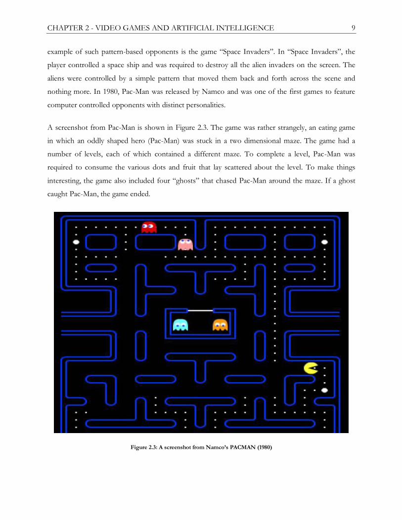
nothing more. In 1980, Pac-Man was released by Namco and was one of the first games to feature
computer controlled opponents with distinct personalities.
A screenshot from Pac-Man is shown in Figure 2.3. The game was rather strangely, an eating game
in which an oddly shaped hero (Pac-Man) was stuck in a two dimensional maze. The game had a
number of levels, each of which contained a different maze. To complete a level, Pac-Man was
required to consume the various dots and fruit that lay scattered about the level. To make things
interesting, the game also included four ―ghosts‖ that chased Pac-Man around the maze. If a ghost
caught Pac-Man, the game ended.
Figure 2.3: A screenshot from Namco‟s PACMAN (1980)

CHAPTER 2 - VIDEO GAMES AND ARTIFICIAL INTELLIGENCE 10
The game developer realized that if each ghost simply follows the player, the player would constantly
be followed by a single-file line of ghosts. By having the ―ghosts‖ cooperate with one another to try
and trap the player, the game became more difficult and more interesting. This inter-ghost
cooperation was implemented by giving each ―ghost‖ its own distinct AI controlled personality [38].
In doing so, Pac-Man became one of the first and most well-known examples of video game AI.
Pac-man is also notable for being one of the first video games to make use of a finite state machine
(FSM) in controlling a game character‘s behavior [3] and since then FSMs have ended up becoming
ubiquitous in the field of video game AI. The Pac-Man AI was a very popular example for the use of
FSMs and has gone on to become a recommended test problem for AI courses teaching FSM
systems [39].
2.2.1 Human Level AI
To date, there is no agreed upon definition of what artificial intelligence is. The definition provided
in [40] states that ―AI is the study of systems that act in a way, that to any observer would appear
intelligent‖. This definition describes the video game AI field perfectly. The main objective of game
AI is to create game opponents that seem as human as possible, leading to the term: human level AI.
As there is no metric to measure the ―humanness‖ of an AI, it is necessary, in order to create a more
concrete list of requirements for a game AI, to briefly delve into the psychology of a game player as
well as the act of playing a game.
There are various reasons why people enjoy playing games, but the simplest reason and the most
obvious is that games are fun [28], [41], [42]. The enjoyment of a game (or fun) is derived from the
challenge offered to the player and the sense of achievement the player gets from completing the
game objectives or defeating the in-game opponents. Most video games feature some type of AI
controlled NPCs which can take many forms, both friend and foe. Gameplay mechanics are often
centered on defeating all the opponents in a game level before being allowed to proceed to the next.
The gameplay of such games is entirely reliant on the high degree of interaction between the player
and the various AI controlled opponents; the overall quality of the game becomes dependent on the
quality of these human-AI interactions. There is a correlation between the level of difficulty of a
game and the level of enjoyment of that game by players [43]. The vast majority of games offer user-
adjustable difficulty levels so as to be able to cater for a large audience of people with different levels
of skill. Adjusting the difficulty level usually means adjusting the behavior of the AI opponents;
often decreasing their reaction times and allowing them to make more mistakes.

CHAPTER 2 - VIDEO GAMES AND ARTIFICIAL INTELLIGENCE 11
In games featuring a high level of player-AI interaction, a successful NPC is expected to respond to
game events in a human-like manner. While humanness is a difficult quality to quantify, the idiom
―to err is human‖ is apt and so the simplest method by which to simulate human behavior is to have
an imperfect (or purposely flawed) AI [44]. This requires that the decision making process as well as
other fundamental game AI systems be capable of returning sub-optimal results.
It is important to note that even though players expect intelligent AI systems, the players are aware
that the actions of AI controlled NPCs will not be perfect (or in some cases will be perfect, resulting
in inhuman actions) and as such will allow a certain degree of error on the AI‘s part. As it stands, it
is impossible to fully simulate a human opponent, and while developers are not expected to succeed
in that task, it is critical to ensure that any highly noticeable AI behavioral errors, such as navigation
mistakes, are kept to a minimum. Players may not notice that an NPC‘s aim is consistently
inaccurate and sometimes may even consider that a feature. However as soon as the NPC does
something obviously incorrect, for example attempting to navigate through a minefield even though
there is a safe route available, then the human-like illusion is shattered.
2.2.2 Comparison to Academic and Industrial AI
Video game AI differs greatly in both requirements and constraints to other prominent industrial
and academic AI fields such as computational intelligence (CI) and robotics [3]. In most AI fields
the goal is to create a ―perfect‖ and specialized AI for a specific problem or operation, an AI that is
faster, more efficient and more accurate than a human could ever be. As these industrial and
academic fields do not require the versatility and adaptability of humans, these specialized AIs are
usually easier to develop [36] [2]. In stark contrast, a video game AI does not need to solve a
problem perfectly but rather needs to solve it to the satisfaction of the player, entailing that the AI
often needs to be both intelligent and yet purposely flawed.
An intelligent and yet purposely flawed AI can present the player with an entertaining challenge, and
yet still be defeatable through the mistakes and inaccuracies of its actions [44]. For example, for the
famous chess match between IBM‘s Deep Blue Chess Computer and Gary Kasparov in May 1997
[45], Deep Blue‘s only goal was to defeat the chess grandmaster without care of whether the
opponent was enjoying the game or not. Its only concern was calculating the optimal next move for
the current situation. Game players want to enjoy playing a game and playing against an opponent
that never makes a mistake isn‘t much fun.

CHAPTER 2 - VIDEO GAMES AND ARTIFICIAL INTELLIGENCE 12
A good example of the necessity of imperfect opponents is a commercial chess game. Such a game
features flawed opponents of various difficulty levels and various personality traits: some opponents
being more aggressive than others, some will sacrifice pieces to achieve victory while others will do
everything possible to avoid losing a piece, and so on. It is these personality traits that result in
imperfect decisions, making playing human players interesting and fun. Players can still enjoy a game
even if they lose, as long as they feel that they lost due to their own mistakes and not due to an
infallible opponent. In the case of a ‗perfect‘ game AI, such as ―Deep Blue‖, there is no incentive for
players to play the game since they realize that they can never win. Game developers realize this and
go to great lengths in attempting to simulate human behavior (including flaws) as closely as possible
[46].
A further distinction between video game AI and other AI fields exists in both the type and the
quality of environmental data available to the AI, as well as the processing and memory constraints
within which the AI is required to make decisions. Due to the virtual self-contained nature of the
game world, video game AIs have perfect knowledge of their environment, whereas in other fields
AIs are designed specifically to deal with and adapt to unknown, incomplete or even incorrect data.
The fact that complete knowledge about the environment is always available to a game AI makes it
all too easy to write a perfect AI, therefore much care must be taken to allow the AI the ability to
make mistakes in such circumstances. Furthermore, in having perfect environmental knowledge at
any given time, NPCs need not have full sets of sensors (discussed in more detail in Section 2.4.1).
In regards to processing and memory constraints, video games are executed on a single CPU. The
CPU therefore needs to be shared amongst the various processor intensive systems that make up the
game engine (discussed in Section 2.3). In sharing the CPU across the various game engine systems,
the game AI is only allocated a small fraction of the total processing time [3]. In comparison, in an
academic or industrial setting, AIs are usually run in isolation, on dedicated hardware having a much
larger allocation (if not all) of the CPU time. Furthermore, game AI systems are often tasked with
controlling numerous NPCs simultaneously, unlike academic and industrial AI systems which are
usually tasked with controlling only a single agent. All these factors combined tend to result in much
looser performance and time constraints being placed on academic/industrial AI systems than on
game AI systems [3]. The performance and memory constraints placed upon game AI systems are
further discussed in Sections 2.3.4 and 2.3.5. These tighter processing and memory constraints limit
the applicability of certain academic techniques and algorithms to game AI systems.

CHAPTER 2 - VIDEO GAMES AND ARTIFICIAL INTELLIGENCE 13
2.3 Game Engine Architecture
The architecture and design of a game engine is, in essence, a software engineering problem and
even though this thesis is focused on game AI systems, specifically pathfinding, it is necessary to go
into detail regarding some of the low-level components, architecture and basic operation of a game
engine to better highlight the various design requirements and performance constraints introduced
by the game engine environment. The following subsections discuss the need for a game engine,
basic game engine architecture, as well as the constraints and requirements introduced by the game
engine.
2.3.1 The Game Engine
As CPU and GPU technologies have grown, so has the complexity of video games. In the past,
video games were written by a single engineer with a small budget, over the course of a few months.
Today‘s video games involve hundred man teams, multimillion dollar budgets and take several years
to develop [47]. Modern games are complex software engineering projects with codebases in excess
of a million lines of code [48] [47]. The massive scale of today‘s games makes writing a game from
scratch infeasible from both an engineering and budgetary standpoint. Game developers will often
reuse key components from one game to the next, saving developers from having to rewrite large
parts of the common game systems. The reuse of existing codebases in the development of a game
will save both time and money, and so is an absolute necessity.
A game engine can be thought of as a framework upon which a game developer builds a game. A
game engine will have built-in libraries for common tasks such as math or physics as well as for
rendering. Game engines allow developers to focus on creating the game and not the technology
behind the game. Game engines allow developers to quickly prototype game features without
spending months re-engineering the wheel, as well as offering the developers prebuilt editing and art
asset tools for the engine [49]. These prebuilt tools further reduce the total engineering time spent
during development. The licensing of third-party game engines (and other game components such as
physics and animation packages) has become big business. As a result, several leading game
development studios such as ―Epic Games‖, ―Crytek‖ and ―Valve Corporation‖ have shifted their
focus into the development of game engines as a critical part of developing the actual games
themselves. This presents such studios with an additional revenue stream, after the release of their
games, by licensing their game engines to other third-party developers. Certain companies only focus
CHAPTER 2 - VIDEO GAMES AND ARTIFICIAL INTELLIGENCE 14
on the development of game engines and game libraries (termed middleware) with the goal of
licensing their product to third-party clients. These companies‘ entire income is dependent on the
licensing of their code bases. Popular middleware companies include ―Havok‖, ―Emergent Game
Technologies‖, and ―RAD Game Tools‖ [50].
Another popular development strategy is to build a custom in-house game engine with the intent of
reusing it for several upcoming titles [49]. While this is large investment in terms of both time and
money, game studios usually produce games of a single genre. Having a game engine that is custom
built for a specific genre ends up more efficient in the long run due to in-house engine familiarity
and specialization of engine features.
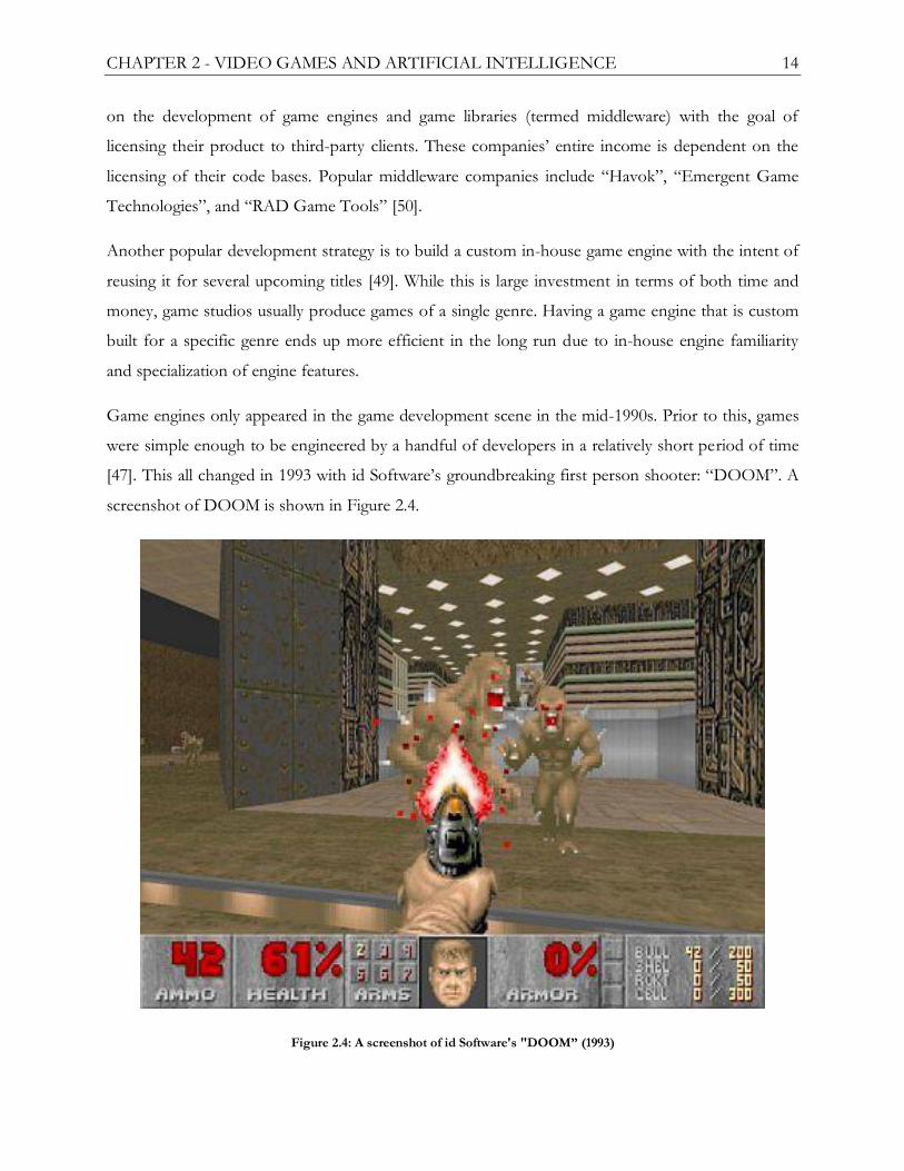
Game engines only appeared in the game development scene in the mid-1990s. Prior to this, games
were simple enough to be engineered by a handful of developers in a relatively short period of time
[47]. This all changed in 1993 with id Software‘s groundbreaking first person shooter: ―DOOM‖. A
screenshot of DOOM is shown in Figure 2.4.
Figure 2.4: A screenshot of id Software's "DOOM” (1993)

CHAPTER 2 - VIDEO GAMES AND ARTIFICIAL INTELLIGENCE 15
DOOM was one of the first games that had a well-defined separation of its core software
components and the game assets (art, levels, etc.) [47]. This allowed the developers to work on the
core game systems without the need for game assets from the art department. Another major benefit
of the content separation of id Software‘s DOOM engine was that it allowed the studio to reuse the
engine in the creation of the game‘s sequel DOOM II.
The prebuilt engine meant that the creation of DOOM II required relatively little effort, resulting in
DOOM II being released less than a year after the original DOOM. DOOM is considered to be one
of the first examples of a true game engine [47]. id Software went on to further pioneer game engine
technology with their ―id Tech‖ series of game engines (the DOOM engine being the first, termed
―id Tech 1‖).
2.3.2 Basic Engine Architecture and Components
Game engines are built in layers with a high level of interconnection between the layers [47]. A
simplified model of the layered architecture of a modern game engine is given in Figure 2.5. The
lowest three layers of a game engine are concerned with the hardware interfaces between the game
engine and the target platform‘s hardware.
These bottom three layers grouped together are referred to as the hardware abstraction layer (HAL).
The developer has no direct means of interaction with the HAL. All interaction with the HAL
occurs through the use of third party platform software development kits (SDK) such as the
Microsoft Windows SDK and DirectX SDK. These platform SDKs interface directly with the HAL
and allow the developer standardized access to the base platform hardware.
Game developers are often required to target multiple platforms for their games and a further
requirement of a modern game engine is cross-platform compatibility. Each platform the game
engine is required to run on will feature its own SDK. This means that the third party SDKs will
often change across platforms, requiring that the game engine includes a layer to wrap the
underlying SDKs into a standardized interface that is used by the higher level systems across all
platforms. This wrapper layer is referred to as the platform independence layer. The platform
independence layer allows developers to simply exchange the layer with an appropriate one when
porting the game across platforms without the need to modify any of the higher level systems.

CHAPTER 2 - VIDEO GAMES AND ARTIFICIAL INTELLIGENCE 16
The next layer in the game engine hierarchy is the core systems layer. This layer contains all the low
level utility libraries used by the game engine such as memory allocation and math libraries. Most of
the game engine systems are built around these core libraries.
The game engine systems layer is the core of the engine and determines the overall feature set of the
game engine. The game engine layer is responsible for all the resource management and scene
management systems as well as all collision detection, physics, user interface and rendering systems.
The game engine systems layer contains interfaces to the various components contained within it
and these interfaces are exposed to the game specific systems layer.
The game engine systems layer can be thought of as nothing more than a collection of black boxes
awaiting instructions.
Overall, the game engine is a basic framework, where the developer simply fills in the gaps. This
―gap-filling‖ occurs within the game specific systems layer. The game specific systems layer contains
and manages all the actual game rules and mechanics, as well as the game AI system. Although the
game AI system‘s overall architecture is similar across games and can be thought of as a core system,
the AI system is highly data driven and the system‘s behaviors and functions are determined by both
the game type and the game data available. The game AI system is specific to the actual game being
developed and cannot be as easily generalized as other core systems, such as scene management or
physics.
2.3.3 Game Engine Operation and the Game Loop
When a game is executed, the first thing that needs to occur is the initialization of the game engine.
The engine therefore enters an initialization stage. The game engine initialization stage is responsible
for initializing all the core game engine systems as well as loading all constant game resources (found
across all the game levels).
Normally, after the game engine initialization completes, the player is presented with a menu from
which various game options can be selected, e.g. to begin a new game, continue a saved one, or to
change game settings. Once the player has made a selection that triggers the start of the game, the
game engine enters the level initialization stage. The level initialization stage is responsible for
loading all the relevant level data and resources as well as resetting any engine systems that require
re-initialization per game level.

CHAPTER 2 - VIDEO GAMES AND ARTIFICIAL INTELLIGENCE 17
Game Specific Systems
Player Cameras
Player Mechanics
Game Mechanics
Etc.
Game AI System
Decision Making
Pathfinding Actuators
Game Engine Systems
Scripting Engine
Scene Management
Collisions & Physics
AnimationSystems
GUI & Input Systems
Low Level Renderer
Shaders
Viewports
Lighting
Textures
Fonts
Cameras
Etc.
Resource Management
Profiling & Debugging
Scene Graph & Culling
Hardware Abstraction Layer
Operating System
Drivers
Hardware
Third Party Platform SDKs
Core Systems
Math LibraryMemory
AllocatorsStrings and
HashingRandom
Number Gen.Etc.
Platform Independence Layer
Figure 2.5: A high level overview of the various game Engine Systems
The game engine features two shutdown stages: the level shutdown stage and the game engine
shutdown stage. The level shutdown stage is entered each time the game transitions from level to
level, and is responsible for releasing all level data and resetting any level specific core systems. The
game engine shutdown stage releases all game resources and shutdowns all game engine systems. A
simplified flowchart of a game engine operation is shown in Figure 2.6. For simplicity‘s sake, all
menu and interface updates have been left out of the flowchart.

CHAPTER 2 - VIDEO GAMES AND ARTIFICIAL INTELLIGENCE 18
Once the level initialization stage completes, the game engine enters a tight loop which is
responsible for the runtime operation of the game: the game loop [48] [47]. The game loop consists
of three stages:
The user input stage: This stage handles all user input and modifies the game state
accordingly.
The simulation stage: The simulation stage is where the game is run. The simulation stage
is responsible for all AI, physics and game rule updates. The simulation stage is often the
most computationally expensive stage of the game loop [47] [48].
The rendering stage: The rendering stage prepares all game objects for rendering, after
which the game objects are sent to the renderer to be drawn to the frame buffer. After this
stage completes, the frame is displayed on the monitor and the game loop restarts.
Each game loop iteration generates a single frame to be displayed. The time needed for a single
iteration of the game loop to complete determines the number of frames that are generated per
second. This is referred to as the frame rate of the game, and is measured in frames per second
(FPS).
2.3.4 Performance Constraints
Video games are primarily visual entertainment, therefore a larger focus is given to the game‘s visual
fidelity. With the improvements in central processing unit and graphical processing unit technology,
developers have the ability to render near photo realistic images albeit at a higher processing cost.
The bulk of the total processing time is allocated to the graphics rendering and scene management
systems.
To maintain smooth animation and provide a good gaming experience, games are required to run at
a worse case minimum of 30 frames per second (FPS) [51]. A minimum frame rate of 60 FPS is
recommended to provide a truly smooth experience [52]. These frame rate limits allow a maximum
processing time of 33ms per iteration of the game loop at the minimum playable frame rate of
30FPS; only 16ms per iteration of game loop is available at 60FPS.

CHAPTER 2 - VIDEO GAMES AND ARTIFICIAL INTELLIGENCE 19
Game Initialization
Game Shutdown
Level Initialization
Level Shutdown
Game Loop
Process User Input
Simulation
Rendering
Perform AI Updates Perform Physics Updates Perform Collision Detection Etc...
Prepare Game Objects for Rendering Send Rendering Data to Renderer Render GUI Etc...
Figure 2.6: A generalized flowchart representing the runtime operation of a game engine.
Although the majority of the available processing time is allocated for the visual rendering of the
scene, recent GPU developments offloaded much of the rendering computational workload of to
the GPU resulting in more processing time available to AI developers than ever before [3]. Even
with this increased processing time, AI systems are only allocated around 10% to 20% of the total
processing time per frame [44].
The 20% of the processing time allocated is further divided amongst the various AI sub-systems
such as perception, pathfinding, and steering. Considering a game with dozens, if not hundreds of
AI controlled NPCs all requiring behavioral updates and/or pathfinding, the 6.7ms (at an optimistic
20% of the frame time) of processing time available at 30FPS puts some very tight performance
constraints on the AI system.
CHAPTER 2 - VIDEO GAMES AND ARTIFICIAL INTELLIGENCE 20
2.3.5 Memory Constraints
Since video games are often targeted at multiple platforms ranging from PCs to mobile phones,
cross platform compliance is an essential feature of a modern game engine. Each of these platforms
has different hardware specifications and limitations.
Whereas on the PC platform large memories are ubiquitous, such is not the case for home consoles,
and when developing for console platforms memory becomes a major concern. Valve Corporation‘s
Monthly Steam Hardware Survey [53] shows that 90% of PC gamers have more than 2GB of RAM
available, with 40% of gamers having more than 4GB.
In addition to primary system memory, the PC platform has separate memory dedicated for the
graphical operations performed by the GPU (known as video memory); 70% of gamers have more
than 512MB of such memory available. This is in stark contrast to the current generation consoles:
Microsoft‘s XBOX360, Sony‘s PlayStation 3 and Nintendo‘s Wii which only have 512MB, 256MB
and 88MB of shared memory (used in both primary and video memory roles) respectively [54] [55].
In discussing modern animation systems, [55] examines the memory implications of a simple
animation system for a five character scene. The memory cost of the animation data alone accounts
for over 10% of the total available memory on an XBOX360. Once 3D model data and bitmap
textures are included into the memory usage, as well as the necessary game engine and physics data,
very little memory remains for AI and pathfinding systems. Allocating 10MB on the PC platform
may not be a problem, but that 10MB may simply not be available on a console platform. In catering
for memory limited platforms such as the Wii, game engine developers often put hard limits on the
memory usage for specific systems [56].
Due to the large memories available on PCs, the memory constraints of games only targeted at the
PC platform can be loosened to a large degree [57]. Unfortunately, as mentioned, video game titles
are often released for multiple platforms simultaneously, meaning that the platform with the lowest
hardware specifications will set the processing and memory constraints for the game. Pathfinding
memory budgets on consoles are on average around 2 to 3MB. Brutal Legend, a console RTS, uses
around 6MB of memory for its entire pathfinding data storage while a console based FPS may use as
little as 1MB or less [58] [57].
CHAPTER 2 - VIDEO GAMES AND ARTIFICIAL INTELLIGENCE 21
2.3.6 The Need for Concurrency
Even though CPU technology continues to grow at a rapid pace, single core performance has
stagnated. In the past, developers were guaranteed that their game‘s performance would be
automatically improved with each new generation of processors as a result of the increase in
processor clock speeds. This increase in clock speed has saturated due to CPU manufacturing
limitations and CPU manufacturers have opted to increase the number of processing cores instead
of increasing the clock speed for new CPUs.
Multi-core processors are now prevalent in everything from low performance netbooks to high-end
workstations, as well as in all current game consoles. Unfortunately, simply adding additional cores
to a processor does not translate into an automatic performance improvement. To make full use of
all the processing power available in a multi-core CPU package, game engines (and their
components) need to be designed with concurrency in mind [59].
Concurrency is essential for all modern high performance applications, not just game engines. While
all the complexities involved in architecting a concurrent game engine are beyond the scope of this
work, they cannot be overlooked when designing a game AI system. A game AI system will reap
large benefits from either the simple parallelization of the workload or from running constantly in a
secondary processing thread [60] [61] [33].
A concurrent approach to software architecture and algorithms is absolutely essential in this day and
age [59] [60], and so needs to be taken into account when designing the AI system architecture.
2.4 The Video Game Artificial Intelligence System
The video game AI system (or simply the game AI system) is part of the game specific layer of a
game engine (refer to Figure 2.5). The game AI system is tasked with controlling all NPC present in
the game. In doing so the game AI system is responsible for all the decision making of game NPCs
as well as executing the decisions made by the NPCs.
The requirements of a game AI system differ greatly across the different game genres, leading to the
design of numerous specialized AI architectures to deal with the distinct requirements of each genre
[44] [37]. As varied as these architectures are, there is a common high level architectural blueprint
present across all the various architectures: AI controlled NPC behaviors are a function of their
environmental input.

CHAPTER 2 - VIDEO GAMES AND ARTIFICIAL INTELLIGENCE 22
Since the game AI system is responsible for controlling NPCs, to properly discuss the requirements,
constraints and architecture of a game AI system, it is first necessary to discuss how NPC‘s decisions
are made and executed.
This section will provide background on the design and architecture of a game AI system.
Subsection 2.4.1 discusses the concept of a game agent as well as game agent architecture.
Subsection 2.4.2 discusses the asynchronous task-based updating of game agents. Subsection 2.4.3
discusses the overall game AI system architecture as well as the need for multi-frame distribution of
the overall AI processing costs. A discussion on the role of pathfinding within a game AI system
concludes the section.
2.4.1 Game Agent Architecture
The AI agent paradigm presented in [2] is critical to the description of the high level AI architecture
of these NPCs. In accordance with the agent paradigm, NPCs are renamed ―game agents‖ or simply
―agents‖. An agent is defined as ―anything that can be viewed as perceiving its environment through
sensors and acting upon the environment through its actuators‖. A generalized game AI agent
architecture has three main components: the agent‘s inputs (or sensors), the agent-function and the
agent‘s actuators. Figure 2.7(a) illustrates the generalized game agent architecture.
The sensors (commonly referred to as an agent‘s perception system) act to inform the agent about
the state of its environment (the game state). Game agent sensors are not actual sensors but are
simple functions that simulate the various agent senses needed to react to the environment [44] [62].
Since perfect information regarding the environment is available, agent sensors are specialized with
regards to the information required by the agent-function. For example, if an agent‘s vision sensor is
only used for target selection then that vision sensor will simply return a list of the nearby enemies
to which the agent has a line of sight.
The agent-function can then determine the best target from the sensor data. An agent‘s sensor data
represents the current game state and is used by the agent to make decisions as to the agent‘s future
actions. These decisions are made by the agent-function.

CHAPTER 2 - VIDEO GAMES AND ARTIFICIAL INTELLIGENCE 23
AGENT SENSORS
AGENT-FUNCTION
AGENT ACTUATORS
ENVIRONMENT
Figure 2.7: The general AI agent architecture.
Just like humans, game agents need to react differently to the same situation based on their
behavioral or ―emotional‖ state. All agent decisions and future actions are determined based on the
agent‘s current state as well as the current game state. The decision making process is contained
within the agent-function which has two major roles.
The first of which is to determine whether an agent will transition from the agent‘s current
behavioral state to a new state based on the current game state. The second role of the agent-
function is to make a decision as to the agent‘s next actions. This decision is based on the agent‘s
current behavioral state, the agent‘s goals as well as the game state. Any decisions made will be sent
down to the bottom layer of the agent architecture (the agent actuators) for execution.
Agent-functions can be thought of as large state machines which transition between states based on
the input data, as such agent-functions are usually implemented as FSMs or fuzzy state machines
(FuSM) [44] [63] [37]; although more recently the use of goal oriented and rule-based agent-
functions is growing in popularity [3]. A detailed description of the various agent-function
architectures is beyond the scope of this work, and interested readers are referred to [2], [64], [65]
[61] [66] [3] [37] and [5] for more information on the topic.
The final layer of the agent architecture represents the agent‘s actuators. These actuators are
responsible for all agent actions (such as movement and combat) and are the only means available to
the agent for interacting with its environment. Any decision made by the agent-function can be

CHAPTER 2 - VIDEO GAMES AND ARTIFICIAL INTELLIGENCE 24
described by a sequence of commands given to the agent‘s actuators. Since high level behavior is
simply a sequence of actuator actions, the overall quality of the behavior will be dependent on the
quality of these actuators.
If, in the above example, the agent encounters an obstacle while moving towards the enemy and
makes no effort to circumvent the obstacle resulting in a collision, then this collision not only results
in the failure of the actuator but the overall failure of the high level behavior as well. As such it is
critical to ensure that the actuators present are of a high quality as they are greatly responsible for the
overall quality of a game agent.
2.4.2 The Game Agent Update
Just like humans players, game agents are required to react as the game events and change their
behavior accordingly. To do this the game agent will need to continuously loop through all three
levels in the agent architecture resulting in a sense-think-act cycle.
Each loop of the agent‘s architecture is referred to as the agent update and is illustrated in Figure 2.8
[44]. Each stage of the agent update compromises of discrete agent update tasks which need to be
completed in order to move onto the next stage [3] [37] [5] [67]. A list of common agent update
tasks for each stage is shown in Figure 2.8.
An agent‘s reaction time is defined as the time taken for the agent to react to a game event, and is
measured as the period between agent updates. If the agent update is run each frame then the
agent‘s reaction times will be the length of each frame, which at 30FPS will be 33ms and will only
decrease as frame rates increase. Average human reaction times have been measured at around
250ms [68], and having game agents react nearly 10 times faster than a human violates the goal of
human level AI.
As such the game agent update period needs to be increased. This is not only essential from a
human level AI perspective but also from a computational one as the game agent update can have
significant computational costs. In multi-agent games (which account for the vast majority of games)
it is simply impossible to update all the game agents in a single frame [67] [3] [62].

CHAPTER 2 - VIDEO GAMES AND ARTIFICIAL INTELLIGENCE 25
Sensing
Planning
Vision Updates
Hearing Updates
FSM Evaluation
Target Selection
Steering Updates
Animation Updates
Target Tracking
Acting
Gam
e W
orl
d In
terf
ace
Movement Planning
Figure 2.8: The game agent update loop
As mentioned, each stage of the agent update is comprised of discrete agent update tasks and the
game agent update should be delayed to simulate human reaction times. Unfortunately, certain agent
update tasks, such as movement and animation updates, need to be performed each and every
frame. Not doing so will result in jittery movement and animation even though the frame rate is
high enough to allow for smooth animation. Agent update tasks are divided into the following
categories as defined in [67]:
Constant agent update tasks: These agent update tasks are required to be performed each
and every frame for every game agent present. These agent update tasks often include
movement and animation updates that are essential for the visual fidelity of the game.
Periodic agent update tasks: These agent update tasks need not be performed every
frame, and therefore can be executed periodically with no ill effects. Periodic tasks include
the sensing and planning stages‘ agent update task and account for the majority of the tasks
performed during an agent update [67].

CHAPTER 2 - VIDEO GAMES AND ARTIFICIAL INTELLIGENCE 26
Because these two AI task categories have different periodicities, the task categories are required to
be executed asynchronously. It is the role of the AI system to manage this asynchronous execution
of agent update tasks for multiple agents.
2.4.3 The AI System Architecture and Multi-Frame Distribution
When designing a game AI system, there are numerous system specific considerations to be taken
into account, for example behavioral requirements and behavioral modification interfaces [69] [44].
This thesis does not go into too much detail regarding the complete architecture of a game AI, but
will focus on the execution of the game agent updates as well as the performance and memory
constraints place upon it. For further information on various game AI architectures please refer to
[67], [70], [61], [71], [66], [72] and [73].
On each frame (iteration of the game loop), the AI system is called to perform game agent updates
(refer to Section 2.3.3). The AI system is allocated a certain percentage of the total processing time
available per frame in which to perform these game agent updates. Estimates place this value
between 5% to 25% of the total frame time [3] [57] [58].
Consider the scenario illustrated in Figure 2.9. It is impossible to perform all agent updates
atomically in the short period of time allocated to the AI system, thereby affecting the frame rate. A
naïve approach to the scheduling of agent updates is shown in Figure 2.10 wherein the atomic agent
updates are distributed across multiple frames. Unfortunately, this scheduling approach does not
take the periodicity of the agent update tasks into account and may result in visual artifacts.
A third approach based on the prioritized task categories scheduler described in [67] as well as the
scheduling approach outlined in [3] is shown in Figure 2.11. In this approach the agent updates are
now longer atomic and the agent update tasks have been distributed across several frames. In this
case both the performance constraints placed upon the AI system as well as the periodicities of the
agent update tasks have been taken into account.
It is important to note, that in Figure 2.11, the agent update tasks scheduled to be run on frame 1
exceed the allocated time for the AI system. In production game AI systems, a hard limit for the
per-frame computational time is not set, but rather a rough computational time budget on the total
computational times for the AI system is set [57].

CHAPTER 2 - VIDEO GAMES AND ARTIFICIAL INTELLIGENCE 27
It is the responsibility of the AI system‘s scheduling algorithm to schedule agent update tasks per
frame such that the total computational time of those agent updates falls within the defined budget.
In practice, the computational times of the required agent update tasks varies during runtime
resulting in fluctuations in the total time spent on AI updates per frame. In some cases the
scheduled AI updates will finish faster than expected, or in the case of Figure 2.11, will exceed the
per-frame computational time budget.
A game AI system is nothing more than an agent update scheduler. The scheduling algorithm
employed is therefore critical to both the operation and performance of a game AI system. A
discussion into various AI scheduling techniques is outside the scope of this thesis. For more
information on the topic please refer to [67] [70] [5] [3] [48], [74] and [73].
2.4.4 The Role of Pathfinding in a Game AI System
The course of action decided upon in an agent‘s planning stage often requires the game agent to
move to a new location, be it to pick up a power-up or simply to attack an enemy. Game agent
movement, as well as collision avoidance between agents, is usually performed using steering [75] or
flocking [76] behaviors [77], [78] [3] [37]. Both steering and flocking behaviors require a goal to
move towards. This goal position is determined during the planning stage of an agent‘s update.
Unfortunately, steering and flocking behaviors are limited in that they simple move agents towards a
goal. This uninformed movement can easily result in agents becoming trapped in dead ends, or
being moved through undesirable areas. Furthermore, there are no guarantees that an agent simply
using a steering behavior will ever reach the goal [3].
Pathfinding (or path planning) is a technique used to plan a route through the game environment
from an agent‘s current position to a required goal position. This planned route can then be
followed using a standard steering behavior [3] guaranteeing that an agent will always reach its goal.
As such, pathfinding is an essential component of the game agent update‘s planning stage.
A good pathfinding algorithm will try to find the best route for an agent through the environment.
In most cases the best route will be the shortest one, but pathfinding can also be used in a tactical
manner to plan routes that are safest for the agent or the most detrimental to the enemy [79].

CHAPTER 2 - VIDEO GAMES AND ARTIFICIAL INTELLIGENCE 28
Frame 1 Agent 1 Update
Total AI Allocated Time
Agent 2 Update Agent 3 Update Agent 4 Update
Frame 2 Agent 1 Update Agent 2 Update Agent 3 Update Agent 4 Update
Frame 3 Agent 1 Update Agent 2 Update Agent 3 Update Agent 4 Update
Frame 4 Agent 1 Update Agent 2 Update Agent 3 Update Agent 4 Update
Figure 2.9: Performing agent updates atomically.
Frame 1 Agent 1 Update
Total AI Allocated Time
Agent 2 Update
Agent 3 Update Agent 4 UpdateFrame 2
Frame 3
Frame 4
Frame 5
Agent 1 Update Agent 2 Update
Agent 3 Update Agent 4 Update
Agent 1 Update Agent 2 Update
Figure 2.10: A naive approach to agent update scheduling.
Frame 1 All agents’ Constant Update Tasks
Total AI Allocated Time
Frame 2
Frame 3
Frame 4
Frame 5
Agent 1 Sensing
All agents’ Constant Update Tasks
All agents’ Constant Update Tasks
All agents’ Constant Update Tasks
All agents’ Constant Update Tasks
Agent 2 Sensing
Agent 3 Sensing
Agent 4 Sensing
Agent 1 Decision Making
Agent 2 Decision Making
Agent 3 Decision Making
Agent 4 Decision Making
Agent 1 Sensing
Agent 2 Sensing
Agent 3 Sensing
Agent 4 Sensing
Agent 1 Decision Making
Agent 2 Decision Making
Figure 2.11: A robust scheduling approach for agent updates.

CHAPTER 2 - VIDEO GAMES AND ARTIFICIAL INTELLIGENCE 29
At a high level, a pathfinding algorithm receives a start position, a goal position and a game
environment. The pathfinding algorithm performs a search through the game environment and
returns the best path possible (if one exists).
This pathfinding search is an atomic action and can be thought of as one of the periodic game
update tasks. Pathfinding differs from other periodic agent updates in that pathfinding searches are
not performed periodically as are other agent updates such as decision making. Rather, pathfinding
actions are only performed as needed.
Pathfinding actions are also significantly expensive from both a computational and a memory
viewpoint and can account for a large portion of the total AI computational and memory costs [3].
The high cost of pathfinding means that care needs to be taken with regards to the selection of the
pathfinding algorithm employed.
2.5 Summary
This chapter provided a brief background introduction to video games and video game
development. Video games have changed significantly over the last few decades. Video games have
become more complex and realistic resulting in the creation of complex game development
frameworks known as game engines. Game engines perform all the tasks necessary for a game to
function but have extremely tight performance constraints placed upon them.
As the levels of complexity and realism increase in modern games, so too does the demand for more
intelligent and human-like computer controlled opponents or NPCs. The video game AI system is
responsible for the control and behavior of a game‘s NPCs. Video games feature multiple NPCs,
requiring the game AI system to control multiple agents.
Each NPC AI behavior makes use of the game agent architecture discussed in Sections 2.4.1 and
2.4.2. This game agent architecture closely models that of human behavior and has three distinct
stages: sensing, planning and acting. These three stages are made up of separate agent update tasks
which need to be performed to update an agent‘s behavior.
As tight as the performance constraints are for a game engine, the constraints placed upon the video
game AI system are even tighter. This has resulted in the need for complex game agent architectures
CHAPTER 2 - VIDEO GAMES AND ARTIFICIAL INTELLIGENCE 30
and agent update task scheduling to allow the AI system to function under the tight performance
constraints placed upon it.
Video game pathfinding is used to plan a route from one location to another in a game environment.
When used in conjunction with an agent steering algorithm, the planned route guarantees that an
agent will always reach the agent‘s intended destination. This is necessary as a steering algorithm
alone cannot guarantee that an agent will reach its intended goal. As such, even though pathfinding
actions have a high cost, pathfinding is a critical part of the game agent update‘s planning stage. The
pathfinding problem as well as all applicable requirements and constraints are discussed in detail in
Chapter 4.

31
Chapter 3 Graph Representations of Video Game Environments
This chapter discusses the representation of complex 3D video game environments as easy to search
navigational graphs. Section 3.1 presents a brief introduction to graph theory and discusses the
necessity of using a graph abstraction to represent the game environments. The three most popular
navigational graph abstraction techniques, namely waypoint graphs, navigation meshes, and
navigational grids are presented in Sections 3.2, 3.3 and 3.4 respectively. Section 3.5 summarizes the
chapter.
3.1 The Navigational Graph Abstraction
To be able to search a game environment, the pathfinding search algorithm firstly needs to be able
to understand the environment and secondly, the environment needs to be stored in a simple, easy
to search format. Unfortunately, as video games have grown in scale and complexity so too have
their environments. Game environments contain a high level of visual detail that is necessary for
player immersion, but this high level of visual detail is irrelevant for planning a path through the
environment.
Consider a human planning a path through a room; a human will only take into account, if and
where any environmental obstructions are present and how to avoid them. There is no thought
given to the type of obstructions or their properties. It doesn‘t matter to the person navigating the
room whether a coffee table is made of glass or wood, but only that the table is there and that it
needs to be avoided.
In most cases, these complex 3D game environments are stored in specialized spatial trees used to
facilitate collision detection and renderer optimizations such as view-frustum culling [47] [54]. The
complex 3D game environments (and their native storage formats) are highly unsuitable for
searching, so game developers are required to generate separate simplified navigational maps from
CHAPTER 3 - GRAPH REPRESENTATIONS OF VIDEO GAME ENVIRONMENTS 32
these complex environments. These navigational maps contain only the essential navigational data
required and store the navigational data in a readily searchable format [4].
The simplest data structure able to contain all the required navigational data is a graph [80] [4] [3]. A
graph is defined as two finite sets: a set of vertices and a set of edges [81]. A vertex is the actual data
being represented by the graph while an edge is simply a link between two vertices. Each vertex may
have numerous edges connecting it to other vertices in the graph.
Consider a map of country. Each city on the map is a graph vertex and the roads connecting cities to
one another are the graph edges. A graph edge may have a weight associated with it, representing the
traversal cost of moving from one vertex to another in the graph across that edge. Using the map
analogy, the edge weight would be the length of the road between two cities. Edges may also have a
direction associated with them, i.e. only allowing movement between two vertices in a single
direction. Graphs that contain edge weights or edge directions are termed weighted graphs and
directed graphs respectively. Graphs are a simple method of representing spatial data as well as for
mapping state transitions of game problems [81] [2]. In this work, graph vertices will be referred to
as nodes to keep in line with the bulk of the pathfinding literature.
A graph containing the navigation data for a game environment is termed a navigational graph
(navgraph). These navgraphs serve as search spaces for the pathfinding search algorithm. Each
navgraph node represents a possible location in the 3D environment and contains that location‘s
environmental properties, e.g. traversal cost and risk factors.
Each navgraph node also maintains a list of the locations directly accessible from that node (the
navgraph edges). Since the navgraph is a simplified version of the game environment, the navgraph
can be thought of as an abstraction of the game environment. The method of abstraction used on
the 3D game environment will determine the size and complexity of the resulting navgraph. The
three most common techniques for the abstraction of 3D game environments follow.

CHAPTER 3 - GRAPH REPRESENTATIONS OF VIDEO GAME ENVIRONMENTS 33
3.2 Waypoint Based Navigation Graphs
The waypoint graph is the traditional method of abstraction for creating a navigational graph from a
game environment. Level designers would manually place navigational waypoints (representing the
navgraph nodes) throughout a level during the design stages. These waypoints are later linked up
either by hand or automatically (by linking nodes that have clear line of sight to one another) to
form the final navgraph.
Figure 3.1a shows the placement and linking of waypoints in an example game environment. As
these waypoints do not cover the entire range of possible locations, start and end nodes of a search
are determined by finding the nearest waypoint that has a clear line of sight to a required location
(the start or goal positions).
a) A waypoint based navigational graph created by hand
placing waypoints throughout the game environment.
b) A waypoint based navigational graph automatically
constructed using a point of visibility approach.
Figure 3.1: Waypoint based navigational graphs
Waypoint placement is usually performed manually. While techniques do exist to automate the
generation of waypoints by examining the 3D level, their high computational cost restricts such
techniques to pre-processing/offline roles [82]. Waypoint based graphs are also not guaranteed to
provide full coverage of the environment (due to human error in waypoint placement) and may also
include a large number of redundant nodes, unnecessarily increasing the overall search space.
A variation on the standard waypoint graph is the point of visibility (POV) graph. The POV graph is
created by replacing the hand placed waypoint nodes with automatically generated inflection points
located at the edges of the convex polygons making up the obstructions in the scene. These
inflection points (representing the navgraph nodes) are then automatically connected via line of sight

CHAPTER 3 - GRAPH REPRESENTATIONS OF VIDEO GAME ENVIRONMENTS 34
checks. An example of a waypoint based graph construction using a POV approach is shown in
Figure 3.1b. POV generated navgraphs are significantly larger (and have a high branching factor)
than standard hand-placed waypoint graphs [82].
Furthermore, POV generated navgraphs exhibit a high degree of redundancy due to the fact that a
geometrically complex obstacle such as a circular pillar may result in the generation of dozens of
inflection points close to one another. A simple room containing several such circular pillars will
generate a navgraph containing several hundred nodes and edges [3] [82]. In such cases, a human
developer is usually required to manually merge several nodes together to reduce the size of the
navgraph. The POV technique does guarantee full coverage of the traversable area present but the
resultant search spaces may be so large and complex, as to be practically unsearchable.
Both methods of waypoint generation, while allowing varying degrees of automation, also require a
high degree of human involvement especially in the case of the POV technique. When presented
with large scale game environments, the human effort required to create or edit the necessary
waypoints can simply be unfeasible.
As automated techniques for the generation of waypoint graphs still require a degree of human
interaction, waypoint based navgraphs are unsuitable for use within dynamic environments. In the
event of an environmental change, there is no guarantee on the quality of automatically generated
waypoints (nor any way to automatically merge redundant nodes) and so waypoint based navgraphs
are best used for static environments [83].
3.3 Mesh Based Navigational Graphs
To allow for a high level of automation, the majority of modern games generate navgraphs using
polygonal navigation meshes [84] [85] [86] [87]. The navigational mesh (navmesh) technique
generates a waypoint graph that successfully minimizes the number of navgraph nodes necessary to
represent an environment while guaranteeing near perfect coverage of the traversable environment.
Navmesh based navgraphs are created from a polygonal representation of the 3D game
environment‘s floor (or ground plane). An example game environment is shown Figure 3.2a. The
game environment‘s floor is subdivided into traversable connected polygonal regions. An example
of this subdivision using triangles is illustrated in Figure 3.2b. There are numerous subdivision

CHAPTER 3 - GRAPH REPRESENTATIONS OF VIDEO GAME ENVIRONMENTS 35
techniques available, but are quite complicated and beyond the scope of this work. Interested
readers are referred to [85], [88], [87], [86] for more information on mesh subdivision techniques.
Once the game environment has been successfully subdivided, the various polygonal regions need to
be connected to one another to create the final navgraph. One method of navgraph construction
makes use of each polygonal region‘s centroid as the navgraph node. The connections between the
various centroids are determined by the polygonal regions‘ geometric connection data (the polygons‘
edges). This method of region centroid connection is illustrated in Figure 3.2c. Triangle based
meshes are preferred due to their low level of connection (number of edges <= 3) which results in a
low branching factor for the final navgraph, as well as for their flexibility in representing complex
environments [85].
a) The base game environment. b) The game environment subdivided into polygonal
traversable regions.
c) The polygonal region centroid calculations and the
connection of the centroid to make up the final
navigational graph.
Figure 3.2: Creating a mesh based navigational graph from a game environment

CHAPTER 3 - GRAPH REPRESENTATIONS OF VIDEO GAME ENVIRONMENTS 36
Due to the drastic reduction of waypoint nodes and the reduced branching factor, navigational
meshes represent the smallest search space out of all current automatically generated navgraph
representations [3] [83]. Navmesh based navgraphs also offer the most accurate representation of
the traversable area present in complex game environments [85]. Unfortunately, the initial
subdivision of the game floor comes at a very high computational cost and so navmesh based
navgraphs are usually created offline [87].
Navigational meshes have a major disadvantage within dynamic environments due to the high
computational cost of navmesh generation. Any changes to the game environment will result in
numerous mesh subdivisions of any polygonal regions affected (See Figure 3.3) and a rebuilding of
the navgraph in that region.
In general, most navmesh generation techniques such as [87], [89] and [86] are not suitable for use in
dynamic environments due to their high processing costs and resultant delays in navgraph updates.
Several subdivision approaches such as [90] and [85] claim suitability with regards to usage within
dynamic game environments. To the author‘s knowledge, no performance evaluation of said
techniques has been performed within dynamic environments. Thus, no evidence exists to support
the subdivision techniques‘ claims of suitability within dynamic environments.
Figure 3.3: The subdivision of a single triangle due to an environmental change

CHAPTER 3 - GRAPH REPRESENTATIONS OF VIDEO GAME ENVIRONMENTS 37
3.4 Grid Based Navigational Graphs
A grid based navgraph is created by superimposing a grid over a game environment, dividing the
game environment in grid cells. For each one of these grid cells, a traversability flag is calculated
indicating whether a cell is traversable or not. A cell obstruction threshold is used to determine
whether a cell is traversable or obstructed. If the obstructed area within a cell is greater than the
obstruction threshold, then the cell is considered obstructed; otherwise the cell is considered
traversable.
The overlaid grid is converted into a graph by creating an abstract node from each grid cell and then
using the grid cells connection geometry (or neighborhood property) to determine the graph edges.
The cell connection geometry is determined by the type of cells (or tiles) used to form the grid: a
standard tile cell features a 4-neighborhood, hex tiles offer a 6-neighborhood, while the most
popular cell type, the octile, features an 8-neighborhood [80]. Figure 3.4 illustrates these three cell
connection geometries.
Since the connection geometry is constant for each cell, as well as there being no need for complex
examination of the environment (like in navmeshes), the creation of a grid based navgraph from a
game environment is simple and efficient [3]. The superimposition of a grid, the calculation of
obstructed cells, and the creation of the navgraph is illustrated in Figure 3.5.
Tile Octile Hex
Figure 3.4: The most common grid cell connection geometries
It is important to note that a grid based navgraph will contain information about both the
traversable areas as well as the obstructed areas, unlike waypoint and navmesh navgraphs that only
contain a representation of the traversable area. This means that a grid-based navgraph will contain a
representation of the entire game environment. All possible game locations are represented as

CHAPTER 3 - GRAPH REPRESENTATIONS OF VIDEO GAME ENVIRONMENTS 38
navgraph nodes. The start and goal position will be existing navgraphs nodes, meaning that no
additional searches to find the nearest navgraph node from the start or goal positions are necessary.
Reflecting environmental changes on the navgraph is inexpensive; any environmental changes in the
game environment result in a recalculation of the traversability flag for the cells overlapping the
affected area. If the traversability state of any cell changes, the associated node is updated directly on
the navgraph. If the overall size (area) of the environment remains fixed (as is the case in the
majority of video games), then a grid based representation will result in a fixed size navgraph.
Environmental changes will not require any form of graph modification or rebuilding. By having a
simple representation of the entire environment as well as cheap environmental updates, grid maps
are primarily used in RTS games [91], especially those featuring dynamic environments.
There are certain drawbacks when using a grid map representation. The resultant navgraph contains
the largest search space of all the possible representations. This is both due to the storage of
obstructions as well as the complete coverage of the game environment. In the case of hex and
octile grid representations, the navgraph will also have a high maximum branching factor.
The large search space presented by these grid-based navgraphs has a significant negative effect on
the performance and potentially the memory cost for any searches performed. As such, numerous
navgraph abstraction techniques have been developed that reduce the search space presented by grid
based navgraphs (and thereby improving search performance) [92]. A detailed discussion of various
graph abstraction techniques is presented in Chapter 5.
Traversable ObstructedTraversable Obstructed
Figure 3.5: A grid-based representation of a Game Environment

CHAPTER 3 - GRAPH REPRESENTATIONS OF VIDEO GAME ENVIRONMENTS 39
3.5 Summary
This chapter discussed the need to convert a complex 3D game environment into a lightweight, easy
to search graph representation suitable for pathfinding searches called a navgraph. Three techniques
were presented to abstract the underlying game environment into a navgraph. Environment
abstraction techniques are compared in regards to the size of the resulting navgraph as well as the
suitability of an abstraction technique for use within dynamic environments.
The first technique presented, the waypoint navgraph, creates the navgraph by connecting manually
placed waypoints. Waypoint-based navgraphs, while potentially offering the smallest search spaces
of the three techniques, require human involvement in their creation and so are unsuitable for
dynamic environments.
The second approach uses polygonal meshes to represent the floor of the game environment. These
polygonal meshes represent the nodes in the navgraph and are connected to one another based on
common edges. The resulting mesh-based navgraphs can be automatically generated, are of high
quality, and are of a small size. Unfortunately, using navigational meshes to create the navgraph is an
expensive operation, as is updating the navgraph when environmental changes occur. The high costs
associated with the creation and updating of mesh-based navgraphs limits their use in dynamic
environments.
The final technique presented in this chapter simply overlays a fixed size grid on the game
environment and calculates which grid cells are traversable and which are obstructed. These grid
cells are connected using a connection geometry to create the final grid-based navgraph. The grid-
based technique unfortunately results in the largest navgraphs out of the three techniques presented,
but to their benefit, grid-based navgraphs offer extremely cheap navgraph updates and so are highly
suitable for dynamic environments.

40

41
Chapter 4 The Requirements and Constraints of Video Game Pathfinding
Chapter 3 discussed the need to convert 3D environments into navigational graphs. This chapter
discusses the requirements and constraints of searching these navgraphs. Section 4.1 provides
background on the need for pathfinding as well as defining the video game pathfinding problem as a
graph search problem. Section 4.2 and 4.3 discuss the requirements and constraints placed upon the
pathfinding graph search problem respectively. Section 4.4 discusses the additional considerations
when pathfinding within a dynamic environment. Guidelines for the selection of a suitable graph
search algorithm are provided in Section 4.5. Finally, Section 4.6 summarizes this chapter.
4.1 The Pathfinding Search Problem
The most basic requirement of a game agent AI is a mechanism to allow the game agent to
successfully navigate the game environment. Any agent that cannot successfully navigate its
environment would appear quite incompetent, irrespective of how many quality high level behaviors
are present.
Navigational errors such as grossly sub-optimal routes, failures in obstacle avoidance or even in
pathfinding, are more visible from a player perspective than any other AI mistakes, especially higher
level errors. Players will tend to be more forgiving of higher level behavioral errors than of lower
level errors, mainly due to players not realizing a mistake has been made. For example, a player may
not notice an agent‘s inaccuracy with a ranged weapon but will always notice if an agent attempts to
move from one room to another by walking through a wall.
Agent navigation consists of both movement and planning. As discussed in Section 2.4.4, an agent‘s
physical movement (the movement actuator) is performed through the use of steering, flocking, or
physics based systems [3]. These movement systems move an agent progressively closer to a goal
location with each game frame. Agent movement is largely unintelligent in that an agent is simply

CHAPTER 4 -THE REQUIREMENTS AND CONSTRAINTS OF VIDEO GAME PATHFINDING 42
moved directly towards its goal location. As such agent movement systems will fail when an agent‘s
goal is not directly reachable from the agent‘s current position.
Video game environments have grown both in scale and complexity. For an agent to be able to
successfully navigate the game environment, the agent‘s movement systems need to be augmented
with a planning system that will guarantee that an agent will always reach its goal, if that goal is
reachable.
The planning component of an agent‘s navigation system is responsible for finding a list of world
positions leading to the agent‘s final goal; each list position being directly reachable from the
previous list position. This list forms a path through the game environment which, if followed by
the agent, will lead to the agent‘s final goal.
Path following is performed by the agent‘s movement system and is guaranteed to succeed since
each position on the path is directly reachable from the previous position on the path. In multi-
agent game environments, collisions may occur between agents during the path traversal and so
agent movement systems often feature localized collision avoidance mechanisms. A detailed
description of agent movement systems is beyond the scope of this thesis and interested readers are
referred to [3], [75] [37] [76].
Fundamentally, finding a path through an environment is a search problem and so can be solved
through the use of a search algorithm. Chapter 3 discussed the representation of complex 3D game
environments in the form of navigation graphs. These navgraphs contain all the traversable areas in
the game environment and so represent the search space for the pathfinding search problem.
Searching these navgraphs requires the use of a graph search algorithm and in so doing reduces the
pathfinding search problem to nothing more than a graph search problem.
The solution to the pathfinding search problem is a path, which is defined as a list of points, cells or
nodes that an agent needs to traverse to get from an initial position to a goal position [4]. As with
any problem there are various requirements and constraints placed upon it. The act of planning a
path for an agent through a game environment is termed a path planning action.

CHAPTER 4 -THE REQUIREMENTS AND CONSTRAINTS OF VIDEO GAME PATHFINDING 43
4.2 Pathfinding Search Problem Requirements
At the most basic level a pathfinding search algorithm has two fundamental requirements [3]:
Algorithm completeness: The completeness of a search algorithm refers to the ability of
the algorithm to find a solution within the search space. An algorithm is considered
complete if the algorithm is guaranteed to find a solution if a solution exists. Conversely an
algorithm that is not guaranteed to find a solution is termed incomplete.
Algorithm optimality: The optimality of a search algorithm is determined by the quality of
the solutions returned. If an algorithm is guaranteed to return the best (optimal) solution
possible, the algorithm is said to be an optimal algorithm. A near optimal search algorithm is
one which will return solutions that are close to, but not optimal.
For each pathfinding problem, there may be multiple solutions with some solutions being better
than others. To quantify the quality of a given solution and allow the comparison of one solution to
another, a path optimality solution metric is used. This path optimality metric is used to quantify the
quality of a search algorithm by providing a means of measuring the average quality of solutions
returned.
As mentioned, pathfinding search algorithms operate on the search space represented by the
navgraph. Depending on the type of representation used for the navgraph, a high level of
abstraction of the original game environment may be present [82]. In such cases, the best navgraph
path found by the search algorithm can result in an aesthetically unappealing as well as sub-optimal
final path through the original game environment [82]. To improve the quality of final paths a path
smoothing step can be used.
4.2.1 Path Optimality
The path optimality metric is a measure of how close a particular solution is to the optimal solution
available. This means that in order measure the optimality of a proposed solution, the optimal
solution will first need to be known. As such, when evaluating the solution optimality of a proposed
non-optimal search algorithm, a secondary optimal search algorithm needs to be used to provide the
control solutions.
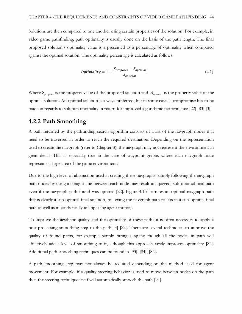
CHAPTER 4 -THE REQUIREMENTS AND CONSTRAINTS OF VIDEO GAME PATHFINDING 44
Solutions are then compared to one another using certain properties of the solution. For example, in
video game pathfinding, path optimality is usually done on the basis of the path length. The final
proposed solution‘s optimality value is a presented as a percentage of optimality when compared
against the optimal solution. The optimality percentage is calculated as follows:
(4.1)
Where Sproposed is the property value of the proposed solution and Soptimal is the property value of the
optimal solution. An optimal solution is always preferred, but in some cases a compromise has to be
made in regards to solution optimality in return for improved algorithmic performance [22] [83] [3].
4.2.2 Path Smoothing
A path returned by the pathfinding search algorithm consists of a list of the navgraph nodes that
need to be traversed in order to reach the required destination. Depending on the representation
used to create the navgraph (refer to Chapter 3), the navgraph may not represent the environment in
great detail. This is especially true in the case of waypoint graphs where each navgraph node
represents a large area of the game environment.
Due to the high level of abstraction used in creating these navgraphs, simply following the navgraph
path nodes by using a straight line between each node may result in a jagged, sub-optimal final path
even if the navgraph path found was optimal [22]. Figure 4.1 illustrates an optimal navgraph path
that is clearly a sub-optimal final solution, following the navgraph path results in a sub-optimal final
path as well as in aesthetically unappealing agent motion.
To improve the aesthetic quality and the optimality of these paths it is often necessary to apply a
post-processing smoothing step to the path [3] [22]. There are several techniques to improve the
quality of found paths, for example simply fitting a spline though all the nodes in path will
effectively add a level of smoothing to it, although this approach rarely improves optimality [82].
Additional path smoothing techniques can be found in [93], [84], [82].
A path-smoothing step may not always be required depending on the method used for agent
movement. For example, if a quality steering behavior is used to move between nodes on the path
then the steering technique itself will automatically smooth the path [94].

CHAPTER 4 -THE REQUIREMENTS AND CONSTRAINTS OF VIDEO GAME PATHFINDING 45
Original Path Smoothed PathNavgraph Node
S
G
Figure 4.1: The effect of path smoothing on a generated path
4.3 Pathfinding Search Problem Constraints
There are various constraints placed upon the pathfinding search problem and these constraints are
divided into two categories:
Performance: The performance constraints of the pathfinding search problem comprise of
the processing costs associated with solving the search problem as well the time required to
do so. Performance constraints are discussed in detail in Section 4.3.1.
Memory: The memory constraints placed upon the pathfinding search problem comprise of
the memory cost incurred when solving a search problem as well as additional memory costs
incurred by the search algorithm instance. Memory constraints are discussed in detail in
Section 4.3.2.
In all cases, pathfinding constraints are determined by the game type as well as the intended
platform. The real-time strategy (RTS) game genre presents a particularly large challenge to the game
pathfinding problem [95]. RTS games are top-down war-games featuring hundreds or in some cases,
like in Gas Powered Games‘ ―Supreme Commander‖ series, thousands of semi-autonomous game
agents [96]. The majority of higher level agent actions will involve movement and so require path
planning actions. Given the large number of in-game agents and the high level of autonomy, the
pathfinding system will often be tasked with finding paths for multiple agents at any given moment.
Path planning for multiple units simultaneously is a massive task and so path planning actions can, in
certain cases, account for more than half of the total computational time of the game [97] [95]. Even

CHAPTER 4 -THE REQUIREMENTS AND CONSTRAINTS OF VIDEO GAME PATHFINDING 46
in game types with lower requirements, path planning actions will still account for a significant
portion of the game loop‘s processing time [3] [4] [83].
As mentioned, the intended platform for a game will also place certain constraints on the
pathfinding search problem. These constraints are passed on the processing power and memory
available on the platform.
4.3.1 Performance Constraints
Path planning actions are atomic actions in that given a start and goal location, the pathfinding
search will be run to completion. The scheduling of agent update tasks was discussed in Section
2.4.3. Path planning actions fall into the periodic agent update task category with the distinction that
path planning actions are only performed when necessary. As such, a path planning action is
required to be able to be performed within the limited time allocated for period agent update tasks
per frame.
It is important to note that pathfinding search algorithms can be paused and restarted allowing them
to be run over several frames, but the scheduling complexities of doing so outweigh the benefits [3].
As such, multi-frame pathfinding is not commonly used. The atomicity as well as the limit on
processing time available for path planning actions can result in a hard time limit being placed upon
path planning actions. For example, Bioware Corp. requires that in Dragon Age [25], a single path
planning action must be completed in less than 3ms.
A common technique to estimate the performance of an algorithm is the computational complexity
measure. The computational complexity refers to an algorithm‘s computational cost in regards to the
number of operations necessary for the algorithm to complete. Computational complexity is
represented in Big-O notation. Unfortunately, Big-O is a worst case estimation of the potential
performance of an algorithm and modeling algorithmic performance in terms of the number of
operations can be misrepresentative of the real world performance profile of an algorithm.
The inaccuracy of the Big-O notation is due in part to the varying costs of memory and numerical
operations on different CPU architectures [33] as well as the fact that the cost of a single operation
may differ between two algorithms. For example, consider two O(n) algorithms, according to the
computational complexity measure the algorithmic performance for both algorithms should be
identical. Now, consider that a single operation in the first algorithm takes twice as long to complete

CHAPTER 4 -THE REQUIREMENTS AND CONSTRAINTS OF VIDEO GAME PATHFINDING 47
when compared to the second algorithm. In real world terms, the first algorithm will be twice as
slow as the second even though their computational complexities are equal. Even though the fringe
search algorithm [11], as discussed in Section 5.6, has a much higher worst case computational cost
than the A* algorithm [7], the average search time for the fringe search algorithm is significantly
lower than that of the A* algorithm.
Due to limited usefulness of the computational complexity, an algorithm‘s execution time (or search
time) is a common method for computational cost comparison between search algorithms [3]. There
are two methods of evaluating a search algorithm based on search times:
Total search time: An algorithm is timed over a fixed set of pathfinding problems and the
total time needed for the algorithm to solve the problems is used as a comparison metric
Average search time: An algorithm is run over a fixed set of problems and the search time
is expressed as the average over the entire set of search problems.
Unfortunately, there is a problem in using execution time as a metric. An algorithm‘s execution time
is dependent on both the implementation of the algorithm as well as the hardware platform the
algorithm is run on. As such, algorithm execution times are not a consistent metric and though
ubiquitous within the pathfinding literature, should not be used to measure the performance of an
algorithm alone.
As will be shown in Chapter 5, there is a direct relationship between a search algorithm‘s
performance and the number of nodes explored (search space exploration) by that algorithm during
a given search. In addition to the number of nodes explored, search algorithms may often revisit
previously explored nodes. These node revisits will add to the total performance cost of the search
algorithm. Node exploration and node revisits have different performance costs, with node revisits
often being cheaper to perform [7].
Using the number of nodes explored and the number of nodes visited as algorithm metrics is
recommended as both of these metrics are platform and implementation independent. Once again,
care needs to be taken when using only the total search space exploration metric since various
algorithms have varying node exploration and revisit costs.

CHAPTER 4 -THE REQUIREMENTS AND CONSTRAINTS OF VIDEO GAME PATHFINDING 48
Both the execution time and node exploration/revisit metrics have limited usefulness on their own.
As such it is recommended that any algorithm performance comparisons be performed using both
types of metrics, namely execution time and node exploration/revisits.
4.3.2 Memory Constraints
The memory constraints of a pathfinding search algorithm are based almost entirely on the intended
game platform. For example, while allocating 24MB for pathfinding data on a PC platform is
acceptable [57], only 1MB to 2MB of memory can be allocated for pathfinding data on a console
platform [58]. The memory limit imposed by a game‘s intended platform will have a significant
impact of the choice of search algorithm used to perform path planning actions within the game.
The memory costs of a search algorithm can be divided into two categories:
Per-node data: This is the algorithm specific data created for each node explored by a
search algorithm. The per-node data is used in calculating shortest routes as well as
constructing the final solution found [7] [10].
Per-algorithm data: For certain types of search algorithms additional memory is needed for
the algorithm specific data used to improve the performance or quality of the search
algorithm. For example, hierarchical pathfinding algorithms [92] require memory to store the
abstraction hierarchies used. Algorithms making use of spatial heuristics [98] also require
memory to store the spatial heuristic data lookup tables.
The memory costs of per-algorithm data remain constant for a given static game environment,
although environmental change within dynamic environments may affect the memory costs of the
per-algorithm data. In most cases, the per-node data memory costs will be significantly higher than
the per-algorithm memory costs [25] [98], therefore the reduction of the per-node memory costs is
the primary focus of search algorithm memory optimization [10] [8].
As mentioned, per-node data is allocated whenever a node is explored, as such the greater the search
space exploration of a search algorithm, the higher the associated memory costs. Node-revisits have
no effect on the memory costs of a search algorithm. The memory costs associated with the per-
node data are referred to as the space complexity of the algorithm.

CHAPTER 4 -THE REQUIREMENTS AND CONSTRAINTS OF VIDEO GAME PATHFINDING 49
Furthermore, the search space exploration performed by a search algorithm is dependent on the
search problem being solved. As such there is a high degree of variation of search space exploration
across search problems making the estimation of the total memory costs of an algorithm
problematic.
A worst case memory costs can be estimated for each algorithm, but as with the computational
complexity, the usefulness of such a metric is limited. To effectively compare search algorithms to
one another with regards to memory costs, an empirical evaluation needs to be performed on both
the average and peak memory costs. Since memory costs are based on search space exploration,
space complexity comparisons are made based on the search space exploration of a search
algorithm.
There has been a lot of research into creating both reduced-memory and memory-limited search
algorithms [10] [25] [11]. Care needs to be taken with memory reduced algorithms as the memory
cost reduction often has a negative effect on either the solution optimality or the search times of a
search algorithm [10] [11]. The effects of memory reduction on graph search algorithms are further
discussed in Sections 5.4 and 5.5.
4.4 Pathfinding in Dynamic Environments
Video games featuring dynamic environments are becoming ever more popular. In these dynamic
environments, players have a high degree of interaction with the environment allowing players to
drastically change the game environment through their actions. Certain games, like Volition Inc.‘s
―Red Faction‖ [99] series as well as Relic Entertainment‘s ―Company of Heroes‖ series [100] rely
heavily on these dynamic environments as a key aspect of their gameplay mechanics.
Figure 4.2 is courtesy of Chris Jurney‘s GDC2007 presentation [91] detailing the level of destruction
present in ―Company of Heroes‖. Figure 4.2a shows an in-game location in its initial state while
Figure 4.2b shows the same in-game location after a lengthy battle.
Due to various player actions and the high level of destructibility offered by the game, the game
environment has been greatly changed to the point of being near unrecognizable. Areas that were
previously traversable are now obstructed and vice versa, as such environmental changes add a high
level of complexity to the pathfinding problem.

CHAPTER 4 -THE REQUIREMENTS AND CONSTRAINTS OF VIDEO GAME PATHFINDING 50
In dealing with an environmental change, the first priority is to update the navgraph to ensure that
any subsequent paths planned will take the environmental change into account. The complexity of
updating the navgraph varies depending on the navgraph representation (refer to Chapter 3 for
more information) and so care needs to be taken in selecting an appropriate navgraph representation
for use within dynamic environments.
a) The initial state of the game environment. b) The same game environment after a lengthy in-game
battle.
Figure 4.2: An example of the level of Destructibility in „Company of Heroes‟
In navigating within dynamic environments, agent pathfinding is performed as in a static
environment with the additional consideration that at any given time an environmental change may
affect all currently planned paths. When an environmental change does have an effect on a planned
path, the effect will be one of two things: the first being that a portion of the planned path is no
longer traversable (refer to Figure 4.3) or that a shortcut (a new optimal path) is now available in the
environment (refer to Figure 4.4). In both cases, a planned path that is affected by an environmental
change will need to be replanned.
In the case when an environmental change obstructs a path, the detection of such an occurrence is
relatively straightforward. Each path in the vicinity of the change is checked to see whether it
contains any invalid nodes: either obstructed nodes or non-existent nodes in the case of a navmesh
representation. If a path does contain invalid nodes, it needs to be replanned. A path is replanned by
performing a new pathfinding search with the same goal node, but originating at the agent‘s current
position in the navgraph. This new pathfinding search is termed a replanning action.

CHAPTER 4 -THE REQUIREMENTS AND CONSTRAINTS OF VIDEO GAME PATHFINDING 51
S
G
a) Original Path b) Obstructed Path c) Replanned Path
S
G
S
G
S
G
Start
Goal
Env. Change
Path
Figure 4.3: The need for path replanning as a result of an environmental change
S
G
S
GS
G
Start
Goal
Env. Change
Orig. Path
New PathS
G
c) New Optimal Replanned Path
b) Environmental change creates a shortcut
a) Original Path
Figure 4.4: An environmental change requiring the replanning of the agent‟s path
The detection of the existence of a new optimal path for a specific search problem is a more difficult
task than simple path validation. Any potential change in the environment irrespective of location
may provide a new optimal solution for an already solved pathfinding search problem. Figure 4.4
illustrates such a situation where an environmental change outside of the existing path vicinity
results in a new optimal path. The only way to check for the existence of a better path is to perform
a replanning action and compare the resulting optimal path found to the existing path. If an optimal
(or near-optimal) algorithm is used then the comparison between the new and the existing path is
redundant since the new path will always be the same or better than the existing path.
Considering that the shortcut-check will always performs a replanning action for each environmental
change, the need for path validity checks will also become redundant as paths will always be
replanned. In fact, no checks need to be performed at all and all game agents‘ paths can simply be
replanned once an environment change occurs. Replanning an agent‘s path each time an

CHAPTER 4 -THE REQUIREMENTS AND CONSTRAINTS OF VIDEO GAME PATHFINDING 52
environment change occurs, guarantees that the agent‘s paths will always be as optimal as the search
algorithm allows.
For each environmental change, all previously planned paths will need to be replanned. In games
featuring a large number of agents, a single environmental change will result in huge number of path
replanning requests. As each path planning action is atomic and since the execution time of the path
planning action determines how many path planning actions can be run per frame, a highly efficient
search algorithm is required for use in highly dynamic multi-agent games.
Unfortunately, even with a highly efficient search algorithm it may not be possible to execute all the
path replanning actions within the agents‘ required response times and agent response times will be
delayed.
4.5 Selecting a Suitable Search Algorithm
The efficiency and suitable of the pathfinding system within certain environments is entirely based
upon the efficiency and suitability of the algorithm within those environments. The ―perfect‖ search
algorithm will provide optimal paths in next to no time and next to no memory usage.
Unfortunately, in practice such a perfect solution does not exist and a real-world system needs to
find an appropriate compromise between the three search algorithm metrics and weigh up the
importance of path optimality versus time and memory [101].
The selection of a search algorithm for use within a specific game is based on the following factors:
The game‘s intended platform,
the number of game agents required, and
the dynamicity of the game environment.
The memory constraints placed upon the search algorithm by the platform are the most important
factors in the selection of the search algorithm to be used. Depending on the limitation of the
environment, drastic compromises with regards to the search speed may need to be made [8].
Using the worst case memory cost for an algorithm as a means of selection will ensure that the
algorithm will never exceed the memory budget. Unfortunately, the worst case memory cost is just
that, the worst case, and for the majority of search problem solves the memory usage of the search
algorithm will be significantly lower than the worst case estimate [3]. Using the worst case memory

CHAPTER 4 -THE REQUIREMENTS AND CONSTRAINTS OF VIDEO GAME PATHFINDING 53
cost as a selection factor results in an over reduction of the memory costs of the search algorithm
often at the expense of algorithmic performance. The peak and average memory costs of a search
algorithm are better selection factors in judging the suitability of a search algorithm for use within
memory limited environments.
The peak and average memory costs of an algorithm will need to be empirically calculated for a large
and varied set of test problems in a test environment representative of the environments found in
the final game. In using the peak memory cost value for algorithm selection care needs to be taken
due to the search space exploration variance exhibited across search problems. If a search
algorithm‘s peak memory cost is close to the limit of the platform, the likelihood of a search
problem exceeding the platform‘s hard limit is higher than if the peak memory cost was further from
the platform‘s memory limit.
If a search algorithm exceeds the available memory it will result in a failed search or in the case of a
badly implemented algorithm an application crash. An algorithm is a better candidate for a memory
limited environment if the algorithm offers a lower peak memory cost when compared to another
algorithm even if the algorithm has a higher average memory cost than the other candidate
algorithm.
With regards to algorithm performance, the faster the algorithm, the better. As mentioned, the
choice of algorithm will be primarily based on the memory constraints. So the selection of the final
search algorithm is simply the search algorithm which offers the lowest execution times while
obeying the memory constraints of the platform.
4.6 Summary
Due to the representation of the video game environments in the form of a graph, the video game
pathfinding problem is reduced to a graph search problem. A graph search problem is solved
through the use of a graph search algorithm. Video game pathfinding has specific requirements and
constraints with regards to the computational and space complexities of the algorithm.
These requirements and constraints limit the choice of search algorithms which can be successfully
used in solving the video game pathfinding problem. Furthermore, when presented with dynamic
game environments the workload placed upon the AI system stemming from pathfinding is
drastically increased making the choice of search algorithm all that more important.

CHAPTER 4 -THE REQUIREMENTS AND CONSTRAINTS OF VIDEO GAME PATHFINDING 54

55
Chapter 5 Discrete Search Algorithms
As discussed in Chapter 4, the pathfinding search problem is fundamentally a graph search problem,
one which is solved through the use of a graph search algorithm. This chapter discusses the most
common graph search algorithms employed today. A short introduction to discrete search
algorithms is presented in Section 5.1. A discussion of Dijkstra‘s search algorithm and its memory
costs is presented in Sections 5.2 and 5.3. The A* algorithm, the iterative deepening algorithm, the
simplified memory-bounded algorithm as well as the fringe search algorithm are discussed in
Sections 5.4 through 5.7. This chapter is concluded by a summary presented in Section 5.8.
5.1 Discrete Search Algorithms
This thesis makes novel use of the terms discrete and continuous in the separation of graph search
algorithms. The distinction between these two terms is discussed in detail in Section 6.1. It is
impossible to define this distinction without first discussing continuous algorithms and so no further
mention of the term will be made within this chapter. For all intents and purposes this chapter may
simply be titled ―graph search algorithms‖.
A graph search algorithm is an algorithm which, given two nodes in a graph, attempts to find a path
between them. If a found path between two nodes in a graph is the shortest possible path, then that
path is referred to as the optimal path.
The pathfinding requirements of a graph search algorithm are that the algorithm will always find a
path if one exists and that the path found will be optimal or near-optimal. Furthermore, the
processing and memory costs of such graph algorithms must be minimized to operate successfully
within tight performance and memory constraints1.
1 A detailed discussion of the requirements and the constraints of the video game pathfinding problem were presented in Chapter 4.

CHAPTER 5 - DISCRETE SEARCH ALGORITHMS 56
5.2 Dijkstra‟s Algorithm
Dijkstra‘s algorithm was presented in Edsger Dijkstra in 1959 as a method to find the shortest
routes from a start node to all other nodes in a weighted graph [6]. In such a graph, each edge
weight represents the traversal cost incurred moving across that edge.
The basic operation of the algorithm is as follows: The algorithm explores every node in the graph,
and while doing so stores shortest route data at each node. Once the algorithm has completed, a
path is then be constructed by starting at the goal node and working backwards to the start node
using the route data stored at each node. The algorithm operates iteratively and each algorithm
iteration will explore (another common term encountered is expand) a single node. The node being
explored is referred to as the parent node for that iteration and its neighboring nodes are referred to
as the node successors (or child nodes).
5.2.1 The Algorithm
Dijkstra‘s algorithm makes use of a single metric, the cost-so-far (CSF) value, in determining the
shortest paths in the graph. The CSF value is simply the traversal cost incurred in reaching a graph
node from the start node. When a node is explored, a CSF value is calculated for each of the
successor nodes.
The CSF value for each successor is the sum of the parent‘s CSF value and the traversal cost of
moving from the parent to the successor. Figure 5.1a illustrates the CSF calculation for a node.
Multiple routes can exist to a single graph node, implying that when Dijkstra‘s algorithm explores
the graph it may encounter successors that already have CSF values (i.e. a previous route to the node
has been found).
In such a case, Dijkstra‘s algorithm checks whether the current route (from the current parent node)
to a successor node is shorter than the previous route found. A new CSF value is calculated from
the current parent to the successor node in question. If the new CSF value is smaller than the
successor node‘s CSF value, it means that the current parent offers a shorter route to that successor
than the previous route found. The successor node‘s CSF is then set to the new smaller CSF value
(i.e. the new shorter route). This ensures that only the shortest routes found to each node are stored.

CHAPTER 5 - DISCRETE SEARCH ALGORITHMS 57
In addition to the CSF value stored at each node, a link to the parent node, from which the CSF
value originated from, is stored as well. This parent node link is necessary so that routes can be
traced back from any node to the start. This parent node link is updated whenever the CSF value of
that node is updated. Simply put, whenever a new shorter route to a node is found, the shorter route
value is saved as well as the node from which that route originated from.
During the exploration of the search space, Dijkstra‘s algorithm will encounter nodes that fall into
the following categories: unseen, unexplored and explored. When an unseen node is first
encountered during the exploration of a parent node to that node, a CSF value originating from the
parent node is calculated.
A B
C
D
Cost: 2
Cost: 5
Cost: 3
CSF: 3Node: X
CSF: 8Node: A
CSF: 5Node: A
CSF: 6Node: A
AB C D
F
KG
E
J
H I
L
Node: B
Node: A
Node: J Node: C
Node: C
Node: K
Node: K
Node: J
Node: E
Node: A
Node: B
Back-trace from K to A: J -> E -> B -> A
Path from A to K: A -> B -> E -> J
a) The cost-so-far calculation b) The path generation performed by Dijkstra‟s algorithm, by means of a back-
trace
Figure 5.1: The Dijkstra's algorithm‟s cost-so-far calculation and path generation
This unseen node will now need to be explored, it is placed on a list containing other nodes that the
algorithm has encountered but not explored. This list is referred to as the open list; nodes on the
open list are all awaiting exploration. Once a node has been explored, it is added to a list containing
all other explored nodes. This list is known as the closed list. The open and closed terminology is
based on the fact that when a node is encountered, it is opened for exploration and it is only closed
once the node has been explored. Nodes awaiting exploration are referred to as open nodes while
already explored nodes are referred to as closed nodes.

CHAPTER 5 - DISCRETE SEARCH ALGORITHMS 58
Dijkstra‘s algorithm is initialized with only the start node present on the open list and an empty
closed list. At each step (iteration) of the algorithm, the node with the lowest CSF value is removed
from the open list. This ensures that the closest node to the start node is always explored. When a
node N is explored, each of N‘s successor nodes S is examined. Each S can belong to one of three
categories: unseen, open or closed. If S is unseen then a CSF value is calculated originating from N,
S‘s parent link is set to N and finally S is placed on the open list. In the case when S has already been
encountered (i.e. either an open or closed node), the new route to S from the start (the CSF value
originating from N) is compared to S‘s existing CSF value, if the new route is shorter than the
existing route then S is updated with the new route‘s CSF value and its parent node link is set to N.
Since a node‘s successor node‘s CSF values are based on its CSF value. If the CSF value of a node is
updated then all the CSF values of it successor nodes must be updated as well. Instead of explicitly
performing this update when an already encountered node is updated, it is simpler to place that node
back onto the open list since the successor node‘s CSF values are automatically checked and updated
as necessary during node exploration. In the case of an already encountered node being open,
nothing more than the CSF/parent link updates are performed. If an updated node was a closed
node, it needs to be removed from the closed list and placed back onto the open list (i.e. the node is
reopened).
Dijkstra‘s algorithm terminates only once the open list is empty, i.e. all the nodes in the graph have
been explored. Once the algorithm has terminated, a path can be generated from the start node to
any node in the graph (the goal node) by starting at the goal node and tracing the stored parent node
links back to the start node (see Figure 5.1b). The complete pseudocode for Dijkstra‘s Algorithm is
shown in Listing 5.1.
From an algorithmic standpoint, Dijkstra‘s algorithm is both a complete and optimal algorithm. This
means that Dijkstra‘s algorithm will always find a solution if it exists and that the found solution will
always be the best solution possible (i.e. the optimal solution).
The memory cost of Dijkstra‘s algorithm consists of the per-node data values for each node in the
graph (CSF and parent link values) and the memory costs of the open and closed lists. Since
Dijkstra‘s algorithm explores each and every node in the graph, per-node data storage is allocated for
every graph node as it is guaranteed to be needed.

CHAPTER 5 - DISCRETE SEARCH ALGORITHMS 59
1) Clear the start node’s parent and CSF values
2) Add start node to open list
3) While open list is not empty
3.1) Remove node N with the lowest CSF cost from the open list
3.2) For each successor node S of N
3.2.1) Calculate the new CSF value (current CSF + traversal cost)
3.2.2) If S is unexplored
a) Set S's CSF to new CSF value
b) Set S’s parent to N
c) Add S to open list
3.2.3) Else if S is on the open list and S's CSF is greater than new CSF
a) Set S's CSF to new CSF value
b) Set S’s parent to N
3.2.4) Else if S is on the closed list and S's CSF is greater than new CSF
a) Set S's CSF to new CSF value
b) Set S’s parent to N
c) Remove S from closed list
d) Add S to open list
3.3) Add N to closed list
Listing 5.1: Pseudocode for Dijkstra's Algorithm
5.2.2 Optimizations
Dijkstra‘s algorithm is not without its weaknesses. Since the algorithm was designed to find all
routes from a single node in a graph, it explores the entire graph and as such has a very high
computational cost, estimated at around O(n2) where n is the number of nodes in the graph [1].
The bulk of the processing costs incurred by Dijkstra‘s algorithm are a result of the open/closed list
operations. Each time a node is selected from the open list, the entire open list is searched to find
the node with the lowest CSF value. With each node explored by the algorithm, the open list grows
in size, and so the cost of performing the search for the closest node in the list increases.
The open list search is the most computationally expensive operation in the algorithm, and therefore
has been the primary focus of algorithmic optimizations both for Dijkstra‘s algorithm and all
algorithms derived from it such as the A* algorithm [7].
The simplest manner in which to reduce the cost of the open list search is to store the open list in an
ordered fashion (usually in order of increasing CSF value). If the open list is ordered, then the first
node in the list will always be the closest node, i.e. the next node to be explored. Selecting the closest
CHAPTER 5 - DISCRETE SEARCH ALGORITHMS 60
node from the list becomes a trivial operation with respect to processing costs. Unfortunately,
keeping the opened list ordered introduces additional costs during node exploration.
When an unseen node is added to the open list, the node needs to be inserted at the correct position
on the list to maintain the correct ordering. As such, node insertions onto the open list will require
an additional search to find the correct insertion position. When an open node is updated, its CSF
value will change and so will its position in the open list. The updated open node needs to be
removed from the open list and reinserted into the correct position to maintain the correct ordering
of the list.
When examining the successors of a node and discovering that a successor node has already been
encountered, the open list, the closed list or both lists need to be searched to check whether that
successor node is open or closed. These list searches are expensive and their costs quickly add up.
There is a simple optimization which removes the need for searching the open and closed lists
during node successor examination. An additional flag value is added to the per-node data of the
algorithm. This flag specifies whether the node is unseen, open or closed. A keen reader may have
realized that the closed list need not actually be stored as a list. The only role of the closed list is to
maintain a record of the explored nodes; if this record is moved into the nodes themselves as
detailed above, the closed list becomes redundant and can be removed. The removal of the closed
list further counteracts the additional memory cost of the flag value and is a free processing cost
optimization.
The only list that needs to be maintained is the open list; moving a node from the closed list to the
open list requires an update to the flag value and an open list insertion. A detailed discussion into
open list data structures and optimization is presented in Section 5.3.3.
The optimizations discussed above are valid for both Dijkstra‘s algorithm as well as itsvariants.
There is one more optimization that needs to be discussed, one which is specific to Dijkstra‘s
algorithm. Since the closest node to the start is explored each iteration, a closer route to a closed
node cannot be found. Successors encountered that are already on the closed list can be safely
ignored since it has been shown that Dijkstra‘s algorithm will never find a better route to an already
explored node [3]. The entire pseudo-code contained in section 3.2.4 of Listing 5.1 can be removed.

CHAPTER 5 - DISCRETE SEARCH ALGORITHMS 61
5.2.3 A Point-to-Point Version of Dijkstra‟s Algorithm
Video game pathfinding searches are point-to-point searches, i.e. only a path from the start node to
the goal node is required. In contrast, Dijkstra‘s algorithm is an all-points search, finding the shortest
path from the start node to every other node in the graph. As such, for any given point-to-point
problem, Dijkstra‘s algorithm will continue exploring the search space even after the shortest path to
the goal node has already been found. This continued exploration and its associated computational
cost is entirely unnecessary, and the original Dijkstra‘s algorithm can be modified to create a point-
to-point version. The point-to-point version offers significant improvements to the computational
cost of the original Dijkstra‘s algorithm when used for point-to-point searches.
This point-to-point version is based on the fact that once a node is explored (placed on the closed
list) no shorter path to that node exists [1], meaning that if the algorithm is terminated once the goal
node has been explored, then the current path found to the goal node is guaranteed to be the
shortest path possible [1].
This ―early‖ termination of the algorithm prevents any continued (and unnecessary) exploration of
the search space while still maintaining the optimality and completeness of the algorithm. Node
exploration accounts for the majority of the processing cost associated with Dijkstra‘s algorithm
(and variants) due to the high costs of open list operations. Reducing the number of nodes explored
reduces the processing costs and improves search times.
In many cases, the goal node may be encountered early on in the search but may not be immediately
explored since there may be other open nodes closer to the start node. In such case, Dijkstra‘s
algorithm will continue to explore the closer open node and ignore the goal node. The goal node
will only be explored once it is the closest node to the start node.
This additional searching may be prevented by simply terminating the search as soon as the goal
node is encountered. Unfortunately, since the goal node is not fully explored, such an early
termination does not guarantee the optimality of the path found and is therefore not recommend.
The pseudo-code for the optimal and complete point-to-point version of Dijkstra‘s algorithm is
shown in Listing 5.2.

CHAPTER 5 - DISCRETE SEARCH ALGORITHMS 62
1) Clear the start node parent and CSF value
2) Add start node to open list
3) While open list is not empty and N is not the goal node
3.1) Remove node N with the lowest CSF cost from the open list
3.2) For each successor node S of N
3.2.1) Calculate the new CSF value (current CSF + traversal cost)
3.2.2) If S is unexplored
a) Set S's CSF to new CSF value
b) Set S’s parent to N
b) Add S to open list
3.2.3) Else if S is on the open list and S's CSF is greater than new CSF
a) Set S's CSF to new CSF value
b) Set S’s parent to N
3.3) Add N to closed list
4. Return No Path Exists
Listing 5.2: Pseudocode for the point-to-point version of Dijkstra‟s algorithm
5.3 The A* Algorithm
Even though the point-to-point version of Dijkstra‘s algorithm is significantly more efficient for
point-to-point searches than the original algorithm, it is far from optimal with respect to search
space exploration and processing costs. The A* algorithm [7] was presented as an improvement to
the point-to-point version of Dijkstra‘s algorithm. To explain the need for, and the improvements
offered by the A* algorithm, it is necessary to first discuss the manner in which the point-to-point
Dijkstra‘s algorithm explores the graph search space. For clarity‘s sake all references to Dijkstra‘s
algorithm will refer to the point-to-point version unless stated otherwise.
By selecting the closest node to explore, Dijkstra‘s algorithm explores outwards in all direction from
the start node. Figure 5.2a and Figure 5.2b illustrated the search space exploration pattern of
Dijkstra‘s algorithm. The undirected nature of the search pattern means that Dijkstra‘s algorithm will
explore many unnecessary nodes in finding a solution. With only point-to-point searches in mind, if
Dijkstra‘s algorithm‘s search can be directed to only explore nodes that have a high likelihood of
leading to the goal, and to ignore nodes that are unlikely to lead to the goal, then the total search
space exploration can be reduced resulting in decreased processing and memory costs.

CHAPTER 5 - DISCRETE SEARCH ALGORITHMS 63
The search space exploration pattern is directed by the selection of the ―best‖ node from the open
list. Dijkstra‘s algorithm ranks nodes according to the closeness of the nodes to the start node. In a
point-to-point search the goal node is just as important as the start node. If the distance to the goal
node, as well as the distance to the start node, is taken into account when selecting the next open
node to explore, the search space exploration pattern can be directed towards the goal node.
The A* algorithm [7] was presented in 1968 as a directed (best first) point-to-point version of
Dijkstra‘s algorithm. Since then, the A* algorithm has become the benchmark for all point-to-point
graph search algorithms, especially in the pathfinding field. The main difference between the A*
algorithm and Dijkstra‘s algorithm is the augmentation of the CSF value with a heuristic value in the
selection of the next open node to explore. To stay in line with the literature, the CSF value will
henceforth be referred to as the G value.
5.3.1 The Algorithm
As mentioned, the A* algorithm is Dijkstra‘s algorithm with a simple change to the manner in which
nodes are selected from the open list. A heuristic value (H) is created for each node and is stored
alongside the other per-node data (the G value and the parent node).
The heuristic value is an estimation of how close a given node is to the goal node, or alternatively an
estimation of the likelihood of a node leading to the goal. The heuristic value is calculated by a
heuristic function that, given two nodes, returns a numeric measure of how close the nodes are
together. A simplistic way of describing the heuristic value is to term it the ―estimated remaining
cost‖.
At each node, the cost-so-far G value and the estimated-remaining-cost H value are added together
to create a new ―total estimated cost‖ value (often referred to as the F value or F cost). Open node
selection is then based on this ―total estimated cost‖ value. Open nodes in the direction of the goal
node (i.e. closer to the goal node) are explored first, preventing the arbitrary exploration of nodes
with small G values that lead away from the goal. Directing the search space exploration towards the
goal node reduces the total overall search space exploration of the algorithm significantly.
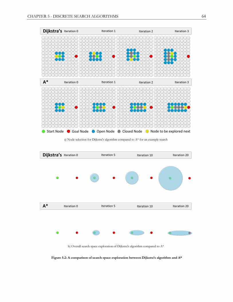
CHAPTER 5 - DISCRETE SEARCH ALGORITHMS 64
Iteration 0Dijkstra’s
Goal Node
Iteration 1 Iteration 2 Iteration 3
Iteration 0A* Iteration 1 Iteration 2 Iteration 3
Open Node Closed NodeStart Node Node to be explored next
Iteration 0Dijkstra’s Iteration 5 Iteration 10 Iteration 20
Iteration 0A* Iteration 5 Iteration 10 Iteration 20
a) Node selection for Dijkstra's algorithm compared to A* for an example search
b) Overall search space exploration of Dijkstra's algorithm compared to A*
Figure 5.2: A comparison of search space exploration between Dijkstra‟s algorithm and A*

CHAPTER 5 - DISCRETE SEARCH ALGORITHMS 65
During open node selection two open nodes may have the same F cost but different G and H
values. In such a case, a tie breaking strategy can be employed to further affect the search behavior.
A good tie-breaking strategy to use is to prefer the node with the lowest G value (i.e. nodes that
contain shorter paths to the start node). Tie-breaking on the G values can potentially reduce the
total search space exploration performed even further [3].
Node exploration in Dijkstra‘s algorithm should ignore closed nodes. In the case of A*, node
exploration occurs based on the heuristic value, which is an estimation of the closeness to the goal.
This estimation may often be overly optimistic, and may cause nodes further from the start node
(higher G value) to be explored before nodes closer to the start node (lower G value), resulting in
the exploration of closed nodes whose G values are overly high and which can still be reduced. This
means that closed nodes cannot be ignored as in Dijkstra‘s algorithm and need to be checked and
updated if necessary.
Unfortunately, this introduces the concept of re-exploring closed nodes. Node re-exploration did
not occur in Dijkstra‘s algorithm. Depending on the search problem and search space, the degree of
node re-exploration can be quite large. This node re-exploration increases the computational cost of
the A* algorithm, but has no effect on the memory costs. Even with this increase in computational
cost, A*‘s total node exploration (explored nodes + node re-explorations) is still significantly less
than that of Dijkstra‘s algorithm [7] [3].
The A* algorithm terminates as soon as the goal node is selected from the open list (i.e. the goal
node has the smallest F cost of all open nodes). This is the same termination condition discussed in
the Section 5.2.3, which was stated as being guaranteed to return optimal solutions. This is not true
in the case of A*. Since node selection is performed on the F cost and not just the G cost, then A*
will need to be run until the open node with the smallest G value has a higher G value than the goal
node in order to maintain the guarantee of optimality. This is effectively the same termination
condition as used for Dijkstra‘s algorithm and will exhibit the exact same final search space
exploration as Dijkstra‘s algorithm, thereby nullifying all performance gains offered by A* [3].
It has been shown in [7] that the A* algorithm is guaranteed to be optimal, using the termination
condition of Dijkstra‘s algorithm, if an admissible heuristic function is used. The definition of an
admissible heuristic is given in [7] as a one that consistently underestimates the closeness of any
node to the goal. If the heuristic value is an underestimate then the F cost will be biased towards the

CHAPTER 5 - DISCRETE SEARCH ALGORITHMS 66
G value since the H value will always be smaller than the actual distance to the goal. The G-biased
F-costs mean that the A* algorithm will prefer to explore nodes closer to the start node, increasing
both the search‘s exploration and the time needed for the search to complete. If the heuristic is
always an underestimate of the actual distance to the goal node, A* is guaranteed to return the
optimal path (the exact same path returned by Dijkstra‘s Algorithm).
The A* algorithm is both complete and optimal (when using an admissible heuristic) as well as
offering significant improvements over Dijkstra‘s Algorithm. The pseudo-code for the A* algorithm
is given in Listing 5.3.
1) Clear Start Node’s parent and heuristic values (F, G, H)
2) Add start node to open list
3) While open list is not empty and N is not the goal node
3.1) Remove node N with the lowest F cost from the open list
3.2) For each neighbor node S of N
3.2.1) Calculate the new G value ( N’s G value + traversal cost)
3.2.2) If S is unexplored
a) Set S's G to new G value
b) Calculate new H value
c) Set S’s parent to N
d) Add S to open list
3.2.3) Else if S is on the open list and S's G is greater than the new G
a) Set S's G value to new G value
b) Set S’s parent to N
3.2.4) Else if S is on the closed list and S's G is greater than new G
a) Set S's G value to new G value
b) Set S’s parent to N
c) Remove S from closed list
d) Add S to open list
3.3) Add N to closed list
4. Return no path exists
Listing 5.3: Pseudocode for the A* algorithm
5.3.2 The Heuristic Function
In ensuring A* optimality, an underestimating heuristic function must be used, this is not to say that
overestimating (and so inadmissible) heuristics are of no use. If a heuristic function overestimates
the difference between a node and the goal, then the F-cost of that node becomes biased towards
the H value. Using an overestimating heuristic function, the A* algorithm will prefer exploring

CHAPTER 5 - DISCRETE SEARCH ALGORITHMS 67
nodes closer to the goal node resulting in a more directed search pattern headed straight towards the
goal node. Since the search is more directed, less of the search space, especially surrounding the start
node, will be explored resulting in reduced processing and memory costs.
Unfortunately, using an overestimating heuristic removes the optimality property of the A*
algorithm meaning that even though solutions will be found quicker, they may now be sub-optimal
[83]. Figure 5.3 clearly shows the effect of overestimating and underestimating the search heuristic
on the final search space exploration of the same search problem. In the example presented in
Figure 5.3, the final solutions are identical, but this is not guaranteed to always be the case. It is the
opinion of [3] as well as [83] that a slightly overestimating heuristic‘s advantages to both
performance and memory costs can outweigh the disadvantages and so is a valid method of
optimizing the A* algorithm.
Underestimating Heuristic Overestimating Heuristic
Closed ListOpen List
Figure 5.3: The effects of inadmissible A* heuristics
More complex heuristic functions exist, such as the ―dead-end‖ and ―gateway‖ heuristics presented
in [98] as well as the cluster heuristic presented in [3]. These complex heuristic functions are not
based on the distance between nodes but rather make use of graph spatial information in calculating
the heuristic value. Such heuristic functions require a computationally expensive pre-processing step
to construct the necessary heuristic information as well as increased memory costs due to the
heuristic data storage.
Even though these heuristics can offer benefits in reducing the search space exploration and thereby
the overall search time, they are unsuitable for use in dynamic environments as each environmental
change will require a complex and expensive update to the heuristic data. Furthermore, to a large
degree these complex heuristic functions are rendered redundant through the use of hierarchical
approaches to pathfinding which also leverage graph spatial information to reduce search space
exploration (refer to Chapter 7 for more details).

CHAPTER 5 - DISCRETE SEARCH ALGORITHMS 68
5.3.3 Optimizations
In addition to the expensive open list operations performed by the A* algorithm, the computational
cost of the heuristic function needs to be discussed. In general, the list operations are the major
contributor to the processing costs of solving a search problem, but in certain cases the processing
costs of calculating the heuristic function for each node encountered can outweigh that of the list
operations [3]. Due to the high degree of variance between search problems and search
environment, it is impossible to make a concrete statement regarding the division of processing
costs between these two contributors.
The heuristic function is decoupled from the actual algorithm as it is simply a numeric distance
estimate between two nodes in a graph. As such, the optimization of the heuristic function can also
be performed separately from the A* algorithm. Since the heuristic functions vary greatly, there is no
common method of optimization. Heuristic functions need to be chosen so that they minimize the
overall explored search space during a search as well as keeping the computational cost of
calculating the heuristic value low.
The cost of open list operations has been briefly discussed in Section 5.2.2. These list operations
generally account for the majority of the processing costs incurred when searching. As such, open
list optimizations have a significant impact on the overall processing costs (and consequently the
search time as well) of the A* search algorithm [83] [3].
As in Dijkstra‘s Algorithm, the only method of removing nodes from the open list is through the
selection of the ―best‖ node on the list (i.e. lowest F cost). Since the cost of finding and removing
the best open node is always incurred, optimizing the removal of the best node is the first step in
optimizing the overall open list operation. Furthermore, during the exploration of the best open
node, an additional M list operations may be performed (where M is the number of successor
nodes).
These additional list operations are made up of either list insertions (in the case of unexplored
successor nodes or if a better path is found to an already closed node) or list updates (in the case of
a better path being found to an already open node). As such, the open list has only four operations
that may be performed on it during the execution of the A* algorithm (listed in order of increasing
cost): search, removal, insertion and update.

CHAPTER 5 - DISCRETE SEARCH ALGORITHMS 69
There are various possible implementations of the open list, each with different computational costs
per list operation. The first and simplest method of implementing the open list is to make use of an
unordered linked list (a dynamic array may also be used). Since the list is unordered, a full search is
required each time the best node is required, i.e. at each iteration. The computational cost of such a
search is O(N). The benefit of using an unordered structure is that node insertions and updates
require no additional care, and are therefore performed in constant time, O(1). Unfortunately, when
searching large search spaces, like those present in video games, the open list rapidly grows in size
meaning that the O(N) cost incurred at each iteration can quickly become prohibitively expensive.
In an attempt to reduce the overall cost of finding and removing the best open node from the open
list, an ordered (best to worst) list may be used. This reduces the cost of finding the best node to
O(1) since the best node is always the first node in the list. Due to the list ordering, when a node is
inserted or updated the open list needs to be searched to find the correct position of the new or
updated node. Consequently node insertions and updates now have a worst case O(N) cost.
The list insertion/updates costs varies depending on the inserted/updated node‘s F value. Nodes
with better F values will have lower costs since they will be inserted closer to the front of the list i.e.
their required position will be found faster. In a standard 2D grid in which each node has eight
neighbors, the higher update and insertion costs mean that the algorithm may potentially need to
perform eight O(N) operations per iteration. This is in stark contrast to the single O(N) operation
required in an unordered list. The higher cost of the insertion and update operations makes using an
ordered list implementation a potential de-optimization in regards to complexity and is not
recommended.
The number of successor operations, per explored node varies, but the removal of the best node
always occurs. To holistically optimize the open list, it is necessary to use an implementation that
offers lower computational costs for both the removal of the best element as well as the node
exploration operations. The recommended implementation of the open list in regards to overall
performance is the priority queue data structure [102] [3] [83] [103] [2] [104]. A priority queue is a
data structure that contains an unordered collection of elements with the property that the best
element is the first element.

CHAPTER 5 - DISCRETE SEARCH ALGORITHMS 70
Priority queues may be implemented in various ways as shown in [105] and [104]. The skew heap
(binary tree) data structure is shown to offer the most efficient implementation [105]. A priority
queue implemented using a binary tree is shown to have an amortized cost for each operation of
O(log N) [106]. This means that an open list implemented as a binary tree based priority queue will
have amortized worst case costs for the removal of the best node, node insertions and updates of
O(log N). By using a priority queue with a O(log N) cost for all operations, the effects of an ever
growing open list are significantly reduced when compared to the previous two implementations,
both featuring O(N) costs for various list operations.
A further A* specific algorithm optimization is presented in [107] offering significant improvements
for the A* algorithm and any A* variants. The optimization is simple: when a node is expanded its
successors‘ F values are checked against the parent node‘s F value. Since the F values of an
expanded node are monotonically non-decreasing [108] and the node with the lowest F value is
always explored, it is likely that that successor will be expanded next if that successor node has the
same F value as the parent node. Since it is known that this successor will likely be expanded next,
the expensive insertion and removal open list operations are redundant and that successor is
immediately expanded without ever being placed on the open list. Such a successor is said to be
expanded fast. This optimization reduces the computational complexity of the A* algorithm at no
cost to memory or solution optimality [107].
The primary performance concern with the A* algorithm is not one of computational complexity
but rather of memory usage. Numerous later algorithms such as IDA* [8], MA* [109] and SMA*
[10] all use the high memory cost of the A* algorithm as the primary motivation for their research. It
is shown in [8] that the A* algorithm could not solve any of the given problems due to the algorithm
exceeding the hardware limitations on the test platform. Memory sizes have increased significantly
since 1985 and the memory cost of the A* algorithm is not as limiting as it once was however this is
not to say that A*‘s memory cost may not be problematic in certain memory constrained
environments.
The primary memory cost of the A* algorithm is in the fact that the algorithm allocates memory for
each node encountered in the graph (for the algorithm specific per-node data). The only method
available for the reduction of the memory cost for the classical A* algorithm is through the use of a
heuristic function that reduces the total number of encountered nodes.

CHAPTER 5 - DISCRETE SEARCH ALGORITHMS 71
Even though the memory cost is thought to be an issue, the search spaces provided within the video
game environment are drastically smaller than those of common academic problems such as the 15
puzzle or a Rubik‘s cube solver [103]. The most basic per-node data structure size for the A*
algorithm is 16 bytes (4 bytes for each of the G, H, parent and list flag values) requiring 16MB of
memory to store all the nodes in an 1024x1024 search space.
As mentioned previously, the A* algorithm greatly reduces the number of nodes encountered during
the search. When using an upper-bound estimate of search space exploration of around 30% for a
search [110], the required memory is reduced to 4.8MB which is trivial on a PC platform and can
still be regarded as acceptable on a modern console such as the XBOX 360. Large memories are
ubiquitous in modern computing, therefore the A* algorithm should not be discarded based on its
memory costs. In fact, A* it is still the primary algorithm in use in the video game pathfinding [4]
[111] [102].
There are methods of reducing the total memory cost of the A* algorithm at the expense of
processing costs. Additional F and H values do not need to be stored per-node but can simply be
calculated each time they are needed. In calculating the H values as needed, the heuristic function to
needs to be evaluated for every single encountered node irrespective of whether it has been
previously encountered or not. The evaluation of the heuristic function for each encountered node
greatly increases the processing costs of the A* algorithm. The calculation of the F cost at each
encountered node is cheaper by comparison to the calculation of the H value, but the processing
costs associated with the summation of the G and H values can easily add up for complex searches.
Due to the increase in processing costs, these memory reduction techniques should only be used
when absolutely necessary.
5.4 Iterative Deepening A*
The Iterative Deepening A* (IDA*) algorithm was presented in 1985 [8] as a low memory optimal
and admissible alternative to the A* algorithm. It has held some interest from the game development
industry as outlined in [103] and [3]. Contrary to the name, IDA* has very little in common with A*
and is more akin to a standard depth first search (DFS). The full pseudo-code for the IDA*
algorithm is given in Listing 5.4. The IDA* algorithm is very simple: the algorithm consists of a
series of depth-limited depth first searches (originating at the start node) with an increasing depth-

CHAPTER 5 - DISCRETE SEARCH ALGORITHMS 72
limit (referred to as the threshold) for each subsequent iteration of the algorithm. DFS searches are
performed recursively.
The initial threshold value is set to that of the estimated cost to the goal (the heuristic value H). This
threshold value limits the total search space available for a DFS. A threshold-limited DFS will only
explore nodes with a total estimated cost value F, where F = CSF + H, that is less than or equal to
the specific threshold value for that search. If an admissible heuristic is used, the initial threshold
value guarantees that the threshold-limited search space will not contain the goal node since the
heuristic will always underestimate the distance to the goal. Whenever a DFS search completes
unsuccessfully, it means that the goal node is not contained within the threshold-limited search
space, requiring the search space to be enlarged by increasing the threshold value. The threshold
value is increased by setting it to the minimum F value encountered during the DFS that exceeds the
current threshold value. In doing so, the algorithm is guaranteed to also explore all nodes in order of
increasing F costs, thereby ensuring that the algorithm will always find the shortest path (with the
lowest F value). If an admissible heuristic is used, then IDA* is guaranteed to be optimal [8].
Path generation is performed once the goal node is found during the unwinding of the DFS
recursion. Once a DFS search finds the goal node, a list is created containing only the goal node. As
each level of recursion is unwound, the node from which that level of recursion originated is added
to the front of the list. Once all the recursion levels are unwound, the list will contain the complete
path from the root node to the goal node.
The primary benefit of the IDA* algorithm is its memory cost: the algorithm does not keep records
of previously explored nodes, having no per-node storage costs. The memory cost of the algorithm
is linear to the number of nodes present in the shortest path [11]. This means that memory is only
allocated per recursion of the DFS (i.e. only once per node) and freed once the DFS backtracks.
This is a trivial amount of memory when compared to the memory cost of the A* algorithm but this
severe memory has some serious performance implications.
In not maintaining any data from previous iterations, each DFS has to be restarted from the start
node. This means that the search space explored by the DFS at any given iteration will be re-
explored by each subsequent iteration. This results in an extremely high level of node re-exploration
and has significant effects on the overall computational efficiency of the algorithm. While A* node
re-explorations did not result in heuristic recalculation, IDA* requires that the heuristic function be

CHAPTER 5 - DISCRETE SEARCH ALGORITHMS 73
evaluated per node encountered by the DFS. The heuristic value can be stored per node to decrease
processing costs, at the consequence of increasing the overall memory cost of the algorithm.
Even though the author in [8] claims that IDA* will explore a similar number of nodes as A* and is
faster than A* due to removal of the node storage overhead [8], this is shown not to be the case
anymore [11]. The authors in [11], compared a memory enhanced IDA* implementation (ME-
IDA*) [9] against a standard A* implementation. The ME-IDA* algorithm, when compared against
a standard IDA* implementation reduces total node exploration (explored + re-explored nodes) by
more than 50% and the overall computational time by more than 30% [9]. This reduction in node
exploration is a result of the algorithm storing CSF values for each encountered node.
When a node is encountered that has a better CSF than the current CSF value, that node is ignored
preventing the ME-IDA* algorithm from continuing a known sub-optimal search. When
benchmarked, the optimized ME-IDA* algorithm was shown to be more than 19 times slower than
the standard A* algorithm as well as exhibiting a total node exploration several orders of magnitude
larger than standard A*. The reduction in memory cost is simply not worth the massive increase in
node re-exploration and heuristic function re-evaluations as well as the resulting decrease in
computational performance.
5.5 Simplified Memory-Bounded Algorithm
The simplified memory-bounded algorithm (SMA*) is a simplification of an earlier memory-
bounded search algorithm (MA*) [109]. Search algorithms primarily use memory as a means of
remembering favorable nodes in the graph thereby reducing the amount of node re-exploration
performed [10]. In reducing node re-exploration, algorithm performance is increased. The MA*
algorithm is presented as a fixed memory variant of the A* algorithm, in which, the least favorable
node from the open list is culled once a predetermined memory limited is reached. In culling the
least favorable node, information is lost, resulting in the algorithm has a high degree of node re-
exploration to counter this loss of information.
To reduce the degree of re-exploration, a node estimated cost backup system is implemented to try
and maintain information regarding culled nodes [109]. The node backup system presented in MA*
is extremely complicated and will not be discussed here. SMA* is presented as a simplified version
offering a lower computational cost [10].

CHAPTER 5 - DISCRETE SEARCH ALGORITHMS 74
IDA*
1) Set Path to null
2) Set Root Node to Start Node
3) Set Threshold to H value of the Start Node
4) While Goal Not Found
4.1) Perform Depth First Search at Root Node with Threshold -> DFS(Root, Threshold)
4.2) If Goal Node not found
4.2.1) If no F Cost found greater than threshold return no path exits
4.2.2) Set Threshold to smallest F cost found that is greater than Threshold
5) Return path created by DFS recursion unwinding
Depth First Search (DFS)
1) If Node N is the Goal Node
1.1) Add Goal Node front of Path
1.2) Return Goal Found
2) If Node N’s F value is greater than the threshold cut off branch by returning Goal Not Found
3) Else for each successor node S of N
3.1) Perform a depth first search with S and Threshold -> DFS(S, Threshold)
3.2) If Goal Found returned
3.2.1) Add node N to front of Path
3.2.2) Return Goal Found
Listing 5.4: Pseudocode for the IDA* Algorithm and depth first search.
The SMA* node backup functions as follows: when a node‘s successor is created, the estimated cost
of the successor is propagated to the successor‘s parent (this is true for SMA*), then to the
successor‘s parent‘s parent and so on. While the successor may be pruned in a future step, the node
backup allows the algorithm to maintain information about how favorable each node‘s successors
may be, thereby introducing a metric for the favorability of re-exploration of nodes. If a successor‘s
parent has a favorable cost backup value, the parent node may be reinserted into the open list from
the closed list, facilitating node re-exploration. The node backup system unfortunately requires that
the open list be stored as a binary tree of binary trees to allow the propagation of these successor
costs, which further increases the overall computational complexity of open list operations.
The overall MA* and SMA* algorithms are complex and have higher per-node memory costs than
A*(one extra F-cost value per node for SMA*, three extra F-cost values per node for MA*).

CHAPTER 5 - DISCRETE SEARCH ALGORITHMS 75
Furthermore, the node exploration costs are extremely high, estimated at an upper bound of 3.5
times that of A* with the estimated exploration costs for SMA* to be 17.5 times worse [10].
Experimental results show significant improvements in the number of nodes explored by SMA* (at
a very small memory cost) when compared against the IDA* algorithm. Increasing the memory limit
of SMA* will reduce the number of node re-explorations performed. Unfortunately, the high
computational costs of SMA* make the algorithm unsuitable for use in a time constrained
environment. This is further augmented by the fact that an ME-IDA* implementation can also
provide significant reductions to the degree of node re-exploration at a similar memory cost but
offers much cheaper node exploration costs [9]. The reduced node re-exploration rate of ME-IDA*
results in reduced computational costs when compared to IDA*.
5.6 Fringe Search
The fringe search algorithm [11] is presented as a means of dealing with the inefficiencies of the
IDA* algorithm. For each iteration of the IDA* algorithm, the DFS search is restarted from the
root node, requiring that the algorithm re-explores every node until the previous threshold is
reached before exploring any unseen nodes [8]. The IDA* algorithm‘s inability to detect previously
explored nodes is its greatest weakness, resulting in an extremely high degree of node re-exploration.
The fringe search algorithm is an IDA* variant that stores the frontier (or fringe) at the end of each
threshold-limited search, allowing the subsequent higher threshold search to restart at that fringe. In
storing the fringe at the end of each search, the fringe search algorithm removes the need to restart
the search, consequently removing the high level of node re-exploration.
Overall algorithmic operation is similar to IDA* in that the algorithm performs a series of threshold-
limited searches. As with IDA*, the search threshold limit is increased to the minimum F value
encountered during each subsequent search and the threshold limit continues to be increased until
the goal is found. The fringe search algorithm makes use of two lists during operation: a ―now‖ and
―later‖ lists. The ―now‖ list is similar to the A* open list in that it contains all the nodes that need to
be explored for a specific search iteration. The ―later‖ list serves as the fringe storage containing all
the encountered nodes whose F values were greater than or equal to the search threshold.
Each threshold-limited search operates as follows: The head (Nhead) of the ‗now‘ list is removed
(popped) and its F value examined. A threshold-limited search completes once the ‗now‘ list is

CHAPTER 5 - DISCRETE SEARCH ALGORITHMS 76
empty. The F value of Nhead is compared against the current search threshold and if the F value is
found to be larger or equal to the threshold, Nhead is added to the back of the ‗later‘ list. In the case
of Nhead‘s F value being less than the threshold, Nhead is expanded and its successors are added to the
front of the ‗now‘ list, awaiting immediate examination.
At the end of the threshold-limited search, the ‗now‘ and ‗later‘ lists are swapped, the search
threshold increased, and the search restarted on the new ‗now‘ list. The fringe search algorithm also
uses the memory enhancement offered by the ME-IDA* algorithm [9] in that CSF values are stored
for each node. Any nodes visited that have an existing CSF value that is lower than the current CSF
calculated are ignored. In this way the exploration of non-optimal paths are removed from the
search. The complete pseudo-code for the fringe search algorithm is given in
Listing 5.5.
The order of insertion into the ‗now‘ and ‗later‘ lists determines the node expansion order of the
fringe search algorithm. Addition of a node‘s successor to the front of the ‗now‘ list results in that
node‘s successors being immediately examined, analogous to performing a standard depth first
search (only without the need for recursion). Addition of the nodes to the rear of the ‗later‘ list
ensures left to right expansion of the nodes. When making use of that list insertion order, the fringe
search algorithm has the exact same node expansion order as IDA* [11].
The fringe search algorithm does not require that the ‗now‘ or ‗later‘ lists be sorted, and therefore
has the same low node expansion costs as IDA* due to the fact that the ‗now‘ list is unsorted. This
is highlighted in the fact that fringe search offered reduced search times (around 25% shorter)
compared to A* even though fringe search expanded and visited a much greater number of nodes
than A* [11]. The high costs of keeping the A* open list sorted outweigh the reduced computational
costs offered by the A* algorithm‘s reduced node expansions.
Fringe search is both complete and optimal for the same reasons as IDA* (refer to Section 0) while
offering improved performance. The resulting computational performance is impressive, providing
lower search times than highly optimized versions of A* and ME-IDA* [11]. Unfortunately since
the fringe search algorithm doesn‘t restart the search at the start node, the method of path
generation used in IDA* cannot be used. As such, fringe search needs to maintain parent values at
each node just like Dijkstra‘s algorithm and A*.
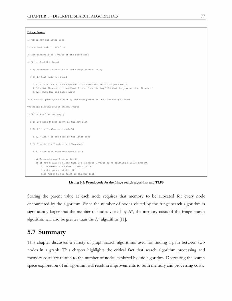
CHAPTER 5 - DISCRETE SEARCH ALGORITHMS 77
Fringe Search
1) Clear Now and Later List
2) Add Root Node to Now list
3) Set Threshold to H value of the Start Node
4) While Goal Not Found
4.1) Performed Threshold Limited Fringe Search (TLFS)
4.2) If Goal Node not found
4.2.1) If no F Cost found greater than threshold return no path exits
4.2.2) Set Threshold to smallest F cost found during TLFS that is greater than Threshold
4.2.3) Swap Now and Later Lists
5) Construct path by backtracking the node parent values from the goal node
Threshold Limited Fringe Search (TLFS)
1) While Now list not empty
1.1) Pop node N from front of the Now list
1.2) If N’s F value >= threshold
1.2.1) Add N to the back of the Later list
1.3) Else if N’s F value is < Threshold
1.3.1) For each successor node S of N
a) Calculate new G value for S
b) If new G value is less than S’s existing G value or no existing G value present
i) Update S’s G value to new G value
ii) Set parent of S to N
iii) Add S to the front of the Now list
Listing 5.5: Pseudocode for the fringe search algorithm and TLFS
Storing the parent value at each node requires that memory to be allocated for every node
encountered by the algorithm. Since the number of nodes visited by the fringe search algorithm is
significantly larger that the number of nodes visited by A*, the memory costs of the fringe search
algorithm will also be greater than the A* algorithm [11].
5.7 Summary
This chapter discussed a variety of graph search algorithms used for finding a path between two
nodes in a graph. This chapter highlights the critical fact that search algorithm processing and
memory costs are related to the number of nodes explored by said algorithm. Decreasing the search
space exploration of an algorithm will result in improvements to both memory and processing costs.

CHAPTER 5 - DISCRETE SEARCH ALGORITHMS 78
Dijkstra‘s algorithm was discussed in Section 5.2 as being both a complete and optimal algorithm.
Dijkstra‘s algorithm was not intended for point-to-point searches and so a modification to the
algorithm was needed to reduce the processing costs when preforming point-to-point searches. The
undirected nature of the search space exploration results in a high degree of exploration resulting in
high processing and memory costs. Unfortunately, the high processing and memory costs make it
unsuitable for video game pathfinding.
Section 5.3 introduced the A* algorithm as an improvement on Dijkstra‘s algorithm by directing the
search space exploration towards the goal node. This search space direction was facilitated by the
use of a heuristic function which acts as an estimation of the likelihood of a node leading to the goal.
The A* algorithm is both complete and can be optimal, though optimality can only be guaranteed if
an underestimating heuristic is used. Section 5.3.2 discusses various heuristic functions as well as the
use of overestimating heuristic functions to speed up graph searches at the expense of solution
optimality.
The IDA* algorithm is discussed in Section 5.4 as a complete and optimal low-memory graph search
algorithm. Unfortunately, the low memory cost of the algorithm comes with exorbitantly high
processing costs. The same can be said of the SMA* algorithm which also offer a significant
memory reduction at a high processing cost. The high processing costs of both algorithms (IDA*
and SMA*) makes them unusable for use in large video game environments.
The final section presents the fringe search algorithm, which is a form of memory enhanced IDA*.
The fringe search algorithm greatly reduces the number of node re-explorations performed, resulting
in a greatly reduced overall processing cost. It has been shown to be around 25% faster than the A*
algorithm but comes at a greater memory cost. As such the fringe search algorithm is an attractive
option for solving the graph search problem when not operating on a limited memory platform.
In conclusion, the A* algorithm still remains the most popular graph search algorithm and its use is
ubiquitous in the video game industry. Numerous optimizations can be performed to the algorithm
both in terms of reducing memory costs as well as processing costs.

79
Chapter 6 Continuous Search Algorithms
This chapter reviews continuous graph search algorithms. A short introduction to continuous search
algorithms is provided in Section 6.1. The three main continuous search algorithm families are
discussed in Sections 6.2, 6.3 and 6.4. The suitability of continuous search algorithms with regards to
use for video game pathfinding in dynamic environments is discussed in section 6.5. The final
section summarizes the chapter.
6.1 Continuous Search Algorithms
The dynamic pathfinding problem is a fundamental one in the field of robotics [12]. Robot agents
are often tasked with pathfinding in unknown or partially unknown environments [12]. Since the
agent does not have complete knowledge of its environment, it is impossible for that agent, at any
given time, to plan a path that is guaranteed to be valid and simply follow it.
Consider a situation where an agent has only a very basic knowledge of its environment. When given
a move order, the agent operates under the free-space assumption in that all unknown nodes are
traversable and plans an initial path accordingly. As the agent traverses the environment, the agent
will receive more information about the environment through its sensors. Certain nodes that were
assumed to be traversable may not be and so the agent‘s path will need to be corrected to take this
new environmental data into account2.
When a robotic agent encounters an environmental change, the agent‘s path is replanned and the
agent proceeds along the new path. This means that the agent‘s path is likely to continuously change
over the course of the agent‘s traversal of the path [18] requiring a large number of replanning
actions, each replanning action requiring a discrete search.
2 Environments which are partially unknown are analogous to highly dynamic video game environments as in both environments, environmental changes may occur over the course of an agent‘s traversal of the environment. As such, an examination of the applicability of robotic pathfinding search algorithms to dynamic video games environments is necessary.

CHAPTER 6 - CONTINUOUS SEARCH ALGORITHMS 80
The costs of running a discrete search for each replanning action can easily overwhelm a pathfinding
system resulting in agents‘ pausing to replan their path each time an environmental change was
encountered [13]. A search algorithm is needed that could operate over the course of an agent‘s path
traversal and provide inexpensive localized path corrections as necessary.
This thesis makes novel use of the terms discrete and continuous in the separation of graph search
algorithms. Using a discrete search algorithm to solve a problem, will return a solution within an
environment at a given time. The algorithm has no means of detecting environmental changes or
correcting the solution found if so required. In contrast, a continuous search algorithm will run
continuously for the duration of the problem, updating its solution as the environment changes.
Recall, from Chapter 4, that discrete search algorithms are problem-centric in that all environmental
knowledge is discarded once a solution to a given problem has been found. In using a discrete
search algorithm for replanning, each environmental change will require the search algorithm to re-
explore the environment, i.e. restart the search from scratch.
It has been shown that the reuse of environmental knowledge can greatly improve replanning costs
[112] [12]. To achieve the re-use of information over the course of the pathfinding problem, a
continuous search algorithm is required. This continuous algorithm is further required to interleave
path planning with agent movement. An algorithm which interleaves execution (agent movement)
with planning is termed an agent-centric algorithm [113].
Continuous algorithms were developed as a means of reducing the re-planning cost incurred in
dynamic environments [13]. Although primary developed to deal with dynamic environments,
certain continuous algorithms (the real-time family of continuous search algorithms) originated as a
means of reducing the memory costs involved in searching large environments [20].

CHAPTER 6 - CONTINUOUS SEARCH ALGORITHMS 81
6.2 Incremental Search Algorithms
The dynamic pathfinding problem can be solved by the simple use of a discrete search algorithm
such as A*. This means that a new A* search needs to be performed each time an environmental
change is discovered by the agent. Since each A* search will be performed atomically, it cannot reuse
any of the environmental knowledge of previous A* searches and each environmental change
encountered will require that the entire environment be searched again.
This is highly wasteful as a single local change may require a further portion of the environment to
be searched again, and so continuous search algorithms have been developed to reuse environmental
information across searches. In reusing prior searches‘ environmental data, the workload of
subsequent searches is greatly reduced [21]. Since these continuous search algorithms perform a
series of incremental searches, such algorithms are termed incremental search algorithms (also
referred to as dynamic search algorithms) [114] [12] [112].
In summary, incremental search algorithms plan an initial complete path and perform (incremental)
replanning actions as necessary over the course of the agent‘s traversal along the path. If an optimal
search algorithm is used for the incremental search then each path planned will be optimal, even in
fully dynamic environments [15] [112].
Subsection 6.2.1 presents an introduction to the incremental graph search algorithm family.
Subsections 6.2.2 and 6.2.3 discuss the two most popular incremental search algorithms: the lifelong
planning A* algorithm and the dynamic A* lite algorithm.
6.2.1 Introduction
The most well-known algorithms in the incremental family are the dynamic A* (D*) [12], the
focused dynamic A* (focused D*) [13] and the lifelong planning A* (LPA*) [112] algorithms. The
D* algorithm was greatly improved after a year by the focused D* algorithm [13]. As such, the term
D* is commonly used to refer to the focused D* algorithm and not the actual original D* algorithm.
In 2002, the focused D* and LPA* algorithms were combined with the aim of decreasing the
complexity of the D* algorithm. The hybridization resulted in the D* lite algorithm [15]. The D* lite
algorithm is significantly simpler and easier to understand than the original focused D* algorithm
and is at least as efficient as the focused D* algorithm [15]. The D* lite algorithm is extremely
CHAPTER 6 - CONTINUOUS SEARCH ALGORITHMS 82
popular and has been used as a base for several advanced continuous algorithms and are discussed in
detail in Section 6.2.3.
There is a recent subfamily of incremental search algorithms originating from the adaptive A*
algorithm presented in [16]. The adaptive A* (AA*) algorithm is simpler than other versions of the
incremental A* algorithm such as D* and LPA* [16]. Due to its simplicity, the adaptive A*
algorithm is easily extensible as shown by the moving target adaptive A* (MTAA*) [115] and the
real-time adaptive A* [116].
This family of adaptive search algorithms returns optimal solutions within unknown search spaces as
well as within dynamic environments in which the only environmental change allowed is for
traversable nodes to become obstructed (or impassable).
In the case of a fully dynamic environment wherein nodes may change their traversability at will,
these adaptive algorithms lose their optimality guarantee and have no lower bound on the sub-
optimality of the solutions returned. This limits their applicability for use within video game
environments. A recent generalized version of the adaptive A* (generalized adaptive A* or GAA*)
algorithm was developed to guarantee path optimality within fully dynamic environments [17].
The GAA* algorithm offers worse performance than the D* lite algorithm for static target searches
while offering improvements in regards to moving target searches [17]. Since AA* is not suitable for
fully dynamic environments and GAA* offers worse performance than D* lite, the adaptive
algorithm family will not be discussed further.
6.2.2 Lifelong Planning A* (LPA*)
Almost all continuous search algorithms that can operate within dynamic environments are built
upon the D* lite algorithm [19] [21]. D* lite is in turn an LPA* variant that is simpler than and at
least as efficient as the standard focused D* algorithm. To discuss the D* lite algorithm, it is
necessary to start with a discussion of the LPA* algorithm [112] as the D* lite algorithm is a
modified, backwards version of LPA*.
LPA* is the combination of the incremental DynamicSWSF-FP algorithm [117] and the heuristic-
based A* algorithm. Fundamentally, LPA* is an incremental version of the A* algorithm that reuses
information from previous searches across search iterations.
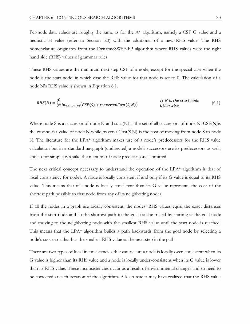
CHAPTER 6 - CONTINUOUS SEARCH ALGORITHMS 83
Per-node data values are roughly the same as for the A* algorithm, namely a CSF G value and a
heuristic H value (refer to Section 5.3) with the additional of a new RHS value. The RHS
nomenclature originates from the DynamicSWSF-FP algorithm where RHS values were the right
hand side (RHS) values of grammar rules.
These RHS values are the minimum next step CSF of a node; except for the special case when the
node is the start node, in which case the RHS value for that node is set to 0. The calculation of a
node N‘s RHS value is shown in Equation 6.1.
( ) { ( )( ( ) ( ))
(6.1)
Where node S is a successor of node N and succ(N) is the set of all successors of node N. CSF(N)is
the cost-so-far value of node N while traversalCost(S,N) is the cost of moving from node S to node
N. The literature for the LPA* algorithm makes use of a node‘s predecessors for the RHS value
calculation but in a standard navgraph (undirected) a node‘s successors are its predecessors as well,
and so for simplicity‘s sake the mention of node predecessors is omitted.
The next critical concept necessary to understand the operation of the LPA* algorithm is that of
local consistency for nodes. A node is locally consistent if and only if its G value is equal to its RHS
value. This means that if a node is locally consistent then its G value represents the cost of the
shortest path possible to that node from any of its neighboring nodes.
If all the nodes in a graph are locally consistent, the nodes‘ RHS values equal the exact distances
from the start node and so the shortest path to the goal can be traced by starting at the goal node
and moving to the neighboring node with the smallest RHS value until the start node is reached.
This means that the LPA* algorithm builds a path backwards from the goal node by selecting a
node‘s successor that has the smallest RHS value as the next step in the path.
There are two types of local inconsistencies that can occur: a node is locally over-consistent when its
G value is higher than its RHS value and a node is locally under-consistent when its G value is lower
than its RHS value. These inconsistencies occur as a result of environmental changes and so need to
be corrected at each iteration of the algorithm. A keen reader may have realized that the RHS value
CHAPTER 6 - CONTINUOUS SEARCH ALGORITHMS 84
is the minimum of all the ‗new G‘ values calculated for each node successor during A* node
exploration.
The LPA* search proceeds in a similar manner to the A* search. The list of potential nodes to
explore is contained within an open list. The open list is sorted by the nodes‘ F values and ties are
broken in favor of the lowest G value. When a node is explored, its RHS value is compared to its G
value. In the case of an over-consistency occurring, this means that a shorter path to that node has
been found.
In that case the G value is set to the RHS value (the new shortest path) and all that node‘s
successors are updated to take the change into account. If the node is consistent or locally under-
consistent then its G value is set to infinity (making it locally over-consistent) and the node, as well
its successors, is updated. A node update is simply a recalculation of that node‘s RHS, F and G
values. The updated node is then inserted into the open list (or its position in the open list is
updated if the node is already present on the open list).
For the LPA* algorithm described above, the initial search performed by the algorithm is exactly the
same as an A* search. The exact nodes are explored in the exact same order as would have occurred
during an A* search [112]. Subsequent searches simply act to repair any detected local
inconsistencies within the graph that may have resulted from environmental changes. When an
environmental change is detected, the changed node is updated (added to the open list) and the
search is continued. The LPA*‘s open list serves to prioritize the repair of locally inconsistent nodes
that are part of the solution (just like A* explores nodes that are more likely to be part of the
solution first).
The termination conditions of each LPA* search, are as follows: the search terminates once the goal
node is locally consistent and the goal‘s F value is smaller than or equal to lowest F value on the
open list (i.e. no node with a potential better route to the goal node exists). A more detailed
discussion of the termination conditions and proof of correctness can be found in section 5.1 of
[112]. The pseudocode for the LPA* algorithm is shown in Listing 6.1.

CHAPTER 6 - CONTINUOUS SEARCH ALGORITHMS 85
Calculate Key for Node N
1. G = the minimum of N’s G value and N’s RHS value
2. F = G + heuristic estimate from N to goal node
3. Return ( F , G )
Update Node N
1. If N not equal to start node calculate RHS value
2. If N is on the open list, remove N from open list
3. If N’s G value not equal to N’s RHS value (i.e. locally inconsistent)
3.1 calculate key for N
3.2 insert N into open List
Compute Shortest Path from Start Node to Goal Node
1. While ( goal node is inconsistent and the goal node’s key is greater than the best node’s key )
1.1 Remove the best node N from the open list
1.2 If N is locally over-consistent (N’s G value > N’s RHS value)
1.2.1 Set N’s G value to N’s RHS value
1.2.2 Update N’s successor nodes
1.3 Else
1.3.1 Set N’s g value to infinity
1.3.2 Update N
1.3.3 Update N’s successor nodes
LPA*
1. Set all nodes’ RHS and G values to infinity
2. Set RHS of start node to 0
3. Calculate start node’s key and insert start node into open list
4. Do forever
4.1 Compute Shortest Path
4.2 Wait for environmental changes
4.3 For all changed nodes C
4.3.1 Update Node C
Listing 6.1: Pseudocode for the LPA* Algorithm
6.2.3 Dynamic A* Lite (D* Lite)
To solve a pathfinding problem as the agent moves through the environment requires that the start
node of the search problem changes over time. Unfortunately, the LPA* algorithm estimates all G
values as being from the start to the goal. As the agent moves from one node to another, this move
invalidates all previous search data as the G values of each node need to be recalculated from the
new start node. To do this would be the same as running a new search for each movement of the
agent, akin to simply using a discrete search algorithm for each replanning action.
The D* lite algorithm is presented as a means to solve the real-time pathfinding problem (moving
agent) in both partially unknown and dynamic environments [15]. To maintain search information

CHAPTER 6 - CONTINUOUS SEARCH ALGORITHMS 86
validity even across searches with varied start nodes, the D* lite algorithm simply reverses the search
direction of LPA* (searches are now performed from the goal node to the start node) resulting in
the per-node G values now representing the cost from goal (CSG) values instead of CSF values.
Paths are constructed forwards from the start node to the goal node by selecting the node with the
lowest RHS as the next step.
Simply reversing the algorithm‘s search direction is not enough to ensure the optimality of the
algorithm [15], as the heuristic values for each node in the graph will also be inaccurate as the agent‘s
start node changes over the course of the agent‘s traversal. If the heuristic values change then the
ordering of the open list of the D* lite algorithm will be invalidated and so the open list will need to
be reordered taking into account the heuristic value changes. D* lite uses a method derived from the
focused D* algorithm to prevent open list reordering, by using node priorities that are lower bounds
to those used in LPA* [13]. To remove the need for open list reordering, the heuristic function used
must satisfy the following properties:
( ) ( ) ( ) ( ) ( ) (6.2)
Where H(S,S') is the heuristic value between nodes S and S' and traversalCost(S,S') is the cost of
moving from node S to S'. This means that the heuristic function must be an underestimation or
exact estimation of the costs between two nodes.
Due to the properties shown in Equation 6.2, when an agent moves from a node S to a node S‘, the
heuristic values will decrease by at most H(S, S‘). This means that the F values in the open list will
have also have decreased by at most H(S, S‘).
To correct the F values of the nodes in the open list, each node‘s F and H values need to have H(S,
S‘) subtracted from them. Since H(S, S‘) is constant, this means that the ordering of the priority
queue will remain unchanged and so the open list will require no reordering upon agent movement.
As with LPA*, repairs need to be performed on any node inconsistencies that may have resulted
from environmental changes.
These repairs may need to insert new nodes into the open list. Even though the open list ordering is
correct, all the nodes‘ H values (and as a result the F values) are now H(S, S‘) too high. Updating
each F and H value of all the nodes in the open list is an expensive operation and can be avoided.
When an environmental change occurs and the agent has changed location (from S to S‘), the H(S,

CHAPTER 6 - CONTINUOUS SEARCH ALGORITHMS 87
S‘) value is added to a Km variable which tracks the changes in heuristic values over the course of the
agent‘s movement. An agent may have moved several steps between environmental changes and so
S and S‘ are not necessarily directly connected.
To prevent the updating of every node in the open list to reflect the decrease in the heuristic values,
the Km variable is simply added to any new nodes‘ F values when they are inserted into the open list.
Adding Km has the effect of maintaining the consistency of the heuristic values across agent moves.
The addition of the Km value is performed automatically by the node update function (refer to the
―calculate key‖ function shown in Listing 6.2) for new nodes being inserted into the open list.
During the search stage, the node with the lowest F value is selected from the open list and
expanded, to maintain node F value correctness, an extra check is performed prior to a node being
selected from the open list. The node with the lowest F value is selected and a new F value is
calculated (taking into account a possibly modified Km value). If the old F value is lower than the
new F value, then the old F value is updated to the new F value and the node‘s position is reinserted
in the open list. Node exploration occurs in the same fashion as in the LPA* algorithm. The
pseudocode for D* lite is presented in Listing 6.2.
The node exploration rate of D* lite is extremely similar to that to that of A* [15] and the per node
memory cost is also similar (the exact same per-node data values, differing only in that the parent
link of A* is replaced with the RHS value in the D* lite algorithm). These similarities result in the D*
lite algorithm‘s overall memory cost being very similar to that of A*.
In summary, the D* lite algorithm has more in common with LPA* than with focused D*. It is
significantly simpler and easier to understand than focused D* and so easier to extend [15].
Furthermore, D* lite is shown to be at least as efficient as focused D*, in many cases being
significantly more efficient [15]. The D* Lite algorithm has been successfully used to map out
unknown environments as well as for robot navigation [15]. The D* lite algorithm has also served as
the base for several state-of-the-art continuous search algorithms (AD* and RTD*) [21] [19].
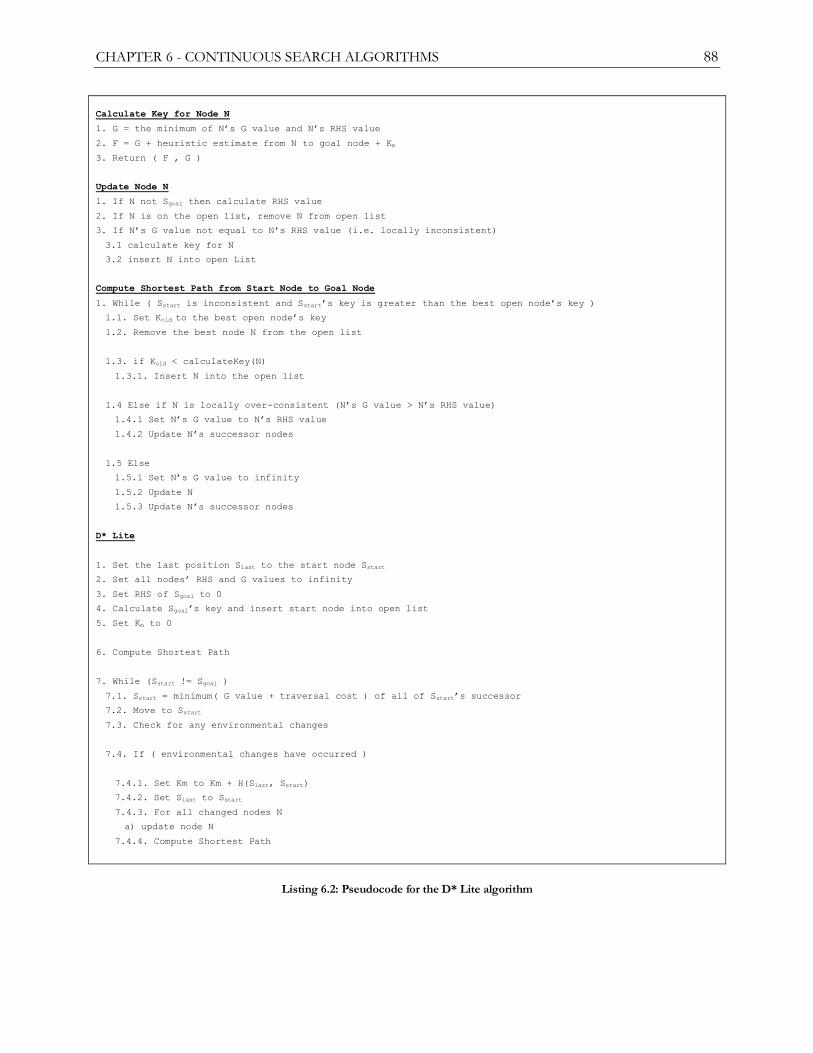
CHAPTER 6 - CONTINUOUS SEARCH ALGORITHMS 88
Calculate Key for Node N
1. G = the minimum of N’s G value and N’s RHS value
2. F = G + heuristic estimate from N to goal node + Km
3. Return ( F , G )
Update Node N
1. If N not Sgoal then calculate RHS value
2. If N is on the open list, remove N from open list
3. If N’s G value not equal to N’s RHS value (i.e. locally inconsistent)
3.1 calculate key for N
3.2 insert N into open List
Compute Shortest Path from Start Node to Goal Node
1. While ( Sstart is inconsistent and Sstart’s key is greater than the best open node’s key )
1.1. Set Kold to the best open node’s key
1.2. Remove the best node N from the open list
1.3. if Kold < calculateKey(N)
1.3.1. Insert N into the open list
1.4 Else if N is locally over-consistent (N’s G value > N’s RHS value)
1.4.1 Set N’s G value to N’s RHS value
1.4.2 Update N’s successor nodes
1.5 Else
1.5.1 Set N’s G value to infinity
1.5.2 Update N
1.5.3 Update N’s successor nodes
D* Lite
1. Set the last position Slast to the start node Sstart
2. Set all nodes’ RHS and G values to infinity
3. Set RHS of Sgoal to 0
4. Calculate Sgoal’s key and insert start node into open list
5. Set Km to 0
6. Compute Shortest Path
7. While (Sstart != Sgoal )
7.1. Sstart = minimum( G value + traversal cost ) of all of Sstart’s successor
7.2. Move to Sstart
7.3. Check for any environmental changes
7.4. If ( environmental changes have occurred )
7.4.1. Set Km to Km + H(Slast, Sstart)
7.4.2. Set Slast to Sstart
7.4.3. For all changed nodes N
a) update node N
7.4.4. Compute Shortest Path
Listing 6.2: Pseudocode for the D* Lite algorithm
CHAPTER 6 - CONTINUOUS SEARCH ALGORITHMS 89
6.3 Anytime Search Algorithms
An anytime search algorithm is a variant of the incremental search algorithm with a key difference.
Whereas an incremental search algorithm will generate an optimal solution and correct the solution
by replanning a new optimal route when environmental changes occur, an anytime algorithm will
begin by generating a grossly sub-optimal solution and proceeds to improve the solution over time
[19] [18]. The justification for the incremental improvement of a grossly sub-optimal route is to
allow the algorithm to always return a solution irrespective of the total time allowed for planning.
For a given time constraint, it may not be possible to perform an optimal search for each planning
action and so a sub-optimal solution is preferred over no solution at all [18]. Anytime algorithms
attempt to provide a sub-optimal path quickly and improve it as much as the allocated planning time
allows. The anytime repair A* (ARA*) algorithm presented in [18] is an improvement on the
anytime A* algorithm presented in [118] by presenting sub-optimality bounds for the solutions.
The ARA* algorithm operates by performing a series of fast incremental searches using an over-
estimated heuristic function (refer to Section 5.3.2 for a discussion on the effects of the over-
estimation of the heuristic function). Information from past searches is reused by subsequent
searches in a similar manner to that used in the GAA* algorithm.
The method of over-estimation used in [18] and [19] is a simple multiplication of the heuristic value
by an inflation factor termed ε, where ε > 1. The level of over-estimation of the heuristic function
(the ε value) is reduced for each subsequent search until the heuristic function is admissible (i.e.
exact or under estimate; achieved by setting ε = 1).
In this manner, the ARA* algorithm will eventually return an optimal solution if it is given sufficient
time to complete. In the case when there is insufficient time to perform a search with ε=1, a sub-
optimal path is returned whose length is no more than ε times the optimal path length [18]. As such,
final optimality of the solution depends on the allocated planning time.
Anytime algorithms are intended for use in complex static search environments, and as such cannot
operate within dynamic environments as there is no mechanism present to deal with environmental
changes occurring during the planning time [19]. To allow for operation within dynamic
environments, the ARA* algorithm was combined with the D* lite algorithm resulting in the
anytime dynamic A* (AD*) algorithm [19].

CHAPTER 6 - CONTINUOUS SEARCH ALGORITHMS 90
The AD* algorithm allows for anytime solution improvement within dynamic environments. At the
current time, the author of this thesis is not aware of any other anytime pathfinding algorithms
capable of operating within dynamic environments. The AD* algorithm is essentially the same as the
ARA* algorithm in that it performs a series of heuristic searches with decreasing inflation factors.
The difference between ARA* and AD* is subtle, in that when environmental changes are detected,
any locally affected nodes are placed back onto the open list and the search for the current inflation
value is repeated (the path is repaired) exactly as in the D* lite algorithm. In the case of substantial
environmental changes, it may be more efficient to replan a more sub-optimal path (higher inflation
value) than repair the path at the current level of sub-optimality [19]; in such a case, the AD*
algorithm increases the heuristic inflation factor and re-plans at a higher level of sub-optimality and
then proceeds to improve the resultant sub-optimal path in the normal fashion.
The AD* algorithm offer no performance or memory cost improvements over the D* lite
algorithm. What it does offer is an anytime capability at the cost of sub-optimality. Furthermore,
there is an expensive open list reordering between searches that may be removed by the inclusion of
a bias term (Km) as in the D* lite algorithm. In a video game environment, there is no anytime
requirement in place as the pathfinding workload may be distributed over a number of frames,
making the added complexity of the AD* redundant when compared to the simplicity of the D* lite
algorithm. The added complexity as well the fact that AD* offers no performance or memory
benefits over the D* lite algorithm within the required application results in there being no benefit in
using the AD* algorithm for a video game application.
6.4 Real-Time Search Algorithms
In an attempt to solve larger search problems by using a heuristic search algorithm (previously
unsolvable due to the memory limitations of the time), the real-time A* algorithm, a real-time
heuristic algorithm, was developed by Richard Korf in 1990 [20].
Real-time heuristic search algorithms make use of depth limited look-ahead search around the
agent‘s current node and determine the next best move using a heuristic function. The depth limit
placed upon the look-ahead search is referred to as the search horizon (or look-ahead depth). As
such the agent will always choose the best move visible to it, where the range of visibility is defined
by the search horizon.
CHAPTER 6 - CONTINUOUS SEARCH ALGORITHMS 91
In only selecting the best move from within a limited visibility, agents face the risk of heading
towards a dead end or selecting sub-optimal moves. To overcome these problems a real-time
heuristic search algorithm will update (or learn) their heuristic function with experience. This led to
the development of the learning real-time A* algorithm (LRTA*) [20], which has become the basis
for the real-time heuristic search algorithm family. Real-time search algorithms places limits on the
memory and the computational cost of each agent planning action.
Real-time planning actions are atomic, fast and use little memory. Since an agent decides its next
move only once the previous move completes, no path is generated. An agent will wander the
environment selecting the best move it can see until it reaches its goal. Furthermore, agents will
often backtrack upon discovering that the route followed has led to a sub-optimal solution [20]. This
results in final paths, constructed by tracing the agent‘s movements from the start to the goal, that
are highly sub-optimal [21] [119] [120].
Real-time algorithms are also intended for use in known, static graphs and are unsuitable for use in
dynamic environments [20] [21]. Real-time algorithms can typically handle finding out that a
previously traversable cell is not blocked, but have no means of dealing with the converse, that is,
when a previously blocked cell becomes traversable [21].
Current research has attempted to hybridize a real-time search algorithm with an incremental search
algorithm for use within dynamic environments resulting in the real-time dynamic A* (RTD*)
algorithm [21]. RTD* is another hybridization of the D* lite algorithm, except that in this case, the
incremental D* lite algorithm is combined with a state-of-the-art real-time algorithm: the local
search space learning real-time A* (LSS-LRTA) [121].
RTD* will not be discussed in detail as it only offers a performance improvement over the D* lite
algorithm in unknown static worlds and worse performance than D* lite in known dynamic worlds
(such as those commonly found within video games) [21].
Due the inherent unsuitability of this family of algorithms for use in dynamic environments, real-
time algorithms will not be discussed in any more detail and interested readers are referred to [20],
[120], [119], [122], [123] for more information on the topic.

CHAPTER 6 - CONTINUOUS SEARCH ALGORITHMS 92
6.5 The Suitability of Continuous Search Algorithms for use
in Dynamic Video Game Environments
Numerous authors casually mention the suitability of their continuous search algorithms for use
within video games [120] [116] [21] without any substantiation of their claims. The basis of these
statements is that algorithms can successfully operate within video game navgraphs as well as the
fact that video game maps are usually used as test environments for these algorithms. Unfortunately,
while the algorithms may be able to successfully operate on video game environments, making a
broad statement on the suitability of the algorithms without taking into account the performance
and memory restrictions of the game platform is short-sighted and potentially misleading.
To explain why continuous search algorithms may be potentially unsuitable in video game
environments, it is necessary to discuss the reasons for the development of continuous search
algorithms. As continuous pathfinding search algorithms originate primarily from the robotics field,
it is necessary to briefly discuss the differences between the two pathfinding problems. A detailed
discussion regarding the robotics field is beyond the scope of this thesis and interested readers are
referred to [2] for more information.
The primary difference between robotics and video game pathfinding is the availability of
environmental information to the agent. In robotics, robotic agents (robots) are often required to
navigate unknown or partially known environments. These robots are required to plan an initial path
based only on what little environmental information the agent has at that time as well the free space
assumption which states that any unknown locations in the environment are traversable [19].
This means that a robot‘s primary path has no guarantee of correctness and the robot is required to
continuously update (or correct) its path as the robot receives more information regarding the
environment during its traversal. This continuous update requirement has led to the development of
continuous pathfinding search algorithms [12]. In contrast, game agents operate in fully known
environments meaning that the agents are not required to make any assumptions when planning
paths. Furthermore game agents are immediately notified of environmental changes irrespective of
the location of the environmental change.

CHAPTER 6 - CONTINUOUS SEARCH ALGORITHMS 93
The second difference between the two pathfinding problems is at a system level. Robots each have
their own processing hardware and memories dedicated to their AI systems. Each robot‘s AI system
is only responsible for that single robot and so most robotic pathfinding search algorithms are
agent-centric [113]. An agent-centric algorithm maintains data relevant to that specific agent and
cannot be used for any other agent [123].
On the other hand, video game AI systems operate in multi-agent environments and are responsible
for control of numerous game agents. Since video game AI systems are multi-agent systems, the
processing time and memory available need to be split across all the game agents. In splitting the
processing power and memory across multiple agents, much tighter performance and memory
constraints are placed upon the game AI system. As will be shown, the use of agent centric
algorithms (especially pathfinding algorithms) in multi-agent environments is extremely problematic
from a memory cost viewpoint.
In the case of pathfinding, the continuous search algorithm is executed over the entire course of the
agent‘s movement from the start node to the goal node in a graph. The memory costs of continuous
algorithms have been briefly discussed and are estimated to be similar to those of discrete algorithms
[21] [15]. Since continuous algorithms operate over the period of time taken for the agent to move
from its start position to its goal position, the associated memory costs of these algorithms are also
present for that period of time.
Game agents will move through the game environments at various speeds and so it is not
uncommon for path traversals to take extended periods of time to complete. This means that, for
the entire time period of the agent‘s path traversal, the continuous algorithms memory costs are
present for that agent. Each agent will require its own memory storage for the necessary data need
for the continuous search algorithm employed.
To illustrate this better, consider a standard RTS game in which a game agent is required to move
from one side of a moderately size game world to the other. The game world consists of 1024x1024
navgraph nodes and the game agent uses a continuous search algorithm for path planning. Assume
that the continuous search algorithm used by the agent has an average search space exploration rate
of 20% (similar to A*) and that the agent requires a minute to complete the movement across the
game world. Taking an optimistic estimate of 8 bytes of memory for the each of algorithm‘s per-

CHAPTER 6 - CONTINUOUS SEARCH ALGORITHMS 94
node data, the algorithm will use around 1.6MB of memory for the duration of the agent‘s path
traversal.
This is a moderate amount of memory and will easy fit within the memory budgets of most games,
even those run on memory limited platforms such as game consoles, but keep in mind this is the
memory cost for a single game agent.
Unfortunately, games do not usually feature a single game agent and as mentioned in chapter 4, it is
not uncommon for RTS games to contain dozens (if not hundreds) of game agents. When using an
agent-centric continuous search algorithm in a multi-agent game environment, each agent will have
its own instance of the search algorithm and each search algorithm instance will have its own
memory costs.
In a multi-agent environment the memory costs will increase as the number of agents increases.
Using the above example and increasing the number of agent to 50, the total memory cost for
pathfinding will be around 80MB (50 agents x 1.6MB). A memory cost that will definitely exceed the
AI memory budgets of any video game. As such, continuous search algorithms are highly unsuitable
for use in multi-agent memory constrained game environments [124].
6.6 Summary
Discrete search algorithms are more problem-centric in that they simply return a solution for a
specific problem (a start-goal pair) and nothing more. The processing costs and memory costs are
paid once per problem, meaning that a pathfinding system using a discrete algorithm will have a
constant memory cost irrespective of the number of game agents present. Unfortunately, once an
environmental change is detected, a new discrete search is required in response to the environmental
change and so using a discrete search algorithm in a dynamic environment means that each
replanning action will require a new discrete search.
Performing numerous discrete searches is analogous to a simplistic incremental search algorithm
that offers no data reuse across searches. This results in very expensive replanning actions [13].
When used in a highly dynamic multi-agent environment, the processing load presented by the
replanning actions of numerous agents can easily overwhelm the pathfinding system resulting in
delayed agent response times.

CHAPTER 6 - CONTINUOUS SEARCH ALGORITHMS 95
Continuous search algorithms were developed to reduce the cost of these replanning actions by
reusing environmental data across the agent‘s traversal. The reuse of environmental data works quite
well and it has been shown that the processing costs of using a continuous search algorithm for a
dynamic environment are several orders of magnitude lower than those of discrete algorithms in the
same environment [13].
Unfortunately as discussed in Section 6.5, continuous search algorithms are unsuitable for use within
dynamic video game environments due to memory restrictions. Furthermore, the high processing
costs of replanning actions when using discrete algorithms make discrete algorithms unsuitable for
use within dynamic environments.

CHAPTER 6 - CONTINUOUS SEARCH ALGORITHMS 96

97
Chapter 7 Hierarchical Search Algorithms
This chapter discusses the most common hierarchical approaches to video game pathfinding, namely
the hierarchical pathfinding algorithm (HPA*), dynamic HPA* (DHPA*) algorithms, the partial-
refinement A* algorithm (PRA*), and the minimal memory (MM) abstraction. This chapter is
structured as follows: Section 7.1 provides an introduction to hierarchical approaches and discusses
the pros and cons of such approaches. Sections 7.2, 7.3 and 7.4 discuss the HPA* algorithm, PRA*
algorithm and the MM abstraction respectively. Section 7.5 summarizes this chapter.
7.1 Hierarchical Approaches
A hierarchical approach to graph search was first presented with the hierarchical A* algorithm [125].
However, it wasn‘t until the hierarchical pathfinding A* (HPA*) algorithm [22] that the suitability of
such approaches for use within video games was shown. Hierarchical pathfinding approaches
provide significant reductions both in terms of the processing and the memory costs associated with
solving a search problem at the cost of path optimality and an increased algorithm memory cost [92].
The following subsection discusses the technique of problem sub-division as a means of improving
performance. The remaining subsections cover the various stages present in a hierarchical search
algorithm as well as additional consideration to keep in mind when using a hierarchical search
algorithm.
7.1.1 Problem Sub-division
One method to decrease the processing costs of performing a discrete search within an environment
is to split the original problem into series of smaller, connected sub-problems [22]. Each sub-
problem is defined by a start and goal node. These start and goal nodes are both referred to as sub-
goals, in part due to the fact that the goal node of each sub-problem will be the start node for the
next sub-problem in the series.
CHAPTER 7 - HIERARCHICAL SEARCH ALGORITHMS 98
Furthermore since these sub-problems are smaller and simpler than the initial overall problem, the
processing and memory costs required in solving each sub-problem are trivial when compared to the
costs of solving the overall problem [22].
Figure 7.1 illustrates the splitting of a search problem into smaller sub-problems as well as
illustrating why splitting the problem into sub-problems offers significant cost reductions. An
example pathfinding problem is shown in Figure 7.1a. The optimal solution for that problem as
found by using an A* discrete search is also shown. In solving the example search problem the A*
algorithm has explored around 50% of the total search space. Consider the four smaller problems as
illustrated in Figure 7.1c. Solving these smaller problems requires very little search space exploration.
The reduced search space exploration results in lower processing and memory costs. If the four sub-
problems‘ solutions are connected to one another, a solution to the original problem is created,
(refer to Figure 7.1b). The total search space examined in solving these sub-problems is a small
fraction of the original search space explored in solving the original problem.
Since each sub-problem is self-contained, the memory costs associated with solving the search
problem are freed once a solution for that sub-problem has been found when using a discrete search
algorithm. This means that the peak memory usage in solving the overall problem by subdivision
into sub-problems is the maximum of the peak memory usages encountered when solving the sub-
problems. Looking at Figure 7.1c, the largest search space explored in solving a single sub-problem
is significantly smaller in comparison to the total search space explored in Figure 7.1a.
It is important to note that the solution presented in Figure 7.1b differs to the solution shown in
Figure 7.1a. In fact, the solution in Figure 7.1b is slightly sub-optimal. The sub-optimality of the
solution in Figure 7.1b occurs as a result of the selection of the sub-goals defining the sub-problems.
If the sub-goals lie on the optimal path then the returned solution will be optimal. This means that
the sub-optimality of the returned solution is dependent on the selection of the sub-goals that define
the sub-problems.

CHAPTER 7 - HIERARCHICAL SEARCH ALGORITHMS 99
To keep the solution sub-optimality low, sub-goals must be well chosen, but unfortunately it is
impossible to find the optimal sub-goals ahead of time without performing an expensive optimal
graph search. As such all techniques that split the overall problem when solving it are inherently sub-
optimal, i.e. all solutions returned will exhibit a degree of sub-optimality.
Hierarchical approaches create a hierarchy of abstract graphs from the base navgraph. These
abstract graphs are then used for the selection of sub-goals allowing a hierarchical approach to
quickly and cheaper split a problem into sub-problems. Each abstract graph is created in a manner
similar to that in which the navgraph was created from the 3D environment (refer to Chapter 3 for
more details).
Hierarchical approaches make use of environmental knowledge to create abstract nodes
(representing the sub-goals). These abstract nodes are then interconnected and form the final
abstract graph. Searching the abstract graph will result in an abstract path or simply put a list of sub-
goals defining the sub-problems needed to be solved to create a solution to the original problem.
As such, hierarchical approaches all have three key stages:
The Build Stage: The build stage is responsible for creating an abstract graph hierarchy
from the navgraph.
The Abstract Planning Stage: The abstract planning stage searches the abstract graph to
find an abstract path. This abstract path determines the list of sub-problems that need to be
solved.
The Path Refinement Stage: The path refinement stage refines the abstract path found
during the abstract planning stage into a low-level path.
To put it plainly, the build stage creates and connects the sub-goals. The abstract planning stage then
identifies the sub-goals to be used in solving a specific problem. The path refinement stage solves
the sub-problems originating from the sub-goal identified in the abstract planning stage and
combines their solutions into a single low-level path. This low-level path is the final solution to the
original problem.
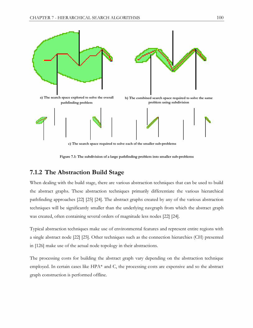
CHAPTER 7 - HIERARCHICAL SEARCH ALGORITHMS 100
b) The combined search space required to solve the same
problem using subdivision
a) The search space explored to solve the overall
pathfinding problem
c) The search space required to solve each of the smaller sub-problems
Figure 7.1: The subdivision of a large pathfinding problem into smaller sub-problems
7.1.2 The Abstraction Build Stage
When dealing with the build stage, there are various abstraction techniques that can be used to build
the abstract graphs. These abstraction techniques primarily differentiate the various hierarchical
pathfinding approaches [22] [25] [24]. The abstract graphs created by any of the various abstraction
techniques will be significantly smaller than the underlying navgraph from which the abstract graph
was created, often containing several orders of magnitude less nodes [22] [24].
Typical abstraction techniques make use of environmental features and represent entire regions with
a single abstract node [22] [25]. Other techniques such as the connection hierarchies (CH) presented
in [126] make use of the actual node topology in their abstractions.
The processing costs for building the abstract graph vary depending on the abstraction technique
employed. In certain cases like HPA* and C, the processing costs are expensive and so the abstract
graph construction is performed offline.

CHAPTER 7 - HIERARCHICAL SEARCH ALGORITHMS 101
When operating within dynamic environments, any environmental changes will result in a change to
the abstract graph as well. As such, abstract graph modifications need to be performed during
runtime, requiring a short simplified build stage to perform any necessary corrections to the abstract
graph. This is an important consideration when choosing an abstraction technique for use in
dynamic environments as complex abstraction techniques will result in higher abstract graph update
costs.
In extremely large environments, it may be beneficial to create several layers of abstraction (i.e.
create an abstract graph from an already abstract graph) to reduce the processing costs even further.
Unfortunately, the added complexity of implementation for multi-level abstraction hierarchies as
well as the additional memory costs for storing the abstraction can outweigh the minimal processing
cost improvements introduced [23] [22].
This is not always the case, as was discussed in [126] where a second level of abstraction was
required to ensure that pathfinding actions completed within the time constraints placed upon a
commercial video game. When dealing with a dynamic environment, having additional levels of
abstraction further increases the costs of environmental changes as all levels of abstraction will need
to be checked and potentially corrected. The benefits of higher levels of abstraction are highly
situational and need to be evaluated per application.
A term often encountered when dealing with abstraction techniques is granularity. Granularity refers
to the severity of the search space reduction performed during abstraction. A coarse granularity
technique would reduce the search space drastically, for example replacing an entire 16x16 portion
of the navgraph with a single abstract node. Such coarse techniques lose a lot of the low-level detail
and are not accurate representations of the underlying graph.
The minimal memory abstraction (refer to section 7.4) is a good example of a coarse abstraction
technique. A fine granularity technique on the other hand would result in a much smaller degree of
search space reduction. Finer techniques such as the ―clique and orphans‖ abstraction technique
used by PRA* (refer to Section 7.3) keep many of the underlying graph features, though at a much
higher build cost. In general, finer abstractions represent the underlying graph in more detail at the
expense of low search space reduction and increased build costs.

CHAPTER 7 - HIERARCHICAL SEARCH ALGORITHMS 102
7.1.3 The Abstract Search Stage
Once the abstract graph has been created from the underlying navgraph, the abstract graph becomes
the starting point for all path planning actions. When presented with a pathfinding problem, an
abstract path needs to be created which will define the number of sub-problems needed as well as
the sub-goals for each sub-problem. In the following explanation of the operation of a hierarchical
algorithm, only a single layer of abstraction is assumed.
The first step to finding an abstract path is to find the two nearest and reachable abstract nodes
(startabstract & goalabstract) to the low-level start (startnavgraph) and goal (goalnavgraph) nodes of the overall
problem. The nearest abstract nodes to the original start and goal nodes are usually found by
performing a series of discrete searches originating from the original start and goal nodes.
A discrete search is then performed on the abstract graph to find the abstract path between the
abstract startabstract and goalabstract nodes. Since the abstract graph is of small size, performing this
abstract search is trivial from both a processing and memory cost perspective when compared to
searching the underlying navgraph [22]. The abstract path returned from the abstract planning stages
contains a list of sub-goals between the startnavgraph and goalnavgraph nodes as well as the startnavgraph and
the goalnavgraph nodes which are positioned at the start and end of the abstract path respectively.
7.1.4 Path Refinement
To create the final solution, the abstract path needs to be refined (or translated) into a low-level
path. Since each node in the abstract path represents a sub-goal, the transition (or edge) between
two abstract nodes defines a sub-problem.
The two abstract nodes are the start and goal nodes of the sub-problem. As the abstract path is
traversed, the edges between the abstract nodes are refined into low-level paths by solving the sub-
problem (refinement action). This procedure is termed path refinement.
To solve a sub-problem, a discrete search is performed on the underlying navgraph. The discrete
search action results in a low-level path. This low-level path is only a portion of the final low-level
path and so is termed a partial path. Both the sub-problems and the abstract search problem can be
solved using any discrete graph search algorithms.

CHAPTER 7 - HIERARCHICAL SEARCH ALGORITHMS 103
Figure 7.2 illustrates a simplified example of solving a search problem, similar to the problem
presented in Figure 7.1, through the use of a hierarchical approach. The navgraph is abstracted using
a very simplistic abstraction technique which divides the navgraph into 10x10 regions and places a
single sub-goal within each region.
Three such neighboring regions are shown in Figure 7.2, in which a path is required from the yellow
start node to the purple goal node. The green and blue nodes are identified as the closest reachable
abstract nodes from the start (yellow) and goal (purple) nodes respectively.
An abstract search is performed on the abstract graph (the abstract graph is not shown for
simplicity‘s sake) and returns the abstract path shown in the figure. This abstract path is then refined
into the final solution shown by the beige nodes. The labels within the beige nodes signify the sub-
problem from which each of the beige nodes originate from.
Once again the final solution presented is grossly sub-optimal, but this is a result of the simplistic
abstraction technique used. The sub-optimality of the final path can be improved through the use of
a better abstraction technique.
1
sp1
sp1
sp1
sp1
sp1
S
sp0sp0
SP0
sp1
sp1
sp1
2sp2sp2sp2sp2
sp2
sp2
sp2
sp2
sp2
sp2
Gsp3sp3
3
sp2
sp2
sp2
sp2
sp 2
sp2
The Low Level Navgraph
1
The Abstract Path Start Navgraph Goal
Goal Navgraph Goal
Low-level Path Abstract Node 3
Abstract Node 2
Abstract Node 1
2 3
Figure 7.2: A basic overview of a hierarchical search.

CHAPTER 7 - HIERARCHICAL SEARCH ALGORITHMS 104
7.1.5 Considerations for Hierarchical Pathfinding
Decreased memory and processing costs are not the only benefits offered by a hierarchical
approach. An additional benefit is that a complete path is not needed before an agent can begin
moving. Since the complete path is made up of a series of partial paths (sub-problem solutions), an
agent can proceed along the path as soon as the first partial path is found (i.e. not completing the
entire path refinement stage). In allowing the game agent to move before the complete path is
planned an agent‘s response time is decreased.
Furthermore, the next partial path need only be solved once an agent approaches the end of its
current partial path. Unlike continuous search algorithms, no information is reused by a hierarchical
approach, meaning that all planning actions, be they abstract or refinement, are self-contained and
atomic. The atomicity of the planning actions as well as the lack of information re-use allows for the
pseudo-continuous operation of a hierarchical pathfinding algorithm over an extended period of
time without any memory implications like those encountered with continuous search algorithms.
The low cost of hierarchical planning actions allows for more planning actions to be performed in
the same time needed for a single planning action in a non-hierarchical approach. The time taken for
the complete path planning (abstract search and complete refinement) using the HPA* algorithm
has been shown to be up to nine times lower than a non-hierarchical approach [22]. The low costs
of planning actions allow multiple agents to receive complete paths (and so begin moving) in the
same time that was previously needed for a single agent to plan a complete path.
As a result, the increased agent responsiveness in multi-agent environments (without any increase in
memory costs) makes a hierarchical approach attractive for use in production multi-agent video
games. Hierarchical approaches are currently used (with great success) in ―Relic Entertainment‘s‖
―Dawn of War‖ and ―Company of Heroes‖ series as well as in ―Bioware‘s‖ critically acclaimed
―Dragon Age‖ role playing game [126] [91].
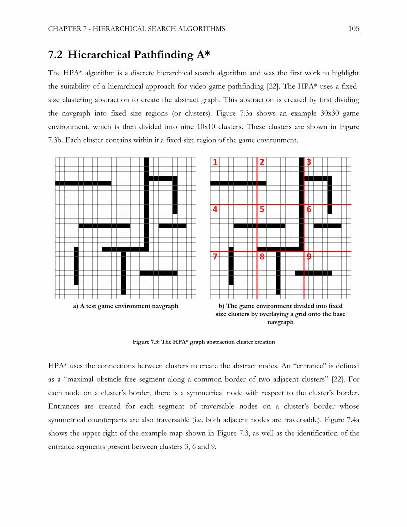
CHAPTER 7 - HIERARCHICAL SEARCH ALGORITHMS 105
7.2 Hierarchical Pathfinding A*
The HPA* algorithm is a discrete hierarchical search algorithm and was the first work to highlight
the suitability of a hierarchical approach for video game pathfinding [22]. The HPA* uses a fixed-
size clustering abstraction to create the abstract graph. This abstraction is created by first dividing
the navgraph into fixed size regions (or clusters). Figure 7.3a shows an example 30x30 game
environment, which is then divided into nine 10x10 clusters. These clusters are shown in Figure
7.3b. Each cluster contains within it a fixed size region of the game environment.
a) A test game environment navgraph b) The game environment divided into fixed
size clusters by overlaying a grid onto the base
navgraph
1 2 3
654
7 8 9
Figure 7.3: The HPA* graph abstraction cluster creation
HPA* uses the connections between clusters to create the abstract nodes. An ―entrance‖ is defined
as a ―maximal obstacle-free segment along a common border of two adjacent clusters‖ [22]. For
each node on a cluster‘s border, there is a symmetrical node with respect to the cluster‘s border.
Entrances are created for each segment of traversable nodes on a cluster‘s border whose
symmetrical counterparts are also traversable (i.e. both adjacent nodes are traversable). Figure 7.4a
shows the upper right of the example map shown in Figure 7.3, as well as the identification of the
entrance segments present between clusters 3, 6 and 9.

CHAPTER 7 - HIERARCHICAL SEARCH ALGORITHMS 106
The transitions between entrances are defined as follows: if the entrance segment has a length less
than a predefined constant (in this case 6), a single transition is created in the center of the entrance
segment (refer to the entrances between clusters 3 and 6 in Figure 7.4b). If the entrance segment
length is greater than the predefined constant then two transitions are created for the entrance
segment, one at each end (refer to the entrance between clusters 6 and 9 in Figure 7.4b). Transitions
across clusters are connected by intra-edges and transitions contained within a single cluster are
connected using intra-edges. These transitions, intra-edges and inter-edges make up the final abstract
graph (shown in Figure 7.4c). The creation of cluster entrances (and their inter-edges) as well as
searching for intra-edges has expensive processing costs and so the abstract graph is constructed
offline when a game environment is loaded.
In a dynamic environment, the abstract graph is created offline just as in a static environment but
needs to be modified as the environmental changes occur. When an environmental change occurs,
the HPA* needs to identify the clusters affected by the change and recalculate all the cluster
entrances as well as find all intra-edges. The abstract graph is then updated with this new cluster
data.
3
6
2
5
a) The top right hand portion
of the subdivided navgraph
3
6
2
5
9
b) The creation of cluster
entrances as well as inter and
intra-edges
9
3 3
66
6 6
99
c) The final abstract graph
from clusters 3 and 6
Figure 7.4: The HPA* graph inter-cluster and intra-cluster links

CHAPTER 7 - HIERARCHICAL SEARCH ALGORITHMS 107
Since the searches performed to find the intra-edges have high processing costs, a lazy approach to
their generation is presented in [127]. Since there is a likelihood the changes may not be immediately
required, the expensive intra-edge searches are postponed until that abstract node is encountered; at
which point the required searches are performed to identify all intra-edges. Simply put, intra-edges
are found as needed. Using a lazy approach does not decrease the workload required when
environmental changes occur, but simply postpones the work in the hope that intra-edges may not
be needed or that the clusters will change again prior to the intra-edges being needed.
HPA* is capable of building multiple levels of abstraction, but it has been shown that increasing the
cluster size decreases processing costs more so than adding extra layers of abstraction (which
increase the memory cost of HPA*) [127]. The choice of an additional abstraction layer instead of
simply increasing the cluster size should therefore be made carefully.
To perform an abstract search using HPA*, [22] propose the insertion of the start and goal nodes
into the abstract graph. The insertion is performed by first creating abstract nodes from the start
node, then performing a series of A* searches to find the nearest abstract node contained within the
same cluster as the start node. Once the nearest reachable abstract node has been found, an edge is
created between the abstract node and the start node [22]. The goal node is similarly inserted into
the abstract graph. Once both the start and goal nodes are inserted into the abstract graph, the
abstract path is found and refined (as described in the previous section). The abstract planning as
well as the path refinement stages are both completed before a path is returned. As such, the HPA*
algorithm as is cannot return partial solutions and so is a discrete search algorithm.
The abstract graph node insertion performed at the start of each search is problematic due to the
cost of the numerous A* searches performed to find the nearest reachable abstract node. The cost
of inserting a node into the abstract graph can be reduced by using Dijkstra‘s algorithm instead of
A* to find the shortest path to all neighboring abstract nodes as outlined in [127], but this
optimization only works within clusters featuring numerous abstract nodes with long or complex
paths between them. In the case of clusters featuring large open spaces or few entrances, using A*
searches to find the nearest reachable nodes is faster [127].
A recent paper [23] presents the dynamic HPA* (DHPA*) algorithm which entirely removes the
cost of inserting the start and goal nodes into the abstract graph. DHPA* achieves this by
maintaining a node cache within a cluster. This cluster node cache stores information regarding the
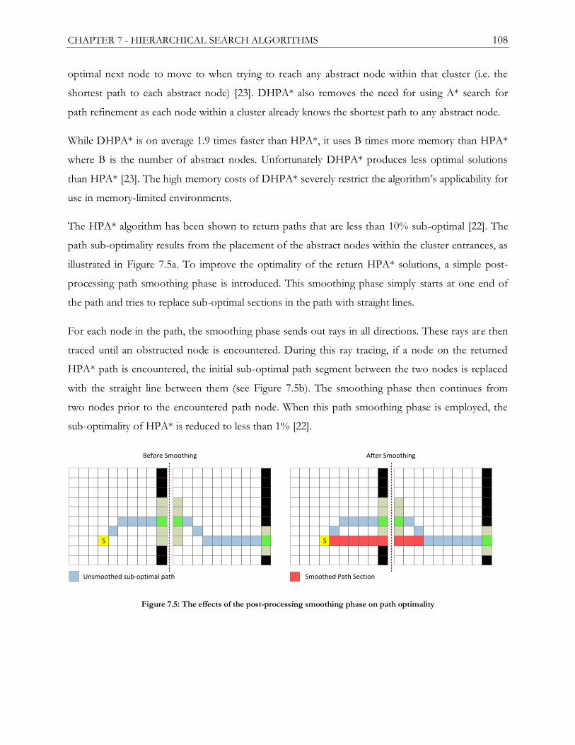
CHAPTER 7 - HIERARCHICAL SEARCH ALGORITHMS 108
optimal next node to move to when trying to reach any abstract node within that cluster (i.e. the
shortest path to each abstract node) [23]. DHPA* also removes the need for using A* search for
path refinement as each node within a cluster already knows the shortest path to any abstract node.
While DHPA* is on average 1.9 times faster than HPA*, it uses B times more memory than HPA*
where B is the number of abstract nodes. Unfortunately DHPA* produces less optimal solutions
than HPA* [23]. The high memory costs of DHPA* severely restrict the algorithm‘s applicability for
use in memory-limited environments.
The HPA* algorithm has been shown to return paths that are less than 10% sub-optimal [22]. The
path sub-optimality results from the placement of the abstract nodes within the cluster entrances, as
illustrated in Figure 7.5a. To improve the optimality of the return HPA* solutions, a simple post-
processing path smoothing phase is introduced. This smoothing phase simply starts at one end of
the path and tries to replace sub-optimal sections in the path with straight lines.
For each node in the path, the smoothing phase sends out rays in all directions. These rays are then
traced until an obstructed node is encountered. During this ray tracing, if a node on the returned
HPA* path is encountered, the initial sub-optimal path segment between the two nodes is replaced
with the straight line between them (see Figure 7.5b). The smoothing phase then continues from
two nodes prior to the encountered path node. When this path smoothing phase is employed, the
sub-optimality of HPA* is reduced to less than 1% [22].
S S
Unsmoothed sub-optimal path Smoothed Path Section
Before Smoothing After Smoothing
Figure 7.5: The effects of the post-processing smoothing phase on path optimality

CHAPTER 7 - HIERARCHICAL SEARCH ALGORITHMS 109
Path smoothing can be an expensive operation and so an optimization is introduced in [127] to
reduce the processing costs of the path smoothing phase. This is achieved by placing a bounding
box around the node from which the rays originate. The bounding box places limits on how far out
the rays extend, thereby reducing the processing costs of the ray tracing operation. In decreasing the
processing costs, this smoothing optimization trades path optimality for performance. No
processing cost comparison was made between the original and the ―optimized‖ smoothing
algorithms and only the increase in sub-optimality was shown [127].
7.3 Partial Refinement A*
As mentioned in section 7.1.5, being able to find quick partial solutions is beneficial in regards to
agent response times. The HPA* algorithm returns complete paths for each search problem and
cannot return partial paths. The HPA* algorithm can be modified such that the abstract path
refinement actions are distributed over the course of an agent‘s movement, thereby allowing HPA*
to return partial solutions (termed incremental hierarchical pathfinding).
Unfortunately, this introduces a large degree of sub-optimality that cannot be reduced through post-
processing techniques such as path smoothing. The low degree of sub-optimality in the HPA*
algorithm is a result of the post-processing smoothing stage. Without this additional stage, the HPA*
algorithm returns paths that are on average approximately 6% sub-optimal (smoothing reduces this
to under 1%) [22]. The PRA* algorithm was presented as the first partial hierarchical search
algorithm, and can find partial solutions that are more optimal than those returned by HPA* [24].
PRA* is based on a different abstraction technique to HPA* and a multi-level abstraction hierarchy
is necessary for the operation of the algorithm. To abstract the base navgraph, PRA* uses a ―clique
and orphans‖ based abstraction [24]. A clique is defined as a set of nodes wherein each node is both
reachable and at most a single step away from every other node in the set (i.e. each node has an edge
to every other node in the set). Cliques are shown in Figure 7.6 and are outlined in red. An orphan is
a node that is reachable from only a single other node (the blue outlined node in Figure 7.6c). PRA*
uses a maximum clique size of 4 in abstracting the navgraph.
PRA* also requires that the navgraph be fully abstracted until only a single node remains at the
highest abstraction level. Each clique represents a node on the abstract graph one level above it.
Orphan nodes are attached to the cliques leading to the orphan node. Since orphan nodes can only

CHAPTER 7 - HIERARCHICAL SEARCH ALGORITHMS 110
be reached by a single edge, they can only be connected to a single clique. A complete example of a
navgraph abstraction using cliques and orphans is presented in Figure 7.6. This abstraction scheme
offers very fine granularity and so at best can only offer a four times reduction in search space over a
lower level. In contrast, the abstraction technique used in the HPA* algorithm creates an abstract
graph several orders of magnitude smaller than the original. The fine granularity of the abstraction
technique also greatly increases the processing and memory costs of creating and storing the
abstraction layers.
PRA* performs the path refinement slightly differently to HPA*, the first step being to identify the
abstraction level SL in which both the start and goal nodes are abstracted into the same abstract
node (refer to Figure 7.6d). Path refinement then commences from level SL/2. This level is chosen
by the authors in [24] to provide low processing costs while still maintaining high path optimality.
An A* search is performed at the SL/2 abstraction level. The resulting abstract path is then refined
as in HPA*. In completing the path-refinement in one step, a complete solution is returned. This
variant is termed PRA*(∞) or infinite refinement PRA*.
G
S
a) The first level of abstraction is created by dividing a
navgraph into 4-cliques.
b) The first abstraction level
d) The final single node level of abstraction.
The start and goal nodes are now both
contained within the abstract node
c) The second abstraction level (including an orphan
node which is outlined in blue)
Figure 7.6: The PRA* Abstraction

CHAPTER 7 - HIERARCHICAL SEARCH ALGORITHMS 111
PRA* uses an extremely fine granularity for its navgraph abstractions compared to that used in
HPA*. This means that the search space reductions between abstract levels is significantly lower for
the PRA* abstraction than the HPA* abstraction. However the fine granularity also means that
abstract paths will contain more-optimal solutions that those within the abstract paths found using
HPA* [24] [128]. Since searching a large search space is expensive, PRA* leverages the cost
reductions offered by the higher levels of abstraction.
Partial path refinement is possible by simply truncating the abstract path found at each abstract level
to a fixed length K and using the tail node of the truncated path as the new goal for lower level
refinement. Applying path truncation during refinement is referred to as the PRA*(K) algorithm.
The PRA*(K) algorithm returns a partial path in a single atomic planning action while still
guaranteeing that an agent following the resulting partial path, as well as subsequently found partial
paths, will eventually reach the goal node [24]. By truncating the path at each abstract level,
PRA*(K) reduces the scope of the abstract search problem for the lower levels, further decreasing
search costs.
The fine granularity allows PRA*(∞) to return paths with a higher optimality (without the need for
an expensive smoothing phase) in similar time to HPA*. Paths returned by PRA*(∞) are within 1%
of optimal 98% of the time. Furthermore, partial paths can be returned, using PRA*(K), offering
only minimal reduction in optimality when compared to the paths returned by PRA*(∞). The path
optimality of paths returned by PRA*(K) is dependent on the K value. A K value of 16 was shown
to produce complete paths within 5% of optimal 98% of the time.
The fine granularity of the clique abstraction as well as the need for a full abstraction hierarchy
makes PRA* unsuitable for dynamic environments. When an environmental change occurs,
depending on the severity of the change, all of the abstract layers will need to be recreated. The fine
granularity also increases the memory storage of an abstract level when compared to HPA* making
the PRA* abstraction unsuitable for memory limited platforms.
As such, the PRA* algorithm is not recommended for use within dynamic environments or on low
memory platforms. The idea of returning partial paths instead of a complete solution must not be
discarded since it can potentially decrease the amount of wasted effort spent on replanning a
complete path each time an environmental change occurs. Partial hierarchical pathfinding will be
further examined in Chapter 8.

CHAPTER 7 - HIERARCHICAL SEARCH ALGORITHMS 112
7.4 Minimal Memory Abstractions
The minimal memory (MM) abstraction approach presented in [25] was developed for use within
memory limited environments. The abstraction technique is similar to the HPA* abstraction method
in that the first step is to overlay a grid onto the navgraph, dividing the navgraph into fixed sized
clusters (referred to as sectors). These sectors are then divided into a set of fully traversable regions,
meaning that each node in the region is reachable from any other node in the region. Figure 7.7b
shows three sectors divided into full traversable regions. A region is defined as the search space
explored by a breadth-first search originating at a traversable node within a sector. Repeating this
search for each traversable node not already in a region returns all the regions within a sector.
The centroid node of a region‘s node set is termed the region center (the red nodes in Figure 7.7b).
Abstract nodes are created from these region centers, representing the regions in the abstract graph.
The regions within a sector cannot be connected to one another. This means that there are no intra-
edges present within sectors. Regions are connected to other regions in adjacent sectors via inter-
edges between their region centers (refer to Figure 7.7b). These region centers and inter-edges make
up the final abstract graph.
This abstraction method strives to reduce the number of abstract nodes by representing an entire
region as a single node unlike the HPA* abstraction technique which uses the sector transitions to
create abstract nodes, thereby possibly creating multiple abstract nodes per region. A comparison of
the abstraction used by HPA* and the MM abstraction is shown in Figure 7.8. There is a significant
reduction in the size and complexity of the abstract graph between the two abstraction techniques,
especially evident in sector 2. This reduction in size and complexity decreases both the memory
costs of storing the abstraction as well as the processing costs when searching the abstraction.
Pathfinding using the MM abstraction is performed similarly to that of HPA*, with the region
centers now being the sub-problem sub-goals. The placement of these region centers has been
shown to affect the processing costs of using the MM abstraction [25]. By optimizing region center
positions to minimize the search space exploration of all refinement actions possible from that node,
the overall search space exploration for the overall search was decreased by at least a factor of two
[126]. Further research into optimal region center placement techniques is still needed.

CHAPTER 7 - HIERARCHICAL SEARCH ALGORITHMS 113
There is a drawback to this simplified abstraction with regards to the optimality of the paths
returned. Since region centers are central to the region, using them to plan abstract paths can result
in grossly sub-optimal low-level paths (refer to Figure 7.9a). To improve on the sub-optimality of
paths returned, a technique for trimming the ends of sub-problem solutions is presented in [25].
Trimming the ends of the sub-problem solutions returned during path refinement results in slightly
more direct low level paths (refer to Figure 7.9b).
While this trimming does decrease the path sub-optimality, it can potentially increase the processing
costs in refining the sub-problems [25] as well as introducing a degree of wasted effort. This wasted
effort results from the fact that when complete sub-problem solutions are planned, then a portion of
those solutions is subsequently deleted. Trimming 10% of the sub-problem paths results in final
paths that are as little as 5% sub-optimal [25]. Further improvements to path sub-optimality can be
achieved by increasing the trimming to 15% and solving two sub-problems per step instead of one.
This improvement will not be discussed in detail here and interested readers are referred to [25] for
more information.
This trimming technique is supplemented by a post-processing smoothing phase like that present in
HPA*. A comparison between the optimality for paths that have been trimmed compared to paths
without trimming after this smoothing step has not been performed. As such no conclusions can be
made on the necessity of this trimming stage when used in conjunction with a smoothing phase.
In a follow up paper, it was shown that the implementation of this memory efficient abstraction in
the critically acclaimed game ―Dragon Age‖ had certain problems [126]. In large game
environments, the generated abstract graphs were too large and complex to be searched efficiently.
Pathfinding searches would run out of time on these large environments.
In smaller environments the abstraction was too coarse and did not accurately represent the smaller
environment. Increasing the granularity would improve path quality (especially for smaller
environments), but would also further increase the abstract search times which were already
problematic for larger environments [126].

CHAPTER 7 - HIERARCHICAL SEARCH ALGORITHMS 114
Region Centers
Underlying Navgraph Top Right Section of Navgraph
a) An example game environment navgraph b) The top left hand corner of the game environment
with the separate regions identified. The green nodes
represent the abstract nodes in the final abstract graph
Inter-edges
Figure 7.7: The Minimal Memory Abstraction
Abstract Nodes
HPA* Abstraction
a) The HPA* abstraction
Inter-edges
Region Centers
MM Abstraction
b) The MM abstraction
Inter-edges
2 Abstract nodes,
3 Inter-edges for Sector 1
4 Abstract nodes,
6 Intra-edges,
4 Inter-edges for Sector 1
Entrances
Intra-edges
1 1 2
3
2
3
Figure 7.8: A comparison between the HPA* and MM* abstractions. (a). (b).

CHAPTER 7 - HIERARCHICAL SEARCH ALGORITHMS 115
S G
MM Path
Optimal Path
S G
MM Path
Trimmed Path
a) Original sub-problem paths b) The trimmed sub-problem paths
Figure 7.9: Improving path sub-optimality through the trimming of sub-problem solutions
To solve this granularity problem, a second level of abstraction was introduced that allowed for a
finer granularity at the first abstraction level while also offering improvements to the abstract search
times. Furthermore, the sector sizes were dynamically modified according to map size. The second
level of abstraction allowed for the abstract searches on both abstraction levels to complete faster
allowing paths to be generated quicker and so decreasing agent response times [126]. As mentioned
in Section 7.1.2, the choice for implementing multiple layers of abstraction is situational and needs
to be evaluated per application.
The MM abstraction technique is suitable for use within dynamic environments, though the addition
of a second level of abstraction may prove problematic with regards to the cost of abstract graph
updates as a result of environmental changes. The simplicity and low memory cost of this
abstraction technique (even with two levels of abstraction) makes it highly suitable for memory-
limited environments.
7.5 Summary
Hierarchical search algorithms are discrete graph search algorithms which greatly improve search
efficiency by splitting a problem into multiple sub-problems. Hierarchical approaches using a
discrete search algorithm have been shown to offer a search time reduction of up to nine times
compared to using the discrete search algorithm alone. In addition to the improved search
efficiency, hierarchical approaches also greatly reduce the peak memory usage of the search
algorithm.

CHAPTER 7 - HIERARCHICAL SEARCH ALGORITHMS 116
Hierarchical search algorithms make use of an abstract graph to split the original problem into sub-
problems. The abstract graph is created from the base navgraph through the use of an abstraction
technique. The techniques of abstraction vary between the hierarchical algorithms.
The first hierarchical pathfinding search algorithm developed was the HPA* algorithm, which uses
the connection between fixed size clusters to create the abstract graph. The paths returned by the
HPA* algorithm are on average only 6% sub-optimal. The sub-optimality of these paths can be
further reduced to be, on average, 1% sub-optimal through the use of a post-processing path
smoothing stage. The HPA* algorithm is suitable for use within dynamic environments and
depending on the size of the game environment may also be applicable to memory limited
environments.
The PRA* algorithm uses a fine granularity in its abstraction technique as well as requiring a
complete abstraction hierarchy to be created. There are two PRA* variants: the PRA(∞) variant
which return complete paths and the PRA*(K) variant which returns partial paths of abstract length
K. The paths returned by PRA* exhibit a very low level of sub-optimality. The PRA* is unsuitable
for highly dynamic environments due to the high costs associated with updating the abstraction
hierarchy each time an environmental change occurs. The PRA* algorithm is also unsuitable for
memory limited platforms due to the need for a complete abstract hierarchy as well as the low level
of search space reduction between abstract levels.
The final hierarchical approach is the MM abstraction. This is basically an HPA* variant that makes
use of a coarse (and therefore more memory efficient) abstraction technique. Unfortunately, the
coarseness of the abstraction technique increases the sub-optimality of the algorithm. To correct the
high level of sub-optimality introduced, a sub-problem trimming system was implemented resulting
in final paths only being 5% sub-optimal. Due to the simplicity and low memory costs of the MM
abstraction technique, it is suitable for use within dynamic environments and on memory limited
platforms.

117
Chapter 8 The Spatial Grid A* Algorithm
This chapter discusses the novel approach for performing discrete pathfinding searches within grid-
based navgraphs presented by this thesis: the spatial A* algorithm. Section 8.1 discusses the domain
specific nature of video game pathfinding. Section 8.2 presents the spatial grid A* algorithm and
variants. Section 8.3 presents an empirical performance evaluation of the spatial grid A* algorithm
on a variety of game maps representing various domains. Section 8.4 summarizes this chapter.
8.1 The Domain Specificity of Video Game Pathfinding
The requirements and constraints of the video game pathfinding problem were discussed in detail in
Chapter 4. An important fact that was alluded to but not explicitly mentioned was the domain
specificity of video game pathfinding. Video game pathfinding problems are domain specific in that
the domain, the game and its intended platforms, will set the requirements and constraints for the
pathfinding problem [3]. The type of game environments present are determined by the game type
and the choice of navgraph representation of the environment is made based on the performance
and memory constraints of the game (platform restrictions, number of game agents, etc.).
Even in the case of two games making use of the same navgraph representation, the navgraph
topologies and scale can vary between the two games and will affect navgraph representation
specific parameters such as the polygon type for navmeshes or the grid cell scale in grid-based
navgraphs. Figures 8.1 and 8.2 illustrate four grid-based navgraphs from four popular games. It is
clear to see that map topologies change drastically across the games. In fact, map topologies can
change drastically within a single genre as ―Company of Heroes‖ and ―Starcraft‖ are both RTS
games and yet have radically different map topologies. As such, the choice of navgraph
representation, representation parameters and the search algorithm employed is made based on the
requirements of a specific game [129]. There is no ―silver bullet‖ pathfinding approach that is
suitable for all games.

CHAPTER 8 – THE SPATIAL GRID A* ALGORITHM 118
b) The resulting grid-based navgraph
a) Sample RTS map from the Company of Heroes game
Figure 8.1: Sample map and resulting gridmap from the Company of Heroes RTS game
c) „brc202d‟ from Dragon Age: Originsa) „BigGameHunters‟ from Starcraft b) „de_train‟ from Counter-Strike
Figure 8.2: Sample maps from various game genres

CHAPTER 8 – THE SPATIAL GRID A* ALGORITHM 119
Another critical factor defining the domain of the pathfinding problem is the dynamicity of the
game environments. When dealing with dynamic game environments all previously planned paths
need to be replanned upon any environmental changes. The higher the number of game agents
present, the higher the number of potential replanning actions that need to be performed per
environmental change.
The greater the dynamicity of the environment, the greater the number of path replanning actions
that need to be performed. Path replanning is especially problematic in the RTS genre due to the
extremely high numbers of game agents present [95]. The only method to mitigate the impact of
path replanning on a game‘s performance is to ensure that path planning actions are performed as
quickly and efficiently as possible. Pathfinding search algorithms that minimize the path planning
time are absolutely essential for use within dynamic environments.
In addition to the speed of path planning actions, the processing costs of applying environmental
changes to the navgraph need to be taken into account. The high costs of performing updates to
navmesh based navgraphs limits the use of navmesh in games featuring dynamic environments. This
is not to say that dynamic navmeshes do not exist and are not in use.
In fact, Ubisoft Toronto‘s ―Splinter Cell: Conviction‖ makes use of exactly such an approach since
both the scale and dynamicity of the environments present in the game is quite low [130]. Waypoint
base navgraphs are highly unsuitable for dynamic environments (as discussed in Chapter 3) while
grid-based navgraphs are highly suitable for dynamic environments but contain massive search
spaces resulting in increased processing and memory costs when searching grid-based navgraphs.
Hierarchical search algorithms were discussed in Chapter 7 as a means of improving both the
performance and the memory costs of discrete search path planning actions especially for large
search spaces. The performance and memory cost improvements of hierarchical approaches result
from the subdivision of the search problem into several smaller sub-problems, which are then
solved individually. In solving each smaller sub-problem individually, hierarchical approaches reduce
the total search space explored in solving the overall problem.
This search space exploration reduction makes hierarchical approaches perfect for dealing with the
massive search spaces contained within grid-based navgraphs. Furthermore, since hierarchical
approaches make use of discrete search algorithms to solve the sub-problems, memory costs are

CHAPTER 8 – THE SPATIAL GRID A* ALGORITHM 120
now paid per sub-problem rather than for the overall problem. This means that the overall memory
cost of solving a single search problem is simply the highest (peak) memory cost encountered in
individually solving each of the sub-problems.
Hierarchical search algorithms are not without their drawbacks. Hierarchical search algorithms
maintain a navgraph abstraction hierarchy which can significantly increase the overall memory costs
of the hierarchical search algorithm. Furthermore, the abstraction hierarchy requires an expensive
pre-processing step to create, and in the case of a dynamic environment, any environmental change
will require an expensive abstraction hierarchy update or rebuild before any path replanning can
commence [22].
When using a simple discrete search algorithm such as A* within a dynamic environment, the only
difference between a planning and a replanning action is the state of the game environment.
Environmental changes require only a modification to the navgraph and in the case of using grid-
based navgraphs, navgraph updates are essentially free [83]. Requiring an expensive abstraction
update or rebuild upon an environmental change will, to a certain degree, negate the benefits of
using grid-based underlying navgraph representation for a dynamic environment.
The spatial grid A* algorithm is presented as a memory reduced version of the A* algorithm for use
on grid-based navgraphs. The spatial grid A* will be shown to offer significant improvements (at the
cost of path optimality) over the A* algorithm in both performance and memory costs within certain
pathfinding problem domains.
8.2 The Spatial Grid A* Algorithm
The spatial grid A* (SGA*) algorithm is presented as a means of performing search problem
subdivision on grid-based navgraphs without incurring the processing and memory costs of
maintaining a navgraph abstraction hierarchy, thereby keeping the cheap environmental updates
afforded by grid-based navgraphs. SGA*‘s sub-goal selection is performed by making use of the
spatial data contained within a grid-based navgraph rather than a navgraph abstraction. The three
SGA* variants are presented below while extensive performance evaluations of the three SGA*
variants are presented in Section 8.3.

CHAPTER 8 – THE SPATIAL GRID A* ALGORITHM 121
8.2.1 Spatial Grid A* Variant 1
Grid-based navgraphs differ from other navgraph representations in that both the traversable and
blocked areas are stored within the navgraph. As such, grid-based navgraphs are the only navgraph
representations which contain the entire game environment and therefore contain more spatial
information about the game environment than any other navgraph representation.
This section discusses the basic SGA* algorithm referred to as variant 1. Sub-section 8.2.1.1
discusses the straight line sub-goal selection technique employed by SGA* variant 1. Sub-section
8.2.1.2 discusses the completeness and optimality of the SGA* variant 1 while Sub-section 8.2.1.3
discusses the partial pathfinding ability of SGA*. A discussion into the path optimality and necessity
of path smoothing concludes this section.
8.2.1.1 Straight Line Sub-goal Selection
Since the division of the game environment into grid cells is uniform, grid-based navgraphs can
simply be represented as two-dimensional traversability maps. Grid-based navgraphs are therefore
often represented as 2D bitmap images (refer to Figure 8.1b). The SGA* algorithm is based on this
idea of representing a grid-based navgraph as a bitmap image, making use of the spatial data and
uniformity of grid cell connections to make decisions regarding sub-problem sub-goal selection.
If a grid-based navgraph (for simplicity‘s sake henceforth referred to as a gridmap) can be
represented as a two dimensional bitmap, then any two nodes (pixels) in the gridmap can be
connected by drawing a straight line between them. The line drawing can be achieved using any
standard 2D line drawing algorithm such as Bresenham‘s line algorithm [131]. If no obstacles exist in
the path of the line between two gridmap nodes then that line is the optimal path between the two
nodes.
In the case when obstacles are present in the path of a straight line between two gridmap nodes, the
obstacles will serve to split the line into line segments. These line segments can then be stored in an
ordered list. Figure 8.3a illustrates the subdivision of a line into line segments due to obstacles
present between two gridmap nodes.

CHAPTER 8 – THE SPATIAL GRID A* ALGORITHM 122
Sub-goal Line Segments A* sub-goal refinement
a) Initial line segment creation stage a) Connection of line segments using A*
Start node Goal node
Figure 8.3: SGA* sub-goal creation and refinement
If the line segments can be joined together by finding a path from the end of one line segment to
the start of the subsequent line segment then once all the line segments are connected, a path will
exist between the two original gridmap nodes (illustrated in Figure 8.3b). As mentioned, if only a
single line segment is created then that line segment is the optimal path between the two gridmap
nodes and so no searching is required.
This basic line drawing and line segment connection is the basis of the basic SGA* algorithm,
referred to as variant 1 (SGA* V1). The motivation behind the development of the SGA* is based
on the observed topology of certain RTS maps, specifically the type of RTS maps found in the
―Company of Heroes‖ games. These ―Company of Heroes‖ RTS maps feature large traversable
regions containing small scattered obstacles.
An example ―Company of Heroes‖ map is illustrated in Figure 8.1b. Furthermore, each of these
large traversable regions is highly connected to the rest of the map meaning that there exist two or
more entrances to each region. These types of RTS maps do not feature any winding
tunnels/corridors or dead ends (single entrance regions), map features which are ubiquitous in FPS
and RPG styles maps (refer to Figure 8.2b and Figure 8.2c).
When performing a standard A* search within maps featuring large traversable regions, the search
space exploration may be unnecessarily high when obstacles are encountered towards the end of a
path. This unnecessary search space exploration is due to the admissible heuristic which, when
presented with an obstacle, will start to explore open nodes closer to the start node rather than open
nodes closer to the goal node.

CHAPTER 8 – THE SPATIAL GRID A* ALGORITHM 123
The admissible heuristic used under-estimates the H value of an open node meaning that in most
cases the under-estimation will be greater further away from the goal node. Since the H values of
open nodes further from the goal are underestimated, the combined F cost (G+H) will often be
lower than the F costs closer to the goal resulting in the further open nodes being explored. Figure
8.4a illustrates the unnecessary search space exploration performed away from the goal node.
As mentioned in Chapter 5, this unnecessary search space exploration can be improved by making
use of a non-admissible over-estimating heuristic but will result in sub-optimal final paths [3]. SGA*
tries to reduce the unnecessary search space exploration by replacing large straight sections within
the A* search with line segments and only performing A* searches around obstacles, thereby
limiting the overall search areas explored to the immediate area around the obstacle. In reducing the
overall search space explored in solving a search problem, the SGA* algorithm offers improvements
to both the processing and memory costs of the A* algorithm.
In fact, the SGA* algorithm can simply be thought of as a technique to improve the costs of a
standard A* algorithm. Figure 8.5 illustrates the difference in search space exploration between the
A* and SGA* algorithms for a search problem within the ―Company of Heroes‖ illustrated in Figure
8.1b. It is important to note that the A* sub-problem searches illustrated in Figure 8.4 and Figure 8.5
are performed backwards. The reasons for this are discussed in Section 8.2.1.2.
Unfortunately, only finding paths between line segment end points result in highly sub-optimal final
paths as illustrated in Figure 8.4b. These highly sub-optimal paths are not as problematic and as will
be discussed in Section 8.2.1.4 can be converted into near-optimal paths through the use of a post-
processing path smoothing step.
Unfortunately, the naïve line drawing technique discussed above performs really poorly within maps
featuring dead ends and disjoint regions, requiring modifications to the algorithm to improve
performance. The problematic topologies and algorithm modifications are discussed in detail in
Section 8.2.2.

CHAPTER 8 – THE SPATIAL GRID A* ALGORITHM 124
b) SGA* search space explorationa) A* search space
exploration
Figure 8.4: Search space comparison between A* and SGA* for a simple search problem
8.2.1.2 Guarantee of Completeness
A guarantee of completeness is essential for any pathfinding search algorithm. If a path does exists
between two nodes in the environment it must be found by the algorithm. The SGA* algorithm
guarantee of completeness is based on the guarantee of completeness of the A* algorithm.
A line segment is composed of a set of connected gridmap nodes, meaning that any node is
reachable from any other node in that line segment. If two line segments are connected to one
another via a connecting path, then the resulting set will also have the property that all nodes within
that set are reachable from one another. If all the line segments created from the start node to the
goal node are connected to one another then the resulting final set will contain within it a path from
the goal node to the start node. Since the connections are made using a complete algorithm if a
connection between two line segments cannot be made then the SGA* algorithm will fail since a
complete connection of the line segments cannot be completed and so a path to the goal node
cannot be returned.

CHAPTER 8 – THE SPATIAL GRID A* ALGORITHM 125
a) A* optimal path
b) SGA* variant 1 unsmoothed path
c) SGA* variant 1 smoothed path
Figure 8.5: The search space reduction of SGA* and effect of path smoothing on a SGA* path

CHAPTER 8 – THE SPATIAL GRID A* ALGORITHM 126
Figure 8.6: Invalid sub-goal creation
Unfortunately, a failed connection between line segments is not a guarantee of completeness as
there exists a pathological special case which will cause the algorithm to fail even though a valid path
does in fact exist. The special case occurs when, during the line segment creation stage, a line
segment is created within a disjoint region of the gridmap. A work-around needs to be included into
the SGA* algorithm to guarantee completeness.
Since this line segment is in a disjoint region of the map, the line segment is unreachable from any of
the other line segments created and any attempts to connect the line segment to the previous or
subsequent line segments will fail. Figure 8.6 illustrates such a case in which the unreachable line
segment is highlighted.
If the SGA* algorithm fails to make a connection between two line segments, then the algorithm
will fail prematurely even though a solution does exist. The workaround for this special case is fairly
straightforward: if a connection between a line segment i and the subsequent line segment i+1 fails,
then a connection is attempted with the subsequent line segment i+2. If that too fails, then a
connection with line segment i+2 is attempted, and so on. In this manner any unreachable line
segments which lie within disjoints regions are ignored. If all attempts to complete a connection
between the path segment containing the start node and a subsequent line segment fail, then, due to
the A* algorithm‘s completeness property, no path exists between the start node and the goal node.
Unfortunately, for an A* search to fail, the entire traversable environment will need to be searched
to ensure that no path exists to the A* search‘s goal node. Meaning that, for a connection to a
disjoint region to fail, the entire traversable environment in the same traversable region as the start
node will need to be explored. This full environment search is extremely expensive, more so than
simply performing an A* search from the start node to the goal node, and should be avoided if at all
possible. A simple optimization is presented below as a means of reducing the unnecessary search
space exploration.

CHAPTER 8 – THE SPATIAL GRID A* ALGORITHM 127
The assumption is made that, in general, straight line paths from the start node will pass through
disjoint areas and not originate within them. If the connection between two line segments is
performed in a backwards fashion, i.e. from the subsequent i+1-th line segment‘s first node to the
current i-th line segment‘s last node, then only the disjoint area would need be explored for the A*
search to fail (refer to Figure 8.7b).
Unfortunately, this optimization only works in cases when line segments pass through enclosed
areas or terminate within enclosed areas. In the case when a search originates in an enclosed area,
the optimization will result in a full search of the environment outside that disjoint region before
failing, meaning that SGA* will require significantly more processing time than A* to fail (refer to
Figure 8.7a). Furthermore, since all the line segments are created prior to performing the line
segment connections, a connection will be attempted with each and every other line segment present
before the SGA* search will fail, if the line segment containing the start node originates within a
disjoint region. As such, the processing costs associated with a failed SGA* search will be
significantly higher than those for A*.
There is another solution available which will completely remove this problem. A preprocessing step
can be introduced which will label each node in a fully traversable region with a region ID. After line
segment creation all line segments containing nodes in a different region to the start node can be
discarded. Furthermore, labeling connected regions allows for an instant search failure check since if
the start and goal nodes are in different regions, then no path is possible between them. The
downside of this approach is that it increases the memory cost of the grid storing albeit minimally as
well as requiring potentially expensive region recalculations upon environmental changes within
dynamic environments. If a static environment is used, then this is a valid optimization and should
be implemented.
It is important to reiterate that SGA* is a domain specific search algorithm designed around a
specific map topology, namely map topologies not containing disjoint regions. The SGA* is
therefore not expected to be an efficient search algorithm for all game map topologies. In fact, since
disjoint regions are not expected in the intended domain, only the backwards connection
optimization is implemented in the experimental versions of the SGA* variants. A performance
evaluation of the region labeling optimization within dynamic environments featuring disjoint
regions is left for future work.

CHAPTER 8 – THE SPATIAL GRID A* ALGORITHM 128
a) SGA* search starting within a disjoint region
(the shaded area represents the search space
explored prior to SGA* termination)
b) SGA* search ending within a disjoint region
(the shaded area represents the search space
explored prior to SGA* termination)
Figure 8.7: Disjoint region SGA* special case
The pseudocode for the SGA* variant 1 (SGA* V1) algorithm is presented in Listing 8.1. Details
regarding the 2D line drawing algorithms are beyond the scope of this thesis and readers are referred
to [131], [132] and [133] for more details on the topic.
8.2.1.3 Partial Pathfinding
There is a beneficial side-effect of the SGA* algorithm which may help to mitigate the severity of
the disjoint region worst case scenario. Unlike standard discrete and hierarchical search algorithms,
the SGA* algorithm is able return a partial path for any failed searches at no additional cost. The
partial pathfinding ability of SGA* is illustrated in Figure 8.7b when, even though the SGA* search
fails to find a complete path to the goal node, a partial path (the initial line segment) to the border of
the enclosed area was found and returned.
Partial pathfinding can be beneficial in simulating human level AI behavior. Any game agent
attempting to move to an unreachable goal node will be given a partial path towards that goal node.
In having the agent follow that partial path, a player is given the impression that the agent only fails
to find a path once the agent has neared its goal. Without the ability for partial path planning, the
agent will simply remain stationary whenever a path planning request fails highlighting the fact that a
game agent has perfect knowledge of the environment. To avoid this unwanted behavior, secondary
path planning actions are often performed in order to find a path to a reachable node that is close to
the goal. The ability of the SGA* algorithm to perform partial pathfinding can reduce any additional
processing costs that may be incurred in finding a reachable node close to the goal.

CHAPTER 8 – THE SPATIAL GRID A* ALGORITHM 129
1) Create line segments between START and GOAL
2) If ( number of line segments > 1 )
2.1) Current line segment = 0
2.2) For ( i = 1; i < number of line segments; i++ )
2.2.1) If ( A* search from the beginning of line segment i to the end of current line segment failed )
a) If ( i = last line segment ) return FAILED
2.2.2) Else
a) Add A* path between line segments to PATH
b) Add line segment i to PATH
c) Set current line segment to i
2.3) Return PATH
3) Else if ( number of line segments == 1)
3.1) Return line segment as PATH
4) Else return FAILED
Listing 8.1: Pseudocode for SGA* variant 1
8.2.1.4 SGA* Path Optimality and the Necessity of Path Smoothing
A keen reader may have noticed the similarity of the SGA* algorithm to a hierarchical search
algorithm. The line segment creation is analogous to the abstract planning stage of a hierarchical
approach in that it creates a list of sub-goals defining a set of sub-problems to be solved. The line
segment connection stage is analogous to the refinement stage in that it solves the sub-problems
defined by the abstract planning stage. Even though the SGA* algorithm can be thought of as a
hierarchical search algorithm, the lack of an abstraction hierarchy distinctly classifies SGA* as a
discrete search algorithm.
Even though SGA* does not use an abstraction hierarchy for sub-goal selection, most of the
advantages and disadvantages associated with hierarchical approaches such as reduced search space
exploration and path sub-optimality also apply to the SGA* algorithm. A major concern for both
SGA* and hierarchical approaches is the optimality and the visual quality of the final paths.
A hierarchical search algorithm uses an abstraction hierarchy to ensure that sub-goal selection is
optimal with regards to the abstraction. In refining an optimal abstract path, hierarchical search
algorithms ensure that agents only select sub-goals that are guaranteed to lead to the goal node.
Since the SGA* algorithm does not make use of any type of abstraction hierarchy and only uses the

CHAPTER 8 – THE SPATIAL GRID A* ALGORITHM 130
straight line between the start and goal nodes, the SGA* algorithm can be said to make naïve or
uninformed decisions regarding the selection of sub-goals.
The straight line sub-goal selection technique can result in zigzag style final paths (refer to Figure
8.9b) of poor quality from both visual and optimality perspectives. Furthermore, the naïve sub-goal
selection of SGA* can result in the algorithm exploring areas which do not lead to the goal whereas
hierarchical approaches will only explore areas guaranteed to lead to the goal. SGA*‘s poor sub-goal
selection is especially prevalent in interior-style game maps such as those found in RPG and FPS
games resulting in highly sub-optimal paths. Since the SGA* algorithm is not guaranteed to return
optimal paths, it is a sub-optimal search algorithm.
Even though the sub-goal selection of hierarchical search algorithms is optimal with regards to the
abstraction layer, the final refined low level paths will also often exhibit a high degree of sub-
optimality [82] [22]. In fact, the minimal level of sub-optimality exhibited by hierarchical search
algorithms is only achieved through the use of a post-processing path smoothing step [22].
It is also important to note that path smoothing is not only used to improve the optimality of paths
but also to improve the visual quality of optimal paths. Note that there may exist multiple optimal
paths (solutions) for any given search problem, with these paths differing only in visual quality.
Figure 8.8a illustrates an optimal path found through the use of the A* algorithm, whose visual
quality is quite poor. Figure 8.8b illustrates the same path after path smoothing has been applied.
While the path optimality of both paths is identical, the visual quality of the smoothed path in Figure
8.8b is superior. The effects of path smoothing on an example SGA* path is illustrated in Figure 8.5.
Due to there not existing any guarantee on the visual quality of found paths, most games will make
use of a path smoothing stage even if the pathfinding search algorithm employed is guaranteed to be
optimal from a length perspective [129] [82]. Even though path smoothing can be a potentially
expensive operation, the fact remains that some sort of path smoothing must be employed,
irrespective of the optimality of the search algorithm used, in order to have visually appealing final
paths.

CHAPTER 8 – THE SPATIAL GRID A* ALGORITHM 131
b) Optimal A* path after smoothingb) Optimal A* path before smoothing
Figure 8.8: The need for path-smoothing for optimal paths
The application of a path smoothing step offers dramatic improvements to both the visual quality
and the path optimality of the final SGA* path (refer to Figure 8.9). In some cases, such as the case
illustrated in Figure 8.9b, path smoothing will convert a grossly sub-optimal SGA* path into an
optimal final path. The fact that a path smoothing technique will be employed irrespective of the
choice of search algorithm means that the path optimality improvements of the SGA* come at no
additional cost. Actual statistics on the optimality of SGA* paths and on the improvements to those
path due to path smoothing are presented in Section 8.3.
8.2.2 Spatial Grid A* Variant 2
Due to the naïve straight line sub-goal selection methods, certain map topologies may prove
problematic for the SGA* as discussed in Section 8.2.1.2. For example, in the situation illustrated in
Figure 8.9, the straight line sub-goal selection will result in an extremely poor path both in optimality
and visual quality. As discussed in Section 8.2.1.3, a path smoothing step can be used to improve
both optimality and visual quality of the path. Unfortunately, selection of the sub-goal in such a
naïve fashion causes the SGA* algorithm to unnecessarily explore a large portion of the search
space. A comparison of the search space exploration of A* and SGA* V1 is shown in Figure 8.9.
When navigating around obstacles (sub-goal refinement using A*), the SGA* algorithm will find a
path to a node directly opposite the start node resulting in the saw-tooth path pattern illustrated in
Figure 8.9. This saw-tooth path pattern is one of the main reasons behind the poor path optimality
exhibited by the SGA* V1 algorithm.
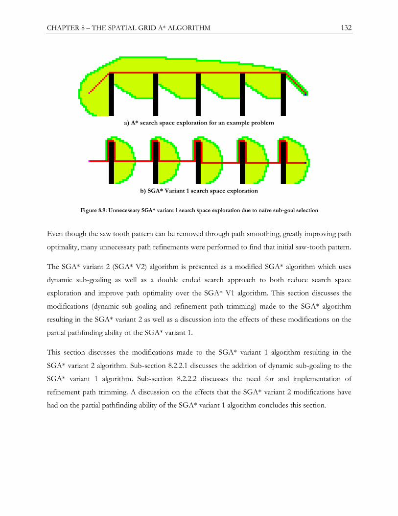
CHAPTER 8 – THE SPATIAL GRID A* ALGORITHM 132
b) SGA* Variant 1 search space exploration
a) A* search space exploration for an example problem
Figure 8.9: Unnecessary SGA* variant 1 search space exploration due to naïve sub-goal selection
Even though the saw tooth pattern can be removed through path smoothing, greatly improving path
optimality, many unnecessary path refinements were performed to find that initial saw-tooth pattern.
The SGA* variant 2 (SGA* V2) algorithm is presented as a modified SGA* algorithm which uses
dynamic sub-goaling as well as a double ended search approach to both reduce search space
exploration and improve path optimality over the SGA* V1 algorithm. This section discusses the
modifications (dynamic sub-goaling and refinement path trimming) made to the SGA* algorithm
resulting in the SGA* variant 2 as well as a discussion into the effects of these modifications on the
partial pathfinding ability of the SGA* variant 1.
This section discusses the modifications made to the SGA* variant 1 algorithm resulting in the
SGA* variant 2 algorithm. Sub-section 8.2.2.1 discusses the addition of dynamic sub-goaling to the
SGA* variant 1 algorithm. Sub-section 8.2.2.2 discusses the need for and implementation of
refinement path trimming. A discussion on the effects that the SGA* variant 2 modifications have
had on the partial pathfinding ability of the SGA* variant 1 algorithm concludes this section.

CHAPTER 8 – THE SPATIAL GRID A* ALGORITHM 133
8.2.2.1 Dynamic Sub-Goaling
Consider a modified version of the SGA* V1 algorithm, where each subsequent line segment is only
drawn as needed, i.e. at the end of each refinement step, and not in advance as presented in Section
8.2.1. Line segments are drawn from the end of the refinement path towards the goal node,
terminating once an obstacle has been encountered. The subsequent sub-goal is simply the first
traversable node found, along the same line, after the encountered obstacle. Since the refinement
path is simply appended to the currently found SGA* path, the end of the refinement path is also
the end of the final path. This simple modification introduces the concept of dynamic sub-goal
selection without modifying the operation or resultant paths of the SGA* V1 algorithm.
On its own, dynamic sub-goaling has no effect on the SGA* V1 algorithm. An observation was
made that refinement paths do not need to reach the sub-goal but can in fact be trimmed once the
refinement path goes around an obstacle. In fact, allowing refinement paths to reach each sub-goal
is what results in the saw tooth pattern exhibited in Figure 8.9. Refinement path trimming when
combined with the dynamic sub-goaling modification results in a selection of sub-goals that differ to
those of the SGA* V1 algorithm, thereby altering the operation of the algorithm.
Dynamic sub-goaling and refinement path trimming result in more direct final paths, thereby
improving path optimality as well as reducing overall search space exploration. The path and search
space exploration reduction resulting from these modifications are illustrated in Figure 8.10a. Two
refinement path trimming techniques are presented in Section 8.2.2.2.
Dynamic sub-goaling and refinement path trimming have improved the search space exploration
significantly but as illustrated Figure 8.10a, the search space exploration reduction offered over the
original SGA* algorithm decreases as the modified SGA* search approaches the goal node. This
observation led to one further modification being made to the SGA* V1 algorithm to create the
final version of the SGA* V2 algorithm: a double ended search approach.
In addition to the refinement path trimming and the dynamic sub-goaling, the SGA* search is now
performed in a double ended manner. In addition to the original forward path, now termed path start,
there now exists a second path, pathtail, which originates at the goal node and heads towards the start
node. For each step of the SGA* V2 algorithm, line segment creation (and sub-goal determination)
is performed from the end of pathstart to the end of pathtail, as well as from the end of pathtail to the
end of pathstart.

CHAPTER 8 – THE SPATIAL GRID A* ALGORITHM 134
b) SGA* Variant 2 search space exploration
a) SGA* search space exploration with dynamic sub-goaling and refinement path trimming
Figure 8.10: SGA* Variant 2 Search Space Exploration
As such for each step of the SGA* V2 algorithm two line segment generation and refinement
actions are performed. The SGA* V2 algorithm terminates immediately once pathstart and pathtail, are
connected either through line segment creation or through a refinement path. The search space
exploration for the SGA* V2 algorithm for the example problem is illustrated in Figure 8.10b.
The double-ended nature of the SGA* V2 algorithm serves to decrease search space exploration
resulting in decreased processing and memory costs, as well as improving path optimality due to the
improved sub-goals selection.
Once again, just like the SGA* V1 algorithm, SGA* V2 is both a complete and a sub-optimal
gridmap search algorithm. The completeness is based on the completeness property of the A*
algorithm. The final connection made between pathstart and pathtail (if not directly connectable via a
straight line) is made via A*. Since the start and the goal nodes are contained within and are
reachable from any node in pathstart and pathtail respectively, then A* is guaranteed to find a path
between pathstart and pathtail if one exists.

CHAPTER 8 – THE SPATIAL GRID A* ALGORITHM 135
8.2.2.2 Refinement Path Trimming
As mentioned above, refinement paths, once found, are trimmed. Two refinement path trimming
techniques are presented below:
Maximum Distance Trimming: The node within the refinement path which has the
furthest distance from the start of the path is found and is termed the maximum distance
node. All nodes from this maximum distance node until the end of the refinement path are
trimmed.
Maximum Deviation Trimming: The node within the refinement path which exhibits the
maximum deviation (in both dimensions) from the start of the path is found and is termed
the maximum deviation node. All nodes from this maximum deviation node until the end of
the refinement path are trimmed.
Figure 8.11 illustrates the difference between the trimming techniques. Figure 8.11a illustrates a path
trimmed to the furthest point on the path from the start while Figure 8.11b illustrates a path
trimmed to the point that exhibits the maximum deviation from the start of the path.
In addition to the trimming techniques presented above, an additional condition needs to be placed
upon the refinement path trimming techniques to ensure that the SGA* V2 algorithm does not
become trapped within U shaped map topologies. In Figure 8.12a, the refinement path trimming
trims the refinement path to the node at the bottom right of the U shaped region. The subsequent
line segment generation directs the path back into the region after which the refinement path
trimming results in the exact same sub-goal being selected as before and the search is once again
directed into the U shaped region.
b) Max deviation trimminga) Max distance trimming
Figure 8.11: The difference between the two refinement path trimming techniques

CHAPTER 8 – THE SPATIAL GRID A* ALGORITHM 136
The refinement path trimming will always result in the exact same sub-goal being selected causing
the SGA* V2 algorithm to remain trapped within the U shaped map region. An additional condition
is placed on the refinement path trimming in that the refinement paths may only be trimmed from a
node that is in front of the start of the refinement path in the direction of the final goal node (the
end node of pathtail or pathstart).
In Figure 8.12b, trimming paths to points in front of the start node results in the path trimming
always moving the subsequent sub-goal forward ensuring that, even though the path will enter the U
shaped region multiple times, the algorithm will eventually leave the U shaped region.
Unfortunately, having the path entering and leaving the U shaped region numerous times will
dramatically increase the overall path length as well as negatively affect the visual quality of the path.
A saving grace to this is that the SGA* V2 search is double ended. Meaning that the final sub-goal
(the end node of pathtail or pathstart) for the SGA* V2 algorithm will keep changing and may serve to
direct the search out of the U shaped region as well as the fact that the search may connect with the
opposite path, further reducing the number of entry and exits from the U shaped region.
Step 1 Step 2 Step 3 Step 4 Step 5
a) Standard refinement path trimming
b) Refinement path trimming ensuring trimming past start point in the direction of the sub-goal
Step 1 Step 2 Step 3 Step 4 Step 5
Figure 8.12: The effect of the additional condition on refinement path trimming
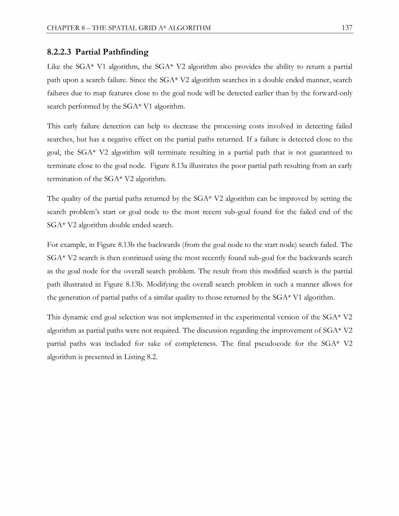
CHAPTER 8 – THE SPATIAL GRID A* ALGORITHM 137
8.2.2.3 Partial Pathfinding
Like the SGA* V1 algorithm, the SGA* V2 algorithm also provides the ability to return a partial
path upon a search failure. Since the SGA* V2 algorithm searches in a double ended manner, search
failures due to map features close to the goal node will be detected earlier than by the forward-only
search performed by the SGA* V1 algorithm.
This early failure detection can help to decrease the processing costs involved in detecting failed
searches, but has a negative effect on the partial paths returned. If a failure is detected close to the
goal, the SGA* V2 algorithm will terminate resulting in a partial path that is not guaranteed to
terminate close to the goal node. Figure 8.13a illustrates the poor partial path resulting from an early
termination of the SGA* V2 algorithm.
The quality of the partial paths returned by the SGA* V2 algorithm can be improved by setting the
search problem‘s start or goal node to the most recent sub-goal found for the failed end of the
SGA* V2 algorithm double ended search.
For example, in Figure 8.13b the backwards (from the goal node to the start node) search failed. The
SGA* V2 search is then continued using the most recently found sub-goal for the backwards search
as the goal node for the overall search problem. The result from this modified search is the partial
path illustrated in Figure 8.13b. Modifying the overall search problem in such a manner allows for
the generation of partial paths of a similar quality to those returned by the SGA* V1 algorithm.
This dynamic end goal selection was not implemented in the experimental version of the SGA* V2
algorithm as partial paths were not required. The discussion regarding the improvement of SGA* V2
partial paths was included for sake of completeness. The final pseudocode for the SGA* V2
algorithm is presented in Listing 8.2.
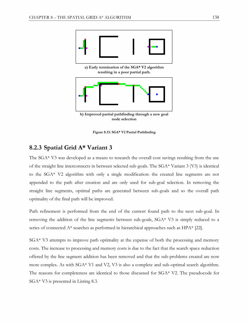
CHAPTER 8 – THE SPATIAL GRID A* ALGORITHM 138
a) Early termination of the SGA* V2 algorithm
resulting in a poor partial path.
b) Improved partial pathfinding through a new goal
node selection
Figure 8.13: SGA* V2 Partial Pathfinding
8.2.3 Spatial Grid A* Variant 3
The SGA* V3 was developed as a means to research the overall cost savings resulting from the use
of the straight line interconnects in between selected sub-goals. The SGA* Variant 3 (V3) is identical
to the SGA* V2 algorithm with only a single modification: the created line segments are not
appended to the path after creation and are only used for sub-goal selection. In removing the
straight line segments, optimal paths are generated between sub-goals and so the overall path
optimality of the final path will be improved.
Path refinement is performed from the end of the current found path to the next sub-goal. In
removing the addition of the line segments between sub-goals, SGA* V3 is simply reduced to a
series of connected A* searches as performed in hierarchical approaches such as HPA* [22].
SGA* V3 attempts to improve path optimality at the expense of both the processing and memory
costs. The increase to processing and memory costs is due to the fact that the search space reduction
offered by the line segment addition has been removed and that the sub-problems created are now
more complex. As with SGA* V1 and V2, V3 is also a complete and sub-optimal search algorithm.
The reasons for completeness are identical to those discussed for SGA* V2. The pseudocode for
SGA* V3 is presented in Listing 8.3.

CHAPTER 8 – THE SPATIAL GRID A* ALGORITHM 139
1) Set SUBGOALstart = START, SUBGOALgoal = GOAL, SUBGOALtemp = 0
2) While ( true )
2.1) Create line segment between SUBGOALstart and SUBGOALgoal, and find SUBGOALtemp
2.2) Add line segment to PATH
2.3) If ( line segment doesn’t reach SUBGOALgoal )
2.3.1) While ( A* search between SUBGOALtemp and end of line segment = FAILED )
a) If (SUBGOALtemp = SUBGOALgoal) RETURN FAILED
b) Else create line segment between SUBGOALtemp and SUBGOALgoal, and find new SUBGOALtemp
2.3.2) If ( A* path doesn’t connect PATH to PATH_TAIL)
a) If ( PATH_TAIL is directly reachable from A* path)
a)create straight line from A* path to PATH_TAIL
b)add straight line to PATH
c)GOTO 3
b) ELSE
a) Trim A* path and add trimmed A* path to PATH
b) SUBGOALStart = end of trimmed A* path
2.3.3) Else
a) Add A* path to PATH
b) GOTO 3
2.3.4) Create line segment between SUBGOALgoal and SUBGOALstart, and find SUBGOALtemp
2.3.5) Add line segment to PATH_TAIL
2.3.6) If ( line segment doesn’t reach SUBGOALstart )
a) While ( A* search between SUBGOALtemp and end of line segment = FAILED )
a) If (SUBGOALtemp = SUBGOALstart) RETURN FAILED
b) Else create line segment between SUBGOALtemp and SUBGOALstart, and find new SUBGOALtemp
c) If ( A* path doesn’t connect PATH to PATH_TAIL)
a)If ( PATH is directly reachable from A* path)
a)create straight line from A* path to PATH
b)add straight line to PATH_TAIL
c)GOTO 3
b) ELSE
a) Trim A* path and add trimmed A* path to PATH_TAIL
b) SUBGOALgoal = end of trimmed A* path
d) Else
a) Add A* path to PATH_TAIL
b) GOTO 3
2.3.7) Else GOTO 3
2.4) Else GOTO 3
3) Add PATH_TAIL to PATH
4) RETURN PATH
Listing 8.2: Pseudocode for SGA* variant 2

CHAPTER 8 – THE SPATIAL GRID A* ALGORITHM 140
1) Set SUBGOALstart = START, SUBGOALgoal = GOAL, SUBGOALtemp = 0
2) While ( true )
2.1) Create line segment between SUBGOALstart and SUBGOALgoal, and find SUBGOALtemp
2.2) If ( line segment doesn’t reach SUBGOALgoal )
2.2.1) While ( A* search between SUBGOALtemp and SUBGOALstart = FAILED )
a) If (SUBGOALtemp = SUBGOALgoal) RETURN FAILED
b) Else create line segment between SUBGOALtemp and SUBGOALgoal, and find new SUBGOALtemp
2.2.2) If ( A* path doesn’t connect PATH to PATH_TAIL)
a) If ( PATH_TAIL is directly reachable from A* path)
a)create straight line from A* path to PATH_TAIL
b)add straight line to PATH
c)GOTO 3
b) ELSE
a) Trim A* path and add trimmed A* path to PATH
b) SUBGOALStart = end of trimmed A* path
2.2.3) Else
a) Add A* path to PATH
b) GOTO 3
2.2.4) Create line segment between SUBGOALgoal and SUBGOALstart, and find SUBGOALtemp
2.2.6) If ( line segment doesn’t reach SUBGOALstart )
a) While ( A* search between SUBGOALtemp and SUBGOALgoal = FAILED )
a) If (SUBGOALtemp = SUBGOALstart) RETURN FAILED
b) Else create line segment between SUBGOALtemp and SUBGOALstart, and find new SUBGOALtemp
c) If ( A* path doesn’t connect PATH to PATH_TAIL)
a) If ( PATH directly reachable from A* path)
a)create straight line from A* path to PATH
b)add straight line to PATH_TAIL
c)GOTO 3
b) ELSE
a) Trim A* path and add trimmed A* path to PATH_TAIL
b) SUBGOALgoal = end of trimmed A* path
d) Else
a) Add A* path to PATH_TAIL
b) GOTO 3
2.2.7) Else
a) Add line segment to PATH
b) GOTO 3
2.3) Else GOTO 3
2.3.1) Add line segment to PATH
2.3.2) GOTO 3
3) Add PATH_TAIL to PATH
4) RETURN PATH
Listing 8.3: Pseudocode for SGA* variant 3
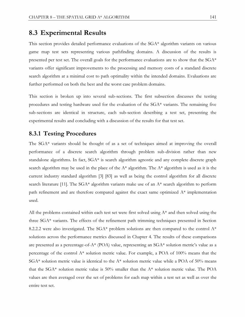
CHAPTER 8 – THE SPATIAL GRID A* ALGORITHM 141
8.3 Experimental Results
This section provides detailed performance evaluations of the SGA* algorithm variants on various
game map test sets representing various pathfinding domains. A discussion of the results is
presented per test set. The overall goals for the performance evaluations are to show that the SGA*
variants offer significant improvements to the processing and memory costs of a standard discrete
search algorithm at a minimal cost to path optimality within the intended domains. Evaluations are
further performed on both the best and the worst case problem domains.
This section is broken up into several sub-sections. The first subsection discusses the testing
procedures and testing hardware used for the evaluation of the SGA* variants. The remaining five
sub-sections are identical in structure, each sub-section describing a test set, presenting the
experimental results and concluding with a discussion of the results for that test set.
8.3.1 Testing Procedures
The SGA* variants should be thought of as a set of techniques aimed at improving the overall
performance of a discrete search algorithm through problem sub-division rather than new
standalone algorithms. In fact, SGA* is search algorithm agnostic and any complete discrete graph
search algorithm may be used in the place of the A* algorithm. The A* algorithm is used as it is the
current industry standard algorithm [3] [83] as well as being the control algorithm for all discrete
search literature [11]. The SGA* algorithm variants make use of an A* search algorithm to perform
path refinement and are therefore compared against the exact same optimized A* implementation
used.
All the problems contained within each test set were first solved using A* and then solved using the
three SGA* variants. The effects of the refinement path trimming techniques presented in Section
8.2.2.2 were also investigated. The SGA* problem solutions are then compared to the control A*
solutions across the performance metrics discussed in Chapter 4. The results of these comparisons
are presented as a percentage-of-A* (POA) value, representing an SGA* solution metric‘s value as a
percentage of the control A* solution metric value. For example, a POA of 100% means that the
SGA* solution metric value is identical to the A* solution metric value while a POA of 50% means
that the SGA* solution metric value is 50% smaller than the A* solution metric value. The POA
values are then averaged over the set of problems for each map within a test set as well as over the
entire test set.
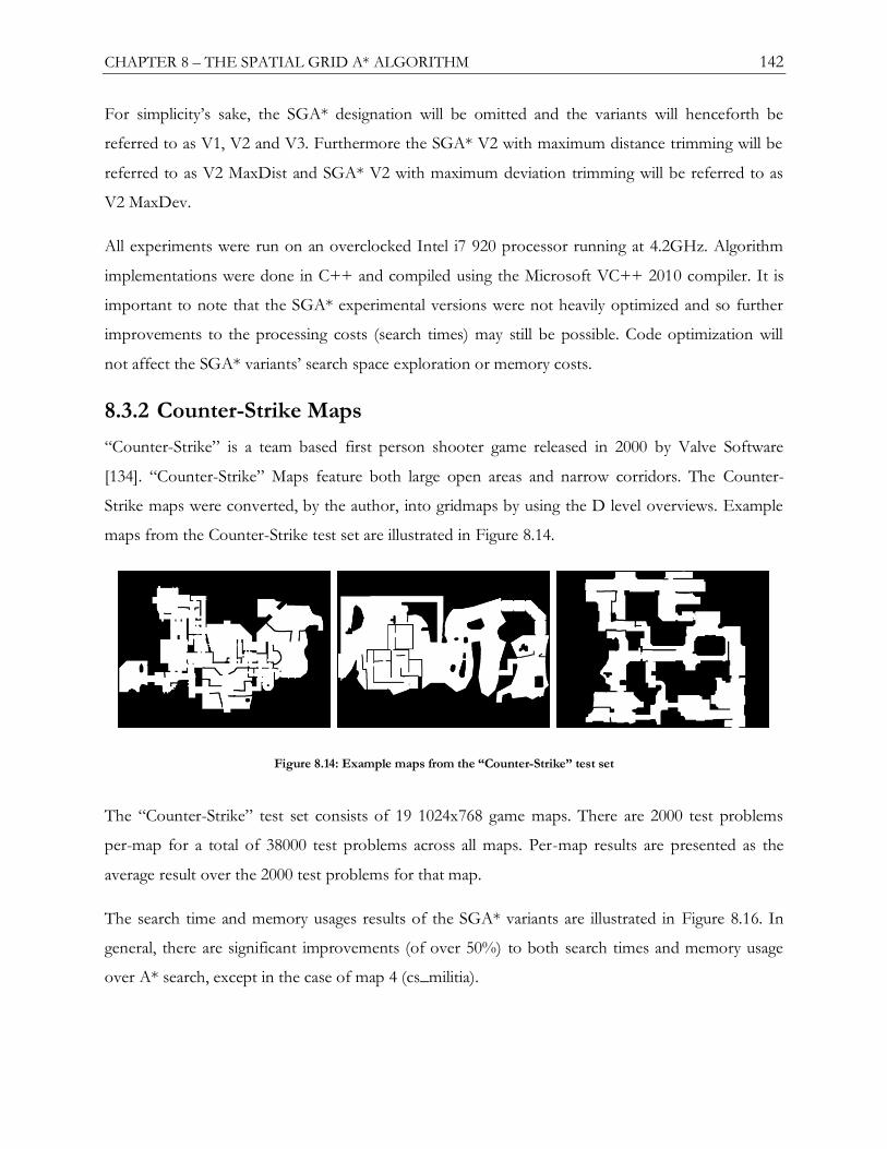
CHAPTER 8 – THE SPATIAL GRID A* ALGORITHM 142
For simplicity‘s sake, the SGA* designation will be omitted and the variants will henceforth be
referred to as V1, V2 and V3. Furthermore the SGA* V2 with maximum distance trimming will be
referred to as V2 MaxDist and SGA* V2 with maximum deviation trimming will be referred to as
V2 MaxDev.
All experiments were run on an overclocked Intel i7 920 processor running at 4.2GHz. Algorithm
implementations were done in C++ and compiled using the Microsoft VC++ 2010 compiler. It is
important to note that the SGA* experimental versions were not heavily optimized and so further
improvements to the processing costs (search times) may still be possible. Code optimization will
not affect the SGA* variants‘ search space exploration or memory costs.
8.3.2 Counter-Strike Maps
―Counter-Strike‖ is a team based first person shooter game released in 2000 by Valve Software
[134]. ―Counter-Strike‖ Maps feature both large open areas and narrow corridors. The Counter-
Strike maps were converted, by the author, into gridmaps by using the D level overviews. Example
maps from the Counter-Strike test set are illustrated in Figure 8.14.
Figure 8.14: Example maps from the “Counter-Strike” test set
The ―Counter-Strike‖ test set consists of 19 1024x768 game maps. There are 2000 test problems
per-map for a total of 38000 test problems across all maps. Per-map results are presented as the
average result over the 2000 test problems for that map.
The search time and memory usages results of the SGA* variants are illustrated in Figure 8.16. In
general, there are significant improvements (of over 50%) to both search times and memory usage
over A* search, except in the case of map 4 (cs_militia).

CHAPTER 8 – THE SPATIAL GRID A* ALGORITHM 143
The cs_militia map, illustrated in Figure 8.15, while featuring large open regions has a low level of
connectivity between the map regions. In fact, a large portion of the map (the highlighted left hand
corner) is only accessible through a single entrance. Any searches originating on the right hand sight
of that region and ending either within or to the left of it, will require that the entire region be
explored needlessly each time a path refinement action is taken. This is a worst case scenario for the
SGA* variants and results in the extremely poor performance exhibited. The V1 algorithm resulted
in search times of over 130% slower than those of A*. The V2 and V3 algorithms performed better
than the V1 but still resulted in nearly 50% slower search times.
As expected, the V2 variant performs better and uses less memory than both V1 and V3. The
presence of dynamic sub-goaling and a double-ended search in the V2 and V3 algorithm are shown
to offer improvements over V1 especially in the case of the problematic map cs_militia.
Figure 8.15: The cs_militia “Counter-Strike” Map”
The performance and memory improvements of the SGA* variants over A* result from the search
space reduction stemming from the search problem subdivision. The SGA* search space reduction
results are shown in Figure 8.17. The SGA* memory usage values shown in Figure 8.16 are based on
the peak search space exploration performed by any single refinement action. It is important to note
the correlation between the graphs in Figure 8.16 and those in Figure 8.17.

CHAPTER 8 – THE SPATIAL GRID A* ALGORITHM 144
The search space exploration data is contained within the search time and peak memory graphs. In
fact the total number of nodes encountered during the operation of the SGA* is irrelevant
considering that each path refinement action is atomic and the only valuable measure is the total
memory reduction afforded by the SGA* variants. Providing results of the total number of nodes
encountered and explored by SGA* is redundant as it is a duplication of the data already presented
through the search time and peak memory results and are therefore omitted from the remainder of
the test set performance discussions.
Path optimality measurements are shown in Figure 8.18. Unsmoothed path optimality is quite poor
for the V1 algorithm with an average sub-optimality of over 35%. The dynamic sub-goaling and
double-ended search in V2 have improved the unsmoothed path optimality by, on average, around
15% over V1. The V3 algorithm provides the highest unsmoothed path optimality but has resulted
in increased search times.
Figure 8.16: Per-map SGA* performance results for the "Counter-Strike" test set
1 2 3 4 5 6 7 8 9 10 11 12 13 14 15 16 17 18 19
V1 48.97 56.72 84.20 237.9 24.54 27.83 57.43 50.03 40.01 49.85 54.60 39.10 50.29 42.29 70.14 34.47 40.26 36.61 33.50
V2 MaxDist 48.32 53.20 76.50 143.5 24.13 25.75 57.28 44.57 37.07 48.73 49.76 38.59 49.65 35.56 67.05 33.08 38.02 33.21 33.04
V2 MaxDev 48.96 54.33 80.77 151.2 24.18 25.85 56.67 45.28 36.96 48.98 51.75 38.97 50.11 35.81 69.48 34.40 38.72 33.48 33.18
V3 61.56 58.44 83.16 136.3 30.19 31.76 56.76 42.29 40.93 49.75 52.34 41.32 50.59 36.28 71.24 35.68 45.07 37.61 39.94
0
50
100
150
200
250
PO
A
Search Time Per Map - "Counter-Strike"
Map
1 2 3 4 5 6 7 8 9 10 11 12 13 14 15 16 17 18 19
V1 53.00 57.81 69.86 113.5 31.42 33.65 57.05 51.42 45.45 50.26 54.89 43.87 48.84 43.98 70.69 38.86 41.93 42.05 37.12
V2 MaxDist 53.65 55.42 66.62 99.57 30.43 32.15 55.76 47.95 43.65 48.89 51.28 43.53 47.86 40.84 69.33 38.39 40.20 39.62 37.31
V2 MaxDev 53.62 55.51 67.21 101.2 30.58 32.08 55.70 47.89 43.30 48.71 52.14 43.46 47.78 40.81 69.19 38.90 40.34 39.67 37.27
V3 58.76 56.07 67.93 92.13 33.90 36.08 53.92 44.77 43.73 46.84 49.88 42.98 48.15 39.72 67.72 37.96 44.05 40.33 40.62
0
20
40
60
80
100
120
PO
A
Peak Memory Per Map - "Counter-Strike"
Map
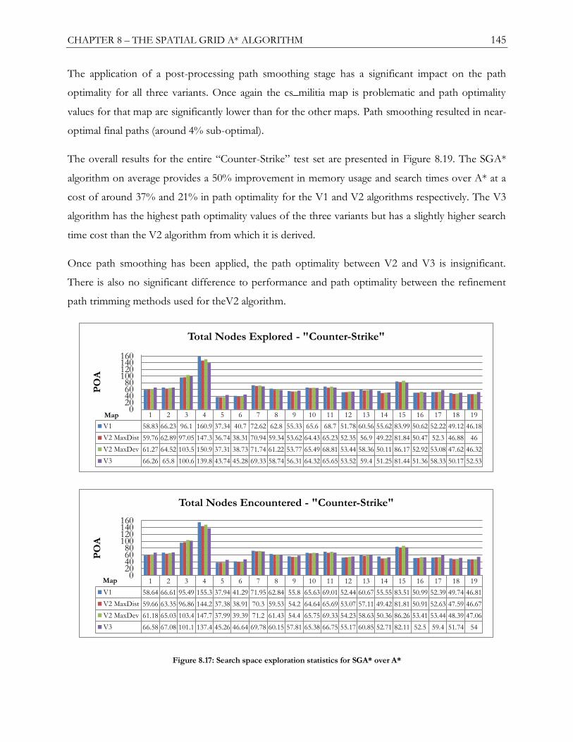
CHAPTER 8 – THE SPATIAL GRID A* ALGORITHM 145
The application of a post-processing path smoothing stage has a significant impact on the path
optimality for all three variants. Once again the cs_militia map is problematic and path optimality
values for that map are significantly lower than for the other maps. Path smoothing resulted in near-
optimal final paths (around 4% sub-optimal).
The overall results for the entire ―Counter-Strike‖ test set are presented in Figure 8.19. The SGA*
algorithm on average provides a 50% improvement in memory usage and search times over A* at a
cost of around 37% and 21% in path optimality for the V1 and V2 algorithms respectively. The V3
algorithm has the highest path optimality values of the three variants but has a slightly higher search
time cost than the V2 algorithm from which it is derived.
Once path smoothing has been applied, the path optimality between V2 and V3 is insignificant.
There is also no significant difference to performance and path optimality between the refinement
path trimming methods used for theV2 algorithm.
Figure 8.17: Search space exploration statistics for SGA* over A*
1 2 3 4 5 6 7 8 9 10 11 12 13 14 15 16 17 18 19
V1 58.83 66.23 96.1 160.9 37.34 40.7 72.62 62.8 55.33 65.6 68.7 51.78 60.56 55.62 83.99 50.62 52.22 49.12 46.18
V2 MaxDist 59.76 62.89 97.05 147.3 36.74 38.31 70.94 59.34 53.62 64.43 65.23 52.35 56.9 49.22 81.84 50.47 52.3 46.88 46
V2 MaxDev 61.27 64.52 103.5 150.9 37.31 38.73 71.74 61.22 53.77 65.49 68.81 53.44 58.36 50.11 86.17 52.92 53.08 47.62 46.32
V3 66.26 65.8 100.6 139.8 43.74 45.28 69.33 58.74 56.31 64.32 65.65 53.52 59.4 51.25 81.44 51.36 58.33 50.17 52.53
020406080
100120140160
PO
A
Total Nodes Explored - "Counter-Strike"
Map
1 2 3 4 5 6 7 8 9 10 11 12 13 14 15 16 17 18 19
V1 58.64 66.61 95.49 155.3 37.94 41.29 71.95 62.84 55.8 65.63 69.01 52.44 60.67 55.55 83.51 50.99 52.39 49.74 46.81
V2 MaxDist 59.66 63.35 96.86 144.2 37.38 38.91 70.3 59.53 54.2 64.64 65.69 53.07 57.11 49.42 81.81 50.91 52.63 47.59 46.67
V2 MaxDev 61.18 65.03 103.4 147.7 37.99 39.39 71.2 61.43 54.4 65.75 69.33 54.23 58.63 50.36 86.26 53.41 53.44 48.39 47.06
V3 66.58 67.08 101.1 137.4 45.26 46.64 69.78 60.15 57.81 65.38 66.75 55.17 60.85 52.71 82.11 52.5 59.4 51.74 54
020406080
100120140160
PO
A
Total Nodes Encountered - "Counter-Strike"
Map
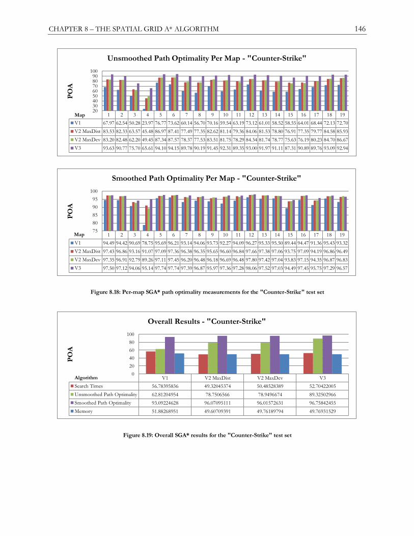
CHAPTER 8 – THE SPATIAL GRID A* ALGORITHM 146
Figure 8.18: Per-map SGA* path optimality measurements for the "Counter-Strike" test set
Figure 8.19: Overall SGA* results for the "Counter-Strike" test set
1 2 3 4 5 6 7 8 9 10 11 12 13 14 15 16 17 18 19
V1 67.97 62.54 50.28 23.97 76.77 73.62 60.14 56.70 70.16 59.54 63.19 73.12 61.01 58.52 58.55 64.01 68.44 72.13 72.70
V2 MaxDist 83.53 82.33 63.57 45.48 86.97 87.41 77.49 77.35 82.62 81.14 79.36 84.06 81.53 78.80 76.91 77.35 79.77 84.58 85.93
V2 MaxDev 83.20 82.48 62.20 49.45 87.34 87.57 78.37 77.53 83.51 81.75 78.29 84.34 81.74 78.77 75.63 76.19 80.23 84.70 86.67
V3 93.63 90.77 75.70 65.61 94.10 94.15 89.78 90.19 91.45 92.31 89.35 93.00 91.97 91.11 87.31 90.89 89.76 93.09 92.94
2030405060708090
100P
OA
Unsmoothed Path Optimality Per Map - "Counter-Strike"
Map
1 2 3 4 5 6 7 8 9 10 11 12 13 14 15 16 17 18 19
V1 94.49 94.42 90.69 78.75 95.69 96.21 93.14 94.06 93.73 92.27 94.09 96.27 95.33 95.50 89.44 94.47 91.36 95.43 93.32
V2 MaxDist 97.43 96.86 93.16 91.07 97.09 97.36 96.38 96.35 95.65 96.60 96.84 97.66 97.38 97.06 93.75 97.09 94.19 96.86 96.49
V2 MaxDev 97.35 96.91 92.79 89.26 97.11 97.45 96.20 96.48 96.18 96.69 96.48 97.80 97.42 97.04 93.83 97.15 94.35 96.87 96.83
V3 97.50 97.12 94.06 95.14 97.74 97.74 97.39 96.87 95.97 97.36 97.28 98.06 97.52 97.03 94.49 97.45 95.75 97.29 96.57
75
80
85
90
95
100
PO
A
Smoothed Path Optimality Per Map - "Counter-Strike"
Map
V1 V2 MaxDist V2 MaxDev V3
Search Times 56.78395836 49.32045374 50.48528389 52.70422005
Unsmoothed Path Optimality 62.81204954 78.7506566 78.9496674 89.32502966
Smoothed Path Optimality 93.09224628 96.07095111 96.01572631 96.75842455
Memory 51.88268951 49.60709391 49.76189794 49.76931529
0
20
40
60
80
100
PO
A
Overall Results - "Counter-Strike"
Algorithm
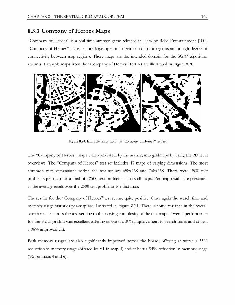
CHAPTER 8 – THE SPATIAL GRID A* ALGORITHM 147
8.3.3 Company of Heroes Maps
―Company of Heroes‖ is a real time strategy game released in 2006 by Relic Entertainment [100].
―Company of Heroes‖ maps feature large open maps with no disjoint regions and a high degree of
connectivity between map regions. These maps are the intended domain for the SGA* algorithm
variants. Example maps from the ―Company of Heroes‖ test set are illustrated in Figure 8.20.
Figure 8.20: Example maps from the “Company of Heroes” test set
The ―Company of Heroes‖ maps were converted, by the author, into gridmaps by using the 2D level
overviews. The ―Company of Heroes‖ test set includes 17 maps of varying dimensions. The most
common map dimensions within the test set are 658x768 and 768x768. There were 2500 test
problems per-map for a total of 42500 test problems across all maps. Per-map results are presented
as the average result over the 2500 test problems for that map.
The results for the ―Company of Heroes‖ test set are quite positive. Once again the search time and
memory usage statistics per-map are illustrated in Figure 8.21. There is some variance in the overall
search results across the test set due to the varying complexity of the test maps. Overall performance
for the V2 algorithm was excellent offering at worst a 39% improvement to search times and at best
a 96% improvement.
Peak memory usages are also significantly improved across the board, offering at worse a 35%
reduction in memory usage (offered by V1 in map 4) and at best a 94% reduction in memory usage
(V2 on maps 4 and 6).
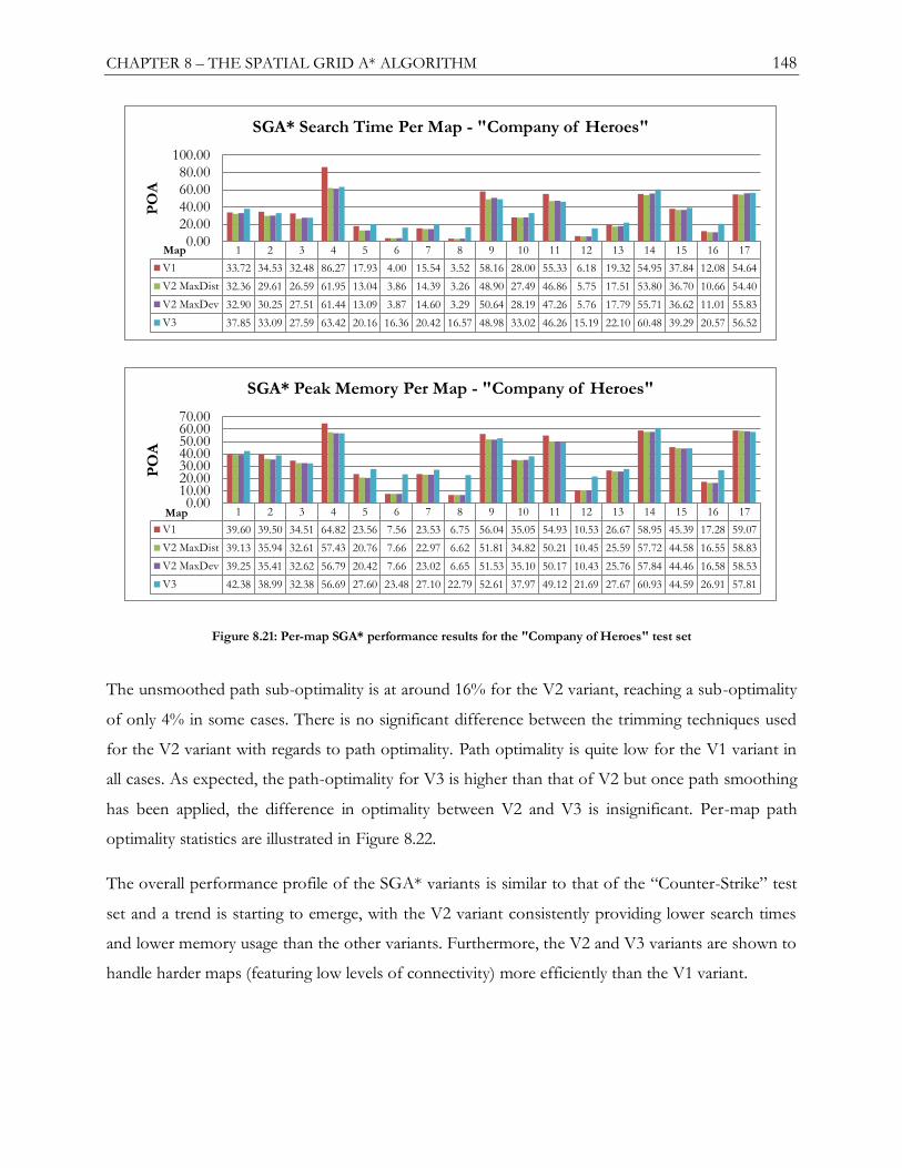
CHAPTER 8 – THE SPATIAL GRID A* ALGORITHM 148
Figure 8.21: Per-map SGA* performance results for the "Company of Heroes" test set
The unsmoothed path sub-optimality is at around 16% for the V2 variant, reaching a sub-optimality
of only 4% in some cases. There is no significant difference between the trimming techniques used
for the V2 variant with regards to path optimality. Path optimality is quite low for the V1 variant in
all cases. As expected, the path-optimality for V3 is higher than that of V2 but once path smoothing
has been applied, the difference in optimality between V2 and V3 is insignificant. Per-map path
optimality statistics are illustrated in Figure 8.22.
The overall performance profile of the SGA* variants is similar to that of the ―Counter-Strike‖ test
set and a trend is starting to emerge, with the V2 variant consistently providing lower search times
and lower memory usage than the other variants. Furthermore, the V2 and V3 variants are shown to
handle harder maps (featuring low levels of connectivity) more efficiently than the V1 variant.
1 2 3 4 5 6 7 8 9 10 11 12 13 14 15 16 17
V1 33.72 34.53 32.48 86.27 17.93 4.00 15.54 3.52 58.16 28.00 55.33 6.18 19.32 54.95 37.84 12.08 54.64
V2 MaxDist 32.36 29.61 26.59 61.95 13.04 3.86 14.39 3.26 48.90 27.49 46.86 5.75 17.51 53.80 36.70 10.66 54.40
V2 MaxDev 32.90 30.25 27.51 61.44 13.09 3.87 14.60 3.29 50.64 28.19 47.26 5.76 17.79 55.71 36.62 11.01 55.83
V3 37.85 33.09 27.59 63.42 20.16 16.36 20.42 16.57 48.98 33.02 46.26 15.19 22.10 60.48 39.29 20.57 56.52
0.00
20.00
40.00
60.00
80.00
100.00P
OA
SGA* Search Time Per Map - "Company of Heroes"
Map
1 2 3 4 5 6 7 8 9 10 11 12 13 14 15 16 17
V1 39.60 39.50 34.51 64.82 23.56 7.56 23.53 6.75 56.04 35.05 54.93 10.53 26.67 58.95 45.39 17.28 59.07
V2 MaxDist 39.13 35.94 32.61 57.43 20.76 7.66 22.97 6.62 51.81 34.82 50.21 10.45 25.59 57.72 44.58 16.55 58.83
V2 MaxDev 39.25 35.41 32.62 56.79 20.42 7.66 23.02 6.65 51.53 35.10 50.17 10.43 25.76 57.84 44.46 16.58 58.53
V3 42.38 38.99 32.38 56.69 27.60 23.48 27.10 22.79 52.61 37.97 49.12 21.69 27.67 60.93 44.59 26.91 57.81
0.0010.0020.0030.0040.0050.0060.0070.00
PO
A
SGA* Peak Memory Per Map - "Company of Heroes"
Map

CHAPTER 8 – THE SPATIAL GRID A* ALGORITHM 149
Figure 8.22: Per-map SGA* path optimality measurements for the "Company of Heroes" test set
Figure 8.23: Overall SGA* results for the "Company of Heroes" test set
1 2 3 4 5 6 7 8 9 10 11 12 13 14 15 16 17
V1 64.30 61.57 60.17 40.27 71.10 89.83 68.81 89.55 59.72 77.72 60.96 84.21 64.55 66.70 65.37 74.47 65.20
V2 MaxDist 83.87 82.40 78.43 71.71 85.79 94.00 83.24 94.25 78.76 87.28 77.59 90.76 81.33 82.37 78.77 86.79 79.10
V2 MaxDev 85.00 83.87 79.55 72.99 86.39 94.33 83.96 94.54 79.02 87.79 78.64 91.17 82.06 82.78 79.64 86.79 79.42
V3 91.19 90.16 88.73 84.11 93.22 97.59 91.33 97.45 88.12 95.01 87.45 94.88 90.13 91.12 89.68 94.03 89.58
30.0040.0050.0060.0070.0080.0090.00
100.00P
OA
Unsmoothed Path Optimality Per Map - "Company of Heroes"
Map
1 2 3 4 5 6 7 8 9 10 11 12 13 14 15 16 17
V1 90.18 93.36 90.93 84.35 94.38 98.83 93.51 98.77 90.12 96.22 92.67 96.89 93.07 90.30 91.68 95.48 91.92
V2 MaxDist 95.81 96.46 94.62 92.05 96.82 99.30 96.19 99.20 95.30 97.87 95.40 97.98 95.72 94.95 94.69 97.37 94.99
V2 MaxDev 95.91 96.64 94.79 92.40 96.84 99.34 96.33 99.23 95.19 97.93 95.59 98.05 95.84 94.93 94.72 97.35 94.89
V3 96.50 96.60 95.56 93.05 97.22 99.18 96.54 99.07 95.60 98.00 96.03 98.36 95.92 96.07 95.78 97.88 95.93
80.00
84.00
88.00
92.00
96.00
100.00
PO
A
Smoothed Path Optimality Per Map - "Company of Heroes"
Map
V1 V2 MaxDist V2 MaxDev V3
Search Times 32.61751463 28.65440104 29.16196071 33.99286403
Unsmoothed Path Optimality 68.49961415 83.32066802 83.99765038 91.39920713
Smoothed Path Optimality 93.09854505 96.16007261 96.2328381 96.66470809
Memory 35.51446893 33.74522993 33.65935131 38.27751355
0
20
40
60
80
100
PO
A
SGA* Overall Results- "Company of Heroes"
Algorithm
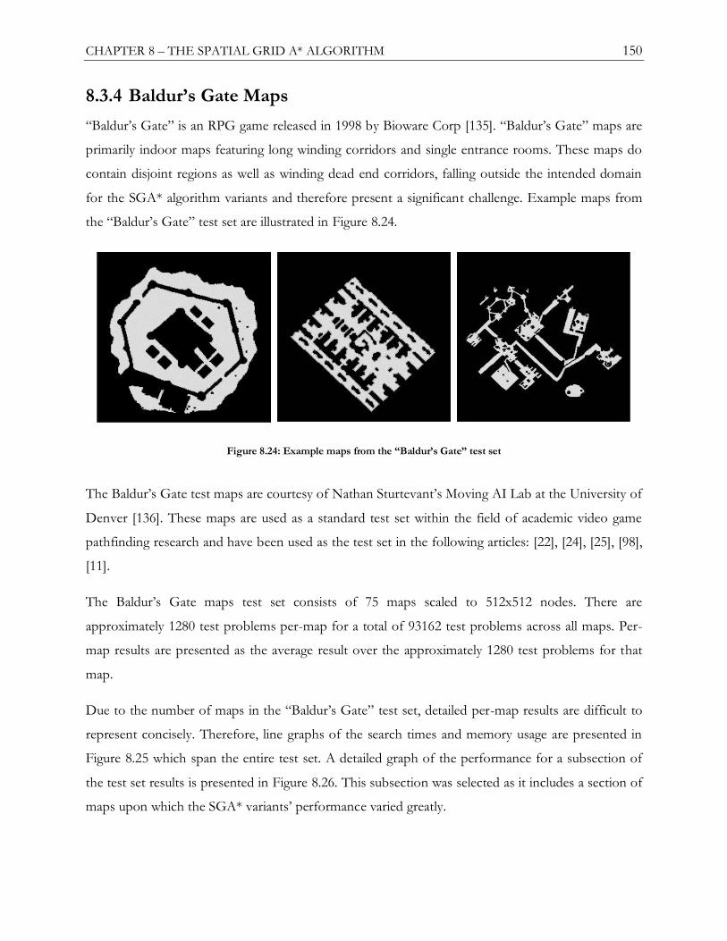
CHAPTER 8 – THE SPATIAL GRID A* ALGORITHM 150
8.3.4 Baldur‟s Gate Maps
―Baldur‘s Gate‖ is an RPG game released in 1998 by Bioware Corp [135]. ―Baldur‘s Gate‖ maps are
primarily indoor maps featuring long winding corridors and single entrance rooms. These maps do
contain disjoint regions as well as winding dead end corridors, falling outside the intended domain
for the SGA* algorithm variants and therefore present a significant challenge. Example maps from
the ―Baldur‘s Gate‖ test set are illustrated in Figure 8.24.
Figure 8.24: Example maps from the “Baldur‟s Gate” test set
The Baldur‘s Gate test maps are courtesy of Nathan Sturtevant‘s Moving AI Lab at the University of
Denver [136]. These maps are used as a standard test set within the field of academic video game
pathfinding research and have been used as the test set in the following articles: [22], [24], [25], [98],
[11].
The Baldur‘s Gate maps test set consists of 75 maps scaled to 512x512 nodes. There are
approximately 1280 test problems per-map for a total of 93162 test problems across all maps. Per-
map results are presented as the average result over the approximately 1280 test problems for that
map.
Due to the number of maps in the ―Baldur‘s Gate‖ test set, detailed per-map results are difficult to
represent concisely. Therefore, line graphs of the search times and memory usage are presented in
Figure 8.25 which span the entire test set. A detailed graph of the performance for a subsection of
the test set results is presented in Figure 8.26. This subsection was selected as it includes a section of
maps upon which the SGA* variants‘ performance varied greatly.

CHAPTER 8 – THE SPATIAL GRID A* ALGORITHM 151
The map topologies across the test set vary greatly. Figure 8.24 illustrates a large difference in map
topology across the three example maps. Furthermore, it is already established that maps with low
connectivity and disjoint regions are especially problematic for the SGA* variants.
The ―Baldur‘s Gate‖ test sets features maps with both of those features and it is these maps that
account for the large variation in SGA* performance across the test set.
On average, the SGA* variants offer significant improvements over A* for the ―Baldur‘s Gate‖ test
set except in the case of three test maps which feature high numbers of disjoint regions. On average
there is around a 55% reduction in both search times and memory usage over A*.
Figure 8.25: Per-map SGA* performance results for the "Baldur‟s Gate" test set
0.000
50.000
100.000
150.000
200.000
1 3 5 7 9 11 13 15 17 19 21 23 25 27 29 31 33 35 37 39 41 43 45 47 49 51 53 55 57 59 61 63 65 67 69 71 73 75
PO
A
Map
Search Time Per Map - "Baldur's Gate"
V1 V2 MaxDist V2 MaxDev V3
0.000
50.000
100.000
150.000
1 3 5 7 9 11 13 15 17 19 21 23 25 27 29 31 33 35 37 39 41 43 45 47 49 51 53 55 57 59 61 63 65 67 69 71 73 75
PO
A
Map
Memory Usage Per Map - "Baldur's Gate"
V1 V2 MaxDist V2 MaxDev V3
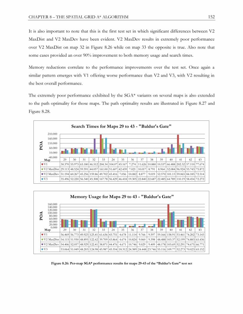
CHAPTER 8 – THE SPATIAL GRID A* ALGORITHM 152
It is also important to note that this is the first test set in which significant differences between V2
MaxDist and V2 MaxDev have been evident. V2 MaxDev results in extremely poor performance
over V2 MaxDist on map 32 in Figure 8.26 while on map 33 the opposite is true. Also note that
some cases provided an over 90% improvement to both memory usage and search times.
Memory reductions correlate to the performance improvements over the test set. Once again a
similar pattern emerges with V1 offering worse performance than V2 and V3, with V2 resulting in
the best overall performance.
The extremely poor performance exhibited by the SGA* variants on several maps is also extended
to the path optimality for those maps. The path optimality results are illustrated in Figure 8.27 and
Figure 8.28.
Figure 8.26: Per-map SGA* performance results for maps 29-43 of the “Baldur‟s Gate” test set
29 30 31 32 33 24 35 36 37 38 39 40 41 42 43
V1 30.370 55.973 65.180 46.512 204.34 104.07 45.167 7.274 11.626 10.880 10.537 66.488 202.32 57.110 77.674
V2 MaxDist 29.113 48.524 59.591 44.057 161.00 51.607 42.439 7.021 10.017 8.791 8.964 52.084 96.924 55.743 75.872
V2 MaxDev 51.194 60.267 45.256 159.86 49.702 43.416 7.056 10.082 8.877 9.019 52.570 101.13 59.065 84.185 72.514
V3 35.496 52.220 56.340 45.308 167.78 56.429 46.418 19.305 22.840 22.687 22.485 64.789 110.19 58.454 72.272
-40.000
10.000
60.000
110.000
160.000
210.000
PO
A
Search Times for Maps 29 to 43 - "Baldur's Gate"
Map
29 30 31 32 33 24 35 36 37 38 39 40 41 42 43
V1 56.469 56.773 49.923 125.41 61.636 43.751 4.678 11.114 9.766 9.597 59.166 158.91 53.461 74.202 73.143
V2 MaxDist 54.115 51.930 48.895 122.42 39.709 43.864 4.674 10.824 9.060 9.398 48.488 103.37 52.199 74.883 65.436
V2 MaxDev 54.406 52.057 48.929 122.41 38.871 44.476 4.671 10.746 9.029 9.409 48.178 103.69 52.291 74.675 66.771
V3 53.064 51.049 48.203 124.98 45.987 45.554 18.312 24.389 24.448 23.746 55.116 109.77 52.273 70.023 65.152
0.00020.00040.00060.00080.000
100.000120.000140.000160.000
PO
A
Memory Usage for Maps 29 to 43 - "Baldur's Gate"
Map

CHAPTER 8 – THE SPATIAL GRID A* ALGORITHM 153
For example, on map 40 (AR0400SR) of the test set, the average path-optimality is over 100% sub-
optimal. This map exhibits the exact same problem as the ―cs_militia‖ map in the ―Counter-Strike‖
test set, namely a large central region with a single point of entry. Furthermore, there exists several
more single entry regions within the map. The problematic test map is illustrated in Figure 8.29.
Overall path optimality follows the same trend as for the previous test sets. V1 exhibits the worst
path optimality both smoothed and unsmoothed. V3 exhibits better unsmoothed path optimality
than V2 but once smoothing has been applied, there is no significant difference between the final
path optimality of V2 and V3. In many cases the smoothed path optimality is actually optimal which
until now has not occurred. The reason for the optimality is that, due to the map topologies, there is
often only a single route between map regions and so A* and SGA* will both return the exact same
final paths.
Figure 8.27: Per-map SGA* path optimality measurements for the "Baldur‟s Gate" test set
-20.000
0.000
20.000
40.000
60.000
80.000
100.000
120.000
1 3 5 7 9 11 13 15 17 19 21 23 25 27 29 31 33 35 37 39 41 43 45 47 49 51 53 55 57 59 61 63 65 67 69 71 73 75
PO
A
Map
Unsmoothed Path Optimality Per Map - "Baldur's Gate"
V1 V2 MaxDist V2 MaxDev V3
40.000
50.000
60.000
70.000
80.000
90.000
100.000
110.000
1 3 5 7 9 11 13 15 17 19 21 23 25 27 29 31 33 35 37 39 41 43 45 47 49 51 53 55 57 59 61 63 65 67 69 71 73 75
PO
A
Map
Smoothed Path Optimality Per Map - "Baldur's Gate"
V1 V2 MaxDist V2 MaxDev V3

CHAPTER 8 – THE SPATIAL GRID A* ALGORITHM 154
Figure 8.28: Per-map SGA* path optimality measurements for maps 29 to 43 of the "Baldur‟s Gate" test set
Figure 8.29: Map AR0400SR from the "Baldur's Gate" test set
29 30 31 32 33 24 35 36 37 38 39 40 41 42 43
V1 62.930 59.800 67.572 24.114 60.892 63.883 98.037 91.905 91.889 92.462 77.327 -2.654 74.980 54.570 42.348
V2 MaxDist 86.127 86.476 85.779 64.892 84.457 84.024 98.568 95.448 95.610 96.242 90.408 61.901 89.815 78.150 74.824
V2 MaxDev 86.134 86.887 86.357 71.034 85.140 84.241 98.752 95.953 96.083 96.307 91.532 67.385 90.237 76.576 74.838
V3 95.048 93.859 95.797 71.006 90.176 91.224 99.371 97.965 97.988 98.464 93.619 66.592 95.719 91.031 82.254
-20.000
0.000
20.000
40.000
60.000
80.000
100.000P
OA
Unsmoothed Path Optimality for Maps 29 to 43 - "Baldur's Gate"
Map
29 30 31 32 33 24 35 36 37 38 39 40 41 42 43
V1 92.059 98.143 95.919 64.389 89.186 95.799 99.969 99.634 99.523 99.802 97.021 48.569 98.337 94.632 88.421
V2 MaxDist 98.415 99.122 99.049 85.167 94.880 97.950 99.971 99.728 99.712 99.852 98.744 83.956 99.162 98.280 95.126
V2 MaxDev 98.250 99.242 99.043 88.792 94.850 97.904 99.971 99.795 99.723 99.872 98.777 85.369 99.131 97.740 95.251
V3 99.357 99.249 99.246 86.596 95.377 98.362 99.976 99.749 99.757 99.910 98.696 83.234 99.452 98.739 95.708
40.000
50.000
60.000
70.000
80.000
90.000
100.000
PO
A
Smoothed Path Optimality for Maps 29 to 43 - "Baldur's Gate"
Map

CHAPTER 8 – THE SPATIAL GRID A* ALGORITHM 155
The overall results for the ―Baldur‘s Gate‖ test set are quite promising but are misleading without
the per-map evaluations presented above. SGA* does not offer improvement across the entire test
set as the overall averages would suggest. The poor performance of the SGA* on several of the test
maps is welcome as it further strengthens the ability to accurately state the domain restrictions for
the SGA* variants. Even though the SGA* variants are not suitable for the entire test set, there are
quite significant overall improvements across the test set.
Figure 8.30: Overall SGA* results for the "Baldur‟s Gate" test set
8.3.5 Starcraft Maps
―Starcraft‖ is currently the most popular real time strategy game in the world and was released in
1998 by Blizzard Entertainment [137]. ―Starcraft‖ maps are highly symmetrical, with most maps
featuring a large open central area surrounded by single entrance ―base‖ areas. Example maps from
the Starcraft test set are illustrated in Figure 8.31.
The ―Starcraft‖ test maps also include a massive number of disjoint regions within the maps. As
such, the ―Starcraft‖ maps are an excellent test set for highlighting the additional processing costs of
sub-goal selection within these disjoint regions (refer to 8.2.1.1). The ―Starcraft‖ test set represents
the absolute worst case scenario for the SGA* variants. The performance of the SGA* variants is
therefore expected to be extremely poor across this test set.
The ―Starcraft‖ maps are once again courtesy of Nathan Sturtevant and are included as part of the
hierarchical open graph 2 (HOG2) project [138].
V1 V2 MaxDist V2 MaxDev V3
Search Times 46.31697269 38.40138867 39.34322524 45.51605038
Unsmoothed Path Optimality 76.31991833 88.9124324 89.53626907 94.00485091
Smoothed Path Optimality 95.60338171 98.11527723 98.25161824 98.35808452
Memory 40.77186441 37.62681519 37.66413995 42.55684235
0
20
40
60
80
100
PO
A
Overall Results - "Baldur's Gate"
Algorithm

CHAPTER 8 – THE SPATIAL GRID A* ALGORITHM 156
The ―Starcraft‖ test set contains 125 maps of varying dimensions. The most common map
dimensions are 512x512 and 768x768. There are 1280 test problems per-map for a total of 160000
test problems across all maps. Per-map results are presented as the average result over the
approximately 1280 test problems for that map.
Figure 8.14
Figure 8.31: Example maps from the “Starcraft” test set
The per-map performance and path optimality results are illustrated in Figure 8.32 and Figure 8.33
respectively. As expected, SGA* performance on the ―Starcraft‖ test set is extremely poor with over
2000% increases to A* search times in certain cases. Memory usage is also negatively affected
although not to the same degree as the search times. What is interesting is that in some of the maps,
SGA* does in fact provide improvements to both search times and memory usage, these
improvements occur on maps that do not feature disjoint regions and have a high degree of
connectivity between map regions.
―Starcraft‖ does not feature dynamic environments and preprocessing the grid map is possible to
allow for the SGA* region labeling optimization from Section 8.2.1.2 to be employed. This
optimization is primarily useful for static environments as any environmental changes may require
region relabeling and so incur additional costs. The region labeling optimization has not been
employed and has been left for future work.
The overall performance results are illustrated in Figure 8.34 and serve to illustrate the unsuitability
of the SGA* variants within such environments.

CHAPTER 8 – THE SPATIAL GRID A* ALGORITHM 157
Figure 8.32: Per-map SGA* performance measurements for the "Starcraft" test set
0100200300400500600700800900
100011001200130014001500160017001800190020002100220023002400250026002700280029003000
1 4 7
10
13
16
19
22
25
28
31
34
37
40
43
46
49
52
55
58
61
64
67
70
73
76
79
82
85
88
91
94
97
100
103
106
109
112
115
118
121
124
PO
A
Map
Search Time Per Map - "Starcraft"
V1 V2 MaxDist V2 MaxDev V3
0100200300400500600700800900
1 4 7
10
13
16
19
22
25
28
31
34
37
40
43
46
49
52
55
58
61
64
67
70
73
76
79
82
85
88
91
94
97
100
103
106
109
112
115
118
121
124
PO
A
Map
Memory Usage Per Map - "Starcraft"
V1 V2 MaxDist V2 MaxDev V3

CHAPTER 8 – THE SPATIAL GRID A* ALGORITHM 158
Figure 8.33: Per-map SGA* path optimality measurements for the "Starcraft" test set
Figure 8.34: Overall SGA* results for the "Starcraft" test set
-150.0
-100.0
-50.0
0.0
50.0
100.0
1 3 5 7 911
13
15
17
19
21
23
25
27
29
31
33
35
37
39
41
43
45
47
49
51
53
55
57
59
61
63
65
67
69
71
73
75
77
79
81
83
85
87
89
91
93
95
97
99
101
103
105
107
109
111
113
115
117
119
121
123
PO
A
Map
Unsmoothed Path Optimality - "Starcraft"
V1 V2 MaxDist V2 MaxDev V3
35.0
45.0
55.0
65.0
75.0
85.0
95.0
105.0
1 3 5 7 911
13
15
17
19
21
23
25
27
29
31
33
35
37
39
41
43
45
47
49
51
53
55
57
59
61
63
65
67
69
71
73
75
77
79
81
83
85
87
89
91
93
95
97
99
101
103
105
107
109
111
113
115
117
119
121
123
PO
A
Map
Unsmoothed Path Optimality - "Starcraft"
V1 V2 MaxDist V2 MaxDev V3
V1 V2 MaxDist V2 MaxDev V3
Search Times 235.8156553 226.9208951 232.395117 227.1394814
Unsmoothed Path Optimality 57.01212218 78.02505095 78.57589416 88.03281314
Smoothed Path Optimality 93.41628507 96.60155727 96.74093898 97.1951301
Memory 95.74639923 91.33244077 91.17046215 91.40208318
0
50
100
150
200
250
PO
A
Overall Results - "Starcraft"
Algorithm

CHAPTER 8 – THE SPATIAL GRID A* ALGORITHM 159
8.3.6 Pseudo Real Time Strategy Maps
In addition to the standard game map test sets, a further test set was used featuring highly connected
maps with an extremely high obstacle density. These maps represent a test set similar to the one
presented in the ―Company of Heroes‖ maps except with a much lower degree of difficulty due to
the high level of connectivity and small obstacle size. These maps represent the absolute best case
scenario for the SGA* algorithm variants and the results were included to show off the potential
benefits of the SGA* variants within the intended domains. Example maps from the ―Pseudo RTS‖
test set are illustrated in Figure 8.35.
Figure 8.35: Example maps from the pseudo RTS test set
The pseudo RTS maps were generated by the author using a pseudo-random map generator. The
test set includes 50 maps with dimension 512x512. There are 1280 test problems per-map for a total
of 64 000 test problems across all maps. Per-map results are presented as the average result over the
1280 test problems for that map.
The SGA* variants provide huge improvements (over 90%) to both the search time as well the
memory usage of A* within the intended problem domain. This test set further highlights the
improvements to both search time and path optimality of the V2 variant over the V1 variant. The
per-map performance and path optimality results are illustrated in Figure 8.36 and Figure 8.37
respectively. Furthermore, within these environments there is a clear effect on the unsmoothed path
optimality of the V2 variant resulting from the choice of path refinement trimming technique. The
maximum deviation trimming technique results in higher optimality paths with no detrimental effect
on the search times.
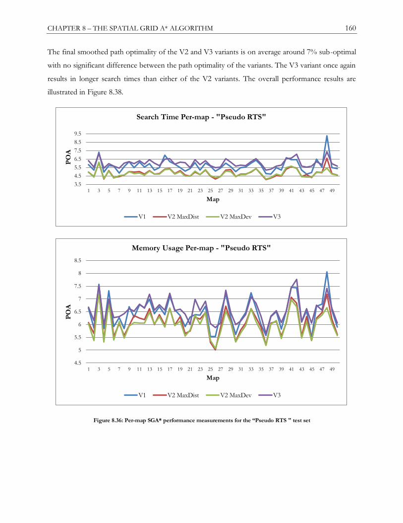
CHAPTER 8 – THE SPATIAL GRID A* ALGORITHM 160
The final smoothed path optimality of the V2 and V3 variants is on average around 7% sub-optimal
with no significant difference between the path optimality of the variants. The V3 variant once again
results in longer search times than either of the V2 variants. The overall performance results are
illustrated in Figure 8.38.
Figure 8.36: Per-map SGA* performance measurements for the “Pseudo RTS " test set
3.5
4.5
5.5
6.5
7.5
8.5
9.5
1 3 5 7 9 11 13 15 17 19 21 23 25 27 29 31 33 35 37 39 41 43 45 47 49
PO
A
Map
Search Time Per-map - "Pseudo RTS"
V1 V2 MaxDist V2 MaxDev V3
4.5
5
5.5
6
6.5
7
7.5
8
8.5
1 3 5 7 9 11 13 15 17 19 21 23 25 27 29 31 33 35 37 39 41 43 45 47 49
PO
A
Map
Memory Usage Per-map - "Pseudo RTS"
V1 V2 MaxDist V2 MaxDev V3

CHAPTER 8 – THE SPATIAL GRID A* ALGORITHM 161
Figure 8.37: Per-map SGA* path optimality measurements for the "Pseudo RTS" test set
Figure 8.38: Overall SGA* results for the "Pseudo RTS" test set
60
65
70
75
80
85
90
1 3 5 7 9 11 13 15 17 19 21 23 25 27 29 31 33 35 37 39 41 43 45 47 49
PO
A
Map
Unsmoothed Path Optimality Per-map - "Pseudo RTS"
V1 V2 MaxDist V2 MaxDev V3
88
90
92
94
96
1 3 5 7 9 11 13 15 17 19 21 23 25 27 29 31 33 35 37 39 41 43 45 47 49
PO
A
Map
Smoothed Path Optimality Per-map - "Pseudo RTS"
V1 V2 MaxDist V2 MaxDev V3
V1 V2 MaxDist V2 MaxDev V3
Search Times 5.728136767 4.850134525 4.811058511 6.017439712
Smoothed Path Optimality 67.37128006 80.81109413 82.91241611 87.03551589
Unsmoothed Path Optimality 90.5721354 93.80655064 94.23238392 94.50701701
Memory 6.455666766 6.08758554 6.007058753 6.56738982
0.0
20.0
40.0
60.0
80.0
100.0
PO
A
Overall Results - "Pseudo RTS"
Algorithm
CHAPTER 8 – THE SPATIAL GRID A* ALGORITHM 162
8.4 Summary and Conclusion
This chapter presented the SGA* algorithm as a complete, domain specific, sub-optimal gridmap
search technique for improving the performance of an A* search algorithm. The SGA* is based on a
problem sub-division approach commonly found in hierarchical search algorithms. The SGA*
algorithm makes use of the game map‘s spatial data to perform sub-goal selection rather than using a
navgraph abstraction hierarchy. The SGA* algorithm was developed as a means of decreasing the
processing and memory costs of the A* algorithm at the expense of path optimality.
SGA* is intended for use in extremely memory limited environments in which the memory cost of
maintaining an abstraction hierarchy may be too expensive. Abstraction graphs can be significantly
more expensive to maintain than gridmaps since the lack of uniformity in the graph require edge
data to be stored for each node.
Unlike hierarchical approaches when used within a dynamic environment, there is no need for any
special considerations with regards to environmental changes apart from directly updating the
gridmap. Furthermore SGA* offers the ability to return partial paths from failed searches, something
which the A* algorithm cannot achieve.
As mentioned, the SGA* variants are domain specific and the intended domain requires that the
environment contain the following features:
Large open regions with high levels of connectivity between the various regions.
No disjoint regions within the map environment.
Three SGA* variants were presented:
Variant 1: Variant 1 is the basic forward-only version of the SGA* algorithm. Sub-goals are
selected in advance after which path refinement occurs.
Variant 2: Variant 2 is a double ended version of the SGA* which makes use of dynamic
sub-goal selection. Sub-goal refinement paths are now trimmed to create the required sub-
goals. Two path refinement trimming techniques were presented in Section 8.2.2.2:
maximum distance trimming and maximum deviation trimming.

CHAPTER 8 – THE SPATIAL GRID A* ALGORITHM 163
Variant 3: Variant 3 is a modification of variant 2 in that the created line segments are not
added to the final path. A* path refinement occurs from sub-goal to sub-goal and not from
the end of a line-segment to a sub-goal.
The SGA* variants were evaluated on four distinct real world game map test sets as well as on a best
case test set. On the test sets which meet the domain specific criteria of the SGA* algorithm
significant improvements to the standard A* algorithm were achieved.
Certain trends were observed across all the test sets. The V2 variant performed significantly better
with respect to search times, memory costs and path optimality than the V1 variant. The V3 variant,
while improving upon the unsmoothed path optimality, did not have any significant effect on the
path optimality of the final smoothed paths and results in longer search times than the V2 variants.
The choice of the path refinement trimming technique used by the V2 variant seems to be largely
inconsequential with only one test set showing any significant difference between trimming
techniques. Even in that single test set, the difference between trimming techniques was only to the
unsmoothed path optimality which, once path smoothing was applied, was nullified.
In light of the results of the simulations, there are no benefits to the V1 or V3 variants over that of
the V2 variant. It is therefore the recommendation of the author that the term SGA* algorithm be
taken to imply the V2 variant.
In conclusion, the SGA* algorithm has been shown to improve the search times and memory usage
by up to 90% within domain specific environments at the cost of around 6% path optimality.

CHAPTER 8 – THE SPATIAL GRID A* ALGORITHM 164

165
Chapter 9 Conclusions and Future Work
This short chapter summarizes the findings of this work. In addition, future work resulting from
these findings is suggested.
9.1 Conclusions
The aim of this thesis was to provide a complete and detailed review of the video game pathfinding
field, with a focus on the pathfinding search algorithms employed in said field. Video game AI was
overviewed, highlighting the difference between video game AI and academic AI. A brief
introduction to video game engines was given to investigate the requirements and constraints placed
upon the video game AI system.
During the discussing of the game agent model, it was shown that the majority of higher level agent
behaviors rely on the ability of an agent to successfully navigate the game environment making
pathfinding an integral component of any video game AI system.
Due to the high complexity of modern video game environments, to be able to find a route through
a game environment, that game environment must be represented in a lightweight simple graph
format. Since game environments are reduced to graphs, the pathfinding search problem is
subsequently reduced to a graph search problem.
There are three methods of graph abstraction used to represent a complex 3D environment into a
graph format: waypoint graphs, navmesh graphs and grid-based graph. The choice of graph
abstraction is dependent on the size and complexity of the environments present within a game.
The requirements and constraints of the pathfinding search problem were investigated and a set of
metrics for the comparison of search algorithms was presented. There are three primary metrics
used for comparing graph search algorithms: performance, memory cost and solution optimality. It
was revealed that improving algorithm performance, a reduction in solution optimality was
acceptable. Furthermore, it was shown that the pathfinding search problem is highly domain

CHAPTER 9 – CONCLUSIONS 166
specific. The domain boundaries are defined by the game‘s performance and memory constraints as
well as the type and complexity of the in-game environments. The problem domain is responsible
for both the choice of navgraph abstraction technique and choice of graph search algorithm
employed.
The three main families of graph search algorithms (discrete, continuous, and hierarchical) employed
today were reviewed next. There is a significant difference between discrete and continuous search
algorithms while hierarchical search algorithms can be seen as an extension of the discrete search
family. Discrete search algorithms return a path between two nodes in a graph through a single
atomic action. Discrete search algorithms are problem centric, meaning that performance and
memory costs are paid per problem and are released upon solving that problem.
On the other hand, continuous search algorithms are agent centric in that a path is found and
updated over the course of an agent‘s movement from the start location to the goal location. The
agent centric nature of the continuous algorithm means that the memory allocated to solve a
problem is now allocated per agent for the duration of the agent‘s move. In multi-agent
environments, the total memory cost of a continuous search algorithm‘s per-agent memory
allocation model can easily exceed the total memory available to the game.
Hierarchical search algorithms were investigated and shown to be a technique allowing for the
subdivision of a complex pathfinding problem into a series of simpler problems. The problem
subdivision was achieved through the use of a navgraph abstraction hierarchy with each higher
abstraction level offering a significant reduction in the total search space over the lower level.
Hierarchical search algorithms are applicable for use within dynamic game environments, but require
that the abstraction hierarchy be updated once an environmental change occurs. This abstraction
hierarchy update can be a potentially expensive operation and may restrict the use of hierarchical
algorithms within dynamic environments.
During the investigation of hierarchical search algorithms the observation was made that pathfinding
problem subdivision may be achieved on grid maps by using the spatial data contained within them
instead of using an abstraction hierarchy. This observation led to the development of the SGA*
algorithm, a technique for the improvement of A* search times through problem subdivision using a
straight line spatial rule.

CHAPTER 9 – CONCLUSIONS 167
The SGA* algorithm is highly domain specific, being tailored to game environments which contain
highly interconnected regions and do not contain disjoint regions. The SGA* algorithm was
evaluated on five distinct sets of game environments and was shown to improve upon the search
times and memory costs of the industry standard A* search algorithm by over 94% at only a 6% cost
to path optimality within the intended search domain.
9.2 Future Research
Research that may follow from this work includes:
SGA* Region Labeling for the SGA* Anti-domain
Although the SGA* algorithm performed admirably within the intended domains, the SGA*
algorithm‘s performance was extremely poor within the ―Starcraft‖ test set. The ―Starcraft‖ test set
features a high number of disjoint regions as well as an extremely low connectivity between regions.
In fact, the ―Starcraft‖ test set can be seen as representing the anti-domain for the SGA* algorithm.
A potential optimization (the region labeling optimization – refer to Section 8.2.1.1) was presented
as a means of improving SGA* performance within maps that feature disjoint regions. This region
labeling optimization should have no effect on the SGA* performance within maps that feature low
connectivity between regions and so was not implemented. It is hoped that the addition of this
region labeling will significantly improve the performance of the SGA* algorithm on anti-domain
environments.
Alternate Spatial Sub-division Criteria
The SGA* algorithm makes use of a straight line drawing technique to allow for sub-goal selection
during problem sub-division. The straight line drawing technique is naïve and is responsible for
various anomalies in the resulting unsmoothed SGA* paths (refer to Chapter 8). Future work may
investigate the use of other subdivision techniques and the effects thereof on the SGA* algorithm.

168

169
Bibliography
[1] Millington, Ian and Funge, John., "Dijsktra." Artificial Intelligence for Games. 2nd. Burlington, MA :
Morgan Kaufman, 2009, 4.2, pp. 204-214.
[2] Russel, Stuart and Norvig, Peter., "Artificial Intelligence: A Modern Approach." [book auth.]
Peter Norvig Stuart Russel. Artificial Intelligence: A Modern Approach. s.l. : Prentice Hall, 2002, 3.3, pp.
59-94.
[3] Millington, Ian and Funge, John., Artificial Intelligence for Games. 2nd. s.l. : Morgan Kaufmann,
2009.
[4] Mesdaghi, Syrus., "Artificial Intelligence: Pathfinding Overview." [ed.] Steve Rabin. Introduction to
Game Development. s.l. : Charles River Media, 2010, 5.4, pp. 559-576.
[5] Buckland, Matt., Programming Game AI by Example. s.l. : Jones & Bartlett Publishers, 2004.
[6] Dijkstra, E. W., "A note on two problems in connexion with graphs." Numerische Mathematik,
Amsterdam : Mathematisch Centrum, 1959, Vol. 1, pp. 269-271.
[7] Hart, P.E, Nilsson, N.J and Raphael, B., "A Formal Basis for the Heuristic Determination of
Minimum Cost Paths." IEEE Transactions on Systems Science and Cybernetics SSC4, 1968, Issue 2,
Vol. 4, pp. 100-107.
[8] Korf, Richard., "Depth-first Iterative-Deepening: An Optimal Admissible Tree Search." Artificial
Intelligence Journal (AIJ), s.l. : Elsevier, 1985, pp. 97-109.
[9] Reinfeld, Alexander and Marsland, T. Anthony., "Enhanced Iterative-Deepening Search."
Transaction on Pattern Analysis and Machine Intelligence, July 1994, Issue 7, Vol. 16, pp. 701-710.
[10] Russel, Stuart., "Efficient Memory-bounded Search Methods." Vienna, Austria : s.n., 1992.
European Conference on Artificial Intelligence (ECAI).
[11] Bjornsson, Yngvi, et al., "Fringe Search: Beating A* at Pathfinding on Game Maps." Colchester,
Essex : IEEE, 2005. IEEE Symposium on Computational Intelligence in Games. pp. 125-132.

BIBLIOGRAPHY 170
[12] Stentz, Anthony., "Optimal and efficient path planning for partially-known environments." San
Diego, CA, USA : IEEE, 1994. Proceedings of IEEE International Conference on Robotics and
Automation . Vol. 4, pp. 3310-3317.
[13] Stentz, Anthony., "The Focussed D* Algorithm for Real-Time Replanning." 1995. In
Proceedings of the International Joint Conference on Artificial Intelligence.
[14] Koenig, Sven, Likhachev, Maxim and Furcy, David., "Lifelong Planning A*." Artificial
Intelligence, s.l. : Elsevier, 2004, Vol. 155, pp. 93-146.
[15] Koenig, S and Likhachev, M., "D* Lite." s.l. : Association for the Advancement of Artificial
Intelligence, 2002. Proceedings of the AAAI Conference of Artificial Intelligence (AAAI). pp. 476-
483.
[16] Koenig, S. and Likhachev, M., "Adaptive A*." s.l. : ACM, 2005. Proceedings of the fourth
international joint conference on Autonomous agents and multiagent systems. pp. 1311-1312.
[17] Sun, X., Koenig, S. and Yeoh, W., "Generalized Adaptive A*." s.l. : International Foundation
for Autonomous Agents and Multiagent Systems, 2008. Proceedings of the 7th international joint
conference on Autonomous agents and multiagent systems. pp. 469-476.
[18] Likhachev, M, Gordon, G and Thrun, S., "ARA*: Anytime A* with Provable Bounds on Sub-
Optimality." Advances in Neural Information Processing Systems, 2003, Vol. 16.
[19] Likhachev, M., et al., "Anytime dynamic A*: An anytime, replanning algorithm." 2005.
Proceedings of the International Conference on Automated Planning and Scheduling (ICAPS. pp.
262-271.
[20] Korf, R., "Real-Time Heuristic Search." Artificial Intelligence, s.l. : Elsevier, 1990, Vol. 42, pp.
189-211.
[21] Bond, D, et al., "Real-Time Search in Dynamic Worlds." Atlanta, GA, USA : Association of the
Advancement of Artificial Intelligence, 2010. The Third Annual Symposium on Combinatorial
Search.
[22] Botea, Adi, Muller, Martin and Schaeffer, Jonathan., "Near Optimal Hierarchical Path-Finding."
Journal of Game Developers, 2004, Vol. 1, pp. 7-28.

BIBLIOGRAPHY 171
[23] Kring, Alex, Champandard, Alex J. and Samarin, Nick., "DHPA* and SHPA*: Efficient
Hierarchical Pathfinding in Dynamic and Static Game Worlds." Stanford, CA : Association for the
Advancement of Artificial Intelligence (AAAI), 2010. Proceedings of the 6th Conference on
Artificial Intelligence and Interactive Digital Entertainment (AIIDE).
[24] Sturtevant, Nathan and Buro, Michael., "Partial Pathfinding Using Map Abstraction and
Refinement." 2005. Proceedings of the National Conference on Artificial Intelligence (AAAI). pp.
1392-1397.
[25] Sturtevant, Nathan., "Memory-Efficient Abstractions for Pathfinding." Stanford,CA :
Association for the Advancement of Artificial Intelligence, 2007. Proceedings of the Third Artificial
Intelligence for Interactive Digital Entertainment Conference (AIIDE). pp. 31-36.
[26] PC Gaming Alliance., "PCGA Horizons 2009 Software Report." [Online] March 21, 2010.
[Cited: September 21, 2010.] www.pcgamingalliance.org/imwp/download.asp?ContentID=17516.
[27] Helft, Miguel., "Will Zynga Become the Google of Games?" The New York Times. [Online] July
24, 2010. [Cited: January 24, 2011.]
http://www.nytimes.com/2010/07/25/business/25zynga.html?_r=1.
[28] Bakie, Robert T., "Games and Society." [ed.] Steve Rabin. Introduction to Game Development. 2nd.
Boston, MA : Charles River Media, 2010, 1.2, pp. 43-58.
[29] Graetz, J. Martin., "The origin of spacewar." Creative Computing. August 1981.
[30] Bakie, Robert T., "A Brief History of Video Games." [ed.] Steve Rabin. Introduction to Game
Development. 2nd. Boston, MA, USA : Course Technology, Cengage Learning, 2010, 1.1, pp. 3-42.
[31] Kent, Steven., The Ultimate History of Video Games: From Pong to Pokemon - The Story Behind the
Craze That Touched Our Lives and Changed the World . s.l. : Three Rivers Press, 2001.
[32] Donovan, Tristan., Replay: The History of Video Games. s.l. : Yellow Ant Media Ltd, 2010.
[33] Preiz, Eric and Garney, Ben., Video Game Optimization. s.l. : Course Technology PTR, 2010.
[34] Ryan, Mark, Hill, Doug and McGrath, Dennis., "Simulation Interoperability with a Commercial
Game Engine." European Simulation Interoperability Workshop, 2005.
BIBLIOGRAPHY 172
[35] Antonio, Carlos A.M., Jorge, Carlos A.F. and Couto, Pedro M., "Using a Game Engine for VR
Simulations in Evacuation Planning." IEEE Computer Graphics and Applications, May/June 2008,
Issue 3, Vol. 28, pp. 6-12.
[36] Laird, John E. and Michael, van Lent., "Human-Level AI‘s Killer Application: Interactive
Computer Games." AI Magazine. 2001, Vol. 22, 2.
[37] Schwab, Brian., AI Game Engine Programming. s.l. : Charles River Media, 2004.
[38] Mateas, Michael., "Expressive AI: Games and Artificial Intelligence." Utrecht : s.n., 2003.
Proceedings of Level Up: Digital Games Research Conference.
[39] Neller, Todd, et al., "Model AI Assignments." Atlanta : Association for the Advancement of
Artificial Intelligence, 2010. EAAI-2010: The First Symposium on Educational Advances in
Artificial Intelligence.
[40] Coppin, Ben., Artificial Intelligence Illuminated. 1st. Sudbury, MA : Jones and Bartlett, 2004.
[41] Williams, Russell B. and Clippinger, Caryl A., "Aggression, competition and computer games:
computer and human opponents." Computers in Human Behavior. 2002, Vol. 18, 5, pp. 495-506.
[42] Colwell, John., "Needs met through computer game play among adolescents." Personality and
Individual Differences. December 2007, Vol. 43, 8, pp. 2072-2082.
[43] Pagulayan, R. J., et al., "User-centered design in Games." [book auth.] J Jacko and A Sears.
Handbook for Human-Computer Interaction in Interactive Systems. Mahwah, NJ : Lawrence Erlbaum
Associates, 2002, pp. 883-906.
[44] Rabin, Steve., "Artificial Intelligence: Agents, Architecture and Techniques." Introduction to Game
Development. 2. s.l. : Charles River Media, 2010, 5.3, pp. 521-528.
[45] Newborn, Monty and Newborn, Monroe., Kasparov Vs. Deep Blue: Computer Chess Comes of Age.
New York : Springer-Verlag, 1997.
[46] Boutros, Dan., "Difficulty is Difficult: Designing for Hard Modes in Games." Game Developer
Magazine. February 2008, pp. 6-13.
[47] Gregory, Jason., Game Engine Architecture. Wellesley MA : A K Peters Ltd., 2009.

BIBLIOGRAPHY 173
[48] Llopis, Noel., "Game Architecture." [ed.] Steve Rabin. Introduction to Game Development. Boston :
Course Tecnology, Cengage Media, 2010, pp. 239-270.
[49] DeLoura, Mark., "Game Engine Showdown." Game Developer Magazine. May 2009, pp. 7-12.
[50] —. "Middleware Showdown." Game Developer Magazine. August 2009, pp. 7-14.
[51] Cannel, Jake., "The Lag Issue: Responsiveness in Current and Future Games." Game Developer
Magazine. November 2010, pp. 44-46.
[52] Claypool, Mark, Claypool, Kajal and Damaa, Feissal., "The Effects of Frame Rate and
Resolution on Users Playing." San Jose : International Society for Optical Engineering, 2006.
Proceedings of ACM/SPIE Multimedia Computing and Networking Conference.
[53] Valve Corporation., "Steam Hardware & Software Survey: October 2010." Steam. [Online]
November 5, 2010. [Cited: November 5, 2010.] http://store.steampowered.com/hwsurvey/.
[54] Akenine-Mölle, Tomas, Haines, Eric and Hoffman, Naty., Real-Time Rendering. 3rd. s.l. : AK
Peters, 2008.
[55] Forsyth, Tom., "Character Animation." [ed.] Steve Rabin. Introduction to Game Development. 2nd.
Boston, MA : Course Technology, 2010, pp. 477-520.
[56] McShaffry, Mike., Game Coding Complete. 3rd. Boston, MA : Course Technology, Cengage
Learning, 2009.
[57] Jurney, Chris., Personal Email Correspondence. [Online] January 2010.
[58] AI Game Dev Forums., "AI Game Dev Forums." AI Game Dev. [Online] January 23, 2011.
[Cited: January 21, 2011.] http://forums.aigamedev.com/showthread.php?t=4736.
[59] Sutter, Herb., "The Free Lunch is Over: A Fundamental Turn Toward Concurrency in
Software." Dr. Dobb's Journal, March 2005, Issue 3, Vol. 30.
[60] Garces, Sergio., "Strategies for Multiprocessor AI." [ed.] Steve Rabin. AI Game Programming
Wisdom 3. Boston, MA : Charles River Media, 2006, 1.6, pp. 65-76.

BIBLIOGRAPHY 174
[61] Bayliss, Jessica., "AI Architectures for Multiprocessor Machines." AI Game Programming Wisdom
4. Boston,MA : Course Technology, Cengage Learning, 2008, pp. 305-316.
[62] Orkin, Jeff., "Agent Architecture Considerations for Real-Time Planning in Games." Stanford,
CA : Association for the Advancement of Artificial Intelligence, 2005. Proceedings of the 1st
Conference on the Artificial Intelligence and Interactive Digital Entertainment (AIIDE).
[63] Dybsand, Eric., "A Finite-State Machine Class." [ed.] Steve Rabin. Best of Game Programming
Gems. Boston, MA, USA : Course Technology, Cengage Learning, 2008, pp. 311-322.
[64] Placeres, Frank., "Generic Perception System." [ed.] Steve Rabin. AI Game Programming Wisdom
4. Boston, MA : Course Technology, Cengage Learning, 2008, pp. 285-295.
[65] Alexander, Thor., "An Optimized Fuzzy Logic Architecture for Decision-Making." [ed.] Steve
Rabin. AI Game Programming Wisdom. Boston,MA : Charles River Media, 2002, pp. 367-374.
[66] Gordon, Elizabeth., "A Goal-Based, Multitasking Agent Architecture." [ed.] Steve Rabin. AI
Game Programming Wisdom. Boston, MA : Charles River Media, 2006, pp. 265-274.
[67] Maclean, Alex., "An Efficient AI architecture Using Prioritized Task Categories." [ed.] Steve
Rabin. AI Game Programming Wisdom. Boston, MA, USA : Charles River Media, 2002, pp. 290-297.
[68] Eckner, J. T., Kutcher, J. S. and Richardson, J. K., "Pilot evaluation of a novel clinical test of
reaction time in National Collegiate Athletic Association Division I football players." Journal of
Athletic Training, 2010, Issue 4, Vol. 45, pp. 327-333.
[69] Scott, Bob., "Architecting a Game AI." [ed.] Steve Rabin. AI Game Programming Wisdom 1. s.l. :
Charles River Media, 2002.
[70] Alexander, Bob., "An Architecture Based on Load Balancing." [ed.] Steve Rabin. AI Game
Programming Wisdom. Boston, MA, USA : Charles River Media, 2002, pp. 298-305.
[71] Wellman, Terry., "A Flexible AI Architecture for Production and Prototyping of Games." [ed.]
Steve Rabin. AI Game Programming Wisdom 4. Boston, MA : Course Technology, Cengage Learning,
2008, pp. 221-228.

BIBLIOGRAPHY 175
[72] Filion, Donovan., "A Unified Architecture for Goal Planning and Navigation." [ed.] Steve
Rabin. AI Game Programming Wisdom 3. Boston, MA, USA : Charles River Media, 2005, pp. 311-320.
[73] Rabin, Steve., "Designing a Robust AI Engine." Game Programming Gems. Boston, MA : Charles
River Media, 2000, pp. 221-236.
[74] —. "Strategies for Optimizing AI." [ed.] Mark De Loura. Game Programming Gems 2. Boston,
MA, USA : Charles River Media, 2001, pp. 251-257.
[75] Reynolds, Craig., "Steering Behaviors for Autonomous Characters." San francisco, CA, USA :
s.n., 1999. Game Developers conference. Available online at
http://www.red3d.com/cwr/papers/1999/gdc99steer.html.
[76] Reynolds, Craig., "Flocks, Herd and Schools: A Distributed Behavioral Model." 1987.
Proceedings of the 14st Annual Conference on Computer Graphics and Interactive Techniques
(SIGGRAPH). Vol. 21(4), pp. 25-34.
[77] Woodcock, Steve., "Flocking: A simple Technique for Simulating Group Behavior." [ed.] Mark
DeLoura. Best of Game Programming Gems. Boston, MA, USA : Course Technology, Cengage Learning,
2008, pp. 297-310.
[78] Scutt, Tom., "Simple Swarms as an Alternative to Flocking." [ed.] Steve Rabin. AI Game
Programming Wisdom. Boston, MA, USA : Charles River Media, 2002, pp. 202-208.
[79] van der Sterren, William., "Tactical Path-Finding with A*." [ed.] Mark DeLoura. Best of Game
Programming Gems. Boston, MA, USA : Course Technology, Cengage Learning, 2008, pp. 271-284.
[80] Yap, Peter., "Grid-Based Path-Finding." s.l. : Springer, 2002. Advances in Artificial Intelligence:
15th Conference of the Canadian Society for Computational Studies of Intelligence. pp. 44-55.
[81] Epp, Susanna S., "Discrete Mathematics with Applications." 4th. s.l. : Brooks Cole, 2010, 10,
pp. 625-716.
[82] Rabin, Steve., "A* Aesthetic Optimizations." [ed.] Mark De Loura. Best of Game Programming
Gems. Boston, MA : Course Technology, Cengage Learning, 2008, pp. 255-270.

BIBLIOGRAPHY 176
[83] —. "A* Speed Optimizations." [ed.] Mark De Loura. Best of Game Programming Gems. Boston,
MA : Course Technology, Cengage Learning, 2008, 3.3, pp. 255-270.
[84] Johnson, Geraint., "Smoothing a Navigation Mesh Path." [ed.] Steve Rabin. AI Game
Programming Wisdom 3. Boston, MA : Charles River Media, 2006, pp. 129-140.
[85] Demyen, Douglas and Buro, Michael., "Efficient Triangulation-Based Pathfinding." Boston :
Association for the Advancement of Artificial Intelligence (AAAI), 2006. Proceedings of the
Twenty-First National Conference on Artificial Intelligence. pp. 942-947.
[86] Hamm, David., "Navigation Mesh Generation: An Empirical Approach." [ed.] Steve Rabin. AI
Game Programming Gems 4. Boston, MA : Course Technology, Cengage Learning, 2008, pp. 113-124.
[87] Tozour, Paul., "Buildint a Near-Optimal Navgiation Mesh." [ed.] Steve Rabin. AI Game
Programming Wisdom. Boston, MA : Course Technology, Cengage Learning, 2002, pp. 171-185.
[88] White, Stephan., "A fast approach to Navigation Meshes." [ed.] Mark De Loura. Best of Game
Programming Gems. Boston, MA : Course Technology, Cengage Learning, 2008, pp. 285-296.
[89] Farnstrom, Fredrik., "Improving on Near-Optimality: More Techniques for Building Navigation
Meshes." [ed.] Steve Rabin. AI Game Programming Wisdom. Boston, MA : Charles River Media, 2006,
pp. 113-128.
[90] McAnlis, Colt and Stewart, James., "Intrinsic Detail in Navigation Mesh Generation." [ed.]
Steve Rabin. AI Game Programming Wisdom 4. Boston, MA : Course Technology, Cengage Learning,
2008, pp. 95-112.
[91] Jurney, Chris., "Dealing with Destruction:AI From the Trenches of Company of Heroes." 2007.
Game Developers Conference.
[92] Duc, LeMinh, Sidhu, Amandeep Singh and Chaudhari, Narendra S., "Hierarchical Pathfinding
and AI-Based Learning Approach in." International Journal of Computer Games Technology, s.l. :
Hindawi Publishing Corporation, 2008, pp. 1-11.
[93] Pinter, Marco., "Realistic turning between waypoints." [ed.] Steve Rabin. AI Game Programming
Wisdom. Boston, MA : Course Technology, Cengage Learning, 2002, pp. 186-192.
BIBLIOGRAPHY 177
[94] Lamiraux, F. and Lammond, J.-P., "Smooth motion planning for car-like vehicles." IEEE
Transactions on Robotics and Automation, s.l. : IEEE, August 2001, Issue 4, Vol. 17, pp. 498-501.
[95] Pottinger, David C., "Terrain analysis in realtime strategy games." San Francisco : s.n., 2000.
Proceedings of the Game Developer Conference.
[96] Amazon.com., Supreme Commander: The Gas Powered Games Interview. Amazon.com.
[Online] January 16, 2011. [Cited: January 16, 2011.]
http://www.amazon.com/gp/feature.html?ie=UTF8&docId=1000057621.
[97] Niewiadomski, Robert, Amaral, Jose Nelson and Holte, Robert., "Crafting Data Structures: A
Study of Reference Locality in Refinement-Based Pathfinding." s.l. : Springer, 2003. International
Conference on High Performance Computing (HiPC). pp. 438-448.
[98] Bjornsson, Yngvi and Halldorsson, Kari., "Improved Heuristics for Optimal Pathfinding on
Game Maps." Stanford, CA : Association for the Advancement of Artificial Intelligence (AAAI),
2006. Proceedings of the Second Artificial Intelligence and Interactive Digital Entertainment
Conference (AIIDE). pp. 20-23.
[99] Volition Inc., Red Faction. [Online] April 4, 2011. [Cited: April 4, 2011.]
http://www.redfaction.com.
[100] Relic Entertainment., Company Of Heroes. [Online] April 4, 2011. [Cited: April 4, 2011.]
http://www.companyofheroes.com/.
[101] Reese, Bjorn and Stout, Bryan., Finding a Pathfinder. s.l. : Association for the Advancement of
Artificial Intelligence, 1999. pp. 69-72, Technical Report.
[102] Higgins, Dan., "How to Achieve Lightning Fast A*." [ed.] Steve Rabin. AI Game Programming
Wisdom. Hingham, MA : Charles River Media, 2002, pp. 133-145.
[103] DeLisle, Robert., "Beyond A*: IDA* and Fringe Search." [ed.] Scott Jacobs. Game Programming
Gems 7. Boston, MA : Course Technology, Cengage Learning, 2008, 3.7, pp. 289-294.
[104] Arge, Lars, et al., "Cache-Oblivious Priority Queue and Graph Algorithm Applications."
Montreal, Quebec : Association for Computing Machinery (ACM), 2002. Proceedings on 34th
Annual ACM Symposium on Theory of Computing (STOC). pp. 268-276.

BIBLIOGRAPHY 178
[105] Budd, Timothy., "Priority Queues." Data Structures in C++ Using the Standard Template Library.
s.l. : Addison Wesley Longman, Inc, 1998, 15, pp. 359-386.
[106] D. D. Sleator, R. E. Tarjan., "Self-Adjusting Heaps." SIAM Journal on Computing (SICOMP),
s.l. : Society for Industrial and Applied Mathematics, 1986, Issue 1, Vol. 15, pp. 52-69.
[107] Sun, Xiaoxun, et al., "Simple Optimization Techniques for A*-Based Search." Budapest,
Hungary : International Foundation for Autonomous Agents and Multiagent Systems (IFAAMAS),
2009. Proceedings of the 9th International Conference on Autonomous Agents and Multiagent
Systems (AAMAS). pp. 10-15.
[108] Pearl, J., Heuristics: Intelligent Search Strategies for Computer Problem Solving. s.l. : Addison-Wesley,
1985.
[109] Chakrabarti, P.P., et al., "Heuristic Search in Restricted Memory." Artificial Intelligence Journal
(AIJ), s.l. : Elsevier, 1989, Vol. 41, pp. 197-221.
[110] Zhang, Z., et al., "A* Search With Inconsistent Heuristics." 2009. Proceedings of the Twenty-
first International Joint Conference on Artificial Intelligence (IJCAI‘09). pp. 634-639.
[111] Stout, Bryan., "The Basics of A* for Path Planning." [ed.] Mark De Loura. Best of Game
Programming Gems. Boston, MA : Course Technology, Cengage Learning, 2008, 3.1, pp. 237-246.
[112] Koenig, S, Likhachev, M and Furcy, D., "Lifelong Planning A*." Artificial Intelligence Journal,
2004, Issue 1-2, Vol. 155, pp. 93-146.
[113] Koenig, S., "Agent-centered search." AI Magazine. 2001, Vol. 22, 4, pp. 109-131.
[114] Koenig, S and Likhachev, M., "Incremental A*." In Advances in Neural Information
Processing Systems (NIPS), 2002, pp. 1539-1546.
[115] Koenig, S., Likhachev, M. and Sun, X., "Speeding up moving-target search." s.l. : ACM, 2007.
Proceedings of the 6th international joint conference on Autonomous agents and multiagent
systems. p. 188.
[116] Koenig, S and Likhachev, M., "Real-Time Adaptive A*." s.l. : ACM, 2006. Proceedings of the
fifth international joint conference on Autonomous agents and multiagent systems. pp. 218-288.

BIBLIOGRAPHY 179
[117] Ramalingam, G and Reps, T., "An incremental algorithm for a generalization of the shortest-
path problem." Journal of Algorithms, 1996, Vol. 21, pp. 267-305.
[118] Zhou, R and Hansen, E., "Multiple Sequence Alignment using A*." s.l. : Association for the
Advancement of Artificial Intelligence, 2002. Proceedings of the National Conference on Artificial
Intelligence.
[119] Bulitko, V and Bjornsson, Y., "kNN LRTA*: Simple Subgoaling for Real-Time Search." s.l. :
Association of the Advancement of Artificial Intelligence, 2009. Proceedings of Artificial
Intelligence and Interactive Digital Entertainment (AIIDE). pp. 2-7.
[120] Bjornsson, Y, Bulitko, V and Sturtevant, N., "TBA*: Time Bounded A*." Pasadeno, CA,
USA : s.n., 2009. Proceedings of the International Joint Conference on Artificial Intelligence
(IJCAI). pp. 431-436.
[121] Koenig, S and Sun, X., "Comparing Real-Time Heuristic Search." Autonomous Agents and
Multi-Agent Systems, 2009, Issue 3, Vol. 18, pp. 313-341.
[122] Bulitko, V., et al., "Dynamic control in path-planning with real-time heuristic search." 2007.
Proceedings of the International Conference on Automated Planning and Scheduling (ICAPS). pp.
49-56.
[123] Sturtevant, N, Bulitko, V and Bjornsson, Y., "On Learning in Agent Centered Search." s.l. :
International Foundation for Autonomous Agents and Multiagent Systems, 2010. Proceedings of
the 9th International Conference on Autonomous Agents and Multiagent Systems. pp. 333--340.
[124] Sturtevant, Nathan., Personal Email Correspondence. [Online] January 2011.
[125] Holte, R.C., et al., "Hierarchical A*: Searching Abstraction Hierarchies Efficiently." 1996.
Proceedings of the National Conference on Artificial Intelligence. pp. 530-535.
[126] Sturtevant, N and Geisberger, R., "A Comparison of High-Level Approaches for Speeding Up
Pathfinding." Stanford, CA, USA : Association for the Advancement of Artificial Intelligence
(AAAI), 2010. Proceedings of the Sixth Artificial Intelligence and Interactive Digital Entertainment
International Conference (AIIDE 2010).
BIBLIOGRAPHY 180
[127] Jansen, M. Renee and Buro, Michael., "HPA* Enhancements." 2007. Proceedings of The
Third Artificial Intelligence and Interactive Digital Entertainment Conference. pp. 84-87.
[128] Sturtevant, N and Jansen, Renee., "An Analysis of Map-Based Abstraction and Refinement."
2007. Proceedings of the 7th International conference on Abstraction, reformulation, and
approximation. pp. 344--358.
[129] Sambavaram, Reddy., "Navigation in the Insomniac Engine." San Francisco : s.n., 2011. Game
Developers Conference.
[130] Walsh, Martin., "Dynamic Navmesh: AI in the Dynamic Environment of Splinter Cell:
Conviction." San Francisco : s.n., 2010. Game Developer's Conference.
[131] Bresenham, Jack., "Algorithm for computer control of a digital plotter." IBM Systems Journal,
1965, Issue 1, Vol. 4, pp. 25-30.
[132] Watt, Alan., "Rasterizing Edges." 3D Computer Graphics. s.l. : Addison Wesley, 2000, p. 184.
[133] Wu, Xiaolin., "An efficient antialiasing technique." New York : ACM, 1991. Proceedings of the
18th annual conference on Computer graphics and interactive techniques. Vol. 25.
[134] Wikipedia., Counter-Strike. Wikipedia. [Online] April 4, 2011. [Cited: April 4, 2011.]
http://en.wikipedia.org/wiki/Counter-Strike.
[135] Bioware., Bioware Legacy Games. Bioware.com. [Online] April 4, 2011. [Cited: April 4, 2011.]
http://www.bioware.com/games/legacy.
[136] Sturtevant, Nathan., Pathfinding Benchmarks. Pathfinding Benchmarks. [Online] 4 4, 2011.
[Cited: 4 4, 2011.] http://movingai.com/benchmarks/.
[137] Wikipedia., Starcraft. Wikipedia. [Online] April 4, 2011. [Cited: April 4, 2011.]
http://en.wikipedia.org/wiki/Starcraft.
[138] Sturtevant, Nathan., HOG2. Google Code. [Online] [Cited: 4 4, 2011.]
http://code.google.com/p/hog2/.
Related Documents