VIDEO CONTENT ANALYSIS FOR AUTOMATED DETECTION AND TRACKING OF HUMANS IN CCTV SURVEILLANCE APPLICATIONS A thesis submitted for the degree of Doctor of Philosophy by Thomas Andzi-Quainoo Tawiah School of Engineering and Design Brunel University August 2010

Welcome message from author
This document is posted to help you gain knowledge. Please leave a comment to let me know what you think about it! Share it to your friends and learn new things together.
Transcript
VIDEO CONTENT ANALYSIS FOR AUTOMATED
DETECTION AND TRACKING OF HUMANS IN
CCTV SURVEILLANCE APPLICATIONS
A thesis submitted for the degree of Doctor of Philosophy
by
Thomas Andzi-Quainoo Tawiah
School of Engineering and Design
Brunel University
August 2010
i
ABSTRACT
The problems of achieving high detection rate with low false alarm rate for human
detection and tracking in video sequence, performance scalability, and improving
response time are addressed in this thesis. The underlying causes are the effect of scene
complexity, human-to-human interactions, scale changes, and scene background-human
interactions. A two-stage processing solution, namely, human detection, and human
tracking with two novel pattern classifiers is presented. Scale independent human
detection is achieved by processing in the wavelet domain using square wavelet
features. These features used to characterise human silhouettes at different scales are
similar to rectangular features used in [Viola 2001]. At the detection stage two detectors
are combined to improve detection rate. The first detector is based on shape-outline of
humans extracted from the scene using a reduced complexity outline extraction
algorithm. A Shape mismatch measure is used to differentiate between the human and
the background class. The second detector uses rectangular features as primitives for
silhouette description in the wavelet domain. The marginal distribution of features
collocated at a particular position on a candidate human (a patch of the image) is used to
describe statistically the silhouette. Two similarity measures are computed between a
candidate human and the model histograms of human and non human classes. The
similarity measure is used to discriminate between the human and the non human class.
At the tracking stage, a tracker based on joint probabilistic data association filter
(JPDAF) for data association, and motion correspondence is presented. Track clustering
is used to reduce hypothesis enumeration complexity. Towards improving response time
with increase in frame dimension, scene complexity, and number of channels; a scalable
algorithmic architecture and operating accuracy prediction technique is presented. A
scheduling strategy for improving the response time and throughput by parallel
processing is also presented.

ii
ACKNOWLEDGEMENTS
I would like to express my sincere gratitude to Professor Mike Lea, my principal
supervisor, and Professor John Stonham, my second supervisor for their patience,
advice, and support over the last four years. Their feedback also proved to be very good
and useful.
My thanks also goes to Dr. Argy Krikelis (formerly of Brunel University) who first
encouraged me to work in video processing (on video compression techniques), and Dr.
Huiyu Zhou (formerly of Brunel University), for the discussions we had on the topic,
which proved to be very helpful.
Finally thanks to all my anonymous friends who supported me in all diverse ways to
make my research work possible.

iii
DECLARATION
The work descr ibed in this thesis has not been previously submit ted for
a degree in this or any other universit y and unless otherwise reference
it is the author ’s own work.

iv
STATEMENT OF COPYRIGHT
The copyr ight of this t hesis rests with the author. No parts from it
should be published without his pr ior wr itten consent , and informat ion
der ived from it should be acknowledged.
© COPYRIGHT BY THOMAS ANDZI -QUAINOO TAWIAH 2009
All Righ ts Reserved

v
TABLE OF CONTENTS Page
ABSTRACT i
ACKNOWLEDGMENTS ii
DECLARATION iii
STATEMENT OF COPYRIGHT iv
TABLE OF CONTENTS v
LIST OF FIGURES xi
LIST OF TABLES xiv
LIST OF ABBREVIATIONS xvii
DEFINITION OF TERMS xviii
CHAPTER 1 INTRODUCTION 1
1.1 Perspective 1
1.1.1 Surveillance for Human Survival 1
1.1.2 Requirements of a Generic Surveillance System 3
1.1.3 Evolution of Visual Surveillance Systems 4
1.1.4 Challenges of Visual Scene Analysis 7
1.1.5 Video Content Analysis 10
1.1.6 Evaluation of Selected VCA Systems 11
1.1.7 Algorithmic Approaches to Object Detection and Tracking 12
1.1.8 Improving Accuracy of Feature-Based Approach in Pattern Space 14
1.1.9 Exploiting Local Features in Two Independent Pattern Spaces 16
1.1.10 Pattern Classification for Object Discrimination 16
1.1.11 Bayesian Tracker for Optimal Object Tracking 17
1.1.12 Software Functionalities Proposed for Video Surveillance
Applications 17
1.1.13 Persistent Problems of Automated Human Detection and Tracking
in Space-Time Domain 20
1.2 Aim and Objectives 23
1.3 Research Strategy 24
1.4 Overview of Thesis 26

vi
1.5 Contribution of Thesis 27
CHAPTER 2 A SURVEY ON OBJECT DETECTION AND TRACKING
ALGORITHMS 28
2.1 Introduction 28
2.2 Object Detection 29
2.3 Object Tracking 33
2.4 Spatial Domain Techniques for Detection and Tracking of Humans 36
2.5 Wavelet-Domain Detection and Tracking of Humans 39
2.6 Model-Based Detection and Tracking of Humans 43
2.7 Appearance-Based Detection and Tracking of Humans 45
2.8 Shape-Based Detection and Tracking of Humans 48
2.9 Motion-Based Recognition of Humans 50
2.10 Summary 51
CHAPTER 3 REVIEW OF DATASETS, PEROFRMANCE METRICS
AND STATE OF THE ART ON PEDESTRIAN
DETECTION 54
3.1 Introduction 54
3.2 Review of Datasets 54
3.2.1 PETS 55
3.2.2 i-LIDS 55
3.2.3 CAVIAR 56
3.2.4 VACE 57
3.2.5 TRECVID 57
3.2.6 PASCAL VOC 2010 Challenge 58
3.2.7 Daimlerchrysler 59
3.2.8 Dataset Classification 60
3.2.9 Choice of Dataset 61
3.3 Review of Performance Metrics 61
3.3.1 Confusion Matrix Based Metrics for Detection and Tracking 62
3.3.2 F1 Measure for Detection and Tracking 64
vii
3.3.3 Receiver Operating Characteristics (ROC) Curve for
Detection and Tracking 66
3.3.4 PASCAL VOC Average Precision Measure for
Classification and Detection 67
3.3.5 PETS 2005 Metrics for Tracking 67
3.3.6 Choice of Benchmark Metrics for Performance Evaluation 69
3.4 State of the Art Performance on Pedestrian Detection 71
CHAPTER 4 REFINEMENT OF RESEARCH OBJECTIVES
AND STRATEGY 73
4.1 Introduction 73
4.2 Motivation for the Choice of Shape Descriptors for Human Detection and
Tracking 74
4.3 Objectives 77
4.4 Strategy 77
CHAPTER 5 INVESTIGATIONS INTO FEATURE EXTRACTION
TECHNIQUES FOR HUMAN DETECTION 82
5.1 Introduction 82
5.2 Feature Extraction in Scale Frequency Domain 83
5.2.1 9/7 Biorthogonal Wavelet Filter for Feature Extraction 85
5.3 Candidate Human Localization in Wavelet Domain 90
5.4 Feature Extraction in Shape Space 90
5.4.1 Reduced Complexity Boundary Extraction Algorithm 92
5.5 Candidate Human Localization in Shape Space 101
5.6 Results 101
CHAPTER 6 INVESTIGATIONS INTO PATTERN CLASSIFIERS
FOR HUMAN DETECTION 102
6.1 Introduction 102
6.2 Wavelet Feature-Based Classifier Specification and Implementation 102
6.2.1 Novel Wavelet-Based Histogram Classifier Design and Training 104
6.2.2 Validation and Testing of Histogram Based Classifier 106

viii
6.3 Shape-Outline Based Classifier Specification and Implementation 111
6.3.1 Feed Forward Neural Network Pattern Predictor
Design and Training 113
6.3.2 Validation and Testing of Shape-Outline Based Human Classifier 117
6.4 Results 119
6.5 Interpretation 121
CHAPTER 7 INVESTIGATIONS INTO HUMAN DETECTION 123
7.1 Introduction 123
7.2 Wavelet Domain Search Strategies 124
7.3 Wavelet Domain Human Discrimination 125
7.4 Wavelet Domain Human Detection 125
7.5 Shape-Outline Based Search Strategies 127
7.6 Shape-Outline Based Human Discrimination 128
7.7 Shape-Outline Based Human Detection 128
7.8 Synthesised Algorithmic Architecture for Human Detection 130
7.9 Simulation 131
7.10 Results 137
7.11 Interpretation 141
CHAPTER 8 INVESTIGATIONS INTO JPDAF TRACKER 146
8.1 Introduction 146
8.2 Track Initialization 147
8.3 Silhouette and Appearance Features Extraction for Human Tracking 149
8.4 Motion Estimation 151
8.5 Measurement Validation 153
8.6 Kalman Prediction 154
8.7 Track Hypothesis Generation and Validation 155
8.8 Track Optimization 163
8.8.1 Sequential State Estimation Mode 163
8.8.2 Batch State Estimation Mode 164
8.8.3 Application to Single Motion Model 164
8.8.4 Application to Multiple Motion Models 164
ix
8.9 Occlusion Handling 164
8.10 Computational Complexity of JPDAF Tracker 166
8.11 Synthesised JPDAF Tracker 168
8.12 Simulations 171
8.13 Results 171
8.14 Interpretation 174
CHAPTER 9 CONSOLIDATION OF RESULTS 177
9.1 Introduction 177
9.2 Determining Optimum Algorithmic Parameters for Human Detection
and Tracking 178
9.3 Adaptive Monitoring and Control of Detection and Tracking Accuracy 180
9.4 Accuracy Prediction Analysis 182
9.5 Detection and Error Rates Analysis 184
9.6 Track Detection and Error Rates Analysis 194
9.7 Task Profiling and Analysis 198
9.8 Accuracy Comparisons with Other Algorithms 199
9.9 Synthesised Architecture for Human Detection and Tracking 203
9.10 Discussion 204
9.11 Review of Research Progress 207
CHAPTER 10 CONCLUSIONS 209
10.1 Conclusions 209
10.2 Future Work 210
10.2.1 Algorithmic investigations 210
10.2.2 Performance Enhancements: Parallel Processing
for Optimum Execution Time and Throughput 211
10.2.3 Proposed Macro Architecture of Multiprocessor Accelerator 211
10.2.4 Task Mapping and Scheduling on Multiprocessor Accelerator 213
10.2.5 Implementation of 9/7 Wavelet Transform on Field
Programmable Gate Array (FPGA) 217
x
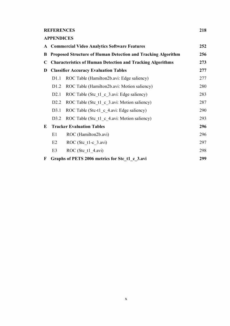
REFERENCES 218
APPENDICES
A Commercial Video Analytics Software Features 252
B Proposed Structure of Human Detection and Tracking Algorithm 256
C Characteristics of Human Detection and Tracking Algorithms 273
D Classifier Accuracy Evaluation Tables 277
D1.1 ROC Table (Hamilton2b.avi: Edge saliency) 277
D1.2 ROC Table (Hamilton2b.avi: Motion saliency) 280
D2.1 ROC Table (Stc_t1_c_3.avi: Edge saliency) 283
D2.2 ROC Table (Stc_t1_c_3.avi: Motion saliency) 287
D3.1 ROC Table (Stc-t1_c_4.avi: Edge saliency) 290
D3.2 ROC Table (Stc_t1_c_4.avi: Motion saliency) 293
E Tracker Evaluation Tables 296
E1 ROC (Hamilton2b.avi) 296
E2 ROC (Stc_t1-c_3.avi) 297
E3 ROC (Stc_t1_4.avi) 298
F Graphs of PETS 2006 metrics for Stc_t1_c_3.avi 299
xi
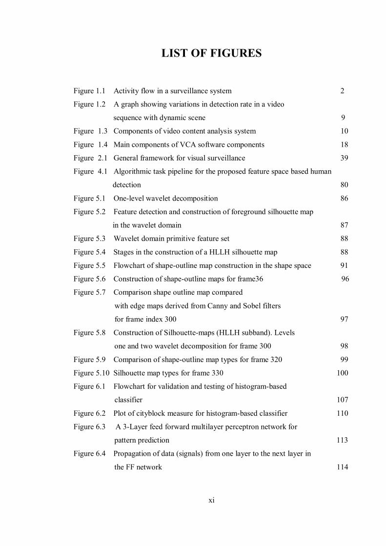
LIST OF FIGURES
Figure 1.1 Activity flow in a surveillance system 2
Figure 1.2 A graph showing variations in detection rate in a video
sequence with dynamic scene 9
Figure 1.3 Components of video content analysis system 10
Figure 1.4 Main components of VCA software components 18
Figure 2.1 General framework for visual surveillance 39
Figure 4.1 Algorithmic task pipeline for the proposed feature space based human
detection 80
Figure 5.1 One-level wavelet decomposition 86
Figure 5.2 Feature detection and construction of foreground silhouette map
in the wavelet domain 87
Figure 5.3 Wavelet domain primitive feature set 88
Figure 5.4 Stages in the construction of a HLLH silhouette map 88
Figure 5.5 Flowchart of shape-outline map construction in the shape space 91
Figure 5.6 Construction of shape-outline maps for frame36 96
Figure 5.7 Comparison shape outline map compared
with edge maps derived from Canny and Sobel filters
for frame index 300 97
Figure 5.8 Construction of Silhouette-maps (HLLH subband). Levels
one and two wavelet decomposition for frame 300 98
Figure 5.9 Comparison of shape-outline map types for frame 320 99
Figure 5.10 Silhouette map types for frame 330 100
Figure 6.1 Flowchart for validation and testing of histogram-based
classifier 107
Figure 6.2 Plot of cityblock measure for histogram-based classifier 110
Figure 6.3 A 3-Layer feed forward multilayer perceptron network for
pattern prediction 113
Figure 6.4 Propagation of data (signals) from one layer to the next layer in
the FF network 114
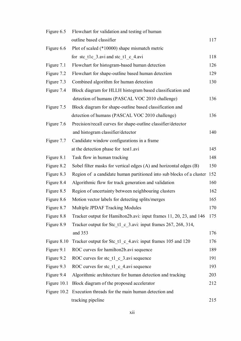
xii
Figure 6.5 Flowchart for validation and testing of human
outline based classifier 117
Figure 6.6 Plot of scaled (*10000) shape mismatch metric
for stc_t1c_3.avi and stc_t1_c_4.avi 118
Figure 7.1 Flowchart for histogram-based human detection 126
Figure 7.2 Flowchart for shape-outline based human detection 129
Figure 7.3 Combined algorithm for human detection 130
Figure 7.4 Block diagram for HLLH histogram based classification and
detection of humans (PASCAL VOC 2010 challenge) 136
Figure 7.5 Block diagram for shape-outline based classification and
detection of humans (PASCAL VOC 2010 challenge) 136
Figure 7.6 Precision/recall curves for shape-outline classifier/detector
and histogram classifier/detector 140
Figure 7.7 Candidate window configurations in a frame
at the detection phase for test1.avi 145
Figure 8.1 Task flow in human tracking 148
Figure 8.2 Sobel filter masks for vertical edges (A) and horizontal edges (B) 150
Figure 8.3 Region of a candidate human partitioned into sub blocks of a cluster 152
Figure 8.4 Algorithmic flow for track generation and validation 160
Figure 8.5 Region of uncertainty between neighbouring clusters 162
Figure 8.6 Motion vector labels for detecting splits/merges 165
Figure 8.7 Multiple JPDAF Tracking Modules 170
Figure 8.8 Tracker output for Hamilton2b.avi: input frames 11, 20, 23, and 146 175
Figure 8.9 Tracker output for Stc_t1_c_3.avi: input frames 267, 268, 314,
and 353 176
Figure 8.10 Tracker output for Stc_t1_c_4.avi: input frames 105 and 120 176
Figure 9.1 ROC curves for hamilton2b.avi sequence 189
Figure 9.2 ROC curves for stc_t1_c_3.avi sequence 191
Figure 9.3 ROC curves for stc_t1_c_4.avi sequence 193
Figure 9.4 Algorithmic architecture for human detection and tracking 203
Figure 10.1 Block diagram of the proposed accelerator 212
Figure 10.2 Execution threads for the main human detection and
tracking pipeline 215

xiii
Figure 10.3 Static schedule showing main processing tasks overlapped with
with frame access 216
xiv
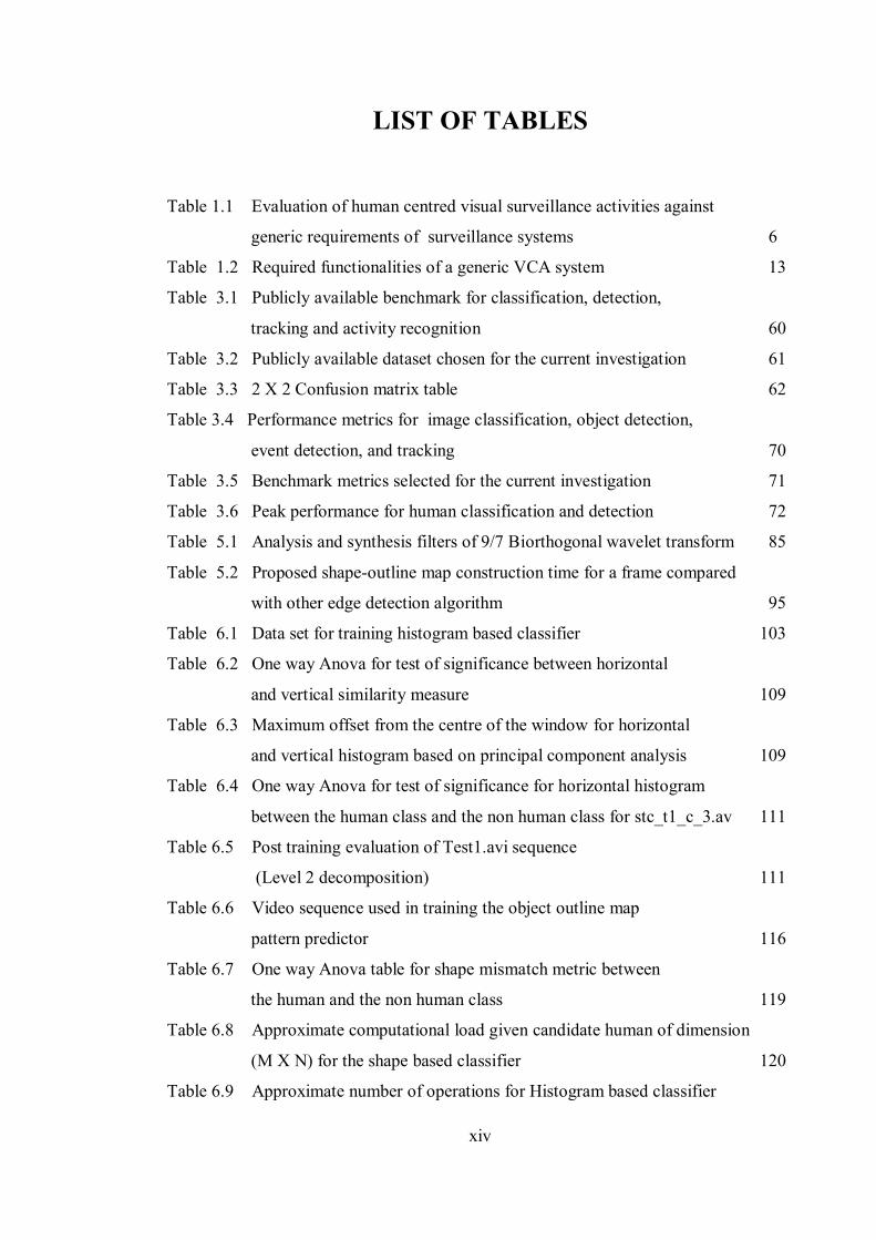
LIST OF TABLES
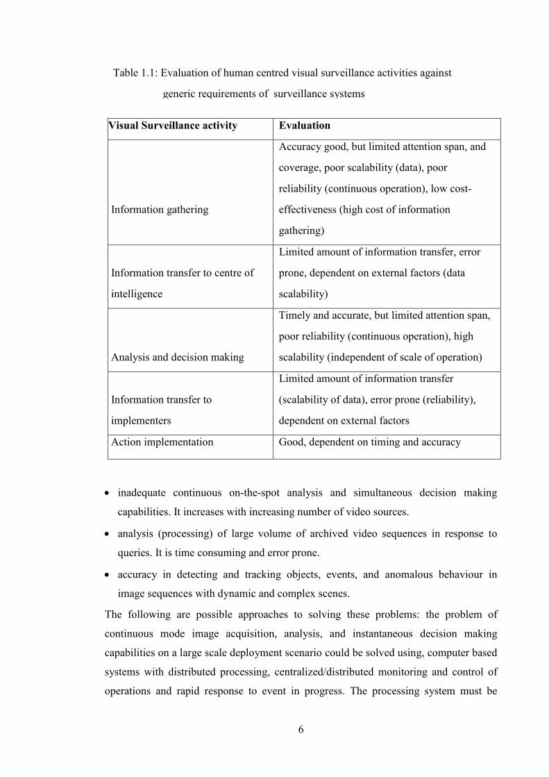
Table 1.1 Evaluation of human centred visual surveillance activities against
generic requirements of surveillance systems 6
Table 1.2 Required functionalities of a generic VCA system 13
Table 3.1 Publicly available benchmark for classification, detection,
tracking and activity recognition 60
Table 3.2 Publicly available dataset chosen for the current investigation 61
Table 3.3 2 X 2 Confusion matrix table 62
Table 3.4 Performance metrics for image classification, object detection,
event detection, and tracking 70
Table 3.5 Benchmark metrics selected for the current investigation 71
Table 3.6 Peak performance for human classification and detection 72
Table 5.1 Analysis and synthesis filters of 9/7 Biorthogonal wavelet transform 85
Table 5.2 Proposed shape-outline map construction time for a frame compared
with other edge detection algorithm 95
Table 6.1 Data set for training histogram based classifier 103
Table 6.2 One way Anova for test of significance between horizontal
and vertical similarity measure 109
Table 6.3 Maximum offset from the centre of the window for horizontal
and vertical histogram based on principal component analysis 109
Table 6.4 One way Anova for test of significance for horizontal histogram
between the human class and the non human class for stc_t1_c_3.av 111
Table 6.5 Post training evaluation of Test1.avi sequence
(Level 2 decomposition) 111
Table 6.6 Video sequence used in training the object outline map
pattern predictor 116
Table 6.7 One way Anova table for shape mismatch metric between
the human and the non human class 119
Table 6.8 Approximate computational load given candidate human of dimension
(M X N) for the shape based classifier 120
Table 6.9 Approximate number of operations for Histogram based classifier
xv
using candidate human window of the same dimension 121
Table 7.1 Parameters of the test video sequence 131
Table 7.2 Main algorithmic parameters for histogram based detector 133
Table 7.3 Main algorithmic parameters for shape-outline based detector 134
Table 7.4 PASCAL VOC 2010 training set 135
Table 7.5 Average precision for PASCAL VOC 2010 challenge 138
Table 7.6 Task profiling of the main functions of the histogram based detector
for decimated wavelet transform (level one) suband 143
Table 7.7 Task profiling of the main functions of histogram based detector
function for decimated wavelet transform (level two) subband 143
Table 7.8 Task profiling of the main functions of the shape-based detector 144
Table 8.1 Relative addresses of sub blocks defining a track cluster 153
Table 8.2 Global parameter settings for JPDAF tracker 171
Table 8.3 Main task profiling of JPDAF tracker (Intensity template only) 173
Table 8.4 Main task profiling of JPDAF tracker (All templates) 173
Table 9.1 Scene complexity descriptor for human detection and tracking 179
Table 9.2 Combined shape and histogram detector for stc_t1_c_3.avi
showing parameters of the third kind 183
Table 9.3 Intermediate computation for determining operating point on
ROC curve during an iteration 184
Table 9.4 Baseline performance of shape-outline based detector 185
Table 9.5 Baseline performance of histogram based detector (Edge saliency) 185
Table 9.6 Baseline performance of histogram based detector (Motion saliency) 185
Table 9.7 Baseline performance of histogram based detector
(Background saliency) 186
Table 9.8 Combined (shape+histogram) detector performance after tracking 194
Table 9.9 Expected false positive rate for the combined shape and histogram
tracker for the test sequence 195
Table 9.10 PETS 2006 Frame based metrics 196
Table 9.11 PETS 2006 Object based metrics 197
Table 9.12 Average execution time of JPDAF tracker with frame resizing 199
Table 9.13a Peak performance of GMM detector based on classifier trained
using GMM blobs 200

xvi
Table 9.13b Accuracy evaluations for proposed human detection algorithm
compared with Gaussian mixture model 201
Table 9.14 Peak performance of mean shift detector /tracker. Positional
accuracy expressed as a fraction of maximum distance of separation
(in pixels) between human locations in two consecutive frames 202
Table 10.1 System architectural parameters for the proposed accelerator 213
Table 10.2 Macro architectural parameters of Pentium IV 214

xvii
LIST OF ABBREVIATIONS
CAD Computer Aided Design
CCTV Closed Circuit Television
CIF Common Intermediate Format
CMP Chip Multiprocessor
CWT Continuous Wavelet Transform
CODEC Compression Decompression
DVR Digital Video Recorder
GMM Gaussian Mixture Modelling
HDT Human Detection and Tracking
JPDAF Joint Probabilistic Data Association Filter
MHTF Multiple Hypothesis Track Filter
MIMD Multiple Instruction stream with Multiple Data stream
NVR Network Video Recorder
OCWT Over Complete Wavelet Transform
PDAF Probabilistic Data Association Filter
PETS Performance Evaluation of Tracking and Surveillance
POS Point of Sale
QCIF Quarter Common Intermediate Format
RMS Root Mean Squared
ROC Receiver Operating Characteristic
SIFT Scale Invariant Feature Transform
SIMD Single Instruction with Multiple Data Stream
SMP Simultaneous Multiprocessor
VHS Video Home System
VCA Video Content Analysis
VSAM Video Surveillance And Monitoring
WT Wavelet Transform

xviii
DEFINITION OF TERMS
Anova: Analysis of variance. A statistical technique for evaluating whether two
groups belong to the same populations.
Candidate human: A rectangular region of a frame which contains salient features
and is to be probed by the classifier for the presence of human.
Candidate human localization: The processing of finding locations of candidate
humans.
CIF: Common Intermediate Format defines a frame of size 352 by 288.
D1: Input video with active frame dimension 704 by 480 pixels.
MIMD: Multiple Input Multiple Data stream. Parallel processing technique which
allows simultaneous input data stream to be processed in parallel.
Object Outline map: A derived frame showing the outline of all potentially
interesting objects in the frame.
Object window: A rectangular region of a frame which contains salient
features and is to be probed by the classifier for the presence of
object of interest.
Window: A rectangular region of a frame or subband.
1
CHAPTER ONE
INTRODUCTION
1.1 Perspective
1.1.1 Surveillance for Human Survival
It’s a paradox that humans as a species have shown remarkable ability to survive in
comparison to other species, despite the fact that individually they are ill-equipped. This
has been attributed to his ability to gather sensory data, communicate, analyse, and
enhance information using his intellect. Indeed humans’ ability to survive in life
threatening situations, depends primarily on living in social communities, sharing and
using sensory information gathered by individuals for the protection of the group. There
are several forms of sensory information available including vision, smell, touch, and
sound, although the preferred form is vision. The earliest form of surveillance,
intelligence information gathering, analysis and decision making started with
information gatherers, who were humans positioned at different locations in the field of
operation. These were typically lookouts, spies, and ordinary observers. Information
gathered was sent through intermediaries such as messengers, horses, and dogs, to their
leader (centre of intelligence) for analysis and decision making. Decisions from the
leader were also sent by intermediaries to action implementers who could be soldiers in
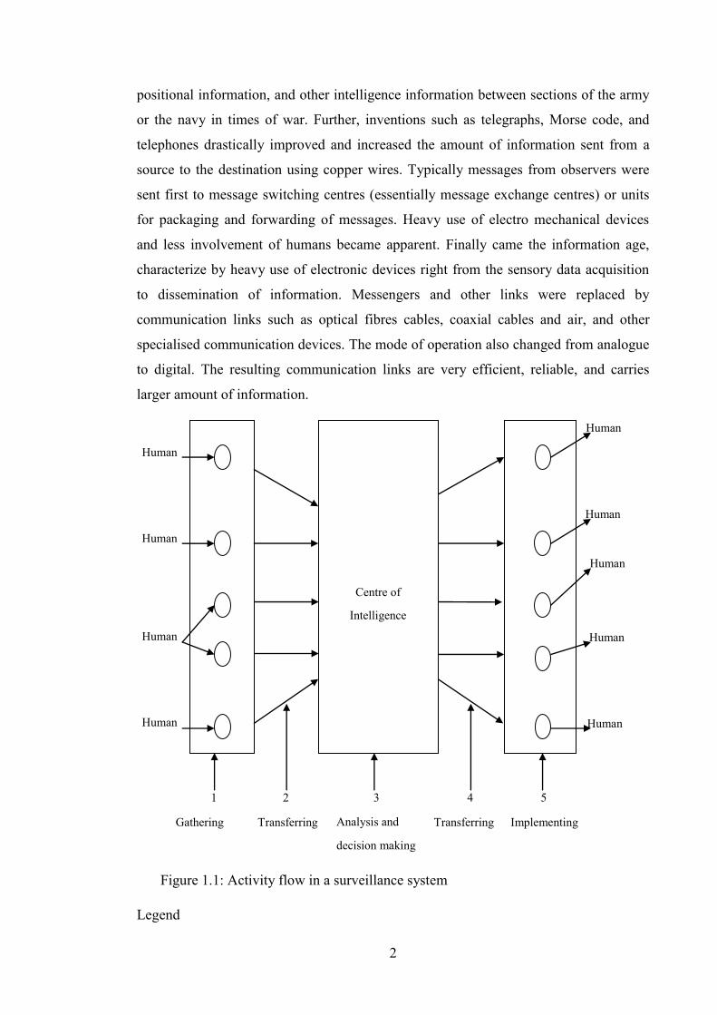
battlefields or ordinary citizens. Figure 1.1 shows information flow in surveillance
systems and is valid for both primitive and modern societies. This earliest approach
relied predominantly on humans throughout its stages of operations. Although it has
evolved over the years the basic structure has stayed the same. The next stage in the
evolution process was the use of semaphores and other forms of coded messages to
reduce reliance on messengers and increase reliability. Information gathered could then
be sent directly to the leader. Semaphores were used extensively to communicate
2
positional information, and other intelligence information between sections of the army
or the navy in times of war. Further, inventions such as telegraphs, Morse code, and
telephones drastically improved and increased the amount of information sent from a
source to the destination using copper wires. Typically messages from observers were
sent first to message switching centres (essentially message exchange centres) or units
for packaging and forwarding of messages. Heavy use of electro mechanical devices
and less involvement of humans became apparent. Finally came the information age,
characterize by heavy use of electronic devices right from the sensory data acquisition
to dissemination of information. Messengers and other links were replaced by
communication links such as optical fibres cables, coaxial cables and air, and other
specialised communication devices. The mode of operation also changed from analogue
to digital. The resulting communication links are very efficient, reliable, and carries
larger amount of information.
Legend
3
Human
Human
Human
Human
Human
5 4
Human
Human
Human
Human
Centre of
Intelligence
2 1
Implementing Gathering Transferring Analysis and
decision making
Transferring
Figure 1.1: Activity flow in a surveillance system

3
1: Information
2: Means of transfer (birds, dogs, wires, cables, free space)
3: Centre of intelligence
4: Means of transfer (birds, dogs, wires, cables, free space)
5: Action implementers
A typical modern intelligent information processing system may still have humans and
electronic sensors as data gathers. Communication links (using any of the above links)
connects data sensors/humans to a central unit (message switching units) via
multiplexors which is responsible for packaging, forwarding, and other housekeeping
operations required to efficiently transmit data to the intelligence centre. Decisions and
actions from the intelligence centre (a control room with humans monitoring and
analysing information) based on the incoming data are sent first through a similar unit
(message switching units) which repackages information in an efficient manner, and
sends via de-multiplexors to the recipients (action implementers).
A very important class of information of interest to man is information about other
humans and their activities, typically for surveillance, people monitoring in shops, real-
time vehicular traffic monitoring, and perimeter protection.
1.1.2 Requirements of a Generic Surveillance System
For effectiveness the sensory information processing must be timely, accurate, reliable,
and relevant to the situation on hand.
Timely: information flow from information gathers to end user must be timely and
appropriate for the situation on hand. Information and action required to prevent
a crime in progress must be available on the spot.
Accurate: accurate information must be provided at all stages of the system, and ideally
analysis and decision making must be error free.
Reliable: information required must be available at all times independent of any
external conditions. It must also be consistent and predictable.
Cost-effective: It must optimize cost, accuracy, reliability, and timeliness. The system
must additionally be easy to use and flexible for widespread deployment and adoption.
The main requirements of generic surveillance systems are summarised as:

4
User friendliness
Ease of use
Ease of deployment
Operational efficiency
Accuracy
Predictable
Consistent
High
Timeliness
Real-time processing
Performance
Scalability
Reliability
Continuous operation
Application flexibility
Cost-effectiveness
Reliability
Reduce cost, high accuracy, and performance optimization
1.1.3 Evolution of Visual Surveillance Systems
Human sensory processing capabilities are limited in the domain of sound, touch, and
smell but well developed in processing visual patterns. The means of human visual
information capture are the eyes, and studies have shown that they have limited range of
visual perception, but good at discriminating features. Man is not unique in processing
sensory information since other animals such as whales have well developed sound
processing capabilities, and rely on them for food and protection. For example, ants
communicate using smell from pheromones deposited on the ground wherever they visit
to assist the colony in search of food. Table1.1 is an evaluation of surveillance activities
based predominantly on humans against requirements of performance (accuracy,
timeliness and reliability), cost-effectiveness and user-friendliness. The main problems
with intelligence gathering centred on humans are: the slow means of information
5
transfer from gatherers to centre of intelligence, slow means of transfer of decisions and
commands from centre of intelligence to action implementers, and low volume of
information transferred per trip. Visual communication using manual processing (rely
predominantly on humans) is relatively slow, expensive and inefficient especially when
visual information is to be gathered over large area of coverage.
A solution to the high cost of gathering information over large areas is the use of
image acquisition devices (cameras, infra red and thermal imaging device). Closed
circuit television (CCTV) cameras in particular provides a cost-effective means of
acquiring images on a continuous basis, and over large areas using multiple cameras. In
response to increasing volume of visual data continuously being acquired storage
devices are used for archiving and playback of video streams. The first storage devices
were analogue device such as charge couple device, magnetic tapes, and VHS cassettes.
Later on digital storage devices such as Digital Video Recorders (DVRs, and
Networked Video Recorders, NVRs) Network storage, and hard disk drives were used
since they have improved reliability, and high accuracy. With increasing number of
cameras being deployed, the problem of effective monitoring of cameras and analysis of
visual scene by humans also came to the attention of designers. Typically operators
would monitor video from several cameras deployed over wide area on display devices
to make on-the-spot decisions about threats, and take appropriate action. One solution
adopted is automation first by analogue storage and processing and later by electronic
processing. The main reason is the higher reliability and availability of information in
digital storage form and access to larger volume of digital storage devices compared to
analogue storage. Electronic information processing also provides a cost-effective
means of linking visual sensors to intelligent processing units using computer networks.
For example several CCTV cameras could be linked remotely to intelligence centres for
processing visual information. Additionally electronic computing is pervasive due to
availability of cheap digital storage media and, diverse processor types (ASIC, DSP and
FPGA) and communication devices. The development of international digital
compression standards for removal of redundant visual information (JPEG, MPEG,
H261, etc) saving on storage and transmission cost also favours digital processing at all
the stages of surveillance system mentioned earlier on. However the following problems
still confront most electronic visual processing systems at the analysis and decision
making step:
6
inadequate continuous on-the-spot analysis and simultaneous decision making
capabilities. It increases with increasing number of video sources.
analysis (processing) of large volume of archived video sequences in response to
queries. It is time consuming and error prone.
accuracy in detecting and tracking objects, events, and anomalous behaviour in
image sequences with dynamic and complex scenes.
The following are possible approaches to solving these problems: the problem of
continuous mode image acquisition, analysis, and instantaneous decision making
capabilities on a large scale deployment scenario could be solved using, computer based
systems with distributed processing, centralized/distributed monitoring and control of
operations and rapid response to event in progress. The processing system must be
Table 1.1: Evaluation of human centred visual surveillance activities against
generic requirements of surveillance systems
Visual Surveillance activity Evaluation
Information gathering
Accuracy good, but limited attention span, and
coverage, poor scalability (data), poor
reliability (continuous operation), low cost-
effectiveness (high cost of information
gathering)
Information transfer to centre of
intelligence
Limited amount of information transfer, error
prone, dependent on external factors (data
scalability)
Analysis and decision making
Timely and accurate, but limited attention span,
poor reliability (continuous operation), high
scalability (independent of scale of operation)
Information transfer to
implementers
Limited amount of information transfer
(scalability of data), error prone (reliability),
dependent on external factors
Action implementation Good, dependent on timing and accuracy
7
characterized by scalable computer processing power to match required processing
power, and scalable processing techniques (parallel/distributed algorithms for robust
content analysis); and real-time processing capability to meet application requirements.
1.1.4 Challenges of Visual Scene Analysis
Typical visual scene analysis algorithms involve the following sequence of tasks: pre
processing, object detection, object tracking, and anomalous behaviour detection. Pre
processing typically involves frame format inter conversion, noise removal,
decompression, and object enhancement. Object detection typically involves scene
modelling, candidate object localization, analysis/synthesis of candidate objects,
classification and detection, and anomalous behaviour analysis. Object localization
typically involves identifying locations of likely objects. For a given object location
object analysis or synthesis technique is applied to identify its features or to model the
object. When several objects are of interest in a scene then one object class must be
differentiated from another object class, hence objects must be classified. Also in
detecting single objects, background objects would have to be differentiated from the
object of interest. Object classification may be part of an object detection task since a
particular object in a class might have to be identified from among other objects not in
the same class. Detection typically follows classification and involves evaluation of
confidence level after classification or some validation test. The output from the
detector is typically the location, and the class of the candidate object. Object tracking
involves establishing correspondence between the same object in different frames.
Anomalous behaviour detection involves defining atypical behaviour as a sequence of
discrete events. Continuous mode visual scene analysis operating twenty-four hours a
day is faced with several challenges including the following:
Analysis complexity: Increasing analysis complexity typically arises in complex scenes
involving illumination changes, scene clutter, scale changes, camera motion, and low
object background contrast. For instance changes in scale brought about by perspective
projection due to object moving away from a stationary camera might make a feature-
based detection technique fail due to difficulty in differentiating object features from
noise at very low object resolution. Similarly, the choice of object models on which
object analysis and synthesis depends on has direct effect on complexity. For instance 3-
8
D models of humans, and its associated motion models are computationally demanding,
although the accuracy is better compared to 2-D models [Ju et al. 1996], [Quentin et al.
2001]. The choice of algorithms and the assumptions on which it is based also has
direct effect on analysis complexity. With 2-D motion models, an assumption of
smoothness of motion or changes in illumination is used in motion tracking, or optical
flow to reduce analysis and computational complexity. Similarly in tracking, multiple
hypotheses tracking with exponential search complexity could be avoided by excluding
certain incompatible events from occurring simultaneously.
Accuracy: The accuracy of object detection and tracking measures how often the
system makes correct and incorrect detection and tracking decisions and the confidence
levels associated with this decision process. The accuracy of detection and tracking
objects in visual scene is dependent on whether objects exist in isolation or part of a
group, besides scene complexity factors. As a general observation, objects in a group
tend to occlude features of each other. For example two humans moving together as a
group might result in features of the person closer to the camera occluding the other
person’s features. Also in detection of multiple objects there are several possible
outcomes depending on object configuration and interaction in the scene. The outcome
could be individuals, sub groups, and the group as a whole could be detected. It also
depends on the associated ground truth defined for the scene. This means that the
robustness of the detection technique depends on how well the detected objects matches
those of the ground truth. Thus one way of achieving flexible detection is to let the
detection and tracking be algorithmic parameter driven to increase it robustness, and
allow the possibility of optimizing based on algorithmic parameters. The implication of
the subjective nature of ground truth labelling means that detection rates may vary with
object-object interactions, and scene-object interactions.
Reliability: In general for dynamic scene, complexity may vary with time of the day,
weather, scene clutter, illumination changes, and object-object interaction, and scene-
object interactions. Thus assumptions valid during the daytime might not be true during
the night. There is a corresponding fluctuation in detection and false alarm rates
(accuracy) over time. This makes it difficult to predict performance. Figure 1.2 is a plot
of detection rate versus frame index over time for stc_t1_c video sequence with multiple
humans (a PETS 2006 video sequence) for frames between 33 and 500. Wide variations
in the detection rate over time are clearly visible. Frame detection rate is defined as:
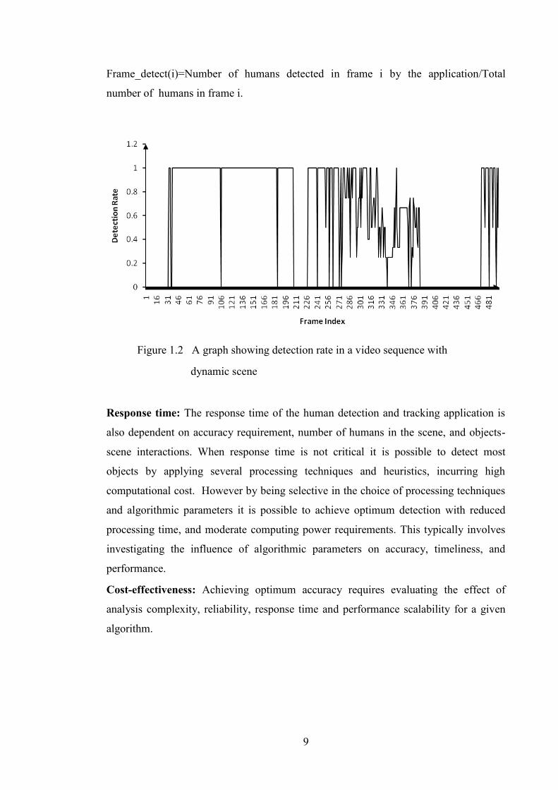
9
Frame_detect(i)=Number of humans detected in frame i by the application/Total
number of humans in frame i.
Response time: The response time of the human detection and tracking application is
also dependent on accuracy requirement, number of humans in the scene, and objects-
scene interactions. When response time is not critical it is possible to detect most
objects by applying several processing techniques and heuristics, incurring high
computational cost. However by being selective in the choice of processing techniques
and algorithmic parameters it is possible to achieve optimum detection with reduced
processing time, and moderate computing power requirements. This typically involves
investigating the influence of algorithmic parameters on accuracy, timeliness, and
performance.
Cost-effectiveness: Achieving optimum accuracy requires evaluating the effect of
analysis complexity, reliability, response time and performance scalability for a given
algorithm.
Figure 1.2 A graph showing detection rate in a video sequence with
dynamic scene
10
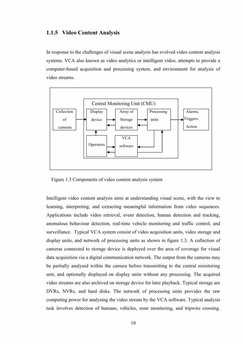
1.1.5 Video Content Analysis
In response to the challenges of visual scene analysis has evolved video content analysis
systems. VCA also known as video analytics or intelligent video, attempts to provide a
computer-based acquisition and processing system, and environment for analysis of
video streams.
Intelligent video content analysis aims at understanding visual scene, with the view to
learning, interpreting, and extracting meaningful information from video sequences.
Applications include video retrieval, event detection, human detection and tracking,
anomalous behaviour detection, real-time vehicle monitoring and traffic control, and
surveillance. Typical VCA system consist of video acquisition units, video storage and
display units, and network of processing units as shown in figure 1.3. A collection of
cameras connected to storage device is deployed over the area of coverage for visual
data acquisition via a digital communication network. The output from the cameras may
be partially analysed within the camera before transmitting to the central monitoring
unit, and optionally displayed on display units without any processing. The acquired
video streams are also archived on storage device for later playback. Typical storage are
DVRs, NVRs, and hard disks. The network of processing units provides the raw
computing power for analysing the video stream by the VCA software. Typical analysis
task involves detection of humans, vehicles, zone monitoring, and tripwire crossing.
Figure 1.3 Components of video content analysis system
Central Monitoring Unit (CMU)
VCA
software
Operators
Array of
Storage
devices
Display
device
Processing
units
Collection
of
cameras
Alarms,
Triggers,
Action
implementers

11
The results of the analysis might also be stored on DVRs, and NVR, displayed on
monitors or communicated to personnel responsible for taking actions appropriate to the
situation on hand, generate alarms, or trigger other events. For example the VSAM
project at Carnegie Mellon University [Collins et al. 2001] implemented a system
consisting of multi-camera sub system linked by digital network which cooperatively
acquire video signals, track multiple moving objects, and fuse information from
multiple cameras into scene level object representation. Locations of cameras overlay
the site map to enable real-time monitoring and control. It has the capabilities of setting
triggers on certain events, which results in specific sequence of action taken. VCAs
have put a lot of emphasis on:
Ease of deployment: End users of the system are expected to configure the application
with ease. This means ability to select performance measures, and fine tune application
parameters. The interface is expected to be user friendly with help facility provided.
Facilities such as alarms and triggers might be required for real-time monitoring
especially in situations where several video streams from different geographical
locations are being monitored simultaneously.
Computational efficiency: The ability to achieve high accuracy without exceptional
increase in computational work load means the system is expected to provide high
reliability, and availability. This has implications on processor and scalability with
increase in frame size, frame rates, and number of video streams channels.
Real-time processing: The ability to match real-time response with different
application scenarios. For example in applications involving crime prevention, it might
be required to prevent a crime in progress from being committed and so it would be
required to set alarms to trigger events in progress for necessary action to be taken.
Cost-effectiveness: The performance of the system is expected to balance accuracy and
reliability constraints, and cost on the other hand. Achieving the optimum level of
performance might involve for instance scaling of algorithmic parameters, processors,
and number of system components.
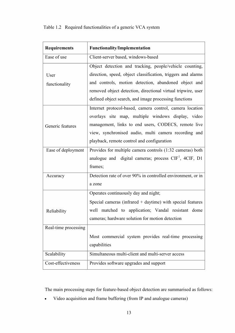
1.1.6 Evaluation of Selected VCA Systems
The purpose of this section is to review typical VCA software functionalities provided
12
by commercial vendors, and identify software functionalities which are required for
robust human detection and tracking. A typical VCR system has the following hardware
components: multiple cameras (analogue and digital), matrix switches for connecting
cameras to storage device, monitors, video codec, DVR and NDVR for storage, and
monitors for display. Installed software typically includes graphical user interface with
functionalities such as video recording, playback, alarms and trigger, camera control via
software interface (pan, tilt, and zoom), motion detection, human tracking, event
detection, and access control management. The hardware components may be internet
protocol (IP) based network. A summary of the evaluation of VCA software is
presented in table 1.2 with additional information on VCA software also provided in
appendix A. The following trends are observed: User interface provided is quite good
since it is window-based and upgradeable with functionalities for object detection and
tracking. It provided generic features and software control of cameras and its motion.
Cost-effectiveness is good since it provides for both software upgrades, and hardware
platform upgrades. Information on accuracy outside the controlled operating
environment is not provided.
1.1.7 Algorithmic Approaches to Object Detection and Tracking
Traditionally, visual sensors capture single image or video in space-time domain and
use vision and signal processing techniques also in the same domain to detect and track
objects. [Dee H.M. 2008] provides a review of vision based approach to human
detection. Algorithms for object detection and tracking can be classified into three main
approaches, namely, feature-based detection and tracking, model-based detection and
tracking, and motion-based recognition. Feature-based detection and tracking relies on
detectable object features in the video stream; model-based technique relies on
generated object model and its associated motion models. Typical 2-D models consist of
view dependent 2-D shape models, and affine transform based motion models [Rohr
1994]. 3-D models include bone and tissues models based on finite element methods,
and its associated motion and pose models, all stored in a model database. Motion based
recognition uses the intrinsic motion of whole or part of the human for detection and
tracking.
13
The main processing steps for feature-based object detection are summarised as follows:
Video acquisition and frame buffering (from IP and analogue cameras)
Table 1.2 Required functionalities of a generic VCA system
Requirements Functionality/Implementation
Ease of use Client-server based, windows-based
User
functionality
Object detection and tracking, people/vehicle counting,
direction, speed, object classification, triggers and alarms
and controls, motion detection, abandoned object and
removed object detection, directional virtual tripwire, user
defined object search, and image processing functions
Generic features
Internet protocol-based, camera control, camera location
overlays site map, multiple windows display, video
management, links to end users, CODECS, remote live
view, synchronised audio, multi camera recording and
playback, remote control and configuration
Ease of deployment Provides for multiple camera controls (1:32 cameras) both
analogue and digital cameras; process CIF1, 4CIF, D1
frames;
Accuracy Detection rate of over 90% in controlled environment, or in
a zone
Reliability
Operates continuously day and night;
Special cameras (infrared + daytime) with special features
well matched to application; Vandal resistant dome
cameras; hardware solution for motion detection
Real-time processing
Most commercial system provides real-time processing
capabilities
Scalability Simultaneous multi-client and multi-server access
Cost-effectiveness Provides software upgrades and support
14
Decompression and colour space conversion
Frame enhancement
Human detection
Human tracking
The video acquisition and frame buffering deals with hardware-software interface for
video sequence acquisition from one or more cameras. Since there are several real-time
solutions available it is not covered in the thesis. Similarly the availability of Codecs
(compression/decompression) solution, and the fact that it is offered as part of the
camera acquisition sub system it is also not covered. Software solutions for RGB to
YUV conversion routines are used where necessary. Frame enhancement functions of
interest include noise removal, illumination normalization, and saturation control.
Object detection involves locating instance of objects, and discriminating the object
from its background or from other classes. Object could be cars, humans, and birds with
emphasis mainly on object properties in the space-time domain (images) or observable
in transform feature space. The outcome of the discrimination process is the assignment
of the object to a class. If the object is assigned to a human class then it asserts a
hypothesis on the existence of human. The output of the object detection phase is passed
on to the tracking stage for mapping out the location and velocity of objects over time.
1.1.8 Improving Accuracy of Feature-Based Approach in Pattern
Space
In feature space classifiable features are extracted and used for object detection or
recognition. Two main types of image based features could be used for detecting
objects, namely features which directly relates to observable object as a whole (global
features), and primitive (local) features which do not uniquely relate to the observable
object features but are used as building blocks to construct higher level object’s parts.
There could be combinations of local and global features for object detection
[Moeslund and Granum 2001]. It could be implemented by part-based detection
[Meyer et al. 1999], [Wu and Nevatia 2005] and then the object as a whole is detected
by inference using the detected parts. An example is the upright human body shape,
and its parts such as hands, head and shoulders, legs, and torso. On the other hand
15
local features such as corners, edges, lines, and circles are primitives which are used
as building blocks to construct parts of the body, before assembling a complete model
of the object. This closely relates to the two level object feature used in computer
vision techniques, namely, local and global features [Danielsson et al. 2008]. Features
which are observed in pattern spaces may have different relationship with the physical
object. Typical examples include wavelet coefficients, histogram of oriented gradients,
optical flow vectors, SIFT features, and shape context. Feature space based detection
and tracking, has relatively smaller computational load, compared with model-based
technique (an alternative approach). However a major challenge with real-world
objects is that they involve concepts such as car, face, human, rather than specific
objects and exhibit large class variability [Swarup 2002]. As a result there is no easy
way to come up with an analytical decision boundary separating one object concepts
from the other using low level image features or features in pattern spaces. The
robustness of a particular solution depends on the choice of suitable feature set, and
the type of application [Wikipedia]. In a typically pattern space feature extraction, the
input data is first transformed into the feature space, and then good features are
extracted followed by feature classification. Good local features for object recognition
must be translation, rotation and scale invariants [Lowe 1999], and at the same time
must be distinctive among many alternatives. [Yilmaz 2006] has provided a review of
different feature types used in object detection and tracking. These include points
(corners, centroids), primitive geometric shapes, object silhouette and contours. Shape
as a global feature has also been used in several human detection and tracking
applications [Lee 2004], [Song 200], and [Berg 2000]. The main limitations of feature
based object detection or recognition [Lowe 1999] is providing enough feature points
as evidence in either detection, recognition or tracking scenario, and coping with scale
changes. In particular scale changes and translational invariance are requirements
which are desirable in object detection. Scale refers to the level of detail at which the
features of a physical object are detected. To meet scale invariance requirements
designers of detectors in feature spaces like scale-frequency domain [Oren et. al 1997]
use hierarchical feature analysis technique to construct wavelet templates. This
ensures features are detectable across several levels of scale. Multi-scale
decomposition provides a means of analysing images and video sequences across
scales.
16
1.1.9 Exploiting Local Features in Two Independent Pattern
Spaces
Clearly, a means of improving robustness of object detection is to complement space-
time domain detection with scale-frequency detections: multiscale analysis of images
features is part of most object detection techniques. Additionally, certain class of
wavelet transform provides translation invariance which is a requirement for generic
object detector. Combining detections in two independent feature space is
hypothesised to improve detection rate if the feature set used in one space is
orthogonal to the other feature set. This is the approach proposed to improve the
accuracy of human detection and tracking. Thus by approaching the human detection
and tracking as pattern analysis/recognition problem posed in two independent
patterns spaces, the combined accuracy is expected to improve. The effect of the two
approaches on the accuracy of human detection and tracking (in wavelet domain and
space-time domain) is examined in the current study via simulation.
1.1.10 Pattern Classification for Object Discrimination
Often large number of features are extracted to represent the target concept, however
many of them could be irrelevant or redundant in the sense that they appear in other
categories. Essentially given a set of d features, the problem of selecting a subset of m
features with the maximum discriminatory power is a classification problem.
[Watanbe 1985] showed that it is possible to make two arbitrary patterns similar by
encoding them with sufficiently large number of redundant features. Feature
extraction aims at removing redundant and non discriminatory features not well
matched to object concepts, whilst object discrimination focuses on the use of
discriminatory features for object class identification. This could be achieved by
classification of object features. Of the two main approaches to classification, namely,
supervised and unsupervised learning, supervised learning provides a mechanism for
reinforced learning since there is a desired feedback as well as inputs [Dayan 1999],
whilst unsupervised learning is purely statistical technique it requires a prior
assumption about the distribution of features in the scene. The difficulty in
determining when adequate training has been given to a classifier however limits it’s
17
accuracy as a universal discriminator. One class of unsupervised learning technique,
histogram-based classifier (a density estimation technique), and a supervised learning
technique, neural network pattern classifier, is used as a vehicle for investigating
performance of classifiers in human detection in the current study.
1.1.11 Bayesian Tracker for Optimal Object Tracking
Two main issues are involved with visual object tracking, namely, object
representation and localization, and filtering and data association [Commaniciu and
Ramesh 2003]. Object representation and localization deals with changes in object
appearance, its location and representation (by measurement estimation). It is a
bottom-up process with specific assumptions about object dynamics. Filtering and
data association is a top-down process dealing with dynamics of the tracked objects,
learning of scene prior, and evaluation of different track hypothesis. Bayesian filters
provide a probabilistic frame work for improving the accuracy of a set of parameters
based on prior information and current estimate (see section 2.3). The optimal
Bayesian filter for multiple object tracking suffers from high computational and
memory requirements on account of its recursive nature. Sub optimal filters such as
JPDAF, probabilistic data association filter, and track likelihood filter may be used
provided application requirements could be met. The dynamics of objects is typically
modelled using Kalman [Marcenaro et al. 2002] predictions if motion is linear, or
sample based techniques such as particle filters [ Zhou et al. 2004], and other Monte
Carlo based techniques. The study investigated joint probabilistic data association
filter for tracking of multiple humans. Its ability to reduce false detections brought
forward from the detection stage was also investigated.
1.1.12 Software Functionalities Proposed for Video Surveillance
Applications
Most commercial VCR software has a user interface through which user requirements
defined as zones, virtual tripwire, and perimeters (region of interest), are defined as
parameters to the detection and tracking module. The output from the detection and
18
tracking module comes out as alarms, alerts, triggers, and event login information
recorded unto an event database, or to video management software. Based on VCR
software evaluation and the proposed algorithm the complete software system consists
of video acquisition interface, graphical user interface (GUI), detection and tracking
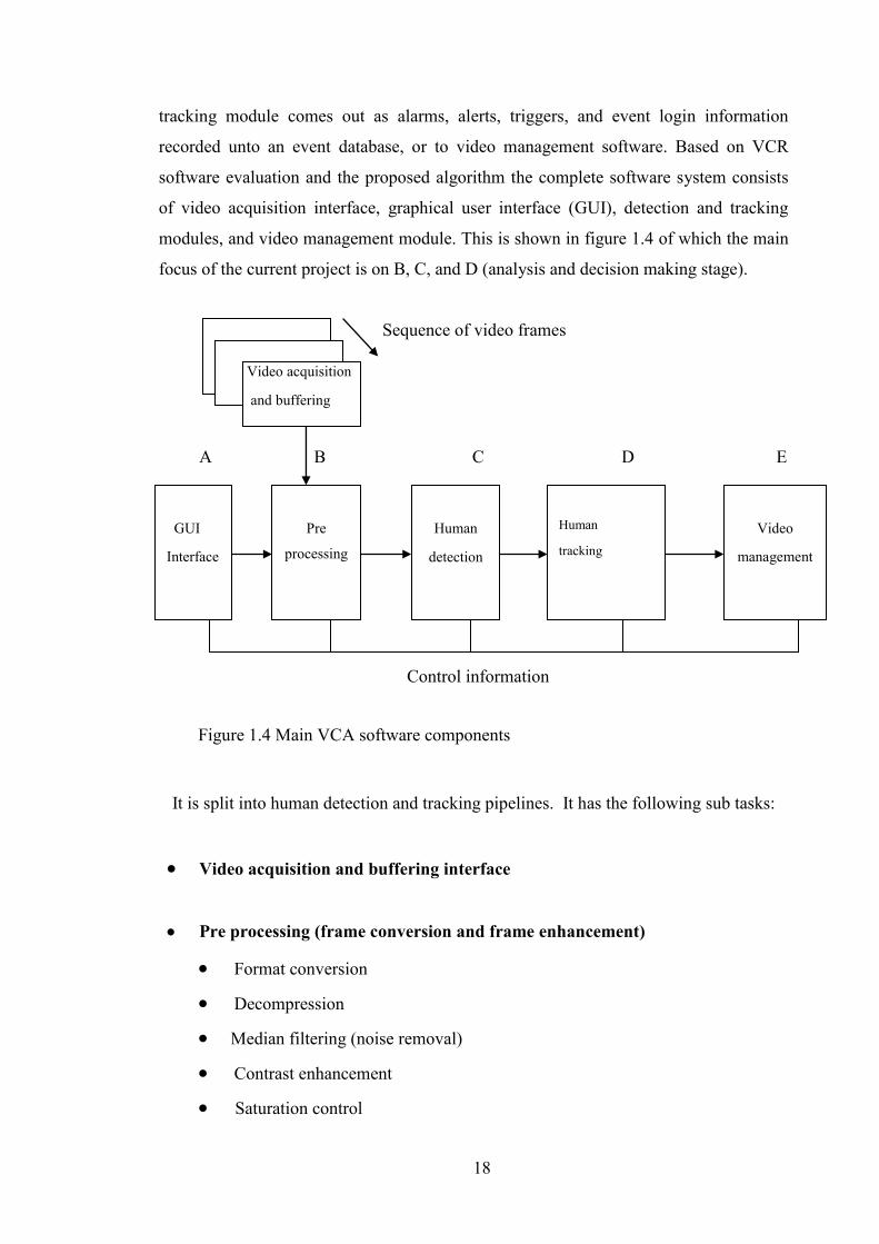
modules, and video management module. This is shown in figure 1.4 of which the main
focus of the current project is on B, C, and D (analysis and decision making stage).
It is split into human detection and tracking pipelines. It has the following sub tasks:
Video acquisition and buffering interface
Pre processing (frame conversion and frame enhancement)
Format conversion
Decompression
Median filtering (noise removal)
Contrast enhancement
Saturation control
A B C D E
Control information
Figure 1.4 Main VCA software components
Video acquisition
and buffering
GUI
Interface
Video
management
Human
tracking
Pre
processing
Human
detection
Sequence of video frames

19
Frame resizing
Human detection
Feature extraction
Construct silhouettes map (wavelet based map construction domain)
Construct shape outline map (Object outline map construction)
Candidates localization (provides location information)
Select candidate regions (from silhouette map)
Select candidate regions (from object outline map)
Human discrimination
Classification and validation
Wavelet based classification
Histogram based classification
Shape-outline based classification
Pattern prediction
Hypothesis generation
Hypothesis validation
Validation
Linear discriminant test for candidate humans after classification
Heuristics test
Update details of found humans
Determine centroids of found humans
Database update.
Merge list of found humans from shape and histogram detectors
The tracking pipeline has the following sub tasks:
Human tracking
Track initialisation
Silhouette extraction and processing

20
Silhouette extraction
Blur image with 5 X 5 averaging filter
Apply intensity-based segmentation
Appearance template feature extraction
Extract gradient and chromatic colours from silhouette region
Determine intensity of pixels representing humans
Measurement computations
Local and global motion vector estimation;
Location estimation;
Measurement validation
Mahalanobis based constraints;
Track hypothesis generation and validation
Compute measurement to track cluster association;
Generate measurements to track association hypotheses;
Compute signatures of found humans in the current frame;
Determine best track for every candidate human using its signature;
Kalman prediction
Next state prediction;
Post processing
Track maintenance (Track activation, deactivation, split, merges)
Occlusion handling and statistics gathering;
1.1.13 Persistent Problems of Automated Human Detection and
Tracking in Space-Time Domain
Most of the current approaches to human detection and tracking is object-based. It relies
on segmentation techniques or indirectly figure-ground separation in the spatial domain
and is based on computer vision techniques. It basically detects blobs and regions which
are direct representation of the object. Vision based processing algorithms in spatial
domain are faced with the problems enumerated earlier (low contrast, illumination
changes, shadows, and occlusions and background motion). The main challenges are:
21
Scene complexity: A closer examination of the algorithmic issues mentioned in section
1.1.4 reveals that the main problems associated with feature-based approach (in spatial
domain) are feature visibility, scale changes, and low contrast. The problems associated
with model-based techniques are the choice and adequacy of the models, and
computational complexity [Rohr 1994]. The problem associated with motion-based
techniques is characterising motion, differentiating fake motion and noise from object
motion, and sensitivity. Additionally, scene clutter and object-object occlusion, and
object-scene occlusion, and the number interesting objects in the scene being detected
or tracked affect all the three approaches, resulting in extra processing steps, and hence
increase in computational complexity.
Real-time processing limitations: Computational load also increases with increasing
frame rates, frame size, number of video inputs (channels), and response time
constraints. Extra algorithmic steps are added to improve robustness (shadow
elimination and background motion compensation, occlusion, etc). The net effect is an
increase in processing workload and hence the execution time which directly affects the
response time. The problem of increasing computational complexity and increasing
computing power requirements can be met by parallel processing with scalable
processors to match increasing computational load. Parallel processing can reduce
execution time by exploiting natural and applied parallelism. Sequential processing is
limited in achievable performance which worsens with increase in frame rates, number
of video channels, and frame size. Issues such as processing scalability becomes a major
consideration.
Accuracy: In reality there are four possible outcomes of object or event detection
assuming crisp categorisation of outcomes. The first one, true negative, occurs when the
algorithm does not detect the presence of a human and truly there is no human present at
the location being probed. The second possibility, false positive, occurs when the
system reports the presence of humans when in reality the human does not exist in the
location being probed. The third outcome, false negatives occur when there is human
but the system fails to detect the human. The last possibility true positive, is when there
is a human and the system detects the human. This means that the detection rate (true
positive divided by count of all instances of humans) is usually a fraction of the ideal
detection rate. Further when multiple humans are interacting in the scene, such as
coming together, and or separating other outcomes are possible. For example several
22
humans could be detected as an instance of a group, resulting in several false negatives
for all the individuals in the group but a single detection event. Thus detection rate of
multiple humans in a group may be smaller than the true positive counts of humans in
the scene. This may also be due to the interactions between humans resulting in
occlusion. At the detection phase another problem is the variations in detection rate and
high false alarm rate when underlying assumptions about a scene are violated. In
tracking the main problem to contend with are positional and tracking errors due to
track data association ambiguities, sparse data resulting in tracks with no measurement
association, and multiple data association with a single track. Object-object interactions,
and object-background interactions also results in partial or total occlusion. This also
causes data association problems, hence affects the accuracy of the system. At the
tracking phase these problems results in low track detection rate, high track miss
detections, track false detections, track fragmentation and merges errors.
From the end user point of view automated human detection and tracking
systems are expected to provide a level of service offered by traditional CCTV cameras
being monitored continuously by humans. Given the above limitations of most current
system, there is the need to improve the analysis and decision making aspect, i.e, object
detection and tracking. Though there have been several reported studies of success of
video analytics systems deployed in indoor and outdoor environments, the majority of
the deployed systems face some of these challenges [Boghossian et al. 2001]. Thus for a
particular scene the analysis of the resulting video sequence using a particular algorithm
might have high accuracy, whilst with another sequence the accuracy level would be
very low.
However users would be comfortable working with tools whose accuracy is very
high and predictable. The existence of these algorithmic accuracy limitations is the
motivation for investigating human detection and tracking in scale-frequency domain,
as a complement to space-time domain processing. For example [Siebel 2002] uses
multiple tracking algorithms to track humans. Wavelets transform feature space
provides a means of detecting both global and local features appropriate for multi-scale
analysis. Several wavelet features have also been used in image analysis [Mallet 1992],
[Strickland 1997], [Unser 1995]. These include wavelets coefficients, normalized
wavelets coefficients, wavelets templates, and wavelets energy, wavelet packets.
Combining object detection in the spatial domain with wavelet domain detection is

23
expected to achieve higher detection rate if multiscale processing capability is exploited
such that detection is independent of scale changes. One possibility is to identify
primitive features which is detectable at all scales. To what extend the increased in
computational load would improve accuracy of detection and tracking of humans is the
subject of the current study.
1.2 Aim and Objectives
The aim of the study is to improve operational efficiency of surveillance systems by
investigating an algorithm with capabilities to improve the accuracy of human detection
and tracking. The accuracy of the algorithm is expected to be independent of scene
complexity, with predictable operating accuracy and performance scalability to improve
timeliness. The objectives are:
Investigate novel algorithms
1. To investigate scale-frequency domain and shape space pattern classifiers for
improving accuracy of detecting humans (improving detection rate, and reducing
false alarm rate).
2. To investigate reduced complexity joint probabilistic data association filter for
reducing false alarms and track positional errors during tracking;
3. Propose parameter driven accuracy prediction technique independent of
scene complexity.
Improve response time
4. Improve performance scalability to cater for increase in frame size, frame rate,
and number of video channels by deriving scalable algorithmic architecture.
Compare accuracy with other algorithms
5. Comparative accuracy evaluation of proposed detector with other competitive
algorithms.

24
1.3 Research Strategy
Human detection and tracking is split into two main parts, namely, human detection and
temporal tracking. Human detection focuses on shape-space, and wavelet template
features for human discrimination via classification. However, tracking is performed in
spatial-temporal domain using multiple motion models for Kalman prediction, and joint
probabilistic data association filter (JPDAF) for data association. Receiver operating
curve (ROC) based prediction of operating accuracy, and synthesis of scalable
algorithmic architecture were also investigated. The following strategy was adopted:
(1) A review of existing algorithmic solution in the literature to the problem of human
detection and tracking under background scene constraints. The effects of scene
factors such as low background contrast, background clutter, scale changes, and
object occlusion on accuracy were examined. The limitations and strengths of
existing algorithms were evaluated.
(2) At the detection phase, proposed new algorithms for human detection by:
Investigating discriminatory feature extraction techniques in two independent
feature spaces for human detection, namely, shape-space and scale-frequency
space (wavelets domain).
Investigating three independent feature space pattern classifiers for improving
human detection. This entailed design, implementation and evaluation of a
shape-outline based classifiers for detecting apparent shape of humans in the
spatial domain. The design, implementation and evaluation of two wavelet
domain classifiers for robust movement, and scale invariant detection were also
investigated.
Specification and implementation of human detection task pipeline combining
detections in the wavelet and shape domains.
Evaluation of accuracy of proposed detection algorithm under the following
scene background characteristics:
scene clutter
scale changes
multiple humans coming together or separating from each other

25
low contrast,
sudden illumination changes.
(3) At the tracking phase proposed a JPDAF tracker algorithm for human tracking,
detailed out its specification. Evaluated the proposed tracker. Investigated low
complexity tracker with the following characteristics:
Used JPDAF and Kalman prediction with motion models for robust tracking.
Application of linear discriminant classifier to reduce track false alarm rate.
Use of Mahalanobis confidence limits for joint detection and tracking in batch
estimation mode to reduce hypothesis enumeration complexity (reduce
computational complexity).
Matching of appearance signature of found human with candidate tracks
to determine the best human-to-track association for track hypothesis
validation.
Evaluation of accuracy of proposed tracker under occlusion, scene clutter, and
scale changes.
(4) Investigated use of ROC curves in predicting operating accuracy. This is based on
first determining optimal algorithmic parameters for the detection and tracking
phase, and then using ROC curves to predict operating performance. Synthesis of
scalable algorithmic architecture for human detection and tracking deriving:
Components (modules in software) for human detection;
Components (modules in software) for human tracking;
Investigated the influence of algorithmic parameters (human width, human
height, aspect ratio, etc) on accuracy on the proposed architecture;
Proposed an integrated human detection and tracking algorithmic
architecture;
Execution time profiling and analysis of the human detection and tracking
algorithm, and then finally make recommendations to speed up execution
based on parallel processing on multiprocessor accelerator hardware.
The end product of this work is a methodology and software modules for optimally
mapping human detection and tracking application onto a MIMD (multiple Input
Multiple Data) multiprocessor system.
26
1.4 Overview of Thesis
Chapter one introduces the rationale and main issues being addressed in human
detection and tracking in the current thesis. Chapter two provides a review of published
work on human detection and tracking (HDT), discusses their strength and limitations.
It also reviews related work on human recognition. Chapter three provides a review of
the main datasets, benchmark metrics and specify accuracy evaluation measures based
on selected metrics used in the current investigation. Chapter four redefines the
objectives and strategy of the current study in view of the findings of the literature
review. Chapter five discusses two proposed feature extraction techniques in the shape
and wavelet feature spaces. It also presents a novel object outline extraction technique
for representing apparent shapes in images. Chapter six focuses on the specification and
design of low complexity histogram-based classifiers in the wavelet domain, and a feed
forward neural network shape-outline pattern predictor. Chapter seven synthesises
architectural building blocks for human detection and evaluates its accuracy, and
profiling of sub tasks. Chapter eight focuses on specification, design, implementation,
and evaluation of a human tracker in space-time domain. It is based on multiple motion
models and joint probabilistic data association filter. It describes a computationally
efficient approach which avoids enumeration of infeasible track hypothesis, and
provides sequential and batch estimation mode of operation to determine the best tracks.
It also presents execution time profiling of the main sub tasks of the tracking phase.
Chapter nine consolidates the results of the detection and tracking phases. It discusses a
technique for determining optimal algorithmic parameters, and presents an algorithm for
predicting operating accuracy. It also discusses trends in detection rate versus error rates
with changing algorithmic parameters, influence of different search strategies on
accuracy, execution time analysis of the combined detection and tracking, and the
different configuration options for human detection and tracking. Comparative
evaluation with other algorithms, and the limitations and strength of the proposed
architecture is discussed. Chapter ten concludes the study and make recommendations
for further investigation into algorithms, accelerator based approach to achieving real-
time performance, scheduling strategies, and parallel processing to improve throughput
and reduce processing time.
27
1.5 Contributions of Thesis
The following are the main contributions which have emerged from this work:
Principled approach to specification and design of pattern classifiers for human
detection. A reduced complexity shape-outline extraction algorithm compared to
common edge detector such as Sobel and Canny edge detector has been
presented.
Specification and design of novel shape-outline based detector in the shape-space
based on shape prediction, hypothesis generation, mismatch metric evaluation,
similarity measure evaluation for classification and post classification validation.
Specification and design of a reduced complexity human detector in wavelet
domain based on joint statistical analysis of primitive wavelet features (histogram
of features, and marginal probability of locating human given a location). The
approach also provides a means of realising bank of classifiers for object
detection. Each detector uses the same classifier, but operates on a different
subband. Each classifier is optimized to operate on a particular scale.
Robust JPDAF tracker with reduced computational complexity, use of multiple
motion models, and use of batch estimation mode in tracking to reduce false
alarms. It also incorporates an object signature based validation step for unique
object-to- track assignment.
Operating accuracy predictions based on ROC curves and linked to both detection
and tracking in a closed loop fashion for algorithmic parameter estimation.
28
CHAPTER TWO
A SURVEY ON OBJECT DETECTION AND
TRACKING ALGORITHMS
2.1 Introduction
The existence of large published works on human detection and tracking based on
different techniques makes it difficult to generalise. The chapter provides a review and a
classification of publications firstly on object detection and tracking in general, and then
focuses on humans in both single frame and in video. It also discusses the main features
of the different algorithms, applicability, and its limitations. Sections 2.2 and 2.3
provide a brief review of object detection and tracking techniques applicable to signle
and multiple frames. Section 2.4 to 2.9 discus detection and tracking of humans in
video. Sections 2.4 provides an overview of space-time domain techniques, whilst
section 2.5 reviews wavelet domain detection and tracking of humans. Section 2.6
reviews model based techniques. Section 2.7 reviews appearance based techniques
whilst section 2.8 focuses on shape-based techniques. Section 2.9 discusses motion-
based recognition of humans through behaviour analysis. Section 2.10 provides a
summary of the chapter. Appendix C provides details on the main approaches, and its
associated problems.
2.2 Object Detection
Object detection in images deals with detecting and locating instances of interesting
objects in a scene by matching features found in the image to object features, or found
object model to a database of possible object models, and is essentially a classification
task [Aggarwal et al. 1999]. The task of detecting and tracking all instances of object of
interest in images typically occurs in computer vision, pattern recognition, autonomous
29
vehicle navigation, and surveillance. In general there may be more than one object in
the scene, and these objects could be anywhere, hence the need for a search strategy.
Another closely related activity, object recognition, is finding a particular object by
discriminating among a group of objects in the same class [Weinman et al. 2006] by
determining its pose. The main distinction between detection and recognition is that
detection is based on inference on image features (low level and iconic), whilst
recognition additionally involves higher (symbolic) level object concepts and reasoning.
Both detection and recognition tasks may use object features such as motion, texture,
colour and shape. Typically in a recognition task there is a database of objects from
which you would have to find the closest match to the current object. Objects may be
classified or categorised to differentiate from other similar objects since most features
are not unique to a particular object, and may be shared by the background or other
related objects. Similarly in model-based detection/recognition the pose must be
determined in order to differentiate models belonging to the same objects. In the
context of object detection and tracking for visual surveillance, objects are usually
detected first and subsequently tracked. Objects may also be tracked for recognition.
Detection provides location information, whilst tracking provides location, direction and
speed of objects. Object detection task could be part of an application whose input is a
single image as in image database retrieval, or image sequence as in video for automatic
target detection and tracking, or human detection and tracking in visual surveillance. A
survey of published work reveals there are three main classification schemes for object
detection in images. The earliest object detection techniques were based on computer
vision applied to single image snapshot, but there are now several other techniques from
pattern recognition and statistical signal processing. There are three main techniques for
object detection, namely, feature-based [Lowe 1999], motion-based recognition
[Bregler 1997],[Gavrila 1996] and model-based recognition [Tan et al. 1998]. Motion-
based techniques use intrinsic motion characteristics of the object for detection, for
example the gait of a walking person. Model-based technique on the other hand use 2-D
or 3-D models of the object for detection, together with motion model and pose
constraints. For example, the VIEWS system [Tan et al. 1998] at the University of
Reading is a three-dimensional (3-D) model for vehicle tracking. The Pfinder system
developed by [Wren et al. 1997] is used to recover 3-D description of a person in large
room. It tracks a single non occluded person in complex scenes in a video, and has been
used in many applications. The first requirement of feature-based object detection in a
30
single snapshot image is to determine a discriminatory feature set either in the image
space or in a suitable feature space. Typical feature-space include wavelets domain,
eigen space (principal component analysis) [Sang 2004], multi-dimensional histogram
feature space [Kang et al. 2004], [Dalai and Triggs 2005] (histogram of oriented
gradients), and shape space. Typical image based features are intensity, directional
intensity gradients, colour, texture and wavelet coefficients are used to describe the
object in image space. Two processing approaches, namely, vision based or pattern
recognition are commonly used for object detection. Vision based techniques requires
analysis and extraction of object features, and detection is achieved by synthesis or
discrimination of object from other classes. In pattern (transform) space criteria such as
minimum variance and minimum number of discriminatory components may be used to
extract features which are then passed to a learning algorithm to extract structural
information.
Special techniques have evolved to exploit the temporal nature of video frames
to facilitate object detection and tracking. Geometric features of objects especially shape
has been used extensively for object detection [Song 2006],[Berg 2005],[Broggi
2001],[Owechko 2004] in both single images and video sequences. Motion based
recognition use the intrinsic pattern of motion of objects for detection or recognition.
Gait based recognition of humans [Lee and Grimson 2002] is a typical example. Model
based recognition use 2-D or 3-D models of the object with some constraints on motion
for recognition [Marchand et al. 1999]. Another classification in single snapshot images,
is segmented versus non segmented approach. Segmented approach relies on
segmentation of the scene into foreground and background objects. A common
segmented approach, motion detection, aims at partitioning regions corresponding to
moving objects from the rest of the image. Motion detection techniques include
background subtraction [Stauffer and Grimson 1998], [Jian et al. 2006], temporal
differencing [Lipton et al. 1998], and optical flow [Meyer et al. 1999]. In scene
modelling a representation of the scene (background) is generated, and compared with
incoming frames to compute deviations. Pixels undergoing deviations are marked for
further processing. This process is known as background subtraction. The foreground is
the difference between the background model and the incoming frame. Other
approaches include Gaussian Mixture Modelling [Stauffer 1998], [Jian 2006], and
morphological change detection algorithms [Stringa 2000]. Direct approach to
segmentation include grouping of pixels in a frame independently into perceptually
31
similar regions and includes mean shift clustering [Comanciu 2002], and segmentation
using graph cuts [Wu 1993]. [Fazli et al. 2009] presented an improved Gaussian mixture
model based segmentation algorithm for detection and tracking of humans. The problem
with background subtraction scheme is detection of false motion, and hence false
objects. The Standard Model Features (SMF) set introduced in [Lowe 2004] also
provides a non segmented approach to object detection combining texture, shape, and
context. [Lowe 2004] achieved invariant detection under rotation, translation, affine,
and projective transform using Scale Invariant Feature Transform (SIFT). Other
detection techniques include shape-based detection [Haritaoglu 2000], [Song 2006],
combine 2-D and 3-D detection models [Gavrila et al. 1996], [Bregler 1997], and point
detectors [Harris 1988].
There are two main non segmented (direct) approaches to object detection,
namely, statistical classifiers, and patch based classifiers. Statistical classifiers aim at
establishing statistical relationship between objects and its parts (features). Patch based
classifiers on the other hand detects objects by examining a patch (a window) of a frame
for evidence of the object. The patch-based classifier approach applies model
descriptors to an object in a single patch (window) [Gabriella 2004], [Viola and Jones
2001]. Further there are three main statistical classifiers, namely, generative,
registration, and discriminative approaches. The generative approach seeks to recognize
highly informative object features and their spatial relationships [Bileschi 2005],[Jordan
2004], and then recombine these features in a known way to synthesize an object model.
Examples include Bayesian Networks [Schneiderman 2004], and cluster-based models.
The registration approach seeks to align and match corresponding feature points
between two or more images [Berg 2005] as in stereo imaging system which results in
disparity maps from which objects are detected. The discriminative model seeks to
categorize objects with generic descriptors by learning a discriminating function. Most
of the non segmented approaches to still image classifications use some image
transform such as steerable pyramid or wavelets transform, and then characterise the
image in that domain using a set of filters. Patch classifier model first extract some
features from the image and learn the structure of these features. The resulting structure
should describe some uniquely recognizable set of features from the underlying patch.
Typical machine learning techniques used for human detection include support vector
machine (SVM), Adaboost, and feed forward neural networks. Machine learning
techniques such as neural networks [Kotsiatis 2007] and boosting are used to learn the
32
underlying structure of an object. They are typically pattern classifier which generalizes
by learning object features in order to discriminate the objects from other classes.
Artificial neural network on the other hand are self organising structures able to adjust
itself after receiving inputs from its environment. It is a non linear network for
approximating functions to any arbitrary level of accuracy. Several neural networks
have been applied to classification problems and human detection [Collins et al. 2000],
[Wohler et al. 1999]. In a typical classifier based human detection there is feature
extraction, then human discrimination by classification. Alternatively, the classifier
automatically determines the discriminating feature set and the class decision function
as in Adaboost [Viola et al. 2004]. Support vector machine (a machine learning
technique) seeks to maximise the margin of separation of a linear decision boundary
between the classes to achieve maximum separation between the classes. Both linear
and non linear SVM have been used in human detection [Paisitkriangkrai et al. 2008],
[Enzweiller and Gavrila 2009]. The training of SVM involves solving a quadratic
optimization problem formulated using all the training examples. It output support
vectors which are the points which lie on the boundary of the separating hyper plane.
The use of kernel functions enables both linear and non linear SVM classifiers to be
realised. Boosting is a general technique whereby a series of weak classifiers (better
than random) are combined in a voting scheme to improve classifier accuracy [Viola
2001]. An adaboost (a boosting algorithm) is a technique of constructing strong
classifiers from several weak classifiers (base classifiers). It creates a sequence of base
learners at each iteration where the current base learner is constructed from the previous
base learner using the same training set. It assigns higher weights to misclassified
example such that the weight minimizes a cost function. This approach helps the
classifier ensemble focuses on the misclassified examples.
2.3 Object Tracking
Object tracking involves linking the same object in consecutive frames over time. It
provides three types of information, namely, location, direction, and speed, and
involves detecting and establishing correspondence between object instances across
frames. It can be performed separately, or jointly. In the first case possible object
locations are identified using object detection techniques. Tracking then corresponds
33
objects across frames. In the later case an object and its correspondence is jointly
estimated by iteratively updating object location and measure object features between
consecutive frames. Tracking then assigns consistent labels to tracked objects.
Tracking algorithms can be classified as single object tracking or multiple object
tracking. In single object tracking only interactions between object and background is
considered in addition to scene complexity. In multiple objects tracking additional
interactions between objects must also be considered. This makes algorithms for
multiple objects tracking more complicated especially in associating measurements
(observations) to model predictions. There are several published works on multiple
objects tracking especially in target tracking community [Black and Popoli 1999],
[Cox 1993]. Tracking can also be classified under feature-based, model based, region
based and contour based tracking as discussed in [Weiming et al. 2004]. Another
classification according to [Yilmaz et al. 2006] is by form of feature representation or
how feature correspondence problem is solved. Under form of representation, there
are three categories, namely, point tracking, kernel tracking, and silhouette tracking.
Point tracking [Veenam 2001] is the correspondence of detected objects represented as
point (for example centroids and SIFT) features across frames. Point trackers are
suitable for tracking objects of all size. Usually multiple points are needed to track
very large objects. Kernel tracking refers to correspondence of objects across frames
using rectangular, elliptical templates [Berg 2005] [Bobick 1996] or density based
approach. It includes geometric shape and appearance features. Motion is described in
the form of parametric transformation such as affine, translation, or rotation.
Silhouette tracking is performed by estimating the object regions directly in each
frame [McKenna 2000]. Tracking objects can be complicated due to loss of
information as a result of projection of 3-D objects unto 2-D image plane, image
noise, complex object motion, partial or full occlusion, complex object shapes, scene
illumination changes, and real-time processing requirements. One can simplify
tracking by imposing constraints on motion and appearance of objects. For example
assumption of smooth motion nearly underlies all tracking algorithms. Prior
Knowledge about the number and size of objects, or object appearance can simplify
the problem. Every tracking method requires an object detection mechanism in every
frame or when the object first appears in a single frame. Thus object detection step is
usually part of the tracking algorithm. Some object tracking methods make use of
temporal information computed from a sequence of frames to reduce the number of
34
false detections. Given an object’s region in the image, it is up to the tracker to
perform object correspondence from one frame to another to generate the tracks. In
tracking non rigid objects with complex shape or in high dimensional space, specific
motion models and search strategies are used to reduce the complexity of the analysis.
Tracking can also be classified according to how frame-to-frame
correspondence is achieved. There are two main ways of solving frame-to-frame
object correspondence problem namely, deterministic and stochastic methods.
Deterministic methods define the cost of associating each object in frame (t-1) to a
single object in frame t using a set of motion constraints. Minimization of the
correspondence cost is formulated as combinatorial optimization problem [Kuhn
1955], [Sethi 1987]. Stochastic technique on the other hand, treats each feature point
as a random process. Stochastic techniques use the state-space approach to model
object properties such as position, velocity and acceleration based on measurements
associated with object trajectories, with some constraints on its motion. Typical
measurements consist of object position in the image which is obtained by a detection
mechanism. The main techniques for state estimation are Kalman filtering [Haykins
1999], [Marcenaro 2002], particle filtering [Cody 2004],[Tanizaki 1987], joint
probability data association filtering [Yunqiang 2001] [RasMussen 2001], and
multiple hypotheses tracking [Reid 1979], [Cox 1996]. The state space approach to
object tracking within Bayesian framework requires computation of posterior state
distribution, p(Xk| Z1:K), also known as filter distribution. Xk denote the state at time
step k, and Z1:K denotes observations obtained from k samples. Then by Bayesian
inference:
)1.2()Z|X(p)X|Z(Ap∝)Z|X(p 1-k:1kkkk:1k
A is a normalization constant. Particle filters provide a general framework for
estimating the probability of general non linear and non Gaussian systems. They are
based on Monte Carlo approach where the density is estimated by sampling. Samples
are drawn from a distribution function known as proposal density or importance
function. Weighted estimate of the sample density function are used cumulatively to
estimate the posterior density. Sample weights are adjusted so that samples
approximate the estimated density function as accurately as possible. Given adequate
35
number of samples arbitrary accuracy could be achieved. Several particle filter based
approach has be applied to tracking of humans [ Bouaynaya and Sconfeld 2005], [Wei
Qu et al. 2005]. Among the search strategies are dynamic model, Taylor model,
Kalman filtering, and stochastic sampling. Dynamics strategy use physical forces
applied to each rigid part of the object model. These forces guide the minimization of
the difference between the object pose and model [Delamarre and Faugeras 2001].
The strategy based on Taylor’s model incrementally improves an existing estimation
using differential of motion parameters as in [Delamarre and Faugeras 1991]. Kalman
filtering is a recursive optimal linear state estimator based on the assumption that
motion parameters are Gaussian [Marcenaro et al. 2002]. To handle non Gaussian, and
multi modal motion parameter distributions, stochastic techniques such as Markov
chain Monte Carlo, and condensation techniques [Isard et al. 1998] are used.
A major issue in multiple object tracking, data association, is how to achieve
optimal mapping between observed measurements and predicted measurements. The
problems of data association uncertainties generated by closely packed measurements,
spurious measurements, and data association ambiguities, all contribute to track
detection failures. Thus data association problems must be resolved first before state
estimation (location and velocity). There are several multiple data association
techniques, namely, probabilistic data association filter (PDAF) [Bar-Shalom and
Jaffer 1972], joint probabilistic data association filter (JPDAF) [Chen et al. 2001],
multiple hypotheses track filter [Cox and Hingorani 1996], Monte Carlo data
association filter [Karlsson and Gustafson 2001], and nearest neighbour filter [Bar-
Shalom and Fortmann 1988]. The optimum data association technique, multiple
hypothesis filter, provides for creation of tracks (track initiation), track termination,
track continuation (track updates), explicit modelling of spurious measurements, and
modelling of uniqueness constraints. However it is offset by the large memory
requirements, and computational complexity [Cox and Hingorani 1996]. The
implication is that less optimum alternatives such as Joint probabilistic data
association filter could be optimised under some constraints. The requirements of a
good state-space tracker are:
Use of robust state estimator (Kalman filter, particle filter, Monte Carlo state
estimator);
36
Use of robust motion model (Linear or non linear motion models) well matched to
object motion;
Detection of stopped or slowly moving objects, and detection of new objects
which enters the scene;
Detection of objects even if occlusion has occurred;
Detection of splits and merges events.
2.4 Spatial Domain Techniques for Detection and Tracking of Humans
Human tracking algorithms are based on three main characteristics, namely, appearance,
shape, and 2-D and 3-D human models together with motion models and constraints. A
review of human tracking, recognition and behaviour analysis is presented in [Weiming
et al. 2004]. Simple appearance based features extracted from the image include height,
width, aspect ratio and moment. These vary from one frame to another, and may be
view dependent. Numerous other approaches to human tracking have been proposed.
These primarily differ from the form of representation, and features used in tracking. It
further depends on the context/environment in which tracking is performed and the end
use for which the tracking information is sought. Different features exist for tracking
including: points [Serby et al. 2004], primitive geometric shapes [Commaniciu et al.
2003], object silhouette and contours [Yilmaz 2004], articulated shape models, skeletal
models [Ali 2001], and appearance based representations. There are also several ways
of representing object appearance features, including, probability density of object
appearance [Elgammal 1990], templates [Fieguth 1997], active appearance models
[Edwards 1998], and multi-view appearance models [Black 998]. Active appearance
models are generated by simultaneously modelling the object shape and appearance.
Multi-view appearance model represent different object views by generating a subspace
from the given view. Subspaces approach such as principal component analysis and
independent component analysis have been used for both shape and appearance
representation [Moghadam 1997]. The selection of appropriate features to track is
related to the object representation. Object features may be chosen manually or by using
automatic feature selection methods, which is divided into filter methods and wrapper
methods [Blum 1997]. A wrapper method selects discriminatory features for detection
and tracking a particular type of object [Tieu 2003], for example the Adaboost
37
algorithm. Principal component analysis is an example of the filter method, and it
involves transformation of possibly correlated variables into a smaller number of
uncorrelated variables. The form of representation of an object’s shape limits the type of
motion or deformation it can undergo. For example if geometric shape representation
like an ellipse is used to represent an object, parametric motion models like affine or
projective transform could be used.
For non rigid object, silhouette or contour is the most descriptive representation
and both parametric and non parametric models can be used to specify motion. The goal
of silhouette tracker is to find the object regions in each frame by means of object model
generated using the previous frame. Silhouette-based approaches provide accurate
description of the shape and the interior of the object. It is useful in describing complex
shape-outline than provided by simple geometric description (ellipses, rectangle, etc).
The most common form of representation is in the form of binary indicator function
which marks the object region by ones, and non object regions by zeros. The interior
model could be colour histogram, object edges, texture, or contour. Shape matching
criteria is used in establishing correspondence between frames. It may use the complete
object silhouette or just the shape or contour in tracking. In [Yilmaz and Shah 2004] a
contour based object tracking with appearance model described by texture and colour is
presented for tracking. Tracking is presented as a two-class discriminant problem, one
class being the object class, and the other class the background. The colour of the object
is modelled using multivariate kernel density estimation technique based on
Epanechnikov kernel. Texture is modelled using the subbands of steerable pyramids as
two component Gaussian mixture model. Shape prior is defined as level sets and is used
to recover object region during occlusion. Objects are tracked based on evolving
contours by minimizing energy functional. During occlusion the shape of the object is
recovered by evaluating a functional based on the level set.
Kernel based tracking use template matching techniques for object
correspondence between frames. It treats a group of points with similar motion, colour,
and texture together. The motion model is in the form of parametric model or dense
flow fields. They are further divided into density-based, templates, and multi-view
based models. Template matching use a brute force search to find regions in the image
similar to the object template defined in the previous frame. Usually image features
such as colour or intensity are used to form the template. A closely related technique,
region based tracking, uses image features in the region to track. The main limitation of
38
region based tracking is that in absence of shape information the object model is
dependent on background model used in the extraction of the region or object model
[Fazi et al. 2009]. Representation such as colour histogram or mixture models can be
computed as appearance model of objects. [Comaniciu et al. 2003] used a weighted
histogram computed from a circular region to represent the objects. Objects are
modelled based on the joint spatial and colour histogram, and Bhattacharyya metric is
used to evaluate similarity between target object histogram and candidate object
histogram using the mean shift procedure. Objects are modelled as ellipsoidal region in
the image after applying Epanechnikov kernel [Comaniciu and Meer 2002]. Adaptation
to scale changes is incorporated. It was successfully applied to human tracking and face
detection in several sequences. An adaptive appearance model has also been proposed
in [Jepson 2001]. He proposed three components mixture consisting of, stable, transient,
and noise components. The stable component identifies the most reliable appearance for
motion estimation. The transient component identifies rapidly changing part, and the
noise component the random part.
A general framework for object detection and tracking in visual surveillance
based on motion detection is described in [Weiming et al. 2004] is shown in figure 2.1.
The environmental model aims at constructing and updating the environment. It covers
modelling of camera motion, illumination changes, shadows, etc. Motion detection
separates regions corresponding to moving objects from non moving part.
Environmental modelling, motion segmentation, and object classification constitutes
motion detection. Tracking follows motion detection.
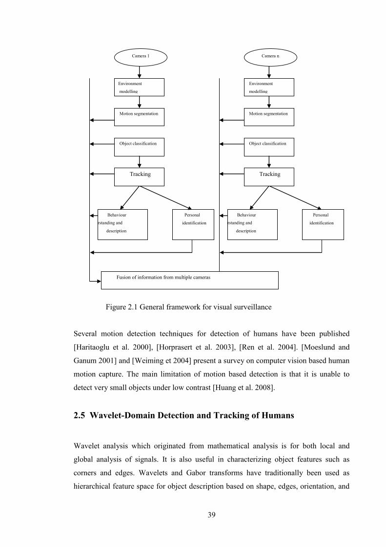
39
Several motion detection techniques for detection of humans have been published
[Haritaoglu et al. 2000], [Horprasert et al. 2003], [Ren et al. 2004]. [Moeslund and
Ganum 2001] and [Weiming et 2004] present a survey on computer vision based human
motion capture. The main limitation of motion based detection is that it is unable to
detect very small objects under low contrast [Huang et al. 2008].
2.5 Wavelet-Domain Detection and Tracking of Humans
Wavelet analysis which originated from mathematical analysis is for both local and
global analysis of signals. It is also useful in characterizing object features such as
corners and edges. Wavelets and Gabor transforms have traditionally been used as
hierarchical feature space for object description based on shape, edges, orientation, and
Fusion of information from multiple cameras
Personal
identification
Behaviour
understanding and
description
Camera n
Environment
modelling
Motion segmentation
Object classification
Tracking
Personal
identification
Behaviour
understanding and
description
Camera 1
Environment
modelling
Motion segmentation
Object classification
Tracking
Figure 2.1 General framework for visual surveillance
40
texture, and for detection of very small objects embedded in Gaussian noise [Strickland
and Hee 1997]. Wavelet analysis applies wavelet filters to decompose images into
subbands, providing multi-scale representation of objects features at different level of
details. Certain class of wavelet transforms are invariant to affine transform, rotation,
and translation and thus provides object detection under these movements. Typically
extracted features are typically fed unto a classification system for object discrimination
For relatively small size objects embedded in noisy background, signal detection
techniques such as match filtering and correlation have been used in detecting such
objects as in [Strickland and Hee 1997], [Laine and Fan 1995]. A matched filter may be
viewed as a convolution kernel with a large positive centre lobe for emphasizing objects
surrounded by smaller negative lobes whose purpose is to subtract the background. Peak
performance occurs when the inner window completely encloses the object leaving the
border window in the background region. It has been shown that the biorthogonal spline
wavelet filters closely approximate the pre whitening matched filter for detecting
Gaussian objects in Markov noise [Strickland and Hee 1997]. By definition a wavelet
transform of an image is the correlation between the image and the scaled wavelets.
Most multi-scale edge detectors smooth the signal at various scales and detect sharp
variation points from their first or second derivative. The extrema of the first derivative
corresponds to the zeros crossings of the second derivative and to the inflection points
of the smoothed signal. There exist a class of wavelets which is constructed using
Gaussian scaling functions such that the first and second derivatives are the first and
second derivative of the smoothed signal respectively. These first and second derivative
wavelets can be viewed edge detectors in the wavelet domain. Zero crossing detection
is equivalent to Marr-Hildreth [Marr 1982] edge detection, whereas the extrema
detection corresponds to edge detection [Canny 1986]. An important issue in edge
detection is the scale of detection. Small-scale filters are sensitive to edge signals but
prone to noise, whereas large-scale filters are robust to noise but can filter out fine
details. When the scale is large enough small signal fluctuations are removed, therefore
only sharp variations in sharp points are detected. Hence multiple scales are employed
to synthesize various edge structures [Marr 1982]. Wavelet domain analysis preserves
both the spatial and frequency domain features in images. [Liang and Fan 1995] showed
that weighting by a factor greater than one across all subbands emphasis high
frequencies, weighting a particular subband by a constant effectively enhances mid
range of frequencies. Thus it is also possible to globally enhance the contrast between
41
background and foreground objects. It is shown in [Strickland 1997] that the sum of
LH+HL subband approximates the output of a Gaussian convolution operator. Object
detection and tracking in the scale-frequency domain (wavelet domain) has the
following advantages over analysis in spatial domain; less sensitive to noise, transient
motion, illumination changes, detection of objects irrespective of changes in size, ability
to detect both small and large changes in motion, and reduction in computational load in
object localization in the subband compared to the original frame [Cheng et al. 2006].
There have been several published studies on wavelets analysis for object detection and
tracking, including face recognition, pedestrian and vehicle detection, as well as in
biomedical applications [Benner 1988],[Mallet 1992],[Unser 1995]. [Oren et al. 1997]
proposed wavelet domain template for pedestrian detection, having observed there is
significant variability in patterns and colours within the boundaries of human body in
images, as well as the lack of constraint on the image background. They proposed
wavelet ratio template which defines the shape of human in terms of the subset of the
wavelet coefficients. Non decimated Haar wavelet transform was applied to an image
frame to define an over complete dictionary of wavelet coefficients, where the distance
between the wavelets at scale n is ½* (2n). They interpreted the wavelets coefficients as
indicating an almost uniform area, i.e, ‘no change’, if their absolute value is relatively
small, or as ‘strong change’ if their absolute value is relatively large. The wavelets
coefficients were classified as horizontal, vertical, and diagonal (corner). Haar wavelet
coefficients were used to describe the relationship between the average intensities of
two neighbouring regions. Multi-scale detection was achieved by resizing an object
window of 128 by 64 from 0.2 to 1.5 in steps of 0.1 based on the template matching
using frontal and rear views of humans. The resulting ratio template is independent of
motion or explicit segmentation. It consists of a set of regular regions of different scales
that correspond to the support of subset of significant wavelet functions. Essentially the
template defines a set of inequality relationships between the average intensities of
different regions of the body expressed as constraints on the values of the wavelet
coefficients. An input wavelet template of a candidate window is compared with the
learned pedestrian template which is represented as ratio of coefficients. The matching
value is the coefficient ratios in agreement with the template ratio. [Elzein et al. 2003]
applied motion detection in the pixel domain to first determine time-to-collision in a
pedestrian-based detection system, and followed by object classification in the wavelet
domain using multiple wavelet templates similar to [Oren et al. 1997]. [Jepson et al.

42
2003] developed a three-part wavelet-based appearance model based on steerable
pyramid and an online expectation maximization algorithm. The motivation for using
wavelet filter’s response is the possibility of localizing stable properties spatially, or
restricted to certain scales as in optical flow estimation and stereo disparity [Fleet 1990],
[Fleet and Adelson 1991]. The system successfully tracked human faces in different
poses. A support vector classifier was applied independently to learn significant ratio
template coefficients using bootstrap training to improve detection. Comparison was
made with the wavelet ratio template matching technique. Peak performance of 81.6%
detection rate with one in fifteen thousand windows turning out to be false resulted
when the support vector classifier was used. The template matching scheme achieved a
peak detection rate of 61%, with one in five thousand windows turning out to be false.
However the method is computationally expensive since humans are searched for at
multiple scales in addition to the wavelet transform computation. In another work,
[Cheng et al. 2006] applied discrete wavelet transform on each frame of a video
sequence resulting in four subbands (LL, LH, HL, HH) with different frequency
characteristics. The high pass band (HH) extracts the detailed images which contain
edges, whilst the low frequency components (LL), the average image. The LL subband
of the third level decomposition was used in motion detection using frame differencing
and thresholding, followed by connected component labelling. The features extracted
for each object were its colours (RGB component), statistics (mean and standard
deviations) and bounding box coordinates. A feature queue was created and similarity
metric defined to compare objects in previous frame to the current frame. An object in
the current frame is the same as in the previous frame if the similarity metrics is within
a threshold. However, it had difficulties in tracking slowly moving objects. It was also
observed that motion detection in wavelet domain filters out transient motion and noise.
However, no explicit scheme was used in handling occlusion, although high detection
rates were achieved using video sequences with multiple humans, some of them coming
together. Searching, a time consuming operation was carried out on the subband rather
than the original frame, resulting in reduced search time. If the computational time for
the wavelet transform is less than the time spent in searching for the object then there is
further justification for object detection in the wavelet domain.
43
2.6 Model-Based Detection and Tracking of Humans
Model-based detection and tracking algorithms represents humans using structural
description and geometric constraints. Structural description describes the relationship
between parts that can easily be identified spatially. Geometric constraints in the form
of motion models describe permissible transformations that the structural description
can undergo. Model-based tracking algorithms track objects by matching projected
object models, produced a priori, from image data. The models are usually constructed
based on manual measurements, CAD tools, or computer vision techniques. The general
processing technique in model-based human tracking is known as, analysis-by-
synthesis. First the pose of the model in the next frame is predicted according to prior
knowledge and tracking history. The predicted model is synthesised and projected into
the image plane for comparison with the image data. A specific pose evaluation function
is required to measure the similarity between the projected and the image data. This is
done recursively using a search strategy or by sampling techniques until the correct pose
is finally found, and is then used to update the model. The main issues are;
representation of possible motion models and constraints, and search strategies (for
location and pose estimation). There are four main types of models for humans, namely,
stick figure, 2-D contour, volumetric, and hierarchical models. The stick figure model
consists of lines and circles representing the torso, the head, and the four limbs with
links and joints. The 2-D contour essentially models the projection of 3-D human body
unto the image plane. Volumetric models are 3-D models constructed to model the body
movement. The hierarchical model describes the human body as hierarchy consisting of
skeleton, ellipsoidal meatball, simulating tissues, and fats. More details of human body
models is found in [Weiming et al. 2004]. Accompanying the human body model is the
motion model with motion constraints to reduce complexity in tracking. Several motion
models have been used including Hidden Markov model, multiple description length
coding, and multiple principal component analysis. Search strategies include dynamics,
Taylor models, Kalman filtering, and stochastic sampling. Dynamics involve
application of physical force to each rigid part of the kinematic 3D model to create
dynamical equations of motion. The solution provides the motion parameters
[Delamarrre and Faugeras 2001]. [Bergman and Doucet 2000], [Isard and Blake 1998]
applied Monte Carlo based techniques to object tracking. Particle filter, an inference
44
technique for estimating the unknown motion state from noisy collection of
observations arriving in sequential fashion is also a Monte Carlo based technique. Two
important components of this model are the state transitions and observation models.
Several studies on particle filters have been reported [Zhou et al. 2004], [Peterfreund
1999]. [Karaulova et al. 2000] used a stick figure representation to build a novel
hierarchical model of human dynamics encoded using hidden Markov models (HMMs)
and realize view-dependent tracking of humans. In 2-D contour representation, the
human body segments are modelled by 2-D ribbons or blobs. For instance [Ju et al.
1996] proposed a cardboard human body model, in which the human limbs are
represented by a set of jointed planar ribbons. [Niyogi et al. 1999] used spatio-temporal
pattern in XYT space to track, analyze and recognize walking figures. They examined
the characteristic braided pattern produced by the lower limbs of a walking human. The
projections of head movements are then located in the spatio-temporal domain, followed
by the identification of the joint trajectories, allowing a more accurate gait analysis.
Volumetric models include elliptical cylinders and cones [Delamarre and Faugeras
1999], [Delamarre and Faugeras 2001], spheres and superquadrics. Volumetric models
requires more processing especially during the matching process. [Rohr 1994] used
fourteen elliptical cylinders to model a human body. [Wachter et al. 1997] established a
3-D model using right elliptical cones. The shape of a person is modelled as a set of
polygons using hidden surface algorithm. Region information such as optical flow,
spatio-temporal gray values derivatives, as well as edges to fit the person’s model to the
human model as a search problem based on a high-dimensional figure of merit function
to be optimized. Hierarchical model uses hierarchical human model to achieve higher
accuracy. In [Plankers and Fua 2001] a model is presented which includes skeleton,
ellipsoid meatballs for fats, polygonal surface representing skin, with shaded rendering.
Compared to other tracking algorithms, model-based tracking have the following
advantages: 3-D contour tracking are more robust under occlusion. Other prior
knowledge about humans such as motion, and structure could be combined to improve
robustness. The pose of humans is acquired naturally, after geometric correspondence
between 2-D and 3-D world coordinates, and the 3-D models can be applied when
objects greatly change their orientations. 3-D model-based tracking are appropriate for
applications such as animation, medicine, surveillance, and man-machine interaction.
Tracking and localizing human body accurately in 3-D space is a difficult problem
despite progress on structure-based methods [Weiming et al. 2004]. Recovering of joint

45
angles from a walking human in a video is still difficult, and the computational cost is
also very high.
2.7 Appearance-Based Detection and Tracking of Humans
Appearance-based systems maintain information about each pixel in an evolving model
of the person. Common image appearance models include templates [Frey 2000],
[Olson 2000], view-based sub space models [Black and Jepson 1998], temporally filter
motion compensated images, and global statistics [Birchfield 1998]. Representation of
a feature in the appearance model could be scalar or vector valued consisting of several
features. Under appearance approach there are four representations, namely, active
appearance, multi-view-based, template-based, density-based (multidimensional
histogram), silhouette-based, and region based. SIFT [Lowe 2004] provide scale and
rotation invariant features suitable for object recognition, motion tracking, and
segmentation. Each feature contains 2D location, scale, and orientation. Features are
robustly detected in the present of clutter and has moderate amount of computational
requirements. [Edwards et al. 1998] generate active appearance models by simultaneous
modelling shape and evolving image information over time. Shape is modelled by a set
of landmarks defined by a contour. For each point or landmark an appearance vector
representing colour, texture, intensity, gradient magnitude is stored. There is a training
phase during which appearance is learned from examples. In [Balcells et al. 2003], the
appearance of humans are modelled using a combination of histogram and correlogram
information. A correlogram is a co-occurrence matrix γ(cx, cy, k) that gives the
probability that a pixel at a distance k from a given pixel of colour ci is of colour cj.
Foreground blobs are extracted after codebook based background subtraction developed
by [Horprasert et al. 2003], and likelihood based segmentation using the colour
histogram and correlogram. The first time a person enters the scene a model for the
individual is stored and is also assigned a label. In the subsequent frames models are
updated and the most similar blobs matched using normalized first norm distance. The
system is able to detect when people merge into groups and able to segment them
during occlusion. Occlusion is handled by colour classification as in [Huang et al.
1999], and no assumption is made about the pose of a human. Multi-view appearance
model, on the other hand models the principal views of an object using Eigen space
46
[Black and Jepson 1996], principal component analysis, or independent component
analysis [Moghadam and Pentland 1997]. Template matching is a brute force method of
tracking. It searches for a region similar to an object template defined in the previous
frame [Jurie and Dhome 2001] in the current frame based on an optimizing function.
Templates could be based on colour, intensity, and directional gradient image.
Limitations of template matching are the high computational cost, and the need for
multiple views (templates) to improve robustness. [Kang et al. 2004] used histogram of
colour and edges as object models. Histograms were generated from concentric circles
to achieve rotation, translation and scale invariance. A matching score was computed
using distance measures such as Kullback-Leibler divergence, and Bhattacharyya
distance. In shape matching a search for the object silhouette in the current frame is
conducted using the previous object silhouette. A match between two silhouettes results
if the matching score was below a threshold. In [Huttenlocher 1993] shape matching is
performed based on Hausdorff distance. The matching score between silhouettes can be
computed using several distance measure including cross correlation, Bhattacharyya
distance, and Kullback-Leibler divergence. To match silhouettes in consecutive frames,
[Haritaoglu et al. 2000] model human appearance using edge information. The edge
model is then used to refine the translation of object using constant velocity assumption.
The object model is re-initialize to handle appearance change in every frame after the
object is located. In [Wu and Nevatia 2006] humans are represented by parts such as
head-shoulder, torso, legs, and full body. Part based representation is used to segment
blobs by considering various articulations and their appearances. First parts are detected
and combined using multi-view detectors trained on Edgelet features [Wu and Nevatia
2005] using boosting technique. The combined response is the union of representation
of its parts and visibility score. If visibility is less than a threshold objects are
considered occluded by other humans. Humans are detected on a frame by frame basis
by the combined multiview detectors ( front and rear view detectors, and left/right view
detectors). An affinity function is defined consisting of part type, size, spatial location,
detection confidence colour, and object visibility. Multiple humans are detected using a
joint likelihood function and occlusion reasoning. The appearance is described by
colour histogram. Two strategies are used in tracking, namely, greedy matching with
data association, and mean shift tracking. Two humans in two consecutive frames are
matched if the average affinity function and the visibility function is above a threshold.
Tracking is implemented in three phases, namely, track initiation, track growing, and
47
track termination. At the track initiation phase tracks are initialised when there is
enough evidence from the detection phase to support the parts and the full-body of the
human. This occurs when an initial computed confidence measure exceeds a threshold.
A track hypothesis is constructed part response function, dynamic model based on
Kalman prediction, and appearance model. For every found human pairs between two
consecutive frames that pass the affinity test, and object visibility test a hypothesis is
generated and the greedy data association technique is applied to establish track
correspondence. Found humans which fail the test, the mean shift tracker is used to
track the individual parts. A likelihood model is constructed from detection probability,
confidence value of the parts, and constant false alarm ratio. The appearance model is
constructed from the initial colour histogram of the part and principal component
analysis to learn the structure of the underlying distribution. Tracks are terminated if no
detection responses are found for an object after a fixed number of consecutive frames.
The main limitations of the approach are that the viewpoint should not exceed 45
degrees, and the resolution not less than 24 X 58 pixels. Region based tracking
techniques on the other hand model object boundary as contours and interior with
suitable appearance feature such as texture, intensity, gradient, etc. Tracking could also
be performed using two different approaches, namely, state-space approach, and energy
minimization. Other reported works include [Isard and Blake 1998], [Terzopoulos and
Szeliski 1992]. In [Bascale 1995] texture is used to represent the interior of objects
which are modelled as deformable templates. The region is parameterized and tracked
by applying 2-D motion model to both the contour and the texture. Matching of current
region with the previous region in the previous frame the best match is obtained by
optimization techniques. A major limitation with region based tracking is that it cannot
handle occlusion very well, and it is also difficult to recover the pose of an object
[Weiming et al. 2004]. The main limitations with appearance based approach are how to
robustly handle occlusion and object splits and merges when the underlying
assumptions fail [Senior et al. 2006].
48
2.8 Shape-Based Detection and Tracking of Humans
Although shape-based detection and tracking is part of silhouette-based techniques, it
deserves a section since numerous studies on shaped based human detection and
tracking, and action recognition has been published. For 2-D shapes several models
exist including discrete shapes, continuous shapes (modelled by compact class
conditional density learned from examples), multipart representation, and shape filters
(edgelets, and shapelets assembled from low level oriented gradients), and
spatiotemporal shapes[Enzweiler and Gavrila 2009]. Application of shape-based
detection and tracking of humans, and their actions in video ranges from generation of
ad hoc models to 3-D models specially construction for motion analysis, and action
recognition. Shape-based object detection and tracking relies on the features of the
perceived shape of an object of interest. Shape as a feature is sometimes used together
with other appearance features such as colour, texture, and edge features, or on its own
as in model based pedestrian detection and tracking. In medical imaging, sports
sciences, and man-computer animation, high precision shape descriptors are required
whilst in human detection for visual surveillance the main the main focus is on detecting
the presence of objects, and precision requirement is secondary. In [Dalal and Triggs
2005] histogram of oriented gradients derived from normalized image orientations is
used in detecting humans. The basic idea being that local object appearance and shape
can be characterised rather well using local intensity gradients. Humans are
characterised using this approach and a model derived using support vector classifier.
The shape context [Malik and Puzicha 2001] used sampled points on object shapes
described by edges, to define a distribution relative to the reference point as a global
means of discriminating points along the shape. First global correspondence is
established by using an aligning transform, and a shape matching similarity metric is
used to measure shape similarity. Shape-based detection has been applied successfully
in several studies on pedestrian detection [Owechko et al. 2004], [Conxia et al. 2007].
Typically morphological characteristics such as strong vertical symmetry of human
shape is exploited to circumvent pose detection problems, and to detect stationary
humans as well. This method allows detection of pedestrians in different poses,
positions and clothing. In [Steffens 1998] pedestrians are detected using a layered
approach and expectation maximization to separate the background from the foreground
49
part of the scene. Shape cue is first used to eliminate non-pedestrian moving objects and
then appearance cue is used to locate the exact position of pedestrians. Templates with
varying sizes are sequentially applied to detect pedestrians at multiple scales to
accommodate different camera distances. A graph matching-based tracking algorithm is
then applied to jointly exploit the shape, appearance and distance information. In [Song
et al. 2006] a model of human shape is used in recognising and tracking humans. Shape
based techniques are able to detect both static and dynamic objects in images sequences,
and are typically appearance based. [Haritaoglu et al. 2000] combines global shape
information and texture template in detecting and tracking multiple person in video
sequence. A comparative study of shape-based retrieval techniques is also provided in
[Dengsheng and Guojun 2001]. An object is typical described using shape primitives
such as lines and curves, and their geometric properties. Texture, edges, points in image
space, and colour may additionally be used to achieve robustness. The presence of
object is then inferred by analyzing and inferring the shape of the object using shape
primitives. Alternatively the whole shape may be learned using machine learning
techniques. Objects are then detected by classifying instances of candidate objects in the
scene. The main problems with this approach are variations in object shape, object
shape visibility, camera motion, background clutter, and motion of other objects in the
scene. Different type of shape descriptors such as contours, edges, feature points,
corners, boxes, silhouettes and blobs are available for classifying moving objects.
Contour tracking on the other hand, evolves an initial contour to its new position in the
current frame by using the state space models or direct minimization of some energy
functional. To track the contour evolution with time requires that the current frame
overlap with the object region in the previous frame. [Chen et al. 2001] proposed a
contour tracker where the contour is parameterized as an ellipse. Each contour has an
associated Hidden Markov Model (HMM) and the state of each HMM is defined by the
points lying on the lines normal to the contour control point. The observation likelihood
of the contour depends on the background and the foreground partitions defined by the
edge along the normal line on the control points. The state transition probabilities are
estimated using Joint probability data association filter (PDAF). Given the observation
likelihood and the state transition probabilities, the current contour state is estimated
using the Viterbi algorithm. After the initial approximation, an ellipse is used to fit and
enforce elliptical shape constraint. VSAM [Collins et al. 2000] takes apparent aspect
ratio of bounding box, image blob area, etc, as key feature and classify moving object
50
blob into humans, vehicles, and clutter using neural network classifier. VSAM classify
objects into single humans, group of people, and vehicles. The real-time visual
surveillance system W4 [Wren et al. 1997] employs a combination of shape analysis
and appearance features for tracking, and construct models of people’s appearances in
order to detect and track individuals, people carrying other objects, and groups of
people, as well as monitor their behaviour even in the presence of occlusion in outdoor
environments. The shape of a 2-D binary silhouette is represented by a projection
histogram. The vertical and horizontal histograms are computed by projecting the binary
foreground region unto the axis perpendicular to and along the major axis. In [Jang et al.
2000] an active template that characterizes regional and structural features of an object
is built dynamically based on shape, texture, colour, and edge features of the region.
Using motion estimation based on Kalman filter, the tracking of a non rigid body by
minimizing the energy function.
2.9 Motion-Based Recognition of Humans
Motion-based recognition technique uses the intrinsic pattern of human motion for
tracking. There are two main approaches. The first approach attempts to characterize
motion itself with reference to known human motion models in order to determine
location or infer behaviour. Behaviour analysis and understanding is considered as a
classification of time varying feature data, i.e, matching unknown test sequence with a
group of labelled reference sequence representing typical behaviour. The first technique
has already been discussed in section 2.4 aims at segmenting regions corresponding to
moving objects from the rest of the image for subsequent analysis, i.e, motion is used as
a cue. In characterising motion itself, objects are detected over many frames and their
trajectories analyzed for periodicity and other cues. By analysing periodicity of motion
from image sequence it is possible to track and predict behaviour as demonstrated in
[Aggarwal 1994]. Gait-based recognition techniques for humans [Takas 1988], [Boser
1992] falls under this category. There are four main ways of viewing human motion
tracking and action recognition. The first one is to recognise action from among a
database of human actions. The second one is to recognise different body parts like
arms, legs, etc, through a sequence of motion labelling. The third defines motion as a
sequence of object configurations or shapes through time (by tracking), and the last use
51
knowledge of shape and motion information of the human body as a guide to the
interpretation of an image sequence to determine a succession of shape modifications.
When transformations applied to a shape correspond with the motion constraints in the
sequence tracking is achieved. In [Lipton 1999] residual flow is used to analyze rigidity
and periodicity of moving objects. In [Bobick et al. 1996], a view-based action
recognition is presented without reference to any feature except motion itself. It is based
on the assumption that a motion model associated with an action is observed when a
known movement is viewed from a given angle. The spatial distribution of motion
integrated over temporal extent, is employed as a filter for associating possible action to
viewing directions based on motion energy. For personal identification, human face and
gait are now regarded as the main biometric identification features that can be used in
video surveillance [Lee et al. 2002]. [Maybank and Tan 2000] used moment features of
image regions to recognize individuals. By assuming that people walk frontal-parallel
towards a fixed camera, the silhouette region is divided into seven sub regions. A set of
moment-based region features is used to recognize people and to predict the gender of
an unknown person by his walking pattern. In [Niyogi and Adelson 1994] the different
motion pattern of head and legs under translation in time-space are used in recognising
humans by fitting unto a figure-stick model. These patterns are first processed to
determine the bounding box of a moving object. Gait signatures are then acquired from
velocity-normalized fitted model, and used in recognition of humans. Among existing
methods are dynamic time warping, finite state machine, hidden Markov model, time
delay neural network, and self organizing neural network. In [Sidenbladh and Black
2000] tracking of human is achieved by projecting 3D motion of the figure in
monocular sequence unto the image plane of the camera using Bayesian framework. A
model is defined in terms of the shape, appearance and motion of the body, and a model
of noise in the pixel intensities. Given these parameter a posterior distribution over
model parameters given observation history is derived. The main difficulty is in
modelling non-linear dynamics of the limbs, ambiguities in the mapping from 2D image
to 3D model, and similarities singularities, among others. Approaches to recognizing
human motion and action can be divided into human action recognition, and motion
based recognition. The former models posture and motion together whilst the later uses
motion as a cue for detection of humans. An interesting work on action recognition
based on motion is presented in [Song et al. 2006].
52
2.10 Summary
Among the object detection and tracking techniques in video, motion detection
combined with other techniques such as object segmentation, view-based classification,
and background-foreground modelling have high accuracy and moderate computational
complexity. The high computational complexity of 3-D model construction and model-
based human detection and tracking makes it less suitable for real-time applications,
whilst its 2-D counterparts with moderate complexity is frequently used in detection and
tracking. In object-based approach, segmentation is applied to detect instances of
interesting objects, whilst in feature-space approach low level features are use to direct a
search in feature space to locate interesting regions. Discriminative features are used by
object based approach to differentiate between different objects, whilst in feature space
approach patch based classifiers examines salient regions, and assign a class to the
hypothetical object at the given location. Verification of the object-based approach
using a confidence measure is then used to confirm the existence of the object. With the
feature-space based approach, similarly, heuristic tests based on the physical
characteristics of the object in the spatial domain may be used to verify the existence of
the object. Appearance-based features include colour distribution, oriented gradient
distribution, silhouette-based features, phase information, texture, and intensity
distribution. Appearance based features combined with shape or silhouette based
features have high accuracy, but typically require regular update, explicit occlusion
detection and object inference techniques under high clutter and low contrast. It is
suitable for both part-based object detection and complete shape-based detection.
Majority of the algorithms for human detection are object based, and consist of the
following sequence of steps: pre processing, motion detection, candidate human
definition, human discrimination (based on physical or appearance features), and human
detection by validation. However there are exceptions: in [Avidan 2005] object
detection and tracking is posed as binary classification problem and detection and
tracking is performed jointly. The background-foreground separation schemes work
well under constant lightning conditions, but unable to cope with sudden changes in
lighting conditions, moving camera, moving background especially when the size of the
moving background compared to the foreground region is very large.
53
The mean shift algorithm, a kernel-based density estimator has been used in both
object detection and tracking with high accuracy in real-time. It provides moderate
complexity and high accuracy when the displacement between object locations is less
than the bandwidth of the kernel density estimator. It is not able to cope with fast
motion which results in no overlap between the kernel locations in consecutive frames.
When the underlying assumption is violated, one option is to use multiple kernels with
different bandwidths, incurring extra computational steps. Statistical object
segmentation techniques such as single Gaussian, multiple-Gaussian model and
expectation maximization have high accuracy, and have been used to model appearance
features and motion. Their main limitations are how to determine the number of
components, slow convergence, high computational cost, and false motion in complex
background. Four main trackers have been identified, namely, region/kernel based
trackers, stochastic trackers (sample based), silhouette based trackers and model based
trackers. Region based trackers use template matching techniques and achieves high
accuracy at the expense of large number of computations. However, its limitation is its
inability to estimate the pose of the object, and small changes in shape and motion. The
main problems with trackers are how to assign measurements to multiple objects when
they are very close to each other or under occlusion.
54
CHAPTER THREE
REVIEW OF DATASETS, PERFORMANCE
METRICS AND STATE OF THE ART
PERFORMANCE ON PEDESTRIAN DETECTION
3.1 Introduction
Performance evaluation in algorithm development is necessary to provide feedback on
quantifiable progress towards automated human detection and tracking, and event
recognition. The main problem with ad hoc approach is exaggerated performance
using dataset which is not representative of the application, and the lack common
performance metrics without which there is no basis for comparison. Thus the first
requirement is availability of standard dataset and performance metrics. The next
requirement is to provide a common site where algorithms can be tested and
evaluated. Since the year 2000, there has been several efforts towards providing
standardised dataset and performance metrics appropriate to specific application
domain. Section 3.1 presents a survey of currently available datasets, whilst section
3.2 presents a review of associated performance metrics for object detection and
tracking.
Sections 3.2.1 to 3.2.7 describe the individual dataset from PETS to Daimlerchrysler.
Section 3.2.8 provides a classification of the dataset. In section 3.2.9 the dataset used
in the current investigation is also described. Section 3.3 discuses metrics for detection
and tracking, and publicly available dataset. Section 3.3.1 to 3.3.5 discusses confusion
matrix, ROC curves, and metrics associated with the dataset. Section 3.3.6 defines
the metrics chosen for the current investigation. Section 3.4 reviews state of the art
performance in pedestrian detection and tracking.
55
3.2 Review of Datasets
The dataset covers single and multiple humans, cars, and other objects. The following
is a brief description of the main datasets available in the public domain:
3.2.1 PETS
The Performance Evaluation of Tracking and Surveillance (PETS) series of
workshops [PETS 2006] was originally sponsored under EPSRC REASON (UK)
project in conjunction with IEEE computer Vision conference with the goal of
evaluating visual tracking and surveillance algorithms in 2000. It was in response to
meet the scientific challenge of devising and implementing automatic systems for
obtaining detailed information about activities and behaviour of people. To date a total
of ten workshops have been held. At every workshop a video dataset is made public to
researchers in order to tackle problems in tracking quantitatively, and submit results to
the workshop. Over the years several dataset has been accumulated and available for
research. Currently performance metrics for motion-based segmentation has been
defined [Aguilera et. al 2005] in the PETS website. The metrics are negative error
rate, misclassification penalty, rate of misclassification, and weighted quality measure.
All the metrics are the sum of two parts: a false positive and false negative scores.
PETS 2006 workshop published several approaches to performance evaluations on
object tracking. PETS 2007 was devoted to activity and behaviour analysis of people
and vehicles (loitering, attended/unattended luggage) in train stations using multiple
camera system. PETS 2009 was devoted to crowd image analysis (crowd density
estimation, tracking of individuals, detection of separate flows in a crowded scene,
and detection of specific crowd events).
3.2.2 i-LIDS
i-LIDs (Imagery Library for Intelligent Detection Systems) is a UK government
initiative to facilitate development of vision based detection systems (VBDS) which

56
meet Government requirements. It was launched in 2006 and deals with events
detection and human tracking. The dataset covers the following scenarios:
Event detection:
Parked vehicle detection
abandoned baggage detection
sterile zone monitoring
doorway surveillance
Object tracking:
multiple camera tracking
Within each event detection scenario certain alarm events are defined. For example in
a parked vehicle scenario if a vehicle is parked in a predefined area for more than one
minute it triggers an alarm event. Video based detection system (VBDS) are required
to report an alarm when any of these events occur in the footage, with minimal false
alarm reports. In object tracking scenarios, individuals or targets identified in the
CCTV imagery are presented to the tracking system. Five CCTV cameras are used to
capture multiple views of the object or target. Object tracking systems are required to
track the target through a network of cameras until the target is either no longer
present or a new target is specified. Tracking systems may be evaluated by HOSDB
for either an overlapping camera or mixed camera role. The overlapping role
comprises cameras 2, 3, and 4, with the mixed role including all the five cameras.
Each dataset scenario is split into three parts; one part is kept by HOSDB (Home
office Scientific Development Branch) for evaluation. The remaining two set is
available to system designers to use to train and evaluate their system. The dataset is
also available for academic research. i-LIDS benchmark data set is based on the F1
measure (see section 3.3.2). The F1 values which must be obtained in order to qualify
for system certification are not made public (i-LIDS user guide 2009). However, i-
LIDS consider events with overall F1 score of 0.75 as meeting evaluation
commissioning acceptance criteria. More information on the evaluation procedure is
available in the i-LIDS user Guide, and the website.
57
3.2.3 CAVIAR
Caviar (Context Aware Vision using Image-based Active Recognition) is an European
Commission (EC) funded research project (IST-2001-37540) to address the
challenge: Can rich local image descriptions from foveal and other image sensors,
selected by a hierarchical visual attention process, guided and processed using task,
scene, function and object contextual knowledge improve image based recognition
process? It was launched in 2002 with the focus of the project on city centre
surveillance, and monitoring of shopping habits of people in order to improve
management of shops. The output of this project has resulted in large dataset which is
available to the public for surveillance algorithm evaluations. However there are no
recommended evaluation metrics (see
http://homepages.inf.ed.ac.uk/rbf/CAVIAR/caviar.htm).
3.2.4 VACE
VACE (Video Analysis and Content Extraction) aims to develop innovative
technologies to perform autonomous analysis on large volumes of video, multimodal
fusion, and event understanding. It was launched in 2000 and sponsored by Advanced
Research and Development Activity (ARDA) in United State of America. It focuses
on detection and tracking of mobile objects such as pedestrians and vehicles from
video sources such as television news broadcasting and Un-manned air vehicles.
Surveillance is one of the application domain. Surveillance events are classified as
person walking, running, or jumping. Action is recognised using multiple agents.
Tracking, events detection and surveillance applications use video sequences for
evaluation.
3.2.5 TRECVID
TRECVID TRECvid (Text REtrieval Video Retrieval Evaluation) is a text-retrieval
conference (TREC)-style video analysis and retrieval. It was launched in 2001 and
sponsored by Intelligence Advanced Research Project Activity (IARPA), and US
58
department of Homeland Security. It consists of several tasks classified under video
summarisation, feature-based searches/retrieval, and surveillance event detection. It
uses a subset of the i-LIDS dataset for surveillance event evaluation. The surveillance
task is meant to track a specified person or multiple people in an airport scenario using
both single and multiple cameras. TRECvid 2009 was co-sponsored by Home Office
Scientific Development Branch (HOSDB) and centre for the protection of national
infrastructure (CPNI). Events such as detection of direction of flow of people in
airport scenario (OpposingFlow), people splitting up from a group (PeopleSplitUp),
people meeting to form a group (PeopleMeet) were tracked. Gestures such as pointing,
embracing, running were also monitored. Data was collected from major airports in
the UK by HOSDB. It is split into development and evaluation sets. The main
performance measure used in the evaluation is the Normalized Detection Cost Rate
(NDCR). NDCR is a weighted linear combination of the miss detection probability,
and the false alarm rate (measured per unit time).
3.2.6 PASCAL Visual Object Classes (VOC) Challenge
Pattern Analysis, Statistical modelling, and Computational Learning (PASCAL) Video
Object Class (VOC) Challenge is a yearly contest which started in 2005. PASCAL
VOC 2010 contest is sponsored by network of excellence on PASCAL, and the
European Union (EU). The dataset is part of a benchmark whose objective is to
investigate methods of object recognition in a wide spectrum of natural images. It
consists of the following tasks: object classification, detection, segmentation, person
layout description, and action classification (Everingham and Gool 2008). Since it
shares common tasks with video surveillance (classification, detection, and
segmentation) it is relevant to video content analysis. The 2010 object class covers
twenty objects including person, horse, bicycles, cars, and cat. Any of listed object
classes, for example a person, could be selected for both classification and detection.
The classification task requires that for each test image the class of any of the objects
of interest is indicated, as well as the classifier confidence value. For the detection task
the bounding box and the confidence value of the detected object is required for
evaluation. The evaluation is based on average precision computed from precision-
recall curves by ranking of the confidence value. The average precision is computed
59
by evaluating the area under the curve by numerical integration. The detection task is
based on an area overlap between the ground truth and the found object. It is required
that the overlap must be more than 0.5, otherwise it is a miss detection. The
segmentation task follows detection, and assigns pixels to the object or the
background within the bounding box of the found object.
3.2.7 Daimlerchrysler
The dataset is meant for generic pedestrian detection in outdoor environment. It was
recorded at various (day) times and locations with no particular constraints on
pedestrian pose or clothing except that pedestrians are standing in an upright position
and are fully visible. The training and test set consist of four thousand and eight
hundred (4800) pedestrian samples each. The dataset is further split into five fully
disjoint sets, three for training and two for testing during experiments. There are five
hundred non pedestrian samples each for training and testing. There are additional one
thousand and two hundred images of non pedestrians for more training if required.
Classifier performance is evaluated by ROC (receiver operating characteristic) curves
which quantify the trade-off between detection rate and false positive rate (see section
3.3.1). Cross validation is used over the training set to determine optimal setting for
algorithmic parameters. The stopping criteria used during training in the original
benchmark was fifty percent false positive rate at detection rate of ninety-nine and half
percent (99.5%). Three detection and false positive rates for a given classifier
algorithm is realised by selecting two out of the three training set to design a classifier,
realising three different classifiers. The three classifiers are then tested on each of the
two training set. Performance of classifier algorithms are evaluated by computing the
mean detection rate at 95 percent confidence interval as given by equation 2.1.
.1.2S*05.1y≈y NS
1-N,2/
N=6, and t denotes student t-distribution at 1-α=0.95. y and S denote the estimated
detection rate and the standard deviation respectively. Hence the estimated standard
deviation S of the detection rate represents 95% confidence interval.

60
Table 3.1 shows the main publicly available benchmark for image and video content
analysis. It is ordered by its relative importance to human detection and tracking. The
first six is geared towards tracking applications, whilst the last one is towards
classification, retrieval and recognition.
3.2.8 Dataset classification
The dataset could further classified as single-frame or multi-frame based, computer
vision based or surveillance based, and academia-based or industry-based as follows:
Single Frame (computer vision based/retrieval/object recognition)
PASCAL VOC Challenge, Daimlerchrysler data set
Multi frame (People and event related)
PETS -- Tracking and event detection
i-LIDS-- object detection (cars, humans, aircraft and associated
monitoring
TRECVid--People monitoring (individuals, groups), and
associated events in offices. Evaluation is based on F4DE by NIST
Table 3.1 Publicly available benchmark for classification,
detection, tracking and activity recognition
Benchmark People Vehicle Animals Objects
PETS
i-LIDS
CAVIAR
VACE
TRECvid
Daimlerchrysler
PASCAL
challenge
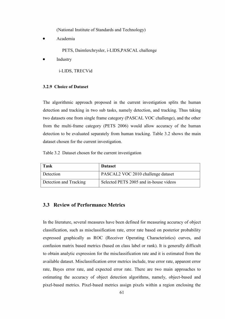
61
(National Institute of Standards and Technology)
Academia
PETS, Daimlerchrysler, i-LIDS,PASCAL challenge
Industry
i-LIDS, TRECVid
3.2.9 Choice of Dataset
The algorithmic approach proposed in the current investigation splits the human
detection and tracking in two sub tasks, namely detection, and tracking. Thus taking
two datasets one from single frame category (PASCAL VOC challenge), and the other
from the multi-frame category (PETS 2006) would allow accuracy of the human
detection to be evaluated separately from human tracking. Table 3.2 shows the main
dataset chosen for the current investigation.
3.3 Review of Performance Metrics
In the literature, several measures have been defined for measuring accuracy of object
classification, such as misclassification rate, error rate based on posterior probability
expressed graphically as ROC (Receiver Operating Characteristics) curves, and
confusion matrix based metrics (based on class label or rank). It is generally difficult
to obtain analytic expression for the misclassification rate and it is estimated from the
available dataset. Misclassification error metrics include, true error rate, apparent error
rate, Bayes error rate, and expected error rate. There are two main approaches to
estimating the accuracy of object detection algorithms, namely, object-based and
pixel-based metrics. Pixel-based metrics assign pixels within a region enclosing the
Table 3.2 Dataset chosen for the current investigation
Task Dataset
Detection PASCAL2 VOC 2010 challenge dataset
Detection and Tracking Selected PETS 2005 and in-house videos

62
detected object either as part of the object or the background. There are two main
approaches to object-based approach, namely, area-based metrics for bounding box,
and distance-based metrics for point based annotations. Area-based metric is based on
spatial overlap between ground truth objects and system output objects to generate a
score. [Manohar et. al 2006] use the metric (Sequence Frame Detection Accuracy,
SFDA) to capture both the detection precision (misses and false alarms) and the
detection precision (spatial alignment). Similarly for tracking, both the tracking
accuracy (number of correctly tracked objects) and the tracking precision (spatial and
temporal accuracy) are measured in a single score (Average Tracking Accuracy). Miss
detection rate versus false positive rate per window is use to evaluate the accuracy of
human detection [Dalai and Triggs 2005]. Miss rate (see equation 2.6) is plotted
against false positives per window plotted on log-log scale. Another measure is the F1
measure which is the harmonic mean between the Precision and Recall (see section
3.2.2). Thus it takes into consideration the ideal detection rate and that realised by an
algorithm. The accuracy of these measures is determined by evaluating the area under
the precision-recall curve.
3.3.1 Confusion Matrix Based Metrics for Detection and Tracking
A confusion matrix [Gunther and Benz 2000] contains information about actual and
predicted classes assigned by a classification system. In pattern recognition, a
confusion matrix is used to represent beliefs in assigning classes to observed patterns
in which the i,jth element represents the number of samples from class i which were
classified as class j. Performance of such systems is commonly evaluated using the
data in the matrix. Its reliability is measured by kappa statistics [Byrt et al. 1988]. The
simplest way of measuring object detection and tracking accuracy is to assign detected
objects into crisp categories, resulting in categorical classification if detailed accuracy
assessment is not important, as is the case with confusion matrix based metrics. Table
3.3 shows a two by two confusion matrix with categorised labels for a binary
classifier.

63
The entries in the confusion matrix have the following meaning:
--TN is the number of correct predictions that an instance is negative.
--FN is the number of incorrect predictions that an instance is positive;
--FP is the number of incorrect predictions that an instance is negative;
--TP is the number of correct predictions that an instance is positive.
The following are the basic standard terms defined for the two class matrix:
--The true positive rate (TPR) or recall is the proportion of positive cases
that were correctly identified, as calculated using the equation 2.2.
TPR=TP/(FN+TP) 2.2.
--The false positive rate (FPR) is the proportion of negatives cases that
were incorrectly classified as positive, as calculated using the equation 2.3.
FPR=FP/(TN+FP) 2.3.
--The true negative rate (TNR) or specificity, is defined as the proportion of
negatives cases that were classified correctly, as calculated using the equation 2.4.
TNR=TN/(TN+FP) 2.4.
--The false negative rate (FNR) is the proportion of positives cases that were
incorrectly classified as negative, as calculated using the equation 2.5.
Predicted (Observed)
Negative Positive
Actual Negative TN FP
Positive FN TP
Table 3.3 2 X 2 Confusion matrix table
64
FNR=FN/(FN+TP) 2.5.
The following complementary relations hold:
TPR+FNR=1 2.6.
TNR+FPR=1 2.7.
Other measures are:
-- Accuracy (AC) is the proportion of the total number of predictions that were correct.
It is determined using the equation 2.8.
AC=(TN+TP)/(TN+TP+FP+FN) 2.8.
-- False discovery rate (FDR) is defined as:
FDR=FP/(FP+TP) 2.9.
--Negative predictive value (NPV) is defined by equation 2.10.
NPV=TN/(TN+FN) 2.10.
--Positive predictive value (PPV) or precision is defined as:
PPV=TP/(TP+FP) 2.11.
The following additional complimentary relation hold:
FDR+PPV=1 2.12.
3.3.2 F1 Measure for Detection and Tracking
In information retrieval the influence of recall on precision is evaluated by computing
the harmonic mean of precision and recall. The F1 measure is used in information
65
retrieval [Van Rijsbergen 1979] and it is defined by equation 3.13.
Fß = (1+ ß2) (precision * recall) /(ß *precision + recall) 3.13.
ß is the weight associated with precision. The F1 measure is defined for the special
case where ß=1. Typically in event retrieval in VCA higher detection rate (TPR) is
achieved at the expense of higher probability of false detection (FPR). To achieve a
balance between TPR, which evaluates the performance of the system without taking
into consideration any error, and FPR, which measures the false detection probabilty
in using the system the F measure is used.
i-LIDS uses a combination of F1 and area overlap test to evaluate event detection
and object tracking performance. The defintion for F1 for event detection is given by
equation 3.14. The recall bias (α) which is equivalent to ß, selectively weighs recall
relative to precision is user defined. α takes on values between zero and one.
F1=[(α+1)Precision*recall]/[recall+α*precision] 3.14.
On substituting the basic definitions above into equation 3.14 and simplifying gives
equation 3.15.
F1=(α+1)*TP/(TP+ αTP+FP+ αFN) 3.15.
From equation 3.15 higher values of FP and FN reduces the value of F1, i.e,
negatively influences the measure.
An object based approach is adopted in i-LIDS for object tracking with α set to
one. The following are the criteria for the basic categories used for object tracking:
Let GTP: Total number of ground truth pixels;
TTP: Total number of tracker pixels;
OP: Total number of overlapping pixels;
True positive (TP) event occurs if there is an area overlap between the ground truth
66
and found object, and additionally
if F1>=0.25 and TTP<3 * GTP 3.16.
False negative (FN) event occurs:
if F1<0.25 and/ or TTP> 3* GTTP 3.17.
False positive (FP) event occurs
if F1< 0.25 and precision< 1 3.18.
Further a system output that produce a very small bounding box (less than 10% of the
ground truth is classified as FP. An overall F1 metric is aslo computed for each object
over the duration of its existence. The average precision is also computed and
expressed in percentage as given by equation 3.19.
Average recall (express in percentage)=Recall *100 3.19.
In object tracking F1 thus evaluates the accuracy of an object on a fame-to-frame basis,
and the average for the existence of the object.
3.3.3 ROC (Receiver Operating Characteristics) Curve for Detection
and Tracking
An alternative to confusion matrix based metrics is the ROC curve (Erkel et al. 1998),
(Centor et al. 1985). It is generated by paired values (Pd, Pf) where Pd is the probability
of correct signal detection, and Pf is the probability of false alarm, i.e, false detection.
Both parameters depend on the values of the parameters regulating behaviour of the
decision module. It was introduced into decision theory as a tool for signal-processing
applications [Trees 1968], and now used to measure accuracy of classifiers and
detectors. The area under the curve gives the probability of correct detection given that
the priori probability of detection is 50%. Global performance is obtained by plotting
67
Pe=(1-Pd+Pf)/2 against different values of detection rate, Pd, under a set of operating
constraints. In object detection task true positive rate may be plotted against the false
alarm rate on the x-axis, or the logarithm of a metric which evaluates the detection rate
versus the false alarm rate. The ideal curve for a binary detector is concave. ROC
points are typically interpolated between measured values if it parametric curve is
known.
3.3.4 PASCAL VOC Average Precision Measure for Classification and
Detection
The basic measure use in computing average precision is the confidence value
associated with the object classification and detection. Firstly a ranking (percentiles)
in ascending order based on the confidence value is produced. Precision is defined as
the proportion of all examples whose ranking exceed a given percentile, and are from
the positive class (humans). In the case of object detection, an area overlap ratio
between the ground truth object and the predicted object (see equation 3.27) of more
than 0.5 to be a true positive, otherwise it is treated as false positive. The precision-
recall curve is produced by computing the precision at a set of eleven equally spaced
recall levels [0, 0.0, 0.2, 0.3, 0.4, ... 1]. The precision at each level is interpolated by
taking the maximum precision measured for a method for which the corresponding
recall exceeds r as defined by equation 3.20. The average precision is defined by
equation 3.20.
Average precision (AP)=(1/11)*∑Pinterp(r) 3.20.
R takes on the values listed above.
3.3.5 PETS 2005 Metrics for Tracking
Tracking involves complex interactions between object-background, and object-to-
object resulting in splits merges and occlusion. Towards evaluating these complex
interactions the PETS (Performance Evaluation of tracking and Surveillance)
68
workshops was set up. Papers submitted by several groups have proposed different
metrics to capture object interactions and evaluate object tracking performance for
surveillance. Two main types of metrics have been proposed, namely, frame-based
and object based metrics. Frame-based metric applies to objects in individual frames.
Each frame is evaluated individually in terms of the number of objects, their sizes, and
locations. Performance is then evaluated by averaging over all the test frames. On the
other hand object-based approach considers the trajectory of object in the frame
sequence (both spatially and temporally) where individual objects are detected and
tracked over their lifespan as separate entities. Temporal overlap is defined as the ratio
of the number of frames where the spatial overlap is met to the number of frames
where the object is observed. Both object-based and frame-based metrics are used in
evaluating video surveillance applications in PETS 2006 (Devijver and Kittler 1982).
Objects are described using either a rectangular bounding box or the actual shape of
the object. Two bounding boxes are said to be coincident if the centroid of one of the
boxes lie inside the other. The PETS metrics in the current investigation is based on
definitions provided in [Bashir and Porikli 2006]. The Frame based metrics are
slightly different from confusion matrix measures (defined above) since multiple
detection events and single detection events occurring within a particular frame are not
differentiated. In frame-based approach a TP event occurs if at least a human is
detected in the frame, otherwise it is classed as FN. An area ratio (spatial) overlap
criteria is used in defining a TP event in object-based approach. In object-based
approach the average overlap over the definition of a track is used in defining TP
event. The averages of the metrics are also computed over the duration of tracking. It
uses both spatial overlap and temporal overlap criteria to detect a track associate with
an object. The following metrics are also defined for tracking: Track detection rate,
track false alarm rate, and average area overlap.
The average area overlap is defined by equation 3.21.
Overlap(k)=area(Bp∩Bgt) /area(Bp U Bgt) 3.21.
Bp and Bgt denotes bounding box for human predicted by the algorithm (application)
and labelled by the ground truth respectively. ∩ and U denotes the intersection and
69
union operations respectively. The average positional error is defined by equation
3.22.
APE= (∑ (B(k) *(G(Xf,k) –Xf,k) 2 + B(k) * (G(Yf,k) –Yf,k) 2 )) /Nrg
3.22.
where, subscript f denotes the frame index, G(Xf,k) denotes the X-coordinate of the
ground truth frame object with index k, similarly G(Yf,k) denotes the y-coordinate of
ground truth object with index k, and Nrg denotes the number of objects in the current
ground truth frame. The summation is over all the objects in the current frame with no
multiple object matching allowed. The average merge error is defined such that for
every one ground truth object there is a possibility of multiple predicted object
matches, i.e, one-to-many relations. Similarly the average fragmentation error is
defined to allow one–to-many matches for predicted to ground truth matches. Detailed
discussion of tracking metrics, is provided in [Brown et al. 2005], [Bashir and Porikli
2006]. Table 3.4 is a summary of the main performance metrics associated with the
publicly available dataset.
3.3.6 Choice of Benchmark Metrics for Performance Evaluation
The following criteria were used for human detection:
A minimum area overlap (see equation 3.21) criteria of 0.5 is used to define true
positive instance, otherwise it is treated as false negative instance in both detection
and tracking scenarios (PASCAL VOC 2010 challenge).
Euclidean distance constraint: The maximum Euclidean distance between the
centroid of the ground truth (Xg,Yg) and the system found human (Xs,Ys) half the
width and height of the bounding box (Generic requirement for overlap).
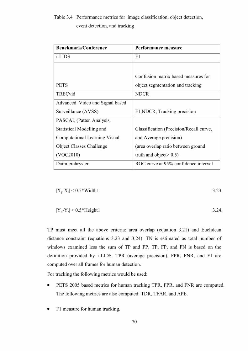
70
|Xg-Xs| < 0.5*Width1 3.23.
|Yg-Ys| < 0.5*Height1 3.24.
TP must meet all the above criteria: area overlap (equation 3.21) and Euclidean
distance constraint (equations 3.23 and 3.24). TN is estimated as total number of
windows examined less the sum of TP and FP. TP, FP, and FN is based on the
definition provided by i-LIDS. TPR (average precision), FPR, FNR, and F1 are
computed over all frames for human detection.
For tracking the following metrics would be used:
PETS 2005 based metrics for human tracking TPR, FPR, and FNR are computed.
The following metrics are also computed: TDR, TFAR, and APE.
F1 measure for human tracking.
Benckmark/Conference Performance measure
i-LIDS F1
PETS
Confusion matrix based measures for
object segmentation and tracking
TRECvid NDCR
Advanced Video and Signal based
Surveillance (AVSS) F1,NDCR, Tracking precision
PASCAL (Patten Analysis,
Statistical Modelling and
Computational Learning Visual
Object Classes Challenge
(VOC2010)
Classification (Precision/Recall curve,
and Average precision)
(area overlap ratio between ground
truth and object> 0.5)
Daimlerchrysler ROC curve at 95% confidence interval
Table 3.4 Performance metrics for image classification, object detection,
event detection, and tracking
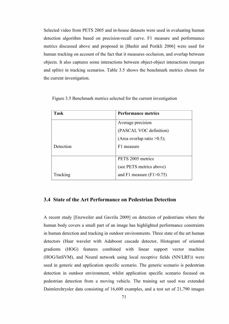
71
Selected video from PETS 2005 and in-house datasets were used in evaluating human
detection algorithm based on precision-recall curve. F1 measure and performance
metrics discussed above and proposed in [Bashir and Porikli 2006] were used for
human tracking on account of the fact that it measures occlusion, and overlap between
objects. It also captures some interactions between object-object interactions (merges
and splits) in tracking scenarios. Table 3.5 shows the benchmark metrics chosen for
the current investigation.
3.4 State of the Art Performance on Pedestrian Detection
A recent study [Enzweiler and Gavrila 2009] on detection of pedestrians where the
human body covers a small part of an image has highlighted performance constraints
in human detection and tracking in outdoor environments. Three state of the art human
detectors (Haar wavelet with Adaboost cascade detector, Histogram of oriented
gradients (HOG) features combined with linear support vector machine
(HOG/linSVM), and Neural network using local receptive fields (NN/LRF)) were
used in generic and application specific scenario. The generic scenario is pedestrian
detection in outdoor environment, whilst application specific scenario focused on
pedestrian detection from a moving vehicle. The training set used was extended
Daimlerchrysler data consisting of 16,600 examples, and a test set of 21,790 images
Task Performance metrics
Detection
Average precision
(PASCAL VOC definition)
(Area overlap ratio >0.5);
F1 measure
Tracking
PETS 2005 metrics
(see PETS metrics above)
and F1 measure (F1>0.75)
Figure 3.5 Benchmark metrics selected for the current investigation

72
(640X480) with 56,492 manual labels, and 259 trajectories of fully visible pedestrians.
Temporal integration of detection results via tracking was used to suppress spurious
false positives. Performance was evaluated at the frame and track level using
sensitivity, precision, and false positives per frame, and reduction in false positives per
frame after tracking. An area overlap ratio (see 3.27) is used in defining true positives.
Frame level performance was visualised using ROC curves. Peak detection rates of
more than ninety-five percent for all three detectors are observed from the ROC curve
for the generic scenario. However, the problem of high false positives remains. For
example at a detection rate of 70 percent, false positives per frames for HOG/linSVM
detector was 0.045, compared to 0.38 and 0.86 for the wavelet-based cascade and
NN/LRF. Thus higher false positives are expected as they approach the peak detection
rate. In the case of application specific scenario the best performance of six false
trajectories per minute at a detection rate of sixty percent was achieved by the
wavelet-based cascade. However the required target performance is eighty percent
trajectory level detection, and a false alarm per ten hours of driving in urban traffic.
Table 3.6 provides a summary of peak performance for person classification and
detection task based on PASCAL2 VOC challenge 2010 and the above study.
Table 3.6 Peak performance of human classification and detection
Task Dataset Peak performance
Classification PASCAL2 VOC 2010 89.5% (Average precision)
Detection PASCAL2 VOC 2010 47.9% (Average precision)
Detection
Extended Daimlerchrysler
dataset 95% (detection rate)
73
CHAPTER FOUR
REFINEMENT OF RESEARCH OBJECTIVES
AND STRATEGY
4.1 Introduction
Human detection is investigated as pattern recognition problem based on classifiers
trained to discriminate humans from non human class in pattern spaces. It combines
motion detection and object detection techniques in video. Tracking on the other hand
is posed as optimum temporal linking of found humans in consecutive frames based
on probabilistic data association, with investigations centred on reduced complexity
implementation. In order to assess the robustness of feature-space based detection, two
features spaces are investigated via pattern classifiers, namely, shape and wavelet
spaces without any assumptions about scene complexity. Most spatial domain
detection techniques on the other hand are based on computer vision and statistical
techniques with assumptions about scene background. Thus comparative study of the
effect of scene background factors with object based detection algorithms in the space-
time domain, and proposed detection algorithm is evaluated. However, the tracking
phase is implemented in the space-time domain, focusing on point-based feature
tracking of humans using the centroid of the bounding box. The centroids are initially
obtained from the output of the detector, and is based on two frames (previous, and the
current frame). It is refined in course of tracking to reduce positional errors. A pattern
space human detector is expected to: detect by parts such as head, upper body, lower
body, arms, and legs, as well as detecting under full human appearance.
The tracking phase primarily provides trajectory information for found humans
over several frames. Since some of the centroids found by the detector are false
positives, and additionally higher detection rate is usually achieved with higher false
detection rate, there is a need to reduce the false positives. In order to reduce false

74
detections it is proposed to use the tracking phase to investigate whether there could
be a reduction in false alarms during tracking. It is supported by fact that if tracking
decisions are made based on more than one frame in the past, it results in improved
detections compared to those based on the previous frame only.
The investigations are aimed at detecting the presence of humans in upright
posture, and no assumptions are made about the camera motion. The input video
sequences are monocular with only one channel of input video. The viewing angle
between the ground plane and the top of the human should be less than 60 degrees.
Extension to multiple video bit streams is provided by considering processing
scalability. Achieving real-time performance and anomalous behaviour detection are
not considered in the current project but relevant research issues are highlighted in the
conclusion chapter. Section 4.2 provides the motivation leading to the investigation
into shape-based descriptors for human detection. Section 4.3 refines the objectives,
whilst section 4.4 the strategy in the light of the findings in chapter two.
4.2 Motivation for the Choice of Shape Features for Human
Detection and Tracking
Geometric features of humans are nearly always observable in image space, thus they
provide a reliable means of human detection. This is due to its insensitivity to colour
and texture, and invariance to scaling and translation. Typical shape descriptors are
silhouettes and shape-outlines. These in turn may be described by intermediate feature
primitives such as lines, corner points, and curves. They in turn may be described by
low level features such as edges. Features of humans in spatial and image-transform
domain for detection, albeit, sharing some of the features with the background are
investigated to synthesise classifiers to discriminate humans from its background. The
background class thus refers to any object in the scene which is not human but might
be significant in the scene. Two proposals, namely, the use of frequency distribution
of co-occurring primitive wavelet features, and low complexity shape-outline
descriptor to model the human and the background classes are investigated. A
discriminant function based on similarity or mismatch measure is used for
differentiating the human from the background class. The alternative approach of
looking for unique features between the human and background class is not
75
investigated since shape based features are robust. Histogram techniques in wavelet
domains have also been applied in related studies in image retrieval [Mandal and
Aboulnasr 1999], object detection [Schneiderman and Kanade 2000], and object
tracking [Huwe and Niemann 1998]. Histogram techniques further, on account of its
low complexity for low dimensional vectors (up to two), makes it a good choice for
human detection. It estimates the underlying probability density function describing an
object category.
The filter bank implementation of wavelet transform acts as a hierarchy of
detectors at discrete object scale [Strickland and Hee 1997]. Wavelet template was
applied to object detection by [Papageorgiou and Poggio 1999]. Over complete Haar
wavelet transform was applied to images with no feature selection. The resulting
subbands were trained using support vector machine. Peak detection rate of more than
90% with false alarm rate of one per ten thousand windows examined was achieved.
The system was later deployed in DaimlerChrysler S class demonstration vehicle for
pedestrian detection. However in (Oren et. al 1997) the shape of an object is described
be a subset of wavelet coefficients. Wavelet template defines the average intensity of a
region with respect to its neighbours using three types of Haar wavelet supports.
Feature selection was achieved by statistical analysis of wavelet coefficients. The
system achieved a pedestrian detection rate of 52.7% with false positive rate of one in
every five thousand windows examined. The effect of wavelet space in filtering out
false motion has also been demonstrated [Yunqiang et al. 2001]. The histogram of
oriented-gradient [Dalai and Triggs 2005] uses a dense grid of uniformly spaced cells
with overlapped local contrast normalization cells for improved performance. The
large number of oriented gradient magnitudes uses block normalization technique to
improve invariance (against illumination and shadows), incurring additional
computations. Finally support vector machine is use to train the classifier using
examples for the human and background class. The histogram captures the normalized
gradient magnitude over orientations between zero and one hundred and eighty
degrees. Very high detection rate with low false positive rate in pedestrian-based
applications [Munder and Gavrila 2006] has been reported. Most shape-based
detectors search for objects at multiple scales by sliding object window (a rectangular
patch of the image) across the image. This also incurs high computational cost in
object localization. Object detection/ recognition is still a challenge in arbitrary image
76
context. Another challenge involves low resolution video surveillance involving
multiple human tracking. For example, the maximum average precision reported in
PASCAL challenge [Mark and Luc 2010] is 48% for human detection. It is 16% in
Caltech 101 dataset [Fei-Fei et al. 2004]. The general conclusion is that higher
detection rate and low false positive rate could be achieved by taking the background
context into consideration as in video where typically higher detection rate has been
reported. It is clear that accuracy varies from one dataset to another, and also depends
on the evaluation modality.
While SIFT features [Lowe 200] provide a general technique for identifying
salient features points invariant to scale and rotation, computationally large number of
operations are required per feature point, as well as large number of feature points. A
good feature space additionally is required to be able to provide unique features which
characterises the object of interest, although in practice features may be shared by the
background class. In absence of unique features co-occurrence of a set of features in
the object regions, and density estimation techniques may be to model an object class
if the underlying distribution of these features is different from the background class.
The shape context [Belongie et. al. 2001] at a reference point captures the
distribution of other feature points relative to it. It offers a globally discriminative
characterization of shapes. It provides a means of comparing two shapes for point-to-
point correspondence: corresponding points have similar shape context. Dissimilarity
between two shapes is computed as the sum of matching errors between
correspondence pair. Finding correspondence between two shapes means finding
points that have the same shape context. However shape matching is posed as tripartite
graph matching introducing algorithmic complexity
On the other hand silhouette descriptors for object boundaries require less number
of primitive to adequately describe the contour. For example a 2-D silhouette of
objects requires sixteen possible blocks of two by two binary shape primitives. The
only requirement is that most of the object boundary must be visible. Contour-based
shape descriptors also suffer from the problem of noise and scale changes although
level set and snake minimization algorithms have achieved high tracking accuracy in
human tracking. Investigation into suitable low complexity shape-outline extraction
and matching in the shape-space is via shape prediction by feed forward neural
network is motivated by the above observations.
77
4.3 Objectives
The main research themes are summarised as: on improving accuracy independent of
scene content; Improving reliability by predicting operating accuracy; improving
performance scalability, and improve timeliness by predicting real-time performance.
Additionally the following objectives have emerged:
1. Investigate salient feature localization techniques to reduce search time in
feature space. The output is the creation of salient (foreground) feature maps and
extraction of candidate humans. This relates to objective one.
2. Investigate the use of tracking phase to reduce false alarms. This objective is
related to objective two.
3. Use of PETS and iLIDS based metrics for accuracy evaluation. This is in
addition to the use of confusion matrix based measures and ROC curves, and it
is related to objective five.
4. Evaluate accuracy of propose detectors on single shot images using PASCAL2
VOC challenge benchmark (objective five).
5. Comparative accuracy evaluation human detection stage with Gaussian mixture
based segmentation and the proposed human detection algorithm. This is related
to original objective five.
6. Comparative accuracy evaluation of proposed JPDAF tracker with mean shift
tracker. This is related to the original objective five.
7. Investigate scheduling strategies to improve application performance scalability.
This involves scheduling for frame based processing sub tasks, and for window
(patch) based processing sub tasks. This is related to objective four.
8. Theoretical investigation on meeting timeliness and throughput requirements.
This is related to objectives four.
4.4 Strategy
The main focus is on feature extraction, optimal classifier design for human detection,
optimal JPDAF tracker design, operating accuracy prediction, synthesis of scalable
algorithmic architecture, and scheduling strategies to improve scalability. At the
78
feature extraction phase suitable shape-space and wavelet domain representation are
investigated. Optimal search strategies are also investigated to enable rapid
localization of salient feature regions as candidate windows. At the salient feature
localization stage the number of features in the feature space is reduced such that only
the most important cues likely to contain humans are retained. A search is conducted
using the salient feature map to determined candidate humans. Thus it aims to retain
minimum number of features required to locate humans. A patch classifier is
subsequently used to discriminate between the human and the background class given
an object window. It returns a hypothesis assigning the window to a human or non
human class. It additionally returns the centroid of the found human relative to the
patch. Linear discriminant test is applied to newly found human windows in addition
to pixel count, and size thresholds to further validate humans found by the classifier.
The detection phase has the following processing steps: pre processing, feature
extraction, salient feature localization, human discrimination, and validation. The
shape-outline and the wavelet domain classifiers are only used at the discrimination
stage. The detection stage thus entails the following four steps:
(1) Pre processing
Frame enhancement
Median filtering to remove impulse noise
Saturation control for brightness adjustment
Histogram Equalization for contrast enhancement
Illumination normalization to compensate for non uniform illumination
(2) Identify candidates
Feature extraction
Shape-outline map construction
Wavelet based feature map construction
Candidates localization
Foreground (salient) shape-outline map construction
(by feature rejection and filtering)
Foreground (salient) silhouette map construction to be used
(by feature rection and filtering)
Define candidates
79
Rectangular regions in the frame
(3) Human discrimination (from background class)
Classification
Shape-outline based classifier
Hypothesis generation
Hypothesis validation
Validation
Linear discriminant test for verification of found humans
Heuristics test (size and pixel count test).
Wavelet based histogram classifier
LL subband classifier
HLLH subband classifier
Validation
Heuristics test (size and pixel count test).
(4) Update details of found objects
Determine centroids of found humans
Update global database of found humans
The detection task is realised with the processing pipeline shown in figure 4.1.
It consists of two processing pipelines, one for shape-outline based detection (A), and
the other wavelet based detection (B). The output of each pipeline is stored on a frame
by frame basis in the common database. The two detectors complement each other,
thus candidate already probed by one detector is not probed again by the other
detector. Two classifiers are trained offline, one for each classifier. Input frames are
processed by passing through the pipeline stages. EOF denotes end of file test
condition. Salient feature localization starts with a dense feature map as input, and
applies feature rejection (by threshold) filtering to reduce the number of features, and
a search strategy to identify candidate human windows. The output is the candidate
human window which is passed to the classifier for discrimination.
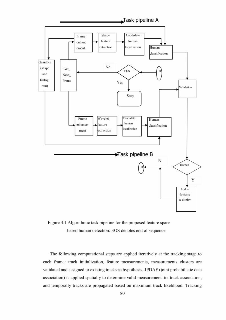
80
The following computational steps are applied iteratively at the tracking stage to
each frame: track initialization, feature measurements, measurements clusters are
validated and assigned to existing tracks as hypothesis, JPDAF (joint probabilistic data
association) is applied spatially to determine valid measurement–to–track association,
and temporally tracks are propagated based on maximum track likelihood. Tracking
Figure 4.1 Algorithmic task pipeline for the proposed feature space
based human detection. EOS denotes end of sequence
detection
Task pipeline B
Task pipeline A
Human
classification
Candidate
human
localization
Wavelet
feature
extraction
Frame
enhance-
ment
Get_
Next_
Frame
classifier
(shape
and
histog-
ram)
D
Yes
No
o EOS
Stop
Validation
N
o D
Y
es
Human
Add to
database
& display
Frame
enhanc
ement
Candidate
human
localization
Shape
feature
extraction Human
classification

81
decisions are made within a group of overlapping frame processing window (a frame
window of ten frames was used in the evaluation phase). Accuracy predications are
made to generate expected detection rate and false alarm rates for the next frame. The
output of the tracker after every track processing window is used to update the
achievable accuracy on a frame-by-frame basis. The processing steps for the tracker
are as follows:
Track initialization
State vector initialization using centroids of found humans
Silhouette and appearance feature extraction (segmentation and outline
extraction)
Appearance templates extraction (intensity, chromatic colours, gradient
magnitude)
Measurements computations (Local and global motion vector estimation)
Measurement validation
Track hypothesis generation and validation
Determine measurement to cluster association (between previous track state and
current measurements based on Kalman prediction)
Update measurement to track cluster association (JPDAF) probabilities
Validate measurements to track hypotheses
Compute signatures of all found humans in the current frame
Determine the best associated track for every candidate human using its signature
Kalman filtering and prediction
Next state prediction
Post processing
Track maintenance (track activation, deactivation, splits, merges);
Occlusion handling;
Appendix B is hierarchical block diagram of the proposed structure for human
detection and tracking algorithm.
82
CHAPTER FIVE
INVESTIGATION INTO FEATURE EXTRACTION
TECHNIQUES FOR HUMAN DETECTION
5.1 Introduction
This chapter presents the investigation carried out to determine suitable feature space
transformation and representation for humans based on apparent shape-outline in shape
space, and scale-frequency domain feature descriptors for human silhouettes. As will be
shown later on, the two forms of representation complements each other in detecting
humans independent of scale changes. Scale changes are brought about whenever the size
of an object and its features change significantly relative to its local neighbourhood.
Section 5.2 justifies the use of wavelet transform to determine discriminatory and
orthogonal feature set. An implementation of 9/7 biorthogonal spline wavelets used in
search of orthogonal and discriminatory features is described in section 5.2.1. A feature
map consisting of the silhouettes of all interesting objects in a frame is proposed as the
basis for human detection in wavelet space. From the feature map are extracted binary
silhouettes of objects using two by two (2X2) binary patterns of the wavelet coefficients
as features. Frequency analysis of the pattern of binary silhouette of humans leads to the
choice of density estimation technique (a projected histogram) as a model for the human
class. Section 5.3 discusses the need to reduce the number of interesting features in order
to probe the wavelet feature space during candidate human localization. A sparse feature
map is also proposed for probing feature locations for candidate human identification.
Section 5.4 on the other hand takes the geometric representation of humans based on
shape-outline, and describes a suitable form of representation similar to edges in shape
space. It is shown that by a suitable choice of threshold, this form of representation is
very similar to edge based representation but with reduced computational cost, and with
83
less spurious points. A boundary extraction algorithm based on this approach is presented
in section 5.4.1. Section 5.5 discusses salient feature map generation in shape space
similar to that discussed on section 5.3. In section 5.6 the main findings and
computational characteristics are discussed.
5.2 Feature Extraction in Scale-Frequency Domain
Two main types of features spaces are available for object detection and tracking, namely,
spatial domain and non spatial domains. Non spatial domain includes eigen space,
principal components feature space, wavelet and Gabor transform feature spaces, and SIFT
(scale invariant feature transform) feature space. Features space transform techniques aim
at reducing the dimensionality and correlation between object features to facilitate object
detection. An image is transformed into wavelet feature space on applying a wavelet
transform. A wavelet filter is any function which has finite energy and is square integrable,
satisfies wavelets regularity and admissible conditions [Daubechies 1990]. It decomposes
signals (functions) into multiresolution components, enabling space-time domain signals to
be represented in scale-time, and frequency-time domains. The basis function of wavelets
transform (defined in equation 5.1), the wavelets, is generated from the mother wavelet by
dilation and translation. The variables s and τ denotes respectively scale and translation
parameters. The wavelet transform (WT) of a one-dimensional signal is two dimensional,
and that of two-dimensional signal is four-dimensional. WT applies high frequency
analysis of signal using small windows and low frequency analysis using large windows.
There are two main types of wavelet transform, namely continuous and discrete wavelet
transform. Continuous wavelet transform results when both the function and the wavelet
are continuous. The continuous wavelet transform of a function f(t), belongs to the vector
space of square integrable function defined by equation 5.2. Hs,t(t) denotes the discrete
wavelet basis function defined in equation 5.1, and * denotes the complex conjugate
operation.
1.5)(h)t(H s-t
s1
,s
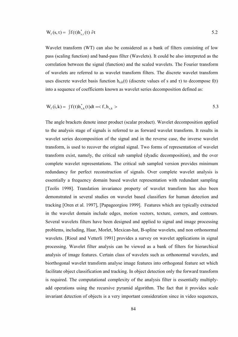
84
2.5t∂)t(h)t(f∫),s(W *,sf
Wavelet transform (WT) can also be considered as a bank of filters consisting of low
pass (scaling function) and band-pass filter (Wavelets). It could be also interpreted as the
correlation between the signal (function) and the scaled wavelets. The Fourier transform
of wavelets are referred to as wavelet transform filters. The discrete wavelet transform
uses discrete wavelet basis function hs,k(t) (discrete values of s and τ) to decompose f(t)
into a sequence of coefficients known as wavelet series decomposition defined as:
3.5h,fdt)t(∫ h)t(f)k,i(W k,s*
k,sf
The angle brackets denote inner product (scalar product). Wavelet decomposition applied
to the analysis stage of signals is referred to as forward wavelet transform. It results in
wavelet series decomposition of the signal and in the reverse case, the inverse wavelet
transform, is used to recover the original signal. Two forms of representation of wavelet
transform exist, namely, the critical sub sampled (dyadic decomposition), and the over
complete wavelet representations. The critical sub sampled version provides minimum
redundancy for perfect reconstruction of signals. Over complete wavelet analysis is
essentially a frequency domain based wavelet representation with redundant sampling
[Teolis 1998]. Translation invariance property of wavelet transform has also been
demonstrated in several studies on wavelet based classifiers for human detection and
tracking [Oren et al. 1997], [Papageorgiou 1999]. Features which are typically extracted
in the wavelet domain include edges, motion vectors, texture, corners, and contours.
Several wavelets filters have been designed and applied to signal and image processing
problems, including, Haar, Morlet, Mexican-hat, B-spline wavelets, and non orthonormal
wavelets. [Rioul and Vetterli 1991] provides a survey on wavelet applications in signal
processing. Wavelet filter analysis can be viewed as a bank of filters for hierarchical
analysis of image features. Certain class of wavelets such as orthonormal wavelets, and
biorthogonal wavelet transform analyse image features into orthogonal feature set which
facilitate object classification and tracking. In object detection only the forward transform
is required. The computational complexity of the analysis filter is essentially multiply-
add operations using the recursive pyramid algorithm. The fact that it provides scale
invariant detection of objects is a very important consideration since in video sequences,
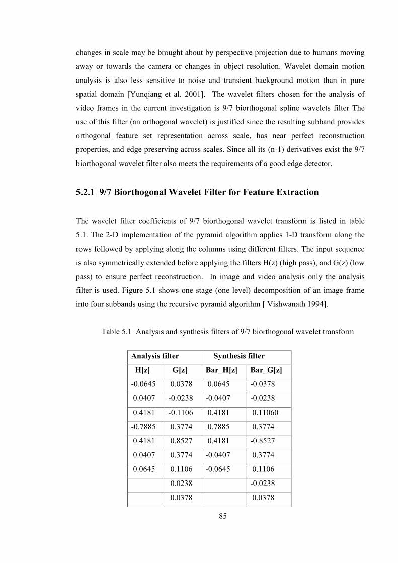
85
changes in scale may be brought about by perspective projection due to humans moving
away or towards the camera or changes in object resolution. Wavelet domain motion
analysis is also less sensitive to noise and transient background motion than in pure
spatial domain [Yunqiang et al. 2001]. The wavelet filters chosen for the analysis of
video frames in the current investigation is 9/7 biorthogonal spline wavelets filter The
use of this filter (an orthogonal wavelet) is justified since the resulting subband provides
orthogonal feature set representation across scale, has near perfect reconstruction
properties, and edge preserving across scales. Since all its (n-1) derivatives exist the 9/7
biorthogonal wavelet filter also meets the requirements of a good edge detector.
5.2.1 9/7 Biorthogonal Wavelet Filter for Feature Extraction
The wavelet filter coefficients of 9/7 biorthogonal wavelet transform is listed in table
5.1. The 2-D implementation of the pyramid algorithm applies 1-D transform along the
rows followed by applying along the columns using different filters. The input sequence
is also symmetrically extended before applying the filters H(z) (high pass), and G(z) (low
pass) to ensure perfect reconstruction. In image and video analysis only the analysis
filter is used. Figure 5.1 shows one stage (one level) decomposition of an image frame
into four subbands using the recursive pyramid algorithm [ Vishwanath 1994].
Analysis filter Synthesis filter
H[z] G[z] Bar_H[z] Bar_G[z]
-0.0645 0.0378 0.0645 -0.0378
0.0407 -0.0238 -0.0407 -0.0238
0.4181 -0.1106 0.4181 0.11060
-0.7885 0.3774 0.7885 0.3774
0.4181 0.8527 0.4181 -0.8527
0.0407 0.3774 -0.0407 0.3774
0.0645 0.1106 -0.0645 0.1106
0.0238 -0.0238
0.0378 0.0378
Table 5.1 Analysis and synthesis filters of 9/7 biorthogonal wavelet transform
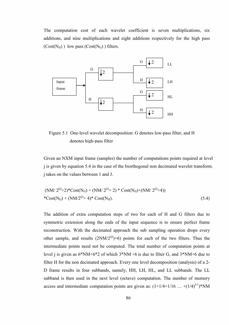
86
The computation cost of each wavelet coefficient is seven multiplications, six
additions, and nine multiplications and eight additions respectively for the high pass
(Cost(NH) ) low pass (Cost(NG) ) filters.
Given an NXM input frame (samples) the number of computations points required at level
j is given by equation 5.4 in the case of the biorthogonal non decimated wavelet transform.
j takes on the values between 1 and J.
(NM/ 2(j)+2)*Cost(NG) + (NM/ 2(j)+ 2) * Cost(NH)+(NM/ 2(j)+4))
*Cost(NG) + (NM/2(j)+ 4)* Cost(NH). (5.4)
The addition of extra computation steps of two for each of H and G filters due to
symmetric extension along the ends of the input sequence is to ensure perfect frame
reconstruction. With the decimated approach the sub sampling operation drops every
other sample, and results (2NM/2(j))+6) points for each of the two filters. Thus the
intermediate points need not be computed. The total number of computation points at
level j is given as 6*NM+6*2 of which 3*NM +6 is due to filter G, and 3*NM+6 due to
filter H for the non decimated approach. Every one level decomposition (analysis) of a 2-
D frame results in four subbands, namely, HH, LH, HL, and LL subbands. The LL
subband is then used in the next level (octave) computation. The number of memory
access and intermediate computation points are given as: (1+1/4+1/16 … +(1/4)J-1)*NM
G
Figure 5.1 One-level wavelet decomposition: G denotes low-pass filter, and H
denotes high-pass filter
H
G
H HH
HL
LH
LL
H
G
Input
frame
2
2
2
2
2
2
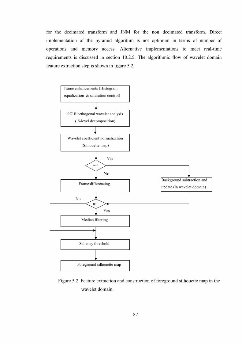
87
for the decimated transform and JNM for the non decimated transform. Direct
implementation of the pyramid algorithm is not optimum in terms of number of
operations and memory access. Alternative implementations to meet real-time
requirements is discussed in section 10.2.5. The algorithmic flow of wavelet domain
feature extraction step is shown in figure 5.2.
Figure 5.2 Feature extraction and construction of foreground silhouette map in the
wavelet domain.
No
A=1
Background subtraction and
update (in wavelet domain) Frame differencing
No
Yes
9/7 Biorthogonal wavelet analysis
( S-level decomposition)
Wavelet coefficient normalization
(Silhouette map)
Frame enhancements (Histogram
equalization & saturation control)
Foreground silhouette map
Saliency threshold
Yes
Median filtering
B=1
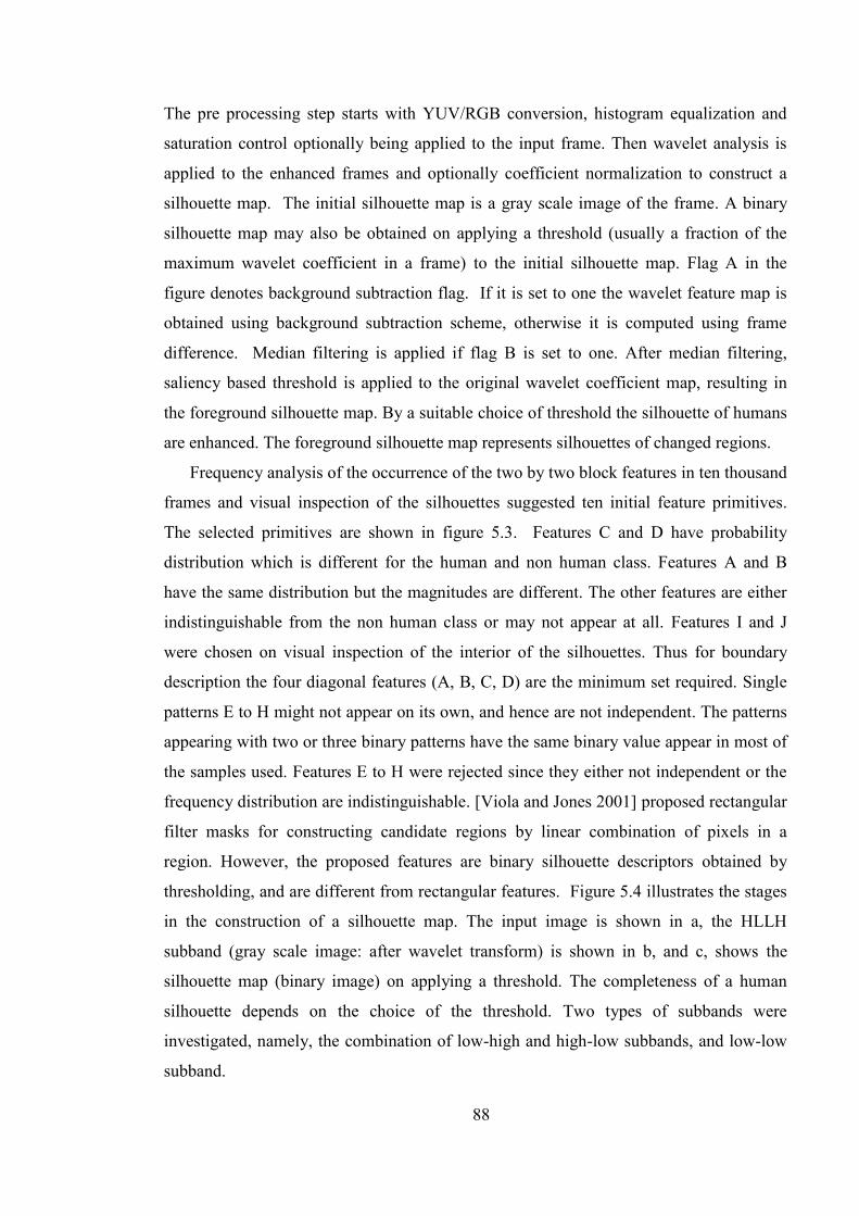
88
The pre processing step starts with YUV/RGB conversion, histogram equalization and
saturation control optionally being applied to the input frame. Then wavelet analysis is
applied to the enhanced frames and optionally coefficient normalization to construct a
silhouette map. The initial silhouette map is a gray scale image of the frame. A binary
silhouette map may also be obtained on applying a threshold (usually a fraction of the
maximum wavelet coefficient in a frame) to the initial silhouette map. Flag A in the
figure denotes background subtraction flag. If it is set to one the wavelet feature map is
obtained using background subtraction scheme, otherwise it is computed using frame
difference. Median filtering is applied if flag B is set to one. After median filtering,
saliency based threshold is applied to the original wavelet coefficient map, resulting in
the foreground silhouette map. By a suitable choice of threshold the silhouette of humans
are enhanced. The foreground silhouette map represents silhouettes of changed regions.
Frequency analysis of the occurrence of the two by two block features in ten thousand
frames and visual inspection of the silhouettes suggested ten initial feature primitives.
The selected primitives are shown in figure 5.3. Features C and D have probability
distribution which is different for the human and non human class. Features A and B
have the same distribution but the magnitudes are different. The other features are either
indistinguishable from the non human class or may not appear at all. Features I and J
were chosen on visual inspection of the interior of the silhouettes. Thus for boundary
description the four diagonal features (A, B, C, D) are the minimum set required. Single
patterns E to H might not appear on its own, and hence are not independent. The patterns
appearing with two or three binary patterns have the same binary value appear in most of
the samples used. Features E to H were rejected since they either not independent or the
frequency distribution are indistinguishable. [Viola and Jones 2001] proposed rectangular
filter masks for constructing candidate regions by linear combination of pixels in a
region. However, the proposed features are binary silhouette descriptors obtained by
thresholding, and are different from rectangular features. Figure 5.4 illustrates the stages
in the construction of a silhouette map. The input image is shown in a, the HLLH
subband (gray scale image: after wavelet transform) is shown in b, and c, shows the
silhouette map (binary image) on applying a threshold. The completeness of a human
silhouette depends on the choice of the threshold. Two types of subbands were
investigated, namely, the combination of low-high and high-low subbands, and low-low
subband.
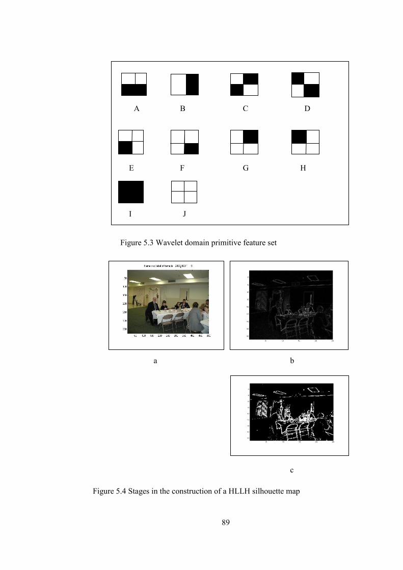
89
Figure 5.3 Wavelet domain primitive feature set
B A
G
I
C
E F
J
D
H
b
c
a
Figure 5.4 Stages in the construction of a HLLH silhouette map
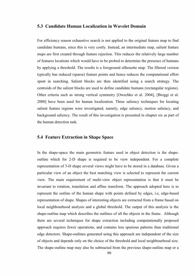
90
5.3 Candidate Human Localization in Wavelet Domain
For efficiency reason exhaustive search is not applied to the original feature map to find
candidate humans, since this is very costly. Instead, an intermediate map, salient feature
maps are first created through feature rejection. This reduces the relatively large number
of features locations which would have to be probed to determine the presence of humans
by applying a threshold. The results is a foreground silhouette map. The filtered version
typically has reduced (sparse) feature points and hence reduces the computational effort
spent in searching. Salient blocks are then identified using a search strategy. The
centroids of the salient blocks are used to define candidate humans (rectangular regions).
Other criteria such as strong vertical symmetry [Owechko et al. 2004], [Broggi et al.
2000] have been used for human localization. Three saliency techniques for locating
salient feature regions were investigated, namely, edge saliency, motion saliency, and
background saliency. The result of this investigation is presented in chapter six as part of
the human detection task.
5.4 Feature Extraction in Shape Space
In the shape-space the main geometric feature used in object detection is the shape-
outline which for 2-D shape is required to be view independent. For a complete
representation of 3-D shape several views might have to be stored in a database. Given a
particular view of an object the best matching view is selected to represent the current
view. The main requirement of multi-view object representation is that it must be
invariant to rotation, translation and affine transform. The approach adopted here is to
represent the outline of the human shape with points defined by edges, i.e, edge-based
representation of shape. Shapes of interesting objects are extracted from a frame based on
local neighbourhood analysis and a global threshold. The output of this analysis is the
shape-outline map which describes the outlines of all the objects in the frame. Although
there are several techniques for shape extraction including computationally proposed
approach requires fewer operations, and contains less spurious patterns than traditional
edge detectors. Shape-outlines generated using this approach are independent of the size
of objects and depends only on the choice of the threshold and local neighbourhood size.
The shape-outline map may also be subtracted from the previous shape-outline map or a
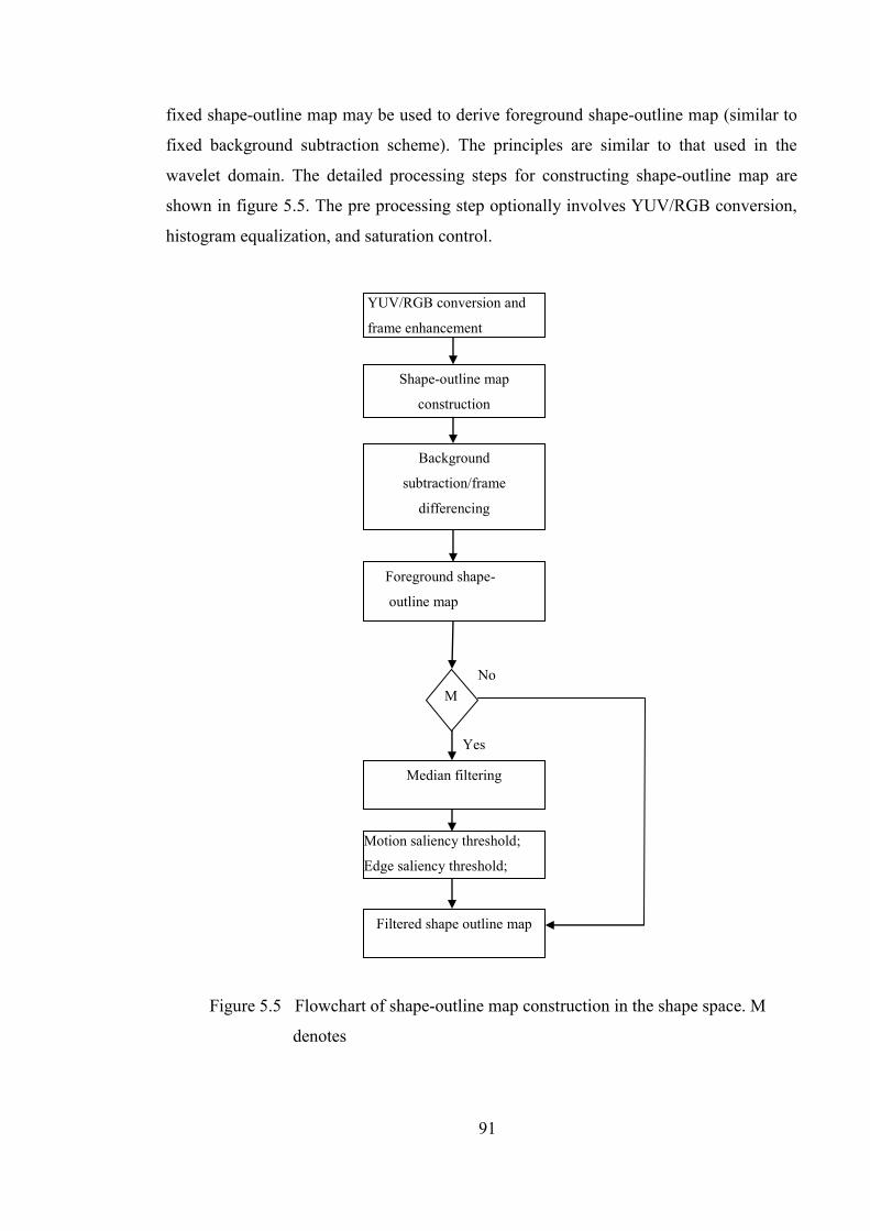
91
fixed shape-outline map may be used to derive foreground shape-outline map (similar to
fixed background subtraction scheme). The principles are similar to that used in the
wavelet domain. The detailed processing steps for constructing shape-outline map are
shown in figure 5.5. The pre processing step optionally involves YUV/RGB conversion,
histogram equalization, and saturation control.
Figure 5.5 Flowchart of shape-outline map construction in the shape space. M
denotes
median filtering flag
YUV/RGB conversion and
frame enhancement
Shape-outline map
construction
Background
subtraction/frame
differencing
Foreground shape-
outline map
No
Yes
Motion saliency threshold;
Edge saliency threshold;
Filtered shape outline map
M
Median filtering

92
It is dependent on the setup information provided. The initial shape-outline map (after
boundary extraction algorithm) is typically noisy hence background subtraction or frame
differencing is applied to extract foreground shapes. Additionally median filtering may
be applied to remove impulse noise and small regions depending on the size of the
median filter applied.
5.4.1 Boundary Extraction Algorithm
The boundary extraction algorithm is based on 8-local neighbourhood comparison for 2-
D arrays. It compares each of the eight neighbours based on intensity. The pseudo code
for the proposed shape-outline map construction given an input frame P(x,y) is as
follows:
Let Nrows, and Ncols be height and width of a frame respectively. Let Threshold, be the
global threshold value for comparing two pixels. Let Map(x, y) be the intermediate binary
image after local neighbourhood pixel comparison. Let Shape_outline_Map be the final
output.
Initialise Map to zeros.
For index1 from 2 to Nrows-1
For index2 from 2 to Ncols-1
Map(x+1,y+1)=(absolute| P(x+1,y+1)-P(x,y)| < Threshold);
Map(x,y+1)=(absolute| P(x,y+1)-P(x,y)| < Threshold);
Map(x,y-1)=(absolute| P(x,y-1)-P(x,y)| < Threshold);
Map(x-1,y)=(absolute| P(x-1,y)-P(x,y)| < Threshold);
Map(x+1,y)=(absolute| P(x+1,y)-P(x,y)| < Threshold);
Map(x+1,y-1)=(absolute| P(x+1,y-1)-P(x,y)| < Threshold);
Map(x-1,y+1)=(absolute| P(x-1,y+1)-P(x,y)| < Threshold);
Map(x-1,y-1)=(absolute| P(x-1,y-1)-P(x,y)| < Threshold);
end
end
%Invert map. This is a comment
Shape_outline_Map=1-map;

93
The number of operations per pixel are nine subtractions (eight plus one), eight absolute
value, eight comparisons, and eight assignments. Compared this with traditional edge
detectors (Canny and Sobel detectors) which are either based on first or second local
derivative operation it becomes obvious the saving in computation times. The algorithm
for Sobel and Canny edge detection in pseudo code are also listed below for comparison.
The pseudo code for Sobel edge map construction is as follows:
Let Gx and Gy denote Sobel filters for vertical and horizontal edge detection.
Let P(x,y) denote pixel intensity at point (x,y) in the image space. Let Ncols and
Nrows denote the width and height respectively of the image.
For all x=1:Ncols
For all y=1: Nrows
G=√(Gx*P(x,y)) 2+ (Gy*(Px,y))2
θ=arctan (Gy*P(x,y))/(Gx*(P(x,y))
end
end
The number of operations per point is twenty multiplications, seventeen additions, one
division, and one square root operation. The output image G is the magnitude image and θ
is the directional image of the input image. The pseudo code for Canny edge map
construction:
1. Let the image function be described by P(x,y) and G the partial derivative of G.
2. Choose a value for standard deviation (=K) of a Gaussian smoothing filter
And substitute into statement 3.

94
3. G(x,y)=e(x2+y2)/22
4. Gn=G/n=nG
5. 2/n2(G*P)=0
6. (G*P)=|Gn*P|
Initialise to K;
Repeat until (=0)
a. Convolve image g(x,y) with a Gaussian smoothing filter G(x,y) defined
above at scale .
b. Estimate the local edge normal direction using (4).
c. Find locations of edges using equation (5).
d. Compute magnitude of edges using (6).
e. Apply hysteresis threshold to output from d.
f. Decrease the value of by 1 (=-1)
end
7. Aggregate the final information about edges at multiple scales (1 to ).
Clearly the operations involve more complex operations (derivative operation is
approximately equivalent to one sobel-point computation), and threshold is applied
iteratively. Table 5.2 shows execution times for Canny edge map, Sobel edge map, and
proposed shape-outline map applied to the same frame. Matlab functions for Canny and
Sobel edge maps were used. It is based on 2.6 GHz Pentium personal computer with two
Gigabytes RAM, and running on Windows professional XP. From the table the minimum
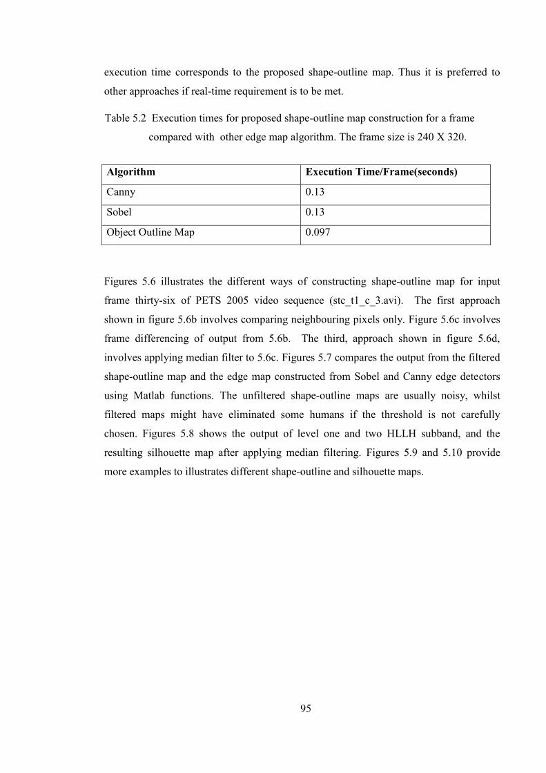
95
execution time corresponds to the proposed shape-outline map. Thus it is preferred to
other approaches if real-time requirement is to be met.
Figures 5.6 illustrates the different ways of constructing shape-outline map for input
frame thirty-six of PETS 2005 video sequence (stc_t1_c_3.avi). The first approach
shown in figure 5.6b involves comparing neighbouring pixels only. Figure 5.6c involves
frame differencing of output from 5.6b. The third, approach shown in figure 5.6d,
involves applying median filter to 5.6c. Figures 5.7 compares the output from the filtered
shape-outline map and the edge map constructed from Sobel and Canny edge detectors
using Matlab functions. The unfiltered shape-outline maps are usually noisy, whilst
filtered maps might have eliminated some humans if the threshold is not carefully
chosen. Figures 5.8 shows the output of level one and two HLLH subband, and the
resulting silhouette map after applying median filtering. Figures 5.9 and 5.10 provide
more examples to illustrates different shape-outline and silhouette maps.
Algorithm Execution Time/Frame(seconds)
Canny 0.13
Sobel 0.13
Object Outline Map 0.097
Table 5.2 Execution times for proposed shape-outline map construction for a frame
compared with other edge map algorithm. The frame size is 240 X 320.

96
b a
d c
Figure 5.6 Construction of shape-outline maps from frame 36. (a) Input
image (b) After neighbourhood pixel comparisons
(c) frame differencing of b (d) after applying
median filter.
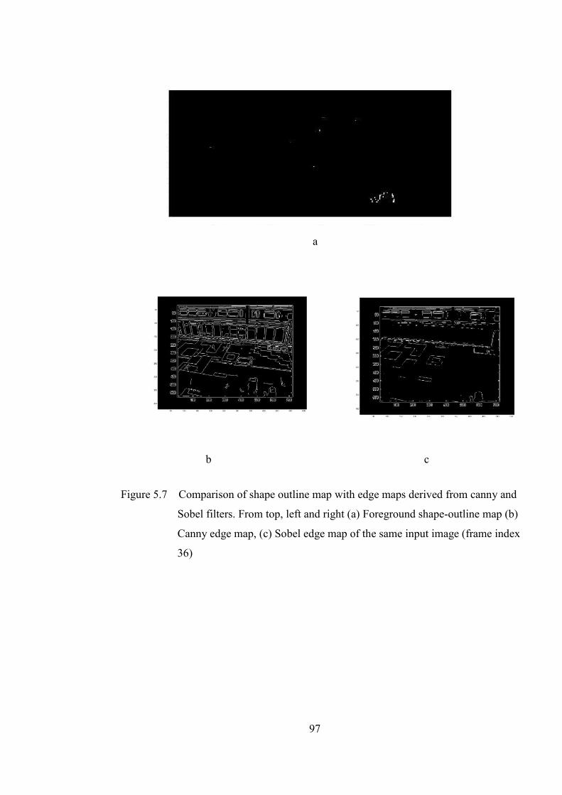
97
Figure 5.7 Comparison of shape outline map with edge maps derived from canny and
Sobel filters. From top, left and right (a) Foreground shape-outline map (b)
Canny edge map, (c) Sobel edge map of the same input image (frame index
36)
b c
a
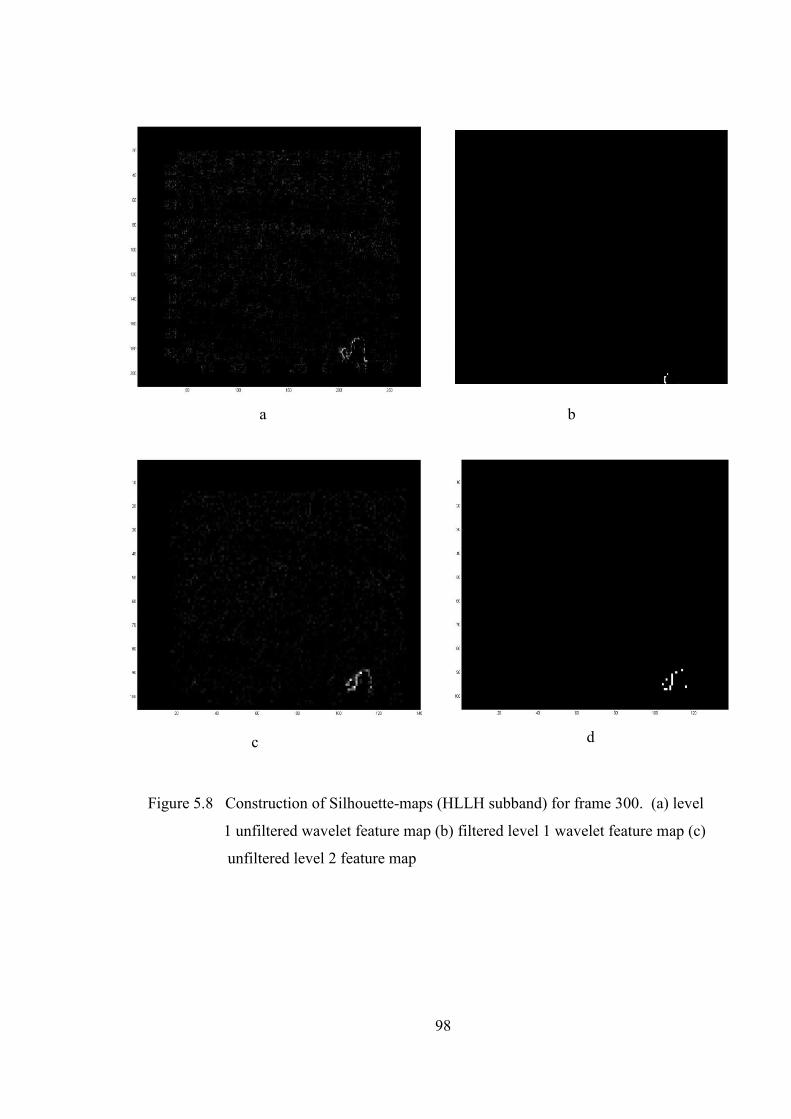
98
Figure 5.8 Construction of Silhouette-maps (HLLH subband) for frame 300. (a) level
1 unfiltered wavelet feature map (b) filtered level 1 wavelet feature map (c)
unfiltered level 2 feature map
wavelet feature
map (d) filtered level 2 wavelet filter map
b
d
a
c
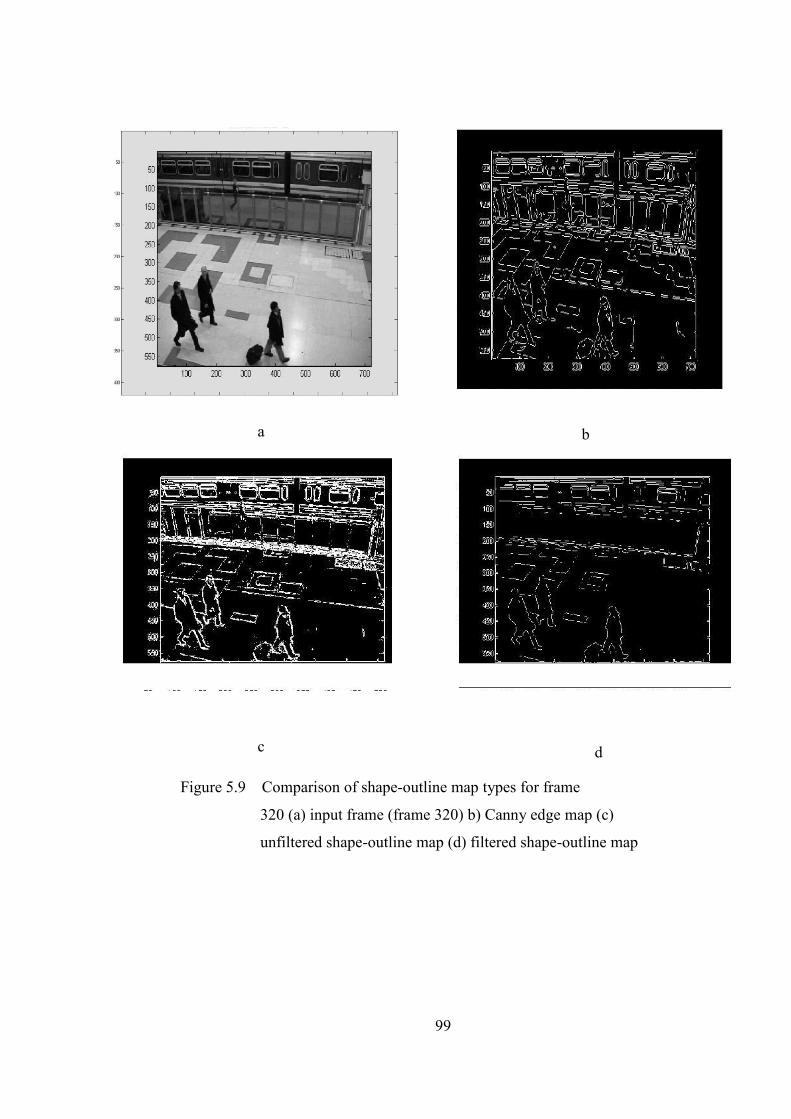
99
b
d c
a
Figure 5.9 Comparison of shape-outline map types for frame
320 (a) input frame (frame 320) b) Canny edge map (c)
unfiltered shape-outline map (d) filtered shape-outline map
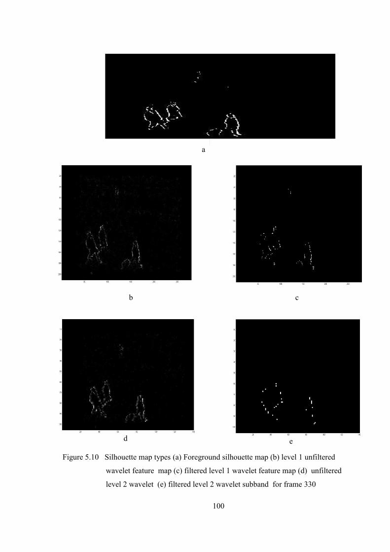
100
Figure 5.10 Silhouette map types (a) Foreground silhouette map (b) level 1 unfiltered
wavelet feature map (c) filtered level 1 wavelet feature map (d) unfiltered
level 2 wavelet (e) filtered level 2 wavelet subband for frame 330
feature map (e) filtered level 2 wavelet feature map
e
a
b c
d
101
5.5 Candidate Human Localization in Shape Space
The steps for candidate human localization is similar to that in wavelet domain as
discussed in section 5.3. The only difference is that it is based on shape-outline map in
shape space. Details of investigations into this aspect of processing are also presented in
chapter seven.
5.6 Results
In scale-frequency space investigation revealed that ten normalized wavelet template
features are adequate to describe the silhouette of humans in the wavelet domain.
Simulation of the full sixteen features using PASCAL VOC 2010 sequence revealed
marginal increase in accuracy compared with the computational effort The spatial
distribution of these patterns for human class varies from that of the background. In shape
space a reduced complexity shape-outline map extraction algorithm has been proposed.
The alogrihm is dependent only on the choice of feature threshold and the size of the local
neighbourhood. It was observed that complete shape-outlines resulted if the threshold is a
fraction of the standard deviation of a subband. The continuity of shape-outlines of real-
objects in the scene implies that some background noise can be removed by applying
median filtering.
It is proposed to use the silhouette and shape-outline maps to investigate pattern
classifiers for human discrimination and detection. The computational complexity of the
proposed shape-outline map extraction is lower than that of the traditional edge detectors.
One of the conclusions from visual inspection of the maps is that global threshold approach
sometimes fails to detect humans if its dimension is smaller than neighbouring objects in
the scene. The wavelet domain approach provides discriminatory descriptors for
silhouettes of humans. Thus the two representations complement each other in detecting
shapes of humans.
Scene background appear as random noise when the size of the background objects is
smaller than humans, and by applying suitable median filter of a particular dimension most
of the background noise is removed. For background objects larger than humans, the
application of background subtraction techniques is able to remove most of the stationary
objects. Simulations results are presented in the chapter six.
102
CHAPTER SIX
INVESTIGATIONS INTO PATTERN
CLASSIFIERS FOR HUMAN DISCRIMINATION
6.1 Introduction
The chapter discusses issues related to the wavelet based histogram and shape based
classifiers for human discrimination. It first provides the specification, design, testing
and validation of the proposed classifiers. Sections 6.2, 6.2.1, 6.2.2 discuss wavelet
based classifier design, validation and testing. Section 6.3, 6.3.1, 6.3.2 discuss shape-
outline based classifier design starting from the feed forward pattern predictor,
hypothesis generation, validation and testing. Section 6.4 discusses the results of the
validation of the two classifiers. Section 6.5 provides an interpretation of the results.
6.2 Wavelet Feature-Based Classifier Specification and
Implementation
An investigation into the use of density based appearance representation using the
wavelet feature primitives (see section 5.2.1) was undertaken. These features are
observable in all the silhouette of humans irrespective of the subband. Projection
histogram of each of the primitive features along the X and Y-axis were generated as a
model of human and background. For each feature, the occurrence frequencies along
the axes are used in constructing the histogram. To ensure a fixed computational cost
the dimension of the histogram is fixed. Two classifiers were designed using
silhouette of humans from LL, and HLLH (sum of LH and HL) subbands. Preliminary
classifier design revealed that of the ten initial primitive features (see page 89), six
were selected as sufficient to discriminate human from the non human class for the
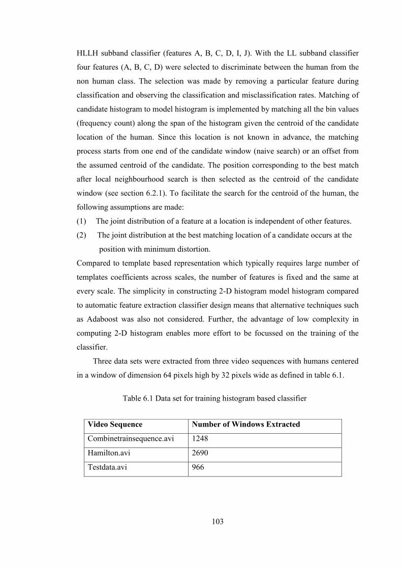
103
HLLH subband classifier (features A, B, C, D, I, J). With the LL subband classifier
four features (A, B, C, D) were selected to discriminate between the human from the
non human class. The selection was made by removing a particular feature during
classification and observing the classification and misclassification rates. Matching of
candidate histogram to model histogram is implemented by matching all the bin values
(frequency count) along the span of the histogram given the centroid of the candidate
location of the human. Since this location is not known in advance, the matching
process starts from one end of the candidate window (naive search) or an offset from
the assumed centroid of the candidate. The position corresponding to the best match
after local neighbourhood search is then selected as the centroid of the candidate
window (see section 6.2.1). To facilitate the search for the centroid of the human, the
following assumptions are made:
(1) The joint distribution of a feature at a location is independent of other features.
(2) The joint distribution at the best matching location of a candidate occurs at the
position with minimum distortion.
Compared to template based representation which typically requires large number of
templates coefficients across scales, the number of features is fixed and the same at
every scale. The simplicity in constructing 2-D histogram model histogram compared
to automatic feature extraction classifier design means that alternative techniques such
as Adaboost was also not considered. Further, the advantage of low complexity in
computing 2-D histogram enables more effort to be focussed on the training of the
classifier.
Three data sets were extracted from three video sequences with humans centered
in a window of dimension 64 pixels high by 32 pixels wide as defined in table 6.1.
Table 6.1 Data set for training histogram based classifier
Video Sequence Number of Windows Extracted
Combinetrainsequence.avi 1248
Hamilton.avi 2690
Testdata.avi 966
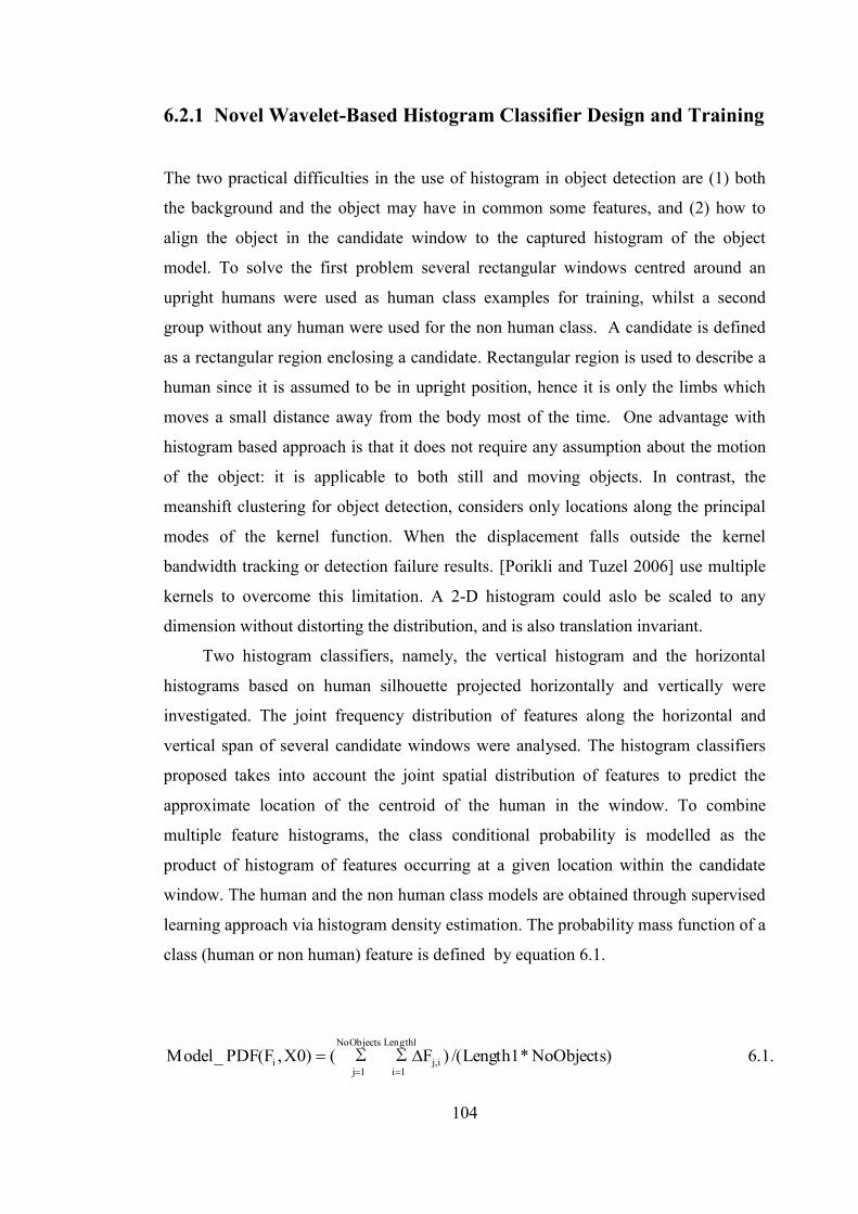
104
6.2.1 Novel Wavelet-Based Histogram Classifier Design and Training
The two practical difficulties in the use of histogram in object detection are (1) both
the background and the object may have in common some features, and (2) how to
align the object in the candidate window to the captured histogram of the object
model. To solve the first problem several rectangular windows centred around an
upright humans were used as human class examples for training, whilst a second
group without any human were used for the non human class. A candidate is defined
as a rectangular region enclosing a candidate. Rectangular region is used to describe a
human since it is assumed to be in upright position, hence it is only the limbs which
moves a small distance away from the body most of the time. One advantage with
histogram based approach is that it does not require any assumption about the motion
of the object: it is applicable to both still and moving objects. In contrast, the
meanshift clustering for object detection, considers only locations along the principal
modes of the kernel function. When the displacement falls outside the kernel
bandwidth tracking or detection failure results. [Porikli and Tuzel 2006] use multiple
kernels to overcome this limitation. A 2-D histogram could aslo be scaled to any
dimension without distorting the distribution, and is also translation invariant.
Two histogram classifiers, namely, the vertical histogram and the horizontal
histograms based on human silhouette projected horizontally and vertically were
investigated. The joint frequency distribution of features along the horizontal and
vertical span of several candidate windows were analysed. The histogram classifiers
proposed takes into account the joint spatial distribution of features to predict the
approximate location of the centroid of the human in the window. To combine
multiple feature histograms, the class conditional probability is modelled as the
product of histogram of features occurring at a given location within the candidate
window. The human and the non human class models are obtained through supervised
learning approach via histogram density estimation. The probability mass function of a
class (human or non human) feature is defined by equation 6.1.
.1.6)NoObjects*1Length/()∑ F∑()0X,F(PDF_Model1Length
1ii,j
NoObjects
1ji
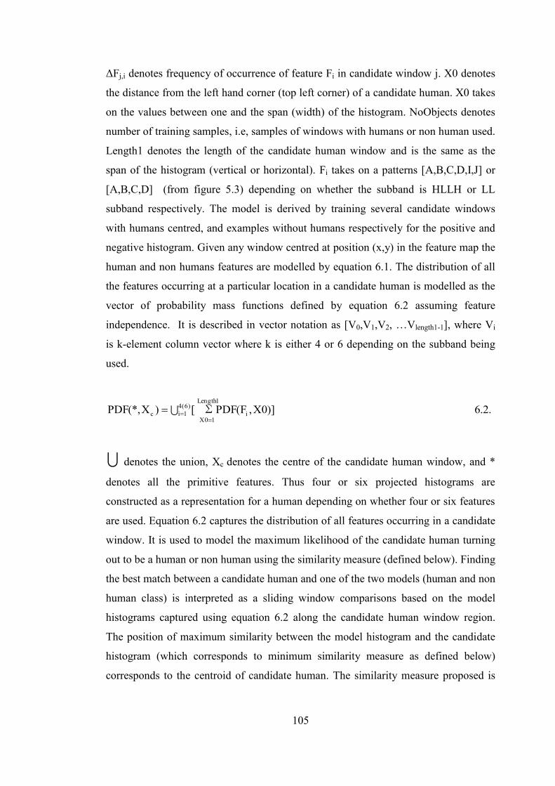
105
ΔFj,i denotes frequency of occurrence of feature Fi in candidate window j. X0 denotes
the distance from the left hand corner (top left corner) of a candidate human. X0 takes
on the values between one and the span (width) of the histogram. NoObjects denotes
number of training samples, i.e, samples of windows with humans or non human used.
Length1 denotes the length of the candidate human window and is the same as the
span of the histogram (vertical or horizontal). Fi takes on a patterns [A,B,C,D,I,J] or
[A,B,C,D] (from figure 5.3) depending on whether the subband is HLLH or LL
subband respectively. The model is derived by training several candidate windows
with humans centred, and examples without humans respectively for the positive and
negative histogram. Given any window centred at position (x,y) in the feature map the
human and non humans features are modelled by equation 6.1. The distribution of all
the features occurring at a particular location in a candidate human is modelled as the
vector of probability mass functions defined by equation 6.2 assuming feature
independence. It is described in vector notation as [V0,V1,V2, …Vlength1-1], where Vi
is k-element column vector where k is either 4 or 6 depending on the subband being
used.
.2.6]∑ )0X,F(PDF[)X(*,PDF1Length
10Xi
)6(41ic
denotes the union, Xc denotes the centre of the candidate human window, and *
denotes all the primitive features. Thus four or six projected histograms are
constructed as a representation for a human depending on whether four or six features
are used. Equation 6.2 captures the distribution of all features occurring in a candidate
window. It is used to model the maximum likelihood of the candidate human turning
out to be a human or non human using the similarity measure (defined below). Finding
the best match between a candidate human and one of the two models (human and non
human class) is interpreted as a sliding window comparisons based on the model
histograms captured using equation 6.2 along the candidate human window region.
The position of maximum similarity between the model histogram and the candidate
histogram (which corresponds to minimum similarity measure as defined below)
corresponds to the centroid of candidate human. The similarity measure proposed is
106
based on city block metric and related to histogram intersection method [Swain and
Ballard 1991]. It is defined as:
Sim(model_class)=∏(Model_Class(x)–Candidate_Class(x))2 /(2*Width ) 6.3.
X takes on the values between 1 and length1. It is computed for both the human and
non human model. The square operation magnifies the differences. The ∏ operation
takes on values between one and four or six depending on whether the subband is LL
or HLLH. The similarity measure is computed per feature and can be interpreted as
the difference between a model histogram Equation 6.3 essentially computes on a bin
by bin basis the distortion between the model histogram and the candidate histogram
for every feature, and evaluates the element wise product for all the features. The
result is a vector of joint feature probabilties. A decision is made to assign the
candidate human to the human class if equation 6.4 is true. It sums up the contribution
from each of the features.
∑Sim(NonHuman_Mark)>=∑Sim(Human_class) 6.4.
The summation is over all the feature set (four or six depending on the subband in
use). The closer the candidate histogram is to the model histogram the smaller is the
city block metric (equation 6.3).
Training: The two classifiers were trained using the holdout approach with
bootstrapping. The training set consisted of 4904 samples (1248+2690+966). During
training any sample which was misclassified was added to the new training set, and
the classifier retrained. This was repeated for until the detection rate is more than 80%.
6.2.2 Validation and Testing of Histogram Based Classifier
The algorithmic steps for the validation and testing of the histogram based classifiers
is outlined in figure 6.1. First the data set is split into validation set and the evaluation
set.
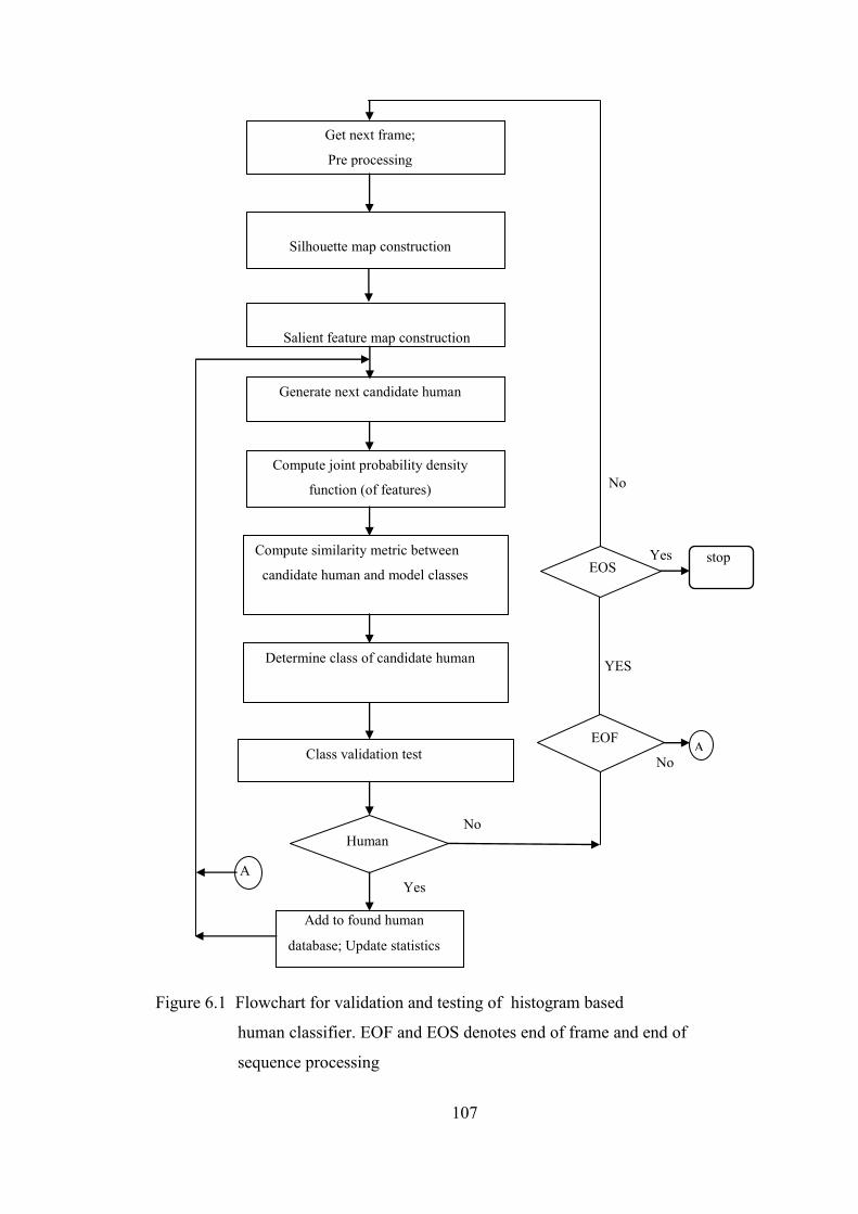
107
Figure 6.1 Flowchart for validation and testing of histogram based
human classifier. EOF and EOS denotes end of frame and end of
sequence processing
Yes
Salient feature map construction
Get next frame;
Pre processing
Generate next candidate human
Compute joint probability density
function (of features)
Silhouette map construction
Compute similarity metric between
candidate human and model classes
Class validation test
Determine class of candidate human
Human
Add to found human
database; Update statistics
A
No
YES
A No
Yes EOS
stop
No
EOF
108
The pre processing step applies median filtering, and illumination normalization to the
incoming frames. The next step applies either level one or level two wavelet transform
depending on whether there is significant scale changes in the scene. Square wavelet
features are constructed from the displaced frame difference of the LL subband or the
HLLH subband. Saliency based thresholding are applied to the resulting feature map
(foreground object map) to reject non salient features. The resulting salient feature
map is used to locate salient regions as candidate humans. Candidate human
localization starts with the construction of salient feature map and ends with the
generation of candidate humans (candidate window). Following candidate human
construction, frequency analysis of the wavelet feature histogram is generated as
described in section 6.2.1. Similarity measures are computed between the histogram of
the candidate human and the model histograms. Due to the fact that the classifier is not
linearly separable, validation of class assignment is confirmed by area and size test.
This entailed evaluating the area occupied by the human, and its dimension. Only
candidate humans which additionally pass the two tests were confirmed as containing
humans, otherwise rejected.
Next, the two underlying assumptions of the classifiers are verified. The first
assumption is verified by one way Anova test on the probability mass function and the
similarity measures, assuming independence of horizontal and vertical features. This is
shown in table 6.2. The low probability of F (0) at 95% confidence level validates this
assumption. The high mean squared error for horizontal histogram classifier
(5.34432e+009) and the vertical histogram classifier (8.65613e+007) indeed confirms
that the positive and negative classes indeed belong to a different population. The
second modelling assumption is verified by principal component analysis. The output
from the wavelet classifier includes the location of the centre (centroid) of the found
human in the candidate human window based on this assumption. The centre of the
found human in the candidate human window (32*64 dimension) relative to the frame
is obtained by adding an address offset. The result of the analysis is shown in table 6.3
which analysis the location output by the classifier by principal component analysis
(PCA) separately, and similarly to the approximate centroid defined manually in the
ground truth based. The table list only the first component which accounts for the
smallest variance. It is noted from the table that least variation occurs in the centroid
location (X,Y), in the following order: vertical features, diagonal plus, and white
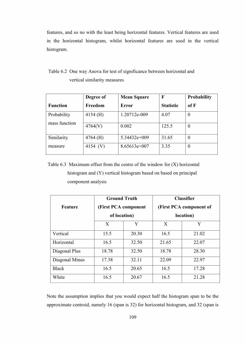
109
features, and so no with the least being horizontal features. Vertical features are used
in the horizontal histogram, whilst horizontal features are used in the vertical
histogram.
Note the assumption implies that you would expect half the histogram span to be the
approximate centroid, namely 16 (span is 32) for horizontal histogram, and 32 (span is
Table 6.3 Maximum offset from the centre of the window for (X) horizontal
histogram and (Y) vertical histogram based on based on principal
component analysis
Feature
Ground Truth
(First PCA component
of location)
Classifier
(First PCA component of
location)
X Y X Y
Vertical 15.5 20.30 16.5 21.02
Horizontal 16.5 32.50 21.65 22.07
Diagonal Plus 18.78 32.50 18.78 28.30
Diagonal Minus 17.38 32.11 22.09 22.97
Black 16.5 20.65 16.5 17.28
White 16.5 20.67 16.5 21.28
Function
Degree of
Freedom
Mean Square
Error
F
Statistic
Probability
of F
Probability
mass function
4154 (H) 1.20712e-009 4.07 0
4764(V) 0.002 125.5 0
Similarity
measure
4764 (H) 5.34432e+009 31.65 0
4154 (V) 8.65613e+007 3.35 0
Table 6.2 One way Anova for test of significance between horizontal and
vertical similarity measures

110
64) for the vertical histogram assuming the human is located at the centre. This is not
exact since the centre is manually labelled in the ground truth, and in practice the
constructed candidate human may not have the human aligned exactly to the centre.
Thus using the horizontal histogram (vertical features) gives the average position of
the centroid based on the ground truth label along the x-and y-axes as (15.5, 20.3)
compared to (16.5, 21.02) predicted by the classifier. Similarly, using the vertical
histogram (use horizontal features) gives the average position of the centroid based on
the ground truth label along the x-and y-axes as (16.5, 32.5) compared to (21.65,
22.07) predicted by the classifier. Additionally it was observed that the classifier
responds more to vertical features (use in the horizontal histogram) than horizontal
features.
The histogram model is further verified by a stacked plot of the similarity
measures for human class and non human class as shown in figure 6.2 based on the
horizontal histogram classifier. The similarity measure is based on city block
(Manhattan distance) [Fabri et al. 2008] measure. The similarity block measure from
the graph appears to be constant. This is attributed to the fact that only one person is in
the video segment for which the measurements were taken. One way Anova result of
the city block distance is shown in table 6.4.
Figure 6.2 Plot of city block measure for histogram-based classifier (a) video
sequence Stc_t1_c_3.avi (b) sequence Stc_t1_c_4.avi

111
The label H denotes features extracted from the horizontal histogram, whilst V
indicates features extracted from the vertical histogram. The high mean squared error
(3.3942e+21) between the similarity measures for the vertical and horizontal similarity
measure suggest that the horizontal and the vertical measure can not belong to the
same population. The Low value of the Probability of F at 95% confidence level also
confirms that there is a significant difference between the human class and the non
human class. Finally, table 6.5 shows the confusion matrix for one of the test
sequence.
6.3 Shape-Outline Based Classifier Specification and
Implementation
Whereas the basic primitive features in wavelet-based histogram is a square block of
dimension two by two pixels, the basic feature of the shape based classifier is an edge
since the shape-outline map is binary. Two main problems confronts this approach,
namely, noise, and changes in human outline. To be able to detect humans in more
Table 6.4 One way Anova table for similarity metric for horizontal histogram
between the human and non human class for stc_t1_c_3.avi sequence
Source
Mean Squared
Error
Degree of
Freedom
F Statistics
Prob> F
Human/Non
Human
3.3942e+21
1
15.72
8.397e-05
Error 1.101e+23 510 - -
Category Predicted
Actual Human Non Human
Human 192 177 15
Non human 170 24 146
Table 6.5 Post training evaluation of Test1.avi sequence (Level 2 decomposition)
112
complex poses, detection by parts such as the head, upper body, lower body, and then
synthesis into whole human outline may be required. Another approach is view based
supervised learning approach provides a solution at the expense of increased
algorithmic complexity. Apparent shape derived from a shape-outline map is used as a
shape descriptor on account of its reduced computational cost and simplicity. Other
shape-based representation investigated included polynomial, Fourier transform based
representation, and continuous shape descriptors. They were not pursued further since
the performance gain in terms of accuracy and computational time compared to the
shape-outline based approach was smaller and higher respectively. Shape based
representation in Fourier space has been studied in [Dengsheng and Lu 2001], in
wavelet space in [Shen and Ip 1999], [Oren et al. 1997], and in spatial domain in
[Berg and Malik 2005], [Lakshmiratan et al. 2000]. Silhouette-based detection has
been studied in wavelet domain and in spatial domain however with noisy inputs the
detector may suffer degradation in performance and this led to a search for a technique
which is tolerant to noise, and led to neural network based pattern predictor for human
shape description. The approach is similar to shape-based detectors which use
matching metric such as Hausdorf distance [Huttenlocher et al. 1993].
Thus instead of using the shapes of candidate humans directly, a feed forward
neural network is trained to learn the complete or partial shapes of humans in upright
posture in order to predict a human shape. The input to the classifier (candidate
human), typically contain noise in the form of spurious edges and shapes. The shape
prediction approach avoids other problems in the spatial domains such as variation in
prototype shape, shadows, illumination and changes. In fact no prior assumption is
made about the scene complexity and composition. It thus provides a means of
removing spurious edges and shapes. From the noisy out of the predictor, two
candidate human windows are generated, one for the human class and the other for the
non human class. Correspondingly, two hypotheses are generated from the predictor’s
output, one for the human class and the other from the non human class. A mismatch
measure is used to assign the output of the predictor to the most likely class. It
penalises mismatched points on predicted output. The measure validates one of the
hypotheses, namely, that the current candidate human window belongs to the human
class or non human class. The sequence of steps which constitutes human detection
are pre processing, foreground shape-outline map creation, candidate human
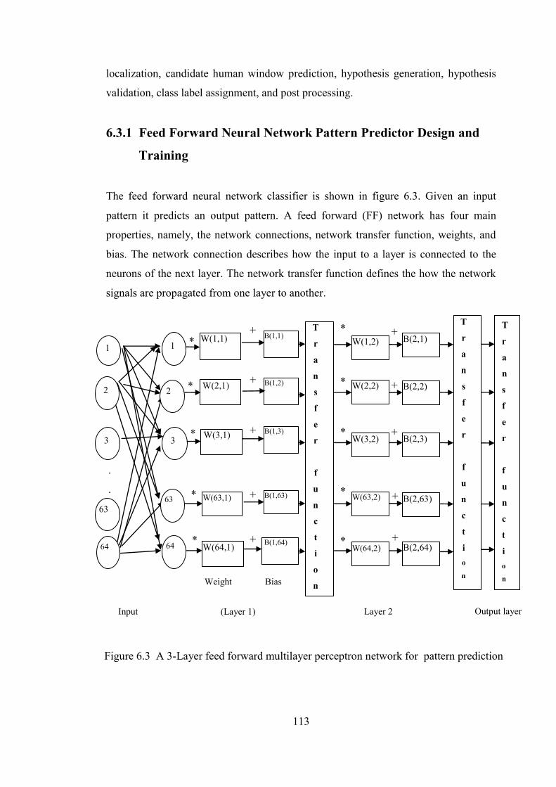
113
localization, candidate human window prediction, hypothesis generation, hypothesis
validation, class label assignment, and post processing.
6.3.1 Feed Forward Neural Network Pattern Predictor Design and
Training
The feed forward neural network classifier is shown in figure 6.3. Given an input
pattern it predicts an output pattern. A feed forward (FF) network has four main
properties, namely, the network connections, network transfer function, weights, and
bias. The network connection describes how the input to a layer is connected to the
neurons of the next layer. The network transfer function defines the how the network
signals are propagated from one layer to another.
Figure 6.3 A 3-Layer feed forward multilayer perceptron network for pattern prediction
Bias
*
*
*
3
Weight
*
*
B(1,63)
B(1,64)
+
+
+
B(1,1)
B(1,2)
B(1,3)
+
+
W(1,1)
W(3,1)
W(64,1)
W(63,1)
1
W(2,1)
2
63
64
2
64
1
.
.
.
3
63
Layer 2 (Layer 1) Input
T
r
a
n
s
f
e
r
f
u
n
c
t
i o
n
*
*
*
*
*
T
r
a
n
s
f
e
r
f
u
n
c
t
i
o
n
+
+
+
+
+
W(3,2)
W(2,2)
W(1,2)
W(63,2)
W(64,2)
B(2,3)
B(2,1)
B(2,2)
B(2,63)
B(2,64)
Output layer
T
r
a
n
s
f
e
r
f
u
n
c
t
i o
n
n
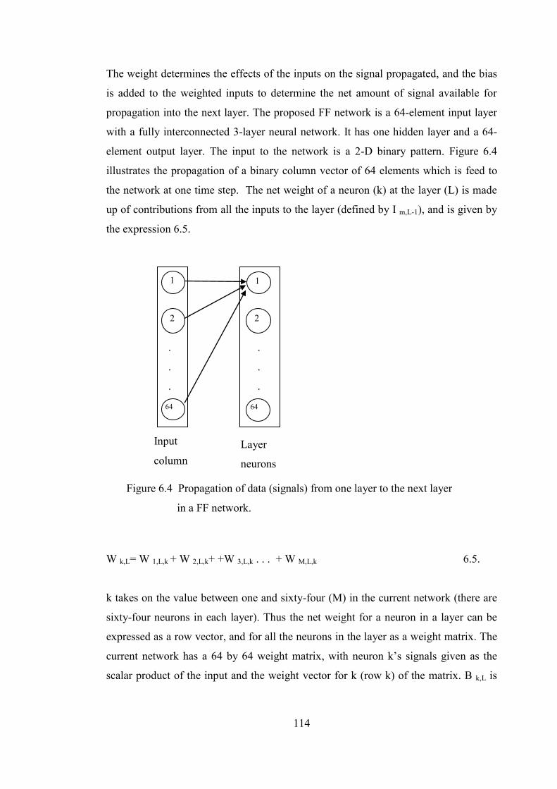
114
The weight determines the effects of the inputs on the signal propagated, and the bias
is added to the weighted inputs to determine the net amount of signal available for
propagation into the next layer. The proposed FF network is a 64-element input layer
with a fully interconnected 3-layer neural network. It has one hidden layer and a 64-
element output layer. The input to the network is a 2-D binary pattern. Figure 6.4
illustrates the propagation of a binary column vector of 64 elements which is feed to
the network at one time step. The net weight of a neuron (k) at the layer (L) is made
up of contributions from all the inputs to the layer (defined by I m,L-1), and is given by
the expression 6.5.
W k,L= W 1,L,k + W 2,L,k+ +W 3,L,k . . . + W M,L,k 6.5.
k takes on the value between one and sixty-four (M) in the current network (there are
sixty-four neurons in each layer). Thus the net weight for a neuron in a layer can be
expressed as a row vector, and for all the neurons in the layer as a weight matrix. The
current network has a 64 by 64 weight matrix, with neuron k’s signals given as the
scalar product of the input and the weight vector for k (row k) of the matrix. B k,L is
Layer
neurons
1 1
2
64
2
64
.
.
.
.
.
.
Input
column
Figure 6.4 Propagation of data (signals) from one layer to the next layer
in a FF network.
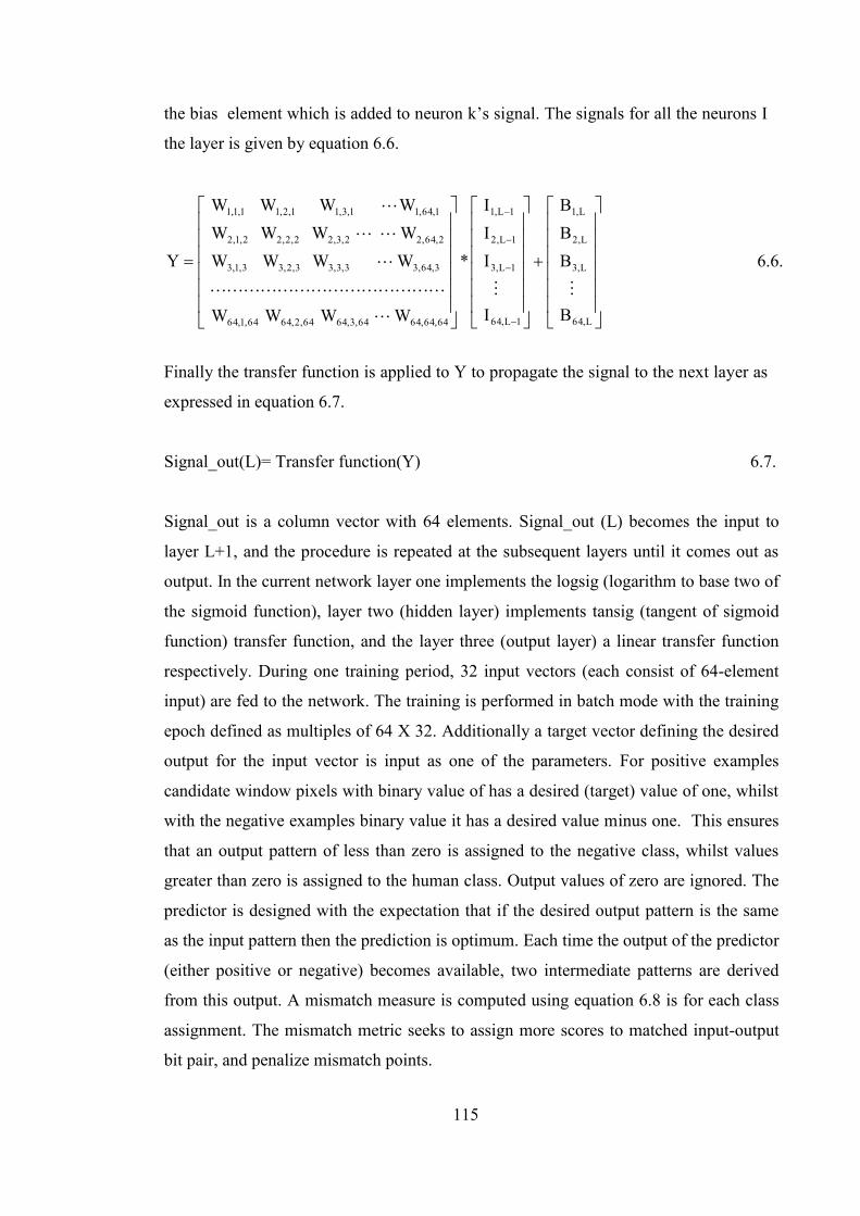
115
the bias element which is added to neuron k’s signal. The signals for all the neurons I
the layer is given by equation 6.6.
.6.6
B
BBB
I
III
*
WWWW
WWWWWWWWWWWW
Y
L,64
L,3
L,2
L,1
1L,64
1L,3
1L,2
1L,1
64,64,6464,3,6464,2,6464,1,64
3,64,33,3,33,2,33,1,3
2,64,22,3,22,2,22,1,2
1,64,11,3,11,2,11,1,1
Finally the transfer function is applied to Y to propagate the signal to the next layer as
expressed in equation 6.7.
Signal_out(L)= Transfer function(Y) 6.7.
Signal_out is a column vector with 64 elements. Signal_out (L) becomes the input to
layer L+1, and the procedure is repeated at the subsequent layers until it comes out as
output. In the current network layer one implements the logsig (logarithm to base two of
the sigmoid function), layer two (hidden layer) implements tansig (tangent of sigmoid
function) transfer function, and the layer three (output layer) a linear transfer function
respectively. During one training period, 32 input vectors (each consist of 64-element
input) are fed to the network. The training is performed in batch mode with the training
epoch defined as multiples of 64 X 32. Additionally a target vector defining the desired
output for the input vector is input as one of the parameters. For positive examples
candidate window pixels with binary value of has a desired (target) value of one, whilst
with the negative examples binary value it has a desired value minus one. This ensures
that an output pattern of less than zero is assigned to the negative class, whilst values
greater than zero is assigned to the human class. Output values of zero are ignored. The
predictor is designed with the expectation that if the desired output pattern is the same
as the input pattern then the prediction is optimum. Each time the output of the predictor
(either positive or negative) becomes available, two intermediate patterns are derived
from this output. A mismatch measure is computed using equation 6.8 is for each class
assignment. The mismatch metric seeks to assign more scores to matched input-output
bit pair, and penalize mismatch points.
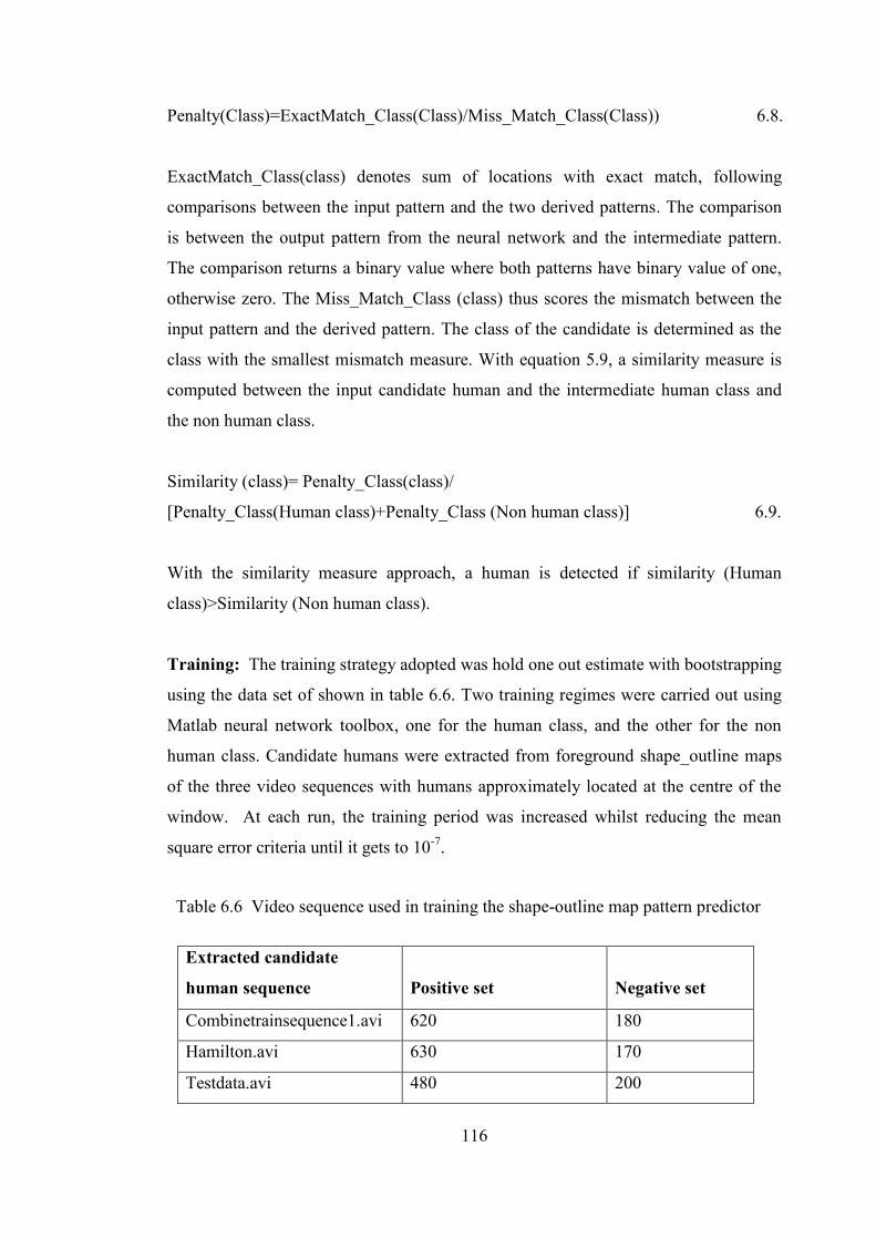
116
Penalty(Class)=ExactMatch_Class(Class)/Miss_Match_Class(Class)) 6.8.
ExactMatch_Class(class) denotes sum of locations with exact match, following
comparisons between the input pattern and the two derived patterns. The comparison
is between the output pattern from the neural network and the intermediate pattern.
The comparison returns a binary value where both patterns have binary value of one,
otherwise zero. The Miss_Match_Class (class) thus scores the mismatch between the
input pattern and the derived pattern. The class of the candidate is determined as the
class with the smallest mismatch measure. With equation 5.9, a similarity measure is
computed between the input candidate human and the intermediate human class and
the non human class.
Similarity (class)= Penalty_Class(class)/
[Penalty_Class(Human class)+Penalty_Class (Non human class)] 6.9.
With the similarity measure approach, a human is detected if similarity (Human
class)>Similarity (Non human class).
Training: The training strategy adopted was hold one out estimate with bootstrapping
using the data set of shown in table 6.6. Two training regimes were carried out using
Matlab neural network toolbox, one for the human class, and the other for the non
human class. Candidate humans were extracted from foreground shape_outline maps
of the three video sequences with humans approximately located at the centre of the
window. At each run, the training period was increased whilst reducing the mean
square error criteria until it gets to 10-7.
Table 6.6 Video sequence used in training the shape-outline map pattern predictor
Extracted candidate
human sequence
Positive set
Negative set
Combinetrainsequence1.avi 620 180
Hamilton.avi 630 170
Testdata.avi 480 200
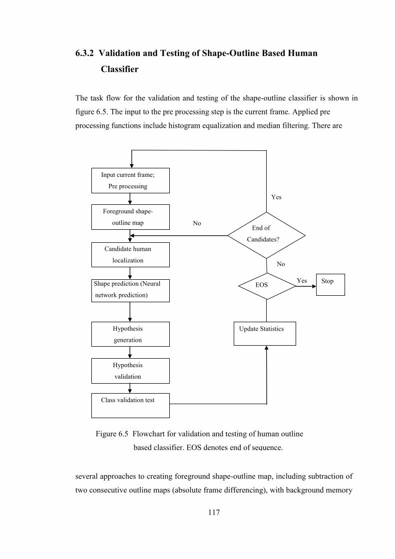
117
6.3.2 Validation and Testing of Shape-Outline Based Human
Classifier
The task flow for the validation and testing of the shape-outline classifier is shown in
figure 6.5. The input to the pre processing step is the current frame. Applied pre
processing functions include histogram equalization and median filtering. There are
several approaches to creating foreground shape-outline map, including subtraction of
two consecutive outline maps (absolute frame differencing), with background memory
No
Yes
Figure 6.5 Flowchart for validation and testing of human outline
based classifier. EOS denotes end of sequence.
Yes
No End of
Candidates?
?ees
Update Statistics
EOS Stop
Candidate human
localization
Input current frame;
Pre processing
Foreground shape-
outline map
Hypothesis
generation
Class validation test
Hypothesis
validation
Shape prediction (Neural
network prediction)
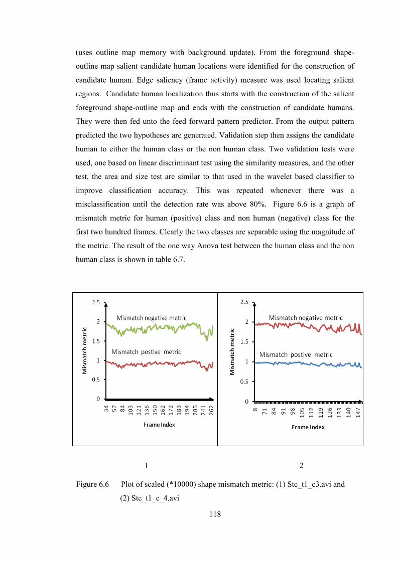
118
(uses outline map memory with background update). From the foreground shape-
outline map salient candidate human locations were identified for the construction of
candidate human. Edge saliency (frame activity) measure was used locating salient
regions. Candidate human localization thus starts with the construction of the salient
foreground shape-outline map and ends with the construction of candidate humans.
They were then fed unto the feed forward pattern predictor. From the output pattern
predicted the two hypotheses are generated. Validation step then assigns the candidate
human to either the human class or the non human class. Two validation tests were
used, one based on linear discriminant test using the similarity measures, and the other
test, the area and size test are similar to that used in the wavelet based classifier to
improve classification accuracy. This was repeated whenever there was a
misclassification until the detection rate was above 80%. Figure 6.6 is a graph of
mismatch metric for human (positive) class and non human (negative) class for the
first two hundred frames. Clearly the two classes are separable using the magnitude of
the metric. The result of the one way Anova test between the human class and the non
human class is shown in table 6.7.
Figure 6.6 Plot of scaled (*10000) shape mismatch metric: (1) Stc_t1_c3.avi and
(2) Stc_t1_c_4.avi
1 2
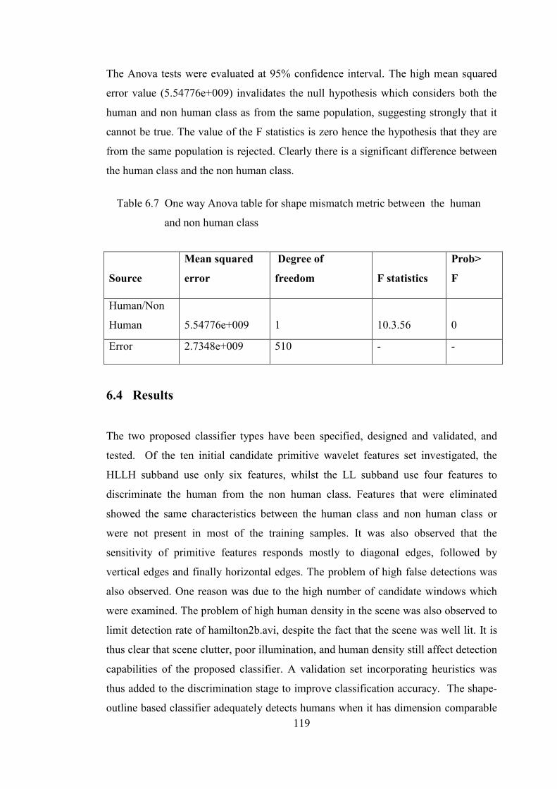
119
The Anova tests were evaluated at 95% confidence interval. The high mean squared
error value (5.54776e+009) invalidates the null hypothesis which considers both the
human and non human class as from the same population, suggesting strongly that it
cannot be true. The value of the F statistics is zero hence the hypothesis that they are
from the same population is rejected. Clearly there is a significant difference between
the human class and the non human class.
6.4 Results
The two proposed classifier types have been specified, designed and validated, and
tested. Of the ten initial candidate primitive wavelet features set investigated, the
HLLH subband use only six features, whilst the LL subband use four features to
discriminate the human from the non human class. Features that were eliminated
showed the same characteristics between the human class and non human class or
were not present in most of the training samples. It was also observed that the
sensitivity of primitive features responds mostly to diagonal edges, followed by
vertical edges and finally horizontal edges. The problem of high false detections was
also observed. One reason was due to the high number of candidate windows which
were examined. The problem of high human density in the scene was also observed to
limit detection rate of hamilton2b.avi, despite the fact that the scene was well lit. It is
thus clear that scene clutter, poor illumination, and human density still affect detection
capabilities of the proposed classifier. A validation set incorporating heuristics was
thus added to the discrimination stage to improve classification accuracy. The shape-
outline based classifier adequately detects humans when it has dimension comparable
Table 6.7 One way Anova table for shape mismatch metric between the human
and non human class
Source
Mean squared
error
Degree of
freedom
F statistics
Prob>
F
Human/Non
Human
5.54776e+009
1
10.3.56
0
Error 2.7348e+009 510 - -

120
to most objects in its surroundings. With the histogram classifier an important
parameter which determines the accuracy is the choice of level for wavelet
decomposition which would result in subbands with humans appearing significant in
its surroundings. The choice of the level is between one and three. The current
implementation used a detection threshold of 80% during training as adequate. This
proved a limiting factor in accuracy evaluations in stc_t1_c_4.avi sequence with
multiple humans and pixel saturation. To improve detection rate and reduce false
positive rate more training is required until the detection rate exceeds 90%, and false
alarms falls to less than 40% of the number of windows examined by the classifier.
The computational loads of the two classifiers are detailed out in table 6.8 and 6.9
assuming floating point operations requires 2 units of basic operations.
Function Number of operations
Pattern prediction
(Matrix-Matrix multiply+Matrix-
Matrix add)* 3
Pattern generation (Matrix-Scalar subtraction) *2
Mismatch measure [Sum(Matrix-Matrix subtraction)+sum(Matrix-
Matrix subtraction + (divide)]*2
Comparison 1
Table 6.8 Approximate computational load given candidate human of dimension
(M X N) for the shape-outline based classifier
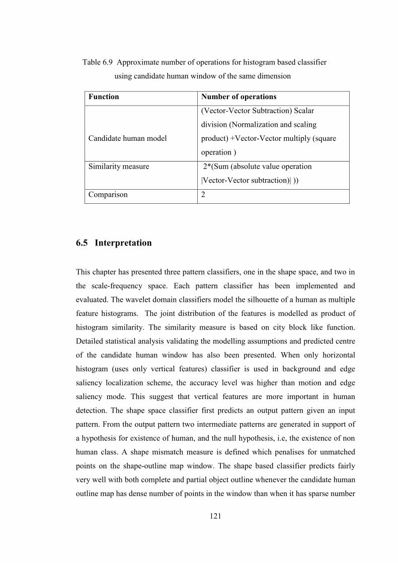
121
6.5 Interpretation
This chapter has presented three pattern classifiers, one in the shape space, and two in
the scale-frequency space. Each pattern classifier has been implemented and
evaluated. The wavelet domain classifiers model the silhouette of a human as multiple
feature histograms. The joint distribution of the features is modelled as product of
histogram similarity. The similarity measure is based on city block like function.
Detailed statistical analysis validating the modelling assumptions and predicted centre
of the candidate human window has also been presented. When only horizontal
histogram (uses only vertical features) classifier is used in background and edge
saliency localization scheme, the accuracy level was higher than motion and edge
saliency mode. This suggest that vertical features are more important in human
detection. The shape space classifier first predicts an output pattern given an input
pattern. From the output pattern two intermediate patterns are generated in support of
a hypothesis for existence of human, and the null hypothesis, i.e, the existence of non
human class. A shape mismatch measure is defined which penalises for unmatched
points on the shape-outline map window. The shape based classifier predicts fairly
very well with both complete and partial object outline whenever the candidate human
outline map has dense number of points in the window than when it has sparse number
Function Number of operations
Candidate human model
(Vector-Vector Subtraction) Scalar
division (Normalization and scaling
product) +Vector-Vector multiply (square
operation )
Similarity measure 2*(Sum (absolute value operation
|Vector-Vector subtraction)| ))
Comparison 2
Table 6.9 Approximate number of operations for histogram based classifier
using candidate human window of the same dimension

122
of points. For video sequence with large scale changes (changes in resolution of
object), level one or two wavelet (histogram) classifier achieves higher detection rate,
and low false positives. For sequence with little scale changes, shape-outline based
classifier achieve high detection rate and relatively low false positives at moderate
computational cost. Combining the two classifiers result in both an increase in
detection and false positive rates at a higher computational cost.
The computational complexity of the classifier could be improved if candidate
human window resizing is avoided. One approach is to design multiple classifiers to
detect body parts such as the head, upper body and lower body. The current
implementation is trained on the global shape and does not detect by part. Although
the proposed classifiers achieve high detection rate it also has high false detections
which is a problem in most visual surveillance application.
123
CHAPTER SEVEN
INVESTIGATIONS INTO HUMAN DETECTION
7.1 Introduction
Whereas the outputs of the previous two chapters relate to objectives one, two and
four in human detection, namely feature extraction, candidate human localization, and
classification. The focus of the current chapter is on proposed algorithmic task for
human detection, accuracy evaluation, task profiling, and algorithmic configuration
options for human detection. The task flow for human detection is a synthesis of sub
tasks involving pre processing, feature extraction, candidate human localization,
discrimination (classification), and update of found human database. Detailed block
diagram of the algorithm is shown in appendix B. From the extracted features in the
pattern space an efficient search mechanism is required to generate candidate humans
before discrimination. This functionality is provided by the search strategies in the
pattern spaces using salient feature maps. Section 7.2 discusses wavelet domain search
strategies for candidate human localization. Section 7.3 discusses human
discrimination in the wavelet domain whilst section 7.4 describes the overall task flow
for wavelet based detection of humans. Section 7.5 discusses shape-outline based
search strategies for candidate human localization, whilst section 7.6 describes shape-
outline based human discrimination. Section 7.7 describes the overall task flow for
shape-outline based human detection. Section 7.8 presents the synthesised algorithmic
architecture for human detection, whilst section 7.9 discuses simulations, accuracy
evaluations, and profiling of human detection tasks. Section 7.10 presents the results.
Section 7.11 discusses the results, trends on accuracy, and task profiling analysis.
124
7.2 Wavelet Domain Search Strategies
The computational load of human detection depends on the effort required in locating
candidate regions for subsequent processing. An efficient search strategy is required to
reduce the number of locations required to identify all candidate humans. For example
if the expected size of the candidate window is 64 pixels high by 32 pixels wide given
an input frame of 480 pixels high by 640 pixels wide then an exhaustive search
requires 52928 (416*608) blocks to locate all instances of human assuming there is
overlap. Inefficient search strategy adds extra processing time, and hence increases
response time. The three search strategies investigated in the current study are
essentially attention drawing mechanisms in feature space, namely, motion saliency,
edge saliency, and background saliency. Motion saliency applies threshold to frame
difference or foreground frames to remove insignificant motion. It is essentially a
feature rejection step. Edge saliency estimates significance of a region based on edge
count after eliminating spurious edges. Background saliency applies threshold to the
difference between LL subband and an accumulated background memory. The
assumption is that foreground objects becomes part of the background frame after
some time. Hence the need to examine background blobs. Saliency is estimated by
applying a global threshold to a subband frame, and grouping residual pixels (binary)
into rectangular blocks, and estimating the pixel activity in these blocks. It is
parameterised as a threshold expressed as a fraction of the brightest pixel in the frame.
In the case of edge and motion saliency it is followed by grouping the residual frame
into blocks and estimating the pixel density in the blocks. With background saliency
connected components (blobs) are located in the background memory as candidates
instead. It is justified since on visual inspection of wavelet subbands of humans and
other moving objects’ in a frame have silhouettes which appear brighter than the
background. The threshold fraction is typically between 0.1 and 0.9. It defines the
fraction of the maximum pixel intensity which is due to salient motion or edges of
significant objects in the scene. The use of candidate human localization techniques is
justified since edges or high frequency components of images are found in HH, HL
and LH subbands, whilst the LL subband contains low frequency component (low
pass image) at a given level of wavelet decomposition or the low pass version of the
frame. Low pass version is appropriate for describing global motion. In the saliency
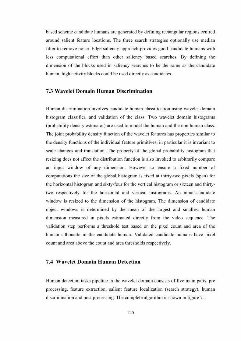
125
based scheme candidate humans are generated by defining rectangular regions centred
around salient feature locations. The three search strategies optionally use median
filter to remove noise. Edge saliency approach provides good candidate humans with
less computational effort than other saliency based searches. By defining the
dimension of the blocks used in saliency searches to be the same as the candidate
human, high activity blocks could be used directly as candidates.
7.3 Wavelet Domain Human Discrimination
Human discrimination involves candidate human classification using wavelet domain
histogram classifier, and validation of the class. Two wavelet domain histograms
(probability density estimator) are used to model the human and the non human class.
The joint probability density function of the wavelet features has properties similar to
the density functions of the individual feature primitives, in particular it is invariant to
scale changes and translation. The property of the global probability histogram that
resizing does not affect the distribution function is also invoked to arbitrarily compare
an input window of any dimension. However to ensure a fixed number of
computations the size of the global histogram is fixed at thirty-two pixels (span) for
the horizontal histogram and sixty-four for the vertical histogram or sixteen and thirty-
two respectively for the horizontal and vertical histograms. An input candidate
window is resized to the dimension of the histogram. The dimension of candidate
object windows is determined by the mean of the largest and smallest human
dimension measured in pixels estimated directly from the video sequence. The
validation step performs a threshold test based on the pixel count and area of the
human silhouette in the candidate human. Validated candidate humans have pixel
count and area above the count and area thresholds respectively.
7.4 Wavelet Domain Human Detection
Human detection tasks pipeline in the wavelet domain consists of five main parts, pre
processing, feature extraction, salient feature localization (search strategy), human
discrimination and post processing. The complete algorithm is shown in figure 7.1.

126
Figure 7.1 Flowchart for histogram-based human detection. EOS
and EOF denote end of sequence and end of frame processing
Yes
No
Feature extraction
Candidate human localization
Pre processing
Get next frame
Start
Histogram-based
classification
Stop
No
Yes
No
Human class
EOS
Database update
Validation
Drop
candidate
Yes
EOF

127
The processing starts with the current frame being wavelet transformed into wavelet
subbands (see section 5.2.1). The resulting subband is searched for candidate humans
using saliency directed search mechanism (see section 5.3). Selected humans
candidates are then passed on to the histogram based classifier. A similarity metric
(city block like measure) is computed for the human class using the histogram model
corresponding to the human class, whilst that of the non human class is computed
using the non human histogram model. A decision is made using equation 6.8. Finally
the validation step involves heuristics (pixel count and size test). It is only when the
validation test is satisfied is the candidate human assigned to the human class.
7.5 Shape-Outline Based Search Strategy
Two salient feature localization techniques were investigated to reduce the number of
salient features in order to efficiently locate candidate humans. The first one is based
on edge saliency (using block activity measure). Given a shape-outline map the edge
saliency approach partitions the frame into non overlapping blocks and computes the
number of edges within each block. It then selects the centroids of blocks whose edge
count exceeds a user defined threshold as candidates. This is described by a pseudo
code below. Another edge saliency scheme selects candidate windows after
suppressing multiple feature points and very small shape outlines within the block by
applying median filtering. Morphological filters could also be applied alternatively.
Motion saliency is similar to the edge saliency, the difference lies in how the map is
obtained. Motion saliency is based on subtracting a previous shape-outline map or a
fixed background map from the current shape-outline map. The main parameters of
the edge saliency based searches are the minimum human separation distance along
the X and Y-axis. The centroid is computed based on the first moment of the candidate
window.
1. Construct shape-outline map for the current frame.
2. Find maximum pixel intensity of the current frame (Max).
3. Select saliency threshold (0<α<1) as a fraction of the maximum intensity value.
4. Threshold current shape-outline map:
For all pixels

128
Salient_shape_outline_map=Find (shape_outline map> (α *Max))
End
5. Output Salient_shape_outline_map.
7.6 Shape-Outline Based Human Discrimination
The processing steps for shape-outline based discrimination are similar to that of
wavelet domain human discrimination in section 7.3. The difference is that it is based
on the shape-outline classifier using shape mismatch measure instead of similarity
measure to assign a class label (see section 6.3, and 6.3.1). Secondly, the validation
step involves two tests. The first test involves using a linear discriminant function. The
discriminant function (Discr) is given by equation 7.1, where Neg, and Pos denotes
shape mismatch due to assigning to non human and human class respectively. It is
only when the discriminant function returns the same class label as that of the
histogram classifier is the next validation step executed. The last validation step
essentially performs a threshold test on the pixel count and area of the human
silhouette in the object window.
Discr (Neg,Pos)=4.014*Pos-5.54*Neg-1 7.1.
7.7 Shape-Outline Based Human Detection
Figure 7.2 shows the task flow for human detection. Detection task involves pre
processing, feature extraction (foreground shape-outline map extraction), candidate
human localization (via block activity measure), shape-outline prediction, generate
hypotheses patterns, shape mismatch measure computations, human classification
(assigns a class label to the current object window). Finally validation is based on
either confidence measure, heuristics (pixel count threshold test, size test), or linear
discriminant function evaluation. In the current implementation heuristics and linear
discriminant function are used to validate the class assignment. It is only when the
validation step is consistent with the human class is the candidate human detected. The
bounding box is then used to describe the detected human.

129
Figure 7.2 Flowchart of shape-outline map based human detection. EOF
denotes end of frame processing, and EOS denotes end of sequence
processing.
Yes No
No
Yes
Update database
Validation
Candidate human
localization
Shape-outline
Prediction
Generate hypotheses
patterns (+ve, -ve)
Shape mismatch
measure computation
Human
EOS Stop
Foreground shape-
outline map
Pre processing
Get next frame
Start
Drop
candidate
Yes
No EOF
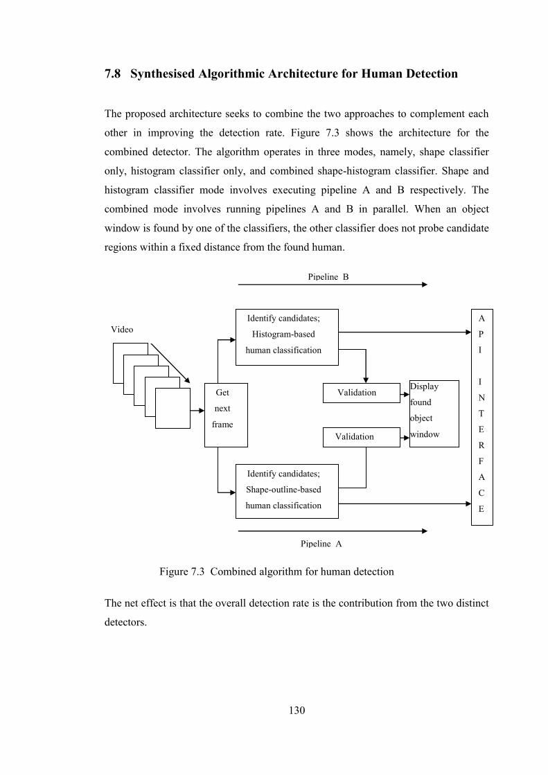
130
7.8 Synthesised Algorithmic Architecture for Human Detection
The proposed architecture seeks to combine the two approaches to complement each
other in improving the detection rate. Figure 7.3 shows the architecture for the
combined detector. The algorithm operates in three modes, namely, shape classifier
only, histogram classifier only, and combined shape-histogram classifier. Shape and
histogram classifier mode involves executing pipeline A and B respectively. The
combined mode involves running pipelines A and B in parallel. When an object
window is found by one of the classifiers, the other classifier does not probe candidate
regions within a fixed distance from the found human.
The net effect is that the overall detection rate is the contribution from the two distinct
detectors.
Figure 7.3 Combined algorithm for human detection
Display
found
object
window
Pipeline A
Pipeline B
A
P
I
I
N
T
E
R
F
A
C
E
Identify candidates;
Shape-outline-based
human classification
Identify candidates;
Histogram-based
human classification
Validation
Validation
Video
Frames
Get
next
frame
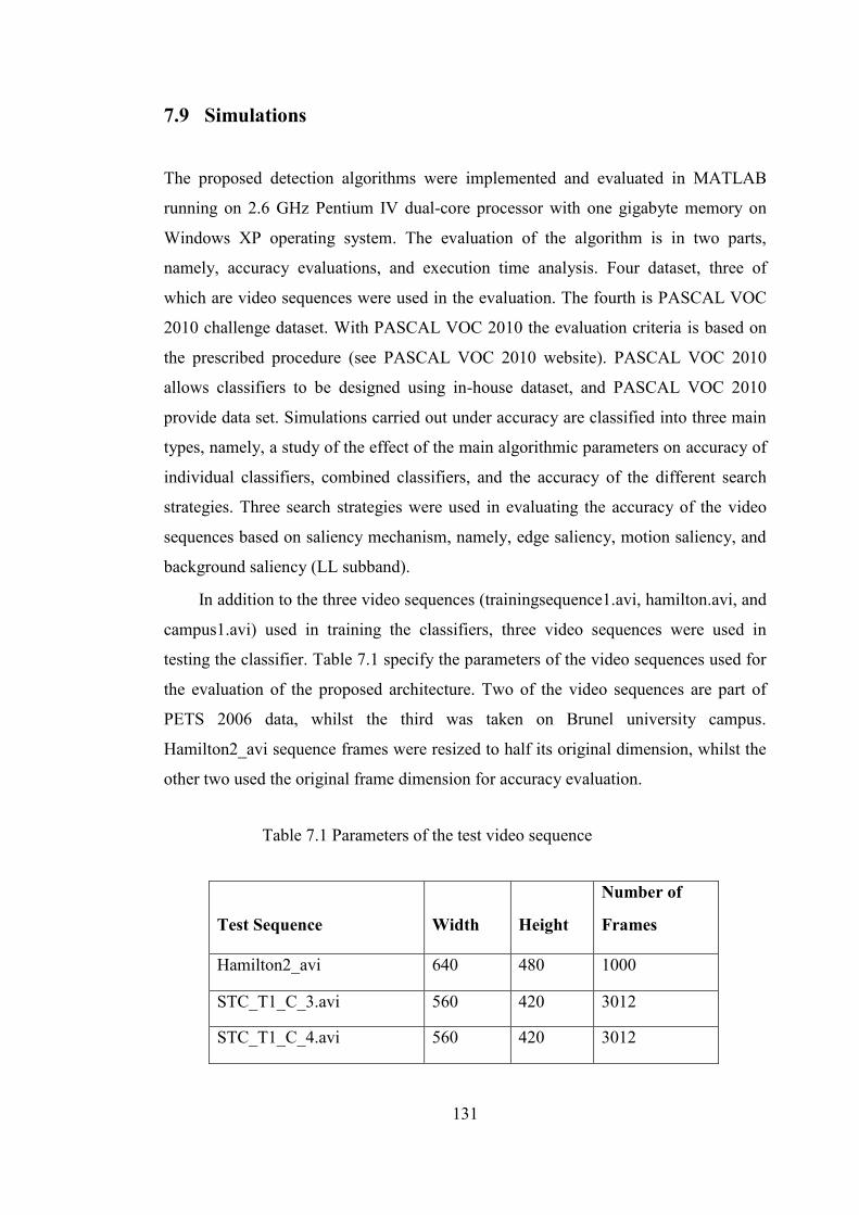
131
7.9 Simulations
The proposed detection algorithms were implemented and evaluated in MATLAB
running on 2.6 GHz Pentium IV dual-core processor with one gigabyte memory on
Windows XP operating system. The evaluation of the algorithm is in two parts,
namely, accuracy evaluations, and execution time analysis. Four dataset, three of
which are video sequences were used in the evaluation. The fourth is PASCAL VOC
2010 challenge dataset. With PASCAL VOC 2010 the evaluation criteria is based on
the prescribed procedure (see PASCAL VOC 2010 website). PASCAL VOC 2010
allows classifiers to be designed using in-house dataset, and PASCAL VOC 2010
provide data set. Simulations carried out under accuracy are classified into three main
types, namely, a study of the effect of the main algorithmic parameters on accuracy of
individual classifiers, combined classifiers, and the accuracy of the different search
strategies. Three search strategies were used in evaluating the accuracy of the video
sequences based on saliency mechanism, namely, edge saliency, motion saliency, and
background saliency (LL subband).
In addition to the three video sequences (trainingsequence1.avi, hamilton.avi, and
campus1.avi) used in training the classifiers, three video sequences were used in
testing the classifier. Table 7.1 specify the parameters of the video sequences used for
the evaluation of the proposed architecture. Two of the video sequences are part of
PETS 2006 data, whilst the third was taken on Brunel university campus.
Hamilton2_avi sequence frames were resized to half its original dimension, whilst the
other two used the original frame dimension for accuracy evaluation.
Test Sequence
Width
Height
Number of
Frames
Hamilton2_avi 640 480 1000
STC_T1_C_3.avi 560 420 3012
STC_T1_C_4.avi 560 420 3012
Table 7.1 Parameters of the test video sequence
132
For the wavelet domain histogram classifier, the accuracy of vertical and horizontal
histogram were studied separately, and then in combination. The threshold values used
in the saliency searches are all expressed as fraction based on the maximum wavelet
coefficient in a frame. Nominal threshold used are [0.1, 0.2, 0.3, 0.4, 0.5, 0.6, 0.7, 0.8,
0.9, 0.95] of the maximum wavelet coefficient in a frame. Background memory flag
enables two background modes to be tested, namely, frame differencing, and fixed
background with update. Use_subband_Flag (see table 7.2) is set when decimated
wavelet transform function is invoked, and was set off when non decimated wavelet
transform is invoked. Tables 7.2 and 7.3 show the main parameters of the histogram
classifier and shape based detector respectively. Discussions on the effect of
algorithmic parameters are based on these tables. In studying the effects of algorithmic
parameters on accuracy for the histogram based detector, maximum distance of
separation in X and Y (from parameters 8 and 9 from table 7.2) were kept constant at
half the candidate object window in X and Y (parameters 2 and 3 from table 7.2)
respectively, i.e, found humans within half the dimension of object search window is
classified as the same object to avoid duplication. The rest of the parameters were kept
constant for a given sequence. As a guide the candidate human dimension was
determined by estimating the width and height of human in the sequence. This
required since the ground truth label only marks the approximate centroid of the
candidate human, and the size of the humans varies from one frame to another. Thus
candidate human dimension is required in order to bound a candidate to a region.
Similar criteria were used in evaluating the shape-based detector. A classification
scheme was also derived to characterise the sequence in terms of scene complexity
and hence a measure of analysis complexity. Video scene complexity were classified
as: slow motion, fast motion, significant scene changes, no scale changes, highly
cluttered, and low contrast for the purpose of setting the algorithmic parameters for
optimal operating accuracy. Profiling of the sub tasks and the proposed architecture
were also evaluated to identify critical sub tasks in the task execution pipelines,
throughput, and scalability of the proposed algorithm.
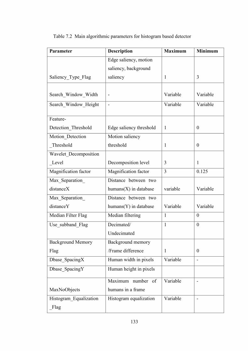
133
Parameter Description Maximum Minimum
Saliency_Type_Flag
Edge saliency, motion
saliency, background
saliency
1
3
Search_Window_Width
-
Variable
Variable
Search_Window_Height - Variable Variable
Feature-
Detection_Threshold
Edge saliency threshold
1
0
Motion_Detection
_Threshold
Motion saliency
threshold
1
0
Wavelet_Decomposition
_Level
Decomposition level
3
1
Magnification factor Magnification factor 3 0.125
Max_Separation_
distanceX
Distance between two
humans(X) in database
variable
Variable
Max_Separation_
distanceY
Distance between two
humans(Y) in database
Variable
Variable
Median Filter Flag Median filtering 1 0
Use_subband_Flag Decimated/
Undecimated
1 0
Background Memory
Flag
Background memory
/Frame difference
1
0
Dbase_SpacingX Human width in pixels Variable -
Dbase_SpacingY Human height in pixels
MaxNoObjects
Maximum number of
humans in a frame
Variable -
Histogram_Equalization
_Flag
Histogram equalization Variable -
Table 7.2 Main algorithmic parameters for histogram based detector
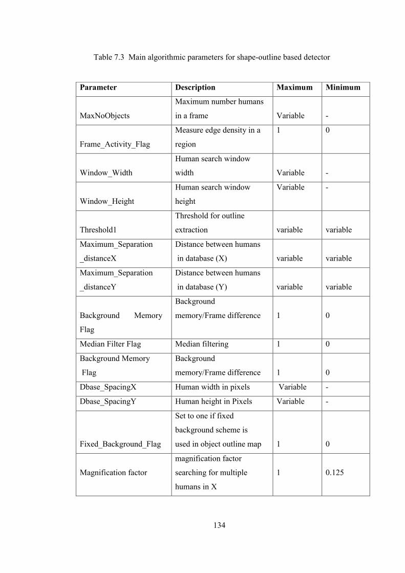
134
Parameter Description Maximum Minimum
MaxNoObjects
Maximum number humans
in a frame
Variable
-
Frame_Activity_Flag
Measure edge density in a
region
1 0
Window_Width
Human search window
width
Variable
-
Window_Height
Human search window
height
Variable -
Threshold1
Threshold for outline
extraction
variable
variable
Maximum_Separation
_distanceX
Distance between humans
in database (X)
variable
variable
Maximum_Separation
_distanceY
Distance between humans
in database (Y)
variable
variable
Background Memory
Flag
Background
memory/Frame difference
1
0
Median Filter Flag Median filtering 1 0
Background Memory
Flag
Background
memory/Frame difference
1
0
Dbase_SpacingX Human width in pixels Variable -
Dbase_SpacingY Human height in Pixels Variable -
Fixed_Background_Flag
Set to one if fixed
background scheme is
used in object outline map
1
0
Magnification factor
magnification factor
searching for multiple
humans in X
1
0.125
Table 7.3 Main algorithmic parameters for shape-outline based detector
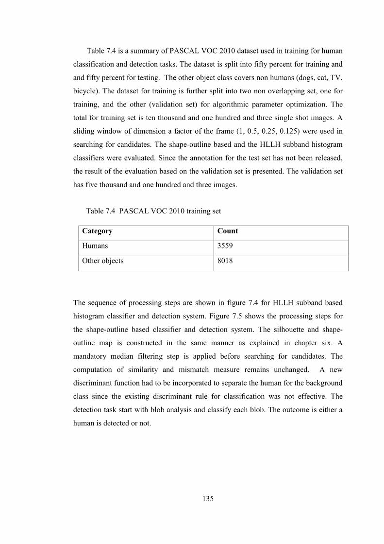
135
Table 7.4 is a summary of PASCAL VOC 2010 dataset used in training for human
classification and detection tasks. The dataset is split into fifty percent for training and
and fifty percent for testing. The other object class covers non humans (dogs, cat, TV,
bicycle). The dataset for training is further split into two non overlapping set, one for
training, and the other (validation set) for algorithmic parameter optimization. The
total for training set is ten thousand and one hundred and three single shot images. A
sliding window of dimension a factor of the frame (1, 0.5, 0.25, 0.125) were used in
searching for candidates. The shape-outline based and the HLLH subband histogram
classifiers were evaluated. Since the annotation for the test set has not been released,
the result of the evaluation based on the validation set is presented. The validation set
has five thousand and one hundred and three images.
The sequence of processing steps are shown in figure 7.4 for HLLH subband based
histogram classifier and detection system. Figure 7.5 shows the processing steps for
the shape-outline based classifier and detection system. The silhouette and shape-
outline map is constructed in the same manner as explained in chapter six. A
mandatory median filtering step is applied before searching for candidates. The
computation of similarity and mismatch measure remains unchanged. A new
discriminant function had to be incorporated to separate the human for the background
class since the existing discriminant rule for classification was not effective. The
detection task start with blob analysis and classify each blob. The outcome is either a
human is detected or not.
Category Count
Humans 3559
Other objects 8018
Table 7.4 PASCAL VOC 2010 training set
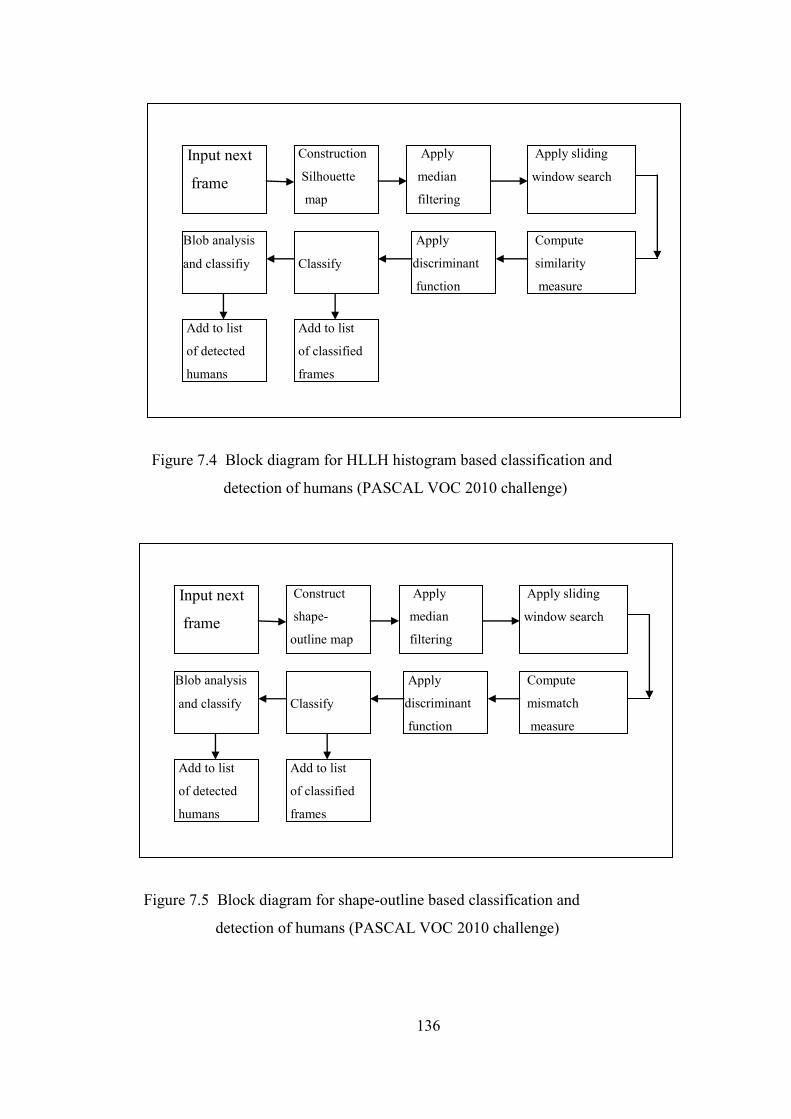
136
Apply
median
filtering
Input next
frame
Add to list
of classified
frames
Construct
shape-
outline map
Apply sliding
window search
Compute
mismatch
measure
Apply
discriminant
function
Classify
Add to list
of detected
humans
Blob analysis
and classify
Figure 7.5 Block diagram for shape-outline based classification and
detection of humans (PASCAL VOC 2010 challenge)
Apply
median
filtering
Input next
frame
Add to list
of classified
frames
Construction
Silhouette
map
Apply sliding
window search
Compute
similarity
measure
Apply
discriminant
function
Classify
Add to list
of detected
humans
Blob analysis
and classifiy
Figure 7.4 Block diagram for HLLH histogram based classification and
detection of humans (PASCAL VOC 2010 challenge)
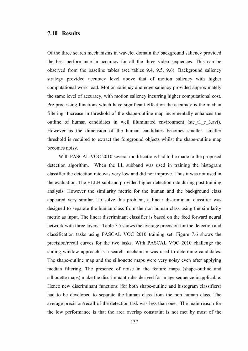
137
7.10 Results
Of the three search mechanisms in wavelet domain the background saliency provided
the best performance in accuracy for all the three video sequences. This can be
observed from the baseline tables (see tables 9.4, 9.5, 9.6). Background saliency
strategy provided accuracy level above that of motion saliency with higher
computational work load. Motion saliency and edge saliency provided approximately
the same level of accuracy, with motion saliency incurring higher computational cost.
Pre processing functions which have significant effect on the accuracy is the median
filtering. Increase in threshold of the shape-outline map incrementally enhances the
outline of human candidates in well illuminated environment (stc_t1_c_3.avi).
However as the dimension of the human candidates becomes smaller, smaller
threshold is required to extract the foreground objects whilst the shape-outline map
becomes noisy.
With PASCAL VOC 2010 several modifications had to be made to the proposed
detection algorithm. When the LL subband was used in training the histogram
classifier the detection rate was very low and did not improve. Thus it was not used in
the evaluation. The HLLH subband provided higher detection rate during post training
analysis. However the similarity metric for the human and the background class
appeared very similar. To solve this problem, a linear discriminant classifier was
designed to separate the human class from the non human class using the similarity
metric as input. The linear discriminant classifier is based on the feed forward neural
network with three layers. Table 7.5 shows the average precision for the detection and
classification tasks using PASCAL VOC 2010 training set. Figure 7.6 shows the
precision/recall curves for the two tasks. With PASCAL VOC 2010 challenge the
sliding window approach is a search mechanism was used to determine candidates.
The shape-outline map and the silhouette maps were very noisy even after applying
median filtering. The presence of noise in the feature maps (shape-outline and
silhouette maps) make the discriminant rules derived for image sequence inapplicable.
Hence new discriminant functions (for both shape-outline and histogram classifiers)
had to be developed to separate the human class from the non human class. The
average precision/recall of the detection task was less than one. The main reason for
the low performance is that the area overlap constraint is not met by most of the

138
detected humans. It is attributed to the feature map produced in using the test
sequence for candidate localization, which is noisy. In the case of video frames,
application of frame differencing or background subtraction followed by median
filtering removes move of the features shared by the background class. The peak
detection rate of the histogram detection is less than 0.003 on account of the high
detections which fails to meet the area overlap test. The actual number of detections
(candidates) passed on to the classifier is 470,520,200 out of which 20,000,540 met
the area overlap constraint. The number of test frame used is 5105. Thus clearly the
low average precision is attributed to the large number of candidates.
Table 7.5 Average precision for PASCAL VOC 2010 challenge
Algorithm Average precision
Classifier/Detector Classification (%) Detection (%)
Shape-outline based
classifier/detector (In-
house training set)
54
-
Shape-outline based
classifier/detector
(PASCAL training set)
40
0.003
HLLH subband classifier/
detector(PASCAL
training set)
54
0.003
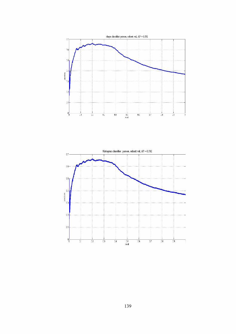
139

140
It was also o
observed that the response of the vertical features (horizontal histogram) is the main
distinct feature in classifying and detecting humans. As a result the horizontal feature
histogram was not used in the evaluation step.
Chapter eight provides more details on accuracy of the combined detector. Tables
7.6, 7.7 and 7.8 provide execution time profiling by function using MATLAB profiler.
The tables exclude initialization (classifier tables and parameter file), frame access,
overheads unique to MATLAB, and post processing. Initialization and post processing
task are executed only once during a run. It was noted that the execution time in
MATLAB varies but the relative execution time expressed as a percentage is stable
hence it is used to measure the relative computational effort required. Since the
execution time depends on the frame dimensions and the number of frames, the
figures quoted are based on assuming a standard frame size of 320 wide by 240 pixels
high. Overheads includes functions such as displaying of graphical objects, colour
Figure 7.6 Precision/recall curves (Top to bottom) (a) shape-outline classifier
(b) HLLH subband histogram classifier (c) Histogram-outline
detector
141
space conversion, intrinsic functions called when generating outputs, and other
functions not directly related to the main task.
7.11 Interpretation
This chapter has investigated three search strategies for candidate human identification
and the rest of the building blocks which forms the two detectors for video content
analysis. These are edge and motion saliency, and background saliency. Edge saliency
estimates the edge density within a block of a candidate search region. Motion
saliency estimates the amount of motion present in a candidate region, and
background saliency estimates the dimension of blobs in the background image and
hence its importance as candidates when background memory scheme is active. Edge
density based measure was used in locating the candidate human. It was noted that
although the candidate human localization strategy is effective, it sometimes filters out
some discriminatory features and limits the ability of the classifier to discriminate
humans from non humans. As an alternative, the original feature map is used by the
classifier in discriminating. The same conclusion is applicable to the wavelet domain
features. Wavelet domain detectors are less sensitive to transient changes due motion
and have more stable detection and false alarm rates. It is supported by higher
detection and lower false positive rates in the background saliency mode of the
wavelet detector
The ROC curves of all the test sequences are a plot of the measured detection and
false alarm rates, and non parametric; thus no attempt was made to fit the points unto
to a curve. This enables the sensitivity of the algorithmic parameters to be studied. The
influence of the following parameters were evaluated during the simulation run:
median filtering, candidate human width, candidate human height, background
modelling scheme, and window scaling factor. In general an increase in candidate
window dimension results in increase in detection rate and false alarm rate until
beyond certain dimension the detection rate falls with increase in window dimension.
Median filtering tends to reduce the detection rate for less cluttered scene but
increases the detection rate for cluttered scene with humans coming together to form
groups frequently. The following observations were made: the difficulty in
differentiating the human class from the background becomes more severe as the
142
scene clutter increases with increasing number of humans to detect. The size of the
median filter chosen must match the background noise characteristics to avoid
removing discriminatory features. The main problem with the proposed detectors is
the high false positive rates. This is observed in the high values of FPR and low
values in PPV and F1 measures. This problem is addressed in chapter seven.
From the result of PASCAL VOC 2010 challenge dataset it is clear that the
proposed technique is not suitable for detection of humans in single frame but suitable
for classification of images. Further work needs to be done to improve the localization
of humans in single frames in order to be suitable for human detection in single frame.
The computational effort spent on the wavelet transform is offset by a reduction
to a quarter the input frame size of the output subband for every unit increase in
wavelet decomposition level. The execution time of wavelet transform is similarly
halved for every level increase in decomposition. From tables 7.6 it is noted that the
most demanding task, the edge saliency tasks operates on candidate windows (images
patches), and are independent of each other. From table 7.7 which uses level-two
wavelet transform the bottleneck lies with the wavelet transform and not the edge
saliency sub task. This is due to the reduced subband frame size (a sixteenth of the
original frame size) compared to table 7.8. From the execution profiling it is also
noted that the level two wavelet detector has the fastest execution times of the three
detection modes. The smaller subband of level two requires correspondingly less
amount of search time, and reduction in execution time of resizing operations (a major
source of computation) on the subband windows. With level one decomposition on the
other hand, the reduction in processing time of salient object feature localization and
frame resizing at level one wavelet transform (giving a reduction of frame size of
0.25) was not enough to offset the execution time of level one wavelet decomposition.
From table 7.8 (shape-outline based detector), the dominating task is object
localization. It is also obvious that approximately equal amount of time is spent
executing the classifier as is spent in object window analysis (Shap_Pre_Window,
Shape_Window_Analysis and Shape_find_ROI_Centroid). Each takes about 14.5% of
the executing time. On the other hand the shape search strategy
(Improved_Shape_Search_Strategy) takes about 38.4%. Most of the sub tasks also
operate on patches of the frame which are independent of each other.

143
Table 7.6 Task profiling of the main functions of histogram based detector for
decimated wavelet transform (level one) subband
Function
Normalized
Execution
Time(Sec)
Percentage of
Execution Time
Improve_Histogram_Analysis 0.027 1.41
Resizing (Frames and windows) 0.24 12.55
Level_One_Wavelet_Transform 0.14 7.32
Improved_Wavelet_Object_Search 0.12 6.28
Histogram_Window_Analysis 0.005 0.26
Edge_Saliency 1.38 72.18
Total 1.91 100
Table 7.7 Task profiling of the main functions of the histogram based detector
for decimated wavelet transform (level two) subband
Function
Normalized
Execution
Time(Sec)
Percentage of
Execution Time
Improve_Histogram_Analysis 0.021 4.07
Resizing (Frames and windows) 0.032 6.23
Level_Two-Wavelet_Transform 0.257 49.9
Improved_Wavelet_Object_Search 0.104 20.19
Histogram_Window_Analysis 0.001 0.19
Edge_Saliency 0.10 19.42
Total 0.52 100

144
From the above profiling data it is obvious that the application would benefit from
applying parallel processing techniques. Figure 7.7 illustrates the difficulty in
assigning evaluating accuracy of detection task. It includes over using sized windows,
humans appearing with variable dimension, and multiple humans being enclosed in a
bounding box. This makes the evaluation task highly variable. The use of proportion-
based threshold (fraction of maximum wavelet coefficient value) in the pattern spaces
(shape and wavelet space) also allows rapid detection of features.
Table 7.8 Task profiling of the main functions of the shape-based detector
Function
Normalized
Execution
Time(Sec)
Percentage
of Execution
Time
Improved_Shape_Search_Strategy_
Object_Window
0.088 38.40
Partial_Human_Shape_Classifier_New 0.034 14.84
Resizing (Frames and object windows) 0.0054 2.36
Object_Outline Map 0.065 28.37
Compute_Frame_Activity 0.003 1.32
Shape_Pre_Window 0.0008 0.35
Shape_Window_Analysis 0.028 12.21
Shape_Find_ROI_Centroid 0.004 1.74
Shape_FoundObjectdatabase 0.00085 0.37
Verify_FoundObject_Objectdatabase 0.0001 0.04
Total 0.23 100
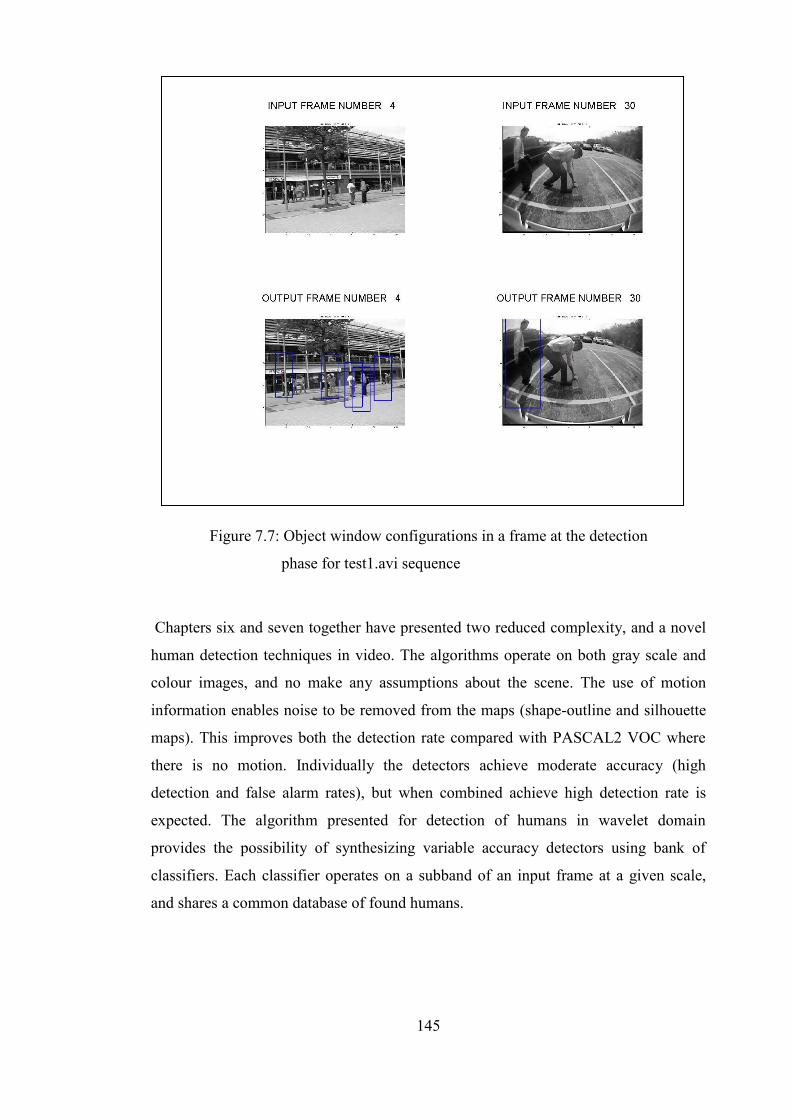
145
Chapters six and seven together have presented two reduced complexity, and a novel
human detection techniques in video. The algorithms operate on both gray scale and
colour images, and no make any assumptions about the scene. The use of motion
information enables noise to be removed from the maps (shape-outline and silhouette
maps). This improves both the detection rate compared with PASCAL2 VOC where
there is no motion. Individually the detectors achieve moderate accuracy (high
detection and false alarm rates), but when combined achieve high detection rate is
expected. The algorithm presented for detection of humans in wavelet domain
provides the possibility of synthesizing variable accuracy detectors using bank of
classifiers. Each classifier operates on a subband of an input frame at a given scale,
and shares a common database of found humans.
Figure 7.7: Object window configurations in a frame at the detection
phase for test1.avi sequence
146
CHAPTER EIGHT
INVESTIGATION INTO JPDAF TRACKER
8.1 Introduction
This chapter presents a reduced complexity silhouette based JPDAF (Joint probabilistic
data association filter) tracker for human tracking based on state-space approach, and
evaluates its accuracy and real-time performance. Firstly, four appearance features
(intensity, directional gradient, chromatic red and green colours) are extracted using the
binary silhouette of candidate humans in the frame. JPDAF is used for data association
spatially within a frame, and track likelihood filter to resolve measurements conflicts
between frames. Additionally the signatures of found humans are used to uniquely assign
humans to track.
Measurements are assumed to be normally distributed, and Kalman prediction is used
to determine the next state vector of the tracks. Section 8.2 describes track initialization
and measurement validation based on Mahalanobis distance. Section 8.3 describes the
algorithm for extracting appearance features. Section 8.4 details out the cluster based
motion vector estimation technique which allows motion vectors to be determined as a
look up table. Partition of measurements into clusters is also discussed. Section 8.5
discusses measurement (location and motion vector estimation) validation constraints.
Kalman prediction for evaluating trajectory of humans undergoing linear motion is
discussed in section 8.6. Section 8.7 discusses measurement-to-track hypotheses
generation and validation. The computation of similarity measure between the signature
of found human and that of a candidate track to determine the best track for association is
also discussed. The use of JPDAF and measurement cluster to update the state of a track
147
is also discussed. Section 8.8 describes the different track optimisation techniques
implemented including multiple motion models, sequential and batch state estimation
mode for improving the accuracy of the tracker. Section 8.9 deals with detecting
occlusion and how it is handled. Section 8.10 analyses the computational complexity of
the tracker. Section 8.11 presents a scalable algorithmic architecture for the tracker.
Simulations and accuracy evaluations are described in section 8.12. Section 8.13
discusses the results whilst 8.14 interprets the results.
8.2 Track Initialization
One of the parameters required for the tracker, Mahalanobis distance, is derived from the
confidence level associated the measurement process as defined by the user. For an M-
dimension measurement vector, Mahalanobis distance is chi-squared distributed with M
degrees of freedom. The locus of points given Mahalanobis distance K, is an M-
dimension ellipse where M is the dimension of the measurement matrix. Thus every
measurement vector has associated with it a validation volume defined by M. It is used in
validating measurements assigned to tracks. A new track is initialized if there is no
evidence between the previous frame and the current frame linking a candidate human to
a track. New tracks are initialized with the x and y coordinates of the centroid. This
occurs at the start of track processing window when the first frame with humans is passed
to the tracker. A track processing window denotes a sequence of frames upon which
track decisions (assignments, expiration, splits, and merges) are made during tracking.
All known tracks are initialised at the start of track processing window. It operates as a
sliding window of the frame sequence. At the end of every track processing period, for
all found humans not associated with any track, the tracker automatically assigns them to
a new track. Global parameters of JPDAF tracker used for the simulation are shown in
table 8.2. The algorithmic task flow for tracking is shown in figure 8.1. The first sub task,
pre processing involves associating centroids in the current frame to existing tracks from
the previous frame provided that the measurement is within its validating volume,
otherwise it is a new track.
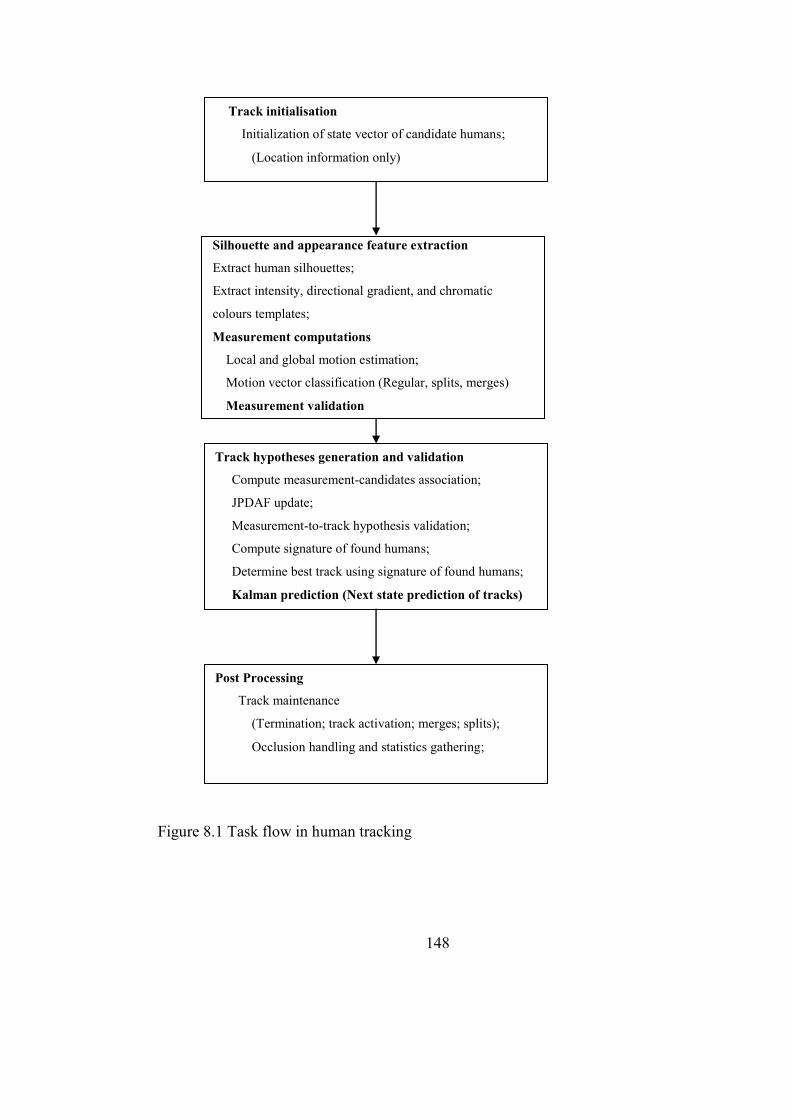
148
Track hypotheses generation and validation
Compute measurement-candidates association;
JPDAF update;
Measurement-to-track hypothesis validation;
Compute signature of found humans;
Determine best track using signature of found humans;
Kalman prediction (Next state prediction of tracks)
Figure 8.1 Task flow in human tracking
Post Processing
Track maintenance
(Termination; track activation; merges; splits);
Occlusion handling and statistics gathering;
Silhouette and appearance feature extraction
Extract human silhouettes;
Extract intensity, directional gradient, and chromatic
colours templates;
Measurement computations
Local and global motion estimation;
Motion vector classification (Regular, splits, merges)
Measurement validation
Track initialisation
Initialization of state vector of candidate humans;
(Location information only)

149
8.3 Silhouette and Appearance Feature Extraction for Human
Tracking
The appearance feature extraction starts with silhouette extraction and then appearance
template modelling based on found humans in the current frame. It is based on the
assumption that there are no significant view point changes between consecutive frames.
Appearance feature extraction based on the silhouettes computed on every frame avoids
the need to update a global template on a frame-by-frame basis. Accumulation of small
changes over several frames would introduce significantly deviations if fixed templates
were used. In [Jephson et al. 2003] an online appearance model consisting of three
components is modelled as Gaussian mixture to reduce the effect of dynamic changes
between frames. The approach adopted is to use the associated appearance descriptor of
the silhouette as the best representation of the candidate human in the window when
comparisons are made between humans in the previous frame. Human silhouettes are
extracted by blurring with an averaging filter (5 by 5 averaging filter) to obtain a low
pass version of the candidate window. Spatial domain segmentation based on intensity
pixel threshold is applied to obtain the silhouette. The resulting silhouette is a binary
representation of the human. They are intensity, directional gradient, and two chromatic
colours (red and green). Chromatic colour space is used since it is less sensitive to
illumination changes [Yeasin et al. 2004]. Any of the four templates could be used alone
or in combination with others for motion tracking. From the appearance templates are
extracted two measurements, namely, motion vector, and spatial location. The decision
on the number of appearance templates to use is dependent on the computational load and
the expected improvement in accuracy required. The directional gradient image is
extracted by applying Sobel filter masks for detecting vertical and horizontal edges as
shown in figure 8.2 and defined by equation 8.1.
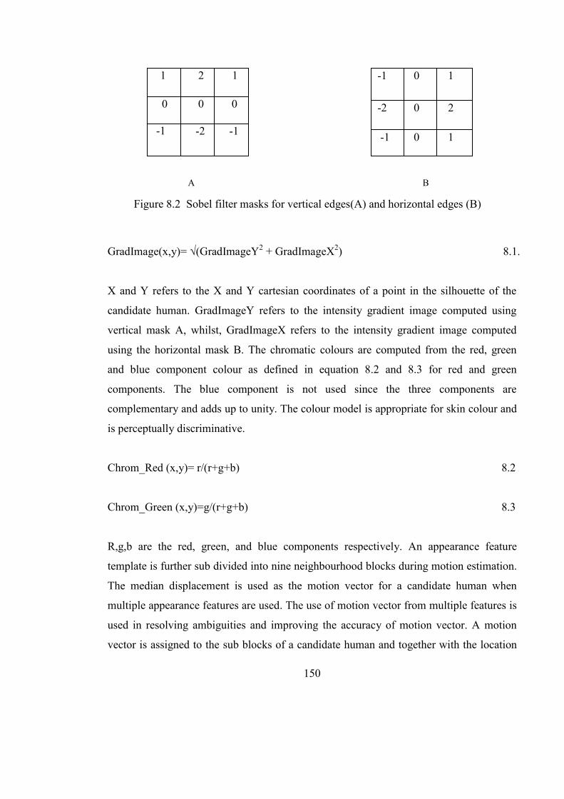
150
GradImage(x,y)= √(GradImageY2 + GradImageX2) 8.1.
X and Y refers to the X and Y cartesian coordinates of a point in the silhouette of the
candidate human. GradImageY refers to the intensity gradient image computed using
vertical mask A, whilst, GradImageX refers to the intensity gradient image computed
using the horizontal mask B. The chromatic colours are computed from the red, green
and blue component colour as defined in equation 8.2 and 8.3 for red and green
components. The blue component is not used since the three components are
complementary and adds up to unity. The colour model is appropriate for skin colour and
is perceptually discriminative.
Chrom_Red (x,y)= r/(r+g+b) 8.2
Chrom_Green (x,y)=g/(r+g+b) 8.3
R,g,b are the red, green, and blue components respectively. An appearance feature
template is further sub divided into nine neighbourhood blocks during motion estimation.
The median displacement is used as the motion vector for a candidate human when
multiple appearance features are used. The use of motion vector from multiple features is
used in resolving ambiguities and improving the accuracy of motion vector. A motion
vector is assigned to the sub blocks of a candidate human and together with the location
1 2 1
-1 -2 -1
Figure 8.2 Sobel filter masks for vertical edges(A) and horizontal edges (B)
A B
-1 -2 -1
0 0 0
0 1 -1
0 1 -1
0 2 -2
-1 -2 -1
1 2 1
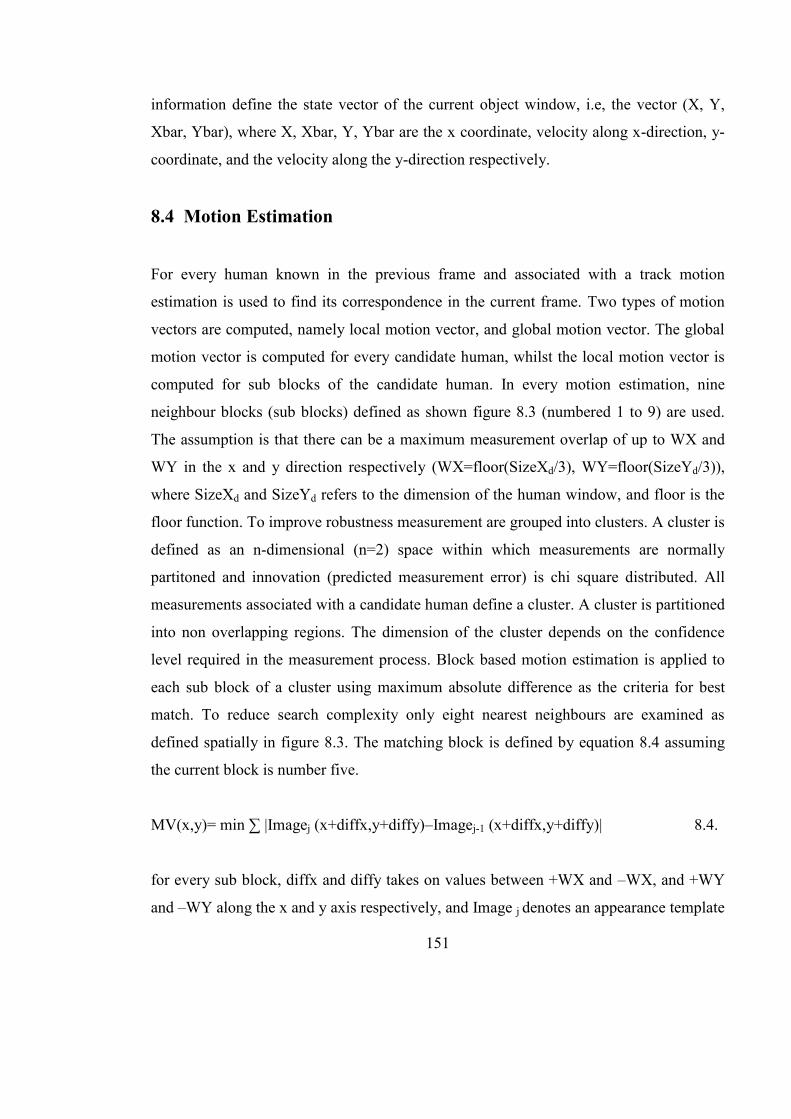
151
information define the state vector of the current object window, i.e, the vector (X, Y,
Xbar, Ybar), where X, Xbar, Y, Ybar are the x coordinate, velocity along x-direction, y-
coordinate, and the velocity along the y-direction respectively.
8.4 Motion Estimation
For every human known in the previous frame and associated with a track motion
estimation is used to find its correspondence in the current frame. Two types of motion
vectors are computed, namely local motion vector, and global motion vector. The global
motion vector is computed for every candidate human, whilst the local motion vector is
computed for sub blocks of the candidate human. In every motion estimation, nine
neighbour blocks (sub blocks) defined as shown figure 8.3 (numbered 1 to 9) are used.
The assumption is that there can be a maximum measurement overlap of up to WX and
WY in the x and y direction respectively (WX=floor(SizeXd/3), WY=floor(SizeYd/3)),
where SizeXd and SizeYd refers to the dimension of the human window, and floor is the
floor function. To improve robustness measurement are grouped into clusters. A cluster is
defined as an n-dimensional (n=2) space within which measurements are normally
partitoned and innovation (predicted measurement error) is chi square distributed. All
measurements associated with a candidate human define a cluster. A cluster is partitioned
into non overlapping regions. The dimension of the cluster depends on the confidence
level required in the measurement process. Block based motion estimation is applied to
each sub block of a cluster using maximum absolute difference as the criteria for best
match. To reduce search complexity only eight nearest neighbours are examined as
defined spatially in figure 8.3. The matching block is defined by equation 8.4 assuming
the current block is number five.
MV(x,y)= min ∑ |Imagej (x+diffx,y+diffy)–Imagej-1 (x+diffx,y+diffy)| 8.4.
for every sub block, diffx and diffy takes on values between +WX and –WX, and +WY
and –WY along the x and y axis respectively, and Image j denotes an appearance template
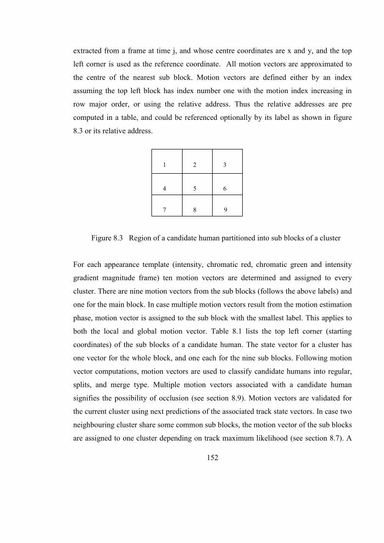
152
extracted from a frame at time j, and whose centre coordinates are x and y, and the top
left corner is used as the reference coordinate. All motion vectors are approximated to
the centre of the nearest sub block. Motion vectors are defined either by an index
assuming the top left block has index number one with the motion index increasing in
row major order, or using the relative address. Thus the relative addresses are pre
computed in a table, and could be referenced optionally by its label as shown in figure
8.3 or its relative address.
For each appearance template (intensity, chromatic red, chromatic green and intensity
gradient magnitude frame) ten motion vectors are determined and assigned to every
cluster. There are nine motion vectors from the sub blocks (follows the above labels) and
one for the main block. In case multiple motion vectors result from the motion estimation
phase, motion vector is assigned to the sub block with the smallest label. This applies to
both the local and global motion vector. Table 8.1 lists the top left corner (starting
coordinates) of the sub blocks of a candidate human. The state vector for a cluster has
one vector for the whole block, and one each for the nine sub blocks. Following motion
vector computations, motion vectors are used to classify candidate humans into regular,
splits, and merge type. Multiple motion vectors associated with a candidate human
signifies the possibility of occlusion (see section 8.9). Motion vectors are validated for
the current cluster using next predictions of the associated track state vectors. In case two
neighbouring cluster share some common sub blocks, the motion vector of the sub blocks
are assigned to one cluster depending on track maximum likelihood (see section 8.7). A
Figure 8.3 Region of a candidate human partitioned into sub blocks of a cluster
3
2
7
9
8
1
4
6
5

153
motion vector from the sub blocks of a cluster must pass measurement validation test,
whilst the motion vector for the whole block must pass both the validation test based and
motion constraint test (based on Kalman prediction) of the associated track.
8.5 Measurement Validation
Measurements estimated are the motion vectors and approximate centroids of human
locations from the four appearance templates, namely, directional gradient, chromatic red
and green components. The expected centroid of human is determined by computing the
median of all centroids of feature template measurements associated with a candidate
human. Measurements are associated with tracks based on the following:
Euclidean distance between a track’s location and the feature template’s location
(along x and y directions);
Euclidean distance between current track’s motion vector and motion vector of
the feature template (along x and y directions);
Constraints on separation along the x and y axes between a track’s location and
the feature template’s location;
Constraints on separation along the x and y axes between a track’s motion vector and
the feature template’s motion vector;
These constraints are typically determined by the dimension of the candidate human
region. The result of applying the criteria above is to assign measurements into partitions
associated with tracks, represented as track association matrix. The element of the matrix
R j,i has a value of one if i and object j belong the same object, otherwise it has a value of
zero.

154
8.6 Kalman Prediction
Kalman filter is an optimum linear detector when measurements and noise distributions
are Gaussian [Haykins 1999]. Kalman prediction is defined by equations 8.5 and 8.6.
Y(n)=C(n)X(n)+Q2(n) 8.5.
X(n+1)=F(n+1)*X(n)+Q1(n) 8.6.
Y(n) defines the observation (measurement) vector, C(n) defines the measurement
matrix, X(n+1) defines the next state vector given the current state, and F(n+1) defines
the state transition matrix from state n to n+1, Q1(n) defines the measurement noise, and
Q2(n) defines the process noise (noise from the state estimation process). Equation 8.6
describes the state model whilst the vector Y describes relationship between the
measurement and state vectors (describes the measurement process).
Sub block Index X Y
1 1 1
2 WX+1 1
3 2WX+1 1
4 1 WY+1
5 WX WY
6 2WX+1 WY+1
7 1 2WY+1
8 WX+1 2WY+1
9 2WX+1 2WY+1
10 WX+1 WY+1
Table 8.1 Relative addresses of sub blocks defining a track cluster
155
R(n)=C(n)*K(n)*CH(n)+Q2(n) 8.7
G(n)=F(n+1)*K(n)CH(n)*R-1(n) 8.8
Est_X(n)=X(n-1)+G(n) *(Y(n)-C(n)*X(n-1)) 8.9.
Where n denotes time step, R(n) is innovation vector error correlation matrix, G(n) is
Kalman gain matrix, K(n) is the predicted state error correlation matrix, Est_X(n) denotes
the estimated state at time step n, and R-1(n) denotes the inverse of matrix R. The
superscript H denotes the transpose as in CH(n), which is the transpose of the measurement
matrix. The superscript -1, denotes the inverse operation. F(n+1), and K(n) are assumed
constant.
The search for the best correspondence between a candidate human in the current
frame and an existing track is determined by validating the state vector of the candidate
human against Kalman prediction (next state) of a candidate track. The inputs to the next
state of a track are the current state (based on current measurements) parameters defined as
a table of association, i.e, track association matrix. The Kalman filtering is defined by
equations 8.7 and 8.8. Equation 8.9 are used to predict the next state. The advantage of
using Kalman prediction is that the next state is dependent on the current measurements,
state, and Kalman gain vector, and the system parameters either evolves with time (one-
step Kalman prediction). Sudden changes in state vector then signifies deviation from its
expected behaviour. Should this happen then the measurement would fall outside the
validation region of the track. Such measurements could be false alarms, object splits, or
merges. The use of Kalman filtering enables multiple motion models to efficiently handle
motion dynamics of humans such that the best model is selected for the particular scene.
The output from the Kalman prediction stage is the innovation matrix, and next state
prediction matrix. An innovation vector is associated with a track if the corresponding
track association matrix element has a value of one, otherwise it is not associated with the
track.
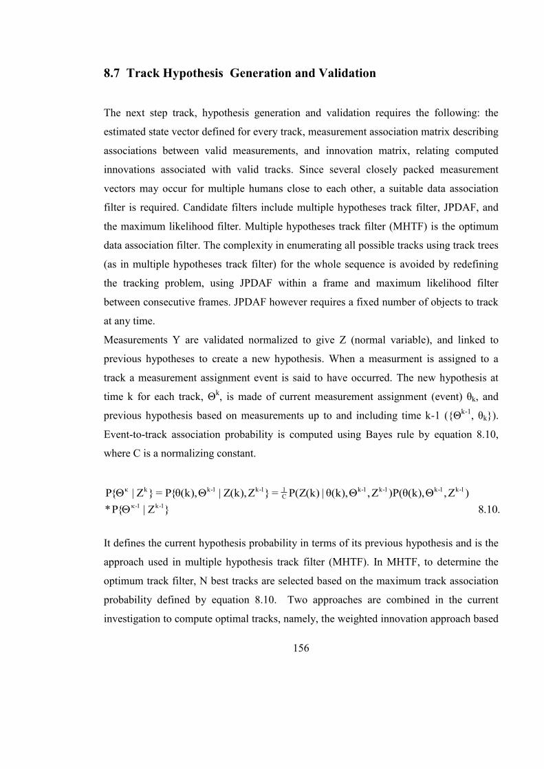
156
8.7 Track Hypothesis Generation and Validation
The next step track, hypothesis generation and validation requires the following: the
estimated state vector defined for every track, measurement association matrix describing
associations between valid measurements, and innovation matrix, relating computed
innovations associated with valid tracks. Since several closely packed measurement
vectors may occur for multiple humans close to each other, a suitable data association
filter is required. Candidate filters include multiple hypotheses track filter, JPDAF, and
the maximum likelihood filter. Multiple hypotheses track filter (MHTF) is the optimum
data association filter. The complexity in enumerating all possible tracks using track trees
(as in multiple hypotheses track filter) for the whole sequence is avoided by redefining
the tracking problem, using JPDAF within a frame and maximum likelihood filter
between consecutive frames. JPDAF however requires a fixed number of objects to track
at any time.
Measurements Y are validated normalized to give Z (normal variable), and linked to
previous hypotheses to create a new hypothesis. When a measurment is assigned to a
track a measurement assignment event is said to have occurred. The new hypothesis at
time k for each track, Θk, is made of current measurement assignment (event) θk, and
previous hypothesis based on measurements up to and including time k-1 ({Θk-1, θk}).
Event-to-track association probability is computed using Bayes rule by equation 8.10,
where C is a normalizing constant.
10.7)Z,Θ),k(θ(P)Z,Θ),k(θ|)k(Z(P=}Z),k(Z|Θ),k(θ{P=}Z|Θ{P 1-k1-k1-k1-kC11-k1-kkκ
.10.8}Z|{P* 1-k1-
It defines the current hypothesis probability in terms of its previous hypothesis and is the
approach used in multiple hypothesis track filter (MHTF). In MHTF, to determine the
optimum track filter, N best tracks are selected based on the maximum track association
probability defined by equation 8.10. Two approaches are combined in the current
investigation to compute optimal tracks, namely, the weighted innovation approach based
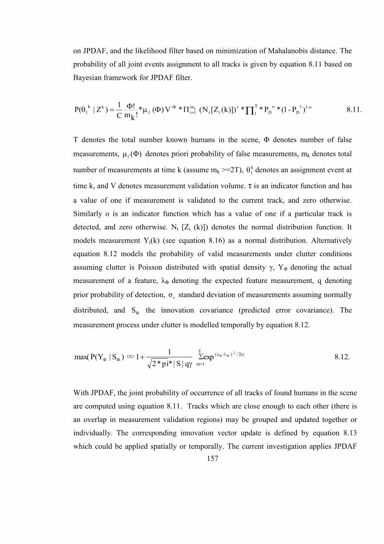
157
on JPDAF, and the likelihood filter based on minimization of Mahalanobis distance. The
probability of all joint events assignment to all tracks is given by equation 8.11 based on
Bayesian framework for JPDAF filter.
.11.8)P-1(*P**)])k(Z[N(*V)(*!km
!C1)Z|(P o-1t
Do
DT1it
m1i
-f
kkl
k
T denotes the total number known humans in the scene, Φ denotes number of false
measurements, )Φ(μf denotes priori probability of false measurements, mk denotes total
number of measurements at time k (assume mk >=2T), kl denotes an assignment event at
time k, and V denotes measurement validation volume. τ is an indicator function and has
a value of one if measurement is validated to the current track, and zero otherwise.
Similarly o is an indicator function which has a value of one if a particular track is
detected, and zero otherwise. Nt [Zi (k)]) denotes the normal distribution function. It
models measurement Yi(k) (see equation 8.16) as a normal distribution. Alternatively
equation 8.12 models the probability of valid measurements under clutter conditions
assuming clutter is Poisson distributed with spatial density γ, YΦ denoting the actual
measurement of a feature, λΦ denoting the expected feature measurement, q denoting
prior probability of detection, zσ standard deviation of measurements assuming normally
distributed, and ΦS the innovation covariance (predicted error covariance). The
measurement process under clutter is modelled temporally by equation 8.12.
.12.8∑expq|S|*pi*2
11∞)S|Y(Pmax(T
1m
|s|2/)-z( 2
With JPDAF, the joint probability of occurrence of all tracks of found humans in the scene
are computed using equation 8.11. Tracks which are close enough to each other (there is
an overlap in measurement validation regions) may be grouped and updated together or
individually. The corresponding innovation vector update is defined by equation 8.13
which could be applied spatially or temporally. The current investigation applies JPDAF
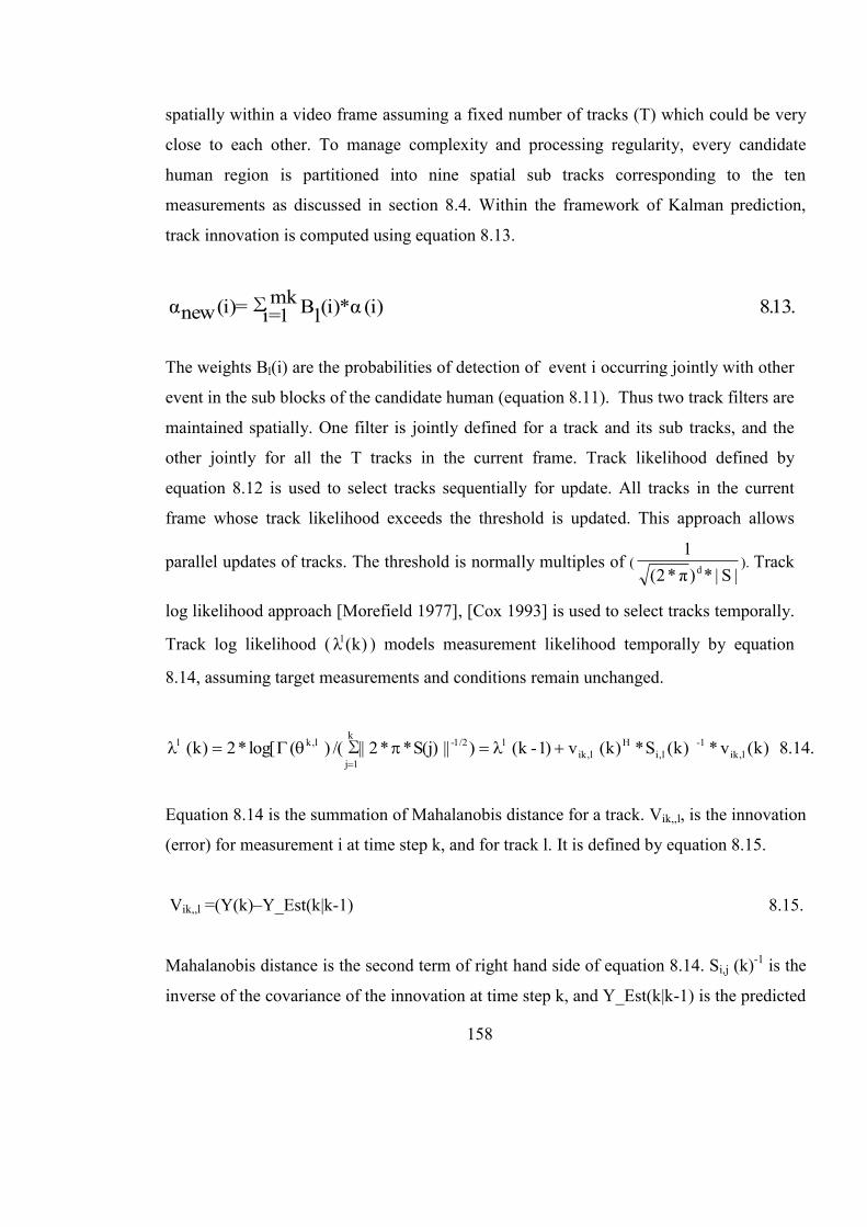
158
spatially within a video frame assuming a fixed number of tracks (T) which could be very
close to each other. To manage complexity and processing regularity, every candidate
human region is partitioned into nine spatial sub tracks corresponding to the ten
measurements as discussed in section 8.4. Within the framework of Kalman prediction,
track innovation is computed using equation 8.13.
.13.8(i)(i)*α∑mk1i= lB(i)=newα
The weights Bl(i) are the probabilities of detection of event i occurring jointly with other
event in the sub blocks of the candidate human (equation 8.11). Thus two track filters are
maintained spatially. One filter is jointly defined for a track and its sub tracks, and the
other jointly for all the T tracks in the current frame. Track likelihood defined by
equation 8.12 is used to select tracks sequentially for update. All tracks in the current
frame whose track likelihood exceeds the threshold is updated. This approach allows
parallel updates of tracks. The threshold is normally multiples of (|S|*)π*2(
1d ). Track
log likelihood approach [Morefield 1977], [Cox 1993] is used to select tracks temporally.
Track log likelihood ( )k(λl ) models measurement likelihood temporally by equation
8.14, assuming target measurements and conditions remain unchanged.
.14.8)k(v*)k(S*)k(v)1-k(∑ )||S(j)**2||/()(log[*2)k( l,ik1-
l,iH
l,ikl
k
1j
1/2-l,kl
Equation 8.14 is the summation of Mahalanobis distance for a track. Vik,,l, is the innovation
(error) for measurement i at time step k, and for track l. It is defined by equation 8.15.
Vik,,l =(Y(k)–Y_Est(k|k-1) 8.15.
Mahalanobis distance is the second term of right hand side of equation 8.14. Si,j (k)-1 is the
inverse of the covariance of the innovation at time step k, and Y_Est(k|k-1) is the predicted
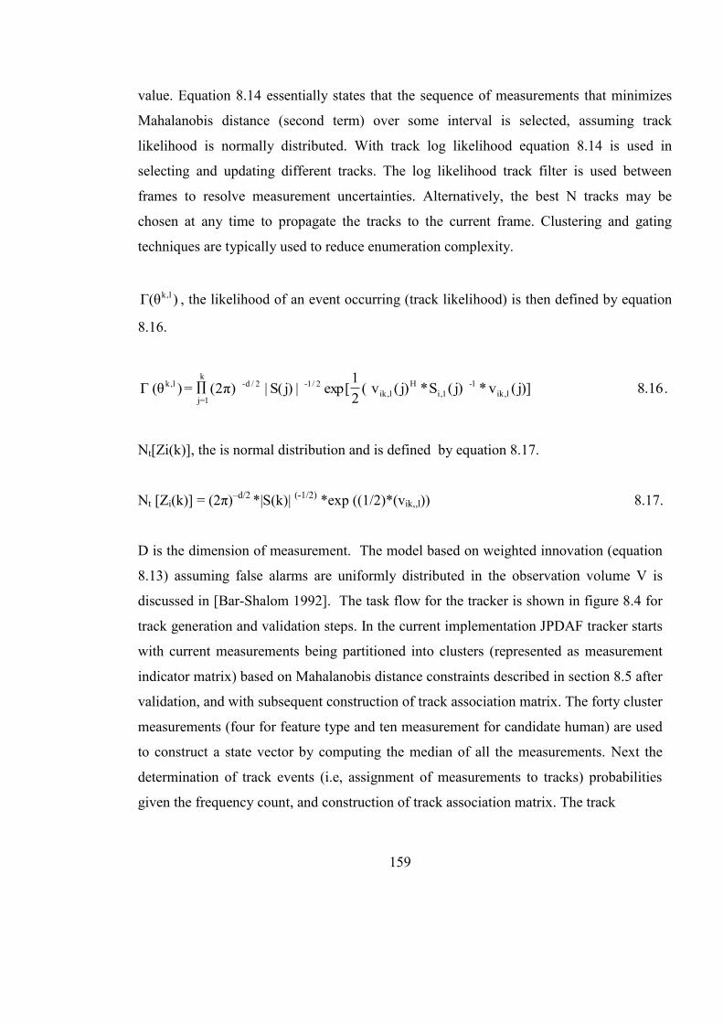
159
value. Equation 8.14 essentially states that the sequence of measurements that minimizes
Mahalanobis distance (second term) over some interval is selected, assuming track
likelihood is normally distributed. With track log likelihood equation 8.14 is used in
selecting and updating different tracks. The log likelihood track filter is used between
frames to resolve measurement uncertainties. Alternatively, the best N tracks may be
chosen at any time to propagate the tracks to the current frame. Clustering and gating
techniques are typically used to reduce enumeration complexity.
)θ(Γ l,k , the likelihood of an event occurring (track likelihood) is then defined by equation
8.16.
(21
exp[∏ |)j(S|)π2(=)θ(Γk
1=j
2/1-2/d-l,k 16.8)]j(v*)j(S*)j(v l,ik1-
1,iH
l,ik .
Nt[Zi(k)], the is normal distribution and is defined by equation 8.17.
Nt [Zi(k)] = (2π)–d/2 *|S(k)| (-1/2) *exp ((1/2)*(vik,,l)) 8.17.
D is the dimension of measurement. The model based on weighted innovation (equation
8.13) assuming false alarms are uniformly distributed in the observation volume V is
discussed in [Bar-Shalom 1992]. The task flow for the tracker is shown in figure 8.4 for
track generation and validation steps. In the current implementation JPDAF tracker starts
with current measurements being partitioned into clusters (represented as measurement
indicator matrix) based on Mahalanobis distance constraints described in section 8.5 after
validation, and with subsequent construction of track association matrix. The forty cluster
measurements (four for feature type and ten measurement for candidate human) are used
to construct a state vector by computing the median of all the measurements. Next the
determination of track events (i.e, assignment of measurements to tracks) probabilities
given the frequency count, and construction of track association matrix. The track
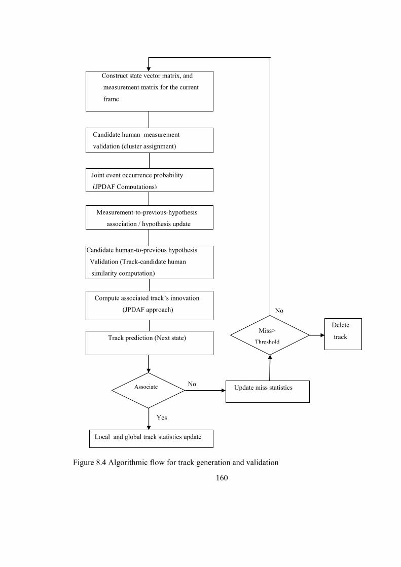
160
Yes
Figure 8.4 Algorithmic flow for track generation and validation
No
Yes
Local and global track statistics update
No Update miss statistics Associate
Miss>
Threshold
Delete
track
Construct state vector matrix, and
measurement matrix for the current
frame
Candidate human measurement
validation (cluster assignment)
Compute associated track’s innovation
(JPDAF approach)
Candidate human-to-previous hypothesis
Validation (Track-candidate human
similarity computation)
Track prediction (Next state)
Joint event occurrence probability
(JPDAF Computations)
Measurement-to-previous-hypothesis
_association / hypothesis update

161
association matrix enumerates all possible cluster associations. Then the probability of
joint occurrence of all assignment events occurring within a cluster and between different
clusters (defines the spatial occurrence of track-measurement events) are computed.
JPDAF probabilities are computed for every sub block of a track, given that N humans
appear in the scene at any time by examining measurement association matrix. The joint
probability of assignment to the different tracks are computed, and tracks whose
probability threshold are above the value set by the applications are selected for update.
The signature of all candidate humans in the current frame is computed and compared
against the signature of the tracks. The signature used in the current investigation consists
of the mean and the standard deviation of the intensity image corresponding to the
candidate human. For every track a measure is defined which evaluates how closely a
candidate human matches a given track. The measure is defined in equation 8.18.
M1= abs(Track_Mean(i)-Cand_Human_Mean) + abs(Track_Std(i)-Cand_Human_Std)
8.18.
I denotes the track index, Track_Mean denotes the mean of the candidate human
associated with track i, Track_Std(i) denotes the corresponding standard deviation,
Cand_Human_Mean denotes the mean of the current candidate human, and
Cand_Human_Std denotes the corresponding standard deviation. The track which best
associates with the current candidate human is the track which gives the minimum value
of M1. The validated state becomes the next current state vector. The innovation matrix
generated for every candidate human cluster is used in computing the innovation of the
valid tracks as defined in equation 8.13. The innovations are computed by using the
predicted state vector (from the previous Kalman next state prediction) of the track. The
innovation update equation (8.13) is used to compute the innovation for tracks. Track
statistics, and local and global track information are also updated. Tracks with no valid
measurement associations are declared as miss tracks, and track miss statistic is updated.
The old track signature is replaced by the new track signature. When the miss count of a
track exceeds a threshold it is declared as inactive. For non valid tracks whose miss count
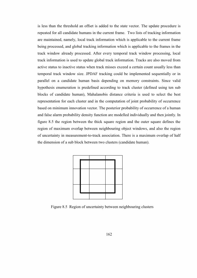
162
is less than the threshold an offset is added to the state vector. The update procedure is
repeated for all candidate humans in the current frame. Two lists of tracking information
are maintained, namely, local track information which is applicable to the current frame
being processed, and global tracking information which is applicable to the frames in the
track window already processed. After every temporal track window processing, local
track information is used to update global track information. Tracks are also moved from
active status to inactive status when track misses exceed a certain count usually less than
temporal track window size. JPDAF tracking could be implemented sequentially or in
parallel on a candidate human basis depending on memory constraints. Since valid
hypothesis enumeration is predefined according to track cluster (defined using ten sub
blocks of candidate human), Mahalanobis distance criteria is used to select the best
representation for each cluster and in the computation of joint probability of occurrence
based on minimum innovation vector. The posterior probability of occurrence of a human
and false alarm probability density function are modelled individually and then jointly. In
figure 8.5 the region between the thick square region and the outer square defines the
region of maximum overlap between neighbouring object windows, and also the region
of uncertainty in measurement-to-track association. There is a maximum overlap of half
the dimension of a sub block between two clusters (candidate human).
Figure 8.5 Region of uncertainty between neighbouring clusters
163
8.8 Track Optimization
The objective of track optimization is to reduce false alarms which occurred at the
detection stage by applying temporal continuity of motion constraints to improve
positional accuracy, filter out false detections, and optimally link found humans
temporally. This is provided through the following means: multiple motion models are
used to describe motion in two contra directions along the x-axis, and two contra
directions along the y-axis. The justification is that motion along the 2-D image plane is
described as consisting of translation along the x and y-axis assuming in-plane rotation is
negligible between consecutive frames, and different motion model might suit different
human motion in the scene. It provides the capability to quickly evaluate different track
motion patterns to determine the most appropriate model based on estimates of detection
rate, positional error, and false alarm rate. Changing the confidence levels associated
with tracks from 95% down to 10% in steps of 10% for measurements-to-track
validation, also results in varying number of measurements associated to tracks. The
constraint essentially filters out unlikely tracks. Further the ability to apply the tracking
module in sequential or in batch processing model enable either reduction in execution
time or to jointly to optimize execution time and tracking accuracy. The influence
tracking parameters are discussed in chapter eight.
8.8.1 Sequential State Estimation Mode
Online implementation of JPDAF tracking is sequential since tracks are updated per
candidate human after measurement-to-track event association probability computation.
The main parameters are the Mahalanobis confidence interval, candidate human
dimension, and Kalman motion parameters. Temporal consistency is verified using two
consecutive frames within which motion is assumed to be Gaussian with clutter modelled
as either Poisson or uniform distribution. The limitation of this approach is that decisions
are made based on the previous and current frames. Instances of track merges cannot be
determined with higher certainty and this may affect the overall accuracy. Since the list

164
of found humans over all the frames in the past is available and could be used to improve
temporal consistency, this approach may not be optimal and inflexible.
8.8.2 Batch State Estimation Mode
In batch processing mode a sequence of N consecutive frames are defined for temporal
optimization (Track window). During track window processing temporal coherency is
used to eliminate false detections. Similarly track merges and occlusion events detected.
This approach provides a more flexible way of optimizing the accuracy of the tracker.
Different track processing window could be investigated to determine the best setting.
8.8.3 Application to Single Motion Model
There are six motion models describing different pattern of motion in the Kalman
predictor. The accuracy of tracker is dependent on the how close the motion model is to
the actual motion of the human in the scene. Different motion models could be combined
with varying Mahalanobis distance to determine optimality of a given set of algorithmic
parameters. This enables fine tuning of parameters.
8.8.4 Application to Multiple Motion Models
Multiple motion models for a fixed set of algorithmic parameters could also be studied to
derive optimum algorithmic parameters. The result of the simulations into the influence
of algorithmic parameters is presented in the result section.
8.9 Occlusion Handling
To be able to detect occlusion, merging of multiple candidate humans must first be
detected and then if it persists over more than one frame occlusion event is assumed to
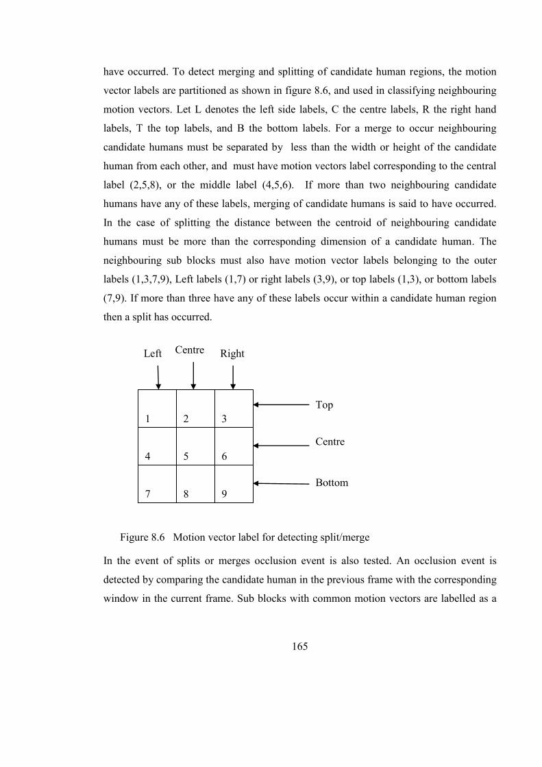
165
have occurred. To detect merging and splitting of candidate human regions, the motion
vector labels are partitioned as shown in figure 8.6, and used in classifying neighbouring
motion vectors. Let L denotes the left side labels, C the centre labels, R the right hand
labels, T the top labels, and B the bottom labels. For a merge to occur neighbouring
candidate humans must be separated by less than the width or height of the candidate
human from each other, and must have motion vectors label corresponding to the central
label (2,5,8), or the middle label (4,5,6). If more than two neighbouring candidate
humans have any of these labels, merging of candidate humans is said to have occurred.
In the case of splitting the distance between the centroid of neighbouring candidate
humans must be more than the corresponding dimension of a candidate human. The
neighbouring sub blocks must also have motion vector labels belonging to the outer
labels (1,3,7,9), Left labels (1,7) or right labels (3,9), or top labels (1,3), or bottom labels
(7,9). If more than three have any of these labels occur within a candidate human region
then a split has occurred.
In the event of splits or merges occlusion event is also tested. An occlusion event is
detected by comparing the candidate human in the previous frame with the corresponding
window in the current frame. Sub blocks with common motion vectors are labelled as a
Figure 8.6 Motion vector label for detecting split/merge
3
2
5
1
6
7
8
9
4
Top
Bottom
Centre
Right Left Centre
166
sub region of the candidate human. The Hausdorff1 distance between the previous
silhouette and the new partitions in the current object window’s silhouette is computed.
When the resulting distance is less than half of the original size occlusion is confirmed,
otherwise object splitting has occurred. On detecting occlusion candidate humans the
centroid of the human is updated by adding the Hausdorff distance, and setting the
motion vector to zero. The algorithm was verified by comparison of the output of the
motion vector classifier prediction’s for occlusion event with several visual observations
of instances of occlusion due to humans coming. However more studies are required to
formalize this approach. Also by comparing the new partition with the matching
silhouette in the previous frame it is possible to detect events such as abandoned and
moved objects based on merge and split events. However the current investigation has
not implemented detection of these events.
8.10 Computational Complexity of JPDAF Tracker
The computational complexity of the critical sections of the tracking task are examined
here. These are the measurement to cluster (hypotheses) association, and computation of
innovation vector based on JPDAF. One-step Kalman prediction is used for both
measurement-to-hypothesis association validation, and in track prediction update step.
Most of the parameters are pre computed offline, however the joint data association
probabilities are updated globally on a frame basis making the calculation sequential up
to that point. Beyond that point the computations could proceed in parallel. Every update
involves pre multiplication by a constant term (update of transition probabilities), and re-
computation of step using equation 8.11. This is due to the fact that the computation is
recursively defined as an update on the previous joint probabilities. Assuming that there
T objects (total number of known objects) with N objects currently present (validated
from current measurements), and assuming there are m measurements (total
1 Hausdorff distance measures how far tow subsets of a metric space are from each other. It turns the set of
non-empty compact subsets of a metric space into a metric space in its own right.
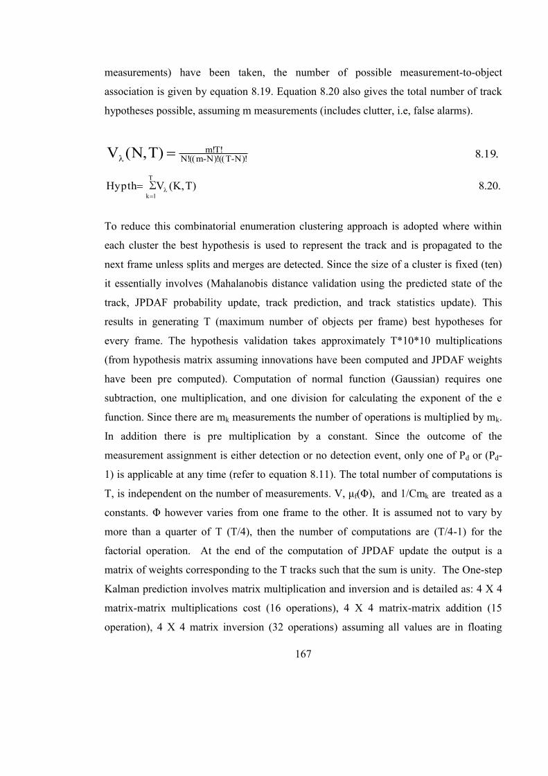
167
measurements) have been taken, the number of possible measurement-to-object
association is given by equation 8.19. Equation 8.20 also gives the total number of track
hypotheses possible, assuming m measurements (includes clutter, i.e, false alarms).
.19.8)!N-T(()!N-m((!N!T!m)T,N(V
.20.8)T,K(∑VHypthT
1k
To reduce this combinatorial enumeration clustering approach is adopted where within
each cluster the best hypothesis is used to represent the track and is propagated to the
next frame unless splits and merges are detected. Since the size of a cluster is fixed (ten)
it essentially involves (Mahalanobis distance validation using the predicted state of the
track, JPDAF probability update, track prediction, and track statistics update). This
results in generating T (maximum number of objects per frame) best hypotheses for
every frame. The hypothesis validation takes approximately T*10*10 multiplications
(from hypothesis matrix assuming innovations have been computed and JPDAF weights
have been pre computed). Computation of normal function (Gaussian) requires one
subtraction, one multiplication, and one division for calculating the exponent of the e
function. Since there are mk measurements the number of operations is multiplied by mk.
In addition there is pre multiplication by a constant. Since the outcome of the
measurement assignment is either detection or no detection event, only one of Pd or (Pd-
1) is applicable at any time (refer to equation 8.11). The total number of computations is
T, is independent on the number of measurements. V, μf(Φ), and 1/Cmk are treated as a
constants. Φ however varies from one frame to the other. It is assumed not to vary by
more than a quarter of T (T/4), then the number of computations are (T/4-1) for the
factorial operation. At the end of the computation of JPDAF update the output is a
matrix of weights corresponding to the T tracks such that the sum is unity. The One-step
Kalman prediction involves matrix multiplication and inversion and is detailed as: 4 X 4
matrix-matrix multiplications cost (16 operations), 4 X 4 matrix-matrix addition (15
operation), 4 X 4 matrix inversion (32 operations) assuming all values are in floating
168
point units. Clearly the computations are linear with the product of the number of
measurements and number of humans to track. It is independent of any enumeration
complexity. The memory requirement is also linear.
8.11 Synthesized JPDAF Tracker
Figure 8.7 shows the proposed tracking architecture. It consists of a fixed number of
clusters (N). On every cluster there are six stages, namely, track initialisation, silhouette
and feature extraction, and measurements computations (estimation). Clusters are defined
based on measurement computations and validation. Additionally the previous track
hypothesis (known tracks) are used to define new hypothesis through measurement event
assignment to tracks. It is followed by JPDAF update, and hypothesis validation. The
input to the JPDAF step are the validated measurements expressed as measurement
matrix. Clusters are defined based on spatial proximity of humans and they run
concurrently, however they share the first three stages. Silhouette and the appearance
template. Motion vectors (local and global) are estimated for the human corresponding to
the current frame. Measurements (motion vectors and location information) are validated,
and assigned to a cluster. A cluster is associated with a sub set of the tracks to reduce
track enumeration complexity. Measurements are associated with tracks on passing
validation test. JPDAF probabilities are computed for the current frame, and tracks are
updated by associating with a human in the current frame. The outputs from the JPDAF
stage are the updated tracks. Among the valid tracks the best track is selected using the
signature of the associated found human. The signature is defined as the mean, and the
standard deviation of the bounded region enclosing the found human. The best match is
defined by computing the sum of the absolute differences between the means, and the
standard deviation. The track with the minimum value is selected as the matching track.
This completes the hypothesis generation and validation step. At the post processing step
predictions are made for the next states of the tracks. Track maintenance is implemented
as the last step. The architecture operates in both frame and mixed mode. In frame
processing mode only clusters related to the current frame are used, whilst in mixed

169
mode previous and current frame clusters could coexist. The computational load depends
on the configuration for the detector. If the detectors run in the combined mode, then
there will be more centroids to track. It also depends of algorithmic parameters such as
human window height, and width and other parameters listed in table 7.4. Thus different
configuration schedule would result in different level of concurrency.
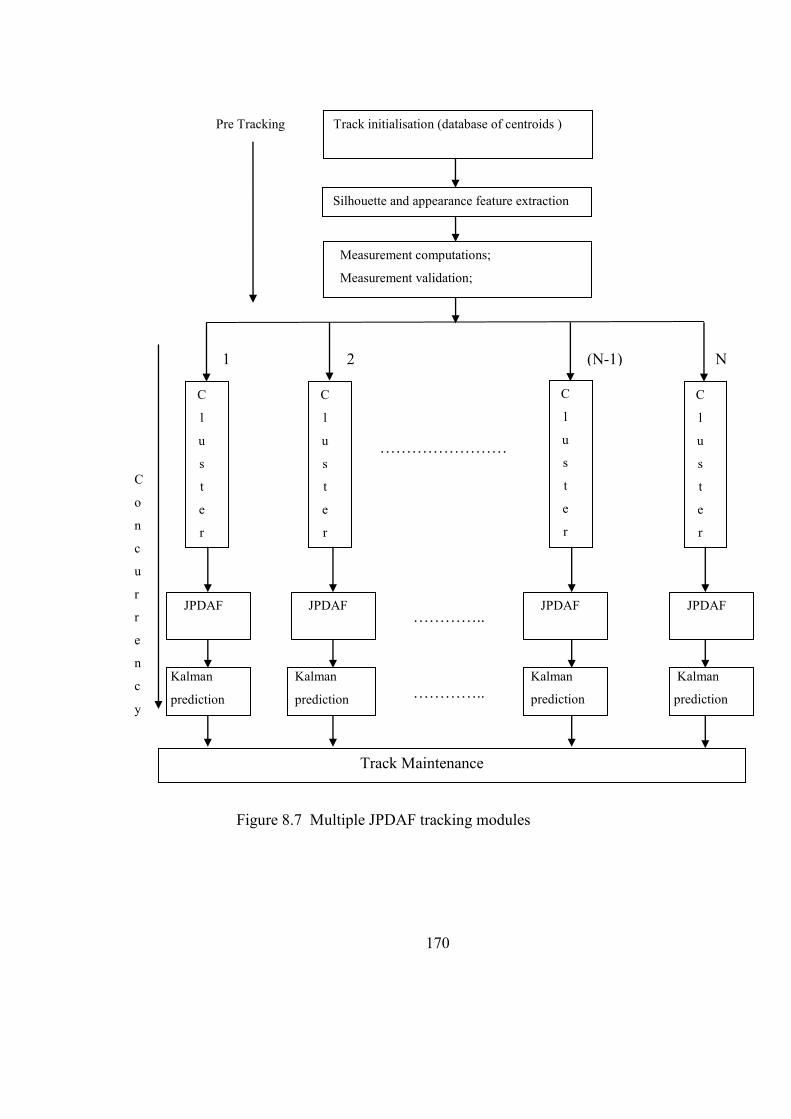
170
Figure 8.7 Multiple JPDAF tracking modules
C
o
n
c
u
r
r
e
n
c
y
……………………
…….
C
l
u
s
t
e
r
n
C
l
u
s
t
e
r
n-
1
C
l
u
s
t
e
r
2
N (N-1) 2 1
C
l
u
s
t
e
r
1
Track Maintenance
Kalman
prediction
………….. JPDAF
JPDAF
JPDAF
JPDAF
………….. Kalman
prediction
Kalman
prediction
Kalman
prediction
Measurement computations;
Measurement validation;
Track initialisation (database of centroids )
Silhouette and appearance feature extraction
Pre Tracking
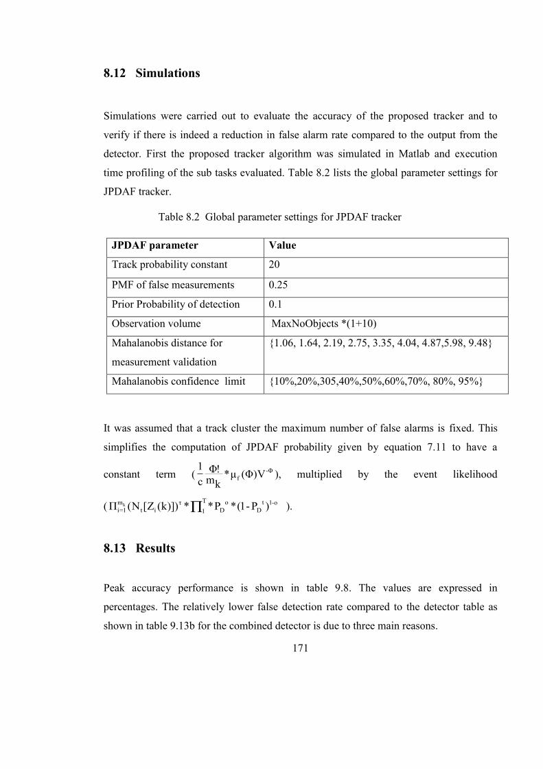
171
8.12 Simulations
Simulations were carried out to evaluate the accuracy of the proposed tracker and to
verify if there is indeed a reduction in false alarm rate compared to the output from the
detector. First the proposed tracker algorithm was simulated in Matlab and execution
time profiling of the sub tasks evaluated. Table 8.2 lists the global parameter settings for
JPDAF tracker.
It was assumed that a track cluster the maximum number of false alarms is fixed. This
simplifies the computation of JPDAF probability given by equation 7.11 to have a
constant term ( Φ-f V)Φ(μ*
km!Φ
c1
), multiplied by the event likelihood
( o-1tD
oD
T1
τit
m1=i )P-1(*P**)])k(Z[N(Π Πk ).
8.13 Results
Peak accuracy performance is shown in table 9.8. The values are expressed in
percentages. The relatively lower false detection rate compared to the detector table as
shown in table 9.13b for the combined detector is due to three main reasons.
Table 8.2 Global parameter settings for JPDAF tracker
JPDAF parameter Value
Track probability constant 20
PMF of false measurements 0.25
Prior Probability of detection 0.1
Observation volume MaxNoObjects *(1+10)
Mahalanobis distance for
measurement validation
{1.06, 1.64, 2.19, 2.75, 3.35, 4.04, 4.87,5.98, 9.48}
Mahalanobis confidence limit {10%,20%,305,40%,50%,60%,70%, 80%, 95%}
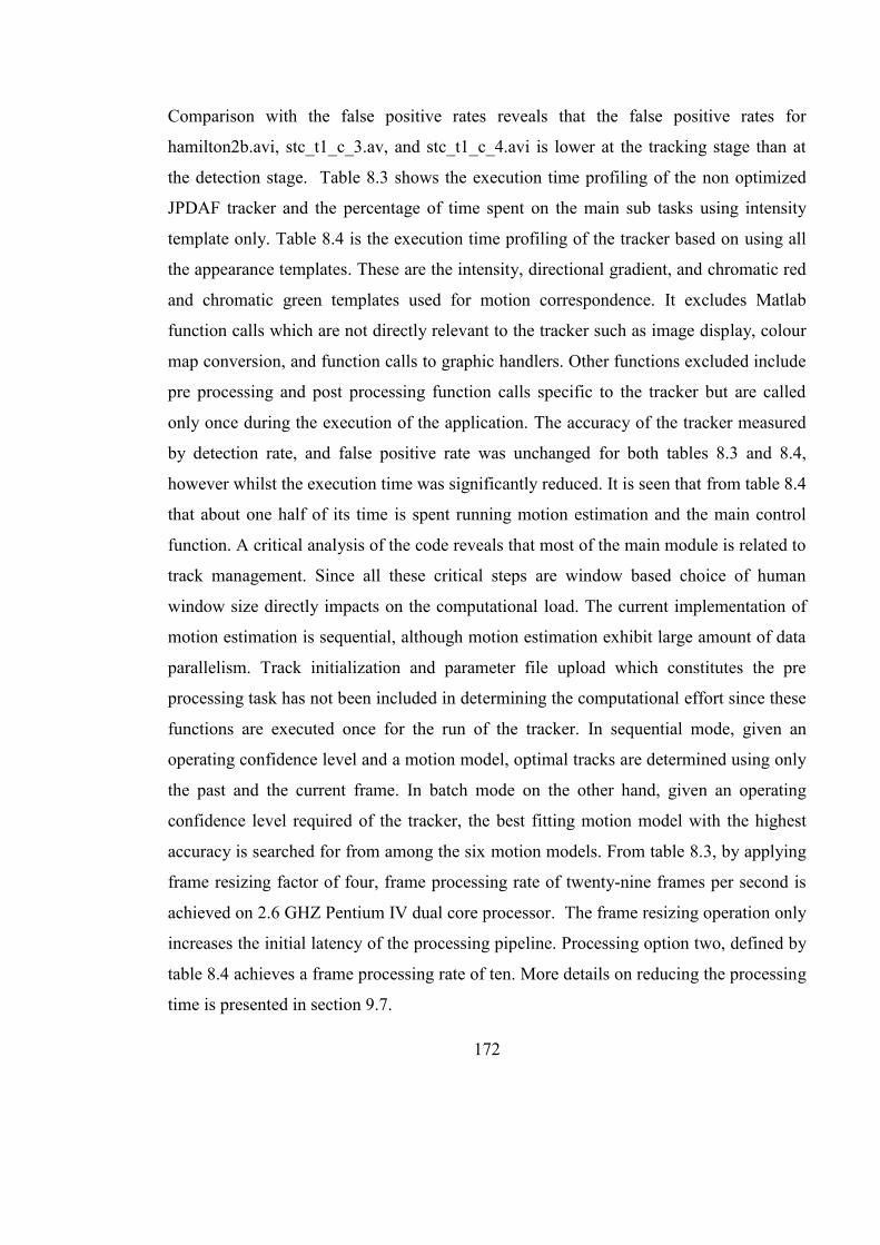
172
Comparison with the false positive rates reveals that the false positive rates for
hamilton2b.avi, stc_t1_c_3.av, and stc_t1_c_4.avi is lower at the tracking stage than at
the detection stage. Table 8.3 shows the execution time profiling of the non optimized
JPDAF tracker and the percentage of time spent on the main sub tasks using intensity
template only. Table 8.4 is the execution time profiling of the tracker based on using all
the appearance templates. These are the intensity, directional gradient, and chromatic red
and chromatic green templates used for motion correspondence. It excludes Matlab
function calls which are not directly relevant to the tracker such as image display, colour
map conversion, and function calls to graphic handlers. Other functions excluded include
pre processing and post processing function calls specific to the tracker but are called
only once during the execution of the application. The accuracy of the tracker measured
by detection rate, and false positive rate was unchanged for both tables 8.3 and 8.4,
however whilst the execution time was significantly reduced. It is seen that from table 8.4
that about one half of its time is spent running motion estimation and the main control
function. A critical analysis of the code reveals that most of the main module is related to
track management. Since all these critical steps are window based choice of human
window size directly impacts on the computational load. The current implementation of
motion estimation is sequential, although motion estimation exhibit large amount of data
parallelism. Track initialization and parameter file upload which constitutes the pre
processing task has not been included in determining the computational effort since these
functions are executed once for the run of the tracker. In sequential mode, given an
operating confidence level and a motion model, optimal tracks are determined using only
the past and the current frame. In batch mode on the other hand, given an operating
confidence level required of the tracker, the best fitting motion model with the highest
accuracy is searched for from among the six motion models. From table 8.3, by applying
frame resizing factor of four, frame processing rate of twenty-nine frames per second is
achieved on 2.6 GHZ Pentium IV dual core processor. The frame resizing operation only
increases the initial latency of the processing pipeline. Processing option two, defined by
table 8.4 achieves a frame processing rate of ten. More details on reducing the processing
time is presented in section 9.7.
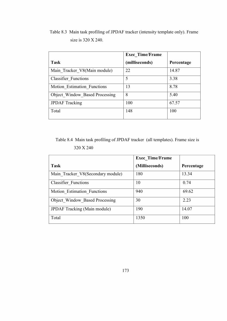
173
Table 8.3 Main task profiling of JPDAF tracker (intensity template only). Frame
size is 320 X 240.
Task
Exec_Time/Frame
(milliseconds)
Percentage
Main_Tracker_V8(Main module) 22 14.87
Classifier_Functions 5 3.38
Motion_Estimation_Functions 13 8.78
Object_Window_Based Processing 8 5.40
JPDAF Tracking 100 67.57
Total 148 100
Table 8.4 Main task profiling of JPDAF tracker (all templates). Frame size is
320 X 240
Task
Exec_Time/Frame
(Milliseconds)
Percentage
Main_Tracker_V8(Secondary module) 180 13.34
Classifier_Functions 10 0.74
Motion_Estimation_Functions 940 69.62
Object_Window_Based Processing 30 2.23
JPDAF Tracking (Main module) 190 14.07
Total 1350 100
174
8.14 Interpretation
Investigation into use of tracking to reduce false positives has been validated by
simulation and the result is discussed in section 9.6. It is shown that a better estimate of
the expected false alarm rate is given by the average of the false alarm rates for the shape
and histogram classifier. It is further shown that with this approach the tracker also
reduces the false alarm rates at the tracking stage compared with the detection stage. By
exploiting different motion models offline the best model setting for tracking can be
determined.
The tracker runs in both sequential and batch estimation mode. By using different
settings for Mahalanobis confidence metric it is possible to quickly select the best track
hypothesis. In sequential mode decisions are made based on the previous frame only,
whilst in batch estimation mode decisions are based on a group of past frames up to the
current frame. In batch estimation mode tracking accuracy is improved compared to
sequential estimation mode. The computational complexity is linear in the number of
humans to track, and is also dependent on the number of feature measurements. There are
four algorithmic configuration options available for tracking based on the number of
feature templates used. It has also been shown that the tracker achieves real-time
processing more than thirty (30) frames per second based on an input frame size of 240 X
320. Figures 8.8 to 8.10 shows typical output of the JPDAF tracker based o the three test
sequence. An ellipse is used to indicate found human. Comparative study with mean shift
tracking is also presented in chapter nine which demonstrates that it achieves higher
detection rate compared to mean shift tracking, but the false positive rate for the mean
shift tracker is relatively low. By carefully adjusting algorithmic parameters is possible to
optimized to track both individuals in a group as well as the group itself. Appendix E is a
table showing accuracy of the proposed JPDAF tracker under changing algorithmic
parameters.
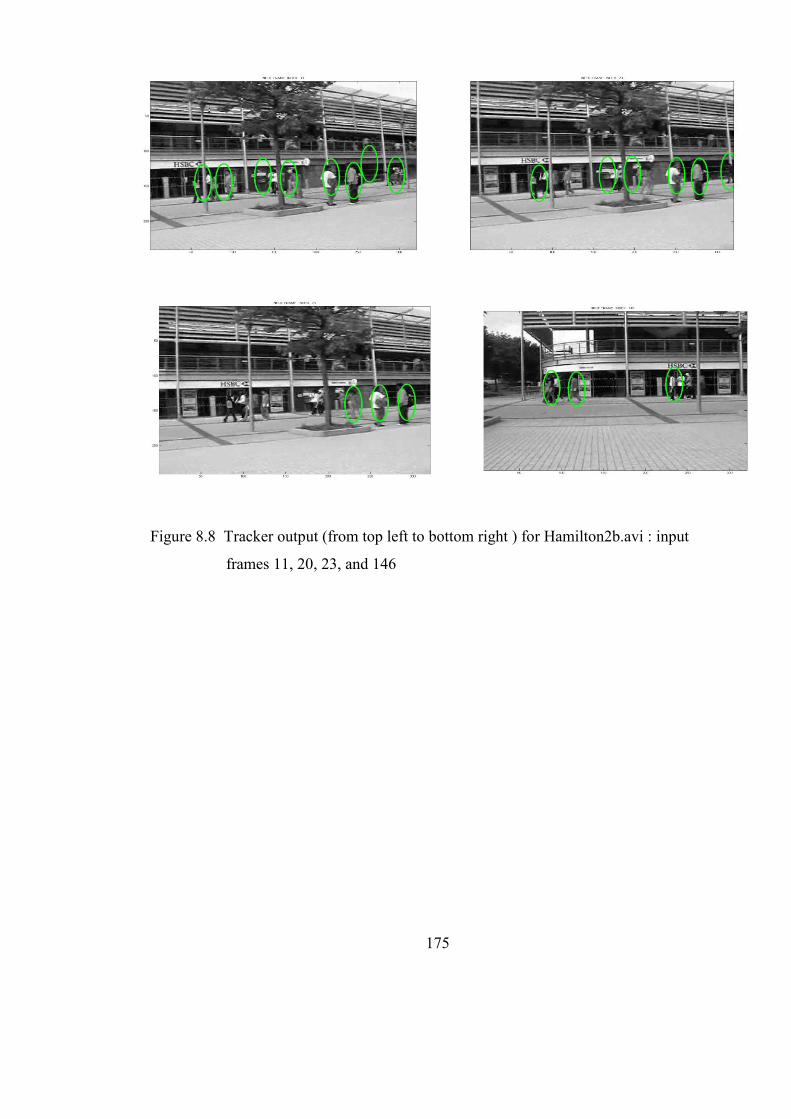
175
Figure 8.8 Tracker output (from top left to bottom right ) for Hamilton2b.avi : input
frames 11, 20, 23, and 146
and 146
(
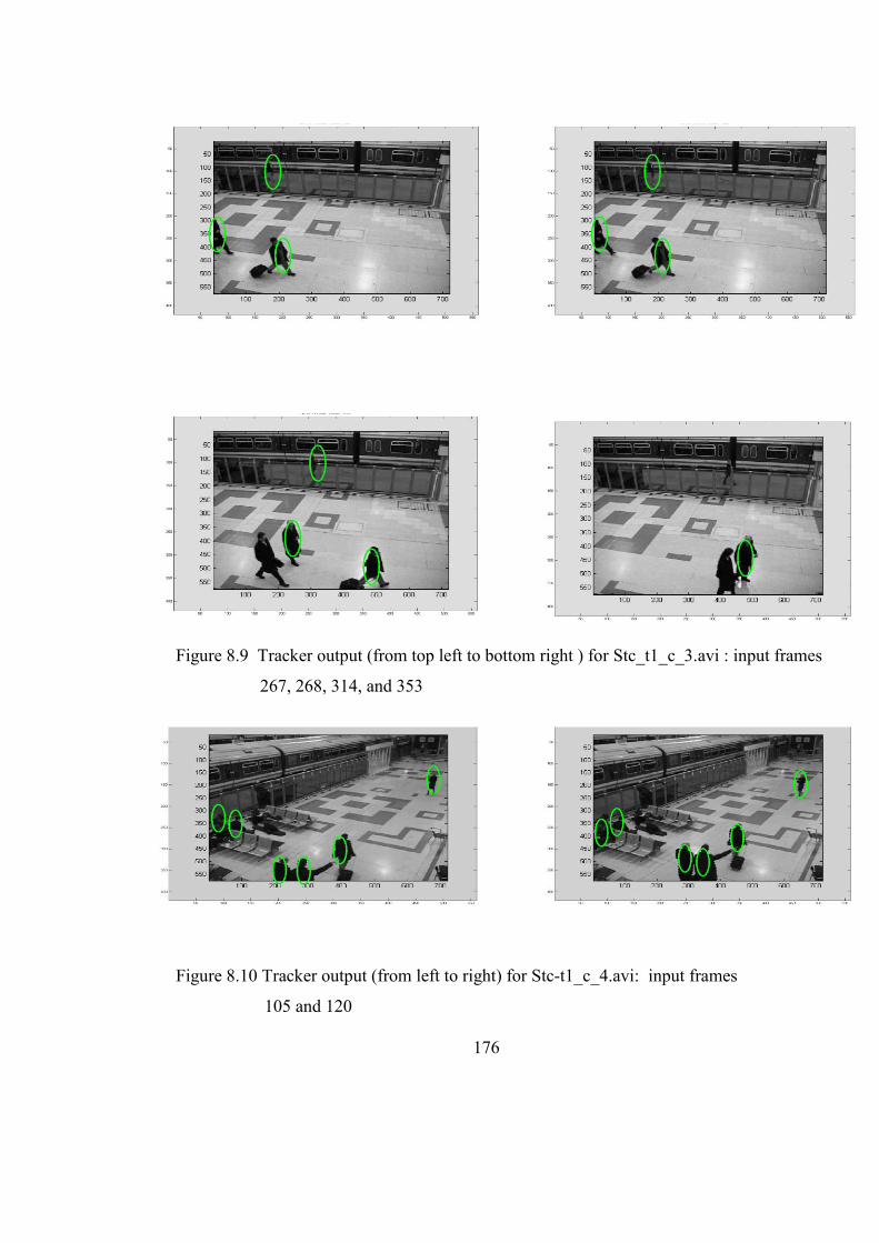
176
Figure 8.10 Tracker output (from left to right) for Stc-t1_c_4.avi: input frames
105 and 120
Figure 8.9 Tracker output (from top left to bottom right ) for Stc_t1_c_3.avi : input frames
267, 268, 314, and 353
177
CHAPTER NINE
CONSOLIDATION OF RESULTS
9.1 Introduction
The results of the combined human detection and tracking stages (chapters six and
seven) are presented in this chapter. Section 9.2 starts with an approach for online
estimation of optimum algorithmic parameters, whilst section 9.3 introduces an
algorithm for adaptive monitoring and control of detection and tracking accuracy.
Section 9.4 by way of analysis illustrates the algorithm implemented as part of
accuracy control in human detection. Section 9.5 discusses trends on detection, miss
detections and false alarm rates, and their sensitivity, whilst section 9.6 discusses
accuracy at the tracking stage. Section 9.7 provides analysis of execution times of sub
tasks of histogram detectors, shape-outline detector, combined shape and histogram
detector, and JPDAF tracker, as well as the different algorithmic configurations
options. Section 9.8 compares the accuracy of the proposed detection and tracking
algorithm with other competitive algorithms using the same video sequences:
Gaussian mixture modelling based human detection technique is compared with the
proposed human detection technique, whilst that of mean shift tracker is compared
with the proposed JPDAF tracker. Additionally the accuracy of the system based on
PETS 2006 evaluation metrics proposed in [Bashir and Porikli 2006] is also presented.
In section 9.9 a scalable algorithmic architecture is synthesised for combined human
detection and tracking. Section 9.10 discusses the results detailing out problems and
progress made at different stages of development of human detection and tracking
algorithm. Section 9.11 provides a review of the research findings.
The three video sequences used in the evaluation stage are classified into three
scenarios: Scenario one is a scene with high clutter, high human density, with humans
178
appearing in groups and as individuals at different times on Brunel university campus
with no scale changes (Hamilton2b.avi sequence). Scenario two is a scene outside a
train station with travellers moving about. It has low scene clutter with moderate
background contrast and poor illumination. Several humans appear in groups of three
or more, as individuals moving towards different directions at different times, and
sometimes partially visible (Stc_t1_c_3.avi). Scenario three is a train station with low
illumination, low contrast with humans appearing darker than the background, and
with low scene clutter. Several individuals come together at different times, and
sometimes with significant scale changes (Stc_t1_c_4.avi). Ground truth labelling was
done such that it included selected individuals in a group, whilst all isolated
individuals in a frame were also labelled. The capability of the proposed algorithm to
detect individuals appearing alone, and within groups were evaluated in the presence
of scene clutter, low contrast, and scale changes. The criteria for detecting matching
candidate humans were discussed in section 2.10.3. The problems of insufficient
overlap, and oversized candidate windows being matched to a ground truth objects are
avoided by specifying minimum area overlap and maximum distance of separation
between system found humans (found by the algorithm) and the ground truth. These
requirements were specified as part of the metrics in section 2.10.2.
9.2 Determining Optimum Algorithmic Parameters for Human
Detection and Tracking
There are three main parameter types used in controlling the accuracy of the human
detection and tracking application. They are constants, flags, and non constants.
Constants remains fixed throughout the execution time of the application. These
include region of interest definition, average dimension of human window, thresholds
for shape-outline map, and minimum pixel count threshold for found human. Flags
(the second category) are used to determine the type of intermediate processing
required. These include flags for median filtering, histogram equalization, pixel
saturation control, classifier type, wavelet decomposition level, and sub sample flag.
The third category includes variable parameters whose values fall within a range of
values. These include threshold for motion detection, threshold for salient feature
localization, number of regions to segment, and minimum pixel count threshold for
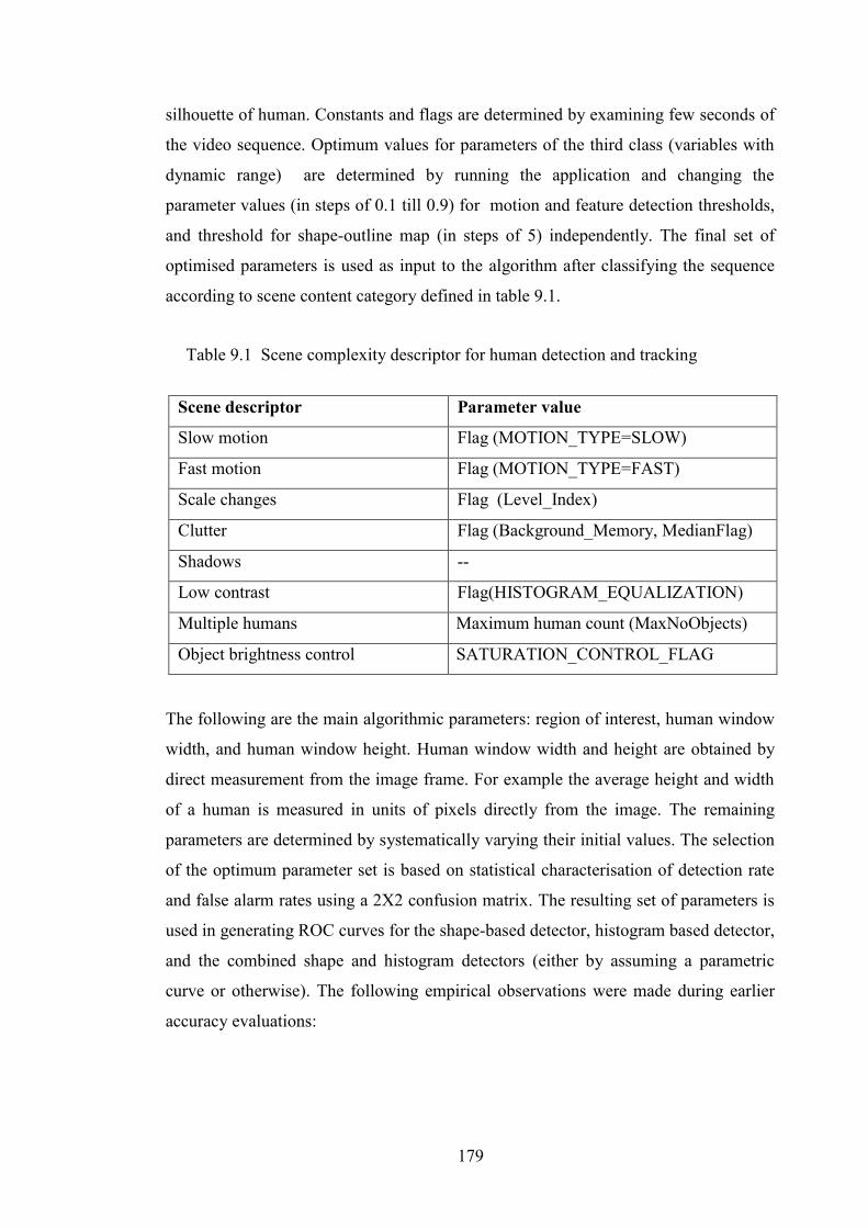
179
silhouette of human. Constants and flags are determined by examining few seconds of
the video sequence. Optimum values for parameters of the third class (variables with
dynamic range) are determined by running the application and changing the
parameter values (in steps of 0.1 till 0.9) for motion and feature detection thresholds,
and threshold for shape-outline map (in steps of 5) independently. The final set of
optimised parameters is used as input to the algorithm after classifying the sequence
according to scene content category defined in table 9.1.
The following are the main algorithmic parameters: region of interest, human window
width, and human window height. Human window width and height are obtained by
direct measurement from the image frame. For example the average height and width
of a human is measured in units of pixels directly from the image. The remaining
parameters are determined by systematically varying their initial values. The selection
of the optimum parameter set is based on statistical characterisation of detection rate
and false alarm rates using a 2X2 confusion matrix. The resulting set of parameters is
used in generating ROC curves for the shape-based detector, histogram based detector,
and the combined shape and histogram detectors (either by assuming a parametric
curve or otherwise). The following empirical observations were made during earlier
accuracy evaluations:
Scene descriptor Parameter value
Slow motion Flag (MOTION_TYPE=SLOW)
Fast motion Flag (MOTION_TYPE=FAST)
Scale changes Flag (Level_Index)
Clutter Flag (Background_Memory, MedianFlag)
Shadows --
Low contrast Flag(HISTOGRAM_EQUALIZATION)
Multiple humans Maximum human count (MaxNoObjects)
Object brightness control SATURATION_CONTROL_FLAG
Table 9.1 Scene complexity descriptor for human detection and tracking
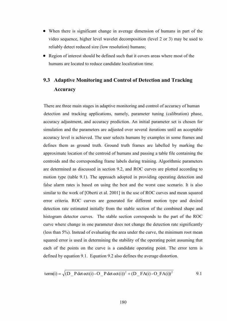
180
When there is significant change in average dimension of humans in part of the
video sequence, higher level wavelet decomposition (level 2 or 3) may be used to
reliably detect reduced size (low resolution) humans;
Region of interest should be defined such that it covers areas where most of the
humans are located to reduce candidate localization time.
9.3 Adaptive Monitoring and Control of Detection and Tracking
Accuracy
There are three main stages in adaptive monitoring and control of accuracy of human
detection and tracking applications, namely, parameter tuning (calibration) phase,
accuracy adjustment, and accuracy prediction. An initial parameter set is chosen for
simulation and the parameters are adjusted over several iterations until an acceptable
accuracy level is achieved. The user selects humans by examples in some frames and
defines them as ground truth. Ground truth frames are labelled by marking the
approximate location of the centroid of humans and passing a table file containing the
centroids and the corresponding frame labels during training. Algorithmic parameters
are determined as discussed in section 9.2, and ROC curves are plotted according to
motion type (table 9.1). The approach adopted in providing operating detection and
false alarm rates is based on using the best and the worst case scenario. It is also
similar to the work of [Oberti et al. 2001] in the use of ROC curves and mean squared
error criteria. ROC curves are generated for different motion type and desired
detection rate estimated initially from the stable section of the combined shape and
histogram detector curves. The stable section corresponds to the part of the ROC
curve where change in one parameter does not change the detection rate significantly
(less than 5%). Instead of evaluating the area under the curve, the minimum root mean
squared error is used in determining the stability of the operating point assuming that
each of the points on the curve is a candidate operating point. The error term is
defined by equation 9.1. Equation 9.2 also defines the average distortion.
1.9)O_FA(i)-)i(FA_D())i(ectdetP_O-)i(ectdetP_D()i(term 22
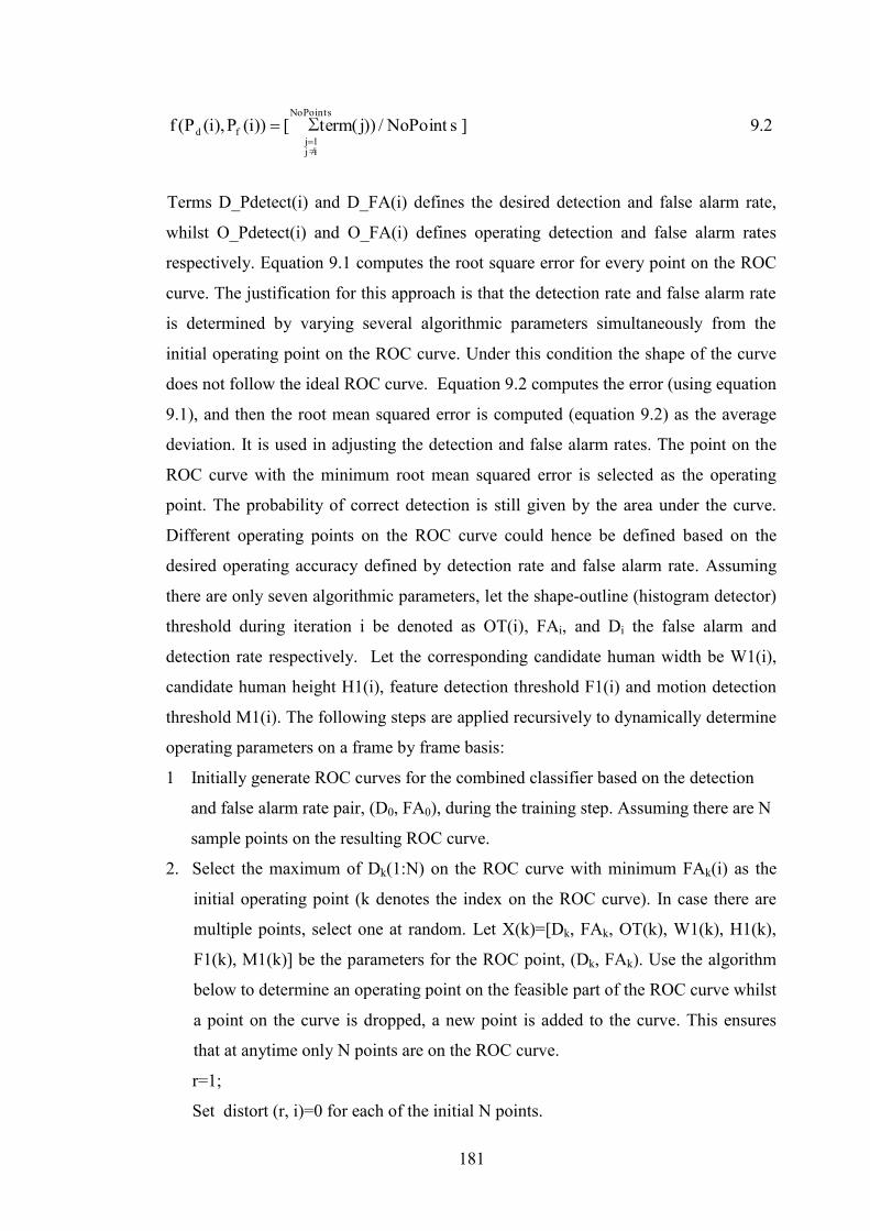
181
2.9]sintNoPo/)∑ )j(term[))i(P),i(P(fsintNoPo
i≠j1j
fd
Terms D_Pdetect(i) and D_FA(i) defines the desired detection and false alarm rate,
whilst O_Pdetect(i) and O_FA(i) defines operating detection and false alarm rates
respectively. Equation 9.1 computes the root square error for every point on the ROC
curve. The justification for this approach is that the detection rate and false alarm rate
is determined by varying several algorithmic parameters simultaneously from the
initial operating point on the ROC curve. Under this condition the shape of the curve
does not follow the ideal ROC curve. Equation 9.2 computes the error (using equation
9.1), and then the root mean squared error is computed (equation 9.2) as the average
deviation. It is used in adjusting the detection and false alarm rates. The point on the
ROC curve with the minimum root mean squared error is selected as the operating
point. The probability of correct detection is still given by the area under the curve.
Different operating points on the ROC curve could hence be defined based on the
desired operating accuracy defined by detection rate and false alarm rate. Assuming
there are only seven algorithmic parameters, let the shape-outline (histogram detector)
threshold during iteration i be denoted as OT(i), FAi, and Di the false alarm and
detection rate respectively. Let the corresponding candidate human width be W1(i),
candidate human height H1(i), feature detection threshold F1(i) and motion detection
threshold M1(i). The following steps are applied recursively to dynamically determine
operating parameters on a frame by frame basis:
1 Initially generate ROC curves for the combined classifier based on the detection
and false alarm rate pair, (D0, FA0), during the training step. Assuming there are N
sample points on the resulting ROC curve.
2. Select the maximum of Dk(1:N) on the ROC curve with minimum FAk(i) as the
initial operating point (k denotes the index on the ROC curve). In case there are
multiple points, select one at random. Let X(k)=[Dk, FAk, OT(k), W1(k), H1(k),
F1(k), M1(k)] be the parameters for the ROC point, (Dk, FAk). Use the algorithm
below to determine an operating point on the feasible part of the ROC curve whilst
a point on the curve is dropped, a new point is added to the curve. This ensures
that at anytime only N points are on the ROC curve.
r=1;
Set distort (r, i)=0 for each of the initial N points.

182
Repeat
3. Vary either one or more of the five parameters, and run the application using the
new parameter set. Let the new parameter set be X(k+r)=[D(i+r), FA(i+r), OT(k+r),
W1(k+r), H1(k+r), F1(k+r), M1(k+r)];
4. Determine the new operating point using equations 9.1 and 9.2.
a. r=r+1;
b. Compute Distort(r, i) for point i based on equation 9.1 for each of the N points.
c. Compute Min= ))i(P),i(P(f fd (equation 9.2).
5. Determine Operat(i) = argmin [Min- Distort(r, i)] of all N points on the ROC curve.
The point on the curve to be dropped is the point closest to the Min(i):
X(o)=[Do, FAo, OT(o), W1(o), H1(o), F1(o), M1(o)]. Add the new point
(Dk,FAk) to the ROC curve, and use [Dk, FAk, OT(k), W1(k), H1(k), F1(k),
M1(k)] as the new algorithmic operating parameter set.
6. Repeat steps 4 and 5 until an operating point as close to the desired operating point
is achieved.
The point on the ROC curve which leaves the ROC curve is the one with the
largest Distort (r, i) term. Section 9.4 applies this accuracy prediction algorithm to
evaluate the optimum accuracy level for stc-t1-c_3.avi. The proposed accuracy
level prediction algorithm is applicable to both the detection and the tracking
phase. The adjustment is performed in steps five and six.
9.4 Accuracy Prediction Analysis
The algorithm defined in section 9.2 is applied to the detection stage of video
sequence stc_t1_c_3.avi as follows: The initial set of points extracted from the
combined shape-outline and histogram detector accuracy table (values as a
percentages) is shown in table 9.2 with the following parameters:
TPR: True positive rate
FPR: False positive rate
C: Candidate human width
D: Candidate human height
A: Feature detection threshold proportion
B: Motion detection threshold proportion
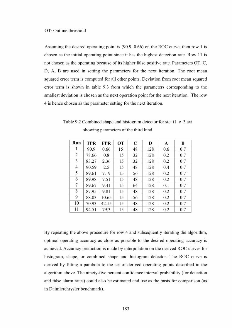
183
OT: Outline threshold
Assuming the desired operating point is (90.9, 0.66) on the ROC curve, then row 1 is
chosen as the initial operating point since it has the highest detection rate. Row 11 is
not chosen as the operating because of its higher false positive rate. Parameters OT, C,
D, A, B are used in setting the parameters for the next iteration. The root mean
squared error term is computed for all other points. Deviation from root mean squared
error term is shown in table 9.3 from which the parameters corresponding to the
smallest deviation is chosen as the next operation point for the next iteration. The row
4 is hence chosen as the parameter setting for the next iteration.
By repeating the above procedure for row 4 and subsequently iterating the algorithm,
optimal operating accuracy as close as possible to the desired operating accuracy is
achieved. Accuracy prediction is made by interpolation on the derived ROC curves for
histogram, shape, or combined shape and histogram detector. The ROC curve is
derived by fitting a parabola to the set of derived operating points described in the
algorithm above. The ninety-five percent confidence interval probability (for detection
and false alarm rates) could also be estimated and use as the basis for comparison (as
in Daimlerchrysler benchmark).
Table 9.2 Combined shape and histogram detector for stc_t1_c_3.avi
showing parameters of the third kind
Run TPR FPR OT C D A B 1 90.9 0.66 15 48 128 0.6 0.7 2 78.66 0.8 15 32 128 0.2 0.7 3 83.27 2.36 15 32 128 0.2 0.7 4 90.59 2.5 15 48 128 0.4 0.7 5 89.61 7.19 15 56 128 0.2 0.7 6 89.98 7.51 15 48 128 0.2 0.7 7 89.67 9.41 15 64 128 0.1 0.7 8 87.95 9.81 15 48 128 0.2 0.7 9 88.03 10.65 15 56 128 0.2 0.7 10 70.93 42.15 15 48 128 0.2 0.7 11 94.51 79.3 15 48 128 0.2 0.7
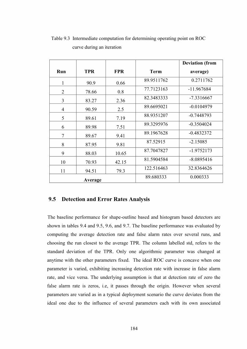
184
8.5 Detection and Error Rates Analysis
9.5 Detection and Error Rates Analysis
The baseline performance for shape-outline based and histogram based detectors are
shown in tables 9.4 and 9.5, 9.6, and 9.7. The baseline performance was evaluated by
computing the average detection rate and false alarm rates over several runs, and
choosing the run closest to the average TPR. The column labelled std, refers to the
standard deviation of the TPR. Only one algorithmic parameter was changed at
anytime with the other parameters fixed. The ideal ROC curve is concave when one
parameter is varied, exhibiting increasing detection rate with increase in false alarm
rate, and vice versa. The underlying assumption is that at detection rate of zero the
false alarm rate is zeros, i.e, it passes through the origin. However when several
parameters are varied as in a typical deployment scenario the curve deviates from the
ideal one due to the influence of several parameters each with its own associated
Table 9.3 Intermediate computation for determining operating point on ROC
curve during an iteration
Run TPR FPR Term
Deviation (from
average)
1 90.9 0.66 89.9511762 0.2711762
2 78.66 0.8 77.7123163 -11.967684
3 83.27 2.36 82.3483333 -7.3316667
4 90.59 2.5 89.6695021 -0.0104979
5 89.61 7.19 88.9351207 -0.7448793
6 89.98 7.51 89.3295976 -0.3504024
7 89.67 9.41 89.1967628 -0.4832372
8 87.95 9.81 87.52915 -2.15085
9 88.03 10.65 87.7047827 -1.9752173
10 70.93 42.15 81.5904584 -8.0895416
11 94.51 79.3 122.516463 32.8364626
Average 89.680333 0.000333
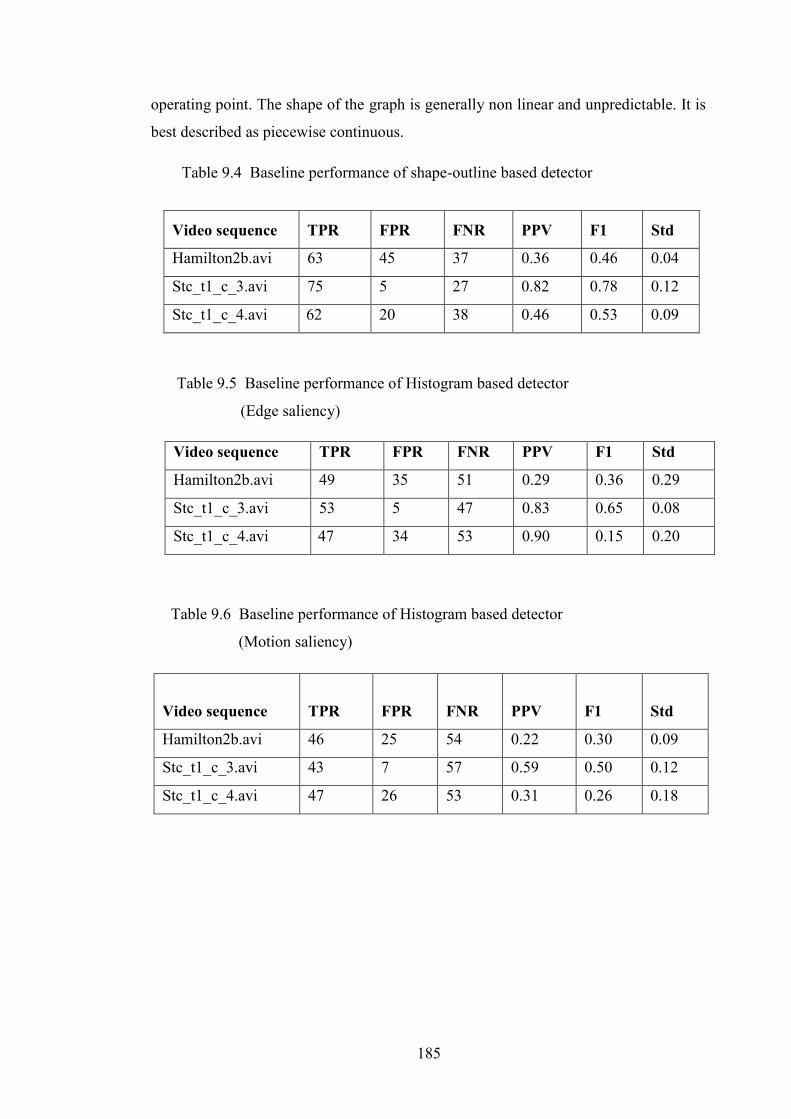
185
operating point. The shape of the graph is generally non linear and unpredictable. It is
best described as piecewise continuous.
Table 9.6 Baseline performance of Histogram based detector
(Motion saliency)
Video sequence
TPR
FPR
FNR
PPV F1 Std
Hamilton2b.avi 46 25 54 0.22 0.30 0.09
Stc_t1_c_3.avi 43 7 57 0.59 0.50 0.12
Stc_t1_c_4.avi 47 26 53 0.31 0.26 0.18
Table 9.4 Baseline performance of shape-outline based detector
Video sequence TPR FPR FNR PPV F1 Std
Hamilton2b.avi 63 45 37 0.36 0.46 0.04
Stc_t1_c_3.avi 75 5 27 0.82 0.78 0.12
Stc_t1_c_4.avi 62 20 38 0.46 0.53 0.09
Table 9.5 Baseline performance of Histogram based detector
(Edge saliency)
Video sequence TPR FPR FNR PPV F1 Std
Hamilton2b.avi 49 35 51 0.29 0.36 0.29
Stc_t1_c_3.avi 53 5 47 0.83 0.65 0.08
Stc_t1_c_4.avi 47 34 53 0.90 0.15 0.20
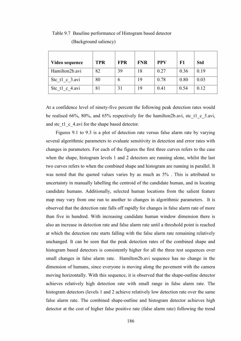
186
At a confidence level of ninety-five percent the following peak detection rates would
be realised 66%, 80%, and 65% respectively for the hamilton2b.avi, stc_t1_c_3.avi,
and stc_t1_c_4.avi for the shape based detector.
Figures 9.1 to 9.3 is a plot of detection rate versus false alarm rate by varying
several algorithmic parameters to evaluate sensitivity in detection and error rates with
changes in parameters. For each of the figures the first three curves refers to the case
when the shape, histogram levels 1 and 2 detectors are running alone, whilst the last
two curves refers to when the combined shape and histogram are running in parallel. It
was noted that the quoted values varies by as much as 5% . This is attributed to
uncertainty in manually labelling the centroid of the candidate human, and in locating
candidate humans. Additionally, selected human locations from the salient feature
map may vary from one run to another to changes in algorithmic parameters. It is
observed that the detection rate falls off rapidly for changes in false alarm rate of more
than five in hundred. With increasing candidate human window dimension there is
also an increase in detection rate and false alarm rate until a threshold point is reached
at which the detection rate starts falling with the false alarm rate remaining relatively
unchanged. It can be seen that the peak detection rates of the combined shape and
histogram based detectors is consistently higher for all the three test sequences over
small changes in false alarm rate. Hamilton2b.avi sequence has no change in the
dimension of humans, since everyone is moving along the pavement with the camera
moving horizontally. With this sequence, it is observed that the shape-outline detector
achieves relatively high detection rate with small range in false alarm rate. The
histogram detectors (levels 1 and 2 achieve relatively low detection rate over the same
false alarm rate. The combined shape-outline and histogram detector achieves high
detector at the cost of higher false positive rate (false alarm rate) following the trend
Table 9.7 Baseline performance of Histogram based detector
(Background saliency)
Video sequence
TPR
FPR
FNR
PPV F1 Std
Hamilton2b.avi 82 39 18 0.27 0.36 0.19
Stc_t1_c_3.avi 80 6 19 0.78 0.80 0.03
Stc_t1_c_4.avi 81 31 19 0.41 0.54 0.12

187
of false alarm rate of the histogram detectors. Clearly using level 2 histogram detector
has not resulted in a significant increase in detection rate. The relatively low detection
rate compared to the other sequence is due to the fact that most of people being
detected are in groups, thus a group might have been detected but a particular
individual may not have been detected. The ground truth labelling was done for
individuals and not for groups as a whole. The main challenge with this sequence is
the high scene clutter, and high human density. The effect of scale changes are
noticeable in Stc_t1_c_3.avi and Stc_t1_c_4.avi, two sequences with multiple humans
appearing with scale changes. Applying level two wavelet analysis results in higher
detection rate compared to level one histogram detector over relatively large changes
in false positive rate. Stc_t1_c_3.avi however has higher detection rate compared to
Stc_t1-c_4.avi where illumination was not quite good, with humans appearing darker
than the background. In sequence stc_t1_c_3.avi, there are several instances where
travellers come to the scene and exit from the scene in different directions, as well as
obvious instances where the classifier fails to detect humans because they were
wearing hats, overcoats, or in a posture exposing minimal features to the classifier.
Histogram equalization technique was applied to the frames but the improvement was
marginal. With the shape based detector the relative sensitivity of detection rate with
false alarm rate, candidate human width and height, and shape-outline threshold were
investigated. Peak detection rate varies between 50- 85% for the shape-outline based
detector. The detection rate also increases with the scale factor parameter for
candidate human window size up to a factor of two after which there is no more
increase. Similarly with histogram detector candidate human window dimension,
saliency thresholds, separation distance between candidates when classifying multiple
humans, and scale factor when searching for multiple humans are the most important
parameters. The general observation is that the histogram detector is relatively less
sensitive to most algorithmic parameter changes. However it is sensitive to changes in
separation distance between humans. It is also observed that the RO curve for the
combined detector can be partitioned into two sections, a stable section and non stable
section. The stable section is less sensitive to changes in false alarm rate (
corresponding to less than 5%), whilst the non stable section is sensitive to algorithmic
parameters changes.
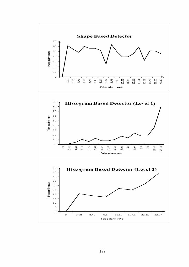
188
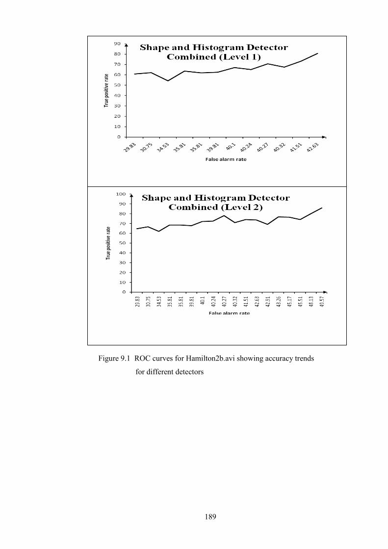
189
Figure 9.1 ROC curves for Hamilton2b.avi showing accuracy trends
for different detectors
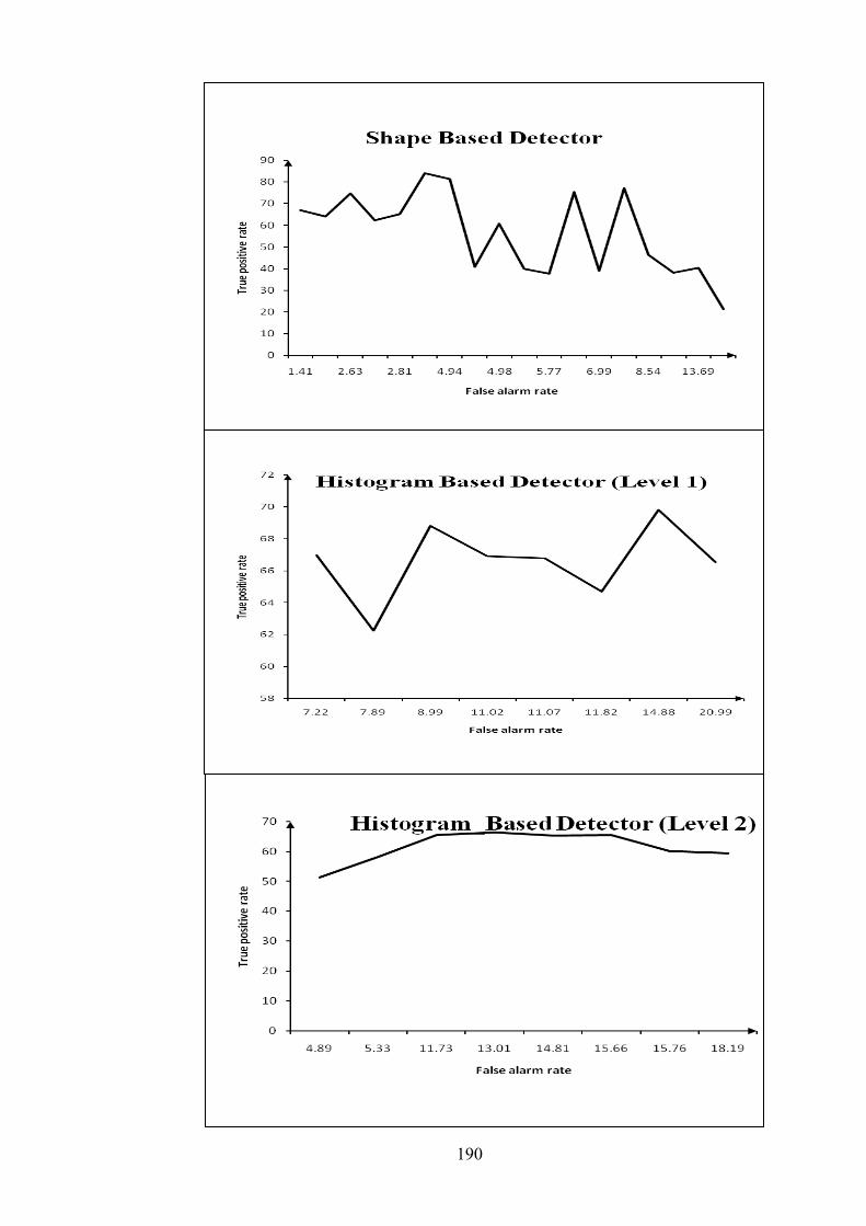
190
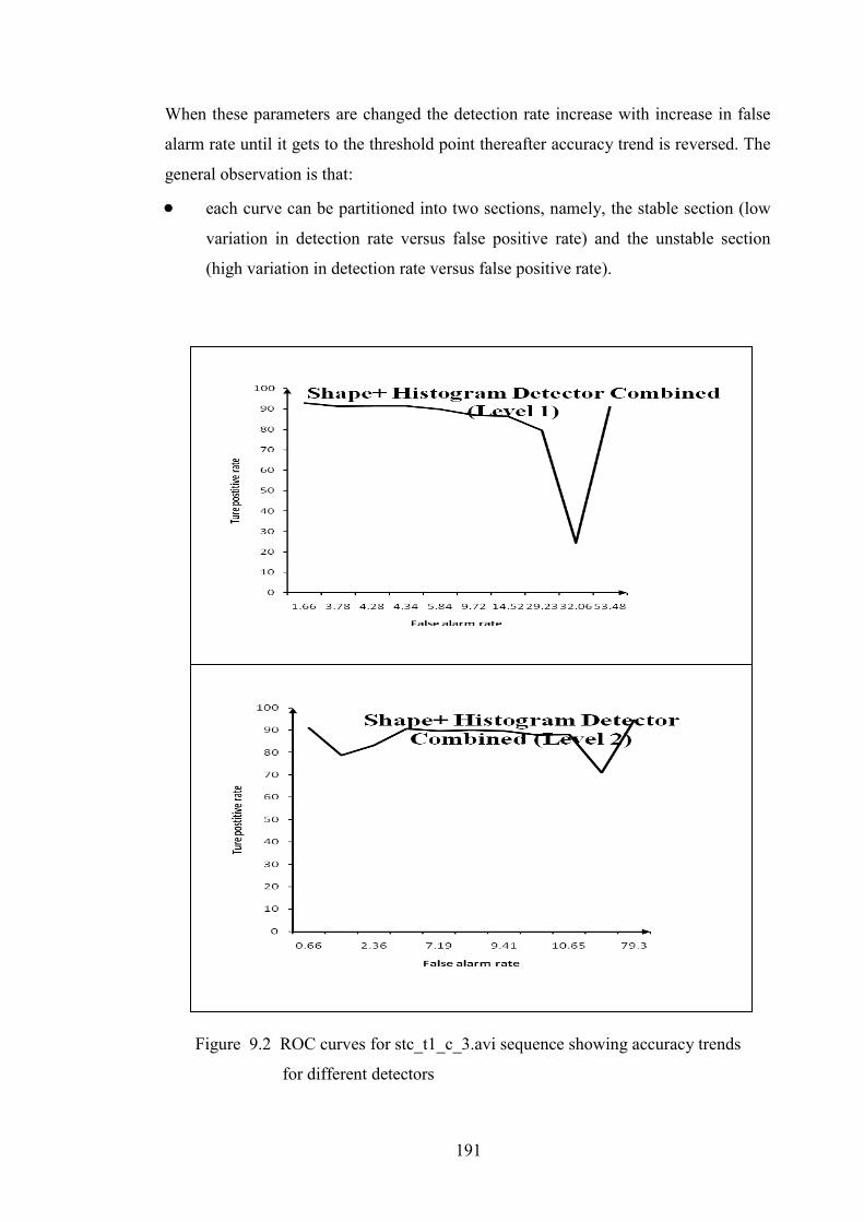
191
When these parameters are changed the detection rate increase with increase in false
alarm rate until it gets to the threshold point thereafter accuracy trend is reversed. The
general observation is that:
each curve can be partitioned into two sections, namely, the stable section (low
variation in detection rate versus false positive rate) and the unstable section
(high variation in detection rate versus false positive rate).
Figure 9.2 ROC curves for stc_t1_c_3.avi sequence showing accuracy trends
for different detectors
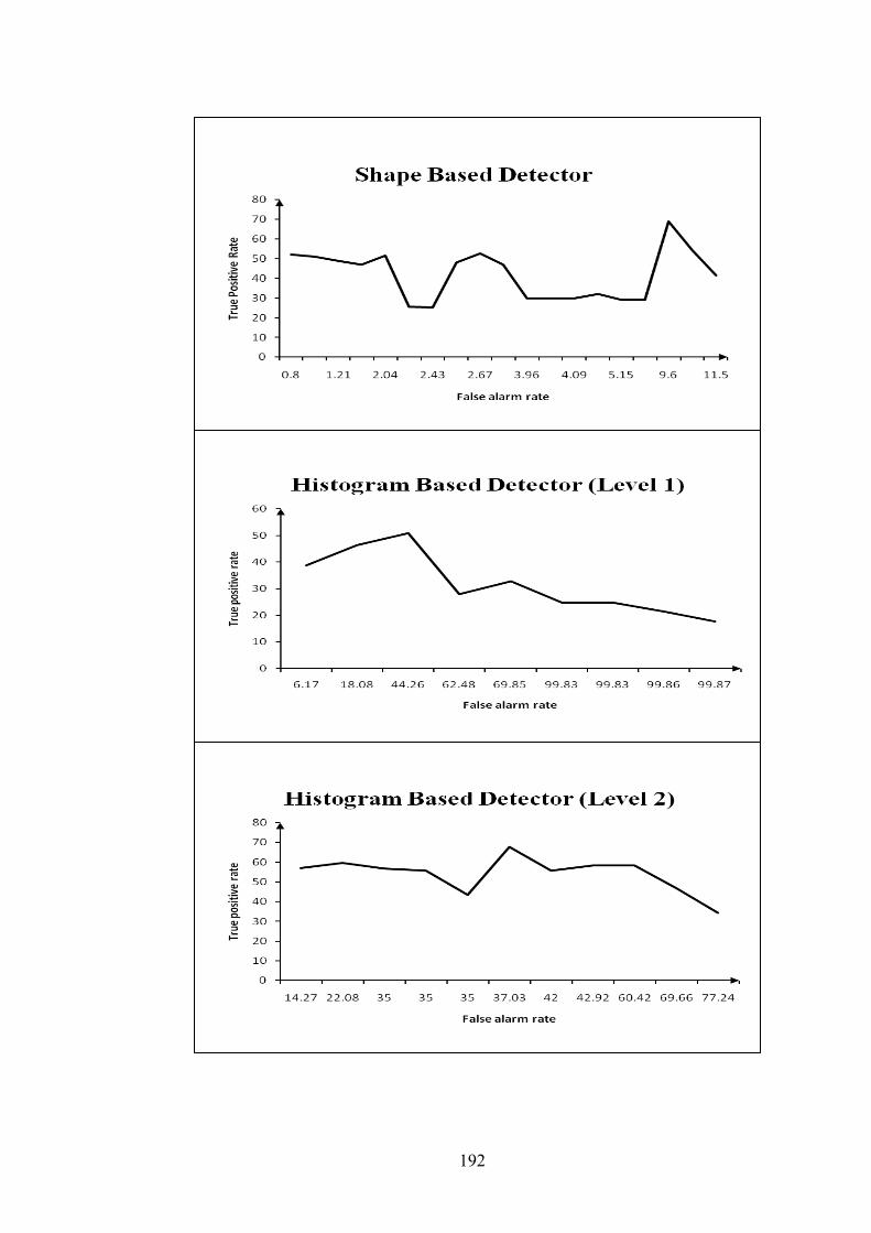
192
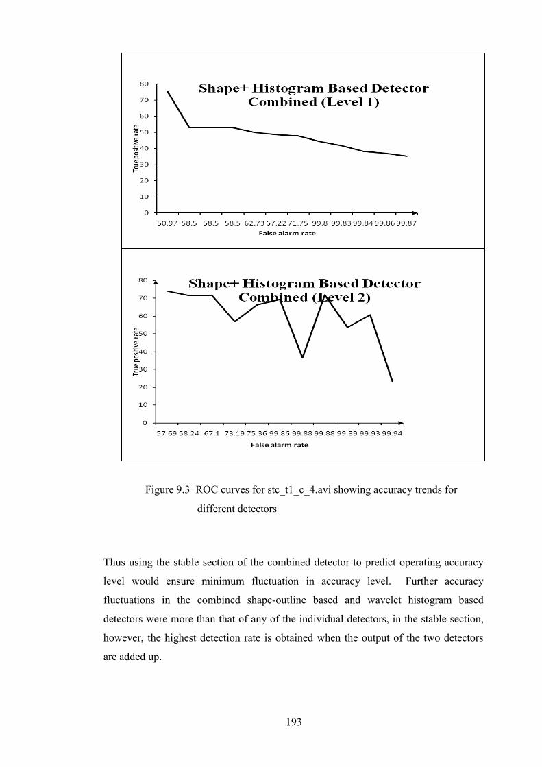
193
Thus using the stable section of the combined detector to predict operating accuracy
level would ensure minimum fluctuation in accuracy level. Further accuracy
fluctuations in the combined shape-outline based and wavelet histogram based
detectors were more than that of any of the individual detectors, in the stable section,
however, the highest detection rate is obtained when the output of the two detectors
are added up.
Figure 9.3 ROC curves for stc_t1_c_4.avi showing accuracy trends for
different detectors
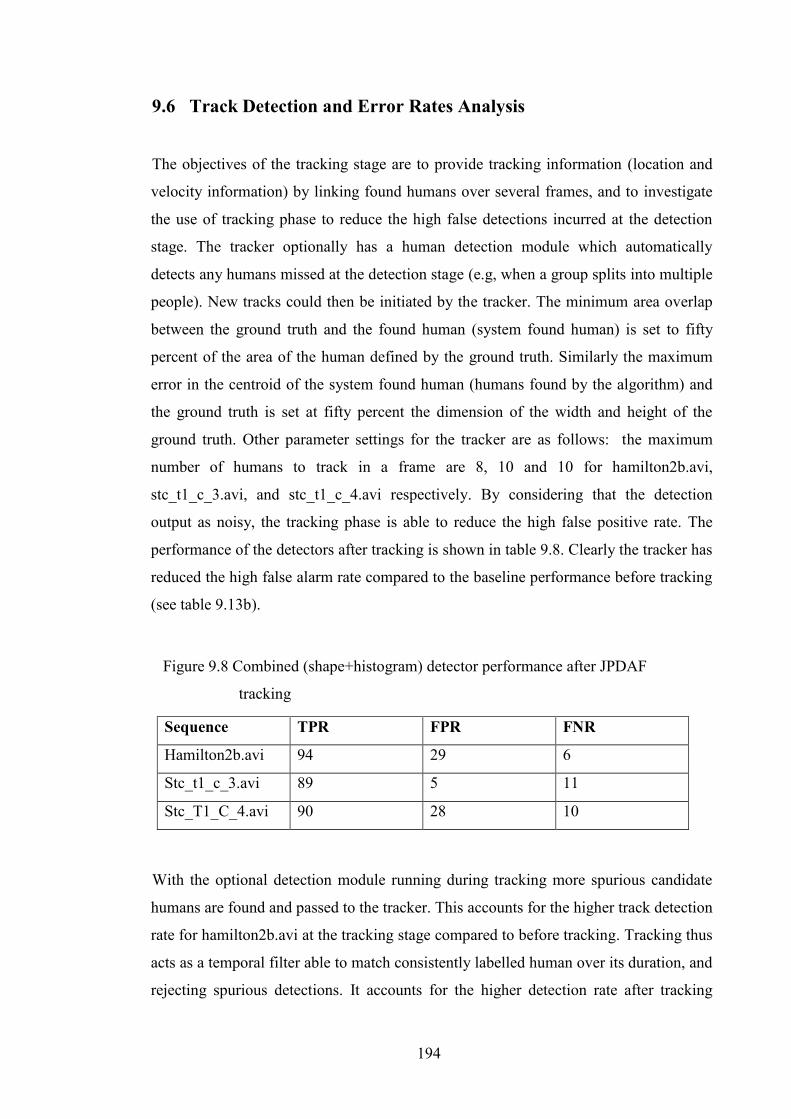
194
9.6 Track Detection and Error Rates Analysis
The objectives of the tracking stage are to provide tracking information (location and
velocity information) by linking found humans over several frames, and to investigate
the use of tracking phase to reduce the high false detections incurred at the detection
stage. The tracker optionally has a human detection module which automatically
detects any humans missed at the detection stage (e.g, when a group splits into multiple
people). New tracks could then be initiated by the tracker. The minimum area overlap
between the ground truth and the found human (system found human) is set to fifty
percent of the area of the human defined by the ground truth. Similarly the maximum
error in the centroid of the system found human (humans found by the algorithm) and
the ground truth is set at fifty percent the dimension of the width and height of the
ground truth. Other parameter settings for the tracker are as follows: the maximum
number of humans to track in a frame are 8, 10 and 10 for hamilton2b.avi,
stc_t1_c_3.avi, and stc_t1_c_4.avi respectively. By considering that the detection
output as noisy, the tracking phase is able to reduce the high false positive rate. The
performance of the detectors after tracking is shown in table 9.8. Clearly the tracker has
reduced the high false alarm rate compared to the baseline performance before tracking
(see table 9.13b).
With the optional detection module running during tracking more spurious candidate
humans are found and passed to the tracker. This accounts for the higher track detection
rate for hamilton2b.avi at the tracking stage compared to before tracking. Tracking thus
acts as a temporal filter able to match consistently labelled human over its duration, and
rejecting spurious detections. It accounts for the higher detection rate after tracking
Sequence TPR FPR FNR
Hamilton2b.avi 94 29 6
Stc_t1_c_3.avi 89 5 11
Stc_T1_C_4.avi 90 28 10
Figure 9.8 Combined (shape+histogram) detector performance after JPDAF
tracking
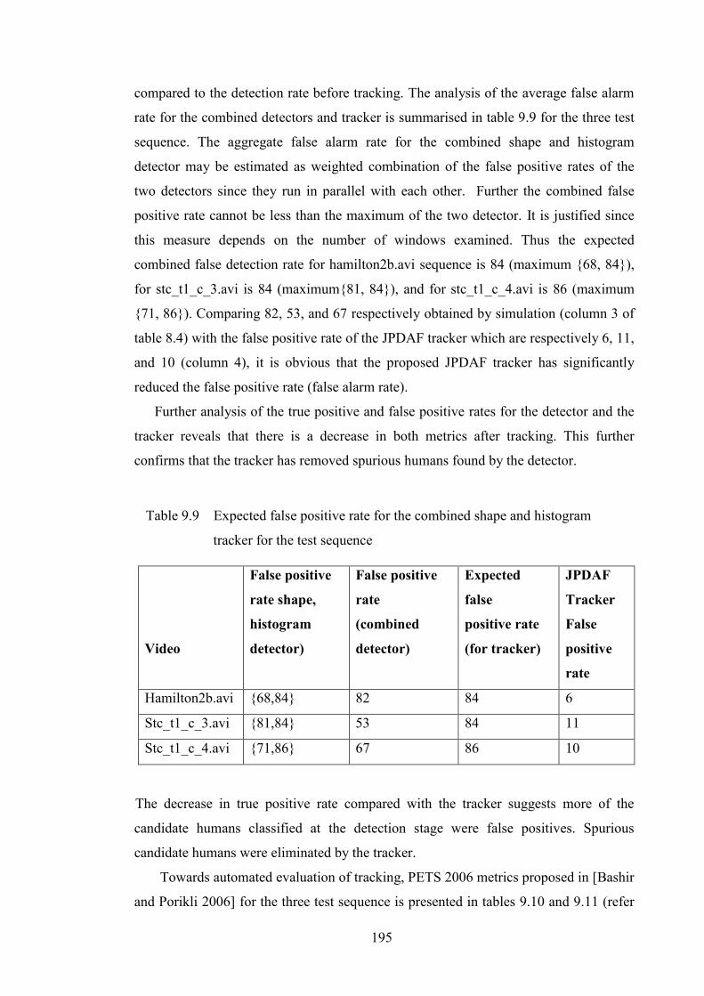
195
compared to the detection rate before tracking. The analysis of the average false alarm
rate for the combined detectors and tracker is summarised in table 9.9 for the three test
sequence. The aggregate false alarm rate for the combined shape and histogram
detector may be estimated as weighted combination of the false positive rates of the
two detectors since they run in parallel with each other. Further the combined false
positive rate cannot be less than the maximum of the two detector. It is justified since
this measure depends on the number of windows examined. Thus the expected
combined false detection rate for hamilton2b.avi sequence is 84 (maximum {68, 84}),
for stc_t1_c_3.avi is 84 (maximum{81, 84}), and for stc_t1_c_4.avi is 86 (maximum
{71, 86}). Comparing 82, 53, and 67 respectively obtained by simulation (column 3 of
table 8.4) with the false positive rate of the JPDAF tracker which are respectively 6, 11,
and 10 (column 4), it is obvious that the proposed JPDAF tracker has significantly
reduced the false positive rate (false alarm rate).
Further analysis of the true positive and false positive rates for the detector and the
tracker reveals that there is a decrease in both metrics after tracking. This further
confirms that the tracker has removed spurious humans found by the detector.
The decrease in true positive rate compared with the tracker suggests more of the
candidate humans classified at the detection stage were false positives. Spurious
candidate humans were eliminated by the tracker.
Towards automated evaluation of tracking, PETS 2006 metrics proposed in [Bashir
and Porikli 2006] for the three test sequence is presented in tables 9.10 and 9.11 (refer
Table 9.9 Expected false positive rate for the combined shape and histogram
tracker for the test sequence
Video
False positive
rate shape,
histogram
detector)
False positive
rate
(combined
detector)
Expected
false
positive rate
(for tracker)
JPDAF
Tracker
False
positive
rate
Hamilton2b.avi {68,84} 82 84 6
Stc_t1_c_3.avi {81,84} 53 84 11
Stc_t1_c_4.avi {71,86} 67 86 10
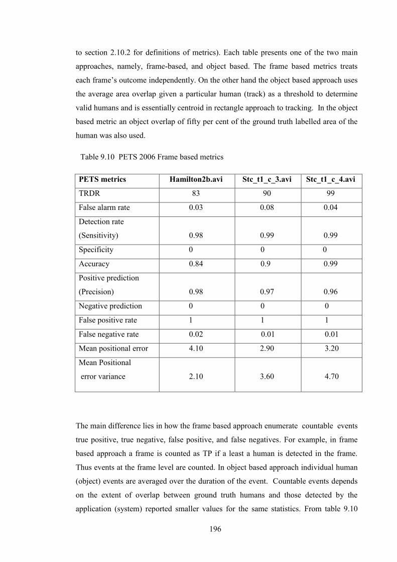
196
to section 2.10.2 for definitions of metrics). Each table presents one of the two main
approaches, namely, frame-based, and object based. The frame based metrics treats
each frame’s outcome independently. On the other hand the object based approach uses
the average area overlap given a particular human (track) as a threshold to determine
valid humans and is essentially centroid in rectangle approach to tracking. In the object
based metric an object overlap of fifty per cent of the ground truth labelled area of the
human was also used.
The main difference lies in how the frame based approach enumerate countable events
true positive, true negative, false positive, and false negatives. For example, in frame
based approach a frame is counted as TP if a least a human is detected in the frame.
Thus events at the frame level are counted. In object based approach individual human
(object) events are averaged over the duration of the event. Countable events depends
on the extent of overlap between ground truth humans and those detected by the
application (system) reported smaller values for the same statistics. From table 9.10
Table 9.10 PETS 2006 Frame based metrics
PETS metrics Hamilton2b.avi Stc_t1_c_3.avi Stc_t1_c_4.avi
TRDR 83 90 99
False alarm rate 0.03 0.08 0.04
Detection rate
(Sensitivity)
0.98
0.99
0.99
Specificity 0 0 0
Accuracy 0.84 0.9 0.99
Positive prediction
(Precision)
0.98
0.97
0.96
Negative prediction 0 0 0
False positive rate 1 1 1
False negative rate 0.02 0.01 0.01
Mean positional error 4.10 2.90 3.20
Mean Positional
error variance
2.10
3.60
4.70
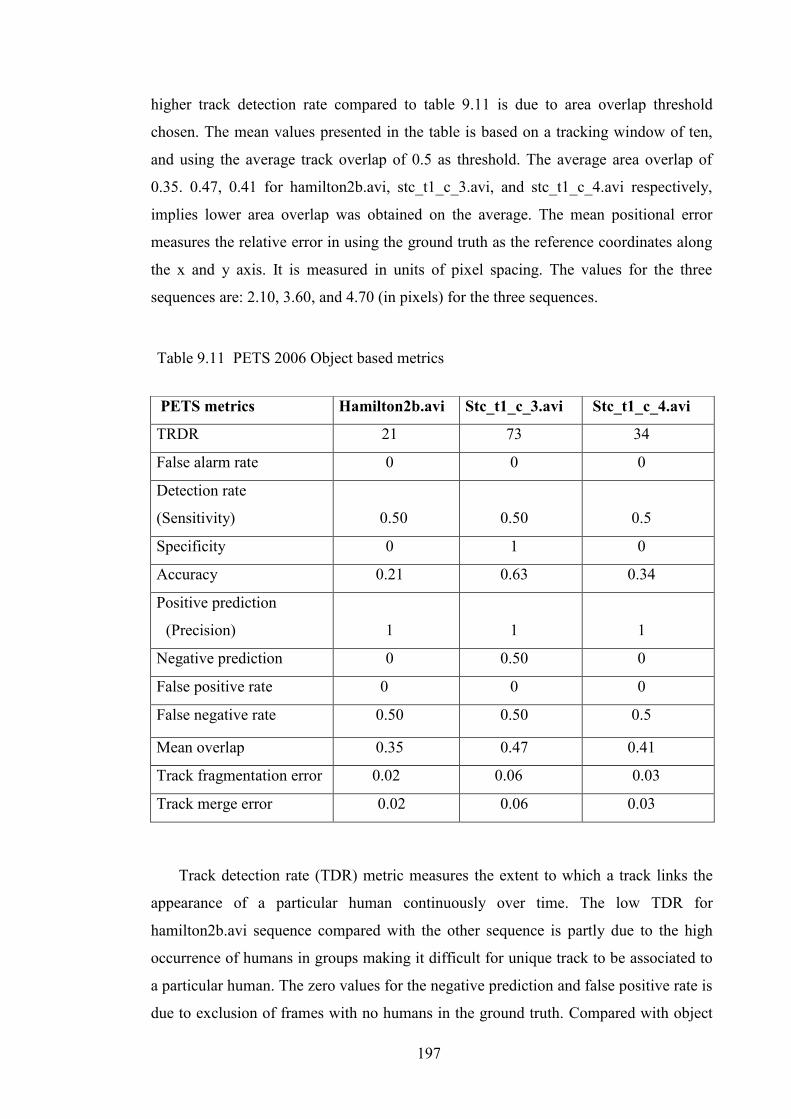
197
higher track detection rate compared to table 9.11 is due to area overlap threshold
chosen. The mean values presented in the table is based on a tracking window of ten,
and using the average track overlap of 0.5 as threshold. The average area overlap of
0.35. 0.47, 0.41 for hamilton2b.avi, stc_t1_c_3.avi, and stc_t1_c_4.avi respectively,
implies lower area overlap was obtained on the average. The mean positional error
measures the relative error in using the ground truth as the reference coordinates along
the x and y axis. It is measured in units of pixel spacing. The values for the three
sequences are: 2.10, 3.60, and 4.70 (in pixels) for the three sequences.
Track detection rate (TDR) metric measures the extent to which a track links the
appearance of a particular human continuously over time. The low TDR for
hamilton2b.avi sequence compared with the other sequence is partly due to the high
occurrence of humans in groups making it difficult for unique track to be associated to
a particular human. The zero values for the negative prediction and false positive rate is
due to exclusion of frames with no humans in the ground truth. Compared with object
Table 9.11 PETS 2006 Object based metrics
PETS metrics Hamilton2b.avi Stc_t1_c_3.avi Stc_t1_c_4.avi
TRDR 21 73 34
False alarm rate 0 0 0
Detection rate
(Sensitivity)
0.50
0.50
0.5
Specificity 0 1 0
Accuracy 0.21 0.63 0.34
Positive prediction
(Precision)
1
1
1
Negative prediction 0 0.50 0
False positive rate 0 0 0
False negative rate 0.50 0.50 0.5
Mean overlap 0.35 0.47 0.41
Track fragmentation error 0.02 0.06 0.03
Track merge error 0.02 0.06 0.03
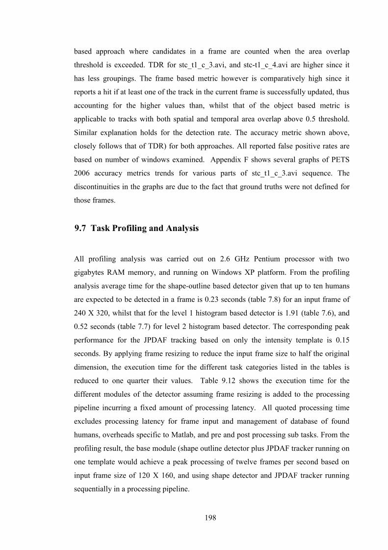
198
based approach where candidates in a frame are counted when the area overlap
threshold is exceeded. TDR for stc_t1_c_3.avi, and stc-t1_c_4.avi are higher since it
has less groupings. The frame based metric however is comparatively high since it
reports a hit if at least one of the track in the current frame is successfully updated, thus
accounting for the higher values than, whilst that of the object based metric is
applicable to tracks with both spatial and temporal area overlap above 0.5 threshold.
Similar explanation holds for the detection rate. The accuracy metric shown above,
closely follows that of TDR) for both approaches. All reported false positive rates are
based on number of windows examined. Appendix F shows several graphs of PETS
2006 accuracy metrics trends for various parts of stc_t1_c_3.avi sequence. The
discontinuities in the graphs are due to the fact that ground truths were not defined for
those frames.
9.7 Task Profiling and Analysis
All profiling analysis was carried out on 2.6 GHz Pentium processor with two
gigabytes RAM memory, and running on Windows XP platform. From the profiling
analysis average time for the shape-outline based detector given that up to ten humans
are expected to be detected in a frame is 0.23 seconds (table 7.8) for an input frame of
240 X 320, whilst that for the level 1 histogram based detector is 1.91 (table 7.6), and
0.52 seconds (table 7.7) for level 2 histogram based detector. The corresponding peak
performance for the JPDAF tracking based on only the intensity template is 0.15
seconds. By applying frame resizing to reduce the input frame size to half the original
dimension, the execution time for the different task categories listed in the tables is
reduced to one quarter their values. Table 9.12 shows the execution time for the
different modules of the detector assuming frame resizing is added to the processing
pipeline incurring a fixed amount of processing latency. All quoted processing time
excludes processing latency for frame input and management of database of found
humans, overheads specific to Matlab, and pre and post processing sub tasks. From the
profiling result, the base module (shape outline detector plus JPDAF tracker running on
one template would achieve a peak processing of twelve frames per second based on
input frame size of 120 X 160, and using shape detector and JPDAF tracker running
sequentially in a processing pipeline.
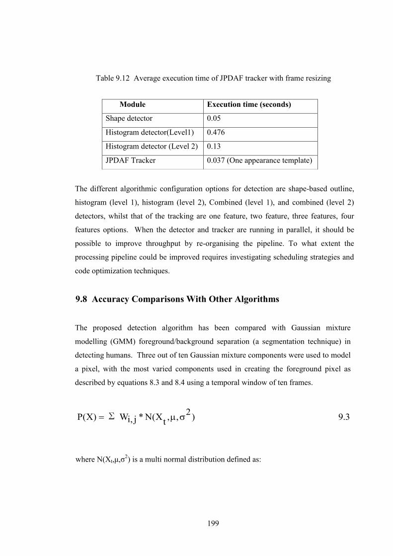
199
The different algorithmic configuration options for detection are shape-based outline,
histogram (level 1), histogram (level 2), Combined (level 1), and combined (level 2)
detectors, whilst that of the tracking are one feature, two feature, three features, four
features options. When the detector and tracker are running in parallel, it should be
possible to improve throughput by re-organising the pipeline. To what extent the
processing pipeline could be improved requires investigating scheduling strategies and
code optimization techniques.
9.8 Accuracy Comparisons With Other Algorithms
The proposed detection algorithm has been compared with Gaussian mixture
modelling (GMM) foreground/background separation (a segmentation technique) in
detecting humans. Three out of ten Gaussian mixture components were used to model
a pixel, with the most varied components used in creating the foreground pixel as
described by equations 8.3 and 8.4 using a temporal window of ten frames.
3.9)2,,tX(N*∑ j,iW)X(P
where N(Xt,μ,σ2) is a multi normal distribution defined as:
Table 9.12 Average execution time of JPDAF tracker with frame resizing
Module Execution time (seconds)
Shape detector 0.05
Histogram detector(Level1) 0.476
Histogram detector (Level 2) 0.13
JPDAF Tracker 0.037 (One appearance template)
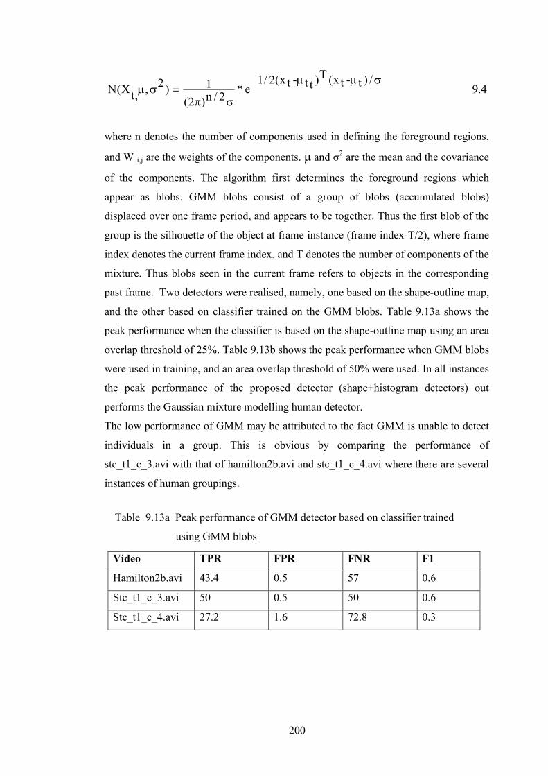
200
4.9/)t-tx(T)tt-tx(2/1
e*2/n)2(1)2,,tX(N
where n denotes the number of components used in defining the foreground regions,
and W i,j are the weights of the components. μ and σ2 are the mean and the covariance
of the components. The algorithm first determines the foreground regions which
appear as blobs. GMM blobs consist of a group of blobs (accumulated blobs)
displaced over one frame period, and appears to be together. Thus the first blob of the
group is the silhouette of the object at frame instance (frame index-T/2), where frame
index denotes the current frame index, and T denotes the number of components of the
mixture. Thus blobs seen in the current frame refers to objects in the corresponding
past frame. Two detectors were realised, namely, one based on the shape-outline map,
and the other based on classifier trained on the GMM blobs. Table 9.13a shows the
peak performance when the classifier is based on the shape-outline map using an area
overlap threshold of 25%. Table 9.13b shows the peak performance when GMM blobs
were used in training, and an area overlap threshold of 50% were used. In all instances
the peak performance of the proposed detector (shape+histogram detectors) out
performs the Gaussian mixture modelling human detector.
The low performance of GMM may be attributed to the fact GMM is unable to detect
individuals in a group. This is obvious by comparing the performance of
stc_t1_c_3.avi with that of hamilton2b.avi and stc_t1_c_4.avi where there are several
instances of human groupings.
Table 9.13a Peak performance of GMM detector based on classifier trained
using GMM blobs
Video TPR FPR FNR F1
Hamilton2b.avi 43.4 0.5 57 0.6
Stc_t1_c_3.avi 50 0.5 50 0.6
Stc_t1_c_4.avi 27.2 1.6 72.8 0.3
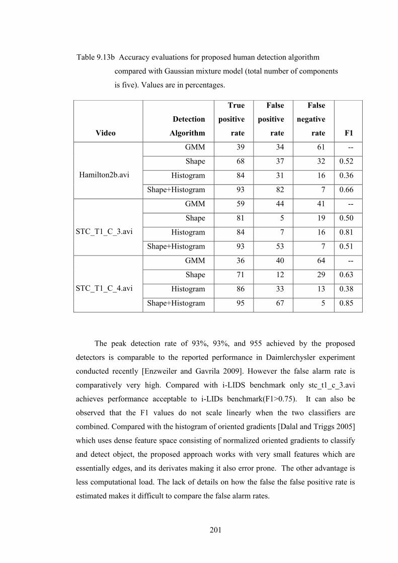
201
The peak detection rate of 93%, 93%, and 955 achieved by the proposed
detectors is comparable to the reported performance in Daimlerchysler experiment
conducted recently [Enzweiler and Gavrila 2009]. However the false alarm rate is
comparatively very high. Compared with i-LIDS benchmark only stc_t1_c_3.avi
achieves performance acceptable to i-LIDs benchmark(F1>0.75). It can also be
observed that the F1 values do not scale linearly when the two classifiers are
combined. Compared with the histogram of oriented gradients [Dalal and Triggs 2005]
which uses dense feature space consisting of normalized oriented gradients to classify
and detect object, the proposed approach works with very small features which are
essentially edges, and its derivates making it also error prone. The other advantage is
less computational load. The lack of details on how the false the false positive rate is
estimated makes it difficult to compare the false alarm rates.
Table 9.13b Accuracy evaluations for proposed human detection algorithm
compared with Gaussian mixture model (total number of components
is five). Values are in percentages.
Video
Detection
Algorithm
True
positive
rate
False
positive
rate
False
negative
rate
F1
Hamilton2b.avi
GMM 39 34 61 --
Shape 68 37 32 0.52
Histogram 84 31 16 0.36
Shape+Histogram 93 82 7 0.66
STC_T1_C_3.avi
GMM 59 44 41 --
Shape 81 5 19 0.50
Histogram 84 7 16 0.81
Shape+Histogram 93 53 7 0.51
STC_T1_C_4.avi
GMM 36 40 64 --
Shape 71 12 29 0.63
Histogram 86 33 13 0.38
Shape+Histogram 95 67 5 0.85

202
The JPDAF tracker algorithm has also been compared with Mean shift detector
/tracker as shown in table 9.14. The version of mean shift developed use Battacharyya
measure to determine similarity between a candidate human from the previous known
location to the current location, and links consecutive locations as a track if the mean
shift distance between corresponding humans in consecutive frames is less than three
pixels wide or high. At every iterative shift along the X and Y directions by a unit
pixel distance, the corresponding mean shift vector is computed. Alternatively if the
number of iterations exceeds half the width and height of the object windows the
candidate human is deemed not to have been found. The mean shift tracker does not
use any discriminatory mechanism except that provided by the histogram classifier.
The results shows that the true positive and false positive rate are lower than the
proposed JPDAF tracker even when the illumination conditions and object
background contrast is high as shown by Stc-t1_c_3.avi. The low performance is
similarly attributed to grouping and other interactions between humans in the scene. It
was also noted for scenes with multiple humans interacting with each other in groups,
the accuracy is not high due to frequent interactions. One possible explanation is that
detecting multiple individuals in a group is difficult for the mean shift tracker. It is
attributed to the fact that the degree of overlap between the kernel and the blob
remains the same once the group has been detected with either one, two or more
humans uniquely detected. It persists over several frames.
Table 9.14 Peak accuracy of mean shift detector/tracker. Positional accuracy is
expressed as a fraction of maximum distance of separation (in pixels)
between humans. MaxPosX and MaxPosY denotes maximum errors in x
and y
locations in two frames. Video TPR FPR FNR MaxPosX MaxPosY
Hamilton2b.avi 52 10 48 3 3
Stc_t1_c_3.avi 62 9 38 3 3
Stc_t1_c_4.avi 65 46 35 3 3
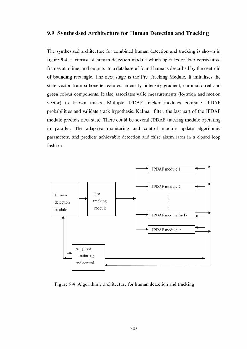
203
9.9 Synthesised Architecture for Human Detection and Tracking
The synthesised architecture for combined human detection and tracking is shown in
figure 9.4. It consist of human detection module which operates on two consecutive
frames at a time, and outputs to a database of found humans described by the centroid
of bounding rectangle. The next stage is the Pre Tracking Module. It initialises the
state vector from silhouette features: intensity, intensity gradient, chromatic red and
green colour components. It also associates valid measurements (location and motion
vector) to known tracks. Multiple JPDAF tracker modules compute JPDAF
probabilities and validate track hypothesis. Kalman filter, the last part of the JPDAF
module predicts next state. There could be several JPDAF tracking module operating
in parallel. The adaptive monitoring and control module update algorithmic
parameters, and predicts achievable detection and false alarm rates in a closed loop
fashion.
Figure 9.4 Algorithmic architecture for human detection and tracking
Pre
tracking
module
Human
detection
module
Adaptive
monitoring
and control
JPDAF module 2
JPDAF module (n-1)
JPDAF module n
JPDAF module 1
204
9.10 Discussion
If VCA applications target at human detection and tracking is to be widely accepted, it
has to be proven to be as good as the human operators who monitor scenes through
visual display devices. To robustly detect humans as (i) individuals, as (ii) a group or
part of a group, (iii) recognise events such as someone entering protected premises,
(iv) abandoning an object, (v) picking up an object, (vi) or running towards a
particular facility. The application must consistently achieve high detection rate with
low false alarm. It must also be supported by event statistics captured continuously for
effective monitoring and control. Other requirements for generic surveillance system
were discussed in section 1.1.2. Requirements such as user friendliness, application
flexibility, and cost-effectiveness were excluded from the current study since most
existing VCA system meets these requirements. The study has focussed on improving
the accuracy of both detection and tracking of humans. One way of comparing the
accuracy of existing system is to use standard data set and evaluation metrics. PETS
(Performance Evaluation of Tracking system) databases and accuracy measures based
on confusion matrix, i-LIDs metrics, and ROC were used in the current investigation.
Towards achieving high accuracy independent of scene complexity new
techniques have been developed which has proven to be robust in human localization
and discrimination. The first proposed detection technique, a novel shape-outline
based detector based on a feed forward neural network designed to predict an output
pattern given an input pattern. The discrimination of the human class from the non
human class is based on a shape mismatch measure expressed as a similarity measure
(used as a discriminant function). The proposed shape mismatch metric is defined
such that there is a penalty whenever there are mismatch points on the predicted
pattern generated compared with the input pattern. The number of such points appear
as a factor in the denominator of equation 6.6. The problem of variable human
dimension in the frames are avoided by resizing the pattern predictor to height and
width of 16 by 32 pixels respectively. This approach copes well when there are no
significant scale changes. Localization of humans in the shape space is based on edge
density and motion saliency measure in a candidate human window. Higher edge
density corresponds to salient feature locations which are further probed by the
classifier. Detection is validated after passing linear discriminant and heuristic tests
205
(threshold and area tests). The main reason for introducing this step is to reduce
further classifier errors. Edge saliency based localization thresholds were chosen as a
fraction of the maximum edge density in the shape-outline map. The offset used is
typically a multiple of the standard deviation of the edge density.
The second detector, a novel wavelet domain based histogram detector is
designed to cope with large scale changes. The detector is based on six square wavelet
templates as primitives wavelet features. These features describe humans irrespective
of the subband in which the candidate is found. Thus it is independent of scale
Wavelet representation such as over complete wavelet transform which is translation
invariant, was used to design two histogram classifiers based on two different subband
types. Saliency based localization thresholds were chosen as a fraction of the
maximum of the normalized wavelet coefficient in a frame deemed significant for
efficient determination of salient locations in the wavelet domain.
The proposed detectors have also been evaluated using single frames from
PASCAL VOC 2010 challenge. It was observed that the detector is acceptable for
single frame classification, but not suitable for human detection in single frame.
Pattern classifier based approach for human detection has been demonstrated as
highly accurate with reduced computational cost despite the need to provide adequate
samples during training to capture as much variability as possible. Detection capability
is however dependent on the spatial distribution of the primitive features. By
providing large number of training examples from different views of humans high
detection of individuals in isolation has been achieved. However there are problems in
detecting groups with classifiers trained on individuals, suggesting the need to develop
separate classifiers for detection of humans in groups. In the test runs it was observed
that when several humans come together to form a group there were high miss
detections and false alarms due to the difficulty of separating the group into
individuals by the search technique. Validation of the centroid of the location of the
human in the candidate human during training was achieved by statistical analysis of
the X and Y values of the estimated centroid. Principal component analysis was used
to determine the principal location along the horizontal and vertical histogram which
accounts for the smallest variation. This corresponds to the centroid of the found
humans. Comparison with the manually extracted values agreed with the observation.
Further one way ANOVA test for F statistics with significance (see section 7.2.2) at
95% confidence level also validated the derived model. It was observed that classifier
206
responded very well to vertical edges but not so well to horizontal edges. The
classifier designed using motion or edge saliency based localization and vertical edges
(horizontal histogram) based on LL subband achieved high detection rate and
relatively moderate amount of false alarm rate. With the HLLH subband only the
vertical features was used to design a classifier. With LL subband both vertical and
horizontal and vertical features were used to design two classifiers which when
combined provided sufficient discriminatory power to detect humans. This is
supported by large deviations for the y-coordinates (use horizontal edges) of the
predictions made by the classifier compared to the x-coordinates (use vertical edges)
of the predictions for human location in the case of the HLLH subband. An
approximation of the y-coordinate is made based on the first moment along the Y axis
(see sections 7.2.1, and 7.6). This is added as an offset to the top left corner of the start
address of the block to determine the approximate location along the X and Y-axis.
However, the positional error along Y-axis is sometimes quite high compared to the
dimension of the histogram. Background saliency based human detection achieved
high accuracy whenever the background scene did have large areas with uniform
illumination, or when humans are the dominant objects moving in the scene based on
size. The presence of large amount of clutter also affects the detection capabilities of
the classifiers, for example a stationary train in the background of stc_t1_c_4.avi
sequence. Other problems such as occlusion due to humans wearing hats or overcoats
which resulted in high miss detections in shape based classifier compared to histogram
classifier (check detection rate of stc_t1_c.4.avi in section 8.3).
A performance bottleneck noted at the detection stage is that most of the candidate
humans examined by the classifier turned out to be non humans hence the need to
improve the feature extraction and discriminating capability of the classifiers.
Towards this end further investigation is required on feature rejection techniques in
the wavelet domain. Other investigations include:
Investigation into background modelling techniques to detect ground plane;
modelling of large scene landmarks in the background.
The shape-outline based detector requires resizing of candidate human window, and
the result could also be a source of error since the mismatch measure penalises for
unmatched points on the input pattern. The joint probabilistic data association filter
207
(JPDAF) tracker is designed primarily to reduce false detections (false alarms) and
provide trajectory information. The assumption is that by making decisions based on a
group of frames defined as a track window better decision would result. Within a track
processing window, tracks are associated to human windows based on measurement
error confidence interval expressed as Mahalanobis distance assuming measurements
are normally distributed. This approach enabled different confidence measurements to
be associated with different measurement clusters, enabling fast pruning of unlikely
measurement by just tightening the confidence interval. Assumptions made in track
window processing also enabled both sequential and batch estimation modes achieve
high track association. Sequential estimation mode requires fixing the motion model,
and the Mahalanobis confidence interval with track decision made solely on the
previous frame. In batch model different motion models are examined using different
confidence interval measure and the best of the models selected after several
iterations, and decisions are made based on track processing window. The accuracy of
the tracker is predicted in batch mode by iterative tracking and varying the confidence
interval in steps of 0.1. This enabled optimum tracking parameters to be achieved. The
tracker achieved real-time performance on applying frame resizing as part of the pre
processing step.
The need to reduce total execution time to provide real-time response for the
combined detection and tracking is obvious since the total execution time of the
combined detector and the tracker pipelines guarantee a maximum of ten frames per
second of 120 X 320 frames being acquired at 30 frames per second assuming a single
video bit stream, and running of 2.6 GHz Pentium PC. This is based on Matlab
profiling tool. For real-time processing clearly code optimization, and optimal
scheduling strategy is required. Further for upward scalability of frame size and
number of video streams, parallel processing is suggested to improve real-time
response and throughput requirements. Towards this end both algorithmic architecture
and parallel processing accelerator is proposed.
9.11 Review of Research Progress
The research started with the literature review which highlighted the fact that given
sufficient computational resources most existing algorithms would be able to improve
208
detection rate if additional techniques are incorporated as either part of the pre and
post processing steps. In Gaussian mixture modelling performance depends on the
dimension of humans compared with other moving background objects. If the
background motion is dominant and the relative size of the human is small then
detection rate tends to be low and vice versa. Also there is large computational load in
modelling per pixel process. Additionally it requires a means of discriminating the
human class from the non human class. The two approaches to human detection
proposed are pattern recognition techniques based on patch classifier (used in the
current investigation). Of the two approaches considered, shape-outline classifier
technique requires less computational resources when deployed (after training). The
histogram detector appears to be less sensitive to algorithmic parameter changes (the
ROC curve tends to be flat). Furthermore it was noted that most algorithms are not
able to maintain accuracy level when the underlying scene constraints are violated.
The algorithm presented for adaptive monitoring and control of operating accuracy
investigated how close the predictions are to the realised accuracy. Indeed, it provides
a means of improving the accuracy irrespective of scene background complexity in
the proposed pattern spaces. It indicates when parameters need to be adjusted. It could
be useful in situation where the expected accuracy is high but the realised accuracy is
low and has to be improved, hence signal for manual intervention. Counting in highly
dense scene also requires a different approach since localization techniques might not
be able to locate most humans in high density areas due to multiple feature occlusions.
A major source of computational overhead in the current implementation is resizing of
candidate humans to fit the dimension of the classifiers. The standard frame
dimension used (240 x 320) probes more than ten thousand candidate windows to
detect all humans assuming the maximum human count in a frame is more than five.
This turned out to be an overhead in human detection and tracking especially. Another
limitation is the high number of candidate humans which are typically examined most
of which turns out to be spurious. It also increases the computational load. One
possibility of reducing the number of candidates is to characterise the silhouette of
humans in the window in order to reject most of the spurious candidates before
classification. The outcome of the theoretical investigations on scheduling and parallel
processing is summarised in chapter nine as part of the recommendations for future
work.
209
CHAPTER TEN
CONCLUSIONS
10.1 Conclusions
The project has addressed the problem of improving the accuracy of human detection
and tracking independent of scene complexity. A parameter driven online accuracy
estimation algorithm linked to both the detection and the tracking stage has been
presented. By optimizing the parameters the desired accuracy required can be met as
close as possible. The detection part is based on two reduced complexity feature
extraction and classifiers designs techniques. The classifiers operate in parallel to
realise high detection rate. Together with the second part, the JPDAF tracker, it is able
to realise high detection rate.
The specification, implementation, and accuracy evaluation in software of the
algorithms have also been detailed.
The problem of scale changes due to changes in perspective projection is solved
by multiscale wavelet domain decomposition of video frames and use of scale
independent pattern classifier. The performance of the classifiers based on
confusion matrix, and ROC curves have also been presented.
Accuracy comparisons with Gaussian mixture modelling based detector, and
mean shift tracking have also been presented which demonstrates higher detection
for most of the test sequences. As shown from the comparative study the effect of
scene background factors has less effect in the proposed shape-space. However
more tests are required.
Modular algorithmic structure has been synthesised for modular synthesis of
human detection and tracking to improve processing scalability. Finally parallel
processing technique has been recommended to improve response time.
210
The techniques presented could be built upon to provide additionally functionality
such as anomalous behaviour analysis and detailed window analysis based on
silhouettes. Operational efficiency has been demonstrated by the high accuracy level
achieved through systematic algorithmic parameter setting using the test sequence,
modular and scalable algorithmic architecture presented to cope with changes in frame
size and number of channels. Classifier based approach to human detection provides a
cost-effective means of achieving high accuracy using moderate amount of computing
power. However to realise its full potential adequate training is required, and detection
by part capability.
The proposed JPDAF tracker achieved high detection rate consistent with the initial
puts from the detection stage. Despite achieving high detection rates the high false
alarm rate is still a problem. This has implications on computational load, and limits
its suitability as generic human detection and tracking. One solution is to design a
second classifier in the spatial domain to reject spurious candidates. To reduce
tracking errors it is proposed to combine the proposed tracker with mean shift tracking
algorithm
10.2 Future Work
To extend the system to include anomalous behaviour analysis and detection the
following algorithmic investigations are proposed:
10.2.1 Algorithmic investigations
Investigation into wavelet based histogram classifier for detection of humans in
groups of two, three and four, and view independent. The inadequacy of using
classifiers trained on single humans for detecting groups of humans has been
highlighted earlier on.
Evaluate the performance of human detection and tracking with moving
background and camera motion using the proposed approach.
Background modelling schemes for handling non uniform illuminations changes,

211
and modelling schemes for motion detection in the presence of moving large
background objects.
Silhouette-based analysis of human windows to identify behaviour such as
identification of moved object, abandoned object, and unauthorised entry or
intrusion. It is proposed that behaviour is represented as hidden Markov states
stored in a behaviour database.
Comparative study of contour based tracking with JPDAF for data association,
versus the proposed method.
Sections 10.2.2 to 10.2.5 details out performance and architectural issues related to
real-time processing and application scalability.
10.2.2 Performance Enhancements: Parallel Processing for
Optimum Execution Time and Throughput
It is clear from the profiling times shown in tables 7.4, 7.5, 7.6, 8.4 and 8.5 that the
total processing time fails to meet real time performance of 30 frames per second
assuming input frame of size 320W X 240H. Additionally, more processing power is
required since at the high performance end up to nine video streams may be processed.
Thus there is a need to investigate parallel processing techniques to reduce execution
time and at the same time increase throughput. One option is an accelerator based
approach to speed up the application. The remaining sections discuss possible
investigations into this aspect of processing.
10.2.3 Proposed Macro Architecture of Multiprocessor Accelerator
A programmable coprocessor based on commercial off-the-shelf (COTS) components
consisting of multiple SMT (simultaneous multithreading) processors (Pentium IV,
IBM POWER5, Xeon, RISC processor, etc), dual ported RAM, and FPGA as shown
in figure 10.1 is proposed. The bus interconnection network may be tightly coupled to
a daughter board or loosely coupled as in network of work stations. The complete
system could be realised on a server or network of personal computers. The FPGA is
normally attached to the host processor. Memory could be shared or partitioned
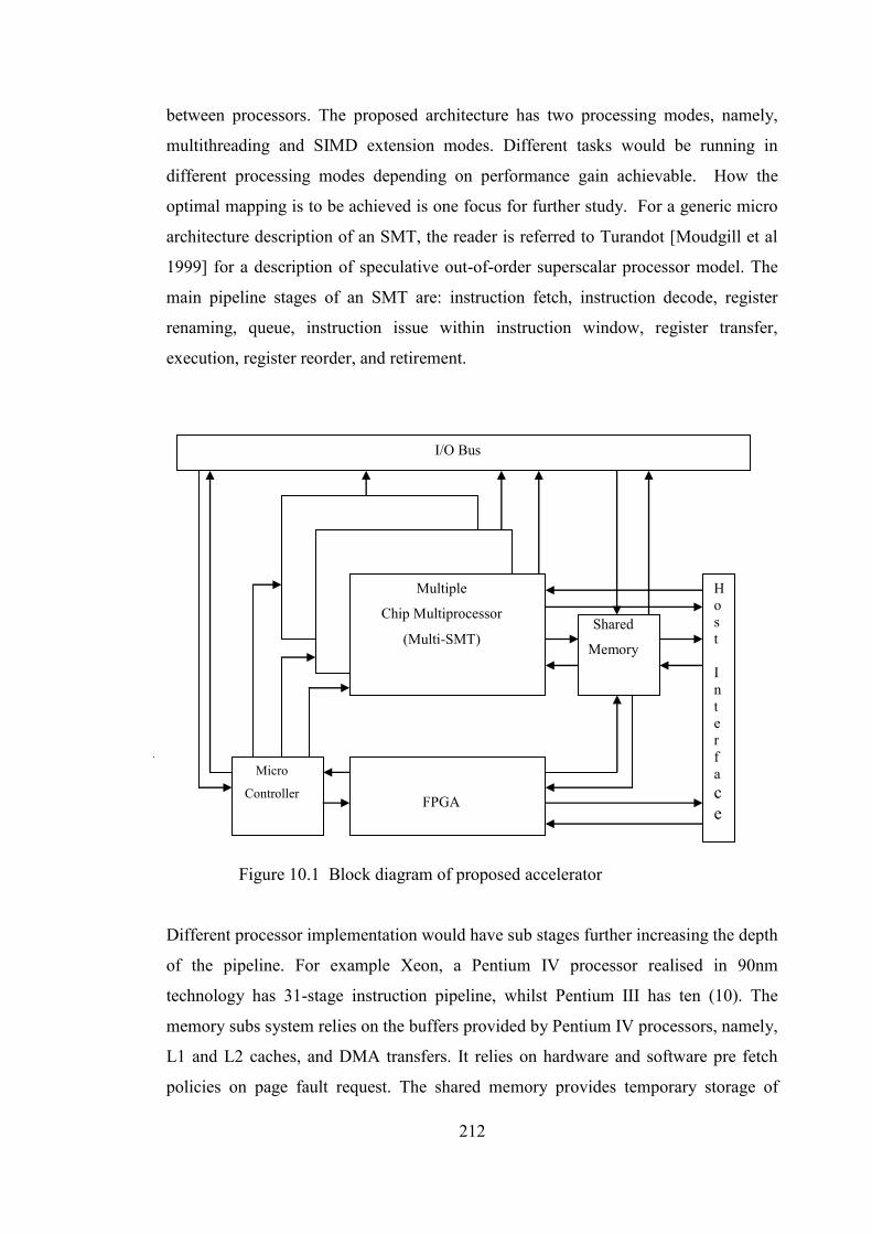
212
between processors. The proposed architecture has two processing modes, namely,
multithreading and SIMD extension modes. Different tasks would be running in
different processing modes depending on performance gain achievable. How the
optimal mapping is to be achieved is one focus for further study. For a generic micro
architecture description of an SMT, the reader is referred to Turandot [Moudgill et al
1999] for a description of speculative out-of-order superscalar processor model. The
main pipeline stages of an SMT are: instruction fetch, instruction decode, register
renaming, queue, instruction issue within instruction window, register transfer,
execution, register reorder, and retirement.
Different processor implementation would have sub stages further increasing the depth
of the pipeline. For example Xeon, a Pentium IV processor realised in 90nm
technology has 31-stage instruction pipeline, whilst Pentium III has ten (10). The
memory subs system relies on the buffers provided by Pentium IV processors, namely,
L1 and L2 caches, and DMA transfers. It relies on hardware and software pre fetch
policies on page fault request. The shared memory provides temporary storage of
I/O Bus
Micro
Controller
H o s t I n t e r f a c e
Multiple
Chip Multiprocessor
(Multi-SMT) Shared
Memory
FPGA
Figure 10.1 Block diagram of proposed accelerator

213
intermediate results and buffer for loading or dumping of results. Since each SMT
features on-chip program and data memories, patches (object windows) are passed
asynchronously to each processor. There are two I/O buses, one for input and the other
for output. The controller is responsible for scheduling that task on the SMP
processors, the FPGA and DMA transfers between the host CPU and shared memory,
shared memory and SMTs and FPGA. The communication network could be a bus
network, optical network of network of workstations with multicore processors. The
controller is responsible for DMA transfers and task scheduling. Table 10.1 and 10.2
provide the main system parameters to be used in evaluating the performance of the
accelerator based on Intel Pentium IV dual core multiprocessor.
10.2.4 Task Mapping and Scheduling on Multiprocessor Accelerator
The sequential code is initially optimized by reducing unused variables, redundant
operations, and reducing the complexity of conditional branches. Then algorithmic
System Parameters1 Value
L1 cache latency 0.794 ns
L2 cache latency 7.296 ns
Main memory latency 143.9 ns
Main memory bandwidth 1.24 GB/s
System Bus interface bandwidth 6.4 GB/s
Bus speed 400MHz
Processor Intel 2.66GHz; 2 Threads per
processor
DRAM 2GB
Table 10.1 System architectural parameters for the proposed accelerator
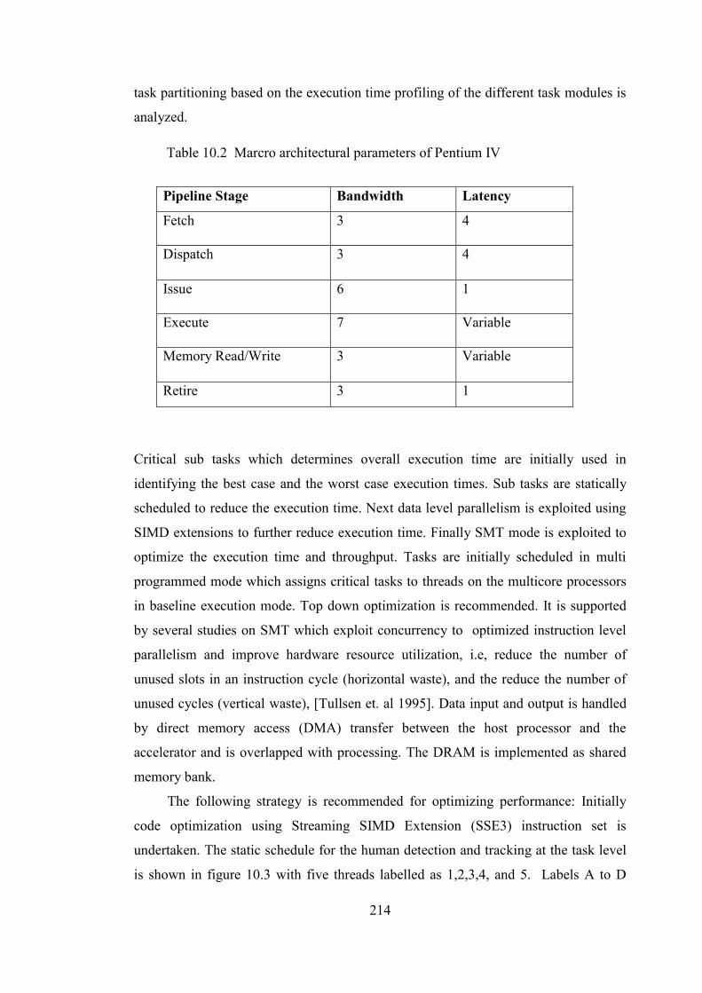
214
task partitioning based on the execution time profiling of the different task modules is
analyzed.
Critical sub tasks which determines overall execution time are initially used in
identifying the best case and the worst case execution times. Sub tasks are statically
scheduled to reduce the execution time. Next data level parallelism is exploited using
SIMD extensions to further reduce execution time. Finally SMT mode is exploited to
optimize the execution time and throughput. Tasks are initially scheduled in multi
programmed mode which assigns critical tasks to threads on the multicore processors
in baseline execution mode. Top down optimization is recommended. It is supported
by several studies on SMT which exploit concurrency to optimized instruction level
parallelism and improve hardware resource utilization, i.e, reduce the number of
unused slots in an instruction cycle (horizontal waste), and the reduce the number of
unused cycles (vertical waste), [Tullsen et. al 1995]. Data input and output is handled
by direct memory access (DMA) transfer between the host processor and the
accelerator and is overlapped with processing. The DRAM is implemented as shared
memory bank.
The following strategy is recommended for optimizing performance: Initially
code optimization using Streaming SIMD Extension (SSE3) instruction set is
undertaken. The static schedule for the human detection and tracking at the task level
is shown in figure 10.3 with five threads labelled as 1,2,3,4, and 5. Labels A to D
Pipeline Stage Bandwidth Latency
Fetch 3 4
Dispatch 3 4
Issue 6 1
Execute 7 Variable
Memory Read/Write 3 Variable
Retire 3 1
Table 10.2 Marcro architectural parameters of Pentium IV
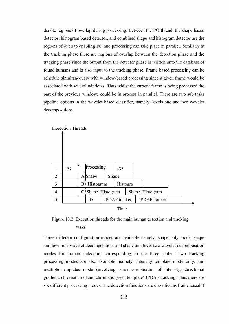
215
denote regions of overlap during processing. Between the I/O thread, the shape based
detector, histogram based detector, and combined shape and histogram detector are the
regions of overlap enabling I/O and processing can take place in parallel. Similarly at
the tracking phase there are regions of overlap between the detection phase and the
tracking phase since the output from the detector phase is written unto the database of
found humans and is also input to the tracking phase. Frame based processing can be
schedule simultaneously with window-based processing since a given frame would be
associated with several windows. Thus whilst the current frame is being processed the
part of the previous windows could be in process in parallel. There are two sub tasks
pipeline options in the wavelet-based classifier, namely, levels one and two wavelet
decompositions.
Three different configuration modes are available namely, shape only mode, shape
and level one wavelet decomposition, and shape and level two wavelet decomposition
modes for human detection, corresponding to the three tables. Two tracking
processing modes are also available, namely, intensity template mode only, and
multiple templates mode (involving some combination of intensity, directional
gradient, chromatic red and chromatic green template) JPDAF tracking. Thus there are
six different processing modes. The detection functions are classified as frame based if
Time
2
3
4
5
1
I/O
B Histogram Histogra
m
A
Shape
C Shape+Histogram
Shape
Shape+Histogram
JPDAF tracker D JPDAF tracker
I/O Processing
Execution Threads
Figure 10.2 Execution threads for the main human detection and tracking
tasks
Shape A
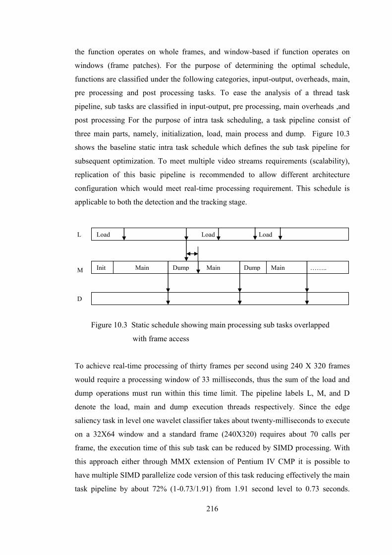
216
the function operates on whole frames, and window-based if function operates on
windows (frame patches). For the purpose of determining the optimal schedule,
functions are classified under the following categories, input-output, overheads, main,
pre processing and post processing tasks. To ease the analysis of a thread task
pipeline, sub tasks are classified in input-output, pre processing, main overheads ,and
post processing For the purpose of intra task scheduling, a task pipeline consist of
three main parts, namely, initialization, load, main process and dump. Figure 10.3
shows the baseline static intra task schedule which defines the sub task pipeline for
subsequent optimization. To meet multiple video streams requirements (scalability),
replication of this basic pipeline is recommended to allow different architecture
configuration which would meet real-time processing requirement. This schedule is
applicable to both the detection and the tracking stage.
To achieve real-time processing of thirty frames per second using 240 X 320 frames
would require a processing window of 33 milliseconds, thus the sum of the load and
dump operations must run within this time limit. The pipeline labels L, M, and D
denote the load, main and dump execution threads respectively. Since the edge
saliency task in level one wavelet classifier takes about twenty-milliseconds to execute
on a 32X64 window and a standard frame (240X320) requires about 70 calls per
frame, the execution time of this sub task can be reduced by SIMD processing. With
this approach either through MMX extension of Pentium IV CMP it is possible to
have multiple SIMD parallelize code version of this task reducing effectively the main
task pipeline by about 72% (1-0.73/1.91) from 1.91 second level to 0.73 seconds.
D
M Init Main Dump Main Dump Main ……..
Load Load Load L
Figure 10.3 Static schedule showing main processing sub tasks overlapped
with frame access
217
Wavelet analysis could also be reduced using a hardware accelerator (as discussed
earlier on to achieve higher throughput. Thus a standard frame could be split into fifty-
five sub windows (5X11 patches) for processing achieving an execution time of 2.5
milliseconds. Similar scheme could be applied to frame resizing. Thus by converting
the whole task from frame based processing to mixed mode (frame-based and
window-based processing [processing spatial neighbourhood windows]), execution
time could be reduced significantly. This applies to all the three human detection
pipelines. In the case of the JPDAF tracker (see tables 8.4 and 8.5) the main bottleneck
lies with motion estimation sub task. Since the current implementation is block-based
it would also benefit from chip level solution. The same analysis could be extended to
cover multiple video streams.
10.2.5 Implementation of 9/7 Biorthogonal Wavelet Transform on
Field Programmable Gate Array (FPGA)
Direct implementation of wavelet transform based on the filter bank approach is
inefficient due to the following: the large amount of intermediate points computation
required during an octave subband decomposition. More than half the computed
samples are not used, large memory is required to store all the computations of the
subband. Thus systems with limited memory would be constrained. There is also high
latency since all computations for a subband is completed before the next level is
computation is initiated. These factors limits real-time performance since it takes a
large amount of the execution time. This prompted the investigation into
programmable processor as an accelerator for this task, and hence the use of FPGA
which allows optimal scheduling with minimum storage requirement. For example, an
algorithm implemented in [Benkrid et al 2001] for a 256*256 image achieves real-
time performance at 75MHz. For a J-stage wavelet transform of N by M frame it has a
period of NM cycles. The algorithm implements row (column) wavelet transform
using RPA [Mallat 1989], and then implement the column (row) transform using
parallel filter, and line buffer, frame buffer, and specialised hardware units (1-K line
delay converter, shift register logic, and address generators) to accelerate
computations.
218
References
[Agga94] Aggarwal J. K. Q. Cai, W. Liao and B. Sabata. Articulated and Elastic
Non-Rigid Motion: A Review. Workshop on Motion of Non-Rigid and
Articulated Objects. Austin, TX, pp. 2 -14, 1994.
[Agga99] Aggarwal J. K, and Cai Q. Human Motion Analysis: A Review.
Computer Vision and Image Understanding, vol. 73, no. 3, pp. 428-440,
1999.
[Agui05] Aguilera J, Wildenauer H, Kampel M, Borg M, Thirde D, and
Ferryman J. Evaluation of Motion Segmentation Quality for
Aircraft Activity Surveillance. In Joint IEEE International Workshop on
Visual Surveillance and Performance Evaluation of Tracking and
Surveillance (VS-PETS), 2005.
[Akan92] Akansu A. N., and Haddad, R. A. Multiresolution Signal Decomposition.
Academic Press, Boston, 1992.
[Alba02] Albanesi M. G., Ferratti M, Dell’Olio. Effectiveness of VLIW
Architecture in a Data Parallel Image Application. 2002 IEEE
International Workshop on Computer Architectures for Machine
Perception (CAMP), pp. 172–183, April 2002.
[Ali01] Ali A., and Aggarwal J. Segmentation and Recognition of Continuous
Human Activity. In Proceedings of IEEE Workshop on Detection and
Recognition of Events In Video, pp. 28-35, 2001.
219
[Amda67] Amdahl G. M. Validity of the Single-Processor Approach to Achieving
Large Scale Computing Capabilities. In AFIPS Conference Proceedings,
vol. 30, Atlantic City, N. J, pp. 483 -485, 18-20th April 1967.
[Amoo88] Amoozegar Farid. Neural-Network-Based Target Tracking State-of-the-
Art-Survey. In Optical Engineer, vol. 37, issue 3, March 1988.
[Andr02] Andreopoulos Y, Munteanu A, Van Der Auwere G, Schelkens P, and
Cornelis J. Scalable Wavelet Video-Coding with In-Band Prediction-
Implementation and Experimental Results. In Proceedings of IEEE
International Conference on Image Processing, vol. 3, Rochester, NY,
pp.729-732, September 2002.
[Anto04] Antoine J-P, Murenzi R., Vandergheynst P., and Syed T. A. Two
Dimensional Wavelets and Their Relatives, Cambridge University,
Cambridge Press, 2004.
[Bao05] Bao P., Lei Zhang, and Xiaolin Wu. Canny Edge Detection Enhancement
by Scale Multiplication. In IEEE Transactions on Pattern
Analysis and Machine Intelligence, vol. 27, no.9, pp. 1485-1490, 2005.
[Belo01] Belongie S., Malik J., and Puzicha J., Matching Shapes. In Proceedings
of Eighth International Conference on Computer Vision, pp. 454-461,
2001.
[Blac99] Blackman S., and R. Popoli. Design and Analysis of Modern Tracking
Systems. Artech House, Norwell, MA, 1999.

220
[Bar72] Bar-Shalom Y., and Jaffer A. G. Adaptive Nonlinear Filtering for
Tracking with Measurements of Uncertain Origin. In Proc. of 11th IEEE
Conference on Decision and Control, pp. 243-247, 1972.
[Bar88] Bar-Shalom Y., and Fortmann T. Tracking and Data Association, volume
179 of Mathematics in Science and Engineering. Academic Press, 1988.
[Bar92] Bar-Shalom Yaakov. Multitarget/Multisensor Tracking: Applications
and Advances: Volume II. Artech House, 1992.
[Bash06] Bashir F., and Porikli F. Performance Evaluation of Object Detection
and Tracking Systems. In Proceedings of 9th IEEE International
Workshop on PETS, New York, pp. 7 -14, June 2006.
[Bast80] Bastiaan M. Gabor Expansion of a Signal into Gaussian Elementary
Signals. In Proceedings of IEEE, vol. 68, pp. 538-539, 1980.
[Benk01] Benkrid A., Crookes D., and Benkrid K. Design and Implementation of
2-D Biorthogonal Discrete Wavelet Transform on FPGA. In Proceedings
of the 9th Annual IEEE Symposium on Field-Programmable Custom
Computing Machines (FCCM’01), 2001.
[Benn88] Benner R. E., Gustafson J. L., and Montry G. R. Development and
Analysis of Scientific Application Programs on a 1024-Processor
Hypercube. Report no. SAND 88-0317, Sandia National Laboratories,
Feb. 1988.
[Bere02] Berekovic M., Hans-Joachim Stolberg, and Peter Pirsch. Multi-core
System-On-Chip Architecture for MPEG-4 Streaming Video. In IEEE
Transactions on Circuits and Systems for Video Technology, vol. 12, no.
221
8, pp. 688-699, 2002.
[Berg05] Berg Alexander C., Tamara L. Berg, and Jitendra Malik. Shape Matching
and Object Recognition using Low Distortion Correspondences. In Proc.
IEEE Computer Society Conference on Computer Vision and Pattern
Recognition (CVPR’05), 2005.
[Bhan86] Bhanu B. Automatic Target Recognition: State of the Art Survey. In
IEEE Trans. Aerospace and Electronic systems, AES-22(4): 364 -379,
1986.
[Bile05] Bileschi Stanley and Lior Wolf. A Unified System for Object Detection,
Texture Recognition, and Context Analysis Based on the Standard model
Feature Set. In Proc. British Machine Vision Conference, 2005.
[Bing02] Bing X., and C. Charoensak. Rapid FPGA Prototyping of Gabor-Wavelet
Transform for Applications in Motion Detection. In Proc. of 7th Intl.
Conference on Control, Automation, Robotics and Vision, pp. 1653–
1657, 2002.
[Birc98] Birchfield S. Elliptical Head Tracking Using Intensity Gradients and
Colour Histograms. In Proc. IEEE Conf. Computer Vision and Pattern
Recognition, pp. 232-237, 1998.
[Blac96] Black M, and Jepson, A. Eigentracking: Robust Matching and Tracking
of Articulated Objects Using a View-Based Representation. In European
Conference on Computer Vision, ECCV’ 96, Cambridge, 1996.

222
[Blum07] Blum, A. L., and Langley, P. Selection of Relevant Features and
Examples in Machine Learning. In Artificial Intelligence, vol. 97, no. 1-
2, pp. 245-271, 1997.
[Bobi96a] Bobick Aaron and James Davis.Real-Time Recognition of Activity
Using Temporal Templates. In IEEE Workshop on Applications of
Computer Vision, pp.39-42, December 1996.
[Bobi96b] Bobick Aaron and Davis, James. An Appearance-Based Representation
of Action. In Proceedings of IEEE International Conference on Pattern
Recognition and Machine Intelligence (ICPR’96), pp.307-312, 1996.
[Bogh05] Boghossian B., and J. Black. The Challenges of Robust 24/7 Video
Surveillance Systems. In IEE International Symposium on Imaging for
Crime Detection and Prevention, pp. 33-38, 2005,
[Bose92] Boser B. E., I. M. Guyon, and V. N. Vapnik. A Training Algorithm for
Optimal Margin Classifier. In Proceedings of 5th ACM Workshop on
Computational Learning Theory, Pittsburgh, PA, July 1992.
[Bou05] Bouaynaya N., and Schonfeld D. A Complete System for Head Tracking
using Motion-Based Particle Filter and Randomly Perturbed Active
Contour. Proceedings of SPIE Conference on Image and Video
Communications and Processing, vol. 5685, March 2005.
[Bregl97] Bregler C. Learning and Recognizing Human Dynamics in Video
Sequences. In Proc. IEEE Conference on Computer Vision and Pattern
Recognition, Puerto Rico, pp. 568-574, 1997.
223
[Brog00] Broggi A., Bertozzi M., Fascioli A., and Sechi, M. Shape-Based
Pedestrian Detection. In Proceedings of the IEEE Intelligent Vehicles
Symposium, pp. 215- 220, 2000.
[Brow05] Brown Lisa M., Senior Andrew W., Ying-li Tian, Jonathan Connell,
Arun Hampapur, Chiao-Fe Shu, Hans Merkl, Max Lu. Performance
Evaluation of Surveillance Systems Under Varying Conditions. In
proceedings of IEEE International Conference on Performance
Evaluation of Tracking and Surveillance, January 2005.
[Broo03] Brooks R. Model-Based Three-Dimensional Interpretations of Two-
Dimensional Images. In IEEE Transactions on Pattern Analysis and
Machine Intelligence, vol. 5, pp. 140-149, 2003.
[Burg96] Burges C. J. C. Simplified Support Decision Rules, 1996.
[Burt83] Burt, P. J., and Adelson E. H. The Laplacian Pyramid as a Compact
Image Code. In IEEE Transactions on Communications, vol. 31, no. 4,
pp. 532-540, 1983.
[Byrt88] Byrt Ted, Janet Bishop and John B. Carlin. Bias, Prevalence, and Kappa.
Journal of Clinical Epidemiology, Vol. 46, no. 5, pp. 423-429, 1988.
[Cann86] Canny J. A Computational Approach to Edge Detection. In IEEE
Transactions on Pattern Analysis and Machine Intelligence, vol. 8, pp.
79- 698, 1986.
[Cent85] Centor R. M, and Schwartz J. S. S. An Evaluation of Methods for
Estimating the Area Under the Receiver Operating Characteristics (ROC)
Curve. Medical Decision Making, vol. 5, no. 2, pp. 149-156, 1985.
[Cedr95] Cedras Claudette and Mubarak Shah. Motion-Based Recognition: A
Survey. In Image and Vision Computing, vol. 13, no. 2, pp. 129–155,
March 1995.
224
[Chen01] Chen Yunqiang, Yong Rui, and Thomas S. Huang. JPDAF Based HMM
for Real-Time Contour Tracking. In Proceedings of IEEE Computer
Society Conference on Computer Vision and Pattern Recognition, vol. 1,
pp. I543-I550, 2001.
[Chen06] Cheng Fang-Hsuan, Yu-Liang Chen. Real-Time Multiple Objects
Tracking and Identification Based On Discrete Wavelet Transform. In
Pattern Recognition, vol. 39, pp. 1126–1139, 2006.
[Chi04] Chi-Man Pun and Moon-Chen Lee. Extraction of Shift Invariant Wavelet
Features for Classifcation of Images with Different Sizes. In IEEE
Transactions on Pattern Analysis and Machine Intelligence, vol. 26, no.
9, pp. 1228- 1233, September 2004.
[Cody04] Cody Kwok, Dieter Fox, and Marian Meila. Real-Time Particle Filters.
In Proceedings of the IEEE, pp. 469-484, 2004.
[Coll00] Collins R. T., Lipton A. J., Kanade T. Fujiyoshi H, Duggins H, Tsin Y,
Tolliver T, Enomoto N, Hasegawa O, Burt P, Wixson L. A System for
Video Surveillance and Monitoring. Carnegie Mellon University,
Pittsburgh, PA, Tech Report, CMU-RI-TR-00-12, 2000.
[Coll01] Collins Robert T., Alan J. Lipton, Hironobu Fujiyoshi, Takeo Kanade.
Algorithms for Cooperative Multisensor Surveillance. In Proceedings of
the IEEE, vol. 89, no. 10, October 2001.
[Comm00] Commaniciu Dorin, Visvanathan Ramesh, and Peter Meer. Real-Time
Tracking of non-Rigid Objects using Mean Shift. In Proceedings of IEEE
Conference on Computer Vision and Pattern Recognition, vol. 2, pp. 13-
15, 2000.
225
[Comm02] Comanciu D., and Meer, P. Mean Shift: A Robust Approach Toward
Feature Space Analysis. In IEEE Transactions on Pattern Analysis and
Machine Intelligence, vol. 24, no. 5, pp. 603-619, 2002.
[Comm03] Commaniciu D., Ramesh V., and Meer, P. 2003. Kernel-Based Object
Tracking. IEEE Trans. on Pattern Analysis and Machine Intelligence,
vol. 25, pp. 564-575, 2003.
[Conx07] Conxia Dai, Yunfei Zheng, and Xin Li. Pedestrian Detection and
Tracking in Infrared Imagery using Shape and Appearance. In Computer
Vision and Image Understanding, vol. 106, Issue 2-3, pp. 288-299, May
2007.
[Cox93] Cox. I. J. A Review of Statistical Data Association Techniques for
Motion Correspondence. International Journal on Computer Vision, vol.
10, no.1, pp. 53-66, 1993.
[Cox96] Cox I. J., and Hingorani Sunita L. An Efficient Implementation of Reid’s
Multiple Hypothesis Tracking Algorithm and Its Evaluation for the
Purpose of Visual Tracking . In IEEE Transactions on Pattern Analysis
and Machine Intelligence, vol. 18, no. 2, pp. 138 -150, 1996.
[Curt05] Curtis-Maury Mathew, Tanping Wang, Christos Antonopoulos and
Dimitrios Nikolopoulos. Integrating Multiple Forms of Multithreaded
Execution on Multi-SMT Systems: A Study with Scientific Applications.
In Proceedings of the Second IEEE International Conference on
Quantitative Evaluation of Systems (QEST’05).
[Dala05] Dalal N., and Triggs B. Histogram of Oriented Gradients for Human
Detection. In Proceedings of IEEE Conference on Computer Vision and
Pattern Recognition, vol. 2, pp. 886-893, June 2005.
226
[Dani08] Danielsson Oscar, Steffan Carlsson, and Josephine Sullivan. Object
Detection Using Multi-Local Feature Manifolds. In Proceedings of
Digital Image Computing: Techniques and Applications (DICTA08), pp.
612-618, dec. 2008.
[Daub90] Daubechies I. The Wavelet Transform: Time-Frequency Localization
and Signal Analysis. In IEEE Transactions on Information Theory, vol.
36, no. 6, pp.961-1005, 1990.
[Daub91] Daubechies I. Ten lectures on Wavelets (CBMS-NSF Series Appl.
Math), SIAM, 1991.
[Daub88] Daubechies I. Orthonormal Bases of Compactly Supported Wavelets. In
Communication on Pure and Applied Mathematics, vol. XLI, pp. 909-
996, 1988.
[Dee08] Dee H. M., and Velastin S. A. How Close are We to Solving the
Problem of Automated Visual Surveillance? A Review of Real-World
Surveillance, Scientific Progress and Evaluative Mechanisms. Springer,
In Special Issue on Video Surveillance Research in Industry and
Academic (Machine Visions and Applications), No. 19 (5-6), pp. 329-
343, 2008.
[Dela99] Delamarre Quentin and Faugeras Olivier. 3D Articulated Models and
Multi-view Tracking With Silhouettes. In Proceedings of IEEE
International Conference on Computer Vision, vol. 2, pp. 716-721, 1999.
[Dela01] Delamarre Quentin, and Faugeras Olivier. 3D Articulated Models and
Multiview Tracking With Physical Forces. In Computer Vision and
Image Understanding, vol. 81, pp.328-357, 2001.
227
[Den01] Dengsheng Zhang and Guojun Lu. A Comparative Study on Shape
Retrieval Using Fourier Descriptors with Different Shape Signatures. In
International Conference onIntelligent Multimedia and Distance
Education (ICIMADE ’01), ND, 1-3 June 2001.
[Devi82] Devijver P.A and J. Kittler. Pattern Recognition. A Statistical Approach.
Prentice-Hall Inc, London, 1982.
[Dona06] Donatello Conte, Pasquale Foggia, Jean-Michell Jolion, Mario Vento. A
Graph-Based Multiresolution Algorithm for Tracking Objects in
Presence of Occlusion. In Pattern Recognition 39, pp. 562 -572, 2006.
[Dyan99] Dyan Peter. Unsupervised Learning. In MIT Encyclopedia of the
Cognitive Sciences, Edited by Wilson R. A, Keil, and Keil, F. 1999.
[Elga90] Elgammal A, Duraiswami R., Harwood D., and Davis L. Background
and Foreground Modelling Using Nonparametric Kernel Density
Estimation for Visual Surveillance. In Proceedings of IEEE, vol. 7, pp.
1151-1163, 1990.
[Ever10] Everingham Mark and Gool Luc Van. The PASCAL Visual Object
Classes (VOC) Challenge. International Journal on Computer Vision,
vol. 88, pp.303-338, 2010.
[Edwa98] Edwards G., Taylor C., and Cootes T. Interpreting Face Images Using
Active Appearance Model. In International Conference on Face and
gesture Recognition, pp. 300-305, 1998.
[Erk98] Erkel A. R., Van P. M., and T. Pattynama. Receiver Operating
Characteristics (ROC) analysis: Basic Principles and Applications in
Radiology. European Journal of Radiology, vol. 27, pp. 88-94, 1998.
228
[Enzw09] Enzweiler M and Gavrila M. Monocular Pedestrian Detection:
Survey and Experiments. IEEE Transaction on Pattern Analysis and
Machine Intelligence, vol. 31, no. 12, Dec. pp. 2179-2195, 2009.
[Fabb08] Fabbri R., Da F. Costa L., and Torreli Julio C. 2D Euclidean Distance
Transform Algorithms: A Comparative Survey. ACM Computing
Surveys, vol. 40, no. 1, article 2, 2008.
[Farr09] Farrugia Nicolas, Franck Mamalet, Sebastian Toux, Fan Yan and Michel
Paindavoine. Fast and Robust Face Detection on Parallel Optimized
Architecture on FPGA. In IEEE Transactions on Circuits and Systems
for Video Technology, vol. 19, no. 4, April 2009.
[Fazl09] Fazli S., Hamed Moradi Pour, and Hamed Bouzari. Multiple Object
Tracking Using improved GMM-Based Motion Segmentation. In
Proceedings of the 6th International Conference on Electrical
Engineering/Electronics, Computer Engineering, Telecommunications
and Information Technology (ECTI-CON 2009), Thailand, vol. 2,
pp.1130-1133, 2009.
[Fei04] Fei-Fei L., Fergus R., and Perona P. Learning Generative Visual Models
from Few Training Examples: An Incremental Bayesian Approach
Tested on 101 Object Categories. Proceedings of Computer Vision and
Pattern Recognition Workshop on Generative-Model Based on Vision,
2004.
[Fieg97] Fieguth P., and Terzopoulos D. Colour-Based Tracking of Heads and
Other Mobile Objects at Video Frame Rates. In Proceedings IEEE
Conference on Computer Vision and Pattern Recognition (CVPR), pp.
21-27, 1997.
229
[Flee92] Fleet D. J. Measurement of Image Velocity. Norwell, Massachusetts,
Kluwer, 1992.
[Flee91] Fleet D. J., and Adelson E. H. Design and Use of Steerable Filters. In
IEEE Transactions on Pattern Analysis and Machine Intelligence, vol.13,
pp. 891- 906, 1991.
[Flor02] Florian Radu. Named Entity Recognition as a House of Cards: Classifier
Stacking. In Proceedings of the 6th Conference on Natural Language
Learning, vol. 20, pp. 1-4, 2002.
[Food96] Foody G. M., and M. K. Arora. Incorporating Mixed Pixels in the
Training, Allocation, and Testing Stages of Supervised Classifications.
In Pattern Recognition Letters, vol. 17, pp. 1389-1398, 1996.
[Franc99] Francos A., and Porat M. Analysis and Synthesis of Multicomponent
Signals Using Positive Time-Frequency Distributions. In IEEE
Transactions on Signal Processing, vol. 47, no. 2, pp. 493- 504, 1999.
[Free91] Freeman William T., and Adelson Edward H. The Design and Use of
Steerable filters. In IEEE Transactions on Pattern Analysis and Machine
Intelligence, vol. 13, no. 9, pp. 891-906, 1991.
[Freu95] Freund Y., and Schapire R. A Decision-Theoretic Generalization of On-
Line Learning and Application to Boosting. Computational Learning
Theory, pp. 23-37, 1995.
[Frey00] Frey B. Filling in Scenes by Propagating Probabilities through layers into
Appearance Models. In Proc. IEEE Conference on Computer Vision and
Pattern Recognition, vol. 1, pp. 185-192, 2000.

230
[Gabr04] Gabriella Csurka, Christopher R. Dance, Lixin Fan, Jutta Williamsowski,
Cedric Bray. Visual Categorization with Bags of Keypoints. In the 8th
European Conference on Computer Vision-ECCV, 2004.
[Gavr96] Gavrila D. M., and Davis L. A. 3-D model-based Tracking of Humans in
Action: A Multi-view Approach. In Proc. IEEE Conference on Computer
Vision and Pattern Recognition, pp. 73-80, 1996.
[Gere98] Gerek, O., and E. Cetin. Linear/NonLinear Adaptive Polyphase Subband
Decomposition Structures for Compression. In IEEE International
Conference on Acoustic, Speech, and Signal Processing, vol. 3, pp.1345-
1348, 1998.
[Geve04] Gevers Theo and Harro Stokman. Robust Histogram Construction from
Color Invariants for Object Recognition. In IEEE Transactions on Pattern
Analysis and Machine Intelligence, vol. 26, no.1, pp.113- 118, January
2004.
[Give99] Givers T and A. W. M. Smeulders. Color Based Object Recognition. In
Pattern Recognition, vol. 32, no. 3, pp. 453-464, 1999.
[Gree94] Greenspan H., Belongie S., Goodman R., Perona P., Rakshit S., and
Anderson C. Over Complete Steerable Pyramid Filters and Rotation
Invariance. In IEEE Conference on Computer Vision and Pattern
Recognition (CVPR), pp. 222-228, 1994.
[Gunt00] Gunther Jager and Ursula Benz. “Measures of Classification Accuracy
Based on Fuzzy Similarity,” IEEE Transactions on Geoscience and

231
Remote Sensing, vol. 38, no.3, May 2000.
[Gunt00] Gunther Jager and Ursula Benz. Measures of Classification Accuracy
Based on Fuzzy Similarity. In IEEE Transactions on Geoscience and
Remote Sensing, vol. 38, no. 3, pp. 1462-1467, May 2000.
[Guoq00] Guoqiang Peter Zhang. Neural Networks for Classification: A Survey. In
IEEE Transactions on Systems, Man, and Cybernetics-Part C;
Applications and Reviews, vol. 30, no. 4, pp. 451- 462, November 2000.
[Hann01] Hanna M. T., and S. A. Mansoori. The Discrete Time Wavelet
Transform: Its Discrete Time Fourier Transform and its Filter Bank
Implementation. In IEEE Trans. Circuits Systems II: Analog and Digital
Signal Process. vol. 48 (2) pp. 180 -183, 2001.
[Harr88] Harris C., and Stephens M. A. Combined Corner and Edge Detector. In
4th Alvery Vision Conference, pp. 147-151, 1988.
[Hari00a] Haritaoglu I., David Harwood and Larry S. Davis. An Appearance-Based
Body Model for Multiple People Tracking. In Proceeding of
International Conference on Pattern Recognition, vol. 4, pp. 184 -187, 3-
7 Sept. 2000.
[Hari00b] Haritaoglu I., Harwood D., and Davis L. W4: Real-Time Surveillance
of People and Their Activities. In IEEE Transaction on Pattern Analysis
and Machine Intelligence, vol. 22, no. 8, pp. 809-830, 2000.

232
[Hast01] Hastie T., Robert Tibshirani, and Jerome Friedman. The Elements of
Statistical Learning (Springer Series in Statistics) pp. xvi+533. 2001.
[Hay99] Haykins S. Neural Networks: A Comprehensive Foundation. Prentice-
Hall International, 2nd Edition, 1999.
[Horn89] Hornik K. Multilayer Feedforward Networks are Universal operators. In
Neural Networks, vol. 2, 1989.
[Horp03] Horprasert T., Kim K., and Harwood D. Codebook-based Adaptive
Background Subtraction for Raw Compressed Videos and a Performance
Evaluation Methodology for Detection Algorithms. To be submitted in
European Conference on Computer Vision 2003.
[Huan08] Huang K., Liangsheng Wang, Tienniu Tan, and Steve Maybank. A Real-
Time Object Detecting and Tracking System for Outdoor Night
Surveillance. In Pattern Recognition vol .41,pp. 432-444, 2008.
[Hutt93] Huttenlocher D., Noh J., and Rucklidge W. Tracking Non rigid Objects
In Complex Scenes. In IEEE International Conference on Computer
Vision (ICCV), pp. 93-101, 1993.
[Huwe98] Huwer S. and Niemann H. 2-D Object Tracking Based on Projection-
Histograms. In Proceedings of the 5th European Conference on Computer
Vision, vol. 1, pp. 861-876, 1998.
[Isar98] Isard M., and Blake A. Condensation-Conditional Density Propagation
for Visual Tracking. In International Journal on Computer Vision, vol.
29, no. 1, pp. 5-28, 1998.
[Ferr06] IEEE Computer Society. Proceedings of the Ninth IEEE International
Workshop on Performance Evaluation of Tracking and Surveillance
233
(PETS 2006) Edited by J. M. Ferryman, 2006.
[Jav02] Javed O., and M. Shah. Tracking and Object Classification for
Automated Surveillance. In Proceedings European Conference on
Computer Vision, vol. 4, 2002.
[Jaggi95] Jaggi Seema, Willsky Allan, Karl W. Clem, Mallat Stephane. Multiscale
Geometric Feature Extraction and Object Recognition with Wavelets and
Morphology. In Proceedings of IEEE International Conference on Image
Processing, vol. 3, pp. 372-375, 1995.
[Jang00] Jang D. S., and H.-I. Choi. Active Models for Tracking of Moving
Objects. In Pattern Recognition, vol. 33, no. 7, pp.1135-1146, 2000.
[Jens95] Jensen K., and D. Anastassiou. Subpixles Edge Localization and Their
Interpolation of Still Images. In IEEE Transactions on Image Processing,
vol. 4, pp. 285-295, March 1995.
[Jeps03] Jepson Allan D., David J. Fleet, and Thomas F. El-Maraghi. Robust
Online Appearance Models for Visual Tracking. In IEEE Transactions
on Pattern Analysis and Machine Intelligence, vol. 25, no. 10, 2003.
[Jian06] Jian C., Jie Yang, YUE Zhou, Yingying Cui. Flexible Background
Mixture Models for Foreground Segmentation. In image and Vision
Computing, vol. 20, pp. 1-10, 2006.
[Jord04] Jordan R. A Survey of Techniques For Object Detection, Final project
Report), Department of computer Sciences, University of British
Columbia. 2004.
[Juri01] Jurie Frederic and Dhome Michael. A Simple and Efficient Template
Matching Algorithm. In Proceedings of 8th IEEE International
Conference on Computer Vision, 2001.
234
[Ju96] Ju S, M. Black, and Y. Yacob. Cardboard People: A Parameterized
Model of Articulated Motion. In Proc. IEEE Conference on Automatic
Face and Gesture Recognition, pp. 38-44, 1996.
[Kang04] Kang J, Cohen, I. and Medioni, G. Object Reacquisition using Geometric
Invariant Appearance Model. In International Conference on Pattern
Recognition (ICPR), pp. 759-762, 2004.
[Kara00] Karaulova I, A. P. M. Hall, and A. D. Marshall. A Hierarchical Model of
Dynamics for Tracking People with Single Video Camera. In Proc.
British Machine Vision Conference, pp. 262-352, 2000.
[Karl01] Karlson R., and F. Gustafsson. Monte Carlo Data Association for
Multiple Target Tracking. In IEEE Target Tracking: Algorithms and
Applications, Netherland, October 2001.
[Khot90] Khotanzad A., and J.–H. Lu. Classification of Invariant Image
Representation Using a Neural Network. In IEEE Transactions on
Acoustics, Speech, and Signal Processing, vol. 38, no. 6, pp.1028-1038,
June 1990.
[Kots07] Kotsiatis S. B. “Supervised Machine Learning: A Review of
Classification Techniques, Informatica vol. 31, 2007, pages 249-268.
[Kulk94] Kulkarni A. D. Artificial Neural Networks for Image Understanding.
VNR, New York, 1994.
[Kuhn55] Kuhn H. The Hungarian Method of Solving The Assignment Problem.
In Naval Research Logistics Quarterly, vol. 2, pp. 83-97, 1955.
[Lain95] Laine A. F., H. Fan, and W. Yang. Wavelets for Contrast Enhancement
of Digital Mammography. In IEEE Engineering in Medicine and
Biology Magazine, vol. 14, pp. 536-550, September 1995.
235
[Laks00] Lakshmi Aparna Ratan, W. Eric L. Grimson, and William M. Welle III.
Object Detection and Localization by Dynamic Template Warping. In
International Journal of Computer Vision, vol. 36, no. 2, pp. 131-147,
2000.
[Law03] Law N.F., and Siu. A Fast and Efficient Computational Structure for the
2D-Over-Complete Wavelet Transform. In IEEE International
Conference on Acoustic, Speech, and Signal Processing (ICASSP’03),
vol. 3, pp. II-309-II312, 2003.
[Lowe04] Lowe D. G. Distinctive Image Features from Scale Invariant Key Points.
In International Journal in Computer Vision, vol. 60, no. 2, November
2004.
[Lowe99] Lowe D. G. Object Recognition from Local Scale-Invariant Features. In
Proc. of the International Conference on Computer Vision, Corfu, 1999.
[Lee04] Lee D. J, P. Zhan, A. Thomas, R. Schoenberger. Shape-Based Human
Intrusion Detection. SPIE International Symposium on Defence and
Security, Visual Information Process XIII, vol. 5438, pp.81-91, Orlando,
Florida, USA, April 12-16, 2004.
[Lee02] Lee L., and W. Grimson. Gait Analysis for Recognition and
Classification. In Proceedings of International Conference on Automatic
Face and Gesture Recognition, pp. 155-162, 2002.
[Liew92] A. W. C. Liew, and N. F. Law. Reconstruction from 2D Wavelet
Transform Modulus Maxima using Projections. In IEE Proceedings on
236
Vision, Image and Signal Processing, vol. 147, pp. 710-732, 1992.
[Lin94] Lin Weisi. Parallel Realization of A Computer Vision System. IEEE
Region 10’s Ninth Annual International Conference. Theme: Frontiers
of Computer Technology (TENCON ’94), 1994.
[Lipt98] Lipton A. J, Fujiyoshi H, and Patil R. S. Moving Target Classification
and Tracking from Real-Time Video. In Proceedings of IEEE Workshop
on Applications of Computer Vision, pp. 8-14, 1998.
[Lipt99] Lipton A. J. Local Application of Optic flow to Analyze Rigid Versus
Non Rigid Motion. In Proc. International Conference on Computer
Vision Workshop Frame-Rate Vision, Corfu, Greece, 1999.
[Lowe91] Lowe D. G. Fitting Parameterized 3-D models to Images. In IEEE
Transactions on Pattern Analysis and Machine Intelligence, vol. 13, pp.
441-450, 1991.
[Mall89] Mallat S. G. Multifrequency Channel Decomposition of Images and
Wavelet Models. In IEEE Transactions on Acoustic, Speech, and Signal
Processing, vol. 37, pp. 2091-2110, 1989.
[Mall92] Mallet S., and S. Zhong. Characterization of Signals from Multiscale
Edges. In IEEE Transactions on Pattern Analysis and Machine
Intelligence, vol. 14, pp. 710-732, 1992.
[Mand99] Mandal M. K., and Aboulnasr T. Fast Wavelet Histogram Techniques for
Image Indexing. In Proceedings of IEEE Workshop on Content-Based
Access of image and Video Libraries, 1999.
237
[Mano06] Manohar Vassant, Boonstra Mathew, Korzhova Valentina, Padmanabhan
Soundarajan, Goldgof Dmitry and Kasturi Rangarchar. PETS vs. VACE
Evaluation Programs: A Comparative Study. Proceedings of the 9th IEEE
International Workshops on PETS. Edited by James M. Ferryman, New
York, June 18, 2006.
[Marc02] Marcenaro L, M. Ferrari, L. Marchesotti, and C. S. Regazzoni. Multiple
Object Tracking Under Heavy Occlusion using Kalman Filters Based on
Shape Matching. In Proceedings of IEEE International Conference on
Image Processing, vol. 3, pp. 341-344, 2002.
[Mar99] Marchand Eric, Bouthemy Patrick, Chaumette Francois, and Moreau
Valerie. Robust Real-Time Visual Tracking using a 2-D-3-D Model-
Based Approach. In Proceedings of the 7th IEEE International
Conference on Computer Vision. Vol. 1, pp. 262-268, 1999.
[Marr80] Marr D., and E. Hildreth. Theory of Edge Detection. Proceedings of the
Royal Society, London, vol. 207, pp. 187-217, 1980.
[Marr82] Marr D. Vision, San Francisco: W. H. Freeman, 1982.
[Mayb00] Maybank S. J., and T. N. Tan. Special Section on Visual Surveillance-
Introduction. In International Journal on Computer Vision, vol. 37, no.
2, pp. 173-174, 2000.

238
[Mcke00] Mckenna S., Jabri Z. Duric., A. Rosenfeld, and H. Wechsler. Tracking
Groups of People. In Computer Vision and Image Understanding, vol.
80, no. 1, pp. 42- 56, 2000.
[Meye95] Y. Meyer. Ondelettes et Operateurs, Tome I. Paris, Herrmann, 1990.
[Meye99] Meyer D, J. Psl, and H. Niemann. Gait Classification with Hidden
Markov Models for Trajectories of Body Parts Extracted by Mixture
Densities. In Proceedings British Machine Vision Conference, pp. 459-
468, 1999.
[Miko03] Mikolajczyk K., and Schmid, C. A Performance Evaluation of Local
Descriptors. In IEEE Conference on Computer Vision and Pattern
Recognition (CVPR), pp. 1615-1630, 2003.
[Mitt05] Mittelman Roni and Moshe Porat. A New Approach to Feature
Extraction for Wavelet-Based Texture Classification. In IEEE
International Conference on Image Processing (ICIP 2005), vol. 3, pp.
1128-1131, Sept. 2005.
[Moe01] Moeslund Thomas B., & Erik Granum. A Survey of Computer Vision-
Based Human Motion Capture. In Computer Vision and Image
Understanding vol. 81, pp. 231-268, 2001.
[Mog97] Moghadam B., and Pentland, A. Probabilistic Visual Learning for Object
Representation. In IEEE Transactions on Pattern Analysis and Machine
Intelligence, vol. 19, no. 7, pp. 696-710, 1997.
[More77] Morefield C. L. Application of 0-1 Integer programming to Multitarget
Tracking Problems. In IEEE Transactions on Automation Control (AC-
239
22(6), June 1977.
[Moud99] Moudgill Mayan, Pradip Bose and Jaime H. Moreno. Validation of
Turandot, a Fast Processor model for Microarchitecture Exploration. In
Proceedings of IEEE International Conference on Performance,
Computing and Communications Conference, February 1999.
[Mund06] Munder S., and D. M. Gavrila. An Experimental Study on Pedestrian
Classification. IEEE Transactions on Pattern Analysis and Machine
Intelligence, vol. 28, no. 11, pp. 1863 -1868, November 2006.
[Niyo94] Niyogi S. A., and E. H. Adelson. Analyzing and Recognizing Walking
Figures in XYT. In Proceedings of IEEE Conference on Computer
Vision and Pattern Recognition, pp. 469-474, 1994.
[Niyo99] Niyogi S. E., and E. H. Adelson. Analyzing and Recognizing Walking
Figures in XYT. In Proceedings of IEEE Conference on Computer
Vision and Pattern Recognition, pp, 469-474, 1999.
[Ober01] Oberti F., Elena Stringa, and Gianni Vernazza. Performance
Evaluation Criterion for Characterizing Video-Surveillance Systems. In
Real-Time Imaging, No. 7, pp. 457-471, 2001.
[Olso00] Olson C. Maximum-Likelihood Template Tracking. In Proc. IEEE
Conference on Computer Vision and Pattern Recognition , vol. 2, pp. 52-
57, 2000.
[Open02] The OpenMP Architecture Review Board. OpenMP C and C++
Application Program Interface,Second Edition,March 2002.
240
[Oren97] Oren M. C. Papageorgiou, P. Sinha, E. Osuna, and T. Poggio. Pedestrian
Detection using Wavelet Templates. In Proceedings of Computer Vision
and Pattern Recognition, pp. 193–99, 1997.
[Owec04] Owechko Yuri, Swarup Medasani, and Narayan Srinivass. Classifier
Swarms for Human Detection in Infrared Imagery. In Proceedings of
Conference on Computer Vision and Pattern Recognition Workshop
(CVPRW’04), vol. 8, pp. 125- 135, June 2004.
[Pain05] Painkras E., Charoensak Charayaphan. A VLSI Architecture for Gabor
Filtering in Face Processing Applications. In Proc. 2005 International
Symposium on Intelligent Signal Processing and Communication
Systems, pp. 437-440, 2005.
[Pais08] Paisitkriangkrai S., Shen S., Zhang J. Performance Evaluation of Local
Features in Human Classification and Detection. IET Computer Vision,
2008, vol. 2, no. 4, pp. 236-246.
[Papa99] Papageorgiou C., and Tomaso Pogio. A Pattern Classification Approach
to Dynamical Object Detection. In Proceedings of International
Conference on Computer Vision, Greece, pp. 1223 -1228, 1999.
[Papa98] Papageorgiou C., P. Michael Oren, and Tomaso Poggio. A General
Framework for Object Detection. In Sixth International Conference on
Computer Vision, vol. 2, pp. 1223 -228, 1999.
[Pete99] Peterfreund N. The PDAF Based Active Contour. In Proceedings of the
7th IEEE International Conference on Computer Vision,vol.1, pp. 227-
233, 1999.
241
[Plan01] Plankers R., and Pascal Fua. Articulated Soft Objects For Video-Based
Body Modeling. In Proceedings of the 8th IEEE International Conference
on Computer Vision, vol. 1, pp. 394-401, July 2001.
[Pogg89] Poggio T., and F. Girosi. Networks for Approximation and Learning. In
Proceedings of IEEE, vol. 78, no. 9, Sept. 1990.
[Pola94] Polana R., and Nelson R. Low Level Recognition of Human Motion. In
Proc. IEEE Workshop on Motion of Non Rigid and Articulated Objects.
Austin, TX, pp. 77-82, 1994.
[Pori05] Porikli F., and Tuzel Oncel. Multi-Kernel Object Tracking. In
Proceedings of IEEE International Conference on Multimedia and Expo,
Amsterdam, 2005.
[Poul96] Poularikas Alexander (Chief Editor). The Transforms and Applications
Handbook, CRC Press, and IEEE Press, (Electrical Engineering
Handbook Series), pp. 747-828, 1996.
[Pun03] Pun C. –M., and M. –C. Lee. Log-Polar Wavelet Energy Signatures for
Rotation and Scale Invariant Texture Classification. In IEEE
Transactions on Pattern Analysis and Machine Intelligence, vol. 25, no.
5, pp. 590-603, May 2003.
[Quan97] Quanq Minh Tieng, and W. W. Boles. Recognition of 2D Object
Contours using the Wavelet Transform Zero-Crossing Representation.
In IEEE Transactions on Pattern Analysis and Machine Intelligence, vol.
19, pp. 910-916, 1997.
[Rasm01] Rasmussen C., and Hager G. Probabilistic Data Association Methods for
Tracking Complex Visual Objects. In IEEE Transactions on Pattern
Analysis and Machine Intelligence, vol, 23, no. 6, pp.560-576, 2001,
1979.
242
[Reid79] Reid D. B. An Algorithm for Tracking Multiple Targets. In IEEE
Transaction on Automation and Control, vol. 24, no. 6, pp. 843-854,
1979.
[Ren03] Ren J., Astheimer P., and Feng D. Real-Time Moving Object Detection
under Complex Background. In Proceedings of 3rd IEEE International
Symposium on Image and Signal Processing and Analysis, pp. 662-667,
2003.
[Riou91] Rioul O., and M. Vetterli. Wavelets and Signal Processing. IEEE Signal
Processing Magazine, pp. 14-38, October 1991.
[Rohr94] Rohr K. Towards Model-Based Recognition of Human Movements In
Image Sequences. In Computer Vision, Graphics, and Image Processing:
Image Understanding, vol. 59, no. 1, pp. 94-115, 1994.
[Roge03] Roger L. Claypoole, Geoffrey M. Davis, Wim Sweldens, Richard G.
Baraniuk. Nonlinear Wavelet Transforms for Image Coding Via Lifting.
In IEEE Transactions on Image Processing, vol. 12, no. 12, December
2003.
[Rose05] Rosenberg C,, Herbert Martial, and Schneiderman Henry. Semi-
Supervised Self-Training of Object Detection Models. In 17th IEEE
Workshop on Computer Vision (WACV/MOTIONS ’05), vol. 1, 2005.
[Sang96] Sang-II Park, M. J. T. Smith and R. Murenzi. Multidimensional
Wavelets for Target Detection and Recognition. In SPIE International
Symposium on Aerospace/Defense Sensing and Controls, Orlando,
Florida, April 8-12, 1996.
[Sang04] Sang Min Yoon and Hyunwoo Kim. Real-Time Multiple People
Detection Using Skin Color, Motion and Appearance Information. In
International Workshop on Robot and Human Interactive
Communication, pages 331-334, 2004.
243
[Said96] Said A., and W. A. Pearlman. An image Multiresolution Representation
for Lossless Image Compression. In IEEE Transactions on Image
Processing, vol. 5, no. 9, pp. 1303-1310, 1996.
[Sar93] Sar-Sarraf H. Multiscale Wavelet Representation and Its Application to
Signal Classification. PhD Dissertation, University of Tennessee,
Knoxville, May 1993.
[Seni06] Senior Andrew, Hampapur Arun, Tian Ying_Li, Brown Lisa, Pankanti,
and Bole Ruud. Appearance Models for Occlusion Handling. In Image
and Vision Computing, vol. 20, pp. 1 -11, 2006.
[Scha02] Scharr M. Van Der, J. Ye, Y. Andreopoulos, and A. Munteanu. Fully
Scalable 3-D Overcomplete Wavelet Coding Using Adaptive Motion
Compensated Temporal Filtering. In ISO/IEC/JTC1/SC29/WG11,
M9037, MPEG, Shanghai, China, October 2002.
[Schn00] Schneiderman H., and Takeo Kanade. A Histogram-Based Method for
Detection of Faces and Cars. In Proceedings on International Conference
on Image Processing, vol. 3, pp. 504 -507, 2000.
[Schn04a] Schneiderman H. Learning a Restricted Bayesian Network for Object
Detection. In IEEE Conference on Computer Vision and Pattern
Recognition, IEEE June 2004.
[Schn04b] Schneiderman H. Feature-Centric Evaluation for Efficient Cascaded
Object Detection. In IEEE Conference on Computer Vision and Pattern
Recognition (CVPR), IEEE June, 2004.
[Serb04] Serby D., Kollier_Meier S., and Gool, L.V. Probabilistic Object
Tracking Using Multiple Features. In IEEE International Conference on
Pattern Recognition (ICPR), pp. 84-187, 2004.
244
[Seth87] Sethi I., and Jain, R. Finding Trajectories of Feature Points in a
Monocular Image Sequence. In IEEE Transactions on Pattern Analysis
and Machine Intelligence, vol. 9, no. 1, pp.56-73, 1987.
[Shaf98] Shafarenko I., Petrou M, and Kittler J. Histogram-Based Segmentation in
Perceptually Uniform Color Space. IEEE Transaction on Image
Processing, vol. 7, no. 9, pp.1354-1358, 1998.
[Shen99] Shen, D., and Ip H. H. S. Discriminative Wavelet Shape Descriptors for
Invariant Recognition of 2-D Pattern. In Pattern Recognition, vol. 32, pp.
151-165, 1999.
[Shin01] Shin M.C., D. B. Goldgof, K. W. Bowyer, and S. Nikiforou.
Comparison of Edge Detection Algorithms Using Structure from Motion
Task. In IEEE Transactions on Systems, Man, and Cybernetics-Part B:
Cybernetics, vol. 31, pp. 589-601, August 2001.
[Side00] Sidenbladh H., and M. Black. Stochastic Tracking of 3D Human Figures
using 2D Image Motion. In Proceedings of European Conference on
Computer Vision, Ireland, pp. 702-718, 2000.
[Sita94] Sitaraman, K. A. Ejnioui, N. Ranganathan. A Parallel Algorithm for
Object Recognition in Images. In Proc. IEEE International Workshop on
Computer Architectures for Machine Perception (CAMP), 2003.
[Smit05] Smith Kevin, Daniel Gatica-Perez, Jean-Marc Odobez, and Sileye Ba.
Evaluating MultiObject Tracking. Proceedings of the IEEE Computer
Society Conference on Computer Vision and Pattern Recognition
(CVPR’05) IEEE Press, 2005.
[Song 06] Song Bi, Amit K. Roy-Chowdhury, and N. Vaswani. Integrated Tracking
and Recognition of Human Activities in Shape Space. International
Journal in Computer Vision, Graphics and Image Processing, pp. 468–
245
479, 2006.
[Stau98] Stauffer Chris and Grimson W. E.L. Adaptive Background Mixture
Models for Real-Time Tracking. Proceedings of the IEEE Computer
Society Conference on Computer Vision and Pattern Recognition ’98.
IEEE Press, 1998.
[Steff98] Steffens J, E. Elagin, and H. Neven. Person Spotter-Fast and Robust
System for Human Detection, Tracking and Recognition. In Proceedings
of IEEE International Conference on Automatic Face and Gesture
Recognition, pp. 516- 521, 1998.
[Stra96] Strang G., and T. Nguyen. Wavelets and Filter Banks. Wellesley-
Cambridge Press, 1996.
[Stri97] Strickland Robin N, and Hee Il Hahn. Transform Methods For Object
Detection and Recovery. In IEEE Transactions on Image Processing, vol.
6, no. 5, pp. 724-735, May 1997.
[Stri00] Stringa E. Morphological Change Detection Algorithms for Surveillance
Applications. In Proceedings of British Machine Vision Conference,
pp.402- 412, 2000.
[Subr99] Subramanian K, S. S. Dlay and Rind F.C. Wavelet Transform for use in
Motion Detection and Tracking Application. In Proceedings of IEE
Conference on Image Processing and Its Applications. 1999.
[Swai91] Michael J. Swain and Ballard Dana H. Color Indexing. In International
Journal of Computer Vision, vol. 7, no. 1, pp. 11-32, 1991.
[Swel96] Sweldens W. The Lifting Scheme: A Custom-Design Construction of
Biorthogonal Wavelets. In Applied and Computational Harmonic
Analysis, vol. 3, no. 2, pp.186-200, 1996.
246
[Swel97] Sweldens W. The Lifting Scheme: A Construction of Second-Generation
Wavelets. In SIAM Journal of Mathematical Analysis, vol. 29, no. 2, pp.
511-546, 1997.
[Taka88] Takas Barnabas and Lev Sadovnik. Three-Dimensional Target
Recognition and Tracking using Neural Networks Trained on Optimal
Views. Optical Eng. vol.37, no.3, March pp. 819-828, 1988.
[Tang00] Tang Y.Y., Yang I. H., Liu J., and Ma H. Wavelet Theory and Its
Application to Pattern Recognition (Series in Machine Perception and
Artificial Intelligence, vol. 36). World Scientific, Singapore, 2000.
[Tan98] Tan T. N., G. D. Sullivan, and K. D. Baker. Model-Based Localization
and Recognition of Road vehicles. In International Journal in Computer
Vision vol. 29, no. 1, pp. 22–25, 1998.
[Tani87] Tanizaki H. Non Gaussian State Space Modelling of Non Stationary
Time Series. In Journal of American Statistical Association, vol. 82, pp.
1032-1063, 1987.
[Tax00] Tax David M. J., Breukelen Martin Van, Duin Robert P. W, and Kittler
Josef. Combining Multiple Classifiers by Averaging or by Multiplying.
In Pattern Recognition, vol. 33, pp. 1475-1485, 2000.
[Terz92] Terzopoulos D., and Szeliski R. Tracking with Kalman Snakes. In Active
Vision. Blake A and Yuille A (Editors). MIT press, 1992.
[Teol98] Teolis Anthony. Computational Signal Processing with Wavelets
Applied and Numerical Harmonic Analysis Series), Birkhauser Verlag
AV, 1998.
247
[Tian96] Tian T., and C. Tomasi. Comparison of Approaches to Egomotion
Computation. In Proc. IEEE Conf. Computer Vision and Pattern
Recognition, 1996.
[Tieu03] Tieu K., and Viola P. Boosting image Retrieval. International Journal of
Computer Vision, vol. 56, no. 1, pp17-36, 2003.
[Toma99] Tomaso Pogio and Papageorgiou Constantine. Trainable Pedestrian
Detection System. In Proceedings of IEEE Intelligent Vehicles
Symposium, Stuttgart, pp. 241 -246, 1999.
[Tou74] Tou J. T., and Gonzalez R. C. Pattern Recognition Principles. Addison-
Wesley, London, 1974.
[Tree68] Trees Van H. Classical Detection and Estimation Theory-Detection,
Estimation, and Modulation Theory. John Wiley & Sons, Inc, pp. 1946,
1968.
[Tull95] Tullsen Dean M., Susan J. Eggers, and Henry M. Levy. Simultaneous
Multithreading: Maximizing On-Chip Parallelism. In Proceedings of the
22nd Symposium on Computer Architecture, pp. 392-403, 1995.
[Unse95] Unser M. Texture Classification and Segmentation using Wavelet
Frames. In IEEE Transactions in Image Processing, vol. 4, no. 11, pp.
1549 –1560, 1995.
[Vapn82] Vapnik V. Estimation of Dependencies Based on Empirical Data.
Springer-Verlag, 1982.
[Veen01] Veenam C., Reinders M., and Backer E. Resolving Motion
Correspondence for Densely Moving Points. In IEEE Transaction on
Pattern Analysis and Machine Intelligence, vol. 23, pp. no.1, pp. 54-72,
2001.
248
[Viol01] Viola P., and Jones Michael. Robust Real-time Object Detection. In
International Workshop on Statistical and Computational Theories of
Vision-Modeling, Learning, Computing and Sampling, Vancouver,
Canada, July 13, 2001.
[Viol03] Viola P., Jones Michael, and D. Snow. Detecting Pedestrians Using
Patterns of Motion and Appearance. Proceedings of International
Conference on Computer Vision, pp. 734 -741, 2003.
[Viol03] Viola P., and Tieu K. Boosting image Retrieval. International Journal on
Computer Vision, vol. 56, 1, 17-36, 2003.
[Vish94] Vishwanath M. The Recursive Pyramid Algorithm for The Discrete
Wavelet Transform. In IEEE Transactions on signal Processing, vol. 42,
no. 3, pp. 673- 676, March 1994.
[Wact97] Wachter S., and H. H. Nagel. Tracking Persons in Monocular Image
Sequences. In Proceedings of IEEE Workshop on Non rigid and
Articulated Motion, pp. 2- 9, 1997.
[Wang95] Wang Yuping and Cai Yuanlong. Construction and Properties of B-
Spline Wavelet Filters for Multiscale Edge Detection. In Proceedings of
the IEEE International Conference on Image Processing, vol. 2, pp.
2145-2148, 1995.
[Wata85] Watanabe S. Pattern Recognition: Human and Mechanical. Wiley, New
York, 1985.
[Webb99] Webb Andrew (Defence Evaluation and Research Agency, UK).
Statistical Pattern Recognition, Arnold, London, 1999.
[Weim04] Weiming Hu, Tienu Tan, Liang Wang, and Steve Maybank. A Survey on
249
Visual Surveillance of Object Motion and Behaviors. In IEEE
Transactions on Systems, Man, and Cybernetics-Part C: Applications
and Reviews, vol. 34, no. 3, August 2004.
[Wei06] Wei Qui Bouaynaya, and Schofeld D. Automatic Multi-Head Detection
and Tracking Systems Using a Novel Detection-Based on Particle Filter
and Data Fusion. Proceedings of IEEE International Conference on
Acoustic Speech, and Signal Processing, vol. 2, 2005, pp.661-664.
[Wein06] Weinman Jerod J., Allen Hanson, and Erik Learned-Miller. Joint Feature
Selection for Object Detection and Recognition. University of
Massachusetts-Arhmerst Technical Report, 06-45, pp. 12, 2006.
[Wohl99] Wohler C., and Anlauf Joachim K. A Time Delay Neural Network
Algorithm for Estimating Image-Pattern Shape and Motion. In Image
and Vision Computing, vol. 17, pp. 281-294, 1999.
[Wre97] Wren, C. R., A. Azarbayejani, T. Darell, and A. P. Pentland. Pfinder:
Real-Time Tracking of the Human Body. In IEEE Transactions on
Pattern Analysis and Machine Intelligence vol. 19, pp. 780 -785, July
1997.
[Wu93] Wu Z., and Leahy R. An Optimal Graph Theoretic Approach to Data
Clustering: Theory and Applications to Image Segmentation. In IEEE
Transactions on Pattern Analysis and Machine Intelligence, vol. 11, pp.
101-1113, 1993.
[Wu05] Wu B., and Nevatia R. Detection of Multiple, Partially Occluded
Humans in Single Image by Bayesian Combination of Edgelet Part
250
Detectors. Proceedings on International Conference on Computer Vision
vol. I, pp. 90-97, 2005.
[Wu06] Wu Bo and Ram Nevatia. Tracking of Multiple, Partially Occluded
Humans based on Static Body Part Detection. In Proceedings of the
IEEE computer Society Conference on Computer Vision and Pattern
Recognition, Vol. 1, pp. 951- 958, 2006.
[Wu07] Wu Bo and Nevatia Ram. Detection and Tracking of Multiple Partially
Occluded Humans by Bayesian Combination of Edgelet Based Part
Detectors. In International Journal of Computer Vision, Springer
Science, USA, 2007.
[Wuns95] Wunsch P., and Laine A. F. Wavelet Descriptors for Multiresolution
Recognition of Handprinted Characters. In Pattern Recognition, vol. 28,
no. 8, pp.1237-1247, 1995.
[Xu92] Xu L., Kryzak A., and Suen C. V. Methods of Combining Multiple
Classifiers and their Applications in Handwriting Recognition. In IEEE
Transactions on Man and Cybernetics, vol. 22, no. 3, pp. 418-435, 1992.
[Yasu94] Yasun Xu, J. Weaver, Healy D, and Lu J. Wavelet Domain Transform
Filters: A Spatially Selective Noise Filtering Technique. In IEEE
Transaction on Image Processing, vol. 3, no. 6, pp. 747-758, Nov. 1994.
[Yeas04] Yeasin Mohammed, Ediz Polat, and Rajeev Sharma. A MultiObject
Tracking Framework for Interactive Multimedia Applications. In IEEE
Transactions on Multimedia, vol. 6, no. 3, June 2004.
[Yilm04] Yilmaz A., Li X., and Shah M. Contour-Based Object Tracking With
Occlusion Handling in Video Acquired Using Mobile Cameras. IEEE
Trans. Pattern Analysis and Machine Intelligence, vol. 26, no. 11, pp.
1531-1536, 2004.
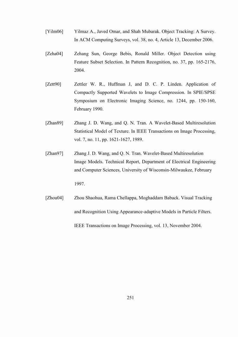
251
[Yilm06] Yilmaz A., Javed Omar, and Shah Mubarak. Object Tracking: A Survey.
In ACM Computing Surveys, vol. 38, no. 4, Article 13, December 2006.
[Zeha04] Zehang Sun, George Bebis, Ronald Miller. Object Detection using
Feature Subset Selection. In Pattern Recognition, no. 37, pp. 165-2176,
2004.
[Zett90] Zettler W. R., Huffman J, and D. C. P. Linden. Application of
Compactly Supported Wavelets to Image Compression. In SPIE/SPSE
Symposium on Electronic Imaging Science, no. 1244, pp. 150-160,
February 1990.
[Zhan89] Zhang J. D. Wang, and Q. N. Tran. A Wavelet-Based Multiresolution
Statistical Model of Texture. In IEEE Transactions on Image Processing,
vol. 7, no. 11, pp. 1621-1627, 1989.
[Zhan97] Zhang J. D. Wang, and Q. N. Tran. Wavelet-Based Multiresolution
Image Models. Technical Report, Department of Electrical Engineering
and Computer Sciences, University of Wisconsin-Milwaukee, February
1997.
[Zhou04] Zhou Shaohua, Rama Chellappa, Moghaddam Baback. Visual Tracking
and Recognition Using Appearance-adaptive Models in Particle Filters.
IEEE Transactions on Image Processing, vol. 13, November 2004.

252
Appendix A
Commercial Video Analytics Software Features
Company: CIEFFE, Location United Kingdom
Area of specialisation: video analytics software
Generic features:
Windows-based GUI
PTZ camera control through software
Multiview screen display
Site map overlaid with camera location
Live video acquisition and synchronised multi camera playback
Visualization of alarms and alarm management
Remote control and configuration
Parameter driven configuration of software (time, speed, size, etc)
Zone selection
Directional virtual tripwire
Text annotation of videos
End user features:
Motion detection
Motion-based recognition
Motion detection and tracking
Abnormal behaviour detection
Abandoned object detection
Removed object detection
Multiple object tracking
Image processing functions
Gamma correction, saturation, sharpening, blurring, contrast enhancement,
Equalization reversing, masking, negative and mosaic, and
compression/decompression

253
Configurability
Supports 1 to 30 cameras
Supports analogues cameras
Internet protocol based (IP)
Alarms
Camera occlusion alarms
Security
Embedded hardware architecture
Embedded operating systems
Integrated firewall for direct internet connection
Real-time processing
25 -30 frames per second
Company: Aimetis, Canada
Area of specialisation: video analytic software and Network video vendor
Generic features
Client server-based
Windows-based GUI
Video management
Remote live video recordings and playback
Automated control of PTZ camera
End user functionality
Motion tracking
Object classification
Object counting (humans/ cars)
Alarms
Sirens
Text to speech
Configurability
Supports up to 16 cameras
Array of storage device

254
Local hard disk, RAID, storage area network (SAN)
Company Name: Videoalert, Software vendor. Integrates with third party platform and
software sub system
End user functionality
Alerts
Event detection
Directional virtual tripwire
Object tracking/Counting
Abandoned objects
Monitoring traffic rule violation
Data statistics
Company Name: Vis-a-pix, Video analytics software vendor
Location: Germany
Generic functions
Zone definitions
Virtual tripwire
Camera locations overlaid with site map
Live video record/playback
Interactive monitoring of camera operations
Runs on windows environment
End user functionality
Alarms implemented as coloured events
People counting
Vehicle detection
Intrusion detection
Behaviour analysis
Anomalous behaviour detection
Works in indoor and outdoor environment
Configuration
Integrate with analogue and digital cameras;

255
Supports up to 8 cameras per personal computer
Accuracy
Detection rate of 90% in zone areas
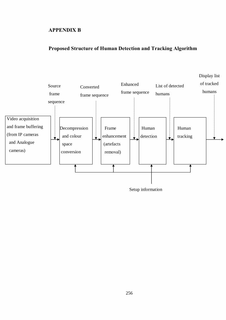
256
APPENDIX B
Proposed Structure of Human Detection and Tracking Algorithm
Source
frame
sequence
Enhanced
frame sequence
Display list
of tracked
humans
Converted
frame sequence
List of detected
humans
Setup information
Human
detection
Decompression
and colour
space
conversion
Video acquisition
and frame buffering
(from IP cameras
and Analogue
cameras)
Human
tracking
Frame
enhancement
(artefacts
removal)
257
Video acquisition and buffering
Array of M IP cameras
Source frame sequence Captured video signals
Video
signals
Video
signals
Array of N analogues cameras
Analogue
camera
N
IP camera
Frame
buffer
R
M
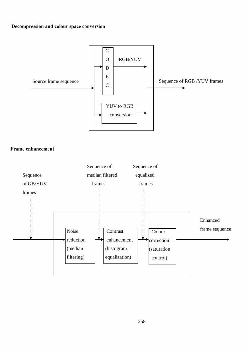
258
Frame enhancement
Decompression and colour space conversion
Noise
reduction
(median
filtering)
Contrast
enhancement
(histogram
equalization)
Colour
correction
(saturation
control)
Enhanced
frame sequence
Sequence
of GB/YUV
frames
Sequence of
equalized
frames
Sequence of
median filtered
frames
Source frame sequence
RGB/YUV
YUV to RGB
conversion
C
O
D
E
C
Sequence of RGB /YUV frames
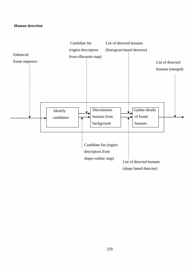
259
Human detection
List of detected humans
(shape based detector)
Candidate list (region
descriptors from
shape-outline map)
List of detected humans
(histogram based detector)
Enhanced
frame sequence
Update details
of found
humans
Discriminate
humans from
background
Identify
candidates
List of detected
humans (merged)
Candidate list
(region descriptors
from silhouette map)
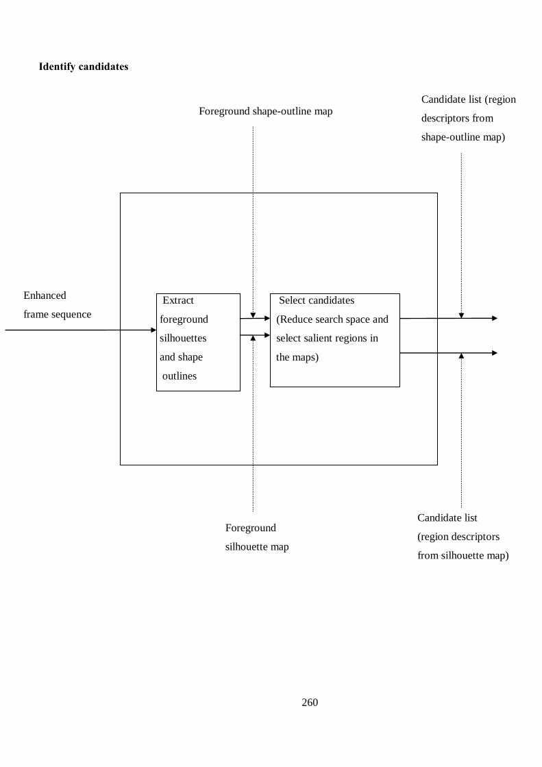
260
Identify candidates
Foreground
silhouette map
frame
Candidate list
(region descriptors
from silhouette map)
Foreground shape-outline map
frame
Enhanced
frame sequence
Candidate list (region
descriptors from
shape-outline map)
Extract
foreground
silhouettes
and shape
outlines
Select candidates
(Reduce search space and
select salient regions in
the maps)
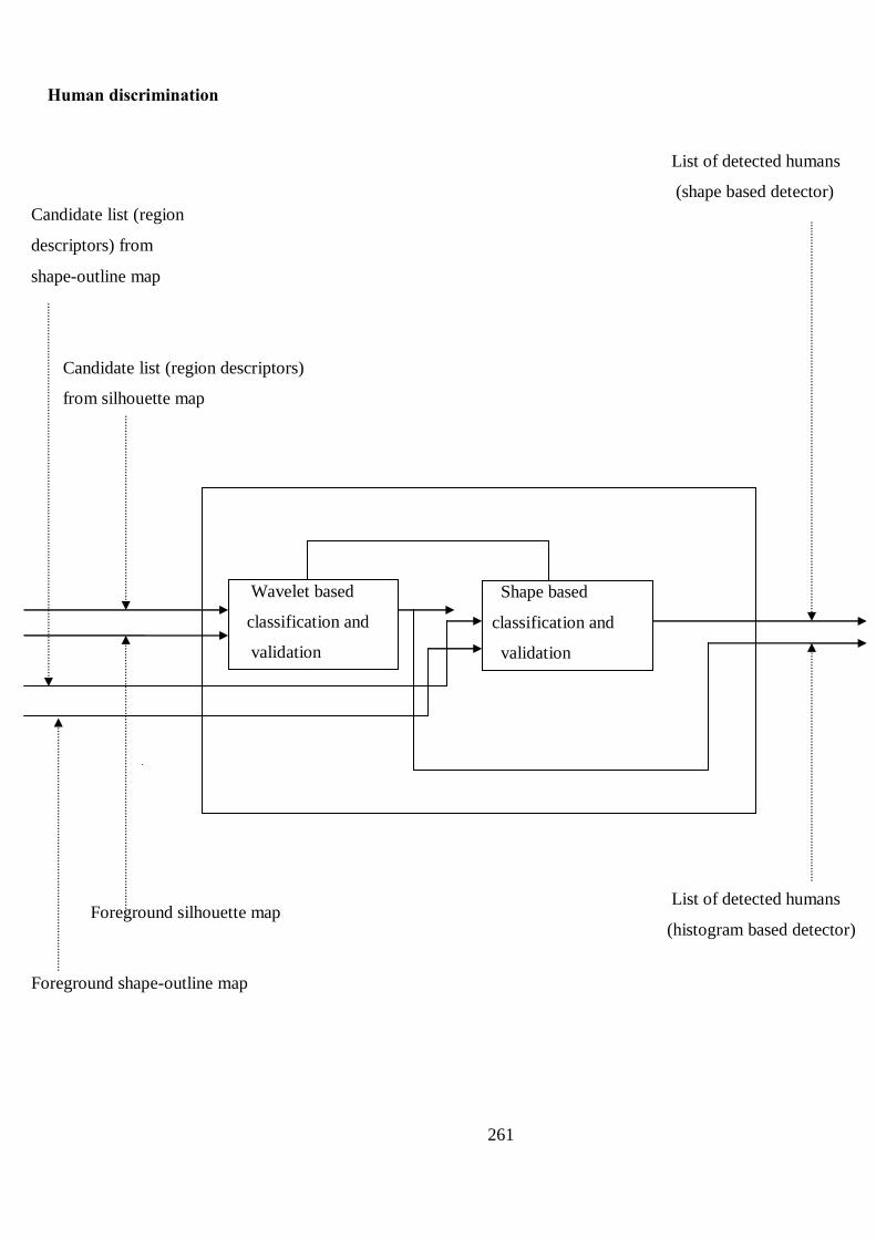
261
Human discrimination
List of detected humans
(shape based detector)
Shape based
classification and
validation
Wavelet based
classification and
validation
List of detected humans
(histogram based detector)
Foreground silhouette map
Foreground shape-outline map
Candidate list (region
descriptors) from
shape-outline map
Candidate list (region descriptors)
from silhouette map
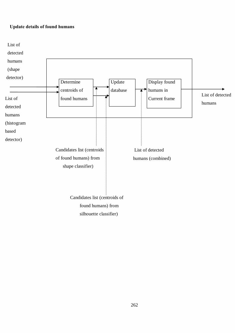
262
Update details of found humans
Candidates list (centroids
of found humans) from
shape classifier)
Candidates list (centroids of
found humans) from
silhouette classifier)
List of detected
humans (combined)
List of detected
humans
Display found
humans in
Current frame
Determine
centroids of
found humans
Update
database
List of
detected
humans
(histogram
based
detector)
List of
detected
humans
(shape
detector)
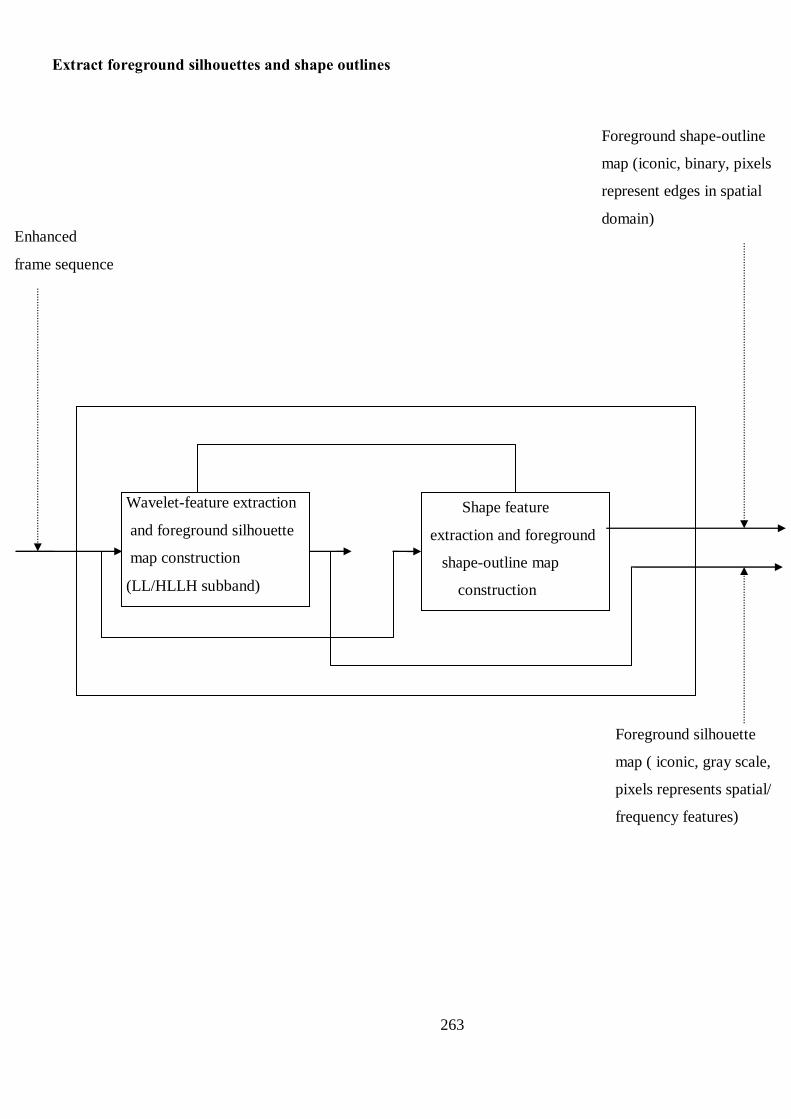
263
Extract foreground silhouettes and shape outlines
Foreground shape-outline
map (iconic, binary, pixels
represent edges in spatial
domain)
Shape feature
extraction and foreground
shape-outline map
construction
construction
Wavelet-feature extraction
and foreground silhouette
map construction
(LL/HLLH subband)
Enhanced
frame sequence
Foreground silhouette
map ( iconic, gray scale,
pixels represents spatial/
frequency features)
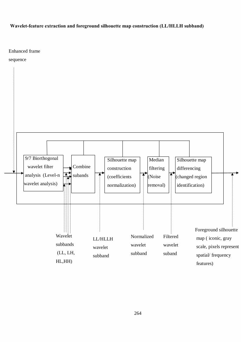
264
Wavelet-feature extraction and foreground silhouette map construction (LL/HLLH subband)
Normalized
wavelet
subband
Filtered
wavelet
suband
LL/HLLH
wavelet
subband
Enhanced frame
sequence
Wavelet
subbands
(LL, LH,
HL,HH)
Silhouette map
differencing
(changed region
identification)
Median
filtering
(Noise
removal)
Silhouette map
construction
(coefficients
normalization)
Combine
subands
9/7 Biorthogonal
wavelet filter
analysis (Level-n
wavelet analysis)
Foreground silhouette
map ( iconic, gray
scale, pixels represent
spatial/ frequency
features)
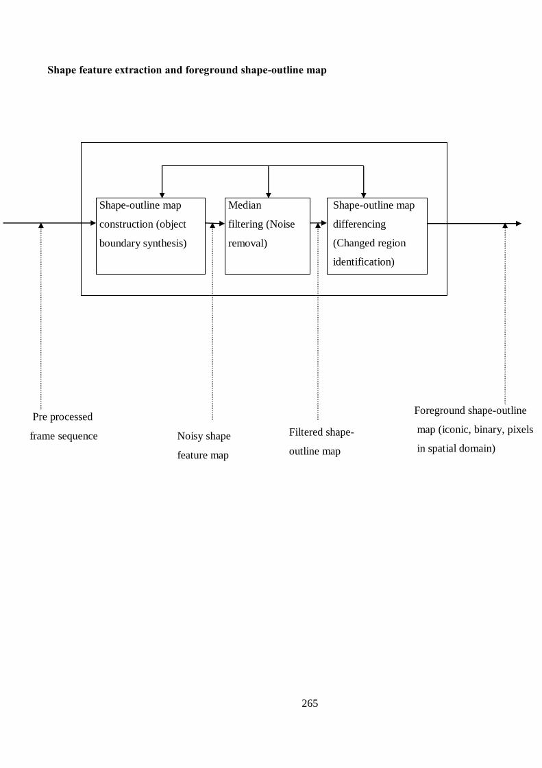
265
Shape feature extraction and foreground shape-outline map
construction
Filtered shape-
outline map
Noisy shape
feature map
Pre processed
frame sequence
Shape-outline map
construction (object
boundary synthesis)
Median
filtering (Noise
removal)
Shape-outline map
differencing
(Changed region
identification)
Foreground shape-outline
map (iconic, binary, pixels
in spatial domain)
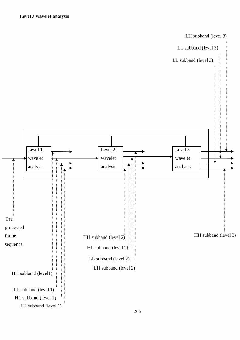
266
Level 3 wavelet analysis
HH subband (level 3)
HH subband (level1)
HL subband (level 1)
LL subband (level 1)
LH subband (level 1)
LH subband (level 3)
LL subband (level 3)
LL subband (level 3)
HH subband (level 2)
HL subband (level 2)
LL subband (level 2)
LH subband (level 2)
Level 2
wavelet
analysis
Pre
processed
frame
sequence
Level 3
wavelet
analysis
Level 1
wavelet
analysis
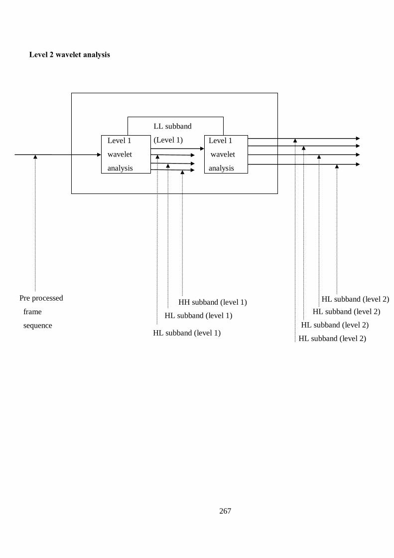
267
Level 2 wavelet analysis
Pre processed
frame
sequence
LL subband
(Level 1) Level 1
wavelet
analysis
Level 1
wavelet
analysis
HL subband (level 2)
HL subband (level 2)
HL subband (level 2)
HL subband (level 2)
HH subband (level 1)
HL subband (level 1)
HL subband (level 1)
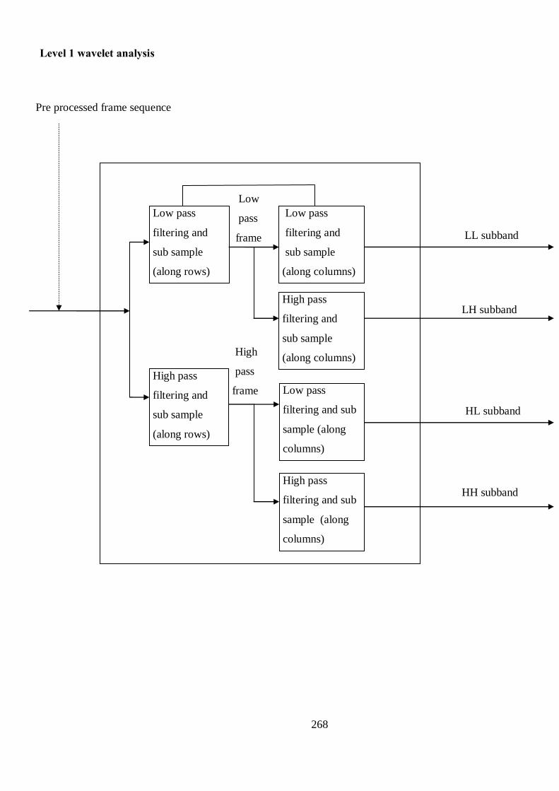
268
Level 1 wavelet analysis
Pre processed frame sequence
Low
pass
frame
Low pass
filtering and
sub sample
(along rows)
Low pass
filtering and
sub sample
(along columns)
LL subband
High
pass
frame
LH subband High pass
filtering and
sub sample
(along columns)
HL subband
Low pass
filtering and sub
sample (along
columns)
High pass
filtering and
sub sample
(along rows)
HH subband High pass
filtering and sub
sample (along
columns)
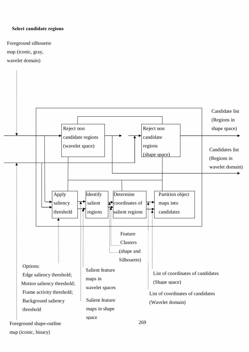
269
Select candidate regions
Foreground silhouette
map (iconic, gray,
wavelet domain)
Candidates list
(Regions in
wavelet domain)
Partition object
maps into
candidates
Foreground shape-outline
map (iconic, binary)
Salient feature
maps in
wavelet spaces
Salient feature
maps in shape
space
Options:
Edge saliency threshold;
Motion saliency threshold;
Frame activity threshold;
Background saliency
threshold
Apply
saliency
threshold
List of coordinates of candidates
(Shape space)
List of coordinates of candidates
(Wavelet domain)
Feature
Clusters
(shape and
Silhouette)
Determine
coordinates of
salient regions
Identify
salient
regions
Candidate list
(Regions in
shape space) Reject non
candidate regions
(wavelet space)
Reject non
candidate
regions
(shape space)
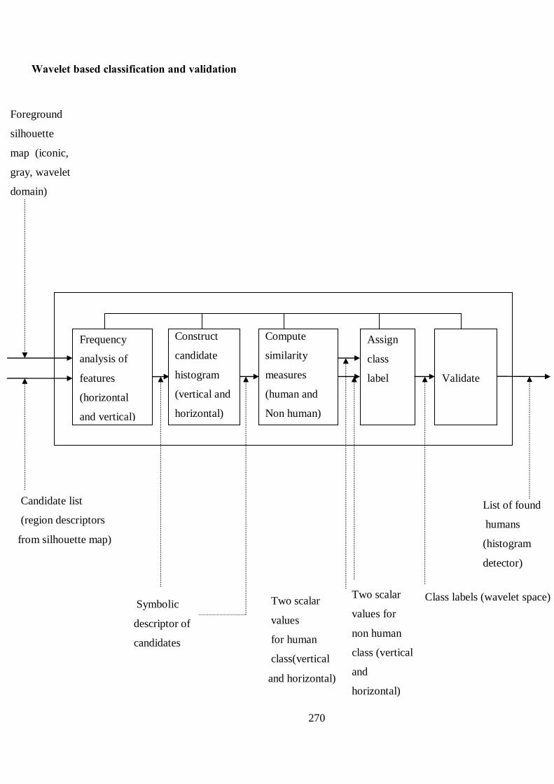
270
Wavelet based classification and validation
Foreground
silhouette
map (iconic,
gray, wavelet
domain)
Candidate list
(region descriptors
from silhouette map)
domain)
List of found
humans
(histogram
detector)
Two scalar
values
for human
class(vertical
and horizontal)
Two scalar
values for
non human
class (vertical
and
horizontal)
Symbolic
descriptor of
candidates
Compute
similarity
measures
(human and
Non human)
Construct
candidate
histogram
(vertical and
horizontal)
Assign
class
label
Frequency
analysis of
features
(horizontal
and vertical)
Validate
Class labels (wavelet space)
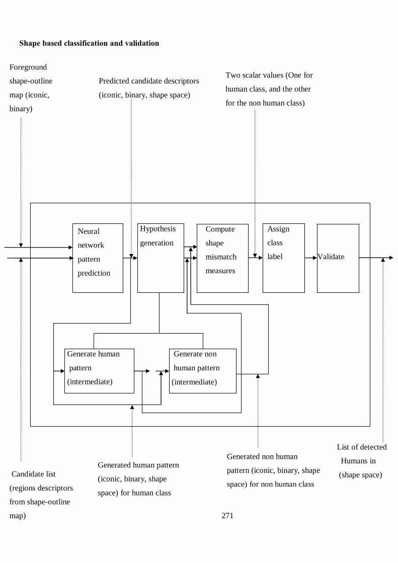
271
Shape based classification and validation
Two scalar values (One for
human class, and the other
for the non human class)
Predicted candidate descriptors
(iconic, binary, shape space)
Validate
Assign
class
label
Compute
shape
mismatch
measures
Generated non human
pattern (iconic, binary, shape
space) for non human class
List of detected
Humans in
(shape space)
Generate human
pattern
(intermediate)
Hypothesis
generation
Neural
network
pattern
prediction
Generate non
human pattern
(intermediate)
Foreground
shape-outline
map (iconic,
binary)
Generated human pattern
(iconic, binary, shape
space) for human class
Candidate list
(regions descriptors
from shape-outline
map)
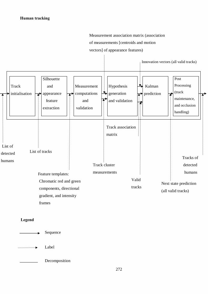
272
Legend
Sequence
Label
Decomposition
Human tracking
List of
detected
humans
Valid
tracks
Silhouette
and
appearance
feature
extraction
Measurement
computations
and
validation
Hypothesis
generation
and validation
Kalman
prediction
Post
Processing
(track
maintenance,
and occlusion
handling)
Track
initialisation
Tracks of
detected
humans
Track association
matrix
Track cluster
measurements
Next state prediction
(all valid tracks)
Measurement association matrix (association
of measurements [centroids and motion
vectors] of appearance features)
Innovation vectors (all valid tracks)
Feature templates:
Chromatic red and green
components, directional
gradient, and intensity
frames
List of tracks

273
Appendix C
Characteristics of Human Detection and Tracking:
Detection
Provides location and boundary information
Optionally may provide pose information
Tracking
Location, direction, and trajectory information (tracks)
Requires motion model, search strategy, and matching criteria
By optimization of a cost function
Taylor approximation
Kalman prediction
Stochastic sampling (Monte Carlo based Sampling, Particle filter)
Based on behaviour analysis
Hidden Markov Model (HMM)
Hierarchical principal component analysis (HPCA)
Space-time domain detection and tracking of humans
Human detection
Feature-based
Point-based feature
Scale invariant feature transform (SIFT feature)
Appearance-based features
Shape/silhouette/contour + appearance characteristics;
Density based representations
Dependence graph
View-based
Supervised classifier
Support vector machine
Feed forward neural network
Sub space methods

274
Principal Component Analysis classifier
Eigen space decomposition classifiers
Non Segmented
Classifier based
Boosting
Feed forward neural network
Support vector classifier
Self organizing feature map
Segmented
Foreground/background modelling
Frame differencing
Background subtraction
Gaussian mixture modelling
Mean shift clustering
Density estimation based on colour, texture, intensity, gradient
Optical flow
Spatio-temporal entropy+ morphological operations
Model-based recognition
2-D human model + motion model+ search strategy
3-D human model + motion model + search strategy
Motion-based recognition
Spatial-temporal motion analysis
Gait-based recognition
Human Tracking
Tracker types
Feature-based
Point-based Feature
Centroids + Kalman prediction
Kernel/Region-based
Geometric shape (rectangular, ellipse, circle)
Appearance-based (probability distribution based)
Multiview appearance

275
Support vector classifier
Feedforward classifier
Template based (Intensity, gradient, colour)
Silhouette-based
Contour-based
Shape-based+ interior representation
Wavelet Domain Detection and Tracking of Humans
Wavelet domain detection
Candidate features
Multiscale edge and motion
Multiscale phase information
Multiscale wavelets coefficients
Multiscale feature classification
Feedforward neural network
Self organizing feature maps
Wavelet-domain tracking
Template matching + motion model + search strategy
Model-based Detection and Tracking of Humans
Appearance-Based Detection and Tracking of Humans
Shape-Based Detection and Tracking of Humans
Edgelet based representation
Fourier based representation
Spline based representation
View based
Part based representation
Full human representation
Motion-Based Recognition and Tracking of Humans
2-D models
3-D model

276
Motion correspondence
Affine-based transform
Kernel or template based matching

Sequence: Hamilton2b.avi
FactorY:Scale factorY
FactorX:Scale factorX
F:Fixed background flag
Theshold1: Object Outline threshold
HE: Histogram equalization
SHAPE-BASED DETECTOR
TPR FPR FNR A B C D E Threshold1 HE F FactorX FactorY MaxNoObjects
61.4 3.06 38.6 24 32 48 64 1 5 0 1 2 2 8
54.52 3.66 45.48 24 32 48 64 1 5 0 1 1.5 1.5 8
48.13 3.77 51.87 24 64 48 128 1 5 0 1 1 1 8
60.07 4.53 39.93 16 50 32 100 1 5 0 1 2 2 8
56.09 5.74 43.91 16 40 32 80 1 5 0 1 0.2 0.2 8
56.09 6.45 43.91 16 32 32 64 1 5 0 1 2 2 8
52.47 8.14 47.53 17 50 32 100 1 5 0 1 1.5 1.5 8
25.33 8.37 74.67 24 64 48 128 1 5 0 1 0.5 0.5 8
63.33 8.75 36.67 12 50 24 100 1 5 0 1 2 2 8
49.82 9.19 50.18 16 40 32 80 1 5 0 1 0.2 0.2 8
39.19 10.62 63.81 16 32 32 64 1 5 0 1 1 1 8
39.45 11.33 60.55 16 50 32 100 1 5 0 1 1 1 8
45.36 12.11 54.64 12 50 24 100 1 5 0 1 1.5 1.5 8
59.11 13.54 40.89 16 40 32 80 1 5 0 1 0.2 0.2 8
32.45 15.62 67.55 12 50 24 100 1 5 0 1 1 1 8
51.26 16.72 48.73 16 40 32 80 1 5 0 1 0.2 0.2 8
50.78 22.06 49.22 16 40 32 80 1 5 0 1 0.2 0.2 8
45.82 24.49 54.16 16 40 32 80 1 5 0 1 0.2 0.2 8
Frames: 1000
D:Object height
B: Dbase_SpacingY
APPENDIX D 1.1
A: Dbase_spacingX Rows: 240
Columns: 320
C:Object width
Edge Saliency
E:Median filtering
277
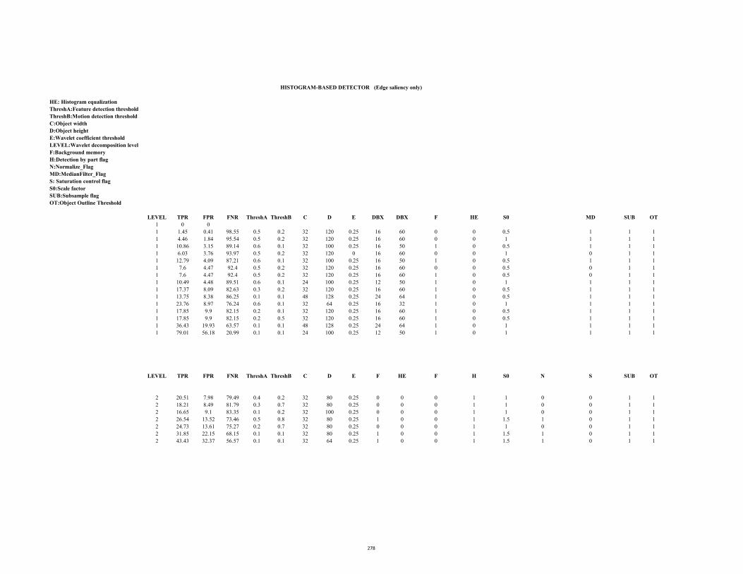
HE: Histogram equalization
F:Background memory
H:Detection by part flag
N:Normalize_Flag
MD:MedianFilter_Flag
S: Saturation control flag
S0:Scale factor
SUB:Subsample flag
OT:Object Outline Threshold
LEVEL TPR FPR FNR ThreshA ThreshB C D E DBX DBX F HE S0 MD SUB OT
1 0 0
1 1.45 0.41 98.55 0.5 0.2 32 120 0.25 16 60 0 0 0.5 1 1 1
1 4.46 1.84 95.54 0.5 0.2 32 120 0.25 16 60 0 0 1 1 1 1
1 10.86 3.15 89.14 0.6 0.1 32 100 0.25 16 50 1 0 0.5 1 1 1
1 6.03 3.76 93.97 0.5 0.2 32 120 0 16 60 0 0 1 0 1 1
1 12.79 4.09 87.21 0.6 0.1 32 100 0.25 16 50 1 0 0.5 1 1 1
1 7.6 4.47 92.4 0.5 0.2 32 120 0.25 16 60 0 0 0.5 0 1 1
1 7.6 4.47 92.4 0.5 0.2 32 120 0.25 16 60 1 0 0.5 0 1 1
1 10.49 4.48 89.51 0.6 0.1 24 100 0.25 12 50 1 0 1 1 1 1
1 17.37 8.09 82.63 0.3 0.2 32 120 0.25 16 60 1 0 0.5 1 1 1
1 13.75 8.38 86.25 0.1 0.1 48 128 0.25 24 64 1 0 0.5 1 1 1
1 23.76 8.97 76.24 0.6 0.1 32 64 0.25 16 32 1 0 1 1 1 1
1 17.85 9.9 82.15 0.2 0.1 32 120 0.25 16 60 1 0 0.5 1 1 1
1 17.85 9.9 82.15 0.2 0.5 32 120 0.25 16 60 1 0 0.5 1 1 1
1 36.43 19.93 63.57 0.1 0.1 48 128 0.25 24 64 1 0 1 1 1 1
1 79.01 56.18 20.99 0.1 0.1 24 100 0.25 12 50 1 0 1 1 1 1
LEVEL TPR FPR FNR ThreshA ThreshB C D E F HE F H S0 N S SUB OT
2 20.51 7.98 79.49 0.4 0.2 32 80 0.25 0 0 0 1 1 0 0 1 1
2 18.21 8.49 81.79 0.3 0.7 32 80 0.25 0 0 0 1 1 0 0 1 1
2 16.65 9.1 83.35 0.1 0.2 32 100 0.25 0 0 0 1 1 0 0 1 1
2 26.54 13.52 73.46 0.5 0.8 32 80 0.25 1 0 0 1 1.5 1 0 1 1
2 24.73 13.61 75.27 0.2 0.7 32 80 0.25 0 0 0 1 1 0 0 1 1
2 31.85 22.15 68.15 0.1 0.1 32 80 0.25 1 0 0 1 1.5 1 0 1 1
2 43.43 32.37 56.57 0.1 0.1 32 64 0.25 1 0 0 1 1.5 1 0 1 1
HISTOGRAM-BASED DETECTOR (Edge saliency only)
ThreshA:Feature detection threshold
C:Object width
E:Wavelet coefficient threshold
ThreshB:Motion detection threshold
D:Object height
LEVEL:Wavelet decomposition level
278
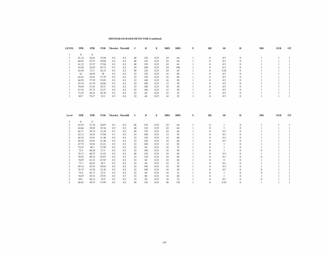
LEVEL TPR FPR FNR ThreshA ThreshB C D E DBX DBX F HE S0 H MD SUB OT
1 0 0
1 61.16 24.61 33.84 0.3 0.2 48 128 0.25 24 64 1 0 0.5 0 1 1 1
1 60.92 25.57 39.08 0.5 0.2 48 128 0.25 24 64 1 0 0.5 0 1 1 1
1 62.12 25.57 37.88 0.2 0.2 48 128 0.25 24 64 1 0 0.5 0 1 1 1
1 54.28 25.85 45.72 0.1 0.2 24 100 0.25 24 100 1 0 0.5 0 1 1 1
1 63.69 27.5 36.31 0.5 0.2 48 128 0.25 24 64 1 0 0.25 0 1 1 1
1 62 28.95 38 0.3 0.2 32 120 0.25 16 64 1 0 0.5 0 1 1 1
1 62.61 32.81 37.39 0.5 0.2 32 120 0.25 16 60 1 0 0.5 0 1 1 1
1 66.95 37.39 33.05 0.3 0.2 32 100 0.25 16 50 1 0 0.5 0 1 1 1
1 65.14 41.74 34.86 0.3 0.2 24 100 0.25 12 50 1 0 0.5 0 1 1 1
1 70.69 51.63 29.31 0.5 0.2 32 100 0.25 16 50 1 0 0.5 0 1 1 1
1 67.43 55.73 32.57 0.5 0.2 24 100 0.25 12 50 1 0 0.5 0 1 1 1
1 73.22 56.21 26.78 0.3 0.2 32 64 0.25 16 32 1 0 0.5 0 1 1 1
1 80.7 78.17 19.3 0.5 0.2 32 64 0.25 16 32 1 0 0.5 0 1 1 1
Level TPR FPR FNR ThreshA ThreshB C D E DBX DBX F HE S0 H MD SUB OT
2 0 0
2 63.93 27.76 36.07 0.3 0.2 48 128 0.25 24 64 1 0 1 0 1 1 1
2 64.66 29.83 35.34 0.5 0.2 48 128 0.25 24 64 1 0 1 0 1 1 1
2 66.71 30.75 33.29 0.5 0.2 48 128 0.25 24 64 1 0 0.5 0 1 1 1
2 62.12 34.53 37.88 0.1 0.2 24 100 0.25 12 50 1 0 0.5 0 1 1 1
2 68.52 35.81 31.48 0.5 0.4 32 120 0.25 16 60 1 0 0.5 0 1 1 1
2 68.52 35.81 31.48 0.5 0.2 32 120 0.25 16 60 1 0 0.5 0 1 1 1
2 67.79 39.81 32.21 0.5 0.2 24 100 0.25 12 50 1 0 1 0 1 1 1
2 72.01 40.1 27.99 0.5 0.2 32 64 0.25 16 32 1 0 1 0 1 1 1
2 72.5 40.24 27.5 0.5 0.2 32 100 0.25 16 50 1 0 1 0 0 1 1
2 78.17 40.27 21.83 0.3 0.2 48 128 0.25 24 64 1 0 0.5 0 1 1 1
2 70.93 40.32 29.07 0.5 0.2 32 120 0.25 16 60 1 0 0.5 0 0 1 1
2 74.07 41.51 25.93 0.5 0.4 32 80 0.25 16 40 1 0 0 0 1 1 1
2 73.7 42.63 26.3 0.5 0.2 32 64 0.25 16 32 1 0 0.5 0 1 1 1
2 69.12 42.91 30.64 0.5 0.2 24 100 0.25 12 50 1 0 0.5 0 1 1 1
2 76.72 43.26 23.28 0.5 0.2 32 100 0.25 16 50 1 0 0.5 0 0 1 1
2 76.6 45.17 23.4 0.5 0.2 32 64 0.25 16 32 1 0 1 0 0 1 1
2 74.07 45.51 25.93 0.5 0.7 32 80 0.25 16 40 1 0 1 0 1 1 1
2 80.1 48.13 19.9 0.5 0.2 32 64 0.25 16 32 1 0 0.5 0 0 1 1
2 86.01 49.57 13.99 0.3 0.2 48 128 0.25 48 128 1 0 0.25 0 1 1 1
HISTOGRAM-BASED DETECTOR (Combined)
279

Sequence:
A: Dbase_spacingX
B: Dbase_SpacingY
C:Object width
D:Objectheight
S0: Scale factor
F:Fixed background flag
MaxNoObjects=8
Theshold1: Object Outline threshold
TPR FPR FNR A B C D E Threshold1 HE F S0
53.56 4.51 46.44 16 32 32 64 1 5 0 1 2
61.88 3.65 38.12 16 50 32 100 1 5 0 1 2
Hamilton2b.avi
SHAPE BASED DETECTOR
APPENDIX D 1.2
Rows: 240
Columns: 320
Frames: 1000
MOTION SALIENCY
280
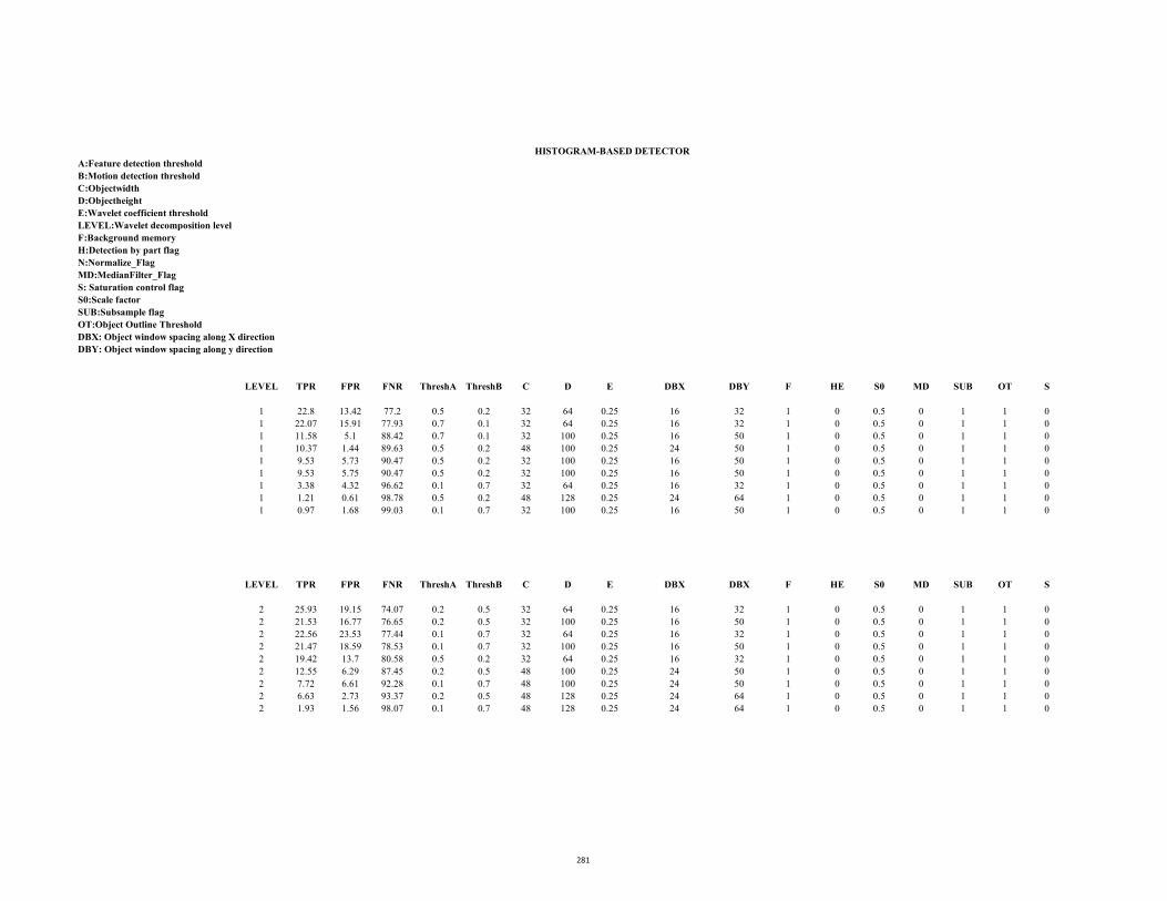
F:Background memory
H:Detection by part flag
N:Normalize_Flag
MD:MedianFilter_Flag
S: Saturation control flag
S0:Scale factor
SUB:Subsample flag
OT:Object Outline Threshold
DBX: Object window spacing along X direction
DBY: Object window spacing along y direction
LEVEL TPR FPR FNR ThreshA ThreshB C D E DBX DBY F HE S0 MD SUB OT S
1 22.8 13.42 77.2 0.5 0.2 32 64 0.25 16 32 1 0 0.5 0 1 1 0
1 22.07 15.91 77.93 0.7 0.1 32 64 0.25 16 32 1 0 0.5 0 1 1 0
1 11.58 5.1 88.42 0.7 0.1 32 100 0.25 16 50 1 0 0.5 0 1 1 0
1 10.37 1.44 89.63 0.5 0.2 48 100 0.25 24 50 1 0 0.5 0 1 1 0
1 9.53 5.73 90.47 0.5 0.2 32 100 0.25 16 50 1 0 0.5 0 1 1 0
1 9.53 5.75 90.47 0.5 0.2 32 100 0.25 16 50 1 0 0.5 0 1 1 0
1 3.38 4.32 96.62 0.1 0.7 32 64 0.25 16 32 1 0 0.5 0 1 1 0
1 1.21 0.61 98.78 0.5 0.2 48 128 0.25 24 64 1 0 0.5 0 1 1 0
1 0.97 1.68 99.03 0.1 0.7 32 100 0.25 16 50 1 0 0.5 0 1 1 0
LEVEL TPR FPR FNR ThreshA ThreshB C D E DBX DBX F HE S0 MD SUB OT S
2 25.93 19.15 74.07 0.2 0.5 32 64 0.25 16 32 1 0 0.5 0 1 1 0
2 21.53 16.77 76.65 0.2 0.5 32 100 0.25 16 50 1 0 0.5 0 1 1 0
2 22.56 23.53 77.44 0.1 0.7 32 64 0.25 16 32 1 0 0.5 0 1 1 0
2 21.47 18.59 78.53 0.1 0.7 32 100 0.25 16 50 1 0 0.5 0 1 1 0
2 19.42 13.7 80.58 0.5 0.2 32 64 0.25 16 32 1 0 0.5 0 1 1 0
2 12.55 6.29 87.45 0.2 0.5 48 100 0.25 24 50 1 0 0.5 0 1 1 0
2 7.72 6.61 92.28 0.1 0.7 48 100 0.25 24 50 1 0 0.5 0 1 1 0
2 6.63 2.73 93.37 0.2 0.5 48 128 0.25 24 64 1 0 0.5 0 1 1 0
2 1.93 1.56 98.07 0.1 0.7 48 128 0.25 24 64 1 0 0.5 0 1 1 0
LEVEL:Wavelet decomposition level
E:Wavelet coefficient threshold
B:Motion detection threshold
HISTOGRAM-BASED DETECTOR
C:Objectwidth
A:Feature detection threshold
D:Objectheight
281
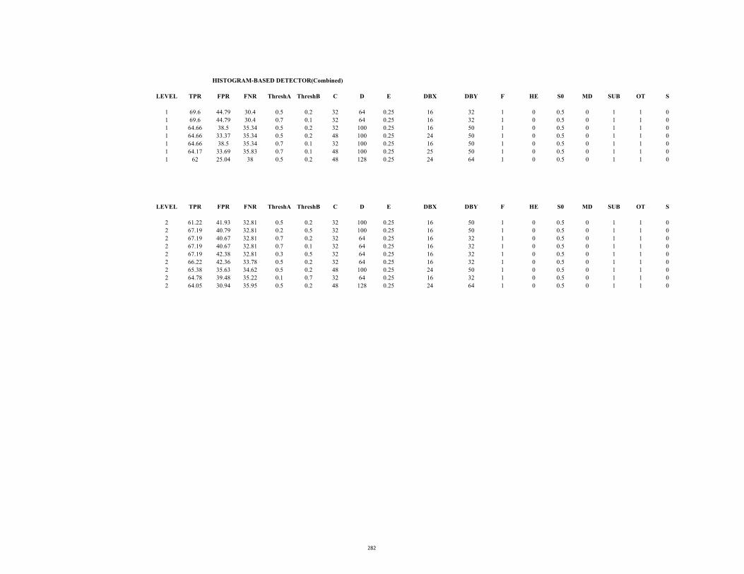
LEVEL TPR FPR FNR ThreshA ThreshB C D E DBX DBY F HE S0 MD SUB OT S
1 69.6 44.79 30.4 0.5 0.2 32 64 0.25 16 32 1 0 0.5 0 1 1 0
1 69.6 44.79 30.4 0.7 0.1 32 64 0.25 16 32 1 0 0.5 0 1 1 0
1 64.66 38.5 35.34 0.5 0.2 32 100 0.25 16 50 1 0 0.5 0 1 1 0
1 64.66 33.37 35.34 0.5 0.2 48 100 0.25 24 50 1 0 0.5 0 1 1 0
1 64.66 38.5 35.34 0.7 0.1 32 100 0.25 16 50 1 0 0.5 0 1 1 0
1 64.17 33.69 35.83 0.7 0.1 48 100 0.25 25 50 1 0 0.5 0 1 1 0
1 62 25.04 38 0.5 0.2 48 128 0.25 24 64 1 0 0.5 0 1 1 0
LEVEL TPR FPR FNR ThreshA ThreshB C D E DBX DBY F HE S0 MD SUB OT S
2 61.22 41.93 32.81 0.5 0.2 32 100 0.25 16 50 1 0 0.5 0 1 1 0
2 67.19 40.79 32.81 0.2 0.5 32 100 0.25 16 50 1 0 0.5 0 1 1 0
2 67.19 40.67 32.81 0.7 0.2 32 64 0.25 16 32 1 0 0.5 0 1 1 0
2 67.19 40.67 32.81 0.7 0.1 32 64 0.25 16 32 1 0 0.5 0 1 1 0
2 67.19 42.38 32.81 0.3 0.5 32 64 0.25 16 32 1 0 0.5 0 1 1 0
2 66.22 42.36 33.78 0.5 0.2 32 64 0.25 16 32 1 0 0.5 0 1 1 0
2 65.38 35.63 34.62 0.5 0.2 48 100 0.25 24 50 1 0 0.5 0 1 1 0
2 64.78 39.48 35.22 0.1 0.7 32 64 0.25 16 32 1 0 0.5 0 1 1 0
2 64.05 30.94 35.95 0.5 0.2 48 128 0.25 24 64 1 0 0.5 0 1 1 0
HISTOGRAM-BASED DETECTOR(Combined)
282

Sequence: Stc_t1_c_3.avi
A: Dbase_spacingX
B: Dbase_SpacingY
C:Object width
D:Object height
E:MedianFlag
TPR:True positive rate
FPR:False positive rate
FNR:False negative rate
HE:Histogram equalization
FactorY: Scale factorY
FactorX: Scale factorX
F:Fixed background flag
Theshold1: Object Outline threshold
HE:Histogram equalization
TPR FPR FNR A B C D E THRESHOLD1 HE F FactorX FactorY MaxNoObject
67.04 1.41 32.96 16 50 32 100 1 15 0 1 0.2 8 8
64.15 2.11 38.85 24 50 48 100 1 15 0 1 2 2 8
74.66 2.63 25.34 16 50 32 100 1 15 0 1 0.2 8 8
62.36 2.75 37.64 16 50 32 100 1 15 0 1 0.2 0.2 8
65.13 2.81 34.87 16 50 32 100 1 15 0 1 0.2 0.2 8
83.95 3.36 16.05 32 64 48 128 1 15 0 1 0.25 0.25 8
81.43 4.94 18.57 32 64 48 128 1 15 0 1 0.5 0.5 8
40.92 4.95 59.08 25 50 48 128 1 15 0 1 1 1 7
60.82 4.98 39.18 16 50 32 100 1 15 0 1 0.2 0.2 8
39.97 5.77 60.23 25 50 56 128 1 15 0 1 1 1 7
37.74 5.77 62.26 32 64 32 90 1 15 0 1 1 1 7
75.28 6.24 24.72 32 64 48 128 1 15 0 1 1 1 7
39 6.99 61 25 50 64 128 1 15 0 1 1 1 7
77.06 7.08 22.94 32 64 48 128 1 15 0 1 1 1 7
46.3 8.54 53.7 32 64 48 128 1 15 0 1 1 1 7
38.08 12.6 61.92 32 64 64 128 1 15 0 1 1 1 7
40.42 13.69 59.58 25 50 56 128 1 15 0 1 1 1 7
21.34 26.34 78.66 32 64 48 128 1 15 0 1 0.5 0.5 7
Nslice: 3021
APPENDIX D 2.1
(EDGE SALIENCY)
Nrows: 420
*, and **: Are used in combination with other parameters from histogram based classifier to generate combined classifier analysis
Ncols: 560
SHAPE-BASED DETECTOR
283
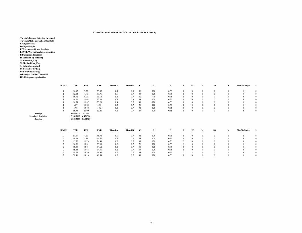
F:Background memory
H:Detection by part flag
N:Normalize_Flag
M:MedianFilter_Flag
S: Saturation control
S0:Second order flag
SUB:Subsample flag
OT:Object Outline Threshold
HE:Histogram equalization
LEVEL TPR FPR FNR ThreshA ThreshB C D E F HE M S0 N MaxNoObject S
1 66.97 7.22 33.03 0.4 0.3 48 128 0.35 1 0 0 0 0 8 0
1 62.24 7.89 37.76 0.6 0.7 48 128 0.35 1 0 0 0 0 8 0
1 68.82 8.99 31.18 0.4 0.7 32 64 0.35 1 0 0 0 0 8 0
1 66.91 11.02 33.09 0.4 0.3 48 128 0.35 1 0 0 0 0 8 0
1 66.79 11.07 33.21 0.4 0.7 48 128 0.35 1 0 0 0 0 8 0
1 64.7 11.82 35.3 0.2 0.7 56 128 0.35 1 0 0 0 0 8 0
1 69.8 14.88 30.2 0.2 0.7 48 128 0.35 1 0 0 0 0 8 0
1 66.54 20.99 33.46 0.1 0.7 64 128 0.35 1 0 0 0 0 8 0
Average 66.59625 11.735
Standard deviation 2.3317862 4.459516
Baseline 68.212066 14.82523
LEVEL TPR FPR FNR ThreshA ThreshB C D E F HE M S0 N MaxNoObject S
2 51.29 4.89 48.71 0.6 0.7 48 128 0.35 1 0 0 0 0 8 0
2 58.24 5.33 41.76 0.4 0.7 48 128 0.35 1 0 0 0 0 8 0
2 65.56 11.73 34.44 0.2 0.7 48 128 0.35 0 0 0 0 0 8 0
2 66.36 13.01 33.64 0.2 0.7 56 128 0.35 0 0 0 0 0 8 0
2 65.38 14.81 34.62 0.2 0.7 56 128 0.35 1 0 0 0 0 8 0
2 65.44 15.66 34.56 0.1 0.7 64 128 0.35 1 0 0 0 0 8 0
2 60.15 15.76 39.85 0.2 0.7 48 128 0.35 0 1 1 0 0 8 0
2 59.41 18.19 40.59 0.2 0.7 48 128 0.35 1 0 0 0 0 8 0
ThreshA:Feature detection threshold
E:Wavelet coefficient threshold
D:Object height
C:Object width
ThreshB:Motion detection threshold
LEVEL:Wavelet level decomposition
HISTOGRAM-BASED DETECTOR (EDGE SALIENCY ONLY)
284
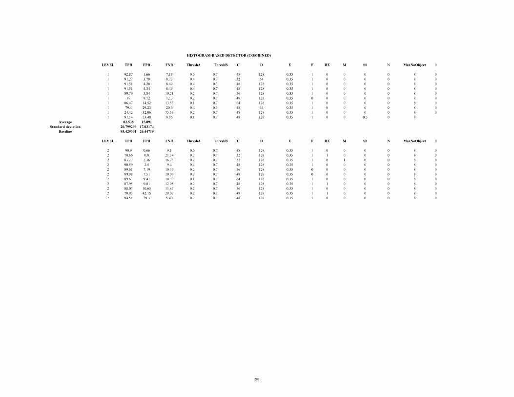
LEVEL TPR FPR FNR ThreshA ThreshB C D E F HE M S0 N MaxNoObject 0
1 92.87 1.66 7.13 0.6 0.7 48 128 0.35 1 0 0 0 0 8 0
1 91.27 3.78 8.73 0.4 0.7 32 64 0.35 1 0 0 0 0 8 0
1 91.51 4.28 8.49 0.4 0.3 48 128 0.35 1 0 0 0 0 8 0
1 91.51 4.34 8.49 0.4 0.7 48 128 0.35 1 0 0 0 0 8 0
1 89.79 5.84 10.21 0.2 0.7 56 128 0.35 1 0 0 0 0 8 0
1 87 9.72 12.3 0.2 0.7 48 128 0.35 0 0 0 0 0 8 0
1 86.47 14.52 13.53 0.1 0.7 64 128 0.35 1 0 0 0 0 8 0
1 79.4 29.23 20.6 0.4 0.3 48 64 0.35 1 0 0 0 0 8 0
1 24.42 32.06 75.58 0.2 0.7 48 128 0.35 1 0 0 0 0 8 0
1 91.14 53.48 8.86 0.1 0.7 48 128 0.35 1 0 0 0.5 0 8
Average 82.538 15.891
Standard deviation 20.799296 17.03174
Baseline 95.429301 26.44719
LEVEL TPR FPR FNR ThreshA ThreshB C D E F HE M S0 N MaxNoObject 0
2 90.9 0.66 9.1 0.6 0.7 48 128 0.35 1 0 0 0 0 8 0
2 78.66 0.8 21.34 0.2 0.7 32 128 0.35 1 1 0 0 0 8 0
2 83.27 2.36 16.73 0.2 0.7 32 128 0.35 1 0 1 0 0 8 0
2 90.59 2.5 9.4 0.4 0.7 48 128 0.35 1 0 0 0 0 8 0
2 89.61 7.19 10.39 0.2 0.7 56 128 0.35 0 0 0 0 0 8 0
2 89.98 7.51 10.03 0.2 0.7 48 128 0.35 0 0 0 0 0 8 0
2 89.67 9.41 10.33 0.1 0.7 64 128 0.35 1 0 0 0 0 8 0
2 87.95 9.81 12.05 0.2 0.7 48 128 0.35 1 1 0 0 0 8 0
2 88.03 10.65 11.87 0.2 0.7 56 128 0.35 1 0 0 0 0 8 0
2 70.93 42.15 29.07 0.2 0.7 48 128 0.35 1 1 0 0 0 8 0
2 94.51 79.3 5.49 0.2 0.7 48 128 0.35 1 0 0 0 0 8 0
HISTOGRAM-BASED DETECTOR (COMBINED)
285
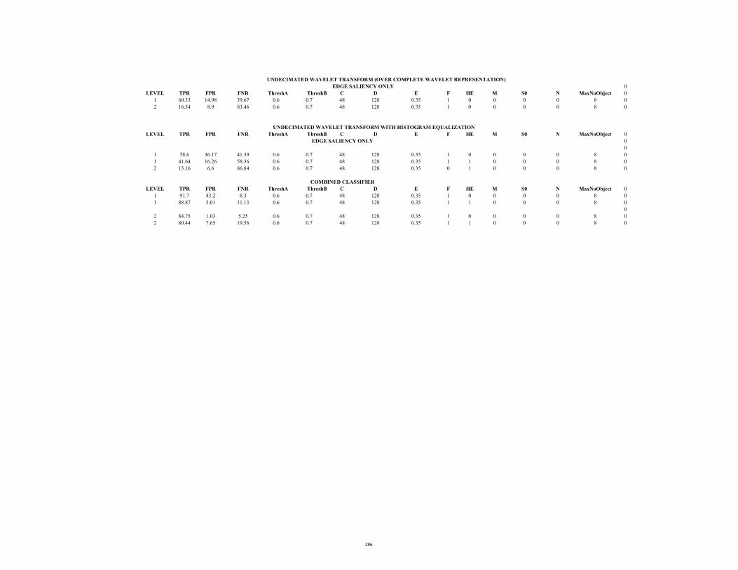
0
LEVEL TPR FPR FNR ThreshA ThreshB C D E F HE M S0 N MaxNoObject 0
1 60.33 14.98 39.67 0.6 0.7 48 128 0.35 1 0 0 0 0 8 0
2 16.54 8.9 83.46 0.6 0.7 48 128 0.35 1 0 0 0 0 8 0
LEVEL TPR FPR FNR ThreshA ThreshB C D E F HE M S0 N MaxNoObject 0
0
0
1 58.6 36.17 41.39 0.6 0.7 48 128 0.35 1 0 0 0 0 8 0
1 41.64 16.26 58.36 0.6 0.7 48 128 0.35 1 1 0 0 0 8 0
2 13.16 6.6 86.84 0.6 0.7 48 128 0.35 0 1 0 0 0 8 0
LEVEL TPR FPR FNR ThreshA ThreshB C D E F HE M S0 N MaxNoObject 0
1 91.7 43.2 8.3 0.6 0.7 48 128 0.35 1 0 0 0 0 8 0
1 88.87 5.01 11.13 0.6 0.7 48 128 0.35 1 1 0 0 0 8 0
0
2 84.75 1.03 5.25 0.6 0.7 48 128 0.35 1 0 0 0 0 8 0
2 80.44 7.65 19.56 0.6 0.7 48 128 0.35 1 1 0 0 0 8 0
UNDECIMATED WAVELET TRANSFORM WITH HISTOGRAM EQUALIZATION
EDGE SALIENCY ONLY
COMBINED CLASSIFIER
UNDECIMATED WAVELET TRANSFORM (OVER COMPLETE WAVELET REPRESENTATION)
EDGE SALIENCY ONLY
286

Sequence: Stc_t1_c_3.avi
Rows: 420
A: Dbase_spacingX Columns: 560
B: Dbase_SpacingY Frames: 3021
C:Object width
D:Object height
E:MedianFlag
FPR:False positive rate
FNR:False negative rate
HE:Histogram equalization
S0: Scale factor
F:Fixed background flag
MaxNoObjects=8
Theshold1: Object Outline threshold
TPR FPR FNR A B C D E THRESHOLD1 HE F S0
64.15 1.11 38.85 24 50 48 100 1 15 0 1 2
Average 64.15 1.11 38.85
Standard deviation 0 0 0
Baseline 64.15 1.11 38.85
APPENDIX D 2.2
MOTION SALIENCY
SHAPE BASED DETECTOR
287
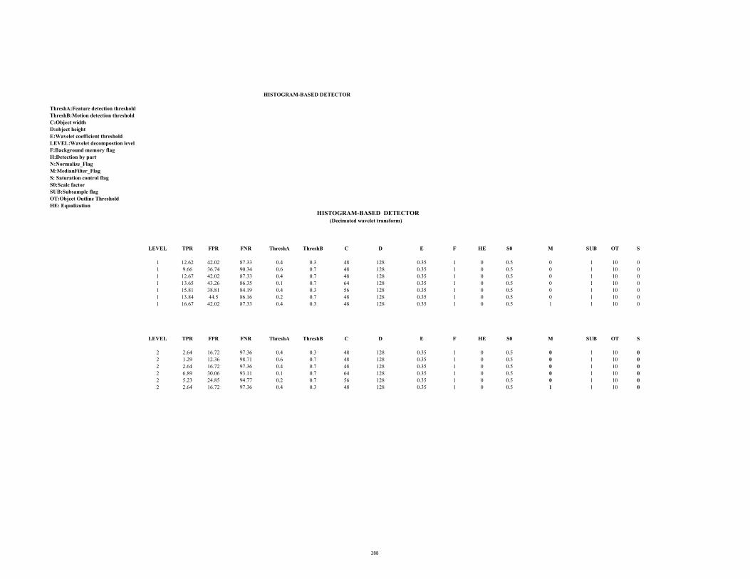
F:Background memory flag
H:Detection by part
N:Normalize_Flag
M:MedianFilter_Flag
S: Saturation control flag
S0:Scale factor
SUB:Subsample flag
OT:Object Outline Threshold
HE: Equalization
LEVEL TPR FPR FNR ThreshA ThreshB C D E F HE S0 M SUB OT S
1 12.62 42.02 87.33 0.4 0.3 48 128 0.35 1 0 0.5 0 1 10 0
1 9.66 36.74 90.34 0.6 0.7 48 128 0.35 1 0 0.5 0 1 10 0
1 12.67 42.02 87.33 0.4 0.7 48 128 0.35 1 0 0.5 0 1 10 0
1 13.65 43.26 86.35 0.1 0.7 64 128 0.35 1 0 0.5 0 1 10 0
1 15.81 38.81 84.19 0.4 0.3 56 128 0.35 1 0 0.5 0 1 10 0
1 13.84 44.5 86.16 0.2 0.7 48 128 0.35 1 0 0.5 0 1 10 0
1 16.67 42.02 87.33 0.4 0.3 48 128 0.35 1 0 0.5 1 1 10 0
LEVEL TPR FPR FNR ThreshA ThreshB C D E F HE S0 M SUB OT S
2 2.64 16.72 97.36 0.4 0.3 48 128 0.35 1 0 0.5 0 1 10 0
2 1.29 12.36 98.71 0.6 0.7 48 128 0.35 1 0 0.5 0 1 10 0
2 2.64 16.72 97.36 0.4 0.7 48 128 0.35 1 0 0.5 0 1 10 0
2 6.89 30.06 93.11 0.1 0.7 64 128 0.35 1 0 0.5 0 1 10 0
2 5.23 24.85 94.77 0.2 0.7 56 128 0.35 1 0 0.5 0 1 10 0
2 2.64 16.72 97.36 0.4 0.3 48 128 0.35 1 0 0.5 1 1 10 0
ThreshB:Motion detection threshold
HISTOGRAM-BASED DETECTOR
ThreshA:Feature detection threshold
C:Object width
(Decimated wavelet transform)
E:Wavelet coefficient threshold
LEVEL:Wavelet decompostion level
D:object height
HISTOGRAM-BASED DETECTOR
288
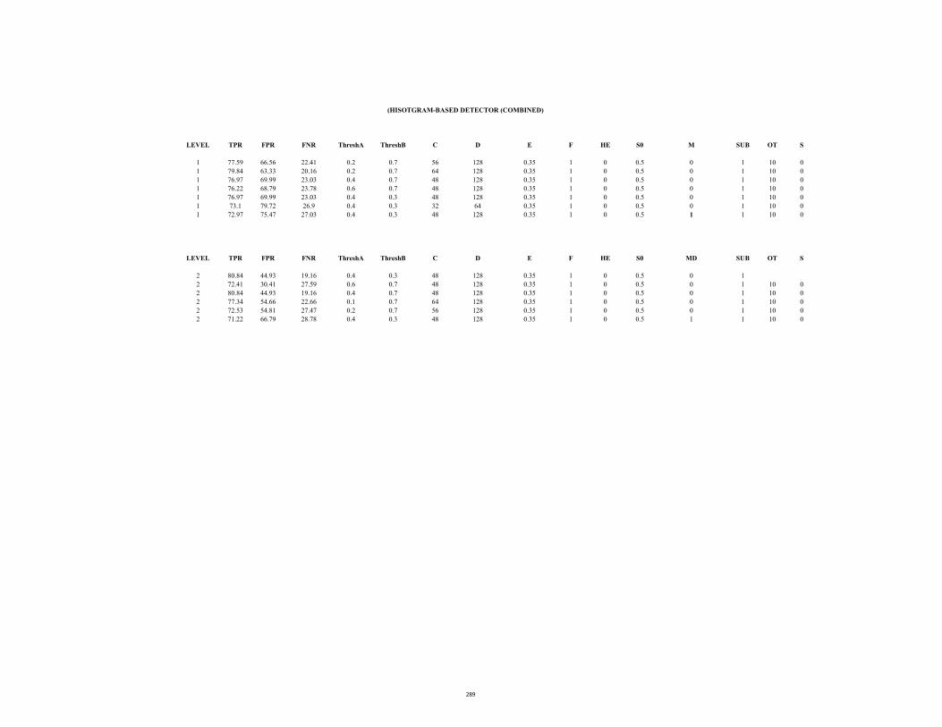
LEVEL TPR FPR FNR ThreshA ThreshB C D E F HE S0 M SUB OT S
1 77.59 66.56 22.41 0.2 0.7 56 128 0.35 1 0 0.5 0 1 10 0
1 79.84 63.33 20.16 0.2 0.7 64 128 0.35 1 0 0.5 0 1 10 0
1 76.97 69.99 23.03 0.4 0.7 48 128 0.35 1 0 0.5 0 1 10 0
1 76.22 68.79 23.78 0.6 0.7 48 128 0.35 1 0 0.5 0 1 10 0
1 76.97 69.99 23.03 0.4 0.3 48 128 0.35 1 0 0.5 0 1 10 0
1 73.1 79.72 26.9 0.4 0.3 32 64 0.35 1 0 0.5 0 1 10 0
1 72.97 75.47 27.03 0.4 0.3 48 128 0.35 1 0 0.5 1 1 10 0
LEVEL TPR FPR FNR ThreshA ThreshB C D E F HE S0 MD SUB OT S
2 80.84 44.93 19.16 0.4 0.3 48 128 0.35 1 0 0.5 0 1
2 72.41 30.41 27.59 0.6 0.7 48 128 0.35 1 0 0.5 0 1 10 0
2 80.84 44.93 19.16 0.4 0.7 48 128 0.35 1 0 0.5 0 1 10 0
2 77.34 54.66 22.66 0.1 0.7 64 128 0.35 1 0 0.5 0 1 10 0
2 72.53 54.81 27.47 0.2 0.7 56 128 0.35 1 0 0.5 0 1 10 0
2 71.22 66.79 28.78 0.4 0.3 48 128 0.35 1 0 0.5 1 1 10 0
(HISOTGRAM-BASED DETECTOR (COMBINED)
289

APPENDIX D 3.1
EDGE SALIENCY
Sequence : Stc_t1_c_4.avi
A: Dbase_spacingX
B: Dbase_SpacingY
C:Object width
D:Object height
E:MedianFlag
TPR:True Positive Rate
FPR:False Positive Rate
FNR:False Negative Rate
HE:Histogram equalization
S0: Scale factor
F:Fixed background flag
MaxNoObject: Maximum number of objects
Theshold1: Object Outline threshold
TPR FPR FNR A B C D E Threshold1 HE F S0
52.08 0.8 47.96 24 64 48 128 1 15 0 1 2
51.06 0.83 48.94 24 50 48 100 1 10 0 1 2
46.82 1.21 53.18 16 32 32 64 1 15 0 1 2
48.94 1.21 51.06 16 64 32 128 1 15 0 1 2
25.45 2.26 74.55 32 64 24 64 1 15 0 1 1
25.29 2.43 74.71 16 32 32 64 1 15 0 1 1
29.85 3.96 70.15 12 64 24 120 1 15 0 1 1
29.85 4.09 70.15 16 32 32 64 1 15 0 1 1
29.85 4.09 70.15 16 60 32 120 1 15 0 1 1
32.14 4.74 67.86 16 64 32 128 1 15 0 1 1
29.2 5.15 70.18 24 60 48 120 1 15 0 1 1
29.2 5.15 70.18 24 64 48 128 1 15 0 1 1
41.6 11.5 58.4 16 64 32 128 1 15 0 1 1
54.06 10.85 45.84 24 64 48 128 1 15 0 1 0.2
46.98 3.03 53.02 24 64 48 128 1 15 0 1 0.2
47.96 2.52 52.04 24 64 48 128 1 15 0 1 0.2
51.55 2.04 48.45 24 64 48 128 1 15 0 1 0.2
52.69 2.67 47.45 24 64 48 128 1 15 0 1 0.2
SHAPE-BASED CLASSIFIER
Rows: 420
Columns: 560
Frames: 3021
290
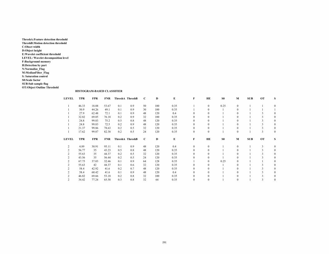
F:Background memory
H:Detection by part
N:Normalize_Flag
M:MedianFilter_Flag
S: Saturation control
S0:Scale factor
SUB:Sub sample flag
OT:Object Outline Threshold
LEVEL TPR FPR FNR ThreshA ThreshB C D E F HE S0 M SUB OT S
1 46.33 18.08 53.67 0.1 0.9 50 100 0.35 1 0 0.25 0 1 1 0
1 50.9 44.26 49.1 0.1 0.9 30 100 0.35 1 0 1 0 1 1 1
1 27.9 62.48 72.1 0.1 0.9 48 120 0.4 0 0 1 0 1 3 0
1 32.82 69.85 76.18 0.2 0.9 32 100 0.35 0 0 1 0 1 3 0
1 24.8 99.83 75.2 0.5 0.8 48 120 0.35 0 0 1 0 1 3 0
1 24.8 99.83 72.5 0.2 0.9 48 120 0.35 0 0 1 0 1 3 0
1 21.37 99.86 78.63 0.2 0.5 32 120 0.35 0 0 1 0 1 3 0
1 17.62 99.87 82.38 0.2 0.5 24 120 0.35 0 0 1 0 1 3 0
LEVEL TPR FPR FNR ThreshA ThreshB C D E F HE S0 M SUB OT S
2 4.89 30.91 95.11 0.1 0.9 48 120 0.4 0 0 1 0 1 3 0
2 56.77 35 43.23 0.5 0.8 48 120 0.35 0 0 1 0 1 3 0
2 55.63 35 44.37 0.2 0.5 32 120 0.35 0 0 1 0 1 3 0
2 43.56 35 56.44 0.2 0.5 24 120 0.35 0 0 1 0 1 3 0
2 67.75 37.03 32.46 0.1 0.9 64 128 0.35 1 0 0.25 0 1 1 0
2 55.63 42 44.37 0.1 0.6 32 120 0.35 0 0 1 0 1 3 0
2 58.4 42.92 41.6 0.2 0.7 48 120 0.35 0 0 1 0 1 3 0
2 58.4 60.42 41.6 0.1 0.9 48 120 0.4 0 0 1 0 1 3 0
2 46.82 69.66 53.18 0.2 0.8 32 100 0.35 0 0 1 0 1 3 0
2 34.42 77.24 65.58 0.3 0.8 32 64 0.35 0 0 1 0 1 3 0
LEVEL: Wavelet decomposition level
HISTOGRAM-BASED CLASSIFIER
ThreshA:Feature detection threshold
ThreshB:Motion detection threshold
C:Obect width
D:Object height
E:Wavelet coefficient threshold
291
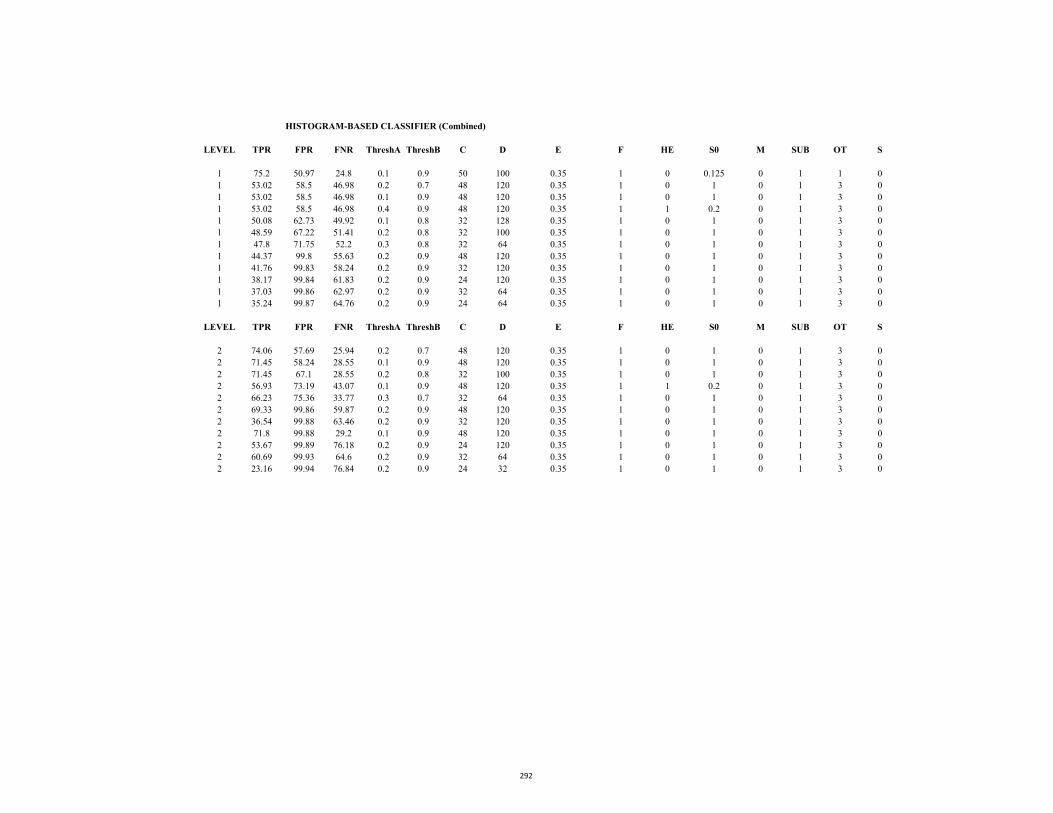
LEVEL TPR FPR FNR ThreshA ThreshB C D E F HE S0 M SUB OT S
1 75.2 50.97 24.8 0.1 0.9 50 100 0.35 1 0 0.125 0 1 1 0
1 53.02 58.5 46.98 0.2 0.7 48 120 0.35 1 0 1 0 1 3 0
1 53.02 58.5 46.98 0.1 0.9 48 120 0.35 1 0 1 0 1 3 0
1 53.02 58.5 46.98 0.4 0.9 48 120 0.35 1 1 0.2 0 1 3 0
1 50.08 62.73 49.92 0.1 0.8 32 128 0.35 1 0 1 0 1 3 0
1 48.59 67.22 51.41 0.2 0.8 32 100 0.35 1 0 1 0 1 3 0
1 47.8 71.75 52.2 0.3 0.8 32 64 0.35 1 0 1 0 1 3 0
1 44.37 99.8 55.63 0.2 0.9 48 120 0.35 1 0 1 0 1 3 0
1 41.76 99.83 58.24 0.2 0.9 32 120 0.35 1 0 1 0 1 3 0
1 38.17 99.84 61.83 0.2 0.9 24 120 0.35 1 0 1 0 1 3 0
1 37.03 99.86 62.97 0.2 0.9 32 64 0.35 1 0 1 0 1 3 0
1 35.24 99.87 64.76 0.2 0.9 24 64 0.35 1 0 1 0 1 3 0
LEVEL TPR FPR FNR ThreshA ThreshB C D E F HE S0 M SUB OT S
2 74.06 57.69 25.94 0.2 0.7 48 120 0.35 1 0 1 0 1 3 0
2 71.45 58.24 28.55 0.1 0.9 48 120 0.35 1 0 1 0 1 3 0
2 71.45 67.1 28.55 0.2 0.8 32 100 0.35 1 0 1 0 1 3 0
2 56.93 73.19 43.07 0.1 0.9 48 120 0.35 1 1 0.2 0 1 3 0
2 66.23 75.36 33.77 0.3 0.7 32 64 0.35 1 0 1 0 1 3 0
2 69.33 99.86 59.87 0.2 0.9 48 120 0.35 1 0 1 0 1 3 0
2 36.54 99.88 63.46 0.2 0.9 32 120 0.35 1 0 1 0 1 3 0
2 71.8 99.88 29.2 0.1 0.9 48 120 0.35 1 0 1 0 1 3 0
2 53.67 99.89 76.18 0.2 0.9 24 120 0.35 1 0 1 0 1 3 0
2 60.69 99.93 64.6 0.2 0.9 32 64 0.35 1 0 1 0 1 3 0
2 23.16 99.94 76.84 0.2 0.9 24 32 0.35 1 0 1 0 1 3 0
HISTOGRAM-BASED CLASSIFIER (Combined)
292

Sequence:
NROWS: 420
NCOLS: 560
NSLICE: 3021
MaxNoObjects=8
A: Dbase_spacingX
B: Dbase_SpacingY
C:ObjectWidth1
D:ObjectHeight1
m:MedianFlag
TPR:True positive rate
FPR:False positive rate
FNR:False negative rate
HE:Histogram equalization
OT:Object outline threshold
F:Fixed background flag
S0:Scale factor
TPR FPR FNR A B C D E THRESHOLD1 HE F S0
48.94 1.24 51.55 16 64 32 128 1 15 0 1 2
APPENDIX D 3.2
SHAPE-BASED DETECTOR
Stc_t1_c_4.avi
MOTION SALIENCY
293
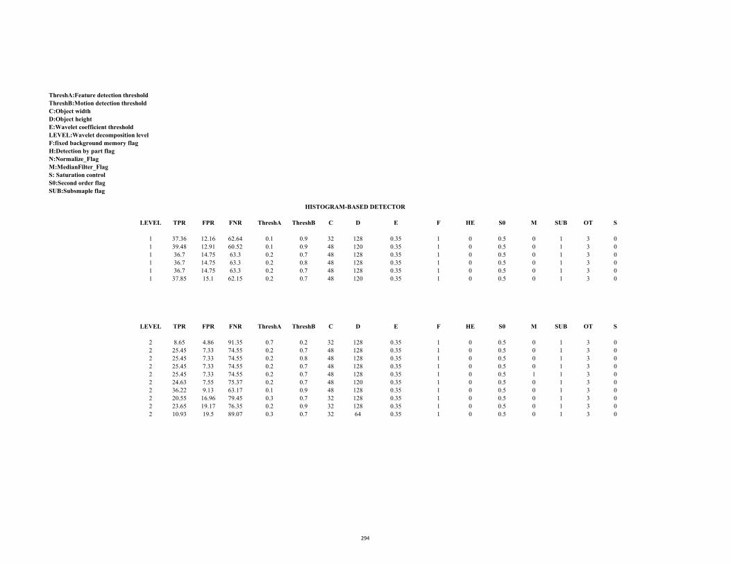
ThreshA:Feature detection threshold
ThreshB:Motion detection threshold
C:Object width
D:Object height
E:Wavelet coefficient threshold
LEVEL:Wavelet decomposition level
F:fixed background memory flag
H:Detection by part flag
N:Normalize_Flag
M:MedianFilter_Flag
S: Saturation control
S0:Second order flag
SUB:Subsmaple flag
LEVEL TPR FPR FNR ThreshA ThreshB C D E F HE S0 M SUB OT S
1 37.36 12.16 62.64 0.1 0.9 32 128 0.35 1 0 0.5 0 1 3 0
1 39.48 12.91 60.52 0.1 0.9 48 120 0.35 1 0 0.5 0 1 3 0
1 36.7 14.75 63.3 0.2 0.7 48 128 0.35 1 0 0.5 0 1 3 0
1 36.7 14.75 63.3 0.2 0.8 48 128 0.35 1 0 0.5 0 1 3 0
1 36.7 14.75 63.3 0.2 0.7 48 128 0.35 1 0 0.5 0 1 3 0
1 37.85 15.1 62.15 0.2 0.7 48 120 0.35 1 0 0.5 0 1 3 0
LEVEL TPR FPR FNR ThreshA ThreshB C D E F HE S0 M SUB OT S
2 8.65 4.86 91.35 0.7 0.2 32 128 0.35 1 0 0.5 0 1 3 0
2 25.45 7.33 74.55 0.2 0.7 48 128 0.35 1 0 0.5 0 1 3 0
2 25.45 7.33 74.55 0.2 0.8 48 128 0.35 1 0 0.5 0 1 3 0
2 25.45 7.33 74.55 0.2 0.7 48 128 0.35 1 0 0.5 0 1 3 0
2 25.45 7.33 74.55 0.2 0.7 48 128 0.35 1 0 0.5 1 1 3 0
2 24.63 7.55 75.37 0.2 0.7 48 120 0.35 1 0 0.5 0 1 3 0
2 36.22 9.13 63.17 0.1 0.9 48 128 0.35 1 0 0.5 0 1 3 0
2 20.55 16.96 79.45 0.3 0.7 32 128 0.35 1 0 0.5 0 1 3 0
2 23.65 19.17 76.35 0.2 0.9 32 128 0.35 1 0 0.5 0 1 3 0
2 10.93 19.5 89.07 0.3 0.7 32 64 0.35 1 0 0.5 0 1 3 0
HISTOGRAM-BASED DETECTOR
294
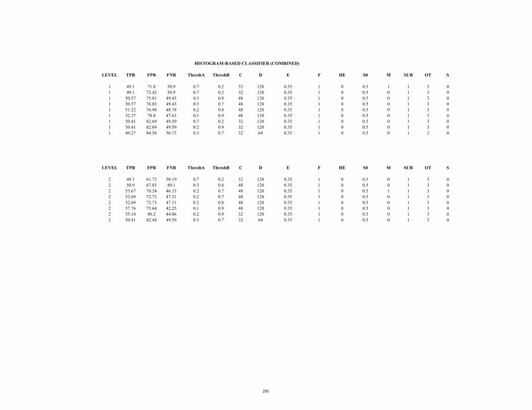
LEVEL TPR FPR FNR ThreshA ThreshB C D E F HE S0 M SUB OT S
1 49.1 71.8 50.9 0.7 0.2 32 128 0.35 1 0 0.5 1 1 3 0
1 49.1 72.42 50.9 0.7 0.2 32 128 0.35 1 0 0.5 0 1 3 0
1 50.57 75.81 49.43 0.3 0.8 48 128 0.35 1 0 0.5 0 1 3 0
1 50.57 76.83 49.43 0.3 0.7 48 128 0.35 1 0 0.5 0 1 3 0
1 51.22 76.98 48.78 0.2 0.8 48 128 0.35 1 0 0.5 0 1 3 0
1 52.37 78.8 47.63 0.1 0.9 48 128 0.35 1 0 0.5 0 1 3 0
1 50.41 82.69 49.59 0.7 0.2 32 128 0.35 1 0 0.5 0 1 3 0
1 50.41 82.69 49.59 0.2 0.9 32 120 0.35 1 0 0.5 0 1 3 0
1 49.27 84.58 50.73 0.3 0.7 32 64 0.35 1 0 0.5 0 1 3 0
LEVEL TPR FPR FNR ThreshA ThreshB C D E F HE S0 M SUB OT S
2 49.1 61.72 50.19 0.7 0.2 32 128 0.35 1 0 0.5 0 1 3 0
2 50.9 67.83 49.1 0.3 0.8 48 120 0.35 1 0 0.5 0 1 3 0
2 53.67 70.24 46.33 0.2 0.7 48 128 0.35 1 0 0.5 1 1 3 0
2 52.69 72.73 47.31 0.2 0.7 48 128 0.35 1 0 0.5 0 1 3 0
2 52.69 72.73 47.31 0.2 0.8 48 120 0.35 1 0 0.5 0 1 3 0
2 57.76 75.64 42.25 0.1 0.9 48 120 0.35 1 0 0.5 0 1 3 0
2 55.14 80.2 44.86 0.2 0.9 32 128 0.35 1 0 0.5 0 1 3 0
2 50.41 82.44 49.59 0.3 0.7 32 64 0.35 1 0 0.5 0 1 3 0
HISTOGRAM-BASED CLASSIFIER (COMBINED)
295

SEQUENCE: HAMILTON2.AVI
NROWS: 240
NCOLS: 320
NSLICE: 3021 (USED 1000)
CLASSIFIER_SEARCH_WINDOW_WIDTH: 48
CLASSIFIER_SEARCH_WINDOW_HEIGHT: 128
A: MAXIMUM DISPLACEMENT FOR CENTROID MATCHING X
B: MAXIMUM DISPLACEMENT FOR CENTROID Y
C: TRACKER_WIDTH
D: TRACKER_HEIGHT
E: FRAME_ACTIVITY_CENTROID
MAG_FACT :MAGNIFICATION FACTOR
SAT_CONTROL: SATURATION CONTROL
S0: SCALE FACTOR
CLUST_FLAG: TRACK CLUSTER_FLAG
NUMBER TPR FPR FNR A B C D E MODEL MAG_FACTOR SAT_CONTROL S0 CLUST_FLAG
CLUSTER_FLAG 1 69.84 42.36 30.16 0.5W 0.5H 0.5W 0.5H 1 0.5 0 1 0
2 70.81 41.78 29.19 0.25W 0.25H 0.25W 0.25H 1 0.25 0 1 0
1 3 59.95 45.34 40.05 0.25W 0.25H 0.25W 0.25H 1 0.25 0 0.5 0
2 4 56.09 41.16 43.91 0.25W 0.25H 0.25W 0.25H 6 0.25 0 0.5 0
2 5 68.52 36.46 31.48 0.25W 0.25H 0.25W 0.25H 6 0.25 0 1 0
2 6 70.81 41.78 29.19 0.25W 0.25H 0.25W 0.25H 5 0.25 0 1 0
2 7 59.95 45.34 40.05 0.25W 0.25H 0.25W 0.25H 5 0.25 0 0.5 0
1 8 70.45 40 30 0.25W 0.25H 0.25W 0.25H 4 0.25 0 1 0
2 7 68.52 34.46 31.48 0.25W 0.25H 0.25W 0.25H 3 0.25 0 1 0
2 8 70.33 41.61 29.67 0.25W 0.25H 0.25W 0.25H 2 0.25 0 1 0
JPDAF TRACKER (HAMILTON2B.AVI)
APPENDIX E1
296

SEQUENCE: STC_T1_C_3.AVI
NROWS: 420
NCOLS: 560
NSLICE: 3021 (USED 1944)
CLASSIFIER_SEARCH_WINDOW_WIDTH: 48
CLASSIFIER_SEARCH_WINDOW_HEIGHT: 128
A: MAXIMUM DISPLACEMENT FOR CENTROID MATCHINGX
B: MAXIMUM DISPLACEMENT FOR CENTROID MATCHINGY
C: TRACKER_WIDTH
D: TRACKER_HEIGHT
E: FRAME_ACTIVITY_CENTROID
E: FRAME_ACTIVITY_CENTROID
MAG_FACT :MAGNIFICATION FACTOR
SAT_CONTROL: SATURATION CONTROL
S0: SCALE FACTOR
CLUST_FLAG: TRACK CLUSTER_FLAG
CLUSTER_FLAG NUMBER TPR FPR FNR A B C D E MODEL MAG_FACTOR SAT_CONTROL S0 CLUSTER_FLAG
0 1 77.68 44.99 22.32 0.25W 0.25H 0.25W 0.25H 1 1 0.25 0 1 0
0 2 77.68 44.99 22.32 0.25W 0.25H 0.25W 0.25H 1 2 0.25 0 1 0
0 3 61.62 54.96 38.38 0.25W 0.25H 0.25W 0.25H 1 3 0.25 0 1 0
0 4 60.89 50.52 39.11 0.25W 0.25H 0.25W 0.25H 1 4 0.25 0 1 0
0 5 61.62 54.96 38.38 0.25W 0.25H 0.25W 0.25H 1 5 0.25 0 1 0
0 6 75.77 43.12 24.12 0.25W 0.25H 0.25W 0.25W 1 6 0.25 0 1 1
0 7 64.21 57.93 35.79 0.25W 0.25H 0.25W 0.25W 1 1 0.25 1 1 1
0 8 69.07 59.75 30.93 0.25W 0.25H 0.25W 0.25W 1 1 0.25 1 1 2
0 9 68.27 54.88 31.73 0.25W 0.25H 0.25W 0.25W 1 1 0.25 0 1 2
0 10 71.4 52.53 28.6 0.25W 0.25H 0.25W 0.25W 1 1 0.25 1 1 2
JPDAF TRACKER (STC_T1_C_3.AVI)
APPENDIX E2
297

SEQUENCE: STC_T1_C_4.AVI
NROWS: 420
NCOLS: 560
NSLICE: 3021 (USED 150)
CLASSIFIER_SEARCH_WINDOW_WIDTH: 48CLASSIFIER_SEARCH_WINDOW_HEIGHT: 128
A: MAXIMUM DISPLACEMENT FOR CENTROID MATCHINGX
B: MAXIMUM DISPLACEMENT FOR CENTROID MATCHINGY
C: TRACKER_WIDTH
D: TRACKER_HEIGHT
E: FRAME_ACTIVITY_CENTROID
E: FRAME_ACTIVITY_CENTROID
MAG_FACT :MAGNIFICATION FACTOR
SAT_CONTROL: SATURATION CONTROL
S0: SCALE FACTOR
CLUST_FLAG: TRACK CLUSTER_FLAG
CLUSTER_FLAG NUMBER TPR FPR FNR A B C D E MODEL MAG_FACTOR SAT_CONTROL S0 CLUSTER_FLAG
0 1 66.86 24.32 3.12 0.5W 0.5H 0.25W 0.25H 1 0.5 1 1 0
0 2 70.64 45.29 29.36 0.5W 0.5H 0.125W 0.125H 1 0.25 1 1 0
0 3 72.59 43.67 27.41 0.5W 0.5H 0.125W 0.125H 1 0.25 0 1 0
0 4 56.12 20.57 43.88 0.5W 0.5H 0.25W 0.25H 1 0.5 0 1 0
0 5 71.29 44.29 28.71 0.5W 0.5H 0.5W 0.5H 1 1 0 1 0
0 6 72.27 46.03 27.73 0.5W 0.5H 0.5W 0.5H 1 1 1 1 0
0 7 51.71 51.66 48.29 0.5W 0.5H 0.5W 0.5H 1 1 1 0.5 0
JPDAF TRACKER (STC_T1_C_4.AVI)
APPENDIX E3
298
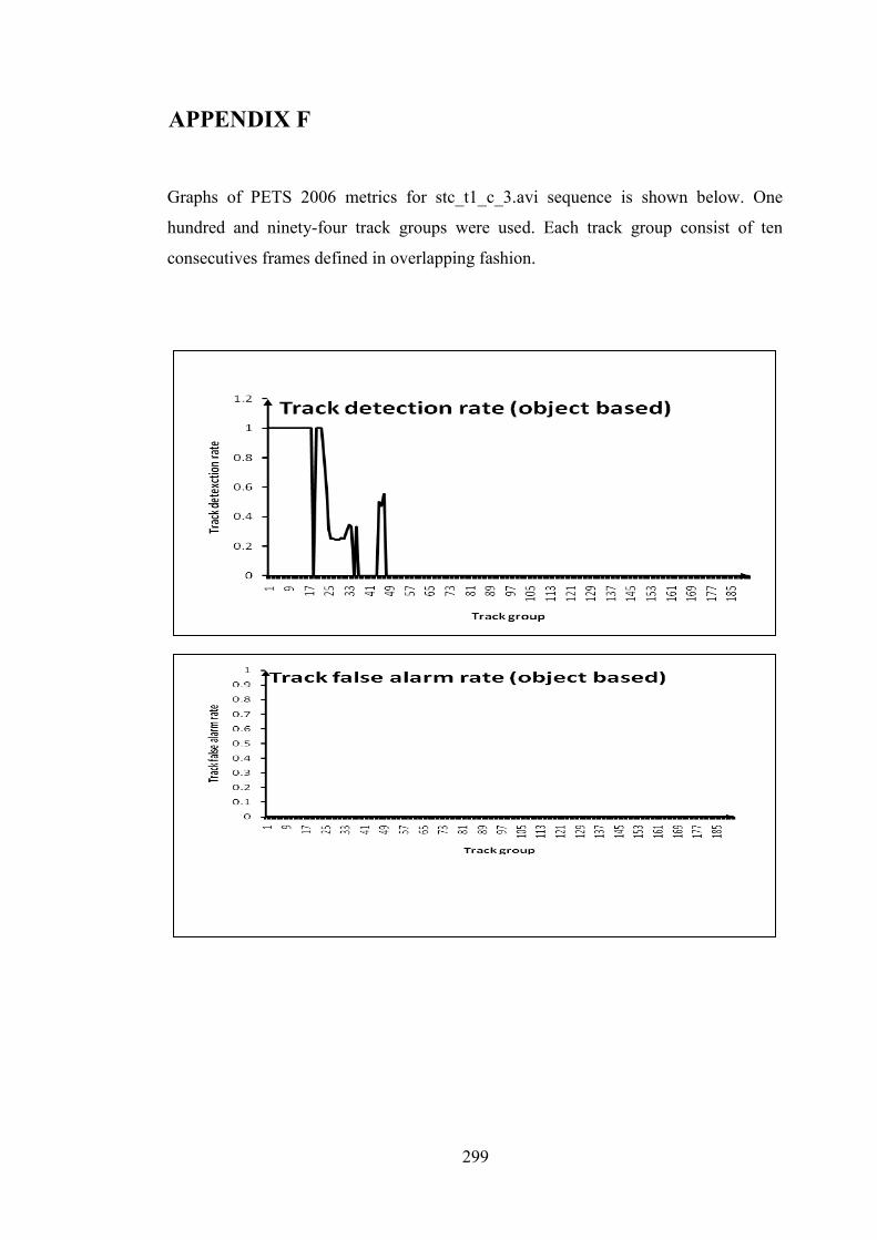
299
APPENDIX F
Graphs of PETS 2006 metrics for stc_t1_c_3.avi sequence is shown below. One
hundred and ninety-four track groups were used. Each track group consist of ten
consecutives frames defined in overlapping fashion.
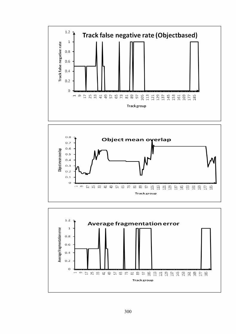
300
V
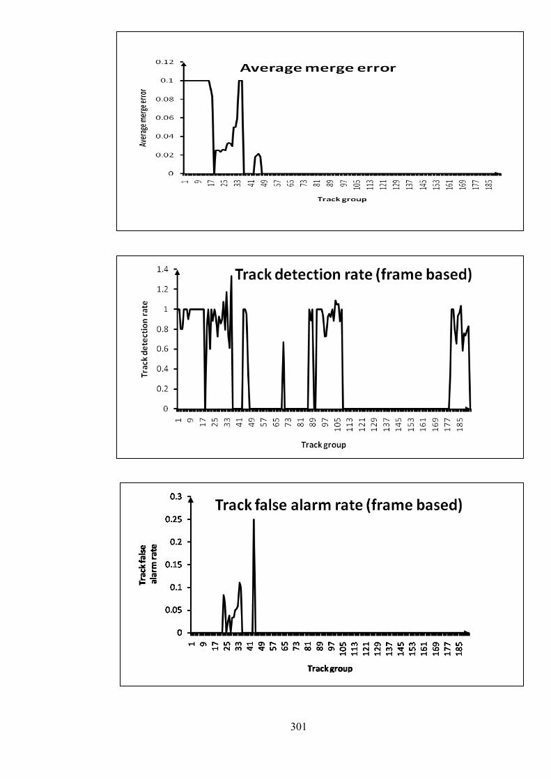
301
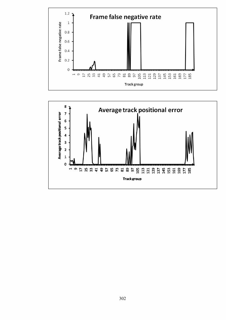
302
Related Documents