School of Aerospace, Civil and Mechanical Engineering The University of New South Wales Australian Defence Force Academy Vibro-acoustic Studies of Brake Squeal Noise Antti Papinniemi A thesis submitted for the Degree of Doctor of Philosophy August 2007

Welcome message from author
This document is posted to help you gain knowledge. Please leave a comment to let me know what you think about it! Share it to your friends and learn new things together.
Transcript

School of Aerospace, Civil and Mechanical Engineering
The University of New South Wales
Australian Defence Force Academy
Vibro-acoustic Studies of
Brake Squeal Noise
Antti Papinniemi
A thesis submitted for the Degree of Doctor of Philosophy
August 2007

ii

iii
Statement of Originality
I hereby declare that this submission is my own work and to the best of my knowledge
it contains no materials previously published or written by another person, or substantial
proportions of material which have been accepted for the award of any other degree or
diploma at UNSW or any other educational institution, except where due
acknowledgement is made in the thesis. Any contribution made to the research by
others, with whom I have worked at UNSW or elsewhere, is explicitly acknowledged in
the thesis. I also declare that the intellectual content of this thesis is the product of my
own work, except to the extent that assistance from others in the project’s design and
conception or in style, presentation and linguistic expression is acknowledged.
Antti Papinniemi
August 2007

iv
Copyright Statement
‘I hereby grant the University of New South Wales or its agents the right to archive and
to make available my thesis or dissertation in whole or part in the University libraries in
all forms of media, now or here after known, subject to the provisions of the Copyright
Act 1968. I retain all proprietary rights, such as patent rights. I also retain the right to
use in future works (such as articles or books) all or part of this thesis or dissertation. I
also authorise University Microfilms to use the 350 word abstract of my thesis in
Dissertation Abstract International (this is applicable to doctoral theses only). I have
either used no substantial portions of copyright material in my thesis or I have obtained
permission to use copyright material; where permission has not been granted I have
applied/will apply for a partial restriction of the digital copy of my thesis or
dissertation.'
Signed ……………………………………………...........................
Date ……………………………………………...........................
Authenticity Statement
‘I certify that the Library deposit digital copy is a direct equivalent of the final officially
approved version of my thesis. No emendation of content has occurred and if there are
any minor variations in formatting, they are the result of the conversion to digital
format.’
Signed ……………………………………………...........................
Date ……………………………………………...........................

v
Abstract
Squeal noise has been an on-going concern with automotive brake systems since their
inception. Even after many decades of research no single theory exists that adequately
describes the phenomenon, and no general methods for eliminating squeal noise exist.
Broadly speaking, three primary methods of analysis have been applied to
understanding and eliminating brake squeal: analytical, experimental and numerical.
Analytical models provide some insight into the mechanisms involved when a brake
squeals, but have limitations in applicability to specific brake systems. Experimental
methods provide the backbone of brake squeal investigations, especially in an industrial
environment. However, the core focus of this thesis is to use a large scale finite element
analysis (FEA) model to investigate brake squeal.
Initially the FEA model was developed and the dynamic characteristics were validated
against experimental modal analysis results. A complex eigenvalue analysis was
performed to identify potential squeal modes which appear as unstable system vibration
modes.
Further techniques are described that allow the deeper probing of unstable brake system
modes. Feed-in energy, which is the conversion of friction work into vibrational energy
during the onset of squeal, is used to determine the relative contribution of each brake
pad to the overall system vibration. The distribution of the feed-in energy across the
face of a brake pad is also calculated. Component strain energy distributions are
determined for a brake system as a guide to identifying which components might best be
modified in addressing an unstable system mode. Finally modal participation is
assessed by calculating the Modal Assurance Criterion (MAC) between component free
modes and the component in the assembly during squeal. This allows participating
modes to be visualised and aids in the development of countermeasures.
The majority of the work in this thesis was performed using the commercial FEA code
MSC.Nastran with user defined friction interfaces. An alternative approach using a
contact element formulation available in Abaqus was also implemented and compared
to the MSC.Nastran results. This analysis showed that considerable differences were
noted in the results even though the overall predicted stability correlated relatively well
to observed squeal. Abaqus was also used in a case study into the design of a brake

vi
rotor in a noisy brake system. The results of this study provided good correlation to
observed squeal and facilitated effective rotor countermeasures to be developed.
Some success was achieved in the main aims of predicting brake squeal and developing
countermeasures. However, while the tools presented do allow a deeper probing of
system behaviour during squeal, their use requires good correlation to observed squeal
on brake system to be established. As such, their use as up-front design tools is still
limited. This shortcoming stems from the complexity of brake squeal itself and the
limitations in modelling the true nature of the non-linearities within a brake system.

vii
Acknowledgments
I would like to thank Professor Joseph Lai who supervised my studies, and I am grateful
for his direction, patience and encouragement over this long period of time. I would
also like to thank Dr Jiye Zhao for providing his support and advice during the project.
The project was funded jointly by the Australian Research Council and PBR
Automotive under the SPIRT scheme. I also thank the ARC for providing me with
APA(I) and UNSW@ADFA for a completion scholarship.
Many members of staff at the School of Aerospace, Civil and Mechanical Engineering,
UNSW@ADFA have contributed to this project, including Mr Robert Clark, Mrs
Marion Burgess, Mr John Waggener, Dr Andrew Dombek, Dr Alex Tarnopolsky, and
many members of the mechanical and electrical workshops.
I would also like to thank some of my fellow students who I shared many enjoyable
times with, both socially and on an intellectual level, including David Martinez-Munoz,
Jon Couldrick, Orio Kieboom, Jeff Mcguire, Stephen Moore, and many others who
came and went during my studies.
Finally I would like to thank Mum and Dad, and the rest of my family. Hopefully we
finally got there.

ix
Table of Contents
Statement of Originality iii
Copyright Statement iv
Authenticity Statement iv
Abstract v
Acknowledgments vii
Table of Contents ix
List of Figures xiii
List of Tables xix
Nomenclature xxi
Chapter 1 Introduction 1
1.1 Automotive Disc Brakes 1
1.2 Brake System Description 3
1.3 Characteristics of Brake Squeal 6
1.4 Thesis outline 11
Chapter 2 Literature Review 13
2.1 Introduction 13
2.2 Reviews of Brake Squeal 15
2.3 Analytical Approaches to Brake Squeal 16
2.3.1 Variable µ Analysis 16
2.3.2 Sprag-Slip Analysis 18
2.3.3 Mode Coupling Analysis 20
2.4 Experimental Approaches to Brake Squeal 23
2.5 Numerical Methods for Brake Squeal Analysis 27
2.6 Brake Squeal Noise in Practice 30
2.7 Summary 34
Chapter 3 Experimental Determination of Vibrational and Acoustical
Characteristics of a Brake System 35
3.1 Introduction 35
3.2 Frequency Response Function 36
3.3 Experimental Set-up 37
3.4 Component Testing 39
3.5 Rotor 39
3.5.1 Brake Rotor Mode Shape Descriptions 39
3.5.2 Rotor Test Grid 42

x
3.5.3 Rotor Test Results 44
3.5.4 In-Plane Mode Detection 46
3.5.5 In-Plane Measurement 48
3.6 Pad 51
3.7 Caliper Housing 53
3.8 Anchor Bracket 54
3.9 Assembled Brake System 56
3.10 Modal Analysis Summary 62
3.11 Brake System Noise Evaluation 63
Chapter 4 Finite Element Modal Analysis 67
4.1 Introduction 67
4.2 Application of FEA to Dynamical Problems 67
4.3 Modelling Approach 69
4.4 Individual Component models 70
4.4.1 Brake rotor 72
4.4.2 Anchor Bracket 75
4.4.3 Caliper Housing 78
4.4.4 Brake Pad 79
4.5 Mounted Rotor 82
4.6 Assembled Models 84
4.6.1 Component Interfaces 84
4.6.1.1 Multi-point constraints 84
4.6.1.2 Linear springs 86
4.6.1.3 Linear vs. non-linear static analysis 88
4.6.1.4 Spring interface tuning 89
4.6.1.5 Friction interface 91
4.7 Summary 93
Chapter 5 Prediction of Unstable Modes 95
5.1 Introduction 95
5.2 Complex Eigenvalue Analysis 99
5.3 Implementation for a Brake System 100
5.3.1 Generation of a validated FEA model 101
5.3.2 Static analysis 101
5.3.3 Friction Model 101
5.3.4 Implementation with MSC.Nastran 103
5.4 Brake System Analysis 104

xi
5.5 Summary 112
Chapter 6 Numerical Methods for Assessing Brake Squeal Propensity 113
6.1 Introduction 113
6.2 Strain energy 114
6.2.1 Viscous Work 116
6.3 Feed-in Energy 118
6.3.1 Feed-in Energy vs. Viscous Work 122
6.4 Modal Participation with Modal Assurance Criterion 123
6.5 Example 4DOF System 124
6.6 Analysis of Numerical Model 132
6.4.1 Model Description and Unstable Modes 132
6.4.2 Feed-in Energy for a Numerical Model 133
6.4.3 Strain Energy for a Numerical Model 137
6.6.4 Modal Participation for a Numerical Model 139
6.6.5 Example Unstable Mode Investigation 142
6.7 Summary 147
Chapter 7 Parametric Study 149
7.1 Introduction 149
7.2 Parameters Under Investigation 151
7.3 Baseline System 151
7.3.1 Complex Eigenvalues 151
7.3.2 Baseline Strain Energy Distributions 152
7.3.3 Baseline Feed-in Energy 154
7.3.4 Baseline Component MAC Modal Participation 154
7.4 Material Properties Sensitivities 161
7.5 Contact Distribution Sensitivities 168
7.6 Damping Shims 172
7.7 Summary 174
Chapter 8 Comparison of Contact Modelling Methods 177
8.1 Introduction 177
8.2 Contact Elements 177
8.2.1 Tied Contact 178
8.2.2 Deformable-Deformable Contact 180
8.2.3 Non-linear Static Analysis 182
8.2.4 Contact Set-up and Solution Steps 183
8.3 Material Properties and Load Cases 185

xii
8.4 Analysis Results 187
8.4.1 Abaqus Results for varying Pressure 187
8.4.2 Abaqus vs Nastran Stability 188
8.4.3 Abaqus vs Nastran MAC 189
8.5 Summary 200
Chapter 9 Applications to Rotor Design in an Industrial Environment 203
9.1 Introduction 203
9.2 Brake system Under Investigation 203
9.3 Noise Evaluation 205
9.4 Mode Description 208
9.5 Stability Prediction 210
9.6 Rotor Modification 212
9.7 Summary 218
Chapter 10 Conclusions 219
10.1 Conclusions 219
10.2 Recommendations for Future Work 222
References 225
Publications Arising From This Thesis 233
Journal Papers 233
Conference Papers 233
Reports 234
Appendix A: Measurement Grids 235
Appendix B: Free Rotor Mode Shapes 239
Appendix C: Example Nastran Input Deck 241
Appendix D: bdfread Source Code 247

xiii
List of Figures
Figure 1.1 Schematic of a siding disc brake caliper. Note that the anchor bracket is
not included for clarity 2
Figure 1.2 Ford AU series II rear brake assembly CAD model 4
Figure 1.3 Ford AU II rear brake assembly components. Clockwise for the top left;
pads, piston, guide pins, caliper housing, and bracket and disc rotor 4
Figure 1.4 Ford AU II rear brake assembly as installed on the vehicle 5
Figure 1.5 Spectrum of a brake squeal event 7
Figure 1.6 Comparison of the same section of two nominally identical tests on the
noise dynamometer. The green dots represent noise occurrences during a single stop 10
Figure 1.7 Example noise sensitivities to brake pressure and IBT 11
Figure 2.1 (a) Number of brake squeal papers according to Thomson ISI Web of
Science on 4 August 2006, (b) Number of brake squeal papers as a percentage of the
papers presented at the SAE Annual Brake Colloquium 14
Figure 2.2 A single degree-of-freedom featuring a block rubbing on a moving
conveyor 17
Figure 2.3 Negative slope µ-v characteristic 17
Figure 2.4 (a) Single strut rubbing against surface, (b) sprag-slip system 19
Figure 2.5 Two degree-of-freedom system analysed by Hoffman, et al 21
Figure 2.6 Example shim material 31
Figure 2.7 Example slotted backplate shim designed to shift the centre of contact
pressure on the piston / pad interface 32
Figure 2.8 Example of pad chamfers 32
Figure 3.1: Schematic of the experimental set-up 38
Figure 3.2 Cross section of a solid drum-in-hat (DIH) rear rotor 40
Figure 3.3 Bending mode descriptions 41
Figure 3.4 In-plane mode descriptions 42
Figure 3.5: Brake rotor experimental grid (384 points). Point numbering is omitted
for clarity 43
Figure 3.6: Cross sectional view of brake rotor showing location of grid points. Each
line radiating from the centre of rotor contains 8 points. Excitation was applied at
point 6 in the z direction 44
Figure 3.7: Spatially averaged rotor FRF traces 45

xiv
Figure 3.8 (a) Out-of-plane vibration, (b)In-plane vibration. Note that the
longitudinal compression is accompanied by expansion in the lateral direction and
longitudinal expansion is accompanied by contraction 47
Figure 3.9 Rotor in an in-plane vibration mode. The top hat provides unsymmetrical
support to the disc itself and may cause out of plane deformation 48
Figure 3.10 In-plane test configuration 49
Figure 3.11 Mode shape for the first circumferential in-plane mode (7840 Hz). The
y-axis represents the normalised displacement from the mean position around the
circumference. The value in this case was actually accelerance, but, once normalised,
it is equivalent to displacement 51
Figure 3.12 (a) Brake pad, (b) Brake pad experimental grid geometry (25 points).
The direction of excitation and measurement in the out-of-plane direction 52
Figure 3.13 (a) Caliper housing. Also seen are the slide pins which were not analysed
as part of these experiments. (b) Caliper housing experimental grid geometry (65
points) 53
Figure 3.14 (a) Anchor bracket, (b) Anchor Bracket experimental grid geometry (36
points) 54
Figure 3.15 Spatially averaged FRF data. (a) Pad, (b) caliper housing, and (c) anchor
bracket 56
Figure 3.16 Assembled brake system test configuration 57
Figure 3.17 Comparison of spatially averaged FRF plots. (a) free rotor, (b) mounted
rotor 59
Figure 3.17 Comparison of spatially averaged FRF plots. (c) assembled no pressure,
(d) assembled 20 bar 60
Figure 3.18 Comparison of the damping factors for the free rotor and 3 assembled
conditions 62
Figure 3.19 Baseline noise performance of the Ford Falcon AUII rear brake system 66
Figure 4.1 Flow chart for generating a validated FEA assembly 70
Figure 4.2 8-node CHEXA element showing grid points 1 through 8 71
Figure 4.3 Rotor mesh generation by revolving a cross sectional plane of shell
elements about the rotor rotation axis 72
Figure 4.4 (a) Rotor mesh of 4916 8-node brick elements. (b) Zoomed in detail of the
pad interface region of the rotor 72
Figure 4.5 Comparison between experimental and FEA predicted driving point FRF
for the free rotor with 0.2% structural damping applied to the FEA model 75
Figure 4.6 Final mesh for the anchor bracket featuring 1434 8-node brick elements 76

xv
Figure 4.7 Comparison of experimental and FEA predicted driving point FRF for the
free anchor bracket 77
Figure 4.8 Caliper mesh consisting of 1648 8-node brick elements 78
Figure 4.9 Driving point FRF comparison between experimental and FEA results for
the free caliper 79
Figure 4.10 (a) Outer pad, (b) inner pad. Both pads feature 430 8-node brick elements 80
Figure 4.11 Driving point FRF comparison between the brake pad experimental and
FEA results. The FEA model had isotropic lining material properties and 1%
structural damping added 82
Figure 4.12 (a) The bolt holes on the rotor were fully constrained in all DOFs. (b)
Close up detail of the constraints shown as a wireframe 83
Figure 4.13 Comparison of driving point FRF for the mounted rotor below 10 kHz 83
Figure 4.14: Implementation of an MPC for creating a sliding connection. The
annular ring on the piston is connected to a central node, as is an annular ring from the
caliper. The central nodes are directly coupled in all DOFs 85
Figure 4.15: Schematic diagram of nodes on adjacent components connected with
linear springs. Note: the gap between the components is illustrative only, and the
nodes are coincident within the FEA model 86
Figure 4.16 Component interface connection schematic 88
Figure 4.17 Overlays of the Nastran static solution and Abaqus non-linear solution
contact areas. The areas in red represent the footprint of the pad from the Abaqus
solution. The blue dots represent active nodes from the Nastran solution 91
Figure 4.18: Basic friction force diagram 92
Figure 5.1 Single degree-of-freedom system with viscous damping 96
Figure 5.2: Response of an unstable SDOF system for various levels of damping 98
Figure 5.3 Location of a an eigenvalue on the complex plane. Its position provides
the level of damping as well as the frequency 100
Figure 5.4 Coincident node mesh at the pad / rotor interface. Note that it is shown
with a gap for clarity 102
Figure 5.5 The assembled FEA model 105
Figure 5.6 108 eigenvalues extracted from the baseline brake system plotted on the
complex plane. The 7 unstable mode pairs appear as symmetric pair about the
imaginary axis 106
Figure 5.7 Damping vs. frequency for the base brake system analysis 106
Figure 5.8 Mode 27 at 3322 Hz. Guide pins are not displayed 109
Figure 5.9 Mode 43 at 4661 Hz. Guide pins are not displayed 109

xvi
Figure 5.10 Mode 54 at 5908 Hz. Guide pins are not displayed 110
Figure 5.11 Mode 73 at 8268 Hz. Guide pins are not displayed 110
Figure 5.12 Mode 79 at 8877 Hz. Guide pins are not displayed 111
Figure 5.13 Mode 81 at 8981 Hz. Guide pins are not displayed 111
Figure 5.14 Mode 105 at 11860Hz. Guide pins are not displayed 112
Figure 6.1 Schematic of approach to reduce brake squeal propensity 114
Figure 6.2 Undamped single degree-of-freedom system of mass m and spring
stiffness k 114
Figure 6.3. Two degree-of-freedom system 115
Figure 6.4 Viscous damped SDOF system 117
Figure 6.5 A simple 2DOF system with sliding friction 119
Figure 6.6 Phase plot of y vs. x displacement for the 2DOF system in Figure 6.4 with
0 < (θy - θx) < 90° 120
Figure 6.7 Phase plots for the system from Figure 6.4. (a) 0 < (θy - θx) < 90°, (b) 90°
< (θy - θx) < 180°, (c) (θy - θx) = 90°, (d) -90° < (θy - θx) < 0, (e) (θy - θx) = 0, (f) (θy -
θx) = 180° 122
Figure 6.8 4DOF system with sliding friction 124
Figure 6.9 (a) A spring element undergoing a displacement of ∆y at one end, and (b)
displacement decomposed into the x’-y’ coordinate frame. Note that the infinitesimal
displacement does not change the angle θ. 125
Figure 6.10 Contact stiffness and forces at the friction interface 128
Figure 6.11 Change in eigenvalues of modes 104 and 105 due to an increase in the
coefficient of friction 133
Figure 6.12 Feed-in energy across the pad surfaces for mode 27. (a) inner pad, (b)
outer pad 135
Figure 6.13 Feed-in energy across the pad surfaces for mode 105. (a) inner pad, (b)
outer pad 136
Figure 6.14 Strain energy distribution for unstable modes of the baseline system with
µ = 0.5 138
Figure 6.15 Strain energy distribution for (a) mode 104, (b) mode 105. The average
strain energy distribution for 108 modes the base system (µ = 0) is also shown in each
chart 139
Figure 6.16 Modal assurance criterion for the unstable mode 27 at 3322 Hz. (a)
Rotor, (b) anchor, (c) caliper, (d) inner pad and (e) outer pad. In each case, only more
significant modes are shown 141

xvii
Figure 6.17 Modal assurance criterion for the unstable mode 105 at 11860 Hz. (a)
Rotor, (b) anchor, (c) caliper, (d) inner pad and (e) outer pad. Only more significant
modes are shown 142
Figure 6.18 Mode shapes of free pad for 6383 Hz, 7536 Hz and 12533 Hz 144
Figure 6.19 Deformed mode shape of free caliper at 11063 Hz 145
Figure 6.20 2nd
Tangential in-plane rotor mode shape of free rotor at 11838 Hz 145
Figure 6.21 2nd
order radial in-plane rotor mode at 2944 Hz 147
Figure 6.22 Caliper housing mode shape at 2763 Hz 147
Figure 7.1 Baseline system, unstable modes with µ varied from 0.3 to 0.6 152
Figure 7.2 Strain energy distribution for the 7 unstable modes of the baseline system
with µ = 0.5 153
Figure 7.3 Mode 27 3322 Hz MAC values 155
Figure 7.4 Mode 43 4661 Hz MAC values 156
Figure 7.5 Mode 54 5908 Hz MAC values 157
Figure 7.6 Mode 73 8268 Hz MAC values 158
Figure 7.7 Mode 79 8877 Hz MAC values 159
Figure 7.8 Mode 81 8981 Hz MAC values 160
Figure 7.9 Mode 105 11860 Hz MAC values 161
Figure 7.10 Negative damping levels of system modes for different rotor modulus
levels, µ = 0.5 163
Figure 7.11 Negative damping levels of system modes for different anchor modulus
levels, µ = 0.5 165
Figure 7.12: Negative damping levels of system modes for reduced caliper modulus, µ
= 0.5 166
Figure 7.13: Negative damping levels of system modes for changes in friction material
modulus, µ = 0. 166
Figure 7.14: Structural damping 167
Figure 7.15: Backplate damping 168
Figure 7.16 Cross section of a modified puck with landing and trailing chamfers 169
Figure 7.17 Slotted shim which removes pressure from one end of the piston, helping
to alter the contact pressure at the friction interface 169
Figure 7.18: Shims applied to the assembly 170
Figure 7.19: Contact distribution 171
Figure 7:20 Negative damping levels of system modes for changes damping shim µ =
0.5 174
Figure 8.1 Master/slave contact in 2 dimensions 179

xviii
Figure 8.2 Abaqus complex eigenvalue results at 4 different pressure levels 187
Figure 8.3 Comparison of complex eigenvalue results of Abaqus and Nastran 188
Figure 8.4 Mode 13 2308 Hz MAC values 192
Figure 8.5 Mode 17 2833 Hz MAC values 193
Figure 8.6 Mode 25 3592 Hz MAC values 194
Figure 8.7 Mode 35 4995 Hz MAC values 195
Figure 8.8 Mode 45 6586 Hz MAC values 196
Figure 8.9 Mode 60 8417 Hz MAC values 197
Figure 8.10 Mode 74 9816 Hz MAC values 198
Figure 8.11 Mode 86 11238 Hz MAC values 199
Figure 8.12 Mode 90 11694 Hz MAC values 200
Figure 9.1 Brake system under investigation in this chapter 204
Figure 9.2 Layout of the brake rotor to identify main features 204
Figure 9.3 Noise dynamometer results for problem brake system with the baseline
rotor design 207
Figure 9.4 FRF in the out-of-plane direction 209
Figure 9.5 FRF in the tangential in-plane direction 209
Figure 9.6 Simplified FE model used to perform the analysis 210
Figure 9.7 Unstable modes in the region of the 2nd tangential in-plane mode. (a)
modal frequencies, (b) negative damping level 211
Figure 9.8 (a) Mode shape of unstable 9458Hz mode, (b) Rotor mode shape for 9473
Hz 213
Figure 9.9 Proposed rotor modifications. (a) sides of hat replaced with conical
section, (b) three stiffeners added to the swan neck 214
Figure 9.10 2nd in-plane modes of the modified rotors as a function of µ. (a) new hat,
(b) stiffened rotor 215
Figure 9.11 New hat design rotor noise dynamometer results (a) SPL vs Frequency,
(b) cumulative occurrence 216
Figure 9.12 3 Stiffeners design rotor noise dynamometer results (a) SPL vs
Frequency, (b) cumulative occurrence 217

xix
List of Tables
Table 1.1 Specification of the Ford Falcon AU II brake system 5
Table 1.2 Main categories of brake noise 6
Table 2.1 Layer specification of typical damping shim material 31
Table 3.1 Experimental equipment for modal measurements 37
Table 3.2 Coordinates for the rotor grid 43
Table 3.3 Rotor modal parameters. Log magnitude is with a reference value of 1
m/Ns2. Mode shapes refer to nodal diameters and circumferences of bending modes
except where prefix is added. TH indicates deformation in predominantly in top hat
region, RI is radial in-plane and CI is circumferential in-plane 46
Table 3.4 Modal parameters of the brake pad 53
Table 3.5: Caliper housing modal parameters 54
Table 3.6 Anchor bracket modal Parameters 55
Table 3.7 Modal parameters for the free rotor and assembled conditions 61
Table 3.8 Parameters for determining the SPL from the test chamber during a noise
test 64
Table 4.1 Final material properties for the brake rotor FEA model 73
Table 4.2 Comparison of the experimental and FEA modal analysis of the free brake
rotor 74
Table 4.3 Final material properties for the anchor bracket FEA model 76
Table 4.4 Comparison of the experimental and FEA modal frequencies of the free
anchor bracket below 10 kHz 77
Table 4.5 Final material properties for the caliper FEA model 78
Table 4.6 Comparison of the experimental and FEA modal frequencies of the free
caliper housing 79
Table 4.7 Example composition of a friction material 80
Table 4.8 Summary of material properties for the brake pad 81
Table 4.9 Comparison of the experimental and FEA modal frequencies of the brake
pad 81
Table 4.10: Interface tuning parameters for baseline model 90
Table 5.1 Summary of unstable modes for the baseline brake system 107
Table 6.1 Parameters for example 4DOF system 129
Table 6.2 Complex eigenvalues from example analysis 130
Table 6.3 Mode shapes from example analysis 130
Table 6.4 Mode three data from example 4DOF analysis 131
Table 6.5 Mode three data from example analysis 131

xx
Table 6.6 Summary of unstable modes up to 12 kHz for the assembled brake system,
µ = 0.5 132
Table 6.7 Summary of feed-in energy for the unstable modes of the assembled brake
system, µ = 0.5 134
Table 6.8 Distribution of strain energy for the unstable modes of the assembled brake
system, µ = 0.5 . The average strain energy distribution for all modes 1st 108 modes
from the base (µ = 0) system is included 138
Table 7.1 Summary of parameters under investigation 150
Table 7.2 Summary of unstable modes for baseline system with µ = 0.5 152
Table 7.3 Summary of most active components for each unstable mode 153
Table 7.4 Baseline feed-in energy values for the 7 seven unstable modes 154
Table 7.5 Simplified shim structure used in the FEA study 172
Table 8.1 Contact interfaces in the Abaqus brake assembly model 184
Table 8.2 Material properties for the assembled FEA model 186
Table 8.3 Summary of test, Nastran and Abaqus results 189
Table 9.1 Brake system specification 205
Table 9.2 PBR TS640 test procedure summary 206
Table 9.3 Cumulative Noise occurrence acceptability for TS640. Each of the warm
and cold sections are calculated and assessed separately 206
Table A.1: Coordinates for the rotor grid 235
Table A.2: Pad grid coordinates. Measurement direction is in the local z direction for
all points 235
Table A.3: Caliper housing grid coordinates and measurement direction 236
Table A.4: Anchor bracket grid coordinates and measurement direction 237
xxi
Nomenclature
C Damping matrix
c Damping
CI Circumferential in-plane
DIH Drum-in-hat (type of rotor)
DOF/DOFs Degree-of-freedom / Degrees-of-freedom
E Elastic modulus
FEA Finite element analysis
FFT Fast Fourier Transform
FRF Frequency response function
IBT Initial brake temperature
K Stiffness matrix
Kf Friction stiffness matrix
k Spring stiffness
M Mass matrix
m Mass
MAC Modal assurance criterion
MPC Multi-point constraint
ND Nodal diameter
NVH Noise vibration and harshness
ODS Operating deflection shape
Ui Strain energy of ith
element
u Displacement vector
RI Radial in-plane
SPC Single-point constraint
λ Eigenvalue
µ Coefficient of friction
ν Poisson’s ratio
ρ Mass density
ω Circular frequency, undamped natural frequency
ωd Damped natural frequency
ζ Damping ratio

1
Chapter 1
Introduction
Noise is an unwanted by-product of many mechanical processes including frictional
processes. Automotive brake systems, which utilise a friction interface to convert
kinetic energy into heat, are also prone to producing noise.
Much work has been done since early last century to address brake noise issues, yet the
problems still persist today. Indeed, with the continued improvement in vehicle NVH
(Noise, Vibration and Harshness) and subsequent reduction in interior noise levels,
brake noise now attracts more effort from automotive manufacturers than at any time in
the past. Of the types of NVH issues that can be present during braking, brake squeal
has received the most attention in both academic and industrial research and
development.
This thesis is focused on the development of numerical methods for investigating disc
brake squeal. The aim of these methods is to provide a deeper understanding of the
mechanisms involved in disc brake squeal and to provide practical tools for addressing
brake noise and countermeasure development.
1.1 Automotive Disc Brakes
A variety of brake systems have been used since the inception of the motor car, but in
principle they are all similar. Work is done by a friction contact interface which
converts the vehicle’s kinetic energy into heat. This facilitates control of the vehicle
speed and is fundamental for safe motor vehicle operation.
As the demands for braking performance have continued to become greater, the modern
disc brake has grown in popularity. Disc brakes started to become widely used for
passenger car front brake systems in the 1970s, and now almost all cars feature front
and rear disc brakes.
A schematic of a disc brake assembly is shown in Figure 1.1. A large flat circular plate
disc, referred to as the brake rotor, is mounted to the wheel axle and rotates with the
wheel around its axis. The brake operates as follows. When hydraulic pressure is

2
applied to the piston, the inner pad is forced against the brake rotor. The caliper
housing itself “floats”, i.e. is free to slide back and forth in the direction of the wheel
axis, and moves in the opposite direction to the piston. Fingers on the caliper force the
outer pad into contact with the other side of the rotor clamping it between the pads. The
caliper assembly is constrained by the anchor bracket from moving about the wheel
axis; hence a braking torque is generated. Note that the anchor bracket has been
removed from the schematic for clarity.
Figure 1.1 Schematic of a siding disc brake caliper. Note that the anchor
bracket is not included for clarity.
Variations to this arrangement exist, some including fixed calipers with pistons that act
on both the inner and outer pads directly, but the sliding caliper is used on the majority
of automotive brake systems.
Fundamental to the operation of the brake of course is that there is some friction force
that acts when the brake pads are forced into contact with the brake rotor. For the
purposes of brake system modelling, the classical Coulomb friction model is usually
used since it is mathematically convenient, yet is applicable in a wide variety of
practical situations. Mathematically the friction force can be expressed as
Hydraulic
fluid
Piston
Caliper
housing
Disc rotor
Rotation axis
Inner pad Outer pad
Seal

3
uNF µ−= (1.1)
where µ the coefficient of friction, N is the normal force at the friction interface and u is
the unit vector in slip direction. The friction force acts in a direction opposite to travel
as denoted by the negative sign, and independent of the slip velocity or the area of
contact.
For a brake system, the retarding torque for a sliding caliper is calculated by the
following equation
pistoneff pArT 2= (1.2)
where reff is the effective radius of pressure application about the wheel axis, taken
usually as the piston centreline, p is the hydraulic line pressure and Apiston is the piston
area.
The equivalent moment of inertia about its rotational axis that a brake is subjected to
during braking is given by
2
rollwheel rmI = (1.3)
where mwheel is the effective mass loading on the wheel during braking and rroll is the
rolling radius of the tyre. mwheel is governed by the weight distribution of the vehicle
and a specific rate of deceleration; thus the brake system balance is optimised for one
specific condition.
1.2 Brake System Description
This investigation is focused on the analysis of brake squeal. The test brake system is
the rear brake assembly fitted to a Ford Falcon AU series II. This system is typical of
many modern disc brake assemblies featuring a floating type caliper as shown in Figure
1.2.
Figure 1.3 shows the six components that comprise the brake assembly - pads, piston,
pins, caliper housing, anchor bracket and rotor. The rotor is a drum-in-hat (DIH) type
with a friction surface for the integral park brake incorporated on the inner section of
the disc. Figure 1.4 shows the system as installed on the vehicle.

4
Figure 1.2 Ford AU series II rear brake assembly CAD model.
Figure 1.3 Ford AU II rear brake assembly components. Clockwise for the
top left; pads, piston, guide pins, caliper housing, and bracket and disc rotor.

5
Figure 1.4 Ford AU II rear brake assembly as installed on the vehicle.
Table 1.1 Specification of the Ford Falcon AU II brake system.
Vehicle Type Large passenger sedan
Engine 6/V8 – 150/175 kW
Drive Wheels Rear
Rolling Radius 305 mm
Gross vehicle mass 2100 kg
Static Weight Distribution Front 45%, Rear 55 %
Brake Inertia (rear) 32 kgm2
Rotor Diameter (rear) 278 mm
Rotor Mass (rear) 6.4 kg
Effective Radius (rear) 120 mm
Piston Diameter (rear) 40 mm

6
Under braking, considerable weight transfer occurs to the front of a vehicle. In the
interests of vehicle stability and safety, it is common for the rear brake of a vehicle to be
considerably smaller than the front. The specification for this brake system is shown in
Table 1.1.
1.3 Characteristics of Brake Squeal
Many types of brake NVH concerns can be found described in the literature (Lang and
Smales, 1983). These include judder, shudder, graunch, groan, squeal, squeak and wire
brush. Table 1.2 notes the main categories and their distinguishing features.
Table 1.2 Main categories of brake noise
Type Frequency Features Prime
contributors
Low frequency brake
noise: Groan, moan,
shudder, graunch, clunk
<500 Hz Low frequency, broadband
structure-borne noise
Suspension
components,
brake assembly
Low Frequency Squeal 1 – 5 kHz Low frequency, tonal,
airborne noise
Brake
assembly
High Frequency Squeal > 5 kHz High frequency, tonal,
airborne noise
Brake rotor
and pads
Wire Brush > 5 kHz High frequency, multiple
frequencies
Brake rotor
and pads
Of the types of NVH that can be present during braking, brake squeal has received the
most attention in both academic and industrial research and development. Brake squeal
is defined as a tonal resonant vibration of the brakes systems at frequencies greater than
1 kHz. Figure 1.5 displays the sound pressure level (SPL) spectrum of a typical squeal
event as recorded on a noise dynamometer at a distance 0.5m from the brake. The tonal
nature of the sound can be seen clearly.

7
Figure 1.5 Spectrum of a brake squeal event.
Brake squeal is a tonal resonant vibration of the brake system. Critical to this is the pad
to rotor friction interface. During squeal the system enters into an unstable vibration
mode and exhibits self-excited vibration, where some friction work is converted into
vibrational energy, which in turn is radiated by the large flat surfaces of the brake rotor
and perceived as sound. The energy added to the system’s vibrations is called feed-in
energy. At the onset of squeal, the amount of feed-in energy is much greater than what
is being dissipated by sound radiation, damping, and other system non-linearities.
Analytically it can be shown that the system is unstable and exhibits a level of negative
damping, which is a measure of how quickly the vibration amplitude will initially grow.
However, as the system vibration level increases, it soon settles into limit cycle
behaviour where the added energy and dissipative effects are balanced.
One of the biggest contributors to brake squeal is the friction material itself. Obviously
a critical factor is the friction coefficient which can directly contribute to the energy
input to the system’s vibration. But many other aspects of the friction material are
important including its mechanical properties such as compressibility and damping, and
its friction versus slip velocity characteristics. Many friction materials exhibit a
negative slope friction versus speed characteristic given by
0
20
40
60
80
100
0 2000 4000 6000 8000 10000 12000 14000 16000 18000 20000
Frequency (Hz)
SP
L (
dB
[A]
re:
20
µP
a)

8
0<
dv
dµ
(1.4)
where v is the slip velocity at the friction interface.
A wide variety of factors need to be considered not only for NVH issues, but for other
aspects of brake performance and finalising the friction material selection for a
automotive brake system may take 12 months. This certainly makes it very difficult to
predict a priori the propensity of a brake system to squeal.
Often in the design of a brake system priority is given to requirements such as braking
performance, cost and ease of manufacture. The common practice for the different
components of a brake system to be manufactured by different suppliers further
complicates matters. The large number of vehicles produced means that even a low
squeal propensity found during initial testing of a brake system can become a major
warranty concern once a vehicle is in production due to a much larger population size.
Modifications towards the end of development phase will have two potential risks: (1)
leading to production delays and increased costs to both the brake and vehicle
manufacturers and (2) leading to products not fully validated with a potential field
warranty concern.
The most significant complication in applied brake research is the fugitive nature of
brake squeal; that is, brake squeal can sometimes be non-repeatable and transient in
nature. A brake system can have many potential squeal frequencies (unstable vibration
modes), some of which will rarely, if ever, observed as squeal. Each individual
component has its own natural modes under free-free boundary conditions. The number
of modes for a rotor within the human hearing range may be in excess of 50. The modal
frequencies and mode shapes of the rotor, caliper housing, anchor bracket and pad will
change once these parts are installed in-situ. During a brake application, these parts are
dynamically coupled resulting in a series of coupled vibration modes, which may be
different from the component free vibration modes.
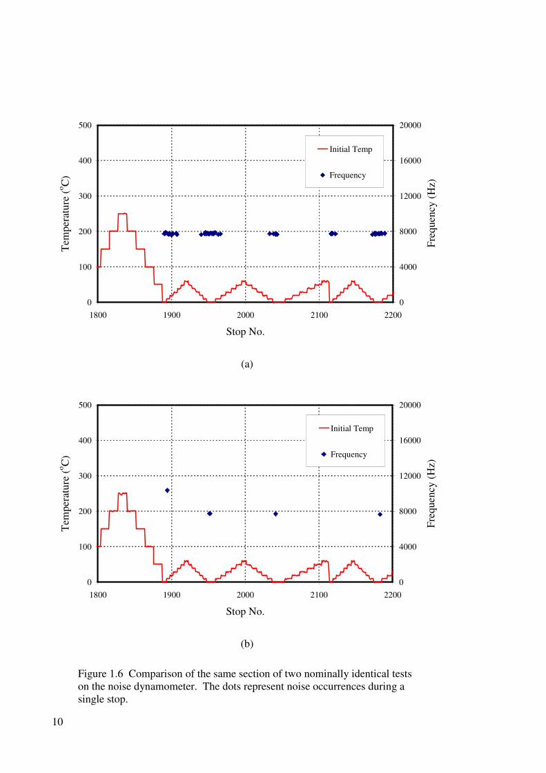
A brake system may not always squeal given the “same” apparent conditions. Critical
changes between components, component interfaces and operational conditions may be
imperceptible on a macroscopic scale. The results of two noise dynamometer tests for
components selected to be matched in terms of component natural frequencies, pad

9
compressibility, environmental conditions and test procedure are compared in Figure
1.6. It is clear that the occurrence of noise on one test was far greater in (a) than (b).
Alternatively, small variations in operating temperature, brake pressure, rotor velocity
or coefficient of friction may result in differing squeal propensities or frequencies.
Figure 1.7 show examples of the percentage occurrence of brake squeal obtained with a
brake noise dynamometer testing a typical brake system. It can be seen from Figure 1.7
(a) that there is no simple relationship between the percentage occurrence and frequency
of the brake squeal and the brake pad pressure. Similarly, the influence of initial brake
temperature (IBT) on both the occurrence and frequency of the brake squeal is equally
complicated as shown in Figure 1.7 (b).
Due to the above mentioned difficulties in designing a noise free brake system, efforts
to eliminate brake squeal have largely been empirical, with problematic brake systems
treated in a case by case manner. The success of these empirical fixes depends on the
mechanism that is responsible for causing the squeal problem.
10
0
100
200
300
400
500
1800 1900 2000 2100 2200
Stop No.
Tem
per
atu
re (
oC
)
0
4000
8000
12000
16000
20000
Fre
quen
cy (
Hz)
Initial Temp
Frequency
(a)
0
100
200
300
400
500
1800 1900 2000 2100 2200
Stop No.
Tem
per
atu
re (
oC
)
0
4000
8000
12000
16000
20000
Fre
quen
cy (
Hz)
Initial Temp
Frequency
(b)
Figure 1.6 Comparison of the same section of two nominally identical tests
on the noise dynamometer. The dots represent noise occurrences during a
single stop.

11
(a) Noise occurrences and Frequency versus brake line pressure
(b) Noise occurrence and frequency versus IBT
Figure 1.7 Example noise sensitivities to brake pressure and IBT
1.4 Thesis outline
In this thesis, many of the difficulties in addressing brake squeal are investigated.
Chapter 2 provides a review of the literature on brake squeal research and outlines the
principal models used for describing the onset of squeal noise.
In Chapter 3, the experimental characterisation of the brake system dynamics is
presented. Firstly the modal properties for the individual components of the brake
system are determined using experimental modal analysis. The properties of the

12
complete brake assembly under various boundary conditions then follow. Finally
practical measurements of brake squeal noise on the brake noise dynamometer are
presented.
Chapters 4 through 6 outline the core numerical investigations using the commercial
finite element analysis (FEA) code MSC.Nastran. Chapter 4 outlines how FEA was
applied in normal modes analysis of both the components and the assembly and Chapter
5 describes the complex eigenvalue analysis procedure used to determine system
stability. Chapter 6 introduces three further analysis techniques to allow further
numerical assessment of the squeal propensity of the test brake system; strain energy,
feed-in energy and modal participation.
In Chapter 7, a parametric study is outlined to illustrate the influence of a variety of
system parameters on the squeal propensity of the brake system.
An alternative FEA code, Abaqus, is also applied to analysing the brake system.
Chapter 8 outlines the differences in approach using Nastran and Abaqus, and compares
their performance in predicting the brake squeal propensity of a brake system. An
example of a practical, real world application of Abaqus to improve the design of a
brake rotor is given in Chapter 9.
Chapter 10 provides a summary of the completed work and discusses areas for future
work.

13
Chapter 2
Literature Review
2.1 Introduction
Research into understanding brake squeal has been ongoing over the last 50 years or
more. Initially drum brakes were studied due to their extensive use in early automotive
brake systems. However, disc brake systems have been common place on passenger
vehicles since the 1960s and are used more extensively in modern vehicles. It follows
that research into brake squeal became focused more onto disc brake systems.
Brake noise, vibration and harshness (NVH) continues to be an extremely active area of
research. As shown in Figure 2.1(a), over the last 20 years, there is a significant
increase in the number of papers on brake squeal published in the period 2001-2005 in
journals included in Thomson ISI citation index. Similarly, Figure 2.1(b) shows that the
number of brake squeal papers presented at the SAE Annual Brake Colloquium has
been increasing steadily from 25% of the total number of papers in the period 1997-
1999 to 37% in the period 2003-2005.
Unfortunately, the large body of research into brake squeal has failed to provide a
complete understanding of, or the ability to predict its occurrence. Certainly the
understanding of certain aspects of brake squeal has improved, and specific modelling
techniques have been shown to offer good correlation to observed squeal in some cases,
but no reliable procedure for eliminating brake squeal altogether has been developed. It
appears likely that a practical, generally applicable cure for all brake squeal will never
come to fruition.
This inability to fully characterise and control squeal should not be viewed as a failure
on the part of researchers. It is partly due to the shear complexity of the mechanisms
that cause brake squeal at both the micro and macroscopic levels, and partly due to the
transient and elusive nature of brake squeal that often limit the direct probing of a
squealing brake.

14
0
10
20
30
40
50
1981-
1985
1986-
1990
1991-
1995
1996-
2000
2001-
2005
Year
(a)
0%
5%
10%
15%
20%
25%
30%
35%
40%
1997-1999 2000-2002 2003-2005
Year
(b)
Figure 2.1 (a) Number of brake squeal papers according to Thomson ISI
Web of Science on 4 August 2006, (b) Number of brake squeal papers as a
percentage of the papers presented at the SAE Annual Brake Colloquium.
The competitive nature of the automotive industry, which limits the amount of
cooperative research that is published in the open literature, has also been an
impediment, although some of these hurdles are being reduced. While component
suppliers and manufacturers may still not always openly disclose the nature of their
research, much progress has been made within European and US working groups on
brake noise in openly discussing some of the key areas of concern and introducing some
standardised testing procedures. This allows more opportunity for researchers to be in
open communication within each other.
This chapter will endeavour to provide an overview on the published research into brake
squeal noise. Firstly the previous reviews of brake squeal will be covered before

15
moving into the main approaches used by previous researchers. These can be broadly
classed as:
1. Analytical
2. Experimental
3. Numerical
2.2 Reviews of Brake Squeal
Several reviews of brake squeal have appeared in the literature. North (1976) provided
coverage of the basic theories used to analyse brake squeal up until that time which
included highly simplified geometry based models, such as cantilevers and pin on disc
models. Use of numerical analysis such as the finite element method (FEM) was not
yet practical at that time so the analytical models were simple with only a limited
number of degrees-of-freedom (DOFs) that didn’t directly relate to any specific brake
geometry.
Yang and Gibson (1997) conducted a review of the modern aspects of brake squeal
research. In particular, they noted the limitation of using large multi-DOF FEM models
for analysis lies in the difficulty in modelling the friction interface. They expressed
hope for the future, but noted that experimental methods had been more productive in
addressing brake noise concerns.
Arguably the most comprehensive review of brake squeal has only recently been
published. Kinkaid et al (2002) examined most aspects of the research that has been
conducted over the years including not only the approaches used by previous
researchers in tackling brake squeal, but also provided a background of modern brake
system operation. While they felt that a truly useful general theory of brake squeal may
not become reality, or may be too complicated to be practical, they did note that there is
considerable scope for improvements in the current modelling methods of brake squeal.
A four part series covering many aspects of automotive brake squeal was published by
the SAE in 2003. Part I covered the mechanisms thought to be the root of brake squeal
(Chen et al, 2003a), Part II looked into simulation and analysis (Ouyang et al, 2003),
Part III tackled testing and evaluation (Chen et al, 2003b), and Part IV covered brake
squeal reduction and prevention (Chen et al, 2003c).
16
2.3 Analytical Approaches to Brake Squeal
Much of the early work into brake squeal can be described as analytical. The theories
used to describe the phenomena hinged upon relatively simple models with a small
number of DOFs that were tractable for hand calculation. The goal was then, as it is
now, to find the source of the instability within a brake system during squeal.
The models that are reviewed in this section were used as possible models to describe
the mechanism of brake squeal. In practice, the squeal may be due to one or more
mechanisms, or not at all. It is difficult to confirm with certainty that they are the exact
physical squeal mechanism in the brake system under investigation.
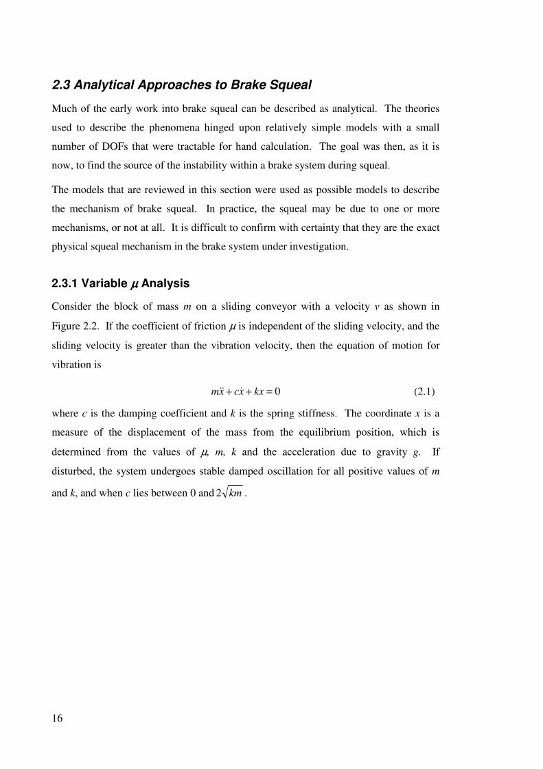
2.3.1 Variable µµµµ Analysis
Consider the block of mass m on a sliding conveyor with a velocity v as shown in
Figure 2.2. If the coefficient of friction µ is independent of the sliding velocity, and the
sliding velocity is greater than the vibration velocity, then the equation of motion for
vibration is
0=++ kxxcxm &&& (2.1)
where c is the damping coefficient and k is the spring stiffness. The coordinate x is a
measure of the displacement of the mass from the equilibrium position, which is
determined from the values of µ, m, k and the acceleration due to gravity g. If
disturbed, the system undergoes stable damped oscillation for all positive values of m
and k, and when c lies between 0 and km2 .

17
Figure 2.2 A single degree-of-freedom featuring a block rubbing on a
moving conveyor.
However, if the coefficient of friction was not constant but a function of velocity as
shown in Figure 2.3, then the potential arises for the system to become unstable.
Figure 2.3 Negative slope µ-v characteristic.
The coefficient of friction decreases as velocity increases giving
ss vv αµµ −= 0)( (2.2)
where µ0 is the coefficient of static friction, α is the negative slope of the friction curve,
and vs is the sliding velocity given by xv &− .
m
k
c
x
v
µ
v
µ0
α
1

18
Incorporating the negative µ - v into from equation (2.2) into equation (2.1) yields
0)( =+−+ kxxmgcxm &&& α (2.3)
where g is the acceleration due to gravity and other symbols as described earlier. It can
be seen that it is possible for the damping within the system to take a negative value, if
mg
c>α (2.4)
This gives rise to the instability and the system can undergo self-excited oscillation.
As cited by Kinkaid et al (2002), this line of thinking prompted early researchers into
brake squeal, such as Mills (1938), and Fosberry and Holubecki (Fosberry and
Holubecki, 1959, Fosbery and Holubecki, 1961), to suggest that the variation in the
friction coefficient with sliding velocity was the root cause of the instability driving
squeal.
The negative µ - v characteristic has since fallen out of favour and it has been shown to
be of little or no importance in brake noise generation other than for very low speed,
low frequency noise such as creep-groan (Lang and Smales, 1983, Eriksson and
Jacobson, 2001).
2.3.2 Sprag-Slip Analysis
Squeal has been shown to occur in brake systems where the coefficient of kinetic
friction is constant. The earliest analysis performed to explain this was by Spurr (1961)
in his investigations into railway, drum and disc brakes in the early 1960s. Spurr
proposed an early sprag-slip model that describes a geometric coupling hypothesis.
Consider a strut inclined at an angle θ to a sliding surface as shown in figure 2.4(a). The
magnitude of the friction force is given by
θµ
µ
tan1−=
LF (2.5)
where µ is the coefficient of friction and L is the load. It can be seen that the friction
force will approach infinity as µ approaches cot θ. When µ = cot θ the strut ‘sprags’ or

19
locks and the surface can move no further. Spurr’s sprag-slip model consisted of a
double cantilever as shown in figure 2.4(b). Here the arm O′P is inclined at an angle θ′
to a moving surface. The arm will rotate about an elastic pivot O′ as P moves under the
influence of the friction force F once the spragging angle has been reached. Eventually
the moment opposing the rotation about O′ becomes so large that O″P replaces O′P, and
the inclination angle is reduced to θ″. The elastic energy stored in O′can now be
released and the O′P swings in the opposite direction to the moving surface. The cycle
can now recommence resulting in oscillatory behaviour.
(a) (b)
Figure 2.4 (a) Single strut rubbing against surface, (b) sprag-slip system
Others extended this idea in an attempt to model a brake system more completely.
Jarvis and Mills (1963) used a cantilever rubbing against a rotating disc, and Earles and
Soar (1971) used a pin-disc model.
Millner (1978) modelled the disc, pad and caliper as a 6-degree of freedom, lumped
parameter model and found good agreement between predicted and observed squeal.
Complex eigenvalue analysis was used to determine which configurations would be
unstable, and tried to apply as much physical relevance to his model as possible.
Parameters investigated included the coefficient of pad friction, Young’s modulus of
pad material, and the mass and stiffness of caliper. Squeal propensity was found to
increase steeply with the coefficient of friction, but squeal would not occur below a cut
off value of 0.28. He found that for a constant friction value, the occurrence of squeal
and squeal frequency depends on the stiffness of pad material (Young’s modulus).

20
Caliper mass and stiffness also displayed distinct narrow regions where squeal
propensity was high.
The terms “geometrically induced instability” and “kinematic constraint instability”
were introduced by Earles and Chambers (1987). These terms and sprag-slip are often
applied interchangeably to the type of behaviour described in these models.
Murakami et al (1984) applied a combination of negative µ-v and sprag-slip in the
models they created and attributed a portion of blame to both phenomena. The µ-v
characteristic was reasoned to provide an energy source for the squeal, and the
geometric instability provides the pathway for squeal generation.
Nishiwaki (1991) argued that the source for all brake noise was the same; variation in
friction forces through a cycle. This can be seen with either negative µ-v friction
behaviour or the variation in normal forces in sprag-slip type models with constant µ.
The common conclusions of kinematic constraint stability models are that brake squeal
can be caused by geometrically induced instabilities that do not require variations in the
coefficient of friction. The variations in frictional forces during the cycle can be
geometrically driven.
2.3.3 Mode Coupling Analysis
Another type of instability that has been described in relation to brake systems is due to
mode coupling. Other names used in the literature include binary flutter and non-
conservative displacement dependant forces. Again, the variation through the cycle of
frictional forces drives the self-excited vibration, but in this case the resulting motions
form when two adjacent vibration modes coalesce.
A detailed analysis of a two DOF system was performed by Hoffman et al ( 2002) in an
effort to provide physical insight into the mode coupling instability. Consider the
system shown in Figure 2.5. Linear springs k1 and k2 are inclined at angles to the
normal (x) and tangential (y) directions respectively, coupling them. A further linear
spring k3 represents the contact stiffness between the mass and the sliding surface, and
coulomb friction coefficient µ acts tangentially.

21
Figure 2.5 Two degree-of-freedom system analysed by Hoffman, et al.
The equations of motion can be expressed as the matrix equation
=
−+
N
F
F
F
y
x
kk
kkk
y
x
m
m
2221
31211
0
0 µ
&&
&& (2.6)
where
k11 = k1cos2α1 + k2cos
2α2,
k12 = k21 = k1sinα1cosα1 + k2sinα2cosα2,
k22 = k1sin2α1 + k2sin
2α2 + k3,
and x&& and y&& are the 2nd
time derivatives of the displacements x and y respectively.
The friction coupling term ∆ = k3µ. appears as an off diagonal term in the system
stiffness matrix, hence it is unsymmetric. With suitably chosen values of m, α1, α2, k1,
k2, and k3, the system possesses two, possibly complex, eigenvalues
[ ]2
1
2,1 ∆−±±= bas (2.7)
where a and b are real numbers.
The value of ∆ is of critical importance to the resulting eigenvalues and eigenvectors. If
∆ < b then two normal, undamped modes occur with distinct frequencies. As ∆
approaches b the modal frequencies converge. At ∆ = b the modes coalesce and form a
stable and an unstable mode pair. The motion of the modes is no longer normal, that is,
k3
k2 k1
m
α1
α2
FN FF
y
x

22
they no longer move perfectly in or out of phase with each other, but now a phase
relationship between the DOFs allows the mass to take on a loop in the x-y plane.
This type of behaviour has been analysed on a variety of levels, ranging from simplified
models of a limited number of degrees-of-freedom in the vein of the sprag-slip models,
through to large scale models using FEA. In systems of much larger DOFs, the mode
coupling can occur between many mode pairs, and a variety of stable/unstable modes
may exist. These are characterised by the same shift away from normal mode behaviour
at the point of coalescence, and the formation of complex modes where non 0° or 180°
phase relationships exist between DOFs.
North (1976) presented an eight-degree of freedom model that included a bar
representing the disc. The model attempted to mimic real aspects of a brake system
more than earlier simplified models, and displayed binary flutter type behaviour.
Work has been done on examining the influence of geometry and symmetry on mode
coupling using relatively simple models. Mottershead and Chan (Mottershead and
Chan, 1992, Mottershead and Chan, 1995) have published several works on the
behaviour of repeated modes or “doublets” in symmetric structures like brake rotors, as
have Lang and co-workers (Lang and Newcomb, 1990, Lang et al, 1993). It should be
noted that much of this work is shifting away from simplified analytical models toward
larger scale FEA models.
Further more recent analysis of simple models have been conducted by Brooks et al
(1993) and El Butch and Ibrahim (1999). Both studies included efforts to optimise
piston location to reduce squeal propensity.
Since these closed form theoretical approaches discussed in previous sections cannot
adequately model the complex interactions between components found in practical
brake systems their applicability has been limited. However, they do provide some
good insight into the mechanisms of brake squeal by probing the fundamental physical
phenomena that occur when a brake system squeals.
Analytical models are not confined to history with the advent of more sophisticated
modelling tools such as FEA. Much work continues in trying to understand the
mechanisms of brake squeal using relatively simple analytical models. An example of
this approach in a practical setting is work performed by Denou and Nishiwaki (2001)

23
who used simple models to provide guidance on the general direction a design should
take before conducting more sophisticated and detailed analysis.
2.4 Experimental Approaches to Brake Squeal
Experimental approaches to brake squeal analysis revolve about understanding the
characteristics of the brake system during a squeal event. This includes evaluating the
modal properties of the brake system, both at a component level and as an assembly,
investigating the nature of the friction processes and interactions within the system, and
also determining the sound radiation of the characteristics of the brake system. A good
understanding of the characteristics is required in support of other brake squeal
analyses, especially in the case of validating a large scale FEA model.
Experimental modal analysis techniques are well suited to determine the modal
properties of a brake; that is, the modal frequencies, damping and mode shapes. A good
example of the characterisation of a brake system as part of a larger research project
was described by Richmond et al (1999). Firstly the components were analysed
individually and their modal properties determined before moving on to the system as
an assembly. Traditional accelerometer based measurements are suitable for component
level analysis, although the advent of laser vibrometry greatly increases the speed at
which this can be achieved.
Experimental modal analysis is of critical importance in understanding the behaviour of
the disc brake rotor itself. Note only is it required to establish the modal properties of
the brake rotor, but the complexity and modes found with a brake rotor, and their
interactions have been found to be key in many studies on high frequency brake squeal,
ie, squeal above 5 kHz (Matsuzaki and Izumihara, 1993, Dunlap et al, 1999, Chen et al
2000, Chen et al 2002).
Brake rotors possess several different types of vibration modes, but can be broadly
classified as in-plane and out-of-plane. In-plane modes came in several types, but the
squeal frequency of a brake system often correlates strongly with the tangential (also
called circumferential or longitudinal) in-plane vibration modes of the rotor (Matsuzaki
and Izumihara, 1993, Dunlap et al, 1999, Chen et al 2000, Chen et al 2002).
Matsuzaki and Izumihara (1993) showed that the squeal noise in their study correlated
with a rotor tangential in-plane noise rather than rotor bending modes. Modifying the

24
brake rotor by cutting slits into the brake rotor friction faces to modify the behaviour of
the in-plane modes and reduced the occurrence of squeal.
Dunlap et al (1999) examined a variety of brake squeal problems, low and high
frequency, but again the high frequency problem was found to correlate strongly with
the existence of tangential in-plane rotor modes.
Chen et al (2000) investigated the relationship between in-plane modes and out-of-plane
modes that were close in frequency. It was reasoned that energy from in-plane modes
could be efficiently transferred to out-of-plane modes if they occurred at the same
frequency driving the squeal. A further investigation provided an in-depth study on 8
different rotor designs to establish the frequency relationship between the in-plane and
bending modes of a rotor (Chen et al, 2002). They concluded that coupling of rotor
tangential in-plane modes and rotor bending modes were the primary cause of high
frequency brake squeal. The squeal frequency would occur at the rotor in-plane
frequency, but the mode shape would correspond to the coupled out-of-plane mode.
The design guideline they provided stipulated that the rotor tangential in-plane modes
should lie within the central 1/3 frequency band of adjacent dominant out-of-plane
modes.
A further study by Chen et al (2004) again focused strongly on the relationship between
in-plane and out-of-plane modes. A key influence other than the rotor design was the
brake pad. Friction forces tend to excite the in-plane modes, and pad bending can excite
out-of-plane modes. Pad chamfering, which reduces the pad foot print on the pad at the
rotor / pad interface, can help alleviate high frequency in-plane related noise. Altering
pad resonant frequencies can also help.
While high frequency brake squeal highlights the importance of the brake rotor modes,
low frequency brake squeal in range of 1 to 4 kHz has been found to depend more
strongly on the caliper components in addition to the rotor.
Baba et al (1995) studied low frequency squeal and found it particularly sensitive to the
characteristics of the caliper mounting bracket. Dunlap et al (1999) showed the
importance of both rotor and caliper modes in the appearance of “modal locking.”
Ishihara et al (1996) concentrated on rotor behaviour, highlighting that any of the major
components are important in low frequency squeal.

25
Control of rotor resonant frequencies pose a concern for both low and high frequency
brake occurrences. Grey cast iron, which is the usual material for brake rotors, is
somewhat unique in that it can change significantly in modulus and therefore modal
frequencies which are proportional to the square root of the modulus. Other brake
components, with the exception of the brake pads, are not made of material that can
vary significantly in modulus or density, so their compositions are not the subject of
specific studies.
Several studies have been done on the nature of a brake rotor’s sensitivity to carbon
content, or more usually carbon equivalent (CE). Malosh (1998) provides an analysis
on the relationship between the elastic modulus E of grey cast iron and the carbon
equivalent as
CEGPaE 1.543.310)( −= (2.8)
for the range of 8.43.3 ≤≤ CE , the range for typical grey cast iron. The carbon
equivalent is given as
3
%%
SiCCE += (2.9)
where %C and %Si are the percentage compositions by weight of carbon and silicon
respectively.
Chatterley and Macnaughton (1999) do not provide an explicit relationship between CE
and modulus, but merely discuss similar trends on the basis of a survey of typical
European rotor materials, their compositions and applications. Also, the equation they
gave for CE takes the form of a carbon equivalent liquidus (CEL) taking into account
the addition of phosphorous also
2
%
4
%%
PSiCCEL ++= (2.10)
To assist in understanding the behaviour of a brake system, it is of great importance to
be able to visualise dynamical deformations, or operating deflection shapes (ODS),
during a squeal event. Taking measurements of a squealing brake is difficult since the
brake rotor itself rotates, so that it is not possible to use conventional measurements, for
example with accelerometers. Further complications to the measurement process also
include the transient and fugitive nature of squeal, which ideally requires an
26
instantaneous measurement, and a large number of components deforming in different
scales, which places demands on the resolution requirements.
A number of optical techniques have been developed in an attempt to overcome these
difficulties. The main type that has achieved practical success is Double Pulse
Holographic Interferometry (DPHI). DPHI provides excellent temporal and spatial
resolution, but is somewhat specialised and suitable mostly for laboratory research.
DPHI has been applied with considerable success since the 1970s. High energy pulses
are generated by a powerful laser such as a ruby laser and illuminate the vibrating object
at two points during a vibration cycle. Each pulse is split into a direct reference beam
falling directly onto a holographic plate and an object beam reflected from the vibrating
object. The difference in path length of the object beam for the two pulses due to the
deformation causes an interference pattern on the holographic plate. The fringe pattern
represents contours of displacement during the cycle. Felske et al (1978) successfully
visualised a squealing disc rotor and caliper components. Time average holography was
also used to visualise an artificially excited brake system. DPHI has further been used
by a number of researchers for visualising the brake systems including Murukami et al
(1984), Nishiwaki et al (1989), and Ichiba and Nagasawa (1993). Fieldhouse and
colleagues have also used DPHI on many disc and drum brake squeal problems
(Fieldhouse and Newcomb, 1991, Fieldhouse and Newcomb, 1996, Fieldhouse and
Rennison, 1998, Fieldhouse and Beveridge, 2000, Fieldhouse and Beveridge, 2001,
Talbot and Fieldhouse, 2001).
While pulse laser systems have improved in their user friendliness and flexibility over
the last several decades, the main features of DPHI applied to brake systems have not
changed a great deal. The main limitations revolve about trying to implement a
practical system that could be used in an industrial environment in a “turn-key” fashion.
Scanning Doppler Laser Vibrometer (DLV) systems offer considerable practical
advantages over DPHI, and now practical, easy to use systems have been employed by
several research groups. McDaniel et al (1999) used a scanning laser vibrometer to
measure the ODS of a statically loaded and artificially excited brake system. These
results were then used to assist the study of sound radiated by the system. Richmond et
al (1999) and Chen et al (2002) also made measurements on a static system in this
manner.

27
Scanning laser systems utilising three heads to resolve 3-D motions are only just
beginning to be employed in industrial research (Polytec, 2007). The future of these
systems is bright since they allow the visualisation of in-plane motions is addition to
out-of-plane. The 3-D systems have been developed specifically to allow investigation
of squealing disc brake systems.
The techniques described in this section have provided some good and useful tools for
investigations into brake vibration characteristics. In particular, accelerometer and laser
based modal property and ODS measurements can be resolved with great accuracy for
static systems. However, the shortfall is in measurements of a system during squeal.
DPHI systems are difficult to implement in practice and scanning laser systems struggle
to provide temporal and spatial resolution for transient events. Hence, these tools need
to be further developed to be useful in the industry. The experimental techniques used in
industry are described in Section 3.11.
The focus of this section has been on understanding the vibration characteristics of the
brake system. These characteristics alone do not determine if a squeal concern will
arise. Understanding the system’s sound radiation provides the link between the
vibration behaviour and a squeal concern. For example, sound radiation efficiency
using the two-microphone technique, or acoustic holography with a microphone array
can be used to investigate the acoustic sound field around the brake system as a result of
system vibration.
2.5 Numerical Methods for Brake Squeal Analysis
Numerical analysis of brake squeal can be considered a more sophisticated extension of
the analytical models discussed earlier. However, by using powerful computers and
finite element analysis (FEA), it is possible to model individual components as
continuous structures and incorporate their elastic properties into a dynamical
description of the system.
FEA has been used to determine the modal frequencies and mode shapes of individual
components. This is also required before a larger assembly analysis can be performed
to validate the individual component modes against experimental measurements.
Examples of this type of work were the work done by Richmond et al (1999) on the
components of an assembly and Saka and Wada (2003) who undertook a study to

28
provide a systematic method for naming mounting bracket modes in terms of a ring and
a bent ring. Kumemura et al (2001) analysed low frequency behaviour of a brake
anchor bracket / suspension knuckle assembly and increased stiffness of the bracket to
improve a low frequency squeal concern.
The prediction of system stability is one area where there has been a large amount of
research using FEA. Complex eigenvalue analysis is the main solution technique that
has been used in assessing system stability. Complex eigenvalue analysis is a large scale
extension of the mode coupling type instability discussed in section 2.3.3. By far the
majority of the research that has been performed has utilised the commercial FEA code
Nastran. Nastran is favoured because it has well established eigenvalue solution
schemes and until recently was the only commercial code to perform the analysis. The
analysis proceeds by solving a static step to determine the static position of the brake
assembly components. The system is then linearised about this base position and a
complex eigenvalue extraction is performed to determine the stability of the system
modes based on the appearance of negatively damped modes.
The first major published work was a study performed by Liles at GM (Liles, 1989).
Liles manually inserted springs and friction elements to model the friction coupling at
the rotor/pad interface, thereby creating an unsymmetrical system stiffness matrix; a
necessary, but not sufficient, condition to produce coupled modes and system instability
(Liles, 1989). Liles went on to study a variety of brake system parameters including
coefficient of friction, pad geometry, caliper and rotor stiffness, and system damping.
This type of analysis was further championed by Nack, also at GM, using much the
same analysis methods as Liles. Nack and Joshi (1995) studied low frequency brake
noise and observed the coupling of system modes at the onset of instability. A further
study focusing on brake squeal was later presented (Nack, 1999). The main limitation
expressed in these studies was the limited modelling of variable friction coefficient, and
future work suggestion was to move toward time domain analysis.
Complex eigenvalue analysis to assess stability forms the first step in many studies and
further analyses have been applied to probe the behaviour of the brake system and to
develop countermeasures. Kung et al (2001a) used the Modal Assurance Criterion
(MAC) to identify modal participation of component modes in unstable modes extracted
from a complex eigenvalue analysis. A parametric study was conducted to observe the

29
influence of varying friction coefficient and brake rotor modulus. A further study was
conducted that involved shifting the frequencies of two system modes further apart in
frequency to reduce their tendency to form a coupled unstable system mode (Kung et al,
2000b).
Park et al (2001) used MAC to assess the modal participation in the unstable system
mode which was the focus of their study, but also used component strain energy to
further identify which component would be best modified.
Zhang et al (2003) also used both MAC and strain energy to aid identifying potential
countermeasures, but also included a number of alternative measures of component
participation. The 1-norm and infinity-norm were calculated and compared as
indicators of component contributions along with strain energy. The norms offered
similar information as to which components contributed the most. Strain energy was
found to offer quite different conclusions due to the significant differences in size and
material properties of each of the components. They suggested that each of the
indicators should be used in a complimentary manner.
Another stream of complex eigenvalue analysis began in 2003 when HKS Abaqus
provided an appropriate eigenvalue solver. The main feature of Abaqus is advance non-
linear and contact solving capabilities in the non-linear static parts of an analysis. Bajer
et al (2003) described the basic formulation of this scheme, and Kung et al (2003)
investigated the instability related to various in-plane rotor modes.
The major advantage of Abaqus over the previous analysis using Nastran is the
seamless integration of non-linear static analysis and dynamic analysis without the
requirement for manual inserted friction coupling terms. The contact element
formulation removes the need for coincident node meshing at the component interfaces.
Abaqus also provides the ability to utilise some aspects of a velocity dependent friction
coefficient.
Guan and Huang (2003) presented the method of feed-in energy analysis for a brake
system. This is a method that calculates the frictional work converted into vibration
energy by considering the relative motions of a friction contact pair at the friction
interface. If the feed-in energy is positive then system vibrational energy is increasing
and the system is unstable, and they showed that feed-in energy is an alternative to
considering the real part of eigenvalue as an indicator of stability.

30
Another form of stability prediction that has been used much less widely is non-linear
transient analysis. This type of analysis follows the evolution of displacements in the
time domain and an unstable state is identified by divergence away from equilibrium. A
Fast Fourier Transform (FFT) analysis is performed to identify frequencies associated
with the noise. Hu and Nagy (1997) performed a non-linear transient analysis using LS-
Dyna and achieved good correlation of measured noise performance. The key benefits
of the analysis as compared to complex eigenvalue analysis that they identified were:
the ability to implement more sophisticated friction behaviour, it was not necessary to
determine system static state prior to analysis, and finally the variation in component
contact during vibration is captured. Chargin et al (1997) also presented a study using
non-linear transient analysis. They did not include a direct correlation to a specific
brake system, but concentrated on a detailed description of their modelling procedure.
Chern at al (2002) have also performed non-linear transient analysis using LS-Dyna.
The main drawback of the technique is the demand on computer resources. The size of
time increments, which is a function of element mesh size and propagation velocity of
vibration waves, requires an enormous number of solutions to be preformed.
The methods covered in this section involve large scale FEA models to investigate the
vibration behaviour of a brake system and components. However, such analysis is not
capable of predicting whether a particular vibration mode will cause an audible squeal
concern. The boundary element method (BEM) can be applied to determine the sound
radiation efficiency of the system, and thus link the vibration characteristics to the
radiated sound.
2.6 Brake Squeal Noise in Practice
The methods for addressing brake squeal noise during development of a production
brake system remain largely empirical. Counter-measures are developed during final
development of the system typically by trial and error in conjunction with noise
dynamometer and on-vehicle testing. This section gives a feel for the types of counter-
measures that are applied to many automotive brake systems in production today.
The addition of shims to the back of pad backplates is used on most brake systems
today, usually in the form of a multilayer form. Two common types of shim are in wide
spread use. The first type utilises several layers of steel shim with grease applied
between the layers. The second type features a multi-layer design of alternating rubber

31
and steel, bonded together to the back of the backplate. The rubber forms a constrained
layer and induces significant damping through shear of the rubber layer. An example
material is shown in Figure 2.6 and material properties in Table 2.1.
Table 2.1 Layer specification of typical damping shim material
Layer (from piston side) Thickness (mm) Rust prevention 0.02
Steel 0.40
Nitrile rubber 0.24
Adhesive 0.12
Total 0.78 Additional removable protective paper layer 0.15
Figure 2.6 Example shim material
The function of shims operates on many different levels (Flint and Hald, 2003). Shims
can provide additional damping for the brake system, shims can decouple the caliper /
pad interface, and shims can alter the pressure distribution between components by
geometry. Figure 2.7 is an example of a shim that has been designed to shift the centre
of contact pressure of the piston on the back of the pad.
Another common strategy for the controlling brake noise is modification of the surface
area of the brake pads at the critical rotor / pad interface, as shown in Figure 2.8. This
is achieved most commonly by inserting chamfers onto the surface of the brake pad.
The final form chamfers take before production begins is often through continuous
refinement and testing.
Piston
side

32
Figure 2.7 Example slotted backplate shim designed to shift the centre of
contact pressure on the piston / pad interface.
Figure 2.8 Example of pad chamfers
Investigation of noise concerns at specific frequencies requires investigation of the
dynamical properties of the components themselves. Care needs to be taken since
properties under free-free boundary conditions may change when the component is
constrained in a brake assembly. However, the free modes near a particular squeal
frequency can be used as a guide when considering structural modifications.
Operational deflection shape (ODS) measurement on a squealing brake can be used to
understand what component modes are active. This leads in the direction of structural
modifications of caliper components or the rotor.

33
Unfortunately the bulk of structural modification implemented in industry proceeds on a
trail and error basis. Changes revolve around changing mass and stiffness
characteristics of components and validation occurs on the brake noise dynamometer or
in vehicle testing.
Most of the structural components within a brake system are made of metal alloys
including steel, aluminium, ductile cast iron and grey cast iron. The elastic moduli and
mass densities of these alloys are usually relatively insensitive to variation in chemical
composition. Hence there is not usually much tuning of material composition in
developing countermeasures. The exception is grey cast iron, which has an elastic
modulus that can vary greatly due to changes in carbon content and other alloying
elements. This, in turn, leads to major changes in the modal frequencies of brake rotors,
and material properties can tuned to address specific noise concerns (Malosh, 1998).
Another key area in brake noise development relates to the compressibility of the brake
pad, or more specifically, the compressibility of the friction material. Brake pads
consist of two main sections; a steel backplate and the friction material which is
moulded to the backplate. The friction material is a composite structure with potentially
dozen of constituents, the exact composition being proprietary information and known
only to the friction supplier. Further, it is not uncommon for an underlayer to be
applied between the friction material and the backplate itself, which can add beneficial
thermal and mechanical properties. The sum of all these components is a pad that is
relatively compressible, with a typical pad showing approximately 0.1mm compression
under high brake pressures.
The static compressibility of the pad can have a strong influence on the noise
performance of a brake system. It is often seen that increased static compressibility
tends to reduce noise occurrences. However, increasing static compressibility can have
a negative impact on other aspects of brake performance such as pedal feel and drag.
To further add to this complexity, friction materials may exhibit behaviour that is a
function of frequency, both in terms of stiffness and damping. For example, the
dynamic compressibility of a friction material may be significantly different from the
static compressibility. While static compressibility measurements are common in
industry, dynamic compressibility, stiffness and damping are not easily quantified and
remain as gaps in the characterisation of friction material behaviour.

34
2.7 Summary
The key methods of brake squeal investigations; analytical, experimental and numerical
have been presented. The analytical work has provided some basic models to help
understand the phenomena within brake systems. However, they have limited
applicability to any specific brake systems and practical brake squeal investigations.
Experimental work continues to be the leading form of brake development, particularly
in industry. While the complex behaviours within the system are only gradually being
revealed as new technologies allow deeper probing into the system, much successful
development work the done on the basis of observation and modification. The
application of optical visualisation techniques such as DPHI and scanning DLV have
allowed more detailed probing into brake system behaviour. Unfortunately DPHI is
difficult to apply in practice and scanning lasers systems have limitations in resolution
for transient events.
The numerical modelling of brake systems has been an area of significant growth over
the last few decades. Complex eigenvalue analysis is in widespread use and no doubt
time domain analysis will follow with the increase in computational power and
reductions in cost. Considerable gaps exist in the numerical techniques. Modelling of
contact interfaces, particularly the key pad / rotor interface, as well as correlation to true
material behaviour across the whole frequency range are still areas undergoing
development.
The focus of this thesis is in the area of numerical modelling to complement industrial
testing and development of brake systems. Complex eigenvalue analysis is the chosen
method of stability analysis due to the lower computational requirements. The areas of
deeper probing into a system behaviour following a complex eigenvalue analysis will be
studied in detail. Feed-in energy analysis as proposed by Guan and Huang (2003) has
not been taken up in widespread use. There is potential to apply it to investigate pad /
rotor interaction and to contrast it to complex eigenvalue prediction. Strain energy has
used widely to identify active components, but meaningful normalisation needs to be
investigated. Finally, addition of MAC calculations to these allows a suite of tools for
understanding system behaviour at system level. Identifying their relevance and
applying them to a large scale FEA model in a complementary manner is a key aim of
this thesis.

35
Chapter 3
Experimental Determination Of
Vibrational and Acoustical Characteristics
of a Brake System
3.1 Introduction
In general, noise problems stem from the dynamic characteristics of any system. One or
more vibration modes are excited and some of the energy is dissipated by radiating
sound. This is the case when a brake squeals. The brake system enters into an unstable
vibration mode and the brake rotor acts as a loudspeaker radiating most of the squeal
sound. Hence, it is of fundamental importance to gain an understanding of the vibration
characteristics of the brake system.
Experimental modal analysis is a technique used to determine the vibration
characteristics of a system. Measurements are made and analysed to evaluate the
vibration modes of the system. Each vibration mode consists of three modal parameters
or properties which together provide a description of the system’s dynamic
characteristics
1. Modal frequency – resonant frequency of oscillation for the mode, usually
expressed in cycles per second (cps) or Hertz (Hz).
2. Modal damping – a measure of the dissipation of vibration energy or the rate at
which the vibration decays, usually expressed as a percentage on the critical
damping; the maximum damping level which will permit free vibration.
3. Mode shape – deformation or displacement pattern of the structure for the
mode, described by complex-valued displacements
Experimental modal analysis can be a very effective analysis tool. Modifying the modal
parameters of a system can control many types of noise problems. Modal testing is also
vital in the development of numerical models such as when using the finite element
method (FEM). The modal analysis results will be required to validate FEM models,
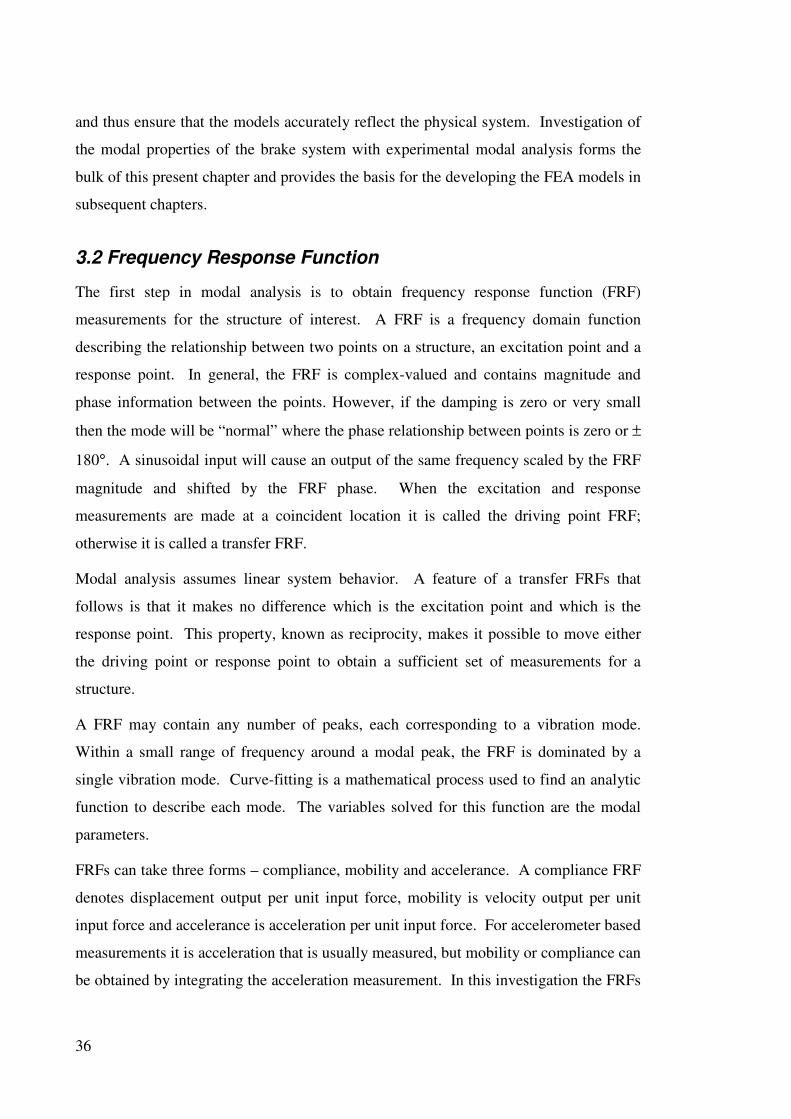
36
and thus ensure that the models accurately reflect the physical system. Investigation of
the modal properties of the brake system with experimental modal analysis forms the
bulk of this present chapter and provides the basis for the developing the FEA models in
subsequent chapters.
3.2 Frequency Response Function
The first step in modal analysis is to obtain frequency response function (FRF)
measurements for the structure of interest. A FRF is a frequency domain function
describing the relationship between two points on a structure, an excitation point and a
response point. In general, the FRF is complex-valued and contains magnitude and
phase information between the points. However, if the damping is zero or very small
then the mode will be “normal” where the phase relationship between points is zero or ±
180°. A sinusoidal input will cause an output of the same frequency scaled by the FRF
magnitude and shifted by the FRF phase. When the excitation and response
measurements are made at a coincident location it is called the driving point FRF;
otherwise it is called a transfer FRF.
Modal analysis assumes linear system behavior. A feature of a transfer FRFs that
follows is that it makes no difference which is the excitation point and which is the
response point. This property, known as reciprocity, makes it possible to move either
the driving point or response point to obtain a sufficient set of measurements for a
structure.
A FRF may contain any number of peaks, each corresponding to a vibration mode.
Within a small range of frequency around a modal peak, the FRF is dominated by a
single vibration mode. Curve-fitting is a mathematical process used to find an analytic
function to describe each mode. The variables solved for this function are the modal
parameters.
FRFs can take three forms – compliance, mobility and accelerance. A compliance FRF
denotes displacement output per unit input force, mobility is velocity output per unit
input force and accelerance is acceleration per unit input force. For accelerometer based
measurements it is acceleration that is usually measured, but mobility or compliance can
be obtained by integrating the acceleration measurement. In this investigation the FRFs

37
were all in terms of accelerance. A comprehensive description of experimental modal
analysis can be found in Modal testing: theory and practice [Ewins, 1984].
3.3 Experimental Set-up
A schematic of the experimental set-up can be seen in Figure 3.1. FRF measurements
were recorded on a fast fourier transform (FFT) analyser before being transferred to a
computer for analysis. Table 3.1 contains a listing of the equipment used for the
measurements. Shaker excitation was used for all of the testing with the exception of the
specific experiments to identify rotor in-plane modes as discussed in section 3.5.5. A
small roving accelerometer that was affixed with bee’s wax was used for the
measurements except for the driving point FRF which was obtained through the
impedance head.
The B&K type 2032 FFT analyser divides the measurement spectrum into 800 lines.
Baseband random noise excitation was used between 0 and 6.4 kHz, and zoom random
noise excitation between 6.4 and 12.8 kHz. This results in a frequency resolution of 8
Hz for 800 lines in each frequency band, which was sufficiently high to allow the FRFs
to be recorded with acceptable accuracy. The FRFs were obtained from 50 averages
using a Hanning window with 50% overlap.
Table 3.1 Experimental equipment for modal measurements.
Item Manufacturer and Type
FFT analyser B&K 2032
Accelerometer B&K 4374
Impedance head B&K 8001
Charge amplifier B&K 2635
Shaker B&K 4810
Power amplifier B&K 2706
Calibrator B&K 4294
Impact hammer B&K 8202
Computer NEC Versa 4050C
Analysis of the experimental data was conducted with STAR Modal v 5.23, a
commercial modal analysis software package. The FRFs were spatially averaged to aid
the identification of modal peaks. Modal peaks can be identified from individual FRFs,
but they can usually be identified more reliably from a spatially averaged spectrum.
Cursor bands were set up around the modal peaks in the averaged FRF data. A cursor

38
band defines a small region of the frequency spectrum where curve-fitting will be
attempted.
Five curve-fitting methods are available in STAR Modal - Coincident, Quadrature,
Peak, Polynomial and Global [Star SytemUser’s Guide, 1994]. Coincident, Quadrature
and Peak are single degree-of-freedom methods and make no estimate of modal
damping. For this reason they were not used except for an initial examination of mode
shapes. Polynomial and Global methods are suitable for single or multiple degree-of-
freedom fitting and can estimate the modal damping, modal frequency and mode
shapes. The Polynomial and Global methods use the Rational Fraction Least Squares
method to identify the modal parameters and were used throughout this investigation.
Figure 3.1: Schematic of the experimental set-up.
FFT
Analyser
Computer
Power amplifier
Charge
amplifiers
Impedance
head
Shaker
Accelerometer
Test
component
Signal generator Ch. A Ch. B

39
3.4 Component Testing
The rotor, pad, caliper housing and anchor bracket were tested and analysed
individually. The remaining components, namely the piston and pins, were not tested.
Testing with either shaker or impact excitation would not be practical due to their small
size.
Testing of the individual components was conducted with free-free boundary
conditions. This was implemented by placing the components on a sheet of foam
insulation during the testing. The rigid body natural frequencies of the component on
the foam mat were several orders of magnitude lower than the lowest structural
resonance of any component so coupling between the test component and base support
was negligible.
3.5 Rotor
3.5.1 Brake Rotor Mode Shape Descriptions
Brake rotors may appear to be relatively thin discs on first appearance, and it may seem
that the dynamic characteristics could be described by bending (out-of-plane) vibration
modes, similar to a circular plate. In reality a brake rotor possesses significantly more
complex geometry than a thin circular plate. A drum-in-hat (DIH) rotor, as shown in
Figure 3.2, is substantially thick and has a hat section that introduces asymmetry in
cross section. The hat section in particular makes it more difficult to assign a
numbering scheme to all brake rotor modes. Therefore the mode descriptions that
follow are concerned mainly with motions of the main annular disc region containing
the friction surfaces, referred to as the friction disc.

40
Figure 3.2 Cross section of a solid drum-in-hat (DIH) rear rotor.
Out-of-plane modes involve rotor bending motion and nodal regions that appear as
either diametrical or circumferential lines, as displayed in Figure 3.3. Here the regions
designated with a “+” and “-” represent regions that are 180˚ out of phase. Two
numbers, m and n, can be used to describe the modes shape in a similar manner to those
devised for circular plates as described in Rossing and Fletcher (1995). The first
number indicates the number of nodal diameters and the second number indicates the
number of nodal circumferences. The primary bending modes involve primarily nodal
diameters and commonly identified merely by the ND (nodal diameter) number.
top-hat section
Service brake
friction faces
friction disc
park brake
friction surface

41
(a) (5,0) Mode
5 nodal diameters
0 nodal circumferences
(b) (0,2) Mode
0 nodal diameters
2 nodal circumferences
(c) (5,1) Mode
5 nodal diameters
1 nodal circumference
Figure 3.3 Bending mode descriptions
In-plane vibration modes are somewhat more complicated in that a number of different
types exist. With reference to Figure 3.4, in-plane modes can be classified as either
tangential or radial modes. Tangential modes are also often also called longitudinal or
circumferential modes, and radial modes are also known as star modes.
Tangential in-plane modes occur in the two distinct forms, compression and shear (also
called racking), as shown in Figure 3.4 (b) and 3.4 (c) respectively. Section 3.5.5
investigates the detection of rotor in-plane modes more specifically.
+
+
+
+
+
+
_
_
_
_
+ + + +
+ _ _
_
+
_
+ +
_
_
+
+ +
+
_ _
_ _

42
(a) Radial in-plane mode with 3
nodal diameters
(b) Tangential in-plane
compression mode with 2 nodal
diameters
(c) Tangential in-plane shear
mode, 1st order.
Figure 3.4 In-plane mode descriptions
It is also possible for the equivalent modes to exist in the top hat region of the rotor.
This leads to the additional complication found in some rotor modes, with coupling
between the disc and top hat modes. Top hat modes are designated in the same way as
the disc modes, but with a prefix of TH.
3.5.2 Rotor Test Grid
The grid for the rotor, displayed in Figure 3.5, consisted of 384 measurement points
arranged along 48 lines radiating from the centre of the rotor at an angular spacing of
7.5˚. Each line featured 8 measurement points as shown in Figure 3.6. Table 3.2 lists
the coordinates for the rotor grid points.
Measurements were taken at the response points in either the local r (radial) and z
(axial) direction, while the excitation was applied with the shaker in the z direction at
point 6, shown in Figure 3.5. As a result, direct measurement of only out-of-plane and
radial in-plane modes was possible. The tangential in-plane modes can be inferred by
the accompanying deformation in the radial or, possibly, out-of-plane direction, and
with the aid of a validated finite element model. Indeed, the 1st and 2
nd tangential in-
plane modes were identified this way. However, due to the relative lack of response, a

43
direct measurement of tangential deformation is not possible while exciting and
measuring in the r and z directions. This issue is addressed further in sections 3.5.5.
Table 3.2: Coordinates for the rotor grid.
Point no. r (mm) θ (°) z (mm) Direction
1 + 8n 40 34 z
2 + 8n 80 34 z
3 + 8n 103 28 r
4 + 8n 103 8 r
5 + 8n 110 0 z
6 + 8n 125 0 z
7 + 8n 140 0 z
8 + 8n 144
7.5n,
n = 0,..,47
-8 r
Figure 3.5: Brake rotor experimental grid (384 points). Point numbering is
omitted for clarity.
Excitation
point
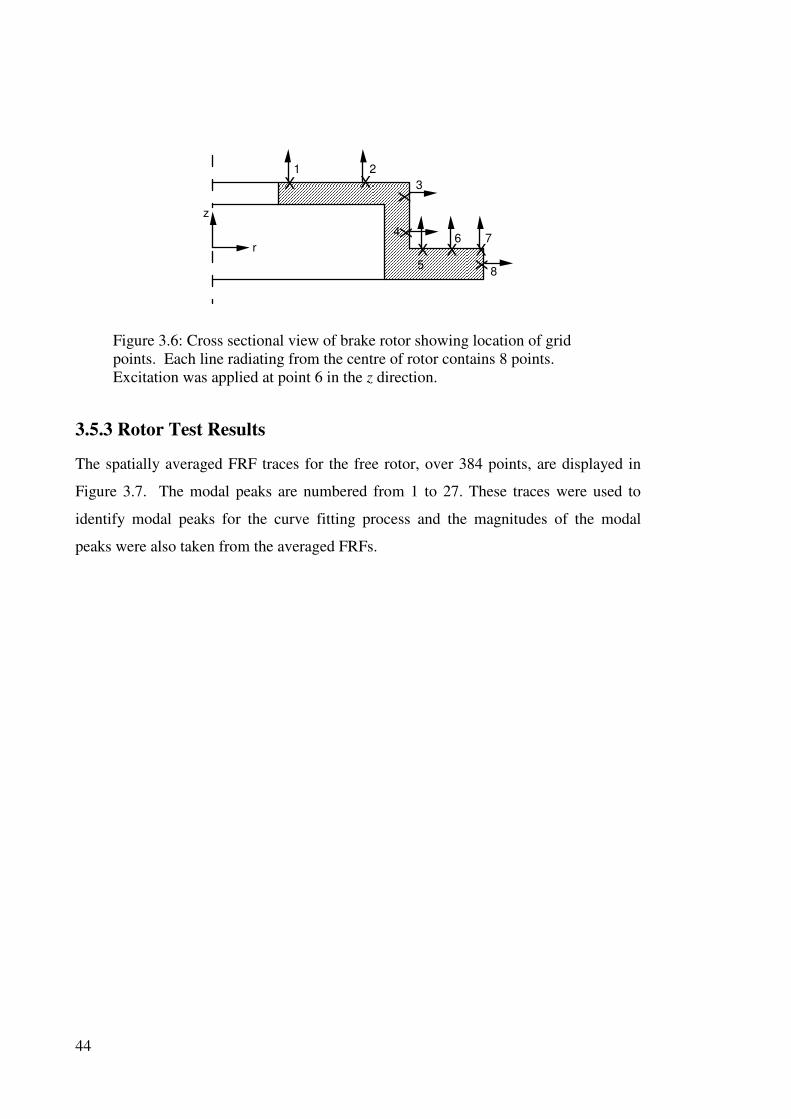
44
X X
X XX
X
X
X
1 2
3
4
5
6 7
8
r
z
Figure 3.6: Cross sectional view of brake rotor showing location of grid
points. Each line radiating from the centre of rotor contains 8 points.
Excitation was applied at point 6 in the z direction.
3.5.3 Rotor Test Results
The spatially averaged FRF traces for the free rotor, over 384 points, are displayed in
Figure 3.7. The modal peaks are numbered from 1 to 27. These traces were used to
identify modal peaks for the curve fitting process and the magnitudes of the modal
peaks were also taken from the averaged FRFs.

45
Figure 3.7: Spatially averaged rotor FRF traces.
Table 3.3 provides a summary of the modal parameters as found by STAR Modal.
Modal damping values range from under 0.1% for the top hat modes through to 0.4%
for the RI 5 mode. Most of the out-of-plane modes have a damping value between 0.1%
to .15%. It is also clear the ND bending modes (nos. 1,3,8,11,14,18,24) have the
highest modal peaks.
The 1st and 2
nd tangential in-plane modes (no. 16 and 26) were also identified, although
the modal peak for the 2nd
mode does not appear very clearly in the spectrum. These
were established through observing the accompanying radial and top hat deformations

46
and comparing these with a finite element model.
Table 3.3 Rotor modal parameters. Log magnitude is with a reference value of 1
m/Ns2. Mode shapes refer to nodal diameters and circumferences of bending
modes except where prefix is added. TH indicates deformation in predominantly
in top hat region, RI is radial in-plane and CI is circumferential in-plane.
Mode No. Mode shape Freq
(Hz)
Damp factor
(%)
Log Mag
(dB)
1 (2,0) 994 0.37 15.3
2 (0,1) 2010 0.19 21.9
3 (3,0) 2430 0.18 27.1
4 (0,2) 2550 0.22 18.7
5 (1,1) 2690 0.15 21.5
6 RI 2 2900 0.15 19.6
7 (1,2) 3200 0.16 17.6
8 (4,0) 3800 0.14 31.9
9 TH(2,1) 4230 0.15 10.2
10 RI 3 4630 0.22 17.8
11 (5,0) 5290 0.13 31.9
12 TH(1,1) + RI 1 5730 0.10 14.5
13 TH(2,2) 6770 0.12 19.1
14 (6,0) 6990 0.11 35.8
15 RI 4 7120 0.12 14.3
16 TI 1 7840 0.17 12.8
17 TH(0,2) 8130 0.11 23.2
18 (7,0) 8900 0.11 40.8
19 TH(3,2) 9090 0.07 23.2
20 TH(1,2) 9230 0.10 27.2
21 TH RI 0 9770 0.08 13.8
22 RI 5 10060 0.40 21.0
23 TH RI 3 TH(3,1) 10560 0.08 21.9
24 (8,0) 10990 0.11 44.9
25 TH(5,1) 11620 0.08 21.5
26 TI 2 12130 0.40 15.3
27 (4,3) 12360 0.07 32.2
3.5.4 In-Plane Mode Detection
Pure longitudinal waves can occur only in solids where the dimensions in all directions
are greater than the wavelength (Cremer et al, 1988). This is not the case with the rotor
since the thickness is small compared to the wavelengths of the modes of interest.
Consequently, the in-plane waves that occur are actually quasi-longitudinal and are
accompanied by deformation in the lateral direction (see Figure 3.8). This makes it
possible to measure some in-plane motion while measuring in the out-of-plane
direction.
47
Figure 3.8 (a) Out-of-plane vibration, (b)In-plane vibration. Note that the
longitudinal compression is accompanied by expansion in the lateral
direction and longitudinal expansion is accompanied by contraction.
A number of experiments were conducted to examine how well in-plane modes could
be detected by measuring in the out-of-plane direction. Matsuzaki and Izumihara
(1983) discussed a method for specifically detecting modes where in-plane vibration is
present. This can be accomplished by measuring the phase difference between the
opposite faces of the rotor. If the surfaces of the rotor have out of plane motions that
are 180˚ out of phase then the mode must have in-plane deformation. All bending
modes would have the faces of the rotor in phase.
In principle, a convenient method of identifying which are the in-plane modes would be
to mount two accelerometers directly opposite one another on the rotor surface. If
broadband excitation is applied the phase can be examined to see at which frequencies
the in-plane modes occur. Unfortunately, this method did not work with this brake
rotor and a possible explanation of why follows.
Significant induced bending can occur during in-plane vibration. Consider the rotor
shown in figure 3.9. Since the rotor is not symmetrical with respect to the plane of the
friction surfaces, this will cause significant secondary bending in addition to the in-
plane deformation. During testing it was found that the two faces of the disc surface
were in phase. This is in direct contrast to the results published by Matzusaki and
Izumihara (1983). However, their test was conducted on a vented rotor which are
usually considerably thicker than the solid type tested here. Since flexural rigidity is
proportional to the 3rd
power of section thickness, it would be reasonable to expect the
bending in their investigation to be significantly reduced compared to the rotor in this
study, making it possible to detect the phase difference between the faces.

48
Figure 3.9 Rotor in an in-plane vibration mode. The top hat provides
unsymmetrical support to the disc itself and may cause out of plane
deformation.
3.5.5 In-Plane Measurement
Experiments were also conducted to directly measure the circumferential in-plane
modes, which the shaker tests with the previous grid could not detect directly. The set
up for these experiments is shown in Figure 3.10. A steel cube of 12 mm side length
was fixed via a steel stud to the outside edge of the rotor to enable the accelerometer to
measure in the circumferential direction. An impact hammer was used to provide the
excitation directly into the in-plane direction. The rest of the experimental set up
remains unchanged from the earlier tests. Here the hammer is striking the edge of the
rotor at an angle of approximately 45°. By using the hammer in this way it is not
possible to accurately measure the magnitude of the FRFs. However, the phase
component remains intact allowing the mode shape to be determined.
The grid for this test consisted of 12 points located around the outer edge of the rotor.
The response point remains unchanged due to its mechanical fastening so a roving
exitiation point was used. The number of wavelengths for the circumferential modes in
the frequency range of interest is at most two, so it was sufficient to use only 12
measurement points around the rotor circumference to resolve the mode shapes.

49
Figure 3.10 In-plane test configuration.
Analysis was conducted for these tests without the STAR Modal software. The
objective here was to be able to visualise the circumferential modes shapes with no
specialised analysis software. The test and analysis procedure that was utilised was as
follows:
1. Measure FRFs at 12 equally spaced around the circumference using a roving
excitation and fixed response point.
2. Identify modal peaks within the FRFs. This can be done by looking for the
magnitude peaks in individual FRFs or by spatially averaging FRFs from all test
points. The averaged FRFs are more reliable than looking at individual FRFs,
but it requires data to be exported from the FFT analyser for analysis.
3. Record magnitude and phase of each point from the FFT analyser for the modal
frequencies identified in step 2. Sort the magnitudes and phase by frequency to
capture complex-valued displacement information for each mode.
4. Set the phase equal to either 1 or -1 signifying in phase or out of phase. This is
to enable the modes to be displayed as normal modes, ie, with all points either in
phase or 180˚ out of phase. Note that the level of damping for the rotor is small,
so normal modes are expected. It is best to add an offset such as 22.5˚ or 67.5˚
to the phase since the relative phase values tend to sit around multiples of 90˚.
This will reduce potential phase errors due to noise if many of the phase values
are scattered around multiples of 90˚. For example, all points with -157.5° <
50
phase ≤ 22.5° are set to 1, and all points with 22.5°< phase ≤ 202.5° are set to -1.
5. Multiply the magnitude by the rounded phase from step 4 for each point and
normalise it by the largest magnitude. The result is a single value for each point
ready for plotting.
6. Repeat steps 4 and 5 for each modal frequency.
This procedure was applied to identify the 1st and 2
nd tangential in-plane modes of the
rotor. Figure 3.11 shows the result for the 1st mode graphically. It is clear that the
displacement represents one wavelength quite well. However, great care needs to be
applied when using this procedure. The phase values can be subject to considerable
scatter and the value chosen for phase offset rounding becomes very important. It is
often best done on a case-by-case basis after inspecting the FRF data. This limitation
makes it time consuming to analyse each mode and automating the process would
require careful implementation. As a result, the procedure should be used with caution
when determining mode shapes and is best used in conjunction with a finite element
model of the structure. This way the finite element model can act as a guide to what
frequency and shape is expected.

51
Figure 3.11 Mode shape for the first circumferential in-plane mode (7840
Hz). The y-axis represents the normalised displacement from the mean
position around the circumference. The value in this case was actually
accelerance, but, once normalised, it is equivalent to displacement.
3.6 Pad
The brake pad, displayed in Figure 3.12 (a), is made of two different materials. The
backing plate is steel and the friction material is a specialised composite material. A test
grid was applied to the backing plate for these experiments. The grid consisted of 25
points with the only direction of measurement being the out-of-plane direction (see
Figure 3.12 (b)). The excitation was applied with a shaker to point 8. Appendix A
displays the coordinate table for the 25 points.

52
(a) (b)
Figure 3.12 (a) Brake pad, (b) Brake pad experimental grid geometry (25
points). The direction of excitation and measurement in the out-of-plane
direction
Modal parameters for the brake pad are shown in table 3.4. Six modes were identified
from the averaged FRF data displayed in Figure 3.15 (a). The mode shapes are defined
in a manner similar to the bending modes of a rectangular plate. The pair of numbers m,
n represent the number of nodal lines in the lateral and longitudinal direction
respectively. The modal damping is high in comparison to the other brake system
components. This is due to the high structural damping of the friction material.

53
Table 3.4 Modal parameters of the brake pad.
Mode No. Mode Shape Freq (Hz) Damp factor
(%)
1 (2,0) 2340 0.96
2 (1,1) 5160 1.02
3 (3,0) 6200 1.34
4 tab only 7460 0.97
5 (2,1) 7760 0.84
6 (4,0) 10090 0.62
3.7 Caliper Housing
The caliper houses the piston within the brake system and is made of cast aluminium
(Figure 3.13 (a)). The grid consisted of 65 points covering the outer surface of the
housing as shown in figure 3.13 (b). Measurements were taken in all three coordinates
to try and capture as much of the vibration behaviour as possible. A comprehensive
table of the coordinates and measurement directions can be found in Appendix A.
(a) (b)
Figure 3.13 (a) Caliper housing. Also seen are the slide pins which were
not analysed as part of these experiments. (b) Caliper housing experimental
grid geometry (65 points).
The caliper housing was found to have 13 vibration modes as tabulated in Table 3.5.
No convenient scheme for identifying the mode shapes was conceived, so the modes are
simply identified by consecutive numbers. It can be seen that the modal damping
values for the caliper are mostly low owing to the light structural damping of
aluminium. The averaged FRF data is displayed in Figure 3.15 (b).

54
Table 3.5: Caliper housing modal parameters.
Mode
No.
Freq
(Hz)
Damp factor
(%)
Mode
No.
Freq
(Hz)
Damp factor
(%)
1 2810 0.21 8 8580 0.10
2 3120 1.20 9 9170 0.10
3 3790 0.43 10 10240 0.08
4 4420 0.19 11 10900 0.05
5 6310 0.15 12 11580 0.10
6 7500 0.07 13 12710 0.04
7 8330 0.07
3.8 Anchor Bracket
The anchor bracket is a cast iron component used for housing the caliper and pads in the
brake assembly. The anchor is shown in Figure 3.14 (a) and the test grid is shown in
Figure 3.15 (b). The grid features 36 points measuring in the local y and z directions.
Excitation was applied at point 1 in the y direction.
(a) (b)
Figure 3.14 (a) Anchor bracket, (b) Anchor Bracket experimental grid
geometry (36 points)
A total of 24 modes were identified from the averaged FRF data in Figure 3.15 (c) and
presented in Table 3.6. Again, as with the caliper, no convenient way of classifying the
modes exists so they are identified by number only. Cast iron has relatively high
structural damping resulting in damping factors higher than those found for the caliper.

55
Table 3.6 Anchor bracket modal Parameters.
Mode
No.
Freq
(Hz)
Damp factor
(%)
Mode
No.
Freq (Hz) Damp factor
(%)
1 990 3.4 13 7280 0.09
2 1020 0.56 14 8020 0.33
3 1200 2.3 15 8180 0.16
4 1710 0.29 16 8670 0.73
5 2810 0.17 17 8920 0.30
6 3170 0.19 18 9170 0.10
7 3260 0.17 19 9970 0.11
8 4340 0.19 20 10510 0.38
9 5290 0.32 21 10870 0.54
10 5940 0.20 22 11230 0.09
11 6610 0.10 23 12370 0.50
12 6830 0.15 24 12460 0.11

56
Figure 3.15 Spatially averaged FRF data. (a) Pad, (b) caliper housing, and
(c) anchor bracket.
3.9 Assembled Brake System
Testing of the assembled brake system was conducted including as much of the original
brake and suspension components as possible. Small feet were attached to the hub
carrier where the lower rear suspension arms would normally be attached. This allowed
the half shaft and hub assembly to be fitted, along with the rotor, anchor bracket and
caliper. The relationship between the components is shown in Figure 3.16.

57
Figure 3.16 Assembled brake system test configuration.
Three assembled test conditions were investigated:
1. Mounted rotor: Rotor only mounted on the carrier hub.
2. Assembled no pressure: Assembled condition but no line pressure.
3. Assembled 20 bar: Assembled condition with 20 bar of line pressure applied.
Measurements were taken using the majority of the rotor grid points. The caliper
partially obscured the rotor surface meaning only 324 measurements were taken instead
of 384. The measurements were confined to the rotor surface. With reference to the
rotor measurement points defined in Table 3.2, points 3 to 8 on lines n = 16 .. 25 were
omitted.
The experimental set up otherwise was the same as for the rotor. The excitation was
applied with the shaker at point 6 in the z (axial) direction. Again, the frequency range
of interest was 0 to 12.8 kHz.
Figure 3.17 shows the resulting averaged FRF values for the 3 assembled conditions as
well as for the rotor. The modes are numbered using the same number as for the rotor
and, where possible, the equivalent modes are identified. The modal parameters
obtained for these modes are tabulated in Table 3.7.
The mounted rotor condition tends to increase modal frequencies due to the additional
stiffness at the top hat. The change was least for the bending modes, where there is
little top hat deformation. Some of the modes where deformation was restricted mainly

58
to the top hat were not found at all due to the direct coupling of the top hat to the carrier
hub. Damping for most of the modes increased also, with the greatest effect visible in
the low frequency modes. A plot of damping values is displayed in Figure 3.18. Here
the change of damping for the lower frequency modes is plain to see.
The assembled no pressure condition continued the trends seen in the mounted rotor
case. Even though there was no line pressure, the pads were still resting against the
rotor surface. This explains the further increases in stiffness and damping that was seen
for this condition.
The greatest effects were seen when a typical braking pressure was applied. Now there
was a large increase in contact stiffness between the components, driving the
frequencies higher. Also, there was a marked increase in damping. The modal peaks
were significantly attenuated and had taken on a much wider profile. This is seen
clearly in Figure 3.18, where the damping ratio had become much higher for all modes.
These effects appear to be greater with the bending modes than the in-plane modes
where out of plane deformation is smaller.
The first bending mode is an exception in that its frequency was reduced in the
assembled 20 bar condition. This is most likely due to the caliper being located close to
an antinode for this mode and the mass loading effect was more pronounced than the
increased stiffening or damping.

59
(a)
-60
-30
0
30
60
0 3200 6400 9600 12800
1
2
3
4
56 7
8
9
10
11
1213
14
15 16
17
18
19
20
21
22 23
24
25 26
27
(b)
-60
-30
0
30
60
0 3200 6400 9600 12800
13
4
56
8
10
11 14
1516
18
19
22
24
26
Figure 3.17 Comparison of spatially averaged FRF plots. (a) free rotor, (b)
mounted rotor.
Acc
eler
ance
(dB
re:
1 m
/Ns2
)
Frequency (Hz)
Acc
eler
ance
(dB
re:
1m
/Ns2
)
Frequency (Hz)

60
(c)
-60
-30
0
30
60
0 3200 6400 9600 12800
13
4
56
8
10
11 14
1516
18
19
22
24
26
(d)
-60
-30
0
30
60
0 3200 6400 9600 12800
13
56
8
1011
14
16
18
19 22
24
Figure 3.17 Comparison of spatially averaged FRF plots. (c) assembled no
pressure, (d) assembled 20 bar.
Acc
eler
ance
(dB
: re
1 m
/Ns2
) A
ccel
eran
ce
(dB
re:
1 m
/Ns2
)
Frequency (Hz)
Frequency (Hz)

61
Table 3.7 Modal parameters for the free rotor and assembled conditions.
Free Rotor Mounted Rotor Assemb. - No P Assemb. - 20 Bar
Mode
No.
Mode
Shape
Freq
(Hz)
Damp
(%)
Freq
(Hz)
Damp
(%)
Freq
(Hz)
Damp
(%)
Freq
(Hz)
Damp
(%)
1 (2,0) 994 0.37 1030 0.74 1060 1.0 860 4.3
2 (0,1) 2010 0.19
3 (3,0) 2430 0.18 2460 0.60 2480 0.44 2690 1.7
4 (0,2) 2550 0.22 2680 0.74 2680 1.6
5 (1,1) 2690 0.15 3070 0.28 3100 0.69 3120 1.1
6 RI 2 2900 0.15 3150 0.36 3160 0.63 3220 1.5
7 (1,2) 3200 0.16
8 (4,0) 3800 0.14 3810 0.15 3870 0.63 4050 1.6
9 TH(2,1) 4230 0.15
10 RI 3 4630 0.22 4680 0.21 4720 0.45 4810 1.0
11 (5,0) 5290 0.13 5290 0.13 5330 0.36 5350 1.5
12 TH(1,1)+ RI1 5730 0.10
13 TH(2,2) 6770 0.12
14 (6,0) 6990 0.11 6980 0.09 7020 0.16 7020 0.61
15 RI 4 7120 0.12 7170 0.14 7180 0.20
16 CI 1 7840 0.17 7840 0.26 7830 0.35 7850 0.60
17 TH(0,2) 8130 0.11
18 (7,0) 8900 0.11 8890 0.09 8910 0.14 9020 1.3
19 TH(3,2) 9090 0.07 8480 0.28 8490 0.35 8460 0.82
20 TH(1,2) 9230 0.10
21 TH RI 0 9770 0.08
22 RI 5 10060 0.40 10120 0.15 10130 0.19 10210 0.60
23 TH RI3 TH(3,1) 10560 0.08
24 (8,0) 10990 0.11 11010 0.23 11050 0.28 11140 0.61
25 TH(5,1) 11620 0.08
26 CI2 12130 0.44 15.3 26 CI2 12130 0.44 15.3
27 (4,3) 12360 0.07

62
0.0
0.2
0.4
0.6
0.8
1.0
1.2
1.4
1.6
1.8
2.0
0 2000 4000 6000 8000 10000 12000 14000
Frequency (Hz)
Dam
pin
g F
acto
r (%
)
Free Rotor
Mounted Rotor
Assembled - No P
Assembled - 20 Bar
Figure 3.18 Comparison of the damping factors for the free rotor and 3
assembled conditions.
3.10 Modal Analysis Summary
An experimental modal analysis has been conducted on a typical passenger car rear
brake system. The modal parameters of the rotor, pad, caliper housing and anchor
bracket have been determined using the STAR Modal commercial modal analysis
software package. It was found that these components had 27, 6, 13 and 24 vibration
modes respectively between 0 and 12.8 kHz.
Specific tests were also conducted using an impact hammer to implement a straight
forward testing procedure to find the circumferential in-plane modes of the rotor. This
procedure was successful in determining the 1st and 2
nd circumferential in-plane modes.
However, the procedure must be used with great care and its applicability as a stand-
alone technique is limited. It was not possible to detect in-plane modes by simply
measuring the phase relationship between the two faces of the rotor because any in-
plane deformation also induces significant bending. However, it may be possible to use

63
this technique to detect in-plane modes with a thicker rotor since the induced bending is
reduced.
The complete brake assembly was also analysed in 3 assembled conditions. The
assembled conditions tend to increase the stiffness of the rotor as well as increasing the
modal damping, resulting in an increase in modal frequencies and an attenuation of
modal peaks. The effects were most significant when pressure was applied to the
system.
Each of the components studied contributes to the generation of noise. The pad/rotor
interface provides the excitation and energy source for squeal noise, but all of the
components participate in system vibration and radiation of sound. Hence it is
important to characterise the dynamic responses of the components and assembly,
which have been the primary focus of this chapter.
3.11 Brake System Noise Evaluation
The evaluation of the noise performance of the brake system was conducted using a
brake noise dynamometer. A brake noise dynamometer is a test rig that can apply
representative brake loads to the brake system in a laboratory environment. The inertial
load, which represents what the brake would experience if fitted to the vehicle, is
applied either as simulated inertia with an electric motor, directly with flywheels, or a
combination of the two.
A variety of stops are applied including deceleration snubs and constant speed drag.
Initial brake temperature (IBT), line pressure and angular velocity are monitored during
each stop and sound pressure level (SPL) measurements are made by means of a
microphone. The semi-anechoic test chamber is 3m x 3m x 2.4m with the microphone
mounted 50 cm from the brake in direct line-of-sight from the brake. Ideally it would
be desirable to measure sound power due to the directivity of the high frequency sound,
but this is not possible for a transient event like brake squeal with a single microphone.
It is typical to run the brake through a matrix of speed, temperature and pressure
conditions to investigate noise performance in a wide range of operating conditions.
On the PBR’s Rubore drag-type brake noise dynamometer, test spec TS 576 was used
for the evaluation, which is based on an extended European AK noise matrix test. The
test procedure called for 1400 individual braking applications with pressures from 0 to

64
30 bars, and initial brake temperature from 50 to 300°C, except for a small fade section
where IBT is in excess of 350°C. The speed range represented includes 0 to 100 km/h,
although primarily it focuses on 0 to 10 km/h given the importance of low speed noise
performance.
During each one of the braking application, an A-weighted, peak hold, sound pressure
level (SPL) spectrum is recorded from within the test chamber with a ½” free-field
microphone. This signal is input for an FFT analyser, and the SPL spectrum is
calculated using the parameters shown in Table 3.8
Table 3.8 Parameters for determining the SPL from the test chamber during a
noise test.
Parameter Value
Frequency range 20 kHz Baseband
Lines 800
Resolution 25 Hz
Window Hanning
Overlap 50%
Averaging Peak hold
No. averages 25/sec
Once the stop is completed the peak value of the FFT is examined. If it exceeds
70dB(A) it is counted as a noisy stop and the stop number, SPL and frequency are
logged. Further stop data can also be logged if required including, but not limited to,
line pressure, IBT, initial speed and effective µ.
The baseline noise performance of the brake system is shown in Figure 3.19 (a) and (b).
Each spot marked on the figures represents a noisy brake stop event, with sound
pressure level plotted against frequency. The curves running through the background
marked R9 to R4 (lowest to highest) represent approximations to a commonly used
vehicle driver subjective scale where R10 is no noise and R1 is unbearable noise. For
this test procedure, R9 is considered acceptable, R8 is borderline, and R7 or worse is
unacceptable.
The primary frequencies of interest are 6-6.5 kHz, 7.5-8 kHz and 11.5-12 kHz. These
frequencies correspond with the problem frequencies reported from vehicle testing. The

65
noise occurrences above 12 kHz were not observed in vehicle testing and were not
considered to be amongst the main problem frequencies.
This illustrates the lack of repeatability between tests of a brake system with different
frequencies apparent in each respective result. The noise occurrence at 11.5-12.0 kHz
represents the greatest risk since it occurs significantly in both tests. The analysis of
11.5-12.0 kHz will be the main focus of the analysis presented in later chapter of this
thesis.

66
(a) Test result 1
(b) Test result 2
Figure 3.19 Baseline noise performance of the Ford Falcon AUII rear brake
system

67
Chapter 4
Finite Element Modal Analysis
4.1 Introduction
In chapter 3, the experimental testing of the individual brake system components and
the complete assembly to establish their dynamical properties was described along with
the testing of brake squeal on a brake noise dynamometer. The focus for the remainder
of this thesis is the analysis of brake squeal propensity using finite element analysis
(FEA).
The objective of this chapter is to describe the development of a FEA model of the
brake assembly; firstly through creating “tuned” individual component models,
followed by assembly into the complete assembled model with appropriate boundary
conditions.
Chapter 5 will describe how the FEA model is used for predicting brake squeal, chapter
6 on some additional analytical methods for investigating behaviour within the brake
system during squeal and chapter 7 describes a parametric study conducted with the
FEA models. Chapters 8 and 9 present the application of these techniques in an
industrial setting.
4.2 Application of FEA to Dynamical Problems
Finite element analysis (FEA) has become a standard analytical tool across many areas
of engineering. Together with the advance in modern computing capacity, FEA has
made it possible to analyse structures with a great deal of accuracy and detail beyond
the hand calculations that were possible in the past.
Essentially the FEA procedure is to convert a continuous physical structure into a
discrete model featuring a finite number of degrees-of-freedom (DOF). In mathematical
terms the structure is represented as a linear system of n equations, where n is the
number of DOF. These equations are treated as a matrix equation of degree n, and
powerful tools from matrix algebra are used for the solution procedures. Detailed

68
descriptions of the formulation of FEA models and solution techniques are described by
Bathe [Bathe, 1996].
The equations of motion for a structure can be expressed in the general form
[ ]{ } [ ]{ } [ ]{ } { }PuKuCuM =++ &&& (4.1)
where [M], [C] and [K] are the mass, damping and stiffness matrices, and { }u { }u& and
{ }u&& are the displacement, velocity and acceleration vectors respectively. The vector
{ }P represents the external loads applied to the structure.
The mass, damping and stiffness matrices represent the distribution of each throughout
the structure. Although it is possible to directly define each of these, they are usually
defined with the aid of a commercial FEA code or pre-processor.
While the stiffness and mass matrices are relatively easy to determine for most physical
structures, the exact nature and distribution of the damping is less simple. Various
methods are used for modelling damping, often purely out of mathematical
convenience, but for the moment only an undamped system will be considered.
Equation (4.1) can be simplified considerably when considering the free vibration of a
structure. No external load vector is required and the effects of damping are negligible
on both the modal frequencies and mode shapes for lightly damped structures such as
the brake components. Subsequently equation (4.1) can be simplified to
[ ]{ } [ ]{ } 0=+ uKuM && (4.2)
To determine the natural frequencies of the structure, sinusoidal motions are assumed,
with the vectors satisfying equation (4.2) of the form
{ } { } tj
iiieuu
ω= (4.3)
where { }iu is the ith
mode shape and ωi is the corresponding modal frequency.
Equation (4.2) can then be rewritten as a linear eigenvalue problem
[ ]{ } 02
=− ii uMK ω (4.4)
If the matrix on the left in equation (4.4) is invertible, then the only possible solution is
the trivial solution, which implies no motion. It follows that the matrix should be non-
invertible which is the case when

69
[ ] 0det 2=− MK ω (4.5)
The resulting eigenvalues are the squares of the modal frequencies of the structure and
the eigenvectors are the mode shapes, and provide a mathematical description of the
dynamical characteristics of the system. For an in depth treatment of the analytical
modal analysis, Inman (1994) or Bathe (1996) can be consulted.
For further dynamical analyses, such as forced response or transient response analysis,
the general form of the equation of motion is required (equation (4.1)). For system with
a large number of DOF, solution procedures will usually be modally based, that is, the
eigenvectors provide a subspace with a smaller number of DOF, thus greatly reducing
the time and space requirements of solving such problems.
4.3 Modelling Approach
MSC.Nastran, a commercially available FEA code, was chosen to analyse the brake
system because of its well developed dynamic analysis capabilities. As described in
chapter 1, brake squeal noise is associated with unstable vibration modes of the system.
The complex eigenvalue analysis technique forms the basis of the stability analysis for
predicting brake squeal in this thesis. MSC.Nastran is one of the few codes that has the
capability to perform complex eigenvalue analysis and has been used extensively for
this reason in brake noise prediction. Chapter 5 will describe in detail the complex
eigenvalue procedure and how it is applied to a brake system.
The FEA model, which was developed using the pre-processor MSC.Patran, is large and
complicated. In total there are in excess of 40000 DOF, six individual components and
seven different material properties. It is simply not possible to create an assembled
model of such a complex system in a single step and expect it to accurately reflect the
dynamical characteristics of the physical system.
A more sensible approach is to create the model in stages that allow comparison with
experimental results more readily. The basic procedure used is shown schematically in
Figure 4.1.

70
Figure 4.1 Flow chart for generating a validated FEA assembly
Two types of experimental results from chapter 4 are used for the comparative
purposes; experimentally determined modal parameters and driving-point frequency
response functions (FRFs).
4.4 Individual Component models
All of the components in the brake system utilised hexahedral (6-sided) brick elements
of the Nastran type CHEXA. While this element type can accommodate 8 to 20 nodes
(also called grid points in Nastran nomenclature), only 8-node elements were used in
the models, as shown in figure 4.2. Each node has only the three translational degrees
of freedom defined; rotational degrees of freedom are not included for 3D continuous
Tuned
component
models
Assembled
model
Component
mesh
Tuned
assembly
Geometry
clean-up
Component
test data
Component interfaces Apply boundary
conditions
Mesh
generation
Tune material
properties
Assembly test data
CAD data

71
elements. The detail of the geometry at the pad / rotor interface requires a relatively
high mesh density, sufficient for mesh convergence without the using higher order
elements.
Figure 4.2 8-node CHEXA element showing grid points 1 through 8.
The geometry for the individual components was supplied by the manufacturer as 3-D
solid models in IGES format. Considerable simplification and clean up of the models
were required before any meshing could be performed to remove unnecessary details.
For example, small fillet radii and other unnecessarily small features were removed
because, while they may contribute considerably to the local stress distribution, they
have negligible impact on the stiffness, and hence modal properties, of the components.
Coincident node meshing is required on all of the component interfaces that use linear
spring connection. This greatly increases the time taken to mesh a model since
automatic meshing, utilising tetrahedral elements, is not possible. At this time, no
commercially available pre-processor or mesher features hexahedral free meshing
capability, so each solid section needs to be iso-parameteric, that is, a solid with 6 faces.
Large sections of mesh with a uniform character can be meshed simultaneously, but
often it was required to create elements on an individual basis to account for detail in
the geometry. Three dimensional hexahedral meshing thus tends to be tedious, and
even relatively minor modifications to components can often be time consuming.

72
4.4.1 Brake rotor
Despite being the largest and dynamically the most significant component in the brake
system, the brake rotor is relatively simple to model for the most part. Its axisymmetric
geometry allowed the bulk of the hexahedral elements to be created as a revolved
extrusion from a radial plane of shell elements as shown in Figure 4.3. The final mesh,
which can be seen in Figure 4.4 (a), contained 4916 8-node brick elements and 7042
nodes.
Figure 4.3 Rotor mesh generation by revolving a cross sectional plane of
shell elements about the rotor rotation axis.
Elements in the region at the pad rotor interface were modified after the brake pad was
meshed to form the coincident node interface to allow the necessary connection to the
brake pads. The top-hat region of the rotor was also modified to account for the
mounting bolt holes.
(a) (b)
Figure 4.4 (a) Rotor mesh of 4916 8-node brick elements. (b) Zoomed in
detail of the pad interface region of the rotor

73
Establishing the correct material properties or “tuning” each component is important to
ensure the dynamical properties agree with those of the physical component. This is
particularly important for the rotor, which is made of grey cast iron. The elastic
modulus of cast irons varies from below 100 GPa through to the values close to that of
steel at approximately 200 GPa. Grey cast iron is particularly variable in properties
depending upon its carbon and, to a lesser degree, silicon content [Malosh, 1998,
Chatterley, 1999]. The type of casting method utilised for production can also vary the
final characteristics of the material, so the most reliable way to set the material
properties is to tune them to the experimentally determined modal properties.
Determining the density is straight forward; the volume of the rotor is known from the
CAD geometry, so the density is adjusted to the measured mass. Young’s modulus is
based largely on the dynamic response of the rotor. The flexural rigidity of the rotor
will scale in proportion to the elastic modulus, so modal frequencies will scale in
proportion to the square root of modulus. Poisson’s ratio is the last variable to be
adjusted, but it has a much smaller effect than the mass or the modulus.
The final material properties for the rotor, based on the tuning process, are listed in
Table 4.1. No damping was included when a FEA normal modal analysis was run. The
level of damping determined for the components in Chapter 3 has negligible impact on
the modal frequencies or mode shapes.
Table 4.1 Final material properties for the brake rotor FEA model.
Density (T/mm3) Modulus (MPa) Poisson’s Ratio
7.10 x 10⁻⁹
118 x 103
0.32
Table 4.2 displays a comparison of the free rotor modal frequencies from the FEA
model compared to those found in the experimental modal analysis. The mode shape
descriptions are the same as those described in section Chapter 3.5. It can be seen that
the FEA modal frequencies agree to within 5% except for the (0,1) mode.
An additional comparison was made between an experimentally measured driving point
FRF and the forced response from the FEA model as shown in Figure 4.5. The % error
values for the modal frequencies shown the Table 4.2 can be seen graphically. A value
of 0.2 % structural damping was applied to the FEA model which corresponds to an
average modal damping value found for the rotor in Chapter 3. The magnitudes of the

74
peaks in Figure 4.5 are in close agreement using this damping value. The shift in
frequency values increases at high frequencies since the limitations in mesh resolution
will become more pronounced as wavelengths decrease. However, the mesh resolution
of 12mm is adequate for the frequency range of interest, and experimental and FEA
modal frequencies agree to within 5%.
Note that an attempt was made to minimise the difference between FEA and
experimental model frequencies for all modes in Table 4.2. Certain modes with
prominent high peaks in Figure 4.5 are shifted uniformly in frequency in one direction.
However, considering some modes with smaller peaks, it can be seen that the final
tuned properties and subsequent frequency shift are a compromise between modes.
Table 4.2 Comparison of the experimental and FEA modal analysis of the free
brake rotor.
Mode Modal Frequency (Hz ) Error (%)
Shape Experimental FEA (2,0) 994 964 -2.9
(0,1) 2010 2214 10.1
(3,0) 2430 2388 -1.7
(0,2) 2440 2626 3.0
(1,1) 2690 2764 2.8
RI 2 2900 2943 1.4
(1,2) 3200 3234 1.0
(4,0) 3800 3734 -1.8
TH(2,1) 4230 4166 -1.4
RI 3 4630 4674 1.0
(5,0) 5290 5157 -2.5
(2,2) n/a 5167 n/a
(0,3) n/a 5748 n/a
TH(1,1) + RI 1 5730 5769 0.7
TH(3,1) n/a 7383 n/a
TH(2,2) 6770 6774 0.1
(6,0) 6990 6774 -3.1
RI 4 7120 7042 -1.1
CI 1 7840 7733 -1.4
TH(0,2) 8130 7862 -3.3
(7,0) 8900 8603 -3.3
TH(3,2) 9090 8687 -4.4
TH(4,1) n/a 8881 n/a
TH(1,2) 9230 9067 -1.8
TH RI 0 9770 9953 1.9
RI 5 10060 9894 -1.7
TH(2,2) n/a 10405 n/a
TH RI 3 TH(3,1) 10560 10554 -0.1
(8,0) 10990 10621 -3.4
Axial shear n/a 10836 n/a
TH(5,1) 11620 11623 0.0
CI 2 12130 11840 -2.4
(4,2) 12360 11834 -4.3
9,0 n/a 12795 n/a

75
-30
-20
-10
0
10
20
30
0 1000 2000 3000 4000 5000 6000 7000 8000 9000 10000
Frequency (Hz)
Experiment
FEM
Figure 4.5 Comparison between experimental and FEA predicted driving
point FRF for the free rotor with 0.2% structural damping applied to the
FEA model.
4.4.2 Anchor Bracket
The anchor bracket was, along with the caliper housing, the more difficult component
for which to generate the FEA mesh. In total, 1434 8-node brick elements were used in
the final model which is shown in Figure 4.6. Symmetry exists about a mirror plane
parallel to the x-y plane which halves the modelling effort, but nevertheless the
geometry is complicated by the intersection of beam like structures of different cross
sectional profiles. The majority of the mesh was created in small sections, often
element by element.
dB
(R
e: 1
m/N
s2)
Frequency (Hz)

76
Figure 4.6 Final mesh for the anchor bracket featuring 1434 8-node brick
elements.
Selecting material properties for the anchor bracket, which is made of nodular cast iron,
proceeded in much the same way as for the rotor. The density is chosen such that the
FEA and measured masses agree, and Young’s modulus and Poisson’s ratio are adjusted
to match modal frequencies between FEA and the experimental modal analysis results.
Final material properties for the anchor bracket are shown in Table 4.3 and a
comparison of modal frequencies in Table 4.4. As was the case with the experimental
mode shapes, no convenient way of naming the modes was devised owing to the
complexity of the resulting motions.
Table 4.3 Final material properties for the anchor bracket FEA model.
Density (T/mm3) Modulus (MPa) Poisson’s Ratio
7.40 x 10⁻⁹
165 x 103
0.30
The error between the modal frequencies predicted by FEA and the experimentally
measured values are within 3% with the exception of the mode predicted at 936 Hz.

77
Table 4.4 Comparison of the experimental and FEA modal frequencies of the free
anchor bracket below 10 kHz.
Modal Frequency (Hz ) Error (%)
Experimental FEA 990 988 -0.2
1020 936 -8.3
1710 1718 0.4
2810 2766 -1.6
3170 3215 1.4
3260 3213 -1.4
4340 4312 -0.6
5290 5283 -0.1
5940 5944 0.1
6610 6772 2.5
6830 6947 1.7
7280 7395 1.6
8020 8153 1.7
8180 8374 2.4
8920 9097 2.0
Figure 4.7 is a plot of predicted driving point FRF compared to the experimentally
measured case, and the agreement between the peaks is good in terms of frequency.
The FEA results do not have structural damping added since the effect on natural
frequencies is negligible at structural damping levels below 1%.
Figure 4.7 Comparison of experimental and FEA predicted driving point
FRF for the free anchor bracket.
0.01
0.1
1
10
100
1000
0 1000 2000 3000 4000 5000 6000 7000 8000 9000 10000
Frequency (Hz)
Experiment
FEM
Acc
eler
ance
(m
/Ns2
)
Frequency (Hz)

78
4.4.3 Caliper Housing
Meshing the caliper housing also proved to be quite time consuming owing to the
complexity of the geometry. Again, as was the case with the anchor bracket, the caliper
is symmetric at the x-y plane, as shown in Figure 4.8. A total of 1648 8-node brick
elements were used in the structure.
Figure 4.8 Caliper mesh consisting of 1648 8-node brick elements.
The caliper was manufactured from aluminium and the final material properties for the
FEA model was again tuned to the experimental modal frequencies. Material properties
are displayed in Table 4.5 and a modal frequency comparison in Table 4.6. Figure 4.9
is the driving point FRF comparison. It can be seen from the FRF that there is a
considerable discrepancy in the behaviour around modal peaks between the
experimental and FEA results. The FEA model was undamped, which significantly
changes the response near the modal peaks. The modal frequency agreement is still
quite acceptable.
Table 4.5 Final material properties for the caliper FEA model.
Density (T/mm3) Modulus (MPa) Poisson’s Ratio
2.65 x 10⁻⁹
68 x 103
0.33

79
Table 4.6 Comparison of the experimental and FEA modal frequencies of the free
caliper housing.
Modal Frequency (Hz ) Error (%)
Experimental FEA 2810 2763 -1.7
3120 -
3790 3674 -3.1
4420 4218 -4.6
6310 6277 -0.5
7500 7277 -3.0
- 7512 -
8330 8428 1.2
8580 8614 0.4
9170 9373 2.2
10240 10229 -0.1
10900 11063 1.5
11580 11586 0.0
12710 12859 1.2
0.01
0.1
1
10
100
1000
0 1000 2000 3000 4000 5000 6000 7000 8000 9000 10000
Frequency (Hz)
Experiment
FEM
Figure 4.9 Driving point FRF comparison between experimental and FEA
results for the free caliper.
4.4.4. Brake Pad
The brake pad is comprised of two sections that are bonded together; the backing plate
and the lining. The inner and outer pads are shown in Figure 4.10. Meshing of each
pad was relatively straight forward since the majority could be extruded from a single
Acc
eler
ance
(m
/Ns2
)
Frequency (Hz)

80
plane of shell elements. However, consideration needed to be given to the coincident
nodes that are required where the pads interface with the piston for the inner pad, and
caliper for the outer pad. Some elements at these interface points are modified for this
reason, so the pads are almost, but not exactly, identical to each other.
(a) (b)
Figure 4.10 (a) Outer pad, (b) inner pad. Both pads feature 430 8-node
brick elements.
Each section of each pad has considerably different material properties. The backing
plates are steel, and the material properties correspond to mild steel. However, the
composition of the linings is not exactly known. Linings are typically made from a
dozen or more constituents, the exact specifications of which are not released by the
manufacturer. Typical lining properties are shown in Table 4.7 as quoted by Eriksson
and Jacobson (2000).
Table 4.7 Example composition of a friction material
Material %
Matrix 19
Fibres 30
Fillers 8
Lubricants 38
Others 5
Determining the properties for lining was done by first setting the backing plate to be
steel, and then modifying the lining properties until agreement with measured modal
frequencies was found. The assumption of standard steel properties for the backing
plate is valid since the properties of mild steels are well known and do not vary. To
complicate matters, the linings are not isotropic in general. Further, the modulus and
damping levels of the lining material are not constant, but can be a function of

81
frequency and amplitude. While some test data was available on the response
characteristics of the material, using isotropic material was found to give acceptable
results. Table 4.8 is a summary of the material properties used for the analysis of the
pad.
Table 4.8 Summary of material properties for the brake pad
Density (T/mm3) Modulus (MPa) Poisson’s Ratio
Lining 2.6 x 10⁻⁹
5.0 x 10³ 0.3
Backing plate 7.86 x 10⁻⁹
207 x 103 0.3
Modal frequency comparisons are displayed in Table 4.9. It can be seen that the
isotropic material properties provide good agreement with the experimentally
determined modal frequencies.
Table 4.9 Comparison of the experimental and FEA modal frequencies of the
brake pad.
Modal Frequency (Hz ) Error (%)
Experimental FEA
2340 2375 1.5
5160 4998 -3.1
6200 6385 3.0
7760 7536 -2.9
10090 10281 1.9
Figure 4.11 is a comparison of the driving point FRF between the experimental results
and the FEA model with isotropic material properties for the lining. Structural damping
of 1% was added to the FEA model and corresponds to the approximate levels of modal
damping found for the pads in Chapter 3.

82
0.1
1
10
100
1000
0 1000 2000 3000 4000 5000 6000 7000 8000 9000 10000
Frequency (Hz)
Experiment
FEM
Figure 4.11 Driving point FRF comparison between the brake pad
experimental and FEA results. The FEA model had isotropic lining material
properties and 1% structural damping added.
4.5 Mounted Rotor
In chapter 3, modal testing of the brake system included testing the brake rotor mounted
on its rotor. Figure 3.16 shows the experimental test configuration.
In this study the rotor was fully constrained in all DOFs at the mounting bolt holes as
shown in Figure 4.12. Fully constraining the rotor at the hub also greatly reduced the
modelling time since the models of the hub and suspension components do not have to
be generated and validated.
Acc
eler
ance
(m
/Ns2
)
Frequency (Hz)
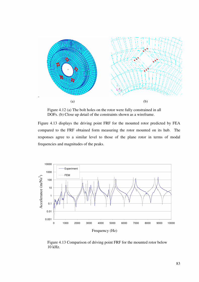
83
(a) (b)
Figure 4.12 (a) The bolt holes on the rotor were fully constrained in all
DOFs. (b) Close up detail of the constraints shown as a wireframe.
Figure 4.13 displays the driving point FRF for the mounted rotor predicted by FEA
compared to the FRF obtained form measuring the rotor mounted on its hub. The
responses agree to a similar level to those of the plane rotor in terms of modal
frequencies and magnitudes of the peaks.
0.001
0.01
0.1
1
10
100
1000
10000
0 1000 2000 3000 4000 5000 6000 7000 8000 9000 10000
Experiment
FEM
Figure 4.13 Comparison of driving point FRF for the mounted rotor below
10 kHz.
Frequency (Hz)
Acc
eler
ance
(m
/Ns2
)
84
4.6 Assembled Models
4.6.1 Component Interfaces
Many different methods can be used in FEA modelling for the contact between
components. These methods are (in order of simplest to most complex):
• Merged nodes
• Multi-point constraints
• Linear springs
• Contact elements
Merged nodes are shared between neighbouring elements so that the components are
effectively fused together. While this is simple, it does not allow for any type of
interfacial property, such as contact stiffness or damping to be applied.
Contact surfaces are by far the most advanced method of coupling components together.
Sophisticated contact surface models exist that allow some level of motion between
components, which include specifying normal and tangential contact stiffness. Here a
more realistic representation of what is a highly non-linear feature can be applied.
Unfortunately, it requires considerable computational effort compared to the other three
methods. Chapter 8 will focus on using contact elements at interfaces with the
commercial FEA code HKS Abaqus.
Components within the finite element model of the brake system within this thesis were
connected using the two remaining methods, multi-point constraints and linear springs,
as described below.
4.6.1.1 Multi-point constraints
Multi-point constraints (MPCs) are general tool for directly coupling selected degrees-
of-freedom (DOFs) in FEA models. They are often used in places where discontinuities
in geometry or FEA mesh. They lend themselves particularly well to connecting
rotating or sliding components.
The brake assembly consists of two areas where components slide within one another.
Firstly, the piston slides within the caliper housing bore when brake line pressure is
applied and forces the inner brake pad against the brake rotor. Secondly, the caliper

85
guide pins, which are rigidly connected to the caliper housing, slide within the anchor
bracket to allow force distribution to the outer pad. In both of these cases two of the
three translational DOF are coupled, as are all the rotational DOF. An MPC is a
straight-forward manner of implementing these sliding connections. The procedure is
illustrated with the piston / caliper interface.
An annular ring of piston nodes is defined as a rigid body element (Nastran element
RBE2). The ring then behaves as a rigid body and has its motion linked to a node at its
centre as shown in Figure 4.14.
A rigid body ring is defined for the caliper which is also linked to a node at its centre.
The two central nodes are directly coupled in all DOF except the sliding direction. A
spring can be used to couple the sliding direction. This allows the piston to slide freely
within the caliper, but provides load transfer when displacement in any other direction
occurs.
Figure 4.14: Implementation of an MPC for creating a sliding connection.
The annular ring on the piston is connected to a central node, as is an
annular ring from the caliper. The central nodes are directly coupled in all
DOFs.
MPCS are also defined to link the caliper slide pins to the anchor bracket in the same
manner. All DOFs are directly coupled except for the sliding in the axial direction.
The slide pins are also linked to the caliper via MPCs. However, in this case a solidly
bolted joint is simulated rather than a sliding one. Hence the MPCs are coupled in all
DOFs with no provision for relative axial displacement.
Nodes on
housing tied to
central node
Nodes on
piston tied to
central node
Central nose tied
in all DOF except
sliding direction

86
The main disadvantage of using MPC connections is they can introduce some additional
stiffness into the components in the regions where MPC is applied. For example, the
annular ring MPCs that are applied to the caliper bore and anchor bracket guide pin
holes provide more rigidity that that of the component alone. However, these regions
are relatively small and would have little impact on overall deformation.
4.6.1.2 Linear springs
The bulk of the contact within the FEA model utilised linear springs. They are a simple
and effective way of allowing load to be transferred between two connected components
and to prevent penetration. While contact itself is a highly non-linear process, within
the small displacements that occur at an interface during vibration, a linear contact
stiffness has been assumed. Figure 4.15 shows the interface between two adjacent
components. A requirement for linear spring connection is coincident node meshing
between components.
Figure 4.15: Schematic diagram of nodes on adjacent components
connected with linear springs. Note: the gap between the components is
illustrative only, and the nodes are coincident within the FEA model.
Selection of an appropriate contact stiffness is a critical part of using linear springs to
connect components. No completely satisfactory method exists to experimentally
determine what this stiffness should be, although a variety of methods have been used.
Liles (1989) used transfer frequency response functions (FRFs) between components to
assess the energy transfer between components. Park et al (2001) used experimental
penetration measurements and material properties to estimate the contact stiffness.

87
Nack (2002) has used surface asperity measurements but that has proved difficult to
implement in practice.
The method used in this study is based on the contact stiffness formulation used by
Ansys 5.7 for initial contact stiffness (Ansys User’s Manual, 2000). The calculation is
based on the material properties and geometry of the elements that are being connected.
The relationship between the (softer) element involved and the contact stiffness is given
by
∑=
n
i i
isj
V
A
n
Kfk
2
(4.6)
where Ai and Vi are the contact area and volume of the ith
element surrounding the jth
node on the contact surface, K is the bulk modulus of the material and fs is a penalty
factor, usually in the range of .01 to 10.
Alternatively, for a friction interface with largely uniform element contact face area and
element volume, equation 4.6 can be expressed as
avg
avg
avg
s
V
A
n
Kfk
2
= (4.7)
where navg is the average number of nodes per element , Aavg is the average elemental
contact face area, and Vavg is the average elemental volume. This sets the contact
stiffness of all the springs across the whole interface rather than setting each one
individually.
The connection between the components, using linear springs and MPCs is shown
schematically in Figure 4.16.

88
Figure 4.16 Component interface connection schematic
4.6.1.3 Linear vs. non-linear static analysis
Nastran provides a variety of solution sequences covering a range of static and dynamic
analyses. Static solutions are available in the both linear and non-linear forms. The
fundamental difference between these types of solutions is that the stiffness matrix may
change as loads are incrementally applied during a non-linear analysis, whereas it
remains constant throughout a linear analysis.
Non-linear solutions are usually used wherever significant non-linearity is present in the
physical system being modelled. Three sources of non-linearity can be applied using
FEA models.
1. Large deformations
2. Material non-linearity
3. Contact
Each of these will cause the stiffness matrix in a finite element model to change from
one load condition to the next during an analysis. It is usual to apply loads in small
increments and iteratively check that the internal system forces and displacements
provide an equilibrium solution given the current external loads to within some small
error or convergence criteria.
Large deformation non-linearity follows from displacements that are large enough to
cause significant variation in geometrical relationships between nodes. Material non-
linearity is caused by non-constant elastic modulus of the material, such as when the
yield stress level is exceeded. Finally, contact causes changes at the structural
Disc
rotor
Outer
pad
Inner
pad
Piston Caliper
housing
Anchor
bracket
Ground
Ground
Springs MPC
MPC Springs Springs Springs
Springs

89
boundaries or component interfaces as loads are added and removed from the system.
Each of these may cause changes in the stiffness matrix.
A linear solution, on the other hand, assumes that no such changes are occurring in the
structure as the load is applied. The geometry, material properties and boundary
conditions do not change with load. Hence there is no requirement for the system
matrix to be updated as the load is applied. The full load is applied and the final state of
the structure can be determined immediately.
The computational cost of performing a non-linear solution can be much greater than a
linear solution. It is therefore preferable to use linear solutions where ever possible
after considering the non-linearity to be expected from the structure under the expected
load condition.
In the case of a brake system, large deformations and material non-linearity are not
significant concerns due to the small structural deformations and low stress levels
respectively. However, contact between components can make the system extremely
non-linear as the contact between components changes.
When using spring elements to connect components, little reason exists for using a non-
linear solution. Unlike contact elements, where nodes at the contact interface can
become (or cease to be) active intermittently through a load step, linear springs remain
active all of the time. Hence the inherent non-linearity of a contact problem cannot be
captured with a single step approach.
However, an iterative linear static procedure was used for the static analysis to capture
the final contact state more accurately. Successive static solutions followed by the
removal of springs under tension effectively achieve a non-linear solution using a model
with purely linear elements.
4.1.6.4 Spring interface tuning
Scope exists for tuning of springs connections in the case of the direct spring
connections. Table 4.10 shows a summary of the baseline model set up for the
assembly.

90
Table 4.10: Interface tuning parameters for baseline model
Interface K
(MPa)
Aavg
(mm2)
Vavg
(mm3)
navg fs k
(N/mm)
Rotor / lining 4200 20 97 1.1 0.1 2 x 10³
Inner Pad BP /
piston 68000 35 308 2.0 10 1.4 x 10
6
Outer Pad BP /
housing 67000 35 77 1.7 10 6.0 x 10
6
Pad BP / anchor (y) 138000 13 19 4.0 10 3.0 x 10⁶
Pad BP / anchor (z) 138000 20 40 2.0 10 7.0 x 10⁶
A key step in using springs at a connection interface is to examine the spring state under
a static load condition. When an interface is under load, different areas may be forced
into compression and other areas may be under tension. Springs behave such that any
relative motion between the “ends” of the springs (the node points that define the
element) results in a reactive spring force. While this is indeed the aim of the spring
under compressive loading, it makes no physical sense for a contact spring to support a
tensile load.
To ensure a realistic contact interaction, the springs which are under tensile loading
must be removed. Hence the static solution is an iterative procedure. All springs are
activated initially and a static solution obtained. Springs that are found to in tension are
then removed and a static solution is again obtained. This is repeated until an
equilibrium solution is obtained with no springs under tension. This is then considered
to be the base static state around which the dynamic perturbation analyses are
performed.
A comparison was made between the preloaded static state of the friction interface from
the Nastran model to an Abaqus non-linear solution utilising contact elements, shown in
Figure 4.17. Each contact interface was examined to compare the areas where contact
and separation were occurring. The areas differ slightly, but the overall agreement is
reasonable.
The penalty factors, as given by fs in equation (4.6), were all set to 0.1 for the initial
comparison. It was found that excessive penetration was found at most of the interfaces
with metal to metal contact, ie all excluding the rotor / lining interface, and a penalty
factor of 10 offered better agreement. For the crucial rotor / lining interface a penalty

91
factor of 0.1 was found to be sufficient. The final contact stiffness values used for all of
the contact interfaces are listed in Table 4.10.
(a) Inner pad
(b) Outer pad
Figure 4.17 Overlays of the Nastran static solution and Abaqus non-linear
solution contact areas. The areas in red represent the footprint of the pad
from the Abaqus solution. The blue dots represent active nodes from the
Nastran solution
4.6.1.5 Friction interface
The interface that connects the brake rotor to the brake pad linings provides the friction
that is required in the braking operation. It also supplies the energy that drives the
structural vibration of the system. This will be discussed in greater detail in later
chapters. However, the basic method of implementing the friction coupling terms is
now presented.

92
Figure 4.18: Basic friction force diagram
Consider the simple two-degree-of-freedom model shown in Figure 4.18. A mass m is
in sliding contact with a conveyor belt; the contact stiffness is k and friction coefficient
µ. The friction force fF and the normal force fN act in the x and y directions respectively.
kyfN −= (4.8)
kyff NF µµ =−= (4.9)
Note that the friction force is one directional in the sense that normal forces result in
frictional forces, but not vice versa. This provides a complication for implementation
into a finite element model since it will result in unsymmetric terms in the system’s
stiffness matrix. Indeed, an unsymmetric stiffness matrix is a necessary condition for
the system to become unstable, the topic of chapter 5.
The friction coupling terms are input directly into the stiffness matrix in the FEA model
via Nastran direct matrix input (DMIG) terms. DMIG entires allow for the direct entry
of stiffness (or mass) to the system matrices in addition to those that are generated by
the finite element code from the node and element input data.
Unfortunately matrices solved in a linear static analysis in Nastran have to be
symmetric. The friction coupling (unsymmetric) terms cannot be added to the stiffness
matrix for the linear solution. Hence the iterative linear solution establishes the normal
contact distributions at the component interfaces including the effects of rotation.
The most significant effect of rotation and the friction force is to force the pad backplate
into contact with the trailing abutment in the rotation direction. It also removes any
fN
x
y
k
fF
m

93
contact for the leading abutment in the rotational direction. Hence, the contact springs
between the leading abutment and the pad backplate that act in the rotation direction
were removed manually.
4.7 Summary
The development of a large scale FEA model has been presented. A step by step
process was followed beginning working with individual component models, flowing
through to the completed assembly.
Initially the CAD geometry and imported, cleaned-up and meshed. Experimental modal
analysis results were used to “tune” the material properties of the components. Finally
the individual components were assembled and boundary conditions and component
interfaces were created. The final assembly forms the basis of the complex eigenvalue
stability analysis that follows in Chapter 5.

94

95
Chapter 5
Prediction of Unstable Modes
5.1 Introduction
In Chapter 4, the development of a validated model of a brake system using finite
element analysis (FEA) is described. The focus of this chapter is to use that model for
predicting the brake system’s brake squeal propensity.
It is commonly accepted amongst researchers that a brake system is in an unstable
vibration mode when it undergoes squeal. Various types of instability have been
described in the literature as described in Chapter 2.
• Stick-slip
• Negative slope µ vs v
• Sprag-slip
• Mode coupling
In principle, the prediction of brake squeal involves evaluating the stability of the brake
system. Two common methods for assessing the stability of a large scale finite element
model can be determined by observing the evolution in the time domain or by
determining the location of poles in the complex eigenvalue analysis.
The approach used in this thesis is complex eigenvalue analysis. In an undamped
system without friction all of the system modes will be normal modes. Addition of
frictional forces into the stiffness matrix of the FEA model allows the possibility of
modes to become coupled and to form a stable/unstable mode pair. This is a larger
scale application of the mode coupling instability described in section 2.3.3.

96
If the response of an unstable system is plotted in the time domain, it is seen to diverge
and the amplitude of vibration continues to grow without bound. In reality, a brake
system in self excited vibration is non linear and exhibits limit cycle behaviour. An
initial perturbation about the base state initially grows exponentially before dissipative
effects balance the friction work being converted into vibrational energy.
Figure 5.1 Single degree-of-freedom system with viscous damping
As described in many dynamics texts such as Inman (1994), a single degree of freedom
system, such as the one shown in Figure 5.1, with mass m, viscous damping c, and
spring stiffness k, the free vibration is given by the 2nd
order differential equation
0=++ kxxcxm &&& (5.1)
The time response can be expressed as a product of sinusoid and an exponential decay
)sin()( φωζω
+=−
tAetx d
t (5.2)
where
km
c
2=ζ
(5.3)
is the damping ratio,
m
k=ω
(5.4)
is the undamped natural frequency, and
21 ζωω −=d (5.5)
is the damped natural frequency. The amplitude A and phase φ are determined from the
initial conditions of the system.
m
c
k
x(t)

97
Examining the two parts to this solution reveals that the sinusoid simply represents
simple harmonic motion at a frequency of ωd. The exponential term provides the decay
and is given by the product ωζ. For solutions of the form given by equation 5.2, ζ can
take any value between 0 (undamped) and 1 (critically damped). Once ζ exceeds the
critical damping ratio of 1 it becomes overdamped and oscillatory motion does not
occur; the mass simply moves toward rest at the equilibrium position. A thorough
description of system behaviour can be found in Inman (1994).
It is a mathematical possibility for the damping ratio to take on a negative value, that is,
the damping coefficient c has a negative value. This implies that the damping force
applied on the mass does not resist the motion of the mass, but rather it acts in the same
direction as travel and reinforces the displacement from equilibrium. If this is the case,
the vibration amplitude grows with increasing time and the system is said to be
negatively damped. As was the case with positive damping, the damping ratio can take
on an absolute value between 0 and 1. If the magnitude of the damping ratio exceeds 1,
the oscillatory motion does not occur and the mass diverges exponentially away from
the equilibrium position.
Figure 5.2 shows these results graphically. Analytically, an unstable brake system
exhibits the negatively underdamped (Figure 5.2(c)) behaviour at the point when
instability occurs.
Analysis in the time domain is one of the methods that can be used to determine system
stability. However, for a large scale FEA model with tens of thousands of degrees-of-
freedom (DOF), considerable computer resources are required. Regardless of the type
of the solution method employed for an analysis, each time increment requires an
equilibrium solution to be obtained. Hence it can become prohibitively expensive
computationally if a long time period with many time increments is analysed.

98
Time
Dis
pla
cem
ent
Time
Dis
pla
cem
ent
(a) Positive underdamped (0 ≤ ζ < 1) (b) Positive overdamped (ζ > 1)
Time
Dis
pla
cem
ent
Time
Dis
pla
cem
ent
(c) Negative underdamped (-1 < ζ ≤ 0) (d) Negative overdamped (ζ <-1)
Time
Dis
pla
cem
ent
s
(e) Undamped
Figure 5.2: Response of an unstable SDOF system for various levels of
damping.
An alternative method is analysing system parameters in the frequency domain.
Equations of motion are solved as a matrix equation for their eigenvalues and
eigenvectors. The eigenvalues provide not only modal frequencies, but also the level of
damping within a mode. Negatively damped (unstable) modes can be readily identified
as potential squeal modes of the brake assembly. This chapter will present the complex
eigenvalue analysis and how it is implemented on a FEA model of the brake system.

99
5.2 Complex Eigenvalue Analysis
The equations of motion for a vibrating system in free vibration can be represented as
the following matrix equation
[ ]{ } [ ]{ } [ ]{ } 0=++ uKuCuM &&& (5.6)
where [M] is the mass matrix, [C] is the damping matrix, [K] is the stiffness matrix and
{ }u { }u& and { }u&& is the displacement vector and its time derivatives respectively. The
system matrices are established using FEA as detailed in Chapter 4.
This eigenvalue problem is solved to yield eigenvalues and eigenvectors that are
complex valued, that is, they have a real and an imaginary part. The eigenvalues take
the form
idiii jωωζλ ±−= (5.7)
where the real partii
ωζ is the damping of the complex mode and the imaginary part id
ω
is the frequency of the complex mode.
Plotting the eigenvalues, as shown in Figure 5.3, on the complex plane provides
information about the system’s modal parameters:
• Modal frequency – determined from the location along the imaginary axis.
• Modal damping – determined from the location along the real axis. The real part
of the eigenvalue is a product of the damping ratio and the undamped natural
frequency.
The stability of the mode is determined by simply examining the real part of the
eigenvalues. An eigenvalue with a positive real part is unstable, and appears on the
right hand side of the complex plane as indicated on Figure 5.3.

100
Figure 5.3 Location of an eigenvalue on the complex plane. Its position
provides the level of damping as well as the frequency
Each of the complex eigenvalues also is accompanied by a complex eigenvector or
mode shape. Complex modes differ from normal modes in that the displacements do
not occur perfectly in-phase or out-of-phase, so a real number is not sufficient for
expressing the displacement of any given node. The motion must now be described by
complex number which contains the relative phase of the node as well as the magnitude
of its displacement from the equilibrium position.
5.3 Implementation for a Brake System
Complex eigenvalue analysis forms one step of the larger modelling problem. The
modelling process consists of the following steps
1. Generation of a validated FEA model
2. Static analysis
3. Apply friction coupling
4. Complex eigenvalue analysis
Each of these will be described in the following sections.
x ζω
21 ςω −
cos-1
ζ
Re
Im
Unstable region

101
5.3.1 Generation of a validated FEA model
Individual component models and an assembled model of the system components were
created from the 3-D CAD models. Experimental modal testing results were used to
“tune” the material properties of the component models and validate the assembled
model, as described in the chapter 4.
5.3.2 Static analysis
A static load analysis was performed to obtain the system’s state under typical braking
pressure. Particular attention was directed to the contact conditions at the pad/rotor
interface. Linear springs are used between coincident nodes on the pad and rotor
surface. Static analyses were run iteratively with the static state of the system updated
in a quasi non-linear analysis.
At the end of the static analysis, the brake system is in a base static state that occurs
during a typical braking occurrence. The dynamic analysis that follows is a linear
perturbation around this base state.
5.3.3 Friction Model
Prior to the complex eigenvalue analysis, the friction coupling terms were inserted into
the system stiffness matrix [K]. A simple friction law of the following form was used
for the friction force with reference to Figure 4.18
kyff NF µµ =−= (4.9 repeated)
where fF is the friction force, fN is the normal force at the friction interface, µ is the
coefficient of friction, k is the contact stiffness and y is the displacement in the friction
interface normal direction.
This same Coulomb friction model is applied to all nodes at the pad / rotor friction
interface. With reference to Figure 5.4, the resulting friction force is a function of the
relative displacement of the node pair in the surface normal direction given by
)( )1( yiiyjx uukf+
−= µ (5.8)

102
where ui is the displacements of the ith
node.
Figure 5.4 Coincident node mesh at the pad / rotor interface. Note that it is
shown with a gap for clarity.
On applying this friction model brings with a number of assumptions:
1. The coefficient of friction is constant, and as such it is independent of normal
force and sliding velocity.
2. The sliding velocity is greater than the tangential vibration velocity, resulting in
a friction force that always acts in the same direction with no possibility of
reversing.
The friction forces expressed in equation (5.8) provides a forcing function for Equation
(5.6), which can be rearranged as
[ ]{ } [ ]{ } [ ]{ } { } [ ]{ }uKFuKuCuM ff ==++ &&& (5.9)
where [Ff] is the friction force and [Kf] is the friction stiffness matrix. Upon further
rearrangement, equation (5.9) can be written in homogeneous form
[ ]{ } [ ]{ } [ ]{ } 0=−++ uKKuCuM f&&& (5.10)
[Kf] couples forces in the friction interface normal direction to the tangential direction,
but not vice versa, and as a result is unsymmetric. Hence the new system stiffness
matrix [K - Kf], which includes the friction stiffness, is also unsymmetric. Indeed, it is a
necessary, but not sufficient, condition for the system expressed in equation (5.10) to
kj
ui+1
ui
x
y
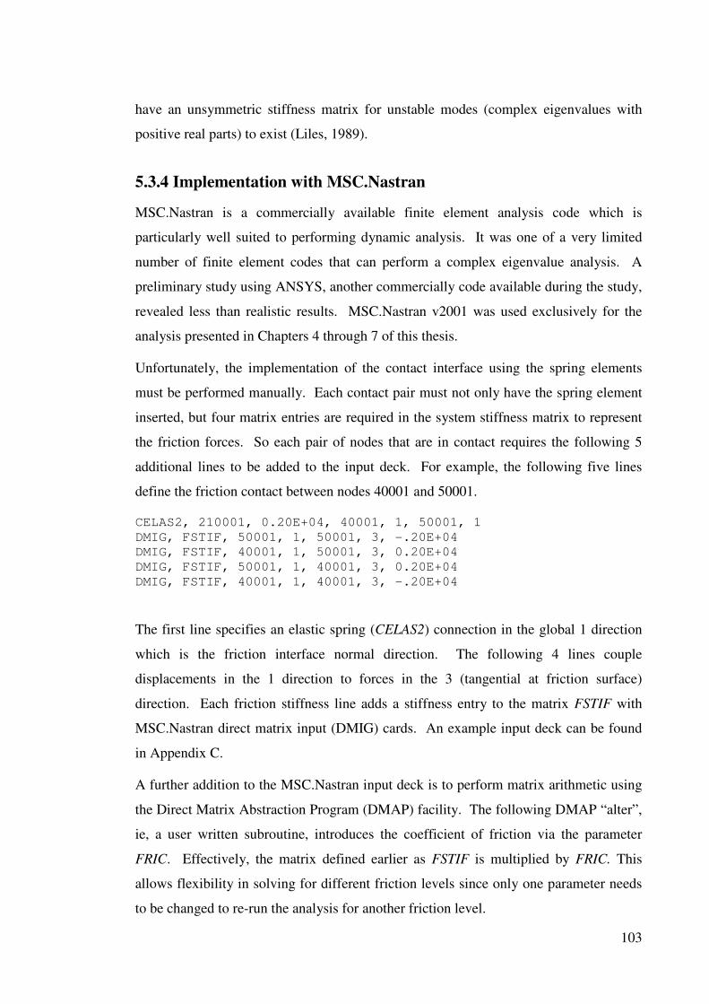
103
have an unsymmetric stiffness matrix for unstable modes (complex eigenvalues with
positive real parts) to exist (Liles, 1989).
5.3.4 Implementation with MSC.Nastran
MSC.Nastran is a commercially available finite element analysis code which is
particularly well suited to performing dynamic analysis. It was one of a very limited
number of finite element codes that can perform a complex eigenvalue analysis. A
preliminary study using ANSYS, another commercially code available during the study,
revealed less than realistic results. MSC.Nastran v2001 was used exclusively for the
analysis presented in Chapters 4 through 7 of this thesis.
Unfortunately, the implementation of the contact interface using the spring elements
must be performed manually. Each contact pair must not only have the spring element
inserted, but four matrix entries are required in the system stiffness matrix to represent
the friction forces. So each pair of nodes that are in contact requires the following 5
additional lines to be added to the input deck. For example, the following five lines
define the friction contact between nodes 40001 and 50001.
CELAS2, 210001, 0.20E+04, 40001, 1, 50001, 1
DMIG, FSTIF, 50001, 1, 50001, 3, -.20E+04
DMIG, FSTIF, 40001, 1, 50001, 3, 0.20E+04
DMIG, FSTIF, 50001, 1, 40001, 3, 0.20E+04
DMIG, FSTIF, 40001, 1, 40001, 3, -.20E+04
The first line specifies an elastic spring (CELAS2) connection in the global 1 direction
which is the friction interface normal direction. The following 4 lines couple
displacements in the 1 direction to forces in the 3 (tangential at friction surface)
direction. Each friction stiffness line adds a stiffness entry to the matrix FSTIF with
MSC.Nastran direct matrix input (DMIG) cards. An example input deck can be found
in Appendix C.
A further addition to the MSC.Nastran input deck is to perform matrix arithmetic using
the Direct Matrix Abstraction Program (DMAP) facility. The following DMAP “alter”,
ie, a user written subroutine, introduces the coefficient of friction via the parameter
FRIC. Effectively, the matrix defined earlier as FSTIF is multiplied by FRIC. This
allows flexibility in solving for different friction levels since only one parameter needs
to be changed to re-run the analysis for another friction level.

104
COMPILE GMA SOUIN=MSCSOU NOLIST NOREF
ALTER 'MTRXIN' $
ADD K2PP, /K2PPX/V,Y,FRIC=(1.0,0.0) $
EQUIVX K2PPX/K2PP/-1 $
ENDALTER
…
…
K2PP = FSTIF
PARAM, FRIC, .5
Defining stiffness entries for each pair of nodes at the friction interface via manual text
input is not practical. Not only is it tedious in the extreme, but it is also prone to error.
To aid in the definition of the friction surface, a FORTRAN 77 code bdfread was
written to connect the coincident node pairs with contact springs and to apply the
friction coupling terms. bdfread was also adapted to apply contact springs at the other
spring interfaces within the FEA model. While these other interfaces required only the
spring element to be inserted without friction terms, automating the process help avoid
errors in the modelling process.
The code reads an existing MSC.Nastran input deck generated by MSC.Patran to find
coincident nodes with a specified search area. Coincidence is determined by measuring
the distance between nodes and if they fall below a specified tolerance (eg, 0.01 mm)
then the appropriate CELAS2 and DMIG entries are written to a text file. Each contact
interface is determined from an individual search area to ensure that the correct spring
directions and contact stiffnesses are used. Once all of the coincident nodes are found
for each interface and the data has been written to a text output file, then the
MSC.Nastran input deck is re-generated with the bdfread output appended from within
MSC.Patran. Appendix D contains the bdfread source code.
5.4 Brake System Analysis
The Complex Lanczos method was used within MSC.Nastran to solve the complex
eigenvalue problem on the brake system FEA model shown in Figure 5.5 (Nastran
Advanced Dynamics Guide, 2002). This solution scheme is particularly efficient for
larger models, and the default choice for large models with MSC.Nastran.

105
Figure 5.5 The assembled FEA model
This model of the brake system is simplified in that it does not include rotational effects.
However, as discussed in Section 3.11, the primary focus of the noise evaluation is low
speed applies where rotational effects are not significant.
The 108 eigenvalues extracted between zero and 12 kHz for the base brake system with
µ = 0.5 are plotted on the complex plane in Figure 5.6. In the baseline case no other
sources of damping are specified. All of the modes have zero damping (lie on the
imaginary axis) except where pairs of modes have become coupled and formed a stable
/ unstable pair. These result in the eigenvalues that occur in conjugate pairs that are
symmetrically located about the imaginary axis. In this case seven unstable modes can
be seen.
An alternative and somewhat more insightful way to express these results is to plot
damping vs frequency as shown in Figure 5.7. Essentially the same information is
available as for the eigenvalue plot, but now the frequency and damping levels can be
directly read off. Note that the seven modes with positive real parts now appear with
negative damping values.

106
Complex Eigenvalues of Base Brake System
0
10000
20000
30000
40000
50000
60000
70000
80000
-250 -200 -150 -100 -50 0 50 100 150 200 250
Real Part of Eigenvalue
Ima
gin
ary
Pa
rt o
f E
ige
nv
alu
e
Figure 5.6 108 eigenvalues extracted from the baseline brake system
plotted on the complex plane. The 7 unstable mode pairs appear as
symmetric pair about the imaginary axis.
Damping vs Frequncy of Base Brake System
-2.0%
-1.5%
-1.0%
-0.5%
0.0%
0.5%
1.0%
1.5%
2.0%
0 2000 4000 6000 8000 10000 12000 14000
Frequency (Hz)
Da
mp
ing
Figure 5.7 Damping factor vs. frequency for the base brake system analysis.
The seven unstable modes, their respective eigenvalues and levels of negative damping
are summarised in Table 5.1.

107
Table 5.1 Summary of unstable modes for the baseline brake system
Mode No. Eigenvalue Frequency (Hz) Damping ratio (%)
27 83.07 + 20871j 3322 -.398
43 219.0 +29283j 4661 -.748
54 27.29 + 37123j 5908 -.074
73 51.84 + 51951j 8268 -.099
79 64.46 + 55776j 8877 -.116
81 49.78 + 56426j 8981 -.088
105 215.4 + 74521j 11860 -.289
While there is no direct proportionality between squeal propensity and the level of
negative damping, it has been suggested that higher values tend to be associated with
modes that are most likely to squeal (Liles, 1989). Furthermore, the sound level emitted
from a squealing brake is also not indicated by negative damping level.
The unstable modes can be compared to the baseline noise performance of the system
reported in section 3.11. Unstable modes have been found that correspond closely to
the frequency ranges of interest at 6-6.5 kHz, 7.5-8 kHz and 11.5-12 kHz. Also
predicted were modes with significant levels of negative damping at 3.3 kHz and 4.7
kHz. The former has not occurred at all in the dynamometer screening, but some
occurrences at 4.5-5 kHz were observed. Several other unstable modes were also
predicted that have not presented a concern in testing. This is a significant issue with
the over predictive nature of complex eigenvalue in that not all of the modes predicted
will cause an actual squeal concern.
Mode shapes for the 7 unstable modes from Table 5.1 are displayed in Figures 5.8 to
5.14. Note the guide pins have been omitted from the assemblies since the highly
magnified deformation level leads to an unnatural appearance of the pins penetrating
adjacent components.
Mode 27 at 3322 Hz (Figure 5.8) shows considerable deformation across the many of
the main components of the system. The rotor appears to have a of (4,0) bending mode
present and the housing features predominately a single mode with bending across the
caliper bridge.
Mode 43 at 4661 Hz (Figure 5.9) features a (6.0) rotor bending mode. While some
deformation can be seen in the housing and bracket, no particular modes can be readily
identified by visual inspection.

108
Rotor deformation is prominent in mode 54 at 5908 Hz (Figure 5.10), but several modes
appear to be participating.
Mode 73 at 8268 Hz (Figure 5.11) has the majority of the deformation occurring in the
caliper assembly itself. Visually it is difficult to identify component modes, but it is
clear the housing, bracket and outer pad are deforming significantly.
High order rotor deformation and bracket deformations feature in both mode 79 at 8877
Hz (Figure 5.12) and mode 81 at 8981 Hz (Figure 5.13). Again, the specific component
modes are somewhat difficult to identify by visual inspection.
The final unstable mode, mode 105 at 11860 Hz (Figure 5.14) shows limited rotor
deformation, but considerable deformation of the caliper housing. The rotor modes that
are present appear to include a 2nd
in-plane tangential mode.
The visual inspection of the mode shapes of unstable modes is a limited method for
assess the behaviour of the assembly. Some insight can be gained into which
components are active and component modes may be participating, but it is clear a
deeper level of analysis is requires to thoroughly characterise the behaviour of the brake
system.

109
Figure 5.8 Mode 27 at 3322 Hz. Guide pins are not displayed.
Figure 5.9 Mode 43 at 4661 Hz. Guide pins are not displayed.

110
Figure 5.10 Mode 54 at 5908 Hz. Guide pins are not displayed.
Figure 5.11 Mode 73 at 8268 Hz. Guide pins are not displayed.
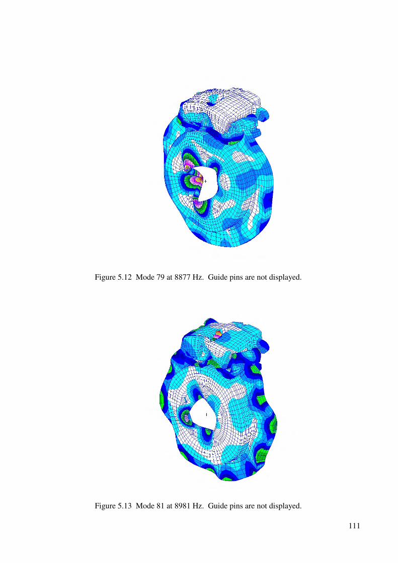
111
Figure 5.12 Mode 79 at 8877 Hz. Guide pins are not displayed.
Figure 5.13 Mode 81 at 8981 Hz. Guide pins are not displayed.
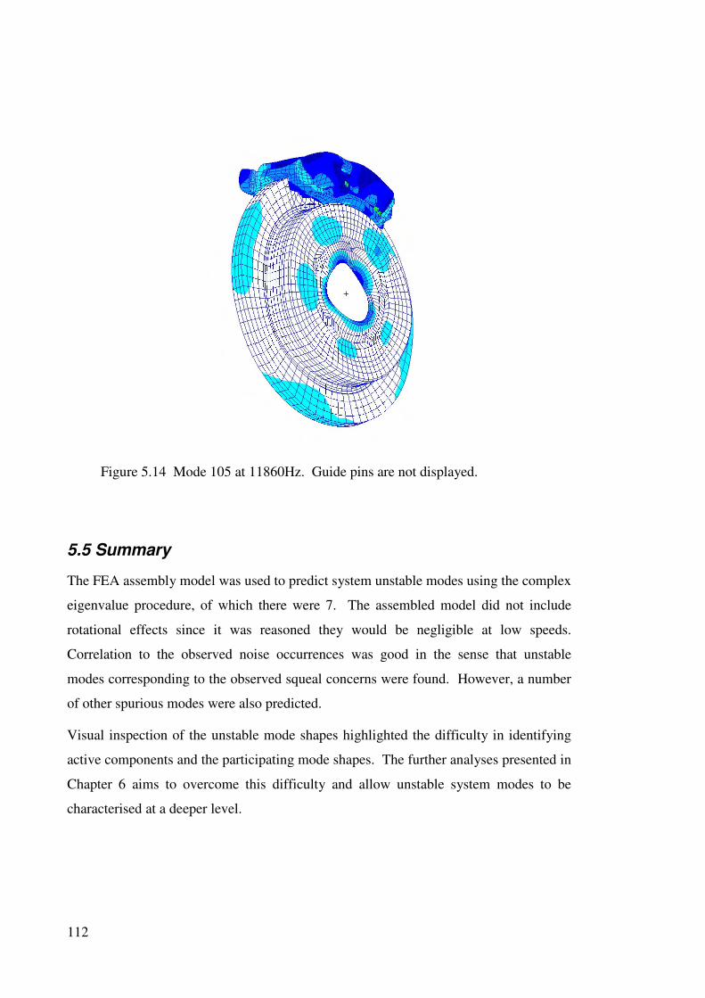
112
Figure 5.14 Mode 105 at 11860Hz. Guide pins are not displayed.
5.5 Summary
The FEA assembly model was used to predict system unstable modes using the complex
eigenvalue procedure, of which there were 7. The assembled model did not include
rotational effects since it was reasoned they would be negligible at low speeds.
Correlation to the observed noise occurrences was good in the sense that unstable
modes corresponding to the observed squeal concerns were found. However, a number
of other spurious modes were also predicted.
Visual inspection of the unstable mode shapes highlighted the difficulty in identifying
active components and the participating mode shapes. The further analyses presented in
Chapter 6 aims to overcome this difficulty and allow unstable system modes to be
characterised at a deeper level.

113
Chapter 6
Numerical Methods for
Assessing Brake Squeal Propensity
6.1 Introduction
In Chapter 5, the use of complex eigenvalue analysis for determining is described if a
brake system is unstable and could potentially lead to a squeal problem. Unfortunately,
while complex eigenvalue analysis allows the assessment of system stability, it offers
no insight into what is occurring internally within the system or what modifications
should be undertaken to increase stability. Visual inspection of unstable system mode
shapes did not offer a sufficient level of understanding of the brake system behaviour.
In this chapter, three different analysis techniques will be introduced for the specific
purpose of understanding how the components within a system are behaving and which
components might be suitable for modification. The three methods are
1. Strain energy – where the distribution of strain energy within the brake system is
calculated.
2. Feed-in energy - where the amount of vibrational energy being added to the
brake system from each friction interface is calculated.
3. Modal participation – where the correlation between individual component
modes under free boundary conditions and within the coupled system is
calculated using the modal assurance criterion (MAC).
While each of these methods provides insight into the behaviour of the brake system
components, each has individual strengths and weaknesses that require them to work in
a complimentary manner. Strain energy distribution indicates how active the
component is in the overall vibration of the system, feed-in energy shows how much
energy is being added from each brake pad during a vibration cycle, and MAC helps
identify which individual component modes are participating in the system’s vibration
motion. This way it is possible to not only see which components should be modified,
but also which vibration modes need to be considered in addressing the stability

114
problem. Figure 6.1 provides a schematic overview of the full system analysis
including the methods to identify treatment options.
Modal testing verify
Experimental
testing by test drive/noise
FE Structural
Model
Complex
Eigenvalue Analysis
Methods to
identify components for
treatment
Unstable mode?
Yes
Evaluate
effectiveness of treatment
verify
Figure 6.1 Schematic of approach to reduce brake squeal propensity.
6.2 Strain energy
The vibration of a structure involves cyclic displacement about some equilibrium
position. Consider the simple case of an undamped single degree-of-freedom (SODF)
system with mass m and spring stiffness k as shown in Figure 6.2.
Figure 6.2 Undamped single degree-of-freedom system of mass m and
spring stiffness k.
In free vibration the governing equation of motion is given by
0=+ kxxm && (6.1)
which has a solution of the form
m
k
x(t)

115
)sin()( φω += tAtx (6.2)
where
m
k=ω (6.3)
is the undamped natural frequency. Both the amplitude A and phase φ depend on the
initial conditions.
During one cycle, the energy within the system is transferred between strain and kinetic
energy. The strain energy is the energy stored in the spring as elastic potential energy
given by
2
2
1kxU = (6.4)
where x is the displacement of the mass from its equilibrium position. The kinetic
energy is given by
2
2
1xmT &= (6.5)
where x& is the velocity of mass. Since there are no dissipative effects present, the total
energy of the system remains constant, and is the sum of the strain and kinetic energy.
That is
constantTU =+ (6.6)
At the equilibrium position (x = 0) the velocity is at its maximum and all of the
system’s energy is kinetic energy. At maximum displacement (x = A) the velocity is
zero and all of the system’s energy is strain energy.
Figure 6.3. Two degree-of-freedom system.
m1
k1
x1(t)
m2
k2
x2(t)

116
Figure 6.3 displays an undamped two degree-of-freedom system described by the
following matrix equation
[ ]{ } [ ]{ } { }0=+ xKxM && (6.7)
where
[ ]
=
2
1
0
0
m
mM (6.8)
is the mass matrix,
[ ]
−
−+=
22
221
kk
kkkK (6.9)
is the stiffness matrix, and{ }x , { }x& and { }x&& are the displacement, velocity and
acceleration vectors respectively.
Similar to the SDOF case, the resulting motions are sinusoidal. However, in this case
there are two possible natural frequencies and two possible displacement vectors. From
the modal point of view the system has two modes; two modal frequencies and two
mode shapes.
The strain and kinetic energies can be calculated in much the same way as the SDOF
case, except they are now vector equations. The strain energy is given by
{ } [ ]{ }xKxUT
2
1= (6.10)
and the kinetic energy by
{ } [ ]{ }xMxTT
&&2
1= (6.11)
where the susperscript T represent the vector transpose.
6.2.1 Viscous Work
The undamped SDOF system described in the preceding section does not exactly
correspond to a physical system. Equation (6.1) predicts oscillatory behaviour that will
continue at a constant amplitude indefinitely. In reality, physical systems are damped
and the amplitude of oscillation decays over time. Eventually, regardless of how small
the damping is, the system will come to rest.

117
The most commonly used, and a mathematically convenient, model for damping is
viscous damping, as seen in Figure 6.4.
Figure 6.4 Viscous damped SDOF system.
The equation of motion for free vibration now becomes
0=++ kxxcxm &&& (6.12)
where c is the damping coefficient. A thorough discussion on viscous damping and the
characterisation of system response can be found in references such as Inman [Inman,
1994] or other elementary dynamics texts.
The underdamped case is of particular interest for studying vibration problems, and
results in motion of the form
)sin()( φωζω
+=−
tAetx d
t (6.13)
where
km
c
2=ζ (6.14)
is the damping ratio which can take any value between 0 and 1, and
21 ζωω −=d (6.15)
is the damped natural frequency. Again, as with the undamped case, A and φ are
determined by the initial conditions.
The roots to equation (6.12) are complex valued and can be written in the form
djωζωλ ±−=2,1 (6.16)
The real part of the root gives the exponent for the damping term in equation (6.13) and
the complex part gives the damped natural frequency.
m
c
k
x(t)

118
A damper is the dissipative element in the system shown in Figure 6.4. The energy that
is dissipated during one period T can be calculated by considering the work done by the
damper
∫∫++
==Tt
t
x
xviscous dtxcdxxcW
1
1
1
1
22
&&π
(6.17)
If a system is driven at ωd, the steady state response is
)sin()( θω += tAtx d (6.18)
and the viscous work becomes
22
0
2)]sin([ AcdxtAcW ddviscous
d
ωπθωωπ
=+= ∫ (6.19)
Substituting equation (6.14) into equation (6.19) and recognising the real and imaginary
parts of equation (6.16), the energy dissipated from the system as viscous work can be
expressed as
2)Im()Re(2 AmWviscous λλπ−= (6.20)
Equation (20) applies to a single degree of freedom, but it can be readily extended to
any number of degrees of freedom if the displacement vectors and mass matrix are
known. In matrix form the viscous work for the ith
mode of a system is
{ } [ ]{ }i
T
iiiviscousi uMuW )Im()Re(2 λλπ−= (6.21)
6.3 Feed-in Energy
The energy source in a squealing brake system is the friction interface between the pad
and the rotor. The exact nature of the friction coupling is not simple and a single,
general model does not exist. However, a number of different models have been used to
analyse the instability that arises in squeal modes as detailed chapter 2.
Mode-coupling type instability has widely been used because it lends itself readily to
use in conjunction with finite element analysis (FEA). Here the friction interface is
modelled as coincident node pairs distributed across the pad / rotor interface. The
friction coupling is a pseudo forcing function whose magnitude depends on the contact

119
stiffness and relative displacement of each coincident node pair. This linear friction
model predicts that no energy is added to the system when normal (stable) modes are
present.
When the system enters an unstable system mode net vibrational energy is added to the
system during the vibration cycle. This energy, called feed-in energy, is added to the
system due to the relative displacement of the friction interface over the course of a
vibration cycle. The formulation presented here is essentially the same as Guan and
Huang [Guan and Huang, 2003].
Consider the simple two-degree-of-freedom model shown in Figure 6.5. A mass m is in
sliding contact with a conveyor belt; the contact stiffness is k and friction coefficient µ.
The friction force fF and the normal force fN act in the x and y directions respectively.
kyf N −= (6.22)
kyff NF µµ =−= (6.23)
Figure 6.5 A simple 2DOF system with sliding friction.
The work done on the mass during one cycle of oscillation is found by integrating the
force in the x direction with respect to distance
∫=cycle
Fx dxfE (6.24)
which, can be expressed in terms of time
fN
x
y
k
fF

120
dtdt
dxfE Fx ∫=
ωπ2
0 (6.25)
where ω is the frequency of oscillation. The motions in each coordinate are
)sin()( xx tAtx θω += (6.26)
)sin()( yy tAty θω += (6.27)
where Ai and θi are the amplitudes and phases respectively. Substituting equations
(6.26) and (6.27) into equation (6.25), the work done on the mass by the friction force is
dtttAkAE yxyxx ∫ ++=ωπ
θωθωωµ2
0)sin()cos( (6.28)
)sin( xyyxx AAkE θθπµ −= (6.29)
Figure 6.6 Phase plot of y vs. x displacement for the 2DOF system in Figure
6.5 with 0 < (θy - θx) < 90°.
Further insight into the importance of the phase of each displacement can be found by
examining Figure 6.6. Here the displacements in the y-direction lead the x-
displacement, which results in a clockwise trajectory. The inclination of the major axis
of the ellipse depends on the relative magnitudes of the x and y amplitudes and the
amount the y leads x.
x
y
1
2 Ax
Ay
-Ax
-Ay
3
4

121
The work added to the mass by friction can be found by integrating around the ellipse
points 1 through 4.
dxfdxfdxfdxfE FFFFx ∫∫∫∫ +++=1
4
4
3
3
2
2
1 (6.30)
Recall from equation (6.23) that the friction force is proportional to the displacement in
the y-direction. Hence, by inspection of the integrals 1 and 3 in equation (6.30) the
friction force and the direction of travel are opposite and the friction force is dissipative.
Integrals 2 and 4 have the force and motion in the same direction and add feed-in energy
to the mass.
After summing the areas, the feed-in energy is proportional to the area within the
ellipse. It is also worth noting that this result is general and does not depend upon the
equilibrium position of the mass.
For cases where the y displacement lags the x displacement, the trajectory reverses
direction and the feed-in energy can become dissipative overall. A summary of the
different cases of trajectories is given in Figure 6.7. Cases (a), (b) and (c) feature
frictional energy being added to the mass, (d) the energy is dissipated, and (e) and (f)
are normal modes.
Equation (6.29) can be extended to incorporate the feed-in energy from the difference in
motion between two coincident points on the friction interface rather than a single point
as shown in Figure 6.5. The feed-in energy from the relative motion of two points a and
b is
)sin( abxabyabyabxabx AAkE θθπµ −= (6.31)
where iabi baA −= is the amplitude of the difference between nodes a and b in the i
th
coordinate and iabi ba )arg( −=θ the phase of the difference.

122
(a) (b)
(c) (d)
(e) (f)
Figure 6.7 Phase plots for the system from Figure 6.5. (a) 0 < (θy - θx) <
90°, (b) 90° < (θy - θx) < 180°, (c) (θy - θx) = 90°, (d) -90° < (θy - θx) < 0, (e)
(θy - θx) = 0, (f) (θy - θx) = 180°.
6.3.1 Feed-in Energy vs. Viscous Work
An unstable system mode has an eigenvalue with a positive real part. From equation
(6.16) it is clear that the damping ratio of such a mode will be negative. So rather than
decaying, the system will exhibit an exponential growth. This doesn’t reflect physical
reality since the system will settle into a limit cycle vibration, but analytically the
system is negatively damped and will continue to grow.
x
y
x
y
x
y
x
y
x
y
x
y

123
In section 6.2.1 the energy dissipated by a viscous damper was discussed.
Mathematically, the same analysis can be applied to a system with negative damping, as
that with positive damping. The viscous “work” in this case takes on a negative value,
and represents energy that is being added to the system rather than dissipated by the
system.
The energy being added to the system can also be considered by calculating the feed-in
energy. Numerically the same value is attained. The energy being added to the system
by the friction interface is exactly the same as the energy being gained by the negative
viscous work.
6.4 Modal Participation with Modal Assurance Criterion
Modal assurance criterion (MAC) calculation provides a quantitative method of
assessing which component modes are significant in the overall system vibration. The
MAC, as the name implies, is used for comparing the correlation between modes shape
and often used for comparing numerical and experimental mode shapes. In the present
study it will be used for comparing FEA results together.
Mathematically, the MAC is a dot product between two vectors, {u1} and {u2}
normalised by their magnitudes
{ } { }
{ } { }( ){ } { }( )*
22
*
11
2*
21
21 ),(uuuu
uuuuMAC
TT
T
= (6.32)
where T indicates the vector transpose and
* indicates the complex conjugate of a
complex valued vector. The comparison of a real vector and a complex vector presents
no difficulty since the conjugate of a real vector is simply the vector itself.
MAC data was used primarily for determining which component modes are active in an
unstable system mode. For example, a system mode is often identified by the mode
shape of the rotor. The MAC allows the identification of the rotor mode shape more
easily because it does not rely on visual observation and a qualitative judgement. A
value of 1 indicates that two modes are identical (although they could be scaled) and a
value of 0 indicates that there is no correlation between the modes at all.

124
6.5 Example 4DOF System
To further highlight the application of the feed-in energy and viscous work, and the
relationship between the two, the 4DOF system in Figure 6.8 will be analysed. This
system is an extension of the simple 2DOF system analysed by Hoffman and colleagues
[Hoffman, 2002].
Figure 6.8 4DOF system with sliding friction.
The global stiffness is assembled using the direct approach from five elemental stiffness
matrices and the friction stiffness matrix. The elemental stiffness matrix for each
element is determined as follows.
Consider a spring aligned with the x’ axis of a rotated coordinate system as shown in
Figure 6.9 (a). The rotation angle between the x’-y’ and global x-y coordinate systems
is θ. The linear spring with a stiffness of k obeys Hooke’s law
lkf ∆= (6.33)
where k is a constant that defines the force f required for a displacement ∆l of the spring.
y2, fy2
k5
k3
k2 k1
m2
m1
α1
α2 y1, fy1
x1, fx1
x2, fx2
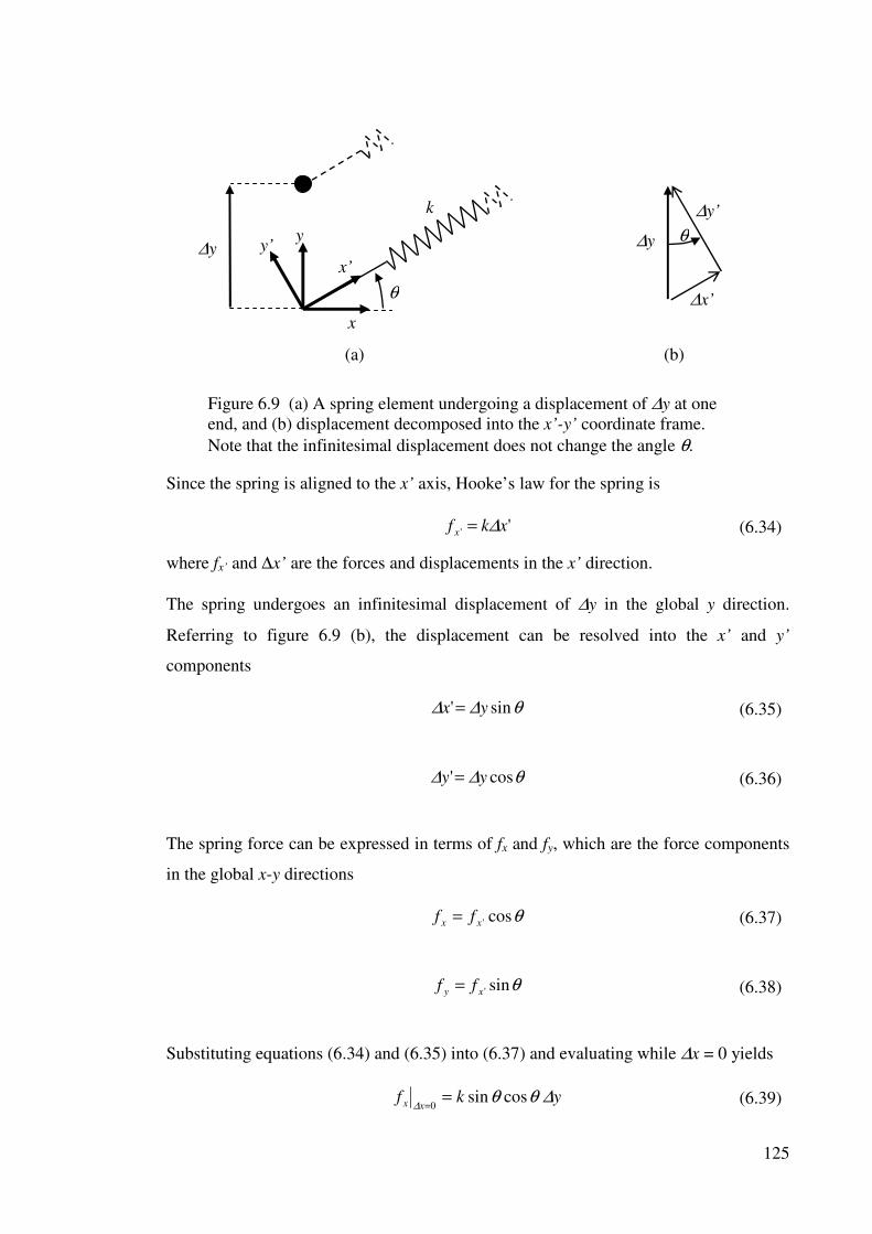
125
∆y
x
y’
x’
y
θ
k
∆x’
∆y’
∆y θ
(a) (b)
Figure 6.9 (a) A spring element undergoing a displacement of ∆y at one
end, and (b) displacement decomposed into the x’-y’ coordinate frame.
Note that the infinitesimal displacement does not change the angle θ.
Since the spring is aligned to the x’ axis, Hooke’s law for the spring is
'' xkf x ∆= (6.34)
where fx’ and ∆x’ are the forces and displacements in the x’ direction.
The spring undergoes an infinitesimal displacement of ∆y in the global y direction.
Referring to figure 6.9 (b), the displacement can be resolved into the x’ and y’
components
θ∆∆ sin' yx = (6.35)
θ∆∆ cos' yy = (6.36)
The spring force can be expressed in terms of fx and fy, which are the force components
in the global x-y directions
θcos'xx ff = (6.37)
θsin'xy ff = (6.38)
Substituting equations (6.34) and (6.35) into (6.37) and evaluating while ∆x = 0 yields
ykfxx ∆θθ
∆cossin
0=
= (6.39)

126
Similarly for fy
ykfxy ∆θ
∆
2
0sin=
= (6.40)
Equations (6.39) and (6.40) provide the relationship between a displacement in the y
direction and spring forces in the global x-y coordinate systems.
The same process can be followed to obtain the relationship between displacements in
the x direction and the x-y forces while ∆y = 0
xkfyx ∆θ
∆
2
0cos=
= (6.41)
xkfyy ∆θθ
∆cossin
0=
= (6.42)
Summing the forces in each direction gives the total force is each coordinate
ykxkfffxxyxx ∆θθ∆θ
∆∆cossincos2
00+=+=
== (6.43)
ykxkfffyxyyy ∆θ∆θθ
∆∆
2
00sincossin +=+=
== (6.44)
Expressing equations (6.43) and (6.44) as a matrix equation yields
=
y
x
kk
kk
f
f
y
x
∆
∆
θθθ
θθθ
2
2
sincossin
cossincos (6.45)
which is Hooke’s law in matrix form. The matrix in the equation is the elemental
stiffness matrix for the spring element.
For the 4DOF system shown in Figure 6.8, the global stiffness matrix will be four times
four in dimension since four-degrees-of-freedom are included the matrix. Each
elemental stiffness matrix can also be expressed in four by four form
=
2
2
1
1
44434241
34333231
24232221
14131211
2
2
1
1
y
x
y
x
kkkk
kkkk
kkkk
kkkk
f
f
f
f
y
x
y
x
(6.46)
The elemental stiffness matrices for the five spring elements in Figure 6.8 are

127
[ ]
=
0000
0000
00sincossin
00cossincos
1
2
1111
1111
2
1
1
ααα
ααα
kk
kk
k (6.47)
[ ]
=
0000
0000
00sincossin
00cossincos
2
2
2222
2222
2
2
2
ααα
ααα
kk
kk
k (6.48)
[ ]
−
−=
33
33
3
00
0000
00
0000
kk
kkk (6.49)
[ ]
=
0000
000
0000
0000
4
4k
k (6.50)
[ ]
=
5
5
000
0000
0000
0000
k
k (6.51)
The coupling at the friction interface is added by considering the spring stiffness as
shown in Figure 6.10. Constant contact is assumed, and also vibration velocity in the x-
direction is much smaller than the sliding velocity. Hence the friction force direction
does not reverse direction and is a function of displacements in the y-direction only.
)( 12311 yykff yx −=−= µµ (6.52)
)( 21322 yykff yx −=−= µµ (6.53)
This linear model of the friction force considers only small perturbations about the
equilibrium position.

128
Figure 6.10 Contact stiffness and forces at the friction interface.
Equations (6.52) and (6.53) can also be expressed as a friction stiffness matrix in terms
of the four degrees-of-freedom
[ ]
−
−
=
0000
00
`0000
00
33
33
kk
kk
k fµµ
µµ
(6.54)
The global stiff matrix is assembled as a summation of the elemental stiffness matrices
and the friction matrix
[ ] [ ] [ ] [ ] [ ] [ ] [ ]fkkkkkkK +++++= 54321 (6.55)
Note that all of the elemental stiffness matrices are symmetric. However, the friction
stiffness matrix is unsymmetric. It follows that the global stiffness matrix is also
unsymmetric.
Table 6.1 is a summary of the system parameters for the example analysis. The values
for k1, k2, k3, α1 and α2 are taken from the example given by Hoffman et al, in their
analysis of a 2DOF system [Hoffman, 2002].
y2, fy2
k3
y1, fy1 x1, fx1
x2, fx2

129
Table 6.1 Parameters for example 4DOF system
Parameter Value Parameter Value
k1 1786.)32(3
2≈− m1 2
k2 488.2)32(3
2≈+ m2 3
k3 333.13
4≈ α1 30°
k4 1 α2 150°
k5 1 µ 0.75
Inserting the values from Table 6.1 into equations (6.47) through (6.55), the global
stiffness and mass matrices are
[ ]
−
−
−=
333.20333.10
1110
333.1021
1002
K (6.56)
[ ]
=
3000
0300
0020
0002
M (6.57)
Note that the global stiffness matrix in equation (6.56) is unsymmetric which follows
from friction coupling terms.
Recall equation (6.7), which is the equation of motion for a multi-degree-of-freedom
system in matrix form
[ ]{ } [ ]{ } { }0=+ xKxM && (6.7)
The matrices [K] and [M] are inserted into equation (6.7) and a complex eigenvalue
extraction is performed to yield the eigenvalues in Table 6.2 and modes shapes in Table
6.3.

130
Table 6.2 Complex eigenvalues from example analysis
Mode Eigenvalue Frequency (Hz) Damping ratio
1 0.4665j .07424 0
2 0.5774j .09189 0
3 0.1109 + 1.137j .18093 -.09707
4 0.1109 – 1.137j .18093 .09707
Table 6.3 Mode shapes from example analysis
Mode x1 y1 x2 y2
1 -0.2169 0.4278 -0.2545 0.3394
2 0 0 0.5774 0
3 0.3929 -0.1364+0.3487j -0.1651+0.1486j 0.2201-0.1981j
4 0.3929 -0.1364-0.3487j -0.1651-0.1486j 0.2201+0.1981j
It can be seen that modes one and two are normal modes. The eigenvalue is purely
imaginary indicating the modes are undamped and the displacements for each degree of
freedom are purely real. By inspection, equation (6.21) yields zero viscous work since
the real parts of the eigenvalues are zero. Also by inspection, equation (6.31) shows the
feed-in energy is also zero since the relative phase terms between degrees of freedom is
either 0° or 180°, and the sine of π, or multiples thereof, are equal to zero.
Modes three and four are clearly complex modes, formed by the coupling of two
adjacent modes. Here the real parts of the eigenvalues indicate that the modes are
negatively damped and therefore unstable. The modal displacement vectors involve
complex motion, that is, there is a phase difference between degrees-of-freedom.
It is also apparent that the mode shapes of mode three and mode four are complex
conjugates of each other. Mode 3 is examined in mode detail and summarised in Table
6.4 and Table 6.5.

131
Table 6.4 Mode three data from example 4DOF analysis
DOF Real Imag Amplitude Phase (Degrees)
x1 0.3929 0 0.3929 0
y1 -0.1364 0.3487 0.3744 111.4
x2 -0.1651 0.1486 0.2221 138.0
y2 0.2201 -0.1981 0.2961 -41.99
Table 6.5 Mode three data from example analysis
x1-x2 y1-y2 A12x A12y θ12x(deg) θ12y(deg)
.5579-.1486j -.3565+.5468j 0.5774 0.6527 -14.91 123.1
The negative viscous work is calculated by using the amplitudes of the mode from
Table 6.4, mass matrix from equation (6.57), and the real and imaginary parts of the
eigenvalue from Table 6.2 and inserting them in equation (6.21).
{ } [ ]{ }i
T
iiiviscous uMuW )Im()Re(2 λλπ−= (6.21)
−=
2961.
2221.
3744.
3929.
3000
0300
0020
0002
2961.
2221.
3744.
3929.
)137.1)(1109(.2
T
viscousW π
792.0−=viscousW (6.58)
The feed-in energy is calculated by taking the stiffness and friction coefficient values
from Table 6.1 together with the relative magnitude and phase values from Table 6.5
and inserting them into equation (6.31).
)sin( 1212121212 xyyxx AAkE θθπµ −= (6.31)
])91.14[]1.123sin([)6527)(.5774)(.333.1)(75(.12 −−= πxE
792.012 =xE (6.59)

132
The equivalent viscous work, which represents the dissipation of energy in the system,
is negative because energy is being added via the feed-in energy; hence, they have the
same magnitude but opposite sign.
6.6 Analysis of Numerical Model
6.6.1 Model Description and Unstable Modes
A numerical model of a brake system was developed using finite element analysis
(FEA) as detailed in Chapters 4 and 5.
Figure 5.5 shows the complete brake system model, which was made from 9858 8-node
brick elements and 14813 nodes. The friction coupling for the model is provided by the
friction stiffness matrix formulated in much the same way as described for the 4DOF
model from section 6.5.
Analysis of the FEA model included varying some system parameter and observing
whether system modes become coupled and unstable. In particular, increasing the
coefficient of friction (µ) of the brake pad material tends to drive many system modes
toward instability, as well documented in the literature. This present analysis used
coefficients of friction of 0.5 and less, which corresponds to the range typically found in
actual brake systems. Setting the coefficient of friction to 0.5 leads to the maximum
number of unstable modes. Table 6.6 is a summary of the eigenvalues, frequencies and
negative damping present for the unstable modes from Chapter 5.
Table 6.6 Summary of unstable modes up to 12 kHz for the assembled brake
system, µ = 0.5.
Mode No. Eigenvalue Frequency (Hz) Damping ratio (%) 27 83.07 + 20871j 3322 -.398
43 219.0 +29283j 4661 -.748
54 27.29 + 37123j 5908 -.074
73 51.84 + 51951j 8268 -.099
79 64.46 + 55776j 8877 -.116
81 49.78 + 56426j 8981 -.088
105 215.4 + 74521j 11860 -.289
It is evident that modes shown in table 6.6 are unstable due to the positive real parts of
the eigenvalues and consequent negative damping. It is possible to track the motion of
the eigenvalues and the effect on the stability by the variation of some system

133
parameter. Figure 6.11 shows the change in eigenvalues for modes 104 and 105 due to
an increase in the coefficient of friction. The modes are driven closer in frequency and
become coupled at some critical value of µ between 0.35 and 0.4. The coupled mode
pair consists of a stable and unstable mode pair, as seen from the real parts of the each
eigenvalue.
Figure 6.11 Change in eigenvalues of modes 104 and 105 due to an
increase in the coefficient of friction.
6.6.2 Feed-in Energy for a Numerical Model
Unfortunately, while the real part of the eigenvalue indicates the level of instability in
the system mode, it does not provide any information about which part of the system
could be modified to stabilise the mode.
A greater understanding of the behaviour of various components within the system can
be obtained by calculating the feed-in energy for each unstable mode. The actual
magnitude can be determined by either direct calculation of the feed-in energy by
equation (6.31), or by calculating the equivalent viscous work by equation (6.21).
However, direct calculation of the feed-in energy was used because it can indicate
which brake pad contributes more energy, and this can then be used as a guide to
determine which part of the system could be modified.
11830
11850
11870
11890
11910
11930
-300 -200 -100 0 100 200 300
Real part
Fre
q (
Hz)
Mode 104
Mode 105
µ = 0.4µ = 0.35
µ = 0.3
µ = 0.25
µ = 0.2
µ = 0
µ = 0.45 µ = 0.5
µ = 0
µ = 0.2
µ = 0.25
µ = 0.3
µ = 0.35
µ = 0.4µ = 0.45µ = 0.5

134
Table 6.7 shows the feed-in energy for the unstable modes of the brake assembly. It can
be seen that the feed-in energy contribution is relatively evenly distributed to both pads
for modes 27, 43 and 79. For the remaining modes, a large difference exists between the
contributions between the pads. For modes 54, 81 and 105 the feed-in contribution for
one pad is negative, indicating that the friction work for the pad is acting to damp the
mode rather than feeding the instability. The potential for a dissipative effect to occur
was examined in section 6.3.
Table 6.7 Summary of feed-in energy for the unstable modes of the assembled
brake system, µ = 0.5.
Feed-in Energy (J) Mode
No.
Freq
(Hz) Inner
Pad
Outer
Pad Total
27 3322 0.32 0.47 0.80
43 4661 2.41 3.03 5.44
54 5908 0.60 -0.07 0.53
73 8268 1.49 0.03 1.52
79 8877 2.37 1.54 3.91
81 8981 7.44 -2.28 5.16
105 11860 -1.87 13.97 12.10
A larger contribution to the feed-in energy indicates a larger relative motion between
the pad and the disc. This relative motion between the pad and rotor interface is
dependant not only on pad and rotor deformation, but also on any deformation in other
supporting components. A large differential between the feed-in contributions between
the pads indicates which pad, and its interface with the anchor or caliper, needs to be
modified.
Feed-in energy can also be used to examine which regions of the pad/rotor interface are
driving the mode. Figure 6.12 and 6.13 plot the feed-in energy across the pad surfaces
for mode 27 and 105 respectively. For mode 27, small contributions from each pad can
be seen. The inner pad is favoured at one end and the outer favours the lower radial
edge. For mode 105 the central region of the outer pad is predominately driving the
instability. It is also apparent how much more feed-in energy is present in mode 105
compared to 27. Plotting the feed-in energy in this way can help to understand the
importance of regions of the pads and help evaluate potential changes to pad shape.
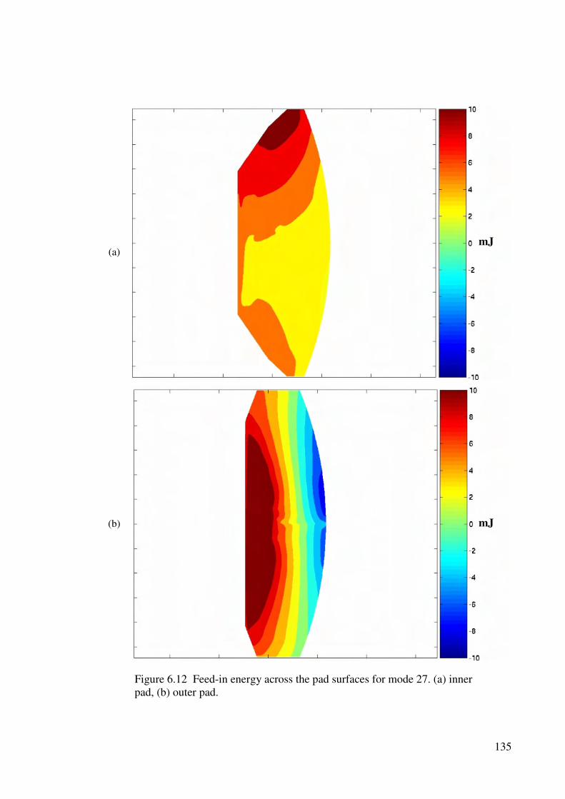
135
(a)
(b)
Figure 6.12 Feed-in energy across the pad surfaces for mode 27. (a) inner
pad, (b) outer pad.
mJ
mJ

136
(a)
(b)
Figure 6.13 Feed-in energy across the pad surfaces for mode 105. (a) inner
pad, (b) outer pad.
mJ
mJ

137
6.6.3 Strain Energy for a Numerical Model
To further assist the determination of which components need to be modified in
controlling an unstable mode, strain energy was calculated for each component in a
system mode. This allows individual components that are particularly active in an
unstable mode to be identified.
In section 6.2, the strain energy of a SDOF and 2DOF system were discussed. Equation
(6.10) is a matrix equation describing the total strain energy of a 2DOF system, but it
applies equally for any multi-degree-of-freedom (MDOF) system. However, some
additional calculation is required if the strain energy is to be broken down component
by component.
Initially, the strain energy of each individual element is calculated from the following
equation
{ } [ ]{ }*
2
1xkxU i
T
i = (6.60)
where [ki] is the elemental stiffness matrix, {x} is the displacement vector, and *
indicates the complex conjugate.
The elements for each component are identified and the strain energies are summed
∑=
i
icomponent UU (6.61)
This process is repeated for each component in the assembly.
Table 6.8 displays the strain energy distributions as a percentage for the unstable modes
of the brake system with µ = 0.5. The larger components are identified individually,
with the remaining components grouped as “other.”
A significant issue to address before the strain energy of each component is considered
is the difference in size and material composition of each component. This leads to a
considerable imbalance in the strain energy distribution throughout the system, making
it difficult to determine if the strain energy for any of the components is unusually high.
To make the comparison easier, the average strain energy distribution from all the 108
modes of the base system (µ = 0) is included in the table.

138
Graphically the results are easier to visualise. Figure 6.14 plots the distribution of strain
energy throughout the system for all unstable modes. The last column is the average
strain energy distribution for all 108 modes of the base system.
Table 6.8 Distribution of strain energy for the unstable modes of the assembled
brake system, µ = 0.5 . The average strain energy distribution for all modes 1st
108 modes from the base (µ = 0) system is included.
Mode Freq
(Hz)
Rotor
(%)
Anchor
(%)
Caliper
(%)
Inner
(%)
Outer
(%)
Other
(%)
Total
(%) 27 3322 54.1 7.5 17.3 0.8 2.5 17.8 100
43 4661 64.9 9.4 2.3 6.3 8.7 8.4 100
54 5908 63.6 3.5 5.2 11.6 1.5 14.6 100
73 8268 14.6 7.8 34.5 6.0 23.6 13.5 100
79 8877 77.7 10.4 1.5 3.3 3.9 3.2 100
81 8981 61.3 11.3 4.1 7.0 6.9 9.4 100
105 11860 20.9 14.1 34.4 8.7 16.0 5.9 100
avg. n/a 48.0 18.3 12.7 4.4 5.2 11.4 100
Baseline Model - µµµµ = 0.5
0%
20%
40%
60%
80%
100%
27 43 54 73 79 81 105 Avg
Unstable Mode Number
Other
Outer
Inner
Housing
Anchor
Rotor
Figure 6.14 Strain energy distribution for unstable modes of the baseline
system with µ = 0.5. The average strain energy distribution is calculated for
108 modes below 12 kHz for the baseline assembly with µ = 0
Figure 6.15 plots the distribution of strain energy throughout the system for modes 104
and 105 as a function of friction level. Note that the modes have become coupled at µ =
0.4, as is also seen from the eigenvalue plot in Figure 6.11, so the distributions for the
coupled modes are identical for 0.4 and 0.5.

139
Strain Energy Distribution - Mode 104
0%
20%
40%
60%
80%
100%
0 0.2 0.4 0.5 avg
Coefficient of Friction
Other
Outer
Inner
Housing
Anchor
Rotor
(a)
Strain Energy Distribution - Mode 105
0%
20%
40%
60%
80%
100%
0 0.2 0.4 0.5 avg
Coefficient of Friction
Other
Outer
Inner
Housing
Anchor
Rotor
(b)
Figure 6.15 Strain energy distribution for (a) mode 104, (b) mode 105. The
average strain energy distribution for 108 modes the base system (µ = 0) is
also shown in each chart.
6.6.4 Modal Participation for a Numerical Model
The modal assurance criterion (MAC) was used to assess the modal participation of
different component modes (see section 6.4). The manner in which it was used is as

140
follows. An eigenvector u of the system contains n subvectors, each corresponding to a
single component.
{ }
=
nu
u
u
uM
2
1
(6.62)
Each subvector is correlated to the component’s free modes using equation (6.32).
Space considerations prevent a summary of all MAC values between each respective
component in each unstable mode from being presented here. Chapter 7, which covers
the parametric study, will feature MAC data as required for the analysis of unstable
modes.
However, to enable the example analysis of Section 6.6.5, MAC data for mode 27 and
105 is shown in Figure 6.16 and 6.17 respectively.

141
Mode 27 - Rotor MAC
0
10
20
30
40
50
965 2943 2944 3732 3735
Freq (Hz)
MA
C (
%)
Mode 27 - Anchor MAC
0
5
10
15
20
25
30
988 1718 2766 3215
Freq (Hz)
MA
C (
%)
(a) (b)
Mode 27 - Caliper MAC
0
20
40
60
80
100
2763 3674
Freq (Hz)
MA
C (
%)
Mode 27 - Inner Pad MAC
0
5
10
15
20
25
30
2366 4972 6313
Freq (Hz)M
AC
(%
)
(c) (d)
Mode 27 - Outer Pad MAC
0
5
10
15
20
25
30
2375 4998 10281
Freq (Hz)
MA
C (
%)
(e)
Figure 6.16 Modal assurance criterion for the unstable mode 27 at 3322 Hz.
(a) Rotor, (b) anchor, (c) caliper, (d) inner pad and (e) outer pad. In each
case, only more significant modes are shown.

142
Mode 105 - Rotor MAC
0
10
20
30
40
6774 9063 10407 10553 11835 11838 11842
Freq (Hz)
MA
C (
%)
Mode 105 - Anchor MAC
0
5
10
15
20
25
30
2766 9097 10744 11275
Freq (Hz)
MA
C (
%)
(a) (b)
Mode 105 - Caliper MAC
0
10
20
30
40
11063 12859 13312 14359
Freq (Hz)
MA
C (
%)
Mode 105 - Inner Pad MAC
0
10
20
30
40
6313 7490 11090 12510
Freq (Hz)
MA
C (
%)
(c) (d)
Mode 105 - Outer Pad MAC
0
5
10
15
20
25
30
6385 7536 11108 12533
Freq (Hz)
MA
C (
%)
(e)
Figure 6.17 Modal assurance criterion for the unstable mode 105 at 11860
Hz. (a) Rotor, (b) anchor, (c) caliper, (d) inner pad and (e) outer pad. Only
more significant modes are shown
6.6.5 Example Unstable Mode Investigation
The aim of this chapter is not to provide a deep analysis of each system mode of the
brake system, but to provide a review of the analysis methods and application. To
highlight how the feed-in energy, strain energy and MAC values are used in the analysis
procedure, modes 27 and 105 will now be examined. These modes provide contrasting
underlying behaviour and show how different countermeasures may be required for
specific system modes.

143
It can seen from Table 6.8 or Figure 6.14 that mode 105 involves less rotor deformation
than average, slightly higher than average level for the anchor and considerably more
strain energy for the caliper housing and pads, in particular the outer pad.
Examining Table 6.7 it is clear that the feed-in energy is being supplied by the outer
pad. Further it can be seen from Figure 6.13 that the central region of the outer pad is
driving the squeal. The inner pad is displaying negative feed-in energy and hence is
actually acting in a dissipative manner. The feed-in energy contribution from the outer
pad is greater than the total feed-in energy of the system overall.
The likely candidates for modification in the case appear to be the outer pad and caliper
housing. Further insight can be gained by examining the MAC values in Figure 6.17.
The outer pad MAC values (Figure 6.17(e)) indicate 3 main contributors; 6385 Hz,
7536 Hz and 12533 Hz. Modes at 7536Hz and 12533Hz feature predominately bending
motion of the top spring tab, as shown in Figures 6.18(b) and 6.18(c). However, the
mode at 6385 Hz in Figure 6.18 (a) is a bending mode of the pad featuring significant
deformation of the whole backplate. Controlling this bending motion, for example by
adding backplate shims, would aid in reducing the instability of this mode.

144
(a) 6385 Hz
(b) 7536
(c) 12533 Hz
Figure 6.18 Mode shapes of free pad for 6383 Hz, 7536 Hz and 12533 Hz
Turning to the caliper (Figure 6.17(c)) reveals that there is a relatively high MAC
between the caliper mode shape and the free caliper mode located 11063 Hz with 27%.
This mode shape, which is shown in Figure 6.19, features considerable bending of the
guide pin ears. Also, some bending across the caliper bridge can be seen. An
adjustment to the caliper mass or stiffness in these areas could also improve the stability
of mode 105.

145
Figure 6.19 Deformed mode shape of free caliper at 11063 Hz.
Figure 6.20 2nd
Tangential in-plane rotor mode shape of free rotor at 11838
Hz.

146
Another aspect to consider within mode 105 is the nature of the rotor modes. The
highest MAC contribution in Figure 6.17(a) is from the rotor mode at 11838 Hz, a
tangential in-plane mode, shown in Figure 6.20. In addition, a number of out-of-plane
modes involved at low levels. The tangential in-plane modes can be particularly
problematic since they may be readily excited by the rotor/pad friction interface, further
reason to control the outer pad motions that are present.
Turning the attention to mode 27, the strain energy distribution from Figure 6.14
indicates that no components are greatly higher than average. The housing and the rotor
are higher than average, but neither is dominating system behaviour. On the other hand
it can be seen that the strain energy contributions of the pads are particularly low,
further highlighted by the feed-in energy values from Figure 6.12, which indicates
relatively little pad activity. The MAC contributions for the pads, as shown the Figure
6.16, do not indicate any particular dominant mode for what little motion there is. In
contrast to mode 105, controlling pad motion may not be a solution to stabilize mode
27.
Figure 6.16 indicates that one particular mode for each of the rotor and caliper housing
do contribute most significantly. The rotor mode at 2944 Hz, shown in Figure 6.21,
contributes 48% to this unstable mode, while Figure 6.22 displays the dominant housing
mode, 2763 Hz, with 92%. The caliper based counter measure could possibly address
the unstable mode by modifying the bridge region which is bending significantly. The
rotor could possibly be also modified in design to modify the behaviour of the 2944 Hz
mode.
Section 3.11 noted that a squeal concern was not found in the 3.3 kHz region, even
though mode 27 was unstable in the analysis. This may stem from the fact that the rotor
radial mode, as shown in Figure 6.21, would be difficult to excite by the friction
interface. Also, the lack of activity in the pads reduces the likeliness of the mode to
squeal.
On the other hand, mode 105 coincides with a significant noise concern between 11.5
and 12.0 kHz. Here the rotor mode involved is a tangential in-plane mode which is far
more likely to be excited by the friction interface. Also significant outer pad bending
participation provides a strong source of feed-in energy to the drive the squeal.

147
Figure 6.21 2nd
order radial in-plane rotor mode at 2944 Hz
Figure 6.22 Caliper housing mode shape at 2763 Hz.
6.7 Summary
Three additional analysis techniques for examining unstable brake system modes have
been presented in this chapter. All three offer complementary information in
determining how to address a specific brake noise concern.
• Feed-in energy analysis provides insight into how vibrational energy is being
added to the unstable mode. The energy attributed to be added by each pad can
be assessed, and even what specific areas of the pad / rotor interface itself can be
identified. This allows counter measures to be implemented that address
specific action of the pads and pad/rotor friction interface.
148
• Strain energy analysis shows the distribution of activity across the system
components. While the components differ considerably in size and material
properties, it is possible to gauge how active each component is by comparing to
an average of all system modes. Modifications should be aimed to address the
behaviour of the components deemed to be the most active in an unstable mode.
• Modal participation using the MAC indicates which component modes are most
dominant in the unstable system mode. This can provide clues on how a
component may be modified to most effectively address the unstable mode.

149
Chapter 7
Parametric Study
7.1 Introduction
Recent decades have a seen a large increase in the use of numerically based analysis
tools such as the finite element method. Previously it was not possible to analyse
complex structures in detail, and analysis was restricted to simple models. Hence the
major portion of engineering development involved experimental work – prototyping
and testing of development components. Now it has become common place to perform
considerable analysis before a single prototype has been manufactured.
The reliance on trial and error type development is particularly true in the brake NVH
area. Engineering judgement and experience that has been built up over many decades
are used to overcome noise issues as they appear during the development cycle. This
can be time consuming and expensive, particularly if noise issues arise after a vehicle
has been put into production. So any insight that can be gained from numerical
simulation work can be a great benefit to the time and money involved in the
development of a new braking system.
This present study applies the analysis techniques described earlier in Chapters 4 - 6 to a
production brake assembly. The purpose for this study was twofold. Firstly, to
illustrate how the analysis techniques are applied to a practical brake system and
secondly, to gain insight into how sensitive the squeal propensity is to various
parameters within the brake system.
The previous three chapters have detailed the development of a large scale finite
element analysis (FEA) model of a brake system, how it is used to predict the stability
of system modes, and methods used to investigate the unstable modes to try and identify
suitable modifications to maintain stability. In this chapter these techniques are used to
systematically investigate parameters to gauge their influence on system stability.

150
Table 7.1 Summary of parameters under investigation
Material Properties Justification
Parameter Datum Alternative
Friction
coefficient
n/a 0, 0.1, .., 0.6 in steps of 0.1 Max range of
friction coefficient
Rotor
Modulus
118 GPa 100 GPa 140 GPa Max range of
rotor modulus
Anchor
Modulus
165 GPa 140 GPa 200 GPa Modification of
anchor stiffness
Caliper
modulus
68 GPa 100 GPa Modification of
caliper stiffness
Pad lining
Modulus
5 GPa 2, 3, .., 10 GPa in steps of 1 GPa Max range of pad
normal modulus
Rotor
damping
0 % .2% Measured rotor
damping
Anchor
damping
0 % .2% Measured rotor
damping
Caliper
damping
0 % .1% Measured caliper
damping
Backplate
damping
0 % 1% 5% 10% Modification of
pad damping
Contact Distribution
Parameter Datum Alternative
Pad chamfer none 15 mm leading/trailing chamfers Commonly used
countermeasure
Pad shim -
pressure
none Piston/pad contact on one side only Commonly used
countermeasure
Heavy usage n/a Contact around edges of pad Simulate heavy
braking
Full contact n/a Contact over full pad face Simulate light
braking / new pad
Damping Shims
Parameter Datum Alternative
Damping
shim
none Composite
0% loss
Composite
50% loss
Composite
100% loss
Typical damping
values of damping
shims
151
7.2 Parameters Under Investigation
A brake assembly is a complex mechanical system incorporating many different
components of differing material and geometrical properties. This leads to a large
selection of possibly parameters that could be included in the study. However, it is not
practically feasible to vary and investigate the influence of every conceivable factor.
Hence the scope of this investigation is limited to three broad classes of parameters
1. Material property changes
2. Contact pressure distribution
3. Geometric changes
Table 7.1 summarises the material property changes that were investigated and the
reason why these parameters were chosen.
7.3 Baseline System
7.3.1 Complex Eigenvalues
The development and analysis of the baseline brake system is described in chapters 4, 5
and 6. Complex eigenvalue analysis revealed that 7 system modes were unstable in the
frequency range from 0 to 12 kHz with a friction level of µ = 0.5, the friction level used
for the majority of the analysis in previous chapters. The unstable modes are plotted as
negative damping verses frequency in Figure 7.1. Also plotted are the unstable modes
for µ = 0.3, 0.4 and 0.6, to illustrate how the instability increases with friction level.
Table 7.2 displays the unstable modes for a friction level of µ = 0.5 in tabular form.
There is some variation in the propensity of the modes to become unstable as a function
of friction level. The modes at 3.3, 4.7 and 8.9 kHz become unstable quite readily with
µ = 0.3, while the 5.9, 8.3 and 11.9 kHz require higher friction levels.

152
Baseline - Negative Damping Vs Frequency
0.0%
0.2%
0.4%
0.6%
0.8%
1.0%
0 2000 4000 6000 8000 10000 12000
Frequency (Hz)
Neg
ati
ve D
am
pin
g
µ = 0.6
µ = 0.5
µ = 0.4
µ = 0.3
Figure 7.1 Baseline system, unstable modes with µ varied from 0.3 to 0.6.
Table 7.2 Summary of unstable modes for baseline system with µ = 0.5.
Mode No. Eigenvalue Frequency (Hz) Damping ratio (%)
27 83.07 + 20871j 3322 -.398
43 219.0 +29283j 4661 -.748
54 27.29 + 37123j 5908 -.074
73 51.84 + 51951j 8268 -.099
79 64.46 + 55776j 8877 -.116
81 49.78 + 56426j 8981 -.088
105 215.4 + 74521j 11860 -.289
7.3.2 Baseline Strain Energy Distributions
The concept of strain energy was built up in Chapter 6. It provides a convenient method
for assessing how active each component in an unstable vibration mode is and for
helping to identify which components might be the most advantageous to modify.
It is useful to examine the distribution of strain energy for the baseline system. For each
of the 7 unstable modes displayed in Table 7.2, the strain energy distributions were
calculated and are shown in Figure 7.2. As was the case with the results shown in
chapter 6, an average strain energy distribution was calculated for the base system on
the basis of 108 system modes below 12 kHz with µ = 0.
A basic summary of the most active components is displayed in Table 7.3. Note that
each of these “most active” cases is determined by comparing the strain energy of a

153
component with its average value over all 108 modes. In outright terms, the rotor
usually has the highest strain energy because it is the largest component and possess
material properties such that any deformation is accompanied by the high levels of
strain energy. The real interest, however, is whether it is more active than usual, hence
the comparison to the average case.
In modes 73 and 105, the caliper housing possesses strain energy in excess of its typical
value. Modes 43, 54, 73, 81 and 105 all have higher than average activity on one or
both of the brake pads, and the rotor is higher than average for all modes except 73 and
105. It follows most treatments for addressing these unstable modes will likely look to
address rotor, pad and housing activity.
Baseline Model - µµµµ = 0.5
0%
20%
40%
60%
80%
100%
27 43 54 73 79 81 105 Avg
Unstable Mode Number
Other
Outer
Inner
Housing
Anchor
Rotor
Figure 7.2 Strain energy distribution for the 7 unstable modes of the
baseline system with µ = 0.5. The average strain energy distribution is
calculated for 108 modes below 12 kHz for the baseline assembly with µ =
0.
Table 7.3 Summary of most active components for each unstable mode.
Mode Most active components compared to average 27 Rotor
43 Rotor, Outer pad
54 Rotor, inner pad
73 Caliper housing, outer pad
79 Rotor
81 Rotor, inner pad, outer pad
105 Caliper housing, outer pad
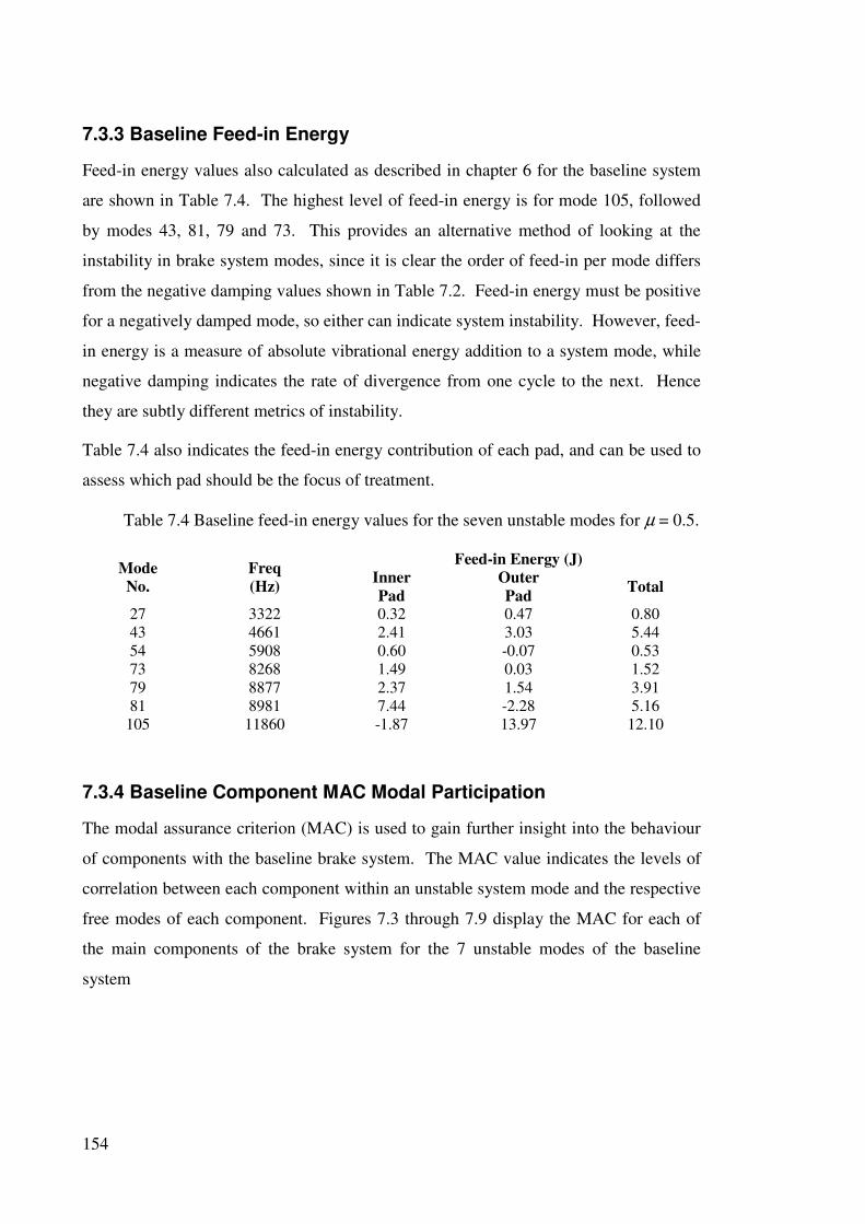
154
7.3.3 Baseline Feed-in Energy
Feed-in energy values also calculated as described in chapter 6 for the baseline system
are shown in Table 7.4. The highest level of feed-in energy is for mode 105, followed
by modes 43, 81, 79 and 73. This provides an alternative method of looking at the
instability in brake system modes, since it is clear the order of feed-in per mode differs
from the negative damping values shown in Table 7.2. Feed-in energy must be positive
for a negatively damped mode, so either can indicate system instability. However, feed-
in energy is a measure of absolute vibrational energy addition to a system mode, while
negative damping indicates the rate of divergence from one cycle to the next. Hence
they are subtly different metrics of instability.
Table 7.4 also indicates the feed-in energy contribution of each pad, and can be used to
assess which pad should be the focus of treatment.
Table 7.4 Baseline feed-in energy values for the seven unstable modes for µ = 0.5.
Feed-in Energy (J) Mode
No.
Freq
(Hz) Inner
Pad
Outer
Pad Total
27 3322 0.32 0.47 0.80
43 4661 2.41 3.03 5.44
54 5908 0.60 -0.07 0.53
73 8268 1.49 0.03 1.52
79 8877 2.37 1.54 3.91
81 8981 7.44 -2.28 5.16
105 11860 -1.87 13.97 12.10
7.3.4 Baseline Component MAC Modal Participation
The modal assurance criterion (MAC) is used to gain further insight into the behaviour
of components with the baseline brake system. The MAC value indicates the levels of
correlation between each component within an unstable system mode and the respective
free modes of each component. Figures 7.3 through 7.9 display the MAC for each of
the main components of the brake system for the 7 unstable modes of the baseline
system

155
Mode 27 - Rotor MAC
0
10
20
30
40
50
965 2943 2944 3732 3735
Freq (Hz)
MA
C (
%)
Mode 27 - Anchor MAC
0
5
10
15
20
25
30
988 1718 2766 3215
Freq (Hz)
MA
C (
%)
(a) (b)
Mode 27 - Caliper MAC
0
20
40
60
80
100
2763 3674
Freq (Hz)
MA
C (
%)
Mode 27 - Inner Pad MAC
0
5
10
15
20
25
30
2366 4972 6313
Freq (Hz)
MA
C (
%)
(c) (d)
Mode 27 - Outer Pad MAC
0
5
10
15
20
25
30
2375 4998 10281
Freq (Hz)
MA
C (
%)
(e)
Figure 7.3 Mode 27 3322 Hz MAC values (a) Rotor, (b) anchor, (c) caliper,
(d) inner pad and (e) outer pad for µ = 0.5.
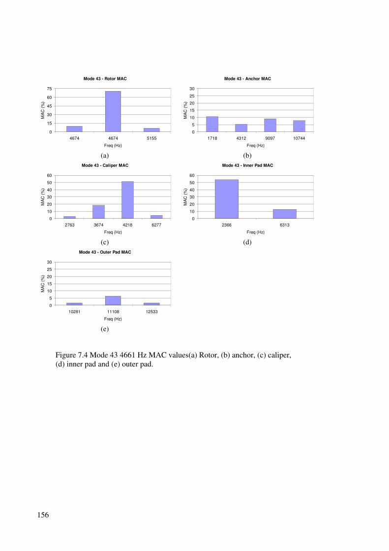
156
Mode 43 - Rotor MAC
0
15
30
45
60
75
4674 4674 5155
Freq (Hz)
MA
C (
%)
Mode 43 - Anchor MAC
0
5
10
15
20
25
30
1718 4312 9097 10744
Freq (Hz)
MA
C (
%)
(a) (b)
Mode 43 - Caliper MAC
0
10
20
30
40
50
60
2763 3674 4218 6277
Freq (Hz)
MA
C (
%)
Mode 43 - Inner Pad MAC
0
10
20
30
40
50
60
2366 6313
Freq (Hz)
MA
C (
%)
(c) (d)
Mode 43 - Outer Pad MAC
0
5
10
15
20
25
30
10281 11108 12533
Freq (Hz)
MA
C (
%)
(e)
Figure 7.4 Mode 43 4661 Hz MAC values(a) Rotor, (b) anchor, (c) caliper,
(d) inner pad and (e) outer pad.

157
Mode 54 - Rotor MAC
0
10
20
30
40
50
60
5153 5748
Freq (Hz)
MA
C (
%)
Mode 54 - Anchor MAC
0
15
30
45
60
75
988 2766 5944 6947
Freq (Hz)
MA
C (
%)
(a) (b)
Mode 54 - Caliper MAC
0
10
20
30
40
50
60
2763 7512 8614
Freq (Hz)
MA
C (
%)
Mode 54 - Inner Pad MAC
0
10
20
30
40
50
60
2366 4972
Freq (Hz)
MA
C (
%)
(c) (d)
Mode 54 - Outer Pad MAC
0
5
10
15
20
25
30
4998 7536
Freq (Hz)
MA
C (
%)
(e)
Figure 7.5 Mode 54 5908 Hz MAC values(a) Rotor, (b) anchor, (c) caliper,
(d) inner pad and (e) outer pad.

158
Mode 73 - Rotor MAC
0
5
10
15
20
25
30
2765 4165 6383 6773 8599
Freq (Hz)
MA
C (
%)
Mode 73 - Anchor MAC
0
5
10
15
20
25
30
988 5944 9299 10004
Freq (Hz)
MA
C (
%)
(a) (b)
Mode 73 - Caliper MAC
0
10
20
30
40
50
60
4218 7277 8428 9373
Freq (Hz)
MA
C (
%)
Mode 73 - Inner Pad MAC
0
5
10
15
20
25
30
2366 4972
Freq (Hz)
MA
C (
%)
(c) (d)
Mode 73 - Outer Pad MAC
0
10
20
30
40
50
60
2375 6385 7536
Freq (Hz)
MA
C (
%)
(e)
Figure 7.6 Mode 73 8268 Hz MAC values(a) Rotor, (b) anchor, (c) caliper,
(d) inner pad and (e) outer pad.

159
Mode 79 - Rotor MAC
0
5
10
15
20
25
30
4165 4166 6773 6774 8608 8686 8687
Freq (Hz)
MA
C (
%)
Mode 79 - Anchor
0
10
20
30
40
5283 6947 9299 12728
Freq (Hz)
MA
C (
%)
(a) (b)
Mode 79 - Caliper MAC
0
5
10
15
20
25
30
7277 8428 9373
Freq (Hz)
MA
C (
%)
Mode 79 - Inner Pad MAC
0
15
30
45
60
75
4972 7490 13033
Freq (Hz)
MA
C (
%)
(c) (d)
Mode 79 - Outer Pad MAC
0
5
10
15
20
25
30
2375 6385 11108
Freq (Hz)
MA
C (
%)
(e)
Figure 7.7 Mode 79 8877 Hz MAC values(a) Rotor, (b) anchor, (c) caliper,
(d) inner pad and (e) outer pad.

160
Mode 81 - Rotor
0
10
20
30
40
4165 6777 8599 8608 8686 8687
Freq (Hz)
MA
C (
%)
Mode 81 - Anchor
0
5
10
15
20
25
30
5283 8153 8374 9097 11275
Freq (Hz)
MA
C (
%)
(a) (b)
Mode 81 - Caliper MAC
0
5
10
15
20
25
30
4218 7277 8428 9373
Freq (Hz)
MA
C (
%)
Mode 81 - Inner Pad MAC
0
5
10
15
20
25
30
4972 7490 10228
Freq (Hz)
MA
C (
%)
(c) (d)
Mode 81 - Outer Pad MAC
0
5
10
15
20
25
30
2375 10281 11108
Freq (Hz)
MA
C (
%)
(e)
Figure 7.8 Mode 81 8981 Hz MAC values(a) Rotor, (b) anchor, (c) caliper,
(d) inner pad and (e) outer pad.

161
Mode 105 - Rotor MAC
0
10
20
30
40
6774 9063 10407 10553 11835 11838 11842
Freq (Hz)
MA
C (
%)
Mode 105 - Anchor MAC
0
5
10
15
20
25
30
2766 9097 10744 11275
Freq (Hz)
MA
C (
%)
(a) (b)
Mode 105 - Caliper MAC
0
10
20
30
40
11063 12859 13312 14359
Freq (Hz)
MA
C (
%)
Mode 105 - Inner Pad MAC
0
10
20
30
40
6313 7490 11090 12510
Freq (Hz)
MA
C (
%)
(c) (d)
Mode 105 - Outer Pad MAC
0
5
10
15
20
25
30
6385 7536 11108 12533
Freq (Hz)
MA
C (
%)
(e)
Figure 7.9 Mode 105 11860 Hz MAC values(a) Rotor, (b) anchor, (c)
caliper, (d) inner pad and (e) outer pad.
7.4 Material Properties Sensitivities
The bulk of the components within the brake system are manufactured from various cast
iron and aluminium alloys. As far as dynamical properties are concerned, this restricts
the amount of change that can occur if the same basic alloy is used for the respective
components.
The natural frequencies of a structure made from a uniform isotropic material scale in
proportion to the speed of sound in the structure. Since structural metals have Poisson’s
ratios of approximately 0.3, it follows that the natural frequencies can be expressed as
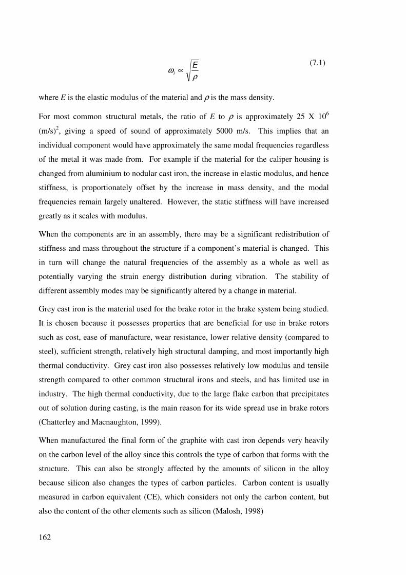
162
ρω
Ei
∝ (7.1)
where E is the elastic modulus of the material and ρ is the mass density.
For most common structural metals, the ratio of E to ρ is approximately 25 X 106
(m/s)2, giving a speed of sound of approximately 5000 m/s. This implies that an
individual component would have approximately the same modal frequencies regardless
of the metal it was made from. For example if the material for the caliper housing is
changed from aluminium to nodular cast iron, the increase in elastic modulus, and hence
stiffness, is proportionately offset by the increase in mass density, and the modal
frequencies remain largely unaltered. However, the static stiffness will have increased
greatly as it scales with modulus.
When the components are in an assembly, there may be a significant redistribution of
stiffness and mass throughout the structure if a component’s material is changed. This
in turn will change the natural frequencies of the assembly as a whole as well as
potentially varying the strain energy distribution during vibration. The stability of
different assembly modes may be significantly altered by a change in material.
Grey cast iron is the material used for the brake rotor in the brake system being studied.
It is chosen because it possesses properties that are beneficial for use in brake rotors
such as cost, ease of manufacture, wear resistance, lower relative density (compared to
steel), sufficient strength, relatively high structural damping, and most importantly high
thermal conductivity. Grey cast iron also possesses relatively low modulus and tensile
strength compared to other common structural irons and steels, and has limited use in
industry. The high thermal conductivity, due to the large flake carbon that precipitates
out of solution during casting, is the main reason for its wide spread use in brake rotors
(Chatterley and Macnaughton, 1999).
When manufactured the final form of the graphite with cast iron depends very heavily
on the carbon level of the alloy since this controls the type of carbon that forms with the
structure. This can also be strongly affected by the amounts of silicon in the alloy
because silicon also changes the types of carbon particles. Carbon content is usually
measured in carbon equivalent (CE), which considers not only the carbon content, but
also the content of the other elements such as silicon (Malosh, 1998)

163
Cast irons, and grey cast iron in particular, differ somewhat to steels and most other
structural metals in that the elastic modulus can be varied significantly by changing CE.
This allows rotors to be manufactured with an elastic modulus that runs from below 100
GPa through to approximately 140 GPa. The baseline FEA model had the rotor
modulus tuned to 118 GPa, so two additional cases were run where the modulus set to
the other extremes of the available range.
Rotor Modulus - Negative Damping Vs Frequency
0.0%
0.4%
0.8%
1.2%
1.6%
2.0%
2.4%
0 2000 4000 6000 8000 10000 12000
Frequency (Hz)
Neg
ati
ve D
am
pin
g
Baseline E = 118 GPa
E = 100 GPa
E = 140 GPa
Figure 7.10 Negative damping levels of system modes for different rotor
modulus levels, µ = 0.5.
Figure 7.10 displays the negative damping levels for the assembly with a change in
modulus with µ = 0.5. The impact of most of the system modes is large, since much of
the brake system’s dynamical properties are governed by the behaviour of the rotor.
This was highlighted by the strain energy in Table 7.3 where rotor activity was
significantly above the average in 5 of the 7 modes.
Compared to the baseline case, setting E = 100 GPa has little effect on the modes at 3.3
kHz, 4.7 kHz, and 9 kHz. However a strong new unstable mode appears at
approximately 7.5 kHz, which is in the range of one of the main concern frequencies
from section 3.11. The unstable modes at 5.9 kHz and 11.9 kHz corresponding to the
test frequencies of concern are suppressed, so the overall noise performance of the
system in testing may be significantly improved. Several other modes with small levels
of instability appear at around 10 to 10.5 kHz.

164
The E = 140 GPa case also significantly impacts the system. Of the main concern
frequencies in testing, the 5.9 and 8.3 kHz are suppressed, but little influence is seen on
the 11.9 kHz mode. Significant new unstable modes have appeared in between 4 and 6
kHz, with a particularly strong mode unstable mode appearing at 4.2 kHz.
Cast iron is also used for the anchor bracket, albeit nodular (also called ductile) cast iron
rather than grey cast iron. The carbon content of nodular irons is lower than grey cast
iron, and the carbon formation is in spheroidal or nodular form. Nodular iron has
tensile strengths of around 400 MPa as opposed to high carbon grey irons which may be
as low as 150 MPa. This, along with an elastic modulus of approximately 170 GPa,
makes them the preferred choice for use in cast iron components in low cost
applications where the hi thermal conductivity of grey iron is less important. The
higher strength is an obvious benefit in most applications, but also the higher modulus is
important since the stiffness of components is proportional to modulus and can be vital
in ensuring proper operation and wear of components. Nodular iron is also relatively
insensitive to small changes in carbon content, so the modulus does not vary
significantly from the region of 170 GPa. A value of 165 MPa was used for the
baseline assembly since this was determined from the tuned FEA bracket model.
Alternative analyses were run with the modulus of the cast iron set to 140 and 200 MPa
respectively with these results displayed in Figure 7.11. While these cases do not
necessarily represent a realistic range for nodular iron, and would require different types
of material, it does provide a convenient method for examining the impact of stiffness
of the bracket which could be achieved with geometry changes.
The anchor also has a significant affect on the stability of the system. Reducing the
modulus to 140 GPa reduced the number of unstable modes to just 2. On the other
hand, increasing the Young’s modulus to 200 GPa had less of an impact with unstable
modes still present at 3.3 kHz, 4.7 kHz, 5.9 kHz and 9 kHz. Several other new unstable
modes appeared also. Reducing bracket stiffness may reduce the brake squeal
propensity of the system overall.
The caliper housing is made from aluminium, with a modulus of 68 GPa determined
from the tuned FEA model used for the baseline assembly. Aluminium does not show
much variation in modulus through alloying, but an alternative case was run with the
caliper modulus set to 100 GPa as shown in Figure 7.12. As was the case with the

165
bracket, this was done as a convenient method for determining the influence of
changing the housing stiffness without requiring geometry changes.
Anchor Modulus - Negative Damping Vs Frequency
0.0%
0.4%
0.8%
1.2%
1.6%
0 2000 4000 6000 8000 10000 12000
Frequency (Hz)
Neg
ati
ve D
am
pin
g
Baseline E = 165 GPa
E = 140 GPa
E = 200 GPa
Figure 7.11 Negative damping levels of system modes for different anchor
modulus levels, µ = 0.5
Many of the same concern frequencies remain, but strong instabilities are seen at 4.2
and 5,8 kHz. It should be noted that 11.9 kHz is no longer unstable, and caliper
stiffness was a potential cure indicated in chapter 6 for that mode. Overall it appears
that caliper stiffness may not be beneficial for overall system stability.
The friction material was the only non-metallic material used in the model of the brake
assembly. Friction material is inherently complex and is a mixture of dozens of
material as described in section 4.4.4. Nine different modulus levels were run, all with
isotropic material model. 5 GPa was used as the baseline, and 2 and 10 GPa were the
alternate extreme levels selected since they represent the approximate extremes found in
friction material. Figure 7.13 displays the lining change results.
The pad friction material results show a mix of trends. The mode at 3.3 kHz is
insensitive to pad modulus change. Referring to the strain energy in Figure 7.2 it can be
seen that pad deformation is very low for this mode rendering it insensitive to pad
modulus. A new mode appears altogether at 4 kHz that is strongly dependant on pad
modulus. The instability level (ie, negative damping) for most modes tends to increase
with a decrease in pad modulus. Increasing pad modulus reduces the overall number of
unstable modes and indicates that overall system stability would be enhanced with

166
higher modulus (stiffness) pads. The most probably physical explanation for this would
be reduction in pad deformation that would follow, hence a reduction in overall feed-in
energy values.
Caliper Modulus - Negative Damping Vs Frequency
0.0%
0.2%
0.4%
0.6%
0.8%
1.0%
1.2%
0 2000 4000 6000 8000 10000 12000Frequency (Hz)
Neg
ati
ve D
am
pin
g
Baseline E = 68 GPa
E = 100 GPa
Figure 7.12: Negative damping levels of system modes for reduced caliper
modulus, µ = 0.5
Pad Modulus - Negative Damping Vs Frequency
0.0%
0.6%
1.2%
1.8%
2.4%
3.0%
0 2000 4000 6000 8000 10000 12000
Frequency (Hz)
Neg
ati
ve D
am
pin
g
Baseline E = 5 GPa
E = 2 GPa
E = 3 GPa
E = 4 GPa
E = 6 GPa
E = 7 GPa
E = 8 GPa
E = 9 GPa
E = 10 GPa
Figure 7.13: Negative damping levels of system modes for changes in
friction material modulus, µ = 0.5

167
The baseline brake assembly analysis was conducted devoid of material damping. This
is mainly because the system is relatively lightly damped and therefore the modal
frequencies and mode shapes are largely unaffected. However, the experimental modal
analysis conducted in chapter 3 provides modal damping levels for the main
components.
The analysis was re-run with structural damping added to the main components, first
one at a time and for all at once, to see if this had any impact on the stability results.
Figure 7.14 displays the impact of structural damping being added to all of the
components. It is clear that the damping acts simply to reduce the negative damping.
Modes with little negative damping may become stable, and modes that are more
unstable have some measure of damping added. An additional slightly unstable mode
appears at 4.1 kHz which is not seen in the baseline case, although at low levels of
instability.
Damping Level - Negative Damping Vs Frequency
0.0%
0.2%
0.4%
0.6%
0.8%
1.0%
0 2000 4000 6000 8000 10000 12000
Frequency (Hz)
Neg
ati
ve D
am
pin
g
Baseline No Damping
Structural Damping
Figure 7.14: Structural damping with µ = 0.5
The use of these low levels of structural damping was considered to not significantly
affect the analyses in this study. The main impact is simply to reduce the instability of
system modes with little influence on the character of the modes themselves.
Further impact due to damping was modelled by applying relatively large levels of
structural damping to the pad backplates. This was done in an effort to simulate the
application of damping shims. Figure 7.15 shows that the application of backplate

168
damping has little affect on most modes. The exceptions are the modes at 7.3 kHz and
11.9 kHz. It is clear from strain energy distributions in Figure 7.2 that both of these
modes have a very high level of pad motion, so the effects of the damping is
maximised. In Chapter 6 it was shown that out pad motion was a key driver of the 11.9
kHz mode.
Backplate Damping - Negative Damping Vs Frequency
0.0%
0.2%
0.4%
0.6%
0.8%
1.0%
0 2000 4000 6000 8000 10000 12000Frequency (Hz)
Neg
ati
ve D
am
pin
g
No BP Damping
BP Damping = 1%
BP Damping = 5%
BP Damping = 10%
Figure 7.15: Backplate damping with µ = 0.5
The remaining components of the assembly, the guide pins and the piston, maintained
their baseline material properties through the study.
7.5 Contact Distribution Sensitivities
A key feature of brake system dynamics is the interaction of components at the various
interfaces. The most critical is the rotor/pad interface, but can also be important at other
interfaces such as the piston/inner backplate.
During the noise package development for a production brake system, many of the
modifications trialled are designed to alter the contact pressure distribution at the
rotor/pad interface. This is achieved usually through one of two ways; modification of
the footprint of the “puck” of friction material that contacts the rotor by use of different
chamfers or cuts, or by the use of slotted or cut shims between the inner backplate and
the piston.

169
Backplate
Friction
material
Removed
material
Figure 7.16 shows a puck that has been modified by the addition of chamfers that
directly change the area of contact between the pad and the rotor. Moving the contact
pressure backward from the leading edge of the pad is considered beneficial for system
stability, so the chamfer is symmetrically added to both the leading and trailing edges of
the pad to remove the need for “handed” pads, i.e., pads that have different geometry
between left and right hand fitment, or differences between inner and outer pads.
Figure 7.16 Cross section of a modified puck with landing and trailing
chamfers
The alternate way to modify the contact pressure distribution of the brake pad is to
apply cut shims to the backplate, an example of which is shown in Figure 7.17. While
backplate shims usually contain damping material to help decouple components and/or
add damping to the system, they also play a role in determining the contact pressure
between the piston and the pad. Slots change the centre of pressure between the piston
and pads, and it follows that the contact pressure between the pad and rotor will also be
modified. Under certain circumstances, slots may also decouple modes.
Figure 7.17 Slotted shim which removes pressure from one end of the
piston, helping to alter the contact pressure at the friction interface.

170
To incorporate these modifications into the FEA model would potentially require a
change the geometry of the pad and/or the addition of an additional component between
the pad and the piston. Neither of these changes were attempted with geometry change
since it was not considered necessary to capture the key factor, that is, modifying the
areas in contact with each other.
Two types of common noise control features were modelled. The first was a shim with
a slot that covered half of the piston contact area, either leading or trailing, was
simulated. Secondly, a 15 mm parallel chamfer on the leading and trailing edges of the
puck, the results of which is shown in Figure 7.19. Both the chamfer on the puck and
the slotted shim were implemented via simply changing the contact areas by
deactivating contact springs in the appropriate locations within the FEA model.
Stiffness Shims - Negative Damping vs Frequency
0.0%
0.4%
0.8%
1.2%
1.6%
2.0%
0 2000 4000 6000 8000 10000 12000
Frequency (Hz)
Neg
ati
ve D
am
pin
g
Baseline
Piston shim - leading slot
Piston shim - trailing slot
Hat shim
Figure 7.18: Shims applied to the assembly with µ = 0.5.
Figure 7.18 displays the results of using shims. Two variations of the piston shim were
run, one with the slot on the leading side and another with the slot on the trailing side of
the piston. Another modification investigated in this study was to examine the effects
of using a top hat shim. This is a steel plate fitted between the rotor and the wheel
which provides significant stiffening of the hat. This was condition was simulated by
constraining all DOFs the regions of the hat within the mounting bolts holes. Some
success has been achieved by stiffening the hat for controlling brake noise in some
brake systems where deformation of the hat is significant. The results are also

171
displayed in Figure 7.18, and it is clear that hat shims and slotted shims have little
beneficial affect on stabilising most of the system modes.
Two further contact pressure distributions on the rotor/pad interface were investigated.
These follow from the nature of the contact between the pad and the rotor in a brake
system in typical use.
When pressure is applied to the brake the pads are forced onto the rotor, but in a non-
uniform way. The inner pad is forced in the central region by the piston, while the outer
pad is forced by the caliper fingers. Since the friction material is relatively soft and the
pad can deform, the pressure distribution can become non-uniform. The outer edges of
the pads tend to pull away from the rotor resulting in the spring tuning described in
section 4.6.1.4.
Contact Distribution - Negative Damping Vs Frequency
0.0%
0.4%
0.8%
1.2%
1.6%
2.0%
0 2000 4000 6000 8000 10000 12000Frequency (Hz)
Neg
ati
ve D
am
pin
g
Baseline
Chamfer
Edge Contact
Full Contact
Figure 7.19: Contact distribution with µ = 0.5
An additional effect of this non-uniform contact pressure is non-uniform wear. An
extreme example occurs when a vehicle descends along a mountain road and undergoes
repeated high torque brake applications is a short period. Wear towards the centre of
the pad is significantly higher in the short term before more moderate braking tends to
normalise the wear rate across the pad. If a low pressure stop is made in such a
configuration the contact area tends to reverse. The central regions have little on no
contact pressure, and the outer edges of the pad are mainly in contact. A simulation of

172
the condition was made where the usual spring locations at the pad/rotor interface were
reversed. That is, only the outer edges of the pads were in contact.
The final contact pressure distribution that was investigated was the case with brand
new pads at extremely low pressure. Here the pad is largely in uniform contact all over
the face. So for this simulation all of the contact springs at the rotor/pad interface were
activated.
It can be seen in figure 7.19 that full pad contact causes considerable instability
compared to the other contact configurations, and reduced contact configuration offers
improved stability. The edge contact case is only a short term effect in a real brake
system, but it appears to offer the best solution. Addition of chamfers to the leading and
trailing edge of the pads also increases stability compared to the baseline case.
7.6 Damping Shims
Application of damping shims to the pad backplates was an alternative method to
simulate damping shims to that discussed in section 7.4 where high levels of structural
damping were added to the pad backplates. This was initially simulated by putting a
layer of 2 dimensional shell elements across the pad back plates. Unfortunately, this
was found to be a completely ineffectual technique. This is because the damping shim
is a three dimensional structure where shear between layers contributes most of the
system damping and a layer of two dimensional shell elements on the backplates do not
capture this behaviour.
The final trials using the pad damping shims were to incorporate full three dimensional
damping shims onto the backplates. The typical damping shim is usually a multi layer
laminate with alternating rubber, steel and adhesive layers, with a typical example
shown in Figure 2.6 and material specification in Table 2.1.
Only one simplified shim material was modelled for this study. The structure, which
represents a simplified shim layout, is shown in Table 7.5
Table 7.5 Simplified shim structure used in the FEA study
Layer Material Thickness
(mm)
Modulus
(GPa)
Poisson’s
ratio Density
Structural
loss factor Piston side Steel 0.40 207 0.3 7.86 none
Pad side Rubber 0.40 0.5 0.49 1.5 0, 50, 100%
Total 0.80

173
The stability results are presented in Figure 7.20. It can be seen that adding the shim
alone without any damping can have a negative impact on the stability of many modes.
A new strongly unstable mode has appeared at 4 kHz and several other modes indicate
increases in instability with no damping. It must be highlighted that addition of the
shims changes the structural behaviour of the base system even without the addition of
damping due to the increase in thickness on the back of the pad and the addition of a
steel layer. The rubber layer also changes the interface been the caliper and pad
backplates.
Application of damping increases stability for all of the modes. However the
comparison is only valid to the undamped shim as a baseline rather than the shim-less
baseline for the reasons mentioned in the previous paragraph. With 100% loss factor,
ie., 50% of critical damping, applied to the shim rubber, it is seen that almost all of the
system modes are stable. Even the 4 kHz mode, which is unstable with the undamped
shim, has been reduced to almost zero instability. These results certainly indicate that
for any given shim structural arrangement, an increase in damping will improve stability
of the system.
It is also worth noting that the results with the shim differ considerably from that shown
in Figure 7.15 for the damped backplate. This is most likely due to the additional
effects of the shim as discussed in section 2.6, including decoupling of components and
shear damping effects. The damped backplates only add a small measure of damping to
the system, and do not adequately capture the physical effects of a full multi-layer
damping shim.

174
Shim Modelling: Negative Damping vs Frequency
0.0%
1.0%
2.0%
3.0%
4.0%
0 2000 4000 6000 8000 10000 12000
Frequency (Hz)
Ne
ga
tiv
e D
am
pin
g
gr5c5 Baseline
Composite - No damp
Composite - 50% Loss
Composite - 100% Loss
Figure 7:20 Negative damping levels of system modes for changes damping
shim µ = 0.5
7.7 Summary
This chapter has presented a study on some of the parameters that affect the noise
propensity of a brake system. Many of the structural modification change the behaviour
in a significant way, and many new unstable modes may be created in addition to
addressing some the existing unstable modes. In this respect, problem modes would be
treated on a case by case basis, and rarely will a modification improve all potential
unstable modes.
Increasing the coefficient of friction of the pad/rotor interface was found to increase the
instability in all system modes. Conversely reducing coefficient of friction may be
considered a general method for improving system stability, but in practice the
performance requirements of a brake system render this approach requires system size
increase to maintain torque capacity.
Reducing pad contact area was found to increase stability of the brake system. Parallel
chamfers offer more stability than the baseline pad case as a counter measure that could
be applied to a production brake system. Increasing pad modulus was found to increase

175
system stability also, although some modes were insensitive to pad modulus due to the
lack of pad deformation.
Modelling of damping was done in numerous ways. Adding structural damping to the
components of the base system was found to slightly increase the stability of the system
modes without greatly changing their character. Simulating backplate damping shims
by adding damping to the backplate increased system stability, but failed to capture the
behaviour of a laminated shim. Adding a damping shim to the back plate was found to
be very affective due to more adequately capturing the behaviour of a physical shim, but
even the addition of a shim without damping can influence the behaviour of the baseline
system since it adds a further structural component.

176

177
Chapter 8
Comparison of Contact Modelling Methods
8.1 Introduction
In the previous four chapters of this thesis, the development of a finite element model
for squeal prediction was presented. The commercial finite element analysis (FEA)
code MSC.Nastran was used for the analysis.
A central feature of using Nastran is the requirement for the user to implement the
contact interfaces within the model. This not only includes the pad / rotor interface with
its crucial friction interface, but other interactions between all of the other components.
Linear springs were used to represent the contact stiffness at the interface, with the
stiffness calculated on the basis of the properties of the adjacent elements. Consequently
the analysis was fully linear.
In this chapter an alternative method is presented which makes use of the powerful
contact modelling capabilities of HKS Abaqus. Contact elements are incorporated into
the code that establishes the required contact conditions at the interfaces automatically,
greatly simplifying the modelling process allowing non-linear contact. The results of
reanalysing the complete assembly using Abaqus are presented and comparisons made
with the results obtained from Nastran.
8.2 Contact Elements
HKS Abaqus is a powerful, non-linear FEA code that features contact modelling with
contact elements. Various types are available and are described in full in the Abaqus
User’s Manual [Abaqus User’s Manual, 2003]. The types for structural analysis are:
• Deformable-deformable - used to model contact between bodies where elastic
deformation of both is important
• Rigid-deformable - typically used where elastic deformation on only one body is
considered such as a manufacturing forming process
• Tied - used to directly fix bodies together, or for joining dissimilar meshes
Each type of contact features strict master-slave relationship between the two
components. A master surface is defined along the outer surface of elements on one

178
component, and a set of nodes on the other body are defined as slave nodes. The master
surface and slave nodes form a contact pair. A 2 dimensional example of a master
surface and slave nodes is shown in Figure 8.1 (a).
During analysis the relative position of the slave nodes compared to master surfaces is
monitored and the overriding condition is that slave nodes cannot penetrate through a
master surface. It is recommended that the master surface is set as the surface with
lower mesh density, or the body with the higher elastic modulus if the mesh densities
are similar.
A striking difference between the contact element formulation compared node to node
definition used in the Nastran analysis is that the actual contact between slave nodes and
their respective master surfaces does not need to be predefined. Slave nodes become
automatically associated with a master surface during the analysis, so the requirement to
have mesh with coincident nodes at the contact pair is removed.
Two types of contact are required for implementing the brake assembly model;
deformable-deformable and tied. A description of each of these follows.
8.2.1 Tied Contact
Tied contact is the simplest form of contact where nodes on the slave surface are simply
tied, or rigidly fixed, to the master surface. An initial contact clearance distance can be
defined and a numerical algorithm checks the projected area from the master surface in
the normal direction, as shown for a 2 dimensional case in Figure 8.1 (b). Any slave
node that falls into this area has its position modified to bring it to lie exactly on the
master surface as shown in Figure 8.1 (c).
The node is geometrically fixed (tied) to the surface, and its forces are distributed
directly onto the adjacent master surface nodes in proportion to their respective
geometric proximity. This operation is performed before the first increment of the first
step of an analysis that follows the activation of the contact pair, and the contact
locations remain fixed throughout the analysis.
In 3 dimensional contact analysis the principle is essentially the same. At the start of
the analysis the contact surface and clearance distance define a volume that checked for
slave nodes. Any node that lies in the volume is modified to bring it to lie on the master
surface and the resulting load on the slave node is distributed to the adjacent master

179
surface nodes.
(a) Initial contact condition showing slave nodes on body 1 and master surface on body 2
(b) Initial clearance with ∆ t used to find nodes requiring positional adjustment
(c) Contact condition after slave nodes within initial clearance have been adjusted
Figure 8.1 Master/slave contact in 2 dimensions.
A key point to note in this modification of slave nodes, and hence the elements formed
by these nodes, is that it is a zero strain operation. That is, the elements after
Master
Slave nodes
Body 2
Body 1
∆ t

180
modification possess zero strain and the modified slave element defines the initial
unloaded condition.
Abaqus also checks for overclosure before an analysis. This is the condition where one
or more of the slave nodes are geometrically located within the master surface. The
same procedure is applied here as for the initial contact clearance check. The location
of the nodes is modified to bring them to lie exactly on the master surface.
The use of the initial clearance setting of the contact pair is to allow for geometric
modelling error and the implied modelling intent is that any tied contact pairs are
supposed to have exact geometrically matching boundaries and fully constrained to each
other for the duration of the analysis.
8.2.2 Deformable-Deformable Contact
Deformable-deformable contact is applied between bodies that are coming into contact
during an analysis, but are not physically fixed to each other. Some similarities to the
tied contact exist, but also many differences.
The analysis commences by examining an area projected from the master surface for a
distance given by the initial contact clearance. Again, as for tied contact, slave nodes in
this area will be adjusted to lie exactly on the master surface. However, the node is not
tied to the master surface for the duration of the analysis. Also, slave nodes that are not
in this area, and therefore remain unadjusted, are not discounted from the contact pair.
These nodes may come into contact at a later stage of the analysis. However, the
geometric adjustment for nodes within the contact clearance is only performed once,
which is prior to the first analysis step after the contact pair is activated.
In deformable-deformable contact nodal forces from a slave node are again transferred
onto the master surface, but the node is not physically fixed in this location. A normal
contact stiffness is added between the node and the master surface nodes, and also a
tangential stiffness is determined on the basis of the interfacial forces and the friction
coefficient. This procedure is completed for every increment of the analysis and nodes
can come into and go out of contact as required on every step of the analysis.
A further distinction in elastic-elastic contact is whether contact slip distance is
negligible, or if it needs to be considered. In “small sliding” the relative slip
displacement between the slave and master surface is much smaller that the length of a
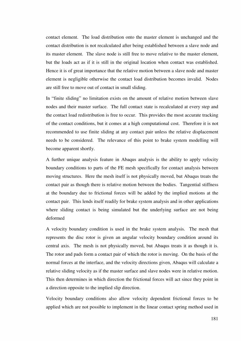
181
contact element. The load distribution onto the master element is unchanged and the
contact distribution is not recalculated after being established between a slave node and
its master element. The slave node is still free to move relative to the master element,
but the loads act as if it is still in the original location when contact was established.
Hence it is of great importance that the relative motion between a slave node and master
element is negligible otherwise the contact load distribution becomes invalid. Nodes
are still free to move out of contact in small sliding.
In “finite sliding” no limitation exists on the amount of relative motion between slave
nodes and their master surface. The full contact state is recalculated at every step and
the contact load redistribution is free to occur. This provides the most accurate tracking
of the contact conditions, but it comes at a high computational cost. Therefore it is not
recommended to use finite sliding at any contact pair unless the relative displacement
needs to be considered. The relevance of this point to brake system modelling will
become apparent shortly.
A further unique analysis feature in Abaqus analysis is the ability to apply velocity
boundary conditions to parts of the FE mesh specifically for contact analysis between
moving structures. Here the mesh itself is not physically moved, but Abaqus treats the
contact pair as though there is relative motion between the bodies. Tangential stiffness
at the boundary due to frictional forces will be added by the implied motions at the
contact pair. This lends itself readily for brake system analysis and in other applications
where sliding contact is being simulated but the underlying surface are not being
deformed
A velocity boundary condition is used in the brake system analysis. The mesh that
represents the disc rotor is given an angular velocity boundary condition around its
central axis. The mesh is not physically moved, but Abaqus treats it as though it is.
The rotor and pads form a contact pair of which the rotor is moving. On the basis of the
normal forces at the interface, and the velocity directions given, Abaqus will calculate a
relative sliding velocity as if the master surface and slave nodes were in relative motion.
This then determines in which direction the frictional forces will act since they point in
a direction opposite to the implied slip direction.
Velocity boundary conditions also allow velocity dependent frictional forces to be
applied which are not possible to implement in the linear contact spring method used in

182
the Nastran model. This is particularly useful for brake system analysis since it is
common for the coefficient of the friction between the rotor and the pad to increase at
lower velocities. A great many options are available for the analysis which can be
found in the Abaqus Users manual (2003).
8.2.3 Non-linear Static Analysis
The Nastran analysis that was presented in preceding chapters utilised linear static
solutions to determine the base state of the brake system during a braking application.
Linearity means that only a single determination of the system’s stiffness matrix and
therefore only a single matrix inversion during solution is required. Linear solutions
also imply that the structural response scales directly with applied loads.
Non-linearity arises when the behaviour of the system changes as load is applied. The
static solution for the brake system is non-linear due to the changing contact conditions
during pressure application. This non-linearity was captured using a manual iterative
procedure where by an initial static analysis is run and contact springs with physically
unrealistic tensile forces are removed. This procedure was repeated until a final
position and contact state which was devoid of tensile contact forces was determined.
This solution strategy is essentially non-linear but each solution was linear.
The forte of Abaqus is the solution of non-linear problems, be they contact, geometric
or material property driven non-linearity. A solution step is approached in small
increments which in themselves are solved iteratively. Thus the loads are applied
gradually with equilibrium achieved for intermediate loads ensuring the convergence to
the correct final state of the system. Abaqus uses an iterative solution technique, the
principle of which, and the relationship between steps, increments and iterations, are
described in the following paragraphs.
During a solution static equilibrium is evaluated by checking the internal nodal forces
are in balance with the externally applied loads, known as a force residual. If they are
not smaller than a small tolerance, then the system is non-linear and updating of the
stiffness matrix will be required.
An overall analysis is decomposed into individual steps that represent different stages of
the analysis. For example, the first step of a brake analysis may be to apply pressure to
a static brake and then step 2 may be to apply the rotor rotation and so on.

183
A solution step is by default assigned a time of 1 second, even though a measure of time
has no physical meaning for a static solution. An initial increment is chosen, for
example 0.05s, and a solution is attempted. This means a load of 0.05 times the overall
required load for the step is applied. If large loads are applied too quickly it can be very
difficult to achieve equilibrium for an increment since the system stiffness matrix
requires substantial updating from one load increment to the next.
The first iteration on the increment is attempted and a new displacement determined
using the current system stiffness matrix. An updated stiffness matrix is formulated and
internal forces calculated. If equilibrium is not achieved under the new displacement
condition, then another iteration is made. Several iterations, each with updates to the
stiffness matrix may be required to converge at each increment.
Once an increment has converged, then a new increment size is determined based on the
size of the current increment, the default value being 1.5 times the current increment
size if convergence occurred with 5 iterations. If more than 5 iterations are required
then the next increment will have the same size as the current one. If, however, the
current increment does not converge within a reasonable number of iterations, the
default being 12 attempts, then the size increment is “cut back” to 0.25 times the current
increment.
Increments are repeated until a time of 1s has been completed. The step is now
complete and the next step of the analysis will commence.
8.2.4 Contact Set-up and Solution Steps
The model employed for the brake system analysis in this present study has identical
geometry and meshing to the Nastran model considered in chapters 4 through 7. Two
types of 3-dimensional elements were used from the Abaqus element library:
• C3D6 – 1st order 3D continuous wedge element with 6 nodes.
• C3D8 – 1st order 3D continuous hexahedral element with 8 nodes.
Also used in the regions where contact occurs are the contact surface elements.
It is not necessary to implement finite sliding contact pairs at any of the locations of
contact within a brake system model. Most of these locations exhibit negligible relative
slip when the brake is loaded. The only exception is the rotor / pad interface where

184
obviously the rotor rotation leads to a high slip rate in a physical brake system.
However, in the contact analysis using Abaqus it is simply a case of defining a velocity
boundary condition to the rotor as described in the section 8.2.2. Table 8.1 displays a
summary of the parameters used for each of the contact interfaces within the brake
assembly.
Table 8.1 Contact interfaces in the Abaqus brake assembly model.
Interface Type Initial Clearance (mm) µµµµ
Rotor / lining Small sliding .005 0.5
Inner Pad BP / piston Small sliding .005 0.12
Outer Pad BP / housing Small sliding .005 0.12
Pad BP / anchor Small sliding .005 0.12
Piston / housing Small sliding .001 0.05
Pins / anchor Small sliding .001 0.05
Pins / housing Tied .01 -
The initial contact clearance values were chosen to be .005 mm for all of the pad
surfaces since these are all intended to have the surfaces resting against each other at the
commencement of the analysis and .005 mm represents the geometric resolution of the
geometry. The pad and piston surfaces use 0.001 mm since these surfaces are not
designed to be in initial contact and are modelled with a finite clearance. The value of
.001 mm ensures that no adjustment of nodes would occur at these contact surfaces
prior to analysis. The housing and pin clearance of .01 mm ensured all of the contact
surfaces will be fully adjusted and tied even if some nodes were up to .005 mm apart
due to modelling tolerance.
The overall solution strategy that was employed is not dissimilar to that used to solve
the Nastran models described in previous chapters. A static analysis establishes the
base state of the system under a typical brake load, and then a complex eigenvalue
solution was performed to determine system stability about this base state. However,
the steps used differ and 4 individual steps were used.
1. Static preload, non-linear static. Pressure is applied to the back of the piston
and inside the bore in the caliper housing. No rotation is applied to the rotor for
this step and the system reflects a stationary brake with pressure applied. This

185
allows non-linear static solver to more easily determine the contact conditions at
the rotor / pad, guide pin and piston interfaces without the complication
introduced by rotation. Solution stabilization, which involves applying artificial
damping to control rigid body motions, is applied to bodies that are not
constrained prior to contact being established. The damping is small enough not
to affect the final static solution when all the contact conditions have been
properly established.
2. Add rotation, non-linear static. A velocity boundary condition was added to
the rotor from the statically loaded state from step 1. The pads react to the
frictional forces at the rotor / pad interface and begin to translate until fully
captured by the pad abutment regions on the anchor bracket. The system
converged into its base state during a brake application. This provided the base
state for the analysis steps that followed.
3. Normal modes. The normal modes solution provides a subspace of modes to be
used for the complex eigenvalue solution in step 4. The number of modes
extracted was 160 covering a frequency range 0 to 18 kHz. The number of
modes in this step needed to be greater than the number of complex modes
requested for step 4 to adequately allow the complex modes to be represented.
4. Complex modes. Complex eigenvalue solution to provide the stability response
of the base statically loaded state. Abaqus implements only a sub-space
projection procedure, hence the requirement for the prior normal modes analysis.
In this analysis 120 complex modes were extracted, covering a range from 0 to
14.5 kHz.
8.3 Material Properties and Load Cases
Material property data for the Abaqus analyses is the same as that used for the Nastran
analysis. There is negligible difference between the normal modes analysis from
Nastran and Abaqus since the material property “tuning” from the Nastran model was
carried over. The properties are summarised in Table 8.2.
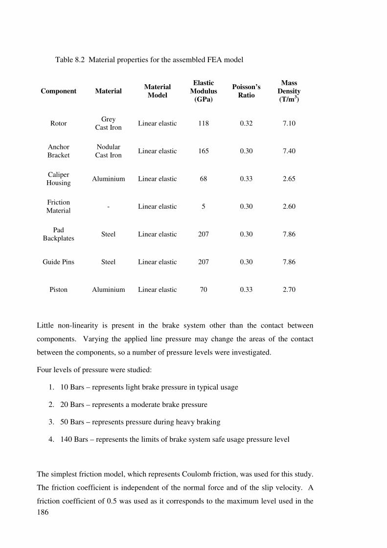
186
Table 8.2 Material properties for the assembled FEA model
Component Material Material
Model
Elastic
Modulus
(GPa)
Poisson’s
Ratio
Mass
Density
(T/m3)
Rotor Grey
Cast Iron Linear elastic 118 0.32 7.10
Anchor
Bracket
Nodular
Cast Iron Linear elastic 165 0.30 7.40
Caliper
Housing Aluminium Linear elastic 68 0.33 2.65
Friction
Material - Linear elastic 5 0.30 2.60
Pad
Backplates Steel Linear elastic 207 0.30 7.86
Guide Pins Steel Linear elastic 207 0.30 7.86
Piston Aluminium Linear elastic 70 0.33 2.70
Little non-linearity is present in the brake system other than the contact between
components. Varying the applied line pressure may change the areas of the contact
between the components, so a number of pressure levels were investigated.
Four levels of pressure were studied:
1. 10 Bars – represents light brake pressure in typical usage
2. 20 Bars – represents a moderate brake pressure
3. 50 Bars – represents pressure during heavy braking
4. 140 Bars – represents the limits of brake system safe usage pressure level
The simplest friction model, which represents Coulomb friction, was used for this study.
The friction coefficient is independent of the normal force and of the slip velocity. A
friction coefficient of 0.5 was used as it corresponds to the maximum level used in the
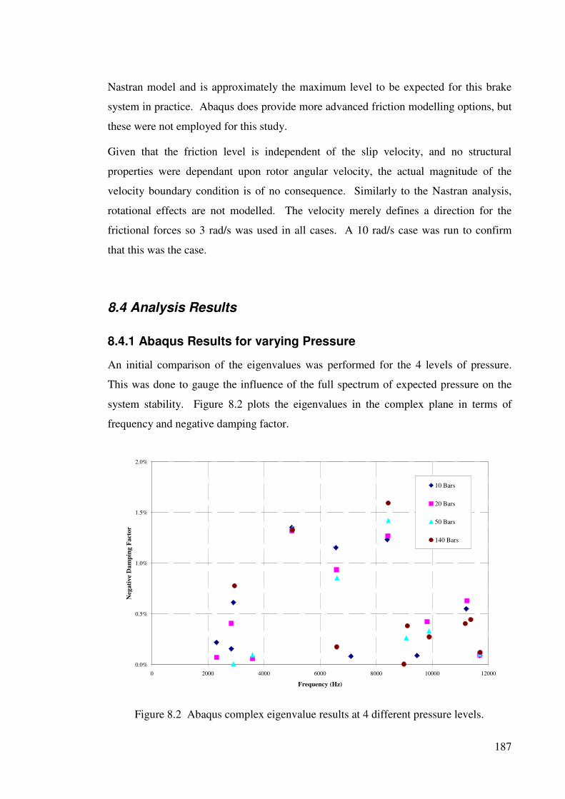
187
Nastran model and is approximately the maximum level to be expected for this brake
system in practice. Abaqus does provide more advanced friction modelling options, but
these were not employed for this study.
Given that the friction level is independent of the slip velocity, and no structural
properties were dependant upon rotor angular velocity, the actual magnitude of the
velocity boundary condition is of no consequence. Similarly to the Nastran analysis,
rotational effects are not modelled. The velocity merely defines a direction for the
frictional forces so 3 rad/s was used in all cases. A 10 rad/s case was run to confirm
that this was the case.
8.4 Analysis Results
8.4.1 Abaqus Results for varying Pressure
An initial comparison of the eigenvalues was performed for the 4 levels of pressure.
This was done to gauge the influence of the full spectrum of expected pressure on the
system stability. Figure 8.2 plots the eigenvalues in the complex plane in terms of
frequency and negative damping factor.
0.0%
0.5%
1.0%
1.5%
2.0%
0 2000 4000 6000 8000 10000 12000
Frequency (Hz)
Neg
ati
ve D
am
pin
g F
acto
r
10 Bars
20 Bars
50 Bars
140 Bars
Figure 8.2 Abaqus complex eigenvalue results at 4 different pressure levels.

188
A total of 12 separate unstable modes were identified between the 4 pressure cases.
Considerable overlap occurs between the load cases with most of the unstable modes
exhibiting similar levels of instability independent of the pressure level.
8.4.2 Abaqus vs Nastran Stability
One single Abaqus pressure case, at 20 Bars, was chosen for a deeper analysis of the
system behaviour. The direct comparison to the stability results from the Nastran
analysis is shown in Figure 8.3.
0.0%
0.5%
1.0%
1.5%
2.0%
0 2000 4000 6000 8000 10000 12000
Frequency (Hz)
Neg
ati
ve D
am
pin
g F
acto
r
Nastran
Abaqus
Figure 8.3 Comparison of complex eigenvalue results of Abaqus and
Nastran
Noted differences can be seen in the comparison of unstable system modes. Overall the
negative damping ratios for the Abaqus models indicate higher levels of instability than
the Nastran model. Also, some differences in the frequencies can be seen, but overall
each model predicts some unstable modes in or close to the frequency ranges of noise
concern. Table 8.3 provides a summary of the test results from Chapter 3.11, as well as
the Nastran and Abaqus prediction results.

189
Table 8.3 Summary of test, Nastran and Abaqus results
Test Concern Frequency Nastran Result Abaqus Result
4.5-5 kHz 4.7 kHz 5 kHz
6-6.5 kHz 5.9 kHz 6.5 kHz
7.5-8 kHz 8.3 kHz 8.4 kHz
11.5-12 kHz 11.9 kHz 11.7 kHz
The Abaqus model predicts higher levels of instabilities for all of the 4 concern
frequency ranges of interest except for the 11.7 kHz. Also, as was the case with the
Nastran model a number of other frequencies were predicted that do not correspond to
any observed test squeal concern. As with the Nastran analysis, this is due to inherent
linearization required to perform a modally based analysis which cannot include system
non-linearities and dissipative effects.
Further investigation of the system at a deeper level was conducted to see what other
differences lie in the predicted unstable modes.
8.4.3 Abaqus vs Nastran MAC
One of the analysis methods from chapter 6 were applied to the system to gain further
insight into its behaviour. MAC values were calculated between the modes in the
Abaqus assembly and the base component free modes. This allows a more accurate
assessment to be made if the modes predicted by either analysis methods offer
comparable modal results but with some frequency shifting, or if the modes predicted
are altogether different.
Figures 8.4 to 8.12 show the MAC values found for the unstable modes from the
Abaqus model. The equivalent results for the Nastran model are shown in Figures 7.3
to 7.9.
The first mode to compare is between the Abaqus mode at 5 kHz (Figure 8.7) to the
Nastran mode at 4.7 kHz (Figure 7.4). The rotor motion in each of these modes is
significantly different. The Abaqus model features a 5153 Hz (5,0) rotor bending mode
at 31%, whereas the Nastran model has the rotor in a 4674 Hz 3rd
order radial in-plane
mode at 70%. The Abaqus model rotor also has some 3rd
order radial in-plane motion,
but only at 17%.
The caliper housing motions are also significantly different, with the 2763 Hz mode in
the Abaqus model at 46%. The Nastran model has the caliper in a 4218Hz mode 52%.

190
It can be concluded that there are significant differences in the modes predicted in this
frequency range by the two models.
In the region of 6-6.5 kHz, the Abaqus and Nastran models predict modes at 6.5 and 5.9
kHz respectively, shown in Figures 8.8 and 7.5. Here the rotor modes are significantly
different also, with the Abaqus model predicting a 6771 Hz (6,0) bending mode at 36 %
against a Nastran prediction of a 5748 HZ (0,2) circumferential bending mode at 60%.
A striking difference in the other component MAC values is that the Abaqus model
does not show any component modes that are strongly dominant. The Nastran model,
on the other hand, shows that individual modes with dominant MAC values for the
anchor bracket (5944 Hz), housing (8614 Hz), inner pad (2366 Hz) and the outer pad
(7536 Hz). Again the conclusion must be that the modes predicted between the two
models do not correspond to each other.
For the region of 7.5 – 8.0 kHz the respective Abaqus and Nastran modes are 8.4 kHz
(Figure 8.9) and 8.3 kHz (Figure 7.5). Neither of these modes lies within the frequency
range of interest, but are the closest in each case.
Here the correlation for the rotor mode is good, with the models predicting the most
significant rotor contribution from the 8599 Hz (7,0) bending modes with MAC values
at 25% and 28% for the Abaqus and Nastran model respectively. The outer pad
motions correlate to 2375 Hz pad bending at 38% and 59%.
For the other components the correlation is quite poor again, with significantly different
contributions for the component modes.
The final frequency range of comparison is the 11.5-12 kHz range where the Abaqus
model mode is at 11.7 kHz (Figure 8.12) and the Nastran mode is at 11.9 kHz (7.9).
Here the main rotor modes predicted by most models correspond well, with the 2nd
tangential in-plane mode at 11838 Hz seen in both models (Abaqus 24%, Nastran 40%)
and also a mode at 10407 Hz (Abaqus 33%, Nastran 19%).
The remaining components show significant differences again, but that isn’t altogether
unexpected in that modes featuring in-plane motion can be relatively insensitive to
caliper assembly.
Overall the correlation between the models seems relatively poor. It is notable that the
Abaqus predicted modes more often than not feature the rotor in a diametrical bending

191
mode and often little defined contribution from other component modes.
The root of these differences stems from the differences in modelling the component
interfaces. The non-linear contact element formulation of Abaqus allows more of the
non-linearity of the static analysis to be captured, even if the eigenvalue analyses
require linearization. In Section 7.5 it was seen that the complex eigenvalue analysis
results were sensitive to the areas of contact at the pad / rotor interface, and Figure 4.17
shows some differences were found between these areas from Nastran and Abaqus. It
seems likely that the contact modelling method of Abaqus provides more realistic
contact distribution to be captured and it is expected that the Abaqus model more
closely resembles the actual case in the brake system.

192
Mode 13 - Rotor MAC
0
10
20
30
40
50
7732 11838Freq (Hz)
MA
C (
%)
Mode 13 - Anchor MAC
0
10
20
30
40
50
936 988 2766 2811
Freq (Hz)
MA
C (
%)
(a) (b)
Mode 13 - Caliper MAC
0
10
20
30
40
50
2763 3674 6277 7512
Freq (Hz)
MA
C (
%)
Mode 13 - Inner Pad MAC
0
10
20
30
40
50
2366 4972
Freq (Hz)
MA
C (
%)
(c) (d)
Mode 13 - Outer Pad MAC
0
10
20
30
40
50
4998 11108
Freq (Hz)
MA
C (
%)
(e)
Figure 8.4 Mode 13 2308 Hz MAC values (a) rotor, (b) anchor, (c) caliper,
(d) inner pad and (e) outer pad.

193
Mode 17 - Rotor MAC
0
20
40
60
80
2626 3231
Freq (Hz)
MA
C (
%)
Mode 17 - Anchor MAC
0
20
40
60
80
1718 1728 2766 2811 3215
Freq (Hz)
MA
C (
%)
(a) (b)
Mode 17 - Caliper MAC
0
20
40
60
80
2763 3674 8614
Freq (Hz)
MA
C (
%)
Mode 17 - Inner MAC
0
20
40
60
80
2366 4972 11090 12510
Freq (Hz)
MA
C (
%)
(c) (d)
Mode 17 - Outer Pad MAC
0
20
40
60
80
2375 13095
Freq (Hz)
MA
C (
%)
(e)
Figure 8.5 Mode 17 2833 Hz MAC values (a) rotor, (b) anchor, (c) caliper,
(d) inner pad and (e) outer pad.

194
Mode 25 - Rotor MAC
0
20
40
60
80
2765 3231 5769
Freq (Hz)
MA
C (
%)
Mode 25 - Anchor MAC
0
20
40
60
80
988 1718 2766 2811
Freq (Hz)
MA
C (
%)
(a) (b)
Mode 25 - Caliper MAC
0
20
40
60
80
2763 3674 7512
Freq (Hz)
MA
C (
%)
Mode 25 - Inner Pad MAC
0
20
40
60
80
4972 6313 7490 11090
Freq (Hz)
MA
C (
%)
(c) (d)
Mode 25- Outer Pad MAC
0
20
40
60
80
2375 4998 7536 10281
Freq (Hz)
MA
C (
%)
(e)
Figure 8.6 Mode 25 3592 Hz MAC values (a) rotor, (b) anchor, (c) caliper,
(d) inner pad and (e) outer pad.

195
Mode 35 - Rotor MAC
0
10
20
30
40
50
4674 5153 5155 5168
Freq (Hz)
MA
C (
%)
Mode 35 - Anchor MAC
0
10
20
30
40
50
936 988 3215 5283 5944 6947 8374
Freq (Hz)
MA
C (
%)
(a) (b)
Mode 35 - Caliper MAC
0
10
20
30
40
50
2763 3674 8428
Freq (Hz)
MA
C (
%)
Mode 35- Inner Pad MAC
0
10
20
30
40
50
2366 4972 11090 12510 13033
Freq (Hz)
MA
C (
%)
(c) (d)
Mode 35 - Outer Pad MAC
0
10
20
30
40
50
4998 7536 11108 13095
Freq (Hz)
MA
C (
%)
(e)
Figure 8.7 Mode 35 4995 Hz MAC values (a) rotor, (b) anchor, (c) caliper,
(d) inner pad and (e) outer pad.
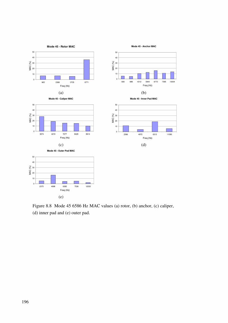
196
Mode 45 - Rotor MAC
0
10
20
30
40
50
965 2388 3735 6771
Freq (Hz)
MA
C (
%)
Mode 45 - Anchor MAC
0
10
20
30
40
50
936 988 4312 5944 6772 7395 10004
Freq (Hz)
MA
C (
%)
(a) (b)
Mode 45 - Caliper MAC
0
10
20
30
40
50
3674 4218 7277 8428 8614
Freq (Hz)
MA
C (
%)
Mode 45 - Inner Pad MAC
0
10
20
30
40
50
2366 4972 6313 11090
Freq (Hz)
MA
C (
%)
(c) (d)
Mode 45 - Outer Pad MAC
0
10
20
30
40
50
2375 4998 6385 7536 12533
Freq (Hz)
MA
C (
%)
(e)
Figure 8.8 Mode 45 6586 Hz MAC values (a) rotor, (b) anchor, (c) caliper,
(d) inner pad and (e) outer pad.

197
Mode 60 - Rotor MAC
0
10
20
30
40
50
4165 5168 6383 6773 7732 7734 8599 10623
Freq (Hz)
MA
C (
%)
Mode 60 - Anchor MAC
0
10
20
30
40
50
1718 4312 5283 6947 7395
Freq (Hz)
MA
C (
%)
(a) (b)
Mode 60 - Caliper MAC
0
10
20
30
40
50
3674 7277 7512 8428
Freq (Hz)
MA
C (
%)
Mode 60 - Inner Pad MAC
0
10
20
30
40
50
2366 4972 6313
Freq (Hz)
MA
C (
%)
(c) (d)
Mode 60 - Outer Pad MAC
0
10
20
30
40
50
2375 7536 10281 12533
Freq (Hz)
MA
C (
%)
(e)
Figure 8.9 Mode 60 8417 Hz MAC values (a) rotor, (b) anchor, (c) caliper,
(d) inner pad and (e) outer pad.
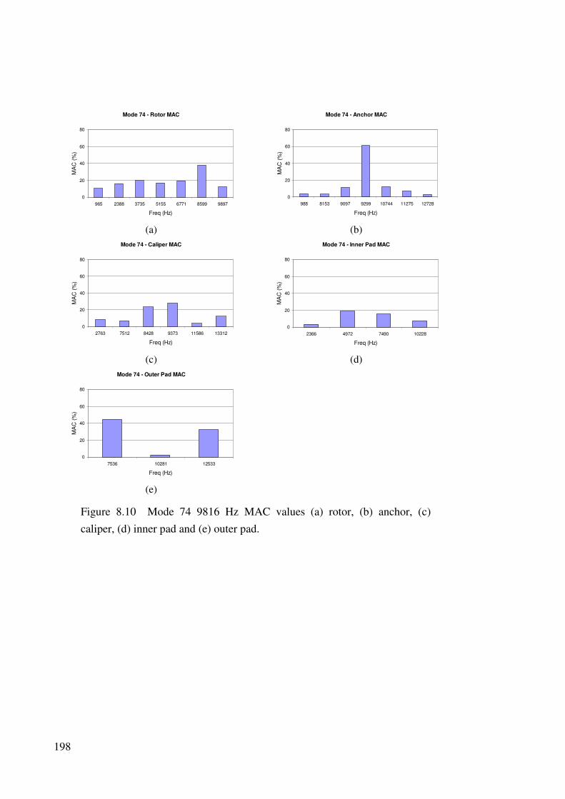
198
Mode 74 - Rotor MAC
0
20
40
60
80
965 2388 3735 5155 6771 8599 9897
Freq (Hz)
MA
C (
%)
Mode 74 - Anchor MAC
0
20
40
60
80
988 8153 9097 9299 10744 11275 12728
Freq (Hz)
MA
C (
%)
(a) (b)
Mode 74 - Caliper MAC
0
20
40
60
80
2763 7512 8428 9373 11586 13312
Freq (Hz)
MA
C (
%)
Mode 74 - Inner Pad MAC
0
20
40
60
80
2366 4972 7490 10228
Freq (Hz)
MA
C (
%)
(c) (d)
Mode 74 - Outer Pad MAC
0
20
40
60
80
7536 10281 12533
Freq (Hz)
MA
C (
%)
(e)
Figure 8.10 Mode 74 9816 Hz MAC values (a) rotor, (b) anchor, (c)
caliper, (d) inner pad and (e) outer pad.

199
Mode 86 - Rotor MAC
0
20
40
60
80
6777 7862 8607 10618 10623 12786
Freq (Hz)
MA
C (
%)
Mode 86 - Anchor MAC
0
20
40
60
80
6947 7395 8153 9097 10744 12559 14385 14879
Freq (Hz)
MA
C (
%)
(a) (b)
Mode 86 - Caliper MAC
0
20
40
60
80
6277 7512 10229 12859 14359
Freq (Hz)
MA
C (
%)
Mode 86 - Inner Pad MAC
0
20
40
60
80
4972 12510 13033
Freq (Hz)
MA
C (
%)
(c) (d)
Mode 86 -Outer Pad MAC
0
20
40
60
80
4998 6385 10281 12533 13095
Freq (Hz)
MA
C (
%)
(e)
Figure 8.11 Mode 86 11238 Hz MAC values (a) rotor, (b) anchor, (c) caliper, (d) inner
pad and (e) outer pad.

200
Mode 90 - Rotor MAC
0
10
20
30
40
50
6774 10407 10553 11838 12851
Freq (Hz)
MA
C (
%)
Mode 90 - Anchor MAC
0
10
20
30
40
50
7395 9097 9299 10744 14385 14879
Freq (Hz)
MA
C (
%)
(a) (b)
Mode 90 - Caliper MAC
0
10
20
30
40
50
2763 3674 4218 6277 8614 11586
Freq (Hz)
MA
C (
%)
Mode 90 - Inner Pad MAC
0
10
20
30
40
50
4972 6313 11090
Freq (Hz)
MA
C (
%)
(c) (d)
Mode 90 - Outer Pad MAC
0
10
20
30
40
50
10281 11108 12533
Freq (Hz)
MA
C (
%)
(e)
Figure 8.12 Mode 90 11694 Hz MAC values (a) rotor, (b) anchor, (c) caliper, (d) inner
pad and (e) outer pad.
8.5 Summary
A complex eigenvalue analysis of the brake system has been presented using an
alternate FEA code, Abaqus. The primary contribution of Abaqus is that it is practically
easy to implement during the modelling process. Further analysis was applied in the
form of MAC calculations to determine the component modes active in the system.
This allows a direct comparison to be made to the Nastran results from Chapters 6 and
7.
Both analysis codes predict a number of unstable modes that correspond to the

201
frequency ranges of interest. However, comparing MAC values shows considerable
differences in the underlying modal contribution to the respective unstable modes.
The differences in the predictions stem from the differences in modelling the component
interfaces. The non-linear contact element formulation of Abaqus allows a more
realistic contact distribution to be captured between the pad and rotor interface, and it is
expected that the Abaqus model more closely resembles the actual case in the brake
system. A comparison to static pressure distribution at pad / rotor interface would be a
good starting point for future work on an assembly. Future work could also include
investigating alternative contact and material property correlation methods to better
understand what analysis method is best, and to improve material modelling input data.
Good correlation was found for the modes at 11.7 and 11.9 kHz between Abaqus and
Nastran respectively, a mode that strongly features 2nd
tangential in-plane motion. This
highlights the problem frequency for the model that was confirmed by experimental
testing. This type of mode is notoriously insensitive to the caliper assembly.

202

203
Chapter 9
Applications to Rotor Design in an
Industrial Environment
9.1 Introduction
In the previous chapter Abaqus was applied to the brake system assembly that formed
the basis of the investigations in this thesis. It was found that considerable differences
were noted in the unstable modes that were predicted by the two analysis codes.
However, in the case of the high frequency squeal mode featuring 2nd tangential in-
plane motion, both analyses predicited comparable system behaviour. In this chapter,
Abaqus was applied in an industrial environment to improve the design of a brake rotor
of a brake system with a known 2nd tangential in-plane related noise concern.
High frequency brake squeal, occurring above approximately 5 kHz, often involves the
tangential in-plane vibration modes of the brake rotor. Noise associated with the
tangential in-plane modes are notoriously difficult to control with typical brake squeal
countermeasures such as backplate shims or modifications to the caliper and bracket
assembly.
This chapter details an investigation into the design of a rotor for front disc brake
system as found on a typical larger passenger vehicle, and how the design can be
improved to reduce the occurrence of rotor related high frequency squeal. Note that this
brake system is not the same as that studied earlier in this thesis, since the industrial
focus required a system that was in current development and development of the
previous system was already completed.
9.2 Brake system Under Investigation
The brake system that was the focus of this investigation is shown in Figure 9.1. It
features a twin piston aluminium caliper of sliding design that is typical for a front
brake of a large passenger sedan, and is considerably larger than that studied in previous
chapters. The rotor, as displayed in Figure 9.2, is a vented design with large cooling
vanes and also features cross drilled holes.

204
Figure 9.1 Brake system under investigation in this chapter.
Figure 9.2 Layout of the brake rotor to identify main features
During braking considerable weight transfer occurs toward the front of a vehicle. As
such it is common for the front axle to support up to 80% for vehicle total brake
capacity. This is reflected in the size of the brake under consideration in this study, the
basic specifications for which are displayed in Table 9.1. This can be compared to the
specifications for the brake shown in Table 1.1, which was for a similarly sized vehicle,
but on a rear axle as opposed to the front application considered here. Also quite
different is the friction material, which is a European style semi-metallic design. The
Cross-drilled
holes
Cheeks
Swan-neck
Hat section
Friction
faces
Vanes

205
friction level is a little higher than that considered earlier, and can be more prone to
noise.
Table 9.1 Brake system specification
Vehicle Type Large passenger sedan
Engine V8 – 210 kW
Drive Wheels Front
Rolling Radius 320 mm
GVM 2150 kg
Static Weight Distribution Front 55%, Rear 45 %
Equivalent Brake Inertia 75 kg m2
Rotor Diameter 323 mm
Rotor Mass 9.9 kg
Effective Radius 141 mm
Piston Diameter 2 x 45.0 mm (equiv. 63.6mm)
9.3 Noise Evaluation
The evaluation of the noise performance of the brake system was conducted using a
brake noise dynamometer. Section 3.11 discussed TS 576, the AK noise matrix based
test, which was used in the evaluation of the noise performance of the AU II rear brake
rear brake system. In this case the TS 640 test procedure was used which is an extended
version of the AK matrix noise procedure to include an additional cold section to the
test.
The addition of the cold section to the test has been found to add considerably to the test
procedure’s ability to uncover more of the potential noise concerns. This is particularly
true of “early morning sickness” type of noise that often occurs on first application at
low speed and pressure, such as an early morning apply departing a driveway.
The test procedure called for 2557 individual braking applications in total between the
warm and cold sections with the main sections summarised in Table 9.2.

206
Table 9.2 PBR TS640 test procedure summary.
Section Stops no. Temperature Pressure Speed
Break-in 32 100 3 MPa 80 km/h
Bedding 30 100 0.2 – 3 MPa 80 km/h
Warm Section 1784 50 – 300 0.2 – 3 MPa 3 – 80 km/h
Fade 15 100 – 450 0.4 G* 100 km/h
Recovery 18 100 3 MPa 80 km/h
Cold Section 678 0 – 50 0.2 – 3 MPa 3 – 10 km/h
The brake end of the dynamometer runs in an environmentally controlled test chamber.
The chamber is 3 m x 3 m in size and is fitted with sound absorbing material on the
walls to ensure background noise spectrum remains under 60 dB(A) between 1.0 and 20
kHz. The sound recording equipment is the same as was shown in Table 3.7
Determining the overall acceptability result for TS640 is done in a straight forward
quantitative manner. A cumulative noise distribution is calculated that notes the
percentage of stops above a given SPL level in both the warm and cold sections of the
test respectively. The acceptance criteria are given in Table 9.3, but are usually
displayed graphically.
Table 9.3 Cumulative Noise occurrence acceptability for TS640. Each of the
warm and cold sections are calculated and assessed separately.
70 dB(A) 80 dB(A) 90 dB(A) 100 dB(A)
Pass ≤ 10 % ≤ 3 % ≤ 0.8 % ≤ 0.2 %
Marginal 10%< SPL ≤20% 3%< SPL ≤6% 0.8%< SPL ≤1.6% 0.2%< SPL ≤0.4%
Fail > 20 % > 6 % > 1.6 % > 0.4 %
The noise performance of this brake system is displayed graphically in Figure 9.3.
Figures 9.3 (a) and (b) show the SPL levels vs. frequency for the noisy stops in the
warm and cold sections of the test respectively. Figure 9.3 (c) displays the cumulative
distribution of noisy stops. The two dashed lines represent the boundary of acceptable
and unacceptable noise in the cumulative result according to the criteria shown in Table
9.3. The area between the two dashed lines represents the marginal zone.

207
70
80
90
100
110
120
2000 4000 6000 8000 10000 12000 14000 16000 18000
Frequency [Hz]
SP
L (
dB
[A])
(a)
70
80
90
100
110
120
2000 4000 6000 8000 10000 12000 14000 16000 18000
Frequency [Hz]
SP
L (
dB
[A])
0.1
1
10
100
70 80 90 100 110 120
Noise Level (dB[A])
No
ise
Cu
mu
lati
ve (
%)
(b) (c)
Figure 9.3 Noise dynamometer results for problem brake system with the
baseline rotor design. (a) warm section, (b) cold section and (c) cumulative
result. A pass result is that the cumulative result remains below the lower
dashed line.
It is clear from Figure 9.3 that the baseline brake system failed the brake noise screening
on the noise dynamometer, with 33% of stops registering 70 dB(A) or above in the cold
section instead of the allowable 10%. The result in the warm section was marginal.
It can also be seen that the noise is exclusively registered at 9.4 kHz in the cold section,
and the same frequency contributes significantly in the warm section. Thus control of
the 9.4 kHz noise is of critical importance for controlling the noise in this brake system.
Warm
Cold
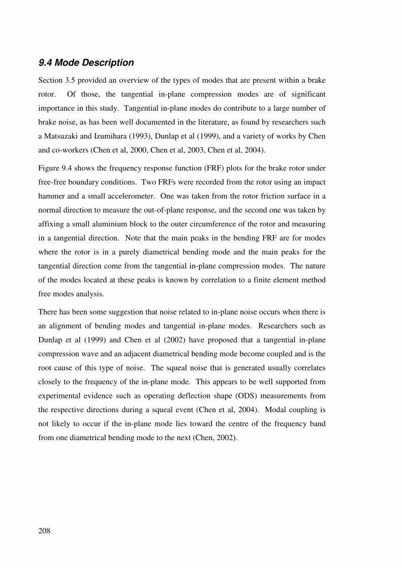
208
9.4 Mode Description
Section 3.5 provided an overview of the types of modes that are present within a brake
rotor. Of those, the tangential in-plane compression modes are of significant
importance in this study. Tangential in-plane modes do contribute to a large number of
brake noise, as has been well documented in the literature, as found by researchers such
a Matsuzaki and Izumihara (1993), Dunlap et al (1999), and a variety of works by Chen
and co-workers (Chen et al, 2000, Chen et al, 2003, Chen et al, 2004).
Figure 9.4 shows the frequency response function (FRF) plots for the brake rotor under
free-free boundary conditions. Two FRFs were recorded from the rotor using an impact
hammer and a small accelerometer. One was taken from the rotor friction surface in a
normal direction to measure the out-of-plane response, and the second one was taken by
affixing a small aluminium block to the outer circumference of the rotor and measuring
in a tangential direction. Note that the main peaks in the bending FRF are for modes
where the rotor is in a purely diametrical bending mode and the main peaks for the
tangential direction come from the tangential in-plane compression modes. The nature
of the modes located at these peaks is known by correlation to a finite element method
free modes analysis.
There has been some suggestion that noise related to in-plane noise occurs when there is
an alignment of bending modes and tangential in-plane modes. Researchers such as
Dunlap et al (1999) and Chen et al (2002) have proposed that a tangential in-plane
compression wave and an adjacent diametrical bending mode become coupled and is the
root cause of this type of noise. The squeal noise that is generated usually correlates
closely to the frequency of the in-plane mode. This appears to be well supported from
experimental evidence such as operating deflection shape (ODS) measurements from
the respective directions during a squeal event (Chen et al, 2004). Modal coupling is
not likely to occur if the in-plane mode lies toward the centre of the frequency band
from one diametrical bending mode to the next (Chen, 2002).

209
-40
-20
0
20
40
60
0 2000 4000 6000 8000 10000 12000
Frequency (Hz)
Ac
ce
lera
nce
(d
B r
e:
1 m
/Ns
^2
)
Figure 9.4 FRF in the out-of-plane direction
-40
-20
0
20
40
60
0 2000 4000 6000 8000 10000 12000
Frequency (Hz)
Acc
ele
ran
ce
(d
B r
e:
1 m
/Ns
^2)
Figure 9.5 FRF in the tangential in-plane direction
It can be seen from Figure 9.5 that the 2nd tangential in-plane mode is well spaced
between the adjacent bending modes. Yet a significant noise problem exists that is
Tang. in-plane
compression modes
Diametrical out-of-
plane modes

210
coincident in frequency with the 2nd tangential in-plane mode of the brake rotor. It
appears that the accepted wisdom of spacing of modes does not hold in this case.
9.5 Stability Prediction
Complex eigenvalue analysis was the focus of Chapter 5 and describes the methods
used for this analysis. Potential squeal modes can be identified analytically as having
positive real parts to their eigenvalues signifying negative damping.
Typically large scale finite element models, such as that used in earlier chapters, include
the brake rotor, a complete caliper assembly, and possibly the steering knuckle and
suspension components. However, since this investigation is concerned mainly with in-
plane modes that might not be strongly influenced by the caliper geometry, and also at
higher frequencies where the influence of steering and suspension components is
negligible, a highly simplified model with only the brake rotor and pads was used. The
mesh used for the analysis can be seen in Figure 9.6, and contains 52000 10-node
tetrahedral elements with 92000 nodes.
Figure 9.6 Simplified FE model used to perform the analysis.
The boundary conditions used for the model are as follows. The brake pad abutments
were constrained in all degrees-of-freedom (DOF) except the friction surface normal
direction, and the rotor was constrained in all DOF at the mounting bolt holes. A
pressure of 1 MPa was applied across the backplate and a non-linear static analysis was
performed that included both a preload step and a rotation step following the same

211
methodology as in Section 8.2.4. Complex eigenvalues were then extracted using the
subspace projection method.
(a)
Baseline Damping
0.00%
0.05%
0.10%
0.15%
0.20%
0 0.1 0.2 0.3 0.4 0.5 0.6
Mu
(b)
Baseline
9420
9430
9440
9450
9460
9470
9480
9490
9500
9510
9520
0 0.1 0.2 0.3 0.4 0.5 0.6
Mu
Fre
qu
en
cy (
Hz)
Figure 9.7 Unstable modes in the region of the 2nd tangential in-plane
mode. (a) modal frequencies, (b) negative damping level.
The baseline model contains a pair of modes that become coupled at 9.4 kHz. Both
involve 2nd tangential in-plane compression modes within the rotor. The rotor itself
possesses axial symmetry, and in the absence of other components or imperfections a
repeated pair of modes, or doublet modes, would exist, both at the same frequency.
µµµµ
µµµµ

212
When included in an assembly this symmetry is disturbed and the frequencies of the
repeated modes deviate slightly from each other.
Figure 9.7 shows the frequency of the original modes with the 2nd tangential in-plane
motion. As the friction level is increased this pair of modes was driven closer in
frequency until the modes become coupled at the onset of instability. This critical
friction coefficient µ was 0.2. Figure 9.6 (b) displays the level of negative damping of
the unstable mode. Initially it is zero as the system is stable, but it grows once the
system has become unstable as mu is increased.
9.6 Rotor Modification
Two modified designs, shown in Figure 9.9, were proposed in an effort to reduce the
coupling of the repeated in-plane modes. Both of the modifications concerned the hat
region of the rotor only so as not to change the friction disc itself. This also means that
the actual modal spacing of the rotor is largely unchanged, since it is primarily
determined by the dimensions of the friction disc. The two proposals were:
1. An addition of 3 ribs spaced evenly around the swan-neck region.
2. Replacement of the swan-neck all together with a conical design.
Both of these modifications aim to alter the interaction of the in-plane modes through
the hat section of the rotor.

213
(a)
(b)
Figure 9.8 (a) Mode shape of unstable 9458Hz mode, (b) Rotor mode shape
for 9473 Hz.

214
(a)
(b)
Figure 9.9 Proposed rotor modifications. (a) sides of hat replaced with
conical section, (b) three stiffeners added to the swan neck.
Inserting the modified rotors into the FEM model and re-running the complex
eigenvalue analysis showed both of these modifications to be an improvement. The
tendency for the in-plane modes to become coupled is shown in Figure 9.10. Both
designs exhibit the same tendency for the repeated 2nd in-plane modes to diverge as the
coefficient of friction µ is increased.
On the basis of these positive analytical results, prototypes of both proposed designs
were manufactured. Figure 9.11 and 912 shows the summary noise test results for the
new hat and 3 stiffeners designs respectively, and it can be seen that neither system
produced any noise at 9.4 kHz. Comparing to the baseline system (Figure 9.3) it can be
seen there is an increase in occurrences at other frequencies. This could be a little
misleading because the noise dynamometer only recorded the highest peak during a
particular stop. It is, therefore, possible that the earlier high peaks at 9.4 kHz was
masking some of the noise at other frequencies at lower levels. Regardless of whether
this is the case or not, the rotors have removed the 9.4 kHz noise altogether and reduced
the overall noise levels into the acceptable range. This is a very positive result given
that it is practically impossible to build a completely noiseless brake system.
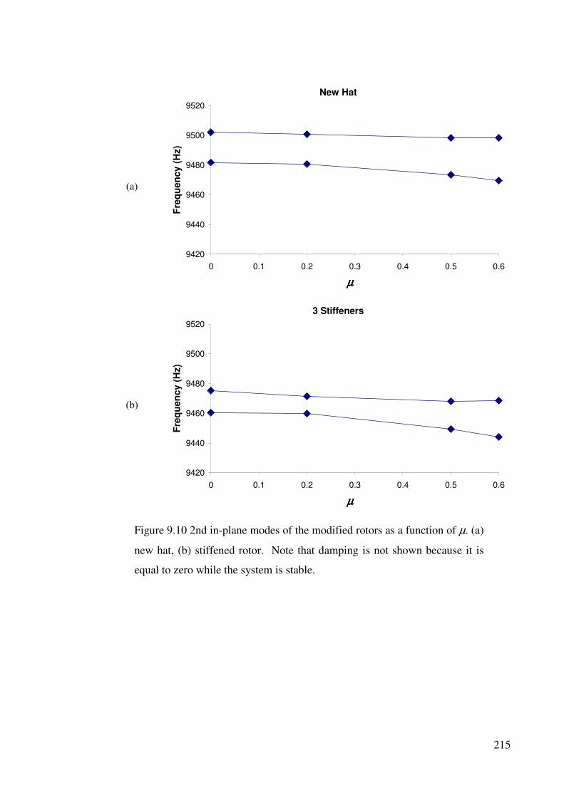
215
(a)
New Hat
9420
9440
9460
9480
9500
9520
0 0.1 0.2 0.3 0.4 0.5 0.6
Mu
Fre
qu
en
cy
(H
z)
(b)
3 Stiffeners
9420
9440
9460
9480
9500
9520
0 0.1 0.2 0.3 0.4 0.5 0.6
Mu
Fre
qu
en
cy
(H
z)
Figure 9.10 2nd in-plane modes of the modified rotors as a function of µ. (a)
new hat, (b) stiffened rotor. Note that damping is not shown because it is
equal to zero while the system is stable.
µµµµ
µµµµ

216
(a)
(b)
Figure 9.11 New hat design rotor noise dynamometer results (a) SPL vs
Frequency, (b) cumulative occurrence.
Warm
Cold
Warm
Cold

217
(a)
(b)
Figure 9.12 3 Stiffeners design rotor noise dynamometer results (a) SPL vs
Frequency, (b) cumulative occurrence
Warm
Cold
Warm
Cold

218
The rotor designs were also subject to a range of structural and thermal analyses to
ensure their suitability to put into service. Neither rotor design showed significant
degradation with regard to the performance requirements and both were deemed
suitable for production. The stiffened rotor has since entered production and returned
good noise performance in the field.
9.7 Summary
The application of complex eigenvalue analysis in an industrial environment was
presented in this Chapter. The analysis showed that the root of the instability was
coupling of repeated tangential in-plane modes, which was confirmed by MAC showing
contributing rotor modes.
Modifications to the swan-neck region of the rotor hat were analysed and two designs
were found that did not exhibit the tendency to become coupled with the friction level
studied. One of the proposed designs featuring 3 lug “stiffeners” has since been put into
production with good noise performance in the field.

219
Chapter 10
Conclusions and Future Work
10.1 Conclusions
This thesis has presented analysis of automotive disc brake squeal based around large
scale FEA models. Initial model set-up was validated against experimental modal
analysis results before the model was used for prediction of potential squeal modes,
which appear as unstable system vibration modes in a complex eigenvalue analysis.
Deeper analysis of system modes was conducted using feed-in energy analysis,
assessing strain energy distributions across the system components, and Modal
Assurance Criterions (MAC) based modal participation analysis. A parametric study
followed where the key factors that influenced unstable system modes was assessed.
An alternative commercial FEA code, Abaqus, using an alternative contact modelling
formulation was put to use in place of MSC.Nastran which had been used in the
preceding analyses in the thesis. A comparison of system stability predicted by
MSC.Nastran and Abaqus was presented, before Abaqus was used in a study to improve
the design of a disc brake rotor in an industrial environment.
An examination of the literature on brake squeal analysis was presented in Chapter 2.
Three main methods of investigation have been reviewed: analytical, experimental and
numerical. The analytical models presented include those commonly used to describe
brake squeal. These models do provide some insight into the nature of brake squeal,
and it can be envisaged how certain types of phenomena act in brake squeal. However
none of these models relate to any specific brake system, so have limited relevance to
addressing an observed squeal concern on a brake. The experimental methods
presented bear much greater relevance to addressing a specific brake squeal concern.
Unfortunately the experimental approaches also do not thoroughly describe the
behaviour of the brake system during squeal, mostly due to the difficulty in adequate
measurement of the relevant effects. The numerical approach provides a larger scale
adaptation of the simple models that allow insight into mechanisms and relevance to a
specific brake system through the use of a large DOF model of a brake system.
Determining the characteristics of a brake system, as described in Chapter 3, revealed
the complexity within a brake system. These results were successfully used in

220
developing the base FEA model in Chapter 4. Tuning of the individual components was
quite straight forward, but assembly required a considerable number of connections
types and interfaces. Reasonable agreement was found in Chapter 5 between the
baseline stability predictions and the observed squeal on the car and brake noise
dynamometer.
The tools presented in Chapter 6 proved to be very useful for deeper probing on the
brake system. While feed-in energy analysis could be used in-place of complex
eigenvalue analysis to assess the level of instability at the onset of squeal, this is not its
leading feature. Feed-in energy can be used to assess which pad is providing more of
the energy to drive the squeal, and can even be used to give very specific information
about which parts of a disc / rotor interface is most important. This should prove useful
for tuning pad designs for reducing brake squeal. Strain energy distributions do provide
good insight into which components are most active in an unstable brake system mode.
However, it needs to be applied with caution due to the differences in size and material
properties of the components so comparison to an average baseline needs to be
performed to make the comparisons valid. MAC based modal participation analysis is
used to identify component modes are most active in an unstable brake system mode.
Chapter 6 highlights the importance of the three analysis methods. Two system modes
where analysed that were both potential squeal modes. However, only one of these
modes corresponds to a concern frequency on the vehicle. Key differences in their
behaviour were identified by examining the feed-in energy, strain energy distributions
and MAC values. The difference in the squeal performance of the two comparison
unstable modes was attributed to the difference in the nature of the brake rotor modes
and their potential to become excited by the pad/rotor friction interface.
Chapter 7 presented a study on some of the parameters that affect the noise propensity
of a brake system. Many of the structural modifications change the behaviour in a
significant way, and many new unstable modes may be created in addition to addressing
some of the existing unstable modes. Reducing pad contact area was found to increase
stability of the brake system, as was increasing pad modulus. Adding structural damping
to the components of the base system was found to slightly increase the stability of the
system modes without greatly changing their character. Simulating backplate damping
shims by adding damping to the backplate increased system stability, but failed to
capture the behaviour of a laminated shim. Adding a damping shim to the back plate

221
was found to be very effective due to more adequately capturing the behaviour of a
physical shim, but even the addition of a shim without damping can influence the
behaviour of the baseline system since it adds further structural modification to the
system.
Chapter 8 presented a comparison on brake squeal analysis using Abaqus and
MSC.Nastran. Both analysis codes predict a number of unstable modes that correspond
to the frequency ranges of interest. However, comparing MAC values shows
considerable differences in the underlying component modal contribution to the
respective unstable modes. The non-linear contact element formulation of Abaqus
allows a more realistic contact distribution to be captured between the pad and rotor
interface, and it is expected that the Abaqus model more closely resembles the actual
case in the brake system. Good correlation was found for the modes at 11.7 and 11.9
kHz between Abaqus and Nastran respectively, a mode that strongly features 2nd
tangential in-plane motion.
Chapter 9 further used Abaqus to assess the design of a brake rotor. The analysis
showed that the root of the instability was coupling of repeated tangential in-plane
modes, which was confirmed by MAC showing contributing rotor modes.
Modifications to the swan-neck region of the rotor hat were analysed and two designs
were found that did not exhibit the tendency to become coupled with the friction level
studied. One of the proposed designs, featuring 3 lug “stiffeners”, has since been put
into production with good noise performance in the field.
The investigation of brake squeal propensity via modally based analysis will require
some level of simplification in all cases. This does not, however, stop useful analysis
from being undertaken. The analysis of the brake rotor designs in Chapter 9 is one
example where a significantly simplified analysis provided a great deal of insight into
system behaviour and allowed alternate rotor designs to be developed.
It must also be noted that the results presented in this thesis draw heavily on
experimental and observed squeal results. At this time is it not practical to apply
complex eigenvalue analysis as an upfront design tool. However, once baseline
correlation has been established, the analyses presented allow detailed examination of
system behaviour. Utilising numerical analysis methods in conjunction with

222
experimental results provides a practical development path for addressing brake squeal
concerns.
10.2 Recommendations for Future Work
The majority of this thesis was focused on the analysis of a large scale MSC.Nastran
FEA model. The method for assessing system stability was modally based, which
requires linearisation of the system before the complex modes analysis. This limits the
modelling options for the friction interface which used linear springs and a Coulomb
friction model. The inherent non-linearity of the contact stiffness and sensitivity of the
friction coefficient to normal pressure and slip velocity are not captured. Abaqus allows
a non-linear solution of the static analysis which captures elements of the non-linear
contact stiffness; however, linearisation before the modal analysis again limits the
nature of the friction model.
Non-linear transient analysis provides an alternate path forward where greater
sophistication can be built into friction and contact stiffness modelling. Re-analysis of
the Abaqus assembly in the time domain may provide a truer representation of the
system behaviour. However, brake squeal is a highly transient phenomenon with highly
complex geometries, interfaces and materials, so whether it will be possible to
accurately capture the full system behaviour even with unlimited computer resources
remains to be seen.
Within the context complex eigenvalue analysis, the discrepancies between the
MSC.Nastran and Abaqus models could be investigated further. A detailed study using
a visualisation technique such as scanning laser vibrometry would provide insight into
which analysis code provides the more realistic system behaviour. This could also be
extended to include the non-linear transient analysis to assess the most useful analysis
method.
A particular area of interest is the tangential in-plane modes which were the basis of the
analysis in Chapter 9. The modelling results indicated almost pure in-plane modes
without coupling to an adjacent bending mode. Some out of plane deformation would
no doubt be required for the modes to radiate high-levels of sound. An investigation
into the sound radiation efficiency of the in-plane modes could indicate if modes of this
type could be responsible for the sound radiation without bending mode involvement.

223
Little work has been found in the literature dealing with the sound radiation of unstable
brake system modes. While stability analysis allows a propensity to the squeal to be
assessed, no direct correlation to the level of squeal can be drawn. Considerable scope
exists for investigation of the sound radiation behaviour of unstable brake system
modes.

224
225
References
Abaqus Analysis User’s Manual (2003), Version 6.4, Vol II: Analysis.
Ansys User’s Manual (2000), Version 5.7, SAS IP.
Baba, H., Okade, M., and Takeuchi, T. (1995), ‘Study on Reducing Low Frequency
Brake Squeal From Modal Analysis of Mounting Bracket’, SAE Paper, No. 952697.
Bajer, A., Belsky, V. and Zeng, L.J. (2003), ‘Combining a Nonlinear Static Analysis
and Complex Eigenvalue Extraction in Brake Squeal Simulation’, SAE Paper No. 2003-
01-3349.
Bathe, K.J. (1996), ‘Finite Element Procedures’, Prentice Hall, New Jersey.
Brooks, P. C., Crolla, D. A., Lang, A. M., and Schafer, D. R. (1993), ‘Eigenvalue
Sensitivity Analysis Applied to Disc Brake Squeal’, Institute of Mechanical
Engineering, C444/004/93, pp 135-143.
Chatterley, T.C. and Macnaughton, M.P. (1999), ‘Cast Iron BRake Discs – Current
Position, Performance and Future Trends in Europe’, SAE Paper No. 1999-01-0141.
Chargin, M. L., Dunne, L. W., and Herting, D. N. (1997), ‘Nonlinerar Dynamics of
Brake Squeal Noise’, Finite Elements in Engineering, Vol. 28, No. 1, pp 69-82.
Chen, F., Chen, S., and Harwood, P. (2000), ‘In-Plane Mode/Friction Process & Their
Contribution to Disc Brake Squeal at High Frequency’, SAE Paper, No. 2000-01-2773.
Chen, F., Chern, J., and Swayze, J. (2002), ‘Modal Coupling and Its Effect on Brake
Squeal’. SAE Paper, No. 2002-01-0922.
Chen, F., Tan, C.A., and Quaglia, R.L. (2003a), ‘On Disc Brake Squeal Part I:
Mechanisms and Causes’, SAE paper no. 2003-01-0683.
Chen, F., Adbelhamid, M.K., Blaschke, P., and Swayze, J. (2003b), ‘On Automotive
Disc Brake Squeal, Part III: Test and Evaluation’, SAE Paper No. 2003-01-1622.

226
Chen, F., Tong, H., Chen S.E. and Quagila, R. (2003c), ‘On Disc Brake Squeal Part IV:
Reduction and Prevention’, SAE paper no. 2003-01-3345.
Chen, F., Mckillip D., Luo, J. and Wu, S.F. (2004), ‘Measurement and Analysis of
Rotor In-plane Induced Disc Brake Squeal and Beyond, SAE Paper No. 2004-01-2798.
Chern, Y., Chen, F. and Swayze, J. (2002), “Non-linear dynamics of of brake squeal”,
SAE Paper No. 2002-01-3138.
Cremer, L., Heckl, M. and Ungar, E.E. (1988), ‘Structure-borne sound: structural
vibrations and sound radiation at audio frequencies’, Springer-Verlag, Berlin.
Denou, Y. and Nishiwaki, M. (2001), ‘First Order Analysis of Low Frequency Disk
Brake Squeal’, SAE Paper, No. 2001-01-3136.
Dunlap, K.B., Riehle, M.A. and Longhouse R.E. (1999), “An investigative overview of
automotive disc brake noise”, SAE paper no. 1999-01-0142.
Earles, S.W.E., and Soar, G.B (1971)., ‘Squeal Noise in Disc Brakes’, Paper C101/71, I
Mech E Symposium on Vibration and Noise in Motor Vehicles.
Earles, S. W. E., and Chambers, P. W. (1987), ‘Disc Brake Squeal Noise Generation:
Predicting its Dependency on System Parameters Including Damping’, Int. J. of Vehicle
Design, Vol 8, Nos 4/5/6, pp538-552.
El Butch, A.M. and Ibrahim (1999), ‘Modelling and Analysis of Geomtrically Induced
Vibrations in Disc Brakes Considering Contact Parameters’ SAE Paper No. 1999-01-
0143.
Eriksson, M., and Jacobson, S. (2000), ‘Tribological surfaces of organic brake pads’,
Tribology International 33, pp817-827.
Eriksson, M. and Jacobson, S (2001). “Friction behaviour and squeal generation of disc
brakes at low speeds”, Proc Instn Mech Engrs, Vol 215, Part D., pp1245-1256.
Ewins, D.J. (1984), ‘Modal testing: theory and practice’, Wiley, New York.

227
Felske, A., Hoppe, G., and Matthai, H. (1978), ‘Oscillation in Squealing Brakes -
Analysis of Vibration Modes by Holographic Interferometry’, SAE Paper, No. 780333.
Fieldhouse, J. D., and Newcomb, T. P. (1991), ‘An Investigation into Disc Brake Noise
Using Holographic Interferometry’, Institute of Mechanical Engineering, C427/11/213.
Fieldhouse, J. D., and Newcomb, T. P. (1996), ‘Double Pulsed Holography used to
Investigate Noisy Brakes’, Optics and Lasers in Engineering, Vol. 25, pp 455-494.
Fieldhouse, J. D, and Rennison, M. (1998), ‘An Investigation of Low Frequency Drum
Brake Noise’, SAE Paper, No. 982250.
Fieldhouse, J. D., and Beveridge, C. (2000), ‘A Visual Experimental Noise
Investigation of a Twin Calliper Disc Brake’, SAE Paper, No. 2000-01-2771.
Fieldhouse, J. D., and Beveridge, C. (2001), ‘An Experimental Investigation of Hot
Judder’, SAE Paper No. 2001-01-3135.
Flint, J. and Hald, J. (2003), “Traveling waves in squealing disc brakes measured with
acoustic holography”, SAE Paper No. 2003-01-3319.
Fosberry, R.A.C., and Holubecki, Z. (1959), ‘Interim report of disc brake squeal’,
MIRA Research Report 1959/4.
Fosberry, R.A.C., and Holubecki, Z. (1961), ‘Disc Brake Squeal; its mechanisms and
suppression’, MIRA Research Report 1961/2.
Guan. D., and Jiang, D. (1998), ‘A study on disk brake squeal using finite element
methods’, SAE Paper, No. 980597.
Guan, D., and Huang, J. (2003), ‘The method of feed-in energy on disc brake squeal’,
Journal of Sound and Vibration, Vol 267, pp 297-307.
Hoffman, N., Fischer, M., Allgaier, R., and Gaul, L. (2002), ‘A Minimal Model for
Studying Properties of the Mode-Coupling Type Instability in Friction Induced
Oscillations’, Mechanics Research Communications, Vol 29, pp197-205.

228
Hu, Y.K. and Nagy, L.I. (1997), ‘Brake Squeal Analysis by Using Nonlinear Transient
Finite Element Method’, SAE Paper 971510.
Ichiba, Y., and Nagasawa, Y. (1993), ‘An Experimental Study on Disc Brake Squeal’,
SAE Paper, No. 93082.
Inman, D.J. (1994), ‘Engineering Vibration’, Prentice Hall, New Jersey.
Ishihara, N., Nishiwaki, M., and Shimizu, H. (1996), ‘Experimental Analysis of Low
Frequency Brake Squeal Noise’, SAE Paper, No. 962128.
Jarvis,R.P., and Mills, B. (1963),‘Vibrations Induced by Dry Friction’, I Mech E Proc,
Vol 178, Pt 1, No. 32, pp 847 – 857.
Kinkaid, N.M., O’Reilly, O.M., and Papadopoulos, P. (2003), ‘Automotive Disc Brake
Squeal’, Journal of Sound and Vibration, Vol 267, pp105-166.
Kumemura, Y., Gamo, Y., Kono, K., and Suga, S. (2001), ‘Analysis for Reducing Low
Frequency Squeal of Disc Brake’, SAE Paper, No., 2001-01-3137.
Kung, S., Dunlap, K. B., and Ballinger, R. S. (2000a), ‘Complex Eigenvalue Analysis
for Reducing Low Frequency Brake Squeal’, SAE Paper, No. 2000-01-0444.
Kung, S., Saligrama, C. V., and Riehle, M. A. (2000b), ‘Modal Participation Analysis
for Identifying Brake Squeal Mechanism’, SAE Paper, No. 2000-01-2764.
Kung S.W., Stelzer, G., Belsky V. And Bajer, A. (2003), ‘Brake Squeal Analysis
Incorporating Contact Conditions and Other Nonlinear Effects’, SAE Paper No. 2003-
01-3343.
Lang, A. M., and Smales, H. (1983), ‘An Approach to the Solution of Disc Brake
Vibration Problems’, Institute of Mechanical Engineering, C37/83, pp 223-231.
Lang, A. M., and Newcomb, T. P. (1990), ‘ The Vibration Charateristics of Squealing
Brakes’, SAE Paper, No. 905170.
229
Lang, A. M., Schafer, D. R., Newcomb, T. P., and Brooks, P. C. (1993), ‘Brake Squeal -
The Influence of Rotor Geometry’, Institute of Mechanical Engineering, C444/016/93,
pp 161-171.
Liles, G. D. (1989), ‘Analysis of Disc Brake Squeal Using Finite Element Methods’,
SAE Paper, No. 891150.
Malosh, J.B. (1998), ‘Disc Brake Noise Redustion Through Metallurgical Control of
Rotor Resonances’, SAE Paper No. 982236.
Matsuzaki, M., and Izumihara, T. (1993), ‘Brake Noise Caused by the Longditudinal
Vibration of the Disc Rotor’, SAE Paper, No. 930804.
McDaniel, J.G., Moore, J., Chen, S.E., and Clarke, C.L. (1999), ‘Acoustic Radiation
Models of Brake Systems from Stationary LDV Measurements,’ IMEC 99, Nashville,
Nov 14-19.
Millner, N. (1978), ‘An Analysis of Disc Brake Squeal’, SAE Paper, No. 780332.
Mills, H.R. (1938), “Brake Squeak”, Technical report 9000 B, Institution of Automobile
Engineers.
Mottershead, J. E., and Chan, S. N. (1992), ‘Brake Squeal - An Analysis of Symmetry
and Flutter Instability’, DE-Vol. 49, Friction-Induced Vibration, Chatter, Squeal, and
Chaos, ASME, pp87- 97.
Mottershead, J. E., and Chan, S. N. (1995), ‘Flutter Instability of Circular Discs with
Frictional Loads’, Journal of Vibration and Acoustics, Vol. 117, pp 161-163.
Murakami, H., Tsunada, N., and Kitamura, T. (1984), ‘A Study Concerned with the
Mechanism of Disc Brake Squeal’, SAE Paper, No. 841233.
Nack, W.V. and Joshi, A.M. (1995), ‘Friction s Induced Vibration: Brake Moan’, SAE
Paper, No. 951095.
Nack, W.V. (1999), ‘Brake Squeal by Finite Elements’, SAE Paper No. 1999-01-1736.
Nack, W.V. (2002), Personal communication.

230
Nastran V7.0, Advanced Dynamics User’s Guide, (2002).
Nishiwaki, M., Harada, H., Okamura, H., and Ikeuchi, T. (1989), ‘Study on Disc Brake
Squeal’, SAE Paper, No. 890864.
Nishiwaki, M. (1991), ‘Generalised Theory of Brake Noise’, Institute of Mechanical
Engineering, C427/11/001.
North, M. R. (1976), ‘Disc Brake Squeal’, Institute of Mechanical Engineering, C38/76,
pp 169-176.
Ouyang, H., Nack, W., Yuan, Y. and Chen F. (2003), ‘On Automotive Disc Brake
Squeal Part II: Simulation and Analysis’, SAE Paper No. 2003-01-0684.
Park, C., Han, M.G., Cho, S.S, Choi, H.G., Jeong, J.D., and Lee, J.M, (2001) ‘A Study
on the Reduction of Disc Brake Squeal Using Complex Eigenvalue Analysis’, SAE
Paper, No. 2001-01-3141.
http://www.polytec.com/int/_files/OM_InFocus_2007_01_US.pdf (2007).
Richmond, J.W., Holton, T.R., Smith, A.C., Beckett, P.B., and Hodges, T., (1999) ‘The
development of an integrated experimental and theoretical approach to solving brake
noise problems’
Rossing, T.D and Fletcher, N.H, (1995) ‘Principles of vibration and sound’, Springer-
Verlag, New York.
Saka, H. and Wada, T. (2003), ‘Study of Brake Squeal – Classification for Vibration
Modes of Mounting Bracket’, SAE Paper No. 2003-01-3344.
Spurr, R.T. (1961), ‘A Theory of Brake Squeal’, I Mech E Auto Div Proc No 1, pp30-
40.
Talbot, C., and Fieldhouse, J. D. (2001), ‘Animations of a Disc Brake Generating
Noise’, SAE Paper, No. 2001-01-3126.

231
Yang, S., and Gibson, R.F. (1997), ‘Brake Vibration and Noise: Reviews, Comments,
and Proposals’, Int. J. of Materials and Product Technology, Vol. 12, Nos 4-6, pp 496-
513.
Zhang, L., Wang, A., Mayer, M. and Blaschke, P. (2003), ‘Component Contribution and
Eigenvalue Sensitivity Analysis for Brake Squeal’, SAE Paper No. 2003-01-3346.


233
Publications Arising From This Thesis
Journal Papers
1. Papinniemi, A.T., Lai J.C.S, Zhao, J. and Loader, L., “Brake squeal: a literature
review” Applied Acoustics, no. 67, 391-400, 2002.
Conference Papers
1. Papinniemi, A.T., Lai, J.C.S, and Zhao, J., ‘Vibration Analysis of Disc Brake
System’, Acoustics 2001, Canberra, ACT, Australia, 21-23 Nov., 2001.
2. Papinniemi, A.T., Lai, J.C.S, and Zhao, J., ‘Modelling of a Disc Brake System for
Investigating Brake Squeal’, Dearborn, Mi, USA, 19-21 Aug, 2002.
3. Papinniemi, A.T., Lai, J.C.S, and Zhao, J., ‘Numerical Modelling of Brake Squeal,
Wespac 8, Melbourne, VIC, Australia, 7-9 April, 2003.
4. Papinniemi, A.T. and Lai, J.C.S, ‘Comparison of Energy Based Methods for Brake
Squeal Propensity’, The 18th International Congress on Acoustics 2004, April 4-9,
Kyoto, Japan, 2004.
5. Papinniemi, A.T., Lai, J.C.S, and Zhao, J., “Vibro-acoustic Studies of Brake Squeal
Noise”, Acoustics 2004, Gold Coast, QLD, Australia, 3-5 Nov, 2004.
6. Papinniemi, A.T., Lai, J.C.S, and Zhao, J., ‘Towards Reducing Brake Squeal
Propensity’, Internoise 2005, Rio de Janeiro, Brazil, 7-10 Aug., 2005.
7. Papinniemi, A.T., Zhao J. and Lai, J.C.S, ‘A Study on In-plane Vibration Modes in
Disc Brake Squeal Noise’, Internoise 2005, Rio de Janeiro, Brazil, 7-10 Aug., 2005.
8. Papinniemi, A.T., Lai, J.C.S and Zhao J., ‘Numerical Prediction of Brake Squeal
Propensity – A Critical Review’, Internoise 2006, Honolulu, Hawaii, USA, 3-6
Dec., 2006.
9. Papinniemi, A.T., Lai, J.C.S, and Zhao, J., ‘Disc Brake Squeal: Progress and
Challenges, ICSV 14, Cairns, Australia, 9-12 July 2007.

234
Reports
1. Papinniemi, A.T. and Lai, J.C.S. “Experimental Modal Analysis of a Disc Brake
System”, Report AVU 0202, School of Aerospace and Mechanical Engineering,
UNSW@ADFA, 2002.

235
Appendix A: Measurement Grids
Table A.1: Coordinates for the rotor grid.
Point no. r (mm) θ (°) z (mm) Direction
1 + 8n 40 34 z
2 + 8n 80 34 z
3 + 8n 103 28 r
4 + 8n 103 8 r
5 + 8n 110 0 z
6 + 8n 125 0 z
7 + 8n 140 0 z
8 + 8n 144
7.5n,
n = 0,..,47
-8 r
Table A.2: Pad grid coordinates. Measurement direction is in the local z direction
for all points.
Point No. x (mm) y (mm) Point No. x (mm) y (mm)
1 0 9 14 54 35
2 0 22 15 54 52
3 15 9 16 70 0
4 15 22 17 70 9
5 28 0 18 70 22
6 28 28 19 70 32
7 38 0 20 80 0
8 38 9 21 80 28
9 38 22 22 93 9
10 38 32 23 93 22
11 54 0 24 108 9
12 54 9 25 108 22
13 54 22

236
Table A.3: Caliper housing grid coordinates and measurement direction.
Point
No.
x
(mm)
y
(mm)
z
(mm)
dir. Point
No.
x
(mm)
y
(mm)
z
(mm)
dir.
1 10 -12 0 x 34 -72 0 10 y
2 0 0 0 y 35 -72 10 -20 y
3 -10 0 0 y 36 -72 10 -80 y
4 -20 10 -20 y 37 -72 0 -90 -z
5 -20 10 -50 y 38 -90 -30 25 z
6 -20 10 -80 y 39 -90 -20 25 z
7 -20 0 -90 -z 40 -90 -10 25 z
8 -20 -15 -90 -z 41 -90 0 20 y
9 -20 -30 -90 -z 42 -90 0 10 y
10 -45 -20 25 z 43 -90 10 -20 y
11 -45 -10 25 z 44 -90 10 -50 y
12 -45 0 20 y 45 -90 10 -80 y
13 -45 0 10 y 46 -90 0 -90 -z
14 -45 10 -20 y 47 -100 -20 25 z
15 -45 10 -50 y 48 -100 -10 25 z
16 -45 10 -80 y 49 -100 0 20 y
17 -45 0 -90 -z 50 -100 0 10 y
18 -45 -15 -90 -z 51 -100 10 -20 y
19 -45 -30 -90 -z 52 -100 10 -50 y
20 -60 -30 25 z 53 -100 10 -80 y
21 -60 -20 25 z 54 -100 0 -90 -z
22 -60 -10 25 z 55 -100 -15 -90 -z
23 -60 0 20 y 56 -100 -30 -90 -z
24 -60 0 10 y 57 -125 10 -20 y
25 -60 10 -20 y 58 -125 10 -50 y
26 -60 10 -50 y 59 -125 10 -80 y
27 -60 10 -80 y 60 -125 0 -90 -z
28 -60 0 -90 -z 61 -125 -15 -90 -z
29 -72 -40 25 z 62 -125 -30 -90 -z
30 -72 -30 25 z 63 -135 0 0 y
31 -72 -20 25 z 64 -145 0 0 y
32 -72 -10 25 z 65 -155 -12 0 -x
33 -72 0 20 y

237
Table A.4: Anchor bracket grid coordinates and measurement direction.
Point
No.
x
(mm)
y
(mm)
z
(mm)
dir. Point
No.
x
(mm)
y
(mm)
z
(mm)
dir.
1 0 35 0 y 19 145 10 10 z
2 0 35 -17.5 y 20 120 0 20 y
3 0 35 -35 y 21 105 0 20 y
4 0 35 -50 -z 22 72 0 20 y
5 0 25 -50 -z 23 40 0 20 y
6 0 0 -50 -z 24 25 0 20 y
7 25 0 -50 y 25 0 10 10 z
8 40 0 -50 y 26 0 30 10 z
9 72 0 -50 y 27 25 -10 -70 -z
10 105 0 -50 y 28 40 -10 -70 -z
11 120 0 -50 y 29 72 -10 -60 -z
12 145 0 -50 -z 30 105 -10 -70 -z
13 145 25 -50 -z 31 120 -10 -70 -z
14 145 35 -50 -z 32 120 -10 30 z
15 145 35 -35 y 33 105 -10 30 z
16 145 35 -17.5 y 34 72 -10 30 z
17 145 35 0 y 35 40 -10 30 z
18 145 30 10 z 36 25 -10 30 z


239
Appendix B: Free Rotor Mode Shapes
1 - (2,0)
994 Hz
2 - (0,1)
2010 Hz
3 - (3,0)
2430 Hz
4 - (0,2)
2550 Hz
5 - (1,1)
2690 Hz
6 - RI 2
2900 Hz
7 - (1,2)
3200 Hz
8 - (4,0)
3800 Hz
9 - TH(2,0)
4230 Hz
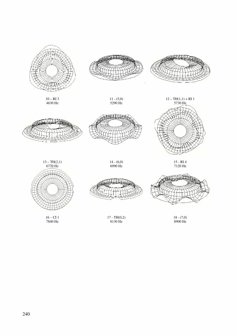
240
10 – RI 3
4630 Hz
11 - (5,0)
5290 Hz
12 – TH(1,1) + RI 1
5730 Hz
13 – TH(2,1)
6770 Hz
14 - (6,0)
6990 Hz
15 - RI 4
7120 Hz
16 – CI 1
7840 Hz
17 - TH(0,2)
8130 Hz
18 - (7,0)
8900 Hz

241
Appendix C: Example Nastran Input Deck
Note: Element, grid and boundary conditions have been omitted except 1st and last
entries to save space.
$ NASTRAN input file created by the MSC MSC.Nastran input file
$ translator ( MSC.Patran 2001 r3 ) on December 17, 2002 at
17:27:22.
ASSIGN DBC='gr5c5.xdb', RECL=1024
$ Complex Eigenvalue Analysis, Direct Formulation, Database
SOL 107
$ Direct Text Input for Executive Control
COMPILE GMA SOUIN=MSCSOU NOLIST NOREF
ALTER 'MTRXIN' $
ADD K2PP, /K2PPX/V,Y,FRIC=(1.0,0.0) $
EQUIVX K2PPX/K2PP/-1 $
ENDALTER
compile sedrcvr souin=mscsou noref nolist
alter 'if.*gpfdr.*statics','' (1,0) $
IF ( GPFDR AND (STATICS OR APP='REIG' OR
APP='CEIGEN' OR APP1='FREQRESP') ) THEN $
alter 'if.*gpfdr.*statics'(2,0),''(2,0) $
IF ( GPFDR AND (STATICS OR APP='REIG' OR
APP='CEIGEN' OR APP1='FREQRESP') ) THEN $
CEND
SEALL = ALL
SUPER = ALL
TITLE = MSC.Nastran job created on 04-Dec-02 at 18:47:55
ECHO = NONE
MPC = 16
$ Direct Text Input for Global Case Control Data
K2PP = FSTIF
PARAM, FRIC, .5
SUBCASE 1
$ Subcase name : linst1
SUBTITLE=linst1
SPC = 2
LOAD = 2
DISPLACEMENT(PLOT,SORT1,REAL)=ALL
SPCFORCES(PLOT,SORT1,REAL)=ALL
STRESS(PLOT,SORT1,REAL,VONMISES,BILIN)=ALL
FORCE(SORT1,REAL,BILIN)=ALL
SUBCASE 2
$ Subcase name : cplx1
SUBTITLE=cplx1
CMETHOD = 1
SPC = 2
VECTOR(PLOT,SORT1,REAL)=ALL
SPCFORCES(PLOT,SORT1,REAL)=ALL
ESE(PLOT,THRESH=0.000000000001)=All
STATSUB = 1
$ Direct Text Input for this Subcase
BEGIN BULK

242
$ /me2/pi20/antti/nastran/griz_rear/analysis/gr5cplx3.res
$
$ DMIG Header
$
DMIG FSTIF 0 1 1 0
$
$ Springs for normal stiffness - area no. 1
$ k = 0.20E+04
$
CELAS2 210001 0.20E+04 40001 1 50001 1
CELAS2 210002 0.20E+04 40004 1 50216 1
……
……
CELAS2 210165 0.20E+04 46976 1 50692 1
CELAS2 210166 0.20E+04 46977 1 50694 1
$
$ Friction stiffness DMIGs for surface no. 1
$
DMIG FSTIF 50001 1 50001 3 -.20E+04
DMIG FSTIF 40001 1 50001 3 0.20E+04
DMIG FSTIF 50001 1 40001 3 0.20E+04
DMIG FSTIF 40001 1 40001 3 -.20E+04
$
DMIG FSTIF 50216 1 50216 3 -.20E+04
……
……
DMIG FSTIF 46977 1 46977 3 -.20E+04
$
PARAM POST 0
PARAM AUTOSPC YES
PARAM,NOCOMPS,-1
PARAM PRTMAXIM YES
EIGC 1 CLAN MAX
0. 120
$ Direct Text Input for Bulk Data
PARAM, PRGPST, NO
$ Elements and Element Properties for region : piston
PSOLID 1 1 0
$ Pset: "piston" will be imported as: "psolid.1"
CHEXA 20001 1 20018 20016 20015 20017 20036
20033
20034 20035
CHEXA 20002 1 20032 20031 20016 20018 20038
20037
20033 20036
……
……
CHEXA 60394 9 60534 60535 60471 60470 60652
60536
60476 60475
$ Referenced Material Records
$ Material Record : steel_pad

243
$ Description of Material : Date: 27-Jan-00 Time:
14:21:07
MAT1 7 207000. .3 7.86-9
$ Material Record : linning
$ Description of Material : Date: 27-Jan-00 Time:
14:21:07
MAT1 4 5000. .3 2.6-9
$ Material Record : cast_iron_rotor
$ Description of Material : Date: 27-Jan-00 Time:
14:21:07
MAT1 6 118000. .32 7.1-9
$ Material Record : cast_iron_anchor
$ Description of Material : Date: 27-Jan-00 Time:
14:21:07
MAT1 2 165000. .3 7.4-9
$ Material Record : alum_piston
$ Description of Material : Date: 27-Jan-00 Time:
14:21:07
MAT1 1 70000. .33 2.7-9
$ Material Record : steel_pin
$ Description of Material : Date: 27-Jan-00 Time:
14:21:07
MAT1 5 207000. .3 7.86-9
$ Material Record : alum_housing
$ Description of Material : Date: 27-Jan-00 Time:
14:21:07
MAT1 3 68000. .33 2.65-9
$ Multipoint Constraints of the Entire Model
MPCADD 16 3 6 9 12 15
RBE2 1 100101 123456 10699 10702 10703 10714
10725
10726 10727 10728 10729 10730 10731 10732
10733
10734 10735 10736 10737 10790 10796 10802
11983
11986 11992 12003 12004 12005 12006 12007
12008
12009 12010 12011 12012 12013 12060 12066
RBE2 2 100102 123456 20035 20036 20038 20041
20042
20044 20046 20048 20050 20052 20054 20055
20057
20059 20061 20064 20067 20068 20069 20071
20074
20075 20077 20079 20081 20083 20085 20087
20089
20092 20094 20096
MPC 3 100102 2 -1. 100101 2 1.
MPC 3 100102 3 -1. 100101 3 1.
MPC 3 100102 4 -1. 100101 4 1.
MPC 3 100102 5 -1. 100101 5 1.
MPC 3 100102 6 -1. 100101 6 1.
RBE2 4 100201 123456 10980 10981 10982 10983
10984

244
10985 10986 10987 10988 10989 10990 10991
10992
10993 10994 10995 10996 10997 10998 10999
11000
11001 11002 11003
RBE2 5 100202 123456 70022 70023 70027 70028
70029
70033 70034 70036 70039 70040 70041 70042
70066
70067 70068 70070 70071 70075 70076 70078
70081
70082 70083 70084
MPC 6 100202 1 -1. 100201 1 1.
MPC 6 100202 2 -1. 100201 2 1.
MPC 6 100202 3 -1. 100201 3 1.
MPC 6 100202 4 -1. 100201 4 1.
MPC 6 100202 5 -1. 100201 5 1.
MPC 6 100202 6 -1. 100201 6 1.
RBE2 7 100301 123456 12234 12235 12236 12237
12238
12239 12240 12241 12242 12243 12244 12245
12246
12247 12248 12249 12250 12251 12252 12253
12254
12255 12256 12257
RBE2 8 100302 123456 80022 80023 80027 80028
80029
80033 80034 80036 80039 80040 80041 80042
80066
80067 80068 80070 80071 80075 80076 80078
80081
80082 80083 80084
MPC 9 100302 1 -1. 100301 1 1.
MPC 9 100302 2 -1. 100301 2 1.
MPC 9 100302 3 -1. 100301 3 1.
MPC 9 100302 4 -1. 100301 4 1.
MPC 9 100302 5 -1. 100301 5 1.
MPC 9 100302 6 -1. 100301 6 1.
RBE2 10 100401 123456 30095 30098 30100 30102
30104
30106 30108 30110 30112 30114 30116 30118
30119
30120 30123 30125 30127 30129 30131 30133
30135
30137 30139 30141
RBE2 11 100402 123456 70184 70187 70188 70191
70192
70198 70199 70204 70210 70214 70215 70216
70217
70218 70221 70223 70225 70227 70229 70231
70233
70235 70237 70239
MPC 12 100402 2 -1. 100401 2 1.
MPC 12 100402 3 -1. 100401 3 1.
MPC 12 100402 4 -1. 100401 4 1.

245
MPC 12 100402 5 -1. 100401 5 1.
MPC 12 100402 6 -1. 100401 6 1.
RBE2 13 100501 123456 31337 31340 31342 31346
31348
31350 31352 31354 31356 31358 31360 31361
31362
31365 31367 31369 31371 31373 31375 31377
31379
31381 31383
RBE2 14 100502 123456 80184 80187 80188 80191
80192
80198 80199 80204 80210 80214 80215 80216
80217
80218 80221 80223 80225 80227 80229 80231
80233
80235 80237 80239
MPC 15 100502 2 -1. 100501 2 1.
MPC 15 100502 3 -1. 100501 3 1.
MPC 15 100502 4 -1. 100501 4 1.
MPC 15 100502 5 -1. 100501 5 1.
MPC 15 100502 6 -1. 100501 6 1.
$ Nodes of the Entire Model
GRID 10001 12.1 113. 41.25
GRID 10002 8.97052 113. 44.3795
……
……
GRID 100502 63.85 136. -72.035
$ Loads for Load Case : linst1
SPCADD 2 4 6
LOAD 2 1. 1. 1 1. 3
$ Displacement Constraints of Load Set : anch_constraint
SPC1 4 123 30447 30450 30453 30456 30459
30462
30465 30466 30471 30474 30477 30480 30483
30484
……
……
46385 46391 46397 46931 46940 46949
$ Loads for Load Case : new
$ Pressure Loads of Load Set : piston_press
PLOAD4 1 20081 14. 20234
20236
PLOAD4 1 20082 14. 20238
20235
……
……
PLOAD4 3 11562 14. 12300
12401
PLOAD4 3 11585 14. 12392
$ Referenced Coordinate Frames
ENDDATA a698e5a1


247
Appendix D: bdfread Source Code
c bdfread v2.1
c
c Reads the Nastran .bdf file and processes coincident nodes.
c Input file bdfread.in contains input data.
c Writes results file with formatting for appendage to final
c .bdf file.
c Write reoprt file stating the number if coincident grids
c and whether DMIGs were written
c
c
c Written by Antti Papinniemi 13/08/02
c
program bdfread
c Global variables
c vec1, mat1 - whole grid point ids, cordinates respectively
c vec2, mat2 - search regoin grid ids and coordinates
c vec3, mat3 - coicident grid ids and cordinates
c bounds - search cordinates x1,x2,y1,y2,z1,z2
c numgd - no of grids in model
c maxgd - no grids in search region
c numct - no contact pairs
c dir1, dir2 - contact surface normal, tangential directions
c nosets - number of contact sets
c offset - spring element id offset
c spstif - stiffnes of normal springs
c tol - search tolerance
c inpfl, outfl, resfl - input, output results files
real mat1(50000, 3), mat2(50000,3), mat3(10000,3),
bounds(24,6)
integer vec1(50000), vec2(50000), vec3(10000,3)
integer maxgd, numct, numgd
integer dir1, dir2
integer i, nosets, offset
real spstif, tol
character inpfl*16, outfl*16, resfl*16
c read executive control data
open (UNIT = 20, FILE = 'bdfread.in')
read(20,*)
read(20,*) inpfl
read(20,*) resfl
read(20,*) outfl
read(20,*) nosets
c open files
open (UNIT = 10, FILE = inpfl)
open (UNIT = 30, FILE = outfl)
open (UNIT = 40, FILE = resfl)

248
c write DMIG header, report header
write(40,500) '$', '$ DMIG Header','$'
write(40,501) 'DMIG', 'FSTIF', 0, 1, 1, 0
write(30,502) 'Report: ', inpfl
write(30,503) 'No of contact regoins: ', nosets
c read all grid points
call readgd(vec1, mat1, numgd)
c loop for each contact set
do 200 i = 1, nosets
c read contact set data
read(20,*)
read(20,*) spstif
read(20,*) tol
read(20,*) dir1,dir2
read(20,*) offset
read(20,*) bounds(i,1), bounds(i,2), bounds(i,3),
+ bounds(i,4), bounds(i,5), bounds(i,6)
c find grids in search region
call search(numgd,vec1,mat1, bounds(i,1), bounds(i,2),
bounds(i,3)
+ ,bounds(i,4),bounds(i,5), bounds(i,6),
+ vec2, mat2, maxgd)
c find coincident grids
call coinct(maxgd, tol, vec2, mat2, vec3, mat3, numct)
c write set results to output file
write(30,504) 'Contact set: ', i
write(30,505) numct , ' coicident pair(s) were found.'
c write springs for contact stiffness
call rtsprg(numct, dir1, vec3, spstif, offset, i)
c write DMIGs (for two sets only)
if (i .LE. 2) then
call rtdmig(numct, i, dir1, dir2, vec3, spstif)
if (numct .GT.1 0) write(30,506) 'DMIGs written'
endif
200 continue
c close files
close (10)
close (20)
close (30)
close (40)
c Format statements
500 format(A1,/,A13,/,A1)
501 format(A4,4X,A8,4(I8))
502 format(/,A8, A12)
503 format(/,A23, I4)

249
504 format(/,A13, I4)
505 format(4X,I6,A)
506 format(8X,A)
stop
end
c---------------------------------------------------------------
---------------
subroutine readgd(vec, mat, num)
c Reads all the grid points ids and cordinates
c
c inputs:
c none
c
c outputs:
c vec - gird point ids
c mat - grid point coordinates
c num - number of grids
c Argument declarations
integer vec(50000)
real mat(50000,3)
c Local variables
integer i, j, num
character line*80
c Read grid points
j = 0
do 100 i = 1, 50000
read(10, 511, END = 999) line
if (line(1:5) .EQ. 'GRID ') then
j = j + 1
backspace(10)
read(10,512) vec(j), mat(j,1),
+ mat(j,2), mat(j,3)
endif
if (line(1:5) .EQ. 'GRID*') then
j = j + 1
backspace(10)
read(10,513) vec(j), mat(j,1),
+ mat(j,2), mat(j,3)
endif
100 continue
999 num = j
c Format statments
511 format(A)
512 format(8X, I8, 8X, 3(E8))
513 format(8X, I16, 16X, 2(E16), /, 8X, E16)

250
return
end
c---------------------------------------------------------------
---------------
subroutine search(num,veca,mata,x1,x2,y1,y2,z1,z2,
+ vecb,matb,max)
c Finds grid points in search area and returns their ids and
coords
c inputs:
c num - number of total grid points in model
c veca - ids of all grids
c mata - coordinates of all grids
c x1,x2,y1,y2,z1,z2 - boundaries of search region
c
c outputs:
c vecb - ids of grids found in search region
c matb - coordinates of grids in search region
c max - number of contact pairs found
c Argument declarations
integer num, max
integer veca(50000), vecb(50000)
real mata(50000,2), matb(50000,3)
real x1,x2,y1,y2,z1,z2
c Local variables
integer i, j
j = 0
do 160 i = 1, num
if ((mata(i,1) .GE. x1) .AND. (mata(i,1) .LE. x2))
then
if ( (mata(i,2) .GE. y1) .AND. (mata(i,2) .LE. y2))
then
if ( (mata(i,3) .GE. z1) .AND. (mata(i,3) .LE.
z2)) then
j = j + 1
vecb(j) = veca(i)
matb(j,1) = mata(i,1)
matb(j,2) = mata(i,2)
matb(j,3) = mata(i,3)
endif
endif
endif
160 continue
max = j
return
end
c---------------------------------------------------------------
---------------

251
subroutine coinct(max, tol, veca, mata, vecb, matb, num)
c Finds the coincident grids in the remaining grid points
c inputs:
c max - number of remaining grid points
c tol - tolerance for coincidence
c veca - all remaining grid ids
c mata - cordinates of remaining grid points
c
c outputs:
c vecb - grid ids of contact pairs
c matb - cordinates of contact pairs
c num - the number of contact pairs
c Argument declarations
integer max, num
integer veca(50000), vecb(10000,3)
real mata(50000,2), matb(10000,3)
real tol
c Local variables
real temp
integer i, j, k
num = 0
do 130 i = 1, max-1
do 120 j = i+1, max
temp = sqrt((mata(j,1)-mata(i,1))**2 + (mata(j,2)
+ -mata(i,2))**2 + (mata(j,3)-mata(i,3))**2)
if (temp .LE. tol) then
num = num+1
vecb(num,1) = num
vecb(num,2) = veca(i)
vecb(num,3) = veca(j)
do 150 k = 1, 3
matb(num,k) = mata(i,k)
150 continue
endif
120 continue
130 continue
return
end
c---------------------------------------------------------------
---------------
subroutine rtsprg(num, dir, vec, stfnes, offset, count)
c Writes the spring entries for the nastran input file
c inputs:
c num - number of springs entries to write (1 per contact
pair)
c dir - spring direction

252
c vec - contact pair id numbers array
c stfnes - contact stifness value
c offset - offset for spring element ids (must be unique)
c count - contact set no
c
c outputs:
c none
c Argument declarations
integer num, dir, offset, count
integer vec(10000,3)
real stfnes
c Local variables
integer elemno
write(40,541) '$','$ Springs for normal stiffness - area
no. ', count
write(40,542) '$ k = ', stfnes, '$'
do 170 i = 1, num
elemno = offset+i
write(40,543)
'CELAS2',elemno,stfnes,vec(i,2),dir,vec(i,3),dir
170 continue
c Format statements
541 format(A1,/,A42, I4)
542 format(A6, E8.2,/,A1)
543 format(A6, 2X, I7, 1X, E8.2, 4(I8))
return
end
c---------------------------------------------------------------
---------------
subroutine rtdmig(num, type, dir1, dir2, vec, stfnes)
c Writes the DMIG entries for the nastran input file
c inputs:
c num - number of DMIGs to write (4 per contact pair)
c type - (1 or 2) opposite contact surfaces need to be
different type
c also specifies no of contact surfaces
c dir1, dir2 - normal and tangential force directions
respectively
c vec - contact pair id numbers array
c stfnes - spring stifness value for simulating normal force
c
c outputs:
c none
c Argument declarations
integer num, type, dir1, dir2
integer vec(10000,3)

253
real stfnes
c local variables
real stiff1, stiff2
if (type .EQ. 1) then
stiff1 = stfnes
stiff2 = -1*stfnes
else
stiff1 = -1*stfnes
stiff2 = stfnes
endif
write(40,553)'$','$ Friction stiffness DMIGs for surface
no.',type,'$'
do 180 i = 1, num
write(40,554) 'DMIG',
'FSTIF',vec(i,3),dir1,vec(i,3),dir2,stiff2
write(40,554) 'DMIG',
'FSTIF',vec(i,2),dir1,vec(i,3),dir2,stiff1
write(40,554) 'DMIG',
'FSTIF',vec(i,3),dir1,vec(i,2),dir2,stiff1
write(40,554) 'DMIG',
'FSTIF',vec(i,2),dir1,vec(i,2),dir2,stiff2
write(40,555) '$'
180 continue
c Format statements
553 format(A1,/,A42,I4,/,A1)
554 format(A4,4X,A8,2(I8),8X,I8,I7,1X,E8.2)
555 format(A1)
return
end
c---------------------------------------------------------------
---------------
Related Documents