MATLAB ANSYS and Vibration Simulation Using © 2001 by Chapman & Hall/CRC

Welcome message from author
This document is posted to help you gain knowledge. Please leave a comment to let me know what you think about it! Share it to your friends and learn new things together.
Transcript

MATLABANSYSand
Vibration Simulation Using
© 2001 by Chapman & Hall/CRC

CHAPMAN & HALL/CRC
MATLABANSYSand
Vibration Simulation Using
Boca Raton London New York Washington, D.C.
M I C H A E L R . H A T C H

This book contains information obtained from authentic and highly regarded sources. Reprinted materialis quoted with permission, and sources are indicated. A wide variety of references are listed. Reasonableefforts have been made to publish reliable data and information, but the author and the publisher cannotassume responsibility for the validity of all materials or for the consequences of their use.
Neither this book nor any part may be reproduced or transmitted in any form or by any means, electronicor mechanical, including photocopying, microfilming, and recording, or by any information storage orretrieval system, without prior permission in writing from the publisher.
The consent of CRC Press LLC does not extend to copying for general distribution, for promotion, forcreating new works, or for resale. Specific permission must be obtained in writing from CRC Press LLCfor such copying.
Direct all inquiries to CRC Press LLC, 2000 N.W. Corporate Blvd., Boca Raton, Florida 33431.
Trademark Notice:
Product or corporate names may be trademarks or registered trademarks, and areused only for identification and explanation, without intent to infringe.
Visit the CRC Press Web site at www.crcpress.com
© 2001 by Chapman & Hall/CRC
No claim to original U.S. Government worksInternational Standard Book Number 1-58488-205-0
Library of Congress Card Number 00-055517Printed in the United States of America 2 3 4 5 6 7 8 9 0
Printed on acid-free paper
Library of Congress Cataloging-in-Publication Data
Hatch, Michael R.Vibration simulation using MATLAB and ANSYS / Michael R. Hatch.
p. cm.Includes bibliographical references and index.ISBN 1-58488-205-0 (alk. paper)1. Vibration--Computer simulation. 2. MATLAB. 3. ANSYS (Computer system) I.Title.
TJ177 .H38 2000620.3
′
01
′
13--dc21 00-055517 CIP

PREFACE
Background
This book resulted from using, documenting and teaching various analysis techniques during a 30-year mechanical engineering career in the disk drive industry. Disk drives use high performance servo systems to control actuator position. Both experimental and analytical techniques are used to understand the dynamic characteristics of the systems being controlled. Constant in-depth communications between mechanical and control engineers are required to bring high performance electro-mechanical systems to market. Having mechanical engineers who can discuss dynamic characteristics of mechanical systems with servo engineers is very valuable in bringing these high-performance systems into production. This book should be useful to both the mechanical and control communities in enhancing their communication.
Purpose of the Book
The book has three main purposes. The first purpose is to collect in one document various methods of constructing and representing dynamic mechanical models. For someone learning dynamics for the first time or for an experienced engineer who uses the tools infrequently, the options available for modeling can be daunting: transfer function form, zpk form, state space form, modal form, state space modal form, etc. Seeing all the methods in one book, with background theory, an example problem and accompanying MATLAB (MathWorks, Inc., Natick, MA) code listing for each method, will help put them in perspective and make them readily available for quick reference. (Also, having equation listings with their accompanying MATLAB code is a good way to develop or reinforce MATLAB programming skills.)
The second purpose is to help the reader develop a strong understanding of modal analysis, where the total response of a system can be constructed by combinations of the individual modes of vibration.
The third purpose is to show how to take the results of large dynamic finite element models and build small MATLAB state space dynamic mechanical models for use in mechanical or servo/mechanical system models.
Audience / Prerequisites
This book is meant to be used as a reference book in senior and early graduate-level vibration and servo courses as well as for practicing servo and mechanical engineers. It should be especially useful for engineers who have limited experience with state space. It assumes the reader has a background in basic vibration theory and elementary Laplace transforms.
© 2001 by Chapman & Hall/CRC

For those with a strong linear systems background, the first 12 chapters will provide little new information. Chapters 13 and 14, the finite element chapters, may prove interesting for those with little familiarity with finite elements. Chapters 15 to 19 cover methods for creating state space MATLAB models from ANSYS finite element results, then reducing the models.
Programs Used
It is assumed that the reader has access to MATLAB and the Control System Toolbox and is familiar with their basic use. The MATLAB block diagram graphical modeling tool Simulink is used for several examples through the book but is not required. Several excellent texts covering the basics of MATLAB usage can be found on the MathWorks Web page, www.mathworks.com. All the programs were developed using MATLAB Version 5.3.1.
Lumped mass and cantilever examples using the ANSYS (ANSYS, Inc., Canonsburg, PA) finite element program are used throughout the text. Where ANSYS results are required for input into MATLAB models, they are available by download without having to run the ANSYS code. For those with access to ANSYS, input code is available by download. The last three chapters contain complete ANSYS/MATLAB dynamic analyses of SISO (Single Input Single Output) and MIMO (Multiple Input Multiple Output) disk drive actuator/suspension systems. Revisions 5.5 and 5.6 of ANSYS were used for the examples.
Organization
The unifying theme throughout most of the book is a three degree of freedom (tdof) system, simple enough to be solved for all of its dynamic characteristics in closed form, but complex enough to be able to visualize mode shapes and to have interesting dynamics.
Chapters 1 to 16 contain background theoretical material, closed form solutions to the example problem and MATLAB and/or ANSYS code for solving the problems. All closed form solutions are shown in their entirety.
Chapters 17 to 19 analyze complete disk drive actuator/suspension systems using ANSYS and MATLAB. All chapters list and discuss the related MATLAB code, and all but the last three chapters list the related ANSYS code. All the MATLAB and ANSYS input codes, as well as selected output results, are available for downloading from both the MathWorks FTP site and the author’s FTP site, both listed at the end of the preface. Reviewers have provided different inputs on the amount and location of MATLAB and ANSYS code in the book. Engineers for whom the material is new have
© 2001 by Chapman & Hall/CRC

requested that the code be broken up, interspersed with the text and explained, section by section. Others for whom MATLAB code is second nature have suggested either removing the code listings altogether or providing them at the end of the chapters or in an appendix. My apologies to the latter, but I have chosen to intersperse code in the associated text for the new user.
A problem set accompanies the early chapters. A two degree of freedom system, very amenable to hand calculations, is used in the problem sets to allow one to follow through the derivations and codes with less work than the three degree of freedom (tdof) system used in the text. Some of the problems involve modifying the supplied tdof MATLAB code to simulate the two degree of freedom problem, allowing one to become familiar with MATLAB coding techniques and usage.
Following an introductory chapter, Chapter 2 starts with transfer function analysis. A systematic method for creating mass and stiffness matrices is introduced. Laplace transforms and the transfer function matrix are then discussed. The characteristic equation, poles and zeros are defined.
Chapter 3 develops an intuitive method of sketching frequency responses by hand, and the significance of the magnitudes and phases of various frequency ranges are discussed. Following a development of the imaginary plane and plotting of poles and zeros for the various transfer functions, the relationship between the transfer function and poles and zeros is discussed. Finally, mode shapes are defined, calculated and plotted.
Chapter 4 discusses the origin and interpretation of zeros in Single Input and Single Output (SISO) mechanical systems. Various transfer functions are taken for a lumped parameter system to show the origin of the zeros and how they vary depending on where the force is applied and where the output is taken. An ANSYS finite element model of a tip-loaded cantilever is analyzed and the results are converted into a MATLAB modal state space model to show an overlay of the poles of the “constrained” system and their relationship with the zeros of the original model.
Chapter 5, the state space chapter, takes the basic tdof model and uses it to develop the concept of state space representation of equations of motion. A detailed discussion of complex modes of vibration is then presented, including the use of Argand diagrams and individual mode transient responses.
Chapter 6 uses the state space formulation of Chapter 5 to solve for frequency responses and time domain responses. The matrix exponential is introduced both as an inverse Laplace transform and as a power series solution for a single degree of freedom (sdof) mass system. The tdof transient problem is
© 2001 by Chapman & Hall/CRC

solved using both the MATLAB function ode45 and a MATLAB Simulink model.
Chapter 7, the modal analysis chapter, begins with a definition of principal modes of vibration, then develops the eigenvalue problem. The relationship between the determinant of the coefficient matrix and the characteristic equation is shown. Eigenvectors are calculated and interpreted, and the modal matrix is defined. Next, the relationship between physical and principal coordinate systems is developed and the concept of diagonalizing or uncoupling the equations of motion is shown. Several methods of normalization are developed and compared. The transformation of initial conditions and forces from physical to principal coordinates is developed. Once the solution in principal coordinates is available, the back transformation to physical coordinates is shown. The chapter then goes on to develop various types of damping typically used in simulation and discusses damping requirements for the existence of principal modes. A two degree of freedom model is used to illustrate the form of the damping matrix when proportional damping is assumed, showing that the answer is not intuitive.
In Chapters 8 and 9 the tdof model is solved for both frequency responses and transient responses in closed form and using MATLAB. A description of how individual modes combine to create the overall frequency response is provided, one of several discussions throughout the book which will help to develop a strong mental image of the basics of the modal analysis method.
Chapter 10, the state space modal analysis chapter, shows how to solve the normal mode eigenvalue problem in state space form, discussing the interpretation of the resulting eigenvectors. Equations of motion are developed in the principal coordinates system and again, individual mode contributions to the overall frequency response are discussed. Real modes are discussed in the same context as for complex modes, using Argand diagrams and individual mode transient responses to illustrate.
Chapter 11 continues the modal state space form by solving for the frequency response. Chapter 12 covers time domain response in modal state space form using the MATLAB “ode45” command and “function” files.
Chapters 13 and 14 discuss the basics of static and dynamic analysis using finite elements, the generation of global stiffness and mass matrices from element matrices, mass matrix forms, static condensation and Guyan Reduction. The purpose of the finite element chapters is to familiarize the reader with basic analysis methods used in finite elements. This familiarity should allow a better understanding of how to interpret the results of the models without necessarily becoming a finite element practitioner. A cantilever beam is used as an example in both chapters. In Chapter 14 a
© 2001 by Chapman & Hall/CRC

complete eigenvalue analysis with Guyan Reduction is carried out by hand for a two-element beam. Then, MATLAB and ANSYS are used to solve the eigenvalue problem with arbitrary cantilever models.
Chapters 15 and 16 use eigenvalue results from ANSYS beam models to develop state space MATLAB models for frequency and time domain analyses. Both chapters discuss simple methods for reducing the size of ANSYS finite element results to generate small, efficient MATLAB state space models which can be used to describe the dynamic mechanical portion of a servo-mechanical model.
Chapter 17 uses an ANSYS model of a single stage SISO disk drive actuator/suspension system to illustrate using dc or peak gains of individual modes to rank modes for elimination when creating a low order state space MATLAB model.
Chapter 18 introduces balanced reduction, another method of ranking modes for elimination, and uses it to produce a reduced model of the SISO disk drive actuator/suspension model from Chapter 17.
In Chapter 19 a complete ANSYS/MATLAB analysis of a two stage MIMO actuator/suspension system is carried out, with balanced reduction used to create a low order model.
Appendix 1 lists the names of all the MATLAB and ANSYS codes used in the book, separated by chapter. It also contains instruction for downloading the MATLAB and ANSYS files from the MathWorks FTP site as well as the author’s Web site, www.hatchcon.com.
Appendix 2 contains a short introduction to Laplace transforms.
For MATLAB product information, contact:
The MathWorks, Inc. 3 Apple Hill Drive Natick, MA, 01760-2098 U.S.A.
Tel: 508-647-7000
Fax: 508-647-7101
E-mail: [email protected]
Web: www.mathworks.com
© 2001 by Chapman & Hall/CRC

For ANSYS product information, contact:
ANSYS, Inc. Southpointe 275 Technology Drive Canonsburg, PA 15317
Tel: 724-746-3304
Fax: 724-514-9494
Web: www.ansys.com
Acknowledgments
There are many people whom I would like to thank for their assistance in the creation of this book, some of whom contributed directly and some of whom contributed indirectly.
First, I would like to acknowledge the influence of the late William Weaver, Jr., Professor Emeritus, Civil Engineering Department, Stanford University. I first learned finite elements and modal analysis when taking Professor Weaver’s courses in the early 1970s and his teachings have stood me in good stead for the last 30 years.
Dr. Haithum Hindi kindly allowed the use of a portion of his unpublished notes for the Laplace transform presentation in Appendix 2 and provided valuable feedback on the nuances of “modred” and balanced reduction.
I would like to thank my reviewers for their thorough and time-consuming reviews of the document: Stephen Birn, Marianne Crowder, Dr. Y.C. Fu, Dr. Haithum Hindi, Dr. Michael Lu, Dr. Babu Rahman, Kathryn Tao and Yimin Niu. Mark Rodamaker, an ANSYS distributor, kindly reviewed the book from an ANSYS perspective. My daughter-in-law, Stephanie Hatch, provided valuable editing input throughout the book.
I would also like to thank Dr. Wodek Gawronski for his words of encouragement and his helpful suggestions to a new author. Dr. Gawronski’s two advanced texts on the subject are highly recommended for those wishing additional information (see References).
© 2001 by Chapman & Hall/CRC

TABLE OF CONTENTS CHAPTER 1: INTRODUCTION 1.1 Representing Dynamic Mechanical Systems 1.2 Modal Analysis 1.3 Model Size Reduction CHAPTER 2: TRANSFER FUNCTION ANALYSIS 2.1 Introduction 2.2 Deriving Matrix Equations of Motion
2.2.1 Three Degree of Freedom (tdof) System, Identifying Components and Degrees of Freedom
2.2.2 Defining the Stiffness, Damping and Mass Matrices 2.2.3 Checks on Equations of Motion for Linear Mechanical
Systems 2.2.4 Six Degree of Freedom (6dof) Model − Stiffness Matrix 2.2.5 Rotary Actuator Model − Stiffness and Mass Matrices
2.3 Single Degree of Freedom (sdof) System Transfer Function and Frequency Response
2.3.1 sdof System Definition, Equations of Motion 2.3.2 Transfer Function 2.3.3 Frequency Response 2.3.4 MATLAB Code sdofxfer.m Description 2.3.5 MATLAB Code sdofxfer.m Listing
2.4 tdof Laplace Transform, Transfer Functions, Characteristic Equation, Poles, Zeros
2.4.1 Laplace Transforms with Zero Initial Conditions 2.4.2 Solving for Transfer Functions 2.4.3 Transfer Function Matrix for Undamped Model 2.4.4 Four Distinct Transfer Functions 2.4.5 Poles 2.4.6 Zeros 2.4.7 Summarizing Poles and Zeros, Matrix Format
2.5 MATLAB Code tdofpz3x3.m – Plot Poles and Zeros 2.5.1 Code Description 2.5.2 Code Listing 2.5.3 Code Output – Pole/Zero Plots in Complex Plane
2.5.3.1 Undamped Model – Pole/Zero Plots 2.5.3.2 Damped Model – Pole/Zero Plots 2.5.3.3 Root Locus, tdofpz3x3_rlocus.m 2.5.3.4 Undamped and Damped Model – tf and zpk Forms
Problems
© 2001 by Chapman & Hall/CRC

CHAPTER 3: FREQUENCY RESPONSE ANALYSIS 3.1 Introduction 3.2 Low and High Frequency Asymptotic Behavior 3.3 Hand Sketching Frequency Responses 3.4 Interpreting Frequency Response Graphically in Complex
Plane 3.5 MATLAB Code tdofxfer.m – Plot Frequency Responses
3.5.1 Code Description 3.5.2 Polynomial Form, For-Loop Calculation, Code Listing 3.5.3 Polynomial Form, Vector Calculation, Code Listing 3.5.4 Transfer Function Form −
Bode Calculation, Code Listing 3.5.5 Transfer Function Form, Bode Calculation with
Frequency, Code Listing 3.5.6 Zero/Pole/Gain Function Form, Bode Calculation with
Frequency, Code Listing 3.5.7 Code Output – Frequency Response Magnitude
and Phase Plots 3.6 Other Forms of Frequency Response Plots
3.6.1 Log Magnitude versus Log Frequency 3.6.2 db Magnitude versus Log Frequency 3.6.3 db Magnitude versus Linear Frequency 3.6.4 Linear Magnitude versus Linear Frequency 3.6.5 Real and Imaginary Magnitudes versus Log
and Linear Frequency 3.6.6 Real versus Imaginary (Nyquist)
3.7 Solving for Eigenvectors (Mode Shapes) Using the Transfer Function Matrix
Problems CHAPTER 4: ZEROS IN SISO MECHANICAL SYSTEMS 4.1 Introduction 4.2 “n” dof Example
4.2.1 MATLAB Code ndof_numzeros.m, Usage Instructions
4.2.2 Seven dof Model – z7/F1 Frequency Response 4.2.3 Seven dof Model – z3/F4 Frequency Response 4.2.4 Seven dof Model – z3/F3, Driving Point Frequency
Response 4.3 Cantilever Model – ANSYS
4.3.1 Introduction 4.3.2 ANSYS Code cantfem.inp Description and Listing
© 2001 by Chapman & Hall/CRC

4.3.3 ANSYS Code cantzero.inp Description and Listing 4.3.4 ANSYS Results, cantzero.m
Problem CHAPTER 5: STATE SPACE ANALYSIS 5.1 Introduction 5.2 State Space Formulation 5.3 Definition of State Space Equations of Motion 5.4 Input Matrix Forms 5.5 Output Matrix Forms 5.6 Complex Eigenvalues and Eigenvectors – State Space Form 5.7 MATLAB Code tdof_non_prop_damped.m:
Methodology, Model Setup, Eigenvalue Calculation Listing 5.8 Eigenvectors – Normalized to Unity 5.9 Eigenvectors – Magnitude and Phase Angle Representation 5.10 Complex Eigenvectors Combining to Give Real Motions 5.11 Argand Diagram Introduction 5.12 Calculating ζ , Plotting Eigenvalues in Complex Plane,
Frequency Response 5.13 Initial Condition Responses of Individual Modes 5.14 Plotting Initial Condition Response, Listing 5.15 Plotted Results: Argand and Initial Condition Responses
5.15.1 Argand Diagram, Mode 2 5.15.2 Time Domain Responses, Mode 2 5.15.3 Argand Diagram, Mode 3 5.15.4 Time Domain Responses, Mode 3
Problems CHAPTER 6: STATE SPACE: FREQUENCY RESPONSE,
TIME DOMAIN 6.1 Introduction – Frequency Response 6.2 Solving for Transfer Functions in State Space Form Using
Laplace Transforms 6.3 Transfer Function Matrix 6.4 MATLAB Code tdofss.m – Frequency Response Using
State Space 6.4.1 Code Description, Plot 6.4.2 Code Listing
6.5 Introduction – Time Domain 6.6 Matrix Laplace Transform – with Initial Conditions 6.7 Inverse Matrix Laplace Transform, Matrix Exponential 6.8 Back-Transforming to Time Domain 6.9 Single Degree of Freedom System – Calculating Matrix
© 2001 by Chapman & Hall/CRC

Exponential in Closed Form 6.9.1 Equations of Motion, Laplace Transform 6.9.2 Defining the Matrix Exponential – Taking Inverse
Laplace Transform 6.9.3 Defining the Matrix Exponential – Using Series
Expansion 6.9.4 Solving for Time Domain Response
6.10 MATLAB Code tdof_ss_time_ode45_slnk.m – Time Domain Response of tdof Model
6.10.1 Equation of Motion Review 6.10.2 Code Description 6.10.3 Code Results – Time Domain Responses 6.10.4 Code Listing 6.10.5 MATLAB Function tdofssfun.m –
Called by tdof_ss_time_ode45_slnk.m 6.10.6 Simulink Model tdofss_simulink.mdl
Problems CHAPTER 7: MODAL ANALYSIS 7.1 Introduction 7.2 Eigenvalue Problem
7.2.1 Equations of Motion 7.2.2 Principal (Normal) Mode Definition 7.2.3 Eigenvalues / Characteristic Equation 7.2.4 Eigenvectors 7.2.5 Interpreting Eigenvectors 7.2.6 Modal Matrix
7.3 Uncoupling the Equations of Motion 7.4 Normalizing Eigenvectors
7.4.1 Normalizing with Respect to Unity 7.4.2 Normalizing with Respect to Mass
7.5 Reviewing Equations of Motion in Principal Coordinates – Mass Normalization
7.5.1 Equations of Motion in Physical Coordinate System 7.5.2 Equations of Motion in Principal Coordinate System 7.5.3 Expanding Matrix Equations of Motion in Both
Coordinate Systems 7.6 Transforming Initial Conditions and Forces 7.7 Summarizing Equations of Motion in Both Coordinate
Systems 7.8 Back-Transforming from Principal to Physical Coordinates 7.9 Reducing the Model Size When Only Selected Degrees of
Freedom are Required 7.10 Damping in Systems with Principal Modes
© 2001 by Chapman & Hall/CRC

7.10.1 Overview 7.10.2 Conditions Necessary for Existence of Principal Modes
in Damped System 7.10.3 Different Types of Damping
7.10.3.1 Simple Proportional Damping 7.10.3.2 Proportional to Stiffness Matrix –
“Relative” Damping 7.10.3.3 Proportional to Mass Matrix –
“Absolute” Damping 7.10.4 Defining Damping Matrix When Proportional
Damping is Assumed 7.10.4.1 Solving for Damping Values 7.10.4.2 Checking Rayleigh Form of Damping Matrix
Problems CHAPTER 8: FREQUENCY RESPONSE: MODAL FORM 8.1 Introduction 8.2 Review from Previous Results 8.3 Transfer Functions – Laplace Transforms
in Principal Coordinates 8.4 Back-Transforming Mode Contributions to Transfer
Functions in Physical Coordinates 8.5 Partial Fraction Expansion and the Modal Form 8.6 Forcing Function Combinations to Excite Single Mode 8.7 How Modes Combine to Create Transfer Functions 8.8 Plotting Individual Mode Contributions 8.9 MATLAB Code tdof_modal_xfer.m – Plotting Frequency
Responses, Modal Contributions 8.9.1 Code Overview 8.9.2 Code Listing, Partial
8.10 tdof Eigenvalue Problem Using ANSYS 8.10.1 ANSYS Code threedof.inp Description 8.10.2 ANSYS Code Listing 8.10.3 ANSYS Results
Problems CHAPTER 9 TRANSIENT RESPONSE: MODAL FORM 9.1 Introduction 9.2 Review of Previous Results 9.3 Transforming Initial Conditions and Forces
9.3.1 Transforming Initial Conditions 9.3.2 Transforming Forces
9.4 Complete Equations of Motion in Principal Coordinates
© 2001 by Chapman & Hall/CRC

9.5 Solving Equations of Motion Using Laplace Transform 9.6 MATLAB Code tdof_modal_time.m – Time Domain
Displacements in Physical/Principal Coordinates 9.6.1 Code Description 9.6.2 Code Results 9.6.3 Code Listing
Problems CHAPTER 10: MODAL ANALYSIS: STATE SPACE FORM 10.1 Introduction 10.2 Eigenvalue Problem 10.3 Eigenvalue Problem – Laplace Transform 10.4 Eigenvalue Problem – Eigenvectors 10.5 Modal Matrix 10.6 MATLAB Code tdofss_eig.m: Solving for Eigenvalues
and Eigenvectors 10.6.1 Code Description 10.6.2 Eigenvalue Calculation 10.6.3 Eigenvector Calculation 10.6.4 MATLAB Eigenvectors – Real and Imaginary Values 10.6.5 Sorting Eigenvalues / Eigenvectors 10.6.6 Normalizing Eigenvectors 10.6.7 Writing Homogeneous Equations of Motion
10.6.7.1 Equations of Motion – Physical Coordinates 10.6.7.2 Equations of Motion – Principal Coordinates
10.6.8 Individual Mode Contributions, Modal State Space Form
10.7 Real Modes – Argand Diagrams, Initial Condition Responses of Individual Modes
10.7.1 Undamped Model, Eigenvectors, Real Modes 10.7.2 Principal Coordinate Eigenvalue Problem 10.7.3 Damping Calculation, Eigenvalue Complex Plane Plot 10.7.4 Principal Displacement Calculations 10.7.5 Transformation to Physical Coordinates 10.7.6 Plotting Results 10.7.7 Undamped/Proportionally Damped Argand Diagram,
Mode 2 10.7.8 Undamped/Proportionally Damped Argand Diagram,
Mode 3 10.7.9 Proportionally Damped Initial Condition Response,
Mode 2 10.7.10 Proportionally Damped Initial Condition Response,
Mode 3 Problems
© 2001 by Chapman & Hall/CRC

CHAPTER 11: FREQUENCY RESPONSE:
MODAL STATE SPACE FORM 11.1 Introduction 11.2 Modal State Space Setup, tdofss_modal_xfer_modes.m
Listing 11.3 Frequency Response Calculation 11.4 Frequency Response Plotting 11.5 Code Results – Frequency Response Plots,
2% of Critical Damping 11.6 Forms of Frequency Response Plotting Problem CHAPTER 12: TIME DOMAIN: MODAL STATE SPACE
FORM 12.1 Introduction 12.2 Equations of Motion – Modal Form 12.3 Solving Equations of Motion Using Laplace Transforms 12.4 MATLAB Code tdofss_modal_time_ode45.m –
Time Domain Modal Contributions 12.4.1 Modal State Space Model Setup, Code Listing 12.4.2 Problem Setup, Initial Conditions, Code Listing 12.4.3 Solving Equations Using ode45, Code Listing 12.4.4 Plotting, Code Listing 12.4.5 Functions Called: tdofssmodalfun.m,
tdofssmodal1fun.m, tdofssmodal2fun.m, tdofssmodal3fun.m
12.5 Plotted Results Problem CHAPTER 13: FINITE ELEMENTS: STIFFNESS MATRICES 13.1 Introduction 13.2 Six dof Model – Element and Global Stiffness Matrices
13.2.1 Overview 13.2.2 Element Stiffness Matrix 13.2.3 Building Global Stiffness Matrix Using Element
Stiffness Matrices 13.3 Two-Element Cantilever Beam
13.3.1 Element Stiffness Matrix 13.3.2 Degree of Freedom Definition – Beam Stiffness Matrix 13.3.3 Building Global Stiffness Matrix Using Element
Stiffness Matrices
© 2001 by Chapman & Hall/CRC

13.3.4 Eliminating Constraint Degrees of Freedom from
Stiffness Matrix 13.3.5 Static Solution: Force Applied at Tip
13.4 Static Condensation 13.4.1 Derivation 13.4.2 Solving Two-Element Cantilever Beam Static Problem
Problems CHAPTER 14: FINITE ELEMENTS: DYNAMICS 14.1 Introduction 14.2 Six dof Global Mass Matrix 14.3 Cantilever Dynamics
14.3.1 Overview – Mass Matrix Forms 14.3.2 Lumped Mass 14.3.3 Consistent Mass
14.4 Dynamics of Two-Element Cantilever – Consistent Mass Matrix
14.5 Guyan Reduction 14.5.1 Guyan Reduction Derivation 14.5.2 Two-Element Cantilever Eigenvalues Closed Form
Solution Using Guyan Reduction 14.6 Eigenvalues of Reduced Equations for Two-Element
Cantilever, State Space Form 14.7 MATLAB Code cant_2el_guyan.m –
Two-Element Cantilever Eigenvalues/Eigenvectors 14.7.1 Code Description 14.7.2 Code Results
14.8 MATLAB Code cantbeam_guyan.m – User-Defined Cantilever Eigenvalues/Eigenvectors
14.9 ANSYS Code cantbeam.inp, Code Description 14.10 MATLAB cantbeam_guyan.m / ANSYS cantbeam.inp
Results Summary 14.10.1 10-Element Beam Frequency Comparison 14.10.2 20-Element Beam Mode Shape Plots, Modes 1 to 5
14.11 MATLAB Code cantbeam_guyan.m Listing 14.12 ANSYS Code cantbeam.inp Listing Problems CHAPTER 15: SISO STATE SPACE MATLAB MODEL
FROM ANSYS MODEL 15.1 Introduction 15.2 ANSYS Eigenvalue Extraction Methods
© 2001 by Chapman & Hall/CRC

15.3 Cantilever Model, ANSYS Code cantbeam_ss.inp,
MATLAB Code cantbeam_ss_freq.m 15.4 ANSYS 10-Element Model Eigenvalue/Eigenvector
Summary 15.5 Modal Matrix 15.6 MATLAB State Space Model from ANSYS Eigenvalue
Run – cantbeam_ss_modred.m 15.6.1 Input 15.6.2 Defining Degrees of Freedom and Number of Modes 15.6.3 Sorting Modes by dc Gain and Peak Gain,
Selecting Modes Used 15.6.4 Damping, Defining Reduced Frequencies and Modal
Matrices 15.6.5 Setting up System Matrix “a” 15.6.6 Setting up Input Matrix “b” 15.6.7 Setting up Output Matrix “c” and Direct Transmission
Matrix “d” 15.6.8 Frequency Range, “ss” Setup, Bode Calculations 15.6.9 Full Model – Plotting Frequency Response,
Step Response 15.6.10 Reduced Models – Plotting Frequency Response,
Step Response 15.6.11 Reduced Models – Plotted Results – Four Modes Used 15.6.12 Modred Description 15.6.13 Defining Sorted or Unsorted Modes to be Used 15.6.14 Defining System for Reduction 15.6.15 Modred Calculations – “mdc” and “del” 15.6.16 Reduced Modred Models – Plotting Commands 15.6.17 Plotting Unsorted Modred Reduced Results –
Eliminating High Frequency Modes 15.6.18 Plotting Sorted Modred Reduced Results –
Eliminating Lower dc Gain Modes 15.6.19 Modred Summary
15.7 ANSYS Code cantbeam_ss.inp Listing CHAPTER 16: GROUND ACCELERATION MATLAB
MODEL FROM ANSYS MODEL 16.1 Introduction 16.2 Model Description 16.3 Initial ANSYS Model Comparison – Constrained-Tip and
Spring-Tip Frequencies/Mode Shapes 16.4 MATLAB State Space Model from ANSYS Eigenvalue
Run – cantbeam_ss_shkr_modred.m
© 2001 by Chapman & Hall/CRC

16.4.1 Input 16.4.2 Shaker, Spring, Gram Force Definitions 16.4.3 Defining Degrees of Freedom and Number of Modes 16.4.4 Frequency Range, Sorting Modes by dc Gain and
Plotting, Selecting Modes Used 16.4.5 Damping, Defining Reduced Frequencies and Modal
Matrices 16.4.6 Setting Up System Matrix “a” 16.4.7 Setting Up Matrices “b,” “c” and “d” 16.4.8 “ss” Setup, Bode Calculations 16.4.9 Full Model – Plotting Frequency Response,
Shock Response 16.4.10 Reduced Models – Plotting Frequency Response,
Shock Response 16.4.11 Reduced Models – Plotted Results, Four Modes Used 16.4.12 Modred – Setting up, “mdc” and “del” Reduction,
Bode Calculation 16.4.13 Reduced Modred Models – Plotting Commands 16.4.14 Plotting Unsorted Modred Reduced Results –
Eliminating High Frequency Modes 16.4.15 Plotting Sorted Modred Reduced Results –
Eliminating Lower dc Gain Modes 16.4.16 Model Reduction Summary
16.5 ANSYS Code cantbeam_ss_spring_shkr.inp Listing CHAPTER 17: SISO DISK DRIVE ACTUATOR MODEL 17.1 Introduction 17.2 Actuator Description 17.3 ANSYS Suspension Model Description 17.4 ANSYS Suspension Model Results
17.4.1 Frequency Response 17.4.2 Mode Shape Plots
17.5 ANSYS Actuator/Suspension Model Description 17.6 ANSYS Actuator/Suspension Model Results
17.6.1 Eigenvalues, Frequency Responses 17.6.2 Mode Shape Plots 17.6.3 Mode Shape Discussion 17.6.4 ANSYS Output Example Listing
17.7 MATLAB Model, MATLAB Code act8.m Listing and Results
17.7.1 Code Description 17.7.2 Input, dof Definition 17.7.3 Forcing Function Definition, dc Gain Calculation 17.7.4 Ranking Results
© 2001 by Chapman & Hall/CRC

17.7.5 Building State Space Matrices 17.7.6 Define State Space Systems, Original and Reduced 17.7.7 Plotting of Results
17.8 Uniform and Non-Uniform Damping Comparison 17.9 Sample Rate and Aliasing Effects 17.10 Reduced Truncation and Matched dc Gain Results CHAPTER 18: BALANCED REDUCTION 18.1 Introduction 18.2 Reviewing dc Gain Ranking, MATLAB Code balred.m 18.3 Controllability, Observability 18.4 Controllability, Observability Gramians 18.5 Ranking Using Controllability/Observability 18.6 Balanced Reduction 18.7 Balanced and dc Gain Ranking Frequency Response
Comparison 18.8 Balanced and dc Gain Ranking Impulse Response
Comparison CHAPTER 19: MIMO TWO-STAGE ACTUATOR MODEL 19.1 Introduction 19.2 Actuator Description 19.3 ANSYS Model Description 19.4 ANSYS Piezo Actuator/Suspension Model Results
19.4.1 Eigenvalues, Frequency Response 19.4.2 Mode Shape Plots 19.4.3 Mode Shape Discussion 19.4.4 ANSYS Output Listing
19.5 MATLAB Model, MATLAB Code act8pz.m Listing and Results
19.5.1 Input, dof Definition 19.5.2 Forcing Function Definition, dc Gain Calculations 19.5.3 Building State Space Matrices 19.5.4 Balancing, Reduction 19.5.5 Frequency Responses for Different Numbers of
Retained States 19.5.6 “del” and “mdc” Frequency Response Comparison 19.5.7 Impulse Response
19.6 MIMO Summary Problems APPENDIX 1: MATLAB and ANSYS Programs
© 2001 by Chapman & Hall/CRC

APPENDIX 2: Laplace Transforms
A2.1 Definitions A2.2 Examples, Laplace Transform Table A2.3 Duality A2.4 Differentiation and Integration A2.5 Applying Laplace Transforms to LODE’s
with Zero Initial Conditions A2.6 Transfer Function Definition A2.7 Frequency Response Definition A2.8 Applying Laplace Transforms to LODE’s
with Initial Conditions A2.9 Applying Laplace Transform to State Space
References
© 2001 by Chapman & Hall/CRC

CHAPTER 1
INTRODUCTION
This book has three main purposes. The first purpose is to cc..-ct in one document the various methods of constructing and representing dynamic mechanical models. The second purpose is to help the reader develop a strong understanding of the modal analysis technique, where the total response of a system can be constructed by combinations of individual modes of vibration. The third purpose is to show how to take the results of large finite element models and reduce the size of the model (model reduction), extracting lower order state space models for use in MATLAB.
1.1 Representing Dynamic Mechanical Systems
We will see that the nature of damping in the system will determine which representation will be required. In lightly damped structures, where the damping comes from losses at the joints and the material losses, we will be able to use “modal analysis,” enabling us to restructure the problem in terms of individual modes of vibration with a particular type of damping called “proportional damping.” For systems which have significant damping, as in systems with a specific “damper” element, we will have to use the original, coupled differential equations for solution.
The left-hand block in represents a damped dynamic model with coupled equations of motion, a set of initial conditions and a definition of the forcing function to be applied. If damping in the system is significant, then the equations of motion need to be solved in their original form. The option of using the normal modes approach is not feasible. The three methods of solving for time and frequency domain responses for highly damped, coupled equations are shown.
1.2 Modal Analysis
Most practical problems require using the finite element method to define a model. The finite element method can be formulated with specific damping elements in addition to structural elements for highly damped systems, but its most common use is to model lightly damped structures.
Figure 1.1
© 2001 by Chapman & Hall/CRC

Coupled Equations of Motion
Initial Conditions Forces
(Chapter 2)
Gain F p ~ n
(Chapter 2)
State Soace Form
(Chapter 5)
Transfer Function E!mn
(Chapter 3)
Solution Frequency Domain
Time Domain
Figure 1.1: Coupled equations of motion flowchart.
The diagram in shows the methodology for analyzing a lightly damped structure using normal modes. As with the coupled equation solution above, the solution starts with deriving the undamped equations of motion in physical coordinates. The next step is solving the eigenvalue problem, yielding eigenvalues (natural frequencies) and eigenvectors (mode shapes). This is the most intuitive part of the problem and gives one considerable insight into the dynamics of the structure by understanding the mode shapes and natural frequencies.
Figure 1.2
© 2001 by Chapman & Hall/CRC

Initial Conditions Forces Eigenvectors
(Chapter 7)
Initial Conditions Eigenvectors Forces (Chapter 7)
(Chapter 2) I (Chapter7) I
1 Generate State-Space Farm
by Inspection
Can skip previous two boxes and go directly to State-
Space or can cany out steps explicitly
~_._.__._.____._.____.-.--.-.---,
(Chapter 11,12) Frequency Domain (Chapter 10)
(Chapter 10-12)
I
or can do in modal coordinates and
transform Frequency Domain (Chanter 10-12) . . I
Figure 1.2: Modal analysis method flowchart.
To solve for frequency and time domain responses, it is necessary to transform the model from the original physical coordinate system to a new coordinate system, the modal or principal coordinate system, by operating on the original equations with the eigenvector matrix. In the modal coordinate system the original undamped coupled equations of motion are transformed to the same number of undamped uncoupled equations. Each uncoupled equation represents the motion of a particular mode of vibration of the system. It is at this step that proportional damping is applied. It is trivial to solve these uncoupled equations for the responses of the modes of vibration to the forcing function andor initial conditions because each equation is the equation of motion of a simple single degree of freedom system. The desired responses are then back-transformed into the physical coordinate system, again using the eigenvector matrix for conversion, yielding the solution in physical coordinates.
The modal analysis sequence of taking a complicated system, (1) transforming to a simpler coordinate system, (2) solving equations in that coordinate system and then (3) back-transforming into the original coordinate system is
© 2001 by Chapman & Hall/CRC

analogous to using Laplace transforms to solve differential equations. The original differential equation is (1) transformed to the “s” domain by using a Laplace transform, (2) the algebraic solution is then obtained and is (3) back- transformed using an inverse Laplace transform.
It will be shown that once the eigenvalue problem has been solved, setting up the zero initial condition state space form of the uncoupled equations of motion in principal coordinates can be performed by inspection. The solution and back-transformation to physical coordinates can be performed in one step in the MATLAB solution.
The advantage of the modal solution is the insight developed from understanding the modes of vibration and how each mode contributes to the total solution.
1.3 Model Size Reduction
It is useful to be able to provide a model of the mechanical system to control engineers using the fewest states possible, while still providing a representative model. The mechanical model can then be inserted into the complete mechanicalkontrol system model and be used to define the system dynamics.
shows how to convert a large finite element model (and most real finite element models are “large,” with thousands to hundreds of thousands of degrees of freedom) to a smaller model which still provides correct responses for the forcing function input and desired output points.
The problem starts out with the finite element model which is solved for its eigenvalues and eigenvectors (resonant frequencies and mode shapes). There are as many eigenvalues and eigenvectors as degrees of freedom for the model, typically too large to be used in a MATLAB model.
Once again, the eigenvalues and eigenvectors provide considerable insight into the system dynamics, but the objective is to provide an efficient, “small” model for inclusion into the mechanical/servo system model. This requires reducing the size of the model while still maintaining the desired input/output relationships.
Figure 1.3
© 2001 by Chapman & Hall/CRC

10,000-1,000,000 Degrees of Freedom
(Chapter 14)
"Reduced" Model with <lo00 Degrees of
Freedom (Chapter 14)
Eigenvaluesl Eigenvectors (Chapter 14)
E k k h u a s "Full" Eigenvalue
Problem (Chapter 15)
/ 7 Include only dofwhere
forces appiied andlor outputs desired
Include only modes which have significant contribution to desired
response (Chapters 15-19)
(Chapter 10)
Frequency Domain Time Domain
(Chapters 15-19)
Figure 1.3: Model size reduction flowchart.
The reduction of the size of the model is accomplished in two steps. The first is to reduce the number of degrees of freedom of the model from the original
© 2001 by Chapman & Hall/CRC

set to a new set which includes only those degrees of freedom where forces are applied and/or where responses are desired.
The second step for Single Input Single Output (SISO) systems is to reduce the number of modes of vibration used for the solution by ranking the relative importance of each mode to the overall response. For Multi Input Multi Output (MIMO) systems, a more sophisticated method of reduction which simultaneously takes into account the controllability and observability of the system is required.
shows the overall frequency response for a SISO cantilever beam model discussed in Chapter 15. Superimposed over the overall frequency response is the contribution of each of the individual 10 modes of vibration which make up the overall response.
cantilew tip displacement for mid-length force, all 10 modes included
-160 -
10’ 1 o2 1 o3 1 o4 1 o5 Frequency, hz
Figure 1.4: Individual mode contribution to overall frequency response.
We will show that modes with little or no displacement at the reduced set of degrees of freedom are candidates for elimination. For example, the three modes which have low frequency magnitudes of less than -120db in
have no effect on the overall frequency response - their peaks do not show up on the overall frequency response. The less important modes either can be eliminated directly or a more sophisticated method can be used which takes into account the low frequency effects of the removed modes. Both types are discussed in detail, accompanied by examples.
A reduced solution can provide very good results with a significant reduction in number of states - a model which is very amenable to being combined with a servo model for a complete servo mechanical system model.
Figure 1.4
Figure1.4
© 2001 by Chapman & Hall/CRC

CHAPTER 2
TRANSFER FUNCTION ANALYSIS
2.1 Introduction
The purpose of this chapter is to illustrate how to derive equations of motion for Multi Degree of Freedom (mdof) systems and how to solve for their transfer functions.
The chapter starts by developing equations of motion for a specific three degree of freedom damped system (indicated throughout the book by the acronym “tdof”). A systematic method of creating “global” mass, damping and stiffness matrices is borrowed from the stiffness method of matrix structural analysis. The tdof model will be used for the various analysis techniques through most of the book, providing a common thread that links the pieces into a whole.
Two additional examples are used to illustrate the method for building matrix equations of motion. The first is a lumped mass six degree of freedom (6dof) system for which the stiffness matrix is developed. The second is a simplified rotary actuator system from a disk drive, for which the complete undamped equations of motion are developed.
Following the equations of motion sections, the chapter continues with a review of the transfer function and frequency response analyses of a single degree of freedom (sdof) damped example. After developing the closed form solution of the equations, MATLAB code is used to calculate and plot magnitude and phase versus frequency for a range of damping values.
The tdof model is then reintroduced and Laplace transforms are used to develop its transfer functions. In order to facilitate hand calculations of poles and zeros, damping is set to zero. The characteristic equation, poles and zeros are then defined and calculated in closed form. MATLAB code is used to plot the pole/zero locations for the nine transfer functions using MATLAB’s “pzmap” command.
MATLAB is used to calculate and plot poles and zeros for values of damping greater than zero and we will see that additional real values zeros start appearing as damping is increased from zero. The significance of the real axis zeros is discussed.
© 2001 by Chapman & Hall/CRC

2.2 Deriving Matrix Equations of Motion
2.2.1 Three Degree of Freedom (tdof) System, Identifying Components and Degrees of Freedom
Figure 2.1: tdof system schematic.
The first step in analyzing a mechanical system is to sketch the system, showing the degrees of freedom, the masses, stiffnesses and damping present, and showing applied forces. The tdof system to be followed throughout the book, shown in Figure 2.1, consists of three masses, numbered 1 to 3, two springs between the masses and two dampers also between the masses. The model is purposely not connected to ground to allow a “rigid body” degree of freedom, meaning that at “low” frequencies the set of three masses can all move in one direction or the other as a single rigid body, with no relative motion between them.
The number of degrees of freedom (dof) for a model is the number of geometrically independent coordinates required to specify the configuration for the model. For consistency, the notation “z” will be used for degrees of freedom, saving “x” and “y” for state space representations later in the book. For the system shown in Figure 2.1 where each mass can move only along the z axis, a single degree of freedom for each mass is sufficient, hence the degrees of freedom 1 2 3z , z and z .
2.2.2 Defining the Stiffness, Damping and Mass Matrices
The equations of motion will be derived in matrix form using a method derived from the stiffness method of structural analysis, as follows:
Stiffness Matrix: Apply a unit displacement to each dof, one at a time. Constrain the dof’s not displaced and define the stiffness dependent constraint force required for all dof’s to hold the system in the constrained position.
c1
m1 m2 m3
k1 k2
c2
z1 z2 z3F1 F2 F3
© 2001 by Chapman & Hall/CRC

The row elements of each column of the stiffness matrix are then defined by the constraints associated with each dof that are required to hold the system in the constrained position.
Damping Matrix: Apply a unit velocity to each dof, one at a time. Constrain the dof’s not moving and define the velocity-dependent constraint force required to keep the system in that state.
The row elements of each column of the damping matrix are then defined by the constraints associated with each dof that are required to keep the system in that state – with one dof moving with constant velocity and all the other dof’s not moving.
Mass Matrix: Apply a unit acceleration to each dof, one at a time. Constrain the dof’s not being accelerated and define the acceleration-dependent constraint forces required.
The row elements of each column of the mass matrix are then defined by the constraints associated with keeping one dof accelerating at a constant rate and the other dof’s stationary. Since in this model the only forces transmitted between the masses are proportional to displacement (the springs) and velocity (viscous damping), no forces are transmitted between masses due to one of the masses accelerating. This leads to a diagonal mass matrix in cases where the origin of the coordinate systems are taken through the center of mass of the bodies and the coordinate axes are aligned with the principal moments of inertia of the body.
Table 2.1 shows how the three matrices are filled out. To fill out column 1 of the mass, damping and stiffness matrices, mass 1 is given a unit acceleration, velocity and displacement, respectively. Then the constraining forces required to keep the system in that state are defined for each dof, where row 1 is for dof 1, row 2 is for dof 2 and row 3 is for dof 3.
© 2001 by Chapman & Hall/CRC

1m2 m3 m1 m3 m1 m2
z1=1
m1m2 m3
z2=1 z3=1
Column 1 Column 2 Column 3
accelUNIT vel dof1
disp
accel
Unit vel dof 2disp
accel
Unit vel dof 3disp
1m
00
2
0m0
3
00
m
dof1dof 2dof 3
1
1
cc0
−
1
1 2
2
cc c
c
−+
− 2
2
0 dof1c dof 2
c dof 3
−
1
1
kk0
−
1
1 2
2
kk k
k
−+
− 2
2
0 dof1k dof 2
k dof 3
−
Table 2.1: m, c, k columns and associated dof displacements. The cross-hatched masses in the figures above each column are constrained and non-cross-hatched mass is moved a unit
displacement.
The general matrix form for a tdof system is shown below, where the “ij” subscripts in ij ij ijm , c , k are defined as follows: “i” is the row number and “j” is the column number.
j=1 j=2 j=3
11 12 13 1 11 12 13 1 11 12 13 1 1
21 22 23 2 21 22 23 2 21 22 23 2 2
31 32 33 3 31 32 33 3 31 32 33 3 3
i 1 m m m z c c c z k k k z Fi 2 m m m z c c c z k k k z Fi 3 m m m z c c c z k k k z F
= = + + = =
(2.1)
Mass Damping Stiffness
© 2001 by Chapman & Hall/CRC

Expanding the matrix equations of motion by multiplying across and down:
11 1 12 2 13 3 11 1 12 2 13 3 11 1 12 2 13 3 1m z m z m z c z c z c z k z k z k z F+ + + + + + + + = (2.2)
21 1 22 2 23 3 21 1 22 2 23 3 2l 1 22 2 23 3 2m z m z m z c z c z c z k z k z k z F+ + + + + + + + = (2.3)
31 1 32 2 33 3 31 1 32 2 33 3 31 1 32 2 33 3 3m z m z m z c z c z c z k z k z k z F+ + + + + + + + = (2.4)
The matrix equations of motion for our tdof problem, from Table 2.1, is:
1 1 1 1 1
2 2 1 1 2 2 2
3 3 2 2 3
1 1 1 1
1 1 2 2 2 2
2 2 3 3
m 0 0 z c c 0 z0 m 0 z c (c c ) c z0 0 m z 0 c c z
k k 0 z Fk (k k ) k z F0 k k z F
− + − + − −
− + − + − = −
(2.5)
Expanding:
1 1 1 1 1 2 1 1 1 2 1
2 2 1 1 1 2 2 2 3 1 1 1 2 2 2 3 2
3 3 2 2 2 3 2 2 2 3 3
m z c z c z k z k z Fm z c z (c c )z c z k z (k k )z k z F
m z c z c z k z k z F
+ − + − =− + + − − + + − =
− + − + = (2.6a,b,c)
2.2.3 Checks on Equations of Motion for Linear Mechanical Systems
Two quick checks which should always be carried out for linear mechanical systems are the following:
1) All diagonal terms must be positive.
2) The mass, damping and stiffness matrices must be symmetrical. For example ij jik k= for the stiffness matrix.
2.2.4 Six Degree of Freedom (6dof) Model – Stiffness Matrix
The stiffness matrix development for a more complicated model than the tdof model used so far is shown below. The figure below shows a 6dof system with a rigid body mode and no damping.
© 2001 by Chapman & Hall/CRC

m1
m2 m3 m4 m5
m6
k1
k2
k3 k4 k5
k6
k7
z1
z2
z3
z4
z5
z6
Figure 2.2: 6dof model schematic.
Moving each dof a unit displacement and then writing down the reaction forces to constrain that configuration for each of the column elements, the stiffness matrix for this example can be written by inspection as shown in Table 2.2. Note that the symmetry and positive diagonal checks are satisfied.
1 2 l 2
1 1 3 7 3 7
3 3 4 6 4 6
4 4 5 5
7 6 5 5 6 7
2 2
(k k ) k 0 0 0 kk (k k k ) k 0 k 00 k (k k k ) k k 00 0 k (k k ) k 00 k k k (k k k ) 0k 0 0 0 0 k
+ − − − + + − − − + + − − − + − − − − + +
−
Table 2.2: Stiffness matrix terms for 6dof system.
2.2.5 Rotary Actuator Model – Stiffness and Mass Matrices
The technique is also applicable to systems with rotations combined with translations, as long as rotations are kept small. The system shown below represents a simplified rotary actuator from a disk drive that pivots about its mass center, has force applied at the left-hand end (representing the rotary voice coil motor) and has a “recording head” 2m at the right-hand end. The “head” is connected to the end of the actuator with a spring and the pivot bearing is connected to ground through the radial stiffness of its bearing.
© 2001 by Chapman & Hall/CRC
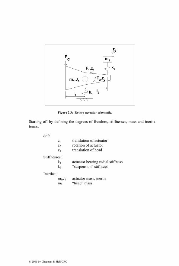
Figure 2.3: Rotary actuator schematic.
Starting off by defining the degrees of freedom, stiffnesses, mass and inertia terms:
dof: z1 translation of actuator z2 rotation of actuator z3 translation of head
Stiffnesses: k1 actuator bearing radial stiffness k2 “suspension” stiffness
Inertias: m1,J1 actuator mass, inertia
m2 “head” mass
z3
k2
m2
m1,J1
F1,z1
T2,z2
k1l1
Fc
l2
© 2001 by Chapman & Hall/CRC

z3
k2
k1 l2
z3
k2z1
z2
k1 l2
z3
k2
z2
k1 l2
z1=1
Z2 = 1
Rotary Actuator Stiffness Example
First Column: z1 = 1
Second Column: z2 = 1
Third Column: z3 = 1
z2
z1
z1
z3=1
Figure 2.4: Unit displacements to define mass and stiffeness matrices.
See Figure 2.4 to define the entries of each column of (2.7), the forces/moments required to constrain the respective dof in the configuration shown.
© 2001 by Chapman & Hall/CRC

1 1 1 2 2 2 2 1 1 c2
1 2 2 2 2 2 2 2 2 2 c 1
2 3 2 2 2 2 3
m 0 0 z (k k ) l k k z F F0 J 0 z l k l k l k z T F l0 0 m z k l k k z 0 0
+ − − + − = = − −
(2.7)
1 cF F= − (2.8)
2 c 1T F l= (2.9)
2.3 Single Degree of Freedom (sdof) System Transfer Function and Frequency Response
2.3.1 sdof System Definition, Equations of Motion
The sdof system to be analyzed is shown below. The system consists of a mass, m, connected to ground by a spring of stiffness k and a damper with viscous damping coefficient c. Since the mass can only move in the z direction, a single degree of freedom is sufficient to define the system configuration. Force F is applied to the mass.
m
z F
c
k
Figure 2.5: Single degree of freedom system.
The equation of motion for this system is given by:
mz cz kz F+ + = (2.10)
2.3.2 Transfer Function
Taking the Laplace transform of a general second order differential equation (DE) with initial conditions is:
© 2001 by Chapman & Hall/CRC
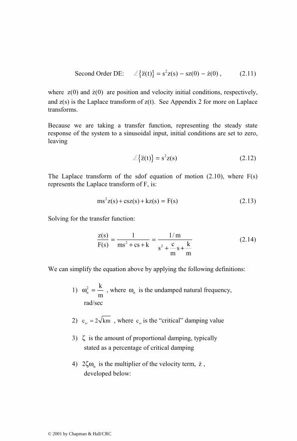
Second Order DE: { } 2z(t) s z(s) sz(0) z(0)= − −L , (2.11)
where z(0) and z(0) are position and velocity initial conditions, respectively, and z(s) is the Laplace transform of z(t). See Appendix 2 for more on Laplace transforms.
Because we are taking a transfer function, representing the steady state response of the system to a sinusoidal input, initial conditions are set to zero, leaving
{ } 2z(t) s z(s)=L (2.12)
The Laplace transform of the sdof equation of motion (2.10), where F(s) represents the Laplace transform of F, is:
2ms z(s) csz(s) kz(s) F(s)+ + = (2.13)
Solving for the transfer function:
22
z(s) 1 1/ mc kF(s) ms cs k s sm m
= =+ + + +
(2.14)
We can simplify the equation above by applying the following definitions:
1) 2n
km
ω = , where nω is the undamped natural frequency,
rad/sec
2) crc 2 km= , where crc is the “critical” damping value
3) ζ is the amount of proportional damping, typically stated as a percentage of critical damping
4) n2ζω is the multiplier of the velocity term, z , developed below:
© 2001 by Chapman & Hall/CRC

n
cr
c 2m
c k2c m
2c k2 km mcm
= ζω
=
=
=
(2.15)
Rewriting, using the above substitutions:
2 2n n
z(s) 1/ mF(s) s 2 s
=+ ζω + ω
(2.16)
2.3.3 Frequency Response
Substituting “ jω ” for “s” to calculate the frequency response, where “j” is the imaginary operator:
2 2n n
2 2n n
2
2n n
2
2
2n n2
2
2n n
z( j ) 1/ mF( j ) ( j ) 2 ( j )
1/ m2 j
1/(m )2 j1
1/(m )2 j1
1/(m )
1 j2
ω =ω ω + ζω ω + ω
=−ω + ζωω + ω
ω=ζω ω− + +ω ω
ω= ω ζω− + ωω
ω= ω ω − + ζ ω ω
(2.17a,b,c,d,e)
The frequency response equation above shows how the ratio (z/F) varies as a function of frequency, ω . The ratio is a complex number that has some interesting properties at different values of the ratio ( )n /ω ω .
© 2001 by Chapman & Hall/CRC

At low frequencies relative to the resonant frequency, 2 2n nω >> ωω >> ω , and
the transfer function is given by:
2 2n n
2 2n n
z( j ) 1/ mF( j ) 2 j
1/ m 1 1 1k km mm
ω =ω −ω + ζωω + ω
≅ = = =ω ω
(2.18)
Since the frequency response value at any frequency is a complex number, we can take the magnitude and phase.
z( j ) 1F( j ) k
z( j ) 0F( j )
ω =ω
ω∠ =ω
(2.19a,b)
Thus, the gain at low frequencies is a constant, (1/k) or the inverse of the stiffness. Phase is 0 because the sign is positive.
At high frequencies, 2 2n nω >> ωω >> ω , the transfer function is given by:
2 2n n
2 2
z( j ) 1/ mF( j ) 2 j
1/ m 1m
ω =ω −ω + ζωω + ω
−≅ =−ω ω
(2.20)
Once again, taking the magnitude and phase:
2 2
z( j ) 1 1F( j ) m m
z( j ) 180F( j )
ω −= =ω ω ω
ω∠ = −ω
(2.21a,b)
At high frequencies, the gain is given by 21/(m )ω and the phase is 180− because the sign is negative.
© 2001 by Chapman & Hall/CRC

At resonance, nω = ω , the transfer function is given by:
2 2n n
2 2n n n
z( j ) 1/ mF( j ) 2 j
1/ m 1/ m 1 1 1 1/ k j / k2 kmj2 j 2 kj 2 j 22 j 2 mj
m
ω =ω −ω + ζωω + ω
−= = = = = = =ζζωω ζ ζ ζζω ζω
(2.22)
Taking magnitude and phase at resonance:
z( j ) j / k 1/ kF( j ) 2 2
z( j ) 90F( j )
ω −= =ω ζ ζ
ω∠ = −ω
(2.23a,b)
The magnitude at resonance is seen to be the gain at low frequency, 1/k, divided by 2ζ . Since ζ is typically a small number, for example 1% of critical damping or 0.01, the magnitude at resonance is seen to be amplified. At resonance the phase angle is 90− .
10-1 100 101
10-3
10-2
10-1
100
101SDOF frequency response magnitudes for zeta = 0.1 to 1.0 in steps of 0.1
frequency, rad/sec
mag
nitu
de
Figure 2.6: sdof magnitude versus frequency for different damping ratios.
© 2001 by Chapman & Hall/CRC

The MATLAB code sdofxfer.m, listed in the next section, is used to plot the frequency responses from (2.17) for a range of damping values for m = k = 1.0, shown in Figures 2.6 and 2.7. These m and k values give a nω value of 1.0 rad/sec.
Since nω is 1.0 rad/sec, the resonant peak in Figure 2.6 should occur at that frequency. The low frequency magnitude was shown above to be equal to 1/k = 1.0. The curves for all the damping values approach 1.0 ( 010 1.0= ) at
low frequencies. At high frequencies the magnitude is given by ( )21/ mω ,
and since m = 1, we should have magnitude of 21/ ω . Checking the plot above, at a frequency of 10 rad/sec, the magnitude should be 1/100 or 0.01.
Note that the slope of the low frequency asymptote is zero, meaning it is not changing with frequency. However, the slope of the high frequency asymptote is “ 2− ,” meaning that for every decade increase in frequency the magnitude at high frequency decreases by two orders of magnitude by virtue of the 2ω term in the denominator. The “ 2− ” slope on a log magnitude versus log frequency plot comes from the following:
( ) ( )22
1log high frequency log log 2log− ∝ = ω = − ω ω (2.24)
10-1 100 101
-180
-160
-140
-120
-100
-80
-60
-40
-20
0SDOF frequency response phases for zeta = 0.1 to 1.0 in steps of 0.1
frequency, rad/sec
mag
nitu
de
Figure 2.7: sdof phase versus frequency for different damping ratios.
© 2001 by Chapman & Hall/CRC

From Figure 2.7, note that at resonance ( n 1.0 rad / secω = ) the phase for all values of damping is 90− . At low frequencies phase is approaching 0 and at high frequencies it is approaching 180− .
2.3.4 MATLAB Code sdofxfer.m Description
The code uses the transfer function form shown in (2.14) to calculate the complex quantity “xfer,” where s j= ω , using a vector of defined ω values. Magnitude and phase of the complex value of the transfer function are then plotted versus frequency.
2.3.5 MATLAB Code sdofxfer.m Listing
% sdofxfer.m plotting frequency responses of sdof model for different damping values clf; clear all; % assign values for mass, percentage of critical damping, and stiffnesses % zeta is a vector of damping values from 10% to 100% in steps of 10% m = 1; zeta = 0.1:0.1:1; % 0.1 = 10% of critical k = 1; wn = sqrt(k/m); % Define a vector of frequencies to use, radians/sec. The logspace command uses % the log10 value as limits, i.e. -1 is 10^-1 = 0.1 rad/sec, and 1 is % 10^1 = 10 rad/sec. The 400 defines 400 frequency points. w = logspace(-1,1,400); % pre-calculate the radians to degree conversion rad2deg = 180/pi; % define s as the imaginary operator times the radian frequency vector s = j*w; % define a for loop to cycle through all the damping values for calculating % magnitude and phase for cnt = 1:length(zeta) % define the frequency response to be evaluated xfer(cnt,:) = (1/m) ./ (s.^2 + 2*zeta(cnt)*wn*s + wn^2);
© 2001 by Chapman & Hall/CRC

% calculate the magnitude and phase of each frequency response mag(cnt,:) = abs(xfer(cnt,:)); phs(cnt,:) = angle(xfer(cnt,:))*rad2deg; end % define a for loop to cycle through all the damping values for plotting magnitude for cnt = 1:length(zeta) loglog(w,mag(cnt,:),'k-') title('SDOF frequency response magnitudes for zeta = 0.1 to 1.0 in steps of 0.1') xlabel('frequency, rad/sec') ylabel('magnitude') grid hold on end hold off grid on disp('execution paused to display figure, "enter" to continue'); pause % define a for loop to cycle through all the damping values for plotting phase for cnt = 1:length(zeta) semilogx(w,phs(cnt,:),'k-') title('SDOF frequency response phases for zeta = 0.1 to 1.0 in steps of 0.1') xlabel('frequency, rad/sec') ylabel('magnitude') grid hold on end hold off grid on disp('execution paused to display figure, "enter" to continue'); pause
© 2001 by Chapman & Hall/CRC

2.4 tdof Laplace Transform, Transfer Functions, Characteristic Equation, Poles, Zeros
We now return to the original tdof model as shown in Figure 2.1. In order to define transfer functions and understand poles and zeros of the system, we need to transform from the time domain to the frequency domain. We do this by taking Laplace transforms of the equations of motion.
2.4.1 Laplace Transforms with Zero Initial Conditions
Repeating (2.5) for the tdof system:
1 1 1 1 1
2 2 1 1 2 2 2
3 3 2 2 3
1 1 1 1
1 1 2 2 2 2
2 2 3 3
m 0 0 z c c 0 z0 m 0 z c (c c ) c z0 0 m z 0 c c z
k k 0 z Fk (k k ) k z F0 k k z F
− + − + − −
− + − + − = −
(2.25)
Taking Laplace transforms assuming initial conditions of zero, where 1 2, 3z , z z now represent the Laplace transforms of the original 1 2, 3z , z z :
21 1 1 1 1
22 2 1 1 2 2 2
23 3 2 2 3
1 1 1 1
1 1 2 2 2 2
2 2 3 3
m 0 0 s z c c 0 sz0 m 0 s z c (c c ) c sz0 0 m s z 0 c c sz
k k 0 z Fk (k k ) k z F0 k k z F
− + − + − −
− + − + − = −
(2.26)
Rearranging:
21 1 1 1 1 1 1
21 1 2 1 2 1 2 2 2 2 2
22 2 3 2 2 3 3
(m s c s k ) ( c s k ) 0 z F( c s k ) (m s c s c s k k ) ( c s k ) z F
0 ( c s k ) (m s c s k ) z F
+ + − − − − + + + + − − = − − + + (2.27)
© 2001 by Chapman & Hall/CRC

2.4.2 Solving for Transfer Functions
In this section we solve for the nine possible transfer functions for all combinations of degrees of freedom where force is applied and where displacements are taken. Solving for the transfer functions for greater than a 2dof system is a task not to be taken lightly – symbolic algebra programs such as Mathematica, Maple or the MATLAB Symbolic Toolbox should be used.
1 1 1
1 2 3
2 2 2
1 2 3
3 3 3
1 2 3
z z zF F Fz z zF F Fz z zF F F
Table 2.3: Nine possible transfer functions for tdof system.
The results below were obtained by use of a symbolic algebra program.
( ) ( )( ) ( )
4 32 3 3 1 3 2 2 21
21 1 2 2 2 3 1 3 2 1 2 2 1 1 2
s m m s m c m c m cz / DenF s c c m k m k m k s c k c k k k
+ + + = + + + + + + +
(2.28)
( ) ( ) ( ){ }3 213 1 1 2 3 1 1 2 1 2 1 2
2
z s m c s c c m k s c k k c k k / DenF
= + + + + + (2.29)
( ) ( ){ }211 2 1 2 2 1 1 2
3
z s c c s c k c k k k / DenF
= + + + (2.30)
( ) ( ) ( ){ }3 223 1 1 2 3 1 1 2 2 1 1 2
1
z s m c s c c m k s c k c k k k / DenF
= + + + + + (2.31)
( ) ( )( )
( )
4 31 3 1 2 3 1
221 2 1 2 3 1
21 2 2 1 1 2
s m m s m c m cz s m k c c m k / DenF
s c k c k k k
+ + = + + + + + +
(2.32)
( ) ( ) ( ){ }3 321 2 1 2 1 2 1 2 2 1 1 2
3
z s m c s m k c c s c k c k k k / DenF
= + + + + + (2.33)
© 2001 by Chapman & Hall/CRC
( ) ( ){ }231 2 1 2 2 1 1 2
1
zs c c s c k c k k k / Den
F= + + + (2.34)
( ) ( ) ( ){ }3 231 2 1 2 1 2 1 2 2 1 1 2
2
zs m c s m k c c s c k c k k k / Den
F= + + + + + (2.35)
( ) ( )( )
( ) ( )
4 31 2 1 2 1 1 2 1
232 1 1 1 1 2 1 2
32 1 1 2 1 2
s m m s m c m c m cz
s m k m k m k c c / DenF
s c k c k k k
+ + + = + + + + + + +
(2.36)
Where Den is:
4 31 2 3 2 3 1 1 3 1 1 2 2 1 3 2
21 3 1 1 3 2 1 2 2 2 1 2 3 1 2 1 1 2
21 2 3
3 1 2 2 2 1 1 2 1 1 1 2 3 2 1 2 1 2
1 1 2 2 1 2 3 1 2
s (m m m ) s (m m c m m c m m c m m c )
s (m m k m m k m m k m c c m c c m c cDen s k m m )
s (m c k m c k m c k m c k m c k m c k )(m k k m k k m k k )
+ + + +
+ + + + + + = + + + + + + + + + +
(2.37)
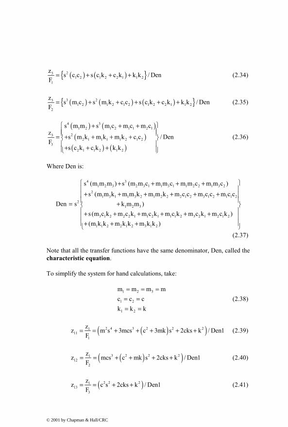
Note that all the transfer functions have the same denominator, Den, called the characteristic equation.
To simplify the system for hand calculations, take:
1 2 3
1 2
1 2
m m m mc c ck k k
= = == == =
(2.38)
( )( )2 4 3 2 2 2111
1
zz m s 3mcs c 3mk s 2cks k / Den1F
= = + + + + + (2.39)
( )( )3 2 2 2112
2
zz mcs c mk s 2cks k / Den1F
= = + + + + (2.40)
( )2 2 2113
3
zz c s 2cks k / Den1F
= = + + (2.41)
© 2001 by Chapman & Hall/CRC

( ) ( )( )3 2 2 2221
1
zz mcs c mk s 2ck s k / Den1F
= = + + + + (2.42)
( )( )2 4 3 2 2 2222
2
zz m s 2mcs 2mk c s 2cks k / Den1F
= = + + + + + (2.43)
( )( )3 2 2 2223
3
zz mcs c mk s 2cks k / Den1F
= = + + + + (2.44)
( )2 2 2331
1
zz c s 2cks k / Den1
F= = + + (2.45)
( )( )3 2 2 2332
2
zz mcs c mk s 2cks k / Den1
F= = + + + + (2.46)
( )( )2 4 3 2 2 2333
3
zz m s 3mcs c 3mk s 2cks k / Den1
F= = + + + + + (2.47)
Where:
( ){ }3 4 2 3 2 2 2 2 2Den1 m s 4m cs 4m k 3mc s 6mcks 3mk s= + + + + + (2.48)
To enable hand calculations of roots, simplify another level by making damping equal to zero:
( )2 4 2 21
1
z m s 3mks k / Den2F
= + + (2.49)
( )2 21
2
z mks k / Den2F
= + (2.50)
21
3
z k / Den2F
= (2.51)
( )2 22
1
z mks k / Den2F
= + (2.52)
© 2001 by Chapman & Hall/CRC

( )2 4 2 22
2
z m s 2mks k / Den2F
= + + (2.53)
( )2 22
3
z mks k / Den2F
= + (2.54)
23
1
zk / Den2
F= (2.55)
( )2 23
2
zmks k / Den2
F= + (2.56)
( )2 4 2 23
3
zm s 3mks k / Den2
F= + + (2.57)
( )2 3 4 2 2 2Den2 s m s 4m ks 3mk= + + (2.58)
2.4.3 Transfer Function Matrix for Undamped Model
A more convenient method of arranging and keeping track of the various transfer functions is to use a matrix form for the transfer function, called the transfer function matrix:
11 12 13
21 22 23
31 32 33
z z zz z zz z z
(2.59)
Where:
1 11 12 13 1
2 21 22 23 2
3 31 32 33 3
z z z z Fz z z z Fz z z z F
=
(2.60)
The transfer function matrix can then be written for the undamped case as follows, where each term of the numerator matrix is divided by the common denominator:
© 2001 by Chapman & Hall/CRC

( )
1
2
3
2 4 2 2 2 2 2
2 2 2 4 2 2 2 2
12 2 2 2 4 2 2
22 3 4 2 2 2
3
zzz
(m s 3mks k ) (mks k ) k(mks k ) (m s 2mks k ) (mks k ) F
k (mks k ) (m s 3mks k ) Fs m s 4m ks 3mk F
=
+ + + + + + +
+ + + + +
(2.61)
2.4.4 Four Distinct Transfer Functions
We will be dealing with only Single Input Single Output (SISO) systems until Chapter 19, when a Multi Input Multi Output (MIMO) system is examined. This means that we will be applying only a single force to the system at any time, 1 2 3F , F or F ,and will only be taking the displacement of a single degree of freedom, 1 2 3z , z or z .
Because there are three inputs and three outputs, there are nine possible SISO transfer functions to investigate. However, because of the symmetry of the system (zij = zji) there are only four distinct transfer functions. Expanding the denominator into factors and simplifying:
( )2 4 2 2
12 3 4 2 2 2
1
z m s 3mks kF s m s 4m ks 3mk
+ +=+ +
(2.62)
( )2 2
22 3 4 2 2 2
1
z (mks k )F s m s 4m ks 3mk
+=+ +
2
2 2 2 2
k(ms k)s (ms k)(m s 3km)
+=+ +
2 2 2
ks (m s 3km)
=+
(note cancelling of pole/zero) (2.63)
( )2
32 3 4 2 2 2
1
z kF s m s 4m ks 3mk
=+ +
(2.64)
© 2001 by Chapman & Hall/CRC
( )2 4 2 2
22 3 4 2 2 2
2
z m s 2mks kF s m s 4m ks 3mk
+ +=+ +
(2.65)
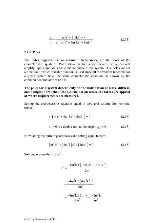
2.4.5 Poles
The poles, eigenvalues, or resonant frequencies, are the roots of the characteristic equation. Poles show the frequencies where the system will amplify inputs, and are a basic characteristic of the system. The poles are not a function of which transfer function is used since all the transfer functions for a given system have the same characteristic equation, as shown by the common denominator of (2.61).
The poles for a system depend only on the distribution of mass, stiffness, and damping throughout the system, not on where the forces are applied or where displacements are measured.
Setting the characteristic equation equal to zero and solving for the roots (poles):
( )2 3 4 2 2 2s m s 4m ks 3mk 0+ + = (2.66)
2s 0= is a double root at the origin 1,2s 0= (2.67)
Now taking the term in parentheses and setting equal to zero:
( ) ( ) ( )3 4 2 2 2m s 4m k s 3mk 0+ + = (2.68)
Solving as a quadratic in s2:
( )
12 4 2 4 2 2
23
4m k 16m k 12m ks
2m
− ± −=
( )
12 4 2 2
3
4m k 4m k
2m
− ±=
2 2 2
3 3
4m k 2m k 2m k2m m
− ± −= =
© 2001 by Chapman & Hall/CRC

2k 6k,2m 2m− −=
k 3k,m m− −= (2.69)
3,4ks j j1m
= ± = ± (2.70)
5,63ks j j1.732m
= ± = ± (2.71)
Because there is no damping, the poles all fall on the s-plane imaginary axis.
2.4.6 Zeros
The zeros of each SISO transfer function are defined by the roots of its numerator. Zeros show the frequencies where the system will attenuate inputs. Unlike the poles, which are a characteristic of the system and are the same for every transfer function, zeros can be different for every transfer function and some transfer functions may have no zeros. Chapter 4 will discuss one physical interpretation of zeros, showing how to calculate the number of zeros for various transfer functions for a series-connected lumped mass system.
Calculate the 1 1z / F zeros:
2 4 2 2m s 3mks k 0+ + = (2.72)
( )
12 2 2 2 2
22
3mk 9m k 4m ks
2m
− ± −=
2
3mk 5mk 3k 5k2m2m
− ± − ±= =
( ) ( )k 3 5 k k0.3820 , 2.618m 2 m m
− ± = = − − (2.73)
Taking the square root of the two values above gives two pair of complex conjugate roots:
© 2001 by Chapman & Hall/CRC

1,2ks j0.618 j 0.618m
= ± = ± (2.74)
3,4ks j1.618 j 1 .618m
= ± = ± (2.75)
Calculate the 2 1z / F zeros:
2 2mks k 0+ = (2.76)
2
2 k ksmk m− −= = (2.77)
1,2ks j jm
= ± = ± (2.78)
Calculate the 3 1z / F zeros:
2k 0= there are no zeros. (2.79)
Calculate the 2 2z / F zeros:
2 4 2 2m s 2mks k 0+ + = (2.80)
( )2 2 2 2
22
2mk 4m k 4m ks
2m
− ± −=
2
2mk k 0m2m
− −= = ± (2.81)
1,2ks j jm
= ± = ± (2.82)
3,4s j= ± (2.83)
As with the poles, since there is no damping in the system, all the zeros are also on the imaginary axis.
© 2001 by Chapman & Hall/CRC

2.4.7 Summarizing Poles and Zeros, Matrix Format
( 0.62, 1.62) j nonej ( j, j) j
none j ( 0.62, 1.62)( 0 j)( 1, 1.732) j
± ± ± ± ± ± ± ± ± ±
± ± ± (2.84)
The 3x3 matrix of zero values for the 3x3 transfer function matrix is in the numerator of (2.82) and the pole values are in the denominator.
2.5 MATLAB Code tdofpz3x3.m – Plot Poles and Zeros
2.5.1 Code Description
The program listing below uses the “num/den” form of the transfer function and calculates and plots all nine pole/zero combinations for the nine different transfer functions. It prompts for values of the two dampers, c1 and c2, where the default values (hitting the “enter” key) are set to zero to match the hand-calculated values in (2.82). The “transfer function” forms of the transfer functions are then converted to “zpk - zero/pole/gain” form to enable graphical construction of frequency response in the next chapter.
The values of the poles and zeros as well as the “zpk” forms of the transfer functions are listed in the MATLAB command window.
Note that in most MATLAB code, the critical definitions and calculations take only a few commands while plotting and annotating the plots take the bulk of the space.
2.5.2 Code Listing
% tdofpz3x3.m plotting poles/zeros of tdof model, all 9 plots clf; clear all; % using MATLAB's pzmap function with the "tf" form using num/den % to define the numerator and denominator terms of the different % transfer functionx % assign values for masses, damping, and stiffnesses m1 = 1; m2 = 1;
© 2001 by Chapman & Hall/CRC

m3 = 1; k1 = 1; k2 = 1; % prompt for c1 and c2 values, set to zero to match closed form solution c1 = input('enter value for damper c1, default is zero, ... '); if isempty(c1) c1 = 0; end c2 = input('enter value for damper c2, default is zero, ... '); if isempty(c2) c2 = 0; end % define row vectors of numerator and denominator coefficients den = [(m1*m2*m3) (m2*m3*c1 + m1*m3*c1 + m1*m2*c2 + m1*m3*c2) ... (m1*m3*k1 + m1*m3*k2 + m1*m2*k2 + m2*c1*c2 + m3*c1*c2 + ... m1*c1*c2 + k1*m2*m3) ... (m3*c1*k2 + m2*c2*k1 + m1*c2*k1 + m1*c1*k2 + … m3*c2*k1 + m2*c1*k2) ... (m1*k1*k2 + m2*k1*k2 + m3*k1*k2) 0 0]; z11num = [(m2*m3) (m3*c1 + m3*c2 + m2*c2) (c1*c2 + m2*k2 +…
m3*k1 + m3*k2) (c1*k2 + c2*k1) (k1*k2)]; z21num = [(m3*c1) (c1*c2 + m3*k1) (c1*k2 + c2*k1) (k1*k2)]; z31num = [(c1*c2) (c1*k2 + c2*k1) (k1*k2)]; z22num = [(m1*m3) (m1*c2 + m3*c1) (m1*k2 + c1*c2 + m3*k1) ... (c1*k2 + c2*k1) (k1*k2)]; % use the "tf" function to convert to define "transfer function" systems sysz11 = tf(z11num,den) sysz21 = tf(z21num,den) sysz31 = tf(z31num,den) sysz22 = tf(z22num,den) % use the "zpk" function to convert from transfer function to zero/pole/gain form zpkz11 = zpk(sysz11) zpkz21 = zpk(sysz21) zpkz31 = zpk(sysz31)
© 2001 by Chapman & Hall/CRC
zpkz22 = zpk(sysz22) % use the "pzmap" function to map the poles and zeros of each transfer function [p11,z11] = pzmap(sysz11); [p21,z21] = pzmap(sysz21); [p31,z31] = pzmap(sysz31); [p22,z22] = pzmap(sysz22); p11 z11 z21 z31 z22 % plot z11 for later use subplot(1,1,1) plot(real(p11),imag(p11),'k*') hold on plot(real(z11),imag(z11),'ko') title('Poles and Zeros of z11') ylabel('Imag') axis([-2 2 -2 2]) axis('square') grid hold off disp('execution paused to display figure, "enter" to continue'); pause % plot all 9 plots on a 3x3 grid subplot(3,3,1) plot(real(p11),imag(p11),'k*') hold on plot(real(z11),imag(z11),'ko') title('Poles and Zeros of z11') ylabel('Imag') axis([-2 2 -2 2]) axis('square') grid hold off subplot(3,3,2) plot(real(p21),imag(p21),'k*') hold on plot(real(z21),imag(z21),'ko') title('Poles and Zeros of z12')
© 2001 by Chapman & Hall/CRC

ylabel('Imag') axis([-2 2 -2 2]) axis('square') grid hold off subplot(3,3,3) plot(real(p31),imag(p31),'k*') hold on plot(real(z31),imag(z31),'ko') title('Poles and Zeros of z13') ylabel('Imag') axis([-2 2 -2 2]) axis('square') grid hold off subplot(3,3,4) plot(real(p21),imag(p21),'k*') hold on plot(real(z21),imag(z21),'ko') title('Poles and Zeros of z21') ylabel('Imag') axis([-2 2 -2 2]) axis('square') grid hold off subplot(3,3,5) plot(real(p22),imag(p22),'k*') hold on plot(real(z22),imag(z22),'ko') title('Poles and Zeros of z22') ylabel('Imag') axis([-2 2 -2 2]) axis('square') grid hold off subplot(3,3,6) plot(real(p21),imag(p21),'k*') hold on plot(real(z21),imag(z21),'ko') title('Poles and Zeros of z23') ylabel('Imag') axis([-2 2 -2 2]) axis('square') grid hold off subplot(3,3,7) plot(real(p31),imag(p31),'k*') hold on plot(real(z31),imag(z31),'ko') title('Poles and Zeros of z31')
© 2001 by Chapman & Hall/CRC

xlabel('Real') ylabel('Imag') axis([-2 2 -2 2]) axis('square') grid hold off subplot(3,3,8) plot(real(p21),imag(p21),'k*') hold on plot(real(z21),imag(z21),'ko') title('Poles and Zeros of z32') xlabel('Real') ylabel('Imag') axis([-2 2 -2 2]) axis('square') grid hold off subplot(3,3,9) plot(real(p11),imag(p11),'k*') hold on plot(real(z11),imag(z11),'ko') title('Poles and Zeros of z33') xlabel('Real') ylabel('Imag') axis([-2 2 -2 2]) axis('square') grid hold off disp('execution paused to display figure, "enter" to continue'); pause % check for real axis values to set plot scale z11_realmax = max(abs(real(z11))); z21_realmax = max(abs(real(z21))); z31_realmax = max(abs(real(z31))); z22_realmax = max(abs(real(z22))); maxplot = max([z11_realmax z21_realmax z31_realmax z22_realmax]); if maxplot > 2 maxplot = ceil(maxplot); else maxplot = 2.0;
end z11_realmax = max(abs(real(z11))); subplot(1,1,1)
© 2001 by Chapman & Hall/CRC

plot(real(p11),imag(p11),'k*') hold on plot(real(z11),imag(z11),'ko') title('Poles and Zeros of z11, z33') ylabel('Imag') axis([-maxplot maxplot -maxplot maxplot]) axis('square') grid hold off disp('execution paused to display figure, "enter" to continue'); pause plot(real(p21),imag(p21),'k*') hold on plot(real(z21),imag(z21),'ko') title('Poles and Zeros of z21, z12, z23, z32') ylabel('Imag') axis([-maxplot maxplot -maxplot maxplot]) axis('square') grid hold off disp('execution paused to display figure, "enter" to continue'); pause plot(real(p31),imag(p31),'k*') hold on plot(real(z31),imag(z31),'ko') title('Poles and Zeros of z31, z13') xlabel('Real') ylabel('Imag') axis([-maxplot maxplot -maxplot maxplot]) axis('square') grid hold off disp('execution paused to display figure, "enter" to continue'); pause plot(real(p22),imag(p22),'k*') hold on plot(real(z22),imag(z22),'ko') title('Poles and Zeros of z22') ylabel('Imag') axis([-maxplot maxplot -maxplot maxplot]) axis('square') grid hold off
© 2001 by Chapman & Hall/CRC

2.5.3 Code Output – Pole/Zero Plots in Complex Plane
2.5.3.1 Undamped Model – Pole/Zero Plots
The pole/zero plot and pole/zero calculated values for c1 = c2 = 0 are shown below. Poles are plotted as asterisks and zeros as circles.
-2 0 2-2
-1
0
1
2Poles and Zeros of z11
Imag
-2 0 2-2
-1
0
1
2Poles and Zeros of z12
Imag
-2 0 2-2
-1
0
1
2Poles and Zeros of z13
Imag
-2 0 2-2
-1
0
1
2Poles and Zeros of z21
Imag
-2 0 2-2
-1
0
1
2Poles and Zeros of z22
Imag
-2 0 2-2
-1
0
1
2Poles and Zeros of z23
Imag
-2 0 2-2
-1
0
1
2Poles and Zeros of z31
Real
Imag
-2 0 2-2
-1
0
1
2Poles and Zeros of z32
Real
Imag
-2 0 2-2
-1
0
1
2Poles and Zeros of z33
Real
Imag
Figure 2.8: Pole/zero plots for nine transfer functions. Poles are indicated by asterisks and zeros by circles.
The first thing to notice about the pole/zero plots is that they all have the same poles. The rigid body mode (resonant frequency = 0 hz) is evident by the pair of zeros at the origin, 0 j± . The zeros of each particular transfer function are seen to be dependent upon which transfer function is taken. Note that with zero damping, all the poles and zeros are on the imaginary axis, indicating that the real portions of their complex values are zero and that there is no damping.
© 2001 by Chapman & Hall/CRC

In the next chapter we will discuss frequency responses of transfer functions and will link the pole/zero locations in the complex plane to amplification/attenuation regions of the frequency response plots.
The poles and zeros from the MATLAB output are listed below:
poles = 0 0 0 + 1.7321i 0 - 1.7321i 0 + 1.0000i 0 - 1.0000i zeros_z11 = 0 + 1.6180i 0 - 1.6180i 0 + 0.6180i 0 - 0.6180i zeros_z21 = 0 + 1.0000i 0 - 1.0000i zeros_z31 = Empty matrix: 0-by-1 zeros_z22 = -0.0000 + 1.0000i -0.0000 - 1.0000i 0.0000 + 1.0000i 0.0000 - 1.0000i
Table 2.3: Poles and zeros of tdof transfer functions, undamped.
Repeating the matrix listing of pole/zero locations from previous analysis:
( 0.62, 1.62) j nonej ( j, j) j
none j ( 0.62, 1.62)( 0 j)( 1, 1.732) j
± ± ± ± ± ± ± ± ± ±
± ± ± (2.85)
© 2001 by Chapman & Hall/CRC

Note that MATLAB calculates an “Empty matrix 0 by 1” for the zeros of z31, which matches our calculations which show “none.” Also note that several of the plots, z12, z21, z22, z23 and z32, have zeros and poles overlaying each other, where the pole cancels the effect of the zero. We will discuss this cancellation further in the next chapter.
2.5.3.2 Damped Model – Pole/Zero Plots
If damping is not set to zero for c1 and/or c2, the poles (with the exception of the two poles at the origin) and zeros will move from the imaginary axis to the left hand side of the complex plane, with the real parts of the poles and zeros having negative values. The pole/zero plot and MATLAB output listing below are for values of c1 = c2 = 0.1, arbitrarily chosen to illustrate the “damped” case.
-2 0 2-2
-1
0
1
2Poles and Zeros of z11
Imag
-2 0 2-2
-1
0
1
2Poles and Zeros of z12
Imag
-2 0 2-2
-1
0
1
2Poles and Zeros of z13
Imag
-2 0 2-2
-1
0
1
2Poles and Zeros of z21
Imag
-2 0 2-2
-1
0
1
2Poles and Zeros of z22
Imag
-2 0 2-2
-1
0
1
2Poles and Zeros of z23
Imag
-2 0 2-2
-1
0
1
2Poles and Zeros of z31
Real
Imag
-2 0 2-2
-1
0
1
2Poles and Zeros of z32
Real
Imag
-2 0 2-2
-1
0
1
2Poles and Zeros of z33
Real
Imag
Figure 2.9: Pole/zero plots for nine transfer functions for c1 = c2 = 0.1. Poles are indicated by asterisks and zeros by circles. Negative real axis zeros not shown because of plot
scaling.
© 2001 by Chapman & Hall/CRC

The limited scale for the nine plots above do not show the real axis zeros, see the figures below for the entire plot. The only poles/zeros that are on the imaginary axis are the two poles at zero, the rigid body mode – which will be described in detail in Chapter 3.
-10 -5 0 5 10
-10
-8
-6
-4
-2
0
2
4
6
8
10Poles and Zeros of z11, z33
Imag
Figure 2.10: Expanded scale pole/zero plots for z11, z33 transfer functions – no real axis zeros.
-10 -5 0 5 10
-10
-8
-6
-4
-2
0
2
4
6
8
10Poles and Zeros of z21, z12, z23, z32
Imag
Figure 2.11: Expanded scale pole/zero plots for z21, z12, z23 and z32 transfer functions – one real axis zero at -10.
© 2001 by Chapman & Hall/CRC

-10 -5 0 5 10
-10
-8
-6
-4
-2
0
2
4
6
8
10Poles and Zeros of z31, z13
Real
Imag
Figure 2.12: Expanded scale pole/zero plots for z31 and z13 transfer functions – two real axis zeros at -10.
-10 -5 0 5 10
-10
-8
-6
-4
-2
0
2
4
6
8
10Poles and Zeros of z22
Imag
Figure 2.13: Expanded scale pole/zero plots for z31 and z13 transfer functions – no real axis zeros.
The MATLAB calculated values for the poles and zeros for the damped case are below:
© 2001 by Chapman & Hall/CRC

p11 = 0 0 -0.1500 + 1.7255i -0.1500 - 1.7255i -0.0500 + 0.9987i -0.0500 - 0.9987i z11 = -0.1309 + 1.6127i -0.1309 - 1.6127i -0.0191 + 0.6177i -0.0191 - 0.6177i z21 = -10.0000 -0.0500 + 0.9987i -0.0500 - 0.9987i z31 = -10.0000 + 0.0000i -10.0000 - 0.0000i z22 = -0.0500 + 0.9987i -0.0500 - 0.9987i -0.0500 + 0.9987i -0.0500 - 0.9987i
Table 2.4: Poles and zeros of tdof transfer functions, damped.
Several observations can be made about the poles and zeros above. First, all of the poles with the exception of the two rigid body poles p11 = 0 are to the left of the imaginary axis, indicating that the system now has damping. Note that there are several new zeros. The z21 transfer function now has a real zero at –10.0 in addition to the two complex zeros. The z31 transfer function has two zeros now at –10, whereas for the no damping case it had no zeros. These extra zeros do not show up on Figure 2.9 because of plot axis scaling but with the real axis expanded in Figures 2.10 to 2.13 they appear. The reason for these “additional” zeros can be seen if we look at the z21 and z31 transfer functions, repeated from (2.31) and (2.34):
© 2001 by Chapman & Hall/CRC

( ) ( ) ( ){ }3 223 1 1 2 3 1 1 2 2 1 1 2
1
z s m c s c c m k s c k c k k k / DenF
= + + + + + (2.86)
( ) ( ){ }231 2 1 2 2 1 1 2
1
zs c c s c k c k k k / Den
F= + + + (2.87)
With values for c1 and c2 not equal to zero, the z21 transfer function is third degree, meaning that it should have three roots. With damping equal to zero, only two complex zeros are calculated by MATLAB and by hand. The third root is located at −∞ . As damping values for c1 and c2 are increased the root at −∞ moves to the right, towards the origin.
The z31 transfer function has no zeros with zero damping, but is second degree and with infinitely small damping values has two roots at −∞ . As the values of c1 and c2 increase, the two zeros at −∞ start moving toward the origin.
2.5.3.3 Root Locus, tdofpz3x3_rlocus.m
In the last two sections we have discussed pole/zero plots for undamped and damped models. For the damped model we chose values of 0.1 for c1 and c2. It would be nice to have a systematic method to display poles and zeros for a range of damping values. There is a MATLAB Control Toolbox function “rlocus” which plots the root locus for an open-loop SISO system. We could use this function if the damping values could be broken out of the system and be treated as a feedback gain. Unfortunately for our tdof system this is not possible, but we can still plot a locus by using a for-loop.
The code listed below, tdofpz3x3_rlocus.m, is taken from the initial section of tdofpz3x3.m. A for-loop cycles through a vector of damping values, calculating and plotting the poles and zeroes for each damping value.
echo off % tdofpz3x3_rlocus.m plotting locus of poles/zeros of z11 for tdof % model for range of damping values. clf; clear all; % assign values for masses, damping, and stiffnesses m1 = 1; m2 = 1; m3 = 1;
© 2001 by Chapman & Hall/CRC

k1 = 1; k2 = 1; % define vector of damping values for c1 and c2 cvec = [0 .2 .4 .6 .8 1.0 1.1 1.05 1.1 1.15 1.16]; for cnt = 1:length(cvec) c1 = cvec(cnt); c2 = cvec(cnt); % define row vectors of numerator and denominator coefficients den = [(m1*m2*m3) (m2*m3*c1 + m1*m3*c1 + m1*m2*c2 + m1*m3*c2) ... (m1*m3*k1 + m1*m3*k2 + m1*m2*k2 + m2*c1*c2 + m3*c1*c2 + ... m1*c1*c2 + k1*m2*m3) ... (m3*c1*k2 + m2*c2*k1 + m1*c2*k1 + m1*c1*k2 + …
m3*c2*k1 + m2*c1*k2) ... (m1*k1*k2 + m2*k1*k2 + m3*k1*k2) 0 0]; z11num = [(m2*m3) (m3*c1 + m3*c2 + m2*c2) …
(c1*c2 + m2*k2 + m3*k1 + m3*k2) .(c1*k2 + c2*k1) (k1*k2)]; z21num = [(m3*c1) (c1*c2 + m3*k1) (c1*k2 + c2*k1) (k1*k2)]; z31num = [(c1*c2) (c1*k2 + c2*k1) (k1*k2)]; z22num = [(m1*m3) (m1*c2 + m3*c1) (m1*k2 + c1*c2 + m3*k1) ... (c1*k2 + c2*k1) (k1*k2)]; % use the "tf" function to convert to define "transfer function" systems sysz11 = tf(z11num,den); sysz21 = tf(z21num,den); sysz31 = tf(z31num,den); sysz22 = tf(z22num,den); % use the "pzmap" function to map the poles and zeros of each transfer function [p11,z11] = pzmap(sysz11); [p21,z21] = pzmap(sysz21); [p31,z31] = pzmap(sysz31); [p22,z22] = pzmap(sysz22); % plot poles and zeros of z11 subplot(1,1,1)
© 2001 by Chapman & Hall/CRC

plot(real(p11),imag(p11),'k*') hold on plot(real(z11),imag(z11),'ko') title('Poles and Zeros of z11 for range of damping values c1 and c2') xlabel('Real') ylabel('Imag') axis([-3 1 -2 2]) axis('square') grid on end hold off
The root locus plot below is for the following values of damping:
cvec = [0 .2 .4 .6 .8 1.0 1.1 1.05 1.1 1.15 1.16];
-3 -2 -1 0 1-2
-1.5
-1
-0.5
0
0.5
1
1.5
2Poles and Zeros of z11 for range of damping values c1 and c2
Real
Imag
Figure 2.14: Pole zero plot for z11 transfer function.
The plot starts out with damping values of zero for c1 and c2. The poles and zeros for zero damping are located on the imaginary axis. The poles are located at 0, 0, 1j± , 1.732 j± . The zeros are located at 0.62 j± and 1.62 j± . As damping is increased from zero, the poles and zeros (except the two poles at the origin) start moving to the left, away from the imaginary axis. The poles and zeros move at different rates as damping is increased. The poles at 1j±
© 2001 by Chapman & Hall/CRC

and zeros at 0.62 j± move to the left less than the poles at 1.732 j± and the zeros at 1.62 j± . In fact, the two poles at 1.732 j± move so much that at damping values of 1.16 the poles intercept the real axis and split. One moves to the left and the other to the right along the real axis.
Plotting pole and zero locations as a function of system parameters was introduced in 1949 (Evans 1949), as the Evans root locus technique. The hand plotting originally used has been largely replaced with computer plotting techniques as shown above or by using the “rlocus” function. However, because the ability to hand sketch root loci is such a powerful tool, it is still taught in beginning control theory courses (Franklin 1994).
2.5.3.4 Undamped and Damped Model – tf and zpk Forms
This section is included to start familiarizing the reader with the various forms of transfer functions available with MATLAB and to prepare for issues in the next chapter.
Table 2.6 shows the transfer function form of the four distinct transfer functions for the tdof model for the undamped (c1 = c2 = 0) and damped (c1 = c2 = 0.1) cases run earlier. The numerator and denominator are both arranged in polynomial form. Table 2.7 shows the zpk form, where the numerator and denominator are both arranged as products of the zeros and poles with a gain term multiplying the numerator.
Note that the denominators of all the undamped transfer functions are the same, as are the denominators of all the damped transfer functions. However, the numerators are all different because of the different number of poles and zeros for each transfer function. For instance the z31 undamped transfer function has no zeros, only a gain term of 1.0, while the z11 undamped transfer function has two sets of complex zeros.
In going from the undamped to damped case, we showed that extra zeros appeared in the z21 and z31 transfer functions. It is easier to see where the extra zeros originate using the zpk form than using the tf form. Comparing the undamped and damped numerators of the z31 zpk transfer function form shows the extra 2(s 10)+ term, from which the two real axis zeros arise. We will use the zpk form of the transfer functions in the next chapter to calculate frequency response at a specific frequency.
© 2001 by Chapman & Hall/CRC

z11 Undamped Transfer function: z11 Damped Transfer function: s^4 + 3 s^2 + 1 s^4 + 0.3 s^3 + 3.01 s^2 + 0.2 s + 1 ------------------------ --------------------------------------------------- s^6 + 4 s^4 + 3 s^2 s^6 + 0.4 s^5 + 4.03 s^4 + 0.6 s^3 + 3 s^2 z21 Undamped Transfer function: z21 Damped Transfer function: s^2 + 1 0.1 s^3 + 1.01 s^2 + 0.2 s + 1 ------------------------ --------------------------------------------------- s^6 + 4 s^4 + 3 s^2 s^6 + 0.4 s^5 + 4.03 s^4 + 0.6 s^3 + 3 s^2 z31 Undamped Transfer function: z31 Damped Transfer function: 1 0.01 s^2 + 0.2 s + 1 ------------------------ --------------------------------------------------- s^6 + 4 s^4 + 3 s^2 s^6 + 0.4 s^5 + 4.03 s^4 + 0.6 s^3 + 3 s^2 z22 Undamped Transfer function: z22 Damped Transfer function: s^4 + 2 s^2 + 1 s^4 + 0.2 s^3 + 2.01 s^2 + 0.2 s + 1 ------------------------ --------------------------------------------------- s^6 + 4 s^4 + 3 s^2 s^6 + 0.4 s^5 + 4.03 s^4 + 0.6 s^3 + 3 s^2
Table 2.5: Transfer function (tf) form of undamped and damped tdof transfer functions.
z11 Undamped Zero/pole/gain: z11 Damped Zero/pole/gain: (s^2 + 0.382) (s^2 + 2.618) (s^2 + 0.0382s + 0.382) (s^2 + 0.2618s + 2.618) --------------------------------- ---------------------------------------------------------- s^2 (s^2 + 1) (s^2 + 3) s^2 (s^2 + 0.1s + 1) (s^2 + 0.3s + 3) z21 Undamped Zero/pole/gain: z21 Damped Zero/pole/gain: (s^2 + 1) 0.1 (s+10) (s^2 + 0.1s + 1) --------------------------- ------------------------------------- s^2 (s^2 + 1) (s^2 + 3) s^2 (s^2 + 0.1s + 1) (s^2 + 0.3s + 3) z31 Undamped Zero/pole/gain: z31 Damped Zero/pole/gain: 1 0.01 (s+10)^2 --------------------------- -------------------------------------------- s^2 (s^2 + 1) (s^2 + 3) s^2 (s^2 + 0.1s + 1) (s^2 + 0.3s + 3) z22 Undamped Zero/pole/gain: z22 Damped Zero/pole/gain: (s^2 + 1)^2 (s^2 + 0.1s + 1)^2 ---------------------------- -------------------------------------------- s^2 (s^2 + 1) (s^2 + 3) s^2 (s^2 + 0.1s + 1) (s^2 + 0.3s + 3)
Table 2.6: Zero/Pole/Gain (zpk) for undamped and damped tdof transfer functions.
© 2001 by Chapman & Hall/CRC

Problems
m1 m2 m3 m4k1k2 k3
k5
k4
z1
z2
z3
z4
k6
Figure P2.1: four dof system.
P2.1 Derive the global stiffness and mass matrices for the four dof system in Figure P2.1.
m1 m2
k1 k2
c2
z1 z2F1 F2
c1
Figure P2.2: two dof problem.
P2.2 Derive the equations of motion in matrix form for the two dof model in Figure P2.2. Check for signs of diagonal terms and symmetry of off-diagonal terms.
P2.3 Solve for the four transfer functions for the two dof problem and define the 2x2 transfer function matrix. Are the denominators of all four transfer functions the same? How many unique transfer functions are there for this problem?
P2.4 Set 1 2m m m 1= = = , 1 2k k k 1= = = and 1 2c c 0= = and solve for the eigenvalues for the system. Solve for the zeros of the system and use the form
© 2001 by Chapman & Hall/CRC

shown in (2.84) to summarize the poles and zeros. Hand sketch the poles and zeros in the s-plane.
P2.5 (MATLAB) Set 1 2m m m 1= = = , 1 2k k k 1= = = . Modify the tdofpz3x3.m file to plot the poles and zeros of the undamped two dof system. Identify the poles and zeros in the MATLAB output listing and compare with the hand-calculated values.
P2.6 (MATLAB) Set 1 2m m m 1= = = , 1 2k k k 1= = = , add damping values of 1 2c c 0.1= = and plot the poles and zeros in the s-plane. List the poles and zeros from MATLAB and correlate the listed values with the plots. Are there any real axis zeros? How do the real axis zero(s) change with different values of 1c and 2c , where 1 2c c= .
© 2001 by Chapman & Hall/CRC

CHAPTER 3
FREQUENCY RESPONSE ANALYSIS
3.1 Introduction
In Chapter 2 we calculated the transfer functions and identified the poles and zeros for the undamped system, which are repeated as (3.1) and (3.2) below, respectively. The next step in understanding the system is to plot the frequency domain behavior of each transfer function. Frequency domain behavior means identifying the magnitude and phase characteristics of each transfer function, showing how they change as the frequency of the forcing function is varied over a frequency range. Each transfer function is evaluated in the frequency domain by evaluating it at s j= ω , where ω is the frequency of the forcing function, radians/sec.
( )
1
2
3
2 4 2 2 2 2 2
2 2 2 4 2 2 2 2
12 2 2 2 4 2 2
22 3 4 2 2 2
3
zzz
(m s 3mks k ) (mks k ) k(mks k ) (m s 2mks k ) (mks k ) F
k (mks k ) (m s 3mks k ) Fs m s 4m ks 3mk F
=
+ + + + + + +
+ + + + +
(3.1)
( 0.62, 1.62) j nonej ( j, j) j
none j ( 0.62, 1.62)( 0 j)( 1, 1.732) j
± ± ± ± ± ± ± ± ± ±
± ± ± (3.2)
Instead of going directly into MATLAB to calculate and plot the frequency responses, we will first sketch them by hand, using information about the low and high frequency asymptotes and the locations of the poles and zeros. We will discuss how to find the gain and phase of a transfer function at a given frequency graphically using the locations of the poles and zeros in the complex plane and then use MATLAB to plot. Finally, mode shapes are defined, then calculated using transfer function information and plotted.
© 2001 by Chapman & Hall/CRC

3.2 Low and High Frequency Asymptotic Behavior
It is always good to check either a system’s rigid body or spring-like low frequency nature by hand. For this tdof system at very low frequencies there are no spring connections to ground so the system moves as a rigid body, no matter where the force is applied, to F1, F2, or F3.
Figure 3.1: Rigid body mode of vibration.
The rigid body equation of motion (where z is the motion of all three masses together) is:
( )
2
3m z Fz 1F 3ms
=
=
&&
(3.3a,b)
Now we can solve for the frequency domain behavior of the system by substituting jω for s.
At a radian frequency of 0.1 rad/sec, a frequency taken to be an order of magnitude less than the lowest resonant frequency of 1 rad/sec, the transfer function is:
( ) ( )2 2
z 1 1F 3m j 3m j 0.1
= =ω
( )1 100 33.3 33.3
3m .01 3m m− − −= = = = − (3.4)
m1 m2 m3
m1 m2 m3
© 2001 by Chapman & Hall/CRC

Converting from vector (real/imaginary) form to magnitude/phase (polar) form and using the definition of db as follows:
10db 20*log (z / F)= (3.5)
z 33.3, or 30.45dbF
z 180F
=
∠ = − o
(3.6a,b)
These results show that at a frequency of 0.1 rad/sec, the magnitude of the motion of the masses is 33.3*F and the motion is 180− o out of phase with the force input.
We will now look at each individual transfer function, checking asymptotic behavior at both low and high frequencies. To do this, the four transfer functions are divided by the mass terms to give coefficients that are proportional to 2
n k / mω = :
Starting with the 1 1z / F transfer function:
2 4 2 2
12 3 4 2 2 2
1
z m s 3mks kF s (m s 4m ks 3mk )
+ +=+ +
(3.7)
Dividing numerator and denominator by 3m allows redefining the equation in terms of nω :
( )
2 24
2 4 2 2 41 n n
2 2 2 4 2 2 41 2 4 n n
2
3
1 3ks ksm m mz s 3 s
F 4ks 3k ms s 4 s 3s sm m
m
+ + + ω + ω = =
+ ω + ω+ +
÷
(3.8)
Substituting s j= ω and looking at low and high frequency behaviors:
© 2001 by Chapman & Hall/CRC
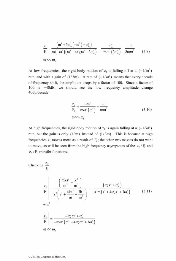
( )( )( )( ) ( )
4 2 2 4 4n n1 n
22 4 2 2 4 2 41 n n n
n
3z 1F 3mm 4 3 m 3
ω + ω −ω + ω ω −= = =ω−ω ω − ω ω + ω − ω ω
ω << ω
(3.9)
At low frequencies, the rigid body motion of z1 is falling off at a 2( 1/ )− ω rate, and with a gain of (1/ 3m) . A rate of 2( 1/ )− ω means that every decade of frequency shift, the amplitude drops by a factor of 100. Since a factor of 100 is 40db− , we should see the low frequency amplitude change 40db/decade.
( )4
122 4
1
n
z 1F mm
−ω −= =ωω ω
ω >> ω
(3.10)
At high frequencies, the rigid body motion of z1 is again falling at a 2( 1/ )− ω rate, but the gain is only (1/ m) instead of (1/ 3m) . This is because at high frequencies z1 moves more as a result of 1F ; the other two masses do not want to move, as will be seen from the high frequency asymptotes of the 2 1z / F and
3 1z / F transfer functions.
Checking 2
1
zF
:
( )( )
2 2
2 2 43 3n n2
2 2 2 4 2 2 41 2 4 n n
2
3
mks ksm mz
F 4ks 3k s m s 4 s 3s sm m
m
+ ω + ω = =
+ ω + ω+ +
÷
(3.11)
( )2 2 4
2 n n2 4 2 2 4
1 n n
n
zF m 4 3
−ω ω + ω=− ω ω − ω ω + ω
ω << ω
© 2001 by Chapman & Hall/CRC
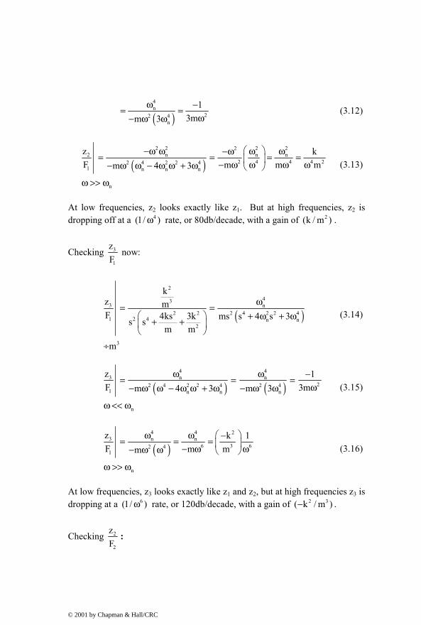
( )4n
22 4n
13mm 3
ω −= =ω− ω ω
(3.12)
( )2 2 2 22
2 n n n2 4 4 4 22 4 2 2 4
1 n n n
n
z kF m m mm 4 3
−ω ω ω ω−ω= = = = − ω ω ω ω− ω ω − ω ω + ω
ω >> ω
(3.13)
At low frequencies, z2 looks exactly like z1. But at high frequencies, z2 is dropping off at a 4(1/ )ω rate, or 80db/decade, with a gain of 2(k / m ) .
Checking 3
1
zF
now:
( )
2
433 n
2 2 2 4 2 2 41 2 4 n n
2
3
kz mF 4ks 3k ms s 4 s 3s s
m m
m
ω= = + ω + ω+ +
÷
(3.14)
( ) ( )4 4
3 n n22 4 2 2 4 2 4
1 n n n
n
z 1F 3mm 4 3 m 3
ω ω −= = =ω− ω ω − ω ω + ω − ω ω
ω << ω
(3.15)
( )4 4 2
3 n n6 3 62 4
1
n
z k 1F m mm
ω ω −= = = − ω ω− ω ω
ω >> ω
(3.16)
At low frequencies, z3 looks exactly like z1 and z2, but at high frequencies z3 is dropping at a 6(1/ )ω rate, or 120db/decade, with a gain of 2 3( k / m )− .
Checking 2
2
zF
:
© 2001 by Chapman & Hall/CRC

( )( )
2 4 2 2
4 2 2 43 3 3n n2
2 2 2 2 4 2 2 42 2 4 n n
3 3
3
m s 2mks ks 2 sm m mz
F 4m ks 3mk ms s 4 s 3s sm m
m
+ + + ω + ω = =
+ ω + ω+ +
÷
(3.17)
( )( )( ) ( )
4 2 2 4 4n n2 n
22 4 2 2 4 2 42 n n n
n
2z 1F 3mm 4 3 m 3
ω + ω −ω + ω ω −= = =ω− ω ω − ω ω + ω − ω ω
ω << ω
(3.18)
( )4
222 4
2
n
z 1F mm
ω −= =ω− ω ω
ω >> ω
(3.19)
At low frequencies, 2 2z / F looks exactly like 1 1z / F , 2 1z / F , and 3 1z / F . But at high frequencies 2 2z / F is dropping at a 2( 1/ )− ω rate and has a higher gain of (1/ m) instead of (1/ 3m) . Thus, the low and high frequency asymptotes look exactly like 1 1z / F .
Summarizing the low and high frequency asymptotes, and solving for the gains and phases at 0.1ω = rad/sec and 10ω = rad/sec.
( )o1
2 21
z 1 1 1 100 33 30.46db, 180F 3(.01) 33m 3m 0.1
rad0.1sec
− − − −= = = = = − =ω
ω =
(3.20)
( )o1
2 21
z 1 1 1 .01 40db, 180F 100m 10
rad10sec
− − −= = = = − = −ω
ω =
(3.21)
© 2001 by Chapman & Hall/CRC

o22
1
z 1 30.46db, 180F 3m
0.1
−= =ω
ω =
(3.22)
( )o2
2 4 41
z k 1 0.0001 80db, 0F m 10
10
= = = = −ω
ω =
(3.23)
o32
1
z 1 30.46db, 180F 3m
0.1
−= =ω
ω =
(3.24)
26 o3
3 6 61
z k 1 1 1e 120db, 180F m 1e
10
−− −= = = − = −ω
ω =
(3.25)
o22
2
z 1 30.46db, 180F 3m
0.1
−= =ω
ω =
(3.26)
( )o2
2 22
z 1 1 .01 40db,180F m 10
10
− −= = = − = −ω
ω =
(3.27)
3.3 Hand Sketching Frequency Responses
Knowing the pole and zero locations and the asymptotes, the complete frequency response can be sketched by hand, as shown in Figure 3.2. We will not worry about the exact magnitudes at the poles and zeros, but will use the hand sketch to get an idea of the overall shape and characteristics of the frequency response. Start by drawing the low and high frequency asymptotes, straight lines with appropriate magnitudes and slopes starting at the 0.1 and 10 rad/sec frequencies. Next, locate the poles and zeros at some distance above and below the asymptote line at the appropriate frequency and start “connecting the dots.” Start at the low frequency asymptote and follow it to the first zero or pole encountered. Keep plotting, moving to the next higher frequency pole or zero until all the poles/zeros are passed and move onto the high frequency asymptote. Note that for z21 the pole and zero at 1 rad/sec cancel as do one of the zeros and the pole for z22. Note that z31 has no zeros,
© 2001 by Chapman & Hall/CRC

only poles. Compare these plots to the MATLAB generated plots in Figure 3.5. Chapter 4 will give a physical interpretation of the zeros.
10-1 100 101-150
-100
-50
0
50xfer function form, Bode z11, z33 db magnitude
frequency, rad/sec
mag
nitu
de, d
b
10-1 100 101-150
-100
-50
0
50xfer function form, Bode z21, z12, z23, z32 db magnitude
frequency, rad/sec
mag
nitu
de, d
b
10-1 100 101-150
-100
-50
0
50xfer function form, Bode z31, z13 db magnitude
frequency, rad/sec
mag
nitu
de, d
b
10-1 100 101-150
-100
-50
0
50xfer function form, Bode z22 db magnitude
frequency, rad/sec
mag
nitu
de, d
b
-40 db/dec-40 db/dec
30.46 db
-40 dbz1 z2
p2p1 30.46 db -40 db/dec
p1
p2
z2
p2
z1, p1 cancel
30.46 db
-120 db
p2
-120 db/dec
-40 db/dec
-40 db/dec
30.46 db
-40 db
-80 db-80 db/dec
-40 db/dec
z1, p1 cancel
Figure 3.2: Hand sketch of frequency responses using asymptotes and pole/zero locations.
3.4 Interpreting Frequency Response Graphically in Complex Plane
There are many ways to plot frequency responses using MATLAB, as shown in the MATLAB code tdofxfer.m in the next section. One method of visualizing graphically what happens in calculating a frequency response is shown below.
In Chapter 2 we defined the four unique transfer functions in both “transfer function” and “zpk” forms. We will use the zpk form to graphically compute the frequency response.
Start by defining a specific frequency for which to calculate the magnitude and phase. Then locate that frequency on the positive imaginary axis.
© 2001 by Chapman & Hall/CRC

The gain and phase of the numerator term of a transfer function is the vector product of distances from all the zeros to the frequency of interest times the dc gain. Consider an undamped model, where all the poles and zeros lie on the imaginary axis. If the frequency happens to lie on a zero, that distance is zero, which multiplies all the other zero distances, resulting in a frequency response magnitude of zero. For a damped model the distance will not be zero, as the zeros are to the left of the imaginary axis, but the distance will be small, giving a small multiplier at that frequency and attenuating the response.
The gain and phase of the denominator term is the product of distances from all the poles to the frequency of interest. For an undamped model, if the frequency happens to lie on a pole, that distance is zero, which multiplies all the other pole distances. When the numerator is divided by the zero denominator value, the response goes to ∞ . For a damped model the distance will not be zero as the poles are to the left of the imaginary axis; the distance will be small, however, giving a small multiplier at that frequency and amplifying the response.
Once the numerator and denominator are known, a vector division will give the transfer function.
The pole/zero plot, pole/zero values and zpk form for the z11 transfer function are shown below. We will calculate the frequency response for 0.25 rad/sec, where the frequency is indicated in Figure 3.3.
-2 -1 0 1 2
-2
-1.5
-1
-0.5
0
0.5
1
1.5
2Poles and Zeros of z11
Imag
Figure 3.3: Interpreting the frequency response graphically for a frequency of 0.25 rad/sec (tdofpz3x3.m).
0.25 rad/sec
© 2001 by Chapman & Hall/CRC

poles = 0 0 0 + 1.7321i 0 - 1.7321i 0 + 1.0000i 0 - 1.0000i zeros_z11 = 0 + 1.6180i 0 - 1.6180i 0 + 0.6180i 0 - 0.6180i
Table 3.1: Poles and zeros of z11 transfer function, MATLAB listing from tdofpz3x3.m.
z11 Undamped Zero/pole/gain:
(s^2 + 0.382) (s^2 + 2.618) --------------------------------- s^2 (s^2 + 1) (s^2 + 3)
Table 3.2: zpk form of z11 transfer function, MATLAB listing from tdofpz3x3.m.
Taking the expression for z11 from the zpk MATLAB listing in Table 3.2, expand the terms to show explicitly the pole and zero values from Table 3.1, substituting s 0.25j= to calculate the frequency response value at 0.25 rad/sec.
2 2
2 2 2
2
2
(s 0.382)(s 2.618)z11s (s 1)(s 3)
(s 0.618j)(s 0.618j)(s 1.618j)(s 1.618j)s (s 1j)(s 1j)(s 1.732j)(s 1.732j)
(0.25j 0.618j)(0.25j 0.618j)(0.25j 1.618j)(0.25j 1.618j)(0.25j) (0.25j 1j)(0.25j 1j)(0
+ +=+ +
+ − + −=+ − + −
+ − + −=+ − .25j 1.732j)(0.25j 1.732j)
0.816 4.740.172
+ −−= = −
(3.28)
© 2001 by Chapman & Hall/CRC

Taking the magnitude and phase of z11:
z11 4.74
z11 180
=
∠ = − o (3.29)
The frequency response plot from MATLAB code tdofxfer.m in Figure 3.4 shows a magnitude of 4.79 (our 4.74 above differs because of rounding errors). The phase plot, not shown here but available by running tdofxfer.m, shows 180− o .
10-1 100 101
10-2
10-1
100
101
102Polynomial Form, for loop z11, z33 magnitude
frequency, rad/sec
mag
nitu
de
Figure 3.4: z11 frequency response highlighting magnitude at 0.25 rad/sec.
3.5 MATLAB Code tdofxfer.m – Plot Frequency Responses
3.5.1 Code Description
Five different methods of calculating the frequency responses are used in the tdofxfer.m code, starting with the simplest and most straightforward method, but not necessarily the most efficient, then going to more sophisticated and efficient methods. The methods are:
1) Polynomial descriptions of the transfer functions: Using a for-loop to cycle through the frequency vector. MATLAB’s complex algebra capabilities are used to evaluate the frequency response at each frequency.
2) Polynomial descriptions of the transfer functions: Using MATLAB’s vector capabilities instead of a for-loop to
0.25 rad/sec gain = 4.79
© 2001 by Chapman & Hall/CRC

calculate the frequency response at the frequencies in the frequency vector.
3) MATLAB’s “transfer function” representations of the transfer functions: MATLAB’s automatic bode plotting capability is used, where MATLAB chooses the frequency range to use and automatically plots results.
4) Transfer function representations of the transfer functions: MATLAB’s bode plotting capability is used, but this time defining outputs and frequency range with the “bode” command, controlling the output for later plotting.
5) MATLAB’s “zero/pole/gain, zpk” form of the input is used.
Because the plotting commands are so lengthy, they will be not be listed. See the downloaded code for the complete code listing.
3.5.2 Polynomial Form, For-Loop Calculation, Code Listing
The “polynomial form” shown below uses (2.28) through (2.36) to define the four distinct frequency responses of the system, allowing the user to specify any values of masses, dampers and springs. MATLAB’s complex number calculation capabilities are used by defining a vector of radian frequencies “w” and substituting “j*w” for “s.” A “for-loop” is then used to cycle through each frequency in the “w” vector and calculate the complex value for the frequency response at that frequency. Because MATLAB does not know how large all of the vectors defined within the “for-loop” are going to be, it resizes each vector during each calculation, a very time-consuming (relatively speaking) operation. We could speed up the operation by defining null vectors of the proper size for each of the “for-loop” variables before the for-loop was entered. This would still require going through the for-loop for every entry in the “w” vector, but would eliminate having to resize the vectors at each calculation. Following the for-loop, magnitudes and phases are calculated using MATLAB’s “abs” and “angle” commands and are available for plotting.
% "Polynomial Form, for-loop" frequency response plotting % assign values for masses, damping, and stiffnesses m1 = 1; m2 = 1; m3 = 1; c1 = 0; c2 = 0; k1 = 1; k2 = 1;
© 2001 by Chapman & Hall/CRC

% Define a vector of frequencies to use, radians/sec. The logspace command uses % the log10 value as limits, i.e. -1 is 10^-1 = 0.1 rad/sec, and 1 is % 10^1 = 10 rad/sec. The 200 defines 200 frequency points. w = logspace(-1,1,200); % pre-calculate the radians to degree conversion rad2deg = 180/pi; % Use a for-loop to cycle through all the frequencies, using MATLAB's % complex algebra capabilities to evaluate. for cnt = 1:length(w) % define s as the imaginary operator times each frequency s = j*w(cnt); % define the frequency responses to be evaluated den(cnt) = s^2*(s^4*(m1*m2*m3) + s^3*(m2*m3*c1 + m1*m3*c1 + m1*m2*c2 + m1*m3*c2) + s^2*(m1*m3*k1 + m1*m3*k2 + m1*m2*k2 ... + m2*c1*c2 + m3*c1*c2 + m1*c1*c2 + k1*m2*m3) ... + s*(m3*c1*k2 + m2*c2*k1 + m1*c2*k1 + m1*c1*k2 ... + m3*c2*k1 + m2*c1*k2) + (m1*k1*k2 + m2*k1*k2 + m3*k1*k2)); z11bf(cnt) = ((m2*m3)*s^4 + (m3*c1 + m3*c2 + m2*c2)*s^3 ... + (c1*c2 + m2*k2 + m3*k1 + m3*k2)*s^2 ... + (c1*k2 + c2*k1)*s + (k1*k2))/den(cnt); z21bf(cnt) = ((m3*c1)*s^3 + (c1*c2 + m3*k1)*s^2 + (c1*k2 + c2*k1)*s ... + (k1*k2))/den(cnt); z31bf(cnt) = ((c1*c2)*s^2 + (c1*k2 + c2*k1)*s + (k1*k2))/den(cnt); z22bf(cnt) = ((m1*m3)*s^4 + (m1*c2 + m3*c1)*s^3 + (m1*k2 + c1*c2 + …
m3*k1)*s^2 + (c1*k2 + c2*k1)*s + (k1*k2))/den(cnt); % calculate the magnitude and phase of each frequency response z11bfmag(cnt) = abs(z11bf(cnt)); z21bfmag(cnt) = abs(z21bf(cnt)); z31bfmag(cnt) = abs(z31bf(cnt)); z22bfmag(cnt) = abs(z22bf(cnt)); z11bfphs(cnt) = angle(z11bf(cnt))*rad2deg; z21bfphs(cnt) = angle(z21bf(cnt))*rad2deg;
© 2001 by Chapman & Hall/CRC

z31bfphs(cnt) = angle(z31bf(cnt))*rad2deg; z22bfphs(cnt) = angle(z22bf(cnt))*rad2deg; end % end of for-loop
3.5.3 Polynomial Form, Vector Calculation, Code Listing
This section of code defines the transfer functions as in the previous section but instead of using the for-loop for obtaining complex values of the desired quantities at each frequency, this code uses MATLAB’s vector calculation capability. MATLAB can perform operations on vectors directly, very quickly and without having to resize anything as discussed in the previous section. In order to define a vector operation between two vectors, precede the operation symbol (*, /, ^, etc) with a period (“.”). This period tells MATLAB to perform an element-by-element operation on or between corresponding elements of the vector(s). For example, to square every element of a vector, “vec”, use the command “vec.^2,” and to multiply two elements, “vec1” and “vec2” element by element, use the command “vec1.*vec2.” This vector calculation capability will be used wherever appropriate in the balance of the code in the text.
% "Polynomial Form, Vector" method - using MATLAB's vector capabilities instead % of the "for" loop. % assign values for masses, damping, and stiffnesses m1 = 1; m2 = 1; m3 = 1; c1 = 0; c2 = 0; k1 = 1; k2 = 1; % Define a vector of frequencies to use, radians/sec. The logspace command uses % the log10 value as limits, i.e. -1 is 10^-1 = 0.1 rad/sec, and 1 is % 10^1 = 10 rad/sec. The 200 defines 200 frequency points. w = logspace(-1,1,200); % pre-calculate the radians to degree conversion rad2deg = 180/pi; % define s as the imaginary operator times the radian frequency vector s = j*w;
© 2001 by Chapman & Hall/CRC

% define the frequency responses to be evaluated, using the "." prefix % in front of each operator to indicate that each % define the frequency responses to be evaluated den = s.^2.*(s.^4*(m1*m2*m3) + s.^3*(m2*m3*c1 + m1*m3*c1 + m1*m2*c2 + m1*m3*c2) + s.^2*(m1*m3*k1 + m1*m3*k2 + m1*m2*k2 ... + m2*c1*c2 + m3*c1*c2 + m1*c1*c2 + k1*m2*m3) ... + s*(m3*c1*k2 + m2*c2*k1 + m1*c2*k1 + m1*c1*k2 ... + m3*c2*k1 + m2*c1*k2) + (m1*k1*k2 + m2*k1*k2 + m3*k1*k2)); z11bfv = ((m2*m3)*s.^4 + (m3*c1 + m3*c2 + m2*c2)*s.^3 ... + (c1*c2 + m2*k2 + m3*k1 + m3*k2)*s.^2 ... + (c1*k2 + c2*k1)*s + (k1*k2))./den; z21bfv = ((m3*c1)*s.^3 + (c1*c2 + m3*k1)*s.^2 + (c1*k2 + c2*k1)*s ... + (k1*k2))./den; z31bfv = ((c1*c2)*s.^2 + (c1*k2 + c2*k1)*s + (k1*k2))./den; z22bfv = ((m1*m3)*s.^4 + (m1*c2 + m3*c1)*s.^3 + (m1*k2 + c1*c2 + m3*k1)*s.^2 + (c1*k2 + c2*k1)*s + (k1*k2))./den; % calculate the magnitude and phase of each frequency response z11bfvmag = abs(z11bfv); z21bfvmag = abs(z21bfv); z31bfvmag = abs(z31bfv); z22bfvmag = abs(z22bfv); z11bfvphs = angle(z11bfv)*rad2deg; z21bfvphs = angle(z21bfv)*rad2deg; z31bfvphs = angle(z31bfv)*rad2deg; z22bfvphs = angle(z22bfv)*rad2deg;
3.5.4 Transfer Function Form – Bode Calculation, Code Listing
This section uses MATLAB’s automatic “bode” calculation and plotting capability, as well as the “transfer function” form of input, where the numerator “num” and denominator “den” of each transfer function are input as row vectors in coefficients of descending powers of “s.” Using the “bode” command with no left-hand arguments results in MATLAB choosing the frequency range to use and automatically generating plots of magnitude and phase.
© 2001 by Chapman & Hall/CRC

% using MATLAB's automatic "bode" plotting capability, defining the transfer % functions in "transfer function" form by row vectors of coefficients of "s" % assign values for masses, damping, and stiffnesses m1 = 1; m2 = 1; m3 = 1; c1 = 0; c2 = 0; k1 = 1; k2 = 1; % define row vectors of numerator and denominator coefficients den = [(m1*m2*m3) (m2*m3*c1 + m1*m3*c1 + m1*m2*c2 + m1*m3*c2) ... (m1*m3*k1 + m1*m3*k2 + m1*m2*k2 + m2*c1*c2 + m3*c1*c2 + ... m1*c1*c2 + k1*m2*m3) ... (m3*c1*k2 + m2*c2*k1 + m1*c2*k1 + m1*c1*k2 + m3*c2*k1 + m2*c1*k2) ... (m1*k1*k2 + m2*k1*k2 + m3*k1*k2) 0 0]; z11num = [(m2*m3) (m3*c1 + m3*c2 + m2*c2) (c1*c2 + m2*k2 + m3*k1 + m3*k2) (c1*k2 + c2*k1) (k1*k2)]; z21num = [(m3*c1) (c1*c2 + m3*k1) (c1*k2 + c2*k1) (k1*k2)]; z31num = [(c1*c2) (c1*k2 + c2*k1) (k1*k2)]; z22num = [(m1*m3) (m1*c2 + m3*c1) (m1*k2 + c1*c2 + m3*k1) ... (c1*k2 + c2*k1) (k1*k2)]; % the bode command with no left hand side arguments automatically chooses % frequency limits and plots results grid on bode(z11num,den); disp('execution paused to display figure, "enter" to continue'); pause bode(z21num,den); disp('execution paused to display figure, "enter" to continue'); pause bode(z31num,den); disp('execution paused to display figure, "enter" to continue'); pause bode(z22num,den); disp('execution paused to display figure, "enter" to continue'); pause
© 2001 by Chapman & Hall/CRC

3.5.5 Transfer Function Form, Bode Calculation with Frequency, Code Listing
This section also uses MATLAB’s “bode” plotting capability with the transfer function form of the input but defines magnitude and phase vectors for output and specifies the frequency vector to use. This code also calculates and plots the low and high frequency asymptotes for the four unique transfer functions.
% using MATLAB's "bode" plotting capability, defining the transfer % functions in "transfer function" form by row vectors of coefficients of % "s"and defining output vectors for magnitude and phase as well as a % defined range of radian frequencies % assign values for masses, damping, and stiffnesses m1 = 1; m2 = 1; m3 = 1; c1 = 0; c2 = 0; k1 = 1; k2 = 1; % define row vectors of numerator and denominator coefficients den = [(m1*m2*m3) (m2*m3*c1 + m1*m3*c1 + m1*m2*c2 + m1*m3*c2) ... (m1*m3*k1 + m1*m3*k2 + m1*m2*k2 + m2*c1*c2 + m3*c1*c2 + ... m1*c1*c2 + k1*m2*m3) ... (m3*c1*k2 + m2*c2*k1 + m1*c2*k1 + m1*c1*k2 + m3*c2*k1 + m2*c1*k2) ... (m1*k1*k2 + m2*k1*k2 + m3*k1*k2) 0 0]; z11num = [(m2*m3) (m3*c1 + m3*c2 + m2*c2) (c1*c2 + m2*k2 + m3*k1 + m3*k2) (c1*k2 + c2*k1) (k1*k2)]; z21num = [(m3*c1) (c1*c2 + m3*k1) (c1*k2 + c2*k1) (k1*k2)]; z31num = [(c1*c2) (c1*k2 + c2*k1) (k1*k2)]; z22num = [(m1*m3) (m1*c2 + m3*c1) (m1*k2 + c1*c2 + m3*k1) ... (c1*k2 + c2*k1) (k1*k2)]; % Define a vector of frequencies to use, radians/sec. The logspace command uses % the log10 value as limits, i.e. -1 is 10^-1 = 0.1 rad/sec, and 1 is % 10^1 = 10 rad/sec. The 200 defines 200 frequency points. w = logspace(-1,1,200); % calculate the rigid-body motions for low and high frequency portions % of all the frequency responses, the denominator entries are vectors with % entries being coefficients of the "s" terms in the low and high frequency % asymptotes, starting with the highest power of "s" and ending with the % "0"th power of "s" or the constant term
© 2001 by Chapman & Hall/CRC

z11num_lo = [1]; z11den_lo = [3 0 0]; % -1/(3*w^2) z11num_hi = [1]; z11den_hi = [1 0 0]; % -1/(w^2) z21num_lo = [1]; z21den_lo = [3 0 0]; % -1/(3*w^2) z21num_hi = [1]; z21den_hi = [1 0 0 0 0]; % -1/(3*w^4) z31num_lo = [1]; z31den_lo = [3 0 0]; % -1/(3*w^2) z31num_hi = [1]; z31den_hi = [1 0 0 0 0 0 0]; % -1/(w^2) z22num_lo = [1]; z22den_lo = [3 0 0]; % -1/(3*w^2) z22num_hi = [1]; z22den_hi = [1 0 0]; % -1/(w^2) % define the "tf" models from "num, den" combinations z11tf = tf(z11num,den); z21tf = tf(z21num,den); z31tf = tf(z31num,den); z22tf = tf(z22num,den); z11tf_lo = tf(z11num_lo,z11den_lo); z11tf_hi = tf(z11num_hi,z11den_hi); z21tf_lo = tf(z21num_lo,z21den_lo); z21tf_hi = tf(z21num_hi,z21den_hi); z31tf_lo = tf(z31num_lo,z31den_lo); z31tf_hi = tf(z31num_hi,z31den_hi);
© 2001 by Chapman & Hall/CRC

z22tf_lo = tf(z22num_lo,z22den_lo); z22tf_hi = tf(z22num_hi,z22den_hi); % use the bode command with left hand magnitude and phase vector arguments % to provide values for further analysis/plotting [z11mag,z11phs] = bode(z11tf,w); [z21mag,z21phs] = bode(z21tf,w); [z31mag,z31phs] = bode(z31tf,w); [z22mag,z22phs] = bode(z22tf,w); [z11maglo,z11phslo] = bode(z11tf_lo,w); [z21maglo,z21phslo] = bode(z21tf_lo,w); [z31maglo,z31phslo] = bode(z31tf_lo,w); [z22maglo,z22phslo] = bode(z22tf_lo,w); [z11maghi,z11phshi] = bode(z11tf_hi,w); [z21maghi,z21phshi] = bode(z21tf_hi,w); [z31maghi,z31phshi] = bode(z31tf_hi,w); [z22maghi,z22phshi] = bode(z22tf_hi,w); % calculate the magnitude in decibels, db z11magdb = 20*log10(z11mag); z21magdb = 20*log10(z21mag); z31magdb = 20*log10(z31mag); z22magdb = 20*log10(z22mag); z11maglodb = 20*log10(z11maglo); z21maglodb = 20*log10(z21maglo); z31maglodb = 20*log10(z31maglo); z22maglodb = 20*log10(z22maglo); z11maghidb = 20*log10(z11maghi); z21maghidb = 20*log10(z21maghi); z31maghidb = 20*log10(z31maghi);
© 2001 by Chapman & Hall/CRC

z22maghidb = 20*log10(z22maghi);
3.5.6 Zero/Pole/Gain Function Form, Bode Calculation with Frequency, Code Listing
This section also uses MATLAB’s “bode” plotting capability. This time, with the zero/pole/gain form of the input. It defines magnitude and phase vectors for output and specifies the frequency vector to use.
% using MATLAB's "bode" plotting capability, defining the transfer % functions in "zero/pole/gain" form by column vectors of poles and zeros % and defining output vectors for magnitude and phase as well as a % defined range of radian frequencies % assign values for masses, damping, and stiffnesses m1 = 1; m2 = 1; m3 = 1; c1 = 0; c2 = 0; k1 = 1; k2 = 1; m = m1; k = k1; % define column vectors of poles and zeros from previous derivation % % there are three ways to make a column vector: % % 1) define a row vector and then transpose it: % % p = [0 0 1*j -1*j sqrt(3*k/m)*j -sqrt(3*k/m)*j]'; % % 2) define a column vector by using semi-colons between elements: % % p = [0; 0; 1*j; -1*j; sqrt(3*k/m)*j; -sqrt(3*k/m)*j]; % % 3) define a column vector directly: % % p = [ 0 % 0 % 1*j % -1*j % sqrt(3*k/m)*j % -sqrt(3*k/m)*j ]; % zeros for z1/f1; quartic so four zeros z11_1 = -sqrt((-3*k-sqrt(5)*k)/(2*m));
© 2001 by Chapman & Hall/CRC
z11_2 = sqrt((-3*k-sqrt(5)*k)/(2*m)); z11_3 = -sqrt((-3*k+sqrt(5)*k)/(2*m)); z11_4 = sqrt((-3*k+sqrt(5)*k)/(2*m)); % zeros for z2/f1; quadratic so two zeros z21_1 = -sqrt(-k/m); z21_2 = sqrt(-k/m); % zeros for z3/f1; no zeros, so use empty brackets z31_1 = []; % zeros for z2/f2: quadratic so two zeros z22_1 = -sqrt(-k/m); z22_2 = sqrt(-k/m); % z11 = [z11_1 z11_2 z11_3 z11_4]'; z21 = [z21_1 z21_2]'; z31 = z31_1; z22 = [z22_1 z22_2]'; p = [0 0 1*j -1*j sqrt(3*k/m)*j -sqrt(3*k/m)*j]'; gain = 1; % use the zpk command to define the four pole/zero/gain systems sys11pz = zpk(z11,p,gain); sys21pz = zpk(z21,p,gain); sys31pz = zpk(z31,p,gain); sys22pz = zpk(z22,p,gain); % Define a vector of frequencies to use, radians/sec. The logspace command uses % the log10 value as limits, i.e. -1 is 10^-1 = 0.1 rad/sec, and 1 is % 10^1 = 10 rad/sec. The 200 defines 200 frequency points. w = logspace(-1,1,200); % use the bode command with left hand magnitude and phase vector arguments % to provide values for further analysis/plotting [z11mag,z11phs] = bode(sys11pz,w); [z21mag,z21phs] = bode(sys21pz,w);
© 2001 by Chapman & Hall/CRC
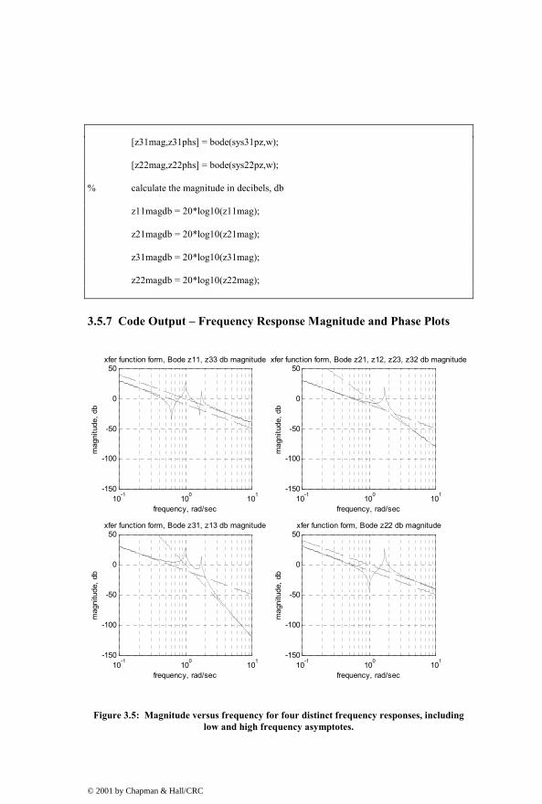
[z31mag,z31phs] = bode(sys31pz,w); [z22mag,z22phs] = bode(sys22pz,w); % calculate the magnitude in decibels, db z11magdb = 20*log10(z11mag); z21magdb = 20*log10(z21mag); z31magdb = 20*log10(z31mag); z22magdb = 20*log10(z22mag);
3.5.7 Code Output – Frequency Response Magnitude and Phase Plots
10-1 100 101-150
-100
-50
0
50xfer function form, Bode z11, z33 db magnitude
frequency, rad/sec
mag
nitu
de, d
b
10-1 100 101-150
-100
-50
0
50xfer function form, Bode z21, z12, z23, z32 db magnitude
frequency, rad/sec
mag
nitu
de, d
b
10-1 100 101-150
-100
-50
0
50xfer function form, Bode z31, z13 db magnitude
frequency, rad/sec
mag
nitu
de, d
b
10-1 100 101-150
-100
-50
0
50xfer function form, Bode z22 db magnitude
frequency, rad/sec
mag
nitu
de, d
b
Figure 3.5: Magnitude versus frequency for four distinct frequency responses, including low and high frequency asymptotes.
© 2001 by Chapman & Hall/CRC
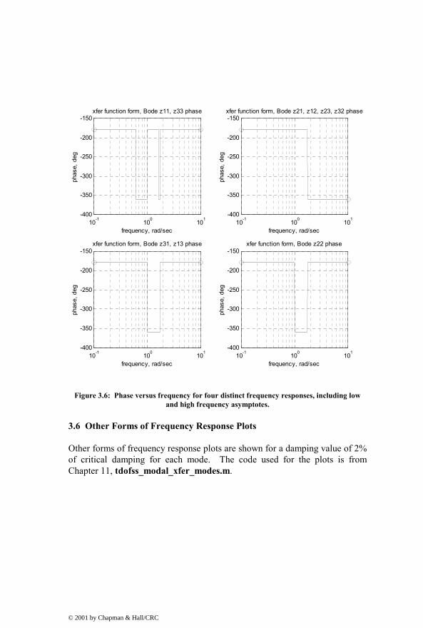
10-1 100 101-400
-350
-300
-250
-200
-150xfer function form, Bode z11, z33 phase
frequency, rad/sec
phas
e, d
eg
10-1 100 101-400
-350
-300
-250
-200
-150xfer function form, Bode z21, z12, z23, z32 phase
frequency, rad/secph
ase,
deg
10-1 100 101-400
-350
-300
-250
-200
-150xfer function form, Bode z31, z13 phase
frequency, rad/sec
phas
e, d
eg
10-1 100 101-400
-350
-300
-250
-200
-150xfer function form, Bode z22 phase
frequency, rad/sec
phas
e, d
eg
Figure 3.6: Phase versus frequency for four distinct frequency responses, including low and high frequency asymptotes.
3.6 Other Forms of Frequency Response Plots
Other forms of frequency response plots are shown for a damping value of 2% of critical damping for each mode. The code used for the plots is from Chapter 11, tdofss_modal_xfer_modes.m.
© 2001 by Chapman & Hall/CRC

3.6.1 Log Magnitude versus Log Frequency
10-1 100 10110-2
100
102z11, z33 log mag versus log freq
mag
nitu
de
10-1 100 101-200
-150
-100
-50
0z11, z33 phase versus log freq
frequency, rad/sec
phas
e, d
eg
Figure 3.7: Log magnitude versus log frequency.
Comments on the log-log plot:
1) The asymptotic behavior at the low and high frequency ends are clear by checking the slopes.
2) The log frequency scale spreads out the resonances, which otherwise would tend to clump at the lower end of the scale.
3) The log amplitude scale allows reading the gain directly without converting from db.
4) Adding the gain from the mechanics to the gain of the frequency response of the control system allows for definition of the overall series (multiplicative) frequency response.
© 2001 by Chapman & Hall/CRC

3.6.2 db Magnitude versus Log Frequency
10-1 100 101-40
-20
0
20
40z11, z33 db mag versus log freq
mag
nitu
de, d
b
10-1 100 101-200
-150
-100
-50
0z11, z33 phase versus log freq
frequency, rad/sec
phas
e, d
eg
Figure 3.8: db magnitude versus log frequency.
Comments on the db-log plot:
1) The asymptotic behaviors at the low and high frequency ends are clear by checking the slopes, i.e.
(1/ω) = 20− db/decade, (1/ 2ω ) = 40− db/decade.
2) The log frequency scale spreads out the resonances, which otherwise would tend to clump at the lower end of the scale.
3) The db amplitude scale makes it necessary to convert to gain if needed.
4) The product of two individual frequency response gains can be found by adding their gains directly on the log scale.
© 2001 by Chapman & Hall/CRC

3.6.3 db Magnitude versus Linear Frequency
0 1 2 3 4 5 6 7 8 9 10-40
-20
0
20
40z11, z33 db mag versus linear freq
mag
nitu
de, d
b
0 1 2 3 4 5 6 7 8 9 10-200
-150
-100
-50
0z11, z33 phase versus linear freq
frequency, rad/sec
phas
e, d
eg
Figure 3.9: db magnitude versus linear frequency.
Comments on the db-linear plot:
1) The asymptotic behaviors at the low and high frequency ends are not clear.
2) The linear frequency scale tends to clump the resonances at the lower end of the scale, although the scale could be shortened since nothing significant is happening at the high end.
3) The db amplitude scale makes it necessary to convert to linear gain if specific gain values are needed.
© 2001 by Chapman & Hall/CRC

3.6.4 Linear Magnitude versus Linear Frequency
0 1 2 3 4 5 6 7 8 9 100
10
20
30
40z11, z33 linear mag versus linear freq
mag
nitu
de
0 1 2 3 4 5 6 7 8 9 10-200
-150
-100
-50
0z11, z33 phase versus linear freq
frequency, rad/sec
phas
e, d
eg
Figure 3.10: Linear magnitude versus linear frequency.
Comments on the linear-linear plot:
1) The asymptotic behaviors at the low and high frequency ends are not clear.
2) The linear frequency scale tends to clump the resonances at the lower end of the scale, although the scale could be shortened since nothing significant is happening at the high end.
3) The linear amplitude scale enables reading gain values directly, but reading values for small gain values is difficult.
4) It is useful for directly adding the individual mode contributions of a frequency response to provide the overall response, shown in Chapter 8, Sections 8.7 and 8.8.
© 2001 by Chapman & Hall/CRC

3.6.5 Real and Imaginary Magnitudes versus Log and Linear Frequency
10-1 100 101-40
-20
0
20z11, z33 linear real mag versus log freq
real
mag
nitu
de
10-1 100 101-10
-5
0z11, z33 linear imaginary versus log freq
frequency, rad/sec
imag
inar
y m
agni
tude
Figure 3.11: Real and imaginary magnitudes versus log frequency.
0 1 2 3 4 5 6 7 8 9 10-40
-20
0
20z11, z33 linear real mag versus linear freq
real
mag
nitu
de
0 1 2 3 4 5 6 7 8 9 10-10
-5
0z11, z33 linear imaginary versus linear freq
frequency, rad/sec
imag
inar
y m
agni
tude
Figure 3.12: Real and imaginary magnitude versus linear frequency.
Comments on real versus linear frequency, imaginary versus linear frequency:
1) These plots are useful in understanding the amplitudes of transfer functions at resonance, as the peaks of the imaginary curve represent the amplitude at resonance.
© 2001 by Chapman & Hall/CRC

2) While the imaginary plot peaks at each resonance, the real plot goes through zero at each resonance.
3.6.6 Real versus Imaginary (Nyquist)
-15 -10 -5 0 5 10 15-15
-10
-5
0
5
10
15z11, z33 real versus imaginary, "Nyquist"
imag
Figure 3.13: Real versus imaginary (Nyquist).
Comments on real versus imaginary:
1) Frequency is not plotted directly on the real/imaginary plot; each point on the plot represents a different frequency.
2) Plotting real versus imaginary is a very useful technique when identifying resonant characteristics. The two resonances can be readily seen, helping in identifying closely spaced resonances.
3) One method of identifying damping in a mode is to use the rate of change of amplitude versus frequency (Maia 1997).
© 2001 by Chapman & Hall/CRC

3.7 Solving for Eigenvectors (Mode Shapes) Using the Transfer Function Matrix
We have reviewed transfer functions, poles, zeros and frequency responses. The next area we will cover in order to completely define the system is eigenvectors, or mode shapes. At each natural frequency, the eigenvector defines the relative motion between degrees of freedom. Understanding the distribution of motion in each mode of vibration is essential in order to intelligently modify the system’s resonant characteristic to solve resonance problems.
Since eigenvectors define the relative motion between degrees of freedom, we need to choose a degree of freedom against which to measure the other motions. We can find the relative motion using any column of the transfer function matrix. Choosing 1z as the reference and solving for 2 1z / z and
3 1z / z using the first column of the transfer function matrix (we will compare results using the second column later to show that they give the same results):
22 2
1 212 4 2 2
1 11
1
zF z mks kz z m s 3mks kF
+= =+ +
(3.29)
32
3112 4 2 2
1 11
1
zzF k
z z m s 3mks kF
= =+ +
(3.30)
Now that the ratios are known, we substitute the resonant frequencies (pole values) one at a time to define the mode shape at that frequency, dropping the second index, 21 2z z→ .
For mode 1: evaluated at 1s j 0= ω =
2 2 22
2 4 2 2 21
z mks k k 1z m s 3mks k k
+= = = =+ +
(3.31)
2 1z z= (3.32)
© 2001 by Chapman & Hall/CRC

2 23
2 4 2 2 21
z k k 1z m s 3mks k k
= = =+ +
(3.33)
3 1z z= (3.34)
The interpretation of this mode shape is that at 1ω the ratios of motion of mass 2 and mass 3 to mass 1 are equal and are equal to 1. This is the rigid body mode at 0 hz.
For mode 2: evaluated at 2ks j jm
= ω =
22 2
22 4 2 2 22
1 2 22
kmk kz mks k 0mz m s 3mks k kk km 3mk k
mm
− + + = = =+ + − + +
(3.35)
2z 0= (3.36)
2 23
2 4 2 2 21 2 2
2
z k k 1z m s 3mks k k km 3mk k
mm
= = = −+ + − + +
(3.37)
3 1z z= − (3.38)
The interpretation of this mode shape is that at 2ω mass 2 has zero motion relative to mass 1 (it is stationary). Mass 3 is moving out of phase with mass 1 with equal amplitude.
For mode 3: evaluated at 33ks j jm
= ω =
22 2
22 4 2 2 2
1 2 22
2 2 2
2 2 2 2
3kmk kz mks k mz m s 3mks k 9k 3km 3mk k
mm
3k k 2k 29k 9k k k
− + + = =+ + − + +
− + −= = = −
− +
(3.39)
© 2001 by Chapman & Hall/CRC

2 1z 2z= − (3.40)
2 23
2 4 2 2 21 2 2
2
2
2
z k kz m s 3mks k 9k 3km 3mk k
mm
k 1k
= =+ + − + +
= =
(3.41)
3 1z z= (3.42)
The interpretation of this mode shape is that at 3ω mass 2 is moving with twice the motion of mass 1 and out of phase with it and mass 3 is moving in phase with mass 1 and with the same amplitude.
Showing that the second column of the transfer function matrix could have been used and would have given the same eigenvectors:
22 4 2 2
2 22 2
1 1
2
zF z m s 2mks kz z mks kF
+ += =+
(3.43)
32 2
322 2
1 1
2
zzF mks k 1
z z mks kF
+= = =+
(3.44)
For mode 1, 1 0ω =
22
21
3
1
z k 1z kz
1z
= =
= (3.45a,b)
For mode 2, evaluated at 2ks j jm
= ω =
© 2001 by Chapman & Hall/CRC

22 2
22 4 2 22
2 221
2 2 2
2 2
k km 2mk kmmz m s 2mks k
kz mks k mk km
k 2k k 00k k
− + + + + = =−+ +
− += =
− +
(3.46)
3
1
z1
z= (3.47)
For mode 3, 33ks j jm
= ω =
22 2
22 4 2 22
2 21 2
2 2 2 2
2 2 2
9k 3km 2mk kmmz m s 2mks k
z mks k 3kmk km
9k 6k k 4k 23k k 2k
− + + + + = =+ − +
− += = = −
− + −
(3.48)
3
1
z1
z= (3.49)
Summarizing the mode shapes in the modal matrix, mz , where the first through third columns represent mode shapes for the first three modes, respectively, and the first through third rows show the relative motion for the first through third dof’s, respectively:
m
1 1 11 0 21 1 1
= − −
z (3.50)
Figure 3.14 shows the mode shapes pictorially. There are many different eigenvector scaling, or normalizing techniques, to be discussed later. It is not important which normalization technique is used in visualizing mode shapes. However, in using the modal matrix to calculate responses, the normalization technique used is critical, as we will see in future chapters.
© 2001 by Chapman & Hall/CRC

Because there is no damping, these modes are known as “normal” (as opposed to “complex”) modes. With a normal mode, if the masses are started with some multiple of the displacements of one of the modes, the system will respond at only that frequency. During that motion, the masses will all reach their maximum and minimum points at the same time. Mode shapes are plotted in Figure 3.14, assuming an arbitrary value of 1 for 1z :
1 1 1
1 -1
1 1-2
Rigid-Body Mode, 0 rad/sec
Second Mode, Middle Mass Stationary, 1 rad/sec
Third Mode, 1.732 rad/sec
m1 m2 m3
m3m2m1
m1 m2 m3
Figure 3.14: Mode shape plots.
© 2001 by Chapman & Hall/CRC

Problems
Note: All the problems refer to the two dof system shown in Figure P2.2.
P3.1 Set 1 2m m m 1= = = , 1 2k k k 1= = = and hand sketch the frequency responses for the undamped system.
P3.2 (MATLAB) Set 1 2m m m 1= = = , 1 2k k k 1= = = , modify the tdofxfer.m code and plot the frequency responses of the two dof undamped system using the transfer function and zero/pole/gain forms of Sections 3.5.5 and 3.5.6.
P3.3 (MATLAB) Set 1 2m m m 1= = = , 1 2k k k 1= = = , add damping to the model from P3.2 and plot the transfer functions in Nyquist form, being careful to use small enough frequency spacing to identify the resonances as shown in Figure 3.13.
P3.4 (MATLAB) Set 1 2m m m 1= = = , 1 2k k k 1= = = , choose one of the transfer functions for the undamped system and plot the poles and zeros in the s-plane. Choose a frequency on the positive imaginary axis and hand calculate the gain at that frequency. Correlate with the MATLAB calculated gain.
P3.5 Solve for the two eigenvectors for the system in P3.3 using the transfer function matrix. Hand plot the mode shapes as in Figure 3.14.
© 2001 by Chapman & Hall/CRC

CHAPTER 4
ZEROS IN SISO MECHANICAL SYSTEMS
4.1 Introduction
Chapters 2 and 3 discussed poles and zeros of SISO systems and their relationship to transfer functions. The origin and influence of poles are clear. They represent the resonant frequencies of the system, and for each resonant frequency a mode shape can be defined to describe the motion at that frequency. We have seen from our frequency response analyses in Chapter 3 that at the frequencies of the zeros, motions approach or go to zero, depending on the amount of damping present. In Chapters 8 and 11 we will illustrate how all the individual modes of vibration can combine at specific frequencies to create zeros of the overall transfer function.
This chapter will expand on analyses shown in Miu [1993] to develop an intuitive understanding for when to expect zeros in Single Input Single Output (SISO) simple mechanical systems and how to predict the frequencies at which they will occur. We will not cover the theory, but will state the conclusions from Miu and show how the conclusions relate to two example systems.
We will start by defining a series arrangement lumped spring/mass system. We will develop guidelines for defining the number of zeros that should be seen and show how to predict their frequencies. A MATLAB model is used to illustrate the guidelines for various combinations of input and output degrees of freedom. Only the MATLAB code results are discussed; the code itself is not listed or discussed as it uses techniques found later in the book. However, the reader is encouraged to run the code and experiment with various values of the input and number of masses in the model to become familiar with the concept.
Next, an ANSYS finite element model of a tip-excited cantilever is analyzed. The resulting transfer function magnitude is plotted using MATLAB to show an overlay of the poles of the “constrained” system and their relationship with the zeros of the original model.
© 2001 by Chapman & Hall/CRC

4.2 “n” dof Example
Figure 4.1 shows a series arrangement of masses and springs, with a total of “n” masses and “n+1” springs. The degrees of freedom are numbered from left to right, 1 nz through z .
Two Degrees of Freedom toRight of Constrained DOF:
Two Zeros
m1 m2 m3 m4 m5 m(n-4)
m(n-3)
m(n-2)
m(n-1) m(n)
z1 z2 z3 z(n)z(n-1)z(n-2)
m1 m2 m3 m4 m5 m(n-4)
m(n-3)
m(n-2)
m(n-1) m(n)
F1 z(n)
m1 m2 m3 m4 m5 m(n-4)
m(n-3)
m(n-2)
m(n-1) m(n)
F5 z(n-2)
m1 m2 m3 m4 m5 m(n-4)
m(n-3)
m(n-2)
m(n-1) m(n)
z3, F3
Four Degrees of Freedom toLeft of Constrained DOF:
Four Zeros
No Degrees of Freedom toLeft of Constrained DOF:
No Zeros
No Degrees of Freedom toRight of Constrained DOF:
No Zeros
Two Degrees of Freedom toLeft of Constrained DOF:
Two Zeros
(n-3) Degrees of Freedomto Right of Constrained
DOF:(n-3) Zeros Number of Zeros for Driving
Point Transfer Function(n-1)
Figure 4.1a,b,c,d: “n” dof system showing various SISO input/output configurations.
Miu [1993] shows that the zeros of any particular transfer function are the poles of the constrained system(s) to the left and/or right of the system defined by constraining the one or two dof’s defining the transfer function. The resonances of the “overhanging appendages” of the constrained system create the zeros.
Two limiting cases are immediately available in (1) and (3) below:
1) For the transfer function from one end of the structure to the other, Figure 4.1b, there are no overhanging appendage
© 2001 by Chapman & Hall/CRC

structures to the left or right of the constrained structure, so there are no zeros.
2) For an arbitrary transfer function, Figure 4.1c, there will be a structure to the left and/or to the right of the constrained dof’s. The total degrees of freedom of the overhanging appendage(s) will give the total number of zeros in the transfer function.
3) For the driving point transfer function, Figure 4.1d, the force and displacement are measured at the same dof, so there are a total of (n 1)− degrees of freedom left, hence (n 1)− zeros of the transfer function. All but one of the masses are overhanging appendages.
In the analysis that follows, we will calculate frequency responses and pole/zero plots for various transfer functions using the MATLAB code ndof_numzeros.m.
4.2.1 MATLAB Code ndof_numzeros.m, Usage Instructions
The MATLAB code is based on the ndof series system in Figure 4.1. The code allows one to choose the total number of masses in the problem and sets the values of the masses and stiffnesses randomly between the values of 1 and 2. The program then allows one to choose which transfer function to calculate, and shows the pole/zero plots for the original system as well as the poles for the two structures to the left and/or right. For now, the reader should not worry about the details of the code, which will be covered in later chapters, but should use the code to study the pole/zero patterns in systems with different numbers of degrees of freedom and for different input/output dof’s. Sometimes the random values chosen for stiffnesses and damping will cause the poles and zeros to be so close together that they will cancel each other. If this is the case and the number of poles and zeros do not match the expected number, rerun the code until more widely spaced poles/zeros are randomly chosen and the required poles and zeros are apparent.
4.2.2 Seven dof Model – z7/F1 Frequency Response
Taking a seven-mass model as an example, the resulting frequency responses and pole-zero plots are displayed on the following pages. In all cases, the random distribution of masses and spring stiffnesses is used, resulting in a different set of variables for each run.
Figure 4.2 shows the frequency response for applying a force at the first mass and looking at the output at the last (seventh) mass. Note that in accordance
© 2001 by Chapman & Hall/CRC

with the prior analysis, there should be no zeros as there are no “overhanging” appendages. Since there are seven masses, there should be seven poles. Since each mass provides an attenuation of –40db/decade, after the last of seven poles the slope of the curve is 7*( 40− db/decade) = 280− db/decade.
10-1 100 101
-300
-250
-200
-150
-100
-50
0
50transfer function, 7 dof, input at 1, output at 7
frequency, rad/sec
mag
nitu
de, d
b
Figure 4.2: z17 transfer function frequency response, seven poles, no zeros.
-2 -1 0 1 2
-2
-1.5
-1
-0.5
0
0.5
1
1.5
2poles/zeros of system
Figure 4.3: z17 pole/zero plot showing only seven poles.
© 2001 by Chapman & Hall/CRC

4.2.3 Seven dof Model – z3/F4 Frequency Response
The same seven dof system provides the following frequency response when the force is applied at mass 3 and the output is taken at mass 4. There are two “overhanging” appendages to the left of mass 3, masses 1 and 2, and there are three “overhanging” appendages to the right of mass 4, masses 5, 6 and 7. These masses should combine to give a total of five zeros and once again, seven poles as shown below.
10-1 100 101
-100
-80
-60
-40
-20
0
20
40
60
80transfer function, 7 dof, input at 3, output at 4
frequency, rad/sec
mag
nitu
de, d
b
Figure 4.4: z34 transfer function frequency response, seven poles and five zeros.
-2 -1 0 1 2
-2
-1.5
-1
-0.5
0
0.5
1
1.5
2
poles/zeros of system
Figure 4.5: z34 pole/zero plot showing seven poles and five zeros.
© 2001 by Chapman & Hall/CRC

-2 0 2-2
-1
0
1
2poles/zeros of system
-2 0 2-2
-1
0
1
2poles of lhs
-2 0 2-2
-1
0
1
2poles of rhs
Figure 4.6: z34 poles and zeros; poles of left-hand and right-hand constrained systems are the same as the zeros of the unconstrained system.
The left-hand plot in Figure 4.6 displays the z34 poles and zeros. The middle plot shows the poles of the system to the left of mass 3. The right plot shows the poles of the system to the right of mass 4. It is clear that the poles of the two right plots are the zeros of the z34 system.
4.2.4 Seven dof Model – z3/F3, Driving Point Frequency Response
For the same seven dof system with force and output taken at the same node (driving point transfer function), there should be six “overhanging” masses providing zeros. Therefore the frequency response plot in Figure 4.7 shows six zeros, with alternating pole/zero pairs.
© 2001 by Chapman & Hall/CRC

10-1 100 101
-50
-40
-30
-20
-10
0
10
20
30
40
50transfer function, 7 dof, input at 3, output at 3
frequency, rad/sec
mag
nitu
de, d
b
Figure 4.7: z33 transfer function frequency response, seven poles and the expected six zeros.
-2 -1 0 1 2
-2
-1.5
-1
-0.5
0
0.5
1
1.5
2
poles/zeros of system
Figure 4.8: z33 pole/zero plot showing seven poles and six zeros.
© 2001 by Chapman & Hall/CRC
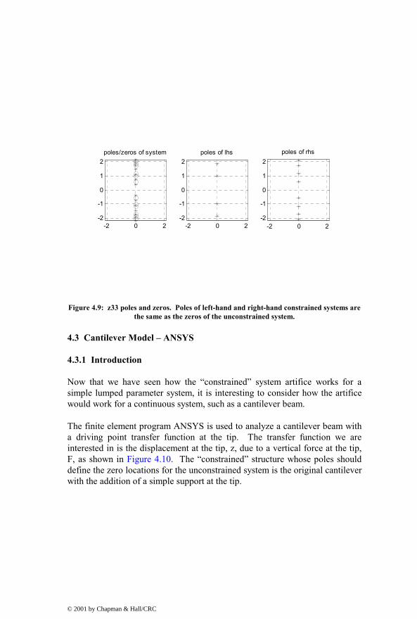
-2 0 2-2
-1
0
1
2poles/zeros of system
-2 0 2-2
-1
0
1
2poles of lhs
-2 0 2-2
-1
0
1
2poles of rhs
Figure 4.9: z33 poles and zeros. Poles of left-hand and right-hand constrained systems are the same as the zeros of the unconstrained system.
4.3 Cantilever Model – ANSYS
4.3.1 Introduction
Now that we have seen how the “constrained” system artifice works for a simple lumped parameter system, it is interesting to consider how the artifice would work for a continuous system, such as a cantilever beam.
The finite element program ANSYS is used to analyze a cantilever beam with a driving point transfer function at the tip. The transfer function we are interested in is the displacement at the tip, z, due to a vertical force at the tip, F, as shown in Figure 4.10. The “constrained” structure whose poles should define the zero locations for the unconstrained system is the original cantilever with the addition of a simple support at the tip.
© 2001 by Chapman & Hall/CRC

z, F
Original Cantilever,Driving Point
Transfer Function
"Constrained"System, with
DOF's of transferfunction
constrained
Figure 4.10: Unconstrained and constrained cantilevers used for driving point transfer function example.
4.3.2 ANSYS Code cantfem.inp Description and Listing
The input listings for the ANSYS models of the cantilever and simply supported tip cantilever are below. The cantilever input program is cantfem.inp and the supported tip input program is cantzero.inp. Both programs can be run if one has access to ANSYS by typing “/input,cantfem,inp” or “/input,cantzero,inp” at the ANSYS program command prompt. The programs will run with no further input and will output graphs of the mode shapes and frequency response. Both programs build the model, and calculate and output the eigenvalues (natural frequencies) and eigenvectors (mode shapes). Cantfem.inp then calculates and outputs the frequency response. The mode shapes are shown in cantfem.grp and cantzero.grp and the frequency response is shown in cantfem.grp2. They can all be viewed by using the ANSYS Display program and loading the appropriate file.
/title, cantfem.inp, 0.05 x 1 x 20mm aluminum cantilever beam, 20 elements /prep7 et,1,4 ! element type for beam ! aluminum ex,1,71e6 ! mN/mm^2 dens,1,2.77e-6 ! kg/mm^3
© 2001 by Chapman & Hall/CRC

nuxy,1,.345 ! real value to define beam characteristics r,1,1,.00001041,.004166,.05,1 ! area, moments of inertia, thickness ! define plotting characteristics /view,1,1,-1,1 ! iso view /angle,1,-60 ! iso view /pnum,mat,1 ! color by material /num,1 ! numbers off /type,1,0 ! hidden plot /pbc,all,1 ! show all boundary conditions csys,0 ! define global coordinate system ! nodes n,1,0,0,0 ! left-hand node n,21,20,0,0 ! right-hand node fill,1,21 ! interior nodes nall nplo ! elements type,1 mat,1 real,1 e,1,2 egen,20,1,-1 ! constrain left-hand end nall d,1,all,0 ! constrain node 1, all dof's ! constrain all but uz and roty for all other nodes to allow only those dof's ! this will give 20 nodes, node 2 through node 21, each with 2 dof, giving a total of 40 dof ! can calculate a maximum of 40 eigenvalues if don't use Guyan reduction to reduce size of ! eigenvalue problem nall nsel,s,node,,2,21 d,all,ux d,all,uy d,all,rotx d,all,rotz nall eall nplo
© 2001 by Chapman & Hall/CRC

eplo ! ******************* eigenvalue run ******************** fini ! fini just in case not in begin /solu ! enters the solution processor, needs to be here to do editing below allsel ! default selects all items of specified entity type, typically nodes, elements antype,modal,new modopt,reduc,20 ! method - reduced Householder, number of modes to extract expass,off ! key = off, no expansion pass, key = on, do expansion mxpand,20,,,no ! nummodes to expand total,20,0 ! total masters, 20 to be used, 1 to exclude rotational dofs allsel solve ! starts the solution of one load step of a solution sequence, modal here fini ! plot first mode /post1 set,1,1 pldi,1 ! ***************** output frequencies ******************** /output,cantfem,frq ! write out frequency list to ascii file .frq set,list /output,term ! returns output to terminal ! ******************* output eigenvectors ********************* ! define nodes for output: forces applied or output displacements nsel,s,node,,21 ! cantilever tip /output,cantfem,eig ! write out eigenvectors to ascii file .eig *do,i,1,20 set,,i prdisp *enddo /output,term ! ******************* plot modes *********************
© 2001 by Chapman & Hall/CRC

! pldi plots /show,cantfem,grp,0 allsel /view,1,,-1,, ! side view for plotting /angle,1,0 /auto *do,i,1,20 set,1,i pldi *enddo /show,term ! *************** calculate and plot transfer functions **************** fini /assign,rst,junk,rst ! reassigns a file name to an ANSYS identifier /solu dmprat,0.01 ! sets a constant damping ratio for all modes, zeta = 0.01 allsel eplo ! show forces applied f,21,fz,1 ! 1 mn force applied to node 21, tip node /title, cantilever with tip load antype,harmic ! harmonic (frequency response) analysis hropt,msup,20 ! mode superposition method, nummodes modes used harfrq,100,1000000 ! frequency range, hz, for solution, -1 to 10 rad/sec hrout,off,off ! amplitude/phase, cluster off kbc,1 nsubst,10000 ! 10000 frequency points for very fine resolution outres,nsol,all, ! controls solution set written to database, nodal dof solution, all ! frequencies, component name for selected set of nodes solve fini /post26 file,,rfrq ! frequency response results
© 2001 by Chapman & Hall/CRC

xvar,0 ! display versus frequency lines,10000 ! specifies the length of a printed page for frequency response listing nsol,2,21,u,z ! specifies nodal data to be stored in results file ! u - displacement, z direction ! note that nsol,1 is frequency vector ! plot magnitude plcplx,0 /grid,1 /axlab,x,frequency, hz /axlab,y,amplitude, mm /gropt,logx,1 ! log plot for frequency /gropt,logy,1 ! log plot for amplitude /show,cantfem,grp1 ! file name for storing plvar,2 /show,term ! plot phase plcplx,1 /grid,1 /axlab,x,freq /axlab,y,phase, deg ! label for y axis /gropt,logx,1 ! log plot for frequency /gropt,logy,0 ! linear plot for phase /show,cantfem,grp1 plvar,2 /show,term ! save ascii data to file prcplx,1 ! stores phase angle in asci file .dat /output,cantfem,dat prvar,2 /output,term fini
4.3.3 ANSYS Code cantzero.inp Description and Listing
/title, cantzero.inp, 0.05 x 1 x 20mm aluminum tip constrained cantilever beam, 20 elements /prep7 et,1,4 ! element type for beam ! aluminum
© 2001 by Chapman & Hall/CRC

ex,1,71e6 ! mN/mm^2 dens,1,2.77e-6 ! kg/mm^3 nuxy,1,.345 ! real value to define beam characteristics r,1,1,.00001041,.004166,.05,1 ! area, moments of inertia, thickness ! define plotting characteristics /view,1,1,-1,1 ! iso view /angle,1,-60 ! iso view /pnum,mat,1 ! color by material /num,1 ! numbers off /type,1,0 ! hidden plot /pbc,all,1 ! show all boundary conditions csys,0 ! define global coordinate system ! nodes n,1,0,0,0 ! left-hand node n,21,20,0,0 ! right-hand node fill,1,21 ! interior nodes nall nplo ! elements type,1 mat,1 real,1 e,1,2 egen,20,1,-1 ! constrain left-hand end nall d,1,all,0 ! constrain node 1, all dof's d,21,uz,0 ! constrain tip ! constrain all but uz and roty for all other nodes to allow only those dof's ! this will give 20 nodes, node 2 through node 21, each with 2 dof, giving a total of 40 dof ! can calculate a maximum of 40 eigenvalues if don't use Guyan reduction to reduce size of ! eigenvalue problem nall nsel,s,node,,2,21 d,all,ux d,all,uy d,all,rotx d,all,rotz
© 2001 by Chapman & Hall/CRC

nall eall nplo eplo ! ****************** eigenvalue run ******************** fini ! fini just in case not in begin /solu ! enters the solution processor, needs to be here to do editing below allsel ! default selects all items of specified entity type, typically nodes, elements antype,modal,new modopt,reduc,20 ! method - reduced Householder, number of modes to extract expass,off ! key = off, no expansion pass, key = on, do expansion mxpand,20,,,no ! nummodes to expand total,20 ! total masters, 20 to be used, exclude rotational dofs allsel solve ! starts the solution of one load step of a solution sequence, modal here fini ! plot first mode /post1 set,1,1 pldi,1 ! ******************** output frequencies *********************** /output,cantzero,frq ! write out frequency list to ascii file .frq set,list /output,term ! returns output to terminal ! ****************** output eigenvectors ********************* ! define nodes for output: forces applied or output displacements nsel,s,node,,10 ! cantilever midpoint /output,cantzero,eig ! write out eigenvectors to ascii file .eig *do,i,1,20 set,,i prdisp *enddo
© 2001 by Chapman & Hall/CRC

/output,term ! ******************* plot modes ********************* ! pldi plots /show,cantzero,grp,0 allsel /view,1,,-1,, ! side view for plotting /angle,1,0 /auto *do,i,1,20 set,1,i pldi *enddo /show,term
4.3.4 ANSYS Results, cantzero.m
The driving point frequency response for cantfem.inp is shown in Figure 4.11. The ANSYS frequency and magnitude output results are read into MATLAB and plotted in order to be able to overlay the resonances from the cantzero.inp ANSYS run. The MATLAB code to plot the overlay is cantzero.m, which reads in two input programs, cantfem_magphs.m and cantzero_freq.m.
The resonant frequencies (poles) of the cantilever and constrained tip cantilever models are listed in Table 4.1.
According to the guidelines for zeros discussed earlier in the chapter, the poles of the frequency response plot should be the same frequencies as shown in the “cantfem freq” column above. The zeros of the frequency response should be the same frequencies as shown in the “cantzero freq” column above.
© 2001 by Chapman & Hall/CRC

mode cantfem freq, hz cantzero freq, hz 1 457.14 2004.6 2 2864.4 6495.0 3 8018.8 13548. 4 15709. 23162. 5 25961. 35336. 6 38771. 50071. 7 54147. 67380. 8 72102. 87291. 9 92672. 0.10985E+06 10 0.11592E+06 0.13520E+06 11 0.14196E+06 0.16337E+06 12 0.17098E+06 0.19495E+06 13 0.20323E+06 0.22951E+06 14 0.23907E+06 0.26909E+06 15 0.27885E+06 0.31129E+06 16 0.32274E+06 0.35968E+06 17 0.37012E+06 0.40928E+06 18 0.41860E+06 0.45602E+06 19 0.46289E+06 0.49344E+06 20 0.49490E+06 0.89212E+06
Table 4.1: Unconstrained (cantfem) and constrained tip (cantzero) cantilever resonances.
The constrained system poles in Figure 4.11 are shown below the curve with “o” symbols. Note that the “o’s” align with the zeros of the unconstrained system.
102 103 104 105 106
-140
-120
-100
-80
-60
-40
-20
0Cantilever Driving Point Transfer Function and Constrained Pole Frequencies
frequency, hz
mag
nitu
de, d
b
unconstrained system constrained system poles match unconstrained systemzeros
Figure 4.11: Cantilever driving point transfer function frequency response plot with overlaid frequencies of contrained-tip cantilever poles – which should match the
unconstrained system zeros.
© 2001 by Chapman & Hall/CRC

Problem
Note: The problem refers to the two dof system shown in Figure P2.2.
P4.1 Use the MATLAB code ndof_numzeros.m to identify the number of poles and zeros for a five dof system for the following: z11, z23, z33. Correlate the poles of the constrained system with the zeros of the original system.
© 2001 by Chapman & Hall/CRC

CHAPTER 5
STATE SPACE ANALYSIS
5.1 Introduction
In Chapter 2 we derived the equations of motion for the tdof system shown in Figure 5.1, and showed how to solve the coupled differential equations for various transfer functions. In order to solve time domain problems using a computer, it is desirable to change the form of the equations for an n dof system with n second order differential equations to 2n first order differential equations. The first order form of equations of motion is known as state space form.
This chapter will develop the state space formulation for the tdof example. Once the state space formulation is completed, the subject of complex eigenvalues and eigenvectors, resulting in complex modes of vibration, will be covered in some detail. Once complex modes are understood, comprehending real modes which arise from the undamped case in the modal analysis section (Chapter 7) is simple.
Having an understanding of complex modes is especially helpful in working with experimental modal analysis. There are some very powerful experimental techniques available for testing and then visualizing the modes of vibration of structures. Frequency response data is taken at a number of selected positions on the structure and software is available to fit the data and define modes of vibration. The software identifies the resonant frequencies of the system and defines a damping value for each mode. It is then possible to create a model of the geometry of the test point locations and build a virtual model which can be animated to display the shape of motion of each mode.
The software has options which allow one to view the mode as either “real” or “complex.” When the mode is viewed as “real,” all the points on the structure move such that they all reach their maximum or minimum positions at the same point in time, which is consistent with our definition of “principal” or “real” modes defined in Chapter 7.
When the mode is viewed as “complex,” the structure does not move such that all points reach either their minimum or maximum positions at the same point in time. Instead there appears to be a wave that moves along the structure as the different points reach their minimum or maximum positions at different times. For lightly damped mechanical structures, the assumption is often made that the modes are “real,” allowing use of modal analysis methods and efficient finite element models. For structures that are not “lightly damped,”
© 2001 by Chapman & Hall/CRC

the modal analysis method cannot be used and the state space formulation is the only practical method of solving the problem.
It is difficult to visualize complex modes without an animated structure model, but we will use a graphical method called an Argand diagram to explain how modes described by complex eigenvectors and complex eigenvalues combine to create physical motion of the system. We will find that if the unforced system is started from a set of initial conditions that match the complex eigenvector then only a single mode is excited. We will show how to calculate the transient response of the system for that specific initial condition case and illustrate how only a single mode is excited.
Chapter 6 will cover how to use the state space formulation to obtain both frequency and time domain results with MATLAB.
5.2 State Space Formulation
Figure 5.1: Original damped tdof system model.
Repeating the matrix equations of motion from (2.25):
1 1 1 1 1
2 2 1 1 2 2 2
3 3 2 2 3
1 1 1 1
1 1 2 2 2 2
2 2 3 3
m 0 0 z c c 0 z0 m 0 z c (c c ) c z0 0 m z 0 c c z
k k 0 z Fk (k k ) k z F0 k k z F
− + − + − −
− + − + − = −
&& &
&& &
&& & (5.1)
Expanding the equations:
1 1 1 1 1 2 1 1 1 2 1
2 2 1 1 1 2 2 2 3 1 1 1 2 2 2 3 2
3 3 2 2 2 3 2 2 2 3 3
m z c z c z k z k z Fm z c z (c c )z c z k z (k k )z k z Fm z c z c z k z k z F
+ − + − =− + + − − + + − =− + − + =
&& & &
&& & & &
&& & &
(5.2a,b,c)
c1
m1 m2 m3
k1 k2
c2
z1 z2 z3F1 F2 F3
© 2001 by Chapman & Hall/CRC

The three equations above are second order differential equations which require knowledge of the initial states of position and velocity for all three degrees of freedom in order to solve for the transient response.
In the state space formulation, the three second order differential equations are converted to six first order differential equations. Following typical state space notation, we will refer to the states as “x” and the output as “y.”
Start by solving (5.2) for the three equations for the highest derivatives, in this case the three second derivatives, 1 2 3z , z , z&& && && :
1 1 1 1 1 2 1 1 1 2 1
2 2 1 1 1 2 2 2 3 1 1 1 2 2 3 2
3 3 2 2 2 3 2 2 2 3 3
z (F c z c z k z k z ) / mz (F c z (c c )z c z k z (k k )z k z ) / m
z (F c z c z k z k z ) / m
= − + − += + − + + + − + +
= + − + −
&& & &
&& & & &
&& & &
(5.3a,b,c)
We now change notation, using “x” to define the six states; three positions and three velocities:
1 1x z= Position of Mass 1 (5.4)
2 1x z= & Velocity of Mass 1 (5.5)
3 2x z= Position of Mass 2 (5.6)
4 2x z= & Velocity of Mass 2 (5.7)
5 3x z= Position of Mass 3 (5.8)
6 3x z= & Velocity of Mass 3 (5.9)
By using this notation, we observe the relationship between the state and its first derivatives:
1 2 1z x x= =& & (5.10)
2 4 3z x x= =& & (5.11)
3 6 5z x x= =& & (5.12)
Also between the first and second derivatives:
1 2z x=&& & (5.13)
2 4z x=&& & (5.14)
3 6z x=&& & (5.15)
© 2001 by Chapman & Hall/CRC

Rewriting the three equations for 1 2 3z , z , z&& && && in terms of the six states 1x through 6x and adding the three equations defining the position and velocity relationships:
1 2
2 1 1 2 1 4 1 1 1 3 1
3 4
4 2 1 2 1 2 4 2 6 1 1 1 2 3 2 5 2
5 6
6 3 2 4 2 6 2 3 2 5 3
x xx (F c x c x k x k x ) / mx xx (F c x (c c )x c x k x (k k )x k x ) / mx xx (F c x c x k x k x ) / m
== − + − +== + − + + + − + +== + − + −
&
&
&
&
&
&
(5.16a-f)
Rewriting the equations above in matrix form as:
11 1 1 11 1
1 1 1 12 2
3 31 1 1 2 1 2 2 2
4 42 2 2 2 2 2
5 5
6 62 2 2 2
3 3 3 3
00 1 0 0 0 0Fk c k c 0 0x xmm m m m
x x0 0 0 1 0 0
x xk c (k k ) (c c ) k c
x xm m m m m m
x x0 0 0 0 0 1
x xk c k c0 0m m m m
− − = +− + − + − −
&
&
&
&
&
&
1
2
2
3
3
0(1)F
m0Fm
u
= +x A x B&
(5.17a,b)
5.3 Definition of State Space Equations of Motion
Schematically, a SISO state space system is represented as shown in Figure 5.2. We will define the blocks in the following sections. The scalar input u(t) is fed into both the input matrix B and the direct transmission matrix D. The output of the input matrix is an nx1 vector, where “n” is the number of states. For a SISO system, the direct transmission matrix is a scalar, and its output is fed into a summing junction to be added to the output of the C matrix.
The output of the B matrix is added to the feedback term coming from the system matrix and is fed into an integrator block, where “I” is an nxn identify matrix. The output matrix has as many rows as outputs, a single row for a
© 2001 by Chapman & Hall/CRC

SISO system, and has as many columns as states, n. The output y(t) is the sum of the output of the C and D matrices.
A
+ +B
D
C∫ Iu(t)x(t)& x(t)
y(t)
Integrator Block
DirectTransmission
Matrix
Output MatrixInput Matrix
System Matrixscalar
vector
Input Output
Figure 5.2: State space system block diagram.
Notation for equations of motion in state space form is:
u= +x Ax B& (5.18)
where the A and B matrices are shown in (5.17a). Matrix A is known as the system matrix, matrix B is the input matrix, and scalar u is the input. The column vector x is the state of the system.
5.4 Input Matrix Forms
Because “u” is a scalar, the nature of the input matrix B changes depending on what input is used. If the system is a Single Input (SI) system with a force either at mass 1, 2 or 3, the B matrix changes as follows:
© 2001 by Chapman & Hall/CRC

1
1
1 2 32
2
3
3
00 00F 0
m 000F : , F : , F : 0F
m0 00 0 F
m0 0
= = =
B B B (5.19a,b,c)
If the same forcing function u (for example, a step function or sine function) is applied to several degrees of freedom simultaneously (for example, a force of magnitude 1F to mass 1 and a force of magnitude 3F to mass 3) the input matrix would become:
1
1
3
3
0Fm000Fm
=
B (5.20)
For a Multi Input (MI) system, where forces are applied independent of one another to the separate masses, a multiple column input matrix is appropriate. For example, for different inputs at mass 1 and mass 2, none at mass 3, the input matrix would become:
1
1
2
2
0 0F 0m 00 F
m00 00 0
=
B (5.21)
© 2001 by Chapman & Hall/CRC

5.5 Output Matrix Forms
To account for the case where the desired output is not just the states but is some linear combination of the states, an output matrix C is defined to relate the outputs to the states. Also, a matrix D , known as the direct transmission matrix, is multiplied by the input “u” to account for outputs that are related to the inputs but that bypass the states.
u= +y Cx D (5.22)
The output matrix C has as many rows as outputs required and as many columns as states. The direct transmission matrix D has the same number of columns as the input matrix B and as many rows as the output matrix C.
In our example, we are interested in all six of the states, displacements and velocities, so the matrix output equation becomes, where C is the identity matrix and D is assumed to be zero:
1 1
2 2
3 3
4 4
5 5
6 6
y x1 0 0 0 0 0 0y x0 1 0 0 0 0 0y x0 0 1 0 0 0 0
(1)y x0 0 0 1 0 0 0y x0 0 0 0 1 0 0y x0 0 0 0 0 1 0
= +
(5.23)
Expanding, the matrix equations become:
1 1 1y x ( z )= = (5.24)
2 2 1y x ( z )= = & (5.25)
3 3 2y x ( z )= = (5.26)
4 4 2y x ( z )= = & (5.27)
5 5 3y x ( z )= = (5.28)
6 6 3y x ( z )= = & (5.29)
© 2001 by Chapman & Hall/CRC

If we were only interested in the three displacements and not the three velocities, the output equation would be, assuming D is zero:
1
21
32
43
5
6
xx
y 1 0 0 0 0 0x
y 0 0 1 0 0 0 (0)(1)x
y 0 0 0 0 1 0xx
= +
(5.30)
Expanding:
1 1 1y x ( z )= = (5.31)
2 3 2y x ( z )= = (5.32)
3 5 3y x ( z )= = (5.33)
On the other hand, if the outputs are linear combinations of the states, as in a control system problem, the output equation could look like (where a, b and c are scalars), assuming D is zero:
1
21
32
43
54
6
xxy 0 0 a 0 b 0xy c 0 1 0 0 0
(0)(1)xy 1 0 0 0 0 0xy 0 0 0 1 0 0x
= +
(5.34)
Expanding:
1 3 5 2 3y ax bx ( az bz )= + = + (5.35)
2 1 3 1 2y cx x ( cz z )= + = + (5.36)
3 1 1y x ( z )= = (5.37)
4 4 2y x ( z )= = & (5.38)
© 2001 by Chapman & Hall/CRC

If a single force is applied and a single output is desired (SISO), for example, a force applied at mass 1 and the output displacement at mass 3, assuming D is zero:
[ ]
1
2
3
4
5
6
xxx
y 0 0 0 0 1 0 (0)(1)xxx
= +
(5.39)
With all the possible variations of the output equation, the state equation never changes; it is always:
u= +x Ax B& (5.40)
5.6 Complex Eigenvalues and Eigenvectors – State Space Form
The most basic analysis one can perform on a dynamic system is to solve for its eigenvalues (natural frequencies) and eigenvectors (mode shapes). In this section we will develop the most general case where there are no limitations on the presence or magnitude of the two damping terms, which could result in complex eigenvalues and eigenvectors.
Start by postulating that there is a set of initial conditions such that if the system is released with that set, the system will respond in one of its natural modes of vibration. To that end, we set the forcing function to zero and write the homogeneous state space equations of motion:
=x Ax& (5.41)
We define motion in a principal mode as:
i ti mi eλ=x x (5.42)
Where:
iλ is the ith eigenvalue, the natural frequency of the ith mode of vibration
ix is the vector of states at the thi frequency
mix is the thi eigenvector, the mode shape for the thi mode
© 2001 by Chapman & Hall/CRC

For our tdof ( 1 3z to z ), six state ( 1 6x to x ) system, for the thi eigenvalue and eigenvector, the equation would appear as:
i i
1i 1i m1i
1i 2i m2i
2i 3i m3it tmi
2i 4i m4i
3i 5i m5i
3i 6i m6i
z x xz x xz x x
e ez x xz x xz x x
λ λ
= = =
x
&
&
&
(5.43)
Differentiating the modal displacement equation above to get the modal velocity equation:
t tmi mi mi
d e edt
λ λ = = λ x x x& (5.44)
Substituting into the state equation and canceling the exponential terms leads to:
t tmi mi
mi mi
mi
e e
( ) 0
λ λ
=
λ =λ =
λ − =
x Axx Ax
x AxI A x
&
(5.45a-d)
Equation (5.45c) is the classic “eigenvalue problem.” If mix is not equal to zero in (5.45d), a solution exists only if the determinant below is zero (Strang 1998):
( ) 0λ − =I A (5.46)
Taking the system matrix A from (5.17a) and inserting in (5.45):
© 2001 by Chapman & Hall/CRC

1 1 1 1
1 1 1 1
1 1 1 2 1 2 2 2
2 2 2 2 2 2
2 2 2 2
3 3 3 3
0 1 0 0 0 0k c k c
0 0m m m m0 0 0 1 0 0
( ) k c (k k ) (c c ) k cm m m m m m0 0 0 0 0 1
k c k c0 0m m m m
− − λ − = λ − − + − +
− −
I A I
(5.47)
In Chapter 10 we will use the undamped version of (5.46) with c1 = c2 = 0 to discuss “normal” modes, where we will find that taking the determinant in closed form is practical. For the tdof damped system matrix, taking the closed form determinant is far too complicated so we will use MATLAB’s “eig” function to solve the eigenvalue problem numerically, using specific values of m, c and k. We will use the MATLAB code tdof_non_prop_damped.m as we continue our exploration of complex modes.
5.7 MATLAB Code tdof_non_prop_damped.m: Methodology, Model Setup, Eigenvalue Calculation Listing
The sequence of development of complex modes is as follows:
1) solve original damped system equation for complex eigenvalues and eigenvectors
2) normalize the eigenvector entries to unity
3) calculate magnitude and phase angle of each of the eigenvector entries
4) use the Argand diagram to visualize the motion of a complex mode
5) calculate the percentage of critical damping (damping ratio) for each mode
6) calculate the motions of the three masses for all three modes
© 2001 by Chapman & Hall/CRC

7) plot the real and imaginary displacements of each of the degrees of freedom separately
We have explored how to calculate the eigenvectors or mode shapes for an undamped problem using the transfer function matrix (Chapter 3). The modes for the undamped problem were real modes, meaning that the position elements of the eigenvectors were real, not complex, and we were able to plot diagrams showing the shape of the modes. For complex modes, it is not possible to draw a picture of the deformed mode shape because there are phase differences between the various degrees of freedom which prevent them from reaching their maximum/minimum points at the same point in time. This leads to the apparent “traveling wave” in an animated mode.
The first section of tdof_non_prop_damped.m sets up the state space equations of motion and solves the eigenvalue problem for damping values of
1 2c 0.1, c 0.2= = :
% tdof_non_prop_damped.m non-proportionally damped tdof model clf; legend off; subplot(1,1,1); clear all; % define the values of masses, springs, dampers m1 = 1; m2 = 1; m3 = 1; k1 = 1; k2 = 1; % define arbitrary damping values c1 = input('input value for c1, default 0.1, ... '); if (isempty(c1)) c1 = 0.1; else end c2 = input('input value for c1, default 0.2, ... '); if (isempty(c2)) c2 = 0.2; else end
© 2001 by Chapman & Hall/CRC

% define the system matrix, aphys, in physical coordinates aphys = [ 0 1 0 0 0 0 -k1/m1 -c1/m1 k1/m1 c1/m1 0 0 0 0 0 1 0 0 k1/m2 c1/m2 -(k1+k2)/m2 -(c1+c2)/m2 k2/m2 c2/m2 0 0 0 0 0 1 0 0 k2/m3 c2/m3 -k2/m3 -c2/m3]; % solve for the eigenvalues of the system matrix [xm,lambda] = eig(aphys); % take the diagonal elements of the generalized eigenvalue matrix lambda lambdad = diag(lambda);
The six eigenvalues, lambda values, are listed below. Since we have three degrees of freedom, there should be three sets of complex conjugate eigenvalues.
xm = Columns 1 through 4 -0.0567 - 0.1940i -0.0567 + 0.1940i 0.2886 - 0.4085i 0.2886 + 0.4085i 0.3452 - 0.0535i 0.3452 + 0.0535i 0.3865 + 0.3190i 0.3865 - 0.3190i 0.0624 + 0.4029i 0.0624 - 0.4029i -0.0218 - 0.0123i -0.0218 + 0.0123i -0.7046 + 0.0162i -0.7046 - 0.0162i 0.0139 - 0.0209i 0.0139 + 0.0209i -0.0057 - 0.2089i -0.0057 + 0.2089i -0.2668 + 0.4208i -0.2668 - 0.4208i 0.3593 + 0.0373i 0.3593 - 0.0373i -0.4004 - 0.2981i -0.4004 + 0.2981i Columns 5 through 6 0.0000 - 0.5774i 0.0000 + 0.5774i 0.0000 + 0.0000i 0.0000 - 0.0000i 0.0000 - 0.5774i 0.0000 + 0.5774i 0.0000 + 0.0000i 0.0000 - 0.0000i 0.0000 - 0.5774i 0.0000 + 0.5774i 0.0000 + 0.0000i 0.0000 - 0.0000i lambda = Columns 1 through 4 -0.2250 + 1.7141i 0 0 0 0 -0.2250 - 1.7141i 0 0 0 0 -0.0750 + 0.9991i 0 0 0 0 -0.0750 - 0.9991i 0 0 0 0
© 2001 by Chapman & Hall/CRC

0 0 0 0 Columns 5 through 6 0 0 0 0 0 0 0 0 -0.0000 + 0.0000i 0 0 -0.0000 - 0.0000i lambdad = -0.2250 + 1.7141i -0.2250 - 1.7141i -0.0750 + 0.9991i -0.0750 - 0.9991i -0.0000 + 0.0000i -0.0000 - 0.0000i
Note that the two eigenvalues which correspond to each of the three modes are complex conjugates of each other, and that the real parts of the second and third mode eigenvalues are all negative.
We did not specify the form of the eigenvalues, which in the most general case can be complex, as in the second and third modes above. We will now discuss the components of complex eigenvalues. We use the term n1λ to describe the first complex eigenvalue of any of the three sets of eigenvalues above. The term n2λ is used to describe the second complex eigenvalue of the set, and the complex conjugacy of the two is stated as: n 2 n1
∗λ = λ , where the “*” indicates a complex conjugate. The real and imaginary parts will be defined using nx nxandσ ω , respectively:
n1 n1 n1
n2 n1 n1 n1
j
j∗
λ = σ + ω
λ = λ = σ − ω (5.48)
See Figure 5.3 for graphical descriptions of the components of a complex eigenvalue. The figure shows two complex conjugate eigenvalues (poles) in the left half plane as “x” symbols. The real parts of the two eigenvalues are the same and are given the symbol σ , with the imaginary parts both having a distance from the origin of ω , referred to as the damped natural frequency. The radial distance from the origin to the poles is given by nω and is referred to as the undamped natural frequency. The angle between the imaginary axis and the line from the origin to the pole is used to define the amount of
© 2001 by Chapman & Hall/CRC

damping of the mode, referred to as ζ , the damping ratio or percentage of critical damping. If 0σ = , 0θ = and there is no damping, therefore
nω = ω .
Im(s)
Re(s)
θ
ωn
ω
σ
Figure 5.3: Complex eigenvalue (pole) nomenclature in complex plane.
Referring to Figure 5.3 for the definition of θ , the equation for calculating ζ for a mode from the real and imaginary components of the eigenvalue is:
1
1
sin
Re( )sin tanIm( )
sin tan
−
−
ζ = θ
λ= λ σ = ω
(5.49)
5.8 Eigenvectors – Normalized to Unity
The section of code below reorders the eigenvectors from low to high frequency and normalizes them. The normalization procedure is to divide each eigenvector by its position state for mass 1, the first term in each eigenvector.
% now reorder the eigenvalues and eigenvectors from low to high frequency,
© 2001 by Chapman & Hall/CRC

% keeping track of how the eigenvalues are ordered in reorder the % eigenvectors to match, using indexhz [lambdaorder,indexhz] = sort(abs(imag(lambdad))); for cnt = 1:length(lambdad) lambdao(cnt,1) = lambdad(indexhz(cnt)); % reorder eigenvalues xmo(:,cnt) = xm(:,indexhz(cnt)); % reorder eigenvector columns end % now normalize the eigenvectors with respect to the position of mass 1, which % will be set to 1.0 for cnt = 1:length(lambdad) xmon1(:,cnt) = xmo(:,cnt)/xmo(1,cnt); end
The eigenvectors, normalized such that the displacements of mass 1 are set to 1.0 are shown below as xmon1.
lambdao = -0.0000 + 0.0000i -0.0000 - 0.0000i -0.0750 + 0.9991i -0.0750 - 0.9991i -0.2250 + 1.7141i -0.2250 - 1.7141i xmo = Columns 1 through 4 0.0000 - 0.5774i 0.0000 + 0.5774i 0.2886 - 0.4085i 0.2886 + 0.4085i 0.0000 + 0.0000i 0.0000 - 0.0000i 0.3865 + 0.3190i 0.3865 - 0.3190i 0.0000 - 0.5774i 0.0000 + 0.5774i -0.0218 - 0.0123i -0.0218 + 0.0123i 0.0000 + 0.0000i 0.0000 - 0.0000i 0.0139 - 0.0209i 0.0139 + 0.0209i 0.0000 - 0.5774i 0.0000 + 0.5774i -0.2668 + 0.4208i -0.2668 - 0.4208i 0.0000 + 0.0000i 0.0000 - 0.0000i -0.4004 - 0.2981i -0.4004 + 0.2981i Columns 5 through 6 -0.0567 - 0.1940i -0.0567 + 0.1940i 0.3452 - 0.0535i 0.3452 + 0.0535i 0.0624 + 0.4029i 0.0624 - 0.4029i -0.7046 + 0.0162i -0.7046 - 0.0162i -0.0057 - 0.2089i -0.0057 + 0.2089i
© 2001 by Chapman & Hall/CRC

0.3593 + 0.0373i 0.3593 - 0.0373i xmon1 = Columns 1 through 4 1.0000 - 0.0000i 1.0000 + 0.0000i 1.0000 1.0000 0.0000 + 0.0000i 0.0000 - 0.0000i -0.0750 + 0.9991i -0.0750 - 0.9991i 1.0000 - 0.0000i 1.0000 + 0.0000i -0.0050 - 0.0498i -0.0050 + 0.0498i -0.0000 + 0.0000i -0.0000 - 0.0000i 0.0502 - 0.0013i 0.0502 + 0.0013i 1.0000 - 0.0000i 1.0000 + 0.0000i -0.9950 + 0.0498i -0.9950 - 0.0498i 0.0000 + 0.0000i 0.0000 - 0.0000i 0.0248 - 0.9978i 0.0248 + 0.9978i Columns 5 through 6 1.0000 - 0.0000i 1.0000 + 0.0000i -0.2250 + 1.7141i -0.2250 - 1.7141i -2.0001 - 0.2630i -2.0001 + 0.2630i 0.9009 - 3.3691i 0.9009 + 3.3691i 1.0001 + 0.2630i 1.0001 - 0.2630i -0.6759 + 1.6550i -0.6759 - 1.6550i
The six rows of each eigenvector are related to the six states, 1 6x to x , where
1 3 5x , x , x are the displacement states and 2 4 6x , x , x are the velocity states. Each velocity row is equal to the displacement row associated with it times its eigenvector, as can be seen by repeating (5.41) and differentiating it.
i
i
ti mi
ti i mi
e
( e )
λ
λ
=
= λ
x xx x&
(5.50)
The tdof model has three degrees of freedom, so we should have three modes of vibration. The first two columns of the eigenvector matrix define mode 1, the third and fourth define mode 2 and the fifth and sixth columns define mode 3. Like the two complex conjugate eigenvalues for each mode, the two eigenvector columns for each of the modes are complex conjugates of each other.
5.9 Eigenvectors – Magnitude and Phase Angle Representation
Another way of looking at the eigenvectors is to calculate the magnitude and phase angle for each entry. The code for doing this follows.
% now calculate the magnitude and phase angle of each of the eigenvector % entries for row = 1:length(lambdad)
© 2001 by Chapman & Hall/CRC

for col = 1:length(lambdad) xmon1mag(row,col) = abs(xmon1(row,col)); xmon1ang(row,col) = (180/pi)*angle(xmon1(row,col)); end end lambdao xmo xmon1 xmon1mag xmon1ang
The magnitude and phase angles are:
xmon1mag = 1.0000 1.0000 1.0000 1.0000 1.0000 1.0000 0.0000 0.0000 1.0019 1.0019 1.7288 1.7288 1.0000 1.0000 0.0501 0.0501 2.0173 2.0173 0.0000 0.0000 0.0502 0.0502 3.4875 3.4875 1.0000 1.0000 0.9962 0.9962 1.0341 1.0341 0.0000 0.0000 0.9981 0.9981 1.7877 1.7877
xmon1ang = 0 0 0 0 0 0 90.0000 -90.0000 94.2930 -94.2930 97.4782 -97.4782 0.0000 0.0000 -95.7723 95.7723 -172.5081 172.5081 90.0000 -90.0000 -1.4793 1.4793 -75.0299 75.0299 0.0000 0.0000 177.1334 -177.1334 14.7356 -14.7356 90.0000 -90.0000 -88.5736 88.5736 112.2138 -112.2138
We will see in Chapter 7 that undamped eigenvector oscillatory modes have phases that are multiples of 90o . For the damped complex eigenvectors the phases are slightly offset from being 90o multiples of each other.
5.10 Complex Eigenvectors Combining to Give Real Motions
Now that we have solved for the complex eigenvalues and eigenvectors, we will discuss how we can have the system respond in only a single mode of vibration by releasing the system with a particular set of initial conditions. We will answer the following question:
© 2001 by Chapman & Hall/CRC

How does a mode that is described by complex eigenvalues and eigenvectors give “real,” physically observable motions (Newland 1989)?
For the nth mode, the motion in that mode is defined as the sum of the motions due to the two conjugate eigenvalues/eigenvectors for that mode, as shown in (5.51). Substituting the complex conjugate value and collecting exponential terms:
n1 n 2
n1 n1
n1 n1 n1 n1
n1 n1 n1
n1
t tn1 n2
t tn1 n1
( j ) t ( j )tn1 n1
t j t j tn1 n1
tn1
(t) e e
e e
e e
e (e e )
2e Re( )
∗
λ λ
λ λ ∗
σ + ω σ − ω ∗
σ ω − ω ∗
σ
= +
= +
= +
= +
=
x x x
x xx xx x
x
(5.51)
The n1j tn1e ω x term represents a vector of magnitude n1x which is rotating
counter-clockwise at the rate of n1ω radians/sec. The n1j tn1e− ω ∗x term represents
a vector of magnitude n1∗x which is rotating clockwise at the rate of n1ω
radians/sec. This counter-rotation is the key to understanding how the sum of two complex numbers becomes real. Since the two counter-rotating eigenvector terms are complex conjugates, their imaginary portions are of opposite sign and as they rotate, the sum of the two results in only a real component as the two imaginary portions cancel each other. See the Argand diagram in the next section for a graphical representation.
The n1teσ term is an exponentially decreasing scalar which multiplies the sum of the two counter-rotating vectors. The n1σ term is the real value of the eigenvalue, and for a stable mode, with the poles in the left half of the s-plane, the value is always negative. Thus, n1teσ is exponentially decreasing with a time constant of n11/ σ .
For real modes, the poles are on the imaginary axis, so n1 0σ = and (0) te 1= . The two counter-rotating vectors are not attenuated in amplitude with time, so the motion is undamped.
If the initial conditions for the system are set at one of the eigenvectors, the system will respond in only that mode. For systems with complex modes, initial conditions of both displacements and velocities of all the masses must be set simultaneously in order for the system to respond only in that mode. If the initial conditions for the system are set at any other value, the
© 2001 by Chapman & Hall/CRC

resulting motion will be composed of a superposition of the motions of several modes.
For undamped systems with normal modes, either the displacement or velocity initial conditions can be set and the system will respond only in that mode (see Chapter 7 for more details).
Equation (5.51) will be used in the MATLAB code for plotting the motion of the system for the two oscillatory modes.
5.11 Argand Diagram Introduction
Since we are dealing with complex modes where different parts of the structure reach their maximum and minimum positions at different times, we cannot plot deformed mode shape plots as we did for the undamped model in Chapter 3. The best way to visualize complex modes is by animating the mode shape, allowing one to see the different parts of the structure moving in time.
The use of an Argand or Phasor diagram is another way to visualize the motion. It plots rotating eigenvectors of position and velocity in the complex plane for each degree of freedom in the eigenvector and shows how the complex conjugate eigenvector components add to create the “real” motion.
The normalized eigenvector matrix, xmon1, is repeated below. The first two states, position and velocity of mass 1, dof z1, are highlighted in bold type for the second mode of vibration.
Figure 5.4 shows Argand diagrams for the highlighted mode and states in the eigenvector matrix below. All three plots are in the complex plane. The upper left-hand plot shows the position and velocity eigenvector components for the third column of the eigenvector matrix, where the position component is 1+0j and the velocity component is –0.075+0.999j. The position component plots from 0 to 1 on the real axis. Notice that the tip of the velocity vector is slightly to the left of the imaginary axis. The 2j te ω term indicates that the position and velocity vectors are both rotating in the counter-clockwise direction at a speed of ω radians/sec, starting from the initial locations defined by the eigenvector components.
© 2001 by Chapman & Hall/CRC

xmon1 = 1.0000 1.0000 1.0000 1.0000 0.0000 + 0.0000i 0.0000 - 0.0000i -0.0750 + 0.9991i -0.0750 - 0.9991i 1.0000 + 0.0000i 1.0000 - 0.0000i -0.0050 - 0.0498i -0.0050 + 0.0498i 0.0000 + 0.0000i 0.0000 - 0.0000i 0.0502 - 0.0013i 0.0502 + 0.0013i 1.0000 + 0.0000i 1.0000 - 0.0000i -0.9950 + 0.0498i -0.9950 - 0.0498i 0.0000 + 0.0000i 0.0000 - 0.0000i 0.0248 - 0.9978i 0.0248 + 0.9978i 1.0000 1.0000 -0.2250 + 1.7141i -0.2250 - 1.7141i -2.0001 - 0.2630i -2.0001 + 0.2630i 0.9009 - 3.3691i 0.9009 + 3.3691i 1.0001 + 0.2630i 1.0001 - 0.2630i -0.6759 + 1.6550i -0.6759 - 1.6550i
2j te ω
2j te− ω
Velocity =- 0.075+0.999j
Position= 1+0j
Velocity =- 0.075-0.999j
Position= 1+0j
Clockwise
Counter-Clockwise
ImaginaryComponents
CancelReal
ComponentsAdd
Figure 5.4: Argand diagram explanation.
The upper right-hand plot is similar to the left-hand plot except that the fourth column entries of the eigenvector matrix for the first two states are plotted and the two vectors are rotating in the clockwise direction. Note that the real components of the position and velocity components are the same as the third column, but that the imaginary components are complex conjugates of each other.
© 2001 by Chapman & Hall/CRC
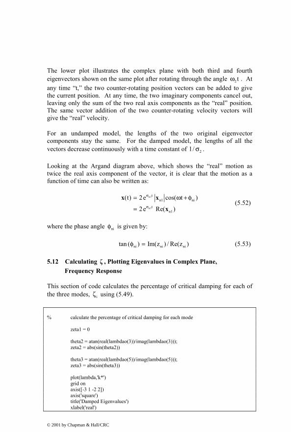
The lower plot illustrates the complex plane with both third and fourth eigenvectors shown on the same plot after rotating through the angle 2tω . At any time “t,” the two counter-rotating position vectors can be added to give the current position. At any time, the two imaginary components cancel out, leaving only the sum of the two real axis components as the “real” position. The same vector addition of the two counter-rotating velocity vectors will give the “real” velocity.
For an undamped model, the lengths of the two original eigenvector components stay the same. For the damped model, the lengths of all the vectors decrease continuously with a time constant of 21/ σ .
Looking at the Argand diagram above, which shows the “real” motion as twice the real axis component of the vector, it is clear that the motion as a function of time can also be written as:
n1
n1
tn1 ni
tn1
(t) 2e cos( t )
2e Re( )
σ
σ
= ω + φ
=
x x
x (5.52)
where the phase angle niφ is given by:
ni ni nitan ( ) Im(z ) / Re(z )φ = (5.53)
5.12 Calculating ζ , Plotting Eigenvalues in Complex Plane, Frequency Response
This section of code calculates the percentage of critical damping for each of the three modes, iζ using (5.49).
% calculate the percentage of critical damping for each mode zeta1 = 0 theta2 = atan(real(lambdao(3))/imag(lambdao(3))); zeta2 = abs(sin(theta2)) theta3 = atan(real(lambdao(5))/imag(lambdao(5))); zeta3 = abs(sin(theta3)) plot(lambda,'k*') grid on axis([-3 1 -2 2]) axis('square') title('Damped Eigenvalues') xlabel('real')
© 2001 by Chapman & Hall/CRC

ylabel('imaginary') text(real(lambdao(3))-1,imag(lambdao(3))+0.1,['zeta = ',num2str(zeta2)]) text(real(lambdao(5))-1,imag(lambdao(5))+0.1,['zeta = ',num2str(zeta3)]) disp('execution paused to display figure, "enter" to continue'); pause
-3 -2 -1 0 1
-2
-1.5
-1
-0.5
0
0.5
1
1.5
2Damped Eigenvalues
real
imag
inar
y
zeta = 0.074857
zeta = 0.13015
Figure 5.5: Plot of eigenvalues in complex plane for tdof model with c1 = 0.1, c2 = 0.2.
10-1 100 101-150
-100
-50
0
50state space, z11, z33 db magnitude
mag
nitu
de, d
b
10-1 100 101-150
-100
-50
0
50state space, z21, z12, z23, z32 db magnitude
mag
nitu
de, d
b
10-1 100 101-150
-100
-50
0
50state space, z31, z13 db magnitude
frequency, rad/sec
mag
nitu
de, d
b
10-1 100 101-150
-100
-50
0
50state space, z22 db magnitude
frequency, rad/sec
mag
nitu
de, d
b
Figure 5.6: Frequency response magnitude plots.
© 2001 by Chapman & Hall/CRC

10-1 100 101-200
-150
-100
-50
0state space, z11, z33 phase
phas
e, d
eg
10-1 100 101-350
-300
-250
-200
-150state space, z21, z12, z23, z32 phase
phas
e, d
eg
10-1 100 101-200
-100
0
100
200state space, z31, z13 phase
frequency, rad/sec
phas
e, d
eg
10-1 100 101-200
-150
-100
-50
0state space, z22 phase
frequency, rad/sec
phas
e, d
eg
Figure 5.7: Frequency response phase plots.
The magnitude and phase frequency response plots for the system with c1 = 0.1 and c2 = 0.2 are shown above, using tdofss.m to plot. Note the significant attenuation of the resonances with zetas of 7.5% and 13% for modes 1 and 2, respectively. (Note: This amount of damping is very difficult to obtain in most practical structures without the use of additive damping.)
5.13 Initial Condition Responses of Individual Modes
The code below calculates the initial condition response for the oscillatory (not rigid body) second and third modes of the system when started with initial conditions defined by the appropriate eigenvector. Equation (5.51) is repeated below to show the form of the equation for x(t) that is used in the code.
n1 n1 n 2
n1 n1 n1 n 2
t j t j tn1 n2
t j t t j tn1 n2
(t) e (e e )
e ( e ) e ( e )
σ ω − ω
σ ω σ − ω
= +
= +
x x xx x
(5.54)
The real and imaginary components of the eigenvalues are calculated to give andσ ω in the equation above. The real and imaginary displacements of
each of the three masses are then calculated for both oscillatory modes for a time period of 15 seconds.
% calculate the motions of the three masses for all three modes - damped case t = 0:.12:15;
© 2001 by Chapman & Hall/CRC

sigma11 = real(lambdao(1)); % sigma for first eigenvalue for mode 1 omega11 = imag(lambdao(1)); % omega for first eigenvalue for mode 1 sigma12 = real(lambdao(2)); % sigma for second eigenvalue for mode 1 omega12 = imag(lambdao(2)); % omega for second eigenvalue for mode 1 sigma21 = real(lambdao(3)); % sigma for first eigenvalue for mode 2 omega21 = imag(lambdao(3)); % omega for first eigenvalue for mode 2 sigma22 = real(lambdao(4)); % sigma for second eigenvalue for mode 2 omega22 = imag(lambdao(4)); % omega for second eigenvalue for mode 2 sigma31 = real(lambdao(5)); % sigma for first eigenvalue for mode 3 omega31 = imag(lambdao(5)); % omega for first eigenvalue for mode 3 sigma32 = real(lambdao(6)); % sigma for second eigenvalue for mode 3 omega32 = imag(lambdao(6)); % omega for second eigenvalue for mode 3 % motion of three masses for mode 1 z111r = exp(sigma11*t).*(exp(i*omega11*t)*xmon1(1,1)); % mass 1 z112r = exp(sigma12*t).*(exp(i*omega12*t)*xmon1(1,2)); % mass 1 z121r = exp(sigma11*t).*(exp(i*omega11*t)*xmon1(3,1)); % mass 2 z122r = exp(sigma12*t).*(exp(i*omega12*t)*xmon1(3,2)); % mass 2 z131r = exp(sigma11*t).*(exp(i*omega11*t)*xmon1(5,1)); % mass 3 z132r = exp(sigma12*t).*(exp(i*omega12*t)*xmon1(5,2)); % mass 3 % motion of three masses for mode 2 z211r = exp(sigma21*t).*(exp(i*omega21*t)*xmon1(1,3)); % mass 1 z212r = exp(sigma22*t).*(exp(i*omega22*t)*xmon1(1,4)); % mass 1 z221r = exp(sigma21*t).*(exp(i*omega21*t)*xmon1(3,3)); % mass 2 z222r = exp(sigma22*t).*(exp(i*omega22*t)*xmon1(3,4)); % mass 2 z231r = exp(sigma21*t).*(exp(i*omega21*t)*xmon1(5,3)); % mass 3 z232r = exp(sigma22*t).*(exp(i*omega22*t)*xmon1(5,4)); % mass 3 % motion of three masses for mode 3 z311r = exp(sigma31*t).*(exp(i*omega31*t)*xmon1(1,5)); % mass 1 z312r = exp(sigma32*t).*(exp(i*omega32*t)*xmon1(1,6)); % mass 1 z321r = exp(sigma31*t).*(exp(i*omega31*t)*xmon1(3,5)); % mass 2 z322r = exp(sigma32*t).*(exp(i*omega32*t)*xmon1(3,6)); % mass 2 z331r = exp(sigma31*t).*(exp(i*omega31*t)*xmon1(5,5)); % mass 3 z332r = exp(sigma32*t).*(exp(i*omega32*t)*xmon1(5,6)); % mass 3
© 2001 by Chapman & Hall/CRC

5.14 Plotting Initial Condition Response, Listing
The code listing below is to plot various combinations of real and imaginary components of the displacements of the three masses when released in states which match the eigenvectors.
% plot real and imaginary motions of each mass for the two complex conjugate % eigenvectors of mode 2 plot(t,real(z211),'k-',t,real(z212),'k+-',t,imag(z211),'k.-',t,imag(z212),'ko-') title('non-prop damped real and imag for z1, mode 2') legend('real','real','imag','imag') xlabel('time, sec') axis([0 max(t) -1 1]) grid on disp('execution paused to display figure, "enter" to continue'); pause plot(t,real(z221),'k-',t,real(z222),'k+-',t,imag(z221),'k.-',t,imag(z222),'ko-') title('non-prop damped real and imag for z2 mode 2') legend('real','real','imag','imag') xlabel('time, sec') axis([0 max(t) -1 1]) grid on disp('execution paused to display figure, "enter" to continue'); pause plot(t,real(z231),'k-',t,real(z232),'k+-',t,imag(z231),'k.-',t,imag(z232),'ko-') title('non-prop damped real and imag for z3 mode 2') legend('real','real','imag','imag') xlabel('time, sec') axis([0 max(t) -1 1]) grid on disp('execution paused to display figure, "enter" to continue'); pause plot(t,real(z211+z212),'k-',t,real(z221+z222),'k+-',t,real(z231+z232),'k.-') title('non-prop damped, z1, z2, z3 mode 2') legend('mass 1','mass 2','mass 3') xlabel('time, sec') axis([0 max(t) -2 2]) grid on disp('execution paused to display figure, "enter" to continue'); pause % plot subplots for notes subplot(2,2,1) plot(t,real(z211),'k-',t,real(z212),'k+',t,imag(z211),'k.-',t,imag(z212),'ko-') title('non-prop damped real and imag for z1, mode 2') legend('real','real','imag','imag') axis([0 max(t) -1 1]) grid on
© 2001 by Chapman & Hall/CRC

subplot(2,2,2) plot(t,real(z221),'k-',t,real(z222),'k+',t,imag(z221),'k.-',t,imag(z222),'ko-') title('non-prop damped real and imag for z2 mode 2') legend('real','real','imag','imag') axis([0 max(t) -1 1]) grid on subplot(2,2,3) plot(t,real(z231),'k-',t,real(z232),'k+',t,imag(z231),'k.-',t,imag(z232),'ko-') title('non-prop damped real and imag for z3 mode 2') legend('real','real','imag','imag') xlabel('time, sec') axis([0 max(t) -1 1]) grid on subplot(2,2,4) plot(t,real(z211+z212),'k-',t,real(z221+z222),'k+-',t,real(z231+z232),'k.-') title('non-prop damped, z1, z2, z3 mode 2') legend('mass 1','mass 2','mass 3') grid on xlabel('time, sec') axis([0 max(t) -2 2]) disp('execution paused to display figure, "enter" to continue'); pause subplot(1,1,1) % plot mode 3 plot(t,real(z311),'k-',t,real(z312),'k+-',t,imag(z311),'k.-',t,imag(z312),'ko-') title('non-prop damped real and imag for z1, mode 3') legend('real','real','imag','imag') xlabel('time, sec') axis([0 max(t) -1 1]) grid on disp('execution paused to display figure, "enter" to continue'); pause plot(t,real(z321),'k-',t,real(z322),'k+-',t,imag(z321),'k.-',t,imag(z322),'ko-') title('non-prop damped real and imag for z2 mode 3') legend('real','real','imag','imag') xlabel('time, sec') axis([0 max(t) -2 2]) grid on disp('execution paused to display figure, "enter" to continue'); pause plot(t,real(z331),'k-',t,real(z332),'k+-',t,imag(z331),'k.-',t,imag(z332),'ko-') title('non-prop damped real and imag for z3 mode 3') legend('real','real','imag','imag') xlabel('time, sec') axis([0 max(t) -1 1]) grid on disp('execution paused to display figure, "enter" to continue'); pause plot(t,real(z311+z312),'k-',t,real(z321+z322),'k+-',t,real(z331+z332),'k.-')
© 2001 by Chapman & Hall/CRC

title('non-prop damped, z1, z2, z3 mode 3') legend('mass 1','mass 2','mass 3') xlabel('time, sec') axis([0 max(t) -4 4]) grid on disp('execution paused to display figure, "enter" to continue'); pause % plot subplots for notes subplot(2,2,1) plot(t,real(z311),'k-',t,real(z312),'k+-',t,imag(z311),'k.-',t,imag(z312),'ko-') title('non-prop damped real and imag for z1, mode 3') legend('real','real','imag','imag') axis([0 max(t) -1 1]) grid on subplot(2,2,2) plot(t,real(z321),'k-',t,real(z322),'k+-',t,imag(z321),'k.-',t,imag(z322),'ko-') title('non-prop damped real and imag for z2 mode 3') legend('real','real','imag','imag') axis([0 max(t) -2 2]) grid on subplot(2,2,3) plot(t,real(z331),'k-',t,real(z332),'k+-',t,imag(z331),'k.-',t,imag(z332),'ko-') title('non-prop damped real and imag for z3 mode 3') legend('real','real','imag','imag') xlabel('time, sec') axis([0 max(t) -1 1]) grid on subplot(2,2,4) plot(t,real(z311+z312),'k-',t,real(z321+z322),'k+-',t,real(z331+z332),'k.-') title('non-prop damped, z1, z2, z3 mode 3') legend('mass 1','mass 2','mass 3') xlabel('time, sec') axis([0 max(t) -4 4]) grid on disp('execution paused to display figure, "enter" to continue'); pause
5.15 Plotted Results: Argand and Initial Condition Responses
The next four sections plot Argand and initial condition transient responses for the two oscillatory modes, illustrating the canceling of the imaginary components and the doubling of the real components.
© 2001 by Chapman & Hall/CRC
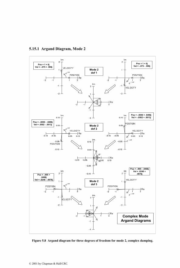
5.15.1 Argand Diagram, Mode 2
Mode 2dof 1
Mode 2dof 2
Mode 2dof 3
Pos = 1 + 0jVel = -.075 + .999j
Pos = -.995 +.0498j
Vel = .0248 - .9978j
Pos = 1 + 0jVel = -.075 - .999j
Pos = -.0050 - .0498jVel = .0502 - .0013j
Pos = -.0050 + .0498jVel = -.0502 + .0013j
Pos = -.995 - .0498jVel = .0248 +
.9978j
tje ω
tje ω−
tje ω
tje ω−
tje ω
tje ω−
Complex Mode Argand Diagrams
Figure 5.8 Argand diagram for three degrees of freedom for mode 2, complex damping.
© 2001 by Chapman & Hall/CRC

5.15.2 Time Domain Responses, Mode 2
The plots below show the motions of the masses decreasing due to the damping. Once again, the imaginary components are out of phase and cancel each other, leaving only twice the real component as the final motion. Unlike the undamped case, the three masses do not reach their maximum or minimum positions at the same time. Since the damping is quite small, it is hard to see on the plots the small differences in times at which the maxima and minima are reached. Note that the unequal damping values for the two dampers make the center mass have a small motion in mode 2. We showed in Chapter 3 that for the undamped case mass 2 has no motion for mode 2.
0 5 10 15-1
-0.5
0
0.5
1non-prop damped real and imag for z1, mode 2
realrealimagimag
0 5 10 15-1
-0.5
0
0.5
1non-prop damped real and imag for z2 mode 2
realrealimagimag
0 5 10 15-1
-0.5
0
0.5
1non-prop damped real and imag for z3 mode 2
time, sec
realrealimagimag
0 5 10 15-2
-1
0
1
2non-prop damped, z1, z2, z3 mode 2
time, sec
mass 1mass 2mass 3
Figure 5.9: Initial condition transient response for mode 2.
© 2001 by Chapman & Hall/CRC

5.15.3 Argand Diagram, Mode 3
Mode 3dof 1
Mode 3dof 2
Mode 3dof 3
Pos = 1 + 0jVel = -.225 + 1.714j
Pos = 1.0001 +.263jVel = -.676+1.655j
Pos = 1 + 0jVel = -.225 - 1.714j
Pos = -2.000-.2630jVel = .9009 - 3.369j
tje ω
tje ω−
tje ω
tje ω−
Complex Mode Argand Diagrams
Pos = -2.000+.2630jVel = .9009 + 3.369j
Pos = 1.0001 -.263jVel = -.676-1.655j
Figure 5.10: Argand diagram for three degrees of freedom for mode 3, complex damping.
© 2001 by Chapman & Hall/CRC

5.15.4 Time Domain Responses, Mode 3
Compared to the responses for the mode 2 in Figure 5.9, the response for mode 3 damps out faster for two reasons. First, it has higher damping, 13% versus 7.5%, as shown in Figure 5.5. Secondly, even if zeta were the same for the two modes, the higher frequency of mode 3 will create higher velocities, hence higher damping from the velocity-dependent damping term.
0 5 10 15-1
-0.5
0
0.5
1non-prop damped real and imag for z1, mode 3
realrealimagimag
0 5 10 15-2
-1
0
1
2non-prop damped real and imag for z2 mode 3
realrealimagimag
0 5 10 15-1
-0.5
0
0.5
1non-prop damped real and imag for z3 mode 3
time, sec
realrealimagimag
0 5 10 15-4
-2
0
2
4non-prop damped, z1, z2, z3 mode 3
time, sec
mass 1mass 2mass 3
Figure 5.11: Initial condition transient response for mode 3.
© 2001 by Chapman & Hall/CRC

Problems
Note: All the problems refer to the two dof system shown in Figure P2.2.
P5.1 Write the damped equations for the two dof system in state space form, both expanded and matrix. Show the input matrix B for a step force of magnitude 1 to mass 1 and magnitude –2 for mass 2. Show the output matrix C for the following outputs:
a) Position of masses 1 and 2
b) Position and velocity of mass 1
c) 2 times velocity of mass 1 plus 3 times the position of mass 2
P5.2 Set up the eigenvalue problem for the damped two dof problem as in (5.46).
P5.3 (MATLAB) With 1 2m m m 1= = = , 1 2k k k 1= = = , modify the code in tdof_non_prop_damped.m for the two dof damped model with
1 2c c 0.1= = and:
a) list the complex eigenvalues, real and imaginary form
b) list the complex eigenvalues, magnitude and phase angle form
c) normalize the eigenvectors for unity values of the position of mass 1 and hand plot the Argand diagrams for the system
d) list the percentage of critical damping for each mode
e) plot the complex eigenvalues in the s-plane and correlate the three different descriptions in (a), (b) and (d)
P5.4 (MATLAB) Set 1 2m m m 1= = = , 1 2k k k 1= = = and plot the initial condition responses for the system in initial conditions which match the two damped eigenvectors.
P5.5 Set 1 2m m m 1= = = , 1 2k k k 1= = = and hand plot the Argand diagrams for modes 1 and 2.
© 2001 by Chapman & Hall/CRC

CHAPTER 6
STATE SPACE: FREQUENCY RESPONSE, TIME DOMAIN
6.1 Introduction – Frequency Response
This chapter will begin with the state space form of the equations of motion. We will use Laplace transforms to define the transfer function matrix. Next we will solve for the closed form transfer function matrix of the undamped tdof model using a symbolic algebra program and compare the answer with the solution presented in Chapter 2. MATLAB code will be used to set up frequency response calculations, using the full system matrix which allows the user to define damping values.
6.2 Solving for Transfer Functions in State Space Form Using Laplace Transforms
Starting with the complete set of state space equations:
uu
= += +
x Ax By Cx D&
(6.1)
Ignoring initial conditions to solve for steady state frequency response, take the matrix Laplace transform of the state equation and solve for (s)x (Appendix 2):
s (s) (s) u(s)= +Ix Ax B (6.2)
(s ) (s) u(s)− =I A x B (6.3)
1(s) (s ) u(s)−= −x I A B (6.4)
Substituting into the Laplace transform of the output equation:
1(s) (s ) u(s) u(s)−= − +y C I A B D (6.5)
Solving for the transfer function (s)u(s)y :
© 2001 by Chapman & Hall/CRC

1(s) (s )u(s)
−= − +y C I A B D (6.6)
Checking consistency of sizes
nx1 (nxn)x(nxn)x(nx1) (nx1)nx1
= +=
(6.7)
Letting 1 2 3 1 2 3 1 2m m m m, k k k k, c c 0= = = = = = = = and rewriting the matrix equations of motion to match the original undamped problem used in Section 2.4.3 allows calculation of results by hand. The MATLAB code which follows, however, will allow any values to be used for the individual masses, dampers and stiffnesses.
1 1 1 1
1 1 1 1
1 1 1 2 1 2 2 2
2 2 2 2 2 2
2 2 2 2
3 3 3 3
1 0 0 0 0 00 1 0 0 0 00 0 1 0 0 0
(s ) s0 0 0 1 0 00 0 0 0 1 00 0 0 0 0 1
0 1 0 0 0 0k c k c
0 0m m m m0 0 0 1 0 0k c (k k ) (c c ) k cm m m m m m0 0 0 0 0 1
k c k c0 0m m m m
− =
− − − − + − +
− −
I A
© 2001 by Chapman & Hall/CRC

1 1 1 1
1 1 1 1
1 1 1 2 1 2 2 2
2 2 2 2 2 2
2 2 2 2
3 3 3 3
s 1 0 0 0 0k c k c
s 0 0m m m m0 0 s 1 0 0k c (k k ) (c c ) k c
sm m m m m m0 0 0 0 s 1
k c k c0 0 sm m m m
− − − + − = − − + + − −
+ −
− − +
s 1 0 0 0 0k ks 0 0 0m m0 0 s 1 0 0k 2k k0 s 0
m m m0 0 0 0 s 1
k k0 0 0 sm m
− − −
= − −
− −
(6.8)
Here, in order to develop the entire 3x3 transfer function matrix, we will use a MIMO representation of B and C.
Taking B equal to the 6x3 matrix gives transfer functions for all three forces:
1
2
3
0 0 01/ m 0 0
0 0 00 1/ m 00 0 00 0 1/ m
=
B (6.9)
Taking C equal to the 3x6 matrix below gives the three displacement transfer functions as outputs:
© 2001 by Chapman & Hall/CRC

1 0 0 0 0 00 0 1 0 0 00 0 0 0 1 0
=
C (6.10)
6.3 Transfer Function Matrix
Now that we have the terms required, we can substitute into the equation for the transfer function matrix:
1(s) (s )u(s)
−= − +y C I A B D (6.11)
We have an expression for (s )−I A above, but need to have its inverse. Using a symbolic algebra program to calculate the inverse even for this relatively small 3x3 problem yields a result which is too lengthy to be listed here in its entirety. To show that the calculation by hand really works, however, we will expand the equation above symbolically and then substitute the appropriate terms from the inverse to give the results for several of the transfer functions. We will refer to the 1(s )−−I A matrix by the notation “sia” and expand it as follows:
1
11 12 13 14 15 16
21 22 23 24 25 26
31 32 33 34 35 36
41 42 43 44 45 46
51
(s) (s )u(s)
siai siai siai siai siai siaisiai siai siai siai siai siai
1 0 0 0 0 0siai siai siai siai siai siai
0 0 1 0 0 0siai siai siai siai siai siai
0 0 0 0 1 0siai si
−= −
=
y C I A B
52 53 54 55 56
61 62 63 64 65 66
ai siai siai siai siaisiai siai siai siai siai siai
0 0 01/ m 0 0
0 0 00 1/ m 00 0 00 0 1/ m
© 2001 by Chapman & Hall/CRC

11 12 13 14 15 16
31 32 33 34 35 36
51 52 53 54 55 56
0 0 01/ m 0 0
siai siai siai siai siai siai0 0 0
siai siai siai siai siai siai0 1/ m 0
siai siai siai siai siai siai0 0 00 0 1/ m
=
12 14 16
32 34 36
52 54 56
siai / m siai / m siai / msiai / m siai / m siai / msiai / m siai / m siai / m
=
(6.12)
Listing the values for the xxsiai terms used above from the symbolic algebra solution:
3 4 2 2 212 56
2 2 232 14 54 36
3 4 2 2 234
252 16
2 3 4 2 2 2
siai siai (m s 3m ks mk ) / Den
siai siai siai siai (m ks mk ) / Den
siai (m s 2m ks mk ) / Den
siai siai mk / Den
where Den s (m s 4m ks 3mk )
= = + +
= = = = +
= + +
= =
= + +
(6.13a-e)
Dividing each of the above terms by “m” and presenting in the transfer function matrix form of (2.61):
( )
2 4 2 2 2 2 2
2 2 2 4 2 2 2 2
1 12 2 2 2 4 2 2
2 22 3 4 2 2 2
3 3
(m s 3mks k ) (mks k ) k(mks k ) (m s 2mks k ) (mks k )z F
k (mks k ) (m s 3mks k )z Fs m s 4m ks 3mkz F
+ + + + + + +
+ + += + + (6.14)
The two derivations are identical.
© 2001 by Chapman & Hall/CRC

6.4 MATLAB Code tdofss.m – Frequency Response Using State Space
6.4.1 Code Description, Plot
The four distinct transfer functions for the default values of m, k and c are plotted using MATLAB in tdofss.m, listed below. The four plots are displayed in Figure 6.1. The A, B, C and D matrices shown in (5.17a) are used as inputs to the program. A MIMO state space model is constructed and the MATLAB function bode.m is used to calculate the magnitude and phase of the resulting frequency responses. As described in the code, the resulting frequency response has dimensions of 6x3x200, where the “6” represents the 6 outputs in the output matrix C, the “3” represents the three columns of the input matrix B and the “200” represents the 200 frequency points in the frequency vector. The desired magnitude and phase can be extracted from the 6x3x200 matrix by defining the appropriate indices. The default values of c1 and c2 are zero.
10-1 100 101-150
-100
-50
0
50state space, z11, z33 db magnitude
mag
nitu
de, d
b
10-1 100 101-150
-100
-50
0
50state space, z21, z12, z23, z32 db magnitude
mag
nitu
de, d
b
10-1 100 101-150
-100
-50
0
50state space, z31, z13 db magnitude
frequency, rad/sec
mag
nitu
de, d
b
10-1 100 101-150
-100
-50
0
50state space, z22 db magnitude
frequency, rad/sec
mag
nitu
de, d
b
Figure 6.1: Four distinct frequency response amplitudes.
6.4.2 Code Listing
% tdofss.m state-space transfer function solution of tdof undamped model using % state-space matrices directly and the bode command clf; legend off; subplot(1,1,1);
© 2001 by Chapman & Hall/CRC

clear all; % define the values of masses, springs, dampers and Forces m1 = 1; m2 = 1; m3 = 1; c1 = input('input value for c1, default 0, ... '); if (isempty(c1)) c1 = 0; else end c2 = input('input value for c2, default 0, ... '); if (isempty(c2)) c2 = 0; else end k1 = 1; k2 = 1; F1 = 1; F2 = 1; F3 = 1; % define the system matrix, a a = [ 0 1 0 0 0 0 -k1/m1 -c1/m1 k1/m1 c1/m1 0 0 0 0 0 1 0 0 k1/m2 c1/m2 -(k1+k2)/m2 -(c1+c2)/m2 k2/m2 c2/m2 0 0 0 0 0 1 0 0 k2/m3 c2/m3 -k2/m3 -c2/m3]; % define the input matrix, b, a 6x3 matrix b = [ 0 0 0 F1/m1 0 0 0 0 0 0 F2/m2 0 0 0 0 0 0 F3/m3]; % define the output matrix, c, the 6x6 identify matrix c = eye(6,6); % define the direct transmission matrix d = 0; % solve for the eigenvalues of the system matrix
© 2001 by Chapman & Hall/CRC

[xm,omega] = eig(a); % Define a vector of frequencies to use, radians/sec. The logspace command uses % the log10 value as limits, i.e. -1 is 10^-1 = 0.1 rad/sec, and 1 is % 10^1 = 10 rad/sec. The 200 defines 200 frequency points. w = logspace(-1,1,200); % use the "ss" function to define state space system for three inputs, forces at % masses 1, 2 and 3 and for all 6 states, three displacements and three velocities sssys = ss(a,b,c,d); % use the bode command with left hand magnitude and phase vector arguments % to provide values for further analysis/plotting % the mag and phs matrices below will be 6x3x200 in size % the appropriate magnitude and phase to plot for each transfer function % are called by appropriate indexing % first index 1-6: z1 z1dot z2 z2dot z3 z3dot % second index 1-3: F1 F2 F3 % third index 1-200: all frequency points, use ":" [mag,phs] = bode(sssys,w); z11mag = mag(1,1,:); z11phs = phs(1,1,:); z21mag = mag(3,1,:); z21phs = phs(3,1,:); z31mag = mag(5,1,:); z31phs = phs(5,1,:); z22mag = mag(3,2,:); z22phs = phs(3,2,:); % calculate the magnitude in decibels, db z11magdb = 20*log10(z11mag); z21magdb = 20*log10(z21mag); z31magdb = 20*log10(z31mag); z22magdb = 20*log10(z22mag); % plot the four transfer functions separately, in a 2x2 subplot form subplot(2,2,1) semilogx(w,z11magdb(1,:),'k-') title('state space, z11, z33 db magnitude') ylabel('magnitude, db') axis([.1 10 -150 50]) grid
© 2001 by Chapman & Hall/CRC
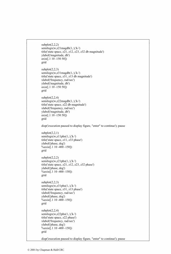
subplot(2,2,2) semilogx(w,z21magdb(1,:),'k-') title('state space, z21, z12, z23, z32 db magnitude') ylabel('magnitude, db') axis([.1 10 -150 50]) grid subplot(2,2,3) semilogx(w,z31magdb(1,:),'k-') title('state space, z31, z13 db magnitude') xlabel('frequency, rad/sec') ylabel('magnitude, db') axis([.1 10 -150 50]) grid subplot(2,2,4) semilogx(w,z22magdb(1,:),'k-') title('state space, z22 db magnitude') xlabel('frequency, rad/sec') ylabel('magnitude, db') axis([.1 10 -150 50]) grid disp('execution paused to display figure, "enter" to continue'); pause subplot(2,2,1) semilogx(w,z11phs(1,:),'k-') title('state space, z11, z33 phase') ylabel('phase, deg') %axis([.1 10 -400 -150]) grid subplot(2,2,2) semilogx(w,z21phs(1,:),'k-') title('state space, z21, z12, z23, z32 phase') ylabel('phase, deg') %axis([.1 10 -400 -150]) grid subplot(2,2,3) semilogx(w,z31phs(1,:),'k-') title('state space, z31, z13 phase') xlabel('frequency, rad/sec') ylabel('phase, deg') %axis([.1 10 -400 -150]) grid subplot(2,2,4) semilogx(w,z22phs(1,:),'k-') title('state space, z22 phase') xlabel('frequency, rad/sec') ylabel('phase, deg') %axis([.1 10 -400 -150]) grid disp('execution paused to display figure, "enter" to continue'); pause
© 2001 by Chapman & Hall/CRC

6.5 Introduction – Time Domain
Starting with the equations of motion in state space, we will use Laplace transforms to discuss the theoretical solution to the time domain problem. We will define and discuss two methods of calculating the matrix exponential. Then we will use a sdof forced system with position and velocity initial conditions to illustrate the technique. The closed form solution for our tdof example problem with step forces applied to all three masses and with different initial conditions for each mass is too complicated to be shown so we will use only MATLAB for its solution.
6.6 Matrix Laplace Transform – with Initial Conditions
We start with the state equations in general form, (6.1). Taking the matrix Laplace transform of a first order differential equation (DE) with initial conditions (Appendix 2):
{ }{ }
(t) s (s) (0)
(t) (s)
= −
=
x x x
x x
&LL
(6.15)
Taking the matrix Laplace transform of (6.1) and solving for x(s):
1 1
s (s) (0) (s) u(s)(s ) (s) (0) u(s)
(s) (s ) (0) (s ) u(s)− −
− = +− = += − + −
x x Ax BI A x x B
x I A x I A B (6.16a,b,c)
Solving for the output vector y(s):
1 1
(s) (s)(s ) (0) (s ) u(s)− −
== − + −
y CxC I A x C I A B
(6.17)
The input matrix B and output matrix C are familiar from earlier state space presentations. There is a new term in the equation for the Laplace transform of y(s), the term 1(s )−−I A .
There are many methods of calculating the inverse 1(s )−−I A (Chen 1999). If the problem is small, for example 2x2, the inverse can be handled in closed form. Then y(s) can be back-transformed term by term to get the solution in the time domain, as we shall see in the example in the next section.
© 2001 by Chapman & Hall/CRC

For another solution method it is useful to recall the geometric series expansion below, for r 1< :
2 31 1 r r r ...1 r
= + + + +−
(6.18)
Expanding 1(s )−−I A with the series expansion analogy above, the inverse results in the infinite series in (6.19).
2 31
2 3
2 3
2 3 4
11 1s(s ) ...
s s s s ss
...s s s s
− − = = = + + + + − −
= + + + +
A A AI A IAI A I
I A A A
(6.19)
6.7 Inverse Matrix Laplace Transform, Matrix Exponential
Now that we have the inverse in series form, it is easy to back-transform to the time domain, term by term. We introduce two new terms, (t)Φ , the inverse Laplace transform of 1(s )−−I A which equals teA , the matrix exponential.
( ){ }
( ) ( )
1-1
2 3-1
2 3 4
2 3
t
(t) s
...s s s s
t tt ...
2! 3!e
−= −
= + + + +
= + + + +
= A
Φ I A
I A A A
A AI A
L
L (6.20)
6.8 Back-Transforming to Time Domain
Now that the form of the matrix exponential is known, we can back-transform the entire equation of motion, from (6.16c):
( )-1 -1 1 1(s) (s ) (0) (s ) u(s)− − = − + − x I A x I A BL L (6.21)
The result is:
© 2001 by Chapman & Hall/CRC
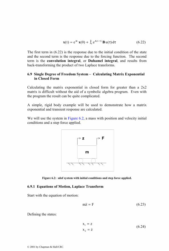
t t (t )0(t) e (0) e u( )d−τ= + ∫ τ τA Ax x B (6.22)
The first term in (6.22) is the response due to the initial condition of the state and the second term is the response due to the forcing function. The second term is the convolution integral, or Duhamel integral, and results from back-transforming the product of two Laplace transforms.
6.9 Single Degree of Freedom System – Calculating Matrix Exponential in Closed Form
Calculating the matrix exponential in closed form for greater than a 2x2 matrix is difficult without the aid of a symbolic algebra program. Even with the program the result can be quite complicated.
A simple, rigid body example will be used to demonstrate how a matrix exponential and transient response are calculated.
We will use the system in Figure 6.2, a mass with position and velocity initial conditions and a step force applied.
m
z F
Figure 6.2: sdof system with initial conditions and step force applied.
6.9.1 Equations of Motion, Laplace Transform
Start with the equation of motion:
mz F=&& (6.23)
Defining the states:
1
2
x zx z
== &
(6.24)
© 2001 by Chapman & Hall/CRC

Defining derivatives and inserting the value for acceleration:
1 2
2
x xFxm
=
=
&
& (6.25)
The above can be written in matrix form, recognizing that F/m is the acceleration and applying a unity magnitude step:
1 1
2 2
0x x0 1
(1)Fx x0 0m
= +
&
& (6.26)
Defining the system matrix:
0 10 0 =
A (6.27)
Taking the inverse of the 1(s )−−I A term:
1 1 21
1 1s 0 0 1 s 1 s s(s )0 s 0 0 0 s 10
s
− −−
−
− = − = =
I A (6.28)
6.9.2 Defining the Matrix Exponential – Taking Inverse Laplace Transform
Using the table of inverse Laplace transforms from Appendix 2 yields the matrix exponential.
2t 1
1 11 ts se0 110
s
−
= =
A L (6.29)
© 2001 by Chapman & Hall/CRC

6.9.3 Defining the Matrix Exponential – Using Series Expansion
A Power Series Expansion can also be used to find the matrix exponential for this simple example because higher powers of tA go to zero quickly:
( ) ( )2 3t t t
e t ...2! 3!
1 0 0 t 0 0(all other terms zero)
0 1 0 0 0 0
1 t0 1
= + + + +
= + + +
=
A A AI A
(6.30)
This is the same solution as (6.29).
6.9.4 Solving for Time Domain Response
Thus, the general solution for x(t) as a function of time becomes:
t t (t )0
t1
02
t1 2
02
2
1 2
2
(t) e (0) e u(t)d
0x (0)1 t 1 t
(1) dFx (0)0 1 0 1m
F(t )x (0) t x (0) m
dx (0) F
m
Ftx (0) t x (0) 2 m
x (0)
−τ= + ∫ τ
− τ = + τ
− τ + = + τ
τ τ − + = +
∫
∫
A Ax x B
t
0
Fm
τ
© 2001 by Chapman & Hall/CRC

22
1 2
2
2
1 2
2
t Ftx (0) t x (0) 2 m
x (0) Ftm
t Fx (0) t x (0) 2 m
x (0) Ftm
− + = +
+ = +
(6.31)
This result is the same as the familiar equations for the position and velocity of a mass undergoing a constant acceleration:
2
1
2
(acceleration) (time )x (t) initialposition time (initial velocity)2x (t)
initial velocity (acceleration) (time)
× + × + = + × (6.32)
6.10 MATLAB Code tdof_ss_time_ode45_slnk.m – Time Domain Response of tdof Model
6.10.1 Equations of Motion Review
There are several ways to numerically solve for transient responses using MATLAB. One method uses numerical integration, calling the integration routine from a command line and defining the state equation in a separate MATLAB function. Another method uses Simulink, a linear/nonlinear graphical block diagram model building tool linked to MATLAB.
We will solve for the transient response of our tdof model using both methods and compare the results with the closed form solution calculated using the modal transient response method in Chapter 9.
© 2001 by Chapman & Hall/CRC

c1
m1 m2 m3
k1 k2
c2
z1 z2 z3F1=1 F2=0 F3=-2
Figure 6.3: tdof model with damping for use in MATLAB/Simulink models.
1 1 2 3 3 5
1 2 2 4 3 6
z (0) x (0) 0 z (0) x (0) 1 z (0) x (0) 1z (0) x (0) 1 z (0) x (0) 2 z (0) x (0) 2
= = = = − = == = − = = = = −& & &
Table 6.1: Initial conditions for tdof model in Figure 6.3.
Step function forces of amplitudes indicated in Figure 6.3 are applied to masses 1 and 3; mass 2 has no force applied. Initial conditions of position and velocity for each mass are shown in Table 6.1.
The equations of motion in state space are then:
1 1 1 11 1
1 1 1 1 12 2
3 31 1 1 2 1 2 2 2
4 42 2 2 2 2 2
5 5
6 62 2 2 2
3 3 3 3
0 1 0 0 0 0 0k c k c 10 0x x
m m m m mx x
0 0 0 1 0 0x x
k c (k k ) (c c ) k cx x
m m m m m mx x
0 0 0 0 0 1x x
k c k c0 0m m m m
− − = +− + − + − −
&
&
&
&
&
&
2
3
0(1)0
m02
m
−
(6.33)
The initial condition vector, x(0) is:
© 2001 by Chapman & Hall/CRC

1 1
2 1
3 2
4 2
5 3
6 3
x (0) z (0) 0x (0) z (0) 1x (0) z (0) 1
(0)x (0) z (0) 2x (0) z (0) 1x (0) z (0) 2
− −
= = =
−
x
&
&
&
(6.34)
The output equation for the displacement outputs (no velocities included) with no feedthrough term is:
1
21
32
43
5
6
xx
y 1 0 0 0 0 0x
y 0 0 1 0 0 0 (0)(1)x
y 0 0 0 0 1 0xx
= +
(6.35)
These are the system matrices that are used in the MATLAB code below.
6.10.2 Code Description
Two methods will be used to solve for the time domain response. The MATLAB code tdof_ss_time_ode45_slnk.m is used for both methods, prompting the user to define which solution technique is desired.
The first method uses the MATLAB Runge Kutta method ODE45 and calls the function file tdofssfun.m, which contains the state equations. The results are then plotted. To use the ODE45 solver, type “tdof_ss_time_ode45_slnk” from the MATLAB prompt and use the default selection.
The second solution uses the Simulink model tdof_ss_simulink.mdl and the plotting file tdof_ss_time_slnk_plot.m.
To use the Simulink solver:
1) Type “tdof_ss_time_ode45_slnk” and choose the Simulink solver.
2) The program will prompt the reader to type “tdof_ss_simulink” at the MATLAB command prompt. This will bring up the Simulink model on the screen.
© 2001 by Chapman & Hall/CRC

3) Click on the “simulation” choice in the model screen and then choose “start.” The Simulink model will then run.
4) To see the plotted results, type “tdof_ss_time_slnk_plot.”
6.10.3 Code Results – Time Domain Responses
0 1 2 3 4 5 6 7 8 9 10
-25
-20
-15
-10
-5
0
5State-Space Displacements of dof 1, 2 and 3
Time, sec
Vib
ratio
n D
ispl
acem
ents
dof 1dof 2dof 3
Figure 6.4: ODE45 simulation motion of tdof model.
0 1 2 3 4 5 6 7 8 9 10
-25
-20
-15
-10
-5
0
5State Space Simulink Calculation of Displacements of dof 1, 2 and 3
Time, sec
Vib
ratio
n Di
spla
cem
ents
dof 1dof 2dof 3
Figure 6.5: Simulink simulation motion of tdof model.
© 2001 by Chapman & Hall/CRC

0 1 2 3 4 5 6 7 8 9 10
-25
-20
-15
-10
-5
0
5Displacements of dof 1, 2 and 3 from Simulink (slnk) and Closed Form (cf)
Time, sec
Vib
ratio
n Di
spla
cem
ents
cf dof 1 cf dof 2 cf dof 3 slnk dof 1slnk dof 2slnk dof 3
Figure 6.6: Overlay of closed form solution from Chapter 9, Figure 9.4, with Simulink solution.
6.10.4 Code Listing
% tdof_ss_time_ode45_slnk.m state-space solution of tdof model with % initial conditions, step function forcing function and displacement outputs % using the ode45 solver or Simulink, user is prompted for damping values clear all; global a b u % this is required to have the parameters available % for the function which_run = input('enter "1" for Simulink or "enter" for ode45 run ... '); if isempty(which_run) which_run = 0 end % define the values of masses, springs, dampers and Forces m1 = 1; m2 = 1; m3 = 1; c1 = input('input value for c1, default 0.0, ... '); if (isempty(c1)) c1 = 0.0; else end c2 = input('input value for c2, default 0.0, ... ');
© 2001 by Chapman & Hall/CRC

if (isempty(c2)) c2 = 0.0; else end k1 = 1; k2 = 1; F1 = 1; F2 = 0; F3 = -2; % define the system matrix, a a = [ 0 1 0 0 0 0 -k1/m1 -c1/m1 k1/m1 c1/m1 0 0 0 0 0 1 0 0 k1/m2 c1/m2 -(k1+k2)/m2 -(c1+c2)/m2 k2/m2 c2/m2 0 0 0 0 0 1 0 0 k2/m3 c2/m3 -k2/m3 -c2/m3]; % define the input matrix, b b = [ 0 F1/m1 0 F2/m2 0 F3/m3]; % define the output matrix for transient response, c, displacements only c = [1 0 0 0 0 0 0 0 1 0 0 0 0 0 0 0 1 0]; % define the direct transmission matrix for transient response, d, the same number of
rows as c and the same number of columns as b d = zeros(3,1); if which_run == 0 % transient response using the ode45 command u = 1; ttotal = input('Input total time for Simulation, default = 10 sec, ... '); if (isempty(ttotal)) ttotal = 10; else end tspan = [0 ttotal]; x0 = [0 -1 -1 2 1 -2]'; % initial condition vector, note transpose
© 2001 by Chapman & Hall/CRC

options = []; % no options specified for ode45 command [t,x] = ode45('tdofssfun',tspan,x0,options); y = c*x'; % note transpose, x is calculated as a column vector in time plot(t,y(1,:),'k+-',t,y(2,:),'kx-',t,y(3,:),'k-') title('State-Space Displacements of dof 1, 2 and 3') xlabel('Time, sec') ylabel('Vibration Displacements') legend('dof 1','dof 2','dof 3') grid else % setup Simulink run % define the direct transmission matrix for transient response, d, the same number of
rows as c and the same number of columns as b % define time for simulink model ttotal = input('Input total time for Simulation, default = 10 sec, ... '); if (isempty(ttotal)) ttotal = 10; else end disp(' '); disp(' '); disp(' '); disp(' '); disp(' '); disp(' '); disp('Run the Simulink model "tdof_ss_simulink.mdl" and then'); disp('run the plotting file "tdof_ss_time_slnk_plot.m"'); end
6.10.5 MATLAB Function tdofssfun.m – Called by tdof_ss_time_ode45_slnk.m
function xprime = tdofssfun(t,x) % function for calculating the transient response of tdof_ss_time_ode45.m global a b u xprime = a*x + b*u;
© 2001 by Chapman & Hall/CRC

6.10.6 Simulink Model tdofss_simulink.mdl
tout
time forsimulink run
dof3 scope
dof3
dof3 disp
dof2
dof2 disp
dof1
dof1 disp
Step
x' = Ax+Bu y = Cx+Du
State-Space
Demux
Demux
Clock
Figure 6.7: Block diagram of Simulink model tdofss_simulink.mdl.
The block diagram was constructed by dragging and dropping blocks from the appropriate Simulink block library and connecting the blocks. The input is the step block. The clock block is used to output time to the tout block for plotting in MATLAB. The model is defined in the state space block, reading in values for the a, b, c and d matrices from the MATLAB workspace, created during execution of tdof_ss_time_ode45_slnk.m. The demux block separates the vector output of the state space block and sends the displacements of the three masses to three blocks for storing for plotting in MATLAB. The scope block brings up a scope screen and shows the position of dof3 versus time as the program executes. This example is so small that the screen displays instantly for the default 10 sec time period, but for a longer time period the scope traces the progress of the simulation.
© 2001 by Chapman & Hall/CRC

Problems
Note: All the problems refer to the two dof system shown in Figure P2.2.
P6.1 Set 1 2m m m 1= = = , 1 2k k k 1= = = , 1 2c c 0= = and define the state space matrices for a step force applied to mass 1 and for output of position of mass 2. Write out by hand the equation for the transfer functions matrix as shown in (6.11). Extra credit: use a symbolic algebra program to take the inverse of the (s )−I A term and then multiply out the equations to see that they match the results of P2.2.
P6.2 (MATLAB) Modify the code tdofss.m for the two dof system and plot the distinct frequency responses.
P6.3 (MATLAB) Modify the code tdof_ss_time_ode45_slnk.m for the two dof system with 1 2m m m 1= = = , 1 2k k k 1= = = and 1 2c c 0= = for the following step forces and initial conditions:
a) 1 2F 0, F 3= = −
b) 1 1 2 2z 0, z 2, z 1, z 2= = − = − =& &
Plot the time domain responses using both MATLAB and Simulink.
© 2001 by Chapman & Hall/CRC

CHAPTER 7
MODAL ANALYSIS
7.1 Introduction
In Chapter 2 we systematically defined the equations of motion for a multi dof (mdof) system and transformed to the “s” domain using the Laplace transform. Chapter 3 discussed frequency responses and undamped mode shapes.
Chapter 5 discussed the state space form of equations of motion with arbitrary damping. It also covered the subject of complex modes. Heavily damped structures or structures with explicit damping elements, such as dashpots, result in complex modes and require state space solution techniques using the original coupled equations of motion.
Lightly damped structures are typically analyzed with the “normal mode” method, which is the subject of this chapter. The ability to think about vibrating systems in terms of modal properties is a very powerful technique that serves one well in both performing analysis and in understanding test data. The key to normal mode analysis is to develop tools which allow one to reconstruct the overall response of the system as a superposition of the responses of the different modes of the system. In analysis, the modal method allows one to replace the n-coupled differential equations with n-uncoupled equations, where each uncoupled equation represents the motion of the system for that mode of vibration. If natural frequencies and mode shapes are available for the system, then it is easy to visualize the motion of the system in each mode, which is the first step in being able to understand how to modify the system to change its characteristics.
Summarizing the modal analysis method of analyzing linear mechanical systems and the benefits derived:
1) Solve the undamped eigenvalue problem, which identifies the resonant frequencies and mode shapes (eigenvalues and eigenvectors), useful in themselves for understanding basic motions of the system.
2) Use the eigenvectors to uncouple or diagonalize the original set of coupled equations, allowing the solution of n-uncoupled sdof problems instead of solving a set of n-coupled equations.
© 2001 by Chapman & Hall/CRC

3) Calculate the contribution of each mode to the overall response. This also allows one to reduce the size of the problem by eliminating modes that cannot be excited and/or modes that have no outputs at the desired dof’s. Also, high frequency modes that have little contribution to the system at lower frequencies can be eliminated or approximately accounted for, further reducing the size of the system to be analyzed.
4) Write the system matrix, A, by inspection. Assemble the input and output matrices, B and C, using appropriate eigenvector terms. Frequency domain and forced transient response problems can be solved at this point. If complete eigenvectors are available, initial condition transient problems can also be solved. For lightly damped systems, proportional damping can be added, while still allowing the equations to be uncoupled.
7.2 Eigenvalue Problem
7.2.1 Equations of Motion
We will start by writing the undamped homogeneous (unforced) equations of motion for the model in Figure 7.1. Then we will define and solve the eigenvalue problem.
Figure 7.1: Undamped tdof model.
+ =mz kz 0&& (7.1)
From (2.5) with 1 2k k k= = and c1 = c2 = 0:
m1 m2 m3
k1 k2
z1 z2 z3F1 F2 F3
© 2001 by Chapman & Hall/CRC

1 1
2 2
3 3
m 0 0 z k k 0 z 00 m 0 z k 2k k z 00 0 m z 0 k k z 0
− + − − = −
&&
&&
&&
(7.2)
7.2.2 Principal (Normal) Mode Definition
Since the system is conservative (it has no damping), normal modes of vibration will exist. Having normal modes means that at certain frequencies all points in the system will vibrate at the same frequency and in phase, i.e., all points in the system will reach their minimum and maximum displacements at the same point in time. Having normal modes can be expressed as (Weaver 1990):
( ) i ij ti mi i i misin t Im(e )ω +φ= ω + φ =z z z (7.3)
Where:
iz = vector of displacements for all dof’s at the thi frequency
miz = the thi eigenvector, the mode shape for the thi resonant frequency
iω = the ith eigenvalue, ith resonant frequency
iφ = an arbitrary initial phase angle
For our tdof system, for the thi frequency, the equation would appear as:
( )1 m1i
2 m2i i i
3 m3i
z zz z sin tz z
= ω + φ
, (7.4)
where the indices in the mkiz term represent the kth dof and the ith mode of the modal matrix mz .
7.2.3 Eigenvalues / Characteristic Equation
Since the equation of motion
0+ =mz kz&& (7.5)
© 2001 by Chapman & Hall/CRC

and the form of the motion
( )i mi i i sin t= ω + φz z (7.6)
are known, iz can be differentiated twice and substituted into the equation of motion:
( )2i i mi i i sin t= −ω ω + φz z&& (7.7)
( ) ( )2i mi i i mi i i sin t sin t 0 −ω ω + φ + ω + φ = m z k z (7.8)
Canceling the sine terms:
2i mi mi 0−ω + =mz kz (7.9)
2mi i mi= ωkz mz (7.10)
Equation (7.10) is the eigenvalue problem in nonstandard form, where the standard form is (Strang 1998):
= λAz z (7.11)
The solution of the simultaneous equations which make up the standard form eigenvalue problem is a vector z such that when z is multiplied by A , the product is a scalar multiple of z itself.
The nonstandard problem is “nonstandard” because the mass matrix m falls on the right-hand side. The form of the matrix presents no problem for hand calculations, but for computer calculations it is best transformed to standard form.
Rewriting the nonstandard form eigenvalue problem as a homogeneous equation:
( )2i mi 0− ω =k m z (7.12)
A trivial solution, mi 0=z , exists but is of no consequence. The only possibility for a nontrivial solution is if the determinant of the coefficient matrix is zero (Strang 1998). Expanding the matrix entries:
© 2001 by Chapman & Hall/CRC

2i mi
k k 0 m 0 0k 2k k 0 m 0 0
0 k k 0 0 m
− − − − ω = −
z (7.13)
Performing the matrix subtraction:
2i
21 mi
2i
k m k 0k 2k m k 0
0 k k m
− ω − − − ω − = − − ω
z (7.14)
Setting the determinant of the coefficient matrix equal to zero:
2i
2i
2i
k m k 0k 2k m k 0
0 k k m
− ω −− − ω − =
− − ω (7.15)
The determinant results in a polynomial in 2iω , the characteristic equation,
where the roots of the polynomial are the eigenvalues, poles, or resonant frequencies of the system.
( )
3 6 2 4 2 2
2 3 4 2 2 2
m 4km 3k m 0
m 4km 3k m 0
− ω + ω − ω =
ω − ω + ω − =
(7.16a,b)
Two of the roots are at the origin:
1 0ω = (7.17)
Solving for 2ω as a quadratic in (7.16b) above:
( )1
2 2 4 2 4 22
3
4km 16k m 12k m
2m
− ± −ω =
−
2 2
3
4km 2km2m
− ±=−
© 2001 by Chapman & Hall/CRC

6k 2k,2m 2m
− −=− −
3k k,m m
= (7.18)
2
3
3kmkm
ω = ±
ω = ± (7.19)
For each of the three eigenvalue pairs, there exists an eigenvector iz , which gives the mode shape of the vibration at that frequency.
7.2.4 Eigenvectors
To obtain the eigenvectors of the system, any one of the degrees of freedom, say z1, is selected as a reference. Then, all but one of the equations of motion is written with that value on the right-hand side:
( )2i mi 0− ω =k m z (7.20)
( )( )
( )
2i
m1i2i m2i
2 m3ii
k m k 0 zk 2k m k z 0
z0 k k m
− ω − − − ω − = − − ω
(7.21)
Expanding the first and second equations, dropping the subscripts “ i ” and “m”:
( )( )
2i 1 2
21 i 2 3
k m z kz 0
kz 2k m z kz 0
− ω − =
− + − ω − = (7.22a,b)
Rewriting with the 1z term on the right-hand side and solving for the ( )2 1z / z ratio from (7.22a):
( )22 i 1kz k m z− = − − ω (7.23)
© 2001 by Chapman & Hall/CRC

22 i
1
z k mz k
− ω= (7.24)
Solving for the ( )3 1z / z ratio from (7.22b):
( )2i 2 3 12k m z kz kz− ω − = (7.25)
( )2 32i
1 1
kzz2k m kz z
− ω − =
(7.26)
( )2
2 3ii
1
kzk m2k m kk z
− ω− ω − =
(7.27)
( )( )2 2i i3
21
2k m k mz1
z k
− ω − ω= − (7.28)
2 4 2 23 i i
21
z m 3km kz k
ω − ω += (7.29)
We now have the general equations for the eigenvector values. If a value is chosen for 1z , say 1.0, then the two ratios above can be solved for corresponding values of 2 3z and z for each of the three eigenvalues.
Since at each eigenvalue there are (n+1) unknowns ( )i mi, zω for a system with n equations of motion, the eigenvectors are only known as ratios of displacements, not as absolute magnitudes. For the first mode of our tdof system the unknowns are i m11 m21 m31, z , z and zω and we have only three equations of motion.
Substituting values for the three eigenvalues into the general eigenvector ratio equations above, assuming 1 2m m m 1= = = , 1 2k k k 1= = = :
For mode 1, 21 0ω =
2
1
z k 1z k
= = (7.30)
© 2001 by Chapman & Hall/CRC

2 1z z= (7.31)
( )( )32
1
2k kz1 2 1 1
z k= − = − = (7.32)
3 1z z= (7.33)
Arbitrarily assigning z1=1:
1
111
=
z (7.34)
1 1 1
Rigid-Body Mode, 0 rad/sec
Figure 7.2: Mode shape plot for rigid body mode, where all masses move together with no stress in the connecting springs.
For mode 2, 22
km
ω =
2
1
kk mz m 0z k
− = = (7.35)
2z 0= (7.36)
( ) ( )32
1
k k2k m k m2k k 0m mz
1 1 1z k2k
− − − = − = − = − (7.37)
© 2001 by Chapman & Hall/CRC

3 1z z= − (7.38)
2
101
= −
z (7.39)
1 -1
Second Mode, Middle Mass Stationary, 1 rad/sec
Figure 7.3: Mode shape plot for second mode, middle mass stationary and the two end masses move out of phase with each other with equal amplitude.
For node 3, 23
3km
ω =
2
1
3kk mz 2km 2z k k
− − = = = − (7.40)
2 1z 2z= − (7.41)
( ) ( ) 23
2 2 21
3k 3k2k m k mk 2k 1m mz 2k 11 1
z k k k
− − − − − − = − = = = (7.42)
3 1z z= (7.43)
3
12
1
= −
z (7.44)
© 2001 by Chapman & Hall/CRC
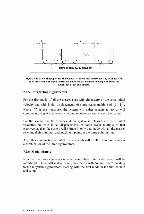
1 1-2
Third Mode, 1.732 rad/sec
Figure 7.4: Mode shape plot for third mode, with two end masses moving in phase with each other and out of phase with the middle mass, which is moving with twice the
amplitude of the end masses.
7.2.5 Interpreting Eigenvectors
For the first mode, if all the masses start with either zero or the same initial velocity and with initial displacements of some scalar multiple of [ ]T1 1 1 , where “T” is the transpose, the system will either remain at rest or will continue moving at that velocity with no relative motion between the masses.
For the second and third modes, if the system is released with zero initial velocities but with initial displacements of some scalar multiple of that eigenvector, then the system will vibrate in only that mode with all the masses reaching their minimum and maximum points at the same point in time.
Any other combination of initial displacements will result in a motion which is a combination of the three eigenvectors.
7.2.6 Modal Matrix
Now that the three eigenvectors have been defined, the modal matrix will be introduced. The modal matrix is an (nxn) matrix with columns corresponding to the n system eigenvectors, starting with the first mode in the first column and so on:
© 2001 by Chapman & Hall/CRC

mode: 1 2 3
m11 m12 m13
m m21 m22 m23
m31 m32 m33
z z z DOF1z z z DOF2z z z DOF3
← = ← ←
z (7.45)
1 2 3
↑ ↑ ↑z z z
For our tdof problem:
m
1 1 11 0 21 1 1
= − −
z (7.46)
7.3 Uncoupling the Equations of Motion
At this point the system is well defined in terms of natural frequencies and modes of vibration. If any further information such as transient or frequency response is desired, solving for it would be laborious because the system equations are still coupled. For transient response, the equations would have to be solved simultaneously using a numerical integration scheme unless the problem were simple enough to allow a closed form solution. To calculate the damped frequency response, a complex equation solving routine would have to be used to invert the complex coefficient matrix at each frequency.
In order to facilitate solving for the transient or frequency responses, it is useful to transform the n-coupled second order differential equations to n-uncoupled second order differential equations by transforming from the physical coordinate system to a principal coordinate system. In linear algebra terms, the transformation from physical to principal coordinates is known as a change of basis. There are many options for change of basis, but we will show that when eigenvectors are used for the transformation the principal coordinate system has a physical meaning; each of the uncoupled sdof systems represents the motion of a specific mode of vibration. The n-uncoupled equations in the principal coordinate system can then be solved for the responses in the principal coordinate system using well-known solutions for single degree of freedom systems. The n-responses in the principal coordinate system can then be transformed back to the physical coordinate system to provide the actual
© 2001 by Chapman & Hall/CRC

response in physical coordinates. This procedure is shown schematically in Figure 7.5.
PHYSICAL COORDINATES
Coupled Equations of MotionInitial ConditionsForcing Functions
PRINCIPAL COORDINATES
Uncoupled Equations of MotionInitial ConditionsForcing Functions
Solution
PHYSICAL COORDINATES
Solution
Transform
Back-Transform
Figure 7.5: Roadmap for Modal Solution
The procedure above is analogous to using Laplace transforms for solving differential equations, where the differential equation is transformed to an algebraic equation, solved algebraically, and back transformed to get the solution of the original problem.
We now need a means of diagonalizing the mass and stiffness matrices, which will yield a set of uncoupled equations.
The condition to guarantee diagonalization is the existence of n-linearly independent eigenvectors, which is always the case if the mass and stiffness matrices are both symmetric or if there are n-different (nonrepeated) eigenvalues (Strang 1998).
Going back to the original homogeneous equation of motion:
0+ =mz kz&& (7.47)
© 2001 by Chapman & Hall/CRC

Having normal modes means that at frequency “i”:
i mi i i sin ( t )= ω + φz z (7.48)
Differentiating twice to get acceleration:
2i i mi i isin ( t )= −ω ω + φz z&& (7.49)
Substituting back into the equation of motion:
{ } { }2i mi i i mi i isin( t ) sin( t ) 0−ω ω + φ + ω + φ =m z k z (7.50)
Canceling sine terms:
2i mi mi 0−ω + =mz kz (7.51)
Rearranging and writing the above equation for both the “ith” and “jth” modes:
2mi i mi= ωkz mz (7.52)
2mj j mj= ωkz mz (7.53)
miz and mjz are the “ith” and “jth” eigenvectors, the “ith” and “jth” columns of the modal matrix.
Premultiplying (7.52) by the transpose of Tmj mj,z z :
T 2 Tmj mi i mj mi= ωz kz z mz (7.54)
Taking the transpose of (7.53), where the transpose of a product is the product of the individual transposes taken in reverse order, i.e., [ ]T T T=AB B A :
T T 2 T Tmj j mj ,= ωz k z m (7.55)
since m and k are symmetrical, T T, and= =m m k k :
T 2 Tmj j mj= ωz k z m (7.56)
© 2001 by Chapman & Hall/CRC

Postmultiplying (7.56) by miz
T 2 Tmj mi j mj mi= ωz kz z mz (7.57)
Now, subtracting (7.57) from (7.54):
T 2 Tmj mi i mj miT 2 Tmj mi j mj mi
2 2 Ti j mj mi
( )0 ( )
= ω− = ω
= ω − ω
z kz z mzz kz z mz
z mz (7.58)
When i j=/ , the term ( )2 2i jω − ω cannot be equal to zero, meaning that the
term Tmj miz mz must be equal to zero.
Tmj mi 0=z mz (7.59)
Looking at the sizes of the matrices multiplied:
Tmj
mi
1xnnxnnx1
=
==
zm
z (7.60)
( ) ( ) ( ) ( )1xn x nxn x nx1 1x1 scalar= = (7.61)
Equation (7.59) can be rewritten:
Tmj mi ijm 0= =z mz , (7.62)
where mij is an off-diagonal term in the mass matrix of the principal coordinate system.
The two eigenvectors mjz and miz are said to be orthogonal with respect to m , where orthogonality is defined as the property that causes all the off-diagonal terms in the principal mass matrix to be zero.
Returning to (7.62), for ( )2 2i ji j, 0= ω − ω = . Thus the product T
mi miz mz can
be set equal to any arbitrary constant iim ,, a diagonal term in the principal mass matrix.
© 2001 by Chapman & Hall/CRC
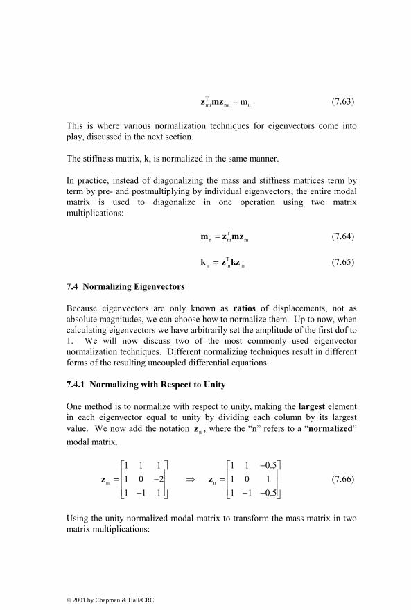
Tmi mi iim=z mz (7.63)
This is where various normalization techniques for eigenvectors come into play, discussed in the next section.
The stiffness matrix, k, is normalized in the same manner.
In practice, instead of diagonalizing the mass and stiffness matrices term by term by pre- and postmultiplying by individual eigenvectors, the entire modal matrix is used to diagonalize in one operation using two matrix multiplications:
Tn m m=m z mz (7.64)
Tn m m=k z kz (7.65)
7.4 Normalizing Eigenvectors
Because eigenvectors are only known as ratios of displacements, not as absolute magnitudes, we can choose how to normalize them. Up to now, when calculating eigenvectors we have arbitrarily set the amplitude of the first dof to 1. We will now discuss two of the most commonly used eigenvector normalization techniques. Different normalizing techniques result in different forms of the resulting uncoupled differential equations.
7.4.1 Normalizing with Respect to Unity
One method is to normalize with respect to unity, making the largest element in each eigenvector equal to unity by dividing each column by its largest value. We now add the notation nz , where the “n” refers to a “normalized” modal matrix.
m n
1 1 1 1 1 0.51 0 2 1 0 11 1 1 1 1 0.5
− = − ⇒ = − − −
z z (7.66)
Using the unity normalized modal matrix to transform the mass matrix in two matrix multiplications:
© 2001 by Chapman & Hall/CRC

Tn
1 1 1 m 0 0 m m m1 0 1 0 m 0 m 0 m0.5 1 0.5 0 0 m .5m m .5m
= − = − − − − −
z m (7.67)
Tn n n
m m m 1 1 .5 3m 0 0m 0 m 1 0 1 0 2m 0.5m m .5m 1 1 .5 0 0 1.5m
− = = − = − − − −
m z mz (7.68)
Similarly transforming the stiffness matrix:
Tn
1 1 1 k k 0 0 0 01 0 1 k 2k k k 0 k.5 1 .5 0 k k 1.5k 3k 1.5k
− = − − − = − − − − − −
z k (7.69)
Tn n n
0 0 0 1 1 .5 0 0 0k 0 k 1 0 1 0 2k 0
1.5k 3k 1.5k 1 1 .5 0 0 4.5k
− = = − − = − − − −
k z kz (7.70)
Note that the original filled stiffness matrix is now diagonal. Also note that if the diagonal elements of the stiffness matrix (7.70) are divided by the corresponding diagonal elements of the mass matrix (7.69), the three terms are the squares of the respective eigenvalues.
7.4.2 Normalizing with Respect to Mass
Another method is to normalize with respect to mass using the equation:
Tni ni 1.0=z mz , (7.71)
making each diagonal mass term equal 1.0. This is the method used by default in ANSYS.
Once again, note that modal matrix subscript “ni” in niz signifies the normalized ith eigenvector. Each normalized eigenvector is defined as follows:
mi mini 1
T i2mi mi
q= =
z zzz mz
(7.72)
© 2001 by Chapman & Hall/CRC

Where qi is defined as:
1n n 2
i mji jk mkij i k 1
q z m z= =
=
∑ ∑ (7.73)
For a diagonal mass matrix, q can be simplified since all the jkm terms are zero:
1n 2
2i k mki
k 1q m z
=
= ∑ (7.74)
Thus, by operating on m by nz ,the mass matrix should be transformed into the identity matrix. Starting with mz and the “q” values from above:
m
1 1 11 0 21 1 1
= − −
z (7.75)
( ) ( ) ( )
( ) ( ) ( )
( ) ( ) ( )
12 2 2 2
1
12 2 2 2
2
12 2 2 2
3
q m 1 m 1 m 1 3m
q m 1 m 0 m 1 2m
q m 1 m 2 m 1 6m
= + + =
= + + − =
= + − + =
(7.76a,b,c)
The modal matrix normalized with respect to mass becomes:
n
1 1 1 1 1 13m 2m 6m 3 2 61 2 1 1 20 03m 6m m 3 61 1 1 1 1 13m 2m 6m 3 2 6
− −= = − −
z (7.77)
Using nz to transform the mass matrix:
© 2001 by Chapman & Hall/CRC

Tn
1 1 1 m m mm 0 03m 3m 3m 3m 3m 3m1 1 m m0 00 m 02m 2m 2m 2m1 2 1 m 2m m
0 0 m6m 6m 6m 6m 6m 6m
− − = = − −
z m (7.78)
Tn n n
m m m 1 1 13m 3m 3m 3m 2m 6mm m 1 20 02m 2m 3m 6mm 2m m 1 1 16m 6m 6m 3m 2m 6m
− −= = − −
m z mz (7.79)
n
m m m m m03m 3m 3m m 3 2 m 3 2
m m m m0 02m 2mm 2 3 m 2 3
m 2m m m m0m 3 6 m 3 6 m 3 6 m 2 6 m 6 2
m 2m mm 3 6 m 3 6 m 3 6
m m0m 2 6 m 2 6
m 4m m6m 6m 6m
1 0 00 1 00 0 1
+ + + −
= + − + +
− + + −
− +
+ − + +
=
m
(7.80)
The original mass matrix has been transformed to the identity matrix.
Similarly transforming the stiffness matrix:
© 2001 by Chapman & Hall/CRC

Tn
1 1 1 1 1 03 3 3
1 1 10 k 1 2 1m 2 2
1 2 10 1 1
6 6 6
− − = − − − −
z k
1 1 1 2 1 1 103 3 3 3 3 3 3
k 1 1 1 10 0 0 0 0m 2 2 2 2
1 2 1 4 1 2 10 06 6 6 6 6 6 6
− − + − − +
− = + + + + + − − + + − − + +
(7.81)
Tn n n
1 1 10 0 0 3 2 61 1 1 2 k0 0
m2 2 3 63 6 3 1 1 16 6 6 3 2 6
− −= = − −
k z kz (7.82)
n
0 0
k 1 1 1 10m 2 22 3 2 3
3 6 3 3 303 6 3 6 3 6 2 6 6 2
0
1 102 6 2 6
3 12 36 6 6
= − + +
− + − −
+ −
+ +
k
(7.83)
© 2001 by Chapman & Hall/CRC

n
0 0 0k0 1 0m
0 0 3
=
k (7.84)
Note that the normalized stiffness matrix is now diagonal and that the diagonal terms are the squares of the corresponding three eigenvalues. The normalized stiffness matrix is also known as the spectral matrix (Weaver 1990).
Because normalizing with respect to mass results in an identity principal mass matrix and squares of the eigenvalues on the diagonal in the principal stiffness matrix, we will use only this normalization in the future. Since we know the form of the principal matrices when normalizing with respect to mass, no multiplying of modal matrices is actually required: the homogeneous principal equations of motion can be written by inspection knowing only the eigenvalues.
7.5 Reviewing Equations of Motion in Principal Coordinates – Mass Normalization
7.5.1 Equations of Motion in Physical Coordinate System
[ ]1 1
2 2
3 3
m 0 0 z k k 0 z0 m 0 z k 2k k z 00 0 m z 0 k k z
− + − − = −
&&
&&
&&
(7.85)
Eigenvalues:
1 0ω = (7.86)
2
3
3kmkm
ω = ±
ω = ± (7.87a,b)
Eigenvectors, normalized with respect to mass:
© 2001 by Chapman & Hall/CRC

n
1 1 13 2 6
1 1 20m 3 6
1 1 13 2 6
−= −
z (7.88)
7.5.2 Equations of Motion in Principal Coordinate System
[ ]p1 p1
p2 p2
p3 p3
0 0 01 0 0 z zk0 1 0 z 0 0 z 0m
0 0 1 z z3k0 0m
+ =
&&
&&
&&
(7.89)
7.5.3 Expanding Matrix Equations of Motion in Both Coordinate Systems
Physical Coordinates
1 1 2
2 1 2 3
3 2 3
mz kz kz 0mz kz 2kz kz 0mz kz kz 0
+ − =− + − =− + =
&&
&&
&&1444442444443
Principal Coordinates
p1
p2 p2
p3 p3
z 0
kz z 0m3kz z 0m
=
+ =
+ =
&&
&&
&&1442443
These equations are coupled and have to be solved simultaneously.
These homogeneous equations are uncoupled and can be solved independently.
Table 7.1: Summary of equations of motion in physical and principal coordinates.
© 2001 by Chapman & Hall/CRC

7.6 Transforming Initial Conditions and Forces
Now that we know how to construct the homogeneous uncoupled equations of motion for the system, we need to know how to transform initial conditions and forces to the principal coordinate system. We can then solve for transient and forced responses in the principal coordinate system using the uncoupled equations.
Starting with the original non-homogeneous equations of motion in physical coordinates:
+ =mz kz F&& (7.90)
Premultiplying by Tnz , the transpose of the modal matrix:
T T Tn n n+ =z mz z kz z F&& (7.91)
Inserting the identify matrix, n n−= 1I z z :
{ {T 1 T 1 Tn n n n n n n
− −+ =z m z z z z k z z z z FI I
&& (7.92)
Rewriting and regrouping terms:
{ {{ {T 1 T 1 Tn n n n n n n
p p p pp
− −+ =z mz z z z kz z z z Fz k z Fm&&
123&&
, (7.93)
where Tn nz mz and T
n nz kz were shown to diagonalize the mass and stiffness matrices in the previous section.
Defining terms:
pm = (nxn) diagonal principal mass matrix
pk = (nxn) diagonal principal stiffness matrix
1n p− =z z z&& && = acceleration vector in principal coordinates
1n p− =z z z = displacement vector in principal coordinates
© 2001 by Chapman & Hall/CRC

Tn p=z F F = force vector in principal coordinates
In the previous section, the definitions for accelerations and displacements in physical and principal coordinates were shown to be:
1p n
1p n
−
−
=
=
z z z
z z z
&& && (7.94)
The same relationships hold for initial conditions of displacement and velocity:
1op n o
1op n o
−
−
=
=
z z z
z z z& & (7.95)
In (7.95), opz and opz& are vectors of initial displacements and velocities, respectively, in the principal coordinate system, and oz and oz& are vectors of initial displacements and velocities, respectively, in the physical coordinate system.
Taking the inverse of the modal matrix to convert initial conditions requires that the modal matrix be square, with as many eigenvectors as number of degrees of freedom. We will see in future chapters that there are instances where not all eigenvectors are available. In one case, we may choose to only calculate eigenvalues and eigenvectors up to a certain frequency in order to save calculation time or because the problem only requires knowledge of response in a certain frequency range. In another case, we may build a “reduced” model where only the most significant modes are retained. Fortunately, a large majority of real life problems involve zero initial conditions.
7.7 Summarizing Equations of Motion in Both Coordinate Systems
The two sets of equations, in physical and principal coordinates, are shown in Table 7.2:
© 2001 by Chapman & Hall/CRC

Physical Coordinates Principal Coordinates
1 1 2 1
2 1 2 3 2
3 2 3 3
1 2 3 1 2 3
mz kz kz Fmz kz 2kz kz Fmz kz kz FIC 's : z , z , z , z , z , z
+ − =− + − =− + =
&&
&&
&&
& & &
p1 p1
p2 p2 p2
p3 p3 p3
p1 p2 p3 p1 p2 p3
z F
kz z Fm3kz z Fm
IC 's : z , z , z , z , z , z
=
+ =
+ =
&&
&&
&&
& & &
Table 7.2: Summary of equations of motion in physical and principal coordinates.
The variables in physical coordinates are the positions and velocities of the masses. The variables in principal coordinates are the displacements and velocities of each mode of vibration.
The equations in principal coordinates can be easily solved, since the equations are uncoupled, yielding the displacements. We now need to back transform the results in the principal coordinate system to the physical coordinate system to get the final answer.
7.8 Back-Transforming from Principal to Physical Coordinates
We showed previously that the relationship between physical and principal coordinates is:
1n p− =z z z (7.96)
Premultiplying by nz :
1n n n p( )− =z z z z z
I123
(7.97)
n p=z z z (7.98)
Thus, the displacement vector in physical coordinates is obtained by premultiplying the vector of displacements in principal coordinates by the normalized modal matrix nz .
© 2001 by Chapman & Hall/CRC

Similarly for velocity:
n p=z z z& & (7.99)
7.9 Reducing the Model Size When Only Selected Degrees of Freedom are Required
So far we have hinted at the fact that only portions of the eigenvector matrix are needed if selected dof’s have forces applied and other (or the same) dof’s are needed for output. This section will show how the reduction in dof’s occurs. This reduction is one of the key steps to be used later in the book when we cover how to reduce the size of models derived from large finite element simulations.
Reviewing the steps in the modal solution, starting with the equations of motion and initial conditions in physical coordinates:
1 1 2 1
2 1 2 3 2
3 2 3 3
1 2 3 1 2 3
mz kz kz Fmz kz 2kz kz F
mz kz kz F
Initial Conditions : z , z , z , z , z , z 0
+ − =− + − =
− + =
=
&&
&&
&&
& & &
(7.100)
Solve for eigenvalues: 1 2 3, ,ω ω ω
Solve for eigenvectors, normalize with respect to mass and form the modal matrix from columns of eigenvectors:
n11 n12 n13
n n21 n22 n23
n31 n32 n33
z z zz z zz z z
=
z (7.101)
Transform forces from physical to principal coordinates:
Tp n=F z F (7.102)
Write the equations of motion in principal coordinates:
© 2001 by Chapman & Hall/CRC

p1 p1
2p2 2 p2 p2
2p3 3 p3 p3
p1 p2 p3 p1 p2 p3
z F
z z F
z z FIC 's : z , z , z , z , z , z 0
=
+ ω =
+ ω =
=
&&
&&
&&
& & &
(7.103a,b,c,d)
Solve the equations in principal coordinates in either time or frequency domain and then back transform to physical coordinates:
n p
n p
=
=
z z z
z z z& &
(7.104)
Note that the two critical transformations (assuming zero initial conditions) involve premultiplying by the transpose of the modal matrix ( p→F F ) in (7.102) or the modal matrix ( p →z z ) in (7.104).
Let us first examine the force transformation by expanding the equations:
Tp n=F z F (7.105)
Tn11 n12 n13 1 n11 n21 n31 1
Tn n21 n22 n23 2 n12 n22 n32 2
n31 n32 n33 3 n13 n23 n33 3
n11 1 n21 2 n31 3
n12 1 n22 2 n32 3
n13 1 n23 2 n33 3
z z z F z z z Fz F z z z F z z z F
z z z F z z z F
z F z F z Fz F z F z Fz F z F z F
= =
+ + = + + + +
(7.106)
Note that the multipliers of 1F in the first column are the elements of the first row of the modal matrix, the multipliers of 2F in the second column are the elements of the second row of the modal matrix and the multipliers of 3F in the third column are the elements of the third row of the modal matrix.
Suppose that force is to be applied at only mass 1, 1F , then only the first row of the modal matrix is required to transform the force in physical coordinates to the force in principal coordinates.
© 2001 by Chapman & Hall/CRC

Now let us examine the displacement transformation by expanding the equations:
n p=z z z (7.107)
1 n11 n12 n13 p1 n11 p1 n12 p2 n13 p3
2 n p n21 n22 n23 p2 n21 p1 n22 p2 n23 p3
3 n31 n32 n33 p3 n31 p1 n32 p2 n33 p3
z z z z z z z z z z zz z z z z z z z z z zz z z z z z z z z z z
+ + = = = = + + + +
z z z
(7.108)
Note that the coefficients of the principal displacements in the first row above are the elements of the first row of the modal matrix. Similarly, coefficients of the second and third rows are the elements of the second and third rows of the modal matrix.
Suppose that the only physical displacement we are interested in is that of mass 2, 2z , then only the second row of the modal matrix is required to transform the three displacements p1 p2 p3z , z , z in principal coordinates to 2z . This leads to the following conclusion about reducing the size of the model:
Only the rows of the modal matrix that correspond to degrees of freedom to which forces are applied and/or for which displacements are desired are required to complete the model.
For this tdof model, reducing the size of the problem is not required; however, we will see later that a realistic finite element model, with hundreds of thousands of degrees of freedom, presents an entirely different problem. Having the ability to reduce the problem size is critical in order to use the detailed results of a complicated finite element model to provide accurate results in a lower order MATLAB model.
7.10 Damping in Systems with Principal Modes
7.10.1 Overview
Damping in complex built-up mechanical systems is impossible to predict with the present state of the art. We will discuss in this section the conditions which determine if a damping matrix can be diagonalized, and the criterion to enable the damped equations to be diagonalized. In general, an arbitrary damping matrix cannot be diagonalized by the undamped eigenvectors, as the
© 2001 by Chapman & Hall/CRC

mass and stiffness matrices can. This leads to using what is called “proportional damping” in most finite element simulations.
If a mechanical system is designed with a specific viscous damping element, for example a dashpot, that dominates the small amount of inherent structural damping present, then that element can be added to the system as a viscous damper. The resulting system is linear, but probably does not exhibit normal modes as discussed in Section 7.2.2. In general this leads to the inability to diagonalize and uncouple the equations of motion, requiring a state space solution of the original, coupled equations of motion.
Viscoelastic damping treatments (damping elastomers) have been used for years in disk drives, most typically as constrained layer dampers on the thin sheet metal suspensions which support the read/write head. The effect of this viscoelastic damping can be approximated at a specific temperature and frequency as proportional damping by using the “modal strain energy” technique in association with a finite element structural model (Johnson 1982).
Ignoring specific viscous, coulomb, and viscoelastic damping elements, damping in typical structures arises from hysteresis losses in the materials as they are strained, in some cases from viscous losses due to structure/fluid interaction but more importantly from relative motion at the interfaces and boundaries where different parts are attached or grounded. Unless a specific damping element is used in a structural design, most structures have damping which varies from mode to mode and will be in the range of 0.05% to 2% of critical damping.
The modes in this chapter are all “real” or “normal” modes as defined earlier. Once again, having normal modes means that at certain frequencies all points in the system will vibrate at the same frequency and in phase, i.e., all points in the system will reach their minimum and maximum displacements at the same point in time. Chapter 5 discussed “complex” modes, modes in which all points in the system do not reach their minimum and maximum displacements at the same point in time.
7.10.2 Conditions Necessary for Existence of Principal Modes in Damped System
With a conservative (no damping) system, normal modes of vibration will exist. In order to have normal modes in a damped system, the mode shapes must be the same as for the undamped case, and the various parts of the system must pass through their minimum and maximum positions at the same instant in time, expressed as:
© 2001 by Chapman & Hall/CRC

( ) thi mi i it for the i modecos= ω + φz z (7.109)
A sufficient condition for the existence of damped normal modes is that the damping matrix be a linear combination of the mass and stiffness matrices. We know that m and k are diagonalized by operating on them with the modal matrix. When c is a linear combination of m and k , then the damping matrix c is also uncoupled (diagonalized) by the same pre- and postmultiplication operations by the modal matrix as with the m and k matrices (Weaver 1990, Craig 1981).
The damped equations of motion then become:
+ + =mz cz kz F&& & , (7.110)
where the damping matrix is a linear combination of and m k :
a b= +c m k (7.111)
Tp n n=c z cz , (7.112)
and where nz is the normalized (with respect to mass) modal matrix.
Writing out the complete equation:
+ + =mz cz kz F&& & (7.113)
{ {{ {{ {− − −+ + =T 1 T 1 T 1 T
n n n n n n n n n n
p p p p p p
z mz z z z cz z z z kz z z z Fz c z k z FI&& &
123&& &
(7.114)
Looking at the c to pc conversion where a b= +c m k :
a b= +c m k (7.115)
a b= +T T Tn n n n n nz cz z mz z kz
pa b= +I k , (7.116)
where pk is a diagonal matrix whose elements are the squares of the eigenvalues.
© 2001 by Chapman & Hall/CRC

The equation for the ith mode is:
( )2 2pi i pi i pi piz a b z z F+ + ω + ω =&& & (7.117)
Rewriting, defining pc , the ( )2ia b+ ω term, using notation:
2pi i i ic a b 2= + ω = ζ ω (7.118)
Where iζ is the percentage of critical damping for the ith mode, defined as:
i i ii 2
cr pi pii pi i
c c cc 2 k m 2m
ζ = = =
ω (7.119)
Then:
2i
ii
a b2+ ωζ =
ω (7.120)
Rewriting the equation in principal coordinates:
2pi i i pi i pi piz 2 z z F+ ζ ω + ω =&& & (7.121)
This type of damping is known as proportional damping, where the damping for each mode (they can all be different) is proportional to the critical damping for that mode. Since the damping is also proportional to velocity, it is of a viscous nature. If the same damping value is used for all modes, it will be referred to as “uniform” damping. Damping in which the damping value for each mode can be set individually will be referred to as “non-uniform” damping.
7.10.3 Different Types of Damping
7.10.3.1 Simple Proportional Damping
Viscous damping in each mode is taken to be an arbitrary percentage, ζ , of critical damping:
© 2001 by Chapman & Hall/CRC

2pi i pi i pi pi
12
p p p p p p
z 2 z z F
2
+ ζω + ω =
+ ζ + = z k z k z F
&& &
&& & (7.122)
This is analogous to the familiar notation used for a single degree of freedom system:
mz cz kz Fc k Fz z zm m m
+ + =
+ + =
&& &
&& & (7.123)
Define critical damping crc 2 km= and define the term multiplying velocity to be:
n
cr
c 2m
c k2c m
2c k2 km mcm
= ζω
=
=
=
(7.124)
Rewriting:
2n n
Fz 2 z zm
+ ζω + ω =&& & (7.125)
7.10.3.2 Proportional to Stiffness Matrix – “Relative” Damping
Recognizing that the higher modes of vibration damp out quickly, “relative” damping yields damping in proportion to frequencies in normal modes, basically letting the “a” term for iζ go to zero:
2i i
ii
a b b2 2
a 0
+ ω ωζ = =ω
=
7.126)
If a value of 1ζ , for the first mode, is assumed, a value can be defined for “b”:
© 2001 by Chapman & Hall/CRC

1
1
2b ζ=ω
, (7.127)
and the value for any other mode i is:
ii 1
1
ωζ = ζω
(7.128)
7.10.3.3 Proportional to Mass Matrix – “Absolute” Damping
Absolute damping is based on making “b” equal to zero, in which case the percentage of critical damping is inversely proportional to the natural frequency of each mode. This will give decreasing damping for modes as their frequencies increase.
2i
ii i
a b a2 2
b 0
+ ωζ = =ω ω
=
(7.129)
If a value of 1ζ , for the first mode, is assumed, a value can be defined for “a”:
1 1a 2= ζ ω , (7.130)
and the value for any other mode i is:
1 1i
i
ω ζζ =ω
(7.131)
© 2001 by Chapman & Hall/CRC

7.10.4 Defining Damping Matrix When Proportional Damping is Assumed
Figure 7.6: Two degree of freedom for damping example.
An interesting question to ask is what the elements of the damping matrix should be in the two degree of freedom (2dof) problem shown in Figure 7.6 in order to be able to diagonalize the equations of motion. We will use the eigenvectors from the undamped case to normalize the damping matrix. Then we will solve for the specific values of the individual dampers which will allow the diagonalization. We will see how non-intuitive the values of
1 2 3c , c and c are in order to be able to diagonalize. (See Craig [1981] for a general expression to calculate the physical damping matrix when given proportional damping values, the original mass matrix, the diagonalized mass matrix and the eigenvalues and eigenvectors.)
7.10.4.1 Solving for Damping Values
Starting with the undamped eigenvalues and eigenvectors:
1 2 2
2 2 3
m n p
c c cm 0 2k kc c c0 m k 2k
k 01 1 1 11 m1 1 1 1 3k2m 0
m
+ −− = = = − +−
= = = − −
m k c
z z k
(7.132)
Solve for the diagonalized damping matrix, assuming proportional damping, and knowing that the diagonalized stiffness matrix elements are squares of the eigenvalues:
c2
m m
k kz1 z2F1 F2
c1
k
c3
© 2001 by Chapman & Hall/CRC

11T 2
p n n p2
02 2
0ω
= = ζ = ζ ω c z cz k (7.133)
Premultiplying by ( ) 1Tnz
− and postmultiplying by ( ) 1
nz − :
( ) ( ) ( ) ( )1
1 11 1T T T 2n n n n n p n2
− −− −= ζz z c z z z k z
II1424314243
(7.134)
( ) ( )1
1 1T 2n p n2
− −= ζc z k z (7.135)
Solving for the inverses above, noting that for this 2dof system, Tn n=z z , and
then performing the operations on pk :
The inverse of a 2 x 2 matrix can be found by:
1. Interchanging the two diagonal elements.
2. Changing the signs of the two off-diagonal elements.
3. Dividing by the determinant of the original matrix.
1
d ba b c a
a bc dc d
−−
− =
Table 7.2: Inverse of 2x2 matrix.
( ) ( )11 T
n n
1 12m
1 11 1 2m1 11 1 2
−−
− − − = = = −− −
z z (7.136)
© 2001 by Chapman & Hall/CRC

11 2
n p
1 01 12m k1 12 m 0 3
1 32k2 1 3
− = −
=
−
z k
(7.137)
11 12
n p n
1 3 1 12k 2m1 12 21 3
1 3 1 32 km4 1 3 1 3
− −
= −−
+ −=
− +
z k z
(7.138)
1 3 1 3km22 1 3 1 3
1 3 1 3km
1 3 1 3
+ −= ζ
− +
+ −= ζ
− +
c
(7.139)
Now we can solve for the specific values for the three dampers:
( )
( )
( )
2
2
c km 1 3
c km 3 1
km .732
− = ζ −
= ζ −
= ζ
(7.140)
© 2001 by Chapman & Hall/CRC

( )
( )
( ) ( )
( )
1 2 2 3
1 3 2
c c c c km 1 3
c c km 1 3 c
km 1 3 3 1
km 2
2 km
+ = + = ζ +
= = ζ + −
= ζ + − −
= ζ
= ζ
(7.141)
Summarizing:
1 3c c 2 km= = ζ (7.142)
( )2c km .732= ζ (7.143)
Note that the values for the three dampers are not at all intuitive and would have been very difficult if impossible to guess to be able to construct a diagonalizable damping matrix. If defining the diagonalizable damping matrix for this 2x2 problem is difficult, imagine trying to define it for a real life finite element problem with thousands of degrees of freedom. Also, it is highly improbable that the back-calculated damping values in physical coordinates would match the actual damping in the structure.
7.10.4.2 Checking Rayleigh Form of Damping Matrix
We have now defined the values of the 1 2 3c , c and c , dampers which allow diagonalizing the equations of motion. Another interesting question is whether the Rayleigh form has been satisfied: Is c a linear combination of and k m ?
?1 3 1 3 1 0 2 1km a m b k
0 1 1 21 3 1 3
+ − − = ζ = + − − + c (7.144)
We have two unknowns, a and b, and essentially two equations, since the two diagonal elements are the same and the two off diagonal elements are the same. First, let us look at the two off diagonal terms, equating terms on the two sides above:
© 2001 by Chapman & Hall/CRC

( ) ( ) ( )
( ) ( )
km 1 3 am 0 bk 1
3 1 mb km 3 1k k
ζ − = + −
−= ζ = ζ −
(7.145)
Now, equating the diagonal terms:
( )
( )
( )
km 1 3 am 2bk
mam 2 3 1 kk
am 2 mk 3 1
ζ + = +
= + ζ −
= + ζ −
(7.146)
( ) ( )am km 1 3 2 mk 3 1
km 1 3 2 3 2
km 3 3
= ζ + − ζ −
= ζ + − +
= ξ −
(7.147)
ka 3 3m = ζ − (7.148)
Checking the two values for a and b by substituting back into (7.146).
© 2001 by Chapman & Hall/CRC

( )
( ) ( )
( )( )
1 3 1 3 1 0kkm m 3 30 1m1 3 1 3
2 1m k 3 11 2k
3 3 0 2 3 2 3 1km
3 1 2 3 20 3 3
1 3 1 3km
1 3 1 3
+ − ζ = ζ − − + −
+ ζ − −
− − − + = ζ + − + − −
+ −= ζ
− +
(7.149)
So c is a linear combination of and k m and the Rayleigh criterion holds.
Problems
Note: All the problems refer to the two dof system shown in Figure P2.2.
P7.1 Set 1 2m m m 1= = = , 1 2k k k 1= = = and solve for the eigenvalues and eigenvectors of the undamped system. Normalize the eigenvectors to unity, write out the modal matrix and hand plot the mode shapes
P7.2 Normalize the eigenvectors in P7.1 with respect to mass and diagonalize the mass and stiffness matrices. Identify the terms in the normalized mass and stiffness matrices. Write the homogeneous equations of motion in physical and principal coordinates.
P7.3 Convert the following step forcing function and initial conditions in physical coordinates to principal coordinates:
a) 1 2F 1, F 3= = −
b) 1 1 2 2z 0, z 2, z 1, z 2= = − = − =& &
P7.4 Using the results of P7.2 and P7.3, write the complete equations of motion in physical and principal coordinates assuming proportional damping.
© 2001 by Chapman & Hall/CRC

CHAPTER 8
FREQUENCY RESPONSE: MODAL FORM
8.1 Introduction
Now that the theory behind the modal analysis method has been covered, we will solve our tdof problem for its frequency response.
Figure 8.1: tdof undamped model for modal analysis.
We will use eigenvalue/eigenvector results from Chapter 7 to define the equations of motion in principal coordinates and to transform forces to principal coordinates. We will then use Laplace transforms to solve for the transfer functions in principal coordinates and back-transform to physical coordinates, where the individual mode contributions will be evident. We will discuss the relationship between the partial fraction expansion transfer function form and the modal form derived here. We discussed in Section 5.13 how to excite only a single mode of vibration by judicious choice of initial conditions. Here we will describe the forcing function combination required to excite only a single mode.
We will spend considerable time in this chapter on developing a greater understanding of how individual modes of vibration combine to give the overall frequency response. MATLAB code is supplied for the tdof problem to illustrate the point. ANSYS is also used to solve the tdof problem and the ANSYS results are described and compared with the MATLAB results.
m1 m2 m3
k1 k2
z1 z2 z3F1 F2 F3
© 2001 by Chapman & Hall/CRC
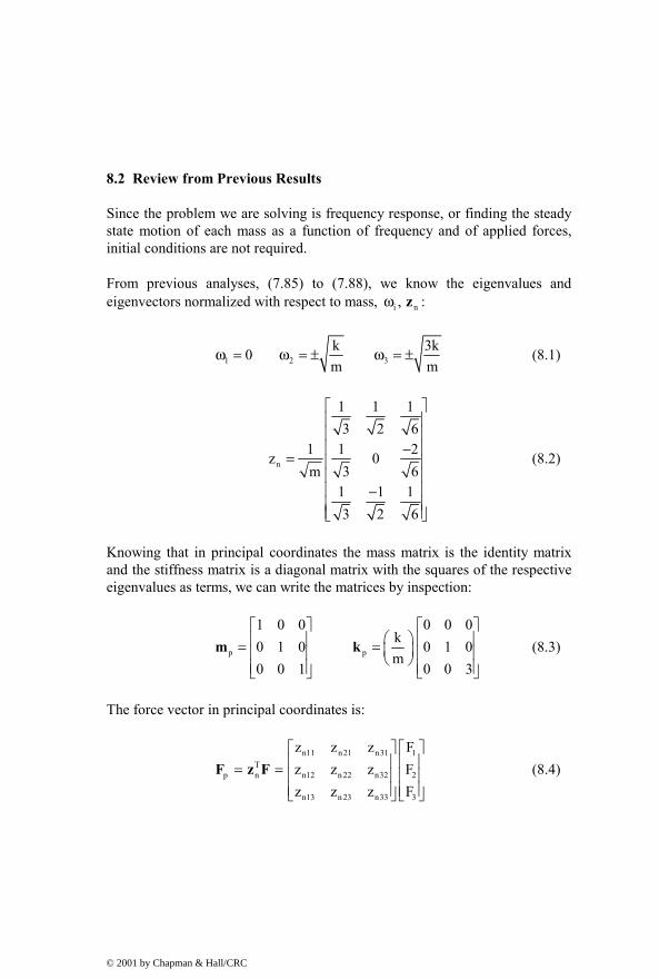
8.2 Review from Previous Results
Since the problem we are solving is frequency response, or finding the steady state motion of each mass as a function of frequency and of applied forces, initial conditions are not required.
From previous analyses, (7.85) to (7.88), we know the eigenvalues and eigenvectors normalized with respect to mass, i n,ω z :
1 2 3k 3k0m m
ω = ω = ± ω = ± (8.1)
n
1 1 13 2 6
1 1 2z 0m 3 6
1 1 13 2 6
−= −
(8.2)
Knowing that in principal coordinates the mass matrix is the identity matrix and the stiffness matrix is a diagonal matrix with the squares of the respective eigenvalues as terms, we can write the matrices by inspection:
p p
1 0 0 0 0 0k0 1 0 0 1 0m
0 0 1 0 0 3
= =
m k (8.3)
The force vector in principal coordinates is:
n11 n21 n31 1T
p n n12 n22 n32 2
n13 n23 n33 3
z z z Fz z z Fz z z F
= =
F z F (8.4)
© 2001 by Chapman & Hall/CRC

Expanding:
p1 n11 1 n21 2 n31 3
p2 n12 1 n22 2 n32 3
p1 n13 1 n23 2 n33 3
F z F z F z F
F z F z F z F
F z F z F z F
= + +
= + +
= + +
(8.5a,b,c)
Performing the actual problem multiplication:
31 2
1 p1T 31
p n 2 p2
3 p331 2
FF F1 1 13 3 33 3 3 F F
FF1 1 1 10 F 0 Fm 2 2 m 2 2F F
1 2 1 FF 2F6 6 6 6 6 6
+ + − = = = + − = − − +
F z F
(8.6)
Writing the resulting equations of motion in principal coordinates in matrix form:
31 2
p1 p131
p2 p2
p3 p331 2
FF F3 3 31 0 0 z 0 0 0 z
FFk 10 1 0 z 0 1 0 z 0m m 2 20 0 1 z 0 0 3 z
FF 2F6 6 6
+ + + = + −
− +
&&
&&
&&
(8.7)
Writing out the equations in expanded form:
( )p1 1 2 3 p11z F F F F3m
= + + =&& (8.8)
© 2001 by Chapman & Hall/CRC

( ) 2p2 p2 1 3 p2 2
k 1 kz z F F Fm m2m
+ = − = = ω&& (8.9)
( ) 2p3 p3 1 2 3 p3 3
3k 1 3kz z F 2F F Fm m6m
+ = − + = = ω&& (8.10)
8.3 Transfer Functions – Laplace Transforms in Principal Coordinates
We now solve for the transfer functions. Taking the Laplace transform of each equation, ignoring initial conditions and collecting the displacement terms, where p1z (s) is the Laplace transform of p1z (Appendix 2):
( )
( ) ( )
( ) ( )
2p1 1 2 3
2 2p2 2 1 3
2 2p3 3 1 2 3
1s z (s) F (s) F (s) F (s)3m1z (s) s F (s) F (s)2m
1z (s) s F (s) 2F (s) F (s)6m
= + +
+ ω = −
+ ω = − +
(8.11a,b,c)
Solving for the three principal displacements and eliminating the “(s)” for simplicity:
( )
( ) ( )( ) ( )
p1 1 2 3 2
p2 1 3 2 22
p3 1 2 3 2 23
1z F F Fs 3m1z F F
s 2m
1z F 2F Fs 6m
= + +
= −+ ω
= − ++ ω
(8.12a,b,c)
Taking the forces one at a time, the elements of a transfer function matrix can be defined.
p1
21
p1
22
p1
23
z 1F s 3mz 1F s 3mz 1F s 3m
=
=
=
(8.13a,b,c)
© 2001 by Chapman & Hall/CRC

( )
( )
p2
2 21 2
p2
2
p2
2 23 2
z 1F s 2m
z0
Fz 1F s 2m
=+ ω
=
−=+ ω
(8.14a,b,c)
( )
( )
( )
p3
2 21 3
p3
2 22 3
p3
2 23 3
z 1F s 6m
z 2F s 6m
z 1F s 6m
=+ ω
−=+ ω
=+ ω
(8.15a,b,c)
Writing out the principal coordinate transfer functions for each external force, F1, F2, and F3:
( )
( )
p1
21
p11p p2
p212 21 1 2
p31p3
2 21 3
z 1F s 3m z
z z 1 zF F s 2m z
z 1F s 6m
= = = + ω + ω
(8.16)
( )
p1
2 2p12
p p2p22
2 2p32
p3 2 23
2
z1F
zs 3mz z0 z
F F2 z
zs 6m
F
= = = − + ω
(8.17)
© 2001 by Chapman & Hall/CRC

( )
( )
p1
23
p13p p2
p232 23 3 2
p33p3
2 23 3
z 1F s 3m z
z z 1 zF F s 2m z
z 1F s 6m
− = = = + ω + ω
(8.18)
8.4 Back-Transforming Mode Contributions to Transfer Functions in Physical Coordinates
Now the transfer functions in principal coordinates can be back-transformed to physical coordinates. This allows one to see the contributions of each mode, where ijz is the physical displacement at dof “ i ” due to a force at dof “j.”
n11 n12 n13 p11 p12 p13 11 12 13
n p n21 n22 n23 p21 p22 p23 21 22 23
n31 n32 n33 p31 p32 p33 31 32 33
z z z z z z z z zz z z z z z z z zz z z z z z z z z
= = =
z z z (8.19)
The equations below show how the results from each of the principal equations (modes) combine to give the overall response. The overall transfer function is seen to be a combination of the three modes of vibration and is referred to as the “modal form.”
1n11 p11 n12 p21 n13 p31
1 1st mode 2nd mode 3rd mode
zz z z z z z
F= + +123 14243 14243
contributions to total 1
1
zF
transfer function.
2n21 p11 n22 p21 n23 p31
1 1st mode 2nd mode 3rd mode
zz z z z z z
F= + +14243 14243 14243
contributions to total 2
1
zF
transfer function.
3n31 p11 n32 p21 n33 p31
1 1st mode 2nd mode 3rd mode
zz z z z z z
F= + +123 14243 14243
contributions to total 3
1
zF
transfer function.
1n11 p12 n12 p22 n13 p32
2 1st mode 2nd mode 3rd mode
zz z z z z z
F= + +123 14243 14243
contributions to total 1
2
zF
transfer function.
© 2001 by Chapman & Hall/CRC

2n21 p12 n22 p22 n23 p32
2 1st mode 2nd mode 3rd mode
zz z z z z z
F= + +14243 14243 14243
contributions to total 2
2
zF
transfer function.
3n31 p12 n32 p22 n33 p32
2 1st mode 2nd mode 3rd mode
zz z z z z z
F= + +14243 14243 14243
contributions to total 3
2
zF
transfer function.
1n11 p13 n12 p23 n13 p33
3 1st mode 2nd mode 3rd mode
zz z z z z z
F= + +123 14243 14243
contributions to total 1
3
zF
transfer function.
2n21 p13 n22 p23 n23 p33
3 1st mode 2nd mode 3rd mode
zz z z z z z
F= + +14243 14243 14243
contributions to total 2
3
zF
transfer function.
3n31 p13 n32 p23 n33 p33
3 1st mode 2nd mode 3rd mode
zz z z z z z
F= + +14243 14243 14243
contributions to total 3
3
zF
transfer function.
We saw earlier that because of symmetry there are only four distinctly different transfer functions of the total of nine:
31 2 2
1 1 1 2
zz z z, , and F F F F
Expanding the four transfer functions:
p11 p21 p311
1
z z zz 1F m 3 2 6
= + +
( ) ( )2 2 2 2 22 3
1 1 1 1m s 3m 3 s 2m 2 s 6m 6
= + +
+ ω + ω
( ) ( ) ( )2 2 2 2 2
2 3
1 1 1s 3m s 2m s 6m
= + ++ ω + ω
© 2001 by Chapman & Hall/CRC

2 2 2 2 22 3
1 1 13m 2m 6ms s s
= + +
+ ω + ω (8.20)
( )2
2 2 21 3
z 1 1 20F m s 3m 3 s 6m 6
= + −
+ ω
2 2 23
1 23m 6m0s s
= + −
+ ω (8.21)
( ) ( )3
2 2 2 2 21 2 3
z 1 1 1 1F m s 3m 3 s 2m 2 s 6m 6
= − +
+ ω + ω
2 2 2 2 22 3
1 1 13m 2m 6ms s s
= − +
+ ω + ω (8.22)
( )2
2 2 22 3
z 1 1 40F m s 3m 3 s 6m 6
= + +
+ ω
2 2 23
1 43m 6m0s s
= + +
+ ω (8.23)
Taking m k 1= = yields: 2 2 21 2 3
k 3k0, 1, 3,m m
ω = ω = = ω = = and
substituting above:
12 2 2
1
1 11z 3 62F s s 1 s 3
= + ++ +
(8.24)
22 2
1
1 1z 3 3F s s 3
= −+
(8.25)
© 2001 by Chapman & Hall/CRC

32 2 2
1
1 11z 3 62F s s 1 s 3
= − ++ +
(8.26)
22 2
2
1 2z 3 3F s s 3
= ++
(8.27)
8.5 Partial Fraction Expansion and the Modal Form
Another way of finding the modal form (not as insightful, but does not require solving the eigenvalue problem) is to take the original transfer functions derived in the Chapter 2 and perform a partial fraction expansion. Partial fraction expansion gives the same results as the modal form in Section 8.4. The four unique transfer functions from (2.62) to (2.65) are repeated below:
( )2 4 2 2
12 3 4 2 2 2
1
z m s 3mks kF s m s 4m ks 3mk
+ +=+ +
(8.28)
22 2 2
1
z kF s (m s 3km)
=+
(8.29)
( )2
32 3 4 2 2 2
1
z kF s m s 4m ks 3mk
=+ +
(8.30)
( )2 4 2 2
22 3 4 2 2 2
2
z m s 2mks kF s m s 4m ks 3mk
+ +=+ +
(8.31)
In order to perform a partial fraction expansion, we need the roots of the characteristic equation, found earlier to be:
2 2 21 2 3
k 3k0m m
ω = ω = ω = (8.32)
Taking the 1 1z / F transfer function and expanding in partial fraction form, setting m = k = 1;
© 2001 by Chapman & Hall/CRC

( )2 4 2 2 4 2 4 2
12 4 2 2 2 2 2 22 3 4 2 2 2
1 2 3
4 2
2 2 2 2 2 2 2 2 2 2 22 3 1 2 3
z m s 3mks k s 3s 1 s 3s 1F s (s 4s 3) s (s )(s )s m s 4m ks 3mk
s 3s 1 A B Cs (s )(s ) s s s
+ + + + + += = =+ + + ω + ω+ +
+ + = + ++ ω + ω + ω + ω + ω
(8.33a,b)
The terms A, B and C, known as “residues,” are evaluated using the “cover-up” method, where each coefficient is evaluated by “covering up” its term in the transfer function and evaluating the remaining expression at 2 2
is = − ω .
Evaluating A:
4 22 2
12 2 2 22 3
2 22 3
s 3s 1A evaluated at s 0(s )(s )
1 1 1(1)(3) 3
+ += = −ω =+ ω + ω
= = =ω ω
(8.34)
Evaluating B:
4 22 2
22 2 23
4 22 22 2 22 2 3
s 3s 1B evaluated at s 1s (s )
3 1 1 3 1 1 11( 1 3) 2 2( )
+ += = −ω = −+ ω
ω − ω + − + −= = = =− − + −−ω −ω + ω
(8.35)
© 2001 by Chapman & Hall/CRC

Evaluating C:
4 22 2
32 2 2 2 22 3
4 2 23 32 2 23 3 2
s 3s 1C evaluated at s 3s (s )(s )
3 1 3 3( 3) 1 13( 3 1) 6( )
+ += = −ω = −+ ω + ω
ω − ω + − − += = =− − +−ω −ω + ω
(8.36)
Combining terms:
4 21
2 2 2 2 2 2 2 2 2 2 21 2 3 1 2 3
1 1 1z s 3s 1 3 2 6F s (s )(s ) s s s
+ + = = + +
+ ω + ω + ω + ω + ω (8.37)
This expression is the same as the term for 1 1z / F in (8.20). Converting the other three transfer functions to partial fraction form also reveals their modal form.
8.6 Forcing Function Combinations to Excite Single Mode
It is instructive at this point to see what types of forcing function combinations will excite each of the three modes separately. From the definition of normal modes, we know that if the system is started from initial displacement conditions that match one of the normal modes, the system will respond at only that mode. An analogous situation exists for combinations of forcing functions. Repeating the transformed equations of motion in principal coordinates from (8.12a,b,c) with m 1= .
( )
( ) ( )( ) ( )
p1 1 2 3 p12
p2 1 3 p22 22
p3 1 2 3 p32 23
1z F F F Fs 3
1z F F Fs 2
1z F 2F F Fs 6
= + + =
= − =+ ω
= − + =+ ω
(8.38a,b,c)
To excite only the first mode, we can start with initial displacements being any multiple of the first eigenvector, which has equal displacements for all masses.
© 2001 by Chapman & Hall/CRC

Now let us see if applying equal forces to all three masses with zero initial conditions excites only the first mode. Set 1 2 3F F F 0= = ≠ , which should excite only the first, rigid body mode:
( )
( ) ( )( ) ( )
p1 1 2 3 12 2
p2 1 3 2 22
p3 1 2 3 2 23
1 1z F F F 3Fs 3 s 3
1z F F 0s 2
1z F 2F F 0s 6
= + + =
= − =+ ω
= − + =+ ω
(8.39a,b,c)
We can see above that the motion for the second and third modes is zero. It is the information contained in the eigenvector, which, when multiplied by the force vector in physical coordinates, determines the force vector in principal coordinates.
To excite the second mode only, applying zero force at mass 1 and equal and opposite sign forces at masses 1 and 2 should work: 1 3 2F F , F 0:= − =
( )
( ) ( ) ( )( ) ( )
p1 1 2 3 2
p2 1 3 12 2 2 22 2
p3 1 2 3 2 23
1z F F F 0s 3
1 1z F F 2Fs 2 s 2
1z F 2F F 0s 6
= + + =
= − =+ ω + ω
= − + =+ ω
(8.40a,b,c)
In this case the combination of the eigenvectors and forcing function signs cancel out the first and third modes, leaving only the second mode.
To excite the third mode only, applying the same force to masses 1 and 3 and twice the force with opposite sign to mass 2 should work: 1 3 2 1F F , F 2F := = −
© 2001 by Chapman & Hall/CRC

( )
( ) ( )( ) ( ) ( )
p1 1 2 3 2
p2 1 3 2 22
p3 1 2 3 12 2 2 23 3
1z F F F 0s 3
1z F F 0s 2
1 1z F 2F F 6Fs 6 s 6
= + + =
= − =+ ω
= − + =+ ω + ω
(8.41a,b,c)
In this case the combination of the eigenvectors and forcing function signs cancel out the first and second modes, leaving only the third mode.
8.7 How Modes Combine to Create Transfer Functions
We have shown that both the normal mode method and partial fraction expansion of transfer functions yield additive combinations of sdof systems for the overall response. The purpose of this section is to develop a general equation for any transfer function, again showing that the system frequency response is an additive combination of sdof systems. Each sdof system has a gain determined by the appropriate eigenvector entries and a resonant frequency given by the appropriate eigenvalue.
The three equations of motion in principal coordinates are:
2p1 1 p1 p1
2p2 2 p2 p2
2p3 3 p3 p3
z z F
z z F
z z F
+ ω =
+ ω =
+ ω =
&&
&&
&&
(8.42a,b,c)
2 2 21 2 3
k 3k0m m
ω = ω = ω = (8.43a,b,c)
Where the forces in principal coordinates are given by:
n11 n21 n31 1T
p n n12 n22 n32 2
n13 n23 n33 3
n11 1 n21 2 n31 3
n12 1 n22 2 n32 3
n13 1 n23 2 n33 3
z z z Fz z z Fz z z F
z F z F z Fz F z F z Fz F z F z F
= =
+ + = + + + +
F z F
(8.44)
© 2001 by Chapman & Hall/CRC

Taking the Laplace transform of the differential equations (8.42a,b,c) and dividing by the coefficients of each principal displacement:
p1 n11 1 n21 2 n31 32 2 2 2
1 1p1
p2 n12 1 n22 2 32 3p p2 2 2 2 2
2 2p3
p3 n13 1 n23 2 n33 32 22 2
33
F z F z F z Fs s
zF z F z F z F
zs s
zF z F z F z F
ss
+ + + ω + ω + + = = = + ω + ω + +
+ ω + ω
z (8.45)
The equation above shows how the individual eigenvector matrix elements contribute to the displacements in principal coordinates.
Since we are only interested in SISO transfer functions that arise from a force applied to a single dof, we will look at the 1 2 3F , F , F cases individually.
For force 1F :
p1 n11 12 2 2 2
1 1p1
p2 n12 1p p2 2 2 2 2
2 2p3
p3 n13 12 22 2
33
F z Fs s
zF z Fz
s sz
F z Fss
+ ω + ω = = = + ω + ω
+ ω + ω
z (8.46)
For force 2F :
p1 n21 22 2 2 2
1 1p1
p2 n22 2p p2 2 2 2 2
2 2p3
p3 n23 22 22 2
33
F z Fs s
zF z Fz
s sz
F z Fss
+ ω + ω = = = + ω + ω
+ ω + ω
z (8.47)
© 2001 by Chapman & Hall/CRC

For force 3F
p1 n31 32 2 2 2
1 1p1
p2 32 3p p2 2 2 2 2
2 2p3
p3 n33 32 22 2
33
F z Fs s
zF z F
zs s
zF z F
ss
+ ω + ω = = = + ω + ω
+ ω + ω
z (8.48)
The equations for displacements in physical coordinates are found by premultiplying the above three equations by nz (7.107).
For 1F :
n13 n13 1n11 n11 1 n12 n12 12 2 2 2 2 2
1 2 31
n23 n13 1n21 n11 1 n22 n12 12 2 2 2 2 2 2
1 2 33
n31 n11 1 n32 n12 1 n33 n13 12 2 2 2 2 2
1 2 3
z z Fz z F z z Fs s s
zz z Fz z F z z Fz
s s sz
z z F z z F z z Fs s s
+ + + ω + ω + ω = = + + + ω + ω + ω + +
+ ω + ω + ω
z (8.49)
Dividing by 1F :
n13 n13n11 n11 n12 n1212 2 2 2 2 2
1 2 31
n23 n132 n21 n11 n22 n122 2 2 2 2 2
1 1 1 2 3
3 n31 n11 n32 n12 n33 n132 2 2 2 2 2
1 1 2 3
z zz z z zzs s sF
z zz z z z zF F s s s
z z z z z z zF s s s
+ + + ω + ω + ω
= = + + + ω + ω + ω
+ +
+ ω + ω + ω
z (8.50)
© 2001 by Chapman & Hall/CRC

Similarly for 1 2F and F :
n13 n23n11 n21 n12 n2212 2 2 2 2 2
1 2 32
n23 n232 n21 n21 n22 n222 2 2 2 2 2
2 2 1 2 3
3 n31 n21 n32 n22 n33 n232 2 2 2 2 2
2 1 2 3
z zz z z zzs s sF
z zz z z z zF F s s s
z z z z z z zF s s s
+ + + ω + ω + ω
= = + + + ω + ω + ω
+ +
+ ω + ω + ω
z (8.51)
n11 n31 n12 n32 n13 n3312 2 2 2 2 2
1 2 33
n21 n31 n22 n32 n23 n3322 2 2 2 2 2
3 3 1 2 3
3 n31 n31 n32 n32 n33 n332 2 2 2 2 2
3 1 2 3
z z z z z zzs s sFz z z z z zz
F F s s sz z z z z z zF s s s
+ + + ω + ω + ω
= = + +
+ ω + ω + ω
+ + + ω + ω + ω
z (8.52)
The nine transfer functions above may be generalized by the following equation. For the transfer function with the force applied at dof “k,” the displacement taken at dof “j” and for mode “i”:
j nj1 nk1 nj2 nk2 nj3 nk32 2 2 2 2 2
k 1 2 3
z z z z z z zF s s s
= + ++ ω + ω + ω
(8.53)
Rewriting in summation form, and generalizing from our tdof system to a general system where “m” is the total number of modes for the system for an undamped (8.54a) and damped (8.54b) system:
mj nji nki
2 2i 1k i
mj nji nki
2 2i 1k i i i
z z zF s
z z zF s 2 s
=
=
=+ ω
=+ ζ ω + ω
∑
∑
(8.54a,b)
Equations (8.54a,b) shows that in general every transfer function is made up of additive combinations of single degree of freedom systems, with each system having its dc gain (transfer function evaluated with s = j0) determined by the appropriate eigenvector entry product divided by the
© 2001 by Chapman & Hall/CRC

square of the eigenvalue, 2nji nki iz z / ω , and with resonant frequency
defined by the appropriate eigenvalue, iω .
For our tdof system, substituting for the iω values:
j nj1 nk1 nj2 nk2 nj3 nk32 2 2
k
z z z z z z zF s s k / m s 3k / m
= + ++ +
(8.55)
This equation makes the graphical combining of modal contributions to the final transfer function more clear. The contribution of each mode is a simple harmonic oscillator at frequency iω with dc gain 2
nji nki iz z / ω , where “ i ” is the mode number.
8.8 Plotting Individual Mode Contributions
Taking 1 1z / F for example, the separate contributions of each mode to the total response can be plotted as follows. First we calculate the DC response of the non-rigid body mode:
Rigid body response: at ω = 0.1 rad/sec z111 = 10.03
= 33.33 = 30.457 db,
slope = –2 Now we calculate the dc gain of the non-rigid body modes:
Second mode response: at DC , z112 = 12
= 0.5 = –6db, slope = 0
resonance at 22 1ω = , slope at ∞ = –2
Third mode response: at DC , z113 = 118
= 0.0555 = –25.1db, slope = 0
resonance at 23 3ω = , slope at ∞ = –2, where the
“ijk” notation in zijk indicates: dof “i,” due to force “j,” for mode k.
Thus, the total response is defined by the additive combination of three single degree of freedom responses, each with its own spring-dominated low
© 2001 by Chapman & Hall/CRC

frequency section, damping dominated resonant section and mass dominated high frequency section.
The MATLAB code tdof_modal_xfer.m is used to calculate and plot the individual mode contributions to the overall frequency response of all four unique transfer functions for the tdof model. The program plots the frequency responses using several different magnitude scalings. We will discuss below the results for the 1 1z / F frequency response, using plots from the MATLAB code to illustrate. The notation “z113” below signifies the transfer function z1/F1 for mode 3, and so forth.
10-1 100 101
-60
-50
-40
-30
-20
-10
0
10
20
30
40Transfer Function - z111, z112, z113 and z11 Magnitude
(-)
(+)
(+)
Frequency, rad/sec
Mag
nitu
de, d
b
z111-1st Modez112-2nd Modez113-3rd Modez11-Total
Figure 8.2: z11 transfer function frequency response plot with individual mode contributions overlaid.
Figure 8.2 shows the overall 1 1z / F (z11) transfer function and the individual modal contributions which add to create it. Because the magnitude scale in Figure 8.2 is in log or “db” units, the individual mode contributions cannot be added graphically. To add graphically requires a linear magnitude axis. We cannot use the log magnitude or db scale for adding directly because adding with log or db coordinates is equivalent to the multiplication of responses, not addition.
There is zero damping in this model, so the amplitudes at the two poles in Figure 8.2 should go to infinity. The peak amplitudes do not go to infinity because they are limited by the resolution of the frequency scale chosen for the plot. The two zeros should go to zero, but once again they do not because of the frequency resolution chosen.
© 2001 by Chapman & Hall/CRC

Figures 8.3 and 8.4 show the same frequency responses plotted on a linear magnitude scale.
10-1 100 1010
5
10
15
20
25
30
35Transfer Function - z111, z112, z113 and z11 Linear Magnitude
(-)
(+)(+)
Frequency, rad/sec
Mag
nitu
de
z111-1st Modez112-2nd Modez113-3rd Modez11-Total
Figure 8.3: z11 frequency response and modal contributions plotted with linear magnitude scale.
Figure 8.4 uses an expanded magnitude axis to more clearly show how the three individual mode sdof responses combine graphically to create the overall frequency response. It also contains notation that shows how the signs change through the resonance. In Chapter 3 we learned how to sketch frequency response plots by hand, knowing the high and low frequency asymptotes and the locations of the poles and zeros. Similarly, we can combine modes by hand if we know the signs (phases) of the individual modes that are being combined. In our tdof example, it just so happens that the signs of the low frequency portions of the second and third modes (1.0 and 1.7 rps) were both positive. In general, it is not the case that all low frequency signs will be positive (see the z31 example below). The discussion below will show how to define the sign (phase) of the low frequency portion of each mode by knowing the signs of the eigenvector entries for the input and output degrees of freedom.
© 2001 by Chapman & Hall/CRC

10-1 100 1010
0.5
1
1.5
2
2.5
3Transfer Function - z111, z112, z113 and z11 Linear Magnitude
(+)
(+)
Frequency, rad/sec
Mag
nitu
de
z111-1st Modez112-2nd Modez113-3rd Modez11-Total
"-" signrigid-body
mode
"+" signbefore
resonance1 rps mode
"+" signbeforeresonance1.7 rpsmode
"-" sign afterresonance1 rps mode
poleat 1 rps
poleat 1.7 rps
"-" sign afterresonance1.7 rpsmode
"+" signbeforeresonance1 rps mode
"+" signbeforeresonance1.7 rpsmode
zero at1.62 rps
zero at0.62 rps
Figure 8.4: z11 frequency response with expanded magnitude scale to see contributors to
the zeros.
Since the phase at frequencies much lower than the resonant frequency is zero for a spring mass sdof system (2.19b), and since each mode in principal coordinates is a sdof system, the phase for each mode contribution to the overall response at low frequency is given by the sign of the eigenvector for the dof whose displacement is desired times the sign of the dof where the force is applied. For the three modes and the transfer function z11, where we are interested in measuring the displacement of mass 1 and in the force being applied to mass 1, the signs for the three modes at low frequencies are found as follows. The normalized modal matrix is repeated to see the signs of the entries:
© 2001 by Chapman & Hall/CRC

Mode 1 Mode 2 Mode 3
dof 1 −0.5774 −0.7071 0.4082
dof2 −0.5774 0.0000 −0.8165
dof3 −0.5774 0.7071 0.4082
Table 8.1: Normalized modal matrix.
Sign of mode 1 low frequency asymptote for z11 frequency response:
dof 1, mode 1: 0.5774− ( )−
dof 1, mode 1: 0.5774− 4 ( )−
Low frequency sign (phase) = ( )− times ( )− = (+), but since resonance is rigid body at zero rad/sec, all frequencies of interest to us are “after resonance” and thus the sign is ( )− because the phase is
180− o .
Sign of mode 2 low frequency asymptote for z11 frequency response:
dof 1, mode 2: 0.7071− ( )−
dof 1, mode 2: 0.7071− ( )−
Low frequency sign (phase) = ( )− times ( )− = ( )+ , 0o
Sign of mode 3 low frequency asymptote for z11 frequency response:
dof 1, mode 3: +0.4082 ( )−
dof 1, mode 3: +0.4082 ( )−
Low frequency sign (phase) = (+) times (+) = (+), 0o
As mentioned earlier, the signs of the low frequency portions of the second and third modes were both (+). The signs of the eigenvector entries above show why this was the case.
© 2001 by Chapman & Hall/CRC
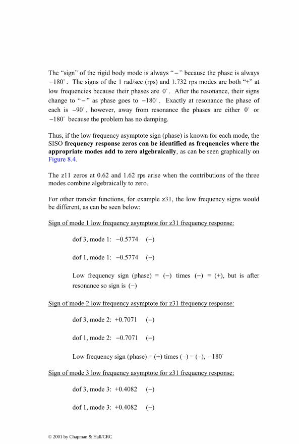
The “sign” of the rigid body mode is always “ − ” because the phase is always 180− o . The signs of the 1 rad/sec (rps) and 1.732 rps modes are both “+” at
low frequencies because their phases are 0o . After the resonance, their signs change to “ − ” as phase goes to 180− o . Exactly at resonance the phase of each is 90− o , however, away from resonance the phases are either 0o or
180− o because the problem has no damping.
Thus, if the low frequency asymptote sign (phase) is known for each mode, the SISO frequency response zeros can be identified as frequencies where the appropriate modes add to zero algebraically, as can be seen graphically on Figure 8.4.
The z11 zeros at 0.62 and 1.62 rps arise when the contributions of the three modes combine algebraically to zero.
For other transfer functions, for example z31, the low frequency signs would be different, as can be seen below:
Sign of mode 1 low frequency asymptote for z31 frequency response:
dof 3, mode 1: 0.5774− ( )−
dof 1, mode 1: 0.5774− ( )−
Low frequency sign (phase) = ( )− times ( )− = (+), but is after resonance so sign is ( )−
Sign of mode 2 low frequency asymptote for z31 frequency response:
dof 3, mode 2: +0.7071 ( )−
dof 1, mode 2: 0.7071− ( )−
Low frequency sign (phase) = (+) times (−) = (−), 180− o
Sign of mode 3 low frequency asymptote for z31 frequency response:
dof 3, mode 3: +0.4082 ( )−
dof 1, mode 3: +0.4082 ( )−
© 2001 by Chapman & Hall/CRC

Low frequency sign (phase) = (+) times (+) = (+), 0o
Now that the low frequency phases of the individual modes are defined, we can follow the combining of modes to get the overall response, indicated by the “+” signs.
Because we are dealing with a linear magnitude axis above, we can graphically add or subtract the contribution of each to get the overall response.
To get the overall response we combine the amplitudes of each mode depending on its sign. For example, at 0.4 rad/sec frequency, we combine the amplitude of the rigid body mode with a negative sign with the two oscillatory modes, each of which has a positive sign:
Rigid body response: at ω = 0.4 rad/sec, 1 0ω = :
111 2 2 2 2
1 1 1 1z 2.0833s 3( j ) 3 3(0.4)
− −= = = = = −ω ω
(8.56)
Second mode response: at ω = 0.4 rad/sec, 2 1ω = :
112 2 2 2 2 2 2 22 2 2
1 1 1 1z 0.5952(s ) 2 ( j ) 2 2 (0.4) 1
= = = = =+ ω ω + ω −ω + ω − +
(8.57)
Third mode response: at ω = 0.4 rad/sec, 3 1.732ω = :
113 2 2 2 2 2 2 23 3 3
1 1 1 1z 0.05866(s ) 6 ( j ) 6 6 (0.4) 3
= = = = =+ ω ω + ω −ω + ω − +
(8.58)
Adding (with proper signs) the three contributions at 0.4 rad/sec gives the amplitude and phase of the overall response at 0.4 rad/sec:
2.083 0.595 0.0586 1.4294− + + = − (8.59)
The amplitude is 1.4294 and the phase is 180− o , as indicated by the negative sign. Because the model has no damping, each mode has 0o phase before
© 2001 by Chapman & Hall/CRC

resonance and immediately after resonance switches phase to 180− o . Exactly at resonance the amplitudes are theoretically infinite.
Let us now track what happens at the frequency of the first zero, which we showed in (2.85) to be 0.618 rad/sec. We will carry out the same calculations as above for a frequency of 0.618 rad/sec:
Rigid body response: at ω = 0.618 rad/sec, 1 0ω = :
111 2 2 2 2
1 1 1 1z 0.87273s 3( j ) 3 3(0.618)
− −= = = = = −ω ω
(8.60)
Second mode response: at ω = 0.618 rad/sec, 2 1ω = :
112 2 2 2 2 22 2
1 1 1z 0.80892(s ) 2 ( j ) 2 (0.618) 1
= = = =+ ω ω + ω − +
(8.61)
Third mode response: at ω = 0.618 rad/sec, 3 1.732ω = :
113 2 2 2 2 23 3
1 1 1z 0.06366(s ) 6 ( j ) 6 (0.618) 3
= = = =+ ω ω + ω − +
(8.62)
Adding (with proper signs) the three contributions gives the amplitude and phase of the overall response at 0.618 rad/sec:
0.8727 0.8089 0.0636 0.0002 0− + + = − ≅ (8.63)
The amplitude is –0.0002. With greater accuracy in the values used for the eigenvalues and the frequency of the zero, the solution would have been exactly zero.
In Chapter 2, we showed that the zeros for SISO transfer functions arose from the roots of the numerator. The modal analysis method shows another explanation of how zeros of transfer functions arise: when modes combine with appropriate signs (phases) it is possible at some frequencies to have no motion.
We will calculate the response at one more frequency to show how the phase changes for a mode when the frequency is higher than the resonant frequency.
© 2001 by Chapman & Hall/CRC

We will choose a frequency of 1.3 rad/sec, which is higher than the second mode but lower than the third mode. We should see that the sign of the contribution for the second mode changes sign from positive to negative. Signs for the first and third mode should remain unchanged.
Rigid body response: at ω = 1.3 rad/sec, 1 0ω = :
111 2 2 2 2
1 1 1 1z 0.19723s 3( j ) 3 3(1.3)
− −= = = = = −ω ω
(8.64)
Second mode response: at ω = 1.3 rad/sec, 2 1ω = :
112 2 2 2 2 22 2
1 1 1z 0.72462(s ) 2 ( j ) 2 (1.3) 1
= = = = −+ ω ω + ω − +
(8.65)
Third mode response: at ω = 1.3 rad/sec, 3 1.732ω = :
113 2 2 2 2 23 3
1 1 1z 0.12726(s ) 6 ( j ) 6 (1.3) 3
= = = =+ ω ω + ω − +
(8.66)
Adding (with proper signs) the three contributions at 1.3 rad/sec gives the amplitude and phase of the overall response at 1.3 rad/sec:
0.1972 0.7246 0.1272 0.7946− − + = − (8.67)
The amplitude is 0.7946 and the phase is 180− o . Note that the sign of the second mode contribution changed from positive to negative when the resonant frequency was passed.
The same calculations can be repeated for any desired frequency. Also, knowing the high and low frequency asymptotes, their signs and resonant frequencies, one can plot the overall frequency response roughly by hand, similar to what was done in Section 3.3. Here, unlike the previous hand plotting, we have not calculated any zeros; they occur by additive combinations of individual modes.
© 2001 by Chapman & Hall/CRC
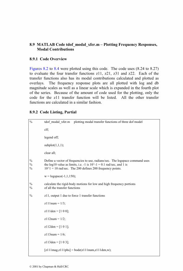
8.9 MATLAB Code tdof_modal_xfer.m – Plotting Frequency Responses, Modal Contributions
8.9.1 Code Overview
Figures 8.2 to 8.4 were plotted using this code. The code uses (8.24 to 8.27) to evaluate the four transfer functions z11, z21, z31 and z22. Each of the transfer functions also has its modal contributions calculated and plotted as overlays. The frequency response plots are all plotted with log and db magnitude scales as well as a linear scale which is expanded in the fourth plot of the series. Because of the amount of code used for the plotting, only the code for the z11 transfer function will be listed. All the other transfer functions are calculated in a similar fashion.
8.9.2 Code Listing, Partial
% tdof_modal_xfer.m plotting modal transfer functions of three dof model clf; legend off; subplot(1,1,1); clear all; % Define a vector of frequencies to use, radians/sec. The logspace command uses % the log10 value as limits, i.e. -1 is 10^-1 = 0.1 rad/sec, and 1 is % 10^1 = 10 rad/sec. The 200 defines 200 frequency points. w = logspace(-1,1,150); % calculate the rigid-body motions for low and high frequency portions % of all the transfer functions % z11, output 1 due to force 1 transfer functions z111num = 1/3; z111den = [1 0 0]; z112num = 1/2; z112den = [1 0 1]; z113num = 1/6; z113den = [1 0 3]; [z111mag,z111phs] = bode(z111num,z111den,w);
© 2001 by Chapman & Hall/CRC

[z112mag,z112phs] = bode(z112num,z112den,w); [z113mag,z113phs] = bode(z113num,z113den,w); if abs(z111phs(1)) >= 10 z111text = '(-)'; else z111text = '(+)'; end if abs(z112phs(1)) >= 10 z112text = '(-)'; else z112text = '(+)'; end if abs(z113phs(1)) >= 10 z113text = '(-)'; else z113text = '(+)'; end z111magdb = 20*log10(z111mag); z112magdb = 20*log10(z112mag); z113magdb = 20*log10(z113mag); % calculate the complete transfer function z11 = ((1/3)./((j*w).^2) + ((1/2)./((j*w).^2 + 1)) + ((1/6)./((j*w).^2 + 3))); z11mag = abs(z11); z11magdb = 20*log10(z11mag); z11phs = 180*angle(z11)/pi ; % truncate peaks for microsoft word plotting of expanded linear scale z11plotmag = z11mag; z111plotmag = z111mag;
© 2001 by Chapman & Hall/CRC

z112plotmag = z112mag; z113plotmag = z113mag; for cnt = 1:length(z11mag) if z11plotmag(cnt) >= 3.0 z11plotmag(cnt) = 3.0; end if z111plotmag(cnt) >= 3.0 z111plotmag(cnt) = 3.0; end if z112plotmag(cnt) >= 3.0 z112plotmag(cnt) = 3.0; end if z113plotmag(cnt) >= 3.0 z113plotmag(cnt) = 3.0; end end % plot the three modal contribution transfer functions and the total using % log magnitude versus frequency loglog(w,z111mag,'k+-',w,z112mag,'kx-',w,z113mag,'k.-',w,z11mag,'k-') title('Transfer Functions - z111, z112, z113 and z11 magnitude') legend('z111-1st Mode','z112-2nd Mode','z113-3rd Mode','z11-Total') text(.11,1.2*z111mag(1),z111text) text(.11,1.2*z112mag(1),z112text) text(.11,1.2*z113mag(1),z113text) xlabel('Frequency, rad/sec') ylabel('Magnitude') grid disp('execution paused to display figure, "enter" to continue'); pause % plot the four transfer functions using db semilogx(w,z111magdb,'k+-',w,z112magdb,'kx-',w,z113magdb,'k.-',w,z11magdb,'k-') title('Transfer Function - z111, z112, z113 and z11 Magnitude') legend('z111-1st Mode','z112-2nd Mode','z113-3rd Mode','z11-Total')
© 2001 by Chapman & Hall/CRC

text(.11,2+z111magdb(1),z111text) text(.11,2+z112magdb(1),z112text) text(.11,2+z113magdb(1),z113text) xlabel('Frequency, rad/sec') ylabel('Magnitude, db') grid disp('execution paused to display figure, "enter" to continue'); pause % plot the four transfer functions using a linear magnitude scale so that % the amplitudes can be added directly semilogx(w,z111mag,'k+-',w,z112mag,'kx-',w,z113mag,'k.-',w,z11mag,'k-') title('Transfer Function - z111, z112, z113 and z11 Linear Magnitude') legend('z111-1st Mode','z112-2nd Mode','z113-3rd Mode','z11-Total') text(.11,1.0*z111mag(1),z111text) text(.11,1.1*z112mag(1),z112text) text(.11,1.1*z113mag(1),z113text) xlabel('Frequency, rad/sec') ylabel('Magnitude') grid disp('execution paused to display figure, "enter" to continue'); pause semilogx(w,z111plotmag,'k+-',w,z112plotmag,'kx-',w,z113plotmag,' …
k.-',w,z11plotmag,'k-') title('Transfer Function - z111, z112, z113 and z11 Linear Magnitude') legend('z111-1st Mode','z112-2nd Mode','z113-3rd Mode','z11-Total') text(.11,1.0*z111mag(1),z111text) text(.11,1.1*z112mag(1),z112text) text(.11,1.1*z113mag(1),z113text) xlabel('Frequency, rad/sec') ylabel('Magnitude') axis([.1 10 0 3]); grid disp('execution paused to display figure, "enter" to continue'); pause % plot phase semilogx(w,z111phs,'k+-',w,z112phs,'kx-',w,z113phs,'k.-',w,z11phs,'k-') title('Transfer Function - z111, z112, z113 and z11 Phase') legend('z111-1st Mode','z112-2nd Mode','z113-3rd Mode','z11-Total') xlabel('Frequency, rad/sec') ylabel('Phase, Deg') grid disp('execution paused to display figure, "enter" to continue'); pause
© 2001 by Chapman & Hall/CRC

8.10 tdof Eigenvalue Problem Using ANSYS
An ANSYS solution to the tdof problem is now shown in order to start becoming familiar with how ANSYS presents its eigenvalue/eigenvector results.
8.10.1 ANSYS Code threedof.inp Description
The ANSYS code threedof.inp below is used to build the model, calculate eigenvalues and eigenvectors, output the frequency listing and eigenvectors, plot the mode shapes, calculate and plot all three transfer functions for a forcing function applied to mass 1: 1 1 2 1 3 1z / F , z / F ,and z / F . The hand calculated values for masses and stiffnesses are used, m1 = m2 = m3 = 1.0, k1 = k2 = 1.0.
To run the code, from the “begin” level in ANSYS, type “/input,threedof,inp,” and the program will run unattended. The various outputs are available as follows:
threedof.frq frequency list, ascii file
threedof.eig eigenvector list, ascii file
threedof.grp2 mode shape plots
threedof.grp1 frequency response plots
Use the ANSYS Display program to load and display the two plot files.
8.10.2 ANSYS Code Listing
/title, threedof.inp, three dof vibration class model, Ansys Version 5.5 /prep7 ! enter model preparation section ! element type definitions et,1,21 ! element type for mass et,2,14 ! element type for spring ! real value definitions r,1,1,1,1 ! mass of 1kg r,2,1 ! spring stiffness of 1mn/mm, or 1n/m ! define plotting characteristics /view,1,-1,0,0 ! z-y plane /angle,1,0 ! not iso
© 2001 by Chapman & Hall/CRC

/pnum,real,1 ! color by real /num,1 ! numbers off /type,1,0 ! hidden plot /pbc,all,1 ! show all boundary conditions csys,0 ! define global coordinate system ! nodes n,1,0,0,-1 ! left hand mass at x = -1.0 mm n,2,0,0,0 ! middle mass at x = 0 mm n,3,0,0,1 ! right hand mass at x = +1.0 mm ! define masses type,1 real,1 e,1 e,2 e,3 ! define springs type,2 real,2 e,1,2 e,2,3 ! define constraints, ux and uy zero, leaving only uz motion nsel,s,node,,1,3 d,all,ux,0 d,all,uy,0 allsel eplo ! *************** eigenvalue run ****************** fini ! fini just in case not in begin /solu ! enters the solution processor, needs to be here to do editing below allsel ! default selects all items of specified entity type, typically nodes, elements ! define masters for frequency response (transfer function) run m,1,uz m,2,uz m,3,uz antype,modal,new modopt,reduc,3 ! method – Block Lanczost expass,off ! key = off, no expansion pass, key = on, do expansion mxpand,3,,,no ! number of modes to expand
© 2001 by Chapman & Hall/CRC

total,3,1 ! total masters, all translational dof allsel solve ! starts the solution of one load step of a solution sequence, modal fini ! ***************** output frequencies ******************* /post1 /output,threedof,frq ! write out frequency list to ascii file .frq set,list /output,term ! returns output to terminal ! ***************** output eigenvectors ********************* ! define nodes for output allsel /output,threedof,eig ! write out eigenvectors to ascii file .eig *do,i,1,3 set,,i prdisp *enddo /output,term ************** plot modes ***************** /show,threedof,grp2,0 ! raster plot, 1 is vector plot, write out to graph file .grp2 allsel *do,i,1,3 set,1,i pldi,1 *enddo /show,term ! **************** calculate and plot transfer functions ****************** fini /assign,rst,junk,rst ! reassigns a file name to an ANSYS identifier /solu dmprat,0 ! sets a constant damping ratio for all modes, zeta = 0
© 2001 by Chapman & Hall/CRC

allsel eplo ! show forces applied f,1,fz,1 ! 1 mn force applied to node 1, left-hand mass /title, threedof.inp, tdof, force at mass 1 antype,harmic ! harmonic (frequency response) analysis hropt,msup,3 ! mode superposition method, nummodes modes used harfrq,0.0159,1.59 ! frequency range, hz, for solution, -1 to 10 rad/sec hrout,off,off ! amplitude/phase, cluster off kbc,1 nsubst,200 ! 200 frequency points outres,nsol,all, ! controls solution set written to database, nodal dof solution, all ! frequencies, component name for selected set of nodes solve fini /post26 file,,rfrq ! frequency response results xvar,0 ! display versus frequency lines,10000 ! specifies the length of a printed page for frequency response listing nsol,2,1,u,z,z1 ! specifies nodal data to be stored in results file ! u - displacement, z direction ! note that nsol,1 is frequency vector nsol,3,2,u,z,z2 nsol,4,3,u,z,z3 ! plot magnitude plcplx,0 /grid,1 /axlab,x,frequency, hz /axlab,y,amplitude, mm /gropt,logx,1 ! log plot for frequency /gropt,logy,1 ! log plot for amplitude /show,threedof,grp1 ! file name for storing plvar,2,3,4 /show,term
© 2001 by Chapman & Hall/CRC

! plot phase plcplx,1 /grid,1 /axlab,x,freq /axlab,y,phase, deg ! label for y axis /gropt,logx,1 ! log plot for frequency /gropt,logy,0 ! linear plot for phase /show,threedof,grp1 plvar,2,3,4 /show,term ! save ascii data to file prcplx,1 ! stores phase angle in asci file .dat /output,threedof,dat prvar,2,3,4 /output,term fini
8.10.3 ANSYS Results
Figure 8.5: ANSYS frequency responses for force at mass 1.
© 2001 by Chapman & Hall/CRC

The resulting ANSYS transfer function plot is shown in Figure 8.5, with the frequency axis in Hz, not rad/sec.
The ANSYS frequency listing from threedof.frq is shown below, in hz units:
***** INDEX OF DATA SETS ON RESULTS FILE *****
SET TIME/FREQ LOAD STEP SUBSTEP CUMULATIVE
1 0.47280E-06 1 1 1
2 0.15915 1 2 2
3 0.27566 1 3 3
Note that the rigid body mode is calculated to be 0.4726e-6, close to 0 hz. The second and third modes are calculated to be 0.15915 and 0.27566 hz, or 0.999969 and 1.732 rad/sec, respectively. This is the same as our hand-calculated results.
The ANSYS eigenvector listing from threedof.eig is below:
*DO LOOP ON PARAMETER= I FROM 1.0000 TO 3.0000 BY 1.0000 USE LOAD STEP 1 SUBSTEP 1 FOR LOAD CASE 0 SET COMMAND GOT LOAD STEP= 1 SUBSTEP= 1 CUMULATIVE ITERATION= 1 TIME/FREQUENCY= 0.47280E-06 TITLE= threedof.inp, three dof vibration class model, Ansys Version 5.5 PRINT DOF NODAL SOLUTION PER NODE ***** POST1 NODAL DEGREE OF FREEDOM LISTING ***** LOAD STEP= 1 SUBSTEP= 1 FREQ= 0.47280E-06 LOAD CASE= 0 THE FOLLOWING DEGREE OF FREEDOM RESULTS ARE IN GLOBAL COORDINATES NODE UX UY UZ ROTX ROTY ROTZ
© 2001 by Chapman & Hall/CRC

1 0.0000 0.0000 0.57735 2 0.0000 0.0000 0.57735 3 0.0000 0.0000 0.57735 MAXIMUM ABSOLUTE VALUES NODE 0 0 1 0 0 0 VALUE 0.0000 0.0000 0.57735 0.0000 0.0000 0.0000 *ENDDO INDEX= I ***** POST1 NODAL DEGREE OF FREEDOM LISTING ***** LOAD STEP= 1 SUBSTEP= 2 FREQ= 0.15915 LOAD CASE= 0 THE FOLLOWING DEGREE OF FREEDOM RESULTS ARE IN GLOBAL COORDINATES NODE UX UY UZ ROTX ROTY ROTZ 1 0.0000 0.0000 -0.70711 2 0.0000 0.0000 0.75552E-14 3 0.0000 0.0000 0.70711 MAXIMUM ABSOLUTE VALUES NODE 0 0 3 0 0 0 VALUE 0.0000 0.0000 0.70711 0.0000 0.0000 0.0000 ***** POST1 NODAL DEGREE OF FREEDOM LISTING ***** LOAD STEP= 1 SUBSTEP= 3 FREQ= 0.27566 LOAD CASE= 0 THE FOLLOWING DEGREE OF FREEDOM RESULTS ARE IN GLOBAL COORDINATES NODE UX UY UZ ROTX ROTY ROTZ 1 0.0000 0.0000 -0.40825 2 0.0000 0.0000 0.81650 3 0.0000 0.0000 -0.40825 MAXIMUM ABSOLUTE VALUES NODE 0 0 2 0 0 0 VALUE 0.0000 0.0000 0.81650 0.0000 0.0000 0.0000
The ANSYS calculated eigenvectors, the three “UZ” listings highlighted in bold type above, arranged in the modal matrix:
n
0.57735 0.707 0.40825ANSYS z 0.57735 0 0.81649
0.57735 0.707 0.40825
− − = −
(8.68)
© 2001 by Chapman & Hall/CRC

The hand-calculated modal matrix is below, only differing from the ANSYS calculated values in the arbitrary “ 1− ” multiplier for the second and third modes:
n
1 1 13 2 6 0.57735 0.707 0.40825
1 1 2z 0 0.57735 0 0.81649m 3 6 0.57735 0.707 0.40825
1 1 13 2 6
− = = − − −
(8.69)
Problems
Note: All the problems refer to the two dof system shown in Figure P2.2.
P8.1 Using the eigenvalues and eigenvectors normalized with respect to mass from P7.2 and forces 1F and 2F applied to mass 1 and mass 2, respectively, write the equations in motion and physical and principal coordinates in matrix form. Identify the components of the forcing function vector in principal coordinates – which eigenvector components and which force, 1 2F or F , are involved.
P8.2 Solve for the four transfer functions for the system of P8.1 and write them in transfer function matrix form. Separate each transfer function in principal coordinates to show p 1 p 2z / F and z / F as in (8.16).
P8.3 Back transform the transfer functions in principal coordinates to physical coordinates. Identify the contributions to the transfer function from mode 1 and from mode 2 for all transfer functions.
P8.4 Take the transfer function results of P2.2 with 1 2m m m 1= = = ,
1 2k k k 1= = = and zero damping and perform a partial fraction expansion on each transfer function. Show that the results are identical to P8.3, the modal form.
P8.5 What is the relationship between 1 2F and F in order to excite mode 1 only? To excite only mode 2?
© 2001 by Chapman & Hall/CRC

P8.6 Plot by hand the individual mode contributions to the 2 1z / F frequency response for zero damping. Note the sign of the dc gain portion of each contribution and add the two contributions appropriately to obtain the overall frequency response. Extra Credit: Plot all three unique frequency responses, showing the individual mode contributions.
P8.7 (MATLAB) Modify tdof_modal_xfer.m for the undamped two dof system with 1 2m m m 1= = = , 1 2k k k 1= = = and plot the overlaid frequency responses.
P8.8 (ANSYS) Modify the threedof.inp code for the two dof system. Run the code and plot the frequency responses for both masses for 1 2F 1, F 0= = . Print out the eigenvalue and eigenvector results. Pick out the appropriate entries of the eigenvector output and write out the modal matrix that ANSYS calculates. Compare it with the modal matrix from P7.1 and identify any differences.
© 2001 by Chapman & Hall/CRC

CHAPTER 9
TRANSIENT RESPONSE: MODAL FORM
9.1 Introduction
The transient response example shown in Figure 9.1 will be solved by hand, using the modal analysis method derivation from Chapter 7. As in the frequency response analysis in the previous chapter, we will again start with the eigenvalues and eigenvectors from Chapter 7. We will use them to transform initial conditions and forces to principal coordinates and write the equations of motion in principal coordinates. Laplace transforms will be used to solve for the motions in principal coordinates and we will then back transform to physical coordinates. Once again, the individual mode contributions to the overall transient response of each of the masses will be evident. The closed form solution is then coded in MATLAB and the results plotted, highlighting the individual mode contributions.
9.2 Review of Previous Results
The applied step forces are as shown in Figure 9.1 and the initial conditions of position and velocity for each of the three masses are shown in Table 9.1.
From previous results, (7.86) to (7.88), we know the eigenvalues and eigenvectors normalized with respect to mass, nz :
1 2 3k 3k0, ,m m
ω = ω = ω = (9.1)
n
1 1 13 2 6
1 1 20m 3 6
1 1 13 2 6
−= −
z (9.2)
© 2001 by Chapman & Hall/CRC

m1 m2 m3
k1 k2
z1 z2 z3F1 F2 F3
Figure 9.1: Step forces applied to tdof system.
Mass 1
o1
o1
z 0z 1
== −&
Mass 2
o2
o2
z 1z 2
= −=&
Mass 3
o3
o3
z 1z 2
== −&
Table 9.1: Initial conditions applied to tdof system.
By inspection, the mass and stiffness matrices in principal coordinates can be written as:
p p
1 0 0 0 0 0k0 1 0 , 0 1 0m
0 0 1 0 0 3
= =
m k (9.3)
9.3 Transforming Initial Conditions and Forces
9.3.1 Transforming Initial Conditions
The initial condition vectors are transformed to principal coordinates by:
1po n o
1po n o
−
−
=
=
z z z
z z z
& & (9.4)
The inverse of nz , found using a symbolic algebra program:
© 2001 by Chapman & Hall/CRC

1n
3 3 33 3 32 2m 0
2 26 6 6
6 3 6
−
−= −
z (9.5)
1po n o
3 3 303 3 3 0
2 2 2m 0 1 m2 2 2
16 6 6 6
6 3 6 2
−
− − = = − = −
z z z (9.6)
1po n o
3 3 3 33 3 3 312 2 2m 0 2 m
2 2 22
6 6 6 7 66 3 6 6
−
− − − = = = − − −
z z z& & (9.7)
9.3.2 Transforming Forces
The force vector in principal coordinates is:
Tp n
31 1 133 3 3 1
1 1 1 1 3 20 02m 2 2 m2
1 2 1 666 6 6
− − = = = − − −
F z F (9.8)
9.4 Complete Equations of Motion in Principal Coordinates
Now the equations in principal coordinates can be written in matrix form:
© 2001 by Chapman & Hall/CRC

p1 p1
p2 p2
p3 p3
331 0 0 z 0 0 0 z
k 3 2 10 1 0 z 0 1 0 zm 2 m0 0 1 z 0 0 3 z
66
− + = −
&&
&&
&&
(9.9)
With initial conditions:
po po
30 3
2 2m , m2 26 7 6
2 6
− − = = −
z z& (9.10)
Summarizing the equations in tabular form:
Equations of Motion, Principal Coordinates
Displacement Initial Conditions: Principal
Coordinates
Velocity Initial Conditions: Principal
Coordinates
p13z
3 m−=&&
p1oz 0= p1o
3mz3
−=&
p2 p2k 3 2z zm 2 m
+ =
&& p2o2mz2
−= p2o2mz2
=&
p3 p33k 6z zm 6 m
− + =
&& p3o6mz2
= p3o7 6mz
6−=&
Table 9.2: Equations of motion and initial conditions in principal coordinates.
© 2001 by Chapman & Hall/CRC

9.5 Solving Equations of Motion Using Laplace Transform
We will now take the Laplace transform of each equation and solve for the transient response resulting from a combination of the forcing function and the initial conditions.
Note that taking the Laplace transform of first and second order differential equations (DE) with initial conditions is (Appendix 2):
First Order DE: { }x(t) sX(s) x(0)= −&L (9.11)
Second Order DE: { } 2x(t) s X(s) sx(0) x(0)= − −&& &L (9.12)
Solving for p1z using Laplace transforms:
p13z
3 m−=&& (9.13)
2p1 p1 p1
3s z (s) sz (0) z (0)s3 m−− − =& (9.14)
2p1
3m 3s z (s) s(0)3 s3 m
− −− − =
(9.15)
2p1
3 3ms z (s)3s3 m
−= − (9.16)
p1 23
3 3mz (s)3ss 3 m
−= −
23
1 3m3ss 3m
−= −
23
1 3m3ss 3m
−= − (9.17)
Back-transforming to time domain, noting that:
© 2001 by Chapman & Hall/CRC

( )n 2
n 1 2 1
n! 2!t or ts s+ +
→ = (9.18)
2
p1tz (t) Forced Response
2 3m
0 Initial Displacement
3m t (Initial Velocity) x (Time)3
−=
+
−
(9.19)
Substituting m = 1, k = 1:
2
p1t 3 tz
32 3−= − (9.20)
Solving for p2z using Laplace transforms:
p2 p2k 3 2z zm 2 m
+ =
&& (9.21)
2p2 p2 p2 p2
k 3 2s z (s) sz (0) z (0) z (s)m 2 ms
− − + =
& (9.22)
2p2 p2
2m 2m k 3 2s z (s) s z (s)2 2 m 2 ms
− − − + = (9.23)
( )2p2
k 3 2 s 2m 2m 3 2 2mz (s) s s 1m 2 2 2s2 m s2 m
+ = − + = + − + (9.24)
2p2 3,4
2 22
2m3 2 2ms2 k2 m 2z (s) ,
k kk ms ss sm mm
= − + ω =
+ ++
(9.25)
Back-transforming to the time domain:
© 2001 by Chapman & Hall/CRC

( ) ( )
( )
o2p2 2 22
22
2
22
3 2 1 2mz (t) 1 cos t sin t 9022 m
cos( t)
2m 1 sin t2
ω= − ω − ω + ωω ω
+ ωω
1442443
(9.26)
Substituting m = k = 1, 2ω =1:
p23 2 3 2 2 2z (t) cos(t) cos(t) sin(t)
2 2 2 2= − − + (9.27)
Solving for p3z using Laplace transforms:
2p3 3 p3
6z z6 m−+ ω =&& (9.28)
2 2p3 p3 p3 3 p3
6s z (s) sz (0) z (0) z (s)6s m−− − + ω =& (9.29)
2 2p3 3 p3
6m 7 6m 6s z (s) z (s) s2 6 6s m
−+ ω − − =
(9.30)
( )2 2p3 3
6 s 6m 7 6mz (s) s26s m 6
−+ ω = + − (9.31)
( ) ( ) ( )p3 2 2 2 2 2 23 3 3
6 1 6m s 7 6mz (s)2s s s6 m 6 s
− = + −+ ω + ω + ω
(9.32)
Back-transforming to the time domain:
( )
( )
p3 323
o33 3
3 3
3
6 1z (t) 1 cos t6 m
6m 7 6m 1sin t 90 sin t2 6
cos ( t)
−= − ω ω ω
+ ω + − ω ω ω ω
1442443
(9.33)
© 2001 by Chapman & Hall/CRC

Substituting 23
3km k 1,m
= = ω = :
p36 6 6 7 6z (t) cos( 3t) cos( 3t) sin( 3t)
18 18 2 6 3−= + + −
6 1 1 7cos( 3t) 3cos( 3t) sin( 3t)6 3 3 3
− = + + −
(9.34)
Note: 26 2 3 2 3 2 6 2 32 3 and 26 3 2 3 3
− −− = − = =
Now that the displacements in principal coordinates are available, they can be plotted to see the motions of each individual mode of vibration.
Displacements in principal coordinates can be back-transformed to physical coordinates:
n p=z z z (9.35)
2
p1
p p2
p3
t 3t32 3
z3 2 3 2 2 2z cos t cos t sin t
2 2 2 2z
6 6 6 7cos 3t cos 3t sin 3t18 18 2 3
− − = = − − + − + + −
z (9.36)
2
n p
t 3t1 1 132 33 2 6
1 2 3 2 3 2 2 20 cos t cos t sin t2 2 2 23 6
1 1 1 6 6 6 7cos 3t cos 3t sin 3t18 18 23 2 6 3
− − − = = − − + − − + + −
z z z
(9.37)
© 2001 by Chapman & Hall/CRC

Rewriting the equations to highlight the contributions to the total motion in physical coordinates of each mode:
1 n11 n12 n13 p1
2 n21 n22 n23 p2
3 n31 n32 n33 p3
z z z z zz z z z z z
z z z z z
= =
(9.38)
1 n11 p1 n12 p2 n13 p3
1st mod e 2nd mod e 3rd mod e
z z z z z z z= + +123 123 123
Mode contributions to total 1z motion
2 n21 p1 n22 p2 n23 p3
1st mod e 2nd mod e 3rd mod e
z z z z z z z= + +123 123 123
Mode contributions to total 2z motion
3 n31 p1 n32 p2 n33 p3
1st mod e 2nd mod e 3rd mod e
z z z z z z z= + +123 123 123
Mode contributions to total 3z motion
(9.39a,b,c)
Because the first mode motion for each degree of freedom is rigid body, and its displacement eventually goes to infinity, it masks the vibration motion of the second and third modes for long time period simulations. If the first mode (rigid body) motion is subtracted from the total motion of z1, z2, and z3, the motion due to the vibration can be seen, as shown in Figure 9.8.
9.6 MATLAB code tdof_modal_time.m – Time Domain Displacements in Physical/Principal Coordinates
9.6.1 Code Description
The MATLAB code tdof_modal_time.m is used to plot the displacements versus time in principal coordinates using (9.19), (9.27) and (9.34) with m k 1= = . Displacements in physical coordinates are obtained by premultiplying principal displacements by the modal matrix.
© 2001 by Chapman & Hall/CRC

9.6.2 Code Results
0 1 2 3 4 5 6 7 8 9 10
-35
-30
-25
-20
-15
-10
-5
0
5
10Displacements in Principal Coordinate System
Time, sec
Dis
plac
emen
ts
zp1zp2zp3
Figure 9.2: Displacements in principal coordinates, motion of the three modes of vibration.
The initial conditions in principal coordinates were 0, 0.707− and 1.225 for p1 p2 p3z , z and z , respectively, which match the results shown in Figure 9.3.
0 0.1 0.2 0.3 0.4 0.5 0.6 0.7 0.8 0.9 1
-2
-1.5
-1
-0.5
0
0.5
1
1.5
2Displacements in Principal Coordinate System
Time, sec
Dis
plac
emen
ts
zp1zp2zp3
Figure 9.3: Displacements in principal coordinates, expanded vertical scale to check initial conditions.
© 2001 by Chapman & Hall/CRC

Plotting the displacements in physical coordinates, where the initial displacement conditions in physical coordinates were 0, 1− and 1 for
1 2 3z , z and z , respectively.
0 1 2 3 4 5 6 7 8 9 10
-25
-20
-15
-10
-5
0
5Displacements in Physical Coordinate System
Time, sec
Dis
plac
emen
ts
z1z2z3
Figure 9.4: Displacement in physical coordinates.
0 1 2 3 4 5 6 7 8 9 10
-25
-20
-15
-10
-5
0
5Displacement of dof 1 for Modes 1, 2 and 3
Time, sec
Dis
plac
emen
ts
Mode 1Mode 2Mode 3
Figure 9.5: Displacements of mass 1 for all three modes of vibration.
© 2001 by Chapman & Hall/CRC

0 1 2 3 4 5 6 7 8 9 10
-25
-20
-15
-10
-5
0
5Displacement of dof 2 for Modes 1, 2 and 3
Time, sec
Dis
plac
emen
ts
Mode 1Mode 2Mode 3
Figure 9.6: Displacements of mass 2 for all three modes of vibration.
0 1 2 3 4 5 6 7 8 9 10
-25
-20
-15
-10
-5
0
5Displacement of dof 3 for Modes 1, 2 and 3
Time, sec
Dis
plac
emen
ts
Mode 1Mode 2Mode 3
Figure 9.7: Displacements of mass 3 for all three modes of vibration.
© 2001 by Chapman & Hall/CRC

0 1 2 3 4 5 6 7 8 9 10
-5
-4
-3
-2
-1
0
1
2
3
4
5Displacements of dof 1, 2 and 3 with Rigid Body Removed
Time, sec
Vibr
atio
n D
ispl
acem
ents
dof 1dof 2dof 3
Figure 9.8: Displacements in physical coordinates, with the rigid body motion removed to show more clearly the oscillatory motion of the three masses.
9.6.3 Code Listing
% tdof_modal_time.m hand solution of modal equations clf; clear all; % define time vector for plotting responses t = linspace(0,10,50); % solve for and plot the modal displacements zp1 = (-t.^2/(2*sqrt(3))) - sqrt(3)*t/3; zp2 = 3*sqrt(2)/2 - (3*sqrt(2)/2)*cos(t) - (sqrt(2)/2)*cos(t) + (sqrt(2)/2)*sin(t);
zp3 = (sqrt(6)/6)*((-1/3) + (1/3)*cos(sqrt(3)*t) + 3*cos(sqrt(3)*t) - … (7/sqrt(3))*sin(sqrt(3)*t));
plot(t,zp1,'k+-',t,zp2,'kx-',t,zp3,'k-') title('Displacements in Principal Coordinate System') xlabel('Time, sec') ylabel('Displacements') legend('zp1','zp2','zp3',3) grid disp('execution paused to display figure, "enter" to continue'); pause
© 2001 by Chapman & Hall/CRC

axis([0 1 -2 2]) disp('execution paused to display figure, "enter" to continue'); pause % define the normalized modal matrix, m = 1 zn = [1/sqrt(3) 1/sqrt(2) 1/sqrt(6) 1/sqrt(3) 0 -2/sqrt(6) 1/sqrt(3) -1/sqrt(2) 1/sqrt(6)]; % define the principal displacement matrix, column vectors of principal displacements % at each time step zp = [zp1; zp2; zp3]; % multiply zn times zp to get z z = zn*zp; z1 = z(1,:); z2 = z(2,:); z3 = z(3,:); plot(t,z1,'k+-',t,z2,'kx-',t,z3,'k-') title('Displacements in Physical Coordinate System') xlabel('Time, sec') ylabel('Displacements') legend('z1','z2','z3',3) grid disp('execution paused to display figure, "enter" to continue'); pause % define the motion of each each dof for each mode, zij below refers to the % motion of dof "i" due to mode "j" z11 = zn(1,1)*zp1; z12 = zn(1,2)*zp2; z13 = zn(1,3)*zp3; z21 = zn(2,1)*zp1; z22 = zn(2,2)*zp2; z23 = zn(2,3)*zp3; z31 = zn(3,1)*zp1; z32 = zn(3,2)*zp2; z33 = zn(3,3)*zp3; plot(t,z11,'k+-',t,z12,'kx-',t,z13,'k-') title('Displacement of dof 1 for Modes 1, 2 and 3')
© 2001 by Chapman & Hall/CRC

xlabel('Time, sec') ylabel('Displacements') legend('Mode 1','Mode 2','Mode 3',3) grid disp('execution paused to display figure, "enter" to continue'); pause plot(t,z21,'k+-',t,z22,'kx-',t,z23,'k-') title('Displacement of dof 2 for Modes 1, 2 and 3') xlabel('Time, sec') ylabel('Displacements') legend('Mode 1','Mode 2','Mode 3',3) grid disp('execution paused to display figure, "enter" to continue'); pause plot(t,z31,'k+-',t,z32,'kx-',t,z33,'k-') title('Displacement of dof 3 for Modes 1, 2 and 3') xlabel('Time, sec') ylabel('Displacements') legend('Mode 1','Mode 2','Mode 3',3) grid disp('execution paused to display figure, "enter" to continue'); pause % define the motion of each each dof with the rigid body motion for that % mode subtracted z1vib = z1 - z11; z2vib = z2 - z21; z3vib = z3 - z31; plot(t,z1vib,'k+-',t,z2vib,'kx-',t,z3vib,'k-') title('Displacements of dof 1, 2 and 3 with Rigid Body Removed') xlabel('Time, sec') ylabel('Vibration Displacements') legend('dof 1','dof 2','dof 3',3) grid disp('execution paused to display figure, "enter" to continue'); pause tplot = t; plot(tplot,z1,'k+-',t,z2,'kx-',t,z3,'k-') title('Displacements of dof 1, 2 and 3') xlabel('Time, sec') ylabel('Vibration Displacements') legend('dof 1','dof 2','dof 3',3) grid disp('execution paused to display figure, "enter" to continue'); pause save tdof_modal_time_z1z2z3 tplot z1 z2 z3
© 2001 by Chapman & Hall/CRC

Problems
Note: All the problems refer to the two dof system shown in Figure P2.2.
P9.1 Using the equations, initial conditions and forcing functions from P7.4, solve for the closed form time domain response in principal coordinates using Laplace transforms. Back transform to physical coordinates and identify the components of the response associated with each mode.
P9.2 (MATLAB) Modify the tdof_modal_time.m code for the two dof system and solve for the time domain responses in both principal and physical coordinates using the equations, initial conditions and forcing functions from P7.4.
© 2001 by Chapman & Hall/CRC

CHAPTER 10
MODAL ANALYSIS: STATE SPACE FORM
10.1 Introduction
In Chapters 5, 6 and 7 we developed the state space (first order differential equation) form of the equations of motion and used them to solve for the eigenvalues and eigenvectors (with real or complex modes) and frequency and transient responses. The state space methodology presented so far was independent of the amount of damping in the system, hence the possibility of complex modes.
In Chapters 8 and 9 we developed the modal analysis method using the second order differential equation form. If the amount of damping in the system is low, we can make the approximation that normal modes exist and solve for the undamped (real) modes of the system. Proportional damping can then be added to the equations of motion in principal coordinates while keeping the equations uncoupled.
In the next three chapters we will combine the state space techniques in Chapters 5, 6 and 7 with the modal analysis techniques in Chapters 8 and 9. In real world situations, finite element models are used to describe dynamic systems. The finite element program is used to solve for eigenvalues and eigenvectors, which are then used to create a state space model in MATLAB. However, one may have the need to solve for eigenvalues and eigenvectors in state space form for a model that is not created using finite elements. For this reason, the chapter will start out with a closed form solution to the tdof eigenvalue problem in state space form. The eigenvalues and eigenvectors which result from the state space eigenvalue problem will contain the same information as in the second order eigenvalue problem, but will be in a different form. The differences will be highlighted and discussed.
We then will use the eigenvalues to form the uncoupled homogeneous equations of motion in the state space principal coordinate system by inspection. Forcing function and initial conditions will then be converted to principal coordinates using the normalized modal matrix, creating the final state equations of motion in the principal coordinate system. As in the second order form, proportional damping can be added to the modal formulation and the solution in principal coordinates back-transformed to physical coordinates for the final result. We will use a method of formulating the input matrix B such that the transformation of forces to principal coordinates and conversion to state space form can happen in one step instead of two. A similar
© 2001 by Chapman & Hall/CRC
formulation will be developed for the output matrix C , where we will define the output vector and convert back to physical coordinates in one step. The method described here can be used for both transient and frequency response solutions.
One might ask why we are going to all the trouble of doing a state space version of modal analysis. Chapter 5 showed that given the state space equations of motion of a system, we can use MATLAB to solve for both frequency and time domain responses without knowing anything about eigenvalues and eigenvectors. The reason we are going to this trouble is that most mechanical simulations are performed using finite element techniques, where the equations of motion are too numerous to be able to be used directly in MATLAB or in a servo system simulation. Since modal analysis results, the eigenvalues and eigenvectors, are available from an ANSYS eigenvalue solution, it would be nice if we knew how to use these results by developing them into a MATLAB state space model. We could then use the power of MATLAB to perform any further analysis.
The techniques described above can be further extended by taking the results set from a large finite element problem and defining a small state space model that accurately describes the pertinent dynamics of the system (Chapters 15 to 19). The small MATLAB state space model can then be used in lieu of the frequency and transient analysis capabilities in the finite element program. The MATLAB state space model can also be combined with a servo system model, allowing complete servo-mechanical system simulations.
10.2 Eigenvalue Problem
We start with the undamped homogeneous equations of motion in state space form:
=x Ax& (10.1)
In Chapter 7 we defined a normal mode as:
( ) i ij ti mi i i mix x sin t x Im(e )ω +φ= ω + φ = (10.2)
For our three degree of freedom ( 1 3z to z ), six state ( 1 6x to x ) system, for the thi eigenvalue and eigenvector, the equation would appear as:
© 2001 by Chapman & Hall/CRC

( ) ( )
1i 1i m1i
1i 2i m2i
2i 3i m3imi i i i i
2i 4i m4i
3i 5i m5i
3i 6i m6i
z x xz x xz x x
sin t sin tz x xz x xz x x
= = ω + φ = ω + φ
x
&
&
&
(10.3)
Differentiating the modal displacement equation above to get the modal velocity equation:
( )
[ ][ ]
i i
i i
j( t )mi i i mi
j( t )mi i
mi i i i i i
mi i i i i i i
mi i i i
d dsin t Im edt dt
Im j e
Im j (cos( t ) jsin( t ))
Im j cos( t ) sin( t )cos( t )
ω +φ
ω +φ
ω + φ =
= ω = ω ω + φ + ω + φ
= ω ω + φ − ω ω + φ= ω ω + φ
x x
x
x
xx
(10.4)
Substituting the derivatives into the state equation we arrive at the eigenvalue problem:
( ) ( )i mi i i mi i i
i mi mi
i mi
j sin t sin tj
( j ) 0
=ω ω + φ = ω + φ
ω =ω − =
x Axx Ax
x AxI A x
&
(10.5)
10.3 Eigenvalue Problem – Laplace Transform
We can also use Laplace transforms to define the eigenvalue problem. Taking the matrix Laplace transform of the homogeneous state equation and solving for (s)x :
s (s) (s)(s ) (s) 0
=− =
Ix AxI A x
(10.6a,b)
This is another form of the eigenvalue problem, again where the determinant of the term (s )−I A has to equal zero to have anything other than a trivial solution.
© 2001 by Chapman & Hall/CRC

(s ) 0− =I A (10.7)
Letting 1 2 3 1 2 1 2m m m m, k k k, c c 0= = = = = = = and rewriting the matrix equations of motion to match the original undamped problem used in (6.8).
s 1 0 0 0 0k ks 0 0 0m m0 0 s 1 0 0
(s ) k 2k k0 s 0m m m0 0 0 0 s 1
k k0 0 0 sm m
− − −
− = − −
− −
I A (10.8)
In Section 6.3 we used this form of the equation to find the state space transfer function matrix, where we needed the inverse of (s )−I A . Here we need the determinant of (s )−I A . Using a symbolic algebra program results in the following characteristic equation:
2 3 4 2 2 2
3 6 2 4 2 2
s (m s 4m ks 3mk ) 0m s 4m ks 3mk s 0
+ + =
+ + = (10.9a,b)
This is the same equation we found in (2.58) for the characteristic equation, whose roots were found to be the poles (eigenvalues). Repeating from Chapter 2, (2.67), (2.70) and (2.71):
1,2s 0=
3,4ks j j1m
= ± = ±
5,63ks j j1.732m
= ± = ± (10.10a,b,c)
In Chapter 5, the state space chapter, we showed that for arbitrary damping the eigenvalues would be complex numbers with both real and imaginary components, where the real part was indicative of there being damping in the system as the poles were offset to the left of the imaginary axis (Figure 5.3).
© 2001 by Chapman & Hall/CRC

We defined the damped eigenvalues as ( n1,n 2 n1 n1jλ = σ ± ω ) (5.48). Note for the undamped eigenvalues above, the σ values are zero, with all poles lying on the imaginary axis.
10.4 Eigenvalue Problem – Eigenvectors
Let us now solve for the eigenvectors in state space form, going back to the original equations of motion for the ith mode, similar to (10.5):
i
m1ii
m2ii
m3i
m4ii
m5ii
m6i
i
j 1 0 0 0 0k k xj 0 0 0m m x0 0 j 1 0 0 x
0k 2k k x0 j 0m m m
x0 0 0 0 j 1xk k0 0 0 j
m m
ω − − ω
ω −
= − − ω
ω − − ω
(10.11)
Expanding the equations:
i m1i m2i
m1i i m2i m3i
i m3i m4i
m1i m3i i m4i m5i
i m5i m6i
m3i m5i i m6i
j x x 0k kx j x x 0m mj x x 0
k 2k kx x j x x 0m m m
j x x 0k kx x j x 0m m
ω − =
+ ω − =
ω − =
− + + ω − =
ω − =
− + + ω =
(10.12a-f)
Dropping the “m” and “i” terms from the eigenvectors:
© 2001 by Chapman & Hall/CRC

i 1 2
1 i 2 3
i 3 4
1 3 i 4 5
i 5 6
3 5 i 6
j x x 0k kx j x x 0m mj x x 0
k 2k kx x j x x 0m m m
j x x 0k kx x j x 0m m
ω − =
+ ω − =
ω − =
− + + ω − =
ω − =
− + + ω =
(10.13a-f)
Selecting the first state, 1x , as a reference and solving for 2x through 6x in terms of 1x .
Solving for 2x from (10.13a):
i 1 2
2 i 1
2i
1
j x x 0x j xx jx
ω − == ω
= ω
(10.14)
Solving for 3x from (10.13b):
1 i 2 3
i i 1 3 1
23 1 i 1
2i
3 1
23 i
1
k kx j x x 0m m
k kj ( j x ) x xm m
k kx x xm m
k mx x
k
x k mx k
+ ω − =
ω ω − = −
− = − + ω
− ω=
− ω=
(10.15)
Solving for 4x from (10.13c):
© 2001 by Chapman & Hall/CRC

i 3 4
2i
i 1 4
2i
4 i 1 i 3
234 i
i i1 1
j x x 0
k mj x x 0
k
k mx j x j xk
xx k mj jx k x
ω − =
− ωω − =
− ω= ω = ω − ω= ω = ω
(10.16)
Solving for 5x from (10.13d):
1 3 i 4 5
2i
1 1
2i
i i 1 5
2 4 2 2i i
5 12
2 4 2 25 i i
21
k 2k kx x j x x 0m m m
k mk 2kx xm m k
k m kj j x x 0k m
m 3mk kx xk
x m 3mk kx k
− + + ω − =
− ω− + − ω+ ω ω − =
ω − ω +=
ω − ω +=
(10.17)
Solving for 6x from (10.13e):
i 5 6
2 4 2 2i i
6 i 1 i 52
2 4 2 26 5i i
i i21 1
j x x 0
m 3mk kx j x j x
k
x xm 3mk kj jx xk
ω − =
ω − ω += ω = ω
ω − ω += ω = ω
(10.18)
Note that the results for the displacement eigenvector components in (10.15) and (10.17) match the two displacement eigenvectors calculated in (7.24) and (7.29), respectively. Also note that all three velocity eigenvector components are equal to ijω times their respective displacement eigenvector components.
© 2001 by Chapman & Hall/CRC

Unlike the complex eigenvectors found in Chapter 5 for the damped model, these undamped eigenvector displacement states are all real; they have no complex terms.
10.5 Modal Matrix
We will see that when we transform to principal coordinates, create the state equations in principal coordinates and back transform results to physical coordinates we only require a 3x3 displacement modal matrix. This is because we can transform positions and velocities separately. The modal matrix (7.46) and normalized modal matrix (7.77) are repeated below, again for m k 1= = :
m
1 1 11 0 21 1 1
= − −
z (10.19)
n
1 1 13 2 6 0.5774 0.707 0.4082
1 1 2z 0 0.5774 0 0.8165m 3 6 0.5774 0.707 0.4082
1 1 13 2 6
− − = = − −
(10.20)
10.6 MATLAB Code tdofss_eig.m: Solving for Eigenvalues and Eigenvectors
10.6.1 Code Description
The MATLAB code tdofss_eig.m solves for the eigenvalues and eigenvectors in the state space form of the system. The code will be listed in sections with commented results and explanations following each section.
10.6.2 Eigenvalue Calculation
% tdofss_eig.m eigenvalue problem solution for tdof undamped model clear all; % define the values of masses, springs, dampers and forces m1 = 1; m2 = 1;
© 2001 by Chapman & Hall/CRC

m3 = 1; c1 = 0; c2 = 0; k1 = 1; k2 = 1; % define the system matrix, a a = [ 0 1 0 0 0 0 -k1/m1 -c1/m1 k1/m1 c1/m1 0 0 0 0 0 1 0 0 k1/m2 c1/m2 -(k1+k2)/m2 -(c1+c2)/m2 k2/m2 c2/m2 0 0 0 0 0 1 0 0 k2/m3 c2/m3 -k2/m3 -c2/m3]; % solve for the eigenvalues of the system matrix [xm,omega] = eig(a)
The resulting eigenvalues, in units of rad/sec, are below. Note that MATLAB uses “i” for imaginary numbers instead of “j” which is used in the text.
omega = Columns 1 through 4 0 + 1.7321i 0 0 0 0 0 - 1.7321i 0 0 0 0 0 0 0 0 0 0 + 1.0000i 0 0 0 0 0 0 0 0 Columns 5 through 6 0 0 0 0 0 0 0 0 0 - 1.0000i 0 0 0
The eigenvalues, what MATLAB calls “generalized eigenvalues,” are the diagonal elements of the omega matrix. The six values that MATLAB calculates are: 1.7321i, 1.732i− , 0, 1.0000i, 1.0000i− , 0, in that order. These are the same values we found using our closed form calculations. Also, the values are all imaginary, as we would expect with a system with no damping and as we found above from our (s ) 0− =I A derivation.
© 2001 by Chapman & Hall/CRC

10.6.3 Eigenvector Calculation
The resulting eigenvectors, directly from MATLAB output are:
xm = Columns 1 through 4 0.2041 0.2041 0.5774 0 + 0.5000i 0 + 0.3536i 0 - 0.3536i 0 -0.5000 -0.4082 -0.4082 0.5774 0 + 0.0000i 0 - 0.7071i 0 + 0.7071i 0 0.0000 0.2041 0.2041 0.5774 0 - 0.5000i 0 + 0.3536i 0 - 0.3536i 0 0.5000 Columns 5 through 6 0 - 0.5000i -0.5774 -0.5000 0.0000 0 - 0.0000i -0.5774 0.0000 0.0000 0 + 0.5000I -0.5774 0.5000 0.0000
Note that unlike the eigenvectors calculated in the Modal Analysis section, which had three rows, these eigenvectors each have six rows, each row corresponding to its respective state. Repeating the state definitions from (5.4) to (5.9):
1 1x z= Position of Mass 1
2 1x z= & Velocity of Mass 1
3 2x z= Position of Mass 2
4 2x z= & Velocity of Mass 2
5 3x z= Position of Mass 3
6 3x z= & Velocity of Mass 3
Thus, the first, third and fifth rows represent the positions of the three masses for each mode, and the second, fourth and sixth rows represent the velocities of the three masses for each mode. Separating into position and velocity components:
xm(position) = 0.2041 0.2041 0.5774 0 + 0.5000i 0 - 0.5000i -0.5774 -0.4082 -0.4082 0.5774 0 + 0.0000i 0 - 0.0000i -0.5774 0.2041 0.2041 0.5774 0 - 0.5000i 0 + 0.5000i -0.5774 xm(velocity) = 0 + 0.3536i 0 - 0.3536i 0 -0.5000 -0.5000 0.0000 0 - 0.7071i 0 + 0.7071i 0 0.0000 0.0000 0.0000 0 + 0.3536i 0 - 0.3536i 0 0.5000 0.5000 0.0000
© 2001 by Chapman & Hall/CRC

What is the relationship between the position and velocity terms in each of the eigenvectors? Once again, knowing that at each undamped frequency a normal mode exists and that the position and velocity can be defined as:
i
i
j ti ni
j ti i ni
e
j e
ω
ω
=
= ω
z z
z z&
(10.21a,b)
Taking the amplitudes of the position and velocity:
n n= ωz z& (10.22)
The amplitude of the velocity eigenvector terms should be equal to the eigenvalue times its respective position eigenvector term. The fact that the velocity entries are complex numbers by virtue of multiplying the “real” position eigenvector entries by the eigenvalue does not make the eigenvectors “complex,” but refers to the fact that in the undamped case velocity is 90o out of phase with position.
Checking the first eigenvector by multiplying the position term (state 1) by the eigenvalue to get the velocity term (state 2): (highlighted in bold type above)
0.2041 * 1.7321j = .3535j (10.23)
Note that for the third and sixth eigenvectors, which have zero eigenvalues, the velocity entries are zero because the position entry is multiplied by zero.
10.6.4 MATLAB Eigenvectors – Real and Imaginary Values
It is interesting to see how MATLAB handles real and imaginary values in its eigenvectors.
xm = 0.2041 0.2041 0.5774 0 + 0.5000i 0 - 0.5000i -0.5774 0 + 0.3536i 0 - 0.3536i 0 -0.5000 -0.5000 0.0000 -0.4082 -0.4082 0.5774 0 + 0.0000i 0 - 0.0000i -0.5774 0 - 0.7071i 0 + 0.7071i 0 0.0000 0.0000 0.0000 0.2041 0.2041 0.5774 0 - 0.5000i 0 + 0.5000i -0.5774 0 + 0.3536i 0 - 0.3536i 0 0.5000 0.5000 0.0000
We know that the position and velocity entries are related by “j” times the eigenvalue, but why are some position eigenvector entries real and some imaginary? For example, the position eigenvector entries for all except the
© 2001 by Chapman & Hall/CRC

mode at 1 rad/sec (the fourth and fifth columns), are real, while the fourth and fifth column position entries are imaginary. From the original normal modes analysis, we know that only the ratios of eigenvector entries are important, and that the eigenvectors can be normalized in several fashions. Therefore, each eigenvector can be multiplied by an arbitrary constant. The fourth and fifth eigenvectors can be multiplied by “ i ” to make their position entries real for consistency with the hand-calculated results.
10.6.5 Sorting Eigenvalues / Eigenvectors
Typically some housekeeping is done on the eigenvalues and eigenvectors before continuing, sorting the eigenvalues from small to large (done by default in ANSYS), rearranging the eigenvectors accordingly and checking for eigenvectors with imaginary position entries and converting them to real by multiplying by “ i .” Also, the signs of the real portion of state 1 are set positive to ensure that sets of eigenvectors are complex conjugates of each other for consistency.
Continuing the listing of tdofss_eig.m, showing the sorting code:
% take the diagonal elements of the generalized eigenvalue matrix omega omegad = diag(omega); % in real problems, we would next convert to hz from radians/sec omegahz = omegad/(2*pi); % now reorder the eigenvalues and eigenvectors from low to high frequency, % keeping track of how the eigenvalues are ordered to reorder the % eigenvectors to match, using indexhz [omegaorder,indexhz] = sort(abs(imag(omegad))) for cnt = 1:length(omegad) omegao(cnt,1) = omegad(indexhz(cnt)); % reorder eigenvalues xmo(:,cnt) = xm(:,indexhz(cnt)); % reorder eigenvector columns end omegao xmo % check for any eigenvectors with imaginary position elements by checking % the first three position entries for each eigenvector (first, third and % and fifth rows) and convert to real
© 2001 by Chapman & Hall/CRC

for cnt = 1:length(omegad) if (real(xmo(1,cnt)) & real(xmo(3,cnt)) & real(xmo(5,cnt))) == 0 xmo(:,cnt) = i*(xmo(:,cnt)); % convert whole column if imaginary else end end xmo % check for any eigenvectors with negative position elements for the first % displacement, if so change to positive to that eigenvectors for the same mode % are complex conjugates for cnt = 1:length(omegad) if real(xmo(1,cnt)) < 0 xmo(:,cnt) = -1*(xmo(:,cnt)); % convert whole column if negative else end end xmo
Printing the results of the MATLAB reordering:
© 2001 by Chapman & Hall/CRC

omegaorder = 0 0 1.0000 These are the re-ordered eigenvalues, from low to high. 1.0000 1.7321 1.7321 indexhz = 3 6 4 This is the ordering of the original eigenvalues. 5 1 2 omegao = 0 0 0 + 1.0000i 0 - 1.0000i 0 + 1.7321i 0 - 1.7321i
Here are the reordered eigenvectors.
xmo = Columns 1 through 4 0.5774 -0.5774 0 + 0.5000i 0 - 0.5000i 0 0.0000 -0.5000 -0.5000 0.5774 -0.5774 0 + 0.0000i 0 - 0.0000i 0 0.0000 0.0000 0.0000 0.5774 -0.5774 0 - 0.5000i 0 + 0.5000i 0 0.0000 0.5000 0.5000 Columns 5 through 6 0.2041 0.2041 0 + 0.3536i 0 - 0.3536i -0.4082 -0.4082 0 - 0.7071i 0 + 0.7071i 0.2041 0.2041 0 + 0.3536i 0 - 0.3536i
Here the converting of imaginary position values to real is performed, note that the third and fourth eigenvectors are converted.
© 2001 by Chapman & Hall/CRC

xmo = Columns 1 through 4 0.5774 -0.5774 -0.5000 0.5000 0 0.0000 0 - 0.5000i 0 - 0.5000i 0.5774 -0.5774 0.0000 0.0000 0 0.0000 0 - 0.0000i 0 - 0.0000i 0.5774 -0.5774 0.5000 -0.5000 0 0.0000 0 + 0.5000i 0 + 0.5000i Columns 5 through 6 0.2041 0.2041 0 + 0.3536i 0 - 0.3536i -0.4082 -0.4082 0 - 0.7071i 0 + 0.7071i 0.2041 0.2041 0 + 0.3536i 0 - 0.3536i
In this step the first row elements are checked to see that they are positive; if not, the column is multiplied by –1.
xmo = Columns 1 through 4 0.5774 0.5774 0.5000 0.5000 0 -0.0000 0 + 0.5000i 0 - 0.5000i 0.5774 0.5774 0.0000 0.0000 0 -0.0000 0 + 0.0000i 0 - 0.0000i 0.5774 0.5774 -0.5000 -0.5000 0 -0.0000 0 - 0.5000i 0 + 0.5000i Columns 5 through 6 0.2041 0.2041 0 + 0.3536i 0 - 0.3536i -0.4082 -0.4082 0 - 0.7071i 0 + 0.7071i 0.2041 0.2041 0 + 0.3536i 0 - 0.3536i
10.6.6 Normalizing Eigenvectors
Now that the eigenvalues and eigenvectors are available, we can normalize the eigenvectors with respect to mass. Then we will check the resulting diagonalization by multiplying the original mass and stiffness matrices by the normalized eigenvectors to see if the mass matrix becomes the identity matrix and the stiffness matrix becomes a diagonal matrix with squares of the eigenvalues on the diagonal (spectral matrix).
© 2001 by Chapman & Hall/CRC

Since we need to deal only with the displacement entries of the 6x6 modal matrix in order to transform the 3x3 mass and stiffness matrices, the mx matrix below is a 3x3 matrix with only displacement entries.
Reviewing, the mass matrix is diagonalized by pre- and postmultiplying by the normalized eigenvector matrix:
Tn n =x mx I , (10.24)
yielding the identity matrix. The stiffness matrix is also diagonalized by pre- and postmultiplying by the normalized eigenvector matrix:
Tn n p=x kx k , (10.25)
yielding the stiffness matrix in principal coordinates, the spectral matrix, a diagonal matrix with squares of the eigenvalues on the diagonal.
Repeating from Section 7.4.2, the normalized modal matrix nx is made up of eigenvectors as defined below:
mi mini 1
T i2mi mi
qx mx= =
x xx (10.26)
Where qi is defined as:
1n n 2
i mji jk mkij i k 1
q x m x= =
=
∑ ∑ (10.27)
For a diagonal mass matrix, simplifying q because all the mjk terms are zero:
1n 2
2i k mki
k 1q m x
=
= ∑ (10.28)
Continuing with code from tdofss_eig.m:
% define the mass and stiffness matrices for normalization of eigenvectors % and for checking values in principal coordinates m = [m1 0 0
© 2001 by Chapman & Hall/CRC

0 m2 0 0 0 m3]; k = [ k1 -k1 0 -k1 k1+k2 -k2 0 -k2 k2]; % define the position eigenvectors by taking the first, third and fifth % rows of the original six rows in xmo xmop1 = [xmo(1,:); xmo(3,:); xmo(5,:)] % define the three eigenvectors for the three degrees of freedom by taking % the second, fourth and sixth columns xmop = [xmop1(:,2) xmop1(:,4) xmop1(:,6)] % normalize with respect to mass for mode = 1:3 xn(:,mode) = xmop(:,mode)/sqrt(xmop(:,mode)'*m*xmop(:,mode)); end xn % calculate the normalized mass and stiffness matrices for checking mm = xn'*m*xn km = xn'*k*xn % check that the sqrt of diagonal elements of km are eigenvalues p = (diag(km)).^0.5; [p abs(imag(omegao(1:2:5,:)))] % rename the three eigenvalues for convenience in later calculations w1 = abs(imag(omegao(1))); w2 = abs(imag(omegao(3))); w3 = abs(imag(omegao(5)));
Back to MATLAB output, with comments added in bold type:
Repeating xmo, the full, rearranged eigenvector matrix: xmo = Columns 1 through 4
© 2001 by Chapman & Hall/CRC

0.5774 0.5774 0.5000 0.5000 0 -0.0000 0 + 0.5000i 0 - 0.5000i 0.5774 0.5774 0.0000 0.0000 0 -0.0000 0 + 0.0000i 0 - 0.0000i 0.5774 0.5774 -0.5000 -0.5000 0 -0.0000 0 - 0.5000i 0 + 0.5000i Columns 5 through 6 0.2041 0.2041 0 + 0.3536i 0 - 0.3536i -0.4082 -0.4082 0 - 0.7071i 0 + 0.7071i 0.2041 0.2041 0 + 0.3536i 0 - 0.3536i Taking only the position rows: xmop1 = 0.5774 0.5774 0.5000 0.5000 0.2041 0.2041 0.5774 0.5774 0.0000 0.0000 -0.4082 -0.4082 0.5774 0.5774 -0.5000 -0.5000 0.2041 0.2041 Taking every other column to form the 3x3 position eigenvector matrix: xmop = 0.5774 0.5000 0.2041 0.5774 0.0000 -0.4082 0.5774 -0.5000 0.2041 Normalizing with respect to mass: xn = 0.5774 0.7071 0.4082 0.5774 0.0000 -0.8165 0.5774 -0.7071 0.4082 Checking the mass matrix in principal coordinates, should be the identity matrix: mm = 1.0000 -0.0000 0.0000 -0.0000 1.0000 -0.0000 0.0000 -0.0000 1.0000 Checking the stiffness matrix in principal coordinates, should be squares of eigenvalues: km = 0.0000 -0.0000 0.0000 -0.0000 1.0000 -0.0000 0.0000 -0.0000 3.0000 Comparing the square root of the diagonal elements of the stiffness matrix in principal coordinates with the eigenvalues: ans =
© 2001 by Chapman & Hall/CRC

0.0000 0 1.0000 1.0000 1.7321 1.7321
10.6.7 Writing Homogeneous Equations of Motion
Now that we know the eigenvalues, we can write the homogeneous equations of motion in the principal coordinate system by inspection. We can also use the normalized eigenvectors to transform the forcing function and initial conditions to principal coordinates, yielding the complete solution for either transient or frequency domain problems in principal coordinates. We can then back-transform to the physical coordinate system to get the desired results in physical coordinates. Through the modal formulation we can define the contributions of various modes to the total response.
For a problem of this size, there is no need to use the modal formulation. When solving real problems, however, whether they be large MATLAB based problems or ANSYS finite element models, using the modal formulation has advantages. As mentioned earlier, ANSYS gives the eigenvalues and eigenvectors normalized with respect to mass as normal output of an eigenvalue run. Therefore, all one has to do to solve in MATLAB is to take that ANSYS output information and build the equations of motion in state space form and solve, taking advantage of the flexibility, plotting capability and speed of MATLAB to perform other studies. The modal approach is what gives us the capability to create complete state space models of the system mechanical dynamics in a form that can be used by the servo engineers in their state space servo/mechanical models.
10.6.7.1 Equations of Motion – Physical Coordinates
We will start with the equations of motion in physical coordinates with forces as shown in (10.29) and assume zero initial conditions. The reason we are assuming zero initial conditions is that converting initial conditions requires the inverse of the complete modal matrix, which is not convenient when using ANSYS modal results to build a reduced (smaller size) model. Fortunately, a large majority of real life problems can be solved with zero initial conditions.
1 1 2 1
2 1 2 3 2
3 2 3 3
1 2 3 1 2 3
mz kz kz Fmz kz 2kz kz Fmz kz kz FIC 's : z , z , z , z , z , z 0
+ − =− + − =− + =
=
&&
&&
&&
& & &
(10.29)
© 2001 by Chapman & Hall/CRC

Knowing the eigenvalues and eigenvectors normalized with respect to mass, we can write the damped homogeneous equations of motion in principal coordinates by inspection. The forces in principal coordinates,
p1 p2 p3F , F and F are obtained by premultiplying the force vector in physical coordinates by the transpose of the normalized eigenvector:
Tp n=F x F (10.30)
nx was defined in (10.20) as a 3x3 matrix of normalized displacement eigenvectors. The multiplication then results in a 3x1 vector of forces in principal coordinates. The resulting elements are entered in the appropriate positions in the equations in principal coordinates below.
10.6.7.2 Equations of Motion – Principal Coordinates
The three equations of motion in principal coordinates become:
p1 p1
2p2 2 2 p2 2 p2 p2
2p3 3 3 p3 3 p3 p3
x F
x 2 x x F
x 2 x x F
=
+ ζ ω + ω =
+ ζ ω + ω =
&&
&& &
&& &
(10.31a,b,c)
where 1 2 3, , andω ω ω are the three eigenvalues, with units of radians/sec. The “zeta” terms, 1 2 3, andζ ζ ζ , represent the percentages of critical damping for each of the three modes, all of which can be different and are typically obtained from experimental results. For example, 2% of critical damping would give a ζ value of 0.02.
Now we can convert the second order differential equations above to state space form by solving for the highest derivative:
p1 p1
2p2 p2 2 p2 2 2 p2
2p3 p3 3 p3 3 3 p3
x F
x F x 2 x
x F x 2 x
=
= − ω − ζ ω
= − ω − ζ ω
&&
&& &
&& &
(10.32a,b,c)
© 2001 by Chapman & Hall/CRC

Defining states:
1 p1x x= displacement of mode 1 (not of mass 1)
2 p1x x= & derivative of displacement of mode 1
3 p2x x= displacement of mode 2
4 p2x x= & derivative of displacement of mode 2
5 p3x x= displacement of mode 3
6 p3x x= & derivative of displacement of mode 3
Rewriting the equations of motion using the states:
1 2
2 p1
3 42
4 p2 2 3 2 2 4
5 62
6 p3 3 3 3 3 3
x xx Fx x
x F x 2 x
x x
x F x 2 x
==
=
= − ω − ζ ω
=
= − ω − ζ ω
&
&
&
&
&
&
(10.33a-f)
Rewriting in matrix form:
u= +x Ax B& (10.34)
1 1
p12 2
3 32
p24 2 2 2 4
5 52
p36 3 3 3 6
0x 0 1 0 0 0 0 xFx 0 0 0 0 0 0 x0x 0 0 0 1 0 0 x
uFx 0 0 2 0 0 x0x 0 0 0 0 0 1 x
Fx 0 0 0 0 2 x
= + −ω − ζ ω
−ω − ζ ω
&
&
&
&
&
&
(10.35)
Now that the complete state space equations of motion are known, the six states in principal coordinates can be solved for their frequency and/or time domain responses.
Let us assume that we are interested in the three displacements and the three velocities. The output matrix equation then becomes, where py is the displacements in principal coordinates:
© 2001 by Chapman & Hall/CRC

1 1
2 2
3 3p
4 4
5 5
6 6
x x1 0 0 0 0 0x x0 1 0 0 0 0x x0 0 1 0 0 0x x0 0 0 1 0 0x x0 0 0 0 1 0x x0 0 0 0 0 1
= = =
y Cx (10.36)
With the six desired outputs in principal coordinates, we can back-transform them into physical coordinates by the following transform:
p11 n11 n12 n13
p21 n11 n12 n13
p32 n21 n22 n23n p
p42 n21 n22 n23
p53 n31 n32 n33
p63 n31 n32 n33
n11 p1 n
yz x 0 x 0 x 0yz 0 x 0 x 0 xyz x 0 x 0 x 0yz 0 x 0 x 0 xyz x 0 x 0 x 0yz 0 x 0 x 0 x
x y x
= =
+
=
x y
&
&
&
12 p3 n13 p5
n11 p2 n12 p4 n13 p6
n21 p1 n22 p3 n23 p5
n21 p2 n22 p4 n23 p6
n31 p1 n32 p3 n33 p5
n31 p2 n32 p4 n33 p6
y x yx y x y x yx y x y x yx y x y x yx y x y x yx y x y x y
+ + + + + + + + +
+ +
(10.37)
Instead of doing the two multiplications shown in (10.36) and (10.37), C times x to get py and then premultiplying py by nx to get the displacements and velocities in physical coordinates, we could have done a single multiplication if C were defined as shown in (10.38), using eigenvector entries directly in the definition:
© 2001 by Chapman & Hall/CRC

n11 n12 n13
n11 n12 n13
n21 n22 n23
n21 n22 n23
n31 n32 n33
n31 n32 n33
x 0 x 0 x 00 x 0 x 0 x
x 0 x 0 x 00 x 0 x 0 x
x 0 x 0 x 00 x 0 x 0 x
=
C (10.38)
Rewriting the output equation using C defined in (10.38) and expanding to see individual terms:
1 n11 n12 n13 1
1 n11 n12 n13 2
2 n21 n22 n23 3
2 n21 n22 n23 4
3 n31 n32 n33 5
3 n31 n32 n33 6
n11 1 n12 3 n13
z x 0 x 0 x 0 xz 0 x 0 x 0 x xz x 0 x 0 x 0 xz 0 x 0 x 0 x xz x 0 x 0 x 0 xz 0 x 0 x 0 x x
x x x x x
= =
+ +
=
Cx
&
&
&
n11 p1 n12 p3 n13 p55
n11 p2 n12 p4 n13 p6n11 2 n12 4 n13 6
n21 p1 n22 p3 n23 p5n21 1 n22 3 n23 5
n21 p2n21 2 n22 4 n23 6
n31 1 n32 3 n33 5
n31 2 n32 4 n33 6
x y x y x yxx y x y x yx x x x x xx y x y x yx x x x x xx yx x x x x x
x x x x x xx x x x x x
+ + + ++ + + ++ +
= ++ + + +
+ +
n22 p4 n23 p6
n31 p1 n32 p3 n33 p5
n31 p2 n32 p4 n33 p6
x y x yx y x y x yx y x y x y
+ + +
+ +
(10.39)
10.6.8 Individual Mode Contributions, Modal State Space Form
In Section 8.7 we discussed in detail how individual modes contribute to the overall frequency response. Here we will show how to calculate individual modal contributions in modal state space form.
We start with repeating (10.35), the modal state space equations of motion.
1 1
p12 2
3 32
p24 2 2 2 4
5 52
p36 3 3 3 6
0x 0 1 0 0 0 0 xFx 0 0 0 0 0 0 x0x 0 0 0 1 0 0 x
uFx 0 0 2 0 0 x0x 0 0 0 0 0 1 x
Fx 0 0 0 0 2 x
= + −ω − ζ ω
−ω − ζ ω
&
&
&
&
&
&
(10.40)
© 2001 by Chapman & Hall/CRC

Notice how the three sets of uncoupled first order equations in (10.40) appear as blocks of 2x2 coefficients along the diagonal. Note also that if the eigenvalues, iω , and damping ratios, iζ , are known, the entire system matrix A can be filled out by inspection, as we will do in future chapters where ANSYS results are used to automatically build a model.
The first 2x2 block along the diagonal
0 10 0
(10.41)
represents the response of the first mode, the second 2x2 block
22 2 2
0 12
−ω − ζ ω
(10.42)
represents the response of the second mode and the third 2x2 block
23 3 3
0 12
−ω − ζ ω
(10.43)
represents the response of the third mode.
Note that the three modes are not coupled and the equations of motion in state space modal form may be rewritten separately as:
1 1
p12 2
0x x0 1u
Fx x0 0 = +
&
& mode 1 (10.44)
3 32
p24 2 2 2 4
0x 0 1 xu
Fx 2 x
= + −ω − ζ ω
&
& mode 2 (10.45)
5 52
p36 3 3 3 6
0x 0 1 xu
Fx 2 x
= + −ω − ζ ω
&
& mode 3 (10.46)
For the output equation, defining a version of (10.42) which will output only displacements, not velocities:
= =z y Cx (10.47)
© 2001 by Chapman & Hall/CRC

Expanding:
1
21 n11 n12 n13
32 n21 n22 n23
43 n31 n32 n33
5
6
xx
z x 0 x 0 x 0x
z x 0 x 0 x 0x
z x 0 x 0 x 0xx
=
(10.48)
Similarly, the output equations can be written separately as (10.49) to (10.51), where the 31,m3z subscript notation stands for the displacement of mass 3 due to force at mass 1 contributed by mode 3. Here we are dealing with only the z11 transfer function. The modal contributions to any of the four unique transfer functions can be solved in a similar fashion.
11,m1 n111
21,m1 n212
31,m1 n31
z x 0x
z x 0x
z x 0
=
mode 1 (10.49)
11,m2 n123
21,m2 n224
31,m2 n32
z x 0x
z x 0x
z x 0
=
mode 2 (10.50)
11,m3 n135
21,m3 n236
31,m3 n33
z x 0x
z x 0x
z x 0
=
mode 3 (10.51)
We are familiar with using (10.35) and (10.39) to solve for frequency responses for systems. With the use of (10.44) to (10.51) we can plot and see how each individual mode contributes to the overall response. We will examine this further in the code seen in the next chapter.
10.7 Real Modes – Argand Diagrams, Initial Condition Responses of Individual Modes
In Chapter 5, we introduced the concept of using Argand diagrams to visualize complex modes and to show how the complex eigenvector components combine to create “real” displacements and velocities. We will use the
© 2001 by Chapman & Hall/CRC

MATLAB code tdof_prop_damped.m to define the eigenvectors for Argand plotting and solve for the transient responses.
The methodology followed is:
1) Solve the original undamped system equation for eigenvalues and eigenvectors.
2) Plot the eigenvectors normalized to unity using a deformed mode shape plot.
3) Normalize the displacement eigenvector entries with respect to mass to convert to principal coordinates for the proportionally damped case.
4) Form the system matrix in principal coordinates using proportional damping.
5) Solve for the eigenvalues and eigenvectors of the system matrix in principal coordinates.
6) Plot the real and imaginary displacements of each of the normal modes separately, since the three modes are uncoupled with proportional damping.
7) Back transform to physical coordinates using the normalized displacement eigenvectors.
8) Plot the real and imaginary displacements of each of the degrees of freedom separately.
For the undamped case we will use c1 = c2 = 0 and the result will be “normal” modes with “real” eigenvectors.
For proportional damping, we will start with the undamped eigenvectors and add a percentage of critical damping to each mode. This will result in “real” eigenvectors since proportional damping satisfies the Rayleigh damping criterion a b= +c m k as discussed in Chapter 7.
10.7.1 Undamped Model, Eigenvectors, Real Modes
The code starts with executing tdofss_eig.m, which calculates the eigenvalues and eigenvectors for the undamped problem, c1 = c2 = 0. The eigenvectors are then normalized with respect to unity for plotting in Argand form.
% tdof_prop_damped.m proportionally damped tdof model % solve for the eigenvalues of the undamped system model
© 2001 by Chapman & Hall/CRC

tdofss_eig; subplot(1,1,1); % now normalize the undamped eigenvectors with respect to the position of % mass 1, which will be set to 1.0 - for plotting of undamped Argand diagram for cnt = 1:length(omegad) xmon1(:,cnt) = xmo(:,cnt)/xmo(1,cnt); end xmon1
The eigenvalues and eigenvectors are:
omegaro = 0 (Note the two poles 0 at the origin) 0 + 1.0000i 0 - 1.0000i 0 + 1.7321i 0 - 1.7321i
xmron1 = 1.0000 1.0000 1.0000 1.0000 1.0000 1.0000 0 0 0 + 1.0000i 0 - 1.0000i 0 + 1.7321i 0 - 1.7321i 1.0000 1.0000 0.0000 0.0000 -2.0000 -2.0000 0 0 0 + 0.0000i 0 - 0.0000i 0 - 3.4641i 0 + 3.4641i 1.0000 1.0000 -1.0000 -1.0000 1.0000 1.0000 0 0 0 - 1.0000i 0 + 1.0000i 0 + 1.7321i 0 - 1.7321i
Note that the pairs of eigenvalues for each mode are complex conjugates of each other and that the pairs of eigenvectors for each mode are also complex conjugates of each other.
Once again, some eigenvector elements have complex parts. Why do we call them “real” when they contain imaginary parts?
“Real” eigenvectors refers to the fact that all of the position entries in the eigenvector are not complex numbers [i.e., not of the form (a+jb)], but are real
© 2001 by Chapman & Hall/CRC

numbers. The fact that the velocity entries are complex numbers by virtue of multiplying the “real” position eigenvector entries by the eigenvalue does not make the eigenvectors “complex” but refers to the fact that in the undamped case velocity is 90o out of phase with position.
1 1 1
1 -1
1 1-2
Rigid-Body Mode, 0 rad/sec
Second Mode, Middle Mass Stationary, 1 rad/sec
Third Mode, 1.732 rad/sec
m1 m2 m3
m3m2m1
m1 m2 m3
Figure 10.1: Mode shape plots, “real” modes.
For “real” eigenvectors, there are two ways of visualizing the mode shapes and resulting motions. One method we have used several times before, the mode shape plot, shows the deformed shapes of the system for each eigenvector.
Since for real eigenvectors all the degrees of freedom reach their maxima and minima at the same times, any snapshot in time will show the relative displacements, which is why we can plot a deformed mode plot as shown in Figure 10.1.
© 2001 by Chapman & Hall/CRC

10.7.2 Principal Coordinate Eigenvalue Problem
The section of code below prompts for the amount of proportional damping, zeta, and then sets up the equations of motion in principal coordinates. After solving the eigenvalue problem, the eigenvalues and eigenvectors are sorted and the magnitude and phase angle of the each eigenvector is defined.
% input proportional damping for equations in principal coordinate system zeta = input('input value for zeta, default = 0.02, 2% of critical ... '); if (isempty(zeta)) zeta = 0.02; else end % setup proportionally damped state-space system matrix in principal coordinates a_ss = [ 0 1 0 0 0 0 0 0 0 0 0 0 0 0 0 1 0 0 0 0 -w2^2 -2*zeta*w2 0 0 0 0 0 0 0 1 0 0 0 0 -w3^2 -2*zeta*w3]; % solve for the eigenvalues of the system matrix with proportional damping [xmp,omegap] = eig(a_ss); % take the diagonal elements of the generalized eigenvalue matrix omegap omegapd = diag(omegap); % now reorder the eigenvalues and eigenvectors from low to high frequency, % keeping track of how the eigenvalues are ordered in reorder the % eigenvectors to match, using indexhz [omegaporder,indexhz] = sort(abs(imag(omegapd))); for cnt = 1:length(omegapd) omegapo(cnt,1) = omegapd(indexhz(cnt)); % reorder eigenvalues xmpo(:,cnt) = xmp(:,indexhz(cnt)); % reorder eigenvector columns end % now calculate the magnitude and phase angle of each of the eigenvector % entries for row = 1:length(omegapd)
© 2001 by Chapman & Hall/CRC

for col = 1:length(omegapd) xmpomag(row,col) = abs(xmpo(row,col)); xmpoang(row,col) = (180/pi)*angle(xmpo(row,col)); end end omegapo xmpo xmpomag xmpoang
10.7.3 Damping Calculation, Eigenvalue Complex Plane Plot
The section below calculates the percentage of critical damping due to the defined amount of input damping, zeta. For example, if 2% of critical damping is defined as input, then we should see that the eigenvalues of the equations of motion in principal coordinates plot as shown in Figure 5.2.
% calculate the percentage of critical damping for each mode zeta1 = 0 theta2 = atan(real(omegapo(3))/imag(omegapo(3))); zeta2 = abs(sin(theta2)) theta3 = atan(real(omegapo(5))/imag(omegapo(5))); zeta3 = abs(sin(theta3)) plot(omegap,'kx') grid on axis([-3 1 -2 2]) axis('square') title('Proportionally Damped Eigenvalues') xlabel('real') ylabel('imaginary') text(real(omegapo(3))-1,imag(omegapo(3))+0.1,['zeta = ',num2str(zeta2)]) text(real(omegapo(5))-1,imag(omegapo(5))+0.1,['zeta = ',num2str(zeta3)]) disp('execution paused to display figure, "enter" to continue'); pause
© 2001 by Chapman & Hall/CRC

-3 -2 -1 0 1
-2
-1.5
-1
-0.5
0
0.5
1
1.5
2Proportionally Damped Eigenvalues
real
imag
inar
yzeta = 0
zeta = 0
Figure 10.2: Undamped model eigenvalue plot in complex plane.
For the undamped model, we should see that the eigenvalues, poles, should lie on the imaginary axis – and they do.
-3 -2 -1 0 1
-2
-1.5
-1
-0.5
0
0.5
1
1.5
2Proportionally Damped Eigenvalues
real
imag
inar
y
zeta = 0.02
zeta = 0.02
Figure 10.3: Proportionally damped eigenvalue plot, zeta = 2% was input.
The eigenvalues for zeta = 0.02 plot slightly to the left of the imaginary axis.
© 2001 by Chapman & Hall/CRC

10.7.4 Principal Displacement Calculations
We showed in (5.54), repeated below, how to calculate the displacements when the system is started with a set of initial conditions which match the eigenvector:
n1 n1 n 2
n1 n1 n1 n 2
t j t j tn1 n2
t j t t j tn1 n2
(t) e (e e )
e ( e ) e ( e )
σ ω − ω
σ ω σ − ω
= +
= +
x x xx x
(10.52)
Since our eigenvalues lie along the imaginary axis, their σ values are zero and 0te 1= , the equations can be simplified to:
n1 n 2j t j tn1 n 2(t) e eω − ω= +x x x (10.53)
A time vector from 0 to 15 seconds is defined, and real and imaginary parts are picked from the eigenvalues. Equation (10.52) is used to calculate the motions.
% calculate the motions of the three masses for all three modes - damped case t = 0:.12:15; sigma11 = real(omegapo(1)); % sigma for first eigenvalue for mode 1 omegap11 = imag(omegapo(1)); % omegap for first eigenvalue for mode 1 sigma12 = real(omegapo(2)); % sigma for second eigenvalue for mode 1 omegap12 = imag(omegapo(2)); % omegap for second eigenvalue for mode 1 sigma21 = real(omegapo(3)); % sigma for first eigenvalue for mode 2 omegap21 = imag(omegapo(3)); % omegap for first eigenvalue for mode 2 sigma22 = real(omegapo(4)); % sigma for second eigenvalue for mode 2 omegap22 = imag(omegapo(4)); % omegap for second eigenvalue for mode 2 sigma31 = real(omegapo(5)); % sigma for first eigenvalue for mode 3 omegap31 = imag(omegapo(5)); % omegap for first eigenvalue for mode 3 sigma32 = real(omegapo(6)); % sigma for second eigenvalue for mode 3 omegap32 = imag(omegapo(6)); % omegap for second eigenvalue for mode 3 % displacements of mode 1 in principal coordinates zp111 = exp(sigma11*t).*(exp(i*omegap11*t)*xmpo(1,1)); % mass 1 zp112 = exp(sigma12*t).*(exp(i*omegap12*t)*xmpo(1,2)); % mass 1 % displacements of mode 2 in principal coordinates zp221 = exp(sigma21*t).*(exp(i*omegap21*t)*xmpo(3,3)); % mass 2
© 2001 by Chapman & Hall/CRC

zp222 = exp(sigma22*t).*(exp(i*omegap22*t)*xmpo(3,4)); % mass 2 % displacements of mode 3 in principal coordinates zp331 = exp(sigma31*t).*(exp(i*omegap31*t)*xmpo(5,5)); % mass 3 zp332 = exp(sigma32*t).*(exp(i*omegap32*t)*xmpo(5,6)); % mass 3
10.7.5 Transformation to Physical Coordinates
The section of code below sets up the appropriate size matrices to enable back-transforming from principal to physical coordinates.
% calculate the motions of each mass for mode 2 % define matrix of displacements vs time for each eigenvector z221 = [zeros(1,length(t)) zp221 zeros(1,length(t))]; z222 = [zeros(1,length(t)) zp222 zeros(1,length(t))]; % back-transform from principal to physical coordinates zmode21 = xn*z221; zmode22 = xn*z222; z1mode21 = zmode21(1,:); z2mode21 = zmode21(2,:); z3mode21 = zmode21(3,:); z1mode22 = zmode22(1,:); z2mode22 = zmode22(2,:); z3mode22 = zmode22(3,:); % calculate the motions of each mass for mode 3 % define matrix of displacements vs time for each eigenvector z331 = [zeros(1,length(t)) zeros(1,length(t)) zp331]; z332 = [zeros(1,length(t)) zeros(1,length(t)) zp332];
© 2001 by Chapman & Hall/CRC

zmode31 = xn*z331; zmode32 = xn*z332; z1mode31 = zmode31(1,:); z2mode31 = zmode31(2,:); z3mode31 = zmode31(3,:); z1mode32 = zmode32(1,:); z2mode32 = zmode32(2,:); z3mode32 = zmode32(3,:);
10.7.6 Plotting Results
The plotting commands for mode 2 are listed below; those for mode 3 have been eliminated for brevity.
% plot principal displacements of mode 2 plot(t,real(zp221),'k-',t,real(zp222),'k+-',t,imag(zp221),'k.-',t,imag(zp222),'ko-') title('principal real and imag disp for mode 2') legend('real','real','imag','imag') axis([0 max(t) -1 1]) grid on disp('execution paused to display figure, "enter" to continue'); pause % plot physical disp of masses for mode 2 plot(t,real(z1mode21),'k-',t,real(z1mode22),'k+-',t,imag(z1mode21), …
'k.-',t,imag(z1mode22),'ko-') title('physical real and imag disp for mass 1, mode 2') legend('real','real','imag','imag') axis([0 max(t) -0.5 0.5]) grid on disp('execution paused to display figure, "enter" to continue'); pause plot(t,real(z2mode21),'k-',t,real(z2mode22),'k+-',t,imag(z2mode21),…
'k.-',t,imag(z2mode22),'ko-') title('physical real and imag disp for mass 2, mode 2') legend('real','real','imag','imag') axis([0 max(t) -0.5 0.5]) grid on disp('execution paused to display figure, "enter" to continue'); pause plot(t,real(z3mode21),'k-',t,real(z3mode22),'k+-',t,imag(z3mode21), …
© 2001 by Chapman & Hall/CRC

'k.-',t,imag(z3mode22),'ko-') title('physical real and imag disp for mass 3, mode 2') legend('real','real','imag','imag') axis([0 max(t) -0.5 0.5]) grid on disp('execution paused to display figure, "enter" to continue'); pause plot(t,real(z1mode21+z1mode22),'k-',t,real(z2mode21+z2mode22), …
'k+-',t,real(z3mode21+z3mode22),'k.-') title('physical disp z1, z2, z3 mode 2') legend('mass 1','mass 2','mass 3') axis([0 max(t) -1 1]) grid on disp('execution paused to display figure, "enter" to continue'); pause % plot subplots for notes % plot principal disp of mode 2 subplot(3,2,1) plot(t,real(zp221),'k-',t,real(zp222),'k+-',t,imag(zp221),'k.-',t,imag(zp222),'ko-') title('principal disp for mode 2') legend('real','real','imag','imag') axis([0 max(t) -1 1]) grid on % plot physical disp of masses for mode 2 subplot(3,2,3) plot(t,real(z1mode21),'k-',t,real(z1mode22),'k+-',t,imag(z1mode21), …
'k.-',t,imag(z1mode22),'ko-') title('physical real and imag disp for mass 1, mode 2') legend('real','real','imag','imag') axis([0 max(t) -0.5 0.5]) grid on subplot(3,2,4) plot(t,real(z2mode21),'k-',t,real(z2mode22),'k+-',t,imag(z2mode21), …
'k.-',t,imag(z2mode22),'ko-') title('physical real and imag disp for mass 2, mode 2') legend('real','real','imag','imag') axis([0 max(t) -0.5 0.5]) grid on subplot(3,2,5) plot(t,real(z3mode21),'k-',t,real(z3mode22),'k+-',t,imag(z3mode21), …
'k.-',t,imag(z3mode22),'ko-') title('physical real and imag disp for mass 3, mode 2') legend('real','real','imag','imag') axis([0 max(t) -0.5 0.5]) grid on subplot(3,2,6)
© 2001 by Chapman & Hall/CRC

plot(t,real(z1mode21+z1mode22),'k+-',t,real(z2mode21+z2mode22), … 'k.-',t,real(z3mode21+z3mode22),'ko-')
title('physical disp for z1, z2, z3 mode 2') legend('mass 1','mass 2','mass 3') axis([0 max(t) -1 1]) grid on disp('execution paused to display figure, "enter" to continue'); pause subplot(1,1,1)
10.7.7 Undamped / Proportionally Damped Argand Diagram, Mode 2
As in the Argand diagrams explained in Chapter 5, the two complex conjugate eigenvectors for each mode are plotted side by side. The direction of the rotation of the eigenvector is indicated by the arrow associated with the
j t j te or eω − ω terms. The addition of the two counter-rotating complex eigenvectors for an arbitrary time “t” is shown in the middle and below the two individual eigenvector plots for each dof. The addition plot shows how the two imaginary components cancel each other out, leaving only the real portion of the motion.
© 2001 by Chapman & Hall/CRC

tje ω
tje ω−
Mode 2DOF 1
Mode 2DOF 2
Mode 2DOF 3
Pos = 1 + 0jVel = 0 + 1j
Pos = 1 + 0jVel = 0 - 1jPos = 1 + 0j
Vel = 0 + 1j
Pos = 0 + 0jVel = 0 + 0j
Pos = 0 + 0jVel = 0 + 0j
Pos = -1 + 0jVel = 0 - 1j
Pos = -1 + 0jVel = 0 + 1j
tje ω
tje ω−
Imaginary Components of TwoCounter-Rotating Vectors
Cancel
Real Componentsof Two Counter-Rotating Vectors
Add
VelocityVector
PositionVector
tω
tω−
Figure 10.4: Argand diagram for undamped or proportionally damped system, mode 2.
© 2001 by Chapman & Hall/CRC

10.7.8 Undamped / Proportionally Damped Argand Diagram, Mode 3
Mode 3DOF 1
Pos = 1 + 0jVel = 0 - 1.732j
Pos = 1 + 0jVel = 0 + 1.732j
Mode 3DOF 2
Pos = -2 + 0jVel = 0 + 3.464j
Pos = -2 + 0jVel = 0 - 3.464j
Mode 3DOF 3
Pos = 1 + 0jVel = 0 - 1.732j
Pos = 1 + 0jVel = 0 + 1.732j
tje ω
tje ω−
tje ω
tje ω−
tje ω−
tje ω
Figure 10.5: Argand diagram for undamped or proportionally damped system, mode 3.
© 2001 by Chapman & Hall/CRC

10.7.9 Proportionally Damped Initial Condition Response, Mode 2
Figures 10.6 to 10.10 show the initial condition responses for mode 2 for proportional damping of 2%. Mode 2 is the mode where mass 2 is stationary and masses 1 and 3 are moving out of phase with each other with equal amplitude.
Figure 10.6 shows the real and imaginary components of the two complex eigenvector responses that make up mode 2. Note that the two imaginary components are out of phase and cancel each other while the two real components are overlaid and will add. Figures 10.7 to 10.9 show the real and imaginary components for each of the three masses. The motions of mass 2 are zero, while the motions of masses 1 and 3 are out of phase with each other, consistent with the shape of mode 2 in Figure 10.1. Figure 10.10 shows the physical displacements of the three masses versus time. The Argand diagram vectors for mode 2, Figure 10.4, can be matched with each figure for each degree of freedom.
0 5 10 15
-1
-0.8
-0.6
-0.4
-0.2
0
0.2
0.4
0.6
0.8
1principal real and imag disp for mode 2
realrealimagimag
Figure 10.6: Principal real and imaginary displacements, mode 2.
© 2001 by Chapman & Hall/CRC
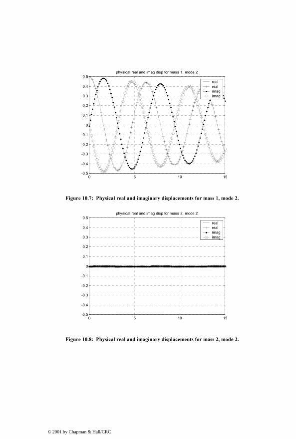
0 5 10 15
-0.5
-0.4
-0.3
-0.2
-0.1
0
0.1
0.2
0.3
0.4
0.5physical real and imag disp for mass 1, mode 2
realrealimagimag
Figure 10.7: Physical real and imaginary displacements for mass 1, mode 2.
0 5 10 15
-0.5
-0.4
-0.3
-0.2
-0.1
0
0.1
0.2
0.3
0.4
0.5physical real and imag disp for mass 2, mode 2
realrealimagimag
Figure 10.8: Physical real and imaginary displacements for mass 2, mode 2.
© 2001 by Chapman & Hall/CRC

0 5 10 15
-0.5
-0.4
-0.3
-0.2
-0.1
0
0.1
0.2
0.3
0.4
0.5physical real and imag disp for mass 3, mode 2
realrealimagimag
Figure 10.9: Physical real and imaginary displacements for mass 3, mode 2.
0 5 10 15
-1
-0.8
-0.6
-0.4
-0.2
0
0.2
0.4
0.6
0.8
1physical disp z1, z2, z3 mode 2
mass 1mass 2mass 3
Figure 10.10: Physical displacements for masses 1, 2 and 3, mode 2.
10.7.10 Proportionally Damped Initial Condition Response, Mode 3
Figures 10.11 to 10.15 show the initial condition responses for mode 3 for 2% proportional damping, where mass 2 moves twice as far and out of phase with masses 1 and 3.
Figure 10.11 shows the real and imaginary components of the two complex eigenvector responses that make up mode 2. As in the previous section, note
© 2001 by Chapman & Hall/CRC

that the two imaginary components are out of phase and cancel each other while the two real components are overlaid and will add. Figures 10.12 to 10.14 display the real and imaginary components for each of the three masses. Figure 10.15 shows the physical displacements of the three masses versus time. The Argand diagram vectors for mode 2, Figure 10.5, can be matched with each figure for each degree of freedom.
0 5 10 15
-0.5
-0.4
-0.3
-0.2
-0.1
0
0.1
0.2
0.3
0.4
0.5principal disp for mode 3
realrealimagimag
Figure 10.11: Principal real and imaginary displacements, mode 3.
0 5 10 15
-0.5
-0.4
-0.3
-0.2
-0.1
0
0.1
0.2
0.3
0.4
0.5physical real and imag disp for mass 1, mode 3
realrealimagimag
Figure 10.12: Physical real and imaginary displacements for mass 1, mode 3.
© 2001 by Chapman & Hall/CRC

0 5 10 15
-0.5
-0.4
-0.3
-0.2
-0.1
0
0.1
0.2
0.3
0.4
0.5physical real and imag disp for mass 2, mode 3
realrealimagimag
Figure 10.13: Physical real and imaginary displacements for mass 2, mode 3.
0 5 10 15
-0.5
-0.4
-0.3
-0.2
-0.1
0
0.1
0.2
0.3
0.4
0.5physical real and imag disp for mass 3, mode 3
realrealimagimag
Figure 10.14: Physical real and imaginary displacements for mass 3, mode 3.
© 2001 by Chapman & Hall/CRC
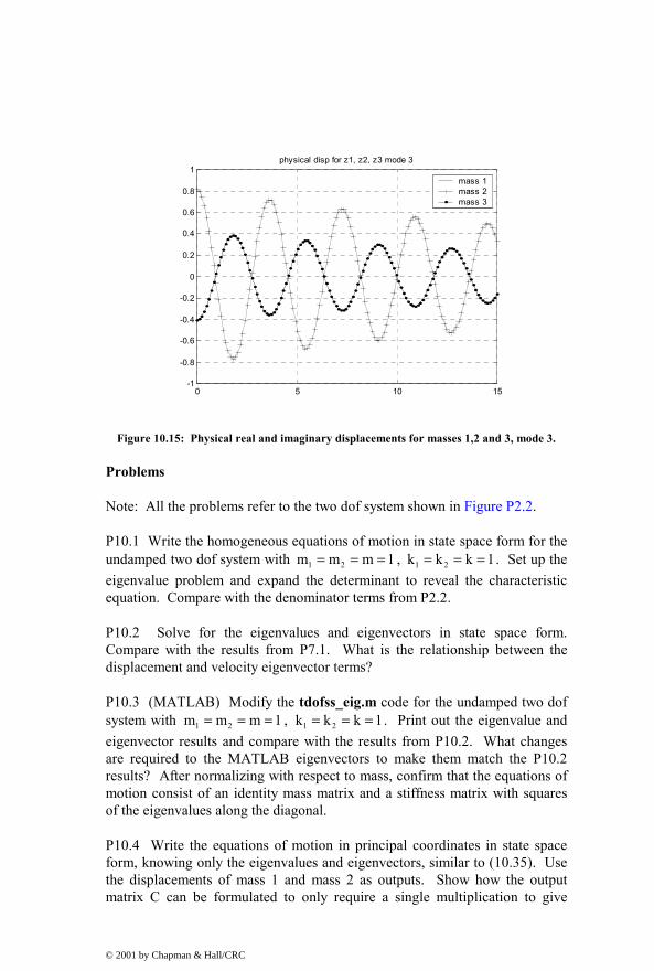
0 5 10 15
-1
-0.8
-0.6
-0.4
-0.2
0
0.2
0.4
0.6
0.8
1physical disp for z1, z2, z3 mode 3
mass 1mass 2mass 3
Figure 10.15: Physical real and imaginary displacements for masses 1,2 and 3, mode 3.
Problems
Note: All the problems refer to the two dof system shown in Figure P2.2.
P10.1 Write the homogeneous equations of motion in state space form for the undamped two dof system with 1 2m m m 1= = = , 1 2k k k 1= = = . Set up the eigenvalue problem and expand the determinant to reveal the characteristic equation. Compare with the denominator terms from P2.2.
P10.2 Solve for the eigenvalues and eigenvectors in state space form. Compare with the results from P7.1. What is the relationship between the displacement and velocity eigenvector terms?
P10.3 (MATLAB) Modify the tdofss_eig.m code for the undamped two dof system with 1 2m m m 1= = = , 1 2k k k 1= = = . Print out the eigenvalue and eigenvector results and compare with the results from P10.2. What changes are required to the MATLAB eigenvectors to make them match the P10.2 results? After normalizing with respect to mass, confirm that the equations of motion consist of an identity mass matrix and a stiffness matrix with squares of the eigenvalues along the diagonal.
P10.4 Write the equations of motion in principal coordinates in state space form, knowing only the eigenvalues and eigenvectors, similar to (10.35). Use the displacements of mass 1 and mass 2 as outputs. Show how the output matrix C can be formulated to only require a single multiplication to give
© 2001 by Chapman & Hall/CRC

outputs (Section 10.6.7.2). Identify the 2x2 submatrices which define the state equations of each mode. Are the individual modes uncoupled?
P10.5 (MATLAB) Modify the tdof_prop_damped.m code for the two dof system with 1 2m m m 1= = = , 1 2k k k 1= = = . Plot the eigenvalue locations in the s-plane for zero damping and for proportional damping of 2% (0.02). List the eigenvalues and eigenvectors for the undamped and proportional damping cases and note the differences. Plot the initial condition responses when started in initial conditions which match each of the two eigenvectors.
P10.6 Plot Argand diagrams for the undamped system.
© 2001 by Chapman & Hall/CRC

CHAPTER 11
FREQUENCY RESPONSE: MODAL STATE SPACE FORM
11.1 Introduction
In Chapter 10 we constructed the modal form of the state equations for the overall frequency response as well as for the individual mode contributions. This short chapter of MATLAB code will carry out both overall and individual mode frequency response calculations. The code will also allow us to plot the different forms of frequency responses covered in Chapter 3.
11.2 Modal State Space Setup, tdofss_modal_xfer_modes.m Listing
After executing the “tdofss_eig.m” code to provide eigenvalues and eigenvectors, we enter a section of code that yields similar results to those resulting from an ANSYS simulation. In the ANSYS case, we would have access to the eigenvalues and mass normalized eigenvectors, similar to the “xn” and “w1, w2 and w3” from tdofss_eig.m.
Since we can add proportional damping to our modal model, the code prompts for a value for zeta.
Knowing zeta and the eigenvalues, the system matrix can be setup as shown in (10.35), as 2x2 blocks along the diagonal. The three 2x2 submatrices of the system matrix are defined for individual mode contribution calculations.
The next step is to define a 6x3 input matrix, 6 states and three possible inputs representing forces applied to only mass 1, only mass 2 or only mass 3. We start out by defining three separate 3x1 force vectors, one for each mass, F1, F2 and F3. Each of these vectors is transformed from physical to principal coordinates by premultiplying by xn transpose. The three 3x1 vectors are padded with zeros resulting in three 6x1 vectors, which are then inserted as columns in the 6x3 input matrix “b.”
The output matrix, “c,” is defined in one step as shown in (10.38) by incorporating the appropriate elements of “xn.” However, only displacement states are output, giving a 3x6 matrix.
The direct transmission matrix is set to zero.
© 2001 by Chapman & Hall/CRC

% tdofss_modal_xfer_modes.m state-space modal form transfer function analysis % of tdof model, proportional damping, modal contribution plotting clf; clear all; % run tdofss_eig.m to provide eigenvalues and eigenvectors tdofss_eig; % note, this is the point where we would start if we had eigenvalue results from ANSYS, % using the eigenvalues and eigenvectors to define state space equations in % principal coordinates % define damping ratio to be used for proportional damping in the state space equation % in principal coordinates zeta = input('input zeta, 0.02 = 2% of critical damping (default) ... '); if (isempty(zeta)) zeta = 0.02; else end % setup 6x6 state-space system matrix for all three modes in principal % coordinates, a_ss a_ss = [0 1 0 0 0 0 0 0 0 0 0 0 0 0 0 1 0 0 0 0 -w2^2 -2*zeta*w2 0 0 0 0 0 0 0 1 0 0 0 0 -w3^2 -2*zeta*w3]; % setup three 2x2 state-space matrices, one for each individual mode a1_ss = a_ss(1:2,1:2); a2_ss = a_ss(3:4,3:4); a3_ss = a_ss(5:6,5:6); % transform the 3x1 force vectors in physical coordinates to principal coordinates and % then insert the principal forces in the appropriate rows in the state-space % 6x1 input matrix, padding with zeros as appropriate % define three force vectors in physical coordinates, where each is for % a force applied to a single mass F1 = [1 0 0]'; F2 = [0 1 0]'; F3 = [0 0 1]';
© 2001 by Chapman & Hall/CRC

% calculate the three force vectors in principal coordinates by pre-multiplying % by the transpose of the normalized modal matrix Fp1 = xn'*F1; Fp2 = xn'*F2; Fp3 = xn'*F3; % expand the force vectors in principal coordinates from 3x1 to 6x1, padding with zeros b1 = [0 Fp1(1) 0 Fp1(2) 0 Fp1(3)]'; % principal force applied at mass 1 b2 = [0 Fp2(1) 0 Fp2(2) 0 Fp2(3)]'; % principal force applied at mass 2 b3 = [0 Fp3(1) 0 Fp3(2) 0 Fp3(3)]'; % principal force applied at mass 3 b = [b1 b2 b3]; % the output matrix c is setup in one step, to allow the "bode" command to % output the desired physical coordinates directly without having to go % through any intermediate steps. % setup the output matrix for displacement transfer functions, each row % represents the position outputs of mass 1, mass 2 and mass 3 % velocities not included, so c is only 3x6 instead of 6x6 c = [xn(1,1) 0 xn(1,2) 0 xn(1,3) 0 xn(2,1) 0 xn(2,2) 0 xn(2,3) 0 xn(3,1) 0 xn(3,2) 0 xn(3,3) 0]; % define direct transmission matrix d d = zeros(3,3);
11.3 Frequency Response Calculation
We will begin this section by defining the vector of frequencies to be used for the frequency response plot. Then we will define a state space model, using the matrices defined in the section above.
Because we are using a 6x3 input matrix and a 3x6 output matrix, we have access to nine frequency response plots, the displacement for all three degrees of freedom for three different force application points. To plot the four distinct frequency responses, the appropriate indices are used to define magnitude and phase.
% Define a vector of frequencies to use, radians/sec. The logspace command uses % the log10 value as limits, i.e. -1 is 10^-1 = 0.1 rad/sec, and 1 is % 10^1 = 10 rad/sec. The 200 defines 200 frequency points.
© 2001 by Chapman & Hall/CRC

w = logspace(-1,1,200); % define four state-space systems using the "ss" command % sys is for all modes for all 3 forcing functions % sys1 is for mode 1 for all 3 forcing functions % sys2 is for mode 2 for all 3 forcing functions % sys3 is for mode 3 for all 3 forcing functions sys = ss(a_ss,b,c,d); sys1 = ss(a1_ss,b(1:2,:),c(:,1:2),d); sys2 = ss(a2_ss,b(3:4,:),c(:,3:4),d); sys3 = ss(a3_ss,b(5:6,:),c(:,5:6),d); % use the bode command with left hand magnitude and phase vector arguments % to provide values for further analysis/plotting [mag,phs] = bode(sys,w); [mag1,phs1] = bode(sys1,w); [mag2,phs2] = bode(sys2,w); [mag3,phs3] = bode(sys3,w); % pick out the specific magnitudes and phases for four distinct responses z11mag = mag(1,1,:); z21mag = mag(2,1,:); z31mag = mag(3,1,:); z22mag = mag(2,2,:); z11magdb = 20*log10(z11mag); z21magdb = 20*log10(z21mag); z31magdb = 20*log10(z31mag); z22magdb = 20*log10(z22mag); z11phs = phs(1,1,:); z21phs = phs(2,1,:); z31phs = phs(3,1,:); z22phs = phs(2,2,:); % pick out the three individual mode contributions to z11
© 2001 by Chapman & Hall/CRC

z111mag = mag1(1,1,:); z112mag = mag2(1,1,:); z113mag = mag3(1,1,:); z111magdb = 20*log10(z111mag); z112magdb = 20*log10(z112mag); z113magdb = 20*log10(z113mag); z111phs = phs1(1,1,:); z112phs = phs2(1,1,:); z113phs = phs3(1,1,:);
11.4 Frequency Response Plotting
% truncate peaks for plotting of expanded linear scale z11plotmag = z11mag; z111plotmag = z111mag; z112plotmag = z112mag; z113plotmag = z113mag; for cnt = 1:length(z11mag) if z11plotmag(cnt) >= 3.0 z11plotmag(cnt) = 3.0; end if z111plotmag(cnt) >= 3.0 z111plotmag(cnt) = 3.0; end if z112plotmag(cnt) >= 3.0 z112plotmag(cnt) = 3.0; end if z113plotmag(cnt) >= 3.0
© 2001 by Chapman & Hall/CRC

z113plotmag(cnt) = 3.0; end end % plot the four transfer functions separately, in a 2x2 subplot form subplot(2,2,1) semilogx(w,z11magdb(1,:),'k-') title('state space, z11, z33 db magnitude') ylabel('magnitude, db') axis([.1 10 -150 50]) grid subplot(2,2,2) semilogx(w,z21magdb(1,:),'k-') title('state space, z21, z12, z23, z32 db magnitude') ylabel('magnitude, db') axis([.1 10 -150 50]) grid subplot(2,2,3) semilogx(w,z31magdb(1,:),'k-') title('state space, z31, z13 db magnitude') xlabel('frequency, rad/sec') ylabel('magnitude, db') axis([.1 10 -150 50]) grid subplot(2,2,4) semilogx(w,z22magdb(1,:),'k-') title('state space, z22 db magnitude') xlabel('frequency, rad/sec') ylabel('magnitude, db') axis([.1 10 -150 50]) grid disp('execution paused to display figure, "enter" to continue'); pause subplot(2,2,1) semilogx(w,z11phs(1,:),'k-') title('state space, z11, z33 phase') ylabel('phase, deg') grid subplot(2,2,2) semilogx(w,z21phs(1,:),'k-') title('state space, z21, z12, z23, z32 phase') ylabel('phase, deg') grid subplot(2,2,3) semilogx(w,z31phs(1,:),'k-') title('state space, z31, z13 phase')
© 2001 by Chapman & Hall/CRC

xlabel('frequency, rad/sec') ylabel('phase, deg') grid subplot(2,2,4) semilogx(w,z22phs(1,:),'k-') title('state space, z22 phase') xlabel('frequency, rad/sec') ylabel('phase, deg') grid disp('execution paused to display figure, "enter" to continue'); pause % plot the overall plus individual mode contributions separately subplot(2,2,1) semilogx(w,z11magdb(1,:),'k-') title('State-Space Modal, z11 db magnitude') ylabel('magnitude, db') axis([.1 10 -60 40]) grid subplot(2,2,2) semilogx(w,z111magdb(1,:),'k-') title('State-Space Modal, z11 db magnitude of mode 1') ylabel('magnitude, db') axis([.1 10 -60 40]) grid subplot(2,2,3) semilogx(w,z112magdb(1,:),'k-') title('State-Space Modal, z11 db magnitude of mode 2') xlabel('frequency, rad/sec') ylabel('magnitude, db') axis([.1 10 -60 40]) grid subplot(2,2,4) semilogx(w,z113magdb(1,:),'k-') title('State-Space Modal, z11 db magnitude of mode 3') xlabel('frequency, rad/sec') ylabel('magnitude, db') axis([.1 10 -60 40]) grid disp('execution paused to display figure, "enter" to continue'); pause subplot(2,2,1) semilogx(w,z11phs(1,:),'k-') title('State-Space Modal, z11 phase') ylabel('phase, deg') grid subplot(2,2,2) semilogx(w,z111phs(1,:),'k-')
© 2001 by Chapman & Hall/CRC

title('State-Space Modal, z11 phase of mode 1') ylabel('phase, deg') grid subplot(2,2,3) semilogx(w,z112phs(1,:),'k-') title('State-Space Modal, z11 phase of mode 2') xlabel('frequency, rad/sec') ylabel('phase, deg') grid subplot(2,2,4) semilogx(w,z113phs(1,:),'k-') title('State-Space Modal, z11 phase of mode 3') xlabel('frequency, rad/sec') ylabel('phase, deg') grid disp('execution paused to display figure, "enter" to continue'); pause subplot(1,1,1); % plot the overlaid transfer function and individual mode contributions loglog(w,z11mag(1,:),'k+:',w,z111mag(1,:),'k-',w,z112mag(1,:),'k-',w, …
z113mag(1,:),'k-') title('State-Space Modal Mode Contributions, z11 db magnitude') xlabel('frequency, rad/sec') ylabel('magnitude, db') axis([.1 10 .001 100]) grid disp('execution paused to display figure, "enter" to continue'); pause semilogx(w,z11mag(1,:),'k+:',w,z111mag(1,:),'k-',w,z112mag(1,:), …
'k-',w,z113mag(1,:),'k-') title('State-Space Modal Mode Contributions, z11 linear magnitude') xlabel('frequency, rad/sec') ylabel('magnitude') grid disp('execution paused to display figure, "enter" to continue'); pause semilogx(w,z11plotmag(1,:),'k+:',w,z111plotmag(1,:),'k-', …
w,z112plotmag(1,:),'k-',w,z113plotmag(1,:),'k-') title('State-Space Modal Mode Contributions, z11 linear magnitude') xlabel('frequency, rad/sec') ylabel('magnitude') axis([.1 10 0 3]); grid disp('execution paused to display figure, "enter" to continue'); pause semilogx(w,z11phs(1,:),'k+:',w,z111phs(1,:),'k-',w,z112phs(1,:),'k-', …
w,z113phs(1,:),'k-')
© 2001 by Chapman & Hall/CRC

title('State-Space Modal Mode Contributions, z11 phase') xlabel('frequency, rad/sec') ylabel('phase, deg') grid
11.5 Code Results – Frequency Response Plots, 2% of Critical Damping
10-1 100 101-150
-100
-50
0
50state space, z11, z33 db magnitude
mag
nitu
de, d
b
10-1 100 101-150
-100
-50
0
50state space, z21, z12, z23, z32 db magnitude
mag
nitu
de, d
b
10-1
100
101
-150
-100
-50
0
50state space, z31, z13 db magnitude
frequency, rad/sec
mag
nitu
de, d
b
10-1
100
101
-150
-100
-50
0
50state space, z22 db magnitude
frequency, rad/sec
mag
nitu
de, d
b
Figure 11.1: Magnitude output for four distinct frequency responses, proportional damping zeta = 2%.
© 2001 by Chapman & Hall/CRC

10-1 100 101-200
-150
-100
-50
0state space, z11, z33 phase
phas
e, d
eg
10-1 100 101-400
-350
-300
-250
-200
-150state space, z21, z12, z23, z32 phase
phas
e, d
eg
10-1
100
101
-800
-600
-400
-200
0state space, z31, z13 phase
frequency, rad/sec
phas
e, d
eg
10-1
100
101
-200
-150
-100
-50
0state space, z22 phase
frequency, rad/sec
phas
e, d
eg
Figure 11.2: Phase output for four distinct frequency responses, proportional damping zeta = 2%.
10-1 100 101-60
-40
-20
0
20
40State-Space Modal, z11 db magnitude
mag
nitu
de, d
b
10-1 100 101-60
-40
-20
0
20
40State-Space Modal, z11 db magnitude of mode 1
mag
nitu
de, d
b
10-1
100
101
-60
-40
-20
0
20
40State-Space Modal, z11 db magnitude of mode 2
frequency, rad/sec
mag
nitu
de, d
b
10-1
100
101
-60
-40
-20
0
20
40State-Space Modal, z11 db magnitude of mode 3
frequency, rad/sec
mag
nitu
de, d
b
Figure 11.3: Magnitude output for z11 frequency response and individual mode contributions.
© 2001 by Chapman & Hall/CRC

10-1 100 101-200
-150
-100
-50
0State-Space Modal, z11 phase
phas
e, d
eg
10-1 100 101-181
-180.5
-180
-179.5
-179State-Space Modal, z11 phase of mode 1
phas
e, d
eg
10-1
100
101
-200
-150
-100
-50
0State-Space Modal, z11 phase of mode 2
frequency, rad/sec
phas
e, d
eg
10-1
100
101
-200
-150
-100
-50
0State-Space Modal, z11 phase of mode 3
frequency, rad/sec
phas
e, d
eg
Figure 11.4: Phase output for z11 frequency response and individual mode contributions.
10-1 100 101
10-3
10-2
10-1
100
101
102State-Space Modal Mode Contributions, z11 db magnitude
frequency, rad/sec
mag
nitu
de, d
b
Figure 11.5: Overlaid magnitude output for z11 frequency response and individual mode contributions.
11.6 Forms of Frequency Response Plotting
This section of code is used to plot various forms of frequency responses for the z11 transfer function, as shown in Chapter 3, Section 3.6. All the plots
© 2001 by Chapman & Hall/CRC

except the Nyquist plot use user-defined damping and 200 frequency points. The Nyquist section recalculates the system matrix to use a damping zeta of 0.02 and 800 frequency points in order to plot in the designated format.
% plot only z11 transfer function in different formats orient tall % log mag, log freq subplot(2,1,1) loglog(w,z11mag(1,:),'k-') title('z11, z33 log mag versus log freq') ylabel('magnitude') grid subplot(2,1,2) semilogx(w,z11phs(1,:),'k-') title('z11, z33 phase versus log freq') xlabel('frequency, rad/sec') ylabel('phase, deg') grid disp('execution paused to display figure, "enter" to continue'); pause % db mag, log freq subplot(2,1,1) semilogx(w,z11magdb(1,:),'k-') title('z11, z33 db mag versus log freq') ylabel('magnitude, db') grid subplot(2,1,2) semilogx(w,z11phs(1,:),'k-') title('z11, z33 phase versus log freq') xlabel('frequency, rad/sec') ylabel('phase, deg') grid disp('execution paused to display figure, "enter" to continue'); pause % db mag, lin freq subplot(2,1,1) plot(w,z11magdb(1,:),'k-') title('z11, z33 db mag versus linear freq') ylabel('magnitude, db') grid subplot(2,1,2) plot(w,z11phs(1,:),'k-') title('z11, z33 phase versus linear freq') xlabel('frequency, rad/sec')
© 2001 by Chapman & Hall/CRC

ylabel('phase, deg') grid disp('execution paused to display figure, "enter" to continue'); pause % lin mag, lin freq subplot(2,1,1) plot(w,z11mag(1,:),'k-') title('z11, z33 linear mag versus linear freq') ylabel('magnitude') grid subplot(2,1,2) plot(w,z11phs(1,:),'k-') title('z11, z33 phase versus linear freq') xlabel('frequency, rad/sec') ylabel('phase, deg') grid disp('execution paused to display figure, "enter" to continue'); pause % linear real versus log freq, linear imag versus log freq z11real = z11mag.*cos(z11phs*pi/180); % convert from mag/angle to real z11realdb = 20*log10(z11real); z11imag = z11mag.*sin(z11phs*pi/180); % convert from mag/angle to imag z11imagdb = 20*log10(z11imag); subplot(2,1,1) semilogx(w,z11real(1,:),'k-') title('z11, z33 linear real mag versus log freq') ylabel('real magnitude') grid subplot(2,1,2) semilogx(w,z11imag(1,:),'k-') title('z11, z33 linear imaginary versus log freq') xlabel('frequency, rad/sec') ylabel('imaginary magnitude'); grid disp('execution paused to display figure, "enter" to continue'); pause % linear real versus linear freq, linear imag versus linear freq subplot(2,1,1) plot(w,z11real(1,:),'k-') title('z11, z33 linear real mag versus linear freq') ylabel('real magnitude') grid
© 2001 by Chapman & Hall/CRC

subplot(2,1,2) plot(w,z11imag(1,:),'k-') title('z11, z33 linear imaginary versus linear freq') xlabel('frequency, rad/sec') ylabel('imaginary magnitude'); grid disp('execution paused to display figure, "enter" to continue'); pause % real versus imaginary (Nyquist), redo frequency response with 800 points for % finer frequency resolution for Nyquist plot and use zeta = 0.02 to fit on plot zeta = 0.02; a_ss = [0 1 0 0 0 0 0 0 0 0 0 0 0 0 0 1 0 0 0 0 -w2^2 -2*zeta*w2 0 0 0 0 0 0 0 1 0 0 0 0 -w3^2 -2*zeta*w3]; w = logspace(-1,1,800); sys = ss(a_ss,b,c,d); [mag,phs] = bode(sys,w); z11mag = mag(1,1,:); z11magdb = 20*log10(z11mag); z11phs = phs(1,1,:); z11real = z11mag.*cos(z11phs*pi/180); % convert from mag/angle to real z11imag = z11mag.*sin(z11phs*pi/180); % convert from mag/angle to imag subplot(1,1,1) plot(z11real(1,:),z11imag(1,:),'k+:') title('z11, z33 real versus imaginary, "Nyquist"') ylabel('imag') axis('square') axis([-15 15 -15 15]) grid
© 2001 by Chapman & Hall/CRC

Problem
Note: This problem refers to the two dof system shown in Figure P2.2.
P11.1 (MATLAB) Modify the tdofss_modal_xfer_modes.m code for the two dof system with 1 2m m m 1= = = , 1 2k k k 1= = = and plot the frequency responses with and without the individual mode contributions overlaid.
© 2001 by Chapman & Hall/CRC

CHAPTER 12
TIME DOMAIN: MODAL STATE SPACE FORM
12.1 Introduction
In Chapter 7 we derived the equations of motion in modal form for the system in Figure 12.1. In this chapter we will convert the modal form to state space modal form and obtain the closed form transient solution for the forcing function and initial conditions described in Figure 12.1. MATLAB will then be used to solve the same equations using the ode45 function.
12.2 Equations of Motion – Modal Form
The applied step forces are as shown in Figure 12.1. The initial conditions of position and velocity for each of the three masses are displayed in Table 12.1, the same as Figure 9.1 and Table 9.1.
m1 m2 m3
k1 k2
z1 z2 z3F1 F2 F3
Figure 12.1: Step forces applied to tdof system.
Mass 1
01
01
z 0z 1
== −&
Mass 2
02
02
z 1z 2
= −=&
Mass 3
03
03
z 1z 2
== −&
Table 12.1: Initial conditions applied to tdof system.
Repeating results from Chapter 9, where we developed the modal form of the equations of motion:
© 2001 by Chapman & Hall/CRC
The force vector in principal coordinates from (9.8) is:
p1
Tp n p2
p3
31 1 133 3 3F 1
1 1 1 1 3 2F 0 02m 2 2 mF 2
1 2 1 666 6 6
− − = = = = − − −
F z F (12.1)
With initial conditions from (9.6), (9.7):
po po
30 3
2 2m , m2 26 7 6
2 6
− − = = −
z z& (12.2)
Using the results of the eigenvalue solution, we can write the homogeneous equations of motion by inspection. The forcing function can be added to the right-hand side, knowing pF :
u= +x Ax B& (12.3)
1 1
p12 2
3 32
p24 2 2 2 4
5 52
p36 3 3 3 6
0x 0 1 0 0 0 0 xFx 0 0 0 0 0 0 x0x 0 0 0 1 0 0 x
uFx 0 0 2 0 0 x0x 0 0 0 0 0 1 x
Fx 0 0 0 0 2 x
= + −ω − ζ ω
−ω − ζ ω
&
&
&
&
&
&
(12.4)
with initial conditions of:
© 2001 by Chapman & Hall/CRC

po1
po1
po2po
po2
p03
p03
0
33z
2z2z
m 2z2z6z
27 66
− −
= =
−
x
&
&
&
(12.5)
12.3 Solving Equations of Motion Using Laplace Transforms
Now that we know the complete state space equations of motion in principal coordinates and the initial conditions on the six states in principal coordinates, the equations can be solved in the time domain. The first order equations of motion above are similar in nature to the second order equations of motion in Table 7.2. The three sets of first order equations in modal state space form are uncoupled as were the three second order equations of motion in modal form (7.89).
Expanding the three sets of equations:
1 2
2 p1
3 42
4 2 3 2 2 4 p2
5 62
6 3 5 3 3 6 p3
x xx F ux x
x x 2 x F u
x x
x x 2 x F u
==
=
= − ω − ζ ω +
=
= − ω − ζ ω +
&
&
&
&
&
&
(12.6a-f)
Taking the Laplace transform of the first two equations above:
1 1 2
p12 2 p1
sx (s) x (0) x (s)F
sx (s) x (0) F u(s)s
− =
− = = (12.7a,b)
Solving for 1x (s) :
© 2001 by Chapman & Hall/CRC

[ ]1 1 2
p11 1 2 p1
p121 1 2
p1 1 21 3 2 2
1 23
sx (s) x (0) x (s)F
s sx (s) x (0) x (0) F u(s)s
Fs x (s) sx (0) x (0)
sF sx (0) x (0)
x (s)s s s
3 0 3mx (s)s 3s3s m
− =
− − = =
= + +
= + +
−= + −
(12.8a-f)
The three terms on the right-hand side of (12.8f) represent the displacement of the first mode of vibration due to the force, initial displacement and initial velocity, respectively. This equation for 1x (s) is the same as for p1z (s) in (9.17). Using the same back-transformation yields the identical result for the principal displacement as for p1z (t) in (9.20).
2
1
2
t 3m tx (t) 032 3m
t 3 t032 3
−= + −
−= + − (12.9)
The two sets of equations for modes 2 and 3 can be solved for 3 5x (t) and x (t) in a similar fashion, again giving results which are the same as for
p2 p3z (t) and z (t) in (9.27) and (9.34). The three velocity states in principal coordinates can be defined by differentiating the displacement states.
Summarizing the solution in principal state space coordinates:
© 2001 by Chapman & Hall/CRC

2
1
2
3
4
5
6
t 3 t32 3
t 3x 33x 3 2 3 2 2 2cos t cos t sin tx 2 2 2 2(t)x 3 2 2 2sin t sin t cos tx 2 2 2x 6 6 6 7cos 3 t cos 3 t sin 3 t
18 18 2 36 3 6 3 7 3sin 3 t sin 3 t cos 3 t18 2 3
− −
− −
− − +
= = + + − + + −
− + −
x (12.10a-f)
Let us assume that we are interested in three displacements and three velocities; the output matrix is shown below in (12.11), repeated from (10.38):
n11 n12 n13
n11 n12 n13
n21 n22 n23
n21 n22 n23
n31 n32 n33
n31 n32 n33
x 0 x 0 x 00 x 0 x 0 x
x 0 x 0 x 00 x 0 x 0 x
x 0 x 0 x 00 x 0 x 0 x
=
C (12.11)
© 2001 by Chapman & Hall/CRC

1 n11 n12 n13 1
1 n11 n12 n13 2
2 n21 n22 n23 3
2 n21 n22 n23 4
3 n31 n32 n33 5
3 n31 n32 n33 6
z x 0 x 0 x 0 xz 0 x 0 x 0 x xz x 0 x 0 x 0 xz 0 x 0 x 0 x xz x 0 x 0 x 0 xz 0 x 0 x 0 x x
1 1 10 0 03 2 6
1 1 10 0 03 2 6
= =
=
Cx
&
&
&
1
2
3
4
5
6
xx1 20 0 0 0x3 6x1 20 0 0 0x3 6
1 1 1 x0 0 03 2 6
1 1 10 0 03 2 6
− − − − (12.12)
With (12.12) we have the complete time domain results in physical coordinates.
12.4 MATLAB Code tdofss_modal_time_ode45.m – Time Domain Modal Contributions
12.4.1 Modal State Space Model Setup, Code Listing
This first section executes tdofss_eig.m to calculate the eigenvalues and eigenvectors. It then sets up the 6x6 system matrix and defines three individual mode 2x2 submatrices.
The force vector in physical coordinates is defined, applying step forces as defined in Figure 12.1. It is transformed to a forcing function in principal coordinates and expanded to 6x1 size by padding with zeros. To specify the input matrices for each of the three modes, three 2x1 submatrices are defined.
The output matrix is setup as a 3x6 matrix, to calculate displacements. Once again, three submatrices of 3x2 size are defined for the individual modes.
© 2001 by Chapman & Hall/CRC

% tdofss_modal_time_ode45.m state space modal form transfer function analysis % of tdof model, proportional damping, modal contribution plotting clf; % run tdofss_eig.m to provide eigenvalues and eigenvectors tdofss_eig; global a_ss a1_ss a2_ss a3_ss b b1 b2 b3 u % note, this is the point where we would start if we had eigenvalue results from ANSYS, % using the eigenvalues and eigenvectors to define state space equations in % principal coordinates % define damping ratio to be used for proportional damping in the state space equation % in principal coordinates zeta = input('input zeta, 0.02 = 2% of critical damping (default) ... '); if (isempty(zeta)) zeta = 0.02; else end % setup 6x6 state-space system matrix for all three modes in principal % coordinates, a_ss a_ss = [ 0 1 0 0 0 0 0 0 0 0 0 0 0 0 0 1 0 0 0 0 -w2^2 -2*zeta*w2 0 0 0 0 0 0 0 1 0 0 0 0 -w3^2 -2*zeta*w3]; % setup three 2x2 state-space matrices, one for each individual mode a1_ss = a_ss(1:2,1:2); a2_ss = a_ss(3:4,3:4); a3_ss = a_ss(5:6,5:6); % transform the 3x1 force vector in physical coordinates to principal coordinates and % then insert the principal forces in the appropriate rows in the state-space % 6x1 input matrix, padding with zeros as appropriate F = [1 0 -2]'; Fp = xn'*F; % expand the force vectors in principal coordinates from 3x1 to 6x1, padding with zeros b = [0 Fp(1) 0 Fp(2) 0 Fp(3)]'; % principal forces applied to all masses
© 2001 by Chapman & Hall/CRC

b1 = b(1:2); b2 = b(3:4); b3 = b(5:6); % the output matrix c is setup in one step, to allow the "bode" command to % output the desired physical coordinates directly without having to go % through any intermediate steps. % setup the output matrix for displacement transfer functions, each row % represents the position outputs of mass 1, mass 2 and mass 3 % velocities not included, so c is only 3x6 instead of 6x6 c = [xn(1,1) 0 xn(1,2) 0 xn(1,3) 0 xn(2,1) 0 xn(2,2) 0 xn(2,3) 0 xn(3,1) 0 xn(3,2) 0 xn(3,3) 0]; c1 = c(:,1:2); c2 = c(:,3:4); c3 = c(:,5:6); % define direct transmission matrix d d = 0;
12.4.2 Problem Setup, Initial Conditions, Code Listing
Now that the model is in place, we can solve for transient response. The input scalar, “u” is set to “1,” for a unity step function. The total time is set and a vector of time span from 0 to 10 seconds (default) is setup for input to the ode routine.
The two 3x1 initial condition displacement and velocity vectors with initial displacements and velocities from Figure 12.1 are set up, then transformed to principal coordinates. Next the 6x1 initial condition vector is constructed from appropriate elements of the two 3x1 vectors. We are now ready to solve the problem.
% transient response using the ode45 command u = 1; ttotal = input('Input total time for Simulation, default = 10 sec, ... '); if (isempty(ttotal)) ttotal = 10; else
© 2001 by Chapman & Hall/CRC

end tspan = [0 ttotal]; % calculate the initial conditions in principal coordinates using the inverse of the % normalized modal matrix x0phys = [0 -1 1]'; % initial condition position, physical coord x0dphys = [-1 2 -2]'; % initial condition velocity, physical coord x0 = inv(xn)*x0phys; x0d = inv(xn)*x0dphys; % create the initial condition state vector x0ss = [x0(1) x0d(1) x0(2) x0d(2) x0(3) x0d(3)]; x0ss1 = x0ss(1:2); x0ss2 = x0ss(3:4); x0ss3 = x0ss(5:6);
12.4.3 Solving Equations Using ode45, Code Listing
The ode45 “options” parameter, which can be used to control many options for use in the solution, is set to a null vector.
Next, the total response in principal coordinates and the three individual mode responses in principal coordinates are calculated using MATLAB’s ode45 differential equation solver. Four functions, listed separately in the following sections, are used by ode45 to define the equations to solve.
The responses in principal coordinates are then transformed to physical coordinates.
% use the ode45 non-stiff differential equation solver options = [ ]; % no options specified % total response, principal coord, states are modes of vibration [t,x] = ode45('tdofssmodalfun',tspan,x0ss,options); % mode 1 response, principal coord [t1,x1] = ode45('tdofssmodal1fun',tspan,x0ss1,options); % mode 2 response, principal coord
© 2001 by Chapman & Hall/CRC

[t2,x2] = ode45('tdofssmodal2fun',tspan,x0ss2,options); % mode 3 response, principal coord [t3,x3] = ode45('tdofssmodal3fun',tspan,x0ss3,options); % total response, physical coord z_ode = c*x'; % mode 1 response, physical coord z_ode1 = c1*x1'; % mode 2 response, physical coord z_ode2 = c2*x2'; % mode 3 response, physical coord z_ode3 = c3*x3';
12.4.4 Plotting, Code Listing
% plot displacements in principal coordinates subplot(1,1,1); plot(t1,x1(:,1),'k+-',t2,x2(:,1),'kx-',t3,x3(:,1),'k-') title('Displacements in Principal Coordinate System, ode45') xlabel('Time, sec') ylabel('Displacements') legend('zp1','zp2','zp3',2) grid disp('execution paused to display figure, "enter" to continue'); pause axis([0 1 -2 2]); disp('execution paused to display figure, "enter" to continue'); pause % plot displacements in physical coordinates plot(t,z_ode(1,:),'k+-',t,z_ode(2,:),'kx-',t,z_ode(3,:),'k-') title('Displacements in Physical Coordinate System, ode45') xlabel('Time, sec') ylabel('Displacements') legend('z1','z2','z3',3) grid disp('execution paused to display figure, "enter" to continue'); pause % load previous closed-form solutions for tplot, z1, z2, z3 if zeta = 0
© 2001 by Chapman & Hall/CRC

if zeta == 0 load tdof_modal_time_z1z2z3; plot(t,z_ode(1,:),'k-',t,z_ode(2,:),'k-',t,z_ode(3,:),'k-',tplot,z1,'k.-',tplot,z2, …
'k.-',tplot,z3,'k.-') title('Displacements in Physical Coordinate System from ode45 (ode) …
and Closed Form (cf)') xlabel('Time, sec') ylabel('Vibration Displacements') legend('ode dof 1','ode dof 2','ode dof 3','cf dof 1','cf dof 2','cf dof 3') grid disp('execution paused to display figure, "enter" to continue'); pause else end % plot the modal contributions to the motion of masses 1, 2 and 3 plot(t1,z_ode1(1,:),'k+-',t2,z_ode2(1,:),'kx-',t3,z_ode3(1,:),'k-') title('Displacement of dof 1 for Modes 1, 2 and 3, ode45') xlabel('Time, sec') ylabel('Displacements') legend('Mode 1','Mode 2','Mode 3') grid disp('execution paused to display figure, "enter" to continue'); pause plot(t1,z_ode1(2,:),'k+-',t2,z_ode2(2,:),'kx-',t3,z_ode3(2,:),'k-') title('Displacement of dof 2 for Modes 1, 2 and 3, ode45') xlabel('Time, sec') ylabel('Displacements') legend('Mode 1','Mode 2','Mode 3') grid disp('execution paused to display figure, "enter" to continue'); pause plot(t1,z_ode1(3,:),'k+-',t2,z_ode2(3,:),'kx-',t3,z_ode3(3,:),'k-') title('Displacement of dof 3 for Modes 1, 2 and 3, ode45') xlabel('Time, sec') ylabel('Displacements') legend('Mode 1','Mode 2','Mode 3') grid
12.4.5 Functions Called: tdofssmodalfun.m, tdofssmodal1fun.m, tdofssmodal2fun.m, tdofssmodal3fun.m
The ode45 differential equation solver calls function files depending on which solution is being performed. The four functions for calculating the system response as well as individual responses of modes 1, 2 and 3 are listed below. Each simply defines the state equation where the derivative of the state vector
© 2001 by Chapman & Hall/CRC

is equal to the system matrix times the states plus the input matrix times the input: = +x Ax Bu& . The “global” assignments make all the variables defined available both to the calling program and to the function.
System response:
function xprime = tdofssmodalfun(t,x) % function for calculating the transient response of tdof_ss_modal_time_ode45.m global a_ss a1_ss a2_ss a3_ss b b1 b2 b3 u xprime = a_ss*x + b*u;
Mode 1 response:
function xprime = tdofssmodal1fun(t1,x1) % function for calculating the transient response of tdof_ss_modal_time_ode45.m global a_ss a1_ss a2_ss a3_ss b b1 b2 b3 u xprime = a1_ss*x1 + b1*u;
Mode 2 response:
function xprime = tdofssmodal2fun(t2,x2) % function for calculating the transient response of tdof_ss_modal_time_ode45.m global a_ss a1_ss a2_ss a3_ss b b1 b2 b3 u xprime = a2_ss*x2 + b2*u;
Mode 3 response:
function xprime = tdofssmodal3fun(t3,x3) % function for calculating the transient response of tdof_ss_modal_time_ode45.m global a_ss a1_ss a2_ss a3_ss b b1 b2 b3 u xprime = a3_ss*x3 + b1*u;
© 2001 by Chapman & Hall/CRC

12.5 Plotted Results
The following figures should be compared with Figures 9.2 through 9.7, which were plotted using the closed form modal solutions.
0 1 2 3 4 5 6 7 8 9 10
-35
-30
-25
-20
-15
-10
-5
0
5
10Displacements in Principal Coordinate System, ode45
Time, sec
Dis
plac
emen
ts
zp1zp2zp3
Figure 12.2: Displacements in principal coordinate system using ode45.
The motions of the rigid body and two oscillatory modes are clearly seen.
0 0.1 0.2 0.3 0.4 0.5 0.6 0.7 0.8 0.9 1
-2
-1.5
-1
-0.5
0
0.5
1
1.5
2Displacements in Principal Coordinate System, ode45
Time, sec
Dis
plac
emen
ts
zp1zp2zp3
Figure 12.3: Displacements in principal coordinate system, expanded scales to see initial conditions.
© 2001 by Chapman & Hall/CRC

0 1 2 3 4 5 6 7 8 9 10
-25
-20
-15
-10
-5
0
5Displacements in Physical Coordinate System, ode45
Time, sec
Dis
plac
emen
ts
z1z2z3
Figure 12.4: Displacements in physical coordinate system.
0 1 2 3 4 5 6 7 8 9 10
-25
-20
-15
-10
-5
0
5Displacements in Physical Coordinate System from ode45 (ode) and Closed Form (cf)
Time, sec
Vibr
atio
n D
ispl
acem
ents
ode dof 1ode dof 2ode dof 3cf dof 1 cf dof 2 cf dof 3
Figure 12.5: Displacements in physical coordinate system – comparing closed form solution from Chapter 7.
The three plots below show how one can study the motions of degrees of freedom due to individual modes. Use zeta = 0 when running tdofss_modal_time_ode45.m in order to plot the closed form solution.
© 2001 by Chapman & Hall/CRC

0 1 2 3 4 5 6 7 8 9 10
-25
-20
-15
-10
-5
0
5Displacement of dof 1 for Modes 1, 2 and 3, ode45
Time, sec
Dis
plac
emen
tsMode 1Mode 2Mode 3
Figure 12.6: Displacement of mass 1 for modes 1, 2 and 3.
0 1 2 3 4 5 6 7 8 9 10
-25
-20
-15
-10
-5
0
5Displacement of dof 2 for Modes 1, 2 and 3, ode45
Time, sec
Dis
plac
emen
ts
Mode 1Mode 2Mode 3
Figure 12.7: Displacement of mass 2 for modes 1, 2 and 3.
© 2001 by Chapman & Hall/CRC

0 1 2 3 4 5 6 7 8 9 10
-25
-20
-15
-10
-5
0
5Displacement of dof 3 for Modes 1, 2 and 3, ode45
Time, sec
Dis
plac
emen
tsMode 1Mode 2Mode 3
Figure 12.8: Displacement of mass 3 for modes 1, 2 and 3.
Problem
P12.1 Using the initial conditions and forcing functions from P7.4, solve for the time domain response of the states in principal coordinates in closed form using Laplace transforms. Define the output matrix if the outputs required are the displacements of both masses.
© 2001 by Chapman & Hall/CRC

CHAPTER 13
FINITE ELEMENTS: STIFFNESS MATRICES
13.1 Introduction
The purpose of this chapter is to use two simple examples to explain the basics of how finite element stiffness matrices are formulated and how static finite element analysis is performed.
Chapter 2 discussed building global stiffness matrices column by column, giving a unit displacement to the dof associated with each column and entering constraint forces for each dof along the column. This chapter will show another method of building global stiffness matrices, based on using element stiffness matrices, combining them in an orderly way to generate the global stiffness matrix. The first example uses the lumped parameter 6dof example seen in Section 2.2.4. The second example uses a two-element cantilever. Static condensation is used to prepare for a development of Guyan reduction in the next chapter.
The next chapter will use element mass matrices to assemble global mass matrices and will introduce dynamics using finite elements.
13.2 Six dof Model – Element and Global Stiffness Matrices
m1
m2 m3 m4 m5
m6
k1
k2
k3 k4 k5
k6
k7
z1
z2
z3
z4
z5
z6
Figure 13.1: Six dof stiffness matrix model.
© 2001 by Chapman & Hall/CRC

13.2.1 Overview
The global stiffness matrix for the model in Figure 13.1 was defined previously by inspection (Table 2.2). Each column of the matrix was defined by giving a unit displacement to the dof associated with that column and then defining the constraints required to hold the system in that configuration. This method works very well for hand calculations, but creating stiffness and mass matrices with computers requires a different, more systematic approach, where individual element stiffness matrices are developed and combined to give the global stiffness matrix.
We can define an element stiffness matrix for each of the springs in the figure, where the size of the element stiffness matrix is (nxn), and n is the total number of degrees of freedom associated with the element. For a uni-axial spring, there are two degrees of freedom, the displacements in the “z” direction at both ends, hence a 2x2 stiffness matrix.
Each element stiffness matrix can be set up using the “inspection” method, by displacing first the left-hand dof for the first column, and then the right-hand dof for the second column as shown in Figure 13.2.
13.2.2 Element Stiffness Matrix
1
1
dof1 dof2
k
F1 = k
F1 = -k F2 = k
F2 = -k
Figure 13.2: Spring element stiffness matrix development.
© 2001 by Chapman & Hall/CRC

The resulting element stiffness matrix, elk , for a general uni-axial spring element is then:
i iel,i
i i
k kk k
− = −
k (13.1)
For spring element 3, for example, the element stiffness matrix would be:
3 3el,3
3 3
k kk k
− = −
k (13.2)
13.2.3 Building Global Stiffness Matrix Using Element Stiffness Matrices
The total number of degrees of freedom for the problem is 6, so the complete system stiffness matrix, the global stiffness matrix, is a 6x6 matrix. Each row and column of every element stiffness matrix can be associated with a global degree of freedom.
For element 1, which is connected to degrees of freedom 1 and 2:
st nd
1 2st
1 1 1el,1 nd
1 1 2
1 and 2 columns of global stiffness matrixz zk k z 1 row of globalstiffness matrixk k z 2 row of globalstiffness matrix
− = −
k
(13.3)
For element 2, which is connected to degrees of freedom 1 and 6:
st th
1 6
st2 2 1
el,2 th2 2 6
1 and 6 columns of global stiffness matrixz zk k z 1 row of globalstiffness matrixk k z 6 row of globalstiffness matrix
− = −
k
(13.4)
For element 3, which is connected to degrees of freedom 2 and 3:
nd rd
2 3
nd3 3 2
el,3 rd3 3 3
2 and 3 columns of global stiffness matrixz zk k z 2 row of globalstiffness matrixk k z 3 row of globalstiffness matrix
− = −
k
(13.5)
© 2001 by Chapman & Hall/CRC

For element 4, which is connected to degrees of freedom 3 and 4:
rd th
3 4
rd4 4 3
el,4 th4 4 4
3 and 4 columns of global stiffness matrixz zk k z 3 row of globalstiffness matrixk k z 4 row of globalstiffness matrix
− = −
k
(13.6)
For element 5, which is connected to degrees of freedom 4 and 5:
th th
4 5
th5 5 4
el,5 th5 5 5
4 and 5 columns of global stiffness matrixz zk k z 4 row of globalstiffness matrixk k z 5 row of globalstiffness matrix
− = −
k
(13.7)
For element 6, which is connected to degrees of freedom 3 and 5:
rd th
3 5
rd6 6 3
el,6 th6 6 5
3 and 5 columns of global stiffness matrixz zk k z 3 row of globalstiffness matrixk k z 5 row of globalstiffness matrix
− = −
k
(13.8)
For element 7, which is connected to degrees of freedom 2 and 5:
nd th
2 5
nd7 7 2
el,7 th7 7 5
2 and 5 columns of global stiffness matrixz zk k z 2 row of globalstiffness matrixk k z 5 row of globalstiffness matrix
− = −
k
(13.9)
The global stiffness matrix starts out as a 6x6 null matrix, then each element is cycled through and its elements added to the previous matrix. The initial null matrix is:
© 2001 by Chapman & Hall/CRC

g
0 0 0 0 0 00 0 0 0 0 00 0 0 0 0 00 0 0 0 0 00 0 0 0 0 00 0 0 0 0 0
=
k (13.10)
After adding the element stiffness matrix for element 1:
1 1
1 1
g
k k 0 0 0 0k k 0 0 0 00 0 0 0 0 00 0 0 0 0 00 0 0 0 0 00 0 0 0 0 0
− −
=
k (13.11)
After adding the element stiffness matrices for elements 1 to 2:
1 2 1 2
1 1
g
2 2
k k k 0 0 0 kk k 0 0 0 00 0 0 0 0 00 0 0 0 0 00 0 0 0 0 0k 0 0 0 0 k
+ − − −
=
−
k (13.12)
After adding the element stiffness matrices for elements 1 to 3:
1 2 1 2
1 1 3 3
3 3g
2 2
k k k 0 0 0 kk k k k 0 0 00 k k 0 0 00 0 0 0 0 00 0 0 0 0 0k 0 0 0 0 k
+ − − − + − −
=
−
k (13.13)
After adding the element stiffness matrices for elements 1 to 4:
© 2001 by Chapman & Hall/CRC

1 2 1 2
1 1 3 3
3 3 4 4g
4 4
2 2
k k k 0 0 0 kk k k k 0 0 00 k k k k 0 00 0 k k 0 00 0 0 0 0 0k 0 0 0 0 k
+ − − − + − − + −
= −
−
k (13.14)
After adding the element stiffness matrices for elements 1 to 5:
1 2 1 2
1 1 3 3
3 3 4 4g
4 4 5 5
5 5
2 2
k k k 0 0 0 kk k k k 0 0 00 k k k k 0 00 0 k k k k 00 0 0 k k 0k 0 0 0 0 k
+ − − − + − − + −
= − + − −
−
k (13.15)
After adding the element stiffness matrices for elements 1 to 6:
1 2 1 2
1 1 3 3
3 3 4 6 4 6g
4 4 5 5
6 5 5 6
2 2
k k k 0 0 0 kk k k k 0 0 00 k k k k k k 00 0 k k k k 00 0 k k k k 0k 0 0 0 0 k
+ − − − + − − + + − −
= − + − − − +
−
k (13.16)
After adding the element stiffness matrices for elements 1 to 7 we have the final global stiffness matrix.
1 2 1 2
1 1 3 7 3 7
3 3 4 6 4 6g
4 4 5 5
7 6 5 5 6 7
2 2
k k k 0 0 0 kk k k k k 0 k 00 k k k k k k 00 0 k k k k 00 k k k k k k 0k 0 0 0 0 k
+ − − − + + − − − + + − −
= − + − − − − + +
−
k
(13.17)
© 2001 by Chapman & Hall/CRC

This checks against the original global stiffness matrix defined by inspection in Table 2.2 and fulfills the symmetry requirement.
1 2 3 4 5 6
1 2 l 2
1 1 3 7 3 7
3 3 4 6 4 6
4 4 5 5
7 6 5 5 6 7
2 2
(k k ) k 0 0 0 k1k (k k k ) k 0 k 020 k (k k k ) k k 030 0 k (k k ) k 040 k k k (k k k ) 05k 0 0 0 0 k6
+ − − − + + − − − + + − − − + − − − − + +
−
(13.18)
13.3 Two-Element Cantilever Beam
We will now do a static finite element displacement analysis of a two-element cantilever beam. We start by showing the original model and defining the degrees of freedom for the idealized beam, Figure 13.3.
Note that even though the left-hand side node is grounded in the actual beam, there are degrees of freedom associated with the node to allow generating global stiffness and mass matrices for all nodes. The constrained degrees of freedom will be accounted for once the complete global stiffness matrix is available. For this model, each of the three nodes has two degrees of freedom, a translation and a rotation.
© 2001 by Chapman & Hall/CRC

Element 1E1, I1, l1
Element 2E2, I2, l2
z1
1θ 2θ 3θ
z2 z3
Original Beam
Idealized BeamNode, dof Definition
dof1 dof3 dof5
dof6dof4dof2
1 2 3
Figure 13.3: Two-element cantilever beam model and node definition.
13.3.1 Element Stiffness Matrix
The element stiffness matrix can be developed by using basic strength of materials techniques to analyze the forces required to displace each degree of freedom a unit value in the positive direction:
© 2001 by Chapman & Hall/CRC

−123EI
l
−62EI
l
123EI
l
2EI
l
62EI
l
−62EI
l
4EI
l−6
2EI
l1
1
−123EI
l
123EI
l6
2EI
l 62EI
l4EI
l−6
2EI
l
2EI
l6
2EI
l
1
1
ΘZ
Column 1 Column 2
Column 3 Column 4
dof Definition:
Figure 13.4: Beam element stiffness matrix terms.
13.3.2 Degree of Freedom Definition – Beam Stiffness Matrix
Using the degrees of freedom in Figure 13.5 results in the following element stiffness matrix:
3 2 3 2i i i i
2 2i ii i
el,i i i
3 2 3 2i i i i
2 2i ii i
12 6 12 6l l l l6 4 6 2
l ll lE I
12 6 12 6l l l l6 2 6 4
l ll l
− − = − − − −
k (13.19)
© 2001 by Chapman & Hall/CRC

z1
1θ 2θ
z2
Beam ElementNode, dof Definition
dof1 dof3
dof4dof2
1 2
Figure 13.5: Beam element node and degree of freedom definition.
13.3.3 Building Global Stiffness Matrix Using Element Stiffness Matrices
To build the global stiffness matrix, we start with a 6x6 null matrix, with the six degrees of freedom being the translation and rotation of each of the three nodes, again including the constrained node 1 degrees of freedom:
g
0 0 0 0 0 0 displacement of node 10 0 0 0 0 0 rotation of node 10 0 0 0 0 0 displacement of node 20 0 0 0 0 0 rotation of node 20 0 0 0 0 0 displacement of node 30 0 0 0 0 0 rotation of node 3
=
k (13.20)
The two 4x4 element stiffness matrices are:
3 2 3 21 1 1 1
2 21 11 1
el,1 1 1
3 2 3 21 1 1 1
2 21 11 1
12 6 12 6l l l l6 4 6 2
l ll lE I
12 6 12 6l l l l6 2 6 4
l ll l
− − = − − − −
k (13.21)
© 2001 by Chapman & Hall/CRC

3 2 3 22 2 2 2
2 22 22 2
el,2 2 2
3 2 3 22 2 2 2
2 22 22 2
12 6 12 6l l l l6 4 6 2
l ll lE I
12 6 12 6l l l l6 2 6 4
l ll l
− − = − − − −
k (13.22)
Building up the global stiffness matrix, element by element, inserting element 1 first:
1 1 1 1 1 1 1 13 2 3 21 1 1 1
1 1 1 1 1 1 1 12 2
1 11 1
1 1 1 1 1 1 1 1g 3 2 3 2
1 1 1 1
1 1 1 1 1 1 1 12 2
1 11 1
12E I 6E I 12E I 6E I 0 0l l l l
6E I 4E I 6E I 2E I 0 0l ll l
12E I 6E I 12E I 6E I 0 0l l l l
6E I 2E I 6E I 4E I 0 0l ll l
0 0 0 0 0 00 0 0 0 0 0
− − − − −
= −
k (13.23)
Inserting the element 2 terms leaves gk :
© 2001 by Chapman & Hall/CRC

1 1 1 1 1 1 1 13 2 3 21 1 1 1
1 1 1 1 1 1 1 12 2
1 11 1
1 1 1 1 1 1 2 2 1 1 2 2 2 2 2 23 2 3 3 2 2 3 21 1 1 2 1 2 2 2
1 1 1 1 1 1 2 2 1 12 2 2
11 1 2
12E I 6E I 12E I 6E I 0 0l l l l
6E I 4E I 6E I 2E I0 0
l ll l
12E I 6E I 12E I 12E I 6E I 6E I 12E I 6E Il l l l l l l l
6E I 2E I 6E I 6E I 4E Ill l l
−
−
− − − −+ + − +
2 2 2 2 2 22
1 2 22
2 2 2 2 2 2 2 23 2 3 22 2 2 2
2 2 2 2 2 2 2 22 2 2
22 2 2
4E I 6E I 2E Il l ll
12E I 6E I 12E I 6E I0 0l l l l
6E I 2E I 6E I 4E I0 0ll l l
− + − − −
−
(13.24)
Note how the contributions for the stiffness elements for node 2 from the left-hand and right-hand beams add together.
13.3.4 Eliminating Constraint Degrees of Freedom from Stiffness Matrix
We now have the entire global stiffness matrix, including the degrees of freedom which are constrained, the translation and rotation of node 1 (the first two rows and columns of gk ). To eliminate the constrained degrees of freedom, we eliminate the rows and columns which correspond to the constrained global degrees of freedom, reducing the global stiffness matrix to a 4x4 matrix:
1 1 2 2 1 1 2 2 2 2 2 23 3 2 2 3 21 2 1 2 2 2
1 1 2 2 1 1 2 2 2 2 2 22 2 2
1 2 21 2 2g
2 2 2 2 2 2 2 23 2 3 22 2 2 2
2 2 2 2 2 2 2 22 2 2
22 2 2
12E I 12E I 6E I 6E I 12E I 6E Il l l l l l
6E I 6E I 4E I 4E I 6E I 2E Il l ll l l
12E I 6E I 12E I 6E Il l l l
6E I 2E I 6E I 4E Ill l l
− −+ + − −+ +
=− − −
−
k
(13.25)
© 2001 by Chapman & Hall/CRC

To facilitate hand calculations, we will make the two-beam elements identical, with the same E, I and lengths, l. The global stiffness matrix can then be rewritten as:
3 3 2
2
g
3 2 3 2
2 2
24 12 60l l l
8 6 20l llEI
12 6 12 6l l l l6 2 6 4
l ll l
−
−
= − − − −
k (13.26)
13.3.5 Static Solution: Force Applied at Tip
We have all the information required to solve a static problem. For example, we could solve for the displacements of the system for a z direction force applied at the tip of the beam. The equation for static equilibrium of the system is:
g =k z F (13.27)
Expanding:
g11 g12 g13 g14 1 1
g21 g22 g23 g24 2 2
g31 g32 g33 g34 3 3
g41 g42 g43 g44 4 4
k k k k z Fk k k k z Fk k k k z Fk k k k z F
=
(13.28)
Where:
1z is translation of node 2
2z is rotation of node 2
3z is translation of node 3
4z is rotation of node 3
1F is z force applied to node 2
© 2001 by Chapman & Hall/CRC

2F is y moment applied to node 2
3F is z force applied to node 3
4F is y moment applied to node 3
13.4 Static Condensation
13.4.1 Derivation
Solving the static equation is trivial using a computer, but doing a 4x4 inverse by hand is difficult, so we will reduce the problem to a 2x2 problem using static condensation. Static condensation is not typically used for static problems, but is the precursor for Guyan reduction (dynamic condensation), which will be introduced in the eigenvalue analysis in the next chapter.
Static condensation involves separating the degrees of freedom into “master” and “slave” degrees of freedom. If master dof’s are chosen such that they include all degrees of freedom where forces/moments are applied and also degrees of freedom where displacements are desired, the resulting solution is exact. If the slave dof set includes dof’s where forces/moments are applied and/or where displacements are desired, the technique will create errors.
For an exact static solution, master dof’s are chosen as dof’s where forces/moments are applied and where displacements/rotations are desired.
For dynamic problems master degrees of freedom are typically chosen as displacements of the higher mass nodes and rotations of the higher mass moment of inertia nodes, with slave degrees of freedom being the displacements and rotations of the relatively lower inertia nodes.
For the two-element cantilever, we will solve for the two translations of node 2 and node 3 as master degrees of freedom, and will condense (reduce out) the two rotations. We will develop the theory first, then will substitute our cantilever example.
The first step is to rearrange the degrees of freedom, rows and columns of the stiffness matrix, into dependent (slave) displacements to be reduced, az , and independent (master) displacements, bz . This involves moving the second and fourth rows and columns of the cantilever stiffness matrix up to become the first and second rows and columns, which moves the first and third rows and columns down to the second and fourth positions.
© 2001 by Chapman & Hall/CRC

=kz F (13.29)
aa ab a a
ba bb b b
=
k k z Fk k z F
(13.30)
Multiplying out the first matrix equation:
aa a ab b a+ =k z k z F (13.31)
Solving for az :
( )1a aa a ab b
−= −z k F k z (13.32)
If no forces (moments) are applied at the dependent (slave) degrees of freedom, [ ]a 0=F , and the equation above becomes:
( )1 1a aa ab b aa ab b
− −= − = −z k k z k k z (13.33)
We can now rewrite the displacement vector in terms of bz only:
11
a aa ab baa abb
b b
−− −− = = =
z k k zk kz z
z zI (13.34)
Defining a transformation matrix for brevity:
1a abaa ab
b b bb
− − = = = =
z Tk kz z z Tz
z II (13.35)
Where:
1ab aa ab
−= −T k k (13.36)
Substituting back into the original static equilibrium equation:
b( )= =kz k Tz F (13.37)
Multiplying both sides by TT to reduce the number of degrees of freedom from (a + b) to b:
© 2001 by Chapman & Hall/CRC

T Tb( ) =T kT z T F (13.38)
Expanding the term in parentheses above, and redefining it to be *bbk :
aa ab ab* T Tbb ab
ba bb
abT Tab aa ba ab ab bb
T Tab aa ba ab ab ab bb
T Tab aa ab ba ab ab ab bb
1 1 1ba aa aa aa ab ba aa ab ba aa
( ) ( )
( ) ( )
( ) ( ) ( ) (− − −
= =
= + +
= + + +
= + + +
= − − + − + −
k k Tk T kT T I
k k I
TT k k T k k
I
T k k T T k k I
T k T k T T k k
k k k k k k k k k k 1ab bb
1 1 1ba aa ab ba aa ab ba aa ab bb
1bb ba aa ab
)−
− − −
−
+
= − − +
= −
k k
k k k k k k k k k k
k k k k
(13.39)
where: 1ab aa ab
−= −T k k and T 1ab ba aa
−= −T k k .
So, the original (a + b) degree of freedom problem now can be transformed to a “b” degree of freedom problem by partitioning into dependent and independent degrees of freedom, and solving for the reduced stiffness matrix
*bbk and reduced force vector *
bF :
* Tb
aTab ba a b
b
1b ba aa a
−
=
= = +
= −
F T F
FT I T F F
F
F k k F
(13.40)
© 2001 by Chapman & Hall/CRC

Then the reduced problem becomes:
* *bb b b=k z F (13.41)
After the bz degrees of freedom are known, the az degrees of freedom can be expanded from the bz masters using, if [ ]a 0=F :
1a aa ab b
−= −z k k z (13.42)
13.4.2 Solving Two-Element Cantilever Beam Static Problem
We will now solve the example cantilever for a force applied at the tip. Earlier we showed that the stiffness matrix is:
3 3 2
2
g
3 2 3 2
2 2
24 12 60l l l
8 6 20l llEI
12 6 12 6l l l l6 2 6 4
l ll l
−
−
= − − − −
k (13.43)
Rearranging rows, 1 to 3, 2 to 1, 3 to 4 and 4 to 2:
2
2 2
g
3 3 2
3 2 3 2
8 6 20l ll
6 2 6 4l ll lEI
24 12 60l l l12 6 12 6l l l l
−
−
= − − − −
k (13.44)
Rearranging columns, 1 to 3, 2 to 1, 3 to 4 and 4 to 2:
© 2001 by Chapman & Hall/CRC

2
2 2
g
2 3 3
2 2 3 3
8 2 60l l l2 4 6 6l l l lEI
6 24 120l l l
6 6 12 12l l l l
−
−
= − − − −
k (13.45)
Breaking out and identifying the four submatrices of dependent (a) and independent (b) degrees of freedom:
aa ab 2
ba bb2 3
8 2 0 6EI EI2 4 6 6l l
0 6 24 12EI EI6 6 12 12l l
− = = −
− = = − − −
k k
k k (13.46a-d)
Finding the inverse of aak :
1aa
2 1l1 414EI
− − = −
k (13.47)
1aa ab
6 6124 1814l
− − − −− = − k k (13.48)
1ba aa ab 3
144 108EI108 14414l
− − = −
k k k (13.49)
© 2001 by Chapman & Hall/CRC

* 1bb bb ba aa ab
3
3
336 168 144 108EI168 168 108 14414l
192 60EI60 2414l
−= −
− − = − − −
− = −
k k k k k
(13.50)
3 3
* 1bb
24 60 24 6014l l60 192 60 1921008EI 72EI
− = =
k (13.51)
Solving for the two displacements, bz for a tip force of magnitude P:
2 * 1 *b bb bb
3
3
3 3 3
zz
24 60 0l60 192 P72EI
60 560Pl Pl Pl72 6
192 192 872EI EI EI72 3
− = =
=
= = =
z k F
(13.52)
The tip displacement is:
3
38Plz3EI
= (13.53)
The well-known solution for the displacement of the tip of a cantilever is:
3
tipPLz3EI
= (13.54)
Knowing that the total length of the cantilever, L, is 2l:
© 2001 by Chapman & Hall/CRC

3 3 3
tipPL P(2l) 8Plz3EI 3EI 3EI
= = = (13.55)
The reduced problem has provided the correct solution. Once again, normally we would not solve a reduced static problem except during a hand calculation, but the derivation of static condensation will be useful in the next chapter when dynamic condensation, Guyan reduction, is introduced.
Problems
P13.1 Assemble the global mass and stiffness matrices for Figure P2.1 element by element. Compare results with P2.1 results.
P13.2 In Section 13.4.2 we solved for the displacements of a two-element cantilever beam with a tip load by reducing out the rotations of the beam. Solve the problem by reducing out the rotations of the middle and tip nodes and the displacement of the middle node. Use a symbolic algebra program to invert the 3x3 aak matrix.
© 2001 by Chapman & Hall/CRC

CHAPTER 14
FINITE ELEMENTS: DYNAMICS
14.1 Introduction
The chapter starts out with discussions of various mass matrix formulations. The 6dof lumped mass example from Chapter 2 is used for the lumped mass matrix example. A two-element cantilever is used to develop the consistent mass example. Using the same technique as in the previous chapter, the global mass matrix is built up as an assemblage of element mass matrices. A method analogous to static condensation, Guyan reduction, is developed and used to reduce the size of the two-element cantilever problem. The cantilever is then solved for its eigenvalues by hand using Guyan reduction. The same cantilever is solved for eigenvalues and eigenvectors using MATLAB and results are compared to the hand calculations.
Following the two-element cantilever example, a second MATLAB code allows solving for eigenvalues and eigenvectors for a uniform cantilever beam with user-defined number of elements. The results of the MATLAB code are compared with the results from an ANSYS model for the same 10-element cantilever.
This 10-element cantilever will be the last eigenvalue analysis in the book using MATLAB. Further chapters will start with eigenvalue results from ANSYS models, which will be used to build state space MATLAB models. These MATLAB models are then used for frequency and time domain analyses. This chapter serves as a bridge between carrying out analyses completely in MATLAB and using ANSYS results as the starting point for state space MATLAB models. Hence, we will reintroduce ANSYS eigenvalue/eigenvector results and start becoming familiar with their form and interpretation.
14.2 Six dof Global Mass Matrix
The lumped mass matrix is simple to construct because there is only a single degree of freedom associated with each mass element. This leads to the 6x6 diagonal mass matrix below, which can be constructed in the same manner as the 6dof stiffness matrix in the previous chapter.
© 2001 by Chapman & Hall/CRC

1
2
3g
4
5
6
m 0 0 0 0 00 m 0 0 0 00 0 m 0 0 00 0 0 m 0 00 0 0 0 m 00 0 0 0 0 m
=
m (14.1)
14.3 Cantilever Dynamics
14.3.1 Overview – Mass Matrix Forms
In order to solve for the dynamics of the cantilever beam, we need to develop a mass matrix to complete the equations of motion. For a beam finite element, there are a number of different mass matrix formulations, each of which will be covered below:
1) Lumped mass, displacements only
2) Lumped mass, displacements and rotations both included
3) Consistent mass – distributed mass effect
14.3.2 Lumped Mass
Beam-element lumped parameter mass and inertia terms in the mass matrix relate point inertial loads to point accelerations and give only diagonal terms. Equation (14.2) below shows the lumped mass matrix including both displacements and rotations:
3y
l
3y
m l 0 0 02
m l Im l0 0 024 2A
ml0 0 02
ml Im l0 0 024 2A
+ =
+
m (14.2)
For the lumped mass for displacement terms only, the (2,2) and (4,4) terms in (14.2) would be set to zero. Notation is as follows: m is mass per unit length,
© 2001 by Chapman & Hall/CRC

l is the element length, yI is the cross-sectional moment of inertia about the y axis and A is the cross section area. This lumped mass formulation assumes a prismatic beam (same area and moment of inertia along the length) and effectively lumps half of the mass and inertia at each end (Archer 1963).
14.3.3 Consistent Mass
Lumped mass formulations were state of the art in structural dynamics until Archer’s classic paper introduced the consistent mass matrix in 1963.
We will see in the development below that the consistent mass matrix for a beam element is a filled matrix. The filled matrix can be combined with other consistent mass matrices of other elements of the structure, in the same manner as the element stiffness matrices are combined, to yield the final global mass matrix.
The element consistent mass matrix for a prismatic beam is, with mass per unit length m and length l (Weaver 1990):
2 2
e
2 2
156 22l 54 13l22l 4l 13l 3lml54 13l 156 22l42013l 3l 22l 4l
− − = − − − −
m (14.3)
Figure 14.1 shows the unit accelerations of each of the four degrees of freedom which correspond to the four columns of the consistent mass matrix, analogous to the beam element stiffness description in Chapter 13.
© 2001 by Chapman & Hall/CRC

13 2l
−22 2l
156l
33l−
−13 2l −22 2l
4 3l54l1
1
−13 2l54l
22 2l
4 3l
22 2l 13 2l
33l−
156l
1
1
Θ
Z
Column 1 Column 2
Column 3 Column 4
dof Definition:
Figure 14.1: Beam element consistent mass matrix terms.
14.4 Dynamics of Two-Element Cantilever – Consistent Mass Matrix
We already have the global stiffness matrix for the two-element cantilever beam from (13.26):
3 3 2
2
g
3 2 3 2
2 2
24 12 60l l l
8 6 20l llEI
12 6 12 6l l l l6 2 6 4
l ll l
−
−
= − − − −
k (14.4)
The global mass matrix (using consistent mass) can also be built by combining the terms from each of the beam elements as follows:
© 2001 by Chapman & Hall/CRC

21 1 1 1 1 1
2 3 21 1 1 1 1 1
21 1 1 1 1 1 2 2
g 2 3 2 21 1 1 1 1 1 2 2
2 22
2 2
21 1
31 1
2 2 21 1 2 2 2 2 2 2
31 1 2
156m l 22m l 54m l22m l 4m l 13m l54m l 13m l (156m l 156m l )1
420 13m l 3m l ( 22m l 22m l )0 0 54m l0 0 13m l
13m l 0 03m l 0 0
( 22m l 22m l ) 54m l 13m l(4m l 4m
+
= − − − +
−
−−
− + −+
m
3 2 32 2 2 2 2
2 22 2 2 2 2 2
3 2 32 2 2 2 2 2
l ) 13m l 3m l13m l 156m l 22m l
3m l 22m l 4m l
− −
− −
(14.5)
Once again, assuming the two elements have the same properties and lengths, the global mass matrix becomes:
2 2
2 3 2 3
2 2
g 2 3 3 2 3
2 2
2 3 2 3
156ml 22ml 54ml 13ml 0 022ml 4ml 13ml 3ml 0 054ml 13ml 312ml 0 54ml 13ml1
420 13ml 3ml 0 8ml 13ml 3ml0 0 54ml 13ml 156ml 22ml0 0 13ml 3ml 22ml 4ml
− − −
= − − − −
− − −
m (14.6)
Taking into account the two constrained degrees of freedom at the built in end, we can eliminate the first two rows and columns:
2
3 2 3
g 2 2
2 3 2 3
312ml 0 54ml 13ml0 8ml 13ml 3ml1
420 54ml 13ml 156ml 22ml13ml 3ml 22ml 4ml
− − = − − − −
m (14.7)
Having the mass and stiffness matrices allows us to solve the eigenvalue problem for the homogeneous equations of motion:
[ ]g g 0+ =m z k z&& (14.8)
© 2001 by Chapman & Hall/CRC

In order to solve the problem by hand, we will need to find several inverses, so we will again see if we can cut the 4x4 problem down to 2x2 size. We will now use Guyan reduction to reduce the size of the problem.
14.5 Guyan Reduction
Guyan reduction is a method of decreasing the number of degrees of freedom in a dynamics problem, similar to the process of static condensation in a statics problem. Unlike static condensation, however, Guyan reduction introduces errors due to the approximations made. The magnitude of the errors introduced depends upon the choice of degrees of freedom to be reduced, the dependent or slave degrees of freedom. The most popular choice of degrees of freedom to be reduced are translations of nodes with relatively lower masses and rotations of nodes with relatively lower mass moment of inertia. This leaves translations of relatively larger mass nodes and rotations of relatively larger mass moment of inertia nodes as the independent degrees of freedom. In a typical finite element problem, the analyst will define masters as degrees of freedom where forces/moment are applied, where displacements or rotations are required for output, or where known large masses/mass moments of inertia occur. The finite element program will then be allowed to choose an additional set of degrees of freedom and add them to the master set. Typically the program sorts along the diagonal of the mass matrix, adding degrees of freedom associated with the larger terms.
14.5.1 Guyan Reduction Derivation
Starting with the undamped equations of motion:
[ ]0+ =mz kz&& (14.9)
Rearranging and partitioning into displacements to be reduced, az , and independent displacements, bz :
aa ab a aa ab a a
ba bb b ba bb b a
+ =
m m z k k z Fm m z k k z F
&&
&& (14.10)
Multiplying out the first matrix equation:
aa a ab b aa a ab b a+ + + =m z m z k z k z F&& && (14.11)
Solving the above for az :
© 2001 by Chapman & Hall/CRC

( )( )
1a aa a ab b aa a ab b
1 1aa ab b aa a aa a ab b
−
− −
= − − −
= − + − −
z k F k z m z m z
k k z k F m z m z
&& &&
&& && (14.12)
Instead of letting az depend upon the entire right-hand side of (14.13), the approximation of static equilibrium is introduced:
1a aa ab b
−= −z k k z (14.13)
Typically the choice of degrees of freedom to be reduced does not include any degrees of freedom to which forces are applied, thus a 0=F . The static equilibrium approximation basically sets the term in brackets in (14.12) to zero. Setting a 0=F and using the second derivative of (14.13), we can see the form of abm :
a aa a ab b
aa a ab b1
aa aa ab b ab b1
aa aa ab ab
1ab aa aa ab
0
( )−
−
−
= − −= − −
= − − −
= −
=
F m z m zm z m zm k k z m z
m k k m
m m k k
&& &&
&& &&
&& && (14.14a,b)
We assume that the aa am z&& terms are zero and that aa abandm m are related as in (14.14b). The force transmission between the a bandz z&& && degrees of freedom is related only to the stiffnesses as denoted in (14.14), hence the “static equilibrium” approximation.
Assuming (14.13) holds, the displacement vector z can be written in terms of bz only:
1
a abaa abb b b
b
− − = = = =
z Tk kz z z Tz
z II (14.15)
where:
1ab aa ab
−= −T k k (14.16)
© 2001 by Chapman & Hall/CRC

ab =
TT
I (14.17)
Substitution of (14.14), with derivatives, into (14.9) yields:
b b+ =mTz kTk F&& (14.18)
Equation (14.18) still contains (a + b) degrees of freedom, so premultiplication by TT is required to reduce to (b) degrees of freedom and to return symmetry to the reduced mass and stiffness matrices:
( ) ( )T T Tb b+ =T mT z T kT z T F&& (14.19)
Rewriting in a more compact form:
* * *bb b bb b b+ =m z k z F&& (14.20)
Equation (14.20) is the final reduced equation of motion which can be solved for the displacements of type b. Displacements of type a (assuming static equilibrium) can then be solved for using (14.13).
*bbk can be shown to be the same as that derived in the static condensation
Section 13.4.1, (13.39):
aa ab ab* Tbb ab
ba bb
=
k k Tk T I
k k I
( ) ( ) abT Tab aa ba ab ab bb
= + +
TT k k T k k
I
T Tab aa ab ba ab ab ab bb= + + +T k T k T T k k
1 1 1 1ba aa aa aa ab ba aa ab ba aa ab bb
− − − −= − − +k k k k k k k k k k k k
1bb ba aa ab
−= −k k k k (14.21)
© 2001 by Chapman & Hall/CRC

14.5.2 Two-Element Cantilever Eigenvalues Closed Form Solution Using Guyan Reduction
Repeating the rearranged global stiffness matrix from the static run, (13.45):
2
2 2
g
2 3 3
2 2 3 3
8 2 60l l l2 4 6 6l l l lEI
6 24 120l l l
6 6 12 12l l l l
−
−
= − − − −
k (14.22)
Breaking out and identifying the four submatrices of dependent (a) and independent (b) degrees of freedom:
aa ab 2
ba bb2 3
8 2 0 6EI EI2 4 6 6l l
0 6 24 12EI EI6 6 12 12l l
− = = −
− = = − − −
k k
k k (14.23a-d)
Finding the inverse of aak :
1aa
2 1l1 414EI
− − = −
k (14.24)
1aa ab
6 6124 1814l
− − − −− = − k k (14.25)
1ba aa ab 3
144 108EI108 14414l
− − = −
k k k (14.26)
© 2001 by Chapman & Hall/CRC

* 1bb bb ba aa ab
3
3
336 168 144 108EI168 168 108 14414l
192 60EI60 2414l
−= −
− − = − − −
− = −
k k k k k
(14.27)
The transformation matrix T is given by:
1
ab aa ab
6 614l 14l24 18
14l 14l1 00 1
−
− − = = =
T k kT
I I (14.28)
The mass matrix now needs to be rearranged into “a” and “b” submatrices and then transformed to *
bbm :
2
3 2 3
g 2 2
2 3 2 3
312ml 0 54ml 13ml0 8ml 13ml 3ml1
420 54ml 13ml 156ml 22ml13ml 3ml 22ml 4ml
− − = − − − −
m (14.29)
Rearranging rows 1 to 3, 2 to 1, 3 to 4 and 4 to 2:
3 2 3
2 3 2 3
g 2
2 2
0 8ml 13ml 3ml13ml 3ml 22ml 4ml1
420 312ml 0 54ml 13ml54ml 13ml 156ml 22ml
− − − − = −
−
m (14.30)
Rearranging columns 1 to 3, 2 to 1, 3 to 4 and 4 to 2:
© 2001 by Chapman & Hall/CRC

3 3 2
3 3 2 2
g 2
2 2
8l 3l 0 13l3l 4l 13l 22lm
420 0 13l 312l 54l13l 22l 54l 156l
− − − − = −
−
m (14.31)
Separating into submatrices:
3 2
aa ab
2
ba bb
8 3 0 13ml ml3 4 13 22420 420
0 13 312 54ml ml13 22 54 156420 420
− = = − − −
− = = −
m m
m m
(14.32a-d)
Calculating *bbm :
* Tbb =m T mT (14.33)
Carrying out the multiplications:
*bb
1528 2411715 1372ml241 471
1372 1715
=
m (14.34)
14.6 Eigenvalues of Reduced Equations for Two-Element Cantilever, State Space Form
The second order reduced equation of motion is shown in (14.35), (14.36), using the 2x2 stiffness matrix from static condensation, (13.50). We will now generate the state space form of the second order reduced equations. It is useful to see how to convert a second order set of differential equations with a filled (not diagonal) mass matrix to state space form. Once we have the equations of motion in state space form, we will use a symbolic algebra program to solve for the eigenvalues.
[ ]* *bb b bb b 0+ =m z k z&& (14.35)
© 2001 by Chapman & Hall/CRC

b1 b13
b2 b2
1528 241z z192 60 0EI1715 1372mlz z241 471 60 24 014l
1372 1715
−
+ = −
&&
&& (14.36)
b1 b2z and z are the first two reduced degrees of freedom, the displacements of nodes 2 and 3.
Normally, we would solve each of the equations of motion for the highest derivative and then convert to state space form, but we cannot do that here because the mass matrix is filled, meaning that there is more than one second derivative in each equation. To get around this problem, we will first convert the equation to state space form. We will then take the inverse of the mass matrix and premultiply, leaving only the identity matrix to multiply with the derivative vector.
Converting to state space form, where 1 2x and x are displacement and velocity of node 2 and 3 4x and x are the displacement and velocity of node 3, respectively:
[ ]ss ss 0+ =m x k x& (14.37)
1 1
3 32 2
3 3
4 43 3
1 0 0 0 0 1 0 0x x 01528ml 241ml 192EI 60EI0 0 0 0x x 01715 1372 14l 14lx x0 0 1 0 0 0 0 1 0x x241ml 471ml 60EI 24EI 00 0 0 0
1372 1715 14l 14l
− − + = − −
&
&
&
&
(14.38)
Note that the “1” terms are on the diagonal in the mass matrix and the “ 1− ” terms are off diagonal in the stiffness matrix. Taking the inverse of ssm :
© 2001 by Chapman & Hall/CRC

1ss
1 0 0 0263760 1687000 0
205367ml 205367ml0 0 1 0
168700 8556800 0205367ml 205367ml
−
− =
−
m (14.39)
Premultiplying the equation of motion by 1ss−m :
1 1
4 42 2
3 3
4 44 4
0 1 0 0x x1 0 0 0 04340280EI 1419600EI0 0x x0 1 0 0 0205367ml 205367mlx x0 0 1 0 0 0 0 1 0x x0 0 0 1 5980800EI 2189880EI 00 0
205367ml 205367ml
− − + = − −
&
&
&
&
(14.40)
Rewriting without the identity matrix:
1 1
4 42 2
3 3
4 44 4
0 1 0 0x x 04340280EI 1419600EI0 0x x 0205367ml 205367mlx x0 0 0 1 0x x5980800EI 2189880EI 00 0
205367ml 205367ml
− − + = − −
&
&
&
&
(14.41)
Converting to standard state space form, = +x Ax Bu& :
1 1
4 42 2
3 3
4 44 4
0 1 0 0x x4340280EI 1419600EI0 0x x205367ml 205367mlx x0 0 0 1x x5980800EI 2189880EI0 0
205367ml 205367ml
− = −
&
&
&
&
(14.42)
Using a symbolic algebra program to solve for the eigenvalues:
© 2001 by Chapman & Hall/CRC

1,2 2
43127070 E I m (3887 20 34178)1 2f2 205367 ml
± = π (14.43)
14.7 MATLAB Code cant_2el_guyan.m – Two-element Cantilever Eigenvalues/Eigenvectors
14.7.1 Code Description
The MATLAB code cant_2el_guyan.m solves for the eigenvalues and eigenvectors of a two-element steel cantilever with dimensions of 0.2 x 2 x 20mm. The code does the following, where each time MATLAB calculates a result it is compared to the hand-calculated result:
1) builds mass and stiffness matrices element by element
2) deletes degrees of freedom associated with constrained left-hand end
3) reorders the matrices and performs Guyan reduction
4) converts to state space form
5) calculates eigenvalues/eigenvectors
The code for cant_2el_guyan.m is not listed as similar code is used in cantbeam_guyan.m, which is listed below.
14.7.2 Code Results
Substituting for E, I, m and l in (14.43) as shown in the code results in eigenvalues of 398.55 and 2521.1 Hz. The first two eigenvalues for a 10-element model using ANSYS (following section) are calculated to be 397.86 and 2493.2 Hz, giving differences between the two-element and 10-element beams of 0.17% and +1.11%, respectively. The differences between the two-element and theoretical values are +0.1697% and +0.0095%, respectively. Archer’s consistent mass paper stated that in order to calculate accurate eigenvalues using consistent mass we only needed one more element than the number of accurate modes desired. In this case we found the frequency of the first mode very accurately using only two elements, and the second mode was only off by 1.11%, even with the errors inherent in the Guyan reduction method.
© 2001 by Chapman & Hall/CRC

14.8 MATLAB Code cantbeam_guyan.m – User-Defined Cantilever Eigenvalues/Eigenvectors
This MATLAB code solves for the eigenvalues and eigenvectors of a cantilever with user-defined dimensions, material properties, number of elements and number of mode shapes to plot. The code is similar to that in cant_2el_guyan.m except that Guyan reduction is an option for this code. If Guyan reduction is chosen, all rotations are reduced, leaving only translations as master degrees of freedom. The code is listed below, but is not broken down and commented because the comments integrated with the code should be sufficient.
In order to compare results with the ANSYS run below, a 10-element beam with the following properties is used: width = 2mm, thickness = 0.2, length = 20mm, modulus = 6 2190e mN / mm , density = 6 37.83e Kg / mm− .
14.9 ANSYS Code cantbeam.inp, Code Description
The ANSYS code solves for the eigenvalues and eigenvectors of the same beam as cantbeam_guyan.m.
14.10 MATLAB cantbeam_guyan.m / ANSYS cantbeam.inp Results Summary
14.10.1 10-Element Beam Frequency Comparison
The Table 14.1 shows the eigenvalues from the 10-element ANSYS and MATLAB runs, both with Guyan reduction, along with theoretical values calculated using the MATLAB code cantbeam_ss_freq_craig.m (Chang 1969). The errors for the first five modes are quite small, with the maximum error (for the ninth mode) being only 6.5%.
© 2001 by Chapman & Hall/CRC

Mode No.
MATLAB Cantbeam_
guyan.m
ANSYS
Cantbeam.inp
Theoretical
Percent Error,
Cantbeam_guyan.m and Theoretical
1 397.88 397.86 397.874572279 -0.0001 2 2493.6 2493.2 2493.437382146 -0.0051 3 6984.5 6982.2 6981.696870181 -0.0408 4 13703 13696 13681.339375292 -0.1646 5 22727 22705 22616.234284744 -0.4887 6 34194 34145 33784.737867762 -1.2113 7 48420 48234 47186.94828572 -2.6126 8 65831 65657 62822.86012645 -4.7893 9 85987 85697 80692.473674351 -6.5619
10 104570 101392 100795.788914948 -3.7445
Table 14.1: 10-element beam frequency comparisons.
14.10.2 20-Element Beam Mode Shape Plots, Modes 1 to 5
Instead of plotting the mode shapes for the 10-element model, we will use a 20-element model to give better resolution and smoother plots. The first five mode shape plots are shown in Figures 14.2 through 14.6 below. Note that for the third and fifth modes the displacements of the middle node are quite small relative to the maximum 1.0. In other words, there is a “node” of the mode near the midpoint of the beam. This meaning for “node” of a mode is not that of a finite element “node,” but is a location along the beam where displacement goes to zero for that mode of vibration.
0 2 4 6 8 10 12 14 16 18 20-1.5
-1
-0.5
0
0.5
1
1.5Cantilever Beam, Mode 1: 398 hz
Distance From Built-In End
Norm
aliz
ed Y
-Dis
plac
emen
t
Figure 14.2: Cantilever beam first mode.
© 2001 by Chapman & Hall/CRC

0 2 4 6 8 10 12 14 16 18 20-1.5
-1
-0.5
0
0.5
1
1.5Cantilever Beam, Mode 2: 2493 hz
Distance From Built-In End
Norm
aliz
ed Y
-Dis
plac
emen
t
Figure 14.3: Cantilever beam second mode.
0 2 4 6 8 10 12 14 16 18 20-1.5
-1
-0.5
0
0.5
1
1.5Cantilever Beam, Mode 3: 6982 hz
Distance From Built-In End
Norm
aliz
ed Y
-Dis
plac
emen
t
Figure 14.4: Cantilever beam third mode. Note “node” near the beam middle.
We are focusing on “nodes” located near the middle of the beam because in the next chapter we will solve for the frequency responses of a cantilever with a force at the center and output displacement at the tip. We will see that modes with small eigenvector entries for input or output (or both) degrees of freedom are able to be removed from the model, as they contribute little to the input or output of the system.
© 2001 by Chapman & Hall/CRC

0 2 4 6 8 10 12 14 16 18 20-1.5
-1
-0.5
0
0.5
1
1.5Cantilever Beam, Mode 4: 13682 hz
Distance From Built-In End
Norm
aliz
ed Y
-Dis
plac
emen
t
Figure 14.5: Cantilever beam fourth mode.
0 2 4 6 8 10 12 14 16 18 20-1.5
-1
-0.5
0
0.5
1
1.5Cantilever Beam, Mode 5: 22621 hz
Distance From Built-In End
Norm
aliz
ed Y
-Dis
plac
emen
t
Figure 14.6: Cantilever beam fifth mode. Note the “node” near the midpoint of the beam, and two additional “nodes” to the left and right of the midpoint.
The 10 eigenvectors from the 10-element cantbeam_guyan.m, normalized to unity, are shown in Table 14.2. The displacement entry for the built-in left-hand end of the beam is not shown, the 10 rows represent the nodes from left to right, starting with the second node from the end.
© 2001 by Chapman & Hall/CRC

Mode: 1 2 3 4 5 6 7 8 9 10 -0.0168 -0.0926 -0.2280 0.3841 -0.5331 -0.6485 0.7129 0.7310 0.7418 -0.6239 -0.0639 -0.3010 -0.6042 0.7519 -0.6535 -0.3274 -0.1055 -0.4942 -0.7714 0.7719 -0.1365 -0.5261 -0.7558 0.4324 0.2109 0.6574 -0.5480 0.0107 0.6458 -0.9023 -0.2299 -0.6834 -0.5256 -0.3153 0.6906 0.1048 0.6100 0.4831 -0.3565 0.9797 -0.3395 -0.7136 -0.0195 -0.7053 -0.0028 -0.6931 -0.0029 -0.6863 -0.0222 -1.0000 -0.4611 -0.5894 0.4737 -0.3249 -0.6948 0.1125 -0.6070 0.4771 0.3953 0.9618 -0.5909 -0.3170 0.6571 0.3971 -0.2215 0.6607 0.5534 0.0186 -0.6692 -0.8674 -0.7255 0.0701 0.3945 0.6411 0.5965 -0.3025 0.1160 -0.5089 0.7788 0.7247 -0.8624 0.5238 -0.2288 0.0504 0.2884 -0.4706 -0.5885 0.6466 -0.6636 -0.5252 -1.0000 1.0000 -1.0000 -1.0000 -1.0000 1.0000 1.0000 -1.0000 1.0000 0.7913
Table 14.2: 10-element beam eigenvectors normalized to unity. Note small values for third, fifth, seventh and ninth mode displacements for midpoint node, in bold type.
The presence of a “node” of a mode can be seen numerically for the 10-element MATLAB model by looking at the fifth row (midpoint of beam) of the eigenvector listing in Table 14.2 and noting the small values for the third, fifth, seventh and ninth modes, highlighted in bold type. Getting a good mental picture of the relationship between the plotted mode shape and the eigenvector listing is quite useful. We will see in the next chapter that the small value of node displacements for certain modes of vibration will mean that for certain transfer functions the modes are less important to include in the reduced (smaller number of states used) state space model, and therefore, can be eliminated.
For eigenvector comparison with the ANSYS results, which are normalized with respect to mass instead of unity, the first two eigenvectors for the 10-element MATLAB beam model, are shown below. Compare with the “UZ” columns in the ANSYS listing below.
4.2387 -23.4098 14.1402 -76.0842 34.4892 -132.9666 58.0918 -172.7285 85.7975 -180.3585 116.5287 -148.9709 149.3145 -80.1210 183.3282 17.7069 217.9284 132.3727 252.7000 252.7326
Table 14.3: MATLAB 10-element beam model, first and second eigenvectors normalized with respect to mass.
© 2001 by Chapman & Hall/CRC

A listing for the first two modes from the ANSYS code cantbeam.eig is shown below. The listing displays the title, resonant frequency (eigenvalue) and a listing of eigenvector entries for each degree of freedom. Even though we used Guyan reduction on the ANSYS model, ANSYS back-calculates the eigenvector values of the reduced dof’s so there are eigenvector values for both the UZ and ROTY degrees of freedom below. Since we constrained all the degrees of freedom except the displacement in the z-direction and rotation about the y axis, all other degree of freedom entries for the eigenvectors are zero.
*DO LOOP ON PARAMETER= I FROM 1.0000 TO 10.000 BY 1.0000 USE LOAD STEP 1 SUBSTEP 1 FOR LOAD CASE 0 SET COMMAND GOT LOAD STEP= 1 SUBSTEP= 1 CUMULATIVE ITERATION= 1 TIME/FREQUENCY= 397.86 TITLE= cantbeam.inp, 0.2 thick x 2 wide x 20mm long steel cantilever beam, 10 PRINT DOF NODAL SOLUTION PER NODE ***** POST1 NODAL DEGREE OF FREEDOM LISTING ***** LOAD STEP= 1 SUBSTEP= 1 FREQ= 397.86 LOAD CASE= 0 THE FOLLOWING DEGREE OF FREEDOM RESULTS ARE IN GLOBAL COORDINATES NODE UX UY UZ ROTX ROTY ROTZ 1 0.0000 0.0000 0.0000 0.0000 0.0000 0.0000 2 0.0000 0.0000 4.2385 0.0000 -4.1366 0.0000 3 0.0000 0.0000 16.140 0.0000 -7.6631 0.0000 4 0.0000 0.0000 34.488 0.0000 -10.586 0.0000 5 0.0000 0.0000 58.090 0.0000 -12.920 0.0000 6 0.0000 0.0000 85.796 0.0000 -14.695 0.0000 7 0.0000 0.0000 116.53 0.0000 -15.954 0.0000 8 0.0000 0.0000 149.31 0.0000 -16.761 0.0000 9 0.0000 0.0000 183.32 0.0000 -17.198 0.0000 10 0.0000 0.0000 217.92 0.0000 -17.366 0.0000 11 0.0000 0.0000 252.70 0.0000 -17.396 0.0000 MAXIMUM ABSOLUTE VALUES NODE 0 0 11 0 11 0 VALUE 0.0000 0.0000 252.70 0.0000 -17.396 0.0000 *ENDDO INDEX= I ***** POST1 NODAL DEGREE OF FREEDOM LISTING ***** LOAD STEP= 1 SUBSTEP= 2
© 2001 by Chapman & Hall/CRC

FREQ= 2493.2 LOAD CASE= 0 THE FOLLOWING DEGREE OF FREEDOM RESULTS ARE IN GLOBAL COORDINATES NODE UX UY UZ ROTX ROTY ROTZ 1 0.0000 0.0000 0.0000 0.0000 0.0000 0.0000 2 0.0000 0.0000 -23.405 0.0000 21.188 0.0000 3 0.0000 0.0000 -76.071 0.0000 29.354 0.0000 4 0.0000 0.0000 -132.95 0.0000 25.705 0.0000 5 0.0000 0.0000 -172.71 0.0000 12.776 0.0000 6 0.0000 0.0000 -180.34 0.0000 -5.7217 0.0000 7 0.0000 0.0000 -148.96 0.0000 -25.506 0.0000 8 0.0000 0.0000 -80.124 0.0000 -42.575 0.0000 9 0.0000 0.0000 17.689 0.0000 -54.169 0.0000 10 0.0000 0.0000 132.34 0.0000 -59.449 0.0000 11 0.0000 0.0000 252.69 0.0000 -60.537 0.0000 MAXIMUM ABSOLUTE VALUES NODE 0 0 11 0 11 0 VALUE 0.0000 0.0000 252.69 0.0000 -60.537 0.0000
14.11 MATLAB Code cantbeam_guyan.m Listing
echo off % cantbeam_guyan.m cantilever beam finite element program, % selectable number of elements. Solves for eigenvalues and % eigenvectors of a cantilever with user-defined dimensions, % material properties, number of elements and number of mode shapes % to plot. Guyan reduction is an option. A 10 element beam is used % as an example. Default beam is 2mm wide by 20mm long by 0.2mm thick. clf; clear all; inp = input('Input "1" to enter beam dimensions, "Enter" to use default ... '); if (isempty(inp)) inp = 0; else end if inp == 0 wbeam = 2.0 tbeam = 0.2 lbeam = 20.0 E = 190e6 density = 7.83e-6 else % input size of beam and material
© 2001 by Chapman & Hall/CRC

wbeam = input('Input width of beam, default 2mm, ... '); if (isempty(wbeam)) wbeam = 2.0; else end tbeam = input('Input thickness of beam, default 0.2mm, ... '); if (isempty(tbeam)) tbeam = 0.2; else end lbeam = input('Input length of beam, default 20mm, ... '); if (isempty(lbeam)) lbeam = 20.0; else end E = input('Input modulus of material, mN/mm^2, default stainless steel 190e6 ... '); if (isempty(E)) E = 190e6; else end density = input('Input density of material, Kg/mm^3, default stainless steel 7.83e-6 ... '); if (isempty(density)) density = 7.83e-6; else end end % input number of elements num_elements = input('Input number of elements for beam, minimum 2, default 10 ... '); if (isempty(num_elements)) num_elements = 10; else end % define whether or not to do Guyan Reduction guyan = input('enter "1" to do Guyan elimination of rotations, … "enter" to not do Guyan ... '); if (isempty(guyan))
© 2001 by Chapman & Hall/CRC

guyan = 0; else end if guyan == 0 num_plot_max = 2*num_elements; num_plot_default = num_elements; else num_plot_max = num_elements; num_plot_default = num_elements; end num_plot = input(['enter the number of modes to plot, max’, … num2str(num_plot_max),', default ',num2str(num_plot_default),' ... ']); if (isempty(num_plot)) num_plot = 9; else end % define length of each element, uniform lengths l = lbeam/num_elements; % define length vector for plotting, right-to-left numbering lvec = 0:l:lbeam; % define the node numbers n = 1:num_elements+1; % number the nodes for the elements node1 = 1:num_elements; node2 = 2:num_elements+1; % size the stiffness and mass matrices to have 2 times the number of nodes % to allow for translation and rotation dof's for each node, including built- % in end max_node1 = max(node1); max_node2 = max(node2); max_node_used = max([max_node1 max_node2]); mnu = max_node_used;
© 2001 by Chapman & Hall/CRC

k = zeros(2*mnu); m = zeros(2*mnu); % now build up the global stiffness and consistent mass matrices, element by element % calculate I, area and mass per unit length of beam I = wbeam*tbeam^3/12; area = wbeam*tbeam; mpl = density*area; for i = 1:num_elements dof1 = 2*node1(i)-1; dof2 = 2*node1(i); dof3 = 2*node2(i)-1; dof4 = 2*node2(i); k(dof1,dof1) = k(dof1,dof1)+(12*E*I/l^3); k(dof2,dof1) = k(dof2,dof1)+(6*E*I/l^2); k(dof3,dof1) = k(dof3,dof1)+(-12*E*I/l^3); k(dof4,dof1) = k(dof4,dof1)+(6*E*I/l^2); k(dof1,dof2) = k(dof1,dof2)+(6*E*I/l^2); k(dof2,dof2) = k(dof2,dof2)+(4*E*I/l); k(dof3,dof2) = k(dof3,dof2)+(-6*E*I/l^2); k(dof4,dof2) = k(dof4,dof2)+(2*E*I/l); k(dof1,dof3) = k(dof1,dof3)+(-12*E*I/l^3); k(dof2,dof3) = k(dof2,dof3)+(-6*E*I/l^2); k(dof3,dof3) = k(dof3,dof3)+(12*E*I/l^3); k(dof4,dof3) = k(dof4,dof3)+(-6*E*I/l^2); k(dof1,dof4) = k(dof1,dof4)+(6*E*I/l^2); k(dof2,dof4) = k(dof2,dof4)+(2*E*I/l); k(dof3,dof4) = k(dof3,dof4)+(-6*E*I/l^2); k(dof4,dof4) = k(dof4,dof4)+(4*E*I/l); m(dof1,dof1) = m(dof1,dof1)+(mpl/420)*(156*l); m(dof2,dof1) = m(dof2,dof1)+(mpl/420)*(22*l^2); m(dof3,dof1) = m(dof3,dof1)+(mpl/420)*(54*l); m(dof4,dof1) = m(dof4,dof1)+(mpl/420)*(-13*l^2); m(dof1,dof2) = m(dof1,dof2)+(mpl/420)*(22*l^2); m(dof2,dof2) = m(dof2,dof2)+(mpl/420)*(4*l^3); m(dof3,dof2) = m(dof3,dof2)+(mpl/420)*(13*l^2); m(dof4,dof2) = m(dof4,dof2)+(mpl/420)*(-3*l^3); m(dof1,dof3) = m(dof1,dof3)+(mpl/420)*(54*l); m(dof2,dof3) = m(dof2,dof3)+(mpl/420)*(13*l^2);
© 2001 by Chapman & Hall/CRC

m(dof3,dof3) = m(dof3,dof3)+(mpl/420)*(156*l); m(dof4,dof3) = m(dof4,dof3)+(mpl/420)*(-22*l^2); m(dof1,dof4) = m(dof1,dof4)+(mpl/420)*(-13*l^2); m(dof2,dof4) = m(dof2,dof4)+(mpl/420)*(-3*l^3); m(dof3,dof4) = m(dof3,dof4)+(mpl/420)*(-22*l^2); m(dof4,dof4) = m(dof4,dof4)+(mpl/420)*(4*l^3); end % now that stiffness and mass matrices are defined for all dof's, including % constrained dof's, need to delete rows and columns of the matrices that % correspond to constrained dof's, in the left-to-right case, the first two % rows and columns k(1:2,:) = []; % translation/rotation of node 1 k(:,1:2) = []; m(1:2,:) = []; m(:,1:2) = []; if guyan == 1 % Guyan Reduction - reduce out the rotation dof's, leaving displacement dof's % re-order the matrices % re-order the columns of k kr = zeros(2*(mnu-1)); krr = zeros(2*(mnu-1)); % rearrange columns, rotation and then displacement dof's mkrcolcnt = 0; for mkcolcnt = 2:2:2*(mnu-1) mkrcolcnt = mkrcolcnt + 1; kr(:,mkrcolcnt) = k(:,mkcolcnt); mr(:,mkrcolcnt) = m(:,mkcolcnt); end mkrcolcnt = num_elements; for mkcolcnt = 1:2:2*(mnu-1) mkrcolcnt = mkrcolcnt + 1; kr(:,mkrcolcnt) = k(:,mkcolcnt); mr(:,mkrcolcnt) = m(:,mkcolcnt);
© 2001 by Chapman & Hall/CRC

end % rearrange rows, rotation and then displacement dof's mkrrowcnt = 0; for mkrowcnt = 2:2:2*(mnu-1) mkrrowcnt = mkrrowcnt + 1; krr(mkrrowcnt,:) = kr(mkrowcnt,:); mrr(mkrrowcnt,:) = mr(mkrowcnt,:); end mkrrowcnt = num_elements; for mkrowcnt = 1:2:2*(mnu-1) mkrrowcnt = mkrrowcnt + 1; krr(mkrrowcnt,:) = kr(mkrowcnt,:); mrr(mkrrowcnt,:) = mr(mkrowcnt,:); end % define sub-matrices and transformation matrix T kaa = krr(1:num_elements,1:num_elements); kab = krr(1:num_elements,num_elements+1:2*num_elements); T = [-inv(kaa)*kab eye(num_elements,num_elements)] % calculate reduced mass and stiffness matrices kbb = T'*krr*T mbb = T'*mrr*T else kbb = k; mbb = m; end % define the number of dof for state-space version, 2 times dof left after % removing constrained dof's
© 2001 by Chapman & Hall/CRC

[dof,dof] = size(kbb); % define the sizes of mass and stiffness matrices for state-space ssdof = 2*dof; aud = zeros(ssdof); % creates a ssdof x ssdof null matrix % divide the negative of the stiffness matrix by the mass matrix ksm = inv(mbb)*(-kbb); % now expand to state space size % fill out unit values in mass and stiffness matrices for row = 1:2:ssdof aud(row,row+1) = 1; end % fill out mass and stiffness terms from m and k for row = 2:2:ssdof for col = 2:2:ssdof aud(row,col-1) = ksm(row/2,col/2); end end % calculate the eigenvalues/eigenvectors of the undamped matrix for plotting % and for calculating the damping matrix c [evec1,evalu] = eig(aud); evalud = diag(evalu); evaludhz = evalud/(2*pi); num_modes = length(evalud)/2; % now reorder the eigenvalues and eigenvectors from low to high freq [evalorder,indexhz] = sort(abs((evalud))); for cnt = 1:length(evalud) eval(cnt,1) = evalud(indexhz(cnt)); evalhzr(cnt,1) = round(evaludhz(indexhz(cnt))); evec(:,cnt) = evec1(:,indexhz(cnt));
© 2001 by Chapman & Hall/CRC

end % now check for any imaginary eigenvectors and convert to real for cnt = 1:length(evalud) if (imag(evec(1,cnt)) & imag(evec(3,cnt)) & imag(evec(5,cnt))) ~= 0 evec(:,cnt) = imag(evec(:,cnt)); else end end if guyan == 0 % now separate the displacement and rotations in the eigenvectors % for plotting mode shapes evec_disp = zeros(ceil(dof/2),ssdof); rownew = 0; for row = 1:4:ssdof rownew = rownew+1; evec_disp(rownew,:) = evec(row,:); end evec_rotation = zeros(ceil(dof/2),ssdof); rownew = 0; for row = 3:4:ssdof rownew = rownew+1; evec_rotation(rownew,:) = evec(row,:); end else evec_disp = zeros(ceil(dof/4),ssdof); rownew = 0; for row = 1:2:ssdof rownew = rownew+1;
© 2001 by Chapman & Hall/CRC

evec_disp(rownew,:) = evec(row,:); end end % normalize the displacement eigenvectors wrt one for plotting for col = 1:ssdof evec_disp(:,col) = evec_disp(:,col)/max(abs(real(evec_disp(:,col)))); if evec_disp(floor(dof/2),col) >= 0 evec_disp(:,col) = -evec_disp(:,col); else end end % list eigenvalues, hz format long e evaludhz_list = sort(evaludhz(1:2:2*num_modes)) format short % list displacement (not velocity) eigenvectors evec_disp(:,1:2:2*num_plot) if guyan == 0 % plot mode shapes for mode_cnt = 1:num_plot evec_cnt = 2*mode_cnt -1; plot(lvec,[0; evec_disp(:,evec_cnt)],'ko-') title(['Cantilever Beam, Mode ', ... num2str(mode_cnt),': ',num2str(abs(evalhzr(evec_cnt))),' hz']); xlabel('Distance From Built-In End') ylabel('Normalized Y-Displacement') axis([0 lbeam -1.5 1.5]) grid on disp('execution paused to display figure, "enter" to continue'); pause end else
© 2001 by Chapman & Hall/CRC

% plot mode shapes, Guyan Reduced for mode_cnt = 1:num_plot evec_cnt = 2*mode_cnt -1; plot(lvec,[0; evec_disp(:,evec_cnt)],'ko-') title(['Cantilever Beam, Mode ', ... num2str(mode_cnt),': ',num2str(abs(evalhzr(evec_cnt))),' hz']); xlabel('Distance From Built-In End') ylabel('Normalized Y-Displacement') axis([0 lbeam -1.5 1.5]) grid on disp('execution paused to display figure, "enter" to continue'); pause end end % normalization with respect to mass on a filled (not diagonal) mass matrix % calculate the displacement (displacement and rotation) eigenvectors % to be used for the modal model eigenvectors xm = zeros(dof); col = 0; for mode = 1:2:ssdof col = col + 1; row = 0; for ndof = 1:2:ssdof row = row + 1; xm(row,col) = evec(ndof,mode); end end % normalize with respect to mass for mode = 1:dof xn(:,mode) = xm(:,mode)/sqrt(xm(:,mode)'*mbb*xm(:,mode)); end % calculate the normalized mass and stiffness matrices for checking
© 2001 by Chapman & Hall/CRC

mm = xn'*mbb*xn; km = xn'*kbb*xn; % check that the sqrt of diagonal elements of km are eigenvalues p = (diag(km)).^0.5; row = 0; for cnt = 1:2:ssdof row = row + 1; evalrad(row) = abs((eval(cnt))); end [p evalrad']/(2*pi) evalhz = evalrad/(2*pi); semilogy(evalhz) title('Resonant Frequencies, Hz') xlabel('Mode Number') ylabel('Frequency, hz') grid disp('execution paused to display figure, "enter" to continue'); pause
14.12 ANSYS Code cantbeam.inp Listing
/title, cantbeam.inp, 0.2 thick x 2 wide x 20mm long steel cantilever beam, 10 elements /prep7 et,1,4 ! element type for beam ! steel ex,1,190e6 ! mN/mm^2 dens,1,7.83e-6 ! kg/mm^3 nuxy,1,.293 ! real value to define beam characteristics r,1,0.4,0.1333,0.0013333,0.2,2 ! area, Izz, Iyy, TKz, TKy ! define plotting characteristics /view,1,1,-1,1 ! iso view /angle,1,-60 ! iso view /pnum,mat,1 ! color by material
© 2001 by Chapman & Hall/CRC

/num,1 ! numbers off /type,1,0 ! hidden plot /pbc,all,1 ! show all boundary conditions csys,0 ! define global coordinate system ! nodes n,1,0,0,0 ! left-hand node n,11,20,0,0 ! right-hand node fill,1,11 ! interior nodes nplo ! elements type,1 mat,1 real,1 e,1,2 egen,10,1,-1 ! constrain left-hand end d,1,all,0 ! constrain node 1, all dof's ! constrain all but uz and roty for all other nodes to allow only those dof's ! this will give 10 nodes, node 2 through node 11, each with 2 dof, giving a total of 20 dof ! can calculate a maximum of 20 eigenvalues if don't use Guyan reduction to reduce size of ! eigenvalue problem, maximum of 10 eigenvalues if use Guyan reduction nall nsel,s,node,,2,11 d,all,ux d,all,uy d,all,rotx d,all,rotz allsel nplo eplo ! ******************* eigenvalue run ******************* fini ! fini just in case not in begin /solu ! enters the solution processor, needs to be here to do editing below allsel ! default selects all items of specified entity type, typically nodes, elements nsel,s,node,,2,11 m,all,uz antype,modal,new
© 2001 by Chapman & Hall/CRC

modopt,reduc,10 ! method - reduced Householder, number of modes to extract expass,off ! key = off, no expansion pass, key = on, do expansion mxpand,10,,,no ! nummodes to expand total,10,1 ! total masters, 10 to be used, exclude rotational dofs allsel solve ! starts the solution of one load step of a solution sequence, modal here fini ! plot first mode /post1 set,1,1 pldi,1 ! ******************* output frequencies ********************** /output,cantbeam,frq ! write out frequency list to ascii file .frq set,list /output,term ! returns output to terminal ! ***************** output eigenvectors ***************** ! define nodes for output: forces applied or output displacements nall !nsel,s,node,,11 ! cantilever tip /output,cantbeam,eig ! write out eigenvectors to ascii file .eig *do,i,1,10 set,,i prdisp *enddo /output,term ****************** plot modes ****************** ! pldi plots /show,cantbeam,grp,0 allsel /view,1,,-1,, ! side view for plotting /angle,1,0 /auto *do,i,1,10
© 2001 by Chapman & Hall/CRC

set,1,i pldi *enddo /show,term
Problem
P14.1 Modify the cantbeam_guyan.m code to allow variable material and geometry properties along the beam by converting the following scalar quantities into user defined vector quantities: wbeam, tbeam, E, density.
Run the modified code for a 20mm long beam with the twice the default values for the left half of the beam and the default parameters for the right-hand side. Plot eigenvalues in hz versus mode number. Plot the first five mode shapes.
© 2001 by Chapman & Hall/CRC

CHAPTER 15
SISO STATE SPACE MATLAB MODEL FROM ANSYS MODEL
15.1 Introduction
This chapter will develop a SISO state space MATLAB model from an ANSYS cantilever beam model. The cantilever is admittedly a trivial example, but like the tdof model used in the first part of the book, will serve as a good model to develop a fundamental understanding of the process. As we are going through the simple cantilever example we should be thinking about applying the process to a model of an actual device, for example a complete model of a disk drive, with hundreds of thousands of nodes and up to hundreds of modes in the frequency range of interest. Our objective for the model will be to provide the smallest MATLAB state space model that accurately represents the pertinent dynamics.
The model cantilever is shown in Figure 15.1. It is a 2mm wide by 0.075mm thick by 20mm long steel beam. The coordinate system is indicated on the figure. A z direction force is applied at the midpoint of the beam and z displacement at the tip is the output. Only x-z plane motion is allowed; all other degrees of freedom are constrained.
Beam Midpoint
Z
Y
FZ
X
Figure 15.1: Cantilever beam with forcing function at midpoint.
We will begin by analyzing the major issues all finite element analysts face when setting up a model: defining the number of elements to use and calculating the effects of Guyan reduction, if used. We will analyze the cantilever with different numbers of elements. We will also analyze with and
© 2001 by Chapman & Hall/CRC

without Guyan reduction and compare the resulting resonant frequencies with theoretical results. Knowing the frequency range of interest for the model, typically defined by servo bandwidth considerations, we will define a model (number of elements) that accurately predicts eigenvalues in the range of interest. In this theoretical example we have the luxury of knowing the exact values for the eigenvalues. However, in real life problems, we know that a finite element model is accurate only if we build another model with finer resolution and compare results, and/or have good experimental mode shape data with which to compare.
While Guyan reduction prior to conducting an eigenvalue analysis has been in the main replaced by the Block Lanczos eigenvalue extraction method, Guyan reduction will be presented because it is still used in creating “superelements” for large models (which are then solved using Block Lanczos) and is also used in correlating finite element and experimental model models.
For some problems, the time to perform frequency response calculations using Block Lanczos is of the same order of time as the eigenvalue extraction, which makes using MATLAB for state space frequency response models an efficient adjunct to ANSYS. We will review how to have MATLAB build a state space model given only the eigenvalues and required eigenvector information (eigenvector entries for all modes for only input and output degrees of freedom). This technique will be used for all following models, in conjunction with various mode elimination/truncation techniques.
The problem to be solved in this chapter is: Determine the smallest state space model which accurately constructs the frequency response characteristics through a given frequency range. We will assume for our problem that the servo system requires all significant modes through 20khz be included. The servo system will apply inputs in the z direction at the node located at the mid-length of the cantilever, with z direction displacement of the tip being the output.
The first step in defining the smallest model is to define the eigenvector elements for all modes for only the input and output degrees of freedom. The second step is to analyze the modal contributions of all the modes and sort them to define which ones have the greatest contribution.
One method for reducing the size of a modal model is to simply truncate the higher frequency modes. If this truncation is performed without understanding the contributions of each of the modes to the response, several problems could arise. One problem is that a high frequency mode that could alias to a lower frequency in a sampled servo system may be missed. Another hazard with arbitrarily truncating higher frequency modes is that a mode with a significant
© 2001 by Chapman & Hall/CRC

dc gain contribution may be eliminated, adversely affecting the model. Typically the contributions of modes decrease as their frequencies increase; however, this is not always the case. In Chapter 16 we will see a cantilever model with an additional tip mass and a tip spring all mounted on a “shaker” base. It is used as an example of how excluding a specific higher frequency mode can result in a model with less than desired accuracy.
15.2 ANSYS Eigenvalue Extraction Methods
ANSYS has a number of different eigenvalue extraction techniques, but for most problems only two methods are commonly used. The first method, Block Lanczos, is the fastest and calculates all the eigenvalues or eigenvalues in a specific frequency range. Most practical models require knowledge of the modes from dc through a specified higher frequency.
The second method, Reduced, performs a Guyan reduction on the model to reduce its size, then calculates all the eigenvalues for the reduced model. All of the “master” degree of freedom eigenvector components are available immediately for use. Obtaining eigenvector components for the reduced degrees of freedom requires an additional calculation step in ANSYS.
For very large models, Block Lanczos has shown to be significantly faster than the Reduced method. If MATLAB state space models are used to calculate frequency responses using Block Lanczos results the total time to get model results can be quite satisfactory. Typically, the Reduced method is used only for small- to medium-size problems.
15.3 Cantilever Model, ANSYS Code cantbeam_ss.inp, MATLAB Code cantbeam_ss_freq.m
The ANSYS code cantbeam_ss.inp, listed in Section 15.7, is designed to allow the user to easily change the number of elements “num_elem” as well as the eigenvalue extraction technique “eigext.”
The model was run for 2, 4, 6, 8, 10, 12, 16, 32 and 64 elements for both eigenvalue extraction methods. The Lanczos method resulted in twice the number of eigenvalues as the Reduced method because both translations and rotations are degrees of freedom for Lanczos, while the Reduced method has the rotations reduced out.
For those interested, the MATLAB code cantbeam_ss_freq.m plots the results of the ANSYS runs along with the theoretical frequencies for up to the first 16 modes (Chang 1969).
© 2001 by Chapman & Hall/CRC

Figures 15.2 and 15.3 show the percentage frequency differences between the first 10 modes of the ANSYS Block Lanczos and Reduced runs and the theoretical prediction.
The maximum frequency difference for the Block Lanczos method is 2% and for the Reduced method it is 5%. For the frequency range of interest in our problem, 20 khz, the maximum frequency errors are 1% and 3%, which is deemed satisfactory. We will use the 10-element model with the Reduced method for the rest of the chapter. Real life models will have greater deviations because they have imperfect geometry, joints and connections to ground which are difficult to model accurately, and variations in material and mass properties.
1 2 3 4 5 6 7 8 9 1010-4
10-3
10-2
10-1
100
101percent frequency differences between Lanczos 10 element and theoretical models
mode number
perc
ent r
eson
ant f
requ
ency
diff
eren
ce
Figure 15.2: Percent resonant frequency differences between 10-element Block Lanczos ANSYS model and theoretical versus mode number.
© 2001 by Chapman & Hall/CRC

102 103 104 10510-4
10-3
10-2
10-1
100
101percent frequency differences between Lanczos 10 element and theoretical models
resonant frequency, theoretical model
perc
ent r
eson
ant f
requ
ency
diff
eren
ce, h
z
Figure 15.3: Percent resonant frequency differences between 10-element Block Lanczos ANSYS model and theoretical versus frequency.
15.4 ANSYS 10-element Model Eigenvalue/Eigenvector Summary
***** INDEX OF DATA SETS ON RESULTS FILE ***** SET TIME/FREQ LOAD STEP SUBSTEP CUMULATIVE 1 149.20 1 1 1 2 935.05 1 2 2 3 2619.0 1 3 3 4 5138.4 1 4 4 5 8521.2 1 5 5 6 12820. 1 6 6 7 18152. 1 7 7 8 24677. 1 8 8 9 32229. 1 9 9 10 39191. 1 10 10
Table 15.1: Frequency listing from cantbeam10red.frq file – frequencies for all 10 modes, hz.
In Table 15.2 we can see the eigenvector listing for the first two modes from the edited cantbeam10red.eig file, which contains information for all nodes for all 10 modes. As discussed in Section 7.4.2, ANSYS normalizes eigenvectors with respect to mass by default. Since our problem has input applied at the middle node (node 7), and output at the tip node (node 11), only those two nodes are required for the MATLAB model. We can choose to use ANSYS to output only the eigenvectors for nodes 7 and 11 or we can input the complete
© 2001 by Chapman & Hall/CRC
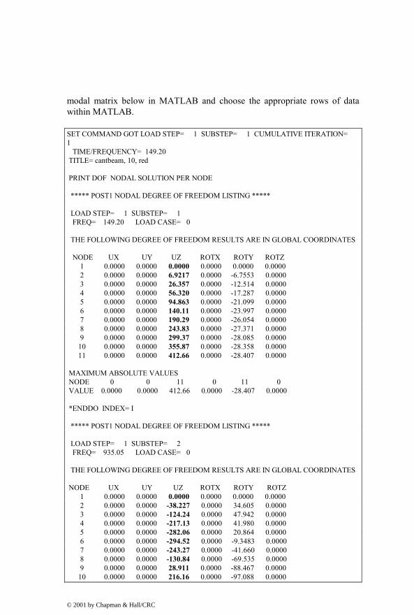
modal matrix below in MATLAB and choose the appropriate rows of data within MATLAB.
SET COMMAND GOT LOAD STEP= 1 SUBSTEP= 1 CUMULATIVE ITERATION= 1 TIME/FREQUENCY= 149.20 TITLE= cantbeam, 10, red PRINT DOF NODAL SOLUTION PER NODE ***** POST1 NODAL DEGREE OF FREEDOM LISTING ***** LOAD STEP= 1 SUBSTEP= 1 FREQ= 149.20 LOAD CASE= 0 THE FOLLOWING DEGREE OF FREEDOM RESULTS ARE IN GLOBAL COORDINATES NODE UX UY UZ ROTX ROTY ROTZ 1 0.0000 0.0000 0.0000 0.0000 0.0000 0.0000 2 0.0000 0.0000 6.9217 0.0000 -6.7553 0.0000 3 0.0000 0.0000 26.357 0.0000 -12.514 0.0000 4 0.0000 0.0000 56.320 0.0000 -17.287 0.0000 5 0.0000 0.0000 94.863 0.0000 -21.099 0.0000 6 0.0000 0.0000 140.11 0.0000 -23.997 0.0000 7 0.0000 0.0000 190.29 0.0000 -26.054 0.0000 8 0.0000 0.0000 243.83 0.0000 -27.371 0.0000 9 0.0000 0.0000 299.37 0.0000 -28.085 0.0000 10 0.0000 0.0000 355.87 0.0000 -28.358 0.0000 11 0.0000 0.0000 412.66 0.0000 -28.407 0.0000 MAXIMUM ABSOLUTE VALUES NODE 0 0 11 0 11 0 VALUE 0.0000 0.0000 412.66 0.0000 -28.407 0.0000 *ENDDO INDEX= I ***** POST1 NODAL DEGREE OF FREEDOM LISTING ***** LOAD STEP= 1 SUBSTEP= 2 FREQ= 935.05 LOAD CASE= 0 THE FOLLOWING DEGREE OF FREEDOM RESULTS ARE IN GLOBAL COORDINATES NODE UX UY UZ ROTX ROTY ROTZ 1 0.0000 0.0000 0.0000 0.0000 0.0000 0.0000 2 0.0000 0.0000 -38.227 0.0000 34.605 0.0000 3 0.0000 0.0000 -124.24 0.0000 47.942 0.0000 4 0.0000 0.0000 -217.13 0.0000 41.980 0.0000 5 0.0000 0.0000 -282.06 0.0000 20.864 0.0000 6 0.0000 0.0000 -294.52 0.0000 -9.3483 0.0000 7 0.0000 0.0000 -243.27 0.0000 -41.660 0.0000 8 0.0000 0.0000 -130.84 0.0000 -69.535 0.0000 9 0.0000 0.0000 28.911 0.0000 -88.467 0.0000 10 0.0000 0.0000 216.16 0.0000 -97.088 0.0000
© 2001 by Chapman & Hall/CRC
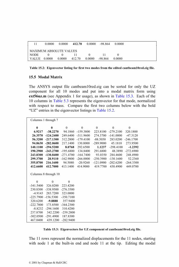
11 0.0000 0.0000 412.70 0.0000 -98.864 0.0000 MAXIMUM ABSOLUTE VALUES NODE 0 0 11 0 11 0 VALUE 0.0000 0.0000 412.70 0.0000 -98.864 0.0000
Table 15.2: Eigenvector listing for first two modes from the edited cantbeam10red.eig file.
15.5 Modal Matrix
The ANSYS output file cantbeam10red.eig can be sorted for only the UZ component for all 10 modes and put into a modal matrix form using ext56uz.m (see Appendix 1 for usage), as shown in Table 15.3. Each of the 10 columns in Table 5.3 represents the eigenvector for that mode, normalized with respect to mass. Compare the first two columns below with the bold “UZ” entries in the eigenvector listings in Table 15.2.
Columns 1 through 7 0 0 0 0 0 0 0 6.9217 -38.2270 94.1860 -159.3800 223.8100 -279.2100 320.1800 26.3570 -124.2400 249.6400 -311.9600 274.3700 -141.0000 -47.3120 56.3200 -217.1300 312.2800 -179.4100 -88.5050 283.0200 -246.1700 94.8630 -282.0600 217.1400 130.8000 -289.9000 45.1810 273.9500 140.1100 -294.5200 8.0768 292.6500 1.1237 -298.4100 -1.2392 190.2900 -243.2700 -195.6800 134.8400 291.6800 48.3890 -272.6900 243.8300 -130.8400 -271.4700 -164.7400 93.0350 284.4600 248.4900 299.3700 28.9110 -162.9800 -266.0000 -250.3900 -130.1600 52.2360 355.8700 216.1600 94.5080 -20.9260 -121.0900 -202.6200 -264.3300 412.6600 412.7000 413.1400 414.9000 419.7700 430.4900 449.0700 Columns 8 through 10 0 0 0 -341.5400 326.0200 223.4200 230.8300 -338.9500 -276.3500 -4.9143 283.7200 323.0000 -225.7900 -156.5300 -350.7100 320.6200 -9.8888 357.9400 -222.7800 173.8500 -344.2300 -8.8232 -294.1600 310.4200 237.8700 342.2200 -259.2800 -302.0500 -291.4900 187.8300 467.0400 439.1200 -282.9400
Table 15.3: Eigenvectors for UZ component of cantbeam10red.eig file.
The 11 rows represent the normalized displacements for the 11 nodes, starting with node 1 at the built-in end and node 11 at the tip. Editing the modal
© 2001 by Chapman & Hall/CRC

matrix to use only the required degrees of freedom (nodes 7 and 11) will take place in MATLAB.
15.6 MATLAB State Space Model from ANSYS Eigenvalue Run – cantbeam_ss_modred.m
In this section we will create a MATLAB state space model using the eigenvalue and eigenvector results from the previous ANSYS run. We discussed in Section 7.9 how to decrease the size of the model by including only degrees of freedom actually used in the particular frequency response or time domain calculations. The new material deals with how to rank the relative importance of the contributions of each of the individual modes. In this chapter, we will use a ranking of dc gains of individual modes to select the modes to be used.
Once the modes are ranked, the most important can be selected for use, with modes with lower dc gains (typically, but not always, the higher frequency modes) eliminated from the model. When these modes are eliminated from the model their dc gain contributions are not included in the overall dc gain, so there is error in the low frequency gain. In order to eliminate this error, the MATLAB function “modred” is introduced and the theory behind the code is discussed. Using “modred” is analogous to using Guyan reduction to reduce some less important degrees of freedom, in that assumptions are made about some modes being more important than others. This allows reducing the size of the problem to that of the “important” modes, while adjusting the overall dc gain to account for the dc gains of the eliminated modes.
We will find that the simple cantilever beam used for an example in this chapter is not very sensitive to the elimination of higher frequency modes. Including a few modes is sufficient for creating a state space model with good accuracy for both frequency response and step response. Whether “modred” is used is not critical for this example. However, we will see that the example in the next chapter is extremely sensitive to dc gain, and will serve as a good model of the benefits of selecting modes to be eliminated judiciously or by using “modred.”
Once the model is created, we will solve for frequency response and step response using various combinations of truncating and sorting modes.
The MATLAB code cantbeam_ss_modred.m will be discussed and listed in detail in the following sections.
© 2001 by Chapman & Hall/CRC

15.6.1 Input
The code in this section asks the user to define how many elements will be used for the analysis. ANSYS runs have been made for 2, 4, 6, 8, 10, 12, 16, 32 and 64 elements. The ANSYS eigenvector results for each have been stripped out of the ANSYS format and put into frequency vector, “freqvec,” and modal matrix, “evr,” form and stored as MATLAB .mat files.
% cantbeam_ss_modred.m clear all; hold off; clf; % load the .mat file cantbeamXXred, containing evr - the modal matrix, freqvec - % the frequency vector and node_numbers - the vector of node numbers for the modal % matrix model = menu('choose which finite element model to use ... ', .... '2 beam elements', ... '4 beam elements', ... '6 beam elements', ... '8 beam elements', ... '10 beam elements', ... '12 beam elements', ... '16 beam elements', ... '32 beam elements', ... '64 beam elements'); if model == 1 load cantbeam2red; elseif model == 2 load cantbeam4red; elseif model == 3 load cantbeam6red; elseif model == 4 load cantbeam8red; elseif model == 5 load cantbeam10red; elseif model == 6 load cantbeam12red; elseif model == 7 load cantbeam16red; elseif model == 8 load cantbeam32red; elseif model == 9 load cantbeam64red; end
© 2001 by Chapman & Hall/CRC

15.6.2 Defining Degrees of Freedom and Number of Modes
The code below checks the size of the modal matrix, where the number of rows indicates how many degrees of freedom are used and the number of columns indicates the number of modes. Since all of the models have an even number of elements, there is always a node at the midpoint of the beam and it is possible to define which row of the modal matrix corresponds to that middle node. The modal matrix row which corresponds to the tip is the last degree of freedom in the matrix. The code also defines a new variable, “xn,” the normalized modal matrix.
% define the number of degrees of freedom and number of modes from size % of modal matrix [numdof,num_modes_total] = size(evr); % define rows for middle and tip nodes mid_node_row = 0.5*(numdof-1)+1; tip_node_row = numdof; xn = evr;
15.6.3 Sorting Modes by dc Gain and Peak Gain, Selecting Modes Used
The next step in creating the model is to sort modes of vibration so that only the most important modes are kept. We will discuss in this section two methods of sorting, one which is applicable for models with the same value of damping for all modes, iζ = ζ = constant (“uniform” damping), and another which is applicable for models with different damping values for each mode (“non-uniform” damping).
Repeating from (8.54a,b) the general equation for the overall transfer function of undamped and damped systems:
mj nji nki
2 2i 1k i
mj nji nki
2 2i 1k i i i
z z zF s
z z zF s 2 s
=
=
=+ ω
=+ ζ ω + ω
∑
∑
(15.1a,b)
This equation shows that in general every transfer function is made up of additive combinations of single degree of freedom systems, with each system
© 2001 by Chapman & Hall/CRC

having its residue determined by the appropriate input/output eigenvector entries, nji nkiz z , and with resonant frequency defined by the eigenvalue, iω . Substituting s j j0 0= ω = = to obtain the ith mode frequency response at dc, the dc gain, which is the same for the undamped and damped cases is:
ji nji nki2
ki i
z z zF
=ω
, (15.2)
where nji nkiz z is the product of the jth (output) row and kth (force applied) row terms of the ith eigenvector divided by the square of the eigenvalue for the ith mode.
At resonance, the peak gain amplitude of each mode is given by substituting 2 2
i is j , s= ω = − ω into (15.1b):
( )
ji nji nki2 2
ki i i i
nji nki2 2 2i i i i
nji nki2
i i
nji nki2
i i
nji nki2
i i
i
z z zF s 2 s
z z2 j
z z2 j
j z z2
z zj2
j dcgain2
=+ ζ ω + ω
=−ω + ζ ω + ω
=ζ ω
−=
ζ ω
−= ζ ω −=ζ
(15.3)
Comparing (15.2) and (15.3) it is evident that the relationship between the dc gain and peak gain for a mode is that the dc gain term is divided by 2ζ and multiplied by “ j− ,” which gives a 90− o phase shift at resonance. Since ζ values for mechanical structures are typically small, a few percent of critical damping, 2ζ is a small number, which serves to amplify the response by virtue of the division, thus the resonant “peak” in the response.
If the same value of ζ is used for all modes, then all the dc gain terms are divided by the same 2ζ terms and the relative amplitudes of the dc gains and
© 2001 by Chapman & Hall/CRC

peak gains are the same, so there is no difference between sorting a uniform damping model using dc gain or peak gain.
However, if the modes have different damping the relationship between the dc gain and peak gain for all the modes is not a constant 1/ 2ζ value and peak gain must be used to rank modes for importance. In this case, the MATLAB damping parameter “zeta” would not be a scalar but would be a vector with entries corresponding to damping in each mode.
We will use dc gain to rank the relative importance of the modes until Chapter 18, where a technique named “balanced reduction” will be introduced. The code shown below, and throughout the book, is easily modified to sort for peak gain instead of dc gain using (15.3) instead of (15.2) and entering a vector of damping values instead of a scalar.
The code below carries out the calculation of the dc gain and sorts from smallest to largest, keeping track of the new column locations in “index_sort.” It then uses the “fliplr” command to list them from largest to smallest, so that the first mode has the highest dc gain. Various plots are then shown to indicate the relative importance of each mode. After plotting the dc gains, the user is asked to define the number of modes to be used in the frequency response, from 1 to all the available modes.
% calculate the dc amplitude of the displacement of each mode by % multiplying the forcing function row of the eigenvector by the output row omega2 = (2*pi*freqvec)'.^2; % convert to radians and square dc_gain = abs(xn(mid_node_row,:).*xn(tip_node_row,:))./omega2; [dc_gain_sort,index_sort] = sort(dc_gain); dc_gain_sort = fliplr(dc_gain_sort); index_sort = fliplr(index_sort) dc_gain_nosort = dc_gain;
index_orig = 1:num_modes_total; semilogy(index_orig,freqvec,'k-'); title('frequency versus mode number') xlabel('mode number') ylabel('frequency, hz') grid pause semilogy(index_orig,dc_gain_nosort,'k-') title('dc value of each mode contribution versus mode number')
© 2001 by Chapman & Hall/CRC

xlabel('mode number') ylabel('dc value') grid off
pause loglog(freqvec,dc_gain_nosort,'k-') title('dc value of each mode contribution versus frequency') xlabel('frequency, hz') ylabel('dc value') grid off
pause semilogy(index_orig,dc_gain_sort,'k-') title('sorted dc value of each mode versus number of modes included') xlabel('modes included') ylabel('sorted dc value') grid off
pause num_modes_used = input(['enter how many modes to include …
, ',num2str(num_modes_total),' default, max ... ']); if (isempty(num_modes_used))
num_modes_used = num_modes_total; end
The first step in any finite element analysis is to understand the resonant frequencies of the model and how they relate to the frequency range of interest for the problem at hand.
1 2 3 4 5 6 7 8 9 10102
103
104
105frequency versus mode number
mode number
frequ
ency
, hz
Figure 15.4: Resonant frequency versus mode number.
© 2001 by Chapman & Hall/CRC

Figure 15.4 shows that modes 8, 9 and 10 have frequencies higher than the required 20 khz required by the problem, so our model should be adequate.
1 2 3 4 5 6 7 8 9 1010-8
10-7
10-6
10-5
10-4
10-3
10-2
10-1dc value of each mode contribution versus mode number
mode number
dc v
alue
Figure 15.5: dc value of each mode contribution versus mode number.
Figure 15.5 shows the dc gain values for all the modes plotted versus mode number. It is interesting that the low values for modes 3, 5, 7 and 9 correspond to small values of the midpoint node elements of the respective eigenvectors (see the bold highlighted entries in columns 3, 5, 7 and 9 in Table 15.3). This means that the midpoint is nearly a “node” for those modes. Again, a “node” for a mode refers not to the number of the end point of the element but a location along the beam where the displacement is zero for a particular mode of vibration.
© 2001 by Chapman & Hall/CRC

102 103 104 10510-8
10-7
10-6
10-5
10-4
10-3
10-2
10-1dc value of each mode contribution versus frequency
frequency, hz
dc v
alue
Figure 15.6: dc Value of each mode contribution versus resonant frequency.
Figure 15.6 shows dc gain versus frequency of the mode. Note that there is a general trend for lower gains as frequency increases. This is not always the case, as we shall see in Chapter 16.
1 2 3 4 5 6 7 8 9 1010-8
10-7
10-6
10-5
10-4
10-3
10-2
10-1sorted dc value of each mode versus number of modes included
modes included
sorte
d dc
val
ue
Figure 15.7: Sorted dc value of each mode versus number of modes included.
Figure 15.7 shows the sorted values for the dc gains, from largest to smallest. The list of mode numbers after sorting is given by “index_sort” below. The ordering can be seen in the dc value versus mode number plot in Figure 15.5.
© 2001 by Chapman & Hall/CRC
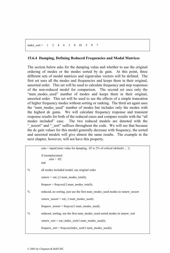
index_sort = 1 2 4 6 3 8 10 5 9 7
15.6.4 Damping, Defining Reduced Frequencies and Modal Matrices
The section below asks for the damping value and whether to use the original ordering of modes or the modes sorted by dc gain. At this point, three different sets of modal matrices and eigenvalue vectors will be defined. The first set uses all the modes and frequencies and keeps them in their original, unsorted order. This set will be used to calculate frequency and step responses of the non-reduced model for comparison. The second set uses only the “num_modes_used” number of modes and keeps them in their original, unsorted order. This set will be used to see the effects of a simple truncation of higher frequency modes without sorting or ranking. The third set again uses the “num_modes_used” number of modes but includes only the modes with the highest dc gains. We will calculate frequency response and transient response results for both of the reduced cases and compare results with the “all modes included” case. The two reduced models are denoted with the “_nosort” and “_sort” suffixes throughout the code. We will see that because the dc gain values for this model generally decrease with frequency, the sorted and unsorted models will give almost the same results. The example in the next chapter, however, will not have this property.
zeta = input('enter value for damping, .02 is 2% of critical (default) ... ');
if (isempty(zeta)) zeta = .02; end
% all modes included model, use original order xnnew = xn(:,(1:num_modes_total)); freqnew = freqvec((1:num_modes_total)); % reduced, no sorting, just use the first num_modes_used modes in xnnew_nosort xnnew_nosort = xn(:,1:num_modes_used); freqnew_nosort = freqvec(1:num_modes_used); % reduced, sorting, use the first num_modes_used sorted modes in xnnew_sort xnnew_sort = xn(:,index_sort(1:num_modes_used)); freqnew_sort = freqvec(index_sort(1:num_modes_used));
© 2001 by Chapman & Hall/CRC

15.6.5 Setting up System Matrix “a”
The section below sets up three state space system “a” matrices. Since we know the form of the modal form state space equation from Chapter 10, it can be built automatically. The general form is given by (15.4). The system matrix is made up of eigenvalue and damping terms for each mode, and each mode is a 2x2 submatrix along the diagonal.
u= +x Ax B& (15.4)
1 12
2 1 1 1 2 p1
3 32
4 2 2 2 4 p2
x 0 1 0 0 ... ... x 0x 2 0 0 ... ... x Fx 0 0 0 1 ... ... x 0x 0 0 2 ... ... x F... ... ... ... ... ... ... ... ...... ... ... ... ... ... ... ... ...
−ω − ζ ω
= + −ω − ζ ω
&
&
&
&u
(15.5)
The first system matrix, “a,” is for the full, non-reduced system and includes all the modes in their original order. The second is “a_nosort” and has the reduced size with the original ordering of modes. The third is “a_sort” and has the reduced number of modes with dc gain ordering.
% define variables for all modes included system matrix, a
w = freqnew*2*pi; % frequencies in rad/sec w2 = w.^2;
zw = 2*zeta*w; % define variables for reduced, nosorted system matrix, a_nosort
w_nosort = freqnew_nosort*2*pi; % frequencies in rad/sec w2_nosort = w_nosort.^2;
zw_nosort = 2*zeta*w_nosort; % define variables for reduced, sorted system matrix, a_sort
w_sort = freqnew_sort*2*pi; % frequencies in rad/sec w2_sort = w_sort.^2;
zw_sort = 2*zeta*w_sort; % define size of system matrix
© 2001 by Chapman & Hall/CRC

asize = 2*num_modes_total; asize_red = 2*num_modes_used; disp(' '); disp(' '); disp(['size of system matrix a is ',num2str(asize)]); disp(['size of reduced system matrix a is ',num2str(asize_red)]); % setup all modes included "a" matrix, system matrix a = zeros(asize); for col = 2:2:asize row = col-1; a(row,col) = 1; end for col = 1:2:asize row = col+1; a(row,col) = -w2((col+1)/2); end for col = 2:2:asize row = col; a(row,col) = -zw(col/2); end % setup reduced, nosorted "a_nosort" matrix, system matrix a_nosort = zeros(asize_red); for col = 2:2:asize_red row = col-1; a_nosort(row,col) = 1; end for col = 1:2:asize_red row = col+1; a_nosort(row,col) = -w2_nosort((col+1)/2);
© 2001 by Chapman & Hall/CRC

end for col = 2:2:asize_red row = col; a_nosort(row,col) = -zw_nosort(col/2); end % setup reduced, sorted "a_sort" matrix, system matrix a_sort = zeros(asize_red); for col = 2:2:asize_red row = col-1; a_sort(row,col) = 1; end for col = 1:2:asize_red row = col+1; a_sort(row,col) = -w2_sort((col+1)/2); end for col = 2:2:asize_red row = col; a_sort(row,col) = -zw_sort(col/2); end
15.6.6 Setting up Input Matrix “b”
As with the system matrix above, here we will set up three different input matrices, “b,” “b_nosort” and “b_sort.” We begin with the force vector in physical coordinates, with “numdof” rows. The rows are all zeros except for the “mid_node_row,” which has a value of 1.0 mN. The force vector in principal coordinates is obtained by premultiplying by the transpose of the modal matrix. The state space form of the force vector in principal coordinates is the “numdof x 1” force vector in principal coordinates padded with zeros to create the same number of rows as states.
© 2001 by Chapman & Hall/CRC

% setup input matrix b, state space forcing function in principal coordinates % f_physical is the vector of physical force % zeros at each output DOF and input force at the input DOF f_physical = zeros(numdof,1); % start out with zeros f_physical(mid_node_row) = 1.0; % input force at node 6, midpoint node % f_principal is the vector of forces in principal coordinates f_principal = xnnew'*f_physical; % b is the vector of forces in principal coordinates, state space form b = zeros(2*num_modes_total,1); for cnt = 1:num_modes_total b(2*cnt) = f_principal(cnt); end % f_principal_nosort is the vector of forces in principal coordinates f_principal_nosort = xnnew_nosort'*f_physical; % b_nosort is the vector of forces in principal coordinates, state space form b_nosort = zeros(2*num_modes_used,1); for cnt = 1:num_modes_used b_nosort(2*cnt) = f_principal_nosort(cnt); end % f_principal_sort is the vector of forces in principal coordinates f_principal_sort = xnnew_sort'*f_physical; % b_sort is the vector of forces in principal coordinates, state space form b_sort = zeros(2*num_modes_used,1); for cnt = 1:num_modes_used b_sort(2*cnt) = f_principal_sort(cnt); end
© 2001 by Chapman & Hall/CRC

15.6.7 Setting up Output Matrix “c” and Direct Transmission Matrix “d”
The output matrices below, “c,” “c_nosort” and “c_sort,” are separated into displacement and velocity matrices, “cdisp” and “cvel,” so that they can be premultiplied by the appropriate modal matrix to obtain vectors of displacements and velocities in physical coordinates. With the defined output displacement and velocity matrices, all displacement and velocity degrees of freedom in physical coordinates are available for plotting or further analysis. Since there is no direct feedthrough on this model, the “d” matrix is zero.
% setup cdisp and cvel, padded xn matrices to give the displacement and velocity % vectors in physical coordinates % cdisp and cvel each have numdof rows and alternating columns consisting of columns % of xnnew and zeros to give total columns equal to the number of states % all modes included cdisp and cvel for col = 1:2:2*length(freqnew) for row = 1:numdof cdisp(row,col) = xnnew(row,ceil(col/2)); cvel(row,col) = 0; end end for col = 2:2:2*length(freqnew) for row = 1:numdof cdisp(row,col) = 0; cvel(row,col) = xnnew(row,col/2); end end % reduced, nosorted cdisp and cvel for col = 1:2:2*length(freqnew_nosort) for row = 1:numdof cdisp_nosort(row,col) = xnnew_nosort(row,ceil(col/2)); cvel_nosort(row,col) = 0;
© 2001 by Chapman & Hall/CRC

end end for col = 2:2:2*length(freqnew_nosort) for row = 1:numdof cdisp_nosort(row,col) = 0; cvel_nosort(row,col) = xnnew_nosort(row,col/2); end end % reduced, sorted cdisp and cvel for col = 1:2:2*length(freqnew_sort) for row = 1:numdof cdisp_sort(row,col) = xnnew_sort(row,ceil(col/2)); cvel_sort(row,col) = 0; end end for col = 2:2:2*length(freqnew_sort) for row = 1:numdof cdisp_sort(row,col) = 0; cvel_sort(row,col) = xnnew_sort(row,col/2); end end % define output d = [0]; %
© 2001 by Chapman & Hall/CRC

15.6.8 Frequency Range, “ss” Setup, Bode Calculations
The first part of this section defines the frequency range to be used for the frequency responses, logarithmically spaced frequency vectors in units of hz and rad/sec. Three “ss” state space systems are defined for the displacement of the tip of the beam, the non-reduced system, the “nosort” and the “sort.” Since “cdisp” contains information about all the degrees of freedom, they are all available for output by defining the appropriate row. The “bode” command is used to calculate the magnitude and phase vectors over the defined frequency range, and the magnitudes are converted to db.
% define frequency vector for frequency responses freqlo = 10; freqhi = 100000; flo=log10(freqlo) ; fhi=log10(freqhi) ; f=logspace(flo,fhi,200) ; frad=f*2*pi ; % take transfer functions, outputting the midpoint and tip node rows of the displacement % vector cdisp % define displacement state space system with the "ss" command sysdisptip = ss(a,b,cdisp(tip_node_row,:),d); % defined reduced systems using num_modes_used nosort modes sysdisptip_nosort = ss(a_nosort,b_nosort,cdisp_nosort(tip_node_row,:),d); % define reduced systems using num_modes_used sorted modes sysdisptip_sort = ss(a_sort,b_sort,cdisp_sort(tip_node_row,:),d); % use "bode" command to generate magnitude/phase vectors [magdisptip,phsdisptip]=bode(sysdisptip,frad) ; [magdisptip_nosort,phsdisptip_nosort]=bode(sysdisptip_nosort,frad) ; [magdisptip_sort,phsdisptip_sort]=bode(sysdisptip_sort,frad) ; % convert magnitude to db magdisptipdb = 20*log10(magdisptip); magdisptipdb_nosort = 20*log10(magdisptip_nosort);
© 2001 by Chapman & Hall/CRC

magdisptipdb_sort = 20*log10(magdisptip_sort);
15.6.9 Full Model - Plotting Frequency Response, Step Response
This section plots the frequency response for tip displacement due to a unit force at the beam midpoint. It then overlays the contribution of each individual mode to the overall response. Since the “a” matrix consists of 2x2 submatrices along the diagonal, all we have to do to get the contribution of each individual mode is to pull out successive 2x2 individual mode system matrices. Similarly, we take the appropriate rows and columns of “b” and “cdisp” for each mode. Because of the systematic form of the matrices, MATLAB can generate the individual mode matrices automatically. To facilitate comparison with the dc gain values calculated for all the modes (and used in their sorting), an “o” is plotted along the left-hand axis for each individual mode. Because the magnitude axis is in db units, the individual contributions cannot be combined graphically like with a linear magnitude axis as shown in Chapter 6. Nevertheless, using the overlaid plots to get a mental image of the combining modes is valuable.
For the unit force step response, a time vector, “t” and input vector “u” are defined for use with the MATLAB function “lsim.”
% start plotting if num_modes_used == num_modes_total % plot all modes included response semilogx(f,magdisptipdb(1,:),'k.-') title(['cantilever tip displacement for mid-length force, all ', …
num2str(num_modes_used),' modes included']) xlabel('Frequency, hz') ylabel('Magnitude, db mm') grid off pause hold on max_modes_plot = num_modes_total; for pcnt = 1:max_modes_plot index = 2*pcnt; amode = a(index-1:index,index-1:index); bmode = b(index-1:index);
© 2001 by Chapman & Hall/CRC

cmode = cdisp(numdof,index-1:index); dmode = [0]; sysdisptip_mode = ss(amode,bmode,cmode,dmode); [magdisptip_mode,phsdisptip_mode]=bode(sysdisptip_mode,frad) ; magdisptip_modedb = 20*log10(magdisptip_mode); semilogx(f,magdisptip_modedb(1,:),'k-') end dc_gain_freq = freqlo*ones(size(freqnew)); semilogx(dc_gain_freq(1:num_modes_used),20*log10(dc_gain
(1:num_modes_used)),'ko:') pause hold off % now use lsim to calculate step response to a unit force ttotal = 0.1; t = linspace(0,ttotal,200); u = ones(size(t)); [disptip,ts] = lsim(sysdisptip,u,t); plot(ts,disptip,'k-') title(['tip disp for mid-length step force, all ',num2str(num_modes_used), …
' modes included']) xlabel('time, sec') ylabel('displacement, mm') grid off pause
© 2001 by Chapman & Hall/CRC

101 102 103 104 105-180
-160
-140
-120
-100
-80
-60
-40
-20
0
20cantilever tip displacement for mid-length force, all 10 modes included
Frequency, hz
Mag
nitu
de, d
b m
m
Figure 15.8: Cantilever tip displacement for mid-length force, all 10 modes included.
Figure 15.8 shows the overall frequency response with the overlaid sdof responses of all the individual modes for the 10-element model using all 10 available modes. The “o’s” at the 10 hz frequency indicate the values of dc gain for each mode. Note that the fifth, seventh and ninth modes have such low gains that their resonant peaks are barely visible on the overall response. The third mode has a higher gain, as indicated by the small pole/zero combination between the second and fourth modes.
0 0.01 0.02 0.03 0.04 0.05 0.06 0.07 0.08 0.09 0.1-0.02
0
0.02
0.04
0.06
0.08
0.1
0.12
0.14tip disp for mid-length step force, all 10 modes included
time, sec
disp
lace
men
t, m
m
Figure 15.9: Cantilever tip displacement for mid-length force, all 10 modes included.
© 2001 by Chapman & Hall/CRC

Figure 15.9 depicts the response of the beam tip due to a 1mN step force at the midpoint. We will be comparing the different modal truncation methods with this overall response.
15.6.10 Reduced Models – Plotting Frequency Response, Step Response
The following section of code does the same thing for the reduced unsorted and sorted models as the last section did for the full model. In all the plots, the full model results are overlaid with the reduced model results to show the differences. In the examples that follow, we will use four modes in the reduced models. The reader is encouraged to run the code using different numbers of reduced modes to see the effects on both frequency and time domain responses.
else % plot unsorted modal truncation semilogx(f,magdisptipdb(1,:),'k-',f,magdisptipdb_nosort(1,:),'k.-') title(['unsorted modal truncation: cantilever tip displacement for mid- …
length force, first ',num2str(num_modes_used),' modes included']) legend('all modes','unsorted partial modes',3) dcgain_error_percent_nosort = 100*(magdisptip_nosort(1) …
magdisptip(1))/magdisptip(1) xlabel('Frequency, hz') ylabel('Magnitude, db mm') grid off pause hold on max_modes_plot = num_modes_used; for pcnt = 1:max_modes_plot index = 2*pcnt; amode = a_nosort(index-1:index,index-1:index); bmode = b_nosort(index-1:index); cmode = cdisp_nosort(numdof,index-1:index); dmode = [0]; sysdisptip_mode = ss(amode,bmode,cmode,dmode); [magdisptip_mode,phsdisptip_mode]=bode(sysdisptip_mode,frad) ;
© 2001 by Chapman & Hall/CRC

magdisptip_modedb = 20*log10(magdisptip_mode); semilogx(f,magdisptip_modedb(1,:),'k-') end dc_gain_freq_nosort = freqlo*ones(size(freqnew_nosort)); semilogx(dc_gain_freq_nosort(1:num_modes_used),20*log10 …
(dc_gain_nosort(1:num_modes_used)),'ko:') pause hold off % plot sorted modal truncation semilogx(f,magdisptipdb(1,:),'k-',f,magdisptipdb_sort(1,:),'k.-') title(['sorted modal truncation: cantilever tip displacement for mid-length force, …
first ',num2str(num_modes_used),' modes included']) legend('all modes','sorted partial modes',3) dcgain_error_percent_sort = 100*(magdisptip_sort(1) - magdisptip(1))/magdisptip(1) xlabel('Frequency, hz') ylabel('Magnitude, db mm') grid off pause hold on max_modes_plot = num_modes_used; for pcnt = 1:max_modes_plot index = 2*pcnt; amode = a_sort(index-1:index,index-1:index); bmode = b_sort(index-1:index); cmode = cdisp_sort(numdof,index-1:index); dmode = [0]; sysdisptip_mode = ss(amode,bmode,cmode,dmode); [magdisptip_mode,phsdisptip_mode]=bode(sysdisptip_mode,frad) ; magdisptip_modedb = 20*log10(magdisptip_mode); semilogx(f,magdisptip_modedb(1,:),'k-')
© 2001 by Chapman & Hall/CRC

end dc_gain_freq_sort = freqlo*ones(size(freqnew_nosort)); semilogx(dc_gain_freq_sort(1:num_modes_used),20*log10 …
(dc_gain_sort(1:num_modes_used)),'ko:') pause hold off % now use lsim to calculate step response to a unit force ttotal = 0.1; t = linspace(0,ttotal,200); u = ones(size(t)); [disptip,ts] = lsim(sysdisptip,u,t); [disptip_nosort,ts_nosort] = lsim(sysdisptip_nosort,u,t); [disptip_sort,ts_sort] = lsim(sysdisptip_sort,u,t); plot(ts,disptip,'k-',ts_nosort,disptip_nosort,'k+-',ts_sort,disptip_sort,'k.-') title(['tip disp for mid-length step force, first ',num2str(num_modes_used) …
,' modes included']) legend('all modes','unsorted partial modes','sorted partial modes') xlabel('time, sec') ylabel('displacement, mm') grid off pause
© 2001 by Chapman & Hall/CRC

15.6.11 Reduced Models – Plotted Results – Four Modes Used
101 102 103 104 105-180
-160
-140
-120
-100
-80
-60
-40
-20
0
20unsorted modal truncation: cantilever tip displacement for mid-length force, first 4 modes included
Frequency, hz
Mag
nitu
de, d
b m
m
all modes unsorted partial modes
Figure 15.10: Cantilever tip displacement for mid-length force, first four modes included – unsorted modal truncation.
101 102 103 104 105-160
-140
-120
-100
-80
-60
-40
-20
0
20sorted modal truncation: cantilever tip displacement for mid-length force, first 4 modes included
Frequency, hz
Mag
nitu
de, d
b m
m
all modes sorted partial modes
Figure 15.11: Cantilever tip displacement for mid-length force, first four modes included – sorted modal truncation.
Figure 15.10 depicts overall plus individual mode contributions for the four unsorted modes model. Note that the first four unsorted modes are used. The dc gain error relative to the full 10-mode model is +0.024% because the dc
© 2001 by Chapman & Hall/CRC

gain terms for the eliminated modes are not included. Note that the last three peaks in the “all modes” response are missed because the modes are not included.
Figure 15.11 shows overall plus individual mode contributions for the four sorted modes model. Note that this time the third mode is skipped and the fifth mode is used instead because it has a higher dc gain. The dc gain error relative to the full 10-mode model is –0.027%.
Figure 15.12: Comparison of step responses for all modes included and four modes included, unsorted and sorted.
Figure 15.12 shows step response for full, reduced unsorted and reduced sorted models. Because the dc gain for the two models is in error only by a fraction of a percent and because the eliminated modes are some 80db (four orders of magnitude) lower than the most significant first mode, there is no discernable difference in the responses of the full and two reduced models.
15.6.12 Modred Description
The MATLAB Control System Toolbox has a function, “modred” (MODel order REDuction), which can be used for reducing models while retaining the overall system dc gain. The “mdc” or “Matched DC” gain option for the function “modred” reduces defined states by setting the derivatives of the states to be eliminated to zero, then solving for the remaining states. The method essentially sets up the eliminated states to be “infinitely fast” and is analogous to Guyan reduction in that the low frequency effects of the eliminated states are included in the remaining states. The other option for
© 2001 by Chapman & Hall/CRC

“modred” is the “del” option, which simply eliminates the defined states, typically associated with the higher frequency modes.
The derivation of the “mdc” option follows. We start with the state space description of the system:
= += +
x Ax Buy Cx Du&
(15.6a,b)
Assume that we have a method of ordering the importance of the modes making up the A, B and C matrices, in our case using dc or peak gains. If we then rearrange and partition the matrices such that the states corresponding to the most important modes are separated from the less important modes, designating the important modes as rx (reduced) and the unimportant modes to be eliminated as ex , we get
[ ]
r r r er r r
e r e ee e e
rr e
e
u
u
= +
= +
A Ax x BA Ax x B
xy C C D
x
&
& (15.7a,b)
Expanding the matrices:
r r r r r e e r
e e r r e e e e
u
u
= + +
= + +
x A x A x Bx A x A x B
&
& (15.8a,b)
Setting the ex& states equal to zero in (15.10) is analogous to setting (14.14) equal to zero in the Guyan reduction process. We are then, in effect, including the low frequency dc gain or static equilibrium characteristics of the eliminated modes in the reduced modes.
e r r e e e e0 u= + +A x A x B (15.9)
Solving for ex :
1 1e ee e r r e e eu
− −= − −x A A x A B (15.10)
Substituting back into the rx& equation and grouping terms:
© 2001 by Chapman & Hall/CRC

( )
( ) ( )1 1
r r r r r e e e e r r ee e r
1 1r r r e e e e r r r r e e e e
u u
u
− −
− −
= + − − +
= − + −
x A x A A A x A B B
A A A A x B A A B
& (15.11)
Substituting back into the expanded output equations:
( )( ) ( )
r r e e
1 1r r e ee e r r e e e
1 1r e ee e r r e ee e
u
u u
u
− −
− −
= + +
= + − − +
= − + −
y C x C x D
C x C A A x A B D
C C A A x D C A B
(15.12)
The new matrices for the reduced model become:
1red r r r e e e e r
1red r r e ee e
1red r e e e e r
1red e ee e
−
−
−
−
= −
= −
= −
= −
A A A A A
B B A A B
C C C A A
D D C A B
(15.13a,b,c,d)
The new state equations are:
red red red red
red red red red
uu
= += +
x A x By C x D&
(15.14a,b)
We will see (Figure 15.14) that the high frequency portion of the response when reducing using “modred” does not roll off quickly with frequency as we are used to seeing. Rather, it will be “flat” with frequency. The reason for the shape of the “modred” high frequency asymptote is in the redD term in (15.13d). In many cases, the direct transmission term D is zero. When using “modred,” however, even if D is zero, there is still the 1
e e e e−−C Α B portion of
redD to contend with. Repeating Figure 5.2 below, we can see the direct transmission term.
© 2001 by Chapman & Hall/CRC

A
+ +B
D
C∫ Iu(t)x(t)& x(t)
y(t)
Integrator Block
DirectTransmission
Matrix
Output MatrixInput Matrix
System Matrixscalar
vector
Input Output
Figure 15.13: State space system block diagram.
At high frequencies, where the system matrix dynamics start to attenuate, the 1
e e e e−−C Α B term of redD starts to dominate the response – hence the “flat” high
frequency response in Figure 15.15.
15.6.13 Defining Sorted or Unsorted Modes to be Used
The section of code below prompts the user to define whether the modes are to be sorted by dc gain or left in the original order for the “modred” operation. One argument of the “modred” command is to define the states to be eliminated. The states to be eliminated can be defined as a vector of arbitrary states or as a continuous partition of states. We will define them in the code below as a continuous block of states, from one index greater than the number of states to be kept to the total number of states. Therefore, if we sort by dc gain before using “modred,” we would keep only the most important states. If we choose to use the unsorted states, we will be eliminating the higher frequency modes and keeping the lower frequency modes.
% use modred to reduce, select whether to use sorted or unsorted modes for the reduction modred_sort = input('modred: enter "1" to use sorted modes for reduced runs, …
"enter" to use unsorted ... '); if isempty(modred_sort) modred_sort = 0 end
© 2001 by Chapman & Hall/CRC

if modred_sort == 1 % use sorted mode order xnnew = xn(:,index_sort(1:num_modes_total)); freqnew = freqvec(index_sort(1:num_modes_total)); else % use original mode order xnnew = xn(:,(1:num_modes_total)); freqnew = freqvec((1:num_modes_total)); end
15.6.14 Defining System for Reduction
In this section we define a new set of “a,” “b,” “c” and “d” matrices which will be used with “modred.”
% define variables for all modes included system matrix, a
w = freqnew*2*pi; % frequencies in rad/sec w2 = w.^2;
zw = 2*zeta*w; % define size of system matrix asize = 2*num_modes_total; % setup all modes included "a" matrix, system matrix a = zeros(asize); for col = 2:2:asize row = col-1; a(row,col) = 1; end for col = 1:2:asize row = col+1; a(row,col) = -w2((col+1)/2); end
© 2001 by Chapman & Hall/CRC

for col = 2:2:asize row = col; a(row,col) = -zw(col/2); end % setup input matrix b, state space forcing function in principal coordinates % f_physical is the vector of physical force % zeros at each output DOF and input force at the input DOF f_physical = zeros(numdof,1); % start out with zeros f_physical(mid_node_row) = 1.0; % input force at node
6,midpoint node % f_principal is the vector of forces in principal coordinates f_principal = xnnew'*f_physical; % b is the vector of forces in principal coordinates, state space form b = zeros(2*num_modes_total,1); for cnt = 1:num_modes_total b(2*cnt) = f_principal(cnt); end % setup cdisp and cvel, padded xn matrices to give the displacement and velocity % vectors in physical coordinates % cdisp and cvel each have numdof rows and alternating columns consisting of columns % of xnnew and zeros to give total columns equal to the number of states % all modes included cdisp and cvel for col = 1:2:2*length(freqnew) for row = 1:numdof cdisp(row,col) = xnnew(row,ceil(col/2)); cvel(row,col) = 0; end end for col = 2:2:2*length(freqnew) for row = 1:numdof
© 2001 by Chapman & Hall/CRC

cdisp(row,col) = 0; cvel(row,col) = xnnew(row,col/2); end end % define output d = [0]; %
15.6.15 Modred Calculations – “mdc” and “del”
This section defines a MATLAB state space, “ss,” system using either the unsorted or sorted eigenvectors and eigenvalues from above, and then both the “mdc” and “del” options with “modred” to calculate two reduced systems. In order to be able to plot not only the overall frequency response from the reduced systems but also the individual mode contributions, we will use the “ssdata” function in MATLAB to define the reduced system matrices. In the next section we will use 2x2 submatrices of the reduced system matrix to define individual modal contributions. The “bode” command is then used to generate the magnitude/phase solution vectors, which are converted to db.
% define state space system for reduction, ordered defined by modred_sort sysdisptip_red = ss(a,b,cdisp(tip_node_row,:),d); % define reduced matrices using matched dc gain method "mdc" states_elim = (2*num_modes_used+1):2*num_modes_total; sysdisptip_mdc = modred(sysdisptip_red,states_elim,'mdc'); [adisptip_mdc,bdisptip_mdc,cdisptip_mdc,ddisptip_mdc] = ssdata(sysdisptip_mdc); % define reduced matrices by eliminating high frequency states, ‘del sysdisptip_elim = modred(sysdisptip_red,states_elim,’del’); [adisptip_elim,bdisptip_elim,cdisptip_elim,ddisptip_elim] = ssdata(sysdisptip_elim); % use "bode" command to generate magnitude/phase vectors for reduced systems [magdisptip_mdc,phsdisptip_mdc]=bode(sysdisptip_mdc,frad) ; [magdisptip_elim,phsdisptip_elim]=bode(sysdisptip_elim,frad) ; % convert magnitude to db magdisptip_mdcdb = 20*log10(magdisptip_mdc);
© 2001 by Chapman & Hall/CRC
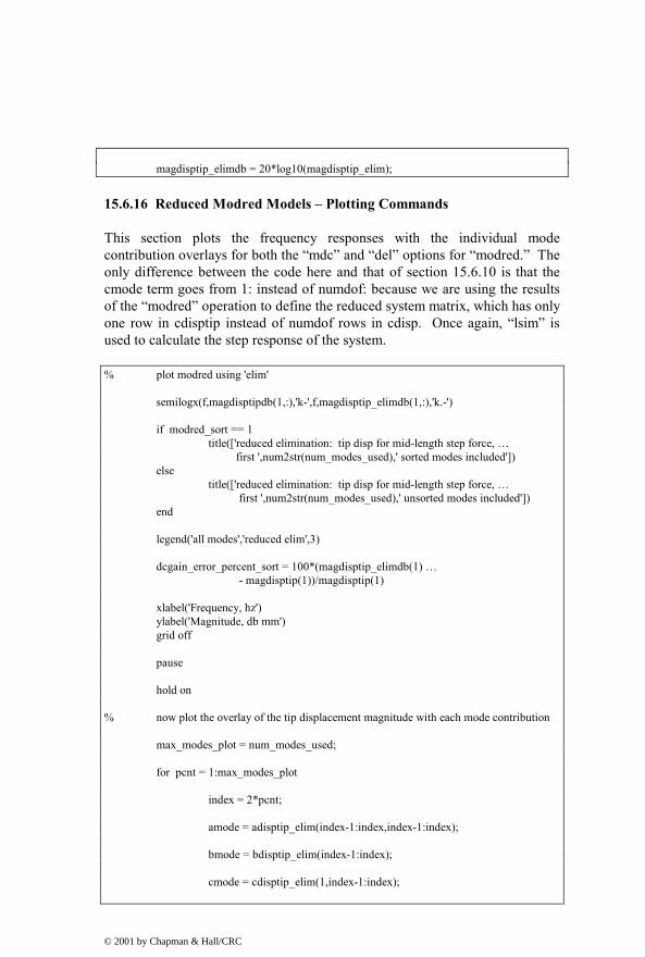
magdisptip_elimdb = 20*log10(magdisptip_elim);
15.6.16 Reduced Modred Models – Plotting Commands
This section plots the frequency responses with the individual mode contribution overlays for both the “mdc” and “del” options for “modred.” The only difference between the code here and that of section 15.6.10 is that the cmode term goes from 1: instead of numdof: because we are using the results of the “modred” operation to define the reduced system matrix, which has only one row in cdisptip instead of numdof rows in cdisp. Once again, “lsim” is used to calculate the step response of the system.
% plot modred using 'elim' semilogx(f,magdisptipdb(1,:),'k-',f,magdisptip_elimdb(1,:),'k.-') if modred_sort == 1 title(['reduced elimination: tip disp for mid-length step force, …
first ',num2str(num_modes_used),' sorted modes included']) else title(['reduced elimination: tip disp for mid-length step force, …
first ',num2str(num_modes_used),' unsorted modes included']) end legend('all modes','reduced elim',3) dcgain_error_percent_sort = 100*(magdisptip_elimdb(1) …
- magdisptip(1))/magdisptip(1) xlabel('Frequency, hz') ylabel('Magnitude, db mm') grid off pause hold on % now plot the overlay of the tip displacement magnitude with each mode contribution max_modes_plot = num_modes_used; for pcnt = 1:max_modes_plot index = 2*pcnt; amode = adisptip_elim(index-1:index,index-1:index); bmode = bdisptip_elim(index-1:index); cmode = cdisptip_elim(1,index-1:index);
© 2001 by Chapman & Hall/CRC
dmode = [0]; sysdisptip_mode = ss(amode,bmode,cmode,dmode); [magdisptip_mode,phsdisptip_mode]=bode(sysdisptip_mode,frad) ; magdisptip_modedb = 20*log10(magdisptip_mode); semilogx(f,magdisptip_modedb(1,:),'k-') end dc_gain_freq_sort = freqlo*ones(size(freqnew_nosort)); pause hold off % modred using 'mdc' semilogx(f,magdisptipdb(1,:),'k-',f,magdisptip_mdcdb(1,:),'k.-') if modred_sort == 1 title(['reduced matched dc gain: tip disp for mid-length step force, …
first ',num2str(num_modes_used),' sorted modes included']) else title(['reduced matched dc gain: tip disp for mid-length step force, …
first ',num2str(num_modes_used),' unsorted modes included']) end legend('all modes','reduced mdc',3) dcgain_error_percent_nosort = 100*(magdisptip_mdcdb(1) …
- magdisptip(1))/magdisptip(1) xlabel('Frequency, hz') ylabel('Magnitude, db mm') grid off pause hold on max_modes_plot = num_modes_used; for pcnt = 1:max_modes_plot index = 2*pcnt; amode = adisptip_mdc(index-1:index,index-1:index); bmode = bdisptip_mdc(index-1:index); cmode = cdisptip_mdc(1,index-1:index);
© 2001 by Chapman & Hall/CRC

dmode = [0]; sysdisptip_mode = ss(amode,bmode,cmode,dmode); [magdisptip_mode,phsdisptip_mode]=bode(sysdisptip_mode,frad) ; magdisptip_modedb = 20*log10(magdisptip_mode); semilogx(f,magdisptip_modedb(1,:),'k-') end dc_gain_freq_nosort = freqlo*ones(size(freqnew_nosort)); pause hold off % now use lsim to calculate step response to a unit force [disptip,ts] = lsim(sysdisptip,u,t); [disptip_elim,ts_elim] = lsim(sysdisptip_elim,u,t); [disptip_mdc,ts_mdc] = lsim(sysdisptip_mdc,u,t); plot(ts,disptip,'k-',ts_mdc,disptip_mdc,'k.-',ts_elim,disptip_elim,'k+-') if modred_sort == 1 title(['modred cantilever tip disp for mid-length step force, …
first ',num2str(num_modes_used),' sorted modes included']) else title(['modred cantilever tip disp for mid-length step force …
, first ',num2str(num_modes_used),' unsorted modes included']) end legend('all modes','reduced - mdc','reduced - elim') xlabel('time, sec') ylabel('displacement, mm') grid off pause end
© 2001 by Chapman & Hall/CRC

15.6.17 Plotting Unsorted Modred Reduced Results – Eliminating High Frequency Modes
101 102 103 104 105-180
-160
-140
-120
-100
-80
-60
-40
-20
0
20reduced elimination: tip disp for mid-length step force, first 4 unsorted modes included
Frequency, hz
Mag
nitu
de, d
b m
m
all modes reduced elim
Figure 15.14: Cantilever tip displacement for mid-length force, first four modes included – unsorted modal truncation, modred “del” option.
101 102 103 104 105-180
-160
-140
-120
-100
-80
-60
-40
-20
0
20reduced matched dc gain: tip disp for mid-length step force, first 4 unsorted modes included
Frequency, hz
Mag
nitu
de, d
b m
m
all modes reduced mdc
Figure 15.15: Cantilever tip displacement for mid-length force, first four modes included – unsorted modal truncation, modred “mdc” option.
Figure 15.14 shows overall frequency response with four overlaid individual mode contributions for the unsorted “del” “modred” option, with the six
© 2001 by Chapman & Hall/CRC

highest frequency modes eliminated. Note that at high frequencies the reduced curve attenuates with frequency similar to the “all modes” curve.
Figure 15.15 shows overall frequency response with four overlaid individual mode contributions for the unsorted “mdc” “modred” option, with the six highest frequency modes reduced. Note the rise in the high frequency portion of the magnitude curve as a result of the matrix reduction operations discussed at the end of Section 15.6.12. Depending on the purpose of the model, the high frequency discrepancy may or may not be important.
Figure 15.16: Comparison of step responses for all modes included and four modes included, “mdc” and “elim” “modred” options.
Figure 15.16 shows the overlay of step response for all mode model and “del” and “mdc” “modred” options. Note that there is no visible difference in the transient responses.
© 2001 by Chapman & Hall/CRC

15.6.18 Plotting Sorted Modred Reduced Results – Eliminating Lower dc Gain Modes
101 102 103 104 105-160
-140
-120
-100
-80
-60
-40
-20
0
20reduced elimination: tip disp for mid-length step force, first 4 sorted modes included
Frequency, hz
Mag
nitu
de, d
b m
m
all modes reduced elim
Figure 15.17: Cantilever tip displacement for mid-length force, first four sorted modes, modal truncation, “modred” “del” option.
101 102 103 104 105-160
-140
-120
-100
-80
-60
-40
-20
0
20reduced matched dc gain: tip disp for mid-length step force, first 4 sorted modes included
Frequency, hz
Mag
nitu
de, d
b m
m
all modes reduced mdc
Figure 15.18: Cantilever tip displacement for mid-length force, first four sorted modes, “modred” “mdc” option.
Figure 15.17 shows overall frequency response with four overlaid individual mode contributions for the sorted “del” “modred” option, with the six lowest
© 2001 by Chapman & Hall/CRC

dc gain modes eliminated. Figure 15.18 shows overall frequency response with four overlaid individual mode contributions for the unsorted “mdc” “modred” option, with the six lowest dc gain modes reduced. Again, note the lack of high frequency attenuation with frequency for the “modred” reduction.
Figure 15.19: Comparison of step responses for all modes included and four sorted modes included, “mdc” and “elim” “modred” options.
Figure 15.19 depicts the overlay of step response for the all mode model and “del” and “mdc” “modred” options. Note that there is no visible difference in the transient responses.
15.6.19 Modred Summary
For this problem, where the dc gain of the response is dominated by the first several modes, there is not much difference between the sorted and unsorted responses. The “mdc” method minimizes low frequency errors by accounting for the dc gain of the unused modes but has high frequency behavior which deviates from the expected, and may not be desirable. The “del” method does not account for the dc gains of the unused modes, which can result in error in the low frequency portion of the frequency response. However, the “del” method has the advantage that it does not exhibit the unusual high frequency direct transmission matrix related behavior of the “mdc” method. If sorting of dc gain values is performed prior to the “del” operation, the system dc gain error may be acceptable while maintaining better high frequency performance.
© 2001 by Chapman & Hall/CRC

15.7 ANSYS Code cantbeam_ss.inp Listing
The ANSYS code cantbeam_ss.inp solves for the eigenvalues and eigenvectors for a tip-loaded cantilever beam, with a sample output shown in Section 15.4. The user can define the number of elements to use for the cantilever and also choose whether to use the “Reduced” or “Block Lanczos” eigenvalue extraction method. The program then writes a frequency list out to a “.frq” file, outputs eigenvector listings to a “.eig” file and plots deformed/undeformed mode shapes to “.grp.”
! cantbeam_ss.inp, 0.075 thick x 2 wide x 20mm long steel cant ! title automatically built based on number of elements and eigenvalue extraction method /prep7 filename = 'cantbeam_ss' ! define number of elements to use num_elem = 64 ! define eigenvalue extraction method, 1 = reduced, 2 = block lanczos eigext = 1 *if,eigext,eq,1, then nummodes = num_elem ! only 1 displacement dof available for each element *else nummodes = 2*num_elem ! both disp and rotation dof's available for
! each element *endif ! create the file name for storing data ! first section of filename aname = filename ! second section of filename, number of elements bname = num_elem ! third section of filename, depends on eigenvalue extraction method *if,eigext,ne,2, then cname = 'red' ! reduced *else cname = 'bl' ! block Lanczos *endif ! input the title, use %xxx% to substitute parameter name or parametric expression
© 2001 by Chapman & Hall/CRC

aname_ti = 'cantbeam_ss - 0.075 thick x 2 wide x 20mm long steel cant' /title,%aname_ti%, %bname%, %cname% et,1,4 ! element type for beam ! steel ex,1,190e6 ! mN/mm^2 dens,1,7.83e-6 ! kg/mm^3 nuxy,1,.293 ! real value to define beam characteristics r,1,0.15,0.05,0.00007031,0.075,0.2 ! area, Izz, Iyy, TKz, TKy ! define plotting characteristics /view,1,1,-1,1 ! iso view /angle,1,-60 ! iso view /pnum,mat,1 ! color by material /num,1 ! numbers off /type,1,0 ! hidden plot /pbc,all,1 ! show all boundary conditions csys,0 ! define global coordinate system ! nodes n,1,0,0,0 ! left-hand node n,num_elem+1,20,0,0 ! right-hand node fill,1,num_elem+1 ! interior nodes nall nplo ! elements type,1 mat,1 real,1 e,1,2 egen,num_elem,1,-1 ! constrain left-hand end nall d,1,all,0 ! constrain node 1, all dof's ! constrain all but uz and roty for all other nodes to allow only those dof's nall nsel,s,node,,2,num_elem+1
© 2001 by Chapman & Hall/CRC

d,all,ux d,all,uy d,all,rotx d,all,rotz nall eall nplo eplo ! ******************* eigenvalue run ****************** fini ! fini just in case not in begin /solu ! enters the solution processor, needs to be here to do editing below allsel ! default selects all items of specified entity type, typically nodes, elements nsel,s,node,,2,num_elem+1 m,all,uz *if,eigext,eq,1,then ! use reduced method antype,modal,new modopt,reduc,nummodes ! method - reduced Householdert expass,off ! key = off, no expansion pass, key = on,
! do expansion mxpand,nummodes,,,no ! nummodes to expand,freq beginning,freq
! ending,elcalc = yes - calculate stresses total,num_elem,1 ! total masters, 1 is exclude rotations *elseif,eigext,eq,2 ! use block lanczos antype,modal,new modopt,lanb,nummodes ! no total required for block lanczos
! because calculates all eigenvalues expass,off mxpand,nummodes,,,no *endif allsel solve ! starts the solution of one load step of a solution sequence, modal here fini ! plot first mode /post1 /format,,,,,10000 set,1,1
© 2001 by Chapman & Hall/CRC

pldi,1 ! **************** output frequencies *********************** save,%aname%%bname%%cname%,sav /output,%aname%%bname%%cname%,frq ! write out frequency list to ascii file .frq set,list /output,term ! returns output to terminal ! ****************** output eigenvectors ************************ ! define nodes for output: forces applied or output displacements nall /output,%aname%%bname%%cname%,eig ! write out frequency list to ascii file .eig *do,i,1,nummodes set,,i /page,,,1000 prdisp *enddo /output,term ! ****************** plot modes ****************** ! pldi plots /show,%aname%%bname%%cname%,grp,0 ! save mode shape plots to file .grp allsel /view,1,,-1,, ! side view for plotting /angle,1,0 /auto *do,i,1,nummodes set,1,i pldi,1 *enddo /show,term
© 2001 by Chapman & Hall/CRC

CHAPTER 16
GROUND ACCELERATION MATLAB MODEL FROM ANSYS MODEL
16.1 Introduction
This chapter will continue to explore building MATLAB state space models from ANSYS finite element results. We will use a different cantilever model, where the cantilever has an additional tip mass and a tip spring all mounted on a “shaker” base. This model will be a crude approximation of understanding the effects of disk drive suspension resonances on undesired unloading of the recording head during external vibration events. The problem shows how to model ground acceleration forcing functions using ANSYS and MATLAB. We will also see how to do sorting of modes in the presence of a rigid body mode. In addition, there is a high frequency mode of the system with a large dc gain, meaning that if unsorted modal truncation were used to decrease the model size, the resulting model would have significant error.
16.2 Model Description
Shaker Mass
Shaker Motion
Cantilever Beam
Beam Tip Mass
Spring
Z
X
Figure 16.1: Ground displacement model for cantilever with tip mass and tip spring.
The figure above shows a schematic of the system to be analyzed. Once again, the cantilever is a 2mm wide by 0.075mm thick by 20mm long steel beam. At the tip, a lumped mass of 0.00002349 Kg is attached. The tip mass was arbitrarily chosen to have the same mass as the beam. The spring attaching the
© 2001 by Chapman & Hall/CRC

beam tip to the shaker has a stiffness of 1e6 mN/mm. The 0.05 Kg shaker mass was chosen to be approximately 1000 times the mass of the beam and tip mass combination, making the motions of the shaker insensitive to resonances of the beam. Thus, we can apply forces to the shaker and excite it to a known acceleration amplitude. This amplitude will then be transmitted to the base of the cantilever and the shaker attachment for the beam tip spring – effectively imparting a “ground acceleration” of any desired amplitude and shape to the flexible system. Of course, since the shaker body is not constrained, it will have large rigid body movements, but we are interested in the difference between the shaker motion and the motion of the tip, so we can ignore the rigid body motion.
In a disk drive, the cantilever would represent the “suspension,” the small sheet metal device which supports the recording head, represented by the beam tip mass. The recording head is typically preloaded onto the disk with several grams of loading force by pre-bending and then displacing the suspension. This loading force is required to counteract the force generated by the air bearing when the disk is spinning, keeping the recording head a controlled distance from the disk and allowing efficient magnetic recording. During transportation of the disk drive it is subject to vibration and shock events in the z direction as indicated by the Shaker Motion arrow. Of course, vibration and shock occur in all directions, but the z direction is the most sensitive. In the z direction, the vibration or shock event may be large enough and have frequency content which will excite the suspension resonances, generating unloading forces at the head that could cause it to become momentarily unloaded. When unloaded, the slider will re-approach the disk and possibly damage the disk. Thus, understanding resonant characteristics of the suspension and the resulting tendency to unload the head is very important. Because the frequency content of typical vibration and shock events are less than several khz, having a good model of the resonant system up to roughly 10 khz is adequate.
16.3 Initial ANSYS Model Comparison – Constrained-Tip and Spring-Tip Frequencies/Mode Shapes
The spring between the beam tip and the shaker is an artifice, created to allow measuring the forces between the beam tip and the shaker. If the spring had infinite stiffness, the tip would become simply supported. The stiffness of the spring used in the model was chosen to have the frequency of the mode involving the beam tip and the spring be very high relative to the first bending mode of the constrained-tip beam. This makes the tip simply supported at frequencies lower than the beam tip/spring mode and will allow a valid force measurement in the frequency range of the major beam bending modes.
© 2001 by Chapman & Hall/CRC

There is always a compromise when using a spring artifice to replace a rigid boundary condition to enable calculating constraint forces. The compromise is that one would like a very stiff spring to make the model more accurate, however a very stiff spring would require more modes to be extracted because the frequency of the tip spring/tip mass mode would be higher. Thus, the eternal compromise with finite element models: between more accuracy (more elements) and a shorter time to solve the problem (fewer elements). The optimal model is always the smallest model which will give acceptable answers, no more, no less. This balance makes finite elements interesting!
In order to understand the effects of the tip spring on the resonances, we will use two ANSYS models. The first model will have the tip constrained in the z direction. The second model will be as described above, but with a tip spring connected to the shaker. The two models will be compared to ensure that the tip spring artifice does not significantly effect the major beam bending modes. The tip constrained model is cantbeam_ss_tip_con.inp, the spring-tip model is cantbeam_ss_spring_shkr.inp, which is listed at the end of the chapter. A comparison of resonant frequencies for the two models, each with 16-beam elements and using the Reduced method for eigenvalue extraction, is shown below:
Mode Tip Constrained Tip Spring Freq, hz Freq, hz 1 0.0030932 0.0000 2 654.37 654.36 3 2120.2 2120.1 4 4424.1 4423.3 5 7567.0 7564.6 6 11553. 11547. 7 16392. 16378. 8 22104. 22069. 9 28730. 28590. 10 36346. 32552. Note 32552 is tip/spring mode 11 45079. 36547. 12 55111. 45164. 13 66628. 55171. 14 79548. 66675. 15 92830. 79583. 16 0.10359E+06 92850.
Table 16.1: Resonant frequencies for tip-constrained and spring-tip models.
The table above tells us that there is very good matching of resonant frequencies for the first 15 modes of the tip-constrained model and the tip spring model. The 92830 hz (15th) mode differs only 20 hz from the tip spring model 92850 hz mode. The difference between the two models is that the tip spring model has an additional mode at 32552 which is the tip spring/tip mass mode. Having good agreement between the two models up through 32552 hz
© 2001 by Chapman & Hall/CRC

means that we will get good results in the 0 to 10 khz range of interest. The ANSYS Display program can be used to plot the mode shapes of the two 16-element models by loading cantbeam16red.grp or tipcon16red.grp for the spring-tip or constrained-tip models, respectively. A MATLAB code, cantbeam_shkr_modeshape.m, can also be used to plot mode shapes for any of the spring-tip models, with selected modes plotted below for the 16-element model.
0 5 10 15 20-5
-4
-3
-2
-1
0
1
2
3
4
5mode shape for 16 element model, mode 1 at 0 hz
distance along beam, mm
Figure 16.2: Rigid body mode, 0 hz.
0 5 10 15 20-5
-4
-3
-2
-1
0
1
2
3
4
5mode shape for 16 element model, mode 2 at 654.36 hz
distance along beam, mm
Figure 16.3: First bending mode, 654 hz.
© 2001 by Chapman & Hall/CRC

0 5 10 15 20-5
-4
-3
-2
-1
0
1
2
3
4
5mode shape for 16 element model, mode 3 at 2120.1 hz
distance along beam, mm
Figure 16.4: Second bending mode, 2120 hz.
0 5 10 15 20-5
-4
-3
-2
-1
0
1
2
3
4
5mode shape for 16 element model, mode 10 at 32552 hz
distance along beam, mm
Figure 16.5: Beam tip / Spring mode at 32552 hz.
Note the deflection at the tip involving the spring for mode 10 for the 16-element model. Since we are interested in using the spring deflections to measure force exerted at the beam tip constraint, we will find that including the 10th mode is important because of its large dc gain value.
© 2001 by Chapman & Hall/CRC
16.4 MATLAB State Space Model from ANSYS Eigenvalue Run – cantbeam_ss_shkr_modred.m
The MATLAB code used in this chapter is very similar to the code in Chapter 15. As such, some of the following descriptions will refer to the previous chapter.
The results shown and discussed in this chapter will be for the 16-element beam model; however, ANSYS data is available for 2-, 4-, 8-, 10-, 12-, 16-, 32- and 64-beam elements.
16.4.1 Input
This Section is similar to that in Section 15.6.1, with the same options available for choosing the number of elements to be analyzed. Eigenvalue/eigenvector results for all the models are available in the respective MATLAB .mat files and are called based on which menu item is picked.
% cantbeam_ss_shkr_modred.m clear all; hold off; clf; % load the .mat file cantbeamXXred, containing evr - the modal matrix, freqvec - % the frequency vector and node_numbers - the vector of node numbers for the modal % matrix model = menu('choose which finite element model to use ... ', .... '2 beam elements', ... '4 beam elements', ... '6 beam elements', ... '8 beam elements', ... '10 beam elements', ... '12 beam elements', ... '16 beam elements', ... '32 beam elements', ... '64 beam elements'); if model == 1 load cantbeam2red_shkr; elseif model == 2 load cantbeam4red_shkr; elseif model == 3 load cantbeam6red_shkr; elseif model == 4
© 2001 by Chapman & Hall/CRC

load cantbeam8red_shkr; elseif model == 5 load cantbeam10red_shkr; elseif model == 6 load cantbeam12red_shkr; elseif model == 7 load cantbeam16red_shkr; elseif model == 8 load cantbeam32red_shkr; elseif model == 9 load cantbeam64red_shkr; end
16.4.2 Shaker, Spring, Gram Force Definitions
The value of the beam tip spring stiffness is the same values as in the ANSYS code and is used to calculate the force between the beam tip and the shaker. The shaker mass value is the same value as in the ANSYS code and is used to define the force required in the MATLAB model to impart a desired acceleration level to the shaker. The force conversion from mN to gram force is defined as 1/9.807.
kspring = 1000000; % mN/mm from ANSYS run shaker_mass = 0.050; % kg from ANSYS run mn2gm_conversion = 0.101968; % conversion factor from mn to gram-f, 1/9.807
16.4.3 Defining Degrees of Freedom and Number of Modes
This section of code is identical to that of Section 15.6.2.
% define the number of degrees of freedom and number of modes from size of % modal matrix [numdof,num_modes_total] = size(evr); % define rows for shaker and tip nodes shaker_node_row = 1; tip_node_row = numdof; xn = evr;
© 2001 by Chapman & Hall/CRC

16.4.4 Frequency Range, Sorting Modes by dc Gain and Plotting, Selecting Modes Used
As in Section 15.6.3, the next step in creating the model is to sort modes of vibration so that only the most important modes are kept. Repeating from Chapter 15 to obtain the frequency response at dc:
m
j nji nki2
i 1k i
z z zF =
=ω∑ , (16.1)
where the dc gain of for the ith mode is given by the expression:
ith mode dc gain: j nji nki2
k i
z z zF
= ω
(16.2)
The difference between the code below and the code in Section 15.6.3 is that we have a rigid body, 0 hz, mode in this model and the previous cantilever did not. The problem is in dividing (16.1) by 2 2
i 1 0ω = ω = , which would give a dc gain of infinity for the rigid body mode. In order to get around this, we do not use zero for the rigid body frequency but instead use the frequency response lower bound frequency for calculating a “low frequency” gain. In this model the lower bound frequency is 100 hz. Another method of ranking would be to rank only the non rigid body modes, recognizing that the rigid body mode is always included.
Once again, dc gain will be used to rank the relative importance of modes. The dc gain calculation for each mode, “dc_value,” is broken into two parts. The first part calculates the gain of the rigid body mode at the “freqlo” frequency while the second part calculates the dc gain of all the non rigid body modes.
The bulk of this section is similar to Section 15.6.3.
% calculate the dc amplitude of the displacement of each mode by % multiplying the forcing function row of the eigenvector by the output row omega2 = (2*pi*freqvec)'.^2; % convert to radians and square % define frequency range for frequency response freqlo = 100; freqhi = 100000;
© 2001 by Chapman & Hall/CRC

flo=log10(freqlo) ; fhi=log10(freqhi) ; f=logspace(flo,fhi,200) ; frad=f*2*pi ; dc_gain = abs([xn(shaker_node_row,1)*xn(tip_node_row,1)/frad(1) ... (xn(shaker_node_row,2:num_modes_total) ... .*xn(tip_node_row,2:num_modes_total))./omega2(2:num_modes_total)]); [dc_gain_sort,index_sort] = sort(dc_gain); dc_gain_sort = fliplr(dc_gain_sort); index_sort = fliplr(index_sort) dc_gain_nosort = dc_gain;
index_orig = 1:num_modes_total; semilogy(index_orig,freqvec,'k-'); title('frequency versus mode number') xlabel('mode number') ylabel('frequency, hz') grid disp('execution paused to display figure, "enter" to continue'); pause semilogy(index_orig,dc_gain_nosort,'k-') title('dc value of each mode contribution versus mode number') xlabel('mode number') ylabel('dc value') grid disp('execution paused to display figure, "enter" to continue'); pause loglog([freqlo; freqvec(2:num_modes_total)],dc_gain_nosort,'k-') title('dc value of each mode contribution versus frequency') xlabel('frequency, hz') ylabel('dc value') grid disp('execution paused to display figure, "enter" to continue'); pause semilogy(index_orig,dc_gain_sort,'k-') title('sorted dc value of each mode versus number of modes included') xlabel('modes included') ylabel('sorted dc value') grid disp('execution paused to display figure, "enter" to continue'); pause num_modes_used = input(['enter how many modes to include, …
',num2str(num_modes_total),' default, max ... ']);
if (isempty(num_modes_used)) num_modes_used = num_modes_total; end
© 2001 by Chapman & Hall/CRC

2 4 6 8 10 12 14 16 18102
103
104
105
106frequency versus mode number
mode number
frequ
ency
, hz
Figure 16.6: Resonant frequency versus mode number for 16-element model.
Figure 16.6 shows the resonant frequency versus mode number for the 16-element model, Reduced method of eigenvalue extraction, showing that modes six and higher have frequencies greater than the 10 khz frequency range of interest for this model. This would lead one to think that only the first six or eight modes would be required to define the force in the 0 to 10 khz frequency range, which is not the case as we shall see.
0 2 4 6 8 10 12 14 16 1810-14
10-12
10-10
10-8
10-6
10-4
10-2
100dc value of each mode contribution versus mode number
mode number
dc v
alue
Figure 16.7: Low frequency and dc gains versus mode number.
© 2001 by Chapman & Hall/CRC

Figure 16.7 shows the low frequency gain for the rigid body mode, mode 1, and the dc gains for all other modes, versus mode number. Note that the second most important mode (the second highest dc gain) is mode 10, and that it is even more important than the first bending mode of the cantilever.
102 103 104 105 10610-14
10-12
10-10
10-8
10-6
10-4
10-2
100dc value of each mode contribution versus frequency
frequency, hz
dc v
alue
Figure 16.8: Low frequency and dc gain versus frequency.
Figure 16.8 shows the same data plotted against frequency instead of mode number. The tip mass / tip spring mode at 32552 hz is the mode with the high gain.
0 2 4 6 8 10 12 14 16 1810-14
10-12
10-10
10-8
10-6
10-4
10-2
100sorted dc value of each mode versus number of modes included
modes included
sorte
d dc
val
ue
Figure 16.9: Sorted low frequency and dc gains versus number of modes.
© 2001 by Chapman & Hall/CRC

In Figure 16.9 we can see the sorted values for the low frequency and dc gains, from largest to smallest. The list of sorted mode numbers is given in the table below. Once again, the 10th mode is the second most significant after the rigid body mode.
index_sort = 1 10 2 4 9 8 6 11 3 12 5 13 14 7 15 16 17
Table 16.2: Sorted low frequency and dc gain indices.
16.4.5 Damping, Defining Reduced Frequencies and Modal Matrices
This section is exactly like that in Section 15.6.4.
zeta = input('enter value for damping, .02 is 2% of critical (default) ... ');
if (isempty(zeta)) zeta = .02;
end % all modes included model, use original order xnnew = xn(:,(1:num_modes_total)); freqnew = freqvec((1:num_modes_total)); % reduced, no sorting, just use the first num_modes_used modes in xnnew_nosort xnnew_nosort = xn(:,1:num_modes_used); freqnew_nosort = freqvec(1:num_modes_used); % reduced, sorting, use the first num_modes_used sorted modes in xnnew_sort xnnew_sort = xn(:,index_sort(1:num_modes_used)); freqnew_sort = freqvec(index_sort(1:num_modes_used));
16.4.6 Setting Up System Matrix “a”
This section is exactly like that in Section 15.6.5.
% define variables for all modes included system matrix, a
w = freqnew*2*pi; % frequencies in rad/sec w2 = w.^2;
zw = 2*zeta*w;
© 2001 by Chapman & Hall/CRC
% define variables for reduced, nosorted system matrix, a_nosort
w_nosort = freqnew_nosort*2*pi; % frequencies in rad/sec w2_nosort = w_nosort.^2;
zw_nosort = 2*zeta*w_nosort; % define variables for reduced, sorted system matrix, a_sort
w_sort = freqnew_sort*2*pi; % frequencies in rad/sec w2_sort = w_sort.^2;
zw_sort = 2*zeta*w_sort; % define size of system matrix asize = 2*num_modes_total; asize_red = 2*num_modes_used; disp(' '); disp(' '); disp(['size of system matrix a is ',num2str(asize)]); disp(['size of reduced system matrix a is ',num2str(asize_red)]); % setup all modes included "a" matrix, system matrix a = zeros(asize); for col = 2:2:asize row = col-1; a(row,col) = 1; end for col = 1:2:asize row = col+1; a(row,col) = -w2((col+1)/2); end for col = 2:2:asize row = col; a(row,col) = -zw(col/2); end
© 2001 by Chapman & Hall/CRC

% setup reduced, nosorted "a_nosort" matrix, system matrix a_nosort = zeros(asize_red); for col = 2:2:asize_red row = col-1; a_nosort(row,col) = 1; end for col = 1:2:asize_red row = col+1; a_nosort(row,col) = -w2_nosort((col+1)/2); end for col = 2:2:asize_red row = col; a_nosort(row,col) = -zw_nosort(col/2); end % setup reduced, sorted "a_sort" matrix, system matrix a_sort = zeros(asize_red); for col = 2:2:asize_red row = col-1; a_sort(row,col) = 1; end for col = 1:2:asize_red row = col+1; a_sort(row,col) = -w2_sort((col+1)/2); end for col = 2:2:asize_red row = col; a_sort(row,col) = -zw_sort(col/2);
© 2001 by Chapman & Hall/CRC

end
16.4.7 Setting Up Matrices “b,” “c” and “d”
The only difference between this section and Sections 15.6.6 and 15.6.7 is in defining the force to be applied to the shaker to give 1g acceleration.
% setup input matrix b, state space forcing function in principal coordinates % f_physical is the vector of physical force % zeros at each output DOF and input force at the input DOF f_physical = zeros(numdof,1); % start out with zeros f_physical(shaker_node_row) = 9807*shaker_mass*1.0; % input force at shaker, 1g % now setup the principal force vector for the three cases, all modes, nosort, sort % f_principal is the vector of forces in principal coordinates f_principal = xnnew'*f_physical; % b is the vector of forces in principal coordinates, state space form b = zeros(2*num_modes_total,1); for cnt = 1:num_modes_total b(2*cnt) = f_principal(cnt); end % f_principal_nosort is the vector of forces in principal coordinates f_principal_nosort = xnnew_nosort'*f_physical; % b_nosort is the vector of forces in principal coordinates, state space form b_nosort = zeros(2*num_modes_used,1); for cnt = 1:num_modes_used b_nosort(2*cnt) = f_principal_nosort(cnt); end % f_principal_sort is the vector of forces in principal coordinates f_principal_sort = xnnew_sort'*f_physical; % b_sort is the vector of forces in principal coordinates, state space form
© 2001 by Chapman & Hall/CRC

b_sort = zeros(2*num_modes_used,1); for cnt = 1:num_modes_used b_sort(2*cnt) = f_principal_sort(cnt); end % setup cdisp and cvel, padded xn matrices to give the displacement and velocity % vectors in physical coordinates % cdisp and cvel each have numdof rows and alternating columns consisting of columns % of xnnew and zeros to give total columns equal to the number of states % all modes included cdisp and cvel for col = 1:2:2*length(freqnew) for row = 1:numdof cdisp(row,col) = xnnew(row,ceil(col/2)); cvel(row,col) = 0; end end for col = 2:2:2*length(freqnew) for row = 1:numdof cdisp(row,col) = 0; cvel(row,col) = xnnew(row,col/2); end end % reduced, nosorted cdisp and cvel for col = 1:2:2*length(freqnew_nosort) for row = 1:numdof cdisp_nosort(row,col) = xnnew_nosort(row,ceil(col/2)); cvel_nosort(row,col) = 0; end end for col = 2:2:2*length(freqnew_nosort)
© 2001 by Chapman & Hall/CRC

for row = 1:numdof cdisp_nosort(row,col) = 0; cvel_nosort(row,col) = xnnew_nosort(row,col/2); end end % reduced, sorted cdisp and cvel for col = 1:2:2*length(freqnew_sort) for row = 1:numdof cdisp_sort(row,col) = xnnew_sort(row,ceil(col/2)); cvel_sort(row,col) = 0; end end for col = 2:2:2*length(freqnew_sort) for row = 1:numdof cdisp_sort(row,col) = 0; cvel_sort(row,col) = xnnew_sort(row,col/2); end end % define output d = [0]; %
16.4.8 “ss” Setup, Bode Calculations
This section differs from that of Section 15.6.8 in that the frequency range definition that exists in 15.6.8 was moved earlier in this code to allow the use of “freqlo” to calculate the low frequency gain of the rigid body mode. Also, the “ss” model below for “sysforce” directly calculates the force in the spring by subtracting the displacement of the shaker from that beam tip and multiplying the difference by the spring stiffness and the mN to gram force conversion. The output then indicates the variation of force between the beam tip and the shaker, or for the disk drive the variation in force which is
© 2001 by Chapman & Hall/CRC

preloading the recording head to the disk. If the variation in force exceeds the preload force, the head will tend to unload.
% define tip force state space system with the "ss" command sysforce = ss(a,b,mn2gm_conversion*kspring*(cdisp(tip_node_row,:)- …
cdisp(shaker_node_row,:)),d); % define reduced system using nosort modes sysforce_nosort = ss(a_nosort,b_nosort,mn2gm_conversion*kspring* …
(cdisp_nosort(tip_node_row,:)-cdisp_nosort(shaker_node_row,:)),d); % define reduced system using sorted modes sysforce_sort = ss(a_sort,b_sort,mn2gm_conversion*kspring* …
(cdisp_sort(tip_node_row,:)-cdisp_sort(shaker_node_row,:)),d); % use "bode" command to generate magnitude/phase vectors [magforce,phsforce] = bode(sysforce,frad); [magforce_nosort,phsforce_nosort] = bode(sysforce_nosort,frad); [magforce_sort,phsforce_sort] = bode(sysforce_sort,frad);
16.4.9 Full Model – Plotting Frequency Response, Shock Response
The code in this section is similar to that in Section 15.6.9, where the overall frequency response and its individual mode contributions are plotted. The “lsim” command is used to calculate the response to a half-sine shock pulse.
% start plotting if num_modes_used == num_modes_total % plot all modes included response loglog(f,magforce(1,:),'k.-') title(['cantilever tip force for mid-length force, all ',num2str(num_modes_used), …
' modes included']) xlabel('Frequency, hz') ylabel('Force, gm') grid on disp('execution paused to display figure, "enter" to continue'); pause hold on max_modes_plot = num_modes_used; for pcnt = 1:max_modes_plot
© 2001 by Chapman & Hall/CRC

index = 2*pcnt; amode = a_nosort(index-1:index,index-1:index); bmode = b_nosort(index-1:index); cmode_shaker = cdisp_nosort(1,index-1:index); cmode_tip = cdisp_nosort(numdof,index-1:index); dmode = [0]; sysforce_mode = ss(amode,bmode,mn2gm_conversion*kspring* …
(cmode_tip - cmode_shaker),dmode); [magforce_mode,phsforce_mode]=bode(sysforce_mode,frad) ; loglog(f,magforce_mode(1,:),'k-') end disp('execution paused to display figure, "enter" to continue'); pause hold off % now use lsim to calculate force due to a 0.002 sec half-sine 100g shock pulse ttotal = 0.03; shock_amplitude = 100; pulse_width = input('enter half-sine shock pulse width, sec, default is 0.002 ... '); if isempty(pulse_width) pulse_width = 0.002; end t = linspace(0,ttotal,1000); dt = t(2) - t(1); for cnt = 1:length(t) if t(cnt) < pulse_width u(cnt) = shock_amplitude*sin(2*pi*(1/(2*pulse_width))*t(cnt)); else u(cnt) = 0; end end
© 2001 by Chapman & Hall/CRC

plot(t,u,'k-') title('acceleration of shaker mass') xlabel('time, sec') ylabel('acceleration, g') grid on disp('execution paused to display figure, "enter" to continue'); pause [force,ts] = lsim(sysforce,u,t); plot(ts,force,'k-') title(['cantilever tip force for ',num2str(shock_amplitude),'g, ',num2str(pulse_width) ... ,' sec input, all ',num2str(num_modes_used),' modes included']) xlabel('time, sec') ylabel('Force, gm') grid on disp('execution paused to display figure, "enter" to continue'); pause peak_force = max(abs(force))
Plots for the 16-beam element model are shown below.
102 103 104 10510-7
10-6
10-5
10-4
10-3
10-2
10-1
100cantilever tip force for mid-length force, all 17 modes included
Frequency, hz
Forc
e, g
m
Figure 16.10: Overall frequency response with overlaid individual mode contributions.
Figure 16.10 shows the overall frequency response with overlaid individual mode contributions for all 16 modes. Note the significant dc gain of the 32 khz beam tip/spring mode, which is higher than even the first bending mode dc gain. One can imagine how the overall response would be changed if the 32 khz mode were not included. Without the dc gain of the mode, the overall dc gain would be significantly in error.
© 2001 by Chapman & Hall/CRC

0 0.005 0.01 0.015 0.02 0.025 0.030
10
20
30
40
50
60
70
80
90
100acceleration of shaker mass
time, sec
acce
lera
tion,
g
Figure 16.11: Acceleration versus time for the 100g, 2msec shock pulse applied to the system.
Figure 16.11 shows the acceleration versus time profile that is applied to the shaker body.
0 0.005 0.01 0.015 0.02 0.025 0.03-4
-3.5
-3
-2.5
-2
-1.5
-1
-0.5
0
0.5cantilever tip force for 100g, 0.002 sec input, all 17 modes included
time, sec
Forc
e, g
m
Figure 16.12: Force in the spring versus time, reflecting the change in preload force applied to the head.
For the shock pulse in Figure 16.11, the force in the spring versus time is shown in Figure 16.12. If the preload force were 3 gm, the head would be in
© 2001 by Chapman & Hall/CRC

danger of unloading from the disk since the peak variation in preload force is 3.6 gm.
16.4.10 Reduced Models – Plotting Frequency Response, Shock Response
This section is similar to Section 15.6.10, setting up frequency response and half-sine shock response for sorted and unsorted modes.
else % unsorted modal truncation loglog(f,magforce(1,:),'k-',f,magforce_nosort(1,:),'k.-') title(['unsorted modal truncation: cantilever tip force for mid-length force, …
first ',num2str(num_modes_used),' modes included']) legend('all modes','unsorted partial modes',3) dcgain_error_percent_nosort = 100*(magforce_nosort(1) - magforce(1))/magforce(1) xlabel('Frequency, hz') ylabel('Force, gm') grid on disp('execution paused to display figure, "enter" to continue'); pause hold on max_modes_plot = num_modes_used; for pcnt = 1:max_modes_plot index = 2*pcnt; amode = a_nosort(index-1:index,index-1:index); bmode = b_nosort(index-1:index); cmode_shaker = cdisp_nosort(1,index-1:index); cmode_tip = cdisp_nosort(numdof,index-1:index); dmode = [0]; sysforce_mode = ss(amode,bmode,mn2gm_conversion*kspring* …
(cmode_tip - cmode_shaker),dmode); [magforce_mode,phsforce_mode]=bode(sysforce_mode,frad) ; loglog(f,magforce_mode(1,:),'k-') end disp('execution paused to display figure, "enter" to continue'); pause
© 2001 by Chapman & Hall/CRC

hold off % sorted modal truncation loglog(f,magforce(1,:),'k-',f,magforce_sort(1,:),'k.-') title(['sorted modal truncation: cantilever tip force for mid-length force, …
first ',num2str(num_modes_used),' modes included']) legend('all modes','sorted partial modes',3) dcgain_error_percent_sort = 100*(magforce_sort(1) - magforce(1))/magforce(1) xlabel('Frequency, hz') ylabel('Force, gm') grid on disp('execution paused to display figure, "enter" to continue'); pause hold on % now plot the overlay of the tip force magnitude with each mode contribution max_modes_plot = num_modes_used; for pcnt = 1:max_modes_plot index = 2*pcnt; amode = a_nosort(index-1:index,index-1:index); bmode = b_nosort(index-1:index); cmode_shaker = cdisp_nosort(1,index-1:index); cmode_tip = cdisp_nosort(numdof,index-1:index); dmode = [0]; sysforce_mode = ss(amode,bmode,mn2gm_conversion*kspring* …
(cmode_tip - cmode_shaker),dmode); [magforce_mode,phsforce_mode]=bode(sysforce_mode,frad) ; loglog(f,magforce_mode(1,:),'k-') end disp('execution paused to display figure, "enter" to continue'); pause hold off % now use lsim to calculate force due to a 0.002 sec half-sine 100g shock pulse ttotal = 0.03;
© 2001 by Chapman & Hall/CRC

shock_amplitude = 100; pulse_width = input('enter half-sine shock pulse width, sec, default is 0.002 ... '); if isempty(pulse_width) pulse_width = 0.002; end t = linspace(0,ttotal,1000); dt = t(2) - t(1); for cnt = 1:length(t) if t(cnt) < pulse_width u(cnt) = shock_amplitude*sin(2*pi*(1/(2*pulse_width))*t(cnt)); else u(cnt) = 0; end end plot(t,u,'k-') title('acceleration of shaker mass') xlabel('time, sec') ylabel('acceleration, g') grid on disp('execution paused to display figure, "enter" to continue'); pause [force,ts] = lsim(sysforce,u,t); [force_nosort,ts_nosort] = lsim(sysforce_nosort,u,t); [force_sort,ts_sort] = lsim(sysforce_sort,u,t); plot(ts,force,'k-',ts_nosort,force_nosort,'k+:',ts_sort,force_sort,'k.-') title(['cantilever tip force for ',num2str(shock_amplitude),'g, ',num2str(pulse_width) ... ,' sec input, ',num2str(num_modes_used),' modes included']) legend('all modes','unsorted partial modes','sorted partial modes',4) xlabel('time, sec') ylabel('Force, gm') grid on disp('execution paused to display figure, "enter" to continue'); pause max_force = max(abs(force)); max_force_nosort = max(abs(force_nosort)); max_force_sort = max(abs(force_sort)); error_nosort_percent = 100*(max_force_nosort - max_force)/max_force error_sort_percent = 100*(max_force_sort - max_force)/max_force
© 2001 by Chapman & Hall/CRC
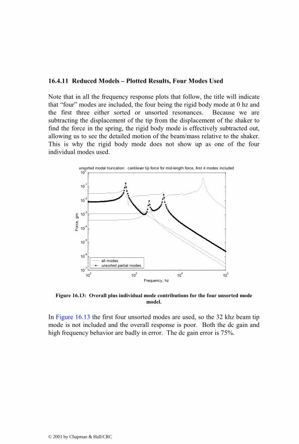
16.4.11 Reduced Models – Plotted Results, Four Modes Used
Note that in all the frequency response plots that follow, the title will indicate that “four” modes are included, the four being the rigid body mode at 0 hz and the first three either sorted or unsorted resonances. Because we are subtracting the displacement of the tip from the displacement of the shaker to find the force in the spring, the rigid body mode is effectively subtracted out, allowing us to see the detailed motion of the beam/mass relative to the shaker. This is why the rigid body mode does not show up as one of the four individual modes used.
102 103 104 10510-7
10-6
10-5
10-4
10-3
10-2
10-1
100unsorted modal truncation: cantilever tip force for mid-length force, first 4 modes included
Frequency, hz
Forc
e, g
m
all modes unsorted partial modes
Figure 16.13: Overall plus individual mode contributions for the four unsorted mode model.
In Figure 16.13 the first four unsorted modes are used, so the 32 khz beam tip mode is not included and the overall response is poor. Both the dc gain and high frequency behavior are badly in error. The dc gain error is 75%.
© 2001 by Chapman & Hall/CRC

102 103 104 10510-7
10-6
10-5
10-4
10-3
10-2
10-1
100sorted modal truncation: cantilever tip force for mid-length force, first 4 modes included
Frequency, hz
Forc
e, g
m
all modes sorted partial modes
Figure 16.14: Overall plus individual mode contributions for the four sorted mode model.
In Figure 16.14 the 32 khz beam tip mode is one of the included modes. Both the overall dc gain and high frequency behavior are quite good matches with the “all modes included” model with only four modes included. The dc gain error is –6.2%.
0 0.005 0.01 0.015 0.02 0.025 0.03-4
-3.5
-3
-2.5
-2
-1.5
-1
-0.5
0
0.5cantilever tip force for 100g, 0.002 sec input, 4 modes included
time, sec
Forc
e, g
m
all modes unsorted partial modessorted partial modes
Figure 16.15: Half-sine shock pulse response for full, reduced unsorted and reduced sorted models.
© 2001 by Chapman & Hall/CRC

Figure 16.15 shows the how the dc gain error in the frequency domain for the unsorted model shows up as a significant error in peak response in the time domain, 67%. The error in the sorted peak response is only 5.6%.
16.4.12 Modred – Setting up, “mdc” and “del” Reduction, Bode Calculations
In this section the user is prompted for whether to use the sorted or original mode order, then the corresponding system matrices are defined. The “modred” command is used with both the “mdc” and “del” options to define two reduced systems. The “bode” command is used to calculate frequency responses.
% use modred to reduce, select whether to use sorted or unsorted modes for the reduction modred_sort = input('modred: enter "1" to use sorted modes for reduced runs, …
"enter" to use unsorted ... '); if isempty(modred_sort) modred_sort = 0 end if modred_sort == 1 % use sorted mode order xnnew = xn(:,index_sort(1:num_modes_total)); freqnew = freqvec(index_sort(1:num_modes_total)); else % use original mode order xnnew = xn(:,(1:num_modes_total)); freqnew = freqvec((1:num_modes_total)); end % define variables for all modes included system matrix, a
w = freqnew*2*pi; % frequencies in rad/sec w2 = w.^2;
zw = 2*zeta*w; % setup all modes included "a" matrix, system matrix a = zeros(asize); for col = 2:2:asize row = col-1;
© 2001 by Chapman & Hall/CRC

a(row,col) = 1; end for col = 1:2:asize row = col+1; a(row,col) = -w2((col+1)/2); end for col = 2:2:asize row = col; a(row,col) = -zw(col/2); end % setup input matrix b, state space forcing function in principal coordinates % f_physical is the vector of physical force % zeros at each output DOF and input force at the input DOF f_physical = zeros(numdof,1); % start out with zeros f_physical(shaker_node_row) = 9807*shaker_mass*1.0; % input force at shaker, 1g % now setup the principal force vector for the three cases, all modes, nosort, sort % f_principal is the vector of forces in principal coordinates f_principal = xnnew'*f_physical; % b is the vector of forces in principal coordinates, state space form b = zeros(2*num_modes_total,1); for cnt = 1:num_modes_total b(2*cnt) = f_principal(cnt); end % setup cdisp and cvel, padded xn matrices to give the displacement and velocity % vectors in physical coordinates % cdisp and cvel each have numdof rows and alternating columns consisting of columns % of xnnew and zeros to give total columns equal to the number of states % all modes included cdisp and cvel for col = 1:2:2*length(freqnew) for row = 1:numdof
© 2001 by Chapman & Hall/CRC

cdisp(row,col) = xnnew(row,ceil(col/2)); cvel(row,col) = 0; end end for col = 2:2:2*length(freqnew) for row = 1:numdof cdisp(row,col) = 0; cvel(row,col) = xnnew(row,col/2); end end % define output d = [0]; % % define state space system for reduction, ordered defined by modred_sort sysforce_red = ss(a,b,mn2gm_conversion*kspring*(cdisp(tip_node_row,:)- …
cdisp(shaker_node_row,:)),d); % define reduced matrices using matched dc gain method "mdc" states_elim = (2*num_modes_used+1):2*num_modes_total; sysforce_mdc = modred(sysforce_red,states_elim,'mdc'); [aforce_mdc,bforce_mdc,cforce_mdc,dforce_mdc] = ssdata(sysforce_mdc); % define reduced matrices by eliminating high frequency states, 'del' sysforce_elim = modred(sysforce_red,states_elim,'del'); [aforce_elim,bforce_elim,cforce_elim,dforce_elim] = ssdata(sysforce_elim); % use "bode" command to generate magnitude/phase vectors for reduced systems [magforce_mdc,phsforce_mdc]=bode(sysforce_mdc,frad) ; [magforce_elim,phsforce_elim]=bode(sysforce_elim,frad) ; % convert magnitude to db magforce_mdcdb = 20*log10(magforce_mdc); magforce_elimdb = 20*log10(magforce_elim);
© 2001 by Chapman & Hall/CRC

16.4.13 Reduced Modred Models – Plotting Commands
Both the “del” and “mdc” reduced systems are plotted and compared with the original, non-reduced system. The individual mode contributions to the two reduced responses are also plotted.
% start plotting % modred using 'elim' loglog(f,magforce(1,:),'k-',f,magforce_elim(1,:),'k.-') if modred_sort == 1 title(['reduced elimination: cantilever tip force for mid-length force, …
first ',num2str(num_modes_used),' sorted modes included']) dcgain_error_percent_elim_sort = 100*(magforce_elim(1) …
- magforce(1))/magforce(1) else title(['reduced elimination: cantilever tip force for mid-length force, …
first ',num2str(num_modes_used),' unsorted modes included']) dcgain_error_percent_elim_nosort = 100*(magforce_elim(1) …
- magforce(1))/magforce(1) end legend('all modes','reduced elimination',3) xlabel('Frequency, hz') ylabel('Force, gm') grid on disp('execution paused to display figure, "enter" to continue'); pause hold on max_modes_plot = num_modes_used; for pcnt = 1:max_modes_plot index = 2*pcnt; amode = aforce_elim(index-1:index,index-1:index); bmode = bforce_elim(index-1:index); cmode = cforce_elim(1,index-1:index); dmode = [0]; sysforce_mode = ss(amode,bmode,cmode,dmode); [magforce_mode,phsforce_mode]=bode(sysforce_mode,frad) ; loglog(f,magforce_mode(1,:),'k-')
© 2001 by Chapman & Hall/CRC

end disp('execution paused to display figure, "enter" to continue'); pause hold off % modred using 'mdc' loglog(f,magforce(1,:),'k-',f,magforce_mdc(1,:),'k.-') if modred_sort == 1 title(['reduced matched dc gain: cantilever tip force for mid-length …
force, first ',num2str(num_modes_used),' sorted modes included']) dcgain_error_percent_mdc_sort = 100*(magforce_mdc(1) …
- magforce(1))/magforce(1) else title(['reduced matched dc gain: cantilever tip force for mid-length …
f orce, first ',num2str(num_modes_used),' unsorted modes included']) dcgain_error_percent_mdc_nosort = 100*(magforce_mdc(1) …
- magforce(1))/magforce(1) end legend('all modes','reduced mdc',3) xlabel('Frequency, hz') ylabel('Force, gm') grid on disp('execution paused to display figure, "enter" to continue'); pause hold on max_modes_plot = num_modes_used; for pcnt = 1:max_modes_plot index = 2*pcnt; amode = aforce_mdc(index-1:index,index-1:index); bmode = bforce_mdc(index-1:index); cmode = cforce_mdc(1,index-1:index); dmode = [0]; sysforce_mode = ss(amode,bmode,cmode,dmode); [magforce_mode,phsforce_mode]=bode(sysforce_mode,frad) ; loglog(f,magforce_mode(1,:),'k-') end
© 2001 by Chapman & Hall/CRC

disp('execution paused to display figure, "enter" to continue'); pause hold off % now use lsim to calculate force due to a 0.002 sec half-sine 100g shock pulse [force_mdc,ts_mdc] = lsim(sysforce_mdc,u,t); [force_elim,ts_elim] = lsim(sysforce_elim,u,t); plot(ts,force,'k-',ts_mdc,force_mdc,'k.-',ts_elim,force_elim,'k+-') if modred_sort == 1 title(['modred cantilever tip force for ',num2str(shock_amplitude),'g, …
',num2str(pulse_width) ,' sec input, ',num2str(num_modes_used), … ' sorted modes included'])
else title(['modred cantilever tip force for ',num2str(shock_amplitude),'g, …
',num2str(pulse_width) ,' sec input, ',num2str(num_modes_used), … ' unsorted modes included'])
end legend('all modes','reduced - mdc','reduced - elim',4) xlabel('time, sec') ylabel('Force, gm') grid on disp('execution paused to display figure, "enter" to continue'); pause max_force_mdc = max(abs(force_mdc)); max_force_elim = max(abs(force_elim)); peak_error_mdc_percent = 100*(max_force_mdc - max_force)/max_force peak_error_elim_percent = 100*(max_force_elim - max_force)/max_force end
16.4.14 Plotting Unsorted Modred Reduced Results – Eliminating High Frequency Modes
This section looks at how well “modred” performs when unsorted modes are used. We will see that the “del” option using the first four unsorted modes does a poor job of matching the original response while the “mdc” option using the same four unsorted modes does a good job of matching the lower frequency range of the response while missing the tenth mode resonance. The overall transient response of the system is matched well by the “mdc” option while the “del” option has significant error.
© 2001 by Chapman & Hall/CRC

102 103 104 10510-7
10-6
10-5
10-4
10-3
10-2
10-1
100reduced elimination: cantilever tip force for mid-length force, first 4 unsorted modes included
Frequency, hz
Forc
e, g
m
all modes reduced elimination
Figure 16.16: Overall frequency response with overload individual mode contributions for unsorted “del” modred option, with the 12 highest frequency modes eliminated.
Figure 16.16 displays the same response as the “unsorted” plot in Figure 16.13 because the “del” option in modred and our simple modal truncation method are equivalent. The dc gain is in error by 75%.
102 103 104 10510-7
10-6
10-5
10-4
10-3
10-2
10-1
100reduced matched dc gain: cantilever tip force for mid-length force, first 4 unsorted modes included
Frequency, hz
Forc
e, g
m
all modes reduced mdc
Figure 16.17: Overall frequency response with overlaid individual mode contributions for unsorted “mdc” modred option, with the 12 highest frequency modes reduced.
© 2001 by Chapman & Hall/CRC

In Figure 16.17, the dc error is very small, 0.0008%. Even though the 32 khz mode is not included, the gain in the portion from 1 to 20 khz is close to the full model gain.
0 0.005 0.01 0.015 0.02 0.025 0.03-4
-3.5
-3
-2.5
-2
-1.5
-1
-0.5
0
0.5modred cantilever tip force for 100g, 0.002 sec input, 4 unsorted modes included
time, sec
Forc
e, g
m
all modes reduced - mdc reduced - elim
Figure 16.18: Half-sine shock pulse response for full, reduced unsorted “mdc” and reduced unsorted “del” models.
Figure 16.18 shows that the effect of the dc gain error in the frequency domain for the unsorted model shows up as a significant error in peak response in the time domain, 67%. The error in the unsorted peak response is only 0.09% for the “mdc” reduction.
16.4.15 Plotting Sorted Modred Reduced Results – Eliminating Lower dc Gain Modes
This Section repeats the analysis of the previous Section but the sorted modes are used, retaining the higher dc gain modes. Since the important tenth mode is included in the retained sorted modes, we would expect that the reduced responses would match the original, all modes included response.
© 2001 by Chapman & Hall/CRC

102 103 104 10510-7
10-6
10-5
10-4
10-3
10-2
10-1
100reduced elimination: cantilever tip force for mid-length force, first 4 sorted modes included
Frequency, hz
Forc
e, g
m
all modes reduced elimination
Figure 16.19: Overall frequency response with overload individual mode contributions for sorted “del” modred option, with the 12 lowest dc gain modes eliminated.
Figure 16.19 shows the same response as the “sorted” plot in Figure 16.14 because the “del” option in modred and our simple sorted modal truncation methods are equivalent. The dc gain is in error by 6.2%.
102 103 104 10510-7
10-6
10-5
10-4
10-3
10-2
10-1
100reduced matched dc gain: cantilever tip force for mid-length force, first 4 sorted modes included
Frequency, hz
Forc
e, g
m
all modes reduced mdc
Figure 16.20: Overall frequency response with overload individual mode contributions for sorted “mdc” modred option, with the 12 lowest dc gain modes eliminated.
Note the high frequency discrepancy in Figure 16.20, related to using the “mdc” modred option. For this problem, which is dominated by the low
© 2001 by Chapman & Hall/CRC

frequency (<10khz) response and the dc gain of the 32 khz mode, the high frequency response is not important. The dc gain is in error by only 0.0025%.
0 0.005 0.01 0.015 0.02 0.025 0.03-4
-3.5
-3
-2.5
-2
-1.5
-1
-0.5
0
0.5modred cantilever tip force for 100g, 0.002 sec input, 4 sorted modes included
time, sec
Forc
e, g
m
all modes reduced - mdc reduced - elim
Figure 16.21: Half-sine shock pulse response for full, reduced unsorted and reduced sorted models.
The errors in peak response are 5.6% for the “del” method and 0.0773% for the “mdc” method.
© 2001 by Chapman & Hall/CRC

16.4.16 Model Reduction Summary
Reduction
Method Used
Dc gain error,
percent
Peak error,
percent
Comments
Nosort
75.45
67
This case should show the worst error because the 32 khz beam tip/spring mode is not included in the lowest four frequency modes.
Nosort, elim
75.45
67
The modred “del” option is the same as the “nosort” case because it just eliminates (truncates) the twelve highest frequency modes.
Sort
6.19
5.61
Sorting for dc gain with four modes includes the 32 khz mode, so the dc gain error is reduced. However, it still contains errors because the dc gain terms from the 12 unused modes are not included.
Sort, elim
6.19
5.61
The modred “del” option is the same as the “sort” case because it just eliminates (truncates) the twelve lowest dc gain modes.
Nosort, mdc
0.0007
0.0913
The modred “mdc” option, even though it does not use the 32 khz mode, takes its dc gain into effect, resulting in the small dc gain error. Because the frequency content of the shock pulse is low (~250 hz), the low frequency portion of the overall transfer function dominates the accuracy of the shock response.
Sort, mdc
0.0025
0.0773
Sorting the modes before reducing does not have a significant effect on the dc gain because the “mdc” operations take into account the dc gain effects of the unused modes.
Table 16.3: Summary of model reduction methods used, ranked from highest to lowest errors, with comments about each method.
Table 16.3 shows that using the modred “mdc,” (“matched dc gain”) method is the preferred method for this problem to obtain accurate results. For results that have accuracy in the 5 to 6% range, sorting by dc gain and then removing the lower dc gain modes is another available approach. It is clear that arbitrarily truncating high frequency modes can lead to significant errors
© 2001 by Chapman & Hall/CRC

because a single, important mode is neglected. Another source of error would occur if the ANSYS model had not included enough elements (modes) to take into account the beam tip mode or if a selected range of eigenvalues had not included the mode.
In summary, every model reduction problem provides new challenges and needs to be analyzed before making a decision about which reduction method is most appropriate.
16.5 ANSYS Code cantbeam_ss_spring_shkr.inp Listing
The ANSYS code in this section is similar to the code cantbeam_ss.inp in Section 15.7 with the exception that a tip spring and “shaker” mass are added.
! cantbeam_ss_spring_shkr.inp, 0.075 thick x 2 wide x 20mm long steel cant with tip ! mass and spring on shaker, shaker mass at cantilever base and coupled to spring ground ! title automatically built based on number of elements and eigenvalue extraction method /prep7 filename = 'cantbeam_ss_spring_shkr' ! define number of elements to use num_elem = 10 ! define eigenvalue extraction method, 1 = reduced, 2 = block lanczos eigext = 2 *if,eigext,eq,1, then nummodes = num_elem+1 ! only 1 displacement dof available for each element *else nummodes = 2*(num_elem+1) ! both disp and rotation dof's available for each
! element *endif ! create the file name for storing data ! first section of filename aname = 'cantbeam' ! second section of filename, number of elements bname = num_elem ! third section of filename, depends on eigenvalue extraction method
© 2001 by Chapman & Hall/CRC

*if,eigext,ne,2, then cname = 'red' ! reduced *else cname = 'bl' ! block Lanczos *endif ! input the title, use %xxx% to substitute parameter name or parametric expression aname_ti = 'cantbeam' /title,%aname_ti%, %bname%, %cname%, spring tip et,1,4 ! element type for beam et,2,14 ! element type for spring et,3,21 ! element type for mass ! steel ex,1,190e6 ! mN/mm^2 dens,1,7.83e-6 ! kg/mm^3 nuxy,1,0.293 ! real value to define beam characteristics r,1,0.15,0.05,0.00007031,0.075,0.2 ! beam properties: area, Izz, Iyy, TKz, TKy r,2,1000000 ! spring stiffness, mN/mm r,3,0.00002349,0.00002349,0.00002349 ! mass at tip, Kg r,4,0.050,0.050,0.050 ! shaker mass, Kg, approximately 1000 times mass ! define plotting characteristics /view,1,1,-1,1 ! iso view /angle,1,-60 ! iso view /pnum,mat,1 ! color by material /num,1 ! numbers off /type,1,0 ! hidden plot /pbc,all,1 ! show all boundary conditions csys,0 ! define global coordinate system ! nodes n,1,0,0,0 ! left-hand node n,num_elem+1,20,0,0 ! right-hand node fill,1,num_elem+1 ! interior nodes n,num_elem+2,20,0,-3 ! spring connection node nall nplo ! elements ! beam
© 2001 by Chapman & Hall/CRC

type,1 mat,1 real,1 e,1,2 egen,num_elem,1,-1 ! spring at tip type,2 real,2 e,num_elem+1,num_elem+2 ! mass at tip type,3 real,3 e,num_elem+1 ! shaker mass type,3 real,4 e,1 ! couple mass and spring end nall d,1,ux,0 ! constrain all except uz for node 1 d,1,uy,0 d,1,rotx,0 d,1,roty,0 d,1,rotz,0 d,num_elem+2,ux,0 ! constrain all except uz for spring end node d,num_elem+2,uy,0 d,num_elem+2,rotx,0 d,num_elem+2,roty,0 d,num_elem+2,rotz,0 ! d,1,uz,0 cp,1,uz,1,num_elem+2 ! uz couple shaker mass and spring end node ! constrain all but uz and roty for all other nodes to allow only those dof's nall nsel,s,node,,2,num_elem+1 d,all,ux d,all,uy d,all,rotx d,all,rotz nall eall
© 2001 by Chapman & Hall/CRC

nplo eplo ! ****************** eigenvalue run ******************* fini ! fini just in case not in begin /solu ! enters the solution processor, needs to be here to do editing below allsel ! default selects all items of specified entity type, typically nodes, elements nsel,s,node,,2,num_elem+1 m,all,uz *if,eigext,eq,1,then ! use reduced method antype,modal,new modopt,reduc,nummodes ! method - reduced Householder, nummodes –
! no to extract expass,off ! key = off, no expansion pass, key = on, do expansion mxpand,nummodes,,,no ! nummodes to expand,freq beginning,freq
! ending,elcalc = yes - calculate stresses total,nummodes,1 ! total masters, 1 is exclude rotations *elseif,eigext,eq,2 ! use block lanczos antype,modal,new modopt,lanb,nummodes ! no total required for block lanczos because
! calculates all eigenvalues expass,off mxpand,nummodes,,,no *endif allsel solve ! starts the solution of one load step of a solution sequence, modal here fini ! plot first mode /post1 /format,,,,,10000 set,1,1 pldi,1 ! ******************** output frequencies ********************** save,%aname%%bname%%cname%,sav /output,%aname%%bname%%cname%,frq ! write out frequency list to ascii file .frq
© 2001 by Chapman & Hall/CRC

set,list /output,term ! returns output to terminal ! ********************* output eigenvectors ******************* ! define nodes for output: forces applied or output displacements nsel,s,node,,1,num_elem+1 /output,%aname%%bname%%cname%,eig ! write out frequency list to ascii file .eig *do,i,1,nummodes set,,i /page,,,1000 prdisp *enddo /output,term ! ******************* plot modes ****************** ! pldi plots /show,%aname%%bname%%cname%,grp,0 ! save mode shape plots to file .grp allsel /view,1,,-1,, ! side view for plotting /angle,1,0 /auto *do,i,1,nummodes set,1,i pldi,1 *enddo /show,term
© 2001 by Chapman & Hall/CRC

CHAPTER 17
SISO DISK DRIVE ACTUATOR MODEL
17.1 Introduction
This chapter will use an ANSYS model of a complete disk drive actuator/suspension system to expand on the methods and examples of the last two chapters.
While simple in appearance, a disk drive actuator/suspension system must fulfill a number of exacting requirements. The suspension system is required to provide a stiff connection between the actuator and the head in the seeking/track-following direction, while providing a compliant system in a direction perpendicular to the plane of the disk. This allows the air bearing supported head to comply to the shape and vibration of the disk. The actuator is designed with low mass to allow fast seeking. It must have resonant characteristics which provide small residual vibration following a seek from one track to another. Since the entire disk drive is subject to various shock and vibration events, the actuator dynamics must aid in preventing the head from unloading from the disk during the event.
The actuator/suspension system used as the example for this and the next chapter is a single disk actuator, with two arms and two suspensions. It is purposely designed with poor resonance characteristics (different thickness arms, coil positioned off the mass center of the system, etc.) in order to provide a richer resonance picture for analysis.
We will assume that the servo system used with the actuator is a sampled system with a 20khz sample rate, meaning that the Nyquist frequency is 10khz. We need to understand all the modes of vibration of the system up to at least 20khz because the sampled system will alias frequencies that are higher than 10khz back into the 0 to 10khz range.
We will find that the dynamics of this ANSYS model with approximately 21000 degrees of freedom can be described well using between 8 and 20 modes of vibration (16 to 40 states), depending on what measure of “goodness” is used. If we are interested in impulse response, we will see in the next chapter that using only eight modes results in a system with approximately a 5% error. For a good fit in the frequency domain through 10 khz only 8 modes are required, while a good fit through 20 khz requires 20 modes. In a well-designed actuator (this example is poorly designed as
© 2001 by Chapman & Hall/CRC

mentioned earlier) fewer than 20 modes are required since symmetry will couple in fewer modes.
This actuator/suspension model is a good example of what the book is all about: generating low order models of complicated systems, in this case a model which is approximately 1000 times smaller than the original model.
Once the ANSYS model results are available, a MATLAB model will be created. Then we will analyze several methods of reducing the size of the model. In the previous chapters, we used dc gains of the individual modes of vibration to rank the most important modes to keep. If we use uniform damping (the same zeta value for all modes) we will reach the same ranking conclusion using either dc gain or peak gain. However, if we use non-uniform damping, peak gain ranking is required. The MATLAB code will prompt for whether uniform or non-uniform damping is being used and will choose the appropriate ranking, dc gain or peak gain. The next chapter will introduce another, more elegant method of ranking modes to be eliminated, balanced reduction.
17.2 Actuator Description
Figure 17.1 shows top and cross-sectioned side views of the actuator used for the analysis. The global XYZ coordinate system for the model is indicated.
Figure 17.1: Drawing of actuator/suspension system.
Voice Coil
Ball Bearing
Actuator Shaft
Adhesive
Suspension
RecordingHead
Disk
Ball Bearing
VCM Force
Actuator Motion
X
Y
Z
X
© 2001 by Chapman & Hall/CRC

The shaft is constrained in all directions, providing a fixed reference about which the actuator rotates on two axially preloaded ball bearings. This actuator is purposely designed to have poor dynamic characteristics, as seen in the side view. The coil, to which the Voice Coil Motor (VCM) forces are applied, is not centered between the two bearings and the two arms are of unequal thickness. Both the coil force mispositioning and the unequal arm thickness inertial effects will tend to excite rotations about the x axis.
The coil is bonded to the aluminum actuator body. During operation, current passes through the coil windings. The current interacts with the magnetic field from pairs of magnets above and below the straight legs of the coil (not shown), creating forces on the straight legs. The direction of the force is dependent on the direction of the current in the coil, clockwise or counterclockwise. The motion of the actuator due to the coil force is indicated by “Actuator Motion.”
The suspensions are designed to provide a preload of several grams force onto the disk surface. During operation the preload is counterbalanced by the air bearing lifting force, controlling the flying height spacing between the head and disk to less than several microinches. During shipment, the preload tends to hold the head down on the disk surface in the event of shock and vibration events, preventing potential damage caused by the head lifting off and striking the disk.
17.3 ANSYS Suspension Model Description
Before analyzing the complete actuator/suspension system, we will analyze only the suspension system. Understanding the dynamics of sensitive components of larger assemblies as components can add considerable insight to interpretation of the dynamics of the overall system.
The suspension portion of the actuator/suspension model is shown in Figures 17.2 and 17.3. The complete suspension is depicted in Figure 17.2, and the “flexure” portion of the suspension is shown in Figure 17.3.
© 2001 by Chapman & Hall/CRC

Figure 17.2: Suspension model.
The recording head (slider) is bonded to the center section of the flexure. The “dimple” at the center of the slider tongue provides a point contact about which the slider can rotate in the pitch and roll directions. The tip of the dimple and the contact point on the underside of the loadbeam are constrained to move together in translation. The flexure body is laser welded to the loadbeam (the triangular section), which is itself laser welded to the swage plate at the left-hand end.
The boundary conditions for the suspension model are: the swage plate is constrained in the x and z directions and the four slider corners are constrained in the z direction. A large mass is attached at the swage plate to allow for y direction ground acceleration forcing function. Because there is no constraint in the y direction there will be a zero-frequency, rigid body mode in that direction.
© 2001 by Chapman & Hall/CRC

Figure 17.3: Flexure and recording head (slider) portion of suspension. Note the “dimple” at the center of the slider, a point about which the slider rotates to comply with the disk
topology.
The model is built with the ability to easily change the critical flatness and forming parameters because the dynamics of the suspension are so dependent on the geometry. Small (0.025 mm, 0.001 inch) defects in critical forming and flatness parameters can drastically change the resonance characteristics,
The suspension model is made completely of eight-node brick elements. Laser welds and bonded joints are simulated by “merging” the nodes being welded or bonded, essentially creating a rigid joint at that connection.
The ANSYS suspension-only model, srun.inp, is included in the available downloads but will not be discussed. Running the model with different values for the three input parameters “zht,” “bump” and “offset” will show the extreme sensitivity of the first torsion mode (described below) to these parameters.
17.4 ANSYS Suspension Model Results
The suspension has six modes of vibration in the 0 to 10 khz frequency range. The ANSYS frequency response plot for the suspension is shown in Figure 17.4. The six modes in the 0 to 10 khz will be plotted and described below.
© 2001 by Chapman & Hall/CRC

17.4.1 Frequency Response
Figure 17.4: Suspension frequency response for a y direction forcing function.
17.4.2 Mode Shape Plots
Figure 17.5: Mode 2, 2053 hz, first bending mode.
© 2001 by Chapman & Hall/CRC

Figure 17.6: Mode 3, 3020 hz, first torsion mode.
Figure 17.7: Mode 4, 6406 hz, second bending mode.
© 2001 by Chapman & Hall/CRC

Figure 17.8: Mode 5, 6937 hz, sway or lateral mode.
Figure 17.9: Mode 6, 8859 hz, second torsion mode.
The suspension frequency response plot and mode shape plots complement each other and help to develop a visual, intuitive understanding of modal coupling. The only modes that have y direction motion of the slider relative to the swage plate are the first torsion and sway modes as can be seen in the frequency response plot of Figure 17.4. All the other modes have motions which are orthogonal to the motion of interest. The first bending mode is the
© 2001 by Chapman & Hall/CRC

most obvious example. Since its motion in only in the z direction, it cannot be excited by a y direction forcing function, and thus, does not couple into the frequency response.
17.5 ANSYS Actuator/Suspension Model Description
The complete actuator/suspension model is shown in Figure 17.10. It also is made of eight-node brick elements except for the inclusion of spring elements which are used to simulate the ball bearings’ individual ball stiffnesses.
The shaft and inner radii of the two ball bearing inner rings are fully constrained. The four corners of each of the sliders are constrained for zero motion in the z direction, essentially creating an infinitely stiff air bearing.
Figure 17.10: Complete actuator/suspension model.
© 2001 by Chapman & Hall/CRC

Figure 17.11: Actuator / suspension model, four views.
The primary motion of the actuator is rotation about the pivot bearing, therefore the final model has the coordinate system transformed from a Cartesian x,y,z coordinate system to a Cylindrical, r, θ and z system, with the two origins coincident.
Figure 17.12: Nodes used for reduced MATLAB model. Shown with partial finite element mesh at coil.
Node 24082
Node 24087
Node 24061
Node 24066Node 22, top head
Node 10022, bottom head
o9.1148o15.1857
o9.1148
o15.1857
© 2001 by Chapman & Hall/CRC

For reduced models we only require eigenvector information for degrees of freedom where forces are applied and where displacements are required. Figure 17.12 shows the nodes used for the reduced MATLAB model. The four nodes 24061, 24066, 24082 and 24087 are located in the center of the coil in the z direction and are used for simulating the VCM force. The forces created by the interactions between the current in the straight legs of the coil and the magnetic field are perpendicular to the straight leg sections. Since the coordinate system is cylindrical, the forces are decomposed into radial and circumferential components as shown in Figure 17.12. Nodes 22 and 10022 are the nodes for the top and bottom heads (heads 1 and 0), respectively. The arrows at the nodes indicate the direction of forces, and the angles show the directions of the force, measured from the circumferential direction. The components in the radial and circumferential directions are taken using the angles.
The model uses only the circumferential motion of the heads, which, if divided by the radius from the pivot to the head, will give output in radians.
The actuator/suspension ANSYS code, arun.inp, is too large to be listed here but is available for downloading.
17.6 ANSYS Actuator/Suspension Model Results
A recommended sequence for analyzing dynamic finite element models is:
1) Plot resonant frequencies versus mode numbers to get a feel for the frequency range. See if there are any significant jumps in frequency between modes which can indicate the system transitioning from one type of characteristic motion to another. For example, a sequence of bending modes transitioning into a sequence of torsional modes.
2) Plot frequency responses to define which modes couple into the response.
3) Plot and animate the mode shapes that contribute to the response, identifying modes that couple into motions in directions of interest and those that do not. Visually get a sense of how the geometry of the structure affects the modes.
4) Run parameter studies to understand the sensitivity of critical modes to design variables: dimensions, tolerances, material properties, etc.
© 2001 by Chapman & Hall/CRC

17.6.1 Eigenvalues, Frequency Responses
The actuator/suspension model was run using the Block Lanczos method to extract the first 50 eigenvalues and eigenvectors. The plot of frequency versus number of modes is shown in Figure 17.13. The first mode, the rigid body mode, was calculated to be 0.0101 hz, with the first oscillatory mode frequency at 785 hz.
0 5 10 15 20 25 30 35 40 45 50102
103
104
105frequency versus mode number
mode number
frequ
ency
, hz
Figure 17.13: Frequencies versus mode number.
Mode 50 is at 22350 hz, which is slightly higher than our objective of including all the modes through 20 khz.
Frequency responses for the displacements of heads 0 and 1 (bottom and top heads) for coil input force can be seen in Figures 17.14 and 17.15. Mode shape plots, with undeformed and deformed shapes, are then shown for the modes which are evident in the frequency response plots. In addition, some typical modes that do not couple into the frequency response are shown.
© 2001 by Chapman & Hall/CRC

103 104
10-7
10-6
10-5
10-4head 0, gap displacement, all 50 modes included
Frequency, hz
Mag
nitu
de, m
m
Figure 17.14: Frequency response for head 0 for coil input.
103 104
10-7
10-6
10-5
10-4head 1, gap displacement, all 50 modes included
Frequency, hz
Mag
nitu
de, m
m
Figure 17.15: Frequency response for head 1 for coil input.
17.6.2 Mode Shape Plots
In this section we will plot overlaid undeformed and deformed modes shapes for selected modes, which will then be described and discussed in the next section.
© 2001 by Chapman & Hall/CRC

Figure 17.16: Mode 1 undeformed/deformed mode shape plot, 0.012 hz rigid body rotation.
Figure 17.17: Mode 2 mode shape plot, 785 hz. Bending of bottom arm.
© 2001 by Chapman & Hall/CRC

Figure 17.18: Mode 3 mode shape plot, 885 hz, coil and bottom arm bending.
Figure 17.19: Mode 6 mode shape plot, 2114 hz, coil torsion.
© 2001 by Chapman & Hall/CRC

Figure 17.20: Mode 7 mode shape plot, 2159 hz, suspension bending modes.
Figure 17.21: Mode 9 mode shape plot, 2939 hz, suspension torsion mode.
© 2001 by Chapman & Hall/CRC

Figure 17.22: Mode 11 mode shape plot, 4305 hz, system mode.
Figure 17.23: Mode 12 mode shape plot, 4320 hz, radial mode.
© 2001 by Chapman & Hall/CRC

Figure 17.24: Mode 13 mode shape plot, 5146 hz.
Figure 17.25: Mode 18 mode shape plot, 6561 hz.
© 2001 by Chapman & Hall/CRC

Figure 17.26: Mode 24 mode shape plot, 9152 hz.
17.6.3 Mode Shape Discussion
We will now correlate the two frequency response plots, Figures 17.14 and 17.15, with the mode shape plots above to start getting an intuitive feel for which modes couple into the response plots and which modes do not.
Mode 1, the rigid body mode, shows up as the 40db/decade low frequency slopes on both frequency responses, head 0 and head 1.
Modes 2 and 3, at 785 and 884 hz, are representative of modes that do not couple because of the direction of the motion. Both modes involve only bending motions of arms and/or coil in the x-z plane. Since the motions are perpendicular (orthogonal) to the direction of force and to the direction of the head in the circumferential direction, the modes should not couple into the frequency response plots. Therefore we see no resonance peaks at these two frequencies.
Mode 6 at 2114 hz is a coil/actuator torsion mode that shows up as the small pole/zero pair in the head 1 frequency response.
Mode 7 at 2159 hz is a suspension bending mode that does not couple into the response.
Mode 9 at 2939 hz is a suspension torsion mode that interacts with the rigid body mode to create the significant pole/zero pair at 2939 hz.
© 2001 by Chapman & Hall/CRC

Modes 11 and 12 at 4305 hz and 4320 hz are the major system modes with significant y direction motion of the coil, bearings, arms and suspensions. These are the two modes associated with the highest resonant peak in the frequency response. What appears to be a single peak is actually two peaks.
Mode 13 at 5146 hz is a mode which involves torsion of the coil and actuator body about the x axis with the suspensions moving torsionally and laterally.
Mode 18 at 6561 hz is a suspension sway mode, where the suspension-only mode at 6937 hz (Figure 17.8) is reduced to 6561 hz because it is attached to the flexible actuator.
Mode 24 at 9152 hz is a highly deformed actuator mode, in which the actuator hub moves significantly about the ball bearing, the coil deforms and suspensions and arms deflect.
17.6.4 ANSYS Output Example Listing
A partial listing of the eigenvector output (actrl.eig) for modes 1, 2, 11 and 12 is shown below. These four modes were chosen for listing and discussion because they illustrate some key points about interpreting ANSYS eigenvector output. The important information in each of the eigenvector sections is highlighted in bold type. The “SUBSTEP” is the mode number, and “FREQ” is the eigenvalue in hz. Since the output is in cylindrical coordinates, UX, UY and UZ refer to radial, circumferential and z axis coordinates, respectively. Since all the elements attached to the six nodes listed are eight-node brick elements, with only translational degrees of freedom, all the rotation eigenvector values are zero. The six nodes listed correspond to the two heads, 22 and 10022 and the four coil forcing function nodes, 24061, 24066, 24082 and 24087. See Figure 17.12 for node locations. We need both radial (UX) and circumferential (UY) directions because the forces applied by the VCM to the coil are perpendicular to the straight legs of the coil, and have both radial and circumferential components.
PRINT DOF NODAL SOLUTION PER NODE ***** POST1 NODAL DEGREE OF FREEDOM LISTING ***** LOAD STEP= 1 SUBSTEP= 1 FREQ= 0.11877E-01 LOAD CASE= 0 THE FOLLOWING DEGREE OF FREEDOM RESULTS ARE IN COORDINATE SYSTEM 1 NODE UX UY UZ ROTX ROTY ROTZ 22 0.30718E-06 32.772 0.85804E-12 0.0000 0.0000 0.0000
© 2001 by Chapman & Hall/CRC

10022 0.30759E-06 32.772 -0.49994E-10 0.0000 0.0000 0.0000 24061 0.11969E-06 16.968 -0.17668E-08 0.0000 0.0000 0.0000 24066 0.77415E-07 10.274 -0.15751E-08 0.0000 0.0000 0.0000 24082 0.68508E-07 10.274 -0.15395E-08 0.0000 0.0000 0.0000 24087 0.10089E-06 16.968 -0.16990E-08 0.0000 0.0000 0.0000 MAXIMUM ABSOLUTE VALUES NODE 10022 22 24061 0 0 0 VALUE 0.30759E-06 32.772 -0.17668E-08 0.0000 0.0000 0.0000 *ENDDO INDEX= I ***** POST1 NODAL DEGREE OF FREEDOM LISTING ***** LOAD STEP= 1 SUBSTEP= 2 FREQ= 785.39 LOAD CASE= 0 THE FOLLOWING DEGREE OF FREEDOM RESULTS ARE IN COORDINATE SYSTEM 1 NODE UX UY UZ ROTX ROTY ROTZ 22 -0.25631 -0.19637E-01 0.15936E-04 0.0000 0.0000 0.0000 10022 0.92764 -0.10736 0 .29519E-02 0.0000 0.0000 0.0000 24061 0.18573 -0.67085E-01 -5.7724 0.0000 0.0000 0.0000 24066 0.17688 -0.88331E-01 -2.1255 0.0000 0.0000 0.0000 24082 0.17616 0.95885E-01 -2.1213 0.0000 0.0000 0.0000 24087 0.18506 0.79278E-01 -5.7661 0.0000 0.0000 0.0000 MAXIMUM ABSOLUTE VALUES NODE 10022 10022 24061 0 0 0 VALUE 0.92764 -0.10736 -5.7724 0.0000 0.0000 0.0000 ***** POST1 NODAL DEGREE OF FREEDOM LISTING ***** LOAD STEP= 1 SUBSTEP= 11 FREQ= 4305.3 LOAD CASE= 0 THE FOLLOWING DEGREE OF FREEDOM RESULTS ARE IN COORDINATE SYSTEM 1 NODE UX UY UZ ROTX ROTY ROTZ 22 -4.4488 27.588 -0.66528E-04 0.0000 0.0000 0.0000 10022 3.9832 41.657 0.44809E-01 0.0000 0.0000 0.0000 24061 -0.43605 -10.023 -8.7664 0.0000 0.0000 0.0000 24066 0.35112 -3.5631 -11.532 0.0000 0.0000 0.0000 24082 3.9625 -1.1137 -14.210 0.0000 0.0000 0.0000 24087 5.0136 -7.8562 -6.0297 0.0000 0.0000 0.0000 MAXIMUM ABSOLUTE VALUES NODE 24087 10022 24082 0 0 0 VALUE 5.0136 41.657 -14.210 0.0000 0.0000 0.0000 ***** POST1 NODAL DEGREE OF FREEDOM LISTING *****
© 2001 by Chapman & Hall/CRC

LOAD STEP= 1 SUBSTEP= 12 FREQ= 4320.1 LOAD CASE= 0 THE FOLLOWING DEGREE OF FREEDOM RESULTS ARE IN COORDINATE SYSTEM 1 NODE UX UY UZ ROTX ROTY ROTZ 22 4.3947 36.811 -0.25761E-02 0.0000 0.0000 0.0000 10022 -0.88223 62.097 0.34209E-01 0.0000 0.0000 0.0000 24061 -5.3622 -11.584 3.9397 0.0000 0.0000 0.0000 24066 -3.9590 -2.2258 10.513 0.0000 0.0000 0.0000 24082 0.81662 -4.0070 7.7931 0.0000 0.0000 0.0000 24087 2.0281 -13.160 6.6813 0.0000 0.0000 0.0000 MAXIMUM ABSOLUTE VALUES NODE 24061 10022 24066 0 0 0 VALUE -5.3622 62.097 10.513 0.0000 0.0000 0.0000
We will now discuss the eigenvector listings above in light of the frequency response and mode shape plots reviewed earlier. Once again, we will make the connection between modes that contribute to frequency responses and those that do not.
Mode 1 shows that all the UX and UZ entries are essentially zero, which is appropriate for a rigid body mode where the actuator is rotating about the shaft, with only circumferential, UY, displacements. The relative amplitudes of each UY entry are related by their radial distances from the shaft. The frequency calculated is not exactly zero because of rounding and slight geometric errors which create small stiffnesses in rotation about the shaft.
Mode 2 is the first oscillatory mode, the arm bending mode. A mode which involves only UZ motion will have no cross-coupling in the y direction since the actuator system is symmetrical about the x axis. In a typical disk drive, the actuator is not perfectly symmetrical, and modes whose motions are primarily in the vertical direction will couple in the y direction. All of the UY entries for this mode are very small relative to the UZ entries, indicating that the contribution of this mode to the y direction motion of the head should be small.
Modes 12 and 13 are the major system modes, those modes with the highest amplitude motion on the frequency response plot. The entries in the UY column are significant relative to the entries for mode 2 and are of the same order of magnitude as those in mode 1. This indicates that this mode is relatively important for our desired frequency response.
© 2001 by Chapman & Hall/CRC

The eigenvalues and UX and UY eigenvector entries are stripped out of the actrl.eig file and stored in the MATLAB .mat file actrl_eig.mat (Appendix 1). Now we are ready to read the ANSYS results into MATLAB and start developing the reduced model.
17.7 MATLAB Model, MATLAB Code act8.m Listing and Results
17.7.1 Code Description
The code starts by reading in the ANSYS model eigenvalue and eigenvector results for all 50 modes from actrl_eig.mat. The VCM force components in the radial and circumferential directions are then defined using the angles shown in Figure 17.12.
The user is prompted to specify whether the same zeta value is to be used for all modes (uniform damping), or whether each mode can have different values, non-uniform damping. If uniform damping is specified, the user is prompted to enter a value for zeta, a vector of uniform damping values is created and dc gains are calculated. If non-uniform damping is chosen, a damping vector is read in from zetain.m and peak gains are calculated. The appropriate gains are then sorted and plotted, indicating the most important modes to retain. Typically uniform damping is taken in the range of 0.005 (0.5% of critical damping) to 0.02 (2% of critical damping). If experimental data is available, the damping values for each mode in zetain.m can be matched to its experimentally determined value.
Once the user defines the number of modes to be retained, two state space systems are automatically built. The first includes all 50 modes and the second includes the sorted, reduced number of modes. The 50-mode response is plotted for either head 0 or head 1 with individual mode contributions overlaid.
Since the servo system postulated for the actuator has a 20 khz sample frequency, the Nyquist frequency is half that, or 10 khz. This means that resonances higher in frequency than the Nyquist frequency will be aliased back to the 0 to 10 khz range. The user is prompted for the sample frequency to be used (default 20 khz). The MATLAB “c2d” command is used to create a discrete model of the original continuous system. A discrete frequency response, with upper limit of the Nyquist frequency, is created and plotted, overlaying the original continuous frequency response. If the sample rate is high enough, this overlay allows one to see that it will not alias critical modes of vibration. Experimentally, the only information available from a discrete servo system frequency response is up to the Nyquist frequency. Measurements which are independent of the servo system (such as from an
© 2001 by Chapman & Hall/CRC

external laser measurement system) are required to identify modes higher than the Nyquist frequency. An example of using a very low sampling frequency with this actuator system will be shown.
Frequency responses are calculated using the reduced, sorted modes, truncating the less important modes and using the “modred” “mdc” option. Truncating is the same as using the “del” option on the MATLAB “modred” command.
17.7.2 Input, dof Definition
The first section of code reads in the eigenvalue/eigenvector data from actrl_eig.mat and defines explicitly the degrees of freedom used. The original ANSYS model has approximately 21000 degrees of freedom. By defining only the degrees of freedom required for the desired frequency response, we can reduce the number of degrees required for the MATLAB model to 12: the radial and circumferential components of the two head nodes and the four coil forcing function nodes.
% act8.m clear all; hold off; clf; % load the Block Lanczos .mat file actrl_eig.mat, containing evr - the modal matrix, % freqvec - the frequency vector and node_numbers - the vector of node numbers % for the modal matrix % the output for the ANSYS run is the following dof's % dof node dir where % 1 22 ux - radial, top head gap % 2 10022 ux - radial, bottom head gap % 3 24061 ux - radial, coil % 4 24066 ux - radial, coil % 5 24082 ux - radial, coil % 6 24087 ux - radial, coil % 7 22 uy - circumferential, top head gap % 8 10022 uy - circumferential, bottom head gap % 9 24061 uy - circumferential, coil % 10 24066 uy - circumferential, coil % 11 24082 uy - circumferential, coil % 12 24087 uy - circumferential, coil load actrl_eig;
© 2001 by Chapman & Hall/CRC

[numdof,num_modes_total] = size(evr); freqvec(1) = 0; % set frequency of rigid body mode to zero xn = evr;
17.7.3 Forcing Function Definition, dc Gain Calculation
A vector of the squares of the eigenvalues, in rad/sec units, for use in the gain calculations is generated. Like the dc gain calculation with a rigid body mode discussed in the last chapter, we will again calculate the low frequency gain of the rigid body mode using the lowest frequency defined in the frequency response calculation.
The forcing function components for the four coil nodes are defined, again using Figure 17.12 as the reference. A unity force is applied at the coil, and evenly distributed among the four nodes. The force at each coil node is decomposed into its components in the radial and circumferential (x and y) directions. The coil forces in physical coordinates are then defined for each coil node and where the ux and uy force entries for the head nodes, dof 1, 2, 7 and 8 are all zero.
A discussion of what is meant by “Single Input Single Output” (SISO) is appropriate here. This model is a “SI” or Single Input model because the same force is applied to all four coil nodes, requiring only a single column vector for the input matrix “b.” The fact that forces are applied to multiple nodes has no significance relative to the “SI” definition.
In Chapter 15, (15.2) and (15.3), we found that the dc gain and peak gain of for the ith mode are given by the expressions:
ji nji nki2
ki i
z z zF
=ω
, (17.1)
( )ji
ki i
z j dcgainF 2
−=ζ
(17.2)
where nji nkiz z , the residue, is the product of the jth (output) row and kth (force applied) row terms of the ith eigenvector divided by the square of the eigenvalue for the ith mode and iζ is the damping for the ith mode. For all the models so far in the book, forces have been applied at a single node and displacements have been taken at a single node, making the above definitions
© 2001 by Chapman & Hall/CRC

clear. Here we are applying the same force to four coil nodes, so we will define a composite forcing function which will consist of the force applied to each node times the eigenvector value for that node, f_physical’*xn. The dimensions of this operation are (1 x ndof) x (ndof x nmodes) = (1 x nmodes), so we have a composite force vector for each mode.
This composite force vector is then multiplied element by element by the rows of the eigenvector matrix corresponding to the uy direction displacements of the two heads.
We will calculate and plot the gains for both head 0 and head 1 but will only calculate frequency response results for one or the other (user defined). Thus there is no ambiguity about whether to rank modes based on the gains of head 0 or head 1, only the one chosen for frequency response calculations is used for ranking.
% calculate the dc amplitude of the displacement of each mode by % multiplying the composite forcing function by the output row omega2 = (2*pi*freqvec)'.^2; % convert to radians and square % define frequency range for frequency response freqlo = 501; freqhi = 25000; flo=log10(freqlo) ; fhi=log10(freqhi) ; f=logspace(flo,fhi,300) ; frad=f*2*pi ; % define radial and circumferential forces applied at four coil force nodes % "x" is radial, "y" is circumferential, total force is unity n24061fx = 0.25*sin(9.1148*pi/180); n24061fy = 0.25*cos(9.1148*pi/180); n24066fx = 0.25*sin(15.1657*pi/180); n24066fy = 0.25*cos(15.1657*pi/180); n24082fx = -0.25*sin(15.1657*pi/180); n24082fy = 0.25*cos(15.1657*pi/180); n24087fx = -0.25*sin(9.1148*pi/180); n24087fy = 0.25*cos(9.1148*pi/180); % f_physical is the vector of physical force % zeros at each output dof and input force at the input dof
© 2001 by Chapman & Hall/CRC

f_physical = [ 0 0 n24061fx n24066fx n24082fx n24087fx 0 0 n24061fy n24066fy n24082fy n24087fy ]; % define composite forcing function, force applied to each node times eigenvector value % for that node force = f_physical'*xn; % choose which head to use for frequency responses head = input('enter "0" default for head 0 or "1" for head 1 ... '); if isempty(head) head = 0; end % prompt for uniform or variable zeta zeta_type = input('enter "1" to read in damping vector (zetain.m) …
or "enter" for uniform damping ... '); if (isempty(zeta_type)) zeta_type = 0;
zeta_uniform = input('enter value for uniform damping, … .005 is 0.5% of critical (default) ... ');
if (isempty(zeta_uniform))
zeta_uniform = 0.005; end
zeta_unsort = zeta_uniform*ones(num_modes_total,1); gainstr = ‘dc gain’; else zetain; % read in zeta_unsort damping vector from zetain.m file gainstr = ‘peak gain’; end
© 2001 by Chapman & Hall/CRC

if length(zeta_unsort) ~= num_modes_total error(['error - zetain vector has ',num2str(length(zeta_unsort)), …
' entries instead of ',num2str(num_modes_total)]); end % calculate dc gains if uniform damping, peak gains if non-uniform if zeta_type == 0 % dc gain gain_h0 = abs([force(1)*xn(8,1)/frad(1) ... force(2:num_modes_total).*xn(8,2:num_modes_total) ... ./omega2(2:num_modes_total)]); gain_h1 = abs([force(1)*xn(7,1)/frad(1) ... force(2:num_modes_total).*xn(7,2:num_modes_total) ... ./omega2(2:num_modes_total)]); elseif zeta_type == 1 % peak gain gain_h0 = abs([force(1)*xn(8,1)/frad(1) ... force(2:num_modes_total).*xn(8,2:num_modes_total) ... ./((2*zeta_unsort(2:num_modes_total))'.*omega2(2:num_modes_total))]); gain_h1 = abs([force(1)*xn(7,1)/frad(1) ... force(2:num_modes_total).*xn(7,2:num_modes_total) ... ./((2*zeta_unsort(2:num_modes_total))'.*omega2(2:num_modes_total))]); end % sort gains, keeping track of original and new indices so can rearrange % eigenvalues and eigenvectors [gain_h0_sort,index_h0_sort] = sort(gain_h0); [gain_h1_sort,index_h1_sort] = sort(gain_h1); gain_h0_sort = fliplr(gain_h0_sort); % max to min gain_h1_sort = fliplr(gain_h1_sort); % max to min index_h0_sort = fliplr(index_h0_sort) % max to min indices index_h1_sort = fliplr(index_h1_sort) % max to min indices index_orig = 1:num_modes_total; if head == 0 index_sort = index_h0_sort; headstr = 'head 0';
© 2001 by Chapman & Hall/CRC

index_out = 2; elseif head == 1 index_sort = index_h1_sort; headstr = 'head 1'; index_out = 1; end % plot results semilogy(index_orig(2:num_modes_total),freqvec(2:num_modes_total),'k-'); title('frequency versus mode number') xlabel('mode number') ylabel('frequency, hz') grid off disp('execution paused to display figure, "enter" to continue'); pause semilogy(index_orig,gain_h0,'k-',index_orig,gain_h1,'k.-') title('dc value of each mode contribution versus mode number') xlabel('mode number') ylabel('dc value') legend('head 0','head 1') grid off disp('execution paused to display figure, "enter" to continue'); pause loglog(freqvec(2:num_modes_total),gain_h0(2:num_modes_total),'k-', ... freqvec(2:num_modes_total),gain_h1(2:num_modes_total),'k.-') title('dc value of each mode contribution versus frequency') xlabel('frequency, hz') ylabel('dc value') legend('head 0','head 1') axis([500 25000 -inf 1e-4]) grid off disp('execution paused to display figure, "enter" to continue'); pause semilogy(index_orig,gain_h0_sort,'k-',index_orig,gain_h1_sort,'k.-') title('sorted dc value of each mode versus number of modes included') xlabel('modes included') ylabel('sorted dc value') legend('head 0','head 1') grid off % choose number of modes to use based on ranking of dc gain values num_modes_used = input(['enter how many modes (including rigid body) … to include, 'num2str(num_modes_total),' max, 8 default ... ']);
if (isempty(num_modes_used)) num_modes_used = 8; end
© 2001 by Chapman & Hall/CRC

num_states_used = 2*num_modes_used;
17.7.4 Ranking Results
Here, we will begin by reviewing the frequency versus mode number plot to get a feel for the frequency range of the model.
0 5 10 15 20 25 30 35 40 45 50102
103
104
105frequency versus mode number
mode number
frequ
ency
, hz
Figure 17.27: Frequency versus mode number.
0 5 10 15 20 25 30 35 40 45 5010-14
10-12
10-10
10-8
10-6
10-4
10-2
100dc gain of each mode contribution versus mode number
mode number
dc v
alue
head 0head 1
Figure 17.28: dc gain versus mode number, uniform damping zeta 0.005 (0.5% of critical damping) for all modes.
© 2001 by Chapman & Hall/CRC

0 5 10 15 20 25 30 35 40 45 5010-12
10-10
10-8
10-6
10-4
10-2
100peak gain of each mode contribution versus mode number
mode number
dc v
alue
head 0head 1
Figure 17.29: Peak gain versus mode number, non-uniform damping, zeta = 0.04 (4% of critical damping) for modes 11, 12 and 13.
The dc and peak gain plots for both head 0 and head 1 are shown above. Note the relative heights of the dc and peak gains for modes 11, 12 and 13. In the peak gain plot, those three gains are lower than the two gains immediately to the left. Conversely, in the dc gain plot the three modes are the highest gains with the exception of the rigid body mode.
The same two plots versus frequency, instead of mode number:
103 104
10-12
10-10
10-8
10-6
10-4dc gain of each mode contribution versus frequency
frequency, hz
dc v
alue
head 0head 1
Figure 17.30: dc gain versus frequency.
© 2001 by Chapman & Hall/CRC

103 104
10-10
10-8
10-6
10-4peak gain of each mode contribution versus frequency
frequency, hz
dc v
alue
head 0head 1
Figure 17.31: Peak gain versus frequency.
The gain plots versus mode number include the rigid body mode low frequency gain, while the gain plots versus frequency do not include the rigid body mode.
Figure 17.32 shows the modes ranked from most to least significant for the uniform damping (dc gain) case and includes the low frequency (500 hz) dc gain of the rigid body mode.
0 5 10 15 20 25 30 35 40 45 5010-14
10-12
10-10
10-8
10-6
10-4
10-2
100dc gain of each mode versus number of modes included
modes included
sorte
d dc
val
ue
head 0head 1
Figure 17.32: Sorted dc gain versus number of modes included.
© 2001 by Chapman & Hall/CRC

Relative to the 500 hz low frequency gain of the rigid body mode, the next most significant mode is lower by almost six orders of magnitude. Note that both head 0 and head 1 have similar magnitude curves, although the ordering of individual ranked modes are different. Furthermore, after the drop in dc gain from the rigid body mode to the second mode, there are no other significant drops. Gain is changing gradually, so there is no clear demarcation indicating the number of modes needed to be included. Picking the number of modes to use will be quite subjective, with each additional mode improving the model only slightly.
17.7.5 Building State Space Matrices
To prepare for building the system matrices, two sets of eigenvalue vectors and eigenvector matrices are defined. The first set is the original, unsorted eigenvalues and eigenvectors. The second set consists of the rearranged eigenvalues, eigenvectors and the damping vector, sorted by dc or peak gain. Using the same techniques defined in earlier chapters, the a, b and c matrices are formed.
% define eigenvalues and eigenvectors for unsorted and sorted modes % all modes included model, use original order xnnew = xn(:,(1:num_modes_total)); freqnew = freqvec((1:num_modes_total)); zeta = zeta_unsort; % all modes included, sorted xnnew_sort = xn(:,index_sort(1:num_modes_total)); freqnew_sort = freqvec(index_sort(1:num_modes_total)); zeta_sort = zeta_unsort(index_sort(1:num_modes_total)); % define variables for all modes included system matrix, a
w = freqnew*2*pi; % frequencies in rad/sec w2 = w.^2;
zw = 2*zeta_unsort.*w; % define variables for all modes included sorted system matrix, a_sort
w_sort = freqnew_sort*2*pi; % frequencies in rad/sec
© 2001 by Chapman & Hall/CRC

w2_sort = w_sort.^2;
zw_sort = 2*zeta_sort.*w_sort; % define size of system matrix asize = 2*num_modes_total; disp(' '); disp(' '); disp(['size of system matrix a is ',num2str(asize)]); % setup system matrix for all modes included model a = zeros(asize); for col = 2:2:asize row = col-1; a(row,col) = 1; end for col = 1:2:asize row = col+1; a(row,col) = -w2((col+1)/2); end for col = 2:2:asize row = col; a(row,col) = -zw(col/2); end % setup system matrix for sorted all modes included model a_sort = zeros(asize); for col = 2:2:asize row = col-1; a_sort(row,col) = 1; end for col = 1:2:asize
© 2001 by Chapman & Hall/CRC

row = col+1; a_sort(row,col) = -w2_sort((col+1)/2); end for col = 2:2:asize row = col; a_sort(row,col) = -zw_sort(col/2); end % setup input matrix b, state space forcing function in principal coordinates % now setup the principal force vector for the three cases, all modes, sort % f_principal is the vector of forces in principal coordinates f_principal = xnnew'*f_physical; % b is the vector of forces in principal coordinates, state space form b = zeros(2*num_modes_total,1); for cnt = 1:num_modes_total b(2*cnt) = f_principal(cnt); end % f_principal_sort is the vector of forces in principal coordinates f_principal_sort = xnnew_sort'*f_physical; % b_sort is the vector of forces in principal coordinates, state space form b_sort = zeros(2*num_modes_total,1); for cnt = 1:num_modes_used b_sort(2*cnt) = f_principal_sort(cnt); end % setup cdisp and cvel, padded xn matrices to give the displacement and velocity % vectors in physical coordinates % cdisp and cvel each have numdof rows and alternating columns % consisting of columns of xnnew and zeros to give total columns equal % to the number of states % all modes included cdisp and cvel for col = 1:2:2*length(freqnew)
© 2001 by Chapman & Hall/CRC

for row = 1:numdof c_disp(row,col) = xnnew(row,ceil(col/2)); cvel(row,col) = 0; end end for col = 2:2:2*length(freqnew) for row = 1:numdof c_disp(row,col) = 0; cvel(row,col) = xnnew(row,col/2); end end % all modes included sorted cdisp and cvel for col = 1:2:2*length(freqnew_sort) for row = 1:numdof cdisp_sort(row,col) = xnnew_sort(row,ceil(col/2)); cvel_sort(row,col) = 0; end end for col = 2:2:2*length(freqnew_sort) for row = 1:numdof cdisp_sort(row,col) = 0; cvel_sort(row,col) = xnnew_sort(row,col/2); end end % define output d = [0]; %
© 2001 by Chapman & Hall/CRC

17.7.6 Define State Space Systems, Original and Reduced
Now that the original and sorted state space matrices are available, we can use the “ss” command to define the systems for analysis. The following systems are set up:
1) unsorted model with all modes included
2) sorted model with all modes included
3) sorted, truncated reduced model using the sorted model from 2) above (same as the “modred” “del” option)
4) sorted, “modred” “mdc” option reduction using the sorted model from 2) above
The bode command is used to define magnitude and phase vectors for (1), (3) and (4) above.
In order to see the effects of different servo sample rates on aliasing of high frequency modes, the user is prompted to enter a sample frequency, which defaults to 20 khz. Examples of several sample rates are shown below. A discussion of aliasing is outside the scope of the book but several references are recommended (Franklin 1994 and Franklin 1998).
% define state space systems with the "ss" command, outputs are the % two gap displacements % define unsorted all modes included system sys = ss(a,b,c_disp(7:8,:),d); % define sorted all modes included system sys_sort = ss(a_sort,b_sort,cdisp_sort(7:8,:),d); % define sorted reduced system a_sort_red = a_sort(1:num_states_used,1:num_states_used); b_sort_red = b_sort(1:num_states_used); cdisp_sort_red = cdisp_sort(7:8,1:num_states_used); sys_sort_red = ss(a_sort_red,b_sort_red,cdisp_sort_red,d); % define modred "mdc" reduced system, modred "del" option same as sorted reduced above
© 2001 by Chapman & Hall/CRC

states_del = (2*num_modes_used+1):2*num_modes_total; sys_mdc = modred(sys_sort,states_del,'mdc'); sys_mdc_nosort = modred(sys,[17:100],'mdc'); % use "bode" command to generate magnitude/phase vectors [mag,phs] = bode(sys,frad); [mag_sort_red,phs_sort_red] = bode(sys_sort_red,frad); [mag_mdc,phs_mdc]=bode(sys_mdc,frad) ; [mag_mdc_nosort,phs_mdc_nosort]=bode(sys_mdc_nosort,frad) ; % convert magnitude to db magdb = 20*log10(mag); mag_sort_reddb = 20*log10(mag_sort_red); mag_mdcdb = 20*log10(mag_mdc); % check on discretized system aliasing sample_freq = input('enter sample frequency, khz, default 20 khz ... '); if isempty(sample_freq) sample_freq = 20; end nyquist_freq = sample_freq/2; disp(['Nyquist frequency is ',num2str(nyquist_freq),' khz']); ts = 1/(1000*sample_freq); freqdlo = 500; freqdhi = 1000*nyquist_freq; % only take frequency response to nyquist_freq fdlo=log10(freqdlo) ; fdhi=log10(freqdhi) ; fd=logspace(fdlo,fdhi,400) ; fdrad=fd*2*pi ; sysd = c2d(sys,ts); [magd,phsd] = bode(sysd,fdrad);
© 2001 by Chapman & Hall/CRC
magddb = 20*log10(magd);
17.7.7 Plotting of Results
The code section below plots the frequency response for the model including all 50 modes and overlaying the individual mode contributions. The sampled frequency response is also plotted, with an overlay of the original 50-mode model response for comparison.
The two reduced models are then plotted, including the individual mode contributions.
The workspace in saved in act8_data.mat for use in the balreal.m code in Chapter 18.
% start plotting % plot all modes included response loglog(f,mag(index_out,:),'k.-') title([headstr ', gap displacement, all ',num2str(num_modes_total),' modes included']) xlabel('Frequency, hz') ylabel('Magnitude, mm') axis([500 25000 -inf 1e-4]) grid off disp('execution paused to display figure, "enter" to continue'); pause hold on max_modes_plot = num_modes_total; for pcnt = 1:max_modes_plot index = 2*pcnt; amode = a(index-1:index,index-1:index); bmode = b(index-1:index); cmode = c_disp(7:8,index-1:index); dmode = [0]; sys_mode = ss(amode,bmode,cmode,dmode); [mag_mode,phs_mode]=bode(sys_mode,frad) ; mag_modedb = 20*log10(mag_mode);
© 2001 by Chapman & Hall/CRC

loglog(f,mag_mode(index_out,:),'k-') end axis([500 25000 -inf 1e-4]) disp('execution paused to display figure, "enter" to continue'); pause hold off loglog(f,mag(index_out,:),'k-',fd,magd(index_out,:),'k.-') title([headstr ', gap displacement, all ',num2str(num_modes_total), ... ' modes included, Nyquist frequency ',num2str(nyquist_freq),' hz']) xlabel('Frequency, hz') ylabel('Magnitude, mm') legend('continuous','discrete') axis([500 25000 1e-8 1e-4]) grid off disp('execution paused to display figure, "enter" to continue'); pause if num_modes_used < num_modes_total % calculate and plot reduced models % sorted modal truncation loglog(f,mag(index_out,:),'k-',f,mag_sort_red(index_out,:),'k.-') title([headstr ', sorted modal truncation: gap displacement, first ', ... num2str(num_modes_used),' modes included']) legend('all modes','sorted partial modes',3) xlabel('Frequency, hz') ylabel('Magnitude, mm') axis([500 25000 1e-8 1e-4]) grid off disp('execution paused to display figure, "enter" to continue'); pause hold on for pcnt = 1:max_modes_plot index = 2*pcnt; amode = a_sort(index-1:index,index-1:index); bmode = b_sort(index-1:index); cmode = cdisp_sort(7:8,index-1:index); dmode = [0]; sys_mode = ss(amode,bmode,cmode,dmode); [mag_mode,phs_mode]=bode(sys_mode,frad) ;
© 2001 by Chapman & Hall/CRC

loglog(f,mag_mode(index_out,:),'k-') end axis([500 25000 -inf 1e-4]) disp('execution paused to display figure, "enter" to continue'); pause hold off % modred using 'mdc' loglog(f,mag(index_out,:),'k-',f,mag_mdc(index_out,:),'k.-') title([headstr ', reduced matched dc gain: gap displacement, first ', ... num2str(num_modes_used),' sorted modes included']) legend('all modes','reduced mdc',3) xlabel('Frequency, hz') ylabel('Magnitude, mm') axis([500 25000 1e-8 1e-4]) grid off disp('execution paused to display figure, "enter" to continue'); pause hold on for pcnt = 1:max_modes_plot index = 2*pcnt; amode = a_sort(index-1:index,index-1:index); bmode = b_sort(index-1:index); cmode = cdisp_sort(7:8,index-1:index); dmode = [0]; sys_mode = ss(amode,bmode,cmode,dmode); [mag_mode,phs_mode]=bode(sys_mode,frad) ; loglog(f,mag_mode(index_out,:),'k-') end axis([500 25000 -inf 1e-4]) disp('execution paused to display figure, "enter" to continue'); pause hold off % modred using 'mdc' with unsorted modes loglog(f,mag(index_out,:),'k-',f,mag_mdc_nosort(index_out,:),'k.-') title([headstr ', reduced unsorted matched dc gain: gap displacement, first ', ...
© 2001 by Chapman & Hall/CRC

num2str(num_modes_used),' sorted modes included']) legend('all modes','reduced mdc',3) xlabel('Frequency, hz') ylabel('Magnitude, mm') axis([500 25000 1e-8 1e-4]) grid off disp('execution paused to display figure, "enter" to continue'); pause hold on for pcnt = 1:num_modes_used index = 2*pcnt; amode = a(index-1:index,index-1:index); bmode = b(index-1:index); cmode = c_disp(7:8,index-1:index); dmode = [0]; sys_mode = ss(amode,bmode,cmode,dmode); [mag_mode,phs_mode]=bode(sys_mode,frad) ; loglog(f,mag_mode(index_out,:),'k-') end axis([500 25000 -inf 1e-4]) disp('execution paused to display figure, "enter" to continue'); pause hold off end % save the workspace for use in balred.m save act8_data
Plots using the code above are discussed in the following sections.
17.8 Uniform and Non-Uniform Damping Comparison
The four figures below show a comparison between the uniform and non-uniform damping cases. The first two depict uniform damping, while the second two show non-uniform damping, with higher damping for modes 11, 12 and 13.
© 2001 by Chapman & Hall/CRC

103 104
10-7
10-6
10-5
10-4head 0, gap displacement, all 50 modes included
Frequency, hz
Mag
nitu
de, m
m
Figure 17.33: Head 0 frequency response, all 50 modes included, uniform damping with zeta = 0.005.
103 104
10-14
10-12
10-10
10-8
10-6
10-4head 0, gap displacement, all 50 modes included
Frequency, hz
Mag
nitu
de, m
m
Figure 17.34: Head 0 frequency response, overlay of individual mode contributions, 50 modes included, uniform damping with zeta = 0.005.
© 2001 by Chapman & Hall/CRC

103 104
10-7
10-6
10-5
10-4head 0, gap displacement, all 50 modes included
Frequency, hz
Mag
nitu
de, m
m
Figure 17.35: Head 0 frequency response, all 50 modes included, non-uniform damping with zeta = 0.005 for all modes except modes 11, 12 and 13, which have zeta = 0.04.
103 104
10-14
10-12
10-10
10-8
10-6
10-4head 0, gap displacement, all 50 modes included
Frequency, hz
Mag
nitu
de, m
m
Figure 17.36: Head 0 frequency response, overlay of individual mode contributions, 50 modes included, non-uniform damping with zeta = 0.005 for all modes except modes 11, 12
and 13, which have zeta = 0.04.
Note the lower gain of the three modes in the 4 to 5.5 khz range for the non-uniform damping case.
© 2001 by Chapman & Hall/CRC

17.9 Sample Rate and Aliasing Effects
In the two figures below we can see the effects of aliasing for two different servo system sample rates.
103 10410-8
10-7
10-6
10-5
10-4head 0, gap displacement, all 50 modes included, Nyquist frequency 10 hz
Frequency, hz
Mag
nitu
de, m
m
continuousdiscrete
Figure 17.37: Discrete system frequency response overlaid on continuous system, sample rate 20 khz, Nyquist frequency 10 khz.
103 10410-8
10-7
10-6
10-5
10-4head 0, gap displacement, all 50 modes included, Nyquist frequency 3.5 hz
Frequency, hz
Mag
nitu
de, m
m
continuousdiscrete
Figure 17.38: Discrete system frequency response overlaid on continuous system, sample rate 7 khz, Nyquist frequency 3.5 khz, showing aliasing effects.
© 2001 by Chapman & Hall/CRC

The discrete system frequency response in Figure 17.37, which has a sample frequency of 20 khz, shows only small differences from the original continuous system response. The discrete system response stops at the Nyquist frequency, 10 khz.
Unlike Figure 17.37, Figure 17.38, which has a much lower sample rate of 7 khz, shows a significant difference from the original continuous system. If one uses the sampled system to experimentally measure the frequency response, it can only measure the response in the 0-Nyquist frequency range. If the discrete system shown in Figure 17.33 were measured, there would be no way to know that the peak at 2.68 khz is not an actual mechanical resonance at 2.68 khz but is the system mode at 4.32 khz which is aliased. As mentioned earlier, only a measurement using a separate system, such as a laser measurement system, will reveal the actual mechanical system response.
17.10 Reduced Truncation and Matched dc Gain Results
This section compares sorted reduced truncation and sorted match dc gain (mdc) methods, both using eight modes.
103 10410-8
10-7
10-6
10-5
10-4head 0, sorted modal truncation: gap displacement, first 8 modes included
Frequency, hz
Mag
nitu
de, m
m
all modes sorted partial modes
Figure 17.39: Reduced sorted modal truncation frequency response, eight modes included.
© 2001 by Chapman & Hall/CRC

103 104
10-8
10-7
10-6
10-5
10-4head 0, sorted modal truncation: gap displacement, first 8 modes included
Frequency, hz
Mag
nitu
de, m
m
all modes sorted partial modes
Figure 17.40: Reduced sorted modal truncation frequency response, eight modes included, showing overlay of eight individual modes.
The reduced sorted truncated system shown in Figures 17.37 and 17.38 matches the original 50-mode system frequency response quite well in the 0 to 10 khz range, but misses four modes between 10 and 20 khz.
103 10410-8
10-7
10-6
10-5
10-4head 0, reduced matched dc gain: gap displacement, first 8 sorted modes included
Frequency, hz
Mag
nitu
de, m
m
all modes reduced mdc
Figure 17.41: Reduced “modred” matched dc gain frequency response, eight modes included.
© 2001 by Chapman & Hall/CRC

103 104
10-8
10-7
10-6
10-5
10-4head 0, reduced matched dc gain: gap displacement, first 8 sorted modes included
Frequency, hz
Mag
nitu
de, m
m
all modes reduced mdc
Figure 17.42: Reduced “modred” matched dc gain frequency response, eight modes included, showing overlay of eight individual modes.
The reduced “modred” matched dc (mdc) gain frequency response is virtually identical to the reduced sorted modal truncation response because the modes were sorted prior to using the matched method and the modes which were eliminated have low dc gain relative to the rigid body gain. Also, since the eliminated modes have such a small contribution to the overall response, the “flat” high frequency portion of the curve (highlighted in Figures 15.15 and 16.17) is not seen. To be sure that this was the case, the “modred” matched dc gain reduction was run on the system with unsorted modes, using the first eight modes. The results are shown below and show that the “flat” high frequency portion of the frequency response has returned.
© 2001 by Chapman & Hall/CRC

103 10410-8
10-7
10-6
10-5
10-4head 0, reduced unsorted matched dc gain: gap displacement, first 8 sorted modes included
Frequency, hz
Mag
nitu
de, m
m
all modes reduced mdc
Figure 17.43: Unsorted Reduced “modred” matched dc gain frequency response, first eight unsorted modes included.
103 104
10-14
10-12
10-10
10-8
10-6
10-4head 0, reduced unsorted matched dc gain: gap displacement, first 8 sorted modes included
Frequency, hz
Mag
nitu
de, m
m
all modes reduced mdc
Figure 17.43: Unsorted Reduced “modred” matched dc gain frequency response, first eight unsorted modes included, showing overlay of eight individual modes.
Only eight modes were used for the reduced frequency responses in this chapter. In Chapter 18 we will compare responses for different number of reduced modes to get a sense for how many modes are required to define the pertinent dynamics.
© 2001 by Chapman & Hall/CRC

CHAPTER 18
BALANCED REDUCTION
18.1 Introduction
In this chapter another method of reducing models, “balanced reduction,” will be introduced. We will compare it with the dc and peak gain ranking methods using the disk drive actuator/suspension model from the last chapter.
We have developed a strong mental picture of ranking individual modes using dc and peak gains. Furthermore, we have developed the ranking method intuitively by graphically showing how the individual modes combine to create the overall frequency response.
The concepts of controllability and observability, commonly referenced in the control community, can be used to rank modes but there is some ambiguity involved. In general, the controllability of a given mode is not related to its observability, and vice versa. The balanced reduction technique simultaneously takes into account both controllability and observability in its ranking and overcomes the uncertainty involved in using either controllability or observability alone.
We will see that for the SISO actuator model introduced in the previous chapter the balanced method provides slightly better impulse response results than the dc gain method, for models with the same number of retained modes/states. For frequency response, the balanced method fits one additional mode over that of the dc gain method, in cases where the same number of reduced modes are used for both methods.
One issue with balanced reduction is that we lose the ability to directly identify individual modes in the reduced system model. After balanced reduction one needs to examine the system matrix to identify which modes are included, while the dc and peak gain ranking techniques retain the identities of the individual modes.
Unlike SISO models, which can be easily ranked using simple dc and peak gain techniques, MIMO models will require the balanced reduction method because it easily handles the problem of ranking multiple inputs and outputs. In the next chapter we will examine a MIMO example, a disk drive actuator with a second stage of actuation in addition to the voice coil motor.
© 2001 by Chapman & Hall/CRC

Gawronski [1996, 1998] are two excellent advanced level texts that cover balanced reduction and balanced control of structures for those interested in examining the subject more deeply.
18.2 Reviewing dc Gain Ranking, MATLAB Code balred.m
So far we have used dc or peak gains of the individual modes to rank the importance of including each mode in the reduced system. Repeating (17.1) and (17.2), the dc gain and peak gain expressions:
ji nji nki2
ki i
z z zF
=ω
, (18.1)
( )ji
ki i
z j dcgainF 2
−=ζ
, (18.2)
where nji nkiz z is the product of the jth (output) row and kth (force applied) row terms of the ith eigenvector divided by the square of the eigenvalue for the ith mode.
For any mode, if the degree of freedom associated with the applied force has a zero value, then the force applied at that degree of freedom cannot excite that mode, so the dc and peak gains will also be zero. If the mode cannot be excited, then it has no effect on the frequency response and can be eliminated. Similarly, if the degree of freedom associated with the output has a zero value, then no matter how much force is applied to that mode, there will be no output. The dc and peak gains are zero, and the mode can be eliminated because it also will have no effect on the frequency response.
Loosely speaking, a mode which cannot be excited by the applied force is uncontrollable and a mode which has no output in the desired direction is unobservable. Conversely, modes which have “large” values for the forcing function degree of freedom are said to be “controllable” and modes with “large” values for the output degree of freedom are said to be “observable.”
The code below, the input section from balred.m, reads in the stored output from act8.m (Chapter 17), stored in act8_data.mat. It then calculates and plots the input and output contributors to the dc gain, nki iz / ω and nji iz / ω and the resulting dc gain. This is the first time we have separated the input and output contributors to the dc gain term; in the past we have dealt only with the dc gain itself. The reason we are highlighting the two contributors is to
© 2001 by Chapman & Hall/CRC

bridge to understanding of the new concepts of controllability and observability.
% balred.m balanced modred reduction of actuator/suspension model clear all; hold off; clf; load act8_data; % plot dc gain and two contibutors, force and xn, versus mode index_states = 1:num_modes_total-1; omega1 = 2*pi*freqvec'; % convert to radians semilogy(index_orig(2:num_modes_total)-1,gain_h0(2:num_modes_total),'k.-', ... index_orig(2:num_modes_total)-1,abs(force(2:num_modes_total)./ ... omega1(2:num_modes_total)),'k-', ... index_orig(2:num_modes_total)-1, ... abs(xn(8,2:num_modes_total)./omega1(2:num_modes_total)),'ko-') title([headstr ' dc gain, force and xn values versus mode number']) xlabel('mode number') ylabel('dc value') legend('dc gain','force','xn',3) grid off disp('execution paused to display figure, "enter" to continue'); pause
Figure 18.1 shows the force and output (xn) components which when multiplied create the dc gain for each mode.
© 2001 by Chapman & Hall/CRC

0 5 10 15 20 25 30 35 40 45 5010-14
10-12
10-10
10-8
10-6
10-4
10-2head 0 dc gain, force and xn values versus mode number
mode number
dc v
alue
dc gainforce xn
Figure 18.1: Force, output and dc gain for each mode.
It is evident from the curves of force and xn in Figure 18.1 that none of the modes has values for the input or output that go to zero, but that there is a three to four order of magnitude span for both the force and xn values. This three to four order of magnitude span for the force and xn vectors, when multiplied, results in an approximate seven order of magnitude span for the dc gain. We have used this span in dc gain values in previous chapters to rank the relative importance of modes, identifying modes for elimination.
18.3 Controllability, Observability
The intuitive descriptions of controllability and observability given above can be stated precisely using standard state space notation. See Chen [1999], Zhou [1996, 1998], Kailath [1980] and Bay [1999] for derivations and more detail.
For a state space system described by
u= +=
x Ax By Cx&
(18.3a,b)
the following definitions of controllability hold:
1) If there is an input “u” that can move the system from some arbitrary state 1x to another arbitrary state 2x in a finite time then the system is controllable.
© 2001 by Chapman & Hall/CRC

2) A controllability matrix C can be formed as:
2 n 1= [ ]−B AB A B .. . A BC (18.4)
If C has full (row) rank n, the system is controllable. The controllability matrix gives no insight into the relative controllability of the different modes, it shows only whether the entire system is controllable or not. If one mode of the system is not controllable, the system is not controllable.
3) Another definition of controllability involves the controllability gramian, cW , the solution to the Lyapunov equation:
T Tc c 0+ + =AW W A BB (18.5)
defined as:
TT
c0
e e d∞
τ τ= τ∫ A AW BB (18.6)
If the solution c (t)W is non-singular (determinant is non-zero), then the system is controllable.
Diagonal elements of the controllability gramian give information about the relative controllability of the different modes and can be used in a manner similar to our use of dc gains to rank the relative controllability of individual modes.
Gramians exists only for systems that have all their poles strictly to the left of the “ jω ” axis. The actuator/suspension system we are analyzing has two rigid body mode poles at the origin, so we will have to analyze only the oscillatory portion of the system. We will do this by partitioning the modal form state matrices into the rigid body mode and the non-rigid body oscillatory modes. Then the definitions of controllability will be applied to only the oscillatory partition.
A similar set of definitions can be made for observability:
© 2001 by Chapman & Hall/CRC

1) If the initial state ox of a system can be inferred from knowledge of the input u and the output y over a finite time ( )0, t then the system is said to be observable.
2) An observability matrix O can be formed as:
n 1
...−
=
CCA
CA
O (18.7)
If O has full (column) rank n, the system is observable.
3) Another definition of observability involves the observability gramian, oW , the solution to the Lyapunov equation:
T To o 0+ + =A W W A C C (18.8)
defined as:
T T
o0
e e d∞
τ τ= τ∫ A AW C C (18.9)
If the solution o (t)W is non-singular (determinant is non-zero) then the system is observable.
The diagonal elements of the observability gramian give information about the relative observability of the different modes and can be used in a manner similar to using dc gains to rank the relative observability of modes.
Because we know the form of the A, B and C matrices for the state space modal form, we are able to substitute those matrices into the Lyapunov equations above and derive closed form controllability and observability gramians (Gawronski 1998). It is interesting to see how the closed form gramian expressions compare with the force and xn components of the dc and peak gains. We saw earlier that the dc gain can be looked at as a product of a “force” and an “output,” xn.
© 2001 by Chapman & Hall/CRC

ji nji nki nji nki2
ki i ii
z z z z z (output)(force)F
= = = ω ωω
, (18.10)
Similarly for the peak gain at resonance:
( )ji nji njinki nki
ki i i i i i i i i
z z zdcgain z z1F 2 2 2 2
= = = ζ ζ ω ω ζ ω ζ ω
(18.11)
Gawronski shows that the closed loop expression for the largest diagonal term in the 2x2 controllability gramian for mode “i” is given by:
2
i 2ci
i i
w4
=ζ ωB
, (18.12)
where the 2
notation represents the Euclidean norm, the square root of the sum of the squares of the elements of a vector.
The largest diagonal term in the 2x2 observability gramian for mode “i” is given by:
2
i 2oi
i i
w4
=ζ ωC
(18.13)
The smaller of the two diagonal terms for both the controllability and observability gramians is derived from the larger term by dividing by the square of the eigenvalue for that respective mode.
The B and C matrices for mode “i” with input at dof “k” and displacement output at dof “j” are as follows:
ik nki
0F z
=
B (18.14)
i njiz 0 = C (18.15)
© 2001 by Chapman & Hall/CRC

Substituting into the two equations above for the closed loop gramians: 2
2 2 2k nkii 2 2 k nki
cii i i i i i
0F z F zw
4 4 4
= = =
ζ ω ζ ω ζ ωB
(18.16)
22 2njii nji2 2
oii i i i i i
z 0 zw
4 4 4
= = =ζ ω ζ ω ζ ωC
(18.17)
Comparing the peak gain terms and the gramian terms:
Force component of dc gain: nki
i i
z2ζ ω
(18.18)
Controllability diagonal: 2nki
i i
z4ζ ω
(18.19)
Output component of dc gain: nji
i i
z
2ζ ω (18.20)
Observability diagonal: 2nji
i i
z4ζ ω
(18.21)
When we have ranked using peak gains, we have used the expression:
nji nki2
i i
z zpeak gain
2=
ζ ω (18.22)
If we had used the controllability and observability gramian terms for each mode to rank, we would have ranked based on
2 2nki nji
2 2i i
z z16ζ ω
(18.23)
In the controllability and observability gramian ranking of modes, we deal with the product of the squares of the eigenvector components while peak gain uses the product without squaring. Both rankings divide by the square of the eigenvalue and there is a difference in the two multipliers “2” and “16” as well as the squaring of the damping term.
© 2001 by Chapman & Hall/CRC

18.4 Controllability, Observability Gramians
The following code section starts by defining a system which consists of the oscillatory modes of the system, excluding the first, rigid body mode. As mentioned above, gramians exist only for strictly stable systems, where all the poles strictly to the left of the “ jω ” axis. The two rigid body poles at the origin need to be eliminated from the system to be able to calculate gramians. In the modal form of the equations, where the modes are uncoupled, we can partition the system into rigid body and oscillatory modes. We can then calculate a reduced oscillatory system based on reducing the oscillatory modes. The full system is then ready to be re-assembled by augmenting the rigid body mode with the reduced oscillatory modes.
The controllability and observability gramians are calculated, plotted with their amplitudes on the z axis and then the diagonal entries are plotted. The position and velocity state terms are identified in each of the gramians and plotted separately.
% define oscillatory system from unsorted model from act8.m, which only % has one output, either head 0 or head 1 so that when use balreal, will only % be taking into account a siso system, not the outputs of both heads 0 and 1 % in act8.m, used output matrix with two rows so both head 0 and head 1 were available a_syso = a(3:asize,3:asize); % ao is a for oscillatory system b_syso = b(3:asize); c_syso = c_disp(index_out+6,3:asize); syso = ss(a_syso,b_syso,c_syso,d); % define controllability and observability gramians for oscillatory system, syso wc = gram(syso,'c'); wo = gram(syso,'o'); [row_syso,col_syso] = size(a_syso); statevec = 1:row_syso; % calculate closed form gramians % define frequencies for oscillatory states omega1 = 2*pi*freqvec'; % convert to radians
© 2001 by Chapman & Hall/CRC

ctr = 0; for cnt = 1:num_modes_total ctr = ctr + 2; omega12(ctr-1) = omega1(cnt); omega12(ctr) = omega1(cnt); zeta_unsort12(ctr-1) = zeta_unsort(cnt); zeta_unsort12(ctr) = zeta_unsort(cnt); end % the notation below is “wc” or “wo” for controllability or observability gramians, % “cf” for closed-form, and “1” or “2” for maximum and minimum values for a mode wccf1 = (b_syso.*b_syso)./(4*zeta_unsort12(3:2*num_modes_total)' …
.*omega12(3:2*num_modes_total)'); % maximum terms wccf12 = wccf1(2:2:row_syso); % pick out velocity terms wccf2 = (b_syso.*b_syso)./(4*zeta_unsort12(3:2*num_modes_total)' …
.*omega12(3:2*num_modes_total)'.^3); % minimum terms wccf22 = wccf2(2:2:row_syso); % pick out displacement terms wocf1 = (c_syso.*c_syso)./(4*zeta_unsort12(3:2*num_modes_total) …
.*omega12(3:2*num_modes_total)); % maximum terms wocf12 = wocf1(1:2:row_syso); % pick out displacement terms wocf2 = (c_syso.*c_syso)./(4*zeta_unsort12(3:2*num_modes_total) …
.*omega12(3:2*num_modes_total).^3); % minimum terms wocf22 = wocf2(1:2:row_syso); % pick out velocity terms % plot controllability and observability gramians meshz(wc); view(60,30); title([headstr ', controllability gramian for oscillatory system']) xlabel('state') ylabel('state') grid on disp('execution paused to display figure, "enter" to continue'); pause meshz(wo); view(60,30); title([headstr ', observability gramian for oscillatory system']) xlabel('state') ylabel('state')
© 2001 by Chapman & Hall/CRC

grid on disp('execution paused to display figure, "enter" to continue'); pause % pull out diagonal elements wc_diag = diag(wc); wo_diag = diag(wo); modevec = 2*(1:num_modes_total-1); % plot diagonal terms of controllability and observability gramians, calculated with % gram function and closed form semilogy(statevec,wc_diag,'k.-',statevec(2:2:row_syso),wccf12,'ko', ... statevec(1:2:row_syso),wccf22,'ko') title([headstr ', controllability gramian diagonal terms']) xlabel('states') ylabel('diagonal') legend('calculated with gram','closed form',3) grid off disp('execution paused to display figure, "enter" to continue'); pause semilogy(statevec,wo_diag,'k.-',statevec(1:2:row_syso),wocf12,'ko', ... statevec(2:2:row_syso),wocf22,'ko') title([headstr ', observability gramian diagonal terms']) xlabel('states') ylabel('diagonal') legend('calculated with gram','closed form',3) grid off disp('execution paused to display figure, "enter" to continue'); pause % position and velocity states plotted separately semilogy(statevec(1:2:row_syso),wc_diag(1:2:row_syso),'k.-', ... statevec(2:2:row_syso),wc_diag(2:2:row_syso),'k-', ... statevec(2:2:row_syso),wccf12,'ko', ... statevec(1:2:row_syso),wccf22,'ko') title([headstr ', controllability gramian diagonal terms']) xlabel('states') ylabel('diagonal') legend('position states','velocity states','closed form','closed form',3) grid off disp('execution paused to display figure, "enter" to continue'); pause semilogy(statevec(1:2:row_syso),wo_diag(1:2:row_syso),'k.-', ... statevec(2:2:row_syso),wo_diag(2:2:row_syso),'k-', ... statevec(1:2:row_syso),wocf12,'ko', ... statevec(2:2:row_syso),wocf22,'ko') title([headstr ', observability gramian diagonal terms']) xlabel('states')
© 2001 by Chapman & Hall/CRC

ylabel('diagonal') legend('position states','velocity states','closed form','closed form',3) grid off disp('execution paused to display figure, "enter" to continue'); pause semilogy(index_states,wc_diag(2:2:row_syso),'k.-', ... index_states,wo_diag(1:2:row_syso),'ko-') title([headstr ', head 0 controllability and observability state gramians']) xlabel('mode number') ylabel('gramian') legend('controllability velocity state','observability position state',3) grid off disp('execution paused to display figure, "enter" to continue'); pause
Figure 18.2: Controllability gramian values.
© 2001 by Chapman & Hall/CRC

Figure 18.3: Observability gramian values.
Figures 18.2 and 18.3 plot the controllability and observability gramian values on a linear z axis scale versus location in the matrix. As noted in Gawronski [1998], for systems described in modal coordinates (with small damping, small ζ values) the gramians are diagonally dominant, meaning that the off diagonal elements are small with respect to the diagonal elements. The largest controllability terms lie along the diagonal in approximately the state 20 to 22 positions, which are the 10th and 11th oscillatory modes. With the rigid body mode included, these become the 11th and 12th modes of the full system, which we identified in the previous chapter as the two system modes in the 4 khz range and identified with the dc gain as the modes with the highest values. Note that there are not any large entries in the higher state numbers for the controllability gramian. The observability gramian plot, however, shows some very high frequency states (~80 to 100) that have circumferential motion at head 0. Intuitively, the relatively heavy coil is not going to have many modes with circumferential motion at high frequencies, while the stiff, low mass suspension will have a number of high frequency modes with circumferential motion.
The diagonal entries of both gramians are plotted versus state in Figures 18.4 and 18.5, where the odd-numbered states are position states and the even-numbered states are velocity states. Values from the “gram” function and the closed form solution (18.16) (18.17) are shown.
© 2001 by Chapman & Hall/CRC

0 10 20 30 40 50 60 70 80 90 10010-20
10-15
10-10
10-5
100head 0, controllability gramian diagonal terms
states
diag
onal
calculated with gramclosed form
Figure 18.4: Controllability gramian diagonal terms.
0 10 20 30 40 50 60 70 80 90 10010-20
10-15
10-10
10-5
100
105head 0, observability gramian diagonal terms
states
diag
onal
calculated with gramclosed form
Figure 18.5: Observability gramian diagonal terms.
Figures 18.6 and 18.7 show the position and velocity terms of each gramian diagonal plotted separately. The position state and velocity state curves are offset by the square of the eigenvalue of each mode.
© 2001 by Chapman & Hall/CRC

0 10 20 30 40 50 60 70 80 90 10010-20
10-15
10-10
10-5
100head 0, controllability gramian diagonal terms
states
diag
onal
position statesvelocity statesclosed form closed form
Figure 18.6: Controllability gramian diagonal position and velocity state terms.
0 10 20 30 40 50 60 70 80 90 10010-20
10-15
10-10
10-5
100
105head 0, observability gramian diagonal terms
states
diag
onal
position statesvelocity statesclosed form closed form
Figure 18.7: Observability gramian diagonal position and velocity state terms.
18.5 Ranking Using Controllability/Observability
Figure 18.8 shows the controllability gramian velocity state and the observability gramian position state (chosen such that the two curves have similar magnitudes for visual comparison). We could use the controllability curve to rank the states for controllability and eliminate those states with low controllability. Alternately, we could use the observability curve to rank the states for observability and then eliminate states with low observability. The
© 2001 by Chapman & Hall/CRC

problem with this approach is that the joint controllability/observability is not taken into account. There is no problem if a state chosen for elimination has a small controllability value and simultaneously a small observability value. However, if as in modes 43 and 44 (states 85 to 88) in Figure 18.8, the controllability value is small but the observability is relatively high, do we eliminate the mode or not? This is the source of ambiguity in ranking using only controllability or only observability gramians.
With the dc and peak gain ranking methods referenced earlier we used the product of the input and output (controllability measure and observability measure), jointly taking into account a measure of the controllability and observability of each mode.
0 5 10 15 20 25 30 35 40 45 5010-10
10-8
10-6
10-4
10-2
100
102head 0, head 0 controllability and observability state gramians
mode number
gram
ian
controllability velocity stateobservability position state
Figure 18.8: Controllability gramian velocity state and observability gramian position state diagonal terms.
18.6 Balanced Reduction
Balanced reduction was introduced in the control community by Moore [1981]. The algorithm used in the MATLAB balancing function “balreal” is taken from Laub [1987].
The algorithm creates a system with identical diagonal controllability and observability gramians. Since the two gramians are equal, either the diagonal or controllability gramian can be used to rank states for elimination and the ambiguity of using either only controllability or only observability is removed.
© 2001 by Chapman & Hall/CRC

For the system “sys” defined by the following equations:
uu
= += +
x Ax By Cx D&
(18.24a,b)
the syntax for the MATLAB “balreal” function is:
[sysb,g,T,Ti] = balreal(sys), (18.25)
where “sysb” is the new, balanced system and “g” is the diagonal of the joint gramian. “T” is the transformation matrix that is used to create “sysb.” “Ti” is the inverse of “T.”
The diagonal terms of the joint gramian, g, are squares of the Hankel singular values of the system. The Hankel matrix is the product of the controllability and observability gramians. Hankel singular values are the squares of the eigenvalues of the Hankel matrix. See Gawronski [1998] for a MATLAB script “bal_op_loop.m” that uses Singular Value Decomposition to calculate the Hankel singular values.
T is the state transformation matrix that is used along with its inverse, 1−T , to create “sysb” from “sys” using:
1b b
1b
u
u
−
−
= +
= +
x TAT x TBy CT x D
& (18.26a,b)
The gramians are also transformed by T to identical diagonal form:
bo bc diag(g)= =W W (18.27)
Because the controllability and observability gramians are identical, there is no ambiguity in deciding whether the most controllable or the most observable states should be chosen. The states to be kept are the states with the largest diagonal terms.
The code below uses “balreal” to calculate the balanced system, “sysob,” and plots the resulting gramians.
% use balreal to rank oscillatory states and modred to reduce for comparison [sysob,g,T,Ti] = balreal(syso);
© 2001 by Chapman & Hall/CRC

% define controllability and observability gramians for balanced % oscillatory system, sysob wcb = gram(sysob,'c'); wob = gram(sysob,'o'); wcb_diag = diag(wcb); wob_diag = diag(wob); modevec = 2*(1:num_modes_total-1); % plot balanced controllability and observability gramians meshz(wcb); view(60,30); title([headstr ', oscillatory system balanced controllability gramian']) xlabel('state') ylabel('state') grid on disp('execution paused to display figure, "enter" to continue'); pause meshz(wob); view(60,30); title([headstr ', oscillatory system balanced observability gramian']) xlabel('state') ylabel('state') grid on disp('execution paused to display figure, "enter" to continue'); pause % plot diagonal terms of balanced controllability and observability gramians semilogy(statevec,wcb_diag,'k.-',statevec,wob_diag,'ko-') title([headstr ', balanced system controllability and observability gramian …
diagonal terms']) xlabel('states') ylabel('diagonal') legend('controllability','observability',3) grid off disp('execution paused to display figure, "enter" to continue'); pause
Figures 18.9 and 18.10 plot terms of the controllability and observability gramian matrices for the balanced system, with the values plotted along the z axis. Comparing them to the original, unbalanced, controllability and observability gramian plots in Figures 18.2 and 18.3, we see that the balanced plots are identical and strictly diagonal.

Figure 18.9: Balanced controllability gramian.
Figure 18.10: Balanced observability gramian.
Plotting diagonal terms of the controllability and observability gramians versus states, Figure 18.11, shows that the two curves overlay one another and that they are ranked from large to small by virtue of the balancing operations.
© 2001 by Chapman & Hall/CRC

0 10 20 30 40 50 60 70 80 90 10010-16
10-14
10-12
10-10
10-8
10-6
10-4head 0, balanced system controllability and observability gramian diagonal terms
states
diag
onal
controllabilityobservability
Figure 18.11: Balanced system controllability and observability gramian diagonal terms.
We are now in a position to use the balanced system gramian (either controllability or observability) to decide which states are relatively less important and can be eliminated. Since the states in the balanced system are organized from most to least significant, the MATLAB function “modred” can be used with either the “del” or “mdc” option to eliminate the states with the lowest joint controllability/observability, the higher numbered states in the balanced system.
18.7 Balanced and dc Gain Ranking Frequency Response Comparison
The code in this section starts by plotting the Hankel singular values and the sorted dc gain of the oscillatory modes to see their similarities. The modred function is then used to reduce the system to the number of modes chosen in the last act8.m run, using both the “del” and “mdc” options. The complete system is then rebuilt by augmenting the reduced oscillatory system with the rigid body mode. Finally, the code plots frequency responses and compares the results of dc gain ranking from act8.m and balanced ranking from balred.m.
% plot sorted diagonal values and dc gain [row_syso,col_syso] = size(a_syso); semilogy(statevec,g,'k.-',2*index_orig((2:num_modes_total)-1), ... gain_h0_sort(2:num_modes_total),'k-') title([headstr ', sorted diagonal terms of balanced gramian and dc gain']) xlabel('state')
© 2001 by Chapman & Hall/CRC

ylabel('diagonal of gramian') legend('balanced','dc gain',3) grid off disp('execution paused to display figure, "enter" to continue'); pause num_oscil_states_used = 2*num_modes_used - 2; % use modred to reduce states from balanced system using both "del" and "mdc" bsys_delo = modred(sysob,num_oscil_states_used+1:2*num_modes_total-2,'del'); bsys_mdco = modred(sysob,num_oscil_states_used+1:2*num_modes_total-2,'mdc'); % rebuild system by appending balanced realization of oscillatory modes to % rigid body mode [a_delo_bal,b_delo_bal,c_delo_bal,d_delo_bal] = ssdata(bsys_delo); a_del_bal = [ a(1:2,1:2) zeros(2,num_oscil_states_used) zeros(num_oscil_states_used,2) a_delo_bal ]; b_del_bal = [b(1:2,:) b_delo_bal]; c_del_bal = [c_disp(index_out+6,1:2) c_delo_bal]; bsys_del = ss(a_del_bal,b_del_bal,c_del_bal,d); [a_mdco_bal,b_mdco_bal,c_mdco_bal,d_mdco_bal] = ssdata(bsys_mdco); a_mdc_bal = [ a(1:2,1:2) zeros(2,num_oscil_states_used) zeros(num_oscil_states_used,2) a_mdco_bal ]; b_mdc_bal = [b(1:2,:) b_mdco_bal]; c_mdc_bal = [c_disp(index_out+6,1:2) c_mdco_bal]; bsys_mdc = ss(a_mdc_bal,b_mdc_bal,c_mdc_bal,d); [magr_del,phsr_del] = bode(bsys_del,frad); [magr_mdc,phsr_mdc] = bode(bsys_mdc,frad); % compare frequency responses for all four reduction methods loglog(f,mag(index_out,:),'k--',f,mag_sort_red(index_out,:),'k-', ... f,magr_del(1,:),'k.-') title([headstr ', results comparison, ',num2str(num_modes_used),' modes, ', ... num2str(num_oscil_states_used),' oscillatory balanced states']) xlabel('Frequency, hz') ylabel('Magnitude, mm') axis([500 25000 1e-8 1e-4]) legend('all modes','sorted truncated','balreal modred del',3)
© 2001 by Chapman & Hall/CRC
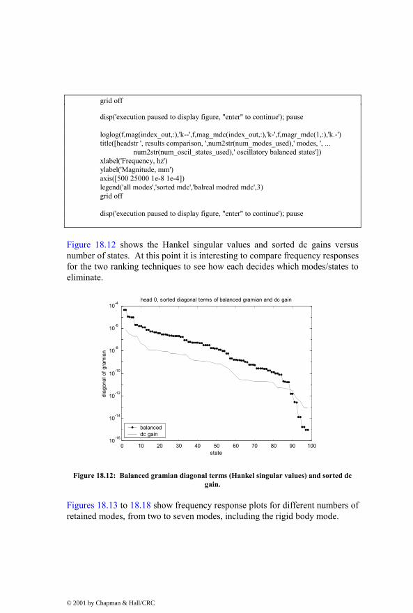
grid off disp('execution paused to display figure, "enter" to continue'); pause loglog(f,mag(index_out,:),'k--',f,mag_mdc(index_out,:),'k-',f,magr_mdc(1,:),'k.-') title([headstr ', results comparison, ',num2str(num_modes_used),' modes, ', ... num2str(num_oscil_states_used),' oscillatory balanced states']) xlabel('Frequency, hz') ylabel('Magnitude, mm') axis([500 25000 1e-8 1e-4]) legend('all modes','sorted mdc','balreal modred mdc',3) grid off disp('execution paused to display figure, "enter" to continue'); pause
Figure 18.12 shows the Hankel singular values and sorted dc gains versus number of states. At this point it is interesting to compare frequency responses for the two ranking techniques to see how each decides which modes/states to eliminate.
0 10 20 30 40 50 60 70 80 90 10010-16
10-14
10-12
10-10
10-8
10-6
10-4head 0, sorted diagonal terms of balanced gramian and dc gain
state
diag
onal
of g
ram
ian
balanceddc gain
Figure 18.12: Balanced gramian diagonal terms (Hankel singular values) and sorted dc gain.
Figures 18.13 to 18.18 show frequency response plots for different numbers of retained modes, from two to seven modes, including the rigid body mode.
© 2001 by Chapman & Hall/CRC

While the code above calculates “sorted truncated” and “balreal modred del” responses, we will only show the following in the figures below:
1) “sorted mdc” – uses dc gain ranking and modred “mdc” to reduce
2) “balreal modred mdc” – uses balreal for ranking and modred “mdc” to reduce
103 10410-8
10-7
10-6
10-5
10-4head 0, results comparison, 2 modes, 2 oscillatory balanced states
Frequency, hz
Mag
nitu
de, m
m
all modes sorted truncated balreal modred del
Figure 18.13: Two modes included.
103 10410-8
10-7
10-6
10-5
10-4head 0, results comparison, 3 modes, 4 oscillatory balanced states
Frequency, hz
Mag
nitu
de, m
m
all modes sorted truncated balreal modred del
Figure 18.14: Three modes included.
© 2001 by Chapman & Hall/CRC

Note that the two ranking methods chose different modes for the three reduced modes. The dc gain method chose the two system modes in the 4.2 khz range (almost coincident) while the balanced method chose one mode at 4.2 khz and another at 5.1 khz.
103 10410-8
10-7
10-6
10-5
10-4head 0, results comparison, 4 modes, 6 oscillatory balanced states
Frequency, hz
Mag
nitu
de, m
m
all modes sorted truncated balreal modred del
Figure 18.15: Four modes included.
For the four reduced mode case, the dc gain method picked up the 5.1 khz mode, while the balanced method chose the suspension torsion mode at 2.9 khz.
103 10410-8
10-7
10-6
10-5
10-4head 0, results comparison, 5 modes, 8 oscillatory balanced states
Frequency, hz
Mag
nitu
de, m
m
all modes sorted truncated balreal modred del
Figure 18.16: Five modes included.
© 2001 by Chapman & Hall/CRC

For the five reduced mode case the dc gain method included the torsion mode but missed the mode at 5.5 khz which was picked up by the balanced method.
103 10410-8
10-7
10-6
10-5
10-4head 0, results comparison, 6 modes, 10 oscillatory balanced states
Frequency, hz
Mag
nitu
de, m
m
all modes sorted truncated balreal modred del
Figure 18.17: Six modes included.
With six reduced modes the balanced method includes the mode at 9 khz, but the dc gain method missed it.
103 10410-8
10-7
10-6
10-5
10-4head 0, results comparison, 7 modes, 12 oscillatory balanced states
Frequency, hz
Mag
nitu
de, m
m
all modes sorted truncated balreal modred del
Figure 18.18: Seven modes included.
With seven or higher modes the balanced and dc gain results are very similar. We will see later when analyzing impulse responses of the oscillatory system
© 2001 by Chapman & Hall/CRC

that the two methods give results which are within a few percent of each other when seven or more modes are included in the reduced model.
18.8 Balanced and dc Gain Ranking Impulse Response Comparison
This section will compare the impulse responses for four different reduced systems, using from 2 through 15 modes. Only the matched dc gain (mdc) methods will be compared as there are minimal differences between the mdc method and the truncation or “del” method of reducing, as can be seen from the eight reduced mode results below.
103 10410-8
10-7
10-6
10-5
10-4head 0, results comparison, 8 modes, 14 oscillatory balanced states
Frequency, hz
Mag
nitu
de, m
m
all modes sorted truncated balreal modred del
Figure 18.19: Frequency response for eight-mode reduced models, sorted truncated and balreal modred “del.”
© 2001 by Chapman & Hall/CRC

103 10410-8
10-7
10-6
10-5
10-4head 0, results comparison, 8 modes, 14 oscillatory balanced states
Frequency, hz
Mag
nitu
de, m
m
all modes sorted mdc balreal modred mdc
Figure 18.20: Frequency response for 8-mode reduced models, sorted “mdc” and balreal modred “mdc.”
In studying the impulse response, we will use only the oscillatory modes. The final model will of course include the rigid body mode, but to study the effects of the various reduced models on transient response it is useful to include only the oscillatory modes. The reason this is useful is that a typical forcing function applied to a rigid body mode will move the system from one position to another, with rigid body displacements quite large relative to the displacements of the oscillatory modes, creating roundoff errors that mask the oscillatory mode responses.
The code below calculates the impulse response using the “lsim” function for five oscillatory systems, the original “all modes included” system and the four reduced systems. The impulse responses are then plotted and the normalized reduction index, δ (Gawronski 1998), is calculated, where the index is defined as:
disp(all mode model)-disp(reduced model)disp(all mode model)
δ = (18.28)
A table of results for δ from earlier runs with different numbers of retained modes is included in the code listing below. Information in the table is also shown graphically in Figures 18.25 and 18.26.
% calculate impulse responses of all four oscillatory systems for comparison ttotal = 0.0025;
© 2001 by Chapman & Hall/CRC

t = linspace(0,ttotal,400); % define oscillatory systems for models % sorted reduced system red_size = 2*num_modes_used; [a_sys_sort_red,b_sys_sort_red,c_sys_sort_red,d_sys_sort_red] = …
ssdata(sys_sort_red); a_sys_sort_redo = a_sys_sort_red(3:red_size,3:red_size); b_sys_sort_redo = b_sys_sort_red(3:red_size); c_sys_sort_redo = c_sys_sort_red(index_out,3:red_size); sys_sort_redo = ss(a_sys_sort_redo,b_sys_sort_redo,c_sys_sort_redo,d); % sorted mdc reduced system [a_sys_sort_mdc,b_sys_sort_mdc,c_sys_sort_mdc,d_sys_sort_mdc] = …
ssdata(sys_mdc); a_sys_sort_mdc = a_sys_sort_red(3:red_size,3:red_size); b_sys_sort_mdc = b_sys_sort_red(3:red_size); c_sys_sort_mdc = c_sys_sort_red(index_out,3:red_size); sys_mdco = ss(a_sys_sort_mdc,b_sys_sort_mdc,c_sys_sort_mdc,d); % use lsim to calculate transient response [disp_syso,t_syso] = impulse(syso,t); [disp_sys_sort_redo,t_sys_sort_redo] = impulse(sys_sort_redo,t); [disp_sys_sort_mdco,t_sys_sort_mdco] = impulse(sys_mdco,t); [disp_bsys_delo,t_bsys_delo] = impulse(bsys_delo,t); [disp_bsys_mdco,t_bsys_mdco] = impulse(bsys_mdco,t); % build matrix of results dispo = [disp_syso(:,1) disp_sys_sort_redo(:,1) ... disp_sys_sort_mdco(:,1) disp_bsys_delo(:,1) ... disp_bsys_mdco(:,1)]; sort_redo_del = dispo(:,1) - dispo(:,2); sort_mdco_del = dispo(:,1) - dispo(:,3);
© 2001 by Chapman & Hall/CRC

delo_del = dispo(:,1) - dispo(:,4); mdco_del = dispo(:,1) - dispo(:,5); % calculate normalized reduction index index_sort_redo = …
sqrt(sum(sort_redo_del.*sort_redo_del))/sqrt(sum(dispo(:,1).*dispo(:,1))) index_sort_mdco = …
sqrt(sum(sort_mdco_del.*sort_mdco_del))/sqrt(sum(dispo(:,1).*dispo(:,1))) index_delo = … sqrt(sum(delo_del.*delo_del))/sqrt(sum(dispo(:,1).*dispo(:,1))) index_mdco = …
sqrt(sum(mdco_del.*mdco_del))/sqrt(sum(dispo(:,1).*dispo(:,1))) [num_modes_used index_sort_redo index_sort_mdco index_delo index_mdco] plot(t_syso,disp_syso(:,1),'k-',t_sys_sort_redo,disp_sys_sort_redo(:,1),'k.-') title([headstr ', displacement vs time, ',num2str(num_modes_used-1), …
' oscillatory modes']) xlabel('time, sec') ylabel('displacement, mm') legend('all modes','sorted reduced system',4) grid off disp('execution paused to display figure, "enter" to continue'); pause plot(t_syso,disp_syso(:,1),'k-',t_sys_sort_mdco,disp_sys_sort_mdco(:,1),'k.-') title([headstr ', displacement vs time, ',num2str(num_modes_used-1), …
' oscillatory modes']) xlabel('time, sec') ylabel('displacement, mm') legend('all modes','sorted modred mdc',4) grid off disp('execution paused to display figure, "enter" to continue'); pause plot(t_syso,disp_syso(:,1),'k-',t_bsys_delo,disp_bsys_delo(:,1),'k.-') title([headstr ', displacement vs time, ',num2str(num_oscil_states_used), …
' oscillatory balanced states']) xlabel('time, sec') ylabel('displacement, mm') legend('all modes','balreal modred del',4) grid off disp('execution paused to display figure, "enter" to continue'); pause plot(t_syso,disp_syso(:,1),'k-',t_bsys_mdco,disp_bsys_mdco(:,1),'k.-') title([headstr ', displacement vs time, ',num2str(num_oscil_states_used), …
' oscillatory balanced states']) xlabel('time, sec') ylabel('displacement, mm')
© 2001 by Chapman & Hall/CRC
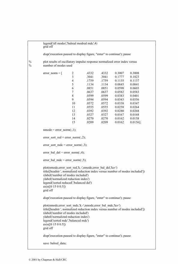
legend('all modes','balreal modred mdc',4) grid off disp('execution paused to display figure, "enter" to continue'); pause % plot results of oscillatory impulse response normalized error index versus % number of modes used error_norm = [ 2 .4332 .4332 0.3007 0.3008 3 .3041 .3041 0.1777 0.1823 4 .1759 .1759 0.1135 0.1137 5 .1134 .1134 0.0845 0.0841 6 .0851 .0851 0.0598 0.0603 7 .0637 .0637 0.0582 0.0583 8 .0599 .0599 0.0383 0.0401 9 .0594 .0594 0.0343 0.0356 10 .0572 .0572 0.0338 0.0347 11 .0555 .0555 0.0258 0.0264 12 .0392 .0392 0.0280 0.0268 13 .0327 .0327 0.0167 0.0168 14 .0270 .0270 0.0162 0.0158 15 .0209 .0209 0.0162 0.0156]; nmode = error_norm(:,1); error_sort_red = error_norm(:,2); error_sort_mdc = error_norm(:,3); error_bal_del = error_norm(:,4); error_bal_mdc = error_norm(:,5); plot(nmode,error_sort_red,'k.-',nmode,error_bal_del,'ko-') title([headstr ', normalized reduction index versus number of modes included']) xlabel('number of modes included') ylabel('normalized reduction index') legend('sorted reduced','balanced del') axis([0 15 0 0.5]) grid off disp('execution paused to display figure, "enter" to continue'); pause plot(nmode,error_sort_mdc,'k.-',nmode,error_bal_mdc,'ko-') title([headstr ', normalized reduction index versus number of modes included']) xlabel('number of modes included') ylabel('normalized reduction index') legend('sorted mdc','balanced mdc') axis([0 15 0 0.5]) grid off disp('execution paused to display figure, "enter" to continue'); pause save balred_data;
© 2001 by Chapman & Hall/CRC

The impulse response comparisons for the same four reduced methods are shown in the four figures below.
0 0.5 1 1.5 2 2.5
x 10-3
-0.04
-0.03
-0.02
-0.01
0
0.01
0.02
0.03
0.04head 0, displacement vs time, 7 oscillatory modes
time, sec
disp
lace
men
t, m
m
all modes sorted reduced system
Figure 18.21: Impulse response comparisons for oscillatory system, full model (all oscillatory modes) and sorted reduced system with seven oscillatory modes.
0 0.5 1 1.5 2 2.5
x 10-3
-0.04
-0.03
-0.02
-0.01
0
0.01
0.02
0.03
0.04head 0, displacement vs time, 7 oscillatory modes
time, sec
disp
lace
men
t, m
m
all modes sorted modred mdc
Figure 18.22: Impulse response comparisons for oscillatory system, full model (all oscillatory modes) and sorted modred with “mdc” option with seven oscillatory modes.
© 2001 by Chapman & Hall/CRC
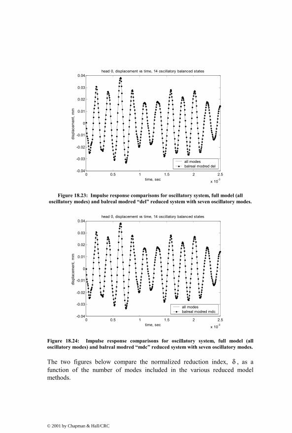
0 0.5 1 1.5 2 2.5
x 10-3
-0.04
-0.03
-0.02
-0.01
0
0.01
0.02
0.03
0.04head 0, displacement vs time, 14 oscillatory balanced states
time, sec
disp
lace
men
t, m
m
all modes balreal modred del
Figure 18.23: Impulse response comparisons for oscillatory system, full model (all oscillatory modes) and balreal modred “del” reduced system with seven oscillatory modes.
0 0.5 1 1.5 2 2.5
x 10-3
-0.04
-0.03
-0.02
-0.01
0
0.01
0.02
0.03
0.04head 0, displacement vs time, 14 oscillatory balanced states
time, sec
disp
lace
men
t, m
m
all modes balreal modred mdc
Figure 18.24: Impulse response comparisons for oscillatory system, full model (all oscillatory modes) and balreal modred “mdc” reduced system with seven oscillatory modes.
The two figures below compare the normalized reduction index, δ , as a function of the number of modes included in the various reduced model methods.
© 2001 by Chapman & Hall/CRC

0 5 10 150
0.05
0.1
0.15
0.2
0.25
0.3
0.35
0.4
0.45
0.5head 0, normalized reduction index versus number of modes included
number of modes included
norm
aliz
ed re
duct
ion
inde
x
sorted reducedbalanced del
Figure 18.25: Impulse response normalized reduction index versus number of modes included in reduction for sorted reduced and balanced modred “del” option reductions.
0 5 10 150
0.05
0.1
0.15
0.2
0.25
0.3
0.35
0.4
0.45
0.5head 0, normalized reduction index versus number of modes included
number of modes included
norm
aliz
ed re
duct
ion
inde
x
sorted mdc balanced mdc
Figure 18.26: Impulse response normalized reduction index versus number of modes included in reduction for sorted modred “mdc” and balanced modred “mdc” options reductions.
As mentioned in the frequency response section, when five or more modes are included, the impulse responses are almost identical for all reduction techniques, with small differences in normalized reduction indices. For less than five modes, it is better to use the balanced technique because it picks up an additional mode in addition to the system mode, whereas the dc gain
© 2001 by Chapman & Hall/CRC

method assigns the first two modes to the almost coincident two modes near the system mode.
© 2001 by Chapman & Hall/CRC

CHAPTER 19
MIMO TWO-STAGE ACTUATOR MODEL
19.1 Introduction
In this chapter we will use an ANSYS model of a two-stage disk drive actuator/suspension system to illustrate the creation of a reduced model for a Multiple Input, Multiple Output (MIMO) system using the balanced reduction method. The results will seem somewhat anticlimactic since the previous chapter covered most aspects of how to use the balanced reduction method. However, understanding the mechanics of setting up a MIMO system should prove useful.
As the track density (tracks per inch, tpi) of disk drives continues to increase, it will be necessary to add a second stage of actuation to the system in order to have the high servo bandwidths required to accurately follow the closely spaced tracks. Many different types of two-stage actuator architectures are being explored. The actuator architecture used for this example is not meant to represent a practical embodiment but will serve to illustrate a two-input, two-output system.
We will begin with descriptions of the actuator system and ANSYS model. Then, ANSYS output, mode shape plots, frequency responses and a partial eigenvector listing will be discussed. The pertinent eigenvector and eigenvalue information will be extracted into a .mat file for input to MATLAB.
The MATLAB code will calculate either dc or peak gains, depending on whether uniform or non-uniform damping is defined. There are four gains to be plotted for this two-input, two-output MIMO system. While dc and peak gains are not required for the “balreal” and “modred” model reduction, they will serve to bridge our understanding from SISO models to MIMO models. We will see the difficulty of choosing which modes to include in a MIMO model using dc or peak gain sorting by discussing the ranking of modes for the four input/output combinations.
In order to perform a balanced reduction, the system is partitioned into rigid body and oscillatory modes, similar to the method used in Chapter 18. The oscillatory modes are balanced and “modred” is used with both the “del” and “mdc” options to reduce the model. Frequency responses for head 0 for both coil and piezo inputs for “del” reduction are shown for various numbers of
© 2001 by Chapman & Hall/CRC

reduced modes, from 6 oscillatory states to 20 oscillatory states included. The 20-state case shows both “del” and “mdc” for comparison.
Impulse responses are calculated for oscillatory systems with various numbers of reduced modes retained. The error is plotted as a function of number of modes retained.
19.2 Actuator Description
Figure 19.1 shows top and cross-sectioned side views of the two-stage actuator used for the analysis.
Figure 19.1: Drawing of actuator/suspension system.
The model is similar to the actuator used in Chapters 17 and 18 except that the arms are now the same thickness and are symmetrically located with respect to the pivot bearing z axis centerline. Also, there is now a piezo-actuator bonded into one side of each of the arms. The piezo actuator consists of a ceramic element that changes size when a voltage is applied. In this case, the voltage would be applied to the piezo element so that it changes length, creating a rotation about the “hinge” section in the other side of the arm. This rotation translates the recording head in the circumferential direction. When this “fine positioning” motion is used in conjunction with the VCM’s “coarse positioning” motion, higher servo bandwidths and consequently higher tpi are possible.
Voice Coil
Ball Bearing
Actuator Shaft
Adhesive
Suspension
RecordingHead
Disk
Ball Bearing
VCM Force
"Hinge"
X
Y
Z
X
Piezo
Micro-actuatorMotion
© 2001 by Chapman & Hall/CRC

The actuator example in the last two chapters had a coil forcing function applied at four nodes in the coil body. Even though there were multiple points at which the force was applied, the fact that the same force was applied to all nodes defined a Single Input system.
Instead of applying voltage as the input into the piezo element, we will assume that we have calculated an equivalent set of forces which can be applied at the ends of the element that will replicate the voltage forcing function. In this model, we will be applying forces to multiple nodes at the ends of both piezo elements. Since the same forces are being applied to both piezo elements, they represent the second input to the now Multi Input system, the first input being the coil force. We will apply equal and opposite forces to the two ends of each piezo actuator, and reverse the signs of the forces applied to the two separate elements. If the same forcing function were applied to both elements, an inertial moment arises which would tend to rotate the entire actuator about the pivot. By using opposite signs for the two arms, this moment is largely eliminated, generating less cross-coupling between the coarse and fine actuator inputs.
In order to make this example a “Multiple Output” system, we will output the displacements of both lower and upper heads, head 0 and head 1.
19.3 ANSYS Model Description
The model description is the same as for the model in Chapter 17. The ANSYS model is shown below, along with a drawing showing the node locations for the coil, piezo elements and heads.
© 2001 by Chapman & Hall/CRC

Figure 19.2: Complete piezo actuator/suspension model.
Figure 19.3: Piezo actuator/suspension model, four views.
© 2001 by Chapman & Hall/CRC
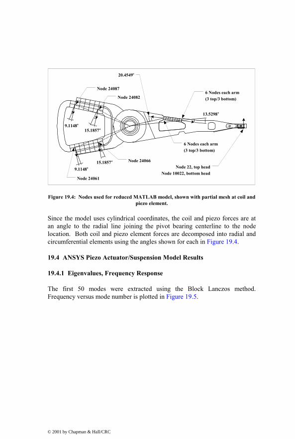
Node 24082
Node 24087
Node 24061
Node 24066Node 22, top head
Node 10022, bottom head
o9.1148o15.1857
o9.1148
o15.1857
o20.4549
o13.5298
6 Nodes each arm(3 top/3 bottom)
6 Nodes each arm(3 top/3 bottom)
Figure 19.4: Nodes used for reduced MATLAB model, shown with partial mesh at coil and piezo element.
Since the model uses cylindrical coordinates, the coil and piezo forces are at an angle to the radial line joining the pivot bearing centerline to the node location. Both coil and piezo element forces are decomposed into radial and circumferential elements using the angles shown for each in Figure 19.4.
19.4 ANSYS Piezo Actuator/Suspension Model Results
19.4.1 Eigenvalues, Frequency Response
The first 50 modes were extracted using the Block Lanczos method. Frequency versus mode number is plotted in Figure 19.5.
© 2001 by Chapman & Hall/CRC

0 5 10 15 20 25 30 35 40 45 50102
103
104
105frequency versus mode number
mode number
frequ
ency
, hz
Figure 19.5: Frequencies versus mode number.
Figure 19.6: Coil input frequency responses for head 0 and head 1 from ANSYS, zeta = 0.005.
Figure 19.6 is the frequency response from ANSYS for coil input for both heads. The same frequency response from the 50-mode MATLAB model is shown in Figure 19.7. Figure 19.8 plots the frequency response for the two piezo inputs.
© 2001 by Chapman & Hall/CRC

103 10410-9
10-8
10-7
10-6
10-5
10-4
gap displacement, all 50 modes included
Frequency, hz
Mag
nitu
de, m
m
head 0, coil inputhead 1, coil input
Figure 19.7: Coil input frequency response from MATLAB, zeta = 0.005.
103 10410-9
10-8
10-7
10-6
10-5
10-4
gap displacement, all 50 modes included
Frequency, hz
Mag
nitu
de, m
m
head 0 piezo inputhead 1 piezo input
Figure 19.8: Piezo input frequency response from MATLAB, zeta = 0.005.
19.4.2 Mode Shape Plots
Selected mode shape plots are shown below, with a brief discussion of each in the following section.
© 2001 by Chapman & Hall/CRC

Figure 19.9: Mode 1 undeformed/deformed plot, 0.014 hz, rigid body rotation.
Figure 19.10: Mode 2, 798 hz, actuator pitching mode.
© 2001 by Chapman & Hall/CRC

Figure 19.11: Mode 3, 1004 hz, arm/coil bending in phase.
Figure 19.12: Mode 4, 1055 hz, arms bending out of phase.
© 2001 by Chapman & Hall/CRC

Figure 19.13: Mode 5, 2027 hz, actuator/coil torsion about x axis.
Figure 19.14: Mode 6, 2085 hz, suspension bending mode, some arm interaction.
© 2001 by Chapman & Hall/CRC

Figure 19.15: Mode 8, 2823 hz, suspension torsion, in phase, arm tip interaction.
Figure 19.16: Mode 9, 2867 hz, suspension torsion, out of phase.
© 2001 by Chapman & Hall/CRC

Figure 19.17: Mode 12, 3415 hz, suspension torsion, arm tip lateral.
Figure 19.18: Mode 13, 3479 hz, coil/arm/suspension lateral mode.
© 2001 by Chapman & Hall/CRC

Figure 19.19: Mode 16, 5387 hz, suspension sway, arm tip lateral.
Figure 19.20: Mode 17, 5664 hz, piezo bending, arm tip torsion, coil bending.
© 2001 by Chapman & Hall/CRC

Figure 19.21: Mode 21, 6822 hz, suspension/arm lateral out of phase.
19.4.3 Mode Shape Discussion
As in Chapter 17, we will now describe the major modes which couple into the frequency response as well as several that do not couple, associating them with the frequency responses in Figures 19.7 and 19.8.
Mode 1 is the rigid body rotation mode, which ANSYS again does not calculate at zero hz because of slight geometric and numerical roundoff issues. The frequency for the rigid body mode is set to zero in the MATLAB code.
Modes 2, 3 and 4 are all modes which involve motion only in the x-z plane, bending type motions. Since the motions are perpendicular, or orthogonal, to the direction of input forces and output displacements, they do not couple into any of the frequency responses.
Mode 5 is an actuator/coil torsion mode, rotating about the x axis. A similar mode can be seen on the model in Chapter 17 as a small pole/zero pair on head 1. A torsional mode like this can be excited by: (1) coil forces, since the coil is offset from both the mass center and bearing stiffness center, and (2) inertial forces, because of the asymmetry of the structure about the mass center location in the z direction. Because the arms are more symmetric on this model than the model in Chapter 17, the pole/zero mode does not appear on the frequency response plot of either head. We will see in the dc gain ranking that mode 5 is two orders of magnitude less important than the major
© 2001 by Chapman & Hall/CRC

modes of the system for coil input, and is almost three orders of magnitude less important for piezo input.
Mode 6 is a suspension bending mode, once again a bending-only mode with no coupling into the circumferential direction.
Mode 8 is a suspension torsion, arm-tip interaction mode. It is the second most important mode for piezo input, but is unimportant for coil input.
Mode 9 is a suspension torsion mode. It is the second most important mode for coil input, but is unimportant for piezo input. The peak on the two frequency responses, just below 3 khz, is in fact two different frequencies and two different modes for the two different forcing functions. For the coil input the peak is at 2867 hz, mode 9. For piezo input, the peak is at 2823 hz, mode 8.
Modes 12 and 13 are the most important modes for piezo and coil inputs, respectively. Mode 12 involves arm tip lateral motion which the piezo can easily excite. Mode 13 is the “system” lateral mode with all components moving laterally, in phase.
Mode 16, another mode involving the tips of the arms and this time the suspension sway mode, is the third most important mode for coil input.
Mode 17 is the fifth most important piezo excitation mode, involving piezo bending, arm tip torsion and coil bending.
Mode 21 is the third most important mode for piezo excitation, with the suspensions and arms moving laterally, out of phase.
19.4.4 ANSYS Output Listing
The ANSYS output listing for input and output nodes for modes 1, 2 and 13 are listed below. These three modes were selected for discussion in order to highlight different aspects of the eigenvectors. Compared with the ANSYS output listing in Chapter 17, there are significantly more nodes in the output, with the additional nodes representing the six nodes at each end of the bottom and top piezo elements.
The rigid body mode, mode 1, should have only UY displacements (circumferential motion in the cylindrical coordinate system). Mode 2, an actuator pitching mode has its most significant motion in the UZ direction, with some slight coupling into the UX and UY directions. Mode 13 is a highly coupled mode, with significant displacements in all three directions for
© 2001 by Chapman & Hall/CRC

some nodes. The UY direction displacements are significant with respect to the UY displacements of mode 2.
***** POST1 NODAL DEGREE OF FREEDOM LISTING ***** LOAD STEP= 1 SUBSTEP= 1 FREQ= 0.14502E-01 LOAD CASE= 0 THE FOLLOWING DEGREE OF FREEDOM RESULTS ARE IN COORDINATE SYSTEM 1 NODE UX UY UZ ROTX ROTY ROTZ 22 0.30584E-06 32.618 0.11285E-11 0.0000 0.0000 0.0000 10022 0.30627E-06 32.618 -0.46777E-10 0.0000 0.0000 0.0000 21538 0.85322E-07 9.7742 0.21745E-08 0.0000 0.0000 0.0000 21546 0.82634E-07 14.735 0.36557E-08 0.0000 0.0000 0.0000 21576 0.10309E-06 9.9634 0.21924E-08 0.0000 0.0000 0.0000 21584 0.16887E-06 14.883 0.37407E-08 0.0000 0.0000 0.0000 21617 0.10951E-06 10.147 0.22079E-08 0.0000 0.0000 0.0000 21625 0.11092E-06 14.978 0.37980E-08 0.0000 0.0000 0.0000 22538 0.85184E-07 9.7742 0.21706E-08 0.0000 0.0000 0.0000 22546 0.82327E-07 14.735 0.36546E-08 0.0000 0.0000 0.0000 22576 0.10295E-06 9.9634 0.21900E-08 0.0000 0.0000 0.0000 22584 0.16856E-06 14.883 0.37381E-08 0.0000 0.0000 0.0000 22617 0.10937E-06 10.147 0.22067E-08 0.0000 0.0000 0.0000 22625 0.11061E-06 14.978 0.37940E-08 0.0000 0.0000 0.0000 24061 0.11911E-06 16.888 -0.95894E-09 0.0000 0.0000 0.0000 24066 0.77030E-07 10.226 -0.53758E-09 0.0000 0.0000 0.0000 24082 0.68150E-07 10.226 -0.48785E-09 0.0000 0.0000 0.0000 24087 0.10037E-06 16.888 -0.86954E-09 0.0000 0.0000 0.0000 24538 0.84850E-07 9.7742 0.20872E-08 0.0000 0.0000 0.0000 24546 0.81937E-07 14.735 0.18321E-08 0.0000 0.0000 0.0000 24576 0.10262E-06 9.9634 0.20998E-08 0.0000 0.0000 0.0000 24584 0.16817E-06 14.883 0.17648E-08 0.0000 0.0000 0.0000 24617 0.10904E-06 10.147 0.21122E-08 0.0000 0.0000 0.0000 24625 0.11021E-06 14.978 0.17139E-08 0.0000 0.0000 0.0000 25538 0.84745E-07 9.7742 0.20835E-08 0.0000 0.0000 0.0000 25546 0.82082E-07 14.735 0.18310E-08 0.0000 0.0000 0.0000 25576 0.10251E-06 9.9634 0.20975E-08 0.0000 0.0000 0.0000 25584 0.16832E-06 14.883 0.17623E-08 0.0000 0.0000 0.0000 25617 0.10894E-06 10.147 0.21110E-08 0.0000 0.0000 0.0000 25625 0.11036E-06 14.978 0.17100E-08 0.0000 0.0000 0.0000 MAXIMUM ABSOLUTE VALUES NODE 10022 22 21625 0 0 0 VALUE 0.30627E-06 32.618 0.37980E-08 0.0000 0.0000 0.0000 *ENDDO INDEX= I ***** POST1 NODAL DEGREE OF FREEDOM LISTING ***** LOAD STEP= 1 SUBSTEP= 2 FREQ= 797.85 LOAD CASE= 0
© 2001 by Chapman & Hall/CRC

THE FOLLOWING DEGREE OF FREEDOM RESULTS ARE IN COORDINATE SYSTEM 1 NODE UX UY UZ ROTX ROTY ROTZ 22 0.49229 -0.14022 -0.10321E-03 0.0000 0.0000 0.0000 10022 -0.89140 0.14245 -0.83465E-03 0.0000 0.0000 0.0000 21538 -1.0283 0.18631 -4.0091 0.0000 0.0000 0.0000 21546 -1.5471 0.23464E-01 -10.200 0.0000 0.0000 0.0000 21576 -1.0204 0.23663 -4.0561 0.0000 0.0000 0.0000 21584 -1.5459 0.72962E-01 -10.473 0.0000 0.0000 0.0000 21617 -1.0084 0.27685 -4.0950 0.0000 0.0000 0.0000 21625 -1.5436 0.11594 -10.631 0.0000 0.0000 0.0000 22538 -0.61275 0.10972 -4.0090 0.0000 0.0000 0.0000 22546 -0.12481 0.83127E-01 -10.200 0.0000 0.0000 0.0000 22576 -0.60478 0.13415 -4.0560 0.0000 0.0000 0.0000 22584 -0.12184 0.86554E-01 -10.473 0.0000 0.0000 0.0000 22617 -0.60100 0.15502 -4.0950 0.0000 0.0000 0.0000 22625 -0.11925 0.89513E-01 -10.631 0.0000 0.0000 0.0000 24061 -0.35220 0.13939 19.652 0.0000 0.0000 0.0000 24066 -0.33572 0.17431 7.3143 0.0000 0.0000 0.0000 24082 -0.33512 -0.17241 7.3089 0.0000 0.0000 0.0000 24087 -0.35171 -0.13563 19.644 0.0000 0.0000 0.0000 24538 0.22023 -0.36868E-01 -4.0205 0.0000 0.0000 0.0000 24546 -0.27795 -0.52244E-01 -10.250 0.0000 0.0000 0.0000 24576 0.21597 -0.43317E-01 -4.0680 0.0000 0.0000 0.0000 24584 -0.27997 -0.42854E-01 -10.524 0.0000 0.0000 0.0000 24617 0.21591 -0.49478E-01 -4.1074 0.0000 0.0000 0.0000 24625 -0.28139 -0.34705E-01 -10.683 0.0000 0.0000 0.0000 25538 0.63806 -0.11349 -4.0206 0.0000 0.0000 0.0000 25546 1.1532 0.79337E-02 -10.250 0.0000 0.0000 0.0000 25576 0.63387 -0.14598 -4.0680 0.0000 0.0000 0.0000 25584 1.1531 -0.29036E-01 -10.524 0.0000 0.0000 0.0000 25617 0.62557 -0.17161 -4.1074 0.0000 0.0000 0.0000 25625 1.1519 -0.61159E-01 -10.683 0.0000 0.0000 0.0000 MAXIMUM ABSOLUTE VALUES NODE 21546 21617 24061 0 0 0 VALUE -1.5471 0.27685 19.652 0.0000 0.0000 0.0000 ***** POST1 NODAL DEGREE OF FREEDOM LISTING ***** LOAD STEP= 1 SUBSTEP= 13 FREQ= 3479.3 LOAD CASE= 0 THE FOLLOWING DEGREE OF FREEDOM RESULTS ARE IN COORDINATE SYSTEM 1 NODE UX UY UZ ROTX ROTY ROTZ 22 -2.1984 60.376 -0.14239E-02 0.0000 0.0000 0.0000 10022 -1.9960 77.045 0.31840E-01 0.0000 0.0000 0.0000 21538 0.80764E-01 0.40397E-01 0.49848 0.0000 0.0000 0.0000 21546 -6.4836 3.9912 -1.2673 0.0000 0.0000 0.0000 21576 0.72358E-01 0.63009E-01 0.42663 0.0000 0.0000 0.0000 21584 -7.6689 4.6553 -1.8884 0.0000 0.0000 0.0000 21617 0.12273 0.57379E-01 0.37047 0.0000 0.0000 0.0000
© 2001 by Chapman & Hall/CRC

21625 -8.7016 5.1772 -2.4325 0.0000 0.0000 0.0000 22538 0.87706E-01 0.17543 0.56748 0.0000 0.0000 0.0000 22546 -6.2831 5.0182 -1.2225 0.0000 0.0000 0.0000 22576 0.92974E-01 0.18824 0.48659 0.0000 0.0000 0.0000 22584 -7.4322 5.6835 -1.8299 0.0000 0.0000 0.0000 22617 0.14368 0.17617 0.42076 0.0000 0.0000 0.0000 22625 -8.4357 6.2048 -2.3541 0.0000 0.0000 0.0000 24061 -1.9369 -12.670 -0.95604 0.0000 0.0000 0.0000 24066 -1.0801 -4.7937 -1.0649 0.0000 0.0000 0.0000 24082 1.5007 -4.5559 -1.4595 0.0000 0.0000 0.0000 24087 2.3829 -12.467 0.10330 0.0000 0.0000 0.0000 24538 -0.93404E-01 0.37757 1.0909 0.0000 0.0000 0.0000 24546 -5.5118 4.1576 2.6594 0.0000 0.0000 0.0000 24576 -0.66009E-01 0.38853 1.0874 0.0000 0.0000 0.0000 24584 -6.3981 4.6967 3.0133 0.0000 0.0000 0.0000 24617 -0.78948E-02 0.37908 1.0812 0.0000 0.0000 0.0000 24625 -7.1715 5.1206 3.3430 0.0000 0.0000 0.0000 25538 -0.30931 0.47682 1.1451 0.0000 0.0000 0.0000 25546 -5.2283 3.4392 2.6949 0.0000 0.0000 0.0000 25576 -0.28463 0.50756 1.1349 0.0000 0.0000 0.0000 25584 -6.1405 3.9607 3.0595 0.0000 0.0000 0.0000 25617 -0.21671 0.51131 1.1213 0.0000 0.0000 0.0000 25625 -6.9354 4.3710 3.4049 0.0000 0.0000 0.0000 MAXIMUM ABSOLUTE VALUES NODE 21625 10022 25625 0 0 0 VALUE -8.7016 77.045 3.4049 0.0000 0.0000 0.0000
The eigenvalues and eigenvectors are stripped out of the ANSYS actrlpz.eig file and are stored in the MATLAB .mat file actrlpz_eig.mat.
19.5 MATLAB Model, MATLAB Code act8pz.m Listing and Results
19.5.1 Input, dof Definition
The act8pz.m MATLAB code starts by defining the degrees of freedom, nodes, directions and locations for the problem for reference in building the model. The degrees of freedom are extracted from the ANSYS eigenvalue/eigenvector listing and are ordered by node number, first the UX direction and then the UY direction. Once again, the UX direction information is required to transform the coil and piezo forces into cylindrical coordinates. The eigenvalue/eigenvector information is then loaded by reading the .mat file actrlpz_eig.mat and the rigid body mode is set to zero frequency.
% act8pz.m clear all;
© 2001 by Chapman & Hall/CRC

hold off; clf; % load the Block Lanczos .mat file actrl_eig.mat, containing evr – the % modal matrix, freqvec -the frequency vector and node_numbers - the % vector of node numbers for the modal matrix % the output for the ANSYS run is the following dof's % dof node dir where % % 1 22 ux - radial, top head gap % 2 10022 ux - radial, bottom head gap % 3 21538 ux - radial, bottom arm piezo, hub end % 4 21546 ux - radial, bottom arm piezo, head end % 5 21576 ux - radial, bottom arm piezo, hub end % 6 21584 ux - radial, bottom arm piezo, head end % 7 21617 ux - radial, bottom arm piezo, hub end % 8 21625 ux - radial, bottom arm piezo, head end % 9 22538 ux - radial, bottom arm piezo, hub end % 10 22546 ux - radial, bottom arm piezo, head end % 11 22576 ux - radial, bottom arm piezo, hub end % 12 22584 ux - radial, bottom arm piezo, head end % 13 22617 ux - radial, bottom arm piezo, hub end % 14 22625 ux - radial, bottom arm piezo, head end % 15 24061 ux - radial, bottom arm piezo, coil % 16 24066 ux - radial, bottom arm piezo, coil % 17 24082 ux - radial, bottom arm piezo, coil % 18 24087 ux - radial, bottom arm piezo, coil % 19 24538 ux - radial, top arm piezo, hub end % 20 24546 ux - radial, top arm piezo, head end % 21 24576 ux - radial, top arm piezo, hub end % 22 24584 ux - radial, top arm piezo, head end % 23 24617 ux - radial, top arm piezo, hub end % 24 24625 ux - radial, top arm piezo, head end % 25 25538 ux - radial, top arm piezo, hub end % 26 25546 ux - radial, top arm piezo, head end % 27 25576 ux - radial, top arm piezo, hub end % 28 25584 ux - radial, top arm piezo, head end % 29 25617 ux - radial, top arm piezo, hub end % 30 25625 ux - radial, top arm piezo, head end % 31 22 uy - circumferential, top head gap % 32 10022 uy - circumferential, bottom head gap % 33 21538 uy - circumferential, bottom arm piezo, hub end % 34 21546 uy - circumferential, bottom arm piezo, head end % 35 21576 uy - circumferential, bottom arm piezo, hub end % 36 21584 uy - circumferential, bottom arm piezo, head end % 37 21617 uy - circumferential, bottom arm piezo, hub end % 38 21625 uy - circumferential, bottom arm piezo, head end % 39 22538 uy - circumferential, bottom arm piezo, hub end % 40 22546 uy - circumferential, bottom arm piezo, head end % 41 22576 uy - circumferential, bottom arm piezo, hub end % 42 22584 uy - circumferential, bottom arm piezo, head end % 43 22617 uy - circumferential, bottom arm piezo, hub end
© 2001 by Chapman & Hall/CRC

% 44 22625 uy - circumferential, bottom arm piezo, head end % 45 24061 uy - circumferential, bottom arm piezo, coil % 46 24066 uy - circumferential, bottom arm piezo, coil % 47 24082 uy - circumferential, bottom arm piezo, coil % 48 24087 uy - circumferential, bottom arm piezo, coil % 49 24538 uy - circumferential, top arm piezo, hub end % 50 24546 uy - circumferential, top arm piezo, head end % 51 24576 uy - circumferential, top arm piezo, hub end % 52 24584 uy - circumferential, top arm piezo, head end % 53 24617 uy - circumferential, top arm piezo, hub end % 54 24625 uy - circumferential, top arm piezo, head end % 55 25538 uy - circumferential, top arm piezo, hub end % 56 25546 uy - circumferential, top arm piezo, head end % 57 25576 uy - circumferential, top arm piezo, hub end % 58 25584 uy - circumferential, top arm piezo, head end % 59 25617 uy - circumferential, top arm piezo, hub end % 60 25625 uy - circumferential, top arm piezo, head end load actrlpz_eig; [numdof,num_modes_total] = size(evr); freqvec(1) = 0; % set rigid body mode to zero frequency xn = evr;
19.5.2 Forcing Function Definition, dc Gain Calculations
The unity coil force is equally divided between the four coil nodes. For this model, the piezo force, “fpz,” is arbitrarily set at 0.2, to be applied with equal magnitudes and with opposite signs to the two ends of each piezo element. For an actual system, the piezo force would be related to the coil force by the appropriate force constants for the VCM and the appropriate voltage/force relationships for the piezo, and would not be arbitrarily chosen.
Given the directions of the coil and piezo forces in Figure 19.4, the forces are transformed to cylindrical coordinates and two forcing function vectors are formed, one for the coil and one for the piezo.
The user is prompted for whether uniform or non-uniform damping is to be used and then dc or peak gains are calculated, respectively.
For a SISO system, we can rank the relative importance of modes using two methods, by using dc or peak gains and by using balancing. For a MIMO system, balancing is the only practical option. However, we will still calculate the dc gains for this MIMO system to get a feel for the relative importance of
© 2001 by Chapman & Hall/CRC

each of the modes for both forcing functions. This will require calculating dc gains for the four combinations possible for the two-input, two-output system.
The four dc gains are calculated, sorted and plotted in the code below.
% define radial and circumferential forces applied at four coil force nodes % "x" is radial, "y" is circumferential, total force is unity fcoil = 0.25; n24061fx = fcoil*sin(9.1148*pi/180); n24061fy = fcoil*cos(9.1148*pi/180); n24066fx = fcoil*sin(15.1657*pi/180); n24066fy = fcoil*cos(15.1657*pi/180); n24082fx = -fcoil*sin(15.1657*pi/180); n24082fy = fcoil*cos(15.1657*pi/180); n24087fx = -fcoil*sin(9.1148*pi/180); n24087fy = fcoil*cos(9.1148*pi/180); % define radial and circumferential forces applied at ends of piezo element % "x" is radial, "y" is circumferential, total force is unity fpz = 0.2/6; % six nodes at each end of the piezo % bottom arm radial force n21538fx = fpz*cos(20.4549*pi/180); n21546fx = -fpz*cos(13.5298*pi/180); n21576fx = fpz*cos(20.4549*pi/180); n21584fx = -fpz*cos(13.5298*pi/180); n21617fx = fpz*cos(20.4549*pi/180); n21625fx = -fpz*cos(13.5298*pi/180); n22538fx = fpz*cos(20.4549*pi/180); n22546fx = -fpz*cos(13.5298*pi/180); n22576fx = fpz*cos(20.4549*pi/180); n22584fx = -fpz*cos(13.5298*pi/180); n22617fx = fpz*cos(20.4549*pi/180); n22625fx = -fpz*cos(13.5298*pi/180); % top arm radial force n24538fx = -fpz*cos(20.4549*pi/180); n24546fx = fpz*cos(13.5298*pi/180); n24576fx = -fpz*cos(20.4549*pi/180); n24584fx = fpz*cos(13.5298*pi/180); n24617fx = -fpz*cos(20.4549*pi/180); n24625fx = fpz*cos(13.5298*pi/180); n25538fx = -fpz*cos(20.4549*pi/180); n25546fx = fpz*cos(13.5298*pi/180); n25576fx = -fpz*cos(20.4549*pi/180);
© 2001 by Chapman & Hall/CRC

n25584fx = fpz*cos(13.5298*pi/180); n25617fx = -fpz*cos(20.4549*pi/180); n25625fx = fpz*cos(13.5298*pi/180); % bottom arm circumferential force n21538fy = -fpz*sin(20.4549*pi/180); n21546fy = fpz*sin(13.5298*pi/180); n21576fy = -fpz*sin(20.4549*pi/180); n21584fy = fpz*sin(13.5298*pi/180); n21617fy = -fpz*sin(20.4549*pi/180); n21625fy = fpz*sin(13.5298*pi/180); n22538fy = -fpz*sin(20.4549*pi/180); n22546fy = fpz*sin(13.5298*pi/180); n22576fy = -fpz*sin(20.4549*pi/180); n22584fy = fpz*sin(13.5298*pi/180); n22617fy = -fpz*sin(20.4549*pi/180); n22625fy = fpz*sin(13.5298*pi/180); % top arm circumferential force n24538fy = fpz*sin(20.4549*pi/180); n24546fy = -fpz*sin(13.5298*pi/180); n24576fy = fpz*sin(20.4549*pi/180); n24584fy = -fpz*sin(13.5298*pi/180); n24617fy = fpz*sin(20.4549*pi/180); n24625fy = -fpz*sin(13.5298*pi/180); n25538fy = fpz*sin(20.4549*pi/180); n25546fy = -fpz*sin(13.5298*pi/180); n25576fy = fpz*sin(20.4549*pi/180); n25584fy = -fpz*sin(13.5298*pi/180); n25617fy = fpz*sin(20.4549*pi/180); n25625fy = -fpz*sin(13.5298*pi/180); % two-input system % first input is coil force % second input is excitation of both piezo elements with opposite polarity % f_coil is the vector of forces applied to coil f_coil = [zeros(14,1) n24061fx n24066fx n24082fx n24087fx zeros(26,1) n24061fy n24066fy n24082fy n24087fy zeros(12,1)]; % f_piezo is vector of forces applied to piezo ends
© 2001 by Chapman & Hall/CRC
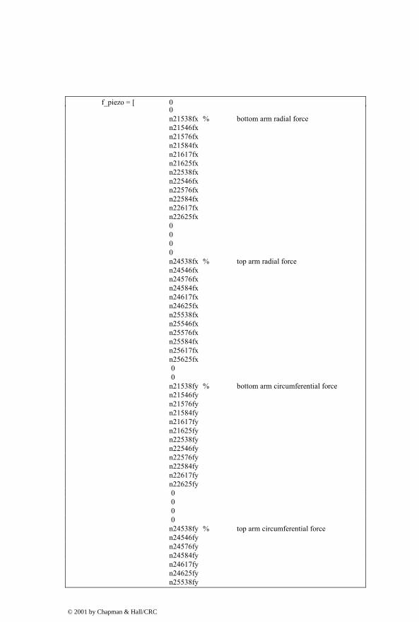
f_piezo = [ 0 0 n21538fx % bottom arm radial force n21546fx n21576fx n21584fx n21617fx n21625fx n22538fx n22546fx n22576fx n22584fx n22617fx n22625fx 0 0 0 0 n24538fx % top arm radial force n24546fx n24576fx n24584fx n24617fx n24625fx n25538fx n25546fx n25576fx n25584fx n25617fx n25625fx 0 0 n21538fy % bottom arm circumferential force n21546fy n21576fy n21584fy n21617fy n21625fy n22538fy n22546fy n22576fy n22584fy n22617fy n22625fy 0 0 0 0 n24538fy % top arm circumferential force n24546fy n24576fy n24584fy n24617fy n24625fy n25538fy
© 2001 by Chapman & Hall/CRC

n25546fy n25576fy n25584fy n25617fy n25625fy ]; % define composite forcing function, force applied to each node times % eigenvector value for that node force_coil = f_coil'*xn; force_piezo = f_piezo'*xn; % prompt for uniform or variable zeta zeta_type = input('enter "1" to read in damping vector (zetain.m) …
or "enter" for uniform damping ... '); if (isempty(zeta_type)) zeta_type = 0; zeta_uniform = input('enter value for uniform damping, …
.005 is 0.5% of critical (default) ... '); if (isempty(zeta_uniform)) zeta_uniform = 0.005; end zeta_unsort = zeta_uniform*ones(num_modes_total,1); else zetain; % read in zeta_unsort damping vector from zetain.m file end if length(zeta_unsort) ~= num_modes_total error(['error - zetain vector has ',num2str(length(zeta_unsort)), …
' entries instead of ',num2str(num_modes_total)]); end % define dc gains, 31 is head 1, 32 is head 0 omega2 = (2*pi*freqvec)'.^2; % convert to radians and square % define frequency range for frequency response freqlo = 501; freqhi = 25000; flo=log10(freqlo) ;
© 2001 by Chapman & Hall/CRC

fhi=log10(freqhi) ; f=logspace(flo,fhi,300) ; frad=f*2*pi ; % calculate dc gains if uniform damping, peak gains if non-uniform if zeta_type == 0 % dc gain gain_h0_coil = abs([force_coil(1)*xn(32,1)/frad(1) ... force_coil(2:num_modes_total).*xn(32,2:num_modes_total) ... ./omega2(2:num_modes_total)]); gain_h1_coil = abs([force_coil(1)*xn(31,1)/frad(1) ... force_coil(2:num_modes_total).*xn(31,2:num_modes_total) ... ./omega2(2:num_modes_total)]); gain_h0_piezo = abs([force_piezo(1)*xn(31,1)/frad(1) ... force_piezo(2:num_modes_total).*xn(32,2:num_modes_total) … ./omega2(2:num_modes_total)]); gain_h1_piezo = abs([force_piezo(1)*xn(31,1)/frad(1) ... force_piezo(2:num_modes_total).*xn(31,2:num_modes_total) ... ./omega2(2:num_modes_total)]); elseif zeta_type == 1 % peak gain gain_h0_coil = abs([force_coil(1)*xn(32,1)/frad(1) ... force_coil(2:num_modes_total).*xn(32,2:num_modes_total) ... ./((2*zeta_unsort(2:num_modes_total))'.*omega2(2:num_modes_total))]); gain_h1_coil = abs([force_coil(1)*xn(31,1)/frad(1) ... force_coil(2:num_modes_total).*xn(31,2:num_modes_total) ... ./((2*zeta_unsort(2:num_modes_total))'.*omega2(2:num_modes_total))]); gain_h0_piezo = abs([force_piezo(1)*xn(31,1)/frad(1) ... force_piezo(2:num_modes_total).*xn(32,2:num_modes_total) ... ./((2*zeta_unsort(2:num_modes_total))'.*omega2(2:num_modes_total))]); gain_h1_piezo = abs([force_piezo(1)*xn(31,1)/frad(1) ... force_piezo(2:num_modes_total).*xn(31,2:num_modes_total) ... ./((2*zeta_unsort(2:num_modes_total))'.*omega2(2:num_modes_total))]); end % sort gains, keeping track of original and new indices so can rearrange % eigenvalues and eigenvectors [gain_h0_coil_sort,index_h0_coil_sort] = sort(gain_h0_coil); [gain_h1_coil_sort,index_h1_coil_sort] = sort(gain_h1_coil); [gain_h0_piezo_sort,index_h0_piezo_sort] = sort(gain_h0_piezo); [gain_h1_piezo_sort,index_h1_piezo_sort] = sort(gain_h1_piezo);
© 2001 by Chapman & Hall/CRC

gain_h0_coil_sort = fliplr(gain_h0_coil_sort); % max to min gain_h1_coil_sort = fliplr(gain_h1_coil_sort); % max to min gain_h0_piezo_sort = fliplr(gain_h0_piezo_sort); % max to min gain_h1_piezo_sort = fliplr(gain_h1_piezo_sort); % max to min index_h0_coil_sort = fliplr(index_h0_coil_sort) % max to min indices index_h1_coil_sort = fliplr(index_h1_coil_sort) % max to min indices index_h0_piez_sort = fliplr(index_h0_piezo_sort) % max to min indices index_h1_piez_sort = fliplr(index_h1_piezo_sort) % max to min indices index_orig = 1:num_modes_total; [index_h0_coil_sort' index_h1_coil_sort' index_h0_piez_sort' index_h1_piez_sort'] % plot results semilogy(index_orig(2:num_modes_total),freqvec(2:num_modes_total),'k-'); title(['frequency versus mode number']) xlabel('mode number') ylabel('frequency, hz') grid off disp('execution paused to display figure, "enter" to continue');%pause semilogy(index_orig,gain_h0_coil,'k.-',index_orig,gain_h1_coil,'k-') title(['coil input: dc value of each mode contribution versus mode number']) xlabel('mode number') ylabel('dc value') legend('h0 coil input','h1 coil input') grid off disp('execution paused to display figure, "enter" to continue');%pause semilogy(index_orig,gain_h0_piezo,'k.-',index_orig,gain_h1_piezo,'k-') title(['piezo input: dc value of each mode contribution versus mode number']) xlabel('mode number') ylabel('dc value') legend('h0 piezo input','h1 piezo input') grid off disp('execution paused to display figure, "enter" to continue');%pause loglog(freqvec(2:num_modes_total),gain_h0_coil(2:num_modes_total),'k.-', ... freqvec(2:num_modes_total),gain_h1_coil(2:num_modes_total),'k-') title(['coil input: dc value of each mode contribution versus frequency']) xlabel('frequency, hz') ylabel('dc value') axis([500 25000 -inf inf]) legend('h0 coil input','h1 coil input') grid off disp('execution paused to display figure, "enter" to continue');%pause
© 2001 by Chapman & Hall/CRC

loglog(freqvec(2:num_modes_total),gain_h0_piezo(2:num_modes_total),'k.-', ... freqvec(2:num_modes_total),gain_h1_piezo(2:num_modes_total),'k-') title(['piezo input: dc value of each mode contribution versus frequency']) xlabel('frequency, hz') ylabel('dc value') axis([500 25000 -inf inf]) legend('h0 piezo input','h1 piezo input') grid off disp('execution paused to display figure, "enter" to continue');%pause semilogy(index_orig,gain_h0_coil_sort,'k.-',index_orig,gain_h1_coil_sort,'k-') title(['coil input: sorted dc value of each mode versus number of modes included']) xlabel('modes included') ylabel('sorted dc value') legend('h0 coil input','h1 coil input') grid off disp('execution paused to display figure, "enter" to continue');%pause semilogy(index_orig,gain_h0_piezo_sort,'k.-',index_orig,gain_h1_piezo_sort,'k-') title(['piezo input: sorted dc value of each mode versus number of modes included']) xlabel('modes included') ylabel('sorted dc value') legend('h0 piezo input','h1 piezo input') grid off disp('execution paused to display figure, "enter" to continue');%pause semilogy(index_orig,gain_h0_coil_sort,'k.-',index_orig,gain_h1_coil_sort,'k.-', ... index_orig,gain_h0_piezo_sort, …
'k-',index_orig,gain_h1_piezo_sort,'k-') title(['coil and piezo input: sorted dc value of each mode versus number …
of modes included']) xlabel('modes included') ylabel('sorted dc value') legend('h0 coil input','h1 coil input','h0 piezo input','h1 piezo input') grid off disp('execution paused to display figure, "enter" to continue');%pause
Figure 19.22 repeats Figure 19.5, plotting resonant frequency versus mode number. Note that there are several “jumps” in the curve, the most significant between mode 4 and mode 5. As indicated in Section 17.6, “jumps” in the frequency plot can indicate the system transitioning from one type of characteristic motion to another. In this case modes 2, 3 and 4 involve bending motions of the system, while mode 5 involves coil torsion.
© 2001 by Chapman & Hall/CRC

0 5 10 15 20 25 30 35 40 45 50102
103
104
105frequency versus mode number
mode number
frequ
ency
, hz
Figure 19.22: Resonant frequencies versus mode number.
The dc gains for head 0 and head 1 for coil input are shown in Figure 19.23. Because the actuator is nearly symmetrical in design the gains of the two heads are quite similar.
0 5 10 15 20 25 30 35 40 45 5010-14
10-12
10-10
10-8
10-6
10-4
10-2
100coil input: dc value of each mode contribution versus mode number
mode number
dc v
alue
h0 coil inputh1 coil input
Figure 19.23: dc gain versus mode for both heads for coil input.
© 2001 by Chapman & Hall/CRC

0 5 10 15 20 25 30 35 40 45 5010-14
10-12
10-10
10-8
10-6piezo input: dc value of each mode contribution versus mode number
mode number
dc v
alue
h0 piezo inputh1 piezo input
Figure 19.24: dc gain versus mode number for both heads for piezo input.
The gains for both heads for piezo inputs are shown in Figure 19.24.
103 104
10-12
10-10
10-8
10-6coil input: dc value of each mode contribution versus frequency
frequency, hz
dc v
alue
h0 coil inputh1 coil input
Figure 19.25: dc gain versus frequency for both heads for coil input.
© 2001 by Chapman & Hall/CRC

103 104
10-12
10-11
10-10
10-9
10-8
10-7
piezo input: dc value of each mode contribution versus frequency
frequency, hz
dc v
alue
h0 piezo inputh1 piezo input
Figure 19.26: dc gain versus frequency for both heads for piezo input.
0 5 10 15 20 25 30 35 40 45 5010-14
10-12
10-10
10-8
10-6
10-4
10-2
100coil input: sorted dc value of each mode versus number of modes included
modes included
sorte
d dc
val
ue
h0 coil inputh1 coil input
Figure 19.27: Sorted dc gain for both heads for coil input.
The sorted dc gains of the two heads, Figure 19.27, are very similar because the actuator design is so symmetrical.
© 2001 by Chapman & Hall/CRC

0 5 10 15 20 25 30 35 40 45 5010-14
10-12
10-10
10-8
10-6piezo input: sorted dc value of each mode versus number of modes included
modes included
sorte
d dc
val
ue
h0 piezo inputh1 piezo input
Figure 19.28: Sorted dc gain for both heads for piezo input.
0 5 10 15 20 25 30 35 40 45 5010-14
10-12
10-10
10-8
10-6
10-4
10-2
100coil and piezo input: sorted dc value of each mode versus number of modes included
modes included
sorte
d dc
val
ue
h0 coil input h1 coil input h0 piezo inputh1 piezo input
Figure 19.29: Sorted dc gain for both heads for both coil and piezo inputs.
The sorted gains of head 0 and head 1 for both coil and piezo inputs can be seen in Figure 19.29. They are of similar magnitude because the piezo force “fpz” in Section 19.5.2 was chosen to be 0.2.
With the partial listing of mode ranking for both heads and both inputs shown in Table 19.1, we can start looking at the difficulties of using dc and peak gains for ranking MIMO systems.
© 2001 by Chapman & Hall/CRC

Table 19.1 lists the mode ranking for the first 15 modes for:
Column 1: head 0, coil input
Column 2: head 1, coil input
Column 3: head 0, piezo input
Column 4: head 1, piezo input
1 1 12 12 13 13 8 8 9 9 21 21 16 16 30 30 12 12 11 11 28 28 13 13 25 25 49 22 29 36 46 49 36 15 22 46 15 29 28 17 11 17 17 28 26 11 29 20 17 26 10 50 47 5 20 14 10 22 50 29
Table 19.1: Ranking for first 15 modes for head 0 and head 1 for coil and piezo inputs.
The first two columns in Table 19.1 show that for coil input, head 0 and head 1 have the same ranking through the first seven modes, then their rankings change. The second two columns show that for piezo input, head 0 and head 1 have the same ranking through the first six modes, then their rankings change.
If one were to choose a single ranking for the model which would take into account both inputs and both outputs, it is difficult to see how to do it given the rankings in the table. Thus the necessity of balanced reduction for MIMO models. (See Problem P19.1 for using dc gain to rank for reduction.)
19.5.3 Building State Space Matrices
In this section of code the system matrices are assembled and the four frequency responses are plotted. For all previous SISO models in the book we have built the system matrices using dc gain ordering of modes. Here, for the MIMO model, we will assemble the system using the original, unsorted ordering and will let “balreal” do all the work of sorting in the next section.
% create five state space systems with all modes included, differing in the ordering % of the modes, the unsorted system will be used for all reductions, letting balreal do all
© 2001 by Chapman & Hall/CRC

% the ordering, the sorted systems will be used to show how the dc gain ordering % compares with the balanced ordering % 1) unsorted % 2) sorted, head 0, coil input % 3) sorted, head 1, coil input % 4) sorted, head 0, piezo input % 5) sorted, head 1, piezo input for num_model = 1:5 if num_model == 1 % unsorted xnnew = xn; freqnew = freqvec; elseif num_model == 2 % sorted, head 0, coil input xnnew = xn(:,index_h0_coil_sort); freqnew = freqvec(index_h0_coil_sort); elseif num_model == 3 % sorted, head 1, coil input xnnew = xn(:,index_h1_coil_sort); freqnew = freqvec(index_h1_coil_sort); elseif num_model == 4 % sorted, head 0, piezo input xnnew = xn(:,index_h0_piezo_sort); freqnew = freqvec(index_h0_piezo_sort); elseif num_model == 5 % sorted, head 1, piezo input xnnew = xn(:,index_h1_piezo_sort); freqnew = freqvec(index_h1_piezo_sort); end % define variables for all modes included system matrix, a w = freqnew*2*pi; % frequencies in rad/sec w2 = w.^2; zw = 2*zeta_unsort.*w; % define size of system matrix asize = 2*num_modes_total;
© 2001 by Chapman & Hall/CRC

disp(' '); disp(' '); disp(['size of system matrix a is ',num2str(asize)]); % setup system matrix for all modes included model a = zeros(asize); for col = 2:2:asize row = col-1; a(row,col) = 1; end for col = 1:2:asize row = col+1; a(row,col) = -w2((col+1)/2); end for col = 2:2:asize row = col; a(row,col) = -zw(col/2); end % setup input matrix b, state space forcing function in principal coordinates % two-input system % first input is coil force % second input is excitation of both piezo elements with opposite polarity f_physical = [f_coil f_piezo]; % f_principal is the matrix of forces in principal coordinates f_principal = xnnew'*f_physical; % b is the matrix of forces in principal coordinates, state space form b = zeros(2*num_modes_total,2); for cnt = 1:num_modes_total b(2*cnt,:) = f_principal(cnt,:); end
© 2001 by Chapman & Hall/CRC

% setup cdisp and cvel, padded xn matrices to give the displacement and velocity % vectors in physical coordinates cdisp and cvel each have numdof rows % and alternating columns consisting of columns of xnnew and zeros to give total % columns equal to the number of states % all modes included cdisp and cvel for col = 1:2:2*length(freqnew) for row = 1:numdof c_disp(row,col) = xnnew(row,ceil(col/2)); cvel(row,col) = 0; end end for col = 2:2:2*length(freqnew) for row = 1:numdof c_disp(row,col) = 0; cvel(row,col) = xnnew(row,col/2); end end % define output d = [0]; % if num_model == 1 % unsorted sys = ss(a,b,c_disp(31:32,:),d); elseif num_model == 2 % sorted, head 0, coil input sys_h0_coil = ss(a,b,c_disp(31:32,:),d); elseif num_model == 3 % sorted, head 1, coil input sys_h1_coil = ss(a,b,c_disp(31:32,:),d); elseif num_model == 4 % sorted, head 0, piezo input sys_h0_piezo = ss(a,b,c_disp(31:32,:),d); elseif num_model == 5 % sorted, head 1, piezo input sys_h1_piezo = ss(a,b,c_disp(31:32,:),d);
© 2001 by Chapman & Hall/CRC

end end % end of for loop for creating system matrices
19.5.4 Balancing, Reduction
Balancing the system involves calculating gramians, which are only defined for negative definite systems. This requires separating the rigid body mode from the oscillatory modes and balancing the oscillatory modes. The system matrices are partitioned and a model of only oscillatory modes is created and balanced. Plotting the diagonal gramian terms (squares of the Hankel singular values) reveals the relative importance of the states.
Modred is used to reduce the states using both the “del” and “mdc” options. The complete system is rebuilt by augmenting the rigid body mode (states) with the reduced oscillatory modes (states). Frequency responses are then plotted, comparing the two reducing methods with the original 50-mode model.
% partition system matrices into rigid body mode and oscillatory modes, can't use balreal % with rigid body mode so will reduce the oscillatory modes and then augment the % resulting system with the rigid body mode % define oscillatory system, where output 31 is head 1, output 32 is head 0 [a,b,c_disp,d] = ssdata(sys); a_syso = a(3:asize,3:asize); b_syso = b(3:asize,:); c_syso = c_disp(1:2,3:asize); syso = ss(a_syso,b_syso,c_syso,d); % define controllability and observability gramians for oscillatory system, syso wc = gram(syso,'c'); wo = gram(syso,'o'); [row_syso,col_syso] = size(a_syso); statevec = 1:row_syso; % plot controllability and observability gramians meshz(wc); view(60,30);
© 2001 by Chapman & Hall/CRC

title(['controllability gramian for oscillatory system']) xlabel('state') ylabel('state') grid on disp('execution paused to display figure, "enter" to continue');%pause meshz(wo); view(60,30); title(['observability gramian for oscillatory system']) xlabel('state') ylabel('state') grid on disp('execution paused to display figure, "enter" to continue');%pause % pull out diagonal elements wc_diag = diag(wc); wo_diag = diag(wo); % plot diagonal terms of controllability and observability gramians semilogy(statevec,wc_diag,'k.-') title(['controllability gramian diagonal terms']) xlabel('states') ylabel('diagonal') grid off disp('execution paused to display figure, "enter" to continue');%pause semilogy(statevec,wo_diag,'k.-') title(['observability gramian diagonal terms']) xlabel('states') ylabel('diagonal') grid off disp('execution paused to display figure, "enter" to continue');%pause % position and velocity states plotted separately semilogy(statevec(1:2:row_syso),wc_diag(1:2:row_syso),'k.-', ... statevec(2:2:row_syso),wc_diag(2:2:row_syso),'k-') title(['controllability gramian diagonal terms']) xlabel('states') ylabel('diagonal') legend('position states','velocity states',3) grid off disp('execution paused to display figure, "enter" to continue');%pause semilogy(statevec(1:2:row_syso),wo_diag(1:2:row_syso),'k.-', ...
© 2001 by Chapman & Hall/CRC

statevec(2:2:row_syso),wo_diag(2:2:row_syso),'k-') title(['observability gramian diagonal terms']) xlabel('states') ylabel('diagonal') legend('position states','velocity states',3) grid off disp('execution paused to display figure, "enter" to continue');%pause % use balreal to rank oscillatory states and modred to reduce for comparison [sysob,g,T,Ti] = balreal(syso); [ao_bal,bo_bal,cdispo_bal,do_bal] = ssdata(sysob); semilogy(g,'k.-') title('diagonal of balanced gramian versus number of states') xlabel('state number') ylabel('diagonal of balanced gramian') grid off osc_states_used = input(['enter number of oscillatory states to use, default 20 ... ']); if isempty(osc_states_used) osc_states_used = 20; end num_modes_used = 1 + osc_states_used/2; % number of modes for overlaid plots % use modred to order oscillatory states from balreal to define reduced order % oscillatory system using both "del" and "mdc" rsys_delo = modred(sysob,osc_states_used+1:2*num_modes_total-2,'del'); rsys_mdco = modred(sysob,osc_states_used+1:2*num_modes_total-2,'mdc'); % rebuild system by appending balanced realization of oscillatory modes to rigid % body mode [a_delo_bal,b_delo_bal,c_delo_bal,d_delo_bal] = ssdata(rsys_delo); a_del_bal = [ a(1:2,1:2) zeros(2,osc_states_used) zeros(osc_states_used,2) a_delo_bal ]; b_del_bal = [b(1:2,:) b_delo_bal]; c_del_bal = [c_disp(1:2,1:2) c_delo_bal]; rsys_del = ss(a_del_bal,b_del_bal,c_del_bal,d); [a_mdco_bal,b_mdco_bal,c_mdco_bal,d_mdco_bal] = ssdata(rsys_mdco);
© 2001 by Chapman & Hall/CRC

a_mdc_bal = [ a(1:2,1:2) zeros(2,osc_states_used) zeros(osc_states_used,2) a_mdco_bal ]; b_mdc_bal = [b(1:2,:) b_mdco_bal]; c_mdc_bal = [c_disp(1:2,1:2) c_mdco_bal]; rsys_mdc = ss(a_mdc_bal,b_mdc_bal,c_mdc_bal,d); % frequency response for unsorted system [mag,phs] = bode(sys,frad); % plot original system response, output of bode command has dimensions % of "i" x "j" x "k" where "i" is output row, "j" is input column and "k" is the % vector of frequencies magh0coil = mag(2,1,:); magh1coil = mag(1,1,:); magh0pz = mag(2,2,:); magh1pz = mag(1,2,:); loglog(f,magh0coil(1,:),'k.-',f,magh1coil(1,:),'k-') title(['gap displacement, all ',num2str(num_modes_total),' modes included']) xlabel('Frequency, hz') ylabel('Magnitude, mm') axis([500 25000 1e-9 2e-4]) legend('head 0, coil input','head 1, coil input',3) grid off disp('execution paused to display figure, "enter" to continue');%pause loglog(f,magh0pz(1,:),'k.-',f,magh1pz(1,:),'k-') title(['gap displacement, all ',num2str(num_modes_total),' modes included']) xlabel('Frequency, hz') ylabel('Magnitude, mm') axis([500 25000 1e-9 2e-4]) legend('head 0 piezo input','head 1 piezo input',3) grid off disp('execution paused to display figure, "enter" to continue');%pause loglog(f,magh0coil(1,:),'k.-',f,magh1coil(1,:),'k.-',f,magh0pz(1,:),'k-',f,magh1pz(1,:),'k-') title(['gap displacement, all ',num2str(num_modes_total),' modes included']) xlabel('Frequency, hz') ylabel('Magnitude, mm') axis([500 25000 1e-9 2e-4]) legend('head 0, coil input','head 1, coil input','head 0 piezo input','head 1 piezo …
input',3) grid off disp('execution paused to display figure, "enter" to continue');%pause % frequency response for balanced reduced modred "del"
© 2001 by Chapman & Hall/CRC

[magr_del,phsr_del] = bode(rsys_del,frad); magr_delh0coil = magr_del(2,1,:); magr_delh1coil = magr_del(1,1,:); magr_delh0pz = magr_del(2,2,:); magr_delh1pz = magr_del(1,2,:); loglog(f,magr_delh0coil(1,:),'k-',f,magr_delh1coil(1,:),'k.-',f,magr_delh0pz(1,:), …
'k.-',f,magr_delh1pz(1,:),'k-') title(['gap displacement, modred "del", ',num2str(osc_states_used), …
' oscillatory states included']) xlabel('Frequency, hz') ylabel('Magnitude, mm') axis([500 25000 1e-9 2e-4]) legend('head 0, coil input','head 1, coil input','head 0 piezo input' …
,'head 1 piezo input',3) grid off disp('execution paused to display figure, "enter" to continue');%pause loglog(f,magh0coil(1,:),'k-',f,magr_delh0coil(1,:),'k.-') title(['gap displacement, modred "del", ',num2str(osc_states_used), …
' oscillatory states included']) xlabel('Frequency, hz') ylabel('Magnitude, mm') axis([500 25000 1e-9 2e-4]) legend('head 0, coil input','"del" reduced head 0, coil input',3) grid off disp('execution paused to display figure, "enter" to continue'); pause loglog(f,magh1coil(1,:),'k-',f,magr_delh1coil(1,:),'k.-') title(['gap displacement, modred "del", ',num2str(osc_states_used), …
' oscillatory states included']) xlabel('Frequency, hz') ylabel('Magnitude, mm') axis([500 25000 1e-9 2e-4]) legend('head 1, coil input','"del" reduced head 1, coil input',3) grid off disp('execution paused to display figure, "enter" to continue');%pause loglog(f,magh0pz(1,:),'k-',f,magr_delh0pz(1,:),'k.-') title(['gap displacement, modred "del", ',num2str(osc_states_used), …
' oscillatory states included']) xlabel('Frequency, hz') ylabel('Magnitude, mm') axis([500 25000 1e-9 2e-4]) legend('head 0, piezo input','"del" reduced head 0, piezo input',3) grid off disp('execution paused to display figure, "enter" to continue'); pause loglog(f,magh1pz(1,:),'k-',f,magr_delh1pz(1,:),'k.-') title(['gap displacement, modred "del", ',num2str(osc_states_used), …
' oscillatory states included']) xlabel('Frequency, hz') ylabel('Magnitude, mm') axis([500 25000 1e-9 2e-4])
© 2001 by Chapman & Hall/CRC
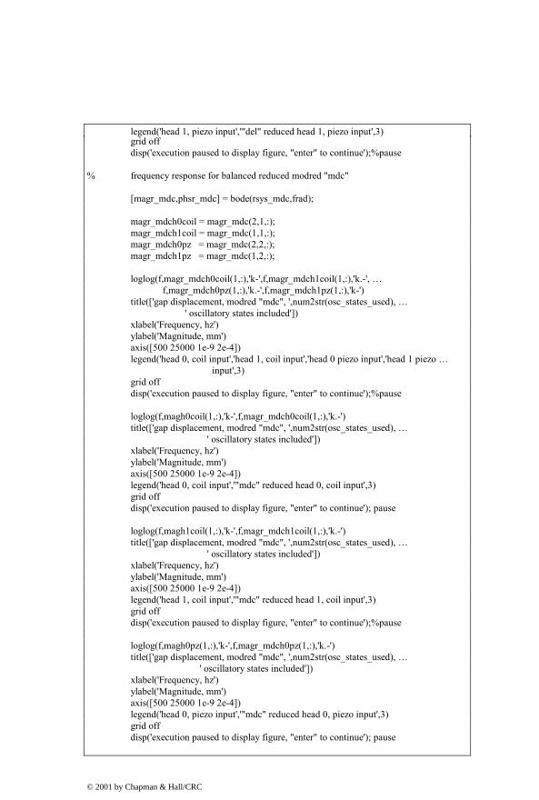
legend('head 1, piezo input','"del" reduced head 1, piezo input',3) grid off disp('execution paused to display figure, "enter" to continue');%pause % frequency response for balanced reduced modred "mdc" [magr_mdc,phsr_mdc] = bode(rsys_mdc,frad); magr_mdch0coil = magr_mdc(2,1,:); magr_mdch1coil = magr_mdc(1,1,:); magr_mdch0pz = magr_mdc(2,2,:); magr_mdch1pz = magr_mdc(1,2,:); loglog(f,magr_mdch0coil(1,:),'k-',f,magr_mdch1coil(1,:),'k.-', …
f,magr_mdch0pz(1,:),'k.-',f,magr_mdch1pz(1,:),'k-') title(['gap displacement, modred "mdc", ',num2str(osc_states_used), …
' oscillatory states included']) xlabel('Frequency, hz') ylabel('Magnitude, mm') axis([500 25000 1e-9 2e-4]) legend('head 0, coil input','head 1, coil input','head 0 piezo input','head 1 piezo …
input',3) grid off disp('execution paused to display figure, "enter" to continue');%pause loglog(f,magh0coil(1,:),'k-',f,magr_mdch0coil(1,:),'k.-') title(['gap displacement, modred "mdc", ',num2str(osc_states_used), …
' oscillatory states included']) xlabel('Frequency, hz') ylabel('Magnitude, mm') axis([500 25000 1e-9 2e-4]) legend('head 0, coil input','"mdc" reduced head 0, coil input',3) grid off disp('execution paused to display figure, "enter" to continue'); pause loglog(f,magh1coil(1,:),'k-',f,magr_mdch1coil(1,:),'k.-') title(['gap displacement, modred "mdc", ',num2str(osc_states_used), …
' oscillatory states included']) xlabel('Frequency, hz') ylabel('Magnitude, mm') axis([500 25000 1e-9 2e-4]) legend('head 1, coil input','"mdc" reduced head 1, coil input',3) grid off disp('execution paused to display figure, "enter" to continue');%pause loglog(f,magh0pz(1,:),'k-',f,magr_mdch0pz(1,:),'k.-') title(['gap displacement, modred "mdc", ',num2str(osc_states_used), …
' oscillatory states included']) xlabel('Frequency, hz') ylabel('Magnitude, mm') axis([500 25000 1e-9 2e-4]) legend('head 0, piezo input','"mdc" reduced head 0, piezo input',3) grid off disp('execution paused to display figure, "enter" to continue'); pause
© 2001 by Chapman & Hall/CRC

loglog(f,magh1pz(1,:),'k-',f,magr_mdch1pz(1,:),'k.-') title(['gap displacement, modred "mdc", ',num2str(osc_states_used), …
' oscillatory states included']) xlabel('Frequency, hz') ylabel('Magnitude, mm') axis([500 25000 1e-9 2e-4]) legend('head 1, piezo input','"mdc" reduced head 1, piezo input',3) grid off disp('execution paused to display figure, "enter" to continue');%pause
103 10410-9
10-8
10-7
10-6
10-5
10-4
gap displacement, all 50 modes included
Frequency, hz
Mag
nitu
de, m
m
head 0, coil inputhead 1, coil input
Figure 19.30: Frequency response for coil input for both heads, all modes included.
103 10410-9
10-8
10-7
10-6
10-5
10-4
gap displacement, all 50 modes included
Frequency, hz
Mag
nitu
de, m
m
head 0 piezo inputhead 1 piezo input
Figure 19.31: Frequency response for piezo input for both heads, all modes included.
© 2001 by Chapman & Hall/CRC

103 10410-9
10-8
10-7
10-6
10-5
10-4
gap displacement, all 50 modes included
Frequency, hz
Mag
nitu
de, m
m
head 0, coil inputhead 1, coil inputhead 0 piezo inputhead 1 piezo input
Figure 19.32: Frequency response for both coil and piezo inputs for both heads, all modes included.
The frequency response plots for both inputs and both outputs are shown above for reference.
© 2001 by Chapman & Hall/CRC

Figure 19.33: Controllability gramian values.
Figure 19.34: Observability gramian values.
Graphically, Figures 19.33 and 19.34 show the two gramians for this MIMO system. The gramians are nearly diagonal. The controllability gramian displays a predominance of lower frequency states, while the observability gramian has some higher frequency states included.
© 2001 by Chapman & Hall/CRC

0 10 20 30 40 50 60 70 80 90 10010-20
10-15
10-10
10-5
100controllability gramian diagonal terms
states
diag
onal
Figure 19.35: Controllability gramian diagonal terms versus states.
0 10 20 30 40 50 60 70 80 90 10010-15
10-10
10-5
100
105observability gramian diagonal terms
states
diag
onal
Figure 19.36: Observability gramian diagonal terms versus states.
Plotting the diagonal elements of the two gramians reveals the same pattern as for the SISO model. The maximum and minimum values for each mode are related by the square of the eigenvalue for that mode.
© 2001 by Chapman & Hall/CRC

0 10 20 30 40 50 60 70 80 90 10010-20
10-15
10-10
10-5
100controllability gramian diagonal terms
states
diag
onal
position statesvelocity states
Figure 19.37: Controllability gramian diagonal position and velocity state terms.
0 10 20 30 40 50 60 70 80 90 10010-15
10-10
10-5
100
105observability gramian diagonal terms
states
diag
onal
position statesvelocity states
Figure 19.38: Observability gramian diagonal position and velocity state terms.
Plotting the position and velocity terms for each gramian separately displays their character on a mode-by-mode basis.
© 2001 by Chapman & Hall/CRC

0 10 20 30 40 50 60 70 80 90 10010-10
10-9
10-8
10-7
10-6
10-5
10-4diagonal of balanced gramian versus number of states
state number
diag
onal
of b
alan
ced
gram
ian
Figure 19.39: Balanced gramian diagonal terms (Hankel singular values) versus state number.
The balanced gramian shows several sharp drops in magnitude, one at 10 states and one at 56 states. We will see in Section 19.5.7 that 10 oscillatory modes (20 oscillatory states) are required for a normalized reduction index of less than 5% for coil input, and that 16 oscillatory modes (32 oscillatory states) are required for a normalized reduction index of less than 5% for piezo input.
19.5.5 Frequency Responses for Different Numbers of Retained States
This section displays pairs of frequency responses, one for head 0 for coil input and one for head 0 for piezo input. Each pair of plots represents an increasing number of oscillatory modes included in the reduced model. The original 50 mode model is overlaid to show the error in the reduced model. Note how the balanced method adds modes and which modes it chooses.
© 2001 by Chapman & Hall/CRC

103 10410-9
10-8
10-7
10-6
10-5
10-4
gap displacement, modred "del", 6 oscillatory states included
Frequency, hz
Mag
nitu
de, m
m
head 0, coil input "del" reduced head 0, coil input
Figure 19.40: Head 0, coil input, six reduced oscillatory states included.
103 10410-9
10-8
10-7
10-6
10-5
10-4
gap displacement, modred "del", 6 oscillatory states included
Frequency, hz
Mag
nitu
de, m
m
head 0, piezo input "del" reduced head 0, piezo input
Figure 19.41: Head 0, piezo input, six reduced oscillatory states included.
With only six oscillatory states included the coil input captures the first two resonances but the piezo input misses the first resonance.
© 2001 by Chapman & Hall/CRC

103 10410-9
10-8
10-7
10-6
10-5
10-4
gap displacement, modred "del", 8 oscillatory states included
Frequency, hz
Mag
nitu
de, m
m
head 0, coil input "del" reduced head 0, coil input
Figure 19.42: Head 0, coil input, eight reduced oscillatory states included.
103 10410-9
10-8
10-7
10-6
10-5
10-4
gap displacement, modred "del", 8 oscillatory states included
Frequency, hz
Mag
nitu
de, m
m
head 0, piezo input "del" reduced head 0, piezo input
Figure 19.43: Head 0, piezo input, eight reduced oscillatory states included.
With 8 oscillatory states included the coil input captures the first two resonances but the piezo input again misses the first resonance.
© 2001 by Chapman & Hall/CRC

103 10410-9
10-8
10-7
10-6
10-5
10-4
gap displacement, modred "del", 10 oscillatory states included
Frequency, hz
Mag
nitu
de, m
m
head 0, coil input "del" reduced head 0, coil input
Figure 19.44: Head 0, coil input, 10 reduced oscillatory states included.
103 10410-9
10-8
10-7
10-6
10-5
10-4
gap displacement, modred "del", 10 oscillatory states included
Frequency, hz
Mag
nitu
de, m
m
head 0, piezo input "del" reduced head 0, piezo input
Figure 19.45: Head 0, piezo input, 10 reduced oscillatory states included.
With 10 oscillatory states included the first three coil input modes are fit well and also the first two piezo input modes.
© 2001 by Chapman & Hall/CRC

103 10410-9
10-8
10-7
10-6
10-5
10-4
gap displacement, modred "del", 12 oscillatory states included
Frequency, hz
Mag
nitu
de, m
m
head 0, coil input "del" reduced head 0, coil input
Figure 19.46: Head 0, coil input, 12 reduced oscillatory states included.
103 10410-9
10-8
10-7
10-6
10-5
10-4
gap displacement, modred "del", 12 oscillatory states included
Frequency, hz
Mag
nitu
de, m
m
head 0, piezo input "del" reduced head 0, piezo input
Figure 19.47: Head 0, piezo input, 12 reduced oscillatory states included.
With 12 oscillatory states included the first three major modes are fitted for both coil and piezo inputs.
© 2001 by Chapman & Hall/CRC

103 10410-9
10-8
10-7
10-6
10-5
10-4
gap displacement, modred "del", 14 oscillatory states included
Frequency, hz
Mag
nitu
de, m
m
head 0, coil input "del" reduced head 0, coil input
Figure 19.48: Head 0, coil input, 14 reduced oscillatory states included.
103 10410-9
10-8
10-7
10-6
10-5
10-4
gap displacement, modred "del", 14 oscillatory states included
Frequency, hz
Mag
nitu
de, m
m
head 0, piezo input "del" reduced head 0, piezo input
Figure 19.49: Head 0, piezo input, 14 reduced oscillatory states included.
For 14 oscillatory states included now the first four major piezo modes are fitted while the coil input starts missing some modes in the 10khz range.
© 2001 by Chapman & Hall/CRC

103 10410-9
10-8
10-7
10-6
10-5
10-4
gap displacement, modred "del", 16 oscillatory states included
Frequency, hz
Mag
nitu
de, m
m
head 0, coil input "del" reduced head 0, coil input
Figure 19.50: Head 0, coil input, 16 reduced oscillatory states included.
103 10410-9
10-8
10-7
10-6
10-5
10-4
gap displacement, modred "del", 16 oscillatory states included
Frequency, hz
Mag
nitu
de, m
m
head 0, piezo input "del" reduced head 0, piezo input
Figure 19.51: Head 0, piezo input, 16 reduced oscillatory states included.
For 16 oscillatory states included the only visible effect of the extra two states is in the piezo input zero in the 8khz range.
© 2001 by Chapman & Hall/CRC

103 10410-9
10-8
10-7
10-6
10-5
10-4
gap displacement, modred "del", 18 oscillatory states included
Frequency, hz
Mag
nitu
de, m
m
head 0, coil input "del" reduced head 0, coil input
Figure 19.52: Head 0, coil input, 18 reduced oscillatory states included.
103 10410-9
10-8
10-7
10-6
10-5
10-4
gap displacement, modred "del", 18 oscillatory states included
Frequency, hz
Mag
nitu
de, m
m
head 0, piezo input "del" reduced head 0, piezo input
Figure 19.53: Head 0, piezo input, 18 reduced oscillatory states included.
For 18 oscillatory states included the coil input response picks up an additional mode in the 10khz range.
19.5.6 “del” and “mdc” Frequency Response Comparison
This section compares the “del” and “mdc” reduced models for the case of 20 included oscillatory states.
© 2001 by Chapman & Hall/CRC

103 10410-9
10-8
10-7
10-6
10-5
10-4
gap displacement, modred "del", 20 oscillatory states included
Frequency, hz
Mag
nitu
de, m
m
head 0, coil input "del" reduced head 0, coil input
Figure 19.54: Head 0, coil input, 20 reduced oscillatory states included, modred “del.”
103 10410-9
10-8
10-7
10-6
10-5
10-4
gap displacement, modred "mdc", 20 oscillatory states included
Frequency, hz
Mag
nitu
de, m
m
head 0, coil input "mdc" reduced head 0, coil input
Figure 19.55: Head 0, coil input, 20 reduced oscillatory states included, modred “mdc.”
There is virtually no difference between the “del” and “mdc” reductions in the two figures above for coil input.
© 2001 by Chapman & Hall/CRC

103 10410-9
10-8
10-7
10-6
10-5
10-4
gap displacement, modred "del", 20 oscillatory states included
Frequency, hz
Mag
nitu
de, m
m
head 0, piezo input "del" reduced head 0, piezo input
Figure 19.56: Head 0, piezo input, 20 reduced oscillatory states included, modred “del.”
103 10410-9
10-8
10-7
10-6
10-5
10-4
gap displacement, modred "mdc", 20 oscillatory states included
Frequency, hz
Mag
nitu
de, m
m
head 0, piezo input "mdc" reduced head 0, piezo input
Figure 19.57: Head 0, piezo input, 20 reduced oscillatory states included, modred “mdc.”
Similarly, there is no difference between the “del” and “mdc” reductions for piezo input.
19.5.7 Impulse Response
Oscillatory system impulse responses due to both coil and piezo forcing functions are calculated. Previously calculated results for normalized reduction index (18.28) versus number of modes included are shown.
© 2001 by Chapman & Hall/CRC

% calculate impulse responses ttotal = 0.0025; t = linspace(0,ttotal,400)'; [disp_syso,t_syso] = impulse(syso,t); [disp_rsys_delo,t_rsys_delo] = impulse(rsys_delo,t); [disp_rsys_mdco,t_rsys_mdco] = impulse(rsys_mdco,t); disph0coil = disp_syso(:,2,1); disph1coil = disp_syso(:,1,1); disph0pz = disp_syso(:,2,2); disph1pz = disp_syso(:,1,2); dispr_delh0coil = disp_rsys_delo(:,2,1); dispr_delh1coil = disp_rsys_delo(:,1,1); dispr_delh0pz = disp_rsys_delo(:,2,2); dispr_delh1pz = disp_rsys_delo(:,1,2); dispr_mdch0coil = disp_rsys_mdco(:,2,1); dispr_mdch1coil = disp_rsys_mdco(:,1,1); dispr_mdch0pz = disp_rsys_mdco(:,2,2); dispr_mdch1pz = disp_rsys_mdco(:,1,2); % build matrix of results dispo = [disph0coil disph1coil disph0pz disph1pz ... dispr_delh0coil dispr_delh1coil dispr_delh0pz dispr_delh1pz ... dispr_mdch0coil dispr_mdch1coil dispr_mdch0pz dispr_mdch1pz]; h0coil_del_del = dispo(:,1) - dispo(:,5); h1coil_del_del = dispo(:,2) - dispo(:,6); h0piezo_del_del = dispo(:,3) - dispo(:,7); h1piezo_del_del = dispo(:,4) - dispo(:,8); h0coil_mdc_del = dispo(:,1) - dispo(:,9); h1coil_mdc_del = dispo(:,2) - dispo(:,10); h0piezo_mdc_del = dispo(:,3) - dispo(:,11); h1piezo_mdc_del = dispo(:,4) - dispo(:,12); index_h0coil_del = …
sqrt(sum(h0coil_del_del.*h0coil_del_del))/sqrt(sum(dispo(:,1).*dispo(:,1))); index_h1coil_del = …
sqrt(sum(h1coil_del_del.*h1coil_del_del))/sqrt(sum(dispo(:,2).*dispo(:,2)));
© 2001 by Chapman & Hall/CRC

index_h0piezo_del = …
sqrt(sum(h0piezo_del_del.*h0piezo_del_del))/sqrt(sum(dispo(:,3).*dispo(:,3))); index_h1piezo_del = …
sqrt(sum(h1piezo_del_del.*h1piezo_del_del))/sqrt(sum(dispo(:,4).*dispo(:,4))); index_h0coil_mdc = …
sqrt(sum(h0coil_mdc_del.*h0coil_mdc_del))/sqrt(sum(dispo(:,1).*dispo(:,1))); index_h1coil_mdc = …
sqrt(sum(h1coil_mdc_del.*h1coil_mdc_del))/sqrt(sum(dispo(:,2).*dispo(:,2))); index_h0piezo_mdc = …
sqrt(sum(h0piezo_mdc_del.*h0piezo_mdc_del))/sqrt(sum(dispo(:,3).*dispo(:,3))); index_h1piezo_mdc = …
sqrt(sum(h1piezo_mdc_del.*h1piezo_mdc_del))/sqrt(sum(dispo(:,4).*dispo(:,4))); [index_h0coil_del index_h1coil_del index_h0piezo_del index_h1piezo_del ... index_h0coil_mdc index_h1coil_mdc index_h0piezo_mdc index_h1piezo_mdc] plot(t_syso,disph0coil,'k.-',t_rsys_delo,dispr_delh0coil, …
'k-',t_rsys_mdco,dispr_mdch0coil,'k--') title(['head 0, displacement vs time, coil impulse input, ', …
num2str(osc_states_used),' oscillatory states included']) xlabel('time, sec') ylabel('displacement, mm') legend('all modes','modred del','modred mdc',4) grid off disp('execution paused to display figure, "enter" to continue');%pause plot(t_syso,disph1coil,'k.-',t_rsys_delo,dispr_delh1coil, …
'k-',t_rsys_mdco,dispr_mdch1coil,'k--') title(['head 1, displacement vs time, coil impulse input, ', …
num2str(osc_states_used),' oscillatory states included']) xlabel('time, sec') ylabel('displacement, mm') legend('all modes','modred del','modred mdc',4) grid off disp('execution paused to display figure, "enter" to continue');%pause plot(t_syso,disph0pz,'k.-',t_rsys_delo,dispr_delh0pz, …
'k-',t_rsys_mdco,dispr_mdch0pz,'k--') title(['head 0, displacement vs time, piezo impulse input, ', …
num2str(osc_states_used),' oscillatory states included']) xlabel('time, sec') ylabel('displacement, mm') legend('all modes','modred del','modred mdc',4) grid off disp('execution paused to display figure, "enter" to continue');%pause
© 2001 by Chapman & Hall/CRC

plot(t_syso,disph1pz,'k.-',t_rsys_delo,dispr_delh1pz, … 'k-',t_rsys_mdco,dispr_mdch1pz,'k--')
title(['head 1, displacement vs time, piezo impulse input, ', … num2str(osc_states_used),' oscillatory states included'])
xlabel('time, sec') ylabel('displacement, mm') legend('all modes','modred del','modred mdc',4) grid off disp('execution paused to display figure, "enter" to continue');%pause % states h0cd h1cd h0pd h1pd h0cm h1cm h0pm h1pm error = [ 10 0.1081 0.1075 0.4162 0.3963 0.1081 0.1075 0.4165 0.3964 12 0.1079 0.1072 0.3154 0.3058 0.1079 0.1073 0.3157 0.3061 16 0.1075 0.1070 0.1393 0.1421 0.1074 0.1070 0.1393 0.1419 20 0.0395 0.0425 0.1391 0.1410 0.0397 0.0425 0.1391 0.1411 24 0.0363 0.0374 0.0839 0.0873 0.0463 0.0473 0.0841 0.0875 28 0.0161 0.0178 0.0469 0.0495 0.0160 0.0191 0.0791 0.0794 32 0.0140 0.0142 0.0145 0.0160 0.0142 0.0143 0.0146 0.0163]; nmode = error(:,1)/2; error_h0coil_del = error(:,2); error_h1coil_del = error(:,3); error_h0piezo_del = error(:,4); error_h1piezo_del = error(:,5); error_h0coil_mdc = error(:,6); error_h1coil_mdc = error(:,7); error_h0piezo_mdc = error(:,8); error_h1piezo_mdc = error(:,9); plot(nmode,error_h0coil_del,'k.-',nmode,error_h0coil_mdc,'k-') title('head 0, coil input normalized reduction index') xlabel('number of modes included') ylabel('normalized reduction index') legend('modred del','modred mdc') axis([0 20 0 0.5]) grid off disp('execution paused to display figure, "enter" to continue');%pause
© 2001 by Chapman & Hall/CRC

plot(nmode,error_h1coil_del,'k.-',nmode,error_h1coil_mdc,'k-') title('head 1, coil input normalized reduction index') xlabel('number of modes included') ylabel('normalized reduction index') legend('modred del','modred mdc') axis([0 20 0 0.5]) grid off disp('execution paused to display figure, "enter" to continue');%pause plot(nmode,error_h0piezo_del,'k.-',nmode,error_h0piezo_mdc,'k-') title('head 0, piezo input normalized reduction index') xlabel('number of modes included') ylabel('normalized reduction index') legend('modred del','modred mdc') axis([0 20 0 0.5]) grid off disp('execution paused to display figure, "enter" to continue');%pause plot(nmode,error_h1piezo_del,'k.-',nmode,error_h1piezo_mdc,'k-') title('head 1, piezo input normalized reduction index') xlabel('number of modes included') ylabel('normalized reduction index') legend('modred del','modred mdc') axis([0 20 0 0.5]) grid off disp('execution paused to display figure, "enter" to continue');%pause
The pages following will show impulse responses for head 0 for both coil and piezo inputs and for both “del” and “mdc” reduced models. Following the impulse responses, the normalized reduction index versus number of reduced modes is plotted. It shows very little difference between the two reduction methods.
© 2001 by Chapman & Hall/CRC

0 0.5 1 1.5 2 2.5
x 10-3
-0.06
-0.04
-0.02
0
0.02
0.04
0.06head 0, displacement vs time, coil impulse input, 20 oscillatory states included
time, sec
disp
lace
men
t, m
m
all modes modred delmodred mdc
Figure 19.58: Impulse response comparison for head 0 for coil input for oscillatory system, full model (all oscillatory modes) and balreal modred “del” and “mdc” reduced systems
with 20 oscillatory modes.
0 0.5 1 1.5 2 2.5
x 10-3
-0.025
-0.02
-0.015
-0.01
-0.005
0
0.005
0.01
0.015
0.02
0.025head 0, displacement vs time, piezo impulse input, 20 oscillatory states included
time, sec
disp
lace
men
t, m
m
all modes modred delmodred mdc
Figure 19.59: Impulse response comparison for head 0 for piezo input for oscillatory system, full model (all oscillatory modes) and balreal modred “del” and “mdc” reduced
systems with 20 oscillatory modes.
© 2001 by Chapman & Hall/CRC

0 2 4 6 8 10 12 14 16 18 200
0.05
0.1
0.15
0.2
0.25
0.3
0.35
0.4
0.45
0.5head 0, coil input normalized reduction index
number of modes included
norm
aliz
ed re
duct
ion
inde
x
modred delmodred mdc
Figure 19.60: Head 0 impulse response normalized error index comparison for reduced modred models using “del” and “mdc” methods, coil input.
0 2 4 6 8 10 12 14 16 18 200
0.05
0.1
0.15
0.2
0.25
0.3
0.35
0.4
0.45
0.5head 0, piezo input normalized reduction index
number of modes included
norm
aliz
ed re
duct
ion
inde
x
modred delmodred mdc
Figure 19.61: Head 0 impulse response normalized error index comparison for reduced modred models using “del” and “mdc” methods, piezo input.
© 2001 by Chapman & Hall/CRC

19.6 MIMO Summary
We started the chapter with a description of key mode shapes for the two-stage actuator/suspension system. ANSYS eigenvector listings for several modes allowed comparing the numeric values in the eigenvector to the visual interpretation from the mode shape plot. Small displacements in the deformed mode shape plot correlate to small numerical values in the eigenvector. If the small numerical values in the eigenvector occur in the input and/or output degrees of freedom, the mode will have a “small” dc gain and is relatively unimportant.
In the next section we calculated and plotted the dc gains for all four input/output combinations. In Table 19.1 we listed the modes for the input/output combinations, sorted by dc gain. We found that head 0 and head 1 dc gain sorted modes for coil input are the same for the first seven modes. For piezo input, both heads have the same mode ranking for the first six modes. This similarity in the most important modes for both heads for the coil and piezo inputs is brought about by the physical symmetry of the actuator/suspension system, and in general will not be the case.
As in the previous chapter, we used balancing to define the system for reduction and used the “modred” “del” and “mdc” options to reduce. Frequency responses for different number of states were plotted and compared for both coil and piezo inputs, overlaying the non-reduced transfer function.
Visually comparing the reduced and non-reduced frequency response magnitudes, we found that including 20 oscillatory states (plus the states from the one rigid body mode) gave a “good” fit through the 10khz range.
The MATLAB model was then used to calculate the impulse responses for the oscillatory reduced and non-reduced systems, where we found that 10 oscillatory modes (20 oscillatory states) were required to have a normalized error index of less than 5% for coil inputs. For piezo inputs, 16 oscillatory modes (32 oscillatory states) were required for less than 5% normalized error index. There was little difference in normalized error index between the “del” and “mdc” reduction options.
© 2001 by Chapman & Hall/CRC

Problems
P19.1 Modify the MATLAB code act8pz.m to reduce the piezo force “fpz” (Section 19.5.2) from the 0.2 value used in the text to 0.02 and 0.002. In both cases, examine the frequency and impulse responses for different number of oscillatory states used. Does the balanced reduction method technique continue to choose roughly equal number of modes for both coil and piezo inputs even when there are large differences in dc gain values between the two inputs?
P19.2 For the piezo force “fpz” of 0.2, choose the first five oscillatory modes from the coil input and the first five oscillatory modes from the piezo input (Table 19.1). Assemble the state equations from the rigid body mode and the 10 oscillatory modes and solve for the frequency and impulse responses. Compare the responses to the 20 oscillatory state balanced reduction. Comment on the similarities/differences.
© 2001 by Chapman & Hall/CRC

APPENDIX 1
MATLAB AND ANSYS PROGRAMS
This appendix lists all the MATLAB and ANSYS codes used in each chapter, along with a short description of the purpose of each.
MATLAB codes have the suffix “.m” and the ANSYS codes have the suffix “.inp.” Additional output files from previous runs are stored as “.grp” or other suffixes and will be used from time to time.
Coding format: All the MATLAB code available from downloading and shown in the book starts over one tab, allowing comment lines to stand out. The code also includes a lot of blank lines for readability (my apologies to tight “c” code programmers).
In most MATLAB code, critical definitions and calculations are only a few lines of code, while plotting and annotating are the bulk of the space. For this reason, some code listings in the book do not show all the plotting commands.
ANSYS eigenvalue/eigenvector results are converted to MATLAB input form using the following MATLAB extraction codes:
ext56ux.m extracts the ANSYS UX degree of freedom
ext56uy.m extracts the ANSYS UY degree of freedom
ext56uz.m extracts the ANSYS UZ degree of freedom
ext56uxuy.m extracts the ANSYS UX and UY degrees of freedom
ext56uxuz.m extracts the ANSYS UX and UZ degrees of freedom
ext56uyuz.m extracts the ANSYS UY and UZ degrees of freedom
ext56uxuyuz.m extracts the ANSYS UX, UY and UZ degrees of freedom
The codes above all call a supporting MATLAB code ext56chk.m. All the codes should be installed in the same directory as the ANSYS output code which is to be extracted or should be installed in a directory which is in the MATLAB path. To use the extraction code, just rename the ANSYS eigenvector output file to have a “.eig” extension and open MATLAB in the
© 2001 by Chapman & Hall/CRC

same directory. MATLAB will then open a window showing all the “.eig” files in the directory. Double-click on the file to extract and MATLAB will output a file with the “ext56xx.mat” name. If several files are to be extracted in the same directory, rename the “ext56xx.mat” name to a unique name with the “.mat” extension.
The “.mat” extracted MATLAB file contains the following information:
evr, the modal matrix, with rows consisting of degrees of freedom and each column representing a mode. The numbering of degrees of freedom is the same as the ANSYS listing, which is in ascending order of the selected node numbers. Where multiple directions are extracted, for instance UX and UY degrees of freedom, the degrees of freedom are listed in that order, first the UX degrees of freedom and then the UY degrees of freedom. The extracted modal matrix is of size: (total dof) x (modes).
freqvec, a vector listing the eigenvalues (resonant frequencies), in hz values. The size of the frequency vector is (modes) x (1).
node_numbers, a vector listing the node numbers for the extracted data, of size (dof) x (1).
The extracted data can then be loaded and used to develop state space models of the system.
Chapter 2: Transfer Function Analysis
sdofxfer.m: Calculates and plots magnitude and phase for a single degree of freedom system over a range of damping values.
tdofpz3x3.m: Uses the “num/den” form of the transfer function, calculates and plots all nine pole/zero combinations for the nine different transfer functions for tdof model. It prompts for values of the two dampers, c1 and c2, where the default (hitting the “enter” key) values are set to zero to match the hand calculated values in (2.82). The “transfer function” forms of the transfer functions are then converted to “zpk - zero/pole/gain” form to enable graphical construction of frequency response in the next chapter.
tdofpz3x3_rlocus.m: Plots pole and zero values for z11 transfer function for a range of damping values.
Chapter 3: Frequency Response Analysis
tdofxfer.m: Plots tdof model poles and zeros in complex plane, user choice of damping values. Uses several different model descriptions and frequency
© 2001 by Chapman & Hall/CRC

response calculating techniques. The model is described in polynomial, transfer function and zpk forms. Magnitude and phase versus frequency are calculated using a scalar frequency “for loop,” vector frequency, automatic bode plotting and bode with magnitude and frequency outputs.
Chapter 4: Zeros in SISO Mechanical Systems
ndof_numzeros.m: Calculates and plots poles/zeros and transfer functions for user selected input/output locations on a “n” dof series spring/mass model. Shows that poles of “constrained” structures to left and right of input/output degrees of freedom are the zeros of the unconstrained structure.
cantfem.inp: ANSYS code for resonant frequencies of cantilever and tip driving point transfer function. Used to identify zero locations to compare with poles of “constrained” system in cantzero.inp.
cantzero.inp: ANSYS code for resonant frequencies of cantilever with simple support at tip. Used to identify poles of “constrained” structure.
cantzero.m: Uses eigenvalues and eigenvectors from cantfem.inp and cantzero.inp to plot overlay of zeros of cantilever with poles of tip supported cantilever, showing the correspondence. Calls cantzero_freq.m, cantfem_magphs.m.
Chapter 5: State Space Analysis
tdof_non_prop_damped.m: This code is used to develop an understanding of the results of MATLAB’s eigenvalue analysis and complex modes.
Chapter 6: State Space: Frequency Response, Time Domain
tdofss.m: Calculates and plots the four distinct frequency responses for the tdof model.
tdof_ss_time_ode45_slnk.m: Solves for time domain response of tdof problem using MATLAB’s ODE45 solver, a Runga-Kutta method of solving differential equations, as well as, MATLAB’s Simulink block-diagram simulation tool.
tdof_ss_time_slnk_plot.m: Plots results from tdof_ss_time_ode45_slnk.m.
tdofssfun.m: Function code called by tdof_ss_time_ode45_slnk.m, contains state equations.
© 2001 by Chapman & Hall/CRC

tdofss_simulink.mdl: Simulink model called by tdof_ss_time_ode45_slnk.m, defines state equations.
Chapter 8: Frequency Response: Modal Form
tdof_modal_xfer.m: Calculates and plots the four distinct frequency responses and the individual modal contributions.
threedof.inp: ANSYS code that builds the undamped tdof model, calculates eigenvalues and eigenvectors, outputs the frequency listing and eigenvectors, plots the mode shapes. Calculates and plots all three transfer functions for a force applied to mass 1.
Chapter 9: Transient Response: Modal Form
tdof_modal_time.m: Plots displacements versus time in principal and physical coordinates.
Chapter 10: Modal Analysis: State Space Form
tdofss_eig.m: Solves for the eigenvalues and eigenvectors in the state space form of the tdof system.
tdof_prop_damped.m: Calculates poles and zeros of proportionally damped tdof system. Plots initial condition responses for modes 2 and 3 in physical and principal coordinate systems.
Chapter 11: Frequency Response: Modal State Space Form
tdofss_modal_xfer_modes.m: Solves for and plots frequency responses for individual modal contributions and overall responses. Has code for plotting frequency responses in different forms.
Chapter 12: Time Domain: Modal State Space Form
tdofss_modal_time_ode45.m: Plots tdof transient responses for overall and individual modal contributions. Calls the function files below, which define the state space system and individual modes.
tdofssmodalfun.m, tdofssmodal1fun.m, tdofssmodal2fun.m, tdofssmodal3fun.m: Function files called by tdofss_modal_time_ode45.m.
© 2001 by Chapman & Hall/CRC

Chapter 14: Finite Elements: Dynamics
cant_2el_guyan.m: Solves for the eigenvalues and eigenvectors of a two-element cantilever beam.
cantbeam_guyan.m: Solves for eigenvalues and eigenvectors of a cantilever with user-defined dimensions, material properties, number of elements and number of mode shapes to plot. Guyan Reduction is an option. A 10-element beam is used as an example.
cantbeam.inp: ANSYS code solves for the eigenvalues and eigenvectors of a 10 element cantilever, the same beam as the cantbeam_guyan.m example.
Chapter 15: SISO State Space MATLAB Model from ANSYS Model
cantbeam_ss.inp: ANSYS code for cantilever beam, allows the user to change the number of elements and the eigenvalue extraction technique. The two variables “num_elem” and “eigext” can be easily changed to see their effects.
cantbeam_ss_freq.m: Compares theoretical frequencies for the first 16 modes for a cantilever beam with MATLAB finite element and ANSYS finite element results.
cantbeam_ss_modred.m: Creates a MATLAB state space model using the eigenvalue and eigenvector results from previous ANSYS runs. Modes are ranked for importance and several reduction techniques are used.
Chapter 16: Ground Acceleration MATLAB Model from ANSYS Model
cantbeam_ss_spring_shkr.inp: ANSYS model of shaker mounted cantilever with tip mass and tip spring to shaker. Outputs mode shape plot file cantbeam16red.grp.
cantbeam_ss_tip_con.inp: ANSYS model of shaker mounted constrained tip cantilever. Outputs mode shape file tipcon16red.grp.
cantbeam_shkr_modeshape.m: Plots mode shapes from ANSYS modal analysis results for any of the tip spring models, with 2, 4, 8, 10, 12, 16, 32 and 64 beam elements.
cantbeam_ss_shkr_modred.m: Creates a MATLAB state space model using the results from ANSYS model cantbeam_ss_spring_shkr.inp. Ranks modes, then uses several reduction techniques to define smaller model.
© 2001 by Chapman & Hall/CRC

Chapter 17: SISO Disk Drive Actuator Model
srun.inp: ANSYS model of suspension.
arun.inp: ANSYS model of actuator/suspension system.
act8.m: MATLAB code for dc and peak gain ranking and reduction of actuator/suspension model. Output from program is used for some input to balred.m in Chapter 18.
Chapter 18: Balanced Reduction
balred.m: MATLAB code for balanced reduction of actuator/suspension model from act8.m.
Chapter 19: MIMO Two-Stage Actuator Model
arunpz.inp: ANSYS model of two-stage actuator/suspension system.
act8pz.m: MATLAB model of two-stage actuator/suspension system, balanced reduction.
Downloading
All the programs listed can be downloaded from the MathWorks FTP site at www.mathworks.com or from the author’s site at www.hatchcon.com.
© 2001 by Chapman & Hall/CRC
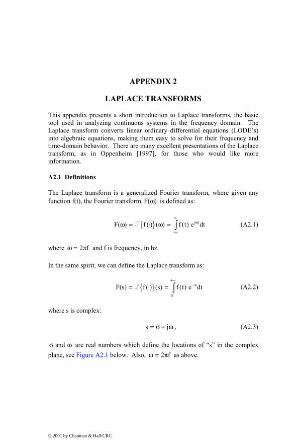
APPENDIX 2
LAPLACE TRANSFORMS
This appendix presents a short introduction to Laplace transforms, the basic tool used in analyzing continuous systems in the frequency domain. The Laplace transform converts linear ordinary differential equations (LODE’s) into algebraic equations, making them easy to solve for their frequency and time-domain behavior. There are many excellent presentations of the Laplace transform, as in Oppenheim [1997], for those who would like more information.
A2.1 Definitions
The Laplace transform is a generalized Fourier transform, where given any function f(t), the Fourier transform F( )ω is defined as:
{ } j tF( ) f ( ) ( ) f (t) e dt∞
ω
−∞
ω = ⋅ ω = ∫F (A2.1)
where 2 fω = π and f is frequency, in hz.
In the same spirit, we can define the Laplace transform as:
{ } st
0
F(s) f ( ) (s) f (t) e dt−
+∞−= ⋅ = ∫L (A2.2)
where s is complex:
s j= σ + ω , (A2.3)
andσ ω are real numbers which define the locations of “s” in the complex plane, see Figure A2.1 below. Also, 2 fω = π as above.
© 2001 by Chapman & Hall/CRC

Im(s)
Re(s)
θ
ωn
ω
σ
Figure A2.1: σ ωand definitions in complex plane.
Remarks:
1) if f (t) 0≡ for t 0< , then
{ } { }f ( ) ( ) f ( ) ( j )⋅ ω = ⋅ ωF L (A2.4)
2) The “ 0− ” limit in the Laplace transform definition takes care of f (t) 's which contain the δ function.
3) The integral in the definition of the Laplace transform need not be finite, i.e. { }f (s)L may not exist for all s ∈ . However, if f(t) is bounded by some exponential:
0tf (t) M eσ≤ (A2.5)
then { }f (s)L will make sense for s ∈ such that { } 0Re s > σ .
© 2001 by Chapman & Hall/CRC

4) The Laplace transform is linear:
{ } { } { }1 1 2 2 1 1 2 2a f a f a f a f+ = +L L L (A2.6)
A2.2 Examples, Laplace Transform Table
1) Exponential
[ ]
at
at st (s a )t
0 0
f (t) e 1(t)
1F(s) e 1(t)e dt e dt s as a− −
−
∞ ∞− − − +
=
= = = >+∫ ∫
(A2.7a,b)
2) Impulse
[ ]st 0
0
f (t) (t)
F(s) (t)e dt e 1 for any s−
∞− −
= δ
= δ = =∫ (A2.8a,b)
3) Step
[ ]
s( ) s(0)st
0
f (t) 1(t)
e e 1F(s) e dt s 0s s−
− ∞ −∞−
=
− − = = = >∫ (A2.9a,b)
Table A2.1 below contains Laplace transforms for a few selected functions in the time domain. The “Region of Convergence” or “ROC” is defined as the range of values of “s” for which the integral in the definition of the Laplace transform (A2.2) converges (Oppenheim 1997).
© 2001 by Chapman & Hall/CRC

f(t) Laplace Transform Region of Convergence
1) (t)δ 1 all s
2) (t T)δ − sTe− all s
3) 1(t) 1s
{ }Re s 0>
4) m1 t 1(t)m!
m 1
1s + { }Re s 0>
5) ate 1(t)− 1s a+
{ } { }Re s Re a>
6) m 1 at1 t e 1(t)(m 1)!
− −
− m
1(s a)+
{ } { }Re s Re a>
7) at(1 e )1(t)−− as(s a)+
{ } { }{ }Re s max 0, Re a>
8) at bt(e a )1(t)− −− b a(s a)(s b)
−+ +
{ } { } { }{ }Re s max Re a ,Re b>
9) sin(at) 1(t) 2 2
as a+
{ }Re s 0>
10) cos(at)1(t) 2 2
ss a+
{ }Re s 0>
11) ate sin(bt)1(t)− 2 2
b(s a) b+ +
{ }Re s a>
12) ate cos(bt)1(t)− 2 2
s a(s a) b
++ +
{ }Re s a>
Table A2.1: Laplace transform table.
© 2001 by Chapman & Hall/CRC

A2.3 Duality
The following duality conditions exist:
dt f (t) F(s)ds
d f (t) s F(s)dt
⇔ −
⇔
(A2.10a,b)
A2.4 Differentiation and Integration
Differentiation and the Laplace transform: Suppose
{ }x (s) X(s)=L (A2.11)
then
{ }x (s) sX(s) x(0 )−= −&L , (A2.12)
so we can interpret “s” as a differentiation operator:
d sdt
↔ (A2.13)
Integration and the Laplace transform: Suppose
{ }x (s) X(s)=L , (A2.14)
then
t
0
1L x( )d (s) X(s)s
τ τ = ∫ , (A2.15)
and we can interpret “1/s” as an integration operator:
t
0
1 dts
↔ ∫ (A2.16)
© 2001 by Chapman & Hall/CRC

A2.5 Applying Laplace Transforms to LODE’s with Zero Initial Conditions
Assume we have a linear ordinary differential equation as shown in (A2.17):
1 2 3 1 2 3y(t) a y(t) a y(t) a y(t) b u(t) b u(t) b u(t)+ + + = + +&&& && & && & (A2.17)
Assume y(t) 0, y(t) 0, y(t) 0= = =&& & and take the Laplace transform of both sides, using the linearity property (A2.6):
{ } { } { } { }
{ } { } { }1 2 3
1 2 3
y (s) a y (s) a y (s) a y (s)
b u (s) b u (s) b u (s)
+ + + =
+ +
&&& && &
&& &
L L L LL L L
(A2.18)
Recalling that “s” is the differentiation operator, replace “dots” with “s”:
3 2 21 2 3 1 2 3s Y(s) a s Y(s) a sY(s) a Y(s) b s U(s) b sU(s) b U(s)+ + + = + + (A2.19)
We are now left with a polynomial equation in “s” that can be factored into terms multiplying Y(s) and U(s):
3 2 21 2 3 1 2 3s a s a s a Y(s) b s b s b U(s) + + + = + + (A2.20)
Solving for Y(s):
21 2 3
3 21 2 3
b s b s bY(s) U(s)
s a s a s a
+ + = + + +
(A2.21)
It can be shown that the terms in the numerator and denominator above are the Laplace transform of the impulse response, H(s):
Y(s) H(s)U(s)= , (A2.22)
[ ]H(s) h( ) (s)= ⋅L , (A2.23)
and h( )⋅ is the impulse response. For the example LODE (A2.17) the Laplace transform of the impulse response is:
2
1 2 3
3 21 2 3
b s b s bH(s)
s a s a s a
+ + = + + +
(A2.24)
© 2001 by Chapman & Hall/CRC

A2.6 Transfer Function Definition
It can be shown that the transfer function of a system described by a LODE is the Laplace transform of its impulse response, H(s), (A2.23).
Taking the Laplace transform of the LODE has provided the Laplace transform of the impulse response. If we could inverse-transform H(s) we could get the impulse response h(t) without having to integrate the differential equation. Typically the inverse transform is found by simplifying/expanding H(s) into terms which can be found in tables, such as Table A2.1, and than inverting “by inspection.”
A2.7 Frequency Response Definition
Having obtained H(s) directly from the LODE by replacing “dots” by “s,” we can obtain the frequency response of the system (the Fourier transform of the impulse response) by substituting “ jω ” for “s” in H(s).
s j
H( j ) H(s)= ω
ω = (A2.25)
A2.8 Applying Laplace Transforms to LODE’s with Initial Conditions
In A2.5 we looked at applying Laplace transforms to LODE’s with zero initial conditions, which led to transfer function and frequency response definitions. Since transfer functions and frequency responses deal with steady state sinusoidal excitation response of the system, initial conditions are of no significance, as it is assumed that all measurements of the system undergoing sinusoidal excitation are taken over a long enough period of time that transients have died out.
On the other hand, if we are solving for the transient response of a system defined by a LODE that has initial conditions, obviously the initial conditions will not be zero. We will use the basic definition of the differentiation operation from (A2.12) to define the Laplace transform of 1st and 2nd order differential equations with initial conditions x(0) and x(0)& :
1st Order: { }x(t) sX(s) x(0)= −&L (A2.26)
2nd Order: { } 2x(t) s X(s) sx(0) x(0)= − −&& &L (A2.27)
© 2001 by Chapman & Hall/CRC

A2.9 Applying Laplace Transform to State Space
We defined the form of state space equations in Chapter 5 as below:
(t) (t) u(t)= +x Ax B& (A2.28)
(t) (t) u(t)= +y Cx D (A2.29)
where the initial conditions are set by o(0) =x x . The general block diagram for a SISO state space system is shown in Figure A2.1.
A
+ +B
D
C∫ Iu(t)x(t)& x(t)
y(t)
Integrator Block
DirectTransmission
Matrix
Output MatrixInput Matrix
System Matrixscalar
vector
Input Output
Figure A2.1: State space block diagram.
Taking Laplace transform of (A2.28):
{ } { } { }{ } { }
(s) (s) u (s)
s (s) (0 ) x (s) u (s)(s) U(s)
−
= +
− = += +
x Ax B
X x A BAX B
&L L LL L (A2.30a,b)
Solving for X(s):
1 1
s (s) (s) (0 ) U(s)(s ) (s) (0 ) U(s)
(s) (s ) (0 ) (s ) U(s)
−
−
− − −
− = +− = +
= − + −
X AX x BI A X x B
X I A x I A B (A2.31a,b,c)
© 2001 by Chapman & Hall/CRC

The two terms on the right-hand side of (A2.31c) have special significance:
1) 1(s ) (0 )− −−I A x is the Laplace transform of the homogeneous solution, the initial condition response.
2) 1(s ) U(s)−−I A B is the Laplace transform of the particular solution, the forced response.
Taking the Laplace transform of (A2.29), the output equation:
(s) (s) U(s)= +Y CX D (A2.32)
Knowing X(s) from (A2.31c) and substituting in (A2.32):
1 1(s) (s ) (0 ) (s ) U(s)− − − = − + − + Y C I A x C I A B D (A2.33)
If the initial conditions are zero, x(0 ) 0− = , then
1(s) (s ) U(s)− = − + Y C I A B D , (A2.34)
with the transfer function for the system being defined by H(s):
1(s) (s )− = − + H C I A B D (A2.35)
When the terms in H(s) above are multiplied out, they will result in the following polynomial form:
b(s)(s)a(s)
= +H D (A2.36)
© 2001 by Chapman & Hall/CRC
REFERENCES
Archer, John S., Consistent Mass Matrix for Distributed Mass Systems, Journal of the Structural Division, Proceedings of the American Society of Civil Engineers, ST4, August, 1963, p. 161.
Bay, J.S., Fundamentals of Linear State Space Systems, McGraw-Hill, Boston, MA, 1999.
Chang, Tish-Chun and Craig, Roy R., Jr., Normal Modes of Uniform Beams, Journal of Engineering Mechanics Division, Proceedings of the American Society of Civil Engineers, Vol. 95, No. EM4, August, 1969, p. 1027.
Chen, C.T., Linear System Theory and Design, Third Edition, Oxford University Press, New York, 1999.
Craig, R.R., Jr., Structural Dynamics, An Introduction to Computer Methods, John Wiley & Sons, New York, 1981.
Evans, W.R., Graphical Analysis of Control Systems, Trans. AIEE, vol. 68, 1949, pp. 765−777.
Franklin, G.F., Powell, J.D., and Emami-Naeini, A., Feedback Control of Dynamic Systems, Third Edition, Addison-Wesley, Menlo Park, CA, 1994.
Franklin, G.F., Powell, J.D., and Workman, M., Digital Control of Dynamic Systems, Third Edition, Addison-Wesley, Menlo Park, CA, 1998.
Gawronski, W.K., Balanced Control of Flexible Structures, Springer, New York, 1996.
Gawronski, W.K., Dynamics and Control of Structures, A Modal Approach, Springer, New York, 1998.
Johnson, C.D. and Kienholz, D.A., Finite Element Prediction of Damping in Structures with Constrained Viscoelastic Layers, AIAA Journal, 20(9), September 1982, p. 1284.
Kailath, T., Linear Systems, Prentice-Hall, Englewood Cliffs, NJ, 1980.
© 2001 by Chapman & Hall/CRC

Laub, A.J., Heath, M.T., Paige, C.C., and Ward, R.C., “Computations of System Balancing Transformations and Other Applications of Simultaneous Diagonalization Algorithms,” IEEE Transactions on Automatic Control, AC-32 (1987), pp. 115−122.
Maia, N.M.M. and Silva, J.M.M., Theoretical and Experimental Modal Analysis, Research Studies Press LTD, Taunton, Somerset, U.K., 1997.
Miu, D.K., Poles and Zeros, Mechatronics, Springer-Verlag, New York, 1993.
Moore, B., “Principal Component Analysis in Linear Systems: Controllability, Observability and Model Reduction,” IEEE Transsactions on Automatic Control, AC-26 (1981), pp. 17−31.
Newland, D.E., Mechanical Vibration Analysis and Computation, John Wiley & Sons, Inc., New York, 1989.
Oppenheim, A.V., Willsky, A.S., and Nawab, S.H., Signals and Systems, Prentice-Hall, Upper Saddle River, NJ, 1997.
Pilkey, Walter D., Formulas for Stress, Strain, and Structural Matrices, John Wiley & Sons, New York, 1994.
Strang, G., Introduction to Linear Algebra, 2nd Edition, Wellesley-Cambridge Press, Wellesley, MA, 1998.
Weaver, W. Jr., Timoshenko, S.P., and Young, D.H., Vibration Problems in Engineering, 5th Edition, John Wiley & Sons, New York, 1990.
Zhou, K., Doyle, J.C., and Glover, K., Robust and Optimal Control, Prentice-Hall, Upper Saddle River, NJ, 1996.
Zhou, K. and Doyle, J.C., Essentials of Robust Control, Prentice-Hall, Upper Saddle River, NJ, 1998.
© 2001 by Chapman & Hall/CRC
Related Documents