HAL Id: tel-01816943 https://tel.archives-ouvertes.fr/tel-01816943 Submitted on 15 Jun 2018 HAL is a multi-disciplinary open access archive for the deposit and dissemination of sci- entific research documents, whether they are pub- lished or not. The documents may come from teaching and research institutions in France or abroad, or from public or private research centers. L’archive ouverte pluridisciplinaire HAL, est destinée au dépôt et à la diffusion de documents scientifiques de niveau recherche, publiés ou non, émanant des établissements d’enseignement et de recherche français ou étrangers, des laboratoires publics ou privés. Viable Multi-Contact Posture Computation for Humanoid Robots using Nonlinear Optimization on Manifolds Stanislas Brossette To cite this version: Stanislas Brossette. Viable Multi-Contact Posture Computation for Humanoid Robots using Non- linear Optimization on Manifolds. Robotics [cs.RO]. Université Montpellier, 2016. English. NNT : 2016MONTT295. tel-01816943

Welcome message from author
This document is posted to help you gain knowledge. Please leave a comment to let me know what you think about it! Share it to your friends and learn new things together.
Transcript

HAL Id: tel-01816943https://tel.archives-ouvertes.fr/tel-01816943
Submitted on 15 Jun 2018
HAL is a multi-disciplinary open accessarchive for the deposit and dissemination of sci-entific research documents, whether they are pub-lished or not. The documents may come fromteaching and research institutions in France orabroad, or from public or private research centers.
L’archive ouverte pluridisciplinaire HAL, estdestinée au dépôt et à la diffusion de documentsscientifiques de niveau recherche, publiés ou non,émanant des établissements d’enseignement et derecherche français ou étrangers, des laboratoirespublics ou privés.
Viable Multi-Contact Posture Computation forHumanoid Robots using Nonlinear Optimization on
ManifoldsStanislas Brossette
To cite this version:Stanislas Brossette. Viable Multi-Contact Posture Computation for Humanoid Robots using Non-linear Optimization on Manifolds. Robotics [cs.RO]. Université Montpellier, 2016. English. NNT :2016MONTT295. tel-01816943

Délivré par l’Université de Montpellier
Préparée au sein de l’école doctorale :
Information Structures Systèmes (I2S)
Et de l’unité de recherche :
Laboratoire d’Informatique, de Robotiqueet de Microélectronique de Montpellier
Spécialité :
Systèmes Automatiques et Microélectroniques
Présentée par Stanislas Brossette
Viable Multi-Contact Posture
Computation for Humanoid
Robots using Nonlinear
Optimization on Manifolds
Soutenue le 10 Octobre 2016 devant le jury composé de
M. Ronan Boulic Dr-HDR EPFL Rapporteur
M. Nacim Ramdani Professeur Université d’Orléans Rapporteur
M. Philippe Fraisse Professeur Université de Montpellier Examinateur
M. Jean-Paul Laumond Directeur de Recherche LAAS-CNRS Examinateur
M. Pierre-Brice Wieber Chargé de Recherche INRIA Grenoble Examinateur
M. Adrien Escande Chargé de Recherche CNRS-AIST JRL Co-encadrant de thèse
M. Abderrahmane Kheddar Directeur de Recherche CNRS-UM LIRMM Directeur de thèse


Acknowledgements
I would like to thank my Ph.D supervisor, Abderrahmane Kheddar, for giving me the
opportunity to work in his team, and for his advices and support all along the course of my
Ph.D.
I am very thankful to my Ph.D co-supervisor, Adrien Escande, without whom this work
would never have gone this far. Thank you for your precious advices, for your support, and
for your patience.
It is a great honor for me to have Ronan Boulic and Nacim Ramdani review this dis-
sertation, and to have this thesis examined by Philippe Fraisse, Jean-Paul Laumond and
Pierre-Brice Wieber.
I would like to thank the AIST and Eiichi Yoshida for hosting me in Japan.
I express my gratitude to Oskar von Stryk from Darmstadt University for giving me the
opportunity to participate with their team in the pre-finals DARPA Robotics Challenge, and
to Francesco Nori for giving me the opportunity to explore a new application of my work.
I would like to thank and acknowledge several people with whom I interacted, had
fruitful conversations, and who helped me in different ways during this work: Hervé Audren,
Benjamin Chrétien, Grégoire Duchemin, Giovanni De Magistris, Gowrishankar Ganesh,
Pierre Gergondet, Francois Keith, Thomas Moulard and Joris Vaillant.
I am very thankful to my family, for supporting me, motivating me and believing in me
all this time.
Finally, I would like to dedicate this thesis to my unconditionally loving girlfriend, Airi
Nakajima, and to thank her for her patience and priceless support all along this Ph.D.


Abstract
Humanoid robots are complex poly-articulated structures with nonlinear kinematics and
dynamics. Finding viable postures to realize set-point task objectives under a set of constraints
(intrinsic and extrinsic limitations) is a key issue in the planning of robot motion and an
important feature of any robotics framework. It is handled by the so called posture generator
(PG) that consists in formalizing the viable posture as the solution to a nonlinear optimization
problem. We present several extensions to the state-of-the-art by exploring new formulations
and resolution methods for posture generation problems. We reformulate the notion of
contact constraints by adding variables to enrich the optimization problem and allow the
solver to decide the shape of intersection of contact polygons, or of the location of a contact
point on a non-flat surface. We present a reformulation of the posture generation problem
that encompasses non-Euclidean manifolds natively and presents a more elegant and efficient
mathematical formulation of it. To solve such problems, we implemented a new SQP solver
that is particularly suited to handle non-Euclidean manifolds structures. By doing so, we
have a better mastering in the way to tune and specialize our solver for robotics problems.
Keywords: posture generation; humanoid robotics; nonlinear optimization; manifolds.
Résumé
Un robot humanoïde est un système poly-articulé complexe dont la cinématique et la dy-
namique sont gouvernées par des équations non-linéaires. Trouver des postures viables qui
minimisent une tâche objectif tout en satisfaisant un ensemble de contraintes (intrinsèques
ou extrinsèques) est un problème central pour la planification de mouvement robotique et
est une fonctionnalité importante de tout logiciel de robotique. Le générateur de posture
(PG) a pour rôle de trouver une posture viable en formulant puis résolvant un problème
d’optimisation non-linéaire. Nous étendons l’état de l’art en proposant de nouvelles formula-
tions et méthodes de résolution de problèmes de génération de posture. Nous enrichissons
la formulation de contraintes de contact par ajout de variables au problème d’optimisation,
ce qui permet au solveur de décider automatiquement de la zone d’intersection entre deux
polygones en contact ou encore de décider du lieu de contact sur une surface non plane.
Nous présentons une reformulation du PG qui gêre nativement les variétés non Euclidiennes
et nous permet de formuler des problèmes mathématiques plus élégants et efficaces. Pour
résoudre de tels problèmes, nous avons developpé un solveur non linéaire par SQP qui
supporte nativement les variables sur variétés. Ainsi, nous avons une meilleure maîtrise de
notre solveur et pouvons le spécialiser pour la résolution de problèmes de robotique.
Mots-clés: génération de posture; robot humanoïde; optimisation non-linéaire; variétés.


Contents
Symbols xi
Introduction 1
1 State of the art and Problem definition 5
1.1 State of the art . . . . . . . . . . . . . . . . . . . . . . . . . . . . . . . . . 5
1.1.1 Inverse Kinematics . . . . . . . . . . . . . . . . . . . . . . . . . . 5
1.1.2 Generalized Inverse Kinematics . . . . . . . . . . . . . . . . . . . 6
1.1.3 Optimization . . . . . . . . . . . . . . . . . . . . . . . . . . . . . 10
1.2 Problem Definition . . . . . . . . . . . . . . . . . . . . . . . . . . . . . . 11
2 Posture Generation: Problem Formulation 15
2.1 Forward Kinematics . . . . . . . . . . . . . . . . . . . . . . . . . . . . . . 15
2.2 Joints formulations . . . . . . . . . . . . . . . . . . . . . . . . . . . . . . 18
2.3 Jacobian computation . . . . . . . . . . . . . . . . . . . . . . . . . . . . . 21
2.4 Joint Limits . . . . . . . . . . . . . . . . . . . . . . . . . . . . . . . . . . 22
2.5 Contact constraints . . . . . . . . . . . . . . . . . . . . . . . . . . . . . . 23
2.6 Collision avoidance . . . . . . . . . . . . . . . . . . . . . . . . . . . . . . 24
2.7 External Forces . . . . . . . . . . . . . . . . . . . . . . . . . . . . . . . . 25
2.8 Static stability . . . . . . . . . . . . . . . . . . . . . . . . . . . . . . . . . 26
2.9 Center of mass projection . . . . . . . . . . . . . . . . . . . . . . . . . . . 28
2.10 Torque limits . . . . . . . . . . . . . . . . . . . . . . . . . . . . . . . . . 29
2.11 Contact Forces and Friction Cones . . . . . . . . . . . . . . . . . . . . . . 30
2.12 Cost Functions . . . . . . . . . . . . . . . . . . . . . . . . . . . . . . . . 31
2.13 Conclusion . . . . . . . . . . . . . . . . . . . . . . . . . . . . . . . . . . 33
3 Extensions of Posture Generation 35
3.1 Integration of Non-Inclusive Contacts in Posture Generation . . . . . . . . 35
3.1.1 Contact geometry formulation . . . . . . . . . . . . . . . . . . . . 38

viii Contents
3.1.2 Non-inclusive contact constraints . . . . . . . . . . . . . . . . . . 38
3.1.3 Simulation results . . . . . . . . . . . . . . . . . . . . . . . . . . 43
3.1.4 Discussion and conclusion . . . . . . . . . . . . . . . . . . . . . . 45
3.2 Torque derivation . . . . . . . . . . . . . . . . . . . . . . . . . . . . . . . 46
3.3 On the use of lifted variables for Robotics Posture Generation . . . . . . . 51
3.3.1 Lifting Algorithm . . . . . . . . . . . . . . . . . . . . . . . . . . . 52
3.3.2 Optimization on lifted variables . . . . . . . . . . . . . . . . . . . 56
3.3.3 Results, experimentation . . . . . . . . . . . . . . . . . . . . . . . 57
3.4 Conclusion . . . . . . . . . . . . . . . . . . . . . . . . . . . . . . . . . . 62
4 Optimization on non-Euclidean Manifolds 63
4.1 Introduction to optimization on Manifolds . . . . . . . . . . . . . . . . . . 63
4.2 Optimization on Manifolds . . . . . . . . . . . . . . . . . . . . . . . . . . 65
4.2.1 Representation problem . . . . . . . . . . . . . . . . . . . . . . . 66
4.2.2 Local parametrization . . . . . . . . . . . . . . . . . . . . . . . . 67
4.2.3 Local SQP on manifolds . . . . . . . . . . . . . . . . . . . . . . . 69
4.2.4 Vector transport . . . . . . . . . . . . . . . . . . . . . . . . . . . . 70
4.2.5 Description of non-Euclidean manifolds . . . . . . . . . . . . . . . 70
4.2.6 Implementation of Manifolds . . . . . . . . . . . . . . . . . . . . 73
4.3 Practical implementation . . . . . . . . . . . . . . . . . . . . . . . . . . . 73
4.3.1 Linear and quadratic problems resolution . . . . . . . . . . . . . . 74
4.3.2 Problem Definition . . . . . . . . . . . . . . . . . . . . . . . . . . 75
4.3.3 Trust-region and limit map . . . . . . . . . . . . . . . . . . . . . . 77
4.3.4 Filter method . . . . . . . . . . . . . . . . . . . . . . . . . . . . . 78
4.3.5 Convergence criterion . . . . . . . . . . . . . . . . . . . . . . . . 78
4.3.6 Feasibility restoration . . . . . . . . . . . . . . . . . . . . . . . . 80
4.3.7 Second Order Correction . . . . . . . . . . . . . . . . . . . . . . . 82
4.3.8 Hessian update on manifolds . . . . . . . . . . . . . . . . . . . . . 83
4.3.9 Hessian Regularization . . . . . . . . . . . . . . . . . . . . . . . . 84
4.3.10 An alternative Hessian Approximation Update . . . . . . . . . . . 84
4.3.11 Hessian Update in Restoration phase . . . . . . . . . . . . . . . . . 85
4.3.12 Solver Evaluation . . . . . . . . . . . . . . . . . . . . . . . . . . . 85
4.4 Diagrams of the algorithms . . . . . . . . . . . . . . . . . . . . . . . . . . 86
4.5 Conclusion . . . . . . . . . . . . . . . . . . . . . . . . . . . . . . . . . . 87

Contents ix
5 Posture Generator 89
5.1 Geometric expressions . . . . . . . . . . . . . . . . . . . . . . . . . . . . 89
5.2 Automatic mapping . . . . . . . . . . . . . . . . . . . . . . . . . . . . . . 92
5.3 Problem formulations . . . . . . . . . . . . . . . . . . . . . . . . . . . . . 93
5.4 Implementation . . . . . . . . . . . . . . . . . . . . . . . . . . . . . . . . 98
5.5 Examples of postures generation . . . . . . . . . . . . . . . . . . . . . . . 100
5.6 Contact on non-flat surfaces . . . . . . . . . . . . . . . . . . . . . . . . . 102
5.6.1 Application to plane-sphere contact . . . . . . . . . . . . . . . . . 102
5.6.2 Contact with parametrized wrist . . . . . . . . . . . . . . . . . . . 103
5.6.3 Contact with an object parametrized on the unit sphere . . . . . . . 104
5.7 Contact with Complex Surfaces . . . . . . . . . . . . . . . . . . . . . . . 105
5.8 Conclusion . . . . . . . . . . . . . . . . . . . . . . . . . . . . . . . . . . 109
6 Evaluation and Experimentation 111
6.1 On the performance of formulation with Manifolds . . . . . . . . . . . . . 111
6.2 Evaluation of the Posture Generation . . . . . . . . . . . . . . . . . . . . . 115
6.3 Application to Inertial Parameters Identification . . . . . . . . . . . . . . . 117
6.3.1 Physical Consistency of Inertial Parameters . . . . . . . . . . . . . 118
6.3.2 Resolution with optimization on Manifolds . . . . . . . . . . . . . 119
6.3.3 Experiments . . . . . . . . . . . . . . . . . . . . . . . . . . . . . 119
6.4 Application to contact planning on real-environment . . . . . . . . . . . . 121
6.4.1 Building an understandable environment . . . . . . . . . . . . . . 123
6.4.2 Constraints for surfaces extracted from point clouds . . . . . . . . . 125
6.4.3 Results . . . . . . . . . . . . . . . . . . . . . . . . . . . . . . . . 125
6.4.4 Discussion . . . . . . . . . . . . . . . . . . . . . . . . . . . . . . 126
6.5 Conclusion . . . . . . . . . . . . . . . . . . . . . . . . . . . . . . . . . . 128
Conclusion 129
Bibliography 133
Academic contributions 143
Appendix A Numerical Optimization: Introduction 145
A.1 Introduction . . . . . . . . . . . . . . . . . . . . . . . . . . . . . . . . . . 145
A.2 Unconstrained Optimization . . . . . . . . . . . . . . . . . . . . . . . . . 146
A.3 Constrained Optimization . . . . . . . . . . . . . . . . . . . . . . . . . . . 147
A.3.1 Optimality conditions . . . . . . . . . . . . . . . . . . . . . . . . 148

x Contents
A.4 Resolution of a NonLinear Constrained Optimization Problem . . . . . . . 150
A.5 Sequential Quadratic Programming . . . . . . . . . . . . . . . . . . . . . . 152
A.5.1 Principle . . . . . . . . . . . . . . . . . . . . . . . . . . . . . . . 152
A.5.2 Globalization methods . . . . . . . . . . . . . . . . . . . . . . . . 155
A.5.3 Restoration phase . . . . . . . . . . . . . . . . . . . . . . . . . . . 160
A.5.4 Quasi-Newton Approximation . . . . . . . . . . . . . . . . . . . . 161
A.6 Conclusion . . . . . . . . . . . . . . . . . . . . . . . . . . . . . . . . . . 162
Appendix B Manifolds Descriptions 163
B.1 The Real Space manifold . . . . . . . . . . . . . . . . . . . . . . . . . . . 163
B.2 The 3D Rotation manifold: Matrix representation . . . . . . . . . . . . . . 163
B.3 The 3D Rotation manifold with quaternion representation . . . . . . . . . . 166
B.4 The Unit Sphere manifold . . . . . . . . . . . . . . . . . . . . . . . . . . 168

Symbols
Number Sets
κ(i) List of indexes of successive joints going from B0 to Bi
F Set of feasible constraints
U Set of unfeasible constraints
E Set of equality constraints indexes
I Set of inequality constraints indexes
Operators
.× . Cartesian product
.∧ . Cross product
.+ Upper Bound of variable .
.− Lower Bound of variable .
.rest Restoration quantity
.−1 Inverse of .
.T Transpose of .
∂a∂b
Derivative of a with respect to b
v 3D skew-symmetric matrix such that vu = v∧u
∇. Gradient operator
~. Denotes a vector

xii Symbols
a ·b Dot product between a and b
Optimization-related Symbols
λ Lagrange multipliers
z−map, z+map Bounds of validity of the tangent map
L(x,λ ) Lagrangian function of the optimization problem
Tx,z(.) Vector transport function from x to ϕx(z)
Ω Feasible set
φx(.) Retractation operator
π(.) Projection on a manifold from its representation space
ψ(.) Functional to represent an element of a manifold in its representation space
ρ Trust-region
ϕx(.) Local parametrization of a manifold on its tangent space at x
ζx(.) Pseudo-logarithm function at point x
ci(.) Constraint function of index i
F Set of linearized feasible directions
f (.) Objective function
Hk Hessian matrix at iteration k
x Optimization variable
x∗ Solution of the optimization problem
Robotics-related Symbols
f Variable describing the external forces
q Variable describing the robot’s joint configuration
R 3D Rotation
t 3D translation vector

Symbols xiii
λi Index of the parent body of B j
E An ellipse
Q Set of viable configurations
Jaci Jacobian of Body i
~f Wrench’s resultant part
~m Wrench’s moment part
BXA 3D transformation from frame A to frame B
Bi Body i
Fi Frame i
Ji Joint i
nB Number of bodies
nJ Number of Joints
Si Motion subspace of joint i
Ti Task i
w Wrench
w|OF Expression of wrench w calculated at the point O expressed in the frame F
XJi Transformation from the reference frame of joint i to the reference frame of its
successor body
Xxi Static transformation of joint i
XPtSi Transformation from Bλi
to Bi
Spaces
E Embedding space ofM
R The Real space
R≥0 The set of positive Reals

xiv Symbols
M A Manifold
S2 The unit 3D sphere manifold
SO(3) The 3D Rotations manifold
TxE Embedding space of TxM
TxM The tangent space of manifoldM at point x
Other Symbols
0n Matrix zero of dimension n
1n Matrix identity of dimension n
Abbreviations/Acronyms
CCS Catmull-Clark Surface
CFSQP C Code for Solving Constrained Nonlinear Optimization Problems
DoF Degrees of freedom
EE End-effector
FP Feasibility Problem
FX, FY, FZ Forces along~x,~y, and~z
IK Inverse Kinematics
IQP Inequality constrained Quadratic Programming
KKT Karush-Kuhn-Tucker first order optimality conditions
LICQ Linear Independence Constraints’ Qualification
MX, MY, MZ Moments around~x,~y, and~z
PG Posture Generation
QP Quadratic Problem
RX, RY, RZ Rotations around~x,~y, and~z
s.t. subject to

Symbols xv
SQP Sequential Quadratic Programming
TX, TY, TZ Translations along~x,~y, and~z
w.r.t with respect to


Introduction
Science fiction novels and movies often present humanoid robots in a technological over-
selling way, being able to reason, plan and achieve a wide variety of tasks as efficiently or
sometimes even better than humans. The road towards creating such performant robots is
still long, and their creation is probably not adequate for the real world. Nevertheless, in the
recent years, we have witnessed a wide growth of the numbers of robots, of various shapes
and sizes, used in many applications, achieving well the tasks they are assigned. For example,
the robotic arms traditionally used to autonomously build cars in factories are replaced slowly
by cobotic systems instead, minimally invasive surgery robots are teleoperated by qualified
surgeons to save lives, submarine robots are exploring the oceans, and humanoid robots are
envisioned seriously as a solution in large-scale manufacturing industries such as aircraft,
building, etc.
The DARPA Robotics Challenge has shone some light on the capabilities and limitations
of current humanoid robots technology. This competition brought together robotics groups

2 Introduction
from Universities, laboratories, and private companies to work on a common goal: develop a
partially teleoperated –i.e. in a shared autonomy scheme, robotic systems that can realize
several tasks without any human co-located intervention or assistance. The robots were
required to drive a car, open a door, climb stairs, cross debris, drill a hole in a wall, etc. All
these tasks can usually be broken down into sets of elementary tasks yet understandable to
common language, such as ‘put hand in contact with target’, ‘put foot on next step’, ‘avoid
collision with that object’, ‘maintain stability’ or ‘look in that direction’, etc. As is, these
tasks do not mean anything for the robot that has no knowledge of its interaction with the
world, nor of human language. All the joints of the robot must be piloted individually and in
coordination in order to make the whole robot complete the required task objectives.
Tasks require motions, which in turn can be defined by a set of continuous discrete
postures. For a given snapshot of time (e.g. before initiating a motion), given a set of tasks
specified by the user for a robot to satisfy, the questions that immediately comes to mind is:
“Is that set of tasks feasible?”. In general, the answer to that question is found by solving
the problem of ‘Posture Generation’, which consists of finding a ‘viable’ configuration of
the robot that satisfies that set of tasks. The tasks are generally expressed in the workspace
of the robot, whereas the solution that we are looking for is a configuration of the robot,
in its articular space potentially augmented by some additional variables. The Posture
Generation problem searches a configuration in the articular space that is a solution to a
problem expressed in the workspace.
The formulation and resolution of posture generation problems are the missions of
the ‘Posture Generator’ (PG), and the development of this tool is the central topic of this
dissertation. Traditionally, this problem is formulated as a collection of constraints and
objective function that translate the tasks to achieve, as well as the conditions for the
configuration to be viable and is solved using optimization algorithms.
The PG is a key tool for many robotics applications and as such, it is an important com-
ponent of any robotics framework. Contact planners make heavy use of posture generators as
they search a sequence of successive feasible postures to go through to reach a goal, each
posture being defined by a set of tasks, such as the list of contacts between the robot and
its environment. The feasibility of each of those postures needs to be checked by a PG
before being used by the planner. Trajectory generation and control also make use of posture
generation as they both often rely on being given some key postures to help guide the robot’s
motion (e.g. initial, intermediate and final configurations).
The formulation of a posture generation problem is often a cumbersome and time-
consuming task for the programmer, requiring a fine-tuning of the problem’s constraints and
cost functions, as well as of the solver, to get satisfactory results. In this thesis, we present a

Introduction 3
posture generation framework that makes the development of posture generation problems
easier, as well as richer, by proposing several extensions to their formulation.
Once the problem of posture generation is formulated, its resolution can take place.
Some variables of a robotic problem belong to a non-Euclidean manifold M, like SO(3)
for the 3D rotation of the base of a mobile robot. A manifold is a topological space that
locally resembles a Euclidean space in the neighborhood of each point. However, an n-
dimensional non-Euclidean manifold cannot always be globally parametrized over a subset of
Rn without presenting problems of singularity. Most of the off-the-shelf optimization solvers
available make the assumption that the search space is Euclidean, and thus, do not feature the
capability of solving problems on non-Euclidean manifolds natively. It is often possible to
parametrizeM over a Euclidean space of higher dimension with added constraints (e.g. unit
quaternions, rotation matrices). Then those problems can be solved with classical solvers
at the cost of additional variables, constraints and special treatments in the resolution of
the optimization problem. There exist some methods and algorithms to solve optimization
problems on non-Euclidean manifolds with no substantial extra cost and guaranteeing a
good coverage of the manifolds without facing parametrization singularities, and with the
minimal number of parameters. However, to our knowledge, these are focused on addressing
non-constrained optimization. We propose to extend those methods to solve constrained
optimization problems on manifolds.
Through this thesis, we develop a nonlinear constrained optimization solver on manifolds,
that we believe to be the first of its kind, and use it to solve optimization problems on
their native search manifolds. We will exhibit the interests of such resolution methods for
solving posture generation problems as well as any other problems formulated on manifolds.
This has the added advantage that, unlike off-the-shelf solvers which are often a black box
on which the user has very limited control, we have full control over that solver and can
specialize/modify it to fit our needs.
Contributions and plan The main focuses of this thesis are the formulation and the reso-
lution of problems of posture generation for robotics systems using nonlinear optimization
on manifolds. Our contribution is twofold, on the one hand, we propose extensions and
improvements of the ways to formulate a posture generation problem, and on the other hand,
we investigate new ways of solving these problems. The organization of this thesis is as
follows:
• In Chapter 1 we describe the state of the art of posture generation and optimization on
manifolds.
• In Chapter 2, we present the detailed formulation of a posture generation problem.

4 Introduction
• In Chapter 3 we present three different and unrelated contributions: two formulation
extensions, one allowing to generate non-inclusive contacts between convex surfaces,
the other is the exact derivation of the joint torques of a robot. We then present our
endeavor to use the ‘Lifted Newton Method’ to solve posture generation problems.
• Chapter 4 describes the principles of nonlinear optimization over non-Euclidean mani-
folds and our implementation of a solver based on those principles.
• In Chapter 5, we present a framework that simplifies and extends the formulation of
posture generation problems by formulating and solving the optimization problem over
native non-Euclidean manifolds, managing automatically the variables of the problems,
and proposing a framework that formalizes and simplifies the writing of functions on
geometric entities often used in robotics.
• In Chapter 6, we evaluate the performances of our solver on manifolds and the perfor-
mances of our posture generator. Then, we present a use case of our solver for inertial
identification problems and some preliminary work on the generation of postures on a
sensor acquired environment.

Chapter 1
State of the art and Problem definition
1.1 State of the art
1.1.1 Inverse Kinematics
Posture generation can be viewed as, and is sometimes called, Generalized Inverse Kinemat-
ics. The Inverse Kinematics (IK) problem consists of finding the joint configuration for an
articulated multibody system in order to complete a given set of tasks that are defined in the
operational space. For example, by solving repeatedly the IK for a desired motion given in
the Cartesian space, we can generate motions in the joint space. By definition, such a process
is purely kinematic. But other constraints need dynamic or other physics-related knowledge
such as the inertia or contact friction parameters. The IK problem has been widely studied
and used in the fields of robotics, computer graphics, games, and animation. In few particular
cases, for example with robotic arms that have less than 7 degrees of freedom, a closed-form
solution can be found. For example, in [AD03] the redundancy in a robot arm is exploited to
derive a closed-form formula for its IK. However, for most complex cases, iterative methods
are required.
Many approaches to solve IK problems use pseudo-inverse or Gauss-Newton method
with the Jacobian, Jacobian transpose, damped least squares with or without singular values
decomposition or selectively damped least squares [BMGS84, TGB00, Bai85, Wam86,
NH86, BK05]. These approaches are all computationally costly and suffer from joint-space
and workspace singularities [AL09].
In [Pec08] an alternative method based on a control approach is proposed, where no matrix
manipulation is required, this approach is as fast as the damped least squares, but outperforms
them in terms of handling singularities. The closed-loop inverse kinematics scheme presented
6 State of the art and Problem definition
in [Sic90] is a well-known approach to solve IK problems in a control context, and uses a
second order tracking scheme to guarantee satisfactory tracking performance.
Handling conflicting constraints in IK is a challenging problem to which [BB04] and
[SK05] propose solutions by enforcing a number of priority levels among constraints in their
resolution schemes to generate whole-body control of complex articulated figures.
Other stochastic approaches such as sequential Monte Carlo [CA08] and a particle
filtering [HRE+08] have the advantage that they only use direct calculations and never
require matrix inversions. They perform particularly well compared to other methods when
solving problems with high numbers of degrees of freedom.
In [AL11, ACL16] the forward and backward reaching inverse kinematics (FABRIK)
resolution method is introduced. This method is based on a geometric iterative heuristic
approach, where the bodies of a robot are moved iteratively and separately to reach a target
with the end effector while maintaining the integrity of the robot’s structure. This approach
is simple to implement, does not suffer from singularities and requires fewer iterations than
most other IK methods. But it cannot easily be extended to take non-geometric constraints
into account.
Finding an acceptable approximate (or a probabilistic) solution to an IK problem without
any regard for its stability is a common approach in the field of randomized path planning.
[CSL02] proposes a method to generate many random configurations for closed loop systems
with an increased probability that they are kinematically valid in terms of closure con-
straints. These configurations are then used in the construction of a Probabilistic RoadMap.
In [LYK99], a similar approach is presented, where the closure constraint is enforced for
each configuration by additional treatment.
1.1.2 Generalized Inverse Kinematics
The term Generalized Inverse Kinematics refers to a problem similar to the Inverse Kinemat-
ics in the sense that it searches for a joint configuration for an articulated figure to achieve
goal tasks, but needs to do so under various constraints, like ensuring the equilibrium stability
of the structure, respecting its torque limits, avoiding collisions with the environment or with
itself, etc.
All the previously mentioned approaches are used to find a robot configuration solution
to the geometric IK problem. To solve a Generalized Inverse Kinematics problem with
stability constraints, one can first solve the associated IK with one of the methods presented
above, and then test the stability of the IK solution, using methods such as the ones presented
in [BL08] or [RMBO08] that determine if the configuration can be statically stable. This
gives a rejection criterion for a proposed solution. If the solution can be stable, the optimal

1.1 State of the art 7
contact forces can be computed using the method proposed in [BW07] (which in turn allows
computing the joint torques). Otherwise, another IK solution is generated and tested. And
the process is repeated until a satisfactory solution is found. This type of sequential approach
for the resolution of a posture generation problem features a rejection criterion that can, in
some cases, be difficult to overcome, making this approach costly, for example, if there is a
small number of contacts and very few configurations are stable.
Another way to solve the posture generation problem is to consider the complete problem
at once, with the IK targets and all the other constraints (stability, collisions, torque limits, etc.)
in a single nonlinear constrained optimization problem. This approach is used in [ZB94] to
solve the IK problem. That is the approach that we and many others use to solve Generalized
Inverse Kinematics problems. In [EKM06], such an approach is employed to generate
postures that are used to grow a tree of usable postures in a multi-contact planning algorithm.
[EKM06] applied the approach to automatically generate a sequence of contact sets and
postures where the HRP-2 robot uses its hand to lean on a table in order to grasp an object
otherwise out of reach. Interestingly, in this study, the C-code that computes the robot’s
kinematics is generated once and for all for each robot, using Maple and the HuMAnS
toolbox [WBBPG06] provided by INRIA. The constraints of contact, stability and collision
are then computed based on the outputs of the generated code. And the problem is solved
by the CFSQP solver [LZT97]. In [HBL+08], a similar posture generation approach is
used to find viable postures for different legged robots on varied terrains in the context of
Probabilistic RoadMap planning, which is a planning approach based on random sampling of
the configuration space. In [BK10a], a generalization of the formulation of posture generation
problems for systems of multiple robots and manipulated objects is proposed. With this
formulation, the notion of contacts is generalized such that they are not necessarily coplanar,
nor necessarily horizontal, frictional, can bear forces or not, and may be unilateral or bilateral.
This generic formulation enables the generation of postures with inter-robot contacts. The
complete posture generation problem is then solved within a single nonlinear constrained
optimization query, computing the contact forces and joint configuration at the same time,
while ensuring the stability of all the ‘robotic agents’, avoiding collision and respecting the
robot’s joint and torque limits.
In the past few years, our team has dedicated considerable efforts in proposing a general
multi-contact motion planner to solve cases of non-gaited acyclic planning, using a posture
generator as a backbone to select valid configurations. Given a humanoid robot, an envi-
ronment, a start and a final desired postures, the planner generates a sequence of contact
stances allowing any part of the humanoid to make contact with any part of the environment
to achieve motion towards the goal. The planner’s role is to grow a tree of contact stances

8 State of the art and Problem definition
iteratively; from a given posture, it tries to add or remove contacts one by one. The tree
grows following some heuristics until the solution is reached. For each set of contacts to
add to the tree, a posture generation problem is solved in order to validate the feasibility of
the set. If it is not feasible, the set is rejected. A typical experiment with an HRP-2 robot
achieving such an acyclic motion is presented in [EKMG08], and the planner is thoroughly
described in [EKM13]. Extensions of this multi-contact planner to multi-agent robots and
objects gathering locomotion and manipulation are presented in [BK12a], and preliminary
validations with some DARPA challenge scenarios, such as climbing a ladder, ingress/egress
a utility car, or crossing through a relatively constrained pathway are presented in [BK12b].
Another way of planning a multi-contact scenario, which is actually often used when planners
fail to find satisfactory solutions, is manual, choosing iteratively which contacts to add and
remove until the goal is reached. This type of approach is used when the plan to execute is
complex and when a lot of fine tuning of the postures is required, as in [VKA+16], where a
sequence of postures allowing the HRP-2 robot to climb a vertical ladder is generated and
tuned manually. Those postures are provided as input to a finite state machine that builds
additional intermediary tasks and specific grasps procedures to be realized on the real robot
by a multi-objective model-based QP controller.
Instead of feeding the key postures directly to the controller and trusting that it will find
a path to connect them, one can take an additional step and compute a dynamically viable
trajectory between successive steps that the controller will then have to follow. Classical
methods generate satisfactory configurations on a discretized time-grid and then extrapolate
the motion between configurations at successive time-grid points. This approach does not
guarantee that the constraints are satisfied at every point of a continuous time interval, which
is dangerous for the robot. Interval analysis methods can be leveraged to compute safe
motions over continuous time intervals, as proposed in [LRF11]. This work was extended
in [LVYK13] to generate whole-body multi-contact dynamic motions. The constraints are
transformed into a computation of extrema of time polynomials, whose coefficients are a
function of the optimization variables, over each time interval. Generating full body dynamic
motions allows one to take advantage of the dynamic effects and to produce motions with
better performances in terms of completion time, energy consumption, or other criteria.
In many planning approaches [KNK+05, Che07, HBL+08, KRN08, BK11] the planning
problem is decomposed into two stages, first the sets of contacts and associated postures are
planned and then the motions to go from one set to another are computed. These two stages
are loosely coupled, which can result in suboptimal use of the contacts available. [MTP12]
presents a different approach to contact planning where some additional terms and variables
are added to the optimization problem to decide whether a contact pair should be active (and

1.1 State of the art 9
bear forces) at any given time during the motion, or not. The contact sets, as well as the
postures associated, are discovered along with the entire movement’s trajectories by using
contact invariant optimization. This allows for the exploitation of any synergies that might
exist between the contact events and the motion trajectory.
In [TPP+16], a multi-contact planning framework is presented that allows the computa-
tion of complex multi-contact motions in very short times. It is based on several heuristics
that allow fast computations of the motions. Starting by generating a guide path that satisfies
the reachability condition, which means that the root body is close to obstacles to allow
making contacts with them but not too close to avoid collisions. A discrete sequence of
statically stable whole-body configurations along this path is then generated efficiently by
taking advantage of several approximations and heuristics. This approach allows generating
complex contact plans in a few seconds, whereas other approaches usually take several
minutes.
In [LME+12], posture generation is used to find the optimal posture and position of
contacts to optimally realize a manipulation task along a path while satisfying geometric,
kinematic, as well as force and torque constraints. The task is defined as a path and forces to
follow with an end effector. Instead of finding a sequence of unrelated postures along the
path, all the postures are found by solving a single optimization problem in which successive
postures are coupled by constraints to ensure that the foot positions remain constant during
the task, even though the rest of the body can move. This approach allows the robot or virtual
character to apply manipulation forces as strongly as possible while avoiding foot slippage.
It also allows taking external perturbations into account to generate more robust postures.
A different utilization of the posture generation was presented in [SLL+07], that deals
with the problem of object reconstruction. An object is presented to the robot in order
to generate automatically its 3D model. To do so, the object is observed from several
different angles with the camera that is mounted in the robot’s head. The satisfactory postures
of the robot to complete this task are obtained by solving a posture generation problem
to which a set of constraints defining the direction in which the robot should look and a
minimum distance from the object are added. While in this work the observation directions
are predefined, [FSEK08] presents an approach where the choice of the best observation
direction is left to the posture generator. The representation of the object is iteratively carved
into a block of 3D voxels, each new point-of-view chosen to allow to carve it a little more
precisely. It uses a modified cost function to evaluate the amount of information on the object
that a given point of view can provide. The posture of the robot that optimizes that cost
function is then found by the posture generator under the classical constraints of stability,
collision avoidance, and other robot’s limitations.

10 State of the art and Problem definition
1.1.3 Optimization
The resolution of a posture generation problem is often done by solving a nonlinear optimiza-
tion problem which consists of finding the optimal point that minimizes a cost function and
maybe constraints, the cost and constraints functions being possibly nonlinear.
Optimization algorithms can be derivative-free or not. The computation of the derivatives
of the functions involved in the problem is a common source of error. The strength of the
derivative-free approaches is that the user does not need to implement the derivatives. But
derivative-free approaches are much slower than their counterparts using derivatives. One
way to avoid implementation errors in the derivatives computation is to use finite differences
to compute them. This method is very slow, especially when the dimension of the problem
is large. In order to design an efficient optimization algorithm, we will focus on methods
using derivative information and will implement those derivatives’ computations. The finite
difference approach can be used to verify the correctness of the computed derivative.
Nonlinear optimization is a well-established research field by its own and has been
extensively studied in the past and nowadays. One can find some excellent reference books
about optimization, such as [NW06, BGLA03, BV04].
Furthermore, several off-the-shelf solvers are available and have been widely used to
solve robotics problems. The CFSQP solver [LZT97] was used in [EK09a] and [EKM13]
where thousands of HRP-2 posture generation queries were made to explore the feasible
space. The IPOPT solver [WB06] has been used in [VKA+14], [VKA+16], [BK12a] where
the posture generator has been extended to handle multi-robot problems with more complex
and various contact constraints. The SNOPT solver [GMS05] was used in [DVT14] to plan
dynamic whole-body trajectories. Several nonlinear optimization solvers are available and
have been packaged for use in robotics problems in the Roboptim Framework [MLBY13],
such as IPOPT, CFSQP, CMinPack [Dev07], NAG [TNAG], KNITRO [BNW06] and PGSolver
(the solver that we develop in this thesis).
Traditionally, optimization problems are solved over Euclidean spaces. When the need
comes to find a solution to an optimization problem in a non-Euclidean space M, the
commonly used method is to represent the elements of M in a Euclidean manifold of
higher dimension, and enforcing that solution of the optimization problem should lie onM
by adding the necessary constraints to the problem. We will detail the drawbacks of such
approaches in Chapter 4. Alternatively, there exists a method to run an optimization algorithm
directly on a non-Euclidean manifold, as it is presented in great detail in the book [AMS08].
A non-Euclidean manifold can be thought of as a space that is locally Euclidean, but is
not so globally. For example, a sphere looks Euclidean if one examines a small-enough
neighborhood, similar to the surface of a giant sphere like the earth that looks flat for a human

1.2 Problem Definition 11
being standing on it. Based on the fact that manifolds are locally Euclidean, the classic
properties of distance, derivatives, and in general all the Euclidean geometry can be used
locally. Based on that property, several optimization methods traditionally used on Euclidean
manifolds have been extended to non-Euclidean manifolds. The gradient methods have
been extended to manifolds in [Lue72, Gab82]. The Newton methods on manifolds which
have better convergence rates were extended to manifolds in [Gab82, SH98, Smi13]. And
Quasi-Newton methods in [Gab82]. Those approaches are only meant to solve unconstrained
optimization problems, which is not enough to solve posture generation problems, where the
presence of constraints is unavoidable.
The main idea to optimize on manifolds is that we use a local map between the neighbor-
hood of the current iterate and its Euclidean tangent space in order to run an optimization
step and choose an increment in the tangent space that is mapped back to the manifold. Once
the iterate has been incremented, the process is repeated with the map and tangent space
associated with the new iterate. This comes down to re-parametrizing the problem around
the current iterate at each iteration.
In the field of robotics, we are only aware of the work of Schulman et al. [SDH+14],
where the authors explain the adaptation of their solver to work on SE(3). In the field
of computer vision, and especially for solving pose estimation problems, optimization on
manifolds is used often, e.g. [HWFS11, LHM00].
In this thesis, we develop a nonlinear solver on manifolds that can handle constraints.
We were largely inspired by the work of Fletcher concerning the notions of ‘Sequential
Quadratic Programming without a penalty function’ [Fle06, Fle10, FL00], along with other
optimization approaches that we adapted to work with manifolds.
1.2 Problem Definition
We consider the problem where we have a robotic system and we want it to realize a
set of tasks Ti. We denote q as the joint configuration (n joints + base) of the robot and
f = fi , i ∈ [1,m] represents the m contact forces applied on the robot. Each task Ti can be
represented by a set of equality and inequality equations:
gi(q, f) = 0
hi(q, f)≥ 0(1.1)
For example, the task of making contact between a body (link) of the robot and a part of the
environment can be represented in such a way.
12 State of the art and Problem definition
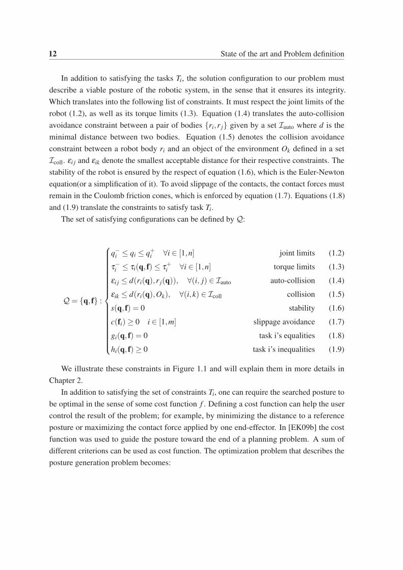
In addition to satisfying the tasks Ti, the solution configuration to our problem must
describe a viable posture of the robotic system, in the sense that it ensures its integrity.
Which translates into the following list of constraints. It must respect the joint limits of the
robot (1.2), as well as its torque limits (1.3). Equation (1.4) translates the auto-collision
avoidance constraint between a pair of bodies ri,r j given by a set Iauto where d is the
minimal distance between two bodies. Equation (1.5) denotes the collision avoidance
constraint between a robot body ri and an object of the environment Ok defined in a set
Icoll. εi j and εik denote the smallest acceptable distance for their respective constraints. The
stability of the robot is ensured by the respect of equation (1.6), which is the Euler-Newton
equation(or a simplification of it). To avoid slippage of the contacts, the contact forces must
remain in the Coulomb friction cones, which is enforced by equation (1.7). Equations (1.8)
and (1.9) translate the constraints to satisfy task Ti.
The set of satisfying configurations can be defined by Q:
Q= q, f :
q−i ≤ qi ≤ q+i ∀i ∈ [1,n] joint limits
τ−i ≤ τi(q, f)≤ τ+i ∀i ∈ [1,n] torque limits
εi j ≤ d(ri(q),r j(q)), ∀(i, j) ∈ Iauto auto-collision
εik ≤ d(ri(q),Ok), ∀(i,k) ∈ Icoll collision
s(q, f) = 0 stability
c(fi)≥ 0 i ∈ [1,m] slippage avoidance
gi(q, f) = 0 task i’s equalities
hi(q, f)≥ 0 task i’s inequalities
(1.2)
(1.3)
(1.4)
(1.5)
(1.6)
(1.7)
(1.8)
(1.9)
We illustrate these constraints in Figure 1.1 and will explain them in more details in
Chapter 2.
In addition to satisfying the set of constraints Ti, one can require the searched posture to
be optimal in the sense of some cost function f . Defining a cost function can help the user
control the result of the problem; for example, by minimizing the distance to a reference
posture or maximizing the contact force applied by one end-effector. In [EK09b] the cost
function was used to guide the posture toward the end of a planning problem. A sum of
different criterions can be used as cost function. The optimization problem that describes the
posture generation problem becomes:

1.2 Problem Definition 13
Figure 1.1 The HRP-4 on a stack of cubes. The color of each box corresponds to the color of
the constraint it depicts.
min.q,f
f (q, f)
s.t. q, f ∈ Q(1.10)
This type of problem is called a nonlinear constrained optimization problem and can be
formulated in a more generic fashion as:
min.x
f (x)
s.t.
ci(x) = 0, ∀i ∈ E
ci(x)≥ 0, ∀i ∈ I
(1.11)
where x is the optimization variable, that we want to find, and which minimizes the cost
function f (x) while satisfying the equality constraints ci(x) = 0, ∀i ∈ E and inequality
constraints ci(x)≥ 0, ∀i ∈ I. Such problems can be solved by a nonlinear optimization solver.
In Appendix A, we present some classical concepts of nonlinear optimization.
In this thesis, we used the off-the-shelf solver IPOPT [WB06] in the beginning. At a later
stage, we developed and use our own nonlinear solver called PGSolver. From here on, we
will formulate and solve posture generation problems as nonlinear constrained optimization
problems. In the next chapter, we focus on formulating all the basic functions and algorithms

14 State of the art and Problem definition
used to describe the robotic constraints and cost function in the formalism of nonlinear
optimization.
Chapter 2
Posture Generation: Problem
Formulation
In this Chapter, we present in detail the formulation of a posture generation problem. We
present the algorithms used to compute the kinematics of a robot and its derivatives as well
as the joint torques. Then we formulate some classical functions that are often used in
posture generation: joint limits, contact constraints, collision avoidance, stability, torque
limits and friction cones. In Figure 1.1, we illustrate those constraints with the result of a
posture generation problem where the HRP-4 robot must climb on a stack of cubes while
being statically stable, respecting its joint and torque limits, the contact forces must remain
within their respective friction cones and the robot must avoid auto-collisions and non-desired
contacts (i.e. collisions) with the environment.
2.1 Forward Kinematics
In this section, we present a formulation of robotic systems that allows specifying most of
the typical constraints encountered in robotics problems.
We consider a robotic system made of nB bodies and nJ(= nB + 1) joints. The global
structure of the robot is described by an ordered graph called multibody graph. The base
body (World) has index 0 and each of the remaining bodies get a different positive integer
index. We denote the body of index i, Bi. B0 refers to the World. Each body Bi has its
reference frame Fi attached to it. F0 denotes the World frame. Bodies are linked together by
joints that also are indexed by positive integers, we denote the joint of index i, Ji, and the
body that comes after it is Bi. Each joint defines the relation between its predecessor and
successor bodies. For joint Ji, they are respectively denoted pred(i) and succ(i), and Bpred(i)

16 Posture Generation: Problem Formulation
Figure 2.1 MultiBody graph
is called the parent body of Bsucc(i). We denote λ ( j) the index of the parent body of B j. The
number of degrees of freedom of Ji is denoted do f Ji and the number of degrees of freedom
of the whole robot is denoted do f . Figure 2.1 illustrates this numbering system for a simple
robot with 4 joints and 5 bodies (including the basis)
The geometric relations between bodies and joints are described through transformations
between their reference frames. We use transformations as described in the Spatial Vector
Algebra chapter of ‘Rigid Body Dynamics Algorithm’ by Roy Featherstone [Fea07]. Motion
vectors (vectors describing motion quantities as positions, velocities and accelerations) and
their force counterpart are defined in [Fea07].
For any 3D vector v∈R3, v denotes the 3×3 skew-symmetric matrix such that vu = v∧u.
Where ∧ denotes the cross product operator.
Let A and B be Cartesian frames with origins O and P respectively. Let t be the coordinate
vector expressing−→OP in A. And R be the rotation matrix that transforms 3D vectors from A
to B coordinates. The transformation from A to B for a motion vector is defined by:
BXA =
[R 0
−Rt R
](2.1)
Its inverse is:
BXA−1
= AXB =
[RT 0
tRT RT
](2.2)
The transformation from A to B for a force vector is defined by:
BX∗A =
[R −Rt
0 R
](2.3)
Its inverse is:
BX−∗A = AX∗B =
[RT tRT
0 RT
](2.4)

2.1 Forward Kinematics 17
Each joint Ji is defined by a static transformation Xxi = Rx
i , txi between the reference
frame of its predecessor body and its own reference frame. Each joint Ji is associated with
a motion subspace which representation matrix is denoted Si. Each column of Si described
a degree of freedom of Ji its upper part for the rotations and lower for translations (see
Section 2.2).
Si =
[SR
i,0 · · · SRi, j · · · SR
i,do f
Sti,0 · · · St
i, j · · · Sti,do f
](2.5)
For a given joint configuration q, the transformation due to the joint Ji current configura-
tion from its reference frame to the reference frame of its successor body is denoted
XJi (q) = R
Ji (q), t
Ji (q).
The transformation between Bλ (i) and Bi is denoted XPtSi (q) = RPtS
i , tPtSi (PtS stands
for ‘Parent to Son’) can then be computed as:
XPtSi (q) = iXλ (i)(q) = XJ
i (q)Xxi (2.6)
Let κ(i) = 0, i1, i2 . . . i be the list of indexes of successive joints going from B0 to Bi. It
can easily be computed by adding iteratively the parent of the current body:
Algorithm 1 Joint Path to Bi
j← i, κ(i) = [i]while j 6= 0 do
j← λ ( j)κ(i)← [κ(i), j]
end while
The transformation from the World base to Bi is denotediX0(q) =
iR0(q),it0(q). The formula (2.6) can be used iteratively on all bodies of the
robot to obtain the expression of iX0(q).
We obtain the full expression of iX0 as:
iX0(q) = ∏j∈κ(i)
XJj (q)X
xj = ∏
j∈κ(i)
jXλ ( j) =iXκ(1)
κ(1)Xκ(2) . . .κ(end−1)XW (2.7)
Which can be computed recursively by a Forward Kinematics algorithm:
In the following section, we provide some detailed description of how to compute XJ(q)
for a variety of useful joints. Using the joint descriptions and the Forward Kinematics
algorithm, we are able to explicit a relation between q the joint parameters of the robot and
the 3D position and orientation of any geometric quantity defined in the reference frame of

18 Posture Generation: Problem Formulation
Algorithm 2 Forward Kinematics
for i = 0 : nJ do
if λ (i) 6=−1 then iX0 =iXλ (i)
λ (i)X0
else iX0 = XPtSi
end if
end for
a body of the robot. Given a transformation pXi defined in the frame of Bi, its value in the
world frame is given by pX0(q) =pXi
iX0(q)
2.2 Joints formulations
The entire geometry of our system is described by the list of static transformations Xxj and of
joint transformations XJj (q). In this section, we explicit the descriptions and formulations of
common joints type.
Let us consider a joint J that governs the transformation between two frames F1 =
O1,x1,y1,z1 and F2 = O2,x2,y2,z2. The most common type of joint encountered in
robotics (and even virtual avatars) systems is the revolute joint, that allows a rotation around
a fixed axis. If J is a revolute joint around the axis (O1,z1) with parameter q, its motion
subspace, rotation, and translation are as follows:
Joint type S Rotation translation
Revolute (O1,z1)
0
0
1
0
0
0
1 0 0
0 cos(q) sin(q)
0 −sin(q) cos(q)
03×1
Similar formulas can be devised for rotations around any other axis, provided that R
describes the rotation of angle q around that axis.
In the case of a prismatic joint, all rotations are blocked, and only one translation along a
given axis is allowed. A prismatic joint along x1 is described by the following formulas:

2.2 Joints formulations 19
Joint type S Rotation translation
Prismatic (x1)
0
0
0
1
0
0
13×3
q
0
0
Planar joints are also frequently used in robotics. A planar joint describes a plane sliding
on another plane. Assuming that the normal to both planes is z1 = z2, this type of joint
allows free relative rotation of F2 around z1 and relative translations along x1 and y1. We
denote q = q1,q2,q3 the joint parameters, q1 corresponding to the rotation and q2, q3 to
the translations. We get:
Joint type S Rotation translation
Planar (z1)
0 0 0
0 0 0
1 0 0
0 1 0
0 0 1
0 0 0
cos(q1) sin(q1) 0
−sin(q1) cos(q1) 0
0 0 1
cos(q1)q2− sin(q1)q3
sin(q1)q2 + cos(q1)q3
0
A spherical joint blocks all translations and allows all rotations. This joint must be
parametrized by a 3D rotation. The space of 3D rotations SO(3) can be represented in
many different ways. The simplest and most intuitive way to parametrize SO(3) is to use
Euler Angles. It comes down to decomposing the 3D rotation into a succession of three 1D
rotations around different axes. For example, the roll, pitch, yaw is a succession of a rotation
of F1 around its x axis, followed by a rotation around the y axis of the resulting frame, finally
a rotation around the z axis of the resulting frame of the latter rotation. The rotation matrix
for such a convention is given by:
R=
1 0 0
0 cos(q3) sin(q3)
0 −sin(q3) cos(q3)
·
cos(q2) 0 −sin(q2)
0 1 0
sin(q2) 0 cos(q2)
·
cos(q1) sin(q1) 0
−sin(q1) cos(q1) 0
0 0 1
(2.8)

20 Posture Generation: Problem Formulation
Euler Angle formulations have the advantage to be simple and intuitive. There are many
other possible choices of the rotation order and conventions. But they all suffer from the
so-called gimbal-lock problem or more generally from singularities, which happens when
two of the three rotation axes become aligned. In such a configuration, the only rotations
possible are one rotation around the two aligned axis and one rotation around the third axis.
Thus, one degree of freedom is lost. Those singularities are prohibitive for the use of that
type of formulation in a posture generation. In [Gra98], Grassia states that any attempt to
parametrize the entire set of 3D rotations by an open subset of Euclidean space (as do Euler
angles) will suffer from gimbal lock. Note that this singularity is only due to the user’s choice
of parametrization, it is not intrinsic to the manifold SO(3). It is possible to parametrize
SO(3) without having to face singularities by parametrizing it over another non-Euclidean
manifold. The most common ones are the set of unit quaternion embedded in R4 and the set
of rotation matrices embedded in R3×3. With the unit quaternion parametrization, a variable
on SO(3) is represented by 4 parameters q = [qw,qx,qy,qz], and it is necessary to ensure that
the quaternion is of norm 1, q ∈ R4 : ||q||= 1. Similarly, if a variable is parametrized by a
rotation matrix, then the matrix M representing it has 9 parameters and M must be orthogonal
and have determinant 1: M ∈ R3×3 : MT M = 13 and det(M) = 1. Similar issues can be
found with the parametrization of other non-Euclidean manifolds, like S2 for example.
A quaternion q= [qw,qx,qy,qz] is a unit quaternion iff q2w+q2
x +q2y +q2
z = 1. It represents
a rotation of angle θ around an axis u such that:
qw = cos(θ/2) (2.9)
qx = sin(θ/2)ux (2.10)
qy = sin(θ/2)uy (2.11)
qz = sin(θ/2)uz (2.12)
(2.13)
The rotation matrix associated with this quaternion is:
R = 2
12−qy
2−qz2 qxqy−qzqw qxqz +qyqw
qxqy +qzqw12−qx
2−qz2 qyqz−qxqw
qxqz−qyqw qyqz +qxqw12−qx
2−qy2
(2.14)
That formulation does not suffer from singularities, but it requires to maintain 4 parame-
ters for a 3D rotation. And those 4 parameters must satisfy the unit norm constraint which
in turn would become an additional constraint in the optimization formulation. Given a
parameter set q = qw,qx,qy,qz, we get the following table.

2.3 Jacobian computation 21
Joint type S Rotation translation
Spherical
1 0 0
0 1 0
0 0 1
0 0 0
0 0 0
0 0 0
2
12−qy
2−qz2 qxqy−qzqw qxqz +qyqw
qxqy +qzqw12−qx
2−qz2 qyqz−qxqw
qxqz−qyqw qyqz +qxqw12−qx
2−qy2
0
0
0
Finally, a free joint allows free motion of its successor body with respect to its predecessor
body. It can be viewed as a combination of a spherical joint and 3 perpendicular prismatic
joints. Given a parameter set q = qw,qx,qy,qz, tx, ty, tz, we get the following table.
Joint type S Rotation translation
Spherical 16 2
12−qy
2−qz2 qxqy−qzqw qxqz +qyqw
qxqy +qzqw12−qx
2−qz2 qyqz−qxqw
qxqz−qyqw qyqz +qxqw12−qx
2−qy2
R−1
tx
ty
tz
2.3 Jacobian computation
In order to solve our problem with a gradient-based nonlinear optimization algorithm,
it is useful to compute the derivatives of every function used as constraint or cost with
respect to any variable of the problem. The transformations iX0 are used in many functions,
therefore, having an efficient algorithm to compute their derivatives and the derivatives of
any transformation defined in Bi is necessary.
Given a static transformation pXi defined in body Bi. Its expression in the world frame ispX0 =
pXiiX0 and its expression in the frame of B j is pX j =
pXiiX0
jXi−1
.
We denote Jaci the Jacobian of body i, and Jaci(X) the jacobian of the frame defined by
X in the referential of body i. qi is the part of q that corresponds to the degrees of freedom of
joint Ji. We denote Jaci.cols( j) the columns of Jaci associated with joint J j. The jacobian of
the frame defined by pXi in Bi with respect to q j is given by
Jaci(pXi).cols( j) = pX j Si (2.15)
The complete Jacobian of a body Jaci is a 6×dof matrix that can be computed by using
the formula 2.15 on every index j in κ(i) and filling the rest of Jaci with zeros.
The algorithm that we use to compute Jaci(pXi) writes as follows:

22 Posture Generation: Problem Formulation
Algorithm 3 Jacobian Computation
Jaci(pXi) = 06×dof
pX0 =pXi (
iX0)−1
for j = 0 : size(κ(i)) do
k← κ( j)pXk =
pX0 (kX0)
−1
Jaci(pXi).cols(k) = pXk Sk
end for
We write the jacobian of each body at its origin as follows:
Jac0i =
∂ iR0
∂q0· · · ∂ iR0
∂q j· · · ∂ iR0
∂qdo f
∂ it0
∂q0· · · ∂ it0
∂q j· · · ∂ it0
∂qdo f
=
[ωi,0 · · · ωi, j · · · ωi,do f
vi,0 · · · vi, j · · · vi,do f
](2.16)
2.4 Joint Limits
Most robotic joints have limits which define the range of value that can be accessed by the
joint variables. The joint limits for 1D joints like revolute and prismatic joints are trivial to
formulate: We denote q− and q+ the lower and upper values accessible and add a boundary
constraint to the optimization problem:
q− ≤ q≤ q+ (2.17)
Most joints are easy to limit because their variables are independent. Limiting the
movements of a spherical joint, and by extension, of a free joint, is more complicated. In
humanoid robotics, spherical joints can be used to model the shoulder or hip joint of the
robot. A common approach to limit shoulder joint, inspired from the biomechanics field,
considers the spherical motion (or swing) and the axial motion (or twist) separately as shown
in Figure 2.2.
Swing
Twist
Figure 2.2 Swing and Twist in ball and socket joint
2.5 Contact constraints 23
The spherical motion can be parametrized by a vector of the 3D unit sphere S2 and
constrained to lay within a limit cone, the axial motion can be parametrized in R and limited
by equation (2.17). This type of formulation is presented in [BB01].
2.5 Contact constraints
Most of the tasks the robots achieve (grasping, manipulation, walking, etc.) are made by
making and breaking contacts. A contact can be defined between 2 surfaces: one on the
robot and the other on the entity (that can be another robot, object or the environment) to
contact with. The most usual types of contact constraint encountered are the planar contact
and the fixed contact. A planar contact constraint is used when a planar surface of a robot is
put in contact with a planar surface of the environment. We denote F1 = O1,~x1,~y1,~z1 a
frame defined on S1, the surface of the first body involved in the contact, such that the 3D
point O1 is on S1 and the vector ~z1 is normal to S1 and pointing toward the inside of the body.
F2 = O2,~x2,~y2,~z2 is a frame on S2, the surface of the second body involved, such that O2
is on S2 and the vector ~z2 is normal to S2 and pointing away from the body.
Constraining S1 and S2 to be coplanar boils down to aligning ~z1 with ~z2 and to ensure that
the projection of the distance between O1 and O2 along ~z1 is null. Note that we avoid using
the dot product of two vectors that are meant to be aligned e.g. ~z1 ·~z2 = 1 because when that
constraint is satisfied, its gradient is zero, which implies that in the optimization context it is
unqualified. That is why we prefer imposing orthogonality constraints. This translates into
adding the following set of constraints to our problem:
−−−→O1O2 ·~z1 = 0
~x1 ·~z2 = 0
~y1 ·~z2 = 0
~z1 ·~z2 ≥ 0
(2.18)
This set of constraints leaves free the displacements of F2 along ~x1 and ~y1 as well as its
rotation around ~z1. We call this a floating planar contact, the optimization algorithm will
be able to choose the location of F2 in the plane O1,~x1,~y1. This contact has 3 degrees of
freedom.
If we constrain the location of F2 in O1,~x1,~y1 such that O1 and O2 are superimposed
and ~x1, ~y1, ~z1 are aligned with respectively ~x2, ~y2, ~z2, we obtain a fixed contact with zero
degrees of freedom. This translates into adding the following set of constraints to our
problem:

24 Posture Generation: Problem Formulation
Figure 2.3 Floating and Fixed Contacts
−−−→O1O2 =~0
~x1 ·~z2 = 0
~y1 ·~z2 = 0
~x1 ·~y2 = 0
~z1 ·~z2 ≥ 0
~x1 ·~x2 ≥ 0
(2.19)
We illustrate those two types of contacts in Figure 2.3
2.6 Collision avoidance
In order to avoid unwanted collisions between bodies of robots, for two bodies B1 and B2,
we want to define a continuously differentiable function dB1,B2(q) that has the properties of
a pseudo-distance:
• dB1,B2(q)> 0 when the bodies are not touching each other
• dB1,B2(q) = 0 when the bodies are in collision without interpenetration
• dB1,B2(q)< 0 when the bodies are in collision with interpenetration
Using the cartesian distance between the exact surfaces of B1 and B2 might result in a
discontinuous gradient of dB1,B2 if the surfaces of B1 and B2 are not convex. A conservative

2.7 External Forces 25
approach is to associate to each body, a strictly convex bounding volume and to compute the
distance between those volumes. [EMK07] and [EMBK14] proposes a method to generate
a strictly convex Sphere-Torus-Patch Bounding Volumes (STP-BV) that guarantees the
gradient continuity of the proximity distance. The distance between the STP-BV of B1 and
B2 computed by an enhanced GJK [GJK88] collision-detection algorithm is a continuously
differentiable pseudo-distance. Thus, we can use this function in our optimization algorithm
to ensure that the distance between the bodies is greater than a safety distance ε12:
dB1,B2(q)≥ ε12 (2.20)
This function can be used to avoid collisions between a robot and the environment as
well as auto collisions between bodies of the same robot. We denote Coll the list of triplets
Bi,B j,εi j defining each collision that we want to avoid.
Then the set of constraints to add to our problem is:
∀Bi,B j,εi j ∈Coll, dBi,B j(q)≥ εi j (2.21)
In many cases, it is possible to avoid the collision between two bodies of a robot by
modifying the joint limits and reducing them to a span where the collision of interest cannot
happen. That approach is conservative and ad-hoc but can save some precious computation
time.
2.7 External Forces
For a robot to contact with the real world (or another robot), its geometric description is not
enough. The robot is subject to forces applied on its bodies as a reaction to that it applies,
and which can be generated by contacts with the environment or with another actor (human,
another robot, manipulated object...), by the effect of physical forces fields like gravitation
or magnetism, or by contacts between two bodies of the robot. Our posture generator must
take those ‘External forces’ into account, to be able to estimate the stability of the robot
and compute the internal torques generated in the joints, or to be able to generate desired
force-driven posture for given tasks when needed.
An external force applied on a rigid body can be represented by a wrench, from screw
theory, and is composed of a resultant part f (sometimes called force) and a moment part
(sometimes called couple). Let w be a wrench, w|OF is the expression of w calculated at the
point O expressed in the frame F . We denote ~f the resultant part of w, and ~f |F the expression

26 Posture Generation: Problem Formulation
of ~f in F . ~m is the moment part of w and ~m|OF the expression of ~m in F calculated at the point
O.
w|OF =
~m~f
O
F
=
~m|OF~f |F
(2.22)
The expression of the moment part on a different point P is given by the Varignon
formula:
~m|PF = ~m|OF +−→PO∧~f |F (2.23)
The resultant part is invariant with respect to the point at which the wrench is calculated.
We drop the frame subscript when the choice of the frame does not matter and all
quantities are computed in the same frame.
2.8 Static stability
We denote g the acceleration of gravity on earth g = 9.81m.s−2. The wrench associated with
the action of gravity on a body of mass M which center of mass is denoted G with~z the
upward vertical vector in the world frame F0 is:
wg|GF0=
~0
−Mg~z
G
F0
(2.24)
A solid is statically stable if it satisfies the Euler-Newton Equation. We consider a robot
on which m external wrench wi =
~mi
~fi
Pi
are applied. We denote P the application point
at which the equation and all its terms are calculated:
∑i
wi|P +wg|
P = 0 (2.25)
which is equivalent to:
∑i~mi|
P +−→GP∧Mg~z = 0
∑i
~fi−Mg~z = 0(2.26)

2.8 Static stability 27
This equation can be simplified by applying it at the center of mass of the body as:
∑i~mi|
G = 0
∑i
~fi−Mg~z = 0(2.27)
Satisfying equation (2.27) ensures the static equilibrium of a rigid body. If the robot’s
actuators are powerful enough to maintain its posture under any external perturbation,
namely, when they can generate infinite or at least large enough torques, then the robot
can be approximated as a rigid body and satisfying equation (2.27) is enough to ensure its
stability. Otherwise, it is necessary to verify that the robot’s actuators can generate large
enough torques to maintain that posture. The details concerning the torque computations are
discussed in Section 2.10
Equation (2.27) can be used in an optimization problem. We consider that each wrench wi
applied on the system is defined by the position of its application point Pi and the values mi
and fi that represent the moment and resultant of wi at Pi. Pi depends on q the joint parameter
of the robot. mi and fi are new variables that need to be added to the problem. In summary,
wi depends on q, mi and fi. We denote f the concatenation of all the variables mi and fi.
s(q, f ) =
∑i~mi +
−→PiG∧~fi
∑i
~fi−Mg~z
= 0 (2.28)
The optimization problem (1.11) becomes (we denote m the dimension of the force
variables):
minq∈C, f∈Rm
f (q)
s.t.
s(q, f ) = 0
ci(q) = 0, ∀i ∈ E
ci(q)≥ 0, ∀i ∈ I
(2.29)
The derivation of the static stability constraint is straightforward. All the terms of
equation (2.27) are components of wrenches. A wrench is completely defined by the frame
in which it is expressed and its values of resultant and moment in that frame. Deriving the
stability condition boils down to deriving each term w.r.t its components values and w.r.t the
transformation of its frame.

28 Posture Generation: Problem Formulation
∂
(∑i
mi|G
)= ∑
i∂ (mi|
G)
∂
(∑i
fi
)= ∑
i∂ ( fi)
(2.30)
We will explicit a method to automatically compute those derivatives in a later chapter.
2.9 Center of mass projection
When all the wrenches applied to the body are due to unilateral punctual contacts on the same
horizontal plane H = O,~x,~y, the stability criterion (2.27) can be simplified. The wrench
wi generated by a unilateral punctual contact is a pure force resultant, its moment part is zero
on the contact point.
wi|Pi =
~0~fi
Pi
Equation (2.27) becomes:
∑i
−→OPi∧~fi−
−→OG∧Mg~z = 0
∑i
~fi−Mg~z = 0(2.31)
We can write−→OG =
−−→OGp + zG~z with GP the projection of G on H. Replacing in the
moment equation gives:
∑i
−→OPi∧~fi−∑
i
−−→OGP∧~fi = 0 (2.32)
With fi = f xi ~x+ f
yi ~y+ f z
i~z, G and Pi can be written as−−→OGP = Gx~x+Gy~y and
−→OPi =
Pix~x+Piy~y. The two first lines of equation (2.32) give:
∑i
Piy f z
i
−Pix f zi
=
Gy
−Gx
∑
i
f zi (2.33)
−−→OGP =
∑i
−→OPi f z
i
∑i
f zi
(2.34)

2.10 Torque limits 29
Since all the contacts are unilateral, all the f zi must be positive. For any set of f z
i ≥ 0,
GP is a barycenter with positive coefficients of the Pi. Any point GP that is included in the
convex hull of all the Pi is a solution.
Thus, we have the property: a rigid body that has all its contacts with the environment
being punctual, unilateral and all lying on the same horizontal plane H, is said stable if and
only if the projection of its center of mass on H is inside the convex hull of all its contact
points.
2.10 Torque limits
In general, satisfying equation (2.27) is not enough to ensure that a robot can be statically
stable. The joint torques that are required to hold the posture must be within the physical
capabilities of the robot, namely, its torque limits. We denote τ−i and τ+i the minimal and
maximal torques that can be generated by the robot’s actuators on joint Ji. In some cases,
the torque limits can depend on the joint parameters τ−i (q) and τ+i (q). For example, it is the
case with the Atlas robot that is hydraulically actuated.
Featherstone [Fea07] proposes a recursive algorithm to compute the torques, accelera-
tions, and velocities generated in a multi-articulated system by a set of external forces called
the Inverse Dynamics Algorithm. For the purpose of generating statically stable postures, the
velocities and accelerations are not needed. Thus, we devise a specialized algorithm to fit our
needs and call it the Inverse Static Algorithm.
We denote ag the gravity acceleration vector with ~ac its rotation part and ~a f its translation
part:
ag =
~ac
~a f
=
~0
g~z
(2.35)
The algorithm first computes the generalized forces f Gi applied to each body. It is the
sum of the action of gravity and of the external forces applied on a body calculated at the
origin of the world frame, expressed in the world frame. Then, the generalized forces are
used to compute the torques. We denote Ii the inertia matrix of body i.
We can write the torques as a function of the joint parameters and the external forces
τ(q, f). The torque limit constraint writes as:
τ− ≤ τ(q, f)≤ τ+ (2.36)
We will detail the derivation of this constraint in Section 3.2.

30 Posture Generation: Problem Formulation
Algorithm 4 Inverse Static Algorithm
for i = 0 : nB do
f Gi = Ii
iX0ag−iX0
∗f exti
end for
for i = nJ−1 : 0 do
τi = f Gi
TSi
if pred(i) 6=−1 then
f Gpred(i)+= XPtS
i (q)−∗
f Gi
end if
end for
2.11 Contact Forces and Friction Cones
The contacts involved in a posture generation problem can be separated into two types:
• Geometric Contacts, and
• Stability Contacts.
The Geometric Contact is a contact where the position of contact is reached with theoretically
zero force, i.e. that contact does not support any forces (this is a necessary step to generate
a sequence of quasi-static transitions). Physically, that correspond to the transition state
between a configuration without contact and a configuration with contact on which forces
are applied. We defined the Geometric Contacts in Section 2.5. The Stability Contact is a
Geometric Contact that bears contact forces.
We denote w1→2 the force applied by body B1 on body B2. Then the force applied by B2
on B1 is w2→1 =−w1→2.
The interaction force resulting from a punctual contact (see Figure 2.4) on a point P can
be modeled as a pure force resultant along the z1 direction ~fn = fz~z1 and the tangential efforts
due to the friction in that contact can be modeled as ~ft = fx~x1 + fy~y1.
w2→1|P =
~0−−→f2→1 = ~ft +~fn
P
(2.37)
This formulation of the interaction force defines a bilateral contact, in the sense that the
force can be in any direction, B1 can push as well as pull on B2.
To model a unilateral contact, we must constrain the normal component of f2→1 to be
oriented toward the inside of B1. This means that only pushing actions can be generated, not
pulling ones. This translates into:
−−→f2→1 ·~z1 = fz ≥ 0 (2.38)

2.12 Cost Functions 31
Figure 2.4 Punctual unilateral stability contact with friction
Furthermore, to avoid slippage, the Coulomb friction law must be respected for each
contact force ~f . Which translates into the following equation, with ~fn and ft , respectively the
normal and tangential parts of ~f and µ , the friction coefficient:
µ‖~fn‖ ≥ ‖~ft‖ (2.39)
Given the decomposition of f2→1 in F1, f2→1 = fx~x1 + fy~y1 + fz~z1, for any punctual
contact in a posture generation problem, we can add the following set of constraint to our
optimization problem: fz ≥ 0
µ2 f 2z − f 2
x + f 2y ≥ 0
(2.40)
When it comes to planar contacts on surface S with ~n the outbound normal to S, the
interaction force can have components of forces and moments in all directions. The forces
components intrinsic to the planar contact model are a resultant part aligned with~n ~fn = fz~z1
and a moment part tangential to S: ~mt = mx~x1 +my~y1. The forces due to friction are a
tangential friction resultant part ~ft = fx~x1 + fy~y1 and a normal friction moment ~mn = mz~z1.
This type of force can be modeled by a set of unilateral punctual efforts applied on each
vertex of a polygon describing the contact area. And ensuring that each of them lay in their
respective friction cone, thus satisfying the equation (2.40). As depicted in Figure 2.5
2.12 Cost Functions
In addition to constraints, it is often useful to add a cost function to our optimization problem.
The submanifold of feasible configurations CF can contain an infinity of solutions and even
some continuous solution areas in which all points are solutions. The cost function helps

32 Posture Generation: Problem Formulation
Figure 2.5 Modeling of a planar contact between the foot on HRP-4 and the ground.
to choose the ‘best’ candidate solution. Various types of cost functions can be chosen, for
example, we can minimize the distance to a reference posture qR:
fposture(q) = ‖q−qR‖2
The effect of that type of cost function is illustrated in Figure 2.6. On both images, the
HRP-2Kai robot is stable, respects its joints and torques limits. The only difference is that
the right one minimizes the distance to a reference posture (standing straight with bent knees)
while the left result does not use a cost function.
Figure 2.6 Effect of cost function. Left: no cost function. Right: Distance to a half-sitting
predefined posture.

2.13 Conclusion 33
One can also want to minimize the sum of norms of the contact forces:
fforces(f) = ∑i
‖ fi(f)‖2
or the torques in the robot’s joints:
ftorques(q, f) = ∑i
‖τi(q, f)‖2
Some more custom cost functions can also be considered, for example, we may want a point
Pi on body Bi with to be as far as possible in a direction ~d
fpoint(q) =−−−→O0Pi · ~d
Any positively weighted combination of cost function can be used, in which case it is
important to choose the weights pi carefully to scale all the costs so that they all can influence
the result and none is completely dominated by another.
fcost(q, f) = ∑i
pi fi(q, f) = p0 fposture(q)+ p1 fforces(f)+ p2 ftorques(q, f)+ · · · (2.41)
2.13 Conclusion
In this Chapter, we have seen how to formulate a robotics problem with several different
tasks and objectives as an optimization problem.
We denote Ti the additional tasks added to the problem, which is described by the set of
equalities gi(q, f) = 0 and inequalities hi(q, f)≥ 0. The contact tasks are included in those
and the equations describing them must encompass the geometric contact constraint equation
like (2.18) as well as the unilateral and friction constraints equations (2.40) in the case of a
unilateral contact.

34 Posture Generation: Problem Formulation
A typical robotics problem can be written as a combination of all those costs and
constraints:
min.q,f
fcost(q, f)
s.t.
q− ≤ q≤ q+
s(q, f) = 0
τ− ≤ τ(f,q)≤ τ+
∀Bi,B j,εi j ∈Coll, dBi,B j(q)> εi j
gi(q, f) = 0 ∀Ti,
hi(q, f)≥ 0 ∀Ti.
(2.42)
In the following chapter, we present an extension to the contact constraint formulation
that allows generating non-inclusive contacts, an algorithm to compute the exact derivatives
of the torques in robot’s joints, and our endeavor to apply a different optimization approach
to solving posture generation problems.

Chapter 3
Extensions of Posture Generation
In this chapter, we present three different and unrelated contributions to the state of the art
of posture generation. First, we present a novel method called Integration of Non-Inclusive
Contacts in Posture Generation that was published in [BEV+14]. Second, we present a
generic algorithm to compute efficiently the derivative of the joint torques of a robot. Third,
we present our endeavor to apply an optimization method called ‘Lifted Newton Method’,
presented in [AD10], to problems of inverse kinematics.
3.1 Integration of Non-Inclusive Contacts in Posture Gen-
eration
In Section 2.5, we defined a set of constraints (equations (2.18)) that ensures the coplanarity
of two planar surfaces in a geometric contact. Those equations guarantee the coplanarity
of two infinite planar surfaces. Another set of constraints needs to be added to ensure the
validity of a contact between two bounded surfaces S1 and S2, to ensure that their intersection
is not empty and that it is large enough to support the contact.
We propose a simple way to formulate geometric contact formation to have an arbitrary
intersection shape that we apply to a robotic (humanoid) posture generation problem, when
searching for a contact between two surfaces. We start by defining convex areas of contact
on the robot’s body and the environment, that we call contact patches. We can generate
contacts with an arbitrary intersection of a pair of any of these predefined contact patches.
Virtually any planar surface can be a contact patch. In our group’s previous works, the
constraints formulating a new contact in the posture generator, states that a contact patch is
totally included into another, which is obviously a limitation of the posture generation. A
simple example is when a human climbs stairs. S/he usually contacts only the front half of

36 Extensions of Posture Generation
Figure 3.1 Using non-inclusive contacts for ladder climbing (green/red: contact polygons;
blue: contact ellipse; red arrows: contact forces resultants)
its foot with each step, the heel almost never touches the steps. Our new geometric contact
modeling writes very simply as additional constraints and variables added to the optimization
problem. It consists of searching for an ellipse inscribed in the intersection of the pair of
patches we want in contact. The result of our posture generator is then a configuration
where contact patches are not necessarily included in one another (therefore we named it
non-inclusive) and the shape and area of their intersection can be monitored. This allows our
posture generator to propose contacts of different shapes with a non-predefined number of
contact points (used later to compute reaction/contact forces). We illustrate the efficiency
of our method in multi-contact posture generation with the HRP-2 and ATLAS humanoid
robots with results that can not be generated automatically by existing methods.
A contact is generally defined by a pair of points (one on each object in contact) and a
normal vector. A contact constraint consists in finding a posture in which the predefined
authorized contact points and normal of each body match [ZLH+13][HBL+08]. Likewise,
in [OGHB11], the position of the feet of the NAO robot is manually tuned in order to obtain
statically stable position during the climbing of a spiral staircase. In [CTS+09], the surface
in contact is chosen according to two criteria: the position of the force sensors of the feet, and
the desired type of contact. In [SK10], the problem of contact discovery in not considered.
In [MTP12], two surfaces are considered in contact as soon as the center point of one of
them touches the other one and their normals match. Although used in many papers, it is not
difficult to see that this definition of contact excludes a series of possibilities that would have
been obtained if the predefined points were placed in different configurations within their
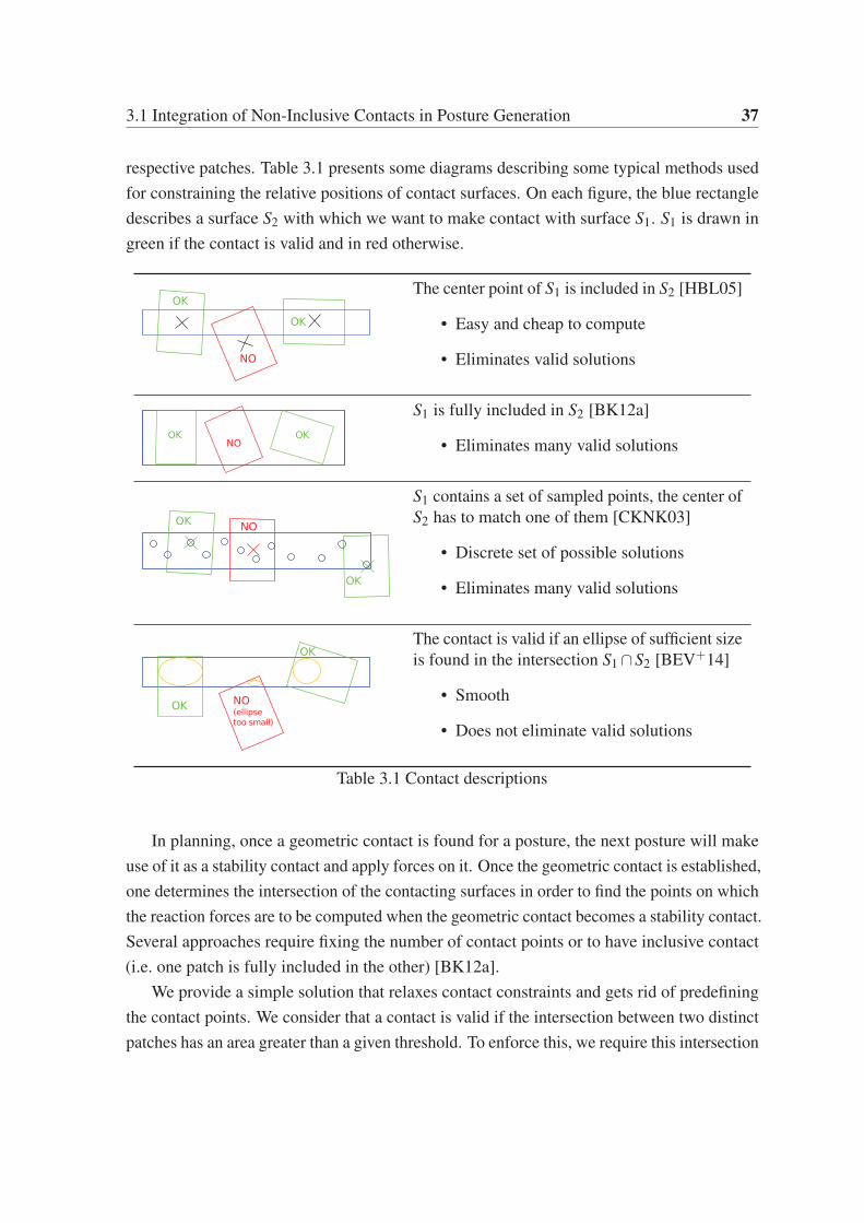
3.1 Integration of Non-Inclusive Contacts in Posture Generation 37
respective patches. Table 3.1 presents some diagrams describing some typical methods used
for constraining the relative positions of contact surfaces. On each figure, the blue rectangle
describes a surface S2 with which we want to make contact with surface S1. S1 is drawn in
green if the contact is valid and in red otherwise.
The center point of S1 is included in S2 [HBL05]
• Easy and cheap to compute
• Eliminates valid solutions
S1 is fully included in S2 [BK12a]
• Eliminates many valid solutions
S1 contains a set of sampled points, the center of
S2 has to match one of them [CKNK03]
• Discrete set of possible solutions
• Eliminates many valid solutions
The contact is valid if an ellipse of sufficient size
is found in the intersection S1∩S2 [BEV+14]
• Smooth
• Does not eliminate valid solutions
Table 3.1 Contact descriptions
In planning, once a geometric contact is found for a posture, the next posture will make
use of it as a stability contact and apply forces on it. Once the geometric contact is established,
one determines the intersection of the contacting surfaces in order to find the points on which
the reaction forces are to be computed when the geometric contact becomes a stability contact.
Several approaches require fixing the number of contact points or to have inclusive contact
(i.e. one patch is fully included in the other) [BK12a].
We provide a simple solution that relaxes contact constraints and gets rid of predefining
the contact points. We consider that a contact is valid if the intersection between two distinct
patches has an area greater than a given threshold. To enforce this, we require this intersection

38 Extensions of Posture Generation
to contain an ellipse whose surface can possibly be maximized. Convex patches allow writing
the inscription constraints easily by means of half-spaces.
3.1.1 Contact geometry formulation
Let us consider a contact defined by two flat surfaces S1 and S2 which are respectively two
convex polygons P1 and P2. For this contact to be valid, it is necessary that the intersection
P1∩P2 is not empty.
An important remark is that the number of sides of the intersection polygon is not known
a priori and, as shown in Figure 3.2, this number can change depending on the configuration.
Each time this number changes, the gradient of the area of the intersection is discontinuous.
This is an issue for integrating any constraint or objective based on the area because we use a
solver for smooth optimization problems. This issue could be dealt with by using non-smooth
optimization algorithms, but such algorithms are slower and less available, and our posture
generator is not designed to use them. Moreover, supposing that we want to write constraints
4 vertices 7 vertices
Figure 3.2 Topological instability of P1∩P2
based on the sides of the contact area, then, the number of constraints would change with
the number of vertex of P1 ∩P2. The large majority of the optimization software cannot
deal with a non-constant number of constraints. The solution proposed in Section 3.1.2
overcomes these issues by defining a set of constraints that is independent of the topology of
the intersection area.
3.1.2 Non-inclusive contact constraints
Main Idea
We propose a smooth formulation of the non-empty intersection between two contact surfaces.
We assume that co-planarity of S1 and S2 is obtained by using the constraints presented
in (2.18). Here we focus on the intersection of the two polygons P1 and P2, respectively
describing the contours of S1 and S2.

3.1 Integration of Non-Inclusive Contacts in Posture Generation 39
To avoid dealing with changes of topology, we consider using an ellipse E included
in P1 ∩P2 to estimate the area of the intersection. Since P1 and P2 are convex polygons,
then P1∩P2 is also a convex polygon. A convex polygon can be seen as an intersection of
half-planes based on the lines supporting its edges. Thus, an ellipse is inside of a convex
polygon if it lies entirely in the corresponding half-planes. Having the ellipse be included in
the intersection of two polygons is equivalent to having it included in both polygons:
E ⊂ P1∩P2 ⇐⇒ E ⊂ P1 AND E ⊂ P2 (3.1)
Even if the number of edges of P1 ∩P2 can change, the numbers of edges of P1 and P2
respectively are fixed. To assert that an ellipse lies in a half-plane, we need a function that
is positive when the ellipse is in it (with zero value when the ellipse is on the edge) and
negative otherwise. The signed distance to the line defining the half-space is a good candidate
(distance ellipse-line if the ellipse is in the half-plane, opposite of the penetration distance if
not), but actually, any pseudo-distance does the job. And a sufficient condition for the ellipse
to be inside the polygons intersection is that the pseudo-distance between the ellipse and
each edge of both polygons is positive (see Figure 3.3). By considering each edge separately
as opposed to the pseudo-distance of the ellipse to a whole polygon, we can write smooth
constraints with a simple pseudo-distance function. We develop such a pseudo-distance in
what follows.
Figure 3.3 Distance between E and P1∩P2.
Pseudo-distance
Computing the distance between an ellipse and a line is not straightforward, whereas the
distance between a line and a circle is very easy to compute. Also, we note that in the frame
FE defined by the ellipse’s axes and pseudo-radius, the ellipse is a circle of radius rE = 1
(The x-unit along the first axis of the ellipse is rx, the first radius of the ellipse, the y-unit
along the second axis of the ellipse is ry, the second radius). The transformation from the

40 Extensions of Posture Generation
original frame F0 in which the ellipse and the polygons are described to the ellipse’s frame
FE is just the composition of a rotation and a scaling of the space along the axes of the ellipse
with a scaling vector [ 1rx, 1
ry]. The effect of such a transformation applied to an ellipse and
two polygons is shown in Figure 3.4. We thus defined the following pseudo-distance from an
ellipse to a half-plane as the signed Euclidean distance from the corresponding unit circle to
the transformed half-plane in the frame FE .
r xry
11
Figure 3.4 Transformation from F0(O0,X0,Y0) to FE(OE ,XE ,YE)
Now let us consider a single segment pi p j and an ellipse E defined in F0. The expression
of a vector vF0T = [vx,vy]F0
in FE is obtained by applying the formula (3.2).
vFE =
[1rx
0
0 1ry
]·
[cos(θ) sin(θ)
−sin(θ) cos(θ)
]·vF0
(3.2)
In FE , the distance between the circumference of E and the segment pi p j is:
ds(E , pi p j) =
−−→pi p j
∣∣FE∧−−→piOE
∣∣∣FE
‖−−→pi p j‖FE
−1 (3.3)
where ∧ denotes the cross product and OE is the center of the ellipse.
To avoid numerical problems when the segment pi p j is small, it is preferable to multiply
this distance by ‖−−→pi p j‖FE before using it as a constraint. Then we get the following constraint:
− −−→pi p j
∣∣FE∧−−→piOE
∣∣∣FE
+‖−−→pi p j‖FE ≤ 0 (3.4)

3.1 Integration of Non-Inclusive Contacts in Posture Generation 41
The combination of these equations (3.2) and (3.4) applied for each edge of the polygons
gives us all the necessary tools to develop a set of constraints that ensures that an ellipse is
inside the intersection of two polygons.
Modification of the optimization problem
To include the above idea in our posture generation, we need to modify the optimization
problem (2.42) as follows. Each non-inclusive geometrical contact adds five variables to the
optimization vector, corresponding to the position, orientation, and radiuses of the ellipse
(x, y, θ , rx and ry). One constraint of ellipse inclusion (as described above) is added to the
problem for each edge of the polygons. The parameters rx and ry are given lower positive
bounds to ensure that the ellipse is not empty. The existence of a contact between S1 and S2
is thus transformed into the existence of rx and ry respecting their bounds. In summary, this
kind of constraint adds 5 variables and card(P1)+ card(P2) constraints to the optimization
problem (where card(P) denotes the number of edges of polygon P), while the ‘usual’
inclusion constraint adds 0 variable and card(P1)card(P2) constraints. The existence of the
contact can alternatively be enforced by imposing a minimum area for the ellipse.
Maximization of the contact area
The formulation in the above section only ensures the existence of a contact of minimal size.
However, one may want to find a contact area as large as possible, so that it is more likely to
be able to support strong forces and have strong friction forces, which is helpful to guarantee
the stability of the robot. Therefore, it seems appropriate to try and maximize the area of
contact between two polygons. As explained before, computing the area of the intersection
surface is not a good practice in our case. But the ellipse computed as above gives a lower
bound of the contact area.
E ⊂ P1∩P2 =⇒A(E)≤A(P1∩P2) (3.5)
with A(X) being the area of X .
Therefore, we can maximize the area of the ellipse in order to maximize the contact area.
This is readily obtained by minimizing the value of fellipse(rx,ry) =−πrxry in the modified
problem (2.42). In case there are other cost functions, the above cost can be added to them
with a desired weight. This requires, however, to scale properly the cost so as to have a
meaningful and easy-to-tune weight: the range of value of the ellipse’s area goes from 0 to
A(P1∩P2)≤min(A(P1),A(P2)). This latter quantity can be small (a typical area of contact
of a humanoid robot is about 0.01m2, some environment surfaces can be smaller). To get a

42 Extensions of Posture Generation
basic cost (before weighting) of magnitude around 1, we use the following scaling:
fellipse(rx,ry) =−πrxry
min(A(P1),A(P2))(3.6)
This cost’s absolute value will always be less than 1, but not much less around the optimum,
in most cases.
Using a non-inclusive contact to maintain stability
The method we presented so far allows finding a configuration in which a new non-inclusive
contact is added, but this contact does not bear any force. It is found as a geometrical contact,
but will eventually have to bear some forces, and thus, become a stability contact. Usually,
for a stability contact, each vertex of the contact area is considered as the application point of
a force that has to be in a friction cone. Since our method allows dealing with surfaces that
are intersecting each other, the contact surface is not known beforehand. Therefore, as soon
as a non-inclusive contact is going to be used for the stability, we compute the intersection
of the two polygons P1 and P2 that are involved, and that intersection P1∩P2 is the contact
surface, and its vertices will bear the forces. We do not present here the algorithm to compute
the intersection of two convex polygons, as it can be found in the literature easily.
Extension to singular cases
Our method can be extended to be used to approximate singular situations, such as finding an
optimal contact with a linear or even punctual surface. This is done by giving a slight width
to the point or the line. This approximation is physically grounded: in terms of real contacts,
linear or punctual contacts do not exist. In fact, since all objects are deformable, even slightly,
the contact area between two objects cannot be a perfect line, and must have a non-null area,
which justifies that linear and punctual contacts can be modeled as thin contact surfaces. By
defining such a surface, we impose partly the orientation of the contact. Here again, one must
be careful with numerical issues. Dealing with small numbers (here we would like to take
the width of a fraction of a centimeter) may induce conditioning problems. Also, having two
close parallel constraints of opposite direction (i.e. g(x)≤ α and −g(x)≤ α with α small)
is not a good practice in optimization as it will lead the solver to take small steps. Therefore,
it is best to apply a scaling to the constraints by applying a geometrical scaling to P1 and P2
in the appropriate direction.
Likewise, constraints on the area of the ellipse should be based on the same formulation as in
equation (3.6).

3.1 Integration of Non-Inclusive Contacts in Posture Generation 43
3.1.3 Simulation results
In order to illustrate our method, we present some examples starring the HRP-2 and ATLAS
humanoid robots, that are typical posture generations encountered in multi-contact plan-
ning. For the implementation of our posture generator, we use the RobOptim optimization
framework [MLBY13] relying on the IPOPT solver [WB06].
Inclined ladder climbing
In this first example, we generate a posture that is part of an inclined ladder climbing planning.
We consider that the robot HRP-2 reached a posture in which its right foot is on the first
step and its right hand is grasping the right guardrail, both of those contacts are bearing
forces. Those contacts are fixed, and we search a posture that adds to it a geometrical contact
between the left foot and the second step. We require the contact to include an ellipse with
both radiuses bigger than 40% of the ladder step’s width. The resulting posture and a close-up
view of the contact areas are shown in Figure 3.5. The latter shows clearly how an ellipse
of sufficient size is found, included in the contact area between the left foot and the second
step. It also shows that the contact forces on the right foot are located on the vertex of the
intersection of the contact surfaces between the right foot and the first step, which was also
generated with our method, in a prior posture generation. One can note that we use a contact
area slightly smaller than the actual surface under the foot of the robot. We use indeed safety
margins to account for modeling errors so that the obtained posture is achievable by the real
robot.
Vertical ladder climbing
In the second example, we generate a posture in which the robot climbs a vertical ladder. In
this particular step, the robot is using its right foot and both hands to maintain its stability
on top of the first rung of the ladder. We search a posture that keeps those previous contacts
and adds a geometrical contact between the left foot and the second rung of the ladder. The
result of that optimization can be observed on Figure 3.1, with the robot posture on the left
and a close-up look at the contact areas on the right. The difficulty of this situation is that a
contact has to be made with a very thin surface of the environment (the ladder rung). The
contact chosen by our software includes an ellipse which first axis is the width of the robot’s
foot and second axis is as thin as the ladder rung. This example also illustrates one limitation
of our method: it only considers planar contacts and if one wants to model a purely linear
contact another contact model must be used, since our modeling of those singular cases is
approximative.

44 Extensions of Posture Generation
Figure 3.5 HRP2 ladder climbing posture and up close view of the contact areas (green/red:
contact polygons; blue: contact ellipse; red arrows: contact forces resultants)
Figure 3.6 Atlas climbing stairs with small steps by maximizing the size of the contact areas
(green/red: contact polygons; blue: contact ellipse; red arrows: contact forces resultants)

3.1 Integration of Non-Inclusive Contacts in Posture Generation 45
Climbing Stairs
In a third simulation, the ATLAS robot climbs a flight of stairs. All the steps are too small for
the robot to put its entire foot on. Therefore, it has to make a non-inclusive contact and we
propose to maximize the size of the contact area with the ellipse included in it, as explained in
Section 3.1.2. The size of the contact area is limited by the fact that the foot cannot penetrate
the wall behind each step. On Figure 3.6, we present 3 postures generated in this environment.
On each of those postures, we see that the ellipse’s size is maximized until the foot enters in
collision with the vertical wall behind each step. And when possible, like on the last step,
the contact area is maximized without collision limitation and the foot is positioned as fully
included in the support surface. We can see here that even when the size of the ellipse is
maximized while competing with other nonlinear constraints like collision avoidance, our
method still works well and leads us to a satisfactory solution. It has been used to actually
make the robot climb a vertical ladder and presented in [VKA+16] and [VKA+14].
Walking along a path made of small objects
In the last simulation, the HRP-2 robot has to cross a gap by making contacts with small
surfaces. As for the previous simulation, the two objects with which the feet of the robot will
be in contact are too small for making a complete contact, instead, non-inclusive geometric
contacts are found by maximizing the area of an ellipse that fits in the intersection of the
polygons involved in the contact. Results are presented in Figure 3.7. As we can see, the
feet turns slightly, to be more aligned with the support surfaces, yet they do not become
completely aligned with these supports, which would permit to get the biggest ellipse area.
This is due to the fact that a posture cost is competing with the area cost, yielding this
compromise. Under each simulation result, an image presents the disposition of the foot
(in green) that is in geometrical non-inclusive contact with a step (in blue) and the optimal
ellipse that has been found.
3.1.4 Discussion and conclusion
Generating arbitrarily shaped contact areas proved to be doable very simply in an optimization
based posture generation module. We focused on writing constraints that have continuous
gradients since the posture generation problem is dominantly smooth. Hence, our geometric
contact model can be useful for other optimization based purposes, for example, control or
trajectory optimization, and any gradient-based descent scheme which handles inequalities
(e.g. [EMW10]). While we were expecting an increase of computation time due to the
addition of new variables in the problem (5 more for a total of 80–100 variables) we noticed

46 Extensions of Posture Generation
Figure 3.7 Simulation results for crossing a gap by walking on small items
that the timings obtained with this method are sensibly the same that with our previous version
of the posture generator with full contact surface inclusion. Consequently, this method
offering a richer contact search (exploration) during planning comes without degrading
computation time. In fact, it truly allows us to substantially reduce the time spent by the
user in ad-hoc tuning the shapes of the contact patches, or fixing the contact positions that
were previously done by hand. Also, it is fairly easy to implement and extends multi-contact
planning algorithms like the one described in [EKM13] to give it richer planning possibilities.
This method extends straightforwardly to point cloud data as far as polygonal convex patches
can be extracted. But one of its limitations is that in its current form, it cannot handle contacts
with non-convex surfaces.
3.2 Torque derivation
In this section, we present an efficient algorithm to compute the Jacobian matrix of the
robot’s joint torques with respect to all its articular variables and the variables involved in the
expression of the external forces applied to this robot. The evaluation of the joint torques
Jacobian matrix is useful to solve optimization problems in which the torques are involved in
the constraints or in the cost function. The computation of the joint torques Jacobian matrix
is done by differentiating algorithm 4. In most cases, the acceleration of gravity could be
replaced by its value on earth ac =~0 and af = g~z. For the sake of generality, we keep it as ac
and af in the algorithm description, which could be useful if the robot is in a moving vehicle,
for example. We first write algorithm 4 in its matrix form (which is more convenient for its
derivation).

3.2 Torque derivation 47
Algorithm 5 Inverse Static algorithm on Matrix Form
for i = 0 : nB do
f Gi =
[mG
i
fGi
]= IW
[iRW 0
−iRWitW
iRW
][ac
af
]−
[iRW −iRW
itW0 iRW
][mext
i
fexti
]
end for
for i = nJ−1 : 0 do
τi = f Gi
TSi
if pred(i) 6=−1 then
f Gpred(i)←
[mG
pred(i)
fGpred(i)
]+
[RPtS
i
TtPtSi RPtS
i
T
0 RPtSi
T
][mG
i
fGi
]
end if
end for
The variables of this algorithm w.r.t. which we need to differentiate it, are the configura-
tion of the robot q and the variables of the external wrenches which can themselves depend
on q and some other variables y, for example, in the case of a contact with another robot, the
application point and value of those forces depend on q and on the configuration of the other
robot. We denote dim(q) and dim(y) the dimensions of q and y respectively. We assume that
the derivatives of mexti and f ext
i :∂mext
i
∂q,
∂mexti
∂y,
∂ f exti
∂q, and
∂ f exti
∂yare known.
Besides mexti and f ext
i , all the quantities of the algorithm depend only on q. Therefore, the
derivation w.r.t y is trivial and is automatically computed by our final algorithm. From here
we will focus on the derivation w.r.t q.
Recall the expression of the Jacobian of a robot’s body:
JacWi =
∂ iRW
∂q0· · · ∂ iRW
∂q j· · · ∂ iRW
∂qdo f
∂ itW∂q0
· · · ∂ itW∂q j
· · · ∂ itW∂qdo f
=
[ωi,0 · · · ωi, j · · · ωi,do f
vi,0 · · · vi, j · · · vi,do f
](3.7)
Note the following relations that make use of the robot’s Jacobian to compute derivatives:
∂ iRW u
∂q j= iRW u∧ωi, j =
iRW uωi, j (3.8)
∂ iRWitW ∧u
∂q j= iRW vi, j∧u+ iRW
(itW ∧u
)∧ωi, j (3.9)
=−iRW uvi, j +iRW
(itW u
)ωi, j (3.10)
Let’s differentiate the first equation of Algorithm 5 w.r.t q j.

48 Extensions of Posture Generation
A =
[iRW 0
−iRWitW
iRW
][ac
af
](3.11)
B =
[iRW −iRW
itW
0 iRW
][mext
i
fexti
](3.12)
f Gi = IW A−B (3.13)
∂A
∂q j=
iRW acωi, j
−iRW
(
itW ac)
ωi, j +iRW acvi, j +
iRW afωi, j
(3.14)
∂B
∂q j=
−iRW
(
itW fexti
)ωi, j +
iRW fexti vi, j +
iRW mexti ωi, j
iRW fexti ωi, j
(3.15)
+
[iRW −iRW
itW
0 iRW
][∂mext
i
∂q∂ fext
i
∂q
](3.16)
We rearrange the equations in order to make the jacobian appear. Putting all the pieces of
ω and v together allows grouping all the j-derivatives to obtain the derivative of f Gi with a
single equation.
M =
iRW ac 0
−iRW
(
itW ac)+ iRW af iRW ac
(3.17)
N =
−iRW
(
itW fexti
)+ iRW mext
iiRW fext
i
iRW fexti 0
(3.18)
∂ f Gi
∂q= (IW M−N)JacW
i +
[iRW −iRW
itW
0 iRW
][∂mext
i
∂q∂ fext
i
∂q
](3.19)
The derivation of the second equation is obvious:
τi = f Gi
TSi (3.20)
∂τi
∂q= ST
i
∂ f Gi
∂q(3.21)
(3.22)

3.2 Torque derivation 49
Note the following relations:
∂RJi
Tu
∂q j=−SR
i, j∧ (RJi
Tu) =
(RJ
i
Tu)SR
i, j (3.23)
∂ tJi ∧RJ
i
Tu
∂q j= St
i, j∧(
RJi
Tu)− tJ
i ∧(
SRi, j∧
(RJ
i
Tu))
(3.24)
=−(RJ
i
Tu)St
i, j +
((RJ
i
Tu)· tJ
i
T−
((RJ
i
Tu)
T· tJ
i
)I3
)SR
i, j (3.25)
(3.26)
The last equation’s derivation goes as follows:
f Gpred(i)← f G
pred(i)+
[RPtS
i
TtPtSi RPtS
i
T
0 RPtSi
T
][mG
i
fGi
](3.27)
= f Gpred(i)+
[Rx
iT tx
i Rxi
T
0 Rxi
T
][RJ
i
TtJi RJ
i
T
0 RJi
T
][mG
i
fGi
](3.28)
(3.29)
We define Ki as:
Ki =
(RJ
i
TmG
i )+(
RJi
TfGi
)· tJ
i
T−((RJ
i
TfGi )
T· tJ
i
)I3 −
(RJ
i
TfGi )
(RJ
i
TfGi ) 0
(3.30)
∂ f Gpred(i)
∂q←
∂ f Gpred(i)
∂q−
[Rx
iT tx
i Rxi
T
0 Rxi
T
]KiSi (3.31)
In the following algorithm, we use the following notation x to combine the variables q
and y:
x =[q y
](3.32)
∂ fext
∂x=
[∂mext
i
∂q
∂mexti
∂y∂ fext
i
∂q
∂ fexti
∂y
](3.33)
The entire algorithm for calculating the torque jacobian is presented in Algorithm 6.

50 Extensions of Posture Generation
Algorithm 6 Torque Jacobian Calculation
Compute the Jacobian of generalized forces
for i = 0 : nB do
f Gi = IW
[iRW 0
−iRWitW
iRW
][ac
af
]−
[iRW −iRW
itW
0 iRW
][mext
i
fexti
]
M =
iRW ac 0
−iRW
(
itW ac)+ iRW af iRW ac
N =
−iRW
(
itW fexti
)+ iRW mext
iiRW fext
i
iRW fexti 0
∂ f Gi
∂x= (IW M−N)
[JacW
i 06×dim(y)
]+
[iRW −iRW
itW
0 iRW
]∂ fext
∂x
end for
Compute the Jacobian of torques
for i = nJ−1 : 0 do
∂τi
∂x=
[Si 06×dim(y)
]T ∂ f Gi
∂x
if pred(i) 6=−1 then
K =
(RJ
i
TmG
i )+(
RJi
TfGi
)· tJ
i
T−((RJ
i
TfGi )
T· tJ
i
)I3 −
(RJ
i
TfGi )
(RJ
i
TfGi ) 0
f Gpred(i)← f G
pred(i)+XPtSi (q)
−∗f Gi
∂ f Gpred(i)
∂x←
∂ f Gpred(i)
∂x−
[Rx
iT tx
i Rxi
T
0 Rxi
T
]K ·
[Si 06×dim(y)
]
end if
end for
This algorithm efficiently computes the exact joint torques Jacobian for a robotic system
subject to any type of external forces.

3.3 On the use of lifted variables for Robotics Posture Generation 51
3.3 On the use of lifted variables for Robotics Posture Gen-
eration
The goal of this thesis is, on the one hand, to enable writing more complex and various
problems in simpler ways by improving the formulation of posture generation problems,
and on the other hand, to improve and adapt the resolution methods for those problems.
This section focuses on the latter issue. We formulate posture generation problems in an
optimization friendly way in order to solve them using nonlinear constrained optimization
algorithms. In this section, we investigated the usage of the lifted optimization method
presented in [AD10] to the posture generation problems. In fact, the authors suggested that
their method would be suitable for inverse kinematic problems.
The idea of lifting optimization is to consider a complex equation F(q) = 0 and decom-
pose it into simpler functions f1, f2, . . . , fm that all depend only on the original variable
q and on the output of functions of lower index eq. (3.34) that are replaced by additional
variables w1,w2, . . . ,wm, that are called the ‘lifted variables’.
wi = fi(q,w1,w2, . . . ,wi−1), ∀i ∈ [1, . . . ,m] (3.34)
Such that they can be used in a chain to recompose F :
F(q) = fF (q,w1,w2, . . . ,wm) (3.35)
= fF (q, f1(q), f2(q,w1), f3(q,w1,w2), . . . , fm(q,w1, . . . ,wm−1)) (3.36)
= fF (q, f1(q), f2(q, f1(q)), f3(q, f1(q), f2(q, f1(q))), . . . , fm(q, . . . , fm−1(q, · · ·)))
(3.37)
With this formulation and the additional lifted variables wi, i ∈ [1, . . . ,m], the problem
F(q) = 0 can be rewritten as the following lifted problem:
G(q,w) =
f1(q)−w1
f2(q,w1)−w2
f3(q,w1,w2)−w3
...
fm(q,w1, . . . ,wm−1)−wm
fF(q,w1, . . . ,wm−1,wm)
= 0 (3.38)

52 Extensions of Posture Generation
This modified formulation can be used for any function of our optimization problem
to reduce the complexity of individual equations at the cost of adding extra variables and
constraints. By reducing the complexity of the functions, which often results in reducing
their polynomial degree, we ought to improve the quality of their quadratic approximations,
which should lead to better convergence properties of the Newton scheme.
One obvious drawback of this approach for solving nonlinear problems is the increased
size of the linearized problem to solve at each iteration of the optimization. Fortunately,
[AD10] proposes an algorithmic trick leveraging the triangularity of the Jacobian of G(q,w)
to condense the lifted problem into a problem of the same size as the original one. Thus, the
resolution of each iteration should take approximately the same time as with the original
problem.
The lifted variable approach is known to be superior to the non-lifted one in the problem
of shooting methods for boundary value problems [Osb69]. With good intuition, the authors
of [AD10] state that the lifting idea could be directly transferred in the context of kinematic
chains found in robotics. Indeed, as we state in Section 2.1, the equation that governs the
transformation of a robot’s end effector on body i, iXW (q) is constructed iteratively and seems
to be a good candidate for lifting. If we consider a single chain robot with m bodies, such
that κ(m) = 0,1,2, . . .m the mXW (q) = Xgoal can straightforwardly be lifted as follows:
G(q,w) =
1XW (q)−w1
2X1(q) ·w1−w2
3X2(q) ·w2−w3
...mXm−1(q) ·wm−1−wm
wm−Xgoal
= 0 (3.39)
The transformation of a body is used in almost all the constraints and cost functions of
posture generation problems, thus, we can use this lifting approach in most functions of our
problems. This formulation can be generalized to more complex robots by considering/lifting
only the bodies in the direct chain from the base to the end effector.
3.3.1 Lifting Algorithm
In order to explore the capabilities of optimization on lifted problems, we developed and
studied several lifting approaches based on different lifting criterion. A lifting criterion is a
criterion that should be satisfied as best as possible by all the functions present at the end of
the lifting process. For example, the degree of a polynomial can be a used, one could require

3.3 On the use of lifted variables for Robotics Posture Generation 53
that all the functions are polynomials of at most degree m. In 3.39, we lifted based one the
criterion that each function should only contain a single joint transformation.
Let us consider an example with a simple planar 2 axis robot, with 2 successive links of
length 1 attached by revolute joints. Its articular variables are denoted q = (q1,q2) and the
expression of the end-effector’s (EE) position is the following:
(cos(q1)+ cos(q1) cos(q2)− sin(q1) sin(q2)
sin(q1)+ cos(q1) sin(q2)+ cos(q2) sin(q1)
)=
(EEx(q)
EEy(q)
)(3.40)
Those equations are polynomials in the variables cos(q1), sin(q1), cos(q2), sin(q2).
Furthermore, they are polynomials of degree 1 in each of those variables separately. This
observation extends to the case of any robot composed of the joints presented in Section 2.2
and that does not contain kinematic loops (kinematic loops are not considered in this thesis).
The operators ‘addition’, ‘subtraction’, ‘multiplication’, ‘sinus’ and ‘cosinus’ are enough to
describe the kinematics of a robot.
We developed a generic algorithm which allows to automatically lift symbolic functions,
and in particular, polynomials of trigonometric functions, based on a given criterion. To
do so, we use symbolic variables. A symbolic equation can be seen as a graph of atomic
operations (addition, multiplication, and other functions), which can, in turn, be explored
and truncated at appropriate places where we insert additional variables. Figure 3.8 presents
the graph of atomic operations for equation (3.40), where the green circles represent the
original variables, the yellow ones represent the lifted variables, the pink ones represent the
atomic operations and the red circles represent the final atomic operations that lead to the
end effector equations.
To lift a set of equations, we explore the graph from left to right. At each node of the
graph, we consider the sub-graph that lies on its left. If this sub-graph violates our criterion,
a lifting variable is added and replaces the sub-graph. Then we iterate this process on the
remaining graph until it does not violate the criterion. Given that the equations to solve
are polynomials in terms of the trigonometric functions, we decided to lift them based on a
criterion of maximum degree of the lifted polynomials. We define the degree function as the
degree of a polynomial with the specificity that trigonometric functions are considered to be
polynomials of infinite degree (and thus are always lifted, no matter the maximum degree
criterion). We also consider the option of eliminating or not the trigonometric functions.
By eliminating the trigonometric functions, we mean that we reformulate the problem so
that, given a variable x that appears in our equations in the forms cos(x) and/or sin(x), we
introduce 2 new variables sx and cx; replace all the occurrences of cos(x) by cx and all the

54 Extensions of Posture Generation
Figure 3.8 Computation graph for end effector position of a 2 axis planar robotic arm. Top:
Direct equations. Bottom: Lifted equations. Green circles represent the original variables,
yellow the lifted ones, pink represent intermediary operations and red represent the final
operation for the end effector equations

3.3 On the use of lifted variables for Robotics Posture Generation 55
occurrences of sin(x) by sx, and to ensure the equivalence of the two formulations, we add
the equation cx2 + sx
2 = 1 to our problem.
For example, lifting the set of equation (3.40) with a maximum degree of 2 and without
eliminating the trigonometric functions gives the following system, with all the wi jbeing the
additional lifted variables:
Lifted Equations
cos(q1) = w11
sin(q1) = w12
cos(q2) = w13
sin(q2) = w14
w11.w13
= w21
w12.w13
= w22
w11.w14
= w23
w12.w14
= w24
End-effector’s position(w11
+w21−w24
= EEx
w12+w22
+w23= EEy
)
(3.41)
Adding to it the elimination of trigonometric functions gives the following system. Note
that here, all the equations are polynomials of degree at most 2, no trigonometric function is
present, and the optimization variables are(cq1
,cq2,sq1
,sq2
)instead of (q1,q2).

56 Extensions of Posture Generation
Lifted Equations
cq1.cq2
= w21
sq1.cq2
= w22
cq1.sq2
= w23
sq1.sq2
= w24
Additional equations(cq1
2 + sq12 = 1
cq22 + sq2
2 = 1
)
End-effector’s position(cq1
+w21−w24
= EEx
sq1+w22
+w23= EEy
)
Eliminated equations (Not used in further calculations)
cos(q1) = cq1
sin(q1) = sq1
cos(q2) = cq2
sin(q2) = sq2
(3.42)
This lifting methodology can be extended to most robotic systems. We also developed a
lifting method that follows the principle described in (3.39), in which case, we get another
set of equations similar to (3.3.1).
3.3.2 Optimization on lifted variables
We want to estimate the gain in terms of performance that result from using a lifted formula-
tion on a posture generation problem. In order to do so, we implemented and/or used several
optimization algorithms.
Given the lifted equations and their derivatives, it is straightforward to solve and compare
the results obtained by the different solvers provided in Matlab (trust-region-reflective;
interior-point; active-set and SQP) for the set of equations with or without lifting. A limitation
of our approach is that it does not allow us to easily use the condensed method presented
in [AD10] in the resolution of the problems because it is necessary to de-condensate and then
update the problem between 2 iterations of the optimization. The lifted condensed problem is
meant to be equivalent to the lifted full-space problem (lifted non-condensed problem), in the
sense that they generate the same optimization steps. Solving lifted problems with or without
using the condensation trick gives the same result in the same number of iterations. The
only difference is that with the lifted full-space problem, each iteration takes more time to

3.3 On the use of lifted variables for Robotics Posture Generation 57
compute. In our study, this is not a problem, we want to evaluate the performances in terms of
the number of iterations first, and if it appears that the lifted problem resolution outperforms
the non-lifted, then we will implement the condensation trick for our problems and solvers,
which will bring the per iteration time to be approximately the same as in the direct problem
case. Therefore, we only tried those algorithms on the direct problems (non-lifted problem)
and the lifted full-space problems.
In addition to the Matlab solvers, we implemented the optimization algorithms proposed
in [AD10], namely: the Lifted Newton, the Lifted Gauss-Newton and the Lifted SQP. With
the only difference that we use the symbolic expressions of all our function and compute
the symbolic expressions of the Jacobians and Hessians of our problems, instead of using
auto-differentiation methods.
We implemented the Newton and Gauss-Newton methods for condensed lifted problems
and obtained the same results as the ones presented in paragraph 5.2 of [AD10] that show
the efficiency of a lifted approach in a specific kind of root finding problems. Our problems
require the use of nonlinear cost and constraints, thus, a Newton method is not sufficient to
solve them, whereas an SPQ method is.
We implemented the lifted and direct SQP approaches as described in paragraph 3.2.3
of [AD10]. The hessian matrices in our problems are usually not symmetric positive definite,
so we need to use a globalization method as well as a regularization of the Hessian to enforce
convergence. For globalization, we implemented some line search methods with Armijo and
Wolfe conditions, as well as a filter with line search (see A.5.2). And for regularization, we
approximate the full-space hessian matrix through BFGS updates (with Powell’s correction)
or SR1 updates. We implemented different ways to initialize the lifted variables. They can
either be all initialized with zero value, or all random, or their initial value can be computed
such that all the lifted equations are satisfied (m first lines of 3.38). Those methods are
presented in [BGLS02].
3.3.3 Results, experimentation
In order to evaluate the performances of the lifting approach in the resolution of posture
generation problems, we conducted many experiments in which we solved simple inverse
kinematics problems with the different solvers and lifting methods available.
A difficulty that arises in that endeavor lays in the inherent combinatorial aspect on the
choice of formulation and resolution method. Indeed, we need to choose one item amongst
each or the categories cited below:
• Type of lifting method
58 Extensions of Posture Generation
– None, direct problem
– Lifted with maximum degree of 2
– Lifted based on Joints (one joint transformation per equation)
• Treatment of trigonometric equations
– Keep trigonometric equations
– Eliminate trigonometric equations
• Type of Solver
– Our custom SQP
– Matlab optimization toolbox fmincon (active-set, interior point, SQP)
• Type of initialization of the lifted variables
– Zeros
– Random
– Satisfying the lifted equations
• Type of Hessian update
– None
– BFGS
– SR1
• Type of globalization
– Wolfe
– Armijo
– Filter
• Cost function
– None
– Norm 2 of articular parameters

3.3 On the use of lifted variables for Robotics Posture Generation 59
Figure 3.9 Examples of robots used
The number of possible combination of choices is large and grows with any new possibility
added.
We devised a set of simple robots to be the toy examples of our experimentation. We used
fixed base robots with revolute joints only. To study the influence of the number of degrees
of freedom of a robot on the optimization performance, we studied planar robots composed
of n successive links of length 1 attached to one another by revolute joints. We also studied
a 7 axis 3D manipulator arm robot and a planar upper body robot with 2 arms. Illustration
of those different types of robots are given in Figure 3.9, where blue lines represent the
links, red circles represent the revolute joints, green squares represent the origin of links, the
biggest green square being the origin of the base link of the robot, and the red cross is the
end effector.
We propose to use the following test to compare the performances of different lifting
methods for all our experiments:
1. Choose a robot and a resolution method
2. Generate 1000 pairs of initial configuration and end effector goal
3. Solve the problem of finding a configuration in which the end effector reaches the goal
for all the available formulations:
• Direct: Direct formulation
• Direct Trigo: Direct with trigonometric elimination
• Lifted: Lifted with maximum degree 2
• Lifted Trigo: Lifted with maximum degree 2 and trigonometric elimination
• Lifted Joint: Lifted based on joints

60 Extensions of Posture Generation
2 4 6 8 10 125
10
15
20
DOF
Iter
atio
ns
Direct
Direct trigo
Lifted
Lifted trigo
Lifted joint
Lifted joint trigo
Figure 3.10 Number of iterations to reach convergence against number of DOF of the n-axis
planar robot for the different lifting methods solved with our Custom SQP, BFGS, filter
line-search, random initialization
• Lifted Joint Trigo: Lifted based on joints and trigonometric elimination
This approach allows to fairly compare the performances of all lifting approaches on a
given problem. And to observe the influence of the number of degrees of freedom of the
robot on those performances, we use the n-axis planar robot model. We plot the average
number of iterations needed to reach convergence against the number of degrees of freedom
of the planar robot. In Figure 3.10 we present the results obtained for the resolution with our
custom SQP, using BFGS updates and a filter line-search, without cost function, initializing
all the variables randomly. In Figure 3.11 we present the best case in favor of the lifted
approach that we encountered, those results are obtained for the resolution with our custom
SQP, using SR1 updates and a filter line-search, without cost function, initializing all the
variables such that the lifted equations are satisfied.
The results presented in Figure 3.10 show that the direct formulation outperforms every
form of lifting for almost all the robots tested. This is the typical result that we observed in
most cases.
In Figure 3.11, we show one specific case where, with long kinematic chains (≥ 10 DOF),
the lifted methods are slightly faster to solve.
We studied many of the possible configurations of resolution methods (22 in total), but
not all of them. Still, it seems possible to draw some conclusions out of it, because in most
cases, the direct approach outperforms the lifted one.

3.3 On the use of lifted variables for Robotics Posture Generation 61
2 4 6 8 10 125
10
15
DOF
Iter
atio
ns
Direct
Direct trigo
Lifted
Lifted trigo
Lifted joint
Lifted joint trigo
Figure 3.11 Number of iterations to reach convergence against number of DOF of the n-
axis planar robot for the different lifting methods solved with our Custom SQP, SR1, filter
Line-Search, initialization satisfying lifted equations
The overall results we extracted from those experiments is that the best performing
method is: solving the direct formulation with our custom solver, using BFGS regularization
and either Armijo or filter line search and no cost function.
We observed that when the lifted variables are initialized randomly the direct problem is
usually solved faster than the lifted one. Whereas when the lifted variables are initialized so
that the lifted equations are initially satisfied, the results are sensibly the same for lifted and
direct approaches.
After comparison of all the results that we obtained, for all the planar robots with 2 to 12
degrees of freedom and across all the resolution methods that we tried, the best performing
formulation is the direct one, except for the 7 DOF robot, where the resolution of the lifted
problem with maximum degree 2 outperforms slightly all the other methods.
Overall, it seems that the idea of lifting does not provide better performances than the
direct formulation for solving inverse kinematics problem. In the view of that observation,
we decided to not go further in this research direction. Even though intuitively, the idea of
lifting seems to apply naturally to robotics equations, the results obtained were not satisfying
enough to justify investing more efforts in this approach so we decided to move on.

62 Extensions of Posture Generation
3.4 Conclusion
In this chapter, we presented three different and unrelated contributions to the field. First,
we proposed a convenient formulation of contact constraints that allows generating non-
inclusive contacts between two surfaces while ensuring that the size of the intersection
is satisfactory. Second, we presented a generic differentiation of the torque computation
algorithm, allowing to compute the joint torque jacobian of a robotic system. And finally,
we described our endeavor to use the idea of variable lifting in optimization to solve posture
generation problems, which unfortunately proved inefficient to accelerate the convergence of
our solvers on those problems.
In the next chapter, we will dive deeper in the field of nonlinear optimization on manifolds,
study how an SQP algorithm can be modified to be able to deal with manifolds and finally
present our own implementation of such an algorithm.

Chapter 4
Optimization on non-Euclidean
Manifolds
4.1 Introduction to optimization on Manifolds
Posture generation has been traditionally formulated as a problem over a Euclidean space.
Robot variables may, however, be more naturally expressed over non-Euclidean manifolds.
The archetypes for this in robotics are the rotational part of the root body of a robot, and ball
joints, whose variables live in SO(3). Some typical tasks are also naturally formulated on
different manifolds. For example, for making contact with any object that can be mapped
on a sphere, the contact point position for this object can be parametrized in S2 [EBK16].
The human shoulder can be elegantly parametrized on S2×R, as proposed in [BB01]. A
non-Euclidean manifold can be thought of as a space that is locally Euclidean, but not
globally. Like a sphere, if one looks in a small enough neighborhood, it looks Euclidean, just
like the surface of a giant sphere like the earth looks flat for a human standing on it.
Formulating the problem over Rn leads either to singularities that can prevent the conver-
gence of the optimization solver, or cumbersome writing of additional constraints to specify
that the variable is actually living on a manifold (see [BK12b]). In addition, since constraints
can be violated during the optimization process, the iterates may not be elements of the
search manifold.
For example, let us consider an optimization problem over the SO(3) manifold:
min.x∈SO(3)
f (x) (4.1)
subject to l ≤ c(x)≤ u

64 Optimization on non-Euclidean Manifolds
SO(3) is a 3-dimensional manifold. As such, it can be parametrized locally by 3 variables,
for example, a choice of Euler angles. But any such parametrization necessarily exhibits
singularities when taken as a global map (e.g. gimbal lock for Euler angles), which can be
detrimental to the optimization process.
For this reason, when addressing SO(3) with classical optimization algorithms, it is often
preferred to use one of the two following parametrizations:
• unit quaternion, i.e. an element q of R4 with the additional constraint ‖q‖= 1,
• rotation matrix, i.e. an element R of R3×3 (or equivalently R9) with the additional
constraints RT R = I and detR≥ 0.
Then, if we use the unit quaternion parametrization, the problem (4.1) becomes:
min.q∈R4
f (q) (4.2)
subject to
l ≤ c(q)≤ u
‖q‖2−1 = 0
The problem has 4 dimensions (to represent a 3-dimensional manifold), and has an
additional constraint that is entirely due to our formulation choice. With this formulation, it
is guaranteed that the solution q∗ is a unit quaternion, but not that all the iterates qk along the
optimization process have a unit norm. During the optimization process, at each iteration,
an increment p is computed by solving a quadratic problem that approximates (4.2) locally
around qk. In particular, this quadratic problem approximates the constraints linearly, thus,
for any step p not null, even if iterate qk is of unit norm, the next iterate qk+1 = qk +p does
not respect the unit-norm constraint (it respects the linearization of the unit-norm constraint).
So the quaternion qk+1 does not represent a rotation, while the objective and constraints
functions might expect it to do so. In general, with non-manifold formulations, at any given
iteration, the parametrization-related constraints can be violated, thus, the iterate might not
lie in the manifold. It is then needed to project them on it. Denoting πM the projection
(for example πM = q‖q‖ in the unit quaternion formulation), to evaluate a function f on a
manifold, we need to compute f πM. Furthermore, if the gradient is needed, then the
projection must also be accounted for in its formulation (authors in [BK12b] explained this
issue in great details for robotics problems with free-floating basis).
Similar issues can be found with the R3×3 matrix representation.
The alternative is to use optimization software working natively with manifolds, like the
ones presented in [BED+15] or [AMS08], and solve the optimization problem as written
in (4.1). This has an immediate advantage: we can write directly the problem without the

4.2 Optimization on Manifolds 65
need to add any parametrization-related constraints. Working directly with manifolds also
has the advantage that at each iteration, the variables of the problem represent an element of
the manifold. Having intermediate values naturally staying on the manifold can be useful to
evaluate additional functions that pre-suppose it (additional constraints, external monitoring,
etc.). It can also be leveraged for real-time applications where only a short time is allocated
repeatedly to the optimization, so that when the optimization process is stopped after a few
iterations, the output is still meaningful in the sense that it is always a point of the manifold.
In this chapter, we present our nonlinear optimization solver able to work on generic
smooth manifolds. We take inspiration from the approach used for unconstrained optimization
on manifolds in [AMS08] and adapt it to constrained optimization. To the best of our
knowledge, studies on constrained optimization on manifolds have been few. This is likely
due to the fact that in most problems the only constraint is to be on the manifold.We are only
aware of the work of Schulman et al. [SDH+14], where the authors explain the adaptation of
their solver to work on SE(3). This adaptation is however not valid for general manifolds
without more care for the Hessian computation.
A background motivation for this choice is to have our own optimization solver, instead
of a black box. This will allow us to specialize the solver for robotic problems, by leveraging
modeling properties and approximations, for a gain in time and robustness.
4.2 Optimization on Manifolds
In this section, we describe a Sequential Quadratic Programming (SQP) approach [NW06]
to solve the following nonlinear constrained optimization program
min.x∈M
f (x) (4.3)
subject to l ≤ c(x)≤ u
where M is a n-dimensional smooth manifold and c is a m-dimensional real-valued
function. The inequality constraints can be replaced with an equality one when the upper and
lower bounds are equal.

66 Optimization on non-Euclidean Manifolds
4.2.1 Representation problem
When M = Rn, the problem (4.3) is solved iteratively, starting from an initial guess x0
and performing successive steps xi+1 = xi +pi where pi is the increment found at the i-th
iteration, until convergence is achieved. The strategy to compute pi depends on the solver.
This classical scheme cannot be readily applied to optimization over non-Euclidean
manifolds. First of all, only (a subset of) the real numbers can be stored in computers. To
manipulate elements of M we need to choose a way to represent them in memory. This
results in choosing a representation space E= Rr (with r ≥ n) and a function
ψ :x 7→ x
M → ψ(M)⊆ E
ψ(M) is the subset of E containing the representation of all the elements of M. The
projection operator πM that we mentioned in Section 4.1 is actually a projection from E to
ψ(M).
With this representation, it is tempting to simply transform problem (4.3) as an opti-
mization over Rr with objective f ψ−1 and constraint cψ−1, and solve it with a classical
solver. But, as we stated in Section 4.1, if r = n we get singularities, and if r > n we add
parametrization-related variables and constraints to our problem and the iterates may not lie
on the manifold and need to be projected on it. So both those approaches are not satisfactory,
and another one needs to be taken.
Figure 4.1 StepOnSphere

4.2 Optimization on Manifolds 67
4.2.2 Local parametrization
By definition, there is always, at a point x of a smooth n-dimensional manifoldM, a smooth
function ϕx between an open set of TxM, the tangent space toM at x (which is isomorphic
to Rn), and a neighborhood of x inM, with ϕx(0) = x.
ϕx :z 7→ ϕx(z)
TxM → M
ϕx gives us a local parametrization forM. Figure 4.1 illustrates the difference between a
step through ϕx in optimization on manifolds and a step followed by a projection πM as it
can be done in classical optimization.
TxM can be identified with Rn, but in some cases, it needs to be considered as a hy-
perplane of a higher dimensionality space. For example, in Figure 4.1 and 4.2, TxM is a
2-dimensional hyperplane embedded in R3. We denote TxE the representation space of TxM.
The driving idea of the optimization on manifolds is to change the parametrization of the
problem by using a local function ϕxiat the current iterate xi at each iteration. Applying this
idea, we can reformulate Problem (4.3) around xi as:
min.z∈Txi
Mf ϕxi
(z) (4.4)
subject to l ≤ cϕxi(z) ≤ b
This is an optimization problem on Rn. If we perform one iteration of a classical solver
starting from xi, we compute an increment zi, which leads to the next iterate xi+1 = ϕxi(zi).
We can then reformulate Problem (4.3) around xi+1, perform a new iteration and repeat the
process until convergence.
However, convergence cannot be achieved without care on the choice of ϕxi. Once the
optimization algorithm chooses an increment zi, we want to move from xi in the direction
of zi on the manifold. In Euclidean spaces (Rn), moving in the direction of a vector is
straightforward. On a manifold, the notion of moving in the direction of a tangent vector,
while staying on the manifold, is generalized by the notion of retractation function.
A retractation R at x, denoted Rx is a function from TxM to M with a local rigidity
condition that preserves gradients at x. Absil [AMS08] defines a retractation as follows:
Definition A retractation on a manifoldM is a smooth function R from the tangent bundle
TM ontoM with the following properties. Let Rx denote the restriction of R to TxM.
1. Rx(0x) = x, where 0x denotes the zero element of TxM.

68 Optimization on non-Euclidean Manifolds
Figure 4.2 There are many possible choices for ϕx but not all yield a curve ϕx(tz) which is
going in the same direction as z: ϕ1 and ϕ2 are correct choices, ϕ3 is not.
2. With the canonical identification T0xTxM≈ TxM, Rx satisfies
DRx(0x) = 1TxM (4.5)
Where DRx(0x) denotes the gradient of Rx at 0x and 1TxM denotes the identity function
on TxM.
This means that for any z, the curve t 7→ ϕxi(tz) is tangent to z, see Figure 4.2, so that the
update xi+1 = ϕxi(zi) is made in the direction given by zi.
The exponential map is a good theoretical candidate, but it is often impractical or
expensive to compute. Depending on the manifold, cheaper functions can be chosen such
that ϕ is a retractation.
With the iterative formulation approach described above, we do not have any parametriza-
tion issue, do not need additional constraints, and have the minimum number of optimization
parameters. We can use the function ψ :M→ ψ(M), which is surjective, to represent the
xi and keep track of them in a global way. Also, the programmer can write the function
f ′ = f ψ−1 as if it were a function from E to R without the need to project on ψ(M)
first (same goes for c′ = cψ−1). For example, ifM= SO(3) and E= R3×3, xi = ψ(xi) is
always a rotation matrix and can be used directly as such when writing the function.

4.2 Optimization on Manifolds 69
Figure 4.3 Diagram summarizing the different functions (in blue) and spaces (in black) used
to represent a function on a manifold.
4.2.3 Local SQP on manifolds
We choose to adopt an SQP approach to solve our problem. We first define the Lagrangian
function
Lx(z,λ ) = f ϕx(z)−λuT (cϕx(z)−u)−λl
T (cϕx(z)− l) (4.6)
with λl ∈ Rm and λu ∈ Rm the vector of Lagrange multipliers respectively associated with
the lower and upper bound constraints. The values of a Lagrange multiplier translate the
activity status of the constraint it is associated with (see 4.3.5).
We denote Hk the Hessian matrix ∇2zzLxk
. Taking z0 = 0, the k-th SQP step for Prob-
lem (4.4) is computed by solving the following quadratic program:
min.z∈Rn
∂ f ϕxk
∂z(0)
T
z+1
2zT Hkz (4.7)
subject to l≤ cϕxk(0)+
∂cϕxk
∂z(0)z≤ u
The basic SQP approach adapted to manifolds can be summarized as follows
1. set k = 0 and xk to the initial value
2. compute z from Problem (4.7) for current xk
3. set xk+1 = ϕxk(z) and k = k+1
4. if convergence is not yet achieved go to step 2

70 Optimization on non-Euclidean Manifolds
Computations of function values and derivatives are based on the fact that f ϕ =
f ′ ψ ϕ (and same for c), and
f ′ : E → R
ψ ϕ : TxM → E
are representable functions (whereas f , ψ and ϕx are not, due to the fact that they featureM
as input or output). The gradient of f ϕx is
∂ f ϕx
∂z=
∂ f ′
∂y(ψ ϕx)×
∂ (ψ ϕx)
∂z(4.8)
∂ f ′
∂ydenotes the gradient of f ′ with respect to an element of E, which is the derivative that
is usually computed for use in classical optimization schemes.
In Figure 4.3, we present a summary of the different functions used in our approach to
represent functions on manifolds.
4.2.4 Vector transport
Nonlinear optimization algorithms such as the SQP rely on the second order information
on the problem that is contained in the Hessian. The exact value the Hessian is not always
available, or might be too expensive to compute. In these cases, we approximate the second
order derivative by comparing first order information (tangent vectors) taken on distinct
points of the manifold. Much like in the case of the retractation operation, comparing tangent
vectors on a Euclidean space is straightforward, but not on a manifold.
Given x1 ∈M and z∈ Tx1M, we denote x2 =ϕx1
(z). We consider two vectors v1 ∈ Tx1M
and v2 ∈ Tx2M that we want to compare, it is necessary to transport v1 into Tx2
M.
Absil [AMS08] gives a formal definition of the vector transport in chapter 8.
One can describe the vector transport function from a point x ∈M along an increment z
as:
Tx,z :v 7→ Tx,z(v)
TxM → Tϕx(z)M
Figure 4.4 illustrates the transport of a vector v1 from Tx1M to Tx2
M.
4.2.5 Description of non-Euclidean manifolds
In order to develop an optimization algorithm on manifolds, we need to define a set of
elements and operations for each elementary manifoldM that will enable us to handle its

4.2 Optimization on Manifolds 71
Figure 4.4 Vector transport on a non-Euclidean manifold.
elements with ease. They need to be implemented once only (it is then trivial to get those
functions for Cartesian products of manifolds). The composition with f ′ and c′ is done
automatically. The expression of those functions is adapted from [BMAS14].
Retractation: We need a retractation operator φx = ψ ϕx and its derivative. During the
optimization process, we need the expression of the derivatives of φx in order to compute
the gradients of the cost function and of the constraints at the beginning of each iteration.
Because we change the parametrization of our problem to be centered on xk at each iteration,
we only need to evaluate the gradient of φx for z = 0,∂φx
∂z(0). In some cases, this quantity is
invariant w.r.t x and can be computed once and for all.
Pseudo-logarithm and distances: It is interesting to compute distances on manifolds. For
that, we define the pseudo-logarithm operator (denoted pseudolog), which is the inverse of
the retractation operator.
ζx :M→ TxM
∀(x,y) ∈M×M, z = ζx(y) is such that φx(z) = y
The pseudolog operator computes the vector of TxM to go from x to y. It is used to compute
the (pseudo-) distance between two points ofM
dist(x,y) = ‖ζx(y)‖
Vector transport: To compare two vectors living in the tangent spaces of different points
of M, it is necessary to use the vector transport operation to transport one of them in the

72 Optimization on non-Euclidean Manifolds
space of the other one before comparing them, see Figure 4.4. This operation will come in
handy for the computation of Hessian approximations explained later in this chapter.
Projections: It is useful to define a projection operator on M, as well as one on TxM,
especially to help eliminate some numerical errors when necessary. The projection operator
onM projects an element of E onto ψ(M)⊆ E while the one on TxM projects an element of
E onto TxM.
Limits of validity of the retractation: The retractation is only valid locally, and we need
to give a (conservative) approximation of its validity region.
To summarize, for each elementary manifoldM, we need to implement the following
elements:
• Tangent space at point x, TxM
• Embedding spaces E and TxE
• Retractation operator φ : (x,z)→ φx(z)
• Gradient of the retractation operator at zero ∂φ(x) :→ ∂φx
∂z(0)
• Pseudo-logarithm operator ζ : (x,y)→ ζx(y)
• Gradient of pseudo-logarithm operator at the iterate∂ζx
∂y(x)
• Transport operator T : (x,z,v)→Tx,z(v)
• Projection from E onM, πM
• Projection from TxE on TxM, πTxM
• Limits of validity of the retractation on TxM, lim
We provide the detailed formulas for those operations in Appendix B for different
elementary manifolds:
• The Real space of dimension n in B.1
• The 3D rotations manifold SO(3) with matrix formulation in B.2
• The 3D rotations manifold SO(3) with quaternion formulation in B.3
• The unit sphere manifold S2 in B.4

4.3 Practical implementation 73
Cartesian Product of Manifolds
Given two manifoldsM1 andM2, we denoteM=M1×M2 their cartesian product. Any
operation on an element of M can simply be computed term by term for each manifold
composingM. For example, the retractation is computed as follows, and that scheme can be
reproduced for all other operations:
x1 ∈M1, z1 ∈ Tx1M1, x2 ∈M2, z2 ∈ Tx2
M2 (4.9)
x =
[x1
x2
]∈M, z =
[z1
z2
]∈ TxM (4.10)
φx(z) =
[φx1
(z1)
φx2(z2)
](4.11)
4.2.6 Implementation of Manifolds
In order to use the manifold formulation described above in other software, and particularly
in a numerical solver, we wrote an independent C++ project. This implementation is open-
source and available at https://github.com/stanislas-brossette/manifolds. The implementation
consists of 3 types of classes: the Manifold class, the elementary manifold classes, and
the Point class. The Manifold class describes the abstract mathematical structure of a
non-Euclidean manifold and defines a common interface for all elementary manifolds to
implement (retractation, pseudoLog,. . . ). Elementary Manifold classes (Rn, SO(3), S2, and
the Cartesian Product) are the concrete manifolds. They inherit from the Manifold class
and implement all their mathematical operations. The Cartesian Product class is used to
build compound manifolds by being ‘multiplied’ with other elementary manifolds. The
Point class represents a point on a manifold, it contains the data that represents its numerical
value. It can only be constructed by a manifold, and provides some proxy to its manifolds
operations. In particular, it is equipped with an increment method, that applies a retractation
on it. Figure 4.5 presents a simplified class diagram of this project, omitting all the settor,
gettor, bookkeeping mechanics and accessory functions.
4.3 Practical implementation
The SQP algorithm presented in Section 4.2.3 works locally, i.e. it is guaranteed to converge
when starting close enough to the solution. In practice, various refinements are made to

74 Optimization on non-Euclidean Manifolds
Manifold
name: stringdimension: inttangentDimension: intrepresentationDimension: int
Manifold(dim, tanDim, reprDim): ManifoldcreatePoint(x): Point virtual retractation(out, x, z): void = 0 virtual pseudoLog(out, x, y): void = 0 virtual distance(x, y): double virtual diffRetractation(x): matrix = 0 virtual diffPseudoLog(x): matrix = 0 virtual applyTransport(out, v, x, z): void = 0 virtual applyInverseTransport(out, v, x, z): void = 0 virtual projectOnM(out, in): void = 0 virtual projectOnTxM(out, in, x): void = 0
RealSpace SO3<Map> S2Cartesian Product
vector<Manifold*> subManifolds
multiply(Manifold: M)
Point
manifold: Manifold&value: vector
Point(Manifold M): Pointvalue(): vectorincrement(z): void
Only method able to create a point
Figure 4.5 Simplified class diagram of the Manifold project.
ensure convergence from any starting point, it is called the globalization. We detail hereafter
the choices we made for the implementation of our solver called PGSolver.
We summarize the entire SQP algorithm in Diagrams 4.6, 4.7 and 4.8, which represent
respectively the main SQP loop, the restoration phase, and the second order correction
algorithm.
4.3.1 Linear and quadratic problems resolution
The central idea of an SQP algorithm is that it solves a series of QP iteratively until a solution
is reached. There are many off-the-shelf QP solvers available and the state of the art is
mature in that field. Thus, we decided to use the LSSOL solver [GHM+86]. LSSOL provides
resolution methods for several types of problems and we are interested in using the resolution
methods for FP (Feasibility Problem) and QP. The LSSOL framework formulates problems as
follows (Note that there are no equality constraints in this formulation):
min.x∈Rn
F(x) (4.12)
subject to l ≤
x
Cx
≤ u (4.13)

4.3 Practical implementation 75
With the F function taking different forms depending on the problem to solve:
FP: None (find a feasible point for the constraints)
QP2: F(x) = cT x+ 12xT Ax A symmetric and positive semi-definite
QP4: F(x) = cT x+ 12xT BT Bx B m×n upper-trapezoidal
The QP4 type of problem is used when a decomposition of the matrix A of QP2, A = BT B
is already available.
4.3.2 Problem Definition
As stated in Eq (4.1) we want to solve a nonlinear constrained optimization problem on
manifold that takes the following form:
min.x∈M
f (x) (4.14)
subject to l ≤ c(x)≤ u
The list of constraints can be separated into 3 categories: Bounds, Linear, and Nonlinear.
For convenience, we formulate our optimization problem in a way that is compatible with
LSSOL by changing all equality constraints into inequality constraints:
c(x) = a⇔ a≤ c(x)≤ a (4.15)
Our problem can be written as:
min.x∈M
f (x) (4.16)
subject to
LB ≤ x≤UB
LL ≤ Ax≤UL
LN ≤ c(x)≤UN
With LB and UB being respectively the lower and upper bounds for Bounds constraints,
LL and UL the lower and upper bounds for Linear constraints, and LN and UN the lower and
upper bounds for Nonlinear constraints. That formulation is conveniently used to define
our problem. Since we are solving this problem on a non-Euclidean manifold, we need to
re-formulate it around the current iterate xi at each iteration. This is done automatically
behind the scene and the user only has to provide the information to build problem (4.16).

76 Optimization on non-Euclidean Manifolds
At iteration i, the problem becomes (for clarity, we drop the subscript i that goes with
each appearance of x):
min.z∈TxM
f (φx(z)) (4.17)
subject to
z−map ≤ z≤ z+map
LB ≤ φx(z)≤UB
LL ≤ Aφx(z)≤UL
LN ≤ c(φx(z))≤UN
With z−map and z+map being respectively the lower and upper bounds of validity of the
tangent map ofM around x. After this reformulation, we note that if φx is nonlinear, then
the bounds and linear constraints of problem (4.16) become nonlinear in problem (4.17). It
is then necessary to treat the problem and evaluate which constraint is linear and which is
not, in order to go back to a formulation of the same type as in problem (4.16). Basically, for
each constraint c j in problem (4.17), if the submanifold of M on which that constraint is
applied is a real space Rm then the constraint maintains its bound, linearity or nonlinearity
status, otherwise, it becomes a nonlinear constraint1. It is, however, unusual to write linear
constraints on non-Euclidean manifolds.
In the particular case of linear constraints (and by extension bound constraints) on a
submanifold that is a real space, the constraints on x are transformed into constraints on z as
follows:
LL ≤ Ax≤UL ⇒ LL−Ax≤ Az≤UL−Ax (4.18)
For bounds constraints, the same goes with A being the identity matrix on the submanifold.
Once those substitutions are done, we obtain a new problem of the following form (where
L′B, L′L, L′N , U ′B, U ′
L, U ′N are the lower and upper bounds for the bounds, linear and nonlinear
constraint, A′ is the matrix of linear constraints and c′ is the list of nonlinear functions):
min.z∈TxM
f φx(z) (4.19)
subject to
L′B ≤ z≤U ′B
L′L ≤ A′z≤U ′L
L′N ≤ c′ φx(z)≤U ′N
1This treatment of the constraints is a planned work, it has not been implemented yet.

4.3 Practical implementation 77
This problem is an exact reformulation of problem (4.16) on TxM. At each step of the
optimization process, we solve the QP approximating this problem (4.19) around z = 0. The
Taylor development of cφx(z) to the first order around z = 0 gives:
c′ φx(z)≈ c′ φxk(0)+
∂c′ φxk
∂z(0)z = c′(xk)+
(∇φxk
(0)∇c′(xk))T
z (4.20)
The trust-region constraint (see Section 4.3.3) is added to the problem to limit the length
of a step, ρ denotes the size of the trust-region. Hk is an estimation of the Hessian computed
as shown in Section 4.3.8. The QP to be solved at each iteration is the following:
min.z∈TxM=Rn
(∇φxk(0)∇ f (xk))
Tz+
1
2zT Hkz
subject to
L′B ≤ z≤U ′B
L′L ≤ A′z≤U ′L
L′N ≤ c′(xk)+(∇φxk(0)∇c′(xk))
Tz≤U ′
N
−ρ ≤ z≤ ρ (trust-region constraint)
(4.21)
The resolution of this QP (4.21) (with LSSOL) gives the optimal solution z∗ and Lagrange
multipliers λ ∗. The new iterate that will be considered is:
xk+1 ← φxk(z∗) (4.22)
λk+1 ← λ ∗ (4.23)
Note that the only additional computation due to the formulation on manifolds is the
multiplication of the gradients of constraints and cost by the map’s gradient at 0. The
computation time related to those products can be reduced by taking advantage of the fact
that ∇φx(0) is block-diagonal.
4.3.3 Trust-region and limit map
Maps ϕx are only valid locally, and we need to be aware of this fact: a step z found by solving
Problem (4.21) should not be outside the validity region of the map. This can be enforced
by adding the limits of the manifold map to the problem as bound constraints. In fact, this
can be done by intersecting the original problem’s bounds with the limits of the map and
imposing the resulting bounds as constraints. This leads naturally to trust region methods
that we, therefore, favor over line-search approaches. We present the classical trust-region
strategy in Section A.5.2.

78 Optimization on non-Euclidean Manifolds
In the case of a robotics problem, different variables often have different orders of
magnitude, for example, contact forces can be of the order of hundreds of Newtons, depending
on the weight and torque capacity of the robot, while joint angles are of the order of radians.
Let x be the variable vector of such problem with x = [θ0,θ1, f0, f1, f2]T
where θi represent
angular variables and fi forces. The shape of the trust-region should reflect those differences,
but we want to keep the simplicity of the classical trust-region strategy. For that, we propose
to separate the trust-region ρ in two parts: its scale ρscale which is a scalar, and its shape ρshape
which in a vector of dimension n (that value is actually stored in the instance of manifold).
ρshape is constant and set at the beginning of the optimization, the i-th element of ρshape is
the order of magnitude of the i-th dimension of the optimization variable. In the previous
example, we’d get ρshape = [1,1,100,100,100]T And ρscale is the scalar that gets updated in
the trust-region strategy.
Finally, the constraints related to the trust-region added to the problem is:
−ρ =−ρscaleρshape ≤ z≤ ρscaleρshape = ρ (4.24)
4.3.4 Filter method
To know if a step z is acceptable or not, one usually uses a penalty-based merit function as
we present in Section A.4. In our early tests, the update of the penalty parameters proved to
be difficult with our types of problems. We now use a filter approach instead, as presented in
Section A.5.2.
Our algorithm is an adaptation of Fletcher’s filter SQP [FL00] to the case of manifolds:
we use an adaptive trust-region that is intersected with the validity region of φxi, and a new
iterate xi+1 = φxi(z) is accepted if either the cost function or the sum of constraint violations
is made better than for any previous iterates.
4.3.5 Convergence criterion
An iterate x,λ is considered to be a solution of the optimization problem if it satisfies the
first-order optimality conditions (presented in Section A.3.1) to within certain tolerances. We
use the same criterion as the one used in SNOPT and presented in [GMS02]. It has the advan-
tage of using two different tolerance constants: τP monitors the primal optimality conditions,
which means the satisfaction of the constraints, and τD monitors the dual conditions, which
means the optimality of the cost function and of the Lagrange multipliers. That gives the
user more control over the quality of the solution.

4.3 Practical implementation 79
Dropping the distinction between Linear and Nonlinear Constraints, the problem can be
rewritten as:
min.x∈M
f (x)
subject to l ≤ c(x)≤ u
(4.25)
Each constraint is considered as a double inequality, thus, is associated with two Lagrange
multipliers: λl for the lower bound and λu for the upper bound. The basic KKT condition for
this problem writes as:
∇L= ∇ f (x)+λl.∇c(x)+λu.∇c(x) = 0
∀i
ci(x)− li ≥ 0
ci(x)−ui ≤ 0
λl i ≤ 0
λui ≥ 0
λl i.(ci(x)− li) = 0
λui.(ci(x)−ui) = 0
(4.26)
For each constraint, there are 3 possible situations:
Lower bound violated or active ci(x)− li ≤ 0 λl i ≤ 0 λui = 0
Constraint satisfied li ≤ ci(x)≤ ui λl i = 0 λui = 0
Upper bound violated or active ci(x)−ui ≥ 0 λl i = 0 λui ≥ 0
Both λl and λu cannot be nonzero at the same time. So for each constraint, we can use a
single Lagrange multiplier that is negative when the lower bound is violated or active, null
when the constraint is satisfied, and positive when the upper bound is active or violated. This
allows to reduce the KKT system to the following:
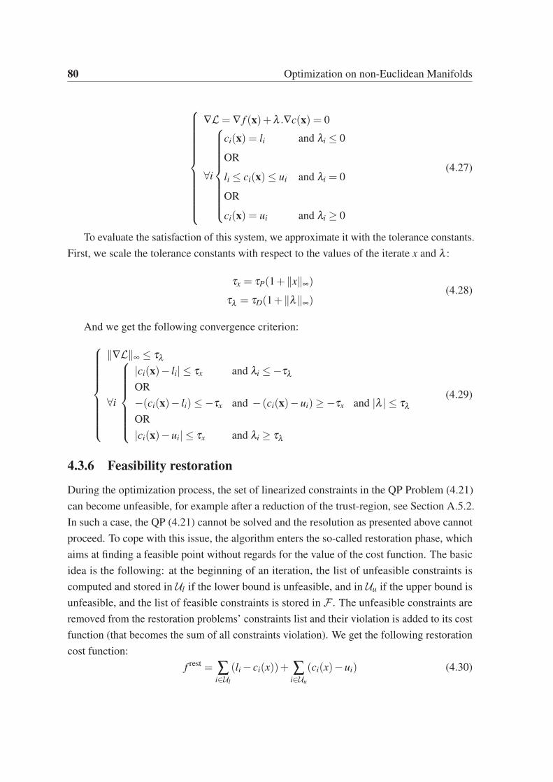
80 Optimization on non-Euclidean Manifolds
∇L= ∇ f (x)+λ .∇c(x) = 0
∀i
ci(x) = li and λi ≤ 0
OR
li ≤ ci(x)≤ ui and λi = 0
OR
ci(x) = ui and λi ≥ 0
(4.27)
To evaluate the satisfaction of this system, we approximate it with the tolerance constants.
First, we scale the tolerance constants with respect to the values of the iterate x and λ :
τx = τP(1+‖x‖∞)
τλ = τD(1+‖λ‖∞)(4.28)
And we get the following convergence criterion:
‖∇L‖∞ ≤ τλ
∀i
|ci(x)− li| ≤ τx and λi ≤−τλ
OR
−(ci(x)− li)≤−τx and − (ci(x)−ui)≥−τx and |λ | ≤ τλ
OR
|ci(x)−ui| ≤ τx and λi ≥ τλ
(4.29)
4.3.6 Feasibility restoration
During the optimization process, the set of linearized constraints in the QP Problem (4.21)
can become unfeasible, for example after a reduction of the trust-region, see Section A.5.2.
In such a case, the QP (4.21) cannot be solved and the resolution as presented above cannot
proceed. To cope with this issue, the algorithm enters the so-called restoration phase, which
aims at finding a feasible point without regards for the value of the cost function. The basic
idea is the following: at the beginning of an iteration, the list of unfeasible constraints is
computed and stored in Ul if the lower bound is unfeasible, and in Uu if the upper bound is
unfeasible, and the list of feasible constraints is stored in F . The unfeasible constraints are
removed from the restoration problems’ constraints list and their violation is added to its cost
function (that becomes the sum of all constraints violation). We get the following restoration
cost function:
f rest = ∑i∈Ul
(li− ci(x))+ ∑i∈Uu
(ci(x)−ui) (4.30)

4.3 Practical implementation 81
Then the restoration problem only contains feasible constraints and has to minimize the sum
of constraint violation. The problem to solve becomes:
min.x∈M
∑i∈Ul
(li− ci(x))+ ∑i∈Uu
(ci(x)−ui) (4.31)
s.t.
∀i ∈ F li ≤ ci(x)≤ ui
∀i ∈ Ul −∞≤ ci(x)≤ ui
∀i ∈ Uu li ≤ ci(x)≤+∞
To simplify the writing of that QP, we denote lrest and urest two vectors that represent
respectively the lower and upper bounds of the constraints of the restoration problem:
∀i ∈ F , lresti = li, urest
i = ui (4.32)
∀i ∈ Ul, lresti =−∞, urest
i = ui (4.33)
∀i ∈ Uu, lresti = li, urest
i =+∞ (4.34)
(4.35)
The problem becomes:
min.x∈M
∑i∈Ul
(li− ci(x))+ ∑i∈Uu
(ci(x)−ui) (4.36)
s.t.∀i lrest
i ≤ ci(x)≤ uresti
That is solved by iterating just like in the SQPs main loop with the difference that at
each iteration, we update the problem based on new lists of unfeasible constraints. An
approximation Hrestk of the Hessian is computed especially for the restoration phase. The
restoration phase has and updates its own trust-region ρrest. Dropping the differences between
bounds, linear and nonlinear constraints, the QP to solve at each iteration of the restoration
phase is the following:
min.z∈TxM
(∇φxk
(0)∇ f rest(xk))T
z+1
2zT Hrest
k z
s.t.
∀i lrest
i ≤ ci(xk)+(∇φxk(0)∇ci(xk))
Tz≤ urest
i
−ρ rest ≤ z≤ ρ rest
(4.37)
The restoration phase has its own filter called the restoration filter. For more details on
the restoration phase, see Section A.5.3.

82 Optimization on non-Euclidean Manifolds
Note that each iteration of the main SQP algorithm starts with the resolution of an FP
(Feasibility Problem), that consists of the same linearized constraints as the QP problem (4.21)
without the cost function.
find z such that:
LB ≤ z≤UB
LL ≤ Az≤UL
LN ≤ c(xk)+(∇φxk(0)∇ci(xk))
Tz≤UN
(4.38)
Its role is to determine whether the set of linearized constraints is feasible. If it is, the
main SQP continues, otherwise, the restoration phase is entered. This feasibility problem is
also solved at the beginning of each restoration iteration to determine whether or not to exit
the restoration phase. As soon as a feasible point is found, the restoration process ends. Once
a feasible point xF is found by the restoration phase, it is used as the new iterate in the main
SQP phase. Since during the restoration no care is taken about the value of the cost function,
it is possible that xF is refused by the main filter, which is not an acceptable behavior. So
xF is forced in the filter, and any pair dominating it is removed. Then the main phase of the
optimization can continue.
4.3.7 Second Order Correction
In the event where a step proposed in the restoration process by the resolution of the
restoration QP is rejected by the restoration filter, instead of immediately reducing the size of
the trust region, we can perform a Second Order Correction Step.
The idea is to re-solve a QP after its solution zk has been rejected by the restoration filter,
but with a better approximation (second order) of the constraints:
ci(xk + z) = ci(xk)+∇ci(xk)T
z+1
2zT ∇2ci(xk)z (4.39)
The restoration QP problem becomes:
min.z∈TxM
(∇φxk
(0)∇ f rest(xk))T
z+1
2zT Hrest
k z
s.t.
∀i lrest
i ≤ ci(xk)+(∇φxk(0)∇ci(xk))
Tz+ 1
2zT ∇2ci(xk)z≤ urest
i
−ρ rest ≤ z≤ ρ rest
(4.40)

4.3 Practical implementation 83
Using 12zT ∇2ci(xk)z≈ ci(xk + zk)− ci(xk)−∇ci(xk)
Tzk we get:
min.z∈TxM
(∇φxk
(0)∇ f rest(xk))T
z+1
2zT Hrest
k z
s.t.
∀i lrest
i ≤ (∇φxk(0)∇ci(xk))
T (z− zk)+ ci(φxk(zk))≤ urest
i
−ρ rest ≤ z≤ ρ rest
(4.41)
Denoting gk = (∇φxk(0)∇ f (xk)) and Ak = (∇φxk
(0)∇ci(xk)), we can rewrite 4.41 as
follows:
min.z∈TxM
gTk z+
1
2zT Hrest
k z
s.t.
∀i lrest
i +Akzk− ci(φxk(zk))≤ AT
k z≤ uresti +Akzk− ci(φxk
(zk))
−ρ rest ≤ z≤ ρ rest
(4.42)
This system is solved iteratively by updating zk (but never changing x) with the solution
of the previous system and updating the values of ci(φxk(zk)) until a satisfactory z is found.
4.3.8 Hessian update on manifolds
Aside from the manifold adaptation, our main departure from Fletcher is in the Hessian
computation, where we used an approximation because the exact Hessian is too expensive
to compute in our problems. After testing several possibilities, we settled for a self-scaling
damped BFGS update [NY93, NW06], adapted to the manifold framework. More precisely,
given the Hessian approximation Hk at iteration k, we compute the approximation Hk+1 as
follows: Note that as explained in Section 4.2.4, the gradients are transformed through vector
transport before being compared.
sk = Tz(z), yk = ∇zLxk+1(0,λk+1)−Tz(∇zLxk
(0,λk))
θk =
1 if sTk yk ≥ 0.2sT
k Hksk
0.8sTk Hksk
sTk
Hksk−sTk
ykotherwise
(Powell update)
rk = θkyk +(1−θk) Hksk (damped update)
τk = min
(1,
sTk rk
sTk Hksk
)(self-scaling)
Hk+1 = τk
(Hk−
HksksTk Hk
sTk Hksk
)+
rkrTk
sTk rk

84 Optimization on non-Euclidean Manifolds
where Tz is a vector transport along z (see [AMS08]) and Hk is such that for u ∈ Txk+1M,
Hku = Tz
(HkT
−1z (u)
).
4.3.9 Hessian Regularization
Despite Powell’s update, Hk might not be positive definite (but still symmetric). We regularize
it as follows: we first perform a Bunch-Kaufman factorization PkHkPTk = LkBkLT
k where Pk
is a permutation matrix, Lk is unit lower triangular and Bk is block diagonal with blocks of
size 1×1 or 2×2 (obtaining Bk as a diagonal matrix is not numerically stable for Cholesky-
like decomposition of indefinite matrices), see [GVL96]. The eigenvalue decomposition
Bk = QkDkQTk is immediate and cheap to compute. From the diagonal matrix Dk, we form
D′k such that d′ii = max(dii,µmin) where µmin > 0 is user-defined (we typically set it to 0.1).
Defining L′k = LkQk(D′k)
1/2, we get a regularized matrix H ′
k = PTk LkLT
k Pk = (LTk Pk)
T LTk Pk.
We take advantage of LSSOL’s capability to receive H in the factorized form H = AT A with
A = LTk Pk upper-trapezoidal as an input. This avoids an internal Cholesky factorization so
that our regularization does not add too much time to the overall process of building and
solving the QP.
4.3.10 An alternative Hessian Approximation Update
In [Fle06], Fletcher presents a new Hessian update method that maintains and update the
Hessian H in the form H =UUT , which is obviously always symmetric and it ensures that it
is always positive semi-definite. Since a decomposition of H is readily available with this
method, we can get rid of the regularization of the Hessian in our algorithm. The matrix U
of size (n,m) is smaller than H and contains only information from the last m iteration, this
means that this method has a built-in limited memory capability. In our robotics problems,
using limited memory Hessian updates is useful because along the iteration process, the
variables may change a lot, and the Hessian value near the solution may be very different
from the one approximated around the first iterations. Thus, it can be helpful to ‘forget’ about
the old components of the approximation to leave room for the latest ones. At each iteration,
the matrix U is updated with either BFGS or SR1, or a hybrid method, based on some tests on
the value of the latest step. When possible, the SR1 update is preferred, because some results
suggest that it allows faster convergence when the SR1 denominator is positive, otherwise, a
BFGS or the hybrid method are used.
Although this method provides a decomposition of H as UUT , U is not trapezoidal, so
we need to apply a QR on UT so that we get UT = QR, then H = RT QT QR = QT Q with Q
trapezoidal and R an orthogonal matrix. Then Q can be fed to LSSOL directly.

4.3 Practical implementation 85
For all those reasons, this update method is very attractive. We implemented it in our
solver, but so far the results have not been very conclusive and some more work will be
dedicated to that issue in the future. As of now, the best results were observed when using
the self-scaling BFGS update method.
4.3.11 Hessian Update in Restoration phase
The Hessian H (computed through whichever method presented above) is meant to approxi-
mate the value of ∇2Lxx(x,λ ) = ∇2 f (x)+λ T ∇2c(x), with f the cost function of the current
problem to solve, and c its constraints. But during the restoration phase, the definitions of f
and c change at each iteration, depending on the sets of unfeasible and feasible constraints
(I and F). In order to account for that change, we propose to compute an approximation of
each constraints second derivative separately, denoting Hi the Hessian of ci, and correctly
combining the Hessians based on the current set of feasible constraints.
Hci≈ ∇2ci
H = ∑i∈I
Hci+ ∑
i∈F
λiHci
(4.43)
With this definition of H, we can ensure the symmetry of H, but nothing guarantees
its positive definiteness. It is then necessary to regularize H after combining the Hci. This
also allows to have an approximation of the Hessian when exiting the restoration phase, by
computing H = H f +∑λiHciwith H f ≈ ∇2 f and regularizing it.
4.3.12 Solver Evaluation
We integrated our solver with the Roboptim framework (http://roboptim.net/) to have a
common interface with other solvers that are already interfaced with roboptim and used
in our team, like IPOPT, CFSQP, and NAG. The roboptim framework provides a list of 72
canonical optimization problems coming from the Hock-Schittkowski-Collection [HS80] that
allows to evaluate the rate of success and speed of each solvers. Although those problems are
all on Rn, and as such, do not take advantage of the non-Euclidean implementations of our
solver, it is beneficial to compare its performances with other solvers. As of now, PGSolver
finds a solution for 51 tests out of 72, using its default parameters. In the same conditions,
IPOPT solves 65 problems, CFSQP 46 and NAG 58. This result serves only as an indication of
the correct behavior of a solver because default parameters are usually not good and a solver

86 Optimization on non-Euclidean Manifolds
reaches its full potential once its parameters have been tuned for a type of problem. Those
tests can also be used in a non-regression criterion for our software.
4.4 Diagrams of the algorithms
In Figure 4.6, 4.7, and 4.8, we summarize the functioning of the algorithms that are re-
spectively the main loop of the SQP, the restoration phase, and the second order correction
phase.
Init x and filter
Update c, ∇c, f , ∇ f , H. . .
Is KKT satisfied?
Convergence
Success
Solve FP
Is problem feasible?
Solve QPFind feasible point
with Restoration Phase
Force add
f (x),c(x)
in filter
Is ‖z‖ ≤ ε?
Null step
Success
Is f (ϕx(z)),c(ϕx(z))
accepted by filter?
Reduce trust region
ρ ← ρ2
Is ρ ≤ ρmin?
Too small step
Failure
x← ϕx(z)
Add to filter
Is step limited
by trust region?
ρ ← 2ρ
no yes
yes no
x
z
yes no
no yes
yes
yesno
no
Figure 4.6 Main SQP Loop

4.5 Conclusion 87
Find Feasible Set
Init Restoration Filter RF
with cI(x),cF (x)
Is Problem Feasible?
Solve FP
Success
Return z to
main SQP loop
Find Feasible
Set Update I,F
Update c(x), ∇c(x), H
Solve Restoration QP
Is cI(ϕx(z)),cF (ϕx(z)
accepted by RF?
Add cI ,cF to RF
x← ϕx(z)
Is step limited
by Trust Region?
ρ ← 2ρ
Find better
solution
with SOC
Did SOC find
a solution?
Has I,F changed?
Force add cI ,cF in RF
x← ϕx(z)ρ ← ρ
2
Is ρ ≤ ρmin?
Too small step
Failure
yesno
yes no
yes no
yesno
no
no
yes
yes
Figure 4.7 Restoration Loop
Init SOC
bestZ ← z
bestC←‖cI‖∞
Is SOC QP feasible?
Solve FP
Exit SOC
No solution Found
cprevI∞ ←‖ci‖∞
Solve SOC QP
Is cI,cE
accepted by RF?
SOC found solution
Return zIs ‖cI‖∞ ≤ bestC?
bestZ ← z
bestC←‖cI‖∞
Is ‖cI‖∞ ≤c
prevI∞
4?
Is ‖cI‖∞ ≤ ε?SOC too slow
Exit no solution
Almost Feasible Point Found
Exit no solution
noyes
noyes
yes
no
noyes
yesno
Figure 4.8 Second Order Correction
4.5 Conclusion
In this chapter, we presented the principle of nonlinear optimization on non-Euclidean
manifolds, and detailed the choices we made to implement an SQP algorithm that solves those

88 Optimization on non-Euclidean Manifolds
problems efficiently. In addition to being used in our posture generation problems, PGSolver
has been used successfully in inertia identification problems as presented in [TBEN16]. In
the next section, we will focus on the formulation of optimization problems for posture
generation.

Chapter 5
Posture Generator
Writing a posture generation problem can easily become cumbersome without the appropriate
tools. Common pitfalls are for example writing the derivative of a function, managing how
the Jacobian matrices of the already implemented functions are modified when a variable is
added to the problem, adding a new type of constraint, or correctly writing a function on a
sub-manifold of the problem manifold. A fair amount of bookkeeping is always necessary,
which should not be the charge of the user writing the constraints. In our PG, we propose
an architecture automating most of the burdensome tasks so that the user can focus on the
mathematical formulation of the problem:
• A system of geometrical and mathematical expression trees that automatically com-
putes the mathematical expressions behind the geometric relations;
• An automatic mapping between the submanifold of each function and the global
manifold of the problem;
• A problem generator that aggregates all the information from the above-mentioned
items to generate an optimization problem that can be passed to the solver.
We then propose an extension to classic posture generation by developing a constraint of
contact with parametrized surfaces which takes advantage of our framework.
5.1 Geometric expressions
Most of the robotic posture generation constraints are geometric. In order to simplify the
writing of functions, we use a dedicated system of expression graph encapsulated in a set
of geometric objects. The main idea is to separate the purely mathematical logic from the
geometric one. As an example, if Pr and−→Vr are a point and a vector attached to the camera

90 Posture Generator
of the robot, and Pe is a fixed point in the environment, the constraint (Pe−Pr) ·−→Vr = 0 can
be used to have the robot’s camera directed toward Pe. With our implementation, the user
creates only those objects and write the code (Pe-Pr).dot(Vr) to create the needed task
function. The geometric layer ensures that all the quantities are expressed in the correct
frame, the mathematical layer performs the corresponding operations. If q is a variable object,
(Pe-Pr).dot(Vr).diff(q) returns automatically the differential of the expression w.r.t. q.
This makes the writing of the constraints very easy.
At the mathematical level, we consider 5 types of expressions which can be either
variables or constants:
• Scalar, a 1-dimensional element of R
• Coordinates, a 3-dimensional element of R3
• Rotation, a 3×3 matrix representing a 3D rotation
• Transformation, a 4×4 matrix representation of a 3D isometry
• Array, a dynamic size array
The meaningful unary (inverse, opposite, norm...) and binary (multiplication, addition,
subtraction, dot product...) operations (with their derivatives by chain rule) are implemented.
We also have a Function class for more complex expressions, for example expressing
q 7→ Ti(q) where Ti is the transformation between the reference frame of the robot and
the frame of its i-th body1. The combinations of those elementary operations define a
computation graph, just like in many symbolic calculation frameworks.
Each expression is able to compute its own value and the value of its derivative with
respect to another expression. For example, let A and B be two unrelated expressions. We
denote dim(x) the dimension of expression x. The value of expressions A or B are obtained
by respectively calling the methods A.value() and B.value(). The derivative of A with
respect to itself is obtained by calling the method A.diff(A) and returns an Identity matrix
of size dim(A). Whereas the derivative of A w.r.t B returns a zero matrix with dim(A) rows
and dim(B) columns.∂A
∂A= 1dim(A),
∂A
∂B= 0dim(A),dim(B)
Each operator on expressions defines its resulting expression, thus, it defines a value and
a diff methods. For example, let us consider that A and B are 3D coordinate expressions
1The kinematics of rigid body systems is handled by the RBDyn library ([email protected]:jrl-umi3218/RBDyn.git)

5.1 Geometric expressions 91
and a new expression C = A ·B that is defined as the dot product of A and B, in code, one can
write C’s definition as simply:
Scalar C = dot(A,B).
The value and the derivative of C w.r.t any x expression are then automatically computed as
follows:
C = A ·B,∂C
∂x= AT ∂B
∂x+BT ∂A
∂x(5.1)
The code of the dot function that translates eq: (5.1) is pretty straightforward:
C.value() = A.value().dot(B.value())
C.diff(x) = A.value().transpose()*B.diff(x)
+ B.value().transpose()*A.diff(x)
It is easy to extend the capabilities of this framework by implementing additional op-
erations. By following this approach, we can easily compute the values and derivatives of
expressions that are the outcome of complex arithmetic trees. Currently, the following binary
operators are available: cross product, dot product, classic product, addition, subtraction,
transformation. And the following unary operators are available: component extraction,
inverse, norm, rotation, square root, transformation, and vectorization.
The geometric layer consists of physical or geometric objects, called features, which
exist independently of their mathematical expression in a given reference frame. We have so
far four objects:
1. A Frame, defined by a Transformation expression and a reference frame.
2. A Point, defined by a Coordinates expression and a reference frame.
3. A Vector, defined by a Coordinates expression and a reference frame.
4. A Wrench, defined by a pair of Coordinates expressions and a reference frame.
We have a special World Frame object to serve as starting reference frame.
For each feature, one can get its expression in a given frame. Basic operations are defined
between those features (when applicable). For example, the subtraction between two Points
gives a Vector. The geometric logic resides in the change of frame and those operations.
Based on that expression system, the robot’s geometry can simply be represented by
a set of frames representing all its links, and functions that keep track and update the
transformations of the frames of all its bodies, with respect to an Array expression on entry,
its articular parameters. The forward kinematics Algorithm 2 and the Jacobian computation

92 Posture Generator
Algorithm 3 are used to define those functions. For a given articular parameter array, the user
can query the frame of any body on the robot, and by composition, any feature defined on
a frame of the robot, as well as its derivatives. This tool allows for a simplified writing of
robotics constraints as a combination of operations on geometric features, without worrying
about the vectors and matrices and without having to write the derivatives.
Let us consider a simple constraint and its expression in this framework: we define a
point Ph on a body of a robot and a point Pe in the environment. We want to write a constraint
that ensures that Ph and Pe match. Given a frame F , we can simply write that as:
P_h.coord(F) - P_e.coord(F)=0
(the "= 0" part of the equation is here for readability only; in the code, the value of the
resulting expression is constrained by boundaries)
In the case of a scalar expression like (Pe−Pr) ·−→Vr = 0, it can be written without any
consideration about frames as
(P_h - P_e).dot(V) = 0.
This mathematical and geometric expression framework simplifies the task of the con-
straints developers. And it helps to avoid calculation mistakes because one only needs to
write the code for elementary functions and their combination is computed automatically by
chain rule.
5.2 Automatic mapping
The manifoldM, on which the optimization takes place, is a Cartesian product of several
sub-manifolds. Same goes for their representation spaces:
M=M1×M2×M3× . . .
E= E1×E2×E3× . . .(5.2)
From the solver’s viewpoint, the entry space of each function is the complete manifold.
But for the developer, writing a function on the complete E is cumbersome because (i)
of the need to manage indexes, and (ii) when the function is implemented, the complete
E may not be known. A user-written function f is usually defined on a subset of E, say
EI = Ei×E j ×Ek . . ., that is minimalistic for that function, and should not account for
unrelated manifolds. One does not want to think about the values of the forces when writing
a geometric constraint for example.

5.3 Problem formulations 93
We developed an automatic mapping tool that keeps track of all the necessary mappings
for each function added and upon the instantiation of the problem, generates the correct
projection functions πI such that the developer can write a function f on EI while the solver
receives it as a function f πI on E.
This tool was built as an add-on to the RobOptim [MLBY13] framework called roboptim-
core-manifold and its goal is to extend the notion of function to take into account its
application manifold and map the correspondence between the values in the input of the
problem and the input of the function. We define a class called DescriptiveWrapper that
contains a RobOptim function and a description of its application manifold. Once a function
is wrapped in a DescriptiveWrapper and the optimization problem is set, we need to establish
the mapping between the variable of the problem, which is defined on the global manifold of
the problem, and the input of the function that must match the description of its application
manifold. That is the role fulfilled by the WrapperOnManifold layer, that compares the two
manifolds, matches them and computes an input mapping from the problem’s input vector to
the function’s, which we denote πI . This mapping is computed once during the instantiation
of the problem and then used at each call of the function. The use of the input mapping is
illustrated by the example in Figure 5.1
Figure 5.1 automatic variable mapping
5.3 Problem formulations
Let q= [qTF ;qT
r ]∈ SE(3)×Mr be the combination of the free-flyer of the robot qF ∈ SE(3) =
R3×SO(3) and the articular parameters qr ∈Mr. LetWi(p) = fi,mi(p) be the wrench
(force+moment) applied by the environment onto the robot at contact i and expressed on
point p. A frame F is composed of a reference point and an orthonormal basis of 3 vectors
F = O,(~x,~y,~z). For frames define on a surface, with one vector of (~x,~y,~z) being the

94 Posture Generator
outbound normal to the surface, and the two others tangent, we rename ~n the normal one
and~t,~b (tangent and bitangent) the two other ones, ensuring that (~n,~t,~b) is an orthonormal
direct basis. When a frame is denoted with the subscript i, Fi, all its components are added
the same subscript.
Here is a list of constraints that we consider in our problems:
• Joint limits q− ≤ qr ≤ q+:
These cannot be directly translated on manifolds other than Rn. For example, spherical
joints can be parametrized on S2×R, then the S2 part can be limited by a cone, and
the R part can have real bounds (in that case the limit constraint is not a simple bound
constraint, but writes as f (qr)≤ 0).
• The Frame constraint is a generic type of constraint which consists in blocking a
predefined set of degrees of freedom of one frame F2 w.r.t. another frame F1. By
default, the frame F2 has 6 degrees of freedom w.r.t. F1, three translational degrees
of freedom TX, TY, and TZ, respectively along ~x1, ~y1 and ~z1 and three rotational
ones RX, RY, and RZ, respectively around (O1,~x1), (O1,~y1) and (O1,~z1). We can
write constraints such that any combination of the translational degrees of freedom is
blocked:
If TX is blocked:−−−→O1O2 ·~x1 = 0 (5.3)
If TY is blocked:−−−→O1O2 ·~y1 = 0 (5.4)
If TZ is blocked:−−−→O1O2 ·~z1 = 0 (5.5)
Similarly, any pair of rotational degrees or the three of them can be blocked (blocking
only one rotation is not possible with that formalism). If the three rotations RX, RY,
RZ are blocked, we get the set of constraints 5.6:
~z1 · ~y2 = 0
~z1 · ~x2 = 0
~x1 · ~y2 = 0
~z1 · ~z2≥ 0
~y1 · ~y2≥ 0
(5.6)

5.3 Problem formulations 95
When two rotational degrees of freedom are blocked, we get the set of constraints 5.7
To generalize the following formulas, we rename the axis X, Y, and Z with respect to
their respective roles in this constraint. The one rotational degree that remains free is
denoted N with vector~n, and the two others are denoted T and B, with vectors~t, and~b.
Those 3 vectors are ordered such that (~n,~t,~b) is an orthonormal direct basis.
~n2 · ~n1 ≥ 0
~n2 ·~t1 = 0
~n2 · ~b1 = 0
(5.7)
In theory, one could simply write that constraint as ~n1 = ~n2, but in practice, this
formulation leads to bad numerical behavior of the optimization, thus we prefer 5.7.
All those independent sets of constraints can be combined to create a wide variety of
geometric constraints. For example, one can create a mobile planar contact constraint
with normal~z1 by blocking TZ, RX and RY. A punctual contact constraint can be
devised by blocking TX, TY and TZ. To completely fix the position of F2 w.r.t. F1, one
can block TX, TY, TZ, RX, RY, and RZ. And many other types of custom constraints
can be devised with this formulation.
In the event that the two frames do not have a satisfying configuration to write the
desired constraint with this formalism (for example, if one wants to write a planar
contact between two surfaces S1 and S2, where ~z1 and ~z2 are outbound normal vectors,
then equation 5.7 is not satisfactory because we want to oppose ~z1 and ~z2, not identify
them). Then the user defines a new frame F ′2 that is a constant 3D transformation away
from F2 (in that case a rotation of π around (O1,~x1) would suffice).
• The stability constraint ensures that the Euler-Newton equation (5.8) is balanced for
the set of external wrenches applied to the robot (gravityWG and contact forcesWi).
∑i
Wi(p)+WG(p) = 0 (5.8)
For each contact that bears forces (‘stability’ contact), a wrench applied on the robot
at the contact point is added to the problem. If the contact is added through a frame
constraint between F1 and F2, the wrench can be formed by a combination of elementary
components that are:
– FX: force along ~x1, value fx

96 Posture Generator
– FY: force along ~y1, value fy
– FZ: force along ~z1, value fz
– MX: moment around (O1,~x1), value mx
– MY: moment around (O1,~y1), value my
– MZ: moment around (O1,~z1), value mz
That wrench is parametrized on a Rm with m the number of components used. We
model the resultant wrench of planar contacts as a combination of punctual forces
applied at each vertex of the contact polygon. In the case of interaction forces between
2 robots, only one wrench is created and it is used as is in the stability equation of one
robot and its opposite is used for the stability of the second robot. That way, we are
guaranteed that the forces in between the robots are balanced and we can evaluate the
stability of each robot separately.
• The friction cone constraint can be used to limit the tangential part of any force to
avoid slippage. We write it as (5.9) (with µ the friction coefficient)
µ2 f 2z − f 2
x − f 2y ≥ 0
fz ≥ 0(5.9)
• The rotational friction limit constraint can be used to limit the friction torque of any
force to avoid slippage. We write it as (5.10) (with σ the rotational friction coefficient)
σ2 f 2z −m2
z ≥ 0
fz ≥ 0(5.10)
• The collision avoidance constraint can be defined between any two bodies. A convex
mesh is attached to each body involved in the constraint. We denote them C1 and C2.
We use the sch-core library described in [BEMK09] that implements an efficient
GJK algorithm to compute the distance d(C1,C2) between 2 convex shapes and its
derivative. A description of strictly convex hulls that can be used for this purpose is
detailed in [EMBK14]. For each collision avoidance constraint, we require that the
distance between the two convex remains superior to a minimal distance dmin
d(C1,C2)≥ dmin (5.11)

5.3 Problem formulations 97
• The torque limit constraint makes use of the Inverse Statics Algorithm 5 to compute
the torques in all the joints of every robots and their derivatives are computed by
Algorithm 6. Denoting τi the torque in joint i resulting from the robot’s configuration
and the external forces applied on it, and its lower and upper limits as τ−i and τ+i . The
torque limit constraint writes as follows:
∀i, τ−i ≤ τi ≤ τ+i (5.12)
Most often, the frame’s configuration depends on a part of the optimization variables,
that must be accounted for in computing the constraints’ Jacobian. Our framework computes
such dependencies automatically.
Another important part is the problem’s cost function. Any function of the problem’s
variables that returns a scalar value can be used as a cost function. In our formulation, we take
a sum of cost functions into account, several different functions fi over different variables can
be defined separately. And then combined in a weighted sum as the problem’s cost function
(with wi the weight of function fi):
cost = ∑i
wi fi (5.13)
Taking advantage of our framework, the set of variables over which the cost function is
defined, its value and its derivatives are then computed automatically.
A typical cost function is the distance to a reference posture q0. On a robot that has all
its articulations parametrized on R the distance can be expressed simply with the Euclidean
norm d = ‖qr−q0‖2. Since we work on non-Euclidean manifolds, the logarithm function on
the manifold must be used. It gives the distance vector between two points in the tangent
space, the norm of this vector can be used as a distance. So we get d =∥∥logq0
(qr)∥∥2
(note
that on Rn,∥∥logq0
(qr)∥∥2
= ‖qr−q0‖2)
We can also use the cost function to set a target value v for the value of a contact force ~F
in a given direction d. By simply implementing the following function:
f =∥∥∥~F · ~d− v
∥∥∥ (5.14)
The list of constraints and cost functions that can be used in robotics posture generation
problems can be extended, and this process is made easier by our framework.

98 Posture Generator
5.4 Implementation
In this section, we provide an overview of some of the key elements of the framework:
Problem’s configuration: The implementation of the core structure of a posture generation
problem is written in C++. A text file in YAML format can be used to configures the solver
and some custom parameters of the problem; It is parsed at runtime to avoid having to
recompile the problem for every configuration change. Also, some Python bindings have
been developed to allow writing the core structure of the problem without compilation.
The Robot class: The RBDyn library contains all the low-level tools and algorithm to
compute the kinematics and statics of a robot. The robot class is built on top of RBDyn
to provide high-level functionalities while adapting it to our manifold formalism (which
RBDyn does not handle natively). The basic structure of the robot is extracted from its URDF
description file. The main functionality of the robot class is to create a Frame attached to each
of its bodies and to update their transformations and derivatives based on the robots articular
variables. It also maintains the transformations of all the collision meshes and contains the
joint and torque limits, as well as the manifold on which its variables live. Additionally, it
contains some useful objects used to maintain and update the external forces applied on the
robot, as well as the joint torques.
The Function Class: The functions that we use derives from the Roboptim’s functions. As
such, they are able to compute their return value and derivative for a given input. Functions
can conveniently be defined through our expression framework to take advantage of their
automatic derivation.
The Constraint class: A constraint object contains all the necessary elements for the
description of a mathematical constraint. That is, a function h and the manifoldMc on which
it should be applied, as well as its lower bound l, upper bound u and the scaling factor of the
constraint. Once a constraint is instantiated by the problem, the input mapping π from the
problem’s complete manifoldM to the function’s application manifold is computed. The
constraint that will then be used in the optimization for a given iterate x can be written as:
l ≤ hπ(x)≤ u (5.15)
Constraints can be equipped with an ‘addStabilityToProblem’ method that is used to specify
the forces generated by the constraint to add to the stability constraint of the problem.
5.4 Implementation 99
The Frame Constraint class: It describes a very useful type of constraint between two
frames F1 and F2. It implements the Frame constraint that we described in Section 5.3 with
some additional features. This specific constraint is composed of four distinct parts:
• The geometric constraint generates the constraints associated with the user’s choice of
combination of degrees of freedom to block amongst TX, TY, TZ, RX, RY, RZ.
• The static constraint part (optional) instantiates the wrench to be added to the stability
constraint of the problem based on the user’s choice of components FX, FY, FZ, MX,
MY, MZ.
• A custom geometric additional function field (optional) allows the user to add extra
geometry constraints to the problem (through a C++11 lambda that is executed after
the geometric constraints are added to the problem).
• A custom static additional function field (optional) allows the user to add extra static
constraints to the problem (through a C++11 lambda that is executed after the con-
straint’s wrench has been created and added to the problem).
The custom geometric additional function can typically be used in the context of a planar
contact to limit the position of O2 to the inside of a polygon defined in the plane (O1,~x1,~x2).
As for the static additional function, it can be used to add constraints on the values of the
constraint’s wrench, for example, enforcing the friction cone constraints.
The PostureProblem class: The PostureProblem class is in charge of building the com-
plete optimization problem that describes the posture generation problem one wants to solve.
It creates and owns the robots (including objects and the environment that we may consider
as additional ‘robots’) present in the problem. It registers all the variables and constraints of
the problem as well as all the functions involved in the cost function. Each function is likely
to bring additional variables with it. For each contact contributing to the balance, a variable
representing the contact force is added to the problem. The associated wrench is added to
the stability constraints. Once the registration is completed, the complete manifold of the
problem is generated and all the functions on manifold used in the problem will generate their
input mapping that will project the complete variable of the problem onto the submanifold
that the function is interested in. Subsequently, the optimization problem can be generated
and passed to the solver. The communication between the solver and the generated problem is
made through the RobOptim framework2 [MLBY13, MCY14]. After creating the complete
2http://www.roboptim.net/

100 Posture Generator
manifold, the PostureProblem class can be used to facilitate the individual initialization of
all the separate variables of the problem without the user having to worry about the indexes.
Finally, it can query the resolution of the problem by the solver and eventually returns the
result.
5.5 Examples of postures generation
In this section, we present some scenarios that are built and solved with our posture generator
and solver.
Application of a desired force In the context of using a humanoid robot in aircraft manu-
facturing3, we formulate a problem where the HRP-4 robot is required to apply a desired
force on a given point of the airplane’s structure (printing or gluing a braquet, preparation for
drilling, etc.). We denote fd the desired value of the force in direction ~d, and ~fc the actual
force at the contact point. One can simply implement the following function ftarget( fc) to
minimize (hence a cost) to get the desired result:
ftarget( fc) =(~fc · ~d− fd
)2
(5.16)
In addition to that cost function, the robot needs to keep its foot on the ground, its left hand
is used to lean on a beam of the structure to allow a longer reach with the right hand that
is in contact with the wall. Those constraints must be satisfied while respecting the joint
and torque limits of the robot, maintaining balance and avoiding auto-collisions. The result
generated by our PGSolver is depicted in Figure 5.2
Generating postures in highly constrained environment In this scenario, we need to
find task-compatible postures of the the HRP-4 inside a highly constrained environment,
in the sense that many obstacles limit its displacement, and it must avoid collision with
them. The goal is to be able to reach the four corners of a panel of circuit breakers (in green
on Figure 5.3) to activate them. We generated a sequence of steps to reach that panel and
then some postures to reach different points of this panel. In Figure 5.3, we show some
extracts of this sequence of postures. In each of them, the two foot are in planar contact
with the ground, alternatively bearing forces, while always respecting the joint, torque limits,
collision avoidance, and stability constraints. On the last posture, the top left corner of the
panel is reached with the tip of the right hand of the robot.
3www.comanoid.eu

5.5 Examples of postures generation 101
Figure 5.2 HRP-4 applying a desired force on a contact point with its right hand.
Figure 5.3 A sequence of resulting postures with the HRP-4 entering a constrained environ-
ments to reach a point on a panel of circuit breakers (in green).

102 Posture Generator
5.6 Contact on non-flat surfaces
Writing relations between geometric quantities defined in frames allows to describe a large
variety of contacts. In particular, it allows to write most types of geometric constraints
between canonical geometric shapes (point, line, plane). The most common type of contact
constraint encountered is the contact between two surfaces S1 and S2. The set of equations
used to define that type of constraint can be obtained through a frame constraint blocking TZ,
RX and RY. Provided that the correct frames are defined, F1 on S1 with ~z1 normal outbound
and F2 on S2 with ~z2 normal inbound, the constraint writes as:
−−−→O1O2 ·~z1 = 0
~z2 ·~z1 ≥ 0
~z2 ·~x1 = 0
~z2 ·~y1 = 0
(5.17)
When the two surfaces are flat, a contact between them can be written simply with the set
of equations (5.17). In that case, the quantities involved in the constraint are invariant with
the location of the contact point, thus, the equations are valid for any point of the surface
(in particular, the normal vector is the same for any point on the surface). When it comes to
non-flat surfaces, the location of the frames used in equations (5.17) matters, as the quantities
in the constraint equations depend on it.
We propose to add an additional variable uS to our optimization problem to represent
the location of the contact frame on a non-flat surface. This gives the ability to our solver
to choose the optimal contact position on a non-flat surface. Depending on its shape, the
manifoldMS on which the surface is parametrized can be R, R2 or S2. Then we can write
the contact constraint on that parametrized frame as follows:
F(uS ∈MS) = O(uS),(x(uS),y(uS),z(uS)) (5.18)
In this section, we successively present several ways to parametrize various non-flat surfaces
to generate contacts with them.
5.6.1 Application to plane-sphere contact
We consider the contact between a body’s flat surface SB of normal nB, with the surface of
a sphere Ss of center cs, radius rs, and let ps and ns be a point and its normal on Ss. The
most general way to express such a constraint is to ensure that ps is on SB and that ns and nB
are opposite. To do that, we create a variable vS2 on S2, add it to our optimization problem

5.6 Contact on non-flat surfaces 103
Figure 5.4 HRP-2Kai leaning on a sphere with its right wrist to point its left gripper as far
as possible in 4 cardinal directions. Top row: semi-predefined contact; Bottom row: free
contact with parametrized wrist. Projection of the CoM on the ground (green dots)
and map pS and nS on it. In our framework, this constraint is expressed exactly as the
contact between 2 planar surfaces, once the mappings of ps(vS2) and ns(vS2) are done. In
a framework that does not handle manifolds, it would require to setup a specific constraint,
ensuring that the distance between cs and SB is equal to rS.
In Figure 5.4 we show the results obtained by solving a problem where the HRP-2Kai
robot has to keep its feet in contact with the ground at fixed positions, touch a sphere with
a side of its right wrist and point as far as possible in a given direction d with its left hand,
under balance constraints. The top row of Figure 5.4 shows the results for this problem with
several different d. In every situation, the projection of the CoM is outside the polygon of
support, meaning that such postures would not be reached without leaning on the sphere.
5.6.2 Contact with parametrized wrist
Being able to parametrize the choice for the location of the contact point on the sphere is
interesting, but a limitation of this formulation is that the contact point on the wrist of the
robot is restricted to one single user-defined face. Instead, we describe the shape of the wrist
body as a parametric function and let the contact point on the wrist as well as its counterpart
on the sphere, result from the optimization process. The section of HRP-2Kai’s wrist is a
square with rounded edges. We parametrize this shape as shown in Figure 5.5: we consider
the angular coordinate θ of the point on the section. It is added as a variable on R to the

104 Posture Generator
Figure 5.5 Parametrization of the wrist of HRP2-Kai
problem. The shape of the quarter of section [0;π/2] is a succession of a vertical line, a
quarter of a circle and a horizontal line. This pattern is repeated for the 3 other quarters. The
equations are given in Figure 5.5. In our framework, we define the function describing the
shape of the wrist, create a frame parametrized by that function and then define the contact
between that frame and the point and the normal on the sphere. This formulation not only
is very easy to implement but most importantly, allows for richer posture generations. The
optimization algorithm chooses the contact point on the sphere as well as the contact point
on the wrist, which leads to a wider accessibility range, and a better optimization of the cost
function.
The bottom row of Figure 5.4 displays the results of this simulation for the robot pointing
in 4 directions. Notice that on the 2nd and the 4th (pointing forward and to the left) images,
the results for the 2 types of models are nearly identical, whereas in the 1st and 3rd images,
different faces of the wrist have been chosen (On the 1st, the wrist is rotated by 180, and
90 on the 3rd). In these 4 cases, the contact with parametrized wrist gives a better value of
the objective function (the left hand points further). This observation scales: we solved this
problem for 5000 random pointing directions, and in average, the contact with parametrized
wrist allows to reach 5mm further. The success rate of the solver is 98.5% in the parametrized
wrist case against 99.9% when the face is fixed. The numbers of iterations are similar.
This method is certainly scalable, and can be used for any kind of humanoid robot and
environment. Yet, it requires having a parametric equation of the surface.
5.6.3 Contact with an object parametrized on the unit sphere
In this case, we want the HRP-4 robot to carry a cube with its two hands. The most general
way to do it is to select a face of the cube for each contact and to enforce the contact between
that face and the hand’s surface. We propose to approximate the cube with a superellipsoid
and to parametrize the resulting shape on S2, thus adding a variable on S2 to our problem.

5.7 Contact with Complex Surfaces 105
Figure 5.6 HRP-4 carrying a 2kg cube. Left: the objective function is to maintain the cube at
a given position. Right: it is to put the cube as far as possible in a given direction
The implicit equation of a superellipsoid is S(x,y,z) = 0, with
S(x,y,z) =(∣∣∣ x
A
∣∣∣r
+∣∣∣ y
B
∣∣∣r) t
r+∣∣∣ z
C
∣∣∣t
−1 (5.19)
A point in S2 is represented by a vector v = (x,y,z) in E = R3. To a given unit vector
v we associate a point αv on the surface of the superellipsoid by solving S(αv) = 0 for α .
At this point, the normal is given by∇S(αv)
‖∇S(αv)‖which simplifies into
∇S(v)
‖∇S(v)‖. Given this
parametrization, we write a contact constraint between the frame of the hand of the robot and
the point and normal on the surface of the superellipsoid.
In Figure 5.6 we present some results for a posture generation problem with manipulation:
On the left side, the feet are free to move on a sphere, and, on the right side, the left foot
position is fixed and the right foot is free to move on the ground. The hands must be in
contact with the cube. The cube is free to move (parametrized by R3×SO(3)) and has it
own set of Euler-Newton equations, which must be fulfilled.
5.7 Contact with Complex Surfaces
We have presented some methods to formulate contact constraints with parametrized surfaces.
The surfaces that we used so far could all be approximately represented by closed-form
equations (sphere, superellipsoid, wrist of HRP-2). This is sufficient to tackle a large
number of interesting scenarios, especially for robots in structured environment [VKA+14]

106 Posture Generator
Figure 5.7 Several Catmull-Clark subdivisions of a cube. From left to right: original mesh,
after 1, 2 and 6 iterations
[VKA+16]. However, contacts with more complex objects are needed too, for unstructured
environment or for manipulating objects.
To work with derivative-based optimization algorithms, such as SQP or Interior Points,
the functions involved in the optimization problem need to be at least C1 and gradients must
be full rank at the solution (for ensuring constraints qualification, see [NW06]). Since the
contact point can be anywhere on our parametrized surface, the gradients must be full rank
everywhere.
In the previously presented parametrizations of typical geometric shapes (sphere, su-
perellipsoid...) those continuity requirements are not a problem. But for a given object, a
parametrization of its surface is rarely available, especially a parametrization conforming
with the continuity requirements. On the contrary, we usually have an approximation of the
object as a mesh.
We can consider two types of surface parametrizations, the surfaces of closed topology,
like a sphere, which are a large part of the objects of interest in our application, that we
parametrize on S2 (because there is no diffeomorphism between the unit sphere and a subset
of R2) and the surfaces of open topology, that generally can be parametrized on R2. The
problem of finding a parametrization satisfying the continuity requirements exists for both of
those when the surface’s representation comes as a mesh.
In [EBK16], we provide a systematic way to obtain a parametric surface closely approxi-
mating a mesh and meeting the continuity requirements mentioned above, for a large class
of objects, namely star-convex objects. To that end, we combine the use of Catmull-Clark
subdivision surfaces with a tailored ray casting algorithm, and propose an efficient and
robust numerical method to evaluate a point, a normal and their derivatives at a given set of
parameters.
The Catmull-Clark algorithm is used to create a smooth surface modeling a given control
mesh. It iteratively subdivides a control mesh by following a set of rules. The limit surface
of this subdivision process is called the Catmull-Clark Surface (CCS), see Figure 5.7. It was
shown by Stam in a seminal paper [Sta98] that points on CCS can be computed by direct
analytical formula without explicitly subdividing the control mesh. A map between each face
of the control mesh and the patch of the CCS associated to it s(u,v) can be devised (with

5.7 Contact with Complex Surfaces 107
Figure 5.8 Catmull-Clark Surfaces (in blue) approximating the mesh of a link on HRP-2 (in
green)
(u,v) a 2D parametrization of a face). To find the point of the CCS associated with a value
d ∈ S2, we use a raycasting algorithm: given c, a center point of the star-convex control mesh
(a point seeing all the surface of the control mesh), we solve numerically c+ td = s(u,v) in
(u,v, t) with a Newton method. This gives us a mapping from S2 to the CCS. From there, we
propose methods to compute the normal to the CCS point associated with an element of S2
and we devise the derivations of both those mappings.
As a result, we get a smooth parametrization of the input mesh that satisfies the continuity
requirements. In Figure 5.8, we show the Catmull-Clark surface (in blue) corresponding
to the mesh (in green) of an HRP-2 link, for two different levels of smoothness. On the
right picture, we first apply twice a simple subdivision scheme, before using Catmull-Clark
subdivisions, thus obtaining a surface closer to the original mesh but less smooth. The red
line is the image of a great circle of the unit sphere through our parametrization.
Because this parametrization respects the continuity requirements for being used effi-
ciently in optimization, we can use it freely in our posture generation problems.
We now show some examples of PG using the proposed approach to generate contacts
with complex objects. We make use of the capacity of our optimization solver to directly
work with a variable d ∈ S2 to parametrize our surfaces.
In the first example (Figure 5.9, left), a HRP-4 robot is asked to grasp an object (here a leg
part of HRP-2) and to hold it as far as possible in front of it, with the following constraints:
contacts must occur between predefined points on the hands of HRP-4 and points free to move
on the surface of the object, modeled as a parametric surface with our approach [EBK16];

108 Posture Generator
Figure 5.9 Left: HRP-4 holding an object, modeled with CCS, as far as possible in front of it.
The red arrows depict the contact forces and the gravity forces applied on each object. Right:
example of grasp generation.
Figure 5.10 HRP-4 climbing a pile of cubes modeled as a single object with a single surface.
(Right) Convex shapes used for collision avoidance

5.8 Conclusion 109
furthermore the robot has to keep its left foot at a given fixed position and has its right foot
anywhere on the floor. The forces applied by the robot on the object must be sufficient to
counter the gravity, and the system (robot, object) must be stable with all forces within their
friction cones. Additionally, the robot must stay within its joint limits. We do not check here
for collisions or torque limits. The solver finds a solution in about 70 iterations.
Contacts also occur in manipulation. Actually, manipulation and locomotion are closely
related. Locomotion can be seen as a manipulation of the environment, it is only a matter of
reference frame (see [BK12a]). The second example (Figure 5.9, right) demonstrates our PG
applied to grasping an object. The base of the hand is fixed, and the contact points on the
fingers are given. The contact points on the objects are parametrized with our method and
are free to move on the entire (approximated) surface of the object: the optimization finds
automatically how to grasp the object so as to be able to maintain its stability, taking about
50 iterations. Note that the object is non-convex.
The third example (Figure 5.10) involves a stack of cubes on which the robot must stand,
using its hands and feet to maintain its stability and respect its torque limits. The stack is
modeled as a single object. Once again, contact points are fixed on the robot and free on
the surface. The surface is modeled by a single object. That object is not convex, thus it
cannot be used as is for collision avoidance. For collisions, we model the stack of cubes with
a set of 21 cubes all slightly smaller than the actual cubes see Figure 5.10 (Right), and we
require the robot to avoid collision with those cubes. The optimization takes around 115
iteration to converge to a solution. Since there is a single surface to contact with, we do not
need to specify with which faces, edges or corners the robot needs to be in contact with. The
optimization decides it automatically. This is a very attractive feature of our approach as it
allows to include discrete choices directly into our PG. This can be used to alleviate the work
to be done by the user, be it a human or a planning algorithm: the user still has to specify
the bodies in contact, but part of the combinatorics relative to the matching of a body with a
particular surface or object is handled directly by the PG.
5.8 Conclusion
In this chapter, we presented our approach for formulating a posture generation problem and
generating an optimization problem that describes it. We presented several tools that are
meant to simplify this process for the developer, with the automatic variable management,
the use of non-Euclidean manifolds and the geometric expressions framework.
Leveraging those tools, we developed methods to formulate constraints involving non-flat
surfaces, by adding an extra variable to our optimization problem to parametrize the location

110 Posture Generator
of a frame on the surface. To avoid optimization issues, we make sure that our formulations
have satisfying continuity properties. This addition allows formulating much richer posture
generation problems, where the location of a contact on a non-flat surface is abstracted and
chosen by the optimization solver. We were able to use this approach to represent several
kinds of surfaces that could be described by closed-form formulas, such as the wrist of
HRP-2, a sphere, and a superellipsoid. We extended that method to approximate surfaces
for which the only available representation is a (star-convex) mesh. This allows formulating
constraints on the surface of a very large variety of objects.
In the next chapter, we evaluate the performances of our solver and our posture generator
before presenting some use cases and extensions to real world situations.

Chapter 6
Evaluation and Experimentation
In this chapter, we study the performances of our solver to solve problems formulated on
manifolds as well as the performances of our posture generator. We then present a use case of
our solver on manifolds with a problem of inertial identification. And finally, we present an
approach to make use of posture generation in real-environment with data acquired directly
from the robot.
6.1 On the performance of formulation with Manifolds
In Chapter 4 we presented our developments for a new nonlinear SQP solver dedicated to non-
Euclidean Manifolds. We then took advantage of it in the posture generator framework, with
use case examples presented in Chapter 5. The choice of using optimization on manifolds
was driven by the intuition that such an approach would lead to relatively faster and more
robust convergence of resolution when the search space is a non-Euclidean manifold (due to
the reduction of the numbers of constraints and variables).
Robotics optimization problems may be complex and many aspects play a role in the
efficiency of their resolution. To isolate the influence of optimizing on manifolds, we consider
a toy problem: cube stacking. Given a set of unit cubes, each one defined on R3×SO(3), we
want to find a configuration in which the cubes are all inside a box, while not interpenetrating
with each other. For any cube Ci, we denote Vi = v0,v1, . . . ,v7 the set of all its vertices,
~ti ∈R3 and Ri ∈ SO(3) respectively represent its translation and rotation w.r.t the world frame.
To ensure that the cubes are inside the box, we write constraints that enforce each corner of
each cube to be inside the box. For each plane composing the box, we denote~n its normal
toward the inside of the box, and d the signed distance from the plane to the origin along~n.
The constraint for each cube Ci being ‘above’ a plane defined by d,~n is of dimension 8 (1

112 Evaluation and Experimentation
per vertex) and can be written as:
∀v ∈Vi, (~ti +Riv) ·~n≥ d (6.1)
To avoid interpenetration of the cubes, we could use the usual collision avoidance
constraints as presented in Section 5.3. But the use of the exact mesh of the cubes would
generate gradient discontinuities of the constraints. Approximating the mesh with STP-BV
would allow avoiding those discontinuities, but then, if the STP-BV approximates the exact
mesh closely, we would have a gradient close to discontinuous. Instead, we propose another
approach that uses non-Euclidean manifolds: for each pair of cubes Ci, C j, we require a
plane Pi j to separate them. The plane’s location can be parametrized by its normal~n ∈ S2
and d ∈R, the signed distance from the plane to the origin along~n. Each plane’s pose can be
represented by a variable on R×S2. Thus we can write a constraint of dimension 16 (1 per
vertex) such that Ci is above Pi j and C j is below Pi j as follows:
∀v ∈Vi, (~ti +Riv) ·~n≥ d
∀v ∈Vj, (~t j +R jv) · (−~n)≥−d(6.2)
In order to simulate gravity, we minimize the potential energy of all the cubes (simplified
by a factor mass times gravity):
f = ∑i
~ti ·~z (6.3)
We consider the problem of stacking n cubes in an open-top box composed of 5 planes
(the ground and 4 walls). In Figure 6.1, we illustrate the case of stacking 3 cubes. With the
initial condition on the left side and a solution on the right.
There is one plane for each pair of cubes, so, n(n−1)/2 planes. Thus the search manifold
is:
M=(R
3×SO(3))n×(R×S2
) n(n−1)2
The problem contains 5 constraints of dimension 8 per cube to fit them in the box and
n(n−1)/2 constraints of dimension 16 to avoid the interpenetration of cubes. We have a
problem of dimension 4.5n+1.5n2 with 32n+8n2 constraints.
In order to compare the resolution with and without the use of manifolds, we also
formulate this problem over Rn. To do so, each variable on SO(3) is replaced by a variable
on R4, while each variable on S2 is replaced by one on R3. In both cases, a norm-1 constraint
on the variable is added to the problem to force those variables on the manifolds. This results

6.1 On the performance of formulation with Manifolds 113
Figure 6.1 Problem of stacking 3 red cubes in a blue box, separating each pair of cubes by a
yellow plane. Initial (left) and final (right) configurations.
in a problem on
M=(R
3×R4)n×(R×R
3) n(n−1)
2 = R5n+2n2
that is a problem of dimension 5n+2n2 with 32.5n+8.5n2 constraints, which isn(n+1)
2more
variables and constraints than with the manifold formulation.
We solve these two problems for different numbers of cubes and compare the results
in terms of number of iterations before convergence, convergence time, and time spent per
iterations. In each resolution, both problems (Real Space and Manifold formulations) are
initialized with the same randomized initial guess. The resolutions with PGSolver are set up
with the same set of parameters, and the ones with the CFSQP solver use its default parameters.
The initial positions of the cubes are chosen randomly, and each plane is initialized at a
position between the two cubes it separates. We display the results of these tests in Figure 6.2.
With 300 resolutions per case, approximately 98% converged when using a manifold
formulation versus 99.5% with a non-manifold formulation with PGSolver, whereas the
success rates of CFSQP drop incrementally from 100% for 2 cubes to 70% for 7 cubes.
Concerning the resolutions with PGSolver, we observe that the numbers of iterations are
sensibly similar for the two types of resolutions, but the time spent per iteration is consistently
smaller in the case of a resolution with manifolds, which is in agreement with our expectations

114 Evaluation and Experimentation
2 4 6
20
40
60
80
number of cubes
Number of iterations
PGSolverMPGSolver Rn
CFSQP Rn
2 4 60
0.5
1
1.5
·10−2
number of cubes
Time per iteration (s)
2 4 60
0.2
0.4
0.6
number of cubes
Total time (s)
Figure 6.2 Comparison of resolutions with and without using manifolds with µ = 10−8.
Red represents the results with PGSolver on the manifold formulation, blue on Real Space
formulation and green with CFSQP on Real Space formulation.
and subsequently, the convergence time is consistently shorter for the formulation with
manifolds. The resolutions with CFSQP take up to 4 times more iterations and each iteration is
on average 3 times longer than with PGSolver. Which results in resolutions with PGSolver
on manifold formulation being on average 7 times faster than with CFSQP on real-space
formulation for this specific type of problem.
During our experimentations, we noticed that the regularization applied on the Hessian
of the problem plays an important role in the convergence speed. In particular, the minimum
value for the diagonal terms µ is important. We observed that for values of µ between
10−8 and 10−2, the behaviors of both resolutions are quite consistent (the influence of µ is
small in that span), with the best results observed for 10−8 (presented in Figure 6.2), and the
formulation with manifolds is consistently faster than the one without manifolds. Values
outside of that span tend to degrade both resolutions. Too high values tend to damp the
Hessian, which translates into bigger numbers of iterations. Too small values make the
hessian closer to being rank deficient, in that case, we observe larger numbers of internal
iterations of the QP solver, which translates into longer times per iteration.
This study shows that on a simple example that makes heavy use of non-Euclidean
manifolds, solving a problem on non-Euclidean manifolds with optimization on manifolds
not only allows the user to profit of a simpler and more intuitive formulation of the problem
but also outperforms the classical approach. And for this specific problem, PGSolver clearly
outperforms CFSQP in term of success rates as well as convergence speed.

6.2 Evaluation of the Posture Generation 115
6.2 Evaluation of the Posture Generation
In an effort to evaluate the performances of our posture generator framework and solver
on manifolds, we devised a campaign of tests in which we solve problems that are known
to be feasible and compare the success rates and computation times of different resolution
approaches for different types of problems. We always search viable solutions, where the
joint and torque limits are respected, collisions are avoided and static stability is guaranteed.
To generate problems that are known to be feasible, we start by computing the pose of 4
frames that the robot can reach simultaneously with its right foot, left foot, right gripper and
left gripper, by querying the Direct Kinematics algorithm for a random configuration qrand
of the robot that is within its joint limits. Given those 4 frames, we can create a posture
generation problem where the robot has to reach those frames with its end-effectors while
respecting its viability constraints. In particular, we require the contacts on the foot to be
fixed unilateral friction contacts (with the forces in the friction cones) and the contacts on
the hands to be fixed bilateral contacts (where the forces can be applied in any direction).
If feasible, this problem can easily be solved by providing as initial guess the configuration
qrand. If a solution q∗ is found, the problem is deemed feasible and is recorded for further
use.
Using this process, we compute three types of problems with different sets of constraints:
• 2 Contacts: only the foot are in contact, the hands are free of constraints.
• 3 Contacts: both foot and the right gripper are in contact, the left hand is free.
• 4 Contacts: both foot and hands are in contact.
Some initial testings where we solved the recorded problems with 4 contacts with the
half-sitting configuration qhalf-sitting as initial guess showed that a solution is found for only
35% of the problems. This is not a surprising result, as the configuration to reach is very far
from the initial posture. We noticed that most of the randomly generated configurations put
the robot in a very twisted posture that seems difficult to reach for the optimization algorithm
when starting from the half-sitting configuration.
We computed another set of feasible problems in which the value of qrand is taken closer
to the half-sitting, by taking the average between a random configuration and the half-sitting:
qrand ←qrand +qhalf-sitting
2(6.4)
The resolution of those feasible problems showed a rate of success of 85%. This implies that
the initial guess and its distance from the solution, which we coin the initial distance, have a

116 Evaluation and Experimentation
crucial importance in the resolution of posture generation problems. The initial distance for
a problem where q0 is the initial guess and q∗ is a solution, is defined as: d = ‖q0−q∗‖2.
We propose to evaluate the effect of the initial distance on the success rate and on the
convergence time of the posture generator. In this case, each feasible problem is solved
several times, with a value of the initial guess increasingly closer to the solution. Given a
randomly chosen initial guess q0, and q∗ being the known solution of the problem, we solve
the problem starting from a configuration qn%0 defined as:
qn%0 = nq0 +(1−n)q∗ (6.5)
With n taking successively the values 1.0, 0.8, 0.6, 0.4,and 0.2. After aggregating the
results, we are able to estimate the influence of the initial distance on the success rate and
convergence time of the optimization. During all our work with our solver, we observed that
the choice of Hessian approximation method has a substantial effect on the resolution. We
take here the opportunity to assess this observation by solving series of problems with the
solver using different Hessian update methods. As we explained in Chapter 4, the Hessian
can be updated as a whole, or individually, in which case a list of Hessians approximating
each constraint’s second-order derivative is maintained and combined in the global Hessian
matrix. We compare the results obtained with the three update methods that are BFGS,
BFGS with self-scaling and SR1 and using whole or individual updates for each of them. We
gather those results after solving 250 different posture generation problems, 5 times each,
starting increasingly close from the solution. We sample the range of initial distances into 20
segments of the same length and report the average results on each segment as a data point
in Figure 6.3.
The results obtained show that there is not one Hessian update method that is much better
than all others in every case. The BFGS and SR1 approaches with individual or grouped
Hessians present similar and consistent behaviors on the 3 types of problems. The BFGS with
self-scaling update is quite inconsistent, as it shows the best success rates and convergence
speeds on problems with 4 contact constraints, but the worst ones for problems with 2, and
on problems with 3 contacts, the individual update fairs correctly while the grouped one has
the worst computation times.
This experiment shows that the closer the initial guess is to the solution, the more likely
the solver is to converge to a solution and it gives us a quantitative estimate of the expected
success rate and convergence times with respect to the initial distance.
Aside from the BFGS with self-scaling methods, all others usually reach convergence in
a few seconds, taking longer when starting further from the solution. On average, a solution
is found faster for problems with only 2 contacts, within 2 seconds, problems with 3 contacts

6.3 Application to Inertial Parameters Identification 117
Figure 6.3 Comparison of rate of success and convergence times of the posture generation
problem resolution with respect to the distance between initial guess and solution for sets of
feasible problems with 2, 3 and 4 contact constraints and for different choices of Hessian
update methods.
take a little longer, up to 3 seconds, and problems with 4 contacts are the longest to solve,
taking up to 4 seconds.
Although those computation times are long, and make it inconvenient to compute large
numbers of postures, as is often done in contact planning, they remain of the same order of
magnitude as the ones reported in [BVK+13], [EKM06], [Bou11] and [HBL+08], that were
all based on off-the-shelf solvers, while we use an open solver that we developed and are
able to modify or even specialize.
It would be interesting to run more tests like those to study the influence of the different
solver options and find optimal strategies to set the solver’s option to solve posture generation
problems. Perhaps choosing automatically the update method and other options based on
the structure of the problem at hand would allow increasing the general performance of our
posture generator.
6.3 Application to Inertial Parameters Identification
Although it was developed with the idea of solving posture generation problems, our solver
and the formulation on manifolds can be used for different types of problems. In this
section, we present an application of our optimization algorithm to solve a problem of inertial
parameters identification that was published in [TBEN16].

118 Evaluation and Experimentation
6.3.1 Physical Consistency of Inertial Parameters
The dynamics of a rigid body is completely defined by its mass distribution:
ρ(.) : R3 7→ R≥0 (6.6)
That function defines the density of a rigid body in the 3D space, it is strictly positive on
points that belong to the rigid body and null everywhere else. The complete dynamics of
a rigid body can be captured by a set of parameters π ∈ R10 representing its mass m, the
position of its center of mass c and its 3D inertia matrix IB. By definition, those parameters
are functionals of ρ(.). The identification of those parameters can in some cases be obtained
from the Computer-Aided Design (CAD) model of the body, but it is often necessary to
evaluate those parameters experimentally. Their identification can be done by measuring the
body acceleration Ag, twist V and the external wrench applied to it F for N different situation
and finding π∗ that minimizes the error in the Newton-Euler equation for those values:
π∗ = arg min.π∈R10
N
∑i=0
‖Y (Agi ,Vi)π−Fi‖
2 (6.7)
Where Y (Agi ,Vi) is a matrix representing the inertial effects in the Newton-Euler equation. To
take into account the physical properties of the inertial parameters, the physical consistency
constraint is traditionally used, it enforces that the mass and inertia matrix are respectively
positive and positive definite. In [TBEN16], we prove that the physical consistency constraint
is not enough to ensure that there exists a mass distribution for a given set of inertial
parameters, thus, we propose an alternate formulation that we call full physical consistency
that ensures it. In this novel formulation, the inertial parameters are parametrized by an
element θ ∈P= R≥0×R3×SO(3)×R3≥0 and the full physical consistency in ensured. In
particular the components of θ are:
• m ∈ R≥0 the mass of the body
• c ∈ R3 the center of mass of the body
• Q ∈ SO(3) the rotation matrix between the body frame and the frame of principal axes
at the center of mass
• L ∈ R3≥0 the second central moment of mass along the principal axes
And we devise a functional πp(θ) : P 7→ R10 that maps this new parametrization to the
corresponding inertial parameters. However, the optimization variable now lives on a non-

6.3 Application to Inertial Parameters Identification 119
Euclidean manifold, because P includes SO(3). Thus, we propose to solve that problem
with our solver on manifolds.
6.3.2 Resolution with optimization on Manifolds
The formulation of the problem becomes:
arg min.θ∈R×R3×SO(3)×R3
N
∑i=1
∥∥Y (Agi ,Vi)π(θ)−Fi
∥∥2
s.t. m≥ 0, Lx ≥ 0, Ly ≥ 0, Lz ≥ 0
(6.8)
We can solve it with our solver on manifolds. It has an immediate advantage: we can write
directly the problem (6.8) without the need to add any parametrization-related constraints.
Because there are fewer variables and fewer constraints, it is also faster to solve. To assess
this, we compared the resolution of (6.8) formulated with each of the three parametrizations
of SO(3) available, namely, native SO(3), unit quaternion and rotation matrix. We solved
the three formulations with our PGSolver, and the two last ones with an off-the-shelf solver
(CFSQP [LZT97]), using the dataset presented in section 6.3.3. The formulation with native
SO(3) was consistently solved faster. We observed timings around 0.5s for it, and over 1s for
non-manifold formulations with CFSQP. The mean time for an iteration was also the lowest
with the native formulation (at least 30% lower when compared to all other possibilities).
Working directly with manifolds has also an advantage that we do not leverage here, but
could be useful for future work: at each iteration, the variables of the problem represent
a fully physically consistent set of inertial parameters. This is not the case with the other
formulations we discussed, as the (additional) constraints are guaranteed to be satisfied only
at the end of the optimization process. Having physically meaningful intermediate values can
be useful to evaluate additional functions that presuppose it (additional constraints, external
monitoring...). It can also be leveraged for real-time applications where only a short time is
allocated repeatedly to the inertial identification, so that when the optimization process is
stopped after a few iterations, the output is physically valid.
6.3.3 Experiments
We ran some experiments with the iCub robot as an example. It is a full-body humanoid
with 53 degrees of freedom [MNN+10]. For validating the presented approach, we used
the six-axis force/torque (F/T) sensor embedded in iCub’s right arm to collect experimental
F/T measurements. We locked the elbow, wrist and hand joints of the arm, simulating the

120 Evaluation and Experimentation
presence of a rigid body directly attached to the F/T sensor, a scenario similar to the one in
which an unknown payload needs to be identified [KKW08].
FT sensor!
!!
!!!
Upper arm
Forearm
Figure 6.4 CAD drawing of the iCub arm used in the experiments. The six-axis F/T sensor
used for validation is visible in the middle of the upper arm link.
We generated five 60 seconds trajectories in which the three shoulder joints were reaching
successive random joint positions using minimum-jerk like trajectories. Each trajectory
is decomposed in sub-trajectories to travel between two consecutive random positions in
respectively 10s, 5s, 2s, 1s and 0.5s (As a result, the trajectories are ordered from the slowest
to the fastest). We played those trajectories on the robot and sampled the F/T sensors
and joint encoders outputs at 100Hz. We used joint positions, velocities and accelerations
with the kinematic model of the robot to compute Ag and V of the F/T sensor for each
time sample. We solved the inertial identification problem (6.7) using a classical linear
algorithm and the one using the proposed fully physically consistent parametrization (6.8)
with our solver on manifolds. We report the identified inertial parameters in Table 6.5.
It is interesting to highlight that for slow datasets (sub-trajectory times of 10s or 5s) the
unconstrained optimization problem (6.7) results in inertial parameters that are not fully
physically consistent. In particular, this is due to the low values of angular velocities and
acceleration, that do not properly excite the inertial parameters, which are then numerically
not identifiable.

6.4 Application to contact planning on real-environment 121
Figure 6.5 Inertial parameters identified with the different datasets and the different optimiza-
tion problems. Inertial parameters identified on R10 optimization manifold that are not fully
physically consistent are highlighted. Masses are expressed in kg, first moment of masses in
kg.m, inertia matrix elements in kg.m2.
The proposed optimization problem clearly cannot identify those parameters anyway,
as the identified parameters are an order of magnitude larger than the ones estimated for
faster datasets, nevertheless, it always estimates inertial parameters that are fully physically
consistent. For faster datasets (sub-trajectory times of 1s or 0.5s) the results of the two
optimization problems are the same because the high values of angular velocities and
accelerations permit to identify all the parameters perfectly. While this is possible to identify
all the inertial parameters of a single rigid body, this is not the case when identifying
the inertial parameters of a complex structure such as a humanoid robot, for which both
structural [AVN14] and numerical [PG91] not identifiable parameters exists. In this later
application, the enforcement of full physical consistency will always be necessary to get
meaningful results.
6.4 Application to contact planning on real-environment
When an exact model of the environment is not available, it in necessary to plan a robot’s
motion based on data acquired by its sensors. In this section, we investigate the generation
of ‘viable’ postures in an environment acquired by an RGBD camera as a point cloud. Our
goal here is to generate postures with constraints that describe contacts between the robot
and the acquired point cloud representing the environment. To do so, we need to formulate
contact and collisions avoidance constraints between geometric features of the robot and a
point cloud. This can be done in two different ways:
• Formulate contacts with the raw point cloud;
• Pre-process the point cloud to extract some geometric features with which contacts
can be formulated;

122 Evaluation and Experimentation
Formulating contact constraints between geometric features of the robot and a raw point
cloud would require the development of new contact formulations, and the high number of
data points may induce longer computation times of some constraints of the optimization
problem. Pre-processing the point cloud data in order to extract geometric features on
which contacts can be generated presents the advantage of simplicity of formulation, as the
posture generation formulation would be unchanged. Also, assuming that the environment
is static, the results of a pre-processing can be used for several posture generations, which
is particularly advantageous in the context of multi-contact planning where the posture
generator is queried many times in a row.
Although the pre-processing of the point cloud takes a long time, it is only done once,
one can assume that the constraint evaluations in the pre-processed case will be faster than
with the raw point cloud, simply due to the fact that simpler geometric entities are used. So
we can assume that for a few posture generations, the formulation on raw point cloud may
be faster, but as we do more generations on the same data-set, the cost of pre-processing
will disappear in front of the time excess of constraint evaluation in the raw point cloud
case. Thus, we decided to take the pre-processing approach to generate postures in a sensory
acquired environment.
To extract geometric features that are relevant to use in a posture generation, we must
deal with two kinds of situations:
• the models of the objects in the environment are known: in this case pre-processing
consists mainly in dealing with recognition, model superposition, and handling uncer-
tainties. In brief, once model superposition is achieved, we can use the 3D model in
the PG as in [EKM13, BK12a, EBK16].
• the models of the hurdles and the environment are not known (e.g. disaster or outdoor
environments, for example, related to the Fukushima disaster that inspired the DARPA
Robotic Challenge), models of the environment need to be built from the robot’s
embedded sensors in an egocentric way. This section deals with this case and we
describe how we construct planar surfaces from the 3D point clouds data and feed
them to the PG.
In robotics, the use of 3D-based vision for recognition and navigation in environments
known or partially unknown has first been used on mobile robots, evolving in a flat envi-
ronment, for example by coupling it with a SLAM system [WCD+10]. Another approach
consists in extracting the surfaces from the point cloud, and then link them to the known
environment or simply consider them as obstacles to be avoided [PVBP08]. Since working
on raw point clouds is costly because of the high number of data points, this extraction

6.4 Application to contact planning on real-environment 123
has also been enhanced [BV12] in order to be run in real-time. This approach has recently
been experimented on a humanoid robot in [MHB12], where two methods are combined:
the surface extraction from a point cloud, and the voxel-based 3D decomposition of the
environment [NL08]. Still, since the robot only navigates in a flat environment, and does not
realize manipulation tasks, the surfaces extracted from the 3D point cloud are down projected
to a 2D plane, on which are based the navigation and collision avoidance processes. The use
of humanoid robots allows to navigate in more complex environments. Some work has been
done to make a humanoid robot go down a ramp [LAHB12] or climb stairs [OHB12].
In order to enable a robot to analyze and plan a motion inside a 3D sensory-acquired
environment, we propose to extract the relevant surfaces of an acquired point cloud, to
directly have a global picture of the environment and determine the convex planar surfaces
that the robot can contact with.
6.4.1 Building an understandable environment
The simplest entity that our PG would be able to deal with and that could correctly describe
the robot’s environment is a set of convex polygonal planar surfaces. Therefore, starting from
an acquired point cloud, we extract a relevant set of such geometric entities that will be used
as the surroundings of the robot.
The Figure 6.6 illustrates the major steps of this point cloud treatment. We use Willow
Garage’s Point Cloud Library1 (PCL) [RC11] extensively for processing the point cloud.
Acquisition of point cloud from an RGB and depth sensor The point cloud representing
the scene is acquired by an Asus Xtion Pro camera. The points are defined by their space
coordinates and colors. We do not use the color information except for display purpose. It
may, however, be useful for future developments in matching object models with sensor data
and to perform color-based segmentation algorithms.
Filtering In order to reduce the computation time and improve the efficiency of our point
cloud treatment algorithm, we filter out the points that are too far and use a voxelized grid
approach to downsample the remaining point cloud. This consists of creating a 3D voxel
grid over the point cloud and replacing the points in each voxel by their centroid. (We use
this step to reduce the number of points to treat by a factor 5 to 6)
1http://pointclouds.org/

124 Evaluation and Experimentation
Figure 6.6 Top: flowchart describing the main elements of our algorithm and the type of data
that is passed between them. Bottom: the data throughout the process, illustrated in the case
of our first experiment.
Region growing segmentation We divide a global point cloud scene into clusters of points
that belong to the same flat area, by using a region growing algorithm [PVBP08] that regroups
the neighboring points that have similar normals into clusters.
Planar extraction For each cluster, we use a plane segmentation to find the plane model
that fits the highest number of points. The outlying points can then be either filtered, or we
can try to find another plane to fit them.
Planar projection and hull convex generation We extract the convex hull of the projec-
tion of each cluster on their respective fitting plane. After this step, each plane surface of
the scene is represented by a frame composed of the barycentre of the set of points and the
convex hull of the surface.
Re-orientation and transfer to the planner After re-orienting each frame to get their
expression with respect to the world frame, the list of frame + convex hull can be sent to
the planner as a list of contact surface candidates.

6.4 Application to contact planning on real-environment 125
6.4.2 Constraints for surfaces extracted from point clouds
Once the surfaces are defined, we can choose which ones are suitable for the robot to make
contact with, using flat contact constraints formulations as described previously. For the time
being, this is determined by heuristics that are defined depending on the situation. If we want
the robot to walk on various surfaces, only those that have a normal vector closely aligned
with the gravity field would be selected as potential candidates (so as to eliminate the walls
and other surfaces on which the robot cannot walk). Similarly, only surfaces located at a
certain height can be considered for hand contact, etc.
For collision avoidance with the environment, we consider each surface generated by our
point cloud treatment algorithm as a thin 3D body. Basically, we extrude each surface by a
few centimeters in the direction opposite to its normal (provided that this normal is pointing
toward the outside of the real body) and create a convex hull surface using QHull [BDH96].
6.4.3 Results
We illustrate this approach with two planning scenarios where the HRP-2 robot is required to
move 2m forward, using the planner presented in [BK10b]. In both scenarios, this results
in climbing on a table (The first one is 71cm high and the second one is 53cm high) with
the help of various surrounding objects. The knowledge of the environment and surrounding
objects is obtained from a point cloud captured with an RGBD camera.
All the computations of the following experiments are performed on a single thread of
an Intel (R) Core (TM) i7–3840QM CPU at 2.80GHz, with 16Go of RAM. This work was
done prior to the development of our posture generator and therefore makes use of a previous
version of it that is presented in [BK10b]. Our plan is now to use our Posture Generator in
this framework.
Plan 1: irregular stairs In this first experiment, the robot has to walk up some irregular
stairs made of several random pieces of furniture to reach its goal. The filtered point cloud
was split into 6 plane surfaces. The whole cloud processing was done in 2.7 s. The planner
generates a sequence of 11 nodes, some of which are depicted in Figure 6.7. We notice that
the robot climbs the stairs one by one without ever putting its two feet on the same step and
without any noticeable problem. In total, 23 nodes were generated and the planning time was
98.4 s.
Plan 2: helping motion with the hand This second experiment was designed to showcase
a more complex plan involving the use of the HRP-2 upper limbs. In this experiment, we

126 Evaluation and Experimentation
Figure 6.7 Table climbing simulation using irregular stairs. Of the 11 nodes of the path, we
depicted the nodes 1, 4, 6, 8, 10 and 11.
Figure 6.8 Slope and step climbing simulation. Of the 19 nodes of the path, we depicted the
nodes 1, 7, 12, 15, 17 and 18.
extracted 11 plane surfaces from the point cloud. The point cloud processing took 2.7 s. The
planner computation generates a path of 19 nodes, some of which are depicted in Figure 6.8.
To climb on the table, the robot uses its left arm and walks on an inclined slope before
climbing a step at the end of the slope, once again, with the help of its left arm as support. In
total, 40 nodes were generated and the planning time was 122.3 s.
6.4.4 Discussion
This work is a first step toward a fully sensory-perception-based multi-contact planner with
posture generation on acquired environment data. We devised a data processing algorithm
that extracts relevant information from a point cloud to generate an environment in which
classical posture generation’s formulations can be used. In this work, we extract convex

6.4 Application to contact planning on real-environment 127
planar surfaces from the acquired point cloud and generate postures where the robot makes
contact with those surfaces. This could straightforwardly be extended to extract other
geometric primitives such as spheres and cylinders from the point cloud.
A direct extension of this work would be to recognize known objects in the environment
and use their 3D models in the posture generations. For example, even in a disaster situation
as in Fukushima nuclear power plants, the inside exploration videos available show that
many objects kept their shape and were not totally destroyed (e.g. door, stairs, ladders, etc.).
So having their models would then still permit to rely on 3D models to plan contacts and
generate postures. For objects of complex shapes, our approach for making contact with
complex surfaces based on a Catmull-Clark approximation presented in Section 5.7 could
be leveraged. In fact, even for unknown objects and parts of the environments, it would be
possible to generate a mesh of their surfaces from the acquired point cloud and a smooth
parametrization of it on which contacts can be generated through our PG. Since a point cloud
acquired from a single point of view provides only partial information, the acquired meshes
should be updated and improved along the execution of the plan with the acquisition of new
point clouds from different point of views.
Alternatively, postures could be generated directly with contacts on point clouds. Ap-
proximating the mesh with a Catmull-Clark surface and smoothly parametrizing the contact
location on it could be a solution. But again, that would require some pre-processing of the
point cloud to generate the surfaces. In [Hau13], a contact formulation between robot and
point clouds is presented, where the mesh representing each object is thickened by a thin
layer, and a little interpenetration of those layers is allowed. A similar formulation could be
used in posture generation to describe the contact constraints when a point cloud is involved.
Besides the issue of generating postures on acquired point cloud data, this study raises
some questions regarding the handling of uncertainties in posture generation. Since the
acquired point cloud data is subject to measurement errors, it would be beneficial to be able
to generate postures that are robust to those errors. For example, given a plane P extracted
from a point cloud, its location in space is known with a limited precision δ in its orientation
and position. It would serve our purpose to devise a formulation that guarantees that for all
imprecision of value less than a given δ , there exists a solution configuration in which the
contact with P is maintained. But such formulation is not straightforward to devise, and as of
now, we have not found any promising leads, except using a space-grid discretisation of the
possible uncertainty and generating a solution posture for each point of the grid. Although
this could be solved fairly quickly in most cases by initializing one posture generation with
the solution found for a neighbor grid point, such approach does not guarantee that solutions
exist for any point between the grid points.

128 Evaluation and Experimentation
6.5 Conclusion
In this section, we presented several evaluations and potential usage applications of our solver
and posture generator. We first evaluated the influence of the formulation on manifolds on
a problem making substantial usage of them and showed that as expected, this formulation
outperforms the classical approach in terms of convergence times. Then we propose an
approach to estimate the success rate of our posture generator with respect to the distance
between the initial guess and the solution. We then present a different application of our
solver to the problem of inertial identification of a rigid body. In which case, working with
manifolds ensures the full physical consistency of the inertial parameters in any situation and
all along the optimization process. There again, the formulation with manifolds outperforms
the classical approach. We then present an application of posture generation to the problem
of planning in a real environment, where we propose a method to segment a sensory acquired
environment to allow the generation of postures on it. Finally, we present some use case
scenarios in which our posture generator has been used efficiently.

Conclusion
In this Ph.D. thesis, we contributed to the formulation and the resolution of the posture
generation problem for robotics. Posture generation is the problem of finding a robot
configuration to fulfill high-level task goals under viability or user-specified constraints (e.g.
find a posture that is statically stable, avoids non-desired contacts and respects the robot’s
intrinsic limitations). This problem is traditionally formulated and solved as an optimization
problem by minimizing a specific cost function under a set of constraints.
We described the formulation of the basic building blocks of the posture generation prob-
lems and proposed some extensions, such as a ’smooth’ formulation of non-inclusive contact
constraints between two polygons; which allows finding optimal contact configurations in
complex situations where two surfaces in contact cannot be included in each other. This
formulation proved very helpful for planning complex scenarios such as making the HRP-2
robot climb a ladder, it allowed to automatically find some contact configurations that would
otherwise take a long time to find manually by trial and errors.
Robotics problems often contain variables that belong to non-Euclidean manifolds, they
are traditionally handled by modifying the mathematical definition of the problem and adding
extra variables and constraints to it. We present a generic way to handle such variables in our
formulation, without modifying the mathematical problem, and most importantly, we propose
an adaptation of existing optimization techniques to solve constrained nonlinear optimization
problems defined on non-Euclidean manifolds. We then detail our implementation of such an
algorithm, based on an SQP approach, which, to our knowledge, is the first implementation
of a nonlinear solver on manifolds that can handle constraints. This, not only allows us to
formulate mathematical problems more elegantly and ensure the validity of our variables at
every step of the optimization process, but also enables us to have a better understanding
of our solver, and flexibility in tuning it for robotics problems. In turn, this allows us to
investigate new ways of solving posture generation problems.
The search space of a posture generation problem is the Cartesian product of several
(sub)manifolds in which different quantities/variables are defined (e.g.translations, rotations,
joint angles, contact forces, etc.). We take advantage of that structure to propose a posture

130 Conclusion
generation framework where the variables and submanifolds are managed automatically, and
geometric expressions can be written intuitively and are differentiated automatically. This
framework helps reducing the work the developer of new functions has to do, as functions
of geometric expressions can be quickly prototyped and their derivatives are computed
automatically, and the variable management allows to simply write the function on its input
space without worrying about the location of said input space within the global search space.
Our framework allows to easily and elegantly write custom constraints on selected sets of
variables defined on the submanifolds of the search space.
We exploit the capabilities of our framework to generate viable robot’s configurations
with contacts on non-flat surfaces by parametrizing the location of the contact point with
additional variables. That approach allowed us to compute manipulation and locomotion
postures involving solids defined only by their meshes and where the choice of the contact
location was left entirely to the solver. That way, we computed some postures of an HRP-4
robot holding the leg of an HRP-2 robot in its grippers, and others, for example, where
HRP-4 is climbing on a stack of cubes and the contacts locations are chosen automatically.
This was made possible by proposing a generic way to parametrize the surface of a solid
represented by a mesh, based on the Catmull-Clark subdivision algorithm, and using it to
compute configurations where the optimal location of contact on a complex object is chosen
by the solver.
We took a great care to eliminate many of the cumbersome aspects of writing a posture
generation problem, and in the end, the genericity of our framework allows the definition
and use of a wide range of functions applied to any variables of the problem (joint angles,
forces, torques or any additional variables). Such function can then be used to define and
solve custom posture generation problems with our solver, and compute viable postures that
satisfy any user-defined tasks.
We evaluate the performances of our solver on problems relying heavily on the manifold
formulation and show that it is superior to the classic approach in terms of convergence
speed and time spent per iteration. We then present an approach to evaluate and compare the
performances of different resolution methods for solving several types of posture generation
problems, which could help develop strategies to tune our solver, based on the problem at
hand.
We developed our solver in order to solve posture generation problems, but we show that
its capabilities can be leveraged to solve other kinds of problems such as the identification
of inertial parameters, where the manifold formulation guarantees that the optimization
iterates are always physically valid. For this problem, our solver and formulation proved
more efficient than the traditional formulation solved with an off-the-shelf solver. Finally, we

Conclusion 131
presented our preliminary work in using posture generation in multi-contact planning in real
sensory acquired environment.
Although we manage to get some satisfying results out of our posture generator, the solver
still requires some tuning of its options, and of the initial guess, to ensure good convergence
rates. We are fully aware that even though the computation times that we observe are of the
same order of magnitude as the ones found in the literature, improvements could and should
be made in the future to make our posture generator more robust and faster, by not only
improving the solver’s implementation, but also specializing it for robotic posture generation
problems. In particular, we believe that the restoration phase, especially the treatment of
the Hessian updates, can be improved. We can also try using other QP solvers than LSSOL.
A sparse solver, for example, may be more suited to take advantage of the structure of our
problem. Most importantly, future works need to develop the solver to make it specialized
for posture generation problems, either by finding optimal solver options or by modifying
the optimization algorithm. In future research, having an open solver and being able to
modify it will be a crucial element of our ability to find and use the most suited algorithm to
solve posture generation and other problems encountered in robotics more efficiently. One
could, for example, choose an initial guess from a database of robot postures and some solver
options automatically, based on an initial study of the structure of the problem. It would
also be possible to take into account the very specific structure of a robot in the resolution
algorithm.
It would be interesting to use our posture generator in a higher-level software, like a
multi-contact stance planner, to automatically generate sequences of viable configuration to
use to guide the motion of the robot. Ideally, we would like to integrate the posture generation
with our multi-contact control framework to allow on-the-fly replanning of postures when
the initial plan becomes not feasible because of issues, such as drift of the robot motion from
the original plan.


Bibliography
[ACL16] Andreas Aristidou, Yiorgos Chrysanthou, and Joan Lasenby. Extending fabrikwith model constraints. Computer Animation and Virtual Worlds, 27(1):35–57,January 2016.
[AD03] Tamim Asfour and Rüdiger Dillmann. Human-like motion of a humanoidrobot arm based on a closed-form solution of the inverse kinematics problem.In Intelligent Robots and Systems, 2003.(IROS 2003). Proceedings. 2003IEEE/RSJ International Conference on, volume 2, pages 1407–1412. IEEE,2003.
[AD10] Jan Albersmeyer and Moritz Diehl. The lifted newton method and its appli-cation in optimization. SIAM J. on Optimization, 20(3):1655–1684, January2010.
[AL09] Andreas Aristidou and Joan Lasenby. Inverse kinematics: a review of existingtechniques and introduction of a new fast iterative solver. University ofCambridge, Department of Engineering, 2009.
[AL11] Andreas Aristidou and Joan Lasenby. FABRIK: A fast, iterative solver forthe inverse kinematics problem. Graphical Models, 73(5):243–260, 2011.
[AMS08] P.-A. Absil, R. Mahony, and R. Sepulchre. Optimization Algorithms on MatrixManifolds. Princeton University Press, 2008.
[AVN14] Ko Ayusawa, Gentiane Venture, and Yoshihiko Nakamura. Identifiabilityand identification of inertial parameters using the underactuated base-linkdynamics for legged multibody systems. The International Journal of RoboticsResearch, 33(3):446–468, 2014.
[Bai85] John Baillieul. Kinematic programming alternatives for redundant manipu-lators. In Robotics and Automation. Proceedings. 1985 IEEE InternationalConference on, volume 2, pages 722–728. IEEE, 1985.
[BB01] Paolo Baerlocher and Ronan Boulic. Parametrization and range of motion ofthe ball-and-socket joint. In Deform. Avatars, pages 180–190. 2001.
[BB04] Paolo Baerlocher and Ronan Boulic. An inverse kinematics architectureenforcing an arbitrary number of strict priority levels. The visual computer,20(6):402–417, 2004.

134 Bibliography
[BDH96] C. Bradford Barber, David P. Dobkin, and Hannu Huhdanpaa. The Quickhullalgorithm for convex hulls. In ACM Transactions on Mathematical Software,Vol. 22, pages 469–483, University of Minnesota, December 1996.
[BED+15] Stanislas Brossette, Adrien Escande, Grégoire Duchemin, Benjamin Chretien,and Abderrahmane Kheddar. Humanoid posture generation on non-euclideanmanifolds. In Humanoid Robots (Humanoids), 2015 IEEE-RAS 15th Interna-tional Conference on, pages 352–358, Nov 2015.
[BEMK09] M. Benallegue, A. Escande, S. Miossec, and A. Kheddar. Fast c1 proximityqueries using support mapping of sphere-torus-patches bounding volumes. InRobotics and Automation, 2009. ICRA ’09. IEEE International Conference on,pages 483–488, May 2009.
[BEV+14] Stanislas Brossette, Adrien Escande, Joris Vaillant, François Keith, ThomasMoulard, and Abderrahmane Kheddar. Integration of non-inclusive contactsin posture generation. In IROS’14: International Conference on Robots andIntelligent Systems, Chicago, United States, September 2014.
[BGLA03] J. Frédéric Bonnans, J. Charles Gilbert, Claude Lemaréchal, and ClaudiaA.Sagastizábal. Numerical Optimization. Springer, 2003.
[BGLS02] Frédéric Bonnans, Charles Gilbert, Claude Lemaréchal, and Claudia A. Sagas-tizábal. Numerical optimization- Theoretical and Practical Aspects. Springer,September 2002.
[BK05] Samuel R Buss and Jin-Su Kim. Selectively damped least squares for inversekinematics. journal of graphics, gpu, and game tools, 10(3):37–49, 2005.
[BK10a] Karim Bouyarmane and Abderrahmane Kheddar. Static multi-contact inverseproblem for multiple humanoid robots and manipulated objects. In 2010 10thIEEE-RAS International Conference on Humanoid Robots, pages 8–13. IEEE,2010.
[BK10b] Karim Bouyarmane and Abderrahmane Kheddar. Static multi-contact inverseproblem for multiple humanoid robots and manipulated objects. In IEEE-RASInternational Conference on Humanoid Robots, pages 8–13, Nashville, TN,6-8 December 2010.
[BK11] Karim Bouyarmane and Abderrahmane Kheddar. Multi-contact stances plan-ning for multiple agents. In IEEE International Conference on Robotics andAutomation, Shanghai, China, 9-13 May 2011.
[BK12a] Karim Bouyarmane and Abderrahmane Kheddar. Humanoid robot locomotionand manipulation step planning. Advanced Robotics, 26, 2012.
[BK12b] Karim Bouyarmane and Abderrahmane Kheddar. On the dynamics modelingof free-floating-base articulated mechanisms and applications to humanoidwhole-body dynamics and control. In IEEE-RAS International Conference onHumanoid Robots, 2012.

Bibliography 135
[BL08] Tim Bretl and Sanjay Lall. Testing static equilibrium for legged robots. IEEETransactions on Robotics, 24:794–807, August 2008.
[BMAS14] Nicolas Boumal, Bamdev Mishra, P.-A. Absil, and Rodolphe Sepulchre.Manopt, a matlab toolbox for optimization on manifolds. Journal of Ma-chine Learning Research, 15:1455–1459, 2014.
[BMGS84] A Balestrino, De MARIA G, and L Sciavicco. Robust control of roboticmanipulators. In 9th World Congress of the IFAC, 1984.
[BNW06] Richard H Byrd, Jorge Nocedal, and Richard A Waltz. Knitro: An integratedpackage for nonlinear optimization. In Large-scale nonlinear optimization,pages 35–59. Springer, 2006.
[Bou11] Karim Bouyarmane. On Autonomous Humanoid Robots: Contact Planning forLocomotion and Manipulation. PhD thesis, Université Montpellier II-Scienceset Techniques du Languedoc, 2011.
[BV04] Stephen Boyd and Lieven Vandenberghe. Convex optimization. Cambridgeuniversity press, 2004.
[BV12] Joydeep Biswas and Manuela M. Veloso. Depth camera based indoor mo-bile robot localization and navigation. In IEEE International Conference onRobotics and Automation, pages 1697–1702, 2012.
[BVK+13] Stanislas Brossette, Joris Vaillant, François Keith, Adrien Escande, and Abder-rahmane Kheddar. Point-Cloud Multi-Contact Planning for Humanoids: Pre-liminary Results. In CISRAM: Cybernetics and Intelligent Systems Robotics,Automation and Mechatronics, volume 1, Manila & Pico de Loro Beach,Philippines, November 2013.
[BW07] Stephen P Boyd and Ben Wegbreit. Fast computation of optimal contact forces.IEEE Transactions on Robotics, 23(6):1117–1132, 2007.
[CA08] Nicolas Courty and Elise Arnaud. Inverse kinematics using sequential montecarlo methods. In International Conference on Articulated Motion and De-formable Objects, pages 1–10. Springer, 2008.
[CF03] Choong Ming Chin and Roger Fletcher. On the global convergence of an slp-filter algorithm that takes eqp steps. Mathematical Programming, 96(1):161–177, 2003.
[Che07] Joel Chestnutt. Navigation planning for legged robots. ProQuest, 2007.
[CKNK03] Joel Chestnutt, James Kuffner, Koichi Nishiwaki, and Satoshi Kagami. Plan-ning biped navigation strategies in complex environments. 2003.
[CSL02] Juan Cortes, Thierry Siméon, and Jean-Paul Laumond. A random loop genera-tor for planning the motions of closed kinematic chains using prm methods.In Robotics and Automation, 2002. Proceedings. ICRA’02. IEEE InternationalConference on, volume 2, pages 2141–2146. IEEE, 2002.

136 Bibliography
[CTS+09] Joel Chestnutt, Yutaka Takaoka, Keisuke Suga, Koichi Nishiwaki, JamesKuffner, and Satoshi Kagami. Biped navigation in rough environments usingon-board sensing. In IEEE/RSJ International Conference on Intelligent Robotsand Systems, (IROS’09), pages 3543–3548, Piscataway, NJ, USA, 2009. IEEEPress.
[Dev07] Frédéric Devernay. C/c++ minpack. http://devernay.free.fr/hacks/cminpack/,2007.
[DVT14] Hongkai Dai, Andrés Valenzuela, and Russ Tedrake. Whole-body motionplanning with centroidal dynamics and full kinematics. In 2014 IEEE-RASInternational Conference on Humanoid Robots, pages 295–302. IEEE, 2014.
[EBK16] Adrien Escande, Stanislas Brossette, and Abderrahmane Kheddar. Parametriza-tion of catmull-clark subdivision surfaces for posture generation. In ICRA:International Conference on Robotics and Automation, Stockholm, Sweden,February 2016.
[EK09a] Adrien Escande and Abderrahmane Kheddar. Contact planning for acyclicmotion with tasks constraints. In IEEE/RSJ International Conference onIntelligent Robots and Systems, pages 435–440, St. Louis, USA, October11-15 2009.
[EK09b] Adrien Escande and Abderrahmane Kheddar. Planning contact supports foracyclic motion with task constraints and experiment on hrp-2. In IFAC 9thInternational Symposium on Robot Control (SYROCO’09), pages 259–264,Gifu, Japan, September 9-12 2009.
[EKM06] Adrien Escande, Abderrahmane Kheddar, and Sylvain Miossec. Planningsupport contact-points for humanoid robots and experiments on HRP-2. InIEEE/RSJ International Conference on Robots and Intelligent Systems, pages2974–2979, Beijing, China, 9-15 October 2006.
[EKM13] Adrien Escande, Abderrahmane Kheddar, and Sylvain Miossec. Planning con-tact points for humanoid robots. Robotics and Autonomous Systems, 61(5):428– 442, 2013.
[EKMG08] Adrien Escande, Abderrahmane Kheddar, Sylvain Miossec, and SylvainGarsault. Planning support contact-points for acyclic motions and experi-ments on HRP-2. In International Symposium on Experimental Robotics,Athens, Greece, 14-17 July 2008.
[EMBK14] Adrien Escande, Sylvain Miossec, Mehdi Benallegue, and AbderrahmaneKheddar. A strictly convex hull for computing proximity distances withcontinuous gradients. Robotics, IEEE Transactions on, 30(3):666–678, June2014.
[EMK07] Adrien Escande, Sylvain Miossec, and Abderrahmane Kheddar. Continuousgradient proximity distance for humanoids free-collision optimized-postures.In IEEE-RAS Conference on Humanoid Robots, Pittsburg, Pennsylvania,November 29 - December 1 2007.

Bibliography 137
[EMW10] Adrien Escande, Nicolas Mansard, and Pierre-Brice Wieber. Fast resolu-tion of hierarchized inverse kinematics with inequality constraints. In IEEEInternational Conference on Robotics and Automation, pages 3733 – 3738,Anchorage, USA, 3-7 May 2010.
[Fea07] Roy Featherstone. Rigid Body Dynamics Algorithms. Springer, 2007.
[FL00] Roger Fletcher and Sven Leyffer. Nonlinear programming without a penaltyfunction. Mathematical Programming, 91:239–269, 2000.
[Fle06] R. Fletcher. A new low rank quasi-Newton update scheme for nonlinearprogramming. (August):275–293, 2006.
[Fle10] Roger Fletcher. The sequential quadratic programming method. In Nonlinearoptimization, pages 165–214. Springer, 2010.
[FSEK08] Toréa Foissotte, Olivier Stasse, Adrien Escande, and Abderrahmane Kheddar.A next-best-view algorithm for autonomous 3d object modeling by a humanoidrobot. In IEEE-RAS International Conference on Humanoid Robots, 2008.
[Gab82] Daniel Gabay. Minimizing a differentiable function over a differential mani-fold. Journal of Optimization Theory and Applications, 37(2):177–219, 1982.
[GHM+86] P. E.Philip E. Gill, Sven J. Hammarling, Walter Murray, Michael A. Saunders,and Margaret H. Wright. User’s guide for lssol (version 1.0): a fortran packagefor constrained linear least-squares and convex quadratic programming. Tech-nical Report 86-1, Standford University, Standord, California 94305, January1986.
[GJK88] E. G. Gilbert, D. W. Johnson, and S. S. Keerthi. A fast procedure for computingthe distance between complex objects in three-dimensional space. IEEEJournal of Robotics and Automation, 4(2):193–203, 1988.
[GMS02] Philip E. Gill, Walter Murray, and Michael A. Saunders. Snopt: An sqpalgorithm for large-scale constrained optimization, 2002.
[GMS05] Philip E Gill, Walter Murray, and Michael A Saunders. Snopt: An sqpalgorithm for large-scale constrained optimization. SIAM review, 47(1):99–131, 2005.
[Gra98] F Sebastian Grassia. Practical parameterization of rotations using the expo-nential map. 3:1–13, 1998.
[GVL96] G. Golub and C. Van Loan. Matrix computations. John Hopkins UniversityPress, 3rd edition, 1996.
[Hau13] Kris Hauser. Robust contact generation for robot simulation with unstructuredmeshes. In Intl. Symposium on Robotics Research, pages 357–373. Springer,2013.
[HBL05] Kris Hauser, Tim Bretl, and Jean-Claude Latombe. Non-gaited humanoidlocomotion planning. In IEEE-RAS International Conference on HumanoidRobots, pages 7–12, December 5-7 2005.

138 Bibliography
[HBL+08] K. Hauser, T. Bretl, J.-C. Latombe, K. Harada, and B. Wilcox. Motionplanning for legged robots on varied terrain. In Intl. J. of Robotics Research27(11-12):1325-1349, 2008.
[HRE+08] Chris Hecker, Bernd Raabe, Ryan W Enslow, John DeWeese, Jordan Maynard,and Kees van Prooijen. Real-time motion retargeting to highly varied user-created morphologies. ACM Transactions on Graphics (TOG), 27(3):27, 2008.
[HS80] W. Hock and K. Schittkowski. Test examples for nonlinear programmingcodes. Journal of Optimization Theory and Applications, 30(1):127–129,1980.
[HWFS11] Christoph Hertzberg, René Wagner, Udo Frese, and Lutz Schröder. IntegratingGeneric Sensor Fusion Algorithms with Sound State Representations throughEncapsulation of Manifolds. (3), July 2011.
[KKW08] Daniel Kubus, Torsten Kröger, and Friedrich M Wahl. On-line estimation ofinertial parameters using a recursive total least-squares approach. In IntelligentRobots and Systems, 2008. IROS 2008. IEEE/RSJ International Conferenceon, pages 3845–3852. IEEE, 2008.
[KNK+05] James Kuffner, Koichi Nishiwaki, Satoshi Kagami, Masayuki Inaba, andHirochika Inoue. Motion planning for humanoid robots. In Robotics Research.The Eleventh International Symposium, pages 365–374. Springer, 2005.
[KRN08] J Zico Kolter, Mike P Rodgers, and Andrew Y Ng. A control architecture forquadruped locomotion over rough terrain. In Robotics and Automation, 2008.ICRA 2008. IEEE International Conference on, pages 811–818. IEEE, 2008.
[LAHB12] C. Lutz, F. Atmanspacher, A. Hornung, and M. Bennewitz. Nao walking downa ramp autonomously. In IEEE/RSJ International Conference on IntelligentRobots and Systems (IROS), pages 5169–5170, Oct. 2012.
[LHM00] C-P Lu, Gregory D Hager, and Eric Mjolsness. Fast and globally convergentpose estimation from video images. IEEE Transactions on Pattern Analysisand Machine Intelligence, 22(6):610–622, 2000.
[LME+12] Mingxing Liu, Alain Micaelli, Paul Evrard, Adrien Escande, and Claude An-driot. Task-driven posture optimization for virtual characters. In Eurographics/ACM SIGGRAPH Symposium on Computer Animation (SCA), pages 155–164,2012.
[LRF11] Sébastien Lengagne, Nacim Ramdani, and Philippe Fraisse. Planning and fastreplanning safe motions for humanoid robots. IEEE Transactions on Robotics,27(6):1095–1106, 2011.
[Lue72] David G Luenberger. The gradient projection method along geodesics. Man-agement Science, 18(11):620–631, 1972.
[LVYK13] Sébastien Lengagne, Joris Vaillant, Eiichi Yoshida, and Abderrahmane Khed-dar. Generation of whole-body optimal dynamic multi-contact motions. TheInternational Journal of Robotics Research, 32(9-10):1104–1119, 2013.

Bibliography 139
[LYK99] Steven M LaValle, Jeffery H Yakey, and Lydia E Kavraki. A probabilisticroadmap approach for systems with closed kinematic chains. In Roboticsand Automation, 1999. Proceedings. 1999 IEEE International Conference on,volume 3, pages 1671–1676. IEEE, 1999.
[LZT97] Craig Lawrence, Jian L. Zhou, and André L. Tits. User’s guide for CFSQPversion 2.5: A C code for solving (large scale) constrained nonlinear (minimax)optimization problems, generating iterates satisfying all inequality constraints,1997.
[MCY14] Thomas Moulard, Bejamin Chrétien, and Eichii Yoshida. Software tools fornonlinear optimization - modern solvers and toolboxes for robotics -. Journalof the Robotics Society of Japan, 32(6):536–541, 2014.
[Mer09] Xavier Merlhiot. Une contribution algorithmique aux outils de simulationmécanique interactive pour la maquette numérique industrielle. PhD thesis,Paris VI University, 2009.
[MHB12] Daniel Maier, Armin Hornung, and Maren Bennewitz. Real-time navigation in3D environments based on depth camera data. In Humanoids’12: 12th IEEE-RAS International Conference on Humanoid Robots, Osaka, Japan, November2012.
[MLBY13] Thomas Moulard, F Lamiraux, K Bouyarmane, and E Yoshida. Roboptim:an optimization framework for robotics. In Japan Society for MechanicalEngineers: Robotics and Mechatronics Conference, 2013.
[MNN+10] Giorgio Metta, Lorenzo Natale, Francesco Nori, Giulio Sandini, David Vernon,Luciano Fadiga, Claes Von Hofsten, Kerstin Rosander, Manuel Lopes, JoséSantos-Victor, et al. The icub humanoid robot: An open-systems platform forresearch in cognitive development. Neural Networks, 23(8):1125–1134, 2010.
[MTP12] Igor Mordatch, Emanuel Todorov, and Zoran Popovic. Discovery of complexbehaviors through contact-invariant optimization. ACM Trans. Graph., 31(4):1–8, July 2012.
[NH86] Yoshihiko Nakamura and Hideo Hanafusa. Inverse kinematic solutions withsingularity robustness for robot manipulator control. Journal of dynamicsystems, measurement, and control, 108(3):163–171, 1986.
[NL08] A. Nakhaei and F. Lamiraux. Motion planning for humanoid robots in envi-ronments modeled by vision. In Humanoids’08: 8th IEEE-RAS InternationalConference on Humanoid Robots, pages 197–204, Dec 2008.
[NW06] Jorge Nocedal and Stephen J. Wright. Numerical Optimization. Springer, 2ndedition, 2006.
[NY93] Jorge Nocedal and Ya-xiang Yuan. Analysis of a self-scaling quasi-newtonmethod. Mathematical Programming, 61(1-3):19–37, 1993.

140 Bibliography
[OGHB11] S. Osswald, A. Gorog, A. Hornung, and M. Bennewitz. Autonomous climbingof spiral staircases with humanoids. In Intelligent Robots and Systems (IROS),2011 IEEE/RSJ International Conference on, pages 4844–4849, Sept 2011.
[OHB12] Stefan Oßwald, Armin Hornung, and Maren Bennewitz. Improved proposalsfor highly accurate localization using range and vision data. In IEEE/RSJInternational Conference on Intelligent Robots and Systems (IROS), pages1809–1814, Vilamoura, Portugal, October 2012.
[Osb69] Mike R Osborne. On shooting methods for boundary value problems. Journalof mathematical analysis and applications, 27(2):417–433, 1969.
[Pec08] Alexandre N Pechev. Inverse kinematics without matrix inversion. In Roboticsand Automation, 2008. ICRA 2008. IEEE International Conference on, pages2005–2012. IEEE, 2008.
[PG91] CM Pham and Maxime Gautier. Essential parameters of robots. In Decisionand Control, 1991., Proceedings of the 30th IEEE Conference on, pages2769–2774. IEEE, 1991.
[PVBP08] J. Poppinga, N. Vaskevicius, A. Birk, and K. Pathak. Fast plane detectionand polygonalization in noisy 3d range images. In IEEE/RSJ InternationalConference on Intelligent Robots and Systems (IROS), pages 3378–3383, Sept2008.
[RC11] Radu Bogdan Rusu and Steve Cousins. 3d is here: Point cloud library (pcl). InIEEE International Conference on Robotics and Automation, Shanghai, China,May 9-13 2011.
[RMBO08] Elon Rimon, Richard Mason, Joel W Burdick, and Yizhar Or. A general stancestability test based on stratified morse theory with application to quasi-staticlocomotion planning. IEEE Transactions on Robotics, 24(3):626–641, 2008.
[SDH+14] J. Schulman, Y. Duan, J. Ho, a. Lee, I. Awwal, H. Bradlow, J. Pan, S. Patil,K. Goldberg, and P. Abbeel. Motion planning with sequential convex opti-mization and convex collision checking. Int. J. Rob. Res., 2014.
[SH98] Andrew Stuart and Anthony R Humphries. Dynamical systems and numericalanalysis, volume 2. Cambridge University Press, 1998.
[Sic90] Bruno Siciliano. A closed-loop inverse kinematic scheme for on-line joint-based robot control. Robotica, 8(03):231–243, 1990.
[SK05] Luis Sentis and Oussama Khatib. Synthesis of whole-body behaviors throughhierarchical control of behavioral primitives. International Journal of Hu-manoid Robotics, 2(04):505–518, 2005.
[SK10] Luis Sentis and Oussama Khatib. Compliant control of multicontact and center-of-mass behaviors in humanoid robots. IEEE Trans. Robot., 26(3):483–501,June 2010.

Bibliography 141
[SLL+07] Olivier Stasse, Diane Larlus, Baptiste Lagarde, Adrien Escande, FrancoisSaidi, Abderrahmane Kheddar, Kazuhito Yokoi, and Frederic Jurie. Towardsautonomous object reconstruction for visual search by the humanoid robot hrp-2. In IEEE RAS/RSJ Conference on Humanoids Robots, page Oral presentation,Pittsburg, USA, 30 Nov. - 2 Dec. 2007.
[Smi13] Steven Thomas Smith. Geometric optimization methods for adaptive filtering.arXiv preprint arXiv:1305.1886, 2013.
[Sta98] Jos Stam. Exact evaluation of catmull-clark subdivision surfaces at arbitraryparameter values. In Proceedings of the 25th Annual Conference on ComputerGraphics and Interactive Techniques, SIGGRAPH ’98, pages 395–404, NewYork, NY, USA, 1998. ACM.
[TBEN16] Silvio Traversaro, Stanislas Brossette, Adrien Escande, and Francesco Nori.Identification of fully physical consistent inertial parameters using optimiza-tion on manifolds. In IEEE/RSJ International Conference on Intelligent Robotsand Systems, To appear in IROS 2016.
[TGB00] Deepak Tolani, Ambarish Goswami, and Norman I Badler. Real-time in-verse kinematics techniques for anthropomorphic limbs. Graphical models,62(5):353–388, 2000.
[TNAG] United Kingdom The Numerical Algorithms Group(NAG), Oxford. The naglibrary. www.nag.com.
[TPP+16] Steve Tonneau, Andrea Del Prete, Julien Pettré, Chonhyon Park, DineshManocha, and Nicolas Mansard. An efficient acyclic contact planner formultiped robots. 2016.
[VKA+14] Joris Vaillant, Abderrahmane Kheddar, Hervé Audren, Francois Keith, Stanis-las Brossette, Kenji Kaneko, Mitsuharu Morisawa, Eiichi Yoshida, and FumioKanehiro. Vertical Ladder Climbing by HRP-2 Humanoid Robot. In IEEE-RASInt. Conf. Humanoid Robot., pages 671–676, Madrid, Spain, 2014.
[VKA+16] Joris Vaillant, Abderrahmane Kheddar, Hervé Audren, François Keith, Stanis-las Brossette, Adrien Escande, Karim Bouyarmane, Kenji Kaneko, MitsuharuMorisawa, Pierre Gergondet, Eiichi Yoshida, Suuji Kajita, and Fumio Kane-hiro. Multi-contact vertical ladder climbing with an HRP-2 humanoid. Au-tonomous Robots, 40(3):561–580, 2016.
[Wam86] Charles W Wampler. Manipulator inverse kinematic solutions based on vec-tor formulations and damped least-squares methods. IEEE Transactions onSystems, Man, and Cybernetics, 16(1):93–101, 1986.
[WB06] Andreas Wächter and Lorentz Biegleri. On the implementation of an interior-point filter line-search algorithm for large-scale nonlinear programming. Math.Program., 106(1):25–57, 2006.

142 Bibliography
[WBBPG06] Pierre-Brice Wieber, Florence Billet, Laurence Boissieux, and Roger Pissard-Gibollet. The humans toolbox, a homogenous framework for motion capture,analysis and simulation. In International Symposium on the 3D Analysis ofHuman Movement, 2006.
[WCD+10] MA. Whitty, S. Cossell, KS. Dang, J. Guivant, and J. Katupitiya. Autonomousnavigation using a real-time 3d point cloud. In ACRA’10: Australasian Con-ference on Robotics & Automation, Brisbane, 1 - 3 December 2010.
[ZB94] Jianmin Zhao and Norman I. Badler. Inverse kinematics positioning usingnonlinear programming for highly articulated figures. ACM Trans. Graph.,13(4):313–336, oct 1994.
[ZLH+13] Y. Zhang, J. Luo, K. Hauser, R. Ellenberg, P. Oh, H.A. Park, M. Paldhe, andC.S.G. Lee. Motion planning of ladder climbing for humanoid robots. In IEEEConf. on Technologies for Practical Robot Applications, 2013.
Academic contributions
• Silvio Traversaro, Stanislas Brossette, Adrien Escande, and Francesco Nori. Identifica-
tion of fully physical consistent inertial parameters using optimization on manifolds.
In IEEE/RSJ International Conference on Intelligent Robots and Systems, To appear in
IROS 2016
• Adrien Escande, Stanislas Brossette, and Abderrahmane Kheddar. Parametrization
of catmull-clark subdivision surfaces for posture generation. In ICRA: International
Conference on Robotics and Automation, Stockholm, Sweden, February 2016
• Joris Vaillant, Abderrahmane Kheddar, Hervé Audren, François Keith, Stanislas Bros-
sette, Adrien Escande, Karim Bouyarmane, Kenji Kaneko, Mitsuharu Morisawa, Pierre
Gergondet, Eiichi Yoshida, Suuji Kajita, and Fumio Kanehiro. Multi-contact vertical
ladder climbing with an HRP-2 humanoid. Autonomous Robots, 40(3):561–580, 2016
• Stanislas Brossette, Adrien Escande, Grégoire Duchemin, Benjamin Chretien, and
Abderrahmane Kheddar. Humanoid posture generation on non-euclidean manifolds.
In Humanoid Robots (Humanoids), 2015 IEEE-RAS 15th International Conference on,
pages 352–358, Nov 2015
• Stanislas Brossette, Adrien Escande, Joris Vaillant, François Keith, Thomas Moulard,
and Abderrahmane Kheddar. Integration of non-inclusive contacts in posture gen-
eration. In IROS’14: International Conference on Robots and Intelligent Systems,
Chicago, United States, September 2014
• Joris Vaillant, Abderrahmane Kheddar, Hervé Audren, Francois Keith, Stanislas Bros-
sette, Kenji Kaneko, Mitsuharu Morisawa, Eiichi Yoshida, and Fumio Kanehiro. Verti-
cal Ladder Climbing by HRP-2 Humanoid Robot. In IEEE-RAS Int. Conf. Humanoid
Robot., pages 671–676, Madrid, Spain, 2014
• Stanislas Brossette, Joris Vaillant, François Keith, Adrien Escande, and Abderrahmane
Kheddar. Point-Cloud Multi-Contact Planning for Humanoids: Preliminary Results. In

144 Bibliography
CISRAM: Cybernetics and Intelligent Systems Robotics, Automation and Mechatronics,
volume 1, Manila & Pico de Loro Beach, Philippines, November 2013

Appendix A
Numerical Optimization: Introduction
A.1 Introduction
In modern science, optimization has an important place. Mechanical engineers optimize
the shape of structural parts. Investors optimize the profit of a portfolio while minimizing
the risks of loss. Chemists optimize the efficiency and speed of reactions. When it comes
to robotics, optimization is widely used. From the design of a robot to its actuation. Any
positioning of a robot requires the computation of the articular parameters of each joint of
the robot, finding such parameters might be possible by using analytical methods for simple
robots, but for robots as complex as humanoid robots, it is not possible. Most often, an
optimization process is used.
The goal of an optimization algorithm is to find an optimal solution x∗ to a problem.
Optimal in the sense that the solution is an optimum of a given objective function f . And
solution of a problem in the sense that it satisfies a set of m constraints ci, i ∈ [1,m]. Both
the constraints and the objective function are defined on the variable space S, which is the
space in which the variable x lives and in which we search a solution x∗ to our problem.
In order to present the principles of optimization, in this chapter, we will always consider
that the variable space is S = Rn. We first consider unconstrained problems. That type
of problem will not be used in the rest of our dissertation, therefore, we will just present
them shortly. We will then focus on constrained optimization problems and the numerous
methods used in their resolution. We will particularly detail one specific constrained problem
resolution algorithm that is the Sequential Quadratic Program (SQP). The extension of those
methods to solving problems on more complex variable spaces that are the non-Euclidean
manifolds is the topic of Chapter 4.
This Appendix does not pretend to give a fully detailed overview of numerical optimiza-
tion methods, it gives the reader a quick overview of some key principles. For more detailed

146 Numerical Optimization: Introduction
information, we invite the reader to refer to the excellent books that we took inspiration from
to write this chapter [NW06, BGLA03, BV04].
A.2 Unconstrained Optimization
An unconstrained optimization problem consists of an objective function to minimize, without
any constraint. This problem, denoted P , can be formulated as follows:
min.x∈Rn
f (x) (A.1)
The classical approach to solve P is to use an iterative algorithm, starting from an
initial guess x0, and converging toward the solution x∗. A very basic optimization scheme is
presented in Algorithm 7.
Algorithm 7 Basic optimization scheme
Starting from an initial guess x0
while Convergence condition not met do
Compute descent direction pk
Update xk+1 ← xk + pk
end while
The objective function is not necessarily completely known, in the sense that we cannot
always have an explicit formula. Often, the function f is computed by another program that
is able to compute f (x), ∇x f (x) and sometimes ∇xx f (x) for a given value of x. In order to
have an efficient algorithm, we need to avoid any unnecessary computation of f (x) and its
derivatives. We denote the values taken by x along the iterations as x0, x1, x2,. . . xi. And f (xi)
is denoted fi.
Since our knowledge of the objective function is only partial, without further assumptions,
it is not possible to guarantee that a point x∗ is a global solution:
x∗ is a global solution of P on S ≡ ∀x ∈ S, f (x∗)≤ f (x) (A.2)
Though, we can find a local solution x∗ of P (a local minimizer of f ): such that there
exist a neighborhood N of x∗ where ∀x ∈ N, f (x∗)≤ f (x). Or even a strict local minimizer
of f : such that there exist a neighborhood N of x∗ where ∀x ∈ N, f (x∗)< f (x). That is the
kind of solution that we are looking for and that our algorithms should find.
Under the assumption that the objective function is smooth and sufficiently continuous
(C2), we have the following sufficient conditions for the optimality of x∗:
A.3 Constrained Optimization 147
Theorem A.2.1 If ∇2 f is continuous in an open neighborhood of x∗, ∇ f (x∗) = 0 and
∇2 f (x∗) is positive definite. Then x∗ is a strict local minimizer of f .
The same definition can be given for a local minimizer with ∇2 f (x∗) positive semi-
definite.
There are several ways to choose a descent direction pk from an iterate xk. The most obvi-
ous one is probably the steepest descent direction −∇ fk. This method provides the direction
along which f decreases most rapidly and only requires the evaluation of the first derivative
of f , but that method can become extremely slow on complicated problems. Another popular
approach is the Newton method, in which the objective function is approximated to the
second order
f (xk + p) = fk + pT ∇ fk + pT ∇2 fk p (A.3)
Then the chosen descent direction is the optimum of that approximated function, the
Newton direction.
pNk =−(∇2 fk)
−1∇ fk (A.4)
The choice of this descent direction implies that the ∇2 fk is positive definite, in which case an
adaptation of the definition of pk is required. Or an approximation Bk of ∇2 fk that guarantees
definite positiveness can be used.
pk =−B−1k ∇ fk (A.5)
pk is then added to xk to compute xk+1 ← xk + pk and the process is repeated until
convergence is reached.
Many methods and refinements exist to solve this problem and some are presented
in [NW06]. Our main focus here is on methods to solve constrained problem as they arise in
robotics.
A.3 Constrained Optimization
Solving a constrained optimization problem consists in minimizing a cost function while
satisfying a set of constraints.
A general formulation for such problems (that we denote P) is:

148 Numerical Optimization: Introduction
P ≡
min.x∈Rn
f (x)
s.t.
ci(x) = 0, ∀i ∈ E
ci(x)≥ 0, ∀i ∈ I
(A.6)
Where f and ci are real-valued functions on a subset of Rn. f is the objective function,
and the ci are the constraint functions. I and E are sets of index such that ci, i ∈ E are the
equality constraints, and ci, i ∈ I are the inequality constraints.
We define the feasible set Ω that contains all the feasible points (points satisfying the
constraints) of P .
Ω = x ∈ Rn : ∀i ∈ E, ci = 0, ∀i ∈ I, ci ≥ 0 (A.7)
The formulation A.6 can then be rewritten as:
P ≡min.x∈Ω
f (x) (A.8)
In the general case, the problem A.8 has multiple local solutions. And finding the global
minimizer of f in Ω is a difficult problem that we do not treat in this thesis. Our goal is to
find a local minimizer x∗ of f in Ω.
A.3.1 Optimality conditions
First-Order Optimality Conditions The First Order Optimality Condition (Karush-Kuhn-
Tucker Condition) is a necessary condition verified by all solutions of problem A.6.
We introduce the Lagrangian function of A.6:
L(x,λ ) = f (x)+ ∑i∈E∪I
λici(x) (A.9)
Any given constraint ci is said to be active at x if ci(x) = 0. In particular, for any feasible
point x, all equality constraints ci, i ∈ E are active. An inequality constraint ci, i ∈ I is
inactive if ci(x)> 0 and active if ci(x) = 0
Definition The active set A(x) at a feasible point x is the set of all the indexes of active
constraint.
A(x) = E ∪i ∈ I : ci(x) = 0 (A.10)
Most optimization algorithms make the assumption that at the solution, the constraints
satisfy the following Linear Independence Constraints’ Qualification (LICQ) definition:

A.3 Constrained Optimization 149
Definition Given a point x and an active set A(x), we say that the LICQ holds if the set of
active constraint gradient ∇ci(x), i ∈ A(x) is linearly independent
In general, if LICQ holds, none of the active constraints gradients can be zero.
Theorem A.3.1 First-Order Necessary Conditions
Suppose that x∗ is a local solution of A.6, that the functions f and ci are continuously
differentiable, and that the LICQ holds at x∗. Then there is a Lagrange multiplier vector λ ∗,
with components λ ∗i , i ∈ E ∪ I, such that the following conditions are satisfied at (x∗,λ ∗)
∇xL(x∗,λ ∗) = 0 ,
ci(x∗) = 0 , ∀i ∈ E
ci(x∗)≥ 0 , ∀i ∈ I
λ ∗i ≥ 0 , ∀i ∈ I
λ ∗i ci(x∗) = 0 , ∀i ∈ E ∪ I
(A.11)
In many cases, the main goal of an optimization algorithm is to find a point that satisfies
the KKT conditions.
Second-Order Optimality Conditions
Definition Given a feasible point x, and the active set A(x), the set of linearized feasible
directions F(x) is:
F(x) =
d
∣∣∣∣∣dT ∇ci(x) = 0 , ∀i ∈ E
dT ∇ci(x)≥ 0 , ∀i ∈ A(x)∩ I
(A.12)
And at a KKT solution (x∗,λ ∗), the critical cone C(x∗,λ ∗) is:
C(x∗,λ ∗) = w ∈ F(x∗)|∇ci(x∗)T
w = 0,∀i ∈ A(x∗)∩ I with λ ∗i > 0 (A.13)
Once the KKT condition is reached for a point (x∗,λ ∗), for a direction w of F(x∗) for
which wT ∇ f (x∗) = 0, it is impossible to tell from first derivative information only, if an
increment in this direction will have a positive effect on the problem resolution. Thus it is
possible that the KKT constraint is not enough to determine if a point is a solution or just a
stationary point.
The Second-Order Sufficient Conditions allow to discriminate local solutions from
stationary points:

150 Numerical Optimization: Introduction
Theorem A.3.2 Suppose that for some feasible point x∗ ∈ Rn there is a Lagrange multiplier
vector λ ∗ such that the KKT conditions are satisfied. Suppose also that
wT ∇2xxL(x
∗,λ ∗)w > 0, ∀w ∈C(x∗,λ ∗), w 6= 0 (A.14)
Then x∗ is a strict local solution for A.6
In particular, this condition is always verified if ∇2xxL(x
∗,λ ∗) is positive definite.
A.4 Resolution of a NonLinear Constrained Optimization
Problem
In the previous section, we presented some theoretical tools to decide if a point is a solution to
a nonlinear constrained optimization problem based on the values of the first and second order
derivatives of its functions. Here we present some methods for actually solving such problems.
There exist many different algorithms to solve a nonlinear constrained optimization problem.
But all have in common to be iterative processes that follow the model of Algorithm 8.
Algorithm 8 Basic scheme for solving a nonlinear constrained optimization problem
Starting from an initial guess x0
repeat
Compute an increment zk such that xk + zk is closer to the solution
Update xk+1 ← xk + zk
until Optimality conditions are met with a precision ε
The resolutions algorithms differ mostly by the method chosen to generate a satisfactory
increment z. We will list here some of the most popular methods:
The penalty method combines the cost and constraints function in a penalty function that,
as its name indicates, penalizes the violation of constraints, without completely proscribing
it. The penalty function can be written as follows, using the notation [y]− = max0,−y:
p(µ,x) = f (x)+µ ∑i∈E
|ci(x)|+µ ∑i∈I
[ci(x)]−
(A.15)
With this approach, an unconstrained optimization approach can be used. The minimum
of p(µ,x) varies with the penalty parameter µ . By increasing µ to ∞, we penalize the
violation of the constraints with increasing severity until reaching a solution x∗.

A.4 Resolution of a NonLinear Constrained Optimization Problem 151
The interior point method generates steps by solving a relaxed constrained problem
where slack variables are introduced to relax inequality constraints. The problem solved is
the following:
min.x,s
f (x)
subject to
ci = 0, i ∈ E
ci− si = 0, i ∈ I
si ≥ 0, i ∈ I
(A.16)
One way to solve this problem is to consider the following associated barrier problem:
min.x,s
f (x)−µ ∑i∈I
log(si)
subject to
ci = 0, i ∈ E
ci− si = 0, i ∈ I
(A.17)
and to find its approximate solutions for a sequence of positive barrier parameters µk
that converges to zero. The minimization of the barrier term −µ ∑i∈I log(si) prevents the
terms of s from becoming too close to zero. The solution for a given µk is obtained by
applying Newton’s method to the nonlinear system that represents the KKT conditions for
the barrier problem. The solution is reached once the optimality conditions of A.16 are met.
The Sequential Quadratic Programming (SQP) is an approach in which the Newton’s
method is used to solve the nonlinear problem raised by the KKT conditions of problem A.6.
Basically, it comes down to finding the increment z∗ that solves the Quadratic Programming
(QP) associated with the problem A.18, at each iterate (xk,λk).
min.z∈Rn
12zT ∇2
xxL(xk,λk)z+∇ f (xk)T
z
subject to ∇ci(xk)T
z+ ci(xk) = 0, i ∈ E
∇ci(xk)T
z+ ci(xk)≥ 0, i ∈ I
(A.18)
Given z∗ the solution of A.18, it can be tempting to directly take the next iterate as
xk+1 = xk + z∗. But using that method as is can be problematic as the length of the iterate
needs not be bounded. Thus it is possible to generate a very large step that satisfies the QP.
The QP only approximates the original problem locally. So taking a too big step can get
us further from the solution than we previously were. To palliate to that issue, mainly two
methods are used:

152 Numerical Optimization: Introduction
• The line-search method: The solution z of A.18 is viewed as a direction and we search a
parameter α ∈ [0;1] so that the next iterate xk +αz is optimal for the original problem.
• The trust-region method adds a set of bound constraints to the QP A.18. So that
the length of the step is limited by the trust-region. The size ρ of the trust region is
modified along the iterations based on the estimated quality of the QP approximation.
In that case, the QP becomes:
min.z∈Rn
12zT ∇2
xxL(xk,λk)z+∇ f (xk)T
z
subject to ∇ci(xk)T
z+ ci(xk) = 0, i ∈ E
∇ci(xk)T
z+ ci(xk)≥ 0, i ∈ I
|z|< ρ
(A.19)
A.5 Sequential Quadratic Programming
The Sequential Quadratic Programming (SQP) method is one of the most effective methods
to solve small and large scale nonlinear constrained optimization problems. Together with
the interior point method, they are currently considered to be the most powerful algorithms
for large-scale nonlinear programming. The SQP methods show their strength when solving
problems with nonlinearities in the constraints [NW06].
A.5.1 Principle
As we stated before, the main idea behind the SQP approach it to use the Newton’s method
to solve the nonlinear problem raised by the KKT conditions. For simplicity, we consider a
problem without inequality constraints. We denote C the vector of equality constraints. We
denote zx and zλ the increments on x and λ respectively.
xk+1 = xk + zx
λk+1 = λk + zλ
(A.20)
The problem is the following:
min.x∈Rn
f (x)
subject to C(x) = 0(A.21)
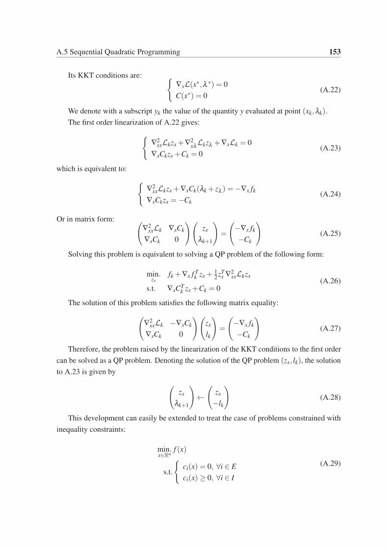
A.5 Sequential Quadratic Programming 153
Its KKT conditions are: ∇xL(x
∗,λ ∗) = 0
C(x∗) = 0(A.22)
We denote with a subscript yk the value of the quantity y evaluated at point (xk,λk).
The first order linearization of A.22 gives:
∇2
xxLkzx +∇2xλLkzλ +∇xLk = 0
∇xCkzx +Ck = 0(A.23)
which is equivalent to:
∇2
xxLkzx +∇xCk(λk + zλ ) =−∇x fk
∇xCkzx =−Ck
(A.24)
Or in matrix form: (∇2
xxLk ∇xCk
∇xCk 0
)(zx
λk+1
)=
(−∇x fk
−Ck
)(A.25)
Solving this problem is equivalent to solving a QP problem of the following form:
min.zx
fk +∇x f Tk zx +
12zT
x ∇2xxLkzx
s.t. ∇xCTk zx +Ck = 0
(A.26)
The solution of this problem satisfies the following matrix equality:
(∇2
xxLk −∇xCk
∇xCk 0
)(zx
lk
)=
(−∇x fk
−Ck
)(A.27)
Therefore, the problem raised by the linearization of the KKT conditions to the first order
can be solved as a QP problem. Denoting the solution of the QP problem (zx, lk), the solution
to A.23 is given by
(zx
λk+1
)←
(zx
−lk
)(A.28)
This development can easily be extended to treat the case of problems constrained with
inequality constraints:
min.x∈Rn
f (x)
s.t.
ci(x) = 0, ∀i ∈ E
ci(x)≥ 0, ∀i ∈ I
(A.29)

154 Numerical Optimization: Introduction
By solving the following Inequality-constrained Quadratic Problem (IQP) system at each
iteration:
min.zx
fk +∇x f Tk zx +
1
2zT
x ∇2xxLkzx
s.t.
∇xcikzx + cik = 0, ∀i ∈ E
∇xcikzx + cik ≥ 0, ∀i ∈ I
(A.30)
The main difficulty in solving that QP A.30 comes from finding the optimal active set Ak.
It is a necessary but costly operation, especially when starting from an initial active set A0.
The process is mostly based on a try and guess approach guided by heuristics (that may vary
with different resolution algorithms).
To find the optimal active set, the QP starts from an initial active set A0 ignore the
non-active constraints and try to solve the QP with the remaining active constraints. At a
step k of the resolution of the IQP, all the constraints in the active set A are treated as equality
constraints and the others are simply ignored, the QP to solve becomes:
EQP≡
min.
zx
fk +∇x f Tk zx +
12zT
x ∇2xxLkzx
s.t. ∇xcikzx + cik = 0, ∀i ∈ Ak
(A.31)
This EQP is solved, and its solution is checked against the constraints that were previously
ignored. If some of them are violated then the solution is not satisfactory and the active
set is updated by adding one or several of the violated constraints to it. This operation is
repeated until there are no more constraints to be added. Once all the constraints have been
added as active constraints to the EQP, the problem may be over-constrained. To detect
that, the Lagrange multipliers are computed and if some of them do not agree with the KKT
conditions of the IQP A.30, then one of them is removed from the active set and the resulting
EQP is solved, and the process continues until a satisfactory solution is found. The heuristics
used to choose which constraints to add or remove from the active set and to avoid cycling
between active sets are out of the scope of this dissertation.
Once the SQP gets close to the solution, the set of active constraints should not change
much from one iterate xk to the next one. It is often useful to initialize the IQP’s active set
with the optimal active set of the previous iterate: A0(xk+1)← A∗(xk). Then the (k+1)th
QP starts from an active set close to optimal and can be solved much faster. That method is
called the warm-start.
The SQP approach to solving the problem A.6 as presented above leans on the assumption
that at each step, the QP generated is feasible. If it is not, a restoration phase is entered and
finds a feasible point, see Section A.5.3.

A.5 Sequential Quadratic Programming 155
Solving the QP problem A.30 gives a solution step to a linearized problem, which in
general is not the solution to the original nonlinear problem. Thus, taking that step without
further verification can be dangerous and lead to bad iterates. To cope with that issue, several
methods exist. In the next few sections, we present the globalization methods that are the
Line Search and Trust Region approaches. They are used alongside methods to choose
whether to accept or reject a step like the merit function and filters in order to monitor the
length and direction of the step with regards to the nonlinear problem. And finally, we discuss
some Hessian approximation methods.
A.5.2 Globalization methods
The globalization phase of an SQP algorithm is meant to modify the steps generated by
the QP resolution in order to improve the global convergence of the algorithm, either by
multiplying them with a coefficient α in the Line-Search approach, or by bounding the norm
of the step found in the QP by adding to the QP a boundary constraint on z that reflects our
trust in the quality of the approximated problem.
The Line-Search Strategy
Given a step zk generated by the resolution of the QP, the goal of the line-search is to find
a coefficient α (typically in [0,1]) such that xk+1 = xk +αzk makes the violation of the
constraints and the value of the cost function decrease sufficiently. To decide whether those
decreases are sufficient, a merit function and a criterion are used. A merit function is a
function of α that transcribes the value of the objective function penalized by the violation
of the constraints. For a problem described by the system A.29, with a penalty parameter µ ,
a typical expression of the merit function M is:
M(α) = f (xk +αzk)+µ ∑i∈E
|ci(xk +αzk)|+µ ∑i∈I
max(0,−ci(xk +αzk)) (A.32)
Although finding the optimal value of α to minimize the 1-dimensional function M is
possible, it can prove costly, and is not necessary, because the only thing that we want is an
optimal solution to the problem A.29, thus the exact value of each iterate does not matter
much. Instead, we use a criterion to decide when the value of α gives a satisfactory decrease.
Various methods and criterion can be used to find a satisfactory value of α . For example, the
Wolfe line-search:
Let µ1 and µ2 be 2 real numbers such that: 0 < µ1 < µ2 < 1. A sufficient decrease
of the merit function can be depicted by the condition M(α) ≤ M(0) + µ1αM′(0). A

156 Numerical Optimization: Introduction
Figure A.1 Illustration of the choice made by the Wolfe line-search for values of α
sufficient increase of its derivative by M′(α)≥ µ2M′(0). The Wolfe Line-Search proceeds
by narrowing iteratively an interval [αL, αR] by trying a value α in this interval against
some tests and based on their results, decide to narrow it by the right or the left and repeat
that operation with the new interval until a satisfying value is found. Note that the Wolfe
line-search is guaranteed to terminate if M is C1 and bounded below.
The Wolfe Line-Search can be schematically described by algorithm: 9 and illustrated
by Figure A.1.
Algorithm 9 The Wolfe line-search
Init [αL,αR]← [0 ,1]loopChoose α ∈ [αL,αR]Evaluate M(α) and M′(α)
(1) M(α)≤M(0)+µ1αM′(0) and M′(α)< µ2M′(0): α is too small, αL ← a
(2) M(α)≤M(0)+µ1αM′(0) and M′(α)≥ µ2M′(0): Terminate, return α
(3) M(α)> M(0)+µ1αM′(0): α is too big, αR ← α
end loop
The Wolfe line-search is popular, but it requires the computation of the derivative of the
merit function, which can be prohibitively expensive in some cases, including in posture
generation for robotics problems, where the derivatives are usually expensive. Other line-
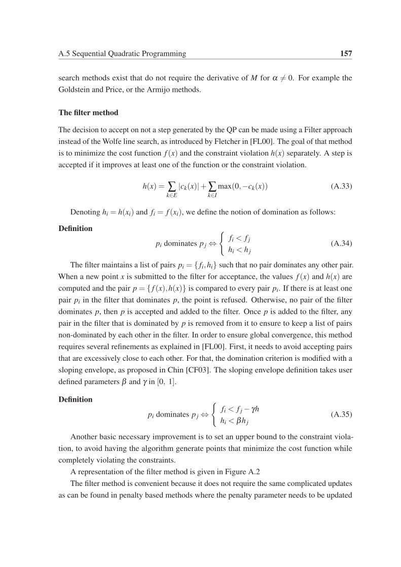
A.5 Sequential Quadratic Programming 157
search methods exist that do not require the derivative of M for α 6= 0. For example the
Goldstein and Price, or the Armijo methods.
The filter method
The decision to accept on not a step generated by the QP can be made using a Filter approach
instead of the Wolfe line search, as introduced by Fletcher in [FL00]. The goal of that method
is to minimize the cost function f (x) and the constraint violation h(x) separately. A step is
accepted if it improves at least one of the function or the constraint violation.
h(x) = ∑k∈E
|ck(x)|+∑k∈I
max(0,−ck(x)) (A.33)
Denoting hi = h(xi) and fi = f (xi), we define the notion of domination as follows:
Definition
pi dominates p j ⇔
fi < f j
hi < h j
(A.34)
The filter maintains a list of pairs pi = fi,hi such that no pair dominates any other pair.
When a new point x is submitted to the filter for acceptance, the values f (x) and h(x) are
computed and the pair p = f (x),h(x) is compared to every pair pi. If there is at least one
pair pi in the filter that dominates p, the point is refused. Otherwise, no pair of the filter
dominates p, then p is accepted and added to the filter. Once p is added to the filter, any
pair in the filter that is dominated by p is removed from it to ensure to keep a list of pairs
non-dominated by each other in the filter. In order to ensure global convergence, this method
requires several refinements as explained in [FL00]. First, it needs to avoid accepting pairs
that are excessively close to each other. For that, the domination criterion is modified with a
sloping envelope, as proposed in Chin [CF03]. The sloping envelope definition takes user
defined parameters β and γ in [0, 1].
Definition
pi dominates p j ⇔
fi < f j− γh
hi < βh j
(A.35)
Another basic necessary improvement is to set an upper bound to the constraint viola-
tion, to avoid having the algorithm generate points that minimize the cost function while
completely violating the constraints.
A representation of the filter method is given in Figure A.2
The filter method is convenient because it does not require the same complicated updates
as can be found in penalty based methods where the penalty parameter needs to be updated

158 Numerical Optimization: Introduction
Figure A.2 Representation of a filter with sloping envelope
regularly. Also, with the filter method, no derivative computation is required. That method is
generally more permissive than merit-based method in the sense that it refuses fewer points.
The filter method, as well as the merit function based methods, can be used in line-search
and trust-region algorithms.
The Trust-Region Strategy
The Trust Region strategy is based on the idea that at any iterate xk the quadratic model made
of the problem and fed to the QP solver can only be trusted to be relevant is a finite region
around the iterate. That region is called the trust region and its size is usually governed by a
single positive parameter ρk that can evolve along the optimization process. This translates
in a modified QP to solve at each iteration. A boundary constraint describing the trust region
is added to the problem. At each step, the modified problem writes as:
min.z∈Rn
12zT ∇2
xxHz+∑i∈U ∇ci(xk)T
z
subject to ∇ci(xk)T
z+ ci(xk) = 0, i ∈ E
∇ci(xk)T
z+ ci(xk)≥ 0, i ∈ I
|z|< ρk
(A.36)

A.5 Sequential Quadratic Programming 159
Figure A.3 Constraint incompatibility generated by trust region approach
Once a solution z of A.36 is found, the potential next iterate xk+1 = xk + z is checked
against the acceptance criterion (should it be a merit function or a filter or other). If it
is accepted, that means that our current model is good, we move to the next step with
xk+1 ← xk + z, and the size of the trust region can be augmented based on some heuristics.
Otherwise, the iterate is refused, the model is less good than expected, the size of the trust
region is reduced based on some heuristics (e.g. ρk+1 ← ρk/2) and the problem A.36 is
solved again with the new value of ρk+1. This is repeated until a satisfying point is found, or
until an unfeasible problem is found.
With this approach, a problem that often arises is the generation of unfeasible problems.
The reduction of the size of the trust region can lead to an incompatible set of constraints.
For example, with a single constraint, as illustrated in Figure A.3. The linearisation of the
constraint is represented by the green line, and the trust region by the black rectangle. If ρ is
too small, there is no intersection between the linearization of the constraint and the trust
region. The QP is then unfeasible. An obvious solution for that would be to increase the size
of the trust region, but that goes against the core idea of the trust region strategy and it would
harm the convergence properties of the algorithm. A more appropriate solution is to enter a
restoration phase when that event occurs. The purpose of a restoration phase is to reduce
the unfeasibility of a problem by relaxing unfeasible constraints without regards for the cost
function. The restoration phase is exited once a feasible point is found, and the course of the
SQP is continued from that point.

160 Numerical Optimization: Introduction
A.5.3 Restoration phase
As we stated previously, a restoration phase is entered when an unfeasible problem is found
by the trust region strategy. The goal of the restoration is to find a solution to the following
problem:
Find x ∈ Rn such that
ci(x) = 0, i ∈ E
ci(x)≥ 0, i ∈ I
|z|< ρk
(A.37)
The restoration phase proceeds in a similar way to the original SQP algorithm described
earlier. At each step, an approximated QP is solved, then its result is compared to an
acceptance criterion, if it is accepted, the trust region can be increased and the algorithm
continues. Otherwise, the trust region is reduced and the problem is solved again. The
acceptance criterion must be tailored for the restoration problem, meaning that it is based
on the values of the cost function of the restoration problem and of its constraints. The big
difference comes from the way the quadratic problem is constructed during this phase.
During a restoration phase step, the first action is to estimate the sets F and U of feasible
and unfeasible constraints. This is done by solving the linearization of problem (A.37) as
presented in (A.38). Each equality constraint is cut in 2 inequality constraints.
Find z ∈ Rn such that
∇ci(xk)T
z+ ci(xk)≥ 0, i ∈ E
−∇ci(xk)T
z− ci(xk)≥ 0, i ∈ E
∇ci(xk)T
z+ ci(xk)≥ 0, i ∈ I
|z|< ρk
(A.38)
The resolution of that FP gives the lists F and U . If the list of unfeasible constraints is
empty, the problem is feasible, so the restoration phase is exited to return to the main SQP
algorithm. The restoration QP to solve is built based on those lists. The unfeasible constraints
are removed from the constraint set and the expression of their violation is added to the cost
function, while the feasible constraints remain in the constraint list. This results in a problem
like A.39 to solve. (Note that the indexes of the constraints are modified to account for the
duplication of the equality constraints)
min.z∈Rn
12zT Hz− ∑
i∈U∇ci(xk)
Tz
subject to ∇ci(xk)T
z+ ci(xk)≥ 0, i ∈ F
|z|< ρk
(A.39)

A.5 Sequential Quadratic Programming 161
This problem is solved by a QP solver, its result is checked against an acceptance criterion,
based on that, the trust region is enlarged or reduced, and we go back to solving the FP.
In the restoration phase, special care must be taken in the computation of the matrix H,
that represents the Hessian of the Lagrangian of a problem that changes at each iteration. One
possible approach is to compute it as the sum of the Hessians of all the individual constraints,
and those can be computed exactly or with a quasi-newton approximation.
A.5.4 Quasi-Newton Approximation
In the SPQ algorithm, it is necessary to have access to the Hessian of the Lagrangian ∇2xxL to
be able to devise the QP subproblem to solve. Sometimes the exact Hessian of the problem
is not positive definite. Also, it is often difficult or computationally expensive to compute
an exact Hessian of the Lagrangian. Since we are following an iterative process, it is not
necessary to have an exact knowledge of the Hessian and using an approximation of it is
usually enough. Also, an approximate Hessian is in most cases less expensive to compute
than the exact one.
The idea behind computing an approximate Hessian is that, starting from an initial
approximate Hessian B0, we compute at each iteration an update to the approximate Hessian
based on the values and first order derivatives of the Lagrangian. This update aims at
capturing some curvature information about the Hessian by evaluating the evolution of the
gradient along the latest step. At step k, the Hessian update is a function of sk and yk:
sk = xk+1− xk, yk = ∇xL(xk+1,λk+1)−∇xL(xk,λk+1) (A.40)
The two most famous Hessian update strategies are called the BFGS (Broyden–Fletcher–
Goldfarb–Shanno) and the SR1(Symmetric Rank 1) updates. BFGS is a rank 2 update while
SR1 is rank 1.
The most basic formulas for the BFGS update is the following:
Bk+1 = Bk−BksksT
k Bk
sTk Bksk
+ykyT
k
sTk yk
(A.41)
Note that using a BFGS update requires that sk and yk satisfy the curvature condition:
sTk yk > 0. If that condition does not hold, then the value of yk is modified, which gives rise to
the Damped BFGS update, which guarantees to keep Bk definite positive:

162 Numerical Optimization: Introduction
θk =
1 if sTk yk ≥ 0.2sT
k Bksk
0.8sTk Bksk
sTk
Bksk−sTk
ykif sT
k yk ≥ 0.2sTk Bksk
rk = θkyk +(1−θk)Bksk
Bk+1 = Bk−BksksT
k Bk
sTk Bksk
+rkrT
k
sTk rk
(A.42)
The SR1 update is computed with the following formula:
Bk+1 = Bk +(yk−Bksk)(yk−Bksk)
T
(yk−Bksk)T
sk
(A.43)
Both those formulas proved to be efficient in some cases. It is not yet clear in which
cases one is better than the other.
A.6 Conclusion
This section gives a general introduction to nonlinear constrained optimization without
regards for specificities of robotics problem or formulations on manifolds, which are topics
considered in the core of this thesis.
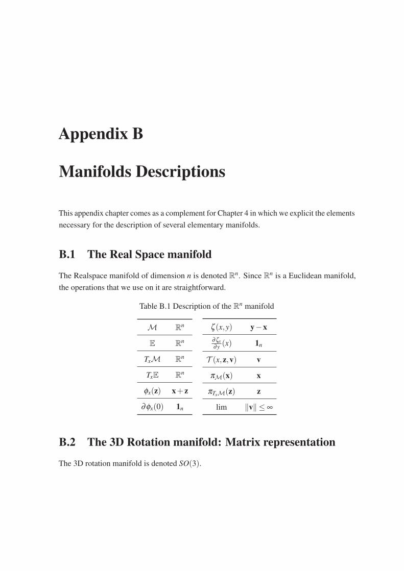
Appendix B
Manifolds Descriptions
This appendix chapter comes as a complement for Chapter 4 in which we explicit the elements
necessary for the description of several elementary manifolds.
B.1 The Real Space manifold
The Realspace manifold of dimension n is denoted Rn. Since Rn is a Euclidean manifold,
the operations that we use on it are straightforward.
Table B.1 Description of the Rn manifold
M Rn
E Rn
TxM Rn
TxE Rn
φx(z) x+ z
∂φx(0) 1n
ζ (x,y) y−x
∂ζx
∂y(x) 1n
T (x,z,v) v
πM(x) x
πTxM(z) z
lim ‖v‖ ≤ ∞
B.2 The 3D Rotation manifold: Matrix representation
The 3D rotation manifold is denoted SO(3).

164 Manifolds Descriptions
An element x of SO(3) is represented by x = ψ(x) in R3×3 by:
x ∈ SO(3), x =
x00 x01 x02
x10 x11 x12
x20 x21 x22
(B.1)
We recall the operators
. :
ω0
ω1
ω2
→
0 −ω2 ω1
ω2 0 −ω0
−ω1 ω0 0
(B.2)
And its inverse:
q. :
x00 x01 x02
x10 x11 x12
x20 x21 x22
→
x21
x02
x10
(B.3)
The exponential map is known as the Rodrigues formula:
∀v ∈ R3, exp(v) = 13 +
sin‖v‖
‖v‖v+
1− cos‖v‖
‖v‖2v2 (B.4)
Note that when ‖v‖ is small, we make the following replacements to avoid numerical
instability. It is important to ensure the precision of the retractation near zero because, in an
optimization process, many small steps are taken, especially when close to the solution.
sin‖v‖
‖v‖= 1−
‖v‖
6(B.5)
1− cos‖v‖
‖v‖2= 0.5−
‖v‖
24(B.6)
And the logarithm is computed as follows (see [Mer09]):
∀R ∈ ψ(SO(3)), f (R) =
0 if Tr(R) = 3
arccos(
Tr(R)−12
)
2sin(
arccos(
Tr(R)−12
))(R−RT
)otherwise
log(R) = ~f (R)
(B.7)

B.2 The 3D Rotation manifold: Matrix representation 165
We consider a point x ∈M and its representation matrix with the following storing order:
x = ψ(x) =
x0 x3 x6
x1 x4 x7
x2 x5 x8
=
x00 x01 x02
x10 x11 x12
x20 x21 x22
(B.8)
The derivative of retractation operation writes as:
∂ϕx
∂z(0) =
0 −x6 x3
0 −x7 x4
0 −x8 x5
x6 0 −x0
x7 0 −x1
x8 0 −x2
−x3 x0 0
−x4 x1 0
−x5 x2 0
(B.9)
And the derivation of the logarithm operation writes as:
v =
x21−x122
x02−x20
2x10−x01
2
(B.10)
f =arccos
(Tr(x)−1
2
)
2sin(
arccos(
Tr(x)−12
)) (B.11)
d f =(Tr(x)−1) f −1
2
(1−
(Tr(x)−1
2
)2) (B.12)
∂ζx
∂y(x) =
0 0 0 f 0 − f
d f .v 0 − f 0 d f .v 0 f 0 d f .v
f 0 − f 0 0 0
(B.13)

166 Manifolds Descriptions
Table B.2 Description of the SO(3) manifold with matrix representation
M SO(3)
E R3×3
TxM R3
TxE R3
ψ(x) = x
x00 x01 x02
x10 x11 x12
x20 x21 x22
φx(z) xexp(z)
∂φx(0) see Equation B.9
ζ (x,y) log(xT y)
∂ζx
∂y(x) see Equation B.10
T (x,z,v) v
πM(x) Q from QR decomposition of x
πTxM(z) z
lim ‖v‖ ≤ π
B.3 The 3D Rotation manifold with quaternion represen-
tation
The 3D rotation manifold is denoted SO(3).
An element x of SO(3) is represented by q = ψ(x) in R4 by:
x ∈ SO(3), q =
qw
qx
qy
qz
=
[qw
qvec
](B.14)
The exponential map is:
exp :
∣∣∣∣∣∣∣∣
R3 → R4
z 7→
cos
(‖z‖2
)
sin(‖z‖2
)z‖z‖
Note that when ‖v‖ is small, we make the following replacements to avoid numerical
instability.
exp(z) =
1− ‖z‖
8+ ‖z‖2
384(0.5− ‖z‖
48+ ‖z‖2
3840
)z
(B.15)

B.3 The 3D Rotation manifold with quaternion representation 167
And the logarithm is:
log :
∣∣∣∣∣R4 → R3
q 7→ arctan(
2‖qvec‖qw
q2w−‖qvec‖
2
)qvec
‖qvec‖
(B.16)
We consider a point q ∈M and its representation quaternion with the following storing
order:
q = ψ(q) =
qw
qx
qy
qz
(B.17)
The derivative of retractation operation writes as:
∂ϕq
∂z(0) =
1
2
−qx −qy −qz
qw −qz qy
qz qw −qx
−qy qx qw
(B.18)
And the derivation of the logarithm operation writes as:
f =arctan
(2‖qvec‖qw
q2w−‖qvec‖
2
)
n(B.19)
g =2qw− f
‖qvec‖2
(B.20)
∂ζx
∂y(x) =
−2qvec
f 13 +gqvecqvec
T
(B.21)

168 Manifolds Descriptions
Table B.3 Description of the SO(3) manifold with quaternion representation
M SO(3)
E R4
TxM R3
TxE R3
φx(z) xexp(z)
∂φx(0) see Appendix B.18
ζ (x,y) log(x−1y)
∂ζx
∂y(x) see Appendix B.19
T (x,z,v) v
πM(x) x‖x‖
πTxM(z) z
lim ‖v‖ ≤ π
B.4 The Unit Sphere manifold
An element x of S2 is represented by x = ψ(x) in R3 by:
x ∈ S2, x =
x0
x1
x2
(B.22)
With this manifold, the tangent space at x is the tangent plane to the unit-sphere at x.
Thus, TxM it is a 2-dimensional space, and its representation space is R3.
For the retractation we simply use a normalized sum:
φx(z) =x+ z
‖x+ z‖(B.23)
We define a distance operation on S2 as:
dist(x,y) = 1−x ·y (B.24)
And the projection on the tangent space:
πTxM(z) = z− (x · z)x (B.25)
The pseudo-logarithm operation is the following:
ζx(y) = dist(x,y)πTxM(z)
‖πTxM(z)‖(B.26)

B.4 The Unit Sphere manifold 169
The vector transport operation of vector v from TxM to TyM with y = φx(v), corresponds
to rotating v by the rotation that transforms x into y:
y = φx(z) (B.27)
R = 13 + x∧y+x∧y
2
1+x ·y(B.28)
T (x,z,v) = Rv (B.29)
Table B.4 Description of the S2 manifold
M S2
E R3
TxM R2
TxE R3
φx(z)x+z‖x+z‖
∂φx(0) 13−x ·xT
ζ (x,y) y− (x ·y)x
∂ζx(x)∂y
13−x ·xT
T (x,z,v) 13 + x∧φx(z)+x∧φx(z)
2
1+x·φx(z)
πM(x) x‖x‖
πTxM(z) z− (x · z)x
lim ‖v‖ ≤ ∞

Related Documents