VHE gamma-ray emission of PKS 2155-304: spectral and temporal variability

arX

iv:1

005.

3702

v2 [

astr

o-ph

.HE

] 21

May

201

0Astronomy & Astrophysicsmanuscript no. HESS˙PKS2155M304˙Variability c© ESO 2010May 24, 2010

VHE γ-ray emission of PKS 2155 −304:spectral and temporal variability

HESS Collaboration, A. Abramowski4, F. Acero15, F. Aharonian1,13, A.G. Akhperjanian2, G. Anton16, U. Barres deAlmeida8 ⋆, A.R. Bazer-Bachi3, Y. Becherini12, B. Behera14, W. Benbow1, K. Bernlohr1,5, A. Bochow1, C. Boisson6,

J. Bolmont19, V. Borrel3, J. Brucker16, F. Brun19, P. Brun7, R. Buhler1, T. Bulik29, I. Busching9, T. Boutelier17,P.M. Chadwick8, A. Charbonnier19, R.C.G. Chaves1, A. Cheesebrough8, J. Conrad31, L.-M. Chounet10, A.C. Clapson1,G. Coignet11, L. Costamante1,34, M. Dalton5, M.K. Daniel8, I.D. Davids22,9, B. Degrange10, C. Deil1, H.J. Dickinson8,A. Djannati-Ataı12, W. Domainko1, L.O’C. Drury13, F. Dubois11, G. Dubus17, J. Dyks24, M. Dyrda28, K. Egberts1,30,

P. Eger16, P. Espigat12, L. Fallon13, C. Farnier15, S. Fegan10, F. Feinstein15, M.V. Fernandes4, A. Fiasson11, A. Forster1,G. Fontaine10, M. Fußling5, S. Gabici13, Y.A. Gallant15, L. Gerard12, D. Gerbig21, B. Giebels10, J.F. Glicenstein7,

B. Gluck16, P. Goret7, D. Goring16, D. Hampf4, M. Hauser14, S. Heinz16, G. Heinzelmann4, G. Henri17, G. Hermann1,J.A. Hinton33, A. Hoffmann18, W. Hofmann1, P. Hofverberg1, M. Holleran9, S. Hoppe1, D. Horns4, A. Jacholkowska19,O.C. de Jager9, C. Jahn16, I. Jung16, K. Katarzynski27, U. Katz16, S. Kaufmann14, M. Kerschhaggl5, D. Khangulyan1,

B. Khelifi10, D. Keogh8, D. Klochkov18, W. Kluzniak24, T. Kneiske4, Nu. Komin7, K. Kosack7, R. Kossakowski11,G. Lamanna11, J.-P. Lenain6, T. Lohse5, C.-C. Lu1, V. Marandon12, A. Marcowith15, J. Masbou11, D. Maurin19,

T.J.L. McComb8, M.C. Medina6, J. Mehault15, R. Moderski24, E. Moulin7, M. Naumann-Godo10, M. de Naurois19,D. Nedbal20, D. Nekrassov1, N. Nguyen4, B. Nicholas26, J. Niemiec28, S.J. Nolan8, S. Ohm1, J-F. Olive3, E. de Ona

Wilhelmi1, B. Opitz4, K.J. Orford8, M. Ostrowski23, M. Panter1, M. Paz Arribas5, G. Pedaletti14, G. Pelletier17,P.-O. Petrucci17, S. Pita12, G. Puhlhofer18, M. Punch12, A. Quirrenbach14, B.C. Raubenheimer9, M. Raue1,34,

S.M. Rayner8, O. Reimer30, M. Renaud12, R. de los Reyes1, F. Rieger1,34, J. Ripken31, L. Rob20, S. Rosier-Lees11,G. Rowell26, B. Rudak24, C.B. Rulten8, J. Ruppel21, F. Ryde32, V. Sahakian2, A. Santangelo18, R. Schlickeiser21,F.M. Schock16, A. Schonwald5, U. Schwanke5, S. Schwarzburg18, S. Schwemmer14, A. Shalchi21, I. Sushch5, M.

Sikora24, J.L. Skilton25, H. Sol6, Ł. Stawarz23, R. Steenkamp22, C. Stegmann16, F. Stinzing16, G. Superina10,A. Szostek23,17, P.H. Tam14, J.-P. Tavernet19, R. Terrier12, O. Tibolla1, M. Tluczykont4, K. Valerius16, C. van Eldik1,G. Vasileiadis15, C. Venter9, L. Venter6, J.P. Vialle11, A. Viana7, P. Vincent19, M. Vivier7, H.J. Volk1, F. Volpe1,10,

S. Vorobiov15, S.J. Wagner14, M. Ward8, A.A. Zdziarski24, A. Zech6, and H.-S. Zechlin4

(Affiliations can be found after the references)

Preprint online version: May 24, 2010

ABSTRACT

Context. Observations of very high energyγ-rays from blazars provide information about accelerationmechanisms occurring in their innermostregions. Studies of variability in these objects allow a better understanding of the mechanisms at play.Aims. To investigate the spectral and temporal variability of VHE(> 100 GeV)γ-rays of the well-known high-frequency-peaked BL Lac objectPKS 2155−304 with the H.E.S.S. imaging atmospheric Cherenkov telescopes over a wide range of flux states.Methods. Data collected from 2005 to 2007 are analyzed. Spectra are derived on time scales ranging from 3 years to 4 minutes. Light curvevariability is studied through doubling timescales and structure functions, and is compared with red noise process simulations.Results. The source is found to be in a low state from 2005 to 2007, except for a set of exceptional flares which occurred in July 2006. Thequiescent state of the source is characterized by an associated mean flux level of (4.32± 0.09stat± 0.86syst) × 10−11 cm−2 s−1 above 200 GeV, orapproximately 15% of the Crab Nebula, and a power law photon index ofΓ = 3.53± 0.06stat± 0.10syst. During the flares of July 2006, doublingtimescales of∼ 2 min are found. The spectral index variation is examined over two orders of magnitude in flux, yielding different behaviour at lowand high fluxes, which is a new phenomenon in VHEγ-ray emitting blazars. The variability amplitude characterized by the fractional r.m.s.Fvar isstrongly energy-dependent and is∝ E0.19±0.01. The light curve r.m.s. correlates with the flux. This is the signature of a multiplicative process whichcan be accounted for as a red noise with a Fourier index of∼ 2.Conclusions. This unique data set shows evidence for a low levelγ-ray emission state from PKS 2155−304, which possibly has a different originthan the outbursts. The discovery of the light curve lognormal behaviour might be an indicator of the origin of aperiodicvariability in blazars.

Key words. gamma rays: observations – Galaxies : active – Galaxies : jets – BL Lacertae objects: individual objects: PKS 2155−304

Send offprint requests to: [email protected] [email protected]/[email protected]⋆ supported by CAPES Foundation, Ministry of Education of Brazil

1. Introduction

The BL Lacertae (BL Lac) category of Active Galactic Nuclei(AGN) represents the vast majority of the population of ener-

http://arxiv.org/abs/1005.3702v2

2 HESS Collaboration et al.: VHEγ-ray emission of PKS 2155−304: spectral and temporal variability

getic and extremely variable extragalactic very high energy γ-rayemitters. Their luminosity varies in unpredictable, highly irreg-ular ways, by orders of magnitude, and at all wavelengths acrossthe electromagnetic spectrum. The very high energy (VHE,E ≥100 GeV)γ-ray fluxes vary often on the shortest timescales thatcan be seen in this type of object, with large amplitudes whichcan dominate the overall output. It hence indicates that theun-derstanding of this energy domain is the most important one forunderstanding the underlying fundamental variability andemis-sion mechanisms at play in high flux states.

It has been, however, difficult to ascertain whetherγ-rayemission is present only during high flux states or also when thesource is in a more stable or quiescent state but with a flux whichis below the instrumental limits. The advent of the current gener-ation of atmospheric Cherenkov telescopes with unprecedentedsensitivity in the VHE regime gives new insights into these ques-tions.

The high frequency peaked BL Lac object (HBL)PKS 2155−304, located at a redshiftz = 0.117, initially dis-covered as a VHEγ-ray emitter by the Mark 6 telescope(Chadwick et al. 1999), has been detected by the first H.E.S.S.telescope in 2002-2003 (Aharonian et al. 2005b). It has beenfrequently observed by the full array of four telescopes since2004, either sparsely during the H.E.S.S. monitoring program,or intensely during dedicated campaigns such as that de-scribed in Aharonian et al. (2005c), showing mean flux lev-els of ∼ 20% of the Crab Nebula flux for energies above200 GeV. During the summer of 2006, PKS 2155−304 exhib-ited unprecedented flux levels accompanied by strong variability(Aharonian et al. 2007a), making temporal and spectral variabil-ity studies possible on timescales of the order of a few minutes.The VHEγ-ray emission is usually thought to originate from arelativistic jet, emanating from the vicinity of a SupermassiveBlack Hole (SMBH). The physical processes at play are stillpoorly understood, but the analysis of theγ-ray flux spectral andtemporal characteristics is well suited to provide better insights.

For this goal the data set of H.E.S.S. observations ofPKS 2155−304 between 2005 and 2007 is used. After describingthe observations and the analysis chain in Section 2, the emissionfrom the “quiescent”, i.e. nonflaring, state of the source will becharacterized in Section 3. Section 4 details spectral variabilityrelated to the source intensity. Section 5 will focus on the de-scription of the temporal variability during the highly active stateof the source, and its possible energy dependence. Section 6willillustrate a description of the observed variability phenomenonby a random stationary process, characterized by a simple powerdensity spectrum. Section 7 will show how limits on the charac-teristic time of the source can be derived. The multi-wavelengthaspects from the high flux state will be presented in a secondpaper.

2. Observations and analysis

H.E.S.S. is an array of four imaging atmospheric Cherenkovtelescopes situated in the Khomas Highland of Namibia(23◦16′18′′ South, 16◦30′00′′ East), at an elevation of1,800 meters above sea level (see Aharonian et al. 2006).PKS 2155−304 was observed by H.E.S.S. each year since2002; results of observations in 2002, 2003 and 2004 can befound in Aharonian et al. (2005b), Aharonian et al. (2005c) andGiebels et al. (2005). The data reported here were collectedbe-tween 2005 and 2007. In 2005, 12.2 hours of observations weretaken. A similar observation time was scheduled in 2006, butfollowing the strong flare of July 26th (Aharonian et al. 2007a)

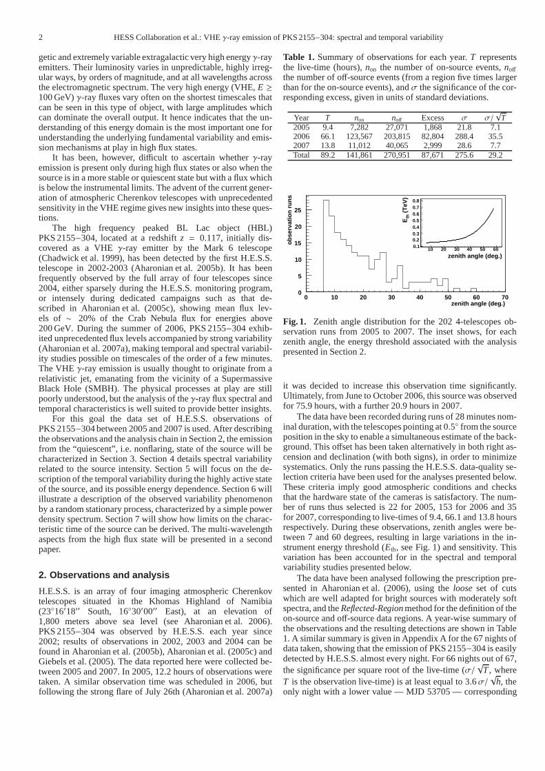
Table 1. Summary of observations for each year.T representsthe live-time (hours),non the number of on-source events,noffthe number of off-source events (from a region five times largerthan for the on-source events), andσ the significance of the cor-responding excess, given in units of standard deviations.

Year T non noff Excess σ σ/√

T2005 9.4 7,282 27,071 1,868 21.8 7.12006 66.1 123,567 203,815 82,804 288.4 35.52007 13.8 11,012 40,065 2,999 28.6 7.7Total 89.2 141,861 270,951 87,671 275.6 29.2

zenith angle (deg.)0 10 20 30 40 50 60 70

obse

rvat

ion

runs

0

5

10

15

20

25

zenith angle (deg.)10 20 30 40 50 60

(T

eV)

thE

0.10.20.30.40.50.60.70.8

Fig. 1. Zenith angle distribution for the 202 4-telescopes ob-servation runs from 2005 to 2007. The inset shows, for eachzenith angle, the energy threshold associated with the analysispresented in Section 2.

it was decided to increase this observation time significantly.Ultimately, from June to October 2006, this source was observedfor 75.9 hours, with a further 20.9 hours in 2007.

The data have been recorded during runs of 28 minutes nom-inal duration, with the telescopes pointing at 0.5◦ from the sourceposition in the sky to enable a simultaneous estimate of the back-ground. This offset has been taken alternatively in both right as-cension and declination (with both signs), in order to minimizesystematics. Only the runs passing the H.E.S.S. data-quality se-lection criteria have been used for the analyses presented below.These criteria imply good atmospheric conditions and checksthat the hardware state of the cameras is satisfactory. The num-ber of runs thus selected is 22 for 2005, 153 for 2006 and 35for 2007, corresponding to live-times of 9.4, 66.1 and 13.8 hoursrespectively. During these observations, zenith angles were be-tween 7 and 60 degrees, resulting in large variations in the in-strument energy threshold (Eth, see Fig. 1) and sensitivity. Thisvariation has been accounted for in the spectral and temporalvariability studies presented below.

The data have been analysed following the prescription pre-sented in Aharonian et al. (2006), using theloose set of cutswhich are well adapted for bright sources with moderately softspectra, and theReflected-Regionmethod for the definition of theon-source and off-source data regions. A year-wise summary ofthe observations and the resulting detections are shown in Table1. A similar summary is given in Appendix A for the 67 nights ofdata taken, showing that the emission of PKS 2155−304 is easilydetected by H.E.S.S. almost every night. For 66 nights out of67,the significance per square root of the live-time (σ/

√T, where

T is the observation live-time) is at least equal to 3.6σ/√

h, theonly night with a lower value — MJD 53705 — corresponding

HESS Collaboration et al.: VHEγ-ray emission of PKS 2155−304: spectral and temporal variability 3

to a very short exposure. In addition, for 61 nights out of 67the source emission is high enough to enable a detection of thesource with 5σ significance in one hour or less, a level usuallyrequired in this domain to firmly claim a new source detection. In2006 the source exhibits very strong activity (38 nights, betweenMJD 53916 – 53999) with a nightlyσ/

√T varying from 3.6 to

150, and being higher than 10σ/√

h for 19 nights. The activityof the source climaxes on MJD 53944 and 53946 with statisticalsignificances which are unprecedented at these energies, the rateof detectedγ-rays corresponding to 2.5 and 1.3 Hz, with 150and 98σ/

√h respectively.

For subsequent spectral analysis, an improved energy re-construction method with respect to the one described inAharonian et al. (2006) was applied. This method is based on alook-up table determined from Monte-Carlo simulations, whichcontains the relation between an image’s amplitude and its re-constructed impact parameter as a function of the true energy,the observation zenith angle, the position of the source in thecamera, the optical efficiency of the telescopes (which tend todecrease due to the aging of the optical surfaces), the number oftriggered telescopes and the reconstructed altitude of theshowermaximum. Thus, for a given event, the reconstructed energy isdetermined by requiring the minimalχ2 between the image am-plitudes and those expected from the look-up table correspond-ing to the same observation conditions. This method yields aslightly lower energy threshold (shown in Fig. 1 as a functionof zenith angle), an energy resolution which varies from 15%to20% over all the energy range, and biases in the energy recon-struction which are smaller than 5%, even close to the threshold.The systematic uncertainty in the normalization of the H.E.S.S.energy scale is estimated to be as large as 15%, correspondingfor such soft spectrum source to 40% in the overall flux normal-ization as quoted in Aharonian et al. (2009).

All the spectra presented in this paper have been obtainedusing a forward-folding maximum likelihood method based onthe measured energy-dependent on-source and off-source distri-butions. This method, fully described in Piron et al. (2001), per-forms a global deconvolution of the instrument functions (energyresolution, collection area) and the parametrization of the spec-tral shape. Two different sets of parameters, corresponding to apower law and to a power law with an exponential cut-off, areused for the spectral shape, with the following equations :

φ(E) = φ0

( EE0

)−Γ(1)

φ(E) = φ0 exp( E0

Ecut

)( EE0

)−Γexp(

− EEcut

)

(2)

φ0 represents the differential flux atE0 (chosen to be 1 TeV),Γ isthe power law index andEcut the characteristic energy of the ex-ponential cut-off. The maximum likelihood method provides thebest set of parameters corresponding to the selected hypothesis,and the corresponding error matrix.

Finally, various data sets have been used for subsequent anal-yses. These are summarized in Table 2.

3. Characterization of the quiescent state

As can be seen in Fig. 2, with the exception of the high stateof July 2006 PKS 2155−304 was in a low state during the ob-servations from 2005 to 2007. This section explores the vari-ability of the source during these periods of low-level activity,based on the determination of the run-wise integral fluxes for thedata setDQS, which excludes the flaring period of July 2006 and

2005Jul

2005Dec

2006Jul

2006Dec

2007Jul

2008Jan

)-1 s

-2 (

E>0

.2T

eV)

(cm

Φ

0

0.1

0.2

0.3

0.4

0.5

0.6-910×

Fig. 2. Monthly averaged integral flux of PKS 2155−304 above200 GeV obtained from data setD (see Table 2), which corre-sponds to the 165 4-telescope runs whose energy threshold isbelow 200 GeV. The dotted line corresponds to 15% of the CrabNebula emission level (see Section 3.2).

also those runs whose energy threshold is higher than 200 GeV(see 3.1 for justification). As for Sections 5 and 6, the control ofsystematics in such a study is particularly important, especiallybecause of the strong variations of the energy threshold through-out the observations.

3.1. Method and systematics

The integral flux for a given period of observations is determinedin a standard way. For subsequent discussion purposes, the for-mula applied is given here :

Φ = Nexp

∫ Emax

EminS(E)dE

T∫ ∞0

∫ Emax

EminA(E)R(E,E′)S(E)dE′dE

(3)

where T represents the corresponding live-time,A(E) andR(E,E′) are, respectively, the collection area at the true energyE and the energy resolution function betweenE and the mea-sured energyE′, andS(E) the shape of the differential energyspectrum as defined in Eq. 1 and 2 . Finally,Nexp is the numberof measured events in the energy range [Emin,Emax].

In the case thatS(E) is a power law, an important source ofsystematic error in the determination of the integral flux vari-ation with time comes from the value chosen for the indexΓ.The average 2005–2007 energy spectrum yields a very well de-termined power law index1. However, in Section 4 it will beshown that this index varies depending on the flux level of thesource. Moreover, in some cases the energy spectrum of thesource shows some curvature in the TeV region, giving slightvariations in the fitted power law index depending on the energyrange used.

For runs whose energy threshold is lower thanEmin, a sim-ulation performed under the observation conditions correspond-ing to the data shows that an index variation of∆Γ = 0.1 impliesa flux error at the level of∆Φ ∼ 1%, this relation being quite lin-ear up to∆Γ ∼ 0.5. However, this relation no longer holds when

1 The average 2005–2007 energy spectrum yields a power law with aphoton indexΓ = 3.37±0.02stat. One should note that some curvature isobserved at higher energies, resulting in a better spectraldeterminationwhen the alternative hypothesis shown in (Eq. 2) is used, yielding aharder index (Γ = 3.05± 0.05stat) with an exponential cut-off at energyEcut = 1.76±0.27stat TeV. This curved model is prefered at a 8.4σ levelas compared to the power law hypothesis. However, the choiceof themodel has little effect on the determination of the integral flux valuesabove 200 GeV, the integral being dominated by the low-energy part ofthe energy spectrum.


Table 2. The various data sets used in the paper, referred to in the text by the labels presented in this table. Only runs with thefull array of four telescopes in operation (202 runs over 210) and an energy threshold lower than 200 GeV (165 runs over 202)are considered. The corresponding period of the observations, the number of runs, the live-timeT (hours), the number ofγ excessevents and its significanceσ are shown. The columnsectionindicates the sections of the paper in which each data set is discussed.Additional criteria for the data set definitions are indicated in the last column.

Label Period Runs T(hours) Excess σ Section Additional criteriaD 2005–2007 165 69.7 67,654 237.4 4, 7 –

DQS 2005–2007 115 48.1 12,287 60.5 3.2, 3.4, 3.3, 7 July 2006 excludedDQS−2005 2005 19 8.0 1,816 22.6 3.4 –DQS−2006 2006 61 26.3 7,472 48.4 3.4 July 2006 excludedDQS−2007 2007 35 13.8 2,999 28.6 3.4 –DJULY06 July 2006 50 21.6 55,367 281.8 4, 5, 6, 7 –DFLARES July 2006 (4 nights) 27 11.8 46,036 284.1 4, 5, 6, 7 –

the energy threshold is aboveEmin, as the determination ofΦbecomes much more dependent on the choice ofΓ. For this rea-son, only runs whose energy threshold is lower thanEmin will bekept for the subsequent light curves. The value ofEmin is chosenas 200 GeV, which is a compromise between a low value whichmaximises the excess numbers used for the flux determinationsand a high value which maximises the number of runs whoseenergy threshold is lower thanEmin.

3.2. Run-wise distribution of the integral flux

From 2005 to 2007, PKS 2155−304 is almost always detectedwhen observed (except for two nights for which the exposurewas very low), indicating the existence, at least during these ob-servations, of a minimal level of activity of the source. Focussingon data setDQS (which excludes the July 2006 data where thesource is in a high state), the distribution of the integral fluxesof the individual runs above 200 GeV has been determined forthe 115 runs, using a spectral indexΓ = 3.53 (the best value forthis data set, as shown in 3.4). This distribution has an asym-metric shape, with mean value (4.32± 0.09stat) × 10−11 cm−2s−1

and root mean square (r.m.s.) (2.48± 0.11stat) × 10−11 cm−2s−1,and is very well described with a lognormal function. Such abehaviour implies that the logarithm of fluxes follows a nor-mal distribution, centered on the logarithm of (3.75± 0.11stat) ×10−11 cm−2s−1. This is shown in the left panel of Fig. 3, wherethe solid line represents the best fit obtained with a maximum-likelihood method, yielding results independent of the choiceof the intervals in the histogram. It is interesting to note thatthis result can be compared to the fluxes measured by H.E.S.S.from PKS 2155−304 during its construction phase, in 2002 and2003 (see Aharonian et al. 2005b and Aharonian et al. 2005c).As shown in Table 3, these flux levels extrapolated down to200 GeV were close to the value corresponding to the peakshown in the left panel of Fig. 3.

The right panel of Fig. 3 shows how the flux distribution ismodified when the July 2006 data are taken into account (data setD in Table 2): the histogram can be accounted for by the super-position of two Gaussian distributions (solid curve). The results,summarized in Table 4, are also independent of the choice of theintervals in the histogram. Remarkably enough, the character-istics of the first Gaussian obtained in the first step (left panel)remain quite stable in the double Gaussian fit.

This leads to two conclusions. First, the flux distribution ofPKS 2155−304 is well described considering a low state and ahigh state, for each of which the distribution of the logarithmsof the fluxes follows a Gaussian distribution. The characteristicsof the lognormal flux distribution for the high state are given

Table 3. Integral fluxes and their statistical errors from2002 and 2003 observations of PKS 2155−304 during theH.E.S.S. construction phase. These values are taken fromAharonian et al. (2005b) and Aharonian et al. (2005c) and cor-respond to flux extrapolations to above 200 GeV.

Month Year Φ [10−11 cm−2s−1]July 2002 16.4± 4.7Oct. 2002 8.9± 5.2June 2003 5.8± 1.4July 2003 2.9± 0.5Aug. 2003 3.5± 0.5Sep. 2003 4.9± 1.2Oct. 2003 5.2± 0.5

Table 4. The distribution of the flux logarithm. First column:distribution as fitted by a single Gaussian law for the “quiescent”regime (data setDQS ). Second column: distribution fitted bytwo Gaussian laws, one for the “quiescent” regime, the otherforthe flaring regime (data setD). Decimal logarithms are quotedto make the comparison with the left panel of Fig. 3 easier andthe flux is expressed in cm−2 s−1. In the first line the average offluxes is reported, while in the second line their r.m.s..

“Quiescent” regime Flaring regime⟨

log10Φ⟩

-10.42± 0.02 -9.79± 0.11r.m.s. of log10Φ 0.24± 0.02 0.58± 0.04

in Sections 5, 6 and 7. Secondly, PKS 2155−304 has a levelof minimal activity which seems to be stable on a several-yeartime-scale. This state will henceforth be referred to as the“quiescent state” of the source.

3.3. Width of the run-wise flux distribution

In order to determine if the measured width of the flux distribu-tion (left panel of Fig. 3) can be explained as statistical fluctua-tions from the measurement process a simulation has been car-ried out considering a source which emits an integral flux above200 GeV of 4.32×10−11cm−2s−1 with a power law photon spec-trum indexΓ = 3.53 (as determined in the next section). Foreach run of the data setDQS the numbernγ expected by convolv-ing the assumed differential energy spectrum with the instrumentresponse corresponding to the observation conditions is deter-mined. A random smearing around this value allows statistical


)−1s−2 (cmΦ10log−11.5 −11 −10.5 −10 −9.5 −9 −8.5 −8

Num

ber

of r

uns

0

5

10

15

20

25

30

35

)−1s−2 (cmΦ10log−11.5 −11 −10.5 −10 −9.5 −9 −8.5 −8

Num

ber

of r

uns

0

5

10

15

20

25

30

35

40

−11.5 −11 −10.5 −10 −9.5 −9 −8.5 −80

5

10

15

20

25

30

35

40

Fig. 3. Distributions of the logarithms of integral fluxes above 200GeV in individual runs. Left: from 2005 to 2007 except the July2006 period (data setDQS), fitted by a Gaussian. Right: all runs from 2005 to 2007 (datasetD), where the solid line represents theresult of a fit by the sum of 2 Gaussians (dashed lines). See Table 4 for details.

fluctuations to be taken into account. The number of events inthe off-source region and also the number of background eventsin the source region are derived from the measured valuesnoff inthe data set. These are also smeared in order to take into accountthe expected statistical fluctuations.

10000 such flux distributions have been simulated, and foreach one its mean value and r.m.s. (which will be called be-low RMSD) are determined. The distribution of RMSD thus ob-tained, shown in Fig. 4, is well described by a Gaussian centredon 0.98×10−11 cm−2s−1 (which represents a relative flux disper-sion of 23%) and with aσRMS D of 0.07× 10−11 cm−2s−1.

It should be noted that here the effect of atmospheric fluc-tuations in the determination of the flux is only taken into ac-count at the level of the off-source events, as these numbers aretaken from the measured data. But the effect of the correspond-ing level of fluctuations on the source signal is very difficultto determine. If a conservative value of 20% is considered2,which is added in the simulations as a supplementary fluctua-tion factor for the number of events expected from the source,a RMSD distribution centred on 1.30 × 10−11 cm−2s−1 with aσRMS D of 0.09× 10−11 cm−2s−1 is obtained. Even in this con-servative case, the measured value for the flux distributionr.m.s.((2.48± 0.11stat) × 10−11 cm−2s−1) is very far (more than 8 stan-dard deviations) from the simulated value. All these elementsstrongly suggest the existence of an intrinsic variabilityassoci-ated with the quiescent state of PKS 2155−304.

3.4. Quiescent-state energy spectrum

The energy spectrum associated with the data setDQS, shown inFig. 5, is well described by a power law with a differential flux at1 TeV ofφ0 = (1.81±0.13stat)×10−12cm−2s−1TeV−1 and an index

2 A similar procedure has been carried out on the Crab Nebula ob-servations. Considering this source to be perfectly stableit allows us todetermine an upper limit to the fluctuations of the Crab signal due to theatmosphere, and a value of∼ 10% was derived. Nonetheless, this valueis linked to the observations’ epoch and zenith angles, and to the sourcespectral shape.

Fig. 4. Distribution of RMSD obtained when the instrumentresponse to a fixed emission (Φ = 4.32 × 10−11 cm−2s−1 andΓ = 3.53) is simulated 10000 times with the same observationconditions as for the 115 runs of the left part of Fig. 3.

of Γ = 3.53± 0.06stat. The stability of these values for spectrameasured separately for 2005, 2006 (excluding July) and 2007is presented in Table 5. The corresponding average integralfluxis (4.23± 0.09stat) × 10−11 cm−2s−1, which is as expected in verygood agreement with the mean value of the distribution shownin the left panel of Fig. 3.

Bins above 2 TeV correspond toγ−ray excesses lower than20γ and significances lower than 2σ. Above 5 TeV excesses areeven less significant (∼ 1σ or less) and 99% upper-limits areused. There is no improvement of the fit when a curvature istaken into account.

6 HESS Collaboration et al.: VHEγ-ray emission of PKS 2155−304: spectral and temporal variability)

-1 T

eV-1

s-2

(cm

φ

-1710

-1610

-1510

-1410

-1310

-1210

-1110

-1010

-910

=

=

±

±0

φ

Γ

1.81 0.13

3.53 0.06

-1 TeV-1 s-2 cm-12x 10

Energy (TeV)

-110 1 10

Res

idua

ls

-1

0

1

Fig. 5. Energy spectrum of the quiescent state for the period2005-2007. The green band correponds to the 68% confidence-level provided by the maximum likelihood method. Points arederived from the residuals in each energy bin, only for illustra-tion purposes. See Section 3.4 for further details.

Table 5. Parametrization of the differential energy spectrumof the quiescent state of PKS 2155−304, determined in theenergy range 0.2–10TeV, first for the 2005–2007 period andalso separately for the 2005, 2006 (excluding July) and 2007periods. Corresponding data sets are those of Table 2.φ0(10−12 cm−2s−1TeV−1) is the differential flux at 1 TeV,Γ the pho-ton index andΦ (10−11 cm−2s−1) the integral flux above 0.2 TeV.Errors are statistical.

Year Data set φ0 Γ Φ

2005–2007 DQS 1.81± 0.13 3.53± 0.06 4.23± 0.092005 DQS−2005 1.59± 0.32 3.56± 0.16 3.83± 0.212006 DQS−2006 1.87± 0.18 3.59± 0.08 4.65± 0.132007 DQS−2007 1.84± 0.24 3.43± 0.11 3.78± 0.16

4. Spectral variability

4.1. Variation of the spectral index for the whole data set2005-2007

The spectral state of PKS 2155−304 has been monitored since2002. The first set of observations (Aharonian et al. 2005b),from July 2002 to September 2003, shows an average energyspectrum well described by a power law with an index ofΓ =3.32±0.06stat, for an integral flux (extrapolated down to 200 GeV) of (4.39±0.40stat)×10−11 cm−2s−1. No clear indication of spec-tral variability was seen. Consecutive observations in Octoberand November 2003 (Aharonian et al. 2005c) gave a similarvalue for the index,Γ = 3.37± 0.07stat, for a slightly higher fluxof (5.22± 0.54stat) × 10−11 cm−2s−1. Later, during H.E.S.S. ob-servations of the first (MJD 53944, Aharonian et al. 2007a) andsecond (MJD 53946, Aharonian et al. 2009) exceptional flaresof July 2006, the source reached much higher average fluxes,corresponding to (1.72 ± 0.05stat) × 10−9 cm−2s−1 and (1.24 ±0.02stat)×10−9 cm−2s−1 3 respectively. In the first case, no strongindications for spectral variability were found and the average

3 corresponding to data set T200 in Aharonian et al. (2009)

MJD-53000940 942 944 946 948 950 952 954

)-1 s

-2 (

E>0

.2T

eV)

(cm

Φ

00.20.40.60.8

11.21.41.61.8

-910×

Fig. 6. Integral flux above 200 GeV measured each night dur-ing late July 2006 observations. The horizontal dashed linecorresponds to the quiescent state emission level defined inSection 3.2.

indexΓ = 3.19± 0.02stat was close to those associated with the2002 and 2003 observations. In the second case, clear evidenceof spectral hardening with increasing flux was found.

The observations of PKS 2155−304 presented in this paperalso include the subsequent flares of 2006 and the data of 2005and 2007. Hence, the evolution of the spectral index is studiedfor the first time for a flux level varying over two orders of mag-nitude. This spectral study has been carried out over the fixedenergy range 0.2–1TeV in order to minimize both systematiceffects due to the energy threshold variation and the effect ofthe curvature observed at high energy in the flaring states. Themaximal energy has been chosen to be at the limit where thespectral curvature seen in high flux states begins to render thepower law or exponential curvature hypotheses distinguishable.As flux levels observed in July 2006 are significantly higher thanin the rest of the data set (see Fig. 6), the flux–index behaviouris determined separately first for the July 2006 data set itself(DJULY06) and secondly for the 2005-2007 data excluding thisdata set (DQS).

On both data sets, the following method was applied. Theintegral flux was determined for each run assuming a power lawshape with an index ofΓ = 3.37 (average spectral index for thewhole data set), and runs were sorted by increasing flux. The setof ordered runs was then divided into subsets containing at leastan excess of 1500γ above 200 GeV and the energy spectrum ofeach subset was determined4.

The left panel of Fig. 7 shows the photon index versus in-tegral flux for data setsDQS (grey crosses) andDJULY06 (blackpoints). Corresponding numbers are summarized in AppendixB.While a clear hardening is observed for integral fluxes abovea few 10−10 cm−2s−1, a break in this behaviour is observed forlower fluxes. Indeed, for the data setDJULY06 (black points)a linear fit yields a slope dΓ/dΦ = (3.0 ± 0.3stat) × 108cm2s,whereas the same fit for data setDQS (grey crosses) yields aslope dΓ/dΦ = (−3.4 ± 1.9stat) × 109cm2s. The latter corre-sponds to aχ2 probability P(χ2) = 71%; a fit to a constant yieldsP(χ2) = 33% but with a constant fitted index incompatible witha linear extrapolation from higher flux states at a 3σ level. Thisis compatible with conclusions obtained either with an indepen-dant analysis or when these spectra are processed followingadifferent prescription. In this prescription the runs were sortedas a function of time in contiguous subsets with similar photonstatistics, rather than as a function of increasing flux.

4 even for lower fluxes, the significance associated with each subsetis always higher than 20 standard deviations


)-1s-2(0.2TeV<E<1TeV) (cmΦ-1110 -1010 -910

Γph

oton

inde

x

3

3.2

3.4

3.6

3.8

4

)-1s-2(0.2TeV<E<1TeV) (cmΦ-1110 -1010 -910

Γph

oton

inde

x

3

3.2

3.4

3.6

3.8

4

Fig. 7. Evolution of the photon indexΓ with increasing fluxΦ in the 0.2–1 TeV energy range. The left panel shows the results forthe July 2006 data (black points, data setDJULY06) and for the 2005–2007 period excluding July 2006 (grey points, data setDQS).The right panel shows the results for the four nights flaring period of July 2006 (black points, data setDFLARES) and one pointcorresponding to the quiescent state average spectrum (grey point, again data setDQS). See text in Sections 4.1 (left panel) and 4.2(right panel) for further details on the method.

The form of the relation between the index versus inte-gral flux is unprecedented in the TeV regime. Prior to theresults presented here, spectral variability has been detectedonly in two other blazars, Mrk 421 and Mrk 501. For Mrk 421,a clear hardening with increasing flux appeared during the1999/2000 and 2000/2001 observations performed with HEGRA(Aharonian et al. 2002) and also during the 2004 observationsperformed with H.E.S.S. (Aharonian et al. 2005a). In addition,the Mrk 501 observations carried out with CAT during the strongflares of 1997 (Djannati-Ataı et al. 1999) and also the recentobservation performed by MAGIC in 2005 (Albert et al. 2007)have shown a similar hardening. In both studies, the VHE peakhas been observed in theνFν distributions of the flaring states ofMrk 501.

4.2. Variation of the spectral index for the four flaring nightsof July 2006

In this section, the spectral variability during the flares of July2006 is described in more detail. A zoom on the variation ofthe integral flux (4-minute binning) for the four nights contain-ing the flares (nights MJD 53944, 53945, 53946, and 53947,called the “flaring period”) is presented in the top panel ofFig. 8. This figure shows two exceptional peaks on MJD 53944and MJD 53946 which climax respectively at fluxes higher than2.5× 10−9 cm−2s−1 and 3.5× 10−9 cm−2s−1 (∼ 9 and∼ 12 timesthe Crab Nebula level above the same energy), both about twoorders of magnitude above the quiescent state level.

The variation with time of the photon index is shown inthe bottom panel of Fig. 8. To obtain these values, theγ ex-cess above 200 GeV has been determined for each 4-minute bin.Then, successive bins have been grouped in order to reach aglobal excess higher than 600γ. Finally, the energy spectrumof each data set has been determined in the 0.2–1 TeV en-ergy range, as before (corresponding numbers are summarizedin Appendix Table B.4). There is no clear indication of spectralvariability within each night, except for MJD 53946 as showninAharonian et al. (2009). However, a variability can be seen fromnight to night, and the spectral hardening with increasing flux

level already shown in Fig. 7 is also seen very clearly in thismanner.

It is certainly interesting to directly compare the spectralbehaviour seen during the flaring period with the hardness ofthe energy spectrum associated with the quiescent state. This isshown in the right panel of Fig. 7, where black points corre-spond to the four flaring nights; these were determined in thesame manner as for the left panel (see 4.1 for details). A linearfit here yields a slope dΓ/dΦ = (2.8±0.3stat)×108cm2s. The greycross corresponds to the integral flux and the photon index asso-ciated with the quiescent state (derived in a consistent wayin theenergy range from 0.2–1 TeV), showing a clear rupture with thetendancy at higher fluxes (typically above 10−10 cm−2s−1).

These four nights were further examined to search for dif-ferences in the spectral behaviour between periods in whichthe source flux was clearly increasing and periods in which itwas decreasing. For this, the first 16 minutes of the first flare(MJD 53944) are of special interest because they present a verysymmetric situation: the flux increases during the first half, andthen decreases to its initial level, the averaged fluxes are sim-ilar in both parts (∼ 1.8 × 10−9 cm−2s−1), and the observationconditions (and thus the instrument response) are almost con-stant — the mean zenith angle of each part being respectively7.2 and 7.8 degrees. Again, the spectra have been determined inthe 0.2–1TeV energy range, giving indices ofΓ = 3.27±0.12statandΓ = 3.27± 0.09stat respectively. To further investigate thisquestion and avoid potential systematic errors from the spectralmethod determination, the hardness ratios were derived (definedas the ratio of the excesses in different energy bands), using forthis the energy (TeV) bands [0.2–0.35], [0.35–0.6] and [0.6–5.0].For any combination, no differences were found beyond the 1σlevel between the increasing and decreasing parts. A similar ap-proach has been applied — when possible — for the rest of theflaring period. No clear dependence has been found within thestatistical error limit of the determined indices, which isdis-tributed between 0.09 and 0.20.

Finally, the persistence of the energy cut-off in the differ-ential energy spectrum along the flaring period has been exam-ined. For this purpose, runs were sorted again by increasingflux


)-1

s-2

cm

-9 (

10

Φ

0.51

1.52

2.53

3.54

4.5

E > 0.2 TeV

)-1

s-2

cm

-9 (

10

Φ 0.5

1

1.5

2

2.5

0.2 < E < 0.35 TeV

)-1

s-2

cm

-9 (

10

Φ

0.10.20.30.40.50.60.70.80.9

0.35 < E < 0.6 TeV

)-1

s-2

cm

-9 (

10

Φ

0.05

0.1

0.15

0.2

0.25

0.3

0.35

0.6 < E < 5 TeV

MJD-53000

944.05 944.90 945.05 945.90 946.10 946.95 947.10

Γph

oton

inde

x

3

3.2

3.4

3.6

3.8

4

Fig. 8. Integrated flux versus time for PKS 2155−304 on MJD 53944–53947 for four energy bands and with a 4-minute binning.From top to bottom:> 0.2 TeV, 0.2–0.35 TeV, 0.35–0.6 TeV and 0.6–5 TeV. These light curves are obtained using a power lawspectral shape with an index ofΓ = 3.37, also used to derive the flux extrapolation down to 0.2 TeV when the threshold is above thatenergy in the top panel (grey points). Because of the high dispersion of the energy threshold of the instrument (see Section 2, Fig. 1),and following the prescription described in 3.1, the integral flux has been determined for a time bin only if the corresponding energythreshold is lower thanEmin. The fractional r.m.s. for the light curves are respectively, 0.86± 0.01stat, 0.79± 0.01stat, 0.89± 0.01statand 1.01± 0.02stat. The last plot shows the variation of the photon index determined in the 0.2–1 TeV range. See Section 4.2 andAppendix B.4 for details.

and grouped into subsets containing at least an excess of 3000 γabove 200 GeV5. For the seven subsets found, the energy spec-trum has been determined in the 0.2–10TeV energy range bothfor a simple power law and a power law with an exponentialcut-off. This last hypothesis was found to be favoured systemati-cally at a level varying from 1.8 to 4.6σ compared to the simplepower-law and is always compatible with a cut-off in the 1–2TeV range.

5. Light curve variability and correlation studies

This section is devoted to the characterization of the temporalvariability of PKS 2155−304, focusing on the flaring period ob-servations. The high number ofγ-rays available not only al-lowed minute-level time scale studies, such as those presentedfor MJD 53944 in Aharonian et al. (2007a), but also to derive de-

5 To be significant, the determination of an energy cut-off needs agreater number ofγ than for a power law fit.

tailed light curves for three energy bands (Fig. 8): 0.2–0.35TeV,0.35–0.6TeV and 0.6–5TeV.The variability of the energy-dependent light curves ofPKS 2155−304 is in the following quantified through theirfractional r.m.s. Fvar defined in Eq. 4 (Nandra et al. 1997,Edelson et al. 2002). In addition, possible time lags betweenlight curves in two energy bands are investigated.

5.1. Fractional r.m.s. Fvar

All fluxes in the energy bands of Fig. 8 show a strong vari-ability which is quantified through their fractional r.m.s.Fvar(which depends on observation durations and their sampling).Measurement errorsσi,err on each of theN fluxesφi of the lightcurve are taken into account in the definition ofFvar:

Fvar =

√

S2 − σ2err

φ(4)


whereS2 is the variance

S2 =1

N − 1

N∑

i=1

(φi − φ)2, (5)

and whereσ2err is the mean square error andφ is the mean flux.

The energy-dependent variabilityFvar(E) has been calcu-lated for the flaring period according to Eq. 4 in all three energybands. The uncertainties onFvar(E) have been estimated accord-ing to the parametrization derived by Vaughan et al. (2003),us-ing a Monte Carlo approach which accounts for the measure-ment errors on the simulated light curves.

Fig. 9 shows the energy dependence ofFvar over the fournights for a sampling of 4 minutes where only fluxes with a sig-nificance of at least 2 standard deviations were considered.Thereis a clear energy-dependence of the variability (a null probabilityof ∼ 10−16). The points in Fig. 9 are fitted according to a powerlaw showing that the variability followsFvar(E) ∝ E0.19±0.01.

Energy E (TeV)0.2 0.3 0.4 1 2 3 4 5

var

Fra

ctio

nal r

.m.s

. F

0.7

1

Fig. 9. Fractional r.m.s.Fvar versus energy for the observationperiod MJD 53944–53947. The points are the mean value of theenergy in the range represented by the horizontal bars. The lineis the result of a power law fit where the errors onFvar andon the mean energy are taken into account, yieldingFvar(E) ∝E0.19±0.01.

This energy dependence ofFvar is also perceptible withineach individual night. In Table 6 the values ofFvar, the rela-tive mean flux, and the observation duration, are reported nightby night for the flaring period. Because of the steeply fallingspectra, the low energy events dominate in the light curves.Thislack of statistics for high energy prevents to have a high fractionof points with a significance more than 2 standard deviation inlight curves night by night for the three energy bands previouslyconsidered. On the other hand, the error contribution dominatesand does not allow to estimate theFvar in all these three energybands. Therefore, only two energy bands were considered: low(0.2–0.5TeV) and high (0.5–5TeV). As can be seen in Table 6also night by night the high-energy fluxes seem to be more vari-able than those at lower energies.

Table 6. Mean Flux and the fractional r.m.s. Fvar night by nightfor MJD 53944–53947. The values refers to light curves with 4minute bins and respectively in three energy bands:>0.2 TeV,0.2–0.5TeV, 0.5–5.0TeV. Since a significant fraction (≈ 40%)of the points in the light curve of MJD 53945 in the energy band0.5–5.0TeV have a significance of less than 2 standard devia-tions, itsFvar is not estimated.

MJD Duration Energy Φ Fvar

(min) (TeV) (10−10 cm−2s−1)53944 88

all 15.44±0.87 0.56±0.010.2 - 0.5 13.28±0.85 0.55±0.010.5 - 5.0 1.94±0.24 0.61±0.03

53945 244all 2.40±0.41 0.67±0.03

0.2 - 0.5 2.35±0.42 0.64±0.030.5 - 5.0 0.34±0.12 -

53946 252all 11.39±0.80 0.35±0.01

0.2 - 0.5 10.02±0.79 0.33±0.010.5 - 5.0 1.39±0.20 0.43±0.02

53947 252all 4.26±0.52 0.22±0.02

0.2 - 0.5 4.02±0.52 0.22±0.020.5 - 5.0 0.37±0.11 0.13±0.09

5.2. Doubling/halving timescale

While Fvar characterizes the mean variability of a source, theshortest doubling/halving time (Zhang et al. 1999) is an impor-tant parameter in view of finding an upper limit on a possiblephysical shortest time scale of the blazar.

If Φi represents the light curve flux at a timeTi , for eachpair ofΦi one may calculateT i, j

2 = |Φ∆T/∆Φ|, where∆T=T j-Ti , ∆Φ=Φ j-Φi andΦ = (Φ j + Φi)/2. Two possible definitionsof the doubling/halving are proposed by Zhang et al. (1999): thesmallest doubling time of all data pairs in a light curve (T2), orthe mean of the 5 smallestT i, j

2 (in the following indicated asT2).One should keep in mind that, according to Zhang et al. (1999),these quantities are ill defined and strongly depend on the lengthof the sampling intervals and on the signal-to-noise ratio in theobservation.This quantity was calculated for the two nights with the high-est fluxes, MJD 53944 and MJD 53946, considering light curveswith two different binnings (1 and 2 minutes). Bins with fluxsignificances more than 2σ and flux ratios with an uncertaintysmaller than 30% were required to estimate the doubling timescale. The uncertainty onT2 was estimated by propagating theerrors on theΦi , and a dispersion of the 5 smallest values wasincluded in the error forT2.

In Table 7, the values ofT2 and T2 for the two nights areshown. The dependence with respect to the binning is clearlyvis-ible for both observables. In this table, the last column shows thatthe fraction of pairs in the light curves which are kept in order toestimate the doubling times is on average∼45%. Moreover, dou-bling timesT2 andT2 have been estimated for two sets of pairsin the light curves where∆Φ=Φ j-Φi is increasing or decreasingrespectively. The values of the doubling time for the two casesare compatible within 1, σ, therefore no significant asymmetryhas been found.

It should be noted that these values are strongly depen-dent on the time binning and on the experiment’s sensitivity, sothat the typical fastest doubling timescale should be conserva-


Table 7. Doubling/Halving times for the high intensity nightsMJD 53944 and MJD 53946 estimated with two different sam-plings, using the two definitions explained in the text. The finalcolumn corresponds to the fraction of flux pairs kept to estimatethe doubling times.

MJD Bin size T2[min] T2[min] Fraction of pairs53944 1 min 1.65±0.38 2.27±0.77 0.5353944 2 min 2.20±0.60 4.45±1.64 0.6253946 1 min 1.61±0.45 5.72±3.83 0.2553946 2 min 4.55±1.19 9.15±4.05 0.38

tively estimated as being less than∼ 2 min, which is compati-ble with the values reported in Aharonian et al. (2007a) and inAlbert et al. (2007), the latter concerning the blazar Mrk 501.

5.3. Cross-correlation analysis as a function of energy

Time lags between light curves at different energies can provideinsights into acceleration, cooling and propagation effects of theradiative particles.

The Discrete Correlation Function (DCF) as a function of thedelay (White & Peterson 1984, Edelson & Krolik 1988) is usedhere to search for possible time lags between the energy-resolvedlight curves. The uncertainty on the DCF has been estimated us-ing simulations. For each delay, 105 light curves (in both en-ergy bands) have been generated within their errors, assuminga Gaussian probability distribution. A probability distributionfunction (PDF) of the correlation coefficients between the twoenergy bands has been estimated for each set of simulated lightcurves. The r.m.s. of these PDF are the errors related to the DCFat each delay. Fig. 10 shows the DCF between the high and lowenergy bands for the four-night flaring period (with 4 minutebins) and for the second flaring night (with 2 minute bins). Thegaps between each 28 minute run have been taken into accountin the DCF estimation.

The position of the maximum of the DCF has been estimatedby a Gaussian fit, which shows no time lag between low and highenergies for either the 4 or 2 minute binned light curves. Thissets a limit of 14± 41 s from the observation of MJD 53946. Adetailed study on the limit on the energy scale on which quantumgravity effects could become important, using the same data set,are reported in Aharonian et al. (2008a).

5.4. Excess r.m.s.–flux correlation

Having defined the shortest variability time scales, the nature ofthe process which generates the fluctuations is investigated, us-ing another estimator: the excess r.m.s.. It is defined as thevari-ance of a light curve (Eq. 5) after subtracting the measurementerror:

σxs =

√

(S2 − σ2err). (6)

Fig. 11 shows the correlation between the excess r.m.s. ofthe light curve and the flux, where the flux here considered areselected with an energy threshold of 200 GeV. The excess vari-ance is estimated for 1- and 4-minute binned light curves, using20 consecutive flux pointsΦi which are at least at the 2σ signif-icance level (81% of the 1 minute binned sample). The correla-tion factors arer1 = 0.60+0.21

−0.25 andr4 = 0.87+0.10−0.24 for the 1 and

4 minute binning, excluding an absence of correlation at the2σand 4σ levels respectively, implying that fluctuations in the flux

Delay (sec)−4000 −2000 0 2000 4000

DC

F

0.55

0.6

0.65

0.7

0.75

0.8

0.85

0.9

0.95

Fig. 10. Discrete Correlation Function (DCF) between the lightcurves in the energy ranges 0.2-0.5 TeV and 0.5-5 TeV andGaussian fits around the peak. Full circles represent the DCFfor MJD 53944–53947 4-minute light curve and the solid line isthe Gaussian fit around the peak with mean value of 43± 51 s.Crosses represent the DCF for MJD 53946 with a 2-minute lightcurve binning, and the dashed line in the Gaussian fit with a peakcentred at 14± 41 s.

are probably proportional to the flux itself which is a characteris-tic of lognormal distributions (Aitchinson & Brown 1963). Thiscorrelation has also been investigated extending the analysis toa statistically more significant data set including observationswith a higher energy threshold in which the determination oftheflux above 200 GeV requires an extrapolation (grey points in thetop panel in Fig. 8). In this case the correlations found are com-patible (r1 = 0.78+0.12

−0.14 andr4 = 0.93+0.05−0.15 for the 1 and 4 minute

binning, respectively) and also exclude an absence of correlationwith a higher significance (4σ and 7σ, respectively).

Such a correlation has already been observed forX-rays in the Seyfert class AGN (Edelson et al. 2002,Vaughan, Fabian & Nandra 2003, Vaughan et al. 2003,McHardy et al. 2004) and in X-ray binaries(Uttley & M cHardy 2001, Uttley 2004, Gleissner et al. 2004),where it is considered as evidence for an underlying stochasticmultiplicative process (Uttley, Mc Hardy & Vaughan 2005),as opposed to an additive process. In additive processes, lightcurves are considered as the sum of individual flares “shots”contributing from several zones (multi-zone models) and therelevant variable which has a Gaussian distribution (namelyGaussian variable) is the flux. For multiplicative (or cascade)models the Gaussian variable is the logarithm of the flux.Hence, this first observation of a strong r.m.s.-flux correlationin the VHE domain fully confirms the log-normality of the fluxdistribution presented in Section 3.2.

6. Characterization of the lognormal process duringthe flaring period

This section investigates whether the variability ofPKS 2155−304 in the flaring period can be described by arandom stationary process, where, as shown in Section 5.4,the Gaussian variable is the logarithm of the flux. In thiscase the variability can be characterized through its Power


)−1 s−2 cm−9 (10ΦMean Flux 0 0.5 1 1.5 2 2.5 3 3.5

)−1

s−2

cm

−9(1

0X

Sσ

Exc

ess

r.m

.s.

0

0.1

0.2

0.3

0.4

0.5

0.6

0.7

0.81 min binning

)−1 s−2 cm−9 (10ΦMean Flux 0 0.5 1 1.5 2 2.5

)−1

s−2

cm

−9(1

0X

Sσ

Exc

ess

r.m

.s.

0

0.1

0.2

0.3

0.4

0.5

0.6

0.7

0.84 min binning

Fig. 11. The excess r.m.s.σxs vs mean fluxΦ for the observa-tion in MJD 53944–53947 (Full circles). The open circles arethe additional points obtained when also including the extrapo-lated flux points – see text). Top:σxs estimated with 20 minutetime intervals and a 1 minute binned light curve. Bottom:σxsestimated with 80 minute time intervals and a 4 minute binnedlight curve. The dotted lines are a linear fit to the points, whereσxs ∝ 0.13×Φ for the 1 minute binning andσxs ∝ 0.3×Φ for the4 minute binning. Fits to the open circles yield similar results.

.

Spectral Density (PSD) (van der Klis 1997) which indicatesthe density of variance as function of the frequencyν. ThePSD is an intrinsic indicator of the variability, usually rep-resented in large frequency intervals by power laws (∝ ν−α)and is often used to define different “states” of variable ob-jects (see e.g., Paltani et al. 1997 and Zhang et al. 1999 forthe PSD of PKS 2155−304 in the optical and X-rays). ThePSD of the light curve of one single night (MJD 53944) wasgiven in Aharonian et al. (2007a) between 10−4 and 10−2 Hz,and was found to be compatible with a red noise process(α ≥2) with ∼ 10 times more power as in archival X-raydata (Zhang et al. 1999), but with a similar index. This studyimplicitely assumed theγ-ray flux to be the Gaussian variable.In the present paper, the PSD is determined using data from4 consecutive nights (MJD 53944–53947) and assuming alognormal process. Since direct Fourier analysis is not welladapted to light curves extending over multiple days andaffected by uneven sampling and uneven flux errors, the PSD

will be further determined on the basis of parametric estimationand simulations.

In the hypothesis where the process is stationary, i.e., thePSD is time-independent, a power law shape of the PSD wasassumed, as for X-ray emitting blazars. The PSD was de-fined as depending on two paramenters and as follows:P(ν) =K(νref/ν)α, whereα is the variability spectral index andK de-notes the “power” (i.e., the variance density) at a reference fre-quencyνref. This latter was conventionally chosen to be 10−4 Hz,where the two parametersα andK are found to be decorrelated.Since a lognormal process is considered,P(ν) is the density ofvariance of the Gaussian variable lnΦ. The natural logarithmof the flux is conveniently used here, since its variance overagiven frequency interval6 is close to the corresponding value ofF2

var, at least for small fluctuations. For a given set ofα andK,it is possible to simulate many long time series, and to modifythem according to experimental effects, namely those of back-ground events and of flux measurement errors. Light curve seg-ments are further extracted from this simulation, with exactly thesame time structure (observation and non-observation intervals)and the same sampling rates as those of real data. The distribu-tions of several observables obtained from simulations fordif-ferent values ofα andK will be compared to those determinedfrom observations, thus allowing these parameters to be deter-mined from a maximum-likelihood fit.The simulation characteristics will be described in Section 6.1.Sections 6.2, 6.3 and 6.4 will be devoted to the determi-nation of α and K by three methods, each of them basedon an experimental result: the excess r.m.s.–flux correlation,the Kolmogorov first-order structure function (Rutman 1978,Simonetti et al. 1985) and doubling-time measurements.

6.1. Simulation of realistic time-series

For practical reasons, simulated values of lnΦ were calculatedfrom Fourier series, thus with a discrete PSD. The fundamentalfrequencyν0 = 1/T0, which corresponds to an elementary binδν ≡ ν0 in frequency, must be much lower than 1/T if T is theduration of the observation. The ratioT0/T was chosen to beof the order of 100, in such a way that the influence of a finitevalue ofT0 on the average variance of a light curve of durationT would be less than about 2%. TakingT0 = 9 × 105 s, thiscondition is fulfilled for the following studies. With this approx-imation, the simulated flux logarithms are given by:

ln Φ(t) = a0 +

Nmax∑

n=1

an cos(2nπν0t + ϕn) (7)

whereNmax is chosen in such a way thatT0/Nmax is less than thetime interval between consecutive measurements (i.e., thesam-pling interval). According to the definition of a Gaussian randomprocess, the phasesϕn are uniformly distributed between 0 and2π and the Fourier coefficientsan are normally distributed withmean 0 and variances given byP(ν) δν/2 with ν = nδν = nν0.From the long simulated time-series, light curve segments wereextracted with the same durations as the periods of continuousdata taking and with the same gaps between them. The simu-lated fluxes were further smeared according to measurement er-rors, according to the observing conditions (essentially zenithangle and background rate effects) in the corresponding data set.

6 If σ2 is the variance of lnΦ, Fvar =√

exp(σ2) − 1.


6.2. Characterization of the lognormal process by the excessr.m.s.–flux relation

For a fixed PSD, characterized by a set of parameters{α,K}, 500light curves were simulated, reproducing the observing condi-tions of the flaring period (MJD 53944–53947), according to theprocedure explained in Section 6.1.

For each set of simulated light curves, segments of 20 min-utes duration sampled every minute (and alternatively segmentsof 80 minutes duration sampled every 4 minutes) were extractedand, for each of them, the excess r.m.s.σxs and the mean fluxΦ were calculated as explained in Section 5.4. For a large rangeof values ofα andK, simulated light curves reproduce well thehigh level of correlation found in the measured light curves. Onthe other hand, the fractional variabilityFvar and Φ are essen-tially uncorrelated and will be used in the following. A likeli-hood function ofα andK was obtained by comparing the simu-lated distributions ofFvar andΦ to the experimental ones. An ad-ditional observable which is sensitive toα andK is the fractionof those light curve segments for whichFvar cannot be calcu-lated because large measurement errors lead to a negative valuefor the excess variance. The comparison between the measuredvalue of this fraction and those obtained from simulations is alsotaken into account in the likelihood function. The 95% confi-dence contours for the two parametersα andK obtained fromthe maximum likelihood method are shown in Fig. 12 for bothkinds of light curve segments. The two selected domains in the{α,K} plane have a large overlap which restricts the values ofαto the interval (1.9, 2.4).

Fig. 12. 95% confidence domains forα andK at νref = 10−4 Hzobtained by a maximum-likelihood method based on theσxs-flux correlation from 500 simulated light curves. The dashedcontour refers to light curve segments of 20 minutes duration,sampled every minute. The solid contour refers to light curvesegments of 80 minutes duration, sampled every 4 minutes. Thedotted contour refers to the method based on the structure func-tion, as explained in Section 6.3.

.

6.3. Characterization of the lognormal process by thestructure function analysis

Another method for determiningα and K is based onKolmogorov structure functions (SF). For a signalX(t),measured atN pairs of times separated by a delayτ,{ti , ti + τ} (i = 1, ...,N), the first-order structure function is de-fined as (Simonetti et al. 1985):

S F(τ) =1N

N∑

i=1

[X(ti) − X(ti + τ)]2 (8)

=1N

N∑

i=1

[lnΦ(ti) − lnΦ(ti + τ)]2

In the present analysis,X(t) represents the variable whose PSDis being estimated, namely lnΦ. The structure function is apowerful tool for studying aperiodic signals (Rutman 1978,Simonetti et al. 1985), such as the luminosity of blazars at var-ious wavelengths. Compared to the direct Fourier analysis,theSF has the advantage of being less affected by “windowing ef-fects” caused by large gaps between short observation periods inVHE observations. The first-order structure function is adaptedto those PSDs whose variability spectral index is less than 3Rutman 1978, which is the case here, according to the resultsof the preceding section.

Fig. 13 shows the first-order SF estimated for the flaring pe-riod (circles) forτ < 60 hr. At fixedτ, the distribution of SF(τ)expected for a given set of parameters{α,K} is obtained from500 simulated light curves. As an example, takingα = 2 andlog10(K/Hz−1) = 2.8, values of SF(τ) are found to lie at 68%confidence level within the shaded region in Fig. 13.

(sec)τDelay 310 410 510

SF

10lo

g

−1.5

−1

−0.5

0

0.5

1

1.5

(sec)τDelay 310 410 510

SF

10lo

g

−1.5

−1

−0.5

0

0.5

1

1.5

Fig. 13. First order structure function SF for the observationscarried out in the period MJD 53944–53947 (circles). Theshaded area corresponds to the 68% confidence limits obtainedfrom simulations for the lognormal stationary process charac-terized byα = 2 and log10(K/Hz−1) = 2.8. The superimposedhorizontal band represents the allowed range for the asymptoticvalue of the SF as obtained in Section 7.

In the case of a power law PSD with indexα, the SF aver-aged over an ensemble of light curves is expected show a vari-ation asτα−1 (Kataoka et al. 2001). However, this property doesnot take into account the effect of measurement errors, nor ofthe limited sensitivity of Cherenkov telescopes at lower fluxes.For the present study, it was preferable to use the distributionsof SF(τ) obtained from realistic simulations including all exper-imental effects. Using such distributions expected for a given set


Table 8. Confidence interval at 68% c.l. forT2 andT2 predictedby simulations forα=2 and log10(K/(Hz−1)) = 2.8 for the twohigh-intensity nights MJD 53944 and MJD 53946, with two dif-ferent sampling intervals (1 and 2 minutes).

MJD Bin size T2[min] T2[min]

53944 1 min 0.93-1.85 1.60-2.6053944 2 min 3.01-4.28 4.52-6.4053946 1 min 1.8-2.3 1.96-2.4153946 2 min 5.3-9.1 6.6-12.1

of parameters{α,K}, a likelihood function can be obtained fromthe experimental SF and further maximized with respect to thesetwo parameters. Furthermore, the likelihood fit was restricted tovalues ofτ lower than 104 s, for which the expected fluctuationsare not too large and are well-controlled. The 95% confidenceregion in the{α,K} plane thus obtained is indicated by the dot-ted line in Fig. 12. It is in very good agreement with those basedon the excess r.m.s.–flux correlation and give the best values forα andK:

α = 2.06± 0.21 and log10(K/Hz−1) = 2.82± 0.08 (9)

The variability indexα at VHE energies is found to be re-markably close to those measured in the X-ray domain onPKS 2155−304, Mrk 421, and Mrk 501 (Kataoka et al. 2001).

6.4. Characterization of the lognormal process by doublingtimes

Simulations were also used to investigate if the estimatorT2can be used to constrain the values ofα and K. However, forα less than 2, no significant constraints on those parametersare obtained from the values ofT2. For higher values ofα,doubling times only provide loose confidence intervals onKwhich are compatible with the values reported above. This canbe seen in Table 8, showing the 68% confidence intervals pre-dicted for T2 and T2 for a lognormal process withα=2 andlog10(K/(Hz−1)) = 2.8, as obtained from simulation. Therefore,the variability of PKS 2155−304 during the flaring period can beconsistently described by the lognormal random process whosePSD is characterized by the parameters given by Eq. 9.

7. Limits on characteristic time of PKS 2155 −304

In Section 5.2 the shortest variability time scale ofPKS 2155−304 using estimators like doubling times havebeen estimated. This corresponds to exploring the highfrequency behaviour of the PSD. In this section the lower(< 10−4 Hz) frequency part of the PSD will be considered,aiming to set a limit on the timescale above which the PSD,characterized in Section 6, starts to steepen toα > 2. A break inthe PSD is expected to avoid infrared divergences and the timeat which this break occurs can be considered as a characteristictime, from which physical mechanisms occurring in AGN couldbe inferred.

Clearly the description of the source variability during theflaring period by a stationary lognormal random process is ingood agreement with the flux distributions shown in Fig. 3.Considering the second Gaussian fit in the right panel of Fig.3,the excess variance in the flaring regime reported in Table 9,al-though affected by a large error, is an estimator of the intrinsic

Table 9. Variability estimators (definitions in Section 5.1) rela-tive to lnΦ both for the “quiescent” and flaring regime, as de-fined in Section 3.2. Experimental variance (line 1), error contri-bution to the variance (line 2), and excess variance (line 3). Thelatter is directly comparable toF2

var.

“Quiescent” regime Flaring regimeσ2

exp of lnΦ 0.304± 0.040 1.78± 0.27σ2

err of lnΦ 0.169± 0.053 0.022± 0.005σ2

xs of lnΦ 0.135± 0.067 1.758± 0.273

variance of the stationary process. It has been demonstrated that2σ2

xs represents the asymptotic value of the first-order structurefunction for large values of the delayτ (Simonetti et al. 1985).On the other hand, as already mentioned, a PSD proportional toν−α with α ≈ 2 cannot be extrapolated to arbitrary low frequen-cies; equivalently, the average structure function cannotrise asτα−1 for arbitrarily long times. Therefore, by setting a 95% con-fidence interval on log10 SFasympt = log10(2σ

2xs) of [0.38, 0.66]

from Table 9, it is possible to evaluate a confidence intervalona timescale above which the average value of the structure func-tion cannot be described by a power law. Taking account of theuncertainties onα andK given by Eq. 9, leads to the 95% con-fidence interval for this characteristic timeTchar of the blazar inthe flaring regime:

3 hours< Tchar< 20 hours

This is compatible with the behaviour of the experimental struc-ture function at timesτ > 104 s (Fig. 13), although the largefluctuations expected in this region do not allow a more accurateestimation. In the X-ray domain, characteristic times of the orderof one day or less have been found for several blazars includ-ing PKS 2155−304 (Kataoka et al. 2001). The results presentedhere suggest a strong similarity between the PSDs for X-raysand VHEγ-rays during flaring periods.

8. Discussion and conclusions

This data set, which exhibits unique features and results, isthe outcome of a long-term monitoring program and dedi-cated, dense, observations. One of the main results here isthe evidence for a VHEγ-ray quiescent-state emission, wherethe variations in the flux are found to have a lognormal dis-tribution. The existence of such a state was postulated byStecker & Salamon 1996 in order to explain the extragalac-tic γ-ray background at 0.03–100 GeV detected by EGRET(Fichtel 1996, Sreekumar et al. 1998) as coming from quiescent-state unresolved blazars. Such a background has not yet beende-tected in the VHE range, as it is technically difficult with the at-mospheric Cherenkov technique to find an isotropic extragalac-tic emission and even more to distinguish it from the cosmic-rayelectron flux (Aharonian et al. 2008b). In addition, the EBL at-tenuation limits the distance from which∼TeV γ-rays can prop-agate to∼ 1 Gpc (Aharonian et al. 2007b). As pointed out byCheng, Zhang and Zhang (2000), emission mechanisms mightbe simpler to understand during quiescent states in blazars,and they are also the most likely state to be found observa-tionally. In the X-ray band, the existence of a steady underly-ing emission has also been invoked for two other VHE emit-ting blazars (Mrk 421, Fossati et al. 2000, and 1ES 1959+650,Giebels et al. 2002). Being able to separate, and detect, flaringand nonflaring states in VHEγ-rays is hence important for suchstudies.


The observation of the spectacular outbursts ofPKS 2155−304 in July 2006 represents one the most ex-treme examples of AGN variability in the TeV domain, andallows spectral and timing properties to be probed over twoorders of magnitude in flux.

Whereas for the flaring states with fluxes above a few10−10 cm−2s−1 a clear hardening of the spectrum with increasingflux is observed, familiar also from the blazars Mrk 421 and Mrk501, for the quiescent state in contrast an indication of a soften-ing is noted. If confirmed, this is a new and intruiging observa-tion in the VHE regime of blazars. The blazar PKS 0208−512(of the FSRQ class) also shows such initial softening and sub-sequent hardening with flux in the MeV range, but no generaltrend could be found forγ-ray blazars (Nandikotkur et al. 2007).In the framework of synchrotron self-Compton scenarios, VHEspectral softening with increasing flux can be associated with,for example, an increase in magnetic field intensity, emissionregion size, or the power law index of the underlying electrondistribution, keeping all other parameters constant. A spectralhardening can equally be obtained by increasing the maximalLorentz factor of the electron distribution or the Doppler factor(see e.g. Fig. 11.7 in Kataoka 1999). A better understandingofthe mechanisms at play would require multi-wavelength obser-vations of similar time span and sampling density as the datasetpresented here.

It is shown that the variability time scaletvar of a fewminutes are only upper limits for the intrinsic lowest char-acteristic time scale. Doppler factors ofδ ≥ 100 of theemission region are derived by Aharonian et al. (2007a) usingthe ∼ 109 M⊙ black hole (BH) Schwarzschild radius lightcrossing time as a limit, while Begelman et al. (2008) arguethat such fast time scales cannot be linked to the size ofthe BH and must occur in regions of smaller scales, suchas “needles” of matter moving faster than average within alarger jet (Ghisellini & Tavecchio 2008), small componentsinthe jet dominating at TeV energies (Katarzynski et al. 2008),or jet “stratification” (Boutelier, Henri & Petrucci 2008).Levinson (2007) attributes the variability to dissipationin the jetcoming from radiative deceleration of shells with high Lorentzfactors.

The flaring period allowed the study of light curves in sep-arated energy bands and the derivation of a power law depen-dence ofFvar with the energy (Fvar ∝ E∼0.2). This depen-dence is comparable to that reported in Giebels et al. (2007),Lichti et al. (2008), Maraschi et al. (2002), whereFvar(E) ∝E∼0.2 between the optical and X-ray energy bands was foundfor Mrk 421 and PKS 2155−304, respectively. An increase withthe energy of the flux variability has been found for Mrk 501(Albert et al. 2007) in VHEγ-rays on timescales comparable tothose observed here.

The flaring period showed for the first time that the intrin-sic variability of PKS 2155−304 increases with the flux, whichcan itself be described by a lognormal process, indicating thatthe aperiodic variability of PKS 2155−304 could be producedby a multiplicative process. The flux in the “quiescent regime”,which is on average 50 times lower than in the flaring period andhas a 3 times lowerFvar, also follows a lognormal distribution,suggesting similarities between these two regimes.

It has been possible to characterize a power spectral den-sity of the flaring period in the frequency range 10−4–10−2 Hz,resulting in a power law of indexα = 2.06± 0.21 valid for fre-quencies down to∼ 1/day. The description of the rapid vari-ability of a TeV blazar as a random stationary process mustbe taken into account by time-dependent blazar models. For

PKS 2155−304 the evidence of this log-normality has beenfound very recently in X-rays (Giebels & Degrange 2009) and aspreviously mentioned, X-ray binaries and Seyfert galaxiesalsoshow lognormal variability, which is thought to originate fromthe accretion disk (McHardy et al. 2004, Lyubarskii et al. 1997,Arevalo and Uttley 2006), suggesting a connection betweenthedisk and the jet. This variability behaviour should therefore besearched for in existing blazar light curves, independently of theobserved wavelength.

Acknowledgements

The support of the Namibian authorities and of the Universityof Namibia in facilitating the construction and operation ofH.E.S.S. is gratefully acknowledged, as is the support by theGerman Ministry for Education and Research (BMBF), the MaxPlanck Society, the French Ministry for Research, the CNRS-IN2P3 and the Astroparticle Interdisciplinary Programme ofthe CNRS, the U.K. Science and Technology Facilities Council(STFC), the IPNP of the Charles University, the Polish Ministryof Science and Higher Education, the South African Departmentof Science and Technology and National Research Foundation,and by the University of Namibia. We appreciate the excellentwork of the technical support staff in Berlin, Durham, Hamburg,Heidelberg, Palaiseau, Paris, Saclay, and in Namibia in thecon-struction and operation of the equipment.

References

Aharonian, F. et al. (HEGRA. Collaboration) 2002, A&A, 393,89Aharonian, F. et al. (H.E.S.S. Collaboration) 2005a, A&A, 437, 95Aharonian, F. et al. (H.E.S.S. Collaboration) 2005b, A&A, 430, 865Aharonian, F. et al. (H.E.S.S. Collaboration) 2005c, A&A, 442, 895Aharonian, F. et al. (H.E.S.S. Collaboration) 2006, A&A, 457, 899Aharonian, F. et al. (H.E.S.S. Collaboration) 2007a, ApJ, 664, L71Aharonian, F. et al. (H.E.S.S. Collaboration) 2007b, A&A, 475, L9Aharonian, F. et al. (H.E.S.S. Collaboration) 2008a, Phys.Rev. Lett, 101, 170402Aharonian, F. et al. (H.E.S.S. Collaboration) 2008b, Phys.Rev. Lett, 101, 261104Aharonian, F. et al. (H.E.S.S. Collaboration) 2009, A&A, 502, 749Aitchinson, J., Brown, J.A.C. 1963,“The Lognormal Distribution (Cambridge

University Press, Cambridge)”Albert, J. et al. (MAGIC Collaboration) 2007, ApJ, 669, 862Arevalo, P. &Uttley, P. 2006, MNRAS, 367, 801Begelman, M.C., Fabian, A.C. & Rees, M.J. 2008, MNRAS, 384, L19Boutelier, T., Henri, G., & Petrucci, P. O. 2008, MNRAS, 390,73Chadwick, P. et al. 1999, ApJ, 513, 161Cheng, K. S., Zhang, X., and Zhang, L. 2000, ApJ, 537, 80 al. 1999, ApJ, 521,

522Djannati-Ataı, A. et al. 1999, A&A, 350, 17Edelson, R. et al. 2002, ApJ, 568, 610Edelson, R.A. & Krolik, J. H. 1988, ApJ, 333, 646Fichtel, C. 1996, A&AS, 120, 23Fossati, G. et al. 2000, ApJ, 541, 153Ghisellini, G. & Tavecchio, F. 2008, MNRAS, 386, 28Giebels, B. et al. 2002, ApJ, 571, 763Giebels, B. et al. (H.E.S.S. Collaboration) 2005, Proc. of the Annual meeting of

the French Society of Astronomy and Astrophysics (Strasbourg), 527Giebels, B., Dubus, G., & Khelifi, B. 2007, A&A, 462, 29Giebels, B. & Degrange, B. 2009, A&A, 503, 797Gleissner, T. et al. 2004, A&A, 414, 1091Katarzynski, K. et al. 2008, MNRAS, 390, 371Kataoka, J. 1999, “X-ray Study of Rapid Variability in TeV Blazars and the

Implications on Particle Acceleration in Jets”, ISAS RN 710Kataoka, J. et al. 2001, ApJ , 560, 659Lemoine-Goumard, M., Degrange, B., & Tluczykont, M. 2006, Astropart. Phys.,

25, 195Levinson, A. 2007, ApJ ,671, L29Lichti, G., et al. 2008, A&A, 486, 721Lyubarskii, Y.E. 1997, MNRAS, 292, 679Maraschi, L. et al. 2002, Proceedings of the Symposium “New Visions of the

X-ray Universe in the XMM-Newton and Chandra Era”, ESTEC 2001,[arXiv:0202418v1]


McHardy, I.M. et al. 2004, MNRAS, 348, 783Nandikotkur, G. et al. 2007, ApJ, 657, 706Nandra, K. et al. 1997, ApJ, 476, 70Paltani, S. et al. 1997, A&A, 327, 539Piron, F. et al. 2001, A&A, 374, 895Poutanen, J. & Stern, B.E. 2008, Int. Journal of Modern Physics, 17, 1619Rutman, J., Proc. IEEE 1978, 66, 1048.Simonetti, J.H., Cordes, J.M. Heeschen D.S. 1985, ApJ, 296,46Sreekumar, P. et al. 1998, ApJ, 494, 523Stecker, F. W. & Salamon, M. H. 1996, ApJ, 464, 600Stern, B.E. 2003, MNRAS, 345, 590Stern, B.E. & Poutanen, J. 2006, MNRAS, 372, 1217Spada, M. et al., 2001, MNRAS 325, 1559Takahashi,T., et al. 2000, ApJ, 542, L105Uttley, P. & Mc Hardy, I.M. 2001, MNRAS, 323, L26Uttley, P. 2004, MNRAS, 347, L61Uttley, P., Mc Hardy, I.M., & Vaughan, S. 2005, MNRAS, 359, 345van der Klis, M. 1997, Proceeding of the conference ”Statistical Challenges in

Modern Astronomy II”, Pennsylvania State University, Ed. Springer-VerlagBerlin, 321

Vaughan, S., Fabian, A.C., & Nandra, K. 2003, MNRAS, 339, 1237Vaughan, S. et al. 2003, MNRAS, 345, 1271White, R.J. & Peterson, B.M. 1994, PASP, 106, 879Zhang, Y.H. et al. 1999, ApJ, 527, 719

1 Max-Planck-Institut fur Kernphysik, P.O. Box 103980, D 69029Heidelberg, Germany

2 Yerevan Physics Institute, 2 Alikhanian Brothers St., 375036Yerevan, Armenia

3 Centre d’Etude Spatiale des Rayonnements, CNRS/UPS, 9 av. duColonel Roche, BP 4346, F-31029 Toulouse Cedex 4, France

4 Universitat Hamburg, Institut fur Experimentalphysik,LuruperChaussee 149, D 22761 Hamburg, Germany

5 Institut fur Physik, Humboldt-Universitat zu Berlin, Newtonstr. 15,D 12489 Berlin, Germany

6 LUTH, Observatoire de Paris, CNRS, Universite Paris Diderot, 5Place Jules Janssen, 92190 Meudon, France

7 CEA Saclay, DSM/IRFU, F-91191 Gif-Sur-Yvette Cedex, France8 University of Durham, Department of Physics, South Road, Durham

DH1 3LE, U.K.9 Unit for Space Physics, North-West University, Potchefstroom

2520, South Africa10 Laboratoire Leprince-Ringuet, Ecole Polytechnique, CNRS/IN2P3,

F-91128 Palaiseau, France11 Laboratoire d’Annecy-le-Vieux de Physique des Particules,

Universite de Savoie, CNRS/IN2P3, F-74941 Annecy-le-Vieux,France

12 Astroparticule et Cosmologie (APC), CNRS, Universite Paris 7Denis Diderot, 10, rue Alice Domon et Leonie Duquet, F-75205Paris Cedex 13, France UMR 7164 (CNRS, Universite Paris VII,CEA, Observatoire de Paris)

13 Dublin Institute for Advanced Studies, 5 Merrion Square, Dublin 2,Ireland

14 Landessternwarte, Universitat Heidelberg, Konigstuhl, D 69117Heidelberg, Germany

15 Laboratoire de Physique Theorique et Astroparticules, UniversiteMontpellier 2, CNRS/IN2P3, CC 70, Place Eugene Bataillon, F-34095 Montpellier Cedex 5, France

16 Universitat Erlangen-Nurnberg, Physikalisches Institut, Erwin-Rommel-Str. 1, D 91058 Erlangen, Germany

17 Laboratoire d’Astrophysique de Grenoble, INSU/CNRS, UniversiteJoseph Fourier, BP 53, F-38041 Grenoble Cedex 9, France

18 Institut fur Astronomie und Astrophysik, Universitat T¨ubingen,Sand 1, D 72076 Tubingen, Germany

19 LPNHE, Universite Pierre et Marie Curie Paris 6, Universite DenisDiderot Paris 7, CNRS/IN2P3, 4 Place Jussieu, F-75252, ParisCedex 5, France

20 Charles University, Faculty of Mathematics and Physics, Institute ofParticle and Nuclear Physics, V Holesovickach 2, 180 00 Prague 8,Czech Republic

21 Institut fur Theoretische Physik, Lehrstuhl IV: WeltraumundAstrophysik, Ruhr-Universitat Bochum, D 44780 Bochum,Germany

22 University of Namibia, Department of Physics, Private Bag 13301,Windhoek, Namibia

23 Obserwatorium Astronomiczne, Uniwersytet Jagiellonski, ul. Orla171, 30-244 Krakow, Poland

24 Nicolaus Copernicus Astronomical Center, ul. Bartycka 18,00-716Warsaw, Poland

25 School of Physics & Astronomy, University of Leeds, Leeds LS29JT, UK

26 School of Chemistry & Physics, University of Adelaide, Adelaide5005, Australia

27 Torun Centre for Astronomy, Nicolaus Copernicus University, ul.Gagarina 11, 87-100 Torun, Poland

28 Instytut Fizyki Jadrowej PAN, ul. Radzikowskiego 152, 31-342Krakow, Poland

29 Astronomical Observatory, The University of Warsaw, Al.Ujazdowskie 4, 00-478 Warsaw, Poland

30 Institut fur Astro- und Teilchenphysik, Leopold-Franzens-Universitat Innsbruck, A-6020 Innsbruck, Austria

31 Oskar Klein Centre, Department of Physics, Stockholm University,Albanova University Center, SE-10691 Stockholm, Sweden

32 Oskar Klein Centre, Department of Physics, Royal InstituteofTechnology (KTH), Albanova, SE-10691 Stockholm, Sweden

33 Department of Physics and Astronomy, The University of Leicester,University Road, Leicester, LE1 7RH, United Kingdom

34 European Associated Laboratory for Gamma-Ray Astronomy,jointly supported by CNRS and MPG

Appendix A: Observations summary

The journal of observations for the 2005-2007 is presented inTable A.1.


Table A.1. Summary of the 2005 to 2007 observations, where for each night MJD is the Modified Julian Date,θz the meanobservation zenith angle (degrees),T the total observation live-time (hours),non the number of on-source events,noff the numberof off-source events (from a region five times larger than for the on-source events). The final three columns are the correspondingexcess, significance (given in units of standard deviations), and the significance per square root of the live-time.

MJD θz T non noff Excess σ σ/√

T53618 16.9 0.87 860 3,202 219.6 7.5 8.053637 16.6 1.09 788 2,673 253.4 9.2 8.853638 14.7 2.18 1,694 6,029 488.2 12.0 8.153665 22.6 0.87 618 2,487 120.6 4.7 5.153666 26.3 1.31 857 3,406 175.8 5.9 5.153668 23.3 1.30 926 3,793 167.4 5.3 4.753669 19.6 0.86 1,027 2,939 439.2 14.7 15.853705 55.6 0.88 512 2,542 3.6 0.1 0.253916 13.7 0.88 993 3,317 329.6 10.7 11.553917 11.8 0.88 933 3,163 300.4 10.1 10.753918 10.2 1.32 1,491 4,596 571.8 15.5 13.553919 10.9 1.32 1,477 4,638 549.4 14.9 13.053941 14.4 1.31 2,445 4,844 1,476.2 35.0 30.653942 13.7 1.76 2,453 5,766 1,299.8 29.5 22.353943 9.8 1.33 1,142 3,627 416.6 12.8 11.153944 13.2 1.33 12,762 3,563 12,049.4 172.9 149.753945 23.9 5.23 8,037 16,352 4766.6 62.0 27.153946 27.7 6.61 35,874 19,881 31,897.8 251.3 97.753947 25.1 5.89 17,158 17,006 13,756.8 142.6 58.853948 27.7 2.75 5,366 7,957 3,774.6 64.6 38.953950 26.6 3.51 5,108 11,955 2,717.0 42.8 22.953951 28.4 2.51 3,275 8,421 1,590.8 30.6 19.353952 35.8 1.76 1,786 5,395 707.0 17.7 13.353953 44.1 0.89 670 2,285 213.0 8.4 8.953962 27.6 0.89 534 2,088 116.4 4.9 5.353963 19.4 1.75 1,613 6,145 384.0 9.5 7.153964 10.3 1.49 1,057 4,146 227.8 6.9 5.653965 15.7 1.57 1,584 5,662 451.6 11.4 9.153966 18.6 0.88 719 2,844 150.2 5.5 5.853967 24.3 0.86 481 1,801 120.8 5.5 5.953968 19.1 0.86 479 1,974 84.2 3.7 4.053969 21.2 1.29 1,738 4,368 864.4 23.0 20.253970 20.9 0.88 690 2,759 138.2 5.1 5.553971 19.8 1.32 1,449 4,313 586.4 16.3 14.253972 16.5 1.30 683 2,499 183.2 7.0 6.153973 14.5 1.32 1,157 4,311 294.8 8.6 7.553974 16.2 1.76 1,504 5,925 319.0 8.1 6.153975 15.8 0.88 804 3,059 192.2 6.7 7.253976 13.8 0.89 727 2,544 218.2 8.2 8.753977 12.0 0.88 832 2,745 283.0 10.1 10.853978 13.3 0.89 687 2,317 223.6 8.7 9.353995 21.4 1.75 1,712 5,989 514.2 12.6 9.553996 25.3 1.33 680 2,834 113.2 4.2 3.653997 26.3 1.32 1,113 4,382 236.6 7.0 6.153998 26.1 1.32 1,247 4,082 430.6 12.6 11.053999 21.4 1.32 1,107 4,262 254.6 7.5 6.654264 8.5 0.13 109 449 19.2 1.8 5.054265 8.5 1.05 920 3,513 217.4 7.1 6.954266 9.3 1.39 1,129 4,553 218.4 6.3 5.454267 9.2 1.32 1,095 4,176 259.8 7.8 6.754268 10.2 0.32 261 1,040 53.0 3.2 5.654269 9.1 0.89 908 2,491 409.8 14.7 15.654270 10.8 0.44 565 1,266 311.8 14.9 22.454271 7.6 0.36 308 983 111.4 6.6 11.054294 7.7 0.44 447 1,337 179.6 9.0 13.554296 7.2 0.44 350 1,289 92.2 4.9 7.454297 9.8 0.44 344 1,265 91.0 4.9 7.454299 7.6 0.44 347 1,232 100.6 5.5 8.254300 7.3 0.44 343 1,245 94.0 5.1 7.654302 7.7 0.44 358 1,234 111.2 6.0 9.054304 7.9 0.88 680 2,765 127.0 4.7 5.054319 8.9 0.88 692 2,650 162.0 6.1 6.554320 8.0 0.89 553 2,199 113.2 4.7 5.054329 11.7 0.44 297 1,258 45.4 2.5 3.854332 7.0 0.16 100 391 21.8 2.1 5.354375 9.4 1.27 811 3,124 186.2 6.4 5.754376 7.9 0.68 395 1,605 74.0 3.6 4.4


Appendix B: Spectral variability

The numerical information associated with Fig. 7 is given inTables B.1 (left panel, grey points), B.2 (left panel, blackpoints)and B.3 (right panel). In addition, numerical information associ-ated with Fig. 8 is given in Table B.4.

Table B.1. Integral flux (10−11cm−2s−1) in the 0.2–1 TeV energyrange versus photon index corresponding to grey points in theleft panel of Fig. 7. Errors are statistical. See Section 4.1formore details.

Φ IndexΓ2.36± 0.13 3.345± 0.203.92± 0.17 3.64± 0.165.33± 0.22 3.46± 0.138.29± 0.30 3.64± 0.1013.82± 0.82 3.82± 0.17

Table B.2. Integral flux (10−11cm−2s−1) in the 0.2–1 TeV energyrange versus photon index corresponding to black points in theleft panel of Fig. 7. Errors are statistical. See Section 4.1formore details.

Φ IndexΓ8.4± 0.3 3.74± 0.1116.9± 0.5 3.82± 0.1024.5± 0.7 3.78± 0.0837.4± 1.0 3.77± 0.0839.7± 1.1 3.76± 0.0846.4± 1.1 3.66± 0.0853.5± 1.3 3.57± 0.0778.6± 1.9 3.44± 0.0691.8± 1.9 3.33± 0.06101.6± 2.8 3.30± 0.07111.7± 3.0 3.33± 0.07154.1± 3.5 3.28± 0.06173.1± 3.8 3.16± 0.06198.5± 3.8 3.28± 0.05210.9± 3.9 3.14± 0.05

Table B.3. Integral flux (10−11cm−2s−1) in the 0.2–1 TeV energyrange versus photon index corresponding to the right panel ofFig. 7. Errors are statistical. See Section 4.1 for more details.

Φ IndexΓ4.2± 0.1 3.52± 0.0717.3± 0.5 3.89± 0.0938.6± 1.1 3.80± 0.0843.6± 1.1 3.60± 0.0751.5± 1.3 3.53± 0.0767.2± 1.9 3.64± 0.0786.1± 1.9 3.38± 0.0697.0± 1.9 3.30± 0.05111.7± 3.0 3.33± 0.07154.1± 3.5 3.28± 0.06173.1± 3.8 3.16± 0.06198.5± 3.8 3.28± 0.05210.9± 3.9 3.14± 0.04

Table B.4. MJD, integral flux (10−11 cm−2s−1) in the 0.2–1 TeV energy range, and photon index corresponding to the en-tries of Fig 8. Only points associated with an energy thresholdlower than 200 GeV are considered. Errors are statistical. SeeSection 4.2 for more details.

MJD Φ IndexΓ53944.02742± 0.00277 188.6± 30.6 3.22± 0.0953944.03298± 0.00277 184.1± 30.9 3.28± 0.0953944.03854± 0.00277 191.7± 32.6 3.45± 0.0953944.04409± 0.00277 252.4± 40.5 3.19± 0.0953944.04965± 0.00277 237.5± 33.8 3.16± 0.0853944.05520± 0.00277 212.8± 30.8 3.04± 0.0853944.06076± 0.00277 190.9± 30.0 3.09± 0.0953944.06909± 0.00555 99.5± 17.5 3.18± 0.1053944.98298± 0.05277 9.2± 3.1 3.89± 0.1853945.04965± 0.01388 34.2± 8.3 3.83± 0.1353945.07604± 0.01250 42.6± 10.2 3.92± 0.1353945.93020± 0.00277 206.9± 34.9 3.2± 0.1053945.93715± 0.00416 190.9± 28.6 3.15± 0.0953945.94409± 0.00277 171.0± 30.5 3.23± 0.1053945.94965± 0.00277 161.2± 28.2 3.06± 0.1053945.95659± 0.00416 173.9± 28.9 3.35± 0.0953945.96354± 0.00277 179.1± 29.4 3.11± 0.1053945.97048± 0.00416 127.8± 22.6 3.36± 0.1053945.98159± 0.00694 91.9± 16.5 3.42± 0.1053945.99687± 0.00833 101.6± 16.9 3.12± 0.1053946.00937± 0.00416 104.4± 19.7 3.28± 0.1153946.01909± 0.00555 92.2± 17.1 3.37± 0.1053946.03020± 0.00555 79.5± 15.9 3.42± 0.1153946.03992± 0.00416 105.6± 19.3 3.26± 0.1053946.04965± 0.00555 114.7± 20.9 3.45± 0.1053946.05937± 0.00416 110.2± 19.6 3.17± 0.1053946.06909± 0.00555 97.2± 19.9 3.54± 0.1153946.08298± 0.00833 75.1± 12.8 3.24± 0.1053946.09826± 0.00694 75.1± 15.5 3.55± 0.1253946.93437± 0.00972 58.1± 13.5 3.92± 0.1353946.95381± 0.00972 50.7± 11.2 3.6± 0.1253946.97604± 0.01250 39.7± 8.7 3.62± 0.1253947.00242± 0.01388 34.0± 7.5 3.62± 0.1253947.02742± 0.01111 40.4± 8.8 3.56± 0.1253947.04965± 0.01111 43.5± 10.3 3.82± 0.1353947.07742± 0.01666 45.8± 10.1 3.75± 0.12

VHE gamma-ray emission of PKS 2155-304: spectral and temporal variability

Documents