Very rare events for diffusion processes in short time

arX

iv:1

901.

1002

5v1

[m

ath.

PR]

28

Jan

2019

Very rare events for diffusion processes in short time

Gerard Ben Arous, Jing Wang

Abstract

We study the large deviation estimates for the short time asymptotic behavior of a stronglydegenerate diffusion process. Assuming a nilpotent structure of the Lie algebra generated bythe driving vector fields, we obtain a graded large deviation principle and prove the existenceof those “very rare events”. In particular the first grade coincides with the classical LargeDeviation Principle.

1 Introduction

Large deviations principles for diffusions in short time are very well understood, as well as therelated study of short-time asymptotics for heat kernels, at least since the work of Schilder ([28]),Varadhan ([30]), Freidlin-Wentzell ([17]), and Azencott ([1]). We study here a rather new aspect ofthis classical question, and show that for non-elliptic diffusions, these estimates may miss the rightorder of magnitude for certain events.

Consider the solution of the Stratonovich stochastic differential equation

dx(t) =m∑

i=1

Xi(x(t)) ◦ dwit +X0(x(t))dt, x(0) = x0, (1.1)

where X0, . . . ,Xm are smooth vector fields on a manifold M and wit, i = 1, . . . ,m are independent

standard Brownian motions. This process is naturally the diffusion generated by the operator L =12

∑mi=1X

2i +X0. (We skip in this preliminary discussion the natural and well-known assumptions

needed for the existence and uniqueness of this process.) For ǫ > 0 , define the rescaled processxǫ(t) = x(ǫ2t), generated by ǫ2L, the classical results mentioned above give a Large DeviationPrinciple (or LDP) for the distribution Pǫ of the rescaled process xǫ on the path space E =C([0, 1],M) (in this form, it is due to [1], see also the reference books [13] and [14]).

Theorem 1.1 The distribution Pǫ satisfies a Large Deviation Principle at rate ǫ−2, with rate func-tion I. For any Borel set A ⊂ E = C([0, 1],M),

lim infǫ→0

ǫ2 log P(xǫ ∈ A) ≥ − inf(I(φ), φ ∈ A) (1.2)

andlim sup

ǫ→0ǫ2 logP(xǫ ∈ A) ≤ − inf(I(φ), φ ∈ A). (1.3)

In this Large Deviation Principle, the rate is ǫ−2 and the rate function I on the path-spaceC([0, 1],M) is given by

I(φ) = inf(1

2‖h‖2H1

,Φx0(h) = φ) (1.4)

1

where φ ∈ E and the functional Φx0 is defined on the Cameron Martin Space H1, by the followingdifferential equation. For x0 ∈M and h ∈ H1 define φ = Φx0(h) to be the solution to

dφ(t) =

m∑

i=1

Xi(φ(t)) ◦ dhit, φ(0) = x0. (1.5)

A remarkable fact about the rate function I is that it does not depend at all on the drift termX0 but only on the diffusion part, i.e. the vector fields (X1, . . . ,Xm). The sets of paths defined bythe image of this map Φx0(h) are usually called (finite energy) horizontal paths. So that the ratefunction I(φ) is finite if and only if φ is a horizontal path. It is thus clear that logPǫ(A) is of orderat least ǫ−2 if the interior of A contains a (finite energy) horizontal path. The order of magnitudeof log Pǫ(A) might be much smaller if the closure of A contains no such horizontal (finite energy)paths. We will call such sets non-horizontally accessible. Our goal here is to begin the study of theorder of magnitude for the probability of such sets which are very rare events.

Let us first concentrate on the simplest and most natural events A of such kind, i.e. those thatonly depend on the final point of the diffusion path. Consider the distribution Qǫ of the end pointof the diffusion, i.e. of xǫ(1) = x(ǫ2). The classical LDP given above obviously implies the followingLDP for Qǫ.

Theorem 1.2 The distribution Qǫ satisfies a Large Deviation Principle at rate ǫ−2, with ratefunction J where

J(y) = inf(I(φ), φ(1) = y) = inf

(

1

2‖h‖2H1

,Φx0(1) = y

)

. (1.6)

It is well known that if the strong Hormander’s condition is satisfied, i.e. if the Lie algebragenerated by the vector fields X1, . . . ,Xm is of full rank at every point x0 ∈ M , then for anyy ∈ M , there is a finite energy horizontal path joining the starting point x0 and y, so that therate function J(y) is finite for every y ∈ M . In fact J(y) is then simply the sub-Riemannian (orCarnot-Caratheodory) distance between the initial point x0 and y. In this case the classical LargeDeviation Principle given above provides the right order of magnitude for the probability Qǫ(B) fora Borel subset B of M , if B has a non empty interior. But, if this Strong Hormander’s conditionis not true, very rare events may exist, where the classical Large Deviation Principle does not givethe right order of magnitude, even when the weak Hormander’s condition is satisfied, and thuseven when a smooth heat kernel exists. This will naturally show that the classical logarithmicasymptotics for the heat kernel in short time cannot be valid, along the lines of the well knownresults due to Varadhan ([30]) for the elliptic case, and Leandre ([24], [25]) for the hypo-ellipticcase, under the Strong Hormander’s condition.

We begin with a very simple example, where the weak Hormander’s condition is satisfied. Thisdispels the idea that these very rare events should be rather pathological.

Example 1 Let us start here with the simplest possible example. Consider the so-called Kol-mogorov diffusion x(t) on R2 generated by the operator L = 1

2X21 +X0, where the vector fields X0

and X1 are given by X0 = x1 ∂∂x2 and X1 = ∂

∂x1 . We fix here the initial condition x(0) = 0. Thisdiffusion is given by the solution of the stochastic differential equation

dx(t) = X1(x(t)) ◦ dwt +X0(x(t))dt, x(0) = 0. (1.7)

Obviously the solution of this SDE is explicit and is given by the Gaussian process

x(t) =

(

wt,

∫ t

0wsds

)

. (1.8)

2

Consider the sets B1 = {(x1, x2) ∈ R2, x1 > 1} and B2 = {(x1, x2) ∈ R2, x2 > 1}. Thenobviously the LDP given above gives the right order of magnitude for the probability P(xǫ(1) ∈ B1)but not for P(xǫ(1) ∈ B2). Indeed B2 is clearly an open and non-horizontally accessible set. TheLarge Deviation Principle given above only tells us that

limǫ→0

ǫ2 logQǫ(B2) = −∞. (1.9)

We will see below that it is easy to compute a much better estimate for the probability Qǫ(B2) ofthis very rare event. Indeed it is obvious here to compute the heat kernel, i.e. the density of thisGaussian process. In this simple case, the right order of magnitude is given by

limǫ→0

ǫ6 logQǫ(B2) = limǫ→0

ǫ6 logP

(

ǫ3∫ 1

0wsds > 1

)

= −3

2. (1.10)

The goal of our paper is to show that such events exists in much more general contexts, and tostudy the order of magnitude of their probability. In this simple Example 1, we have (at least) twodifferent powers of ǫ as rates for short time large deviations, i.e. ǫ−2 and ǫ−6, for different types ofevents. We want to understand this phenomenon in greater generality.

Before discussing this generalization, it might be useful to discuss here a natural guess for a wayto estimate the probability of these non-horizontally accessible events. We first recall the classicalStroock-Varadhan support theorem, and then dwell more on our simple example.

Define the functional Ψǫx0

on the Cameron Martin Space H1 by the following differential equa-tion. For x0 ∈M and h ∈ H1, let ψ = Ψǫ

x0(h) be the solution to

dψ(t) = ǫm∑

i=1

Xi(ψ(t)) ◦ dhit + ǫ2X0(ψ(t))dt, ψ(0) = x0. (1.11)

The Stroock-Varadhan support theorem ([29]) says that the support of the distribution Pǫ isgiven by the closure in E of the image Ψǫ

x0(H1). It is then tempting to guess that the order of

magnitude of log Pǫ(A) for an event A ⊂ E is rather given by the infimum of Iǫ than the infimumof I, where

Iǫ(ψ) = inf

(

1

2‖h‖2

H1,Ψǫ

x0(h) = ψ

)

. (1.12)

In the simple context of the Kolmogorov diffusion example above, it is indeed true that (cfSection 4.3.1)

limǫ→0

logPǫ(A)

inf(Iǫ(ψ), ψ ∈ A)= −1 (1.13)

for both the sets A1 = {ψ,ψ(1) ∈ B1} and A2 = {ψ,ψ(1) ∈ B2}. But this fact is not alwaystrue. We will see that, still in the very simple case of the Kolmogorov diffusion, there exists a(rather pathological) set A ⊂ E, such that this guess is not correct (see Section 4.3.2). It would beinteresting to characterize the sets for which this estimate is true.

Our main result will not follow this route but rather use a very important characteristic of oursimple example, which is that the Lie algebra generated by the vector fields driving the equationis nilpotent. Our main result generalizes this “graded” behavior to the general case where the Liealgebra L generated by the vector fields driving the equation (3.37) is nilpotent.

We first introduce a simple definition.

Definition 1.3 We call a Borel set A ⊂ E to be of grade α for the probability measure Pǫ if

−∞ < lim infǫ→0

ǫ2α log Pǫ(A) ≤ lim supǫ→0

ǫ2α log Pǫ(A) < 0.

3

We now give our first general result.

Theorem 1.4 Assume that the vector fields X0, . . . ,Xm are complete and generate a nilpotent Liealgebra L. There exist positive (rational) numbers 1 = α1 < · · · < αℓ < ∞, such that for each1 ≤ k ≤ ℓ, there exist Borel subsets Ak of grade αk.

We will prove this in Section 3. In fact we will prove there our main result Theorem 3.4, whichis sharper and more quantitative, since it gives a sufficient condition to check if an event is of gradeαk. This condition is algebraic in nature and rather complex. It will imply in particular that

Theorem 1.5 Under the assumptions of Theorem 1.4, the sets Ak can be chosen to depend onlyon the final point, i.e. there exists sets Bk ⊂M such that Ak = {φ ∈ E,φ(1) ∈ Bk}.

The nilpotence assumption may seem too restrictive, and it probably is, for understanding thegeneral phenomenon of “very rare events”. But this assumption is important to get the resultabove about the different grades being powers of ǫ. Indeed it is easy to see that, even though veryrare events do exist, this grading behavior will be not be valid if we consider even the simplest casewhere the Lie algebra L is not nilpotent but solvable.

Example 2 We look here at a diffusion which can be seen as the solution of the following SDE onR2

dx(t) = X1(x(t)) ◦ dwt +X0(x(t))dt, x(0) = 0, (1.14)

where the vector fields X0 and X1 are given by X0 = ex1 ∂∂x2 and X1 = ∂

∂x1 . The solution of thisSDE is also explicit and is given by

x(t) =

(

wt,

∫ t

0ewsds

)

. (1.15)

Again, for simplicity let us consider the same event B2 = {(x1, x2) ∈ R2, x2 > 1}. Again here, theevent is not horizontally accessible. The computation is a bit more delicate but it is still possibleto compute the right order of magnitude of the probability of event (see Section 4.4).

limǫ→0

ǫ2

log2(1/ǫ)log P(xǫ(1) ∈ B2) = −2 (1.16)

Here we also have two rates, but they are not polynomial in ǫ since one of them is logarithmic. Thiscomes from the fact that the Lie algebra L is solvable but not nilpotent. It is natural to assumethat a similar lines of results is true for general solvable diffusions.

Assuming nilpotence of L, our strategy is to exploit a well known tool for the diffusions x(t),known as the stochastic Taylor formula (see Yamato [32], Castell [10], [7]), giving an explicitrepresentation. It shows that the diffusion x(t) can be seen as a smooth and explicit function ofthe family of all Stratonovich iterated integrals of length at most r. More precisely, for any integerk, and multi-index J of length |J | = k in {0, . . . ,m}k, say J = (j1, . . . , jk), define the iteratedStratonovich integral

W Jt =

∫

0<t1<···<tk<tdwj1

t1◦ · · · ◦ dwjk

tk, (1.17)

where we use the convention that w0t = t. Consider the family of all such iterated integrals of length

less than or equal to r, and denote it by Yt = (W Jt )|J |≤r. The stochastic Taylor formula shows that

there exists a smooth function F such that

x(t) = F (x0, Yt). (1.18)

4

In fact this function F is very explicit, see (3.38). At last in Section 4, we will focus on the simpleexamples that are mentioned above, give explicit computations, and compare to the estimatesobtained by applying Theorem 3.4.

2 Graded Large Deviations for a universal nilpotent diffusion

In this section we consider the “universal” nilpotent diffusion Yt = (Y Jt )|J |≤r where Y J

t := W Jt on

RD. It is known that Yt is in fact a solution of a SDE on RD (see [32]),

dYt =

m∑

i=0

Qi(Yt) ◦ dwit, |J | ≤ r,

where in Cartesian coordinates (yJ , |J | ≤ r) of RD we have explicitly QJi , J = (j1, . . . , jk) given by

Q(j1,...,jk)i =

{

y(j1,...,jk−1)δjki∂

∂yJ, k > 1

δjki∂

∂yJ, k = 1

,

where δji denotes the Kronecker delta function of integers i, j.

Remark 2.1 In fact it is a bit too large a “universal” diffusion. It would be more natural to workwith the natural diffusion on the free nilpotent algebra with m + 1 generators and of step r, butthis would complicate a bit our exposition.

We will need a few simple definitions before we can introduce our first graded large deviationtheorem for the universal nilpotent diffusion Yt.

Definition 2.2 For any multi-index J = (j1, . . . , jk), we denote by p(J) the number of zeros, andn(J) the number of non-zeros in J = (j1, . . . , jk). We call ‖J‖ := n(J)+2p(J) the size of J . Whenn(J) is not zero, the α-index of J is defined to be

α(J) := 1 +2p(J)

n(J)=

‖J‖n(J)

.

We use this definition of the α-indices to define a flag of vector subspaces of RD correspondingto the α-indices. We first extend naturally the definition by defining α(J) to be infinite if n(J) = 0.Denote by {eJ , |J | ≤ r} the basis of RD. For any α > 0, let

W (α) = Span{eJ , α(J) ≤ α}. (2.19)

Clearly W (α′) ⊂ W (α) if α′ ≤ α. Let

d(α) = dim W (α), (2.20)

then d : [1,+∞) → Z+ is a right continuous increasing step function and 0 ≤ d(α) ≤ D. Letαj , 1 ≤ j ≤ be such that limδ→0+ d(αj − δ) < d(αj). Then we obtain a graded structure1 = α1 < · · · < α <∞ and the corresponding flag

W (α1) ( · · · ( W (α) ( RD. (2.21)

We denote by Παk is the natural projection map from RD to W (αk).We then define an important family of dilations on RD. For any 1 ≤ k ≤ and any multi-index

J , with |J | ≤ r, we define

γαk(J) = (αk · n(J)− ‖J‖)+ = (n(J)(αk − α(J)))+. (2.22)

5

Definition 2.3 For any η > 0 , and 1 ≤ k ≤ , we define the dilation map Tαkη on RD by

Tαkη (v) = (ηγ

αk (J)vJ)|J |≤r, (2.23)

for v ∈ RD.

Our first result is a Large Deviation Principle for the dilated processes Y ǫ,k := Tαkǫ (Y ǫ), for

each 1 ≤ k ≤ .

Theorem 2.4 For each 1 ≤ k ≤ , the distribution of dilated process Y ǫ,k := Tαkǫ (Y ǫ) satisfies a

Large Deviation Principle at rate ǫ−2αk with rate function

Iαk(ϕ) := inf

(

1

2‖h‖2H1

,Φαk0 (h) = ϕ

)

, (2.24)

where Φαk0 (h) := Παk ◦ ΦY

0 (h). Παk is the projection map from RD to W (αk), and ΦY0 (h) =: φ is

the solution of the ODE on RD:

dφt =m∑

i=1

Qi(φt)dhit, φ0 = 0.

Proof. We begin by a simple but important scaling argument, for which we will need a more flexiblenotation here for stochastic iterated integrals, singling out the role of the Brownian stochasticintegrals versus the deterministic ones. For any multi-index J = (j1, . . . , jk), we will denote by

IJ(Wt, t) = Y Jt =W J

t =

∫

0<t1<···<tk<tdwj1

t1 ◦ · · · ◦ dwjktk, (2.25)

where we use again the convention that w0t = t.

The scaling argument at the core of our argument is given in the following obvious lemma.

Lemma 2.5 For any multi-index J = (j1, . . . , jk), the three processes YJǫ2t, ǫ

‖J‖Y Jt and IJ(ǫ

α(J)Wt, t)have the same distribution.

Proof. If we rescale time by a factor ǫ2, the natural Brownian scaling invariance shows that Y Jǫ2t

has the same distribution as ǫ‖J‖Y Jt . Indeed Y J

ǫ2t = IJ(Wǫ2t, ǫ2t) has the same distribution as

ǫ‖J‖IJ(Wt, t) = ǫ‖J‖Y Jt . It is also easy to see that the distribution of Y J

ǫ2t is the same as the

distribution of the stochastic integral IJ(ǫα(J)Wt, t), where we rescale the Brownian integrands by

ǫα(J) but do not rescale the time integrands (i.e. dw0t ). Indeed IJ(ǫ

α(J)Wt, t) = ǫα(J)n(J)IJ(Wt, t) =ǫ‖J‖Y J(t). �

We consider now the process

(Zǫ,k)J =

{

ǫαk·n(J)W Jt , α(J) ≤ αk

0, α(J) > αk

, |J | ≤ r.

Lemma 2.6 The process Zǫ,k satisfies a Large Deviation Principle at rate ǫ−2αk and rate function

Iαk(ϕ) := inf

(

1

2‖h‖2

H1,Φαk

0 (h) = ϕ

)

, (2.26)

where Φαk0 (h) := Παk ◦ ΦY

0 (h).

6

Proof. Consider the process zǫ in C([0, 1],RD), defined as the solution to the SDE

dzǫt = ǫ

m∑

i=1

Qi(zǫt ) ◦ dwi

t +Q0(zǫt )dt.

With our notations above, we have zǫ = (zǫJ)|J |≤r where

zǫJ(t) = IJ(ǫWt, t). (2.27)

So that zǫαk

J (t) has the same distribution as ǫαkn(J)IJ(Wt, t). This proves that the process Zǫ,k isgiven by a simple projection:

Zǫ,k = Παk(zǫαk

t ). (2.28)

This allows us to prove very simply a Large Deviation Principle for Zǫ,k. Indeed, we know that(see [1]), the distribution of the process zǫ satisfies a Large Deviation Principle with rate ǫ−2 andrate function

I0(ϕ) := inf

(

1

2‖h‖2H1

,ΦY0 (h) = ϕ

)

, (2.29)

where ΦY0 (h) = φ is the solution of the ODE in C([0, 1],RD):

dφ(t) =

m∑

i=1

Qi(φ(t))dhit, φ(0) = 0.

A simple contraction principle and the Large Deviation Principle for zǫ show that Zǫ,k satisfy aLarge Deviation Principle at rate ǫ−2αk and rate function

Iαk(ϕ) := inf

(

1

2‖h‖2H1

,Φαk0 (h) = ϕ

)

,

where Φαk0 (h) := Παk ◦ΦY

0 (h). �

We now prove the theorem. From the construction of the γαk -indices (2.22) we easily see thatthe J-th component of Y ǫ,k is given by

(Y ǫ,k)J =

{

ǫαk·n(J)W Jt , α(J) ≤ αk

ǫα(J)·n(J)W Jt , α(J) > αk.

We thus will use Zǫ,k to approximate Y ǫ,k, for each 1 ≤ k ≤ .

Lemma 2.7 The process Zǫ,k is an αk- exponentially good approximation of Y ǫ,k, i.e.

lim supǫ→0

ǫ2αk log P(‖Zǫ,k − Y ǫ,k‖[0,1],∞ > δ) = −∞. (2.30)

Proof. We first note that the Large Deviation Principle for the process zǫJ(t) = IJ(ǫWt, t) showsthat there exists a constant Cδ > 0 such that

lim supǫ→0

ǫ2α(J) logP(‖IJ(ǫα(J)Wt, t)‖[0,1],∞ > δ) ≤ −Cδ.

So that, for any α < α(J)

lim supǫ→0

ǫ2α logP(‖IJ(ǫα(J)Wt, t)‖[0,1],∞ > δ) = −∞.

7

We now remark that

Y ǫ,k − Zǫ,k = (ǫα(J)·n(J)W Jt )α(J)>αk ,|J |≤r,

which proves thatlim sup

ǫ→0ǫ2αk log P(‖Zǫ,k − Y ǫ,k‖[0,1],∞ > δ) = −∞, (2.31)

and concludes the proof of the lemma. �

The fact that Zǫ,k satisfies a Large Deviation Principle at rate ǫ−2αk and this approximationresult show that Y ǫ,k satisfies a Large Deviation Principle with the same rate and same rate function,which closes the proof of the theorem. �

Remark 2.8 Note that the statement of Theorem 2.4 for the grade α1 is a direct consequenceof the classical LDP (Theorem 1.1) applied to Y ǫ. Indeed Y ǫ,1 = Πα1(Y ǫ) and the contractionprinciple together with Theorem 1.1 imply that Y ǫ,1 satisfies a LDP with rate ǫ2, and rate functionIα1(ϕ) := inf(I(ψ),Πα1 (ψ) = ϕ).

It is easy to see that Iα1(ϕ) := inf(12‖h‖2H1,Πα1 ◦ΦY

0 (h) = ϕ), which is exactly the rate functionof Theorem 2.4 for α1 = 1, since Tα1

η = Id and Y ǫ,1 = Πα1(Y ǫ).

We are now ready to give large deviation estimates for the distribution of Y ǫ itself. In order tostate our result we need to introduce new notions of closed (open) α-dilation of A for any Borel setA ⊂ C([0, 1],RD).

Definition 2.9 For any measurable sets A ⊂ C([0, 1],RD) (or RD) and α > 0, we call

Clα(A) = ∩δ>0∪η≤δ Tαη (A), and Intα(A) = ∪δ>0

◦>∩η<δ T

αη (A) (2.32)

the closed α-dilation of A and the open α-dilation of A.

We now state our graded large deviation estimates for Y ǫ.

Theorem 2.10 There exists an integer ≥ 1, rational numbers 1 = α1 < · · · < α, such that forany Borel set A ⊂ C([0, 1],RD), we have

lim infǫ→0

ǫ2αk log P(Y ǫ ∈ A) ≥ − inf (Iαk(ϕ), ϕ ∈ Intαk(A)) (2.33)

andlim sup

ǫ→0ǫ2αk logP(Y ǫ ∈ A) ≤ − inf (Iαk(ϕ), ϕ ∈ Clαk(A)) . (2.34)

Remark 2.11 Note that this statement is not a LDP for k ≥ 2. The rate functions Iαk are good,but the sets Clαk(A) and Intαk(A) are not the closure nor the interior of A in a topological sense.An alternative expression for the “rate functions” (2.33) and (2.34) can be given by

lim infǫ→0

ǫ2αk logP(Y ǫ ∈ A) ≥ − inf

(

1

2‖h‖2

H1,Παk ◦ΦY

0 (h) ∈ Intαk(A)

)

(2.35)

and

lim supǫ→0

ǫ2αk log P(Y ǫ ∈ A) ≤ − inf

(

1

2‖h‖2H1

,Παk ◦ ΦY0 (h) ∈ Clαk(A)

)

. (2.36)

8

Proof of Theorem 2.10 (1) We first prove the upper bound (2.33). We just need to show that

lim supǫ→0

ǫ2αk log P

(

Y ǫ,k ∈ Tαkǫ (A)

)

≤ − inf (Iαk(ϕ), ϕ ∈ Clαk(A)) .

For any δ > 0, when ǫ is small enough we have

P(

Y ǫ,k ∈ Tαkǫ (A)

)

≤ P(

Y ǫ,k ∈ ∪η≤δ Tαkη (A)

)

.

Apply Theorem 2.4 we obtain that

lim supǫ→0

ǫ2αk logP(

Y ǫ,k ∈ ∪η≤δ Tαkη (A)

)

≤ − inf(

Iαk(ϕ), ϕ ∈ ∪η≤δ Tαkη (A)

)

:= −mδ.

Thus for all δ > 0, lim supǫ→0 ǫ2αk logP

(

Y ǫ,k ∈ Tαkǫ (A)

)

≤ −mδ. Let m′ = supδ>0mδ, then

lim supǫ→0

ǫ2αk log

(

Y ǫ,k ∈ Tαkǫ (A)

)

≤ −m′.

Denote m = inf (Iαk(ϕ), ϕ ∈ Clαk(A)) where Clαk(·) is as in (2.32). We claim that m = m′. It isstraight forward to see m′ ≤ m by noting ∩δ∪η≤δ T

αkη (A) ⊂ ∪η≤δ T

αkη (A). To prove m′ ≥ m, we

consider the following situations:

(a) If m′ = +∞, since m′ ≤ m we have m = +∞ = m′.

(b) If m′ < +∞. That is to say for any δ > 0, mδ ≤ m′ < +∞. Since ∪η≤δ Tαkη (A) is closed and

Iαk is lower semicontinuous, there exists an ϕδ ∈ C([0, 1],RD) such that

Iαk(ϕδ) = mδ.

We consider a sequence δn → 0 as n→ 0, then for any fixed δ > 0, we have for n large enoughthat

ϕδn ∈ ∪η≤δn Tαkη (A) ⊂ ∪η≤δ T

αkη (A).

Hence there exists a ϕ0 ∈ C([0, 1],RD) such that ϕ0 ∈ ∪η≤δ Tαkη (A) and

limn→0

‖ϕ0 − ϕδn‖[0,1],∞ = 0,

and satisfies that Iαk(ϕ0) ≤ m′. At the end note ϕ0 ∈ ∩δ∪η≤δ Tαkη (A) = Clαk(A), we obtain

m ≤ Iαk(ϕ0) ≤ m′,

hence m = m′ and the conclusion.

(2) The proof of lower bound (2.33) is similar. For any fixed δ > 0 and ǫ small enough we have

P(

Y ǫ,k ∈ Tαkǫ (A)

)

≥ P

(

Y ǫ,k ∈◦

>∩η<δ Tαkη (A)

)

.

Apply Theorem 2.4 we obtain that

lim infǫ→0

ǫ2αk log P(

Y ǫ,k ∈ Tαkǫ (A)

)

≥ − inf

(

Iαk(ϕ), ϕ ∈◦

>∩η<δ Tαkη (A)

)

:= −mδ.

We denote m = inf (Iαk(ϕ), ϕ ∈ Intαk(A)) and m′ = infδ>0mδ, we claim that m = m′. Obviouslywe have m′ ≥ m. To show m′ ≤ m we consider the following two cases.

9

(a) If m = +∞, then m′ = +∞ hence m′ = m.

(b) If m < +∞, then for any δ′ > 0, there exists an ϕ ∈ Intαk(A) such that Iαk(ϕ) ≤ m + δ′.

However since Intαk(A) = ∪δ>0

◦>∩η<δ T

αkη (A), so ϕ ∈

◦>∩η<δ T

αkη (A) for some δ0 > 0. Thus

Iαk(ϕ) ≥ mδ0 ≥ m′.

Therefore we have m+ δ′ ≥ m′ for any δ′ > 0, hence m ≥ m′ and the conclusion.

The proof is then completed.

3 General nilpotent case

In this section we introduce graded large deviation estimates for the diffusion process x(t),

dx(t) =m∑

i=1

Xi(x(t)) ◦ dwit +X0(x(t))dt, x(0) = x0, (3.37)

where the driving vector fields X0, . . . ,Xm generate a nilpotent Lie algebra L.We begin by recalling here the main tool of our approach, i.e. the stochastic Taylor formula

(see Yamato [32], Castell [10], Ben Arous [7]). In the nilpotent case, this formula is given by

x(t) = F (x0, Yt) = expx0

∑

|J |≤r

cJ(Wt, t)XJ

, cJ(Wt, t) =∑

σ∈σ|J|

(−1)e(σ)

|J |2(|J |−1e(σ)

)W J◦σ−1

. (3.38)

and it connects x(t) to the “universal” nilpotent diffusion Yt. The key step here is to describe thecontraction from RD to the ideal I = {XJ , J 6= 0} of L. Then we will obtain graded large deviationestimates for Borel sets in C([0, 1],L), which induce graded large deviation estimates for Borel setsin C([0, 1],M)

As before, in order to introduce a natural dilation strategy, we need to construct the followingflags of L.

First flag with respect to the α-grading

For any α > 0, consider Wα the vector space generated in the (finite dimensional) Lie algebra L bythe brackets XJ with α(J) ≤ α, i.e.

W (α) = Span{XJ , α(J) ≤ α}. (3.39)

It then induces a graded structure 1 = α1 < · · · < αℓ <∞ with a flag

W (α1) ( · · · (W (αℓ) = I ⊆ L, (3.40)

where αj , 1 ≤ j ≤ ℓ are such that limδ→0+ dimW (αj − δ) < dimW (αj). Note W (αℓ) = I ( L ifand only if X0 6∈W (αℓ). We have L =W (αℓ)⊕ Span{X0}.

10

Secondary flag with respect to the dilation strength for each αk

For each fixed 1 ≤ k ≤ ℓ, let γk(·) be such that

γk(J) = n(J)(αk − α(J)), ∀ |J | ≤ r,XJ 6= 0.

In particular γk((0)) = −∞. For any γ ≥ 0, we consider the space

V k(γ) = Span{XJ , γk(J) ≥ γ}. (3.41)

Similarly as before, it induces a sequence γk1 > · · · > γkℓk = 0 and a corresponding flag of W (αk):

V k1 ( · · · ( V k

ℓk=W (αk), (3.42)

where V kj = V k(γkj ), j = 1, . . . , ℓk.

Let Bj be the collection of words |J | ≤ r such that n(J)(αk − α(J)) = γkj , by definition of γkj ,

{XJ , J ∈ Bj} generates new dimensions in V kj that are not in V k

j−1, i.e.,

V kj = V k

j−1 ⊕ Span{XJ , J ∈ Bj}.

We can then define maps Ψkj : RD → V k

j , 1 ≤ j ≤ ℓk such that for any v = (vJ ) ∈ RD,

Ψkj ((v

J )|J |≤r) =∑

K∈Bj

vKXK .

We call the vector γk := (γk1 , . . . , γkℓk) the dilation strength at grade αk. However, in order

to introduce a dilation map on L, we need to decompose it into direct sums. Of course such adecomposition is not intrinsic. It is necessary to introduce the following notion of block structure.

Block structure and dilations for αk grade

Consider a block structure Uk = (Ukj )

ℓkj=1 of W (αk) which is adapted to the flag (3.42), and let

Ukℓk+1 be such that W (αk)⊕ Uk

ℓk+1 = I.

I = Uk1 ⊕ · · · ⊕ Uk

ℓk⊕ Uk

ℓk+1.

Of course L = Uk1 ⊕ · · · ⊕ Uk

ℓk⊕ Uk

ℓk+1 ⊕ Uk0 , where

Uk0 =

{

Span{X0}, if I ( L

0 if I = L.

Denote the projection map on Ukj by Πk

j , j = 1, . . . , ℓk+1. We define another map Φk : RD → I

such that each component Φkj : RD → Uk

j , j = 1, . . . , ℓk is given by

Φkj (v) = Πk

j ◦Ψkj (v), for all v = (vJ)|J |≤r ∈ RD.

Here we define Ψkℓk+1 = 0.

Now we are ready to define our dilation map T k on I. For any given block structure Uk, forany u = (u1, . . . , uℓk+1) ∈ I, let

T kη (u) =

ℓk+1∑

j=1

ηγkj Πk

j (u) =

ℓk+1∑

j=1

ηγkj uj,

11

where γkℓk+1 = 0. It induces a dilation on the path space C([0, 1],I) by (T kη (v))t := T k

η (vt) for anyvt, 0 ≤ t ≤ 1.

Let y(t) =∑

|J |≤r cJ(Wt, t)X

J ∈ C([0, 1],L), we know from the stochastic Taylor formula that

xǫ(t) = expx0(yǫ(t)). Let y(t) =

∑

|J |≤r,J 6=0 cJ(Wt, t)X

J , then clearly y(t) ∈ C([0, 1],I). We shallprove that yǫ is αk-exponentially well approximated by yǫ for any 1 ≤ k ≤ ℓ.

Lemma 3.1 yǫ is αk-exponentially well approximated by yǫ, i.e. for any δ > 0,

limǫ→0

ǫ2αk logP(‖yǫ − yǫ‖[0,1],∞ > δ) = −∞.

Proof. Since when ǫ is small enough, we have P(‖yǫ − yǫ‖[0,1],∞ > δ) = P(‖ǫ2t‖[0,1],∞ > δ) = 0 <

e−12α for any α > αk. Therefore conclusion holds. �

Our next theorem gives a a graded LDP for the dilated process yk,ǫ(t) := T kǫ (y

ǫ(t)) in C([0, 1],I).

Theorem 3.2 The distribution of yk,ǫ satisfies a Large Deviation Principle at rate ǫ−2αk with ratefunction

Ik(ϕ) = − inf

(

1

2‖h‖2H1

,Φk(c(ht, t)) = ϕ

)

. (3.43)

Proof. From our definitions, we have that the j-th component of yk,ǫ is given by

yk,ǫj (t) = ǫ‖J‖+γkj cJ(Wt, t)Π

kj (X

J).

By the definition of Ukj we know that Πk

j (XJ ) = 0 if γk(J) = n(J)αk − ‖J‖ < γkj . Let Cj be the

collection of words J such that γk(J) = n(J)αk − ‖J‖ > γkj . Then we have

yk,ǫj (t) =∑

J∈Bj

ǫ‖J‖+γkj cJ(Wt, t)Π

kj (X

J ) +∑

J∈Cj

ǫ‖J‖+γkj cJ(Wt, t)Π

kj (X

J ).

Using a similar argument as in Lemma 2.7, we can show that yk,ǫj (t) is αk-exponentially well ap-

proximated by∑

J∈Bjǫ‖J‖+γk

j cJ(Wt, t)Πkj (X

J ), which is in fact Φkj

(∑

XJ∈I cJ(ǫαkWt, t)X

J)

, since

∑

J∈Bj

ǫ‖J‖+γkj cJ(Wt, t)Π

kj (X

J ) =∑

J∈Bj

cJ(ǫαkWt, t)Πkj (X

J )

= Πkj ◦Ψk

j

(

∑

|J |≤r

cJ(ǫαkWt, t)XJ

)

= Φkj

(

∑

|J |≤r

cJ(ǫαkWt, t)XJ

)

,

where cJ(ǫαkWt, t) :=∑

σ∈σ|J|

(−1)e(σ)

|J |2(|J|−1e(σ) )

IJ◦σ−1(ǫαkWt, t). By the contraction principle, we know

that Φk

(

∑

|J |≤r cJ(ǫαkWt, t)X

J

)

satisfies a classical LDP at rate ǫ−2αk with rate function (3.43).

Which completes the proof. �

At last we want to obtain graded large deviation estimates for x(t) (started from x0). As before,let us first define the notions of closed graded dilation and open graded dilation of a set of paths.

Definition 3.3 For any Borel set B ⊂ C([0, 1],I), let

Clk(B) = ∩δ>0∪η≤δ T kη (B), Intk(B) = ∪δ>0

◦>

∩η<δ Tkη (B). (3.44)

be the closed graded dilation of B and the open graded dilation of B.

12

We now state our graded large deviation estimates for the distribution of a general nilpotentdiffusion x(t) on M .

Theorem 3.4 There exists an integer ℓ ≥ 1, rational numbers 1 = α1 < · · · < αℓ, such that, forany Borel set A ⊂ C([0, 1],M), we have that

lim infǫ→0

ǫ2αk log P(xǫ ∈ A) ≥ − inf(

Ik(ϕ), ϕ ∈ Intk(I(exp−1x0

(A))))

(3.45)

andlim sup

ǫ→0ǫ2αk log P(xǫ ∈ A) ≤ − inf

(

Ik(ϕ), ϕ ∈ Clk(I(exp−1x0

(A))))

, (3.46)

where I(exp−1x0

(A)) = exp−1x0

(A) ∩ C([0, 1],I).

Proof. By stochastic Taylor formula we know that P(xǫ ∈ A) = P(yǫ ∈ exp−1x0

(A)). By Lemma3.1 we know that yǫ is αk-exponentially well approximated by yǫ. Hence we just need to estimateP(yǫ ∈ exp−1

x0(A)). Note the fact that yǫ ∈ C([0, 1],I), we have

P(yǫ ∈ exp−1x0

(A)) = P(yǫ ∈ I(exp−1x0

(A))) = P

(

yǫ,k ∈ T kǫ (I(exp

−1x0

(A)))

)

.

Using Theorem 3.2 we then have the conclusion (3.45) and (3.46) following exactly the same argu-ments as in the proof of Theorem 2.10. To avoid repetition, we omit the details here. �

Remark 3.5 We want to emphasis here that T k, Φk, Clk(·) and Intk(·) all depend on the choice ofthe block structure Uk. However, the large deviation estimates in Theorem 3.4 are independent of

the choice of Uk. More precisely, we can introduce the maps Θ+k ,Θ

−k :

(

C([0, 1],M), ‖ · ‖[0,1],∞)

→(

C([0, 1],RD), , ‖ · ‖[0,1],∞)

, such that for any A ⊂ C([0, 1],M),

Θ+k (A) =

(

Φk)−1 (

Clk(I(exp−1x0

(A))))

, Θ−k (A) =

(

Φk)−1 (

Intk(I(exp−1x0

(A))))

. (3.47)

We can easily show that Θ+,Θ− do not depend on the choice of the block structure. To see this,consider two different block structures Uk and Uk that are both adapted to the flag V k of L. LetClk, Intk and Clk, ˆIntk denote the corresponding graded dilations. From the construction of Uk

and Uk we know there exists an invertible map S such that

ΠUk

j = S ◦ ΠUk

j , ∀j = 1, . . . , ℓk + 1.

Hence T Uk

η =∑ℓk+1

j=1 ηγkj ΠUk

j = S ◦ TUk

η , which implies that for B = I(exp−1x0

(A))

ˆIntk(B) = S ◦ Intk(B), Clk(B) = S ◦Clk(B). (3.48)

On the other hand, we have

ΦUk=

ℓk+1∑

j=1

S ◦ΠUk

j ◦Ψj = S ◦ ΦUk. (3.49)

By combining (3.48), (3.49) and (3.47) we obtain the conclusion.

13

We then have an alternative expression of the large deviation estimates (3.45) and (3.46) inTheorem 3.4.

lim infǫ→0

ǫ2αk logP(xǫ ∈ A) ≥ − inf

(

1

2‖h‖2

H1, c(ht, t) ∈ Θ−

k (A)

)

(3.50)

and

lim supǫ→0

ǫ2αk logP(xǫ ∈ A) ≤ − inf

(

1

2‖h‖2

H1, c(ht, t) ∈ Θ+

k (A)

)

. (3.51)

Proof of Theorem 1.4 and 1.5 The grades 1 = α1 < · · · < αℓ can be found as in (3.42). Wejust need to construct Bk ⊂M such that the corresponding Ak = {φ ∈ C([0, 1],M), φ(1) ∈ Bk} ofgrade αk with respect to Pǫ. Consider Bk = expx0

(Ck) where

Ck =

(

φ ∈ C([0, 1],W (αk)), |ΠW (αk−1)φ(1) − φ(1)| > 1

)

.

4 Examples

4.1 Theorem 3.4 at grade α1

In this section we discuss the comparison of Theorem 3.4 with the classical Large Deviation Principle(Theorem 1.1).

Proposition 4.1 The large deviation estimates in Theorem 3.4 with grade α1 = 1 implies Azen-cott’s Large Deviation Principle in Theorem 1.1.

Proof. We start from Theorem 3.4 at grade α1 = 1. Clearly for all |J | ≤ r, γ1(J) ≤ 0. Henceγ11 = 0, and we have V 1

1 = Span{XJ , α(J) = 1} =W (α1). The flag of L is simply

V 11 ⊂ L.

We have B1 = {J, α(J) = 1} and Ψ1(c) =∑

α(J)=1 cJXJ . The block structure U1 is

U11 ⊕ U1

2 = L

where U11 = V 1

1 . In particular if X0 ∈ V 11 then U1

2 = ∅. We then have the dilation Tα1η = Id and

hence the graded dilations

Cl1(A) = exp−1x0 (A), Int1(A) =

◦>

exp−1x0

(A)

for all A ⊂ C([0, 1],L). NoteXJ ∈ U11 for all J such that α(J) = 1, we have Φ1(v) =

∑

α(J)=1 vJXJ .

From (1.5) and (3.38) we can easily check that expx0(Φ1(c(ht, t))) = Φx0(h)(t). Then Theorem 3.4

can be stated as follows. For any A ⊂ C([0, 1],M),

lim infǫ→0

ǫ2 log P(xǫ ∈ A) ≥ − inf

(

1

2‖h‖2

H1,Φ1(c(ht, t)) ∈

◦>

exp−1x0

(A)

)

(4.52)

and

lim supǫ→0

ǫ2 log P(xǫ ∈ A) ≤ − inf

(

1

2‖h‖2

H1,Φ1(c(ht, t)) ∈ exp−1

x0 (A)

)

. (4.53)

We therefore complete the proof by noting that exp−1(A) ⊂◦

>

exp−1(A) and exp−1(A) ⊃ exp−1(A).�

14

4.2 Graded Large Deviations for the Kolmogorov process

4.2.1 Theorem 3.4 for the Kolmogorov process

In this section we apply Theorem 3.4 to the Kolmogorov process x(t), as defined in Example 1.Assume it starts from point (x10, x

20), then

x(t) =

(

x10 + wt, x20 + x10t+

∫ t

0wsds

)

. (4.54)

Theorem 4.2 The distribution of the Kolmogorov process x(t) satisfies graded large deviation es-timates at grades α1 = 1 and α2 = 3. For any A ⊂ C([0, 1],R2) equipped with ‖ · ‖[0,1],∞ norm,

(1) At grade α1 = 1, we have

lim supǫ→0

ǫ2 log P(xǫ ∈ A) ≤ − inf

(

1

2‖h‖2H1

, (ht, 0) ∈ exp−1x0

(A)

)

(4.55)

and

lim infǫ→0

ǫ2 log P(xǫ ∈ A) ≥ − inf

(

1

2‖h‖2H1

, (ht, 0) ∈ exp−1x0

(A)

)

. (4.56)

(2) At grade α2 = 3, we have

lim supǫ→0

ǫ6 logP(xǫ ∈ A) ≤ − inf

(

1

2‖h‖2

H1,

(

ht,

∫ t

0hsds−

1

2tht, 0

)

∈ Cl2I((exp−1x0

(A)))

)

(4.57)and

lim infǫ→0

ǫ6 log P(xǫ ∈ A) ≥ − inf

(

1

2‖h‖2H1

,

(

ht,

∫ t

0hsds−

1

2tht, 0

)

∈ Int2I((exp−1x0

(A)))

)

.

(4.58)

Proof. Clearly L has grading α1 = 1, α2 = 3, and

W (α1) (W (α2) = I ( L.

where W (α1) = Span{X1} and W (α2) = Span{X1, [X1,X0]}. Recall from (3.38) that c(1)(ht, t) =ht, c

(1,0)(ht, t) =12

∫ t0 hsds, c

(0,1)(ht, t) =12

∫ t0 sdhs and c(0)(ht, t) = t.

(1) For grade α1 = 1, we have V 11 =W (α1) ( I, γ11 = 0. The block structure is simply

I = U11 ⊕ U1

2

where U11 = Span{X1} and U1

2 = Span{[X1,X0]}. The corresponding map Φ1 for any c =(c(1), c(1,0), c(0,1), c(0)) ∈ C([0, 1],R4) is given by Φ1(c) = (c(1), 0, 0). Hence we have

I1(ϕ) = − inf

(

1

2‖h‖2H1

, ht = ϕ

)

.

Moreover, since the corresponding T 1η dilation is the identity map, we have Cl1(B) = B and

Int1(B) = B for all B ⊂ C([0, 1],I). Hence Theorem 3.4 at grade α1 = 1 implies that for any Borelset A ⊂ C([0, 1],R2),

lim supǫ→0

ǫ2 logP(xǫ ∈ A) ≤ − inf

(

1

2‖h‖2

H1, (ht, 0, 0) ∈ I(exp−1

x0 (A))

)

15

and

lim infǫ→0

ǫ2 log P(xǫ ∈ A) ≥ − inf

(

1

2‖h‖2

H1, (ht, 0, 0) ∈

◦>

I(exp−1x0

(A))

)

.

At last note that I(exp−1x0 (A)) ⊂ I(exp−1

x0(A)) and

◦>

I(exp−1x0

(A)) ⊃ I(exp−1x0

(A)), and the fact that

(

(ht, 0, 0) ∈ I(B)

)

=

(

(ht, 0, 0) ∈ B

)

for any B ⊂ C([0, 1],L), we obtain the conclusion in (4.55) and (4.56).(2) For grade α2 = 3, we have the secondary flag structure giving by

V 21 ( V 2

2 = I ( L, 2 = γ21 > γ22 = 0

where V 21 = Span{X1} and V 2

2 = Span{X1, [X1,X0]}. We have B1 = {(1)}, B2 = {(1, 0), (0, 1)}.Also

Ψ21(c) = c(1)X1, Ψ2

2(c) = c(1,0)[X1,X0] + c(0,1)[X0,X1].

We take the block structure I = U21 ⊕ U2

2 where

U21 = Span{X1}, U2

2 = Span{[X1,X0]}.

Let U20 = Span{X0}, then L = I⊕ U2

0 . The dilation T 2η on I is given by T 2

η (v) = η2Π21(v) + Π2

2(v)for any v ∈ I. We also have

Φ2(c) =

(

c(1), c(1,0) − c(0,1), 0

)

.

Theorem 3.4 then implies (4.57) and (4.58). �

We apply the above theorem to the Example 1 where x0 = 0 and B2 = {(x1, x2) ∈ R2, x2 > 1}.We show now that our estimate implies the estimates stated in (1.10).

Example 1 (Proof of the estimate (1.10)) By Theorem 4.2 we have at grade α2 = 3,

lim supǫ→0

ǫ6 logQǫ(B2) ≤ − inf

(

1

2‖h‖2

H1,

(

h1,

∫ 1

0hsds−

1

2h1, 0

)

∈ Cl2I((exp−10 (B2)))

)

. (4.59)

Note(

ht,∫ t0 hsds − 1

2 tht, 0)

∈ Cl2(I(exp−10 (B2))) if and only if for any δ > 0, there exists a

sequence ηn < δ and (fn, ℓn, 0) ∈ I(exp−10 (B2)), such that

limn→∞

η2nfn = ht, limn→∞

ℓn =

∫ t

0hsds −

1

2tht.

Note (fn, ℓn, 0) ∈ I(exp−10 (B2)) means that (fn, ℓn)|t=1 ∈ B2, i.e. ℓn(1) > for all n ≥ 1. This

implies that Cl2(I(exp−10 (B2))) ⊂

(

h ∈ H1,∫ 10 hsds ≥ 1 + 1

2h1

)

. Hence (4.59) implies that

lim supǫ→0

ǫ6 logQǫ(B2) ≤ − inf

(

1

2‖h‖2

H1,

∫ 1

0hsds ≥ 1 +

1

2h1

)

= −3

2.

(2) By (4.58) we have

lim infǫ→0

ǫ6 log P(xǫ ∈ B2) ≥ − inf

(

1

2‖h‖2

H1,

(

h1,

∫ 1

0hsds−

1

2h1, 0

)

∈ Int2I((exp−10 (B2)))

)

.

(4.60)

16

Note(

ht,∫ t0 hsds− 1

2tht, 0)

∈ Int2(I(exp−10 (B2))) if and only if there exists a δ > 0, and ρ > 0

such that for all (f, g, 0) ∈ C([0, 1],I) satisfying

‖f − h‖[0,1],∞ < ρ,

∥

∥

∥

∥

g −(∫ t

0hsds −

1

2tht

)∥

∥

∥

∥

[0,1],∞

< ρ,

we have (f, g, 0) ∈ T 2η (I(exp

−10 (B2))) for all η ≤ δ, i.e. g1 > 1 for all η ≤ δ. Hence we have

Int2(I(exp−10 (B2))) =

(

h ∈ H1,

∫ 1

0hsds−

1

2h1 > 1

)

.

Therefore

lim infǫ→0

ǫ6 logQǫ(B2) ≥ − inf

(

1

2‖h‖2

H1,

∫ 1

0hsds > 1 +

1

2h1

)

= −3

2.

All together we obtain (1.10).

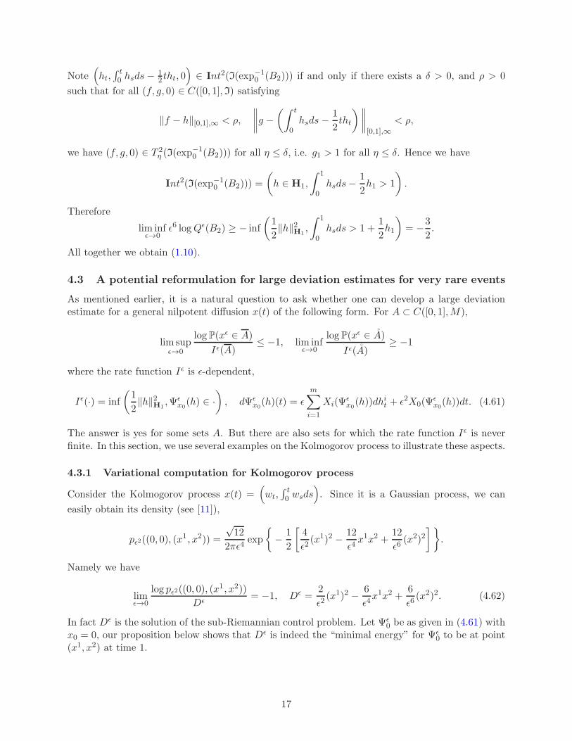
4.3 A potential reformulation for large deviation estimates for very rare events

As mentioned earlier, it is a natural question to ask whether one can develop a large deviationestimate for a general nilpotent diffusion x(t) of the following form. For A ⊂ C([0, 1],M),

lim supǫ→0

log P(xǫ ∈ A)

Iǫ(A)≤ −1, lim inf

ǫ→0

logP(xǫ ∈ A)

Iǫ(A)≥ −1

where the rate function Iǫ is ǫ-dependent,

Iǫ(·) = inf

(

1

2‖h‖2

H1,Ψǫ

x0(h) ∈ ·

)

, dΨǫx0(h)(t) = ǫ

m∑

i=1

Xi(Ψǫx0(h))dhit + ǫ2X0(Ψ

ǫx0(h))dt. (4.61)

The answer is yes for some sets A. But there are also sets for which the rate function Iǫ is neverfinite. In this section, we use several examples on the Kolmogorov process to illustrate these aspects.

4.3.1 Variational computation for Kolmogorov process

Consider the Kolmogorov process x(t) =(

wt,∫ t0 wsds

)

. Since it is a Gaussian process, we can

easily obtain its density (see [11]),

pǫ2((0, 0), (x1 , x2)) =

√12

2πǫ4exp

{

− 1

2

[

4

ǫ2(x1)2 − 12

ǫ4x1x2 +

12

ǫ6(x2)2

]}

.

Namely we have

limǫ→0

log pǫ2((0, 0), (x1 , x2))

Dǫ= −1, Dǫ =

2

ǫ2(x1)2 − 6

ǫ4x1x2 +

6

ǫ6(x2)2. (4.62)

In fact Dǫ is the solution of the sub-Riemannian control problem. Let Ψǫ0 be as given in (4.61) with

x0 = 0, our proposition below shows that Dǫ is indeed the “minimal energy” for Ψǫ0 to be at point

(x1, x2) at time 1.

17

Proposition 4.3 For any (x1, x2) ∈ R2, we have

inf

(

1

2‖h‖2H1

,Ψǫ0(h)(1) = (x1, x2)

)

= Dǫ.

The minimum is achieved at ht =6x2

ǫ3(t− t2)+ x1

ǫ (3t2 − 2t), t ∈ [0, 1] and the optimal path is given

by

Ψǫ0(h)(t) =

(

6x2

ǫ2(t− t2) + x1(3t2 − 2t), x2(3t2 − 2t3) + ǫ2x1(t3 − t2)

)

. (4.63)

Proof. This is a simple optimization problem: minimize ‖h‖2H1

under the constraint

Ψǫ0(h)(1) =

(

ǫh1, ǫ3

∫ 1

0hsds

)

= (x1, x2).

We have

h1 =x1

ǫ,

∫ 1

0htdt =

x2

ǫ3. (4.64)

Note that any critical point of ‖h‖2H1

under the linear constraints has to be quadratic in time.Therefore we can assume

ht = at2 + bt,

such that

h1 = a+ b,

∫ 1

0hsds =

a

3+b

2.

By plugging into (4.64) we obtain that{

a = −6x2

ǫ3+ 3x1

ǫ

b = 6x2

ǫ3− 2x1

ǫ .

Hence we have ht =6ǫ3x

2(t− t2) + x1

ǫ (3t2 − 2t) and (4.63). We can then compute

1

2‖h‖2

H1=

6(x2)2

ǫ6− 6x1x2

ǫ4+

2(x1)2

ǫ2

which agrees with (4.62). The proof is then complete. �

Remark 4.4 It is important to emphasize the potential non-local character of this variationalproblem. It can indeed happen that finding the optimal path is not a local problem.

(1) When x2 = 0, the optimal path converges to Φ0(h)(t) = (x1(3t2 − 2t), 0). When the targetpoint (x1, 0) is close to the starting point (0, 0), the optimal path stays in a neighborhoodof these points. The reason is indeed that the point (x1, 0) is horizontally accessible. Theprocess xǫ only needs to move along the admissible direction ǫX1 = ǫ ∂

∂x1 to attain the targetpoint. Also there exists a horizontal path of minimal (finite) energy connect to (x1, 0). Aclassical LDP then tells us that Pǫ(x(1) = (x1, 0)) concentrates around this optimal path asǫ→ 0.

(2) When x2 6= 0, the optimal path (4.63) diverges away as ǫ tends to 0, and is not confined.Indeed the reason is that the target is no longer horizontally accessible.The process xǫ needsthe help from the drift ǫ2X0 = ǫ2x1 ∂

∂x2 to make its vertical displacement. However, themagnitude of the drift is extremely small as ǫ→ 0, unless the diffusion can make a horizontaldisplacement of size 1

ǫ2to offset this small magnitude. This explains why the optimal path

horizontally diverges to infinity as ǫ→ 0.

18

4.3.2 Example of a “bad” set

In this section we given an example to illustrate that it is not possible to develop a large deviationestimate of the form (4.61) for processes satisfying a weak Hormander’s condition, even for verysimple ones like the Kolmogorov process.

Proposition 4.5 Let x(t) =(

wt,∫ t0 wsds

)

. There exists a C ⊂ C([0, 1],R2) such that

limǫ→0

ǫ6 log P(xǫ ∈ C) = −2 but Iǫ(C) = −∞.

Proof. Let C = A×B be a product set in C([0, 1],R)2 where B = {g ∈ C([0, 1],R), g(1) ≥ 1} andA is given as below.

Let {fi}i≥0 be an orthonormal basis in L2([0, 1],R) of smooth functions. In particular we letf0(s) = 1− s. For any continuous function w(s) such that w(0) = 0, we consider

Zi(w) =

∫ 1

0fi(s)dw(s).

Then Zi are i.id N(0, 1) under Wiener measure. Moreover, for any p ∈ Z+,∑p

i=1 Z2i is a χ2(p− 1)

random variable in distribution whose density is given by 1Γ(p/2)e

−u/2up/2−1. We take p = 4 then

P(χ2(3) ≥ v) =1

Γ(3)

∫ ∞

ve−

u2 udu.

Let

Ai =

{

w(·) : Z24i−3 + Z2

4i−2 + Z24i−1 + Z2

4i ≥1

i

}

, A = ∩i≥1Ai. (4.65)

Observe that Ai are independent, therefore

P(A) = Πi≥1P(Ai) = Πi≥11

4

∫ ∞

1/ie−

u2 udu.

Let Pǫ(A) = Πi≥1Pǫ(Ai) := Πi≥1P(A

ǫi) where Aǫ

i = {ǫw(·) : (Z24i−3 + Z2

4i−2 + Z24i−1 + Z2

4i) ≥ 1i },

then

Pǫ(A) = Πi≥11

4

∫ ∞

1/iǫ2e−

u2 udu.

Obviously Pǫ(A) > 0 and lim supǫ→0 ǫ2 logPǫ(A) = −∞. In fact − logPǫ(A) grows faster than ǫ−2

with an extra log factor.However, notice that set A is closed in C([0, 1],R) under uniform topology and contains no

Cameron-Martin path. This is because for any h ∈ H1 we have∑

i≥1 Z2i (h) < +∞. Hence

Iǫ(C) = inf

(

1

2‖h‖2

H1, ǫh ∈ A, ǫ3

∫ 1

0htdt ≥ 1

)

= −∞.

On the other hand, since

P (xǫ ∈ C) = P

(

ǫw ∈ A, ǫ3∫

wsds ∈ B

)

= Pǫ(A)P

(

ǫ3∫

wsds ∈ B

)

,

19

we know for some constant K ∈ R,

− ǫ4

log(1/ǫ)K+ǫ6 log P

(

ǫ3∫ t

0wsds ∈ B

)

≤ ǫ6 logPǫ (C) ≤ ǫ4

log(1/ǫ)K+ǫ6 logP

(

ǫ3∫ t

0wsds ∈ B

)

.

Hence

limǫ→0

ǫ6 log P (xǫ ∈ C) = limǫ→0

ǫ6 logP

(

ǫ3∫ 1

0wsds ≥ 1

)

= −3

2. (4.66)

�

As a comparison, we apply Theorem 4.2 at grade α2 = 3 to the above example. Though there is nohorizontal path in C, our graded large deviation estimate still provide a reasonable upper bound.

Proposition 4.6 Let C ⊂ C([0, 1],R2) be given as above. We have

lim supǫ→0

ǫ6 logP(xǫ ∈ C) ≤ − inf

(

1

2‖h‖2H1

,

∫

h ∈ B

)

= −3

2.

Proof. From (4.57) we have

lim supǫ→0

ǫ6 log P(xǫ ∈ C) ≤ − inf

(

1

2‖h‖2H1

,

(

ht,

∫ t

0hsds−

1

2tht, 0

)

∈ Cl2(I(exp−10 (C)))

)

.

We claim that

inf

(

1

2‖h‖2H1

,

(

ht,

∫ t

0hsds−

1

2tht, 0

)

∈ Cl2(I(exp−10 (C)))

)

= inf

(

1

2‖h‖2H1

,

∫

h ∈ B

)

. (4.67)

First, let us consider the minimizer of inf(

12‖h‖2H1

,∫

h ∈ B)

and denote it by h ∈ H1. We want

to show that(

ht,∫ t0 hsds− 1

2tht, 0)

∈ Clα2(I(exp−10 (C))). Due to the fact that B is closed and

‖ · ‖H1 : H1([0, 1],R) → [0,+∞) is lower semicontinuous, we know that∫

h ∈ B. We just need toprove that there exists a sequence (hn, gn, 0) ∈ I(exp−1

0 (C)) where hn ∈ A, gn ∈ B and ǫn > 0 suchthat

limn→∞

∥

∥

∥

∥

(

ǫ2nhn, gn − 1

2hnt, 0

)

−(

ht,

∫ t

0hsds−

1

2htt, 0

)∥

∥

∥

∥

[0,1],∞

= 0. (4.68)

We construct hn as follows. Let k ∈ A and ‖k‖[0,1],∞ = M < ∞, then ‖k‖H1 = +∞. We assumethat Zi(h) 6= 0 for 1 ≤ i ≤ m, let

k =

∫ m∑

i=1

Zi(k)fi,

then Zi(k − k) = 0 for all i ≤ m. We now let hn = k − k + 1ǫ2nh. It suffice to prove

(a) hn ∈ A.

(b) limn→∞ ‖ǫ2nhn − h‖∞ = 0.

(c) gn := 12hnt+

∫ t0 hsds− 1

2htt ≥ 1.

20

To prove (a) we first denote Ui(·) = Z24i−3(·)+Z2

4i−2(·)+Z24i−1(·)+Z2

4i(·), since for any i >[

m4

]

,

Ui(k − k) = Ui(k) ≥1

i,

thus Ui(hn) ≥ 1i for all i >

[

m4

]

. For i ≤[

m4

]

, since Ui(h) > 0, we just need choose ǫ1 (first termof the decreasing sequence {ǫn}n≥1) small enough such that Ui(h/ǫ

21) ≥ 1

i . Then we have for all1 ≤ i ≤

[

m4

]

,

Ui(hn) ≥ Ui(h/ǫ2n) ≥

1

i.

Hence (a) is proved. Now to prove (b) we just need to observe that

‖ǫ2nhn − h‖∞ = ǫ2n‖k − k‖∞.Since ‖k‖∞ < ∞, claim (b) easily follows. To see (c), we just need to realize that hn ≥ ht when nis large enough.

Therefore we have the minimizer(

ht,∫ t0 hsds− 1

2tht, 0)

∈ Cl2(I(exp−10 (C))). Hence

inf

(

1

2‖h‖2

H1,

(

ht,

∫ t

0hsds−

1

2tht, 0

)

∈ Cl2(I(exp−10 (C)))

)

≤ inf

(

1

2‖h‖2

H1,

∫

h ∈ B

)

.

To prove the other direction, note(

ht,∫ t0 hsds− 1

2tht, 0)

∈ Cl2(I(exp−10 (C))) means there exist

(fn, gn) ∈ C and ǫn > 0 such that

limn→∞

∥

∥

∥

∥

(

ǫ2nfn, gn, 0)

−(

ht,

∫ t

0hsds−

1

2tht, 0

)∥

∥

∥

∥

[0,1],∞

= 0,

which implies that∫ 10 hsds ≥ 1

2h1 + 1. Hence we can easily obtain that

{

(

ht,∫ t0 hsds− 1

2tht, 0)

∈

Cl2(I(exp−10 (C)))

}

⊂ {∫

h ∈ B}. This implies that

inf

(

1

2‖h‖2H1

,

(

ht,

∫ t

0hsds − tht, 0

)

∈ Cl2(I(exp−10 (C)))

)

≥ inf

(

1

2‖h‖2H1

,

∫

h ∈ B

)

.

Hence we have (4.67). At the end, we can conclude the upper bound for the exponential estimate:

lim supǫ→0

ǫ6 log P(xǫ ∈ C) ≤ − inf

(

1

2‖h‖2

H1,

∫ 1

0htdt ≥ 1

)

= −3

2.

This agrees with the previous estimate in (4.66). �

Remark 4.7 As for the lower bound,(

ht,∫ t0 hsds− 1

2tht, 0)

∈ Int2(I(exp−10 (C))) means that

there exist σ > 0 and ρ > 0 such that for all (f, g) satisfying

‖f − h‖[0,1],∞ < ρ,

∥

∥

∥

∥

g −∫

h

∥

∥

∥

∥

[0,1],∞

< ρ,

we have (f, g, 0) ∈ T 2η (I(exp

−10 (C))) for all η ≤ σ, i.e,

f

η2∈ A, g(1) ≥ 1 for all η ≤ σ.

Since A is a bounded set, {∩η≤ση2A} = {0} has no interior. There is no information given for the

lower bound.

21

4.4 Solvable diffusions

In this section we briefly discuss the large deviation estimate for the very simple solvable diffusiongiven in Example 2, which is the natural diffusion on the simple affine group. Clearly x(t) =(wt,

∫ t0 e

wsds) is the solution of (1.14). The Lie algebra L generated by X0 = ex1 ∂∂x2 and X1 =

∂∂x1

is not nilpotent but solvable. Indeed [X1, · · · [X1, [X,X0]]] = X0 for any number of brackets withX1, but

L1 = [L,L] = Span{X0}, [L1,L1] = 0,

gives the chain L ⊃ L1 of step 2.In this case the α-indices no longer provides useful information of the grading structure. We still

have grade α1 = 1 for events that are horizontally accessible, but the second grade α2 is not welldefined. In fact the second grade of large deviation estimate is not a polynomial of ǫ, but includes

a log factor. The correct grading for large deviation estimate is ǫ2 and(

ǫlog 1

ǫ

)2. In the following

example, we exhibit this phenomenon by a simple estimate of the non-horizontally accessible event(xǫ(1) ∈ B2) where B2 = {(x1, x2) ∈ R2, x2 > 1}.

Proposition 4.8 For any a > 0, we have

limǫ→0

ǫ2

log2(1/ǫ)logP

(

ǫ2∫ 1

0eǫwsds > a

)

= −2.

Proof. First note that

P

(

ǫ2∫ 1

0eǫwsds > a

)

≤ P(

eǫ‖w‖[0,1],∞ >a

ǫ2

)

= P

(

ǫ‖w‖[0,1],∞ > log a+ log1

ǫ2

)

≤ P

(

ǫ‖w‖[0,1],∞ > log1

ǫ2

)

= P

(

ǫ

log 1ǫ2

‖w‖[0,1],∞ > 1

)

≈ e−log2 1/ǫ2

2ǫ2

where ≈ denote exponential approximation at the scale of e−log2(1/ǫ2)

ǫ2 . On the other hand, for anyfixed 0 < α < 1

2 , consider the event

Eδ :=

{

‖ǫw‖α := supt,s∈[0,1]

|wt − ws||t− s|α < δ

}

.

Let t0 be such that wt0 = max[0,1]wt. Then in Eδ, for any η > 0 and s ∈ (0, 1) such that |s−t0| < η,

0 < wt0 − ws < δηα.

Hence∫ 1

0eǫwsds ≥

∫ t0+η

t0−ηeǫ(wt0−δηα)ds ≥ eǫwt0

(

2ηe−δηα)

.

We then have

P

(

ǫ2∫ 1

0eǫwsds > a

)

≥ P((

eǫwt0

(

2ηe−δηα)

>a

ǫ2

)

∩ Eδ

)

≥ P(

eǫwt0

(

2ηe−δηα)

>a

ǫ2

)

− P (Eδ) .

22

Since P (Eδ) = P (‖ǫw‖α > δ) = e−Cδǫ2 for some constant Cδ > 0, and

P

(

eǫwt0 >aeδη

α

2ηǫ2

)

= P

maxt∈[0,1]

wt >log(

aeδηα

2η

)

ǫ+

log(1/ǫ2)

ǫ

≈ P

(

maxt∈[0,1]

wt >log(1/ǫ2)

ǫ

)

≈ e−log2(1/ǫ2)

2ǫ2 ,

hence we obtain the desired conclusion. �

Such a grading structure is also reflected in the explicit calculations of transition density of x(t) inYor-Matsumoto [27] (also see Barrieu-Rouault-Yor [4] and Gerhold [18]).

At last we revisit the discussion of the non-local optimal path and related rate function Iǫ forthe event (xǫ(1) ∈ B2),

inf (Iǫ(ψ), ψ(1) ∈ B2) = inf

(

1

2‖h‖2

H1, ǫ2∫ 1

0eǫhsds > a

)

.

It amounts to solve a variational problem, i.e. find the extremal of inf(

12‖h‖2H1

, ǫ2∫ 10 e

ǫhsds = a)

.

Proposition 4.9 For any a > 0, we have

inf

(

1

2‖h‖2

H1, ǫ2∫ 1

0eǫhsds = a

)

=2β

ǫ2(β − tanh β) , (4.69)

where β is the solution of aǫ2

= sinh 2β2β . The minimum is achieved at

ht =1

ǫlog

cosh2 β

cosh2(β(1 − t)), t ∈ [0, 1]

and the optimal path is given by

Ψǫ0(h)t =

(

logcosh2 β

cosh2(β(1− t)),ǫ2 cosh2 β

β(tanh2 β − tanh2(β(1 − t)))

)

. (4.70)

Proof. Note

inf

(

1

2‖h‖2

H1, ǫ2∫ 1

0eǫhsds = a

)

=1

ǫ2inf

(

1

2‖g‖2

H1,

∫ 1

0egsds =

a

ǫ2

)

where gs = ǫhs. We use the method of Lagrange multiplier. Let

Λ(g) =1

2

∫ 1

0g2sds+ λ

∫ 1

0egsds.

Then dΛ(g) ◦ k =∫ 10 gsksds+ λ

∫ 10 e

gsksds = 0 for any k ∈ H1 implies that

g1 = 0, gs = λegs .

We can solve the above ODE explicitly and obtain that

egt =eg1

cosh2(

√

−λ2 e

g12 (1− t)

) . (4.71)

23

Plug in the constraints∫ 10 e

gsds = aǫ2

and g0 = 0 we then obtain

a

ǫ2=

sinh 2β

2β, (4.72)

where β =√

−λ2 e

g12 . From (4.71) we can obtain that

1

2‖g‖2

H1= 2β (β − tanh β) .

From (4.71) we can obtain the extremal

gt = cosh2 β − 2 log cosh(β(1− t)).

Equation (4.70) then follows by plugging in Ψǫ0(h)t =

(

gtǫ , ǫ

2∫ t0 e

gsds)

. �

Remark 4.10 In particular, from (4.72) we know that β = log 1ǫ + o(log 1

ǫ ). Plug it into (4.69) wehave

inf

(

1

2‖h‖2

H1, ǫ2∫ 1

0eǫhsds = a

)

=2(log 1

ǫ )2

ǫ2+ o

(

(log 1ǫ )

2

ǫ2

)

.

By Proposition 4.8 we then obtain that

limǫ→0

logQǫ(B2)

inf(Iǫ(ψ), ψ(1) ∈ B2)= −1,

which agrees with the statement in (1.13).

Acknowledgements: The authors would like to thank S. R. S. Varadhan for his helpful adviceon the example of “bad” set in Section 4.3.2.

24

References Cited

[1] R. Azencott, Large Deviation theory and Applications, Saint-Flour summer school in proba-bility Th. Lecture Notes Math, vol 774, Springer-Verlag, 1982

[2] R. Azencott et Al, Geodesiques et diffusions en temps petit, Asterisque 1984-1985, S.M.F.,1981.

[3] D. Barilari, U. Boscain, R. Neel, Small time heat kernel asymptotics at the sub-Riemanniancut locus, JDG Vol 92, No.3, 2012, pp. 373-416.

[4] P. Barrieu, A. Rouault, M. Yor, A study of the Hartman-Watson distribution motivated bynumerical problems related to Asian options pricing, Journal of Applied Probability, Vol. 41,No. 4, 1049-1058 (2004)

[5] F. Baudoin, Bakry-Emery meet Villani, arXiv:1308.4938

[6] R. Beals, B. Gaveau, P.C. Greiner, Hamilton-Jacobi theory and the heat kernel on Heisenberggroups, J. Math. Pures Appl. 79, 7 (2000) 633-689

[7] Ben Arous, G. Flots et series de Taylor stochastiques. Probab Theory Relat Fields. (1989)81(1) 29-77.

[8] G. Ben Arous, Developpement asymptotique du noyau de la chaleur hypoelliptique hors ducut-locus, Ann. Sci. Ecole Norm. Sup. (4), 21 (1988), pp. 307-331.

[9] G. Ben Arous and R. Leandre, Decroissance exponentielle du noyau de la chaleur sur la diag-onale. II, Probab. Theory Related Fields, 90 (1991), pp. 377-402.

[10] F. Castell, Asymptotic expansion of stochastic flows, Probability Theory and Related Fields,(1993), Volume 96, Issue 2, pp 225-239

[11] M. Chaleyat-Maurel, L. Elie, Geodesiques et diffusions en temps petit Asterisque vol. 84-85(1981), p. 255-279

[12] C. Cinti, S. Menozzi, S. Polidoro, Two-Sided bounds for degenerate processes with densitiessupported in subsets of RN , Potential Anal (2015) 42, 39-98

[13] A. Dembo, O. Zeitouni, Large deviations techniques and applications, Springer, 1998

[14] J.-D. Deuschel, D. Stroock, Large Deviations, Academic Press, New York, 1989.

[15] J-P. Eckmann, M. Hairer, Spectral Properties of Hypoelliptic Operators, Communications inMathematical Physics, April 2003, Volume 235, Issue 2, pp 233-253

[16] J. Franchi, Small time asymptotics for an example of strictly hypoelliptic heat kernel, Seminairede Probabilites XLVI, Volume 2123 of the series Lecture Notes in Mathematics pp 71-103

[17] M. Freidlin, A. Wentzell, Random perturbations of dynamical systems, Springer, Berlin, 1984.

[18] S. Gerhold, The Hartman-Watson distribution revisited: asymptotics for pricing Asian options,Journal of Applied Probability, Vol. 48, No. 3, 892-899 (2011)

[19] B. Helffer, F. Nier, Hypoelliptic estimates and spectral theory for Fokker-Planck operators andWitten Laplacians. Lecture Notes in Mathematics, 1862. Springer-Verlag, Berlin, (2005).

25

[20] F. Herau, F. Nier, Isotropic hypoellipticity and trend to equilibrium for the Fokker-Planckequation with high degree potential, Arch. Ration. Mech. Anal., 171(2):151-218, (2004).

[21] L. Hormander, Hypoelliptic second order differential equations, Acta Math., 119, (1967), 147-171.

[22] V. Konakov, S. Menozzi, S. Molchanov, Explicit parametrix and local limit theorems for somedegenerate diffusion processes, Annales de l’Institut Henri Poincare (Serie B). 46-4 (2010),908-923.

[23] H. Kunita, On the representation of solutions of stochastic differential equations, Sminaire deprobabilits de Strasbourg, 14 (1980), p. 282-304

[24] R. Leandre, Majoration en temps petit de la densite d’une diffusion degeneree, Probab. TheoryRelated Fields, 74 (1987), no. 2, 289-294.

[25] R. Leandre, Minoration en temps petit de la densite d’une diffusion degeneree, J. Funct. Anal.74 (1987), no. 2, 399-414.

[26] A. Pascucci, S. Polidoro, Harnack inequalities and Gaussian estimates for a class of hypoellipticoperators, Trans. of Amer. Math. Soc., Vol 358, No. 11 (2006), 4873-4893

[27] H. Matsumoto, M. Yor, Exponential functionals of Brownian motion, I: Probability laws atfixed time, Probability Surveys Vol. 2 (2005) 312?347

[28] M. Schilder, Some asymptotic formulars for Winer integrals, Tran. of Amer. Math. Soc., Vol125, No.1 (1966), pp 63-85

[29] D. W. Stroock, S. R. S. Varadhan, On the support of diffusion processes with applications tothe strong maximum principle. Proceedings of the Sixth Berkeley Symposium on MathematicalStatistics and Probability, 3(638), 333-359.

[30] S. R. S. Varadhan, Diffusion processes in a small time interval, Communications on Pure andApplied Mathematics 20.4 (1967), 659-685.

[31] C. Villani, Hypocoercivity, Mem. Amer. Math. Soc. 202 (2009), no. 950.

[32] Y. Yamato Stochastic differential equations and Nilpotent Lie algebras. Zeitschrift furWahrscheinlichkeitstheorie und Verwandte Gebiete.(1979) 47(2):213-229.

[33] M. Yor, On Some Exponential Functionals of Brownian Motion, Advances in Applied Proba-bility Vol. 24, No. 3 (1992), pp. 509-531

26