Verification of variable-density flow solvers using manufactured solutions q Lee Shunn a,⇑ , Frank Ham b , Parviz Moin a,b a Stanford University, Department of Mechanical Engineering, Stanford, CA 94305-3030, USA b Stanford University, Center for Turbulence Research, Stanford, CA 94305-3035, USA article info Article history: Received 16 February 2011 Received in revised form 26 October 2011 Accepted 20 January 2012 Available online 30 January 2012 Keywords: Code verification Method of manufactured solutions Numerical error Variable-density Equation-of-state abstract The method of manufactured solutions (MMS) is used to verify the convergence properties of a low-Mach number, variable-density flow code. Three MMS problems relevant to com- bustion applications are presented and tested on a variety of structured and unstructured grids. Several issues are investigated, including the use of tabulated state properties (i.e., density) and the effect of sub-iterations in the time-advancement method. The MMS implementations provide a quantitative framework to evaluate the impact of these prac- tices on the code’s convergence and order-of-accuracy. Simulation results show that linear interpolation of the equation-of-state causes numerical fluctuations that impede conver- gence and reduce accuracy. Likewise, the sub-iterative time-advancement scheme requires a significant number of outer iterations to subdue splitting errors in highly nonlinear com- bustion problems. These findings highlight the importance of careful code and solution ver- ification in the simulation of variable-density flows. Ó 2012 Elsevier Inc. All rights reserved. 1. Introduction Over the past several decades, the complexity of computational algorithms has grown in response to demands for high-fidelity simulations in science and engineering. State-of-the-art simulation codes often involve complex exchanges of information amongst various physics modules, each of which may solve different equations using different algorithms on different grid topologies. As simulations become more sophisticated, thorough verification of codes and solutions becomes increasingly challenging and time consuming, yet also more essential. Code verification implies a systematic demonstration that a computer code correctly solves its governing mathematical equations. A code that has been properly verified, therefore, is in likelihood free of programming errors (bugs) that affect the theoretical order-of-accuracy of the numerical algorithm. As such, code verification should be an early and integral step in building confidence in the predictive capabilities of simulation software. It is important to recognize that even a thoroughly verified computer code can produce inaccurate solutions to certain problems. For example, an algorithm may be implemented correctly, but simply be ineffective at solving a certain problem or set of conditions. The practice of solution verification involves analyzing the accuracy of a computed solution (including any input and output data) to determine the ‘‘correctness’’ of the result. Identifying and quantifying numerical errors that result from discretization or incomplete iteration generally falls into this category of verification. Neither code nor solution verification should be confused with model validation, a term often used to imply favorable comparison of a numerical simulation with experimental data. The goal of validation is to gauge whether the underlying 0021-9991/$ - see front matter Ó 2012 Elsevier Inc. All rights reserved. doi:10.1016/j.jcp.2012.01.027 q This work was supported by the US Department of Energy through the Predictive Science Academic Alliance Program (PSAAP). Computer resources were provided by Sandia and Lawrence Livermore National Laboratories. ⇑ Corresponding author. Current address: Idaho National Laboratory, Energy Systems & Technology, Idaho Falls, ID 83415-2210, USA. E-mail address: [email protected] (L. Shunn). Journal of Computational Physics 231 (2012) 3801–3827 Contents lists available at SciVerse ScienceDirect Journal of Computational Physics journal homepage: www.elsevier.com/locate/jcp

Welcome message from author
This document is posted to help you gain knowledge. Please leave a comment to let me know what you think about it! Share it to your friends and learn new things together.
Transcript

Journal of Computational Physics 231 (2012) 3801–3827
Contents lists available at SciVerse ScienceDirect
Journal of Computational Physics
journal homepage: www.elsevier .com/locate / jcp
Verification of variable-density flow solvers using manufactured solutions q
Lee Shunn a,⇑, Frank Ham b, Parviz Moin a,b
a Stanford University, Department of Mechanical Engineering, Stanford, CA 94305-3030, USAb Stanford University, Center for Turbulence Research, Stanford, CA 94305-3035, USA
a r t i c l e i n f o a b s t r a c t
Article history:Received 16 February 2011Received in revised form 26 October 2011Accepted 20 January 2012Available online 30 January 2012
Keywords:Code verificationMethod of manufactured solutionsNumerical errorVariable-densityEquation-of-state
0021-9991/$ - see front matter � 2012 Elsevier Incdoi:10.1016/j.jcp.2012.01.027
q This work was supported by the US Department oprovided by Sandia and Lawrence Livermore Nation⇑ Corresponding author. Current address: Idaho N
E-mail address: [email protected] (L. Shunn).
The method of manufactured solutions (MMS) is used to verify the convergence propertiesof a low-Mach number, variable-density flow code. Three MMS problems relevant to com-bustion applications are presented and tested on a variety of structured and unstructuredgrids. Several issues are investigated, including the use of tabulated state properties (i.e.,density) and the effect of sub-iterations in the time-advancement method. The MMSimplementations provide a quantitative framework to evaluate the impact of these prac-tices on the code’s convergence and order-of-accuracy. Simulation results show that linearinterpolation of the equation-of-state causes numerical fluctuations that impede conver-gence and reduce accuracy. Likewise, the sub-iterative time-advancement scheme requiresa significant number of outer iterations to subdue splitting errors in highly nonlinear com-bustion problems. These findings highlight the importance of careful code and solution ver-ification in the simulation of variable-density flows.
� 2012 Elsevier Inc. All rights reserved.
1. Introduction
Over the past several decades, the complexity of computational algorithms has grown in response to demands forhigh-fidelity simulations in science and engineering. State-of-the-art simulation codes often involve complex exchangesof information amongst various physics modules, each of which may solve different equations using different algorithmson different grid topologies. As simulations become more sophisticated, thorough verification of codes and solutionsbecomes increasingly challenging and time consuming, yet also more essential.
Code verification implies a systematic demonstration that a computer code correctly solves its governing mathematicalequations. A code that has been properly verified, therefore, is in likelihood free of programming errors (bugs) that affect thetheoretical order-of-accuracy of the numerical algorithm. As such, code verification should be an early and integral step inbuilding confidence in the predictive capabilities of simulation software.
It is important to recognize that even a thoroughly verified computer code can produce inaccurate solutions to certainproblems. For example, an algorithm may be implemented correctly, but simply be ineffective at solving a certain problemor set of conditions. The practice of solution verification involves analyzing the accuracy of a computed solution (includingany input and output data) to determine the ‘‘correctness’’ of the result. Identifying and quantifying numerical errors thatresult from discretization or incomplete iteration generally falls into this category of verification.
Neither code nor solution verification should be confused with model validation, a term often used to imply favorablecomparison of a numerical simulation with experimental data. The goal of validation is to gauge whether the underlying
. All rights reserved.
f Energy through the Predictive Science Academic Alliance Program (PSAAP). Computer resources wereal Laboratories.ational Laboratory, Energy Systems & Technology, Idaho Falls, ID 83415-2210, USA.
3802 L. Shunn et al. / Journal of Computational Physics 231 (2012) 3801–3827
mathematical model is adequate or appropriate for a given application. Verification is largely a mathematical endeavor withclearly identifiable metrics for success or failure. Validation, on the other hand, generally requires a judgement callabout whether the right model is being used to describe the physics of the target application. Model validation is beyondthe scope of the current manuscript. A detailed discussion of verification and validation is available in the book byOberkampf and Roy [1].
The present work touches on aspects of both code and solution verification. Attention is focused on hydrodynamics codesamenable to low-Mach-number combustion where acoustic effects are unimportant. Turbulent flows and engineering appli-cations are the ultimate target of the code featured in this work, and much of the presentation and discussion is colored bythat application scope.
A variable-density formulation of the Navier–Stokes equations is used in many combustion codes due to its computa-tional efficiency relative to the fully compressible equations. The pressure and density are decoupled by defining the densitythrough an equation-of-state (EOS) expressed in terms of transported scalars. The EOS may be given by an analytical expres-sion, or as is common for complex reactive systems, it may be precomputed and tabulated as a function of the scalars.
Tabulated state-equations are heavily used in many turbulent combustion models. Examples include laminar flamelets[2,3], intrinsic low-dimensional manifolds (ILDM) [4], conditional moment closures (CMC) [5–7], and some transportedPDF methods [8–10]. Implementations of these models commonly tabulate properties such as density and chemical sourceterms as a function of temperature or species concentrations or various combinations thereof. While validation studies ofcombustion codes are routinely performed, the application of systematic verification studies is less common. In particular,the ramifications of tabulated state-relationships on the convergence and accuracy of combustion codes has not been widelyinvestigated. As the EOS in typical combustion systems is multi-dimensional and highly nonlinear, its implications on codeperformance are not straightforward.
Many combustion codes employ iterative algorithms to solve the discretized system of nonlinear equations. With thesemethods, solutions are iteratively refined from an initial guess until all equations are approximately satisfied at a given pointin time. Iterative approaches, by definition, do not exactly satisfy the discrete equations, and therefore, unavoidably involve aresidual error. The matter of how small residuals must become for the numerical solution to be a valid approximation of thegoverning equations is of obvious and practical relevance. In large-scale computations it may be prohibitively expensive toconverge all solvers to machine precision. A popular execution mode, therefore, is to perform a fixed number of iterationsand then proceed to subsequent steps in the algorithm. The impact of this approach on the solution is difficult to assess apriori.
The method of manufactured solutions (MMS) is a powerful technique that can help unravel these complexities. Manu-factured solutions are exact solutions to a set of governing equations that have been modified with forcing terms. This con-cept has been around since the early days of computer codes [11, for example] and has recently been formalized under thename MMS in a series of papers [12–17]. The objective of this work is to use the method of manufactured solutions to ex-plore the effects of tabulated state relationships and iteration errors on the computational performance of a low-Mach num-ber combustion code.
2. Method of manufactured solutions
The method of manufactured solutions (MMS) is a general procedure that can be used to construct analytical solutions tothe differential equations that form the basis of a simulation code. The resulting solutions, while not necessarily physicallyrelevant, can be used as benchmark solutions for verification tests. The accuracy of the code is gauged by running the testproblems with systematic refinement of the grid and/or time step and comparing the output with the analytical manufac-tured solution. The behavior of the error is examined against the theoretical order-of-accuracy inherent in the code’s numer-ical discretizations. Thus, a verification test using MMS provides an unambiguous result as to whether or not the algorithm isimplemented correctly. MMS has been successfully applied in a variety of applications including fluid dynamics [18,19], heattransfer [20,21], fluid–structure interaction [22], and turbulence modeling [23].
Application of MMS is conceptually straightforward. Consider a generic system of differential equations
DðwÞ ¼ 0; ð1Þ
where w is a vector of unknown variables and D(�) is a differential operator whose specific form depends on the governingpartial differential equations. In MMS, the analyst selects a sufficiently differentiable function w to describe the desired evo-lution of the variables in space and time. Since w does not necessarily satisfy the original governing Eq. (1), a correspondingset of source terms _Qw are ‘‘manufactured’’ by simply applying the differential operator to w in order to balance the system
DðwÞ ¼ _Qw: ð2Þ
The new set of equations given by (2) constitutes an exact analytical solution that exercises all of the same differential termsas Eq. (1) (provided that w is sufficiently differentiable). Consequently, Eq. (2) can be used to test numerical codes designed tosolve Eq. (1) with only modest additional coding to account for the source terms. Note that imposition of the manufacturedsolution automatically generates a set of initial and boundary conditions. Care must be taken when constructing w to ensurethat these conditions are consistent with the mathematical character of the differential equations.
L. Shunn et al. / Journal of Computational Physics 231 (2012) 3801–3827 3803
As the generality of the current discussion demonstrates, there is near limitless flexibility in constructing manufacturedsolutions. Useful guidelines for the effective design and application of MMS are available in the books by Knupp and Salari[15] and Oberkampf and Roy [1].
3. Governing equations
The combustion systems of interest in this study are characterized by relatively low Mach numbers (Ma < 0.3); hence, theassumption of negligible compressibility and acoustic effects is generally valid. The low-Mach-number equations can be for-mally derived by decomposing the pressure field into a fluctuating, dynamic component and a spatially-uniform backgroundpressure. Since the ratio of the pressure fluctuations to the background pressure is on the order of Ma2, the background valueis a reasonable approximation to the total pressure. This substitution is applied everywhere except the momentum equation,where pressure gradients are important and deviations from the background pressure must be retained. The fluid density isdefined by a thermodynamic EOS that depends only on the background pressure. In this way, the density is allowed to varywith the local temperature and species concentration (i.e., the transported scalars), but is not a function of local pressurefluctuations.
Other commonly-used simplifications such as binary diffusion fluxes, a steady background pressure, and negligible vis-cous heating and body forces are also employed. In general, a more sophisticated description of diffusion processes (includ-ing multicomponent, pressure, and temperature effects) is necessary to faithfully reproduce behaviors observed in laminarflames. Further details regarding the implications, limits, and applicability of these assumptions are available in Williams[24] and Peters [25]. Under the current simplifications, variable-density reacting flows are described by the following con-servation equations for mass, momentum, and scalars, combined with a suitable EOS:
oqotþ oquj
oxj¼ _Qq ð3Þ
oqui
otþ oqujui
oxj¼ � op
oxiþ o
oxj2lSij� �
þ _Quið4Þ
oq/k
otþ oquj/k
oxj¼ o
oxjqak
o/k
oxj
� �þ _Q/k
ð5Þ
q ¼ f ð/1;/2; . . .Þ: ð6Þ
The rate-of-strain tensor in the momentum Eq. (4) is given by:
Sij ¼12
oui
oxjþ ouj
oxi
� �� 1
3dij
ouk
oxk: ð7Þ
For generality, a generic volumetric source term _QX has been added to the right-hand side of each transport equation in(3)–(5). This notation will have utility in the manufactured solutions presented in Section 4.
3.1. Numerical algorithm
The simulations in this work were performed using the unstructured multi-physics code CDP. CDP is a set of massivelyparallel unstructured flow solvers developed by Stanford’s Center for Integrated Turbulence Simulations as part of the USDepartment of Energy’s Advanced Simulation and Computing (ASC) Alliance Program.
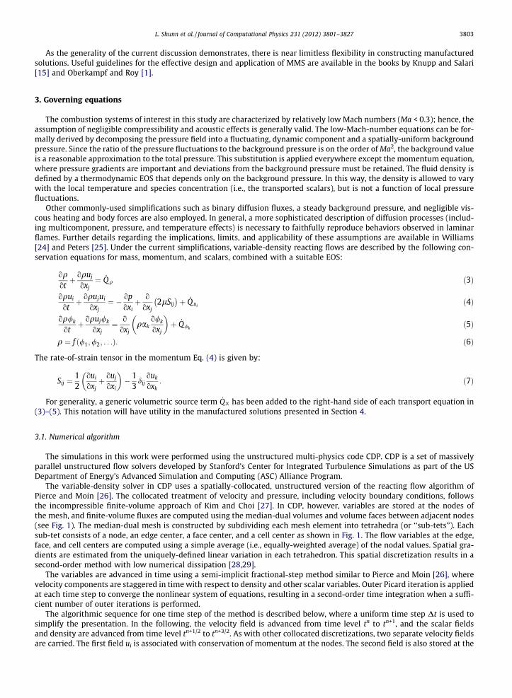
The variable-density solver in CDP uses a spatially-collocated, unstructured version of the reacting flow algorithm ofPierce and Moin [26]. The collocated treatment of velocity and pressure, including velocity boundary conditions, followsthe incompressible finite-volume approach of Kim and Choi [27]. In CDP, however, variables are stored at the nodes ofthe mesh, and finite-volume fluxes are computed using the median-dual volumes and volume faces between adjacent nodes(see Fig. 1). The median-dual mesh is constructed by subdividing each mesh element into tetrahedra (or ‘‘sub-tets’’). Eachsub-tet consists of a node, an edge center, a face center, and a cell center as shown in Fig. 1. The flow variables at the edge,face, and cell centers are computed using a simple average (i.e., equally-weighted average) of the nodal values. Spatial gra-dients are estimated from the uniquely-defined linear variation in each tetrahedron. This spatial discretization results in asecond-order method with low numerical dissipation [28,29].
The variables are advanced in time using a semi-implicit fractional-step method similar to Pierce and Moin [26], wherevelocity components are staggered in time with respect to density and other scalar variables. Outer Picard iteration is appliedat each time step to converge the nonlinear system of equations, resulting in a second-order time integration when a suffi-cient number of outer iterations is performed.
The algorithmic sequence for one time step of the method is described below, where a uniform time step Dt is used tosimplify the presentation. In the following, the velocity field is advanced from time level tn to tn+1, and the scalar fieldsand density are advanced from time level tn+1/2 to tn+3/2. As with other collocated discretizations, two separate velocity fieldsare carried. The first field ui is associated with conservation of momentum at the nodes. The second field is also stored at the
edge
face
nodeP
cell
nodeQ
,
,
Fig. 1. Schematic of node-based variable arrangement. Pressure, velocity, and scalars are stored at the node locations (e.g., P and Q), and fluxes arecomputed through internal faces and boundary faces (when present) using the medial-dual mesh defined by the edge, face, and cell centers.
3804 L. Shunn et al. / Journal of Computational Physics 231 (2012) 3801–3827
nodes, but is represented as a momentum vector qui = mi. This field is combined with the gradient of a scalar w to construct avelocity field that satisfies the discrete continuity equation at each node. Time advancement proceeds as follows:
0. At the conclusion of the previous time step, the density and velocity fields satisfy the discrete continuityequation:
Vqnþ1=2 � qn�1=2
DtþX
st
mni
st þrstwn� �
Ai;st þX
st
12ðqn�1=2 þ qnþ1=2Þun
isf Ai;sf ¼ 0; ð8Þ
where V is the node-based median-dual volume, q is the density, and superscripts generally refer to the time level. Thearea vectors Ai,st and Ai,sf refer to internal ‘‘sub-tet’’ and boundary ‘‘sub-face’’ triangles of the medial-dual mesh as de-fined in Fig. 1. The overline operator ð�Þst represents a second-order interpolation that is implemented as a simple aver-age of corner values of the sub-tet triangle. Similarly, ð�Þsf represents a second-order interpolation that is implementedas a simple average of corner values of the sub-face boundary triangle. The operator rst is the linear gradient in thesub-tet (based on the corner values), and w is a scalar field that is related to the pressure in a way that will be de-scribed hereafter.To simplify the discrete notation, the internal and boundary mass flows are written as:
Mst ¼ mist þrstw
� �Ai;st ð9Þ
Msf ¼12ðqn�1=2 þ qnþ1=2Þun
isf Ai;sf ð10Þ
1. The density, mass conserving velocities, pressure, and boundary velocities are initialized at the next time level via lin-ear extrapolation:
q ¼ 2qnþ1=2 � qn�1=2 ð11Þcmi ¼ 2mni �mn�1
i ð12Þw ¼ 2wn � wn�1 ð13Þ
Note that due to linearity, these extrapolated fields will satisfy the continuity equation at the new time level. After theextrapolation, the density can be clipped according to its physical bounds to prevent numerical problems such as smallor negative densities.The pressure is initialized by simply taking the previous value:
p ¼ pn�1=2 ð14Þ
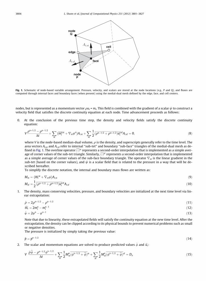
2. The scalar and momentum equations are solved to produce predicted values / and bui :
Vqb/ � qn�1=2/n�1=2
DtþX
st
12
Mnstð/
n�1=2 þ b/Þst þX
sf
12
Mnsfð/
n�1=2 þ b/Þsf ¼ D/ ð15Þ

L. Shunn et al. / Journal of Computational Physics 231 (2012) 3801–3827 3805
V2ðqþ qnþ1=2Þ bui � ðqn�1=2 þ qnþ1=2Þun
i
DtþX
st
14
Mnst þ bMst
� �un
i þ bui� �
st þX
sf
14
Mnsf þMnþ1
sf
� �un
i þ bui� �
sf ¼ Dui� V
dpdxi
;
ð16Þ
where the discretization of the diffusive and viscous terms has been simplified to D/ and Duirespectively, and the dis-
crete pressure gradient is defined as:
dpdxi¼ 1
V
Xst
pstAi;st þX
sf
psf Ai;sf
!: ð17Þ
Eqs. (15) and (16) are solved with a Jacobi solver and normally converge rapidly.
3. The provisional scalar values are used to evaluate the new density from the equation-of-state: qnþ3=2 ¼ f ð/Þ, and thedensity is used to correct the scalar values to ensure primary conservation:
/nþ3=2 ¼ q/=qnþ3=2 ð18Þ
4. A pressure Poisson equation is formulated by considering the projection step that, when added to Eq. (16), yields aconsistent discretization of the momentum equation:
V2ðqnþ1=2 þ qnþ3=2Þunþ1
i � ðqþ qnþ1=2Þ bui
Dt¼ V
dpdxi� V
dpnþ1=2
dxi: ð19Þ
By defining mnþ1i ¼ 1
2 ðqþ qnþ1=2Þ bui þ Dtdp=dxi, Eq. (19) can be expressed at the sub-tet faces, where taking the discretedivergence yields a Poisson equation for pressure:
Xst
rstpnþ1=2Ai;st ¼1Dt
qnþ3=2 � qnþ1=2
DtþX
st
mnþ1i
stAi;st þX
sf
Mnþ1sf
!: ð20Þ
Note that the discrete continuity equation has been used to eliminate the unknown velocity unþ1i , and that the
boundary mass flows (which are known) are included in the Poisson source term. This allows the Poisson operatorto be applied only over the internal sub-tet faces. The Poisson equation is efficiently solved using the HYPRE alge-braic multigrid solver [30,31].
5. To complete the step, the scalar wn+1 is updated as wn+1 = �Dtpn+1/2, and the velocity field is obtained from Eq. (19).6. The process is repeated from step 2 until convergence is achieved.
All computations for this study were performed using double precision arithmetic.
4. Example problems
In this section example MMS problems are introduced which attempt to illustrate ‘‘canonical’’ phenomena in variable-density flows. It has been argued that because code verification is a purely mathematical exercise, manufactured solutionsneed not be ‘‘realistic’’ [14]. While this statement is true, it does not fully acknowledge the utility of well-craftedmanufactured solutions in identifying the vulnerabilities and strengths of a computational algorithm. For instance, amanufactured solution that is suggestive of some elementary physics, provides not only a statement about the code’sorder-of-accuracy, but also gives a preview of how the code might perform in more complex problems where the mimickedphysics are pervasive.
In this spirit, the current examples are constructed such that they identically obey a subset of the governing physicswithout extra source terms (for example, they analytically conserve mass), and apply manufactured sources to satisfy theremaining conservation laws. Mass conservation is afforded preferential treatment in these examples due to its central rolein the solution algorithm presented in Section 3.1. The resulting manufactured solutions attempt to balance simplicity withrealism in an effort to understand how the code performs in ‘‘representative’’ scenarios.
The verification problems in this report are based on the EOS for isothermal binary mixing between miscible fluids:
qð/Þ ¼ /q1þ 1� /
q0
� ��1
: ð21Þ
The scalar variable / in Eq. (21) is known as the mixture fraction and assumes values ranging from 0 to 1. A similar mixturefraction variable is ubiquitously used in combustion modeling to describe the ‘‘mixedness’’ between fuel and oxidizer. Thequantities q0 and q1 are the pure component densities, i.e. q0 = q (/ = 0) and q1 = q (/ = 1). Although this EOS is simple, it isdeceptively nontrivial. Large density ratios result in extremely nonlinear behavior that can challenge variable-density solversin a manner similar to the reactive state-equations associated with combustion chemistry.
In order to focus on the effects of density, the viscosity l and the ‘‘dynamic’’ diffusivity qak in Eqs. (4) and (5) are assumedconstant in the MMS examples presented here.
3806 L. Shunn et al. / Journal of Computational Physics 231 (2012) 3801–3827
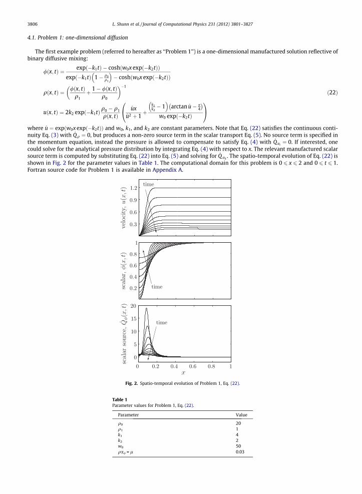
4.1. Problem 1: one-dimensional diffusion
The first example problem (referred to hereafter as ‘‘Problem 1’’) is a one-dimensional manufactured solution reflective ofbinary diffusive mixing:
/ðx; tÞ ¼ expð�k1tÞ � coshðw0x expð�k2tÞÞexpð�k1tÞ 1� q0
q1
� �� coshðw0x expð�k2tÞÞ
qðx; tÞ ¼ /ðx; tÞq1
þ 1� /ðx; tÞq0
� ��1
ð22Þ
uðx; tÞ ¼ 2k2 expð�k1tÞq0 � q1
qðx; tÞux
u2 þ 1þ
k1k2� 1
� �arctan u� p
4
� �w0 expð�k2tÞ
0@ 1A
where u ¼ expðw0x expð�k2tÞÞ and w0, k1, and k2 are constant parameters. Note that Eq. (22) satisfies the continuous conti-nuity Eq. (3) with _Qq ¼ 0, but produces a non-zero source term in the scalar transport Eq. (5). No source term is specified inthe momentum equation, instead the pressure is allowed to compensate to satisfy Eq. (4) with _Qui¼ 0. If interested, onecould solve for the analytical pressure distribution by integrating Eq. (4) with respect to x. The relevant manufactured scalarsource term is computed by substituting Eq. (22) into Eq. (5) and solving for _Q/k
. The spatio-temporal evolution of Eq. (22) isshown in Fig. 2 for the parameter values in Table 1. The computational domain for this problem is 0 6 x 6 2 and 0 6 t 6 1.Fortran source code for Problem 1 is available in Appendix A.
Fig. 2. Spatio-temporal evolution of Problem 1, Eq. (22).
Table 1Parameter values for Problem 1, Eq. (22).
Parameter Value
q0 20q1 1k1 4k2 2w0 50qa/ = l 0.03
L. Shunn et al. / Journal of Computational Physics 231 (2012) 3801–3827 3807
Fig. 2 shows that the initial, steep profile of /(x) broadens, or ‘‘diffuses’’, over time. This pseudo-diffusion is actually con-trolled by the relative values of the parameters k1 and k2, and is independent of the physical scalar diffusivity, ak. The dif-fusivity still appears in the MMS problem, but only affects the shape and magnitude of the source term, _Q/k
. If k1 = k2 inthis problem, then the integrated mass of the system
R10 qðxÞdx is constant. A value of k1 > k2 is selected in order to provide
a positive velocity at the outflow boundary, and avoid the possibility of inflows due to (small) numerical errors. The remain-ing parameter, w0, controls the sharpness of the initial scalar profile.
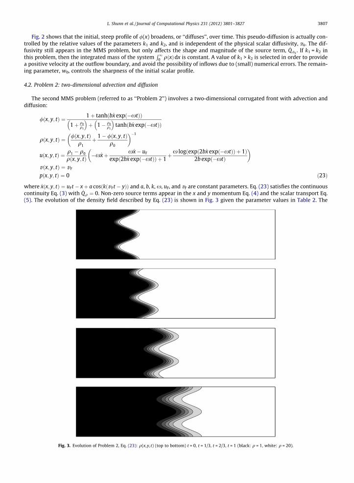
4.2. Problem 2: two-dimensional advection and diffusion
The second MMS problem (referred to as ‘‘Problem 2’’) involves a two-dimensional corrugated front with advection anddiffusion:
/ðx; y; tÞ ¼ 1þ tanhðbx expð�xtÞÞ1þ q0
q1
� �þ 1� q0
q1
� �tanhðbx expð�xtÞÞ
qðx; y; tÞ ¼ /ðx; y; tÞq1
þ 1� /ðx; y; tÞq0
� ��1
uðx; y; tÞ ¼ q1 � q0
qðx; y; tÞ �xxþ xx� uF
expð2bx expð�xtÞÞ þ 1þx logðexpð2bx expð�xtÞÞ þ 1Þ
2b expð�xtÞ
� �vðx; y; tÞ ¼ vF
pðx; y; tÞ ¼ 0 ð23Þ
where xðx; y; tÞ ¼ uFt � xþ a cosðkðvFt � yÞÞ and a, b, k, x, uF, and vF are constant parameters. Eq. (23) satisfies the continuouscontinuity Eq. (3) with _Qq ¼ 0. Non-zero source terms appear in the x and y momentum Eq. (4) and the scalar transport Eq.(5). The evolution of the density field described by Eq. (23) is shown in Fig. 3 given the parameter values in Table 2. The
Fig. 3. Evolution of Problem 2, Eq. (23): q(x,y, t) (top to bottom) t = 0, t = 1/3, t = 2/3, t = 1 (black: q = 1, white: q = 20).
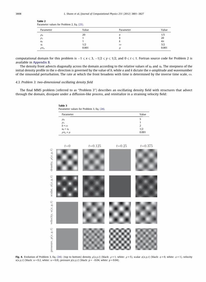
Table 2Parameter values for Problem 2, Eq. (23).
Parameter Value Parameter Value
q0 20 a 1/5q1 1 b 20uF 1 k 4pvF 1/2 x 3/2qa/ 0.001 l 0.001
3808 L. Shunn et al. / Journal of Computational Physics 231 (2012) 3801–3827
computational domain for this problem is �1 6 x 6 3, �1/2 6 y 6 1/2, and 0 6 t 6 1. Fortran source code for Problem 2 isavailable in Appendix B.
The density front advects diagonally across the domain according to the relative values of uF and vF. The steepness of theinitial density profile in the x-direction is governed by the value of b, while a and k dictate the x-amplitude and wavenumberof the sinusoidal perturbation. The rate at which the front broadens with time is determined by the inverse time scale, x.
4.3. Problem 3: two-dimensional oscillating density field
The final MMS problem (referred to as ‘‘Problem 3’’) describes an oscillating density field with structures that advectthrough the domain, dissipate under a diffusion-like process, and reinitialize in a straining velocity field:
Fig. 4.u(x,y, t)
Table 3Parameter values for Problem 3, Eq. (24).
Parameter Value
q0 5q1 1k = x 2uF = vF 1/2qa/ = l 0.001
Evolution of Problem 3, Eq. (24): (top to bottom) density q(x,y, t) (black: q = 1, white: q = 5), scalar /(x,y, t) (black: / = 0, white: / = 1), velocity(black: u = 0.2, white: u = 0.8), pressure p(x,y, t) (black: p = �0.04, white: p = 0.04).

Table 4Space–t
Grid
Spati64
128256512
102420484096
Time
Temp25
102550
100200400800
L. Shunn et al. / Journal of Computational Physics 231 (2012) 3801–3827 3809
/ðx; y; tÞ ¼ 1þ sinðpkxÞ sinðpkyÞ cosðpxtÞ1þ q0
q1
� �þ 1� q0
q1
� �sinðpkxÞ sinðpkyÞ cosðpxtÞ
qðx; y; tÞ ¼ /ðx; y; tÞq1
þ 1� /ðx; y; tÞq0
� ��1
uðx; y; tÞ ¼ q1 � q0
qðx; y; tÞ�x4k
� �cosðpkxÞ sinðpkyÞ sinðpxtÞ ð24Þ
vðx; y; tÞ ¼ q1 � q0
qðx; y; tÞ�x4k
� �sinðpkxÞ cosðpkyÞ sinðpxtÞ
pðx; y; tÞ ¼ 12
qðx; y; tÞ uðx; y; tÞ vðx; y; tÞ
where x ¼ x� uFt and y ¼ y� vFt. Eq. (24) satisfies the continuous continuity Eq. (3) with _Qq ¼ 0. Non-zero source termsappear in the x and y momentum equations (4) and the scalar transport Eq. (5). The evolution of the flow variables describedby Eq. (24) is shown in Fig. 4 for the parameter values in Table 3. Since the evolution of Problem 3 is periodic in time, thecycle depicted in Fig. 4 repeats every 2/x time units. The computational domain for this problem is �1 6 x 6 1, �1 6 y 6 1,and 0 6 t 6 1. Fortran source code for Problem 3 is available in Appendix C.
Similar to Problem 2, the scalar field in Problem 3 convects through the domain with horizontal and vertical velocities uF
and vF, respectively. The spatial period of the variable-density structures is set by the value of the wavenumber k, and thetemporal period of the oscillations is governed by the frequency x.
5. Results
5.1. Spatial and temporal convergence
A combined spatial and temporal refinement study using Problem 1 was conducted to assess the convergence propertiesof CDP’s numerics. Computational grids consisting of 64, 128, 256, 512, 1024, 2048, and 4096 uniformly-spaced control vol-umes were used, with time steps ranging from Dt = 0.5 (nt = 2) to Dt = 0.00125 (nt = 800). This combination produced max-imum convective CFL numbers in the range 0.048 (for nx = 64 and nt = 800) to 1223 (for nx = 4096 and nt = 2). The convectiveCFL number is defined in a general control volume using the cell volume V, the face areas Ai, and the face normal velocity un,i:
CFL ¼ Dt2V
Xi¼faces
jun;i Aij: ð25Þ
Diffusive CFL numbers were several orders of magnitude greater than the convective CFL numbers, due to their 1/Dx2 depen-dence. Despite the large CFL numbers, stability was not an issue for the implicit time-advancement method.
The boundary conditions at x = 0 were u = 0 and o//ox = 0. At the domain exit, an ‘‘outflow’’ boundary condition was used
owotþ uc
owon¼ 0; ð26Þ
ime convergence: L1- and L2-error in /(x, t = 1) for Problem 1.
points nx L1-error /(x, t) Observed order L2-error/(x, t) Observed order
al convergence (nt = 800)2.6407e�02 6.7197e�033.2633e�03 3.02 9.5846e�04 2.811.1724e�03 1.48 3.5391e�04 1.443.5933e�04 1.71 1.1075e�04 1.689.9107e�05 1.86 3.0840e�05 1.842.6570e�05 1.90 8.2771e�06 1.907.5165e�06 1.82 2.3308e�06 1.83
steps nt L1-error /(x, t) Observed order L2-error/(x, t) Observed order
oral convergence (nx = 4096)6.4645e�02 2.1180e�021.9322e�02 1.32 6.1355e�03 1.355.4344e�03 1.83 1.8212e�03 1.759.5562e�04 1.90 3.1888e�04 1.902.5016e�04 1.93 8.3148e�05 1.946.8156e�05 1.88 2.2481e�05 1.892.1938e�05 1.64 7.0939e�06 1.661.0406e�05 1.08 3.2983e�06 1.107.5165e�06 0.47 2.3308e�06 0.50
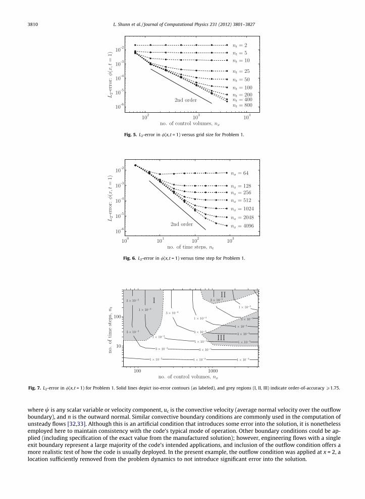
Fig. 5. L2-error in /(x, t = 1) versus grid size for Problem 1.
Fig. 6. L2-error in /(x, t = 1) versus time step for Problem 1.
Fig. 7. L2-error in /(x, t = 1) for Problem 1. Solid lines depict iso-error contours (as labeled), and grey regions (I, II, III) indicate order-of-accuracy P1.75.
3810 L. Shunn et al. / Journal of Computational Physics 231 (2012) 3801–3827
where w is any scalar variable or velocity component, uc is the convective velocity (average normal velocity over the outflowboundary), and n is the outward normal. Similar convective boundary conditions are commonly used in the computation ofunsteady flows [32,33]. Although this is an artificial condition that introduces some error into the solution, it is nonethelessemployed here to maintain consistency with the code’s typical mode of operation. Other boundary conditions could be ap-plied (including specification of the exact value from the manufactured solution); however, engineering flows with a singleexit boundary represent a large majority of the code’s intended applications, and inclusion of the outflow condition offers amore realistic test of how the code is usually deployed. In the present example, the outflow condition was applied at x = 2, alocation sufficiently removed from the problem dynamics to not introduce significant error into the solution.
L. Shunn et al. / Journal of Computational Physics 231 (2012) 3801–3827 3811
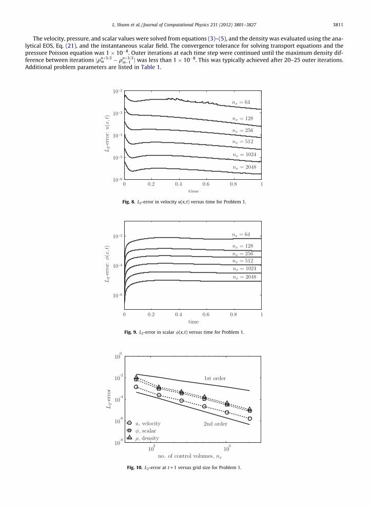
The velocity, pressure, and scalar values were solved from equations (3)–(5), and the density was evaluated using the ana-lytical EOS, Eq. (21), and the instantaneous scalar field. The convergence tolerance for solving transport equations and thepressure Poisson equation was 1 � 10�8. Outer iterations at each time step were continued until the maximum density dif-ference between iterations jqnþ3=2
m � qnþ3=2m�1 j was less than 1 � 10�8. This was typically achieved after 20–25 outer iterations.
Additional problem parameters are listed in Table 1.
Fig. 8. L2-error in velocity u(x, t) versus time for Problem 1.
Fig. 9. L2-error in scalar /(x, t) versus time for Problem 1.
Fig. 10. L2-error at t = 1 versus grid size for Problem 1.

3812 L. Shunn et al. / Journal of Computational Physics 231 (2012) 3801–3827
The maximum (L1) and volume-averaged (L2) errors for u(x, t), /(x, t), and q(x, t) were monitored throughout the simula-tions. Error data for /(x, t = 1) are presented in Table 4, with L2-error values plotted in Figs. 5 and 6. Errors in u(x, t) and q(x, t)are qualitatively similar to those in /(x, t) and are not reported separately.
The general behavior apparent in Figs. 5 and 6 is typical of many space–time order-of-accuracy studies, and illustrates oneof the challenges to comprehensive convergence verification. As the time step becomes large (small nt), temporal errors over-whelm spatial errors, and convergence stagnates with respect to spatial refinement. Similarly, small time steps (large nt) ren-der temporal errors negligible relative to spatial errors, and temporal convergence stalls. Methods for simultaneouslytreating temporal and spatial discretization error have been proposed [34, for example], however, such approaches can pro-duce misleading results unless the code is operating in an intermediate range of nt and nx where spatial and temporal errorsare of comparable magnitude.
In the current example, convergence approaches its expected second-order rate in the three regions depicted in Fig. 7. Inregion I, temporal errors are small compared to spatial errors, and spatial refinement quickly reduces errors that result fromtrying to represent the sharp features of Problem 1 on the coarsest grid. This super-convergence with respect to x is balancedby a reduction in the apparent order-of-accuracy at the next two refinement levels. As the spatial grid is further refined, thetheoretical order-of-accuracy is again approached in region II, where asymptotic convergence persists until temporal errorscompete in magnitude. Similarly, region III represents the boundary of asymptotic temporal convergence. In the area aboveregion III spatial errors dominate the solution, while below region III time steps are too large to achieve the theoretical rate ofconvergence.
Plots of the L2-error versus time for u(x, t) and /(x, t) are shown in Figs. 8 and 9 on various grids using the smallest timestep (nt = 800). Note that the error smoothly decays with time in each simulation as the flow features diffuse and becomemore easily resolved. At this level of temporal resolution, the error trends toward second-order convergence with respectto nx for all variables (see Fig. 10). The L1-error behaved similarly on all of the grids except when nx = 2048 andnx = 4096, where iteration and time errors began to contaminate the solution after t � 0.5.
5.2. Effect of EOS tabulation on convergence
The manufactured solution Problem 1 was used to evaluate the effect of EOS (density) tabulation on code performance. Toaccomplish this, a refinement study was conducted in which the EOS, Eq. (21), was interpolated linearly from successively-refined tables of uniformly-spaced points in /-space. A summary of the tabulation resolutions and their associated errors is
Table 5EOS lookup table: resolutions and errors.
EOS grid n/ Max error q(/)/q0 Avg error q(/)/q0
21 8.0591e�02 3.6803e�0331 4.7323e�02 1.6942e�0351 2.2125e�02 6.2316e�04
101 6.9391e�03 1.5738e�04201 1.9681e�03 3.9449e�05401 5.2606e�04 9.8689e�06801 1.3613e�04 2.4676e�06
Table 6Effect of EOS interpolation: maximum L1- and L2-error for Problem 1.
EOS grid n/ L1-error u(x, t) Observed order L2-error u(x, t) Observed order
21 3.0450e�02 2.3991e�0231 1.8274e�02 1.31 1.4032e�02 1.3851 9.2087e�03 1.38 8.5121e�03 1.00
101 3.5173e�03 1.41 3.2208e�03 1.42201 2.0185e�03 0.81 1.9794e�03 0.71401 9.2466e�04 1.13 8.6672e�04 1.20801 5.2006e�04 0.83 4.3319e�04 1.00
EOS grid n/ L1-error u(x, t) Observed order L2-error u(x, t) Observed order
21 5.4061e�02 1.8100e�0231 2.8370e�02 1.66 9.5723e�03 1.6451 1.1613e�02 1.79 3.9251e�03 1.79
101 3.2998e�03 1.84 1.1030e�03 1.86201 9.6504e�04 1.79 3.0885e�04 1.85401 3.4493e�04 1.49 9.9923e�05 1.63801 1.5400e�04 1.17 4.1577e�05 1.27

Fig. 12. L2-error in scalar /(x, t) versus time for Problem 1 on nx = 1024 grid. Results are shown for different EOS table sizes, n/.
Fig. 11. L2-error in velocity u(x, t) versus time for Problem 1 on nx = 1024 grid. Results are shown for different EOS table sizes, n/.
Fig. 13. Maximum L2-error on nx = 1024 grid versus EOS table size for Problem 1.
L. Shunn et al. / Journal of Computational Physics 231 (2012) 3801–3827 3813
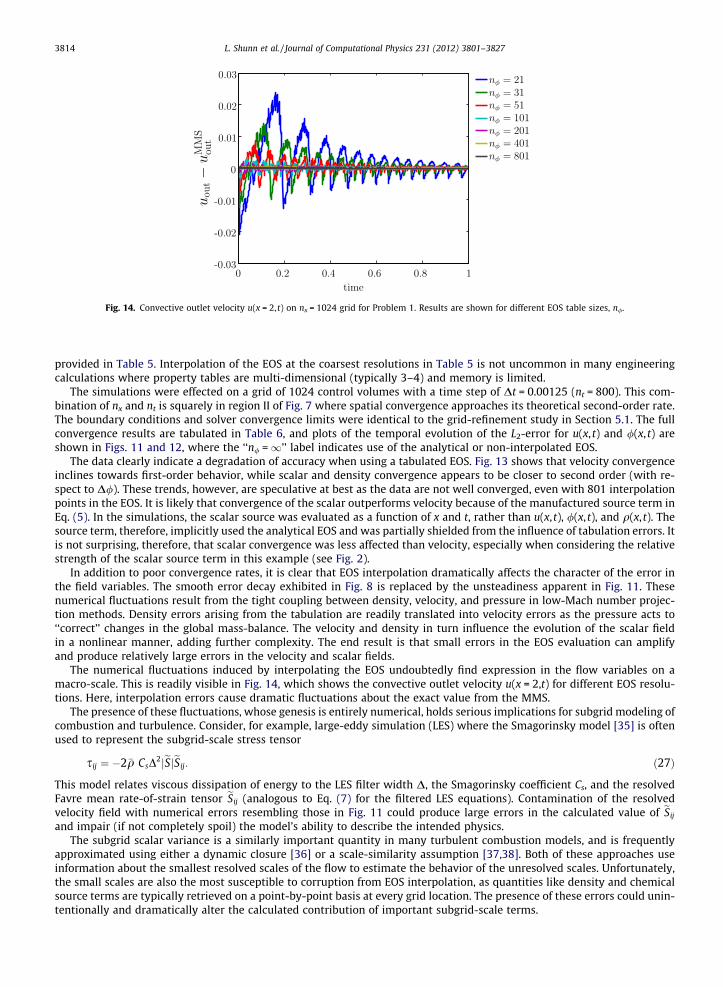
Fig. 14. Convective outlet velocity u(x = 2, t) on nx = 1024 grid for Problem 1. Results are shown for different EOS table sizes, n/.
3814 L. Shunn et al. / Journal of Computational Physics 231 (2012) 3801–3827
provided in Table 5. Interpolation of the EOS at the coarsest resolutions in Table 5 is not uncommon in many engineeringcalculations where property tables are multi-dimensional (typically 3–4) and memory is limited.
The simulations were effected on a grid of 1024 control volumes with a time step of Dt = 0.00125 (nt = 800). This com-bination of nx and nt is squarely in region II of Fig. 7 where spatial convergence approaches its theoretical second-order rate.The boundary conditions and solver convergence limits were identical to the grid-refinement study in Section 5.1. The fullconvergence results are tabulated in Table 6, and plots of the temporal evolution of the L2-error for u(x, t) and /(x, t) areshown in Figs. 11 and 12, where the ‘‘n/ =1’’ label indicates use of the analytical or non-interpolated EOS.
The data clearly indicate a degradation of accuracy when using a tabulated EOS. Fig. 13 shows that velocity convergenceinclines towards first-order behavior, while scalar and density convergence appears to be closer to second order (with re-spect to D/). These trends, however, are speculative at best as the data are not well converged, even with 801 interpolationpoints in the EOS. It is likely that convergence of the scalar outperforms velocity because of the manufactured source term inEq. (5). In the simulations, the scalar source was evaluated as a function of x and t, rather than u(x, t), /(x, t), and q(x, t). Thesource term, therefore, implicitly used the analytical EOS and was partially shielded from the influence of tabulation errors. Itis not surprising, therefore, that scalar convergence was less affected than velocity, especially when considering the relativestrength of the scalar source term in this example (see Fig. 2).
In addition to poor convergence rates, it is clear that EOS interpolation dramatically affects the character of the error inthe field variables. The smooth error decay exhibited in Fig. 8 is replaced by the unsteadiness apparent in Fig. 11. Thesenumerical fluctuations result from the tight coupling between density, velocity, and pressure in low-Mach number projec-tion methods. Density errors arising from the tabulation are readily translated into velocity errors as the pressure acts to‘‘correct’’ changes in the global mass-balance. The velocity and density in turn influence the evolution of the scalar fieldin a nonlinear manner, adding further complexity. The end result is that small errors in the EOS evaluation can amplifyand produce relatively large errors in the velocity and scalar fields.
The numerical fluctuations induced by interpolating the EOS undoubtedly find expression in the flow variables on amacro-scale. This is readily visible in Fig. 14, which shows the convective outlet velocity u(x = 2,t) for different EOS resolu-tions. Here, interpolation errors cause dramatic fluctuations about the exact value from the MMS.
The presence of these fluctuations, whose genesis is entirely numerical, holds serious implications for subgrid modeling ofcombustion and turbulence. Consider, for example, large-eddy simulation (LES) where the Smagorinsky model [35] is oftenused to represent the subgrid-scale stress tensor
sij ¼ �2�q CsD2jeSjeSij: ð27Þ
This model relates viscous dissipation of energy to the LES filter width D, the Smagorinsky coefficient Cs, and the resolvedFavre mean rate-of-strain tensor eSij (analogous to Eq. (7) for the filtered LES equations). Contamination of the resolvedvelocity field with numerical errors resembling those in Fig. 11 could produce large errors in the calculated value of eSij
and impair (if not completely spoil) the model’s ability to describe the intended physics.The subgrid scalar variance is a similarly important quantity in many turbulent combustion models, and is frequently
approximated using either a dynamic closure [36] or a scale-similarity assumption [37,38]. Both of these approaches useinformation about the smallest resolved scales of the flow to estimate the behavior of the unresolved scales. Unfortunately,the small scales are also the most susceptible to corruption from EOS interpolation, as quantities like density and chemicalsource terms are typically retrieved on a point-by-point basis at every grid location. The presence of these errors could unin-tentionally and dramatically alter the calculated contribution of important subgrid-scale terms.

L. Shunn et al. / Journal of Computational Physics 231 (2012) 3801–3827 3815
5.3. Effect of iteration error on convergence
The method of manufactured solutions was also used to investigate the error-contribution from iteration residuals in thetime-advancement method outlined in Section 3.1. Problem 2 (Eq. (23)) was simulated on computational grids comprising200 � 50, 400 � 100, 800 � 200, and 1600 � 400 hexahedral control volumes with a uniform time step of Dt = 0.00125(nt = 800). This time step produced maximum convective CFL numbers (Eq. (25)) ranging from 0.15 to 1.18 on the variousgrids. Dirichlet boundary conditions were imposed at x = �1, an ‘‘outflow’’ boundary condition (Eq. (26)) was applied atx = 3, and periodic boundary conditions were used at y = ±1/2. Tolerances for the scalar, momentum, and pressure solverswere set to 1 � 10�10 in all of the simulations. Additional problem parameters are supplied in Table 2.
The focus of this section is to investigate the effect of applying multiple outer iterations to fully converge the system ofnonlinear Eqs. (3)–(6) at each time step. Fig. 15 shows the spatial-convergence of the L2-error of the flow variables when 20outer iterations are employed. Under these conditions, the bulk of the iteration error is eliminated and all variables tend to-ward second-order convergence with grid refinement — confirming the expected accuracy of CDP’s spatial operators. Fig. 16shows how the convergence is affected when fewer outer iterations are used at each time level. The observed convergence isapproximately first order when 10 iterations are applied, and less than first order with fewer iterations.
In a related study, the simulations of Fig. 16 were repeated using a more moderate density ratio of q0/q1 = 5. In this case,second-order convergence was observed after 5–10 outer iterations versus the 15–20 iterations for the q0/q1 = 20 case. Thisaccelerated convergence is encouraging for applications with modest density ratios, but also indicates an unappealingdependence of the algorithm’s convergence properties on the EOS.
The errors depicted in Fig. 16 are a complicated mixture of spatial, temporal, and iterative contributions that depend onthe grid, time step, and other operating conditions. A closer examination of the temporal component of the error is instruc-tive. Fig. 17 shows the convergence of the L2-error with respect to Dt for a simulation on the 800 � 200 grid when only one
Fig. 15. L2-error at t = 1 for Problem 2 using 20 outer iterations.
Fig. 16. L2-error in u(x, t = 1) for Problem 2 using different numbers of outer iterations.
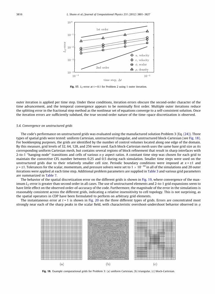
Fig. 17. L2-error at t = 0.1 for Problem 2 using 1 outer iteration.
3816 L. Shunn et al. / Journal of Computational Physics 231 (2012) 3801–3827
outer iteration is applied per time step. Under these conditions, iteration errors obscure the second-order character of thetime advancement, and the temporal convergence appears to be nominally first order. Multiple outer iterations reducethe splitting error in the fractional step method as the nonlinear set of equations converge to a self-consistent solution. Oncethe iteration errors are sufficiently subdued, the true second-order nature of the time–space discretization is observed.
5.4. Convergence on unstructured grids
The code’s performance on unstructured grids was evaluated using the manufactured solution Problem 3 (Eq. (24)). Threetypes of spatial grids were tested: uniform Cartesian, unstructured triangular, and unstructured block-Cartesian (see Fig. 18).For bookkeeping purposes, the grids are identified by the number of control volumes located along one edge of the domain.By this measure, grid levels of 32, 64, 128, and 256 were used. Each block-Cartesian mesh uses the same base grid size as itscorresponding uniform Cartesian mesh, but contains several regions of block refinement that result in sharp interfaces with2-to-1 ‘‘hanging-node’’ transitions and cells of various x-y aspect ratios. A constant time step was chosen for each grid tomaintain the convective CFL number between 0.25 and 0.5 during each simulation. Smaller time steps were used on theunstructured grids due to their relatively smaller cell size. Periodic boundary conditions were imposed at x = ±1 andy = ±1. Tolerances for the scalar, momentum, and pressure solvers were set to 1 � 10�10 in all of the simulations and 20 outeriterations were applied at each time step. Additional problem parameters are supplied in Table 3 and various grid parametersare summarized in Table 7.
The behavior of the spatial discretization error on the different grids is shown in Fig. 19, where convergence of the max-imum L2-error is greater than second order in all cases. The use of unstructured elements and 2-to-1 grid expansions seem tohave little effect on the observed order-of-accuracy of the code. Furthermore, the magnitude of the error in the simulations isreasonably consistent across the different grids, indicating a relative insensitivity to cell topology. This is not surprising, asthe spatial operators in CDP have been formulated to perform on arbitrary grid elements.
The instantaneous error at t = 1 is shown in Fig. 20 on the three different types of grids. Errors are concentrated moststrongly near each of the sharp peaks in the scalar field, with characteristic overshoot-undershoot behavior observed in /
Fig. 18. Example computational grids for Problem 3: (a) uniform Cartesian, (b) triangular, (c) block-Cartesian.
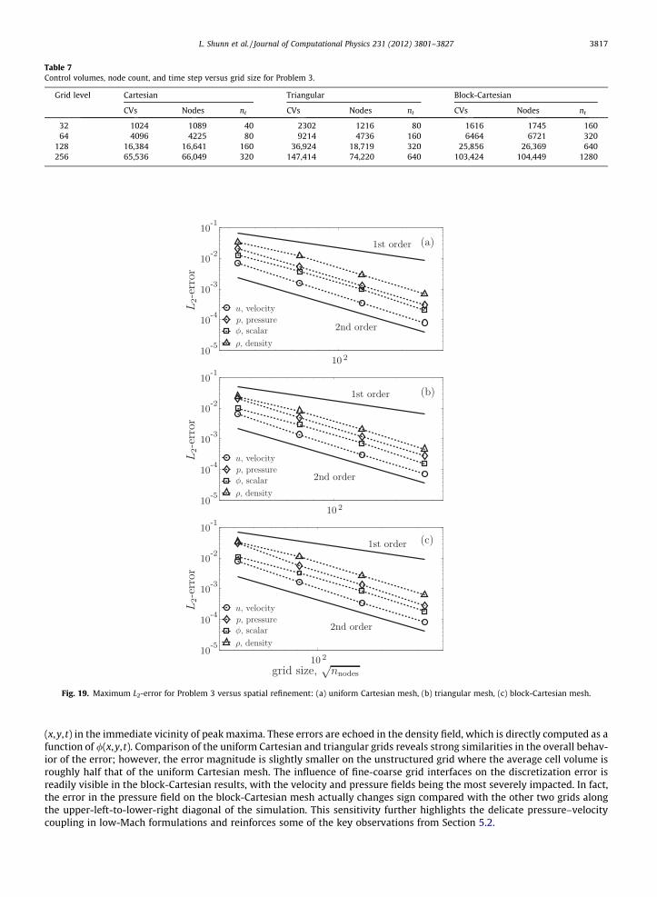
Fig. 19. Maximum L2-error for Problem 3 versus spatial refinement: (a) uniform Cartesian mesh, (b) triangular mesh, (c) block-Cartesian mesh.
Table 7Control volumes, node count, and time step versus grid size for Problem 3.
Grid level Cartesian Triangular Block-Cartesian
CVs Nodes nt CVs Nodes nt CVs Nodes nt
32 1024 1089 40 2302 1216 80 1616 1745 16064 4096 4225 80 9214 4736 160 6464 6721 320
128 16,384 16,641 160 36,924 18,719 320 25,856 26,369 640256 65,536 66,049 320 147,414 74,220 640 103,424 104,449 1280
L. Shunn et al. / Journal of Computational Physics 231 (2012) 3801–3827 3817
(x,y, t) in the immediate vicinity of peak maxima. These errors are echoed in the density field, which is directly computed as afunction of /(x,y, t). Comparison of the uniform Cartesian and triangular grids reveals strong similarities in the overall behav-ior of the error; however, the error magnitude is slightly smaller on the unstructured grid where the average cell volume isroughly half that of the uniform Cartesian mesh. The influence of fine-coarse grid interfaces on the discretization error isreadily visible in the block-Cartesian results, with the velocity and pressure fields being the most severely impacted. In fact,the error in the pressure field on the block-Cartesian mesh actually changes sign compared with the other two grids alongthe upper-left-to-lower-right diagonal of the simulation. This sensitivity further highlights the delicate pressure–velocitycoupling in low-Mach formulations and reinforces some of the key observations from Section 5.2.
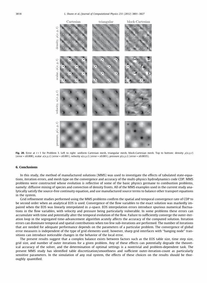
Fig. 20. Error at t = 1 for Problem 3. Left to right: uniform Cartesian mesh, triangular mesh, block-Cartesian mesh. Top to bottom: density q(x,y, t)(error = ±0.008), scalar /(x,y, t) (error = ±0.001), velocity u(x,y, t) (error = ±0.001), pressure p(x,y, t) (error = ±0.0035).
3818 L. Shunn et al. / Journal of Computational Physics 231 (2012) 3801–3827
6. Conclusions
In this study, the method of manufactured solutions (MMS) was used to investigate the effects of tabulated state-equa-tions, iteration errors, and mesh type on the convergence and accuracy of the multi-physics hydrodynamics code CDP. MMSproblems were constructed whose evolution is reflective of some of the basic physics germane to combustion problems,namely: diffusive mixing of species and convection of density fronts. All of the MMS examples used in the current study ana-lytically satisfy the source-free continuity equation, and use manufactured source terms to balance other transport equationsin the system.
Grid refinement studies performed using the MMS problems confirm the spatial and temporal convergence rate of CDP tobe second order when an analytical EOS is used. Convergence of the flow variables to the exact solution was markedly im-paired when the EOS was linearly interpolated in /-space. EOS interpolation errors introduce spurious numerical fluctua-tions in the flow variables, with velocity and pressure being particularly vulnerable. In some problems these errors canaccumulate with time and potentially alter the temporal evolution of the flow. Failure to sufficiently converge the outer-iter-ation loop in the segregated time-advancement algorithm acutely affects the accuracy of the computed solution. Iterationerrors can dominate temporal and spatial contributions when too few sub-iterations are performed. The number of iterationsthat are needed for adequate performance depends on the parameters of a particular problem. The convergence of globalerror measures is independent of the type of grid elements used; however, sharp grid interfaces with ‘‘hanging node’’ tran-sitions can introduce noticeable changes in the behavior of the local error.
The present results suggest that a complex balance exists between factors such as the EOS table size, time step size,grid size, and number of outer iterations for a given problem. Any of these effects can potentially degrade the theoret-ical accuracy of the solver, and the determination of optimal settings is a nontrivial and problem-dependent task. Thepresent MMS study has identified table discretization/smoothness and sufficient outer-iteration-count as particularlysensitive parameters. In the simulation of any real system, the effects of these choices on the results should be thor-oughly quantified.
L. Shunn et al. / Journal of Computational Physics 231 (2012) 3801–3827 3819
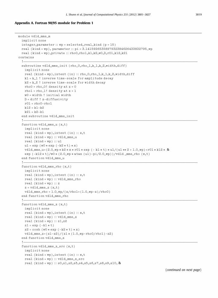
Appendix A. Fortran 90/95 module for Problem 1
module vd1d_mms_mimplicit none
integer,parameter :: wp = selected_real_kind (p = 15)
real (kind = wp), parameter :: pi = 3.1415926535897932384626433832795_wpreal (kind = wp),private :: rho0,rho1,k1,k2,w0,D,r01,k12,k21
contains
!————————————————————————————————————————————————————————————————————————————————————————
subroutine vd1d_mms_init (rho_0,rho_1,k_1,k_2,width,diff)implicit none
real (kind = wp),intent (in) :: rho_0,rho_1,k_1,k_2,width,diffk1 = k_1 ! inverse time-scale for amplitude decay
k2 = k_2 ! inverse time-scale for width decay
rho0 = rho_0! density at z = 0
rho1 = rho_1! density at z = 1
w0 = width ! initial width
D = diff ! z-diffusivity
r01 = rho0-rho1
k12 = k1-k2
k21 = k2-k1
end subroutine vd1d_mms_init!————————————————————————————————————————————————————————————————————————————————————————
function vd1d_mms_u (x,t)
implicit none
real (kind = wp),intent (in) :: x,t
real (kind = wp) :: vd1d_mms_ureal (kind = wp) :: u1
u1 = exp (w0 ⁄ exp (-k2 ⁄ t) ⁄ x)vd1d_mms_u=(2.0_wp ⁄ k2 ⁄ x ⁄ r01 ⁄ exp (- k1 ⁄ t) ⁄ u1/(u1 ⁄⁄ 2 + 1.0_wp)+r01 ⁄ k12 ⁄ &exp (-k12 ⁄ t)/w0 ⁄ (2.0_wp ⁄ atan (u1)-pi/2.0_wp))/vd1d _mms_rho (x,t)
end function vd1d_mms_u!————————————————————————————————————————————————————————————————————————————————————————
function vd1d_mms_rho (x,t)
implicit none
real (kind = wp),intent (in) :: x,t
real (kind = wp) :: vd1d_mms_rhoreal (kind = wp) :: z
z = vd1d_mms_z (x,t)
vd1d_mms_rho = 1.0_wp/(z/rho1+(1.0_wp-z)/rho0)end function vd1d_mms_rho!————————————————————————————————————————————————————————————————————————————————————————
function vd1d_mms_z (x,t)
implicit none
real (kind = wp),intent (in) :: x,t
real (kind = wp) :: vd1d_mms_zreal (kind = wp) :: z1,z2
z1 = exp (-k1 ⁄ t)z2 = cosh (w0 ⁄ exp (-k2 ⁄ t) ⁄ x)vd1d_mms_z=(z1-z2)/(z1 ⁄ (1.0_wp-rho0/rho1)-z2)
end function vd1d_mms_z!————————————————————————————————————————————————————————————————————————————————————————
function vd1d_mms_z_src (x,t)
implicit none
real (kind = wp),intent (in) :: x,t
real (kind = wp) :: vd1d_mms_z_srcreal (kind = wp) :: s0,s1,s2,s3,s4,s5,s6,s7,s8,s9,s10, &
(continued on next page)

3820 L. Shunn et al. / Journal of Computational Physics 231 (2012) 3801–3827
s11,s12,s13,s14,s15,s16,s17,s18,s19,s20
s0 = exp (-k1 ⁄ t)s1 = exp (-k2 ⁄ t)s2 = sech (w0 ⁄ s1 ⁄ x)s3 = tanh (w0 ⁄ s1 ⁄ x)s4 = exp (w0 ⁄ s1 ⁄ x)s5 = s0/s1
s6 = s0 ⁄ s2s7 = rho1 + r01 ⁄ s6! rho
s8 = 2.0_wp ⁄ atan (s4)-1.0_wp/2.0_wp ⁄ pis9 = s6 ⁄ s3 ⁄ w0s10=-s9 ⁄ s1 ⁄ rho1 + s9 ⁄ s1 ⁄ rho0s11 = 1.0_wp-s3 ⁄⁄ 2s12 = s4 ⁄⁄ 2 + 1.0_wps13=-1.0_wp + s6s14=-k1 ⁄ s6 + s9 ⁄ k2 ⁄ s1 ⁄ xs15 = s6 ⁄ s3 ⁄⁄ 2 ⁄ w0 ⁄⁄ 2 ⁄ s1 ⁄⁄ 2s16 = 2.0_wp ⁄ k2 ⁄ r01 ⁄ s0 ⁄ s4/s12s17 = s6 ⁄ s11 ⁄ w0 ⁄⁄ 2 ⁄ s1 ⁄⁄ 2s18 = s16 ⁄ x + r01 ⁄ k12 ⁄ s5/w0 ⁄ s8s19 = s9 ⁄ s1 ⁄ s7-s13 ⁄ s10s20 = 2.0_wp ⁄ s4 ⁄ s1 ⁄ (s16 ⁄ x ⁄ s4 ⁄ w0-r01 ⁄ k12 ⁄ s5)/s12vd1d_mms_z_src=&-s14 ⁄ rho1-(s16 + s16 ⁄ x ⁄ w0 ⁄ s1-s20) ⁄ s13 ⁄ rho1/s7 + s18 ⁄ rho1 ⁄ s19/s7 ⁄⁄ 2 &-D ⁄ rho1 ⁄ (-s15 ⁄ s7 ⁄⁄ 2 + s17 ⁄ s7 ⁄⁄ 2 + 2.0_wp ⁄ s9 ⁄ s1 ⁄ s10 ⁄ s7–2.0_wp ⁄ s13 ⁄ s10 ⁄⁄ 2 &-s13 ⁄ r01 ⁄ s7 ⁄ s17 + s13 ⁄ r01 ⁄ s7 ⁄ s15)/s7 ⁄⁄ 3
end function vd1d_mms_z_src!————————————————————————————————————————————————————————————————————————————————————————
function sech (x)
implicit none
real (kind = wp),intent (in) :: x
real (kind = wp) :: sech
sech = 1.0_wp/cosh (x)
end function sech
end module vd1d_mms_m
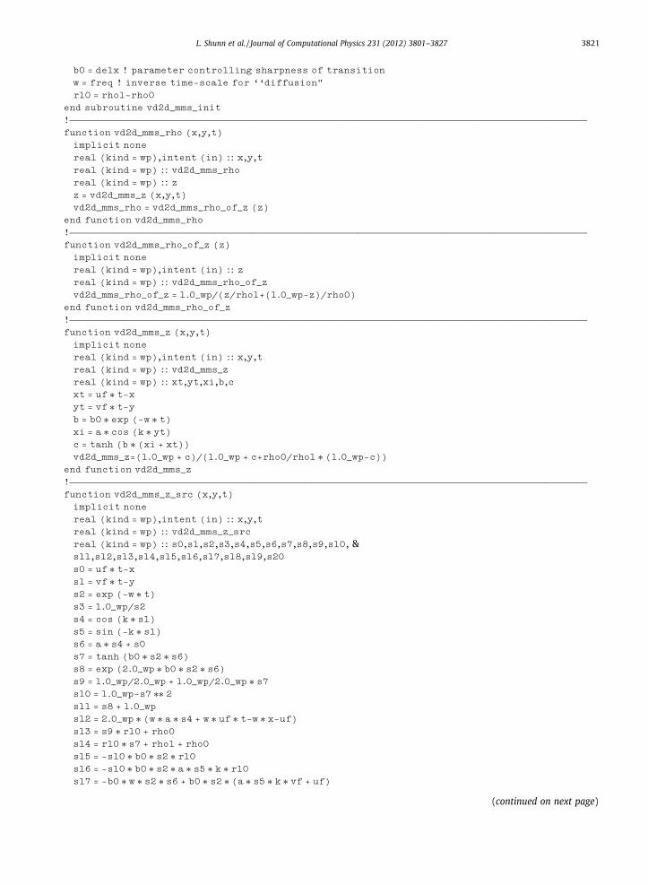
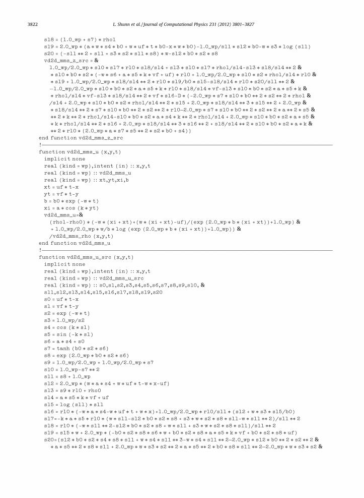
Appendix B. Fortran 90/95 module for Problem 2
module vd2d_mms_mimplicit none
integer,parameter :: wp = selected_real_kind (p = 15)
real (kind = wp),parameter :: pi = 3.1415926535897932384626433832795_wpreal (kind = wp),private :: rho0,rho1,D,mu,uf,vf,a,k,b0,w,r10
contains
!————————————————————————————————————————————————————————————————————————————————————————
subroutine vd2d_mms_init (den0,den1,diff,visc,xvel,yvel,ampl,wnum,delx,freq)
implicit none
real (kind = wp),intent (in) :: den0,den1,diff,visc
real (kind = wp),intent (in) :: xvel,yvel,ampl,wnum,delx,freq
rho0 = den0! density at z = 0
rho1 = den1! density at z = 1
mu = visc ! dynamic viscosity
D = diff ! diffusion coefficient: rho ⁄ alpha_zuf = xvel ! x convective velocity
vf = yvel ! y convective velocity
a = ampl ! amplitude of rho perturbation
k = wnum ⁄ pi! wave number of rho perturbation
L. Shunn et al. / Journal of Computational Physics 231 (2012) 3801–3827 3821
b0 = delx ! parameter controlling sharpness of transition
w = freq ! inverse time-scale for ‘‘diffusion"
r10 = rho1-rho0
end subroutine vd2d_mms_init!————————————————————————————————————————————————————————————————————————————————————————
function vd2d_mms_rho (x,y,t)
implicit none
real (kind = wp),intent (in) :: x,y,t
real (kind = wp) :: vd2d_mms_rhoreal (kind = wp) :: z
z = vd2d_mms_z (x,y,t)
vd2d_mms_rho = vd2d_mms_rho_of_z (z)
end function vd2d_mms_rho!————————————————————————————————————————————————————————————————————————————————————————
function vd2d_mms_rho_of_z (z)
implicit none
real (kind = wp),intent (in) :: z
real (kind = wp) :: vd2d_mms_rho_of_zvd2d_mms_rho_of_z = 1.0_wp/(z/rho1+(1.0_wp-z)/rho0)
end function vd2d_mms_rho_of_z!————————————————————————————————————————————————————————————————————————————————————————
function vd2d_mms_z (x,y,t)
implicit none
real (kind = wp),intent (in) :: x,y,t
real (kind = wp) :: vd2d_mms_zreal (kind = wp) :: xt,yt,xi,b,c
xt = uf ⁄ t-xyt = vf ⁄ t-yb = b0 ⁄ exp (-w ⁄ t)xi = a ⁄ cos (k ⁄ yt)c = tanh (b ⁄ (xi + xt))vd2d_mms_z=(1.0_wp + c)/(1.0_wp + c+rho0/rho1 ⁄ (1.0_wp-c))
end function vd2d_mms_z!————————————————————————————————————————————————————————————————————————————————————————
function vd2d_mms_z_src (x,y,t)
implicit none
real (kind = wp),intent (in) :: x,y,t
real (kind = wp) :: vd2d_mms_z_srcreal (kind = wp) :: s0,s1,s2,s3,s4,s5,s6,s7,s8,s9,s10, &s11,s12,s13,s14,s15,s16,s17,s18,s19,s20
s0 = uf ⁄ t-xs1 = vf ⁄ t-ys2 = exp (-w ⁄ t)s3 = 1.0_wp/s2s4 = cos (k ⁄ s1)s5 = sin (-k ⁄ s1)s6 = a ⁄ s4 + s0s7 = tanh (b0 ⁄ s2 ⁄ s6)s8 = exp (2.0_wp ⁄ b0 ⁄ s2 ⁄ s6)s9 = 1.0_wp/2.0_wp + 1.0_wp/2.0_wp ⁄ s7s10 = 1.0_wp-s7 ⁄⁄ 2s11 = s8 + 1.0_wps12 = 2.0_wp ⁄ (w ⁄ a ⁄ s4 + w ⁄ uf ⁄ t-w ⁄ x-uf)s13 = s9 ⁄ r10 + rho0s14 = r10 ⁄ s7 + rho1 + rho0s15 = -s10 ⁄ b0 ⁄ s2 ⁄ r10s16 = -s10 ⁄ b0 ⁄ s2 ⁄ a ⁄ s5 ⁄ k ⁄ r10s17 = -b0 ⁄ w ⁄ s2 ⁄ s6 + b0 ⁄ s2 ⁄ (a ⁄ s5 ⁄ k ⁄ vf + uf)
(continued on next page)
3822 L. Shunn et al. / Journal of Computational Physics 231 (2012) 3801–3827
s18 = (1.0_wp + s7) ⁄ rho1s19 = 2.0_wp ⁄ (a ⁄ w ⁄ s4 ⁄ b0 + w ⁄ uf ⁄ t ⁄ b0-x ⁄ w ⁄ b0)-1.0_wp/s11 ⁄ s12 ⁄ b0-w ⁄ s3 ⁄ log (s11)
s20 = (-s11 ⁄⁄ 2 + s11 + s3 ⁄ s2 ⁄ s11 ⁄ s8) ⁄ w-s12 ⁄ b0 ⁄ s2 ⁄ s8vd2d_mms_z_src = &1.0_wp/2.0_wp ⁄ s10 ⁄ s17 ⁄ r10 ⁄ s18/s14 + s13 ⁄ s10 ⁄ s17 ⁄ rho1/s14-s13 ⁄ s18/s14 ⁄⁄ 2 &⁄ s10 ⁄ b0 ⁄ s2 ⁄ (-w ⁄ s6 + a ⁄ s5 ⁄ k ⁄ vf + uf) ⁄ r10 + 1.0_wp/2.0_wp ⁄ s10 ⁄ s2 ⁄ rho1/s14 ⁄ r10 &⁄ s19 + 1.0_wp/2.0_wp ⁄ s18/s14 ⁄⁄ 2 ⁄ r10 ⁄ s19/b0 ⁄ s15-s18/s14 ⁄ r10 ⁄ s20/s11 ⁄⁄ 2 &�1.0_wp/2.0_wp ⁄ s10 ⁄ b0 ⁄ s2 ⁄ a ⁄ s5 ⁄ k ⁄ r10 ⁄ s18/s14 ⁄ vf-s13 ⁄ s10 ⁄ b0 ⁄ s2 ⁄ a ⁄ s5 ⁄ k &⁄ rho1/s14 ⁄ vf-s13 ⁄ s18/s14 ⁄⁄ 2 ⁄ vf ⁄ s16-D ⁄ (-2.0_wp ⁄ s7 ⁄ s10 ⁄ b0 ⁄⁄ 2 ⁄ s2 ⁄⁄ 2 ⁄ rho1 &/s14 + 2.0_wp ⁄ s10 ⁄ b0 ⁄ s2 ⁄ rho1/s14 ⁄⁄ 2 ⁄ s15 + 2.0_wp ⁄ s18/s14 ⁄⁄ 3 ⁄ s15 ⁄⁄ 2 + 2.0_wp &⁄ s18/s14 ⁄⁄ 2 ⁄ s7 ⁄ s10 ⁄ b0 ⁄⁄ 2 ⁄ s2 ⁄⁄ 2 ⁄ r10–2.0_wp ⁄ s7 ⁄ s10 ⁄ b0 ⁄⁄ 2 ⁄ s2 ⁄⁄ 2 ⁄ a ⁄⁄ 2 ⁄ s5 &⁄⁄ 2 ⁄ k ⁄⁄ 2 ⁄ rho1/s14-s10 ⁄ b0 ⁄ s2 ⁄ a ⁄ s4 ⁄ k ⁄⁄ 2 ⁄ rho1/s14 + 2.0_wp ⁄ s10 ⁄ b0 ⁄ s2 ⁄ a ⁄ s5 &⁄ k ⁄ rho1/s14 ⁄⁄ 2 ⁄ s16 + 2.0_wp ⁄ s18/s14 ⁄⁄ 3 ⁄ s16 ⁄⁄ 2 + s18/s14 ⁄⁄ 2 ⁄ s10 ⁄ b0 ⁄ s2 ⁄ a ⁄ k &⁄⁄ 2 ⁄ r10 ⁄ (2.0_wp ⁄ a ⁄ s7 ⁄ s5 ⁄⁄ 2 ⁄ s2 ⁄ b0 + s4))
end function vd2d_mms_z_src!————————————————————————————————————————————————————————————————————————————————————————
function vd2d_mms_u (x,y,t)
implicit none
real (kind = wp),intent (in) :: x,y,t
real (kind = wp) :: vd2d_mms_ureal (kind = wp) :: xt,yt,xi,b
xt = uf ⁄ t-xyt = vf ⁄ t-yb = b0 ⁄ exp (-w ⁄ t)xi = a ⁄ cos (k ⁄ yt)vd2d_mms_u=&(rho1-rho0) ⁄ (-w ⁄ (xi + xt)+(w ⁄ (xi + xt)-uf)/(exp (2.0_wp ⁄ b ⁄ (xi + xt))+1.0_wp) &+ 1.0_wp/2.0_wp ⁄ w/b ⁄ log (exp (2.0_wp ⁄ b ⁄ (xi + xt))+1.0_wp)) &/vd2d_mms_rho (x,y,t)
end function vd2d_mms_u!————————————————————————————————————————————————————————————————————————————————————————
function vd2d_mms_u_src (x,y,t)
implicit none
real (kind = wp),intent (in) :: x,y,t
real (kind = wp) :: vd2d_mms_u_srcreal (kind = wp) :: s0,s1,s2,s3,s4,s5,s6,s7,s8,s9,s10, &s11,s12,s13,s14,s15,s16,s17,s18,s19,s20
s0 = uf ⁄ t-xs1 = vf ⁄ t-ys2 = exp (-w ⁄ t)s3 = 1.0_wp/s2s4 = cos (k ⁄ s1)s5 = sin (-k ⁄ s1)s6 = a ⁄ s4 + s0s7 = tanh (b0 ⁄ s2 ⁄ s6)s8 = exp (2.0_wp ⁄ b0 ⁄ s2 ⁄ s6)s9 = 1.0_wp/2.0_wp + 1.0_wp/2.0_wp ⁄ s7s10 = 1.0_wp-s7 ⁄⁄ 2s11 = s8 + 1.0_wps12 = 2.0_wp ⁄ (w ⁄ a ⁄ s4 + w ⁄ uf ⁄ t-w ⁄ x-uf)s13 = s9 ⁄ r10 + rho0s14 = a ⁄ s5 ⁄ k ⁄ vf + ufs15 = log (s11) ⁄ s11s16 = r10 ⁄ (-w ⁄ a ⁄ s4-w ⁄ uf ⁄ t + w ⁄ x)+1.0_wp/2.0_wp ⁄ r10/s11 ⁄ (s12 + w ⁄ s3 ⁄ s15/b0)s17=-k ⁄ a ⁄ s5 ⁄ r10 ⁄ (w ⁄ s11-s12 ⁄ b0 ⁄ s2 ⁄ s8 + s3 ⁄ w ⁄ s2 ⁄ s8 ⁄ s11-w ⁄ s11 ⁄⁄ 2)/s11 ⁄⁄ 2s18 = r10 ⁄ (-w ⁄ s11 ⁄⁄ 2-s12 ⁄ b0 ⁄ s2 ⁄ s8 + w ⁄ s11 + s3 ⁄ w ⁄ s2 ⁄ s8 ⁄ s11)/s11 ⁄⁄ 2s19 = s15 ⁄ w + 2.0_wp ⁄ (-b0 ⁄ s2 ⁄ s8 ⁄ s6 ⁄ w + b0 ⁄ s2 ⁄ s8 ⁄ a ⁄ s5 ⁄ k ⁄ vf + b0 ⁄ s2 ⁄ s8 ⁄ uf)s20=(s12 ⁄ b0 ⁄ s2 ⁄ s4 ⁄ s8 ⁄ s11 + w ⁄ s4 ⁄ s11 ⁄⁄ 3-w ⁄ s4 ⁄ s11 ⁄⁄ 2–2.0_wp ⁄ s12 ⁄ b0 ⁄⁄ 2 ⁄ s2 ⁄⁄ 2 &⁄ a ⁄ s5 ⁄⁄ 2 ⁄ s8 ⁄ s11 + 2.0_wp ⁄ w ⁄ s3 ⁄ s2 ⁄⁄ 2 ⁄ a ⁄ s5 ⁄⁄ 2 ⁄ b0 ⁄ s8 ⁄ s11 ⁄⁄ 2–2.0_wp ⁄ w ⁄ s3 ⁄ s2 &
L. Shunn et al. / Journal of Computational Physics 231 (2012) 3801–3827 3823
⁄⁄ 2 ⁄ a ⁄ s5 ⁄⁄ 2 ⁄ s8 ⁄⁄ 2 ⁄ b0 ⁄ s11 + 4.0_wp ⁄ s12 ⁄ b0 ⁄⁄ 2 ⁄ s2 ⁄⁄ 2 ⁄ a ⁄ s5 ⁄⁄ 2 ⁄ s8 ⁄⁄ 2-w ⁄ s2 ⁄ s3 &⁄ s4 ⁄ s8 ⁄ s11 ⁄⁄ 2–4.0_wp ⁄ a ⁄ w ⁄ s5 ⁄⁄ 2 ⁄ b0 ⁄ s2 ⁄ s8 ⁄ s11) ⁄ a ⁄ k ⁄⁄ 2 ⁄ r10/s11 ⁄⁄ 3
vd2d_mms_u_src=&-w ⁄ r10 ⁄ s14–1.0_wp/2.0_wp/s11 ⁄⁄ 2 ⁄ r10 ⁄ s12 ⁄ (-2.0_wp ⁄ b0 ⁄ w ⁄ s2 ⁄ s6 + 2.0_wp ⁄ b0 &⁄ s2 ⁄ s14) ⁄ s8 + 1.0_wp/2.0_wp/s11 ⁄ r10 ⁄ (2.0_wp ⁄ w ⁄ a ⁄ s5 ⁄ k ⁄ vf + 2.0_wp ⁄ w ⁄ uf) &+ 1.0_wp/2.0_wp ⁄ s3 ⁄ w ⁄ r10 ⁄ s19/s11/b0–2.0_wp ⁄ s16/s13 ⁄ s18 + 1.0_wp/2.0_wp &⁄ s16 ⁄⁄ 2/s13 ⁄⁄ 2 ⁄ s10 ⁄ b0 ⁄ s2 ⁄ r10 + s17 ⁄ vf-mu ⁄ ((16.0_wp/3.0_wp/s11 ⁄⁄ 3 ⁄ r10 &⁄ s12 ⁄ b0 ⁄⁄ 2 ⁄ s2 ⁄⁄ 2 ⁄ s8 ⁄⁄ 2–16.0_wp/3.0_wp/s11 ⁄⁄ 2 ⁄ r10 ⁄ w ⁄ b0 ⁄ s2 ⁄ s8–8.0_wp &/3.0_wp/s11 ⁄⁄ 2 ⁄ r10 ⁄ s12 ⁄ b0 ⁄⁄ 2 ⁄ s2 ⁄⁄ 2 ⁄ s8–8.0_wp/3.0_wp ⁄ s3 ⁄ w ⁄ s2 ⁄⁄ 2 ⁄ b0 ⁄ s8 &⁄ r10 ⁄ (-s11 + s8)/s11 ⁄⁄ 2)/s13–4.0_wp/3.0_wp ⁄ s18/s13 ⁄⁄ 2 ⁄ s10 ⁄ b0 ⁄ s2 ⁄ r10 &+ 2.0_wp/3.0_wp ⁄ s16/s13 ⁄⁄ 3 ⁄ s10 ⁄⁄ 2 ⁄ b0 ⁄⁄ 2 ⁄ s2 ⁄⁄ 2 ⁄ r10 ⁄⁄ 2 + 4.0_wp/3.0_wp ⁄ s16 &/s13 ⁄⁄ 2 ⁄ s7 ⁄ s10 ⁄ b0 ⁄⁄ 2 ⁄ s2 ⁄⁄ 2 ⁄ r10 + s20/s13 + s17/s13 ⁄⁄ 2 ⁄ s10 ⁄ b0 ⁄ s2 ⁄ a ⁄ s5 ⁄ k &⁄ r10 + 1.0_wp/2.0_wp ⁄ s16/s13 ⁄⁄ 3 ⁄ s10 ⁄⁄ 2 ⁄ b0 ⁄⁄ 2 ⁄ s2 ⁄⁄ 2 ⁄ a ⁄⁄ 2 ⁄ s5 ⁄⁄ 2 ⁄ k ⁄⁄ 2 ⁄ r10 &⁄⁄ 2 + s16/s13 ⁄⁄ 2 ⁄ s7 ⁄ s10 ⁄ b0 ⁄⁄ 2 ⁄ s2 ⁄⁄ 2 ⁄ a ⁄⁄ 2 ⁄ s5 ⁄⁄ 2 ⁄ k ⁄⁄ 2 ⁄ r10 + 1.0_wp/2.0_wp &⁄ s16/s13 ⁄⁄ 2 ⁄ s10 ⁄ b0 ⁄ s2 ⁄ a ⁄ s4 ⁄ k ⁄⁄ 2 ⁄ r10)
end function vd2d_mms_u_src!————————————————————————————————————————————————————————————————————————————————————————
function vd2d_mms_v (x,y,t)
implicit none
real (kind = wp),intent (in) :: x,y,t
real (kind = wp) :: vd2d_mms_vvd2d_mms_v = vf
end function vd2d_mms_v!————————————————————————————————————————————————————————————————————————————————————————
function vd2d_mms_v_src (x,y,t)
implicit none
real (kind = wp),intent (in) :: x,y,t
real (kind = wp) :: vd2d_mms_v_srcreal (kind = wp) :: s0,s1,s2,s3,s4,s5,s6,s7,s8,s9,s10, &s11,s12,s13,s14,s15,s16,s17,s18,s19
s0 = uf ⁄ t-xs1 = vf ⁄ t-ys2 = exp (-w ⁄ t)s3 = 1.0_wp/s2s4 = cos (k ⁄ s1)s5 = sin (-k ⁄ s1)s6 = a ⁄ s4 + s0s7 = tanh (b0 ⁄ s2 ⁄ s6)s8 = exp (2.0_wp ⁄ b0 ⁄ s2 ⁄ s6)s9 = 1.0_wp/2.0_wp + 1.0_wp/2.0_wp ⁄ s7s10 = 1.0_wp-s7 ⁄⁄ 2s11 = s8 + 1.0_wps12 = 2.0_wp ⁄ (w ⁄ a ⁄ s4 + w ⁄ uf ⁄ t-w ⁄ x-uf)s13 = s9 ⁄ r10 + rho0s14=-r10 ⁄ (-w ⁄ s11 ⁄⁄ 2-s12 ⁄ b0 ⁄ s2 ⁄ s8 + w ⁄ s11 + s3 ⁄ w ⁄ s2 ⁄ s11 ⁄ s8)/s11 ⁄⁄ 2s15 = 2.0_wp ⁄ (-s12 ⁄ b0 ⁄ s2 ⁄ s8 + s11 ⁄ w)+s2 ⁄ s11 ⁄ (s12 ⁄ b0-s3 ⁄ w ⁄ s11 + s3 ⁄ w ⁄ s8)s16 = 2.0_wp ⁄ b0 ⁄ s11 ⁄ (w ⁄ a ⁄ s4 + w ⁄ uf ⁄ t-w ⁄ x)-s12 ⁄ b0-s3 ⁄ w ⁄ log (s11) ⁄ s11s17=-w ⁄ s11 ⁄⁄ 2-s12 ⁄ b0 ⁄ s2 ⁄ s8 + s11 ⁄ w + s3 ⁄ w ⁄ s2 ⁄ s11 ⁄ s8s18=-b0 ⁄ w ⁄ s2 ⁄ s6 + b0 ⁄ s2 ⁄ (a ⁄ s5 ⁄ k ⁄ vf + uf)s19 = 1.0_wp/2.0_wp ⁄ (s10 ⁄ s18 ⁄ r10 ⁄ vf-s10 ⁄ b0 ⁄ s2 ⁄ a ⁄ s5 ⁄ k ⁄ r10 ⁄ vf ⁄⁄ 2)+s14 ⁄ vfvd2d_mms_v_src=&1.0_wp/12.0_wp ⁄ mu ⁄ r10 ⁄⁄ 3 ⁄ s16 ⁄ b0/s11/s13 ⁄⁄ 3 ⁄ s10 ⁄⁄ 2 ⁄ s2 ⁄⁄ 2 ⁄ a ⁄ s5 ⁄ k &-mu ⁄ (1.0_wp/6.0_wp ⁄ s14/s13 ⁄⁄ 2 ⁄ b0 ⁄ s2 ⁄ a ⁄ s5 ⁄ k ⁄ r10–1.0_wp/6.0_wp ⁄ a &⁄ s5 ⁄ k ⁄ r10 ⁄⁄ 2 ⁄ s17/s11 ⁄⁄ 2/s13 ⁄⁄ 2 ⁄ b0 ⁄ s2–1.0_wp/6.0_wp ⁄ r10 ⁄⁄ 2 ⁄ s16 &⁄ b0/s11/s13 ⁄⁄ 2 ⁄ s7 ⁄ s2 ⁄⁄ 2 ⁄ a ⁄ s5 ⁄ k) ⁄ s10 + s19 + 2.0_wp/3.0_wp ⁄ mu ⁄ b0 ⁄ s2 &⁄ s8 ⁄ a ⁄ s5 ⁄ k ⁄ r10 ⁄ s15/s11 ⁄⁄ 3/s13
end function vd2d_mms_v_src!————————————————————————————————————————————————————————————————————————————————————————
(continued on next page)
3824 L. Shunn et al. / Journal of Computational Physics 231 (2012) 3801–3827
function vd2d_mms_p (x,y,t)
implicit none
real (kind = wp),intent (in) :: x,y,t
real (kind = wp) :: vd2d_mms_pvd2d_mms_p = 0.0_wp!! NOTE: pressure can vary by a constant and still satisfy the mms
end function vd2d_mms_pend module vd2d_mms_m
Appendix C. Fortran 90/95 module for Problem 3
module vd2d_mms_mimplicit none
integer,parameter :: wp = selected_real_kind (p = 15)
real (kind = wp),parameter :: pi = 3.1415926535897932384626433832795_wpreal (kind = wp),private :: k,w,rho0,rho1,D,mu
contains
!————————————————————————————————————————————————————————————————————————————————————————
subroutine vd2d_mms_init (wave_num,freq,rho_0,rho_1,visc,diff)implicit none
real (kind = wp),intent (in) :: wave_num,freq,rho_0,rho_1,visc,diffk = wave_numw = freq
rho0 = rho_0rho1 = rho_1mu = visc
D = diff
end subroutine vd2d_mms_init!————————————————————————————————————————————————————————————————————————————————————————
function vd2d_mms_rho_of_z (z)
implicit none
real (kind = wp),intent (in) :: z
real (kind = wp) :: vd2d_mms_rho_of_zvd2d_mms_rho_of_z = 1.0_wp/(z/rho1+(1.0_wp-z)/rho0)
end function vd2d_mms_rho_of_z!————————————————————————————————————————————————————————————————————————————————————————
function vd2d_mms_z (x,y,t)
implicit none
real (kind = wp),intent (in) :: x,y,t
real (kind = wp) :: vd2d_mms_zvd2d_mms_z = &(1.0_wp + sin (k ⁄ pi ⁄ x) ⁄ sin (k ⁄ pi ⁄ y) ⁄ cos (w ⁄ pi ⁄ t))/ &(1.0_wp + rho0/rho1+(1.0_wp-rho0/rho1)&⁄ sin (k ⁄ pi ⁄ x) ⁄ sin (k ⁄ pi ⁄ y) ⁄ cos (w ⁄ pi ⁄ t))
end function vd2d_mms_z!————————————————————————————————————————————————————————————————————————————————————————
function vd2d_mms_rho (x,y,t)
implicit none
real (kind = wp),intent (in) :: x,y,t
real (kind = wp) :: vd2d_mms_rhovd2d_mms_rho = vd2d_mms_rho_of_z (vd2d_mms_z (x,y,t))
end function vd2d_mms_rho!————————————————————————————————————————————————————————————————————————————————————————
function vd2d_mms_u (x,y,t)
implicit none
real (kind = wp),intent (in) :: x,y,t
L. Shunn et al. / Journal of Computational Physics 231 (2012) 3801–3827 3825
real (kind = wp) :: vd2d_mms_uvd2d_mms_u=-w/k/4.0_wp ⁄ cos (k ⁄ pi ⁄ x) ⁄ sin (k ⁄ pi ⁄ y) ⁄ sin (w ⁄ pi ⁄ t)&⁄ (rho1-rho0)/vd2d_mms_rho (x,y,t)
end function vd2d_mms_u!————————————————————————————————————————————————————————————————————————————————————————
function vd2d_mms_v (x,y,t)
implicit none
real (kind = wp),intent (in) :: x,y,t
real (kind = wp) :: vd2d_mms_vvd2d_mms_v = vd2d_mms_u (y,x,t)
!! NOTE: v obtained from u by transposing x <–> y
end function vd2d_mms_v!————————————————————————————————————————————————————————————————————————————————————————
function vd2d_mms_p (x,y,t)
implicit none
real (kind = wp),intent (in) :: x,y,t
real (kind = wp) :: vd2d_mms_pvd2d_mms_p = &vd2d_mms_rho (x,y,t) ⁄ vd2d_mms_u (x,y,t) ⁄ vd2d_mms_v (x,y,t)/2.0_wp
!! NOTE: pressure can vary by a constant and still satisfy the mms
end function vd2d_mms_p!————————————————————————————————————————————————————————————————————————————————————————
function vd2d_mms_z_src (x,y,t)
implicit none
real (kind = wp),intent (in) :: x,y,t
real (kind = wp) :: vd2d_mms_z_srcreal (kind = wp) :: s0,s1,s2,s3,s4,s5,s6,s7,s8,&s9,s10,s11,s12,s13,s14,s15,s16
s0 = cos (w ⁄ pi ⁄ t)s1 = sin (w ⁄ pi ⁄ t)s2 = cos (k ⁄ pi ⁄ x)s3 = sin (k ⁄ pi ⁄ x)s4 = cos (k ⁄ pi ⁄ y)s5 = sin (k ⁄ pi ⁄ y)s6 = rho1-rho0
s7 = 1.0_wp + s3 ⁄ s5 ⁄ s0s8 = (0.5_wp + 0.5_wp ⁄ s3 ⁄ s5 ⁄ s0) ⁄ s6 + rho0! rho
s9 = rho1 ⁄ s3 ⁄ s5 ⁄ s0 + rho1-s3 ⁄ s5 ⁄ s0 ⁄ rho0 + rho0s10 = rho1 ⁄ s2 ⁄ k ⁄ pi ⁄ s5 ⁄ s0-s2 ⁄ k ⁄ pi ⁄ s5 ⁄ s0 ⁄ rho0s11 = rho1 ⁄ s3 ⁄ s4 ⁄ k ⁄ pi ⁄ s0-s3 ⁄ s4 ⁄ k ⁄ pi ⁄ s0 ⁄ rho0s12 = rho0 ⁄ s3 ⁄ s5 ⁄ s1 ⁄ w ⁄ pi-s3 ⁄ s5 ⁄ s1 ⁄ w ⁄ pi ⁄ rho1s13 = s3 ⁄ k ⁄⁄ 2 ⁄ pi ⁄⁄ 2 ⁄ s5 ⁄ s0 ⁄ rho0-rho1 ⁄ s3 ⁄ k ⁄⁄ 2 ⁄ pi ⁄⁄ 2 ⁄ s5 ⁄ s0s14 = 1.0_wp/4.0_wps15 = 2.0_wp ⁄ Ds16 = s15 ⁄ pi ⁄ pivd2d_mms_z_src=&-rho1 ⁄ (s8 ⁄ s3 ⁄ s5 ⁄ s1 ⁄ w ⁄ pi ⁄ s9 ⁄⁄ 2 ⁄ k + s8 ⁄ s7 ⁄ s12 ⁄ s9 ⁄ k + s14 ⁄ s2 ⁄⁄ 2 ⁄ pi ⁄ s5 ⁄⁄ 2 &⁄ s0 ⁄ s1 ⁄ w ⁄ s6 ⁄ s9 ⁄⁄ 2 ⁄ k-s14 ⁄ s7 ⁄ s5 ⁄ s1 ⁄ w ⁄ s6 ⁄ s2 ⁄ s10 ⁄ s9 + s14 ⁄ s3 ⁄⁄ 2 ⁄ s4 ⁄⁄ 2 ⁄ pi &⁄ s0 ⁄ s1 ⁄ w ⁄ s6 ⁄ s9 ⁄⁄ 2 ⁄ k-s14 ⁄ s7 ⁄ s3 ⁄ s1 ⁄ w ⁄ s6 ⁄ s4 ⁄ s11 ⁄ s9-s16 ⁄ k ⁄⁄ 3 ⁄ s3 ⁄ s5 ⁄ s0 &⁄ s9 ⁄⁄ 2-s15 ⁄ k ⁄⁄ 2 ⁄ s2 ⁄ pi ⁄ s5 ⁄ s0 ⁄ s10 ⁄ s9 + s15 ⁄ k ⁄ s7 ⁄ s10 ⁄⁄ 2-s15 ⁄ k ⁄ s7 ⁄ s13 ⁄ s9 &-s15 ⁄ k ⁄⁄ 2 ⁄ s3 ⁄ s4 ⁄ pi ⁄ s0 ⁄ s11 ⁄ s9 + s15 ⁄ k ⁄ s7 ⁄ s11 ⁄⁄ 2)/s9 ⁄⁄ 3/k
end function vd2d_mms_z_src!————————————————————————————————————————————————————————————————————————————————————————
function vd2d_mms_u_src (x,y,t)
implicit none
real (kind = wp),intent (in) :: x,y,t
real (kind = wp) :: vd2d_mms_u_srcreal (kind = wp) :: s0,s1,s2,s3,s4,s5,s6,s7,s8,&
(continued on next page)
3826 L. Shunn et al. / Journal of Computational Physics 231 (2012) 3801–3827
s9,s10,s11,s12,s13,s14,s15
s0 = cos (w ⁄ pi ⁄ t)s1 = sin (w ⁄ pi ⁄ t)s2 = cos (k ⁄ pi ⁄ x)s3 = sin (k ⁄ pi ⁄ x)s4 = cos (k ⁄ pi ⁄ y)s5 = sin (k ⁄ pi ⁄ y)s6 = rho1-rho0
s7=(0.5_wp + 0.5_wp ⁄ s3 ⁄ s5 ⁄ s0) ⁄ s6 + rho0! rho
s8 = 1.0_wp/64.0_wps9 = s8 ⁄ 2.0_wps10 = s9 ⁄ 2.0_wps11 = s10 ⁄ 3.0_wps12 = s10 ⁄ 4.0_wps13 = pi ⁄ pi/6.0_wps14 = s13 ⁄ 2.0_wps15 = s14 ⁄ 2.0_wpvd2d_mms_u_src=&w ⁄ s6 ⁄ (-s12 ⁄ s5 ⁄ s0 ⁄ w ⁄ pi ⁄ s2 ⁄ s7 ⁄⁄ 3-s11 ⁄ s5 ⁄⁄ 2 ⁄ s1 ⁄⁄ 2 ⁄ w ⁄ s6 ⁄ s2 ⁄ s3 ⁄ pi ⁄ s7 ⁄⁄ 2 &-s9 ⁄ s5 ⁄⁄ 3 ⁄ s1 ⁄⁄ 2 ⁄ w ⁄ s6 ⁄⁄ 2 ⁄ s2 ⁄⁄ 3 ⁄ pi ⁄ s0 ⁄ s7 + s10 ⁄ s4 ⁄⁄ 2 ⁄ pi ⁄ s1 ⁄⁄ 2 ⁄ w ⁄ s6 ⁄ s2 ⁄ s3 &⁄ s7 ⁄⁄ 2-s9 ⁄ s5 ⁄ s1 ⁄⁄ 2 ⁄ w ⁄ s6 ⁄⁄ 2 ⁄ s2 ⁄ s3 ⁄⁄ 2 ⁄ s4 ⁄⁄ 2 ⁄ pi ⁄ s0 ⁄ s7-s15 ⁄ mu ⁄ s1 ⁄ s2 ⁄ k ⁄⁄ 2 &⁄ s5 ⁄ s7 ⁄⁄ 2 + s15 ⁄ mu ⁄ s1 ⁄ s2 ⁄ k ⁄⁄ 2 ⁄ s5 ⁄⁄ 2 ⁄ s6 ⁄ s3 ⁄ s0 ⁄ s7 + s13 ⁄ mu ⁄ s1 ⁄ s2 ⁄⁄ 3 ⁄ k ⁄⁄ 2 &⁄ s5 ⁄⁄ 3 ⁄ s6 ⁄⁄ 2 ⁄ s0 ⁄⁄ 2-s14 ⁄ mu ⁄ s1 ⁄ s2 ⁄ k ⁄⁄ 2 ⁄ s3 ⁄ s6 ⁄ s4 ⁄⁄ 2 ⁄ s0 ⁄ s7 + s13 ⁄ mu ⁄ s1 ⁄ s2 &⁄ k ⁄⁄ 2 ⁄ s3 ⁄⁄ 2 ⁄ s6 ⁄⁄ 2 ⁄ s4 ⁄⁄ 2 ⁄ s0 ⁄⁄ 2 ⁄ s5-s9 ⁄ s5 ⁄ s1 ⁄⁄ 2 ⁄ w ⁄ s6 ⁄ s3 ⁄⁄ 2 ⁄ pi ⁄ s4 ⁄ s7 ⁄⁄ 2 &+ s9 ⁄ s5 ⁄ s1 ⁄⁄ 2 ⁄ w ⁄ s6 ⁄ s2 ⁄⁄ 2 ⁄ pi ⁄ s4 ⁄ s7 ⁄⁄ 2-s8 ⁄ s5 ⁄⁄ 2 ⁄ s1 ⁄⁄ 2 ⁄ w ⁄ s6 ⁄⁄ 2 ⁄ s2 ⁄⁄ 2 ⁄ s3 &⁄ s4 ⁄ pi ⁄ s0 ⁄ s7)/k/s7 ⁄⁄ 3
end function vd2d_mms_u_src!————————————————————————————————————————————————————————————————————————————————————————
function vd2d_mms_v_src (x,y,t)
implicit none
real (kind = wp),intent (in) :: x,y,t
real (kind = wp) :: vd2d_mms_v_srcvd2d_mms_v_src = vd2d_mms_u_src (y,x,t)
!! NOTE: v obtained from u by transposing x <–> y
end function vd2d_mms_v_srcend module vd2d_mms_m
References
[1] W.L. Oberkampf, C.J. Roy, Verification and Validation in Scientific Computing, Cambridge University Press, Cambridge, 2010.[2] N. Peters, Local quenching due to flame stretch and non-premixed turbulent combustion, Combust. Sci. Technol. 30 (1983) 1–17.[3] N. Peters, Laminar diffusion flamelet models in non-premixed turbulent combustion, Prog. Energy Combust. Sci. 10 (1984) 319–339.[4] U. Maas, S.B. Pope, Simplifying chemical kinetics: Intrinsic, low-dimensional manifolds in composition space, Combust. Flame 88 (1992) 239–264.[5] A.Y. Klimenko, Multicomponent diffusion of various admixtures in turbulent flow, Fluid Dyn. 25 (1990) 327–334.[6] R.W. Bilger, Conditional moment closure for turbulent reacting flow, Phys. Fluids A 5 (1993) 436–444.[7] A.Y. Klimenko, R.W. Bilger, Conditional moment closure for turbulent combustion, Prog. Energy Combust. Sci. 25 (1999) 595–687.[8] S.B. Pope, PDF methods in turbulent reactive flows, Prog. Energy Combust. Sci. 11 (1985) 119–192.[9] S.B. Pope, Computations of turbulent combustion: progress and challenges, Proc. Combust. Inst. 23 (1990) 591–612.
[10] C. Dopazo, Recent developments in PDF methods, in: P.A. Libby, F.A. Williams (Eds.), Turbulent Reacting Flows, Academic Press, London, 1994, pp.375–474.
[11] O.R. Burggraf, Analytical and numerical studies of the structure of steady separated flows, J. Fluid Mech. 24 (1966) 113–151.[12] P.J. Roache, Verification and Validation in Computational Science and Engineering, Hermosa Publishers, Albuquerque, 1998.[13] P.J. Roache, Verification of codes and calculations, AIAA J. 36 (1998) 696–702.[14] P.J. Roache, Code verification by the method of manufactured solutions, J. Fluids Eng. 124 (2002) 4–10.[15] P. Knupp, K. Salari, Verification of Computer Codes in Computational Science and Engineering, Chapman & Hall, CRC, Boca Raton, 2003.[16] W.L. Oberkampf, T.G. Trucano, C. Hirsch, Verification, validation, and predictive capability in computational engineering and physics, Appl. Mech. Rev.
57 (2004) 345–384.[17] C.J. Roy, Review of code and solution verification procedures for computational simulation, J. Comput. Phys. 205 (2005) 131–156.[18] C.J. Roy, C.C. Nelson, T.M. Smith, C.C. Ober, Verification of Euler/Navier-Stokes codes using the method of manufactured solutions, Int. J. Num. Meth.
Fluids 44 (2004) 599–620.[19] R.B. Bond, C.C. Ober, P.M. Knupp, A manufactured solution for verifying CFD boundary conditions, part III, Paper 2006-3722, AIAA, 2006.[20] T.A. Brunner, Development of a grey nonlinear thermal radiation diffusion verification problem, Trans. Am. Nucl. Soc. 95 (2006) 876–878.[21] S.P. Domino, G. Wagner, A. Luketa-Hanlin, A. Black, J. Sutherland, Verification for multi-mechanics applications, Paper 2007-1933, AIAA, 2007.[22] D. Tremblay, S. Etienne, D. Pelletier, Code verification and the method of manufactured solutions for fluid-structure interaction problems, Paper 2006-
3218, AIAA, 2006.

L. Shunn et al. / Journal of Computational Physics 231 (2012) 3801–3827 3827
[23] L. Eca, M. Hoekstra, A. Hay, D. Pelletier, On the construction of manufactured solutions for one- and two-equation eddy-viscosity models, Int. J. Num.Meth. Fluids 54 (2007) 119–154.
[24] F.A. Williams, Combustion Theory, 2nd ed., Westview Press, Boulder, 1985.[25] N. Peters, Turbulent Combustion, Cambridge University Press, Cambridge, 2000.[26] C.D. Pierce, P. Moin, Progress-variable approach for large-eddy simulation of non-premixed turbulent combustion, J. Fluid Mech. 504 (2004) 73–97.[27] D. Kim, H. Choi, A second-order time-accurate finite volume method for unsteady incompressible flow on hybrid unstructured grids, J. Comput. Phys.
162 (2000) 411–428.[28] F. Ham, G. Iaccarino, Energy conservation in collocated discretization schemes on unstructured meshes, Annual Research Briefs Center for Turbulence
Research, Stanford University/NASA Ames (2004) 3–14.[29] F. Ham, K. Mattsson, G. Iaccarino, Accurate and stable finite volume operators for unstructured flow solvers, Annual Research Briefs Center for
Turbulence Research, Stanford University/NASA Ames (2006) 243–261.[30] R.D. Falgout, U.M. Yang, HYPRE: A library of high performance preconditioners, in: P.M.A. Sloot, C.J.K. Tan, J.J. Dongarra, A.G. Hoekstra (Eds.),
Computational Science – ICCS 2002 Part III, Lecture Notes in Computer Science, vol. 2331, Springer-Verlag, New York, 2002, pp. 632–641.[31] V.E. Henson, U.M. Yang, Boomer AMG: A parallel algebraic multigrid solver and preconditioner, Appl. Numer. Math. 41 (2002) 155–177.[32] L. Halpern, M. Schatzman, Artificial boundary conditions for incompressible flows, SIAM J. Math. Anal. 20 (1989) 308–353.[33] J.H. Ferziger, M. Peric, Computational Methods for Fluid Dynamics, 3rd ed., Springer, New York, 2002.[34] J.R. Kamm, W.J. Rider, J.S. Brock, Combined space and time convergence analysis of a compressible flow algorithm, Paper 2003-4241, AIAA, 2003.[35] J. Smagorinsky, General circulation experiments with the primitive equations, Mon. Weather Rev. 91 (1963) 99–164.[36] C.D. Pierce, P. Moin, A dynamic model for subgrid-scale variance and dissipation rate of a conserved scalar, Phys. Fluids 10 (1998) 3041–3044.[37] A.W. Cook, J.J. Riley, A subgrid model for equilibrium chemistry in turbulent flows, Phys. Fluids 6 (1994) 2868–2870.[38] M. Germano, A. Maffio, S. Sello, G. Mariotti, On the extension of the dynamic modeling procedure to turbulent reacting flows, in: J.P. Collet, P.R. Voke, L.
Kleiser (Eds.), Direct and Large Eddy Simulation II, Kluwer Academic Publishers., Amsterdam, 1997, pp. 291–300.
Related Documents