
Welcome message from author
This document is posted to help you gain knowledge. Please leave a comment to let me know what you think about it! Share it to your friends and learn new things together.
Transcript


Venus Sample Return Mission
ii
Table of Contents List of Figures ..................................................................................................................................................................v List of Tables ..................................................................................................................................................................vii List of Abbreviations....................................................................................................................................................viii List of Symbols ............................................................................................................................................................... ix Chapter 1 - Introduction.................................................................................................................................................. 1
1.1 - Mission Summary ............................................................................................................................................. 1 1.2 - Venus Science Information ............................................................................................................................. 1
Chapter 2 - Mission Concepts........................................................................................................................................ 3 2.1 - Constraints.......................................................................................................................................................... 3 2.2 - Propulsion Systems ........................................................................................................................................... 3
2.2.1 - Orbiter......................................................................................................................................................... 3 2.2.2 - Venus Insertion Package ......................................................................................................................... 3 2.2.3 - Venus Ascent Vehicle .............................................................................................................................. 4 2.2.4 - Earth Insertion Package........................................................................................................................... 4
2.3 - Entry Systems .................................................................................................................................................... 4 2.3.1 - Venus Entry ............................................................................................................................................... 4 2.3.2 - Earth Entry ................................................................................................................................................. 4
2.4 - Attitude Determination and Control Systems ............................................................................................... 5 2.5 - Thermal............................................................................................................................................................... 5
2.5.1 - Orbiter......................................................................................................................................................... 5 2.5.2 - Venus Lander ............................................................................................................................................ 5
2.6 - Mechanisms ........................................................................................................................................................ 6 2.7 - Computer / Communications .......................................................................................................................... 7
2.7.1 - Computer.................................................................................................................................................... 7 2.7.2 - Communications....................................................................................................................................... 7
2.8 - Rendezvous........................................................................................................................................................ 7 2.9 - Power................................................................................................................................................................... 8 2.10 - Venus Landing Site....................................................................................................................................... 10 2.11 - Summary......................................................................................................................................................... 10
Chapter 3 - Main Orbiter Bus...................................................................................................................................... 11 3.1 - Configuration ................................................................................................................................................... 11
3.1.1 - Heliogyro and Support Structure ......................................................................................................... 11 3.1.2 - Main Bus.................................................................................................................................................. 14 3.1.3 - Aeroshell .................................................................................................................................................. 14
3.2 - Thermal............................................................................................................................................................. 16 3.3 - Attitude Determination and Control System .............................................................................................. 17
3.3.1 - Attitude Determination.......................................................................................................................... 17 3.3.2 - Control Systems ...................................................................................................................................... 18
3.4 - Power................................................................................................................................................................. 22 3.5 - Computer / Communication .......................................................................................................................... 23
3.5.1 - Computer.................................................................................................................................................. 23 3.5.2 - Communications..................................................................................................................................... 24
3.6 - Propulsion......................................................................................................................................................... 25 3.6.1 - Solar Sailing Basics................................................................................................................................ 25 3.6.2 - Equations of Motion............................................................................................................................... 26 3.6.3 - Interplanetary Travel.............................................................................................................................. 28 3.6.4 - Travel Around Venus............................................................................................................................. 30 3.6.5 - Future Analysis ....................................................................................................................................... 33
3.7 - Mechanisms ...................................................................................................................................................... 34 3.7.1 - Lightband................................................................................................................................................. 34 3.7.2 - Solar Sail Blade Thrusters..................................................................................................................... 34 3.7.3 - Blade Rotation Motors........................................................................................................................... 34
3.8 - System Mass .................................................................................................................................................... 34

Venus Sample Return Mission
iii
3.9 - Summary ........................................................................................................................................................... 35 Chapter 4 - Venus Lander ............................................................................................................................................ 36
4.1 - Configuration ................................................................................................................................................... 36 4.2 - Sizing Methodology........................................................................................................................................ 37
4.2.1 - Helium tanks............................................................................................................................................ 37 4.2.2 - Titanium Platform .................................................................................................................................. 39 4.2.3 - Landing Legs........................................................................................................................................... 40 4.2.4 - Center of Mass........................................................................................................................................ 40
4.3 - Thermal............................................................................................................................................................. 41 4.4 - Attitude Determination and Control Systems ............................................................................................. 43 4.5 - Power................................................................................................................................................................. 44 4.6 - Computer .......................................................................................................................................................... 45
4.6.1 - Venus Lander Computer ....................................................................................................................... 45 4.6.2 - Sample Capsule Computer.................................................................................................................... 45
4.7 - Mechanisms ...................................................................................................................................................... 46 4.7.1 - Ultrasonic Drill/Corer............................................................................................................................ 46 4.7.2 - Mechanical Arm and Scoop.................................................................................................................. 46 4.7.3 - Sample Containers.................................................................................................................................. 47
4.8 - Scientific Instrumentation.............................................................................................................................. 47 4.8.1 - Variometer............................................................................................................................................... 47 4.8.2 - Wind Vane ............................................................................................................................................... 48 4.8.3 - Panoramic Micro-Imager ...................................................................................................................... 48
4.9 - Venus Entry and Descent............................................................................................................................... 48 4.9.1 - Ballute Introduction ............................................................................................................................... 48 4.9.2 - Shape......................................................................................................................................................... 48 4.9.3 - Materials ................................................................................................................................................... 50 4.9.4 - Sizing........................................................................................................................................................ 51 4.9.5 - Trajectory ................................................................................................................................................. 52 4.9.6 - Post-Entry Descent................................................................................................................................. 56
4.10 - Venus Ascent................................................................................................................................................. 58 4.10.1 - Venus Ascent Vehicle (Balloon)....................................................................................................... 58
4.10.1.a - Material Selection........................................................................................................................ 58 4.10.1.b - Shape and Size ............................................................................................................................. 61 4.10.1.c - Balloon Ascent ............................................................................................................................. 63
4.10.2 - Venus Ascent Vehicle (Rocket)......................................................................................................... 65 4.11 - System Mass .................................................................................................................................................. 72 4.12 - Summary......................................................................................................................................................... 72
Chapter 5 - Earth Entry Vehicle .................................................................................................................................. 73 5.1 - Configuration ................................................................................................................................................... 73
5.1.1 - Sample Collector .................................................................................................................................... 73 5.2 - Thermal............................................................................................................................................................. 74 5.3 - Attitude Determination and Control Systems ............................................................................................. 74 5.4 - Power................................................................................................................................................................. 75 5.5 - Computer .......................................................................................................................................................... 75 5.6 - Propulsion......................................................................................................................................................... 76 5.7 - Earth Entry and Descent ................................................................................................................................ 77 5.8 - Sample Analysis .............................................................................................................................................. 78 5.9 - System Mass .................................................................................................................................................... 79 5.10 - Summary......................................................................................................................................................... 79
Chapter 6 - Cost Analysis............................................................................................................................................. 80 6.1 - Components and Fabrication......................................................................................................................... 80 6.2 - Summary ........................................................................................................................................................... 81
Chapter 7 - Summary and Conclusions...................................................................................................................... 82 7.1 - Summary ........................................................................................................................................................... 82 7.2 - Conclusions...................................................................................................................................................... 82

Venus Sample Return Mission
iv
References....................................................................................................................................................................... 83 Appendix A – Mission Timeline................................................................................................................................. 86 Appendix B – Venus Lander Schematic .................................................................................................................... 87 Appendix C – Orbiter Schematic ................................................................................................................................ 88

Venus Sample Return Mission
v
List of Figures Figure 1 – Blade Taper ................................................................................................................................................. 11 Figure 2 - Stowed Orbiter Configuration................................................................................................................... 12 Figure 3 - Hexagonal Ring Structure.......................................................................................................................... 12 Figure 4 - Blade Arm Deployment Procedure .......................................................................................................... 13 Figure 5 – Intermediate Deployed Orbiter ................................................................................................................ 13 Figure 6 - Deployed Orbiter......................................................................................................................................... 14 Figure 7 - Venus Lander Aeroshell............................................................................................................................. 14 Figure 8 – Hypersonic Shock Wave Profile .............................................................................................................. 15 Figure 9 - Hypersonic Shock Wave Through Ballute ............................................................................................. 16 Figure 10 - Multi-Layered Insulation Cross-Section............................................................................................... 17 Figure 11 - Radial (Lengthwise) Stress Analysis ..................................................................................................... 20 Figure 12 - Tensile Stress Along Blade Chord ......................................................................................................... 20 Figure 13 - Coning Angle versus Position Along Length of Blade ...................................................................... 21 Figure 14 - Blade Shape versus Position Along Length of Blade ......................................................................... 21 Figure 15 - RHPPC Mechanical Concept (Ref. 9) ................................................................................................... 24 Figure 16 - System before photon strike .................................................................................................................... 25 Figure 17 - Polar Coordinates Defined ...................................................................................................................... 27 Figure 18 - Mean Thrust for Travel to Venus........................................................................................................... 28 Figure 19 - Travel Trajectory From Earth to Venus at Minimum Travel Time Conditions............................. 29 Figure 20 - Travel Trajectory From Venus to Earth at Minimum Travel Time Conditions............................. 29 Figure 21 - Overview of Venus Capture.................................................................................................................... 31 Figure 22 - Venus Capture Close-up .......................................................................................................................... 32 Figure 23 - Venus Escape Trajectory ......................................................................................................................... 33 Figure 24 - Deployed Venus Lander .......................................................................................................................... 36 Figure 25 - Stowed Venus Lander.............................................................................................................................. 37 Figure 26 - Shock Absorber Deployed and Stowed Configurations..................................................................... 37 Figure 27 - Venus Lander Main Platform.................................................................................................................. 39 Figure 28 - Venus Lander Leg Deployed Configuration ........................................................................................ 40 Figure 29 - Venus Lander Center of Mass Layout................................................................................................... 41 Figure 30 - Venus Lander Thermal Shields .............................................................................................................. 41 Figure 31 - Venus Thermal Shielding ........................................................................................................................ 42 Figure 32 - Venus Shielding Heat Transfer versus Time ........................................................................................ 43 Figure 33 - Thermal Conductivity versus Temperature .......................................................................................... 43 Figure 34 - Close up of the Ultrasonic Drill/Corer .................................................................................................. 46 Figure 35 - Attached Aeroshell (Ref. 18) .................................................................................................................. 49 Figure 36 - Torroidal Ballute and Aeroshell ............................................................................................................. 49 Figure 37 - Cross Section of Torroidal Ballute......................................................................................................... 50 Figure 38 - Ballute with Final Dimensions............................................................................................................... 52 Figure 39 - Venus Entry Trajectory ............................................................................................................................ 53 Figure 40 - Entry Sensitivity........................................................................................................................................ 54 Figure 41 - Entry Deceleration and Density versus Altitude................................................................................. 55 Figure 42 - Velocity and Density versus Altitude.................................................................................................... 56 Figure 43 - Descent Altitude versus Time ................................................................................................................. 57 Figure 44 - Descent Velocity versus Time ................................................................................................................ 57 Figure 45 - Chemical structure of PBO (Ref. 42) .................................................................................................... 59 Figure 46 - Strength and Modulus versus Temperature (Ref. 35)......................................................................... 59 Figure 47 - Balloon Seam (from 99-3858) ................................................................................................................ 61 Figure 48 - Balloon With Both Payload Attachments............................................................................................. 63 Figure 49 - Lifting Gas Analysis................................................................................................................................. 64 Figure 50 - Ascent Altitude versus Time ................................................................................................................... 65 Figure 51 - Venus Ascent Vehicle Concept.............................................................................................................. 68 Figure 52 - Venus Ascent Vehicle Dimensions........................................................................................................ 68 Figure 53 - Venus Ascent Vehicle Flight Path Profile ............................................................................................ 70

Venus Sample Return Mission
vi
Figure 54 - Venus Ascent Vehicle Launch Profile .................................................................................................. 70 Figure 55 - Venus Ascent Vehicle Altitude versus Time ....................................................................................... 71 Figure 56 - Orbiter and EEV with Extended Capture Cone................................................................................... 74 Figure 57 – Dual Single Board Computer................................................................................................................. 76 Figure 58 - Orbiter and Earth Entry Vehicle Separation......................................................................................... 77 Figure 59 - Earth Entry Vehicle with Descent Parachutes ..................................................................................... 78

Venus Sample Return Mission
vii
List of Tables Table 1 - Attitude Determination and Control System Summary ........................................................................... 5 Table 2 - Orbiter Mechanisms ....................................................................................................................................... 6 Table 3 - Lander Instruments......................................................................................................................................... 7 Table 4 - Power Requirements for Spacecraft Components..................................................................................... 9 Table 5 - Summary of Power Sources.......................................................................................................................... 9 Table 6 - Temperature Ranges for Sensitive Components (Ref. 39).................................................................... 16 Table 7 - Orbiter Batteries............................................................................................................................................ 23 Table 8 - RHPPC Feature Summary (Ref. 9)............................................................................................................ 23 Table 9 - Radiation Hardness (Ref. 9)........................................................................................................................ 24 Table 10 - Orbiter Mass................................................................................................................................................ 35 Table 11 - Helium Tank Geometry and Mass Combinations................................................................................. 38 Table 12 - Venus Lander Batteries (Ref. 32) ............................................................................................................ 44 Table 13 - Ballute Film Materials (Ref. 42) .............................................................................................................. 50 Table 14 - Ballute Fiber Materials (Ref. 42) ............................................................................................................. 50 Table 15 - Tensile Stress Analysis of Kapton and PBO (Ref. 22) ........................................................................ 51 Table 16 - Final Ballute Materials and Masses......................................................................................................... 52 Table 17 - Balloon Material Comparison (Ref. 35) ................................................................................................. 58 Table 18 - Possible Corrosive Protection Materials ................................................................................................. 60 Table 19 - Initial Balloon Sizing Analysis ................................................................................................................ 62 Table 20 - Final Balloon Specifications..................................................................................................................... 64 Table 21 - Propellant Performance Characteristics (Ref. 17 p. 353) .................................................................... 65 Table 22 - Material Properties of Graphite (Ref. 17 p. 310) .................................................................................. 66 Table 23 - Venus Ascent Vehicle Stage One Configuration.................................................................................. 67 Table 24 - Venus Ascent Vehicle Stage Two Configuration ................................................................................. 67 Table 25 - Venus Lander Mass.................................................................................................................................... 72 Table 26 - Apparent Thermal Conductivity (Ref. 41)............................................................................................. 74 Table 27 - Performance Characteristics of Propulsion Systems (Ref. 19 p. 692)............................................... 76 Table 28 - Earth Entry Vehicle Mass......................................................................................................................... 79 Table 29 - Component Costs........................................................................................................................................ 80 Table 30 - Fabrication Costs........................................................................................................................................ 81

Venus Sample Return Mission
viii
List of Abbreviations Abbreviations Description
ADCS Attitude Determination and Control System AIAA American Institute for Aeronautics and Astronautics BOL Beginning of Life CCD Charge-Coupled Device CFBI Composite Flexible Blanket Insulation DC Direct Current
DSBC Dual Single Board Computer DSN Deep Space Network DSP Digital Signal Processor EEV Earth Entry Vehicle EIP Earth Insertion Package EOL End of Life ESA European Space Agency FOV Field-of-View HCI Horizon Crossing Indicator HGA High Gain Antenna JPL Jet Propulsion Laboratory
NASA National Aeronautics and Space Administration MIPS Millions of Instructions per second MLI Multi-Layer Insulation PBO Polybenzoxazole PMI Panoramic Micro-Imager
RAM Random Access Memory RFP Request for Proposal
RHPPC Radiation Hardened PowerPC RHVP Radiation Hardened Vector Processor SEM Scanning Electron Microscopes TEM Transmission Electron Microscope
USDC Ultrasonic Drill/Corer VAV Venus Ascent Vehicle VIP Venus Insertion Package VSC Venus Sample Capsule
VSRM Venus Sample Return Mission XRD X-Ray Diffraction XRF X-Ray Fluorescence

Venus Sample Return Mission
ix
List of Symbols
Variable Description As Cross-sectional Area c Speed of Light (3× 10⁸ m/s)
CD Drag Coefficient cg Center of Gravity cpa Aerodynamic Center cps Center of Solar Pressure ∆Τ Total transfer time ∆V Change in Velocity Fs Solar constant (1,367 W/m2) g Acceleration due to gravity g0 Acceleration due to gravity on Earth’s surface (9.8 m/s2) γ Flight path angle h Angular Momentum Isp Specific Impulse µ Gravitational constant P Orbital Period p Orbital Parameter q Reflectance Factor r Atmospheric Density R Orbital Radius
Rearth Radius of Earth Rvenus Radius of Venus
q Maximum Deviation of Z-axis from Local Vertical θA Allowable Motion t Time
Tsp Maximum Solar Radiation Pressure Torque V Velocity Ve Exit velocity
Venus Sample Return Mission
1
Chapter 1 - Introduction
1.1 - Mission Summary
The mission to Venus involves a complex set of equipment and maneuvers. A Delta IV Medium Plus (5m)
lifter rocket is used to send the Venus spacecraft out of the Earth’s influence. A heliogyro solar sail
transports the spacecraft to Venus. The twelve solar sail blades deploy once the Venus spacecraft is
separated from the Delta IV upper stage. This heliogyro device is a propulsion system that allows the mass
of the spacecraft to be significantly lower than a craft using chemical propulsion. The heliogyro is used to
maneuver the spacecraft to rendezvous with Venus 452 days after leaving Earth.
The orbiter maneuvers into a Venus orbit with an 800-km periapsis and 275,000 km apoapsis. Once the
orbiter reaches this orbit the lander, inside its aeroshell, is detached and sent into Venus’s atmosphere. The
lander enters Venus’s atmosphere and deploys a ballute to slow its descent. Once the lander reaches an
altitude of about 70-km the ballute detaches with the upper aeroshell and releases a balloon. The balloon is
used to slow the lander as it descends to the surface.
During descent, atmospheric samples are taken and wind direction consistency is recorded. An ultrasonic
corer and mechanical arm are used to acquire a two-kilogram surface sample once the lander reaches the
surface. The balloon then lifts a rocket containing the sample to an altitude of about 61-km. The rocket
launches and transports the sample into an 800-km orbit. The orbiter collects the sample and the spacecraft
returns to Earth.
The travel time from Venus to Earth is approximately 119 days, once again using the heliogyro solar sail for
propulsion. The Earth Entry Vehicle (EEV) is detached and sent into Earth’s atmosphere along with the
sample and collected data. The sample lands in the Pacific Ocean and is retrieved for analysis.
A detailed graphical timeline is located in Appendix A.
1.2 - Venus Science Information
The most challenging obstacle to overcome in a Venus surface mission is preparing for the planet’s
environmental conditions. The Venusian environment is among the harshest in the solar system. The
atmosphere is 96% carbon dioxide, 3.5% nitrogen, and 0.5% trace compounds, including carbon monoxide,
sulfuric acid, hydrochloric acid, and hydrofluoric acid. The high amount of carbon dioxide is a direct result
of the greenhouse effect prevalent on the planet. This greenhouse effect is due to the planet’s close
proximity to the sun, a distance of roughly 0.72 AU. The surface temperature is an inhospitable 750 K and
the surface pressure about 90 atmospheres. Atmospheric density at the surface is one tenth that of water.
The surface atmospheric density of Earth is one thousandth that of water by comparison.
Venus Sample Return Mission
2
Another characteristic of the Venus environment is a layer of sulfuric acid found in the upper atmosphere.
This layer ranges from about 50 km to 60 km above the surface. Other cloud layers range from altitudes of
48 km to 68 km, with a layer of haze down to roughly 33 km. The atmosphere is clear beneath the haze
layer. Jet streams in the upper atmosphere travel with a speed of 85 m/s, circling the planet once every four
days. The motion of these jet streams is uniform resulting in little or no circulation. Winds on the surface
are much calmer, with speeds less than 3 m/s.
A successful Venus landing craft must be designed to withstand all elements of the Venus environment.
Previous missions such as Venera and Vega found that surviving for a significant length of time in such an
environment is a daunting task.
Sending a spacecraft to Venus to acquire a surface sample requires expert engineering and innovative
techniques. The following chapters describe in detail the mission design to send a spacecraft to Venus,
acquire a surface sample of at least one-kilogram, and return that sample to Earth for analysis. Chapter 2
gives an overview of the spacecraft systems and mission phases, Chapter 3 details the orbiter spacecraft
design, Chapter 4 describes the Venus lander components and systems, Chapter 5 explains the design of the
Earth Return Vehicle, and Chapter 6 provides a cost analysis. Appendices A, B, and C at the end of the
paper illustrate the mission timeline, the Venus lander schematic, and the orbiter spacecraft design
respectively.

Venus Sample Return Mission
3
Chapter 2 - Mission Concepts The following chapter gives a concise overview of the main constituents of the mission to Venus.
Constraints of the mission and important details about the various systems and phases are briefly described.
Greater detail is given in Chapters 3 through 6.
2.1 - Constraints
The mission constraints detailed by the AIAA competition Request for Proposal (RFP) include a minimum
sample return mass of 1.0 kg, the use of a US launch vehicle, and a budget limitation of 650 million dollars.
The mass of our design is directly limited by the US launch vehicle constraint coupled with the minimal
budgetary allowance. US launch vehicles are among the most expensive in the world, averaging between
100 and 200 million dollars per launch. The use of multiple launches is not practical due to this high cost.
The use of only one launch for this mission limits the mass of the entire design. Venus introduces its own
constraints through the harsh conditions on its surface. Temperatures exceeding 700 K and pressures up to
90 Earth atmospheres add a great deal of design complexity and structural mass to any system hoping to
survive on the Venusian surface.
2.2 - Propulsion Systems
2.2.1 - Orbiter
The orbiter’s propulsion system consists of a heliogyro solar sail design with counter spinning blade
segments. Each spinning segment has six blades attached to it. Counter spinning the blades removes the
angular momentum vector from the spacecraft and allows for steering and control through manipulation of
the relative angle of the sail blades to the Sun. The heliogyro serves as the main propulsion system for the
interplanetary travel, Venus orbit insertion and escape, and rendezvous phases of the mission. The solar
sail concept requires no propellant mass to be taken for the trips to and from Venus and allows for
flexibility of launch dates and travel times.
2.2.2 - Venus Insertion Package
The Venus Insertion Package (VIP) uses a hydrazine and fluorine liquid propulsion system for de-orbiting
and controlling the Venus lander during approach. The assumed Isp for the fuel to oxidizer mixture is 425
seconds (Ref. 19 p.692). Two thrusters and two spherical tanks containing the fuel and oxidizer for each
thruster are located on each axis of the lander. The VIP is capable of providing a 25 m/s ∆V along each
axis for attitude control and a 211 m/s ∆V along one axis for de-orbiting. The VIP separates from the
Venus Lander prior to ballute deployment.
Venus Sample Return Mission
4
2.2.3 - Venus Ascent Vehicle
The Venus Ascent Vehicle (VAV) is a two-stage solid propellant rocket. The propellant has an assumed Isp
of 290 seconds. The rocket is constructed from a graphite composite to maximize performance and
minimize mass. At an altitude of around 61 km, the first stage launches from a cylindrical launch tube
suspended from a balloon. The rocket thrusts vertically, relative to the surface, for five seconds and then
begins a gravity turn with an initial angle of 72 degrees. The first stage then burns for 75 more seconds.
The VAV coasts along the trajectory for 530 seconds before the second stage begins the final 15-second
burn. The final burn places the sample capsule stored in the rocket into an 800 km circular orbit around
Venus.
2.2.4 - Earth Insertion Package
The Earth Insertion Package (EIP) uses the same basic system as the VIP. The EIP is a hydrazine and
fluorine liquid propulsion system with two thrusters for each axis and two tanks for each thruster. The EEV
is released from a 1,000,000-km orbit and therefore requires more ∆V for attitude control and de-orbiting
than the VIP. The EIP is designed to provide a total ∆V of 50 m/s for each axis and 1,500 m/s ∆V along
one axis for de-orbit. The Earth Insertion Package enters the Earth’s atmosphere with the Venusian surface
samp le and scientific data intact.
2.3 - Entry Systems
2.3.1 - Venus Entry
The Venus lander utilizes a ballute for deceleration through the upper Venusian atmosphere. The ballute
deploys when the VIP is released and the lander enters the appreciable atmosphere at an altitude of 180 km.
The ballute slows the lander to approximately 10 m/s at an altitude of 70 km. At this time, the upper
aeroshell detaches from the lower aeroshell and extends the balloon. The balloon inflates while the ballute
and upper aeroshell remain attached to the top of the balloon. Once the balloon is fully inflated, the
aeroshell and the ballute separate from the lander. The balloon and lander continue to descend until at a
few kilometers above the surface of Venus the lower section of the aeroshell disconnects, allowing the legs
of the lander to deploy. Finally, the Venus lander touches down at about 4 m/s.
2.3.2 - Earth Entry
The EEV is modeled after NASA and JPL’s Stardust Sample Return Capsule (Ref. 23). The EIP thrusters
provide the ∆V to de-orbit and maintain the orientation of the EEV during Earth approach. The EEV enters
the atmosphere and free falls until drogue parachutes deploy, slowing the craft down and enabling the main
parachutes to deploy. A radio locator beacon is then activated and the EEV continues to descend on the
main parachutes until landing in the Pacific Ocean.

Venus Sample Return Mission
5
2.4 - Attitude Determination and Control Systems
The Attitude Determination and Control System (ADCS) is divided into sections corresponding to the three
main segments of the spacecraft: the orbiter, the Venus Lander, and the EEV. Each of the segments
operates independently from the others at various times during the mission and so each has its own ADCS
configuration. The orbiter’s ADCS is the only one that is operational throughout the entire course of the
mission. ADCS for the other segments become operational as necessary. A summary of the determination
and control methods for each segment is provided in Table 1.
Table 1 - Attitude Determination and Control System Summary
SPACECRAFT SEGMENT ADCS COMPONENTS MANUFACTURER Orbiter Sun sensors Ball Aerospace Star trackers Ball Aerospace Venus Lander Hydrazine thrusters In House Sun sensors Ball Aerospace Star trackers Ball Aerospace Earth Return Vehicle Hydrazine thrusters In House Sun sensors Ball Aerospace Horizon sensors Ithaco, Inc.
2.5 - Thermal
2.5.1 - Orbiter
The orbiter’s thermal control system tends the craft towards a cold state. The system is designed this way
in order to prevent the components from overheating while in Venus’s orbit. A standard white paint coating
coats the antennas and protects by increasing the reflection of solar radiation. While in transit to Venus and
back to Earth, components sensitive to colder temperatures are regulated using Kapton heaters and multi-
layered insulation (MLI) blankets (Ref. 2).
2.5.2 - Venus Lander
Thermal shielding is used for the rocket, instrument cylinders, and sample container. Multi-layer insulation
constitutes the basis of the system’s design. The outside layer, Ti-6AI-4V Titanium, has an excellent
strength to mass ratio and is able to tolerate the sulfuric acid found in the clouds of Venus. The innermost
layer is Type-304 stainless steel. A Fiberglass insulation and Xenon gas layer lies between the inner and
outer layers. Each layer is designed to reduce the effect of the atmospheric pressures and temperatures of
Venus on the components housed inside.

Venus Sample Return Mission
6
2.6 - Mechanisms
Tables 2 and 3 describe the mechanisms used on the orbiter, the Earth return vehicle, and the Venus lander.
A brief description of each device, the location of each component, the mass, and the power required by
each is listed. More details are given in Sections 3.8, 4.7, and 4.8.
Table 2 - Orbiter Mechanisms
Mechanism Details Location Mass Power Lightband separation mechanism
Detaches the Earth entry vehicle (EEV) from the main orbiter bus; Detaches the Venus lander from the EEV
Interface between orbiter bus and EEV; Interface between Venus lander and EEV
1.36 kg each 35 W each
Sail blade motors Allows the blades to
rotate 180 degrees At end of each blade 0.16 kg each 960 W each
EEV sample collection cone deployment mechanism
Spring loaded telescoping mechanism to deploy cone from folded position
On end of EEV next to Venus lander
310 kg 0
Sample capture "claws"
Locks sample sphere into EEV
Inside EEV 10 kg for each set
0
Sail blade base separation mechanism
Telescoping spring separates blade bases with enough room for blades to rotate 180 degrees without interference
Between two solar sail blade bases
49.2 kg for each set
0

Venus Sample Return Mission
7
Table 3 - Lander Instruments
Instrument Details Location Mass Power Mechanical Arm Graphite epoxy arm
with tungsten steel lipped scoop attached to the end
On side of sample cylinder
135 g 25 W max
Corer Designed and
manufactured by Cybersonics Inc.
On bottom of sample cylinder
500 g 1000 W
Variometer Measures magnetic
Fields, or lack thereof Within sample cylinder
500 g 1 W
Wind Vane Records consistency
of wind direction Top of lander 250 g 2 W
Panoramic Micro- Imager
Acquires images of Venusian surface and of sample collection
Within sample cylinder
500 g 4 W
Radar Altimeter Measures altitude Inside rocket
payload container 4 kg 10 W
2.7 - Computer / Communications
2.7.1 - Computer
The mission to Venus requires many versatile computer systems. The orbiter, Venus lander, EEV, and both
insertion packages require computer systems to accomplish their necessary tasks. Each computer system is
able to carry out operations autonomously.
2.7.2 - Communications
The main driver of the communication system design is the fact that the majority of the mission is
autonomous. A steerable High Gain Antenna (HGA) allows the spacecraft to remain on course during data
transfer. Digital cameras and omni-directional S-band antennas provide necessary data for an autonomous
rendezvous with the sample capsule. A radio locator beacon is then used on the EEV for sample location.
NASA’s Deep Space Network (DSN) is used to monitor the spacecraft during all phases of the mission.
2.8 - Rendezvous
The autonomous rendezvous between the orbiter and sample capsule hold the key to mission success. The
orbiter actively tracks and intercepts the Venus Sample Capsule (VSC) using the previously mentioned
communication instruments. Success of the rendezvous phase depends on accurate insertion of the VSC
Venus Sample Return Mission
8
into close proximity of the orbiter. The VAV achieves its orbit, releases the VSC, and activates the S-band
radio beacon.
The orbiter, which is trailing several kilometers behind the VSC, locates the signal and maneuvers closer
until the VSC is within range of the digital cameras. The optical range of the cameras is approximately 100
meters. The cameras determine relative range, bearing, and range rate between the orbiter and the VSC.
The orbiter then captures the VSC in the rendezvous cone. The VSC travels down the cone into the EEV
where three clamping mechanisms hold it in place (Ref. 30).
2.9 - Power
The spacecraft power system, like the attitude control and determination system, is divided into sections.
Each section of the spacecraft must operate independently at various times during the mission. Therefore,
the following sections each have their own power supply and power requirements: the orbiter, Venus
Insertion Package, Venus Lander, Venus Ascent Vehicle, Earth Insertion Package, and Earth Entry Vehicle.
Several variables affect the component selection and sizing of the power system. Time is a major factor in
designing the power system for the lifetime of the various components dictates whether or not rechargeable
batteries are necessary. Time spent in eclipse while in Venus and Earth orbit affect the sizing of the
rechargeable batteries. Power requirements also vary with time depending on what components are
operating, and whether or not they are constantly operating at peak power levels. The individual power
systems consist of various combinations of primary batteries, secondary (rechargeable) batteries, and solar
panels. Table 5 provides a summary of the power sources used by each spacecraft segment.

Venus Sample Return Mission
9
Table 4 - Power Requirements for Spacecraft Components
Component Power Required (Watts) Venus Lander Computer 15 Drill 1000 Arm 25 Deployment Mechanisms 5 Sensors 7 Sample Retrieval/Storage 5
Total Power 1043 Venus Insertion Package ADCS Sensors 8 Computer 15 Thrusters 60
Total Power 83 Orbiter Computer 15 Blade Motors 960 Thrusters 5 Antenna/Communications 60 Rendezvous Package 65 ADCS Sensors 15
Total Power 1120 Earth Entry Vehicle Locator Beacon 5 Parachute Deployment Mechanism 5 Computer 15
Total Power 25 Earth Insertion Package ADCS Sensors 8 Computer 15 Thrusters 60
Total Power 83 Venus Ascent Vehicle Computer 15 ADCS Sensors 8 Ignition 2
Total Power 25
Table 5 - Summary of Power Sources
Spacecraft Segment Power Supply Manufacturer Venus Lander 15 Li-Ion primary batteries Saft Battery Company Venus Thruster Package Li-Ion primary batteries Saft Battery Company Venus Rocket Li-Ion primary batteries Saft Battery Company Orbiter GaAs solar cells Spectrolab, Inc. NiCd rechargeable batteries Sanyo Batteries ERV Lander 1 Li-Ion primary battery Saft Battery Company ERV Thruster Package Li-Ion primary batteries Saft Battery Company

Venus Sample Return Mission
10
2.10 - Venus Landing Site
An equatorial landing site is selected because planar orbit transfers are assumed throughout the mission.
Launching from an equatorial site slightly decreases the required ∆V to launch due to the planetary
rotation. It is difficult to accurately land a spacecraft autonomously, that is why a relatively large and flat
landing site is also preferred. The landing sight is located at 1ºN, 130ºE in the Aphrodite Terra just north of
the Thetis Regio. This site is approximately 108 km by 108 km, which allows for a large margin of error
upon landing.
2.11 - Summary
The previous sections in Chapter two provide a brief overview of the systems and components used for the
sample return mission to Venus. Guidelines set by the AIAA’s RFP are considered along with the
requirements to survive the trips in interplanetary space and the time on Venus. The following chapter
describes the main orbiter’s structural design and components in greater detail.

Venus Sample Return Mission
11
Chapter 3 - Main Orbiter Bus The following sections detail the configuration of the orbiter’s main bus. The bus is designed to provide
transportation to Venus and then return the sample safely back to Earth. Descriptions of the main structure
and the structures and functions of the components housed within the bus are provided. Additionally, the
means of interplanetary travel to and from Venus are explained.
3.1 - Configuration
3.1.1 - Heliogyro and Support Structure
The twelve blades of the heliogyro are made of a Kapton film approximately 2 µm thick. The Kapton is
coated with a 0.5 µm thick layer of aluminum with a reflectivity of about 0.88 to 0.9. Each blade has a
length of 1,000 m and a width of 4 m. The blades taper to a width of 1 m at the root. This taper occurs
over a length of 4.45 m. Figure 1 shows a close up of a blade root.
Figure 1 – Blade Taper
The blades are set in a staggered configuration with two sets of six blades on each support ring. Figure 2
shows the staggered blade configuration. The overall length of the orbiter is 8.22 m in the stowed
configuration.

Venus Sample Return Mission
12
Figure 2 - Stowed Orbiter Configuration
The blades are connected to a hollow hexagonal support ring with a point-to-point diameter of 4.0 m. This
ring has a rectangular cross-section with a wall thickness of 0.6 cm, a depth of 0.3 m and a width of 0.2 m.
The panels of the ring structure are constructed of iso-grid aluminum. The center section of the hexagonal
ring structure is cut out to reduce the mass of the orbiter. Figure 3 shows the hexagonal support ring.
Figure 3 - Hexagonal Ring Structure
The upper heliogyro support ring is rotated 3.5 degrees to ensure that the upper and lower blades do not
interfere with each other in their stowed configuration. The upper support ring is supported by aluminum
bars, which are used to stabilize the ring structure and carry the launch loads. The blades are connected to
the support rings by a blade arm. The blade arm is composed of a 1.0 m bar that is pinned to the center the
blade root. The blade arm is rotated and locked into the deployed position. Figure 4 illustrates the blade
arm deployment procedure.
Venus Sample Return Mission
13
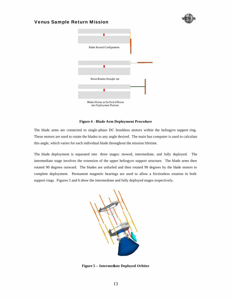
Figure 4 - Blade Arm Deployment Procedure
The blade arms are connected to single-phase DC brushless motors within the heliogyro support ring.
These motors are used to rotate the blades to any angle desired. The main bus computer is used to calculate
this angle, which varies for each individual blade throughout the mission lifetime.
The blade deployment is separated into three stages: stowed, intermediate, and fully deployed. The
intermediate stage involves the extension of the upper heliogyro support structure. The blade arms then
rotated 90 degrees outward. The blades are unfurled and then rotated 90 degrees by the blade motors to
complete deployment. Permanent magnetic bearings are used to allow a frictionless rotation in both
support rings. Figures 5 and 6 show the intermediate and fully deployed stages respectively.
Figure 5 – Intermediate Deployed Orbiter

Venus Sample Return Mission
14
Figure 6 - Deployed Orbiter
The orbiter layout is described in detail in Appendix B.
3.1.2 - Main Bus
The main bus is also a hexagonal structure with the same diameter, depth and thickness dimensions as the
heliogyro support rings. The center section is not removed to provide space for the computer, batteries, and
connection wires that branch out to the ADCS system and to the blade motors.
3.1.3 - Aeroshell
The aeroshell for the Venus Lander is composed of three aluminum conical sections and one aluminum face
section, each 0.6 cm thick. Figure 7 is a rendering of the shell with dimensions included.
Figure 7 - Venus Lander Aeroshell
Venus Sample Return Mission
15
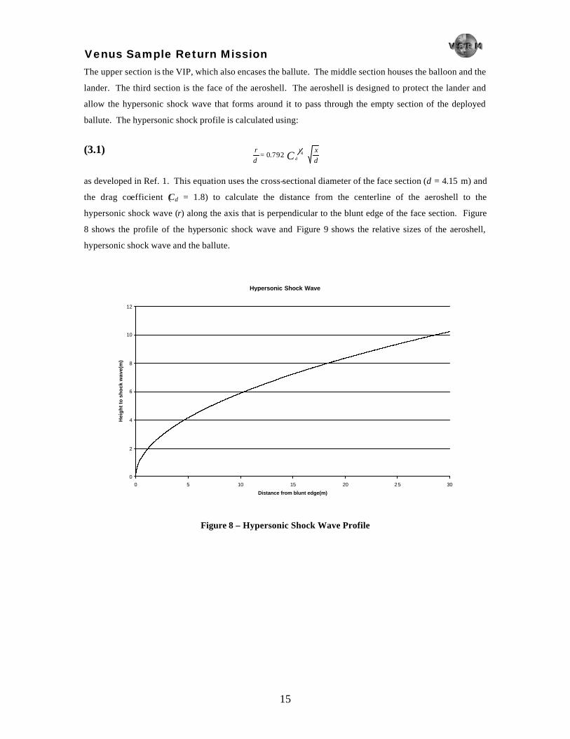
The upper section is the VIP, which also encases the ballute. The middle section houses the balloon and the
lander. The third section is the face of the aeroshell. The aeroshell is designed to protect the lander and
allow the hypersonic shock wave that forms around it to pass through the empty section of the deployed
ballute. The hypersonic shock profile is calculated using:
(3.1) dx
dr
C d⋅⋅= 4
1792.0
as developed in Ref. 1. This equation uses the cross-sectional diameter of the face section (d = 4.15 m) and
the drag coefficient (Cd = 1.8) to calculate the distance from the centerline of the aeroshell to the
hypersonic shock wave (r) along the axis that is perpendicular to the blunt edge of the face section. Figure
8 shows the profile of the hypersonic shock wave and Figure 9 shows the relative sizes of the aeroshell,
hypersonic shock wave and the ballute.
Hypersonic Shock Wave
0
2
4
6
8
10
12
0 5 10 15 20 25 30
Distance from blunt edge(m)
Hei
gh
t to
sh
ock
wav
e(m
)
Figure 8 – Hypersonic Shock Wave Profile

Venus Sample Return Mission
16
Figure 9 - Hypersonic Shock Wave Through Ballute
3.2 - Thermal
One side of the spacecraft is continually exposed to sunlight during the trip to Venus. All sides of the
spacecraft are exposed to extreme temperature gradients while in orbit around Venus. The solar intensity in
orbit at Venus is approximately twice the intensity encountered at Earth. The temperature of the outside of
the orbiter will reach as low as -200 degrees centigrade. The following thermal control system is modeled
after the Magellan spacecraft sent to Venus in 1989 (Ref. 2).
The most sensitive components on the spacecraft are the electronics, batteries, and thruster propellant tanks.
Table 6 shows the operating temperature range for each.
Table 6 - Temperature Ranges for Sensitive Components (Ref. 39)
Component Operating Temperature (°C) Non-operating Temperature (°C) Battery
Charging 0 – 45 NA Discharging -20 – 60 NA
Thruster propellant tank Below -190 -269 – 9 Computer -40 – 85
All electrical components and thruster propulsion tanks are wrapped in MLI blankets to protect them from
thermal extremes. The outside layer of the blanket is made of astroquartz, a material similar to glass-fiber
cloth that handles intense solar radiation extremely well. Chemical binders often used in astroquartz to
control flaking must be baked out to reduce the risk of discolorization leading to heat buildup. The inner
layers of the blanket alternate between perforated, aluminized Mylar and B-4-A polyester netting. The

Venus Sample Return Mission
17
bottom layer is made of Kapton. The overall thickness of an average 8-layered blanket is 1.2 cm (the
netting is not counted in the number of layers). Figure 10 shows the layering of the thermal blanket used
on the Venus spacecraft.
Figure 10 - Multi-Layered Insulation Cross-Section
The antenna is coated with a white, inorganic, water-based paint developed at NASA’s Goddard Space
Flight Center. This paint reflects solar radiation and prevents discolorization. Electronic compartments in
the orbiter bus, Venus Lander, and EEV have louvers around them that open and close automatically to
regulate heat dissipation (Ref. 2).
This thermal control system tends the craft and components toward cold temperatures. Kapton heaters are
therefore attached to protect cold-sensitive components. Temperature sensors are mounted on each
component and software is written to ensure that the heaters are activated when a component becomes too
cold (Ref. 2).
3.3 - Attitude Determination and Control System
3.3.1 - Attitude Determination
Control for the orbiter is performed solely by collective and cyclic pitch of the blades, so no additional
hardware such as control moment gyros or thrusters are required to provide pointing control. The attitude
determination sensors used by the orbiter are star trackers and sun sensors. The sun sensor is located on the
front face of the spacecraft, in the location most likely to maintain a position oriented towards the sun. Two
star trackers are located on the spacecraft bus, where spacecraft spin is not a factor. This combination of
sensors provides redundancy in the case of a sensor malfunction.

Venus Sample Return Mission
18
The star trackers are CT-602 High Accuracy Star Trackers provided by Ball Aerospace. These are small,
low mass devices capable of tracking up to five stars, with an accuracy of 3 arc seconds. Their Field-of-
View (FOV) is approximately 7.8º ´ 7.8º, and they provide two-axis attitude determination as well as star
intensity data. They contain a radiation-hardened processor for environmental tolerance, and additional
memory for greater programmability. The sensor package also includes optics, a 512 ´ 512 pixel Charge-
Coupled Device (CCD) detector, a thermoelectric cooler, command and data interface, and a spacecraft
power and mechanical interface.
The sun sensor is Ball Aerospace’s Precision Sun Tracking Sensors. These particular sun sensors have an
accuracy of 30 arc seconds with an 110º FOV, and are flexible for use on both spin stabilized and three-axis
stabilized spacecraft. The sun sensor, which is constructed of 6061 aluminum, is also radiation hardened
and uses CCD based imaging. The sun sensor is 0.165 m in diameter and 0.057 m tall with a hexagonal
cross section. The sun sensor, like the star trackers, provides two-axis determination.
3.3.2 - Control Systems
Spinning the heliogyro blades stabilizes them and removes the need for structure along the blades. The
spin rate is 0.04 radians/sec, or 2.3 degrees/sec. For a blade length of 1000 m, the corresponding angular
momentum is 39.79 kg-m2/s. The two sets of blades are spinning opposite each other to insure that the
angular momentum vector has a magnitude of zero. The spin of the sail provides the tension necessary to
hold the blades flat and in the proper position. Rotating the blades using the blade motors provides further
attitude control. The blades are rotated in both collective and cyclic manners.
Collective pitch constitutes applying a constant twist to each blade and is used to change the heliogyro spin
rate. The same torque must be applied to each blade for this maneuver, resulting in the same pitch angle for
each blade. This pitch mode is not time varying, because the angle applied is constant for all blades, and
does not change with rotation of the sail. This type of maneuver is also called a torque-control maneuver
(Ref. 21 p. 88).
Cyclic pitch is time varying and may be modulated every rotation period. It is used to force the heliogyro
spin axis to precess by creating torques across the blade disk (Ref. 21 p. 88). Pure cyclic pitch induces a
lateral force component in the plane of the blades that is used for planetary escape and capture spirals. Pure
cyclic pitch expressed as a function of time is given by equation (3.2).
(3.2) )sin()( 0ψθ −Ω= tAt
A is the cyclic pitch amplitude component, Ω is the spin rate, and ψ0 is the phase angle. Pure cyclic pitch
contains no component of collective pitch. Cyclic and collective pitching can be combined for more
complicated maneuvers requiring both changes in spin rate and movement of the heliogyro spin axis. Such

Venus Sample Return Mission
19
maneuvers may be necessary for satisfying pointing requirements. This type of movement is used to
reorient the heliogyro and orbiter for capturing the VSC in Venus orbit. The equation of motion for this
mode is given by equation (3.3).
(3.3) )sin()( 00 ψθθ −Ω⋅+= tAt
U0 is the collective pitch angle. Other, more complicated schemes can be generated to provide various
modes of control, depending on the mission requirements. The heliogyro can be fully controlled in all
flight modes and for all pointing requirements using various combinations of collective and cyclic control.
Determining the blade shape and coning angle from the spin rate and solar radiation effects is central to
controlling the heliogyro. A blade tensile stress analysis is performed on the heliogyro for this purpose.
For heliogyros with blade length R, chord C, a density ρ, and thickness h rotating with angular velocity Ω ,
the radial and chordwise tensile stresses are determined by equations (3.4) and (3.5).
(3.4) )(21
)( 222 rRrr −⋅Ω⋅⋅= ρσ
(3.5)
−
⋅Ω⋅⋅= 2
22
221
)( xC
xx ρσ
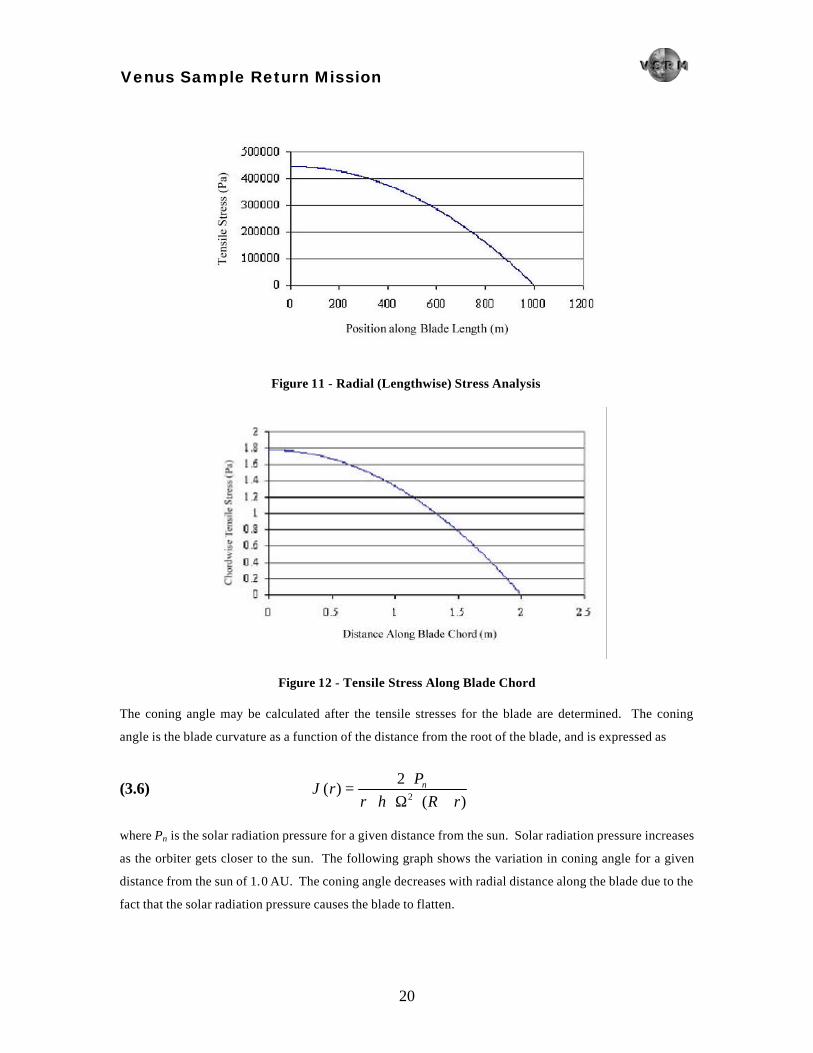
σr(r ) and σx(x) are the radial and chordwise tensile stresses, respectively (Ref. 21 p. 88). The distance
outward along the sail blade is represented by r, and the distance in the chordwise direction along the sail
blade is represented by x. Results of these equations along the length of the blade are found in the
following graphs. The tensile stress decreases exponentially as one moves outward along the blade or
outward away from the midline at the root.
Venus Sample Return Mission
20
Figure 11 - Radial (Lengthwise) Stress Analysis
Figure 12 - Tensile Stress Along Blade Chord
The coning angle may be calculated after the tensile stresses for the blade are determined. The coning
angle is the blade curvature as a function of the distance from the root of the blade, and is expressed as
(3.6) )(
2)(
2 rRhP
r n
+⋅Ω⋅⋅⋅
=ρ
ϑ
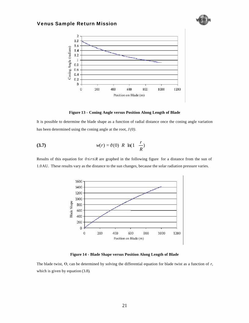
where Pn is the solar radiation pressure for a given distance from the sun. Solar radiation pressure increases
as the orbiter gets closer to the sun. The following graph shows the variation in coning angle for a given
distance from the sun of 1.0 AU. The coning angle decreases with radial distance along the blade due to the
fact that the solar radiation pressure causes the blade to flatten.
Venus Sample Return Mission
21
Figure 13 - Coning Angle versus Position Along Length of Blade
It is possible to determine the blade shape as a function of radial distance once the coning angle variation
has been determined using the coning angle at the root, ϑ(0).
(3.7) )1ln()0()(Rr
Rrw +⋅⋅ϑ=
Results of this equation for 0≤r≤R are graphed in the following figure for a distance from the sun of
1.0 AU. These results vary as the distance to the sun changes, because the solar radiation pressure varies.
Figure 14 - Blade Shape versus Position Along Length of Blade
The blade twist, U, can be determined by solving the differential equation for blade twist as a function of r,
which is given by equation (3.8).
Venus Sample Return Mission
22
(3.8) 0)(21
2
222 =−⋅−⋅−⋅ θ
θθdrd
rdrd
rR
This blade twist is independent of mechanical properties of the blade. A root torque Mo is required to twist
the blade through the desired angle and can be calculated using equation (3.9).
(3.9) 00
0208.1
σθ
⋅⋅⋅
= IR
M
U0 is the desired blade twist or pitch angle at the root, and σ0 is the radial tensile stress at the blade root,
and I is the area moment of inertia, determined by equation (3.10).
(3.10) hCI ⋅⋅= 3
121
The required torque increases linearly with increasing blade twist. The torque is small because the area
moment of inertia is small due to the minimal thickness of the blades.
3.4 - Power
The power system for the orbiter utilizes a solar panel to provide the required power. The cells used for the
solar panel are gallium arsenide cells with a germanium substrate, and are manufactured by Spectrolab Inc.
The cells are monolithic, two terminal, triple junction cells with a Beginning-of-Life (BOL) efficiency of
26% and an End-of-Life (EOL) efficiency of 21%. Each cell has an area of 30 cm2, a thickness of 140 µm,
and a mass per unit area of 84 mg/cm2 (Ref. 36). Assembly methods for the cells include soldering,
thermocompression, and ultrasonic wire bonding. The total area available for the solar panel, which is
located on the sun-facing surface of the orbiter, is 10.22 m2. The power output for this area is 3,086 W.
This provides more than enough power for the orbiter.
The power generated by the solar panel is stored in secondary batteries for use during times of eclipse, such
as in Earth or Venus orbit. Nickel-Cadmium batteries provided by Sanyo are used as the secondary
batteries. The particular battery used is a KR-series CADNICA battery, the KR-10000M. The KR-series
Sanyo batteries are standard space-rated batteries known for their high performance and reliability. Data on
the Sanyo CADNICA battery chosen is provided in Table 7.

Venus Sample Return Mission
23
Table 7 - Orbiter Batteries
Sanyo CADNICA Battery (KR-10000M) Nominal Voltage 1.2 V Capacity 10000 mA·h Diameter 43.1 mm Height 91.0 mm Mass 400 g Charge Temperature Range 0oC – 45oC Discharge Temperature Range -20oC – 60oC Storage Temperature Range -30oC – 50oC (-30oC – 35oC for long periods)
3.5 - Computer / Communication
3.5.1 - Computer
Calculating the motions of the individual blades in order to perform pointing, turning, and spin
maintenance is very complicated. The orbiter requires extensive computer calculations for ADCS. There
are two computers on the orbiter, one main computer and a backup computer. The computer selected for
the orbiter is the Radiation Hardened PowerPC (RHPPC) Single Board Computer from Honeywell. This
computer uses a radiation hardened PowerPC 603e™ processor. This particular computer system is
designed to operate for 15 years in the severe thermal and radiation environments of space. Table 8 shows
some of the features of the computer system, and Figure 15 shows a picture of this computer system.
Table 8 - RHPPC Feature Summary (Ref. 9)
Processor RHPPC RISC (PowerPC 603e™ licensed) 210 MIPS (Drhystone) @ 150MHz, 1.4 IPC
16Kbtye each Icache & Dcache L2 cache 512KB, look aside, write through Memory 4MByte SRAM, EDAC
4Mbyte EEPROM, super EDAC 64Kbyte SUROM (PROM)
Backplane Bus cPCI, 32-bit, 33MHz, 3.3V I/O MIL-STD-1553B
2 Synchronous Serial full duplex ports, 12.5Mbps (RS422) 2 UART full duplex ports, 9.6K to 1M BAUD (RS422) 16 pins programmable as interrupt or discretes
Debug/test port JTAG (1149.1), COP, RHPPC debug Timers/counters 5, 32-bit general purpose, 4 with 8-bit prescale
50-bit mission timer with 6-bit prescale 32-bit watchdog timer, 2 stage
Form Factor cPCI 6U x 220 (9.187” x 8.661”) with 2 PMC-like slots (74 x 149 mm) Mass 2.2 pounds Power 12.5W (nom), 3.3Vdc ± 5%
Radiation hardness Natural space

Venus Sample Return Mission
24
Table 9 shows the radiation hardness of the computer system. The software tools that can be used with this
computer system are Wind River Systems' Tornado™ environment, GNU C/C++ tools, and Wind River’s
VxWorks™ real-time operating system. The operating temperature range is between -40 °C and 80 °C.
The 210 MIPS provided by this computer is more than enough processor speed and power to perform this
mission. This system will cost about $400,000 fo r each computer (Ref. 9).
RH P PC
LM111
RS
422Rcv
r26F
32
RS232
Rcv
r26F
32
1553
D ua lX C V R
1553XFM R
1553XFM R
RS4
22
Drv
26L
S32
OS
CO S C
512K x 8E EPR O M
512K x 8E EPR O M
512K x 8E EPR O M
512K x 8E EPR O M
512K x 8EE PR OM
512K x 8E EPR O M
512K x 8E EPR O M
512K x 8EE PR OM
512K x 8EE PR OM
512K x 8EE PR OM
512K x 8EE PRO M
RR
RR
RR
RR
RR
RR
RR
RR
RR
RR
RR
RR
RR
RR
RR
PCI - PCIBri dg e
PCI - PCIBri dg e
PP C - P E C
L M111
51
2K
x 8
SR
AM
51
2K
x 8
SR
AM
51
2K
x 8
SR
AM
51
2K
x 8
SR
AM
51
2K
x 8
SR
AM
51
2K
x 8
SR
AM
51
2K
x 8
SR
AM
51
2K
x 8
SR
AM
51
2K
x 8
SR
AM5
12
K x
8S
RA
M5
12
K x
8S
RAM
51
2K
x 8
SR
AM
51
2K
x 8
SR
AM
51
2K
x 8
SR
AM
51
2K
x 8
SR
AM
51
2K
x 8
SR
AM
51
2K
x 8
SR
AM
51
2K
x 8
SR
AM
32 K x 8PROM
32 K x 8PROM
AC245
A C245
AC 245
AC 245
AC 245
AC 245
A C245
A C245
AC 245
AC 245
RR
RR
RR
RR
RR
RR
RR
RR
RR
RR
RR
RR
RR
RR
RR
RR
Figure 15 - RHPPC Mechanical Concept (Ref. 9)
Table 9 - Radiation Hardness (Ref. 9)
Total dose 1E5 rad Dose rate upset 1E8 rad/s Dose rate survive 1E11 rad/s Neutrons (1MeV DES) 1E13 n/cm2 SEU without L2 4.4E-5 u/d SEU with L2 8.4E-5 u/d Latchup none
3.5.2 - Communications
The steerable HGA utilizes an X-band signal with a frequency of about 80 GHz in order for the DSN
ground stations to pick up the data. The DSN is the monitoring agent on Earth for the duration of the
mission. DSN has the adequate coverage for the orbiter to be able to receive data at all times during the
mission. The HGA dish is 1.5 m in diameter and has a 2 m boom. The boom is connected to a 0.5 m arm
for stowing during launch. The HGA requires 60 W of power to operate and has a power output of 25 W
(Ref. 11).

Venus Sample Return Mission
25
3.6 - Propulsion
The heliogyro propulsion system provides one main advantage over conventional chemical propulsion
systems. The mass of the propellant required to accomplish this mission with chemical propulsion is in
excess of 10,000 kg. The heliogyro propulsion system has a mass of roughly 300 kg by comparison.
Decreasing the overall launch mass reduces the size of the launch vehicle and ultimately the cost of the
mission.
3.6.1 - Solar Sailing Basics
A solar sail is a large, low mass reflective structure in space. Thrust is produced by photon pressure from
the Sun or other beamed energy sources. This concept gives a solar sail the ability to operate with an
unlimited supply of fuel (the Sun) within the inner solar system. When traveling in the outer solar system
the solar radiation pressure is significantly reduced (the drop in pressure falling proportionally with the
square of the distance to the Sun). Solar radiation pressure is the transfer of momentum from photons to
the sail. This momentum transfer occurs twice with the sail. The first transfer (Figure 16a) occurs when
the photon strikes the sail, and the momentum of the photon is transferred to the sail/photon system.
Figure 16 - System before photon strike
The photon has momentum +p before making contact and the sail has 0 momentum. The photon/sail
system has momentum +p during contact. The photon is then reflected off the sail (the percentage of
photons reflected depends on the reflectivity of the sail material) transferring momentum to the sail (Figure
16b). The photon now has momentum –p and the sail has momentum +2p.
The optimal incident angle at which to hold the sail is 45 degrees with respect with the sun for a perfectly
reflecting surface. Surfaces do not reflect perfectly, which means that the angle of incidence is not equal to
Venus Sample Return Mission
26
the angle of reflection. The ideal pitch angle equals the cone angle of the reflected photon. Mathematical
modeling is done assuming an ideally behaving sail at 45 degrees.
3.6.2 - Equations of Motion
Patched conics are used to determine a preliminary trajectory for the solar sail. Circular planetary
motion and co-planar travel are assumed. The basic equation of motion in polar coordinates uses µ as the
gravitational constant of the influencing gravitational body, r as the position vector from the center of mass
of the influencing body, T as the thrust acting on the sail, and m as the mass of the spacecraft.
(3.11) Trr
mrm
rr&&r +⋅⋅
−=⋅ 3
µ
Thrust for solar sail propulsion, T is given by equation (3.12).
(3.12)
⋅⋅
⋅=θα
αee
APT r
ˆcos
ˆsinr
P is the solar radiation pressure, A is the surface area viewable by the sun and α is the angle of the sail with
respect to the Sun. Solar radiation pressure is given by equation (3.13).
(3.13) ( )
cRL
P⋅⋅
+⋅= 22
1 ρ
L is the solar luminosity, ρ is the reflectivity of the sail material, R is the distance to the Sun, and c is the
speed of light. Figure 17 illustrates the polar conventions used in these equations.
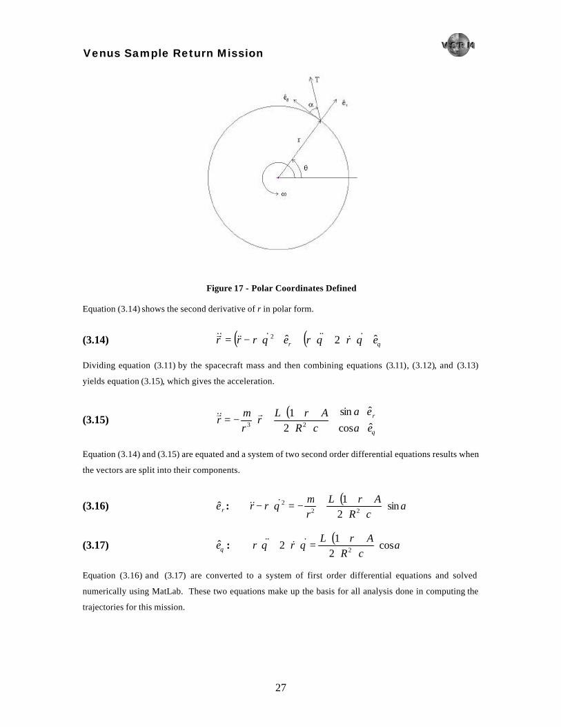
Venus Sample Return Mission
27
Figure 17 - Polar Coordinates Defined
Equation (3.14) shows the second derivative of r in polar form.
(3.14) ( ) ( ) θθθθ errerrr r ˆ2ˆ2 ⋅⋅⋅+⋅+⋅⋅−= &&&&&&&&&r
Dividing equation (3.11) by the spacecraft mass and then combining equations (3.11), (3.12), and (3.13)
yields equation (3.15), which gives the acceleration.
(3.15) ( )
⋅⋅
⋅⋅⋅
⋅+⋅+⋅−=
θααρµ
ee
cRAL
rr
r r
ˆcos
ˆsin21
23
r&&r
Equation (3.14) and (3.15) are equated and a system of two second order differential equations results when
the vectors are split into their components.
(3.16) re : ( )
αρµ
θ sin21
222 ⋅
⋅⋅⋅+⋅
+−=⋅−cR
ALr
rr &&&
(3.17) θe : ( )
αρ
θθ cos2
12 2 ⋅
⋅⋅⋅+⋅
=⋅⋅+⋅cR
ALrr &&&&
Equation (3.16) and (3.17) are converted to a system of first order differential equations and solved
numerically using MatLab. These two equations make up the basis for all analysis done in computing the
trajectories for this mission.

Venus Sample Return Mission
28
The front blades will periodically cast shadows on the rear blades because of the counter spinning motion
of the heliogyro. The shadows reduce the thrust output of the sail by reducing the viewable area of the sail
to the Sun. This was modeled as a simple sine curve that follows equation (3.18).
(3.18)
⋅⋅
⋅⋅+⋅=180
sin25.075.0 maxmaxrpmt
TTTπ
Tmax is the maximum thrust possible, which occurs when the sun strikes all the blades, t is the time in
seconds, and rpm is the revolutions per minute of the blades. Figure 18 shows the thrusting profile for the
first half of the mission (travel to Venus).
Figure 18 - Mean Thrust for Travel to Venus
3.6.3 - Interplanetary Travel
Assumptions are made in addition to those mentioned above in order to simplify calculations to obtain a
reasonable estimate for the flight path of the spacecraft. The first assumption is to hold the solar sail’s
angle to the Sun, α, constant for the duration of the trip to and from Venus. The solar sail can vector its
thrust 90 degrees in either direction from the Sun. It is also assumed that the thrust produced by the solar
sail is the maximum possible at that distance from the Sun. The dynamics of this design allow throttling
from no thrust to full thrust. Both of these capabilities allow the solar sail to depart at anytime and arrive at
the desired destination without having to adhere to specific launch windows. Travel to Venus is calculated
holding the thrust angle at 135 degrees. Figure 19 shows the trajectory from Earth to Venus as computed
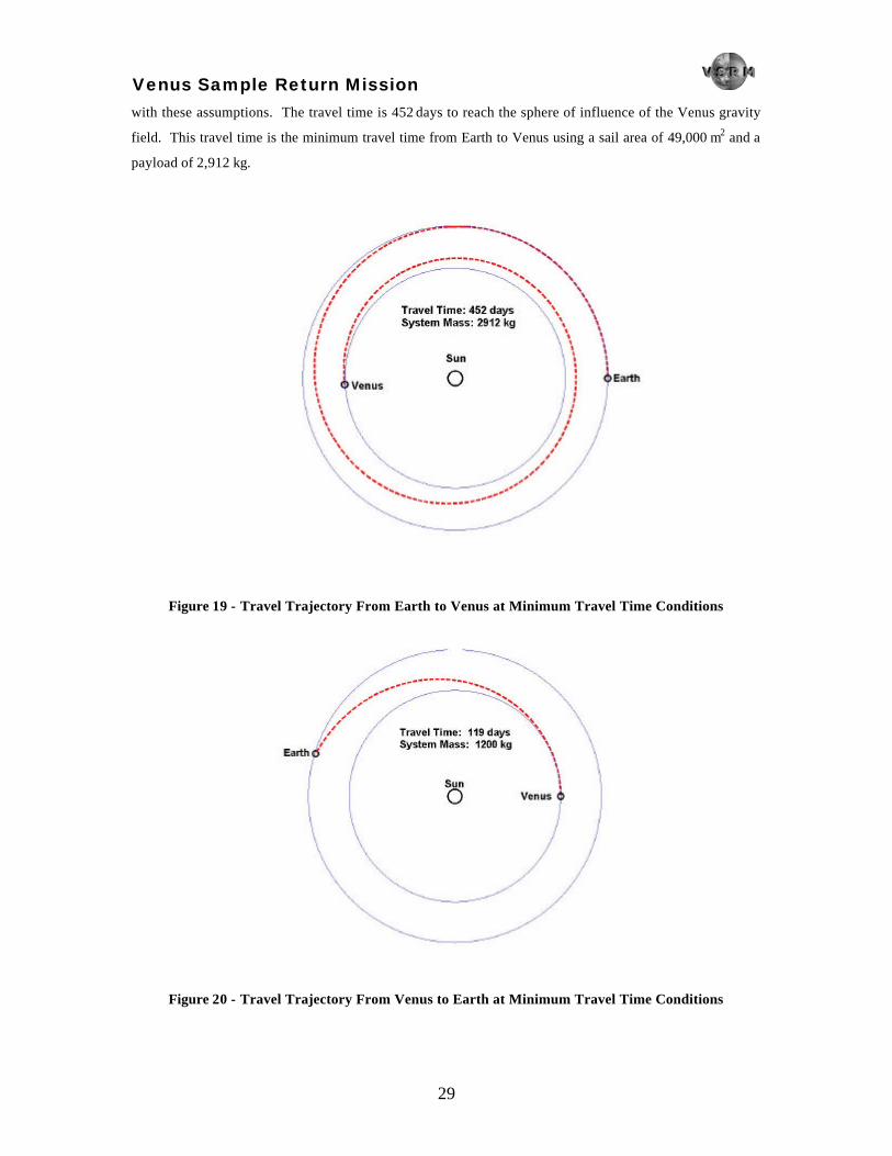
Venus Sample Return Mission
29
with these assumptions. The travel time is 452 days to reach the sphere of influence of the Venus gravity
field. This travel time is the minimum travel time from Earth to Venus using a sail area of 49,000 m2 and a
payload of 2,912 kg.
Figure 19 - Travel Trajectory From Earth to Venus at Minimum Travel Time Conditions
Figure 20 - Travel Trajectory From Venus to Earth at Minimum Travel Time Conditions

Venus Sample Return Mission
30
To achieve this travel time a departure from Earth would have to be on March 28, 2005 at the earliest and
arrival at the Venus sphere of influence would occur on June 23, 2006. Launching on any other date
increases the travel time to intercept Venus. The return trip of the interplanetary travel phase (Figure 20) is
quicker due to the lower mass of the payload returning to Earth. The thrust angle for this portion of the trip
is held constant at 45 degrees in order to spiral outward. Again, considering the shortest possible trip time,
the first available launch opportunity comes on October 29, 2007. The travel time back to Earth would be
119 days and arrival at Earth would occur on February 26, 2008.
3.6.4 - Travel Around Venus
The travel within the sphere of influence of a planet was analyzed with a different set of assumptions from
that of the interplanetary travel. For this case the thrust angle is no longer held constant, rather the thrust
angle must vary with the position of the solar sail in the planet’s orbit. Energy is added or removed in order
to spiral out or in respectively. Thrust is vectored in the direction opposite the velocity vector to decrease
the energy and spiral towards the planet. When it is not possible to thrust against the velocity vector,
thrusting is stopped by positioning the blades of the sail parallel to the direction of the Sun. Figure 21
depicts this mode of thrusting involved in Phase I. When a suitable perigee is achieved in the capture orbit
a new approach to thrusting is taken in which thrusting only occurs within a specific distance from the
planet. This radius is 100,000 km for the Venus capture orbit. This method of thrusting changes perigee by
1000 km but reduces the apogee distance by over 100,000 km as can be seen in Figure 21 as Phase II of the
capture.

Venus Sample Return Mission
31
Figure 21 - Overview of Venus Capture
A closer inspection at perigee shows the small variance of the perigee point with each pass, shown in
Figure 22. Also shown is the entry path of the lander into the atmosphere.

Venus Sample Return Mission
32
Figure 22 - Venus Capture Close-up
For this case, Phase I lasts approximately 49 days and Phase II takes about 199 days. The orbiter releases
the lander at apogee just under four days after the completion of Phase II, and the lander takes 3 more days
to enter the atmosphere. Total time for this section of the mission is approximately 255 days.
The previous paragraph describes the latest design change in the mission. The original mission concept
called for the orbiter to spiral into an 800 km circular orbit to perform the rendezvous. Trajectory
computations calculating this orbit transfer produce unacceptable mission times of more than 3 years for
completion of the spiral transfer to the 800 km circular orbit. The need to change the mission to a more
appropriate time frame arose from this analysis. This new concept brings the orbiter into the highly
elliptical orbit shown in Figure 21, where perigee is at 800 km altitude and apogee is at 275,000 km. As
discussed in Section 4.10.2, the rocket would need to be resized to match such an orbit so that a rendezvous
can be achieved. With this mission concept the ∆V required to insert the lander into the Venus atmosphere
is reduced to 20 m/s at the apogee of the orbiter’s orbit (Figure 21).
The Venus escape portion of the mission begins after the rendezvous occurs. The escape is similar to the
capture Phase I in thrusting with the exception of that energy will now be added to the orbit by positioning

Venus Sample Return Mission
33
part of the thrust vector in the velocity direction. Figure 23 demonstrates an escape trajectory given
optimal conditions. This trajectory takes approximately 108 days to complete.
Figure 23 - Venus Escape Trajectory
3.6.5 - Future Analysis
There is room to improve the accuracy of these models. Matching the final conditions of interplanetary
travel with the initial conditions of planetary travel is one of the more important areas for improvement.
This is accomplished through vectored thrusting and throttling and would increase the estimated minimum
trip time on the order of months. Another area of improvement would be to 3-dimensionalize the
mathematics of the modeling. The initial 2-D assumption made is reasonable, however, there is
approximately 3 degrees of inclination separating the Earth orbit from the Venus orbit around the Sun.
Referring to Figure 18, further study could be done to explain the flat portions of the thrust curve that occur
at the beginning of the transfer and at 300 days into the transfer.
Further analysis is also needed in the study of blade flutter that may result from the counter spinning blades
casting shadows on each other. This may or may not be a problem with the projected spin rate of 0.38

Venus Sample Return Mission
34
revolutions/minute. Possible corrections to this problem include reshaping the blades to make them thinner
in width and longer in length or increasing the spin rate of the heliogyro. If the harmonic response of this
flutter is small enough and occurs away from the resonance frequency of the blades it may also be an
option to allow the small amount of flutter to occur. Other blade dynamics that are of concern include the
blade twist that can occur down the length of the blade and response lag to rotations applied at the root.
3.7 - Mechanisms
3.7.1 - Lightband
Lightband is a separation device that allows two spacecraft to detach from one another. Walter Holemans,
of the Planetary Systems Corporation, invented the device’s simple design. A string held in tension holds
the two halves of the system together. When the tension is released by melting through the string, the two
halves separate and the spacecraft float apart. Lightband has heritage in the University Nanosat program
with the spacecraft trio, ION-F, involving three universities: Virginia Tech, University of Washington, and
Utah State University. The system separated the three satellites successfully in 2003.
The Lightband mechanism allows the Venus lander to detach from the Earth return vehicle. In addition, the
separation of the Earth return vehicle from the main bus also utilizes Lightband. Lightband has a mass of
1.363 kg and requires a 30 W burst of power for activation (Ref. 13).
3.7.2 - Solar Sail Blade Thrusters
Thrusters along the outside of the orbiter fire to begin rotation of the solar sail bases. The rotation initiates
deployment of the solar sail blades. Once the correct rotational speed is reached, frictionless magnetic
bearings allow the rotation to continue without deceleration.
3.7.3 - Blade Rotation Motors
Blade rotation motors located within the blade support ring of the orbiter allow the solar sail blades to
rotate. The ability to rotate enables the sail to control the direction in which the spacecraft travels.
Planetary gearhead motors, model EC32, from Maxon Precision Motors Company, are used for the blade
rotation. The motors provide a torque of 2.25 N⋅m and have a mass of 162 grams. A total of twelve motors
are needed to allow each solar sail blade to rotate a full 180 degrees independently of other blades. Each
motor requires 80 W to operate (Ref. 20).
3.8 - System Mass
The mass breakdown for the orbiter is shown in Table 10.

Venus Sample Return Mission
35
Table 10 - Orbiter Mass
Equipment List Mass (kg)
ADCS 10 Battery / Cells 15
Communications 25 Computer / Elec. 3
Mechanisms 25 Rendezvous Structure 310
Solar Sail 247 Structure (Shaft) 42
Structure (Blade Rings) 100 Structure (Support Bars) 32
Structure (Bus Ring) 100 Thermal 25
Total 934
3.9 - Summary
The Orbiter Main Bus is a complex system as described above. Means of travel between Earth and Venus,
the structure and functions of the orbiter’s components, and the structure of the bus itself are all integral
parts of the design. The Venus lander also has many intricate components and functions to perform.
Chapter 4 explains the lander in detail.
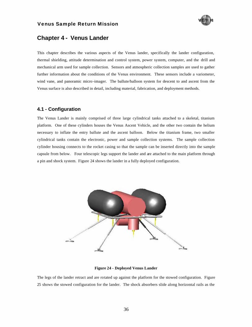
Venus Sample Return Mission
36
Chapter 4 - Venus Lander This chapter describes the various aspects of the Venus lander, specifically the lander configuration,
thermal shielding, attitude determination and control system, power system, computer, and the drill and
mechanical arm used for sample collection. Sensors and atmospheric collection samples are used to gather
further information about the conditions of the Venus environment. These sensors include a variometer,
wind vane, and panoramic micro -imager. The ballute/balloon system for descent to and ascent from the
Venus surface is also described in detail, including material, fabrication, and deployment methods.
4.1 - Configuration
The Venus Lander is mainly comprised of three large cylindrical tanks attached to a skeletal, titanium
platform. One of these cylinders houses the Venus Ascent Vehicle, and the other two contain the helium
necessary to inflate the entry ballute and the ascent balloon. Below the titanium frame, two smaller
cylindrical tanks contain the electronic, power and sample collection systems. The sample collection
cylinder housing connects to the rocket casing so that the sample can be inserted directly into the sample
capsule from below. Four telescopic legs support the lander and are attached to the main platform through
a pin and shock system. Figure 24 shows the lander in a fully deployed configuration.
Figure 24 - Deployed Venus Lander
The legs of the lander retract and are rotated up against the platform for the stowed configuration. Figure
25 shows the stowed configuration for the lander. The shock absorbers slide along horizontal rails as the

Venus Sample Return Mission
37
legs rotate, as shown in Figure 26, so they remain extended throughout the descent until impact with the
surface. The lander configuration is described in more detail in Appendix C.
Figure 25 - Stowed Venus Lander
Figure 26 - Shock Absorber Deployed and Stowed Configurations
4.2 - Sizing Methodology
4.2.1 - Helium tanks
The layout of the lander is primarily based on the volume and mass of the top cylinders. The size of the
rocket housing comes directly from the size of the Venus Ascent Vehicle. Section 4.3 details the materials
used as well as the mass of the rocket housing. Sizing of the two helium tank cylinders begins with an
initial volume estimate based on the perfect gas law (equation (4.1)), where P represents pressure in
Pascals, v indicates volume in kg/m3, m is the mass of the gas in kg, R is the universal gas constant, and T is
the temperature in degrees Kelvin. An internal temperature and pressure of 250 K and 19 MPa respectively
are used for this analysis.
(4.1) TRmvP ⋅⋅=⋅

Venus Sample Return Mission
38
Application of equation (4.1) yields a volume of 2.1 m3. This volume is the total tank volume necessary,
and is divided between two tanks. The two-tank system is used to create lander symmetry. A hoop stress
analysis (equation (4.2)) determines a wall thickness for different combinations of vessel length and radius
for the desired volume. Stress is represented by σx, in units of Pascals. P again represents pressure, r is the
tank radius in meters, and t is the wall thickness in meters.
(4.2) t
rPz
⋅=σ
Table 11 shows the results for various geometric combinations for the half volume for four different
materials. The highlighted row represents the chosen geometry and material.
Table 11 - Helium Tank Geometry and Mass Combinations
Graphite Vessel Radius (m) Vessel Length (m) Wall thickness (mm) Vessel Mass (kg)
0.1 33.29 1.38 45.09 0.2 8.09 2.76 45.73 0.3 3.31 4.15 47.47 0.4 1.56 5.53 50.86 0.5 0.67 6.91 56.45 0.6 0.13 8.29 64.79
Titanium
Vessel Radius (m) Vessel Length (m) Wall thickness (mm) Vessel Mass (kg) 0.1 33.29 2.07 197.76 0.2 8.09 4.13 200.61 0.3 3.31 6.20 208.32 0.4 1.56 8.27 223.34 0.5 0.67 10.34 248.10 0.6 0.13 12.40 285.04
Aluminum
Vessel Radius (m) Vessel Length (m) Wall thickness (mm) Vessel Mass (kg) 0.1 33.29 6.61 373.58 0.2 8.09 13.22 379.30 0.3 3.31 19.83 394.84 0.4 1.56 26.43 425.11 0.5 0.67 33.04 475.01 0.6 0.13 39.65 549.45
Steel
Vessel Radius (m) Vessel Length (m) Wall thickness (mm) Vessel Mass (kg) 0.1 33.29 1.38 229.83 0.2 8.09 2.76 233.10 0.3 3.31 4.15 241.98 0.4 1.56 5.53 259.26 0.5 0.67 6.91 287.74 0.6 0.13 8.29 330.24
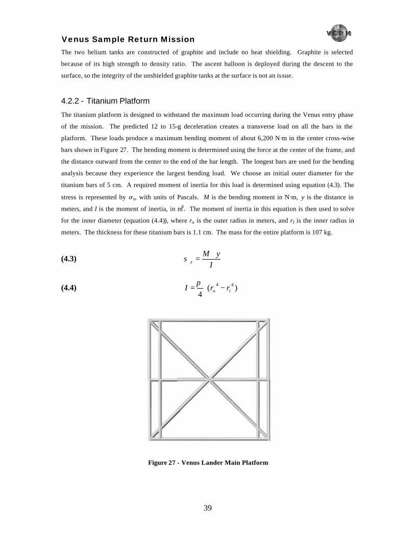
Venus Sample Return Mission
39
The two helium tanks are constructed of graphite and include no heat shielding. Graphite is selected
because of its high strength to density ratio. The ascent balloon is deployed during the descent to the
surface, so the integrity of the unshielded graphite tanks at the surface is not an issue.
4.2.2 - Titanium Platform
The titanium platform is designed to withstand the maximum load occurring during the Venus entry phase
of the mission. The predicted 12 to 15-g deceleration creates a transverse load on all the bars in the
platform. These loads produce a maximum bending moment of about 6,200 N·m in the center cross-wise
bars shown in Figure 27. The bending moment is determined using the force at the center of the frame, and
the distance outward from the center to the end of the bar length. The longest bars are used for the bending
analysis because they experience the largest bending load. We choose an initial outer diameter for the
titanium bars of 5 cm. A required moment of inertia for this load is determined using equation (4.3). The
stress is represented by σx, with units of Pascals. M is the bending moment in N·m, y is the distance in
meters, and I is the moment of inertia, in m4. The moment of inertia in this equation is then used to solve
for the inner diameter (equation (4.4)), where ro is the outer radius in meters, and rI is the inner radius in
meters. The thickness for these titanium bars is 1.1 cm. The mass for the entire platform is 107 kg.
(4.3) I
yMz
⋅=σ
(4.4) )(4
44io rrI −⋅=
π
Figure 27 - Venus Lander Main Platform

Venus Sample Return Mission
40
4.2.3 - Landing Legs
The legs of the lander are telescoping, concentric cylinders. The legs are subjected to both bending and
buckling loads. The bending load is the limiting factor in this case. The shock absorbers are designed to
allow for 0.23 m of travel at an impact velocity of 4 m/s, creating a bending load of 6,000 N·m in each leg.
The sizing includes a large factor of safety to account for possible difficulties with balloon inflation. The
upper/outer cylinder for each leg has the same dimensions as the bars used for the main platform. The
lower/inner cylinder for each leg is a solid 2.8 cm diameter bar. The entire leg is 1.6 m long when
deployed. These legs are pinned to the lander and lander feet, and they are connected to the shock
absorbers with ball and socket joints. The landing feet are 0.3 m diameter plates. Figure 28 shows a leg in
its deployed configuration.
Figure 28 - Venus Lander Leg Deployed Configuration
4.2.4 - Center of Mass
The center of mass for the lander is important both for aerodynamic stability during descent and to ensure
that the landing loads are distributed evenly across the platform. The upper cylinders are symmetrically
placed; the lower cylinders are not. The center of mass for the VAV is located 0.04 m from the center of the
platform. The sample collection cylinder is attached to the rocket casing directly below the payload
section, a distance of 0.75 m from the center of the platform. The rocket mass is 310 kg, and the mass of
the sample collection cylinder is 35.4 kg. The cylinder containing the battery pack has a mass of 53.1 kg.
Summing the moments about the center axis places the battery cylinder 0.2 m from the center of the
platform on the same side as the rocket center of mass. Figure 29 shows the placement of these cylinders
with their respective distances from the center of the platform.

Venus Sample Return Mission
41
Figure 29 - Venus Lander Center of Mass Layout
4.3 - Thermal
The shielding is designed to prevent electronics meltdown premature rocket ignition. The rocket has a
safety temperature of 78 °C; at that point the fuel in the rocket ignites. The electronics must be maintained
at a temperature less than 40 °C. Figure 30 refers to components of the lander that use the thermal
shielding for protection.
Figure 30 - Venus Lander Thermal Shields
Rocket Tube
Electronics Container
Sample Container
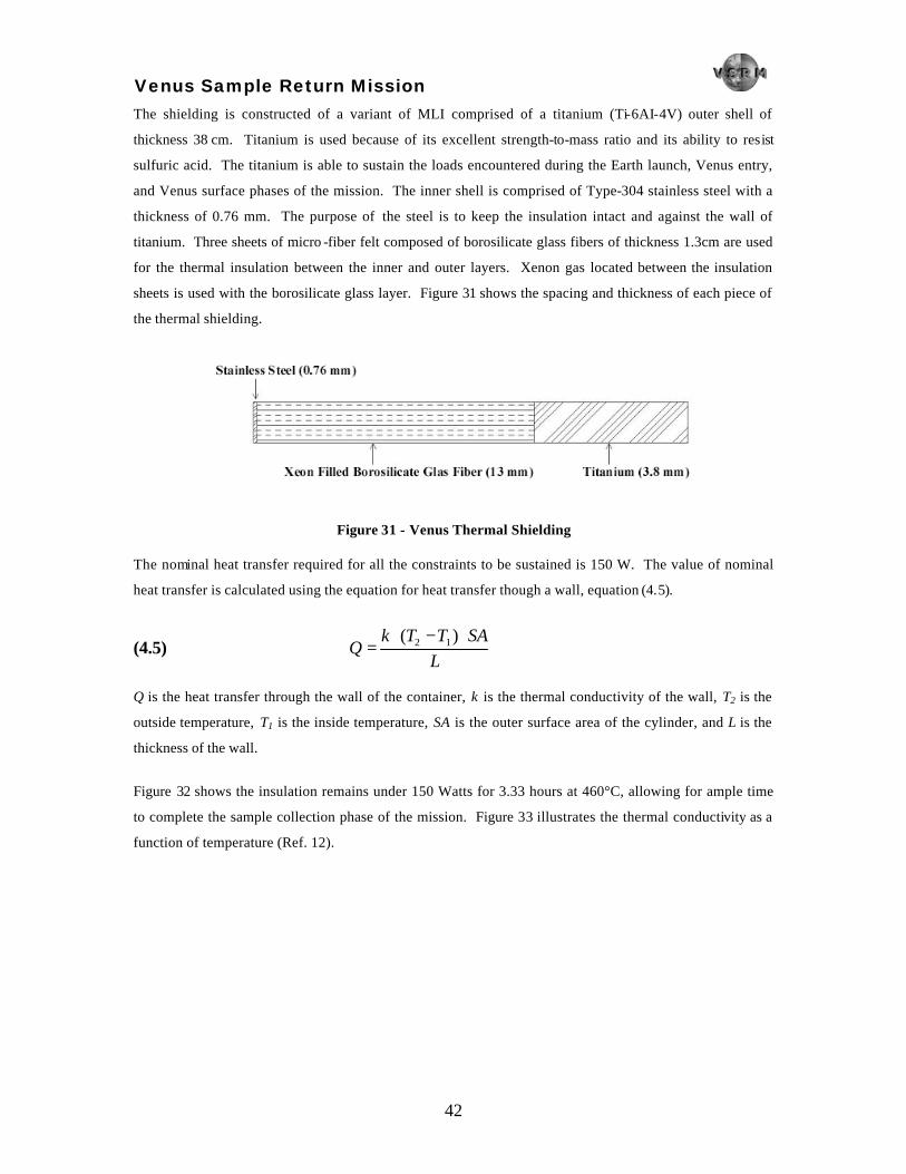
Venus Sample Return Mission
42
The shielding is constructed of a variant of MLI comprised of a titanium (Ti-6AI-4V) outer shell of
thickness 38 cm. Titanium is used because of its excellent strength-to-mass ratio and its ability to resist
sulfuric acid. The titanium is able to sustain the loads encountered during the Earth launch, Venus entry,
and Venus surface phases of the mission. The inner shell is comprised of Type-304 stainless steel with a
thickness of 0.76 mm. The purpose of the steel is to keep the insulation intact and against the wall of
titanium. Three sheets of micro -fiber felt composed of borosilicate glass fibers of thickness 1.3cm are used
for the thermal insulation between the inner and outer layers. Xenon gas located between the insulation
sheets is used with the borosilicate glass layer. Figure 31 shows the spacing and thickness of each piece of
the thermal shielding.
Figure 31 - Venus Thermal Shielding
The nominal heat transfer required for all the constraints to be sustained is 150 W. The value of nominal
heat transfer is calculated using the equation for heat transfer though a wall, equation (4.5).
(4.5) L
SATTkQ
⋅−⋅=
)( 12
Q is the heat transfer through the wall of the container, k is the thermal conductivity of the wall, T2 is the
outside temperature, T1 is the inside temperature, SA is the outer surface area of the cylinder, and L is the
thickness of the wall.
Figure 32 shows the insulation remains under 150 Watts for 3.33 hours at 460°C, allowing for ample time
to complete the sample collection phase of the mission. Figure 33 illustrates the thermal conductivity as a
function of temperature (Ref. 12).
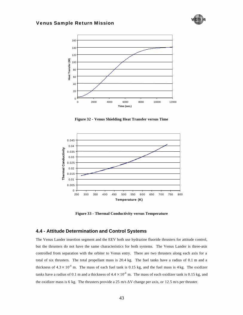
Venus Sample Return Mission
43
0
20
40
60
80
100
120
140
160
0 2000 4000 6000 8000 10000 12000 Time (sec.)
Hea
t T
ran
sfer
(W
)
Figure 32 - Venus Shielding Heat Transfer versus Time
0 0.005 0.01
0.015 0.02
0.025 0.03
0.035 0.04
0.045
250 300 350 400 450 500 550 600 650 700 750 800 Temperature (K)
Th
erm
al C
ond
uct
ivit
y
Figure 33 - Thermal Conductivity versus Temperature
4.4 - Attitude Determination and Control Systems
The Venus Lander insertion segment and the EEV both use hydrazine fluoride thrusters for attitude control,
but the thrusters do not have the same characteristics for both systems. The Venus Lander is three-axis
controlled from separation with the orbiter to Venus entry. There are two thrusters along each axis for a
total of six thrusters. The total propellant mass is 20.4 kg. The fuel tanks have a radius of 0.1 m and a
thickness of 4.3×10⁻⁴ m. The mass of each fuel tank is 0.15 kg, and the fuel mass is 4 kg. The oxidizer
tanks have a radius of 0.1 m and a thickness of 4.4×10⁻⁴ m. The mass of each oxidizer tank is 0.15 kg, and
the oxidizer mass is 6 kg. The thrusters provide a 25 m/s ∆V change per axis, or 12.5 m/s per thruster.

Venus Sample Return Mission
44
Attitude determination onboard the Venus Lander is accomplished through the use of a sun sensor and a
star sensor. Ball Aerospace provides both, and they are identical to the sensors used on the spacecraft
orbiter. Although they are housed in the lander insertion segment with the thrusters, they are located at a
distance away from the thrusters so that any propellant exhaust does not affect their performance.
4.5 - Power
The use of solar panels for power generation on Venus is impractical due to the lack of adequate sunlight on
the Venusian surface. Primary batteries are the best choice for a lander power supply; their number and
size are dictated by the lander power requirements. The Venus Lander requires three separate systems, one
for the lander, a second for the VIP, and a third for the rocket to transport the sample to the orbiter.
The lander must be operational for the duration of the surface mission in addition to the time required to
descend to the surface and then ascend to the appropriate altitude for rocket launch. Thus the lander
batteries must provide power for up to nine hours. Lithium ion batteries manufactured by Saft Battery
Company (Ref. 32) provide an adequate power supply for the length of the surface mission, as well as for
the thruster package. The lander batteries are packaged as a cylindrical cell, in a sealed aluminum case, and
are affixed to the lander base. The thruster package batteries are packed the same way, but are contained in
the thruster housing section, and thus discarded before landing. Characteristics of Saft’s lithium ion
batteries are provided in Table 12.
Table 12 - Venus Lander Batteries (Ref. 32)
Saft Lithium Ion Batteries Length 250 mm Diameter 54.2 mm Mass 1,132 g Average Voltage 3.6V at C/2 EOCV 4.1 V Power 132 W·hr Specific Power 117 W·hr/kg Power Efficiency >94%
The lander power requirement for the surface mission is 1,043 W for 1.5 hours, for a total required capacity
of 1,564.5 W·hr. Additional power is required during the descent and ascent phases of the lander mission to
support the sensors and computer. Assuming a maximum time of 8 hours for the descent and ascent phases
of the Venus mission leads to a power requirement of 176 W·hr. These two power requirements together
yield a capacity of 1,740.5 W·hr. Using Saft’s lithium ion batteries to provide this power leads to a total
battery mass of 14 kg, corresponding to 15 batteries each with a volume of 5.8×10⁻⁴ m3, leading to a total
battery pack volume of 8.12×10⁻³ m3.
The Venus insertion package is operational from the time of release from the orbiter to the point at which it
is disconnected from the lander. The primary power requirement in this segment of the lander is the power

Venus Sample Return Mission
45
necessary to fire the thrusters. This is not a constant power requirement since the thrusters are not firing
continuously. The thruster package requires a power supply for five days, the length of time it must remain
operational. Assuming the thrusters are firing, the maximum power requirement is 83 W. The power
requirement assuming no thrusters are firing is 23 W. Again, the lithium ion primary batteries will also be
used in this segment.
4.6 - Computer
4.6.1 - Venus Lander Computer
The Venus Lander uses a Radiation Hardened Vector Processor (RHVP) by Honeywell. This computer can
handle 25 MIPS and has 2.7 MB of onboard static Random Access Memory (RAM). This system has a
general-purpose Digital Signal Processor (DSP) onboard with the vector processor. Applications not suited
for the fast vector processor are handled by the DSP. The computer controls the separation of the Venus
thruster package, ballute deployment, balloon deployment, collecting and controlling scientific data while
on the surface, and transferring data to the sample capsule computer. Software supported includes Vector
Builder, Vector Sim, and COTS tools. This computer system costs about $100,000 (Ref. 14).
4.6.2 - Sample Capsule Computer
The sample capsule computer controls the rocket’s flight and first and second stage separations, operate the
omni-directional s-band antenna, and store all surface collected data. The sample capsule uses the RHVP
computer along with a 48 MB extra solid-state memory card. The memory card cost about $200,000 and
can store up to 48 MB of flash RAM solid-state data, adequate for storing all necessary data for the
mission. All of the data collected from the Venus Lander is transferred from the lander’s computer to the
sample capsule and stored in the extra memory card. The entire system costs about $300,000 (Ref 14).

Venus Sample Return Mission
46
4.7 - Mechanisms
4.7.1 - Ultrasonic Drill/Corer
Figure 34 - Close up of the Ultrasonic Drill/Corer
An Ultrasonic Drill/Corer (USDC) acquires about 230 g of surface sample from Venus. The inner diameter
of the corer is 2.67 cm, and the drill stem length is 15 cm. The drill requires 1,000 W of power. The corer
works by using an ultrasonic horn driven at 20 to 23 kHz. A transformer converts the frequency to a drive
signal and a 60 to 1,000 Hz sonic wave. The USDC impacts the rock and creates fractures in the material
to achieve penetration.
Cybersonics Inc, located in Erie, Pennsylvania is working on the USDC in cooperation with NASA’s JPL.
The USDC drills into hard rock samples including basalt, ice, and construction brick. The USDC has the
capability of drilling through Venus’s basalt surface to retrieve the required sample.
The corer connects to the bottom of the sample retrieval cylinder so that the drill stem tip hovers 0.35 cm
above the Venusian surface. An extend/retract device attached to the top of the corer allows the drill stem
to reach the surface. A ball and joint connection between the extend/retract device and the corer enables the
instrument to align itself perpendicular to the surface in case the lander does not land level.
The USDC bit is not sharpened, so there is no concern with the bit wearing out and losing performance
capabilities. The corer is ideal in that it is not subject to drill walk, does not apply large lateral forces on
its platform, and the drilling speed does not degrade with time. High temperatures are handled well by this
instrument as it has only two moving parts that are easily adapted (Ref. 3).
4.7.2 - Mechanical Arm and Scoop
The mechanical arm collects the rest of the 2 kg sample that will be returned. The arm requires a power of
up to 25 W. It is composed of two sections of graphite epoxy, each 0.4 m in length. Each section is hollow,
with a 2.54 cm inner diameter and a 3.0 cm outer diameter. The mass of the arm is 135 g, and the scoop

Venus Sample Return Mission
47
volume is 50 cm3. The arm is composed of three sections: a shoulder joint joins the sample retrieval
cylinder and the first arm section, an elbow joint connects the two arm pieces, and a wrist joint attaches the
scoop to the arm. The rim of the scoop contains a top layer of tungsten steel to give the scoop added
toughness for trenching. Three narrow pieces of tungsten steel, known as ripper tines, protrude from the
back of the scoop. These ripper tines (Ref. 26) ra ke the surface to break up the rock and allow the scoop to
collect the sample.
The arm digs up about 45 cm3 of Venusian dirt, tilts the scoop upward, and allows the sample to fall down
the first section of the arm. A door connecting the sample container and the arm opens as the dirt begins to
descend down the arm. The pressure in the sample container is less than that on the surface, so when the
door opens a suction force helps collect the dirt falling down the arm. The mechanical arm continues to dig
and drop the samples through the hollow arm until a device in the sample container informs the arm that the
sample has been obtained. At this time the door to the sample container seals shut. Through the procedure
of using the suction force of the sample container, an atmospheric sample at surface level is obtained in
addition to the rock sample (Ref. 26).
4.7.3 - Sample Containers
The sample containers consist of a cylinder to hold the core sample, a surface sample sphere for the arm
sample, and two atmospheric sample spheres. The sample containers’ volumes are designed using the
density and characteristics of basalt. Extra volume is added to the arm sample sphere to provide room for
atmospheric and surface level samples.
Two small containers for high altitude atmospheric samples are included. The containers are spherical in
shape and acquire their samples by suction. The computer signals the containers’ door mechanisms to open
at 70 km (above the cloud layer) for one container and then at 40 km (in the cloud layer) for the other
container.
Atmospheric samples are obtained by using a pressure difference technique. The containers are pressurized
prior to Earth launch at a pressure lower than that of the sample to be collected. The container valve opens
at the desired altitude, allowing the atmospheric sample to be obtained. A timer is used to close the valve,
capturing the atmospheric sample in the container.
4.8 - Scientific Instrumentation
4.8.1 - Variometer
A variometer is an instrument designed to detect magnetic fields. Venus is not believed to have a magnetic
field, but little data has been acquired in this area. The variometer is used to verify or disprove this belief.
The variometer requires 1 W of power and has a mass of 500 g (Ref. 8).

Venus Sample Return Mission
48
4.8.2 - Wind Vane
A wind vane is attached to the top of the lander. The wind vane deploys from the lander after the balloon is
deployed. This instrument determines whether the directions of the winds on Venus change or blow
constantly in one direction. The device is not designed to measure the magnitudes or direction of the
winds, but only the consistency of their direction. The wind vane requires 2 W of power and has a mass of
200 g.
4.8.3 - Panoramic Micro-Imager
The Panoramic Micro-Imager (PMI) acquires panoramic images of the Venusian surface and of the
mechanical arm and drill collecting surface samples. The PMI requires 4 W of power and has a mass of
500 g. The imager is located in the sample cylinder under the lander (Ref. 8).
4.9 - Venus Entry and Descent
4.9.1 - Ballute Introduction
Entry designs were limited in the past by the mass cost of entry vehicles. The Venus Sample Return
Mission utilizes a new type of planetary entry device, known as a ballute (Ref. 22), which allows for a
reduction in entry mass by the elimination of the massive heat shield.
A ballute is the physical union of a parachute and a balloon. The idea behind the ballute is to reduce the
heat flux incurred during entry until a heat shield is no longer necessary. A ballute achieves reduced
heating values by increasing the drag of the payload. A parachute cannot be used in the zero gravity
environment of space because of its inability to deploy. The ballute incorporates the rigidity of a balloon
with the drag characteristics of a parachute to increase the cross section and drag profile of the payload
(Ref. 22).
The ballute concept requires a drag producing and load carrying material, a storage and deployment
container, gas for inflation in zero gravity, and a tank to store the gas. The gas and tank requirements are
easy to fill because these systems are already provided for the ascent balloon.
4.9.2 - Shape
Ballutes can be either attached to the payload or connected by a tether. Attached ballutes, as seen in Figure
35, have the advantage of reducing the heating values on the payload to those of the ballute.

Venus Sample Return Mission
49
Figure 35 - Attached Aeroshell (Ref. 18)
Detached ballutes can achieve higher drag profiles with smaller surface areas as evidenced by the lens
shape, which can be used to reach drag coefficient values as high as 2.0. The application of a disk with an
outer ring permits the further reduction of material usage while keeping the same essential shape and drag
profile. The outer ring is necessary to keep the peak heating values of the disk edge low. The ballute
chosen for the VSRM is in the shape of a toroid, as shown in Figure 36. The toroidal shape allows for the
shockwave from the payload to pass through the center of the ballute without affecting the flow around the
ballute. The material requirement for the ballute is minimized by using two tubes at each edge of the film,
as shown in Figure 37 (Ref. 22).
Figure 36 - Torroidal Ballute and Aeroshell

Venus Sample Return Mission
50
Figure 37 - Cross Section of Torroidal Ballute
4.9.3 - Materials
The materials required for this type of mission need to exhibit good thermal mechanical properties and
have high specific strength. A list of the possible materials for use in the ballute film application is
presented in Table 13 along with some of their properties. Fluoropolymers exhibit excellent thin film
qualities, but they are not considered due to their higher densities. DuPont produces both Aramid and
Kapton. Aramid is a long-chain synthetic polyamide, an organic thermoplastic (Ref. 10), and Kapton is a
polyamide, a non-thermoplastic polymer. Aramid displays higher strength, but for this application the
thermal properties of Kapton are more desirable. Polybenzoxazole (PBO) is a liquid crystal polymer that is
developed by Foster-Miller . PBO demonstrates superior thermal and mechanical properties but is only
developed in smaller sizes making the fabrication of a large ballute difficult.
Table 13 - Ballute Film Materials (Ref. 42)
Property Unit Kapton Aramid Polybenzoxazole Density g/cm3 1.420 1.500 1.54 Melting Temp °C none none none Glass Transition Temp °C 350 280 none Tensile Strength kg/mm2 18 50 56-63 Tensile Elongation % 70 60 1-2
Kapton has a low density, intermediate thermal properties, and mature fabrication processes. Its lower
tensile strength is made insignificant by the addition of a load-carrying net around the ballute. Fibers for
the netting are presented in Table 14.
Table 14 - Ballute Fiber Materials (Ref. 42)
Property PBO Aramid Spectra Carbon Density (g/cm3) 1.56 1.44 0.97 1.8-1.9
Tensile Strength (kg/mm2) 577 351-281 306 492-351 Elongation, Break (%) 3.0 1.5-4.0 3.5 1.5-2.0

Venus Sample Return Mission
51
Spectra and Aramid both have poor high temperature characteristics, making PBO fibers the obvious choice
for use as the ballute netting. The tensile strength analysis of Kapton film and PBO fiber are shown in
Table 15.
Table 15 - Tensile Stress Analysis of Kapton and PBO (Ref. 22)
Temperature °C Kapton film (kg/mm2) PBO fiber (kg/mm2) 20 21.1 577 100 15.8 473 200 10.8 363 300 7.7 254 400 5.55 208 500 3.94 200
The PBO fiber displays high strength even at high temperatures, and the Kapton film produces adequate
strength since it will not be the load carrying material. The structural integrity of the ballute throughout the
entire descent is not critical. The peak heating values occur in the matter of a couple minutes so any minor
holes ripped into the film have little effect on the success of the ballute as a whole.
4.9.4 - Sizing
Three factors influence the sizing of the ballute: the entry mass, entry speed, and material properties. The
entry mass, including the aeroshell, is 1,433 kg and the entry speed is 9.9 km/s. The maximum entry
temperature established by the ballute material is 500 °C, so a ballute radius of 23 m is required for a
material thickness of 14 µm. The 23 m radius represents the adequate radius for a disk shaped ballute,
creating a cross sectional area of 1,662 m2. Manipulation of this data for a toroidal ballute is done by
determining the dimensions that create an equivalent surface area (Ref. 22).
Optimization of the toroidal shape is accomplished by considering the material mass, mass of Helium gas
needed for inflation, and opening size needed for the shockwave. The Helium gas mass drives most of the
optimization because the large surface area of the ballute creates a large volume to be filled by the Helium.
An inflated pressure of 25 kPa is chosen because little pressure is needed to maintain the shape of the
ballute in the zero pressure, zero gravity environment of deployment. The results are presented in Figure
38 and Table 16, where r represents the radius. Final analysis shows that there is a 34 m opening for the
shockwave to travel through. Shortening the length of the connecting tubes that run between the lander and
the ballute solves further problems with the toroid swallowing the shockwave. The lengths of the fiber and
tubing used are approximated as suggested in Ref. 22.

Venus Sample Return Mission
52
Figure 38 - Ballute with Final Dimensions
Table 16 - Final Ballute Materials and Masses
Component Size Mass (kg) Film (Kapton, 20 g/m2) 1662 m2 33 Fiber (PBO fiber, 5 g/m) 15·r 4 Tubing (PBO film, 24 g/m) 20·r 10 Helium Gas (25 kPa) 145 m3 7 Total 54
4.9.5 - Trajectory
Entry trajectory and profile analysis is accomplished using second order differential equations for the
position. The second time derivative of the position is formulated from equation (4.6) where F represents
force in Newtons, m is mass in kg, and a is acceleration in m/s2.
(4.6) xmamFv&&vv
⋅=⋅=
The position is calculated using a numerical integrator. The calculations account for the drag and gravity
forces acting on the ballute. All other forces are considered negligible. The accelerations due to drag and
gravity are presented in equations (4.7) and (4.8), respectively. Cd represents the drag coefficient, ρ
represents the density in kg/m3, S represents the surface area in m2, x represents distance in meters, and m
represents the mass in kg. The gravitational parameter of Venus, µ, is 3.249×10¹⁴ m3/s2.

Venus Sample Return Mission
53
(4.7) m
SxCx d ⋅⋅⋅⋅
=2
21
r&v
&& ρ
(4.8) xx
x vv&& ⋅= 2
µ
An accurate density model is required for the Venus entry and landing phase of the mission, from the
beginning of the significant atmosphere to approximately 60 km. Equation (4.9) is obtained by curve
fitting atmospheric data (Ref. 16).
(4.9) 17.35) - 0.8686 + 0.0133 - 0.0000625 0912(-0.000000 234
e xxxx ⋅⋅⋅+⋅=ρ
This density model is used to plot the planetary trajectory as shown in Figure 39. The velocity tangential to
the planet’s surface decreases rapidly, denoted by the sharp turn in trajectory. This plot leads to the
conclusion that the lander experiences large decelerations during descent. The deceleration loads can be
minimized using Figure 40. This figure shows the variations in maximum acceleration for varying entry
angles and velocities. D. Altering entry angles combined with velocity may reduce or increase the
maximum acceleration encountered during entry, and simultaneously, reduces the loads experienced by the
lander. A minimum deceleration load of 7.7 g is possible at an entry angle of 5.65° for an entry speed of
9.87 km/s. The entry sensitivity figure can be used to determine the entry angle corridor that is necessary
to sustain deceleration loads less than 10, which for the mission is approximately 0.2° and gets smaller as
the velocity increases.
Figure 39 - Venus Entry Trajectory

Venus Sample Return Mission
54
Figure 40 - Entry Sensitivity
Entry trajectories are calculated using the conditions for the smallest deceleration load, and the resulting
deceleration and velocity values are plotted against the altitude in Figure 41 and Figure 42. Both of these
graphs show that the lander makes a slight skip during entry at an altitude of approximately 115 km. The
velocity plot shows that the skip decreases the deceleration rate because the slope of the velocity curve
becomes larger at 115 km. These graphs also show that primary deceleration begins at approximately
120 km altitude where the density is still on the order of 10-6 kg/m3.

Venus Sample Return Mission
55
Figure 41 - Entry Deceleration and Density versus Altitude
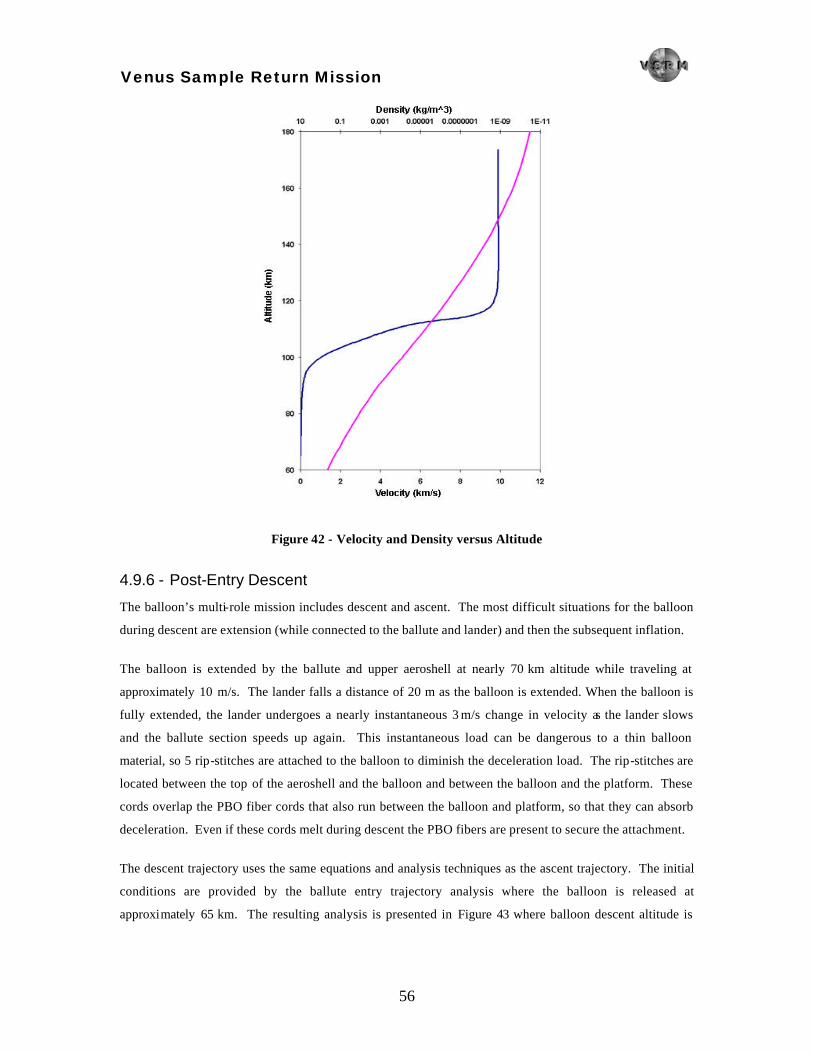
Venus Sample Return Mission
56
Figure 42 - Velocity and Density versus Altitude
4.9.6 - Post-Entry Descent
The balloon’s multi-role mission includes descent and ascent. The most difficult situations for the balloon
during descent are extension (while connected to the ballute and lander) and then the subsequent inflation.
The balloon is extended by the ballute and upper aeroshell at nearly 70 km altitude while traveling at
approximately 10 m/s. The lander falls a distance of 20 m as the balloon is extended. When the balloon is
fully extended, the lander undergoes a nearly instantaneous 3 m/s change in velocity as the lander slows
and the ballute section speeds up again. This instantaneous load can be dangerous to a thin balloon
material, so 5 rip-stitches are attached to the balloon to diminish the deceleration load. The rip-stitches are
located between the top of the aeroshell and the balloon and between the balloon and the platform. These
cords overlap the PBO fiber cords that also run between the balloon and platform, so that they can absorb
deceleration. Even if these cords melt during descent the PBO fibers are present to secure the attachment.
The descent trajectory uses the same equations and analysis techniques as the ascent trajectory. The initial
conditions are provided by the ballute entry trajectory analysis where the balloon is released at
approximately 65 km. The resulting analysis is presented in Figure 43 where balloon descent altitude is

Venus Sample Return Mission
57
plotted against time. Most importantly, the lander touches down after nearly 3 hours of descent from the
upper atmosphere and the touchdown speed is only 4 m/s, as shown in Figure 44.
Figure 43 - Descent Altitude versus Time
Figure 44 - Descent Velocity versus Time

Venus Sample Return Mission
58
4.10 - Venus Ascent
4.10.1 - Venus Ascent Vehicle (Balloon)
The balloon is designed to serve two basic purposes: to slow the lander during descent and to raise the
rocket for eventual launch at an altitude of 60 km. The limits of technology are pushed even farther in
designing a balloon to survive at such extremes as 150 mph winds, 460°C temperatures, 9 MPa pressures,
high impact velocities incurred while being dropped into the deployed position, and thick sulfuric acid
clouds. Balloon materials must exhibit:
• Low gas permeability • Acceptable pinhole seaming • Acceptable fabrication and folding • Toughness in tear resistance • Toughness in impact resistance • High specific strength • Resistance to sulfuric acid • Maintenance of mechanical properties at high temperatures
The Venus Sample Return Mission requires the lander to descend through the atmosphere to the surface,
acquire the sample, and then return to a higher altitude for rocket ignition. A balloon is advantageous to the
Venus Sample Return Mission because it has uses in both the descent phase and the ascent phase.
4.10.1.a - Material Selection
Finding a balloon material to satisfy all of the mission requirements is nearly impossible. A list of possible
balloon materials is listed in Table 17, and comparing the data it becomes relatively obvious that there
really is no comparison. PBO, Polybenzoxazole, is
Table 17 - Balloon Material Comparison (Ref. 35)
Specific Strength (in)
Material Film Fiber Maximum Working Temperature (°C)
PBO 68.8 495 – 516 500 Teflon 1.5 – 4.0 16 – 30 260 HDPE 4.5 – 5.9 519 80 – 120 Kapton 9.6 – 20.6 250 – 320
Upilex R 34.3 270 Upilex S 64.8 290 Kevlar 392 – 458 180
Spectra 1000 602 147 Vectran HS 345 – 432 110
Nomex 93 310
a conjugated aromatic heterocyclic liquid crystalline polymer that can withstand the rigors of this
environment unlike no other known organic material. PBO’s rigid-rod molecular structure as shown in
Figure 45 creates a microscopic self-reinforcing structure that gives PBO the strength and stiffness of a
composite without the fiber and matrix interface problems. PBO has no melting temperature, no glass
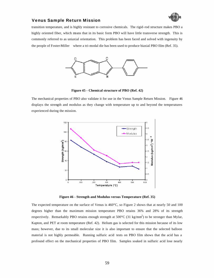
Venus Sample Return Mission
59
transition temperature, and is highly resistant to corrosive chemicals. The rigid-rod structure makes PBO a
highly oriented fiber, which means that in its basic form PBO will have little transverse strength. This is
commonly referred to as uniaxial orientation. This problem has been faced and solved with ingenuity by
the people of Foster-Miller where a tri-modal die has been used to produce biaxial PBO film (Ref. 35).
Figure 45 - Chemical structure of PBO (Ref. 42)
The mechanical properties of PBO also validate it for use in the Venus Sample Return Mission. Figure 46
displays the strength and modulus as they change with temperature up to and beyond the temperatures
experienced during the mission.
Figure 46 - Strength and Modulus versus Temperature (Ref. 35)
The expected temperature on the surface of Venus is 460°C, so Figure 2 shows that at nearly 50 and 100
degrees higher than the maximum mission temperature PBO retains 36% and 28% of its strength
respectively. Remarkably PBO retains enough strength at 500°C (31 kg/mm2) to be stronger than Mylar,
Kapton, and PET at room temperature (Ref. 42). Helium gas is selected for this mission because of its low
mass; however, due to its small molecular size it is also important to ensure that the selected balloon
material is not highly permeable. Running sulfuric acid tests on PBO film shows that the acid has a
profound effect on the mechanical properties of PBO film. Samples soaked in sulfuric acid lose nearly

Venus Sample Return Mission
60
75% of their strength and become plasticized. Based on these results a protective layer needs to be applied
(Ref. 31).
Possibilities for corrosive protection of the balloon include a fluoropolymer film and a noble metal coating.
Fluoropolymer films serve as a multilayer composite with the PBO. Fluoropolymers have satisfactory
corrosive resistance, but they have poor heat resistance. The poor thermal-mechanical properties may be
excusable since the fluoropolymer would not be the load carrying film, but the other disadvantage is the
relatively high density of the Fluoropolymers as shown in Table 18. Metal coatings can prove difficult to
sufficiently adhere to balloon materials but they also provide satisfactory corrosive protection for much less
mass. Based on the information provided in Ref. 31 from NASA, balloon manufacturers, and coating
experts, the best decision is to use a physical vapor disposition process to bond a protective layer of gold
onto the surface of PBO. For best adherence of the gold layer a tie coat metal layer would also need to be
deposited to the surface. Based on information from Ref. 31 the sufficient layering would be a tie coat
layer of Titanium from 50 to 100 Å thick and a gold layer from 1000 to 1200 Å thick. The best adhesive
results are obtained by a proprietary “heat and glow” treatment of the bonding surface. The resulting mass,
provided in Table 18, shows that the mass savings for metal coating are drastic, making the use of metal
coatings an easy decision despite their tendency to crack upon folding.
Table 18 - Possible Corrosive Protection Materials
Material Density (g/cm3) Coating Mass (g/m2)
PFA film (12.5 µm) 2.13 – 2.16 26.6 – 27.0
PTFE film (12.5 µm) 2.13 – 2.20 26.6 – 27.5
FEP film (12.5 µm) 2.14 – 2.17 26.8 – 27.1
Gold layer (1200Å) 19.3 2.316
Titanium tie coat (100Å) 4.5 0.034
Total metal coatings 2.350
The balloon seaming is another important issue to be solved, since typical stitches, tapes, and adhesives
cannot be used to attach one PBO sheet to another. The configuration of the balloon seam is presented in
Figure 47.
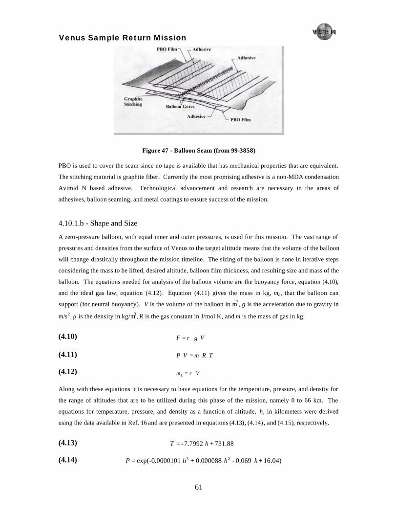
Venus Sample Return Mission
61
Figure 47 - Balloon Seam (from 99-3858)
PBO is used to cover the seam since no tape is available that has mechanical properties that are equivalent.
The stitching material is graphite fiber. Currently the most promising adhesive is a non-MDA condensation
Avimid N based adhesive. Technological advancement and research are necessary in the areas of
adhesives, balloon seaming, and metal coatings to ensure success of the mission.
4.10.1.b - Shape and Size
A zero -pressure balloon, with equal inner and outer pressures, is used for this mission. The vast range of
pressures and densities from the surface of Venus to the target altitude means that the volume of the balloon
will change drastically throughout the mission timeline. The sizing of the balloon is done in iterative steps
considering the mass to be lifted, desired altitude, balloon film thickness, and resulting size and mass of the
balloon. The equations needed for analysis of the balloon volume are the buoyancy force, equation (4.10),
and the ideal gas law, equation (4.12). Equation (4.11) gives the mass in kg, mL, that the balloon can
support (for neutral buoyancy). V is the volume of the balloon in m3, g is the acceleration due to gravity in
m/s2, ρ is the density in kg/m3, R is the gas constant in J/mol⋅K, and m is the mass of gas in kg.
(4.10) VgF ⋅⋅= ρ
(4.11) TRmVP ⋅⋅=⋅
(4.12) VmL ⋅= ρ
Along with these equations it is necessary to have equations for the temperature, pressure, and density for
the range of altitudes that are to be utilized during this phase of the mission, namely 0 to 66 km. The
equations for temperature, pressure, and density as a function of altitude, h, in kilometers were derived
using the data available in Ref. 16 and are presented in equations (4.13), (4.14), and (4.15), respectively.
(4.13) 731.88 + 7.7992- hT ⋅=
(4.14) 16.04) + 0.069 - 0.000088 + -0.0000101exp( 23 hhhP ⋅⋅⋅=
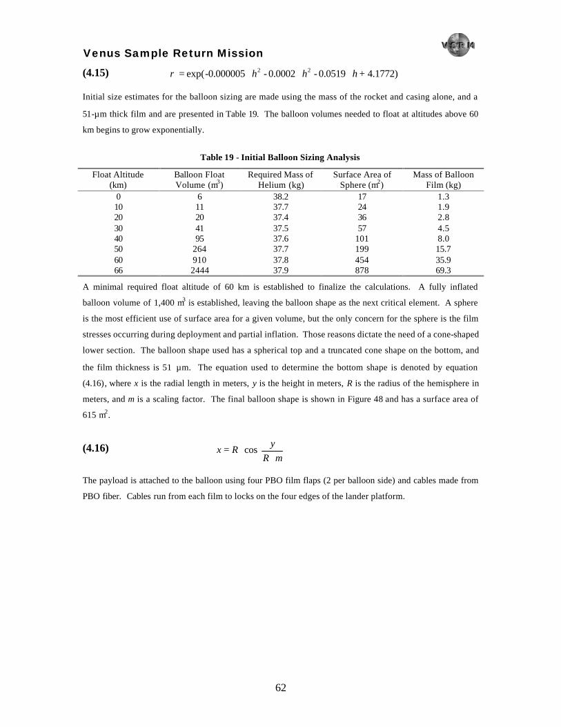
Venus Sample Return Mission
62
(4.15) 4.1772) + 0.0519 - 0.0002 - -0.000005exp( 22 hhh ⋅⋅⋅=ρ
Initial size estimates for the balloon sizing are made using the mass of the rocket and casing alone, and a
51-µm thick film and are presented in Table 19. The balloon volumes needed to float at altitudes above 60
km begins to grow exponentially.
Table 19 - Initial Balloon Sizing Analysis
Float Altitude (km)
Balloon Float Volume (m3)
Required Mass of Helium (kg)
Surface Area of Sphere (m2)
Mass of Balloon Film (kg)
0 6 38.2 17 1.3 10 11 37.7 24 1.9 20 20 37.4 36 2.8 30 41 37.5 57 4.5 40 95 37.6 101 8.0 50 264 37.7 199 15.7 60 910 37.8 454 35.9 66 2444 37.9 878 69.3
A minimal required float altitude of 60 km is established to finalize the calculations. A fully inflated
balloon volume of 1,400 m3 is established, leaving the balloon shape as the next critical element. A sphere
is the most efficient use of surface area for a given volume, but the only concern for the sphere is the film
stresses occurring during deployment and partial inflation. Those reasons dictate the need of a cone-shaped
lower section. The balloon shape used has a spherical top and a truncated cone shape on the bottom, and
the film thickness is 51 µm. The equation used to determine the bottom shape is denoted by equation
(4.16), where x is the radial length in meters, y is the height in meters, R is the radius of the hemisphere in
meters, and m is a scaling factor. The final balloon shape is shown in Figure 48 and has a surface area of
615 m2.
(4.16)
⋅⋅=
mRy
Rx cos
The payload is attached to the balloon using four PBO film flaps (2 per balloon side) and cables made from
PBO fiber. Cables run from each film to locks on the four edges of the lander platform.

Venus Sample Return Mission
63
Figure 48 - Balloon With Both Payload Attachments
These same cords also continue in towards the rocket casing where they are connected a second time so
that they serve in both phases. After the sample has been collected the locks at the edges of the platform
disengage and the cords become taught to the rocket casing. Upon completion of the landing phase the
rocket casing is released from the platform and the balloon rises to complete the second part of its mission.
4.10.1.c - Balloon Ascent
The final key to assuring proper balloon design is proving satisfactory ascent of the rocket. The ascent
analysis is performed using a numerical integrator to solve second order differential equations for the
position of the balloon. The acceleration on the balloon due to gravity, drag, and buoyancy is represented
in equation (4.17). The coefficient of drag for the balloon is taken to be 0.9.
(4.17) xxm
Vm
SxCx
xx d v
r&vv
&& ⋅⋅⋅+⋅⋅⋅⋅
+⋅=2
221
2
µρρµ
These equations are utilized along with the pressure, temperature, and density equations to model the
balloon altitude, velocity, volume, and times during ascent. The first important factor to consider in balloon
design is the time to ascend. At 54 km the temperature is 39 °C, a temperature that does not endanger the
rocket. The time that it takes for the balloon to achieve that altitude is directly related to

Venus Sample Return Mission
64
Figure 49 - Lifting Gas Analysis
the amount of Helium gas that used in the balloon. Time for ascent decreases as the amount of Helium
increases, and conversely as the amount of Helium increases the maximum attainable altitude decreases.
This relationship is presented in Figure 49. The amount of Helium chosen is based on the storage tank
limitations (approximately 63 kg, maximum height 59.3 km). 13 kg of Helium is vented from the balloon
once the float altitude is reached to achieve a maximum altitude of 61 km. The final specifications are
shown in Table 20; the rip-stitches are discussed in the Venus descent phase.
Table 20 - Final Balloon Specifications
Material / Part Mass (kg) Balloon film, PBO film, (51 µm thick)
48.00
Seams, Adhesives, and Stitches 5.00
Titanium tie coat (100Å) 0.02
Gold layer (1200Å) 1.40
Attachment Films (PBO film)
4.00
Attachment cord (PBO fiber, d=3.43mm) 0.20
Helium gas 63.00
5 Rip-stitches 5.00
Total 126.62

Venus Sample Return Mission
65
Using these values, the altitude is plotted against time for the ascent trajectory in Figure 50. It is important
to note that this data ignores the affects of high altitude winds. This analysis shows that the balloon ascent
takes just over 4.5 hours to reach maximum altitude and only 4.1 hours to reach 54 km.
Figure 50 - Ascent Altitude versus Time
4.10.2 - Venus Ascent Vehicle (Rocket)
The Venus ascent vehicle is a two-stage rocket using solid propellant. The performance characteristics of
the propellant used to model the rocket are shown in Table 21. These characteristics are for a typical solid
propellant and were used for the preliminary design of the Venus ascent vehicle. In future studies, the use
of aluminized gelled propellants will be considered because they show an increase in performance for
rockets and have more complete, uniform propellant burns.
Table 21 - Propellant Performance Characteristics (Ref. 17 p. 353)
Chamber pressure (Pa) 5170000 Burning Time (s) 90 Isp (s) 290 Density (kg/m3) 1800 Characteristic Velocity (m/s) 1527

Venus Sample Return Mission
66
The motor case design for the two stages is constructed of a graphite composite with an epoxy resin matrix
for structural stability. The properties of the graphite are listed in Table 22. Other materials were
investigated during the design of the rocket, including Titanium, 2219 Aluminum, D6aC Steel, and 4130
Steel. The analysis performed on the Venusian rocket includes a 400 kg constraint on the total mass of the
system including payload since the rocket plus heat shielding needs to be lifted to a high altitude using a
balloon. Titanium is the only other material that had a positive payload of about 4 kg; the steel and
aluminum motor casings take up the entire dry mass payload. Graphite composite allows a payload size of
around 11.5 kg and so was decided upon as the material to use for the rocket even though graphite is the
most expensive material of the three.
Table 22 - Material Properties of Graphite (Ref. 17 p. 310)
Density (kg/m3) 1550 Tensile Strength (GPa) 1.0 Elasticity (GPa) 105
The modeling of the first and second stages is accomplished using the graphite and propellant properties
from Table 21 and Table 22. First, a single stage rocket is modeled to get an approximate size of the rocket.
The mass of the propellant in kg, mp, is calculated using equation (4.18).
(4.18)
−⋅= ⋅
∆
10gIspV
fp emm
Equation (4.18) contains a simple ∆V needed to achieve the desired orbit, plus a gravity and drag
correction. A 750 m/s (Ref. 19 p. 722) drag correction was used along with a gravity correction of 3%
(Ref. 19 p. 722) of the total ∆V. The final mass, mf, was specified at 20 kg to include unloaded rocket mass
and payload mass. This number kept the total mass of the rocket under the 400 kg constraint. Numbers are
run with these conditions for various materials as described above, and estimated propellant masses are
calculated. Simple geometry equations are used to calculated the motor case size and estimate the unloaded
rocket mass. The thickness of the motor casing is estimated using a burst pressure and a factor of safety of
1.25. Once the initial rocket design is completed, a more detailed launch profile is done to determine the
number of stages and the size of each stage necessary to achieve the desired orbit. The detailed launch
profile is explained later in this section. Two burns are needed to achieve the desired orbit. The initial
estimations of gravity and drag prove to be good since there is just the right amount of propellant to get into
the desired orbit. The time for each burn determines how the propellant is divided between the two stages.
These propellant masses are used for the rocket analysis to design the motor case and size for each stage.
Table 23 shows the details of the first stage of the Venus Ascent Vehicle. To maximize the thrust, the
nozzle is designed to expand to the average pressure that the first stage experiences. The throat area of the
nozzle is determined using equation (4.19) (Ref. 17 p. 310). Exit areas of the nozzles are calculated using
equation (4.20) (Ref. 38 p. 55).

Venus Sample Return Mission
67
Table 23 - Venus Ascent Vehicle Stage One Configuration
Mass (kg) Motor Case (m) Rocket Nozzle Length Radius Thickness
1.3 0.18
0.0016
Throat Area (m2) Exit Area (m2) Throat Diameter (m)
9.5×10⁻⁴
0.0066
0.035
Propellant Motor Case Nozzle Igniter
242 6
2.0×10⁻⁴
5.0×10⁻⁴ Total 248
(4.19) Cb
pVt Pt
mCA
⋅⋅=
(4.20)
γγ
γγ
γγγ
11
11
111
21
−
−
−⋅
−+⋅
⋅
+
=
c
e
C
e
te
PP
PP
AA
Table 24 shows the details of the second stage of the Venus Ascent Vehicle. The nozzle for the second
stage is modeled to bring the exit pressure close to zero since the second stage fires outside the Venusian
atmosphere. Figure 51 is an AutoCAD rendering of the Venus Ascent Vehicle. The overall length of the
entire rocket is 2.15 m from the bottom of the first stage nozzle to the top of the blunt nose cone. Figure 52
shows the heights of the motor casing and nozzles with the sample capsule in the payload area. This rocket
design allows for an 11.5 kg sample capsule payload. The use of a better propellant increases the payload
mass; this is an area needing further study for optimization. The rocket’s total mass is about 310 kg
including the mass of the loaded sample capsule.
Table 24 - Venus Ascent Vehicle Stage Two Configuration
Mass (kg) Motor Case (m) Rocket Nozzle Length Radius Thickness
0.26 0.18
0.0016
Throat Area (m2) Exit Area (m2) Throat Diameter (m)
9.5×10⁻⁴
0.0115
0.035
Propellant Motor Case Nozzle Igniter
49 2.5
8.0×10⁻⁵
1.9×10⁻⁴ Total 51
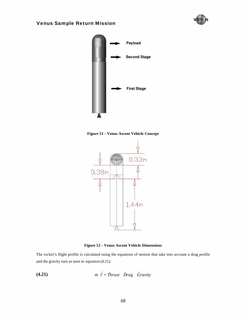
Venus Sample Return Mission
68
Figure 51 - Venus Ascent Vehicle Concept
Figure 52 - Venus Ascent Vehicle Dimensions
The rocket’s flight profile is calculated using the equations of motion that take into account a drag profile
and the gravity turn as seen in equation (4.21).
(4.21) ravityGragDhrustTrmrrr&&r ++=⋅

Venus Sample Return Mission
69
Thrust was modeled using equation (4.22). Drag was modeled using equation (4.23) and the gravity was
modeled using equation (4.24). The symbols used are defined as follows: γ is the flight path angle, Ve is the
exit velocity in m/s, ρ is the density in kg/m3, A is the cross sectional area in m2, V is the current velocity in
m/s, CD is the drag coefficient, µ is the gravitational constant in km3/s2, r is the current radius from Venus in
km, and er and eθ are the coordinate system of the rocket.
(4.22) ( ) ( )( )θγγ eemVhrustT re ˆcosˆsin ⋅+⋅⋅⋅= &r
(4.23) ( ) ( )( )θγγρ eeACVragD rD ˆcosˆsin221 ⋅+⋅⋅⋅⋅⋅⋅=
r
(4.24) r
rocket erm
ravityG ˆ2
⋅⋅
=µr
These equations are turned into four first order ordinary differential equations and solved using MatLab.
Initial conditions are modified until the desired orbit is attained. The following data are the results from an
800 km circular orbit optimization. The first stage provides 75 seconds of constant thrust getting the rocket
to 147 km off the surface of Venus. Next, the first stage motor case and nozzle are ejected leaving the
payload and second stage. The rocket remains in an elliptical orbit for 534 seconds. After 534 seconds the
rocket becomes tangent to the desired 800 km orbit. The second stage then fires for 15 seconds bringing
the speed of the rocket to match that of the 800 km desired orbit. The second stage motor case and nozzle
are then ejected from the payload sample capsule. The payload sample capsule remains in orbit until the
orbiter rendezvous and collects the capsule. Figure 53 shows the over all launch profile from the surface of
Venus to the 800 km orbit. Figure 54 is a close up of the surface to orbit launch profile. The profile of the
rocket’s altitude with respect to time can be seen in Figure 55.
The orbiter is unable to achieve an 800 km circular orbit within three years. In the next design loop the
rocket needs to be resized for an elliptical orbit with a perigee of 800 km with a velocity of 9.53 km/s and
an apogee of 273,000 km. Initial calculations determine that the rocket only needs 2.9 seconds of extra
thrust during the second stage to achieve this orbit.
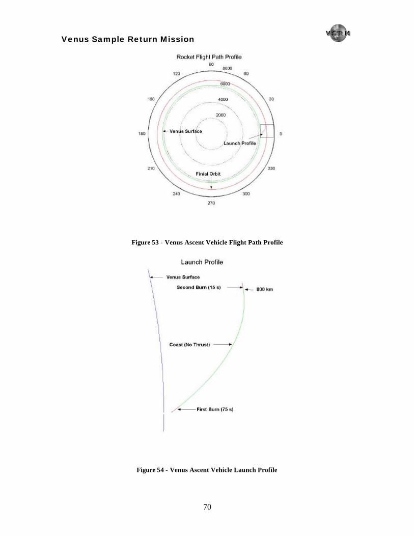
Venus Sample Return Mission
70
Figure 53 - Venus Ascent Vehicle Flight Path Profile
Figure 54 - Venus Ascent Vehicle Launch Profile

Venus Sample Return Mission
71
Figure 55 - Venus Ascent Vehicle Altitude versus Time

Venus Sample Return Mission
72
4.11 - System Mass
The mass breakdown for the Venus Lander is shown in Table 25.
Table 25 - Venus Lander Mass
Equipment List Mass (kg)ADCS (Thrusters) 45 ADCS (Sensors) 5 Aeroshell 406 Balloon 126
Ballute 53 Batteries (Orbit) 5 Batteries (ground) 15 Computer / Elec. 1 Drill 32 He 44 He Tank 112 Liquid Propulsion 174 Misc Data Collection 10 Parachute 5 Robotic Arm 0.2 Rocket 310 Structure (plat,legs) 168 Shielding (sample) 35 Shielding (rocket) 100 Shielding (batt) 54
Total 1700
4.12 - Summary
The Venus Lander accomplishes the critical tasks of reaching the Venusian surface, acquiring a sample, and
then returning the sample to orbit for rendezvous with the orbiter. Instruments used on the lander are
designed to withstand the harsh environment of Venus and an innovative ballute/balloon system allows the
lander to safely descend to the surface and with the Venus ascent vehicle, takes the sample back to orbit.
After rendezvous, the orbiter and ERV transport the sample back to Earth. The ERV is described in the
following chapter.

Venus Sample Return Mission
73
Chapter 5 - Earth Entry Vehicle This chapter details the aspects of the Earth Entry Vehicle, or EEV. The EEV is used to return the Venus
surface sample to Earth. It consists of the sample collector/containment device and the Earth Insertion
Package, or EIP. The EEV has its own attitude determination and control system, propulsion system, power
system, thermal shielding, and computer system since it must function separately from the orbiter. The
following sections describe these systems in detail.
5.1 - Configuration
The EEV is a 60-degree blunt body capsule, which is modeled after NASA and JPL’s Stardust Sample
Return Capsule (Ref. 23). The EEV is composed of aluminum with a maximum cross sectional diameter of
1.5 m and a height of 0.9 m. Two drogue parachutes and three reinforced ring-slot descent parachutes are
contained inside the EEV (Ref. 24). Barometric switches are used to deploy the parachutes at the
appropriate altitude (Ref. 28). Also contained inside the EEV are the onboard computer, batteries, and a
radio locator beacon. The radio locator beacon is activated upon parachute deployment. The radio locator
uses approximately 5 W of power and has a range of 3 km.
The Venus Sample Capsule remains in the captured position throughout the entry and landing procedure.
No floatation system is used for the EEV. The EEV displaces 955 kg of seawater when fully submerged,
and the mass of the EEV is 242 kg, therefore the EEV is buoyant in water.
5.1.1 - Sample Collector
The orbiter collects the VSC after the VAV launches it into orbit. A rendezvous cone, modeled after the
European Space Agency (ESA) rendezvous cone, is extended when the Venus Lander detaches from the
orbiter (Ref. 8). The rendezvous cone is designed so that once the VSC enters the cone it cannot bounce
out. The narrow end of the capture cone leads to a narrowing cylinder that runs through the Earth Entry
Vehicle. The VSC travels through the EEV cylinder to the narrow end where it docks with the EEV. Figure
56 shows the extended capture cone awaiting capture of the VSC.
The VSC travels through the EEV cylinder and comes to rest in the Capsule Containment Compartment.
Three capture claws latch around the VSC to hold it in place until it can be retrieved after Earth entry
(Ref. 8). After the sample capture maneuver is complete, the rendezvous cone is jettisoned to reduce the
spacecraft mass for the return trip to Earth.

Venus Sample Return Mission
74
Figure 56 - Orbiter and EEV with Extended Capture Cone
5.2 - Thermal
The heat shielding for the EEV consists of two layers of Composite Flexible Blanket Insulation (CFBI).
CFBI is designed to have high emissivity, resistance to a high heat flux, and insulation capability between
1,450 and 1,650 degrees C. Two types of insulation, CFBI-1 and CFBI-2, have been tested at pressures of
1.0, 0.1 and 0.01 atm and temperatures of 23, 200, and 400 ºC (Ref. 41). The apparent thermal conductivity
of CFBI-1 and CFBI-2 is shown in Table 26.
Table 26 - Apparent Thermal Conductivity (Ref. 41)
CFBI-1 CFBI-2 Temperature (°C) at 1.0 ATM
Thermal Conductivity (W/m⋅K)
23 0.036 0.035 200 0.051 0.049 400 0.059 0.084
CFBI-1 is made of silicon carbide and alumina covered with aluminized Kapton on one side, whereas
CFBI-2 is covered with aluminized Kapton on both sides. Both CFBI-1 and CFBI-2 are 0.026 m thick and
have average densities of 133 kg/m3 and 149 kg/m3 respectively (Ref. 41). CFBI-1 is chosen over CFBI-2
for use on the EEV because of its lower average density and lower thermal conductivity at higher
temperatures.
5.3 - Attitude Determination and Control Systems
The EEV requires a separate ADCS from the orbiter, since it operates independently during Earth re-entry
and landing. The EEV is equipped with hydrazine-fluoride thrusters for three-axis attitude control. There
are two thrusters directed along each axis, for a total of six thrusters. The tanks required for the fuel have a

Venus Sample Return Mission
75
radius of 0.06 m, thickness of 0.00026 m, and mass of 0.03 kg. The fuel mass is 0.86 kg. The oxidizer
tanks are the same size, and the oxidizer mass is 1.3 kg. The thrusters are fired when needed to maintain
the proper orientation in orbit and for re-entry. Each thruster provides a ∆V of 25 m/s.
The EEV has two types of attitude determination sensors: sun sensors and horizon sensors. The sun sensor
used is identical to those on the spacecraft orbiter. The horizon sensor is the Horizon Crossing Indicator
(HCI) provided by Ithaco Inc. The HCI provides 0.1º accuracy with a 1.0° × 1.0° FOV, with a mass of
0.65 kg. It requires less than 0.7 W of power with a peak current of 3 A.
5.4 - Power
The EEV has two separate power systems, one for the return vehicle, and one for the attached EIP. Lithium
Ion batteries from Saft are utilized, with the battery packages resized to fit the requirements of the EEV
lander and EIP. The two power systems are separate since the EIP is discarded once atmospheric reentry is
underway, and the EEV still requires power for the beacon and parachute deployment mechanism. The
power capacity required for the EEV primary battery is approximately 25 W·hr, assuming a 15 minutes for
atmospheric entry and additional operational time the EEV to be detected and found. One lithium ion
primary battery is sufficient for this final phase of the mission, since one Saft lithium ion battery supplies
132 W·hr (Table 12).
5.5 - Computer
The earth lander computer will control the thruster package separation, the parachute deployment schemes,
and control the radio locator beacon that is located on the lander.
The Dual Single Board Computer (DSBC) was selected for this mission. This computer system can
perform 1.15 MIPS at 6 MHz and only requires 5.5 W of power at its maximum peak and 4 W of power
during normal operation. This computer system is radiation hardened, costs nearly $50,000, and can be
seen in Figure 57 (Ref. 14).
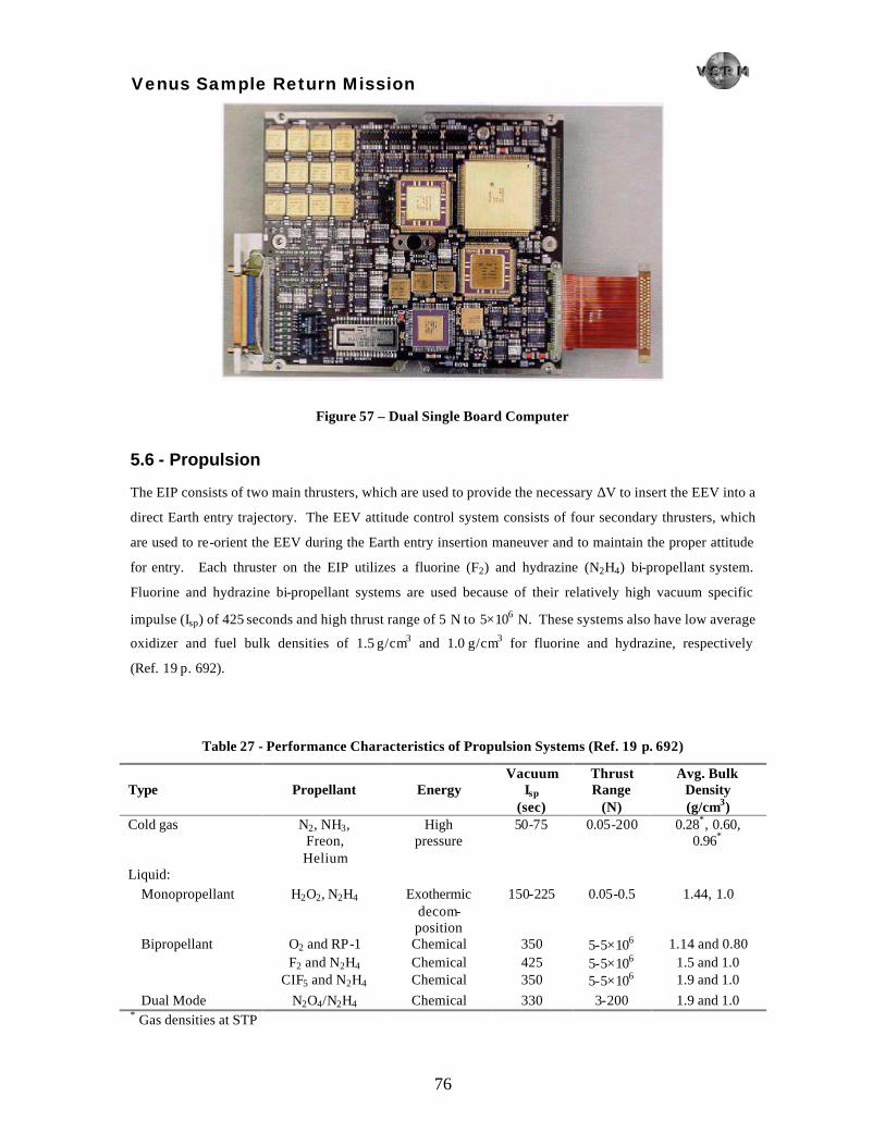
Venus Sample Return Mission
76
Figure 57 – Dual Single Board Computer
5.6 - Propulsion
The EIP consists of two main thrusters, which are used to provide the necessary ∆V to insert the EEV into a
direct Earth entry trajectory. The EEV attitude control system consists of four secondary thrusters, which
are used to re-orient the EEV during the Earth entry insertion maneuver and to maintain the proper attitude
for entry. Each thruster on the EIP utilizes a fluorine (F2) and hydrazine (N2H4) bi-propellant system.
Fluorine and hydrazine bi-propellant systems are used because of their relatively high vacuum specific
impulse (Isp) of 425 seconds and high thrust range of 5 N to 5×10⁶ N. These systems also have low average
oxidizer and fuel bulk densities of 1.5 g/cm3 and 1.0 g/cm3 for fluorine and hydrazine, respectively
(Ref. 19 p. 692).
Table 27 - Performance Characteristics of Propulsion Systems (Ref. 19 p. 692)
Type Propellant Energy Vacuum
Isp (sec)
Thrust Range
(N)
Avg. Bulk Density (g/cm3)
Cold gas N2, NH3, Freon, Helium
High pressure
50-75 0.05-200 0.28*, 0.60, 0.96*
Liquid: Monopropellant
H2O2, N2H4 Exothermic decom- position
150-225 0.05-0.5 1.44, 1.0
Bipropellant O2 and RP-1 Chemical 350 5-5×10⁶ 1.14 and 0.80 F2 and N2H4 Chemical 425 5-5×10⁶ 1.5 and 1.0 CIF5 and N2H4 Chemical 350 5-5×10⁶ 1.9 and 1.0 Dual Mode N2O4/N2H4 Chemical 330 3-200 1.9 and 1.0
* Gas densities at STP

Venus Sample Return Mission
77
5.7 - Earth Entry and Descent
The orbiter releases the EEV at the edge of Earth’s sphere of influence. The EEV faces the orbital velocity
direction, and the heat shield faces in the negative orbital velocity direction when the EEV detaches from
the orbiter. Figure 58 depicts the separation of the EEV from the orbiter.
Figure 58 - Orbiter and Earth Entry Vehicle Separation
The EIP thrusters fire to provide the necessary ∆V to insert the EEV into a direct Earth entry trajectory.
Next, the EIP thrusters fire to rotate the EEV 180º about its non-symmetry axis so that the heat shield is
facing in the orbital velocity direction to prepare for atmospheric entry. The EIP is separated prior to entry.
The EEV enters the Earth’s atmosphere at approximately 11 km/s with an entry angle of approximately 10°,
and then free falls through the atmosphere. Two drogue parachutes, shown in Figure 59, are released to
slow down the EEV from approximately 140 m/s to 80 m/s at approximately 7 km altitude. Three main
descent parachutes are deployed and an omni-directional radio locator beacon is activated at approximately
3 km altitude. The main parachutes decelerate the EEV to a final landing velocity of approximately 9 m/s
(Ref. 28). The VSC is recovered and the sample is taken to the appropriate facility for analysis.

Venus Sample Return Mission
78
Figure 59 - Earth Entry Vehicle with Descent Parachutes
5.8 - Sample Analysis
Electron-microprobe, X-Ray Diffraction (XRD), Transmission Electron Microscope (TEM) and Scanning
Electron Microscopes (SEM) are techniques commonly used to obtain the mineral composition. All of
these techniques can be done at a university such as Virginia Tech. X-Ray Fluorescence (XRF) analysis is
used to determine the bulk composition of the Venus sample. Virginia Tech does not have the equipment to
perform this bulk analysis, so it must be done at a national laboratory.
The cost of all analysis done on the Venus sample depends on scientist salaries, equipment cost, sample
preparation time, and sample analysis time. Sample preparation time may take several hours, but sample
analysis time varies widely. Dr. Benedix of the Virginia Tech Geology Depart ment estimates that the entire
sample analysis will cost approximately $50,000 (Ref. 5).

Venus Sample Return Mission
79
5.9 - System Mass
The mass breakdown for the Earth Entry Vehicle is shown in Table 28.
Table 28 - Earth Entry Vehicle Mass
Equipment List Mass (kg)ADCS (Thrusters) 19 ADCS (Sensors) 5 Batteries 5 Heat Shield 10 Parachute 5 Sample / Payload 12 Structure 210 Total 266
5.10 - Summary
The EEV is designed to transport the VSC safely through the Earth’s atmosphere. Fluorine and hydrazine
bipropellant propulsion systems are used to control and de-orbit the EEV. Thermal shielding is required to
protect the EEV from the extreme temperatures it will encounter during entry, and a parachute descent
system is required to land the EEV safely in the Pacific Ocean. The EEV is designed to accomplish all
aspects of the Earth Entry phase autonomously. The following chapter will discuss the cost analysis of this
entire mission.

Venus Sample Return Mission
80
Chapter 6 - Cost Analysis
6.1 - Components and Fabrication
Determining the cost of a mission of this scope is inherently difficult. Many manufacturers are hesitant to
give out actual cost numbers for materials and fabrication for design projects such as this. The prices and
fabrication costs for some components are presented in Table 29 and Table 30. Many of the structural
components and off the shelf electronics are presented here. Fabrication and material costs for
experimental components such as the Venus Ascent Vehicle, insertion ballute, ascent balloon, and the
aluminum coating for the sail blades are not known. The total known cost for the mission of approximately
$150M is well below the $650M budget. This cost estimate does not include any ground support costs or
developmental costs for the experimental components.
Table 29 - Component Costs
Component Company
Purchasing From Cost per unit # of units Total
Computers Honeywell Co. Orbiter Lander VSC
Memory EEV
$400,000.00 $100,000.00 $100,000.00 $200,000.00 $50,000.00
2 2 1 1 1
$800,000.00 $200,000.00 $100,000.00 $200,000.00 $50,000.00
Ultrasonic Drill Cybersonics Inc. $8,000.00 1 $8,000.00 Mechanical Arm Virginia Tech $100,000.00 1 $100,000.00 Sample Container $10,000.00 1 $10,000.00 Sun Sensors and Star Trackers
Ball Aerospace $50,000.00 6 $300,000.00
Horizon sensor Ithaco, Inc. $50,000.00 1 $50,000.00 Delta IV Boeing Co. $145,000,000.00 1 $145,000,000.00 Heliogyro blade Kapton layer
DuPont $26,500.00 12 $318,000.00

Venus Sample Return Mission
81
Table 30 - Fabrication Costs
Component Cost per unit # of units Total Venus Lander platform $1,200.00 1 $1,200.00 Lander legs $1,000.00 4 $4,000.00 Heliogyro rings $4,000.00 2 $8,000.00 Orbiter bus $4,800.00 1 $4,800.00 Aeroshell $32,000.00 1 $32,000.00
The cost of all analysis done on the Venus sample depends on scientist salaries, equipment cost, sample
preparation time, and sample analysis time. Sample preparation time may take several hours, but sample
analysis time varies widely. Dr. Benedix of the Virginia Tech Geology Department estimates that the entire
sample analysis will cost approximately $50,000 (Ref. 5).
6.2 - Summary
The heliogyro blade coatings, ballute, balloon, and Venus Ascent Vehicle are vital components. Along with
the cost of ground support, these items account for most of the budget. The known mission cost of $150M
makes it possible to include these mentioned items and remain below the $650M cap. This is the best
available estimate at this time.

Venus Sample Return Mission
82
Chapter 7 - Summary and Conclusions
7.1 - Summary
The spacecraft is launched to the edge of the Earth’s gravitational influence by a Delta IV M+ rocket. A
small rocket provides the thrust to initialize the spacecraft spin. This initial spin deploys the Heliogyro
blades and the spacecraft begins to spiral into Venus. Upon arrival at Venus, the orbiter performs the
thrusting maneuvers needed for capture in Venus orbit. The Venus Lander is released when the desired orbit
is achieved and enters the Venusian atmosphere. Prior to entering the atmosphere, the ballute is deployed
and is subsequently used to slow the lander down through the atmosphere with no heat shielding. The
balloon is deployed to slow the remainder of the descent to the surface. On the surface, the sample is
collected and placed into the Venus Ascent Vehicle. The Venus Ascent Vehicle is released from the Lander
and a balloon carries it to an altitude of approximately 60 km where the Venus Ascent Vehicle launches into
rendezvous orbit. This rendezvous orbit is achieved through the use of a gravity turn. The orbiter then
captures the sample capsule in the Earth Entry Vehicle and returns to Earth. The Earth Entry Vehicle is
released on a direct entry trajectory at the edge of the Earth’s gravitational influence. It enters the Earth’s
atmosphere and is slowed for landing using parachutes.
7.2 - Conclusions
Early in the design process we discovered that the Venus Lander was the most important piece of the
mission. Designing the Lander for survival dictated the requirements of the rest of the system. Iterations
were performed on the Lander/Balloon/Rocket combination to determine the required mass to get the
sample into the initial rendezvous orbit. The orbiter was designed with this mass in mind. The mission
schedule was then determined. Changing the rendezvous orbit to optimize the tradeoff between capture
time and VAV mass will affect every aspect of the mission because the VAV is included in the Lander mass.
More design iterations are required for this mission to be feasible. Further research in several key areas is
also needed. These areas include autonomous rendezvous, reflective and emissive coatings for the solar sail
material, Heliogyro thrust vectoring, and cost analysis techniques.
Several technological breakthroughs are also required to make this mission possible. Construction of the
Venus Balloon is not possible with current PBO fabrication techniques. Solar sail technology such as
deployment methods that do not tear or wrinkle the material need testing and further development.
Research into the blade dynamics and response lag times along the length of each blade should be
completed. The ballute technology also needs to be tested and proven to be reliable for this mission. All
other technologies used in this mission are already well tested and proven to be reliable.

Venus Sample Return Mission
83
References
1. Anderson, John D., Hypersonic and High Temperature Gas Dynamics, New York, McGraw-Hill Book Company, 1989.
2. Baalke, Ron, The Magellan Venus Explorer's Guide. Available at http://www.jpl.nasa.gov/magellan/guide.html. Accessed October 20, 2000.
3. Bar-Cohen, Yoseph, Stewart Sherrit, Benjamin Dolgin, Dharmendra Pal, Thomas Peterson, Jason Kroh, and Ron Krahe, “Ultrasonic/sonic drilling/coring (USDC) for in-situ planetary applications.” JPL/Caltech, Pasadena, CA. Available at http://ndeaa.jpl.nasa.gov. Accessed February 2001.
4. Bate, Roger R. et al., Fundamentals of Astrodynamics, New York, Dover Publications, Inc., 1971.
5. Benedix, Gretchen K., Virginia Tech Geology Department. Personal Correspondence. November 15, 2000.
6. Blevins, Bruce A., Electromagnetic Systems Branch – Spacecraft Antennas. Available at http://www.psl.nmsu.edu/antennas/SpaceAnt.html. Accessed March 23, 2001.
7. Callister, William D., Materials Science and Engineering , New York, John Wiley & Sons, Inc., 1997.
8. Coradini, M., G. Scoon, and J.-P Lebreton, Venus Sample Return Assessment Study Report, Document SCI(98)3, European Space Agency, The Netherlands, 1998.
9. Elmhurst, Richard, Honeywell Inc. Personal correspondence. April 10, 2001.
10. FiberSource, FiberSource: The Manufactured Fiber Industry, Available at http://www.fibersource.com. Accessed on April 2, 2001.
11. Goodhall, Kirk, Communication Systems. Available at http://mars3.jpl.nasa.gov/mgs/overvu/sc/tele/tele.html. Accessed April 4, 2001.
12. Hall, Jeffrey L. et al., “Thermal and Structural Test Results for a Venus Deep-Atmosphere Instrument Enclosure,” AIAA Paper, 1999.
13. Holemans, Walter, “Lightband Interface Control Document,” Planetary Systems Coporation, Washington, DC, February 2000.
14. Honeywell Inc., “Dual Single Board Computer Product Sheet,” Honeywell Inc., 1999.
15. Honeywell Inc., “Radiation Hardened Vector Processor Product Sheet,” Honeywell Inc., 1999.
16. Hunten, D. M. et al., Venus, University of Arizona Press, Tucson, AZ, 1983.
17. Humble, Ronald W., Gary N. Henry, and Wiley J. Larson, Space Propulsion Analysis and Design, The McGraw-Hill Companies, Inc and Primis Custom Publishing, New York, 1995.
18. ILC Dover, ILC Dover Online, Space Inflatables, Aerobrakes and Ballutes, Available at http://www.ilcdover.com. Accessed on February 15, 2001.
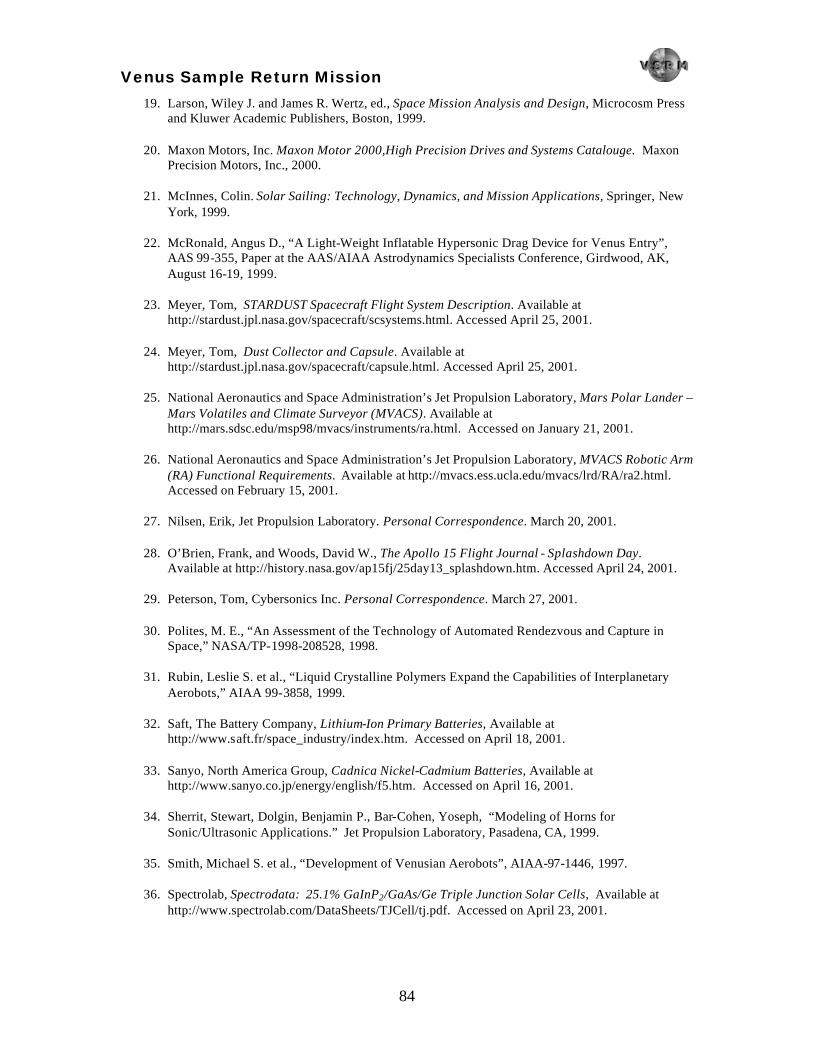
Venus Sample Return Mission
84
19. Larson, Wiley J. and James R. Wertz, ed., Space Mission Analysis and Design, Microcosm Press and Kluwer Academic Publishers, Boston, 1999.
20. Maxon Motors, Inc. Maxon Motor 2000,High Precision Drives and Systems Catalouge. Maxon Precision Motors, Inc., 2000.
21. McInnes, Colin. Solar Sailing: Technology, Dynamics, and Mission Applications, Springer, New York, 1999.
22. McRonald, Angus D., “A Light-Weight Inflatable Hypersonic Drag Device for Venus Entry”, AAS 99-355, Paper at the AAS/AIAA Astrodynamics Specialists Conference, Girdwood, AK, August 16-19, 1999.
23. Meyer, Tom, STARDUST Spacecraft Flight System Description. Available at http://stardust.jpl.nasa.gov/spacecraft/scsystems.html. Accessed April 25, 2001.
24. Meyer, Tom, Dust Collector and Capsule. Available at http://stardust.jpl.nasa.gov/spacecraft/capsule.html. Accessed April 25, 2001.
25. National Aeronautics and Space Administration’s Jet Propulsion Laboratory, Mars Polar Lander – Mars Volatiles and Climate Surveyor (MVACS). Available at http://mars.sdsc.edu/msp98/mvacs/instruments/ra.html. Accessed on January 21, 2001.
26. National Aeronautics and Space Administration’s Jet Propulsion Laboratory, MVACS Robotic Arm (RA) Functional Requirements. Available at http://mvacs.ess.ucla.edu/mvacs/lrd/RA/ra2.html. Accessed on February 15, 2001.
27. Nilsen, Erik, Jet Propulsion Laboratory. Personal Correspondence. March 20, 2001.
28. O’Brien, Frank, and Woods, David W., The Apollo 15 Flight Journal - Splashdown Day. Available at http://history.nasa.gov/ap15fj/25day13_splashdown.htm. Accessed April 24, 2001.
29. Peterson, Tom, Cybersonics Inc. Personal Correspondence. March 27, 2001.
30. Polites, M. E., “An Assessment of the Technology of Automated Rendezvous and Capture in Space,” NASA/TP-1998-208528, 1998.
31. Rubin, Leslie S. et al., “Liquid Crystalline Polymers Expand the Capabilities of Interplanetary Aerobots,” AIAA 99-3858, 1999.
32. Saft, The Battery Company, Lithium-Ion Primary Batteries, Available at http://www.saft.fr/space_industry/index.htm. Accessed on April 18, 2001.
33. Sanyo, North America Group, Cadnica Nickel-Cadmium Batteries, Available at http://www.sanyo.co.jp/energy/english/f5.htm. Accessed on April 16, 2001.
34. Sherrit, Stewart, Dolgin, Benjamin P., Bar-Cohen, Yoseph, “Modeling of Horns for Sonic/Ultrasonic Applications.” Jet Propulsion Laboratory, Pasadena, CA, 1999.
35. Smith, Michael S. et al., “Development of Venusian Aerobots”, AIAA-97-1446, 1997.
36. Spectrolab, Spectrodata: 25.1% GaInP2/GaAs/Ge Triple Junction Solar Cells, Available at http://www.spectrolab.com/DataSheets/TJCell/tj.pdf. Accessed on April 23, 2001.
Venus Sample Return Mission
85
37. Spectrolab, Spectrodata: Space Solar Panels, Available at http://www.spectrolab.com/DataSheets/Panel/panels.pdf. Accessed on April 23, 2001.
38. Sutton, George P., Rocket Propulsion Elements, Sixth Edition, John Wiley & Sons, Inc., New York, 1992.
39. Swartz, Jana, Craig Stevens, et. all. “HokieSat Interface Control Document,” Virginia Tech, Blacksburg, VA, November, 2000. Available at http://www.aoe.vt.edu/~hokiesat/.
40. Turner, Martin J. L., Rocket and Spacecraft Propulsion , Praxis Publishing, Chichester, UK, 2000.
41. United States Patent and Trademark Office, United States Patent: 5,277,959 . Available at “http://164.195.100.11/netacgi/nph-Parser?Sect1 =PTO1&Sect2 =HITOFF&d=PALL&p=1&u=/netahtml/srchnum.htm&r=1&f=G&l=50&s1='5277959'.WKU.&OS=PN/5277959&RS=PN/5277959”. Accessed April 20, 2001.
42. Yavrouian, A., et al., “High Temperature Materials for Venus Balloon Envelopes,” AIAA Paper, 1995.

Venus Sample Return Mission
86
Appendix A – Mission Timeline

Venus Sample Return Mission
87
Appendix B – Orbiter Schematic

Venus Sample Return Mission
88
Appendix C – Venus Lander Schematic
Related Documents


