Velocity profiles in strongly turbulent Taylor-Couette flow

Velocity profiles in strongly turbulent Taylor-Couette flow

Siegfried Grossmann1, Detlef Lohse2, and Chao Sun2

1 Fachbereich Physik, Renthof 6, Philipps-Universitaet Marburg, D-35032 Marburg, Germany

2 Department of Science & Technology, Mesa+ Institute,

and J. M. Burgers Centre for Fluid Dynamics,

University of Twente, 7500 AE Enschede, The Netherlands

(Dated: October 24, 2013)

We derive the velocity profiles in strongly turbulent Taylor-Couette flow for the

general case of independently rotating cylinders. The theory is based on the Navier-

Stokes equations in the appropriate (cylinder) geometry. In particular, we derive the

axial and the angular velocity profiles as functions of distance from the cylinder walls

and find that both follow a logarithmic profile, with downwards-bending curvature

corrections, which are more pronounced for the angular velocity profile as compared

to the axial velocity profile, and which strongly increase with decreasing ratio η be-

tween inner and outer cylinder radius. In contrast, the azimuthal velocity does not

follow a log-law. We then compare the angular and azimuthal velocity profiles with

the recently measured profiles in the ultimate state of (very) large Taylor numbers.

Though the qualitative trends are the same – down-bending for large wall distances

and (properly shifted and non-dimensionalized) angular velocity profile ω+(r) be-

ing closer to a log-law than (properly shifted and non-dimensionalized) azimuthal

velocity profile u+ϕ (r) – quantitative deviations are found for large wall distances.

We attribute these differences to the Taylor rolls and the height dependence of the

profiles, neither of which are considered in the theoretical approach.

PACS numbers: 47.27.-i, 47.27.te, 47.52.+j, 05.40.Jc

arX

iv:1

310.

6196

v1 [

phys

ics.

flu-

dyn]

23

Oct

201

3

2

I. INTRODUCTION

Having measured, analyzed, and discussed the global properties of the Rayleigh-Benard

(RB) (cf. [1, 2]) and of the Taylor-Couette (TC) [3–5] devices, the two paradigmatic systems

of fluid mechanics, which realize strongly turbulent laboratory flow, there is increasing inter-

est in the local properties of these flows, e. g. in their flow profiles. In the ultimate state of

RB thermal convection logarithmic profiles have been measured [6–10] and calculated from

the Navier-Stokes-equations [11].

In Taylor-Couette flow between independently rotating cylinders one can get considerably

deeper into the ultimate range than in RB flow, cf. [5], due to the better efficiency of

mechanical driving as compared to thermal one. In this ultimate TC flow regime, i. e.,

for very large Taylor numbers Ta & 5 · 108 [12], the profiles of the azimuthal velocity have

recently been measured [13] within the Twente Turbulent Taylor-Couette (T3C) facility [14].

In figure 1a we reproduce the mean azimuthal velocity profile at the inner cylinder for two

large Ta numbers. In ref. [13] it was argued that the flow profiles roughly follow the von

Karman law [15] for wall distances ρ much larger than in the viscous sublayer and much

smaller than half of the gap, whose width is d = ro − ri. Indeed, as seen from figure 1a, for

the Ta = 6.2 · 1012 case and for log10 ρ+ ≈ 2.5 – two orders of magnitude smaller than the

outer length scale which is the half width d/2 of the gap – the azimuthal velocity profile

Uϕ(r) after proper shifting seems to be possibly consistent with a log-law,

u+(ρ+) ≡ ωi · riu∗i− Uϕ(r)

u∗i≈ κ−1 ln ρ+ +B, (1)

over a small range, but for larger wall distances ρ+ the curve bends down towards smaller

values. This behavior is pronouncedly different from the standard pipe flow case [15–19], for

which the profiles first bend up before they bend down towards the center of the flow. In

equation (1) the azimuthal velocity and the distance ρ from the wall have been presented

in the usual wall units u∗i and δ∗i = ν/u∗i , marked with the usual superscript + and to be

exactly defined later. In figure 1a we also show the angular velocity profiles ω+(ρ+) in the

3

respective wall unit, resulting from the mean angular velocity Ω(r) = Uϕ(r)/r. Both the

azimuthal velocity profile u+(ρ+) as well as the angular velocity profile ω+(ρ+) are shifted

so that they are zero at the inner cylinder and then have positive slope. Also ω+(ρ+) is

normalized with wall units, i.e.,

ω+(ρ+) ≡ ωi − Ω(ρ+)

ω∗i=ωiri − ri

ri+ρuϕ

u∗i=

1

1 + ρri

u+ϕ (ρ+) +

ωiriu∗i

ρri

1 + ρri

, (2)

with ω∗i = u∗i /ri. In the regime of the log-law ω+(ρ+) is nearly indistinguishable from the

azimuthal velocity itself (see figure 1), since ρ/ri 1, but note that obviously not both

u+(ρ+) and ω+(ρ+) can follow a log-law, due to the extra ρ-dependent factor in between

them and the extra additive term. It is the last term in equation (2) which brings the

ω+ profile above the u+ profile with increasing ρ/ri, because ωiri/u∗i will turn out to be

significantly larger than one, e.g., it varies from 40 to 54 for Ta from 6 ×1010 to 6 ×1012.

One can calculate the difference between ω+ and u+ by adding and subtracting properly

in the first term of eq. (2) and finds

ω+(ρ+)− u+(ρ+) =Uϕu∗i

ρri

1 + ρri

. (3)

The first factor will turn out to be (see table II, for Ta = 6 × 1012) between 54 near the

wall and about 21.6 at midgap (see Figure 2 in Huisman et al. [13]); the second factor

varies between 0 at the cylinder and (1− η)/(1 + η), thus 0.166 for T3C [14] at midgap. For

the difference (3) this gives an increase between 0 and about 3.6, which can be observed in

Figure 1 (and also in Figure 2) and explains the increasing separation between ω+ and u+.

Note that ω+ is much nearer to the log-law than u+ is.

The best way to test how well data follow a particular law is to introduce compensated

plots, as has also been done for structure functions [20] and for RB global scaling laws such

as Nu or Re vs Rayleigh number Ra. Here, to test how well the data follow eq. (1), rather

than plotting u+ vs log10 ρ+ as done in fig. 1a, we plot the compensated slope ρ+du+/dρ+

of the profile, see fig. 1b. If an exact log-law would hold exactly, this should be a constant

4

102

103

104

0

1

2

3

4

5

+

+ !

u+ /

!

+,

+ !

"+ /

!

+

102

103

104

10

15

20

25

30

+

u+, !

+

Ta=6.2x1012

Ta=3.8x1011

u+

ω+ von Kármán

u+

ω+

u+

ω+

u+

Ta=6.2x1012

Ta=3.8x1011

ω+

(a) (b)

von Kármán

FIG. 1: (color online) (a) log-linear plot of the azimuthal velocity profiles in so-called wall units

u+(ρ+) (see text) for two Taylor numbers Ta = 6.2 · 1012 and Ta = 3.8 · 1011 as measured in ref.

[13], for fixed height. In these units the profiles for various Ta collapse for small wall distances ρ+

in the viscous sublayer. To calculate the derivatives shown in (b) the data of ref. [13] (or of (a))

have been fitted with a 5th order polynomial for smoothening. Also shown as a straight dashed

line is the von Karman log-law κ−1 ln ρ+ +B, with the von Karman constant κ = 0.4 and the offset

B = 5.2 [13]. In addition, we show the two angular velocity profiles ω+(ρ+) resulting from the

azimuthal velocity profiles, which obviously nearly overlap with u+(ρ+) for small wall distances ρ+,

but for larger ρ+ closer to the center range of the gap bend down less strongly. The data all extend

to mid gap d+/2. (b) The compensated slopes ρ+du+/dρ+ and ρ+dω+/dρ+ of the azimuthal and

angular velocity profiles, respectively, vs log10 ρ+ for the same curves as in figure (a).

horizontal line. From the figure we see that this does not hold, neither for the azimuthal

velocity u+, nor for the angular velocity ω+. There is only a broader maximum between

log10 ρ+ ≈ 2.0 and 2.3 (depending on Ta), i.e., at a scale roughly two order of magnitude

larger than the inner length scale and two orders of magnitude smaller than the outer length

scale.

Clearly, these data ask for a theoretical interpretation and explanation from the Navier-

5

Stokes equations. For strongly driven RB flow such an explanation for the corresponding

temperature profiles, which also show a logarithmic profile [6], has already been offered

previously in [11]. In the present paper we shall derive the velocity profiles for strongly

driven TC flow from the Navier-Stokes equations in the very same spirit and discuss their

physics and features. In particular, we will check whether the experimentally observed

down-bending of the azimuthal velocity profiles (and also of the angular velocity profiles)

can be understood as a curvature effect, caused by the curvature of the wall, i.e., of the

inner cylinder. We will find that the profiles following from our theoretical approach indeed

bend down, but weaker than experimentally found. Therefore the strong down-bending

experimentally found in ref. [13] must have additional reasons.

We start in the next section (II) by summarizing the Navier-Stokes based approach for the

derivation of the profiles in cylinder coordinates. We then in section III shall derive and study

the profile of the axial component uz versus wall distance ρ = r−ri or ρ = ro−r. Here ri,o are

the inner and outer cylinder radii, respectively. We analyze the axial component at first, since

we consider this – together with ur – as the representative of the so-called “wind”, responsible

for the transport of the angular velocity ω = uϕ/r, whose difference ωi−ωo between the inner

and outer cylinders drives the Taylor-Couette turbulence. Unfortunately, experimental data

for the wind profile are not yet available, in contrast to the above mentioned measurements

of the azimuthal component [13]. Next, in section IV, the mean azimuthal velocity profile

Uϕ(ρ) or rather the mean angular velocity profile Ω(ρ) = Uϕ(ρ)/r versus ρ is derived from

the respective Navier-Stokes equation. Analogously to the temperature field in RB flow here

in TC the angular velocity field ω is transported by the wind and by its fluctuations u∗i at

the inner or u∗o at the outer cylinder, originating from the respective (kinetic) wall stress

tensor element σrz. In section V we extend the comparison with the experimental data of

ref. [13] and then close with some concluding remarks in section VI.

6

II. THEORETICAL BASIS

By detailed comparison of TC with RB flow we identify in this section the relevant

quantities to calculate (and useful to measure). The theory has, of course, to be based on

the Navier-Stokes equations for the three velocity components and the (kinetic) pressure

field p (equal to the physical pressure divided by the fixed density ρfluid of the fluid). We

repeat them here in the appropriate (cylinder) coordinates for the readers’ convenience (cf.

[21]):

∂tuϕ + (~u · ~∇)uϕ +uruϕr

= −1

r∂ϕp+ ν

(∆uϕ −

uϕr2

+2

r2∂ϕur

), (4)

∂tuz + (~u · ~∇)uz = −∂zp+ ν∆uz , (5)

∂tur + (~u · ~∇)ur −u2ϕ

r= −∂rp+ ν(∆ur −

uϕr2− 2

r2∂ϕuϕ). (6)

In addition, incompressibility is assumed. As usual the velocity fields are decomposed into

their long-time means and their fluctuations, whose correlations give rise to the Reynolds

stresses, which will be modeled appropriately. We shall apply the well known mixing

length ansatz [15, 21] and introduce turbulent viscosity and turbulent angular-momentum-

diffusivity. All this then will lead to the respective profile equations.

There are two basic differences between RB and TC flow. First, in contrast to RB, which

is thermally driven by a temperature difference ∆ = Tb − Tt between the bottom and top

plate temperatures Tb,t, leading to a vertical temperature and a horizontal velocity (wind)

profile, in TC flow there is a velocity (vector) field ~u(~x, t) only. This is driven by a torque

input due to different rotation frequencies ωi and ωo of the inner and outer cylinders. Second,

TC-flow can be compared to non-Oberbeck-Boussinesq-(NOB)-flow (the more “NOBness”,

the smaller η = ri/ro), because its inner and outer boundary layers (BLs) have different

profile slopes and thus BL-widths, as shown in [22] (which we henceforth cite as EGL). It is

r3i ·∂ω

∂r

∣∣∣i

= r3o ·∂ω

∂r

∣∣∣o. (7)

7

To take care of the different BL thicknesses we consider the inner and outer BLs separately.

This does not require different physical parameters as for NOB effects in RB, for which

the NOBness originates from the temperature dependence of the fluid properties, e.g. the

kinematic viscosity. In TC the kinematic viscosity ν is the same in both BLs; it is the

boundary conditions which are different in TC, in particular the different wall curvatures at

the inner and outer cylinders, leading to different profile slopes.

The three velocity components in TC flow (instead of the velocity and temperature fields

in RB flow) are subdivided into (a) the two components ur and uz, known as the perpen-

dicular components, and (b) the longitudinal component uϕ or angular velocity ω = uϕ/r.

The former ones correspond to the convection or transport flow, the so-called “wind” field,

the latter one to the thermal field in RB. This interpretation is based on the expression for

the angular velocity current Jω and the corresponding TC-Nusselt number Nω, which in TC

play the role of the thermal current J and Nusselt number Nu in RB flow. In EGL [22] we

have shown that

Jω = r3 [〈urω〉A,t − ν∂r〈ω〉A,t] (8)

is r-independent and defines the (dimensionless) angular velocity current

Nω = Jω/Jωlam. (9)

Here Jωlam denotes the analytically known angular momentum current in the laminar flow

state of small Taylor number TC flow, see EGL [22], eq.(3.11). The non-dimensional torque

is

G = ν−2Jω = ν−2JωlamNω, (10)

which is related to the physical torque T by T = 2π`ρfluidν2G = 2π`ρfluidJ

ω. The relation

to the (r, ϕ)-component of the stress tensor is (e.g. at the inner cylinder)

Πrϕ(ri) ≡ ρfluid σrϕ(ri) = −ρfluid ν ri(∂ω

∂r

)

ri

= ρfluidr−2i Jω. (11)

8

(For all this we refer to EGL [22].) As TC flow is considered to be incompressible, we can

always use the kinematic quantities and equations, i.e., after dividing by ρfluid, which then

plays no explicit role anymore. In particular, we henceforth always use the kinetic stress

tensor σij.

The global transport properties depend on ωi and ωo in form of the Taylor number, which

we define as

Ta =r4a

r4g

d2r2a(ωi − ωo)2

ν2. (12)

Here ra = (ri + ro)/2 is the arithmetic mean of the two cylinder radii and rg =√riro their

geometric mean; d = ro− ri is the gap width between the cylinders. In case of resting outer

cylinder we in particular have

Ta =r6a

r4gr

2i

Re2i =

(1+η

2

)6

η4Re2

i . (13)

The inner cylinder Reynolds number is given by Rei = riωid/ν. Here η is the radius

ratio η ≡ ri/ro ∈ (0, 1) as usual. With respect to the coordinates we note the following

correspondence between those for the top and bottom plates in RB samples as compared

to the curved TC cylinder coordinates: It corresponds x in RB ↔ z in TC, stream wise

direction; z in RB ↔ r in TC, wall normal direction; and y in RB ↔ ϕ in TC, lateral

direction.

While the angular velocity ω = uϕ/r in TC corresponds to the temperature field in

RB, as already explained by EGL [22], the transport flow or convection field, known as the

wind, is described by the components ur and uϕ. The Taylor roles (or their remnants in

the turbulent state) correspond to the RB-rolls. The wind ux(z) in RB has a profile as

a function of height z, while the component uz in TC has a profile as a function of r or

rather of ρ = r − ri or ρ = ro − r, which measure the wall normal distance. The up and

down flow along the side walls of RB has its analogue in the ur component of TC flow. In

contrast to the mainly studied aspect ratio Γ = 1 samples (or Γ of order 1) in RB, in TC

we usually have larger Γ (order 10 or more). Thus there are more than only one Taylor

9

role remnants in TC. We shall have in mind one of those as representative. With all these

identifications we shall decompose the flow field components into their long(er)-time means

and their fluctuations as follows: uϕ = Uϕ(r) + u′ϕ = rΩ(r) + u′ϕ, uz = Uz(r) + u′z, and

ur = u′r, where the fluctuations u′ still depend on the full coordinates ~x and t. There is a

mean angular velocity flow profile Ω(r), there is also a mean axial flow profile Uz(r) at least

within each roll remnant, but there is no longer-time mean radial flow component across the

gap in a roll remnant.

III. THE WIND PROFILE

Using the correspondences just described we have to study the axial component’s time-

mean Uz as a function of inner cylinder wall distance ρ = r − ri in order to derive and

understand the profile of the wind field near the inner cylinder. Time averaging the z-

equation (5) we have ∂t=0, ∂ϕ=0, and in the assumed approximation no height dependence

∂z=0. There also is no axial pressure drop, i.e., ∂zp = 0. With all this the viscous term of

(5) is ν 1r∂rr∂rUz(r). The nonlinear terms (with the continuity equation) can be rewritten as

(~u · ~∇)uzt

= ~∇ · ~uuzt

= 1r∂r(ru′ru

′z

t). Putting both contributions together, the Navier-Stokes

equation for the wind profile reduces to 1r∂r[...] = 0 or [...] ≡ ru′ru

′z

t − νr∂rUz = constant.

As there are no Reynolds stress contributions at the cylinder walls, we find

νro∂rUz(ro) = νri∂rUz(ri) ≡ ri(u∗z,i)

2 = ro(u∗z,o)

2, (14)

which defines the wind fluctuation scales u∗(z,i),(z,o) in terms of the inner and outer cylinder

kinetic wall stress tensor component σrz(ri,o) ≡ ν∂rUz(ri,o) (cf. [21], Sect. 16). Note that from

eq. (14) it follows that the wind fluctuation amplitudes are different at the two cylinders:

u∗z,o/u∗z,i =

√ri/ro =

√η 6= 1 in the TC system. Depending on the radius ratio η the wind

fluctuation amplitude is thus somewhat weaker in the outer cylinder boundary layer (BL)

than in the inner one. One may interpret this as more space being available.

10

While the velocity fluctuation amplitudes u∗(z,i),(z,o) are defined in terms of the rz-wall

stress, independent of the Reynolds stress, this latter one acts in the interior of the flow.

Thus for determining the wind profile an ansatz is needed for it. The Reynolds stress is, of

course, responsible for the turbulent viscosity in the convective transport. We assume that

the mixing length idea can be used for TC flow, too, and write

u′zu′r = −νturb(r)∂rUz. (15)

We furthermore assume the validity of the mixing length modeling for the turbulent viscosity

νturb(r), considering it as depending on the wall distance as the characteristic length scale

and the velocity fluctuation amplitude as the characteristic velocity scale,

νturb(r) = KTi (r − ri)u∗z,i and = KT

o (ro − r)u∗z,o, (16)

respectively. Here KTi,o are non-dimensional constants, denoted as transversal von Karman

constants, possibly different for the inner and outer cylinders.

Let us now, for simplicity, concentrate on the inner cylinder; the respective outer cylinder

formulas are straightforward then. With the said ansatz the wind profile is determined by

the equation (ν + νturb(r)) · r∂rUz = ri · (u∗z,i)2 or

r ∂r Uz(r) =ri · (u∗z,i)2

ν +KTi · (r − ri) · u∗z,i

. (17)

The relevant length scale is the distance ρ = r−ri ≥ 0 from the cylinder wall, i. e., r = ri+ρ.

Defining the characteristic viscous wall distance(s)

δ∗(z,i),(z,o) ≡ν

u∗(z,i),(z,o)(18)

at which νturb(r) is of the order of the molecular viscosity ν, we can introduce wall units as

usual,

ρ+(z,i),(z,o) ≡ ρ/δ∗(z,i),(z,o) and U+

(z,i),(z,o) ≡ Uz(ρ)/u∗(z,i),(z,o). (19)

11

Then the profile slope equation(s) for the wind in axial direction near the cylinder wall(s)

as a function of the respective wall distance in wall units reads

dU+

dρ+=

1

(1 + ρ+/r+i,o)(1 +KT

i,oρ+). (20)

The first factor in the denominator is the factor r from the lhs of eq. (17) and r+i,o denotes

the inner (or outer) cylinder radius in the respective wall units. Usually the characteristic

wall distance is rather small, ρ+/r+i,o 1, of course unless the inner cylinder is very thin,

η ≈ 0.

Let us now draw conclusions:

(i) For sufficiently small distances ρ+ 1 and ρ+ r+i,o we find the viscous, linear

sublayer as usual,

U+ = ρ+ = ρ/δ∗z . (21)

If it were possible to measure the slopes of the viscous, linear sublayers, one would be able to

immediately determine the viscous length scales and therefore also the velocity fluctuation

scales u∗(z,i),(z,o) = ν/δ∗(z,i),(z,o).

(ii) In general, we can decompose the fraction in eq. (20) into partial fractions and find

the profile as a sum of two log-terms,

U+(ρ+) =1

KT·

ln(1 +KTρ+)− ln(1 + ρ+/r+i,o)

1− 1/(r+i,oK

T ). (22)

Also here KT means KTi,o. This solution for the wind profile satisfies the boundary condition

at the cylinder wall U+(0) = 0 and also reproduces the linear viscous sublayer law U+ = ρ+

for small ρ+. – The case r+i,o = 1/KT

i,o deserves special care, see (iii).

(iii) If one of the relations either for the inner or for the outer cylinder is valid, r+i,o = 1/KT

i,o

or r(z,i),(z,o) = δ∗i,0/KT = ν/(u∗(z,i),(z,o) K

T ), i. e., for tiny inner or outer cylinder radius ri,o,

the profile slope is dU+/dρ+ = 1/(1+KTρ+)2]. Therefore U+(ρ+) = ρ+/(1+KTρ+) and for

large ρ+ 1 there is no log-profile in this special case but instead U(ρ+) is ρ+-independent.

This case is obviously more a mathematical pecularity, rather than being physically relevant.

12

(iv) The main difference between the wind profile in curved TC flow and that of plane

plate flow (e.g. in RB) is the factor of r in the profile equation (17) or (1 + ρ+/r+i,o) in

the profile equation (20). Now, r = ri + ρ varies between ri and ri + d/2; beyond, for

even larger ρ, one is in the outer part of the gap. Therefore the relative deviation of r

from ri is at most d/(2ri) or 0.5(η−1 − 1). If this is less than the experimental precision

of say 20%; 10%; 5%, the curvature is unobservable. This happens for all radius ratios

η less than some characteristic, precision dependent value ηe > 0.714; 0.833; 0.909. The

smaller the observable relative deviation is, the larger the characteristic ηe or the smaller

the characteristic gap width must be. For η > ηe up to ≈ 1 the experimental uncertainty

hides the curvature effects in the wind profile. – This estimate must even be sharpened

for the observation of deviations from the log-layer, since this does not extend until gap

half width, thus increasing the requirements for experimental identification of the curvature

effects in the log-layer range.

(v) In general, r+i,o will be large since ri,o δ∗(z,i),(z,o). We shall confirm this below with an

estimate of u∗(z,i),(z,o). Then the implication of the finite curvature radius r+i,o of the cylinder

walls can be discussed as follows: The factor 1 + ρ+/r+i,o in the denominator of the profile

equation (20) varies between 1 and 1 + d+/(2r+i,o) = (1 + η−1)/2. (Analogously for the outer

cylinder 1+d+/(2r+o ) = 1+d/(2ro) = (3−η)/2 ). For the Twente T 3C facility with its radius

ratio η = 0.7158 the factor 1 + ρ+/r+i,o for the inner BL varies between 1 and 1.199 ≈ 1.20.

For the outer cylinder the corresponding slope modification factor is 1.14. As expected the

curvature effects are always smaller at the outer than at the inner cylinder. – The profile

equation thus describes a log-layer slope modified by a slightly decreasing (or an increasingly

smaller) slope.

The slope decrease will be the stronger the smaller the radius ratio η is. In order to have

d/(2ri) = 1 (or even 5) one needs to consider η = 1/3 = 0.333 (or even η = 1/11 = 0.091).

The smaller η, the better the curvature effects at the inner cylinder are visible. In contrast,

for η → 1, plane channel flow, there is no slope decrease anymore; there is then the pure

13

log-law of the wall for the wind profile.

We close this section on the wind profile by estimating the fluctuation amplitude(s)

u∗(z,i),(z,o) and thus the viscous scales. To be specific we again consider the T 3C facility [14].

Its working fluid is water with ν = 10−6m2s−1. Its geometric parameters are ri = 0.2000m,

ro = 0.2794m, d = ro − ri = 0.0794m, its radius ratio is η ≈ 0.7158. In order to estimate

the size of the fluctuation amplitude u∗z,i we write this as u∗z,i =u∗z,iUi· Rei · νd with the inner

cylinder velocity Ui and the corresponding Reynolds number Rei = Uidν

. The outer cylinder

be at rest, i.e., Rei characterizes the flow stirring.

Now we have to estimate the ratio u∗z,i/Ui for various Ta or Rei, respectively. In [23] we

have derived an explicit expression for u∗z/U as function of Re (and have applied it to RB

flow in [11, 23]). In lack of any measurements for u∗z/Ui for the wind fluctuation scale in TC

flow, we have to build on those RB estimates. Since the fluctuation velocity u∗z is determined

by the wall stress, only the immediate neighborhood of the cylinders is felt by the flow field,

i.e., we might neglect the curvature and calculate u∗ as for plane flow. According to [23] the

relative fluctuation strength then is given by

u∗zU

=κ

W ( κbRe)

with b ≡ e−κB. (23)

B is the logarithmic intercept of the common log-law of the wall u+ = 1κlnz+ + B. We

use κ = 0.4 and B = 5.2 (cf. [15, 21]) which implies b = e−κB = 0.125. The argument of

Lambert’s function W then is 3.2× Re. Depending on the values of the constants κ and b,

which are taken here from pipe flow, channel flow, or flow along plates but have not yet been

measured for TC flow, the fluctuation amplitudes u∗z,i/Ui at the inner (or outer) cylinder

wall might differ slightly.

Our results are compiled in table I for various Ta and the respective Rei in the first two

columns. Since in the present case of resting outer cylinder the relation between Ta and Rei

is given by eq. (13), for the T 3C facility with above η we in particular have Ta = 1.5186 Re2i .

Column 3 offers u∗z,i/Ui. This allows us to determine the corresponding u∗z,i shown in column

14

Ta Reiu∗z,iUi

u∗z,i in ms−1 δ∗z,i = νu∗z,i

riδ∗z,i

d/2δ∗z,i

d/100δ∗z,i

6× 1010 2.0× 105 0.03645 0.09181 10.9× 10−6 m 18350 3642 73

4.6× 1011 5.5× 105 0.03360 0.23275 4.30× 10−6 m 46510 9233 185

3× 1012 1.4× 106 0.03133 0.55242 1.81× 10−6 m 110500 21930 439

6× 1012 2.0× 106 0.03054 0.76927 1.30× 10−6 m 153850 30540 611

TABLE I: Values for the wind fluctuation amplitude u∗z,i for some Taylor numbers, the correspond-

ing Rei = 0.8115√Ta, also the respective viscous length scales and the inner cylinder radii and the

gap half widths in wall units. For details see text. Note that d+/(2r+i ) = d/(2ri) = 0.1985. The

values for u∗z,i/Ui have been calculated with eq. (23), cf. [23].

4. From that we obtain the respective viscous length scales δ∗z,i = ν/u∗z,i (see column 5).

Knowing all this we can determine also r+i = ri/δ

∗z,i and d+/2 and d+/100 (the wall distance

where experimentally an approximate log-law for the azimuthal velocity uϕ(ρ) had been

found in ref. [13], see next section), all compiled in columns 6, 7, and 8 of table I.

A final remark concerning the relevant Reynolds number Re for calculating u∗z,i. One

might argue that instead of the inner cylinder Reynolds number Rei one better should use

the so-called wind Reynolds number Rew, introduced in reference [5], page 130. For resting

outer cylinder, i.e., for µ ≡ ωo/ωi = 0, this is Rew = 0.0424 · Ta0.495 for the T 3C-geometry.

This is roughly 5% of Rei. Since Rew is significantly smaller than the inner cylinder Reynolds

number Rei, one needs much larger Ta to realize the Reynolds numbers in column 2 of table

I. Also there is a significant difference between the RB-wind and the TC-wind: While in

RB the wind is the only coherent fluid motion available in the (otherwise resting) system,

in TC there is an intrinsic stimulus for fluid motion due to the inner cylinder rotation (or in

general the difference in the rotation frequencies of the two cylinders). Thus there are two

different velocities available, the wind Uw and the inner cylinder velocity Ui. To improve

insight, Table III in the appendix provides detailed numbers for the fluctuation amplitude

15

due to the wind Uw instead of the inner cylinder velocity Ui.

In any case, presently no experimental data on the wind velocity profiles are available for

TC flow. So we do not know whether the predicted log-profile with curvature corrections

(22) exists and, if so, how far it will extend towards the gap center. To detect the curvature

corrections experimentally, a far extension towards the center will be crucial (as otherwise

the correction factor will be too close to 1), and, as discussed above, obviously a small value

of η – strong geometric NOBness – will help to. In the next section we will discuss these

issues in much more detail for the angular velocity profile, for which experimental data exist.

IV. THE ANGULAR VELOCITY PROFILE

In TC flow, as has been explained, the mean angular velocity profile Ω(r) – and not the

azimuthal velocity Uϕ(r) – corresponds to the temperature profile in RB thermal convection.

This conclusion, as has been detailed in section II, is based on the comparison of the re-

spective expressions for the transport currents, which one can derive from the Navier-Stokes

and Boussinesq equations. To calculate the Ω-profile in TC flow we start from the equation

of motion (4) for the azimuthal velocity uϕ(~x, t). Again we decompose the equation into

the long(er)-time mean and the fluctuations, uϕ = Uϕ + u′ϕ = rΩ(r) + u′ϕ. Again we have

∂t=0, ∂ϕp = 0, ∂ϕUr = 0 and arrive at

(~u · ~∇)uϕt

+uruϕ

t

r= ν

(∆Uϕ −

Uϕr2

). (24)

Reorganize the nonlinear lhs: (~u · ~∇)uϕt

+ uruϕt

r= ~∇· (~uuϕ)

t+ uruϕt

r= 1

r∂r(ruruϕ

t)+ uruϕt

r=

∂ruruϕt + 2uruϕ

t

r= 1

r2∂r(r

2uruϕt). Then reorganize the rhs: ν(∆Uϕ − Uϕ

r2) = ν(1

r∂rr∂rUϕ −

Uϕ

r2) = ν

r2(r∂rr∂rUϕ−Uϕ) = ν

r2∂r(r

3∂rUϕ

r). Thus time averaging leads to r2u′ru

′ϕ

t−νr3∂rUϕ

r=

constant. A very similar expression is well-known from the derivation of the angular velocity

current, see EGL [22]. Apparently it is Uϕ

r, i. e. Ω(r), the angular velocity, which is relevant,

since it is ∂rΩ and not ∂rUϕ which determines the current as well as the profile(s) near the

wall(s), as just derived.

16

Also the nonlinear term can be expressed in terms of ω′, by separating a factor of r from

u′ϕ. For the corresponding Reynolds stress we suggest the ansatz u′rω′t = −κturb(r)∂rΩ(r).

The turbulent transport coefficient κturb(r) has dimension `2/t; we call it the turbulent ω-

diffusivity (in analogy to the turbulent temperature diffusivity). Having thus modeled the

ω-Reynolds stress, the Ω profile satisfies the equation

r3 (ν + κturb(r)) ∂rΩ(r) = r3i,oν∂rΩ

∣∣i,o

= −Jω. (25)

(The Reynolds stress u′ω′t

does not contribute at the cylinder walls ri,o.) This results in the

profile equation

∂rΩ(r) =−Jω

r3(ν + κturb(r)). (26)

If Jω is positive, i. e., transport from the inner to the outer cylinder, the Ω-profile decreases

with r, as it should be.

We now have to model the turbulent ω-diffusivity κturb(r). It seems reasonable to again

use the mixing length ansatz, saying that κturb(ρ) ∝ distance ρ = r − ri from the wall

times a characteristic fluctuation velocity. But this time (i.e., for the angular velocity rather

than for the wind velocity) there are two candidates for such a characteristic velocity am-

plitude. First, again there is u∗(z,i),(z,o), the transverse velocity fluctuation amplitude due to

the (kinetic) wall stress tensor component σrz(ri,0), responsible for the wind profile Uz(r) as

discussed in the previous section III, where (u∗z)2 = σrz = ν∂rUz. However now, in addition,

there is another wall stress induced fluctuation amplitude, because Jω/r2i,o = ri,oν∂rω also

has the dimension of a squared velocity. Note that Jω/r2i,o = σrϕ(ri,o) ≡ (u∗i,o)

2 is the r, ϕ-

component of the (kinetic) wall stress tensor, cf. [21], Section 15, eq. (15.17) and also EGL

[22], Section 3, eq. (3.5). We address u∗i,o as the longitudinal velocity fluctuation amplitude.

It deserves experimental check or theoretical proof, whether the longitudinal velocity

fluctuation u∗ and the transversal one u∗z are of equal size or are different. An argument for

the former is that the Navier-Stokes equations couple all velocity components so strongly

that they all fluctuate with the same amplitude. Another one in the same direction is that

17

both σrz and σrϕ express the (kinetic) shear along the cylinder wall, one in axial (stream-

wise), the other one in azimuthal (lateral) direction.

Thus there are two possible expressions for the turbulent ω-diffusivity: κturb ∝ ρ · u∗z or

κturb ∝ ρ·u∗. Until sufficiently clarified we use the latter one, being aware that the remaining

constants just differ by the factor of u∗z/u∗, possibly depending on the Taylor number Ta. We

shall find, see Table II, that this ratio (for the inner cylinder) turns out to slightly increase

with Ta, in the given Ta range increasing from 1.3 to 1.6. That its deviation from 1 might

have its origin in an insufficient estimate of u∗z, in which the parameters b and κ had to be

guessed from pipe, channel, or plate flow, cf. Sec. III. If these fit parameters would depend

on Ta, that would be reflected in a Ta-dependence of the fluctuation amplitude ratio u∗z,i/u∗i .

Our ansatz for the turbulent ω-diffusivity thus is

κturb(ρ) = KLρ u∗ with ρ = r − ri or ρ = ro − r. (27)

The longitudinal von Karman constant KL may or may not depend on Taylor number, as

does the transversal von Karman constant KT from eq. (16). Again, u∗ and KL may be

different for the inner and outer boundary layers. In the following, for simplicity, we have

in mind the inner cylinder, omitting the label i, but the corresponding equations hold for

the outer BL, respectively.

Introduce now as usual the viscous length scale

δ∗ = ν/u∗. (28)

The wall distance and the inner cylinder radius in ω-wall units are

ρ+ = ρ/δ∗; r+i = ri/δ

∗ . (29)

As a normalized angular velocity which increases with distance from the wall we define

Ω :=ωi − Ω(r)

ωi. (30)

18

This dimensionless profile Ω is zero at the cylinder surface and increases with increasing wall

distance ρ+. In contrast to ω+ it is normalized with the inner cylinder rotation frequency

ωi instead of u∗i /ri ≡ ω∗i . The equation for Ω(ρ+), from eq.(26), then reads

dΩ

d(ρ+/r+i )

= Fi1

( 1r+i

+KL ρ+

r+i)(

1 + ρ+

r+i

)3 , (31)

where the distance from the wall now has been expressed in terms of

x = ρ+/r+i = ρ/ri. (32)

Here the dimensionless constant Fi, the slope factor of the profile equation, is defined as

Fi ≡Jωδ∗ir3iωiν

=2(1− µ)

1− η2· N

ω

r+i

. (33)

Up to geometric features (η and r+i ) and the rotation ratio µ = ωo/ωi, Fi is just the ω-

Nusselt number Nω. To derive the slope factor Fi from eq. (26) one writes Jω as Jωlam ·Nω

and then uses Jωlam = 2νr2i r

2oωi−ωo

r2o−r2ifrom eq. (3.11) in EGL [22]. Note that the slope factor

Fi does not depend on the longitudinal von Karman constant KL.

Yet another form of Fi is of interest. Reminding Jω/r2i = (u∗i )

2 and using the definition

δ∗i = ν/u∗i of the inner length scale, one arrives at

Fi =u∗iriωi

=u∗iUi

=ω∗iωi. (34)

Here we have introduced the fluctuation scale ω∗i of the angular velocity by

ω∗i ≡ u∗i /ri. (35)

It is the very ratio of the angular velocity fluctuation amplitude ω∗i and the inner cylinder ro-

tation rate ωi which measures the size Fi of the Ω-profile slope. Next, Fi can be incorporated

in the normalization of the profile, giving the profile in the usual wall units,

ω+(ρ+) ≡ ωi − Ω(r)

ω∗i, (36)

19

as already anticipated in equation (2). ω+(ρ+) satisfies the profile equation in wall units,

dω+(ρ+)

dρ+=

1

(1 +KLρ+)(

1 + ρ+

r+i

)3 . (37)

Expressed in terms of x = ρ+/r+i = ρ/ri this equation reads

dω+(x)

dx=

1

( 1r+i

+KLx) (1 + x)3 . (38)

The analogous formulae hold for the outer cylinder. The advantage of this latter represen-

tation (38) in terms of x rather than in terms of ρ+ is that – apart from the very small

correction 1/r+i – the profile (38) is universal, i.e., valid for all Ta. Such universal measure

x for the wall distance (cf. eq. (32)) can be introduced in TC in contrast to the plate flow

case – as ri (or ro) serve as a natural length unit, presenting the curvature radii of the walls.

We now discuss the obtained results on the slope of the angular velocity:

(i) If both conditions ρ+ r+i,o and ρ+ 1/KL

i,o hold, one finds, as expected, the linear,

viscous sublayer also for the angular momentum profile, ω+ = ρ+.

(ii) In case of rotation ratio µ = 1, i.e., ωo = ωi, the slope is Fi = 0 and from eq. (31) we

obtain dΩdρ+

= dω+

dρ+= 0. The angular velocity thus is constant, we have solid body rotation.

(iii) As in general r+i,o – the inner (or outer) cylinder radius in terms of the tiny viscous

scales – is large, 1 + ρ+/r+i,o = 1 + x varies only slightly between 1 at the wall and its largest

value at mid-gap 1 + d+/(2r+i,o). We have discussed this already for the axial velocity profile

in Sect. III. Thus the profile slope according to eq. (37) again is that of a logarithmic profile

∝ 1/(1 + KLρ+), modulated by a reduction factor, which here is 1/r3 instead of only 1/r

as in the case of the wind profile. Therefore for fixed wall distance the curvature effects are

much stronger and are much better visible in the angular velocity profile, as compared to the

wind velocity profile. The physical reason for this significantly stronger reduction ∝ 1/r3 of

the profile slope of the azimuthal velocity than for the axial velocity with ∝ 1/r is that the

azimuthal motion has to follow the curved, circular cylinder surface, while the axial motion

is along the straight axis of the cylinder. The slope reduction is the stronger, the larger the

20

!" #

!" $

!%

!&

!'

!(

!)

!*

$"

$!

$$

+

,-./ -

!" #

!" $

!" !

$

!

"

!

$

#

%

&

'

'( ()*(+( (',('( (!*(+( ('

0.05 0.1 0.15 0.212

14

16

18

20

22

24

26

28

30

x

u+,

+

!" #

!" $

!" !

!$

!%

!&

!'

$"

$$

$%

$&

$'

#"

(

)*+, *

u+

von K

ármán

ω+

u+ (theory, B = 33)

ω+ (theory, B = 33)

von Kármán

u+

ω+

d/2d/10d/100

u+ (theory, B = 33)

ω+ (theory, B = 33)

d/2d/10d/100

d/2d/10d/100d/100

u+ (theory, B = 33)

ω+ (theory, B = 33)

von K

ármán

u+ von Kármán

ω+

u+ (theory, B = 33)

ω+ (theory, B = 33)

ω+

u+

(a) (b)

(c) (d)

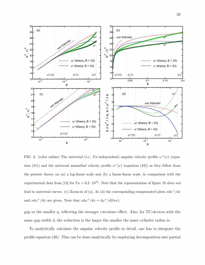
FIG. 2: (color online) The universal (i.e., Ta-independent) angular velocity profile ω+(x) (equa-

tion (41)) and the universal azimuthal velocity profile u+(x) (equation (43)) as they follow from

the present theory on (a) a log-linear scale and (b) a linear-linear scale, in comparison with the

experimental data from [13] for Ta = 6.2 · 1012. Note that the representation of figure 1b does not

lead to universal curves. (c) Zoom-in of (a). In (d) the corresponding compensated plots xdu+/dx

and xdω+/dx are given. Note that xdω+/dx = dω+/d(lnx).

gap or the smaller η, reflecting the stronger curvature effect. Also, for TC-devices with the

same gap width d, the reduction is the larger the smaller the inner cylinder radius is.

To analytically calculate the angular velocity profile in detail, one has to integrate the

profile equation (38). This can be done analytically by employing decomposition into partial

21

fractions. We will do so using the fact that in general 1/r+i KLx or 1 KLρ+. Then

the partial fraction decomposition of the rhs of eq. (38) reads (apart from the factor 1/KL)

1

x(1 + x)3=A

x+

B3

(1 + x)3+

B2

(1 + x)2+

B1

1 + x. (39)

The coefficients can be calculated by multiplying with the denominator on the lhs, leading

to

1 = A(1 + x)3 + x[B3 +B2(1 + x) +B1(1 + x)2

]. (40)

The four coefficients can all be calculated by comparing the respective x-powers. The result

is A = 1, Bi = −1 for all i = 1, 2, 3. They of course do not depend on any system parameter.

We now integrate equation (38) for the slope of the angular velocity with the decomposition

(39) term by term and get

ω+(x) =1

KL

(ln x+

1/2

(1 + x)2+

1

(1 + x)− ln(1 + x)

)+B′. (41)

The last term B′ is part of the usual additive shift in the log-regime and is determined from

experiment. However, also the 2nd and 3rd term contain such an additive shift, namely

1.5/KL, which we absorb in B′ (which then we call B) to finally obtain the main result of

this paper, namely the universal (i.e., Ta-independent) angular velocity profile

ω+(x) =1

KL

(ln x− x(2 + 3x)

(1 + x)2− ln(1 + x)

)+B. (42)

The angular velocity profile thus is a log-profile with downward corrections; it is plotted in

figure 2 in various representations. For very small x the first log-term will dominate. This

slowly increasing log-term will – with increasing x – be turned downwards, representing

the downward trend of the profile. In the limit r+i,o → ∞, channel flow, we have x → 0

and the mere log-profile ∝ (K−1L lnx + B) is recovered. Equation (42), together with the

definition (32) of the dimensionless length x, thus nicely reveals that in general there is an

extra intrinsic lengthscale r+i,o in the TC profile, in contrast to that for plate flow.

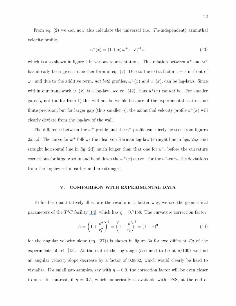
22

From eq. (2) we can now also calculate the universal (i.e., Ta-independent) azimuthal

velocity profile,

u+(x) = (1 + x)ω+ − F−1i x. (43)

which is also shown in figure 2 in various representations. This relation between u+ and ω+

has already been given in another form in eq. (2). Due to the extra factor 1 + x in front of

ω+ and due to the additive term, not both profiles, ω+(x) and u+(x), can be log-laws. Since

within our framework ω+(x) is a log-law, see eq. (42), thus u+(x) cannot be. For smaller

gaps (η not too far from 1) this will not be visible because of the experimental scatter and

finite precision, but for larger gap (thus smaller η), the azimuthal velocity profile u+(x) will

clearly deviate from the log-law of the wall.

The difference between the ω+-profile and the u+ profile can nicely be seen from figures

2a,c,d: The curve for ω+ follows the ideal von Karman log-law (straight line in figs. 2a,c and

straight horizontal line in fig. 2d) much longer than that one for u+, before the curvature

corrections for large x set in and bend down the ω+(x) curve – for the u+-curve the deviations

from the log-law set in earlier and are stronger.

V. COMPARISON WITH EXPERIMENTAL DATA

To further quantitatively illustrate the results in a better way, we use the geometrical

parameters of the T 3C facility [14], which has η = 0.7158. The curvature correction factor

A =

(1 +

ρ+

r+i

)3

=

(1 +

ρ

ri

)3

= (1 + x)3 (44)

for the angular velocity slope (eq. (37)) is shown in figure 3a for two different Ta of the

experiments of ref. [13]. At the end of the log-range (assumed to be at d/100) we find

an angular velocity slope decrease by a factor of 0.9882, which would clearly be hard to

visualize. For small gap samples, say with η = 0.9, the correction factor will be even closer

to one. In contrast, if η = 0.5, which numerically is available with DNS, at the end of

23

the log range (again assumed to be d/100) the log-slope is reduced by a factor of 0.9706,

which may become visible. For larger wall distances ρ d/100 the correction factor A

gets visibly smaller than 1. However, for these distances it was found experimentally that

one is already far away from a log-range, see figure 1. In figure 3b we apply the correction

factor to the angular velocity slope (38), which is universal (i.e., independent of Ta) for

large wall distances. We see that for small wall distances the correction factor indeed brings

the compensated profile closer to the log-profile (i.e., a horizontal line in this plot), but that

this curvature effect is very small. The correction factor only becomes substantial close to

the outer scale ρ ∼ d/2 where the log-regime clearly has already ceased.

In figure 2, in addition to the universal theoretical profiles for ω+(x) and u+(x), we also

include the experimentally measured [13] profiles for the largest available Taylor number

Ta = 6.2 · 1012. We see that the experimental curves qualitatively follow the same trend

as the theoretical ones. In particular, the ω+(x) profiles are closer to the log-profiles as

the u+(x) profiles, and both show increasing deviations from the log-profiles for increasing

x. However, there are pronounced quantitative differences between theory and experiment:

First of all, for very large x ∼ 0.1 the experimental profiles bend up again. This is to be

expected as then one is already very close to the gap center and the effect of the opposite

side of the gap becomes relevant – one is then simply far away from the boundary layers.

But second, and more seriously, already at x ∼ 4 · 10−3, corresponding to a wall distance of

d/100, the quantitative deviations between theory and experiment become very visible.

What are the reasons for the quantitative descrepancies between theory and experiments?

The theory has made certain assumptions like the existence of a turbulent ω-diffusivity

and its functional dependence (27) on the wall distance. We consider this as a relative

innocent assumption. More seriously is the fact that the theory does not take full notice

of the Taylor roll-structure of the flow and the resulting flow inhomogeneity in vertical

(z-)direction. From the numerical simulations of Ostilla et al. [24] we know however that

the boundary layer profiles pronouncedly depend on the vertical direction, at least up to

24

Taylor numbers Ta ∼ 1010 (larger ones are presently numerically not yet achievable), but

presumably beyond. Log-layers develop in particular in the regions in which plumes are

emitted and in shear layers, but not in regions in which plumes impact. For increasing Ta

the height dependence gets weaker, but it still persists at Ta = 6.2 · 1012 [4], for which we

present the experimental data here and which is the largest available Taylor number. In

fact, as seen from figure 2b of ref. [4] at Ta = 1.5 · 1012 the local Nusselt number can vary

from height to height even up to a factor of two, with the corresponding consequences on

the local profiles. The reason for the persistence of the vertical dependence is the limited

mobility of the Taylor rolls, due to their confinement between the upper and lower plates.

Though the aspect ratio – TC cell height dived by gap width d – in experiment is Γ = 11.7

[4], the six to eight Taylor rolls are still relatively fixed in space. The profile measurements

of ref. [13] took place at fixed position, namely mid-height. The theoretical results should

be understood as some height-averaged results, and strictly speaking such height-averaging

only makes sense if there is no or hardly any vertical dependence.

Clearly, it would be of utmost importance to measure the height dependence of the

angular velocity and azimuthal velocity profiles, in order to quantify it and to see whether

the relatively poor quantitative agreement between theory and experiment is better at other

heights. Also numerical simulations to further explore the height dependence of the profiles

would be useful, similar to what had already been done in ref. [24], but now for both ω+(x)-

and u+(x)-profiles and also profiles of the vertical (i.e., wind) velocity, for even larger Ta,

for smaller η, and finally for different values of co- and counter-rotation, i.e., different µ, but

of course all in the turbulent regime. Work in this direction is on its way.

Finally, we estimate the wall parameters, the amplitude u∗ of the azimuthal velocity

fluctuations, and the slope parameter Fi, all based on experimental data. In the experiment

[13] the outer cylinder was kept at rest, ωo = Reo = 0. Then (at the inner cylinder)

(u∗)2 = NωJωlam/r2i = Nω νr2

oωi/(ra · d). Expressed in terms of Ta (for ωo = 0) one has

25

!" #

!" $

!" !

"

!

$

#

%

&

'

(

)

*

+

,-+- -!.-/- -+

-

-

102

103

104

0.5

0.6

0.7

0.8

0.9

1

1.1

+

1/A

(a) (b)

Ta=6.2x1012

Ta=3.8x1011

Ta=6.2x1012

Ta=3.8x1011

von Kármán

A =(1 + ρ+/r+i

)3With corr.

A = 1Without corr.

FIG. 3: (color online) (a) (Inverse) correction factor A =(

1 + ρ+

r+i

)3as function of log10 ρ

+ for the

two Taylor numbers of figure 1a; here η = 0.7158 as in ref. [13]. The correction factor A is applied

to the angular velocity and in (b) we show the compensated angular velocity slope xdω+/dx vs

x = ρ+/r+i on a log-linear scale.

ωi = νr2g

√Ta/(r3

ad) and Rei = (η2/(1+η2

)3)√Ta = 0.8115

√Ta; here ra, rg are the arithmetic

and geometric mean radii. The Nusselt number Nω as function of the Taylor number Ta for

the T 3C apparatus has already been measured for T 3C in [5]. Putting all together leads to

u∗i =√

6.81× 10−3νrorgr2ad

Ta0.4375 . (45)

Inserting the material and geometry parameters of T 3C as given above one obtains an

explicit expression for u∗i ,

u∗i = 1.1948× 10−6 × Ta0.4375 ms−1 . (46)

This allows us to determine all physical parameters of interest. They are compiled in table

II.

26

Ta u∗i in ms−1 Re∗ω,i =u∗i ·dν δ∗i = ν

u∗i

riδ∗i

d/2δ∗i

d/100δ∗i

Fi =Re∗iRei

=ω∗iωi

u∗zu∗i

6× 1010 0.0620 4 900 16.2× 10−6m 12 300 2 440 49 2.47× 10−2 1.48

4.6× 1011 0.151 12 000 6.61× 10−6m 30 300 5 980 120 2.18× 10−2 1.54

3× 1012 0.344 27 200 2.91× 10−6m 68 700 13 540 271 1.94× 10−2 1.61

6× 1012 0.465 36 700 2.15× 10−6m 93 100 18 420 368 1.85× 10−2 1.65

TABLE II: The longitudinal velocity fluctuation amplitudes u∗i (second column) in the inner

cylinder boundary layer for some Taylor numbers Ta (first column). Third column the respective

values of the fluctuation Reynolds number Re∗ω,i in the inner cylinder BL. The fourth column shows

the respective viscous length scales δ∗i = ν/u∗i . The fifth column offers the inner cylinder radius

0.2000 m in the respective δ∗i -wall units, known as r+i . The gap half width in these wall units (sixth

column) is (d+/2 =)d/2δ∗i= d

2rir+i = 1

2(η−1 − 1)r+i = 0, 1985r+

i , i.e., d+/2 is about r+i /5. Column

seven shows d+/100, below which the experimental data are closest to a log-law. Column eight

shows Fi, which equals Re∗ω,i/Rei = ω∗i /ωi, the relative ω-fluctuation amplitude. The last (nineth)

column compiles the factor u∗z/u∗i , the ratio of the transversal and longitudinal velocity fluctuation

amplitudes; this is obtained with the values from column 2 of this table and column 4 of Table I.

VI. CONCLUDING REMARKS

In summary, we have derived a Navier-Stokes-based theory for the velocity and angular

velocity profiles in turbulent TC flow, following the same approach as that one of ref. [11]

for RB flow, but in cylinder geometry appropriate for TC flow, taking proper care of the

wall curvature(s). The main findings are

• that the angular velocity profile follows an universal log-law (eq. (42), reflecting the

curvature corrections),

• that the universal azimuthal velocity profile eq. (43) correspondingly cannot follow a

log-law,

27

• and that also the axial velocity profile follows an universal log-law eq. (22), but with

weaker curvature corresions, due to the less pronounced effect of the curvature in the

flow direction.

Though the experimentally measured angular velocity and azimuthal velocity profiles at fixed

mid-height qualitatively follow above trends, the quantitative agreement is not particularly

good as the measured deviations from the log-law are much stronger. This could be due to

the roll structure of the flow, leading to height dependences of the flow profiles, which are

not considered in the theory. We finally suggest various further experimental and numerical

measurements to further validate for falsify the presented theory.

Acknowledgement

We thank Rodolfo Ostilla and Sander Huisman for various insightful discussions on the

subject and all authors of ref. [13] for making the data of that paper available for the present

one. We finally acknowledge FOM for continuous support of our turbulence research.

Appendix A: Alternative choice of transversal fluctuation amplitude

We here check the idea that the relevant velocity for determining the transversal fluctu-

ation amplitude u∗w,z is not the inner cylinder rotation velocity Ui but, instead, the coherent

flow – or wind – due to the remnants of the rolls, called Uw. Its amplitude has been given for

the T 3C facility in [5], page 130, to be Rew = 0.0424×Ta0.495; this holds for a = 0 and in the

range 3.8 × 109 . Ta . 6.2 × 1012. This rather small value for the wind Reynolds number

rests on PIV measurements, cf. [4]. A similar but even smaller value has been obtained with

DNS, [12]: In the regime 4× 104 . Ta . 1× 107 it is Rew = 0.0158×Ta0.53. – The relevant

quantities are given in Table III.

28

Ta Rew Uw = Rewνd

UwUi

u∗w,z

Uw= κ

W (3.2Rew) u∗w,z = Uwκ

W (3.2Rew)

u∗w,z

u∗i

6× 1010 9174 0.1161 m/s 0.0461 0.04887 5.6738 ×10−3 m/s 0.092

4.6× 1011 25144 0.3183 m/s 0.0456 0.04401 14.0084 ×10−3 m/s 0.093

3× 1012 63612 0.8052 m/s 0.0452 0.04029 32.4415 ×10−3 m/s 0.094

6× 1012 89650 1.1291 m/s 0.0451 0.03906 44.1026 ×10−3 m/s 0.095

TABLE III: The wind fluctuation amplitude u∗w,z based on the wind Reynolds number for different

Taylor numbers (column 1). The corresponding wind Reynolds number Rew = 0.0424 · Ta0.495

are listed in column 2. The next columns, 3 and 4, show the respective wind velocities Uw =

Rew · ν/d in m/s (with system parameters ν = 1 · 10−6 m2s−1 and d = 0.0794 m) as well as

the wind velocity relative to the inner cylinder rotation velocity, Uw/Ui, turning out to be of

order 4.6%, only very slightly depending on Ta; it is Uw/Ui = 0.052193 · Ta−0.005, were we used

Rei = 0.8115 Ta0.5 for a = 0, as was reported in the main text. Column 5 offers the relative

fluctuation amplitude u∗w,z/Uw, obtained from the formula with Lambert’s W-function derived

in [23], u∗w,z/Uw = κ/W (3.2Rew) (again we have used κ = 0.4 as von Karman’s constant and

b = 0.125 to determine the argument κbRew of W . Column 6 contains the respective transversal

fluctuation amplitudes u∗w,z = Uw · κW (3.2Rew) . Finally in column 7 the ratios of the transversal

wind fluctuation amplitude u∗w,z and the longitudinal angular momentum fluctuation amplitude u∗i

are offered for the Ta-values of interest from Table II. Note that the transversal wind fluctuation

amplitude is about 9.5% of the longitudinal ω-fluctuation amplitude, determined in Section IV,

pretty independent of Ta.

[1] G. Ahlers, S. Grossmann, and D. Lohse, Heat transfer and large scale dynamics in turbulent

Rayleigh-Benard convection, Rev. Mod. Phys. 81, 503 (2009).

[2] D. Lohse and K.-Q. Xia, Small-scale properties of turbulent Rayleigh-Benard convection, Ann.

29

Rev. Fluid Mech. 42, 335 (2010).

[3] D. P. M. van Gils, S. G. Huisman, G. W. Bruggert, C. Sun, and D. Lohse, Torque scaling in

turbulent Taylor-Couette flow with co- and counter-rotating cylinders, Phys. Rev. Lett. 106,

024502 (2011).

[4] S. G. Huisman, D. P. M. van Gils, S. Grossmann, C. Sun, and D. Lohse, Ultimate turbulent

Taylor-Couette flow, Phys. Rev. Lett. 108, 024501 (2012).

[5] D. P. M. van Gils, S. G. Huisman, S. Grossmann, C. Sun, and D. Lohse, Optimal Taylor-

Couette turbulence, J. Fluid Mech. 706, 118 (2012).

[6] G. Ahlers, E. Bodenschatz, D. Funfschilling, S. Grossmann, X. He, D. Lohse, R. Stevens, and

R. Verzicco, Logarithmic temperature profiles in turbulent Rayleigh-Benard convection, Phys.

Rev. Lett. 109, 114501 (2012).

[7] D. Funfschilling, E. Bodenschatz, and G. Ahlers, Search for the ultimate state in turbulent

Rayleigh-Benard convection, Phys. Rev. Lett. 103, 014503 (2009).

[8] G. Ahlers, D. Funfschilling, and E. Bodenschatz, Transitions in heat transport by turbulent

convecion at Rayleigh numbers up to 1015, New J. Phys. 11, 123001 (2009).

[9] X. He, D. Funfschilling, H. Nobach, E. Bodenschatz, and G. Ahlers, Transition to the ultimate

state of turbulent Rayleigh-Benard convection, Phys. Rev. Lett. 108, 024502 (2012).

[10] X. He, D. Funfschilling, E. Bodenschatz, and G. Ahlers, Heat transport by turbulent Rayleigh-

Benard convection for Pr = 0.8 and 4 × 1011 . Ra . 2 × 1014: ultimate-state transition for

aspect ratio Γ = 1.00, New J. Phys.. 14, 063030 (2012).

[11] S. Grossmann and D. Lohse, Logarithmic temperature profiles in the ultimate regime of thermal

convection, Phys. Fluids 24, 125103 (2012).

[12] R. Ostilla, R. J. A. M. Stevens, S. Grossmann, R. Verzicco, and D. Lohse, Optimal Taylor-

Couette flow: direct numerical simulations, J. Fluid Mech. 719, 14 (2013).

[13] S. G. Huisman, S. Scharnowski, C. Cierpka, C. Kahler, D. Lohse, and C. Sun, Logarithmic

boundary layers in strong Taylor-Couette turbulence, Phys. Rev. Lett. 110, 264501 (2013).

30

[14] D. P. M. van Gils, G. W. Bruggert, D. P. Lathrop, C. Sun, and D. Lohse, The Twente turbulent

Taylor-Couette (T 3C) facility: strongly turbulent (multi-phase) flow between independently

rotating cylinders, Rev. Sci. Instr. 82, 025105 (2011).

[15] S. B. Pope, Turbulent Flow (Cambridge University Press, Cambridge, 2000).

[16] I. Marusic, B. J. McKeon, P. A. Monkewitz, H. M. Nagib, A. J. Smits, and K. R. Sreenivasan,

Wall-bounded turbulent flows at high Reynolds numbers: Recent advances and key issues, Phys.

Fluids 22, 065103 (2010).

[17] M. Hultmark, M. Vallikivi, S. C. C. Bailey, and A. J. Smits, Turbulent Pipe Flow at Extreme

Reynolds Numbers, Phys. Rev. Lett. 108, 094501 (2012).

[18] I. Marusic, J. P. Monty, M. Hultmark, and A. J. Smits, On the logarithmic region in wall

turbulence, J. Fluid. Mech. 716, R3 (2013).

[19] M. Hultmark, M. Vallikivi, S. C. C. Bailey, and A. J. Smits, Logarithmic scaling of turbulence

in smooth- and rough-wall pipe flow, J. Fluid. Mech. 728, 376 (2013).

[20] S. Grossmann, D. Lohse, and A. Reeh, Different intermittency for longitudinal and transversal

turbulent fluctuations, Phys. Fluids 9, 3817 (1997).

[21] L. D. Landau and E. M. Lifshitz, Fluid Mechanics (Pergamon Press, Oxford, 1987).

[22] B. Eckhardt, S. Grossmann, and D. Lohse, Torque scaling in turbulent Taylor-Couette flow

between independently rotating cylinders, J. Fluid Mech. 581, 221 (2007).

[23] S. Grossmann and D. Lohse, Multiple scaling in the ultimate regime of thermal convection,

Phys. Fluids 23, 045108 (2011).

[24] R. Ostilla, E. P. van der Poel, R. Verzicco, S. Grossmann, and D. Lohse, Boundary layer

dynamics at the transition between the classical and the ultimate regime of Taylor-Couette

flow, Phys. Fluids x, y (2014).