VEHICLE DASHBOARD TRAFFIC LIGHT SYSTEMS AT A 4-WAY ...

University of New MexicoUNM Digital Repository

Electrical and Computer Engineering ETDs Engineering ETDs

6-9-2016

VEHICLE DASHBOARD TRAFFIC LIGHTSYSTEMS AT A 4-WAY INTERSECTIONAlejandro Flores

Follow this and additional works at: https://digitalrepository.unm.edu/ece_etds

This Thesis is brought to you for free and open access by the Engineering ETDs at UNM Digital Repository. It has been accepted for inclusion inElectrical and Computer Engineering ETDs by an authorized administrator of UNM Digital Repository. For more information, please [email protected].

Recommended CitationFlores, Alejandro. "VEHICLE DASHBOARD TRAFFIC LIGHT SYSTEMS AT A 4-WAY INTERSECTION." (2016).https://digitalrepository.unm.edu/ece_etds/87

i

Alejandro Flores Candidate

Electrical and Computer Engineering

Department

This thesis is approved, and it is acceptable in quality and form for publication:

Approved by the Thesis Committee:

Wei Wennie Shu, Chairperson

Guohui Zhang

Daryl O. Lee

ii

VEHICLE DASHBOARD TRAFFIC LIGHT SYSTEMS AT A

4-WAY INTERSECTION

by

ALEJANDRO FLORES

B.SC. ENGINEERING TECHNOLOGY

NEW MEXICO STATE UNIVERSITY, 2005

THESIS

Submitted in Partial Fulfillment of the

Requirements for the Degree of

Master of Science

Computer Engineering

The University of New Mexico

Albuquerque, New Mexico

May, 2016

iii

© 2016, Alejandro Flores

iv

Dedication

To my wonderful parents who have taught me the meaning of hard work and dedication. To my

brother and sisters who have infused their hopes and dreams onto me and have provided nothing

but love and support. To my amazing wife who has been my copilot throughout this journey and

has sacrificed so much to support me! Last but not least, to God who has allowed me to enjoy a

life of great challenges and happy moments like these!

v

Acknowledgements

I would like to thank my academic advisor, W. Shu, for challenging me throughout this

thesis by asking the hard questions and guiding me through the process. I’d also like to

thank my coding mentor and great friend Dr. Lee, who offered countless consulting

sessions. Finally, to Dr. Zhang for his support and mentoring in developing this topic.

vi

Vehicle Dashboard Traffic Light Systems at 4-way Intersections

by

Alejandro Flores

B. SC., Engineering Technology, New Mexico State University, 2005

M.S., Computer Engineering, University of New Mexico, 2016

Abstract

In recent years, a wave of technological innovations have turned many of the gadgets we

use into smart devices. However, some areas of industry remain somewhat isolated from

modernization with little to no improvements in their overall functionality. Traffic lights

at an intersection are a perfect example of a technology that has remained behind the

times. While there is a lot of potential for reducing CO2 gas emissions, oil consumption,

and commuting times, research in this area has resulted in minor changes. In this thesis,

we improve on what others have learned to provide a solution in vehicle coordination that

is smart, practical and innovative. We leverage the power of Vehicle Ad-hoc Networks

(VANET’s) to develop a Vehicle Traffic Dashboard Light System that can gather real-

time traffic information to effectively coordinate vehicles crossing a 4-way intersection.

In detail, we developed a Lazy Algorithm that focuses on reducing vehicular average

waiting times, maximizing intersection throughput and minimizes the number of vehicles

that need to make unnecessary stops. We then compare the Lazy Algorithm to two other

algorithms by conducting various simulations. Furthermore, we study the impact on the

average waiting time vehicles experience while crossing two consecutive intersections

equipped with a Vehicle Traffic Dashboard Light System. The results from our many

vii

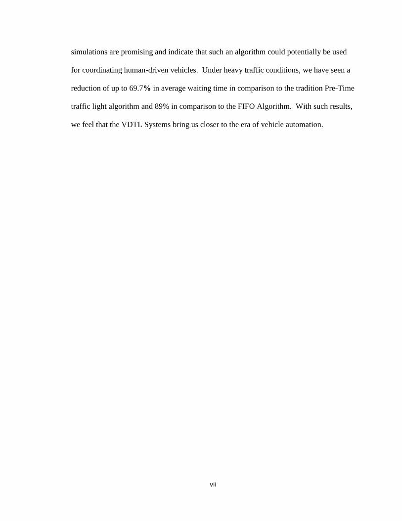
simulations are promising and indicate that such an algorithm could potentially be used

for coordinating human-driven vehicles. Under heavy traffic conditions, we have seen a

reduction of up to 69.7% in average waiting time in comparison to the tradition Pre-Time

traffic light algorithm and 89% in comparison to the FIFO Algorithm. With such results,

we feel that the VDTL Systems bring us closer to the era of vehicle automation.

viii

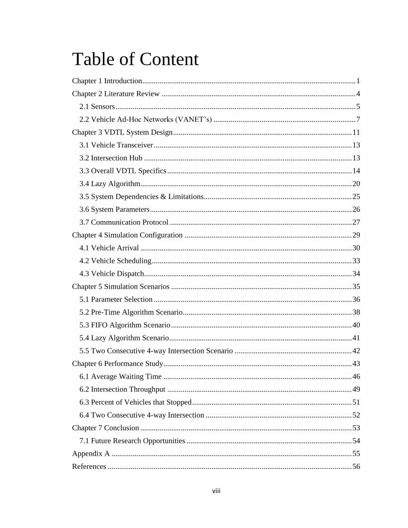
Table of Content Chapter 1 Introduction ............................................................................................................... 1

Chapter 2 Literature Review ..................................................................................................... 4

2.1 Sensors ............................................................................................................................. 5

2.2 Vehicle Ad-Hoc Networks (VANET’s) .......................................................................... 7

Chapter 3 VDTL System Design ............................................................................................. 11

3.1 Vehicle Transceiver ....................................................................................................... 13

3.2 Intersection Hub ............................................................................................................ 13

3.3 Overall VDTL Specifics ................................................................................................ 14

3.4 Lazy Algorithm .............................................................................................................. 20

3.5 System Dependencies & Limitations ............................................................................. 25

3.6 System Parameters ......................................................................................................... 26

3.7 Communication Protocol ............................................................................................... 27

Chapter 4 Simulation Configuration ....................................................................................... 29

4.1 Vehicle Arrival .............................................................................................................. 30

4.2 Vehicle Scheduling ........................................................................................................ 33

4.3 Vehicle Dispatch ............................................................................................................ 34

Chapter 5 Simulation Scenarios .............................................................................................. 35

5.1 Parameter Selection ....................................................................................................... 36

5.2 Pre-Time Algorithm Scenario........................................................................................ 38

5.3 FIFO Algorithm Scenario .............................................................................................. 40

5.4 Lazy Algorithm Scenario ............................................................................................... 41

5.5 Two Consecutive 4-way Intersection Scenario ............................................................. 42

Chapter 6 Performance Study .................................................................................................. 43

6.1 Average Waiting Time .................................................................................................. 46

6.2 Intersection Throughput ................................................................................................ 49

6.3 Percent of Vehicles that Stopped ................................................................................... 51

6.4 Two Consecutive 4-way Intersection ............................................................................ 52

Chapter 7 Conclusion .............................................................................................................. 53

7.1 Future Research Opportunities ...................................................................................... 54

Appendix A ............................................................................................................................. 55

References ............................................................................................................................... 56

ix

List of Figures

Figure 2.1 Example of Vehicle Waiting at an Intersection with Sensors …….…….… 6 Figure 3.1 Vehicle Dashboard Traffic Light (VDTL) System ……………...….…...… 11

Figure 3.2 Platooning ….………………………………………………………………. 12

Figure 3.3 T2P for Vehicles in a Platoon ……………………………………………… 16

Figure 3.4 Example of Time Slot Blocking under FIFO Algorithm .…………….….... 17

Figure 3.5 Intersection Hub Light Status Response …………………………………... 19

Figure 3.6: Lazy Algorithm Pseudo Code…………...…………………………………. 23

Figure 3.7: Example of Time Slot Blocking under Lazy Algorithm ……………...…… 24

Figure 3.8 Single Communication Protocol ………………………………………….... 28

Figure 3.9 Multiple Communication Protocol ……………………………………….... 29

Figure 4.1: Vehicles Speed Adjustments ………………………...…………….…….... 32

Figure 4.2: Linked List Used as Queue ………………………………………………. 33

Figure 4.3: Illustration of Time-to-Pass (T2P) based on Vehicle Type ……….……… 34

Figure 4.4: Simulation Code Execution Order ………………………………………... 35

Figure 5.1: Max Intersection Occupancy ……………….………………..…………..... 37

Figure 5.2: Min intersection Occupancy …………………………………………….… 37

Figure 5.3: Pre-Time Algorithm Pseudo Code …………......…………………….…… 39

Figure 5.4: FIFO Algorithm Pseudo Code …………………………………………….. 41

Figure 5.5: Algorithm though Consecutive Intersections ……………………………… 42

Figure 6.1: Average Waiting Time Comparison …...……………………...……….…. 46

Figure 6.2: Pre-Time Algorithm Straight/Right Platoon Bins …...…………...…..…… 47

Figure 6.3: FIFO Algorithm Straight/Right Platoon Bins ………………...…….……. 48

Figure 6.4: Lazy Algorithm Straight/Right Platoon Bins …….………………………... 48

Figure 6.5: Average Platoon Size …………………………….…………………..……. 49

Figure 6.6: Intersection Throughput ………………………..………………………….. 50

Figure 6.7: Percent of Vehicles that Stopped at the Intersection ……………………..... 51

Figure 6.8: AWT for Consecutive 4-way Intersection using FIFO Algorithm ….….... 52

x

Figure 6.9: AWT for Consecutive 4-way Intersections using Lazy Algorithm …...…… 52

xi

List of Tables

Table 2.1: Parameters used in Traffic Coordination Schemes …………………...……. 5

Table 3.1: Data Broadcasted by VDTL Vehicle ……………………………………….. 14

Table 3.2: Lazy Algorithm Modifiable Parameters ………………………………....… 27

Table 4.1: Definition of Traffic Conditions ……………….……………………….…... 31

Table 4.2 List of Vehicle Parameters Available ……………………………………… 31

Table 4.3: Program Global Parameters ……………………………………….………. 32

Table 5.1: T2P Times used in Simulation ………………………………………..……. 36

Table 5.2: Max Intersection Occupancy Calculation …………...…………………….. 37

Table 5.3: Minimum Intersection Occupancy Calculation ………………………….... 37

Table 5.4: Traffic Condition Definition …………………………………………...….. 38

Table 5.5: Global Scenario Parameter Values …………...…………………………... 38

Table 5.6: Pre-Time Cycle Time Scenario Parameters ……………..……………….... 39

Table 5.7: Lazy Algorithm Scenario Parameters ……………………………………… 41

Table 6.1: Pre-Time Algorithm Performance Study ……………………...……..…… 44

Table 6.2: FIFO Algorithm Performance Study …………….………...………..….…. 44

Table 6.3: Lazy Algorithm Light Traffic Performance Study ………….……......…… 45

Table 6.4: Lazy Algorithm Moderate Traffic Performance Study …………..…...…… 45

Table 6.5: Lazy Algorithm Heavy Traffic Performance Study …………...….……..… 46

1

Chapter 1 Introduction

The 21st century has brought us many innovations in technology that in some way or

other have improved our quality of life. However, certain areas remain stagnant and have

made little to no improvements to its overall functionality. A good example of this is the

tradition 4-way traffic light.

Vehicle traffic lights have been in existence for many decades now, yet the main

algorithm and mechanics used to coordinate vehicle crossing at an intersection have not

evolved much. Yes, sensors have been added to the system and many studies have been

conducted on determining the optimum light timing but none have been able to yield

significant improvements over the current model of the dynamic Pre-Time traffic light.

Meanwhile, the number of vehicles on the streets keeps increasing, forcing local

governments to install additional traffic lights as a way to maintain traffic flow. In a

2011 report, the United States Federal Highway Administration reported there were a

whopping 246 million registered vehicles in the nation [1]. This volume of vehicles

traveling on our roadways has become of great concern to many government agencies

and the community at large. Not only does it create a traffic flow nightmare but most

importantly, the impact that fuel consumption and CO2 gas emissions have on the

environment are quite significant [2].

In recent years, the Obama administration has been particularly interested in

breaking the U.S. dependence on foreign oil, increasing vehicle fuel consumption, and

addressing the threat of climate change [3-4]. Yet, little is being done to improve the

current traffic light system infrastructure that could potentially have a significant

2

reduction in both fuel consumption and emission of CO2 gasses released into the

environment.

Early versions of the traffic light signals used a fixed pre-configured timing

mechanism that would allocate a fixed amount of green time to each direction. As the

number of vehicles on our roadways increased, this basic model of coordination proved

to be inefficient. It was only then that traffic engineers began using other techniques to

better determine the traffic light timing that could maximize the intersection use.

As a way to improve the fixed pre-configured timing model, engineers began

using induction loop sensors that could determine when a vehicle was present [5]. These

sensors would then allow the light controller to adjust to traffic light timing throughout

the day based on traffic patterns obtained from these sensors. Unfortunately, such

sensors were very intrusive, expensive and resulted in higher maintenance costs [6]. As

an improvement, traffic engineers began using non-intrusive type sensors such as motion,

video, and microwave sensors, to name a few. While these sensors were less expensive,

they were also less accurate [6].

With the development of wireless networks, the idea of using such a technology

for traffic coordination has gained more and more support. In recent years, many

researchers have proposed the use of Vehicle Ad-hoc Networks (VANET’) such as

Vehicle to Vehicle (V2V) and Vehicle to Infrastructure (V2I) to collect data that could

then be used to adjust the traffic light timing in real-time [7].

Regardless of the method being used for controlling the traffic light timing, the

fact is that vehicles are still required to stop. In some cases, vehicles are required to stop

and wait for the green light even if there is no other vehicle at the intersection. Similarly,

3

vehicles taking a trajectory that does not conflict with other vehicles will also be required

to stop. As a result, there is a lot of potential to further reduce fuel consumption and CO2

gas emissions into the environment by reducing the vehicle waiting at the intersections.

In a paper published by the University of New Mexico in collaboration with the

University of Shanghai in China, the author suggests evaluating vehicles on an individual

basis so that non-conflicting vehicles at the intersection can continue without having to

stop [11]. While the model sounds very promising, the number of vehicles that are

required to stop at the intersection during moderate and high traffic conditions is still

quite high. Furthermore, the model assumes that all vehicles will take 4 seconds to cross

the intersection when in reality, this time, can vary on vehicle type and velocity.

In this paper, we improve on a previously proposed algorithm for dispatching

vehicles in a 4-way intersection by not only evaluating each vehicle individually but also

as a group. The solution being proposed in this paper is called Vehicle Dashboard Traffic

Light (VDTL) System and it consists of an intersection and vehicle transceiver that

communicate wirelessly to systematically dispatch vehicles across the intersection. The

system evaluates each vehicle independently and as a group (platoon) to determine if the

vehicle can cross the interaction without stopping by making use of what we call a lazy

algorithm. The decision is then wirelessly sent to each vehicle and displayed on the

vehicle’s traffic light dashboard. The purpose of this proposed algorithm is to reduce the

average waiting time for each vehicle in an effort to increase traffic flow, reduce fuel

consumption, and reduce CO2 emissions.

4

As we would expect, such change to the vehicle traffic light system shakes the

foundation of how we think about vehicular traffic flow and presents an option to moving

it to the 21st century.

In chapter 2, we analyze the work others have conducted in this area and identify

gaps that could potentially be addressed by the work on this thesis. Chapter 3 will look

into the details of the overall system design, the technologies it relies on to effectively

operate a VDTL system and describe algorithm being proposed. In chapter 4, we

describe the simulation configuration that was developed to compare the Lazy Algorithm

with other algorithms such as the Pre-Time and FIFO Algorithm. Chapter 5 will go over

the different simulation scenarios that were performed to identify the parameters that

produced the best results. In chapter 6 we go over the performance study results.

Finally, in chapter 6 we go over the results obtained in simulation and conclude with

chapter 7 by identifying future areas of research interest.

Chapter 2 Literature Review

The 4-way Pre-Time traffic control system that we all encounter on a daily basis has

proven to be very restrictive in terms of maximizing the use of the intersection or what

we refer to in this paper as the critical zone. The issue with the Pre-Time traffic control

system is that vehicles are forced to stop at an intersection when there is possibly no other

vehicle is making use of the critical zone. As the number of vehicles on our roads

increase, the importance of maximizing the use of the critical zone has become more and

more important. Not only is overall fuel consumption increased but the amount of CO2

5

gasses released into the environment becomes very significant as we aggregate the

number of vehicles that travel across US road intersections.

In recent years, a lot of research has been conducted in an effort to eliminate

unnecessary vehicle stops at intersections. Table 2.1 provides a brief summary of the

many parameters that have been considered when developing solutions to reduce vehicle

waiting time at the intersections.

Evaluating

Unit

Technology Frequency

of Light

Switching

Type of

Vehicle

Traffic

Conditions

Road

Infrastructure

- Individual

- Platoon

- Sensors

(Intrusive or

Non-Intrusive)

- Vehicle ad-

hoc Networks

(VANET)

(V2V or V2I)

- Per Cycle

- Per Platoon

- Per Vehicle

- Automated

- Human

Driven

- Light

- Moderate

- Heavy

-Traffic Light

-No Traffic

Lights

Table 2.1: Parameters used in Traffic Coordination Schemes

2.1 Sensors

In a study conducted by Universiti Pultra Malaysia, the authors make a comparison

between time-based and sensor-based traffic light control systems. In their research, they

modulate the light timing based on a set platoon size. More specifically, their algorithm

checks the number of vehicles waiting to cross the intersection to determine the amount

of time the green light should stay on. If the number of vehicles waiting to cross the

intersection is small, the resulting green light durations will be short. If the number of

vehicles waiting increases, so does the green light duration [6].

6

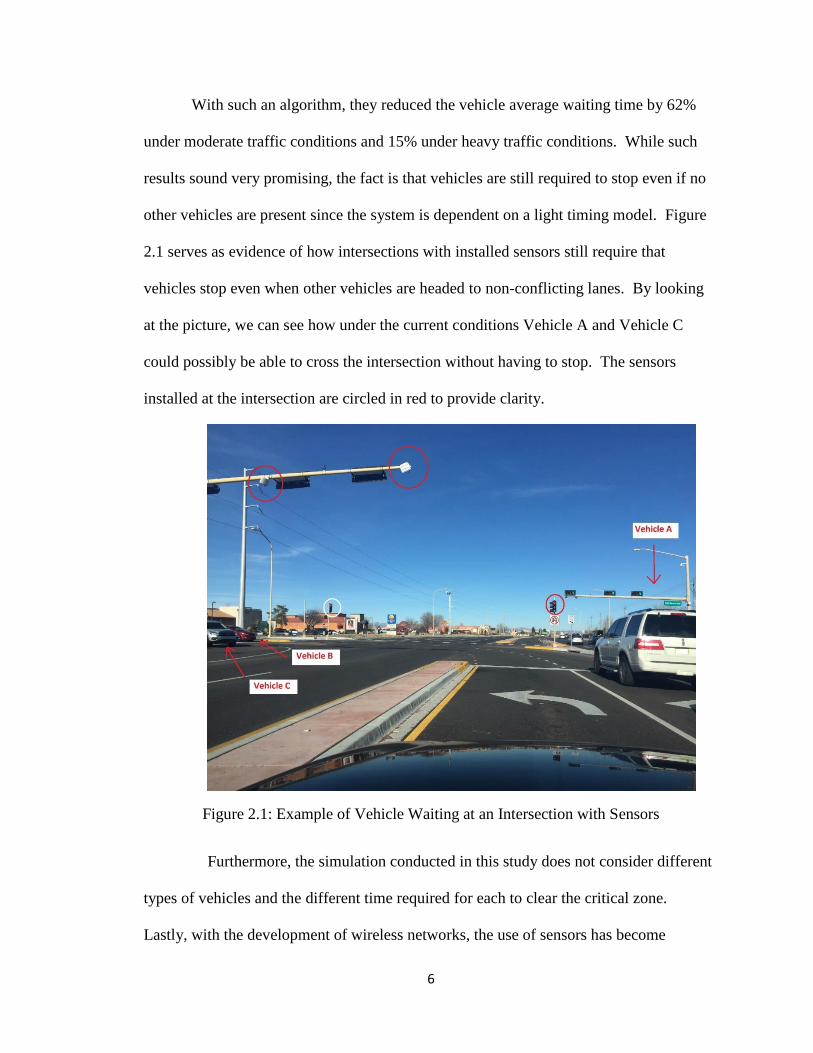
With such an algorithm, they reduced the vehicle average waiting time by 62%

under moderate traffic conditions and 15% under heavy traffic conditions. While such

results sound very promising, the fact is that vehicles are still required to stop even if no

other vehicles are present since the system is dependent on a light timing model. Figure

2.1 serves as evidence of how intersections with installed sensors still require that

vehicles stop even when other vehicles are headed to non-conflicting lanes. By looking

at the picture, we can see how under the current conditions Vehicle A and Vehicle C

could possibly be able to cross the intersection without having to stop. The sensors

installed at the intersection are circled in red to provide clarity.

Figure 2.1: Example of Vehicle Waiting at an Intersection with Sensors

Furthermore, the simulation conducted in this study does not consider different

types of vehicles and the different time required for each to clear the critical zone.

Lastly, with the development of wireless networks, the use of sensors has become

7

somewhat a thing of the past. The use of wireless technologies to obtain data directly

from vehicles approaching the intersection has become a more valuable approach to

modulating traffic controller light timing.

2.2 Vehicle Ad-Hoc Networks (VANET’s)

The use of VANETs for coordinating vehicles across intersections has become a very

popular research topic. More specifically, the use of Vehicle-to-Vehicle (V2V) and

Vehicle-to-Infrastructure (V2I) networks have proven to be particularly useful in

obtaining vehicle information that otherwise would be unobtainable. For instance, by

making use of ad-hoc networks, intersection controllers can now obtain real-time

information such as vehicle speed, lane, type and distance to name a few. Additionally,

the possibility of communicating traffic condition from vehicle to vehicle with the use of

this technology becomes particularly important when needing to redirect traffic after a

major highway accident. As one can imagine, the possibilities are endless.

Studies that have implemented the use of V2V and V2I communication include

those done by the University of Bucharest in collaboration with Rutgers University. In

their study, the V2V network is used to relay a message from one vehicle to another to

alert the intersection controller of the upcoming vehicle approaching the intersection.

The vehicle closest to the intersection uses the V2I network to inform the intersection

controller of the amount of vehicles approaching the critical zone from each direction.

The intersection controller then uses this information to adjust the green light timing for

the next cycle. In other words, the controller uses information obtained from the previous

cycle to generate a forecast of what the green light timing should be for the next cycle.

8

The cycle length is calculated by finding the flow per capacity ratio based on Webster’s

formula [8]. Simulation results indicated that a reduction of 28.3% in total delay from a

Pre-Time intersection could be achieved by implementing such a strategy.

In a similar manner, Pandit, Ghosal, Zhang, and Chuah make use of VANET’s to

dynamically adjust the intersection controller light timing. However, in their Adaptive

Traffic Signal Control with Vehicular Ad hoc Networks paper, they group vehicles into

platoons rather than considering each vehicle individually like Grandinescu [7, 8]. In

their proposed oldest job first (OJF) algorithm, they suggest creating vehicle platoons of

equal size and allowing groups with the oldest arrival time to cross first. They leverage

the power of VANET’s to effectively create the vehicle platoons. By doing this, they

discovered that the delay vehicles experienced at the intersections was significantly

reduced during light and moderate traffic conditions. Under heavy traffic, they found

that their OJF algorithm had less of an impact. In comparing this algorithm to the Pre-

Time traffic algorithm, simulation results suggest a possible reduction of up to 39% in the

average delay per vehicle [7].

Another interesting research that makes use of VANET’s in combination with

Stochastic and Heuristic Algorithms is one conducted by Kwatirayo et. al. Their study

results yield a reduction in average travel time ranging from 17.6% to 21.8%. In this

study, they propose a reduction in average travel time by using an optimization method

called Simultaneous Perturbation Stochastic Algorithm (SPSA) to find the optimal

solution for setting the maximum green light time [9]. However, the use of optimization

methods does not eliminate the unnecessary wait time from vehicles waiting for the light

9

to change but rather simply minimizes that wait time as much as possible. However,

vehicles with non-conflicting trajectories are still required to stop.

Recent research related to vehicle coordination via VANET’s is now focusing on

the coordination of automated vehicles without the use of traffic lights at each

intersection [10]. In theory, V2V and V2I networks in combination with collision

avoidance technologies could be used to virtually eliminate all waiting time experienced

by vehicles crossing the intersection. With such a coordination scheme, multiple vehicles

could be traveling inches apart from each other within the critical zone without the risk of

collision. For instance, two vehicles traveling perpendicular to one another could

possibly cross the critical zone without stopping as long as there is a slight space gap

between each of them. Although this could be the ideal solution to intersection

coordination, the reality is that we are a few years away from seeing fully automated

vehicles in our roadways. Therefore, solutions that take into consideration the many

uncertainties that come with human-driven vehicles will likely be the most effective

solutions for the short term implementation.

A similar approach to coordinating vehicles at an intersection without making use

of traffic lights while still considering human driven vehicles is one done by Al-

Mashhadani et. al. They transition the traffic lights from the street to the vehicle by

introducing a Dashboard Traffic Light (DTL) device that communicates wirelessly with

the intersection controller. Their innovative FIFO Algorithm evaluates vehicles

individually as they approach the intersection. The intersection controller reserves the

critical zone on a first come first serve bases and allows vehicles with non-interfering

trajectories to continue without stopping. What's more, their multiple simulations

10

ranging from 5 to 90 vehicles per minute yield a promising 86.5% reduction in average

waiting times in comparison to Pre-Time intersection under heavy traffic conditions. In

analyzing the work done in this research, it is clear that realistic variability in time

required for each vehicle to cross the critical zone is not considered. For their study, they

assume that it will take all vehicles 4 seconds to cross the intersection regardless of their

profile type and speed. Furthermore, during heavy traffic conditions, the simulations

results indicate that the percent of vehicles required to stop is higher when using their

proposed algorithm in comparison with the Pre-Time. In other words, the FIFO

Algorithm becomes counterproductive under moderate and heavy traffic patterns. And

while no algorithm will completely eliminate vehicle waiting time under heavy traffic

patterns, it certainly should not make it worse.

In this thesis, we propose a heuristic algorithm that helps address the gaps found

between the Pre-Time Algorithm and the FIFO Algorithm. The Lazy Algorithm takes a

combination of both of these approaches to evaluate vehicles individually and as a group

(platoon) to achieve a lower waiting time experienced by all vehicles. The strategy

leverages the power of VANET’s to gather vehicle information that is crucial to the

constant adjustment of vehicle processing during light, moderate, and heavy traffic

conditions. Furthermore, it uses the Vehicle Dashboard Traffic Light (VDTL) system as

a way of eliminating the use of intersection traffic lights and expediting the dispatch

process of each vehicle. In the following chapter will touch on the details of the overall

systems, parameters, and assumptions that are being considered to make an improvement

in vehicle waiting time.

11

01

54

3 2

6 7

Critical Zone

Intersection Hub

Chapter 3 VDTL System Design

The Vehicle Dashboard Traffic Light (VDTL) is a system in which no actual traffic lights

are installed at each intersection but rather displayed within a vehicle’s dashboard.

Intersections are equipped with transponders connected to an intersection hub responsible

for coordinating the use of the intersection critical zone. This is very similar to a

computer processor model in which tasks need to be performed by a single processor.

Figure 3.1 illustrates how a VDTL system might look. Note that the traffic light in each

vehicle represent the dashboard and the antenna like symbols represent the vehicle

transceiver. Lanes are numbered clockwise direction starting from the east end.

Figure 3. 1 Vehicle Dashboard Traffic Light (VDTL) System

The intersection hub schedules vehicles based on an elaborate Lazy Algorithm

that not only evaluates vehicles individually but also in a platoon configuration.

12

However, to fully comprehend the design, a basic understanding of how we define

platoons needs to be reviewed. Figure 3.2 below explains what we consider to be a

platoon.

01

54

3 2

6 7

Intersection Hub

#1

#2

West Platoon 1Straight

Platoon 1 North

Straight

West Platoon 2 Straight

(Will need to stop)

#3

Figure 3.2 Platooning

A platoon is a group of vehicles that is allowed to consecutively cross the

intersection critical zone without the interruption of any other trajectory conflicting

vehicle. As seen in figure 3.5, the west platoon 1 is made up of 3 vehicles rather than 5.

This platoon cut off is caused by platoon 1 approaching from the north and arriving at the

critical zone before platoon 2 approaching from the left. Both the Pre-Time and Lazy

Algorithms make use of this platooning mechanism to improve efficiency.

This VDTL system assumes that all vehicles are still driven by humans and that

all vehicles are equipped with a VDTL system device. And although the system is

designed specifically for a four-way intersection that has a dedicated lane for turning left

13

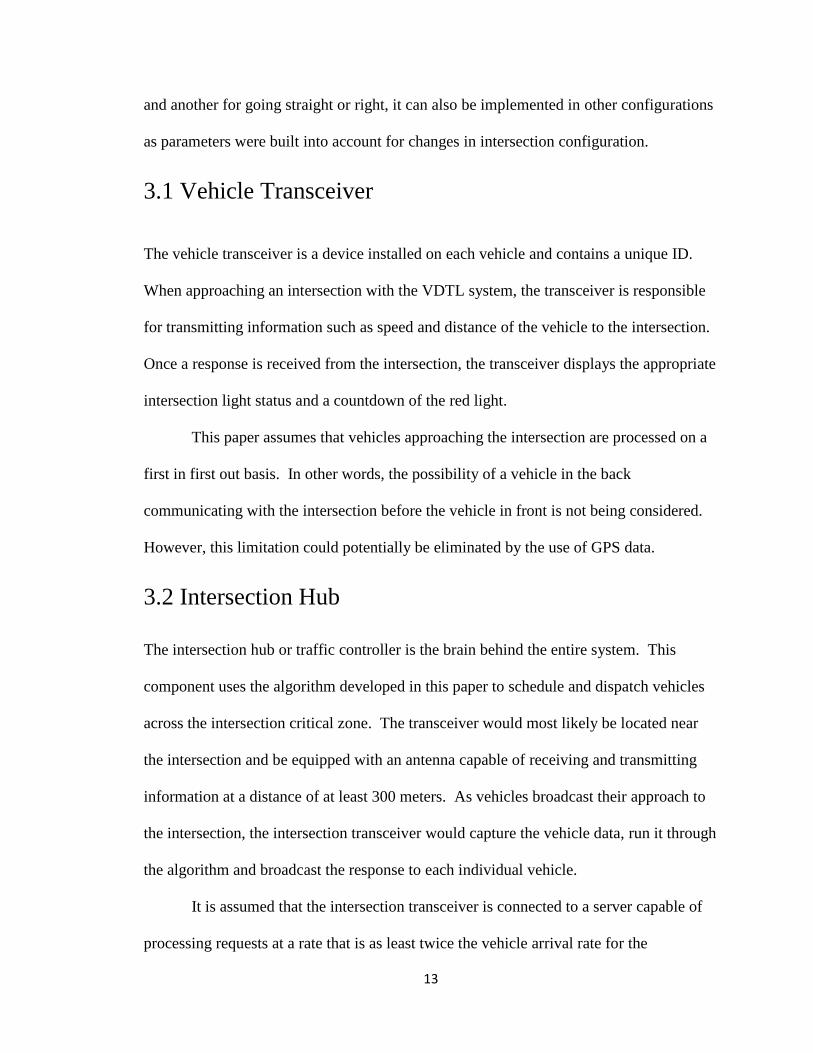
and another for going straight or right, it can also be implemented in other configurations

as parameters were built into account for changes in intersection configuration.

3.1 Vehicle Transceiver

The vehicle transceiver is a device installed on each vehicle and contains a unique ID.

When approaching an intersection with the VDTL system, the transceiver is responsible

for transmitting information such as speed and distance of the vehicle to the intersection.

Once a response is received from the intersection, the transceiver displays the appropriate

intersection light status and a countdown of the red light.

This paper assumes that vehicles approaching the intersection are processed on a

first in first out basis. In other words, the possibility of a vehicle in the back

communicating with the intersection before the vehicle in front is not being considered.

However, this limitation could potentially be eliminated by the use of GPS data.

3.2 Intersection Hub

The intersection hub or traffic controller is the brain behind the entire system. This

component uses the algorithm developed in this paper to schedule and dispatch vehicles

across the intersection critical zone. The transceiver would most likely be located near

the intersection and be equipped with an antenna capable of receiving and transmitting

information at a distance of at least 300 meters. As vehicles broadcast their approach to

the intersection, the intersection transceiver would capture the vehicle data, run it through

the algorithm and broadcast the response to each individual vehicle.

It is assumed that the intersection transceiver is connected to a server capable of

processing requests at a rate that is as least twice the vehicle arrival rate for the

14

intersection during heavy traffic conditions. Additionally, the server would have the

capabilities of storing a log of vehicle stats and calculating in real time the average

vehicle waiting time and max waiting time per vehicle.

3.3 Overall VDTL Specifics

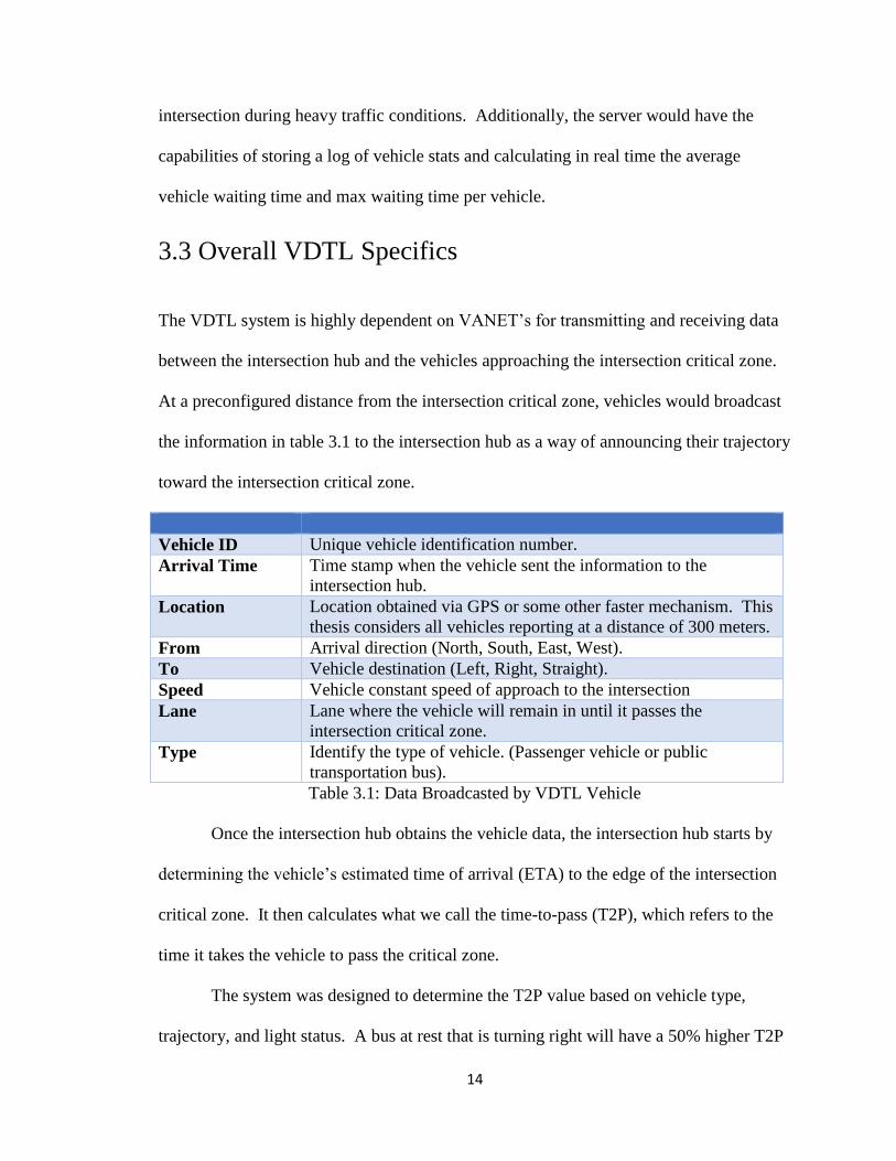
The VDTL system is highly dependent on VANET’s for transmitting and receiving data

between the intersection hub and the vehicles approaching the intersection critical zone.

At a preconfigured distance from the intersection critical zone, vehicles would broadcast

the information in table 3.1 to the intersection hub as a way of announcing their trajectory

toward the intersection critical zone.

Vehicle ID Unique vehicle identification number.

Arrival Time Time stamp when the vehicle sent the information to the

intersection hub.

Location Location obtained via GPS or some other faster mechanism. This

thesis considers all vehicles reporting at a distance of 300 meters.

From Arrival direction (North, South, East, West).

To Vehicle destination (Left, Right, Straight).

Speed Vehicle constant speed of approach to the intersection

Lane Lane where the vehicle will remain in until it passes the

intersection critical zone.

Type Identify the type of vehicle. (Passenger vehicle or public

transportation bus).

Table 3.1: Data Broadcasted by VDTL Vehicle

Once the intersection hub obtains the vehicle data, the intersection hub starts by

determining the vehicle’s estimated time of arrival (ETA) to the edge of the intersection

critical zone. It then calculates what we call the time-to-pass (T2P), which refers to the

time it takes the vehicle to pass the critical zone.

The system was designed to determine the T2P value based on vehicle type,

trajectory, and light status. A bus at rest that is turning right will have a 50% higher T2P

15

value than a passenger vehicle headed straight that is also at rest. If SLM is the amount of

time it takes a sedan in motion to turn left, SLR is the amount of time it would take a sedan

to turn left when starting at rest once it’s located at the edge of the intersection critical

zone. Similarly, BLM is the amount of time it would take a bus in motion to turn left and

BLR the time needed to turn left from rest. Equations 1, 2 and 3, below describe how we

calculated the timing for both sedans and buses at motion and rest. Such T2P equations

were determined by conducting a time study at a four-way intersection in Albuquerque,

NM.

𝑆𝐿𝑀 = 𝑥 | 𝑆𝐿𝑅 = 𝑥 + 0.33 ∗ 𝑥 𝐵𝐿𝑀 = 𝑥 | 𝐵𝐿𝑅 = 𝑥 + 0.25 ∗ 𝑥 (1)

𝑆𝑆𝑀 = 𝑦 | 𝑆𝑆𝑅 = 𝑦 + 0.50 ∗ 𝑦 𝐵𝑆𝑀 = 𝑦 | 𝐵𝑆𝑅 = 𝑦 + 0.33 ∗ 𝑦 (2)

𝑆𝑅𝑀 = 𝑧 | 𝑆𝑅𝑅 = 𝑧 + 0.10 ∗ 𝑧 𝐵𝑅𝑀 = 𝑧 | 𝐵𝑅𝑅 = 𝑧 + 0.50 ∗ 𝑧 (3)

The system is designed to assign a different T2P to vehicles that are part of a

platoon. As Figure 3.2 explains, the first vehicle in the platoon will be assigned a T2P

time that is based on vehicle trajectory, vehicle type, and waiting conditions. The rest of

the vehicles within that same platoon will get assigned a 1 second T2P, thus creating

some sort of capsule in which the first vehicle in the platoon always has a slightly higher

T2P. As previously mentioned, only the Pre-Time and Lazy Algorithms make use of the

platooning mechanism and therefore are capable of adjusting the T2P as explained in the

figure below.

16

54

3 2

6 7

1 Second T2P for the rest of the

platoon

Is assigned a T2P based on vehicle type, trajectory and

waiting conditions.

Figure 3.3: T2P for Vehicles in a Platoon

With knowledge of the vehicle’s ETA and T2P, the hub then searches for an

available time slot for the vehicle to cross the critical zone. If the ETA of the

approaching vehicle is before the last vehicle arrival, then the system adds it to the back

of the queue and adds a one-second delay as a safety guard. If the ETA is after the last

vehicle arrival, then the approaching vehicle is simply appended to the end of the queue.

If the time slot reserved by the intersection hub comes after the vehicle’s ETA, then the

vehicle will be forced to stop before crossing the intersection critical zone. The time slot

taken by the newly arrived vehicle is then reserved and time slots from other conflicting

trajectories are blocked for the duration of the vehicle’s T2P. As an example, a vehicle

arriving from the south and turning left would require that not only the time slot for his

lane be reserved but also the time slot for vehicles headed straight from the west. Figure

3.4 attempts to clarify the concept of time slot reservation by illustrating how multiple

vehicles in non-conflicting trajectories can arrive at slightly different times, yet still cross

the critical zone without stopping.

17

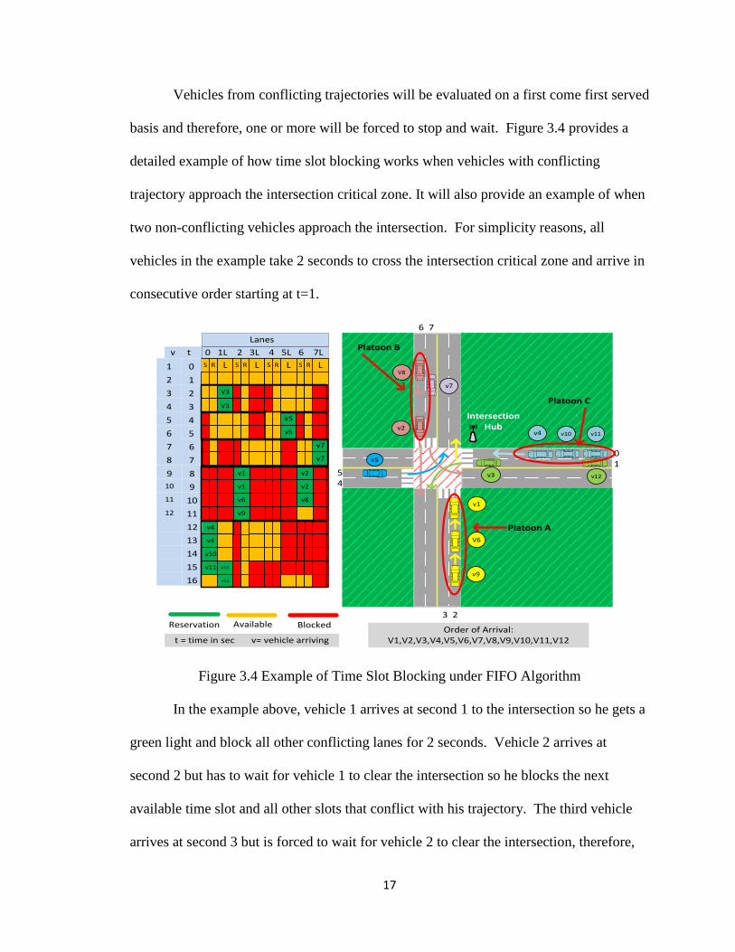
Vehicles from conflicting trajectories will be evaluated on a first come first served

basis and therefore, one or more will be forced to stop and wait. Figure 3.4 provides a

detailed example of how time slot blocking works when vehicles with conflicting

trajectory approach the intersection critical zone. It will also provide an example of when

two non-conflicting vehicles approach the intersection. For simplicity reasons, all

vehicles in the example take 2 seconds to cross the intersection critical zone and arrive in

consecutive order starting at t=1.

v t 0 1L 2 3L 4 5L 6 7L

V54

5

8

9

10

11

13

14

15

16

v5

v1 v2

v6 v8

v9

v4

v4

v10

v11 v12

v12

v1 v2

Reservation Available BlockedOrder of Arrival:

V1,V2,V3,V4,V5,V6,V7,V8,V9,V10,V11,V12

5

6

9

10

11

12

2

3

V3

V3

3

4

S L L L L0

1

R S S SR R R1

2

t = time in sec v= vehicle arriving

Lanes

01

54

3 2

6 7

Intersection Hub

v3

v1

v5

v2

V6

V8

v9

v4 v10 v11

12

v12

6 v77

7 v78

v7

Platoon A

Platoon B

Platoon C

Figure 3.4 Example of Time Slot Blocking under FIFO Algorithm

In the example above, vehicle 1 arrives at second 1 to the intersection so he gets a

green light and block all other conflicting lanes for 2 seconds. Vehicle 2 arrives at

second 2 but has to wait for vehicle 1 to clear the intersection so he blocks the next

available time slot and all other slots that conflict with his trajectory. The third vehicle

arrives at second 3 but is forced to wait for vehicle 2 to clear the intersection, therefore,

18

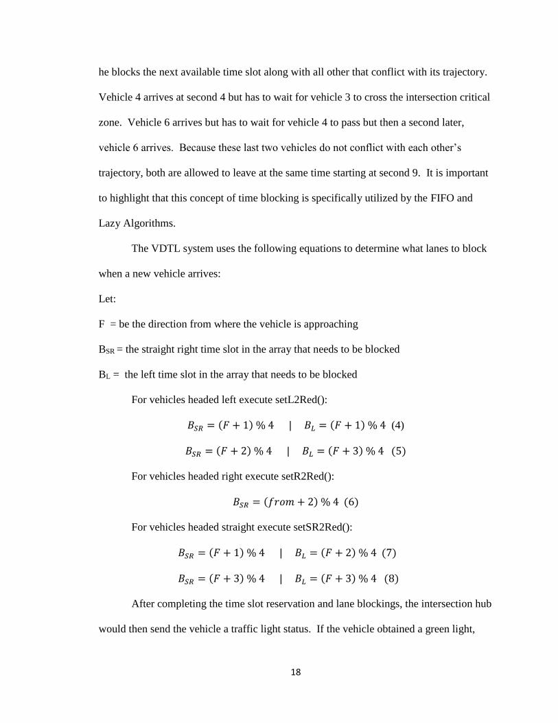
he blocks the next available time slot along with all other that conflict with its trajectory.

Vehicle 4 arrives at second 4 but has to wait for vehicle 3 to cross the intersection critical

zone. Vehicle 6 arrives but has to wait for vehicle 4 to pass but then a second later,

vehicle 6 arrives. Because these last two vehicles do not conflict with each other’s

trajectory, both are allowed to leave at the same time starting at second 9. It is important

to highlight that this concept of time blocking is specifically utilized by the FIFO and

Lazy Algorithms.

The VDTL system uses the following equations to determine what lanes to block

when a new vehicle arrives:

Let:

F = be the direction from where the vehicle is approaching

BSR = the straight right time slot in the array that needs to be blocked

BL = the left time slot in the array that needs to be blocked

For vehicles headed left execute setL2Red():

𝐵𝑆𝑅 = (𝐹 + 1) % 4 | 𝐵𝐿 = (𝐹 + 1) % 4 (4)

𝐵𝑆𝑅 = (𝐹 + 2) % 4 | 𝐵𝐿 = (𝐹 + 3) % 4 (5)

For vehicles headed right execute setR2Red():

𝐵𝑆𝑅 = (𝑓𝑟𝑜𝑚 + 2) % 4 (6)

For vehicles headed straight execute setSR2Red():

𝐵𝑆𝑅 = (𝐹 + 1) % 4 | 𝐵𝐿 = (𝐹 + 2) % 4 (7)

𝐵𝑆𝑅 = (𝐹 + 3) % 4 | 𝐵𝐿 = (𝐹 + 3) % 4 (8)

After completing the time slot reservation and lane blockings, the intersection hub

would then send the vehicle a traffic light status. If the vehicle obtained a green light,

19

01

54

3 2

6 7

Intersection Hub

#1

#3

#2#4

Vehicle A

Vehicle B

Vehicle C

Vehicle D

which would mean that it can continue its trajectory toward the intersection critical zone

without stopping. If the vehicle receives a red light with a countdown, this would result

in the vehicle having to stop at the edge of the critical zone for a set amount of seconds.

The countdown clock would not start counting down until the vehicle is at rest at the edge

of the intersection critical zone. The concept of deceleration as the vehicle approaches

the intersections is not being considered in our simulation.

The intersection hub vehicle light status response process would look something

similar to what is described figure 3.5.

Figure 3.5: Intersection Hub Light Status Response

In this case, vehicles A, B, and C would see a green light in their dashboard since

the intersection hub would detect non-conflicting trajectories. On the other hand, because

vehicle D was the last one to report to the intersection hub and the critical zone is already

busy, it will be forced to stop. As a result, vehicle D would see a countdown red light

indicating to the driver that it must stop at the edge of the intersection critical zone and

wait until the light turns to green.

20

A final step for the intersection hub is to calculate the vehicle’s estimated time of

departure (ETD). The ETD is the time when the vehicle has completely cleared the

intersection critical zone. Ideally, this task could be performed after a light status

response is sent to the vehicle and kept for statistical reasons.

Throughout this process, it is assumed that vehicles will maintain lane position,

trajectory, and constant speed. The equation below is used to determine the time window

available for a two-way communication between the vehicle and intersection hub.

𝑆𝑝𝑒𝑒𝑑 𝑖𝑛 𝑚𝑝𝑠 = 𝑠𝑝𝑒𝑒𝑑 (𝑚𝑝ℎ) (9)

𝑡𝑖𝑚𝑒(sec) =𝑑𝑖𝑠𝑡𝑎𝑛𝑐𝑒 (𝑚𝑒𝑡𝑒𝑟𝑠)

𝑠𝑝𝑒𝑒𝑑 (𝑚𝑝𝑠) (10)

As an example, it would take a vehicle 19.8 seconds to get to the intersection

critical zone when traveling at 35mph and at a distance of 300 meters. In our design, we

assume that all vehicles will initialize communication with the intersection hub at 300

meters and that their speed varies between 35mph and 25mph. As such, it is highly

suggested that all communication between the vehicle and intersection hub happen within

a 10-second window. If the communication time window is missed, there is a very high

potential of two of more vehicles colliding. As previously mentioned, all requests to

make use of the intersection critical zone would be processed on a first come first serve

basis. Communication contention from two vehicles with conflicting directions is not

being considered in this paper.

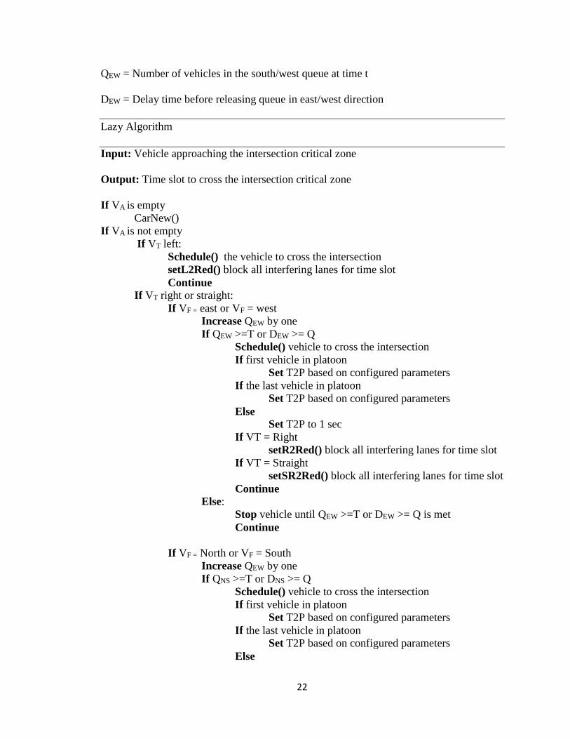
3.4 Lazy Algorithm

Perhaps the most valuable contribution to this research is the heuristic Lazy Algorithm

21

being proposed. This algorithm attempts to reach a middle ground between the Pre-

Time existing model and other proposed methods that we believe worsen conditions

rather than improving them [11]. To do this, a unique approach was taken where vehicles

are evaluated not only on an individual basis but also as a platoon. This concept becomes

particularly important during heavy and moderate traffic conditions where other solutions

have proven to become equivalent to a 4-way stop.

The algorithm uses a combination of parameters, such as vehicle queue count and

time delay, to determine if vehicles headed in a straight or right direction are required to

wait before entering the intersection critical zone. By using a combination of vehicle

queue count and time delay, we open the possibility of allowing two or more vehicle

access to the critical zone as a group rather than individually. The actual flow for the

Lazy Algorithm is as follows.

Let:

Schedule() = function used to determine the time slot to be used by a vehicle

CarNew() = function that generates vehicles based on Poisson Distribution

HandleCross() = function that dispatches the vehicles once they have been scheduled

T = Time delay configured

Q = Vehicle Q size configured

VA = Vehicle arrival array

VF = Direction from where the vehicle is arrives at the intersection

VT = Direction where vehicle is headed after crossing the intersection

QNS = Number of vehicles in the north/south queue at time t

DNS = Delay time before releasing queue in north/south direction

22

QEW = Number of vehicles in the south/west queue at time t

DEW = Delay time before releasing queue in east/west direction

Lazy Algorithm

Input: Vehicle approaching the intersection critical zone

Output: Time slot to cross the intersection critical zone

If VA is empty

CarNew()

If VA is not empty

If VT left:

Schedule() the vehicle to cross the intersection

setL2Red() block all interfering lanes for time slot

Continue If VT right or straight:

If VF = east or VF = west

Increase QEW by one

If QEW >=T or DEW >= Q

Schedule() vehicle to cross the intersection

If first vehicle in platoon

Set T2P based on configured parameters

If the last vehicle in platoon

Set T2P based on configured parameters

Else Set T2P to 1 sec

If VT = Right

setR2Red() block all interfering lanes for time slot

If VT = Straight

setSR2Red() block all interfering lanes for time slot

Continue

Else:

Stop vehicle until QEW >=T or DEW >= Q is met

Continue

If VF = North or VF = South

Increase QEW by one

If QNS >=T or DNS >= Q

Schedule() vehicle to cross the intersection

If first vehicle in platoon

Set T2P based on configured parameters

If the last vehicle in platoon

Set T2P based on configured parameters

Else

23

Set T2P to 1 sec

If VT = Right

setR2Red() block all interfering lanes for time slot

If VT = Straight

setSR2Red() block all interfering lanes for time slot

Continue

Else:

Stop vehicle until QNS >=T or DNS >= Q is met

Continue

for each direction

HandleCross() Dispatch Vehicle according to the scheduling array

Figure 3.6: Lazy Algorithm Pseudo Code

The important aspect to understand about the Lazy Algorithm is that vehicles headed

in a straight and right direction are forced to wait a set amount of time or until a vehicle

quorum count is met before being allowed to use the intersection critical zone.

Additionally, the T2P for the first vehicle in the platoon is based on vehicle type,

trajectory, and vehicle motion. All vehicles processing the leading vehicle in a platoon

are assigned a 1 second T2P because it is expected that vehicles will already be in motion

by the time they get to the edge of the intersection critical zone. Finally, keep in mind

that the Lazy Algorithm parameters are configured to avoid becoming a 4-way stop

during heavy and moderate traffic conditions.

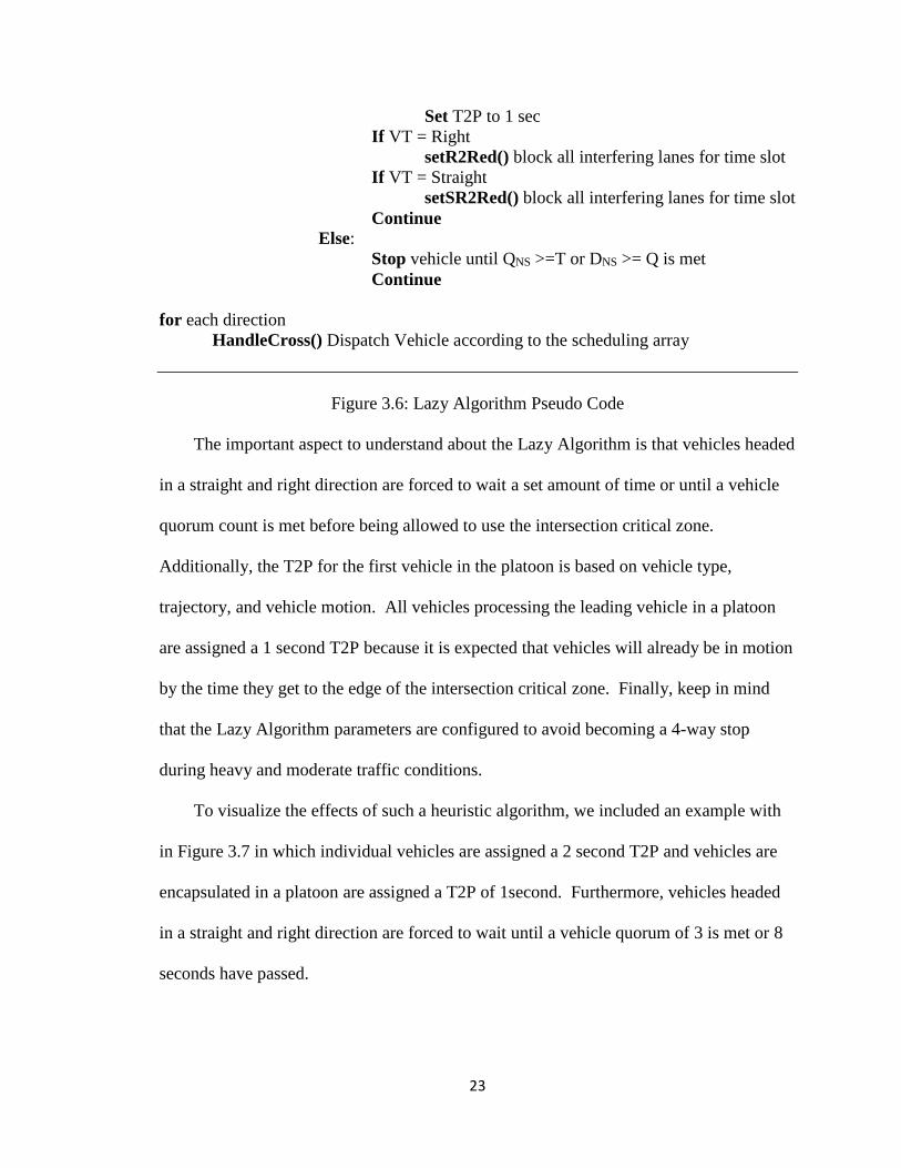
To visualize the effects of such a heuristic algorithm, we included an example with

in Figure 3.7 in which individual vehicles are assigned a 2 second T2P and vehicles are

encapsulated in a platoon are assigned a T2P of 1second. Furthermore, vehicles headed

in a straight and right direction are forced to wait until a vehicle quorum of 3 is met or 8

seconds have passed.

24

v t 0 1L 2 3L 4 5L 6 7L

V54

5

8

9

10

11

13

14

15

16

v5

v1 v2

v6 v8

v9

v4

v4

v10

v11 v12

v12

v1 v2

Reservation Available BlockedOrder of Arrival:

V1,V2,V3,V4,V5,V6,V7,V8,V9,V10,V11,V12

5

6

9

10

11

12

2

3

V3

V3

3

4

S L L L L0

1

R S S SR R R1

2

t = time in sec v= vehicle arriving

Lanes

01

54

3 2

6 7

Intersection Hub

v3

v1

v5

v2

V6

V8

v9

v4 v10 v11

12

v12

6 v77

7 v78

v7

Platoon A

Platoon B

Platoon C

Figure 3.7: Example of Time Slot Blocking under Lazy Algorithm

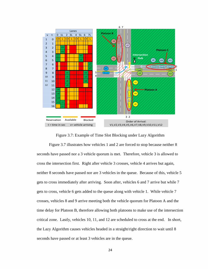
Figure 3.7 illustrates how vehicles 1 and 2 are forced to stop because neither 8

seconds have passed nor a 3 vehicle quorum is met. Therefore, vehicle 3 is allowed to

cross the intersection first. Right after vehicle 3 crosses, vehicle 4 arrives but again,

neither 8 seconds have passed nor are 3 vehicles in the queue. Because of this, vehicle 5

gets to cross immediately after arriving. Soon after, vehicles 6 and 7 arrive but while 7

gets to cross, vehicle 6 gets added to the queue along with vehicle 1. While vehicle 7

crosses, vehicles 8 and 9 arrive meeting both the vehicle quorum for Platoon A and the

time delay for Platoon B, therefore allowing both platoons to make use of the intersection

critical zone. Lastly, vehicles 10, 11, and 12 are scheduled to cross at the end. In short,

the Lazy Algorithm causes vehicles headed in a straight/right direction to wait until 8

seconds have passed or at least 3 vehicles are in the queue.

25

While the proposed heuristic algorithm provides what we believe to be an

improvement to the intersection average waiting time, it is not the optimal solution to the

problems. In this thesis, we focused on obtaining a solution that could provide an

improvement over the well-known Pre-Time Algorithm and FIFO Algorithm developed

by [11]. Furthermore, the fact that our algorithm targets traffic headed in the straight and

right direction is based on the assumption that a particular traffic intersection has more

vehicles headed in the straight and right direction. During the design process, attempts

were made to delay vehicles making a left turn. However, such an approach resulted in an

increase in average waiting time which we attribute to the small amount of vehicles

headed in the left direction in comparison to those headed straight or right direction.

3.5 System Dependencies & Limitations

As previously mentioned, the VDTL system would be highly depended on an ad-hoc

wireless network capable of reaching a preconfigured distance. Vehicles crossing the

intersection would be required to have a VDTL device installed and communicate to the

intersection transceiver at a distance of at least 300 meters. Vehicles approaching the

intersection will need to maintain a constant speed that is between the system’s specified

speed ranges and not change lanes. The possibility of having vehicles stranded on the

intersection is not being considered as part of this paper and overall system design.

Once a vehicle receives a response from the intersection hub on its scheduled time

to cross the intersection, all communications between the two are terminated and no

further updates are possible. In other words, the system is not designed to alter an

already issued cross schedule. Once vehicles are given a green light, the deceleration

speed that is caused by turns is indirectly considered. Vehicle deceleration is considered

26

in the amount of time we specify that it takes a vehicle to cross the intersection. Vehicles

turning left and right will require more time to cross the intersection critical zone than a

vehicle headed in a straight direction. Finally, it is assumed that vehicles will continue

to be driven by humans.

3.6 System Parameters

There is a clear understanding that not all intersections are built in a perpendicular

direction and that all possesses a different traffic flow. For this reason, the algorithm

offers the capability of adjusting the vehicle arrival rate per direction, the vehicle queue

size and waiting time per direction. As previously mentioned, our algorithm reduces the

average waiting time by not only considering what is beneficial to individual vehicles but

rather the platoon as a whole. To make this possible, a combination of queue time delay

and vehicle count are considered when determining if a vehicle gets a green light.

Another important and crucial feature that we feel adds a more realistic approach

to our solutions is the consideration of the variable time required for vehicles to cross the

intersection critical zone. The time to pass (T2P) is the time it takes a vehicle to clear the

intersection critical zone based on its type and speed. For instance, a vehicle at rest

would require more time to clear the intersection than a vehicle that is already in motion.

Furthermore, a vehicle at rest will require less time to pass the intersection than a bus at

the intersection. This is why it is very important the intersection hub knows what type of

vehicle is making the request as this will help it determine the time to pass. For this

reason, the T2P parameter is also modifiable.

27

In our design, we considered vehicles approaching the intersection at speeds

between 11.2 mps-15.6mps and a distance of 300 meters. Nevertheless, we understand

there is a possibility of using this system at intersections that allow a narrower or wider

range. Therefore, we have included a parameter to adjust the speed range and the

distance where communication is initiated. Table 3.3 goes over the list of parameters that

can be modified in the code.

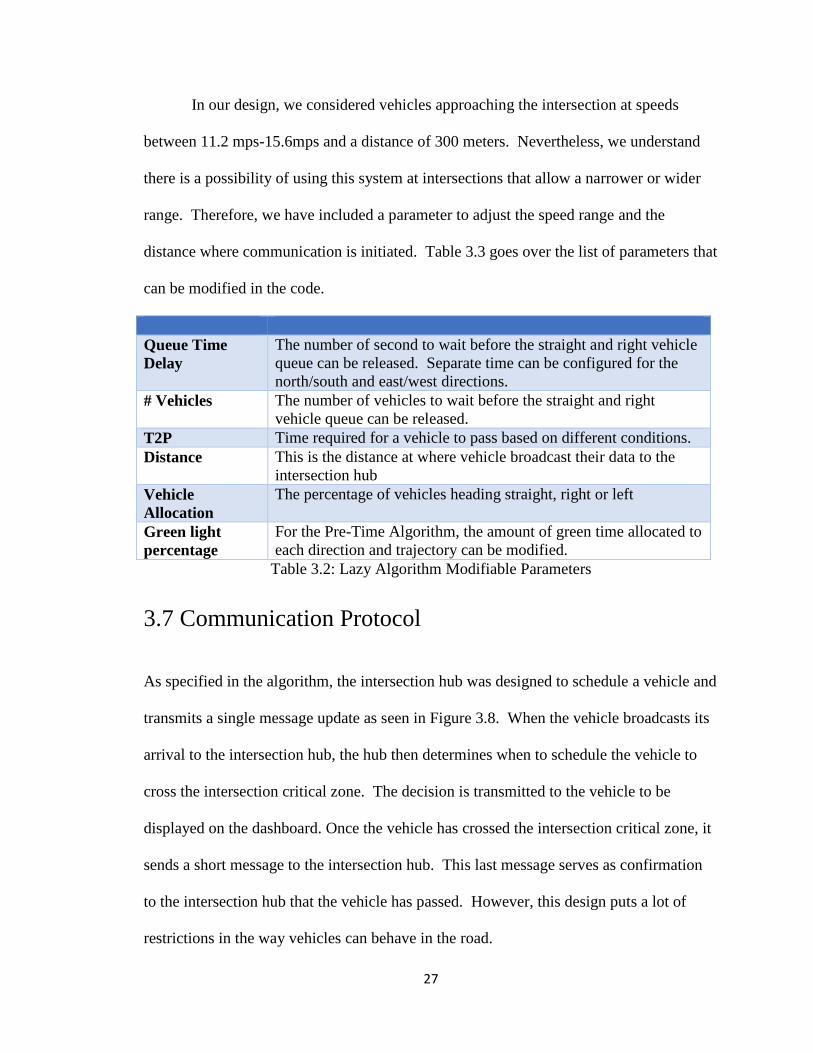
Queue Time

Delay

The number of second to wait before the straight and right vehicle

queue can be released. Separate time can be configured for the

north/south and east/west directions.

# Vehicles The number of vehicles to wait before the straight and right

vehicle queue can be released.

T2P Time required for a vehicle to pass based on different conditions.

Distance This is the distance at where vehicle broadcast their data to the

intersection hub

Vehicle

Allocation

The percentage of vehicles heading straight, right or left

Green light

percentage

For the Pre-Time Algorithm, the amount of green time allocated to

each direction and trajectory can be modified.

Table 3.2: Lazy Algorithm Modifiable Parameters

3.7 Communication Protocol

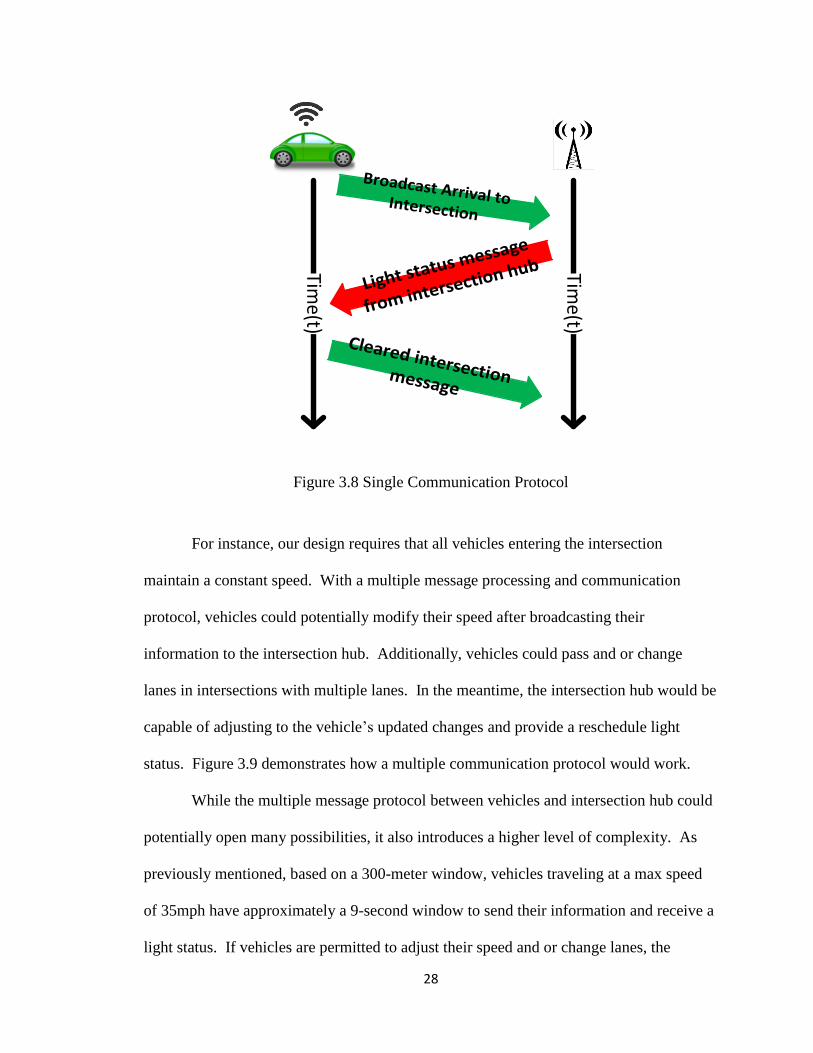
As specified in the algorithm, the intersection hub was designed to schedule a vehicle and

transmits a single message update as seen in Figure 3.8. When the vehicle broadcasts its

arrival to the intersection hub, the hub then determines when to schedule the vehicle to

cross the intersection critical zone. The decision is transmitted to the vehicle to be

displayed on the dashboard. Once the vehicle has crossed the intersection critical zone, it

sends a short message to the intersection hub. This last message serves as confirmation

to the intersection hub that the vehicle has passed. However, this design puts a lot of

restrictions in the way vehicles can behave in the road.

28

Time(t)

Time(t)

Broadcast Arrival to Intersection

Light status message

from intersection hub

Cleared intersection message

Figure 3.8 Single Communication Protocol

For instance, our design requires that all vehicles entering the intersection

maintain a constant speed. With a multiple message processing and communication

protocol, vehicles could potentially modify their speed after broadcasting their

information to the intersection hub. Additionally, vehicles could pass and or change

lanes in intersections with multiple lanes. In the meantime, the intersection hub would be

capable of adjusting to the vehicle’s updated changes and provide a reschedule light

status. Figure 3.9 demonstrates how a multiple communication protocol would work.

While the multiple message protocol between vehicles and intersection hub could

potentially open many possibilities, it also introduces a higher level of complexity. As

previously mentioned, based on a 300-meter window, vehicles traveling at a max speed

of 35mph have approximately a 9-second window to send their information and receive a

light status. If vehicles are permitted to adjust their speed and or change lanes, the

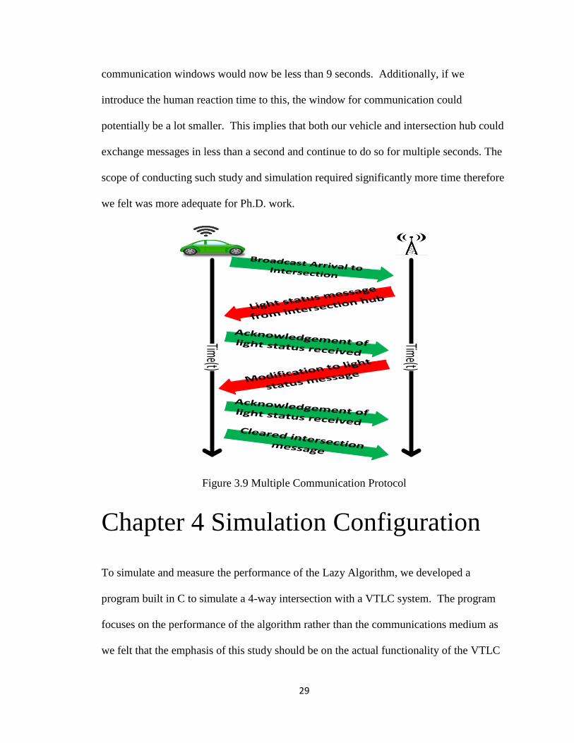
29

communication windows would now be less than 9 seconds. Additionally, if we

introduce the human reaction time to this, the window for communication could

potentially be a lot smaller. This implies that both our vehicle and intersection hub could

exchange messages in less than a second and continue to do so for multiple seconds. The

scope of conducting such study and simulation required significantly more time therefore

we felt was more adequate for Ph.D. work.

Figure 3.9 Multiple Communication Protocol

Chapter 4 Simulation Configuration

To simulate and measure the performance of the Lazy Algorithm, we developed a

program built in C to simulate a 4-way intersection with a VTLC system. The program

focuses on the performance of the algorithm rather than the communications medium as

we felt that the emphasis of this study should be on the actual functionality of the VTLC

Time(t)

Time(t)

Broadcast Arrival to Intersection

Light status message

from intersection hub

Cleared intersection message

Acknowledgement of light status received

Modification to light

status message

Acknowledgement of light status received

30

systems in combination with the algorithm. While the developed program turned out a

bit complex, the basic functionality was built on three main components: vehicle arrival,

vehicle scheduling, and vehicle dispatch.

4.1 Vehicle Arrival

The first component of our simulation consisted of developing a mechanism to simulate

random vehicles approaching the intersection. To make this possible, we constructed a

NewVehicle function in which we create a vehicle and then used Poisson distribution

function to randomly re-execute the NewVehicle function. By doing this, we simulate

the arrival of the first vehicle and the let Poisson distribution function determine when the

next vehicle should arrive. The reason we used Poisson distribution is it would allow us

to generate a discrete integer by specifying a desired mean value. The Poisson Mass

Distribution Function (PMF) is as follows:

𝑃(𝑜𝑓 𝑘 𝑒𝑣𝑒𝑛𝑡𝑠 ℎ𝑎𝑝𝑝𝑒𝑛𝑖𝑛𝑔) = 𝜆𝑘𝑒−𝜆

𝑘! (11)

𝑤ℎ𝑒𝑟𝑒:

𝜆 = 𝑎𝑣𝑒𝑟𝑎𝑔𝑒 𝑛𝑢𝑚𝑏𝑒𝑟 𝑜𝑓 𝑒𝑣𝑒𝑛𝑡𝑠

𝑒 = 𝐸𝑢𝑙𝑒𝑟′𝑠 𝑛𝑢𝑚𝑏𝑒𝑟 2.71828

𝑘 = 𝑎𝑛 𝑖𝑛𝑡𝑒𝑔𝑒𝑟 𝑠𝑡𝑎𝑟𝑡𝑖𝑛𝑔 𝑎𝑡 𝑧𝑒𝑟𝑜

𝑘! = 𝑡ℎ𝑒 𝑓𝑎𝑐𝑡𝑜𝑟𝑖𝑎𝑙 𝑜𝑓 𝐾

Therefore, configuring an arrival rate with a mean of 8 would result in 7.5 vehicles

arriving per minute per direction totaling 30 in all directions. It is important to highlight

that the mean value does not specify the vehicle arrival rate but rather when the

NewVehicle function is called for the next vehicle to arrive. Table 4.1 goes over the

mean parameter used for each of the traffic condition used in this study.

31

Traffic Conditions Poisson Mean Intersection Vehicle Rate of Arrival

Light 8 30 vehicles/minute

Moderate 7 34.28 vehicles/minute

Heavy 6 40 vehicles/minute

Table 4.1: Definition of Traffic Conditions

Once the vehicle arrived, we then needed to come up with the additional

parameters that would normally be provided by the vehicle approaching the intersection.

Table 4.1 goes over these parameters and the possible values that each could take.

Parameter Possible Values

Vehicle ID Auto increasing integer number that starts at 0 and

increases by one.

Distance This is the distance at where the vehicle starts

communicating with the intersection hub. Based on our

code, this could be set to any value.

From The program is set to assign a vehicle from each

direction (East, South, West, and North) each second.

To Randomly selected code where the vehicle is headed to

(Straight, Right, Left) based on the specified parameters.

Speed Lower Bound Specify the lower bound that can be randomly selected

for vehicle speed.

Speed Upper Bound Specify the upper bound that can be randomly selected

for vehicle speed.

Lane Identify where the vehicle is located based on the To

direction mentioned above,

Type Randomly select the type of vehicle (Sedan or Bus)

based on the parameter specified

Table 4.2: List of Vehicle Parameters Available

In addition to the parameters above, our code also offers the option to change a set of

global parameters. Table 4.3, goes over the global parameters:

Parameter Possible Values

Time Specify the simulation time in seconds

Mean Specifies the mean separation between vehicles arriving

at a single side of the intersection.

Lazy Switch Specify if the Lazy Algorithm is enabled (1=ON)

Vehicle Queue Timer (Available only on Lazy Algorithm) Specify the amount

of time a vehicle has to wait before being issues a green

light.

32

01

54

3 2

6 7

Intersection Hub

These Vehicles will be forced to match the speed of the

vehicle in front.

EW Queue Size (Available only on Lazy Algorithm) Specify the amount

of vehicles that need to be in the East/West queue before

being issued a green light.

NS Queue Size (Available only on Lazy Algorithm) Specify the amount

of vehicles that need to be in the North/South queue

before being issued a green light.

Cycle Time Total light cycle time in seconds. (Available only on the

Pre-Time Algorithm)

Left Turn Time Duration Green light time allocated to left turns in seconds.

(Available only on the Pre-Time Algorithm)

Straight/Right Time

Duration

Green light time allocated to straight/right in seconds.

(Available only on the Pre-Time Algorithm)

Table 4.3: Program Global Parameters

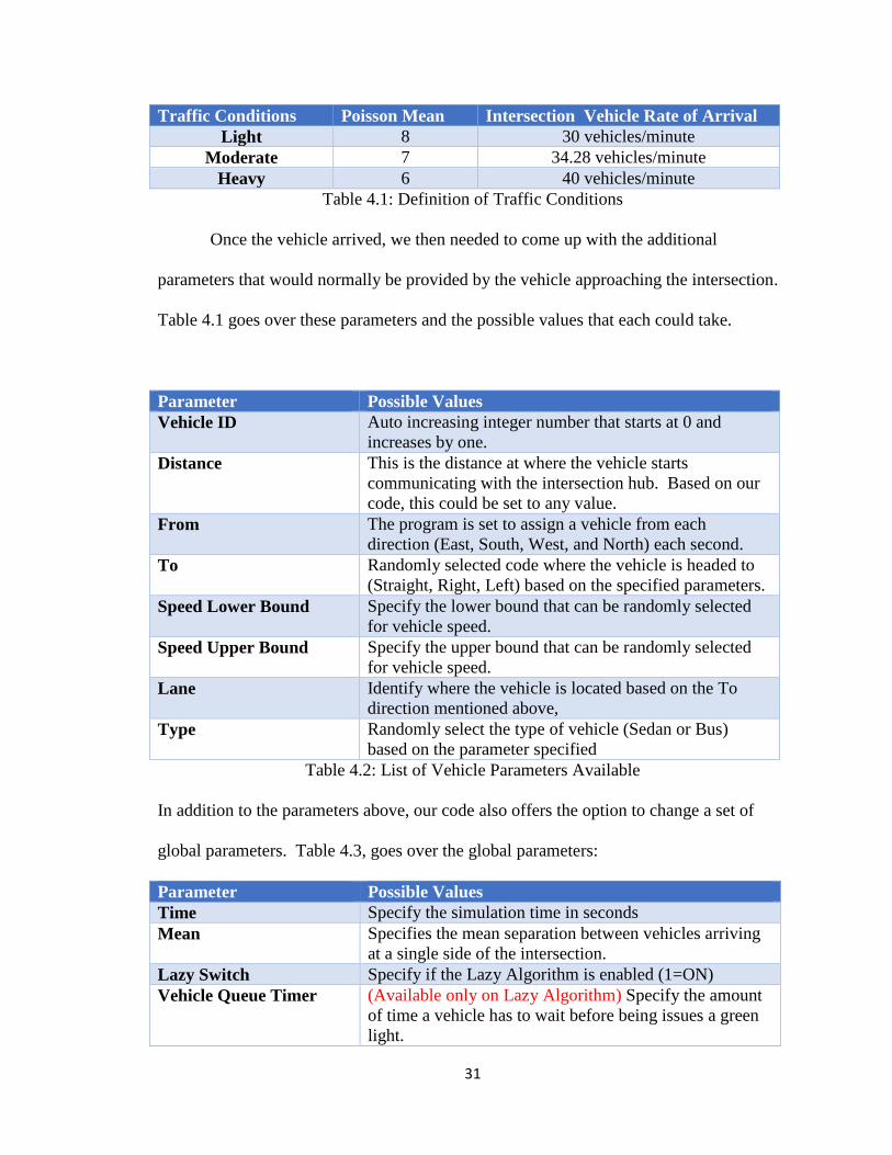
It is important to highlight that vehicles arriving from a lane that already had a

vehicle waiting to cross would be forced to match the speed of the vehicle in front.

Adjusting the speed would prevent a vehicle pileup at the intersection. Figure 4.1

illustrates an instance of when vehicle speed would need to be matched by the vehicle in

front. The actual mechanism to adjust the vehicle speed was not explored in this paper.

Figure 4.1: Vehicles Speed Adjustments

33

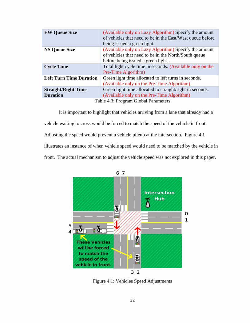
After all the vehicle parameters have been identified, the code then adds the

vehicle to a first-in-first-out (FIFO) queue (Linked List) in which it keeps track of the

order each vehicle arrived.

*DATA

*NEXT

Node 0

*DATA

*NEXT

Node 1

*DATA

*NEXT

Node 2

Figure 4.2: Linked List Used as Queue

As seen in figure 4.2, Node 0 would contain the information regarding the first vehicle

that arrives at the intersection. The *Next pointer for Node 0 would hold the address of

the next vehicle pointer. By taking this approach, we avoid running out of memory as we

keep adding vehicles to the simulations.

4.2 Vehicle Scheduling

The second major component of our simulation code involved the actual scheduling of

the vehicles. This involves determining when the vehicle is scheduled to make use of the

intersection critical zone. To do so, our code first finds the last time slot taken by a

vehicle located in the same lane as the new vehicle. If the intersection hub determines

that the new vehicle will arrive at the intersection critical zone before the last vehicle, it

automatically blocked a second at the back and append the new vehicle. The one-second

separation was added as a precautionary measure. On the other hand, if the intersection

hub determines that the new vehicle will arrive after the last vehicle, it simply adds the

new vehicle to the back of the queue. After the new vehicle is placed in the appropriate

time slot, the time slots for conflicting lanes are also blocked.

34

01

54

3 2

6 7

Intersection Hub

The bus will block the

intersection for a few seconds more than the

sedan

This vehicle needs the bus

and car to clear the intersection before he can

go

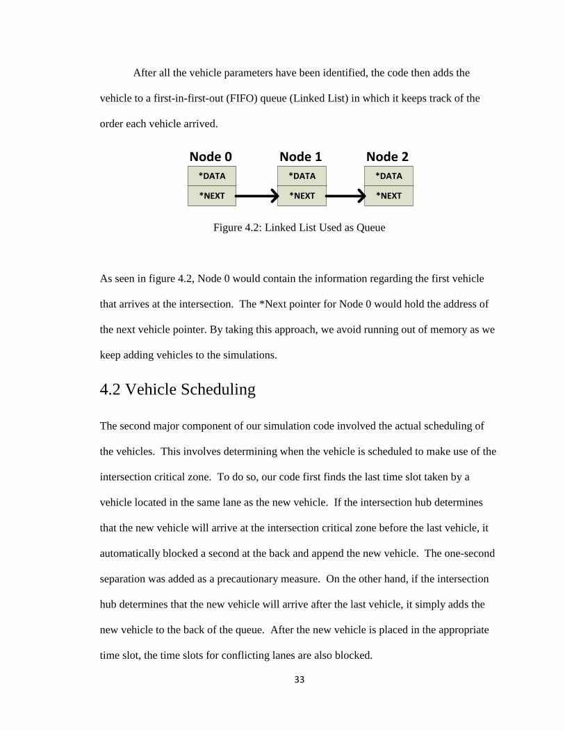
During this stage, we also assign what we call the time-to-pass (T2P) parameter.

As previously mentioned, the T2P is the time, in seconds, it takes a vehicle to cross the

intersection critical zone. The T2P times become particularly important when two

vehicles with conflicting trajectories are needing to make use of the critical zone. As see

in figure 4.2 below.

Figure 4.3: Illustration of Time-to-Pass (T2P) based on Vehicle Type

4.3 Vehicle Dispatch

In the final stage of our simulation code, we simply process the vehicles in the order they

got put into the time slot array and queue. The time slot array specifies the exact time

when a vehicle should be allowed to use the intersection critical zone. The queue simply

keeps track of the order but not the time. A combination of arrays and queues were used

as a precautionary measure to ensure vehicles got processed in the correct order.

Therefore, in our simulation code, we check to make sure that the vehicle specified in the

35

time slot array matches what is next on the queue. Once the vehicle is released to cross

the intersection critical zone, the code starts collecting as much statistical information as

possible to find the average waiting time, longest waiting time, and percent of stopping

vehicles among others. A copy of the code is provided in appendix A and a brief

overview of the functions and their order of execution are illustrated in figure 4.3.

CarArrive (dir, sec)

-CarNew (dir, to) [Added to queue]

-IdentofyLane (dir, to)

-SchedCross (newptr, sec) [Added to time slot array]

-t2p (schedT, type, to, eta)

-CarPrint (newptr, sec)

HandleCross (dir, sec)

CarPass (carptr, dir)

Figure 4.4: Simulation Code Execution Order

Chapter 5 Simulation Scenarios

To effectively evaluate the performance of our Lazy Algorithm, we decided to compare it

with the standard Pre-Time Algorithm and the FIFO Algorithm proposed by [11]. The

performance of each algorithm was evaluated in terms of average waiting time,

intersection throughput and percent of stopping vehicles under light, moderate and heavy

traffic conditions.

Furthermore, we wanted to compare the performance of both the FIFO and Lazy

Algorithm through a second 4-way DVTL equipped intersection. The average waiting

time for each intersection would then be recorded to see if a second intersection improves

of worsens the overall traffic flow. It is important to highlight that our focus was placed

36

on a single direction, meaning that we studied the average waiting time for vehicles

exiting the first intersection from the west and entering the second intersection from the

east.

5.1 Parameter Selection

Before testing each algorithm, we first needed to determine parameters such as T2P and

vehicle arrival rate among others. The values obtained are intended for simulation

purposes and therefore can be adjusted as needed.

As previously mentioned, the T2P values were determined by conducting a time

study at an intersection located in Albuquerque, NM. Table 5.1 are the results we

obtained and the values we decided to use in all of our scenarios.

Time to Pass(T2P)

Sedans Buses

Motion Rest Motion Rest

Left 3 sec 4 sec 4 sec 5 sec

Straight 2 sec 3 sec 3 sec 4 sec

Right 1 sec 2 sec 2 sec 3 sec

Table 5.1: T2P Times used in Simulation

As seen in table 5.1, sedans and buses have different T2P based on where they are

going and if they are at rest.

To effectively identify the light, moderate, and heavy traffic conditions, we first

needed to identify the intersection average occupancy, where the vehicle occupancy is

defined as the number of vehicles that could simultaneously make use of the intersection

critical zone. To evaluate our intersection, we came up with the maximum and minimum

intersection critical zone occupancy.

37

01

54

6 7

Intersection Hub

Total: 6 vehicles 4: Right2: Left

3 2

01

54

6 7

Intersection Hub

Total: 2 vehicles

2: Straight

3 2

Figure 5.1: Max Intersection Occupancy Figure 5.2: Min Intersection Occupancy

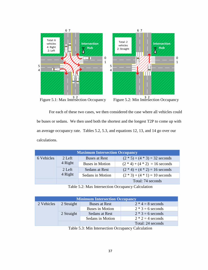
For each of these two cases, we then considered the case where all vehicles could

be buses or sedans. We then used both the shortest and the longest T2P to come up with

an average occupancy rate. Tables 5.2, 5.3, and equations 12, 13, and 14 go over our

calculations.

Maximum Intersection Occupancy

6 Vehicles 2 Left

4 Right

Buses at Rest (2 * 5) + (4 * 3) = 32 seconds

Buses in Motion (2 * 4) + (4 * 2) = 16 seconds

2 Left

4 Right

Sedans at Rest (2 * 4) + (4 * 2) = 16 seconds

Sedans in Motion (2 * 3) + (4 * 1) = 10 seconds

Total: 74 seconds

Table 5.2: Max Intersection Occupancy Calculation

Minimum Intersection Occupancy

2 Vehicles 2 Straight Buses at Rest 2 * 4 = 8 seconds

Buses in Motion 2 * 3 = 6 seconds

2 Straight Sedans at Rest 2 * 3 = 6 seconds

Sedans in Motion 2 * 2 = 4 seconds

Total: 24 seconds

Table 5.3: Min Intersection Occupancy Calculation

38

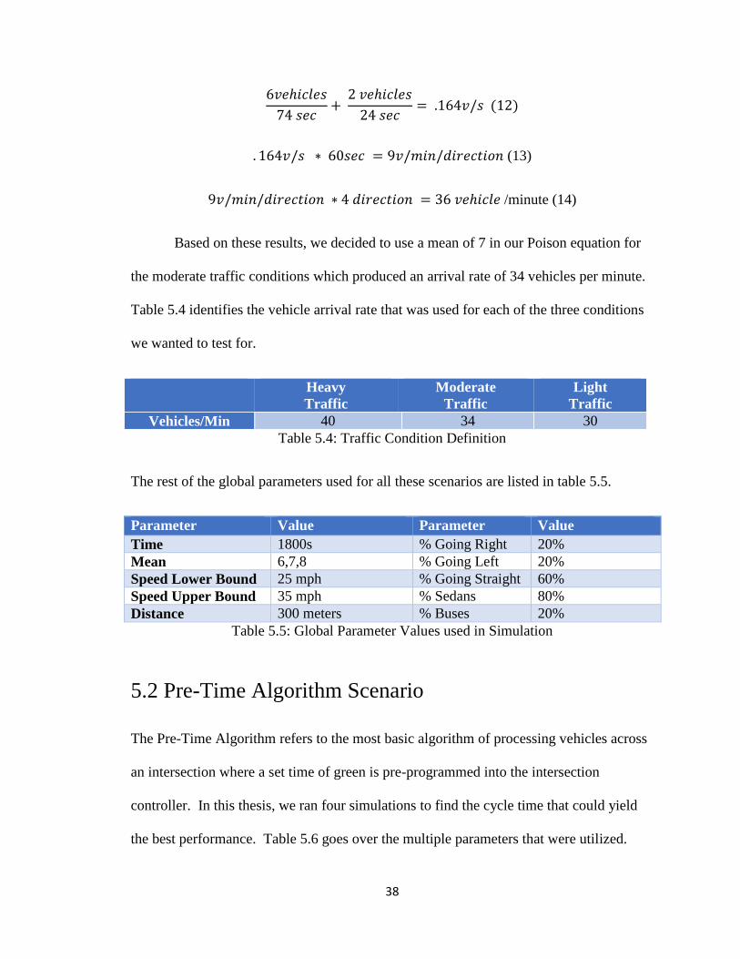
6𝑣𝑒ℎ𝑖𝑐𝑙𝑒𝑠

74 𝑠𝑒𝑐+

2 𝑣𝑒ℎ𝑖𝑐𝑙𝑒𝑠

24 𝑠𝑒𝑐= .164𝑣/𝑠 (12)

. 164𝑣/𝑠 ∗ 60𝑠𝑒𝑐 = 9𝑣/𝑚𝑖𝑛/𝑑𝑖𝑟𝑒𝑐𝑡𝑖𝑜𝑛 (13)

9𝑣/𝑚𝑖𝑛/𝑑𝑖𝑟𝑒𝑐𝑡𝑖𝑜𝑛 ∗ 4 𝑑𝑖𝑟𝑒𝑐𝑡𝑖𝑜𝑛 = 36 𝑣𝑒ℎ𝑖𝑐𝑙𝑒 /minute (14)

Based on these results, we decided to use a mean of 7 in our Poison equation for

the moderate traffic conditions which produced an arrival rate of 34 vehicles per minute.

Table 5.4 identifies the vehicle arrival rate that was used for each of the three conditions

we wanted to test for.

Heavy

Traffic

Moderate

Traffic

Light

Traffic

Vehicles/Min 40 34 30

Table 5.4: Traffic Condition Definition

The rest of the global parameters used for all these scenarios are listed in table 5.5.

Parameter Value Parameter Value

Time 1800s % Going Right 20%

Mean 6,7,8 % Going Left 20%

Speed Lower Bound 25 mph % Going Straight 60%

Speed Upper Bound 35 mph % Sedans 80%

Distance 300 meters % Buses 20%

Table 5.5: Global Parameter Values used in Simulation

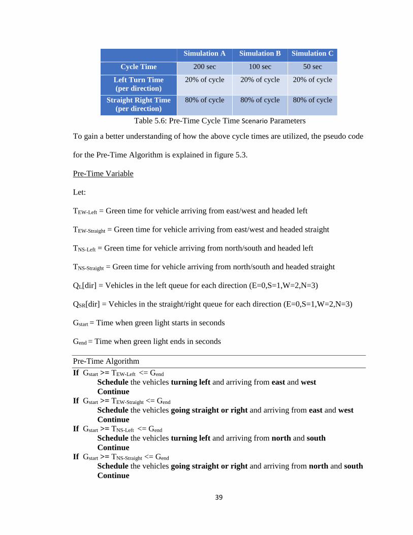
5.2 Pre-Time Algorithm Scenario

The Pre-Time Algorithm refers to the most basic algorithm of processing vehicles across

an intersection where a set time of green is pre-programmed into the intersection

controller. In this thesis, we ran four simulations to find the cycle time that could yield

the best performance. Table 5.6 goes over the multiple parameters that were utilized.

39

Simulation A Simulation B Simulation C

Cycle Time 200 sec 100 sec 50 sec

Left Turn Time

(per direction)

20% of cycle 20% of cycle 20% of cycle

Straight Right Time

(per direction)

80% of cycle 80% of cycle 80% of cycle

Table 5.6: Pre-Time Cycle Time Scenario Parameters

To gain a better understanding of how the above cycle times are utilized, the pseudo code

for the Pre-Time Algorithm is explained in figure 5.3.

Pre-Time Variable

Let:

TEW-Left = Green time for vehicle arriving from east/west and headed left

TEW-Straight = Green time for vehicle arriving from east/west and headed straight

TNS-Left = Green time for vehicle arriving from north/south and headed left

TNS-Straight = Green time for vehicle arriving from north/south and headed straight

QL[dir] = Vehicles in the left queue for each direction (E=0,S=1,W=2,N=3)

QSR[dir] = Vehicles in the straight/right queue for each direction (E=0,S=1,W=2,N=3)

Gstart = Time when green light starts in seconds

Gend = Time when green light ends in seconds

Pre-Time Algorithm

If Gstart >= TEW-Left <= Gend

Schedule the vehicles turning left and arriving from east and west

Continue If Gstart >= TEW-Straight <= Gend

Schedule the vehicles going straight or right and arriving from east and west

Continue If Gstart >= TNS-Left <= Gend

Schedule the vehicles turning left and arriving from north and south

Continue If Gstart >= TNS-Straight <= Gend

Schedule the vehicles going straight or right and arriving from north and south

Continue

40

Repeat the cycle

Figure 5.3: Pre-Time Algorithm Pseudo Code

5.3 FIFO Algorithm Scenario

The FIFO Algorithm was developed by the University of New Mexico in collaboration

with Shanghai Jiaotong University in China. This algorithm is the baseline structure for

the algorithm developed in this thesis. However, as previously mentioned, the

performance of this algorithm worsens in comparison to the Pre-Time Algorithm under

heavy traffic conditions. Additionally, their algorithm does not take into consideration

the different types of vehicles and the time it requires the vehicle to pass the critical zone.

Most importantly, it does not take advantage of creating platoons to reduce the T2P of

each vehicle. The simulation was once again executed using this algorithm for a total of

1800 seconds and the pseudo code is as follows:

FIFO Variables

Let:

VA = Vehicle arrival array

VF = Direction from where the vehicle arrives to the intersection

VT = Direction where vehicle is headed to after crossing the intersection

FIFO Algorithm

If VA is not empty

Do the following for each VF

If VT left:

Schedule the vehicle to cross the intersection

Then block all interfering lanes for that time slot

Continue If VT right:

Schedule the vehicle to cross the intersection

Then block all interfering lanes for that time slot

41

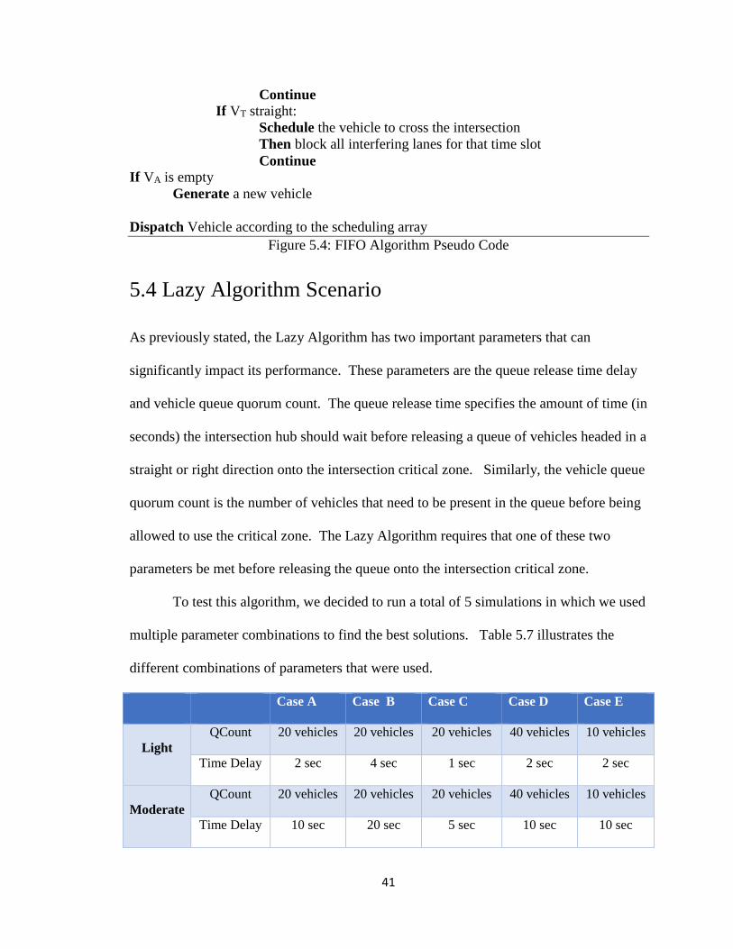
Continue If VT straight:

Schedule the vehicle to cross the intersection

Then block all interfering lanes for that time slot

Continue If VA is empty

Generate a new vehicle

Dispatch Vehicle according to the scheduling array

Figure 5.4: FIFO Algorithm Pseudo Code

5.4 Lazy Algorithm Scenario

As previously stated, the Lazy Algorithm has two important parameters that can

significantly impact its performance. These parameters are the queue release time delay

and vehicle queue quorum count. The queue release time specifies the amount of time (in

seconds) the intersection hub should wait before releasing a queue of vehicles headed in a

straight or right direction onto the intersection critical zone. Similarly, the vehicle queue

quorum count is the number of vehicles that need to be present in the queue before being

allowed to use the critical zone. The Lazy Algorithm requires that one of these two

parameters be met before releasing the queue onto the intersection critical zone.

To test this algorithm, we decided to run a total of 5 simulations in which we used

multiple parameter combinations to find the best solutions. Table 5.7 illustrates the

different combinations of parameters that were used.

Case A Case B Case C Case D Case E

Light

QCount 20 vehicles 20 vehicles 20 vehicles 40 vehicles 10 vehicles

Time Delay 2 sec 4 sec 1 sec 2 sec 2 sec

Moderate

QCount 20 vehicles 20 vehicles 20 vehicles 40 vehicles 10 vehicles

Time Delay 10 sec 20 sec 5 sec 10 sec 10 sec

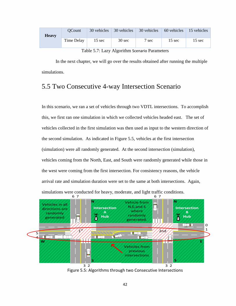
42

Heavy

QCount 30 vehicles 30 vehicles 30 vehicles 60 vehicles 15 vehicles

Time Delay 15 sec 30 sec 7 sec 15 sec 15 sec

Table 5.7: Lazy Algorithm Scenario Parameters

In the next chapter, we will go over the results obtained after running the multiple

simulations.

5.5 Two Consecutive 4-way Intersection Scenario

In this scenario, we ran a set of vehicles through two VDTL intersections. To accomplish

this, we first ran one simulation in which we collected vehicles headed east. The set of

vehicles collected in the first simulation was then used as input to the western direction of

the second simulation. As indicated in Figure 5.5, vehicles at the first intersection

(simulation) were all randomly generated. At the second intersection (simulation),

vehicles coming from the North, East, and South were randomly generated while those in

the west were coming from the first intersection. For consistency reasons, the vehicle

arrival rate and simulation duration were set to the same at both intersections. Again,

simulations were conducted for heavy, moderate, and light traffic conditions.

Figure 5.5: Algorithms through two Consecutive Intersections

01

54

3 2

6 7

1st

Vehicles in all directions are

randomly generated

Intersection A

Hub

3 2

6 7

2nd

Vehicle from N,E,and S

where randomly

generated.

Vehicles from previous

intersections

Intersection B

Hub

N

S

E

N

S

W

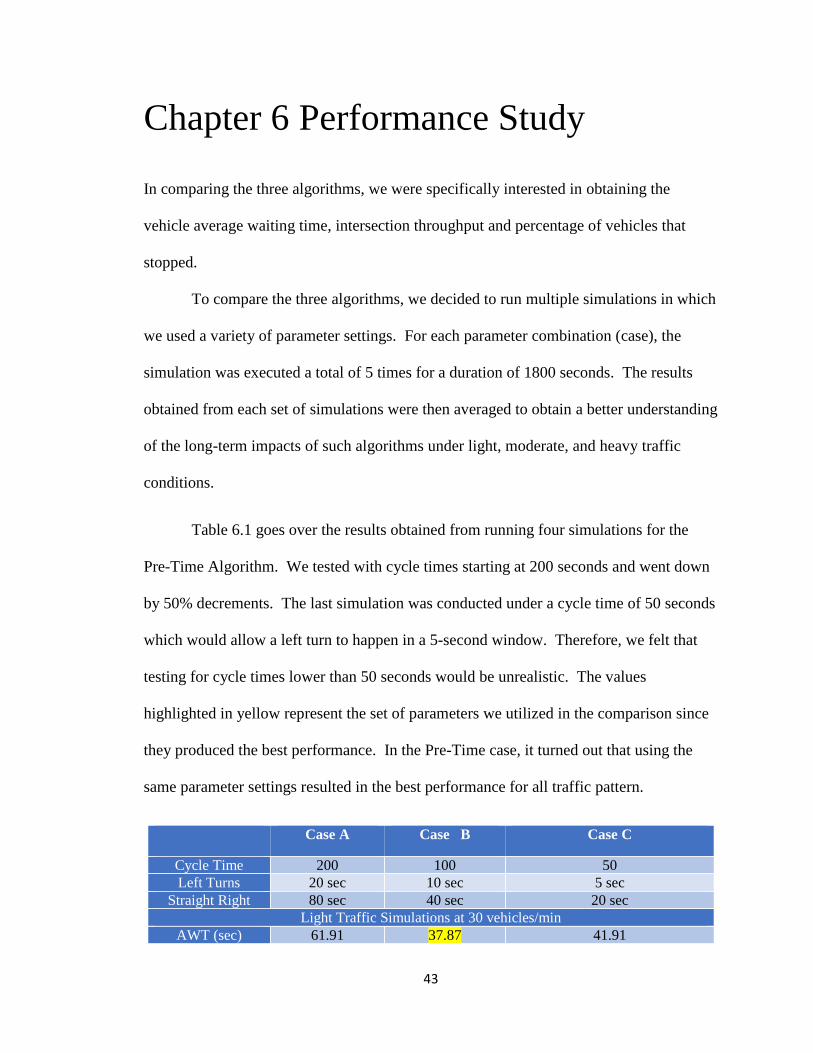
43

Chapter 6 Performance Study

In comparing the three algorithms, we were specifically interested in obtaining the

vehicle average waiting time, intersection throughput and percentage of vehicles that

stopped.

To compare the three algorithms, we decided to run multiple simulations in which

we used a variety of parameter settings. For each parameter combination (case), the

simulation was executed a total of 5 times for a duration of 1800 seconds. The results

obtained from each set of simulations were then averaged to obtain a better understanding

of the long-term impacts of such algorithms under light, moderate, and heavy traffic

conditions.

Table 6.1 goes over the results obtained from running four simulations for the

Pre-Time Algorithm. We tested with cycle times starting at 200 seconds and went down

by 50% decrements. The last simulation was conducted under a cycle time of 50 seconds

which would allow a left turn to happen in a 5-second window. Therefore, we felt that

testing for cycle times lower than 50 seconds would be unrealistic. The values

highlighted in yellow represent the set of parameters we utilized in the comparison since

they produced the best performance. In the Pre-Time case, it turned out that using the

same parameter settings resulted in the best performance for all traffic pattern.

Case A Case B Case C

Cycle Time 200 100 50

Left Turns 20 sec 10 sec 5 sec

Straight Right 80 sec 40 sec 20 sec

Light Traffic Simulations at 30 vehicles/min

AWT (sec) 61.91 37.87 41.91

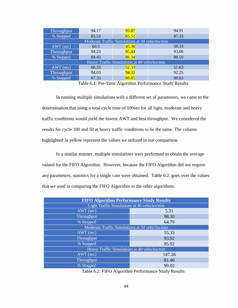
44

Throughput 94.17 95.87 94.91

% Stopped 83.52 85.51 87.33

Moderate Traffic Simulations at 34 vehicles/min

AWT (sec) 60.5 45.36 50.33

Throughput 94.23 95.44 93.06

% Stopped 84.43 86.34 88.50

Heavy Traffic Simulations at 40 vehicles/min

AWT (sec) 66.33 52.33 51.63

Throughput 94.03 94.32 92.25

% Stopped 87.33 88.85 90.63

Table 6.1: Pre-Time Algorithm Performance Study Results

In running multiple simulations with a different set of parameters, we came to the

determination that using a total cycle time of 100sec for all light, moderate and heavy

traffic conditions would yield the lowest AWT and best throughput. We considered the

results for cycle 100 and 50 at heavy traffic conditions to be the same. The column

highlighted in yellow represent the values we utilized in our comparison.

In a similar manner, multiple simulations were performed to obtain the average

valued for the FIFO Algorithm. However, because the FIFO Algorithm did not require

any parameters, statistics for a single case were obtained. Table 6.2. goes over the values

that we used in comparing the FIFO Algorithm to the other algorithms.

FIFO Algorithm Performance Study Results Light Traffic Simulations at 30 vehicles/min

AWT (sec) 5.31 Throughput 98.30 % Stopped 64.79

Moderate Traffic Simulations at 34 vehicles/min AWT (sec) 55.33 Throughput 93.92 % Stopped 95.92

Heavy Traffic Simulations at 40 vehicles/min AWT (sec) 147.26 Throughput 81.46 % Stopped 99.02

Table 6.2: FIFO Algorithm Performance Study Results

45

Lastly, simulation results for the Lazy Algorithm were obtained by executing 5

simulations for each case in which we created a base parameter set and then varied both

the vehicle queue count and time delay to determine the best combination. As seen in

Figures 6.3,6.4, and 6.5 the yellow columns represent the set of values where the

algorithm performed its best. Therefore, the corresponding parameters to those values

were used to compare the Lazy Algorithm to both the Pre-Time and FIFO Algorithms.

As with the Pre-Time Algorithm, we ran into instances where more than one set of

parameters presented an improvement over both the Pre-Time and FIFO Algorithms.

Lazy Algorithm Light Traffic Performance Study Results

30 vehicles/min

Base Case Case A Case B Case C Case D

2x Time

Delay

½ Time Delay 2x Queue

Count

½ Queue

Count

Queue Count 20 vehicles 20 vehicles 20 vehicles 40 vehicles 10 vehicles

Time Delay 2 sec 4 sec 1 sec 2 sec 2 sec

AWT (sec) 5.96 7.34 5.96 6.81 6.24

Throughput (%) 98.00 98.05 98.00 97.91 98.35

% Stopped 63.24 83.42 63.24 66.61 68.24

Table 6.3: Lazy Algorithm Light Traffic Performance Study

Lazy Algorithm Moderate Traffic Performance Study Results

34 vehicles/min

Base Case Case A Case B Case C Case D

2x Time

Delay

½ Time Delay 2x Queue

Count

½ Queue

Count

Queue Count 20 vehicles 20 vehicles 20 vehicles 40 vehicles 10 vehicles

Time Delay 10 sec 20 sec 5 sec 10 sec 10 sec

AWT (sec) 10.79 13.93 48.18 11.59 11.38

Throughput (%) 97.67 97.84 94.63 97.92 97.82

% Stopped 94.96 94.95 97.88 95.00 95.65

Table 6.4: Lazy Algorithm Moderate Traffic Performance Study

Lazy Algorithm Heavy Traffic Performance Study Results

40 vehicles/min

Base Case Case A Case B Case C Case D

2x Time

Delay

½ Time Delay 2x Queue

Count

½ Queue

Count

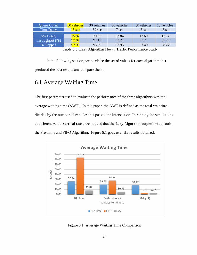
46

Queue Count 30 vehicles 30 vehicles 30 vehicles 60 vehicles 15 vehicles

Time Delay 15 sec 30 sec 7 sec 15 sec 15 sec

AWT (sec) 15.82 20.95 82.84 18.69 17.77

Throughput (%) 97.84 97.16 89.21 97.71 97.28

% Stopped 97.96 95.99 98.95 98.40 98.27

Table 6.5: Lazy Algorithm Heavy Traffic Performance Study

In the following section, we combine the set of values for each algorithm that

produced the best results and compare them.

6.1 Average Waiting Time

The first parameter used to evaluate the performance of the three algorithms was the

average waiting time (AWT). In this paper, the AWT is defined as the total wait time

divided by the number of vehicles that passed the intersection. In running the simulations

at different vehicle arrival rates, we noticed that the Lazy Algorithm outperformed both

the Pre-Time and FIFO Algorithm. Figure 6.1 goes over the results obtained.

Figure 6.1: Average Waiting Time Comparison

52.3439.43 35.92

147.26

55.34

5.3115.82 10.79 5.97

0.00

20.00

40.00

60.00

80.00

100.00

120.00

140.00

160.00

40 (Heavy) 34 (Moderate) 30 (Light)

Seco

nd

s

Vehicles Per Minute

Average Waiting Time

Pre-Time FIFO Lazy

47

In analyzing the result for the AWT, we noticed an overall reduction in the AWT

when intersections are equipped with a VDTL systems that use the Lazy Algorithm. As

seen in figure 6.6, the Lazy Algorithm proved to reduce the AWT under all traffic

conditions. While the Pre-Time Algorithms maintains a somewhat constant AWT, the

FIFO Algorithm worsens as the rate of vehicles approaching the intersection increases.

On the other hand, the Lazy Algorithm maintains a low AWT under all traffic conditions

by taking advantage of the platooning mechanism and adjusting its parameters based on

traffic conditions. Recall that the Lazy Algorithm is capable of creating platoons that

result in a lower T2P for all vehicles encapsulated within the same platoon. Figure 6.2,

6.3, and 6.4 present a histogram under heavy traffic conditions of one of the many

simulations in which we can see how each of the algorithms is capable of creating

platoons.

Figure 6.2: Pre-Time Algorithm Straight/Right Platoon Bins

0

2

4

6

8

10

12

14

1 2 3 4 5 6 7 8 9 10 11 12 13 14 15 16

Nu

mb

er o

f V

ehic

les

Bin

Pre-Time Algorithm Straight/Right40 Vehicles Per Min

PlatoonBins

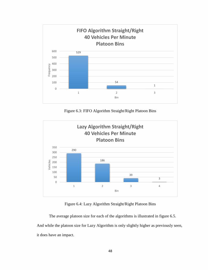
48

Figure 6.3: FIFO Algorithm Straight/Right Platoon Bins

Figure 6.4: Lazy Algorithm Straight/Right Platoon Bins

The average platoon size for each of the algorithms is illustrated in figure 6.5.

And while the platoon size for Lazy Algorithm is only slightly higher as previously seen,

it does have an impact.

529

541

0

100

200

300

400

500

600

1 2 3

Freq

uen

cy

Bin

FIFO Algorithm Straight/Right40 Vehicles Per Minute

Platoon Bins

290

186

393

0

50

100

150

200

250

300

350

1 2 3 4

Veh

icle

s

Bin

Lazy Algorithm Straight/Right40 Vehicles Per Minute

Platoon Bins

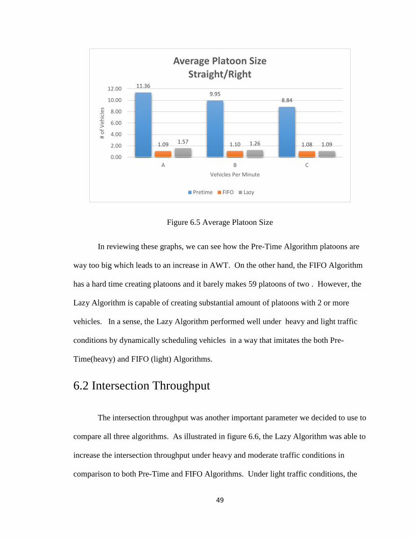
49

Figure 6.5 Average Platoon Size

In reviewing these graphs, we can see how the Pre-Time Algorithm platoons are

way too big which leads to an increase in AWT. On the other hand, the FIFO Algorithm

has a hard time creating platoons and it barely makes 59 platoons of two . However, the

Lazy Algorithm is capable of creating substantial amount of platoons with 2 or more

vehicles. In a sense, the Lazy Algorithm performed well under heavy and light traffic

conditions by dynamically scheduling vehicles in a way that imitates the both Pre-

Time(heavy) and FIFO (light) Algorithms.

6.2 Intersection Throughput

The intersection throughput was another important parameter we decided to use to

compare all three algorithms. As illustrated in figure 6.6, the Lazy Algorithm was able to

increase the intersection throughput under heavy and moderate traffic conditions in

comparison to both Pre-Time and FIFO Algorithms. Under light traffic conditions, the

11.36

9.958.84

1.09 1.10 1.081.57 1.26 1.09

0.00

2.00

4.00

6.00

8.00

10.00

12.00

A B C

# o

f V

ehic

les

Vehicles Per Minute

Average Platoon Size Straight/Right

Pretime FIFO Lazy

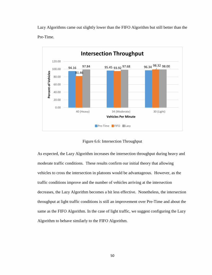
50

Lazy Algorithms came out slightly lower than the FIFO Algorithm but still better than the

Pre-Time.

Figure 6.6: Intersection Throughput

As expected, the Lazy Algorithm increases the intersection throughput during heavy and

moderate traffic conditions. These results confirm our initial theory that allowing

vehicles to cross the intersection in platoons would be advantageous. However, as the

traffic conditions improve and the number of vehicles arriving at the intersection

decreases, the Lazy Algorithm becomes a bit less effective. Nonetheless, the intersection

throughput at light traffic conditions is still an improvement over Pre-Time and about the

same as the FIFO Algorithm. In the case of light traffic, we suggest configuring the Lazy

Algorithm to behave similarly to the FIFO Algorithm.

94.16 95.45 96.34

81.46

93.9298.3297.84 97.68 98.00

0.00

20.00

40.00

60.00

80.00

100.00

120.00

40 (Heavy) 34 (Moderate) 30 (Light)

Pe

rce

nt

of

Ve

hic

les

Vehicles Per Minute

Intersection Throughput

Pre-Time FIFO Lazy

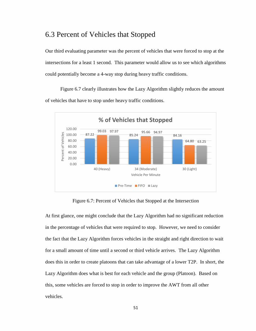
51

6.3 Percent of Vehicles that Stopped

Our third evaluating parameter was the percent of vehicles that were forced to stop at the

intersections for a least 1 second. This parameter would allow us to see which algorithms

could potentially become a 4-way stop during heavy traffic conditions.

Figure 6.7 clearly illustrates how the Lazy Algorithm slightly reduces the amount

of vehicles that have to stop under heavy traffic conditions.

Figure 6.7: Percent of Vehicles that Stopped at the Intersection

At first glance, one might conclude that the Lazy Algorithm had no significant reduction

in the percentage of vehicles that were required to stop. However, we need to consider

the fact that the Lazy Algorithm forces vehicles in the straight and right direction to wait

for a small amount of time until a second or third vehicle arrives. The Lazy Algorithm

does this in order to create platoons that can take advantage of a lower T2P. In short, the

Lazy Algorithm does what is best for each vehicle and the group (Platoon). Based on

this, some vehicles are forced to stop in order to improve the AWT from all other

vehicles.

87.22 85.24 84.1699.03 95.66

64.80

97.97 94.97

63.25

0.00

20.00

40.00

60.00

80.00

100.00

120.00

40 (Heavy) 34 (Moderate) 30 (Light)

Per

cen

t o

f V

ehic

les

Vehicle Per Minute

% of Vehicles that Stopped

Pre-Time FIFO Lazy

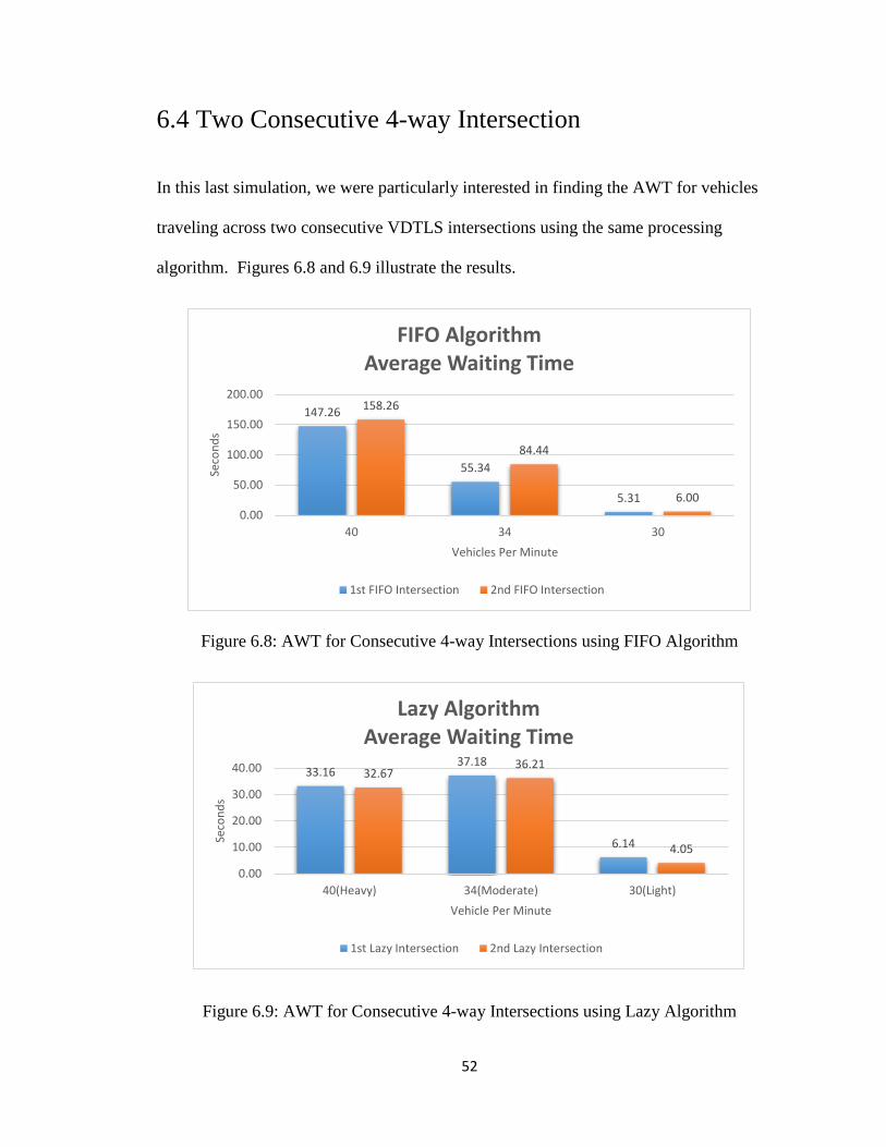
52

6.4 Two Consecutive 4-way Intersection

In this last simulation, we were particularly interested in finding the AWT for vehicles

traveling across two consecutive VDTLS intersections using the same processing

algorithm. Figures 6.8 and 6.9 illustrate the results.

Figure 6.8: AWT for Consecutive 4-way Intersections using FIFO Algorithm

Figure 6.9: AWT for Consecutive 4-way Intersections using Lazy Algorithm

147.26

55.34

5.31

158.26

84.44

6.00

0.00

50.00

100.00

150.00

200.00

40 34 30

Seco

nd

s

Vehicles Per Minute

FIFO Algorithm Average Waiting Time

1st FIFO Intersection 2nd FIFO Intersection

33.1637.18

6.14

32.6736.21

4.05

0.00

10.00

20.00

30.00

40.00

40(Heavy) 34(Moderate) 30(Light)

Seco

nd

s

Vehicle Per Minute

Lazy AlgorithmAverage Waiting Time

1st Lazy Intersection 2nd Lazy Intersection

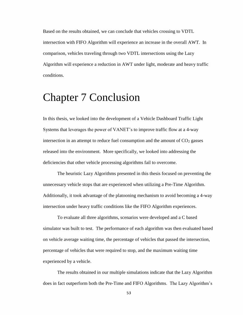
53

Based on the results obtained, we can conclude that vehicles crossing to VDTL

intersection with FIFO Algorithm will experience an increase in the overall AWT. In

comparison, vehicles traveling through two VDTL intersections using the Lazy

Algorithm will experience a reduction in AWT under light, moderate and heavy traffic

conditions.

Chapter 7 Conclusion

In this thesis, we looked into the development of a Vehicle Dashboard Traffic Light

Systems that leverages the power of VANET’s to improve traffic flow at a 4-way

intersection in an attempt to reduce fuel consumption and the amount of CO2 gasses

released into the environment. More specifically, we looked into addressing the

deficiencies that other vehicle processing algorithms fail to overcome.

The heuristic Lazy Algorithms presented in this thesis focused on preventing the

unnecessary vehicle stops that are experienced when utilizing a Pre-Time Algorithm.

Additionally, it took advantage of the platooning mechanism to avoid becoming a 4-way

intersection under heavy traffic conditions like the FIFO Algorithm experiences.

To evaluate all three algorithms, scenarios were developed and a C based

simulator was built to test. The performance of each algorithm was then evaluated based

on vehicle average waiting time, the percentage of vehicles that passed the intersection,

percentage of vehicles that were required to stop, and the maximum waiting time

experienced by a vehicle.

The results obtained in our multiple simulations indicate that the Lazy Algorithm

does in fact outperform both the Pre-Time and FIFO Algorithms. The Lazy Algorithm’s

54

capability of releasing a vehicle headed into the straight/right direction onto the

intersection critical zone based on vehicle quorum count or time delay has proven to be

advantageous. However, after running a significant amount of simulations, we came to

realize there is a fundamental tradeoff that must happen when configuring each of these

algorithms. We found that one needs to find the right balance between minimizing the

AWT and maximizing the number of vehicles that cross the intersection critical zone. As

stated in the previous sections, making use of platoons can highly enhance the

performance of the intersection during heavy and moderate traffic conditions if used with

moderation. In other words, the size of the platoon should not be too big or too small.

7.1 Future Research Opportunities

Without a doubt, the topic of maximizing the traffic flow through a 4-way intersection

will continue to be a topic of interest. And while this thesis attempts to bring us closer to

a feasible solution, there is still plenty of work to be done.

To start with, making adaptations to the Lazy Algorithm so that vehicles can

adjust their crossing schedule after their initial introduction to the intersection would be

very advantageous. Vehicles could then be allowed to change lanes when possible

without impacting the overall crossing schedule. Furthermore, a queue flush mechanism

should be developed that would permit vehicles on a particular side to go green when an

emergency vehicle is approaching. Lastly, the creation of some sort of failsafe that can

prevent a pileup in the event that a vehicle breaks somewhere within the intersection

perimeter.

55

Appendix A

Code repository: https://github.com/alejflor/VDTL.git

56

References [1] "Highway finance data collection," U.S. Department of Transportation Federal

Highway Administration, last modified May 23, 2010,

http://www.fhwa.dot.gov/policyinformation/pubs/hf/pl11028/

[2] M. Barth and K. Boriboonsomsin, “ Real- World CO2 Impacts of Traffic

Congestion,” Transportation Research Record pp. 1-23,2008,

http://uctc.net/research/papers/846.pdf

[3] "Remarks by the President on Fuel Efficiency Standards of Medium and Heavy-

Duty Vehicles," The White House President Barack Obama, last modified

February 18, 2014, https://www.whitehouse.gov/the-press-

office/2014/02/18/remarks-president-fuel-efficiency-standards-medium-and-

heavy-duty-vehicl

[4] "Advancing American Energy," The White House President Barack Obama,

accessed February 28, 2016, https://www.whitehouse.gov/energy/securing-

american-energy

[5] "National Traffic Signal Report Card Technical Report," National Transportation

Operation Coalition, accessed February 1, 2016,

http://library.ite.org/pub/e265477a-2354-d714-5147-870dfac0e294

[6] A. Y. Abd-Fatah, R. M. Yusuff, F. A. Aziz and N. Zulkifli, "Simulation of "time-

based" versus "sensor-based" traffic light system," Communication Software and

Networks (ICCSN), 2011 IEEE 3rd International Conference on, Xi'an, 2011, pp.

789-792.

[7] K. Pandit, D. Ghosal, H. M. Zhang and C. N. Chuah, "Adaptive Traffic Signal

Control With Vehicular Ad hoc Networks," in IEEE Transactions on Vehicular

Technology, vol. 62, no. 4, pp. 1459-1471, May 2013.

[8] V. Gradinescu, C. Gorgorin, R. Diaconescu, V. Cristea and L. Iftode, "Adaptive

Traffic Lights Using Car-to-Car Communication," 2007 IEEE 65th Vehicular

Technology Conference - VTC2007-Spring, Dublin, 2007, pp. 21-25.

[9] S. Kwatirayo, J. Almhana, Z. Liu and J. Siblini, "Optimizing road intersection

traffic flow using stochastic and heuristic algorithms," 2014 IEEE International

Conference on Communications (ICC), Sydney, NSW, 2014, pp. 586-591.

57

[10] M. A. S. Kamal, J. i. Imura, T. Hayakawa, A. Ohata and K. Aihara, "A

Vehicle-Intersection Coordination Scheme for Smooth Flows of Traffic Without

Using Traffic Lights," in IEEE Transactions on Intelligent Transportation

Systems, vol. 16, no. 3, pp. 1136-1147, June 2015.

[11] M. M. Al-Mashhadani, W. Shu and M. Y. Wu, "Enhancing Traffic Flow

Using Vehicle Dashboard Traffic Lights with V2I Networks," 2015 IEEE Global

Communications Conference (GLOBECOM), San Diego, CA, 2015, pp. 1-5.

[12] M. Kamal Abbas, M. N. Karsiti, M. Napiah and B. B. Samir, "Traffic light

control via VANET system architecture," 2011 IEEE Symposium on Wireless

Technology and Applications (ISWTA), Langkawi, 2011, pp. 174-179.

[13] B. Zhang, L. Shang and D. Chen, "A Study on the Traffic Intersection

Vehicle Emission Base on Urban Microscopic Traffic Simulation Model,"

Education Technology and Computer Science, 2009. ETCS '09. First International

Workshop on, Wuhan, Hubei, 2009, pp. 789-794.

[14] L. Li, D. Wen and D. Yao, "A Survey of Traffic Control With Vehicular

Communications," in IEEE Transactions on Intelligent Transportation Systems,

vol. 15, no. 1, pp. 425-432, Feb. 2014.

[15] G. Wu, K. Boriboonsomsin, L. Zhang and M. J. Barth, "Simulation-based

benefit evaluation of dynamic lane grouping strategies at isolated intersections,"

2012 15th International IEEE Conference on Intelligent Transportation Systems,

Anchorage, AK, 2012, pp. 1038-1043.

[16] L. C. Bento, R. Parafita, S. Santos and U. Nunes, "Intelligent traffic

management at intersections: Legacy mode for vehicles not equipped with V2V

and V2I communications," 16th International IEEE Conference on Intelligent

Transportation Systems (ITSC 2013), The Hague, 2013, pp. 726-731.

[17] L. Chen and C. Englund, "Cooperative Intersection Management: A Survey," in

IEEE Transactions on Intelligent Transportation Systems, vol. 17, no. 2, pp. 570-

586, Feb. 2016.