Vector Solitons and Their Internal Oscillations in Birefringent Nonlinear Optical Fibers * By Jianke Yang In this article, the vector solitons in birefringent nonlinear optical fibers are studied first. Special attention is given to the single-hump vector solitons due to evidences that only they are stable. Questions such as the existence, uniqueness, and total number of these solitons are addressed. It is found that the total number of them is continuously infinite and their polarizations can be arbitrary. Next, the internal oscillations of these vector solitons are inves- tigated by the linearization method. Discrete eigenmodes of the linearized equations are identified. Such modes cause to the vector solitons a kind of permanent internal oscillations, which visually appear to be a combination of translational and width oscillations in the A and B pulses. The numerically observed radiation shelf at the tails of interacting pulses is also explained. Fi- nally, the asymptotic states of the perturbed vector solitons are studied within both the linear and nonlinear theory. It is found that the state of internal os- cillations of a vector soliton is always unstable. It invariably emits energy radiation and eventually evolves into a single-hump vector soliton state. Address for correspondence: Department of Mathematics and Statistics, The University of Vermont, 16 Colchester Avenue, Burlington, VT 05401. E-mail: [email protected] * “Vector solitons” is a name researchers in nonlinear optics use for solitary waves in birefringent nonlinear optical fibers. They are not solitons in a strict mathematical sense, but are nevertheless shape preserving. STUDIES IN APPLIED MATHEMATICS 98:61–97 61 © 1997 by the Massachusetts Institute of Technology Published by Blackwell Publishers, 350 Main Street, Malden, MA 02148, USA, and 108 Cowley Road, Oxford, OX4 1JF, UK.

Welcome message from author
This document is posted to help you gain knowledge. Please leave a comment to let me know what you think about it! Share it to your friends and learn new things together.
Transcript
Vector Solitons and Their Internal Oscillations inBirefringent Nonlinear Optical Fibers∗
By Jianke Yang
In this article, the vector solitons in birefringent nonlinear optical fibers arestudied first. Special attention is given to the single-hump vector solitonsdue to evidences that only they are stable. Questions such as the existence,uniqueness, and total number of these solitons are addressed. It is found thatthe total number of them is continuously infinite and their polarizations canbe arbitrary. Next, the internal oscillations of these vector solitons are inves-tigated by the linearization method. Discrete eigenmodes of the linearizedequations are identified. Such modes cause to the vector solitons a kind ofpermanent internal oscillations, which visually appear to be a combination oftranslational and width oscillations in the A and B pulses. The numericallyobserved radiation shelf at the tails of interacting pulses is also explained. Fi-nally, the asymptotic states of the perturbed vector solitons are studied withinboth the linear and nonlinear theory. It is found that the state of internal os-cillations of a vector soliton is always unstable. It invariably emits energyradiation and eventually evolves into a single-hump vector soliton state.
Address for correspondence: Department of Mathematics and Statistics, The University of Vermont, 16Colchester Avenue, Burlington, VT 05401. E-mail: [email protected]* “Vector solitons” is a name researchers in nonlinear optics use for solitary waves in birefringent nonlinearoptical fibers. They are not solitons in a strict mathematical sense, but are nevertheless shape preserving.
STUDIES IN APPLIED MATHEMATICS 98:61–97 61© 1997 by the Massachusetts Institute of TechnologyPublished by Blackwell Publishers, 350 Main Street, Malden, MA 02148, USA, and 108 Cowley Road,Oxford, OX4 1JF, UK.
62 Jianke Yang
1. Introduction
The idea of using solitons as information bits in a high-data-rate telecom-munication system was first proposed by Hasegawa and Tappert [1] in 1973.Since then, a great deal of experimental and theoretical work has been doneon the pulse propagation in a nonlinear optical fiber. The early theoreti-cal work took the nonlinear Schrodinger equation (NLS) as the underlyingmathematical model, and the propagation of solitonian pulses have all thenice properties associated with the integrable NLS equation. Menyuk [3] firstrealized the importance of birefringence in an optical fiber and studied itseffects on the pulse propagation. Birefringence can lead to pulse splitting,which is not desirable in communication applications. This effect may bebalanced by nonlinearity in the fiber since nonlinearity tends to hold pulsestogether. When all these effects (birefringence, nonlinearity, linear disper-sion, etc.) are taken into consideration, a multiple-scale perturbation analysiscan be employed to obtain the evolution equations of pulses in a birefrin-gent nonlinear optical fiber. This has been done by Menyuk [3]. After somesimplifications, the equations can be written as
iAt +Axx + ��A�2 + β�B�2�A = 0; (1.1a)
iBt + Bxx + ��B�2 + β�A�2�B = 0; (1.1b)
where A and B represent the complex amplitudes of the two polarizationcomponents, and β is a real-valued cross-phase modulation coefficient. Thesystem (1.1) is integrable only when β is equal to 0 or 1. But for most opticalfibers, β is not equal to 0 or 1. This destroys integrability and complicates thepulse evolution behaviors. For instance, vector solitons still exist in the system(1.1), but when they collide, they may merge into a single soliton, destroyeach other, or be reflected back by each other. A certain amount of energyradiation is also emitted when collision takes place [4, 5]. Additionally, vectorsolitons, when perturbed, undergo complicated internal oscillations and shedradiation [6].
Vector solitons in the system (1.1), although not as robust as those as-sociated with an integrable system, still play an important role in the solu-tion evolution. They have been investigated by Mesentsev and Turitsyn [7],Kaup et al. [8], Haelterman and Sheppard [9], Silberberg and Barad [10],and Yang and Benney [5]. Mesentsev and Turitsyn proved the stability ofthe vector solitons of equal amplitudes by constructing a Lyapunov func-tion for the Hamiltonian associated with Equations (1.1). Kaup et al. studiedthe internal dynamics of vector solitons by the variational principle method.They approximated the vector solitons by a Gaussian ansatz, inserted it intothe Lagrangian density, and then obtained a system of ordinary differential
Nonlinear Optical Fibers 63
equations (o.d.e.) for the evolution of the ansatz parameters. They found acontinuous family of fixed points of the o.d.e. system, which represent sym-metric vector solitons with an arbitrary polarization. They also showed thatthese vector soliton solutions are stable by examining the linear stability ofthose fixed points. Haelterman and Sheppard’s results confirmed the exis-tence of these vector solitons. Silberberg and Barad identified two familiesof vector solitons, one symmetric and the other one antisymmetric. They alsoshowed numerically that only the symmetric family of solutions are stable.In joint work with D. Benney, we studied the same problem. We found, bya numerical approach, infinite families of vector solitons. Only one of thesefamilies is single-humped and symmetric, and it corresponds to the one foundby Kaup et al. All other families of solutions are multi-humped. On the basisof some analytical results and numerical evidence, we conjectured that onlythe single-humped vector solitons are stable.
The internal oscillations of vector solitons is a complicated process. Thisproblem has been studied by Ueda and Kath [6] and Kaup et al. [8] using thevariational principle method. Ueda and Kath assumed the spatial shapes ofthe pulses to take the form of the NLS solitons with frequency chirping, butallowed the shape parameters such as pulse position and width to evolve withtime. Inserting the NLS solitons into the Lagrangian density and taking varia-tions with respect to each pulse parameter, they derived a system of ordinarydifferential equations which govern the evolution of the shape parameters.They identified two types of internal oscillations (translational oscillation andpulse-width oscillation) and determined their frequencies. They also showedthat there is a transfer of energy between these two types of oscillations,which results in the inelastic nature of the soliton collisions. Kaup et al. usedthe same variational principle method except they approximated the pulsesby a Gaussian ansatz. This oversimple approximation enabled them to solveall the necessary integrals involved in their analysis. They found a contin-uous family of stationary solutions, which represent vector solitons with anarbitrary polarization. Examining small internal vibrations of these vectorsolitons, they found three oscillational eigenmodes; two were those found byUeda and Kath and one was new.
The analytical models by Ueda and Kath and Kaup et al. can qualita-tively describe some aspects of the vector solitons’ internal dynamics overshort time scales. The major drawback of their models is that radiation wasnot considered. It is well known that radiation is one of the key players inthe internal dynamics of vector solitons. Radiation carries energy away fromthe dominant pulses and has a damping effect on them. In particular, low-wavenumber radiation has been observed numerically as a low shelf at thetails of the oscillating pulses. Such radiation propagates at velocities close tothat of the vector soliton and therefore remains close to the pulses and af-fects their dynamics over long time scales. Clearly the exclusion of radiation
64 Jianke Yang
in an analytical model will make its predictions invalid over long time scales.Another drawback of their models is that they limited the evolution of thepulse shape to the ansatz chosen, so shape changes cannot go beyond thosemodeled by changes in the shape parameters. The true pulse shape and itsevolution are still unclear.
In this article, the problem of vector solitons and their internal oscillationsis revisited. First, we address the existence, uniqueness, and total number of(stable) single-hump vector solitons. Next, we study the internal oscillationsof vector solitons with radiation included. The linearization and perturbationmethods are used. The oscillational eigenmodes found by Ueda and Kathand Kaup et al. are reconsidered and their true natures clarified. The truepulse shape in the internal oscillations is determined. Predictions on the long-time-pulse dynamics are also given. The results obtained provide a clear andcomplete picture of the internal dynamics of vector solitons.
2. Vector solitons
It has been known that vector solitons of the form
A = eiω1t r1�x�; (2.1a)
B = eiω2t r2�x� (2.1b)
exist in the system (1.1), in which case r1 and r2 satisfy the equations
r1xx −ω1r1 + �r21 + βr2
2 �r1 = 0; (2.2a)
r2xx −ω2r2 + �r22 + βr2
1 �r2 = 0: (2.2b)
We are interested only in the solitary waves that exponentially decay as �x� →∞, so it is necessary that ω1;ω2 > 0. For convenience, we take ω1 = 1. Thiscan always be achieved by a rescaling of variables r1; r2, and x. We furtherdenote ω2 as ω. Equations (2.2) have a great number of solutions for anyvalue of β (see [5]). The degenerate solutions, in which one of r1 and r2 isequal to zero, is easy to determine. For instance, if r2 = 0, then
r1 =√
2 sech x: (2.3)
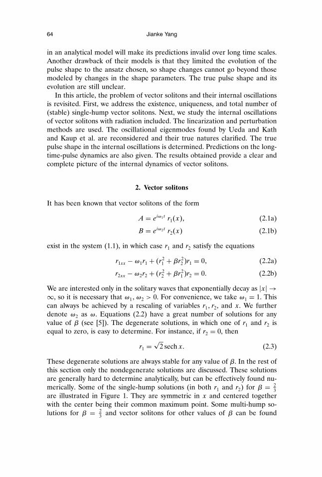
These degenerate solutions are always stable for any value of β. In the rest ofthis section only the nondegenerate solutions are discussed. These solutionsare generally hard to determine analytically, but can be effectively found nu-merically. Some of the single-hump solutions (in both r1 and r2) for β = 2
3are illustrated in Figure 1. They are symmetric in x and centered togetherwith the center being their common maximum point. Some multi-hump so-lutions for β = 2
3 and vector solitons for other values of β can be found
Nonlinear Optical Fibers 65
in [5]. Evidence in [5] shows that when β > 0, the single-hump solutionsare stable while the multi-hump ones are not; when β < 0, both the singleand multi-hump solutions are unstable. So, in the following, we focus on thesingle-hump solutions for β > 0.
As is clear from Figure 1, the polarizations of the single-hump solutionsr2�0�/r1�0� change continuously with ω. At one extreme where r2 � r1,r2 is called a daughter wave or a shadow. In this case, ω is found tobe [5]
ω = ωI ≡�√1+ 8β− 1�2
4: (2.4)
At the other extreme where r1 � r2, it is found that
ω = ωII ≡4
�√1+ 8β− 1�2 : (2.5)
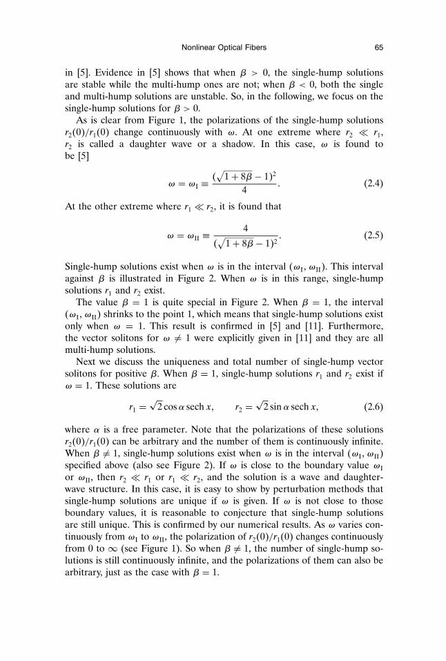
Single-hump solutions exist when ω is in the interval �ωI;ωII�. This intervalagainst β is illustrated in Figure 2. When ω is in this range, single-humpsolutions r1 and r2 exist.
The value β = 1 is quite special in Figure 2. When β = 1, the interval�ωI;ωII� shrinks to the point 1, which means that single-hump solutions existonly when ω = 1. This result is confirmed in [5] and [11]. Furthermore,the vector solitons for ω 6= 1 were explicitly given in [11] and they are allmulti-hump solutions.
Next we discuss the uniqueness and total number of single-hump vectorsolitons for positive β. When β = 1, single-hump solutions r1 and r2 exist ifω = 1. These solutions are
r1 =√
2 cosα sech x; r2 =√
2 sinα sech x; (2.6)
where α is a free parameter. Note that the polarizations of these solutionsr2�0�/r1�0� can be arbitrary and the number of them is continuously infinite.When β 6= 1, single-hump solutions exist when ω is in the interval �ωI;ωII�specified above (also see Figure 2). If ω is close to the boundary value ωIor ωII, then r2 � r1 or r1 � r2, and the solution is a wave and daughter-wave structure. In this case, it is easy to show by perturbation methods thatsingle-hump solutions are unique if ω is given. If ω is not close to thoseboundary values, it is reasonable to conjecture that single-hump solutionsare still unique. This is confirmed by our numerical results. As ω varies con-tinuously from ωI to ωII, the polarization of r2�0�/r1�0� changes continuouslyfrom 0 to ∞ (see Figure 1). So when β 6= 1, the number of single-hump so-lutions is still continuously infinite, and the polarizations of them can also bearbitrary, just as the case with β = 1.
66 Jianke Yang
Figure 1. Some of the single-hump �r1; r2� solutions in Equations (2.2) with β = 23 . The value
of ω is (a) 0.6; (b) 0.8; (c) 1; (d) 1.2; (e) 1.4; (f) 1.6. Solid curves, r1; dashed curves, r2.
Figure 2. The �ω; β� region (shaded) where single-hump solutions exist in Equations (2.2).The two boundary curves are given by (2.4) and (2.5).
Nonlinear Optical Fibers 67
3. Internal oscillations of vector solitons
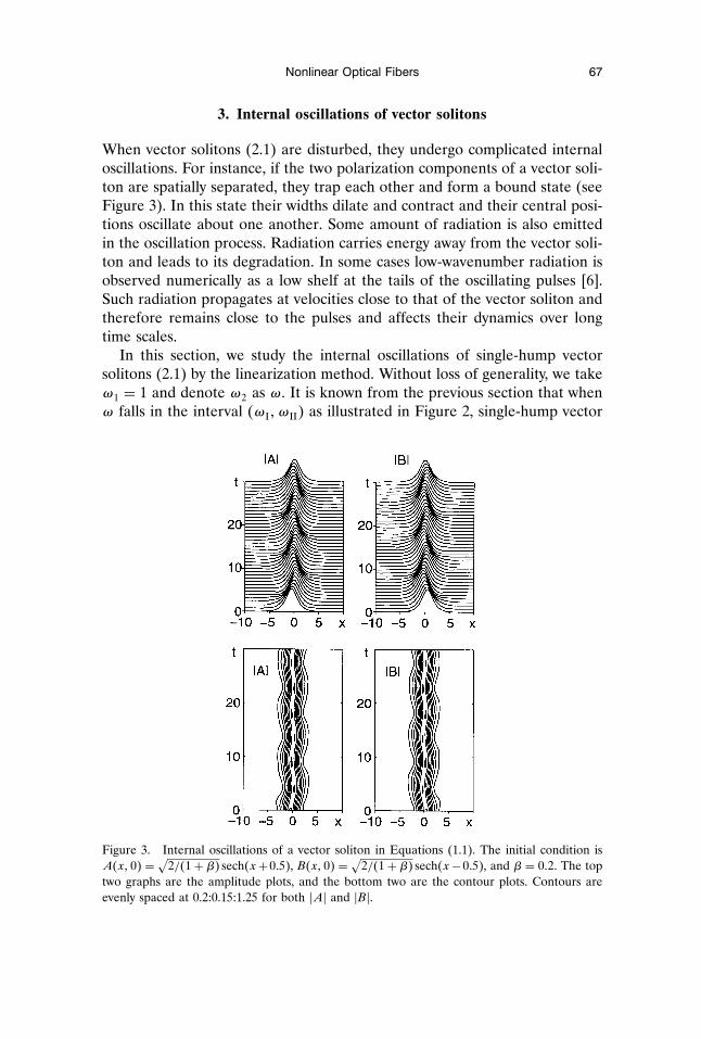
When vector solitons (2.1) are disturbed, they undergo complicated internaloscillations. For instance, if the two polarization components of a vector soli-ton are spatially separated, they trap each other and form a bound state (seeFigure 3). In this state their widths dilate and contract and their central posi-tions oscillate about one another. Some amount of radiation is also emittedin the oscillation process. Radiation carries energy away from the vector soli-ton and leads to its degradation. In some cases low-wavenumber radiation isobserved numerically as a low shelf at the tails of the oscillating pulses [6].Such radiation propagates at velocities close to that of the vector soliton andtherefore remains close to the pulses and affects their dynamics over longtime scales.
In this section, we study the internal oscillations of single-hump vectorsolitons (2.1) by the linearization method. Without loss of generality, we takeω1 = 1 and denote ω2 as ω. It is known from the previous section that whenω falls in the interval �ωI;ωII� as illustrated in Figure 2, single-hump vector
Figure 3. Internal oscillations of a vector soliton in Equations (1.1). The initial condition isA�x; 0� = √2/�1+ β� sech�x+0:5�, B�x; 0� = √2/�1+ β� sech�x−0:5�, and β = 0:2. The toptwo graphs are the amplitude plots, and the bottom two are the contour plots. Contours areevenly spaced at 0.2:0.15:1.25 for both �A� and �B�.
68 Jianke Yang
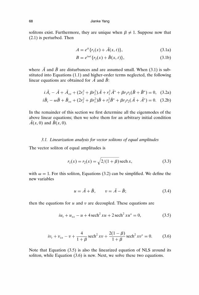
solitons exist. Furthermore, they are unique when β 6= 1. Suppose now that(2.1) is perturbed. Then
A = eit�r1�x� + A�x; t��; (3.1a)
B = eiωt�r2�x� + B�x; t��; (3.1b)
where A and B are disturbances and are assumed small. When (3.1) is sub-stituted into Equations (1.1) and higher-order terms neglected, the followinglinear equations are obtained for A and B:
iAt − A+ Axx + �2r21 + βr2
2 �A+ r21 A∗ + βr1r2�B + B∗� = 0; (3.2a)
iBt −ωB + Bxx + �2r22 + βr2
1 �B + r22 B∗ + βr1r2�A+ A∗� = 0: (3.2b)
In the remainder of this section we first determine all the eigenmodes of theabove linear equations; then we solve them for an arbitrary initial conditionA�x; 0� and B�x; 0�.
3.1. Linearization analysis for vector solitons of equal amplitudes
The vector soliton of equal amplitudes is
r1�x� = r2�x� =√
2/�1+ β� sech x; (3.3)
with ω = 1. For this soliton, Equations (3.2) can be simplified. We define thenew variables
u = A+ B; v = A− By (3.4)
then the equations for u and v are decoupled. These equations are
iut + uxx − u + 4 sech2 xu + 2 sech2 xu∗ = 0; (3.5)
ivt + vxx − v +4
1+ β sech2 xv + 2�1− β�1+ β sech2 xv∗ = 0: (3.6)
Note that Equation (3.5) is also the linearized equation of NLS around itssoliton, while Equation (3.6) is new. Next, we solve these two equations.
Nonlinear Optical Fibers 69
3.1.1. Solution of Equation (3.5). It is convenient to work with the vari-ables u and u∗. We denote U = �u; u∗�T, where the superscript T representsthe transpose. Then, U satisfies the equation
iUt + LU = 0; (3.7)
where the linear operator L is
L = σ3�∂xx − 1� + 2 sech2 x�2σ3 + iσ2�; (3.8)
and
σ1 =(
0 11 0
); σ2 =
(0 −ii 0
); σ3 =
(1 00 −1
)(3.9)
are Pauli spin matrices. The eigenstates of Equation (3.7) are of the form
U�x; t� = eiλtψ�x�; (3.10)
where
Lψ = λψ: (3.11)
These states have been worked out by Kaup [12]. The eigensolutions in thecontinuous spectrum of L are
ψ�x; k� = eikx(
1− 2ik�k+ i�2 e
−x sech x)(
01
)+ e
ikx sech2 x
�k+ i�2(
11
)(3.12)
with λψ = k2 + 1 and
ψ�x; k� = σ1ψ; with λψ = −�k2 + 1�: (3.13)
The solutions in the discrete spectrum of L are a linear combination of thetwo functions
ψe�x� = sech x(
1−1
); ψ0�x� = sech x tanh x
(11
)(3.14)
with the same eigenvalue λ = 0. Since L is not self-adjoint, two more states,
φe�x� = sech x�x tanh x− 1�(
11
)and φ0�x� = xψe (3.15)
need to be included for closure. These two states are the generalized eigen-states and the L operator acting on them gives
Lφe = −2ψe; Lφ0 = −2ψ0: (3.16)
70 Jianke Yang
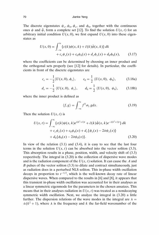
The discrete eigenstates ψe;ψ0; φe, and φ0, together with the continuousones ψ and ψ, form a complete set [12]. To find the solution U�x; t� for anarbitrary initial condition U�x; 0�, we first expand U�x; 0� into these eigen-states as
U�x; 0� =∫ ∞−∞�c�k�ψ�x; k� + c�k�ψ�x; k��dk
+ ceψe�x� + c0ψ0�x� + deφe�x� + d0φ0�x�; (3.17)
where the coefficients can be determined by choosing an inner product andthe orthogonal sets properly (see [12] for details). In particular, the coeffi-cients in front of the discrete eigenstates are
ce = −12�U�x; 0�; φe�; c0 =
12�U�x; 0�; φ0�; (3.18a)
de = −12�U�x; 0�; ψe�; d0 =
12�U�x; 0�; ψ0�; (3.18b)
where the inner product is defined as
�f; g� =∫ ∞−∞f Tσ3 gdx: (3.19)
Then the solution U�x; t� is
U�x; t� =∫ ∞−∞�c�k�ψ�x; k�ei�k2+1�t + c�k�ψ�x; k�e−i�k2+1�t�dk
+ ceψe�x� + c0ψ0�x� + de�φe�x� − 2itψe�x��+ d0�φ0�x� − 2itψ0�x��: (3.20)
In view of the relation (3.1) and (3.4), it is easy to see that the last fourterms in the solution U�x; t� can be absorbed into the vector soliton (3.3).This absorption results in a phase, position, width, and velocity shift of (3.3)respectively. The integral in (3.20) is the collection of dispersive wave modesand is the radiation component of the U�x; t� solution. It can cause theA andB pulses of the vector soliton (3.3) to dilate and contract simultaneously, justas radiation does in a perturbed NLS soliton. This in-phase width oscillationdecays in proportion to t−1/2, which is the well-known decay rate of lineardispersive waves. When compared to the results in [6] and [8], it appears thatthis transient in-phase width oscillation was accounted for in their analyses asa linear symmetric eigenmode for the parameters in the chosen ansatzes. Thismeans that in their analyses radiation in U�x; t� was treated as a nondecayingsymmetric width oscillation. Next, we analyze the integral in (3.20) a littlefurther. The dispersion relations of the wave modes in the integral are λ =±�k2 + 1�, where λ is the frequency and k the far-field wavenumber of the
Nonlinear Optical Fibers 71
wave. When time is large, the only dominant modes in the vicinity of thevector soliton are those with group velocity Cg = ±2k close to 0, i.e., k ≈0 and λ ≈ ±1. This indicates that in the solution U�x; t�, the radiationcomponent near the vector soliton consists of mainly low-wavenumber wavemodes that are oscillating at frequencies ±1 when time gets large. Morespecifically, for large t and small or moderate x,∫ ∞
−∞�c�k�ψ�x; k�ei�k2+1�t + c�k�ψ�x; k�e−i�k2+1�t�dk
−→√π
4t�c�0�ψ�x; 0�ei�t+π/4� + c�0�ψ�x; 0�e−i�t+π/4��; t →∞:
(3.21)
Recall that the functions
ψ�x; 0� =(− sech2 x
tanh2 x
); ψ�x; 0� = σ1ψ�x; 0�; (3.22)
are even in x and have a shelf in both x directions, so, the integral (3.21)asymptotically becomes a symmetric low shelf at the tails of the vector soliton.This low shelf constitutes part of the radiation shelf, which has been observednumerically [6]. We discuss this problem further later in the article.
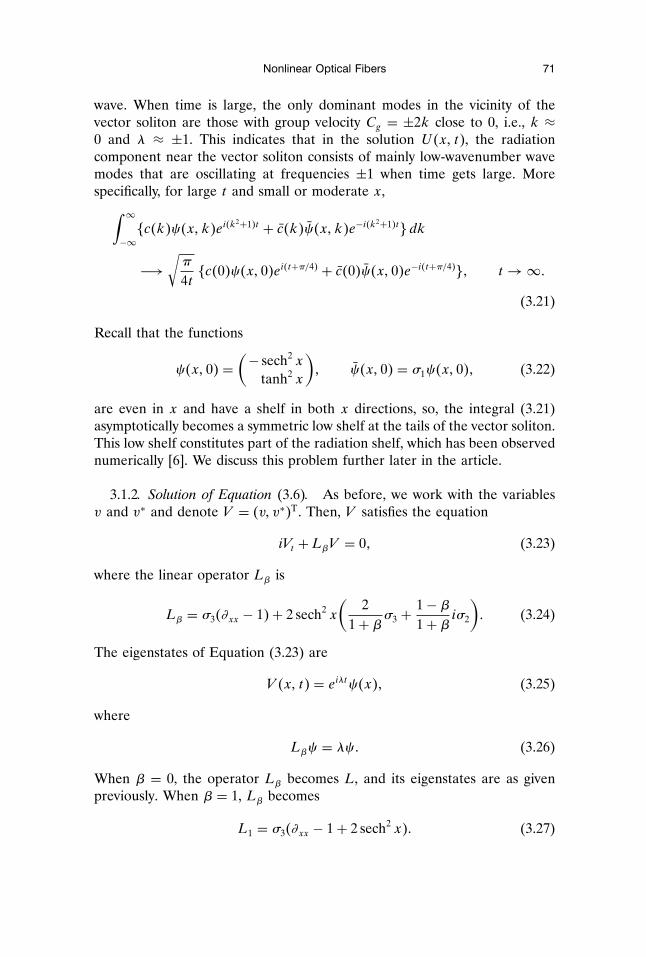
3.1.2. Solution of Equation (3.6). As before, we work with the variablesv and v∗ and denote V = �v; v∗�T. Then, V satisfies the equation
iVt + LβV = 0; (3.23)
where the linear operator Lβ is
Lβ = σ3�∂xx − 1� + 2 sech2 x
(2
1+ βσ3 +1− β1+ βiσ2
): (3.24)
The eigenstates of Equation (3.23) are
V �x; t� = eiλtψ�x�; (3.25)
where
Lβψ = λψ: (3.26)
When β = 0, the operator Lβ becomes L, and its eigenstates are as givenpreviously. When β = 1, Lβ becomes
L1 = σ3�∂xx − 1+ 2 sech2 x�: (3.27)
72 Jianke Yang
In this case, L1 has two discrete eigenfunctions
ψ1e = ψe = sech x(
1−1
); φ1e = sech x
(11
)(3.28)
with the same eigenvalue λ = 0. The continuous spectrum of L1 is �λ� ≥ 1.For each λ > 1 or λ < −1, there are two linearly independent eigenfunctions.Let us denote them as ψ�1�1 �x; λ� and ψ�2�1 �x; λ�. When λ < −1, these twofunctions are
ψ�1�1 =
(f1�x; λ�
0
); ψ
�2�1 =
(f2�x; λ�
0
); (3.29)
where f1 and f2 are the two linearly independent solutions of the Schrodingerequation
fxx − �1+ λ�f + 2 sech2 xf = 0 (3.30)
and can be expressed in terms of the hypergeometric functions [13]. Whenλ > 1,
ψ�1�1 �x; λ� = σ1ψ
�1�1 �x;−λ�; ψ
�2�1 �x; λ� = σ1ψ
�2�1 �x;−λ�: (3.31)
When λ = 1 or −1, there is only one eigenfunction �tanh x 0�T or�0 tanh x�T. Since the operator L1 is Hermitian, all these eigenstatesform a complete set.
When β continuously moves away from 0 to 1, the eigenstates of theoperator Lβ change accordingly. First of all, the discrete eigenstate
ψβe = ψe = sech x(
1−1
)(3.32)
with λ = 0 remains unchanged, but its generalized eigenstate becomes
φβe = g�x;β�(
11
); (3.33)
where g�x;β� is the solution of the equation
gxx − g +6− 2β1+ β sech2 xg = −2 sech x: (3.34)
The operator Lβ acting on φβe gives
Lβφβe = −2ψβe: (3.35)
Equation (3.34) has a unique localized solution for g if β 6= 1. This solutioncan be determined numerically. When β = 0,
g�x; 0� = sech x�x tanh x− 1�: (3.36)
Nonlinear Optical Fibers 73
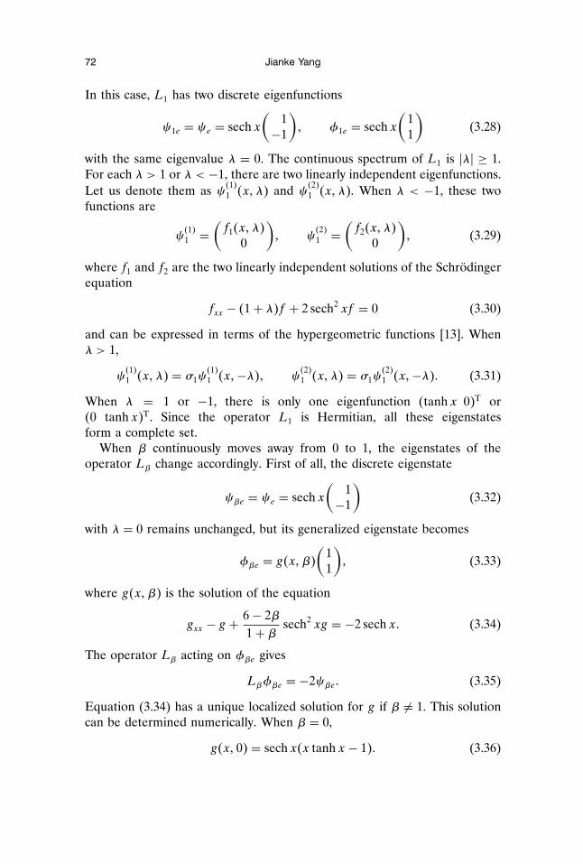
As β → 1, g�x;β� −→ sech x (when normalized so that g�0; β� = 1).Second, as β moves away from 0, the discrete eigenstate ψ0 (with λ = 0)and its generalized eigenstate φ0 split into two discrete eigenstates ψβ0 andψβ0 �= σ1ψβ0� with nonzero eigenvalues λβ �> 0� and −λβ respectively.These states can be determined numerically using the shooting method. Thedependence of λβ on β is plotted in Figure 4. When β is small, the per-turbation analysis by this author and D. J. Benney [5] shows that to leadingorder, λβ ≈
√64β/15. Another result by Ueda and Kath [6] is also relevant
here. As we show later in this article, the eigenstates ψβ0 and ψβ0 cause tothe vector soliton (3.3) a kind of internal oscillation that looks like a com-bination of translational and width oscillations discussed in [6]. Ueda andKath showed that the frequency of the translational oscillation (when ad-justed to the present context) is
√64β/�15�1+ β�� for small β. This result is
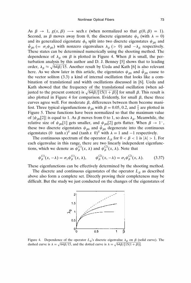
also plotted in Figure 4 for comparison. Evidently, for small β, these threecurves agree well. For moderate β, differences between them become mani-fest. Three typical eigenfunctions ψβ0 with β = 0:05; 0:2, and 2
3 are plotted inFigure 5. These functions have been normalized so that the maximum valueof �ψβ0�2�� is equal to 1. As β moves from 0 to 1, so does λβ. Meanwhile, therelative size of ψβ0�1� gets smaller, and ψβ0�2� gets flatter. When β → 1−,these two discrete eigenstates ψβ0 and ψβ0 degenerate into the continuouseigenstates �0 tanh x�T and �tanh x 0�T with λ = 1 and −1 respectively.
The continuous spectrum of the operator Lβ for 0 < β < 1 is �λ� > 1. Foreach eigenvalue in this range, there are two linearly independent eigenfunc-tions, which we denote as ψ�1�β �x; λ� and ψ�2�β �x; λ�. Note that
ψ�1�β �x;−λ� = σ1ψ
�1�β �x; λ�; ψ
�2�β �x;−λ� = σ1ψ
�2�β �x; λ�: (3.37)
These eigenfunctions can be effectively determined by the shooting method.The discrete and continuous eigenstates of the operator Lβ as described
above also form a complete set. Directly proving their completeness may bedifficult. But the study we just conducted on the changes of the eigenstates of
Figure 4. Dependence of the operator Lβ’s discrete eigenvalue λβ on β (solid curve). Thedashed curve is λ = √64β/15, and the dotted curve is λ = √64β/�15�1+ β��.
74 Jianke Yang
Figure 5. The discrete eigenfunctions ψβ0 for β equal to (a) 0.05, (b) 0.2, and (c) 23 . The solid
curves are ψβ0�1� and the dashed ones are ψβ0�2�.
Lβ as β moves from 0 to 1 leaves little doubt that they are indeed complete.As a result, any initial condition V �x; 0� can be decomposed into these statesas
V �x; 0� =∫�c�1�ψ�1�β �x; λ� + c�2�ψ�2�β �x; λ��dλ
+ cβeψβe�x� + dβeφβe�x� + c1ψβ0�x� + c2ψβ0�x�; (3.38)
where the integral is over the intervals (–∞ –1) and �1 ∞� for λ. Thecoefficients in (3.38) can be determined from V �x; 0� by a method similar tothat in [12]. In particular, we find that the coefficients in front of the discreteeigenstates are
cβe =�V �x; 0�; φβe��ψβe; φβe�
; dβe =�V �x; 0�; ψβe��ψβe; φβe�
; (3.39a)
c1 =�V �x; 0�; ψβ0��ψβ0 ψβ0�
; c2 =�V �x; 0�; ψβ0��ψβ0; ψβ0�
= c∗1 ; (3.39b)
where the inner product � ; � is defined in (3.19). The relation c2 = c∗1 isobtained in view of the fact that V �x; 0� = �v�x; 0�; v∗�x; 0��T. The timeevolution of the initial condition V �x; 0� is now readily given as
V �x; t� =∫�c�1�ψ�1�β �x; λ� + c�2�ψ�2�β �x; λ��eiλtdλ + cβeψβe�x�
+ dβe�φβe�x� − 2itψβe�x�� + c1ψβ0�x�eiλβt
+ c∗1 ψβ0�x�e−iλβt : (3.40)
It is clear from the relation (3.1) and (3.4) that the solution V �x; t� causes Aand B to evolve asymmetrically. Note that the terms cβeψβe and dβe�φβe −2itψβe� can be absorbed into the vector soliton (3.3) and cause an opposite
Nonlinear Optical Fibers 75
phase and width shift to its A and B pulses respectively. More interestingare the terms c1ψβ0e
iλβt + c2ψβ0e−iλβt . To reveal their effects on the vector
soliton (3.3), we assume that initially
V �x; 0� = c1ψβ0 + c∗1 ψβ0; (3.41)
so that its time evolution is
V �x; t� = c1ψβ0eiλβt + c∗1 ψβ0e
−iλβt : (3.42)
We also assume that the disturbance
U�x; t� = 0: (3.43)
Then, from the relations (3.1), (3.3), and (3.4), we find that the solutionsA�x; t� and B�x; t� are
A�x; t� = eit�√
2/�1+ β� sech x+ 12c1ψβ0�1�eiλβt+
12c∗1ψβ0�2�e−iλβt�; (3.44a)
B�x; t� = eit�√
2/�1+ β� sech x− 12c1ψβ0�1�eiλβt−
12c∗1ψβ0�2�e−iλβt�: (3.44b)
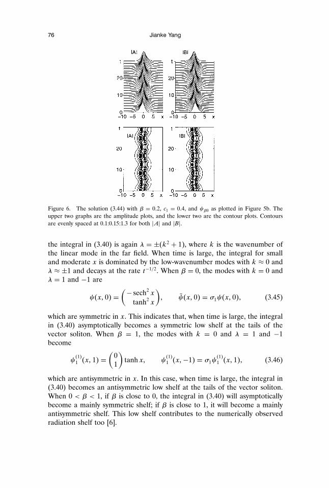
If we take β = 0:2, then λβ ≈ 0:76 and the normalized eigenfunction ψβ0 isplotted in Figure 5b. If we further take c1 = 0:4, then the amplitudes of thesolutions (3.44) are plotted in Figure 6. We find that the discrete eigenmodesψβ0 and ψβ0 cause to (3.3) a kind of internal oscillation in which the centralpositions of the A and B pulses appear to oscillate about one another andthe widths simultaneously dilate and contract, both at the same frequency λβ.This combined visual effect can be clearly seen in Figure 6. In the variationalprinciple analyses by Ueda and Kath [6] and Kaup et al. [8], these positionand width oscillations were treated as two processes with independent fre-quencies. In our analysis, these two oscillations are just the visual effects of asingle internal oscillation process caused by the discrete eigenfunctions ψβeand ψβe, having a single frequency λβ. This internal oscillation is permanentwithin the linearization theory. The integral in (3.40) is a collection of dis-persive wave modes and is the radiation part of the V solution. It can causethe A pulse of the vector soliton (3.3) to dilate (or contract) and the B pulseto contract (or dilate). This out-of-phase width oscillation decays at the ratet−1/2. Interestingly, using the variational principle method and excluding ra-diation, Kaup et al. [8] identified similar linear eigenmodes. But it should bepointed out that such modes they identified are not really linear eigenmodes.Rather, they are radiation modes and only cause transient oscillations to thevector solution (3.3).
The asymptotic behavior of the integral in (3.40) can be analyzed as wedid for the integral in (3.20). The dispersion relation of the linear modes in
76 Jianke Yang
Figure 6. The solution (3.44) with β = 0:2, c1 = 0:4, and ψβ0 as plotted in Figure 5b. Theupper two graphs are the amplitude plots, and the lower two are the contour plots. Contoursare evenly spaced at 0.1:0.15:1.3 for both �A� and �B�.
the integral in (3.40) is again λ = ±�k2 + 1�, where k is the wavenumber ofthe linear mode in the far field. When time is large, the integral for smalland moderate x is dominated by the low-wavenumber modes with k ≈ 0 andλ ≈ ±1 and decays at the rate t−1/2. When β = 0, the modes with k = 0 andλ = 1 and −1 are
ψ�x; 0� =(− sech2 x
tanh2 x
); ψ�x; 0� = σ1ψ�x; 0�; (3.45)
which are symmetric in x. This indicates that, when time is large, the integralin (3.40) asymptotically becomes a symmetric low shelf at the tails of thevector soliton. When β = 1, the modes with k = 0 and λ = 1 and −1become
ψ�1�1 �x; 1� =
(01
)tanh x; ψ
�1�1 �x;−1� = σ1ψ
�1�1 �x; 1�; (3.46)
which are antisymmetric in x. In this case, when time is large, the integral in(3.40) becomes an antisymmetric low shelf at the tails of the vector soliton.When 0 < β < 1, if β is close to 0, the integral in (3.40) will asymptoticallybecome a mainly symmetric shelf; if β is close to 1, it will become a mainlyantisymmetric shelf. This low shelf contributes to the numerically observedradiation shelf too [6].
Nonlinear Optical Fibers 77
Finally, when β > 1, the discrete eigenstate ψβe (with λ = 0) and itsgeneralized eigenstate φβe still exist, but the other two discrete eigenstatesψβ0 and ψβ0 disappear. As a result, the permanent internal oscillations areno longer present. The other aspects of the solution evolution is similar tothose with 0 < β < 1.
3.1.3. An example. For any disturbed state of the vector soliton (3.3), thetime evolution of the solution can be determined by the methods describedabove in view of the relations (3.1) and (3.4). As an example, we now deter-mine the asymptotic state of the solution if initially the A and B pulses ofthe vector soliton (3.3) are slightly separated in space, i.e.,
A�x; 0� =√
2/�1+ β� sech�x+ x0�; (3.47a)
B�x; 0� =√
2/�1+ β� sech�x− x0�; (3.47b)
where x0 is small. In this case,
A�x; 0� =√
2/�1+ β��sech�x+ x0� − sech x�; (3.48a)
B�x; 0� =√
2/�1+ β��sech�x− x0� − sech x�; (3.48b)
and
u�x; 0� =√
2/�1+ β��sech�x+ x0� + sech�x− x0� − 2 sech x�; (3.49a)
v�x; 0� =√
2/�1+ β��sech�x+ x0� − sech�x− x0��: (3.49b)
First, we determine the asymptotic state of u�x; t�. From (3.20) we get
U�x; t� −→ ceψe�x� + c0ψ0�x� + de�φe�x� − 2itψe�x��+ d0�φ0�x� − 2itψ0�x��; t →∞; (3.50)
where ce; c0; de, and d0 are found from (3.18) to be
ce = c0 = d0 = 0; de = −∫ ∞−∞u�x; 0� sech xdx: (3.51)
It follows that
u�x; t� −→ de�sech x�x tanh x− 1� − 2it sech x�; t →∞: (3.52)
Next, we determine the asymptotic state of v�x; t�. From (3.40) we get
v�x; t� −→ cβeψβe�x� + dβe�φβe�x� − 2itψβe�+ c1ψβ0e
iλβt + c∗1 ψβ0e−iλβt ; t →∞: (3.53)
78 Jianke Yang
If we denote ψβ0 = �h1�x;β�; h2�x;β��T, then the coefficients are foundfrom (3.39) to be
cβe = dβe = 0; c1 =∫∞−∞ v�x; 0��h1 − h2�dx∫∞
−∞�h21 − h2
2�dx: (3.54)
Therefore,
v�x; t� −→ c1�h1�x;β�eiλβt + h2�x;β�e−iλβt�; t →∞: (3.55)
The functions h1 and h2, as well as λβ, can be determined numerically fromEquation (3.26).
The asymptotic states of A and B can now be obtained from (3.4), (3.52),and (3.55). So when time is large, we obtain from (3.1) and (3.3) that
A�x; t� −→ eit�√
2/�1+ β� sech x+ 12de�sech x�x tanh x− 1� − 2it sech x�
+ 12c1�h1e
iλβt + h2e−iλβt��; t →∞; (3.56a)
B�x; t� −→ eit�√
2/�1+ β� sech x+ 12de�sech x�x tanh x− 1� − 2it sech x�
− 12c1�h1e
iλβt + h2e−iλβt��; t →∞: (3.56b)
The de terms can be absorbed into the vector soliton and cause a width shiftto it. This can be easily done and we get
A�x; t� −→√
2/�1+ β� r sech rxeir2t
+ 12c1�h1e
i�1+λβ�t + h2ei�1−λβ�t�; (3.57a)
B�x; t� −→√
2/�1+ β� r sech rxeir2t
− 12c1�h1e
i�1+λβ�t + h2ei�1−λβ�t�; (3.57b)
where r = 1 − √�1+ β�/8 de. For the linearization theory to be valid, theinitial disturbances A�x; 0� and B�x; 0� in (3.48) need to be small. This re-quires x0 to be small. Under this condition, the formulas for de; c1, and r canbe simplified. We can easily show that
de ≈√
21+ β
x20
3; r ≈ 1− x
20
6; (3.58a)
c1 ≈ −√
81+ β
∫∞−∞ sech x tanh x�h1 − h2�dx∫∞
−∞�h21 − h2
2�dxx0: (3.58b)
Nonlinear Optical Fibers 79
If we take β = 0:2, then λβ ≈ 0:76, and the normalized eigenfunction ψβ0 =�h1 h2�T is as shown in Figure 5b. We then find numerically that
c1 ≈ 0:78x0: (3.59)
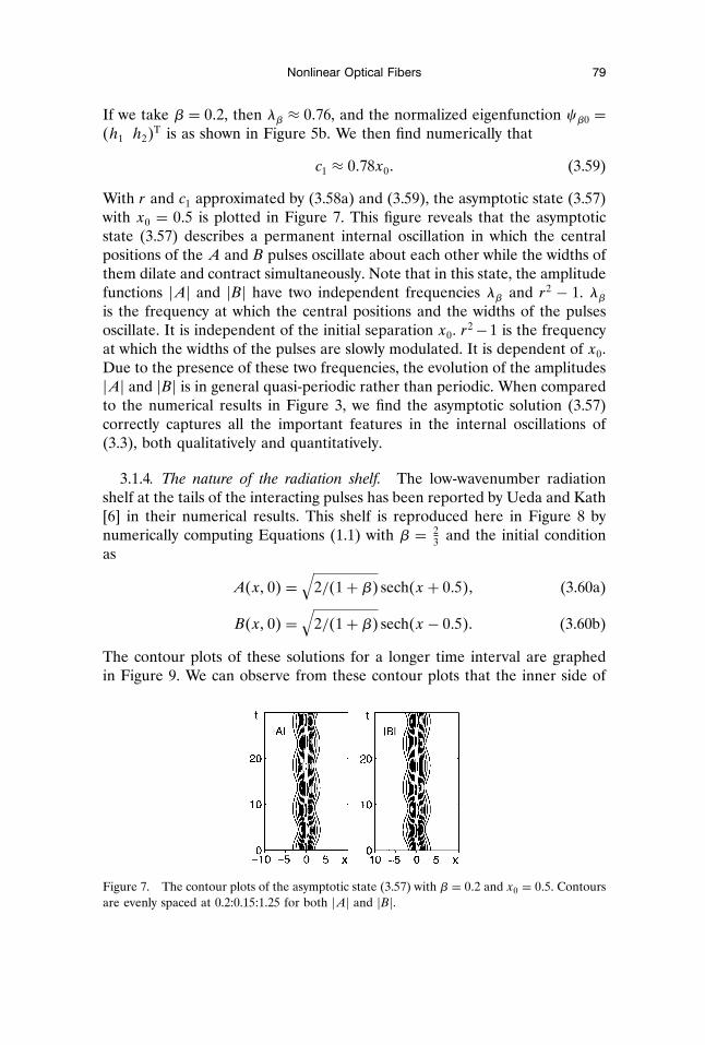
With r and c1 approximated by (3.58a) and (3.59), the asymptotic state (3.57)with x0 = 0:5 is plotted in Figure 7. This figure reveals that the asymptoticstate (3.57) describes a permanent internal oscillation in which the centralpositions of the A and B pulses oscillate about each other while the widths ofthem dilate and contract simultaneously. Note that in this state, the amplitudefunctions �A� and �B� have two independent frequencies λβ and r2 − 1. λβis the frequency at which the central positions and the widths of the pulsesoscillate. It is independent of the initial separation x0. r2−1 is the frequencyat which the widths of the pulses are slowly modulated. It is dependent of x0.Due to the presence of these two frequencies, the evolution of the amplitudes�A� and �B� is in general quasi-periodic rather than periodic. When comparedto the numerical results in Figure 3, we find the asymptotic solution (3.57)correctly captures all the important features in the internal oscillations of(3.3), both qualitatively and quantitatively.
3.1.4. The nature of the radiation shelf. The low-wavenumber radiationshelf at the tails of the interacting pulses has been reported by Ueda and Kath[6] in their numerical results. This shelf is reproduced here in Figure 8 bynumerically computing Equations (1.1) with β = 2
3 and the initial conditionas
A�x; 0� =√
2/�1+ β� sech�x+ 0:5�; (3.60a)
B�x; 0� =√
2/�1+ β� sech�x− 0:5�: (3.60b)
The contour plots of these solutions for a longer time interval are graphedin Figure 9. We can observe from these contour plots that the inner side of
Figure 7. The contour plots of the asymptotic state (3.57) with β = 0:2 and x0 = 0:5. Contoursare evenly spaced at 0.2:0.15:1.25 for both �A� and �B�.
80 Jianke Yang
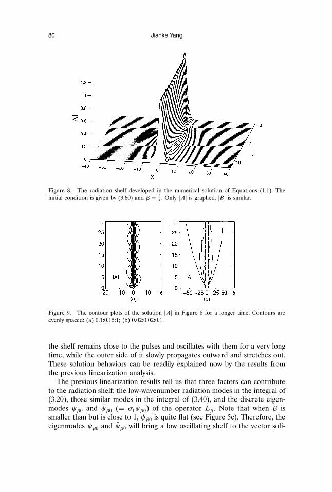
Figure 8. The radiation shelf developed in the numerical solution of Equations (1.1). Theinitial condition is given by (3.60) and β = 2
3 . Only �A� is graphed. �B� is similar.
Figure 9. The contour plots of the solution �A� in Figure 8 for a longer time. Contours areevenly spaced: (a) 0.1:0.15:1; (b) 0.02:0.02:0.1.
the shelf remains close to the pulses and oscillates with them for a very longtime, while the outer side of it slowly propagates outward and stretches out.These solution behaviors can be readily explained now by the results fromthe previous linearization analysis.
The previous linearization results tell us that three factors can contributeto the radiation shelf: the low-wavenumber radiation modes in the integral of(3.20), those similar modes in the integral of (3.40), and the discrete eigen-modes ψβ0 and ψβ0 �= σ1ψβ0� of the operator Lβ. Note that when β issmaller than but is close to 1, ψβ0 is quite flat (see Figure 5c). Therefore, theeigenmodes ψβ0 and ψβ0 will bring a low oscillating shelf to the vector soli-

Nonlinear Optical Fibers 81
Figure 10. The solution (3.44) with β = 23 , c1 = 0:25 and ψβ0 as plotted in Figure 5c. Low-
radiation shelf can be observed. Only �A� is plotted. �B� is similar.
ton (3.3). To demonstrate this, we plot in Figure 10 the solution (3.44) withβ = 2
3 and c1 = 0:25. The eigenfunction ψβ0 is as shown in Figure 5c. Asexpected, we observe a low shelf similar to that in Figure 8. In the contourplots of solution (3.44) shown in Figure 11, we can see that for all time, thisshelf remains close to the pulses and oscillates with them at frequency λβ,which is approximately equal to 0.982 when β is 2
3 (see Figure 4). It is nowclear that the oscillating inner shelf in Figure 9 is caused by the eigenmodesψβ0 and ψβ0 and is only a special case of the linearly permanent internaloscillations discussed before. This is why this inner shelf can stay close toand oscillate with the pulses for a long time. The slowly propagating outershelf observed in Figure 9 is due to the low-wavenumber radiation modesin the integrals of (3.20) and (3.40). These modes have small group veloci-ties and propagate slowly. Due to dispersion, they decay at the rate t−1/2. Astime gets large, these low-wavenumber radiation modes will be seen at theouter side of the shelf. At the inner side of the shelf, the radiation modeswill be negligible and the eigenmodes ψβ0 and ψβ0 will be dominating andcause long-lasting internal oscillations to the pulses. Finally, we comment thatwhen β is not close to 1, either the discrete eigenmodes ψβ0 and ψβ0 existbut are not flat (for β < 1, see Figure 5), or ψβ0 and ψβ0 do not exist at all(when β > 1). In both cases, the radiation shelf will be contributed solelyby the low-wavenumber radiation modes in the integrals of (3.20) and (3.40).Therefore, this shelf will disperse away and decay and will be less visible atthe tails of the pulses.
82 Jianke Yang
Figure 11. The contour plots of the solution �A� in Figure 10 for a longer time. Contours areevenly spaced: (a) 0.1:0.15:1; (b) 0.02:0.02:0.1.
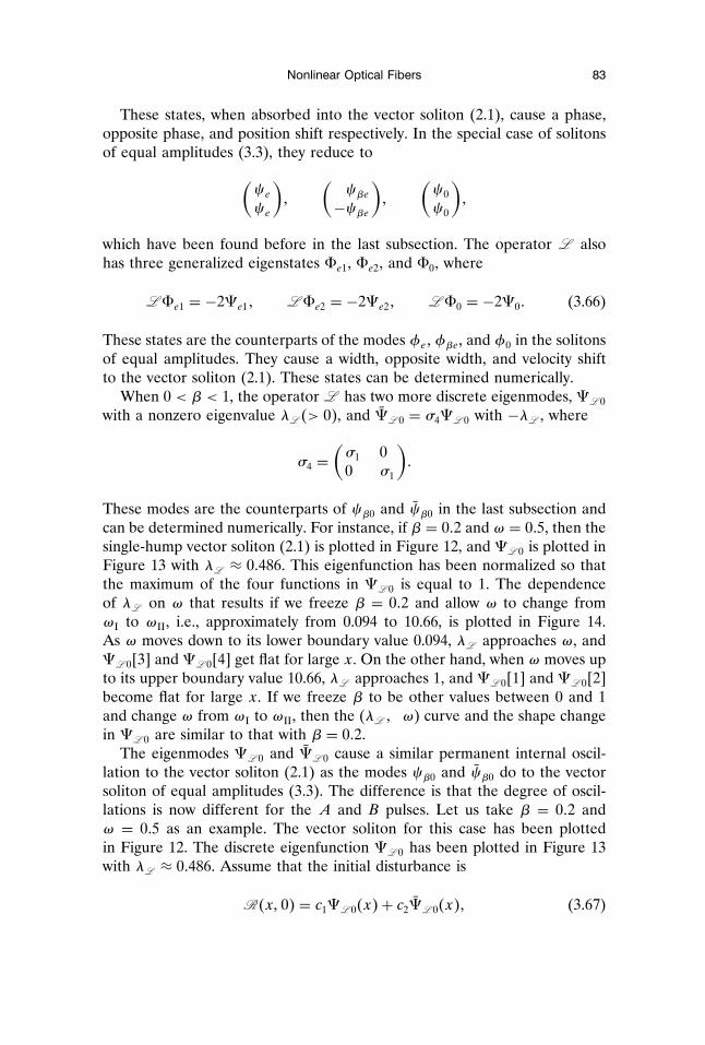
3.2. Linearization analysis for general single-hump vector solitons
For general single-hump vector solitons (2.1) of arbitrary polarization, thedisturbances A and B are governed by Equations (3.2). We denote R ≡�A; A∗; B; B∗�T. Then the linear system for R can be readily obtained from(3.2). It is
iRt +L R = 0; (3.61)
where the operator L is
L =( �∂xx−1+2r2
1+βr22 �σ3+ir2
1σ2 βr1r2�σ3+iσ2�βr1r2�σ3+iσ2� �∂xx−ω+2r2
2+βr21 �σ3+ir2
2σ2
):
(3.62)
The eigenstates of R are of the form
R = eiλt9�x�; (3.63)
where
L9 = λ9: (3.64)
Recall that single-hump vector solitons (2.1) exist for ω in the interval(ωI;ωII), which is illustrated in Figure 2. For these single-hump solitons, theoperator L has the following three discrete eigenmodes with λ = 0:
9e1 =
r1−r1r2−r2
; 9e2 =
r1−r1−r2r2
; 90 =
r1xr1xr2xr2x
: (3.65)
Nonlinear Optical Fibers 83
These states, when absorbed into the vector soliton (2.1), cause a phase,opposite phase, and position shift respectively. In the special case of solitonsof equal amplitudes (3.3), they reduce to(
ψeψe
);
(ψβe−ψβe
);
(ψ0ψ0
);
which have been found before in the last subsection. The operator L alsohas three generalized eigenstates 8e1, 8e2, and 80, where
L 8e1 = −29e1; L 8e2 = −29e2; L 80 = −290: (3.66)
These states are the counterparts of the modes φe;φβe, and φ0 in the solitonsof equal amplitudes. They cause a width, opposite width, and velocity shiftto the vector soliton (2.1). These states can be determined numerically.
When 0 < β < 1, the operator L has two more discrete eigenmodes, 9L 0with a nonzero eigenvalue λL �> 0�, and 9L 0 = σ49L 0 with −λL , where
σ4 =(σ1 00 σ1
):
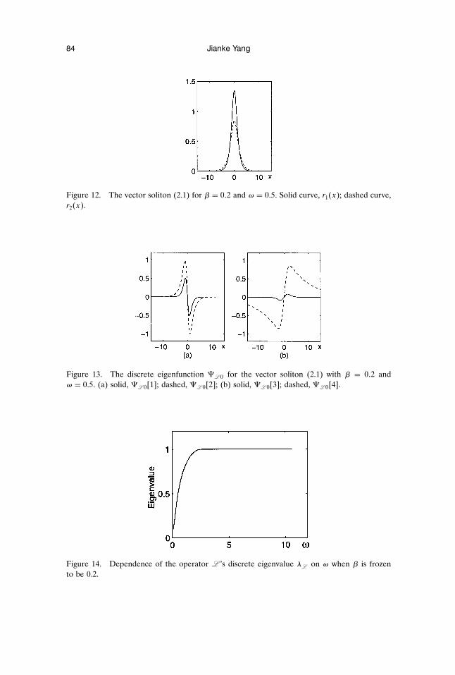
These modes are the counterparts of ψβ0 and ψβ0 in the last subsection andcan be determined numerically. For instance, if β = 0:2 and ω = 0:5, then thesingle-hump vector soliton (2.1) is plotted in Figure 12, and 9L 0 is plotted inFigure 13 with λL ≈ 0:486. This eigenfunction has been normalized so thatthe maximum of the four functions in 9L 0 is equal to 1. The dependenceof λL on ω that results if we freeze β = 0:2 and allow ω to change fromωI to ωII, i.e., approximately from 0.094 to 10.66, is plotted in Figure 14.As ω moves down to its lower boundary value 0.094, λL approaches ω, and9L 0�3� and 9L 0�4� get flat for large x. On the other hand, when ω moves upto its upper boundary value 10.66, λL approaches 1, and 9L 0�1� and 9L 0�2�become flat for large x. If we freeze β to be other values between 0 and 1and change ω from ωI to ωII, then the (λL ; ω) curve and the shape changein 9L 0 are similar to that with β = 0:2.
The eigenmodes 9L 0 and 9L 0 cause a similar permanent internal oscil-lation to the vector soliton (2.1) as the modes ψβ0 and ψβ0 do to the vectorsoliton of equal amplitudes (3.3). The difference is that the degree of oscil-lations is now different for the A and B pulses. Let us take β = 0:2 andω = 0:5 as an example. The vector soliton for this case has been plottedin Figure 12. The discrete eigenfunction 9L 0 has been plotted in Figure 13with λL ≈ 0:486. Assume that the initial disturbance is
R �x; 0� = c19L 0�x� + c29L 0�x�; (3.67)
84 Jianke Yang
Figure 12. The vector soliton (2.1) for β = 0:2 and ω = 0:5. Solid curve, r1�x�; dashed curve,r2�x�.
Figure 13. The discrete eigenfunction 9L 0 for the vector soliton (2.1) with β = 0:2 andω = 0:5. (a) solid, 9L 0�1�; dashed, 9L 0�2�; (b) solid, 9L 0�3�; dashed, 9L 0�4�.
Figure 14. Dependence of the operator L ’s discrete eigenvalue λL on ω when β is frozento be 0.2.
Nonlinear Optical Fibers 85
where c1 and c2 are small complex constants. It can be shown that the relationc1 = c∗2 needs to be satisfied to ensure consistency. Then the later timeevolution for R is
R �x; t� = c19L 0�x�eiλL t + c29L 0�x�e−iλL t : (3.68)
It follows that the solutions A and B are
A�x; t� = eit�r1�x� + c19L 0�1�eiλL t + c29L 0�2�e−iλL t�; (3.69a)
B�x; t� = eit�r2�x� + c19L 0�3�eiλL t + c29L 0�4�e−iλL t�: (3.69b)
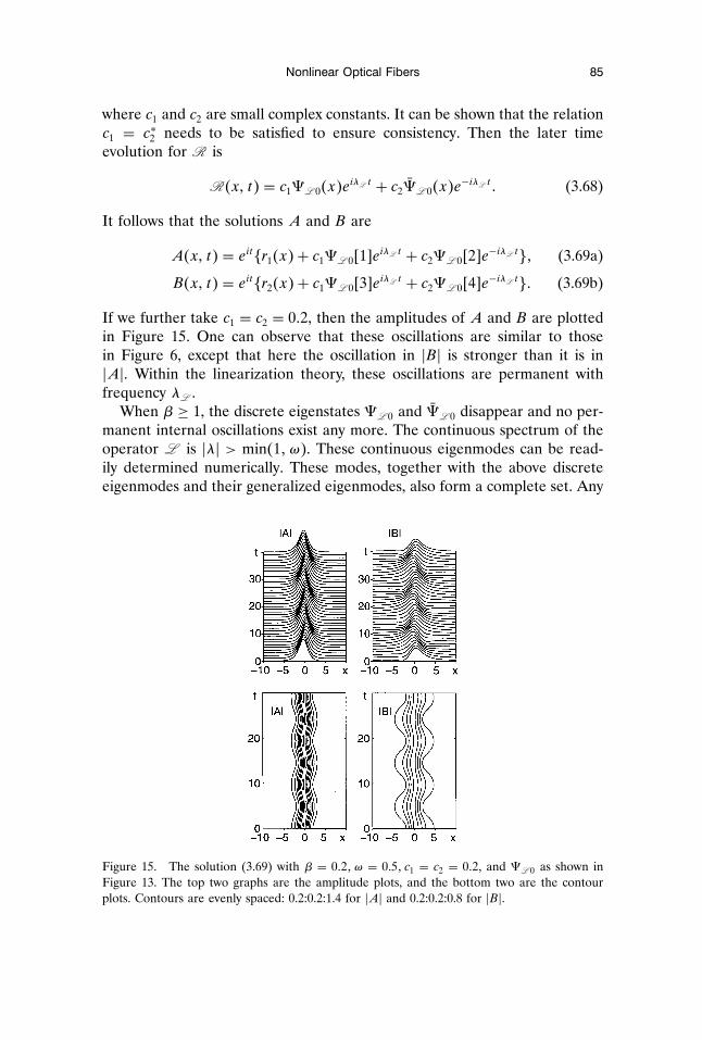
If we further take c1 = c2 = 0:2, then the amplitudes of A and B are plottedin Figure 15. One can observe that these oscillations are similar to thosein Figure 6, except that here the oscillation in �B� is stronger than it is in�A�. Within the linearization theory, these oscillations are permanent withfrequency λL .
When β ≥ 1, the discrete eigenstates 9L 0 and 9L 0 disappear and no per-manent internal oscillations exist any more. The continuous spectrum of theoperator L is �λ� > min�1;ω�. These continuous eigenmodes can be read-ily determined numerically. These modes, together with the above discreteeigenmodes and their generalized eigenmodes, also form a complete set. Any
Figure 15. The solution (3.69) with β = 0:2;ω = 0:5; c1 = c2 = 0:2, and 9L 0 as shown inFigure 13. The top two graphs are the amplitude plots, and the bottom two are the contourplots. Contours are evenly spaced: 0.2:0.2:1.4 for �A� and 0.2:0.2:0.8 for �B�.
86 Jianke Yang
initial disturbance A�x; 0� and B�x; 0� can be decomposed into these eigen-states. Therefore, its time evolution can be easily determined. This analysisis similar to what we did in the last section and is not reproduced here.
3.3. Linearization analysis for degenerate vector solitons
The degenerate vector solitons, in which one of the A and B componentsvanishes, are different from the single-hump vector solitons (2.1) describedin Section 2. A separate linearization analysis is needed to study their internaloscillations.
Without loss of generality, we assume that the degenerate vector soliton is
A =√
2 sech xeit ; B = 0: (3.70)
When it is disturbed, then
A = eit�√
2 sech x+ A�; B = B; (3.71)
where A and B are small disturbances. When (3.71) is substituted into (1.1)and higher-order terms neglected, then the linearized equations for A and Bare
iAt + Axx − A+ 4 sech2 xA+ 2 sech2 xA∗ = 0; (3.72)
iB + Bxx + 2β sech2 xB = 0: (3.73)
Equation (3.72) is the same as (3.5) whose solution has been given in Sec-tion 3.1. An initial disturbance in A may cause phase, position, width, andvelocity shifts to the A soliton, but there is no permanent internal oscillationsinvolved. Equation (3.73) is the time-dependent linear Schrodinger equation.Its eigenstates are
B = eiλtb�x�; (3.74)
where
Mβb = λb; (3.75)
and
Mβ = ∂xx + 2β sech2 x (3.76)
is the Schrodinger operator and is Hermitian. It is well known in quantummechanics that Equation (3.75) can be solved exactly [13] and the eigensolu-tions �b�x�; λ� can be analytically determined. When 0 < β ≤ 1, the operatorMβ has a single discrete eigenstate
b1�x� = sechs x; λ1 =14�√
1+ 8β− 1�2; (3.77)
Nonlinear Optical Fibers 87
where s = �√1+ 8β − 1�/2. This state is reminiscent of the daughter wavestate of a vector soliton (2.1). When 1 < β ≤ 3, beside �b1�x�; λ1�, Mβ hasone more discrete eigenstate
b2�x� = sechs x sinh x; λ2 =14�√
1+ 8β− 3�2: (3.78)
When β > 3, even more discrete eigenstates will appear.The continuous spectrum of Mβ is λ ≤ 0 when β = n�n + 1�/2; �n =
1; 2; : : :�, and λ < 0 for other positive values of β. The continuous eigen-functions can be expressed in terms of the hypergeometric functions. They,together with the above discrete eigenfunctions, form a complete set sinceMβ is Hermitian.
An initial disturbance in B can be decomposed into the eigenstates of Mβ.The collection of the continuous eigenmodes corresponds to radiation anddecays at the rate t−1/2. The discrete eigenmodes will persist for all time.When 0 < β ≤ 1, there is only one such mode. Therefore, when time islarge, B will asymptotically approach this eigenstate in which no amplitudeoscillations are present. But when β > 1, two or more discrete eigenmodesexist. Hence, B will asymptotically approach a state which is a linear super-position of these discrete eigenmodes. In this state, the amplitude oscillatespermanently with time. For demonstration purposes, let us suppose that ini-tially there is no A disturbance, and B consists of only the two lowest discreteeigenmodes, i.e.,
A�x; 0� = 0; B�x; 0� = c1b1�x� + c2b2�x�; (3.79)
where c1 and c2 are two arbitrary small complex constants. Then, the timeevolution for A and B is
A�x; t� =√
2 sech xeit ; (3.80a)
B�x; t� = c1b1�x�eiλ1t + c2b2�x�eiλ2t : (3.80b)
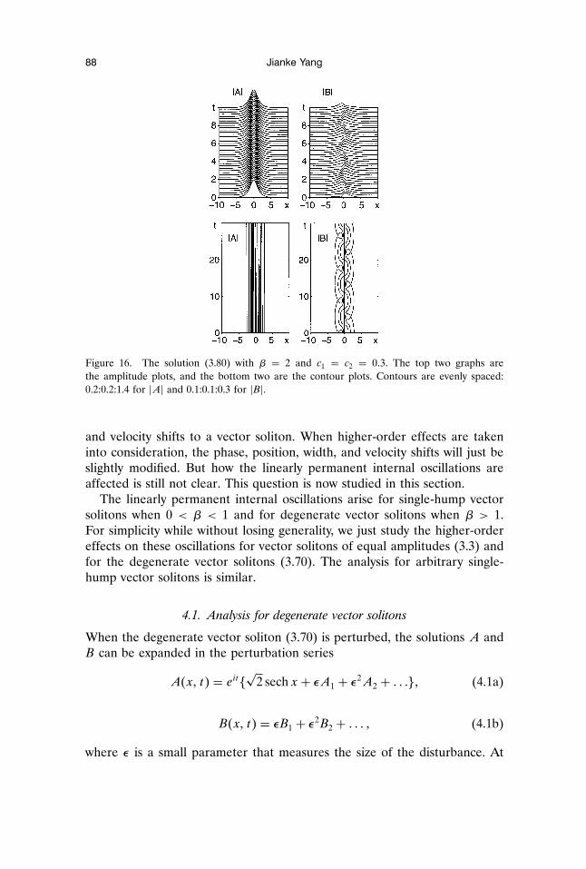
If we take β = 2 and c1 = c2 = 0:3, then their amplitudes are plotted inFigure 16. In the solution (3.80), �A� does not change with time, but �B� os-cillates back and forth with frequency λ1−λ2 =
√1+ 8β−2. This oscillation
in �B� is also permanent within the linearization theory.
4. Higher-order effects
The linearization analysis in the last section shows that small disturbancesmay cause permanent internal oscillations as well as phase, position, width,
88 Jianke Yang
Figure 16. The solution (3.80) with β = 2 and c1 = c2 = 0:3. The top two graphs arethe amplitude plots, and the bottom two are the contour plots. Contours are evenly spaced:0.2:0.2:1.4 for �A� and 0.1:0.1:0.3 for �B�.
and velocity shifts to a vector soliton. When higher-order effects are takeninto consideration, the phase, position, width, and velocity shifts will just beslightly modified. But how the linearly permanent internal oscillations areaffected is still not clear. This question is now studied in this section.
The linearly permanent internal oscillations arise for single-hump vectorsolitons when 0 < β < 1 and for degenerate vector solitons when β > 1.For simplicity while without losing generality, we just study the higher-ordereffects on these oscillations for vector solitons of equal amplitudes (3.3) andfor the degenerate vector solitons (3.70). The analysis for arbitrary single-hump vector solitons is similar.
4.1. Analysis for degenerate vector solitons
When the degenerate vector soliton (3.70) is perturbed, the solutions A andB can be expanded in the perturbation series
A�x; t� = eit�√
2 sech x+ εA1 + ε2A2 + : : :�; (4.1a)
B�x; t� = εB1 + ε2B2 + : : : ; (4.1b)
where ε is a small parameter that measures the size of the disturbance. At
Nonlinear Optical Fibers 89
order ε, the equations for A1 and B1 are
iA1t +A1xx −A1 + 4 sech2 xA1 + 2 sech2 xA∗1 = 0; (4.2)
iB1t + B1xx + 2β sech2 xB1 = 0: (4.3)
These equations are the same as (3.72) and (3.73). Actually, if order ε2 andhigher terms in (4.1) are neglected, this analysis will become the linearizationanalysis as in Section 3, and the solutions for A1 and B1 have been deter-mined there. The linearly permanent internal oscillations are present in theB1 solution when β > 1. They are caused by two or more discrete eigen-modes of the operator Mβ. Since our objective is to study the higher-ordereffects on these permanent oscillations, for simplicity, we take
A1�x; t� = 0; B1�x; t� = c1b1�x�eiλ1t + c2b2�x�eiλ2t ; (4.4)
where bi and λi �i = 1; 2� are given by (3.77) and (3.78), and ci �i = 1; 2�are arbitrary complex constants. At order ε2, A2 is governed by the equation
iA2t +A2xx −A2 + 4 sech2 xA2 + 2 sech2 xA∗2 = η; (4.5)
where
η = −√
2β sech x�c1c∗1b
21 + c2c
∗2b
22 + �c1c
∗2ei�λ1−λ2�t + c∗1c2e
−i�λ1−λ2�t�b1b2�:(4.6)
To find its solution, we work with the variables A2 and A∗2. Let us denoteW = �A2;A
∗2�T. Then W satisfies the equation
iWt + LW = η(
1−1
); (4.7)
where the operator L is given by Equation (3.8). Recall that the homoge-neous equation of (4.7) has been solved exactly in Section 3. Therefore, oncewe can find an inhomogeneous solution Wp to (4.7), then (4.7) will be solved.Since Equation (4.7) is linear, Wp can be written as
Wp�x; t� = −√
2β{�c1c
∗1w1�x� + c2c
∗2w2�x��
(11
)
+ c1c∗2w3�x�ei�λ1−λ2�t + c∗1c2w4�x�e−i�λ1−λ2�t
}; (4.8)
where the scalar functions w1; w2 and the vector functions w3; w4 are inho-
90 Jianke Yang
mogeneous solutions of the following equations:
w1xx −w1 + 6 sech2 xw1 = b21 sech x; (4.9)
w2xx −w2 + 6 sech2 xw2 = b22 sech x; (4.10)
Lw3 − �λ1 − λ2�w3 = b1b2 sech x(
1−1
); (4.11)
Lw4 + �λ1 − λ2�w4 = b1b2 sech x(
1−1
): (4.12)
The homogeneous equations of (4.9) and (4.10) have a localized solution,sech x tanh x, which is orthogonal to the inhomogeneous terms b2
1 sech x andb2
2 sech x, i.e.,∫ ∞−∞b2
1 sech2 x tanh xdx = 0;∫ ∞−∞b2
2 sech2 x tanh xdx = 0: (4.13)
Therefore, localized inhomogeneous solutions exist in Equations (4.9) and(4.10). These solutions can be written as
wi = wip + α sech x tanh x; i = 1; 2; (4.14)
where wip; i = 1; 2 are inhomogeneous solutions of (4.9) and (4.10), and αis a real-valued constant. To make w1p and w2p unique, we can require thatthey are even functions of x. These solutions can be determined numericallyif β is given.
Next, we consider the solutions of Equations (4.11) and (4.12). For β > 1,which is the case we are considering,
λ1 − λ2 =√
1+ 8β− 2 > 1: (4.15)
So λ1 − λ2 is in the continuous spectrum of the operator L. As a result,the homogeneous equation of (4.11) has two linearly independent boundedsolutions ψ�x; k� and ψ�x;−k� (note that ψ�x;−k�=ψ∗�x; k�), where thefunction ψ�x; k� is given by (3.12),
k2 = λ1 − λ2 − 1 =√
1+ 8β− 3; (4.16)
and k > 0. Note that ψ�x; k� and ψ�x;−k� have oscillating tails at infinity.For Equation (4.11), localized inhomogeneous solutions exist if and only ifthe compatibility condition
I�β� ≡∫ ∞−∞ψT�x; k�σ3b1b2 sech x
(1−1
)dx = 0 (4.17)
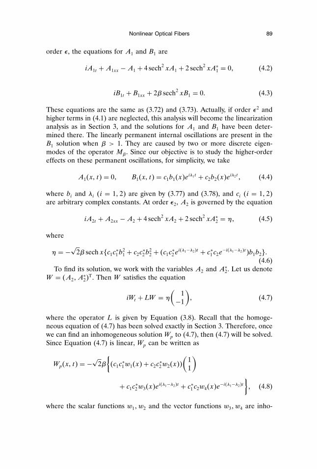
Nonlinear Optical Fibers 91
is satisfied. But this is not the case. The magnitude of I�β� against β is plot-ted in Figure 17. We can observe that I�β� is never equal to zero for β > 1.This indicates that Equation (4.11) has no localized inhomogeneous solu-tions. All its bounded solutions are not localized. Instead, they are oscillatoryat infinity. Similarly, the homogeneous equation of (4.12) has two linearly in-dependent solutions ψ�x; k� = σ1ψ�x; k� and ψ�x;−k� = σ1ψ
∗�x; k�. Thecompatibility condition for the existence of localized inhomogeneous solu-tions in Equation (4.12) can be shown to be the same as (4.17), which isnever satisfied. Therefore, all inhomogeneous solutions of Equation (4.12)are not localized either. They also have oscillating tails at infinity.
Now we consider the initial value problem of Equation (4.5). Suppose ini-tially that A2�x; 0� is equal to zero or is any localized function. The forc-ing terms in (4.5) will generate a response in the solution A2�x; t�. Thepresence of infinity-oscillating tails in the inhomogeneous solution (4.8) re-veals that A2 will gradually develop and spread out such oscillating tails.These tails have frequencies ±�λ1−λ2� = ±�
√1+ 8β−2� and wavenumbers
k = ±√√
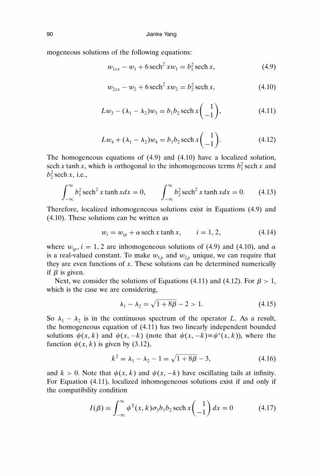
1+ 8β− 3, and they travel to infinity at their group velocity 2k.Due to this energy drain to the oscillating tails at infinity, the linearly per-manent internal oscillations in (3.80) (see Figure 16) are unstable. They willbecome weaker and weaker until they eventually disappear. As for the solu-tion (4.1), it will gradually lose its oscillational energy to the oscillating tailsand asymptotically approach a single-hump vector soliton (2.1) of wave anddaughter-wave structure. These predictions can be verified in Figures 18 and19, where the numerical solution of Equations (1.1) is plotted with β = 2and the initial condition as
A�x; 0� =√
2 sech x; B�x; 0� = c1b1�x� + c2b2�x�; (4.18)
with c1 = c2 = 0:3. Within the linearization theory in Section 3, such ini-tial conditions will lead to the solution (3.80) with permanent internal os-
Figure 17. Dependence of the magnitude of I�β� on β.
92 Jianke Yang
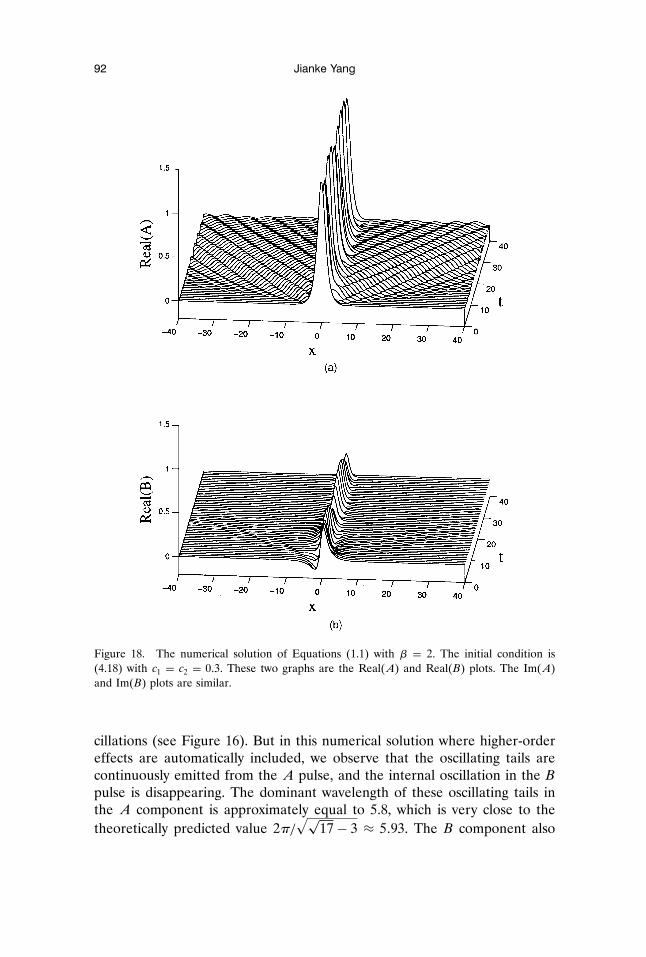
Figure 18. The numerical solution of Equations (1.1) with β = 2. The initial condition is(4.18) with c1 = c2 = 0:3. These two graphs are the Real(A) and Real(B) plots. The Im(A)and Im(B) plots are similar.
cillations (see Figure 16). But in this numerical solution where higher-ordereffects are automatically included, we observe that the oscillating tails arecontinuously emitted from the A pulse, and the internal oscillation in the Bpulse is disappearing. The dominant wavelength of these oscillating tails inthe A component is approximately equal to 5.8, which is very close to thetheoretically predicted value 2π/
√√17− 3 ≈ 5:93. The B component also
Nonlinear Optical Fibers 93
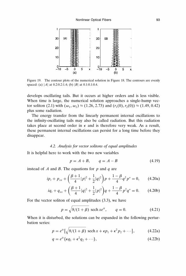
Figure 19. The contour plots of the numerical solution in Figure 18. The contours are evenlyspaced: (a) �A� at 0.2:0.2:1.4; (b) �B� at 0.1:0.1:0.4.
develops oscillating tails. But it occurs at higher orders and is less visible.When time is large, the numerical solution approaches a single-hump vec-tor soliton (2.1) with �ω1;ω2� ≈ �1:26; 2:73� and �r1�0�; r2�0�� ≈ �1:49; 0:42�plus some radiation.
The energy transfer from the linearly permanent internal oscillations tothe infinity-oscillating tails may also be called radiation. But this radiationtakes place at second order in ε and is therefore very weak. As a result,these permanent internal oscillations can persist for a long time before theydisappear.
4.2. Analysis for vector solitons of equal amplitudes
It is helpful here to work with the two new variables
p = A+ B; q = A− B (4.19)
instead of A and B. The equations for p and q are
ipt + pxx +(β+ 1
4�p�2 + 1
2�q�2
)p + 1− β
4q2p∗ = 0; (4.20a)
iqt + qxx +(β+ 1
4�q�2 + 1
2�p�2
)q + 1− β
4p2q∗ = 0: (4.20b)
For the vector soliton of equal amplitudes (3.3), we have
p =√
8/�1+ β� sech xeit ; q = 0: (4.21)
When it is disturbed, the solutions can be expanded in the following pertur-bation series:
p = eit{√8/�1+ β� sech x+ εp1 + ε2p2 + · · ·}; (4.22a)
q = eit�εq1 + ε2q2 + · · ·�; (4.22b)
94 Jianke Yang
where ε is a small parameter measuring the size of the disturbance. Thefollowing analysis is analogous to that for the degenerate vector solitons inthe previous subsection. At order ε, the equations for p1 and q1 are foundto be
ip1t + p1xx − p1 + 4 sech2 xp1 + 2 sech2 xp∗1 = 0; (4.23)
iq1t + q1xx − q1 +4
1+ β sech2 xq1 +2�1− β�
1+ β sech2 xq∗1 = 0: (4.24)
Note that Equations (4.23) and (3.5) are the same, and (4.24) and (3.6) arethe same. If ε2 and higher-order terms in (4.22) are neglected, the analysiswill become the linearization analysis done in Section 3, and the solutions forp1 and q1 are as given by (3.20) and (3.40). The linearly permanent internaloscillations of the vector soliton (3.3) are caused by q1’s eigenmodes ψβ0 andψβ0. To examine the higher-order effects on these permanent oscillations, forsimplicity we take
p1 = 0; q1 = c h1�x;β�eiλβt + c∗h2�x;β�e−iλβt ; (4.25)
where ψβ0 = �h1; h2�T and c is an arbitrary complex constant. At order ε2,p2 is governed by the equation
ip2t + p2xx − p2 + 4 sech2 xp2 + 2 sech2 xp∗2
= −√
2/�1+ β� �cc∗δ0�x� + c2δ1�x�e2iλβt + c∗2δ2�x�e−2iλβt�; (4.26)
where
δ0 = sech x�h21 + �1− β�h1h2 + h2
2�; (4.27a)
δ1 = sech x{h1h2 +
12�1− β�h2
1
}; (4.27b)
δ2 = sech x{h1h2 +
12�1− β�h2
2
}: (4.27c)
We work with the variables p2 and p∗2 and denote D = �p2; p∗2�T. Then D
satisfies the equation
iDt + LD = −√
2/�1+ β�{cc∗δ0
(1−1
)+ c2e2iλβt
(δ1−δ2
)+ c∗2e−2iλβt
(δ2−δ1
)}: (4.28)
Nonlinear Optical Fibers 95
We seek an inhomogeneous solution of (4.28) of the form
Dp�x; t� = −√
2/�1+ β�{cc∗d0�x�
(11
)+ c2d1�x�e2iλβt + c∗2d2�x�e−2iλβt
}; (4.29)
where the scaler function d0 and the vector functions d1 and d2 are theinhomogeneous solutions of the following equations
d0xx − d0 + 6 sech2 xd0 = δ0; (4.30)
Ld1 − 2λβd1 =(
δ1−δ2
); (4.31)
Ld2 + 2λβd2 =(
δ2−δ1
): (4.32)
Localized inhomogeneous solutions exist in Equation (4.30) since δ0�x� is aneven function in x and the compatibility condition∫ ∞
−∞δ0 sech x tanh xdx = 0 (4.33)
is therefore satisfied. These solutions can be readily determined numerically.The solutions of (4.31) and (4.32) are a little bit more complicated. When2λβ > 1, which happens when approximately 0:07 < β < 1 (see Figure 4),the homogeneous equation of (4.31) has two linearly independent solutionsψ�x; k� and ψ�x;−k� = ψ∗�x; k� with k2 = 2λβ − 1. The compatibilitycondition for the existence of localized inhomogeneous solutions in (4.31) is∫ ∞
−∞ψ�x; k�Tσ3
(δ1−δ2
)dx = 0: (4.34)
It can be checked numerically that this condition is never satisfied. The com-patibility condition for Equation (4.32) can be readily found to be the sameas (4.34) and is not satisfied either. This indicates that for 0:07 < β < 1,all inhomogeneous solutions of Equations (4.31) and (4.32) are not local-ized. They always have oscillating tails at infinity. Therefore, given a local-ized initial condition p2�x; 0� for Equation (4.26), those oscillating tails willbe generated and spread out to infinity in the solution p2. Due to this loss ofenergy, the linearly permanent oscillations in solution (4.22) with p1 and q1as in (4.25) are not stable. The oscillational energy is gradually transferredinto the outward-propagating oscillating tails, as is the case in the internaloscillations of degenerate vector solitons discussed in the previous subsection
96 Jianke Yang
(also see Figures 18 and 19). On the other hand, when 0 < 2λβ < 1, i.e.,0 < β < 0:07, 2λβ and −2λβ are no longer in the spectrum of the opera-tor L. Therefore, the homogeneous equations of (4.31) and (4.32) have nobounded solutions. It follows that there is a unique localized solution d1�x�and d2�x� in Equation (4.31) and (4.32). It is then clear that a localized in-homogeneous solution Dp�x; t� of the form (4.29) can be constructed forEquation (4.28). The homogeneous solutions Dh�x; t� of (4.28) are a linearsuperposition of all the eigenmodes of the operator L as determined in Sec-tion 3. When time is large, the continuous eigenmodes in Dh�x; t� disperseaway as energy radiation so that only the inhomogeneous solution Dp�x; t�and the discrete eigenmodes of L remain. These discrete eigenmodes can beabsorbed into the vector soliton. When this is done the solution D �x; t� isleft only with the localized solution Dp�x; t�, which has a finite amount of en-ergy. We can see now that only a small amount of energy will be transferredfrom the linearly permanent oscillations (terms up to order ε in (4.22)) intothe order ε2 terms. Therefore, these linearly permanent oscillations will per-sist with only a little modification when terms up to second order in ε areconsidered in the solution (4.22). But it is easy to see that infinity-oscillatingtails will appear sooner or later in the higher-order terms in (4.22) and thelinearly permanent internal oscillations of vector solitons are always unsta-ble. Of course, in these cases, the energy loss to oscillating tails will be evenslower and these internal oscillations will sustain for a longer time.
Similar analysis can be carried out for an arbitrary single-hump vectorsoliton (2.1), and the results are qualitatively similar. Due to higher-order ef-fects, the linearly permanent internal oscillations invariably generate infinity-oscillating tails, transfer energy into them, and gradually disappear. Recallthat before the higher-order effects come into play, the linearization theoryin Section 3 shows that the disturbed vector soliton will approach the stateof permanent internal oscillations. It is then concluded that internal oscilla-tions of vector solitons are never stable. They invariably emit energy to thefar field and become weaker and weaker until they eventually disappear. Thesolution will asymptotically approach a single-hump vector soliton state.
5. Concluding remarks
The internal oscillations of vector solitons in birefringent nonlinear opticalfibers is quite complicated in general. But by the linearization analysis, weclarified all the important features of those oscillations. We determined thediscrete and continuous eigenmodes of the linearized equations around asingle-hump vector soliton. We further identified the discrete eigenmodesthat cause permanent internal oscillations to the vector soliton. These os-cillations appear visually to be a combination of central position and width
Nonlinear Optical Fibers 97
oscillations in the A and B pulses. When higher-order effects are included,we found that the internal oscillations of vector solitons are always unstable.The oscillational energy is gradually transferred into the oscillating tails andis lost to the far field. But this energy transfer is usually very slow; there-fore, the linearly permanent internal oscillations can sustain for a long timebefore they disappear. Eventually, the pulses undergoing internal oscillationswill approach a single-hump vector soliton state, which is stable.
References
1. A. Hasegawa and F. Tappert, Transmission of stationary nonlinear optical pulses indispersive dielectric fibers, Appl. Phys. Lett. 23:142 (1973).
2. L. F. Mollenauer, R. H. Stolen, and J. P. Gordon, Experimental observation of pi-cosecond pulse narrowing and solitons in optical fibers, Phys. Rev. Lett. 45:1045 (1980).
3. C. R. Menyuk, Nonlinear pulse propagation in birefringent optical fibers, IEEE J. Quan-tum Electron QE-23:174 (1987).
4. B. A. Malomed and S. Wabnitz, Soliton annihilation and fusion from resonant inelasticcollisions in birefringent optical fibers, Optim. Lett. 16:1388 (1991).
5. J. Yang and D. J. Benney, Some properties of nonlinear wave systems, Stud. Appl. Math.96:111 (1996).
6. T. Ueda and W. L. Kath, Dynamics of coupled solitons in nonlinear optical fibers, Phys.Rev. A 42:563 (1990).
7. V. K. Mesentsev and S. K. Turitsyn, Stability of vector solitons in optical fibers, Optim.Lett. 17:1497 (1992).
8. D. J. Kaup, B. A. Malomed, and R. S. Tasgal, Internal dynamics of a vector soliton ina nonlinear optical fiber, Phys. Rev. E 48:3049 (1993).
9. M. Haelterman and A. P. Sheppard, The elliptically polarized fundamental vector soli-ton of isotropic Kerr media, Phys. Lett. A 194:191 (1994).
10. Y. Silberberg and Y. Barad, Rotating vector solitary waves in isotropic fibers, Optim.Lett. 20:246 (1995).
11. N. N. Akhmediev, A. V. Buryak, J. M. Soto-Crespo, and D. R. Andersen, Phase-locked stationary soliton states in birefringent nonlinear optical fibers, J. Optim. Soc. Am.B 12:434 (1995).
12. D. J. Kaup, Perturbation theory for solitons in optical fibers, Phys. Rev. A 42:5689 (1990).
13. L. D. Landau and E. M. Lifshitz, Quantum Mechanics: Non-relativistic Theory, PergamonPress, 1977.
The University of Vermont
(Received December 28, 1995)
Related Documents


![Topological Control of Extreme Waves - arXivrapidly oscillations [18{22]. RWs are giant disturbances appearing and disappearing abruptly in a nearly constant background [23{34]. Solitons](https://static.cupdf.com/doc/110x72/60f6afe9ef3291360951ee23/topological-control-of-extreme-waves-arxiv-rapidly-oscillations-1822-rws-are.jpg)