Vector Calculus lecture notes - Tom Baird PhD · Vector Calculus lecture notes Thomas Baird December 13, 2010 Contents ... a vector space is di erent from R3 as a coordinate space.

Vector Calculus lecture notes

Thomas Baird

December 13, 2010

Contents

1 Geometry of R3 21.1 Coordinate Systems . . . . . . . . . . . . . . . . . . . . . . . . . . . . . . . 2

1.1.1 Distance . . . . . . . . . . . . . . . . . . . . . . . . . . . . . . . . . 31.1.2 Surfaces . . . . . . . . . . . . . . . . . . . . . . . . . . . . . . . . . 5

1.2 Vectors . . . . . . . . . . . . . . . . . . . . . . . . . . . . . . . . . . . . . . 61.2.1 Geometric approach . . . . . . . . . . . . . . . . . . . . . . . . . . 61.2.2 Algebraic Approach . . . . . . . . . . . . . . . . . . . . . . . . . . . 8

1.3 Dot Product . . . . . . . . . . . . . . . . . . . . . . . . . . . . . . . . . . . 91.4 Cross Product . . . . . . . . . . . . . . . . . . . . . . . . . . . . . . . . . . 111.5 Equations for a Line . . . . . . . . . . . . . . . . . . . . . . . . . . . . . . 161.6 Equations for a Plane . . . . . . . . . . . . . . . . . . . . . . . . . . . . . . 18

2 Vector-valued Functions of a Single Variable and Space Curves 202.1 Derivatives . . . . . . . . . . . . . . . . . . . . . . . . . . . . . . . . . . . . 212.2 Arc Length . . . . . . . . . . . . . . . . . . . . . . . . . . . . . . . . . . . 232.3 Curvature . . . . . . . . . . . . . . . . . . . . . . . . . . . . . . . . . . . . 25

3 Scalar-valued Functions of Several Real Variables 283.1 Limits and Continuity . . . . . . . . . . . . . . . . . . . . . . . . . . . . . 313.2 Partial Derivatives . . . . . . . . . . . . . . . . . . . . . . . . . . . . . . . 33

3.2.1 Higher derivatives . . . . . . . . . . . . . . . . . . . . . . . . . . . . 353.3 Partial Differential Equations . . . . . . . . . . . . . . . . . . . . . . . . . 36

3.3.1 Harmonic Functions and the heat equation . . . . . . . . . . . . . . 363.3.2 Wave equation . . . . . . . . . . . . . . . . . . . . . . . . . . . . . 37

3.4 Tangent Planes and Linear Approximation . . . . . . . . . . . . . . . . . . 383.5 Chain Rule . . . . . . . . . . . . . . . . . . . . . . . . . . . . . . . . . . . 413.6 Directional Derivatives and Gradients . . . . . . . . . . . . . . . . . . . . . 433.7 Maxima and Minima . . . . . . . . . . . . . . . . . . . . . . . . . . . . . . 46

3.7.1 Absolute maxima and minima . . . . . . . . . . . . . . . . . . . . . 493.8 Lagrange Multipliers . . . . . . . . . . . . . . . . . . . . . . . . . . . . . . 51

1

4 Integrating Multi-variable Scalar Functions 534.1 Integrating Two Variable Scalar Functions . . . . . . . . . . . . . . . . . . 53

4.1.1 Polar coordinates . . . . . . . . . . . . . . . . . . . . . . . . . . . . 584.1.2 General change of coordinates in dimension two . . . . . . . . . . . 61

4.2 Integrating Three Variable Scalar Functions . . . . . . . . . . . . . . . . . 654.2.1 Change of variables in dimension three . . . . . . . . . . . . . . . . 674.2.2 Cylindrical coordinates . . . . . . . . . . . . . . . . . . . . . . . . . 674.2.3 Spherical coordinates . . . . . . . . . . . . . . . . . . . . . . . . . . 68

5 Calculus of Vector Fields 705.1 Line Integrals and the Fundamental Theorem . . . . . . . . . . . . . . . . 705.2 Green’s Theorem . . . . . . . . . . . . . . . . . . . . . . . . . . . . . . . . 755.3 Parametrized Surfaces . . . . . . . . . . . . . . . . . . . . . . . . . . . . . 77

5.3.1 Surface Area . . . . . . . . . . . . . . . . . . . . . . . . . . . . . . . 785.4 Integrating Vector Fields over Surfaces: Flux . . . . . . . . . . . . . . . . . 80

1 Geometry of R3

1.1 Coordinate Systems

Recall that the Cartesian plane is the set of ordered pairs of real numbers.

R2 = R× R = (a, b)|a, b ∈ R

For a point p = (a, b) ∈ R2 the numbers a, b are called the x- and y-coordinates of prespectively.

Geometrically, R2 is represented as plane with a horizontal x-axis and vertical y-axis

Proceeding by analogy, Cartesian 3-space is the set of ordered triples of real numbers:

2

R3 = R× R× R = (a, b, c)| ∈ R]

For a point p := (a, b, c) ∈ R3 the numbers a, b, c are the x-, y- and z-coordinates of prespectively. R3 is represented geometrically with three coordinate axes.

The point O = (0, 0, 0) is called the origin. The plane spanned by any two axes iscalled a coordinate plane, there are three: the xy-plane, the xz-plane and the yz-plane.

More generally one may consider Cartesian n-space for any positive integer n. In thiscourse we will mainly be concerned with doing calculus in R3, but many of the ideasextend transparently to all n.

1.1.1 Distance

For p and q be two points in R3, denote by pq the straight line segment joining them

3

The (Euclidean) distance between p := (x1, y1, z1) and q := (x2, y2, z2) is defined bythe formula

|pq| =√

(x1 − x2)2 + (y1 − y2)2 + (z1 − z2)2

This quantity corresponds to the usual geometric notion of length of the line segment|pq| by the following argument. Consider the diagram

The rectangle is drawn with sides parallel to the coordinate planes. The side lengthssatisfy |pa| = |x1 − x2|,|ab| = |y1 − y2| and |q

¯| = |z1 − z2|. The points p, a,b form the vertices of a right

triangle in a plane parallel to xy-plane, so using the usual Pythagorean theorem

|PB| =√|PA|2 + |AB|2 =

√(x1 − x2)2 + (y1 − y2)2

The points P,B,Q also form the vertices of a right triangle so

|PQ| =√|PB|2 + |BQ|2 =

√(x1 − x2)2 + (y1 − y2)2 + (z1 − z2)2

4

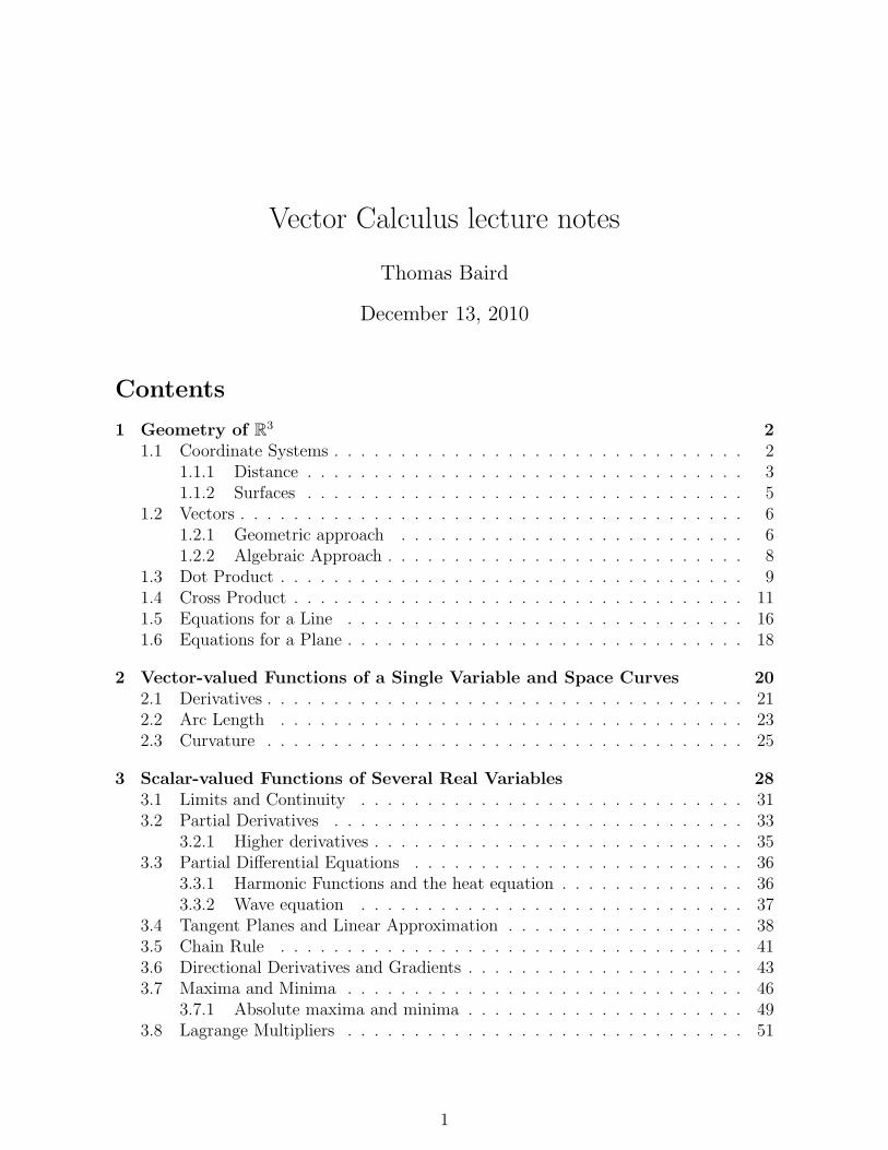
1.1.2 Surfaces

Recall that solution sets of equations in x and y (normally) determine curves in R2.Equations in the variables x, y, z determine surfaces in R3.

Example 1. Graph the solution set of y = 7

The sphere in R3 centered at C with radius R is by definition the set P ∈ R3||PC| =R. Using the distance formula, this sphere is the solution set of the equation

R =√

(x− a)2 + (y − b)2 + (z − c)2

or alternativelyR2 = (x− a)2 + (y − b)2 + (z − c)2

Example 2. Graph the solution set of 4 = (x− 1)2 + (y)2 + (z + 2)2

5

1.2 Vectors

1.2.1 Geometric approach

Given two points P,Q in R3 (or Rn), let ~PQ denote the arrow pointing from P to Q.

This arrow represents a vector in R3. The data defining a vector consists of its lengthor norm

| ~PQ| = |PQ|

and its direction. In particular, two arrows that are related by a translation represent thesame vector.

There are two basic operations that can be performed on vectors.Vector addition: Given two vectors ~u and ~v in R3 we form a new vector, ~u + ~v, by

the triangle rule:

6

In words, translate ~v so that its base is at the tip of ~u and make ~u + ~v the arrowspanning from the base of ~u to the tip of ~v. Notice that by the following diagram

~u+ ~v = ~v + ~u. (this is sometimes called the parallelogram law). The unique vector oflength zero is denoted ~0 and satisfies ~0 + ~v = ~v.

Scalar multiplication: If c ∈ R and ~u a vector, then we may form a new vectorc~u called the scalar product of ~u with c. The magnitude of c~u satisfies |c~u| = |c||~u|. Ifc ≥ 0 then c~u is the vector with the same direction as ~u and if c < 0 then c~v points in theopposite direction to ~u.

7

Observe that ~u+ (−1)~u = ~0.

The set of vectors in R3 equipped with these operations is called the space of vectorsin R3.

1.2.2 Algebraic Approach

Observe now that any arrow in R3 can be translated to a unique arrow based at the origin.

Consequently, there is a one-to-one correspondence

vectors in R3 ∼= R3

It is customary to identify the set of vectors in R3 with R3 itself, even though R3 asa vector space is different from R3 as a coordinate space. To distinguish the two, I willwrite a 3-tuple < a, b, c > when I wish to think of it a vector and (a, b, c) when it is apoint.

In terms of coordinates, the basic operations are:

Vector addition: < a1, a2, a3 > + < b1, b2, b3 >=< a1 + b1, a2 + b2, a3 + b3 >

Scalar multiplication: c < a1, a2, a3 >=< ca1, ca2, ca3 >

Norm: | < a1, a2, a3 > | =√a2

1 + a22 + a2

3

The above formulas generalize naturally to Rn for any positive integer n.Here are some properties of Rn as a vector space.

8

Proposition 1.1. Let ~a,~b,~c be vectors in Rn and c, d scalars. Then

i) ~a+~b = ~b+ ~a v) (c+ d)~a = c~a+ d~a

ii) (~a+~b) + ~c = ~a+ (~b+ ~c) vi) (cd)~a = c(d~a)

iii) ~a+~0 = ~a vii) c(~a+~b) = c~a+ c~b

iv) ~a+ (−1)~b = ~0 viii) 1~a = ~a

i), iii) and iv) we’ve already seen geometrically. We do v) algebraically as an illustra-tion and leave the rest as an exercise.

(c+ d)~a = < (c+ d)a1, ..., (c+ d)an >

= < ca1, ..., can > + < da1, ..., dan > = c~a+ d~a

When working in Rn it is useful to distinguish a set of standard basis vectors. In R3

these are the vectors~i :=< 1, 0, 0 >

~j :=< 0, 1, 0 >

~k :=< 0, 0, 1 > .

Any other vector in R3 can be expressed as a linear combination of ~i,~j,~k as follows:

< a1, a2, a3 >= a1 < 1, 0, 0 > +a2 < 0, 1, 0 > +a3 < 0, 0, 1 >= a1~i+ a2

~j + a3~k

A unit vector is a vector of length one. If ~a is a non-zero vector, the vector 1|~a|~a is the

unique unit vector pointing in the same direction as ~a.

Example 3. Find the unit vector ~u pointing in the same direction as ~a = 4~i− 2~j + ~k.

|~a| =√

42 + (−2)2 + 12 =√

21, so

~u =1√21~a =

4√21~i+

−2√21~j +

1√21~k

1.3 Dot Product

The dot product is a function that inputs a pair of vectors and outputs a real number.For vectors ~a :=< a1, a2, a3 > and ~b =< b1, b2, b3 > the dot product is defined

~a ·~b = a1b1 + a2b2 + a3b3

9

The dot product makes sense in any Rn by the general formula

~a ·~b =n∑i=1

aibi

The geometric meaning of the dot product is captured by the following theorem

Theorem 1.2. Let ~a and ~b be two vectors in R3 ( more generally Rn), and let θ be theangle between them. Then

~a ·~b = |a||b|cos(θ)

Proof. See the textbook.

Got this far last time.

Corollary 1.3. The angle θ between vectors ~a and ~b is given by the formula

cos(θ) =~a ·~b|~a||~b|

We say that two vectors are perpendicular or orthogonal if the angle between them is90 degrees.

Corollary 1.4. Vectors ~a and ~b are orthogonal if and only if ~a ·~b = 0.

Example 4. Show that 7~i− 2~j + ~k is orthogonal to ~i+ 2~j − 3~k.

(7~i− 2~j + ~k) · (~i+ 2~j − 3~k) = 7 · 1− 2 · 2− 1 · 3 = 0

Definition 1. Let ~a and ~b be vectors in Rn. The projection of ~a onto ~b a vector definedby the formula

proj~b(~a) =(~a ·~b|~b|2

)~b

Proposition 1.5. Geometrically, the projection of a vector can be understood by thefollowing picture:

10

Proof.

proj~b(~a) =(~a ·~b|~b|

) ~b|~b|

= |~a|cos(θ)~u

where θ is the angle between ~a and ~b and ~u is the unit vector in the direction ~u. Theassertion follows from the diagram.

Exercise 1. Show that (~a− proj~b(~a)) ·~b = 0. Consequently the sum

~a = proj~b(~a) + (~a− proj~b(~a)),

decomposes ~a into sum of a vector orthogonal to ~b and one parallel to ~b.

1.4 Cross Product

The cross product is a function that inputs two vectors in R3 and outputs a vector in R3.Unlike the dot product, the cross product is special to R3. If ~a,~b ∈ R3, then the crossproduct is

~a×~b = (a2b3 − a3b2, a3b1 − a1b3, a1b2 − a2b1) (1)

The formula for the cross product is most easily remembered and understood as thedeterminant of a matrix. Consider the matrix, ~i ~j ~k

a1 a2 a3

b1 b2 b3

(2)

with the standard basis vectors occuring as entries in the first row, and ~a and ~b occuringas rows two and three respectively (it may seem strange that vectors are occuring both

11

as rows and as matrix entries, but bear with me). Because scalars and vectors can bemultiplied, it makes sense to take the determinant of (2),

∣∣∣∣∣∣~i ~j ~ka1 a2 a3

b1 b2 b3

∣∣∣∣∣∣ =~i

∣∣∣∣ a2 a3

b2 b3

∣∣∣∣−~j ∣∣∣∣ a1 a3

b1 b3

∣∣∣∣+ ~k

∣∣∣∣ a1 a2

b1 b2

∣∣∣∣= (a2b3 − a3b2)~i− (a1b3 − a3b1)~j + (a1b3 − a3b1)~k

= ~a×~b

giving a new formula for the cross product.

Corollary 1.6. Suppose ~a and ~b are linearly dependent, i.e. for some scalar c, c~a = ~b or~a = c~b. Then ~a×~b = ~0.

Proof. In the first case, ~a = c~b then by row deduction

~a×~b =

∣∣∣∣∣∣~i ~j ~ka1 a2 a3

b1 b2 b3

∣∣∣∣∣∣ =

∣∣∣∣∣∣~i ~j ~kcb1 cb2 cb3

b1 b2 b3

∣∣∣∣∣∣ =

∣∣∣∣∣∣~i ~j ~k0 0 0b1 b2 b3

∣∣∣∣∣∣ = ~0. (3)

The case ~b = c~a is similar.

Proposition 1.7. For any three vectors ~a,~b,~c ∈ R3 we have

(~a×~b) · ~c =

∣∣∣∣∣∣c1 c2 c3

a1 a2 a3

b1 b2 b3

∣∣∣∣∣∣ (4)

Equation 4 is sometimes called the scalar triple product of ~a,~b and ~c.

Proof.

(~a×~b) · ~c = (a2b3 − a3b2)c1 − (a1b3 − a3b1)c2 + (a1b3 − a3b1)c3

= c1

∣∣∣∣ a2 a3

b2 b3

∣∣∣∣− c2

∣∣∣∣ a1 a3

b1 b3

∣∣∣∣+ c3

∣∣∣∣ a1 a2

b1 b2

∣∣∣∣=

∣∣∣∣∣∣c1 c2 c3

a1 a2 a3

b1 b2 b3

∣∣∣∣∣∣In some sense formula (4) is more fundamental than (1) . That is, ~a × ~b should be

defined to be the vector satisfying (4), and formula (1) worked out as a calculation.

Corollary 1.8. The crossproduct ~a×~b is orthogonal to both ~a and ~b.

12

Proof. By Corollary (1.3) this equivalent to showing (~a×~b) · ~a = 0 = (~a×~b) ·~b.Using formula 4

(~a×~b) · ~a =

∣∣∣∣∣∣a1 a2 a3

a1 a2 a3

b1 b2 b3

∣∣∣∣∣∣ = 0

because two of the rows are equal. Similarly, for (~a×~b) ·~b.

Corollary 1.8 determines the direction of ~a ×~b up to a sign. The sign is determinedas follows. If ~a and ~b are linearly independent, then they span a plane in R2. From oneside of the plane, the angle sweeping counter-clockwise from ~a to ~b is less than 90 degrees.This is the side ~a×~b points into. This can remembered using the right-hand rule.

Exercise 2. Illustrate the right hand rule with the example ~i×~j = ~k.

It remains to understand the norm |~a×~b| geometrically.

Theorem 1.9. For ~a,~b ∈ R3, let θ ∈ [0, π] be the angle between ~a and ~b. Then

|~a×~b| = |~a||~b|sin(θ) (5)

Proof.

|~a×~b|2 = (a2b3 − a3b2)2 + (a3b1 − a1b3)2 + (a1b2 − a2b1)2

= (a21 + a2

2 + a23)(b2

1 + b22 + b2

3)− (a1b1 + a2b2 + a3b3)2

= |~a|2|~b|2 − ~a ·~b = |~a|2|~b|2(1− cos2(θ))

= |~a|2|~b|2sin2(θ)

Taking (positive) square roots completes the argument.

Corollary 1.10. Vectors ~a and ~b in R3 are parallel if and only if ~a×~b = ~0.

Even more geometrically, (5) can be interpreted as the area of the parallelogram

spanned by ~a and ~b as shown.

13

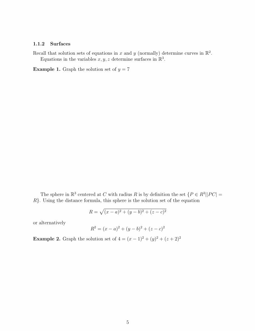
Proposition 1.11. Given ~a,~b,~c ∈ R3, the quantity |(~a×~b) · ~c| is equal to the volume of

the parallel-piped spanned by ~a, ~b and ~c.

Proof. Drawing the parallel-piped

the volume V, satisfies V = Ah where A is the area of the base pararellogram spannedby ~a and ~b and h is the height measure orthogonal to the base. By earlier results we haveA = |~a×~b| and h = |proj~a×~b(~c)|. Thus

V = Ah = |~a×~b||(~a×~b) · ~c

|~a×~b|2~a×~b| = |(~a×~b) · ~c|.

One application of the cross product in physics is the concept of torque. Consider aforce ~f acting on a rigid body in R3 at a point ~r. The torque of this action (relative tothe origin) is the cross product

~τ = ~r × ~f.

If there are multiple forces ~f1, ..., ~fn acting at positions ~r1, ..., ~rn then the total torqueis a sum of vectors

~τ =n∑i=1

~ri × ~fi

The analogue of Newton’s second law of motion for says that the angular velocity ofa rigid body will accelerate around the axis spanned by ~τ , at a rate proportional to thenorm of ~τ . In particular, if the rigid body is in equilibrium, then ~τ = ~0.

Example 5. Consider see-saw, with one arm of length 3m and the other of length 5m.Suppose a person weighing 120 pounds sits on the long end of the see-saw. How muchweight must be placed at the other end if the see-saw is to remain balanced. Does thisweight depend on the angle of inclination of the see-saw?

14

We list some properties satisfied by the cross product.

Theorem 1.12. Let ~a,~b,~c be vectors in R3 and let λ ∈ R be a scalar. Theni) (λ~a)×~b = ~a× (λ~b) = λ(~a×~b)ii) ~a× (~b+ ~c) = ~a×~b+ ~a× ~ciii) (~a+~b)× ~c = ~a× ~c+~b× ~civ) ~a×~b = −~b× ~av) ~a · (~b× ~c) = (~a×~b) · ~c

The first three properties can be summarized: the cross product is linear in botharguments.

Proof. Of v) only. By earlier formulas

(~a×~b) · ~c =

∣∣∣∣∣∣c1 c2 c3

a1 a2 a3

b1 b2 b3

∣∣∣∣∣∣and

~a · (~b× ~c) = (~b× ~c) · ~a =

∣∣∣∣∣∣a1 a2 a3

b1 b2 b3

c1 c2 c3

∣∣∣∣∣∣The first matrix can be transformed into the other using two row transpositions. It followsthat determinants differ by a factor of (−1)2 = 1 and thus are equal.

It is worthwhile noting that the following expressions are not equal in general:

~a× (~b× ~c) 6= (~a×~b)× ~c.

Consider the counterexample

(~i×~i)×~j = ~0×~j = ~0

which is not equal to~i× (~i×~j) =~i× ~k = −~j.

We say that the cross product is not associative.

15

1.5 Equations for a Line

A line L in R3 is completely determined by a point in L, and the direction of L. Usingvectors, this geometric fact can be used to produce an equation for L.

In the following diagram, let ~r0 denote a vector based at the origin and with tip on L,and let ~v be a vector pointing parallel to L.

Using the triangle rule for vector addition, it is clear that for any other vector ~r ∈ L,the difference ~r − ~r0 must be parallel to L thus also to ~v. So for some scalar c ∈ R wehave ~r − ~r0 = t~v. In particular the equation

~r = ~r0 + t~v (6)

has a unique solution t ∈ R for any ~r ∈ L. We call (6) a vector parametric equation forL. If ~v =< a, b, c > and ~r0 =< x0, y0, z0 >, then L is equal to the set of points (x, y, z)satisfying

x = x0 + ta, y = y0 + tb, z = z0 + tc

for some t ∈ R. These are called scalar parametric equations for L.It is sometimes useful to think of t as a time variable and the parametric equations as

describing the tranjectory of a particle moving along L (without acceleration).

Example 6. Produce parametric equations for the line L in R3 passing through the points~r0 := (1, 2, 0) and ~r1 := (0,−3, 1). What values of t describe points on the line segmentbetween ~r0 and ~r1?

The difference ~v = ~r1 − ~r0 =< −1,−5, 1 > is parallel to L, so we obtain the vectorparametric equation

~r = ~r0 + t~v =< 1, 2, 0 > +t < −1,−5, 1 >=< 1− t, 2− 5t, 0 + t > (7)

16

In coordinates, L is the set of 3-tuples (x, y, z) satisfying

x = 1− t, y = 2− 5t, z = t

for some t ∈ R. Thinking in terms of a trajectory, notice that (7) equals ~r0 when t = 0 and~r1 when t = 1, so the line segment between 0 and 1 correspond to those values 0 ≤ t ≤ 1.

This equation for the line segment can be rewritten as follows

~r = ~r0 + t~v = ~r0 + t(~r1 − ~r0) = (1− t)~r0 + t~r1 (8)

for 0 ≤ t ≤ 1, putting ~r0 and ~r1 on a more even footing. Vectors ~r satisfying (8) are calledconvex linear combinations of ~r0 and ~r1.

It is possible to define a line L using equations in x, y, z without introducing an extraparametric variable like t. Consider again the parametric equations

x = x0 + ta, y = y0 + tb, z = z0 + tc

If none of a, b, c are zero, then manipulating to isolate t, we get

x− x0

a=y − y0

b=z − z0

c

the solutions of which define L. These are called the symmetric equations of L. If a = 0and b, c do not, then we instead get equations

x = x0,y − y0

b=z − z0

c

which means that the line lies in the plane x = x0. If a, b = 0 then get equations

x = x0, y = y0.

describing a line parallel to the z-axis.

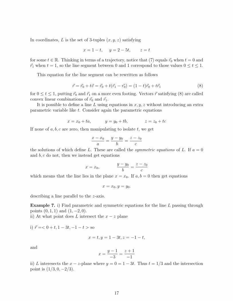
Example 7. i) Find parametric and symmetric equations for the line L passing throughpoints (0, 1, 1) and (1,−2, 0).ii) At what point does L intersect the x− z plane

i) ~r =< 0 + t, 1− 3t,−1− t > so

x = t, y = 1− 3t, z = −1− t,

and

x =y − 1

−3=z + 1

−1

ii) L interesects the x− z-plane where y = 0 = 1− 3t. Thus t = 1/3 and the intersectionpoint is (1/3, 0,−2/3).

17

1.6 Equations for a Plane

A plane P is determined by a point ~r0 in P and by two linearly independent vectors ~uand ~v which are parallel to P .

This gives rise to a parametric vector equation for P : Every point ~r on P can beexpressed

~r = ~r0 + s~u+ t~v

for a unique choice s, t ∈ R. Expressing this equation in coordinates give scalar parametricequations for P . If ~r0 =< x0, y0, z0 >, ~u =< u1, u2, u3 > and ~v =< v1, v2, v3 > then Pconsists of points (x, y, z) satisfying:

x = x0 + su1 + tv1, y = y0 + su2 + tv2, z = z0 + su3 + tv3.

for some s, t ∈ R.We think of s and t as defining a new set of coordinates, or parameters for P .

Example 8. Find parametric equations for the plane P containing the points (1, 0, 0), (0, 1, 0), (0, 1, 2).

Any difference of distinct points in the plane determines a vector parallel to the plane.Thus ~u =< 1, 0, 0 > − < 0, 1, 0 >=< 1,−1, 0 > and ~v =< 1, 0, 0 > − < 0, 1, 2 >=<1,−1,−2 > are parallel to P and are linearly independent. This gives parametric equa-tions for P :

~r =< 1, 0, 0 > +s < 1,−1, 0 > +t < 0, 1, 2 >

and

x = 1 + s, y = −s+ t, z = 2t

18

Like in the case of lines, it is possible to define a plane using equations in x, y, z withoutintroducing auxiliary variables like s, t. In fact, a single equation suffices to define a plane.

A normal vector ~n to a plane P is a vector that is perpendicular to P (i.e. perpen-dicular to all vectors that are parallel to P ). For instance, if P is given be a parametricequation

~r = ~r0 + s~u+ t~v

then the cross product ~n := ~u×~v is perpendicular to both ~u and ~v and thus to the entireplane P .

Given a vector ~r0 =< x0, y0, z0 > lying on P and a normal vector ~n =< a, b, c >, it isclear that any other vector ~r =< x, y, z > in P must satisfy

~n · (~r − ~r0) = 0

or in coordinates

a(x− x0) + b(y − y0) + c(z − z0) = 0 (9)

so P is equal to the solutions of this equation.

Example 9. Find a parametric equation for the plane determined by 5x− 2y + z = 4Solution: First manipulate the expression to put it into the form of (9) . For example

equation (10) is equivalent to

5x− 2y + (z − 4) = 0 (10)

So the plane is normal to ~n =< 5,−2, 1 > and passes through the point (0, 0, 4). To gettwo vectors parallel to the plane, we choose vectors whose dot product with ~n is zero, say~u :=< 1, 0,−5 > and ~v :=< 0, 1, 2 >. Then a parametric equation for P with parameterss, t ∈ R

~r :=< 0, 0, 4 > +s < 0, 1, 2 > +t < 1, 0,−5 >

19

2 Vector-valued Functions of a Single Variable and

Space Curves

A vector valued function of a real variable is a function whose input is a real number andwhose output is a vector (we will focus on this case that the output is a vector in R3).That is, a vector valued function

~r : I → R3

associates to any real number in the domain t ∈ I ⊆ R, a vector ~r(t) ∈ R3. If f(t), g(t)and h(t) are the components of the vector ~r(t) then we write

~r(t) =< f(t), g(t), h(t) >= f(t)~i+ g(t)~j + h(t)~k

where f(t), g(t), h(t) are real valued functions.We define the limit of a vector-valued function to be the limit of its components:

limt→t0

< f(t), g(t), h(t) >=< limt→t0

f(t), limt→t0

g(t), limt→t0

h(t) > .

A vector valued function is continuous if limt→t0(~r(t)) = ~r(t0) for all t0 ∈ R. This isequivalent to the components f(t), g(t), h(t) being continuous.

Given a continuous vector valued function of one variable ~r :=< f(t), g(t), h(t) > theset C of points (x, y, z) ∈ R3 satisfying

x = f(t), y = g(t), z = h(t)

for some t ∈ R is called a space curve. The vector-valued function ~r(t) is a called aparametrization of C and t is the parameter.

Example 10. Sketch the curve parametrized by ~r(t) :=< sin(t), cos(t), t >.

Solution: The curve lies on the cylinder x2 + y2 = 1 winding around at a regular pace.The z coordinate also increases at a constant rate. The curve spirals upwards around thecylinder, forming a helix.

20

Example 11. Find a parametrization for the curve C defined by the equations x2+y2 = 1and x+ z = 3.Solution:The equation x2 +y2 = 1 determines a cylinder. The equation x+z = 3 definesa plane orthogonal to < 1, 0, 1 > containing the point (0, 0, 3). Plotting:

We have seen that the x = sin(t), y = cos(t) will define a curve winding around thecylinder. To control the z coordinate, solve sin(t) + z = 3 to z = 3 − sin(t). Thus aparametrization is ~r(t) =< sin(t), cos(t), 3 − sin(t) >. If we want to parametrize thecurve so that each point is counted only once, we can restrict the domain 0 ≤ t < 2π.

2.1 Derivatives

A vector-valued function ~r(t) is called differentiable at t if the limit

(~r)′(t) =d~r(t)

dt:= lim

h→0

~r(t+ h)− ~r(t)h

We call (~r)′(t) the derivative of ~r(t). In terms of our interpretation of ~r(t) describing thetrajectory of a moving particle, (~r)′(t) is is the velocity vector of the particle. The norm|(~r)′(t)| is the speed.

In the geometric terms, d~r/dt is a limit of scalar multiples of secant vectors to thepath. This means in particular that d~r/dt is tangent to the curve.

The tangent line to the curve parametrized by ~r(t) at the point ~r(t0) for some constant

t0, is the line with parametrization ~l and parameter s:

21

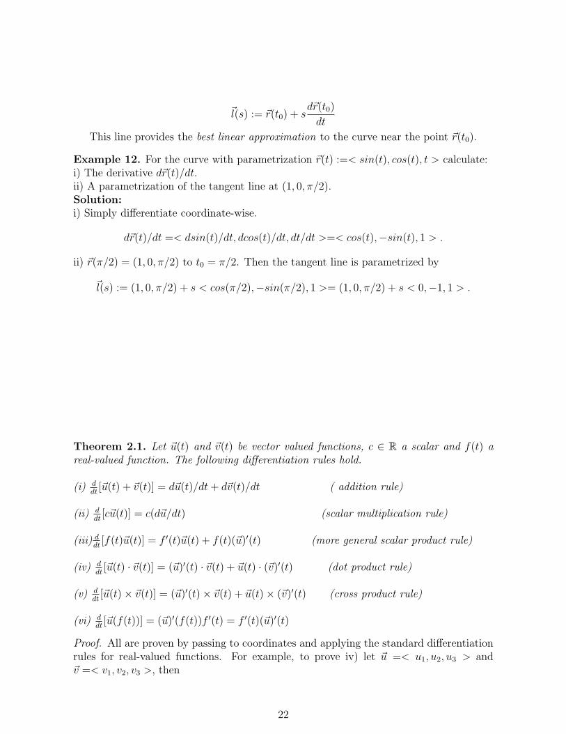
~l(s) := ~r(t0) + sd~r(t0)

dt

This line provides the best linear approximation to the curve near the point ~r(t0).

Example 12. For the curve with parametrization ~r(t) :=< sin(t), cos(t), t > calculate:i) The derivative d~r(t)/dt.ii) A parametrization of the tangent line at (1, 0, π/2).Solution:i) Simply differentiate coordinate-wise.

d~r(t)/dt =< dsin(t)/dt, dcos(t)/dt, dt/dt >=< cos(t),−sin(t), 1 > .

ii) ~r(π/2) = (1, 0, π/2) to t0 = π/2. Then the tangent line is parametrized by

~l(s) := (1, 0, π/2) + s < cos(π/2),−sin(π/2), 1 >= (1, 0, π/2) + s < 0,−1, 1 > .

Theorem 2.1. Let ~u(t) and ~v(t) be vector valued functions, c ∈ R a scalar and f(t) areal-valued function. The following differentiation rules hold.

(i) ddt

[~u(t) + ~v(t)] = d~u(t)/dt+ d~v(t)/dt ( addition rule)

(ii) ddt

[c~u(t)] = c(d~u/dt) (scalar multiplication rule)

(iii) ddt

[f(t)~u(t)] = f ′(t)~u(t) + f(t)(~u)′(t) (more general scalar product rule)

(iv) ddt

[~u(t) · ~v(t)] = (~u)′(t) · ~v(t) + ~u(t) · (~v)′(t) (dot product rule)

(v) ddt

[~u(t)× ~v(t)] = (~u)′(t)× ~v(t) + ~u(t)× (~v)′(t) (cross product rule)

(vi) ddt

[~u(f(t))] = (~u)′(f(t))f ′(t) = f ′(t)(~u)′(t)

Proof. All are proven by passing to coordinates and applying the standard differentiationrules for real-valued functions. For example, to prove iv) let ~u =< u1, u2, u3 > and~v =< v1, v2, v3 >, then

22

d

dt[~u(t) · ~v(t)] =

d

dt[u1v1 + u2v2 + u3v3]

= u′1v1 + u1v′1 + u′2v2 + u2v

′2 + u′3v3 + u3v

′3

= u′1v1 + u′2v2 + u′3v3 + u1v′1 + u2v

′2 + u3v

′3

= (~u)′ · ~v + ~u · (~v)′

Example 13. Show that if the norm of a vector valued function is constant, |~r(t)| = c,then the derivative (~r)′(t) is perpendicular to ~r(t) for all t.Solution: Abbreviate ~r = ~r(t). If |~r(t)| = c then ~r · ~r = c2 is constant and

d

dt(~r · ~r) = (~r)′ · ~r + ~r · (~r)′ = 2~r · (~r)′ = 0.

Thus ~r · (~r)′ and ~r is perpendicular to (~r)′.

2.2 Arc Length

Let C be a curve in R3 with differentiable parametrization ~r(t). The arc length of C isdefined to be the limit of lengths of inscribed polygonal paths, as illustrated below:

This definition can made more precise using the language of Riemann sums, but wewill avoid this language.

Because C admits a differentiable parametrization ~r(t), it is possible to express the arclength using an integral equation. Recall that the derivative (~r)′(t) may be interpretedas the velocity of a particle moving along C and |(~r)′(t)| as the speed. Consequently, itmakes sense that the length L of the curve between points ~r(a) and ~r(b) is equal to theintegral of the speed function,

L =

∫ b

a

|(~r)′(t)|dt (11)

Observe that |(~r)′(t)| is a real number, so the expression (11) is simply the integral ofa real valued function. If ~r(t) =< f(t), g(t), h(t) > then (11) can be rewritten

L =

∫ b

a

|√f ′(t)2 + g′(t)2 + h′(t)2|dt

23

Example 14. Determine the length of the curve C parametrized by ~r(t) :=< sin(t), cos(t), t >between the points (0, 1, 0) and (1, 0, π/2).Solution: ~r(t) passes (0, 1, 0) at t = a = 0 and crosses (1, 0, π/2) at t = b = π/2. Thusthe length of the arc equals

∫ π/2

0

|(~r)′(t)|dt =

∫ π/2

0

| < cos(t),−sin(t), 1 > |dt =

∫ π/2

0

|√cos2(t) + sin2(t) + 1|dt

=

∫ π/2

0

√2dt = π/

√2

For a chosen constant a ∈ R, define the arc-length function

s(t) :=

∫ t

a

|(~r)′(t)|dt

A parametrization ~u(t) of C is called an arc-length parametrization if the norm of thevelocity vector is one for all t:

|(~u)′(t)| = 1

i.e. the particle moves with unit speed. Let ~r(t) be a differentiable parametrization ofC and suppose that |(~r)′(t)| > 0 for all t (such a parametrization is called regular orsmooth). Then the arc-length function s(t) is a strictly increasing function of t, and it ispossible to find an inverse function so t = t(s).

Define the arc-length parametrization ~u(t) by the formula

~u(s) = ~r(t(s))

To see that ~u(s) has unit speed, differentiate:

d

ds[~u(s)] =

d

ds[~r(t(s))] = (~r)′(t)

dt

dsso

| dds

[~u(s)]| = |(~r)′(t)||dt/ds| = |dsdt|| dtds| = 1

24

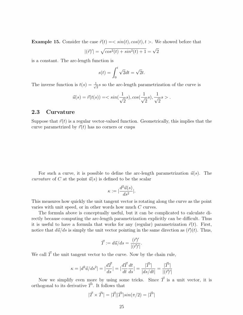
Example 15. Consider the case ~r(t) =< sin(t), cos(t), t >. We showed before that

|(~r)′| =√cos2(t) + sin2(t) + 1 =

√2

is a constant. The arc-length function is

s(t) =

∫ t

0

√2dt =

√2t.

The inverse function is t(s) = 1√2s so the arc-length parametrization of the curve is

~u(s) = ~r(t(s)) =< sin(1√2s), cos(

1√2s),

1√2s > .

2.3 Curvature

Suppose that ~r(t) is a regular vector-valued function. Geometrically, this implies that thecurve parametrized by ~r(t) has no corners or cusps

For such a curve, it is possible to define the arc-length parametrization ~u(s). Thecurvature of C at the point ~u(s) is defined to be the scalar

κ := |d2~u(s)

ds2|.

This measures how quickly the unit tangent vector is rotating along the curve as the pointvaries with unit speed, or in other words how much C curves.

The formula above is conceptually useful, but it can be complicated to calculate di-rectly because computing the arc-length parametrization explicitly can be difficult. Thusit is useful to have a formula that works for any (regular) parametrization ~r(t). First,notice that d~u/ds is simply the unit vector pointing in the same direction as (~r)(t). Thus,

~T := d~u/ds =(~r)′

|(~r)′|.

We call ~T the unit tangent vector to the curve. Now by the chain rule,

κ = |d2~u/ds2| = |d~T

ds| = |d

~T

dt

dt

ds| = |~T ′||ds/dt|

=|~T ′||(~r)′|

Now we simplify even more by using some tricks. Since ~T is a unit vector, it isorthogonal to its derivative ~T ′. It follows that

|~T × ~T ′| = |~T ||~T ′|sin(π/2) = |~T ′|

25

Substituting in we get

κ =|~T × ~T ′||(~r)′|

.

This isn’t much of a simplication so far, but bear with me.Observe that

(~r)′ = |(~r)′|~T =ds

dt~T . (12)

Differentiating both sides with respect to t, and employing the (scalar) product rule

(~r)′′ =d2s

dt2~T +

ds

dt~T ′. (13)

Take the cross product of (12) and (13) and use the fact the ~T × ~T = 0:

(~r)′ × (~r)′′ =ds

dt

d2s

dt2~T × ~T +

(dsdt

)2~T × ~T ′ =

(dsdt

)2~T × ~T ′ = |(~r)′|2 ~T × ~T ′

So plugging into the previous formula we get

Proposition 2.2. The curvature κ of a curve with parametrization ~r(t) satisfies

κ =|~T × ~T ′||(r)′|

=|(r)′ × (r)′′||(r)′|3

Example 16. Compute the curvature of the curve with parametrization ~r(t) =< sin(t), cos(t), t >.Solution: We have

(~r)′(t) =< cos(t),−sin(t), 1 >

and(~r)′′(t) =< −sin(t),−cos(t), 0 >

Thus

~r′ × ~r′′ = < 0 + cos(t), 0− sin(t),−cos2(t)− sin2(t) >

= < cos(t),−sin(t),−1 >

and|~r′ × ~r′′| =

√cos2(t) + sin2(t) + 1 =

√2

We saw before that |~r′| =√cos2(t) + sin2(t) + 12 =

√2, so

κ =|~r′ × ~r′′||~r′|3

=

√2

(√

2)3=

1

2

We will explore further the geometric meaning of κ, but first we need more terminology.The principal unit normal vector ~N = ~N(t) to the curve ~r is the unit vector pointing

in the same direction as ~T ′:

26

~N :=~T ′

|~T ′|This is of course only defined when ~T ′ 6= 0. The binormal vector ~B = ~B(t) is defined by

~B = ~T × ~N

Since ~T and ~N are orthogonal unit vectors, ~B is a unit vector orthogonal to both ~T and~N . Thus ~T (t), ~N(t), ~B(t) form an orthonormal basis for all t (when they are defined).

The plane spanned by ~N(t) and ~B(t) is called the normal plane to the curve at ~r(t). The

plane spanned by ~T (t) and ~N(t) is called the osculating plane from the Latin osculum,meaning to kiss.

Now we can explain the geometric meaning of the curvature. In the osculating planeat ~r(t), draw a circle with radius 1/κ(t) which is passes through ~r(t) and whose centre is

in the direction of ~N(t). This circle is not only tangent to the curve, but has the samecurvature, normal and binormal at ~r(t). This is called the osculating circle, or kissingcircle.

Example 17. Find the principal unit normal and binormal vectors to the curve ~r(t) =(sin(t), cos(t), t), and describe the osculating circle to the point (0, 1, 0).

Solution: (~r)′ =< cos(t),−sin(t), 1 > has constant norm√

2, so

~T (t) =1√2< cos(t),−sin(t), 1 > .

Thus ~T ′(t) = 1√2< −sin(t),−cos(t), 0 > and

~N(t) =< −sin(t),−cos(t), 0 > .

Taking cross products

~B(t) = ~T × ~N =1√2< cos(t),−sin(t),−1 > .

The point (0, 1, 0) = ~r(0), so there the osculating plane is spanned by ~T (0) =< 1, 0, 1 >

and ~N(0) =< 0,−1, 0 >. The curvature is κ = 1/2, so the osculating circle has radius 2and is centred at

2 ~N(0) + ~r(0) = 2 < 0,−1, 0 > +(0, 1, 0) = (0,−1, 0).

27

3 Scalar-valued Functions of Several Real Variables

Definition 2. A scalar-valued function of several real variables f is a function whoseinput is a point (x1, ..., xn) ∈ Rn and whose output is a scalar f(x1, ..., xn) ∈ R. The setof points in Rn where the function is defined is called the domain of f . The set of valuesin R attained by f is called the range of f .

We first consider functions of two variables, f(x, y), because they are easier to visualize.Draw a diagram of a two variable function:

Example 18. The function f(x, y) = 2 + x− xy + x3 is a function of two variables.

A two variable function can be visually represented in a number of ways.

Definition 3. The graph of a two variable function f(x, y) is the set of points in (x, y, z) ∈R3 satisfying the equation

z = f(x, y).

This determines a surface in R3 (if f is continuous).

28

Example 19. Suppose that (x, y) are latitude and longitude coordiates on a map, andthe h(x, y) equals the height above sea level of the land at the point (x, y). Then graphz = h(x, y) recreates the mountains and valleys of the landscape.

Example 20. Draw the graph of the function f(x, y) = 2 + x− y.Solution: This means plot the solutions to the equation z = 2 + x− y. This equation isequivalent to

x− y − z + 2 = 0 = < x, y, z − 2 > · < 1,−1,−1 >

= (< x, y, z > − < 0, 0, 2 >)· < 1,−1,−1 >

which is the equation of the plane through (0, 0, 2) with normal vector < 1,−1,−1 >.

Example 21. Draw the graph of the function f(x, y) =√

1− x2 + y2, with domain(x, y)|x2 + y2 ≤ 1.Solution: Solve the equation z =

√1− x2 + y2. This is equivalent to z2 = 1 − x2 − y2

and z ≥ 0. Equivalentlyx2 + y2 + z2 = 1 and z ≥ 0.

These equation describes the upper hemisphere of the sphere with radius one, centeredat the origin

Another common way to represent a function of two variables is using level curves.

Definition 4. A level curve of a function f of two variables is the set of solutions in R2

of the equation f(x, y) = k, where k is constant scalar in the range of f . Level curves arealso called contour lines.

29

Example 22. Recall the example h(x, y) where (x, y) are longitude and latitute on a mapand h(x, y) is the height function. If we draw enough level curves, we get a topographicalmap. The contour lines describe paths of constant height.

Example 23. Level curves are also frequently used on weather maps. In these examples(x, y) are again longitude and latitute, f(x, y) might be the temperature, or the air pres-sure. Often, colour or shading is put in between contour lines to indicate the value of thefunction in between.

Example 24. Draw level curves for the function f(x, y) = 4x2 + y2.Solution: The level curves are those of the form 4x2 + y2 = k for k a constant scalar.Such a curve is only non-empty when k ≥ 0. At k = 0 get a single solution, the origin.When k > 0 get a one dimensional curve - an ellipse centred at the origin.

We will also be interested in scalar valued functions of three variables: f(x, y, z). Thisis a function whose input is an element of R3 and whose output is a scalar in R.

In this case it is not possible to plot the graph w = f(x, y, z) because this would live in R4.We can however consider level surfaces which are solutions to the equation k = f(x, y, z)in R3, where k is a constant.

Example 25. Draw level surfaces of the function f(x, y, z) = x2 + y2 + z2.Solution: The equation k = x2 + y2 + z2 has solutions only when k ≥ 0. When k = 0the origin is the only solution. When k > 0 the level surface is the sphere centered at theorigin of radius

√k.

30

3.1 Limits and Continuity

Definition 5. Let A = (a1, ...an) ∈ Rn and let f be a scalar valued function of n-variableswhose domain contains points arbitrarily close to A. We say that f has limit L ∈ R atA, denoted

limX→A

f(X) = L

if for every ε > 0 there exists a δ > 0 depending on ε, such that if X = (x1, ..., xn) ∈ Rn

satisfies|X − A| =

√(x1 − a1)2 + ...+ (xn − an)2 < δ

then|f(X)− L| < ε.

This can be understood using the diagram

Example 26. Find the limit

lim(x,y)→(0,0)

−xy2

x2 + y2

if it exists.Solution: Observe that y2 ≤ x2 + y2 for any ordered pair (x, y). Thus, if (x, y) 6= (0, 0)we have

| −xy2

x2 + y2| = |x| |y

2||x2 + y2|

≤ |x| ≤√x2 + y2

Thus for any ε > 0 choose δ = ε. Then if

0 < |(x, y)− (0, 0)| =√x2 + y2 < δ = ε

then

| −xy2

x2 + y2− 0| ≤

√x2 + y2 < ε

So the limit exists and equals 0.

31

Limits of multivariable functions can be related to limits of single variable functionsin the following way. Suppose for concreteness that F (x, y, z) is a three variable functionand

lim(x,y,z)→(a,b,c)

F (x, y, z) = L

and let (f(t), g(t), h(t)) be a continuous parametrized curve or path in R3 which crosses(a, b, c). I.e., for some constant value t0 ∈ R, we have

(f(t0), g(t0), h(t0)) = (a, b, c).

Then the limitlimt→t0

F (f(t), g(t), h(t)) = L.

Example 27. Determine whether the function f(x, y) = xy2

x2+y4has a limit at (x, y) =

(0, 0).Solution: First we try approaching (0, 0) along straight lines. We parametrize a line

of slope m in the x−y plane by (t,mt) and this passes through (0, 0) at time t = 0. Then

limt→0

f(t,mt) = limt→0

m2t3

t2 +m4t4= lim

t→0

m2t

1 +m4t2= 0

which is consistent with the limit being 0. Consider now a path approaching along theparabola y2 = x, say (t2, t). Then

limt→0

f(t2, t) = limt→0

t2t2

t4 + t4= lim

t→0

1

2= 1/2

So we get different limits by approaching (0, 0) along different paths, so lim(x,y)→(0,0) f(x, y)does not exist.

Now that we know what limits are, we can speak of continuous functions.

Definition 6. Let f be a scalar valued function of n-variables and let A = (a1, ...an) ∈ Rn

be a point in the domain of f . We say that f is continuous at A, if

limX→A

f(X) = f(A).

The function f is called continuous if it is continuous at all points in its domain.

32

Theorem 3.1. Let f(X) and g(X) be continuous real valued functions of several variablesX ∈ Rn and let h(x) be a continuous function of one-variable. Then,(i) Constant functions are continuous.(ii) Functions of the form F (x1, ..., xn) = h(xi) are continuous.(iii) The sum f(X) + g(X) is continuous.(iv) The product f(X)g(X) is continuous.(v) The quotiennt f(X)/g(X) is continuous at all points where g(X) 6= 0.

Proof. Identical to one-variable case.

Example 28. Show that the function

f(x, y) =x2 + sin(y)

x4y2 + 1

is continuous.Solution:The numerator x2 + sin(y) is a sum of one-variable continuous functions,

hence continuous. The function x4y2 is a product of one-variable continuous functions,hence continuous and x4y2 +1 is a sum of continuous, hence continuous. Note x4y2 +1 > 0

so the quotient x2+sin(y)x4y2+1

is continuous and everywhere well-defined.

3.2 Partial Derivatives

Let f(x, y) be a function of two variables. We want to develop a notion of derivative forf(x, y). The derivative should be the “rate of change” of the function f(x, y), but therate of change with respect to what? Consider the following diagram

We may try taking the rate of change of f(x, y) along a parametrized curve (x(t), y(t)).As yesterday, we may compose these functions to get f(x(t), y(t)), a scalar valued functionof a single variable - and this we know how to differentiate. Partial derivatives are obtainedby applying this construction to arc-length parametrizations parallel to the coordinateaxes.

33

Definition 7. Let f(x, y) be a scalar-valued function of two variables. The partial deriva-tive with respect to x of f at the point (a, b) ∈ R2 is the limit

fx(a, b) =∂f

∂x(a, b) := lim

h→0

f(a+ h, b)− f(a, b)

h

if this exists. Similarly, the partial derivative with respect to y of f at (a, b) is the limit

fy(a, b) =∂f

∂y(a, b) := lim

h→0

f(a, b+ h)− f(a, b)

h

Notice that both fx and fy are both derivatives with respect to h of functions of theform f(x(h), y(h)) where (x(h), y(h)) = (a + h, b) in the first case and (a, b + h) in thesecond.

By varying (a, b), partial derivatives are made into scalar-valued functions themselves:

fx(x, y) =∂f

∂x(x, y) := lim

h→0

f(x+ h, y)− f(x, y)

h

and

fy(x, y) =∂f

∂y(x, y) := lim

h→0

f(x, y + h)− f(x, y)

h

In practice, when calculating partial derivatives, we don’t need to introduce the dummyvariable h. To differentiate f(x, y) with respect to x, simply treat y like a constant anddifferentiate f(x, y) as though it were simply a function of x. Likewise to differentiatewith respect to y.

Example 29. Find the partial derivatives of the function f(x, y) = x2 + 2xy3 − y.Solution: To calculate fx, we treat y like a constant and differentiate with respect to x.

fx(x, y) = 2x+ 2y3 + 0 = 2x+ 2y3

To calculate fy, treat x like a constant and differentiate with respect to y.

fy(x, y) = 0 + 6xy2 − 1 = 6xy2 − 1

Example 30. Find the partial derivatives of the function f(x, y) = sin( x1+y

).Solution: This time we must use the chain rule.

∂f

∂x=

∂

∂x(sin

( x

1 + y

)) = cos

( x

1 + y

) ∂∂x

( x

1 + y

)= cos

( x

1 + y

) 1

1 + y

and∂f

∂y=

∂

∂y(sin

( x

1 + y

)) = cos

( x

1 + y

) ∂∂y

( x

1 + y

)= cos

( x

1 + y

) (−x)

(1 + y)2

It is useful to picture geometrically what the partial derivatives are measuring.

34

The partial derivatives of fx and fy are measuring the slopes of the tangent lines tothe graph z = f(x, y) lying parallel to the x− z-plane and y− z-plane respectively. Thesetwo lines span a plane, called the tangent plane that we will study in greater depth later.

All this makes extends without effort to scalar-valued functions of three or more vari-ables:

Definition 8. The partial derivatives of a scalar-valued function f(x, y, z) of three vari-ables are defined:

∂f

∂x= fx = lim

h→0

f(x+ h, y, z)

h

∂f

∂y= fy = lim

h→0

f(x, y + h, z)

h

∂f

∂z= fz = lim

h→0

f(x, y, z + h)

h

whenever these limits are defined.

3.2.1 Higher derivatives

Since the output of a partial derivative is a scalar-valued function, it makes sense to iteratethe process.

For instance, the second order partial derivatives of f(x, y) are:

(fx)x = fxx =∂

∂x

(∂f∂x

)=

∂2f

(∂x)2

(fx)y = fxy =∂

∂y

(∂f∂x

)=

∂2f

∂y∂x

(fy)x = fyx =∂2f

∂x∂y

(fx)x = fxx =∂2f

(∂x)2

An example of a third order partial derivative is:

((fx)x)y = fxxy =∂3f

∂y(∂x)2

35

Example 31. Calculate the second order partial derivatives of f(x, y) = x2 + xy3 − y.Solution:

fx = 2x+ y3

fxx = 2, fxy = 3y2

fy = 3xy2 − 1

fyx = 3y2, fyy = 6xy

Notice that in this example fxy = fyx. This is an example of

Theorem 3.2 (Clairaut’s Theorem). Let f be defined on a disk D containing the point(a, b) and suppose both fxy and fyx are continuous on D. Then

fxy(a, b) = fyx(b, a)

Proof. Skipped

Lets consider now the geometric meaning of the second order partial derivatives. Con-sider a graph z = f(x, y)

The partial derivative fxx and fyy describe the convexity of the surface along the x andy directions respectively. The meaning of fxy = fyx is more subtle, and will be explainedlater when we study max-min problems.

3.3 Partial Differential Equations

This subsection is to motivate some of these concepts and will not be tested.

3.3.1 Harmonic Functions and the heat equation

Suppose that u(x, y, z) describes the heat density in a uniform medium ( say a block ofmetal). Heat tends to flow from hot to cold, so u will vary with time. Thus we can thinkof u = u(x, y, z, t) as depending on four variables, with t = time. The flow of heat satisfiesthe heat equation:

c∂u

∂t=∂2u

∂x2+∂2u

∂y2+∂2u

∂z2

36

where c is some constant depending on the medium.Under reasonable conditions, this equation has only one solution given initial condi-

tions u(x, y, z, 0). If the domain of u is not all of R3, then we must also impose boundaryconditions.

Example 32. Suppose take a (spherical) roast at room temperature (70 degrees F), andput it in an oven at 350 degrees F. This can be modeled as a region in R3 for which initialconditions

u(x, y, z, 0) = 70

for x2 + y2 + z2 < 1 and boundary conditions

u(x, y, z, t) = 350

for x2 + y2 + z2 = 1. The heat equation describes how the roast heats up in time.

In the long run when t gets large, the heat function of the roast will approach theconstant function u(x, y, z) ≈ 350. This is called the equilibrium state. In general, theequilibrium state is the solution to the Laplace equation

0 =∂2u

∂x2+∂2u

∂y2+∂2u

∂z2

which exists and is unique for a given set of boundary conditions. A function u(x, y, z)satisfying the Laplace equations is called harmonic.

The Laplace equation comes up in many other contexts and is of great importance inphysics and engineering.

3.3.2 Wave equation

Now suppose that u(x, t) describes the motion of a vibrating string

37

Then u(x, t) satisfies the wave equation:

∂2u

∂t2= a2∂

2u

∂x2

where a is a positive constant.An solution to the wave equation is given by

u(x, t) = cos(x− at).

If the argument is set to zero, x − at = 0 we see that x/t = a so a is the speed ofpropagation of the wave.

The wave equation also makes sense with more variables:

∂2u

∂t2= a2

(∂2u

∂x2+∂2u

∂x2

)This equation can describe the vibrations of a drum, or waves in deep water.

3.4 Tangent Planes and Linear Approximation

The graph of a continuous two variable function, z = f(x, y) determines a surface in R3.It is often useful to try to approximate a surface near a point (x0, y0, z0) by a tangentplane.

If the partial derivative fx and fy are continuous at (x0, y0) then the tangent plane tothe graph at (x0, y0, z0) exists and satisfies the equation:

z − z0 = fx(x0, y0)(x− x0) + fy(x0, y0)(y − y0).

To see why this plane works, observe that the plane is the graph of the function

p(x, y) := fx(x0, y0)(x− x0) + fy(x0, y0)(y − y0) + z0

Plugging in p(x0, y0) = z0 so the graph passes through (x0, y0, z0). Furthermore, takingpartial derivative:

px(x, y) = fx(x0, y0), py(x, y) = fy(x0, y0)

so it has the same partial derivatives as f at (x0, y0). The function p(x, y) is called thelinear approximation of f(x, y) near (x0, y0).

38

Example 33. Let f(x, y) = x2 +2xy3 +y. Calculate the equation of the tangent plane tothe graph of f at the point (1, 0, 1). Use the linear approximation to estimate the valueof f(1.1, 0.1).Solution:First calculate partial derivatives:

fx(x, y) = 2x+ 2y3, fx(1, 0) = 2

fy(x, y) = 6xy2 + 1, fy(1, 0) = 1

Thus the tangent plane at (1,0,1) has equation z − 1 = 2(x− 1) + y.The linear approximation is

p(x, y) = z = 2(x− 1) + y + 1

sof(1.1, 0.1) ≈ p(1.1, 0.1) = 2(0.1) + 0.1 + 1 = 1.3

Informally, we say a scalar-valued multivariable function f(x, y) is differentiable at apoint (a, b) if the linear approximation p(x, y) exists at (a, b) and is good near (a, b).

A more precise definition is the following.

Definition 9. A scalar-valued function of two variable f(x, y) is called differentiable, ifthe partial derivative fx(a, b) and fy(a, b) exists, so we can define a linear approximation

p(x, y) = f(a, b) + fx(a, b)x+ fy(a, b)y

and if the difference

f(x, y)− p(x, y) = ε1(x, y)(x− a) + ε2(x, y)(y − b),

where ε1, ε2 are continuous functions satisfying ε1(a, b) = ε2(a, b) = 0. A function f(x, y)is simply called differentiable if it is differentiable at all points in its domain.

The following criterion is an easy way to verify the a function is differentiable.

Theorem 3.3. A function f(x, y) is differentiable at (a, b) if the partial derivativesfx(x, y) and fy(x, y) exist near (a, b) and are continuous at (a, b).

Caution: the converse of Theorem 3.3 is not true. I.e., it is possible for f to bedifferentiable even if the partial derivatives are not continuous.

Example 34. Show that the function f(x, y) = x2y − 2y2 is differentiable everywhere.Solution: Take partial derivatives

fx(x, y) = 2xy, fy(x, y) = x2 − 4y

both of which are continuous (they are sums and products of one-variable continuousfunctions), so f is differentiable by Theorem 3.3.

39

Example 35. Consider the function

f(x, y) =

yx2sin( 1

x) + y if x 6= 0

y if x = 0

Show that f(x, y) is differentiable at (0, 1).

Solution: Taking partial derivative with respect to x at points x 6= 0:

fx(x, y) = 2yxsin(1

x

)+ yx2cos

(1

x

)(−1

x2

)= 2xysin

(1

x

)− ycos

(1

x

)Observe that fx is not continuous at (0, 1) because the term ycos( 1

x) rapidly between

±1 as (x, 1) goes to (0, 1), so we cannot apply Theorem 3.3 .On the other hand, computing directly using the limit definition:

fx(0, 1) = lim(h,1)→(0,1)

h2sin( 1h) + 1− 1

h= lim

(h,1)→(0,1)hsin(

1

h) = 0

by the squeeze theorem, because |hsin( 1h)| ≤ |h| → 0. Also

fy(0, 1) = limh→0

f(0, 1 + h) = limh→0

1 + h− 1

h= 1.

Thus the linear approximation p(x, y) = y. Sure enough,

f(x, y)− p(x, y) = f(x, y)− y = yε(x, y)

where

ε(x, y) =

x2sin( 1

x) if x 6= 0

0 if x = 0

is continuous and equal to zero at (0, 1). So f is differentiable at (0, 1).

All this stuff generalizes easily to three and more dimensions.

Proposition 3.4. If f(x, y, z) is a scalar-function, then

• The linear approximation at a point (a, b, c) is

p(x, y, z) = f(a, b, c) + fx(a, b, c)(x− a) + fy(a, b, c)(y − b) + fz(a, b, c)(z − c).

• f is called differentiable if

f(x, y, z)− p(x, y, z) = ε1(x− a) + ε2(y − b) + ε3(z − c)

where ε1, ε2, ε3 are continuous functions vanishing at (a, b, c).

• f is differentiable at (a, b, c) if (but not only if) the partial derivatives fx, fy, fz existand are continuous at (a, b, c).

40

3.5 Chain Rule

Theorem 3.5. Let f(x, y) be a scalar valued function, which is differentiable at (a, b).Suppose (x(t), y(t)) is a differentiable path such that (x(t0), y(t0)) = (a, b) for some numbert0. Then composing we have f(x(t), y(t)) is single-variable function which is differentiableat t = t0 and

df

dt=∂f

∂x

dx

dt+∂f

∂y

dy

dt

with functions evaluated at (a, b) and t0 as appropriate:

df(x(t0), y(t0))

dt=∂f(a, b)

∂x

dx(t0)

dt+∂f(a, b)

∂y

dy(t0)

dt

Proof. We use the limit definition for derivatives:

df

dt|t=t0 = lim

h→0

f(x(t0 + h), y(t0 + h))− f(x(t0), y(t0))

h.

Before proceeding, we introduce simplifying notation. Let ∆t = t− t0 = h which we thinkof as the “change in t”. Let ∆x = x(t0 + ∆t)− x(t0) be the “ change in x”, and ∆y and∆f be the change in y and f . In this notation,

df

dt= lim

∆t→0

∆f

∆t.

By assumption, f is differentiable at (a, b) so,

f(x, y) = f(a, b) +(∂f∂x

(a, b) + ε1(x, y))∆x+

(∂f∂y

(a, b) + ε2(x, y))∆y.

where lim(x,y)→(a,b) εi = 0 for both i = 1, 2. Thus

lim∆t→0

∆f

∆t=

f(x(t), y(t))− f(a, b)

∆t

= lim∆t→0

( (∂f∂x

+ ε1

)∆x

∆t+(∂f∂y

+ ε2

)∆y

∆t

)= lim

∆t→0

(∂f∂x

+ ε1

)lim

∆t→0

∆x

∆t+ lim

∆t→0

(∂f∂y

+ ε2

)lim

∆t→0

∆y

∆t

=∂f

∂x

dx

dt+∂f

∂y

dy

dt

Example 36. If z = x2y + xy3 and x = sin(3t) and y = cos(−t) determine dz/dt at thetime t = 0.

Solution: Employing the chain rule:

dz

dt=dz

dx

dx

dt+dz

dy

dy

dt= (2xy + y3)3cos(3t) + (x2 + 3xy2)sin(t)

41

At t = 0 we have x = sin(0) = 0 and y = cos(0) = 1, so

dz

dt|t=0 = 1 · 3 + 0 · 0 = 3

Example 37. Determine if the function

f(x, y) =

y3

x2+y2if (x, y) 6= (0, 0)

0 if (x, y) = (0, 0)

is differentiable at (x, y) = (0, 0).Solution: Compute partial derivatives using the limit approach:

fx(0, 0) = limh→0

0

h= 0

fy(0, 0) = limh→0

h3/h2

h= lim

h→01 = 1

So the partial derivatives exist and determine a linear approximation p(x, y) = y.Now consider the differentiable path (x(t), y(t)) = (t, t), which passes through the

origin at t = 0. Composing with f and differentiating:

df

dt=

d

dt

( t3

t2 + t2

)=

d

dt(t/2) = 1/2

However, according to the chain rule if f(x, y) is differentiable at (0, 0)

df

dt=∂f

∂x

dx

dt+∂f

∂y

dy

dt= 0 · 1 + 1 · 1 = 1 6= 1/2

which is a contradiction, so f is not differentiable at (0, 0).

The chain rule works in more general situations. Suppose that f = f(x, y) is adifferentiable function of x, y and that x = x(s, t) and y = y(s, t) are differentiablefunctions of s, t. By composing we may consider

f(x(s, t), y(s, t))

as a two variable function. In this expression, s, t are sometimes called independentvariables and x, y are called intermediate variables. The chain rule for partial derivativesin this case is:

∂f

∂s=∂f

∂x

∂x

∂s+∂f

∂y

∂y

∂s,

∂f

∂t=∂f

∂x

∂x

∂t+∂f

∂y

∂y

∂t

One way of remembering these formulas is using a tree diagram:

42

Example 38. Let f = f(x, y) = x2 − 4xy4 and x = est y = sin(s + t) determine thepartial derivative fs as functions of s, t.

Solution:

∂f

∂s=

∂f

∂x

∂x

∂s+∂f

∂y

∂y

∂s= (2x− 4y4)test + 16xy3cos(s+ t)

= (2est − 4sin4(s+ t))test + 16estsin3(s+ t)cos(s+ t)

A multivariable scalar-valued function is differentiable at a point if its linear approxi-mation exists and is a good approximation at that point, in similar fashion to two-variablefunctions. The chain rule extends to differentiable multi-variable, scalar-valued functionsas follow:

Theorem 3.6. Let f(x1, ...., xn) be a differentiable function of n variables, and for eachi = 1, ..., n let xi = xi(t1, ..., tm) be differentiable in m variables. Then the composition isdifferentiable function in m variables and the partial derivatives satisfy

∂f

∂tk=

∂f

∂x1

∂x1

∂tk+ ...+

∂f

∂xn

∂xn∂tk

for each k = 1, 2, ...,m.

Proof. Since the partial derivative of f with respect to ti is defined by setting the othervariables tj, j 6= i to be constant, this follows immediately from Theorem 3.5.

3.6 Directional Derivatives and Gradients

The partial derivatives of a scalar function can be packaged together into a single vector-valued function, called the gradient.

Definition 10. Let f(x1, ..., xn) be a multivariable scalar-valued function, differentiableat the point A = (a1, ..., an). The gradient of f at A is a vector in Rn defined by

∇f(A) =< fx1(A), ..., fxn(A) > .

If f is differentiable on its domain, the gradient ∇f is a vector-valued multivariablefunction

∇f =< fx1 , fx2 , ..., fxn >

The gradient of a scalar function is our first example of a vector field. We will explorethese in greater depth later. A vector field V is a function that associates to each pointA in ( a region of ) Rn a vector V (A) = VA in Rn. This can be represented visually whenn = 2 as follows:

43

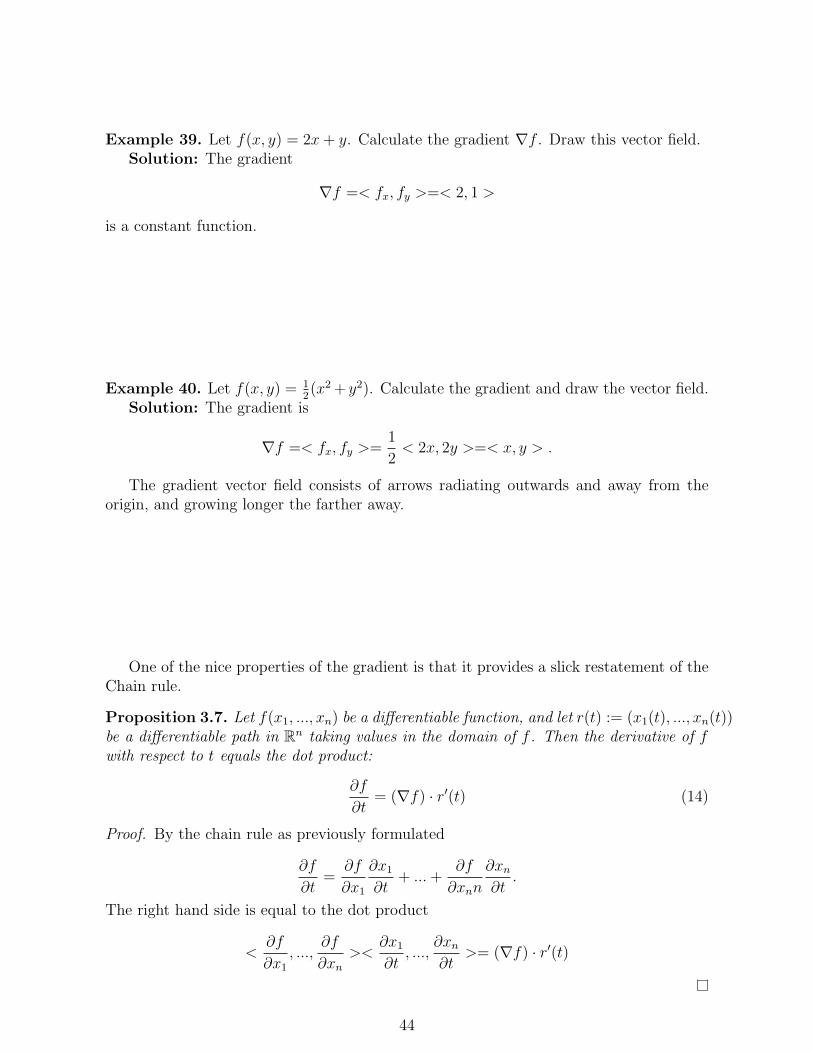
Example 39. Let f(x, y) = 2x+ y. Calculate the gradient ∇f . Draw this vector field.Solution: The gradient

∇f =< fx, fy >=< 2, 1 >

is a constant function.

Example 40. Let f(x, y) = 12(x2 + y2). Calculate the gradient and draw the vector field.

Solution: The gradient is

∇f =< fx, fy >=1

2< 2x, 2y >=< x, y > .

The gradient vector field consists of arrows radiating outwards and away from theorigin, and growing longer the farther away.

One of the nice properties of the gradient is that it provides a slick restatement of theChain rule.

Proposition 3.7. Let f(x1, ..., xn) be a differentiable function, and let r(t) := (x1(t), ..., xn(t))be a differentiable path in Rn taking values in the domain of f . Then the derivative of fwith respect to t equals the dot product:

∂f

∂t= (∇f) · r′(t) (14)

Proof. By the chain rule as previously formulated

∂f

∂t=

∂f

∂x1

∂x1

∂t+ ...+

∂f

∂xnn

∂xn∂t

.

The right hand side is equal to the dot product

<∂f

∂x1

, ...,∂f

∂xn><

∂x1

∂t, ...,

∂xn∂t

>= (∇f) · r′(t)

44

Observe that the formula ... depends only on the velocity vector of the path r(t) andnot on the path itself.

It follows from Proposition 3.7 that the partial derivatives of f can be recovered fromthe gradient ∇f . In two dimensions, we have

< 1, 0 > ·∇f = 1fx + 0fy = fx , < 0, 1 > ·∇f = 0fx + 1fy = fy

Similarly, in three dimensions

~i · ∇f =< 1, 0, 0 > · < fx, fy, fz >= fx, ~j · ∇f = fy, ~k · ∇f = fz

More generally a similar result holds for directional derivatives.

Definition 11. Let ~u be a unit tangent vector in Rn and let f(x1, ..., xn) be a scalarfunction which is differentiable at a point A = (a1, ..., an). The directional derivative of fat A in the direction ~u, is a real number denoted D~u(f)(A) := ~u · (∇f).

By the Proposition 3.7, we may interpret D~u(f)(A) as the rate of change of f at A inthe direction ~u.

Corollary 3.8. The level sets of a differentiable scalar function f(x1, ..., xn) are orthog-onal to ∇f .

Proof. If r(t) is a differentiable path lying on a level curve f(x1, ..., xn) = k for someconstant k, then the composition f(r(t)) = k is constant and has zero derivative. Thus

∂f

∂t= (∇f) · r′(t) = 0

Thus the velocity vector r′(t) which is tangent to the level curve is orthogonal to∇f .

Example 41. Recall the example f(x, y) = 12(x2 + y2 + z2). The gradient vector field

looks like:

45

The level curves must look be concentric circles centered at the origin. This is true becausef(x, y) equals half the distance between (x, y) and the origin, so the level curves shouldbe circles centered at the origin.

This actually provides a helpful strategy to draw level curves, because gradients tendto be easy to compute.

Corollary 3.9. The gradient ∇f points in the direction of “steepest ascent” for the func-tion f and the magnitude |∇f | is the directional derivative in this direction.

Proof. Let ~u be a unit vector and let θ be the angle between ∇f and θ. Then

D~u(f) = ~u · ∇f = |~u||∇f |cos(θ) = |∇f |cos(θ)which is maximized when θ = 0, so when ~u points in the same direction as ∇f , in whichcase

D~u(f) = |∇f |.

3.7 Maxima and Minima

Definition 12. Let f(x1, ..., xn) be a scalar valued function. We say that f has a localmaximum at A = (a1, ..., an) if for all points X = (x1, ..., xn) in a neighbourhood of A,we have

f(A) ≥ f(X).

Similarly, we say that f has a local minimum at A if

f(A) ≤ f(X)

for all X in a neighbourhood of A. In both cases, we say that f has a local extremumat A.

If the above inequality holds for all points X in the domain of f , we say that f hasan absolute maximum, absolute minimum or absolute extremum respectively.

Proposition 3.10. If f has a local extremum at A, f is defined in a neighbourhood of Aand the partial derivatives are defined at A, then ∇f(A) = ~0.

Proof. Consider the n = 2 case for simplicity, so f = f(x, y). If f has a local extremumat A = (a, b) then the single variable function f(t, b) has a local extremum at t = a.Fermat’s theorem then implies that

df

dt|t=a = fx(a, b) = 0.

Similarly, fy(a, b) = 0, so

∇f(a, b) =< fx(a, b), fy(a, b) >= ~0.

46

Definition 13. A point A in the domain of a differentiable function f is called a criticalpoint if ∇f(A) = 0.

It follows from Proposition 3.10 that if f is differentiable everywhere, then local max-ima and minima must occur at critical points. The converse is not true.

Example 42. Find the critical points of f(x, y) = x2 − y2. Find all local maxima andminima.

Solution: The gradient ∇f =< fx, fy >=< 2x,−2y > is defined everywhere andvanishes only at (0, 0), so (0, 0) is the only critical point. However f(0, 0) = 0 whilef(x, 0) = x2 > 0 for x near 0 and f(0, y) < 0 for y near 0, so f(0, 0) is neither a localmaximum, nor a local minimum.

A critical point like the one in this example is called a saddle point, because its graphis shaped like a saddle. One way to check whether a critical point is local minimum,maximum or saddle point is the second derivative test.

Proposition 3.11 (Second Derivative Test). Suppose that f(x, y) is a scalar function oftwo variables, for which ∇f(a, b) = 0 and the partial derivatives fx and fy are definedand continuous in a neighbourhood of (a, b). Define

D = det

(fxx(a, b) fxy(a, b)fyx(a, b) fyy(a, b)

)= fxx(a, b)fyy(a, b)− [fxy(a, b)]2

• If fxx(a, b) > 0 and D > 0 then f has a local minimum at (a, b).

• If fxx(a, b) < 0 and D > 0 then f has a local maximum at (a, b).

• If D < 0 then f has a saddle point at (a, b) and it is not a local extremum.

• Otherwise, the test is inconclusive.

Proof. Idea of proof: Consider the situation where fxy(a, b) = fyx(a, b) = 0. Then thedeterminant simplifies to

D = fxx(a, b)fyy(a, b)

47

If fxx(a, b) > 0 and D > 0 then fyy(a, b) > 0, so f is concave up in both the x andy-directions, and we expect f to have a local minimum at (a, b). Similarly, if fxx(a, b) < 0and D > 0 then fyy(a, b) < 0, so f is concave down in both the x and y-directions, andwe expect f to have a local maximum at (a, b). If D < 0 then the concavity in the x andy directions differ, so we know that f does not have a local extremum at (a, b), and isshaped like a saddle.

The general case can be reduced to the situation fxy(a, b) = 0 by a “change of coordi-nates argument” that we will omit.

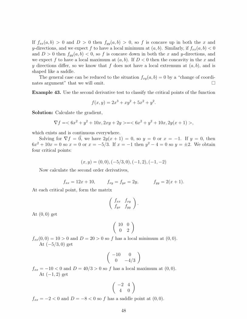
Example 43. Use the second derivative test to classify the critical points of the function

f(x, y) = 2x3 + xy2 + 5x2 + y2.

Solution: Calculate the gradient,

∇f =< 6x2 + y2 + 10x, 2xy + 2y >=< 6x2 + y2 + 10x, 2y(x+ 1) >,

which exists and is continuous everywhere.Solving for ∇f = ~0, we have 2y(x + 1) = 0, so y = 0 or x = −1. If y = 0, then

6x2 + 10x = 0 so x = 0 or x = −5/3. If x = −1 then y2 − 4 = 0 so y = ±2. We obtainfour critical points:

(x, y) = (0, 0), (−5/3, 0), (−1, 2), (−1,−2)

Now calculate the second order derivatives,

fxx = 12x+ 10, fxy = fyx = 2y, fyy = 2(x+ 1).

At each critical point, form the matrix(fxx fxyfyx fyy

).

At (0, 0) get (10 00 2

)fxx(0, 0) = 10 > 0 and D = 20 > 0 so f has a local minimum at (0, 0).

At (−5/3, 0) get (−10 0

0 −4/3

)fxx = −10 < 0 and D = 40/3 > 0 so f has a local maximum at (0, 0).

At (−1, 2) get (−2 44 0

)fxx = −2 < 0 and D = −8 < 0 so f has a saddle point at (0, 0).

48

At (−1,−2) get (−2 −4−4 0

)fxx = −2 < 0 and D = −28 < 0 so f has a saddle point at (0, 0).

3.7.1 Absolute maxima and minima

Recall the Extreme Value Theorem for single variable, scalar functions.

Theorem 3.12. Let f(x) be a continuous scalar function defined on a closed, boundedinterval [a, b] ⊂ R. Then f achieves an absolute maximum and absolute minimum valuein [a, b]. This means there exists c, d ∈ [a, b] such that for every value x ∈ [a, b],

f(c) ≤ f(x) ≤ f(d).

This theorem extends to multi-variable scalar functions as follows.

Theorem 3.13. Let f(x1, ..., xn) be a continuous, scalar function defined on a closed,bounded region Ω ⊂ R. Then f achieves an absolute maximum and absolute minimumvalue on Ω. This means there exists C = (c1, ..., cn) ∈ Ω and D = (d1, ..., dn) ∈ Ω suchthat for every point X = (x1, ..., xn) ∈ Ω,

f(C) ≤ f(X) ≤ f(D).

Of course, we need to define what closed and bounded means. We concentrate on thecase n = 2. A region Ω ⊂ R2 is bounded if it can be covered with a sufficiently largedisk:

A region Ω ⊂ R2 is closed if it contains all of its boundary points. A boundarypoint of a region Ω is a point A for which every disk centered at A intersects both Ω andits complement. All other points in Ω are called interior points.

49

Proposition 3.14. Let Ω ⊂ R2 be a closed and bounded region, and let f be a continuous,differentiable scalar function on Ω. The absolute minimum and maximum values of foccur either at critical points of f in the interior of Ω, or on the boundary of Ω.

Proof. Since an absolute extremum is also a local extremum, this follows from Proposition3.10.

Example 44. Let f(x, y) = 4x+6y−x2−y2. Find the absolute maximum and minimumvalues of f on the region Ω := (x, y) ∈ R2| 0 ≤ x ≤ 4, 0 ≤ y ≤ 5.

Solution: Calculate ∇f(x, y) =< 4− 2x, 6− 2y >. Then the only critical point is

(x, y) = (2, 3).

The boundary in broken into four line segments: L1, L2, L3, L4 pictured below.

Along L1, we have x = 0, 0 ≤ y ≤ 5, so f(0, y) = 6y − y2. The only critical value ofthis one dimensional function is y = 3. Of course, f might be extremized on L1 at one ofthe end points (0, 0) or (0, 5).

Continuing in this fashion, we find eight possible locations of absolute extrema alongthe boundary. The critical points along L1, L2, L3, L4:

(0, 3), (2, 5), (4, 3), (2, 0)

and the end points of these line segments, which are also the corners of Ω,

(0, 0), (0, 5), (4, 5), (4, 0)

To find the absolute maximum and minimum of f , we check all of these values:

f(2, 3) = 13, f(0, 3) = 9, f(2, 5) = 9,

f(4, 3) = 9, f(2, 0) = 4, f(0, 0) = 0,

f(0, 5) = 5, f(4, 5) = 5, f(4, 0) = 0.

So f has absolute maximum 13 achieved at the point (2, 3) and absolute minimum 0achieved at the point (0, 0) and (4, 0).

50

3.8 Lagrange Multipliers

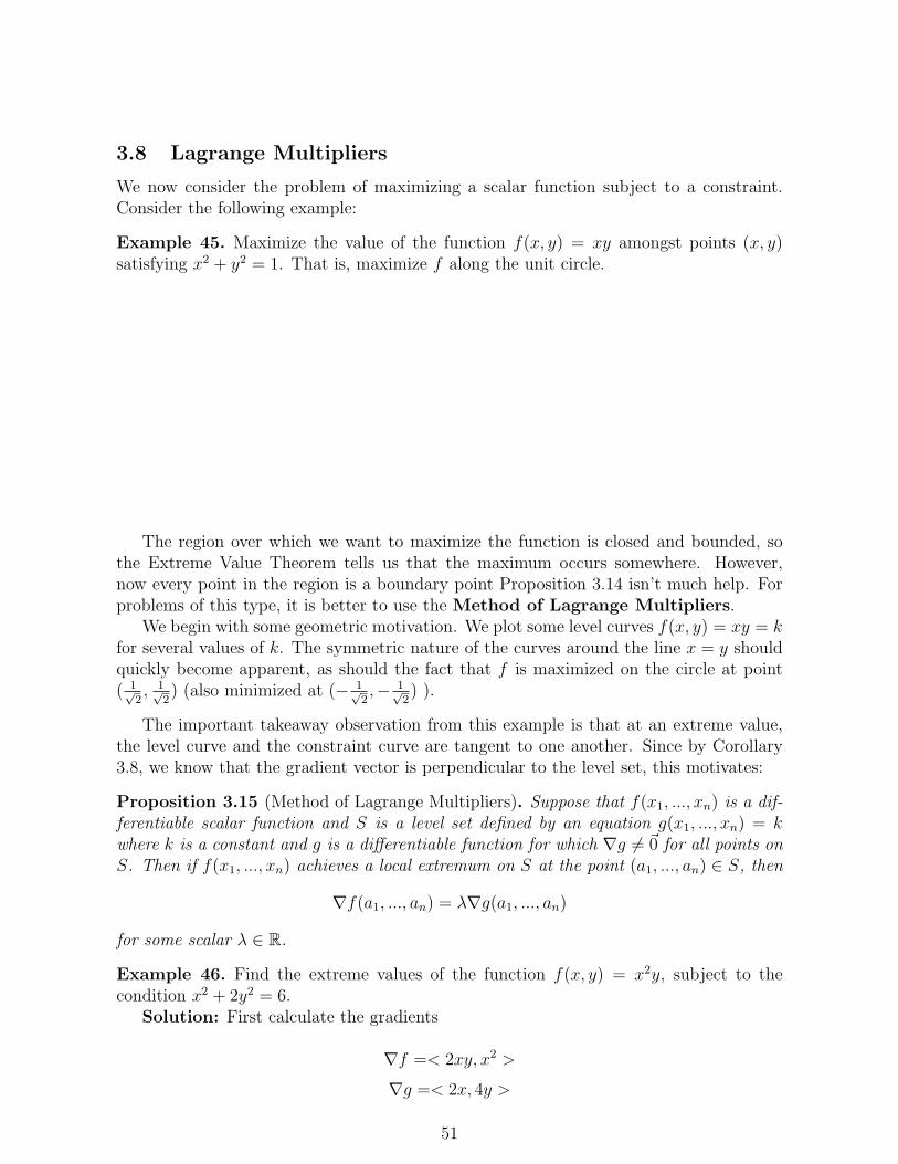
We now consider the problem of maximizing a scalar function subject to a constraint.Consider the following example:

Example 45. Maximize the value of the function f(x, y) = xy amongst points (x, y)satisfying x2 + y2 = 1. That is, maximize f along the unit circle.

The region over which we want to maximize the function is closed and bounded, sothe Extreme Value Theorem tells us that the maximum occurs somewhere. However,now every point in the region is a boundary point Proposition 3.14 isn’t much help. Forproblems of this type, it is better to use the Method of Lagrange Multipliers.

We begin with some geometric motivation. We plot some level curves f(x, y) = xy = kfor several values of k. The symmetric nature of the curves around the line x = y shouldquickly become apparent, as should the fact that f is maximized on the circle at point( 1√

2, 1√

2) (also minimized at (− 1√

2,− 1√

2) ).

The important takeaway observation from this example is that at an extreme value,the level curve and the constraint curve are tangent to one another. Since by Corollary3.8, we know that the gradient vector is perpendicular to the level set, this motivates:

Proposition 3.15 (Method of Lagrange Multipliers). Suppose that f(x1, ..., xn) is a dif-ferentiable scalar function and S is a level set defined by an equation g(x1, ..., xn) = kwhere k is a constant and g is a differentiable function for which ∇g 6= ~0 for all points onS. Then if f(x1, ..., xn) achieves a local extremum on S at the point (a1, ..., an) ∈ S, then

∇f(a1, ..., an) = λ∇g(a1, ..., an)

for some scalar λ ∈ R.

Example 46. Find the extreme values of the function f(x, y) = x2y, subject to thecondition x2 + 2y2 = 6.

Solution: First calculate the gradients

∇f =< 2xy, x2 >

∇g =< 2x, 4y >

51

Now by equating the gradients and imposing the constraint, we get three equations inthree variables.

2xy = 2λx

x2 = 4λy

x2 + 2y2 = 6

By the first equation, we know that either x = 0 or λ = y. If we set x = 0 then 2y2 = 6 soy = ±

√3 and λ = 0. If we set λ = y then x2 = 4y2, so 6y2 = 6, so y = ±1 and x = ±2.

We obtain six solutions:

(x, y) = (0,±√

3), (±2,±1)

Now we can plug these into f(x, y) to get f(0,√

3) = 0, f(±2, 1) = 4, f(±2,−1) = −4.Thus f achieves its minimum of −4 at the points (±2,−1) and its maximum at the points(±2, 1).

Example 47. Find the extreme values of the function f(x, y, z) = xyz subject to theconstraint that x2 + 2y2 + 3z2 = 6.

Solution: Let g(x, y, z) = x2 + 2y2 + 3z2. Calculate the gradients,

∇f =< yz, xz, xy >

∇g =< 2x, 4y, 6z >

This provides four equations an four unknowns:

yz = 2λx

xz = 4λy

xy = 6λz

x2 + 2y2 + 3z2 = 6

First observe that if any of x, y or z equals zero, then f(x, y, z) = 0. Now assume thatx, y, z 6= 0. Then isolating λ in each equation we get

2yz

x=xz

y,

3yz

x=xy

z

then cross-multiplying gives and canceling gives

2y2 = x2, 3z2 = x2

Plugging back into the constraint equations gives 3x2 = 6, so x = ±√

2. Similarlyy = ±1 and z = ±

√2/3. Thus we have extreme values 2√

3and − 2√

3, each achieved at

four different points.

52

Example 48. Maximize the function f(x, y) = 4x + 3y2 over the region Ω := (x, y) ∈R2|x2 + y2 ≤ 1.

Solution: Calculate the gradient

∇f =< 4, 6y > .

Observe that ∇f vanishes nowhere, so f has no critical points in the interior of Ω. Thusthe extreme values all occur on the boundary g(x, y) = x2 + y2 = 1, so we apply themethod of Lagrange multipliers to locate them.

∇g =< 2x, 2y >

Then equating ∇f = λ∇g we get equations

4 = 2λx

6y = 2λy

x2 + y2 = 1

If y does not equal 0, then dividing the second equation by y get λ = 3, so x = 2/3 so(2/3)2 +y2 = 1 and y = ±

√5/3. If y = 0 then x2 = 1 and get solutions (±1, 0). Checking

these points, get

f(1, 0) = 4, f(−1, 0) = −4, f(2/3,±√

5/3) = 8/3 + 5/3 = 13/3 = 4 + 1/3

So f is maximized in Ω at the points (2/3,±√

5/3) where f(2/3,±√

5/3) = 13/3.

4 Integrating Multi-variable Scalar Functions

4.1 Integrating Two Variable Scalar Functions

We begin with a review of the two variable case.Let f(x, y) be a continuous, scalar function and let Ω be a region in R2. The integral

of f over Ω is a real number ∫Ω

f(x, y)dA = V1 − V2

where V1 is the volume of the solid bounded above by the graph of f and below by Ωlying in the x− y coordinate plane, and V2 is the solid bounded below by the graph of fand bounded above by Ω lying in the x− y coordinate plane.

53

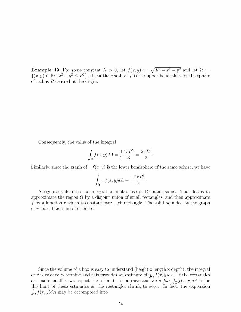
Example 49. For some constant R > 0, let f(x, y) :=√R2 − x2 − y2 and let Ω :=

(x, y) ∈ R2| x2 + y2 ≤ R2. Then the graph of f is the upper hemisphere of the sphereof radius R centred at the origin.

Consequently, the value of the integral∫Ω

f(x, y)dA =1

2

4πR3

3=

2πR3

3.

Similarly, since the graph of −f(x, y) is the lower hemisphere of the same sphere, we have∫Ω

−f(x, y)dA =−2πR3

3.

A rigourous definition of integration makes use of Riemann sums. The idea is toapproximate the region Ω by a disjoint union of small rectangles, and then approximatef by a function r which is constant over each rectangle. The solid bounded by the graphof r looks like a union of boxes

Since the volume of a box is easy to understand (height x length x depth), the integralof r is easy to determine and this provides an estimate of

∫Ωf(x, y)dA. If the rectangles

are made smaller, we expect the estimate to improve and we define∫

Ωf(x, y)dA to be

the limit of these estimates as the rectangles shrink to zero. In fact, the expression∫Ωf(x, y)dA may be decomposed into

54

• dA is the area of an infinitesimally small rectangle (the base of a box in the Riemannsum)

• f(x, y) is the “height” of the box (which might be positive or negative). The (signed)volume of the box is then f(x, y)dA

•∫

Ωmeans summing up the contributions of these boxes over the region Ω.

We say that the integral exists if the limit of Riemann sums converges.

Proposition 4.1. The integral∫

Ωf(x, y)dA exists if f is continuous and Ω is closed and

bounded.

Proof. Omitted.

Proposition 4.2. Let f(x, y) and g(x, y) be continuous scalar functions defined on aclosed and bounded region Ω.

•∫

Ωcf(x, y)dA = c

∫Ωf(x, y)dA for c a constant scalar.

•∫

Ωf(x, y) + g(x, y)dA =

∫Ωf(x, y)dA+

∫Ωg(x, y)dA

• If Ω is equal to a disjoint union of bounded functions Ω1∪Ω2 = Ω, then∫

Ωf(x, y)dA =∫

Ω1f(x, y)dA+

∫Ω2f(x, y)dA

Proof. Since the integral is defined in terms of a limit of Riemann sums, it is enough toverify these statements after replacing Ω by a dijoint union of rectangles and f and g byfunctions that are constant on those rectangles. We leave this as an exercise.

The definition of integrals in terms of Riemann sums is theoretically quite useful, butrather cumbersome for the purposes of calculation. In practice, multivariable integralsare usually reduced to an interation of single variable integrals using Fubini’s Theorem.

Theorem 4.3. Let f(x, y) be a continuous scalar function defined on the rectangularregion Ω := (x, y) ∈ R2|a ≤ x ≤ b, c ≤ y ≤ d. Then we have equality between themultivariable integral and the iterated single variable integrals:∫

Ω

f(x, y)dA =

∫ d

c

(∫ b

a

f(x, y)dx)dy =

∫ b

a

(∫ d

c

f(x, y)dy)dx

The expression∫ dc

( ∫ baf(x, y)dx

)dy means that for each value of y we define a func-

tion F (y) :=∫ baf(x, y)dx, treating y as a constant in this integral, and then integrate∫ d

cF (y)dy. The brackets are normally dropped so that we write∫ d

c

(∫ b

a

f(x, y)dx)dy =

∫ d

c

∫ b

a

f(x, y)dxdy

55

Idea of Proof. Assume for simplicity that f(x, y) ≥ 0, so the integral∫

Ωf(x, y)dA is

simply the volume the region,

For any fixed value y = y0, the value of the function F (y0) =∫ab f(x, y0)dx is sim-

ply the area of the two dimensional cross section lying in the plane y = y0. Thus∫ dc

( ∫ baf(x, y)dx

)dy =

∫ dcF (y)dy is integrating the cross sectional areas and this should

give the volume.

Example 50. Evaluate the iterated integrals∫ 3

1

∫ 1

0(1+4xy)dxdy and

∫ 1

0

∫ 3

1(1+4xy)dydx.

Solution:

∫ 3

1

∫ 1

0

(1 + 4xy)dxdy =

∫ 3

1

[x+ 2x2y]10dy

=

∫ 3

1

1 + 2ydy

= [y + y2]31 = (3 + 9− 2) = 10

∫ 1

0

∫ 3

1

(1 + 4xy)dydx =

∫ 1

0

[(y + 2xy2]31dx

=

∫ 1

0

(2 + 2x(9− 1))dx

= [2x+ 8x2]10 = 10

Notice that the value of the two iterated integrals is the same, as they must be accordingto Theorem 4.3

Fubini’s Theorem also generalizes to integrals over non-rectangular regions.

Theorem 4.4. Let f(x, y) be a continuous scalar function defined on a closed and boundedregion Ω ⊂ R2. If

Ω := (x, y) ∈ R2|a ≤ x ≤ b, l(x) ≤ y ≤ u(x)

56

for some continuous single variable functions l(x) and u(x), then∫Ω

f(x, y)dA =

∫ b

a

∫ u(x)

l(x)

f(x, y)dydx.

Similarly, if Ω = (x, y) ∈ R2|c < y < d, l(y) ≤ x ≤ u(y) then∫Ω

f(x, y)dA =

∫ d

c

∫ u(y)

l(y)

f(x, y)dxdy.

Example 51. Evaluate the integral∫

Ωf(x, y)dA, when f(x, y) := xcos(y) and Ω is the

region bounded by curves, y = 0, y = x2, x = 1Solution: First, sketch the region Ω.

We see that Ω = (x, y)|0 ≤ x ≤ 1, 0 ≤ y ≤ x2. By Fubini we have

∫Ω

f(x, y)dA =

∫ 1

0

∫ x2

0

xcos(y)dydx

=

∫ 1

0

[xsin(y)]x2

0 dx

=

∫ 1

0

xsin(x2)dx

Now we use a substitution u = u(x) = x2, du = 2xdx. Then u(1) = 1 and u(0) = 0, so

57

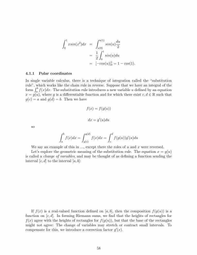
∫ 1

0

xsin(x2)dx =

∫ u(1)

u(0)

sin(u)du

2

=1

2

∫ 1

0

sin(u)du

= [−cos(u)]10 = 1− cos(1).

4.1.1 Polar coordinates

In single variable calculus, there is a technique of integration called the “substitutionrule”, which works like the chain rule in reverse. Suppose that we have an integral of theform

∫ baf(x)dx. The substitution rule introduces a new variable u defined by an equation

x = g(u), where g is a differentiable function and for which there exist c, d ∈ R such thatg(c) = a and g(d) = b. Then we have

f(x) = f(g(u))

dx = g′(u)du

so ∫ b

a

f(x)dx =

∫ g(d)

g(c)

f(x)dx =

∫ d

c

f(g(u))g′(u)du

We say an example of this in ..., except there the roles of u and x were reversed.Let’s explore the geometric meaning of the substitution rule. The equation x = g(u)

is called a change of variables, and may be thought of as defining a function sending theinterval [c, d] to the interval [a, b]:

If f(x) is a real-valued function defined on [a, b], then the composition f(g(u)) is afunction on [c, d]. In forming Riemann sums, we find that the heights of rectangles forf(x) agree with the heights of rectangles for f(g(u)), but that the base of the rectanglesmight not agree: The change of variables may stretch or contract small intervals. Tocompensate for this, we introduce a correction factor g′(x).

58

Example 52. Integrate∫ 2

0x2dx using the substitution x = 2u.

Solution: This integral is of course easy to do without the substitution:∫ 2

0x2dx =

[x3/3]20 = 8/3. Now consider how this integral behaves under the substitution x = g(u) =2u.

Notice that an interval in the u variable corresponds to an interval in the x-variable oftwice the length. That is the geometric meaning of dx = g′(u)du = 2du. In effect, weare multiplying the composed function by 2, doubling the heights of the rectangles tocompensate for the fact that the intevals are half as long.

Applying the substituion rule and integrating :∫ 2

0x2dx =

∫ g(1)

g(0)x2dx =

∫ 1

2(2u)22du =

8∫ 1

0u2du = 8[u3/3]10 = 8/3

A similar principle applies to multi-variable functions. In this case however, the changeof variables is sometimes motivated by the shape of the region of integration.

Consider a region of the form Ω := (x, y) ∈ R2|1 ≤ x2 + y2 ≤ 2, y ≥ 0:

In order to integrate this in the coordinates x, y, we must subdivide into regionsΩ1,Ω2,Ω3 and the determine equation y = l(x) and y = u(x) for the upper and lowerboundary curves. This is going to be messay and a lot of work.

For integrals over regions like Ω, it is usually better to use “polar coordinates”. Intro-duce coordinates r ≥ 0 and 0 ≤ θ ≤ 2π and functions

x = rcos(θ), y = rsin(θ).

Geometrically,

59

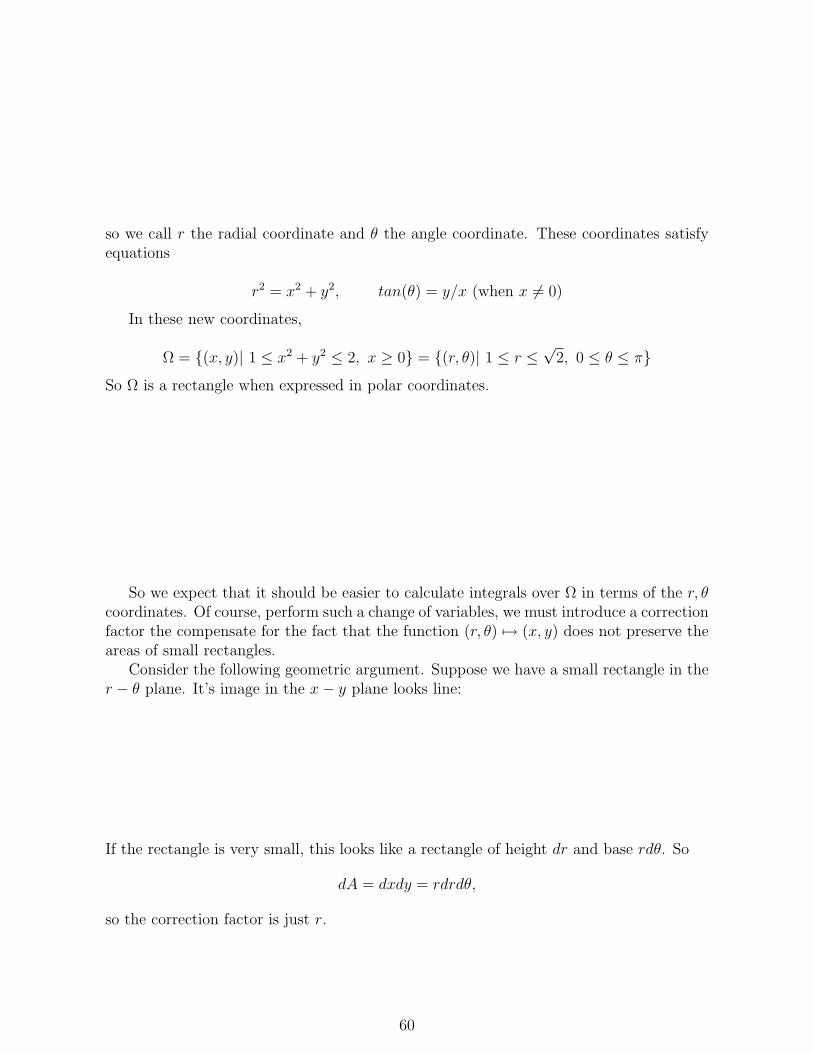
so we call r the radial coordinate and θ the angle coordinate. These coordinates satisfyequations

r2 = x2 + y2, tan(θ) = y/x (when x 6= 0)

In these new coordinates,

Ω = (x, y)| 1 ≤ x2 + y2 ≤ 2, x ≥ 0 = (r, θ)| 1 ≤ r ≤√

2, 0 ≤ θ ≤ π

So Ω is a rectangle when expressed in polar coordinates.

So we expect that it should be easier to calculate integrals over Ω in terms of the r, θcoordinates. Of course, perform such a change of variables, we must introduce a correctionfactor the compensate for the fact that the function (r, θ) 7→ (x, y) does not preserve theareas of small rectangles.

Consider the following geometric argument. Suppose we have a small rectangle in ther − θ plane. It’s image in the x− y plane looks line:

If the rectangle is very small, this looks like a rectangle of height dr and base rdθ. So

dA = dxdy = rdrdθ,

so the correction factor is just r.

60

Proposition 4.5. Let f(x, y) be a continuous function defined on a closed, bounded regionΩ ⊂ R2. We have an equality of integrals:∫

Ω

f(x, y)dA =

∫Ω

f(x(r, θ), y(r, θ))dA =

∫Ω

f(x(r, θ), y(r, θ))rdrdθ

Example 53. Evaluate the integral∫

Ωe−x

2−y2dA over the region Ω bounded between the

semi-circle x =√

4− y2 and the y-axis.Solution: Sketch the region Ω,

Switch to polar coordinates,

∫Ω

e−(x2+y2)dA =

∫Ω

e−r2

rdrdθ

=

∫ 2

0

∫ π/2

−π/2e−r

2

rdθdr

= π

∫ 2

0

e−r2

rdr (u = r2, du = 2rdr)

=π

2

∫ u(2)

u(0)

e−udu

=π

2[−e−u]40

=π

2(1− e−4)

4.1.2 General change of coordinates in dimension two

More generally, suppose we have a pair of differentiable functions x = x(s, t) and y =y(s, t). We think of this as a function T , assigning to every point in the s − t-plane andpoint in the x− y-plane: T (s, t) = (x(s, t), y(s, t))

61

Given a region Ω in x− y-plane, we say that x(s, t), y(s, t) are a change of coordinatesfor Ω if there is a region Ω′ in s− t-plane for T restricts to a one-to-one and onto functionfrom Ω′ to Ω.

The Jacobian for a change of variables (x(s, t), y(s, t)) is

J(s, t) := det

(∂x∂s

∂x∂t

∂y∂s

∂y∂t

)= det

(xs xtys yt

)The absolute value |J(s, t)| provides the correction factor for integration.

Theorem 4.6. Let f(x, y) be a continuous function defined on a closed, bounded regionΩ ⊂ R2. We have an equality of integrals:∫

Ω

f(x, y)dA =

∫Ω

f(x(s, t), y(s, t))dA =

∫Ω

f(x(s, t), y(s, t))|J(s, t)|dsdt

Proof. The correction factor should equal the ratio between the area of a small rectanglein the s− t-plane, and the area of its image under T .

Consider arc-length parametrizations of the lines parallel to the coordinate axes in thes − t-plane. Composing these with T we obtain parametrized curves in the x − y plane,with velocity vectors equal to < ∂x

∂s, ∂x∂t> and < ∂y

∂s, ∂y∂t> (by the chain rule).

The area of a small square based at (s, t), wit side length l is l2. The image ofthis square should be approximated by the parallel-piped with sides l < ∂x

∂s, ∂x∂t

> and

l < ∂y∂s, ∂y∂t> based at the point (x(s, t), y(s, t)). Thus the area of the image of an l × l

square is approximately: ∣∣∣ det

(lxs lxtlys lyt

) ∣∣∣ = l2|J(s, t)|

so the correction factor is equal to |J(s, t)| as desired.

62

Example 54. Find the Jacobian for a polar change of coordinates.Solution:

Here x(r, θ) = rcos(θ) and y(r, θ) = rsin(θ). Calculating partial derivatives,

xr = cos(θ), xθ = −rsin(θ)

yr = sin(θ), yθ = rcos(θ).

Thus,

J(r, θ) = det

(xr xθyr yθ

)= det

(cos(θ) −rsin(θ)sin(θ) rcos(θ)

)= rcos2(θ) + rsin2(θ) = r

so the correction factor is |J(r, θ)| = |r| = r as expected.

Example 55. Integrate∫

Ωy2dA over the region Ω bounded by the curves xy = 1, xy = 2,

xy2 = 1, xy2 = 2.Solution:

The region is Ω := (x, y) ∈ R2|1 ≤ xy ≤ 2, 1 ≤ xy2 ≤ 1. This suggests making anchange of coordinates u = xy and v = xy2. Solving for x and y we get

y = vu−1 = (xy2)/(xy), x = u2v−1 = (xy)2/(xy2)

Observe that these equations are valid if xy and xy2 are non-zero, which will alwaysbe the case for (x, y) ∈ Ω.

The Jacobian for this change of variables is

J(x, y) := det

(xu xvyu yv

)= xuyv − xvyu = (2uv−1)(u−1)− (−u2v−2)(−vu−2) = v−1

Notice that J(u, v) = v−1 = |J(u, v)| because v is bounded between 1 and 2, hence positiveon Ω.

Thus,

I =

∫Ω

y2dxdy =

∫Ω

(vu−1)2(v−1dudv)

=

∫ 2

1

∫ 2

1

vu−2dudv =

∫ 2

1

[−vu−1]21dv

=

∫ 2

1

v(−1/2 + 1)dv =1

4[v2]21 =

3

4

Example 56. Evaluate the integral∫

Ωe(x+y)/(x−y), where Ω is the trapezoidal region

(1,0), (2,0) (0,-2) and (0,-1).Solution: Begin by sketching the region Ω,

63

The integral I =∫

Ωe(x+y)/(x−y)dxdy is awkward to handle directly, so we introduce

coordinates u = x+ y and v = x− y. Now solving for x and y gives

x =1

2(u+ v), y =

1

2(u− v).

The Jacobian for this transformation is

J(u, v) = det

(xu xvyu yv

)= xuyv − xvyu = (

1

2)(

1

2)− (

1

2)(−1

2) =

1

2

So we have

I =1

2

∫Ω

eu/vdudv

which seems simpler. We still have to express Ω in terms of the u, v-coordinates.Observe that the bounding curves for Ω are the lines with equations y = x − 1 ⇒

x − y = 1, x − y = 2, x = 0 and y = 0. These same lines in the u, v - coordinates arev = 1, v = 2, u+ v = 0, and u− v = 0. Sketching Ω in the u− v-plane gives

This region is most easily described Ω = 1 ≤ v ≤ 2,−v ≤ u ≤ v. So we set up aniterated integral,

I =1

2

∫ 2

1

∫ v

−veuv

−1

dudv =1

2

∫ 2

1

[veuv−1

]v−vdv

=1

2

∫ 2

1

(ve1 − ve−1)dv =1

2

∫ 2

1

(e− e−1)vdv

=1

4(e− e−1)[v2]21 =

3

4(e− e−1)

64

4.2 Integrating Three Variable Scalar Functions

We now consider integration of three variable functions. There is no serious conceptualleap in passing from two to three variables, but it does get harder to picture what is goingon.

We begin with integrals over rectangular solids.

Example 57. Integrate the function f(x, y, z) = xy2z−1 over the region Ω := (x, y, z) ∈R3|0 ≤ x ≤ 2, 0 ≤ y ≤ 1, 1 ≤ z ≤ 3.

Solution: We denote this integral by

I =

∫Ω

xy2z−1dV

We think of dV is the volume of an infinitesimal cube in R3. Thinking geometrically interms of Riemann sums, I is the signed volume of four dimensional solid. It is probablybetter not to try to picture this though.

Instead, we compute I using the three dimensional version of Fubini’s theorem. I.e.,I is equal to the iterated integral:

I =

∫ 3

1

∫ 1

0

∫ 2

0

xy2z−1dxdydz

This iterated integration can be done in any order of the variables.

I =

∫ 3

1

∫ 1

0

[(x2/2)y2z−1]20dydz

=

∫ 3

1

∫ 1

0

2y2z−1dydz

=

∫ 3

1

[(2y3/3)z−1]10dz

=2

3

∫ 3

1

z−1dz

=2

3[ln(z)]31

=2

3(ln(3)− ln(1)) =

2ln(3)

3

In this example, it is also possible to use a short cut. Since when we integrate withrespect to a particular variable, the other variables are treated like constants, we areallowed to pull them outside the integral signs∫ 3

1

∫ 1

0

y2z−1

∫ 2

0

xdxdydz =

∫ 3

1

z−1

∫ 1

0

y2

∫ 2

0

xdxdydz

Because the intervals of integration are constants (indepent of any variables), we mayalso pull the differentials through the integral signs, to get

65

(∫ 3

1

z−1dz)(∫ 1

0

y2dy)(∫ 2

0

xdx)

= [ln(z)]31[y3/3]10[x2/2]20 = (ln(2))(1/3)(2).

as before.

Fubini’s theorem also works for non-rectangular regions. For instance suppose a 3-dimensional region Ω is defined

(x, y, z) ∈ R3|a ≤ x ≤ b, l(x) ≤ y ≤ u(x), b(x, y) ≤ z ≤ t(x, y) (15)

where l, u, b, t are continuous scalar functions on one and two variables respectively. Thenfor a continuous scalar function f(x, y, z) defined over Ω, we have equality of integrals:∫

Ω

f(x, y, z)dV =

∫ b

a

∫ u(x)

l(x)

∫ t(x,y)

b(x,y)

f(x, y, z)dzdydx

Example 58. Compute the volume of the solid region Ω bounded between the coordinateplanes and the plane x+ y + z = 1.

Solution: We begin by sketching the region Ω.

Finding the volume of a solid is the same as integrating the constant function 1 overit, so we want to compute I =

∫Ω

1dV . We need to find a description of Ω similar to(15). Certainly we have x ≥ 0, y ≥ 0, z ≥ 0 in Ω. Also we know that x + y + z ≤ 1, soz ≤ 1− x− y. Also, for any value of z ≥ 0, we have x+ y ≤ 1 so y ≤ 1− x. Finally, forany value of y, z ≥ 0, x ≤ 1. Thus,

Ω = (x, y, z)|0 ≤ x ≤ 1, 0 ≤ y ≤ 1− x, 0 ≤ z ≤ 1− x− yConsequently,

I =

∫Ω

1dV =

∫ 1

0

∫ 1−x

0

∫ 1−x−y

0

1dzdydz

=

∫ 1

0

∫ 1−x

0

[z]1−x−y0 dydx =

∫ 1

0

∫ 1−x

0

(1− x− y)dydx

=

∫ 1

0

[y − xy − y2/2]1−x0 dx =

∫ 1

0

((1− x)(1− x)− (1− x)2/2)dx

=

∫ 1

0

((1− x)2/2)dx =1

2

∫ 1

0

(1− 2x+ x2)dx

=1

2[x− x2 + x3/3]10 = 1/6

66

4.2.1 Change of variables in dimension three

We also have a change of variables formula for three variable integrals. Consider anintegral ∫

Ω

f(x, y, z)dxdydz

over a closed and bounded region Ω ⊂ R3. A change of coordinates for Ω is a set of threedifferentiable functions

x = x(u, v, w), y = y(u, v, w), z = z(u, v, w)

determining a (almost-everywhere) one-to-one and onto transformation for Ω. Then wehave an equality of integrals

∫Ω

f(x, y, z)dxdydz =

∫Ω

f(x(u, v, w), y(u, v, w), z(u, v, w))|J(u, v, w)|dudvdw

where J(u, v, w) is the Jacobian for the change of variables, and is defined by

J(u, v, w) := det

xu xv xwyu yv ywzu zv zw

4.2.2 Cylindrical coordinates

Cylindrical coordinates are appropriate for integrating over regions with rotational sym-metry around the z-axis. They are,

x = rcos(θ), y = rsin(θ), z = z.

where r ≥ 0 and θ ∈ [−π, π] (we may also choose θ ∈ [0, 2π] as appropriate). This is es-sentially just polar coordinates in the x-y-plane, because we leave z as it was. Calculatingthe Jacobian

J(r, θ, z) := det

xr xθ xzyr yθ yzzr zθ zz

= det

cos(θ) −rsin(θ) 0sin(θ) rcos(θ) 0

0 0 1

= r(cos2(θ)+sin2(θ)) = r.

Observe that this is the same correction factor as for polar coordinates. This makes sensebecause we left z unchanged.

Example 59. Find the volume of the solid that lies within both the cylinder x2 + y2 = 1and the sphere x2 + y2 + z2 = 4.

Solution: Sketch the region Ω,

67

In cylindrical coordinates, the equations for the cylinder and spere are r2 = 1 andr2 + z2 = 4. Consequently, the region Ω satisfies,

Ω = (r, θ)|0 ≤ r ≤ 1, 0 ≤ z ≤ (4− r2)1/2

Thus the volume of Ω equals

V =

∫Ω

1dV

=

∫ 1

0

∫ (4−r2)1/2

0

∫ 2π

0

rdθdzdr

= 2π

∫ 1

0

[rz](4−r2)1/2

0 dr

= 2π

∫ 1

0

(4− r2)1/2rdr

Use a substitution u = 4− r2, du = −2rdr, to get

V = 2π

∫ u(1)

u(0)

u1/2(−1

2

)du = −π[

2

3u3/2]34 =

2π

3(8− (3)3/2)

4.2.3 Spherical coordinates

Spherical coordinates are useful for integrating over regions that are “radially” symmetric,such as sphere or cones. Spherical coordinates consist of two “angle” coordinates θ, φ andone “length” coordinate ρ as depicted in the following diagram:

Geometrically it is clear that we should restrict 0 ≤ θ ≤ 2π, 0 ≤ φ ≤ π and ρ ≥ 0. Toget the change of variable formulas, it is actually easier to first pass through cylindricalcoordinates

68

z = ρcos(φ), r = ρsin(φ), θ = θ

so plugging these into the cylindrical change of coordinates formula, we get

x = rcos(θ) = ρsin(φ)cos(θ), y = rsin(θ) = ρsin(φ)sin(θ), z = ρcos(φ)

Now to compute the Jacobian.

J(ρ, φ, θ) := det

xρ xφ xθyρ yφ yθzρ zφ zθ

= det

sin(φ)cos(θ) ρcos(θ)cos(φ) −ρsin(φ)sin(θ)sin(φ)sin(θ) ρcos(φ)sin(θ) ρsin(φ)cos(θ)

cos(φ) −ρsin(φ) 0

= ρ2sin(φ) det

sin(φ)cos(θ) cos(θ)cos(φ) −sin(θ)sin(φ)sin(θ) cos(φ)sin(θ) cos(θ)

cos(φ) −sin(φ) 0

= ρ2sin(φ)

[− sin(θ) det

(sin(φ)sin(θ) cos(φ)sin(θ)

cos(φ) −sin(φ)

)− cos(θ) det

(sin(φ)cos(θ) cos(θ)cos(φ)

cos(φ) −sin(φ)

)]= ρ2sin(φ)[−(sin2(θ) + cos2(θ)) det

(sin(φ) cos(φ)cos(φ) −sin(φ)

)]

= ρ2sin(φ)(−1)(−sin2(φ)− cos2(φ))

= ρ2sin(φ)

Example 60. Evaluate∫

Ω(9 − x2 − y2)dV where Ω is the solid hemisphere defined by

x2 + y2 + z2 ≤ 9 and z ≥ 0.Solution: Sketch the region:

Observe that x2 + y2 = r2 = (ρsin(φ))2 so,

I =

∫Ω

9− x2 − y2dV =

∫Ω

(9− ρ2sin2(φ))dV =

∫Ω

(9− ρ2sin2(φ))ρ2sin(φ)dρdφdθ

In the new coordinates

Ω = (ρ, θ, φ)|0 ≤ ρ ≤ 3, 0 ≤ φ ≤ π/2, 0 ≤ θ ≤ 2π

69

I =

∫ 3

0

∫ π/2

0

∫ 2π

0

9ρ2sin(φ)dθdφdρ−∫ 3

0

∫ π/2

0

∫ 2π

0

ρ4sin3(θ)dθdφdρ = I1 − I2

I1 =(∫ 3

0

9ρ2dρ)(∫ π/2

0

sin(φ)dφ)(∫ 2π

0

1dθ)

= [3ρ3]30 [−cos(φ)]π/20 [θ]2π0

= (34)(1)(2π) = 2(34)π

I2 =(∫ 3

0

ρ4dρ)(∫ π/2

0

(1− cos2(φ))sin(φ)dφ)(∫ 2π

0

1dθ)

= [ρ5/5]30 [−cos(φ) + cos3(φ)/3]π/20 [θ]2π0

= (35/5)(2/3)(2π) = (8/5)34π

So I = I1 − I2 = 6534π

5 Calculus of Vector Fields

A vector field F is a function that assigns to every point p in a domain D ⊆ Rn a vectorF(p) in Rn.

Concretely, any vector field F in R2 can be described in coordinates

F(x, y) =< f(x, y), g(x, y) >

where f and g are continuous real valued functions defined on D ⊆ R2. Similarly, a vectorfield on R3 may be expressed

F(x, y, z) =< f(x, y, z), g(x, y, z), h(x, y, z) >

for some continuous scalar functions f, g, h defined on D ⊆ R3.

Example 61. The gradient ∇f of a differentiable scalar function f is a vector field.

5.1 Line Integrals and the Fundamental Theorem

Let r(t) = (x1(t), ..., xn(t)) be a differentiable path in Rn. If F is a vector field on Rn, wedefine the line integral by ∫ r(b)

r(a)

F · dr =

∫ b

a

(F · r′(t))dt

70

Example 62. Find the line integral of the vector field F(x, y) =< x2, xy > with respectto the path r(t) = (x(t), y(t)) = (cos(t), sin(t)), 0 ≤ t ≤ π/2.

Solution: Begin with a rough sketch of the vector field and the curve,

Since the angle between F(x, y, z) and r(t) is always obtuse along the curve, we know theintegral should be negative. Calculating,

r(t) =< −sin(t), cos(t) >

∫ r(b)

r(a)

F · dr =

∫ π/2

0

< x(t)2,−x(t)y(t) > · < −sin(t), cos(t) > dt

=

∫ π/2

0

< cos2(t),−cos(t)sin(t) > · < −sin(t), cos(t) > dt

=

∫ π/2

0

−2cos2(t)sin(t)dt

=2

3[cos3(t)]

π/20 =

2

3(0− 1) = −2

3

Although, the line integral is defined using a parametrized curve (a.k.a. path) thevalue of the line integral depends only on the curve (and its orientation), not on theparametrization.

Proposition 5.1. The line integral of a vector field along a curve is independent of theparametrization of the curve.

Proof. Easy consequence of the chain rule (Exercise).

If the vector field is the gradient of a scalar function, the line integral only dependson the end points of the curve. This result is known as the First Fundamental Theoremof Line Integrals.

71

Theorem 5.2. If F = ∇f is the gradient of a differentiable scalar function f , then

f(r(b))− f(r(a)) =

∫ r(b)

r(a)

F · dr

for any is any continuous and piecewise differentiable path r(t).

Proof. Omitted.

Example 63. To motivate Theorem 5.2, it is helpful to consider the one variable case.Let f = f(x) be a differentiable function with gradient F = ∇f =< f ′(x) >. Consider acurve r(t) = (x(t)) = (t) for a ≤ t ≤ x. Then the theorem says:

f(b)− f(a) =

∫ r(b)

r(a)

F · dr =

∫ b

a

< f ′(x(t)) >< 1 > dt =

∫ b

a

f ′(t)dt

which we recognize as the first fundamental theorem of (single variable) calculus.

Example 64. Consider f(x, y) = y, so F(x, y) = ∇f =< 0, 1 >. Consider the curver(t) = (t, t) from 0 ≤ t ≤ 1, joining (0, 0) to (1, 1). Integrating:

∫ 1

0

∇f · r′dt =

∫ 1

0

< 0, 1 > · < 1, 1 > dt =

∫ 1

0

1dt = 1 = f(1, 1)− f(0, 0).

Similarly, if we consider the path r(t) = (t, t2) from 0 ≤ t ≤ 1 also joining (0, 0) to(1, 1) then,∫ 1

0

∇f · r′dt =

∫ 1

0

< 0, 1 > · < 1, 2t > dt =

∫ 1

0

2tdt = [t2]10 = 1 = f(1, 1)− f(0, 0).

Definition 14. A vector field F is called conservative if it satisfies the property that

any line integral∫ r(b)

r(a)F · dr depends only on the value of the endpoints r(b) and r(a).

It follows from Theorem 5.2 that any gradient vector field ∇f is conservative. TheSecond Fundamental Theorem of Line Integrals is the converse of that statement.

Theorem 5.3. If F is a conservative vector, then there exists a differentiable function fsuch that F = ∇f .

72

Proof. Using Theorem 5.2, we know that for any pair of points a = (a1, .., an), b =(b1, ..., bn) in the domain of F, the difference

f(b)− f(a) =

∫F · dr

for some path r joining a to b. Observe that this quantity is well-defined because the lineintegral is independent of the choice of r. This formula determines f up to an arbitraryconstant ( much like antiderivatives in single variable calculus are determined up to aconstant).

In contrast with single variables, in dimension greater than one most vector fields arenot gradients of scalar functions, so most vector fields are not conservative. Is is possibleto determine whether a vector field is conservative, without checking every line integraland constructing a scalar “anti-derivative”? The answer is yes (with some conditions).

Proposition 5.4. Let F(x, y) :=< P (x, y), Q(x, y) > be a conservative and continuouslydifferentiable vector field. Then

∂P

∂y− ∂Q

∂x= 0.

Proof. Because F is conservative, we know by the second Fundamental Theorem, thatF = ∇f =< fx, fy > for some differentiable scalar function f(x, y). Consequently, P = fxand Q = fy and

∂P

∂y− ∂Q

∂x= fxy − fyx = 0

by Clairaut’s Theorem.

The function Py −Qx is evidently interesting, so we give it a name.

Definition 15. We define the curl of a two-dimensional vector field F =< P,Q > to bethe scalar function

curl(F) = Py −Qx.

Proposition 5.4 has a partial converse,

Theorem 5.5. Suppose F is a continuously differentiable vector field defined on a rect-angular region D ⊆ R2 or defined everywhere on R2. Then F is conservative if and onlyif curl(F) = 0.

Proof. Omitted.

Why is the constraint on the domain D necessary?

73

Example 65. Consider the vector field F := 1x2+y2

< −y, x >=< P,Q >. In this case

Py = −∂y(x2 + y2)−1

∂y= −(x2 + y2)−1 + 2y2(x2 + y2)−2

Qx =∂x(x2 + y2)−1

∂x= (x2 + y2)−1 − 2x2(x2 + y2)−2

Thus,

curl(F) = Py −Qx = −2(x2 + y2)−1 + (2x2 + 2y2)(x2 + y2)−2 = 0.

On the other hand, if we consider the graph of the vector field,

It is clear that taking the line integral counter-clockwise around a circle centered at theorigin with give a positive number (Exercise: Find this number). This does not contradictTheorem 5.6, because F is not defined at the origin. In fact, if we integrate around anyloop that does not contain the origin, we will get zero.

Definition 16. A simple, closed curve C in R2 is a curve that doesn’t intersect itselfanywhere except at its endpoints. That is, C admits a parametization r(t), a ≤ t ≤ bwith r(a) = r(b) but r(t1) 6= r(t2) for any a ≤ t1 < t2 < b.

Every simply connected curve in R2 divides its complement into an bounded interiorregion and an unbounded exterior region (Aside: this is called the Jordan curve theorem).

Definition 17. A region Ω ⊆ R is called simply connected if for every simple closedcurve C ⊂ Ω, the region bounded by C is contained in Ω.

74

The second fundamental theorem of calculus generalizes to

Theorem 5.6. Suppose F is a continuously differentiable vector field defined on a simplyconnected region D ⊆ R2. Then F is conservative if and only if curl(F) = 0.

5.2 Green’s Theorem

What if the curl of a vector field is nonzero? Is it still telling us something interesting?

Theorem 5.7 (Green’s Theorem). Let C be a simple closed piecewise differentiable curvewith counter-clockwise orientation and suppose F is a vector field defined and continuouslydifferentiable on C and on the region Ω bounded by C.

Then there is an equality of integrals:∫C

F · dr =

∫Ω

curl(F)dA

Proof. The idea of the proof is to decompose the region Ω into little squares Ωn so that∫Ω

curl(F)dA =∑n

∫Ωn

curl(F)dA.

Each Ωn is bounded by a square curve Cn. Because changing the orientation of a lineintegral introduces a minus sign, we get,∫

C

F · dr =∑n

∫Cn

F · dr.

Finally, argue that for sufficiently small Ωn, we have∫Cn

F · dr ≈∫

Ωn

curl(F)dA.

75

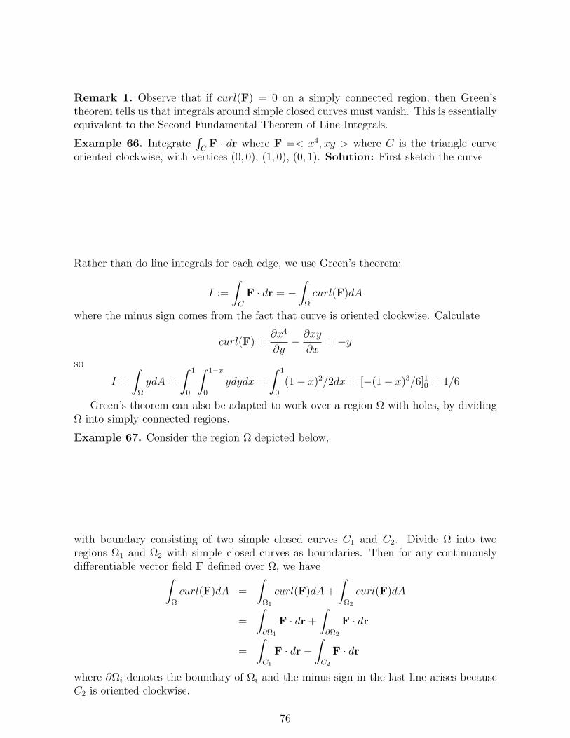
Remark 1. Observe that if curl(F) = 0 on a simply connected region, then Green’stheorem tells us that integrals around simple closed curves must vanish. This is essentiallyequivalent to the Second Fundamental Theorem of Line Integrals.

Example 66. Integrate∫C

F · dr where F =< x4, xy > where C is the triangle curveoriented clockwise, with vertices (0, 0), (1, 0), (0, 1). Solution: First sketch the curve

Rather than do line integrals for each edge, we use Green’s theorem:

I :=

∫C

F · dr = −∫

Ω

curl(F)dA

where the minus sign comes from the fact that curve is oriented clockwise. Calculate

curl(F) =∂x4

∂y− ∂xy

∂x= −y

so

I =

∫Ω

ydA =

∫ 1

0

∫ 1−x

0

ydydx =

∫ 1

0

(1− x)2/2dx = [−(1− x)3/6]10 = 1/6

Green’s theorem can also be adapted to work over a region Ω with holes, by dividingΩ into simply connected regions.

Example 67. Consider the region Ω depicted below,

with boundary consisting of two simple closed curves C1 and C2. Divide Ω into tworegions Ω1 and Ω2 with simple closed curves as boundaries. Then for any continuouslydifferentiable vector field F defined over Ω, we have∫

Ω

curl(F)dA =

∫Ω1

curl(F)dA+

∫Ω2

curl(F)dA

=

∫∂Ω1

F · dr +

∫∂Ω2

F · dr

=

∫C1

F · dr−∫C2

F · dr

where ∂Ωi denotes the boundary of Ωi and the minus sign in the last line arises becauseC2 is oriented clockwise.

76

Example 68. Let F = 1x2+y2

< −y, x >. Show that the value of the integral∫C

F · dr isthe same for every simple, closed curve C, oriented counter-clockwise and bounding theorigin.

Solution: This vector field was shown before to be defined everywhere except theorigin, and to satisfy curl(F) = 0. Thus, if we take two circles C1 and C2 centred atthe origin with different radii, then by applying Green’s theorem to the region boundedbetween the curves, we discover that∫

C1

F · dr =

∫C2

F · dr.

Now given an arbitrary simple closed curve C bounding the origin, we may choose a circleC1 containing C. By the same argument∫

C1

F · dr =

∫C

F · dr.

5.3 Parametrized Surfaces

Recall that parametrized curve or path in R3 is simply a continuous function

r(t) = (x(t), y(t), z(t))

defined on some interval t ∈ [a, b] ⊆ R.Similarly, a parametrized surface in R3 is defined to be a continuous two variable

functionr(u, v) = (x(u, v), y(u, v), z(u, v))

defined on some region Ω ⊆ R2. This concept is illustrated in the following diagram

In the same way we can do calculus on parametrized curves (tangent lines, arc length,line integrals), we can do calculus on parametrized surfaces (tangent planes, surface areaand surface integrals).

We say r(u, v) is differentiable if the coordinate functions x(u, v), y(u, v), z(u, v) areall continuous. We define vector-valued functions

ru(u, v) =< xu, yu, zu >, rv(u, v) =< xu, yu, zu >

77

Definition 18. Let r(u, v) = (x(u, v), y(u, v), z(u, v)) be a differentiable parametrizedsurface S in R3. Given a constant (a, b) in the domain of r, the tangent plane to S atr(a, b) is parametrized in variable s, t by:

P (s, t) = r(a, b) + ru(a, b)s+ rv(a, b)t

Example 69. Find a parametrization for the surface z2 = x2 + 2y2 and z ≥ 0, and finda parametrization for the tangent plane at the point (1, 0, 1).

Solution: Since we are only considering points with z ≥ 0, z2 = x2 + 2y2 ⇒ z =√x2 + 2y2. Thus a good parametrization is

r(u, v) = (u, v, (u2 + v2)1/2),

with the domain of r equal to all of R2. To find the tangent plane, we take partialderivatives,

ru =< 1, 0, (u2 + v2)−1/2u >, rv =< 0, 1, (u2 + v2)−1/2v >

In this parametrization r(1, 0) = (1, 0, 1). Thus the formula for the tangent plane is,

p(s, t) = r(1, 0) + ru(1, 0)s+ rv(1, 0)t = (1, 0, 1) + s < 1, 0, 1 > +t < 0, 1, 1 >

= (1 + s, t, 1 + s+ t)

5.3.1 Surface Area

Recall that when we performed change of variable for two variable functions, we needed tointroduce the Jacobian as a correction factor. Geometrically, the Jacobian measures thearea of a small rectangle changes in the new coordinates. To do integrals over parametrizedsurfaces, we must do something similar.

Given a differentiable parametrized surface r(u, v) in R3, consider a square in the u-vplane, based at the point (a, b), with sides the unit vectors < 1, 0 > and < 0, 1 >. Underthe “linear approximation” to r(t), this square is sent to the parallel-piped in the tangentplane to r(a, b), with sides ru(a, b) and rv(a, b).

78

The area of the parallel-piped is equal to the norm of the cross-product:

Area = |ru(a, b)× rv(a, b)|

so this is the appropriate correction factor for integrating scalar functions over parametrizedsurfaces in R3. In particular,

Proposition 5.8. The surface area of a surface S with differentiable parametrizationr(u, v) with domain Ω is equal to the two variable, scalar integral

Area(S) =

∫S

dA =

∫Ω

|ru × rv|dudv

Remark 2. Observe the similarity of between this formula and the formula for arc-length: Arc-length =

∫ ba|r′(t)|dt.

Example 70. Find the surface area of the surface z = x2+y2 bounded between 0 ≤ z ≤ 1.Solution: Draw a sketch

We can parametrize the surface by r(u, v) = (u, v, u2 +v2) with Ω := (u, v)|u2 +v2 ≤ 1.Taking partial derivatives gives,

ru(u, v) =< 1, 0, 2u >, rv(u, v) =< 0, 1, 2v >

Forming the cross-product ∣∣∣∣∣∣~i ~j ~k1 0 2u0 1 2v

∣∣∣∣∣∣ =< −2u,−2v, 1 >,

so that |ru × rv| = (4u2 + 4v2 + 1)1/2. Thus the surface area is equal to the integral

A =

∫Ω

(4u2 + 4v2 + 1)1/2dudv.

79

Since Ω is a disk of radius 1 we change to polar coordinates, u = rcos(θ), v = rsin(θ),

A =

∫ 1

0

∫ 2π

0

(4r2 + 1)1/2rdθdr

= 2π

∫ 1

0

(4r2 + 1)1/2rdr

= 2π

∫ t(1)

t(0)

(t1/2/8)dt, (t = 4r2 + 1, dt = 8dr)

=π

4[(2/3)t3/2]50

=π

653/2

5.4 Integrating Vector Fields over Surfaces: Flux

Now we learn how to integrate vector fields over surfaces.Let F(x, y, z) be a vector field on R3 and S ⊂ R3 a surface. An orientation at a

point a ∈ S is a choice of unit normal vector n to the surface at a. An orientation on Sis a continuously varying choice of orientations at all points.

Example 71. If S is the unit sphere then there are two possible orientations: normalvectors either point out or in.

Example 72. A mobius strip S does not admit any orientation.

Definition 19. Let F be a vector field in R3 and let S be a surface in R3 with orientationn. Then we define the flux of F over the S to be the integral∫

S

(F · n)dA.

If we imagine the vector field F as current of a flowing fluid, then the flux∫S(F ·n)dA

equals the rate at which the fluid passes through the surface in the direction n.

80

Example 73. Suppose S is the unit disk defined by x2 +y2 ≤ 1 and z = 0 with (constant)normal vector n =< 0, 0, 1 >.

If F =< 0, 0, l > is constant vector field consisting of length l vectors pointing in thez-direction, the flux is

∫S(F · n)dA =

∫S(l)dA = lπ, the length of the vector times the

area of the surface. If F =< 0, 1, 0 > points in the y-direction, then the flux is zero (nofluid is passing through the surface).

If the surface S is curved, computing the flux is best accomplished using a parametriza-tion of S. So suppose that r(u, v) is a parametrization of S with domain Ω ⊆ R2. Thenfrom the last section we know,

Flux =

∫S

(F · n)dA =

∫Ω

(F · n)|ru × rv|dudv.

This formula can be simplified. Recall that the cross-product ru× rv is perpendicularto the surface, so it is a scalar multiple of the unit normal n. Thus

ru × rv = ±|ru × rv|n

where the ambiguity of sign is a result of two possible choices of orientation. It followsthat

Flux =

∫Ω

(F · n)|ru × rv|dudv

=

∫Ω

(F · (|ru × rv|n))dudv

= ±∫

Ω

F · (ru × rv)dudv

Example 74. Let F :=< xzey,−xzey, z > and let S be the part of the plane x+y+z = 1lying in the first octant and oriented downwards in the z direction. Calculate the flux.

Solution: Sketch the surface,

81

Observe that this the graph of z = 1 − x − y, restricted to the domain x + y ≤ 1and x, y ≥ 0. This suggests a parametrization, r(u, v) = (u, v, 1 − u − v) with domainΩ := (u, v) | 0 ≤ u, 0 ≤ v ≤ u. Calculating

ru =< 1, 0,−1 >, rv =< 0, 1,−1 >, ru × rv =< 1, 1, 1 >

Observe that the cross product ru × rv points in the opposite direction from the desiredorientation of S. Thus

Flux = −∫

Ω

F · (ru × rv)dudv

=

∫Ω

< u(1− u− v)ev,−u(1− u− v)ev, 1− u− v > · < 1, 1, 1 > dudv

=

∫Ω

(1− u− v)dudv

=

∫ 1

0

∫ 1−u

0

(1− u− v)dvdu

=

∫ 1

0

[(1− u)v − v2/2]1−u0 du

=

∫ 1

0

(1− u)2/2du = [−(1− u)3/6]10 = 1/6

82