Vasicek Model Project

VASICECK ONE AND TWO

FACTOR

Fall 2015

Projects in Mathematical and Computational Finance CEDRIC L. MELHY

NJIT | New Jersey Institutes of Technology

1 | P a g e

Abstract

The Vasicek Model introduced by Oldrich Vasicek in 1977 is one of the earliest stochastic

models of the term structure of interest rate. It represents one of the first and well known interest

rates models and is still in active use. This method of modeling interest rates movement

describes the movement of an interest rate as a factor of market risk, time and equilibrium value

that the rate tends to revert towards. It is also used in the valuation of interest rates futures. The

scope of this study is to show how to estimate the single factor model but we will also show how

this can be extended to the multifactor framework, using available data such as Zero coupon

Bond and then estimate the zero-coupon bond yield curve of tomorrow by using Vasicek yield

curve model with the zero-coupon bond yield data of today. We will give the results for the

estimation of the model parameters using two different ways including extensive R code for

parameters estimation and bond pricing

Finally, we will emphasize a comparative study of the Ornstein-Uhlenbeck and the Cox,

Ingersoll, and Ross (CIR, developed in 1985) model of the short rate

Keywords: one and two factors Vasicek model, CIR model, Equilibrium model, Bond Pricing, interest rate term structure.

2 | P a g e

TABLE OF CONTENTS

Chapter Page

1 Introduction ……………………………………………………………. Page 3

1.1 Background ……..……………………………………………………. Page 3 1.2 Interest Rate Model ……………………………………………………... Page 3

1.2.1 Description…………………….……………………………… Page 3 1.2.2 Equilibrium Model…………………………………………….. Page 4

2 Vasicek Interest Rate Model………………………………………………….. Page 6

3 Parameter Estimation ………………………………………………………… Page 7 3.1 Least Square Regressions…..……………………………………………. Page 7

3.1.1 Data…………………………………………………………… Page 7 3.1.2 Parameter Estimation using Least Square Regression Technique Page 10 3.1.3 Maximum Likelihood Estimator……………………………… Page 12

4 Zero Coupon Bond Pricing……………………………………………………… Page 14

4.1 Data……………………………………………………………………… Page 14 4.2 Calibration of model parameters using bond prices…………………….. Page 14 4.3 Data: Euribor from January 18, 1999 to November 18, 2008…………… Page 16 4.4 Data: Euribor from January 2005 to March 2006…………..…………… Page 17

5 Monte Carlo Simulation of the term Structure for Vasicek Model Parameters Page 21

6 Term Structure………………………………………………………………… Page 22

7 The two-factor Vasicek Model………………………………………………… Page 23 7.1 Case Studied ……………………………………………………………... Page 26

3 | P a g e

8 Comparative study of the Vasicek and the CIR Model……………………… Page 26

9 Conclusion…………………………………………………………………… Page 28

10 Appendix…………………………………………………………………….. Page 29

11 References…………………………………………………………………… Page 35

4 | P a g e

1. Introduction

1.1. Background

The short rate r, at time t is the rate that applies to an infinitesimally short period of time at time

t. It sometimes referred to as the instantaneous short rate. Bond prices and other derivatives

prices depend only on the process followed by r in a risk neutral world. The process for r in the

real world is irrelevant. The value at time t of an interest rate derivative that provides a payoff of

�� at time T is ��[���(���)��) where �� denotes the expected value in the traditional risk-

neutral world. Then at time t, the price of zero coupon bond [Z (t, T)] that pays off $1 at time T

is Z (T, t) = ��[���(���)]

= ���(�,�)(���) where R (t, T) is the continuously compounded rate at time t for a term

of T-t

That will lead us to the relation R (t, T) = �

��� ln ��[���(���)]

1.2 Interest Rates model

1.2.1 Description

Interest rate models can be used to model the dynamics of the yield curve, which is vital in

pricing and hedging of fixed-income securities and also of great importance from a macro

economical point where we can estimate the future short-term interest rates, inflation and

economic activity. Traditionally these models specify a stochastic process for the term structure

dynamics in a continuous-time setting. A stochastic process means that the outcome depends

both from a determined and a random component and is thus given the form:

dr(t) = ��dt + ��dW(t) Here the first term is deterministic and called the drift-term. The second

term describes the randomness of the process. Models can be roughly divided into equilibrium

models and no-arbitrage models. The essential difference between the two types of models is

5 | P a g e

therefore as follows: In an equilibrium model, the initial term structure of interest rates is an

output from the model and doesn’t fit the current term structure automatically whereas the

arbitrage free model use the current term structure as an output and is designed to be exactly

consistent with the current term structure. Also, for no-arbitrages models , bond prices of the

model are equivalent to the bond prices. Only equilibrium models are described here and from

those only the Vasicek model used will be covered in greater detail.

1.2.2 Equilibrium Model

Equilibrium models usually start with assumptions about economic variables and derive a

process for the short rate r . They explore what the process for r implies about bond prices and

option prices. The name equilibrium comes from the fact that these models aim to achieve a

balance between the supply of bonds and other interest rate derivatives and the demand of

investors. In Vasicek, the coefficient of the Wiener-Process is simply the volatility σ and thus

independent of the short rate r. These models should be arbitrage free otherwise the economy

would not be at equilibrium. The diffusion process proposed by Vasicek is a mean reverting

process. Vasicek’s goal is to choose simplified tractable version of stochastic differential

equation which fits the actual stochastic behavior of the short rate. The disadvantage of the

equilibrium models is that they do not automatically fit today’s term structure of interest rates

contrarily to the arbitrage free model where the bond prices are equivalent to the market bond

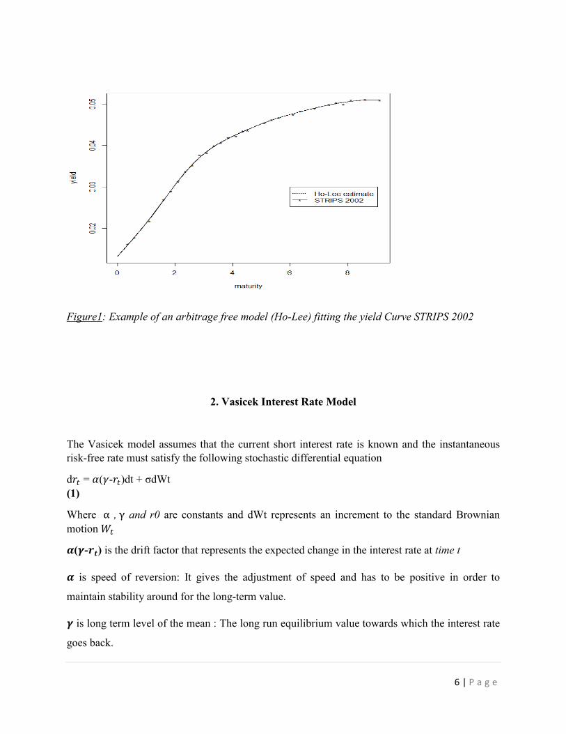
prices (i.e. the model yield curve perfectly fits to the market one). Ho-Lee, Hull White Extended

Vasicek, Hull-White Extended CIR and Black-Derman-Toy are some classical no-arbitrage

models.

6 | P a g e

Figure1: Example of an arbitrage free model (Ho-Lee) fitting the yield Curve STRIPS 2002

2. Vasicek Interest Rate Model

The Vasicek model assumes that the current short interest rate is known and the instantaneous risk-free rate must satisfy the following stochastic differential equation

d�� = �(�-��)dt + σdWt

(1)

Where α , γ and r0 are constants and dWt represents an increment to the standard Brownian

motion ��

�(�-��) is the drift factor that represents the expected change in the interest rate at time t

� is speed of reversion: It gives the adjustment of speed and has to be positive in order to

maintain stability around for the long-term value.

� is long term level of the mean : The long run equilibrium value towards which the interest rate

goes back.

7 | P a g e

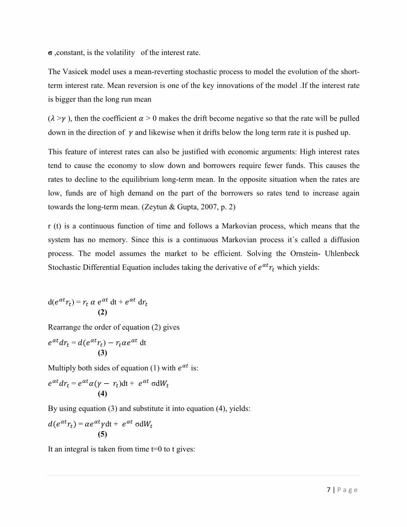
σ ,constant, is the volatility of the interest rate.

The Vasicek model uses a mean-reverting stochastic process to model the evolution of the short-

term interest rate. Mean reversion is one of the key innovations of the model .If the interest rate

is bigger than the long run mean

(� >� ), then the coefficient � > 0 makes the drift become negative so that the rate will be pulled

down in the direction of � and likewise when it drifts below the long term rate it is pushed up.

This feature of interest rates can also be justified with economic arguments: High interest rates

tend to cause the economy to slow down and borrowers require fewer funds. This causes the

rates to decline to the equilibrium long-term mean. In the opposite situation when the rates are

low, funds are of high demand on the part of the borrowers so rates tend to increase again

towards the long-term mean. (Zeytun & Gupta, 2007, p. 2)

r (t) is a continuous function of time and follows a Markovian process, which means that the

system has no memory. Since this is a continuous Markovian process it´s called a diffusion

process. The model assumes the market to be efficient. Solving the Ornstein- Uhlenbeck

Stochastic Differential Equation includes taking the derivative of ����� which yields:

d(�����) = �� � ��� dt + ��� d��

(2)

Rearrange the order of equation (2) gives

������ = �(�����) − ������ dt (3)

Multiply both sides of equation (1) with ��� is:

������ = ����(� − ��)dt + ��� σd��

(4)

By using equation (3) and substitute it into equation (4), yields:

�(�����) = �����dt + ��� σd��

(5)

It an integral is taken from time t=0 to t gives:

8 | P a g e

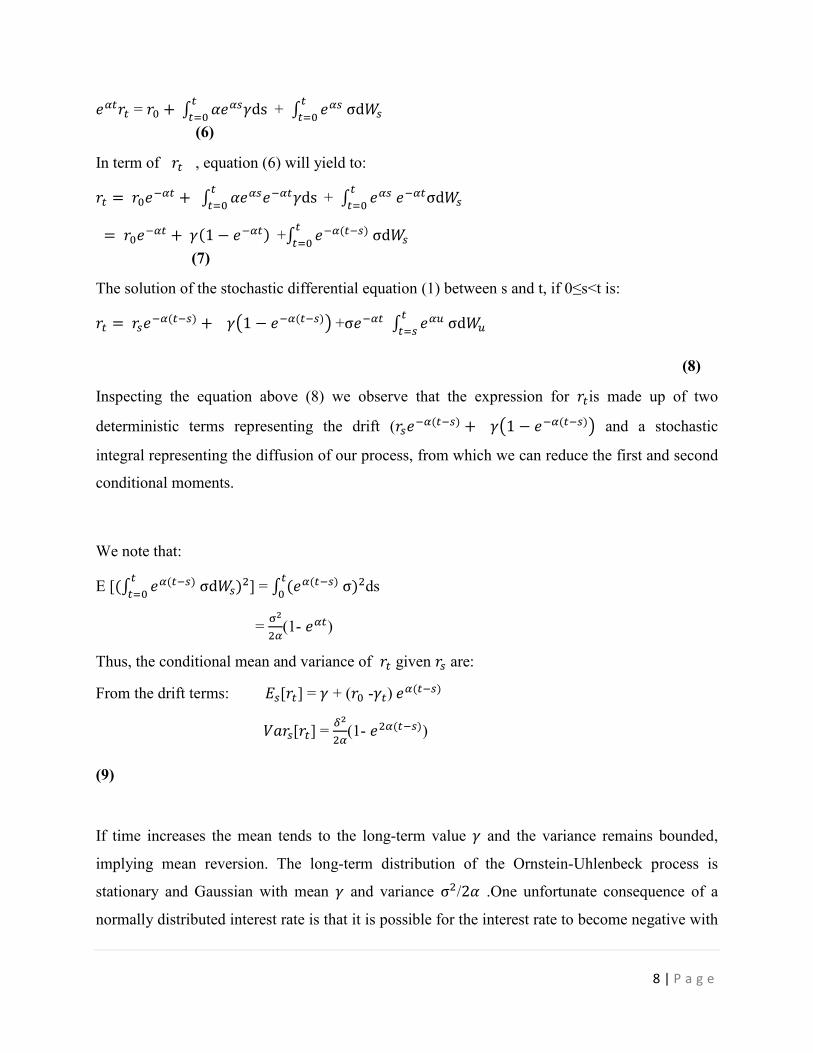
����� = �� + ∫ �����ds �

��� + ∫ ��� σd��

�

���

(6)

In term of �� , equation (6) will yield to:

�� = ������ + ∫ ���������ds �

��� + ∫ ��� ����σd��

�

���

= ������ + �(1 − ����) +∫ ���(���) σd���

���

(7)

The solution of the stochastic differential equation (1) between s and t, if 0≤s<t is:

�� = �����(���) + ��1 − ���(���)� +σ���� ∫ ��� σd���

���

(8)

Inspecting the equation above (8) we observe that the expression for ��is made up of two

deterministic terms representing the drift (�����(���) + ��1 − ���(���)� and a stochastic

integral representing the diffusion of our process, from which we can reduce the first and second

conditional moments.

We note that:

E [(∫ ��(���) σd���

���)�] = ∫ (��(���) σ

�

�)�ds

= ��

��(1- ���)

Thus, the conditional mean and variance of �� given �� are:

From the drift terms: ��[��] = � + (�� -��) ��(���)

����[��] = ��

��(1- ���(���))

(9)

If time increases the mean tends to the long-term value � and the variance remains bounded,

implying mean reversion. The long-term distribution of the Ornstein-Uhlenbeck process is

stationary and Gaussian with mean � and variance σ�/2� .One unfortunate consequence of a

normally distributed interest rate is that it is possible for the interest rate to become negative with

9 | P a g e

positive probability. This isn´t a big problem with real interest rates since they often can be

negative but nominal ones are unlikely to be negative.

3. Parameter Estimation

Since Vasicek first introduced his model of short term risk free interest rate the discussion of the

parameters estimation continues. In this section we will discuss the well-known techniques for

parameter estimation

3.1 Least Square Regressions

3.1.1 Data

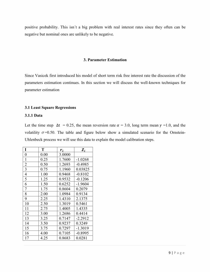
Let the time step Δt = 0.25, the mean reversion rate � = 3.0, long term mean � =1.0, and the

volatility =0.50. The table and figure below show a simulated scenario for the Ornstein-

Uhlenbeck process we will use this data to explain the model calibration steps.

I T �� �� 0 0.00 3.0000 1 0.25 1.7600 -1.0268 2 0.50 1.2693 -0.4985 3 0.75 1.1960 0.03825 4 1.00 0.9468 -0.8102 5 1.25 0.9532 -0.1206 6 1.50 0.6252 -1.9604 7 1.75 0.8604 0.2079 8 2.00 1.0984 0.9134 9 2.25 1.4310 2.1375 10 2.50 1.3019 0.5461 11 2.75 1.4005 1.4335 12 3.00 1.2686 0.4414 13 3.25 0.7147 -2.2912 14 3.50 0.9237 0.3249 15 3.75 0.7297 -1.3019 16 4.00 0.7105 -0.8995 17 4.25 0.8683 0.0281

10 | P a g e

18 4.50 0.7406 -1.0959 19 4.75 0.7314 -0.8118 20 5.00 0.6232 -1.3890

Table 1 Data used for the model calibration in the example above

3.1.2 Parameter Estimation using Least Square Regression Technique

One possible way to calibrate the estimations of � , �, σ, and r(t) is to employ the least

squares approach such that the generated term structure can best fit data over historical time. In

this section we will discuss the least squares regression method for calibrating the model

parameters of the Vasicek Model.

The relation between two consecutive observations �� and ���� is linear with independent

identical random values � such that:

���� = a�� + b + � (10)

Where a=����� b= �(1- �����) ���= σ ��� ������

��

(11)

We note here �� is the observation of the interest rate r at time t (r�)

and ���� the observation of the interest rate r at time t+1 (r���)

Express these equations in terms of the parameters � , � and σ , we have

� = - �� �

�� � =

�

��� σ = ����

�����

��(����)

(12)

In order to simplify further calculations, a least square regression can easily be done by using the quantities bellows:

�� = ∑ �������� �� = ∑ ��

����

11 | P a g e

��� = ∑ ������

��� ��� = ∑ ����

��� ��� = ∑ ������ ����

(13)

From which we get the following estimated parameters a, b, ��� of the least square fit

�� = ���� � ����

�������� �� =

��� � ���

� ���� = �

���� � �� � � �� (���� � ����)

�(���)

The figure below shows a simulated scenario for the Ornstein-Uhlenbeck process

Figure2: Relationship between consecutive observations ��

In this plot, rnext and r are respectively ���� and �� in the equation (10), and we observe the

Least Square fitting of the line of data.

Applying the regression to the data in table 1, we will get the estimated parameters below:

Parameters Value �� 22.5302 �� 20.1534

��� 30.83392

��� 25.19744

��� 22.2223

A 0.4574064

12 | P a g e

B 0.4923971 Sd 0.2072782 � 3.128732

� 0.9074879

Σ 0.5830761

Table 2 Estimated Parameters using Least Square Regression Technique

3.2 Maximum Likelihood Estimator

The maximum likelihood estimation is a powerful method. It handles bond prices and

therefore it is possible to estimate parameters of the interest rate process. The generalized

method of moments can be used for Vasicek and CIR models.

In order to estimate the parameters � , � and � of the model we use a maximum likelihood

method as suggested in James & Webber (2004, p. 506-507). The maximum likelihood method

finds the parameter values so that the actual outcome has the maximum probability. An

advantage of the maximum likelihood method over for example generalized methods of

moments (GMM) is that it provides an exact maximum likelihood estimator. On the downside it

assumes that the variance of the stochastic variable is constant between the discrete observations.

Let’s define the likelihood function. Then we have to find the parameter values that maximize

the value of this likelihood function. These values are then the maximum likelihood estimated.

The conditional density functions for �� given ���� is:

�(�� / ���� ; � , � σ) = �

√���� exp[

�(����������∆���������∆��)�

���]

Where �� = ��� (������∆�)

��

(14)

13 | P a g e

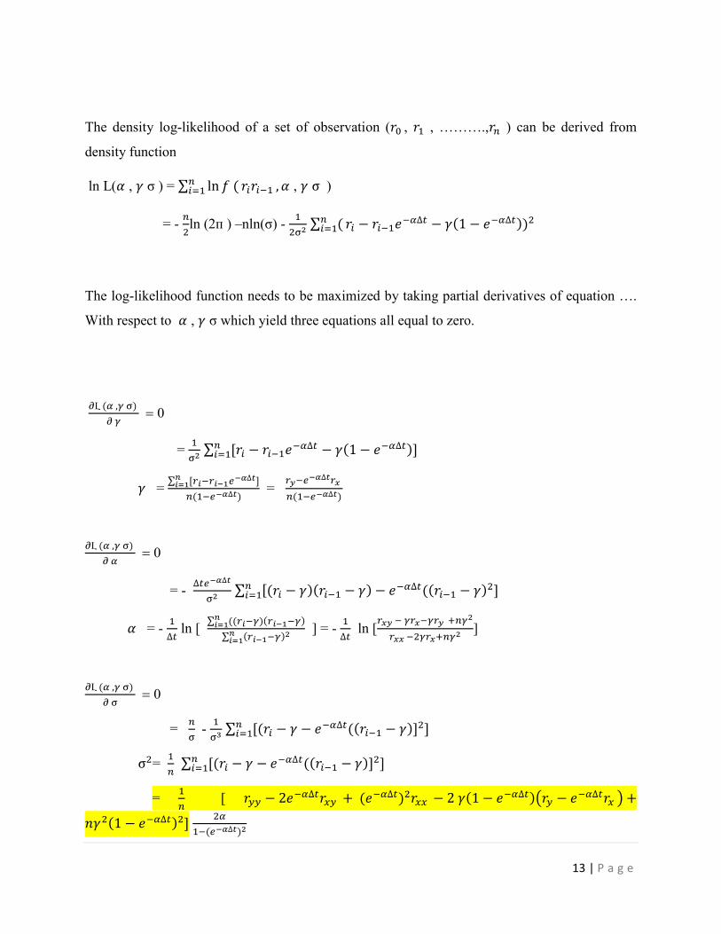
The density log-likelihood of a set of observation (�� , �� , ……….,�� ) can be derived from

density function

ln L(� , � σ ) = ∑ ln � (���� ������ , � , � σ )

= - �

�ln (2ᴨ ) –nln(σ) -

�

��� ∑ (�

��� �� − �������∆� − �(1 − ���∆�))�

The log-likelihood function needs to be maximized by taking partial derivatives of equation ….

With respect to � , � σ which yield three equations all equal to zero.

�Լ (� ,� �)

� � 0

= �

�� ∑ [�� − �������∆� − �(1 − ���∆�)]�

���

� = ∑ [����������∆�]�

���

�(�����∆�) =

������∆���

�(�����∆�)

�Լ (� ,� �)

� � 0

= - ∆����∆�

�� ∑ [(�� − �)(���� − �) − ���∆�((���� − �)�]�

���

� = - �

∆� ln [

∑ ((����)(������)����

∑ (������)�����

] = - �

∆� ln [

��� � ������� ����

��� ��������� ]

�Լ (� ,� �)

� � 0

= �

� -

�

�� ∑ [(�� − � − ���∆�((���� − �)]�]�

���

σ�= �

� ∑ [(�� − � − ���∆�((���� − �)]�]�

���

= �

� [ ��� − 2���∆���� + (���∆�)���� − 2 �(1 − ���∆�)��� − ���∆��� � +

���(1 − ���∆�)�] ��

��(���∆�)�

14 | P a g e

(The highlight part correspond to sigma2 in the code: See Appendix 8.2)

Table 3 Estimated Parameters using the Maximum Likelihood Estimation technique

4. Zero Coupon Bond Pricing

4.1 Data: Treasury Strips on January 8, 2002 (Pietro Veronesi, Valuation, Risk and Risk Management P 543)

In this Section we are going to use the STRIPS prices on January 8, 2002 with maturity ranging

from May 15, 2002 to February 15, 2011 collected from the Wall Street Journal. We use this date

as the yield Curve was particularly steep, which in turns highlights some issues that arise when

using the Vasicek Model. The third column in the Table 3.3.1 below reports time to maturity T,

and the last column depict the continuously compounded yields.

PriceofStrips maturity yield 99.4375 0.3479 0.016212 98.9375 0.6000 0.017803

Parameters estimated Values

� 0.9074879

� 3.128732

Σ 0.5531545

15 | P a g e

97.6250 1.1041 0.021770 95.7813 1.6000 0.026940 94.7813 1.8521 0.028940 ---------- -------- ----------- --------- -------- ----------- 64.4688 8.6000 0.051045 62.9063 9.1041 0.050914

Table 4 STRIPS on January 8, 2002 (just some data from the 28 observations)

4.2 Data: Treasury Strips on September 25, 2008

*The Table 5 below reports the treasury Strips on September 25, 2008. Let the short term rate be

�� = 2%. You can download data from the Federal Reserve Web site (http://federalreserve.gov/releases/h15/data.htm)

time to maturity ZCB Yield 0.139 99.918 0.6 0.389 99.498 1.31 0.689 98.999 1.59 0.889 98.493 1.72 1.139 98.002 1.78 1.389 97.507 1.83 1.639 96.899 1.93 1.889 96.314 2 2.139 95.742 2.05 2.389 94.85 2.23 2.639 94.324 2.23 ……… ……….. ……… ……… ……….. ……… 7.889 73.613 3.92 8.139 72.106 4.06

Table 5 STRIPS on September, 2008 (just some data from the 33observations)

16 | P a g e

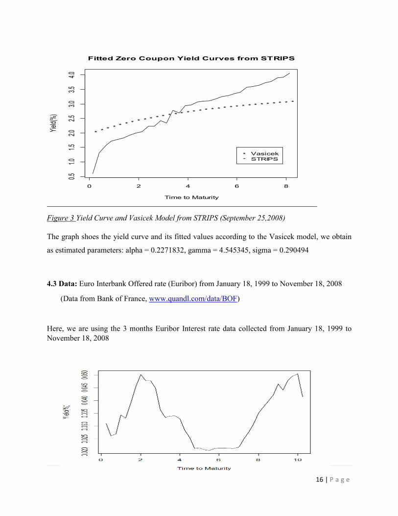
Figure 3 Yield Curve and Vasicek Model from STRIPS (September 25,2008)

The graph shoes the yield curve and its fitted values according to the Vasicek model, we obtain

as estimated parameters: alpha = 0.2271832, gamma = 4.545345, sigma = 0.290494

4.3 Data: Euro Interbank Offered rate (Euribor) from January 18, 1999 to November 18, 2008

(Data from Bank of France, www.quandl.com/data/BOF)

Here, we are using the 3 months Euribor Interest rate data collected from January 18, 1999 to November 18, 2008

0 2 4 6 8

0.51.0

1.52.0

2.53.0

3.54.0

Fitted Zero Coupon Yield Curves from STRIPS

Time to Maturity

Yield

(%)

* * * * * * * * * * * * * * * * * * * * * * * * * * * * * * * * *

*-

VasicekSTRIPS

17 | P a g e

Figure 4: Euribor 3 Months period daily rates (Jan 1999- March2008)

4.4 Data: Euro Interbank Offered rate (Euribor) from January 2005 to March 2006

(Data from Bank of France, www.quandl.com/data/BOF)

In this example, we calibrate the Vasicek Model to the current yield curve . The short rate now r(0) is the one month rate r(0,1month) . We now find the estimated parameters alpha, gamma, sigma so that the Vasicek model best fit the current term structure.

Parameters estimated Values � 0.024

� 0.49

σ 0.06

Table 6 Estimated Parameters (EURIBOR Jan 2005-March 2006) using the least square Regression

18 | P a g e

Figure5: Fitted Vasicek Model to the Market yield curve (Euribor 01/2005 to 03/2006)

From the Figure 5, we see the Ornstein- Uhlenbeck model better fitted the Maket yield than the previous cases, although it is obvious the model does fit the actual yield curve optimally.

Let’s denote the time to maturity ɽ = T-t, the term structure of interest rates is a function of the

current interest rate �� and ɽ. The yields can then be calculated easily for all maturities using the

price of the corresponding zero-coupon bonds

��(ɽ) = - �� (�(��,ɽ))

ɽ = -

�(ɽ)

ɽ +

�(ɽ)

ɽ��

(19)

We start with the parameter estimates � , �, σ . We must also specify the interest rate prevailing

at time t=0 and the maturity of zero-coupon bond. In this case, T=10 years. The program then

calculates the values of A (t, T), B (t, T) and the zero coupon bond price Z (t, T)

The time step needs to be quite small in order to achieve accuracy with the Euler-discretization

19 | P a g e

Figure 6 Fitted Zero Coupon Yield Curves from STRIPS (January 8, 2002)

As we can see, the Vasicek Model is not able to match the term structure of interest rates on

January 8, 2002, except a single point. That could be explain by the fact that the Vasicek Model

is a simple model, with only three parameters and one driving factor (��). Also, this could be

created when the term structure is very steep (case where the Federal Reserve want to lower the

target Funds rate to boost the U.S economy)

20 | P a g e

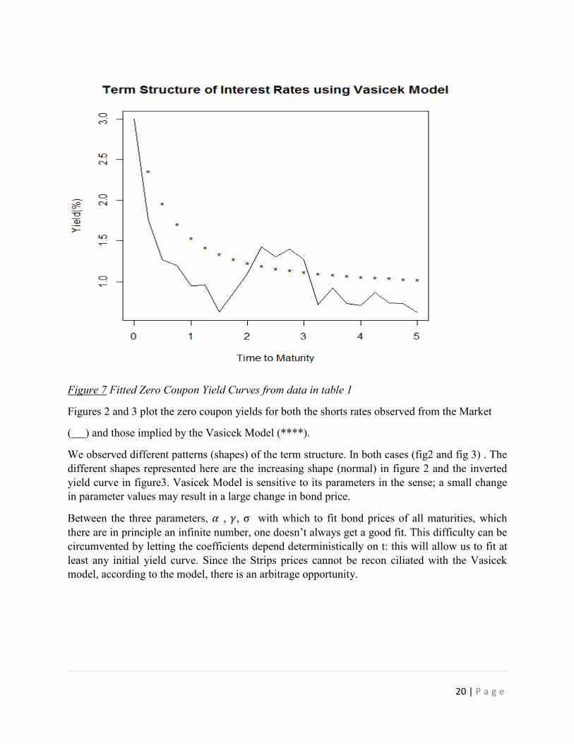
Figure 7 Fitted Zero Coupon Yield Curves from data in table 1

Figures 2 and 3 plot the zero coupon yields for both the shorts rates observed from the Market

( ) and those implied by the Vasicek Model (****).

We observed different patterns (shapes) of the term structure. In both cases (fig2 and fig 3) . The different shapes represented here are the increasing shape (normal) in figure 2 and the inverted yield curve in figure3. Vasicek Model is sensitive to its parameters in the sense; a small change in parameter values may result in a large change in bond price.

Between the three parameters, � , �, σ with which to fit bond prices of all maturities, which there are in principle an infinite number, one doesn’t always get a good fit. This difficulty can be circumvented by letting the coefficients depend deterministically on t: this will allow us to fit at least any initial yield curve. Since the Strips prices cannot be recon ciliated with the Vasicek model, according to the model, there is an arbitrage opportunity.

21 | P a g e

5. Monte Carlo Simulation for Vasicek Model Parameters

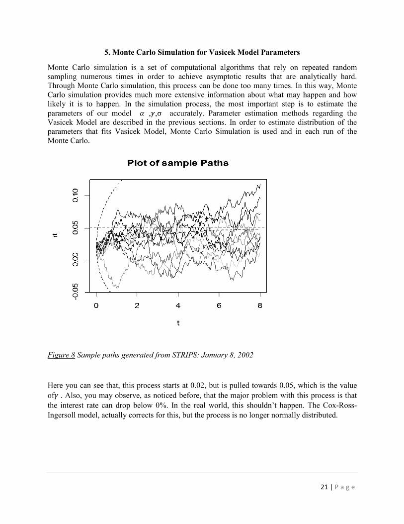
Monte Carlo simulation is a set of computational algorithms that rely on repeated random sampling numerous times in order to achieve asymptotic results that are analytically hard. Through Monte Carlo simulation, this process can be done too many times. In this way, Monte Carlo simulation provides much more extensive information about what may happen and how likely it is to happen. In the simulation process, the most important step is to estimate the parameters of our model � ,�,σ accurately. Parameter estimation methods regarding the Vasicek Model are described in the previous sections. In order to estimate distribution of the parameters that fits Vasicek Model, Monte Carlo Simulation is used and in each run of the Monte Carlo.

Figure 8 Sample paths generated from STRIPS: January 8, 2002

Here you can see that, this process starts at 0.02, but is pulled towards 0.05, which is the value

of� . Also, you may observe, as noticed before, that the major problem with this process is that the interest rate can drop below 0%. In the real world, this shouldn’t happen. The Cox-Ross-Ingersoll model, actually corrects for this, but the process is no longer normally distributed.

22 | P a g e

6. Term Structure

The term structure of interest rates, also known as a yield curve, illustrates the relationship between interest rates and different times of maturity. The yield curve can be basically shape, but there are some cases where it should look different. There are four main patterns that can characterize the term structure: normal, flat, inverted and humped. The Vasicek model can generate all of them. The yields curves implied by Vasicek Model in Figure 2 and Figure 3 highlighted consecutively the normal yield and the inverted yield curve.

Under normal market conditions, (figure 1) the investors think the economy will continue to grow and expect higher yields for instruments with longer maturities.

The inverted yield curve (Figure 2) is the opposite. In such market conditions, bonds with maturities dates further into the future are expected to yield less than bonds with shorter maturity.

If we note that Z(0,T) = ���� � where �� is the continuous time yield for a zero coupon bond with maturity T. We can denote the term structure of interest rates as a function of the current

interest rates �� and time to maturity ɽ. This is given by:

�� (ɽ) = - �� (�(��,ɽ))

ɽ = �� = -

�(ɽ)

ɽ +

�(ɽ)

ɽ�� with ɽ = T-t

To demonstrate some of the possible curve shapes allowed by the Vasicek model, I produced the following chart. Notice that the yield curve can be both increasing and decreasing with maturity.

Figure 9 Five Spot curves implied by the Vasicek Model

23 | P a g e

r = 3.5% r = 3% r = 2.5%

Figure10 Vasicek Yield vs maturity for three initial spot rate �� : Parameters � = -0.2352252, � = 0.02509691

σ = 0.003787045

We observe (fig 9) that the level, slope and curvature change over the time. The figure shows that if the current short term rate is low, the vasicek model implies a rising term structure of interest rate. In case we have a high current short term interest, the model implies a decreasing term structure. The term structure moves relatively to the interest rate. As mentioned above, these movements are correlated. The two factor vasicek model will take of the problem.

Depite the model’s simplicit, the mean-reverting feature of the spot rate process allows for varied behavior of the term structure of yields to maturity as we can see on figure 10

7. The two-factor Vasicek Model

Let’s assume that the short term interest rate is given by

��� r�,� + r�,�

(20)

We consider two different factors denoted by r�,� and r�,� and assume they move according to the

process

24 | P a g e

Where the risk neutral factor dynamics have the general form

dr�,� = ��( r� − r�,�))dt + σ�d��,�

(21)

dr�,� = ��( r� − r�,�))dt + σ�d��,�

(22)

With �� �� r� and r� the risk neutral parameters, ��,� and ��,� denote independent standard

Brownian motion

From the risk neutral factor dynamics be given by the equations 21 and 22, and the interest rate be linear in the factors as in equation 20, the zero coupon bond price is given by

��(ɽ ) = ��(ɽ )����(ɽ)� where i=1, 2 (23)

Z(r�,�, r�,�,t,T) = ��(�;�)���(�;�)��,����(�;�)��,�

(24)

Where

��(t; T) =�

��[1 − ����(���)];

(25)

A(t; T) = (��(t; T) - (T-t)) (r� − ��

�

�(��)�) -

���

�����(�; �)�

We can write the process for the short term rate �� as follows

d�� = [��∗ (r�

∗-��) +��∗r�

∗ + (��∗ − ��

∗) r�,�]dt + σ�d�� + σ�d�� (27) Contrarily to the one factor model, the risk neutral drift here depends on the second factor r�,�

with

dr�,� = ��(�� − r�,�) dt + σ�(r�,�, t) d��,�

(28)

The yields can then be calculated easily for all maturities using the price of the corresponding zero-coupon bonds

��(ɽ) = - �� (����,�,��,� ,�,��)

ɽ

��(ɽ) = - �(ɽ)

ɽ +

��(ɽ)

ɽr� +

�(ɽ)

ɽr�,�

(29)

25 | P a g e

In practice, the components �� and �� of the short rate are not observables. An observable quantity is the short rate

r� = r�,� + r�,� and we note r�,� in equation (29) means the long interest rate is not

perfectly correlated with the short rate. r�,� and r�,� only affect the interest rater� when

looking for his average level which correspond to equation (20).

The expectation and the variance under the real probability measure are:

E [��,�/��]= ���(���)��,� + �(1 − ���(���)) , i= 1,2

Var[��,�/��]=��

�

��(1 − ���(���)) i=1,2

The limiting distributions of both Ornstein-Uhlenbeck processes forming the two-factor Vasicek model are known to be normal distributions with density

�� (x) = �

������ �

�(����)�

����

i= 1,2

Let’s denote the long term yield ��,� and �� the short term yield, thus the coefficients ��,� ,

��,� ��,� are for a long term period as well. From the equation (29) of the zero coupon spot rate,

we derive to the dynamics of long and short term yields below using Ito Lemma

d�� = (�� + ���� + �� ��,� ) dt + σ�d��,� + σ�d��,�

(30)

d��,� = (��,� + ��,��� + ��,� ��,� ) dt + σ�,�d��,� + σ�,�d��,�

(31)

As we can see in the equations 30 and 31, the short term rate and long term rate are feeding themselves .

The volatilities of the long term yield and the short term yield are related as we can see in the equation below

σ�,� = σ�������∗ɽ�

ɽ� ; σ�,� = σ�

������∗ɽ�

ɽ�

(32)

We should notice that these volatilities are computed from historical data.

26 | P a g e

7.1 Case studied

Let today be January 8, 2002. Now we use the two factor model to fit the coupon bonds traded on that day and estimate the parameters using the nonlinear least square method. As data, we use the same strips prices as in the example above. We select the 5 year yield as the long term zero

coupon yield ɽ� = 5 added to the current short term free rate and 1-month T-bill rate for the short term. It’s not easy to observe the 5 year zero coupon yield daily, but we should estimate from fitting the discount curve Z(0,T). As notice earlier, these volatilities are computed from historical data. Let’s fix the volatility of the short rate (1-month rate) and the long term rate (5-year yield)

respectively by σ�,������ =0.0221 and σ�,� ���� = 0.0125 and since r�,� and r�,� are not

identifiable as together, we could set r�,� = 0. As with the one factor model, we can search the

parameters ��∗ , ��

∗, ��∗, ��

∗, σ� and σ� such that the following quantity is minimized.

J (��∗ , ��

∗, ��∗, ��

∗, σ� σ� ) = ∑ (������� − ��

����)�����

8. Comparative study of the Vasicek and the CIR Model

Vasicek and CIR are two of the historically most important short rate models used in the pricing of interest rate derivatives. In CIR model (sometimes called square root model) under the risk-neutral measure Q, the instantaneous short rate follows the stochastic differential equation

d�� = �(�-��)dt + �dWt , r(0) = 0

(33)

Where � ,�,σ are positive constants, and W(t) is a Brownian motion. When we impose the

condition 2 �� > σ2 then the interest rate is always positive, otherwise we can only guarantee

that it is non-negative. The drift factor �(�-��) is same as in the Vasicek model. Therefore, the

short rate is mean-reverting with long run mean � and speed of mean-reversion equal to �. The

volatility of the Vasicek model is multiplied with the term ���,and this eliminates the main

drawback of the Vasicek model, a positive probability of getting negative interest rates. As the short-rate rises, the volatility of the short-rate also raises .When the interest rate approaches zero

then � approaches zero, cancelling the effect of the randomness, so the interest rate remains

always positive. When the interest rate is high then the volatility is high.

27 | P a g e

Vasicek CIR Hist. Data

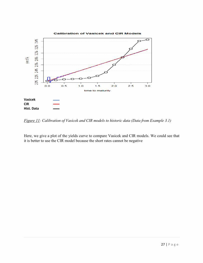
Figure 11: Calibration of Vasicek and CIR models to historic data (Data from Example 3.1)

Here, we give a plot of the yields curve to compare Vasicek and CIR models. We could see that it is better to use the CIR model because the short rates cannot be negative

28 | P a g e

9. Conclusion

In this study,I worked on the Vasicek, Comparative study of the Vasicek and the CIR

Model and the Two Factor Vasicek equilibrium models . I used the R language for

implementation and sometimes Matlab for reconciliation and check the results. Note that for the

two factor models, I haven’t expanded the details and the implementation I used MLE and Least

square methods for estimating the model parameters. Moreover, parameter estimation of affine

term structure is essentially a time-series problem. Most papers have been focused on Kalman

filter which doesn’t require that the variables be observable. the estimation of Vasicek model

using either MLE or Least Squares gives accurate estimates of the mean alpha gamma and

volatility sigma, but poor estimates of the mean reversion alpha Short-rate simulation and bond

pricing are not so difficult, as for the CIR model the exact distribution of rt is known and

analytical formulas exist for bond pricing. As elaborated in section 8, the CIR model estimates

the yield curve relatively much better compared to the Vasicek Model, It is better to use this

model since the short rates values cannot be negatives. In the other hand, we have another model,

the Nelson Siegel Model which fits the yield curve perfectly. I goes however without saying that,

understand complex interest rates models like vasicek Model requires a lot of practice and work

specially multiple factors models.

29 | P a g e

10. Appendix

R code

10.1 Estimation of parameters in Vasicek Model using Least Square Regression Technique

## The values of interest rates observed r <- c(3, 1.76, 1.2693, 1.196, 0.9468, 0.9532, 0.6252, 0.8604, 1.0984, 1.431, 1.3019, 1.4005, 1.2686, 0.7147, 0.9237, 0.7297, 0.7105, 0.8683, 0.7406, 0.7314, 0.6232) n <- 20 ## number of observations delta <- 0.25 ## time step delta = ti+1 - ti ## Least Square Calibration function [alpha,gamma,sigma] = Vas_LS(r,delta) n = length(r)-1; rx <- sum(r[1:length(r)-1]) ry <- sum(r[2:length(r)]) rxx <- crossprod(r[1:length(r)-1], r[1:length(r)-1]) rxy <- crossprod(r[1:length(r)-1], r[2:length(r)]) ryy <- crossprod(r[2:length(r)], r[2:length(r)]) a <- (n*rxy - rx * ry ) / ( n * rxx - rx^2 ) b <- (ry - a * rx ) / n sd <- sqrt((n * ryy - ry^2 - a * (n * rxy - rx * ry)) / (n * (n-2))) ## Now, the parameters estimated using the Least Square Calibration (with R) alpha <- -log(a)/delta ## denote the speed of reversion gamma <- b/(1-a) ##denote long term level of the mean sigma <- sd * sqrt( -2*log(a)/delta/(1-a^2)) ## denote the volatility end ## I estimate the parameters using the Least Square Calibration (with Matlab) to check r = [3.0000 1.7600 1.2693 1.1960 0.9468 0.9532 0.6252 0.8604 1.0984 1.4310 1.3019 1.4005 1.2686 0.7147 0.9237 0.7297 0.7105 0.8683 0.7406 0.7314 0.6232]; delta = 0.25; [alpha, gamma, sigma] = VAS_LS(S,delta) ##Outputs alpha = 0.90748 sigma = 0.58307

30 | P a g e

gamma = 3.12873

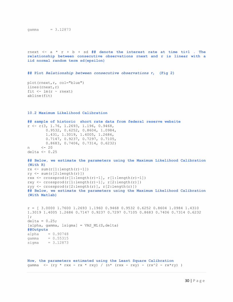
rnext <- a * r + b + sd ## denote the interest rate at time ti+1 . The relationship between consecutive observations rnext and r is linear with a iid normal random term sd(epsilon)

## Plot Relationship between consecutive observations �� (Fig 2)

plot(rnext,r, col="blue") lines(rnext,r) fit <- lm(r ~ rnext) abline(fit) 10.2 Maximum Likelihood Calibration ## sample of historic short rate data from federal reserve website r <- c(3, 1.76, 1.2693, 1.196, 0.9468, 0.9532, 0.6252, 0.8604, 1.0984, 1.431, 1.3019, 1.4005, 1.2686, 0.7147, 0.9237, 0.7297, 0.7105, 0.8683, 0.7406, 0.7314, 0.6232) n <- 20 delta <- 0.25 ## Below, we estimate the parameters using the Maximum Likelihood Calibration (With R) rx <- sum(r[1:length(r)-1]) ry <- sum(r[2:length(r)]) rxx <- crossprod(r[1:length(r)-1], r[1:length(r)-1]) rxy <- crossprod(r[1:length(r)-1], r[2:length(r)]) ryy <- crossprod(r[2:length(r)], r[2:length(r)]) ## Below, we estimate the parameters using the Maximum Likelihood Calibration (With Matlab) r = [ 3.0000 1.7600 1.2693 1.1960 0.9468 0.9532 0.6252 0.8604 1.0984 1.4310 1.3019 1.4005 1.2686 0.7147 0.9237 0.7297 0.7105 0.8683 0.7406 0.7314 0.6232 ]; delta = 0.25; [alpha, gamma, lsigma] = VAS_ML(S,delta) ##Outputs alpha = 0.90748 gamma = 0.55315 sigma = 3.12873

Now, the parameters estimated using the Least Square Calibration gamma <- (ry * rxx - rx * rxy) / (n* (rxx - rxy) - (rx^2 - rx*ry) )

31 | P a g e

alpha <- -log((rxy - gamma * rx - gamma * ry + n * gamma^2) / (rxx - 2 * gamma * rx + n * gamma^2)) / delta sigma2 <-(ryy -2*a * rxy + a^2 *rxx -2*gamma *(1-a)*(ry - a * rx) + n * gamma^2*(1 - a)^2)/n sigma <-sqrt(sigma2*2 * alpha/(1 - a^2)) ## refer to the highlight part in yellow ,sect. 3.2 R Code Fig 3 (extend) r <- c(3, 1.76, 1.2693, 1.196, 0.9468, + 0.9532, 0.6252, 0.8604, 1.0984, + 1.431, 1.3019, 1.4005, 1.2686, + 0.7147, 0.9237, 0.7297, 0.7105, + 0.8683, 0.7406, 0.7314, 0.6232) n <- 20 ## number of observations ##define the function B(t,T) T<-seq(0.25,5,0.25) B<- (1/alpha)*(1-exp(-alpha*T)) delta<-0.25 ##time step ##define the function A(t,T) A <-(gamma-(sigma^2)/(2*(alpha^2)))*(B-T)-((sigma^2)*((B^2)/(4*alpha))) r0 <-3 Z <-exp(A-(B*r0)) rvas<-(-A/T) + (B*r0)/T T <-seq(0.25,5,0.25) ## Plot Vasicek and CIR Model dev.new() plot(T,r,type="l", lty=1, xlab="Time to Maturity", ylab="Yield(%)", main="Comparison between Vasicek and CIR Model ") points(T,rvas, pch="*")

Outputs: gamma 0.9074879 alpha 3.128732 sigma 0.5531545 8.2 Fitted Zero Coupon Yield Curves from Strips: January 8, 2002 R Code ##give the strips data for january 2,2002 strips<-read.csv("C:/Users/cedric/Desktop/Data/Strips.csv") dim(strips) price<-strips[,1,1:28] mat<-strips[,2,1:28] # assigning maturity as a column vector from column 2 of Strips yield<-strips[,3,1:28] # assigning yield as a column vector from column 3 of Strips matrix

32 | P a g e

yvas<-function(T,strips,rt) { alpha= (strips$alpha) gamma= (strips$gamma) sigma= (strips$sigma))^2 B=1/alpha*(1-exp(-alpha*T)) A=(gamma-sigma2/(2*alpha^2))*(B-T)-sigma2/(4*alpha)*B^2 yield=-(A-B*rt)/T if(T[1]==0) { yield[1]=rt } return( yield ) } } ##Treasury Strips observed (September 2008)# data got from Veronesi, we could find it from www.federalreserve.gov/releases/h15/data.htm as well strips2008<-read.csv("C:/Users/cedric/Desktop/Data/strips2008.csv") ## gives the strips data for september 25,2008 dim (strips2008) price<-strips2008[,1,1:33] maturity<-strips2008[,2,1:33] yield<-strips2008[,3,1:33] n<-33 delta<-0.25 ##time step r0<-2 ##current short rate rx <- sum(yield[1:length(yield)-1]) ry <- sum(yield[2:length(yield)]) rxx <- crossprod(yield[1:length(yield)-1], yield[1:length(yield)-1]) rxy <- crossprod(yield[1:length(yield)-1], yield[2:length(yield)]) ryy <- crossprod(yield[2:length(yield)], yield[2:length(yield)]) a <- (n*rxy - rx * ry ) / ( n * rxx - rx^2 ) b <- (ry - a * rx ) / n sd <- sqrt((n * ryy - ry^2 - a * (n * rxy - rx * ry)) / (n * (n-2))) ## Parameters estimation alpha <- -log(a)/delta ## denote the speed of reversion gamma <- b/(1-a) ##denote long term level of the mean sigma <- sd * sqrt( -2*log(a)/delta/(1-a^2)) ## denote the volatility ##define the function B(t,T) T<-seq(0.25,8.25,0.25) B<- (1/alpha)*(1-exp(-alpha*T)) ##define the function A(t,T) A <-(gamma-(sigma^2)/(2*(alpha^2)))*(B-T)-((sigma^2)*((B^2)/(4*alpha))) r0 <-2 ## Current short rate Z <-exp(A-(B*r0)) rvas<-(-A/T) + (B*r0)/T alpha 0.2019314 gamma 0.06356295 sigma 0.002218611

33 | P a g e

## Monte Carlo Simulation for Vasicek Model Parameters

## define model parameters (from Strips, January 8, 2002, Veronesi Example)

r0 <- 0.02 # current overnight rate gamma <- 0.0509 alpha <- 0.3262 sigma <- 0.0221 ## simulate short rate paths n <- 1000 # MC simulation trials T <- 8 # total time m <- 200 # subintervals dt<- T/m # difference in time each subinterval r <- matrix(0,m+1,n) # matrix to hold short rate paths r[1,] <- r0 for(j in 1:n){ for(i in 2:(m+1)){ dr <- alpha*(gamma-r[i-1,j])*dt + sigma*sqrt(dt)*rnorm(1,0,1) r[i,j] <- r[i-1,j] + dr } } ## plot of sample paths t <- seq(0, T, dt) rT.expected <- gamma + (r0-gamma)*exp(-alpha*t) rT.stdev <- sqrt( gamma^2/(2*alpha)*(1-exp(-2*alpha*t))) matplot(t, r[,1:10], type="l", lty=1, main="Plot of sample Paths", ylab="rt") abline(h=gamma, col="red", lty=2) lines(t, rT.expected, lty=2) lines(t, rT.expected + 2*rT.stdev, lty=2) lines(t, rT.expected - 2*rT.stdev, lty=2) points(0,r0)

---------Calibration of Vasicek and CIR models to historic data (Data from Example 3.1) mat=c(0.00, 0.25,0.50, 0.75, 1.00, 1.25, 1.50, 1.75, 2.00, 2.25, 2.50, 2.75, 3.00) t=seq(from=min(mat),to=max(mat),length=500) yestVas<-optim(f=l2norm,p=log(c(exp(0.174),yield[1],0.004)),y=cbind(mat,yield), familie="yvasicek", rt=yield[1],control=list(maxit=400)) yestCIR<-optim(f=l2norm,p=log(c(exp(0.16),yield[1],0.04)),y=cbind(mat,yield), familie="ycir", rt=yield[1],control=list(maxit=400)) vas.par=list(lambda=exp(yestVas$par[1]),theta=exp(yestVas$par[2]),sigma=exp(yestVas$par[3]),r=yield[1]) cir.par=list(k=exp(yestCIR$par[1]),theta=exp(yestCIR$par[2]),sigma=exp(yestCIR$par[3]),r=yield[1]) vas.par cir.par plot(mat,yield,type="b",col="black",lwd=2,ylim=range(yield),xlab="time to maturity",ylab="yield %",yaxt="n",main="Calibration of Vasicek and CIR Models",cex=2)

34 | P a g e

lines(t,yvas(t,list(lambda=yestVas$par[1],theta=yestVas$par[2],sigma=yestVas$par[3]),yield[1]),lty=1,col="blue",lwd=2) lines(t,ycir(t,list(lambda=yestCIR$par[1],theta=yestCIR$par[2],sigma=yestCIR$par[3]),yield[1]),lty=1,col="red",lwd=2) axis(side=2,at=yticks,labels=paste(format(100*yticks,digits=3),"%",sep="")) legend(0.5,3.2,legend=c("Vasicek","CIR","STRIPS"),pch=c("blue","red"),"o")

## Figure 10 shows the effect of changing the values of current short rates on the vasicek yield r0<-3.0 ## Set up the first current short rate r1<-3.5 ## second short rate r2<-2.5 ## third short rate rvas<-(-A/T) + (B*r0)/T ## vasicek yield for ro rvas1<-(-A/T) + (B*r1)/T ## vasicek yield for r1 rvas2<-(-A/T) + (B*r2)/T ## vasicek yield for r2 ## Plot differents curves for short rates r0,r1,r2 plot(T,rvas,type="l", lty=1, xlab="Maturity", ylab="rvas", main="Vasicek Yield vs maturity for three values of initial spot rate ",) par(new=TRUE) lines(T,rvas1,col='red') par(new=TRUE) lines(T,rvas2,col='blue')

35 | P a g e

11. References

Zeytun & Gupta. 2007. A comparative Study of the Vasicek and the CIR Model of the Short Rate

Vasicek 1977. An Equilibrum Characterization of the Term Structure

On the Simulation and Estimation of the Mean – Reverting Ornstein – Uhlenbeck Process. William Smith Feb 2010

Fixed Income Securities. Valuation, Risk, and Risk Management by Pietro Veronesi

Risk Properties and Parameter estimation on Mean Reversion and Garch Models by Roelf Sypkens

Short rates and bond prices in one-factor models by Muhammad Naveed Nazir

A comparative Study of the Vasicek and the CIR Model of the Short Rate by Serkan Zeytun,Ankit Gupta

Lecture Notes in Empirical Finance: Yield Curve Models 2 (MLE and GMM) by Paul Soderlind

Affine Interest Rate Models-Theory and Practice. By Dr Josef Teichmann

Interest Rate Modelling. John Willey and Son by James,Jessica & Webber,Nick 2004

Mathematical analysis of term structure models by Beata Stehlikova

Affine Interest Rate Models – Theory and Practice by Christa Cuchievo

Term Structure forecasting by Emile van Elen

Affine Term Structure Models: Theory and Implementation by David Bolder

Options : recent advances in theory and practices vol 2 by Stewart Hedges

An Introduction to the Mathematics of Financial Derivatives (2nd Edition) by Salith N. Neftci

Pricing derivative Securities by EPPS