Varnek A., Tutorial on Ensemble Learning - Unistrainfochim.u-strasbg.fr/new/CS3_2010/Tutorial/Ensemble/Ensemble... · Tutorial on Ensemble Learning 1 ... The following ensemble learning

Tutorial on Ensemble Learning

1


Igor Baskin, Gilles Marcou and Alexandre Varnek

Faculté de Chimie de Strasbourg

Laboratoire d‟Infochimie

4, rue Blaise Pascal, 67000 Strasbourg, FRANCE

Tutorial on Ensemble Learning ........................................................................................................... 1

Introduction ......................................................................................................................................... 2

Part 1. Classification models. .............................................................................................................. 3

1. Data and descriptors. ............................................................................................................... 3

2. Files ......................................................................................................................................... 3

3. Exercise 1: Instability of interpretable rules ............................................................................ 3

4. Exercise 2: Bagging and Boosting .......................................................................................... 5

5. Exercise 3: Random forest..................................................................................................... 10

6. Exercise 4: Combining descriptor pools ................................................................................ 13

Part 2. Regression Models ................................................................................................................. 15

1. Data and Descriptors ............................................................................................................. 15

2. Files ....................................................................................................................................... 15

3. Exercise 5: Individual MLR model ....................................................................................... 15

4. Exercise 6: Bagging of MLR models .................................................................................... 19

5. Exercise 7: Applying the random subspace method .............................................................. 22

6. Exercise 8: Additive regression based on SLR models ......................................................... 26

7. Exercise 9: Stacking of models ............................................................................................. 29

Literature ........................................................................................................................................... 35

Appendix .............................................................................................................................................. 36

1. Notes for Windows .................................................................................................................... 36

2. Notes for Linux ......................................................................................................................... 36


2

Introduction

This tutorial demonstrates performance of ensemble learning methods applied to

classification and regression problems. Generally, preparation of one individual model

implies (i) a dataset, (ii) initial pool of descriptors, and, (iii) a machine-learning approach.

Variation of any of these items can be used to generate an ensemble of models. Here, we

consider the following ensemble learning approaches: bagging and boosting (dataset

variation), random subspace (descriptors variation) and stacking (machine-learning methods

variation). In some of popular approaches, both dataset and descriptors vary (e.g., random

forest).

In all calculations, the ISIDA descriptors were used. They represent the counts

(occurrences) of some fragments in a molecular graph. Three types of fragments are

considered: sequences (type 1), unlimited augmented atoms (type 2) and restricted augmented

atoms (type 3). A sequence is the shortest path connected two given atoms. For each type of

sequence, the lower (l) and upper (u) limits for the number of constituent atoms must be

defined. The program generates „„intermediate‟‟ sequences involving n atoms (l=<n<=u)

recording both atoms and bonds. Unlimited augmented atom represents a selected atom with

its closest environment. Restricted augmented atom is a combination of types 1 and 2: an

atom representing an origin of several sequences containing from l to u atoms. Three sub-

types, AB, A and B are defined for each class. They represent sequences of atoms and bonds

(AB), of atoms only (A), or of bonds only (B).

Thus, each fragmentation is coded by the pattern txYYlluu. Here, x is an integer

describing the type of the fragmentation (1: sequences; 2: unlimited augmented atoms; 3:

restricted augmented atoms), YY specifies the fragments content (AA: atoms only; AB: atoms

and bond; BB: bonds only), l and u are the minimum and maximum number of constituent

atoms.

The following ensemble learning procedures are considered in the tutorial:

Bagging – combination of bootstrapping and averaging used to decrease the variance

part of prediction errors [2]

AdaBoost – the most well-known boosting algorithm used to solve classification

problems [3]

Random Subspace Method – combination of random subsets of descriptors and

averaging of predictions [4]

Random Forest – a method based on bagging (bootstrap aggregation, see definition of

bagging) models built using the Random Tree method, in which classification trees are

grown on a random subset of descriptors [5].


3

Additive Regression – a form of regression gradient boosting: it enhances performance

of basic regression methods [6]

Stacking - combines several machine learning methods using the stacking method [7,

8].

The following individual machine learning methods (base learners [9]) are used:

JRip is the Weka implementation of the algorithm Ripperk [10]. This algorithm uses

incremental reduced-error pruning in order to obtain a set of classification rules; k is

the number of optimization cycles of rules sets.

Multiple Linear Regression (MLR) – classical multiple linear regression without

descriptor selection, in which for the sake of numeric stability the diagonal elements

of the variance-covariance matrix XTX are modified by adding a small 1.0e-8 number

(actually a form of the ridge regression).

Simple Linear Regression (SLR) – classical linear regression on a single descriptor.

Partial Least Squares (PLS)

M5P – a kind of regression trees [11]

Part 1. Classification models.

1. Data and descriptors.

The dataset for this tutorial contains 27 ligands of Acetylcholinesterase (AchE) and 1000

decoy compounds chosen from the BioInfo database [1]. This dataset is split into the training

set (15 actives and 499 inactives) and the test set (12 actives and 501 inactives). The

t3ABl2u3 fragments are used as descriptors.

2. Files

The following files are supplied for the tutorial:

train-ache.sdf/test-ache.sdf – Molecular files for training/test set

train-ache-t3ABl2u3.arff/test-ache-t3ABl2u3.arff – descriptor

and property values for the training/test set

ache-t3ABl2u3.hdr – descriptors' identifiers

3. Exercise 1: Instability of interpretable rules


4

In this exercise, we build individual models consisting of a set of interpretable rules. The goal

is to demonstrate that the selected rules depend on any modification of the training data, e.g.,

the order of the data in the input file.

Step by step instructions

Important note for Windows users: During installation, the ARFF files should have been associated

with Weka. In this case, it is highly recommended to locate and double click on the file train-ache-t3ABl2u3.arff and to skip the following three points.

In the starting interface of Weka, click on the button Explorer.

In the Preprocess tab, click on the button Open File. In the file selection interface,

select the file train-ache-t3ABl2u3.arff.

The dataset is characterized in the Current relation frame: the name, the number of instances,

and the number of attributes (descriptors). The Attributes frame allows user to modify the set

of attributes using select and remove options. Information about the selected attribute is given

in the Selected attribute frame in which a histogram depicts the attribute distribution.

Click on the tab Classify.

Into the Test options frame, select Supplied test set and click Set....

In the pop-up window, click the Open file... button and select the test-ache-

t3ABl2u3.arff file. Then click Close.

Click More options... then in the pop-up window click the Choose button near output

predictions and select CSV.

In the classifier frame, click Chose, then select the JRip method.

Click Start to learn the model and apply this to the test set. Right click on the last line

of the Result list frame and select Save result buffer in the pop-up menu. Name the file

as JRip1.out.

Use ISIDA/Model Analyzer to visualize both confusion matrix and structures of the

compounds corresponding to different blocks of this matrix. Here, on the “…” button

and select the JRip1.out file and the test-ache.sdf file, then click to Start.

In the Weka Classifier output frame, check the model opened in ISIDA/Model Analyzer.

Attributes used by the rules are given the ache-t3ABl2u3.hdr file which can be

opened with any text editor (WordPad preferred).

In Weka, return to the Pre-process tab.


5

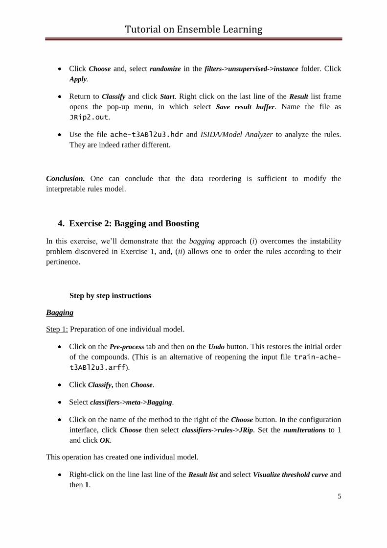
Click Choose and, select randomize in the filters->unsupervised->instance folder. Click

Apply.

Return to Classify and click Start. Right click on the last line of the Result list frame

opens the pop-up menu, in which select Save result buffer. Name the file as

JRip2.out.

Use the file ache-t3ABl2u3.hdr and ISIDA/Model Analyzer to analyze the rules.

They are indeed rather different.

Conclusion. One can conclude that the data reordering is sufficient to modify the

interpretable rules model.

4. Exercise 2: Bagging and Boosting

In this exercise, we‟ll demonstrate that the bagging approach (i) overcomes the instability

problem discovered in Exercise 1, and, (ii) allows one to order the rules according to their

pertinence.

Step by step instructions

Bagging

Step 1: Preparation of one individual model.

Click on the Pre-process tab and then on the Undo button. This restores the initial order

of the compounds. (This is an alternative of reopening the input file train-ache-

t3ABl2u3.arff).

Click Classify, then Choose.

Select classifiers->meta->Bagging.

Click on the name of the method to the right of the Choose button. In the configuration

interface, click Choose then select classifiers->rules->JRip. Set the numIterations to 1

and click OK.

This operation has created one individual model.

Right-click on the line last line of the Result list and select Visualize threshold curve and

then 1.


6

The ROC curve is plotted. As one can see, the ROC AUC value (about 0.7) is rather poor

which means that a large portion of active compounds cannot be retrieved using only one rule

set.

Save the model output. Right-click on the last line of the Result list and select Save

result buffer. Name your file as JRipBag1.out.

Step 2: Preparation of ensemble of models.

Produce new bagging models using 3 and 8 models by repeating the previous steps,

setting numIterations to 3, then to 8. Save the corresponding outputs in files

JRipBag3.out and JRipBag8.out, respectively.

One can see that ROC AUC for the consensus model increases up to 0.825 (see Figure 1).

Figure 1. ROC AUC of the consensus

model as a function the number of

bagging iterations


7

Step 3 (optionally): Analysis of the models: retrieval rate as a function of the confidence

threshold.

Use ISIDA/Model Analyzer to open JRipBag3.out and the test-ache.sdf file.

Navigate through the false negative examples.

The false negative examples are ordered according to the degree of consensus in the ensemble

model. A few false negatives could be retrieved by changing the confidence threshold. On the

other hand, this leads to the increase of the number of false positives.

Repeat the analysis using the JRipBag8.out file.

As reflected by the better ROC AUC, it is now possible to retrieve maybe one false negative,

but at a lower cost in terms of additional false positives. The confidence of prediction has

increased. In some sense, the model has become more discriminative.

Step 4 (optionally): Analysis of the models: selecting of common rules.

The goal is to select the rules which occur in, at least, two individual models.

Open the JRipBag3.out in an editor and concatenate all the rules from all the

models, then count how many of them are repeated. It should be one or two.

Do the same for the file JRipBag8.out. This time, it should be around ten.

A systematic study show how the “unique” rules rate in the ensemble decreases with the

number of bagging iterations (Figure 2). Each bagging iteration can be considered as a

sampling of some rule distribution. The final set of rules repeats more often those rules that

are most probable. When the sampling is sufficiently representative, the ensemble model

converges toward a certain rules distribution.


8

Boosting

Another approach to leverage predictive accuracy of classifiers is boosting.

Using Weka, click on the Classify tab.

Click Choose and select the method classifiers->meta->AdaBoostM1.

Click AdaBoostM1 in the box to the right of the button. The configuration interface of

the method appears.

Click Choose of this interface and select the method classifiers->meta->JRip.

Set the numIterations to 1.

Click on the button OK.

When the method is setup click Start to build an ensemble model containing one

model only.

Right-click on the last line of Result list and save the output by choosing Save result

buffer. Name your file JRipBoost1.out.

Repeat the experiment by setting the parameter numIterations to 3 and to 8. Save the

outputs as JRipBoost3.out and JRipBoost8.out respectively.

Notice that the ROC AUC increases more and faster than that with bagging.

Figure 2. Rate of unique rules as a

function of the number of bagging

iterations


9

It is particularly interesting to examine the files JRipBoost1.out,

JRipBoost2.out and JRipBoost3.out with ISIDA/Model Analyzer.

Open the files JRipBoost1.out, JRipBoost2.out and JRipBoost3.out with

ISIDA/Model Analyzer.

Compare the confidence of predictions for the false negative examples and the true

negatives.

Using one model in the ensemble, it is impossible to recover any of the false negatives. Notice

that with three models, the confidence of predictions has slightly decreased but the ROC AUC

has increased. It is possible to recover almost all of the false negatives, still discriminating

most of the negative examples. As the number of boosting iterations increases, it generates a

decision surface with greater margin. New examples are classified with greater confidence

and accuracy. On the other hand, the instances for which the probability of error of individual

models is high, are wrongly classified with greater confidence. This is why, with 8 models,

some false negative cannot be retrieved.

A systematic study of the ROC AUC illustrates this effect (Figure 3).

4.2. Conclusion

Bagging and boosting are two methods transforming “weak” individual models in a “strong”

ensemble of models. In fact JRip is not a “weak” classifier. This somehow damps the effect of

ensemble learning.

Generating alternative models and combining them can be achieved in different ways. It is

possible, for instance to select random subsets of descriptors.

Figure 3. ROC AUC as a function

of the number of boosting

iterations


10

5. Exercise 3: Random forest

Goal: to demonstrate the ability of the Random Forest method to produce strong predictive

models.

Method. The Random Forest method is based on bagging (bootstrap aggregation, see

definition of bagging) models built using the Random Tree method, in which classification

trees are grown on a random subset of descriptors [5]. The Random Tree method can be

viewed as an implementation of the Random Subspace method for the case of classification

trees. Combining two ensemble learning approaches, bagging and random space method,

makes the Random Forest method very effective approach to build highly predictive

classification models.

Computational procedure

Step 1: Setting the parameters

Click on the Classify tab of Weka.

Make sure that the test set is supplied and that output predictions will be displayed in

CSV format.

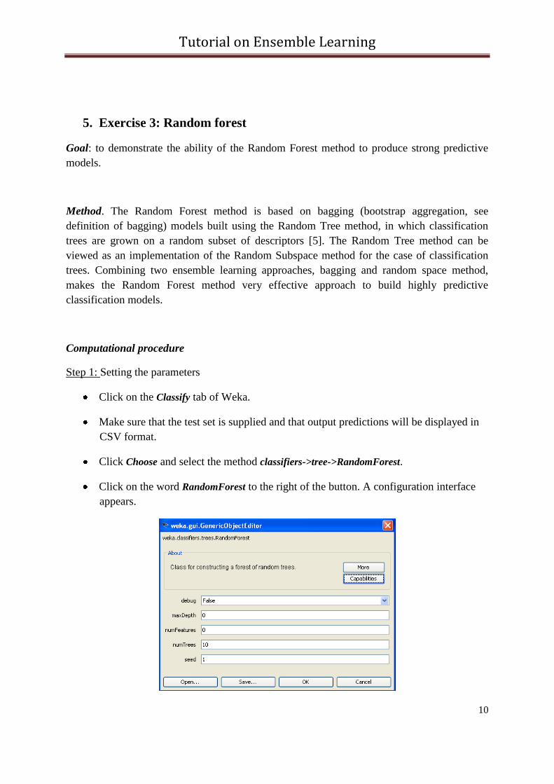
Click Choose and select the method classifiers->tree->RandomForest.

Click on the word RandomForest to the right of the button. A configuration interface

appears.


11

Step 2: Building a model based on a single random tree.

Set the numTrees to 1, then click the button OK.

Click Start.

This setup creates a bagging of one random tree. The random tree is grown as much as

possible and 11 attributes are selected at random to grow it. Results should be rather good

already.

Right click on the last line of the Result list frame.

Select Save result buffer. Save the output as RF1.out.

Step 3: Building models based on several random trees.

Build the Random Forest models based on 10 Random Trees. See below


12

All statistical characteristics became considerably stronger

Save the output as RF10.out

Repeat the study for 100 trees. Save result as RF100.out.

Build Random Forest models for different numbers of trees, varying from 1 to 100.

Build the plot ROC AUC vs. Number of trees

One may conclude that Random Forest outperforms the previous bagging and boosting

methods. First, a single fully grown and unpruned random tree seems as least as useful as a

more interpretable small set of rules. Second, the ensemble model is saturated later, using

more individual models; on another hand the maximal ROC AUC achieved is extremely high.

Step 4. Examine the file RF1.out, RF10.out and RF100.out using ISIDA/Model

Analyzer.

This single tree forest does not provide any confidence value for the prediction. It is therefore

impossible to modulate the decision of the model. When using 10 trees, most false negative

can be retrieved accepting roughly one false positive for each of them. At last, using 100 trees

in the model, all the same false negatives can be retrieved at the cost of accepting only one

Figure 4. ROC AUC as a function of

the number of trees


13

false positive. The last active compound can be retrieved only at the cost of accepting around

40 false positives.

6. Exercise 4: Combining descriptor pools

ISIDA/Model Analyzer can be used also to combine different models. The file AllSVM.txt

sum up the results of applying different SVM models, trained separately on different pools of

descriptors. The file contains a header linking it to a SDF file, giving indications about the

number of classes and the number of predictions for each compound and weights of each

individual model. These weights can be used to include or exclude individual models from the

consensus: a model is included if its corresponding value is larger than 0 and not included

otherwise. Next lines correspond to prediction results for each compound.

In each line, the first number is the number of the compound in the SDF file, the second

number is an experimental class and the next columns are the individual predictions of each

model. Optionally, each prediction can be assigned to a weight, which is represented by

additional real numbers on each line.

Open the AllSVM.txt file with ISIDA/Model Analyzer.

Several models are accessible. It is possible to navigate among them using the buttons Next

and Prev. It is also possible to use the list box between the buttons to select directly a model.

The tick near the name of the model indicates that it will be included into the ensemble of

models. It is possible to remove the tick in order to exclude the corresponding model. As can

be seen, the overall balanced accuracy is above 0.8 with some individual models performing

better than 0.9.

Click on the button Vote. A majority vote takes place. A message indicates that the

results are saved in a file Vote.txt. The proportion of vote is saved as well.

Load the file Vote.txt in ISIDA/Model Analyzer and click the button Start. The

ensemble model seems to have a suboptimal balanced accuracy.

Click on the headers of the columns of the confusion matrix to make appear column

related statistics. Recall, Precision, F-measure and Matthew's Correlation Coefficient

(MCC) are computed for the selected class. The ROC AUC is computed and data are

generated to plot the ROC with any tool able to read CSV format.

As can be seen, accepting only 20 false positives, all active compounds are retrieved. It is

possible to plot the ROC as in the following figure (Figure 4):


14

Figure 5. ROC curve for Exercise 4


15

Part 2. Regression Models

In this part of Tutorial, the Explorer mode of the Weka program is used. The tutorial includes

the following steps:

(1) building an individual MLR model,

(2) performing bagging of MLR models,

(3) applying the random subspace method to MLR models,

(4) performing additive regression based on SLR models,

(5) performing stacking of models.

1. Data and Descriptors

In the tutorial, we used aqueous solubility data (LogS). The initial dataset has been randomly

split into the training (818 compounds) and the test (817 compounds) sets. A set of 438

ISIDA fragment descriptors (t1ABl2u4) were computed for each compound. Although this

particular set of descriptors is not optimal for building the best possible models for this

property, however this set of descriptors allows for high speed of all calculations and makes it

possible to demonstrate clearly the effect of ensemble learning.

2. Files

The following files are supplied for the tutorial:

train-logs.sdf/test-logs.sdf – molecular files for training and test sets

logs-t1ABl2u4.hdr – descriptors identifiers

train-logs-t1ABl2u4.arff/test-logs-t1ABl2u4.arff – descriptor

and property values for the train/test set

3. Exercise 5: Individual MLR model


16

Important note for Windows users: During installation, the ARFF files should have been

associated with Weka. In this case, it is highly recommended to locate and double click on the

file train-logs-t1ABl2u4.arff, and to skip the following three points.

Start Weka.

Press button Explorer in the group Applications.

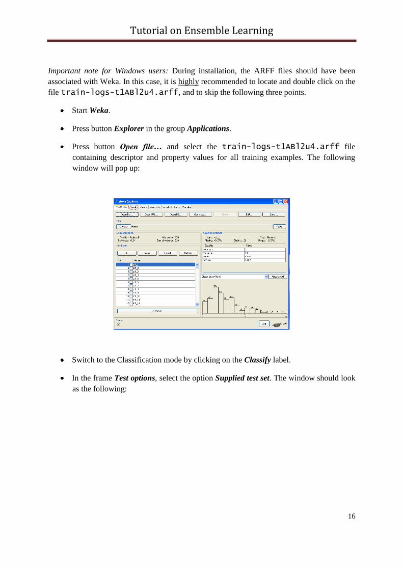
Press button Open file… and select the train-logs-t1ABl2u4.arff file

containing descriptor and property values for all training examples. The following

window will pop up:

Switch to the Classification mode by clicking on the Classify label.

In the frame Test options, select the option Supplied test set. The window should look

as the following:


17

Press the button Set… right to it.

In the window that pops up press the button Open file… and select the test-logs-

t1ABl2u4.arff file containing descriptor and property values for the test set. Press

Close to close this window.

The aim of this part of the tutorial is to build a MLR model on the training set and test it using

the specified test set. To do that:

Click on the Choose button in the panel Classifier. The following window with the

hierarchical tree of available machine learning methods appears:


18

Choose the method weka->classifiers->functions->LinearRegression from the

hierarchical tree.

Click on the word LinearRegression. The weka.gui.GenericObjectEditor window

related to the MLR method, in which the method‟s parameters can be settled, appears.

Switch off the descriptor selection option by changing the option

attributeSelectionMethod to No attribute selection. The windows at the screen should

be like these:

Press OK to close the window.

Click on the Start button to run the MLR method.

After the end of calculation the window of Weka should look as follows:


19

The predictive performance of the model, as estimated using the supplied external test set, is

presented at the right panel. One can see that the correlation coefficient (between predicted

and experimental values of LogS on the test set) is 0.891, mean absolute error (MAE) of

prediction on the test set is 0.7173 LogS units, the root-mean-square error (RMSE) of

prediction on the test set is 1.0068 LogS units, the relative absolute error of prediction on the

test set is 43.2988%, the root relative squared error of prediction on the test set is 47.4221%.

All these characteristics can be used for comparing predictive performances of different

regression models. In this tutorial we will use the RMSE error of prediction on the supplied

external test set to compare predictive performances of regression models.

4. Exercise 6: Bagging of MLR models

Goal: to demonstrate the ability of ensemble learning based on bagging to decrease prediction

errors of MLR models.

Method. The bagging procedure consists of: (i) generating several samples from the original

training set by drawing each compound with the same probability with replacement (so-called

bootstrapping), (ii) building a base learner (MLR in our case) model on each of the samples,

(iii) averaging the values predicted for test compounds over the whole ensemble of models

[4]. This procedure is implemented in Weka by means of a special “meta-classifier” with the

name Bagging.


20

Computational procedure.

Step 1: Setting the parameters.

Click Choose in the panel Classifier.

Choose the method weka->classifiers->meta->Bagging from the hierarchical tree of

classifiers.

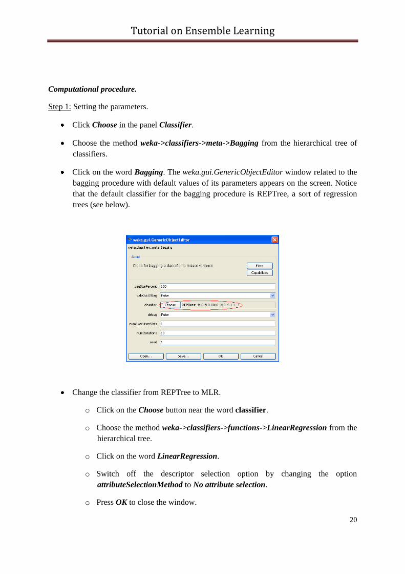
Click on the word Bagging. The weka.gui.GenericObjectEditor window related to the

bagging procedure with default values of its parameters appears on the screen. Notice

that the default classifier for the bagging procedure is REPTree, a sort of regression

trees (see below).

Change the classifier from REPTree to MLR.

o Click on the Choose button near the word classifier.

o Choose the method weka->classifiers->functions->LinearRegression from the

hierarchical tree.

o Click on the word LinearRegression.

o Switch off the descriptor selection option by changing the option

attributeSelectionMethod to No attribute selection.

o Press OK to close the window.


21

Step 2: Building a model based on a single bagging sample.

Change the number of bagging iterations to 1 by editing the field labeled

numIterations (see below).


Click on the Start button to run bagging with one MLR model.

The following results are obtained (see the output panel):

All statistical characteristics are worse in comparison with the individual model. In particular,

the RMSE rose from 1.0068 to 1.3627. This could be explained by the fact that the dataset

after resampling contains approximately 67% of unique examples, so approximately 33% of

information does not take part in learning in a single bagging iteration.

Step 3: Building models based on several bagging iterations.

Click on Bagging.

Set the number of iterations (near the label numIterations) to 10.


22


Click on the Start button to run bagging with 10 iterations.

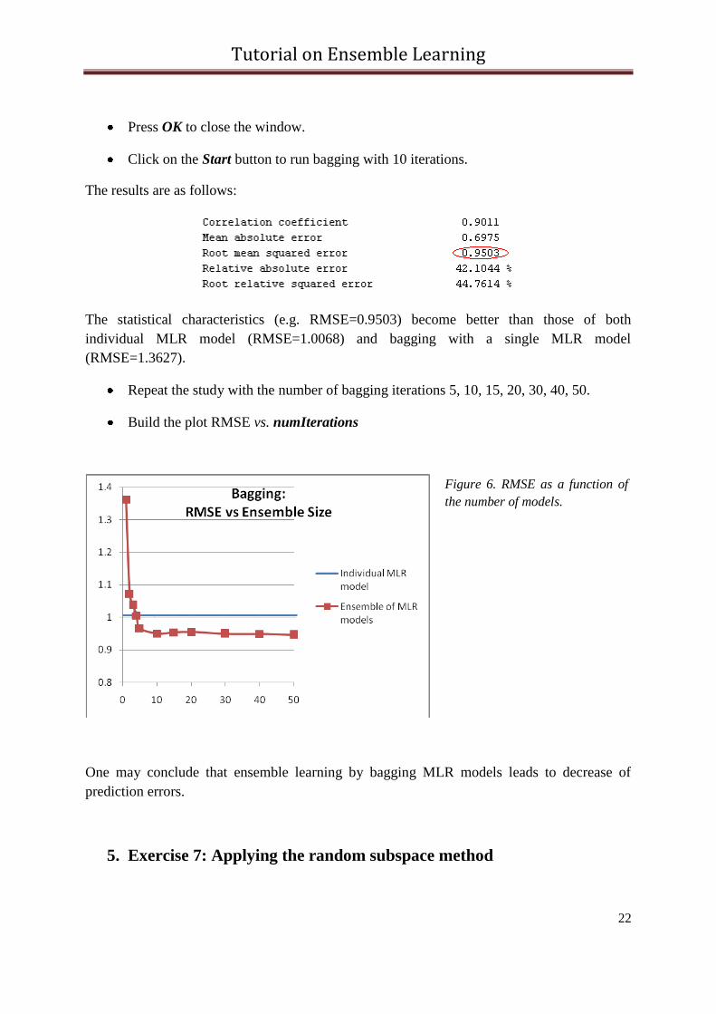
The results are as follows:

The statistical characteristics (e.g. RMSE=0.9503) become better than those of both

individual MLR model (RMSE=1.0068) and bagging with a single MLR model

(RMSE=1.3627).

Repeat the study with the number of bagging iterations 5, 10, 15, 20, 30, 40, 50.

Build the plot RMSE vs. numIterations

One may conclude that ensemble learning by bagging MLR models leads to decrease of

prediction errors.

5. Exercise 7: Applying the random subspace method

Figure 6. RMSE as a function of

the number of models.


23

Goal: to demonstrate the ability of ensemble learning based on the random subspace approach

to decrease prediction errors of MLR models.

Method. The random subspace procedure consists of: (i) random selection of descriptors

subsets from their initial pool, (ii) building a base learner (here, MLR) model on each of these

subsets, (iii) application of each individual MLR model to a test set compound following by

the averaging of all predictions [4]. This procedure is implemented in Weka in the

RandomSubSpace “meta-classifier”.



Click Choose in the Classifier panel.

On the hierarchical tree of classifiers, choose the method:

weka->classifiers->meta->RandomSubSpace.

Click on RandomSubSpace. Notice that the default classifier for the random subspace

procedure is REPTree (see below).

Change the classifier from REPTree to MLR.


24



hierarchical tree.

o Click on LinearRegression.




Notice that the default value 0.5 for subSpaceSize means that for each model only 50% of

descriptors are randomly selected. The performance of the random subspace methods

significantly depends on this parameter. Here, we won‟t optimize subSpaceSize, its default

value 0.5 will be used in all calculations.

Step 2: Building a model based on a single random subspace sample.

Change the number of iterations of the random subspace method to 1 by editing the

numIterations field (see below)


Click on the Start button to run the random subspace procedure with one MLR model.

The following results are obtained (see output panel):


25

The model performance (RMSE = 1.1357) is less good than that obtained for the individual

MLR model (RMSE = 1. 0068, see Exercise 5). This could be explained by reduction of the

number of variables. Indeed, only a half of the descriptor pool is used.

Step 3: Building models based on a several random subspace samples.

Click on RandomSubSpace. Set the number of iterations (numIterations = 10).


Click on the Start button to run the random subspace method with 10 iterations.

The results should be as follows:

The model performance becomes better compared to the previous calculation: RMSE=0.9155.

Repeat the modeling varying the number of random subspace iterations:

numIterations = 50, 100, 150, 200,. 300 and 400.

Build the plot RMSE vs numIterations


26

One may conclude that the random space method involving ensemble MLR models leads to

significant decrease of the prediction errors compared to one individual model.

6. Exercise 8: Additive regression based on SLR models

Goal: to demonstrate the ability of additive regression (a kind of regression boosting) to

improve the performance of simple linear regression (SLR) models.

Method. Additive regression enhances the performance of a base regression base method [6].

Each iteration fits a model to the residuals left on the previous iteration. Prediction is

accomplished by summing up the predictions of each model. Reducing the shrinkage

(learning rate) parameter, on one hand, helps to prevent overfitting and has a smoothing effect

but, on the other hand, increases the learning time. Default = 1.0, i.e. no shrinkage is applied.

This method of ensemble learning is implemented in Weka in AdditiveRegression meta-

classifier.



Click on Choose in the Classifier panel.

Figure 7. RMSE as

a function of the

number of models.


27

On the hierarchical tree of classifiers, choose the method:

weka->classifiers->meta->AdditiveRegression.

Click on AdditiveRegression. Notice that the default classifier (i.e. machine learning

method) for the additive regression procedure is DecisionStump (see below).

Change the classifier from DecisionStump to SLR.


o Choose the method weka->classifiers->functions->SimpleLinearRegression

from the hierarchical tree.

Notice the default value 1.0 for the shrinkage parameter. This means that we are not doing

shrinkage at this stage of tutorial.

Step 2: Building a model based on a single iteration of the additive regression method.

Change the number of iterations of the additive regression method to 1 by editing the

field labeled numIterations (see below).


28


Click on the Start button to run the additive regression procedure with one SLR model

(actually, an individual SLR model).

The following results are obtained (see output panel):

The result is rather bad because the model has been built on only a single descriptor.

Step 3: Building models based on a several random subspace samples.

Repeat the modeling varying the number of additive regression iterations:

numIterations = 10, 50, 100, 500, and 1000.

Change the shrinkage parameter to 0.5 and repeat the study for the same number of

iterations.

Build the plot RMSE vs. numIterations


29

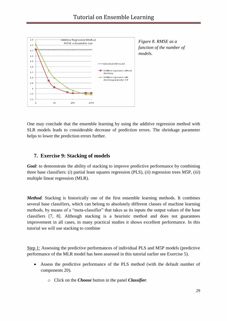
One may conclude that the ensemble learning by using the additive regression method with

SLR models leads to considerable decrease of prediction errors. The shrinkage parameter

helps to lower the prediction errors further.

7. Exercise 9: Stacking of models

Goal: to demonstrate the ability of stacking to improve predictive performance by combining

three base classifiers: (i) partial least squares regression (PLS), (ii) regression trees M5P, (iii)

multiple linear regression (MLR).

Method. Stacking is historically one of the first ensemble learning methods. It combines

several base classifiers, which can belong to absolutely different classes of machine learning

methods, by means of a “meta-classifier” that takes as its inputs the output values of the base

classifiers [7, 8]. Although stacking is a heuristic method and does not guarantees

improvement in all cases, in many practical studies it shows excellent performance. In this

tutorial we will use stacking to combine

Step 1: Assessing the predictive performances of individual PLS and M5P models (predictive

performance of the MLR model has been assessed in this tutorial earlier see Exercise 5).

Assess the predictive performance of the PLS method (with the default number of

components 20).

o Click on the Choose button in the panel Classifier.

Figure 8. RMSE as a

function of the number of

models.


30

o Choose the method weka->classifiers->functions->PLSClassifier from the

hierarchical tree.

o Click on the Start button to run the PLS method.


Assess the predictive performance of the M5P method.

o Click on the Choose button in the panel Classifier.

o Choose the method weka->classifiers->trees->M5P from the hierarchical tree.

o Click on the Start button to run the M5P method.


Step 2: Initialize the stacking method.

Click on the Choose button in the panel Classifier.

Choose the method weka->classifiers->meta->Stacking from the hierarchical tree of

classifiers.

Click on the word Stacking. The weka.gui.GenericObjectEditor window related to the

stacking procedure with default values of its parameters appears on the screen (see

below).


31

Step 3: Form a list of base classifiers.

Click on the field containing the text “1 weka.classifiers.Classifier” right from the

label classifiers.

A new window containing the list of currently selected classifiers pops up.

Delete the ZeroR method by clicking on the Delete button.

Add the PLS classifier to the empty list of classifiers. Do the following:


o Choose the method weka->classifiers->functions->PLSClassifier from the

hierarchical tree.

o Click on the Add button.

Add the M5P method to the list of currently selected classifiers. Do the following:


o Choose the method weka->classifiers->trees->M5P from the hierarchical tree.



32

Add the MLR method to the list of currently selected classifiers. Do the following:



hierarchical tree.

o Click on the word LinearRegression.





At this stage the window should look like this:

Close the window by clicking at the cross.

Step 4: Set the meta-classifier for the stacking method to be the multiple linear regression

(MLR). Do the following:

o Click on the Choose button near the word metaClassifier.


hierarchical tree.

At this stage the weka.gui.GenericObjectEditor window should be as follows:


33

Step 5: Run stacking of methods and assess the predictive performance of the resulting

ensemble model.


Click on the Start button to run the stacking method.

Weka finds the following optimal combination of the base classifiers:

The statistical results are as follows:

Step 6: Repeat the study by adding 1-NN. Repeat Step 3 and:

o Choose the method weka->classifiers->lazy->IBk from the hierarchical tree.

The results become even better.


34

The results for stacking are presented in Table 1.

Learning algorithm R (correlation

coefficient)

MAE RMSE

MLR 0.8910 0.7173 1.0068

PLS 0.9171 0.6384 0.8518

M5P 0.9176 0.6152 0.8461

1-NN 0.8455 0.85 1.1889

Stacking of MLR,

PLS, M5P

0.9366 0.5620 0.7460

Stacking of MLR,

PLS, M5P, 1-NN

0.9392 0.537 0.7301

Conclusion. One may conclude that stacking of several base classifiers has led to

considerable decrease of prediction error (RMSE=0.730) compared to that for the best base

classifier (RMSE=0.846).


35

Literature

[1.] http://cheminfo.u-strasbg.fr:8080/bioinfo/91/db_search/index.jsp

[2] Leo Breiman (1996). Bagging predictors. Machine Learning. 24(2):123-140.

[3] Yoav Freund, Robert E. Schapire: Experiments with a new boosting algorithm. In:

Thirteenth International Conference on Machine Learning, San Francisco, 148-156, 1996.

[4] Tin Kam Ho (1998). The Random Subspace Method for Constructing Decision Forests.

IEEE Transactions on Pattern Analysis and Machine Intelligence. 20(8):832-844.

[5] Leo Breiman (2001). Random Forests. Machine Learning. 45(1):5-32.

[6] J.H. Friedman (1999). Stochastic Gradient Boosting. Computational Statistics and Data

Analysis. 38:367-378.

[7] David H. Wolpert (1992). Stacked generalization. Neural Networks. 5:241-259.

[8] A.K. Seewald: How to Make Stacking Better and Faster While Also Taking Care of an

Unknown Weakness. In: Nineteenth International Conference on Machine Learning, 554-561,

2002.

[9] K. Varmuza, P. Filzmoser. Introduction to Multivariate Statistical Analysis in

Chemometrucs. CRC Press, 2009.

[10] William W. Cohen: Fast Effective Rule Induction. In: Twelfth International Conference

on Machine Learning, 115-123, 1995.

[11] Ross J. Quinlan: Learning with Continuous Classes. In: 5th Australian Joint Conference

on Artificial Intelligence, Singapore, 343-348, 1992.

http://cheminfo.u-strasbg.fr:8080/bioinfo/91/db_search/index.jsp


36

Appendix

1. Notes for Windows

On Windows, Weka should be located on the usual program launcher, in a folder Weka-

version (e.g., weka-3-6-2).

It is recommended to associate Weka to ARFF files. Thus, by double clicking an ARFF,

Weka/Explorer will be launched and the default directory for loading and writing data will be

set to the same directory as the loaded file. Otherwise, the default directory will be Weka

directory.

If you want to change the default directory for datasets in Weka, proceed as follows:

Extract from the java archive weka.jar, the weka/gui/explorer/Explorer.props

file. It can be done using an archive program such as WinRAR or 7-zip.

Copy this file in your home directory. To identify your home directory, type the

command echo %USERPROFILE% in a DOS command terminal.

Edit the file Explorer.props with WordPad.

Change the line InitialDirectory=%c by InitialDirectory=C:/Your/Own/Path

If you need to change the memory available for Weka in the JVM, you need to edit the file

RunWeka.ini or RunWeka.bat in the installation directory of Weka (root privilege may be

required). Change the line maxheap=128m by maxheap=1024m. You cannot assign more than

1.4Go to a JVM because of limitations of Windows.

2. Notes for Linux

To launch Weka, open a terminal and type:

java -jar /installation/directory/weka.jar.

If you need to assign additional memory to the JVM, use the option -XmMemorySizem,

replacing MemorySize by the required size in megabytes. For instance to launch Weka with

1024 Mo, type:

java -jar -Xm512m /installation/directory/weka.jar.

Varnek A., Tutorial on Ensemble Learning - Unistrainfochim.u-strasbg.fr/new/CS3_2010/Tutorial/Ensemble/Ensemble... · Tutorial on Ensemble Learning 1 ... The following ensemble learning

Documents