Variational principles for nonpotential operators

VARIATIONAL PRINCIPLES FOR NONPOTENTIAL OPERATORS

V. M. Filippov, V. M. Savchin, and S. G. Shorokhov UDC 517.972.5 517.972.7

One presents numerous approaches for the construction of variational principles for equations with operators which, in general, are nonpotential. One considers separately linear and nonlinear ordinary differential equations, partial and integropartial differential equations. One constructs and investigates both extremal and stationary variational principles and one gives applications of these principles in theoretical physics and in analytic mechanics. A series of unsolved problems are indicated. The survey is intended for mathematicians, physicists, working in both theoretical and applied areas, as well as for graduate students of physics and mathematics.

INTRODUCTION

By integral variational principles for the system of equations of some given model we mean in general the

construction of functionals for which the set of critical (extremal or stationary) points coincides with the set of the solutions

of the initial system. The wide prevalence and the systematic use of variational principles in mathematics, classical

mechanics, theoretical physics, mechanics of continuous media is due to a series of remarkable consequences of the variational formulations:

-- in theoretical investigations the extremal variational principles give the possibility to establish the existence of the solutions of the initial equations;

- - in applications it is important to have the possibility of the determination of stable approximations of the solutions of the considered equations by the so-called variational methods;

- - on the basis of the variational formulations it is possible to obtain the integrals of the evolution equations, including conservation laws.

However, in the course of a long time, all these advantages of the variational principles have been used only for the narrow class of the so-called potential operators.

In addition, in the mechanics of continuous media it is known that "all the invertible physical phenomena can be

described by variational principles, i.e. statements regarding the fact that in the actually realized processes some func-

tionals have a stationary value" (V. L. Berdichevskii [7, p. 7]). At present one has established the existence of functionaIs

of variational principles (namely, quasiclassical, i.e. bounded both from above and below) for arbitrary linear equations with an invertible operator and for large classes of nonlinear equations.

The actuality of the consideration of the inverse problems of the calculus of variations in contemporary theoretical physics is connected, as mentioned in the conclusion of V. I. Man'ko's survey [54], also with the fact that "the usual

procedure of quantization is based on the knowledge of the corresponding functional. Therefore, ambiguities in the choice of the functional lead to completely different quantum pictures .. . . However, presently there are no complete solutions of

IPCV for physically very important problems: 1) For the classical Maxwell equations of electrodynamics uniqueness has not been proved and not one Harniltonian, distinct from the known one, has been found.* 2) The IPCV for the equations of Einstein's general relativity theory has not been solved, i.e. on the one hand, one has not constructed an example of an-

other nontrivial action, giving the same equations of gravitation as those given by the usual action, and, on the other hand

*In a recent paper, V. V. Dodonov and V. I. Man'ko [28] have constructed one of these functionals, different from the classical Hamiltonian.

Translated from Itogi Nauki i Tekhniki, Seriya Sovremennye Problemy Matematiki, Noveishie Dostizheniya, Vol. 40, pp. 3-176, 1992.

1072-1964/94/6803-0275©1994 Plenum Publishing Corporation 275

one has not proved the uniqueness of the solution of the IPCV for the equations of the gauge fields (for example, the Yang--Mills equations). The solution of these purely mathematical problems would give the possibility to construct various quantum models (quantum chromodynamics, etc.)."

Thus, for equations with nonpotential operators the search of the functionals of the corresponding variational principles is a nontrivial actual problem: in spite of the significant number of investigations in this direction in the last 25 years, there exist a series of problems, basically in the area of the constructive determination of the solutions of the inverse problems of the calculus of variations (IPCV) for such operators. Numerous attempts for and the importance of obtaining particular solutions of the IPCV have led to fundamentally different formulations and different approaches to their solu- tions; this paper is devoted, basically, to a survey of these results.

2 7 6

Chapter I

AUXILIARY INFORMATION AND THE FORMULATIONS OF INVERSE PROBLEMS OF THE CALCULUS OF VARIATIONS (IPCV)

1.1. Auxiliary Information

1 . 1 . 1 . Cer t a in Auxi l i a ry Nota t ions and D e f i n i t i o n s

1. R is the field of real numbers.

2. R m is the m-dimensional Euclidean space of points (x 1 . . . . . xm).

3. 9 is a domain, i.e. an open connected set, in R m with a piecewise smooth boundary ag; 9 is the closure of 9 in R m .

4. Z ~ n is the set of all m-dimensional vectors c~ = (c~ 1 . . . . . O~m) with nonnegative integers o~ 1 . . . . . c~ m.

For any o~, [3 E Z ~ n we set c~ + /3 = (cq + 131 . . . . . ~m + /3m)"

The notation c~ >_ /3 means that 0q -> ~i (i = 1 . . . . . m).

The notation i = 1, . . . , n means that i assumes all the integers f rom 1 to n. / \

5. The binomial coefficient ( ; ) f o r the vectors c~,/3 E z~n is de f inedby the equality

= , " " ~ . , =~=,Lilt/ if a > ~ ,

i f a <13,

where ( ; : ) = ~fl l[~,l (c¢~ - - [~i)t].

6.

7.

respect to

8.

derivative

.

The symbol v means "for each," "for any." The symbol ~ denotes the empty set.

D i o r Dxi is the total derivative with respect to the variable x i. D ia i is the total derivative of order ai with

the variable x i. D ~ = D1 c~l . . . Dream is the total derivative corresponding to the multi index c~ E Z ~ n.

O i = 0 /0X i is the partial derivative with respect to the variable x i. O= = 01~l/(0xX) ~1 . . . ( 0 x m ) c~m is the partial m

corresponding to the multiindex c~, I c¢ I= ~ ~ , u==O=tt. i = l

A --__ ~ ~ / ( O x q ~ is the Laplace operator.

10. ttx~ = dirt, ttxixi (x) = O2tt (x) / Oxt Ox ].

11. CS(9) (CS((])) is the set of all functions that are continuous in the domain 9(9) together with all the partial derivatives up to and including the order s.

0 0

C s (f~) ~ C s (~) is the set of all functions f rom Cs(9) that vanish on 09 together with all the partial derivatives up to and including the order s.

C = N C~ (~). ~=0

0

C ~ (f~) is the set of all functions f rom C°°(t?) for which all the partial derivatives of an arbitrary order in ~ exist and vanish on 09.

I f Q T = 9 x (0, T) is some domain in the space of the variables (x, t) = (x 1, . . . . x m, t), then Cx,t"'q (Qr) is the

class of functions which on the se t Q T have continuous derivatives with respect to x 1 . . . . . x m up to order p and continuous derivatives with respect to t up to order q.

Sometimes, for the sake of brevity, the argument (x, t) is not indicated for the class "'q C~,,, (Qr) i . 12. For a vector-valued function u(x) = (ul(x) . . . . . un(x)) the norm in CS(9) is defined by the equality

277

I[ t t lC'(~)l l___2 ~ max lu ' (x)l. i=l I~l<sxt~ I ct

13. In this survey we have adopted the standard rule of tensor calculus: repeated indices of factors, situated at

different levels, denote summation. The range of the variation of the indices will be clear from the context.

14. The Leibnitz formula is

15. By U, V we shall denote everywhere normed linear spaces over the field R of real numbers. 0u, 0 v are the

zero elements in U and V, respectively.

16. O(.,.)~-<.,.>:VNU-~-R is a nonlocal bilinear form.

The classical bilinear forms are nonlocal bilinear forms, defined by formulas of t y p e • (v, g) = ~ v. gdx. a

O ( u ; . , ")~-<', ">,, : VNU--,'-R is a local bilinear form.

17. D(N) is the domain of definition, R(N) is the range of the operator N.

The linearity of the operator N means that

N (~,]ul+)~2u ~) =XINul+'L2Nu 2

Y~l, ~,~R, Vu I, uZ~D(N).

18. D(N, B) = {u : u~D(N)ND(B)},

RN(B ) = {Bu: u E D(N, B)}.

19. N* is the adjoint operator relative to a given bilinear form, N -1 is the inverse operator, I is the identity

operator. 20. The class of Euler--Lagrange functionals, or the Euler class E m,n,s of functionals is the set of functionals of

the form

[ul = l f (x, u. (x)) ax, Q

. ~ • • o ~ ~ ff l~ where x = (x 1, . . xm), u (x) = (td (x), tt ~ (x)), u~ (x) = d~u (x), EZ+; s is the highest order of the derivatives

occurring in the integrand. 21. By an infinite dimensional system we mean a material system whose state cannot be defined by a finite number

of generalized coordinates. 22. Two systems of equations are considered to be equivalent if each solution, considered in a definite sense, of

one of them is a solution also of the other system. We give the notations related with the use of the contemporary geometric approaches in the consideration of

differential equations and the corresponding formulations of the IPCV. 23. By ~ we denote an n-dimensional connected paracompact C~-manifold. As a rule, at the consideration of

differential equations we can restrict ourselves to the case when ~t is an open subset of the Euclidean space R n.

24. For each point x E ~ one can introduce the concept of a tangential vector to the manifold ~t at the point x as

an equivalence class of the parametrized curves, passing through the point x. The collection of all tangent vectors to the

manifold ~ at the point x is called the tangent space to JR at the point x and it is denoted by Tx(~t). The collection of the

tangent spaces, corresponding to all the points x of the manifold Jl~, forms the tangent bundle of the manifold ~ and it is

denoted T ( ~ ) = UxEat Tx(~). The tangent bundle T(~t) is a C~-manifold of dimension 2n. Considering the tangent

bundle of the manifold T(~) , we obtain the second tangent bundle of the manifold ~t, denoted T(T(.I~)).

By a smooth vector field f on a manifold ~ we mean a smooth mapping f : ~ --, T ( ~ ) such that 7r o f = id~ (under

the mapping r : T ( ~ ) --, ~t each vector from Tx(~t) is projected into the point x E ~ ) , i.e. the juxtaposition of the vector

fx E Tx(~) to each point x E ~ . The set of all smooth vector fields on 3t, denoted by ~ ( ~ ) , is a Lie algebra (of infinite

dimension) over R relative to the commutator [f, g], f, g E 3~(~t).

25. The canonical projection 7r induces linear mappings 7r.:TvT(Jl) --" TTr(v)(~). The elements of the space TvT(~t), i ~tangent to the fiber over ~'(v) and, consequently, belonging to the kernel of the mapping 7r., are called vertical

278

vectors. The subspace in TvT(~t.), formed by the vertical vectors, is called a vertical subspace. The collection of all

vertical subspaces is called the vertical bundle and it is denoted by VT(M,).

By the horizontal bundle we mean the vector subbundle HT(M.) that is the complement of VT(J~) in T(T(Jd.)), i.e.

T(T(&)) = HT(M.)@ VT(~) . The elements of HT(~) are called horizontal vectors. The subspace in TvT(dJ.), formed by

the horizontal vectors, is called a horizontal subspace. As a rule, the horizontal bundle is generated by a connection or by

a differential equation on a manifold. 26. For the investigation of individual aspects of the IPCV the technique of differential forms has an exceptional

effectiveness.

A differential k-form ~ at a point x of the manifold M. is a k-linear skew-symmetric function (an exterior k-form)

~o : T ~ ( ~ ' ) X T ~ ( J ) X . . . XT~(,///')--~R.

The space of the differential k-forms at the point x is denoted by Ak(Tx*(~)). By definition, a 0-form at a point x

is a real number. The space Tx(~ ) = AI(T×*(~)) of the 1-forms is the space of the linear functions on: Tx(~), i.e. the

dual vector space of the tangent space Tx(~)~ and is called the cotangent space to ~ at the point x.

The set Ak(T*(JI/[.)) = Ux~tAk(Tx*(.kt.)) is called the bundle of differential k-forms; in particular, the set AI(T*(M.))

is called the cotangent bundle and is denoted simply by T*(3~). By a differential 1-form we mean a smooth mapping

w:~ --, T*(~) such that ~r* o o~ = id~t (here 7r* is the projection ~r*:T*(&) --, (M.), i.e., the assignment of the-covector

from Tx*(3~ ) at each point x E M.. In an analogous manner one introduces the differential k-forms on M..

27. Let % be a fibered manifold with projection 7r:~ ~ ~ . The local sections f and g of the manifold % (Tr o f =

id~t , 7r o g = id~t ) are said to be q-equivalent at the point x E ~ , q _> 0, if in local coordinates we have

f , (x)= g~ (x), O~ f , (x)= c)~gZ (x) V ~, 1 ~< l ~ ] ~< q.

The property of q-equivalence does not depend on the selection of the system of coordinates in the neighborhood of the

point x. The q-equivalence class is called the q-jet of this section at the point x and is denoted by jq(f)(x). The set Jq(~) =

UxE~t Jq(~)x, where Jq(~)× is the set of q-jets of all possible local sections % at the point x, forms the bundle of q-jets of

the fibered manifold %. 28. Let E x, Ey be Banach spaces, let Exy be the space of all continuous linear mappings from E x into Ey; N(x) is,

for each fixed x, a mapping from a convex open set ~o C E x into Exy. If vx, h E E x the function ~(t) = (N(x + th), h ) ,

0 _ t _< 1, is continuous with respect to t, then such a mapping is said to be radially continuous. 29. A mapping N, acting from a normed space E x into a normed space Ey is said to be:

Ex demicontinuous at the point u E D(N) if for an arbitrary sequence tt~-+ tt (tt~ED (N)) the sequence N(un) ~ N(u)

(weak convergence); hemicontinuous at the point u 0 E D(N) if for arbitrary elements u, such that u 0 + tu E D(N) for 0 ___ t _<

(c~ = ~(u) > 0), and sequence t n --, 0 for n --, c o (0 < t n < c~), the sequence N(u 0 + tnU) ~ N(u0).

We mention that from the demicontinuity of the operator N there follows its hemicontinuity, while from hemi-

continuity on D(N) there follows that (h, N(u 0 + tu)) is continuous with respect to t qh E Ey* if u o + tu E D(N).

30. The survey consist of six chapters, which are divided into sections; the latter, in turn, are sometimes divided

into subsections. The numbering of the formulas starts anew in each section; a reference to the formula (k.m.n) means

formula (n) in Sec. k.m; here k denotes the number of the chapter.

31. In view of frequent recurrence, the following abbreviations are used in the survey:

ODE - ordinary differential equation;

PDE - partial differential equation;

IPDE - integropartial differential equation;

IPCV - inverse problem of the calculus of variations;

VP - variational principle;

PC - potentiality condition.

1.1.2. S o m e E l e m e n t s o f t h e C a l c u l u s o f Variations. Assume that there is given an operator N, defined on a

lineal D(N), dense in a real Banach space U and acting from U into the conjugate Banach space V = U*. If for some u E

D(N) and for each h E U there exists

279

l i r a N (u + 8 h ) - - N (u) _ D N (u, h), (1) 8-.+0 8

which is a linear expression with respect to h, DN(u, h) = Nu'h , then the linear operator N u is called the Gdtteaux derivative of the operator N at the point u. The limit in (1) is understood in the sense of the convergence with respect to

the norm of the space V; various conditions for the existence and the continuity of the G~iteaux derivative for nonlinear

operators are given by M. M. Vainberg [12]. The computation of the Gfiteaux derivative of an operator (and, consequent-

ly, also of a functional as a special case of an operator for V = R) can be carried out conveniently by the formula

(2)

For the quantity N~h = DN(u, h) (the Gfiteaux differential), by analogy with the classical calculus of variations, we use, for th = 6u (6u is the variation of the function), the notation DN(u, 6u) = Nu6u = 6N(u).

We assume now that on V × U there is defined a nondegenerate bilinear functional ( . , • ) : V x U --, R, so that the spaces U and V are considered dual relative to this form (., .).

Definition 1. The operator N: U --, U* is said to be potential on some set w C U if there exists a continuously Gglteaux differentiable functional f[u], defined on o~, such that qh E D(N~)

{ f '[u], h ) = l i r a f[u+ehl--fIu] .---- (N(u ) , h ) . e--*O 8 (3)

Denoting f'[u] = N[u] = grad flu], the functional f is called the potential of the operator N, while the operator N

is called the gradient of the functional f. The equation f'[u] = 0 v is called the Euler equation for the functional f. Functionals of the form

f [u]-- I ~ (x, u(x), u,, (x) . . . . . Gm (x)) dx, o (4)

where x = (x 1 . . . . . x m) E ~ C R m and ~ is a sufficiently smooth function of 2m + 1 variables, are called Euler--La- grangefunctionals (written for second order PDE).

Under certain assumptions regarding the smoothness of the functions occurring in (4) (for example, it is sufficient

that u E C2(~), ~ E C3(R2m+I)), from the condition f'[u] = 0 there follows the classical Euler--Lagrange equation

0u°~' D,- ~°~' - o (xEf~).- (5)

For the more general class of functionals

13 [u] ---- l S (u(x), .~ t t . . . . . .~rU) d x , (6) fl

under some requirements (Pomraning [360], V. M. Filippov [105]) on the linear operator ~i (i = 1 . . . . . r), the Eu-

ler--Lagrange equation has the form

as + ~ , a as = 0 (xEf~). (7) au (~W)

1.1.3. Local and Nonlocal Bilinear Forms. Let E i (i = 1, 2) be linear spaces over the field R.

Definition 2. A mapping ¢ ( . , • ) = (. ,. ):E 1 × E 2 ---- R is said to be a bilinearform if it is linear with respect to each argument; for E 1 = E 2 such a mapping ¢ is said to be a symmetric form if

O(v, g ) = O ( g , v) Vg, v6E~=E 2,

and a skew-symmetric form if

~(v , g ) = - - O ( g , v) Vg, v6E'=E ~.

Such mappings are called also nonlocal bilinearforms.

280

Definition 3. By a local bilinearform we mean a mapping ~(u; -,.) =- ( , ) u : V x U -+ R, which to each triple of

elements v E V, h, u E U assigns a number from the field R and is a bilinear form with respect to v, h.

Definition 4. A local bilinear form ,I,(u; • ,. ):V x U --, R is said to be nondegenerate if:

1) from the condition

there follows that h = 0u;

2) from the condition

~(u; v, h)=OVveV, VueU (8)

CO(u; v, h ) = 0 V h , u~U (9)

there follows that v = 0 v.

For fixed elements v E V, h E U, the expression ~I,(. ; v, h) defines an operator, whose value depends on u E

U. In the sequel we assume that for each considered local bilinear form there exists the Gfiteaux derivative of this operator and in this case we write

(10) q)'. (g; v, k ) = l l m +{O(t t + e g ; v, h)--q}(u; v, h)}.

8--*0

In order to emphasize the fact that flu is a 3-linear form with respect to the elements v E V, g, h E U, we shall

use also the notation

( g; v, h ) u = % ( g ; v, h). (11)

If the G~teaux derivative of the operator N exists, then we have the equality (Nashed [339])

N ( u + e h ) = N ( u ) + s N ' . h + r (u, eh), uED (N), (i2)

where for any fixed element h E D(Nu' ) we have

lira r (u. s,~) __Ov. (13) e~O 8

We give examples of local and nonlocal bilinear forms which, incidentally, will be used in the sequel.

Example 1. Let ~2 be a bounded domain of the Euclidean space R m of points x = (x ' . . . . . x ~) ; v (x) = (v ~ (x) . . . . . vn(x))6U, h(x)=(h~(x) . . . . . hn(x))EU, where v ~, h~Eg~=c(~2)(i=l-'~n), g = ( g ~ . . . . . U '~) . ( ' , . ) :UXU.-~R.

We define a nonlocal bilinear form (. ,- ):U x U --- R by the equality

= I ~2 i= l

A bilinear form, defined by a formula of the form (14), will be said to be classical. Example 2. Assume that there are given the functions a , j=ai i (x , tt~), xEfacR '~ (i, j = l , n; l ~ j = 0 , s),

where tt=-----O~tt, aEZ~-, u(x)---(u1(x) . . . . ,tz~(x))EU, utEU~=C*(~) ( i = 1 , n), and not all derivatives Oaij/Ou ~' are equal to zero in ~. Then the formula

S ( v, h ) ~ exp(aq) .v t (x ) .M(x)dx a (15)

defines a local bilinear form on U x U.

Assuming that auEC' (gaX R q) ( i , j = 1, tz),

obtain the Gfiteaux differential where q is the dimension of the vector {u=} (I ~I = 0 . . . . . s), we

? O a L t r t < g; v, h > , = j exp (aq) O - ~ . g . v .Mdx.

f~ (16)

281

1.2. Formulations of Inverse Problems of the Calculus of Variations

Within the framework of contemporary calculus of variations, the following formulation of an IPCV is classical. Assume that the operator N maps the set D(N), dense in a real Banach space E, into the conjugate space E* and

assume that on E* × E there is defined a nondegenerate symmetric bilinear form (.,.). Formulation 1. For the operator N of the equation

N(u) = 0 (1) find a functional ~[u] such that

6cI~[u] = (N (u), 6u) Vu6D (N), (2)

or, in another terminology,

grad fb[ul=N (u ) Vu~O (N). (3)

The operators N for which the functionals (2), (3) exist are said to be potential relative to the given bilinear form.

This paper is devoted to survey the solutions of IPCV precisely in the case when the given operator N is non- potential for the selected bilinear form (-,-); therefore, we consider generalized formulations of IPCV.

Formulation 2. For a second-order linear PDE (x E f~ C R n)

~ u ~ p~v (x) D[sDvu(x)Jr Z q~(x) D[su(x )q-r (x ) t t= f (x) (4) v , f~=l [5=1

(with sufficiently smooth coefficients; see Sec. 4.4), considered on some set D(~), find a function •(x) E CI(0), kt(x) ;~ 0 in 0, and a functional F[u] in the class of quadratic Euler--Lagrange functionals (4) (of Sec. 1.1) such that

[u] = I ~ (x ) .{aeu- f}auclx vttED (~) . (5) aF f~

For nonlinear differential equations of order m

N Ix, u] ~ N (x, u (x), Dlu . . . . . Dnu . . . . . DiD~u [t,j=l--.-.-~ . . . . ) = f (x), (6)

the following generalizations of the classical inverse problem are natural:

Formulation 3. For the equation (6) find a function #(x, u, u t) =-- ~ (x, tt(x) . . . . . D)u(x) . . . . ), ] = 1, n;

i = 0, k; k -.< [ 2 1 ' r~ 4 = 0 in f / v u E D(N) and in the corresponding class of Euler--Lagrange functionals

F [u]= l ~? (x, u(x) . . . . . D~u(x) l,=-6-5,~ . . . . ) dx (7) f~ = l , n

find a functional F[u] such that

P 6F [u] = ~ ~ (x, u, uO.{N Ix, u]-- f}6udx VttGD (N). (8)

o

Formulation 4. There is given a family of functions {ua(x)}. Find a functional Fo[u ] whose set of critical points

coincides with the set {ua(x) }, i.e.,

~{uo ( x) }~aVo[ ff]=o. (9)

Formulation 5. For a given operator N find a functional ~[u] such that:

A. N(fi) = 0 ** 6,I,[fi] = 0. In this case one imposes frequently additional conditions on the desired functionals. B. For a differential operator N the functional ~[u] contains derivatives of the unknown function u(x) of smaller

order than the equation N(u) = 0, and in the case of a linear operator N the functional ~[u] is quadratic. C. The functional ~[u] is bounded from below on D(N).

2 8 2

In many cases one succeeds to establish a stronger property.

D. There exists, a unique element u 0, minimizing in some space H N the functional ~[u]; moreover, the element u 0 coincides With some generalized (unique) solution of the equation N(u) = 0.

The functionals from the class of Euler--Lagrange functionals, i.e., the solutions of the inverse problems in the

formulations 1--3, possessing also the properties B--D, are called the classical solutions (functionals) of the IPCV: the preimage of such a solution is a Dirichlet functional for the Laplace equation. The functionals, satisfying the requirements A, B, C, are called quasiclassicat solutions (functionals) of the IPCV; such functionals do not belong necessarily to the

class of Euler--Lagrange functionals. We mention that the problem of the construction of functionals with the properties A, B, C, D for nonsymmetric

operators has been formulated at the beginning of the sixties by L. D. Kudryavtsev; in the course of its solving the

dissertations of V. M. Shalov [125] and V. M. Filippov [97, 112] have been completed.

We point out the importance of the properties A--D of the desired functionals for theoretical investigations, as well as for the applications. Property C enables us to use in proofs the well developed scheme of the method of a minimizing sequence (S. L. Sobolev [89]), while in applications the various methods of minimization of functionals; in particular, the

latter is important if at the numerical implementation by the Ritz method one obtains a system of equations with a large number of unknowns (see G. I. Marchuk and V. I. Agoshkov [59], G. I. Marchuk and Yu. A. Kuznetsov [60], Nashed [338]). It has been repeatedly mentioned (Yu. I. Nyashin [73], V. L. Berdichevskii [7]) that the direct methods of the

calculus of variations are especially effective in those cases when the functional has a unique critical point which is a point

of maximum or minimum.

283

Chapter 2

POTENTIALITY CONDITIONS FOR SYSTEMS OF DIFFERENTIAL AND INTEGRODIFFERENTIAL EQUATIONS

The investigation of the problem of the construction of the required functionals from a given equation starts always with elucidating whether the operator of the equation is potential. Therefore, although the main object of this survey is formed by nonpotential operators, in this chapter we present an entire series of conditions for the potentiality of operators, both for abstract and concrete differential equations and systems (ODE, PDE, IPDE). These results are relevant here also because of the fact that the constructions of the functionals of the IPCV for nonpotential operators, given in the sequel, are based in many cases on the generalizations of the corresponding statements for potential operators.

2.1. Potentiality Conditions in Operator Form

Assume that there is given an equation

N(u) =0, (1)

where the operator N maps a convex open set D(N) of some normed real space E into the set R(N) of the space E*, strongly conjugate with respect to a given form (.,.). We have

THEOREM 1. Assume that the operator N is Gfiteaux differentiable at each point of D(N) and the G~tteaux differential DN(u, h) is hemicontinuous (see Subsection 1.1.1, (25)) with respect to u. Then for the potentiality of the

operator N *=~ that the bilinear functional (DN(u, hi), h2) be symmetric, i.e. that vu, hl, h 2 from D(N) we have

(DN (u, hi), h 2 ) = ( D N (u, h2), hi). (2)

Under the condition of the existence of the Gfiteaux derivative Nu, this equality reduces to the condition of its

symmetry: vh 1, h 2 E D(N)

( N ' ,hp h 2 } = ( N ' k2 , h I } (ruED (N)). (3)

In this case the desired functional flu): N(u) = grad flu) has the form 1

/ (it) --~ f o -}- I ( N (tto + t (t t-- tto) ), t t - - tt o } dr, (4) 0

where f0 is an arbitrary fixed element of the space E* and (y, u) is the value of the linear functional y E E* at the element

u E E . In this form, Theorem 1 has been established by M. M. Vainberg [12]; the result goes back to the investigations

of Volterra [445] and Kerner [2871. COROLLARY 1. For a bounded linear operator A from the condition (3) there follows that for the potentiality of

the operator A ~ A = A*, i.e. that A be a self-adjoint operator (and not only symmetric). Various generalizations of the given Volterra--Kerner--Vainberg theorem are known. In particular, for

nondifferentiable operators, from M. K. Gavurin's results [18] one obtains (see M. M. Vainberg [12]) the following theorem, elucidating, by analogy with classical mathematical analysis, the essence of the concept of the potentiality of an operator.

II, THEOREM 2. Let N be a radially continuous operator, acting from an open set oa C E x into E x. Then for the

potentiality of N *=* that for any polygonal line 1 C co the curvilinear integral ~ (N(u), du) be independent of the

e

integration path. For operators acting in Hilbert spaces one has established (Langenbach [50]) more concrete sufficient conditions for

the applicability of the variational method.

284

THEOREM 4. Assume that a nonlinear operator N acts in a Hilbert space H, let D(N) = H, and assume that:

A) N(0) = 0; the G~tteaux differential DN(u, h) exists for all u, h E D(N), it is linear relative to h, and as an

element of H it is continuous in any "plane" containing the point u; B)(N" (u)h,, h~)=(N" (u)h2, h~) Vu, h~, h2~O(N); C)(N" (u)h, h) ~.O Vu, h6O(N), h----/=O.

Under these conditions, an element u 0 E D(N) is a solution of the equation

N(u )= f , u6D (N), (5)

if and only if u o minimizes in D(N) the functional 1

o [u] = f (N (ttt), u) at -- ( f , tt). (6) 0

In this case the solution u 0 of the equation (5) is unique. THEOREM 5. Assume that conditions A, B of Theorem 4 hold, as well as condition

D) (N'(u)h, h)~>~,~llhl[ ~ Vu, h~D(N), y=/=O.

Then the assertions of Theorem 4 hold, the functional ,I,[u] (6) is bounded from below in H, and any minimizing

sequence converges in the metric of H to the same limit element from H.

We mention that in [439] Vanderbauwhede has established a useful generalization of Theorem 1 to the case when

the G~teaux derivative N u of the operator N acts in some closed subspace E 0 of a real Banach space E: in this case a criterion

for the potentiality of an operator N, acting in E, relative to a subspace E 0 is the validity of the identity (3) for arbitrary u E

E, h 1, h 2 being in E 0. Taking

E=C2k(fi), eo={u (x)eC2~(~): n%=O(xEOf~)V~:l~l < k --1},

and making use of a special construction of the desired potential, Horova [280] has constructed potentials in explicit form for a sufficiently large class of nonlinear elliptic PDE of divergence type.

Thus, the potentiality criterion (3) must be satisfied for all functions from D(Nu' ) (in (3) we assume D(N) =

D(Nu') ), i.e. on the set of functions satisfying the corresponding boundary conditions. However, for differential and integrodifferential operators, considered on some domain f~ C R n it is practically more convenient to verify first the condition of formal potentiality:

( N'.hv hz ) = ( N'~h2, hi ) Vu, h I, h2EC ~ (f2). * (7)

Of course, in the general case, the condition (7) of formal potentiality is only necessary, but not sufficient for the potentiality of the boundary operator N: in the book by Lions and Magenes [51] there is given an example of a correct elliptic operator A,

Au--~-A2u+u=g(x), x6f2~R '~,

u = A u = 0 , x~,Of~,

(8)

(9)

D(A) = {u(x) E C4(0), u(x) satisfies the conditions (7)}, which is formally potential but not potential, precisely because of the boundary conditions (9). (Although it is easy to verify that the operator A, considered on the set D(A) = {u(x) E C4(0), u = 0u/0h = 0}, is potential.)

*We mention that in a series of problems of theoretical physics it turns out to be sufficient to restrict oneself to the set D(N} = Co = (Q).

285

In the above given potentiality criteria for operators one has used nonlocal bilinear forms. However, the concept of the potentiality of an operator can be generalized also relative to a local bilinear form ¢(u, • , . ) - (-, .)u:V × U --- R,

where V, U are real linear normed spaces. For this, in Definition 1 of Subsection 1.1.2 one has to replace the relation (3) by the equality

( i f (t 0 , It) =~lim f ( u + t h ) - - f ( u ) t.+o t - - ( N (u), h ) u.

(10)

THEOREM 6 (V. M. Savchin [84]). Assume that the Ggtteaux differentiable operator N:D(N) C U ---, V and the local bilinear form ( ,)u: V × U --, R are such that for any fixed elements u E D(N), g, h E D(N~) the function e ~

(N(u + eh), g)u+eh is continuously differentiable on the segment [0, 1]. Then for the potentiality of the operator N on the convex set D(N) relative to the considered bilinear form it is necessary and sufficient that we have

( N ' . k , g ) u + ( h; N ( u ) , g ) == ( N'ug, h ) ~ + ( g; N ( u ) , h ) u

ruED(N) , vg, hO.D (N'u). (11)

In this case, the potential of the operator N is determined by the formula 1

f l u ] = s (N(uo+X(t t - - t to) ) , t t-- Uo > uo+z(~-..) dX+const, (12) 0

where u 0 is a fixed element from D(N).

The possibility of using local bilinear forms for the generalization of the concept of the potentiality of an operator has been mentioned by Magri [317].

Problem 1. There exist no sufficiently general statements that would enable us to determine constructively, after the

formal potentiality of the operator N has been established, whether the operator is potential under the given initial--boundary conditions. In a more general setting, one does not know descriptions of sets of boundary conditions, under which a formally

potential operator would be potential. These same problems are of actuality and are more complicated for B-potential operators (see Secs. 3.2, 4.4).

2.2. Conditions for the Potentiality of Systems of Ordinary Differential Equations

The investigation of the question of the solvability of IPCV for systems of ODE in the classical formulation 1 can

be based on several distinct approaches, each of them having its own deficiencies and advantages. For example, the

deficiencies of the classical analytic approach, owing its origin to Helmholtz [252], consist in the dependence on the selection

of the coordinate system and in the cumbersome character of the obtained formulas. On the other hand, the geometric

approach, in the framework of which the IPCV reduces to the investigation of the geometry of the tangent bundle of the configuration manifold, enables us to obtain compact invariant formulations of the fundamental results. The operator

approach, based on the Volterra--Kerner--Vainberg theorem (Theorem 1 of Sec. 2.1), by virtue of its generality, is the most effective for the derivation of "variationality" conditions for a system of ODE. The particularities of the various approaches to the IPCV have been discussed by Schafir [411].

2.2.1. The Formal Potentiality of a System of ODE. We consider a real n-dimensional configuration space ~ with coordinates u 1 . . . . . u n and a system of N-th order ODE on ~ ,

F• t, t t(0,-~-tt t(t ) . . . . . 7 u (0 -----0, I x= l , n ; t~[to, t,], (1)

F~EC °° (ug).

We denote by P(~t) the Cartesian product of n copies of the functional space C°°([t0, tl]), which is an infinite- dimensional real Hilbert space with inner product

t t

( u , ~ ) = l u, (t) v~ (t) d t , te

u=(u, (t)), v=(v~ (t)) (2)

286

(here and in the sequel summation from 1 to n is carried out with respect to repeated indices).

We consider a nonlinear ordinary differential operator N, defined on P(AI) and acting from P(N,) into P(At) according

to the rule

( . . . . . dt-- W-d~ u(t)), (N(a(t)))~--F~ t, u(t), ~i-u(t)

u(t) = (ul(t), ..., Un(t) ), t E [to, tl]. Then the system (1) is equivalent to the operator equation N(u) = 0, u E P(~L). In accordance with the general theory, presented in Sec. 2.1, we introduce conditions for the formal potentiality of

the operator N relative to the classical bilinear form, corresponding to the inner product (2). The Gfiteaux derivative Nu,

defined according to (1.1.2), represents an N-th order linear differential operator

N ' OF @OF d OF d 'v

. = -~ ~ - 2 - i + ' " -~ o**(x) u # '

acting from P (~ ) into P(/~) according to the rule N

, OF v (k) (N (h))~ = Z ~ hv

~ = 0 '.* u,,.)

where u(v 0) = uv, h(v °) = hr. The verification of the criterion of formal potentiality (2.1) enables us to obtain the following

statement. LEMMA. Necessary and sufficient conditions for the formal potentiality of the operator N, defined by the system

of ODE (1), are the equalities

N c)Fl~ OF v ( OFv ~(~) 0% 0% X (-- 1) '~ ~ = 0 , (3) t, o4 )

N

(--1)' (~) =0, (4) Ou(vl) k=] [ ~'u(~) ]

j = l , N , [~, v==l ,n .

Remark 1. Conditions (3) and (4) are necessary and sufficient conditions for potentiality (and not only for formal potentiality) relative to the classical bilinear form for sufficiently large classes of boundary conditions for the system (1). For example, this is valid for the case when the nonlinear operator acts on a set of functions, satisfying the boundary conditions

k = O , N - - 1 ,

In the sequel, unless otherwise mentioned, we shall consider precisely this case; therefore, conditions (3), (4) will be considered as potentiality conditions for N.

Remark 2. By considering nonclassical bilinear forms one can extend in an essential manner the class of systems of ODE with potential operators. For example [105], the operator of the simplest ODE

du dt f ( t ) = 0, tcio, T] (5)

is not potential relative to the corresponding classical bilinear form. At the same time, by using the bilinear form T T--t

<u, v >o= I u(t) .i (T -- t-- ,) v (,) dxd, 0 (

potentiality does take place and the solution of the equation (5) with the initial condition u(0) = 0 is a critical point of the functional

T T T--I

0 0 0

u (*) d*dt.

287

Remark 3. An essential assumption of the Volterra--Kerner--Vainberg theorem (Theorem 1 of Sec. 2.1) is the convexity of the domain of definition of the operator N. In the case when this condition is not satisfied, the relations (3)--(4) ensure nevertheless the local existence of a functional that is a solution of the IPCV in the Formulation 1. (This circle of questions is developed in a more detailed manner in Sec. 4.1).

Remark 4. Starting with Hirsch's papers [262]--[263], several authors (see, for example, [388]), for the investigation of the "variationality" of a system of differential equations, have used the concept of the-self-adjointness of the system of equations in variations, introduced by Jacobi [283]. The indicated method is equivalent to the approach presented in Sec. 2.1 and leads to the same potentiality conditions.

2.2,2. Potentiality Conditions for Systems of ODE. The Hehnholtz Conditions. For a system of first-order ODE of the form

F . ( t , u , h ) = 0 , t , = l l fi, (6)

the potentiality conditions (3), (4) are the relations

OF~ OF~ d OFv du,~ O-~ +-a-T ( ' ~ " / = 0 ' (7)

OF~ OF v o~ + ~ = o, r~, ,~= 1, n, (8)

where d/dt = a/0t + ux(0/0u×). From (7) there follow the relations

O2F~ au',,adz = O, ~, ,~, ~ = 1, n, (9)

for which it is necessary and sufficient that the functions Fi,,/, = 1 . . . . . n, should depend on t1 v in a linear manner, i.e. the system (6) should have the form

F , (t, It, ;t)~C.v(t, tt)ti~+ D. (t, u)=0, ~=1 , n. (I0)

Introducing the equalities (10) into (7), (8), we obtain the following result.

T H E O R E M 1. Necessary and sufficient conditions for the potentiality of the operator, corresponding to the system (10), are (~, v, X = 1 . . . . , n):

C,,~ + C,j, = O, (11)

ac.~ ac~ ac~. O, aTx +-6V~'~ q- u-6V$-v = (12)

OC~v ODix OD v o t o--~ + - ~ . = ° . (13)

Remark 5. By virtue of (11), the matrix (C~,v) has a nonzero determinant only for even n = 2m. Systems of ODE of the form (10), satisfying (11)--(13), have been considered by Birkhoff [9] and presently they are called Birkhoffsystems

[19]. Theorem 1 is proved in Havas [251].

Remark 6. The derivation of the conditions (11)--(13), based on the concept of self-adjointness, and a detailed analysis are contained in Santilli [388], Ob~deanu and Marinca [345].

Remark 7. We note that, according to Theorem 1, the operator of any system of first-order ODE, solved relative to the highest derivatives,

u . + f ~ ( t , u)=O, Ix=l,"---n,

is not potential since condition (11) is not satisfied. This holds also for the system of canonical equations

~ OH = O, " . oH 0 op~ P"+T. = '

which, as it is known, admits the Hamilton variational principle.

288

ODE

The necessary and sufficient potentiality conditions (3), (4), written for the operator of the system of second-order

F ~ ( t , u , t2, ~ ) = 0 , ~ = l , n (14)

have the form (~, v = 1 , . . . , n)

where d/dt = O/Ot + Ux(O/Oux) symmetric form

c)F~ OF v = 0 , (15)

OFg OF v d / OFv \ (16)

(17)

+ tix(O/Ol?x). Condition (17), taking into account (16), can be rewritten in the more

OF~ OF v 1 d ( OF~ OF v

Thus, a consequence of the Volterra--Kerner--Vainberg theorem is T H E O R E M 2. Necessary and sufficient conditions for the potentiality of the operator of the system of ODE (14)

are the conditions (15), (16), (18). Remark 8. The necessity of the conditions (15)--(18) has been proved for the first time by Helmholtz [252];

therefore, relations (15)--(18) (and also some other equivalent forms of these conditions) are called the Helmholtz conditions.

The sufficiency of these conditions has been proved independently by Mayer [330] and G. K. Suslov [94]. Making equal to zero the coefficients of u(x3) in (16), we obtain the relations

°~e~ = 0 (~, ~, ~ = 1 n), Ou~Ou v

i.e. the system (14) must be quasilinear (linear relative to the highest derivatives) and has the form

F (t, u, u, u, n.

Now the potentiality conditions can be written in the form (i, j, k = 1 . . . . . n)

(19)

ohy__al~=O, O~tk O=i~=o ' (20) o:~j ohi

On] Oui

0l~ 0[~j 1 , , { / 0 ~ • 0 ~ 0~j)__=0. (22) 0-, 0-, 2 ~ 3 T T ttk ~-@ ~ °~'

• O'uj O'u~ ) The unique additional requirement imposed on the matrix (~ij) is its nonsingularity, i.e. det(oqj) # 0. Also the equalities (20)--(22) are called the Helmholtz conditions.

Example (Santilli [388], Ob~deanu and Marinca [345]). We determine the PC for a system of second-order ODE, solved relative to the highest derivatives:

~ t , ~ f t ( t , u , [ t ) = O , i = l , n .

Taking into account that ~ij = 6ij, Hi = - f i , from (20)--(22) there follows that the functions fi are linear with respect to t~j, i.e. fi - Pij( t, u)t~j + ai(t, u); then the PC have the form

p~j + pj~ = O,

Opt] ~_Oplk ..t Opk~ 0 o~k "-Y~7"~l - - - ~ 7 = ' OpU Otr~ j.. Ocq = O. Ot Ou I i Ou~

289

From the conditions (20)~(22) one obtains a series of consequences. We denote the left-hand sides of the equalities (21) and (22) by Sij and Gij , respectively, and we introduce the notation

~*;.= 2 ~ o'=j o;,t ' i, j = I , n.

Then from (21), taking into account (20), we obtain the equalities

OSlk OS~k c)~l I O~ik . c)~jk o~ .ohs = o~, o=j + ~ = 0 '

while from (22) there follow the relations (i, j, k = 1 . . . . , n)

1 (OOjt . OOik OOkj~ C)Yij _~OYIlz , OYhl T )---;;; + 7=0,

The relations (23), (24) have been used in the investigation of several authors [394].

One can show (S. G. Shorokhov [128]) that from the equalities (20), (23), (24) there follow the relations

(23)

(24)

oSis o814 O G U

ouj "~-ff~ oh----~ ~ 0. (25)

Finally, if the coefficients of the system (19) and their derivatives are defined in some neighborhood of the set u = 0 in the phase space R2n{u, u}, then an obvious consequence of (22) is given by the equalities

~Op (26) \ouj ou t 2 ot \ o T l o;q ~=0

Remark 9. In certain papers (I. M. Rapoport [81]) the consequences (23), (24) are considered parallel with the potentiality conditions (20)--(22) (in one or another form) as the "variationality" conditions of the initial system, i.e. the "variationality" conditions contain a redundant group of relations.

The assumptions of Theorem 2 can be relaxed, as shown by

T H E O R E M 3 (S. G. Shoroldmv [128]). The conditions (20), (21), (24), (25) are equivalent to the Helmholtz conditions (20)--(22), i.e. they are necessary and sufficient conditions for the potentiality of the operator of the system (19).

Remark 10. In the general case condition (22) is stronger than the conditions (24), (26), and the equivalence (established with the use of (25)) holds only if (20), (21) are satisfied.

Remark 11. Relations (23)--(26) can be used in the problems of the investigation of the structure of forces in mechanics (S. G. Shorokhov [127], [129]) and also in various concrete problems as necessary conditions of potentiality.

Besides the Helmholtz conditions, various authors have suggested alternative forms for the variationality conditions of the system (19). Thus, in several investigations one makes use of the potentiality conditions of the system (19), obtained from the system of ODE

/t~-- f ~ (t, u, t ~ ) = 0, I~ ~--- 1, n, (27)

solved relative to the highest derivatives, by multiplication by a nonsingular n × n matrix (~ij(t, u, u)), i.e. under the condition that in (19) we have

]3, = - - ec~vf~, p = 1.; n. (28)

For example, by introducing (28) into the equalities (23), (22), (21), one can obtain the conditions (I. M. Rapoport [81])

c)eu c)=ik Oc~i~ _ Ohk ~- Oul ~ =O, (29)

- ( 3 o )

0 ° 0 ccU-}- 2 ~=lk0dtffccl~0fft ) = 0 , (31)

where

290

I. M. Rapoport [81] has proved that for the variationality of the system (19), obtained from (27) by multiplication

by the matrix (cqj), it is necessary and sufficient that the relations (20), (29)--(31) be satisfied. The conditions, suggested

by I. M. Rapoport, can be used in principle for the solving of the IPCV for the system (19); however, considerably more

suitable for applications are the conditions obtained by Douglas (see Chap. 4). Engels [224] has suggested two alternative forms of the Helmholtz conditions. It is shown that the Helmholtz

conditions (20)--(22) (to which one has adjoined the consequence (23)), can be written in the form

~o~j+oj~=0, 0~.~J_--0, aco~j+0v~ 0vj 0 ' o ~ dt -- Ouj Ou~-- (32)

where , , = I~,-- (-~- O) o~ .Or1, nt-tz~ ~ q~, ~°~---~u/5-o-~ while the functions ¢i(t, u, t~) must be determined from the system of

P D E 0~pj/0fi i = oqj, for the compatibility of which it is necessary and sufficient that the equalities (20) be satisfied. Within

the framework of the second approach one introduces' the functions ~5 i = qh + ;~, F~ = ' h -- ~ , where the functions xi(t , dt

u) are particular solutions of the system of PDE

c)Z~ 0~i t-~%y=O Ou I Ott~

(the compatibility of this system follows from (32)). Then the necessary and sufficient potentiality conditions (19) can be

written in the form

0_~4Ol ' J=0 ' oo~ 0a, j or~ orj 0 u j - - o ~ 0~j - -0 t lz ' 0~---j=0u---~" (33)

Remark 12. The functions cI, i, I" i in the relations (33) have the following simple interpretation

OL OL

Remark 13. In the general case the application of the conditions (32) or (33) for the verification of the potentiality

of concrete systems, does not lead to a reduction of the volume of the computations (which has been Considered the

fundamental purpose in Engels [224]) since for the determination of the functions ~i and Xi one requires the integration of

the corresponding systems of PDE. Remark 14. On the other hand, the forms of the Helmholtz conditions, suggested by Engels, may be useful at the

consideration of certain theoretical problems. For example, with the use of the conditions (32), Yu. B. Klyuchkovskii and P. P. Navrotskii [41] have obtained the following result.

Assume that a system of second-order ODE for two collections of variables x = (xi), i = 1 . . . . . n, y = (y~), tz = 1 , . . . , m

F~ (t, x, x'. Z v, ~;, ? ) = 0 , ~ (t, x, ~, 3c', y, ~, ? ' )= 0,

i = 1, n, p .= 1, m, (34)

is partially Lagrange in the sense that for each of the two subsystems of (34) one knows Lagrangians L(X)(t, x, x, y, y),

L(Y)(t, x, :t, y, 27), i.e. F i = %i (x) (L(X)), G, = %~(Y) (L(Y)), where %i(x), %~(Y) are Euler--Lagrange operators relative to the variables x i and y , , respectively. Then, as shown in [41], the system (34) admits a unique Lagrange function if and only if for some functions cr 1, cr 2, cr 3 we have the equality

d L~x~(t, x, x, v, k)-L~y~(t, x, 3c, v, ~) - -~ , ( t , x, ~ ) - ~ 2 ( t , v, ff)+57-~3(t, x, u).

Another approach to the investigation of the potentiality of the system (19) has been developed by Krupkova [301]. The equalities (20)--(21) are considered as a system of PDE for the determination of the unknowns 13i(t , u, u) for given ~ij(t, u, t~). Under the conditions (20), which are necessary and sufficient conditions for the compatibility of the system (21)--(22), one has constructed the general solution of this system. Thus, one has obtained a general description of the entire collection of potential systems of the form (19) and for the verification of the potentiality of a concrete system it is necessary to see whether it belongs to the obtained collection of systems.

291

Approaches to the formulation of potentiality conditions of systems of the form (19), making use in an essential manner of the technique of exterior forms, have been considered in Sec. 2.4.

For a regular Lagrange function L(t, u, 1~, ..., u(m)), the Euler--Lagrange equations

represent a system of (quasilinear) ODE of order 2m. Therefore, we consider the system of ODE (1) for an even N = 2m. In [160] Boehm has proved the following result.

THEOREM 4. For the (local) existence of a function L(t, u, a . . . . . u (m)) such that

m

F~-----X(--1)'(o~----)) (k), ~ = l , n ,

it is necessary and sufficient that we have

= ( - - 1 ) k - , k = O , 2m, ~, v = l , n. Ou Cv~ ) ' / "~ ~c)u (v*+ O "{- " " " -~- ( - -1 ) 2m-k ( 2m22 k ) ( ~ c)u h ~ , (36)

Obviously, conditions (36) are equivalent to the conditions (3)--(4) of the potentiality of the differential operator with higher derivatives, corresponding to the system (1).

2.3. The Helmholtz Potentiality Conditions for Systems of Partial Differential and Integropartial Differential Equations

2.3.1. Potentiality Conditions for Systems of Integropartial Differential Equations (IPDE) Relative to a Local

Bilinear Form. In this subsection, making use of the potentiality criterion of the operators (11) (Sec. 2.1), we give an

analogue of the Helmholtz conditions for a large class of systems of IPDE at the investigation of potentiality relative to a

given local bilinear form. We consider the system of IPDE of the form

N'(tt)-~--- f l ( x , u=)q - l /~ t [x , y, u~(x), u ~ , ( y ) ] d y = O , Ka

/ G a c R ' , /=-1 , n, I~1, 1131, i ~ ' l = O , s , (1)

where f~ is a bounded domain with a piecewise smooth boundary all; f i e C*+~ (~X Rq), Y~'~EC **~ ~ ) < ~ X R ~ X R q) (i = . . . , ~ r/1 1, n); q are the dimensions of the vector {u=} (1 c, I = 0 , s; EZ+ ); s is the highest order of the derivatives, occurring

in this system; u(x) = (ul(x) . . . . , un(x)) is an unknown vector-valued function.

We set

D ( N ) ~ D ( N I . . . . . N n ) = { t t E U = ( U ~ . . . . . U n) : t £ E U i = C v ( ~ ,

c~vu ] on; o~= 'p~ (~= 07, so)} . . . . (2)

q~ __(qD . . . . . q ~ ) (~=0 , So) are given smooth vector-valued where n x is the exterior normal to the boundary aft; - -

functions. Here and in the sequel the number s o depends on s. If s is even, then s o = s/2 - 1. For odd s we set s o = (s + 1 ) / 2 - 1.

We denote V = (V J . . . . . Vn): V l = C (~) (i = 1, n) and we define a local bilinear form (.,.)u: V x U --, R by the equality

g ) = = I a , , (x, u) v ' (x) gJ (x) dx , ( g J, (3)

292

where aqfiC* (~X R") (i, j = i , n). T H E O R E M 1 (V. M. Savchin [84]). If

Oair Oai] - - - - 0 VxfifL Vtt~D(N); i, j , r ~ l(t~, (4)

OuJ OU r

then for the potentiality of the operator (1), (2) relative to the bilinear form (3) it is necessary and sufficient that on f~ we should have the relations

/ 02f ~ \ 02g t ] + ! [ ( - - 1 ) ' = l ( )D=-vla, i'~u~ )--cttr'~M~ ]dy=O

v (5)

ruED(N), j , r = l , n ; I ~ ] = 0 , s,

t( 'ox~)l ~ 0.*7 (--1) '"'l a , , . D , , ~ @ , ~ - - a , ~ . ~ , ~ j = 0

u-~* (6) ruED (N), j , r = ~-.-.~,

where the notation (. • .) 1 ~2~ means that in the expression within the parentheses one has to interchange x and y.

We mention that for m = 1, s = 2, ~i = 0 (i = 1 . . . . . n), and aij = ~ij (i, j = 1 . . . . . n) (the Kronecker symbol), from the relations (5), (6)there follow the Helmholtz conditions [252], obtained for second-order ODE. Therefore, the potentiality criterion (5), (6) can be considered as the analogue of the Helmholtz conditions for the system of IPDE (1) and

the local bilinear form (3). 2.3.2. On the Potentiality Conditions of Systems of PDE Relative to Nonlocal and Local Bilinear Forms. The

problem of the determination of potentiality conditions for partial differential operators, i.e. analogue of the Helm~holtz conditions for PDE, has attracted the interest of several mathematicians.

In [81], I. M. Rapoport has considered the general second-order partial differential equation

f (x k, u, uxk, Ux~rr)=0, XGf~CIt~; k, r = I, m, (7)

with boundary condition

u I oa = ~ (x). (8)

One has proved (I. M. Rapoport [81]) T H E O R E M 2. If the smooth function f = f (x k, u, uxk, ~kxr ) satisfies the conditions

°o@k of +6k,Dr Of .~ 1,---~ (9) 2 = D r OUxkxr OUxrx-~r, =

(~kr is the Kronecker symbol), which are necessary and sufficient conditions for the existence of functions ~ = ~(x k, u, Uxk), satisfying the identity*

0.~, D , 0~' (t0) OUxk '

then the functional

0 , S [ * ] = f i f (xk' *' *xk' *,:4,,.)3-ud~'dx (11)

*In other words, the lef t -hand side of (7) is the Eu le r -Langrange expression for the funct ional a r ~dx.

293

has a constant value for each function ~b = ~b(k; x), satisfying the boundary condition

~[o~=q ~, ~l~=~o=U0, ~l~=~=u. The value of the functional S is determined by prescribing two functions

(12)

such that

Uo=Uo(X), u=u(x),

Uolo~=ulo..

O/l

OUxk

Oll n Of" _~ DIDk ~ ,

(13)

If the admissible function 0 is a stationary point of the functional S, then it is a solution of the equation (7). In Tonti's paper [429], for the system of equations

0 f r (lZl, i i . uxk, tZx~x/):0, xfif2cRm; ut~C2(9.); i, r ~ l , n, (14)

one has found an analogue of the Helrnholtz conditions in the form of the relations

Of l C)f r

°f~ 4-2D/ °.~ft~ , (15) OlZlk Ol~Xltycj

Of, r, l, s -~ 1, n; k, j ~--- 1, m,

For the derivation of these conditions one makes use of a criterion for the potentiality of operators (see formula (3) in Sec. 2.1).

V. L. Berdichevskii [6], [7] has given analogues of the Helmholtz conditions for a general nonlinear system of PDE

f r (x, tt ~, u~ . . . . . tt~,..ap ) = 0 , x~ f~cR m, k, r = 1, n, (16)

where u~,..ao=Opuk/Ox~'...dx~v; the unknown functions u k (k = 1 . . . . . n) are subjected to the relations

Ovuk OnVx[O • =qo~, k = l , n ; "v=0, Vo, Vo=vo(p). (17)

These conditions have been represented by V. L. Berdichevskii in the form N--t~

OU ofr ~ ~ (-- 1) ~+t C~+lDtk+l""Dtk+t r ' (18)

Ol~lx...tk l=0 OUip"ikik+l"dk+l

r, s = l, n; il . . . . . i k = l, p; k = O , N,

where C~ = k!/(m!(k - m)!). By V. L. Berdichevskii's terminology [7], the relations (18) constitute the holonomy conditions (i.e. 5'6(...) =

66'(...)) for the functional

n

(19)

We mention that in V. I. Zaplatnyi's paper [33], the Helmholtz potentiality conditions for a system of second-order PDE have been obtained by a generalization of I. M. Rapoport's approach. A corresponding generalization to the case of a single fourth-order equation is presented in V. I. Zapiatnyi's dissertation [32].

The common feature of the above mentioned investigations is the fact that in them one studies the potentiality of partial differential operator only relative to a nonlocal bilinear form of the classical form

n (20)

294

We consider now the following system of PDE:

N ' ( u ) ~ f f ( x , tt~)=O, x i lQ~R m, i=l,----n; ]o~ l=O,s , (21)

where u(x) = (ul(x), ..., un(x)) is an unknown vector-valued function, fi (i = 1 . . . . , n) are given functions of class

CS+l(~ × Rq), q is the dimension of the vector {u~} (] a] = 0 . . . . . s), and the domain of definition of the considered

operator N --- (N 1 . . . . . N n) is given by the relation (2) (Sec. 2.3).

We define a local bilinear form (-,.)u: V × U --- R by the equality

( v, g ) u = ~ ctq (x, u~). v l (x). gJ (x) dx, (22) tl

where all i lC'+1((lNR q) (i, j=l,----~; 115[~---0, s), and on 9 we have

t de (au)~,j=~@0 gui lD(N) .

We have (V. M. Savchin [84])

T H E O R E M 3. For the potentiality of the operator (21), (2) relative to the local bilinear form (22) it is necessary

and sufficient that

l o O_ (a,F f )_~_~uiv(ai . f , )=O (--1)l~l (~ , )Da-vOu ~

vxilQ, g u i ld (N); j , r = 1, n; ],fl=0,----s. (23)

The relations (23) are the analogues of Helmholtz 's conditions for the system of PDE (21) at the investigation of

potentiality relative to the local bilinear form (22).

2.2.3. Analogues of the Hehnhol tz Condit ions for Systems of PDE Relat ive to a Given Bi l inear F o r m with

Convolut ions . Assume that there is given a system of PDE of the form

N'(u)-~f ' (x, t, t t (~))=0, (x, t) i lQr=QX(0, T),

i = l , n ; k~_-0, l; [c~[=0, s, (24)

where u(x, t) = (ul(x, t) . . . . . un(x, t)) is an unknown vector-valued function, f~ is a bounded domain in R m with a piecewise

smooth boundary 0~2,

D (N) ={uGU = (U 1 . . . . . U9: u~ilU ' = C 2"+') (C~r) Oku (~ 1 n), I - - ~ (x), x i la (k =o , l---;o),

(25) o~.]l = ~ , £r-----0f~×(0, T) 0 = 0 , So)}.

On~ lrr

Here ~o k, ~b, are given, sufficiently smooth vector-valued functions. The numbers l 0 and s o depend on l and s, respectively.

I f l , s a r e e v e n , t h e n l o = l/2 - 1, s O = s / 2 - 1. F o r o d d I , s w e s e t l o = ( l + 1 ) / 2 - 1, s O = (s + 1 ) / 2 - 1.

We denote V = (V 1 . . . . . vn): V i = C(0T) (i = 1 . . . . . n) and we define a bilinear form (.,.): V x U -> R by the equality

T

aq (x). v t (x, t). BgJ (x, t) dxd t , (26) 0

where aij (i, j = 1 , . . . , n) are given functions of class CS(f~), BgJ(x, t) = gJ(x, T - t). We have (V. M. Savchin [84])

T H E O R E M 4. In order that the operator (24), (25) be potential relative to the bilinear form (26), it is necessary and sufficient that

ak-~ ( o/t ) of (4) { "

: , r = l , n; , , = 0 , z; 1 6 1 = ~ £

v (x, t)ilQr, guilD (N); (27)

295

where C~ = kl/(v!(k - v)l).

From the relations (27) for l = 2, s = 2, aij = 1 (i, j = 1 . . . . . n) there follows the corresponding result of Bampi and Morro [153].

It should be specially emphasized that in the general case the relations (27) imply additional restriction also on the domain of definition of the operator N.

Example. We consider a nonlinear PDE of the form

- -u--bt .x i N (tt) =-- ttt+ aqt~fl e 2t

r ~ + t ( 7 _ t ) + r , = 0 , (28) (x, t)EQr=f~X(O, T),

where u = u(x, t) is the unknown function, f~ is a bounded domain in R 3 with a piecewise smooth boundary Off; a i, b i (i =

1 . . . . . 3) are given quantities, constant with respect to x, t;

D (N) ={uEU = C2 (Qr): tt [t:o = q~ (x), xE~,

U[rr=~(x , t), r r = a ~ × ( 0 , T)}, (29)

~¢, ¢ are given continuous functions on 0 and 0 f × [0, T], respectively. Assume that there is given a bilinear form of the form

7"

0 (30)

where Bg(x, t) = g(x, T - t). It turns out (V. M. Savchin [84]) that for the potentiality of the operator (28), (29) relative to the bilinear form (30),

it is necessary and sufficient that for any function u E D(N) we have the relation

{u6O(N) :u(x, t )=u(x , T--t)},

Consequently, the operator (28), considered in the new domain of definition

{uGD(N) :u(x, t )=u(x , T--t)},

is potential relative to the bilinear form (30). Problem 2. Investigate the solvability of the system of equations (23) relative to aij (i, j = 1 , . . . , n) for given

functions P (i = 1 . . . . . n).

2.4. Formulations of Potentiality Conditions with the Use of the Technique of Exterior Differential Calculus

Among the many advantages of the application of the concepts and methods of the theory of exterior differential

forms, one has to point out the compactness and the considerable algorithmicity of the obtained results. The use of differential forms at the investigation of the IPCV gives the possibility to obtain generalizations of the conditions of potentiality for the case of arbitrary smooth manifolds (Sec. 2.5) and gives the key to the solving of the problem of the global existence of the solutions of IPCV by means of considering the variational complex (Sec. 4.1).

2.4.1. The Formulation of Potentiality Conditions for Systems of ODE. To the system of first-order ODE (2.10)

we associate the 2-form

1 o = y C~vdtt~ A dtt~ + D~dtt~ A dr, (1)

where C~(t, u), D~(t, u) are the coefficients of the system (2.10) and we assume that the matrix (C~v) is skew-symmetric, i.e. the relations (2.11) are satisfied. We compute the exterior derivative of co:

296

- - -~ 4- - - | dtt~ A du,~ A dt. (2) 6 t la" Aa" A '+Yt o., o. l

Comparing (2) with the PC (2.11)--(2.13), we obtain

T H E O R E M 1. A necessary and sufficient condition for the potentiality of the system of first-order ODE (2. t0), satisfying (2.11), is the closedness of the 2-form (1), i.e. dco = 0.

The mentioned theorem is given and discussed in Santilli's book [388]. We formulate now potentiality conditions for a system of second-order ODE of the form (2.19) relative the standard

bilinear form with the use of the technique of exterior differential calculus, following the investigation of Mimura and Nono [335]. To the system (2.19) there corresponds the 2-form 9

1 013i f~ = aisd~'~ A 0 j - - 2 0t/# 0t A0s- - [3i0~ Adt , (3)

where aij, Hi are the coefficients in the system of ODE (2.19), 0i. are contact 1-forms, having the expression 0 i = du i - u~dt. Taking into account the equalities du~--O~ + [hdt, dO = - - d u A d t the exterior derivative of the 2-form f~ has the form

• • 0aik • • I 1 /013t 0131 ]__&ziS 0c~dk , d~q=~qclu 'AduiAdt -F o~-s duiAduiAOk - - {V[~i - l - -~u t] Ot - - t z " ~ u k j d u ' A S i i \ d t - -

o,13, I . . i o 1 3 , / o , 1 3 , . o"-13, 11 -- \ V OdsOdzk -- Ou s / O, A0sAdu~ . + [0-~u/-- -2- [ ~ " F ttk ~ 7 / 0 ; A0sA dt -- (4)

1 0~13i - - 2 0us0uk O~AOsAOk"

Comparing (4) with the conditions (2.20)--(2.24) and Theorems 2--3 of Sec. 2.2, we obtain T H E O R E M 2. The system (2.19) is potential if and only if the 2-form f/, corresponding to the system (2.19), is

closed (dO = 0).

Remark 1. In a more general formulation, Theorem 2 has been given for the first time by Balachandran, Marmo,

Skagerstam, and Stern [ 150]; various reformulations and modifications of this result are contained in Crampin [ 182], Schafir [409], [410], Heimeaux [254], et al.

Remark 2. From the equality (4) there follows that, in the bases dt, 0i, du i, the closedness of the form f/is equivalent to the validity of the Helmholtz conditions (2.20)--(2.22) and of their consequences (2.23), (2.24).

We consider a system of N-th order ODE of the general form (2.1). For the formulation of the potentiality conditions of the system (2.1) one can use Kolar's approach [296], consisting of the following. One considers the differential d r and the Lagrange differential (5, defined by the formulas

N

dnf=k~=o ~Of art(n),

where the differentiations D, ~0, ~ are given by the relations

N

/Z(~+I),

~pf=O, qDdttt_=O , epdttff)~__ledtt(ff-l), k > O ,

% o = (deg (o) o~.

According to [296], the equality

(P, , (t, u, . . . . . d ' ° ) = o

represents a criterion for the (local) existence of the Lagrangian for the system of ODE (2. I).

2 9 7

The conditions for the potentiality of an N-th-order partial differential operator P(x, u . . . . . u (N)) can be also

represented as a condition of the closedness of a differential form (relative to an appropriately defined differential). This fact follows, for example, from the exactness of the variational complex

D D D E 1 ~ 2 6 0"-~ R-+ A0-+ A1-+ . . . -+ A~--~ A,-+ A.--~ . . .

(Olver [352]) in the term. A 1 (see Sec. 4.1).

Various approaches to the formulation of potentiality conditions, making use of the technique of differential forms, are contained in a series of other investigations (Anderson [140], Kolar [295], Krupka [297], Krupkova [300], Lawruk and Tulczyjew [308], Litinsky [312], Horndeski [278], etc.).

2.4.2. Conditions of Potentiality for PDE and Balance Forms. The variational descriptions of second-order partial differential equations can be based on the formalism of the so-called balance forms (Edelen [222]).

Let At and E be manifolds of dimensions n and n + N, respectively, and let E be a bundle over At and the (n +

N + nN)-dimensional manifold JI(E) is the bundle of the 1-jets of the manifold E. For our purpose it is sufficient to restrict ourselves to the case when A[. = R n, E = R n × R N and, consequently, Jl(e) = R n × R N × R nN and on the manifolds ~ ,

E, JI(E) there are given the coordinates (x~), (x ~, P~), (M, o =, v~), i = 1, n, ~z= l, N, respectively.

In the sequel we use the volume n-form/z = dx 1 A dx 2 A ... A dx n and the (n - 1)-forms/x i = 0~_J~, i= ' 1 , n.

• The mapping ,p:Jl --, JI(E) is said to be regular if ,p*tz ~ 0, ~p*C c~ = 0, ~x = 1 . . . . . N, where ~o* is the induced mapping

from the exterior algebra A(E) into A (~) , C ~ = do ~ -- p~dx ~, c~ = 1, N , are contact 1-forms on JI(E). If the mapping

~p:dI ---, JI(E) is regular, then in local coordinates ~ is defined by the formulas

(x ~) = (x ~, u~ (x~), O~u ~ (x~)), (5)

i.e. p~ = u ~ (xq, p~= O~u ~ (xq, where the functions u~(x i) are the sections of the bundle E.

We consider the system of second-order PDE

- , y , . 2 [3 • A ~ (x k, u ~, oku ) aiju ~ B= (x k, u "z, Oku "~) ~ O, (6)

where (xk), k = 1 , . . . , n, are independent variables, (u~'), 7 = 1 . . . . . N, are dependent variables, Ac~i~J, B~ are known

functions. Following Cartan's method [39], we reduce the system (6) to a system of exterior differential forms. If we have

a system of n-forms

F ~ = A ~ (x k, p", p~') dp~iA[~i4- B,, (x k, pv, p~) ~,

then, taking into account (5),

q~*~ --ASS (x k, uv, Ok uv) d(Otu~)A~j + B= (x ~, u v, Oku v) ~.

By virtue of the equalities d x k / k ~ j = 6}p,, we have

and, consequently,

d (0 l tt~) A ~y = c)~k~dxk A ~j = O~]ut~t~,

~ * F = = ( A ~ ( x ~, uv, Okuv) O~ju~+ B= (x k, uv, 0~uv)) p.

Thus, a regular mapping ¢ : ~ ~ JI(E) is a solution of the system of quasilinear PDE (6) if and only if ,p*F a = 0,

o~ = 1 . . . . . N. We mention that a system of exterior differential forms is not associated in a unique manner to the PDE (6).

A more limited class of quasilinear PDE, but with extensive applications (Edelen [222]), consists of the balance

equations. These equations are derived from the balance n-forms

B=~---W= (x k, p'e, p~) ~ - - d W ~ (x k, pv, P ~ ) / ~ i , c~='l, N , (7)

by taking into account the equalities

qg*B=-~ (W~ (x k, uv , Okuv)-- D ~W~ (xL u "e, O~u~)) I~, (8)

where D i is the .total derivative with respect to x i.

298

The forms (7) are called balance forms since as a result of the integration of (8) over 9 C N and the application

of Stokes' theorem one obtains the equalities

1, N fa o.q

having the form of integral balance laws.

In the classical variational formulation of the systems of PDE (6) one makes use of a smooth Lagrange function of the form L(x', u~(x~), d~u~(x')). By virtue of the equality cP*L( x~, PL P,~)=L( x~, u~(x'), d~u~(x~)), , the

Lagrangian L can be considered as an element of the exterior algebra A(JI(E)), namely L C A°(JI(E)). Therefore the

"action" functional, depending on the regular mapping ~: f/ C ~ -+ JI(E) and the function L E A°(JI(E)), has the form

Iq)J--- f q~* (Lj,). (9) O

To the Lagrangian L there correspond the Euler--Lagrange n-forms

0 t E==(O,L)~- -d ( ~,L)A[~,, c~_~l, N. (10)

We have an assertion (Edelen [223]) regarding the fact that the regular mapping ~o:f~ C ~ --, JI(E) stationarizes the action

(9) if and only if the equalities

qo*E~,=O, o~-~1, N (11)

(the Euler--Lagrange equations) are satisfied at all the interior points of fL

We mention that in local coordinates the equations (11) are equivalent to the following system of PDE:

D,( )=O, N, Ou = 0 (Oju =)

where D i is the total derivative with respect to x i. Obviously, the arbitrary Euler--Lagrange n-forms (10) can be represented in the form of the balance n-forms (7).

The inverse problem regarding the representation of a balance form as an Euler--Lagrange form is one of the possible

formulations of the IPCV. We shall say that the system of balance forms (7)on JI(E) admits a variational principle if there

exists a Lagrange function L E A°(JI(E)) such that B~ =- E~(L), i.e. Wc~ ~ at, L, W i = 0 ~ .

Assume that there is given a system of balance forms (7). We define a 1-form W by the equality W = W~dp ~ +

wc~idPiCL We have THEOREM 3 (Edeten [223]). The system of balance forms (7) admits a variational principle if and only if the (n +

1)-form (W A Ix) is closed.

Obviously, not each system of balance forms on JI(E) admits a variational principle in the above indicated sense. For example, the balance form B 1 = d(pldx I + p}dx 2) for the linear diffusion equation in the case of one space variable does not admit a variational principle on JI(E) with coordinates (x 1, x 2, pt, p}, pl) and contact form C 1 = dp 1 - pldx I - p21dx 2.

The IPCV for balance forms can be solved by using the extensions of the manifolds E and JI(E), as ascertained by the following

THEOREM 4 (Edelen [223]). Any system of balance forms Bc~ = Wdz - dWc~i A #i, c~ = 1, . . . , N, on JI{E) can be extended to a system of balance forms on JI(E) × R N+nN with coordinates (x ~, p=, p~, ~v=, p~) and additional

exterior forms C~=dp~--io~dx t, Ba-- t f / r~ /x- -d l~/Mh so that the system of forms {Bc,, t3c, } admits a variational principle. For this it is sufficient to select

~v, = o', (ved~ + v/~;,~).

In this case the Lagrange function has the fonn L = Wf~13 at-W~13.

We mention that the method of considering the conjugate system of the balance form is analogous to the method of introducing auxiliary complementary variables (see Sec. 4.5).

299

2.5. Variationality Conditions for Differential Equations on Manifolds

In this section we consider vector fields, corresponding to differential equations on manifolds, and we give

"variationality" conditions for these fields, namely their deducibility from some Lagrangian. The IPCV for differential

equations on manifolds is distinguished by a series of peculiarities. For example, in the general case a smooth manifold is not a Banach space and, therefore, the general theory, given in Sec. 2.1, in particular, the concept of potentiality, cannot

be applied to differential equations on manifolds. The investigation of the IPCV for differential equations on manifolds requires also the use of various concepts and

methods of the theory of dynamical systems and differential geometry (V. I. Arnol'd [4], V. I. Arnol'd, V. V. Kozlov, and

A. I. Neishtadt [5], Abraham and Marsden [135], Godbillon [22], Marmo, Saletan, Simoni, and Vitale [327], Marmo and

Rubano [323], Crampin and Pirani [188], Libermann and Marie [310], de Le6n and Rodrigues [200], [202], Saunders [407],

Morandi, Ferrario, Lo Vecchio, Marmo, and Rubano [336]). Due to the essential differences, the cases of autonomous and nonautonomous differential equations are considered

separately. 2.5.1. Variationality Conditions for Vector Fields on Manifolds (the Stationary Case). We consider a smooth

manifold M of even dimension n and a vector field X E ~(M), having a local expression X = fi(x)0/axi. The integral

curves of X satisfy in the local coordinates the system of first-order ODE

~ct~___ f l (x). (1)

By the IPCV for the vector field X we shall mean the problem of the determination of a Lagrangian L E C°°(TM)

of the form

L =~--}-h, (2)

where h is the pullback of the function h E C°~(M) relative to the projection r: TM --, M; /2 E C°°(TM) is a function,

linear on the fibers of TM and connected with the 1-form/z E AI(M) by the relation

(u, v)= ~(v)l., ueM, (u, v)erM,

for which the Euler--Lagrange equations (in the local coordinates) are equivalent to (1). The Lagrangian (2) is degenerate

and, therefore, the above indicated formulation of the IPCV for the vector field X requires some additional justification (see

[169]). THEOREM 1 (Carifiena, L6pez, and Rafiada [169]). If the 1-form /~ C AI(M) is such that the 2-form d# is

symplectic and the Lie derivative ~x/~ is closed, then there exists (locally) a Lagrangian L E C~(TM) of the form (2) that

is a solution of the IPCV for the vector field X. The most adequate object for the description of autonomous dynamical systems with a finite-dimensional

configuration manifold M is the tangent bundle TM of a differentiable manifold M. We introduce some geometric structures

on TM, occurring at the investigation of the IPCV for second-order equations on M. We shall use the local coordinates (u~',

v~) on TM, where (u~) are local coordinates on M. By the vector field of homotheties (or the Liouville vector field) we mean the vector field A E ~ (TM) having the

local expression A = v~a/av a. By a vertical endomorphism we mean a tensor field S of type (1, 1), defined in local coordinates in the following

manner:

o S ~ ® du =.

To systems of second-order ODE in local coordinates on the manifold M there correspond vector fields on TM, satisfying an additional condition. A vector field r on TM is called a second-orderdifferential equation field on the manifold

M if s(.r) =A,

300

where A is the Liouville vector field. In other words, the vector field !" in local coordinates must have the following expression:

r = v ~ °---4-r~(u, v) 0 Ou ¢~ - - J Ov"-~ , (3)

and the integral curves of r satisfy in local coordinates the system of 2n first-order ODE

while the projections of the integral curves of r on M are solutions of the system of second-order ODE

As it is known (Abraham and Marsden [135], Libermann and Marle [310], Morandi, Ferrario, Lo Vecchio, Marmo,

and Rubano [336]), the invariant form of the Euler--Lagrange equations has the following form.

Let L E C~(TM) be a Lagrange function. Then one introduces the Caftan i-form O L = SdL and the Lagrange 2-

form flL = -d@L, having the local expressions

OL = O_L_L dut, c) ,) i

f~z-- o2L dut A d v ]" I / O~L O~L ) dttt A d u L

The Lagrangian L is said to be regular if the 2-form f~L is nondegenerate (and, consequently, it is symplectic). If

the Lagrangian L is regular, then there exists a unique vector field I" such that

irQL = dEL, (4)

where E L = A(L) - L is the energy corresponding to the Lagrangian L. Taking into account Cartan's formula

~ r = i rod + doir ,

relation (4) can be written in the form

SfrOz -- dL = O, (5)

called usually the invariant form of the Euler--Lagrange equations.

One can show (Crampin and Pirani [188]) that a vector field F E 3~ (TM), satisfying (4) or (5), is a second-order

differential equation field on M and the projections of the integral curves of F onto M in local coordinates satisfy the

Euler--Lagrange equations. Such a vector field I' is called an Euler--LagrangefieM with Lagrangian L.

The IPCV for a second-order equation vector field on the manifold M consists in the determination of the conditions,

under which this field is an Euler--Lagrange field with some Lagrangian L. We have the following

T H E O R E M 2 (Balachandran, Marmo, Skagerstam, and Stern [150]). A necessary and sufficient condition for the

(in general, local) existence of a Lagrangian L for a second-order differential equation I' on M is the existence of a nondegenerate 2-form ¢o on TM, satisfying the conditions

¢0 (h 1, h2) = O, (6)

co (vl, v2) = 0 , (7)

~rCO = 0, (8)

do) ~ 0, (9)

where v], v 2 E VTM and h 1, h 2 E HTM are arbitrary vertical and horizontal vector fields, respectively.

Remark 1. The horizontal subbundle HTM, defined by the second-order differential equation £ on M, is generated by the basis horizontal vector fields

i ofJ a ~ ( T M ) . H i = q 2 ~v ~ #vJ

The vertical subbundle VTM is generated by the basis vertical fields Vj = (#/~vJ) @ ~ (TM). The conditions of Theorem 2 can be relaxed, as shown by

THEOREM 3 (Crampin [182]). In order that a given second-order differential equation £ on a manifold M be derivable from a regular Lagrangian it is necessary and sufficient that there exist on T(M) a nondegenerate 2-form w, satisfying the conditions (7)--(8) and the condition

ihd(o (Vl, 02) =0 , (10)

where Vl, v 2 E T(M) are arbitrary vertical vector fields, h E HTM is an arbitrary horizontal vector field, and i h is the interior product on h.

Remark 2. A subspace (of dimension n) of the tangent space to a manifold M at a point u is said to be Lagrangian

with respect to a given 2-form if the 2-form vanishes at each pair of vectors from this subspace. Taking into account this, conditions (7) and (10) can be reformulated in the following manner: all the vertical subspaces are Lagrangian both for co and for ihdW , where h is an arbitrary horizontal vector field.

Following Crampin [182], we express the necessary and sufficient conditions of Theorem 3 in the local coordinates (u i, vJ). We recall that the indices vary from 1 to n and summation is carried out with respect to repeated indices.

The collection of the basis horizontal and vertical vector fields {Hi, Vj} forms a basis in ~ (TM); the dual basis consists of the 1-forms {0 i, ¢i}, where

~:=dz::---~ du ~. (11) 01 = d t t t , Ott k

The Lie derivatives of these forms with respect to r are given by the relations

1 o/~ O: 4- ~t , ~q'rot-~dv~ 20v l

eer,,=-±r(Oii a,,j i 2 \Or / ] 2 #v /

i . 1 O f i . = %0 ~ + - ~ ~ ~Y'

(12)

where

j = ~ l 4 ov k avJ 2 .\ovJ )"

We write the 2-form w, satisfying the conditions of Theorem 3, in the basis {0 i, l~i}:

co = ~ 0 ~ A , J + i 3 u 0 i A 0 ~ ,

where, without loss of generality,/3ij + flji = 0. The absence of the terms ~i A ~J follows from (7). Taking into account (12), we have

Ofk ~ t aer,0=(r (13.)+p,. A0/4-

If, according to (8), we make equal to zero the coefficients of the linearly independent terms-~b i A ffJ in (13), then we obtain

(14)

302

Considering separately the skew-symmetric and the symmetric parts of the matrix of the coefficients for 0 i A ~bJ, taking into account (14), we obtain

~i.i= O,

_ _ 1 O f le _ _ I Of[~ O. r (o~u)t-~ ~ik ~ - , - y ~kj o~---- 7 =

(15)

(16)

Finally, the vanishing of the coefficients of 0 i A 0J, taking into account (15), gives the relations

c¢ ~,t~ ~ (17)

Taking into account (15), co = c~ij0i A 0J and, therefore, co is nondegenerate if and only if det(~ij ) ~ 0. The coefficient of 0 i A ~J A 0 k in the 3-form dco is equal to 0oqj/0v k and, therefore, condition (10) reduces to the

equalities c)o~11 Oc~ik b ~ - - 0vJ" (18)

Thus, in local coordinates, in order to satisfy the conditions of Theorem 3, it is necessary and sufficient that the nondegenerate 2-form co should have the form

co=o~ij0~A0~, det(c~i~) =/=0,

where the coefficients ~ij satisfy the equalities (14), (16), (17), (18).

Remark 3. The equalities (14), (16), (17), (18) represent the Douglas conditions, a special form of the Helmholtz conditions; these are sufficiently well suited for solving the problem of the determination of the variational multiplier matrix (see Chap. 4).

The investigation of various problems, including the IPCV, for differential equations on manifolds requires the use of additional geometric structures (Klein [291], [292], Griffone [243], Crampin [185], Sarlet [397], etc.).

In Sarlet, Cantrijn, and Crampin [402] one introduces the set of vector fields

~ = {~'c~ ( T M ) : S (It, Y]) = o}

and the set of 1-forms

(here ~*(TM) is the set of all 1-forms on TM), corresponding to a given second-order equation vector field r on M. The elements of the sets 3~ r and ~ r * have the local expressions

o 0

• = ajdv~+ F (at) du j.

respectively, where/xi(u, v), ~j(u, v) are arbitrary functions.

The sets ~ r and ~ r * can be used for the isolation of the vector fields F that are fields of Euler--Lagrange equations.

A 1-form ~5 E 3~r* is said to be nondegenerate if dS(~) is a symplectic form (locally this condition means that det(0aj/Ovi) ¢ 0). We have

T H E O R E M 4 (Sarlet, Cantrijn, and Crampin [402]). A second-order equation vector field F is an Euler--Lagrange field (with Lagrangian L) if and only if there exists a nondegenerate exact 1-form q~ E ~ r* , i.e. ¢, = dL, L @ C~°(TM).

A second-order equation vector field r is locally an Euler--Lagrange field if and only if there exists a nondegenerate closed 1-form ~ E 3~* r : dq, = 0.

The subsequent development of the results given here, as well as applications to the investigation of symmetries and conservation laws, are contained in the works of Sarlet [3981, Carifiena, L6pez, and Martinez [168], et al.

2.5.2. Variationality Conditions for Vector Fields on Manifolds (the Nonstationary Case). We consider a nonautonomous dynamical system, whose configuration space is a smooth n-dimensional manifold M with local coordinates (ui). For an adequate description of the motions of such a system it is necessary to consider the evolution space R × TM, which can be identified with the bundle of 1-jets of smooth mappings R -~ M, denoted by JI(R, M).

303

A vector field I' on jI(R, M) is said to be a second-order dif ferential equat ion vector f i e l d if all the integral curves I' are 1-jets of curves in M. This means that

i r0~=0 , ~z= 1, n, i r d t = l ,

where the contact 1-forms O '~ have the coordinate expression

O~=du=- -v~d t .

In local coordinates

0 a 0 0 r = - b T + V ou-----Z-t-f~(t, u, v ) . (19)

0 v ~

The integral curves of (19) satisfy the system of ODE

h" (t) = v ~ (t), v " (t) = f " (t, u (t), v (t))

and are, therefore, 1-jets of the integral curves of the system of second-order ODE

0 i .

~."=y" (t, u, h).

In the nonstationary case, considered here, the vertical endomorphism S has the coordinate expression S = (0/Ov i) ®

The dual operator of S is denoted by S*, i.e.

S'co(X) =(z (SX), (z~ '* (RXTM), X~a~ (R)KTM).

The vector fields V a and H a on jI(R, M), defined by the equalities

0 0 b 0 , o 1 Of b Va = -O-~v a , 'I-I a = Ou a Aa ~v b Aa : 2 O~J a '

form local bases of vertical and horizontal vector fields on jI(R, M), respectively, while the vector fields {V a, H b, I'} form

a local basis of all the vector fields on jI(R, M). The dual basis is formed by the 1-forms {0% ~b b, dt}, where

~,~ = d.vO _ f o a l _]_ AbaOa = aOaaua + dvO __ ( f o + A°a,va) dr.

The basis of 1-forms {0 a, ~b, at} turns out to be very suitable for the study of the geometry of the system of

Euler--Lagrange equations and, in particular, at the consideration of the inverse problem of the calculus of variations. One

of the reasons consists in the fact that in this case one has the identities

iron=O, i r~O=0, i r d t = l . (20)

We mention that the considered basis is not the only one which possesses the properties (20). For example, in

Crampin [181], Prince [361] one has made use of the basis {0% dv a - j~dt, dt}, which also satisfies (20). Assume that on jI(R, M) there is given a smooth Lagrange function L and that the Lagrangian L is regular, i.e. the

matrix a with the elements

0 2 g

CZao = Va (V~ (L)) OvaOvb

is nonsingular. A vector field F of the form (19), where the functions fa are determined from the system of linear algebraic

equations

OL Vb O~L 02L

~ a b f °=--" Ou a OuOOva OvaOt '

is called an E u l e r - - L a g r a n g e f i e l d (with a regular Lagrangian L). R e m a r k 4. We consider the 2-form fL having the following coordinate expression

9a = ~ , ,b$" /~Ob; (21)

3 0 4

then the Euler--Lagrange field F is the unique characteristic vector field f~, satisfying the normalization condition, namely

i r Q = 0 , i r d t = l . (22)

Thus, ~ determines I" in a unique manner.

Remark 5. On the other hand, there exist various 2-forms, satisfying (22) for a given vector field F. An essential criterion, separating a 2-form ft from such forms is the fact that ~ represents the exterior derivative of the Cartan 1-form 0 L = Ldt + Va(L)0 a, namely f~ = aab¢ a A 0 b = dO L.

Now we consider the IPCV for a vector field r on R × TM of the form (19); namely, we give the conditions under which F is an Euler--Lagrange field with some regular Lagrangian. We have

THEOREM 5 (Crampin, Prince, Thompson [190]). In order that a given second-order differential equation F should result from a regular Lagrangian, it is necessary and sufficient that there exist a nondegenerate 2-form f~ such that

f~ (v,, v,.) =0, (23)

ir~=O, (24)

E~? r fl = 0, (25)

iHd~ (V,, V2) = 0 (26)

for any pair of vertical fields v 1, v 2 and any horizontal vector field H.

Remark 6. Conditions (23) and (24) ensure that the 2-form ft, being expressed in terms of the basis 1-forms {0 a, Cb, dt}, has the form

f2 = aab tpa A Ob-}-~abO~ A Ob.

Potentiality conditions for a differential equation F in local coordinates can be obtained as in Subsection 2.5.1. If

the form ~ satisfies the conditions of Theorem 3 (in this case it has necessarily the form (21)), then the functions %b are elements of the matrix multiplier and satisfy the Helmholtz conditions (see Sec. 2.2).

In Rafiada's paper [367] for the formulation of the variationality conditions for a vector field F on R × TM one makes use of the concept of semibasic form. We recall that a 1-form c~ E AI(R × TM) is said to be semibasic (relative to

the projection 7r: R × TM + TM) if io/oto~ = 0. For a given l-form ~x E AI(R × TM) we denote by c~ sb the semibasic part of o~, i.e. o~ sb = o~ - (i0/0ta)dt.

THEOREM 6 (Rafiada [367]). Let I' be a vector field on R × TM and assume that S(F) = 0 and irdt = 1. In order that F be an Euler--Lagrange field it is necessary and sufficient that there exist a 2-form co on R × TM such that

1) co is closed and con /x dt is the element of volume;

°(o+, o ~7-vj ) = O, i , j = l , n ;

( o ± ~ - o , 3) o~ ..~Tv~, o t ) - - i - - l , n ;

4) (~r°~) ~b=0-

In the investigations published in recent years (Sarlet, Cantrijn, and Crampin [402], Sarlet [397], Carifiena and

Martinez [170], Carifiena, L6pez, and Martinez [168], Rafiada [367], Sarlet, Prince, and Crampin [406], etc.), devoted to the IPCV, Noether's theorem, the symmetries of a second-order differential equation vector field r , a significant role is played by the sets

~ ' r = {A'E¢~ (R X T/ l / ) :S (.~VrX) = 0 , i xd t ~- 0},

,,///'~" = {,u, E A 1 (R X T,YI):S* ( -~r~)=0, i r~=0} ,

~ 'r ={OeA ~ (R × T m ) : ~ r (S*~)= ~},

* "A t (R X T 114)-+ A 1 (R X T Jr1), defined by the equality and also by the mapping *r"

~ (~)= ~ - S* (_wv=) - (ira) de.

3 0 5

For example, Carifiena and Martinez [170] have proved the following result.

THEOREM 7. The following statements are equivalent:

1) the field I' of a second-order differential equation is an Euler--Lagrange field;

2) there exist a 1-form ,p E ~ r * and a function f E C~°(R × TM) such that ,p + fdt is an exact 1-form; 3) there exists a closed 1-form c~ E AI(R × TM) such that ~£r(r~(a)) = 0.

A somewhat more general variant of the variationality conditions has been obtained by Sarlet, Prince, and Crampin

[406]. THEOREM 8. Assume that the 1-form ¢ E 7~i,* is nondegenerate (i.e. the 2-form dS(,p) + ~p /x dt has maximal

rank) and d~o /~ dt = 0. Then I" is a (local) Euler--Lagrange field. In Sarlet, Prince, and Crampin [406] one has given a series of other formulations of the variationality conditions for

a vector field on R × TM, in which the concept of adjoint symmetry occurs.

306

Chapter 3

EXTREMAL INVERSE PROBLEMS OF THE CALCULUS OF VARIATIONS

Among the inverse problems of the calculus of variations a special place is occupied by the problems of the construction of functionals, satisfying, besides the basic variational condition of type (2), (3), (5), (7) (Sec. 1.2), also the condition of the boundedness from above or from below of this functional in a corresponding functional space.

The "litmus test" of the investigations regarding the construction of functionals with the properties A, B, C is the Dirichlet principle for the Laplace equation, more precisely, its contemporary interpretation, which has become classical due to the works of Hilbert [260], [261], S. L. Sobolev [89], Friedrichs [234]--[236]. Within the framework of this approach, S. M. Nikol'skii [69], [70], L. D. Kudryavtsev [461, [47], have developed a powerful technique, namely the theory of special classes of functional spaces, the results of which have enabled the investigation by a direct variational method of large classes of equations: we leave aside the numerous results of this school, concerning basically potential operators.

3.1. The Martynyuk--Petryshyn--Shalov Direct Variational Method for Linear Equations with B-Symmetric, B-Positive Operators

Between 1957-1965, A. E. Martynyuk [55]--[58], Petryshyn [356], [357], V. M. Shalov [123]--[126] have developed basically the following direct variational method for solving linear equations with an arbitrary invertible, in general nonsymmetric, nondefinite operator (we present this approach by following V. M. Fillipov's monograph [105]).

We consider the equation

Au=f (1)

with a linear operator A, acting in a real Hilbert space H, Hu I Hll -= HuH = (u, u) 1/2, D(A)=H. a) We construct some auxiliary linear operator B,. H ~ D (B)~D (A), Ra (B)=--{By : rED (A)} =H, such that the

following properties hold: -- B-symmetry

-- B-positivity

or B-positive definiteness

(Au, By)= (Bu, Av) Vu, v~D (A) ; (2)

(Au, B u ) ~ a ~. Ilu[[ 2 Vu~D(A), (3)

(Au, Bu)~a21tull 2, (Au, B u ) ~ 2. ]jBu[[ 2, (4)

where the positive constants c~, 13 do not depend on u. The symmetrizing operator B must be such that the expression (Au, Bu) after integration by parts on the set D(A)

should contain derivatives of the unknown function of lower order than the initial equation (1) (see condition B of Sec. 1.2).

We mention that in the case of a B-symmetric, B-positive operator A one needs its weak closedness: for {un}, u n E D(A) from II Un ]I -" 0 = (Au n, Sv) ---- 0 Vv E D(A). For a B-symmetric, B-positive definite operator A the condition of the weak closedness of A is not necessary.

We also mention that condition (3) is equivalent (V. M. Filippov [105]) to the following property of B-positivity of the operator A, defined by V. M. Shalov [124].

A linear operator A is said to be B-positive if

(Au, Bu) >O VueD(A), u=/=O

and for any sequence {Un}, u n e D(A) from (Au n, Bun) ~ 0 there follows II Un II -* 0 (n --, c~). b) We define, first on D(A), an inner product and a norm of the "energy" space

307

ltt, vl~[lt, VIAB~-(Att, By),

II I~[[AB=[ l~' ul 1/2'

(5)

(6)

and the Friedrichs space HAS is defined as the completion of the space D(A) in the norm (6). c) We consider the functional

If the inequality

holds, in particular, if

D/li t] = II u t k ~ - 2 ( f , Bu), ueD (A).

I (f, Bu)IJ~C(f)IlUlIAB Vu~D(A), fell,

(7)

(8)

l (f, Bu) l~Cllfl/-/ll IIUIIAB VuED(A), VfeH, (9)

> 0 does not depend on f and on u, or if the operator A is B-positive definite, then the linear where the constant C

functional (f, Bu), bounded in HAB, can be extended by continuity (with respect to u) in HAB to a linear functional /f(u), lf(u) = (f, Bu) Yu E D(A), bounded on all of HAl 3. Then the functional

is defined even on all of HAB.

If u 0 @

Dj Iu] = lI/~ limB- 2tl (u)

d) The generalized solution of the equation (1) is defined as an element u o E HAB such that

[uo, v]= if, By) VvED(A).

D(A), then, taking into account (5), from (11) we have

(Auo--f, By)=0 VvED(A),

(10)

(11)

from where, by virtue of condition RA (B) = H, there follows that

A/Ao~ f

in the sense of the initial Hi]bert space H.

In the more general case u 0 E HAB the properties of such a generalized solution u 0 are characterized in the following

manner (V. M. Filippov [105]). LEMMA 1. An element u 0 E HA13 is a generalized solution of the equation (1) ¢==* there exists a sequence {Uk},

u k E D(A) qk = 1, 2, ..., such that the relations

Ilu~--uollA~-+O, (Aug--f, Bv)--~O (k--+oo),

hold simultaneously, where the last relation is satisfied vv C D(A). e) We consider the variational problem of minimizing the functional Df[u] (10), i.e. the determination of an element

u 0 E HAB such that

D/[Uo] = rain D,: [u]. HA B " ,

For B-symmetric, B-positive definite operators one has established (see V. M. Filippov [105]) the following fundamental statements regarding the scheme of the direct variational method.

THEOREM 1. If inequality (9) is satisfied (or inequality (8) for some f E H) or if the operator A is B-positive definite, then vf E H (resp. for this f E H) there exists in HAB a unique element u 0, minimizing in HAB the functional

Df[u] (10). THEOREM 2. If condition (9) is satisfied or if the operator A is B-positive definite, then the element u o, minimizing

in HAB the functional Df[u], depends continuously on f E H; more precisely, we have the estimate

ItuotlAB~C" IIf lHII.

308

3.2. Constructive Solutions of Extremal Inverse Problems of the Calculus of Variations for Certain PDE

3.2.1. On the Nonexistence of Solutions of IPCV in the Classes of Euler--Lagrange Functionals. V. M. Filippov

[105] has obtained the following description of the classes of B-symmetric, B-positive definite operators. LEMMA 1. a) An operator A (R (A) =H) is B-symmetric, B-positive for some operator B *=* there exists A -z,

defined on R(A); b) An operator A (R (A) =I4)is B-symmetric, B-positive definite for some B *=* the operator A -1 is bounded on

R(A) in the norm of the space H.

In this case the symmetrizing operator B can be represented in the form

B= ( A - ' ) * - c , (1)

where C is an arbitrary self-adjoint and positive definite (in the usual sense) operator with'. D (C)~_D (A).

Of course, the representation (1) is nonconstructive for producing the symmetrizing operator B in the case of

meaningful boundary value problems with partial derivatives; therefore, in the determination of the form in which one has to seek the symmetrizing operator B, an important role is played by the following results.

Let 12 be a bounded domain in R n with a piecewise smooth boundary F = 012, pij = pji, qi (i, j = 1 . . . . . n) are

constant quantities, defined in l], r(x) E C(~), fix) E C(~) are given functions of x = (x 1 . . . . . Xn), ui(x ) - Diu - 0u/0x i, i = 1 . . . . . n. For the operator ~ , defined by the relation

n

~c~'tt=-- 2 p'JD,Dju@~.~qiDiu-}-ru=f (x), xEa, i , ] ~ l i~ l

u ( x ) = 0 , xE09.,

(2)

(3)

D (,~.)--(u (x)EC2 (Q) 21C' (~) f'l C (~}== 214, (4)

we introduce the class of Euler--Lagrange functionals

lul = ~r x, ~ (x), ~ . . . . . 0x---2- (5) fl

In this class of functionals for the equation (2) the formulations 1, 2, 3 of the IPCV are known (see Sec. 1.2).

However, in the formulation 1 the inverse problem has a solution only for symmetric operators (see the potentiality criterion

in Corollary 1 of Sec. 2.1). In the formulation 3, if in (7) (Sec. 1.2) we have 0/x/0u e~ 0 or 0F/0u i ~ 0 for some i E 1 . . . . . n, then, by virtue of the nonlinearity of the integrand in (7) (Sec. 1.2), even for N -= ~ , a linear operator, obviously, the desired functional ~[u] (5) is nonquadratic. Since for a linear operator it is appropriate if we restrict ourselves (condition

B in Sec. 1.2) to quadratic functionals (5), we make more concrete formulation 2 of the IPCV for the problems (2)--(3). Formulation 2'. Find a function/~(x) E C1(~), ~(x) ~ 0 vx E fl and a functional F[u] in the class (5), quadratic

with respect to u, DlU . . . . . Dnu, so that

6F [u] = f ~" (x){~tt--fI6ttdx vuEM. (6) a

0 in ~), we can set ~t(x) = -2exp ~(x) and restrict ourselves to the set of quadratic functionals from (5) of Since ~t(x) the form

Vit t ]-- I expe(x) aUtt, ttj+2ttZbq~,~c(x)tt2+2gtt dx. i , J = l i=l

(7)

Here the coefficients aiJ = a ji, b i (i, j = 1 . . . . . n), constant in f~, and the functions c(x) E C(0), g(x) E C(,Q), ~(x) E C(O) are subject to determination (in order to satisfy the identity (6)). Copson [180] has proved that for the parabolic operator

of (2)--(3) the considered IPCV does not have a solution. In 1957 Adler has rediscovered this result for the heat

309

conduction equation in the case/~(x) = 1, n = 1; simple heuristic considerations regarding the derivation of this same result have been given by Yu. I. Nyashin [73].

V. M. Filippov, V. M. Savchin [112], [119] have established also the following statements: T H E O R E M 1. For any ultrahyperbolic (including the properly hyperbolic) operator ~ (2)--(3) there exist no

semibounded solutions on M (i.e. bounded from above of from below) of the IPCV in the formulation 2'. For an elliptic operator ~ (2)--(3), assuming for the sake of definiteness

n

2 P~Jg~gJ>~Vtlg[ 2 > 0 , ~ c o n s t , vg=(g~ . . . . . g~)~R,, (8) i,]=I

we also have (V. M. Filippov, V. M. Savchin [112], [119]) the following

T H E O R E M 2. There exists r 0 = ro(ft, ql . . . . . qn) - const > 0 such that for all r > r 0 for the elliptic operator (2)--(3) there exist no semibounded solutions of the IPCV in the formulation 2'.

Thus, it turns out that if we restrict ourselves to the class of Euler--Lagrange functionals, generally accepted in the calculus of variations, then even for the basic equations of mathematical physics, hyperbolic, parabolic, and a large class of elliptic equations, there exist no quasiclassical, i.e. semibounded solutions of the IPCV in the formulation 2'. We mention

that already in 1929, Milikan has proved the nonexistence in the class of Euler--Lagrange functionals of solutions of IPCV in the formulation 1 also for the Navier--Stokes PDE, describing the motion of an incompressible fluid. Therefore, for the solving of extremal IPCV, for many PDE it has become necessary to introduce certain special, non-Eulerian classes of

functionals

O[u]-= I • (x, u (x), ~ u . . . . . ~NU) dx, (9) t l

where not all operators ~j are "purely" differential or algebraic. Such classes of functionals may generate some new

functional spaces HAB of nonclassical type (see V. M. Filippov [105, Secs. 9, 10]). 3.2.2. The Shalov--Filippov Approach for the Construction of Extremal Integral Variational Principles. In this

subsection we present an approach, developed by V. M. Shalov [125], [126] and V. M. Filippov [96]--[113], for the construction in an explicit form of the solution of the extremal IPCV in the formulation 5 (Sec. 1.3). We note that numerous "negative" results (Copson [180], Adler [136], Balatoni [151]) regarding the nonexistence of solutions of IPCV in the

formulations 1--3 for parabolic equations have given a basis to conclude that "direct variational methods commonly used to the solution of elliptic boundary value problems and based on the minimization of corresponding functionals, are not used in parabolic problems, because functionals with similar properties do not exist" (Rektorys [374]). As mentioned above, such functionals, i.e. solutions of IPCV in the formulation 5 (A--C) (Sec. 1.3), with the necessary properties do exist, but in

other, non-Eulerian classes of functionals. We consider the boundary value problem for the parabolic operator:

t" Ou ~ c (x) ut---~2

u(x, 0 ) = t t ( x , T), a~x~<'f(O)-----"f(T),

19/£ k-~n = , ( t ) , (x, t)eI'9-----{x, t : x=a , O~<t..<T},

(10)

(11)

(12)

tt(x, t)=o, (x, 0err={x, t :x=x(t), 0<t-.<T}, (13)

where the bounded domain f~-----{x' t :0/-.,x < 'I (t) < b, 0 < t < T}, is such that the boundary I' - 09 is piecewise smooth and the lines t = r (0 < r < T) are not tangent to I' and intersect r r only at one point; k (x, t)EC~', ° (~), (x)eC[a,O], O<~..<k(x,t), x-------const, (x, t)E~, c(x)=/=O in[a , b]. On the set ~2'~(~;rr, T)={u

t- C 21 (x, )~ "~'a(~):u(x, t)=O, (x,t)eFr;. u(x, O) --tt(x, T)=O, xE[a, "t (T)]} t he re i sg ivenanope ra to rA , defined

by the left-hand sides of the equations (10), (12):

310

(the conditions (11), (13) are satisfied for uEC z'l (~; IT; T). We introduce an auxiliary operator B

- d0 ~ (15) R v = v ( x , t)-- ~ ~ ~-67.ty c(~)vt(~, t)

v(t) a

for vE (~z'l (~, Pr, T); the first and the second components of the operators A and B are defined on f~, Pl, respectively. The basic identity, demonstrating the B-symmetry and the B-positivity of the operator A, and obtained by integration

by parts on ~2,t (~; Fr, T)., has the form:

0u (A~, 8~)- s {c.,- (k.~)~IO~da+ S k ~ ~ d t =

a r~, (16)

d£. f l a a

Here the norm of the energy space HAB, where

arA~ = ~',' (~; r~, r) ,

does not belong to the class of Euler--Lagrange functionals (5). Further constructions and investigation of the solution of the extremal IPCV for (10)--(13) are carried out according to the above given scheme a)--e); the desired functional has the form

~1 [u]=][ tt limB-- 2 1 gRttda--2 S tp(t) Ru(a, t)dr. a r~, (18)

For other boundary value problems for parabolic equations, constructive solutions of extremal IPCV have been obtained by V. M. Filippov in [99], [105], [115], [121]. Finlayson [233] has carried out straightforward computations, showing, in particular, that the Euler equation for the functional (18) is the heat transfer equation. V. M. Fflippov [105] has shown that from the functional (18) one obtains the functional obtained by Brezis and Ekeland [163] for the Dirichlet problem for a special case of the equation (10) (for k(x, t) =- 1 =- c(x)) by the methods of nonlinear semigroup theory.

Within the framework of the scheme a)--e), presented in See. 3.1, it may happen that the norm l[' [ HAB i[ of the energy space HAB belongs to the class of Euler--Lagrange functionals, however, the desired functional Dr[u] (10) (Sec. 3.1) need not belong to this class because of the linear part (f, Bu) in (10) (Sec. 3.1): precisely this case occurs for the hyperbolic integrodifferential operator of the following boundary value problem:

Ou at ~ u - ~ 4 ( k ( ~ ' ~l)-a-~)q-q(~' ~1)" S li(~. ~l) S ¢~(~' x)d" =--'g(~' ~l)' ("11) E~' W(TI) ~,(~)

u [ v. = % X . = rTra u r4£5,

O~

°= I - - - - ~ (s), p.p,

tt I r .r , = 0 (s) ,

(19)

(20)

(21)

(22)

(23)

(24)

311

0-~ r ,r ,ur,or ,, = ~ (s), (25)

u I r , r , u r , r i = ~ (s). (26)

Here the domain fl is such that each of the characteristics ( = x + t, rl = x - t either intersects F = 09 in at most two points or merges with 1 ̀along some part of it; r i = {(i, rli}, i = 1 . . . . . 11, are the points of intersection of 1 ̀with the

corresponding characteristic lines ( or ~; ( = 3'1@) @0 -< ~ -< ~74) is the equation of the curve r 0 r ~ r 2 r 3 r 4 ; ~ = v2(~)

((8 -< ( -< (0) is the equation of the curve rar9rl0r r0. We assume that k((, n) E C1(9) C3 C(O), k(x, t) _> × - const > 0 in 9.

We note that from the general problem (19)--(26) there follow known particular cases of initial--boundary value problems for the wave equation; for example:

-- the Goursat problem, if we have only the sections 1`5I'6, rOrl, F8F9, r s r i , F 8 = r6, which form a closed curve, bounding a domain in the form of a right "triangle" with a curve as "hypothenuse";

-- the Darboux problem, if only the sections rsr ,/"61"7 , FOr' 1, F l lF o are present (1`11 = r 7 , 1`1 = I'5), forming a rectangle;

-- a mixed boundary value problem, if the sections I"51"6, 1"6r7, r 9 r 10, I'3F4 of the characteristics are missing (1"9 = rl0r, 1"4 = r2) ; on the section "/H there are given the initial conditions (20)--(22), while on the "lateral" boundaries 1`81"9, r4r3 there are given the conditions (25), (26), of the first and second kind, respectively.

On the set C2(~) we introduce the operator A, defined by the left-hand sides of the equations (19)--(26)

On_. on__{_. Ou o__~_u. } (27) A u = ~t t ; u; Os' On' as ; u; oq' u

and an auxiliary operator B, defined by the relation

Bv={Kv; KHv; K'Hv; K~av; T,~v; T~v; Tl, v; T~. v} (28)

with components given on f~, q/H, "YH, 7H, 1"51"6, 1`6r7 , li =riF2U'F3F,, tz=FsFgUF~0F., where

• "~ at K v = I k(~.~l) ! v(~, "r) d'r,

v,(n) ~',(D TI

K H v = c o s ( n , tl) v(g, "Od'c=7"~v=Tt:v, v, ) (29)

A k K , , . v = - - K v . sin (2 [n. tl]).-~-,

/%

Tt ,v = - - Kc). k . stn (n, ~1);

Tnv = -- K v . k . sin2 (n, ~l) = - - K~h v.

One defines the Hilbert space Lz(f~, 1`) of the vector-valued functions f of the right-hand sides of the equations

(19)--(26)

Oq~ t = { ( g ( ~ , n ) ) ; ~ - > ~(s) ; 0 ( s ) ; ~(s) ; X(s); o(s)} (30)

(the components of which are also given on 9, 3/H, q/H, "/H, 1`5r6, r 6 r 7 , ll, 12) with inner product

Qi Yn 'YM ~ll

+ I o,o s + S + S ,. r t r t rer~ ll It

(31)

By integration by parts one establishes the validity of the identity

(Au, Bv)=~ uvdf~ Vu, vEC2(O), (32)

3 1 2

showing the B-symmetry and the B-positivity of the operator A (27) of the boundary value problem (19)--(26). Then the desired functional has the form

b~[u]=l lul t~(f~) 11~--2(f, Bu). (33)

We note that the functional obtained for the problem (19)--(26) does not contain at all derivatives of the unknown function; the existence of such a function follows from the representation (1). In addition, here II u I HAB II = II u j t~(a)I], i.e. the norm of the energy space HAB belongs to the class of Euler--Lagrange functionals, but the functional itself does not belong to this class because of the form of the linear term (f, Bu) (see (28)--(31)).

V. M. Shalov [126] for a special case of the equation (19) (for q((, ~) --- 0, k((, rl) =-- 1 in 0), with the aid of another symmetrizing operator B has constructed the functional (10) (Sec. 3.1), where 11 u I NAB II = II u ) qcl(a)II , but the functional does not belong to the class of Euler--Lagrange functionals, again because of the special form of the linear part (f, Bu).

The symmetrizing operators, given here, have been found "by inspection": some heuristic considerations regarding their search are presented in V. M. Filippov's monograph [105]. In the investigations of V. M. Shalov [126], A. E. Martynyuk [56--58], V. M. Filippov [991, [104]--[106], [1101, [112], [113] one has succeeded to select an appropriate oPerator B for individual types of equations. BUt for a long time there was no general approach for the construction of a symmetrizing operator B. Only in 1978, V. P. Didenko [25] has suggested the following method for the construction of a symmetrizing operator B and of the corresponding functionals D[u] = (Au, Bu) - 2{f, Bu) with the properties A--C (Sec. 1.3) for a large class of systems of PDE, independent of their type.

3.2.3. A Variational Method on the Basis of A Priori Estimates in Negative Spaces. Assume that there is given a system of linear PDE

Au = a~ ju~ j + attt~ t + aou = f (x), xE ~ = R ~, (34)

Altt: O, xEOfL (35)

where u(x) is unknown m-dimensional vector-valued function, f(x) is a given m-dimensional vector-valued function, m _> 1, aij(x), ai(x) (i, j = 1 .... , n), ao(x) are given m x m matrices, whose components belong (these requirements can be relaxed) to C2(~), CI(O), C(O), respectively. In (34) and in the sequel we assume summation with respect to repeated indices; A 1 in (35) is some local linear boundary differential operator of order zero or one.

Assuming the operator A defined first on the set of functions from C2(0), satisfying the conditions (35), D(A) -

Cb2d(0), we introduce the space Wb~- by completing D(A) in the norm 11' ] wl(f~)]l. Obviously, I ~ (a)~W~d = W~ (f~). The space Wbd+ + is defined as the closure in the norm of the space W~(f/) of the set of functions Cgr+2([] ) = D(A*), i.e. the functions from C2(0), satisfying for any (fixed) u E Cbad(f~) the equality

where

(Au, v)=(u, A'v), (36)

A*v = (a~jv)~,x I - (av)~ l +noV.

Then an element u E W~- d is called (Yu. M. Berezanskii [8], V. P. Didenko [25]) a solution of the problem (34)--(35) if ¥v E Cgr+2(~ ) we have the identity

I { - (aisv)xl ttxj + a=/txzv ÷ aottV} df~ = l fvdfL (37)

The variational method developed by V. P. Didenko turns out to be applicable, just as the previous method (see V. M. Fillipov [96], [102], [114]), to problems with right-hand side f from the Sobolev--Schwartz negative spaces Wbd+-; the space Wbd- can be defined as the closure of C~(~) in the norm

I(". v)l I! ul lg~-dll = sup

~.o II,, 1 ~b-~ti" (38) ~ + d

313

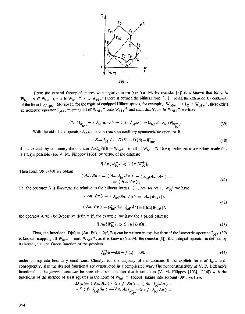
o1(----

Fig. 1

From the genera 1 theory of spaces with negative norm (see Yu. M. Berezanskii [8]) it is known that for u E

Wbd +, V E Wbd- (or u E Wbd+ +, v E Wbd+-) there is defined the bilinear form (-,.), being the extension by continuity

of the form (',')L2(n). Moreover, for the triple of equipped Hilbert spaces, for example, Wbd + - D L 2 D Wbd + +, there exists an isometric operator Jbd+, mapping all of Wbd + - onto Wbd+ + and such that Yu, v E Wbd + - we have

(tt, v ) % ~ + = ( Jbcl+tt, v ) = ( ~t, Jbd÷V ) = (Jbd+U, Jbd+V)~,+ . (39) .. bd,+

With the aid of the operator Jbd + one constructs an auxiliary symmetrizing operator B:

B = J ~ . A , D (B) = D (A) = W~, (40)

if one extends by continuity the operator A:Cbd2(O) -~ Wbd+- to all of Wbd + D D(A); under the assumptions made this is always possible (see V. M. Filippov [105]) by virtue of the estimate

II Au l W~÷ [l ~< C [l u I W ~ ll.

Then from (39), (40) we obtain ( Au, Bu ) = ( Au, Jbd~.A,'o ) = ( Jbd+AU ' Av ) =

----- ( Bu, Av ) , (41)

i.e. the operator A is B-symmetric rdative to the bilinear form (.,.). Since for vu E Wb~ we have

( At, t, B t t ) ----- ( Jbd+Att, AU ) - .--- I1AulW~., 11 =, (42)

( Au, Bu ) =(J t~ .Au , Jbd.Au)=ll BuIW~+IIu, the operator A will be B-positive definite if, for example, we have the a priori estimate

, I I A u l W ~ - , I I > C l i u l L , _ ( f ~ ) I I . (43)

Thus, the functional D[u] = (Au, Bu) - 2(f, Bu) can be written in explicit form if the isometric operator Jbd + (39) is known, mapping all Wbd+- onto Wbd++; as it is known (Yu. M. Berezanskii [8]), this integral operator is defined by its kernel, i.e. the Green function of the problem

Jbd~U-~att--~ f (X), Xe~, (44)

under appropriate boundary conditions. Clearly, for the majority of the domains fl the explicit form of Jbd+ and, consequently, also the desired functional are constructed in a complicated way. The nonconstructivity of V. P. Didenko's functional in the general case can be seen also from the fact that it coincides (V. M. Filippov [103], [114]) with the functional of the method of least squares in the norm of Wbd+-. Indeed, taking into account (39), we have

D [ u ] = ( Au, Bu ) - - 2 ( f , B t t ) --_ ( Au, Jbd;Au )

- -2 ( f , Jb~Att ) ~-(Au, A tt)w~d--2 ( f , Jbd.AU ) _~_

314

= (Au, Au )~d * -- 2 ( f , Au)~,,bd ~ = ll A u - - f I W ~ , [I 2 - (45)

--11 f l W ~ ÷ I12-- [ 1 A u L f [W~bd" It 2 - C~.

But the norm II u I Wbd+- II (see (38)) is difficult to compute in the case of an arbitrary domain ~2 C R n even for elementary functions. V. M. Filippov [114], [102] has carried out constructive computations of this norm and, consequently, of the functionals (45), for the case Wbd+ +, i.e. a space with dominating mixed derivative. We also mention that V. P. Didenko and his student A. A. Popova [26] have presented various ways for the numerical (approximate) minimization of the

functional (45) without its representation in explicit form. 3.2.4. The Construct ion of a Symmetrizing Operator with the A i d o f Fourier Series. We mention that, although

in the general case of the linear operator equation Au = f all the constructions of the Martynyuk--Petryshyn--Shalov scheme can be easily generalized (see V. M. Shalov [123], [124]) to the case of complex-valued operators in complex Hilbert spaces (then, in particular, from the condition (3) of B-positivity there follows the condition (4) of B-symmetry (Sec. 3.1), nevertheless, in this case, the practical constructive determinations of the symmetrizing B-operators become considerably more complicated. Therefore, the following approach (see S. E. Zhelezovskii, V. F. Kirichenko, and V. A. Krys'ko [31]) of the application of the Martynyuk--Petryshyn--Shalov direct variational method for the abstract hyperbolic operator A of

the problem

v" (t) +C2v (t) =f( t ) , 0 < t < r<oo , (46)

v(o) =v ' (o) =0, (47)

considered, in general, in a complex Hilbert space G, presents interest. Here C is an arbitrary self-adjoint, positive definite operator in G; D (---C) = G, having a completely continuous inverse operator C - 1; obviously, the operator A of the boundary

value problem does notcover the case of the usual wave equation utt - Uxx = f(x, t), (x, t) E f] C R 2. We introduce the linear space H = L2([0, T], G) of abstract measurable functions, mapping the segment [0, T] C

R 1 into G with the metric T

( f , g)H = I ( f (t), g (t)) d r , (48) 0

and also the subspace H 1 C H of functions such that for almost all t E (0, T) we have v(t) E D(G), Cv E H, v' E H,

v(0) = 0, with the metric

[v, w l = (v', w') n + ( Cv, Cw) ~r. (49)

The operator A of the left-hand side of the equation (46) is defined on the set D(A) C H 1 of functions v(t): [0, T] --, H, such that v(t) E D(C), Cv E H, v" E H, v(0) = v'(0) = 0. For a self-adjoint, positive definite operator C there exists an

orthonormal system of eigenelements {Uk}, forming a basis in the space G. The symmetrizing operator B is defined by the

relation

B~ (t) = ~, (~' (~), u~)~. cos [~,~ (t - ~ ) 1 - ~.=1 ]l (50)

- - ~,~ ('o (x), ttk)a sin [Z, (t - - x)] dx tcu,

where X k are the eigenvalues of the operator G, corresponding to the eigenfunctions Uk, k = 1, 2, 3, 4, . . . . One has established (S. E. Zhelezovskii [31]) the following fundamental properties of B-symmetry, B-positive

definiteness of the operator A:

(Av, B w ) H = ( B v , A w ) H = ( v , w)h,,,

2 (Aw, Bw) > -y- II B w It ~,

(51)

(52)

(Aw, Bw) > const 11 w l H il 2, (53)

315

giving the possibility to obtain for the problem (46), (47) all the assertions of Theorems 1--3 of the Martynyuk--Petryshyn--Shalov direct variational method.

S. E. Zhelezovskii's idea, presented here, for the construction of the symmetrizing operator B (50) for the wave operator A of the problem (46), (47), can be easily extended also to the case of the parabolic operator A of the problem

Av=-v'+Cv=r, (54)

v(0) - o . (55)

The operator A of the problem (54)--(55) is defined on the set D(A) = {v: v E h, v' E H for almost all t E (0, T); v(O) = o}.

In this case the symmetrizing operator B can be introduced in the following manner:

By = Z (v (x), tt,) o exp [X~ (t -- x)] dx u,. (56) h = l

In this case, also by integration by parts, one can establish the relations (3), (4) (Sec. 3.1) of B-symmetry, B-positive definiteness of the operator A, necessary for the application of the direct variational method: vw, v E H 1 one has

(Av, Bw)H=(B v, Aw)•=-[v, W]A B,

(Av, By). = Iv, ~]AB = II VII ~B,

ilBvll.-.<cllvJ[Ap, c ~ e o n s t > 0,

1 (Av, By) > ~ 1] v I! ~.

Remark 1. The symmetrization of the equations of mathematical physics, i.e. the reduction of a nonsymmetric equation to an equivalent symmetric one by multiplication of the initial equation by an auxiliary ("symmetrizing") multiplier, has been known for a long time (see, for example, Marty [329], where one has considered the symmetrization of an integral equation). Sufficiently complete results have been obtained first for equations with symmetrizable bounded or completely continuous operators (Lax [309], Reid [378], Zaanen [450]). For the symmetrizing operator B = I, where I is an isometric unitary operator; there exists the theory of I-isometric operators (M. G. Krein [44]). A systematic approach to the investigation of equations with a symmetric differential operator has been given by Friedrichs [234], [235] (see also D. F. Kharazov [122], Sarason [390], Silberstein [415]). The symmetrizafion of a composite boundary value problem for the neutron transport equation has been carried out by V. S. Vladimirov [17].

Remark 2. The idea of considering B-positive operators has been expressed for the first time by M. F. Kravchuk and N. M. Krylov (see also M. F. Kravchuk's monograph [42] and the bibliography given there): the direct methods developed on the basis of their ideas are called Krylov methods or moment methods (see A. E. Martynyuk [56], [58]).

In the investigations of Friedrichs [237], Morawetz [337], etc. one has developed the "a--b--c" method, giving the possibility to establish the uniqueness of the solution of the equation A~b(x, y) = fix, y) by obtaining and analyzing the relations 0 = (A~,, a~b + b~b x + C~ky) -> ]] ~b [[ 2 >_ 0. It should be mentioned that already in 1955, Lions [311] has defined, for a given elliptic operator A, a Hilbert space with inner product [u', V]A n = (Au, Bu) with some auxiliary operator B. In 1969 Lions [51] has carried out a symmetrization (by the Martynyuk--Petryshyn--Shalov scheme) of the "nonvariational" boundary value problem (8)--(9) (Sec. 2.1) for the elliptic equation and has posed the problem of finding (Lions [51, p. 255 of the Russian edition]) a general approach for the construction of symmetrizing B-operators for various classes of IPCV. The problem of the construction of operators B for a linear hyperbolic system of first-order equations Au = f, so that the generalized energy inequality (Au, Bu) _ ][ u [[ 2 be satisfied, has been formulated also by A. A. Dezin [23, p. 47].

As it follows from the given survey, the constructive determination of the auxiliary operator B with the properties (2), (3), (4) (See. 3.1) remains a problem of actuality: one does not know explicit constructions of such operators, not even, for example, for the fundamental boundary value problems for nondivergent PDE of elliptic, hyperbolic, and parabolic types with variable coefficients in a multidimensional domain ~ C R n of general form. In particular, the construction of such

316

operators would enable us to apply well developed methods to the approximate solving of the corresponding equations (see

Petryshyn [356], [357]).

3.3. Extremal Variational Principles for Nonlinear Equations with Nonpotential Operators

Let N be a nonlinear operator, acting from the real Banach space U into the conjugate space V = U*, defined on

a lineal D(N), dense in U. In this section we shall consider the problem of the construction of functionals with the properties A--C of the Formulation 3 (Sec. 1.3) for nonpotential operators. We recall (Sec. 2.1) that for operators, satisfying the

potentiality criterion

( N'uh 1, h 2 ) = ( h I, N'uh 2 ) Vtt, hi, h2ED (N), (1)

the desired function f[u] is obtained from the formula I

f [ t t ]=f0-+- l (N( t t t ) , tt ) dt , f0~cons t . (2) 0

3.3.1. The Lyashko--Nashed Scheme of Generalizing the Volterra--Kerner--Vainberg--Langenbach Variational Method. The fundamental idea for the extension of the scheme (see Sec. 2. l) of Volterra [445], Kerner [287], M. M. Vainberg [12], Langenbach [50] to nonlinear, nonpotential operators is due to Nashed [338] and A. D. Lyashko [52]. A more systematic modern presentation of the variational method for nonlinear B-potential operators has been given by Dinc~ [213], while another presentation and the extension of the method to larger classes of B-potential operator has been carried out by V. M. Filippov [105, Chap. IV]. The essence of these generalizations consists in the following.

We consider the equation

N(x) =f, (3)

where the operator N (in general, nonlinear) acts in some real Hilbert space H with inner product (',.) and norm II x II H =

(x, x)l/2; f is a given function from H. We introduce the following conditions: ~) the operator N is defined on a linear manifold D(N) of functions, dense in H; N(0) = 0; vx E D(N) there exists

a continuous (with respect to x) G~tteaux derivative N x such that

H'( t )=(N~+tu% ~)EC,[O, 1] V'x, y, % ~ED (N);

3) there exists a linear closable operator B, D (B)DD(N), J~N (B) = I~ such that( N'xu' By) = (Bu, N'~v)

V x, u, rED (N);

~t")

"0 (N ' (0) tt, Btt) >~ Co Ii a l1 ~ vttED (N);

"I') (N'xtt, Bit) > C (N' (0) zt, Bu) Vx, uED (N);

](f, Bu)l l~Cs(N'(O)u, Bu) x/2 Vu~D(N), fEH,

where C, C o, Cf are positive constants, not depending on x, u. As before, if the linear operator A --- N'(0) is B-symmetric and B-positive (i.e. 3') and/3) hold (for x = 0)), then

it must be also weakly closable. If, however, the B-symmetric, B-positive operator A - N'(0) satisfies also V. M. Shalov's condition 3"") [1231 for any f E H, then it will be (V. M. Filippov [105]) also B-positive definite [Sec. 3.1, (4)1 in the Martynyuk--Petryshyn sense, and the condition of weak closability (see Sec. 3.1) of the operator N'(0) is not required.

The fundamental idea for the extension of the Vainberg--Langenbach variational method to the class of, in general, nonpotential operators N (~) -- 3"")) consists in the following result.

THEOREM 1. If the conditions a)--3'') are satisfied and the element x o E D(N) is a solution of the equation (3), then x o realizes a minimum in D(N) of the functional

1

• (x) = I (N (ix), Bx) tit -- ( f , Bx). (4) 0

317

2. If the conditions ~),/3) are satisfied, then the converse also holds: an element x 0 E D(N), minimizing in D(N) the functional (4), is a solution of the equation (3).

In order to establish the existence of a minimum of the functional (4), one introduces, just as in the linear case (Sec. 3.1), the "energy" space HNB by the completion of D(N) in the metric

[u, v] = (N' (0) u, By),

(5) II u lH~B lI = {u, u y 2.

Subsequent essential progress in this domain has been possible due to Petryshyn's results [358]: he has developed constructions of solvable extensions of sufficiently general nonlinear, nonpotential operators; these constructions have generalized widely the known constructions, i.e. the solvable (variational) Friedrichs extensions [234], [235] of linear self- adjoint operators. On the basis of these results of Petryshyn, V. M. Filippov has introduced into the monograph [105], besides the "usual" solution from D(N), also the generalized solutions, strong and weak, of the equation (3) and has constructed the corresponding extensions ~ of the functional cb(x) (4). In particular, one has obtained (V. M. Filippov [105])

THEOREM 2, Assume that the operator N satisfies conditions ~),/3), 3") with a B-positive definite operator A =

N'(0). Then Vf @ HAB there exists a unique strong solution in HNB of the equation (3); this solution coincides with the unique element which minimizes in HNB the extension ~ of the functional ~ (4) and depends continuously on the given function f.

We mention that from these results, as particular cases, there follow:

-- for N -- A, a linear operator, the Martynyuk--Petryshyn--Shalov direct variational method for solving linear equations with a B-symmetric, B-positive operator A;

-- for B = I, the identity operator, the Kerner--Vainberg--Langenbach direct variational method for nonlinear equations with potential operators;

-- for N = A, B = I, the Friedrichs--Mikhlin direct variational method (see [65]) for linear equations with self- adjoint positive definite operators.

We emphasize that the above mentioned (Sec. 3.2) problem of the constructive determination of a symmetrizing operator B in the nonlinear case is complicated by the fact that one has to seek a linear operator B, satisfying/3), 7') for any element x, occurring as a parameter in ~), 3") in general in a nonlinear manner. We give an example of an operator, satisfying the conditions c0--3'" ).

Example. l

N i t r i c ( - - 1) ~ dk f(/Z(¢+l))-~- x %tt(2P-')=g(x), xE(a, b), (6) , d x k a p ~ l

u(a) = u ' ( a ) = ~' (b) . . . . . u(~) (b),

where k, l are integers, k>~0, 1 < l . . < 2 k + l , f(x)ECk(R1), f ( 0 ) = 0 , t t=u(x) , u(i)-- cd___ff_u. - - d x t '

C2~+I [a, b], satisfying the conditions (7)}; H -- L2(a, b). For any u E D(N), the Gg~teaux differential of the operator N has the form

l

m' (u) tt = (-- 1)~ ~ [ f ' (tt(~+l) h(~+,)] q - Z % h(zp~l)" p = l

Obviously, the potentiality criterion, namely the symmetry condition

(N' (u)h, v)= (N'(u)v, h) Vu, v, h6O(N)

is not valid on all of D(N), i.e. the operator N (6), (7) is nonpotential. We set Bv = v'(x), D(B) = D(N). Then vu, v E D(N), integrating by parts, we obtain

(7)

o (N) = {u (x)e

(8)

1 l

(N' (u) h, By)= f {f" (//(/~+1) F/(/~+l),o(/e+l ) "-~X (-- 1)P+'aph(P)v(P)}dx. 0 p = l

(9)

318

From here we conclude that not only condition a) is satisfied, but also condition fl), i.e. the B-symmetry of the operator N'(u). We assume that

Then from (9) we have

ff (u (~+'~) ~ f f (0) ~ C 5 > 0 Vu6D (N), (10)

b l

Z (-- 1)Pap [tt(P)] 2dx >~ 0 ruED (N) (11) p = i

b

(N' (u) v, By) >1 Cs f [v(~+l) (x)pdx > Ca II v l Lz (a, b)II 2, a

and, therefore, the conditions 3'), 3'') are satisfied. Taking into account (12), by virtue of the obvious relations

[(g, Bu)[~ltgll~ "Iiu'll ~ C , Ilgll~ -(N'(O)u, Bu) "=, condition 3'") is also satisfied.

In this case the space HNB is the completion of D(N) in the metric

[luI[Ns=(N'.(O) u, Bu] ~/~,

b l

Iu, vl=(N'(0)u, B y ) = if(0) a~k+,a~'" a~+,a~+'~' -F~=~ ap(-1F +~ ax~ a~pj dx.

In the given actual case (6), (7), the desired functional (4) has on D(N) the form

1 1 b

• I 1= S(N S dt S + 0 0 a

-Jr- (--1)P ap [tt(V) (x)]2-- gtt' (x) dx. a 1

(12)

(13)

(14)

(15)

Then from Theorems 1, 2 we obtain

COROLLARY 1. a) An element u 0 E D(N) is a solution of equation (6) *=* u 0 minimizes in D(N) the functional • [u] (15);

b) For any g E L2(a, b) there exists a unique element u o E HNB and a sequence {Un}, u n E D(N), n = 1, 2 . . . . . such that

11 u ~ - u 0 1 H ~ t l - * o (n-+ oo), O [ u ~ l ~ d ~ inl~ O[u].

D ( N )

Other examples of the application of the given scheme for the construction of the functionals (4) for the class of nonlinear, nonpotential operators N(c~ -- 2/") have been given by Dinc~ [213].

We mention that if for the linear operators N - A (including the nonpotential ones) one knows some sufficient conditions for the existence of an auxiliary operator B (o~ -- 3`") (see Lemma 1 of Subsection 3.2.1), then for the nonlinear operators N the problem of the determination of the existence of auxiliary operators B (c~ -- 3'") for some classes of operators remains actual.

3.3.2. Tonti's Scheme for Solving IPCV for Nonlinear, Nonpotential Operators. Tonti [432], [433] has suggested another construction of the general solution of the IPCV for a nonlinear equation

N(u) =0~ (16)

with a nonpotential operator N.

THEOREM 3 (Tonti [432]). Assume that an operator N, acting from a Banach space U into the Banach space V = U*, is such that D(N) is a convex set, dense in U, R(N) contains the zero element 0 v of V, the Gfiteaux derivative N~ exists, and the operator (N~)* is invertible wu E D(N).

319

Then for any symmetric linear operator K, invertible on R(K), such that D(K)2R(N), R(K)~ D [(N~)*] vtt£D (N),,~ the operator/q, defined by the relation

~r (tt) = (N'#)*. K. N (u), D (~') = D (N), (17)

has the following properties:

a) an element u 0 E D(N) is a solution of the equation (16) *=* N(u0) = 0;

b) the operator N is potential; the set of solutions from D(N) of the equation (16) coincides with the set of the critical points of the functional

F ( u ) = 1 ( N ( , u ) , / f N ( u ) ) , D(ff)=D(N), (18)

where (.,.) is some real, symmetric, nondegenerate bilinear functional on U x V.

V. M. Filippov [105] has shown that if the operator K is not only symmetric but also positive definite, the operator N acts in a Hilbert space H, so that the bilinear functional (.,-), used in the theorem, is the inner product in H, then the functional F (18) is (just as in V. P. Didenko's approach; see formula (45) in Subsection 3.2.3) the functional of the method of least squares in the Hilbert space Hk:

il ul Hxll2= < u,/¢u> =(u, u)K, 1 2 (7') T'(u)=+ (N(u), K N (u) ) =TflN(u)lHxl[.

For the case H = L2(Q ) one can take for example H K = W}-l(f~) so that for the Dirichlet problem for the Laplace equation

- - A u = f (x), x ~ C : R ~ u (x) = O, x@f2

the functional F:(u) (7') coincides with the known Dirichlet functional

D lul=--FluI=y ~ {I Vttl2--2fttIdx+C/, Cl=(f , Kf). n

V. M. Filippov [105] has established also for the case U = V = L2(fl) that the symmetrizing operator K, given in Theorem 3, exists for large classes of nonlinear PDE of finite order with sufficiently smooth coefficients, i.e. R(N) G C(O),

with local (or nonlocal of the form ~] ~,~a~D ~'uirk--=O, I'kcF=Of2) boundary conditions. Here the symmetrizing al..<l

operator K can be constructed as the operator of the Green function of a homogeneous boundary value problem for a polyharmonic equation in the considered domain f~: this Shows, on the one hand, the closeness of the Tonti and V. P. Didenko approaches (see (7) and (45) of Sec. 3.2) and, on the other hand, the complexity of the construction in this manner in an explicit form of the functionals (18) for domains t] C R n of sufficiently general form. For some nonlinear ODE such

functionals have been constructed by Tonti [432], [433].

3.4. Dual Variational Principles

3.4.1. General Approaches for the Construction of Dual Variational Principles. The dual variational principles,

called sometimes "complementary," "counterprinciple" (see S. G. Mikhlin [65], Velte [441], [442]), play an important role in establishing an a posteriori estimate of the approximate solution of the corresponding variational minimization problem (we shall call it the direct variational problem), especially for nonpotential operators. First we mention, however, some aspects of the determination of a priori estimates of the approximate solution of the direct variational problem of the minimization of the functional for nonpotential operators, on the example of the functional

D [ u ] =[t u]~8 --2 (f, Bou), I~]-[AB. (1)

obtained (Sec. 3.1) for the equation Au = f with a B-symmetric, B-positive definite operator. Here B o is the extension of the symmetrizing operator B (2)--(4)(Sec. 3.1) by continuity tO the entire space HAB (5), (6) (Sec. 3.1), which is possible

320

by virtue of the second relation in (4) (Sec. 3.1). Then there exists a unique element u 0 E HAm minimizing the functional

D[u] in HAB, such that

d ----- ~vaBmin D [tt] =mAin {]1 tt -- Uo [l~8 --I! ~'~ [I~8} = - I [ uo 1[~8. (2)

From here it is easy to conclude that the derivation of an a priori estimate of II Un -- u0 [1AB of the approximate solution of the direct variational problem can be reduced to the following problem of the theory of approximation of

functions. Assume that it is known (from theorems regarding the smoothness of the solution of the equation Au = f or of the

solution of the variational problem) that u 0 belongs to some class W c~ ___ HAB; let {~On} be a system of coordinate functions,

with respect to which one constructs the approximate solution

n

~z. = ~ ak% (x). (3) tz=l

Then the problem of the determination of an a priori estimate of ]] u n - u 011AB is formulated in the following

manner: for an element u 0 E W '~ E HAB estimate its best approximation in the norm 11. ] HAB 11 by linear combinations of the form (3) (i.e. the approximation of this element by systems of algebraic, trigonometric polynomials, etc.). For PDE

with a self-adjoint and positive operator A the norm II- I HAB II (5), (6) (Sec. 3.1), where B - I, belongs to the known class of Euler--Lagrange functionals and the mentioned problem of the theory of approximation of functions has in many cases

a sufficiently complete solution (see S. M. Nikol'skii [69], [70], L. D. Kudryavtsev [47]).

However, for nonsymmetric operators A the norm ]1. I HAB 11 (5), (6) (Sec. 3.1) need not belong to the class of Euler--Lagrange functionals (as, for example, for parabolic equations (see formulas (18), (17) (Sec. 3.2))) and the derivation

of a priori estimates of the solution of the variational problem in the norm []. [ HAB 1[ requires new results in the theory of

approximation of functions. Therefore, for equations with nonpotential operators, a special importance is acquired by the a posteriori estimates

of the approximate solution

[[un--uoll~<e,, n = l , 2, 3 . . . . (4)

where e n are numbers obtained in the process of the computation of u n. The estimate (4) is usually obtained in the following manner. From (2) it is easy to conclude that vun E HAl 3, n =

1, 2, 3, ... we have

d,~ =D[unl~d, (5)

(6)

If one succeeds to construct a functional ~(v) such that

R" (v)~d VvED(W), (7)

sup '~(~,)=a, o (%=ar , O(t~) (8)

then one can find a sequence {Vn} , v n E D(~) 'on = 1, 2, 3 . . . . such that

6n=-W (v~)--~d (n-+oo), (9)

6n<d, n=l, 2, 3 . . . . . (10)

From (6)--(10) we obtain the a posteriori estimate

Ilu.-u01H~[I~<VD[uJ--6~. (11)

321

From (11) and the formulas (4)--(6) (Sec. 3.1) there follows an a posteriori estimate in the norm,of the initial Hilbert space H:

1 II u . - - tto l I I ll ~< '~ V D [u,]-- 6n. (12)

In a series of cases it is possible to construct a variational problem of maximization of the functional ,I,(v), dual to (2), such that

mln D [tt]= D [uol=_d ~ tF luo] = max tF (v), HAB .~I (13)

where t7I is some lineal in D(~), H N HABOUO. For equations (1) with a B-symmetric and B-positive definite operator A, the variational problem (13) is constructed on I:I = D (A)gu0, for example, in the following manner. From (2) ¥u E HAB we have

D [u] > O [Uo], (14)

o [u l - -D lu0] + II u - u 0 (15)

For u E D(A), by virtue of (4), we have

11 tt I]~B = ( A u , Bu)< ~- C [I Au 112,

or, replacing u by u - u o and taking into account that Au o = f, we obtain

(16)

From (14)--(17) there follows that

I] u-- Uo limb ~< ~C ]] Au-- f ]]2. (17)

D [u] > D ltt0] > D [u]---~-II A u - - f II 2, (18)

where equality both on the left and on the right is attained only for u = Uo; this enables us to pose a pair of dual problems

of the form (13): mjn D [u ]= D [Uo] ~ d = tF [uo] = m a x tF (v), H'AB D(A) (19)

where

(v) = D [v] -- ~ II Av -- f 112, D (tit) = D (A). (20)

3.4.2. Three Directions of Development of Dual Principles. For B = I, i.e. for the equation Au = f with a self- adjoint and positive definite operator, the dual variational problem (19), (20) has been obtained through other constructions

by Bittner [158], Pomraning [359], [360] (see also W. Smith [417], P. Smith [418]). At the same time, the presence in the dual functional (20) of the norm ]l Av - f I H [] eliminates in fact the advantage of the "energy" method over the method of least squares: in the case of a differential operator A, H = L2(~), the functional ~I,(v) contains derivatives of the same order as the initial equation; such functionals do not satisfy condition B (Sec. 1.2).

The above presented construction of the dual variational problem can be extended to the case of the nonlinear equation

N(u) =V, (21)

in the following manner (W. Smith [417]). Assume that the operator N can be represented in the form

N (u) =No (u) +Lu , (22)

where N o is a potential operator for which Nff 1 exists Vu E D(N), while L is a symmetric operator on the linear D(N). From (22) we find

322

No (t t) %- Ltt = f=o-u----- No~ { f - - L u } ~ - - Ltt + L Not { f -- L it} = 0. (23)

LEMMA 1. For a potential operator P (df(u, h) = (P(u), h)), symmetric operator L, and a fixed element f E H we have the formula

grad {F (Lu--[) }=LP (Lu--[). (24)

Indeed, we set/I,(u) - F(Lu - f). Then

--'--(#)(u+th)--ak(u))=ltm l--(F (Ltt + t L h - - f ) - - d( I ) ( lL" ~ ) = l ] ~ I ~ 0 t ' t...O t

- - F ( L u - - f ) ) = (P ( L u - - f ) , L h ) - (LP (Lu-- f ) , h),

which proves (24).

Taking into account the symmetry of the operator L and the lemma, for the equation (23) we obtain the desired potential in the form

1 1

Lu)-- t ( I f - Lu], N o 1 [t ( f G (tt) = -- -~ (tt, -- at. (25) Lu)]) 0

We have

THEOREM 4. Let L be a self-adjoint, positive definite operator in a Hilbert space H and assume t:hat the potential operator N 6-1 satisfies the condition

(DNT~ (tt, h), h) > 6. II h ][~,

where 6 ][ L H > - 1 if 6 < 0. Then the equation No(u ) + Lu = f has a unique solution u o and, moreover,

G [u~] = max O [u]. D(P)

Of course, this simplest scheme of W. Smith is applicable only to certain forms of nonlinearity since it requires the explicit form of N 6-1

The dual variational principles form a vast independent branch of the modern calculus of variations and a survey

of its results requires a separate paper. Here, for the orientation of the reader, we give only a brief historical survey of the investigations related to the construction of dual variational principles.

The idea of the transformation of the initial variational problem of minimizing a functional into a corresponding maximization problem goes back to Zaremba [452], [453], Trefftz [434], Friedrichs [234]. The investigations of these authors form the basis of three fundamental directions of the determination of additional variational principles: conventionally, these directions may be called geometric, operatorial, and functional. The first two are closely related in their modern treatment since they make use of the concept of orthogonal decomposition of Hilbert spaces or of the corresponding representation of the operator. Within the framework of these two approaches one has obtained, already in the forties and

fifties, complementary variational principles and a posteriori approximation estimates by variational methods of the solutions of various boundary value problems (M. G. Slobodyanskii [86], [87], Diaz [209]--[212], Greenberg [242], Synge [421],

[422], Washizu [446], Weinberger [447]), The Trefftz method has been generalized to a wide class of boundary value problems by M. Sh. Birman [11], [10]. We mention that in applications the results of these investigations have been used basically for equations with potential operators (see also Telega [425], [426], Collins [176]) since the initial variational minimization problems have been known only for them.

The third direction, a functional one, is based on the dual transformation, introduced by Friedrichs [234] and generalizing the Legendre transformation for the class of Euler functionals (it is discussed in detail in Courant and Hilbert [49]). M. G. Slobodyanskii [86]--[88], generalizing this transformation, has presented a sufficiently simple method for the reduction of a problem of minimizing the "energy" functional to the problem of the maximization of the corresponding functional with the determination of an a posteriori estimate of the approximation (see also Hersch [259]). Starting with the investigations of Noble [342], Sewell [412], Synge [422], in which Courant's canonical transformations have been generalized, this direction has been intensively developed in the works of several foreign mathematicians (see Arthurs [144], Barnsley and Robinson [154], [155], Bittner [158], Carasso [165], Kaplan [286], Pomraning [359], [360], Rall [366], Velte [441]), since it has enabled to obtain simultaneously direct and complementary variational principles for several classes of

323

linear and nonlinear equations. We mention, however, that, also in this direction, the majority of the results have been obtained (see the surveys of Arthurs [14-4] and Robinson [380]) for the equations

Au=F(u) .

Here F is a potential operator, while the linear operator A in most investigations can be represented in the form

A = T . T * + Q ,

where Q is a positive operator, while the operator A is either bounded in the initial space H or satisfies the condition

~,llult2<.(Au, u)~<r~21lull 2, ~,, t~const>0 .

3.4.3. A Generalization of the Constructions of M. G. Slobodyanskii and Velte of Dual Variational Principles on Nonpotential Operators. We indicate two possible directions of the generalizations of the constructions of dual

variational problems to equations with nonpotential operators in the case of the functional and operator approaches. First we give the extension of M. G. Slobodyanskii's approach [87], [88] to the construction of a pair of dual

variational problems for the equation Au = f with a B-symmetric and B-positive definite operator A so that the dual

functional ~(v) (13) will not contain explicitly, as in (19), (20), the operator A. Assume first that u E D(A) and that the operator A can be represented in the form of a sum of operators:

l

A=~.~ Aj, D (A)cD (Aj)c__l-I, (21) ]=l

and for each Aj 3 Bj: D (Bj)~_D (Ai), j = f l l,

l

B = X B j, O (B)c_D ( B 9 2 H , (22) ]=l

vu, v E D(Aj),j = 1, . , l , wehave:

(A~u, Bjv)= (Bju, A~v), (23)

(A~u, B~u)~ct~llul[ 2, (24)

(A~u, B:u) ~.~[3'[IB:ul[ ~. (25)

One introduces the linear set W = D(A1)' ... - D(A/) of/-dimensional vector-valued functions v' = ( v 1 . . . . . Vl) ,

whose independent components vj (j = 1 , . . . , l) are defined first on D(Aj), respectively. The properties (23)--(25) enable

us to define on W the inner product l 1

< u', v' > =X(Ajuj, Bjvj)= x [uj, vj]afi. (26) ]=l y=l

By H'AB we denote the completion of the set W in the norm

11 H II= < , ,'. ,' > (27)

By construction, H'AB -~ HAB (5), (6) Sec. 3.1, if we identify an element from HAB with the/-dimensional vector u' = (u . . . . . u) .

We have (V. M. Filippov [105]) THEOREM 5. If the operator A is B-symmetric, B-positive definite and the relations (21)--(25) are satisfied, then

vf E H 3!u 0 E HAB such that

min D [u] = D [Uo]----- L [u0] = max L (~)'), (28) HAB nAB

324

where L(v') = - I I v'[H'AB II 2 and the vector v' satisfies the relation

(v', ~)=([ , B~) V~=(~ . . . . . :[,)6D.(A). (29)

COROLLARY 2. If the element u 0, minimizing the functional D[u], belongs to D(A) and ~ RA(B)=H,: then

condition (29) is equivalent to the equality

Av' ~-f. (30)

Thus, in this case M. G. Slobodyanskii's variational principle, dual to (1), consists in the maximization of L(v') = - I[ v'IH'AB [I 2 on the set of the vectors v' = (v 1 . . . . . vl), vj E D(Aj), j = 1 . . . . . l, satisfying the equation

A~viq- . . . q-Alvl=f. (31)

For applications this feature is very important, namely that only one equation (31) connects the l independent

variables v 1 . . . . . v I (regarding this question, see Hersch [259]). In the same simple manner one has carried out (V. M. Filippov [105]) the extension of Velte's construction [442]

of a pair of dual variational principles to equations with B-symmetric, B-positive operators.

The functional direction in the theory of dual variational problems consists in the construction of 'the maximizable

functional q (13) from the known functional (1) of the direct variational problem. Pomraning [360] has extended this approach to non-Eulerian functionals, enabling V. M. Filippov [105, Sec. 7] to obtain new dual variational principles, in

particular, for equations with B-symmetric, B-positive operators. In conclusion we mention that the important merit of the dual variational principles and the determination with their

aid of a posteriori estimates have been emphasized in a communication by Courant [179], where, among three basic

drawbacks of the variational method, he names first the fact that the approximations of the solution need not converge to the exact solution, even if their derivatives converge. The dual variational principles give the possibility to obtain not only

an a posteriori integral estimate of the form (12), but also a pointwise two-sided estimate of the approximate solution (see

Cooperman [178], Diaz [210], Fujita [238], Velte [441], Washizu [446]).

325

Chapter 4

STATIONARY VARIATIONAL PRINCIPLES FOR NONPOTENTIAL OPERATORS

Conditions C, D of Formulation 5 (Sec. 1.2) of the inverse problem of the calculus of variations complicate in a significant manner the construction of the desired functional for several important PDE with variable coefficients in multidimensional domains of general form. But in a series of applications of the IPCV (for the numerical solution, for

example by the Ritz method, of boundary value problems if it is not necessary to establish the existence of the solution by the variational method, in applications in theoretical mechanics (see A. S. Galiullin [19]), in the mechanics of continuous media (V. L. Berdichevskii [7])) the condition of the semiboundedness of the desired functionals is not necessary. Therefore, in this chapter we conslder the results of the solving of the IPCV in the Formulation 5, only under the conditions A, B (Sec. 1.2).

4.1. On Global Solutions of IPCV

4.1.1. The Global Lagrangian and Obstacles for Its Existence. We consider the question of the determination of the Lagrange function L(t, u, u) for the second-order ODE (2.2.19) in the case when the operator of this system is potential and the coefficients a,v,/3~ E C~(Ren+I). The proofs of the sufficiency of the Helmholtz conditions, given by G. K. Suslov [94] and Mayer [330], for the existence of a function L(t, u, t)), satisfying the equalities

a_._{ oL I oL at I, Oh~ ] Ou~

are constructive and contain the first method of the calculation of the Lagrangian. According to (1), the Lagrange function L(t, u, t~) satisfies the equalities

i = l , n, (1)

o2L o~io~j = ~tj, (2)

from which, taking into account (2.2.20), there follows that the function L(t, u, u) is determined from the system (2) in the

form I. (t, u, d) = L (t, u, £) .+ (t, C°) (t, u),

I L (2) (t, u, u) = l (1 -- x) ~U (t, u, ~it) t tdt jd, (3)

0

uniquely to within arbitrary functions Li(1) , i = 1 , . . . , n, L(°). Introducing (3) into (1), taking into account (2), we obtain

02L (2) . 1~/_, (2) ( o3L~ 1, OL ~l) 1

For the determination of Li(1)(t, u) we differentiate (4) with respect to uj:

0 8 , o~L <2> °~L (2) ( ~--Y " o-~k ) °~L e) oAj -- o;~p~j o.iohj + +u~ ~ 4

From here, taking into account (2) and (2.2.21), we obtain

Ou I Oat - - 2 \ O n I

(~L (o) 02L (2) •]. ~1)

OL(t l) OL~ 1) duj Out "

(4)

(5)

326

The compatibility of the system (5) follows from (2.2.24). Finally:

1

S , . + %"4 °' LP ) (t, u ) = 7 ~ ou I ' (6) 0

where ~(t, u) is an arbitrary function. The function L(0)(t, u) is determined from the system

oL(o) OL} ~) Out == Ot --[3~(t 'u'O)' (7)

which is obtained from (4) for 0 = 0. It is easy to verify that the compatibility conditions of the system (7) are the equalities (2.2.26) and the solution of (7) has the form

!

L (0) (t, u)~- - - f [3k(t, xg, 0) 0~p(L LI.)

(8) ot 0

Thus, we have THEOREM 1. If the operator, corresponding to the system of second-order ODE (2.2.19), is potential, then the

Lagrangian is determined to within an arbitrary function ~(t, u) by the formulas (3), (6), (8). Remark I. A survey of the various approaches to the construction of the Lagrangian is contained in Santilli's book

[388-389]; see also Engels [225]. In the case when the coefficients a~;, ~3~ of the system of ODE (2.2.19) are defined in some domain f~ C

R2n+l{t, u, 0}, in spite of the fact that the Helmholtz conditions (2.2.20)--(2.2.22) are satisfied, the Lagrange function L, defined everywhere in 9, need not exist. For example (Morandi, Ferrario, Lo Vecchio, Marmo, and Rubano [336]), for

the system of ODE

~1 - - r'~-~--~ O, "" u t 2 2 u2+-F-=O, r~=u~ + u 2,

considered in the domain ~ = R 2 \{ (0, 0)}, the Helmholtz conditions are satisfied, but a global Lagrangian on f~ does not exist (local Lagrangians exist, for example,

1 "2

There exist various kinds of obstructions to the existence of a global Lagrangian for systems of differential equations which are locally Lagrangian (Ibort and L6pez-Lacasta [281]). However, the basic ones the topological

obstructions, covmected with the nontriviality of the cohomology group H2(M) of the configuration space M. A guarantee for the existence of a global Lagrangian for a locally Lagrangian system is the exactness of the so-called variational complex.

4.1.2. On the Variational Complex. The variational complex has been constructed for the first time by A. M. Vinogradov [15]. Subsequent investigations of the variational complex can be found in the works of A. M. Vinogradov [16], [443], [444], Tulczyjew [4351, Takens [4231, Anderson and Duchamp [141], Kuperschmidt [3021, Olver [352], Olver and Shakiban [353], Shakiban [413], et al. We give the construction of the variational complex by following Olver's book [75].

The space of the independent variables x 1 . . . . . xP is denoted by X, while the space of the dependent variables u 1 . . . . . uq by U.

By a total differential k-form on M C X x U we mean an expression w = I: I PJ [u] dx 1, where the coefficients PI are differential functions, dx J = d x J , / k . . . / k d x &, 1 -.<j~ < . . . < ] k ~ p (if instead of u we place the function u = f(x), then we obtain the usual differential k-form on X). The total differential form of co is obtained when at the differentia- tion of co we consider u as functions of x, i.e.

p

Do~ ---. X X D,P- 'dxl AdxJ . i=1 d

The space of the total k-forms is denoted by A k.

3 2 7

By a vertical k-form on M C X x U we mean a finite sum of the form

=~P,[uldu,,A... Adtt,~.

where the coefficients P~j are differential functions (in the vertical forms only the differentials d ~ are present). The analogue of the usual differential is the vertical differential

The space of the vertical k-forms is denoted by ~k.

On the space j~k of vertical k-forms one can define an equivalence relation, under which & is equivalent to &' if they differ by a total divergence

~ - - ~ ' = D j v ( q ) = ~ D ~ @ ~l,Gfi~ k, i=!

where the total derivative D i acts on r/i in accordance with the rules of linearity, differentiation (the Leibnitz rule), commutativity with the vertical differential. The equivalence class, containing d~ E Xk, is called a functional k-form and it is denoted with the use of the integral sign: ~ c~dx. The space of the equivalence classes forms the space of functional k- forms, denoted by

A. = Xk/Div (Ak).

By the variational differential of the functional k-form w = J c~dx we mean the functional (k + 1)-form, corresponding to the vertical differential form &:

~o~ = ~ (do;) dx.

We mention that one can identify the spaces Ap and A°; therefore, if we consider the functional ~£ = ~ L dx as an

element of A °, then its variational differential is the functional 1-form

which, after integration by parts, assumes the form

(here E is the Euler--Lagrange operator). A subdomain M C X x U is said to be totally starlike if each vertical layer M x = {u: (x, u) @ M} is a starlike

domain in U and the horizontal layer in the basis • = {x: (x, 0) E M} is a starlike subdomain in X. Now, after introducing the required concepts and notations, we can formulate the following

Statement. The complete variational complex

D D D D E 1 6 2 6 0 ~ R ~ A o ~ A1 ~ • • • ~ Ao=-1 -~ A p ~ A , - ) - A , ~ . . .

is exact on totally starlike domains M C X × U. The exactness of the variational complex at the term A 1 brings about the existence of global solutions of the IPCV.

Thus, the variatiOnal differential of the functional 1-form ¢o = j {P'du} dx is equal to

dtt• Adtt=J dx = I {Dp (du) Adu} dx,

where Dp is the Fr6chet derivative of P. Integration by parts enables us to obtain the expression

=+ S 328

From here it follows that the form o~(~) is closed if and only if the differential operator Dp is symmetric. From the

exactness of the variational complex there follows THEOREM 2 (Olver [75]). Assume that the domain of definition of P[u] is a totally starlike domain M C X x

U. Then P is the Euler--Lagrange expression for some variational problem ~ = f L dx (P -= E(L)) if and only if the Fr6chet derivative Dp is symmetric (Dp* = Dp).

Remark 2. In this case the Lagrangian for P can be constructed with the aid of the homotopy formula

1

t [.J = 1 tt. p [~ul ax.

4.2. Variational Principles for Systems of Linear ODE

In this section we present approaches for solving the IPCV for systems of ODE with nonsymmetric operators by taking into account the specific linearity of the system: as it will be seen in the sequel, the approaches for solving the IPCV for nonlinear equations and systems, presented in a series of other sections of this chapter, can be also applied to the

linear case, but they have their own particularities. 4.2.1. A Symmetrizing Operator for Systems of Second-Order Linear ODE. Without loss of generality, we

consider a system of n second-order linear ordinary equations

u@2A 1 (t) t~ + A0 (t) tt = 0, (1)

where A 1, A 0 are n x n matrices, defined and sufficiently smooth on an open interval, containing the initial value t o. We consider an IPCV for the system (1) in the following formulation: determine a nonsingular matrix B(t) such

that, after multiplication by it, the system (1) represents the system of Euler--Lagrange equations for a functional of the

form (4) (Sec. 1.1), i.e.

B (t) (~ + 2A1 (t) t / + A0 (t) . ) =-- e ( oL ~ oL (2)

From the point of view of the general theory of variational principles for linear equations (Sec. 3.1), the formu- lated problem reduces in fact to the determination of a linear operator B such that the linear differential operator

d 2 A=-~-ir+ 2AI ~-~T + Ao,

is B-symmetric, assuming that the linear operator B is the operator of multiplication by the matrix B(t). The Helmholtz conditions (2.2.15)--(2.2.17) for the system (2) can be written in the form

B = B r, (3a)

= BA I + ATB r,

Br = 2 ~ (BA1)r+ BAo-- (BA0) r.

(3b)

(3c)

We have (Sarlet and Bahar [399]) THEOREM 1. The potentiality conditions (3) are equivalent to the conditions

S ~ ,sT~

#=A~I B + BA1,

B (Xo-- A~ - - A1) = (B (Ao-- A~ -- A0) r,

(4a)

(4b)

(4c)

329

where S = B(to).

Remark 1. Condition (4c) can be obtained from (3c) as a result of the elimination of 13 by virtue of (3a)--(3b). Obviously, taking into account (3b), the matrix B(t), having a symmetric initial value S, remains symmetric also after- wards; therefore, (3a) is equivalent to (4a).

Remark 2. If the assumptions of Theorem 1 are satisfied, then, obviously, the Lagrange function assumes the form

ur Bu @ urA, Biz + I ur (Arl SA1 _ S (Ao-- A~-- A,)) u. L = 7

We introduce the operator ~A1, associating to an arbitrary differentiable n x n matrix q,(t) the n x n matrix ~A1(¢) according to the rule

~A, (q)) = [A~, q)] -}- d), [A,, O] = AIO-- OA~. (5)

Now we define the operators ,~A1 k, k E N, acting on an arbitrary, sufficiently smooth n x n matrix ,I,(t) in the following manner:

~, , (~))=/~, (/~=~ (¢)), k > 2, . ~ . , ((I)) = -~A, (q)). (6)

Finally we consider the n × n matrices o(k)(t), k = 0, 1, 2 . . . . . defined by the equalities

(I }(°) = Ao -- A~ -- Jt 1, (7a)

elk) = ~ , (¢10)) = [A1, ~(~-')J -}- ~ q)(~-o, kEN'. (7b)

We have the following statement (Sarlet, Engels, and Bahar [405]).

THEOREM 2. The system (1) admits a variational multiplier matrix B(t) if and only if there exists a constant nonsingular symmetric n x n matrix S, satisfying the conditions

S ~ (~/(to) = (SO (~ (t0)f, k = 0, 1, 2 . . . . . (8)

Remark 3. The conditions (8) represent an infinite system of linear homogeneous algebraic equations and, in the

general case, the existence of a nonsingular matrix S, satisfying (8), cannot be justified by the investigation of a finite subsystem of the infinite system (8); therefore, in applications, the relations (8) are important, first of all, as necessary

conditions for the existence of a multiplier matrix and are used for the proof of the fact that such a multiplier does not

exist. However, in certain case, Theorem 2 enables the proof of the existence of a multiplier matrix, as shown by the

following COROLLARY. If for some I E N we have

(I) ~l~ (t) ~ 0 , (9)

then for the existence of a variational multiplier matrix B(t) it is necessary and sufficient to that conditions (8) be satisfied

f o r k = 0 , 1 . . . . . l - 1. We single out the particular case when l = l, while condition (9) has the form

~1 [A1, Ao-- -A~] q - ~ (A0-- A ~ - .41)= 0. (10)

In this case the multiplier matrix B(t) is determined as the solution of the matrix differential equation (4b), having as initial value a nonsingular matrix S, such that the matrices S and S(Ao(to) - A12(to) - ,h,l(to) ) are symmetric.

We note that in the case of constant A o and A 1, the equality (10) reduces to the condition

[A~, A0]=0, (11)

and, therefore, the conditions of the form (9) are called conditions of generalized commutativity of order I (Sarlet [393]). The commutativity conditions (11) have been investigated and applied in several works (Kwatny, Bahar, and Massimo [305], Sarlet [393], Bahar and Kwatny [147], etc.).

330

If the first-order commutativity condition (10) is satisfied, then the system (1) admits at least n independent

multiplier matrices. Indeed, the symmetry condition of the matrix S(Ao(t0) - AlZ(t0) - Al(t0)) imposes at most n(n - 1)/2 constraints of equality type on the n(n + 1)/2 elements of the symmetric matrix S; therefore, the matrix B(t) is at least n-parametric.

Thus, if ,b(1) = 0 and B 1 is a multiplier for the system (1), then the matrix B 2 = BI,I,(°) is also a multiplier for (1) (Sarlet, Engels, and Bahar [405]); moreover the mentioned property has direct analogues in the case of commutativity of higher order, but under additional constraints.

We also mention that, under the condition (10), to each multiplier matrix B(t) of the system (1) there corresponds a quadratic first integral of the system (1) (Sarlet and Bahar [399]):

I = itrB[z a c 2 u r A r B i t -t- tt r ( B ~ I°) -b ArIBA~) tt. (12)

4.2.2. The Description of Systems of Linear ODE, Admitting a Variational Multiplier. We consider a linear transformation of the independent variables

u = U ( t ) v , (13)

where U(t) is a nonsingular n x n matrix, a particular solution of the matrix differential equation

(]-I-AiU=O. (14)

The straightforward substitution of (13) into (1) shows that in the new variables the system (1) assumes the form

v + Z ( t ) v = O , Z = " r - t ' ' 2 u (~.0-- A~ -- A1) U. (15)

Due to the absence in (15) of terms containing v, the conditions of type (4) for the system obtained by multiplying (14) by the multiplier matrix S, have the form

S = S r , (t6a)

5 = 0 , (16b)

S Z ( t ) = (SZ ( t ) )r. (16c)

Remark 4. The choice of the notation S for the variational multiplier matrix of the system (15) is justified by the fact that if U(t) is the solution of (14), having the n × n identity matrix as the initial value, then the general solution of (4b) is determined by the formula

B (t) = (U- ' ) r s g - ' , (17)

where S is an arbitrary nonsingular symmetric constant n x n matrix and, moreover, introducing (17) into (4c), we obtain

(16c), i.e. the matrix S, being the initial value of B(t) and defined according to (4), satisfies (16); the converse also holds. The systems of the form (1), admitting a multiplier matrix B(t), can be characterized (Sarlet, Engels, and Bahar

[405]) in the following manner. Since the matrix S is symmetric and nonsingular, there exists a constant orthogonal matrix T such that the matrix A = TTST is diagonal with nonzero diagonal entries; then the matrix f/(t) = TTz(t)T must have the following "semisymmetric" structure

[: o~v o12 . . . ~

a = | a~2°~12 °~22 "" " |

~130)13 a23~23... . . . . . . . . .}

where ¢oij, i _< j, are arbitrary functions of t, aij, i < j, are arbitrary constants, satisfying the equalities

a~a~h=a~j, i ~ ] ~ k .

We have (Sarlet, Engels, and Bahar [405]) the following

331

THEOREM 3. A system of the form (1) admits a variational multiplier matrix B(t) if and only if the matrices Al(t ) and A0(t ) have the following structure

A~ = --/.2U -~,

A0 = U (f2-- U -~ U + 2 (U-~U)2) U % (19)

where ~](t) is an arbitrary matrix of the form (18) and U(t) is an arbitrary nonsingular matrix, whose initial value T = U(t0) is an orthogonal matrix.

Remark 5. Obviously, Theorem 3 has only a theoretical value since for a given system (1) it is complicated to verify whether the matrices A 1 and A 0 have the form (19).

4.3. Variational Principles for Systems of Nonlinear ODE with Nonpotential Operators

4.3.1. A Variational Multiplier Matrix for Systems of Second-Order ODE. In order that the system of ODE

t t ~ = f i ( t , u, tz), i = ' I , n, (1)

and the system of Euler--Lagrange equations for some regular Lagrange function L(t, u, u)

d___(O~)__at OukO--~-L = 0' k = l,----n, (2)

should have the same set of solutions, it is sufficient that the system (1), after multiplication by some nonsingular n × n matrix (cxij(t, u, l))), should satisfy the potentiality conditions (2.2.20)--(2.2.22) with the consideration of the equalities

~ i = - - (xijf j, i = l , ft. (3)

In this case, the function L(t, u, 0) and the elements of the matrix (oqj) are connected by the relations O2L

a~ j_ OdiOu~ ' i, j = l , n.

Definition 1. If the indicated matrix (~ij) for the system (1) exists, then we say that the system (1) admits a

variational multiplier matrix. We mention that the problem of the determination of the variational multiplier matrix for the system (1) can be

considered also as a particular case of the more general problem of determining an auxiliary linear operator according to

the scheme of Subsection 3.3.1 of the extension of the variational method to nonlinear equations with nonpotential

operators. For the construction of a system of equations relative to the elements of the unknown matrix (~ij) it is sufficient to

introduce (3) into (2.2.21), (2.2.22), as a result of which we obtain a system of algebraic equations and partial differential

equations relative to c~ij. In the case of the compatibility of this system, under the condition that det(~ij ) # 0, the IPCV for

the system (1) in the corresponding class of Euler--Lagrange functionals is solvable and the solution is determined

according to Theorem 1 of Sec. 4.1. We mention that I. M. Rapoport [81] has obtained a system that differs from the indicated system by the presence

of a group of redundant equations, which follow from the equalities (2.2.23) and can be obtained as a consequence of other

equations of the system. However, the formal integrability of Rapoport's system has not been investigated. The approach to the investigation of the IPCV suggested by Douglas [218]--[220] is much more efficient. THEOREM 1. A nonsingular n x n matrix c~ = (oqj(t, u, fl)) is a variational multiplier for the system (1) if and

only if the conditions (2.2.20) and the conditions

D_._~ (ZA -]- ATo¢, (4a) D t - -

(Z~ (0) = (gO(O))T~- (4b)

332

are satisfied, where D/Dt = 0/0t + 121k0/0u k + fk0/0(lk, ~(0) = B - A 2 - DA/Dt, while the elements of the n x n matrices A and B are determined by the equalities

I Oft Of~ Ai] = - 20d]' Bu=--Ou'-'- l' i, j = ~ , n.

Remark 1. The necessity and sufficiency of the conditions of Theorem 1 have been obtained by Douglas directly without the use of the Helmholtz conditions, although the equalities (4a) and (4b) can be derived from the relations (2.2.21), (2.2.22), respectively, by taking into account (2.2.20) (Sarlet [394]).

Directly from Theorem 1 we obtain the following

COROLLARY 2 (Sarlet [394]). If the functions fk do not depend on u, then the elements of the matrix o~, not depending on u, are constants.

In the case of adiagonal multiplier matrix ~x, the mentioned statement has been given by Havas [250].

We mention that the equalities (2.2.20) and (4) represent an overdetermined system of partial differential equations, which is represented in a form that is very convenient for subsequent investigation. Thus, some of the equations are linear

algebraic, enabling us to perform easily a reduction of the system. The system has normal form, which facilitates the application of the methods from the theory of the formal compatibility of systems of PDE. Finally, the application of the

operator D/Dt to the algebraic equations, occurring in the system, and the use of (4a) allow us, without special computa- tional exertion, to extend the system and to obtain new algebraic equations, and, ultimately, also to integrate the system.

However, so far this has been done only for n = 1 (Darboux [194]), n = 2 (Douglas [220]) and for a diagonal matrix c~

for arbitrary n (Havas [250]).

For the general case one has obtained a series of results that facilitate the investigation of the compatibility of the

system (2.2.20), (4). THEOREM 2 (Sarlet [394]). Let U(t, u, t)) be the solution of the matrix partial differential equation (the existence

of which is ensured by the Cauchy--Kovalevskaya theorem)

DU 57-+AU=0

with initial value U(t o, u, u) = I n, where I n is the n × n identity matrix. Then any multiplier matrix c~ of the system (1)

can be represented in the form

~= ( U-') ~sU-', (5)

where the matrix S = (Sij(t, u, £t)) satisfies the conditions

°SJkll (S,/--Sj,)I,=to=O,(°o@i~ ~--~-/,,=,° = O,

OSk, oSI, . 1 o [of, o off..L s,j))l,=,o O, (6)

D"'~S'=o, S Z = ( S Z ) T, Z = U - 1 0 ( ° ) U . Dt

We consider the n × n matrices q,(k)(t, u, t)), k = 1, 2, ..., defined recursivety by

O (~+1) (t, It, tt)---~- DO(") D¢ b[A, O(~)], [A, O(~)]=A@(~)--O(¢)A. (7)

Since the matrices ~x(t, u, u) and S(t, u, u) for t = t o coincide, we denote their common value by ~(u, u):

(i (u, ~ ) = ~ (to, u, ~ ) = S (to, u, h).

THEOREM 3 (Sarlet [394]). The system (1) admits a multiplier matrix a if and only if there exists a nonsingular matrix a(u, t)), satisfying the conditions

o~ik 0~jk (8a) = at , o~j - o~-7-'

OCTkl O(~]i . 1 C) /Oft ~ Oft (ill) = 0, (8b)

3 3 3

O0 (~) It=t, = (a~, (~) It=to) r, k : O, 1, 2 . . . . . (8c)

Remark 2. For the given system (1) all the matrices •(k) consist of known elements and, therefore, the linear homogeneous algebraic equations (8c) can be solved successively with respect to the elements of the symmetric matrix a. Thus, the investigation of the conditions (8c) alone may lead to the conclusion that the system (1) has no solution of the IPCV in the class of Euler--Lagrange functionais, i.e. in the Formulation 3 (Sec. 1.3).

We point out some other investigations in which one has considered the problem of the determination of the variational multiplier matrix for systems of the general form (1).

In Caviglia [171], the considered problem is reduced to the determination of compatibility conditions for some

exterior differential system, corresponding to the system of PDE (2.2.20), (4a), (4b), relative to the unknown elements of the matrix c~. The assertions obtained with the aid of Cartan's approach [39] form a certain development of Sarlet's results [394].

In Caviglia [172] one has also introduced a system of necessary conditions for the existence of a matrix multiplier

and one has shown that the elements of the matrix multiplier are transformed at a change of coordinates as the components

of a symmetric (0, 2)-tensor field if and only if the indicated elements are polynomials in the generalized velocities with coefficients depending on the coordinates and on time; finally, Caviglia [172] has obtained an infinite system of linear

equations with respect to aij, called invariance identities. It has been established that the consistency of the compatibility conditions and the invariance identities guarantees the existence of the variational multiplier matrix.

In Morandi, Ferrario, Lo Vecchio, Marmo, and Rubano [336], Marmo and Rubano [321], [323], at the consider-

ation of IPCV for the system (1), one has made use in an effective manner of the method of bivector fields.

The problem of the determination of the variational multiplier matrix for (1) can be considered in the presence of

additional restrictions. For example, following Marmo, Rubano, and Thompson [324], we consider the case when

- - r j ~ = r ~ j

(the functions Fjlk are interpreted as the symmetric connectedness coefficients) and the multiplier matrix ~ has the form a -- (aij(u)) (then the corresponding Lagrangian L = 1/2t~ij(U)tli0J is quadratic). The indicated formulation of the problem

has extensive applications in Riemannian geometry and in general relativity theory (Schmidt [414], Hall and Kay [248],

]hrig [282], et al.). One of the results obtained by Marmo, Rubano, and Thompson [324] with the use of the methods of IPCV is the following: a necessary condition for the solvability of the above indicated problem is the existence of

nontrivial solutions of the system of linear algebraic equations (relative to ~ij)

h k a [~ Ri,,akl-- Rj,,aki + R~,,aki -- Ri,,aki ~ 0,

where R]i j are the components of the curvature tensor, corresponding to the connectedness (pjik). In a series of investigations the authors have introduced by various methods conditions for the potentiality of a

nonlinear differential operator, determined by the initial system of ODE, including also the case of the system (1),

multiplied by some matrix a. However, the most difficult and, in the general case, unsolved question consists in the

elimination of the elements of the matrix o~ from the potentiality conditions and in the determination of solvability

conditions of IPCV in the form of relations imposed only on the right-hand sides of the initial system of ODE (1). Presently there are known only some investigations containing results in this direction. These are the results of Darboux

for n = 1, of Douglas for n = 2, and of Havas for the case of a diagonal matrix a for arbitrary n, to be considered in the

subsequent subsections of this section, and also the results of Sarlet, Engels, and Bahar [405] for the case of a system of

linear ODE, considered in Sec. 4.2. 4.3.2. The Case of a Diagonal Variational Multiplier Matrix. An exhaustive investigation of the case when the

multiplier matrix o~ is diagonal, i.e.

a-~diag(ai(t , u, u) , . . : . , a,( t , u, u) )

has been carried out by Havas [250]. THEOREM 4 (Havas [250]). The nonlinear differential operator, corresponding to the system of ODE, obtained

by multiplying the system (1) by a diagonal matrix or, is potential i f and only if the following conditions hold:

Oat n i ~ j , • ' ----- ~' ( 9 ) Oa]

334

O~ifl Oc~]f 1 ~-.--7-:---.---0, i4=j ,

Ouj oui

Oatfi &z t • __Ocq Out ous uj--t---~,

O~tfi 0 ~ - : - = ~ , i # j # k # i , Ou jOun

where i, j, k = 1, . . . , n.

C)¢zlf i O(z]f] ( l~k~-~--~f ) O(ztf-----~l , i4= j , Ott] du i Oh]

(10)

(11)

(12)

(13)

(14)

Remark 3. The equalities (9) follow from the relations (2.2.20), (10)--(11) from the relations (2.2.21), (12)--(13) from the relations (2.2.23) (and are therefore redundant), while (14) follows from (2.2.22) by taking into account (10).

Conditions (9)--(14) represent a system of PDE relative to the unknown functions oq(t, u, t~), i = l . . . . . n, and

now the fundamental problem consists in obtaining necessary and sufficient conditions that have to be imposed only on the right-hand sides fi(t, u, t~), i = 1 . . . . . n, of the initial system (1) for the compatibility of (9)--(14), and the system of equations for the determination of the integrating factors c~i(t, u, t~), i = 1 . . . . . n.

Definition 2. A system of ODE

O~ (t, i t 1 . . . . . t t . , h 1 . . . . . u . , ,~i . . . . . ttn) = 0 (15)

is said to be irreducible if (15) cannot be partitioned into subsystems such that the sets of the indices of the variables,

occurring in these subsystems, are disjoint. For any pair of equations of the system (1) with indices r, s we introduce the notation Crs, defined in the following

manner:

1) if 0fr/0U s ~ 0, then Crs = --Ofs/OUr(Ofr/Oas)-l;

2) if Ofr O, of~ 4=0, then C,~ - ° f " {Of, ]-,; =- o . , j

3) if Of--~O, Ofr = 0 , then the quantity Crs is not defined. OUs OUs

Definition 3. We shall say that the equations from (1) with indices r, s are joined by a "chain" if there exists

expressions of the form

Cry, = CrvCw, C~vq~ = C~vC~qCq~ . . . .

(no summation is carried out with respected to the repeated indices), where all the quantities Cij are defined.

THEOREM 5 (Havas [250]). For an irreducible system of ODE (1) a diagonal multiplier matrix ~ exists if and

only if for any pair of equations with indices i, j all the chains joining these equations have a common value C[ijl, i.e.

Ctij| ~ C l ] ~ C i . / ~ Ci. . j = . . .

and the following conditions hold:

°(~-4=0, r4=s=~°/. ~ 4=0, (16a) OUs Our

c) f_~r O ' Oft =/= S=~c)of ; = 0 , O~r ou~ o-~-&O, r o/ , 4=0, (16b)

: . ors O f t = o , Oft- = 0 , r =/= s=*-. = 0 , Of~ = 0 , (16c) OUs OUs OUr OUr

O"f~ --= O, (16d) OhkO~

0 Ohi (C[t~l (C[ul)-~))= O, (16e)

335

p O~ft 0 c)~ft -I- O - - '-' I'~1 " ~ +0-'~[ In Clin I = - - Clul-o-~u~ ~ . . ~ u t In Clu ~, (16f)

O~fk ~ __ Oouk Ctktl ~ ) - - 0 ' (16g)

0__ 0'/___.! + ~ui in C[uq) = 0, (16h) o& ( - c i . , i o,i~ '

0 C l u l Ou---~ ~ ) Civil 0u~"7"2-" )'

Ou~O'~ ( -- CI'¢I °2ft+ °-~-lnCF~l)=~ul(--Clkq ~ ) out (16j)

~-'/--- f t - - f ~ In °f.t = --°J&-~ll4°-~-{°lt)-'4-°l~(°i~]-' O,k k m ~ ~ Ouk Out--Ouk t ~ ) ' O-~,t~O-d~i) ' (16k)

( ~ . 0 0 0 0 ) 0f~ 0/k (16/) u"~o,+Ti-- f~ - f~Y~-~ ~nct'"~=o;, o~ "

The unknown multipliers a i, i = 1, . . . , n, can be obtained with the aid of the following statement. T H E O R E M 6 (Havas [250]). The integrating multipliers satisfy the following equations for i = 1 . . . . . n and k ;e

¢x k = C l~ilCX t, (17a)

_.o._ In ¢x t = O, (17b) Ouk

In ~x t =-~0. In Cii~ 1, (17c) Out Oui

O In a t - O'yk (17d) = - - C ' [ ~ i l ~ , duk d~ i

,~ O~/j. 0 (17e) 0utO In cq = - - '~ li~l ~ -t-~u t In Cliel,

c) Of i 0 ( ) 0-- / ln~ '= °d--'t+f"~"t lncli~I+~m+, Ct'~'~'°~f'-'--~tt~h~ "~ + Ctl~] o'u~°Y' 0ui° lnCli~ 1 /t,. (17t")

Remark 4. In order to find ai(t, u, 120, i = 1 . . . . . n, it is sufficient to solve the system of PDE (17b)--(17f) relative to one of the multipliers, while the remaining ones are determined according to (17a). The integrating multipliers a i, i = 1, . . . , n, are determined from (17a)--(17f) to within a multiplication by an arbitrary constant.

In the general case the initial system of ODE (1) must be decomposed into irreducible subsystems and Theorems 5, 6 are applied to each of these subsystems. If each of the subsystems admits a diagonal multiplier matrix, then, obviously, this property is shared also by the initial system and, moreover, the Lagrange function for the initial system (1)

is equal to the sum of the Lagrange functions for the subsystems. We give an illustrative example (Havas [250]) for the existence of a diagonal multiplier matrix. Example 1 (Harmonic oscillator with damping). The equations of the motion

m--~=--k~---Kr- r = ( x l , x2, xa), kK+O, 4 i n K - - k 2 > 0

of a harmonic oscillator with damping admit a diagonal multiplier matrix a = diag(al, ..., an), where

"2 " 2 I al = (mxt + kxtxt + Kxi)- , i = 1, 3.

In this case the Lagrange function has the form

-- ,,?. [x~--~-m~k~ ctg \ xt-~-m-------~"--~_k2' ) l l n ( m x , + k x t x , + K x , ) }.

336

4.3.3. Constructive Solutions of the IPCV for One and a System of Two Second-Order Nonlinear ODE. The cases of a single nonlinear ordinary differential equation and of a system of two such equations, whose operators are

nonpotential, have been investigated by several authors, taking into account their specific character, in a more complete manner and by methods that are different from those presented in the previous subsections.

First we consider one second-order ODE

~ ' = f (t, u, u). (18)

It is easy to verify, making use of the potentiality conditions (2.2.20)--(2.2.22), that the operator of the differential equation (18) is nonpotential in the sense of Formulation 3 (Sec. 1.3), if 0f/0t~ ~ 0. However, equation (18) always admits infinitely many solutions of the IPCV in the Formulation 3 and, moreover, with essentially distinct (alternative) Lagran- gians L(t, u, 4). This result has been obtained for the first time by Darboux [194] (p. 53 of the Russian edition) in 1894.

Darboux, similarly to N. Ya. Sonin's approach [90], has reduced the problem of the determination of L(t, u, u) to the integration of one linear second-order PDE

O~L . j r . O~L 02L OL o,--- ~ 3"_ ~ h - t - = 0 , (19) o~ot Ou

for which the existence of the solution for fit, u, u) E C°~(9), 9 C R3{t, u, u} is guaranteed by the Cauchy--Kovalev- skaya theorem, and the solution has generality c~ lf(2), i.e. it depends on an arbitrary function of two arguments. Introduc- ing the notation c~ = 02L/0t~ 2, by differentiating (19) with respect to ~1, we obtain the equation

oa ~'u " Oa. , Oa 0u y 4- c~ (20) t ~ u a t e - = 0 ,

for the determination of the integrating multiplier ~(t, u, l~). The general solution of (20) in implicit form is determined by

the formula

O(qh, £o2, q~s)=0,

where ,I, is an arbitrary function, while ~i(t, u, t), ~), i = 1 . . . . . 3, are independent first integrals of the system of ODE

dcz dtz d u - - - - - 3 7 - : - - f - =- -d --=dr" (21) - ~ 0--T

Equation (20) represents the unique restriction on c~, imposed by the Helmholtz conditions (2.2.20)--(2.2.22) for n = 1; therefore, by virtue of the sufficiency of the Helmholtz conditions, each solution of (20) is a multiplier for (18). Thus, the problem of the determination of the entire collection of integrating factors for n = 1 reduces to the determination of a complete system of first integrals of the system (21).

If the multiplier c~(t, u, t~) has been found, then the Lagrangian L(t, u, fl) can be computed in a different manner (Yan [448], Sarlet [391], et al.), for example, by the formula (V. V. Dodonov, V. I. Man'ko, and V. D. Skarzhinskii [29]):

S S " ' L (t, u, ~t)= ( i t - - z )cz( t , u, z ) d z 4 - f ( t , r 1, tt ,)c~(t, ~1, tt,)dTl+~- •, . t l , t Z ,

An other approach for the construction of the Euler--Lagrange functional has been suggested by Kobussen [293]. Various particular cases of the determination of Euler--Lagrange functionals for the one-dimensional case have

been considered by several authors (Yan [448], G. L. Shpil'ker [132], Ramires and German [79], Jones and Vujanovic [284], et al.). We mention also a series of investigations in which one has obtained alternative variational formulations in the class of Euler--Lagrange functionals for a one-dimensional oscillator, including the case with damping (Denman [204], van der Vaart [437], Bahar and Kwatny [148]). As a rule, in these works also the question of the quantization of the corresponding classical system has been considered.

337

When passing from the single second-order equation (18) to the system of second-order equations (i), the problem

of the determination of the set of the solutions of the IPCV in the formulation 3 (Sec. 1.3) becomes significantly more

complicated since the unique partial differential equation (20) is replaced by an overdetermined system of PDE relative to n(n + 1)/2 unknown functions and there arises the problem of the compatibility of this system.

The first results in the problem of the construction of the entire collection of the desired Euler--Lagrange

functionals for n = 2 refer to actual systems of ODE. Hamel [249] has obtained the solution for the case when the integral curves of the system of the ODE are straight lines, i. e. the system of the ODE has the form ti --= 0, ~' = 0. Davis [195] has derived a system of PDE for the components of the variational multiplier matrix in the general case; however, the

mathematical difficulties, arising during the investigation of this system, have restricted him to the consideration of some

actual examples. Significant results relative to the solvability of the IPCV in the class of Euler functionals for n = 2 are contained

in a cycle of papers by Douglas [218]--[220]. Douglas has obtained for an arbitrary n a system of PDE relative to the

elements of the variational multiplier matrix, differing from Davis' system [195] and more suitable for integration; he has

investigated the formal compatibility of this system for most of the occurring cases, making use of the methods of Riquier's orthonomic systems [379]. As mentioned in certain investigations (see Santilli [388]), the mathematical complex- ity and awkwardness of Douglas' results have hindered to a certain degree the interest in the construction of variational principles in the class of Euler--Lagrange functionals for systems of ODE with nonpotential operators. We give here only

some results due to Douglas [220]. Assume that the initial system of ODE has the form

u = F (t, u , v , tt, v ) , ;o = O (t , tt, v , u , v ) , (22)

where the functions F and G are analytic in some neighborhood of some fixed point (t 0, u 0, v o, rio, %). For an arbitrary n Douglas has shown that the problem of the determination of the variational multiplier matrix reduces to the integration

of the system (2.2.20), (4a), (4b), consisting of PDE and linear algebraic equations relative to the elements of this matrix.

For the elements of the 2 x 2 matrix ~ we introduce the following notations: L = OLll, U = ~ 1 2 = °t21, N =

~22' Obviously, the matrix c~ is nonsingular if and only if

LN_M2~O. (23)

In the considered case the equations (4a) assume the form

dL dt +F~L ~-G~M=O,

dM ~_~£ F;,L I 1 at +7 (F;, +G;) +-zG?,N-~O,

aN-kF;M -+- G~N = O, dt

(24)

where

e o • o 4 o o _ _ + 0 o d--r~-Y/+u-g~ ÷ -b-b - + F o~ o--~"

The second group of equations (2.2.20) has the form

L~M~, N~=M~, (25)

while the system of linear homogeneous algebraic equations (4b) reduces to the single equation

where

AoL + BoM+CoN= 0,

Ao= ~ Fg--2F~ - 1 Fg(F~-}-G~),

cl 2 Bo= --.--dT F;..I- ~i-G;.-b 2 (F,,-- G~)-k - t (F ~ --G~ ),

1G~(F[~--]-G~). C o = - - .-~T G ~ -I- 2 G u -I- y

(26)

338

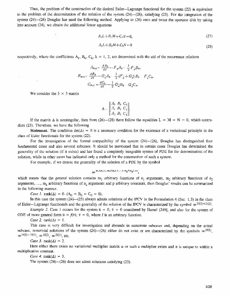
Thus, the problem of the construction of the desired Euler--Lagrange functional for the system (22) is equivalent

to the problem of the determination of the solution of the system (24)--(26), satisfying (23). For the integration of the

system (24)--(26) Douglas has used the following method. Applying to (26) once and twice the operator d/dt by taking

into account (24), we obtain the additional linear equations

A1L+BIM+CIN=O,

A2L-~ B2M + C2N = 0

(27)

(28)

respectively, where the coefficients Ak, Bk, Ck, k = 1, 2, are determined with the aid of the recurrence relations

n~+l dAk FuAk - I F dt ~ ~Bk,

B k + l - dBk G£A~-- 1 dt 7 (F £.+ Gg) Bk-- F ;C,,

Ck+1- dCk 1 dt 2 G;,Bk-- G;C~.

We consider the 3 × 3 matrix

= A0 B0 Co . A A1 BI C1

A2 B2 C2

If the matrix A is nonsingular, then from (26)--(28) there follow the equalities L = M = N = 0, which contra-

dicts (23). Therefore, we have the following

Statement. The condition det(A) = 0 is a necessary condition for the existence of a variational principle in the

class of Euler functionals for the system (22).

For the investigation of the formal compatibility of the system (24)--(26), Douglas has distinguished four

fundamental cases and also several subcases. It should be mentioned that in certain cases Douglas has determined the

generality of the solution (if it exists) and has found a completely integrable system of PDE for the determination of the

solution, while in other cases has indicated only a method for the construction of such a system.

For example, if we denote the generality of the solution of a PDE by the symbol

OO ralf(n~)+m2f(n~)+"'+mlef(nk)+°,

which means that the general solution contains m 1 arbitrary functions of n 1 arguments, m 2 arbitrary functions of n 2

arguments . . . . . m k arbitrary functions of n k arguments and p arbitrary constants, then Douglas' results can be smnmarized

in the following manner.

Case 1. rank(A) = 0. (A 0 = B 0 = C 0 = 0).

In this case the system (24)--(25) always admits solutions of the IPCV in the Formulation 4 (Sec. 1.3) in the class

of Euler--Lagrange functionals and the generality of the solution of the IPCV is characterized by the symbol o 02f(3)+2f(2).

Example 2. Case 1 occurs for the system ~i = 0, ~ = 0 considered by Hamel [249], and also for the system of

ODE of more general form fi = f(V), '0 = 0, where f is an arbitrary function.

Case 2. rank(A) = 1.

This case is very difficult for investigation and abounds in numerous subcases and, depending on the actual

subcase, nontrivial solutions of the system (24)--(26) either do not exist or are characterized by the symbols co2f(2), co lf(2)+lf(1), co lf(2), co2f(1), etc.

Case 3. rank(A) = 2.

Here either there exists no variational multiplier matrix a or such a multiplier exists and it is unique to within a multiplicative constant

Case 4. rank(A) = 3.

The system (24)--(26) does not admit solutions satisfying (23).

339

4.3.4. On the Hamilton and Pfaff Variational Principles for Systems of First-Order ODE. One of the fundamental variational principles, having extensive applications in mechanics and mathematical physics, is Hamilton's principle of stationary action. This principle, for equations written in canonical variables, consists in the fact that the set of the critical points of the Hamiltonian action functional

tl i=l . (29)

in the phase space of the generalized coordinates qi and impulses Pi, where H(t, q, p) is the Hamiltonian, coincides with the set of the solutions of the system of canonical equations

~]t= OH OH -a'ff~ ' ; 2 , = i = l ; n . (30) Oq~ '

Considering a system of 2n first-order ODE of the form

q l = Q , ( / , q , p ) , "pt=Pt (t, q, p), i = l , n, (31)

we obtain in an entirely obvious manner that the system (31) admits a variational formulation in the class of functionals

(29) if and only if the right-hand sides of (31) satisfy the conditions

OQ¢ OOj OQ t OPj OP i OP] i, j = 1, n. (32) Opj -- Opi ' ~ "~ a"~-z = 0 ' Oqj Oqt '

Thus, the system (31) admits a Hamilton VP under the sufficiently rigid constraints (32) on the structure of the

right-hand side. We mention that the range of the applicability of the Hamilton VP can be extended somewhat if we allow the possibility of those transformations of the space R2n{q, p} under which to the initial space of coordinates u = (u 1, u 2,

.... U2n) = (ql, "", qn, Pl . . . . . Pn) there corresponds the space of coordinates u' = (uc~(1), ua(2) . . . . . ua(2n)) , where g is a permutation of the set of indices {1, 2, ~.., 2n}. Under such transformations, the form of the equations of the system (31)

does not change and only their orders and the corresponding orders in the considered coordinate space are altered. We mention that the functional (29) of the Hamilton VP in the canonical variables does not belong to the class

E 1,2n,0 of Euler--Lagrange functionals since it contains derivatives of the coordinates with respect to time of the same

order as the system (31). Birkhoff [9] has considered a system of 2n first-order ODE of the form

1 ( {OR. OR~ tz,-- o/3 + W / - ) = 0 ' ~ = l , 2 n ; (33)

therefore, the equations (33) are called Birkhoffequations (Santilli [389]), the function B(t, u) is called the Birkhoffian, the

functions R~(t, u) are the Birkhofffunctions, and the tensor co with the components co~ = 0RJ0u~ - 0RJ0u~ is the Birkhoff tensor. The Birkhoff equations have been investigated from various (including algebraic and geometric) points of

view in a series of works (see Santilli [389]). The Birkhoff system (33) represents a direct generalization of the Hamilton system (30). Indeed, for

u~=q~, v = l , n , uv- - p~- , , ~ = t z + l , 2 n , R v = p~, ~ = l'~ n,

R v = 0 , ~ = n + 1, 2n,

B(t, u) = H(t, q, p) the equations (33) assume the form of the canonical equations. An important property of the Birkhoff equations (33) is the fact that on the solutions of the system (33) the

functional t~

[tt] = I (R~ (t, u) try - - B (t, u)) dt, (34)

called sometimes the Pfaffian action (Santilli [389]) or the Birkhoffian action (A. S. Galiullin [19]), assumes a stationary value. The corresponding variational principle is called the tyaff (Birkhoff) variational principle.

340

As an application of this principle, we consider the system of first-order ODE of general form

F,, (t, u, tJ) = 0, ~ = 1, 2n. (35)

Obviously, in order that the system (35) should admit a Pfaff VP of the form (34), it is sufficient that the system

(35) should have the form

C, , ( t , u)t~,+D~,(t, t 0 = 0 , ~ = 1 , 2n, det(Cr~v)=/=0, (36)

(i.e. the functions F~, v = 1 . . . . . 2n, should depend on tl in a linear manner) and the functions C#~, D~, should have the

following structure:

OR,p OR~t OB OR~, C ~ = 0% Ouv- ' D~ = -- 0% 0"-7"-" (37)

But in order that the above indicated conditions be satisfied it is necessary and sufficient that the operator, corresponding to the system (36), be potential (see Sec. 2.2), i.e. the conditions (2.2.11)--(2.2.13) of Theorem 1 of Sec. 2.2 be satisfied.

Remark 6. Conditions (2.2.11)--(2.2.13) are necessary and sufficient compatibility conditions for the system of

PDE (37); in this case the functions Rp, v = 1 . . . . . n, and B are determined from (37) according to the following formulas

1

R,, (t, u) = I ~Cp.,v (t, '1:/~) ug, d ' f , o

] 1 (, aC#v 8 (t , , )= 3 (1 - , ) D~ (t, "1;//.)/-£ p. a~'l:.

o o

For a system of 2n first-order ODE, written in the normal form

(38)

one can pose the problem of the determination of a 2n x 2n matrix C(t, u), after multiplication by which the system (38)

is transformed into the form (36), where the functions C~,~ and D# satisfy the conditions of Theorem 1 of Sec. 2.2; in

other words, the system (38) turns into a form that admits a variational formulation in the class of functionals (34). The

following statements hold. THEOREM 7 (S. Hojman [266]). For any system of ODE of the form (38) with analytic functions f~, v = 1 . . . . .

2n, in some neighborhood of any regular point of the system (38) there exists a nonsingular 2n x 2n matrix such that after

multiplication by it the system (38) admits a VP in the class (34). The proof of this statement is based on the Cauchy--Kovalevskaya theorem. THEOREM 8 (S. Hojman [266]). Assume that in the neighborhood of a regular point of the system (38) the right-

hand sides of (38) are analytic and one knows 2n functionally independent first integrals I~,(t, u), i.e.

d Ol 0I~ Ol -a-TI~=-~+ 0b-~f~,=0, det( -'~\0uv ]I=/=0.

Then the multiplier matrix C(t, u) has the following general form

{oG

Remark 5. An essential requirement in the conditions of Theorems 7 and 8 is that the number of equations in the system (38) be even. In the case of an odd number of equations, for the construction of a VP it is necessary to apply other methods (for example, the method of introducing additional variables; see Sec. 4.5).

4.3.5. On the Relation of the Variational Descriptions of Systems of First- and Second-Order ODE. The

passage from a system of second-order ODE

F~ (t, u, tt, "u) = 0, p. = i ; n, (40)

341

to a system of first-order ODE can be performed by introducing the auxiliary variables v. = O~, v = 1 . . . . . n; in this case we obtain the system

t t~=v~, F~(t , tt, v , v ) = O , ~ . = l , n . (41)

At the inverse passage, half of the equations of the system of first-order ODE are solved with respect to half of the dependent variables, the obtained equalities are differentiated with respect to time and are introduced into the remaining equations of the system of ODE, as a result of which we obtain a system of second-order ODE of the form (37).

Obviously, the passage from a system of second-order ODE to a system of first-order ODE, as well as the inverse passage, are performed in a nonunique manner.

The approach, based on the passage from the system (40) of second-order ODE to the system (41) of first-order ODE, has been applied for the investigation of various aspects of IPCV in a series of works (Sarlet [392], Hermeaux [253],

[254], S. Hojman and Urrutia [275], S. Hojman and Gomes [269], R. Hojman, S. Hojman, and Sheinbaum [264], S.

Hojman and Zertuche [277], Pardo [355]). For example, with the use of the indicated approach, in R. Hojman, S. Hojman, and Sheinbaum [264] the following result is proved.

THEOREM 9. If for the system of second-order ODE

"ut-- f ' (t, tt, u )~O, i-~ l, n, (42)

there exists an admissible regular Lagrangian L(t, u, u), then there exists another Lagrangian. L'(t, u, f~, ii), which differs

from L by the total derivative with respect to time of some function g(t, u, t~):

L ' (t, tt, u, u) = L (t, u, t~) + ~ g (t, u, h) (43)

and which can be written as a linear combination of the left-hand sides of the system (42),

L' (t, tt, tt it) ~ Ih (t, tt, t t ) (u ' - - f t (t, it, tt)). (44)

Remark 6. By virtue of (43), the Euler--Lagrange equations for the Lagrangians L and L' coincide.

Remark Z The functions/zi(t, u, f0, i = 1 . . . . . n, occurring in (44), satisfy the equalities

Ola~ 0~1 Oh 4 --Oh~ ' (45)

D { D - - Ofk ~ ~k c)fk = 0 , ot t " ~ ~l -t- ~k 0-7) -- O~ - -7 (46)

where

D ¢ • "~ ¢ • -I a o t at # u 0 - y - k ] a;~.

Theorem 9 can be "inverted" and used for the formulation of conditions for the existence of a variational multiplier

matrix for (42). THEOREM 10 (R. Hojman, S. Hojman, and Sheinbaum [264]). If there exist functions #i(t, u, t~), i = 1 , . . . , n,

satisfying (45), (46), then the n × n matrix cx with elements

• , a / k ~ ÷ a ~ ! ,

(on which one has to impose the additional condition det(c 0 # 0) is a variational multiplier matrix for the system (42). Remark 8. Although Theorem 10 enables us to reduce the problem of the determination of the variational multiplier

matrix to that of the finding of n unknown functions/z i (in Theorem 1 one has to determine n(n + 1)/2 unknown func- tions, namely the elements of the variational multiplier matrix), the system of PDE (45), (46) relative to /~i contains second-order partial derivatives; therefore, the problem of the investigation of the compatibility and the integration of this system is very complicated and has not been considered in the literature devoted to the IPCV.

342

A question which presents specific interest is that of the connection between VP of the form (34) for systems of

first-order ODE and VP in the class of Euler functionals for the corresponding systems of second-order ODE, since, as it

is known (Douglas [220]), a VP in the class of Euler functionals for systems of second-order ODE does not exist always,

while, according to Theorems 7, 8, a VP of the form (34) exist for large classes of systems of ODE of the form (38).

It turns out that, passing from a VP of the form (34) for the system (38) to a variational formulation for systems of

second-order ODE, we obtain in the general case a VP with a Lagrange function that depends linearly on the second

derivatives of the dependent variables with respect to time. In this case the terms in the Lagrangian, containing second

derivatives, can be suppressed by a gauge transformation if and only if the obtained system of ODE is potential (Henneaux

[254], S. Hojman and Urrutia [275]). In particular, we have

T H E O R E M 11 (Henneaux [254]). A variational formulation in the class of Euler functionals for the system of

second-order ODE, obtained from the system of first-order ODE (38), exists if and only if there exists a multiplier matrix

C(t, u) for the system (38), satisfying the conditions of Theorem 1 of Sec. 2.2 and having the following structure:

C ~ c~ 0 '

where a , /3 are n x n matrices.

4.4. B-Potentiality of Partial Differential Operators

In this section we consider various approaches for the construction of the solutions of IPCV in the Formulation 5

(A, B) (Sec. 1.3) for partial differential and integropartial differential equations (in general, nonlinear, nonpotential). Of

course, a series of the results given in the sequel remain valid also for ordinary differential equations, for which in the

previous sections we have presented approaches for the construction of variational principles by taking into account the

specific character of these equations.

4.4.1. Conditions of B-Potentiality of Nonlinear Operators Relative to a Local Bilinear Form. Assume that

there is given a one-parameter family of elements

{u(X), X6[0, 11}, (1)

belonging to the simply connected domain of definition D(N) of some operator N, acting from a Banach space U into a

Banach space V _ U. This family can be considered as a line l in the space U, passing through the points u -= u(1) and

u 0 - u(0). Considering that the mapping u: [0, l] ~ D(N) C U is continuously differentiable, one can define a tangent

vector to the line l at the point u(X) by the formula

~Sa =O" (~') d~,. (2) 0~

We consider the nondegenerate local bilinear form ~b(u;.,.) -=- (',')u: V x V --, R vu E D(N) (see Sec. 1.1).

Definition 1. An operator N: D(N) C U --, V is said to be B-potential in the domain D(N) relative to the bilinear form (.,')u: V × V ~ R if there exist a linear operator B: D(B) C V --, V and a Ggtteaux differentiable functional F N such

that

~FN[~, h]=---lim!{F^,[u-+-eh]--FN[U]}= (N(.u), ah ) 8~0 8

ruED (N), VhO.D (N;,, B). (3)

In this case the operator N is called the B-gradient of the functional FN, while F N is the B-potential of the operator

N, written N = B-gradeF N. If from the context it is clear which bilinear form is considered, then we shall also use the notation N = grad F N (for B = I).

We have (V: M. Savchin [84])

LEMMA 1. Let u: [0, 1] --, D(N) C U be an arbitrary fixed continuously differentiable mapping such that u(t) = u, u(0) = u0; let N: D(N) ~ V be a B-potential operator and assume that the function

Z ~ <N (u (L)), B (Ou 0~)/0~) )={,) (4)

343

is continuous on [0, 1]. Then the functional JL=I

F,v [u] = ~.~o

determines the B-potential of the operator N. Indeed, we consider the mapping

(N(tt(~,)), B(OttO~)/O~ ) )~,(x)d3, +cons t ,

~'-"q~(~%)=F~v[U(Z,)l, ~,6[0, 1].

We have

qD, (x)= lira I {FNIu (~,+A~,)/-- FN [u(X)]}= a~.--,-0 A~,

= (N(u($,)) , B(Ott(X)lO~,) ) .(~).

Since, by assumption, the mapping (4) is continuous on the segment [0, 1], from (7) we obtain

1 !

FN [ U ] - FN [Uo] = (P (1)-- qo (0) = I (p' (L) dX = l ( N (tt (~,)), B (Ott (L)/O~.)) .(x) dX, 0 0

(5)

(6)

(7)

which is what we intended to prove. T H E O R E M 1 (V. M. Savchin [84]). Assume that the Gglteaux differentiable operator N: D(N) C U --> V and the

bilinear form (',')u: V x V ---> R are such that for any fixed elements u C D(N), g, h E D(N u, B) the function e (N(u + eh),Bg)u+eh is continuously differentiable on the segment [0, 1]. Then for the B-potentiality of the operator N in

the simply connected D(N) relative to the considered bilinear form it is necessary and sufficient that

(N'uh, Bg ) uq- ( h; N(u), B g ) , , = ( N'.g, Bk ) u + (8)

-J- ( g ; N(u) , Bh ),, 'CueD(N), Vg, h~D(N', , , B).

In this case the B-potential of the operator N is expressed by the formula (5) under the conditions

u(O)=--uo, u(1) - -u , (9)

where u o is a fixed element from D(N). Proof. Necessity. Let N be a B-potential operator. We consider the function

q)n,h ,g ( 8 ) : F N [U + 8 / t -1-eg] - - FN [/L .qt_ Ch] - - (FN [tt --}- eg] - - F N [U]), (10)

where u E D(N), g, h E D(N u, B) are arbitrary fixed elements. Taking into account that by virtue of the formula (12) (Sec. 1.1) we have

FN [U -~- e/t -~- eg] -- FN [tZ 3 I- eh] = e ( N (tt q-- ek), Bg ) .+~ + ~r(u+eh, eg),

FNIu+~g]--FN[UI=~ ( N ( u ) , Bg ) , -}-r(a, eg),

from the equality (10) we obtain

q~,,n,g ( e ) = s ( N (u-C-eh), Bg ) ,+eh--e ( N (tt), Bg ) ~ + o (e~). (11)

Since, by the assumption of the theorem, the function e ~ (N(u + eh), Bg)u+eh is continuously differentiable on [0, 1],

from (11) there follows that

% , h , g ( e ) : e ( N ( t t ) + e N ' u h + o ( e ) , Bg ) ~ q-e2 ( It; N (u) +

+ e N ' h+o(e) , Bg ) ~--e (N( t t ) , Bg ) ~,+o(s2)= (12)

= s2 (N'~h, B , g ) . + e 2 ( h ; N(tt) , B g ) u + o ( e 2 ) .

From here we obtain

~,,,h,g (8) ~ . ~ ( N',,h, B g ) ,, + ( h; N (tt), B g ) ,, "+" o 8 =(s ~) (13)

344

On the other hand, we have

%,g,~ (s) s~ = ( N~g, h ) ~-4- ~(-g; N (u), Bh ) ~,-1- °(s:)s~ (14)

Since

%,e,~ (8) q~u,h,g (s) lira , (15) lira ~ ~ 8.-*-0 8-~,-0

from (13)--(15) we conclude that condition (8) is necessary. We prove the sufficiency of the relation (8). For this we show that, in the case of its validity, formula (5) defines

a B-potential operator N. Taking into account formulas (5), (9), we have the equality

1

I ( N (t~ (~) + ~eh), B (Ou (k)/0~) + sBh ) ~(~)+x~dL + const. FN [u + 8 h ]

0

From here we obtain

Consequently,

1

FN [tt-}- eh] = S [ ( N (it (~)) + eN'u(x)kh + o (e), B (Oft (L)/0L) -~ 0

-}-eBb ) . (~)+e (~h; N (tt(~))--~-eN'.(~.)Lh-}-o(~),

B (Ou (~)/OZ) -t- ~Bh ) .(~)d~ 4- o (s) --}- const.

1

8FN [U, ~]-= f [ ( N (tt (X)), Bh ) .(~) 4- ( N',,O,)~'h, 0

B (O'tt(k)lc)~)) .p.)-[- ( 2.h; N (tt (L)), B (Ott (L)/OX)) .(~)] d)~. (16)

Taking into account condition (8) we obtain

( N'~,o,)~h, B (Ott(~)/O~)) .(~) + ( ~h; N (u (~,)), B (Ott()~)/O)~)) ~(~)~

= ( N~¢~)~ (Ott(L)/O~), Bh ) ~,¢~) + ( ~ (Ott (~)/0~); N (it (~)), Bh ) ~(~>

Vu(L)GD (N), vh, Ou()~)/O~ED (N'., B).

Therefore, equality (16) can be represented in the form

1

6VN[tt, h ] = I [ (N',(~)~,(c)tt(~)/O)~), Bh ) .(~)-[- 0

• "4- ( L (Ou (X)/O)~); N (u (X)), Bh ) .(z) 4- ( N (tt (Z)), Bh ) u(x)d)~.

Taking into account that d d'-X ( N (tt(L)), Bh ) .(~,)=.

1 = lira ~-~-[ ( N (tt(~ +A)~)), Bh ) .(~+~)-- (N(u(~)) , Bh ) . (~)]= A&~0

= 2 ~ m 1 1 ( N (tt(~))+ALN;(x)(Ott(L)/OX)-}-o(AL), Bh ) .(~)+

-4- AL ( art (~)/OX; N (it (~.)) + A~N'.p.) (0it ()~)/dX,) +

-i-o(A~), Bh ) .(~)-- (N(t t(L)) , Ba ) ~(~) + o (A~,)]= = ( N'(x)(Ott(Z)/OX ), Bh ) .(~.)-t- ( Ou(L)/OX; N (tt (~,)), Bh ) .(~).

(17)

equality (17) can be written as 1

6F~v[tt, h ] = d [L ( N (tt (X)), Bh ) .(~) d~. = Z ( N (ttQ.)), Bh ) u(x) lx=o-- ( )

V ~ D (N), Vh6D (N',,, B).

345

Thus, representation (3) holds and this concludes the proof of the theorem.

Relation (8) will be called the criterion for the B-potentiality of the operator N relative to the local bilinear form (',')u.

In the case when the considered bilinear form (',')u: V × V --, R is nonlocal, i.e. ( ' , ')u - ( ' , '), the identity (8) assumes the form (A. D. Lyashko [52], iDinc~ [213], V. M. Filippov [105]):

( N'uh, Bg ) = ( N',g, Bh ) VuGD (N), Vg, tt~D (N~, B). (18)

4.4.2. The Fulfillment of the Generalized Potentiality Criterion by the Selection of the Bilinear Form. It is easy to see that if the range of the "symmetrizing" linear operator B, namely B, RN'~ (B)={Bv:veD(Nu')DD(B)}, dense in the space V, then the B-potentiality of the operator N (3) means that

8F2v[u] =0-¢~N (u) =0v , (19)

i.e. condition A of the Formulation 5 (Sec. 1.2) of the inverse problem of the calculus of variations is satisfied. Of course,

(19) is only a consequence of (3) and equality (3) is more substantive for the constructive determination of the solution of the IPCV, satisfying also condition B of the formulation (5) (Sec. 1.2): in particular, from (3), (8) there follows that the validity of condition (8), which is a criterion for the B-potentiality (3) of the operator N for some local bilinear form (.,-)u, can be achieved either by searching for a "symmetrizing" operator B or by the selection of the bilinear form (.,.)u. Gurtin [244], [246], with the aid of the operation of convolution of two functions

t

(v.g) (x, t ) = l v (x, x)g(x, t - -x)dx, (20) 0

has suggested an interesting approach for the construction of variational principles for initial--boundary value problems of parabolic (23), (22a), (22c)and hyperbolic (21), (22a), (22b), (22c)types:

c2utt=.A,, (x, t)Ef~X(0, T), (21)

u(x, 0)=u0(x), xe~, (22a)

ut(x, O)=v0(x), xGf2, (22b)

u=U(x, t), (x, t ) e 0 ~ X ( 0 , T), (22c)

ut=&Au, (x, t) Ef~ X (0, T). (23)

(the functions u(x, t), u0(x), v0(x), U(x, t), x = (x 1 . . . . , x m) E R rn and the boundary 0~2 of the bounded domain f~ C R m

are assumed to be sufficiently smooth; c~, c - const > 0 in ~ C R m. The fundamental idea of this approach consists in the fact that with the aid of the convolution (20) the equations (21), (22a), (22b) and, respectively, (23), (22a) can be written in the form of a single integrodifferential relation, more suitable for the construction of the variational principle. More precisely, we have (Gurtin [246]):

LEMMA 2. The function fi(x, t) satisfies (21), (22a)--(22c) *=, fi(x, t) satisfies the relations

g.V~u-u=f, (x, t )~X(0, T), u=U(x, t), (x, t )E0flX(0, T), (24)

where g(x, t) = c2.t, f(x, t) = -Uo(X ) - t-v0(x ).

LEMMA 3. The function fi(x, t) satisfies (23), (22a) ~ u(x, t) satisfies the relations

q*V~u--u=p, (x, t ) e Q X ( O , T),

where q(x, t) = o~ 2 ---- const,

p (x, t) =--uo (x).

346

Let K be a set of sufficiently smooth functions, satisfying the conditions (22c). The following two variational principles hold for hyperbolic and parabolic initial--boundary value problems (Gurtin [246]).

THEOREM 2. For the functional

A , [ u l = f ( u , u + g , v u , v u + 2 f ,u)df2 tE(O, T), (25)

the relation 8At[fi ] = 0 is satisfied on K *==* fi(x, t) is a solution of the problem (21), (22a)--(22c). THEOREM 3. For the functional

P, I/t] = I (u*tt + q * V u * V t t + 2p,tt) rig2, (26)

the relation 6Pt[fi ] = 0 is satisfied on the set K ¢=~ fi(x, t) is a solution of the problem (23), (22a), (22c).

Gurtin's presented method has obtained prevalence in applications to the construction by variational methods of approximate solutions of various initial--boundary value problems (see Gurtin [246], Reddy [375], Yu. I. Nyashin, A. A. Skorokhodov, and I. N. Anan'ev [74], and "Variational Methods in Engineering, Internat. Congress., Univ. of Southamp-

ton, Great Britain, September, 1973, vols. 1, 2"). However, for theoretical investigations (for example, for the proof of the existence of solutions of initial--boundary value problems or of the corresponding variational problems) this method is of small suitability since, as mentioned by Gurtin [247], the functionals (25), (26) are not bounded on the set K, neither from above, nor from below.

Gurtin's method for initial--boundary value problems removes also the disadvantage of the Hamilton variational T

approach when at the variation of the integrals I S ( ' ' ' ) (x, t) dfMt there arises the necessity of prescribing the values 0 £

of the unknown function u(x, t) or of its derivatives, not only at t = 0 (as in (22)), but also at t = T. From this point of view, Gurtin's variational principle is not integral, but differential with respect to time, formulated at an arbitrary instant t E (0, T). A more rigorous and systematic presentation of the reduction of initial--boundary value problems to functional-valued equations with the construction of Gurtin's variational principles has been given by Herrera and Bielak [258].

Tonti [430], [431] has observed that Gurtin's approach is based on a special selection of the bilinear form

T

tl 0

v (x, T - - t). tt (x, t) dtdQ. (27)

Indeed, it is easy to verify that, for example, on the set of functions, satisfying the homogeneous boundary conditions (22a), (22c), the derivative 0/0t is symmetric relative to the form (27):

Ou , OV ('-Yi- v ) = ( u, --6-i- ) .

This property has enabled Tonti [431] to construct functionals of type (25), (26) for a series of initial--boundary value problems.

Developing this idea, Magri [316] has suggested the following method for the construction of a variational principle for an arbitrary linear equation

.C,#'u=• (28)

with an invertible operator ~ , acting in a pair of normed spaces V, U (U = V*). One selects an arbitrary symmetric bilinear form (.,.), relative to which the operator ~ may be nonpotential, i.e. nonsymmetric, and one constructs a new bilinear form

<u, v> = (u, . .~v),

relative to which the operator ~ is already, obviously, symmetric:

<~u, v>= (~u, Y'v) = (,~v, ~ u ) =<v, ~u>.

347

Therefore (S. G. Mikhlin [65]) the desired functional for the equation (28) has the form

~l~u]= (.oqeu, u)--2<f, u). (29)

For the functional ~ (29), taking into account the invertibility of the operator ~ , it is easy to verify that

,5.¢ [ u l = O - ~ . ~ u = f .

However, one can show that in the case V = H is a Hilbert space, when the form (.,.) is the inner product in H, the functional ~[u] (29) differs only by a constant from the functional of the method of least squares:

• , [u]~--~- ( .~tt, u ) - - 2 ( f , u ) .-~(.~tt, . ~ t t ) - - 2 ( f , .~ t t ) =

= (~'tt-- f , . .~tt- - f ) . ( f , f ) = I1 ~ u - f II~,-11 f It~,. (30)

Therefore, apparently, in applications this approach does not give the solutions of IBVP, satisfying condition B of formulation 5 (Sec. 1.2): the functional (30) contains derivatives of the same order as the initial equation ~ u = f. But it turns out that, with the aid of the selection of the initial special bilinear form (.,.), one can lower the order of the derivatives in this functional; we illustrate this idea on the simplest example:

u ' ( t ) = f ( t ) , 0 < t < r , (31)

u(0) =0 . (32)

Magri's scheme, applied to the "usual" inner product in L2(0, T), yields 2"

(vl, v2 )= f vl ( t ) . v 2 ( t ) d t , 0

7"

( v , u ) = v(t)~i_dt ' 0

T T

i.e. the functional contains derivative of the same order as the equation (31).

Moreover, the initial bilinear form can be selected in the following manner:

T

("Ol' "02) = S 'f)l (t)" 70 2 (t) a t ,

o (33)

where

T

6(t)_- I s (t, ,) . v~ (T) dr, 0

1, O ~ t + ~ < T , s ( t " O = O, T<t+T- .<2T.

Then it can be easily seen, taking into account (32), that by Magri's scheme we have

(34)

T T--t T

< v , tz ) = v (t) . --2-4- d r . d t = v (t).tt ( r - - t) t i t ,

i.e. the new bilinear form turns out to be the convolution of two functions on [0, T]. Of course, it turns out that the corresponding Magri functional (29)

T T

3 4 8

also contains the derivative du(t)/dt, just as the initial equation (31).

However, if in the bilinear form (33) instead of (34) we take

.(,,.,-{o',-'-" T < t + ~ < 2 T ,

then, integrating by parts, one obtains

( v , u ) ~---lv(t) [z'(x) d~ d r - - 2 f ( t ) . u(x) d x d t = 0 0 0

T T T-- t

= I S i(,). S "(')'". 0 0 0

Therefore, in general, the functional (29):

T T--t T T-- t

~4)u] - f a . 0 0 0 0

T T T--t

0 0 0

constructed for the problem (31), (32), does not contain derivatives.

This scheme for the construction of functionals without derivatives, achieved by a special selection of the form

(33), has been realized by Magri for the heat conduction equation and for the second-order ODE

d " u d u at 2 ~- P(t) -d-( 'q-q( t ) t t= f (t).

It is easy to see that in the given case of the solving of the IPCV, the problem of the construction of the desired

symmetrizing operator B is "replaced" by the problem of the determination of an appropriate bilinear form; indeed, these

two approaches turn out to be reducible to each other (see Magri [316]).

Telega [426] has suggested the following generalization of Magri's mentioned method to the case of nonlinear

equations. One selects a symmetric continuous nondegenerate bilinear form ( ' , ) : V x V --, R. Fixing an element u 0 E

D(N) so that N'.lu=.o is not the zero operator, one constructs a bilinear form ( . , . ) . o : V X V - + R of the form

( g, h ) .o = (X',,h,=.og, h).

Then the linear operator N u is symmetric relative to this bilinear form if the following condition holds:

( g, N'.h ) .0= ( h, N'~g ) .. VuED (N), Vg, bED (N'.).

This relation imposes restrictions on the set of nonlinear operators that

an approach has given the possibility to extend the class of potential (in

4.4.3. Variational Multipliers for Nonlinear Equations and

of general form

are potential relative to the selected form, but such

the generalized sense) operators (see Telega [426]).

Systems of PDE. We consider the system of PDE

= (ul(x),

N'( t t ) -~ f ' ( x ,u~) - - -O, xED, / = l , n , [ c* l=O,s , (35)

.... un(x)) is an unknown vector-valued function, fi (i = 1 . . . . . n) are given functions of class

c , = ( a 1 . . . . . c~m); ft is a

where u(x)

cs+l(O >(Rq), q being the dimension of the vector {uc~ } ( I cz l=o , s); lz~(x)=d~u(x); bounded domain in R m with a piecewise smooth boundary Oft.

We define the domain of definition of the operator N = (N 1 . . . . . N n) by the relation

D ( N ) = { u E U = (U' . . . . . Un):u'EU ~ = C2" (~) ( i= 1, n), (36)

Ioo= . (.=oWL)}. where n x is the exterior normal to the boundary Oft; %----(q~ . . . . . q~.~), (,~-----0, so) are given smooth vector-valued

functions; for s even we set s o = s/2 - 1, while if s is odd, then s o = (s + 1)/2 - 1.

349

We assume that the considered operator N is not potential on D(N) (36) relative to a fixed bilinear form 4>. We form the system of PDE

l~tl (it) ~ M~NJ (u) = O, i = 1, n, (37)

assuming that the unknown functions M~ ~ M~ (x, tit3) (i, j ~ 1, n; I~]-----~, s - - 1).. belong to the class C =+1 (~X R0 (q is the dimension of the vector {u#} ( 1131=-07, s -- 1)) and satisfy on I the condition

d e t / M ~ ~" 4=0 vttGD (N). (38) t j l i , j = l

If, moreover, the operator lq, corresponding to the system of equations (37), is potential in the domain D(lq) = D(N) relative to the bilinear form ~, then the functions Mj i (i, j = 1 . . . . . n) are called variational integrating multipliers.

For the determination of the functions Mj i (i, j = 1 . . . . , n) one can use the corresponding analogue of the Helmholtz conditions for the system of equations (37).

In the case of the classical bilinear form

ff~(v, g ) ~ ( v, g ) = l ~ v i ( x ) g ' ( x ) d x ' (39) i~l

for the determination of the unknown multipliers Mj i one can write the system of equations (see V. M. Savchin [84])

Ouj '

"~, r = l , n; [~l-----0, s.

(40)

In the general case, the obtained system of linear PDE is overdetermined. The authors are not aware of investiga- tions regarding the compatibility of the system (40) in a sufficiently general form.

Anderson and Duchamp [142] have investigated in a sufficiently complete manner the question of the existence and uniqueness of the variational integrating multiplier M = M(x, u, uk) for one quasilinear PDE

N(u)---~-a'~(x, u, uh)uo+b(x , u, uh)=0, x ~ f ~ R m, (41)

where u is the unknown function, u k = OkU, u~j=GO~u, a~J=a ~ (i, ]= 1, m). The domain of definition of the operator N is defined by the equality

°" lo.=,P(x) }, o (N)=(tteC2 ([2) M C' (~):~n~ (42)

Here n x is the exterior normal to the boundary Of/and ,p is a given continuous function. The considered IPCV consists in finding a multiplier M ~ 0 and a functional

F [tt] = f y" (x, tt, uk) dx, (43)

such that

M(x, u, u~ ) .N(u )=E(~ ' ) ruED(N) , (44)

where E is the Euler operator for the functional (43). As shown by Anderson and Duchamp [142], the necessary and sufficient conditions for the existence of the

representation (44) reduce in this case to the equalities

O(M'N(u) )=Dj (M.akJ ) ruED(N) , k = l , m. (45) 0uk

With the aid of (45) one establishes THEOREM 4 (Anderson and Duchamp [142]). Let M = exp g(x, u, Uk). Then M is a variational integrating

multiplier for the equation (41) if and only if the following conditions hold:

350

Og . a t ] _ Og _ ate] Oa kj Oat].

ante Ou~ aui auk' (46) (ag Og ) og_g_.b==ab aa ij aa d ~x~-}--~ tq at l - - au I auj ax ~ au ut (47)

vtw.ro (N), i, j , k = 1, m.

Before passing to the question of the existence of solutions of this system, we give the following result, character- izing the uniqueness of the desired solution.

THEOREM 5 (Anderson and Duchamp [142]). Let °R C R m+l be an open, simply connected set and let M(x, u, Uk) be a variational integrating multiplier for the equation (41). If rank (aiJ)ijm _> 2 on jI(OR) = {(x, u, Uk):(x, u) E OR}, then M is the unique multiplier to within multiplication by an arbitrary function h(x), satisfying the conditions

a U - ~ j = O , i _ 1 , m. c)x (48)

COROLLARY 1. If rank(niJ)mi,j= 1 = m, then the desired variational integrating multiplier for the equation (41) is unique to within multiplication by a constant.

The question of the constructive methods of solving the system of equations (46), (47) is complicated. In the case when equation (41) has the form

O~y- N (u )~ auiO,j u q + b ( x , u, u~)=0,

where rank(029-/0ui0uj)mi,j= 1 _> 2, the variational integrating multiplier M does not depend on u k, i.e,

M = M (x, u).

As shown by Anderson and Duchamp [142], in this case the problem of the determination of the multiplier M = exp(g)

can be reduced to the integration of a linear first-order partial differential equation of the form

ag o,_~ 0_gg. a~ = N ( u ) _ E ($r), ax ---5" an (49)

where pi = c35-/0/xi, ~ = _ ._~- + (03-/0ui) . ui" For fixed values of u k, for the search of g one can use the method of characteristics. However, there remains the

question of elucidating when is the obtained solution g independent of %.

In [256], Henneaux has considered an analogous IPCV for a system of quasilinear PDE of the form

N~ (u ) - -a~ (x, u, ute). u~j+ 0~ (x, u, .te) = 0, ~ = l,'---n, x f i O c R ' , (50)

where u(x) = (ul(x) . . . . . un(x)) is an unknown vector-valued function.

Here the problem consists in the determination of a nonsingular matrix 3 { = [M~ (x, u, u~)]=,~=t and of a

functional F[u] = . l ~" (x, u, ute) dx, such that

a Nt(u)=--M~.N6(u)=E~(gr), r = 1,---n. (51)

For the case when the functions a{x½ (i, j ~ 1, m; ~z, [3 = 1, rt) do not depend on u k (k = 1, . . . , m), we have

THEOREM 6 (Henneaux [256]). If O~a~/Ou~=O (i, j , /~-----1, m ; c~, [3, x=l,--n)., then the variational integrating multipliers satisfy the conditions

(oM~ oM~ \ oM~ oM~ Ou# - - Ou# J ~v Ou; ~ Ou I _.~,, gu i lD(N) . (52)

In several applied problems the functions a~eiJ can be represented in the form

a ~ = d=~ (x, u). h" (x, .u), where the matrix (da6)~,~=l is nonsingular.

(53)

351

T H E O R E M 7 (Henneaux [256]). If rank (ktJ)':,s=~ > 2, then the variational integrating multipliers of the system (50), (53) do not depend on u k.

The considered .condition (53) is satisfied, for example, by the Laplace tensor equations

where g = det(gij)mi,j= 1 by gij, i.e.

N ~ (u) ~ ]/-g'. d,,~ " u~l.r g ' j = l / g. d~ ,Au~= O, (54)

# 0, while the notation u#li denotes the covariant derivative in the Riemannian metric, defined

ttlz ~ t t i - ] - l " . a . tt ,

(Here I'fl~i are the Christoffel symbols of the second kind.)

The solution of the formulated IPCV for (54) is connected with the conditions

(55)

m

i , y ~ l

= l~J n and (~i)2 1 or 0; ~ij is the Kronecker symbol. If there exists a tensor ( ~)~,~=, satisfying the relations (56), then the equations

M~. N ~ ( u ) = 0 , c~= 1, rt, (57)

follow from the stationarity conditions of the functional

VIl, S (58) fl

We consider some particular cases. a) Let n = 1, dc~t3 = i. Then condition (43) assumes the form

M,~=O, (59)

and, consequently, M is a constant. In this case, according to the above presented result of Anderson and Duchamp, there exists a unique functional that is a solution of the IPCV in the formulation 3 (Sec. 1.3) (if the integrands differ by an expression div(...) or by a constant factor, then such functionals are considered equivalent).

b) c~ = 1 . . . . . n, dc, e = g~e.Then condition (56) can be written in the following manner:

A'~I~ = 0. (60)

In a Riemann space, a nontrivial symmetric tensor, satisfying (60), exists under the condition that the metric is decompos-

able, i.e. one has a system of coordinates t% y~ ( a = 1, n <n ; a = ~ + 1, n), in which

ds2 ~ g~:dx~dx j = ga~ (tk) d t~d tb + g z ~ (Y~) dya-cly°-"

From here there follows (see Henneaux [256]) the uniqueness of the solution of the formulated IPCV for tensor Laplace equations in a decomposable Riemannian metric.

We mention that in Henneaux's paper [256] one has considered the formulated inverse problem also for the system of "harmonic map" equations

N a ( u ) ~ V g" dc~(tt) (Att~ + F~v'u~ • ttVf g 'J)=O, ~ = 1, ft. (61)

The necessary and sufficient conditions for the existence of variational integrating multipliers M~ for this system have the form

OM~/Ox ~=0 , ~4~; v=O,

where the symbol ; denotes the covariant derivative in the metric da~. If they are satisfied, then the solution of the IPCV is given by the formula

v I,,I= l V 'g" fl

352

where

M ~ l i = 0 , a, 15= l ,n ; i = l , m , (56)

If the Riemannian metric with d ~ is indecomposable, then (Henneaux [256]) the multipliers have the form M~ =

c6~ (c = const) and, consequently, the Lagrangian F[u] with M ~ = dc~ ~ is unique.

The question of the existence of a variational integrating factor of the form M = M(x, y, u, u x, Uy) (see formula-

tion 3 of the IPCV (Sec. 1.3)) for the quasilinear equation

.~u.-~-au~+2bu~+cu~--=G(x, g, u, ux, u~), (x, g)E'fL (62)

are sufficiently has been considered by Balatoni [151]. Here u = u(x, y), a=a(x, V), c=c(x, g), G(x, y, u, u~, u~) smooth functions with respect to the totality of the variables.

Balatoni has used Hirsch's results [262], from which it has followed, in particular, that the second-order PDE f(x,

y, u, Ux, Uy, Uxx , Uxy, Uyy) = 0 is the Euler equation for the functional (4) (Sec. 1.3) ** the function f can be represented

in the form

f = M 2 (ttxxttyy- Wry ) 4- Rt~xx'+ 2Sttxy 4-Tgyy + N, (63)

where M, N, R, S, T are functions only of x, y, u, u x, Uy, satisfying the relations

[ M ~ + M~ux+ S~y -- T~x= O, y My + M,uy -- R~y + S , x = O, Rx-{-R~2x@Sy4-Sutty-- N u , = 0 , (64)

Sx+Su x-4- y+Tuuy--N~y-----O.

By the analysis of these relations one establishes that if the equation (62) is of parabolic type in the domain Q, then

there exists no solution of the IPCV in the formulation 3 (Sec. 1.3), while for a nonparabolic equation (62) we have

THEOREM 8. For a quasilinear nonparabolic differential equation (62), considered on the set D(~£) =

0 C 2 (Q)NC (Q), there exists a solution of the IPCV in the formulation 3 (Sec. 1.3) ¢0 we have:

1. G(x, y, u, u x, Uy) can be represented in the form

u2 2 u \

2. There exists a function ~2 = ~2(x, y, u) @ CI(R3), satisfying the conditions:

1 [B--(a~+by) b[ ~Q~' : -d- C --(3~+cv)c ['

1 : g - - ( a ~ + b y ) I Q Y : Y --(6r+%) '

where

A=A(x,V,u), B=B(x,g,u),

d = t a 6 / 4 : 0 i n Q ' o c

C = C (x, v, u),

In this case the desired variational multiplier M in the formulation 3 (Sec. 1,3) has the form: M = exp f~. This result of Balatoni generalizes significantly Adler's result [136] on the nonexistence of the solution of the IPCV

in the formulation 1 for the linear parabolic equation u t - Uxx = g(x, t). At the same time, the complexity of the analysis of the nonlinear relations of Hirsch of type (63), (64) makes

extremely difficult (and so far unsolved) the problem of the extension of Balatoni's results to quasilinear PDE, multidimen-

sional or of order higher than two. 4.4.4. A Variational Multiplier for Linear PDE and Their Systems. First we give the results concerning the

case of a single PDE of the form

.q?u~.p~. O~Oju+qiO~u+ru=O, (65)

353

where u = u(x), x = (x l . . . . . x m) E f] C R m, 0 i = 0/0x i, pij = pij(x) ' qi = qi(x), r = r(x) are given smooth functions in ~ and pij = pji (i, j = 1, . . . , m); the bounded domain fi has a piecewise smooth boundary Off;

D (~) :{uEC2 (Q) 71C 1 (~): tt I o ~ : 0}. (66)

The following formulation of an IPCV is considered. In the class of functionals of the form

F [ u ] ~ l exp (Ix(x)).[a'J(x).Otu.Ojtt + b t (x).Ottt-}-2c (x). tt2] dx, (67)

one has to find a functional such that

6F [u,,/z] = 0 vtteD (,E',~), (68)

¢=~ the function fi E D(~£) satisfies the equation (65).

From the comparison of (65), (68) we obtain a system of equations for the determination of the unknown functions in (67) aij(x), bi(x), c(x):

ptJ:at / , i, j = 1, m, (69)

q~=a~J.Oj~-kOja u, i = l , m, (70)

] . m i i --O,b +b O,Ix--c. (71)

It is easy to find a particular solution of this system: the functions b i (i -- 1 . . . . . m) can be taken to be arbitrary, and then, as soon as from the equations (69), (70) one has found the functions aij, t~, from the equation (71) one can determine the function c.

Consequently, for the determination of the function t~(x) one obtains the system of equations

qi_ OjpU: ptJOi~, i : 1, rrt. (72)

Thus, the condition of the existence of the desired function ~(x) reduces to the known condition of the integrability

of the system of first-order PDE (72):

r I ] 0 _[Pik t.~-- 0 n~') 1--L-],ll P l J 0, L p , , (q ' - - 0, ")I~--fi'~J= ' ' " '~" (73) i , j ~ l , m ,

where Pij is the cofactor of the element pij, [[ p [] = det (pU)~u= l .

Thus, if det tnlh,~ 4=0, (i.e. in the case when the equation (65) is nonparabolic), then, under the conditions ~1" l i ) ] = 1

(73), the system of equations (69)--(72) is solvable and the corresponding functional (67) determines the solution of the

formulated IPCV. As shown by Copson [180], in the case of a parabolic equation there exists no functional of the form

(67) for which the Euler--Lagrange equation is equivalent to the equation (65). We mention that Copson [180] has obtained similar results also for the system of PDE of the form

i j l i pklOtdjU -kqklOiut+rklu t : 0 , k : 1, n, (74)

for which the solution of the IPCV is sought in the class of functionals of the form

[tt] ~ I exp (Ix (x))[ct~ItOittt~Oyttt q-2b~lukOlUt-bCktUkUt] dx. (75) F ft

354

4.5. Variational Formulations by Means of the Transformation of the Dependent and Independent Variables of the Initial Problem

4.5.1. The Method of Auxiliary Variables. In theoretical mechanics (Appell [3], p. 429 of the Russian edition)

the following, so-called Liouville method, is widely known We consider the system of ODE

where X i (i = 1 . . . . . n) are given functions of class CI(R n+ i).

We introduce auxiliary variables v i (i = 1 . . . . . n) and we set

Then the system of equations (1) can be represented in the form

For the determination of the auxiliary variables v i (i = 1 , . . . , n) we consider the system

The equations (3), (4) form a canonical Hamiltonian system, admitting a variational formulation: the desired fnnc, t i ~ n M ie

0

This method of auxiliary variables has been generalized by Bateman [156] to the case of PDE. For this, an

arbitrary system of equations

with sufficiently smooth functions fi (i = 1 . . . . , n) and fixed boundary conditions is extended in such a manner that the

obtained system admits a variational formulation. According to Bateman's method, for this it is sufficient to introduce

auxiliary variables v i (i = 1 . . . . . n) and set

By setting equal to zero the first variation of this functional, we obtain equations of the form

Dedecker [197] has shown that Bateman's approach can be obtained as a special case of the Lagrange multipliers method, which consists in finding the extremals of the functional

u

in the space of the variables x, u, X. In order to obtain the functional (6) it is sufficient if in (9) we set ~ = 0, ;k i = v i.

We mention the following feature of the expressions gi (i = 1 . . . . , n) in (8).

T H E O R E M 1 (Bateman [156], Dedecker [197]). The expressions gi (i = 1 . . . . . n), being linear with respect to vc~, represent the conjugate system of the equations in variations of the system (5).

355

This fact is the basis of several examples, illustrating the application of the method of auxiliary variables. Thus, in the Morse--Feshbach monograph [66], for the variational formulation of the equation

mu+r'u+ku=O, m, r, k--cons t , (10)

describing the motion of a one-dimensional oscillator with friction, for the determination of the auxiliary variable v one has obtained the equation

m'v'-- r;o -k kv = 0. (11)

For fixed boundary conditions, the system of equations (10), (11) follows from the conditions of stationarity of the functional

T

F[tt, v l= l [ m [ t v - - l r (viz--ttv)--kuv] dt. (12) 2

o

In [431], in order to obtain the variational formulation of the problem

0t t A t t - - k~ -=O, (x, t)EQx(O, T )~R m+', (13)

tt(x, 0) = tto (x), (14)

u I~'r = q~ (x, t), r r = 0.ca × (o, T), (15)

Tonti considers the conjugate problem

Avd-le°V-5-=O, (x, t)fiQX(0, T)cRm+L (16) ot

:v (x, T) = a (x), (17)

v Irr = ~P (x, t). (18)

The extended pair of problems (13)--(18), obtained in this manner, is equivalent to a variational problem for the functional

T Ov F [it, v ] = I I (Vtt" Vv--lett"-~)dxdt--lletto'v(x, O) dx. (19)

0 ~ ~

with boundary conditions (15), (17), (18). In Finlayson [231], for a nonlinear operator equation

one finds the equation

N(u)=O, u6D(N)~U,

g(tt, v)---(N',)*v=O,

(20)

(21)

and one constructs the functional

F [u, v] = I v. N (tt) dx. (22) fa

Then the pair of equations (20), (21) forms the Euler--Lagrange equations for the functional (22). From the comparison of the expressions (6), (22) it is clear that the Finlayson approach is the operator form of the

method of auxiliary variables. A rigorous mathematical foundation of this method in operator form is given by Telega

[426].

356

Let (NO* be the conjugate operator of the operator N u relative to the bilinear form (.,.): U x V -, R, i.e. we have

( g, N'.h } = ( h, (N',,)*g), N ' * uED(N), VhfD (Nu), vgED ( ( . ) ). (23)

S e t t i n g U 2 = U X U , V 2 = V × V, one defines a bilinear form {.,.} on the Cartesian product U 2 x V 2 by the formula

g}=(h,, < h,, g , ) + <,%, g2), (24)

where gi E V, h i E U, (i = 1, 2). For a given operator equation

N(u) = f (25)

with a Fr6chet differentiable operator N one considers the system of operator equations

.~ (X) = Y-~ f ,

where Y = (g, f) E V × V is a given vector, X = (u, v) E D(N) × U; by Nj: we denote the Fr6chet derivative of the operator lq at the point X E U 2.

We have T H E O R E M 2 (Telega [426]). Assume that the operator N of the equation (25) is twice continuously Fr6chet

differentiable and there exists the operator (N~)* for any u E D(N). Then the Fr6chet derivative lq~ of the operator (26) satisfies the potentiality condition

Moreover, the formula

{h, N'xg}--{g, N'xh } vg, bED (Nx) cU~.

1

F [xl = I { X - - X 0, N (X 0 + 7~ ( X - - X0)) -- Y} d~ + const O

determines the potential of the operator lq. We mention that the method of auxiliary variables has obtained a purposeful development in classical dynamics

(M. F, Shul'gin [133]). In this scheme for the equations

u '=f ' ( t , u, tt), i = 1 , n, (27)

one introduces the auxiliary variables u n+ 1 . . . . . u 2n and the Lagrangian is defined by the formula

L = ~ (£'. it "+' + f ' . u"+'). (28) i = 1

The corresponding equations of motion of the extended system can be represented in the form:

! t oL 0L =0, #hn+~ Oun+i oL 0c = 0. i = 1, n, (29)

Here the first group of equations coincides with the given system of equations (27), while the second group serves for the determination of the auxiliary variables U n + l . . . . , u 2n.

In the case of the higher-order equations of motion

(ttt)(20=fl(t, tt(~-l)), i = l , n---; k = l , 2---/ (30)

357

the method of auxiliary variables enables the construction of the Lagrangian (V. M. Savchin [83])

tl

L = ~] [ ( - 1W) ( t t ' )~o . (tt"+')c ') - - f'u"+'l. i=1

If

(31)

( t t i )¢2o=fi ( t , tt<~-o), i = l , n ; k=l,t----~, (32)

then certainly the corresponding extended system can be represented in the form of the canonical Hamilton--Ostrogradskii equations.

We mention that the method of the auxiliary variables has a universal significance in the sense that it enables us,

under certain conditions of smoothness of the operator, to "immerse" the given system of equations into an extended

system, for which one can always construct a variational formulation. A serious disadvantage of this method in applications

is the fact that at its numerical implementation the number of unknown functions is significantly increased.

4.5.2. Variational Formulation of Equations with the Aid of the Transformations of the Independent Variables. We assume that the considered System of PDE can be represented in the form of the Euler--Lagrange

equations, corresponding to the functional

F [tt] = I y" (x, u, ttk) dx, (33) ~2

0 where tt = tt (x) = (u I (x) . . . . . u" (x)), x = (x I . . . . . xm)Gf~cR ~, t t k : Oku, .qrEc2 ( ~ N Rm+~), tt~EC ~ (f2) ~ 214 (i = 1, n).

We define the nonsingular transformation

{ yk = y~ (x), k = l, m, (y~6c ~ (~)),

det (~-~t" 4: 0, xG~. (34) \Ox ]~ t=1

The inverse transformation will be denoted by x = x(y).

We have

THEOREM 3 (V. M. Filippov and V. M. Savchin [119]). For any u i E M (i = 1 . . . . . n) we have the equalities

x=x(u) \Ox ~ ]r,~=i au i [ ~ (y' tt (y), uk (Y)) det ( Oxr I n ] Oy s ]r,s=l J'

i = 1, n, (35)

where

F /Z (X (y ) ) ,

0 ) -= u (x 0)).

~ O~(y(x)) Oy t ] t-I 0Y t 0xk '

The relations (35) illustrate the transformation of the Euler--Lagrange equations by passing to new independent

variables.

One of the possible approaches to the construction of the variational formulation of the operator equation N(u) =

0 with a nonpotential operator N consists in the search of a change of variable u = M(v) with such an invertible operator

M that to the equivalent equation lq(v) = N(M(v)) = 0 there should correspond a potential operator lq. We mention that

the possibility of the use of such a method has been mentioned already by Havas [252].

In the case of a general linear operator equation

L u = f . (36)

Tonti [432] has formulated without proof the following result.

THEOREM 4. Let D ( L ) = U and assume that L -1 exists. Then for any invertible symmetric operator M:

D(M) C U* ~ U with D(M) C R(L*) and R(M) 3 D(L), the substitution u = ML*v reduces (36) to the equation LML*v = f with an invertible symmetric operator. The element v is a solution of this equation ~=~ v is a stationary point

of the functional

358

F [ v ] = 1 ( M L * v , L*v } -- ( f , v0 }. (37)

In this case the solution u o of the initial problem is uniquely determined by the equality u 0 = ML*v 0.

The extension of the method of the transformation of the independent variables to the case of nonlinear equations has been carried out by Bampi and Morro [153].

We assume that there is given a nondegenerate nonlocal bilinear form (.,.): U × U --, R. If an operator N: D(N) C U --* U is potential relative to this form, then there exists a potential F N such that

6FN [U, h I = ( N (u), h } v/zeD (N), VhED iN'u). (38)

We perform a change of variable u = M(v), where M is an invertible operator. In this case to the transform of the

functional F N there corresponds the functional FN[V] = FN[M(v)]. Making use of the equality (38), one can show that the Euler--Lagrange equation for Fn[v] has the form

(M ' )*N (~/! (v)) = O. (39)

In the case of the invertibility of the operator (Mv)*, the equation (39) turns out to be equivalent to the equation

N(u) =0, (40)

which is the Euler--Lagrange equation for the functional F N.

From the equality (39) there follows that, in the general case, under the change of variables u = M(v), the

operator N(M(')) is not always potential. We illustrate the method of the combined transformation of the independent and dependent variables for the

construction of the solution of the IPCV (in the formulation defined below) for the problem

{ &vu~plJttq-} - qt t t i -Fru= f (x), xSf~, (41) u l o~ = 0. (42)

Here fl is a bounded domain in R m with a piecewise smooth boundary Off; pij = pji (i, j = 1 . . . . . n), qi (i = 1 . . . . . n), r

are coefficients, constant in ~; f(x) E C(fl) is a given function; u=u(x)EC2(f~)ifqCl(f f)NC(f~)=M, x = ( x ~ . . . . . xm),

tt~-~-adt, uti~O~c)itt. Formulation of the IPCV: find a function #(x) E CI(~), g(x) ;~ 0 (x E ~) and a functional Fg[u] of the form

l ~" (x, u, ttt) dx, (43) fJ

quadratic with respect to u, ui, such that

6F , [tt, 6tt] = I Ix (x)" (S~tt-- f ) 6ttdx. (44)

It is known (see Courant and Hilbert [49, Vol. II]) that each PDE (41), by a change of independent variables

Ix t = tJy], i = 1, m (x = Ty), i m 0 [det (tj),, j=,÷ (6= const)

(45)

can be transformed into the form

02u ' " i Ou .~,u--a' (--E-~;+ o~ 7 + r , l z = g~ (g), (46)

where the constants a' (i= 1, m) assume the values 0 or 1 or - 1 ; b i, r 1 are constants, gl(Y) = f(Ty).

359

For an equation (41), nonparabolic in fl, by the change of the unknown function

Itt (Y)=V (y)exp (--@ z), b t (47)

one can (Courant and Hilbert [49, Vol. II]) transform the equation (46) to the form

t)2f3

(Oy') 2 (48)

where

t/z

~,--r 1 ~ (b~) ~ ' - 1 - ¥ ~ - - - y

- 1 g = g~ • exp ~ z .

(49)

But for the equation (48) it is known that the functional

~2 (5o)

is a solution of the IPCV. Therefore, we have THEOREM 5 (V. M. Filippov and V. M. Savchin [119]). Assume that the problem (48), (49), (42) has been

obtained from (41), (42) with the aid of the transformations (45), (47). Then the general solution of the given IPCV for the

problem (41), (42) is the functional

(51)

3 6 0

Chapter 5

EQUIVALENT VARIATIONAL PRINCIPLES FOR DIFFERENTIAL EQUATIONS

The solutions of the inverse problems of the calculus of variations can be used for the determination of Lagrangian (Hamiltonian) evolution systems, admitting variational descriptions with Lagrangians (Hamiltonians), differing in an

essential manner from the initial one. The interest in the determination of new variational formulations is explained, to a certain extent, by the deep connection, discovered in recent time, between the "variational property" of equations and the questions of integrability and quantization of evolution systems.

5.1. Equivalent Variational Principles for ODE

5.1.1. Equivalent Lagrangian Descriptions of Systems of Second-Order ODE. We consider a system of second- order ODE in the form that is solved relative to the highest derivatives

h.~ = f ~ (t , u, ~), k = 1, n. (1)

Definition 1. A smooth function L(t, u, ~1) is said to be an admissible Lagrangian for the system (1) if

+ uJ + f j eL oL Ou k Ouk

Remark I. As a rule, on the Lagrangian L one imposes the additional regularity condition

det( 0=/; )4=0.

Remark 2. Obviously, the set of all admissible Lagrangians for the system (1) is a R-linear vector space.

Definition 2. The admissible Lagrangians L 1 and L 2 for the system (1) are said to be (trivially) equivalent if there

exist a constant C and a function ~(t, u) such that

Ll (t, tt, i t ) ~ C L2(t, tt, it) + ff--Tcp(t, u). (2)

Otherwise, the Lagrangians L 1 and L 2 are said to be alternative. Remark 3. Parallel with the above defined concepts, in a series of works (for example, [271], [272], [277]) one

makes use of the concept S-equivalent (soliton-equivalent) Lagrangians, uniting equivalent and alternative Lagrangians in the sense of Definition 2.

Remark 4. The assertion regarding the fact that the Lagrangians L 1 and L2, satisfying (2), can lead to the same equations of motion is well known and is given in the majority of textbooks on classical mechanics. The function ~o from the relation (2) is called sometimes a gauge function.

Remark 5. The possibility of the existence of alternative Lagrangians has been established for the first time by N.

Ya. Sonin [90] and Darboux [194], who for the case of one second-order equation have proved the existence of an infinite collection of admissible Lagrangians and have obtained explicit formulas for these Lagrangians (see Subsection 4.2.3).

In Henneaux [255] the concept of equivalence of Lagrangians is introduced in the following manner.

Definition 3. The Lagrangians Ll(t, u, l)) and L2(t, u, u) are said to be equivalent if a) the Euler--Lagrange equations

~¢~(L 0 = 0 , i = l , n , _~i(L2)=O, i = l , n

are equivalent, i.e. they have the same set of solutions;

b) the Poisson brackets, corresponding to the Lagrangians L 1 and L 2, are equivalent, namely they are proportional with coefficient c~ = const ~ 0:

[u ' , AJlL, = = luJ, ~qL, , [h.', h.qL, = ~ [~.', hqL,.

361

Henneaux [255] has proved a theorem, according to which the equivalence of the Lagrangians in the sense of

Definition 3 means their trivial equivalence, i.e. the validity of the equality (2). Moreover, one investigates the question of the conditions under which a system of ODE does not admit alternative Lagrangians. The methods given in this paper are illustrated on the example of the equations of the motion of a particle situated in a time-independent, spherically symmet- ric, potential field of forces.

The investigation of the one-dimensional case is considered by Currie and Saletan [193], who have proved, in particular, the following

THEOREM 1. Let Ll(t, u, fl) and L2(t, u, t~) be admissible Lagrangians for the equation

then one has the equality

= f (t, tt, tt); (3)

~ ' (L2)=g~'(LO, &o= a 0 0 at O[~ On' (4)

where g~ is the Euler--Lagrange operator, the function g(t, u, t~) is the constant of motion (i.e. a constant or a first integral). Conversely, assume that the admissible Lagrangian L 1 and the constant of motion g for the equation (3) do not vanish in the domain 9~ of the space of the variables (t, u, l~); then in 9~ there exists a unique (to within a term that is a total derivative with respect to t) admissible Lagrangian 1_,2, satisfying (4).

Obviously, if g(t, u, t~) is a first integral, then the Lagrangians L 1 and L 2 are alternative.

Thus, in the one-dimensional case there exists a one-to-one correspondence between the alternative Lagrangians

and the first integrals of the ODE, expressed by the relation (4): to each first integral there corresponds an alternative Lagrangian and conversely.

Alternative Lagrangians for actual second-order equations have been obtained in several investigations (Denman

[203]--[206], Denman and Buch [207], Currie and Saletan [193], Sona [419], S. Hojman and Montemayor [271], Okubo [350], Tartaglia [424], Kiehn [288], V. V. Dodonov, V. I. Man'ko, and V. D. Skarzhinskii [29], etc.).

The investigation of the problem of the existence of alternative Lagrangians for systems of ODE becomes

significantly more complicated, in the same way in which in this case the formulation and the methods of solving the IPCV become more complicated (see Sec. 4.3).

For systems of ODE one has also established the relation between alternative Lagrangians and first integrals. Let

~'i (L2) = A / ( t , tt, b.) ~'j (L O,

where Ll(t, u, t~), L2(t, u, u) are admissible Lagrangians for the system (1), ~i, i = 1 . . . . . n, are Euler--Lagrange operators, the elements AiJ(t, u, fl) form a nonsingular n x n matrix A. The following statements hold.

THEOREM 2 (Lutzky [313]). The determinant of the n x n matrix A is a constant of motion (a constant or a first

integral) of the system (1), i.e.

d (det (A)) = 0. d[

THEOREM 3 (S. Hojman and Harleston [270]). The trace of any powe r of the matrix A is a constant of motion (a constant or a first integral) of the system (1), i.e.

a (tr (A) k)=0, kEN. at

Remark 6. Obviously, Theorems 2 and 3 can be reformulated in the following manner: all the invariants (or eigenvalues) of the matrix A are constants of motion.

The theorems of Lutzky and S. Hojman--Harleston have been repeatedly proved again by different methods. For example, in Henneaux [253], S. Hojman and Gomes [269] one makes use of the method of passing from a system of n second-order equations to a system of 2n first-order equations, while in R. Hojman and Zanelli [265] one makes use of the representation of the Lagrangian in the form of a linear combination of the equations of the initial system.

Several authors have investigated the relation between the question of the existence of alternative Lagrangians and the symmetries of a system of ODE. The first results have been obtained by Lutzky [314], where one has remarked that the point symmetries, which are not symmetries of the initial Lagrangian, enable the determination of a new Lagrangian. Prince [362] has established conditions under which a dynamical symmetry (depending on the generalized velocities) also

362

enables the determination of an alternative Lagrangian. Sarlet [396] has shown that the presence of an alternative

Lagrangian enables the determination of a pair of symmetries, to which there corresponds a pair of first integrals. Various symmetry aspects of the Lagrange equations and of the corresponding alternative Lagrangians have been discussed in S.

Hojman [267], Crampin and Prince [1891, Sarlet and Crampin [404], Carifiena and Ibort [167], etc.

As shown in the investigations of a series of authors, the existence of alternative Lagrangians for some systems is connected with the separation of variables in the Lagrangian. For the two-dimensional case, with the use of Douglas'

approach [220], one has proved the following result: THEOREM 4 (S. Hojman and Ramos [272]). A necessary and sufficient condition for the existence of alternative

Lagrangians for the system with Lagrangian

1 L = y m ( x 2 + i / 2 ) - - V ( x, Y, O,

is the representability of L in the form

L =--U (tt -4-v2)--V 1 (it, [)--V2(v, t),

where u = c~x + 13y, v = 7x + 6y, c~, 3, "Y, 15 being constants. The given statement has been generalized to the n-dimensional case in geometric form by Ferrario, Lo Vecchio,

Marmo, Morandi, and Rubano [229] (see Sec. 5.3). In a series of works one has investigated the connection of the alternative Lagrangians with the questions of the

existence of the Lax representation and the complete integrability of the initial system; however, by virtue of the geometric

form of the theorems obtained in these works, we present these results in Sec. 5.3. Examples of alternative Lagrangian for actual systems in the multidimensional case have been obtained by Gelman

and Saletan [240] (two-dimensional classical oscillator), S. Hojman and Montemayor [271] (a free particle in R2), Henneaux and Shepley [257] (a particle in a potential force field with a spherical potential in R3), Marmo and Rubano

[321] (a particle in a magnetic field), V. V. Dodonov, V. I. Man'ko, and V. D. Skarzhinskii [29], etc. Example 1 (Antonini, Marmo, and Rubano [143], Marmo and Rubano [323]). We consider a Toda chain, consisting of 3 particles, whose Lagrangian has the form

1 L =-~- (u~ q-t~ + tt~)-}-, exp (it1 tt2)-}-exp ( u 2 - ua)+exp(ua--tt O.

We introduce new variables:

v3= V___f_ (ul + u=+ u3).

where

In the new variables v 1, v2, v 3 the Lagrangian L has the form

L=v~ + L ' (vv v2, ;o,, v2),

Lt ~ I "2 T (v, -so- v~) + exp (v2-- v,)--}-

+o p( 2 V l - - - / V3'-.-}- | - - 'V'3"--- 1 ~-

Since the variable v 3 "has been separated," it is easy tO verify that the formula

Z=kL'(v,; v2, ~3,, 4~2)+ f 633,

where k = const • 0 and f is an arbitrary function, the second derivative of which is different from zero, defines the family of alternative Lagrangians. Indeed, this formula determines the entire collection of alternative Lagrangians for Toda chains of three particles (Antonini, Marmo, and Rubano [143]).

5.1.2. Equivalent Variational Principles for Systems of First-Order ODE. We restrict ourselves to the case when the system of first-order ODE consists of an even number of equations.

363

As it is known (see Sec. 4.3), a system of first--order ODE of the form

t t t : f ' ( l , u), i = l, 2rt, (5)

after multiplication by an appropriate matrix (cij(t, u)), assumes the form of the Birkhoff equations, following from the Pfaff variational principle and, moreover, the system (5) admits (locally) an infinite set of (equivalent) variational formulations in the class of Pfaff functionals.

We consider another approach for the determination of equivalent variational principles for the system (5). We introduce the notations

qt : u~, p t : un÷~, i : l, rt

and we shall assume that qi and pi are the generalized coordinates and impulses, respectively. Assume that the equations of motion are determined by the Hamiltonian H(q, p), i.e.

itl ~ o q D i H ,

where the elements wiJ form a 2n x 2n matrix w

having n × n blocks.

o D.i= OuJ' (6)

Definition 4. A transformation of coordinates v = v(u) is said to be canonical if the system (6) in the new coordinates v = (Q, P) can be represented in the form of systems of canonical equations with some new Hamilton function

K(v): @ = oJ~JD.iK, " D . = c) 1 Or] "

Definition 5. The Hamiltonians H(u) and K(v) are said to be q-equivalent (Currie and Saletan [193]) if the canonical transformation, connecting H and K, has the form

@=qi, p i=p i (q , p), (7)

i.e. it transforms only the generalized impulses. The transformations (7) have an obvious physical meaning since precisely the generalized coordinates are the

observed quantities in a physical experiment, while the generalized impulses play a secondary role. The problem of the determination of the entire collection of q-equivalent Hamiltonians and related questions have

been considered in a series of papers (Currie and Saletan [193], Gelman and Saletan [240], Marmo and Saletan [326], Marmo and Simoni [328], Razavy [369], Razavy and Kennedy [370], O. Espindola, Teixeira, and M. L. Espindola [226]).

However, effective general methods for the determination of q-equivalent Hamiltonians have not been developed and, as a rule, the problem is solved by passing to a Lagrangian formulation of the system of equations. For example, the entire collection of Hamiltonians, corresponding to the initial system of second-order ODE (1) is determined from the system of PDE (V. V. Dodonov, V. I. Man'ko, and V. D. Skarzhinskii [29])

o~14 . O~H OH O'~H 0 1 4 = f ~ ( t , q , OHI, i = l , n . OtOpi ?Oq]Opi OpJ OplOpi OqJ "~"p] (8)

The system (8) is nonlinear and can be integrated only in particular cases (V. V. Dodonov, V. I. Man'ko, and V. D. Skarzhinskii [29]). Therefore, one of the most frequently applied method is the construction of q-equivalent Ham- iltonians from the known equivalent Lagrangian with the aid of the Legendre transformation.

Equivalent Hamiltonian formulations of systems of differential equations are especially actual in connection with the problem of the quantization of classical systems.

5.1.3. The Nonuniqueness of Quantization and Equivalent Variational Descriptions of Classical Systems. The classical systems are characterized by the fact that their motion is described by systems of second-order ODE. By the quantization of a classical system we mean a procedure which consists in the passage from the parametrized curves, characterizing the motion of the system between two fixed states, to some complex-valued function G, having the physical

364

sense of the amplitude of the transition probability from a state to the other. Moreover, the initial system of ODE is replaced by a PDE relative to the function G (or by some operator equation). The amplitude G of the transition contains

the entire information about the quantum system and, in the classical limit, must faithfully restore the motion of the initial classical system.

The quantization procedure is essentially nonunique and presently one has developed an entire series of quantiza- tion methods, based on various initial concepts and differing in the obtained quantum models (Rosen [381]). Several quantization methods of classical system make use explicitly of the available Lagrangian or Hamiltonian of the initial

system. For example, in the canonical quantization method (Dirac [27]) the Hamiltonian H(t, q, p) is replaced by the

Hamilton operator I2I(t, q, 15) and the amplitude G(q, t; q0, to) of the transition probability is determined by the Schr6dinger equation

,,,_a_c_O. O0 (t, q, ~0 )O(q, t; qo, to)=i~6(t--to)O(q--qo )

Feynman's method (Feynman and Hibbs [95]) operates with the Lagrangian L(t, u, u) of the classical system,

while the function G is computed with the aid of the path integral

i {+i } G(tt, t; u0, to)= exp L(t, u, it)dt D{u(t)}, l l o ~ o

where D{u(t)} is the integration measure. Even those quantization methods in which the Lagrangian or the Hamiltonian of the classical system does not

occur, as, for example, the Yang--Feldman method of solving Heisenberg operator equations (Yang and Feldman [449]), depend in one way or another on the Lagrangian (Hamiltonian), used in the variational formulation of the system (V. V. Dodonov, V. I. Man'ko, and V. D. Skarzhinskii [29]). Therefore, due to the fact that the classical models may admit an infinite set of equivalent Lagrangian or Hamiltonian variational formulations, the nonuniqueness of the quantization

procedure is increased in an essential manner. In a series of papers (Razavy and Kennedy [370], Razavy [372], Marmo and Saletan [326], Tartaglia [424], Okubo

[351], Havas [251], et al.) one has shown that if for the quantization of the classical system one makes use of its different equivalent Lagrangians or Hamiltonians, then as a result one obtains essentially different quantum systems, nonequivalent

from the point of view of physics. Example 2 (V. V. Dodonov, V. I. Man'ko, and V. D. Skarzhinskii [217], V. D. Skarzhinskii [416]). The

equations of motion of a charged particle, situated in a one-dimensional magnetic field, have the form

ql--c@2=0, q2+o~q~=0, ~0=const. (9)

The IPCV for the system (9) in the class of Lagrangians, quadratic with respect to the generalized velocities, admits the following three particular solutions

• ] "2 (o • q2) + y (q,q2-- q,q2), Lo(q, q)=-T(q1+ "2

t • " L l (~, q ) = "~- (q~- q22) sin ,or l - 4,4e cos cot,

• 1 " 2 " " L2(t, q)---z(q~--q~) cos o)t-- qlq2 sin cot

(the system (9) possesses also nonquadratic admissible Lagrangians, not depending on time).

Although the Lagrangians L0, L1, L 2 lead to the same equations of motion (9), the quantum systems, correspond- ing to these Lagrangian, differ in an essential manner. For example, in the case of the use of the standard Lagrangian L0, the operators, corresponding to Cll and q2, do not commute and are not simultaneously measurable, while for the Lagrangians L 1 and L a such measurements are possible. For the Lagrangian L o the energy operator t~ has the discrete spectrum E n = h~o(n + 1/2), while for the other Lagrangians the energy spectrum is continuous.

Thus, the problem of the determination of equivalent variational descriptions of the classical systems and the methods of the inverse problem of the calculus of variations, used here, have an immense importance in quantum theory.

365

In several works (V. V. Dodonov, V. I. Man'ko, and V. D. Skarzhinskii [29], S. Hojman and Urrutia [276], V.

D. Skarzhinskii [416], etc.) one has posed the problem of the criteria of selection of the variational description of the

classical system. Here the problem remains entirely open, although preference is given either to Lagrangians that are quadratic with respect to the generalized velocities or to Lagrangians satisfying the additivity principle (V. V. Dodonov, V. I. Man'ko, and V. D. Skarzhinskii [29]).

We mention that the possibility of using, for quantization, action functionals from non-Euler classes has not been sufficiently investigated (V. V. Dodonov, V. I. Man'ko, and V. D. Skarzhinskii [29]), although the modification of the Schr6dinger equation to the case of the use of such functionals is possible (Razavy, Kennedy [370]--[372]).

5.1.4. Equivalent Variational Principles for Sys tems of ODE with Higher Derivatives. The system of variational Euler--Lagrange equations, corresponding to the Lagrangian L = L(t, u, t~ . . . . . u(N)), N > 1, u = (u I . . . . .

Un) has the following form: N

~=o • d#" (10)

~ystem (~) c~nsists ~f ~DE ~f ~rder 2N and~ u~der the regu~rity c~nditi~n ~f Lagrangian L ( det( ~L ) ) . ou(N)Ou(N) ~=0 ,

i ] ,

it can be solved relative to the highest derivatives and written in the form

u~2X)= f t(t, U, [Z . . . . . u(~X'l)), i ~ I, n. (11)

It is easy to prove that the same equations (11) are obtained also at the use of the Lagrangian

L' (t, u, it . . . . . l l ( N ) ) ~ c L (t, U., ~ . . . . . II. (N)) .Ai-- ~ q)(t, U, ~ . . . . , //fiN--l)), (12)

where c is an arbitrary constant, ~,(t, u, t~ . . . . . u(N-l)) is an arbitrary function (it is shown in Anderson [139] that the

variational derivative of the function ~I,(t, u, u . . . . . u(N)), where

O(t,-tt, tt . . . . . u ( N ) ) = ff-~tp(t, U, ~ . . . . . ~(N--I))

is identically equal to zero). Definition 6. The admissible Lagrangians L(t, u, tL ..., u (N)) and L'(t, u, 13 . . . . . u(N)) are said to be (trivially)

equivalent if they are connected by a relation of the form (12). Otherwise, they are said to be alternative. Remark 7. The Lagrangian L and L' are alternative if and only if there exist functions kiJ(t , u, fl . . . . . u(N)),

forming a nonsingular n × n matrix A = (XiJ), det(A) # 0, such that

~r, (L') = ~ {~s (L), (13)

and the matrix A # cI, where c = const and I is the n x n identity matrix.

The problem of the determination of equivalent (alternative) Lagrangians reduces to the determination of the multiplier matrix A. Ryan [382] and Anderson [139] have considered questions of existence and selection of equivalent

Lagrangians in the one-dimensional case. Following Negri and da Silva [341], we consider two sufficiently general approaches to the construction of

alternative Lagrangians, depending on higher-order derivatives.

It has been noted by Constantelos [177] that the use of the Lagrangian formalism with higher derivatives gives the

possibility of decreasing the dimension of the configuration space. As shown by the following theorems, also the inverse

passage is of a certain interest. Without loss of generality, we give the formulation for the case n = 1. THEOREM 5 (Negri and da Silva [341]). Let L(t, u I, t~l, Ul , . . . , UtN)) be a Lagrange function for a system with

one generalized coordinate u 1, N > 1. Then there exists a Lagrangian L'(t, Ul, fll . . . . , ut N-l), u 2, t)2), depending on two generalized coordinates u 1, u 2 and with the orders of the occurring derivatives smaller by one unit, so that in the initial configuration space the Euler--Lagrange equations for L and L' admit the same solutions. The Lagrangian L' is given by the formula

L ' = (D (U2ulN--0) __ L)[ u[N)=Q~N),

where the function Q~N) ___ QtN)(t, Ul ' 131 . . . . . Ut N - l ) , u2) is determined from the relation

366

dL ~2 Ou~N ) •

An improvement of this result is

THEOREM 6 (Negri and da Silva [341]). Let L(t, Ul, fil . . . . . utN)) be the Lagrange function for a system with one generalized coordinate u I, N > 1. Then there exists a Lagrangian L'(t, u i, t~ 1, vj, ,?j), j = 0 . . . . . . N - 2, depending on N generalized coordinates and velocities, such that in the initial configuration space the Euler--Lagrange equations for L and L' admit the same solutions. Moreover, the Lagrangian L' is given by the formula

L '= (-- I): D (:o flz~ N-l-1)) . ' \1=0 ~ (2)=¢.(2)~.. . ,~(N =QIN)

where the functions Qlk)= Q ~)(t, ul, tza, v i, zJj), k = 2, N, are determined from the system of equations

OL "00= o n } N ) '

• OL ; - - 1 N - - 2 . 7 ) . i : V j - l - ~ - ( - - - 1 ) ] C)u~N--] ) ' J - - , . . . .

Remark 8. This theorem can be used in the following manner in the problem of the determination of alternative

Lagrangians with higher-order derivatives: the initial Lagrangian is replaced by a first-order Lagrangian in the configura- tion space with additional variables, then one determines alternative Lagrangians, and one returns to the Lagrangian

formalism with higher derivatives. However, as shown by the example of Negri and da Silva [341], the Euler--Lagrange

equations for the Lagrangians obtained in this manner can be only consequences of the initial equations. Such Lagrangians are sometimes said to be semiequivalent.

Another approach of the mentioned paper of Negri and da Silva makes use of the potentiality conditions of an ordinary differential operator with higher-order derivatives in the form obtained by Boehm [160] and given in Sec. 2.2.

Straightforward computations, with the use of the equalities (2.2.36) for A = 2N, 2N - 1, show (Negri and da

Silva [341]) that the n × n matrix A, connecting the equivalent Lagrangians L and L', satisfy, according to (13), the

equalities

d (tr(Am))=0, m 1,2 , . a--T "" (14)

Remark 9. The function tr(A m) contain derivatives of u of order not higher than N and, therefore, the function

tr(A m) cannot be a first integral and it is a constant. From here it follows, in particular, that for the one-dimensional case (n = 1) the function X, occurring in the relation ~(L') = X~'(L), connecting the equivalent Lagrangians L and L', is

necessarily a constant; therefore, there exist no alternative Lagrangians for one ODE with higher derivatives.

In [290], Kirkovits has investigated for N = 2 time-independent alternative Lagrangians such that the matrix is scalar, i.e.

~", (/_.' (it, z}, ~))=~.(u, z~, ~) ~' , (L) it, ~, ~)), ~,(u, u, ui'=/=O. (15)

It is proved that if X ;~ 0 and dX/dt ;e 0 (X # const), then it follows that the functions L and L' are linear with

respect to ilk:

L=A~(u, it)tt~=-F B~ (tt, d), L'=A'~(#, [t)tt~+ B' (u, tl). (16)

Further, by straightforward computations it is shown that for the functions L and L' of the form (16), where A k 0A/0fik, i.e. A k is not the gradient with respect to fik of some function A, from (15) there follows that X = const.

The case when A k = 0A/0fi k and, consequently, A~ = 0A'/0fik, is a gauge transformation L = L - dA/dt, L' = L' - dA'/dt, reduces to the case of first-order Lagrangians.

5.2. Equivalent Variational Principles for PDE

Unlike the case of systems of ODE, the case of PDE, considered in this section, is considerably more complicated to investigate and presently only isolated results are known (Farias and Teixeira [228], S. Hojman and Shepley [274]).

367

We note that in certain investigations (see, for example, Geffen [239]), by equivalent variational principles one means such variational, principles which can be obtained from each other as a result of integration by parts. Such an approach is not considered here (although it may present interest from the point of view of concrete applications) since we are interested essentially in alternative variational formulations in the following sense.

Following S. Hojman and Shepley [274], first give the formulation of a "trace theorem," the analogue of Theorem 3 of Sec. 5.1, for the case of classical field theory. We consider a field with N real-valued components ,1,% restricting

ourselves to the case when one has a single space coordinate x. As subscripts we shall write the variables on which the function depends (except the time variable t); for example,

• ~ ------- O" (x, t), ~ - - ~ . - t). • .L , ,xyz = ~ ,~.A~ y , Z ,

We shall use also the following convention: repeated superscripts imply summation, while repeated subscripts imply integration (over the entire space of the variation of the corresponding variables); for example,

N

B ~xv,C ~6-v, = z_, ~ I f Ba~ (x, y, z, t) C ~ (y, z, t) a y d z . 13=1

The considered objects are the Lagrange functionals of the form

L (ff~, ?9, ~ ,, a~ ,, ~ . ~,~ O~ - - r , ~ d , amf~ - - ~ , a ~ v 4)~,~l~,,,v t) = .4o + Am x~x + A2x~Ox~v + . . . 7" o o , ~ -1- z,~**~x,~s -I- o z x ~ x ~ ' , + . . . . (1)

where ¢,~ = Ocp~/Ot and the coefficients are assumed to be symmetric relative to the corresponding indices. The derivative of L with respect to ,I,~ has the form

~ o x = A~x'-l- 2Z2yxOy-~- . . . -i-.zalvr~, u' l- Deuzx~v z _qt_ . . .

(in a similar manner one determines the derivative of L with respect to ~ ) .

The equations of the motion of the system with the Lagrangian L(O, ~, t) follow from the variational principle

6 f L ( O , O, t ) d t = O

and have the form

8'~ (L) = O, (2)

where

a o o e o + + ~ o

The Lagrange functional L(~, ~, t) is regular if the equations (2) can be written in the form

ctl~ "13 13 W x y ( O y - - Fy ) = 0

with a nonsingular N × N matrix (W~y3).

We assume that there exists an inverse matrix U~y~ such that the equalities

W a'¢W/v[ 3 _ Aal3A x z - - ~ y - - v v ( X - - y )

are satisfied (in the sense of generalized functions), where 6 a3 is the Kronecker symbol, 6(x - y) is the Dirac function. Assume that the equations of the motion of the considered system can be obtained also from another Lagrange

functional L*(cI,, ~,, t), i.e. the Euler--Lagrange equations for L* can be written in the form

W , a ~ "'t~ 13 ~y ( ~ , - F~) = O.

We consider the matrix A, defined by the formula A = UW*, i.e. Axa~ = ~x,,,zutrav*v/*vt~. In [274], S. Hojman and Shepley have obtained the following

T H E O R E M 1. For any analytic function f we have the equality

__q_o tr f (A) -- 0, (3) Dt

368

where

D O .6= O . F = 0

Remark 1. The assertion of Theorem 1 can be reformulated in the following manner: for any analytic function f the trace of the matrix f(A) is a constant of the motion.

Remark 2. The matrix f(A) is computed by using the power series expansion of the function f. Remark 3. In [234] the question of the existence of integrals and of the convergence of series is not investigated

and, therefore, Theorem 1 is valid only under the condition of the existence of the N x N matrices U, A, f(A) (whose

elements are functionals) and of other auxiliary objects.

5.3. Geometric Properties of Systems with Alternative Lagrangians

The existence of (at least) two distinct Lagrangians, determining the same second-order differential equation on a

smooth manifold M, gives us the possibility to consider some additional geometric objects on M and implies a series of

significant consequences (Crampin [186], Morandi, Ferrario, Lo Vecchio, Marmo, and Rubano [336]). 5.3.1, Alternative Lagrangians and the Recursion Tensor. Let L1, L 2 be smooth (Lagrange) functions on the

tangent bundle TM, let f~l, t]2 be the corresponding Lagrange 2-forms (see Sec. 2.5) and assume that the Lagrangian L I is

regular (i.e. the 2-form [21 is nondegenerate). For any vector field X on TM, ixf~ 2 is a 1-form on TM and, by virtue of the nondegeneracy of f~l, there exists a unique vector field R(X) on M, satisfying the equality

iR(x>~, = ix~5. (1)

Since the 1-form ix~22 depends linearly on X, also R(X) is linear with respect to X and, therefore, R is a tensor field of

type (1, 1). The tensor field R possesses a series of properties (see Morandi, Ferrario, Lo Vecchio, Marmo, aM Rubano

[336]); for example, R commutes with the vertical endomorphism S (see Sec. 2.5): R o S = S o R. In the sequel we restrict ourselves to the case when the functions L 1 and L 2 are admissible Lagrangians for the

same vector field I" of a second-order differential equation on M. Definition 1. A tensor field R of type (1, 1) is said to be a recursion tensor for the vector field F (defined by the

Lagrangian L 1 or L2). The number of important properties of the recursion tensor R includes the following. Statement 1 (Crampin [186]). The recursion tensor R for I' possesses the following properties:

1) R is nonsingular,

2) ~ r R = 0, 3) f~L((~yR)X, Z)=f~((.~R)X, Y),

where ~L is a Lagrange 2-form, corresponding to any admissible (for 17) Lagrangian L, X is an arbitral3' horizontal, while

Y, Z are arbitrary vertical vector fields on M. Remark 1. Statement 1 follows from Theorem 3 of Sec. 2.5 and, moreover, if a tensor field R of type (1, 1)

satisfies the assumptions of Statement 1, then the 2-form iRf~ L satisfies the assumptions of Theorem 3 of Sec. 2.5. The subsequent properties of a recursion tensor R follow from the condition (2) of Statement 1. Definition 2. A vector field X such that ~£x F = 0 is called a dynamical symmetry of the vector field of a second-

order differential equation I'. Statement 2 (Crampin [186]). If X is dynamical symmetry of 17, then R(X) is also a dynamical symmetry of I7. From the equality ~ r ( R k) = 0, k E N, taking into account that the operations of Lie differentiation and convolu-

tion commute, we obtain Statement 3. The traces of the powers of the tensor R are constants of motion of the vector field I'. Remark 2. Statement 3 is the global variant of the S. Hojman--Harleston theorem (Theorem 3 of Sec. 5.1). In the local coordinates (u i, v i) on TM the recursion tensor has the expression

t? =p~.(Hl®dM + Vt®•J),

where (H i, Vi) is a local basis of vector fields,

369

I f , - - O AJi 0 , Vt = a Ayz__ 1 Of y Out OvJ Ov ---F' 2 0 v i '

(du i, ~b i) is the dual basis of 1-forms, ~b i = AjiduJ + dv i.

In the local coordinates, with the recursion tensor R one can connect the so called Lax representation. We intrgduce on TM new local coordinates ~1 . . . . , ~2n (~i = u i, ~i+n = v i, i = 1 . . . . . n), in which

O[i '

Then (Morandi, Ferrario, Lo Vecchio, Marmo, and Rubano [336])

{~:z~ A~ , Opk OU / 0 ®d~i,

and, therefore, (2) is equivalent to the equality

• oi, i c=(cj), (3)

Thus, Eq. (2), written in the local coordinates (~i), is equivalent to equations of the form (3), one of the forms of the Lax equations. We have

THEOREM 1 (Marmo and Rubano [320]). If a second-order differential equation is an Euler--Lagrange field, then to each alternative Lagrangian there corresponds some Lax representation.

5.3.2. The Nijenhuis Tensor.

Definition 3. For any tensor field A of type (1, 1) by the Nijenhuis tensor (torsion) we mean the tensor field N A of type (1, 2), defined by the equality

NA(X, Y)=A2[X, Y]q-[AX, AY]--A[AX, Y]--A IX, AY].

The Nijenhuis tensor for A can be defined also in a different manner (Stone [420]).

In the sequel we shall be interested in the Nijenhuis tensor N R for the recursion tensor R.

At the investigation of the bi-Hamiltonian evolution PDE, an important significance has the vanishing of the Nijenhuis torsion; an analogous situation takes place also for a second-order differential equation on manifolds. For example, we have

Statement 4 (Antonini, Marmo, and Rubano [143]). Let f~l, ~2 be symplectic structures and define a bracket by the relation

{f' g}={f' g}'q-{f" g}~' (4)

where {','}i, i = 1, 2, denotes the Poisson bracket corresponding to ~2 i. Then the Nijenhuis tensor field R, defined by the equality ~22 = iRf~ 1, vanishes if and only if the Poisson bracket (4) satisfies the Jacobi identity.

Remark 3. Thus, the vanishing of the Nijenhuis tensor means the compatibility of the Poisson structures, corre- sponding to the Lagrange 2-forms f~l, f~e.

In Morandi, Ferrario, Lo Vecchio, Marmo, and Rubano [336] one gives various statements regarding the properties of the recursion tensor R for the case when the Nijenhuis tensor N R vanishes.

5.3.3. Complete Integrability and Separation of Variables. It is known (Crampin [186]) that if the Nijenhuis tensor N R vanishes, R has n distinct eigenfunctions k a (n is the dimension of the manifold M) and the 1-forms dX a are linearly independent, then

1) the distribution, generated by any r eigenvectors, 1 < r _< n, is integrable in the Frobenius sense; 2) each eigenfunction is invariant with respect to any eigenvector corresponding to one of the remaining n - 1

eigenfunctions. Under some additional conditions, 1) the distribution, determined by the eigenvectors corresponding to any eigenfunctions, is integrable; 2) each eigenfunction is constant on distributions, corresponding to any other eigenvector field.

370

With the use of the given statements one can prove a theorem that solves the question on the complete integrability

of a second-order differential equation on a manifold (regarding the existence of a complete collection of first integrals in involution).

THEOREM 2 (Crampin, Marmo, and Rubano [187]). If the recursion tensor R has n distinct eigenfunctions and

the Nijenhuis tensor N R vanishes, then the eigenfunctions, taken pairwise, are in involution with respect to the Poisson bracket, defined by the Lagrange 2-form f~L; consequently, the differential equation on the manifold is completely integrable.

in a series of papers (de Filippo, Vilasi, Marmo, and Salerno [199], Ferrario, Lo Vecchio, Marmo, Morandi, and Rubano [229], Ferrario, Lo Vecchio, Marmo, Morandi, and Rubano [230], Morandi, Ferrario, Lo Vecchio, Marmo, and

Rubano [336]) one has considered the question of the diagonalizabitity of the recursion tensor R and of the separation of variables in the second-order equation I'.

THEOREM 3 (Ferrario, Lo Vecchio, Marmo, Morandi, and Rubano [229]). Let r be the vector field of a second- order differential equation on TM, admitting alternative Lagrangians and assume that the recursion tensor R satisfies the

requirements of Theorem 2 regarding complete integrability. Then in the neighborhood of any point p E M one can find a system of coordinates ((i, ~i) on the tangent bundle TM such that I' separates completely, i.e.

/g

r=~rL, t = 1

where, locally,

(summation is not carried out with respect to repeated indices). The converse statement also holds. The proof of Theorem 3, given in [229], is constructive and represents a concrete procedure for the determination

of an atlas on TM, in which the variables can be separated. THEOREM 4 (Ferrario, Lo Vecchio, Marmo, Morandi, and Rubano [229]). Assume that the vector field F of a

second-order differential equation on TM satisfies the conditions of Theorem 3 and on TM one has fixed an atlas in which the separation of variables holds for I'. Then for any Lagrangian L, corresponding to F, the separation of variables will

hold again; namely, to within the terms that can be suppressed by gauge transformations, any Lagrangian will have the

form

n

i = l

371

Chapter 6

SOME APPLICATIONS OF THE SOLUTIONS OF INVERSE PROBLEMS OF THE CALCULUS OF VARIATIONS

6.1. Determination of Conservation Laws on the Basis of Variational Principles

The use of symmetries for the determination of conservation laws in classical mechanics goes back to Jacobi [134].

Combining the methods of the calculus of variations and of the theory of Lie groups, Noether [344] has established a

general algorithm for the construction of conservation laws under the condition of the invariance of an integral functional of the form

fi F [u ] = 3 Y' (x, u= (x)) d x

a (1)

relative to some group of transformations. Moreover, she has considered finite and infinite-dimensional continuous groups

of transformations. We recall that a group G r is said to be a finite continuous group if all of its transformations are

included in the most general transformation, depending analytically on r parameters a l . . . . . % and, moreover, the

parameters c~ 1 . . . . . ot r cannot be represented in the form of functions of a smaller number of parameters.

By an infinite continuous group Goo r we mean a group for which the most general transformation depends on

essential arbitrary functions C~l(X ) . . . . . %(x) and of their derivatives, either analytically or so that the indicated dependence

is expressed by functions that are continuously differentiable a sufficient number of times.

Instead of the integral (1) one can consider (N. Kh. Ibragimov [35]) the elementary action ~g(x, u,~)dx.

Let F = (F 1 . . . . . Fn) be an analytic vector-valued function of x = (x 1 . . . . . x m) and of the differentiable variable u = (u 1 . . . . , un). The s-th order equation

F ( x , t t], . . .:)=O, ]1 . . . . . i s = l , m, (2)

is considered together with all the differential consequences and thus it generates an infinite-dimensional manifold [F],

defined by the infinite system of equations

[F]: F = 0, Dt , . • • Dt~F = 0, i 1 . . . . . iv = 1, m;

v = l , 2, 3 . . . . .

Let A be the space of differentiable functions of the form l = f (x, u~ ..... h )

and on the differentiable functions u ~ = u ~ (x' . . . . . x TM) A:

the Lie--Bi~cklund operator

(3)

( s < o o ) , depending on x 1 . . . . . x m

(i = l,n). We consider the following linear operators, defined on

0 c ) 0._..._~* X = ~ + q ~+]~s>, L...~ "i ' (4)

whose coordinates ~k, ~/i are arbitrary functions from A, while the coordinates ; i A...ls

~,...ls----- D j , . . . D j, (Ti ~ - ~ku~) + ~u~1,...1,;

the Euler--Lagrange operators

o 6~' ~ Ou'O _I_X(__I)~Dj,...D:~ o=~,...I ",

are defined by the formulas

(5)

(6)

*Illegible in Russian original - - P u b l i s h e r .

3 7 2

the Noether operators

" o4s,...:, +

( ' + "-~ Z nq'" "nqr (1]t--[ll'l'~ Olz~q,...q;

0) q - Z ( - - 1)s D:~" • "DI~ i s>~l OUkq~...qr]~...]s

By a conservation law for the equation (2) we mean a relation

Dh(C k) =0,

where C k E A and the equation itself must be satisfied on the manifold [F].

T H E O R E M 1. (N. Kh. Ibragimov [35]). Let ~ E A and assume that the elementary action

.~ dx,

is invariant relative with the Lie--B~icklund group with the operator

o .~'___ X q- D~ (~k) dx--d~x,

Then the functions

(7)

(8)

(9)

(10)

C a-- N k (.~), k - - 1, m (11)

satisfy the conservation law (8) for the Euler--Lagrange equations

6_w 0 , (12) ~u--7= , i = 1 n.

Example 1 (N. Kh. Ibragimov [35]). The equation

utt-ffA2u=O, (x, t) EQT=f~X(0, T), f~cR 2, (13)

describes the transverse oscillations of a plate. Here ,5 = D 2 + D 2. To the equation (13) there corresponds the density of

the Lagrangian

~ = ,-?- u;-(AuF. (14)

For the one-parameter group of translations t ' = t + a the application of the formulas (7), (11), (14) enables us to

find the conservation law

Dt (u~ q- (hu) 2) q- div (2utV (ku) - - k u V u , ) = O. (15)

The invariance with respect to the group of rotations in the plane leads to the conservation law

Dt (tout) q-div (~V (&u) - - G uVo~ q-.C~°~,) = O, (16)

where co = XUy - yu x, X = (y, - x ) . The elementary action is invariant also with respect to the 2-parameter group of

translations x 'i = x i + a i, i = 1, 2, where x 1 = x, x 2 = y. The corresponding conservation laws can be written in the

form

Dt(.ci,)--~Dj(.fiJ)=O, i = t , 2, (17)

where

"d=ut.u~, ~liJ=uiAu~--u~j Au, i ,]=l, 2.

373

6.2. An Operator Approach to the Classification of Forces

In classical mechanics, the methods of investigation of the motion of discrete systems, situated in a field of

potential forces, have obtained a significant development. In this case the generalized forces Qi = Qi( t, u, t~) (i = 1 , . . . ,

n) are said to be generalized potential forces if there exists a function W = W(t, u, u) such that the following equalities

hold:

crOW ow i = l , n. Q~=dt Ou i Ou ?

In this case

The function W(t, u, t~) is called the generalized potential (see, for example, M. A. Aizerman [1]). Here u(t) = (ul(t) . . . . .

un(t)) is the vector of the generalized coordinates of the system.

With the aid of the operator approach one can give in the following manner a general unique classification of

forces, both for finite-dimensional and for infinite-dimensional systems (see V. M. Savchin [84]).

Let ~2 be a bounded domain in R m with a piecewise smooth boundary 0f~ and let QT = ~2 × (0, T); the points of

the domain QT will be denoted by (x, t).

We assume that the state of the considered evolution system is determined by the vector-valued function u(x, t) =

(ul(x, t), ..., un(x, t)), belonging to some real linear normed space U, while the motion equations with given boundary

conditions define an operator N with a simply connected domain of definition D(N) C U and range R(N) from a linear

normed space V _ U.

Assume that, in general, there is given a local bilinear form ~I,(u; •, • ) = ( . , • )u:V x U --- R and suppose that

the forces acting on the system can be represented analytically by the expression f(u) = (fl(u) . . . . . fn(U)), called in the

sequel the density of the forces. Here f = (fl . . . . . fn):D(f) C U --, V is an arbitrary operator. We shall assume that D(f) =

D(N). Definition 1. The forces with density f(u) are said to be potential (nonpotential) in the domain D(f) relative to a

given bilinear form ff if there exists a (there exists no) functional Wf: U --, R such that one has the equality

6Wl[u, tt]= ( - - f ( t t ) , h )~ VuED(f), VItED ( f ' ) . (1)

T H E O R E M 1 (V. M. Savchin [84]). Assume that the G&teaux differentiable operator f: D(f) C U --, V and the

local bilinear form ( ' , )u: V x U --, R are such that for arbitrary fixed elements u E D(f); g, h E D(fu' ) the function

q~ : e ~ <[ (u+eh) , g>u+~h, (2)

is continuously differentiable on the segment [0, 1]. Then for the potentiality of the forces with density f(u) in the simply

connected domain D(f) relative to the given local bilinear form it is necessary and sufficient that

( f '~k, g ) , + ( h ; f(u), g ) u = (f '~g, l z ) , - k (3)

+ ( g; f (u), tt ) ~ ruED (f), Vg, bED (f'~).

W l [ u ] ' = - - I ( f (u(~,; x, t)), .°~(~; x, t) ) ~;~,,I d~ -}- const, o~, (4)

~=0

where u(X; x, t)6D(N) ( O ~ X ~ I ) , u ( l ; x , t)=u(x, t). Example 1 (V. M. Savchin [84]). We consider the equation of the motion of a circular membrane of radius r in a

resistant medium

Oeu a t 02u , _ Ou N(u)~- or- ~ x ~ +te -j-i-=O, (x, t )EQr=f~X(O, T), (5)

where u = u(x, t) is the unknown function, a~=eonst4:0 (i-- 1, 2), k = c o n s t > 0 , f l = { x = (x', x z) : ( (xi)Z+ (xZ)Z)l/Z~r}. We assume that the domain of definition of the operator N is given by the equality

D (N) ={ttEU = C2 (Qr): t t I t=0= u0 (x) (x~f~), (6)

u}t=r=Ul(X) (x~f~), Ul r r=0} ,

374

where u i (i = O, 1) are given continuous functions, I ' a. = Of~ x (0, T); 3f~ is the boundary of the domain ~. In the considered case the expression

is the density of the forces. We denote V = C(0T). The operator

O"u Ott

f ( u ) = a' (o.ey l~ ot (7)

0 ~ 0 f = a ~ (Ox~y k Or' (8)

is not potential in the domain (6) relative to the classical bilinear form if(-,.): V × U ~ R of the form

T

O(v, g ) = S f v g d x d t , (9) 0

and neither relative to the bilinear form CI, l(.,.): V × U ~ R, defined by the formula T

O 1 (v, g ) = S S ektvgdxdt" (10) 0 ~2

Consequently, the forces with density (7) are not potential in the domain (6) relative to bilinear forms of the form (9) and (10).

At the same time, performing integration by parts, one can show that the operator (8) is potential in the domain (6) relative to the bilinear form (I,2(',-): V × U --- R of the form

T

O2 (v, = ~ f ~ (*' t) g ~*, r - 0 a . a t . (11) g) 0

The corresponding potential Wf can be written in the form T

1 I ! [ Ou(x,T-- t )~ a ~ O U ( x , t ) O u ( x . T - - t ) ] d x d t . (12) WI [u]= - y k u ( x , t) ot Ox ~ o.~ "

Thus, the forces with density (7) are potential in the domain (6) relative to the bilinear form (11). According to

formula (12), the corresponding force functional has the form

o t O x-------- ~ -fix- 7 d x. (13)

We mention that this functional does not belong to the classes of Euler--Lagrange functionals. Remark 1. At the proof of the potentiality of the operator (8) in the domain (6) relative to the bilinear form (11),

the condition u [ t=T = Ul(X) is not used. Now we consider force densities of the form

The operator

o2u , t o2u ou (14) f l (u)-- -- Wir -+-a (ox~y k -Ti-"

0 2 O ~ Ou f l = Ot~ ]-al k (Oxty ot (15)

is not potential in the domain (6) relative to the bilinear form (9). However, it is potential in the indicated domain relative to the bilinear form (10); consequently, the forces with density (14) are potential in the domain (6) relative to the bilinear form (10). Applying formula (4), one can find the corresponding potential Wf in the form

T

Wtl[u] l I I e k , [ _ [ 0 u ~ q _ a , [ 0 u ] ~ ] o a [ ~Ot) \Ox t ] ] d x d t . (16)

375

Continuing the classification of the forces, we assume that, in general, there is given a local bilinear form ,I,(u; , ) = (, ' )u: V × V --, R, whose values depend parametrically on t, i.e.

(v~, vz>u( t )=(v i (x , i), vt(x, t) >u(x.o.

We denote by t) the derivative 0u(x, t)/0t. We shall assume that for any element u E D(N) there exists t~ E V.

Definition 2. Forces with density f(u) are said to be dissipative in the domain D(f) relative to a given local bilinear form (.,')u: V × V --, R if on D(f) we have

<f(u), u>u~0. (17)

Definition 3. Forces with density f(u) are said to be gyroscopic in the domain D(f) relative to a given local bilinear form (-,-)u: V × V - , R if

</(u), u>u=0 VuED(f). (18)

Definition 4. Forces with density f(u) are said to be circulational in the domain D(f) relative to a given local bilinear form (.,.)u: V × U --, R if the operator f does not contain the operation of differentiation with respect to t and one has the equality

<f(u), u)~,=0 Vu6D(f). (19)

We consider force densities of the form

f (u)= f f (u~), c¢~Z~_, I a I=0 , sl (20)

where ~-- = (9" 1, ..., #'-n) is a given vector-valued function, continuously differentiable with respect to the aggregate of the variables, while u(x, t) = (u*(x, t) . . . . . u~(x, t) ), u=(x, t)=O=u(x, t).

We define the domain of definition of the considered operator by the equality

D ( f ) ={ t tEU = (U I . . . . . Un): ttl~U l = C ='° (Qr),

On--~ ~rr=0' i = l , n ; ~ = 0 , s - -1 , (21)

where QT = ft × (0, T) c R 4, 1' T = Oft × (0, T); Oft is the piecewise smooth boundary of the domain ft. THEOREM 2 (V. M. Savchin [84]). Every force density of the form (20) can be represented in the domain (21)

in the following manner:

5~[u] + r (u), f (u) 6,, (22)

where a/6 [u] = _~ °21 (/z~) d x is an unknown force functional and r(u) = R(u(~) is the density of the circulational forces. ~2

Assume that there is given a force density of the form

a ~ (23) f (~)=ar(&), ez+, l a l=o , s,

where 3 - = (9-1, ..., ~'-n) is a fixed vector-valued function, continuously differentiable with respect to the aggregate of the variables; u (x, t) = (u' (x, t) . . . . . u" (x, t) ), U~ (x, t) =Ou~ (x, t)/Ot.

We set

D ( f ) = { u £ U - ~ (U' . . . . . U"): U t : C 2='L (~)r), °v~'il } On----Slrr=O, i=l,n; v=0, s - - 1 , (24)

where QT = ft × (0, T), ft C R 3, while Oft is the pieeewise smooth boundary of the domain ft. THEOREM 3 (V. M. Savchin [84]). Every force density f(u) = .~(i~) of the form (23) can be represented in the

domain (24) in the following manner:

376

where G l~l = f g (h=) ax f~

where

6~ (25)

is some functional, r(t~c0 is the density of the gyroscopic forces.

Example 2 (V. M. Savchin [84]). Assume that a force density f(u) = (fl(u), f2(u)) is given by the formulas

f l (u) = a l (ul) 2 u~, f2 (u)=a~tz2 (tt~) ~, at = const (i -- 1, 2), (26)

tt=('ul, u2), ttiEUi=C2'° (Qr) ( i = 1 , 2 ) , Q r = ( a , b )X (O, T). We set

D ( f ) - - {uG U = (U', Us) : uz]~=~ = tt"[~=0 = 0 (i = 1, 2)}. (27)

According to Theorem 2, the given force density (26) can be represented in the form of a sum of potential and circulationa! components. In this case the desired force functional has the form

b

a

The components of the density of the circulational forces are determined by the formulas

r , ¢t t )= 1--a . tttl~2~ ~-a~z2tte .~ -4-- a 2 " " 4 , , , ~ - - - x - ~ - ~ ( u ~ ) 2 u L ,

1 1 2

By a straightforward integration by parts one can easily verify that

b

( r (u), u ) -~ l lrl (u) u l + r~(u) uq d x = 0 Vtt~D (f) . a

(28)

(29)

(30)

(31)

In connection with the above presented classification of forces, we mention that the investigation of the effect of

the structure of the distributed forces on motion stability presents a considerable interest.

6.3. On the Bihamiltonian Property of Evolution Systems

0

Let 9 be a bounded domain in R m, u = (tt I . . . . . tt~)EU = ( C ~ (Qr))n; Q r = Q X ( 0 , T).

We consider the bilinear form ,I~(., .) - ( . , • ):U × U - , R and the operator G: U ~ U, skew-symmetric relative

to the given bilinear form cb, i.e. for all g, h E U we have the equality

(g, G h ) = - - ( h , Gg). (1)

For 9- 4, the space of Gfiteaux differentiable functionals on U, we define a bilinear operation {- ,. }: 3re x 3re "-" 3re by

the formula

{F, F2}a=(grad Ft, G grad F~). (2)

By virtue of (1) we have the equality

{F,, F2}G=--{F2, Ft}a. (3)

If the above-mentioned operator G satisfies additionally the Jacobi identity

{F,, {F2, F,}G}~+.{G, {F3, FJ~}G+{G, {F,, G}G}~=0. (4)

then it is said to be an implectic operator (see Fuchssteiner and Fokas [237]). In this case formula (2) defines the Poisson bracket.

377

Assume that there is given a system of evolution equations, representing in operator form

ou Ot -- N (u). (5)

This system is said to be Hami l ton ian if (see Magri [318])

Ou N "tt" ~ O grad, H [u], (6)

where G is an implectic operator and H E ~-,~ is Hamiltonian.

An operator G is said to be Noether ian for the system (5) if it is skew-symmetric and satisfies the equality

G ' , N - - G (g'u)* - - N ~ G = O. (7)

We have

THEOREM 1 (Magri [318], Fuchssteiner and Fokas [237]). Let G: U --, U be a skew-symmetric operator. Then the following statements are equivalent:

l) G is implectic;

2) G is Noetherian for the system (6);

3) for any F1, F 2 E o~-~ we have the equality

(O grad F1).' " (O grad F2) - - (G grad F2)', (G grad F1) = (7 ( ( grad F1, G grad F2 ) )'u" I.

Let G1, G 2 be implectic operators. The pair (G1, G2) of operators is said to be cons is ten t if the sum G 1 + G 2 is also an implectic operator.

We introduce the notations

Iv, g, tt h = ( g, GI. (h; O2v) ) ,

Iv, g, h 12= ( g, o L (h; Glv) >. (8)

LEMMA 1 (Magri [318]). The implectic operator G 1 and G 2 are consistent if and only if the bracket

I v,'g, hi = iv, g, hi , + Iv, g, hi2,

satisfies the Jacobi identity.

An operator 9~:U --, U is said to be a recurs ion operator of the system (5) if it maps the symmetries of (5) into the symmetries of this system (Olver [75]).

The system of equations

is said to be b ihami l ton ian if

O u i i Ot - - N2 (it), i = 1, n (9)

N2 (u) --- G1 grad Hi[u] = G2grad H2[u], (10)

where G 1, G 2 are implectic operators. We have THEOREM 2 (Olver [75]). Let

Ou, _ N 2 [tt] = Gt grad H 1 [tz] : G2 grad H2 [u] (11) ot

be a bihamiltonian system of equations and, moreover, the operator G~ -1 exists and (G1, G2) is a consistent pair of implectic operators.

Let ~R = G1G 2-1 be the corresponding recursion operator, N 1 = G2grad H 1. We assume that for n = 2, 3, 4 . . . . one can determine the operators

N,~ =9~Nn-1.

Then there exists a sequence of functionals H1, H2, H 3 . . . . such that:

378

1) Ou 3-F-= N~ (u) -- 02 grad tl~ [u] = Ot grad H~_~ [u];

2) the functionals H n are in involution relative to the Poisson brackets { . , they define conservation laws for the equations (12).

"}G1 and { ' ,

(12)

}62 and, consequently,

6.4. Potential Operators and Bifurcations

In a series of cases, in order to apply the formalism of bifurcation theory it is necessary to represent the considered system of equations in the form of the gradient of some potential. Following Rabinowitz [363], we consider, for example, the bifurcation theorem for operator equations of the following form.

Let E be a real Banach space and let ft be some neighborhood of zero in E. We denote by ck(~, E) the space of the mappings from ft into E, for which there exist Fr6chet derivatives up to and including the kth order. We assume that

L, H C C(a, E), where L is a linear operator and H(u) = o( [1 u II) for n --, 0. Then for all X E R the equation

Lu+H (u) =~.u (1)

admits the trivial solution u = 0. Definition 1. A point (ix, 0) E R x E is said to be a point of bifurcation of the equation (1) if each sufficiently

small neighborhood of (ix, 0) contains nontrivial solutions of (1).

We consider the problem about the investigation of the points of bifurcation of the equation (1). The first results in this problem have been obtained by M. A. Krasnosel'skii [43] under rather strong assumptions (L is compact and symmetric and, consequently, the spectrum o(L) consists only of real values of finite multiplicity). Subsequently, these

results have been generalized and refined in a series of papers (Marino and Prodi [319], Berger [157], Reeken [377], Naumann [340], Clark [175]). It is easy to show that in order that the point (ix, 0) be a point of bifurcation it is necessary

that the number # belong to the spectrum cffL) of the operator L. However, as shown by simple counterexamples, this

condition is not sufficient. We have THEOREM 1 (Rabinowitz [363]). Assume that the functional f C C2(~, R) and

f" (u) = Luq-H (u), (2)

where f' is the Fr6chet derivative, L is a linear operator, and H(u) = o( 11 u 11) for u ~ 0. If # is an isolated e!genvalue of

L of finite multiplicity, then the point (ix, 0) is a point of bifurcation for (1).

In addition, at least one of the following properties is satisfied:

1) the point (ix, 0) is not an isolated solution of (1) on the set {/x} x E; 2) there exists a one-sided neighborhood A of the number ix (~ , ix + e] or [ix - e, ix]) such that for all X E A \

{ix} the equation (1) admits at least two distinct nontrivial solutions; 3) there exists a neighborhood A of the number ix such that for all X E A \ {ix} the equation (1) admits at least one

nontrivial solution. In subsequent investigations the bifurcation theorem has been extended to the case when the operator equation

depends on a nonlinear manner on the parameter X. The fundamental result of Kielhofer's paper [289] consist in the following.

Assume that the operator G:R x ~ --, E, G(X, 0) = 0 has a continuous Fr6chet derivative with respect tO u in the neighborhood of the point (X, u) = (0, 0), Gu0,, 0) = A(X) and, moreover, A(0): ~2 --, E is a Fredholm operator of index zero, having an isolated zero eigenvalue.

We assume that there exists a Fr6chet differentiable potential g: R x ~ - , R such that

g,,(~, u)h= (a(~, u), h) V h ~ (3)

and for any (X, u) in the neighborhood of the point (0, 0). Then we have THEOREM 2. (Kielhofer [289]). Under the above made assumptions on the operator G, if x(A(X), 0) ~ 0, where

x(A(X), 0) is the number of eigenvalues of A(X), whose real parts have turned positive from negative at the variation of the parameter from negative to positive values, then the point (0, 0) is a point of bifurcation of the equation

a(~., u )=0 , (~, u)~RXQ.

379

6.5. IPCV and Symbolic Calculations on a Computer

In a series of concrete cases, the solving of an IPCV in one or another class of functionals is accompanied by very

tedious calculations. On the other hand, several methods of the IPCV can be easily algorithmized, giving actuality to the

application of symbolic calculations on a computer for the construction of variational principles for systems with non- potential operators.

For example, the solving of the problem of the determination of the variational multiplier matrix for the system of ODE

u ~ = f ~ ( t , u , u ) , k = l , n , (1)

reduces (according to Douglas' approach [220]) to the integration of the system (2.2.20), (4.3.4a), (4.3.4b), consisting of linear first order PDE and linear algebraic equations relative to the elements of a nonsingular n × n matrix c~ = (oqj). For

n > 1 the indicated system is an overdetermined system of PDE and, in the general case, the integration of this system

leads to an unpredictable volume of computations. To the system (2.2.20), (4.3.4a), (4.3.4b) one can apply the methods of

the general theory of the compatibility of systems of PDE (Pommaret [76]); however, much more effective is the following

algorithm (S. G. Shorokhov [130]), using the particularities of this system and based on the results of Douglas [220] and Sarlet [394], [398].

The algorithm starts with the computation of the elements of the n × n matrices A, B, ,I, from the known right-

hand sides ft(t, u, O) of the system (1). After this, the process of the construction of new linear algebraic equations starts:

differentiating the elements of the matrix relations (4.3.4b) with respect to u and summing the expressions that differ by a

cyclic permutation of the indices, we obtain n(n - 1)(n - 2)/6 linear algebraic equations

Making use of the notations/3 k, k = 1 . . . . . m, m = n(n + 1)/2, for the unknown elements ~ij, 1 _< i _< j _< n

(taking into account the equalities aij = otji), we can rewrite the linear algebraic equations (4.3.4b), (2) and the PDE

(4.3.4a) in the form

bij(t, u, tz)[~i=0, i = 1, r, (3)

D~t =cq ( t , u, tt)~j, i = l , m , (4) Dt

respectively (the symbol D/Dt denotes differentiation by virtue of the system (1)). Here r = (n + 1)n(n - 1)/6 and, in

general, the system (3) contains some redundant linear equations. After computing the rank of the matrix (bij), these

redundant equations can be easily excluded and, therefore, without loss of generality, we can assume that the equations,

occurring in (3), are independent and that the rank of the matrix (bij) is equal to r.

Differentiating (3) with respect to t by virtue of (4), we obtain new linear algebraic equations relative to/3 k, k --

1 . . . . , m, of the form D

Dt bf'y~JJI-bljcJ ~k=O' i-----1, r. (5)

If the system (5) contains equations that are independent of (3), then these equations must be adjoined to (3) and then

differentiated with respect to t by virtue of (4) in order to obtain new equations of the form (5). The process terminates

when each equation, occurring in (5), is a linear combination of the equations in (3).

If, after completing the above described process, the rank r of the matrix (bij) in (3) is equal to m, then this means

that the problem of the determination of the variational multiplier matrix for (1) does not have solutions. Otherwise, taking

into account (3), one can express/3 i, i = 1 . . . . . m, in terms of new dependent variables aj, j = 1 . . . . . m - r, with the aid

of the linear equalities

~=d~j(t, u, u)r~j, (6)

380

where the vectors d i = (dij) form a basis in the complement of the space generated by the rows of the matrix (bij). In

particular, if r = m - 1, then ~ = C~l[bl, b2, ..., bm_l] , b i = (bij), where the square brackets denote the m-dimensional

vector product.

After introducing (6) into the second group of the equalities (2.2.20) and the equality (4), we obtain a system of

first-order linear homogeneous PDE

~ (t, u, i4 0 ~ ± g ~ (t, ~, h) o ~ + ~ ? ~ (t, u, u) o ~ = . ~ (t, u, th ~ = 0, i = 1 s (7) '] O~J * 0u ---7 c-37-~ si ,

relative to the new unknowns aj, j = 1, . . . , m - r. Without loss of generality, we can assume that the equations (7) are

linearly independent.

We introduce the s x (2n + 2) matrices Ek, k = 1 . . . . . m - r:

F~(~) -2(~) "2~) ~(~) ~(~) ~(k) ~(~)-I | ~ I 1 ,~T2 • • . g i n ~ g l l • - . ~ i n g l ~;1 |

i~(~ ' ) "2c~') "-2 e) _ f~) crib) -2(e) ~ ( ~ ) | 2 k = / e , 2 l g22 . . .~ '2n g21 • . . t ~ 2 n g 2 g2 I " (8)

[%(~) C(~) "2(#) ~(#) ~(,~) 2(e) ~ ( # ) / - , ~ g s l ~:~s2 • • • g s n g s t • . • g s n g s i:(,s J

Now the matrix of the coefficients of the system (7) can be expressed in terms of ~k and, by assumption, we have

rank(EiE2. • • E ..... ) = s .

We introduce the notation

sk= rank(.. .S1~_~Ek+l.. .), k - = l , m - - r .

We assume that for some j E {1, 2, ..., m - r} we have s - sj _> 2; then some equations (or linear combinations of

equations) of the system (7) form a subsystem of the PDE relative to the single unknown crj, containing s - sj equations.

The general solution of such a subsystem can be easily obtained by the method of the Jacobi brackets. If the system (7)

splits into m - r such subsystems, then it can be integrated in the indicated manner. Otherwise, after adjoining new

equations, appearing in the selected subsystems, the system (7) must be integrated with the application of the methods of

the general theory (Pommaret [76]).

The particularities of the given algorithm and concrete examples, obtained with the aid of the implementation of

the algorithm in the system of symbolic computation REDUCE, have been discussed by S. G. Shorokhov [130], [131].

In the system REDUCE one has realized (R. G. Mukharlyamov and S. G. Shorokhov [68]) an algorithm for the

construction of a variational principle in the class of Euter functionals for a linear second-order PDE with constant

coefficients, described in V. M. Filippov's monograph [105].

381

LITERATURE CITED

.

2.

3.

4. 5.

.

7. 8.

9. 10.

11.

12. 13. 14.

15.

16. 17.

18.

19. 20.

21.

22. 23.

24.

25.

26.

27.

M. A. Aizerman, Classical Mechanics, 2nd edition [in Russian], Nauka, Moscow (1980). L. Ainola, "Variational principles and general formulas for a mixed problem of the wave equation," Izv. Akad. Nauk t~SSR,:Fiz., Mat., 18, No. 1, 48-56 (1969).

P. Appel, Trait6 de M6canique Rationnelle. Tome II. Dynamique des Syst6mes. M6canique Analitique, Gauthier--Villars, Paris (1931).

V. I. Arnol'd, Mathematical Methods of Classical Mechanics, 3rd edition [in Russian], Nauka, Moscow (1989). V. I. Arnol'd, V~ V. Kozlov, and A. I. Neishtadt, Mathematical Aspects of Classical and Celestial Mechanics, Itogi Nauki i Tekhniki, Ser. Sovrem. Probl. Mat. Fund. Napravl., Vol. 3, Akad. Nauk SSSR, VINITI, Moscow (1985).

V. L. Berdichevskii, "The variational equation in continuum mechanics," in: Problems of the Mechanics of a Rigid Deformable Body [in Russian], Sudostroenie, Leningrad (1970), pp. 55-56. V. L. Berdichevskii, Variational Principles of Continuum Mechanics [in Russian], Nauka, Moscow (1983). Yu. M. Berezanskii (Yu. M. Berezanskii), Expansion in Eigenfunctions of Self-Adjoint Operators, Am. Math. Soc., Providence (1968).

G. D. Birkhoff, Dynamical Systems, Am. Math. Soc., Providence (1927). M. Sh. Birman, "On minimal functionals for second-order elliptic differential equations," Dokl. Akad. Nauk SSSR, 93, No. 1,953-956 (1953). M. Sh. Birman, "On Trefftz's variational method for the equation Au = f," Dokl. Akad. Nauk SSSR, 101, No. 2, 201-204 (1955). M. M. Vainberg, Variational Methods for the Study of Nonlinear Operators, Holden--Day, San Francisco (1964). R. S. Varga, Functional Analysis and Approximation Theory in Numerical Analysis, SIAM, Philadelphia (1971). A. M. Vershik and L. D. Faddeev, "Lagrangian mechanics in an invariant presentation," in: Problems of Theoretical Physics, II, Theory of the Atom, Functional Methods in Quantum Field Theory and Statistical Physics, Mathematical Physics [in Russian], Leningrad Univ. (1975), pp. 129-141. A. M. Vinogradov, "On the algebro--geometric foundations of Lagrangian field theory," Dokl. Akad. Nauk SSSR, 236, No. 2, 284-287 (1977). A. M. Vinogradov, "Hamiltonian structures in field theory," Dokl. Akad. Nauk SSSR, 241, No. 1, 18-21 (1978). V. S. Vladimirov, "Mathematical problems of the uniform-speed theory of transport," Trudy Mat. Inst. Akad. Nauk SSSR, 61 (1961). M. K. Gavurin, "Analytical methods for the investigation of nonlinear functional transformations," Uch. Zap. Leningr. Gos. Univ., Ser. Mat., 19 (1950). A. S. Galiullin, "Generalizations of Hamiltonian systems," Differents. Uravn., 24, No. 5,751-760 (1988). I. M. Gel'fand and I. Ya. Dorfman, "Schouten bracket and Hamiltonian operators," Funkts. Anal. Prilozhen., 14, No. 3, 71-74 (1980). I. M. Gel'fand, Yu. I. Manin, and M. A. Shubin, "Poisson brackets and the kernel of the variational derivative in the formal calculus of variations," Funkts. Anal. Prilozhen., 10, No. 4, 30-34 (1976). C. Godbillon, G6om6trie Diff6rentielle et M6canique Analytique, Hermann, Paris (1969). A. A. Dezin, "Existence and uniqueness theorems for boundary value problems for partial differential equations in function spaces," Usp. Mat. Nauk, 14, No. 3, 21-73 (1959). A. V. Dzhishkariani, "On the question of the stability of approximate methods of variational type," Zh. Vychisl. Mat. Mat. Fiz., 11, 569-579 (1971). V. P. Didenko, "A variational method for the solution of boundary value problems whose operator is not symmet- ric," Dokl. Akad. Nauk SSSR, 240, No. 6, 1277-1280 (1978). V. P. Didenko and A. A. Popova, Inequalities with a negative norm and variational problems for asymmetric differential operators. Preprint No. 29, Akad. Nauk Ukr. SSR, Inst. Kibernet., Kiev (1981). P. A. M. Dirac, The Principles of Quantum Mechanics [Russian translation], Nauka, Moscow (1979).

382

28.

29.

30.

31.

32.

33.

34.

35.

36.

37.

38.

39. 40.

41.

42. 43.

44. 45.

46.

47.

48.

49.

50.

51.

52.

V. V. Dodonov and V. I. Man'ko, "Invariants and correlated states of nonstationary quantum systems," Tmdy Fiz. Inst. Lebedev, 183, 71-181 (1987). V. V. Dodonov, V. I. Man'ko, and V. D. Skarzhinskii, "Ambiguities of variational description of classical systems and the quantization problem," Tr. Fiz. Inst. Lebedev, 152, 37-89 (1983). V. V. Zharinov and N. G. Marchuk, "Green formulas and bilinear conservation laws," Mat. Zametki, 40, No. 4, 478-483 (1986). S. E. Zhelezovskii, V. F. Kirichenko, and V. A. Krysko, "On the linear hyperbolic equations in a Hilbert space with a B-symmetric and B-positive operator in the left-hand side," Differents. Uravn., 25, No. 4, 652-659 (1989). V. I. Zaplatnyi, "Extremal properties of the motion of certain mechanical systems with a finite number of degrees of freedom and continual systems," Candidate's Dissertation, KPI, Kiev (1980. V. I. Zaplatnyi, "On the construction of the Lagrange density function from a given system of second-order partial differential equations," Dokl. Akad. Nauk Ukr. SSR, Set. A, No. 7, 535-538 (1979). V. I. Zaplatnyi and N. E. Tkachenko, "Construction of the Lagrange function for dissipative systems on the basis of the solution of the inverse problem of the calculus of variations," Dokl. Akad. Nauk Ukr. SSR, Set. A, No. 2,

30-32 (1986). N. Kh. Ibragimov (N. H. Ibragimov), Transformation Groups Applied to Mathematical Physics, D. Reidel, Dordrecht (1985). V. A. II'in, "Some inequalities in function spaces and their application to the investigation of the convergence of variational processes," Trudy Mat. Inst. Akad. Nauk SSSR, 53, 64-127 (1959). G. G. Kazaryan, "A variational problem for a nonregular equation and the uniqueness of the classical solution," Differents. Uravn., 18, No. 11, 1907-1917 (1982). M. V. Karasev and V. P. Maslov, Nonlinear Poisson Brackets. Geometry and Quantification [in Russian], Nauka, Moscow (1991). I~. Cartan, Les Syst6mes Diff6rentiels Ext6rieurs et Leurs Applications G6om6triques, Hermann, Paris (1945). S. N. Kirpichnikov, "On a potential-theoretic method of solving problems of mechanics," Vestn. Leningr. Univ., 16, No. 13, Vyp. 3, 103-110 (1961). Yu. B. Klyuchkovskii and P. P. Navrotskii, "Conditions for the existence of a unique Lagrange function for a partially Lagrange system of ordinary differential equations," Mat. Metody Fiz.-Mekh. Polya, No. 24, 34-37

(1986). M. F. Kravchuk, Vid-vo VUAI (1936). M. A. Krasnosel'skii, Topological Methods in the Theory of Nonlinear Integral Equations, Macmillan, New York

(1964). M. G. Krein, "On the theory of weighted integral equations," Izv. Akad. Nauk MoldSSSR, No. 7, 40-46 (1965). N. N. Krylov, "Sur une m6thode d'int6gration approch6e contenant cornme cas particuliers la m6thode de W. Ritz, ainsi que celle des moindres carr6s," C. R. Acad. Sci. Paris, 676-678 (1926) [also in: Selected Works, Vol. 1 [in Russian], Akad. Nauk Ukr. SSR, Kiev (1961), pp. 262-264]. L. D. Kudryavtsev, "On the solution by the variational method of elliptic equations which degenerate on the boundary of the domain of definition," Dokl. Akad. Nauk SSSR, 108, No. 1, 16-19 (1956). L. D. Kudryavtsev (L. D. Kudrjavcev), Direct and Inverse Imbedding Theorems, Applications to the Solution of Elliptic Equations by Variational Methods, Am. Math. Soc., Providence (1974). B. A. Kupershmidt, "Lagrangian formalism in the calculus of variations," Funkts. Anal. Prilozhen., 10, No. 2, 77-78 (1976). R. Courant and D. Hilbert, Methods of Mathematical Physics, I; II, Partial Differential Equations, Interscience, New York (1966). A. Langenbakh (A. Langenbach), "On the application of a variational principle to some nonlinear differential equations," Dokl. Akad. Nauk SSSR, 121, No. 2, 214-217 (1958). J. L. Lions and E. Magenes, Non-Homogeneous Boundary Value Problems and Applications, Vols. I-Ill, Springer, New York (1972-73). A. D. Lyashko, "On the variational method for nonlinear operator equations," Kazan. Gos. Univ. Uch. Zap., 125, No. 2, 95-101 (1965 (1966)).

383

53.

54.

55.

56. 57.

58.

59.

60.

61.

62.

63.

64.

65. 66. 67.

68.

69.

70. 71.

72.

73.

74.

75. 76.

77.

78.

79.

A. D. Lyashko and M. M. Karchevskii, "An investigation of the method of straight lines for nonlinear elliptic equations," Zh. Vychisl. Mat. Mat. Fiz., 7, No. 3, 677-680 (1967). V. I. Man'ko, "Symplectic group and invariants of quantum systems," Itogi Nauki i Tekhniki, Ser. Mat. Analiz, 22, 59-100 (1984). A. E. Martynyuk, "On a certain generalization of a variational method," Dokl. Akad. Nauk SSSR, 117, No. 3, 374-377 (1957). A. E. Martynyuk, "On the Galerkin moment method," Uch. Zap. Kazansk. Univ., 117, No. 2, 70 (1957). A. E. Martynyuk, "Variational methods in boundary value problems for weakly elliptic equations," Dokl. Akad. Nauk SSSR, 129, No. 6, 1222-1225 (1959). A. E. Martynyuk, "An application of the Galerkin and Galerkin-moments methods to certain partial differential equations of I. N. Vekua type," Izv. Vyssh. Uchebn. Zaved., Mat., No. 3, 188-204 (1960). G. I. Marchuk and V. I. Agoshkov, Introduction to Projection-Grid Methods [in Russian], Nauka, Moscow (1981). G. I. Marchuk and Yu. A. Kuznetsov, Iterative Methods and Quadratic Functionals [in Russian], Nauka, Novosibirsk (1972). N. G. Marchuk, "A large class of Green formulas and conservation laws," Dokl. Akad. Nauk SSSR, 285, No. 6, 1325-1327 (1985). R. Ya. Matsyuk, "On the existence of a Lagrangian for a system of ordinary differential equations," Mat. Metody Fiz.-Mekh. Polya, No. 13, 34-38 (1981). R. Ya. Matsyuk, "On the existence of a Lagrangian for a nonautonomous system of ordinary differential equa- tions," Mat. Metody Fiz.-Mekh. Polya, No. 20, 16-19 (1984). Yu. A. Mitropol'skii, N. N. Bogolyubov, Jr., A. K. Prikarpatskii, and V. G.. Samoilenko, Integrable Dynamic Systems: Spectral and Differential-Geometric Aspects [in Russian], Naukova Dumka, Kiev (1987). S. G. Mikhlin, Variational Methods in Mathematical Physics, 2nd edition [in Russian], Nauka, Moscow (1970). Ph. M. Morse and H. Feshbach, Methods of Theoretical Physics, Part I, McGraw--Hill, New York (1953). N. K. Moshchuk, "On the reduction of the equations of motion of certain nonholonomic Chaplygin systems to the form of Lagrangian and Hamiltonian equations," Prikl. Mat. Mekh., 51, No. 2, 223-229 (1987). R. G. Mukharlyamev and S. G. Shorokhov, Methodical Recommendations to the Investigation of the Foundations of Symbolic Calculations on a Computer and Their Applications [in Russian], Univ. Druzhby Narodov, Moscow

(1991). S. M. Nikol'skii, "On the question of solving the polyharmonic equation by a variational method," Dokl. Akad.

Nauk SSSR, 38, No. 3,409-411 (1953). S. M. Nikol'skii, "A variational problem," Mat. Sb., 62, No. 1, 53-75 (1963). S. P. Novikov, "The Hamiltonian formalism and a multivalued analogue of Morse theory," Usp. Mat. Nauk, 37,

No. 5, 3-49 (1982). V. S. Novoselov, "The application of Helmholtz's method to the study of the motion of Chaplygin's system,"

Vestn. Leningr: Univ. Mat., No. 13, 102-111 (1958). Yu. I. Nyashin, "On a variational formulation of the nonstationary problem of heat conduction," Perm. Politekhn.

Inst. Sb. Nauchn. Trudov No. 152, 3-9 (1974). Yu. I. Nyashin, A. N. Skorokhodov, and I. N. Anan'ev, "A variational method for the computation of a non- stationary temperature field," Inzh.--Fiz. Zh., 26, No. 3,770-776 (1974). P. J. Olver, Applications of Lie Groups to Differential Equations, Springer, New York (1986). J. F. Pommaret, Systems of Partial Differential Equations and Lie Pseudogroups, Gordon & Breach, New York

(1978). A. A. Popova, "Variational methods of the approximate solution of boundary value problems of mathematical physics with a nonsymmetric operator," Candidate's Dissertation, Kiev State Univ., Kiev (1981). S. I. Pokhozhaev, "On a constructive method of the calculus of variations," Dokl. Akad. Nauk SSSR, 298, No. 6,

1330-1333 (1988). R. O. Ramires and A. A. German, "On the problem of the construction of the Lagrange function," in: Numerical Methods in Problems of Mathematical Physics [in Russian], Univ. Druzhby Narodov, Moscow (1985), pp. 118-

120.

384

80.

81.

82.

83.

84.

85.

86.

87.

88.

89. 90.

91.

92.

93.

94. 95. 96.

97.

98.

99.

100.

101.

102.

I. M. Rapoport, "The inverse problem of the calculus of variations," Zh. Inst. Mat. Akad. Nauk USSR, No. 4, 35-40 (1937).

I. M. Rapoport, "The inverse problem of the calculus of variations," Izv. Fiz.--Mat. Ob-va pri Kazan. Gos. Univ., 10, Ser. 3, 93-135; 11, Ser. 3, 47-69 (1938).

I. M. Rapoport, "The inverse problem of the calculus of variations," Dokl. Akad. Nauk SSSR, 18, No. 3, 131- 135 (1938). V. M. Savchin, "The Ostrogradskii method and inverse problem of mechanics," Candidate's Dissertation, Univ. Druzhby Narodov, Moscow (1984).

V. M. Savchin, Mathematical Methods of the Mechanics of Infinite-Dimensional Nonpotential Systems [in Russian], Univ. Druzhby Narodov, Moscow (1991). V. M. Savchin, "On the interrelation of potential and Hamiltonian operators," in: Abstracts of the Reports of the 27th Scientific Conference of the Physico-Mathematical and Natural Sciences Department, Univ. Druzhby Narodov, Izd. Univ. Druzhby Narodov, Moscow (1991), p. 128. M. G. Slobodyanskii, "An error estimate of the sought quantity in the solution of linear problems by a variational method," Dokl. Akad. Nauk SSSR, 86, No. 2, 243-246 (1952). M. G. Slobodyanskii, "An error estimate of the approximate solutions of linear problems," PriN. Mat. Mekh., 17, No. 2, 229-244 (1953). M. G. Slobodyanskii, "An approximate solution of some boundary value problems for an elliptic differential equation and error estimates," Dokl. Akad. Nauk SSSR, 89, No. 2, 221-224 (1953). S. L. Sobolev, Applications of Functional Analysis in Mathematical Physics, Am. Math. Soc., Providence (1963). N. Ya. Sonin, "On the determination of the maximal and minimal properties of plane curves," Izv. Varshavsk.

Univ., No. 1, 1-68 (1886). A. S. Sumbatov, "Integrals that are linear with respect to velocity. Generalization of Jacobi's theorem," Itogi Nauki i Tekhniki, Ser. Obshch. Mekh:, 4, 3-57 (1979). A. S. Sumbatov, "Nonextremality of families of curves defined by dynamic equations of nonholonomic Chaplygin systems," Differents. Uravn., 11, No. 5, 897-899 (1984). A. S. Sumbatov, "On an inverse problem of the calculus of variations," in: Problems on the Investigation of Stability and Stabilization of Motion [in Russian], Akad. Nauk SSSR, Vychisl. Tsentr, Moscow (1985), pp. 105-

117. G. K. Suslov, "On the Helmholtz kinetic potential," Mat. Sb., 19, No. 1, 197-210 (1886). R. P. Feynman and A. R. Hibbs, Quantum Mechanics and Path Integrals, McGraw--Hill, New York (1965). V. M. Filippov, "A variational method for solving boundary value problems of mathematical physics, and function spaces," Differents. Uravn., 15, No. 11, 2056-2065 (1979). V. M. Filippov, "Functional spaces and their applications to the solving of parabolic equations by a variational method," Candidate's Dissertation. V. A. Steklov Mathematical Institute, Academy of Sciences of the USSR,

Moscow (1980). V. M. Filippov, "A variational method for solving the wave equation with boundary conditions on the entire boundary of the domain," in: Differential Equations and Functional Analysis [in Russian], Univ. Druzhby Narodov, Moscow (1983), pp. 114-119. V. M. Filippov, "A variational method of solving a nonlocal boundary value problem for a parabolic equation," in: Differential Equations and Inverse Problems of Dynamics [in Russian], Univ. Druzhby Narodov, Moscow (1983), pp. 26-30. V. M. Filippov, "On strongly B-positive operators," in: Differential Equations and Inverse Problems of Dynamics [in Russian], Univ. Druzhby Narodov, Moscow (1983), pp. 95-99. V. M. Filippov, "On the direct variational method of solving complicated boundary value problems for the wave equation," in: Numerical Methods in Theoretical Physics and Physical Chemistry [in Russian], Univ. Druzhby Narodov, Moscow (1983), pp. 84-88. V. M. Filippov, "Some corollaries of the isometry of the spaces W2k(fl) to spaces W~(9)," in: Differential Equations and Functional Analysis [in Russian], Univ. Druzhby Narodov, Moscow (1984), pp. 141-147.

385

103.

104.

105.

106.

107.

108.

109.

110.

111.

112.

113.

114.

115.

116.

117.

118.

119.

120.

121.

122.

123.

124.

125.

126.

V. M. Filippov, "On the relation of the least squares method to symmetrization of differential operators," in: Differential Equations and Functional Analysis [in Russian], Univ. Druzhby Narodov, Moscow (1984), pp. 148-153. V. M. Filippov, "A variational method for solving boundary value problems for the wave equation," Differents. Uravn., 20, No. 11, 1961-1968 (1984). V. M. Filippov, Variational Principles for Nonpotential Operators [in Russian], Univ. Druzhby Narodov, Moscow (1985). V. M. Filippov, "Quasiclassical Euler--Lagrange functionals for nonlinear operators," in: Analogues of Gravita- tional and Electromagnetic Phenomena [in Russian], Univ. Druzhby Narodov, Moscow (1985), pp. 124-128. V. M. Filippov, "On the variational method in spaces with dominating mixed derivative," in: Proc. All-Union Conf. dedicated to the 80th birthday of Acad. S. M. Nikol'skii [in Russian], 180 (1987), pp. 265-266. V. M. Filippov, "On dual variational principles for asymmetric equations," in: Boundary Value Problems of Mathematical Physics and some Problems in the Theory of Function Spaces [in Russian], Univ. Druzhby Narodov, Moscow (1985), pp. 134-140. V. M. Filippov, On a general approach to symmetrization of differential operators," Differents. Uravn., 21, No. 3,539-541 (1985). V. M. Filippov, "On variational principles for hypoelliptic equations," Dokl. Akad. Nauk SSSR, 285, No. 2, 302- 305 (1985). V. M. Filippov, "On quasiclassical solutions of an inverse problem of the calculus of variations," Dokl. Akad. Nauk SSSR, 285, No. 1, 53-56 (1985). V. M. Filippov, "Quasiclassical solutions of inverse problems of the calculus of variations and non-Euler classes of functionals and functional spaces," Doctoral Dissertation, V. A. Steklov Mathematical Institute, Academy of Sciences of the SSSR, Moscow (1986). V. M. Filippov, "On a variational principle for an equation of composite type," in: Differential Equations and Functional Analysis [in Russian], Univ. Druzhby Narodov, Moscow (1986), pp. 110-115. V. M. Filippov, "The variational method of V. P. Didenko in spaces with a dominant mixed derivative," in: Differential Equations and Functional Analysis [in Russian], Univ. Druzhby Narodov, Moscow (1986), pp. 100- 109. V. M. Filippov, "On a variational method for ultraparabolic equations," in: Analysis of Information--Computing Systems [in Russian], Univ. Druzhby Narodov, Moscow (1986), pp. 107-111. V. M. Filippov, "The variational principle for hypoelliptic equations with constant coefficients," Differents. Uravn., 22, No. 2, 338-343 (1986). V. M. Filippov, "On semibounded solutions of inverse problems of the calculus of variations," Differents. Uravn., 23, No. 9, 1599-1607 (1987). V. M. Filippov and V. M. Savchin, "Quasiclassical invariant variational problems," in: General Relativity Theory and Its Applications [in Russian] (1986), pp. 91-98. V. M. Filippov and V. M. Savchin, "On the nonexistence of semibounded solutions of inverse problems of the calculus of variations," Manuscript deposited at VINITI, No. 736-87 (1987). V. M. Filippov and A. N. Skorokhodov, "The principle of the minimum of a quadratic functional for the a boundary value problem of heat conduction," Differents. Uravn., i3, No. 8, 1434-1445 (1977). V. M. Filippov and A. N. Skorokhodov, "On a quadratic functional for the heat-conduction equation," Differents. Uravn., 13, No. 6, 1113-1123 (1977). D. F. Kharazov, "Symmetrizable linear operators which depend monotonically on a parameter, and their applica- tions," Izv. Vyssh. Uchebn. Zaved., Mat., No. 8, 82-93; No. 11, 90-97 (1967). V. M. Shalov, "Solution of non-self-adjoint equations by a variational method," Dokl. Akad. Nauk SSSR, 151,

No. 3, 511-512 (1963). V. M. Shalov, "A certain generalization of K. O. Friedrichs' space," Dokl. Akad. Nauk SSSR, 151, No. 2, 292- 294 (1963). V. M. Shalov, "A variational method for solving non-self-adjoint equations," Candidate's Dissertation, V. A. Steklov Mathematical Institute of the Academy of Sciences of the USSR, Moscow (1964). V. M. Shalov, "The minimum principle of a quadratic functional for a hyperbolic equation," Differents. Uravn., 1, No. 10, 1338-1365 (1965).

386

127. S .G. Shorokhov, "The representability of systems of ordinary differential equations in the form of equations of mechanics with a given force structure," Differents. Uravn., 24, No. 10, 1738-1746 (1988).

128. S . G . Shorokhov, "Structure of forces and inverse problems of dynamics," Candidate's Dissertation, Univ. Druzhby Narodov, Moscow (1989).

129. S.G. Shorokhov, "The application of the inverse problem of the calculus of variations to the investigation of the force structure," in: Variational Principles in Mathematical and Theoretical Physics [in Russian], Univ. Druzhby Narodov, Moscow (1989), pp. 86-97.

130. S .G. Shorokhov, "Symbolic computation of alternative Langrangians," in: Fourth International Conference on Analytic Calculations on a Computer in Physical Investigations (Dubna, May 22-26, 1990), Abstracts of Reports, Dubna (1990), p. 59.

131. S .G. Shorokhov, "Variational descriptions of nonpotential systems with the use of symbolic calculations on a computer," in: All-Union Conf. "Analytic Transformations on a Computer in the Automatization of Scientific Research," Vilnius, June 20-23, 1990, Abstracts of Reports [in Russian], IPKRRSNKh, Vilnius (1990), pp. 33-34.

132. G.L. Shpil'ker, "A particular solution of the Lagrange variational equation," Dokl. Akad. Nauk SSSR, 242, No. 2, 306-308 (1978).

133. M . F . Shul'gin, On Certain Differential Equations of Analytical Dynamics and Their Integration [in Russian], SAGU, Tashkent (1958).

134. C . G . J . Jacobi, Vorlesungen tiber Dynamik, Reimer, Berlin (1866). 135. R. Abraham and J. E. Marsden, Foundations of Mechanics, 2nd edition, Benjamin, New York (1978). 136. G. Adler, "Sulla caratterizzabilit& dell'equazione del calore dal punto di vista del calcolo delle variazioni," Magyar

Tud. Akad. Mat. Kutat6 Int. K6zl., 2, No. 3/4, 153-157 (1957). 137. H.F. Ahner and A. E. Moore, "Covariant inverse problem of the calculus of variations," J. Math~ Phys., 18, No.

7, 1367-1373 (1977). 138. S .J . Aldersley, "Higher Euler operators and some of their applications," J. Math. Phys., 2t), No. 3, 522-531

(1979)o 139. D. Anderson, "Equivalent Lagrangians in generalized mechanics," J. Math. Phys., 14, No. 7, 934-936 (1973). 140. I .M. Anderson, "Tensorial Euler--Lagrange expressions and conservation laws," Aequationes Math., 17, No. 1,

113-114 (1978). 141. I .M. Anderson and T. E. Duchamp, "On the existence of global variational principles," Am. J. Math., 102, No.

5,781-868 (1980). 142. I .M. Anderson and T. E. Duchamp, "Variational principles for second-order quasilinear scalar equations," J.

Differential Equations, 51, No. 1, 1-47 (1984). 143. P. Antonini, G. Marmo, and C. Rubano, "Alternative Lagrangians and complete integrability: some remarks,"

Nuovo Cimento B, 86, No. 1, 17-30 (1985). 144. A .M. Arthurs, "Dual extremum principles and error bounds for a class of boundary value problems," J. Math.

Anal. Appl., 41,781-795 (1973). 145. A.M. Arthurs, Complementary Variational Principles, 2nd edition, Clarendon Press, Oxford (1980). 146. R .W. Atherton and G. M. Homsy, "On the existence and formulation of variational principles for nonlinear

differential equations," Stud. Appl. Math., 54, No. 1, 31-60 (1975). 147. L . Y . Bahar and H. G. Kwatny, "Some remarks on derivability of linear nonconservative systems from a

Lagrangian," Hadronic J., 3, No. 4, 1262-1280 (1980). 148. L . Y . Bahar and H. G. Kwatny, "Generalized Lagrangian and conservation law for the damped harmonic

oscillator," Am. J. Phys., 49, No. 11, 1062-1065 (1981). 149. L.Y. Bahar and H. G. Kwatny, "Mixed variational principles for some nonselfadjoint dynamical systems," Mech.

Res. Commun., 11, No. 4, 253-263 (1984). 150. A.P. Balachandran, G. Marmo, B. S. Skagerstam, and A. Stern, "Supersymmetric point particles and monopotes

with no strings," Nuclear Phys. B, 164, No. 3, 427-444 (1980). 151. F. Balatoni, "Ober die Characterisierbarkeit partieller Differentialgleichungen zweiter Ordnung mit Hilfe der

Variationsrechnung," Magyar Tud. Akad. Mat. Kutat6 Int. K6zl., 5, No. 1-2, 229-233 (1960). 152. F. Bampi and A. Morro, "The inverse problem of the calculus of variations applied to continuum physics," J.

Math. Phys., 23, No. 12, 2312-2321 (1982).

387

153. F. Bampi and A. Morro, "Topics in the inverse problem of the calculus of variations," Boll. Un. Mat. Ital. Suppl., 5, 93-115 (1986).

154. M . F . Barnsley and P. D. Robinson, "Dual variational principles and Pad&type approximants," J. Inst. Math. Appl., 14, 229-249 (1974).

155. M.F. Barnsley and P. D. Robinson, "Bivariationalbounds," Proc. R. Soc. (London) Ser. A, 338,527-533 (1974). 156. H. Bateman, "On dissipative systems and related variational principles," Phys. Rev., 38, No. 4, 815-819 (1931). 157. M.S . Berger, "Bifurcation theory and the type numbers of Marston Morse," Proc. Nat. Acad. Sci. U.S.A., 69,

No. 7, 1737-1738 (1972). 158. L. Bittner, "Absch/itzungen bei Variationsmethoden mit Hilfe yon Dualit/itss/itzen. I," Numer. Math., 11, No. 2,

129-143 (1968). 159. U. Bleyer and V. D. Skarzhinsky, "The inverse variational problem applied to Treder's tetrad theory," Hadronic

J., 6, No. 6, 1711-1721 (1983). 160. K. Boehm, "Die Existenzbedingungen eines von den ersten und zweiten Differentialquotienten der Coordinates

abh/ingigen kinetischen Potentials," J. Reine Angew. Math., 121, 124-140 (1900). 161. M. Borneas, "The Lagrange function in a general problem," Nuovo Cimento, 16, No. 5, 806-810 (1960). 162. H. Brezis, "Quelques propri&6s des op6rateurs monotones et des semi-groupes non lin6aires," in: Nonlinear

Operators and the Calculus of Variations, Lecture Notes in Math., No. 543, Springer, Berlin (1976), pp. 56-82. 163. H. Brezis and I. Ekeland, "Un principe variationnel associ6 ~ certaines 6quations paraboliques," C. R. Acad. Sci.

Paris, S6r. A--B, 282, No. 17, A971-A974; No. 20, A1197-Al198 (1976). 164. F. Cantrijn, M. Crampin, and W. Sarlet, "Evading the inverse problem for second-order ordinary differential

equations by using additional variables," Inverse Problems, 3, No. 1, 51-63 (1987). 165. A. Carasso, "Error bounds in the final value problem for the heat equation," SIAM J. Math. Anal., 7, No. 2, 195-

199 (1976). 166. C. Carath6odory, "Ober die Variationsrechnung bei mehrfachen Integralen," Acta Szeged 4, 193-216 (1929) [also

in: Gesammelte Mathematische Schriften. I, C. H. Beck'sche Verlagsbuchhandlung, M~inchen (1954), pp. 401-

426]. 167. J .F . Carifiena and L. A. Ibort, "Non-Noether constants of motion," J. Phys. A, 16, No. 1, 1-7 (1983). 168. J .F. Carifiena, C. L6pez, and E. Martinez, "A geometric characterisation of Lagrangian second-order differential

equations," Inverse Problems, 5, No. 5,691-705 (1989). 169. J . F . Carifiena, C. L6pez, and M. F. Rafiada, "Geometric Lagrangian approach to first-order systems and

applications," J. Math. Phys., 29, No. 5, 1134-1142 (1988). 170. J .F . Carifiena and E. Martinez, "Symmetry theory and Lagrangian inverse problem for time-dependent second-

order differential equations," J. Phys. A, 22, No. 14, 2659-2665 (1989). 171. G. Caviglia, "A note on the solubility of the self-adjointness condition for the inverse problem of Lagrangian

dynamics," Boll. Un. Mat. Ital., 4, No. 3, 743-760 (1985). 172. G. Caviglia, "Helmholtz conditions, covariance, and invariance identities," Internat. J. Theoret. Phys., 24, No. 4,

377-390 (1985). 173. G. Caviglia, "Dynamical symmetries, first integrals and the inverse problem of Lagrangian dynamics," Inverse

Problems, 1, No. 2, L13-L17 (1985). 174. S.-N. Chow and R. Lauterbach, "A bifurcation theorem for critical points of variational problems;" Nonlinear

Anal., 12, No. 1, 51-61 (1988). 175. D.C. Clark, "Eigenvalue bifurcation for odd gradient operators," Rocky Mountain J. Math., 5, 317-336 (1975). 176. W.D. Collins, "Dual extremum principles for the heat equation," Proc. R. Soc. Edinburgh, 77A, 273-292 (1977). 177. G.C. Constantelos, "Integrals of motion for Lagrangians including higher-order derivatives," Nuovo Cimento, 21,

No. 2, 279-288 (1974). 178. P. Cooperman, "An extension of the method of Trefftz for finding local bounds on the solutions of boundary value

problems, and on their derivatives," Quart. Appl. Math., 10, 359-373 (1953). 179. R. Courant, "Remarks about the Rayleigh--Ritz method," in: Boundary Problems in Differential Equations, Univ.

Wisconsin, Madison (1960), pp. 273-277. 180. E.T. Copson, "Partial differential equations and the calculus of variations," Proc. R. Soc. Edinburgh, 46, 126-135

(1925).

388

181. M. Crampin, "Constants of the motion in Lagrangian mechanics," Internat. J. Theor. Phys., 16, No. 10, 741-754 (1977).

182. M. Crampin, "On the differential geometry of the Euler--Lagrange equations, and the inverse problem of Lagrangian dynamics," J. Phys. A, 14, No. 10, 2567-2575 (1981).

183. M. Crampin, "A note on non-Noether constants of motion," Phys. Lett. A, 95, No. 5,209-212 (1983). 184. M. Crampin, "Defining Euler--Lagrange fields in terms of almost tangent structures," Phys. Lett. A, 95, No. 9,

466-468 (1983).

185. M. Crampin, "Tangent bundle geometry for Lagrangian dynamics," J. Phys. A, 16, No. 16, 3755-3772 (1983). 186. M. Crampin, "Alternative Lagrangians in particle dynamics," in: Differential Geometry and Its Applications

(Brno, 1986), Reidel, Dordrecht (1987), pp. 1-12. 187. M. Crampin, G. Marmo, and C. Rubano, "Conditions for the complete integrabiiity of a dynamical system

admitting alternative lagrangians," Phys. Lett. A, 97, No. 3, 88-90 (1983). 188. M. Crampin and F. A. E. Pirani, Applicable Differential Geometry, Cambridge Univ. Press, Cambridge (1986). 189. M. Crampin and G. E. Prince, "Equivalent lagrangians and dynamical symmetries: some comments," Phys. Lett.

A, 108, No. 4, 191-194 (1985). 190. M. Crampin, G. E. Prince, and G. Thompson, "A geometrical version of the Helrmholtz conditions in time-

dependent Lagrangian dynamics," J. Phys. A, 17, No. 7, 1437-1447 (1984). 191. M. Crampin, W. Sarlet, and F. Cantrijn, "Higher-order differential equations and higher-order Iagrangian

mechanics," Math. Proc. Cambridge Philos. Soc., 99, No. 3,565-587 (1986). 192. M. Crampin and G. Thompson, "Affine bundles and integrable almost tangent structures," Math. Proc. Cambridge

Philos. Soc., 98, No. 1, 61-71 (1985). 193. D . G . Currie and E. J. Saletan, "q-EquivalentparticleHamiltonians. I. The classical one-dimensional case," J.

Math. Phys., 7, No. 6, 967-974 (1966). 194. G. Darboux, Lemons sur la Th6orie G6n6rale des Surfaces, III, Gauthier--Villars, Paris (1894). 195. D.R. Davis, "The inverse problem of the calculus of variations in higher space," Trans. Am. Math. Soc., 30, No.

4, 710-736 (1928). 196. D.R. Davis, "The inverse problem of the calculus of variations in a space of (n + 1) dimensions," Bull. Am.

Math. Soc., Bull. Austral. Math. Soc., 35, No. 3, 371-380 (1929). 197. P. Dedecker, "Sur une m6thode de Bateman dans le probl6me inverse du calcul des variations," Acad. Roy.

Belgique, Bull. C1. Sci. (5), 35, 774-792 (1949). 198. P. Dedecker, "Sur un probl6me inverse du calcul des variations," Acad. Roy. Belgique, Bull. CI. Sci. (5), 36, 63-

70 (1950). 199. S. de Filippo, G. Vilasi, G. Marmo, and M. Salerno, "A new characterization of completely integrable systems,"

Nuovo Cimento B, 83, No. 2, 97-112 (1984). 200. M. de Le6n and P. D. Rodrigues, Generalized Classical Mechanics and Field Theory, North--Holland, Amster-

dam (1985). 201. M. De Le6n and P. D. Rodrigues, "Second-order differential equations and non-conservative Lagrangian

mechanics," J. Phys. A, 20, No. 15, 5393-5396 (1987). 202. M. de Le6n and P. D. Rodrigues, Methods of Differential Geometry in Analytical Mechanics, North--Holland,

Amsterdam (1989). 203. H .H. Denman, "Invariance and conservation laws in classical mechanics. 1," J. Math. Phys., 6, No. 11, 1611-

1616 (1965). 204. H.H. Denman, "On linear friction in Lagrange's equation," Am. J. Phys., 34, No. 12, 1147-1149 (1966). 205. H.H. Denman, "Invariance and conservation laws in classical mechanics. II," J. Math. Phys.,, 7, No. 11, 1910-

1915 (1966). 206. H.H. Denman, "Time-translation invariance for certain dissipative classical systems," Am. J. Phys., 36, No. 6,

516-519 (1968). 207. H . H . Denman and L. H. Buch, "Solution of the Hamilton--Jacobi equation for certain dissipative classical

mechanical systems," J. Math. Phys., 14, No. 3,326-329 (1973). 208. R. de Riffs, G. Marmo, G. Platania, and P. Scudellaro, "Inverse problems in classical mechanics: dissipative

systems," Internat. J. Theor. Phys., 22, No. 10, 931-946 (1983).

389

209. J .B. Diaz, "Upper and lower bounds for quadratic functionals," Collect. Math., 4, No. 2, 3-49 (1951). 210. J.B. Diaz, "Upper and lower bounds for quadratic integrals, and at a point, for solutions of linear boundary value

problems," in: Boundary Problems in Differential Equations, Univ. Wisconsin, Madison (1960), pp. 47-83. 211. J . B . Diaz, "Upper and lower bounds for quadratic functionals," in: Proc. Symp. on Spectral Theory and

Differential Problems, Oklahoma Agricultural and Mechanical College, Stillwater, Oklahoma (1951), pp. 279-289. 212. J .B. Diaz and H. J. Greenberg, "Upper and lower bounds for the solution of the first boundary value problem of

elasticity," Quart. Appl. Math., 6, 326-331 (1948). 213. G. Dinc~, Metode Variaiionale ~i Aplica~ii, Edit. TehnicL Bucharest (1980).

214. G. Dinc~ and I. Ro~ca, "Une m6thode variationelle pour l'6tude des op6rateurs non lin6aires h diff6rentielle K- positivement d6finie," C. R. Acad. Sci. Paris, S6r. A--B, 286, No. 1, A25-A28 (1978).

215. G. Dinc~ and I. Ro~ca, "A variational method for nonlinear operators," Rev. Roumaine Math. Pures Appl., 25, No. 4, 543-572 (1980).

216. V . V . Dodonov, V. I. Man'ko, and V. D. Skarzhinskii (V. D. Skarzhinsky), "The inverse problem of the variational calculus and the nonuniqueness of the quantization of classical systems," Hadronic J., 4, No. 5, 1734- 1804 (1980/81).

217. V.V. Dodonov, V. I. Man'ko, and V. D. Skarzhinskii (V. D. Skarzhinsky), "Classically equivalent Hamiltonians and ambiguities of quantization: a particle in a magnetic field," Nuovo Cimento B, 69, No. 2, 185-205 (1982).

218. J. Douglas, "Solution of the inverse problem of the calculus of variations," Proc. Nat. Acad. Sci. U.S.A., 25, 631-637 (1939).

219. J. Douglas, "Theorems in the inverse problem of the calculus of variations," Proc. Nat. Acad. Sci. U.S.A., 26, 215-221 (1940).

220. J. Douglas, "Solution of the inverse problem of the calculus of variations," Trans. Am. Math. Soc., 50, No. 1, 71-128 (1941).

221. D . G . B . Edelen, Nonlocal Variations and Local Invariance of Fields, American Elsevier, New York (1969). 222. D . G . B . Edelen, Isovector Methods for Equations of Balance, Sijthoff and Noordhoff, Alphen aan den Rijn

(1980). 223. D . G . B . Edelen, Applied Exterior Calculus, Wiley, N. Y. (1985). 224. E. Engels, "On the Helmholtz conditions for the existence of a Lagrange formalism," Nuovo Cimento B, 26, No.

2, 421-492 (1975). 225. E. Engels, "A method for the computation of a Lagrangian within the context of the inverse problem of Newtonian

mechanics," Hadronic J., 1,465 (1978). 226. O. Espindola, N. L. Teixeira, and M. L. Espindola, "On the generation of equivalent Hamiltonians," J. Math.

Phys., 27, No. 1, 151-152 (1986). 227. J .R. Farias, "On the conditions for the existence of a Lagrangian in field theory," Phys. Rev. D, 26, No. 12,

3732-3734 (1982). 228. J .R . Farias and N. L. Teixeira, "Equivalent Lagrangians in field theory," J. Phys. A, 16, No. 7, 1517-1521

(1983). 229. C. Ferrario, G. Lo Vecchio, G. Marmo, and G. Morandi, "Separability of completely integrable dynamical

systems admitting alternative Lagrangian descriptions," Lett. Math. Phys., 9, No. 2, 141-148 (1985). 230. C. Ferrario, G. Lo Vecchio, G. Marmo, G. Morandi, and C. Rubano, "A separability theorem for dynamical

systems admitting alternative Lagrangian descriptions," J. Phys. A, 20, No. 11, 3225-3236 (1987). 231. B . A . Finlayson, The Method of Weighted Residuals and Variational Principles, Academic Press, New York

(1972). 232. B.A. Finlayson, "Existence of variational principles for the Navier--Stokes equation," Phys. Fluids, 15, No. 6,

963-967 (1972). 233. B.A. Finlayson, "Variational principles for heat transfer," in: Numerical Properties and Methodologies in Heat

Transfer (College Park, Md., 1981), Ser. Comput. Methods Mech. Thermal Sci., Hemisphere, Washington (1983), pp. 17-31.

234. K .O. Friedrichs, "Ein Verfahren der Variationsrechnung das Minimum eines Integrals als das Maximum eines anderen Ausdruckes darzustellen," Nachr. d. Ge. Wiss. G0ttingen, Math. Phys. KI., 13-20 (1929).

390

235.

236.

237.

238.

239.

240.

241.

242.

243.

244.

245. 246.

247.

248. 249. 250. 251.

252,

253. 254. 255.

256.

257.

258.

259.

260. 261. 262.

263.

K. O. Friedrichs, "On the identity of weak and strong extensions of differential operators," Trans. Am. Math. Soc., 5g, 132-151 (1944).

K. O. Friedrichs, "Symmetric positive linear differential equations," Commun. Pure Appl. Math., 11, No. 3, 333- 418 (1958).

B. Fuchssteiner and A. S. Fokas, "Symplectic structures, their B~icklund transformations and hereditary symme- tries," Phys. D, 4, 47-66 (1981). H. Fujita, "Contribution to the theory of upper and lower bounds in boundary value problems," J. Phys. Soc. Jpn., 10, 1-8 (1955). N. Geffen, "Alternative variational formulations for first order partial differential systems," Quart. Appl. Math., 41, No. 2, 245-252 (1983). Y. Gelman and E. J. Saletan, "q-Equivalent particle Hamiltonians. 2. The two-dimensional classical oscillator," Nuovo Cimento B, 18, No. 1, 53-71 (1973). F. Gonzfilez-Gasc6n, "Symmetries of the Lagrange equations and equivalent Lagrangians," J. Phys. A, 13, No. 6, 1965-1968 (1980). H. J. Greenberg, "The determination of upper and lower bounds for the solution of the Dirichlet problem," J. Math. Phys., 27, 161-182 (1948). J. Griffone, "Structure presque-tangente et connexions. I; If," Ann. Inst. Fourier, 22, No. 1,287-334; No. 3,291- 338 (1972). M. E. Gurtin, "Variational principles in the linear theory of viscoelasticity," Arch. Rational Mech. Anal., 13, 179-

191 (1963). M. E. Gurtin, "Variational principles for linear elastodynamics,"Arch. Rational Mech. Anal., 16, 34-50 (1964). M. E. Gurtin, "Variational principles for linear initial-value problems," Quart. Appl. Math., 22, No. 3,252-256

(1964). M. E. Gurtin and G. Benthien, "A principle of minimum transformed energy in linear elastodynamics," Trans. ASME, Ser. E, J. Appl. Mech., 37, 1147-1149 (1970). G. S. Hall and W. Kay, "Holonomy groups in general relativity," J. Math. Phys., 29, No. 2, 428-432 (1988). G. Hamel, "Ober die Geometrieen, in denen die Geraden die Ktirzesten sind," Math. Ann., 57, 231-264 (1903). P. Havas, "The range of application of the Lagrange formalism. I," Nuovo Cimento, 5, Suppl., 363-388 (1957). P. Havas, "The connection between conservation laws and invariance groups: folklore, fiction, and fact," Acta

Phys. Austr., 38, No. 2, 145-167 (1973). H. Helmholtz, "Ober die physikalische Bedeutung des Princips der kleinsten Wirkung," J. Reine Angew. Math.,

100, 137-166 (1887). M. Henneaux, "On a theorem by Hojman and Harleston," Hadronic J., 4, No. 6, 2137-2143 (1980/81). M. Henneaux, "On the inverse problem of the calculus of variations," J. Phys. A, 15, No. 3, L93-L96 (1982). M. Henneaux, "Equations of motion, commutation relations and ambiguities in the Lagrangian formalism," Ann. Phys., 140, No. 1, 45-64 (1982). M. Henneaux, "On the inverse problem of the calculus of variations in field theory," J. Phys. A, I7, No. 1, 75-85 (1984). M. Henneaux and L. C. Shepley, "Lagrangians for spherically symmetric potentials," J. Math. Phys., 23, No. 1 I, 2101-2107 (1982). I. Herrera and J. Bielak, "A simplified version of Gurtin's variational principles," Arch. Rational Mech. Anal., 53, No. 2, 131-149 (!974). J. Hersch, "Une transformation variationnelle apparent6e h celle de Friedrichs, conduisant h la m6thode des probl~mes auxiliaires unidimensionels," Enseign. Math., 11, 159-169 (1965). D. Hilbert, "Ober das Dirichletsche Prinzip," Jber. Deutsch. Math., 8, 184-188 (1900). D. Hilbert, "Ober alas Diricfiletsche Prinzip," Math. Ann., 59, 161-186 (1904). A. Hirsch, " ~ e r eine charakteristische Eigenschaft der Differentialgleichungen der Variationsreclmung," Math. Ann., 49, 49-72 (1897). A. Hirsch, "Die Existenzbedingungen des verallgemeinerten kinetischen Potentials," Math. Ann., 50, 429-441 (1898).

391

264.

265.

266.

267.

268.

269.

270.

271.

272.

273. 274.

275.

276.

277.

278.

279.

280.

281.

282.

283.

284. 285.

286.

287. 288.

289. 290.

291.

R. Hojman, S. Hojman, and J. Sheinbaum, "Shortcut for constructing any Lagrangian from its equations of

motion," Phys. Rev. D, 28, No. 6, 1333-1336 (1983). R. Hojman and J. Zanelli, "An acceleration-dependent Lagrangian proof of the conserved traces' theorem," Nuovo

Cimento B, 94, No. 1, 87-92 (1986). S. Hojman, "Construction of genotopic transformations for first order systems of differential equations," Hadronic

J., 5, No. 1, 174-184 (1981/82). S. Hojman, "Symmetries of Lagrangians and of their equations of motion," J. Phys. A, 17, No. 12, 2399-2412

(1984). S. Hojman, "Comment on a paper by Espindola, Teixeira, and Espindola, J. Math. Phys., 27, 151 (1986)]," J.

Math. Phys., 27, No. 10, 2489 (1986). S. Hojman and J. G6mez, "First-order equivalent Lagrangians and conservation laws," J. Math. Phys:, 25, No. 6,

1776-1779 (1984). S. Hojman and H. Harleston, "Equivalent Lagrangians: multidimensional case," J. Math. Phys., 22, No. 7, 1414-

1419 (1981). S. Hojman and R. Montemayor,"S-Equivalent Lagrangians for free particles and canonical quantization," Hadronic

J., 3, No. 6, 1644-1657 (1979/80). S. Hojman and S. Ramos, "Two-dimensional s-equivalent Lagrangians and separability," J. Phys. A, 15, No. l 1,

3475-3480 (1982). S. Hojman and L. C. Shepley, "Lagrangianos equivalentes," Rev. Mexicana Fis., 28, No. 2, 149-205 (1981/82). S. Hojman and L. C. Shepley, "Equivalent Lagrangians in classical field theory," Found. Phys., 16, No. 5, 465-

481 (1986). S. Hojman and L. F. Urrutia, "On the inverse problem of the calculus of variations," J. Math. Phys., 22, No. 9,

1896-1903 (1981). S. Hojman and L. F. Urrutia, "Physical consequences of the choice of the Lagrangian - comments (letter)," Phys.

Rev. D, 26, No. 2, 527-528 (1982). S. Hojman and F. Zertuche, "S-Equivalence and symmetries of first-order differential systems," Nuovo Cimento B,

88, No. 1, 1-8 (1985). G. W. Horndeski, "Differential operators associated with the Euler--Lagrange operator," Tensor, 28, 303-318

(1974). G. W. Horndeski, "Sufficiency conditions under which a Lagrangian is an ordinary divergence," Aequationes

Math., 12, 232-241 (1975). I. HorovL "On the variational principles for partial differential equations," Arch. Math. (Brno), 24, No. 1, 17-23

(1988). L. A. Ibort and C. L6pez-Lacasta, "On the existence of local and global Lagrangians for ordinary differential

equations," J. Phys. A, 23, No. 21, 4779-4792 (1990). E. Ihrig, "An exact determination of the gravitational potentials g~ in terms of the gravitational fields Ri~ ~,'' J. Math. Phys., 16, No. 1, 54-55 (1975). C. G. J. Jacobi, "Zur Theorie der Variations-Rechnung und der Differential-Gleichnngen," J. Reine Angew.

Math., 17, 68-82 (1837). S. E. Jones and B. Vujanovic, "On the inverse Lagrangian problem," Acta Mech., 73, No. 1,245-251 (1988). H. Kamo and R. Sugano, "Necessary and sufficient conditions for the existence of a Lagrangian. The case of

quasi-linear field equations," Ann. Physics, 128, No. 2, 298-313 (1980). S. Kaplan, "An analogy between the variational principles of reactor theory and those of classical mechanics,"

Nucl. Sci. Eng., 23, No. 3,234-237 (1965). M. Kerner, "Die Differentiale in der allgemeinen Analysis," Ann. Math., 34, 546-572 (1933). R. M. Kiehn, "An extension of Hamilton's principle to include dissipative systems," J. Math. Phys., 15, No. 1, 9-

13 (1974). H. Kielh6fer, "A bifurcation theorem for potential operators," J. Funct. Anal., 77, No. 1, 1-8 (1988). M. Sz. Kirkovits, "Equivalent problems in the calculus of variations whose fundamental functions involve second- order derivatives," Acta Math. Hung., 43, No. 3-4, 341-346 (1984). J. Klein, "Espaces variationnels et m6canique," Ann. Inst. Fourier, 12, 1-124 (1962).

392

292. J. Klein and A. Voutier, "Formes ext6rieures g6n6ratrices de sprays," Ann. Inst. Fourier, 18, No. 1, 241-260 (1968).

293. J .A. Kobussen, "Generalized Hamiltonian dynamics for fields," Hadronic J., 2, No. 2, 321-359 (1979). 294. L. Koenigsberger, "Uber die allgemeinen kinetischen Potentiale," J. Reine Angew. Math., 121, 141-167 (1900). 295. I. Kol~i~, "On the Hamiltonian formalism in fibered manifolds," Scripta Fac. Sci. Natur. UJEP Brunensis--Phys.,

5, No. 3-4, 249-253 (1975).

296. I. Kolgt~, "On the Euler--Lagrange differential in fibered manifolds," Rep. Mathematical Phys., 12, No. 3, 301- 305 (1977).

297. D. Krupka, "Some geometric aspects of variational problems in fibered manifolds," Folia Fac. Sci. Nat. UJEP, Brun, 14, 1-65 (1973).

298. D. Krupka, "Of the structure of the Euler mapping," Arch. Math. (Basel), 10, No. 1, 55-61 (1974/75). 299. D. Krupka, "A geometric theory of ordinary first order variational problems in fibered manifolds. I. Critical

sections," J. Math. Anal. Appl., 49, 180-206 (1975). 300. O. Krupkovgt, "Lepagean 2-forrns in higher order Hamiltonian mechanics. I. Regularity," Arch. Math. (Brno), 22,

No. 2, 97-120 (1986). 301. O. Krupkov~i, "A note on the Helmholtz conditions," in: Differential Geometry and Its Applications (Brno, 1986),

Univ. J. E. Purkyn6, Brno (1987), pp. 181-188. 302. B.A. Kupershmidt, "Geometry of jet bundles and the structure of Lagrangian and Hamiltonian formalisms," in:

Geometric Methods in Mathematical Physics (Proc. NSF--CBMS Conf., Univ. Lowell, Lowell, Mass., 1979), Lecture Notes in Math,, No. 775, Springer, Berlin (1980), pp. 162-218.

303. J. K/~rsch~ik, "Ober eine charakteristische Eigenschaft der Differentialgleichungen der Variationsrechnung," Math. Ann., 60, 175-165 (1905).

304. J. Kt~rsch~ik, "Die Existenzbedingungen des verallgemeinerten kinetischen Potentials," Math. Ann., 62, 148-155 (1906).

305. H.G. Kwatny, L. Y. Bahar, and F. M. Massimo, "Linear nonconservative systems with asymmetric parameters derivable from a Lagrangian," Hadronic J., 2, No. 5, 1159-1177 (1979).

306. L. La Paz, "An inverse problem of the calculus of variations for multiple integrals," Trans. Am. Math. Soc., 32, No. 3, 509-519 (1930).

307. A. Langenbach, "Variationsmethoden in der nichtlinearen Elastizit~ts- und Plastizit~tstheorie," Wiss. Z. Humboldt- Univ.Berlin Math.--Nat. Reihe, 9, 145-164 (1959/60).

308. B. Lawruk and W. M. Tulczyjew, "Criteria for partial differential equations to be Euler--Lagrange equations," J. Differential Equations, 24, No. 2, 211-225 (1977).

309. P .D. Lax, "Symmetrizable linear transformations," Commun. Pure Appt. Math., 7, No. 4, 633-647 (1954). 310. P. Libermann and C.--M. Marle, Symplectic Geometry and Analytical Mechanics, Reidel, Dordrecht (1987). 311. J . L . Lions, "Sur quelques probl6mes aux limites relatifs g des op6rateurs diff6rentiels elliptiques," Bull. Soc.

Math. France, 83, No. 3,225-250 (1955). 312. E. Litinsky, "On the variational form of evolution equations," Phys. D, 17, No. 2, 215-226 (1985). 313. M. Lutzky, "Non-invariance symmetries and constants of the motion," Phys. Lett. A, 72, No. 2, 86-88 (1979). 314. M. Lutzky, "Origin of non-Noether invariants," Phys. Lett. A, 75, No. 1-2, 8-10 (1979). 315. M. Lutzky, "Conservation laws and discrete symmetries in classical mechanics," J. Math. Phys., 22, No. 8, 1626-

1627 (1981). 316. F. Magri, "Variational formulation for every linear equation," Internat. J. Eng. Sci., 12, No. 6, 537-549 (1974). 317. F. Magri, "An operator approach to Poisson brackets," Ann. Phys., 99, No. 1, 196-228 (1976). 318. F. Magri, "A simple model of the integrable Hamiltonian equation," J. Math. Phys., 19, No. 5, t156-1162

(1978). 319. A. Marino and G. Prodi, "La teoria di Morse per gli spazi di Hilbert," Rend. Sem. Mat. Univ. Padova, 64, 43-68

(1968). 320. G. Marmo and C. Rubano, "Equivalent Lagrangians and Lax representations," Nuovo Cimento B, 78, No. 1, 70-

84 (1983). 321. G. Marmo and C. Rubano, "Alternative lagrangians for a charged particle in a magnetic field;" Phys. Lett. A,

119, No. 7, 321-324 (1987).

393

322.

323. 324.

325.

326.

327.

328.

329. 330.

331.

332.

333.

334.

335.

336.

337.

338.

339.

340.

341.

342. 343.

344.

345.

346.

347.

G. Marmo and C. Rubano, "On the uniqueness of the Lagrangian description for charged particles in external magnetic field," Nuovo Cimento A, 98, No. 4, 387-399 (1987). G. Marmo and C. Rubano, Particle Dynamics on Fiber Bundles, Bibliopolis, Naples (1988). G. Marmo, C. Rubano, and G. Thompson, "When does the motion of test particles determine the metric tensor?," Classical Quantum Gravity, 7, No. 11, 2155-2167 (1990).

G. Marmo and E. J. Saletan, "Ambiguities of the Lagrangian and Hamiltonian formalism: transformation properties," Nuovo Cimento B, 40, No. 1, 67-89 (1977).

G. Marmo and E. J. Saletan, "Q-equivalent particle Hamiltonians. 3. The two-dimensional quantum oscillator," Hadronic J., 1, No. 3, 955-965 (1978).

G. Marmo, E. J. Saletan, A. Simoni, and B. Vitale, Dynamical Systems. A Differential Geometric Approach to Symmetry and Reduction, Wiley, Chichester (1985). G. Marmo and A. Simoni, "Q-Dynamical systems and constants of motion," Lett. Nuovo Cimento, 15, No. 6, 179-184 (1976).

J. Marty, "Valeurs singuliers d'une 6quation de Fredholm," C. R. Acad. Sci. Paris, 150, 1499-1502 (1910). A. Mayer, "Die Existenzbedingungen eines kinetischen Potentiales," Bet. Verhand. Kgl. Sachs. Ges. Wiss. Leipzig, 48, 519-529 (1896).

C. B. Milikan, "On the steady motion of viscous, incompressible fluids with particular reference to a variational principle," Philos. Mag., 7, No. 44, 641-662 (1929). F. Mimura and T. N6no, "Conservation laws in nonconservative linear elastodynamics," Bull. Kyushu Inst. Tech. Math. Natur. Sci., No. 33, 5-19 (1986). F. Mimura and T. N6no, "Conservation laws derived from equivalent Lagrangian densities in continuum mechanics," Bull. Kyushu Inst. Tech. Mathl Natur. Sci., No. 33, 21-35 (1986). F. Mimura and T. N6no, "Conservation laws for nonconservative continuum dynamics," Tensor (N. S.), 43, No. 1, 42-55 (1986). F. Mimura and T. N6no, "The inverse problem of Lagrangian dynamics within the context of the calculus on differential forms," Tensor (N. S.), 48, No. 2, 187-197 (1989). G. Morandi, C. Ferrario, G. Lo Vecchio, G. Marmo, and C. Rubano, "The inverse problem in the calculus of variations and the geometry of the tangent bundle," Phys. Rep., 188, Nos. 3 & 4, 147-284 (1990). C. S. Morawetz, "A weak solution for a system of equations of elliptic--hyperbolic type," Commun. Pure Appl. Math., 11, No. 3, 315-331 (1958). M. Z. Nashed, "The convergence of the method of steepest descents for nonlinear equations with variational or quasi-variational operators," J. Math. Mech., 13,765-794 (1964). M. Z. Nashed, "Differentiability and related properties of nonlinear operators: some aspects of the role of differentials in nonlinear functional analysis," in: Nonlinear Functional Anal. and Appl. (edited by L. B. Rall), Academic Press, New York (1971), pp. 103-309. J. Naumann, "Variationsmethoden fOr Existenz und Bifurkation von L6sungen nichtlinearer Eigenwerprobleme. I; II," Math. Nachr., 54, 285-296 (1972); 55, 325-344 (1973). L. J. Negri and E. G. da Silva, "S-EquivalentLagrangiansingeneralized mechanics," Phys. Rev. D, 33, No. 8, 2227-2232 (1986). B. Noble, Complementary Variational Principles for Boundary Value Problems, Univ. of Wisconsin Press (1964). B. Noble and M. J. Sewell, "On dual extremum principles in applied mathematics," J. Inst. Math. Appl., 9, No. 2, 123-193 (1972). E. Noether, "Invariante Variationsprobleme," Nachr. v. d. Ges. d. Wiss. zu G/Sttingen, 235-257 (1918) [also in: Collected Papers, Springer, Berlin (1983), pp. 248-270.] V. Ob~deanu and V. Marinca, "Sur le probl~me inverse darts la m6canique newtonienne," An Univ. Timi~oara Ser. Stiinl. Mat., 25, No. 1, 49-53 (1987). V. Ob~deanu and V. Marinca, "Sur le probl6me inverse dans la m6canique newtonienne," Tensor (N. S.), 48, No. 1, 30-35 (1989). V. Ob~deanu and V. Marinca, "Le probl6me inverse dans la m6canique newtonienne. 3 (Formalisme Hamiltonien), Semin. Mec. Univ. Timi~oara, No. 6, 1-24 (1988).

394

348.

349.

350.

351.

352.

353. 354.

355.

356.

357.

358.

359.

360.

361.

362.

363. 364.

365.

366. 367.

368.

369. 370.

371. 372.

373.

374.

V. Marinca and V. Ob~deanu, "Forme de Lagrange d'un syst6me routhien," in: The Proceedings of the Fifth National Seminar of Finsler and Lagrange Spaces (Bra~ov, 1988), Soc: ~tiinie Mat. R. S. Romfinia, Bucharest (1989), pp. 227-232.

V. Ob~deanu and V. Marinca, "Le probl6me inverse dans la m6canique newtonienne en formalisme birkhoffien," Semin. Mec. Univ. Timi~oara, No. 12, 1-35 (1988).

S. Okubo, "Does the equation of motion determine commutation relation?," Phys. Rev. D, 22, No. 4, 919-923 (1980).

S. Okubo, "Canonical quantization of some dissipative systems and nonuniqueness of Lagrangians," Phys. Rev. A, 23, No. 6, 2776-2784 (1981). P. J. Olver, "On the Hamiltonian structure of evolution equations," Math. Proc. Cambridge Philos. Soc., 88, No. 1, 71-88 (1980).

P. J. Olver and C. Shakiban, "A resolution of the Euler operator. I," Proc. Am. Math. Soc., 69, 223-239 (1978). Z. Oziewicz, "Classical mechanics: inverse problem and symmetries," Rep. Math. Phys., 22, No. 1, 91-111 (1985). F. Pardo, "The Helmholtz conditions in terms of constants of motion in classical mechanics," J. Math. Phys., 30, No. 9, 2054-2061 (1989). W. V. Petryshin, "Direct and iterative methods for the solution of linear operator equations in HUbert space," Trans. Am. Math. Soc., 105, 136-175 (1962). W. V. Petryshin, "On a class of K-p. d. and non-K-p.d, operators and operator equations," J. Math. Anal. Appl., 10, 1-24 (1965). W. V. Petryshin, "On the extension and the solution of nonlinear operator equations," Illinois J. Math., 10, No. 2, 255-274 (1966). G. C. Pomraning, "Complementary variational principles and their application to neutron transport, problems," J. Math. Phys., 8, No. 10, 2096-2108 (1967). G. C. Pomraning, "Reciprocal and canonical forms of variational problems involving linear operators," J. Math. Phys., 47, No. 2, 155-169 (1968). G. Prince, "Toward a classification of dynamical symmetries in classical mechanics," Bull. Austral. Math. Soc., 27, No. 1, 53-71 (1983). G. Prince, "A complete classification of dynamical symmetries in classical mechanics," Bull. Austral. Math. Soc., 32, No. 2, 299-308 (1985). P. H. Rabinowitz, "A bifurcation theorem for potential operators," J. Funct. Anal., 25, 412-424 (t977). M. Rajan, "Direct methods of solution for problems in mechanics from invariance principles," Hadronic J., 9, No. 1, 13-24 (1986). L. B. Rail, "Variational methods for nonlinear integral equations," in: Nonlinear Integral Equations, Univ. Wisconsin Press, Madison, Wis. (1964), pp. 155-189. L. B. Rail, "On complementary variational principles," J. Math. Anal. Appl., 14, 174-184 (1966). M. F. Rafiada, "Time-dependent Lagrangian systems: a geometric approach using semibasic forms," J. Phys. A, 23, No. 15, 3475-3482 (1990). T. H. Rawles, "The invariant integral and the inverse problem in the calculus of variations," Trans. Am. Math. Soc., 30, No. 4, 765-784 (1928). M. Razavy, "Q-EquivalentHamiltonianoperators," Can. J. Phys., 50, No. 17, 2037-2047 (1972). M. Razavy and F. J. Kennedy, "Generalized phase space formulation of the Hamiltonian dynamics," Can. J. Phys., 52, No. 16, 1532-1546 (1974). M. Razavy, "On the quantization of dissipative systems," J. Phys. B, 26, No. 2, 201-206 (1977). M. Razavy, "Hamilton's principal function for the Brownian motion of a particle and the Schr6dinger--Langevin equation," Can. J. Phys., 56, No. 3, 311-320 (t978). M, Razavy, "Quantum-mechanical irreversible motion of an infinite chain," Can. J. Phys., 57, No. 10, 1731-1737 (1979). K. Rektorys, "On application of direct variational methods to the solution of parabolic boundary value problems of arbitrary order in the space variables," Czechoslovak Math. J., 21, 318-339 (1971).

395

375.

376.

377.

378.

379. 380.

381. 382.

383.

384.

385.

386.

387.

388.

389.

390.

391.

392.

393.

394.

395.

396. 397.

398.

399.

400.

J. N. Reddy, A mathematical theory of complementary--dual variational principles and mixed finite-element approximations of linear boundary value problems in continuum mechanics. Ph.D. Thesis, Univ. of Alabama in Huntsville (1974). J. N. Reddy, "A note on mixed variational principles for initial-value problems," Quart. J. Mech. Appl. Math., 28, No. 1, 123-132 (1975).

M. Reeken, "Stability of critical points under small perturbations. Part II: Analytic theory," Manuscripta Math., 8, 69-92 (1973).

T. Reid, "Symmetrizable completely continuous linear transformations in Hilbert space," Duke Math. J., 18, 41-56 (1951). Ch. Riquier, Les Syst6mes d'l~quations aux D6riv6es Partielles, Gauthier--Villars, Paris (1910). P. D. Robinson, "Complementary variational principles," in: Nonlinear Functional Analysis and Applications (edited by L. B. Rail), Academic Press, New York (1971), pp. 507-576. G. Rosen, Formulations of Classical and Quantum Dynamical Theory, Academic Press, New York (1969). C. Ryan, "Hamiltonian formalism for general Lagrangian systems in an exceptional case," J. Math. Phys., 13, No. 3,283-285 (1972). R. S. Sandhu and K. S. Pister, "A variational principle for linear coupled field problems in continuum mechanics," Internat. J. Eng. Sci., 8, No. 12, 989-999 (1970). R. S. Sandhu and K. S. Pister, "Variational principles for boundary value and initial--boundary value problems in continuum mechanics," Internat. J. Solids Structures, 7, 639-654 (1971). R. M. Santilli, "Necessary and sufficient conditions for the existence of a Lagrangian in field theory. I. Variational approach to self-adjointness for tensorial field equations," Ann. Phys., 103, No. 2, 354-408 (1977). R. M. Santilli, "Necessary and sufficient conditions for the existence of a Lagrangian in field theory. II. Direct analytic representations of tensorial field equations," Ann. Phys., 103, No. 2, 409-468 (1977). R. M. Santilli, "Necessary and sufficient conditions for the existence of a Lagrangian in field theory. III. Generalized analytic representations of tensorial field equations," Ann. Phys., 105, No. 2, 227-258 (1977). R. M. Santilli, Foundations of Theoretical Mechanics. I. The Inverse Problem in Newtonian Mechanics, Springer, New York (1978). R. M. Santilli, Foundations of Theoretical Mechanics. II. Birkhoffian Generalization of Hamiltonian Mechanics, Springer, New York (1983). L. Sarason, "Differentiable solutions of symmetrizable and singular symmetric first order systems," Arch. Rational Mech. Anal., 26, No. 5, 357-384 (1967). W. Sarlet, "Invariance and conservation laws for Lagrangian systems with one degree of freedom," J. Math. Phys., 19, No. 5, 1049-1054 (1978). W. Sarlet, "On the transition between second-order and first-order systems within the context of the inverse problem of Newtonian mechanics," Hadronic J., 2, No. 2, 407-432 (1979). W. Sarlet, "On linear nonconservative systems derivable from a variational principle," Hadronic J., 3, No. 2, 765- 793 (1979/80). W. Sarlet, "The Helmholtz conditions revisited. A new approach to the inverse problem of Lagrangian dynamics," J. Phys. A, 15, No. 5, 1503-1517 (1982). W. Sarlet, "Note on linear systems derivable from a variational principle," Phys. Lett. A, 95, No. 2, 72-75 (1983). W. Sarlet, "Note on equivalent Lagrangians and symmetries," J. Phys. A, 16, No. 7, L229-L233 (1983). W. Sarlet, "Geometrical structures related to second-order equations," in: Differential Geometry and Its Applica- tions (Brno, 1986), Reidel, Dordrecht (1987), pp. 279-299. W. Sarlet, "Contribution to the study of symmetries, first integrals, and the inverse problem of the calculus of variations in theoretical mechanics," Acad. Analecta, 49, No. 1, 27-57 (1987). W. Sarlet and L. Y. Bahar, "Quadratic integrals for linear nonconservative systems and their connection with the inverse problem of Lagrangian dynamics," Internat. J. Non-Linear Mech., 16, No. 3-4, 271-281 (1981). W. Sarlet and F. Cantrijn, "On some aspects of the inverse problem for general first-order systems," Hadronic J., 1, No. 1, 101-133 (1978).

396

401.

402.

403.

404.

405.

406.

407. 408.

409.

410.

411.

412.

413. 414. 415. 416.

417.

418.

419.

420. 421.

422.

423.

424.

425.

426.

427.

428.

W. Sarlet and F. Cantrijn, "Canonical transformations and the Hamilton--Jacobi problem for general first-order systems derivable from a variational principle," Hadronic J., 1, No. 5, 1497-1521 (1978).

W. Sarlet, F. Cantrijn, and M. Crampin, "A new look at second-order equations and Lagrangian mechanics," J. Phys. A, 17, No. 10, 1999-2009 (1984).

W. Sarlet, F. Cantrijn, and M. Crampin, "Pseudosymmetries, Noether's theorem and the adjoint equation," J. Phys. A, 20, No. 6, 1365-1376 (1987). W. Sarlet and M. Crampin, "Some recent results on symmetries of Lagrangian systems re-examined," J. Phys. A, 18, No. 14, 2849-2855 (1985). W. Sarlet, E. Engels, and L. Y. Bahar, "Time-dependent linear systems derivable from a variational principle," Internat. J. Eng. Sci., 20, No. 1, 55-66 (1982). W. Sarlet, G. E. Prince, and M. Crampin, "Adjoint symmetries for time-dependent Second-order equations," J. Phys. A, 23, No. 8, 1335-1347 (1990). D. J. Saunders, The Geometry of Jet Bundles, Cambridge Univ. Press, Cambridge (1989). V. M. Savchin, "A possible generalization of the field-theoretical Hamilton's equations," Hadronic J., 11, No. 6, 279-286 (1988). R. L. Schafir, "The variational principle and natural transformations. I. Autonomous dynamical~ systems," Math. Proc. Cambridge Philos. Soc., 90, No. 3,537-560 (1981). R. L. Schafir, "The variational principle and natural transformations. II. Time dependent theory," Math. Proc. Cambridge Philos. Soc., 91, No. 2, 331-341 (1982). R. L. Schafir, "Functional analytic versus finite-dimensional methods in the inverse problem of the calculus of variations," Hadronic J., 7, No. 3, 531-539 (1984). M. J. Sewell, "On dual approximation principles and optimization in continuum mechanics," Philos. Trans. R. Soc. London, Ser. A, 265, 319-351 (1969/70). C. Shakiban, "A resolution of the Euler operator. II," Math. Proc. Cambridge Philos. Soc., 89, 501-510 (1981). B. G. Schmidt, "Conditions on a connection to be a metric connection," Commun. Math. Phys., 29, 55-59 (1973). J. P. O. Silberstein, "Symmetrisable operators. II; III," J. Austral. Math. Soc., 4, No. 1, 15-30; 31-48 (1964). V. D. Skarzhinskii (V. D. Skarzhinsky), Ambiguities of quantization procedure and choice of the Hamiltonian,"

• in: Differential Geometry and Its Applications (Brno, 1986), Reidel, Dordrecht (1987), pp. 329-338. W. Smith, "Complementary variational principles for the solution of a large class of operator equations," in: Internat. Sympos. Variational Methods in Engineering, Vol. 1, Southampton (1973), pp. 1/26-1/41. P. Smith, "Approximate operators and dual extremum principles for linear problems," J. Inst. Math: Appl., 22,

No. 4, 457-465 (1978). P. G. Sona, "On the Lagrangian and Hamiltonian formalism for nonconservative forces," Energia Nucl., 13, No.

6, 318-322 (1966). A. P. Stone, "Conservation laws and differential concomitants," J. Differential Geom., 15, No. 4, 595-603 (1980). J. L. Synge, "The method of hypercircle in function space for boundary value problems," Proc. R. Soc. London Ser. A, 191,447-467 (1947). J. L. Synge, "The method of the hypercircle in elasticity when body forces are present," Quart. Appl. Math., 6,

15-19 (1948). F. Takens, "A global version of the inverse problem of the calculus of variations," J. Differential Geom., 14, 543-

562 (1979). A. Tartaglia, "General Lagrangians for the motion of a point particle in a viscous medium and the problem of quantization," Nuovo Cimento B, 57, No. 1, 131-145 (1980). J. J. Telega, "An operator approach to the formulation of variational principles for plastic solids," Mech. Teor. Stos., 14, No. 4, 557-570 (1976). J. J. Telega, "On variational formulations for nonlinear, nonpotential operators," J. Inst. Math. Appl., 24, No. 2, 175-195 (1979). G. Thompson, "Second-order equation fields and the inverse problem of Lagrangian dynamics," J. Math. Phys., 28, No. 1'2, 2851-2857 (1987). E. Tonti, "Variational principles in electromagnetism," Rend. Inst. Lombardo, Acad. Sci. e Lett., 102, No. 5, 845-861 (1968).

397

429.

430.

431.

432.

433.

434.

435.

436. 437.

438.

439.

440.

441. 442.

443.

444.

445. 446.

447. 448.

449.

450.

451. 452.

453.

E. Tonti, "Variational formulation of nonlinear differential equations. I; II," Acad. Roy. Belg. Bull. C1. Sci., 55, No. 3, 137-166; No. 4, 262-278 (1969). E. Tonti, "A systematic approach to the search for variational principles," in: Internat. Sympos. Variational Methods in Engineering, Vol. 1, Southampton (1973), pp. 1/1-1/11. E. Tonti, "On the variational formulation for linear initial value problems," Ann. Mat. Pura Appl., 95, 331-359 (1973). E. Tonti, "A general solution of the inverse problem of the calculus of variations," Hadronic J., 5, No. 4, 1404-

1450 (1981/82). E. Tonti, "Variational formulation for every nonlinear problem," Internat. J. Eng. Sci., 22, No. 11-12, 1343-1371 (1984). E. Trefftz, "Ein Gegenst~ck zum Ritzschen Verfahren," Verhandl. d. 2 Internat. Kongr. Tech. Mech. (Z~irich, 1927), (1927), pp. 131-138. W. M. Tulczyjew, "An intrinsic geometric construction for the Lagrange derivative," Bull. Acad. Polon. Sci. S6r. Sci. Math. Astronom, Phys., 23, No. 9, 963-969 (1975). W. M. Tulczyjew,~"The Lagrange complex," Bull. Soc. Math. France, 105, No. 4, 419-431 (1977). H. R. van der Vaart, "Variational principle for certain nonconservative systems," Am. J. Phys., 35, No. 5, 419-

423 (1967). A. L. Vanderbauwhede, "Potential operator and the inverse problem of classical mechanics," Hadronic J., 1, No.

4, 1177-1197 (1978). A. L. Vanderbauwhede, "Potential operators and variational principles: a generalization," Hadronic J., 2, No. 3,

620-641 (1979). A. L. Vanderbauwhede, "The inverse problem of nonlinear dynamical systems: an alternative approach," Hadronic

J., 4, No. 5, 1889-1915 (1980/81). W. Velte, Direkte Methoden der Variationsrechnung, Teubner, Stuttgart (1976). W. Velte, "Komplement~ire Extremalprobleme," in: Methoden und Verfahren der Mathematischen Physik., Vol. 15, Bibliographisches Inst., Mannheim (1976), pp. 1-41. A. M. Vinogradov, "The C-spectral sequence, Lagrangian formalism, and conservation laws. I. The linear

theory," J. Math. Anal. Appl., 100, No. 1, 1-40 (1984). A. M. Vinogradov, "The C-spectral sequence, Lagrangian formalism, and conservation laws. II. The nonlinear

theory;" J. Math. Anal. Appl., 100, No. 1, 41-129 (1984). V. Volterra, Lemons sur les Fonctions de Lignes, Gauthier--Villars, Paris (1913). K. Washizu, "Bounds for solutions of boundary value problems in elasticity," J. Math. Phys., 32, No. 2-3, 117-

128 (1953). H. F. Weinberger, "Upper and lower bounds for torsional rigidity," J. Math. Phys., 32, No. 1, 54-62 (1953). C. C. Yan, "Construction of Lagrangians and Hamiltonians from the equation of motion," Am. J. Phys., 46, No.

6, 671-675 (1978). C. N. Yang and D. Feldman, "The S-matrix in the Heisenberg representation," Phys. Rev., 79, No. 6, 972-978

(1950). A. C. Zaanen, "Ober vollstetige symmetrische und symmetrisierbare Operatoren," Nieuw. Arch. Wiskunde (2),

22, 57-80 (1943). B. Zainea, "Metoda energetic~ generalizat~," An. Univ. Bucure~ti Mat.--Mec., 21, No. 2, 119-128 (1972). S, Zaremba, "Sur un probl6me toujour possible comprenant a titre de cas particuliers, le probl6me de Dirichlet et celui de Neumann," J. Math. Pures Appl., 6, No. 3, 127-163 (1927). S. Zaremba, "Sur le principle de minimum," Bull. Int. Acad. Sci. Cracovie, C1. Sci., No. 7, 197-264.

398