Variational Principle and Running Couplings Alejandro Hern´ andez A. Advisor: PhD. Pedro Bargue˜ no Co-advisor: PhD. Ernesto Contreras A document submitted in fulfilment of the requirements for the degree of MSc. Physics.

Welcome message from author
This document is posted to help you gain knowledge. Please leave a comment to let me know what you think about it! Share it to your friends and learn new things together.
Transcript
Variational Principle and Running Couplings
Alejandro Hernandez A.
Advisor:
PhD. Pedro Bargueno
Co-advisor:
PhD. Ernesto Contreras
A document submitted in fulfilment of the requirementsfor the degree of MSc. Physics.

1
Abstract:
The purpose of this work is to study the theory of scale-dependent gravity in (2 + 1)
and (3 + 1) dimensions. We do this by using generalized field equations derived from ap-
plying the variational principle to an effective action. In (2 + 1) dimensions this theory is
studied in the context of non-linear electrodynamics, making emphasis on the thermody-
namic properties of charged black holes. In (3 + 1) dimensions, we concentrate on studying
the cosmological consequences of this theory and compare our results with those of the
ΛCDM model. Regarding (3 + 1) dimensions, one of the most important results is that
when we consider the case of “true running”, in which the Newton “constant” G and the
dark energy density ρΛ are scale-dependent functions, namely G(t) and ρΛ(t), our model fits
well with the experimental data for the Hubble parameter H(z). This is due to a very slow
decay of G(t). This essentially makes our model indistinguishable from the ΛCDM model,
therefore requiring further test or more measurements in order to determine the advantages
(or disadvantages) of our model over the classical one.

2
Resumen:
El proposito de este trabajo es estudiar la teorıa de gravedad dependiente de escala en
dimension (2+1) y (3+1). Esto lo hacemos usando ecuaciones de campo generalizadas
derivadas de aplicar el principio variacional a una accion efectiva. En dimension (2+1)
se estudia esta teorıa en el contexto de electrodinamica no lineal, haciendo enfasis en las
propiedades termodinamicas de agujeros negros cargados. En dimension (3+1), nos con-
centramos en estudiar las consecuencias cosmologicas de dicha teorıa y comparar nuestros
resultados con los del modelo ΛCDM. Al respecto de dimension (3+1), uno de los resul-
tados mas importantes es que cuando consideramos el caso “true running”, en el cual la
“constante” de Newton G y la densidad de energıa oscura ρΛ son funciones dependiente de
escala, a saber, G(t) y ρΛ(t), nuestro modelo se ajusta muy bien a los datos experimentales
para el parametro de Hubble H(z). Esto se lo atribuımos a un decaimiento muy lento de
G(t). Lo anterior hace que nuestro modelo no difiera esencialmente de los resultados predi-
chos por ΛCDM, haciendo necesaria la adquisicion de nuevas mediciones o la aplicacion
de otras pruebas de nuestro modelo para poder establecer las ventajas (o desventajas) de
nuestro enfoque sobre el modelo clasico.

Contents
1 Introduction 5
2 Linear and non-linear electrodynamics and scale-dependent gravity in (2+1)
dimensions 7
2.0.1 Classical linear and non-linear electrodynamics in (2+1) dimensions 9
2.0.2 Einstein-Maxwell case . . . . . . . . . . . . . . . . . . . . . . . . 11
2.1 Einstein-power-Maxwell case . . . . . . . . . . . . . . . . . . . . . . . . . 12
2.2 Scale dependent couplings and scale setting . . . . . . . . . . . . . . . . . 13
2.3 The null energy condition . . . . . . . . . . . . . . . . . . . . . . . . . . 15
2.4 Scale dependence in Einstein-Maxwell theory . . . . . . . . . . . . . . . . 16
2.4.1 Solution . . . . . . . . . . . . . . . . . . . . . . . . . . . . . . . 17
2.4.2 Asymptotic behaviour . . . . . . . . . . . . . . . . . . . . . . . . 18
2.4.3 Horizons . . . . . . . . . . . . . . . . . . . . . . . . . . . . . . . 21
2.4.4 Thermodynamic properties . . . . . . . . . . . . . . . . . . . . . 21
2.4.5 Total charge . . . . . . . . . . . . . . . . . . . . . . . . . . . . . 24
2.5 Einstein-power-Maxwell scale dependence . . . . . . . . . . . . . . . . . . 25
2.5.1 Solution . . . . . . . . . . . . . . . . . . . . . . . . . . . . . . . 26
2.5.2 Asymptotic behaviour . . . . . . . . . . . . . . . . . . . . . . . . 26
2.5.3 Horizons . . . . . . . . . . . . . . . . . . . . . . . . . . . . . . . 29
2.5.4 Thermodynamic properties . . . . . . . . . . . . . . . . . . . . . 30
2.5.5 Total charge . . . . . . . . . . . . . . . . . . . . . . . . . . . . . 33
2.6 Discussion . . . . . . . . . . . . . . . . . . . . . . . . . . . . . . . . . . 33
3 Cosmology and scale-dependent gravity in (3+1) dimensions 35
3

CONTENTS 4
3.1 ΛCDM and running–vacuum models . . . . . . . . . . . . . . . . . . . . 35
3.1.1 G(t) = G0 and ρΛ(t) 6= 0 . . . . . . . . . . . . . . . . . . . . . . 37
3.1.2 G(t) 6= 0 and ρΛ(t) = ξ . . . . . . . . . . . . . . . . . . . . . . . 38
3.1.3 G(t) 6= 0 and ρΛ(t) 6= 0 . . . . . . . . . . . . . . . . . . . . . . . 39
3.2 Scale–dependent couplings and scale setting . . . . . . . . . . . . . . . . 40
3.2.1 The model . . . . . . . . . . . . . . . . . . . . . . . . . . . . . . 42
3.2.2 G = G0 and ρΛ 6= 0 . . . . . . . . . . . . . . . . . . . . . . . . . 43
3.2.3 G 6= 0 and ρΛ = ξ . . . . . . . . . . . . . . . . . . . . . . . . . 44
3.2.4 G(t) 6= 0 and ρΛ(t) 6= 0. . . . . . . . . . . . . . . . . . . . . . . 44
4 Conclusions 46
4.1 Conclusions . . . . . . . . . . . . . . . . . . . . . . . . . . . . . . . . . . 46
A Appendix 49
A.1 Detailed calculations in (2+1) dimensions . . . . . . . . . . . . . . . . . . 49

Chapter 1
Introduction
A theoretical description of gravity can be obtained from the classical Einstein–Hilbert (EH)
action
Γ0[gµν ] =
∫d4x√−g
[1
2κ0
(R− 2Λ0
)+ LM
]. (1.0.1)
Varying respect to the metric field one obtains
Gµν + Λ0gµν = κ0Tµν , (1.0.2)
where Gµν is the Einstein tensor, R is the Ricci scalar, Tµν is the energy–momentum tensor,
Λ0 and G0 are the cosmological and Newton’s couplings, respectively, and κ0 = 8πG0 is
the so–called Einstein’s constant. Besides, the energy momentum tensor is defined in terms
of the matter lagrangian density LM as
Tµν = LMgµν − 2δLMδgµν
. (1.0.3)
Usually, the couplings in Einstein’s field equations, G0 and Λ0, are considered as fixed values.
However, some models which go beyond General Relativity consider that these quantities
are no longer constant. Dirac was the first one who considered the gravitational coupling
5

CHAPTER 1. INTRODUCTION 6
as a time dependent quantity [1]. After Dirac’s paper, other models appeared as candidates
to explain why and how these coupling “constants” depend on space and time [2, 3, 4]. In
those models, Einstein field equations are obtained by promoting G0,Λ0 to G(t),Λ(t)
directly in Eq. (1.0.2). Also, some measurements suggest that the coupling “constants”
G0 and Λ0 could, indeed, vary in time [5, 6]. Following those ideas, many models have
been made in order to incorporate time dependence of the of the coupling constants G0
and Λ0 (for an incomplete list see, [6, 7, 8, 9]). Usually the starting point is within the
Einstein field equations for time dependent couplings. However, those procedures have
the problem that most ad hoc modifications of the field equations lead to inconsistencies
with the symmetries of the underlying theory. Even though such models have proven to
fit successfully to experimental data of both couplings [10], it is necessary to provide a
self consistent treatment which give us effective equations from the variational principle
incorporating running couplings.
Those issues of self consistency can be avoided in a new approach, where the coupling con-
stants are treated as functions of a scale/field. This new approach has been proposed and
successfully applied to cosmology and black holes physics [11, 12, 13, 14, 15, 16, 17, 18, 19,
20]. It is inspired by the fact that the effective quantum action presents a scale dependent
behavior, which is very well known in the literature. Thus, one has to take into account
deviations from the classical (non scale dependent) solutions of general relativity. Similar
ideas of models with running gravitational coupling have been considered in the context of
grand unification theories [21].
In this work we will investigate several features of scale-dependent gravity in (2+1) and
(3+1) dimensions. In the first case, we will focus on studying linear and non-linear electro-
dynamics and some thermodynamical aspects of charged black holes. In the second case,
we will do a detailed analysis of the cosmological evolution of the matter-dominated era of
the universe taking into account several cases for the scale dependence of the couplings.

Chapter 2
Linear and non-linear electrodynamics
and scale-dependent gravity in (2+1)
dimensions
In recent years gravity in (2+1) dimensions has attracted a lot of interest for several rea-
sons. The absence of propagating degrees of freedom, its mathematical simplicity, and the
deep connection to Chern-Simons theory [22, 23, 24] are just a few of the reasons why to
study threedimensional gravity. In addition (2+1) dimensional black holes are a good test-
ing ground for the four-dimensional theory, because properties of (3+1)-dimensional black
holes, such as horizons, Hawking radiation and black hole thermodynamics, are also present
in their threedimensional counterparts.
On the other hand, the main motivation to study non-linear electrodynamics (NLED) was
to overcome certain problems of the standard Maxwell theory. In particular, non-linear
electromagnetic models are introduced in order to describe situations in which this field is
strong enough to invalidate the predictions provided by the linear theory. Originally, the
Born-Infeld nonlinear electrodynamics was introduced in the 30’s in order to obtain a finite
7
CHAPTER 2. LINEAR AND NON-LINEAR ELECTRODYNAMICS AND SCALE-DEPENDENTGRAVITY IN (2+1) DIMENSIONS 8
self-energy of point-like charges [25]. During the last decades this type of action reappears
in the open sector of superstring theories [26, 27] as it describes the dynamics of D-branes
[28]. Also, these kind of electrodynamics have been coupled to gravity in order to obtain,
for example, regular black holes solutions [29, 30, 31, 32], semiclassical corrections to the
black hole entropy [33] and novel exact solutions with a cosmological constant acting as
an effective Born-Infeld cutoff [34]. A particularly interesting class of NLED theories is the
so called power-Maxwell theory described by a Lagrangian density of the form L(F ) = F β,
where F = FµνFµν/4 is the Maxwell invariant, and β is an arbitrary rational number. When
β = 1 one recovers the standard linear electrodynamics, while for β = D/4 with D being
the dimensionality of spacetime, the electromagnetic energy momentum tensor is traceless
[35, 36]. In 3 dimensions the generic black hole solution without imposing the traceless con-
dition has been found in [37], while black hole solutions in linear Einstein-Maxwell theory
are given in [38, 39].
As mentioned in previous sections, scale dependence at the level of the effective action is
a generic result of quantum field theory. Regarding quantum gravity it is well-known that
its consistent formulation is still an open task. Although there are several approaches to
quantum gravity (for an incomplete list see e.g. [40, 41, 42, 43, 44, 45, 46, 47] and refer-
ences therein), most of them have something in common, namely that the basic parameters
that enter into the action, such as the cosmological constant or Newton’s constant, become
scale dependent quantities. Therefore, the resulting effective action of most quantum grav-
ity theories acquires a scale dependence. Those scale dependent couplings are expected to
modify the properties of classical black hole backgrounds.
The main objective of this chapter is to study the scale dependence at the level of the
effective action of threedimensional charged black holes in linear (Einstein-Maxwell) and
non-linear (Einstein-power-Maxwell) electrodynamics. We use the formalism and notation

CHAPTER 2. LINEAR AND NON-LINEAR ELECTRODYNAMICS AND SCALE-DEPENDENTGRAVITY IN (2+1) DIMENSIONS 9
of [16, 17] where the authors applied the same technique to the BTZ black hole [48, 49].
2.0.1 Classical linear and non-linear electrodynamics in (2+1) dimensions
In this section we present the classical theories of linear and non-linear electrodynamics.
Those theories will then be investigated in the context of scale dependent couplings. The
starting point is the so-called Einsteinpower-Maxwell action without cosmological constant
(Λ0 = 0), assuming a generalized electrodynamics i.e. L(F ) = c0|F |β which reads
Γ0 =
∫d3x√−g[
1
16πG0
R− 1
e2β0
L(F )
], (2.0.1)
where G0 is Einstein’s constant, e0 is the electromagnetic coupling constant, R is the Ricci
scalar, L(F ) is the electromagnetic Lagrangian density where c0 is a constant, F is the
Maxwell invariant defined in the usual way i.e. F = (1/4)FµνFµν and Fµν = ∂µAν − ∂νAν
is the electromagnetic field strength tensor. We use the metric signature (−,+,+), and
natural units (c = ~ = kB = 1) such that the action is dimensionless. Note that β is
an arbitrary rational number, which also appears in the exponent of the electromagnetic
coupling in order to maintain the action dimensionless. The special case β = 1 reproduces
the classical Einstein-Maxwell action, and thus the standard electrodynamics is recovered.
For β 6= 1 one can obtain Maxwell-like solutions. In the following we shall consider both
cases: first when β = 3/4, since it is this value that allows us to obtain a trace-free
electrodynamic tensor, precisely as in the four-dimensional standard Maxwell theory, and
second when β = 1 because is the usual electrodynamics in 2+1 dimensions. In both
cases one obtains the same classical equations of motion, which are given by Einstein’s field
equations
Gµν =κ0
e2β0
Tµν . (2.0.2)
The energy momentum tensor Tµν is associated to the electromagnetic field strength Fµν

CHAPTER 2. LINEAR AND NON-LINEAR ELECTRODYNAMICS AND SCALE-DEPENDENTGRAVITY IN (2+1) DIMENSIONS 10
through
Tµν = L(F )gµν − LFFµγFν γ, (2.0.3)
where LF = dL/dF . In addition, for static circularly symmetric solutions the electric field
E(r) is given by
Fµν = (δrµδtν − δrνδtµ)E(r). (2.0.4)
For the metric, circular symmetry implies
ds2 = −f(r)dt2 + g(r)dr2 + r2dφ2 (2.0.5)
Note that in the classical case one finds that g(r) = f(r)−1. Finally, the equation of motion
for the Maxwell field Aµ(x) reads
Dµ
(LFF µν
e2β0
)= 0. (2.0.6)
With the above in mind, for charged black holes one only needs to determine the set of
functions f(r), E(r). Using Einstein’s field equations (2.0.2) and (2.0.6) combined with
Eq. (2.0.4) and the definition of LF , one obtains the classical electric field as well as the
lapse function f(r). It is possible to determine the electric field as well as the lapse func-
tion without assuming a particular value for β for classical solutions, however we will focus
on two of them. First, the Einstein-Maxwell case is in itself interesting due to its relation
with the four-dimensional case. On the other hand, the Einstein-power-Maxwell case with
β = 3/4 is a desirable one due to a remarkable property: it has a null trace, which is also
present in the four-dimensional case.
CHAPTER 2. LINEAR AND NON-LINEAR ELECTRODYNAMICS AND SCALE-DEPENDENTGRAVITY IN (2+1) DIMENSIONS 11
2.0.2 Einstein-Maxwell case
The field equations (2.0.2) for β = 1 read
8πc0G0E(r)2
e0
+e0f
′(r)
r= 0,
e0f′′(r) =
8πc0G0E(r)2
e0
= 0,
(2.0.7)
and the Maxwell equations (2.0.6) reduces to
c0 (rE ′(r) + E(r))
e0r= 0. (2.0.8)
The set of equations (2.0.7), (2.0.8) are easily solved and the classical (2+1)-dimensional
Einstein-Maxwell black hole solution (β = 1) is given by
f0(r) = −M0G0 −1
2
Q20
e20
ln(r/r0), (2.0.9)
E0(r) =Q0e
20
r, (2.0.10)
where M0 is the mass and Q0 is the electric charge of the black hole and r0 stands for the
radius where the electrostatic potential vanishes. The apparent horizon r0 is obtained by
demanding that f0(r0) = 0, which reads
r0 = r0e− 2M0G0e
20
Q20 , (2.0.11)
and rewriting the lapse function using the apparent horizon one gets
f0(r) = −Q20
2e20
ln
(r
r0
). (2.0.12)
Since black holes have thermodynamic behaviour, it is interesting to study such a behaviour
for the β = 1 case. Here, the Hawking temperature T0, the Bekenstein-Hawking entropy
CHAPTER 2. LINEAR AND NON-LINEAR ELECTRODYNAMICS AND SCALE-DEPENDENTGRAVITY IN (2+1) DIMENSIONS 12
S0, as well as the heat capacity C0 are found to be
T0(r0) =1
4π
∣∣∣∣∣ Q20
2e20r0
∣∣∣∣∣, (2.0.13)
S0(r0) =AH(r0)
4G0
, (2.0.14)
C0(r0) = T∂S
∂T
∣∣∣∣∣Q
= −S0(r0). (2.0.15)
Note that AH(r0) is the horizon area which is given by
AH(r0) =
∮d2x√h = 2πr0. (2.0.16)
2.1 Einstein-power-Maxwell case
The field equations (2.0.2) and the Maxwell equation (2.0.6) are
4 4√
2πc0G0E(r)3/2
e3/20
+f ′(r)
r= 0,
f ′′(r) =8 4√
2πc0G0E(r)3/2
e3/20
,
c0 (rE ′(r) + 2E(r))
e3/20 rE(r)1/2
= 0.
(2.1.1)
Solving the previous equations, the lapse function f(r) and the electric field E(r) are found
to be
f0(r) =4G0Q
20
3r−G0M0, (2.1.2)
E0(r) =Q0
r2. (2.1.3)
It is worth mentioning that, unlike in the previous section, the solutions here considered
do not contain the electromagnetic coupling. This is due to the fact that a dimensional
analysis on the action (2.0.1) for β = 3/4 reveals that the electric charge is dimensionless

CHAPTER 2. LINEAR AND NON-LINEAR ELECTRODYNAMICS AND SCALE-DEPENDENTGRAVITY IN (2+1) DIMENSIONS 13
in this case. As a consequence, we can set the electromagnetic coupling to unity without
affecting the classical action. At classical level a horizon is present, and it is computed by
requiring that f(r0) = 0, which reads
r0 =4
3
Q20
M0
. (2.1.4)
Expressing the mass M0 in terms of the horizon one obtains
f0(r) =4
3G0Q
20
[1
r− 1
r0
]. (2.1.5)
Classical thermodynamics plays a crucial role since it provides us with valuable information
about the underlying black hole physics. The Hawking temperature T0, the Bekenstein-
Hawking entropy S0 as well as the heat capacity C0 are given by
T0(r0) =1
4π
∣∣∣∣∣M0G0
r0
∣∣∣∣∣, (2.1.6)
S0(r0) =AH(r0)
4G0
, (2.1.7)
C0(r0) = −AH(r0)
4G0
, (2.1.8)
In agreement with the notation in the previous section, AH(r0) is the so-called horizon area.
2.2 Scale dependent couplings and scale setting
This section summarizes the equations of motion for the scale dependent Einstein-Maxwell
and Einstein-powerMaxwell theories. The notation follows closely [50] as well as [16, 17].
The scale dependent couplings of the theories are i) the gravitational coupling Gk, and ii)
the electromagnetic coupling 1/ek. Furthermore, there are three independent fields, which
are the metric gµν(x), the electromagnetic four-potential Aµ(x), and the scale field k(x).

CHAPTER 2. LINEAR AND NON-LINEAR ELECTRODYNAMICS AND SCALE-DEPENDENTGRAVITY IN (2+1) DIMENSIONS 14
The effective action for the non-linear electrodynamics reads
Γ[gµν , k] =
∫d3x√−g[
1
2κkR− 1
e2βk
L(F )
], (2.2.1)
The equations of motion for the metric gµν(x) are given by
Gµν =κk
e2βk
T effecµν , (2.2.2)
with
T effecµν = T EM
µν −e2βk
κk∆tµν . (2.2.3)
Note that T EMµν is given by Eq. (2.2.3), κk = 8πGk is the Einstein constant and the
additional object ∆tµν is defined as follows
∆tµν = Gk
(gµν−∇µ∇ν
)G−1k . (2.2.4)
The equations of motion for the four-potential Aµ(x) taking into account the running of ek
are
Dµ
(LFF µν
e2βk
)= 0. (2.2.5)
It is important to note that since the renormalization scale k is actually not constant any
more, this set of equations of motion do not close consistently by itself. This implies that
the stress energy tensor is most likely not conserved for almost any choice of functional
dependence k = k(r). This type of scenario has largely been explored in the context of
renormalization group improvement of black holes in asymptotic safety scenarios [51, 52,
53, 54, 55, 56, 57, 58, 59, 60, 61, 62, 63, 64, 65]. The loss of a conservation laws comes
from the fact that there is one consistency equation missing. This missing equation can be
CHAPTER 2. LINEAR AND NON-LINEAR ELECTRODYNAMICS AND SCALE-DEPENDENTGRAVITY IN (2+1) DIMENSIONS 15
obtained from varying the effective action (2.2.1) with respect to the scale field k(r), i.e.
d
dkΓ[gµν , k] = 0, (2.2.6)
which can thus be understood as variational scale setting procedure [11, 13, 66, 50, 67].
The combination of (2.2.6) with the above equations of motion guarantees the conservation
of the stress energy tensors. A detailed analysis of the split symmetry within the functional
renormalization group equations, supports this approach of dynamic scale setting [68].
The variational procedure (2.2.6), however, requires the knowledge of the exact beta func-
tions of the problem. Since in many cases the precise form of the beta functions is unknown
(or at least unsure) one can, for the case of simple black holes, impose a null energy condi-
tion and solve for the couplings G(r),Λ(r), e(r) directly [16, 17, 14, 15]. This philosophy
of assuring the consistency of the equations by imposing a null energy condition will also be
applied in the following study on Einstein-Maxwell and Einstein-power-Maxwell black holes.
2.3 The null energy condition
The so-called Null Energy Condition (hereafter NEC) is the less restrictive of the usual
energy conditions (dominant, weak, strong, and null), and it helps us to obtain desirable
solutions of Einstein’s field equations[69, 70]. Considering a null vector `µ, the NEC is
applied on the matter stress energy tensor such as
Tmµν`µ`ν ≥ 0. (2.3.1)
The application of such a condition was appropriately implemented in Ref. [16] inspired
by the Jacobson idea [70]. Note that in proving fundamental black hole theorems, such as
the no hair theorem [71] and the second law of black hole thermodynamics [72], the NEC

CHAPTER 2. LINEAR AND NON-LINEAR ELECTRODYNAMICS AND SCALE-DEPENDENTGRAVITY IN (2+1) DIMENSIONS 16
is, indeed, required. For scale dependent couplings, one requires that the aforementioned
condition is not violated and, therefore, the NEC is applied on the effective stress energy
tensor for a special null vector `µ = f−1/2, f 1/2, 0 such as
T effecµν `µ`ν = (T EM
µν − α∆tµν)`µ`ν ≥ 0. (2.3.2)
In addition, the left hand side (LHS) is null as well as T EMµν `
µ`ν = 0 and the condition reads
∆tµν`µ`ν = 0 (2.3.3)
One should note that Eq. (2.3.3) allows us to obtain the gravitational coupling G(r) easily
by solving the differential equation
G(r)d2G(r)
dr2− 2
(dG(r)
dr
)2
= 0 (2.3.4)
which leads to
G(r) =G0
1 + εr(2.3.5)
The NEC allows us to decrease the number of degrees of freedom, and thus it becomes an
important tool for scale dependent black hole problems.
Let us begin by presenting the general equations of the scale dependent (2+1) gravity
coupled to a power-Maxwell source for an arbitrary β.
2.4 Scale dependence in Einstein-Maxwell theory
In order to get insight into non-linear electrodynamics regarding the running of couplings,
one first has to discuss the effects of scale dependence in linear electrodynamics. With this
in mind, one also needs to determine the set of four functions G(r), E(r), f(r), e(r)2

CHAPTER 2. LINEAR AND NON-LINEAR ELECTRODYNAMICS AND SCALE-DEPENDENTGRAVITY IN (2+1) DIMENSIONS 17
which are obtained by combining Einstein’s effective equations of motion with the NEC
taking into account the EOM for the four-potential Aµ.
2.4.1 Solution
The solution for this scale dependent black hole is given by
G(r) =G0
1 + εr,
E(r) =Q0
re(r)2,
f(r) = − G0M0
(rε+ 1)2− Q2
0
2e20
(ln(r/r0) + rε)
(rε+ 1)2, (2.4.1)
e(r)2 = e20
[1
(1 + rε)3+ 4
rε
(1 + rε)3− (4M0G0 − 5Q2
0 + 2Q20 ln(r/r0))
r2ε2
(1 + rε)3
],
where the integration constants are chosen such as the classical Einstein-Maxwell (2+1)-
dimensional black hole is recovered according to [39]. It is relevant to say that the gravi-
tational coupling G(r) is obtained by taking advantage of NEC, hile the electric field E(r)
is given by the covariant derivative (2.2.5), which depends on the electromagnetic coupling
constant e(r). Besides, the lapse function f(r) and the coupling e(r) are directly obtained
by using Einstein’s effective field equations combined with the solutions for E(r) and G(r).
In addition, our solution reproduces the results of the classical theory in the limit ε→ 0, i.e.
limε→0
G(r) = G0,
limε→0
E(r) =Q0e
20
r,
limε→0
f(r) = −G0M0 −Q2
0
2e20
ln(r/r0), (2.4.2)
limε→0
e(r)2 = e20.
which justifies the naming of the constants aforementioned G0,M0, Q0, e0 in terms of their
meaning in the absence of scale dependence [16], as it should be. Besides, the parameter ε

CHAPTER 2. LINEAR AND NON-LINEAR ELECTRODYNAMICS AND SCALE-DEPENDENTGRAVITY IN (2+1) DIMENSIONS 18
controls the strength of the new scale dependence effects, and therefore it is useful to treat
it as a small expansion parameter as follows
G(r) ≈ G0
[1− rε+O(ε2)
](2.4.3)
E(r) ≈ Q0e20
r
[1 + εr +O(ε2)
], (2.4.4)
f(r) ≈ f0(r) +
[2G0M0 −
Q20
2e20
+Q2
0
e20
ln(r/r0)
]rε+O(ε2) (2.4.5)
e(r)2 ≈ e20
[1 + εr +O(ε2)
](2.4.6)
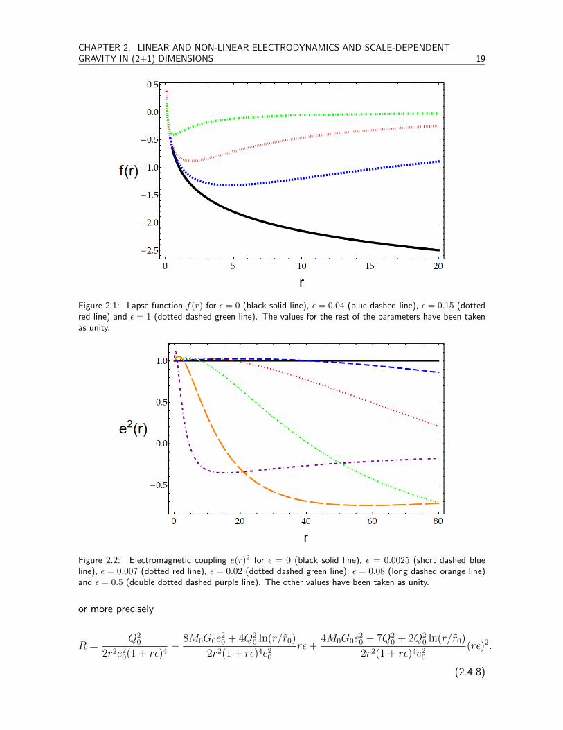
In Figure 2.1 the lapse function f(r) is shown for different values of ε in comparison to
the classical (2+1)- dimensional Einstein-Maxwell solution. The figure shows that the
scale dependent solution for small εr values is consistent with the classical case. However,
when εr becomes sufficiently large, a deviation from the classical solution appears. The
electromagnetic coupling e(r) is shown in Figure 2.2 for different values of ε. Note that
when ε is small the classical case is recovered, but when ε increases the electromagnetic
coupling tends to decrease until it is stabilized.
2.4.2 Asymptotic behaviour
In this subsection a few invariants need to be revisited. In particular we will focus on the
Ricci scalar R and the Kretschmann scalar K. Both of them are relevant in order to check
if some additional divergences appear. For the static and circularly symmetric metric we
have considered, the Ricci scalar is given by
R = −f ′′(r)− 2f ′(r)
r(2.4.7)
CHAPTER 2. LINEAR AND NON-LINEAR ELECTRODYNAMICS AND SCALE-DEPENDENTGRAVITY IN (2+1) DIMENSIONS 19
Figure 2.1: Lapse function f(r) for ε = 0 (black solid line), ε = 0.04 (blue dashed line), ε = 0.15 (dottedred line) and ε = 1 (dotted dashed green line). The values for the rest of the parameters have been takenas unity.
Figure 2.2: Electromagnetic coupling e(r)2 for ε = 0 (black solid line), ε = 0.0025 (short dashed blueline), ε = 0.007 (dotted red line), ε = 0.02 (dotted dashed green line), ε = 0.08 (long dashed orange line)and ε = 0.5 (double dotted dashed purple line). The other values have been taken as unity.
or more precisely
R =Q2
0
2r2e20(1 + rε)4
− 8M0G0e20 + 4Q2
0 ln(r/r0)
2r2(1 + rε)4e20
rε+4M0G0e
20 − 7Q2
0 + 2Q20 ln(r/r0)
2r2(1 + rε)4e20
(rε)2.
(2.4.8)
CHAPTER 2. LINEAR AND NON-LINEAR ELECTRODYNAMICS AND SCALE-DEPENDENTGRAVITY IN (2+1) DIMENSIONS 20
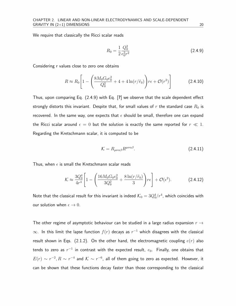
We require that classically the Ricci scalar reads
R0 =1
2
Q20
e20r
2(2.4.9)
Considering r values close to zero one obtains
R ≈ R0
[1−
(8M0G0e
20
Q20
+ 4 + 4 ln(r/r0)
)rε+O(r2)
](2.4.10)
Thus, upon comparing Eq. (2.4.9) with Eq. [?] we observe that the scale dependent effect
strongly distorts this invariant. Despite that, for small values of r the standard case R0 is
recovered. In the same way, one expects that ε should be small, therefore one can expand
the Ricci scalar around ε = 0 but the solution is exactly the same reported for r 1.
Regarding the Kretschmann scalar, it is computed to be
K = RµναβRµναβ. (2.4.11)
Thus, when ε is small the Kretschmann scalar reads
K ≈ 3Q40
4r4
[1−
(16M0G0e
20
3Q20
+8 ln(r/r0)
3
)rε
]+O(ε2). (2.4.12)
Note that the classical result for this invariant is indeed K0 = 3Q40/r
4, which coincides with
our solution when ε→ 0.
The other regime of asymptotic behaviour can be studied in a large radius expansion r →
∞. In this limit the lapse function f(r) decays as r−1 which disagrees with the classical
result shown in Eqs. (2.1.2). On the other hand, the electromagnetic coupling e(r) also
tends to zero as r−1 in contrast with the expected result, e0. Finally, one obtains that
E(r) ∼ r−2, R ∼ r−4 and K ∼ r−6, all of them going to zero as expected. However, it
can be shown that these functions decay faster than those corresponding to the classical

CHAPTER 2. LINEAR AND NON-LINEAR ELECTRODYNAMICS AND SCALE-DEPENDENTGRAVITY IN (2+1) DIMENSIONS 21
solutions. In fact, in absence of running coupling, a straightforward calculation reveals that
E(r) ∼ r−1, R ∼ r−2 and K ∼ r−4.
2.4.3 Horizons
The apparent horizon occurs when the lapse function vanishes, i.e. f(rH) = 0. Thus, this
Einstein-Maxwell black hole solution represents a non trivial deviation from the classical
solution which is manifest when we compare our solution with the corresponding black hole
solution without the scale dependence. Here, the horizon read
rH =1
εW
(εe− 2G0M0e
20
Q20
)(2.4.13)
where W () is the so-called Lambert-W function, which is a set of functions, namely the
branches of the inverse relation of the function Y (rε) = rεerε with rε being a complex
number. In particular, Eq (2.4.13) is also the principal solution for rε. In Figure 3 the scale
dependent effect on horizon is shown. We can see that the deviation from the classical case
is also evident for small M0 values.
In addition, one can expand the horizon around ε = 0 obtaining the classical solution plus
corrections i.e.
rH ≈ r0
[1− εr0 +O(ε2)
](2.4.14)
2.4.4 Thermodynamic properties
After having gained experience on the horizon structure one can now move towards the
usual thermodynamic properties associated with our solution shown at Eq. (2.4.1). Thus,
the Hawking temperature of the black hole assuming the ansatz (2.0.5) is given by
TH(rH) =1
4π
∣∣∣∣∣ limr→rH
∂rgtt√−gttgrr
∣∣∣∣∣, (2.4.15)
CHAPTER 2. LINEAR AND NON-LINEAR ELECTRODYNAMICS AND SCALE-DEPENDENTGRAVITY IN (2+1) DIMENSIONS 22
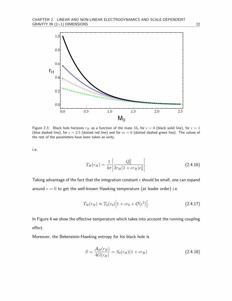
Figure 2.3: Black hole horizons rH as a function of the mass M0 for ε = 0 (black solid line), for ε = 1(blue dashed line), for ε = 2.5 (dotted red line) and for eε = 6 (dotted dashed green line). The values ofthe rest of the parameters have been taken as unity.
i.e.
TH(rH) =1
4π
∣∣∣∣∣ Q20
2rH(1 + εrH)e20
∣∣∣∣∣. (2.4.16)
Taking advantage of the fact that the integration constant ε should be small, one can expand
around ε = 0 to get the well-known Hawking temperature (at leader order) i.e.
TH(rH) ≈ T0(r0)∣∣∣1 + εr0 +O(ε2)
∣∣∣. (2.4.17)
In Figure 4 we show the effective temperature which takes into account the running coupling
effect.
Moreover, the Bekenstein-Hawking entropy for his black hole is
S =AH(rH)
4G(rH)= S0(rH)(1 + εrH) (2.4.18)

CHAPTER 2. LINEAR AND NON-LINEAR ELECTRODYNAMICS AND SCALE-DEPENDENTGRAVITY IN (2+1) DIMENSIONS 23
Figure 2.4: The Hawking temperature TH as function of the classical mass M0 for ε = 0 (black solid line),ε = 750 (blue dashed line), ε = 1800 (dotted red line) and ε = 3000 (dotted dashed green line). The othervalues of the rest of the parameters have been taken as unity. Note that the vertical axis is scaled OJO1 : 170.
and assuming small values of ε one can expand to get
S ≈ S0(r0)
[1− 1
2(εr0)2 +O(ε3)
](2.4.19)
In Figure 5 below we show the entropy for our (2+1)-dimensional Einstein-Maxwell scale
dependent black hole. It is clear that the running effect is dominant when ε is not small,
while for large values of M0 the effect is practically zero.
Finally, the heat capacity is computed in the usual way i.e.:
CQ = T∂S
∂T
∣∣∣∣∣Q
(2.4.20)
which read
CQ = −S0(rH)(1 + εrH). (2.4.21)
CHAPTER 2. LINEAR AND NON-LINEAR ELECTRODYNAMICS AND SCALE-DEPENDENTGRAVITY IN (2+1) DIMENSIONS 24
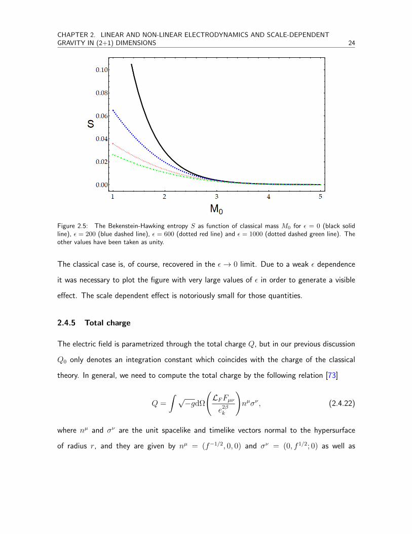
Figure 2.5: The Bekenstein-Hawking entropy S as function of classical mass M0 for ε = 0 (black solidline), ε = 200 (blue dashed line), ε = 600 (dotted red line) and ε = 1000 (dotted dashed green line). Theother values have been taken as unity.
The classical case is, of course, recovered in the ε→ 0 limit. Due to a weak ε dependence
it was necessary to plot the figure with very large values of ε in order to generate a visible
effect. The scale dependent effect is notoriously small for those quantities.
2.4.5 Total charge
The electric field is parametrized through the total charge Q, but in our previous discussion
Q0 only denotes an integration constant which coincides with the charge of the classical
theory. In general, we need to compute the total charge by the following relation [73]
Q =
∫ √−gdΩ
(LFFµνe2βk
)nµσν , (2.4.22)
where nµ and σν are the unit spacelike and timelike vectors normal to the hypersurface
of radius r, and they are given by nµ = (f−1/2, 0, 0) and σν = (0, f 1/2; 0) as well as
CHAPTER 2. LINEAR AND NON-LINEAR ELECTRODYNAMICS AND SCALE-DEPENDENTGRAVITY IN (2+1) DIMENSIONS 25
√−gdΩ = rdφ. Making use of these we obtain
Q = 2πQ0, (2.4.23)
which is proportional to the classical value and has no ε dependence.
2.5 Einstein-power-Maxwell scale dependence
This section is devoted to the study of a (2+1) scale dependent gravity coupled to a
power-Maxwell source. As mentioned before, the case β = 3/4 leads to a dimensionless
electromagnetic coupling which was set to the unity in the section 2.1. However, if one
considers a scale dependent gravity, the electromagnetic coupling has a non-trivial scale
dependence. Therefore, in this section we shall hold the electromagnetic coupling depen-
dence of the action (2.0.1). In this way, the solution consists of a set of four functions
G(r), E(r), f(r), e(r)3, which are obtained by combining Einstein’s effective equations
of motion with the NEC taking advantage of the EOM for the four-potential Aν . In what
follows we shall obtain the solutions of the system in terms of the functions mentioned
above.

CHAPTER 2. LINEAR AND NON-LINEAR ELECTRODYNAMICS AND SCALE-DEPENDENTGRAVITY IN (2+1) DIMENSIONS 26
2.5.1 Solution
The integration constants have been chosen such as the scale dependent solution reduces
to the classical NLED case when the appropriate limit is taken. Thus, our solution reads
G(r) =G0
1 + εr,
E(r) =Q0
r2
(e(r)
e0
)3
, (2.5.1)
f(r) =4G0Q
20
3r(rε+ 1)3− M0G0 (r3ε2 + 3r2ε+ 3r)
3r(rε+ 1)3,
e(r)3 = e30
[(2rε(3rε+ 2) + 1)
(rε+ 1)4− M0r
3ε2(rε+ 4)
4Q20(rε+ 1)4
].
In the limit ε→ 0 we obtain
limε→0
G(r) = G0,
limε→0
E(r) =Q0
r2, (2.5.2)
limε→0
f(r) =4G0Q
20
3r−G0M0,
limε→0
e(r)3 = e30.
Note that if we set e0 = 1, the classical solution in section 2.1 is recovered. Even more, if
one demands that G0 = 1 (which is the standard lore) then we are in complete agreement
with the classical solution given at Ref. [35].
2.5.2 Asymptotic behaviour
The asymptotic behaviour of this solution can be studied by computing geometrical invari-
ants i.e. the Ricci scalar, which for our solution is
R = −4G0ε
[M0 + 4Q2ε
r(rε+ 1)5
], (2.5.3)
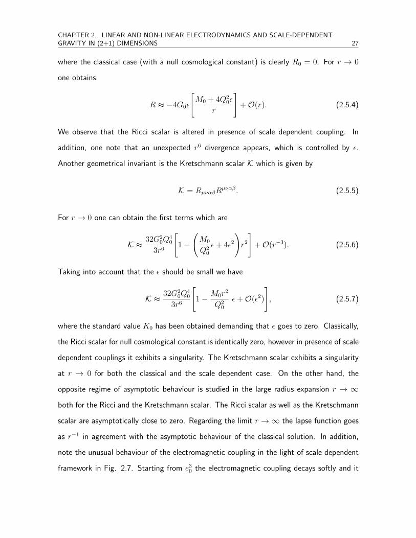
CHAPTER 2. LINEAR AND NON-LINEAR ELECTRODYNAMICS AND SCALE-DEPENDENTGRAVITY IN (2+1) DIMENSIONS 27
where the classical case (with a null cosmological constant) is clearly R0 = 0. For r → 0
one obtains
R ≈ −4G0ε
[M0 + 4Q2
0ε
r
]+O(r). (2.5.4)
We observe that the Ricci scalar is altered in presence of scale dependent coupling. In
addition, one note that an unexpected r6 divergence appears, which is controlled by ε.
Another geometrical invariant is the Kretschmann scalar K which is given by
K = RµναβRµναβ. (2.5.5)
For r → 0 one can obtain the first terms which are
K ≈ 32G20Q
40
3r6
[1−
(M0
Q20
ε+ 4ε2
)r2
]+O(r−3). (2.5.6)
Taking into account that the ε should be small we have
K ≈ 32G20Q
40
3r6
[1− M0r
2
Q20
ε+O(ε2)
], (2.5.7)
where the standard value K0 has been obtained demanding that ε goes to zero. Classically,
the Ricci scalar for null cosmological constant is identically zero, however in presence of scale
dependent couplings it exhibits a singularity. The Kretschmann scalar exhibits a singularity
at r → 0 for both the classical and the scale dependent case. On the other hand, the
opposite regime of asymptotic behaviour is studied in the large radius expansion r → ∞
both for the Ricci and the Kretschmann scalar. The Ricci scalar as well as the Kretschmann
scalar are asymptotically close to zero. Regarding the limit r →∞ the lapse function goes
as r−1 in agreement with the asymptotic behaviour of the classical solution. In addition,
note the unusual behaviour of the electromagnetic coupling in the light of scale dependent
framework in Fig. 2.7. Starting from e30 the electromagnetic coupling decays softly and it

CHAPTER 2. LINEAR AND NON-LINEAR ELECTRODYNAMICS AND SCALE-DEPENDENTGRAVITY IN (2+1) DIMENSIONS 28
stabilizes when
limr→∞
e(r)3 = −(
1
3r0ε
)e3
0, (2.5.8)
instead of reach the classical value. The electric field tends to zero as expected but slowly
compared with the classical case. In fact, E(r) behaves as r−1 in clearly deviation with
respect to the result shown in Eq. (2.1.3). Finally, the curvature and Kretschmann scalars
hold the same asymptotic behaviour of the results obtained in absence of running, i.e.
R ∼ r−4 and K ∼ r−6.
Figure 2.6: Lapse function f(r) for ε = 0 (black solid line), ε = 0.04 (blue dashed line), ε = 0.15 (dottedred line) and ε = 1 (dotted dashed green line). The values for the rest of the parameters have been takenas unity.

CHAPTER 2. LINEAR AND NON-LINEAR ELECTRODYNAMICS AND SCALE-DEPENDENTGRAVITY IN (2+1) DIMENSIONS 29
Figure 2.7: Electromagnetic coupling e(r)3 for ε = 0 (black solid line), ε = 0.25 (dashed blue line),ε = 0.45 (dotted red line), ε = 1 (dotted dashed green line). The other values have been taken as unity.
2.5.3 Horizons
Applying the condition f(rH) = 0 one obtains the scale dependent horizon which reads
rH = −1
ε
[1−
[1 + 3 εr0
]1/3], (2.5.9)
r± = −1
ε
[1 +
1
2(1± i
√3)
[1 + 3εr0
]1/3]. (2.5.10)
where r0 is the classical value given by Eq. (2.1.4). Note that one obtains three horizons,
out of which one is real (physical horizon) and two r± are complex (nonphysical).
In addition, since the scale dependence of coupling constants is usually assumed to be weak,
it is reasonable to consider the dimensionful parameter ε as small compared to the other
scales and, therefore, one can expand around ε close to zero, which gives us
rH ∼= r0
[1− εr0 +
5
3(εr0)2 + · · ·
]. (2.5.11)
One should note that when ε tends to zero the classical case is recovered. Besides, although

CHAPTER 2. LINEAR AND NON-LINEAR ELECTRODYNAMICS AND SCALE-DEPENDENTGRAVITY IN (2+1) DIMENSIONS 30
Figure 2.8: Black hole horizons rH as a function of the mass M0 for ε = 0 (black solid line), for ε = 1(blue dashed line), for ε = 1 (dotted red line) and for eε = 2 (dotted dashed green line). The values of therest of the parameters have been taken as unity.
ε could take positive or negative values, here in order to obtain desirable physical results we
require that ε > 0. In our set of solutions G(r), E(r), f(r), e(r) we can expand around
zero for small values of ε, i.e.
G(r) ≈ G0
[1− rε+O(ε2)
], (2.5.12)
E(r) ≈ E0(r) +O(ε2), (2.5.13)
f(r) ≈ f0(r) +
[2G0M0 −
4G0Q20
r
]rε+O(ε2), , (2.5.14)
e3(r) ≈ e30
[1 +O(ε2)
], (2.5.15)
2.5.4 Thermodynamic properties
Using the horizon structure and the lapse function (which is given by Eq. (2.5.1)) one can
calculate the Hawking temperature of the corresponding scale dependent black hole. At the
CHAPTER 2. LINEAR AND NON-LINEAR ELECTRODYNAMICS AND SCALE-DEPENDENTGRAVITY IN (2+1) DIMENSIONS 31
outer horizon this temperature is given by the simple formula
TH =1
4π
∣∣∣∣∣ limr→rH
∂rgtt√−gttgrr
∣∣∣∣∣, (2.5.16)
which reads in term of the horizon radius
TH =1
4π
∣∣∣∣∣ M0G0
rH(1 + εrH)
∣∣∣∣∣. (2.5.17)
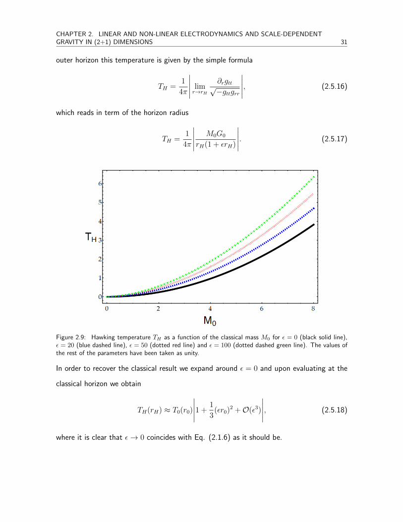
Figure 2.9: Hawking temperature TH as a function of the classical mass M0 for ε = 0 (black solid line),ε = 20 (blue dashed line), ε = 50 (dotted red line) and ε = 100 (dotted dashed green line). The values ofthe rest of the parameters have been taken as unity.
In order to recover the classical result we expand around ε = 0 and upon evaluating at the
classical horizon we obtain
TH(rH) ≈ T0(r0)
∣∣∣∣∣1 +1
3(εr0)2 +O(ε3)
∣∣∣∣∣, (2.5.18)
where it is clear that ε→ 0 coincides with Eq. (2.1.6) as it should be.
CHAPTER 2. LINEAR AND NON-LINEAR ELECTRODYNAMICS AND SCALE-DEPENDENTGRAVITY IN (2+1) DIMENSIONS 32
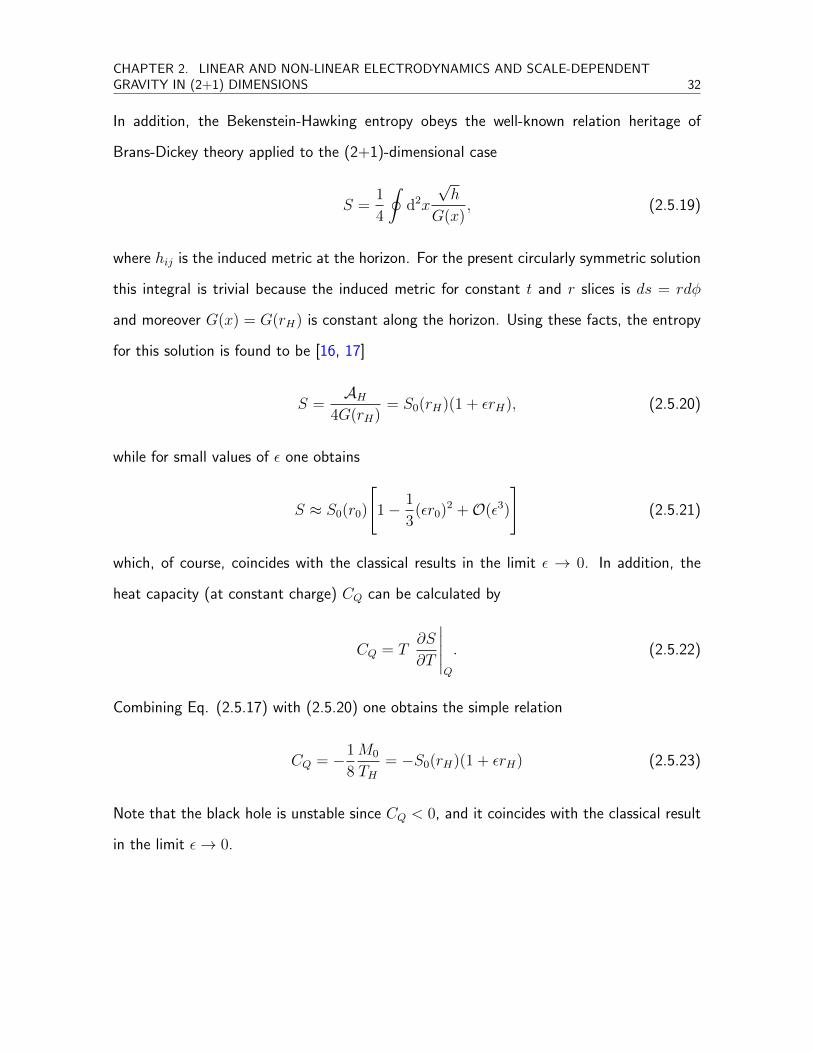
In addition, the Bekenstein-Hawking entropy obeys the well-known relation heritage of
Brans-Dickey theory applied to the (2+1)-dimensional case
S =1
4
∮d2x
√h
G(x), (2.5.19)
where hij is the induced metric at the horizon. For the present circularly symmetric solution
this integral is trivial because the induced metric for constant t and r slices is ds = rdφ
and moreover G(x) = G(rH) is constant along the horizon. Using these facts, the entropy
for this solution is found to be [16, 17]
S =AH
4G(rH)= S0(rH)(1 + εrH), (2.5.20)
while for small values of ε one obtains
S ≈ S0(r0)
[1− 1
3(εr0)2 +O(ε3)
](2.5.21)
which, of course, coincides with the classical results in the limit ε → 0. In addition, the
heat capacity (at constant charge) CQ can be calculated by
CQ = T∂S
∂T
∣∣∣∣∣Q
. (2.5.22)
Combining Eq. (2.5.17) with (2.5.20) one obtains the simple relation
CQ = −1
8
M0
TH= −S0(rH)(1 + εrH) (2.5.23)
Note that the black hole is unstable since CQ < 0, and it coincides with the classical result
in the limit ε→ 0.
CHAPTER 2. LINEAR AND NON-LINEAR ELECTRODYNAMICS AND SCALE-DEPENDENTGRAVITY IN (2+1) DIMENSIONS 33
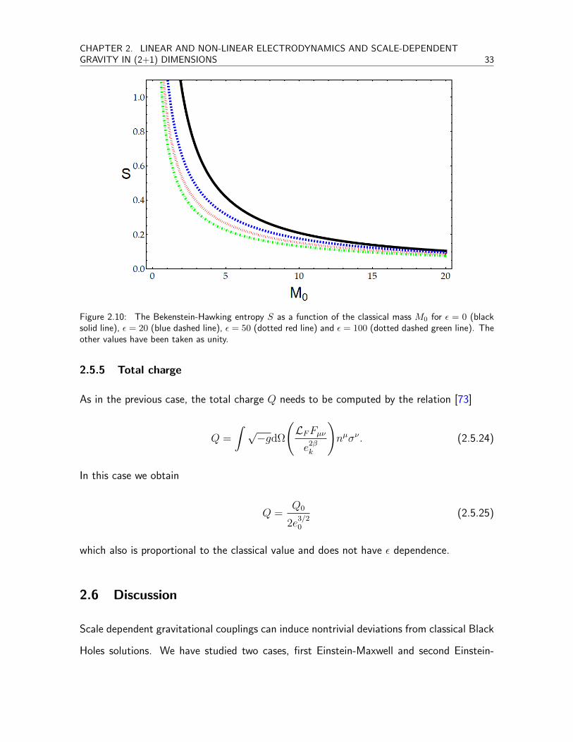
Figure 2.10: The Bekenstein-Hawking entropy S as a function of the classical mass M0 for ε = 0 (blacksolid line), ε = 20 (blue dashed line), ε = 50 (dotted red line) and ε = 100 (dotted dashed green line). Theother values have been taken as unity.
2.5.5 Total charge
As in the previous case, the total charge Q needs to be computed by the relation [73]
Q =
∫ √−gdΩ
(LFFµνe2βk
)nµσν . (2.5.24)
In this case we obtain
Q =Q0
2e3/20
(2.5.25)
which also is proportional to the classical value and does not have ε dependence.
2.6 Discussion
Scale dependent gravitational couplings can induce nontrivial deviations from classical Black
Holes solutions. We have studied two cases, first Einstein-Maxwell and second Einstein-

CHAPTER 2. LINEAR AND NON-LINEAR ELECTRODYNAMICS AND SCALE-DEPENDENTGRAVITY IN (2+1) DIMENSIONS 34
power-Maxwell case. Both of them have a common feature: the lapse function tends to
zero when r!→∞, characteristic which is absent in the classical solutions. In addition, the
total charge is modified as a consequence of our scale dependent framework. Moreover, we
have found that, for the same value of the classical black hole mass, the apparent horizon
radius (and the Bekenstein-Hawking entropy) decreases when the strength of the scale
dependence increases. This is in agreement with the findings in [51, 52, 53, 54, 55, 56, 57,
58, 59, 60, 61, 62, 63, 64, 65]. On the other hand, the Hawking temperature increases with
ε. Please, note that the effect of the scale dependence in the Einstein-power-Maxwell case
is stronger than the Eintein-Maxwell case. The behaviour of the electromagnetic coupling
e(r) depends on the choice of the electromagnetic Lagrangian density. While e(r) goes to
zero in the limit r →∞ for a Maxwell Lagrangian density, it approaches a constant value for
the power-Maxwell case. Finally, it is well known that a black hole (as a thermodynamical
system) is locally stable if its heat capacity is positive [74]. In both scale dependent cases
it is found that these black holes are unstable (CQ < 0), like their classical counterparts.

Chapter 3
Cosmology and scale-dependent
gravity in (3+1) dimensions
In this chapter we deduce the effective Einstein field equations assuming scale (temporal)
dependent couplings for a FLRW background. After that, we solve the corresponding
effective Einstein field equations in some relevant cases and compare the solutions with the
previously obtained solutions reported in Ref. [75, 10]) and with observations in case this is
available. Throughout the manuscript we will be interested in one of the main cosmological
functions related to the scale factor of the Universe, which is the Hubble parameter as a
function of the redshift, H(z). Even more, given the large number of both measurements
and theoretical computations on H(z) (see [10, 76] and references therein) in a matter
dominated epoch, we focus our attention only in this era.
3.1 ΛCDM and running–vacuum models
In this section we briefly review both ΛCDM and some running-vacuum cosmological models
which have received considerable attention given the concordance between them and recent
measurements [10]. We first start by revisiting the classical ΛCDM model which corresponds
35

CHAPTER 3. COSMOLOGY AND SCALE-DEPENDENT GRAVITY IN (3+1) DIMENSIONS 36
to constant couplings, namely usual General Relativity [77]. Specifically, both the Newton’s
constant, G0, and the vacuum energy density, ρΛ0 ≡ Λ0/(8πG0), are taken as constants.
As an additional constraint, this model takes advantage of the covariant conservation of the
energy–momentum tensor, namely
∇µTµν = 0. (3.1.1)
Besides, it assumes a perfect fluid such that Tµν = diag(ρm, pm, pm, pm). Using Eq. 3.1.1
for a perfect fluid it is obtained that
ρm + 3H (ρm + pm) = 0. (3.1.2)
The unknowns are the scale factor a(t), the matter density ρm(t) and the pressure pm(t).
In the simplest case, one can assume dust (pm(t) = 0) and one just needs to find the other
two functions. The classical Friedmann equations are sufficient for determining those two
unknown functions.
Regarding the running cases, the simplest model consists in working with the usual Fried-
mann equations but replacing G0,Λ0 with G(t),Λ(t). The equations are given by
H2 =1
3κ(t)
[ρ(t) +
Λ(t)
κ(t)
]− K
a2, (3.1.3)
H +H2 = −1
6κ(t)
[ρ(t) + 3p(t)
]+
1
3Λ(t), (3.1.4)
where, as usual, κ(t) ≡ 8πG(t). Nevertheless, these equations are not enough to solve
for the unknowns in general, as it will be shown in the following. In this sense, extra
information is needed to account for a complete description of the cosmological model
under consideration.
CHAPTER 3. COSMOLOGY AND SCALE-DEPENDENT GRAVITY IN (3+1) DIMENSIONS 37
3.1.1 G(t) = G0 and ρΛ(t) 6= 0
The key assumption lying at the heart of this case is promoting only Λ0 → Λ(t) in Einstein’s
equations, namely
Gµν + Λ(t)gµν = κ0Tµν . (3.1.5)
By using ∇µGµν = 0, one obtains
ρΛ + ρm + 3H (ρm + pm) = 0. (3.1.6)
In this case, an exchange of energy between matter and vacuum takes place. The unknowns
are a(t), ρm(t) and Λ(t). Therefore, Eqs. (3.1.3), (3.1.4) and (3.1.6) allow to solve for the
unknowns provided an extra input on ρΛ. A common choice is [78]
ρΛ(t) =Λ(t)
8πG0
= m0 +m1H(t) +m2H(t)2, (3.1.7)
where m0,m1 and m2 are coupling constants and the Hubble paramenter H(t) is defined
according to H(t) ≡ a(t)/a(t). As pointed out recently [10], the above expression has been
suggested in the literature from the quantum corrections of QFT in curved spacetime. The
running parameter m0 is of order 10−3M4, while m1 ∼ 10−4M3, and m2 ∼ 10−2M2 where
M is an average (large) mass scale (see, for example, [79, 80, 81] and references therein).
Although the present case is considered in Refs. [82, 83], in these references the authors
do not present an explicit solution for H(t), which is the observable we are interested in, as
previously commented. The analytical solution we find in this case is
H(t) =2M
8πm2 − 3tan(M (2c1 + t)
)− 4πm1
8πm2 − 3, (3.1.8)

CHAPTER 3. COSMOLOGY AND SCALE-DEPENDENT GRAVITY IN (3+1) DIMENSIONS 38
and the scale factor is given by the simple relation
a(t) = C2 exp
(−2 (log (cos (M (2c1 + t))) + 2πm1t)
8πm2 − 3
). (3.1.9)
This can be written as
a(t) = C2e− 4πm1
8πm2−3tcos
23−8πm2
(M(2c1 + t)
), (3.1.10)
where we have defined the auxiliary function
M =
√2πm0
(8πm2 − 3
)−(2πm1
)2. (3.1.11)
The remaining unknowns Λ(t) and ρm(t) are easily obtained from the previous expressions.
3.1.2 G(t) 6= 0 and ρΛ(t) = ξ
In this case, we will consider the two quantities G(t),Λ(t) keeping the vacuum energy
density as a constant value. Thus, from the covariance of the Einstein’s tensor we obtain
[3H(p+ ρ) + ρ
]+χ(ρ+ ρΛ) = 0. (3.1.12)
where χ ≡ G(t)/G(t).
In this case, the modified Einstein field equations given by Eqs. (3.1.3) and (3.1.4), combined
with Eq. (3.1.12), are not enough to solve for the four unknowns a(t), ρm(t), Λ(t), G(t).
In addition we can not use the ansatz (3.1.7) since ρΛ is constant, thus we need to get
the extra information from some additional assumptions. One possibility suggested in this
context can be expressed as [84]
ρm(t) = m4a(t)−3+ε, (3.1.13)
where ε signals a possible deviation from ΛCDM. We note that a partial solution for this

CHAPTER 3. COSMOLOGY AND SCALE-DEPENDENT GRAVITY IN (3+1) DIMENSIONS 39
case is developed in [84]. With this, one gets
G(t) =
(m4a(t)ε−3 +m0
m0 +m4
)ε
3−ε (3.1.14)
Nevertheless, an analytical expression for a(t) is not presented here because it is too lengthy.
3.1.3 G(t) 6= 0 and ρΛ(t) 6= 0
This is the most general case within this framework. In addition to Eqs. (3.1.3) - (3.1.4)
and the covariance of the Einstein tensor, the covariant conservation of Tµν is assumed [78],
giving
ρΛ + χ(ρ+ ρΛ) = 0, (3.1.15)
which can be solved, using some ansatz, for instance, for ρΛ(t) (see Eq. (3.1.7)). Interest-
ingly, the function G(H) can be obtained analytically, as
G(H) =G0
1 +m2 ln (H2/H20 ), (3.1.16)
where G0 and H0 are the Newton’s constant and the Hubble parameter at a given time
(usually taken as the present time), respectively.
In Fig. (3.1) we show the comparison between experimental data (see text for details) and
the computations under the ΛCDM and the running–vacuum model previously discussed
for H(z). The values of the parameters m0, m1, m2 were fixed as in [83]. Given the
experimental uncertainty, all the considered models reproduce fairly well the observations.
Therefore, H(z) does not provide an stringent test and other observables are needed. At
this point it is worth mentioning the recent work by Sola et al. [10], in which the authors
constrain possible running–vacuum models using the cosmological observables SN Ia + BAO
+ H(z) + LSS + BBN + CMB. However, as we will show in the following section(s), H(z)

CHAPTER 3. COSMOLOGY AND SCALE-DEPENDENT GRAVITY IN (3+1) DIMENSIONS 40
is enough to discriminate between ΛCDM, running–vacuum and variational running–vacuum
models.
Figure 3.1: Behavior of H(z) for the running vacuum cases considered in the present section. See text fordetails.
3.2 Scale–dependent couplings and scale setting
In the present section we will introduce the general scale–dependent framework. From now
on, we will refer to it as the variational running vacuum model (VRV model hereafter).
The notation follows closely Ref. [50] as well as Refs. [16, 17, 18, 19, 85]. The classical
couplings are the Newton and the cosmological constant, both of them being promoted to
scale–dependent couplings, namely, G0,Λ0 → Gk,Λk which, in general, depend on the
renormalization scale, k. In addition, there are two independent fields, which are the metric
gµν(x) and the scale field k(x). The effective action is given by
Γ[gµν , k] =
∫d4x√−g
[1
2κk
(R− 2Λk
)+ LM
]. (3.2.1)

CHAPTER 3. COSMOLOGY AND SCALE-DEPENDENT GRAVITY IN (3+1) DIMENSIONS 41
The effective Einstein’s field equations are
Gµν + Λkgµν = κkTeffecµν , (3.2.2)
and the effective energy–momentum tensor is defined according to
κkTeffecµν ≡ κkTµν −∆tµν , (3.2.3)
where ∆tµν is a tensor which takes into account the scale–dependence of the gravitational
coupling. This term is given by the following expression
∆tµν = Gk
(gµν−∇µ∇ν
)G−1k . (3.2.4)
Note that, since the renormalization scale k is actually not constant anymore, the corre-
sponding set of equations of motion is not closed, which means that the energy momentum–
tensor could be not conserved for an arbitrary choice of k. This kind of problem has
been investigated through renormalization group improvement of black holes in asymptotic
safety scenarios [86, 87, 53, 54, 56, 57, 58, 59, 60, 61, 62, 63, 64, 65]. It is however
preferable to maintain the classical conservation laws and to formulate a closed system of
equations. This problem can be solved by a variational scale–setting procedure according
to [11, 13, 66, 50, 67]. Taking the renormalization scale k as an additional field k(x) one
obtains the algebraic equation
δΓ
δk= 0. (3.2.5)
With the help of Eq. (3.2.5) combined with Eq. (3.2.2), we guarantee the conservation of
the stress–energy tensor. Despite of that, a problem is still present: it is necessary to know
the explicit form of beta functions which encode the dependence of a coupling parameter
on the energy scale. The explicit computation is achievable by different mathematical
CHAPTER 3. COSMOLOGY AND SCALE-DEPENDENT GRAVITY IN (3+1) DIMENSIONS 42
techniques which, in general, do not produce the same solution. Since our interest is the
variation of the cosmological quantities in time, and not with respect to k(t), we assume
that Ok → O(t).
Since, as we mentioned before, this ansatz is insufficient to determine the system we are
going to introduce an additional ansatz for ρΛ(H) in order to have enough information for
the system of equations to be solved. Finally, it is worth mentioning that, in general, a
solution for a scale–dependent model allows for recovering the classical limit when certain
running parameter is turned off [16, 17, 18, 19]. However, as it will be shown later, this
is not the case for certain VRV cases because either the running parameter can not be
identified due to the numerical nature of the solutions or the classical solution is forbidden
(see Sects. 3.2.3 and 3.2.4 for details).
3.2.1 The model
As usual, Tµν stands for the energy-momentum tensor which is defined as follows
Tµν ≡−2√−g
δ(√−gLM)
δgµν= gµνLM − 2
δLMδgµν
, (3.2.6)
and for a perfect fluid we have
Tµν =(ρ+ p
)uµuν + pgµν , (3.2.7)
where uµ = (1, 0, 0, 0) is the velocity vector field and gµν is the metric tensor corresponding
to the Friedmann–Lemaıtre–Robertson–Walker geometry, namely
ds2 = −dt2 + a(t)2
[1
1−Kr2dr2 + dΩ2
]. (3.2.8)
CHAPTER 3. COSMOLOGY AND SCALE-DEPENDENT GRAVITY IN (3+1) DIMENSIONS 43
Assuming a flat universe (i.e. K = 0) and considering dust matter (pm(t) = 0), the
generalized Friedmann equations coming from (3.2.2) are
H2
[1− χ
H
]=
1
3κ(t)
[ρ+ ρΛ
], (3.2.9)
H +H2
[3
2− χ
H
]− 1
2
[χ− χ2
]=
1
2κ(t)ρΛ. (3.2.10)
Here we have defined the parameter χ ≡ ˙G(t)/G(t) which encodes the variability of the
Newton parameter. Further, we are able to get complementary information by the compu-
tation of the covariant derivative of the generalized Einstein equations (3.2.2)
(H2 + H)χ+Hχ2 +1
3κ(t)
[3H(p+ ρ) + (ρ+ ρΛ) + χ(ρ+ ρΛ)
]= 0. (3.2.11)
In addition, in some special cases will be useful to assume the conservation of the matter
stress–energy tensor in the classical sense, i.e. when the couplings are constant, which reads
from (3.2.11) and assuming p = 0
ρ+ 3Hρ = 0. (3.2.12)
In the rest of the present chapter we will explore some particular cases of these VRV models,
trying to constrain their validity by computing H(z) and comparing both with previous
running–vacuum models and experimental data. When possible, analytical solutions will be
given.
3.2.2 G = G0 and ρΛ 6= 0
If the gravitational Newton coupling G is constant, this implies that the tensor ∆tµν = 0 and
the variational principle leads to the same Equations corresponding to subsection (3.1.1).
CHAPTER 3. COSMOLOGY AND SCALE-DEPENDENT GRAVITY IN (3+1) DIMENSIONS 44
3.2.3 G 6= 0 and ρΛ = ξ
In this case, we assume the same ansatz for the baryonic energy density as we used in
Section 3.1.2, that is
ρm(t) = m4a(t)−3+ε (3.2.13)
in order to have enough information to solve the system. We use this ansatz in order to
follow as close as possible the protocol that Sola uses to solve his equations in each one
of the cases. Even more, since we are introducing the running parameter ε, we interpret
it as a perturbation parameter with respect to the ΛCDM model, therefore, its numerical
value will be small. Taking into account the above, the system of differential equations to
solve consist of just the generalized Friedmann equations, and in this particular case they
are given by
a2 (3H(H − χ)−m0κ(t)) = m4κ(t)aε−1, (3.2.14)
m0κ(t)− 2H + 2Hχ− 3H2 + χ− χ2 = 0, (3.2.15)
After an appropriate manipulation of equations (3.2.14), (3.2.15) we get
G(t) =3H2
8π
(m4aε−3(H−(ε−2)H2)
H+2H2 +m0
) . (3.2.16)
But an analytical solution for the scale factor a(t) was not obtained due to the complexity
of the equation.
3.2.4 G(t) 6= 0 and ρΛ(t) 6= 0.
This is the most general case within the VRV framework. In addition to Friedmann equa-
tions, we assume the covariant conservtions of the energy momentum tensor Tµν in order
CHAPTER 3. COSMOLOGY AND SCALE-DEPENDENT GRAVITY IN (3+1) DIMENSIONS 45
to have enough equations to solve for the unknowns a(t), G(t) and ρm(t). We make this
assumption since in this general case, we need to have the usual conservation of energy-
momentum in order to properly compare the results of this case to the ΛCDM model.
Therefore, the corresponding equations in this case are
H2
[1− χ
H
]=
1
3κ(t)
(ρ+ ρΛ
)(3.2.17)
H +H2
[3
2− χ
H
]− 1
2
[χ− χ2
]=
1
2κ(t)ρΛ, (3.2.18)
3Hρ+ ρ = 0 (3.2.19)
where, again, the first two equations correspond to the generalized Friedmann equations and
the last one is the usual conservation of the energy momentum tensor. After manipulating
the previous equations, introducing the dependences G(H(t)), Λ(H(t)), considering the
ansatz for ρΛ(t) given in Eq. (3.1.7), and doing the change of variables t→ z, we can solve
numerically for the function H(z).
Chapter 4
Conclusions
4.1 Conclusions
In the case of (2+1) dimensions, we have studied the scale dependence of charged black holes
in three-dimensional spacetime both in linear (Einstein-Maxwell) and non-linear (Einstein-
power-Maxwell) electrodynamics. In the second case we have considered the case where the
electromagnetic energy momentum tensor is traceless, which happens for β = 3/4. After
presenting the models and the classical black hole solutions, we have allowed for a scale
dependence of the electromagnetic as well as the gravitational coupling, and we have solved
the corresponding generalized field equations by imposing the ”null energy condition” in
three-dimensional spacetimes with static circular symmetry. Horizon structure, asymptotic
spacetimes and thermodynamics have been discussed in detail.
With respect to (3+1)-dimensions we have introduced a scale–dependent cosmological
model in a matter–dominated era. In the first part we have extensively reviewed the so–
called running vacuum models, incorporating some points not previously considered in the
literature. In all these cases the model fits well with experimental data for H(z) by consid-
ering an standard equation of state for dark energy pΛ = −ρΛ. Despite of that, it could be
more satisfactory, for a theoretical point of view, to have a running vacuum model coming
46

CHAPTER 4. CONCLUSIONS 47
from a variational principle. In this spirit, starting with an effective action based on the usual
Einstein–Hilbert one, we have promoted G0, ρΛ0 to scale–dependent couplings, Gk, ρΛk
to implement this scale–setting procedure into a cosmological context (variational running
vacuum model) for a matter–dominated era in the second part. Specifically, and for the
sake of comparison with other running vacuum models, we have limited our study to the
case of time–dependent couplings. It is worth mentioning that we have also assumed the
same ansatz for ρΛ(H) which were considered in the original running vacuum case. Note
that, since this ansatz comes from QFT considerations in a FLRW background, we keep
it as a suitable feature also for the variational running vacuum model. However, different
parametrizations for ρΛ(H) coming from other approaches to quantum gravity could be
assumed.
Within the variational procedure, we have studied several cases and a brief summary of the
key points in each one of them is shown in Table 4.1.
Table 4.1: Several cases of the VRV model.
Case Key point Description
1. G(t) = cte., ρΛ(t) = cte. Classical GR, that is, ΛCDM.
2. G(t) = cte., ρΛ(t) 6= 0 ∇µTµν 6= 0 and it is the same as Sola’s case.
3. G(t) 6= 0, ρΛ(t) = cte. ∇µTµν 6= 0 and we assume ρm(t) ∝ a(t)−3+ε .
4. G(t) 6= 0, ρΛ(t) 6= 0 True running, in which we assume ∇µTµν = 0.
First, if ρΛ is taken as a constant value, an analytic solution for the modified Einstein’s
field equations (including G(t)) is obtained. It is worth mentioning that this solution does
not correspond to a true running since the classical solution can not be recovered by turning
off of any parameter. Therefore, once the running case has been considered, the classical
case is automatically discarded. This feature is remarkable due in previous scale depen-
dent problems we always can recover the classical solution under certain election of the
CHAPTER 4. CONCLUSIONS 48
so–called running parameter of the theory. Second, a complete numerical solution has been
obtained when both ρΛ and G(t) are taken into account into the model. Although this
case corresponds to a true running, due to the numerics involved, we have not been able
to find any parameter which could control the strength of the scale–dependence for both
ρΛ and G(t). Third, regarding the comparison of these two models with the experimental
data for H(z), there are not significantly differences with respect to the ΛCDM model. A
possible explanation could be given in terms of the behavior of the Newton’s coupling. As
the classical solution implies a constant value, G0, for this coupling, we should expect the
decay to be slow so that its variation, with respect to the classical case, is not appreciable.
This turn out to be exactly the case, therefore the behavior of the Newton’s coupling with
respect to the constant coupling’s case could be an important point to take into account in
order to test the viability of any extension of general relativity, regardless of the fact that G
is not an observable of the model. In addition, we note that a slower decay of G(t) in the
corresponding running vacuum case gives place to an excellent agreement with experimental
data. Beyond that, it is necessary to say that what we did in the (3+1)-dimensional case
is only a preliminary test to establish whether or not the scale dependent gravity theory
fits well or not to the experimental data available for the time evolution of the Hubble
factor, and although this preliminary test is satisfied by our VRV model, further test are
required in order to decide if this model reproduces well the behavior of our universe at all
cosmological scales or not. Specifically, we can consider solar system test of our model or
linear perturbations of both the metric and the energy densities. Those and other aspects
of scale–dependent cosmology are currently under study and will eventually be the object
for future publication.

Appendix A
Appendix
A.1 Detailed calculations in (2+1) dimensions
In this appendix we study some features of the scale dependent (2 + 1) gravity coupled to
a power-Maxwell source for an arbitraty β. For this system the action is given by
S =
∫d3x√−g[
R
16πG(r)− L(F )
e(r)2β
], (A.1.1)
where G(r) and e(r) are the gravitational and the the electromagnetic scale-dependent
couplings, R is the Ricci scalar, L(F ) = Cβ|F |β is the electromagnetic Lagrangian density,
F = (1/4)FµνFµν is the Maxwell invariant, and C is a dimensionless constant which de-
pends on the choice of β. Metric signature (−,+,+) and natural units (c = ~ = kB = 1)
are used in our computations.
Variations of the Eq. (A.1.1) with respect to the metric field lead to the modified Einstein’s
equations
Rµν −1
2gµνR = 8π
G(r)
e2β(r)Tµν −∆tµν , (A.1.2)
49
APPENDIX A. APPENDIX 50
where Tµν stands for the power–Maxwell energy momentum tensor and
∆tµν = G(r)(gµν−∇µ∇ν)1
G(r). (A.1.3)
is the non-material energy momentum tensor which arises as a consecuence of the scale
dependence of the gravitational coupling. On the other hand, after variations of the action
Eq. (A.1.1) with respect to the electromagnetic four–potential, Aµ, one obtains the modified
Maxwell equations
Dµ
(F µ
νLFe(r)2β
)= 0. (A.1.4)
Henceforth, only static and spherically symmetric solutions will be considered. Therefore
we shall assume the ansatz
ds2 = −f(r)dt2 + f(r)−1dr2 + r2dΩ2 (A.1.5)
Fµν = (δtµδrν − δrµδtν)E(r) (A.1.6)
for the metric and the electromagnetic tensor, respectively. With the former prescription is
straightforward to prove, from Eq. (A.1.4), that the electric field is given in terms of the
electromagnetic coupling by
E(r) =2β−12β−1A−
β2β−1Q
12β−1
0 e(r)2β
2β−1
β1
2β−1 r1
2β−1
(A.1.7)
Please, note that setting β = 1 and A = 1 the electric field reported in Eq. (2.4.1) is
recovered
E(r) =Q0
re(r)2 (A.1.8)

APPENDIX A. APPENDIX 51
In the same way, for β = 3/4 and A = 27/33−43 e2
0Q2/3 one obtain
E(r) =Q0
r2
(e(r)
e0
)3
(A.1.9)
in complete agreement with Eq. (2.5.1). It is worth noting that, even in the general case the
electric field depends on an specific power of the charge as a consequence of the non–linear
electrodynamics, in the cases β = 1 and β = 3/4, this behaviour is not observed due to a
particular setting of A.
If the null energy condition is imposed on the solutions, we obtain that the scale–dependent
gravitational coupling reads
G(r) =G0
1 + εr, (A.1.10)
where G0 is Newton’s constant and ε is the running parameter. Note that the classical
limit is recovered in the limit ε → 0. Finally, Eq. (A.1.2) reduces to a pair of differential
equations for f(r), e(r) given by
π23−7β1−2β (2β − 1)G0rA
−αQ2αe(r)2α + β2αr2α ((2rε+ 1)f ′(r) + 2εf(r)) = 0, (A.1.11)
π23−7β1−2βG0A
−αQ2αe(r)2α − β2αr2α ((rε+ 1)f ′′(r) + 2εf ′(r)) = 0, (A.1.12)
where α = β2β−1
. It can be checked by the reader that, in the case β = 3/4, the solutions
of the set of equations (A.1.11), (2.5.13), (A.1.10) and (A.1.7) coincide with those listed
in Eq.(2.5.1) after an appropriate choice of the integration constants.
Bibliography
[1] P. A. M. Dirac. The large numbers hypothesis and the einstein theory of gravitation. In
Proceedings of the Royal Society of London A: Mathematical, Physical and Engineering
Sciences, volume 365, pages 19–30. The Royal Society, 1979.
[2] M. S. Berman. Cosmological models with variable gravitational and cosmological “con-
stants”. General Relativity and Gravitation, 23(4):465–469, 1991.
[3] O. Bertolami. Time-dependent cosmological term. Il Nuovo Cimento B (1971-1996),
93(1):36–42, 1986.
[4] O. Bertolami. Brans-dicke cosmology with a scalar field dependent cosmological term.
Fortschritte der Physik, 34(12):829–833, 1986.
[5] John D Barrow. Time-varying g. Monthly Notices of the Royal Astronomical Society,
282(4):1397–1406, 1996.
[6] Schubert G. Trimble V. Anderson, J. D. and M. R. Feldman. Measurements of newton’s
gravitational constant and the length of day. EPL (Europhysics Letters), 110(1):10002,
2015.
[7] H. Fritzsch and J. Sola. Fundamental constants and cosmic vacuum: the micro and
macro connection. Modern Physics Letters A, 30(22):1540034, 2015.
52

BIBLIOGRAPHY 53
[8] Nunes R. C. Fritzsch, H. and J. Sola. Running vacuum in the universe and the time
variation of the fundamental constants of nature. arXiv preprint arXiv:1605.06104,
2016.
[9] S. Desai. Frequentist model comparison tests of sinusoidal variations in measurements
of newton’s gravitational constant. EPL (Europhysics Letters), 115(2):20006, 2016.
[10] Gomez-Valent A. Sola, J. and Javier de Cruz Perez. First evidence of running cosmic
vacuum: challenging the concordance model. arXiv preprint arXiv:1602.02103, 2016.
[11] M. Reuter and H. Weyer. Renormalization group improved gravitational actions: A
Brans-Dicke approach. Phys. Rev. D, 69(10):104022, May 2004.
[12] M. Reuter and H. Weyer. Running Newton constant, improved gravitational actions,
and galaxy rotation curves. Phys. Rev. D, 70(12):124028, December 2004.
[13] B. Koch and I. Ramırez. Exact renormalization group with optimal scale and its appli-
cation to cosmology. Classical and Quantum Gravity, 28(5):055008, March 2011.
[14] C. Contreras, B. Koch, and P. Rioseco. Black hole solution for scale-dependent gravita-
tional couplings and the corresponding coupling flow. Classical and Quantum Gravity,
30(17):175009, September 2013.
[15] B. Koch and P. Rioseco. Black hole solutions for scale-dependent couplings: the de
Sitter and the Reissner-Nordstrom case. Classical and Quantum Gravity, 33(3):035002,
February 2016.
[16] B. Koch, I. A. Reyes, and A. Rincon. A scale dependent black hole in three-dimensional
space-time. Classical and Quantum Gravity, 33(22):225010, November 2016.
[17] A. Rincon, B. Koch, and I. Reyes. BTZ black hole assuming running couplings. In
Journal of Physics Conference Series, volume 831 of Journal of Physics Conference
Series, page 012007, March 2017.
BIBLIOGRAPHY 54
[18] A. Rincon, E. Contreras, P. Bargueno, B. Koch, G. Panotopoulos, and A. Hernandez-
Arboleda. Scale-dependent three-dimensional charged black holes in linear and non-
linear electrodynamics. European Physical Journal C, 77:494, July 2017.
[19] A. Rincon and B. Koch. On the null energy condition in scale dependent frameworks
with spherical symmetry. ArXiv e-prints, May 2017.
[20] A. Rincon and G. Panotopoulos. Quasinormal modes of scale dependent black holes
in (1 +2 )-dimensional Einstein-power-Maxwell theory. Phys. Rev. D, 97(2):024027,
January 2018.
[21] D. Reeb. Running of Newton’s Constant and Quantum Gravitational Effects. ArXiv
e-prints, January 2009.
[22] A. Achucarro and P. K. Townsend. A Chern-Simons action for three-dimensional anti-de
Sitter supergravity theories. Physics Letters B, 180:89–92, November 1986.
[23] E. Witten. (2 + 1) dimensional gravity as an exactly soluble system. Nuclear Physics
B, 311:46–78, December 1988.
[24] E. Witten. Three-Dimensional Gravity Revisited. ArXiv e-prints, June 2007.
[25] M. Born and L. Infeld. Foundations of the New Field Theory. Proceedings of the Royal
Society of London Series A, 144:425–451, March 1934.
[26] M. B. Green, J. H. Schwarz, and E. Witten. Superstring theory. Volume 2 - Loop
amplitudes, anomalies and phenomenology. 1987.
[27] B. Zwiebach. A First Course in String Theory. A First Course in String Theory.
Cambridge University Press, 2004.
[28] C.V. Johnson. D-Branes. Cambridge Monographs on Mathem. Cambridge University
Press, 2003.

BIBLIOGRAPHY 55
[29] H P de Oliveira. Non-linear charged black holes. Classical and Quantum Gravity,
11(6):1469, 1994.
[30] E. Ayon-Beato and A. Garcıa. Regular Black Hole in General Relativity Coupled to
Nonlinear Electrodynamics. Physical Review Letters, 80:5056–5059, June 1998.
[31] E. Ayon-Beato. New regular black hole solution from nonlinear electrodynamics. Physics
Letters B, 464:25–29, October 1999.
[32] N. Morales-Duran, A. F. Vargas, P. Hoyos-Restrepo, and P. Bargueno. Simple regular
black hole with logarithmic entropy correction. European Physical Journal C, 76:559,
October 2016.
[33] E. Contreras, F. D. Villalba, and P. Bargueno. Effective geometries and generalized
uncertainty principle corrections to the Bekenstein-Hawking entropy. EPL (Europhysics
Letters), 114:50009, June 2016.
[34] P. Bargueno and E. C. Vagenas. Black holes with constant topological Euler density.
EPL (Europhysics Letters), 115:60002, September 2016.
[35] M. Cataldo, N. Cruz, S. del Campo, and A. Garcıa. (/2+1)-dimensional black hole
with Coulomb-like field. Physics Letters B, 484:154–159, June 2000.
[36] Y. Liu and J.-L. Jing. Propagation and Evolution of a Scalar Field in Einstein-Power-
Maxwell Spacetime. Chinese Physics Letters, 29(1):010402, January 2012.
[37] O. Gurtug, S. H. Mazharimousavi, and M. Halilsoy. 2+1-dimensional electrically
charged black holes in Einstein-power-Maxwell theory. Phys. Rev. D, 85(10):104004,
May 2012.
[38] K. C. K. Chan and R. B. Mann. Static charged black holes in (2+1)-dimensional dilaton
gravity. Phys. Rev. D, 50:6385–6393, November 1994.

BIBLIOGRAPHY 56
[39] C. Martınez, C. Teitelboim, and J. Zanelli. Charged rotating black hole in three space-
time dimensions. Phys. Rev. D, 61(10):104013, May 2000.
[40] T. Jacobson. Thermodynamics of Spacetime: The Einstein Equation of State. Physical
Review Letters, 75:1260–1263, August 1995.
[41] A. Connes. Gravity coupled with matter and the foundation of non-commutative ge-
ometry. Communications in Mathematical Physics, 182:155–176, December 1996.
[42] M. Reuter. Nonperturbative evolution equation for quantum gravity. Phys. Rev. D,
57:971–985, January 1998.
[43] C. Rovelli. Loop Quantum Gravity. Living Reviews in Relativity, 1:1, January 1998.
[44] R. Gambini and J. Pullin. Consistent Discretization and Loop Quantum Geometry.
Physical Review Letters, 94(10):101302, March 2005.
[45] A. Ashtekar. Gravity and the quantum. New Journal of Physics, 7:198, September
2005.
[46] P. Nicolini. Noncommutative Black Holes, the Final Appeal to Quantum Gravity: A
Review. International Journal of Modern Physics A, 24:1229–1308, 2009.
[47] E. Verlinde. On the origin of gravity and the laws of Newton. Journal of High Energy
Physics, 4:29, April 2011.
[48] M. Banados, C. Teitelboim, and J. Zanelli. Black hole in three-dimensional spacetime.
Physical Review Letters, 69:1849–1851, September 1992.
[49] M. Banados, M. Henneaux, C. Teitelboim, and J. Zanelli. Geometry of the 2+1 black
hole. Phys. Rev. D, 48:1506–1525, August 1993.
[50] B. Koch, P. Rioseco, and C. Contreras. Scale setting for self-consistent backgrounds.
Phys. Rev. D, 91(2):025009, January 2015.

BIBLIOGRAPHY 57
[51] A. Bonanno and M. Reuter. Renormalization group improved black hole spacetimes.
Phys. Rev. D, 62(4):043008, August 2000.
[52] A. Bonanno and M. Reuter. Spacetime structure of an evaporating black hole in
quantum gravity. Phys. Rev. D, 73(8):083005, April 2006.
[53] M. Reuter and E. Tuiran. Quantum Gravity Effects in Rotating Black Holes. ArXiv
High Energy Physics - Theory e-prints, December 2006.
[54] M. Reuter and E. Tuiran. Quantum gravity effects in the Kerr spacetime. Phys. Rev.
D, 83(4):044041, February 2011.
[55] K. Falls and D. F. Litim. Black hole thermodynamics under the microscope. Phys.
Rev. D, 89(8):084002, April 2014.
[56] Y.-F. Cai and D. A. Easson. Black holes in an asymptotically safe gravity theory with
higher derivatives. J. Cosmol. Astropart. Phys., 9:002, September 2010.
[57] D. Becker and M. Reuter. Running boundary actions, Asymptotic Safety, and black
hole thermodynamics. Journal of High Energy Physics, 7:172, July 2012.
[58] D. Becker and M. Reuter. Asymptotic Safety and Black Hole Thermodynamics. ArXiv
e-prints, December 2012.
[59] B. Koch and F. Saueressig. Structural aspects of asymptotically safe black holes.
Classical and Quantum Gravity, 31(1):015006, January 2014.
[60] B. Koch, C. Contreras, P. Rioseco, and F. Saueressig. Black holes and running cou-
plings: A comparison of two complementary approaches. ArXiv e-prints, November
2013.
[61] B. F. L. Ward. Planck Scale Remnants in Resummed Quantum Gravity. Acta Physica
Polonica B, 37:1967, July 2006.

BIBLIOGRAPHY 58
[62] T. Burschil and B. Koch. Renormalization group improved black hole space-time in
large extra dimensions. Soviet Journal of Experimental and Theoretical Physics Letters,
92:193–199, October 2010.
[63] K. Falls, D. F. Litim, and A. Raghuraman. Black Holes and Asymptotically Safe Gravity.
International Journal of Modern Physics A, 27:1250019–1–1250019–38, 2012.
[64] B. Koch and F. Saueressig. Black holes within asymptotic safety. International Journal
of Modern Physics A, 29:1430011, March 2014.
[65] A. Bonanno, B. Koch, and A. Platania. Cosmic censorship in quantum Einstein gravity.
Classical and Quantum Gravity, 34(9):095012, May 2017.
[66] S. Domazet and H. Stefancic. Renormalization group scale-setting from the action -
a road to modified gravity theories. Classical and Quantum Gravity, 29(23):235005,
December 2012.
[67] C. Contreras, B. Koch, and P. Rioseco. Setting the Renormalization Scale in QFT.
In Journal of Physics Conference Series, volume 720 of Journal of Physics Conference
Series, page 012020, May 2016.
[68] R. Percacci and G. P. Vacca. The background scale Ward identity in quantum gravity.
European Physical Journal C, 77:52, January 2017.
[69] V. A. Rubakov. The null energy condition and its violation. Physics Uspekhi, 57:128–
142, February 2014.
[70] Ted Jacobson. When is g tt g rr = -1? Classical and Quantum Gravity, 24(22):5717,
2007.
[71] M. Heusler. No-hair theorems and black holes with hair. Helvetica Physica Acta,
69:501–528, November 1996.

BIBLIOGRAPHY 59
[72] J. M. Bardeen, B. Carter, and S. W. Hawking. The four laws of black hole mechanics.
Communications in Mathematical Physics, 31:161–170, June 1973.
[73] S. M. Carroll. Spacetime and geometry. An introduction to general relativity. 2004.
[74] M. K. Zangeneh, A. Sheykhi, and M. H. Dehghani. Thermodynamics of higher dimen-
sional topological dilation black holes with a power-law Maxwell field. Phys. Rev. D,
91(4):044035, February 2015.
[75] Joan Sola, Alexander Andrianov, Domenec Espriu, Vladimir Andrianov, and Sergei
Kolevatov. Vacuum energy and cosmological evolution. In AIP Conference Proceedings,
volume 1606, pages 19–37. AIP, 2014.
[76] J. Sola, A. Gomez-Valent, and J. de Cruz Perez. The H0 tension in light of vacuum
dynamics in the universe. Physics Letters B, 774:317–324, November 2017.
[77] S. Weinberg. Cosmology. Cosmology. OUP Oxford, 2008.
[78] J. Sola. Vacuum energy and cosmological evolution. In American Institute of Physics
Conference Series, volume 1606 of American Institute of Physics Conference Series,
pages 19–37, July 2014.
[79] I. L. Shapiro, J. Sola, C. EspanA-Bonet, and P. Ruiz-Lapuente. Variable cosmological
constant as a Planck scale effect. Physics Letters B, 574:149–155, November 2003.
[80] C. Espana-Bonet, P. Ruiz-Lapuente, I. L. Shapiro, and J. Sola. Testing the running
of the cosmological constant with type Ia supernovae at high z. J. Cosmol. Astropart.
Phys., 2:006, February 2004.
[81] A. Gomez-Valent and J. Sola. Vacuum models with a linear and a quadratic term in
H: structure formation and number counts analysis. Int. J., Phys. D, 24:2810–2821,
April 2015.

BIBLIOGRAPHY 60
[82] J. Grande, J. Sola, J. C. Fabris, and I. L. Shapiro. Cosmic perturbations with running
G and Λ. Classical and Quantum Gravity, 27(10):105004, May 2010.
[83] J. Sola. Cosmological constant vis-a-vis dynamical vacuum: Bold challenging the
ΛCDM. International Journal of Modern Physics A, 31:1630035, August 2016.
[84] Branko Guberina, Raul Horvat, and Hrvoje Nikolic. Dynamical dark energy with a
constant vacuum energy density. Physics Letters B, 636(2):80–85, 2006.
[85] E. Contreras, A. Rincon, B. Koch, and P. Bargueno. A regular scale-dependent black
hole solution. ArXiv e-prints, November 2017.
[86] A. Bonanno and M. Reuter. Renormalization group improved black hole spacetimes.
Phys. Rev. D, 62(4):043008, August 2000.
[87] A. Bonanno and M. Reuter. Spacetime structure of an evaporating black hole in
quantum gravity. Phys. Rev. D, 73(8):083005, April 2006.
Related Documents