Variational Bayes approach for model aggregation in unsupervised classification with Markovian dependency

Variational Bayes approach for model aggregation in

unsupervised classification with Markovian dependency

Stevenn Volant1,2, Marie-Laure Martin Magniette1,2,3,4,5 and Stephane Robin1,2

May 5, 2011

1AgroParisTech, 16 rue Claude Bernard, 75231 Paris Cedex 05, France.2INRA UMR MIA 518, 16 rue Claude Bernard, 75231 Paris Cedex 05, France.

3INRA UMR 1165, URGV, 2 rue Gaston Cremieux, CP5708, 91057, Evry Cedex, France.4UEVE, URGV, 2 rue Gaston Cremieux, CP5708, 91057, Evry Cedex, France.

5CNRS ERL 8196, URGV, 2 rue Gaston Cremieux, CP5708, 91057, Evry Cedex, France.

Abstract

We consider a binary unsupervised classification problem where each observationis associated with an unobserved label that we want to retrieve. More precisely, weassume that there are two groups of observation: normal and abnormal. The ‘normal’observations are coming from a known distribution whereas the distribution of the‘abnormal’ observations is unknown. Several models have been developed to fit thisunknown distribution. In this paper, we propose an alternative based on a mixture ofGaussian distributions. The inference is done within a variational Bayesian frameworkand our aim is to infer the posterior probability of belonging to the class of interest.To this end, it makes no sense to estimate the mixture component number since eachmixture model provides more or less relevant information to the posterior probabilityestimation. By computing a weighted average (named aggregated estimator) over themodel collection, Bayesian Model Averaging (BMA) is one way of combining modelsin order to account for information provided by each model. The aim is then the es-timation of the weights and the posterior probability for one specific model. In thiswork, we derive optimal approximations of these quantities from the variational theoryand propose other approximations of the weights. To perform our method, we con-sider that the data are dependent (Markovian dependency) and hence we consider aHidden Markov Model. A simulation study is carried out to evaluate the accuracy ofthe estimates in terms of classification. We also present an application to the analysisof public health surveillance systems.

Keywords: Model averaging, Variational Bayes inference, Markov Chain, Unsu-pervised classification.

1

arX

iv:1

105.

0760

v1 [

stat

.ML

] 4

May

201

1

1 Introduction

Binary unsupervised classification We consider an unsupervised classification prob-lem where each observation is associated with an unobserved label that we want to retrieve.Such problems occur in a wide variety of domains, such as climate, epidemiology (see Caiet al. [17]), or genomics (see McLachlan et al. [11]) where we want to distinguish ‘normal’observations from abnormal ones or, equivalently, to distinguish pure noise from signal. Insuch situations, some prior information about the distribution of ‘normal’ observations, orabout the distribution of the noise is often available and we want to take advantage of it.More precisely, based on observations X = Xt, we want to retrieve the unknown binarylabels S = St associated with each of them. We assume that ‘normal’ observations(labelled with 0) have distribution φ, whereas ‘abnormal’ observations (labelled with 1)have distribution f . We further assume that the null distribution φ is known, whereas thealternative distribution f is not. In a classification perspective, we want to compute

Tt = PrSt = 0|X. (1)

Bayesian model averaging (BMA) The probability Tt depends on the unknowndistribution f . Many models can be considered to fit this distribution and we denoteM = fm;m = 1, . . . ,M a finite collection of such models. As none of these models islikely to be the true one, it seems more natural to gather information provided by each ofthem, rather than to try to select the ‘best’ one. The Bayesian framework is natural forthis purpose, as we have to deal with model uncertainty.Bayesian model averaging (BMA) has been mainly developed by Hoeting et al. [4] and pro-vides the general framework of our work. It has been demonstrated that BMA can improvepredictive performances and parameter estimation in Madigan and Raftery [8], Madiganet al. [7], Raftery et al. [13, 18] or Raftery and Zheng [14]. Jaakkola and Jordan [5] alsodemonstrated that model averaging provides a gain in terms of classification and fitting.The determination of the weight αm associated with each model m when averaging is akey ingredient of all these approaches.

Weight determination As shown in Hoeting et al. [4] the standard Bayesian reasoningleads to αm = PrM = m|X, where M stands for the model. In a classical context, thecalculation of αm requires one to integrate the joint conditional distribution P (M,Θ|X),where Θ is the vector of model parameters, and several approaches can be used. The BICcriterion (Schwarz [16]) is based on a Laplace approximation of this integral, which is ques-tionable for small sample sizes. One other classical method is the MCMC (Monte CarloMarkov Chain) [1] which samples the distribution and can provide an accurate estimationof the joint conditional, but at the cost of huge (sometimes prohibitive) computationaltime.In the unsupervised classification context, the problem is even more difficult as we need to

2

integrate the conditional P (M,Θ, S|X) since the labels are unobserved. This distributionis generally not tractable but, for a given model, Beal and Ghahramani [2] developed avariational Bayes strategy to approximate P (Θ, S|X). Variational techniques aim at min-imising the Kullback-Leibler (KL) divergence between P (Θ, S|X) and an approximateddistribution QΘ,S (Wainwright and Jordan [19], Corduneanu and Bishop [3]). Jaakkolaand Jordan [5] proved that the variational approximation can be improved by using amixture of distributions rather than factorised distribution as the approximating distribu-tion. A mixture distribution Qmix is chosen to minimise the KL-divergence with respectto P (Θ, S|X). Unfortunately, they need to average the log of Qmix over all the configura-tions which leads to untractable computation and a costly algorithm involving a smoothingdistribution must be implemented.

Our contribution In this article, we propose variational-based weights for model aver-aging, in presence of a Markov dependency between the unobserved labels. We prove thatthese weights are optimal in terms of KL-divergence from the true conditional distributionP (M |X). To this end, we optimise the KL-divergence between P (Θ, S,M |X) and an ap-proximated distribution QΘ,S,M (Section 2). This optimisation problem differs from thatof Jaakkola and Jordan (see equation 14 in [5]). Based on the approximated distributionof P (θ, S|M,X), we derive other estimations of the weights.We then go back to the specific case of unsupervised classification and consider a collectionM of mixtures of parametric exponential family distributions (Section 3). We propose acomplete inference procedure that does not require any specific development in terms ofinference algorithm. In order to assess our approach, we propose a simulation study whichhighlights the gain of model averaging in terms of binary classification (Section 4). We alsopresent an application to the analysis of public health surveillance systems (Section 5).

2 Variational weights

2.1 A two-step optimisation problem

In a Bayesian Model Averaging context, we focus on averaged estimator to account formodel uncertainty It implies evaluating the conditional distribution:

P (M |X) =

∫P (H,M |X)dH, (2)

where H stands for all hidden variables, that is H = (S,Θ), and M denotes the model.

In order to calculate this distribution, we need to compute the joint posterior distri-bution of H and M . Due to the latent structure of the problem this is not feasible butthe mean field/variational theory allows one to derive an approximation of this distribu-tion. It has mainly been developed by Parisi [12] and provides an alternative approach to

3

MCMC for inference problem within a Bayesian framework. The variational approach isbased on the minimisation of the KL-divergence between P (H,M |X) and an approximateddistribution QH,M . The optimisation problem can be decomposed as follows:

minQH,M

KL(QH,M ||P (H,M |X)) = minQM

[KL(QM ||P (M |X))

+∑m

QM (m) minQH|m

KL(QH|m||P (H|X,m))

]. (3)

This decomposition separates QM and QH|M , and so these optimisations can be realised in-dependently. We are mostly interested in QM which provides an approximation of P (M |X)given in Equation 2. Furthermore, since the collection M is finite, we do not need to putany restriction on the form of QM and may deal with the weights αm = QM (m) for eachm ∈M. In the following, we will first minimise the KL-divergence with regard to QM lead-ing to weights that depend on QH|m. In a second step, we will consider the approximationof P (H|X,m).

2.2 Weight function of any approximation of P (H|X,m)

We now consider the optimisation of QM . Proposition 2.1 provides the optimal weights.

Proposition 2.1 The weights that minimise KL(QH,M ||P (H,M |X)) with respect to QM ,for given distributions QH|m,m ∈M, are

αm(QH|m) ∝ P (m) exp[−KL(QH|m||P (H|X,m)) + logP (X|m)],

with∑

m αm(QH|m) = 1.

Proof 2.1 KL(QH,M ||P (H,M |X)) can be rewritten as:∑m

∫QH|m(h)QM (m) log

[QH|m(h)QM (m)

P (h,m,X)/P (X)

]dh

=∑m

∫QH|m(h)QM (m)

[logQH|m(h) + logQM (m) + logP (X)− logP (h,m,X)

]dh

=∑m

(∫QH|m(h)QM (m)

[log

QH|m(h)

P (h,X|m)+ logQM (m)− logP (m)

]dh

)+ logP (X)

=∑m

(QM (m)

[KL(QH|m||P (H,X|m)) + logQM (m)− logP (m)

])+ logP (X)

The miminisation with respect to QM subject to∑

mQM (m) = 1 gives the result.

Note that if QH|m = P (H|X,m) then KL-divergence in the exponential is 0, so αmresumes to P (m|X).

4

2.3 Weights based on the optimal approximation of P (H|X,m)

We now derive three different weights from the variational Bayes approximation.

Full variational approximation To solve the optimisation problem 3 we still need tominimise the divergenceKL(QH|m||P (H|X,m)) for each model m, where H = (S,Θ).

Due to the latent structure, the optimisation cannot be done directly. When P (X,S|Θ,M)belongs to the exponential family and if P (Θ|M) is the conjugate prior, the VariationalBayes EM (VBEM: Beal and Ghahramani [2]) algorithm allows us to minimise this KL-divergence within the class of factorised distributions: Qm = QH|m : QH|m = QS|mQΘ|m.Due to the restriction, the optimal distribution

QV BH|m = arg minQ∈Qm

KL(QH|m||P (H|X,m))

is only an approximation of P (H|X,m). This allows us to define the optimal variationalweights.

Corollary 2.1 The weights αV Bm achieving the optimisation problem 3 for factorised con-ditional distribution QH|m are:

αV Bm ∝ P (m) exp[− minQH|m∈Qm

KL(QH|m||P (H|X,m)) + logP (X|m)].

Plug-in weights The weights αm = PrM = m|X can be estimated by using a plug-inestimation based on a direct application of Bayes’ theorem. The conditional probabil-ity P (m|X) is proportional to P (X|m) that equals to P (X|m,Θ)P (Θ|m)/P (Θ|X,m) forany value of Θ, which avoids integrating over S. The distribution QV BΘ|m resulting from

the VBEM algorithm is an approximation of P (Θ|X,m). Setting Θ at its (approximate)posterior mean θ∗ = EQV B

Θ(Θ), we define the following plug-in estimate

αPEm ∝ P (m)P (X|m, θ∗)P (θ∗|m)

QV BΘ|m(θ∗). (4)

Importance sampling The weights given in Corollary 2.1 are based on an approxima-tion of the conditional distribution P (H|X). But, the weights defined in 2 can be estimatedvia importance sampling (Marin and Robert [9]). For any distribution R, we have

P (m|X) ∝∫P (m)

P (X|h,m)P (h|m)

R(h)R(h)dh.

Importance sampling provides an unbiased estimator of P (m|X). The importance functionR can be chosen to minimise the variance of the estimator. The minimal variance is reached

5

when R(H) equals P (H|X) [9]. Thus, in the variational framework, the approximatedposterior distribution QV BH|m is a natural choice for the importance function R, leading tothe following weights:

αISm ∝ P (m)1

B

B∑b=1

P (X|H(b),m)P (H(b))

QV BH|m(H(b)), H(b)b=1,...,B i.i.d. ∼ QV BH|m.

Although this estimate is unbiased, when the number of observations is large, it may re-quire a long computational time to get a reasonably small variance.

3 Unsupervised classification

3.1 Binary hidden Markov model

We now come back to the original binary classification problem with Markov dependencebetween the labels. To this aim we consider a classical hidden Markov model (HMM). Weassume that St1≤t≤n is a first order Markov chain with transition matrix Π = πij ; i, j =0, 1. The observed data Xt1≤t≤n are independent conditionally to the labels. We denoteφ the emission distribution in state 0 (’normal’) and f the emission distribution in state1 (‘abnormal’). We recall that the function φ is known whereas f is unknown and weconsider the collectionM = fm;m = 1, . . . ,M where fm is a mixture of m components:

fm(x) =

m∑k=1

pkφk(x), with

m∑k=1

pk = 1.

This collection is large as it allows us to fit the data from a two-component mixture (seeMcLachlan et al. [11]) to a semi-parametric kernel-based density (see Robin et al. [15]).When f is approximated by a mixture of m components, the initial binary HMM withlatent variable S can be rephrased as an (m + 1)-state HMM with hidden Markov chainZt taking its values in 0, . . . ,m with transition matrix

Ω =

π00 π01p1 . . . π01pmπ10 π11p1 . . . π11pm

......

......

π10 π11p1 . . . π11pm

.

The observed data Xt1≤t≤n are independent conditionally to the Zt with distribution

Xt|Zt ∼ φZt ,

where φ0 = φ. Hence, we have two latent variables Z and S which correspond to the groupwithin the whole mixture and to the binary classification, respectively.

6

3.2 Variational Bayes inference

The VBEM (Beal and Ghahramani [2]) aims at minimising the KL-divergence in expo-nential family/conjugate prior context. The quality of the VBEM estimators has beenstudied in Wang and Titterington ( [22], [23], [21]) for mixture models. Wang and Tit-terington [20] have also studied the quality of variational approximation for state spacemodels. The VBEM algorithm has been studied by McGrory and Titterington [10] for theHMM with emission distributions belonging to the exponential family. In these articles,the authors have demonstrated the convergence of the variational Bayes estimator to themaximum likelihood estimator, at rate O(1/n). They also show that the covariance matrixof the variational Bayes estimators is underestimated compared to the one obtained for themaximum likelihood estimators.

In our case, P (X,S|Θ,M) does not belong to the exponential family whereas P (X,Z|Θ,M)does. We will therefore make the inference on the (m+ 1)-state hidden Markov model in-volving Z rather than the binary hidden Markov model involving S. Despite the spe-cific form of the transition matrix Ω, it does not modify the framework of the expo-nential family/conjugate prior. To be specific, logP (X,Z|Θ,M) can be decomposed aslogP (Z|Θ,M) + logP (X|Z,Θ,M) and only the first term involves Ω:

logP (Z|Θ,M) =

m∑k=1

m∑j=1

Nkj log π11 +N00 log π00 +

m∑k=1

Nk0 log π10

+m∑j=1

N0j log π01 +m∑k=1

Z1k log q1 + Z10 log q0

+m∑k=0

m∑j=1

Nkj log pj +m∑k=1

Z1k log pk, (5)

with Nkj =∑

t≥2 Zt−1,kZtj and q is the stationary distribution of Π. Since logP (Z|Θ,M)can be written as a scalar product Φ.u(Z) with Φ the vector of parameters and u(Z) thevector containing the Nkj1≤k,j≤m and the sums over Z, it shows that Z|Θ,M belongsto the exponential family and that this specific form of Ω only affects the updating step ofhyper-parameters.

3.3 Model averaging

For each model m from the collection M, the VBEM algorithm provides the optimaldistributions QV BH|m, from which we can derive the three weights defined in Section 2: αV Bm ,

αPEm and αISm . Based on these weights, we can get an averaged estimate of the distributionf :

fA =∑

αAmfm,

7

where A corresponds to one of the proposed approaches (VB, PE or IS). Although thelargest model only involves M components, the averaged distribution is a mixture withM(M + 1)/2 components. As we are mostly interested in the estimation of the posteriorprobability Tt defined in 1, we similarly define its averaged estimate:

TAt = 1−∑m

αAmEQV BZ|m

(St),

where EQV BZ|m

(St) corresponds to the expected value of S calculated with the optimal

variational posterior distribution of Z. This expectation does not depend on A.

4 Simulation study

In this section, we study the efficiency of the estimators defined in the previous sections.First, we study the accuracy of αV B and αPE in terms of weight estimation. Then, wefocus on the accuracy from a classification point of view. We therefore liken the averagedestimator of the posterior probability Tt to the theoretical one. We also compare theaveraging approach with a classical two-state HMM and with the HMM which has thehighest weight calculated with the importance sampling approach, called throughout thepaper “selected HMM”.

4.1 Simulation design

We simulate a binary HMM as described in Section 3, where f is non Gaussian and defineas the probit transformation of a uniform-distribution on [0, 1

c ], with c ∈ [5, 7, 10, 15]. Thedifficulty of the problem decreases with the parameter c. We also consider four differenttransition matrices which have the same form given by:

Πu =

(1− lu lul(1− u) 1− l(1− u)

)(6)

where l is the shifting rate which varies from 0 to 1 and u corresponds to the propor-tion of the group of interest and is chosen within 0.05, 0.1, 0.2, 0.3. For each of the 16configurations we generate P = 100 samples of size n = 100. The inference is done ina semi-homogeneous case: for each simulation condition, we fit a 7-component Gaussianmixture with common variance σ2 and mean µk for the alternative. In a Bayesian context,the parameters are random variables with prior distributions. These distributions are cho-sen to be consistent with the exponential conjugate family. We denote by λ the precisionparameter, λ = 1

σ2 , we have:

• Transition matrix: For j = 1, 2, πj. ∼ D(1, 1).

8

• Mixture proportions: p ∼ D(1, . . . , 1).

• Precision: λ ∼ Γ(0.01, 0.01).

• Means: µk|λ ∼ N(

0, 10.01×λ

)4.2 Results

We present the results for l = 0.6. We considered other values for this parameter but theperformances are almost similar.

4.2.1 Accuracy of the weight

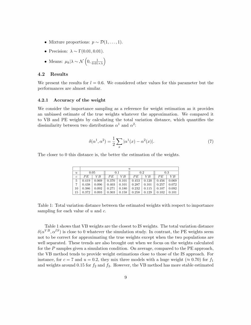
We consider the importance sampling as a reference for weight estimation as it providesan unbiased estimate of the true weights whatever the approximation. We compared itto VB and PE weights by calculating the total variation distance, which quantifies thedissimilarity between two distributions α1 and α2:

δ(α1, α2) =1

2

∑x

|α1(x)− α2(x)|. (7)

The closer to 0 this distance is, the better the estimation of the weights.

uu 0.05 0.1 0.2 0.3c PE V B PE V B PE V B PE V B5 0.419 0.069 0.370 0.101 0.453 0.120 0.456 0.0697 0.438 0.096 0.403 0.101 0.287 0.101 0.257 0.07210 0.386 0.092 0.271 0.180 0.232 0.115 0.107 0.09215 0.372 0.093 0.303 0.158 0.258 0.129 0.102 0.101

Table 1: Total variation distance between the estimated weights with respect to importancesampling for each value of u and c.

Table 1 shows that VB weights are the closest to IS weights. The total variation distanceδ(αV B, αIS) is close to 0 whatever the simulation study. In contrast, the PE weights seemnot to be correct for approximating the true weights except when the two populations arewell separated. These trends are also brought out when we focus on the weights calculatedfor the P samples given a simulation condition. On average, compared to the PE approach,the VB method tends to provide weight estimations close to those of the IS approach. Forinstance, for c = 7 and u = 0.2, they mix three models with a huge weight (≈ 0.70) for f1

and weights around 0.15 for f2 and f3. However, the VB method has more stable estimated

9

weights than IS. PE is the more stable approach among the three but it tends to only selectthe two-component model with an average weight around 0.95.

Conclusion on the weight estimation By directly analysing the weight estimation,the similarities between the IS and the VB methods have clearly appeared. The VB methodprovides a good estimation of the true weights which is not the case for PE. Hence, whenthe computational time of the IS method is becoming very high, we get a real advantageby using the VB method in terms of weight estimation.

4.2.2 Accuracy of the posterior probabilities

Once the weights have been estimated, the averaged estimates of the posterior probabilitiesTt are computed for each approach. The aim of the VB method is to cluster the datainto two populations. In many cases, these populations are difficult to distinguish butsome observations are easily classifiable without any statistical approach. Hence, we putaside observations with a theoretical probability of belonging to the cluster of interestsmaller than 0.2 or higher than 0.8. A classical indicator to measure the quality of a givenclassification is the MSE (Mean Square Error) which evaluates the difference between theaveraged estimate TA of one method of A and the theoretical values T (th).

MSEA =1

P

P∑p=1

1

n

n∑t=1

(TAt,p − T(th)t,p )2, (8)

The MSEA estimation allows us to evaluate the quality of the estimates provided by Modelm over all datasets p = 1, ..., P and one approach of A. The smaller the MSE, the betterthe performances are.

Since we deal with synthetic data, we can look at the best achievable MSE. This aimsat minimising the MSE within the averaged estimator family to obtain an oracle weightWe denote this oracle by α∗ and we have:

α∗ = argminα||T (th) −

M∑m=1

αmT(m)||2, (9)

with∑M

m=1 αm = 1 and ∀m ∈ 1, ...,M, 0 ≤ αm ≤ 1. The variable T (m) is the estimationof T supplied by model m. This oracle can be viewed as the weights we would choose if thetheoretical posterior probability of belonging to the group of interest were known. Thisoracle estimator is obtained by a functional regression under non-negativity constraint andit can be written as:

α∗ = (T ′T )−1T ′T (th) × γ (10)

10

u = 0.05c PE V B IS SelectedHMM Oracle5 0.44(0.04) 0.36 (0.03) 0.38(0.04) 0.42(0.03) 0.31(0.02)7 0.54(0.04) 0.42 (0.04) 0.43(0.04) 0.47(0.03) 0.34(0.02)10 0.35(0.04) 0.30 (0.04) 0.30 (0.04) 0.34(0.04) 0.21(0.03)15 0.38(0.04) 0.34(0.04) 0.33 (0.04) 0.36(0.03) 0.23(0.03)

u = 0.1c PE V B IS SelectedHMM Oracle5 0.40(0.04) 0.37 (0.03) 0.39(0.03) 0.39(0.03) 0.29(0.03)7 0.29(0.03) 0.23 (0.03) 0.23 (0.03) 0.25(0.03) 0.17(0.02)10 0.28(0.03) 0.28(0.03) 0.23 (0.03) 0.28(0.03) 0.16(0.02)15 0.25(0.04) 0.22(0.03) 0.20 (0.03) 0.22(0.03) 0.17(0.02)

u = 0.2c PE V B IS SelectedHMM Oracle5 0.33(0.03) 0.29 (0.03) 0.30(0.03) 0.31(0.03) 0.19(0.02)7 0.26(0.03) 0.23 (0.02) 0.24(0.02) 0.25(0.02) 0.18(0.02)10 0.23(0.03) 0.20(0.02) 0.19 (0.02) 0.23(0.01) 0.17(0.02)15 0.08(0.01) 0.09(0.01) 0.07 (0.01) 0.09(0.01) 0.06(0.02)

u = 0.3c PE V B IS SelectedHMM Oracle5 0.23(0.02) 0.19 (0.01) 0.20(0.01) 0.22(0.01) 0.16(0.01)7 0.13(0.01) 0.11 (0.01) 0.12(0.01) 0.13(0.01) 0.09(0.01)10 0.17(0.02) 0.12(0.01) 0.11 (0.01) 0.18(0.01) 0.03(0.01)15 0.12(0.01) 0.10(0.01) 0.09 (0.01) 0.12(0.01) 0.06(0.01)

Table 2: Mean(sd) of the misclassification rate for the three averaging approaches.

where γ is a normalising constant and T is the matrix containing the estimates T (m)

for all model m. Several algorithms allow one to calculate this estimator numerically bytaking constraints into account. In this article, the optimisation has been achieved by theNewton-Raphson algorithm.

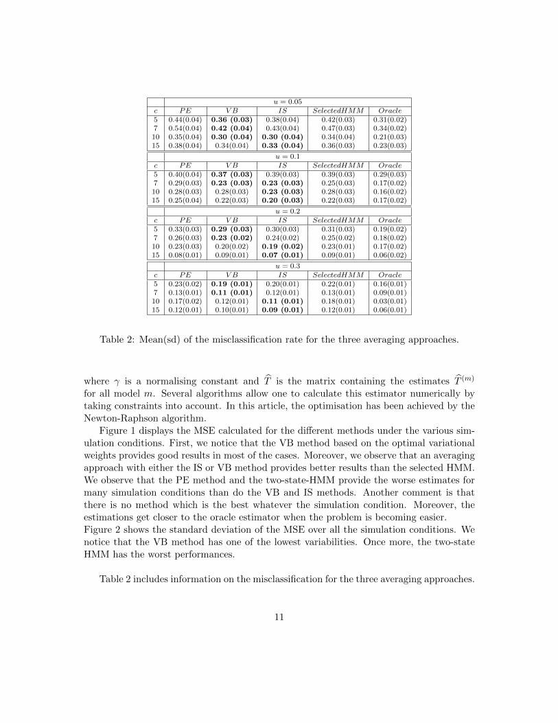
Figure 1 displays the MSE calculated for the different methods under the various sim-ulation conditions. First, we notice that the VB method based on the optimal variationalweights provides good results in most of the cases. Moreover, we observe that an averagingapproach with either the IS or VB method provides better results than the selected HMM.We observe that the PE method and the two-state-HMM provide the worse estimates formany simulation conditions than do the VB and IS methods. Another comment is thatthere is no method which is the best whatever the simulation condition. Moreover, theestimations get closer to the oracle estimator when the problem is becoming easier.Figure 2 shows the standard deviation of the MSE over all the simulation conditions. Wenotice that the VB method has one of the lowest variabilities. Once more, the two-stateHMM has the worst performances.

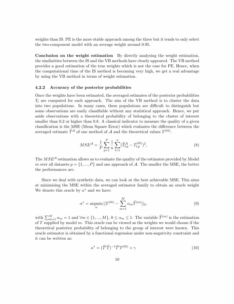
Table 2 includes information on the misclassification for the three averaging approaches.

11

Figure 1: Mean square error (MSE) between the true posterior probabilities and the esti-mates as a function of the uniform parameters. Methods: ”∆”: PE, ”∇”: two-state-HMM,”*”: IS, ”•”: Selected HMM, ”♦”: VB, ”O” : Oracle. Top left: Π0.05, Top right: Π0.1,Bottom left: Π0.2, Bottom right: Π0.3. VB and Oracle are in dotted lines.

12

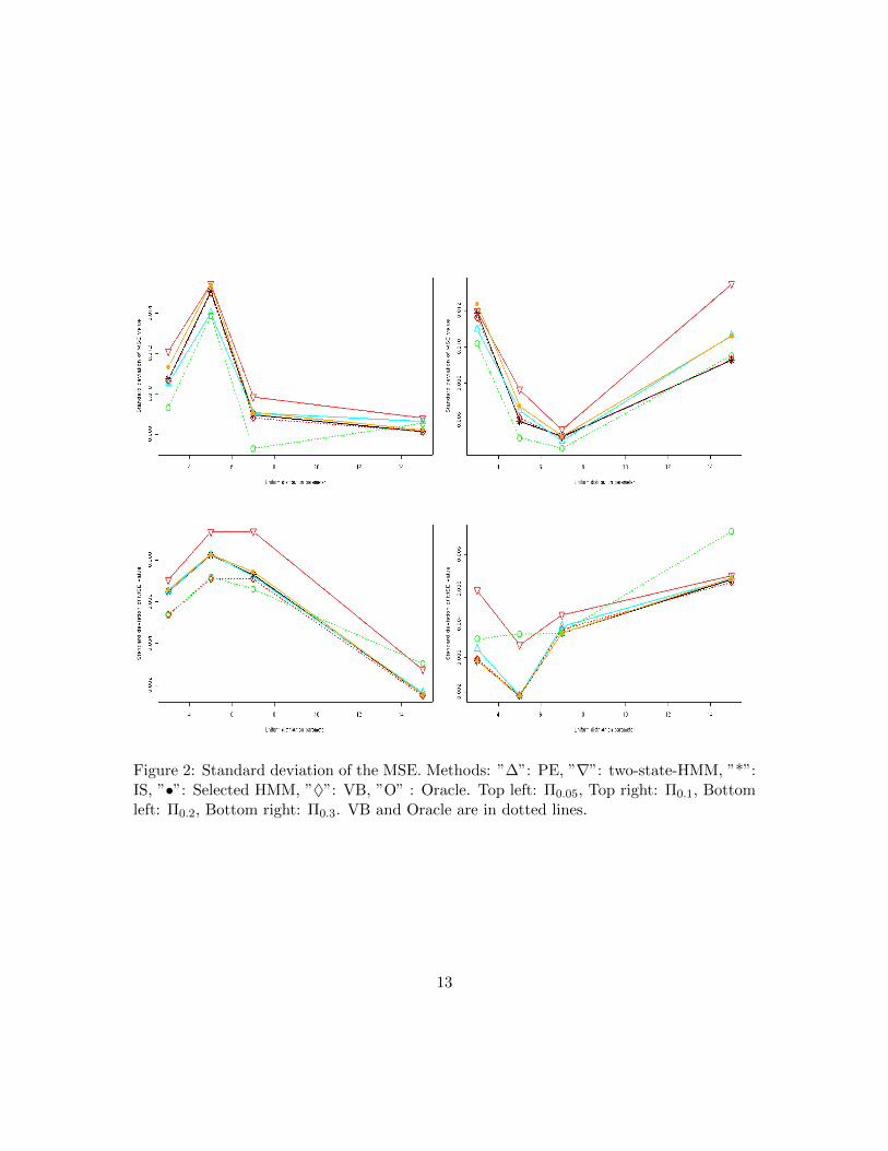
Figure 2: Standard deviation of the MSE. Methods: ”∆”: PE, ”∇”: two-state-HMM, ”*”:IS, ”•”: Selected HMM, ”♦”: VB, ”O” : Oracle. Top left: Π0.05, Top right: Π0.1, Bottomleft: Π0.2, Bottom right: Π0.3. VB and Oracle are in dotted lines.

13

The misclassification rate is calculated on the P samples whatever the simulation condition.The values in bold correspond to the smallest misclassification rate among the PE, VBand IS approaches. First, we note that the VB and the IS methods have very similarmisclassification rates whatever the simulation condition. Moreover, this rate correspondsto the best rate of the three averaging methods. The averaged estimator supplied by theplug-in weights estimation seems to misclassify more data than the other approaches. Onceagain, Table 2 shows us that the VB approach provides good results when the simulationcondition is complicated. In fact, when c equals either 5 or 7, the averaging methodbased on optimal variational weights provides the lowest misclassified rate among the threeaveraging approaches. Since the misclassification rate of the oracle is close to the ratesobtained by VB and IS estimation, the two approaches provide good results for each valueof c and u. An other comment is that the selected HMM approach always prodives worseresults than the IS and VB ones. This means that the averaging approach brings a gain tothe posterior probability estimation.

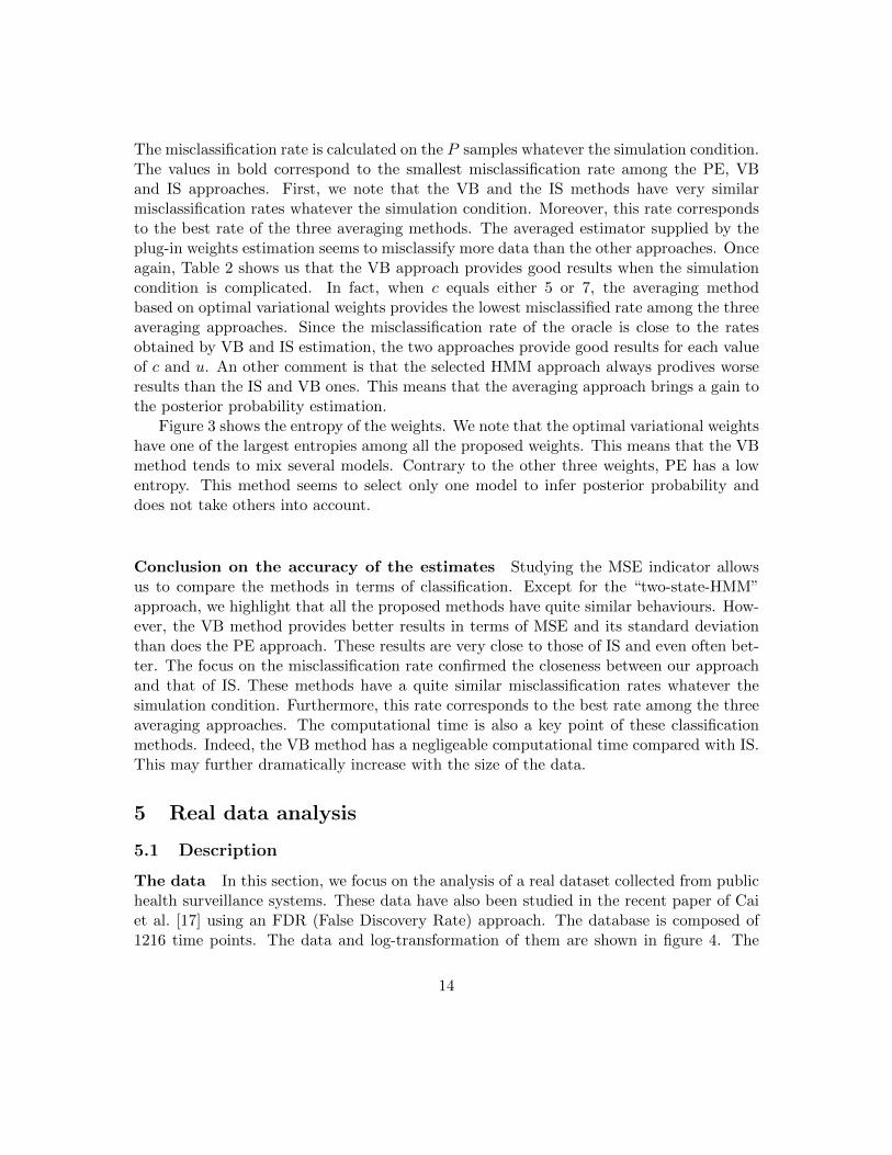
Figure 3 shows the entropy of the weights. We note that the optimal variational weightshave one of the largest entropies among all the proposed weights. This means that the VBmethod tends to mix several models. Contrary to the other three weights, PE has a lowentropy. This method seems to select only one model to infer posterior probability anddoes not take others into account.

Conclusion on the accuracy of the estimates Studying the MSE indicator allowsus to compare the methods in terms of classification. Except for the “two-state-HMM”approach, we highlight that all the proposed methods have quite similar behaviours. How-ever, the VB method provides better results in terms of MSE and its standard deviationthan does the PE approach. These results are very close to those of IS and even often bet-ter. The focus on the misclassification rate confirmed the closeness between our approachand that of IS. These methods have a quite similar misclassification rates whatever thesimulation condition. Furthermore, this rate corresponds to the best rate among the threeaveraging approaches. The computational time is also a key point of these classificationmethods. Indeed, the VB method has a negligeable computational time compared with IS.This may further dramatically increase with the size of the data.

5 Real data analysis

5.1 Description

The data In this section, we focus on the analysis of a real dataset collected from publichealth surveillance systems. These data have also been studied in the recent paper of Caiet al. [17] using an FDR (False Discovery Rate) approach. The database is composed of1216 time points. The data and log-transformation of them are shown in figure 4. The

14

Figure 3: Entropy of the weights. Methods: ”∆”: PE, ”∇”: two-state-HMM, ”*”: IS,”•”: Selected HMM, ”♦”: VB, ”O” : Oracle. Top left: Π0.05, Top right: Π0.1, Bottom left:Π0.2, Bottom right: Π0.3. VB and Oracle are in dotted lines.

15

m mean variance proportions αV B

1 4.9 1.1 1 < 10−4

2(

4.5, 5)

0.9(

0.67, 0.33)

< 10−4

3(

4, 4.2, 6)

0.3(

0.32, 0.32, 0.34)

0.34

4(

3.9, 4.1, 5, 6.3)

0.2(

0.22, 0.27, 0.26, 0.25)

0.66

5(

3.8, 4, 4.1, 5.2, 6.4)

0.18(

0.17, 0.19, 0.22, 0.22, 0.20)

< 10−4

6(

3.8, 4, 4.1, 4.8, 5.6, 6.5)

0.15(

0.14, 0.16, 0.16, 0.20, 0.16, 0.18)

< 10−4

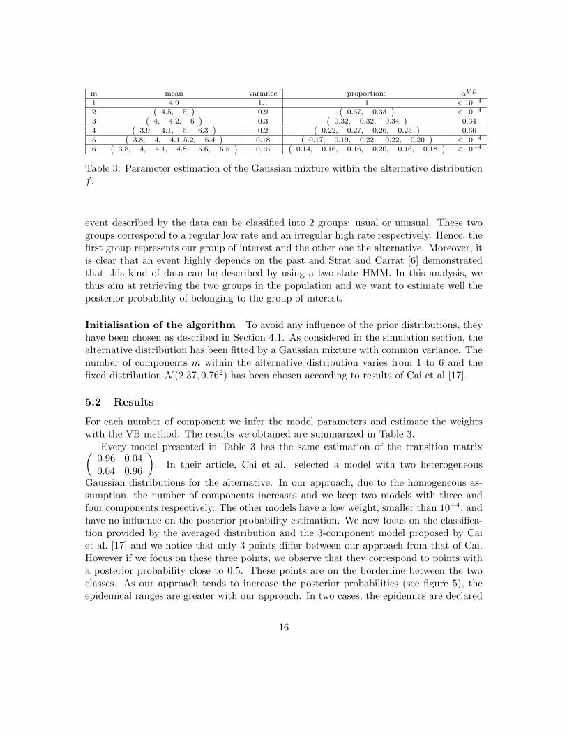
Table 3: Parameter estimation of the Gaussian mixture within the alternative distributionf .

event described by the data can be classified into 2 groups: usual or unusual. These twogroups correspond to a regular low rate and an irregular high rate respectively. Hence, thefirst group represents our group of interest and the other one the alternative. Moreover, itis clear that an event highly depends on the past and Strat and Carrat [6] demonstratedthat this kind of data can be described by using a two-state HMM. In this analysis, wethus aim at retrieving the two groups in the population and we want to estimate well theposterior probability of belonging to the group of interest.

Initialisation of the algorithm To avoid any influence of the prior distributions, theyhave been chosen as described in Section 4.1. As considered in the simulation section, thealternative distribution has been fitted by a Gaussian mixture with common variance. Thenumber of components m within the alternative distribution varies from 1 to 6 and thefixed distribution N (2.37, 0.762) has been chosen according to results of Cai et al [17].

5.2 Results

For each number of component we infer the model parameters and estimate the weightswith the VB method. The results we obtained are summarized in Table 3.

Every model presented in Table 3 has the same estimation of the transition matrix(0.96 0.040.04 0.96

). In their article, Cai et al. selected a model with two heterogeneous

Gaussian distributions for the alternative. In our approach, due to the homogeneous as-sumption, the number of components increases and we keep two models with three andfour components respectively. The other models have a low weight, smaller than 10−4, andhave no influence on the posterior probability estimation. We now focus on the classifica-tion provided by the averaged distribution and the 3-component model proposed by Caiet al. [17] and we notice that only 3 points differ between our approach from that of Cai.However if we focus on these three points, we observe that they correspond to points witha posterior probability close to 0.5. These points are on the borderline between the twoclasses. As our approach tends to increase the posterior probabilities (see figure 5), theepidemical ranges are greater with our approach. In two cases, the epidemics are declared

16

earlier with the VB method than with that of Cai.Figure 5 displays the averaged posterior probabilities against the estimations obtained

by the model proposed by Cai. The first comment is that the two approaches provideclose estimations. This is especially the case for probabilities smaller than 0.3 or greaterthan 0.7. These ranges correspond to low entropy areas. The main comment is that anaveraging approach tends to refine posterior probabilities between 0.3 and 0.7. This highentropy area is considered as a difficult area for estimating the probabilities. In fact, itmainly corresponds to data points which are on the borderline between the two classes.

6 Conclusion

We proposed a method for binary classification problems based on averaged estimatorswithin a variational Bayesian framework. This approach allows us to avoid model selectionand take model uncertainty into account. It can theoretically be proved that using anaveraged estimator provides a gain in terms of MSE and increases the lower bound of thelog-likelihood. We proposed a method based on optimal variational weights which derivefrom a modification of the classical lower bound of the log-likelihood. Our method doesnot required more computational time than classical one. For studying the performances,the method has been used on both synthetic and real data.

The results we obtained on synthetic data showed that our method enhances the es-timator in terms of MSE in many simulation conditions. We also highlighted that theaveraging approach improves the posterior probability estimation provided by the classicalselection approach. Moreover, we showed that optimal variational weights are closer toimportance sampling than the plug-in one. Since the importance sampling coped withcomputational time problems for high dimensional datasets, our method is of significantinterest in this case.

A real data analysis has been carried out on a clinical dataset. In this context, the ag-gregation model still refines the estimation of posterior probabilities. We note in particularthat the classification is different in cases where the probability is close to 0.5, i.e. whenthe classification is difficult. It allows us to refine the start of the epidemic period.

17

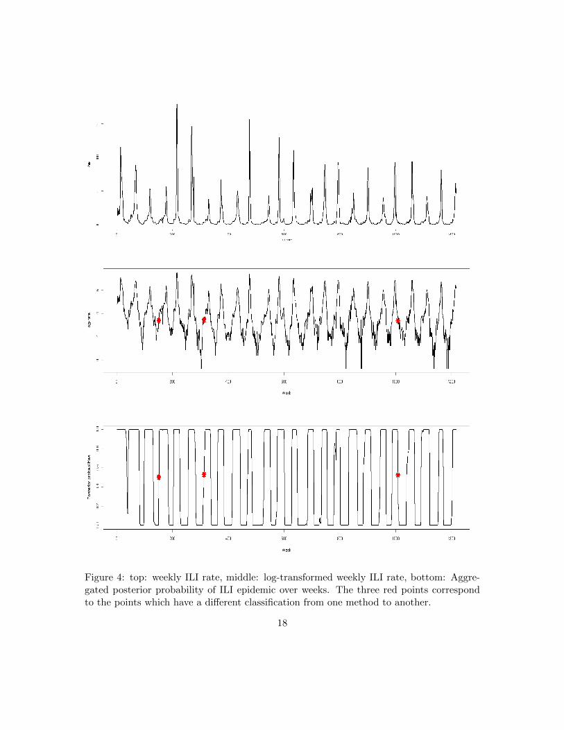
Figure 4: top: weekly ILI rate, middle: log-transformed weekly ILI rate, bottom: Aggre-gated posterior probability of ILI epidemic over weeks. The three red points correspondto the points which have a different classification from one method to another.

18

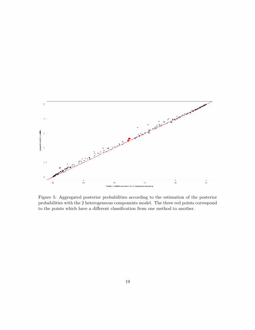
Figure 5: Aggregated posterior probabilities according to the estimation of the posteriorprobabilities with the 2 heterogeneous components model. The three red points correspondto the points which have a different classification from one method to another.

19

References

[1] Christophe Andrieu. An introduction to mcmc for machine learning, 2003.

[2] M. J Beal and Z. Ghahramani. The variational bayesian EM algorithm for incompletedata: with application to scoring graphical model structures, 2003.

[3] Adrian Corduneanu and Christopher M. Bishop. Variational bayesian model selectionfor mixture distributions. Statistics in Medicine, 18(24):3463–3478, 2001.

[4] Jennifer A Hoeting, David Madigan, Adrian E Raftery, and Chris T Volinsky. Bayesianmodel averaging: A tutorial. Statistical science, 14(4):382—417, 1999.

[5] Tommi S. Jaakkola and Michael I. Jordan. Improving the mean field approximationvia the use of mixture distributions. In Proceedings of the NATO Advanced StudyInstitute on Learning in graphical models, pages 163–173, Erice, Italy, 1998. KluwerAcademic Publishers.

[6] Yann Le Strat and Fabrice Carrat. Monitoring epidemiologic surveillance data usinghidden markov models. Statistics in Medicine, 1999.

[7] David Madigan and Fred Hutchinson. Enhancing the predictive performance ofbayesian graphical models. Communications in statistics: Theory and methods, 24,1995.

[8] David Madigan and Adrian E Raftery. Model selection and accounting for modeluncertainty in graphical models using occam’s window. Journal of the AmericanStatistical Association, 1993.

[9] Jean-Michel Marin and Christian P Robert. Importance sampling methods forbayesian discrimination between embedded models. 0910.2325, October 2009.

[10] C. A McGrory and D. M Titterington. Variational bayesian analysis for hidden markovmodels. Australian & New Zealand Journal of Statistics, 51:227–244, 2006.

[11] G. J. McLachlan, R. W. Bean, and D. Peel. A mixture model-based approach to theclustering of microarray expression data. 2002.

[12] G Parisi. Statistical field theory. Addison Wesley, 1988.

[13] Adrian E Raftery, Jennifer A Hoeting, and David Madigan. Bayesian model averagingfor linear regression models. Journal of the American Statistical Association, 92:179—191, 1997.

20

[14] Adrian E. Raftery, Yingye Zheng, N-We, Merlise Clyde, Jennifer Hoeting, and DavidMadigan. Long-run performance of bayesian model averaging. Journal of the AmericanStatistical Association, 98:931–938, 2003.

[15] Stephane Robin, Avner Bar-Hen, Jean-Jacques Daudin, and Laurent Pierre. A semi-parametric approach for mixture models: Application to local false discovery rateestimation. Comput. Stat. Data Anal., 51(12):5483–5493, 2007.

[16] Gideon Schwarz. Estimating the dimension of a model. The Annals of Statistics,6(2):461–464, 1978.

[17] Wenguang Sun and Tony Cai. Large-scale multiple testing under dependence. Journalof the Royal Statistical Society, 71:393–424, 2009.

[18] Chris T Volinsky, David Madigan, Adrian E Raftery, and Richard A Kronmal.Bayesian model averaging in proportional hazard models: Assessing the risk of astroke. Applied statistics, pages 433—448, 1997.

[19] Martin J Wainwright and Michael I Jordan. Graphical Models, Exponential Families,and Variational Inference. Now Publishers Inc., Hanover, MA, USA, 2008.

[20] Bo Wang and D. M Titterington. Lack of consistency of mean field and variationalbayes approximations for state space models. Neural Processing Letters, 20:151–170,2003.

[21] Bo Wang and D. M. Titterington. Local convergence of variational bayes estimatorsfor mixing coefficients. 2003.

[22] Bo Wang and D. M. Titterington. Convergence and asymptotic normality of vari-ational bayesian approximations for exponential family models with missing values.In Proceedings of the 20th conference on Uncertainty in artificial intelligence, pages577–584, Banff, Canada, 2004. AUAI Press.

[23] Bo Wang and D. M. Titterington. Inadequacy of interval estimates corresponding tovariational bayesian approximations, 2004.

21