Variational assimilation of ocean tomographic data: Twin experiments in a quasi-geostrophic model

Q. J. R. Meteorol. Soc. (2002), 128, pp. 1739–1758

Variational assimilation of ocean tomographic data: Twin experiments in aquasi-geostrophic model

By ELISABETH REMY1, FABIENNE GAILLARD2∗ and JACQUES VERRON3

1Scripps Institution of Oceanography, USA2Laboratoire de Physique des Oceans, France

3Laboratoire des Ecoulements Geophysiques et Industriels, France

(Received 6 February 2001; revised 1 November 2001)

SUMMARY

The possibility of using tomography data as a constraint in variational data assimilation is explored byperforming twin experiments. Realistic travel-time data are generated in a quasi-geostrophic model applied tothe western Mediterranean Sea. After checking the robustness of the method with this dataset, a sensitivity studyanalyses the propagation of information by the model, and tests the effect of different parameters such as thestarting point of the optimization or the length of the assimilation period. It appears that the variational methodis well adapted to the nature of tomographic data that provide at the same time high time resolution and spaceintegrals. The results clearly show the ability of this dataset to recover the temporal evolution of heat content ineach layer and improve various components of the circulation described by the model. Tomography must then beconsidered as an important source of information that may contribute with altimetry or local in situ measurementto the description of the ocean state and its evolution.

KEYWORDS: Ocean acoustic tomography Western Mediterranean Sea

1. INTRODUCTION

In the context of global ocean observing systems for studying climate, the oceano-graphic community is exploring different ways of building the optimal combination ofin situ observations, complementary with satellite observations, under the constraint thatthese measurements be sustained on a long-term basis. Among the existing observationaltechniques, acoustic tomography represents a potential valuable candidate and a fewpilot sites are already planned in a number of CLImate VARiability projects. Oceanacoustic tomography samples the ocean in depth and over large distances, during longtime periods and with high temporal resolution. It directly provides a strong constrainton the heat content over vertical sections across ocean basins, which may be used toprevent the drift observed in the models when doing long-term climate studies or removebiases due to undersampling of the mesoscale field. It is also important information tohelp discriminate between steric and dynamic effects contained in altimetric data. Pro-posed in the late seventies (Munk and Wunsch 1979) as a remote-sensing measurementtool, acoustic tomography has since then been applied in a large number of experiments,either as stand alone, or merged in multi-instrumental arrays. A synthesis of the possi-bilities, based on the results of the most illustrative experiments, is presented in Dushawet al. (2001).

Tomography data have mostly been used in diagnostic methods (or inversions).These methods rely on a combination of data, statistics and stationary conservationconstraints. Such methods were applied to study local phenomena as convection events(Send et al. 1995; Morawitz et al. 1996; Gaillard et al. 1997) as well as to estimate basin-scale temperature fields over the Pacific Ocean (Dushaw 1999), or over an unaccessibleregion such as the Arctic (Mikhalevsky et al. 1999). The range of scales resolved by thedata is determined by the size of the cells defined by the sections of the observational

∗ Corresponding author: Laboratoire de Physique des Oceans, IFREMER, BP70. 29280 Plouzane, France.e-mail: [email protected]© Royal Meteorological Society, 2002.

1739

1740 E. REMY et al.

array. Depending on the array geometry and scale, and on the availability of additionaldatasets, the above analyses were able to provide estimates of horizontally averaged heatcontent and vorticity or low-resolution three-dimensional (3-D) fields of temperatureand horizontal velocity.

Given the wide range of space and time-scales in the ocean, a full description of thecirculation cannot be obtained based only on observations and statistics. Assimilationin a prognostic ocean model is necessary to relate the variables sampled at differentpoints and times. This is how altimetric data are now commonly analysed (Fukumori2000). In order to reproduce the full vertical structure of the ocean, these data need tobe complemented by observations of the ocean interior. Assimilation of local in situdata is rapidly developing, and exploration of remote in situ data such as tomography isstarting. Menemenlis et al. (1997) performed the first assimilation of real tomographicdata to estimate the circulation of the Mediterranean Sea. They used the heat-contenttime series deduced from range-independent inversions of three tomography sections,in combination with altimetry.

In the present work we explore the possibility of directly assimilating the acoustictravel times, and study their impact on the model behaviour. By retaining featuresthat cannot be resolved by a simple inversion, we expect to make a better use of theinformation contained in the observations. A simplified ocean configuration is designed,having in mind future assimilation of the Thetis 2 experiment that took place in thewestern Mediterranean basin during the year 1994 (Send et al. 1997). Working in theperspective of post-experiment analysis (reanalysis), the variational method, which usesthe full time series of observations as a constraint for the model, seems appropriate. Twinexperiments will provide the possibility for exact comparison of the solution proposedby the assimilation with the true field used to simulate the observations.

The information content of tomographic data has been studied already in thecontext of inversions. Malanotte-Rizzoli and Holland (1985) simulated two sectionsplaced at different locations of a gyre in a three-layer quasi-geostrophic model. Theyperformed a one-dimensional inversion to estimate the total heat content over the sectionand the mean pycnocline displacements. Gaillard (1992) studied the case of three-dimensional inversion with a mesoscale array. The data were simulated in a quasi-geostrophic spectral model with three baroclinic modes. In both studies, the acousticdata was simulated by ray tracing in the sections extracted from the full 3-D sound-speed field provided by the model. The first twin experiment based on variationalassimilation of a dataset, similar to tomography, was done by Sheinbaum (1995). Heconsidered the highly simplified situation of a barotropic model advecting temperatureto demonstrate the possibility of assimilating integrals of temperature along horizontallines. In this simple case, the integral observations have an efficiency similar to that ofpoint observations.

None of the above experiments cover the full domain of realistic tomographicdata assimilation. Before going to the assimilation of the full Thetis 2 travel-timesdataset, we feel the need for a twin experiment based on an ocean model representingthe main features of the real ocean in terms of horizontal and vertical scales, andtomographic travel times close to real data in terms of sampling and geometry. We choseto work with a quasi-geostrophic model and its adjoint. Such a model does not containthermodynamics, and is obviously not adapted for real-data assimilation. On the otherhand, a quasi-geostrophic model provides the time and space variability that allowstesting of the resolution of the tomographic array and studying of how the informationis propagated. Its simplicity makes numerous testing procedures and sensitivity studyeasy.

OCEAN TOMOGRAPHIC DATA 1741

The configuration is that of a rectangular basin, with size and stratification of thewestern Mediterranean basin, forced by monthly winds. The acoustic data are obtainedby the method of Gaillard (1992). The interface deviations are related to temperaturevariations and sound speed, then a ray tracing is performed in the sound-speed field. Weadd here the simplifying assumption that the ray paths, computed in the ocean at rest,remain unchanged.

The first goal of the twin experiments is to evaluate the feasibility of variationalassimilation of tomographic data. Then, if convergence towards an acceptable solutionis reached, we wish to define the efficiency of this integral dataset in controllingthe model. In particular, we want to know what variables are influenced, how isinformation propagated in time and which components of the circulation are wellconstrained. Knowledge of the information content of a particular dataset is necessarybefore performing any type of data merging, or in the design of future experiments. Insection 2 we describe the model, the assimilation method and how we have simulatedthe acoustic data. Section 3 is a sensitivity study concerning various parameters of theassimilation. The results of a standard run are analysed in section 4.

2. ASSIMILATION METHOD

Data assimilation combines a prognostic model and observations, in order to givethe best estimate of the state of the system under study. The numerical model is a setof differential equations representing an approximation of physical laws and wherethe unresolved processes are parametrized. It predicts the evolution of the variablesof the system, as determined by the forcing terms, boundary and initial conditions,which are known with uncertainties that may sometimes be large. As a consequence,the modelled circulation develops biases which grow over acceptable levels in the long-term simulations. Observations of quantities related to the model variables can be usedto compensate for the model deficiencies. Observations have their own limitations: theysample the model in time and space at a rate usually much lower than the model grid sizeor time step and so cannot fully determine the model state. They contain measurementerrors and subgrid processes and thus the relation with the model variables is onlyapproximate. For combining those two sources of information, inverse and assimilationmethods rely on complementary statistical knowledge expressing the errors associatedwith the model and data, and a priori information on the ocean state.

Data assimilation has been used in meteorology for several decades, and is nowoperationally employed for prediction. In oceanography, a growing number of datasetsare now available and represent potential candidates for assimilation. Selecting betweensequential or variational methods depends on the objectives of the analysis and of thetype of data available. Sequential methods are more commonly used in the real-timeapplications, since they only require past and present data. In the present study, thefocus is on acoustic tomographic data, which are travel-time measurements of soundpropagation through a large volume of ocean. These data have integrated temperatureand current effects over long distances, and at different levels. They are available witha high time resolution. We work here in the context of post-analysis, which means thatwe process a time series of the order of several months, all at once, in order to providethe best estimate of the ocean circulation during that period. Since we are free of thereal-time processing constraint, we select the variational approach where the model isapplied as a strong constraint. We will explore the feasibility of the method and evaluatethe performances with a tomographic dataset.

1742 E. REMY et al.

(a) Principles of the adjoint methodThe variational method was introduced for assimilation in meteorological models

(Le Dimet and Talagrand 1986; Talagrand and Courtier 1987) and later in oceanography(Thacker and Long 1988). A cost function containing a data misfit term, representingthe distance between the model and the data, and a penalty term, representing anyknowledge we have on the field, are built. The solution is defined by the minimumof the cost function relative to the variations of control parameters, usually the initialconditions. In the unified notation described by Ide et al. (1997), the cost function iswritten

J = (Hx − yobs)TW−1(Hx − yobs)+ R(x), (1)

where x is the state vector, representing the model variables at all time steps and yobs

is a vector containing all observations available in the assimilation period. The datamisfit term is the quadratic difference between observations and their equivalent interms of model variables; H is the observation operator relating the model variablesto the data and W is the prescribed error covariance matrix on observations which setsthe acceptable amplitude of the misfit. It represents both the measurement errors andthe representativity error due to the approximation in H. The R term contains a prioriinformation on the solution. It is needed to prevent the problem becoming ill-posed.In the case of under-determined problems, it ensures the uniqueness of the solution.

The cost function is minimized iteratively, the increment defining the new valueof the control vector being deduced from the gradient of the cost function. If weintroduce the tangent linear model Mi = ∂Mi/∂x0, the gradient of the cost functionis approximated by(

∂J

∂x0

)T

= HT0 W−1

0 (y0 − yobs0 )

+n∑i=1

{MT1 . . . MT

i−1MTi HT

i W−1i (yi − yobs

i )} +(∂R(x0)

∂x0

)T

. (2)

From this expression, we see that the adjoint model MTi is integrated backwards in time,

forced by the misfit term. The direct model propagates forwards in time the informationintroduced by the new initial conditions.

(b) The prognostic modelThe prognostic model was developed in Grenoble and is derived from Holland

(1978). The adjoint code was developed by Luong (1995) for altimetry. The quasi-geostrophic nonlinear equations are written in terms of stream function ψ ; they givethe time evolution of the vorticity qk in each layer k:

∂qk

∂t+ J (ψk, qk) = −A∇4ψk + δk,1

rotzτ

H1− δk,nε∇2ψk on �, [0, T ], (3)

where z is height, δ is the Kroenecker symbol, H is the layer thickness, hi is the level ofthe layer limit, τ is wind stress, f0 is the mean Coriolis parameter, ε is the bottom frictioncoefficient, � is the model domain and T is the time range of the model. Vorticity isdefined as

qk = ∇2ψk + f + f0

Hk

(hk+ 1

2− h

k− 12).


0o 3oE 6oE 9oE

36oN

38oN

40oN

42oN

44oN

H

SW1

W2 W3

W4

W5

Figure 1. Western Mediterranean basin: bathymetry, limits of the model domain (rectangle) and position of thetomographic array, with H, S and W representing different source types. The depth contour interval is 500 m.

Instrument W1, west of the Balearic islands has not been used in the twin experiments.

The right-hand-side terms represent, respectively: lateral diffusion, wind forcing andvertical diffusion. The domain is a rectangular closed basin with a flat bottom centredon the western Mediterranean basin (Fig. 1). The parameters of the stratification arechosen using hydrological profiles of this region. The three layers represent the principalwater masses: modified Atlantic water in the surface layer, Levantine intermediate waterfrom the eastern basin in the second layer and deep Mediterranean water in the deeplayer (Millot 1987). The horizontal resolution is 5 × 5 km, and the first deformationradius is 12 km. The circulation is forced by the monthly climatological wind field fromMay (1982) which is given with a spatial resolution of 1◦ × 1◦. The forcing terms areinterpolated in time and space down to the model resolution and time step. Althoughhighly simplified, this configuration reproduces a circulation with sufficiently realisticspace- and time-scales.

The circulation obtained after two years of spin-up is rather turbulent and dominatedby the barotropic mode, especially in the lower layers. The barotropic mode represents85% of the total kinetic energy. The upper layer reproduces the observed cycloniccirculation around the basin and the north Balearic front. South of this, large-scaleeddies are found with the correct scale of one hundred kilometres. The intermediateand deep layers show very similar circulation patterns, because a realistic circulationin the intermediate layer cannot be reproduced without a density forcing through theStraits of Gibraltar (west) and Straits of Sicily (east) (Herbaut et al. 1996).

1744 E. REMY et al.

1500 1550−2500

−2000

−1500

−1000

−500

0

c (m s−1 )

Dep

th (

m)

0 0.5 1 1.5 2Distance (10 5 m)

(a) (b)

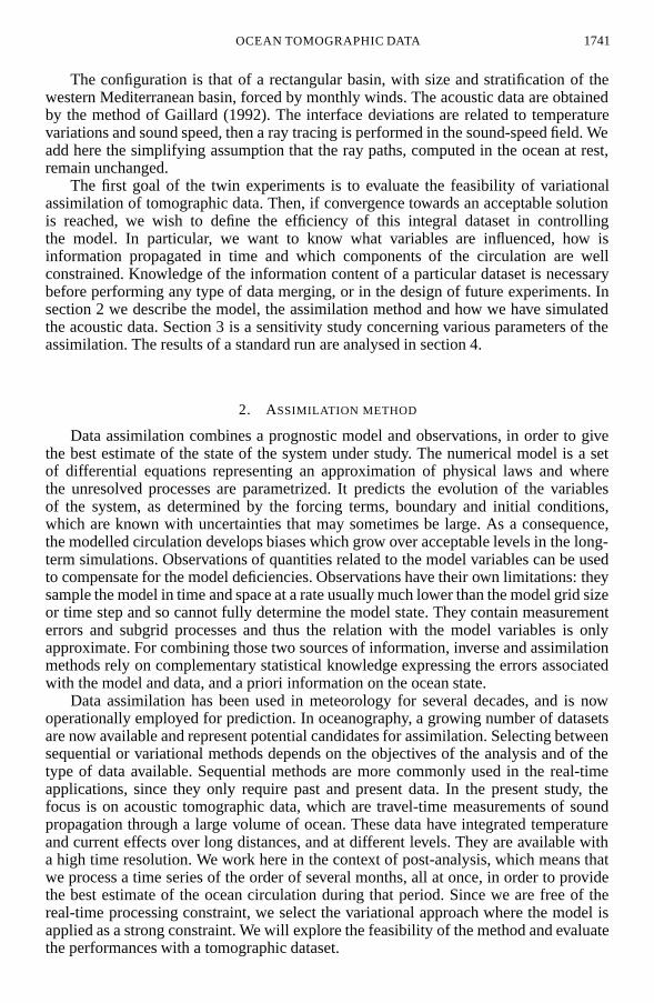
Figure 2. (a) Mean sound-speed profile for the western Mediterranean and (b) corresponding ray paths betweena source and a receiver 250 km apart.

(c) Cost functionThe solution is found by minimizing the cost function defined by Eq. (1), where

the control vector is the stream-function initial conditions. The solution is searchediteratively from a starting point—the first guess. At each iteration, the full nonlinearmodel is run forward in time, while the adjoint is run backwards. The relationshipbetween the observations and the state vector at all time steps appears in the costfunction through the data misfit term. Observations are weighted by W. Additionalinformation on the control vector is brought by the regularization function R. In ourexperiments, we assimilate the tomographic data related to temperature, also called‘acoustic thermometry’. We detail here the construction of H and present the expressionof the penalty term R.

(i) Simulated acoustic tomography data. Acoustic thermometry uses the travel-timeanomaly, defined as the difference between the measured travel time and the travel timepredicted in a reference ocean (Munk et al. 1995) with mean sound-speed profile C 0(z).The reference profile and a few corresponding ray paths are shown Fig. 2. Variations ofthe sound speed modifies the ray path itself. We neglect here this nonlinear effect andassume fixed ray paths. Under this ‘frozen rays’ approximation, the travel-time anomalyδτ is linearly related to the sound-speed anomaly δC along the ray path R0:

δτ = −∫

R0

δC(x, y, z)

C20 (z)

dl. (4)

The observation operator H relating δτ to the model variables is defined as in Gaillard(1992). In the quasi-geostrophic model, the sound-speed variations are only related tothe displacement of interface between each layer:

δCk+ 1

2= ∂Cp

∂z

∣∣∣∣z(k+ 1

2 )

hk+ 1

2, (5)

where

hk+ 1

2= f0

g′k+ 1

2

(ψk+1 − ψk).


Here ∂Cp/∂z is the vertical gradient of the potential sound speed, δCk+ 1

2is the average

value of the high-resolution ∂Cp/∂z profile over layer k, and g ′ = g�ρ/ρ0, where g isthe acceleration due to gravity, ρ0 is the mean density and �ρ is the density anomalywith respect to ρ0. The integral over a particular ray path R0l is replaced by a discretesum over m model grid cells encountered. The distance dl is also computed on thisfine grid and interpolated on the coarser vertical model grid. To every grid point mcorresponds a triplet (i, j, k + 1

2 ), locating the point in the x, y and z dimension of themodel:

δτl =∑

m∈R0l

(∂Cp/∂z

C20

)k+ 1

2

dlm

hm. (6)

The observational array used to simulate the observations is similar to the Thetis 2array deployed in the western Mediterranean in 1994 (Fig. 1). Ray tracing is performedalong 12 sections, and we obtain on average 20 ray paths per section. Transmissions aresimulated twice a day.

In the case of a real experiment, the acceptable misfit to observations specified inthe covariance matrix W represents both the measurement error and the representativityerror of H introduced by the various approximations. In the present study, the data aregenerated with the observation matrix H itself and we do not add any synthetic noise.The data are then perfect relative to the model and the problem of noise effect is notaddressed here. Nevertheless, the matrix W is used to adimensionalize the misfit termand introduce a weighting relative to the regularization term. It is built as a unit matrixwith (5 ms)2 amplitude.

(ii) Regularization term. Since the number of independent data is smaller than thedimension of the control vector, the problem is highly underdetermined and manysolutions are compatible with the data. An additional term R is necessary to avoid theproblem being ill-posed by ensuring the uniqueness and stability of the solution.

It is introduced here as a smoothing function that gives one constraint per grid pointon the stream function at initial time. This makes the problem formally over-constrained.

R(ψt=0)=3∑

k=1

ny∑j=1

nx∑i=1

1

αk(�hψi,j,k)

2 + 1

γk(�2

hψi,j,k)2

+ 1

βk

{f 2

0

Hkg′k

(ψi,j,k−1 − ψi,j,k)− f 20

Hkg′k+1

(ψi,j,k − ψi,j,k+1)

}2 . (7)

Each term is adimensionalized by a scaling factor, αk, βk and γk, computed as the root-mean-square (r.m.s.) amplitude of the corresponding term in one of the model runs.

The first term, expressed as a Laplacian, represents the kinetic energy, the secondterm is a bi-Laplacian and corresponds to the enstrophy. Both terms act as horizontalfilters with a length-scale depending on the derivation degree. The Laplacian inducesa correlation length of about 35 km while the biharmonic is more scale selective. Thelast term corresponds to a vortex-stretching; it imposes a vertical correlation betweeninterface deviations of two successive layers. In summary, this regularization functionwill maintain kinetic energy, enstrophy and vortex-stretching at initial time, withinacceptable limits. Small-scale perturbations will be penalized.

1746 E. REMY et al.

3. SENSITIVITY STUDY

We start the study with a basic experiment, based on ‘reasonable’ assumptions,and analyse in that case the relative influence of the data misfit term, including theobservation matrix, and the regularization terms. The directions of search, the rate atwhich we converge towards the solution and the choice of a particular solution stronglydepend on the shape of the cost function in the control parameter space. In order toevaluate the basic experiment results obtained, we will modify two parameters thatinfluence the cost function: the starting point of the minimization (the first guess) andthe length of the assimilation period. Since twin experiments allow exact comparison ofthe solution with the true field, r.m.s. differences, computed over the model domain, areused as a global measure of distance between two fields.

(a) The basic experimentAfter a three-year spin-up, the model has reached a stable annual cycle. The

reference or true field, in which observations are simulated, is taken starting at thebeginning of May of the fourth year. The first guess used to initialize the minimizationis the field obtained in May, two years after the true field. Comparison of the two fieldsshows large differences: the northern cyclonic gyre is more concentrated in the firstguess, a strong dipole in the centre present in the true field does not exist in the firstguess (see Fig. 4, experiment 0). We are here in an extreme case, where the first guessis far from the true field, that will permit testing the robustness of the method underdifficult conditions.

The length of the assimilation window is 50 days, beginning in May. The modeltrajectory that best fits the observations is found by minimizing the cost function J withrespect to the control vector, the initial conditions for the stream function:

J (ψt=0) =50 days∑t=0

1

σ 2δτ

(Hψt − δτ obst )2 + R(ψt=0). (8)

The first term is the quadratic misfit to travel-time anomalies δτ , normalized by theirerror. The second term is the regularization term described in section 2.

The control-vector dimension equals the number of grid points times the numberof layers (approximately 38 × 103). At each assimilation step (every 12 hours), 360observations are provided, but not all of them are independent from the model pointof view, as will be seen in the observation matrix study. Part of the data at time t + 1can be predicted by the model from the data at time t . In the end, the total number ofindependent data is bounded by 30 × 103 but the exact number is probably much lowerby at least one order of magnitude. Whatever the exact number of independent data, itis obviously smaller than the dimension of the control vector. The problem is clearlyunderdetermined and the regularization term is needed to introduce complementaryinformation on the unknowns.

(i) Analysis of the observation matrix. The misfit which appears in the cost functionmeasures the distance between the data and their equivalent in terms of model variableas given by Eq. (6). The observation matrix H represents the weighting of eachobservation with respect to the model variables. The study of this matrix weighted by theobservational covariance error matrix brings some elements about the observability ofthe ocean with the considered tomographic data. The specificity of tomographic data dueto the integral nature of the measurements is expressed in H. The measurements do not


give direct access to the model variables, but only to linear combinations of elements ofthis vector, the interface deviations along the ray path. The singular value decomposition(SVD) of WTHW, WTHW = U�VT, gives an idea of the relative importance of thedata and of the information they bring to the system; � are the eigenvalues, U isthe matrix of eigenvectors spanning the data space, and V the matrix of eigenvectorsspanning the model variable space, which here are the interface deviations at each gridpoint of the sections.

The resolution matrix R defines how the true value of ψt is filtered by the obser-vational array: ψobs

t = Rψ truet . It is built with the eigenvectors associated to non-zero

eigenvalues: R = VVT. The closest R is to a unit matrix, the closestψ obst is to ψ true

t . Thediagonal elements of the resolution matrix for each single pair are dominant, but they aremuch smaller than unity, meaning that the stream function or interface deviation cannotbe resolved at individual points along the section by the tomographic measurementsalone. The coefficients associated with the second-interface deviations are smaller thanfor the first interface. When all sections are used simultaneously, the resolution im-proves at the section crossings. The vertical resolution provided by the ray paths is notexploited by the assimilation because it exceeds the vertical resolution of the model,which has only three layers. Tomographic measurements bring information about thefirst baroclinic mode, which is the dominant component of the interface deviations, butsays nothing about the barotropic circulation.

This analysis gives an idea of the information available at every measurement time.The exact information used by the assimilation, which combines data and model, canformally be accessed by computing the Hessian matrix of the cost function but, suchcomputation being too heavy, the information provided by the model will be exploredindirectly in section 3(c).

When data are provided for a single section, the estimated correction at the dataintroduction time is approximately constant and maximum along the section. Sincetomographic data are integral measurements, a change in the field, equal to the meanvalue of the difference between the first guess and the true field is sufficient to fit theobservations. When the full array is assimilated, it becomes necessary to introduce spacevariability in the correction, and this is how horizontal resolution is gained.

(ii) Decrease of the cost function. The first diagnostic of the success of the minimiza-tion is the decrease of the cost function during iteration. Figure 3 shows the evolutionof the total cost function, the observation misfit and regularization terms for the basiccase. At the beginning of the iteration process, the misfit to observations is two ordersof magnitude larger than the regularization term. In the first ten iterations, the misfitto observations decreases rapidly while the regularization term increases. This term islargely dominated by the biLaplacian term, indicating that, in order to match the obser-vations, small scales features are introduced. They are not present in the true field . Itshould be noted that these small scales appear at the initial time (the control vector),but are rapidly attenuated by the model dynamics. As the minimization goes on, theregularization term starts to decrease slowly, showing that it succeeds in reducing thesmall-scale development. The regularization term should also decrease down to the levelit had at the beginning of the minimization because the solution has the same propertiesas the first guess in terms of horizontal scales and vortex stretching. The data misfit keepsdecreasing. After 100 iterations, the value of the cost function is divided by almost twoorders of magnitude and the two terms have comparable size. The misfit to observationsreached the a priori error level. Even if it does not represent a realistic criterion in twinexperiments, we stop the optimization at this point as the convergence becomes really

1748 E. REMY et al.

0 20 40 60 80 10010

4

105

106

107

Iteration number

J(Ψ

)

(a)

20 40 60 80 1002500

3000

3500

5500

6000

6500

7000(b)

Iteration number

r.m

.s. e

rror

Figure 3. (a) Evolution of the cost function versus iteration number: total cost function (solid line), data misfit(dashed line) and regularization (grey line). (b) Root-mean-square error of stream function (m2s−1): barotropic

mode (solid line), first baroclinic mode (dashed line) and second baroclinic mode (grey line).

slow and the result does not change significantly. This is shown by the evolution of ther.m.s. error in Fig. 3. The main improvements are done during the first 20 iterations.

(b) Influence of the choice of the first guessBy initializing the minimization with different first guess we would like to know

first if we are going in the right direction (as the cost function seems to indicate), andsecond if we obtain a better solution when starting closer to the true field. If the answeris positive, then we can conclude that the system is robust and that both the method andthe dataset, when correctly initialized and/or complemented, can contribute efficientlyto the estimation of the true field. The minimization method used, a quasi-Newtonianmethod, is based on the assumption that the function to minimize is nearly quadratic,so the gradient given by the adjoint provides a good descent direction. Starting from afirst guess very distant from the true field enhances the nonlinear effects, and the adjointtechnique, which relies on linear approximation, is not so efficient in such cases andincreases the risk of finding local minima.

We will compare three experiments in which we vary the distance between thefirst guess and the true field. The first case is the basic experiment (experiment 0);it represents the maximum distance studied (d). In the second and third experiments,the first guess is interpolated at intermediate distances between the basic first guessand the true field. Experiment 1 starts at distance 3d/4 and experiment 2 at distanced/2. Figure 4 shows a map of the elevation of the first interface at the initial time (thecontrol variable), as specified by the first guess and the solution obtained at the end ofthe minimization. The field at initial time (Fig. 4) is well reconstructed in experiment2. The main structures are now located correctly, although some amplitudes are stillunderestimated, and the tendency to create small-scale structures is strongly reduced.In order to measure the progress made over the whole time period, we also presentthe r.m.s. error for the first interface deviation as a function of time for the differentexperiments in Fig. 4. In each experiment, the solution is closer to the true field than thefirst guess over the entire assimilation period. Experiments 1 and 2 demonstrate that thesolution improves when the starting point is closer to the true field. The r.m.s. distancesare smaller over the whole assimilation interval.

The choice of the first guess is of primary importance with this iterative methodbased on linear approximation. It is clear that to obtain the best results from a givendataset, the first guess must not differ too strongly from the true field. This problemis probably enhanced by the integral nature of tomographic data that cannot locate the


100 200 300 400

100

200

300

400

500

600

(a) First guess 0 (d)

100 200 300 400

100

200

300

400

500

600

(d) Result 0

100 200 300 400

100

200

300

400

500

600

(b) First guess 1 (3d/4)

100 200 300 400

100

200

300

400

500

600

(e) Result 1

100 200 300 400

100

200

300

400

500

600

(c) First guess 2 (d/2)

100 200 300 400

100

200

300

400

500

600

(f) Result 2

100 200 300 400

100

200

300

400

500

600

(g) Reference

0 10 20 30 40 502000

3000

4000

5000

6000

7000

(h) Rms(ψk=1)

<(ψ

−ψ

ref)2 >

Time in days

exp 0

exp 1

exp 2

Figure 4. (a)–(g) Elevation of the upper interface at the initial time (m). Effect of distance di (km) to thetrue field: (a)–(c) first guess and (d)–(f) result, for experiments 0, 1 and 2 for which di = d (basic experiment),di = 3d/4 and di = d/2, respectively. (g) Reference elevation. Contour interval is 20 m and negative values are

dashed. (h) Root-mean-square error on the estimation of elevation of the upper interface as a function of time.

1750 E. REMY et al.

structures accurately. This lack of spatial resolution can be compensated by direct mea-surements such as hydrographic sections, expandable bathy thermographs or profilingfloats. In a monitoring configuration, the first guess problem occurs only once, at thebeginning of the monitoring. It is then conceivable to design some intensive array, basedon direct measurements, to complement a large-scale tomographic array in order to ini-tialize the assimilation.

(c) Propagation of information by the modelIn the variational formalization used here, the initial conditions are modified by the

observations distributed over all times, through the data misfit term, in order to keepa dynamical coherence between these observations. The information attached to eachpiece of data is carried forward in time by the direct model, and backward by the adjoint.Considering that at a single time step we have many fewer observations than unknowns,it is tempting to use as many data as possible. Increasing the time period over which dataare assimilated increases the number of data, and so should improve the solution. On theother hand, lengthening the period of assimilation increases the effect of nonlinearities,and the linear tangent approximation on which the adjoint relies may become invalid.We will examine here how the specific tomographic information is propagated in timeand space by the model and try to define the optimal period over which we can extendthe assimilation.

(i) Optimizing the length of the assimilation period. Part of the information introducedat large scales on the baroclinic modes is transferred towards smaller scales and tothe barotropic mode through mode coupling and nonlinear interactions. The nonlinearterms then play the double, and contradictory, role of contributing to the transfer ofinformation and simultaneously imposing a strong limitation on the duration of theassimilation period.

The time limitation depends crucially on the validity of the tangent linear model.To determine this period of validity, we compute the time evolution of the differencebetween two states separated at the initial time by a small perturbation δψ0, and compareit to its linear approximation:

Mt0→ti (ψ0 + δψ0) − Mt0→ti (ψ0)= Miδψ0 + %(δψ20 ), (9)

where % is some function of the nonlinear perturbation. We chose δψ0 as being 10% ofthe difference between the first guess and the true field, which is approximately 1% ofψ 0amplitude, and we consider that the error due to the nonlinear terms, %(δψ 2

0 ), becomestoo important when its magnitude is the same as the linear term. The barotropic modestarts to diverge after 40 days, followed by the first baroclinic mode 5 days later, after50 days even the second baroclinic mode has grown over the acceptable level.

The growth of the error due to nonlinear terms depends not only on the time ofintegration but also on the amplitude of the initial disturbance, and the above resultscannot be simply transposed to the real assimilation case. Therefore, the length ofassimilation period can only be optimized by running the assimilation over differentdurations. The results of the basic experiment are compared to those of two additionalexperiments in which a shorter assimilation period Ta = 30 days and a longer oneTa = 70 days are tested. For all cases, we compare the r.m.s. error over the longer 70-dayperiod. This means that in the 30-day and 50-day cases, the integration is continued upto 70 days, without assimilation. The results are analysed in terms of equivalent verticalmodes of the model. Only the barotropic and first baroclinic modes are considered,the second baroclinic mode is not well estimated and has a minor contribution to the total


0 10 20 30 40 50 60 70

0.6

0.7

0.8

0.9

1

1.1

1.2

Rel

ativ

e r.

m.s

. err

or

0 10 20 30 40 50 60 70

0.6

0.7

0.8

0.9

1

1.1

1.2

t (days)

Rel

ativ

e r.

m.s

. err

or

(a)

(b)

Figure 5. Root-mean-square error normalized by the a priori error in the case of different assimilation periods:(a) barotropic mode and (b) first baroclinic mode. Ta = 30 days (light grey line), Ta = 50 days (dark line), andTa = 70 days (dark grey line). Dashed lines represent the continuation of the run in prognostic mode with no

assimilation.

stream function. The r.m.s. errors, normalized by the r.m.s. initial error (first guess−truefield), are shown in Fig. 5. In this representation, the normalized first guess error isuniformly equal to one by definition. It is difficult to establish a clear criterion for theoptimal assimilation length since the results depend on the particular situation. The runT70 gives the best results over the period 0–60 days for the barotropic mode; it degradesconsiderably in the last 10 days. The baroclinic mode estimation is not as good as the twoshorter runs during the first 30 days, but it is clearly the best from day 30 to day 70. RunT30 is more or less equivalent to run T50 over the first 30 days: the longer assimilationperiods tend to slightly degrade the initial time estimate, while improving the centralperiod. The run T50 seems the best trade-off, confirming the study on the developmentof nonlinearities by the model.

(ii) Reconstruction of the 4D circulation. The basic experiment is stopped after100 iterations. At this stage, the cost function has decreased by almost two orders ofmagnitude, the data misfit term is below the a priori noise level and the decrease ratehas become very low. Comparing the amplitudes of the different fields: first guess,result and true field in the middle of the assimilation period give an overview of thequality of the estimation. Figure 6 presents those fields for the two main equivalent

1752 E. REMY et al.

0 200 4000

200

400

600

(a)

(km)

(km

)

0 200 4000

200

400

600N1

P1

P2

P3

(c)

0 200 4000

200

400

600

(b)

0 200 4000

200

400

600

(km)

(km

)

0 200 4000

200

400

600

0 200 4000

200

400

600

N1

P1

P2

P3

N1

P1

P2

P3

(km)

(km)

(km)

(km)

(d) (e) (f)

Figure 6. Amplitude of (a)–(c) barotropic and (d)–(e) first baroclinic modes for the basic-run solution. Theassimilation interval Ta is 50 days. Results are shown in the middle of the assimilation interval, at t = 30 days.The contour interval is 2000 m2s−1 in (a)–(c) and 1000 m2s−1 in (d)–(e). Negative values are dashed with shading

above 0. N1 and P1, P2 and P3 denote a negative and three positive structures, respectively (see text).

modes at t = 30 days. The barotropic mode of the true field is dominated by a strongnegative structure N1 at 350–500 km. In our solution, the first guess has been modifiedin such way that the structure N1 initially at 200–500 km, is now placed approximatelyhalf way from its correct position. Three secondary positive structures P1, P2, P3 arerecovered with different quality. Structure P3, placed on the intersection of severaltomographic sections is now placed correctly but a ghost of the initial structure remainsnear the western border, away from the tomographic sections. Structure P2 is buildingon. Structure P1, mostly out of the array, is not correctly recovered but the field hasevolved in the right direction. The baroclinic mode is dominated by a negative structureN1 and three secondary positive structures. In the solution of the basic experiment, N1 isbuilding on but lacks intensity, here again the best results are obtained for P3. With threelayers a second baroclinic mode exists but, given the very weak stratification betweenlayers 2 and 3, this mode has negligible amplitude and almost no effect on the total field.Results for this mode are not discussed.

In summary, the solution proposed by the basic run is closer to the true field thanwas the first guess especially in the vicinity of tomographic sections. Our first goalis reached: feasibility of assimilating tomographic data with a variational method is


demonstrated in a realistic configuration. Although considerable progress has beenmade, the exact solution has not been recovered. We will now analyse what parametershave influenced the choice of the solution and how they could be modified in order toimprove the result. We must also evaluate what components of the field are recovered,and what components are not controlled by the dataset. This can be useful for designingfuture experiments associating different data types.

We also conducted an experiment where a random normally distributed noise isadded to the simulated data. The result, even if slightly worse than for the basicexperiment, is not really different. The higher vertical and temporal resolution of theobservations reduce the effect of the noise by using redundant information. The issue ofthe noise is secondary here, where our data do not allow us to recover the true solutioncompletely.

4. ANALYSIS OF THE ‘BASIC SOLUTION’

As seen in the previous section, the first guess for the basic run is probably notclose enough to the truth, and the dataset is not sufficient to totally determine thefield. Nevertheless, we study the characteristics of this basic solution, expecting thatthe robust features will survive in other experiments. The tomographic data are integralmeasurements and they provide almost direct information on the heat content. Themodel plays a minor role in the estimation of this quantity, at least along the datasections. We will quantify here the estimation of the heat content along different sectionsover the assimilation interval. Regarding the reconstruction of structures at scalessmaller than the tomographic array grid size, the model is of major importance. Theacoustic data provide only large-scale baroclinic information. We have already seen thatthe model dynamic is able to transfer this information to different horizontal scales andto the barotropic mode. We will determine which variables of the model are modifiedand how their time and space variability are recovered.

(a) Heat content estimateA specificity of tomography measurements is their high temporal frequency. This

type of large-scale integral information, related to heat content, cannot be obtainedfrom any other measurement technique presently used. If these data are proven to beefficient constraints on the evolution of the heat content, it would provide a way ofcorrecting the long-term drift of the models. In the present case, temperature is not avariable of the quasi-geostrophic model but heat content variations can be related tointerface displacements. Density variations are related to the vertical gradient of thestream function: ρ ′ = −(ρ0f0/g)(∂ψ/∂z). If those variations of density are essentiallydue to temperature variations, the heat content θ for layer k can be expressed in termsof interface deviations:

δθk = αk

n∑i=1

(hik+1/2 − hik−1/2), (10)

where i is the horizontal index of model boxes crossed by the ray path. The travel-timeanomaly δτ is similarly expressed as a linear combination of interface deviations alongthe considered ray path. We see from Fig. 7 that the time series of the mean interfacedeviations over the assimilation period is almost perfectly recovered for the upperinterface (within 0.7 m r.m.s.), and fairly well estimated for the lower one (within 2.9 mr.m.s.), along the observed sections. Along an arbitrary zonal or meridional section, the

1754 E. REMY et al.

0 200 4000

100

200

300

400

500

600H

S

W3

W5

S1

S2

(km)

(km

)

0 10 20 30 40 50−625

−600

−575

−150

−125

−100H−W3

0 10 20 30 40 50−625

−600

−575

−150

−125

−100S−W5

0 10 20 30 40 50−625

−600

−575

−150

−125

−100S1

0 10 20 30 40 50−625

−600

−575

−150

−125

−100S2

(a)

(b) (c)

(d) (e)

Figure 7. (a) Positions of data sections between sources (solid lines), and two sections (S1 and S2) away fromthe data (dashed lines). (b)–(e) Interface depth (m) of the first (nearest surface) and second interface along the

four sections over 50 days: true field (solid line), first guess (grey) and result of assimilation (dashed).


0 50 100 150 200 250 300 3500

0.5

1

1.5

2

2.5

(km)

day 0(a)

0 50 100 150 200 250 300 3500

0.5

1

1.5

2

2.5

(km)

mean(b)

Figure 8. Relative energy spectra of the error averaged over the assimilation period for (a) day 0 and (b) themean. Error of the first guess (dashed line) and error of the assimilation result (solid line). The area between twocurves is shaded for the scales at which the solution has been improved by the assimilation of tomography data.

correct heat content is recovered within 10 m r.m.s. The estimate improves after tendays of assimilation. The tomographic constraint is able to drive the time evolution ofthe heat content in all three layers, even with a very poor first guess.

(b) Internal scale transfer of information

(i) Barotropic mode estimation. Tomography data constrain almost directly the meaninterface deviations along sections. These deviations are dominated by the first baro-clinic component of the stream function. We have seen in the sensitivity study thatthe model transfers the information from the baroclinic mode to the barotropic mode(Fig. 5). What is most surprising is that, although this mode is not directly constrained,it becomes as well estimated as the baroclinic mode after only a few days. It must berecalled that in this simulation the barotropic mode strongly dominates the field, conse-quently it is probably necessary to estimate the barotropic mode correctly, in order toproduce a baroclinic field that fits the data.

(ii) Spatial spectra of error. The spatial resolution of tomography data is defined bythe length of the sections when independent sections are used, or by the size of thecells formed by the section crossings when they form an array, as is the case here. Thisinformation, provided on the large scale can be transferred towards smaller scales bythe model. Tanguay et al. (1995) have studied in detail the transfer across scales in abarotropic spectral model, where the data were provided at grid points. They noted that,when they assimilate only the large-scale part of the data, the small-scale component ofthe solution at initial time diverges, until the nonlinearities act to transfer informationfrom large to smaller scales. They concluded that, in this case, the assimilation intervalmust be longer than the characteristic period of the nonlinear processes, which itselfdepends on wavelength.

We analyse the stream function in the first layer and define the error as the differencewith the true field. The wave-number spectrum of the error is computed for the first guessand for the estimated field. The spectrum for the initial conditions and the spectrumaveraged over the assimilation period and are shown in Fig. 8. Also shown by shadingare the scales at which the solution has been improved by the assimilation of tomographydata. At the initial time, only the scales between 140 and 200 km, are better represented.These scales correspond to the scales at which the information is introduced. On averageover the 50 days, the energy spectrum of the error is reduced for all scales above 40 km.The transfer of information towards smaller scales continues down to the deformationradius. Our data behave as the large-scale data of Tanguay et al. (1995), but combine the

1756 E. REMY et al.

transfer across vertical modes. The tomography data, which provide information on thelarge-scale baroclinic component of the field, are able to constrain all scales and modesof the model when assimilated with a variational method.

5. CONCLUSION

We have investigated the possibility of assimilating tomography data in a numericalmodel with a variational method. A twin experiment approach has been chosen in orderto evaluate the performance of the system and decide the pertinence of this methodand dataset in providing valuable informations on the ocean state. Although we haveworked in the simplified case of a quasi-geostrophic model, the main characteristicsof a real ocean in terms of time variability, horizontal scales and vertical structure arerepresented.

Used as a stand-alone dataset, tomography is able to drive the model towards thecorrect solution, even when starting from a very different first guess. The method isrobust and the linear tangent approximation remains valid over assimilation periods of50 days. This period is clearly linked to the dynamics of the Mediterranean basin repre-sented here. The benefit of the variational technique is obvious in the way informationis transferred in both time directions, and across horizontal and vertical modes. Themean temperature over long cross-basin sections is perfectly controlled and tomographycan be thought of as a means of preventing model drifts during assimilation over longtime-scales. No other in situ dataset has this capacity of filtering the mesoscale withoutaliasing.

Several aspects of this preliminary study need to be complemented. Since theduration of the assimilation period is limited, a strategy has to be designed for analysinglonger periods, while conserving heat contents. Methods have been proposed suchas overlapping intervals (Luong et al. 1998), or successive assimilations with refinedresolution at each step (Versee and Thepaut 1998).

It must be kept in mind that interface deviations calculated from the stream functionare relative to the dynamic of the circulation and not the response to thermodynamicalprocesses. Although a relation has been established between interface deviations andtemperature, some conclusions of this study must be reviewed with a model describingexplicitly thermodynamic processes and forcing which are observed by tomography.

Finally, the horizontal resolution of tomography data will always remain limitedto large scale, and should be complemented by independent measurements to improvedetermination of the solution. As seen in the spectrum of the error, the mesoscale bandis not well constrained by this dataset and must be adjusted by both the model andthe regularization term. Tomography is an interesting partner for two types of data—altimetry and profiling floats. Tomography will constrain the large-scale heat contentthat may be biased by profilers which undersample the mesoscale field. It will also helpdiscriminate between static and dynamic effects in the altimetry signal.

ACKNOWLEDGEMENTS

During this work, one of the authors was supported by contract EPSHOM 87.470and IFREMER 96/2 210 892/FC. Computations were done at the IFREMER computercentre. Particular thanks go to B. Luong for providing the model and its adjoint. Themanuscript has been greatly clarified with the help of anonymous reviewers.


REFERENCES

Dushaw, B. D. 1999 Inversion of multi-megameter range acoustic data for oceantemperature. IEE J. Oceanic. Eng., 24, 205–223

Dushaw, B. D., Bold, G.,Chiu, C. S., Colosi, J.,Cornuelle, B., Dzieciuh, M.,Forbes, A., Gaillard, F.,Gould, J., Howe, B.,Lawrence, M., Lynch, J.,Menemenlis, D., Mercer, J.,Mikhalevsky, P., Munk, W.,Nakano, I., Schott, F.,Send, U., Spindel, R., Terre, T.,Worcester, P. and Wunsch, C.

2001 ‘Observing the ocean in the 2000s: A strategy for the roleof acoustic tomography in ocean climate observation’.Pp. 391–418 in Observing the oceans in the 21st century.Eds. C. J. Koblinsky and N. R. Smith. Global Ocean Data As-similation Experiment project office, Bureau of MeteorologyResearch Centre, GPO Box 1289K, Melbourne VIC 3001,Australia.

Fukumori, I. 2000 ‘Altimetric data assimilation’. In Satellite altimetry: Theory, mea-surements, and geophysical applications. Eds. L.-L. Fu andA. Cazenave. Academic Press, New York

Gaillard, F. 1992 Evaluating the information content of tomographic data: Applica-tion to mesoscale observations. J. Geophys. Res., 97, 15489–15505

Gaillard, F., Desaubies, Y., Send, U.and Schott, F.

1997 A four dimensional analysis of the thermal structure in the Gulfof Lyon. J. Geophys. Res., 102, 12515–12537

Herbaut, C., Mortier, L. andCrepon, M.

1996 A sensitivity study of the general circulation of the westernMediterranean Sea. Part I: The response to density forcingthrough the straits. J. Phys. Ocean., 26, 65–84

Holland, W. R. 1978 The role of mesoscale eddies in general circulation of theocean: Numerical experiments using a wind-driven quasi-geostrophic model. J. Phys. Ocean., 8, 363–392

Ide, K., Courtier, P., Ghil, M. andLorenc, A. C.

1997 Unified notation for data assimilation: Operational, sequential andvariational. J. Meteorol. Soc. Jpn., 75, 181–189

Le Dimet, F. and Talagrand, O. 1986 Variational algorithms for analysis and assimilation of meteoro-logical observations: Theoretical aspect. Tellus, 38A, 97–110

Luong, B. 1995 ‘Techniques de controle optimal pour un modele quasi-geostrophique de circulation oceanique, application al’assimilation variationelle de donnees altimetriques’.Thesis, Universite Joseph Fourier, France

Luong, B., Blum, J. and Verron, J. 1998 A variational method for the resolution of a data assimilationproblem in oceanography. Inverse Problems, 14, 979–997

Malanotte-Rizzoli, P. andHolland, W. R.

1985 Gyre-scale acoustic tomography: Modeling simulations. J. Phys.Ocean., 15, 416–438

May, W. P. 1982 Climatological flux estimates in the Mediterranean Sea. Part I:Wind and wind stress. NORDA Technical report No. 54.Naval Oceanographic and Atmospheric Research Labora-tory, St. Louis, Mi, USA

Menemenlis, D., Webb, T.,Wunsh, C., Send, U. andHill, C.

1997 Basin-scale ocean circulation from combined altimetric, tomo-graphic and model data. Nature, 385, 618–621

Mikhalevsky, P. N., Gavrilov, A.and Baggeroer, A. B.

1999 The Transarctic Acoustic Propagation experiment and climatemonitoring in the Arctic. IEEE J. Oceanic Eng., 24, 183–201

Millot, C. 1987 Circulation in the western Mediterranean Sea. Oceanol. Acta, 10,143–149

Morawitz, W. M. L., Sutton, P. L.,Worcester, P. F.,Cornuelle, B. D., Lynch, J. F.and Pawlowitcz, R.

1996 Three-dimensional observations of a deep convective chimney inthe Greenland Sea during winter 1988/89. J. Phys. Ocean.,26, 2316–2343

Munk, W. and Wunsh, C. 1979 Ocean acoustic tomography: A scheme for large scale monitoring.Deep-Sea Res., 26A, 123–161

Munk, W., Worcester, P. andWunsh, C.

1995 Ocean Acoustic Tomography. Cambridge Monographs onMechanics, Cambridge University Press

Send, U., Schott, F., Gaillard, F. andDesaubies, Y.

1995 Observation of a deep convection regime with acoustic tomogra-phy. J. Geophys. Res., 100, 6927–6941

Send, U., Krahmann, G.,Mauury, D., Desaubies, Y.,Gaillard, F., Terre, T.,Papadakis, J., Taroudakis, M.,Skarsoulis, E. and Millot, C.

1997 Acoustic observation of heat content across the MediterraneanSea. Nature, 385, 615–617

1758 E. REMY et al.

Sheinbaum, J. 1995 Variational assimilation of simulated acoustic tomography dataand point observations: A comparative study. J. Geophys.Res., 100, 20745–20761

Talagrand, O. and Courtier, P. 1987 Variational assimilation of meteorological observations with theadjoint vorticity equation. Part I: Theory. Q. J. R. Meteorol.Soc., 113, 1311–1328

Tanguay, M., Bartello, P. andGauthier, P.

1995 Four-dimensional data assimilation with a wide range of scales.Tellus, 47 A, 974–997

Thacker, W. C. and Long, R. B. 1988 Fitting dynamics to data. J. Geophys. Res., 93, 1227–1240Versee, F. and Thepaut, J.-N. 1998 Multiple-truncation incremental approach for four-dimensional

variational data assimilation. Q. J. R. Meteorol. Soc., 124,1889–1908

Variational assimilation of ocean tomographic data: Twin experiments in a quasi-geostrophic model

Documents