Variational Approaches to Free Energy Calculations ...

Variational Approaches to

Free Energy Calculations

Dissertation

for the award of the degree

Doctor rerum naturalium

of the Georg-August-Universität Göttingen

within the doctoral program IMPRS-PBCS

of the Georg-August University School of Science (GAUSS)

Submitted by

Martin Reinhardt

from Ludwigshafen

Göttingen 2020

Thesis Committee

Prof. Dr. Helmut Grubmüller 1

Prof. Dr. Jörg Enderlein 2

Prof. Dr. Michael Habeck 3 1

Examination Board

Prof. Dr. Helmut Grubmüller (Reviewer) 1

Prof. Dr. Jörg Enderlein (Reviewer) 2

Prof. Dr. Michael Habeck 3 1

Prof. Dr. Marcus Müller 4

Prof. Dr. Marina Bennati 1

Prof. Dr. Stefan Klumpp 5

Date of Oral Examination

December 18th, 2020

1 Max Planck Institute for Biophysical Chemistry, Göttingen2 Third Institute of Physics, Georg August University, Göttingen3 Jena University Hospital4 Institute for Theoretical Physics, Georg August University, Göttingen5 Institute for the Dynamics of Complex Systems, Göttingen

A�davit

Hiermit bestätige ich, dass ich diese Arbeit selbstständig verfasst und keineanderen als die angegebenen Quellen und Hilfsmittel verwendet habe.

Göttingen, den 06.11.2020

Martin Reinhardt

Abstract

Gradients in free energy are the driving forces of thermodynamic systems.Knowledge thereof thus enables a �rst-principles understanding of condensed-phasemany-body systems such as macromolecular assemblies, colloids or imperfect crys-tals, and allows quantitative descriptions of associated processes including, for in-stance, molecular recognition or drug binding. To predict free energy di�erencescomputationally with high accuracy, state-of-the-art methods based on atomisticHamiltonians use �alchemical transformations�. For these, sampling is not onlyconducted in the two states of interest, but also in intermediate states that bridgecon�guration space. These intermediates are typically de�ned as a linear interpo-lation of the end state Hamiltonians. The term `alchemical' refers to the fact that,in some cases, di�ering atoms are thereby transformed from one type into another.

However, linear interpolations are still a very special case amongst all possiblefunctional forms, and it is likely that alternative ones yield more accurate pre-dictions. Hence, in this thesis, all possible functional forms were considered. Fordi�erent schemes to calculate free energy di�erences, and under the assumptionof independent sampling, intermediate states yielding predictions with optimal ac-curacy � the Variationally derived Intermediates (VI) � were derived. Thesedi�er substantially from established linear intermediates. Furthermore, as the VIderivation holds for any number of intermediate states and almost any number ofsample points, it enables the generalization of several past analytical results de-rived under more restrictive assumptions. In the next step, the accuracy of VI wasassessed: For a Lennard-Jones gas transformation, almost ten times less samplingwas required for VI to achieve the same accuracy as for linear intermediates. Forconverting charges of molecular systems in solution, the accuracy improved by ap-proximately a factor of two, whereas the VI calculation of solvation free energydi�erences yielded accuracies similar to the ones from established methods. Inthe latter case, limiting factors and targets for future methodological improvementwere identi�ed.

Contents

Abstract iv

List of Abbreviations vii

List of Publications ix

1 Introduction 1

2 Theory and Methods 15

2.1 De�nitions . . . . . . . . . . . . . . . . . . . . . . . . . . . . . . . . 15

2.2 Equilibrium Sampling Approaches . . . . . . . . . . . . . . . . . . 17

2.3 Soft-core Interactions and other Choices of Intermediate States . . 22

2.4 Non-Equilibrium Approaches . . . . . . . . . . . . . . . . . . . . . 29

2.5 Molecular Dynamics Simulations . . . . . . . . . . . . . . . . . . . 32

3 Variationally Derived Intermediates 41

3.1 Determining Free-Energy Di�erences Through Variationally DerivedIntermediates . . . . . . . . . . . . . . . . . . . . . . . . . . . . . . 41

3.2 Abstract . . . . . . . . . . . . . . . . . . . . . . . . . . . . . . . . . 42

3.3 Introduction . . . . . . . . . . . . . . . . . . . . . . . . . . . . . . . 42

3.4 Theory . . . . . . . . . . . . . . . . . . . . . . . . . . . . . . . . . . 46

3.5 Results and Discussion . . . . . . . . . . . . . . . . . . . . . . . . . 49

3.6 Atomistic Test Cases . . . . . . . . . . . . . . . . . . . . . . . . . . 59

3.7 Conclusions . . . . . . . . . . . . . . . . . . . . . . . . . . . . . . . 62

3.8 Supporting Information . . . . . . . . . . . . . . . . . . . . . . . . 64

3.9 Full MSE Result . . . . . . . . . . . . . . . . . . . . . . . . . . . . 65

3.10 Solving the Systems of Equations . . . . . . . . . . . . . . . . . . . 66

3.11 Exponential Error Metrics . . . . . . . . . . . . . . . . . . . . . . . 70

v

Contents

4 Correlated Free Energy Estimates 73

4.1 Variationally derived intermediates for correlated free-energy esti-mates between intermediate states . . . . . . . . . . . . . . . . . . 73

4.2 Abstract . . . . . . . . . . . . . . . . . . . . . . . . . . . . . . . . . 744.3 Introduction . . . . . . . . . . . . . . . . . . . . . . . . . . . . . . . 744.4 Theory . . . . . . . . . . . . . . . . . . . . . . . . . . . . . . . . . . 774.5 Test Simulations . . . . . . . . . . . . . . . . . . . . . . . . . . . . 844.6 Results . . . . . . . . . . . . . . . . . . . . . . . . . . . . . . . . . . 854.7 Discussion and Conclusion . . . . . . . . . . . . . . . . . . . . . . . 874.8 Appendix A: Avoiding numerical instabilities . . . . . . . . . . . . 884.9 Further Interpretation . . . . . . . . . . . . . . . . . . . . . . . . . 90

5 GROMACS Implementation 91

5.1 Abstract . . . . . . . . . . . . . . . . . . . . . . . . . . . . . . . . . 925.2 Program Version Summary . . . . . . . . . . . . . . . . . . . . . . 925.3 Introduction . . . . . . . . . . . . . . . . . . . . . . . . . . . . . . . 935.4 Avoiding End State Singularities . . . . . . . . . . . . . . . . . . . 955.5 Program Structure and Usage . . . . . . . . . . . . . . . . . . . . . 995.6 Example and test cases . . . . . . . . . . . . . . . . . . . . . . . . . 1005.7 Summary . . . . . . . . . . . . . . . . . . . . . . . . . . . . . . . . 1055.8 Code and Data Availability . . . . . . . . . . . . . . . . . . . . . . 105

6 LJ Analysis and Non-equilibrium Application 107

6.1 Separate Decoupling of vdW Attraction and Pauli Repulsion . . . . 1076.2 Non-Equilibrium Application . . . . . . . . . . . . . . . . . . . . . 118

7 Conclusion and Outlook 125

7.1 Conclusion . . . . . . . . . . . . . . . . . . . . . . . . . . . . . . . . 1257.2 Outlook . . . . . . . . . . . . . . . . . . . . . . . . . . . . . . . . . 129

Bibliography 133

Acknowledgements 159

vi

List of Abbreviations

AI Arti�cial Intelligence

AFM Atomic Force Microscopy

BAR Bennett Acceptance Ratio

cFEP correlated Free Energy Perturbation

CFT Crooks Fluctuation Theorem

CGI Crooks Gaussian Intersection

cVI correlated Variationally Derived Intermediates

DFT Density Functional Theory

EDS Enveloping Distribution Sampling

EMSE Exponential Mean Squared Error

FEP Free Energy Perturbation

FPI Fixed Point Iteration

GAFF Generalized Amber Force Field

GPU Graphical Processing Unit

GROMACS Groningen Machine for Chemical Simulations

LJ Lennard-Jones

MBAR Multistate Bennett Acceptance Ratio

MC Monte Carlo

MD Molecular Dynamics

ML Machine Learning

MSE Mean Squared Error

MVP Minimum Variance Path

NMR Nuclear Magnetic Resonance

vii

OSP One-Step Perturbation

OS Overlap Sampling

QM Quantum Mechanics

RE Replica Exchange

REMSE Relative Exponential Mean Squared Error

SMD Steered Molecular Dynamics

TI Thermodynamic Integration

US Umbrella Sampling

VI Variationally Derived Intermediates

WHAM Weighted Histogram Analysis Method

viii

List of Publications

Parts of this thesis consist of the following publications

M. Reinhardt, H. Grubmüller, �Determining Free-Energy Di�er-ences Through Variationally Derived Intermediates�, Journal ofChemical Theory and Computation, vol. 16, issue 6, pp. 3504-3512 (2020)

M. Reinhardt, H. Grubmüller, �Variationally derived intermedi-ates for correlated free-energy estimates between intermediatestates�, Physical Review E, vol. 102, issue 4, p. 043312 (2020)

or the submitted manuscript, respectively

M. Reinhardt, H. Grubmüller, �GROMACS Implementation ofFree Energy Calculations with Non-Pairwise Variationally De-rived Intermediates�

(in review in Computer Physics Communications)

ix

1Introduction

Thermodynamic systems strive towards a state of minimal free energy. As such, thefree energy � as well as changes therein � is a central quantity for understand-ing and predicting a wide variety of phenomena in solid state, soft matter andbiophysics [1�7], and, in extension, useful to a range of biomedical applications[8�11] or material design [12�15]. For example, predicting the folded structure ofa protein requires �nding its free energy minimum. These predictions remain along-standing problem in biology and would help address, e.g., neurodegenerativediseases caused by misfolding and subsequent protein aggregation [16�18].

Along similar lines, free energy di�erences determine how strongly and in whichlikely conformation a (potential) ligand binds to a protein [19, 20], thereby enactingsignaling paths which comprise the communication between cells. In pathologicalcases, knowledge thereof aids the design of ligand-based drugs, which, for example,modulate the actions of a receptor [11, 21]. Furthermore, the rate at which, e.g.,a ligand reversibly interchanges between a bound and an unbound state is directlyrelated to the energetic barriers separating the two states [22, 23]. In addition, thedi�erence in solvation free energy, which will also be addressed in this thesis, isrelated to the partition coe�cient of a solute between organic and aqueous solu-tions. These coe�cients provide a measure of hydrophobicity, thereby indicatingthe ability of, e.g., a drug candidate to permeate through a cellular lipid membrane[24, 25] and reach its target.

Di�erences in free energies can directly or indirectly be inferred from exper-iments. For example, binding free energies are obtained via isothermal titrationcalorimetry [26, 27] by measuring the heat exchange during the binding process.Free energy di�erences between protein conformations are inferred from the relative

1

Chapter 1

amount that they are encountered in, e.g., solution state nuclear magnetic reso-nance (NMR) [28, 29]. Furthermore, optical tweezers [30, 31] and single-moleculeatomic force microscopy (AFM) [32�34] experiments deduce folding free energiesfrom the work required to pull a protein from a folded to an unfolded state. Parti-tion coe�cients are determined, among other techniques, using high performanceliquid chromatography (HPLC) [35�37] or UV-Vis Spectroscopy [38].

However, obtaining such information for a large variety of molecules, as, e.g.,routinely required in �hit to lead� and �lead optimization� stages of drug develop-ment processes, is very costly due to the complexity of synthesizing a large numberof di�erent compounds. Hence, there is a large interest in accurate computationalpredictions. In addition, some of the employed models and techniques give furthermechanistic insights at a molecular level that are inaccessible via experiments dueto temporal and spacial resolution limits.

Computational approaches to predict free energies can broadly be divided in�data driven� and ��rst principles� approaches. The former category includes, e.g.,statistical inference, machine learning (ML) and arti�cial intelligence (AI) meth-ods. These approaches identify correlations in an underlying training data set andextract the most relevant features for accurate predictions. Examples include es-timating binding a�nities based on structural elements [39, 40] or using neuralnetworks for predicting partition coe�cients depending on the atomic or aminoacid composition of a protein [41, 42]. The main advantage of these approachesis their relatively small computational e�ort once properly trained. Their maindisadvantage is their need for large training data sets, as well as their inability tocorrectly predict free energies for molecules that lack resemblance to those in thetraining set. On an interesting side note, one of the major models that describesthe perceptual processes of a neuronal net and the brain � that underly some ofthe above data driven methods � also follows a �free energy principle� [43�46].Whereas this principle does not refer to the minimization of an actual physicalenergy, it is based on the same probabilistic framework and constructs from statis-tical physics as the ones used in this thesis.

In contrast, �rst principles approaches are based on physically motivated mod-els. For example, docking methods �t a compound to a target by minimizinginteraction energies using force �elds that have been developed using either ex-perimental measurements [47, 48] or ab initio calculations [49, 50]. In the lattercase, conceptually, these models are derived solely from theory and do not require

2

Introduction

any experimental data to make predictions for novel compounds. However, whereasdocking methods mainly rely on optimizing the enthalpic contributions, the free en-ergy additionally depends on entropic e�ects. As such, sampling based approaches,such as Monte Carlo (MC) or Molecular Dynamics (MD) simulations, can be used,where the latter integrates the classical equations of motion while representing thesystem on an atomistic basis. Generally, the methodology depends on the systemscale and required level of detail. For larger systems, coarse-grained simulations[51, 52] that approximate several atoms or chemical groups as one particle canbe used to analyze the free energies of, e.g., RNA folding [53]. In contrast, on asmaller scale where quantum mechanical (QM) e�ects cannot be solely approxi-mated through force �elds anymore, sampling with ab initio methods [54�56] isused to study, e.g., the free energy landscape associated with reactive sites of anenzyme [57]. Naturally, it can also be advantageous to combine data driven with�rst principles approaches. For example, ML can be used to determine force �eldparameters [58, 59]. Conversely, MD simulations can be used to generate data thatML approaches are trained on and physical constraints can be incorporated intoML methods [60].

MD simulations, which are used in this work for sampling, have become increas-ingly popular and the ground work was recognized by the nobel prize in chemistry toMartin Karplus, Michael Levitt and Arieh Warshel in 2013 [61�63]. The widespreaduse of MD has been further supported by the increased availability of structures[64, 65], as well as progress in computing power, especially for graphical process-ing units (GPU) that are well suitable for the calculation of interaction forces[66�68]. For MD based free energy calculations, the accuracy of their predictionsis in�uenced by two main factors: Firstly, and similar to most MD applications,the quality of the force �elds [69, 70]. Secondly, and most relevant for this work,the sampling approach. For instance, in the recent SAMPL6 blind challenge [71],the participants were asked to calculate a range of binding free energies based ontheir sampling approach of choice, but using only MD with force �eld parametersthat had been provided by the organizers. The outcome demonstrated that the freeenergy predictions substantially di�er between the individual sampling approaches.

In terms of sampling, the challenge in making accurate predictions lies in thefundamental characteristic of the free energy

F = −β−1 ln

(1

h3

∫ ∞−∞

∫ ∞−∞

e−βH(x,p)dxdp

)(1.1)

3

Chapter 1

itself, where the thermodynamic beta is denoted by β = (kBT )−1, kB the Boltz-mann constant, T the temperature and h the Planck constant. The positions andmomenta of all particles are denoted by x and p, respectively. A thermodynamicsystem does not rest in a single micro state {x,p} the entire time, but instead isconstantly changing, and the probability of encountering each micro state decreasesexponentially with the Hamiltonian H(x,p), which is for the cases in this thesis(i.e., absence of external potentials, zero center-of-mass movement and includingcorrection terms for changes in volume) the enthalpy of the system associated withx and p. For example, a speci�c con�guration of an unbound ligand may be muchless favorable in enthalpy than a bound one, and as such, less likely. However, theamount of unbound con�gurations � or, in continuum, the con�guration spacevolume � is far greater in the �rst case. Therefore, the unbound state, consideredas the combination of all micro states that belong to this category, has a muchhigher entropy. The free energy, expressed in macroscopic variables

F = H − TS , (1.2)

combines the contributions of enthalpy H and (temperature weighted) entropy Sand indicates which state is the more likely one (note that in a constant pressureregime it is referred to as the Gibbs free energy and will be denoted as G, forfurther de�nitions see section 2.1).

Consequently, determining the exact free energy requires considering all the-oretically possible micro states, a number that is astronomically high for manyof the applications mentioned above, and is, therefore, not feasible for samplingbased in silico approaches. However, in almost all of these applications, it su�cesto know only the free energy di�erence between various states, e.g., between amolecule either in an aqueous or an organic solution. In contrast, knowledge of theabsolute free energies, such as the one in aqueous solution alone, is not required.Fortunately, as outlined below, estimates of these di�erences can often be obtainedmuch more e�ciently, and therefore more accurately, than of the absolute ones.

For sampling based approaches, some of the underlying principles can be illus-trated by using the analogy of a dart board, as shown in Fig. 1.1. The task consistsof obtaining the di�erence in area between two forms, such as a pentagon and ahexagon (blue and red, respectively), representing, for example, the con�gurationspace volumes of two di�erent ligands. Sampling is conducted by a beginner playerrandomly throwing darts onto a board (grey circle), leaving the green holes behind.

4

Introduction

Figure 1.1: �Dart board sampling�. The (di�erence in) area between two forms(blue, red) is determined by throwing darts at random onto a board (grey circle).The green dots indicate the resulting holes. (a) Separate sampling. (b) Simultane-ous sampling, assuming the forms can be taken o� the board to count the holes ineach one of them in the end. (c) Importance sampling, i.e., sampling only withinregions relevant to the di�erences. (d) Unequal sampling, which is undesired. Thedart player has lost the ability to sample the entire board, but instead only throwsat the upper right area.

The area is obtained as a fraction of the circle by counting the number of holesinside the respective shape compared to the overall number of holes. The accuracyof this approach can be evaluated by comparing how much an estimate based on,e.g., one hundred holes deviates on average from the exact area.

Several approaches to obtain the di�erence in area can be distinguished. Tostart with, the area of each shape can be determined separately (panel a), andsubtraction yields the di�erence. Assuming that it takes much more time to throwthe darts compared to counting the resulting holes inside the two sheets pinnedto the board, e�ciency can be gained by throwing the darts onto both forms atonce (panel b). For atomistic simulations, the same principle applies, as it is muchmore di�cult to obtain statistically uncorrelated samples compared to evaluating

5

Chapter 1

the energies of these under di�erent conditions. Furthermore, e�ciency can begained through importance sampling: In this case, by directing the samples to re-gions most relevant for the di�erence (panel c). The concept of intermediate states,which will be introduced below, falls into this category. Lastly, complications ariseif samples are not distributed equally over the dart board (panel d), representing,e.g., the complication of an MD simulation to exit a local energy minimum. Even ifthe increased probability to obtain samples in the upper right corner of the shapesis accounted for in post processing, the result would be more accurate if the samplepoints were more evenly distributed. Naturally, the dart board analogy is simpli-�ed in a number of ways. One of them is that samples can only have values of zero(outside) and one (inside), whereas the (Boltzmann weighted) Hamiltonians canreach a large range of values.

In analogy to the overlapping shapes in the dart board example, calculating thedi�erences in free energy becomes more accurate the more similar the con�gura-tion space densities of the considered states are. As such, whereas, e.g., the bindingfree energy is also only a di�erence between a bound and an unbound ligand, theentirely di�erent con�gurations still make it a di�cult task. It became possiblein the recent decade to calculate binding free energies with an accuracy of below1 kcal/mol [72�75], however, considerable computing power is still required. Theiradvantage is that they represent a criterion similar to a scoring function, which canbe used for data base screening. However, it is often su�cient to know only whichout of two or several ligands binds more favorably, i.e., calculating only relativebinding energies (therefore, technically, the di�erence of a di�erence).

This case is an example in which thermodynamic cycles can be used, as areillustrated in Fig. 1.2. Here, the horizontal arrows indicate the two absolute bind-ing free energies, ∆GAbind and ∆GBbind of ligands A and B, respectively. These are,however, not calculated directly. Instead, due to the higher similarity in con�gu-ration space density, a higher accuracy is achieved by calculating the di�erencesalong the vertical arrows [10, 76], i.e., between the two receptor bound ligands,∆GABreceptor, as well as between the unbound states, where the latter is identical tothe di�erence in solvation free energy ∆GABsolv. Using the fact that the free energyis a thermodynamic state function and that the di�erences along the entire cyclesum up to zero, the relative binding free energy ∆∆Gbind is obtained.

Furthermore, when comparing two ligands in solution as required for ∆GABsolv,the con�guration space densities may still not be similar enough. The accuracy can

6

Introduction

Figure 1.2: Thermodynamic cycle to calculate relative binding free energies. Twoligands A and B are depicted by a red triangle and a blue square, respectively, thatbind to a receptor (grey). Instead of calculating the binding free energies of A and Bdirectly (horizontal green arrows), for reasons of accuracy the di�erences betweenthe two ligands in the bound state and in the unbound states are determined(vertical arrows), where the latter corresponds to the di�erence in solvation freeenergy. As the energies in the circle sum up to zero, the vertical calculations alsoyield the relative binding free energy, and thereby the desired information as towhich ligand binds more favorably.

be further improved through bridge sampling [77, 78], a speci�c form of importancesampling that is illustrated in Fig. 1.1(c). Rather than comparing the states ofinterest directly, sampling is conducted in intermediate states that are de�ned asa function of the Hamiltonians HA(x,p) and HB(x,p) that de�ne the ligands Aand B. Most commonly, these are interpolated linearly

Hλ(x,p) = (1− λ)HA(x,p) + λHB(x,p) , (1.3)

where λ denotes the path variable. For the example of di�ering geometricshapes, Fig. 1.3(a) illustrates how the forms of the end states A and B are notcompared directly, but rather through a morphing sequence of stepwise changingones. From the pairwise di�erences between neighboring shapes, the overall dif-ference is obtained. For two Hamiltonians consisting of harmonic potentials with

7

Chapter 1

Figure 1.3: Alchemical transformations. To calculate the, e.g., solvation freeenergy di�erence between two ligands indicated by the dashed box in Fig. 1.2,intermediate states are used. (a) Geometric illustration of how the shapes graduallychange between the red and blue ones that the di�erences is to be calculated of.The green arrows indicate that the di�erences are calculated between neighboringshapes. (b) Linear interpolation series of intermediate Hamiltonians (transparentlines) between two harmonic potentials with di�erent rest length xA0 and xB0 , aswell as di�erent spring constants. (c) Chemical bonds between two atoms, wherethe type of the right one di�ers between, e.g., the two ligands of interest. As aconsequence, the rest length changes (shown exaggeratedly). For an intermediatestate, the linearly interpolated Hamiltonian can be interpreted as simulating withan atom type (grey) with a rest length between xA0 and xB0 .

8

Introduction

minima at xA0 and xB0 , shown in Fig. 1.3(b), the Hamiltonians determined throughthe linear interpolation scheme (transparent colors), Eq. 1.3, govern the interme-diate states.

The use of such a morphing sequence or path is referred to as alchemical trans-formation. The term �alchemical� re�ects the fact that if a number of atoms di�erbetween A and B, then these atoms are transformed into one another, therebyrealizing the proverbial alchemical dream of transforming matter. Hence, also thethermodynamic cycle shown in Fig. 1.2 is sometimes referred to as an alchemicalcycle. As an example, the interpolated Hamiltonian shown in Fig. 1.3(b) also hasthe form of a harmonic potential. Therefore, for a bond where one of the twoatoms changes its type, as illustrated by the red and blue colors in Fig. 1.3(c),the intermediate state can be interpreted as an atom type (grey) with a bondrest length between the one belonging to the end states. Even though such inter-mediate atom types do not exist in physical reality, the information gained fromsampling in these intermediate states considerably improves the accuracy of thefree energy estimates. In case the ligands di�er by entire chemical groups with,e.g., ligand A having a larger number of atoms than ligand B, then excess atomsare transformed into �ghost� particles with an identical mass, but zero interactionenergies in B to ensure equal dimensionality of x between A and B. These willbe referred to as �vanishing particles�, and the process as �decoupling� in this thesis.

Two types of approaches can be distinguished to calculate free energy di�er-ences along such an alchemical transformation: Firstly, for equilibrium sampling,simulations are conducted at discrete steps of the path variable λ on time scales forwhich, as the name implies, it can be assumed that samples are randomly drawnfrom the con�guration space density corresponding to thermal equilibrium. Es-timators have been developed in the context of Free Energy Perturbation (FEP)theory, such as the Zwanzig formula [79] or the Bennett Acceptance Ratio (BAR)method [80], to evaluate the di�erence between adjacent intermediates. Secondly,for non-equilibrium approaches, λ is continuously changed in each integration stepwithin a simulation, that is, therefore, out of equilibrium. Initially, this approachbuilt the basis of the slow-growth method [81�83], where λ is increased so slowlythat the system is nonetheless assumed to be close enough to equilibrium, suchthat the required work to transform the system between A and B equals the freeenergy di�erence. Later, Jarzynski [84] laid the theoretical foundations that re-late these work values with the free energy di�erence � even arbitrarily far fromequilibrium � therefore also allowing to increase λ much faster. As a consequence,

9

Chapter 1

non-equilibrium approaches became more popular and widely used to calculate freeenergy di�erences in various contexts [85�89]. A special case between the two typesof approaches is Thermodynamic Integration (TI) [90], which has been derived as-suming continuous sampling along λ. However, sampling is nonetheless conductedat equilibrium in a number of states similar to the ones used for FEP. The freeenergy di�erence between adjacent states is then determined through numericalintegration over λ.

A number of alterations to the linear interpolation scheme, Eq. 1.3, have beendeveloped, with soft-core methods [91�96] being the most prominent ones. Forsimulations of systems with vanishing particle, these will generally overlap withother ones in one of the end states. When calculating the energy of such con-�gurations at states where the particle is still interacting, divergences occur forLennard-Jones (LJ) and Coulomb interactions. Therefore, various λ-dependencesof HA(x,p, λ) and HB(x,p, λ) were constructed such that these divergences areavoided. Further alternatives to Eq. 1.3 are the One-Step Perturbation (OSP) [97�99] and Enveloping Distribution Sampling (EDS) [100�103] methods. These meth-ods calculate the di�erence between several end states by simulating in a referencepotential that �envelopes� their con�guration space densities, i.e., that combines allregions in con�guration space relevant to at least one of the end states. Further-more, for TI, the Minimum Variance Path (MVP) [78, 104, 105] has been derivedthat interpolates the con�guration state densities rather than the Hamiltoniansalong λ.

A di�erent class of methods also alters the free energy landscape, but aimsat alleviating the frequent complication that not all relevant regions in con�gura-tion space are su�ciently sampled, as also illustrated for the dart board examplein Fig. 1.1(d). These complications arise because the free energy landscapes ofbiomolecules are generally rugged [106�109], and therefore energetic barriers arenot crossed at su�ciently high rates.

To address this problem, two types of methods can be distinguished: Firstly, fora given state, biasing methods gradually raise the energy levels for con�gurationsthat have already been sampled, thereby forcing the system to evolve into otherpreviously less sampled regions. Variants that rely on these principles are, for ex-ample, conformational �ooding [110, 111], metadynamics [112�115] or acceleratedMD [116�119].

10

Introduction

Secondly, Replica Exchange (RE) methods conduct several simulations in par-allel and switch con�gurations between these using a Metropolis criterion [120]to sample di�erent regions of con�guration space. For Hamiltonian RE [121�124]methods, these simulations are conducted in states such as the ones de�ned bythe linear and soft-core interpolation schemes, Eq. 1.3, with di�erent λ-values. REwith solute tempering [125�127] further deforms the Hamiltonian as such that theacceptance probability for the exchange of replica con�gurations is increased, yield-ing an improved e�ciency. For Parallel Tempering [128�132] (the name being oftenused synonymously to RE) simulations are conducted at di�erent temperatures ofthe state of interest and above, thereby increasing the variety of con�gurations thatare exchanged.

In addition to determining free energy di�erences between two states, variantsof the above techniques can also be used to calculate the free energy along anactual physical path, thereby providing information on barriers along this path.For example, the linear alchemical path for calculating the free energy di�erencebetween an ion located on the inside and the outside of a cellular membrane wouldmean that the ion interactions on the inside would be gradually decoupled, whileoppositely, a decoupled particle on the outside would be transformed into an ion.Whereas the alchemical path is likely to predict the free energy di�erence moreaccurately than a physical one, it neither reveals the permeation rate nor the me-chanics of the corresponding ion channel. The most intuitive approach to thisaim is free sampling, where the free energy di�erence is obtained based on spon-taneous transitions of the system between the end states. However, especially forhigh energetic barriers along the path, this approach may yield only poor statistics.

In this case, as an example of an equilibrium approach, Umbrella Sampling (US)[133�135] is the method of choice. In the �rst step, a �nite number of points alongthe physical path is selected, in this case through the ion channel. In the nextstep, harmonic potentials are applied to restrain the sampling region around thispoint. These �umbrella windows� have to be chosen such that the resulting con�g-urational distributions have su�cient overlap. The free energy along the path isthen obtained via the Weighted Histogram Analysis Method (WHAM) [136�138]that counts occurrences of con�gurations in bins and accounts for the umbrellabias. Without binning (i.e., in the limit of zero-bin width), WHAM reduces to theMultistate Bennett Acceptance Ratio (MBAR) method, a generalization of BARthat is also used between alchemical states. WHAM and BAR can also be derivedfrom a unifying Bayesian approach [139].

11

Chapter 1

An example for a similar non-equilibrium approach along a physical path isSteered Molecular Dynamics (SMD) [140�142], where either a constant force is ap-plied to one or several atoms, or these atoms are moved with a constant velocitywhile keeping track of the required force or work to do so. In this sense, SMDmimics AFM experiments. Among other purposes, SMD can, in combination withJarzynski's theory [84], be used to create free energy pro�les [143, 144].

Lastly, in cases where such a path (or multiple ones) between two states are ofinterest but unknown, transition path �nding methods are used. These generallyuse an initial trial path that is varied to determine the optimum. For example,chain-of-state methods, such as the Nudged Elastic Band [145�147] or the Stringmethod [148�151] aim at �nding the minimum energy path. Other methods, suchas action-derived MD [152�154] are based on the principle of least action. Ex-tensions, such as the Action Conformational Space Annealing method [155, 156],penalize searches too close to the initial trial path to avoid identifying only theclosest local minimum.

This thesis focuses on the theory of alchemical transformations to determinefree energy di�erences. For these transformations, the most commonly used pathis the linear interpolation scheme between the end state Hamiltonians, Eq. 1.3, andsoft-core variants thereof. This path is illustrated by the straight arrow in Fig. 1.4.However, the linear interpolation is only a very special case among all possible waysto change HA(x,p) into HB(x,p), as indicated by the curved arrows. Only fewhave so far been considered in the literature and, with the exception of the MVP,have mostly been empirically constructed based on a trial and error optimization.

The present thesis therefore addresses the question: From all possible transfor-mations, which sequence of intermediate states yields free energy estimates withoptimal accuracy?

Chapter 2 will give an introduction about the fundamentals of the free energymethods relevant for this work, as well as the underlying principles of MD simula-tions.

In chapter 3, for FEP and BAR, the sequence of intermediate states that yieldsestimates of free energy di�erences with minimal mean squared error (MSE) willbe derived using variational calculus. These resulting states will be referred to

12

Introduction

Figure 1.4: Question of this thesis. Di�erent paths connecting the two endstate Hamiltonians, HA(x,p) and HB(x,p), are possible. Most commonly, a linearinterpolation is employed (straight upper grey arrow); however, alternative ones(curved arrows below) are also possible. The grey bars denote discrete states labeledby s that simulations are conducted in for alchemical equilibrium techniques. Thisthesis addresses the question of the functional form fs de�ning the optimal sequenceof intermediate states.

as Variationally Derived Intermediates (VI) and compared against existing meth-ods for one-dimensional test systems. A parallelizable approximation to the VIsequence will be suggested and assessed through test systems of increasing com-plexity, which consist of a 1-D potential, a LJ gas and the electrostatic decouplingof butanol in solution.

In chapter 4, the derivation of a more e�cient variant of VI, correlated Varia-tionally Derived Intermediates (cVI), will be developed and assessed. It considersthe common practice to increase e�ciency by using the same sample points froman intermediate state to evaluate the di�erence to both adjacent ones. For thispractice, however, correlations arise between the step-wise free energy estimatesthat had not been considered up to this point. The cVI sequence yields the opti-mal MSE under these conditions.

The implementation of the approximated VI sequence suggested in chapter 3into the Groningen Machine for Chemical Simulations (GROMACS) MD softwarepackage [157�159] will be described in detail in chapter 5. In addition, the methodwill be extended by an approach to avoid numerical instabilities for vanishing par-

13

Chapter 1

ticles. An assessment of its accuracy will be provided, as well as example casesthat describe the usage of the new functionalities for potential users.

For vanishing molecules in solution, the VI method developed in chapter 5yielded accuracies that were similar to the ones of established methods, suggestingthat it does not represent the optimum in this context, yet. The underlying reasonswill be investigated in chapter 6. Furthermore, the VI method will be applied tonon-equilibrium applications, and its accuracy assessed.

14

2Theory and Methods

This chapter will lay out the underlying theory and extend upon the conceptsand methods from the introduction that a) will either be used in this thesis, b)the derivations in the following chapters are based on, or c) are alternatives tothe linear interpolation scheme, which the VI method derived in this work will becompared to. Furthermore, MD simulations, which will be predominantly used toconduct sampling for atomistic systems, will be described.

2.1 De�nitions

Extensive descriptions of the statistical physics background and context of free en-ergies can be found in numerous textbooks, such as the ones by Landau et al. [160]and Nolting [161]. The essential de�nitions will be repeated here.

A canonical ensemble describes a system in contact with a thermal reservoir ofconstant temperature T , where energy can be freely exchanged. It is assumed thatthe reservoir is much larger than the system of interest such that the temperaturechange of the reservoir due to the energy exchange is negligible. This assumptionis ful�lled for the cases of interest for this thesis, as, e.g., a single protein is muchsmaller than the surrounding cell or organism.

A classical Hamiltonian system with n particles is considered. Assuming ther-mal equilibrium with the heat bath, the probability p of a microstate, characterizedby the 3n dimensional canonical positions x and conjugate momenta p, is given by

p(x,p) =1

h3 Ze−βH(x,p) , (2.1)

15

Chapter 2

where h is the Planck constant, β = 1kBT

the reciprocal temperature, kB theBoltzmann constant andH(x,p) the Hamiltonian. The exponential term is referredto as the Boltzmann factor. For indistinguishable particles, the prefactor reads as

1n!h3n Z

. The partition function

Z =1

h3

∫ ∞−∞

∫ ∞−∞

e−βH(x,p)dx dp (2.2)

serves as a normalization constant in Eq. 2.1. The term 1/h3 cancels in all deriva-tions in this thesis. For ease of notation, it is therefore omitted in the remainingparts of this work.

The free energy is de�ned via the partition function as

F = −β−1 lnZ , (2.3)

which, upon inserting Z, Eq. 2.2, yields Eq. 1.1 from the introduction.

Using macroscopic variables,

F = H − TS , (2.4)

where H denotes the enthalpy and S the entropy. For an NVT ensemble (i.e., asystem with �xed particle number, volume and temperature), F is referred to asthe Helmholtz free energy. In this case, the enthalpy reduces to the internal energyH = U .

The Gibbs free energy corresponds to an NPT ensemble, and is generally de-noted by G. Here, H = U + PV , where the additional term PV accounts for theenergy corresponding to a change in volume. Equations 2.2 and 2.3 also hold forthe Gibbs free energy, provided that the Hamiltonian HG(x,p) = H(x,p) + PV

is de�ned such that it includes the correction term. As most biophysical processesand experiments are conducted at constant pressure and temperature, all furtherde�nitions will be based on the Gibbs free energy, but can be applied similarly tothe Helmholtz free energy, too.

16

Theory and Methods

2.2 Equilibrium Sampling Approaches

Free Energy Perturbation

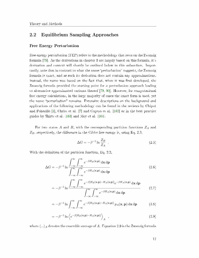
Free energy perturbation (FEP) refers to the methodology that rests on the Zwanzigformula [79]. As the derivations in chapter 3 are largely based on this formula, it'sderivation and context will shortly be outlined below in this subsection. Impor-tantly, note that in contrast to what the name �perturbation� suggests, the Zwanzigformula is exact, and as such its derivation does not contain any approximations.Instead, the name was based on the fact that, when it was �rst developed, theZwanzig formula provided the starting point for a perturbation approach leadingto alternative approximated variants thereof [79, 90]. However, for computationalfree energy calculations, in the large majority of cases the exact form is used, yetthe name �perturbation� remains. Extensive descriptions on the background andapplications of the following methodology can be found in the reviews by Chipotand Pohorille [1], Christ et al. [7] and Gapsys et al. [162] or in the best practiceguides by Shirts et al. [163] and Mey et al. [164].

For two states A and B, with the corresponding partition functions ZA andZB, respectively, the di�erence in the Gibbs free energy is, using Eq. 2.3,

∆G = −β−1 lnZBZA

. (2.5)

With the de�nition of the partition function, Eq. 2.2,

∆G = −β−1 ln

∫ ∞−∞

∫ ∞−∞

e−βHB(x,p) dxdp∫ ∞−∞

∫ ∞−∞

e−βHA(x,p) dxdp

(2.6)

= −β−1 ln

∫ ∞−∞

∫ ∞−∞

e−β[HB(x,p)−HA(x,p)]e−βHA(x,p) dxdp∫ ∞−∞

∫ ∞−∞

e−βHA(x,p) dxdp

(2.7)

= −β−1 ln

∫ ∞−∞

∫ ∞−∞

e−β[HB(x,p)−HA(x,p)] pA(x,p) dxdp (2.8)

= −β−1 ln⟨e−β[HB(x,p)−HA(x,p)]

⟩A

, (2.9)

where 〈...〉A denotes the ensemble average ofA. Equation 2.9 is the Zwanzig formula

17

Chapter 2

[79]. The ensemble average can either be calculated analytically, or by samplingin state A using an MC or MD based approach. In this thesis, the state that theensemble average is calculated of (i.e. A in Eq. 2.9) is referred to as the referencestate, whereas B is the target state.

In the following chapters, the Zwanzig formula, Eqs. 2.9, will be expressed onlyas a function of H(x). The reason is based on the decomposition of H(x,p) =

T (p) + V (x), where T (p) denotes the kinetic energy contribution. As the kineticterm only depends on particle momenta, it can be integrated out analytically. Asthe individual masses do not change between A and B in all applications of thefollowing chapters, these contributions cancel out, and will therefore be omitted inthe above formalism. In cases where masses do change, the average kinetic energyis still the same in A and B, due to the equipartition theorem and coupling tothe heat bath. However, as the temperature of the system within the heat bath is�uctuating, the kinetic energy contributions to A and B do not generally cancelout and, given the non-linearity of Eq. 2.9, still have to be considered. Therefore,this chapter uses the more general formulation.

Along similar lines, the expectation value of other observables O(x,p) of B canbe calculated as

〈O(x,p)〉B =

⟨O(x,p) e−β[HB(x,p)−HA(x,p)]

⟩A⟨

e−β[HB(x,p)−HA(x,p)]⟩A

, (2.10)

i.e., based on an ensemble average in A.

As outlined in the introduction, a sequence ofN states, i.e., N−2 intermediates,will be used to improve sampling accuracy. In this case, the total di�erence iscalculated as,

∆G =N−1∑s=1

∆Gs,s+1 (2.11)

= −β−1N−1∑s=1

ln⟨e−β[Hs+1(x,p)−Hs(x,p)]

⟩s, (2.12)

where ∆Gs,s+1 denotes the free energy di�erence between states s and s+ 1 withs = 1 denoting state A and s = N denoting state B. Similarly, the di�erencebetween A and B of any other ensemble based observable can be calculated by

18

Theory and Methods

using Eq. 2.10 in a step-wise approach. Whereas the terminology is sometimesused ambivalently, in the context of this thesis FEP refers to using the Zwanzigformula in multiple steps.

Paths and Sequences

This thesis distinguishes between alchemical paths and sequences. The �rst refersto a (continuous) transformation of the Hamiltonians along a path variable λ, suchas the linear interpolation scheme, Hλ(x,p) = (1 − λ)HA(x,p) + λHB(x,p), de-scribed in the introduction.

For FEP and other equilibrium techniques, sampling is conducted in a seriesof N states governed by the Hamiltonians H1(x,p), ...,HN (x,p). Such a series ofstates will be referred to as a sequence. In practice, these Hamiltonians are almostexclusively characterized by a set of λ points {λ1, ..., λN} (with λ1 = 0 and λN = 1)along a path, and usually along the linearly interpolated one. The choice of theintermediate λ points has been the subject to a number of optimization approaches[6, 165].

This thesis distinguishes between path and sequence, as for the latter one, anyde�nition of intermediate Hamiltonians can be used without assuming a path a

priori. In chapter 3, it will be shown that, in fact, the sequence yielding theoptimal MSE � the VI sequence � is such a case and, in its exact form, does notrequire any choice of a path variable.

Bennett Acceptance Ratio Method

In the limit of an in�nite number of sample points, the Zwanzig formula, Eq. 2.9,yields the exact result no matter if using A or B as the reference state that sam-pling is conducted in. However, for �nite sampling, the convergence properties ofboth variants generally di�er. Except for a number of special cases, the free energyestimates improve if the information from samples in both states are used. Themain estimator for this purpose is the Bennett Acceptance Ratio (BAR) method.It will be extensively used throughout this thesis and chapter 3 will provide analternative derivation and generalization thereof. BAR will therefore be brie�ydescribed below.

Bennett started by expanding the de�nition of the di�erence in free energy

19

Chapter 2

∆G = −β−1 lnZBZA

(2.13)

= −β−1 ln

ZB

∫ ∞−∞

∫ ∞−∞

w[HA(x,p), HB(x,p)] e−HA(x,p)−HB(x,p) dxdp

ZA

∫ ∞−∞

∫ ∞−∞

w[HA(x,p), HB(x,p)] e−HA(x,p)−HB(x,p) dxdp

(2.14)

= β−1 ln

⟨w[HA(x,p), HB(x,p)] e−HA(x,p)

⟩B⟨

w[HA(x,p), HB(x,p)] e−HB(x,p)⟩A

(2.15)

by an arbitrary weighting function w. Optimizing w such that the estimates in thefree energy di�erence yield the smallest variance leads to the BAR method

∆G = β−1 ln

⟨f [β(HA(x,p)−HB(x,p) + C)]

⟩B⟨

f [β(HB(x,p)−HA(x,p)− C)]⟩A

+ C , (2.16)

where f(x) = 1/(1 + exp(x)) is the Fermi function, and the variance of the freeenergy estimate minimal if

C = −β−1 ln

(ZB nAZA nB

)(2.17)

= ∆G− β−1 ln

(nAnB

). (2.18)

The numbers nA and nB denote the number of independent sample points in statesA and B, respectively. Due to the dependence of C on ∆G, equation 2.16 isan implicit problem. It is solved iteratively by using an initial guess for C, andthen updating C by using Eqs. 2.16 and 2.18 until convergence. Equivalently, theequation

nA∑i=1

f(β[HA(xi,pi)−HB(xi,pi) + C]

)=

nB∑j=1

f(β[HA(xj ,pj)−HB(xj ,pj)− C]

),

(2.19)

where i and j label the samples obtained from state A and B, respectively, canbe solved numerically for C. The di�erence ∆G is then subsequently calculated

20

Theory and Methods

through Eq. 2.18.

When using N > 2 states as in Eq. 2.12, given a sample point xi,pi from states, it is not only possible to calculate the Hamiltonians Hs(xi,pi) and Hs+1(xi,pi)

of the states s and s + 1, but instead of all states s = 1, ..., N . The estimator �the multistate Bennett Acceptance Ratio (MBAR) [166] method � uses this infor-mation and was developed based on a related extended bridge sampling technique[167]. The free energies {Gs} of all states s,

Gs = − ln

N∑t=1

nt∑i=1

e−βHs(xti,p

ti)

N∑k=1

nk eGk−βHk(xti,p

ti)

, (2.20)

are calculated with respect to an unkown constant, where s, t and k are labelsfor states, and xti and pti denote the i

th positions and momenta, respectively, fromstate t. The integer numbers nk and nt denote the total number of sample pointsfrom the state indicated by the subscript. Once all {Gs} have been determined,the di�erences are obtained by, e.g., subtracting G1 from all {Gs}, yielding thedesired free energy di�erence between the end states through GN −G1. Again, theset of equations 2.20 is an implicit problem, and is solved iteratively.

Thermodynamic Integration

The most prominent equilibrium method next to FEP is Thermodynamic Integra-tion (TI). It provides the basis of the minimum variance path (MVP) that willbe described in the next section and used as a comparison to the VI sequence inchapter 3.

21

Chapter 2

If the path is di�erentiable with respect to λ between 0 and 1, then

∂G

∂λ= −β−1 ∂

∂λln

∫ ∞−∞

∫ ∞−∞

e−βH(x,p,λ)dxdp (2.21)

=

∫ ∞−∞

∫ ∞−∞

e−βH(x,p,λ)∂H(x,p, λ)

∂λdxdp∫ ∞

−∞

∫ ∞−∞

e−βH(x,p,λ)dx dp

(2.22)

=

⟨∂H(x, λ)

∂λ

⟩λ

(2.23)

⇒ ∆G =

∫ 1

0

⟨∂H(x,p, λ)

∂λ

⟩λ

dλ , (2.24)

where Eq. 2.24 is referred to as Thermodynamic Integration (TI) [90]. Notethat TI is derived based on an equilibrium average for each λ, while integratingcontinuously along λ. In practice, sampling is therefore also conducted at discretesteps in equilibrium, while Eq. 2.24 is calculated via numerical integration using,e.g., the Simpson or the trapezoid rule.

2.3 Soft-core Interactions and other Choices of Inter-

mediate States

All methods mentioned above contain evaluations of a sample that was generatedin a reference state s with a Hamiltonian of a di�erent target state, e.g., s+1. Fur-thermore, for the common linear interpolation scheme, to determine Hs+1(x,p),both HA(x,p) and HB(x,p) need to be calculated. In the following it is assumedthat the system contains vanishing particles, as illustrated in Fig. 2.1 on the ex-ample of calculating solvation free energies. Therefore, particles coupled throughregular LJ interactions in B are represented as decoupled �ghost� particles in A

with zero interaction energies.

The linearly interpolated intermediates of such a vanishing LJ particle areshown in Fig. 2.2(a). When sampling is conducted in A, represented by the �atblue line, these �ghost� particles will overlap with other ones. In these cases, com-plications will arise if such a con�guration from A would be evaluated at HB(x,p)

(red line), due to the divergence at r = 0 of the LJ term that accounts for the Paulirepulsion. Furthermore, when decoupling a charged atom or particle, these com-plications would be enhanced in intermediate states closer to A in the sequence, if

22

Theory and Methods

Figure 2.1: End states for calculating the solvation free energy di�erence throughdecoupling LJ interactions. (a) Decoupled state, representing the state where thesolute has been removed from water. The solute does not interact with its sur-rounding, therefore it overlaps with some water molecules. (b) Coupled state: Thesolute interacts regularly with water. Image courtesy Dr. Vytautas Gapsys.

a remaining attractive electrostatic interaction was strong enough to overcome theweak Pauli repulsion down to small center-center separations that could otherwisenot occur.

To avoid the problem for electrostatic interactions, these can be decoupledseparately in a �rst step while using full LJ interactions, which are decoupled inthe second step [168, 169]. More importantly, soft-core potentials [91, 92] can beused by replacing the divergence at r = 0 with a �nite maximum, high enough suchthat it will never be visited for state B, but becoming low enough such that it willbe visited for intermediate states. To this aim, a λ dependence of the end states isintroduced, such that the intermediate Hamiltonians are calculated as

Hλ(x,p) = (1− λ)HA(x,p, λ) + λHB(x,p, λ) . (2.25)

In the LJ potential

V LJ(rij) = 4εij

[(σijrij

)12

−(σijrij

)6]

, (2.26)

where σij and εij denote the LJ parameter, the distance rij between two atoms i

23

Chapter 2

Figure 2.2: Intermediate interaction energies at distance r of a vanishing par-ticle without and with soft-core (SC) treatment. In state B (red line), it is fullyinteracting through a LJ potential. In contrast, in A (blue line), the interactionenergy is zero at all r. The lines in between indicate the intermediate Hamiltoniansobtained through (a) the linear interpolation scheme, Eq. 1.3, and (b) the soft-corevariant thereof, i.e., Eq. 2.25.

and j is replaced by two altered radii

rA(rij , λ) =(ασcAλ

b + rcij) 1c , (2.27)

rB(rij , λ) =(ασcB(1− λ)b + rcij

) 1c , (2.28)

for each end state. Here, α, b and c are dimensionless soft-core parameters, andσA and σB the LJ parameters in the end states A and B, respectively. As can beseen, both rA and rB are �nite at rij = 0, for all intermediate λ points, therebyavoiding divergences. The resulting Hamiltonians for a sequence of equally spacedλ values are shown in Fig. 2.2(b). The correct end states without alteration arereproduced at λ = 0 for A, and λ = 1 for B. The intermediate form withoutsoft-core is obtained for α = 0.

In the form by Steinbrecher et al. [93], Eq. 2.25 was further generalized by re-placing the prefactors with (1−λ)a and λa, where a is another soft-core parameter.However, to date a = 1, α = 0.5, b = 1 or 2, and c = 6 are considered optimal[164, 170, 171] and also used in this thesis, such that the generalization by a did

24

Theory and Methods

not reveal any signi�cant improvements, yet.

For σA = 0 and σB = σij , as well as εA = 0 and εB = εij , as in the exampleabove, the LJ interactions in the intermediate state are calculated as

V LJλ (rij) = (1− λ)V LJ(rA(rij)) + λV LJ(rB(rij)) (2.29)

= 4λ εij

([α(1− λ)b +

(rijσij

)c ]− 12c

−[α(1− λ)b +

(rijσij

)c ]− 6c

).

(2.30)

This form is the one most commonly found in the literature, whereas Eqs. 2.27 and2.28 present the more general one.

If the decoupling of LJ and Coulomb interactions should be conducted simul-taneously, then the soft-core approach can be extended to Coulomb interactionsas well. In this case, these are also calculated based on the modi�ed distancesrA(rij , λ) and rB(rij , λ). Assuming again that A represents the decoupled state,where the charges do not to interact with their surrounding, the interaction iscalculated along λ as

V coulλ (rij) =

qi qj

4πε0εr

[α(1− λ)b + rcij

] 1c

, (2.31)

where qi and qj denote the charges in the coupled state, and ε0 and εr the vacuumand relative permittivity, respectively.

Soft-core potentials will be used to calculate solvation free energies in chap-ter 3 and 5. In addition, an approach similar in principle will be devised andimplemented in chapter 5.

Minimum Variance Path

The soft-core variant, Eq. 2.25 o�ers more �exibility in devising an alchemical paththrough regulating the λ dependence of the end states than the regular linear inter-polation path, Eq. 1.3. However, it still represents only a very special case amongall possible ones. The most relevant one for this work � the Minimum VariancePath (MVP) � was derived by Blondel [104] and will emerge as a limiting caseof the VI sequence derived in chapter 3. States from the MVP will be used for acomparison in accuracy. Its derivation is therefore shortly outlined below.

25

Chapter 2

Blondel aimed at minimizing the variance of the free energy estimates,∫ 1

0

⟨(∂Hλ(x,p)

∂λ

)2

−⟨∂Hλ(x,p)

∂λ

⟩2

λ

⟩λ

dλ (2.32)

=

∫ 1

0

⟨(∂Hλ(x,p)

∂λ

)2⟩λ

dλ−∫ 1

0

⟨∂Hλ(x,p)

∂λ

⟩2

λ

dλ (2.33)

for TI. In the next step, he used the translation invariance: At each λ point, abias function B(λ), which is constant across con�guration space, can be added tothe Hamiltonian

H ′λ(x,p) = Hλ(x,p) + B(λ) . (2.34)

The derivatives of the bias function will cancel out in Eq. 2.32 but can be designedsuch that the second term for the altered Hamiltonian,⟨

∂H ′λ(x,p)

∂λ

⟩λ

= 0 , (2.35)

thereby simplifying the derivation. Next, considering the �rst term in Eq. 2.33,∫ 1

0

⟨(∂H ′λ(x,p)

∂λ

)2⟩λ

dλ (2.36)

=

∫ 1

0

∫ ∞−∞

∫ ∞−∞

(∂H ′λ(x,p)

∂λ

)2

e−βH′λ(x,p)dxdpdλ (2.37)

=

∫ ∞−∞

∫ ∞−∞

∫ 1

0

(∂H ′λ(x,p)

∂λe−β

H′λ(x,p)

2

)2

dλ dx dp , (2.38)

where, in the last step, Blondel assumed that the integrals converge to a �nite valueand can therefore be exchanged. Furthermore, for any point,∫ 1

0

∂H ′λ(x,p)

∂λe−β

H′λ(x,p)

2 dλ = −2β−1(e−

β2HA(x,p) + e−

β2HB(x,p)

)(2.39)

:= C . (2.40)

Hence, in the next step, the inner integral in Eq. 2.38 of the form∫ 1

0f(λ)2dλ (2.41)

26

Theory and Methods

can be minimized by setting

f(λ) = C ⇒∫ 1

0f(λ)dλ = C (2.42)

as for any other function∫ 1

0g(λ)2dλ = C2 +

∫ 1

0[g(λ)− C]2dλ > C2 . (2.43)

Blondel now obtained Hλ(x,p) by integrating Eq. 2.39 from 0 to λ,

−2β−1(e−

β2H′λ(x,p) − e−

β2HA(x,p)

)= −λ2β−1

(e−

β2HB(x,p) − e−

β2HA(x,p)

)(2.44)

yielding the Hamiltonian

Hλ(x,p) = −2β−1 ln(

(1− λ)e−β2HA(x,p) + λe−

β2HB(x,p)

)+ λ∆G2 , (2.45)

where the last term was added to transform from H ′λ(x,p) to H(x,p) again, whichwas required for Eq. 2.35. Therefore, the minimum variance path (MVP) is optimalif ∆G ≈ ∆G.

Later, Pham and Shirts [105] also derived this path by adapting a result fromGelman and Meng [78]. Furthermore, they established that Eq. 2.45 yields the op-timal variance for high con�guration space overlap between the end states, whereasin the low overlap case, the prefactors cos(λπ2 ) and sin(λπ2 ) are preferred insteadof (1− λ) and λ.

Note that these paths di�er only for continuous and equal sampling along λ.However, when using discrete states, as general practice for TI, any pair of prefac-tors ζ1 and ζ2 can be rescaled by the factor r = 1/(ζ1 + ζ2) such that rζ1 + rζ2 = 1.The term ln(r) will appear as an additive constant in Eq. 2.45, and therefore willdrop out for all intermediates when calculating the step-wise free energy di�erencebetween the end states. Therefore, rede�ning λ := rζ2 ⇒ (1−λ) = rζ1 leads to theoriginal form of Eq. 2.45. As such, for discrete states, any set of λ steps along thepath designed for the low overlap case yields, on average, equivalent total estimatesas another set of steps in the high overlap variant.

27

Chapter 2

Enveloping Distribution Sampling

Other alternatives to Eq. 2.25 are the One-Step Perturbation (OSP) [97�99] andthe Enveloping Distribution Sampling (EDS) [100, 101] class of methods. These aredesigned to calculate free energy di�erences from a single simulation by constructinga reference potential that �envelopes�, i.e., combines all con�guration space regionsrelevant to one or more end states. For example, in one application, OSP [99] wasapplied to compare di�erent rigid ligands to an estrogen receptor. The referencestate was designed by using a �ghost� particle at the positions were the atoms di�erbetween the ligands. For EDS, the con�guration space density of the reference stateis constructed by summing over the ones from the Ni end states

e−βsHref (x,p) =

Ni∑i=1

e−βs(Hi(x,p)−Ei) , (2.46)

where s and Ei, for i = 1, ..., Ni, are adjustable parameters. The Zwanzig formula[79], Eq. 2.9, is used to calculate the free energy di�erence between the referencestate and each end state.

If the con�guration space regions of all end states were disjunct, equal samplingwould, assuming uncorrelated sample points, be conducted in these regions if Ei =

Gi. However, in other cases, the optimal Ei may di�er for more than two endstates. Furthermore, the parameter s can be adjusted to avoid barriers and typicallyranges between 0.001 and 1 [101]. For small s, such that βsHi(x,p) << 1, aseries expansion of the exponentials and the logarithm in Eq. 2.46 yields the linearinterpolation

Href (x,p) =

Ni∑i=1

Hi(x,p) + const . (2.47)

Therefore, s switches between the interpolation of the Hamiltonians (small s) andthe con�guration space densities (s = 1). A very recent variant, λ-EDS [103], whichwas constructed also based on our work in chapter 3, now also calculates the freeenergy di�erence between only two end states, but using several intermediate onesinstead.

The usage of the s factor will also be combined with the VI sequence and bemade accessible through the GROMACS implementation described in chapter 5.

28

Theory and Methods

2.4 Non-Equilibrium Approaches

The second class of methods that employ the concept of alchemical paths, as de-scribed in the introduction, are non-equilibrium techniques. Here, transitions fromA to B are simulated by increasing λ at every step; the system is therefore out ofequilibrium. In chapter 6, an approximated path deduced from the VI sequencewill be tested with non-equilibrium methods.

Small perturbations away from equilibrium, such as for very slow transitions,can be described using linear response theory [172�176]. More generally, Jarzynski[84] derived the identity

e−β∆G =⟨e−βWA→B

⟩, (2.48)

where the brackets indicate an ensemble average over several transitions startingfrom A and ending at B. The work values are obtained similarly to TI by integra-tion along λ

W =

∫ 1

0

⟨∂H(x, λ)

∂λ

⟩λ

dλ . (2.49)

The starting con�gurations need to represent the equilibrium ensemble. Fascinat-ingly, Eq. 2.48 holds arbitrarily far from equilibrium, which, in addition to thetheory, has been demonstrated by experiments through reversible and irreversiblepulling of an RNA molecule [177] for the �rst time.

To utilize the information from both forward and backward transitions, wherePf (W ) and Pr(W ) denote corresponding work distributions, the Crooks Fluctua-tion Theorem (CFT) [178, 179] (also valid for NPT ensembles [180])

Pf (W )

Pr(−W )= eβ(W−∆G) (2.50)

provides the basis of several methods [181, 182]. For example, the Crooks GaussianIntersection (CGI) estimator approximates Pf (W ) and Pr(W ) by two Gaussianfunctions and estimates the free energy di�erence through their intersection.

Furthermore, the BAR estimator was also adapted for non-equilibrium simula-

29

Chapter 2

tions [183], where the free energy is determined through numerical solution of

nf∑i=1

1

1 + exp (β(Wi − C))=

nr∑j=1

1

1 + exp (−β(Wj − C)), (2.51)

for C, which, similar to Eq. 2.18, relates to the free energy as

∆G = C + β−1 ln

(nfnr

). (2.52)

Here, nf and nr denote the numbers of transitions in forward and reverse di-rections, respectively. Furthermore, it was shown that the BAR estimator yieldsthe free energy with the maximum likelihood, given the observed work values [183].

Both the BAR and CGI estimator will be used in chapter 6 to calculate freeenergy di�erences based on non-equilibrium trajectories.

Overlap Sampling

In an extensive series of publications [184�189], the group of Kofke and coworkersanalyzed the scenario in which the relevant regions in con�guration space of, e.g.,state B, represent only a small subset, and are completely embedded within theones of state A. Their example in this case consists of a vanishing particle, which inthe decoupled state A has a much higher entropy as in state B, where its positionis restricted by its neighboring particles.

Through a variety of theoretical considerations and simulations, they estab-lished that for one-sided simulations, the systematic error, i.e., the bias of the freeenergy estimates, is lower when starting from the state of higher, and targeting thestate with lower entropy. For a vanishing particle, the trajectories should thereforebe started from the decoupled state, in other words, insertion is preferable to dele-tion. In this special case, conducting only one-sided simulations has even a smallerbias than when trajectories from both sides are used with the approaches outlinedin the beginning of this section.

Next, they considered the case in which the con�guration space volumes of Aand B are more similar, and these two overlap in a region O. Then, by de�nition,O is a subset region of both A and B. Therefore, when introducing O as anintermediate state and calculating the free energy di�erence through A → O andB → O, where the arrow indicates a set of non-equilibrium transitions starting

30

Theory and Methods

from the �rst and ending at the second state, then in both cases, the transitionsstart at the state of higher entropy and end at the one lower entropy. Using theuse of the Jarzynski identity [84], Eq. 2.48,

e−β∆G =

⟨e−βWA→O

⟩A⟨

e−βWA→O⟩B

. (2.53)

This approach is referred to as the Overlap Sampling (OS) method [186]. In anal-ogy, the principle can be applied to FEP using the Zwanzig formula

e−β∆G =

⟨e−β[HO(x,p)−HA(x,p)]

⟩A⟨

e−β[HO(x,p)−HB(x,p)]⟩B

. (2.54)

Note that in this case, sampling is conducted only in A and B. Therefore, O rep-resents a virtual intermediate, i.e., a state that no sampling is conducted in, butwhich is used as a target state.

They suggested a simple form for O that uses the average of the end statesHO(x,p) = (HA(x,p) + HB(x,p))/2, which already considerably improved thebias compared to calculating the estimate without the virtual intermediate. Similarto BAR, they extended the de�nition of O through a weighting function w

HO(x,p) = −β−1 lnw[HB(x,p)−HB(x,p)] +1

2[HA(x,p) +HB(x,p)] ,

(2.55)

where the two approaches are equivalent if

w(∆H(x,p)) =1

cosh

[β

2(∆H(x,p)− C)

] , (2.56)

which is the Gaussian hyperbolic secant function, and where C corresponds to thede�nition of Bennett [80], Eq. 2.18.

Virtual intermediate states and their connections to estimators will be em-ployed to construct the setup for free energy calculations underlying the VI andcVI sequences in chapter 3 and 4, respectively.

31

Chapter 2

2.5 Molecular Dynamics Simulations

An important method for sampling used in this work are MD simulations. Thesemodel at a high level of detail � describing both the biomolecules and the solventon an atomistic basis � while still being based on a classical many particle descrip-tion of the system. It is important to distinguish that the underlying phenomena,e.g., the stretching of a bond, are non-classical.

MD simulations can, with current computer technology and algorithms, simu-late time scales on the order of 50 to 100 ns per day for a two million atom system(on the example of the GROMACS 2018 software package with 8 standard CPUsand a GPU [68]). While simulations going beyond these limits have been con-ducted, these usually require substantial computational e�orts. For example, �rstsimulations above one millisecond were already conducted in 2011 [190] for severalprotein folding processes (system size of the order of ten thousand atoms) on theANTON supercomputer [191], whose hardware was speci�cally optimized for theproperties of MD. As for scale; recently (2019), a proof of concept run above onebillion atoms of a gene locus was conducted [192]; however, progressing only at onenanosecond per day on 130,000 processor cores.

A large number of MD software packages has been developed such as NAMD[193, 194], AMBER [195], GROMOS [196], LAMMPS [197, 198] or OpenMM [199].The one used and extended in this thesis is the GROMACS [157�159] software pack-age. Its main advantage is its wide spread usage and its high speed compared toother packages. In contrast, alternatives, such as OpenMM, o�er a higher degree ofdeveloper and user friendliness instead, where, e.g., integrators can be easily mod-i�ed through a python interface. Therefore, a disadvantage of GROMACS is thatsuch a change would, at least for the GROMACS 2019 and 2020 version, requiremore substantial changes in the source code than for, e.g., OpenMM.

Foundations and Approximations

Extensive descriptions about the fundamentals of MD simulations can be found inthe recent book by Leimkuhler and Matthews [200], or the slightly older ones byRapaport [201] or Frenkel and Smit [202]. A brief summary of the underlying prin-ciples and approximations of MD, and in extension, of the abilities and limitationsof MD based free energy calculations, will be provided below.

32

Theory and Methods

As a �rst approximation, gravitational interactions are neglected, as these are,for example, roughly an order of 40 magnitudes weaker than electrostatic ones.Secondly, relativistic e�ects are considered negligible, due to the small masses andsmall velocities compared to the speed of light.

With these two approximations, systems at atomic length scales are describedby the time-dependent Schrödinger equation [203]

i~∂

∂tψ(re; rn) = Hψ(re; rn) , (2.57)

where ~ = h2π denotes the reduced Planck constant and H the Hamiltonian opera-

tor. The wave-function ψ(re; rn) that describes the system depends on the positionsof both the nuclei and the electrons rn, and re, respectively.

Next, the fact that electrons are around 2000 times lighter than a nucleon and,therefore, move much faster, is considered. For this reason, the Born-Oppenheimerapproximation [204] assumes that the electronic wave function instantaneously fol-lows the motion of the nuclei, allowing to separate the wave function

ψ(re; rn) = ψn(rn)ψe(re; rn) (2.58)

into the nuclear wave-function ψn(rn) and the electronic wave-function ψe(re; rn),where the latter only depends on rn parametrically. The decoupling of the timescales allows us to determine ψe with the time-independent Schrödinger equation

Heψe(re; rn) = Ee(rn)ψe(re; rn) , (2.59)

where Ee(rn) denotes the ground state energy. Based on the Born-Oppenheimer ap-proximation, the position of the nuclei is described by the time-dependent Schrödingerequation (

Tn + Ee(rn))ψn(rn) = i~

∂

∂tψ(rn) , (2.60)

where Tn denotes the kinetic energy operator of the nuclear motion.

Note that the Born-Oppenheimer approximation rests on the assumption thatall electrons remain in the same state the entire time. This assumption is valid fortemperatures around 300 K, where most of the biological systems operate. Here,given approximately 0.025 eV thermal energy per electron, the electrons are in the

33

Chapter 2

ground state, and as excitation energies generally exceed 1 eV (e.g., 10.2 eV forhydrogen), spontaneous excitation of electrons is unlikely. However, for the samereason, processes such as photon absorption cannot be addresses with standard MD.

Equation 2.60 describes the evolution of the entire nuclear wave-function. How-ever, for applications targeted by MD simulations, it is su�cient to calculate theexpectation value of the atom positions, now represented by the position of theirnuclei under the above assumptions. These expectation values evolve according tothe Ehrenfest theorem [205]

d〈rn〉dt

= 〈vn〉 (2.61)

and

d〈vn〉dr

= −∇V (rn)

m, (2.62)

where vn denotes the velocity and m the mass of the nuclei in a potentialV (rn). Given the similarity of Eqs. 2.61 and 2.62 to Newton's (classical) equationsof motion, the evolution of the expectation values of an atom position and velocitycan be considered as the ones of a point particle.

Integration of Equations of Motion

Newtons second equation of motion,

mi∂2ri∂t2

= Fi , (2.63)

where i = 1, ..., n, is solved numerically for all n atoms with mass mi and forceFi = ∇ri acting on atom i. The most widely used integrator for MD simulationsis the leap-frog algorithm, a second-order integrator and equivalent to the velocityVerlet method. The positions of the atoms are propagated as

ri(t+ ∆t) = r(t) + vi

(t+

∆t

2

)∆t (2.64)

and the velocities as

vi

(t+

∆t

2

)=

(t− ∆t

2

)+

Fi(t)

mi∆t . (2.65)

34

Theory and Methods

In this work, a time step of 2 fs is used in MD simulations. This value istypically used to keep the integration error substantially below errors caused byother approximations of MD simulations, such as the ones from force �elds.

Force Fields

The interaction potential and the gradient thereof to calculate the force in Eq. 2.65are determined by quantum mechanical e�ects. Calculating these is completely im-practical for molecules consisting of more than a few hundred atoms, and thereforealso for most of the applications of free energy calculations listed in the introduc-tion. Therefore, force �elds have been designed, that are an approximation to theground state energy of the electrons. Their parameters are determined either fromab initio calculations [49, 50] for the interaction between individual atoms or smallchemical groups, or through adjusting the parameters such that experimental ob-servables [47, 48] of small model systems are reproduced (or, of course, a mixtureof both approaches).

Conventional force �elds divide the interaction potentials into bonded and non-bonded interactions. The former depend on bond lengths, Eq. (2.67), bond angles(2.68), dihedral angles (2.69) and improper dihedrals (2.70) that restrict out-of-plane motions to, e.g., keep aromatic rings planar. The non-bonded interactionsconsist of electrostatic (2.71), van-der-Waals interactions and Pauli repulsion, withthe latter two described by a Lennard-Jones potential (2.72), which has alreadybeen described in section 2.2 for soft-core potentials. In total,

35

Chapter 2

V (r) = Vbonded(r) + Vnonbonded(r) (2.66)

=∑

bonds i

ki2

(bi − bi,0)2 (2.67)

+∑

angles i

fi2

(θi − θi,0)2 (2.68)

+∑

dihedrals i

V di

2[1 + cos(nφ)] (2.69)

+∑

impropers i

κi(ζi − ζi,0)2 (2.70)

+∑

pairs i,j

qiqj4πε0εrrij

(2.71)

+∑

pairs i,j

4εij

[(σijrij

)12

−(σijrij

)6], (2.72)

where ki, fi and κi/2 denote the spring constants of the harmonic potentials forthe bond length bi, angle θi and improper dihedral angle ζi, around their respec-tive rest lengths, indicated by the subscript 0. Dihedral potentials depend on thebarrier height V d

i between di�erent conformers and the periodicity n. Coulomb in-teractions at a distance rij between two atoms are calculated based on the chargesqi, the vacuum permittivity ε0 and permittivity εr, whereas σij and εij denote theLennard-Jones parameters. Note that the partial charges aim at reproducing theelectrostatic potential not only for localized charges such as ions, but also for, e.g.,delocalized electron systems, and, therefore, are generally non-integer values.

Developing force �elds that give accurate results for a large variety of systemsis a challenging task. Therefore, a number of di�erent prominent force �elds havebeen developed, such as the amber [206, 207], charmm [208, 209], opls [210], andgromos [211] force �elds. These are often more accurate in predicting a numberof experimental observables correctly, such as conformational energies [212, 213],and less accurate in predicting others. Similarly, many force �elds are reasonableaccurate for, e.g., globular proteins with a conserved structure, but give largelydi�ering results for, e.g., intrinsically disordered proteins [214]. As such, to checkthe robustness of a prediction, it has become common practice to repeat the same

36

Theory and Methods

simulations using di�erent force �elds [215] as well as to constantly validate thesepredictions through comparison with experiments.

Generally, force �elds and MD simulations do not allow chemical reactionsor bond breaking. Similarly, polarization e�ects are usually not accounted for.However, approaches into both directions have been developed [216�220] and maybecome more widely used in the future.

The force �eld mainly used in chapters 3 and 5 of this thesis is the GeneralizedAmber Force Field (GAFF) [221]. The reason is simply that simulation setups,which were already equilibrated with GAFF, are conveniently available from theSolvationToolkit package [222]. In these chapters, to separate force �eld errorsfrom sampling errors, the accuracies of di�erent approaches are always obtainedby comparison of a large number of short simulations with respect to a convergedreference result, based on the same force �eld. As such, the particular choice of aforce �eld is, in this context, unimportant. Naturally, for the success of the �eld ofcomputational free energy calculations as a whole, force �elds are a crucial factor.

Temperature and Pressure Coupling

A canonical system is coupled to the temperature, and in most cases, also the pres-sure of a much larger external system. Thermostats and barostats are algorithmsthat model these coupling e�ects.

To start with one of the simplest thermostats, it is considered that the instan-taneous temperature T of the system and the velocities {vi} of np particles arerelated via

3

2kBT =

⟨miv2i

2

⟩(2.73)

=1

np

np∑i=1

miv2i

2. (2.74)

If the target (= external) temperature T ′ di�ers from the current one, then thesimplest approach is to rescale all velocities according to

v′i =

√T ′

Tvi (2.75)

such that T ′ is reached. This method is referred to as velocity rescaling. However,

37

Chapter 2

as the temperature is not able to �uctuate in this approach, the properties ofa canonical system, which free energy energy simulations are conducted in, arenot reproduced. One option to circumvent this problem is to randomly draw thecomponents of all velocities v′′i from a Gaussian distribution around the ones of v′i,i.e.,

p(v′′i,x) =1√

2πσiexp

(−v′2i,x2σ2

i

), (2.76)

with variance σ2i = kBT/mi , where, as an example, v′′i,x denotes the �nal velocity

of particle i in x-direction. Conducting this procedure only after certain time in-tervals gives the system further room for �uctuations.

The main advantage of velocity scaling is its simplicity with respect to imple-mentation. Whereas the resulting ensemble does not correspond exactly to thecanonical one, the deviations are in practice often rather small [223]. It was there-fore used, e.g., for the simple test system of a LJ gas with a self-written simulationprogram in chapter 3. A more re�ned method yielding more continuous velocities aswell as better ensemble properties is the Nose-Hoover thermostat [224, 225]. Here,an additional degree of freedom γ is introduced that determines an (anti)frictionterm in the equations of motion

d

dtmivi = Fi − 2γvi (2.77)

dγ

dt=

1

τ

(∑i

1

2miv

2i −

3

2npkBT

), (2.78)

where τ controls the timescale of the temperature regulation, and Fi denotes thetotal force acting on particle i. The Nose-Hoover thermostat is used in all simula-tions based on the GROMACS software package in this thesis.

Similar principles apply to barostats that regulate the pressure for NPT en-sembles. Similar to velocity rescaling, the Berendsen barostat [223] rescales thepositions, and thereby the volume of the system. The rescaling is, however, notconducted in one step; instead it depends on a parameter τp that regulates how fastthe target pressure should be reached. The advantage of the Berendsen barostatis that it is well behaved, and therefore often used to stabilize a system prior tofurther equilibration and production runs. However, similarly to velocity-rescalingit does not produce the correct (isobaric-isoenthalpic) canonical ensembles.

38

Theory and Methods

The Anderson barostat [226] uses the volume as an additional degree of free-dom, which is coupled to the system through equations of motion, similar to apiston. The volume is therefore assigned a kinetic and potential energy, wherethe latter is determined through the di�erence of the instantaneous to the target(= external) pressure. A conceptual �mass� is assigned to the volume, which is auser-chosen parameter that regulates the extent of the system �uctuations. TheParrinello-Rahman [227, 228] barostat is an extension that allows the shape of thevolume to deviate from the one it was initially assigned to. Both barostats correctlyreproduce the canonical ensemble.

In this thesis, if not speci�ed otherwise, all GROMACS based simulations followthe same procedure: First, an energy minimization is conducted of the system,using the steepest-descent algorithm [229]. Secondly, the system is equilibrated inan NVT ensemble, followed by equilibration in an NPT ensemble. The latter isdivided in two parts: Firstly, using the Berendsen barostat, secondly, using theParrinello-Rahman barostat. All subsequent production runs (i.e., the parts of thesimulations that are used to calculate the free energy di�erences) are conductedwith the Parrinello-Rahman barostat.

39

Chapter 2

40

3Variationally Derived Intermediates

3.1 Determining Free-Energy Di�erences Through Vari-

ationally Derived Intermediates

The following section consists of the article

M. Reinhardt, H. Grubmüller, Determining Free-Energy Di�er-ences Through Variationally Derived Intermediates, Journal ofChemical Theory and Computation vol. 16, issue 6, pp. 3504-3512 (2020). [230]

published under the CC BY creative commons open access license and the con-tent reprinted based on the 2020 Copyright Agreement by the American ChemicalSociety with consent of the authors.

The format, including the numbering of equations, �gures and tables, has beenaltered to match the format of this thesis. Furthermore, all references are listed inthe bibliography at the end of this thesis rather than at the end of this article.

Both authors contributed to conceiving the study and writing the manuscript.I implemented, conducted and analyzed all test systems and simulations.

41

Chapter 3

Figure 3.1: Table of Contents image

3.2 Abstract

Free energy calculations based on atomistic Hamiltonians and sampling are keyto a �rst principles understanding of biomolecular processes, material properties,and macromolecular chemistry. Here, we generalize the Free Energy Perturbationmethod and derive non-linear Hamiltonian transformation sequences yielding freeenergy estimates with minimal mean squared error with respect to the exact values.Our variational approach applies to �nite sampling and holds for any �nite numberof intermediate states. We show that our sequences are also optimal for the BennettAcceptance Ratio (BAR) method, thereby generalizing BAR to small sampling sizesand non-Gaussian error distributions.

3.3 Introduction

Free energy calculations provide essential insights into numerous physical and bio-chemical systems. Examples range from predicting binding processes of biomoleculesfor drug design [8, 10, 11] to determining thermodynamic properties of crystallinematerials [13, 14]. For large and complex systems with slow relaxation rates andtypically 105 to 107 particles, only limited accuracy is achieved [231], despite sub-stantial methodological progress [84, 183, 232, 233] and immense computationale�ort. Besides force �eld inaccuracies, insu�cient sampling is the main bottle-neck [74]. Within a generalized framework connecting two of the most establishedmethods, Free Energy Perturbation (FEP) [79] and the Bennett Acceptance Ra-tio method (BAR) [80], with the latter generally considered the more accurateone [171], we here will develop and evaluate a variational approach for optimalsampling that minimizes the error due to limited sampling.

Given the Hamiltonians H1(x) and HN (x) of two states 1 and N , where x ∈IR3M denotes the position of all M particles of the simulation system, the free

42

Variationally Derived Intermediates

energy di�erence ∆G1,N between these states is given by the Zwanzig formula [79],

∆G1,N = − ln〈e−[HN (x)−H1(x)]〉1 , (3.1)

where 〈〉1 denotes an ensemble average de�ned by H1(x), which is approximatedby averaging over a �nite sample of size n obtained from atomistic simulations orMonte Carlo sampling. For ease of notation, all energies are expressed in units ofkBT .

Alchemical transformations substantially reduce errors in the free energy es-timates [184, 185] by introducing N − 2 intermediate states s and accumulatingsmall free energy di�erences between all adjacent states s and s+ 1,

∆G1,N =N−1∑s=1

∆Gs,s+1 . (3.2)

Using the Zwanzig formula between s and s+1, this technique is referred to as FEP.The same approach is also employed in other �elds, for example in the context ofBayesian statistics, where the plausibility of two di�erent models is compared bycalculating their marginal likelihood ratio [78, 139].

The most common interpolation scheme for the intermediate states is along apath variable λ

Hs(x) = (1− λs)H1(x, λs) + λsHN (x, λs), λs ∈ [0, 1] . (3.3)

Figure 3.2(a) shows as a simple example a linear interpolation between twoone-dimensional Hamiltonians H1(x) and HN=9(x). In the case of soft-corepotentials [91�93], a non-linear dependence of the end states H1(x, λ) andHN (x, λ) on λ is introduced under the requirement that H1(x, λ = 0) = H1(x)

and HN (x, λ = 1) = HN (x). In this context, it has been attempted to �nd bettersequences of Hamiltonians by optimizing the distribution of λ points for a givenform of a sequence or pathway[165].

Even though there is some freedom in the construction of these transformationsequences, Eq. (3.3) describes only a very small subset of all possible sequencesof intermediate states, and in this sense, is not the most general. Speci�cally,the terms containing the information and parameters of the two di�erent endstates are always combined in an additive manner, and, e.g., any de�nition ofintermediate Hamiltonians Hs(x) that would involve cross terms of the form

43

Chapter 3

Figure 3.2: Sequences of intermediates between a harmonic potential H1(x) =12x

2 + b and a quartic potential H9(x) = (x − x0)4 + c (thick lines), where b andc have been determined such that Z1 = Z9 = 1, i.e., ∆G1,9 = 0. Sampling statesare described by odd-numbered Hamiltonians (solid lines), virtual target statesby even-numbered ones (dashed lines). (a) A linear interpolation between H1(x)and H9(x). For better visualization, the intermediates are vertically o�set to alignthe minima. (b) Intermediate Hamiltonians and (c) resulting con�guration spacedensities of VI. The yellow area highlights the con�guration space density overlapK between states 1 and 9.

44

Variationally Derived Intermediates

f(H1(x, λ) ·HN (x, λ)) would not be possible with the de�nition of Eq. (3.3).

Therefore, a number of alternative approaches, modifying Eq. (3.3), havebeen developed. For example, an empirical potential has been proposed in theEnveloping Distribution Sampling (EDS) method [100, 101] that interpolatesbetween the con�guration space densities (rather than the Hamiltonians) of two orseveral end states and is, as we will �nd, remarkably close to the optimal solutionfor a single intermediate state.

Further, a continuous path between two such end states, the 'minimum variancepath' (MVP), which optimizes the variance for Thermodynamic Integration [90](TI) was derived by Blondel [104] and later, through a di�erent formalism, byPham and Shirts [105] based on the results from the statistical sciences by Gelmanand Meng [78].

Here, we will generalize this interpolation scheme for FEP and BAR. Speci�-cally, we ask which sequence H2(x) . . . HN−1(x) � amongst all possible sequencesof higher order functions {Hs[H1(x), HN (x)]} that map two functions onto func-tions Hs (with s = 2, ..., N − 1) � yields, on average, the smallest mean squarederror (MSE),

MSE(

∆G(n))

= E[(

∆G−∆G(n))2], (3.4)

of the free energy estimate ∆G(n) obtained through �nite sampling with n samplepoints with respect to the exact free energy di�erence ∆G. Figures 3.2(b) and (c)show such a general interpolation sequence, which we refer to as Variationally-

derived Intermediates (VI) method.

Our approach di�ers from previous approaches in that here we optimizethe full MSE. Because the MSE can be decomposed into the sum of variance,E[(E[∆G(n)

]−∆G(n)

)2]and squared bias,

(E[∆G−∆G(n)

])2, it has been at-

tempted to analyze and optimize these two terms separately [105, 171, 234, 235].For the MVP in the context of TI, continuous sampling along the path variableλ is assumed; for practical applications, however, discrete integration is preferred,which implies an additional bias that is di�cult to assess and, therefore, not in-cluded within the optimization. As we will �nd, optimizing the sum of both,variance and bias, yields a conceptionally improved result.

45

Chapter 3

3.4 Theory

Optimal Mean Squared Error Sequence of Intermediates for Free

Energy Perturbation

To solve the above variational problem and to �nd the optimal sequence of Hs,we consider the FEP scheme displayed in Fig. 3.3(a) as oneof several possibleimplementation of Eq. (3.2) using Eq. (3.1). In this particular variant, which issymmetric with respect to exchange of the two end states to avoid hysteresis e�ects,sample points are solely drawn from the odd-numbered 'sampling states', indicatedby the solid lines in Figs. 3.2 and 3.3. The even-numbered states serve as virtual'target states' (dashed lines), similar to e.g. the Overlap Sampling method [236].From the sum of the individual perturbation steps, the average MSE of this schemeis

MSE(

∆G(n)1,N

)= E

∆G1,N −

N−2∑s=1s odd

(∆G

(n)s→s+1 −∆G

(n)s+2→s+1

)2 . (3.5)

As in Fig. 3.3, the arrows point from sampling to target states.

Assuming for each sample state s a set of n independent sample points {xi},drawn from ps(x) = e−Hs(x)/Zs, with partition function Zs, the terms arising fromexpanding Eq. (3.5),

MSE(

∆G(n)1,N

)= (∆G1,N )2 +

N−2∑s=1s odd

E[(

∆G(n)s→s+1

)2+(

∆G(n)s+2→s+1

)2]

− 2∆G1,N

N−2∑s=1s odd

(E[∆G

(n)s→s+1

]− E

[∆G

(n)s+2→s+1

])−

N−2∑s=1s odd

N−2∑t=1t odd

E[2 ∆G

(n)s→s+1 ∆G

(n)t+2→t+1

](3.6)

will be considered one by one. As the exact free energy di�erence is a constant,

E [∆G1,N ] = ∆G1,N . (3.7)

46

Variationally Derived Intermediates

Figure 3.3: Two schemes of free energy calculation. Yellow dots represent samplesets in the respective potential; arrows indicate the evaluation of di�erences ∆H(x)between adjacent Hamiltonians. Free energy di�erences are either determined by(a) FEP, or by (b) BAR with multiple steps. Both schemes give identical resultsat the stated conditions.

For the linear term, the average over all sample realizations reads

E[∆G

(n)s→s+1

]=−

∫ps(x1)dx1...

∫ps(xn)dxn

ln

[1

n

n∑i=1

e−(Hs+1(xi)−Hs(xi))

],

(3.8)

and for the quadratic term

E[(

∆G(n)s→s+1

)2]

=

∫ps(x1)dx1...

∫ps(xn)dxn(

ln

[1

n

n∑i=1

e−(Hs+1(xi)−Hs(xi))

])2

.

(3.9)

Similar expressions are obtained for ∆G(n)s+2→s+1. The exact free energy di�er-

ences are∆Gs,s+1 = − ln

∫e−(Hs+1(x)−Hs(x))ps(x)dx . (3.10)

For shifted HamiltoniansH ′s(x) = Hs(x)− Cs andH ′s+1(x) = Hs+1(x)− Cs+1 ,Eq. (3.1) yields

∆G(n)s′→(s+1)′ = ∆G

(n)s→s+1 − Cs+1 + Cs, (3.11)

which also holds for the exact value ∆G1′,N ′ . The o�sets on the right hand sideof Eq. (3.11) cancel out when calculating the MSE of Eq. (3.5). Choosing Cs and

47

Chapter 3

Cs+1 such that the term in the logarithm of Eqs. (3.8) and (3.9) is close to one,and thus all ∆G

(n)s′→(s+1)′ are small with respect to kBT = 1, �rst order expansion

of the logarithm allows to factorize the integrals, therefore,

E[∆G

(n)s′→(s+1)′

]= −

∫e−(H′s+1(x)−H′s(x))ps(x)dx + 1 . (3.12)

For the shifted Hamiltonians, the same expansion can be applied to the exact freeenergy di�erence of Eq. (3.10). Therefore, Eq. (3.12) reduces to

E[∆G

(n)s′→(s+1)′

]= ∆Gs′,s′+1 . (3.13)

The con�guration space densities of the shifted and the initial Hamiltoniansare identical, i.e.

p′s(x) =e−Hs(x)−Cs∫e−Hs(x)−Csdx

= p(x). (3.14)

Note the underlying assumption that the same o�sets Cs and Cs+1 can beused to enable the series expansion of the exact and the estimated free energydi�erence. This assumption, as we will later �nd, holds for the vast majorityof cases, but may break down in case of very few sample points and very lowcon�guration space density overlap between two neighboring states.

For the cross terms in Eq. (3.6), note that the estimated free energy di�erencesof the individual steps are based on uncorrelated sample sets, and therefore

E[∆G

(n)s′→t′ ·∆G

(n)u′→v′

]=E

[∆G

(n)s′→t′

]E[∆G

(n)u′→v′

]= ∆Gs′,t′ ∆Gu′,v′ ,

(3.15)

for (s′ → t′) 6= (u′ → v′). Expanding Eq. (3.9) yields

E[(

∆G(n)s′→(s+1)′

)2]

=1

n2

n∑i=1

∫ps(x1)dx1...

∫ps(xn)dxn(

e−(H′s+1(xi)−H′s(xi)) − 1)2

+1

n2

n∑i=1

n∑j=1j 6=i

∫ps(x1)dx1...

∫ps(xn)dxn

(e−(H′s+1(xi)−H′s(xi)) − 1

)(e−(H′s+1(xj)−H′s(xj)) − 1

).

(3.16)

Using Eq. (3.15), all expressions from the cross terms only depend on exact free

48

Variationally Derived Intermediates

energy di�erences. Summarizing these terms by fs′ , Eq. (3.16) can be written as

E[(

∆G(n)s′→(s+1)′

)2]

=1

n

∫e−2(H′s+1(x)−H′s(x))ps(x)dx

+ fs′(∆Gs′,(s+1)′) .

(3.17)

Inserting Eqs. (3.13) and (3.17) into Eq. (3.5),

MSE(

∆G(n)1,N

)=

N−2∑s=1s odd

1

n

(∫ps(x) dx e−2(H′s+1(x)−H′s(x))

+

∫ps+2(x) dx e−2(H′s+1(x)−H′s+2(x))

+ gs′(∆Gs′,(s+1)′ ,∆G(s+2)′,(s+1)′ ,∆G1′,N ′)),

(3.18)

where gs′ again denotes an expression that only depends on exact free energydi�erences and thus is dropped for the optimization below.

3.5 Results and Discussion

Optimal Sequence

With these expressions, the variational problem can be solved analytically. For theodd-numbered states s, variation of MSE

(∆G

(n)1,N

), Eq. (3.18),

∂

∂Hs(x)

(MSE

(∆G

(n)1,N

)+ ν

∫(e−Hs(x) − Zs)dx

)!

= 0 (3.19)

yields

Hs(x) = −1

2ln(e−2(Hs−1(x)−Cs−1) + e−2(Hs+1(x)−Cs+1)

), (3.20)

where Zs =∫e−Hs(x)dx is the (�nite) partition sum and ν is a Lagrange multiplier.

Similarly, for the even-numbered states,

Hs(x) = ln(eHs−1(x)−Cs−1 + eHs+1(x)−Cs+1

). (3.21)

An additive term Cs in Eqs. (3.20) and (3.21) was omitted, as it cancels in∆G

(n)s−1→s −∆G

(n)s+1→s. The result is a set of equations for all states s for which

each Hamiltonian Hs(x) depends only on the two adjacent states. The initial

49

Chapter 3

requirement for small ∆G(n)s′→(s+1)′ is ful�lled by setting Cs = − lnZs , as in this

case, all Z ′s are one. Rearranging terms for odd s,

e−2Hs(x) = e−2Hs−1(x) · r−2s−1,s + e−2Hs+1(x) · r−2

s+1,s (3.22)

and for the virtual target states, i.e. even s,

eHs(x) = eHs−1(x) · rs−1,s + eHs+1(x) · rs+1,s (3.23)

with rs,t = Zs/Zt.

Eqs. (3.22) and (3.23) are the �rst main result of this article, they de�ne thesequence of Hamiltonians yielding the best MSE for FEP free energy calculations.

Generalization of BAR

The second main result is that Eq. (3.21) serves to generalize the BAR formula.To see this, consider Eq. (3.21) for N = 3, i.e., with one intermediate target state.Applied to the two involved free energy di�erences, the Zwanzig formula yields

∆G(n)1,3 =∆G

(n)1→2 −∆G

(n)3→2 (3.24)

=− ln〈e−[H2(x)−H1(x)])〉1 + ln〈e−[H2(x)−H3(x)])〉3. (3.25)

Inserting Eq. (3.21) as the target state Hamiltonian H2(x) yields the BAR formula

e−(∆G1,3−C) =

⟨1

1 + eH3(x)−H1(x)−C

⟩1

/⟨ 1

1 + eH1(x)−H3(x)+C

⟩3

, (3.26)

with C = C3 − C1.

Notably, the above derivation yields the more general result that Eq. (3.26)provides the best MSE free energy estimate also for �nite and small n, even downto n = 1 given su�cient con�guration space density overlap between adjacentstates, which is ful�lled, for instance, in the limit of many intermediates. Incontrast, because the derivation by Bennett [80] strictly holds only for in�nitesampling, so far n was required to be large, and proper convergence had to beassumed. Further, in the original derivation [80] the error distribution of the freeenergy estimates had to be assumed to be Gaussian, which in our above result isalso not required. While it has been known that BAR yields the lowest varianceout of the asymptotically unbiased estimators[166], the above derivation shows

50

Variationally Derived Intermediates

that this also holds for the MSE at �nite n, and that BAR is the best out of allestimators, including, in addition, also the asymptotically biased ones. In thecontext of the Overlap Sampling method [184, 185, 187, 189, 236], it has beenshown that a virtual FEP intermediate can be de�ned that yields the weightingfunction from Bennett's derivation; the above results prove that this intermediateis indeed optimal for the FEP scheme. Note that, in the extreme case of smallcon�guration space density overlap and very few sample points, the averagedeviation between the series expansions of the exact and the estimated expressionsof Eq. (3.12) can become too large, in which case our approach may miss theabsolute optimum and, therefore, a better solution may exist. However, as we willsee later in the context of Fig. 3.7, the VI result yields a better MSE than allother approaches that we assessed, even for small n at small con�guration spacedensity overlaps between the end states.

The third main result is that the optimal intermediates for FEP are also optimalfor BAR. To see this, consider again the Eqs. (3.22) and (3.23) yielding optimalFEP intermediates for any (odd) number N − 2 of intermediate states. As wasshown in the derivation of Eq. (3.26), using the intermediate of Eq. (3.23) withFEP between two sampling states is equivalent to using BAR between these two.Applied recursively to many states, and as illustrated in Fig. 3.3, the N = (N+1)/

2 sampling states from any sequence of N FEP-optimal Hamiltonians {Hs(x)} arealso optimal for BAR with multiple states, where so far, too, mostly states havebeen used of the form as in Eq. (3.3). The governing system of equations for BARwith multiple states is obtained by replacing Hs−1(x) and Hs+1(x) in Eq. (3.22)with the expression of Eq. (3.23), yielding for odd s

e−2Hs(x) =(eHs−2(x)rs−2,s + eHs(x)

)−2

+(eHs+2(x)rs+2,s + eHs(x)

)−2.

(3.27)

Here, the sampling states are now coupled directly, and only knowledge of thepartition sum ratios between these is required. Solving the system of equations ofEq. (3.27) for all sampling states yields the intermediates with optimal MSE forBAR. Conversely, for the setup of one sampling state between two given targetend states 1 and 3, Eq. (3.20) recovers the EDS potential when using a factor of 2in the exponent of Ref. [101]. In summary, both BAR and EDS are special casesof, or approximations to, our more general variational VI result that also requiresfewer assumptions.

51

Chapter 3

To solve Eqs. (3.22) and (3.23) for the optimal FEP intermediate HamiltoniansHs(x), or, alternatively, Eq. (3.27) to directly obtain the optimal BAR intermedi-ates, respectively, note that the unknown free energy di�erences ∆Gs,t = − ln rs,t

are part of the equations which, therefore, have to be solved iteratively. Withan initial guess for all rs,t, the set of equations is solved in a point-wise fashionfor any given x. After sampling all odd-numbered states, the rs,t values areupdated iteratively, such that the sequence of intermediate states convergestowards the optimum. This iteration converges to the optimal result, becauseboth, the estimates as well as the linear approximation of the series expansion inEq. (3.12) converge simultaneously. For a typical biomolecular many-body system,the additional computational e�ort is small compared to computing H1(x) andHN (x).

For the above illustrative example, Fig. 3.2(b) and (c) show the optimizedHamiltonians and the con�guration space densities, respectively, of the convergedsequence of intermediate states. To this end, initial values rs,t = 1 were used andEqs. (3.22) and (3.23) were iterated until convergence, using numerical integrationover x and updating the rs,t during the process. Unlike the linear interpolationsshown in Fig. 3.2(a), the VI sequence leads to a probability density, which graduallydecreases in the region of A and increases in the region of B, while remaining almostconstant at the point of maximum con�guration space overlap.

One-dimensional Test Case

Figure 3.4(a) shows the results of numerical simulations using the one-dimensionaltest case shown in Fig. 3.2. Di�erent equilibrium constants x0 (42 di�erent values)are used for HN (x), thereby varying con�guration space overlaps

K =

∫ ∞−∞

min(p1(x), pN(x))dx (3.28)

between the end states, indicated by the yellow area in Fig. 3.2(b). Sets of n = 100

uncorrelated sample points are drawn from ps(x) through rejection sampling ineach of the N = 3 sampling states. Based on these sets, BAR (solid lines) isused to calculate the free energy di�erence between the individual states, andsubsequently, between the start and end state. As a comparison, the dashed linesin Fig. 3.2(a) show the results using MBAR[166], where the di�erences in theHamiltonians for all states are considered for each sample point. The free energyestimate is compared to the exact free energy di�erence. For each K, the MSE,

52

Variationally Derived Intermediates

Figure 3.4: Accuracies of free energy calculations for di�erent overlaps betweenthe end states, determined numerically for the model Hamiltonians from Fig. 3.2.For the solid lines, BAR is used between adjacent sampling states, for the dashedlines, MBAR is used. (a) Comparison between VI and two variants of linear inter-mediates: a linearly spaced λ2 and an empirically optimized λ2 yielding the lowestMSE. (b) Accuracies for di�erent numbers of VI sampling states for a given totalsampling size.

Eq. (3.5), is calculated by averaging over 600,000 of such realizations.

VI (blue curve) yields the smallest MSD for all K, compared to both the �rstlinear interpolation variant (light green) using a linearly spaced λ2 = 1

2 , like in atypical free energy calculation, and even compared to the second variant (darkgreen) using the empirically determined λ2 value that yields the best MSE thatcan be achieved by linear interpolation. To obtain the latter, we loop over theallowed range between zero and one in steps of 0.01. To reliably calculate theMSD with respect to the exact value, for each λ2, 150,000 free energy estimatesare calculated. Once the lowest MSE λ2 is determined, the corresponding MSDis calculated once again using 600,000 realizations. The procedure is repeated foreach value of K. We note that the λ2 yielding the best MSE varies for di�erent K,and is inaccessible in practice for high-dimensional systems.

53

Chapter 3

The largest improvements of VI are seen for small con�guration space densityoverlaps that notoriously cause the largest uncertainties. Also for MBAR[166],shown by the dashed lines in Fig. 3.4(a), VI gives the better MSE than the linearintermediates. Figure 3.4(b) shows how the MSE of VI improves with increasingnumber of states N , keeping the total number of sample points, and hence the totalcomputational e�ort, constant. For this example, the MSE increases up to N = 5,beyond which no further improvement appears.

Approximated Sequence and Comparisons

In the above VI scheme, Eqs. (3.22) and (3.23) connect all intermediates and,therefore, cannot be solved e�ciently in a straightforward way for many-particlesystems. To overcome this limitation, we propose and assess two approximationswhich will yield analytical expressions for Hs that can be used even in large scalesimulations. The �rst approximation is to switch to a hierarchical solution forthe VI scheme. In a �rst step, the sampling state in the middle of the sequence,HN/2

, is determined as the optimal state between H1 and HNusing Eq. (3.22). In

the next step, HN/4

is determined as the optimal state between H1 and HN/2

, as

well as H3N/4

between HN/2

and HN, and so on. The hat above the Hamiltonian

indicates the approximated form.

The second approximation is that only the sampling states are coupled usingEq. (3.22), and no virtual states are used. Therefore, while still using BARbetween two adjacent sampling states, the states are optimized as if the Zwanzigformula, i.e., Eq. (3.1) was used to calculate the free energy di�erence betweenthem.

Using these two approximations, an analytical result for the sequence of inter-mediate states is obtained,

Hs(x) = −1

2ln[(1− ζs)e−2H1(x) + ζse

−2(HN

(x)−C)], (3.29)

where all Hs(x) are a function of only H1 and HN

and ζ ∈ [0, 1], and onlyC = CN − C1 ≈ ∆G has to be determined iteratively. Consequently, no otherprior knowledge of the di�erences between the individual states is required, andtherefore, the sampling simulations for each state can be run in parallel withoutcommunication. Note that these two approximations introduce a parameter ζs,

54

Variationally Derived Intermediates

Figure 3.5: Comparison between con�guration space densities of the approxi-mated VI sequence, i.e., Eq. (3.29) (dashed lines) with that of the optimal VIsequence (solid lines) for the one-dimensional example shown in Fig. 3.2(c). Forbetter visualization, the three intermediate sampling states s = 3, 5, 7 are shownseparately.

which is not part of the exact result, Eqs. (3.22) and (3.23), and here plays asimilar role as the λs in Eq. (3.3) for the linear intermediates.

For the one-dimensional example in Fig. 3.2(c), Figure 3.5 compares thecon�guration space densities p(x) of the approximate intermediate HamiltoniansHs(x) (dashed lines) with those of the optimal Hs(x) (solid lines). As can be seen,the overall shape is similar.

The approximated VI in Eq. (3.29) is similar but not identical to the form of theMVP. The obvious di�erence to the approximated VI is the prefactor in the expo-nentials (2 and 1/2, respectively). The deeper conceptual di�erence is, as outlinedin the introduction, that the approximated VI is an approximation to the sequencethat optimizes the MSE, and thereby also accounts for the biases. It is, further,optimized for FEP and BAR, explicitly considering discrete states with �nitesampling. In contrast, the MVP optimizes the variance for TI in the large samplelimit assuming independent samples, continuously drawn along the path variable λ.

Next, we compare both the optimal VI and the approximated VI to the

55

Chapter 3

Figure 3.6: Comparison between optimal VI, approximated VI, and the MVP(Minimum Variance Path)[104, 105] at di�erent numbers of sampling states N .(a) One intermediate sampling state, FEP is used to determine the free energydi�erence to the end states. In this case, optimal VI equals the mid-point of theapproximated VI. (b) 5 sampling states, BAR is used to calculate the free energydi�erence between these. The overall number of sample points is kept constant,i.e., the number of samples per state is lower for a higher number of states. (c)Using 20 sampling states, otherwise as (b).

56

Variationally Derived Intermediates

MVP. Figure 3.6 shows the results for di�erent numbers of intermediates states.The same model system and procedure as the one used to obtain the results forthe comparison to the linear intermediates, shown in Fig. 3.4 and described insection 3.5, is used. Again, for a fair comparison, the overall number of samplepoints was kept constant, i.e., the number of points per state is smaller for a largernumber of intermediates.

As can be seen, for all values of K the optimal VI yields the smallest MSEsat all numbers of intermediates. The approximated VI, that is equivalent to theoptimal VI at ζ = 0.5 when sampling in only one intermediate state, Fig. 3.6(a),therefore also yields a smaller MSE than both the midpoint MVP (λ = 0.5, purple)and the MVP with the best lambda (light red). The latter was again determinedempirically by iterating over all possible lambda values in steps of 0.01.

Conversely, for 20 states, shown in Fig. 3.6(c), the approximated VI yields ahigher MSE, indicating that for increasing numbers of steps the approximationshave a larger e�ect. Except for low values of K, similar MSEs are obtained forboth the optimal VI and MVP, because for large numbers of sampling states, FEPand TI become equivalent.

Interestingly, these MSEs are larger than for optimal VI with 5 states, shownin Fig. 3.6(b), suggesting that there is an optimal number of states. Here, theMVP performs better than the approximated VI at equidistant spacing, whereasfor the best spacing, the respective MSEs are similar. For �ve states, the bestspacing was obtained by adjusting the λ and ζ values, such that the best �tof the con�guration space densities with optimal VI was obtained, as shown inFig. 3.5. Through further variation, we tested if an even better combination ofpath variables could be found, which was not the case.

The fact that the approximated VI and the MVP converge to the optimalsolution in opposite cases indicates that they are limiting cases to the generaloptimal VI result.

Figure 3.7 shows how the MSE depends on the number of sample points. Thesame procedure as for Fig. 3.6(b) with �ve sampling states was used, but now withonly one equilibrium distance between the minima of the harmonic and quarticpotential of x0 = 3 (i.e., K ≈ 0.02, see Fig. 3.2). To avoid the problem of theoptimization of a path variable, we compare only the optimal VI and the MVP

57

Chapter 3

Figure 3.7: Comparison of the achieved accuracy by the minimum variance pathmethod (MVP) and VI for di�erent numbers of sample points per state using 5states. (a) Obtained MSE for both methods and (b) their respective ratios.

with equidistant spacing, that, in the case of Fig. 3.6(b), yielded similar MSEs asthe MVP with the best spacing.

As can be seen in panel (a), a smaller MSE is achieved by VI across a broadrange of numbers of sample points. The ratio of the MSEs of both methods,Fig. 3.7(b), is essentially constant, indicating an overall improvement of about20-25%, independent of the sample size.

As discussed, both the variance and the bias contribute to the MSE. Surpris-ingly, we found that � for this setup � the bias is almost negligible, with thesquared bias contributing less than 1 % to the overall MSE at all n. Therefore,VI also yields a better variance than � despite what the name suggests � theminimum variance path by Blondel [104] and Pham and Shirts [105]. The reason isagain that the latter was optimized under di�erent assumptions and for a di�erentestimator. However, note that while we have derived the sequence with the optimalMSE, the magnitude of the improvement compared to, e.g., linearly interpolatedintermediates is system dependent, and, as we will see, actually can be much larger

58

Variationally Derived Intermediates

for many-particle systems than for one-dimensional ones.

3.6 Atomistic Test Cases

To compare the MSE of VI with that of established intermediates, we have per-formed test simulations for two atomistic many particle simulation systems, aLennard-Jones gas and a solvated butanol molecule.

Lennard-Jones Gas

The free energy di�erence between an Argon and a Helium Lennard-Jones (LJ)gas with M = 20 atoms was calculated. A reference free energy di�erence wasdetermined by conducting a long simulation with each method using 12 stateswith linearly spaced λs of both the linear intermediates and the approximatedVI sequence and computation runs of 10 µs in each state. At this length, therelative di�erence of the estimates between the two methods is below 10−5

(∆G = 0.23252kBT). Using this reference value, the MSE of a distribution of 800free energy di�erences determined with only �ve intermediates depending on thesimulation time in each state was calculated.

In each state, the atoms were placed at random positions without overlap in-side a cubic box. The atoms were assigned velocities drawn from the Boltzmanndistribution corresponding to the temperature of T = 298 K. The simulations wereconducted in the NVT ensemble at T = 298 K in a cubic box using periodicboundary conditions. The volume of the box was set to (43.5 Å)3, correspondingto a pressure of about 10 bar. The atomic interaction at a distance r between thecenters of two atoms was described through a Lennard-Jones potential

H(r) = 4ε

[(σr

)12−(σr

)6]

(3.30)

with parameters σ = 3.405 Å, ε = 1.0446 kJ/mol and m = 39.95 u for Argon, andσ = 2.64 Å, ε = 0.0906 kJ/mol and m = 4 u for Helium [237].

The leap-frog algorithm with a time step of 5 fs was used and velocity rescalingat every 20th time step. For both sequences, the 800 free energy simulations werecarried out with 1 ns equilibration time and 5 ns production runs in each state.Five intermediate, i.e., seven states in total were used. In absence of furtherknowledge, equal spacing of λs and ζs, i.e, {0, 0.17, 0.33, 0.5, 0.67, 0.83, 1} was used.For the approximated VI sequence (Eq.(3.29)), C = 0 was used throughout the

59

Chapter 3

Figure 3.8: An Argon LJ gas is morphed into a Helium LJ gas. The MSE withrespect to a converged reference value is shown as a function of the simulationtime in each intermediate. It was obtained using linear intermediates (red) and theapproximated VI intermediates (green). For both, an equal spacing of λ values,and ζ values, respectively, has been used.

whole simulation. The di�erence of the Hamiltonians between adjacent states wasrecorded at every 200th step. Free energy di�erences were subsequently calculatedusing BAR.

Figure 3.8 shows the resulting MSEs. For short simulation lengths, the MSEimproves rapidly. For longer simulation times, the improvement of VI becomes mostpronounced. At 5 ns, VI (green) has a four times lower MSE than conventionallinear intermediates (red). Conversely, the MSE achieved by linear intermediatesat 5 ns is already obtained at 0.56 ns by VI, which, at this level, thus requiresalmost 10 times less sampling.

Charge Decoupling of Butanol

For a last system closer to biomolecular applications, the approximated VI inter-mediates were implemented into GROMACS 2019. We calculated the solvationfree energy di�erence between charged and uncharged butanol (15 atoms) solvatedin water (1800 atoms in total). The topology from the SolvationToolkit packagefrom Bannan et al. [222] was used. As for the Lennard-Jones gas, a referencevalue was obtained through extensive simulations, which then was comparedto the estimates of a number of shorter simulations with fewer states. For thereference value we used 51 linear intermediates with equidistant λ states (i.e.,∆λ = 0.02) and production runs of 100 ns simulation time in each state, totalling

60

Variationally Derived Intermediates

Figure 3.9: Accuracies of the estimates for the solvation free energy di�erencebetween charged and uncharged butanol in dependence of simulation time. Linearintermediates (red) are compared to VI using di�erent initial guesses.

5.1 µs total simulation time. Energy values were recorded at every 200th step.Equilibration of 100 ps at constant volume and 200 ps at constant pressure withthe Parrinello-Rahman barostat [228] was conducted prior to the production runs.

A reference value between the coupled and decoupled charges of8.708 ± 0.001 kBT was obtained. Next, simulations in �ve di�erent stateswere carried out with both conventional linear intermediates and VI using λs, andζs values, respectively, of 0, 0.25, 0.5, 0.75 and 1. In each state, �ve production runswere conducted of 100 ns simulation time each, and smaller portions of the trajec-tories of di�erent lengths were used to asses the MSEs as a function of trajectorylength. For each trajectory length, a free energy di�erence estimate was calculated.

Figure 3.9 shows the obtained MSE for linear intermediates as well as for threedi�erent VI variants (see Supporting Information for a table of the MSEs), whichdi�er in the choice of the initial guess: The MSE of the VI sequence with theexact estimate (blue) for C in Eq. (3.29) is about a factor of two better than thelinear intermediates (red) at all simulation lengths, or equivalently, only half theamount of simulation time is necessary to obtain the same level of MSE. For an

61

Chapter 3

unrealistically large error in the initial guess C the MSE of the VI sequence is lower(green). However, with a more realistic initial estimate deviating by 1 kBT from thereference value (yellow) the MSE also improved about a factor of two with respectto the linear intermediates, except for very long simulation lengths. Such estimatescan, e.g., easily be obtained by linear intermediates with a simulation time of lessthan 40 ps � and therefore only a small fraction of the total simulation time �after which VI becomes the signi�cantly better option than linear intermediates.In addition, the estimate can be further re�ned during the simulation process.

3.7 Conclusions

Using a variational principle, we have derived a minimum MSE sequence ofintermediate Hamiltonians for free energy calculations using FEP and BAR. Ourapproach di�ers from previous ones in that it, �rstly, optimizes the full MSE withrespect to the exact free energy di�erence rather than the variance only (i.e., theprecision). Secondly, it directly optimizes the sequence of discrete states, insteadof a two step approach, where �rst a continuous TI path is optimized [78, 104, 105]and, subsequently, a discrete subset of states is chosen from this path. Thirdly, itholds for �nite sampling and for any number of intermediate states, thus provinganalytically that BAR is the optimal MSE estimator also for �nite sampling.

We assessed the performance of our method using three test systems. First asimple one-dimensional model was considered. Compared to linear interpolations,a marked improvement in the MSEs was observed. Two limiting cases of ourgeneral VI result are notable. In the limit of many steps, the MSEs of theoptimal VI and the MVP [78, 104, 105] are similar. In the limit of few steps,an approximated sequence was derived, the form of which appears similar toMVP, but di�ers in the exponent by factors of 2 and 1/2, respectively. However,for this model the smallest overall MSE was achieved for given computationale�ort at a medium number of intermediates (�ve in our case). Interestingly, theimprovement in the MSE of the optimal VI compared to the MVP was mainlydue to improvements of the variance; thus, the discretization of the path not onlya�ects the bias, but also the variance.

Next, we considered an argon and a helium LJ gas and, somewhat closerto real applications for complex biomolecular systems, the solvation free energydi�erence between charged and uncharged butanol. For both many-particle testsystems systems, marked improvements compared to conventional intermediates

62

Variationally Derived Intermediates

were seen.

This work focused on the theory and derivation of our variational approach.We have so far not tested our method on larger, more complex biomolecularsystems involving conformational transitions. Therefore, further work is requiredtowards the practical applicability, along several lines.

First, VI was derived assuming statistically independent sample points xi.For atomistic simulation based sampling, as well as, to a lesser extent, for MCsampling, subsequent sample points are typically correlated, however, partic-ularly when the relevant con�guration space densities are separated by largebarriers. In these cases, VI is not necessarily the optimal sequence, but canbe combined with enhanced sampling techniques, such as Hamiltonian replicaexchange [125, 128, 238], appropriate biasing potentials [110, 112, 239], or a com-bination thereof. Another possible route, indicated by the EDS method[100, 101],is to change the Hamiltonians such as to reduce energy barriers and, thereby, toreduce time-correlations. We are, however, unaware of any variational approachto optimize this trade-o� and, therefore, further research will be required towardsthis aim.

Second, VI requires an initial estimate of the free energy di�erences. For allof our test cases, this requirement involved only little additional computationalcost. Whether this remains true for more complex biomolecular systems, remainsunclear at present.

Third, vanishing particles are a particular challenge due to possible singulari-ties. Interestingly, preliminary simulations (data not shown) on systems with suchvanishing LJ particles suggest that VI automatically generates intermediate Hamil-tonians that resemble soft-core potentials. However, the singularities still causedinstabilities in our test simulations. Smoothening the potential of the VI inter-mediates in these regions avoided this problem, suggesting that VI can also beused in this context. Clearly, additional work will be required to provide a widelyapplicable sequence for the disappearance of particles in solution.

63

Chapter 3

3.8 Supporting Information

sim. time [ps] linear VI, C exact20 (6.46 ± 0.04)·10−1 (3.89 ± 0.04)·10−1

40 (3.50 ± 0.03)·10−1 (2.22 ± 0.04)·10−1

100 (1.49 ± 0.02·10−1 (7.3 ± 0.2)·10−2

200 (7.7 ± 0.2)·10−2 (3.40 ± 0.08)·10−2

400 (3.8 ± 0.1)·10−2 (1.57 ± 0.04)·10−2

1000 (1.5 ± 0.1)·10−2 (6.6 ± 0.3)·10−3

2000 (7.5 ± 0.5)·10−3 (3.4 ± 0.2)·10−3

4000 (3.7 ± 0.3)·10−3 (1.8 ± 0.2)·10−3

10000 (1.4 ± 0.1)·10−3 (8 ± 1)·10−4

Table 3.1: Mean squared errors (MSE) as a function of total simulation time forthe electrostatic decoupling of solvated butanol. All MSEs are given in units of[(kBT)2]. The linear intermediates are compared to three variants of VI. Firstly,with an exact initial estimate of the free energy di�erence, secondly, with an esti-mate that is 1 kBT smaller than the exact reference value, and, thirdly, with anestimate of 0 kBT, i.e., 8.708 kBT smaller than the reference value. For the lattertwo variants see continuation in Table 2.

sim. time [ps] VI, ∆C = 1kBT VI, C = 0

20 (4.2 ± 0.1)·10−1 14.61 ± 0.0640 (2.6 ± 0.1)·10−1 8.36 ± 0.06100 (8.2 ± 0.4)·10−2 4.05 ± 0.05200 (4.1 ± 0.2)·10−2 2.82 ± 0.05400 (2.0 ± 0.1)·10−2 2.43 ± 0.061000 (1.0 ± 0.1)·10−2 2.50 ± 0.092000 (5.9 ± 0.9)·10−3 2.75 ± 0.144000 (3.5 ± 0.7)·10−3 2.82 ± 0.0810000 (1.9 ± 0.6)·10−3 3.21 ± 0.21

Table 3.2: Continuation of Table 1

End of publication

64

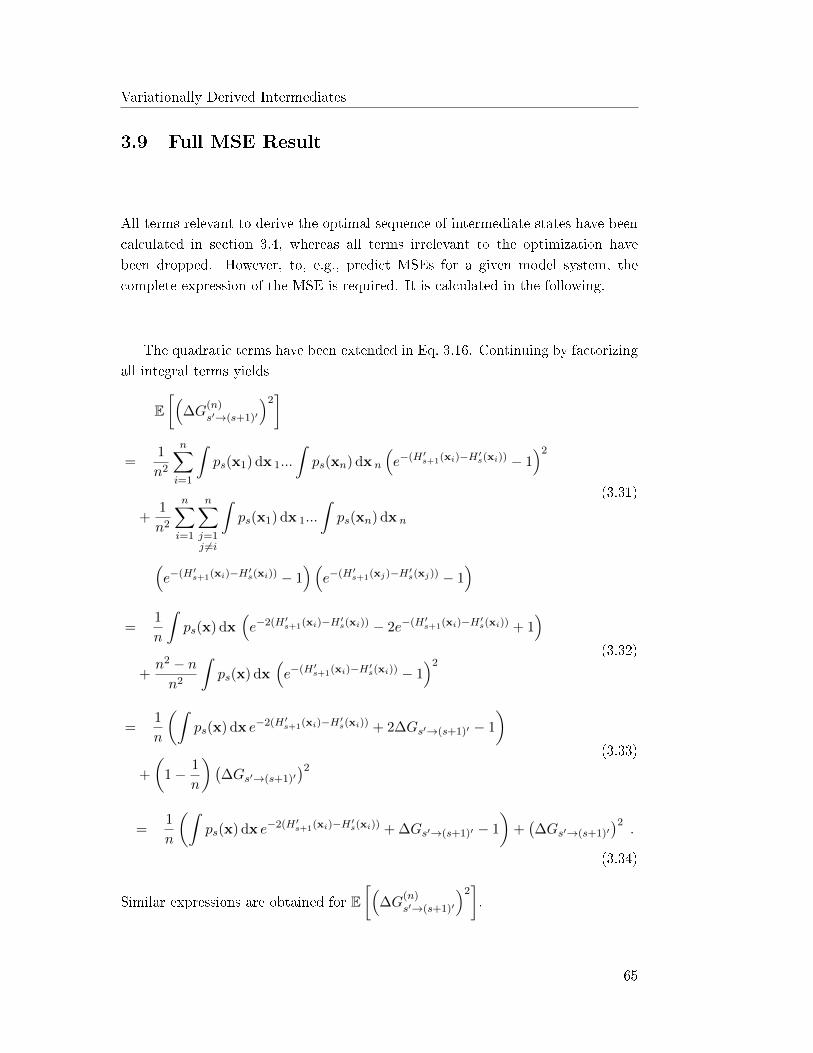
Variationally Derived Intermediates

3.9 Full MSE Result

All terms relevant to derive the optimal sequence of intermediate states have beencalculated in section 3.4, whereas all terms irrelevant to the optimization havebeen dropped. However, to, e.g., predict MSEs for a given model system, thecomplete expression of the MSE is required. It is calculated in the following.

The quadratic terms have been extended in Eq. 3.16. Continuing by factorizingall integral terms yields

E[(

∆G(n)s′→(s+1)′

)2]

=1

n2

n∑i=1

∫ps(x1) dx 1...

∫ps(xn) dx n

(e−(H′s+1(xi)−H′s(xi)) − 1

)2

+1

n2

n∑i=1

n∑j=1j 6=i

∫ps(x1) dx 1...

∫ps(xn) dx n

(e−(H′s+1(xi)−H′s(xi)) − 1

)(e−(H′s+1(xj)−H′s(xj)) − 1

)

(3.31)

=1

n

∫ps(x) dx

(e−2(H′s+1(xi)−H′s(xi)) − 2e−(H′s+1(xi)−H′s(xi)) + 1

)+n2 − nn2

∫ps(x) dx

(e−(H′s+1(xi)−H′s(xi)) − 1

)2(3.32)

=1

n

(∫ps(x) dx e−2(H′s+1(xi)−H′s(xi)) + 2∆Gs′→(s+1)′ − 1

)

+

(1− 1

n

)(∆Gs′→(s+1)′

)2 (3.33)

=1

n

(∫ps(x) dx e−2(H′s+1(xi)−H′s(xi)) + ∆Gs′→(s+1)′ − 1

)+(∆Gs′→(s+1)′

)2.

(3.34)

Similar expressions are obtained for E[(

∆G(n)s′→(s+1)′

)2].

65

Chapter 3

Next, addressing the second line in Eq. 3.6, using Eq. 3.13, yields

−2∆G1,N

N−2∑s=1s odd

(E[∆G

(n)s→s+1

]− E

[∆G

(n)s+2→s+1

]) = −2(∆G1,N )2 (3.35)

Similarly, the third line of Eq. 3.6 is treated as in Eq. 3.15. All terms without aprefactor of 1/n, can, under the condition of Eq. 3.7, be summarized as a binomialand cancel with (∆G1,N )2. As such, the remaining terms yield,

MSE(

∆G(n)1,N

)=

1

n

N−2∑s=1s odd

(∫ps(x) dx e−2(H′s+1(xi)−H′s(xi))

+

∫ps+2(x) dx e−2(H′s+1(xi)−H′s+2(xi))

+ ∆Gs′→(s+1)′ + ∆G(s+2)′→(s+1)′ − 2

)(3.36)

where the last line corresponds to the constant expression g′s in Eq. 3.18. Therefore,the MSE converges to zero with increasing n. However, as can be seen, the MSEis increased for non-zero free energy di�erences between the shifted Hamiltonians.

3.10 Solving the Systems of Equations

The system of Eqs. 3.22 and 3.23 de�ning the sequence of optimal Hamiltonians{Hs(x)} also depends on the partition functions {Zs} of all states s, and vice versa.Whereas numerous numerical algorithms exist for solving systems of equations,this interdependence complicates the application to Eqs 3.22 and 3.23. For allone-dimensional model systems presented in this thesis, �xed point iteration (FPI)was used. The details of its application to VI are provided below. On the one handside, FPI was stable in all cases and converged to a unique solution independent ofthe initial guess. On the other hand side, it is slow compared to most alternativealgorithms and therefore the application of a faster stable algorithm would bedesirable for the future.

66

Variationally Derived Intermediates

Figure 3.10: Di�erent variants of a virtual intermediate state (dashed lines)between the end states (solid lines). The black dashed line depicts the optimalintermediate. The red and blue dashed lines show the intermediates, where oneof the underlying shifting constants, C1 and C3, is too large. Top: Hamiltonian,Bottom: Con�guration space density.

In�uence of the Estimated Partition Functions

The form of an intermediate state s depends on the form of the adjacent statess− 1 and s+ 1. For one virtual intermediate state between the two end states, theoptimal intermediate, using 3.21, is de�ned via

eH2(x) = eH1(x)−C1 + eH3(x)−C3 (3.37)

where the accuracy is optimal if the shifting constant Ci = − lnZi (i = 1, 3).In this case,

p2(x)−1 α p1(x)−1 + p3(x)−1 . (3.38)

To illustrate how C1 and C3 in�uence the form of the intermediate, Figure 3.10shows the Hamiltonian and con�guration space density of di�erent variants of avirtual intermediate (dashed lines) between the end states (solid lines). In the

67

Chapter 3

optimal case (black), p2(x) is largest in the regions where the con�guration spacedensities of the end states overlap. If, however, either C1 or C3 (red and bluedashed line, respectively) are too large, then the form of the virtual intermediatebecomes closer to either state 1 or 3. It has been tested that in this case the MSEsare suboptimal. Hence, the shifting constant involved in the following FPI largelyin�uence the form of the intermediate states.

Fixed Point Iteration and VI

Denoting the set of all intermediate Hamiltonians asH(x) = {H2(x), ...,HN−1(x)},and the corresponding shifting constants as C = {C2, ..., CN−1}, then the systemof equations is solved through the iteration

Hk(x) = f(Hk−1(x), Ck−1

)(3.39)

Ck = − ln

∫ ∞−∞

e−Hk(x)dx , (3.40)

where k denotes the iteration step and

f(Hk(x), Ck

)=

ln[eH1(x)−C1 + eH

k3 (x)−Ck3

]−1

2 ln[e−2(Hk

2 (x)−Ck2 ) + e−2(Hk4 (x)−Ck4 )

]ln[eH

k3 (x)−Ck3 + eH

k5 (x)−Ck5

]−1

2 ln[e−2(Hk

4 (x)−Ck4 ) + e−2(Hk6 (x)−Ck6 )

]...

ln[eH

kN−1(x)−CkN−1 + eHN (x)−CN

]

. (3.41)

The integral notation in Eq. 3.40 denotes that at each step k and for each state sthe integration

Cks = − ln

∫ ∞−∞

e−Hks (x)dx (3.42)

is conducted. As the end state Hamiltonians H1(x) and HN (x) are �xed, C1 andCN only need to be calculated once at the start of the FPI.

The integration, Eq. 3.40, is required at every step k due to the fact thatHks (x) is calculated as the optimum between the adjacent intermediates s− 1 and

68

Variationally Derived Intermediates

s + 1 from the previous step k − 1. Once Ck has been determined up to a step κfor k = 0, ..., κ, the optimal set of Hamiltonians Hκ(x) of a con�guration x thathad previously not been considered, is determined through iteration of Eq. 3.39only. Note that, to be able to do so, it is necessary to store Ck in memory for allsteps, such that the iteration of Eq. 3.39 can be conducted.

The FPI is completed once a convergence criterion is ful�lled. For the cases inthis chapter, the criterion ∣∣∣∣Cks − Ck−1

s

Cks

∣∣∣∣ ≤ 10−6 ∀ s (3.43)

was used.

As for the initial guess H0(x): Whereas it was tested that the FPI reliablyconverges to a unique solution independent of the initial guess, convergence isachieved in fewer steps if H0(x) is closer to the optimal form. Therefore, theapproximated VI form derived in section 3.5, which is relatively close to the exactVI form, was used, i.e.,

H0(x) =

−12 ln

[(1− λ2)e−2(HA(x)−CA) + λ2e

−2(HB(x)−CB)]

−12 ln

[(1− λ3)e−2(HA(x)−CA) + λ3e

−2(HB(x)−CB)]

...

−12 ln

[(1− λN−1)e−2(HA(x)−CA) + λN−1e

−2(HB(x)−CB)]

. (3.44)

For all test systems, the {λs} were chosen as λs = (s − 1)/(N − 1), i.e., inequidistant steps.

For high-dimensional many-body systems, performing multiple integrationsover the entire con�guration space is, by nature of the problem, infeasible. However,it is possible to perform the �rst few steps of the FPI: Firstly, a set of simulationsis conducted with the approximated VI sequence, i.e., the initial guess. Based onestimates of the free energy di�erences between adjacent states, the relative shiftconstants C0

s −C1 are calculated for all states s. In the next step, simulations areconducted in states governed by H1

s determined by Eq. 3.39, and so on. Thereby,the resulting form of the intermediate states will become closer to the optimal onethan the form of the approximated VI sequence.

69

Chapter 3

3.11 Exponential Error Metrics

The VI derivation is based on two assumptions:

1. Sample points are independent.

2. A set of shifting constants {Cs} exists such that both ∆Gs→t << 1 kBT and∆G

(n)s→t << 1 kBT for t = s − 1 and t = s + 1. Therefore, as indicated in

section 3.5, even the exact VI form may not be optimal in the rare case ofvery few samples point and very small overlap in con�guration space densitybetween adjacent states.

This sections outlines how, in theory, the violation of these two assumptions canbe distinguished for cases with suboptimal MSEs.

The following error metric, referred to as the Exponential Mean Squared Error(EMSE), is de�ned as

EMSE(

∆G(n)1,N

)

= E

N−2∑

s=1s odd

−e−∆Gs→s+1 + e−∆Gs+2→s+1 + e−∆G(n)s→s+1 − e−∆G

(n)s+2→s+1

2 .(3.45)

Upon insertion of all ∆Gs→t and ∆G(n)s→t (t = s− 1 and t = s+ 1) into Eq. (3.45),

the exponentials cancel with the logarithms in the de�nitions of the free energydi�erences. The subsequent expression is identical to Eq. 3.18, which wasminimized in section 3.5 and yielded the VI.

Importantly, the VI are therefore obtained by variation of the EMSE withoutany analytical approximation. As a consequence, for independent sampling,the EMSE of the VI sequence is always optimal, also in cases where the MSEis not. Furthermore, if ∆G

(n)s→t and ∆Gs→t are small compared to kBT, then

EMSE(

∆G(n)1,N

)≈ MSE

(∆G

(n)1,N

). Therefore, in case assumption 2 is violated,

the MSE and EMSE di�er. Alternatively, if the samples are not independent (i.e.,violation of assumption 1), then both the MSE and EMSE would be a�ected, andthe EMSE of VI would therefore also be suboptimal.

For test simulations, one further change is required: The EMSE is, unlikethe MSE, not invariant against constant shifts in the Hamiltonians, such as

70

Variationally Derived Intermediates

H ′s(x) = Hs(x) − Cs. Therefore, the EMSE can simply be minimized by choos-ing a constant such that e−∆Gs→s+1 is small, which would, however, not enableany conclusions about the underlying form with respect to the MSE. Therefore,one option to identify optimal forms in test simulations is to compare the EMSEbetween states with equal partition functions only (i.e., similar to the analyticalderivation, where the partition sums of the intermediates are restrained to a con-stant through Lagrange multipliers). Alternatively, the Relative Exponential MeanSquared Error (REMSE) metric,

REMSE(

∆G(n)1,N

)

= E

N−2∑

s=1s odd

−e−∆Gs→s+1 + e−∆G(n)s→s+1

e−∆Gs→s+1+e−∆Gs+2→s+1 − e−∆G

(n)s+2→s+1

e−∆Gs+2→s+1

2 ,

(3.46)

may be used. Here, the di�erence in each individual step is normalized by the expo-nentially weighted di�erence itself. As can be easily validated, REMSE

(∆G

(n)1,N

)is invariant to any constant shifts in the intermediate Hamiltonians. For small freeenergy di�erences ∆G

(n)s→t and ∆Gs→t, the REMSE reduces to the MSE, as desired.

71

Chapter 3

72

4Correlated Free Energy Estimates

4.1 Variationally derived intermediates for correlated

free-energy estimates between intermediate states

The following section consists of the article

M. Reinhardt, H. Grubmüller, �Variationally derived intermedi-ates for correlated free-energy estimates between intermediatestates�, Physical Review E, vol. 102, issue 4, p. 043312 (2020)[240]

published under the Creative Commons Attribution 4.0 International licenseand the content reprinted based on the 2020 Copyright Agreement by the AmericanPhysical Society with consent of the authors.

The format, including the numbering of equations and �gures, has been alteredto match the format of this thesis. Furthermore, all references are listed in thebibliography at the end of this thesis rather than at the end of this article.

Both authors contributed to conceiving the study and writing the manuscript.I implemented, conducted and analyzed all test simulations.

73

Chapter 4

4.2 Abstract

Free energy di�erence calculations based on atomistic simulations generally improvein accuracy when sampling from a sequence of intermediate equilibrium thermody-namic states that bridge the con�guration space between two states of interest. Forreasons of e�ciency, usually the same samples are used to calculate the step-wisedi�erence of such an intermediate to both adjacent intermediates. However, thisprocedure violates the assumption of uncorrelated estimates that is necessary toderive both the optimal sequence of intermediate states and the widely used Ben-nett acceptance ratio (BAR) estimator. In this work, via a variational approach,we derive the sequence of intermediate states and the corresponding estimator withminimal mean squared error that account for these correlations and assess its ac-curacy.

4.3 Introduction

Free energy calculations are widely used to investigate physical and chemicalprocesses [1�7]. Their accuracy is essential to biomedical applications such ascomputational drug development [8�11] or material design [12�15]. Amongst themost widely used methods based on simulations with atomistic Hamiltoniansare alchemical equilibrium techniques, including the Free Energy Perturbation(FEP) [79] and Thermodynamic Integration (TI) [90] methods. These techniquesdetermine the free energy di�erence between two states, representing, for example,two di�erent ligands bound to a target, by sampling from intermediate stateswhose Hamiltonians are constructed from those of the end states. The free energydi�erence between the end states is then determined via a step-wise summation ofthe di�erences between the intermediate states.

The choice of these intermediates critically a�ects the accuracy of the freeenergy estimates [165, 231, 241] by determining which parts of the con�gurationspace are sampled to which extent [169], thereby performing a function similarto importance sampling [78]. In addition, di�erent estimators that determinethe free energy di�erences between these intermediates and the end stateshave been developed, most prominently the Zwanzig formula [79] for FEP, theBennett Acceptance Ratio method (BAR) [80], and multistate BAR (MBAR) [166].

We have recently derived [230] the sequence of discrete intermediate states �the variationally derived intermediates (VI) � that yield, for �nite sampling, thelowest mean squared error (MSE) of the free energy estimates with respect to

74

Correlated Free Energy Estimates

the exact value. Their form di�ers from the most common scheme, which, for Nstates, linearly interpolates between the end states HamiltoniansH1(x) andHN (x),respectively, along a path variable λs,

Hs(x) = (1− λs)H1(x, λs) + λsHN (x, λs), λs ∈ [0, 1] (4.1)

where x ∈ IR3M denotes the coordinate vector of all M particles in the system.All states are labeled by an integer s with 1 ≤ s ≤ N , and λs corresponding tostate s. The additional λs argument of the end states Hamiltonians indicates thecommmon use of soft-core potentials [91�93] to avoid divergences for vanishingparticles. Other approaches involve the interpolation of exponentially weightedHamiltonians of the end states, such as Enveloping Distribution Sampling [100](and variants thereof [102, 103]) or the Minimum Variance path [104, 105] for TI.

In contrast, the VI are not directly de�ned via the end states; instead, theoptimal form of each intermediate s is determined by the form of the adjacent oness− 1 and s+ 1. For the setup shown in Fig. 4.1(a), which consists of two types ofintermediates, sampling is conducted in the �rst type labeled with even numbereds and indicated by the solid lines with yellow points. These are governed by theoptimal Hamiltonian

Hs(x) = −1

2ln[e−2Hs−1(x) · r−2

s−1,s + e−2Hs+1(x) · r−2s+1,s] , (4.2)

where rs,t = Zs/Zt denotes the ratio of the con�gurational partition sums of statess and t. Virtual intermediates are the second type, and labeled with odd numberss with 2 < s < N − 1 and indicated by the dashed lines in Fig. 4.1(a). For these,

Hs(x) = ln[eHs−1(x) · rs−1,s + eHs+1(x) · rs+1,s] . (4.3)

Virtual intermediates are used as target states to evaluate the di�erence in freeenergy to, and no sampling is conducted in those. Due to the coupling of the VI,the optimal MSE sequence of Hamiltonians H2(x)...HN−1(x) is determined bysolving the system of N − 2 equations of Eqs. (4.2) and (4.3).

The variational MSE minimization has been conducted based on the Zwanzigformula [79]

∆Gs,s+1 = − ln〈e−[Hs+1(x)−Hs(x)]〉s (4.4)

being used to calculate the di�erence between two adjacent states, as indicated

75

Chapter 4

Figure 4.1: Two schemes of free energy calculation. The arrows indicate theZwanzig formula is used to evaluate the free energy di�erence to the adjacent statebased on sample sets represented through yellow dots. The dashed lines representvirtual intermediate states that no sampling is conducted in. (a) Separate anduncorrelated sample set are used to calculate the free energy di�erence of therespective intermediate to the state above and below (b). The same sample set isused for this purpose.

by the arrows in Fig. 4.1. However, using the virtual target states describedby Eq. (4.3) is equivalent to using BAR directly between two sampling states[186, 230], and, therefore, Eq. (4.3) also describes the optimal intermediates forBAR.

Note that the Hamiltonians of the optimal intermediates, Eqs. (4.2) and (4.3),depend on the ratios of the partition sums, i.e., the desired quantity. Therefore,the system of equations has to be solved iteratively. The principle is the same asfor BAR, where the estimator depends on an estimate of the free energy di�erence,and the optimal estimator is, therefore, determined iteratively. However, BARis, in practice, mostly used with sampling states that are governed by Eq. (4.1)and a user chosen λ value. The VI method generalizes the BAR principle anddetermines not only the estimator, but the form of all intermediates through suchan iterative optimization by using the information of the free energy estimatesbetween these states. The resulting form di�ers from Eq. (4.1) and does notrequire any additional user choice of a λ variable.

76

Correlated Free Energy Estimates

However, for both BAR and VI to be optimal for multiple states, the free energyestimates to the states above and below an intermediate in the sequence have to bebased on separate, uncorrelated sample points. This is illustrated by the separateyellow points in Fig. 4.1(a) that we refer to as the regular FEP setup, which was thetopic of our previous work [230]. Yet, it would be twice as e�cient to use the samesample points in both directions, as illustrated by Fig. 4.1(b), and as generally donein practice. However, this introduces correlations between the estimates to bothadjacent intermediates, thereby violating the assumptions underlying the deriva-tion of Eqs. (4.2) and (4.3). Therefore, in this case, BAR and the above variationalintermediates are not optimal anymore. Due to these correlations, we refer tothe Fig. 4.1(b) as the correlated FEP (cFEP) setup, which is the topic of this work.

Here, we derive the minimal MSE sequence of intermediate states and thecorresponding estimators for cFEP, as used in practice, that take these correlationsproperly into account. This is in contrast to the derivation of VI [230] for FEP,where these correlations do not occur. As will be shown below, what might seem asa minor technical twist, markedly changes the shape of the optimal intermediatesand considerably improves the accuracy of the obtained free energy estimates.

4.4 Theory

For the cFEP scheme shown in Fig. 4.1(b), we aim to derive the sequence of inter-mediate Hamiltonians H2(x) . . . HN−1(x) that optimizes the MSE

MSE(

∆G(n))

= E[(

∆G−∆G(n))2]

(4.5)

along similar lines as for the regular FEP scheme [230], shown in Fig. 4.1(a). Here,∆G

(n)1,N denotes the free energy estimate based on a �nite number of sample points

n, and ∆G1,N the exact di�erence between the end states 1 and N .

For the optimization metrics, di�erent choices are possible, such as theKullback-Leibler divergence [242] or the Fisher information metric [165, 243] thatmeasure the (dis)similarity between con�guration space densities. Instead, herewe chose to directly optimize the MSE, as it quanti�es the average accuracy withrespect to the exact free energy di�erence, which is the relevant measure for mostpractical applications. Furthermore, as the MSE can be decomposed into varianceplus bias squared, we account for both of these contributions that are oftentimesoptimized separately in the literature [171, 234].

77

Chapter 4

The cFEP variant in Fig. 4.1(b) only uses sampling in the intermediate states.Setups that, in addition, involve sampling in the end states, can also be treatedwith the formalism below. However, �rstly, as we have tested, the accuracy fora given computational e�ort does not increase in this case. Secondly, mixingtwo di�erent types of sample points (the ones used to evaluate ∆H to only oneadjacent state vs. to both adjacent states) further complicates the analysis.

For cFEP, the estimated di�erence is

∆G(n) =

N−2∑s=2s even

(∆G

(n)s→s+1 −∆G

(n)s→s−1

). (4.6)

As in Fig. 4.1(b), the arrows point from sampling to target states, i.e., either theend states or the virtual intermediates. Assuming for each sample state s a set ofn independent sample points {xi}, drawn from ps(x) = e−Hs(x)/Zs, with partitionfunction Zs, expanding Eq. (4.5) with the use of Eq. (4.6) reads

MSE(

∆G(n)1,N

)=

(∆G1,N )2 +N−2∑s=2s even

E[(

∆G(n)s→s+1

)2+(

∆G(n)s→s−1

)2]

− 2∆G1,N

N−2∑s=2s even

(E[∆G

(n)s→s+1

]− E

[∆G

(n)s→s−1

])−

N−2∑s=2s even

N−2∑t=2t even

E[2 ∆G

(n)s→s+1 ∆G

(n)t→t−1

].

(4.7)

The �rst two lines of Eq. (4.7) have already been processed in Ref. 230, but thelast term di�ers. Previously, as in the regular FEP scheme in Fig. 4.1(a), these lastexpectation values were originally derived from independent sample sets and were,therefore, uncorrelated. In the present context of cFEP, however, these estimatesare correlated. Therefore, the term needs to be split in two sums, distinguishingbetween the pairs with samples from the same state and the ones from di�erent

78

Correlated Free Energy Estimates

states,

N−2∑s=2s even

N−2∑t=2t even

E[2 ∆G

(n)s→s+1 ∆G

(n)t→t−1

]

= 2

N−2∑s=2s even

E[∆G

(n)s→s+1 ∆G

(n)s→s−1

]

+ 2N−2∑s=2s even

N−2∑t=2t event6=s

E[∆G

(n)s→s+1

]E[∆G

(n)t→t−1

],

(4.8)

where the expectation value of the product between the two estimates based ondi�erent sample sets has been separated, as these are uncorrelated.

As we are only interested in the intermediates that optimize the MSE, and notin the absolute value of the MSE, we focus on the terms that will not drop out inthe optimization below.

Continuing with the expression inside the sum of the �rst term on the righthand side of Eq. (4.8),

E[∆G

(n)s→s+1 ∆G

(n)s→s−1

](4.9)

=−∫ps(x1)dx1...

∫ps(xn)dxn

ln

[1

n

n∑i=1

e−(Hs+1(xi)−Hs(xi))

]

ln

[1

n

n∑i=1

e−(Hs−1(xi)−Hs(xi))

].

(4.10)

As in the derivation of Ref. 230, the Hamiltonians are now shifted by a constanto�set Cs, i.e., H ′s(x) = Hs(x)− Cs. This o�set will cancel out for a given shapeof an intermediate when calculating the accumulated free energy di�erence inEq. (4.6). However, as the intermediate states will turn out to be coupled, theseo�sets do in�uence the shape of these intermediates. The o�sets can now bechosen such that the terms inside the logarithms of Eq. (4.10) are close to one. Inthis case, E

[∆G

(n)s′→(s+1)′

]= ∆Gs′,(s+1)′ [230], and, therefore, the two linear terms

arising from Eq. (4.10) can be expressed in terms of the exact free energy di�erences.

79

Chapter 4

Next, the product of the two sums in Eq. (4.10) is split into terms based on thesame and di�erent sample points, respectively,

E[∆G

(n)s′→(s+1)′ ∆G

(n)s′→(s−1)′

](4.11)

=− 1

n2

∫ps(x1)dx1...

∫ps(xn)dxn

(n∑i=1

e−(H′s+1(xi)−H′s(xi))

) n∑j=1j 6=i

e−(H′s−1(xj)−H′s(xj))

+

n∑i=1

e−H′s+1(xi)−H′s−1(xi)+2H′s(xi)

]+ fs′(∆Gs′→(s−1)′ ,∆Gs′→(s+1)′) ,

(4.12)

where the terms that can be expressed solely based on (constant) free energydi�erences are summarized by the term fs. Again, the �rst two terms of Eq. (4.12)can be expressed in terms of the free energy di�erences between s and s + 1 aswell as between s and s− 1, respectively.

Collecting all terms arising from Eq. (4.7)

MSE(

∆G(n)1,N

)=

N−2∑s=2s odd

1

n

(∫ps(x) dx e−2(H′s+1(x)−H′s(x))

+

∫ps+2(x) dx e−2(H′s+1(x)−H′s+2(x))

+

∫ps+1(x) dx e−H

′s+2(x)−H′s(x)+2Hs+1(x)

+ gs′(∆Gs′,(s+1)′ ,∆G(s+2)′,(s+1)′ ,∆G1′,N ′)),

(4.13)

where the function g′s serves the same purpose as f ′s and can be dropped in theoptimization below.

The condition of small ∆G(n)s′→(s+1)′ is ful�lled by setting Cs = − lnZs. By

variation of the MSE from Eq. (4.13),

∂

∂Hs(x)

(MSE

(∆G

(n)1,N

)+ ν

∫(e−Hs(x) − Zs)dx

)!

= 0 , (4.14)

80

Correlated Free Energy Estimates

where ν is a Lagrange multiplier, the optimal sequence of Hamiltonians is obtained.For s even, we obtain

Hs(x) = −1

2ln(e−2Hs−1(x)r−2

s−1,s + e−2Hs+1(x)r−2s+1,s

−2e−Hs−1(x)−Hs+1(x)r−1s−1,sr

−1s+1,s

) (4.15)

For s odd and 2 < s < N − 1:

Hs(x) = ln(eHs−1(x)rs−1,s + eHs+1(x)rs+1,s

)− ln

(e−Hs−2(x)+Hs−1(x)rs−1,s−2

+ e−Hs+2(x)+Hs+1(x)rs+1,s+2

) (4.16)

where, as in Eqs. (4.2) and (4.3), the ratios rs,t of the partition sums betweenstates s and t have to be determined iteratively. The above sequence, Eqs. (4.15)and (4.16), that we refer to as the correlated Variational Intermediates (cVI), yieldthe minimal MSE estimates for cFEP.

Figure 4.2 shows the resulting con�guration space densities of the aboveintermediates for the example of a start state with a harmonic Hamiltonian,H1(x) = 1

2x2, and an end state with a quartic one, HN (x) = (x− x0)4. Panel (a)

shows the VI that are optimal for the regular FEP scheme in Fig. 4.1(a). Panel (b)shows the cVI, optimal for cFEP.

The yellow (light) areas in Fig. 4.2, Eq. (4.17), provide a simple measure of thecon�guration space density overlap K between the end states 1 and N ,

K =

∫ +∞

−∞dx min(pA(x), pB(x)) , (4.17)

Here, K = 0 indicates two separate distributions without any overlap, and K = 1

full overlap, i.e., identical con�guration space densities.

The two rows in Fig. 4.2(a) and (b) depict the result for two di�erent valuesof x0, and correspondingly, varying K.

As can be inferred from Eq. (4.15), for N = 3, H2(x) diverges at the pointswhere p1(x) = p3(x), and therefore, p2(x) = 0 at these points, as can also be seenfor the intermediate sampling state shown in Fig. 4.2(a). More generally, H2(x)

of cVI �directs� sampling away from the overlap regions and towards the ones

81

Chapter 4

Figure 4.2: Con�guration space densities of VI (left column), and cVI (rightcolumn) for (a) N = 3 and (b) N = 7 states. The individual rows show di�erentshifts in x-direction between the minima of the harmonic, H1(x) (red, towards theleft in each panel), and the quartic, HN (x) (blue, towards the right), potentials ofthe end states, thereby showing setups with di�erent con�guration space densityoverlap K between the end states, indicated by the yellow (light) area. Sampling isconducted in the even numbered intermediates. The dashed lines in (b) indicate the(odd numbered) virtual intermediate target states that no sampling is conductedin.

that are only relevant for one, but not both end states. For instance, the tailsof the start state in the upper row of (a) are sampled more for cVI than for VI.For larger horizontal shifts of x0, i.e., low values of K, the two variants becomeincreasingly similar, as the additional term in Eq. (4.15) with respect to Eq. (4.2)becomes smaller compared to the �rst term.

For N = 7 states, Fig. 4.2(b) shows the converged resulting con�guration spacedensities. The case of x0 = 0, as shown in (a), was omitted in (b) as the visualiza-tion is more di�cult in this case due to the higher number of states. In (b), theadditional changes from VI to cVI become more complex. As in (a), the samplingstates have smaller densities p(x) in the overlap regions of the end states, but, incontrast to (a), still di�er between VI and cVI for smaller values of overlap K. Thereason is that while the overlap between the end states vanishes with decreasing K,an overlap between adjacent intermediate states remains that a�ects the shape ofthe intermediates. Note that the divergences mentioned above introduce instabili-

82

Correlated Free Energy Estimates

ties in solving the system of Eqs. (4.15) and (4.16). Hence, for N > 3 the factor 2of the additional term in the logarithm Eq. (4.15) has been replaced by a factor κthat was set to slightly below 2 (κ = 1.95) in case of Fig. 4.2(b). See Appendix Afor details.

cBAR Estimator

As mentioned above, using the Zwanzig formula [79] to evaluate the free energydi�erence between two sampling states with respect to the virtual intermediate,Eq. (4.3), of VI is equivalent to BAR [186, 230]. Correspondingly, the virtualintermediate de�ned by Eq. (4.16) of cVI also corresponds to an estimator, thatis optimal for the sampling states of cFEP and that we will refer to as correlatedBAR (cBAR).

To derive cBAR, we use the relation between the two approaches. Determiningthe free energy di�erence between two sampling states labeled s− 1 and s + 1 byusing the virtual intermediate s to evaluate the di�erence between the adjacentstates yields

∆G(n)s−1,s+1 = − ln

〈e−(Hs(x)−Hs+1(x))〉s+1

〈e−(Hs(x)−Hs−1(x))〉s−1. (4.18)

Using the approach of Bennett [80] instead,

∆G(n)s−1,s+1

= ln〈w(Hs−1(x), Hs+1(x))e−Hs−1(x)〉s+1

〈w(Hs−1(x), Hs+1(x))e−Hs+1(x)〉s−1. (4.19)

where w(Hs−1(x), Hs+1(x)) is a weighting function. From Eqs. (4.21) and (4.19)follows that the two approaches are equivalent if the weighting function relates tothe Hamiltonian of the virtual intermediate state through

w(Hs−1(x), Hs+1(x)) = e−Hs(x)+Hs−1(x)+Hs+1(x) . (4.20)

Therefore, any Hamiltonian of a virtual intermediate state corresponds to a weight-ing function. Bennett optimized the weighting function with respect to the varianceyielding the famous BAR result

∆G(n)s−1,s+1 − C = ln

〈f(Hs−1(x)−Hs+1(x)− C)〉s+1

〈f(Hs+1(x)−Hs−1(x) + C)〉s−1, (4.21)

where C ≈ ∆Gs−1,s+1 has to be determined iteratively and f(x) is the Fermi

83

Chapter 4

function. This result is equivalent to using the virtual intermediate of Eq. (4.3)with Eq. (4.18). Note that the relation of a virtual intermediate to BAR resulthad already been obtained by Lu et al. [186], albeit through a di�erent formalism,and that using the hyperbolic secant function (Eq. 10, p. 2980), in their OverlapSampling approach [186, 187] is equivalent to Eq. (4.20).

Next, for cFEP, using the Hamiltonian of the virtual intermediate fromEq. (4.16) in Eq. (4.20) yields the weighting function of cBAR,

w(Hs−2(x), Hs−1(x), Hs+1(x), Hs+2(x),

Cs−2,s−1, Cs−1,s+1, Cs+1,s+2

)=(e−Hs−2(x)+Hs−1(x)+Cs−2,s−1

e−Hs+2(x)+Hs+1(x)+Cs+2,s+1

)/(eHs−1(x)−Hs+1(x)−Cs+1,s−1 + 1

),

(4.22)

where the MSE of the resulting estimates is minimal if all Cs,t ≈ ∆Gs,t. Anumerator of 1 in Eq. (4.22) would yield the original BAR result.

Note that Hs−2(x), and Hs+2(x), are also virtual intermediates determined byEq. (4.16). As such, the result is a system of weighting functions, i.e., one forevery pair of adjacent sampling states. The optimal estimate can, therefore, onlybe found by iteratively solving for the free energy estimates between all samplingstates at once. In this regard, the procedure is similar to MBAR [166].

4.5 Test Simulations

To assess to what extent our new variational scheme improves accuracy, weconsider the one-dimensional system with a harmonic and a quartic end stateshown in Fig. 4.2. Rejection sampling is used to obtain uncorrelated sample points.The free energy estimate, obtained from these �nite sample sets, is comparedto the exact free energy di�erence. The MSE, Eq. (4.5), is then calculated byaveraging over one million of such realizations. With this procedure, di�erentcombinations of overlapK, numbers of statesN and sample points n are considered.

We compare three variants. Firstly, using VI, Eqs. (4.2) and (4.3), with FEP,i.e., the scheme in Fig. 4.1(a). Here, the estimates to both adjacent states are basedon separate sample sets and, therefore, not correlated. Secondly, also using VI,

84

Correlated Free Energy Estimates

but now with cFEP, shown in Fig. 4.1(b). In contrast to variant 1, these estimatesare based on the same sample sets and, therefore, correlated. In order to keep thetotal computational e�ort constant, the number of sample points per set (i.e., peryellow point in Fig. 4.1) is two times larger for cFEP than for FEP. Thirdly, us-ing cVI, Eqs. (4.15) and (4.16), that accounts for these correlations, also with cFEP.

4.6 Results

For N = 3 states, Fig. 4.3(a) shows the MSEs of the three variants for di�erentnumbers of sample points. Here, for the quartic end state, x0 = 0, correspondingto K = 0.85, was used. The corresponding con�guration space densities of VI andcVI are shown in the upper row of Fig. 4.2(a).

As can be seen, cVI with cFEP, shown by the dark blue (lower) line, yieldsthe best MSE for all numbers of sample points except very few ones. The othertwo variants, i.e., VI with FEP (dashed green line) and cFEP (red, upper line)yield very similar MSEs. As such, the gain in information from evaluating theHamiltonians to both adjacent states for all sample points yields only a very smallimprovement compared to using separate sample sets for this purpose.

In order to quantify the improvement of cVI compared to VI for cFEP,Fig. 4.3(b) shows the ratio of the MSEs of the two variants, again in relation tothe number of sample points per set. The dark orange (upper) curve (K = 0.85),corresponds to the MSEs shown in (a) (i.e., the values of the red curve dividedby the blue curve). The improvement in the MSE plateaus slightly above two formore than two hundred sample points per state. In addition, the improvementsfor setups with di�erent overlap K between the end states are shown (orangeto yellow). This improvement becomes smaller for smaller values of K, but thequalitative dependence on the number of sample points remains the same.

For a constant number of sample points n = 200 (and n = 100 per setfor VI with FEP, shown by the dashed green line), Fig. 4.3(c) shows howthe MSEs of the three variants improve with increasing K. The MSEs con-verge at low K, which is in agreement with the observation from Fig. 4.2(a) thatthe phase space densities of the intermediate state become more similar in this case.

Figure 4.3(d) shows the MSEs for N = 7 states. The corresponding con�g-

85

Chapter 4

Figure 4.3: Comparison of the accuracy of VI and cVI using the schemes ofFig. 4.1. The accuracies were obtained from test simulations based on the setupsshown in Fig. 4.2. (a) Using N = 3 states and comparing three variants of freeenergy calculations: Using cVI with cFEP (blue, lower solid line), VI with cFEP(red, upper solid line) and VI with FEP (green, dashed line). The MSEs of freeenergy calculations are shown for di�erent number of sample points. (b) The ratioof the MSEs, and therefore, the improvement, of using cVI compared to VI forcFEP. The dark orange (upper) line (K = 0.85) corresponds to the ratio betweenthe red and the blue (solid) lines in (a). In addition, the results for di�erentcon�guration space density overlaps K between the end states are shown (orangeto yellow). (c) Using n = 200 sample points, the MSEs of the three variants from(a) are shown over the full range of K. (d) As in (c), but with N = 7 states. Thecomputational e�ort was kept constant by reducing the number of sample pointsper state.

86

Correlated Free Energy Estimates

uration space densities for two di�erent values of K are shown in Fig. 4.2(b).Here, VI with FEP and cFEP still yield similar MSEs, whereas cVI with cFEP,in contrast to N = 3, now yields the best MSE for all K. The improvement toVI ranges from around 20 % for low K, to around 50 % for large K. This is inline with the observation from Fig. 4.2(b) that the con�guration space densitiesbetween VI and cVI become more similar but do not fully converge for a largernumber of states in the limit of small K.

Lastly, the cBAR estimator can be used with any choice of intermediate statesfor cFEP. To assess how much the cBAR estimator improves the accuracy offree energy estimates compared to BAR for cFEP, we conducted test simulationswhere the sampling states were chosen as in Eq. (4.1), i.e., by linear interpolationbetween the Hamiltonians of the end states. Test simulations were conducted atvarying values of K and at N = 5 and N = 7. Evaluating the MSE, we found astatistically signi�cant improvement, however, only in the range of 1− 2 % (datatherefore not shown here). The improvement was independent of K and similarfor both numbers of N .

Considering that the MSEs of cVI and VI can improve up to an order of mag-nitude compared to the linear intermediates de�ned in Eq. (4.1) (for a detailedcomparison between VI and linear intermediates, see Ref. 230), the large majorityof improvements is not due to an improved estimator, but due to the way samplesare generated.

4.7 Discussion and Conclusion

In summary, we have derived a new variant of variational intermediates (cVI) thatyield the optimal free energy estimate with minimal MSE when using the samesample points to evaluate the di�erences between the adjacent states above andbelow in the sequence (cFEP). This procedure is commonly used in free energysimulations, as it is computationally much cheaper to evaluate sample points atdi�erent Hamiltonians than to generate these. However, the resulting correlationsbetween these estimates have not been considered yet.

Our test simulations for a one-dimensional Hamiltonian show that cVI withcFEP yields an improved MSE compared to the optimal sequence (VI) with FEP,i.e., using di�erent sample points for estimates to states above and below in thesequence. For N = 3 states, the �rst variant improved the MSE by more than

87

Chapter 4

a factor of two for end states with high con�guration space density overlap K,whereas at low K the MSEs were similar. For N = 7 states, the MSE improvedbetween 20 % (low K) and 50 % (large K).

Interestingly, due to the correlations mentioned above, using VI with FEPyields only slightly worse MSEs for all K as using VI with cFEP, even though thelatter involves twice as many evaluations of Hamiltonians from adjacent states.Only for cVI, thereby accounting for these correlations, the additional gain ininformation translates into a marked improvement of the MSE.

Similar to most other theoretical analyses and derivations of free energycalculation methods, we also needed to assume that all sample points within eachintermediate state are uncorrelated. If atomistic simulations are used for sampling,the resulting time-correlations reduce the number of essentially independentsample points. Unfortunately, for our one-dimensional systems, cVI increasesbarrier heights, thereby increasing correlation times. We have so far not tested ourmethod on any complex biomolecular systems, so it is unclear if these barriers canbe circumvented or what the expected increase in correlation times is. However,to avoid such correlations between sample points in atomistic simulations, usuallyonly a small subset of all sample points is used to calculate free energy di�erences.Based on our �ndings and in contrast to common practice, we therefore recommendto use di�erent subsets to evaluate the free energy di�erences to di�erent adjacentstates.

The above derivation provides an example on how optimal intermediates andestimators with minimal MSE can be derived for di�erent types of setups based on�nite sampling that may help to incorporate a variety of assumptions and modelsinto future theoretical approaches.

4.8 Appendix A: Avoiding numerical instabilities

The divergence in Eq. (4.15) at all x for which

e−2Hs−1(x)r−2s−1,s + e−2Hs+1(x)r−2

s+1,s

= 2e−Hs−1(x)−Hs+1(x)r−1s−1,sr

−1s+1,s

(4.23)

88

Correlated Free Energy Estimates

causes numerical instabilities in solving the system of Eqs. (4.15) and (4.16). Re-placing the factor 2 in Eq. (4.15) in the logarithm with a factor κ, i.e., for s even,

Hs(x) = −1

2ln(e−2Hs−1(x)r−2

s−1,s + e−2Hs+1(x)r−2s+1,s

−κe−Hs−1(x)−Hs+1(x)r−1s−1,sr

−1s+1,s

),

(4.24)

and setting, e.g., κ = 1.95, avoids these complications. As can be easily validated,the inside of the logarithm in Eq. (4.24) is larger than zero for 0 < κ < 2 for allHs−1(x) and Hs+1(x). As shown for cVI in Fig. 4.2(b), κ < 2 prevents ps(x) togo to zero at the crossing points of ps−1(x) and ps+1(x) of the neighboring states,but is still lowered at these points.

End of publication

89

Chapter 4

4.9 Further Interpretation

The optimal form of a cVI intermediate sampling state, Eq. 4.15, is determinedthrough

e−2Hs(x) = e−2Hs−1(x)r−2s−1,s + e−2Hs+1(x)r−2

s+1,s

− 2e−Hs−1(x)−Hs+1(x)r−1s−1,sr

−1s+1,s

(4.25)

α

(e−Hs−1(x)

Zs−1− e−Hs+1(x)

Zs+1

)2

. (4.26)

Expressing Eq. 4.26 through con�guration space densities,

ps(x) α | ps−1(x)− ps+1(x) | , (4.27)

where the equality holds once the cVI sequence has converged through an iterativeprocedure such as the FPI described in section 3.10.

When considering only one intermediate sampling state I between the end statesA and B, then Eq. 4.27 reads

pI(x) α | pA(x)− pB(x) | . (4.28)

This form shows explicitly what has been observed in the context of Fig. 4.2:It is optimal to sample the regions where the con�guration space densities of theend states di�er. If there is no overlap, then the resulting form equals the one fromVI. If the densities pA(x) and pB(x) are identical for all x, then Hs(x) divergeseverywhere. Essentially, no sampling is required in this case.

This �nding agrees with the analogy of dart board sampling, developed in theintroduction in the context of Fig. 1.1(c). Here importance sampling improvesthe e�ciency of determining the di�erence in area by conducting sampling onlyin the regions where the shapes di�er. However, this result contradicts previousassumptions that most of the sampling should be conducted in the overlap region.In practice, by sampling in states from the linear interpolation scheme that shiftthe intermediate con�guration space density from A to B, most of the samplingis conducted either in the overlap region or in regions that are relevant to neitherA nor B. Whereas this practice avoids barriers in the free energy landscape, it issuboptimal for independent sampling with cFEP.

90

5GROMACS Implementation

The following chapter consists of the manuscript

M. Reinhardt, H. Grubmüller, �GROMACS Implementationfor Free Energy Calculations with Non-Pairwise VariationallyDerived Intermediates�.

that is currently under review in Computer Physics Communications and isavailable as a preprint at https://arxiv.org/abs/2010.14193.

Both authors contributed to conceiving the study and writing the manuscript.I conducted the described implementation and simulations.

91

Chapter 5

5.1 Abstract

Gradients in free energies are the driving forces of physical and biochemical sys-tems. To predict free energy di�erences with high accuracy, Molecular Dynamics(MD) and other methods based on atomistic Hamiltonians conduct sampling sim-ulations in intermediate thermodynamic states that bridge the con�guration spacedensities between two states of interest ('alchemical transformations'). For un-correlated sampling, the recent Variationally derived Intermediates (VI) methodyields optimal accuracy. The form of the VI intermediates di�ers fundamentallyfrom conventional ones in that they are non-pairwise, i.e., the total force on a par-ticle in an intermediate states cannot be split into additive contributions from thesurrounding particles. In this work, we describe the implementation of VI into thewidely used GROMACS MD software package (2020, version 1). Furthermore, avariant of VI is developed that avoids numerical instabilities for vanishing particles.The implementation allows the use of previous non-pairwise potential forms in theliterature, which have so far not been available in GROMACS. Example cases onthe calculation of solvation free energies, and accuracy assessments thereof, areprovided.

5.2 Program Version Summary

Program Title: GROMACS-VI

CPC Library link to program �les: (to be added by Technical Editor)

Developer's respository link: https://www.mpibpc.mpg.de/gromacs-vi-extensionand https://gitlab.gwdg.de/martin.reinhardt/gromacs-vi-extension

Licensing provisions: LGPL

Programming language: C++14, CUDA

Supplementary material: All topologies and input parameter �les required to repro-duce the example cases in this work, as well as user and developer documentationwill be provided online together with the source code.

Journal reference of previous version:* M.J. Abraham, T. Murtola, R. Schulz, S.Pall, J.C. Smith, B. Hess, E. Lindahl, GROMACS: High performance molecularsimulations through multi-level parallelism from laptops to supercomputers, Soft-wareX, 1-2 (2015)

Does the new version supersede the previous version?: No

92

GROMACS Implementation

Reasons for the new version:* Implementation of variationally derived intermedi-ates for free energy calculations

Nature of problem: The free energy di�erence between two states of a thermo-dynamic system is calculated using samples generated by simulations based onatomistic Hamiltonians. Due to the high dimensionality of many applications asin, e.g., biophysics, only a small part of the con�guration space can be sampled.The choice of the sampling scheme critically a�ects the accuracy of the �nal freeenergy estimate. The challenge is, therefore, to �nd the optimal sampling schemethat provides best accuracy for given computational e�ort.

Solution method(approx. 50-250 words): Sampling is commonly conducted in inter-mediate states, whose Hamiltonians are de�ned based on the Hamiltonians of thetwo states of interest. Here, sampling is conducted in the variationally derived in-termediates states that, under the assumption of uncorrelated sample points, yieldoptimal accuracy. These intermediates di�er fundamentally from the common in-termediates in that they are non-pairwise, i.e., the forces on a particle are onlyadditive in the end state, whereas the total force in the intermediate states cannotbe split into additive contributions from the surrounding particles.

5.3 Introduction

Thermodynamic systems are driven by free energy gradients. Hence, knowledgethereof is key to the molecular understanding of a wide range of biophysical andchemical processes, as well as to applications in the pharmaceutical [8, 244, 245]and material sciences [12, 13, 246]. Consequently, in silico calculations of freeenergies are popular in providing complementary insights to experiments orassisting the selection of chemical compounds in the early stages of drug discoveryprojects.

The microscopic calculation of the free energy,

∆G = −β−1 lnZ (5.1)

= −β−1 ln

∫ ∞−∞

e−βH(x)dx , (5.2)

requires integration over all positions x of all particles in the system, where Zdenotes the partition sum, β = 1/(kBT ) the thermodynamic β, kB the Boltzmannconstant, T the temperature and H(x) the Hamiltonian. As an exact integration

93

Chapter 5

is not feasible for high-dimensional x in case of many particles, sampling basedapproaches such as Monte-Carlo (MC) or Molecular Dynamics (MD) simulationsare commonly used. Furthermore, in practice, it oftentimes su�ces to know onlythe free energy di�erence between two states, which can be calculated much moreaccurately. The most basic approach,

∆GA,B = −β−1 ln⟨e−β[HB(x)−HA(x)]

⟩A

(5.3)

rests on the Zwanzig formula [79]. The brackets 〈〉A indicate an ensembleaverage over A is calculated. More recent methods with close relations to Eq. (5.3)that use samples from both A and B are the Bennett Acceptance Ratio (BAR)and multistate BAR (MBAR) method [80, 166] methods.

For sampling based approaches, the accuracy of a free energy di�erence esti-mate between two states A and B generally improves when sampling is not onlyconducted in A and B, but also in intermediate states. Commonly, a mostly linearinterpolation between the end state Hamiltonians HA(x) and HB(x) is used,

Hlin(x, λ) = (1− λ)HA(x, λ) + λHB(x, λ) , (5.4)

where λ ∈ [0, 1] denotes the path variable. The λ dependence of the end stateHamiltonians enables the use of soft-core potentials [91�93] that avoid divergencesin case of vanishing particle for, e.g., the calculation of solvation free energies (wherethe molecules �vanishes� from solution). A step-wise summation,

∆GAB =

N−1∑i=1

∆Gi,i+1 (5.5)

yields the total free energy di�erence, where N denotes the total number ofstates. In the sum of Eq. (5.5), i = 1 corresponds to state A and i = N to stateB, respectively. Alternatively, for many steps the di�erence can be calculated withThermodynamic Integration (TI) [90],

∆GAB =

∫ 1

0

⟨∂H(x, λ)

∂λ

⟩λ

dλ . (5.6)

Importantly, advantageous de�nitions of intermediate states exist that go be-

94

GROMACS Implementation

yond the de�nition of Eq. (5.4). For example, variationally derived intermediates(VI) [230, 240] minimize the mean squared error (MSE) of free energy estimatesusing FEP and BAR. An easily parallelizable approximation for a small number ofstates is

HV I(x, λ) = − 12β ln

{(1− λ) exp

[− 2βHA(x)

]+ λ exp

[− 2β

(HB(x)− C

)]},

(5.7)

where, similar to BAR, the free energy di�erence estimate is optimal if C ≈ ∆G.It is similar in shape to the minimum variance path (MVP) [78, 104, 105] for TI (2vs 1/2 in the exponents). Enveloping Distribution Sampling (EDS) [100, 101], andextensions such as Accelerated EDS [102, 247] use a reference potential similar inshape to Eq. (5.7) to calculate the free energy di�erence between two or more endstates.

Note a particular characteristic of the VI sequence and related methods, whichis illustrated in Fig. 5.1: Its Hamiltonians cannot be formulated as the pair-wisesum of interaction potentials for all particles. To see this, consider the force onparticle j (blue), obtained through the derivative of Eq. (5.7). It still dependson the full Hamiltonians of the end states. The consequence can be understoodby considering a particle i (red), with λ dependent parameters, positioned at adistance rij so large such that all direct interactions between i and j are negligible.However, when particle i changes its position with respect to its neighboringparticles, the end states Hamiltonians also change, and, therefore, so does theforce on particle j.

In this work, we, �rstly, describe our implementation of the VI approach, and,by extension, also the MVP and basic principles of the EDS methods for two endstates, into GROMACS [157�159]. It is among the most widely used MD softwarepackages; however, none of the above approaches are available so far in GROMACS.Secondly, we introduce an approach to avoid singularities for vanishing particleswith VI.

5.4 Avoiding End State Singularities

Interestingly, the VI sequence, Eq.(5.7), already exhibits soft-core characteristicsfor vanishing particles, as shown in Fig. (5.2)(a) on the example of a two-particle

95

Chapter 5

Figure 5.1: Non-pairwise potentials and forces in VI intermediates. Two particlesi and j (red and blue, respectively) are considered that are λ dependent, i.e., theirinteraction potential di�ers between A and B. It is assumed that direct interactionsbetween i and j in both A and B are negligible. If particle i changes its position,then HA(x) and / or HB(x) change accordingly, and so does HV I(x, λ). Due tothe form of the VI sequence, the derivative, and therefore, the force on particle jchanges.

Lennard-Jones (LJ) potential. However, divergences can still occur when con�gu-rations from the decoupled states are evaluated at foreign states, i.e., the ones thatno sampling is conducted in, but that the Hamiltonian is evaluated at such as,e.g., state B in Eq. (5.3). Furthermore, when two particles start to overlap, verysmall changes in their separation r lead to large changes in force, which causesinstabilities due to �nite integration steps.

To avoid these divergences, a dependence of the end state Hamiltonians on λanalogous to common soft-core potentials [91] is introduced, i.e., HA = HA(x, λ)

with HA(x, 0) = HA(x), and HB = HB(x, λ), with HB(x, 1) = HB(x). For twoparticle i and j with distance rij , the Coulomb and Lennard-Jones interactions instate A and B are calculated based on the modi�ed distances rA and rB, respec-tively, that are de�ned as

96

GROMACS Implementation

Figure 5.2: Intermediate VI states for a vanishing particle system. The thick redline shows the Lennard-Jones potential between two particles. The blue one showsthe decoupled end state, i.e., the particles don't �see� each other anymore. Theinterpolated colors represent the intermediate states. (a) The VI sequence withoutand (b) with λ dependent end states.

rA(rij , λ) =(ασ6

ijλp + r6

ij

) 16 , (5.8)

rB(rij , λ) =(ασ6

ij(1− λ)p + r6ij

) 16 , (5.9)

where α and p are soft-core parameters to be speci�ed by the user, and σij theLennard-Jones parameter in the coupled state. For a system of two Lennard-Jonesparticles, Fig. (5.2) shows the resulting VI states without (a) and with (b) the useof λ dependent end states. As can be seen, the transition to the overlap regionbecomes markedly smoother.

Secondly, for increasingly complex molecules, the likelihood of barriers betweenthe relevant parts of con�guration space of the end states rises. Aside of additionaltechniques such as replica exchange, or meta-dynamics, the factor 2 in the exponentcan be replaced by a user speci�c smoothing factor s introduced in the EDS [100,101] method. In the limit of small s, a series expansion of the exponential termsyields the conventional pathway, i.e., Eq. (5.4). The modi�ed VI sequence thusreads as

97

Chapter 5

HV I(x, λ) = − 1

sβln

{(1− λ) exp

[− sβHA(x, λ)

]+ λ exp

[− sβ

(HB(x, λ)− C

)]}.

(5.10)

The force on particle i,

FV Ii (x, λ) = − ∂HV I(x, λ)

∂xi(5.11)

= exp[sβHV I(x, λ)

]{(1− λ) exp

[− sβHA(x, λ)

]FAi (x)

+ λ exp[− sβ

(HB(x, λ)− C

)]FBi (x)

},

(5.12)

in the intermediate state characterized by λ, depends on both HA(x, λ) andHB(x, λ), as well as on the sum of the forces, FAi (x) and FBi (x) on particle i inend state A and B, respectively.

Along similar lines, the derivate

∂HV I(x, λ)

∂λ=

exp[sβHV I(x, λ)

]βs{(

(1− λ)sβ∂HA(x, λ)

∂λ+ 1

)exp

[− sβHA(x, λ)

]+

(λsβ

∂HB(x, λ)

∂λ− 1

)exp

[− sβ(HB(x, λ)− C)

]}(5.13)

depends on the derivatives ∂HA(x, λ)/∂λ and ∂HB(x, λ)/∂λ in the end states.Equation (5.13) is used for TI.

Due to the dependence of Eq. (5.10) on C, where the accuracy is optimal ifC ≈ ∆GAB, the free energy di�erence has to be determined in an iterative process,

Cn+1 = ∆GAB′ + Cn , (5.14)

where Cn denotes the free energy guess at iteration step n. The free energy dif-ference ∆GAB′ is obtained from simulations between state A and B′, where thelatter denotes the end state shifted by the constant C, i.e., that is governed by

98

GROMACS Implementation

H ′B(x, λ) = HB(x, λ)− C. The di�erence ∆GAB′ converges to zero, such that thedesired quantity ∆GAB = ∆GAB′ + Cn ≈ Cn at the end of the iteration process.

5.5 Program Structure and Usage

The end states Hamiltonians,

HA(x, λ) = HλA(x, λ) +Hc(x) (5.15)

HB(x, λ) = HλB(x, λ) +Hc(x), (5.16)

can be split into the λ-dependent energy contributions HλA(x, λ) and Hλ

B(x, λ),and the common contributions summarized by Hc(x) that are equal in both endstates, such as water-water interactions. To calculate HA(x, λ) and HB(x, λ),GROMACS only evaluates the λ-dependent contributions separately for the endstates, whereas Hc(x) is calculated only once. Note that, due to the λ dependenceof the end states, Hλ

A(x, λ) andHλB(x, λ) di�er for di�erent intermediates for α > 0.

The same holds for the VI sequence, Eq. (5.10). Inserting Eqs. 5.15 and 5.16,yields

HV I(x, λ) = HλV I(x, λ) +Hc(x) , (5.17)

where HλV I(x, λ) is described by Eq. (5.10), where the end states Hamil-

tonians HA(x, λ) and HB(x, λ) have been replaced by the parts HλA(x, λ) and

HλB(x, λ), respectively, that only sum over λ-dependent interactions. The same

principle applies to the calculation of the forces and λ-derivatives. Therefore,the computational e�ort of VI is very close to the using conventional intermediates.

However, in the current GROMACS implementation structure, all force andenergy contributions from di�erent interaction types are interpolated between theend states right after they have been calculated, i.e., the overall calculation has theform,

Hλlin(x, λ) =

∑interactiontype k

...∑

particlesi,j

(1− λ)HkA(xi,j , λ) + λHk

B(xi,j , λ) (5.18)

F iλ(x) =∑

interactiontype k

...∑

particles j

(1− λ)F kA(xi,j , λ) + λF kB(xi,j , λ) . (5.19)

99

Chapter 5

Whereas this has the least memory requirement, for VI, the full Hamiltoniansand forces in the end states need to be known before the individual forces canbe calculated. Therefore, the end states Hamiltonians and forces are storedseparately. After all λ-dependent contributions have been collected, �rst theHamiltonian and subsequently the forces are calculated.

The implementation was built based on the GROMACS 2020 version 1 (lastmerged with the master branch of the developer's repository on October 19th,2019). VI can be used with the new following entries in the mdp (i.e., inputparameter) �le:

v a r i a t i o na l−morphing = 1smoothing−f a c t o r = 2 .de l tag−es t imate = 10 .3 ; in kJ / mol

Furthermore, the option

ns t ca l c ene rgy = 1

should be set, as the force calculation requires the Hamiltonians of the end state.The λ dependence of the end state Hamiltonians for VI are controlled via thealready existing soft-core infrastructure,

sc−alpha = 0 .7sc−r−power = 6sc−cou l = nosc−sigma = 0 .3

By nature of Eq. 5.10, the transformation only takes place along a single λvariable, to be speci�ed by the mdp parameter fep-lambdas. As such, it is notpossible to decouple several interactions simultaneously with di�erent λ spacingfor each type. It is, of course, possible to decouple electrostatic and LJ interac-tions in a sequence, that can be de�ned via coul-lambdas and vdw-lambdas,respectively, whereas the other is set to either zero (full interaction) or one (nointeraction) for all intermediate states.

5.6 Example and test cases

When VI is switched o�, all interactions are calculated as in Eqs. (5.18), (5.19) and(5.13). To test that VI collects all contributions correctly, for the following optionsin the mdp �le,

100

GROMACS Implementation

Figure 5.3: Structure of nitrocyclohexane, which is used as an example case.

v a r i a t i o na l−morphing = 1l i n e a r−t e s t = 1

Gromacs-VI calculates the intermediate Hamiltonian based on,

HλV I(x, λ) = (1− λ)

∑interactiontype k

...∑

particlesi,j

HkA(xi,j , λ)

︸ ︷︷ ︸HλA(x,λ)

+λ∑

interactiontype k

...∑

particlesi,j

HkB(xi,j , λ)

︸ ︷︷ ︸HλB(x,λ)

,(5.20)

and likewise, for the forces and λ derivatives. Setting the seed to a �xed valuesuch as,

ld−seed = 1

it can be validated that all energies required for the free energy calculation thatare stored in the dhdl.xvg �le match between the implementation of the VI andthe conventional sequence.

Equilibrium States

As an example case, the solvation free energy of nitrocyclohexane in water wascalculated (structure shown in Fig. 5.3). The topologies of the solvation toolkitpackage [222] created with the Generalized AMBER Force Field [221] were used.Upon energy minimization, 2 ns NVT (constant volume and temperature) and4 ns NPT (constant pressure and temperature) equilibration were conducted,followed by 100 ns production runs.

101

Chapter 5

Figure 5.4: Free energy di�erences along intermediate states between A (coupledstate) and B (decoupled state). The bars show the di�erences between the statesdenoted below. The conventional linear interpolation method, panels (a) and (c),is shown in red, whereas VI is shown in blue (panels (b) and (d)). Coulomb inter-actions were decoupled �rst (with LJ interactions still turned on), LJ interactionssecond (Coulomb interactions switched o�).

To asses whether the VI implementation yields accurate results consistent withthe ones from conventional intermediates, �rst, through extensive sampling with101 states (i.e., λ steps of 0.01), a reference value value of (9.85 ± 0.02) kJ/molwas obtained. It can be divided into (10.46 ± 0.01) kJ/mol electrostatic, and(-0.61 ± 0.02) kJ/mol LJ contributions. Next, a set of simulations with 5 states,i.e., λ steps of 0.25, were conducted.

The distribution of the free energy estimates between the di�erent states isshown for Coulomb and LJ interactions in Fig. (5.4) and di�ers considerablybetween the two methods. The bars denote the free energy di�erence betweenthe states denoted at the bottom. Again, A represents the coupled, and B the

102

GROMACS Implementation

decoupled state. The plots shown for VI were created based on the runs whereC was set to the respective reference value, and, as such, sum up to about zero.When decoupling Coulomb interactions with a conventional linear interpolationmethod, shown in panel (a), the largest di�erences between the states occur inthe �rst steps and gradually decreases. For VI (b), the free energy path alongthe intermediates has be become very small (note the di�ering unis on the axis).In contrast, for LJ interactions, the di�erences for VI (d) become larger than forthe linear interpolation (c). The reason is, most likely, that the di�erences in thecontributions from the attractive and the repulsive part of the LJ potential don'tcancel for all intermediates.

To compare the accuracy of both methods, Fig. 5.5 shows the MSEs withtotal simulation time, distributed equally over all �ve states. The MSEs wereobtained by dividing the trajectories of the production runs into smaller ones,and comparing the resulting free energy di�erence to the reference value. For VI,two di�erent smoothing values were considered (blue and green lines), as well asan exact initial estimate (solid line) and one that is 1 kJ/mol too low (dashed lines).

For electrostatic interactions, the MSEs in Fig. 5.5(a) are signi�cantly betterfor VI with s = 2 and an estimate close to the exact one than the MSE obtainedwith linear intermediates, thereby validating the result of Ref. 230. However,in this case the MSEs are quite sensitive to the initial guess. For Lennard-Jonesinteractions, Fig. 5.5(b), VI and linear intermediates yield similar MSEs, butthe VI estimates are less sensitive to the initial guess. In both cases, the MSEscorresponding to VI with a smoothing factor of 0.1 are close to the linear onesand insensitive to the initial guess for most of the trajectory lengths in Fig. 5.5.As such, it is advantageous to start the iteration process with a smaller smoothingfactor that is gradually increased with an improved estimate for C.

103

Chapter 5

Figure 5.5: MSEs as a function of simulation time for decoupling (a) Coulomb and(b) Lennard-Jones interactions. The red line indicates the use of the conventionallinear interpolation method, the blue and green line the VI approach, Eq. 5.10,using two di�erent s values. The solid line indicate the MSEs that were obtainedby using an exact initial guess, whereas a guess of 1 kJ/mol is indicated by thedashed lines.

104

GROMACS Implementation

5.7 Summary

We have implemented the VI sequence of states into the GROMACS MD soft-ware package. For Coulomb interactions, our implementations yields signi�cantlysmaller MSEs and, in this sense, higher accuracy as compared to linearly interpo-lated intermediates. This results requires a su�ciently accurate initial estimate,which for the test cases presented here requires only a few percent of the overallsimulation time. Furthermore, using the λ dependence of the end states addedto VI, for LJ interactions, similar MSEs as for conventional soft-core approachesare achieved. Given the many stepwise improvements that eventually led to theaccuracy of current soft-core protocols, the fact the VI approach achieves similaraccuracy already in the �rst attempt suggests that future re�nements, e.g., of thelambda dependency on the end states, will push the accuracy even further.

5.8 Code and Data Availability

The source code is available at https://www.mpibpc.mpg.de/

gromacs-vi-extension or https://gitlab.gwdg.de/martin.

reinhardt/gromacs-vi-extension. Documentation, topologies andinput parameter �les of the above test cases are also available on the website andthe repository. In the gitlab repository, all changes with respect to the o�cialunderlying GROMACS code can be retraced.

As installation is identical to that of GROMACS 2020, refer tohttp://manual.gromacs.org/documentation/2020/install-guide/

index.html for detailed instructions.

105

Chapter 5

106

6LJ Analysis and Non-equilibrium Application

In the last chapter, the MSEs of VI were assessed for calculating the solvationfree energy of nitrocyclohexane (see Fig. 5.5). For the decoupling of electrostaticinteractions (i.e., turning all Coulomb interaction energies of nitrocyclohexanewith its environment to zero), VI yielded lower MSEs than linearly interpolatedintermediate states. However, for decoupling LJ interactions, the MSEs were onlysimilar, and in some cases, even slightly worse for VI compared to establishedsoft-core variants of the linear interpolation scheme. Therefore, the �rst sectionof this chapter will investigate the underlying reasons and identify potentialapproaches that could improve the accuracy of VI.

Furthermore, is has been shown empirically that if a variant of the linearinterpolation scheme yields accurate predictions with equilibrium methods,then the underlying path also yields accurate predictions with non-equilibriumalchemical approaches [85, 248]. Therefore, in the second section of this chapter,it will be investigated if this �nding also holds true for VI.

6.1 Separate Decoupling of vdW Attraction and Pauli

Repulsion

The LJ potential,

VLJ(rij) =C12

r12ij

− C6

r6ij

, (6.1)

expressed through the LJ parameters C12 = 4εijσ12ij and C6 = 4εijσ

6ij from

Eq. 2.72, combines attractive (vdW) and repulsive (Pauli) interactions. However,

107

Chapter 6

Figure 6.1: Separate decoupling of LJ interactions using VI. The Hamiltoniansof the intermediates are shown as a function of distance. For illustration, the LJparameters of argon were used [237]. (a) In the �rst step, attractive interactionsare decoupled by setting C6 = 0 in state B, while maintaining full repulsive interac-tions. (b) In the second step, C6 = 0 is maintained, and the repulsive interactionsare decoupled by setting C12 = 0 in B.

the underlying physics of these two contributions di�er. To detect complications,their decoupling was analyzed in two separate sets of simulations: In the �rst set,repulsive interactions are maintained, whereas the attractive ones are switchedo�. In the second set, also the repulsive interaction energies are removed. TheHamiltonian form of the resulting VI states is shown in Fig. 6.1.

Simulation Setup

The MSEs are determined for butanol, but otherwise along similar lines as inchapter 5. For the attractive part of the LJ interactions, C6 was changed from itsregular value in state A to C6 = 0 in state B whereas C12 remains unchanged.A reference simulation using 51 states with regular λ spacing and the linearinterpolation scheme yielded a free energy di�erence of 62.013± 0.007 kJ/mol. Forthe repulsive part, C6 = 0 was maintained for all states, whereas C12 was changedfrom its regular value to zero. The reference simulations yielded a di�erence of−69.95± 0.02 kJ/mol.

108

LJ Analysis and Non-equilibrium Application

To assess the MSEs of both VI and the linear interpolation scheme, in eachcase �ve states were used for decoupling C6 and C12 (regular λ steps of 0.25). Inaddition, a third set of simulations was conducted as a comparison, where the LJinteractions were decoupled simultaneously (i.e., equal to the procedure of decou-pling LJ interactions for nitrocyclohexane in chapter 5). To keep the computationale�ort at the same level, ten states were used in this case (λ steps of 0.11), and thereference result was obtained from the two above as −7.94 ± 0.02 kJ/mol. Foreach state, upon energy minimization, 2 ns NVT and 4 ns NPT equilibration wereconducted, followed by 100 ns production runs that were split into smaller trajec-tories to analyze the MSEs. BAR was used to calculate the free energy di�erencebetween adjacent states. For VI, the reference values were used for the estimateC. The soft-core path and parameters by Steinbrecher et al. [93] described in themethods chapter (section 2.3) was used for the linear path, and the λ dependenceof the end states described in chapter 5 was used for VI.

Results

Firstly, as shown by the red lines in Fig. 6.2, decoupling the full LJ interactionssimultaneously yields MSEs for VI (solid line) that are similar to the ones from thelinear scheme (dashed line), as was also observed for nitrocyclohexane in chapter 5.When decoupling the attractive contribution only (blue), then the MSEs aresigni�cantly smaller, and VI is more accurate than the linear scheme. However, forremoving repulsive interactions (green), both methods yield substantially higherMSEs than before. Whereas the MSEs obtained from the linearly interpolatedstates still decrease with simulation time, estimates of VI are highly biased, as theMSEs barely improve with increasing simulation time.

To quantify the contribution of each step to the total free energy estimatebetween the states in the sequence, the individual free energy di�erences areshown for each method and interaction type in Fig. 6.3. Only the last bar ineach histogram di�ers, and denotes the total free energy di�erence between A andB. The decoupling of the full LJ interactions is shown in the �rst line. For thelinear path, the contributions of the individual steps gradually turn from positiveto negative. For VI (blue), note again that as the initial estimate was set to thereference result, a total free energy di�erence of zero is expected. Here, the laststep (second last bar) consists of a positive free energy di�erence that is largerthan all other (negative) ones combined. Furthermore, the di�erence is muchlarger than for any step-wise di�erence of the linear scheme.

109

Chapter 6

Figure 6.2: Decoupling of LJ interactions of butanol in water. The dashed linesdenote that the conventional soft-core variant (Steinbrecher et al. [93]) of thelinear interpolation scheme was used, the solid lines the use of the VI method forvanishing particles described in section 5.4. Three cases are considered: Firstly,the regular case of full LJ interactions in the �rst and none in the second endstate (red). Secondly, decoupling the two contributions separately, by setting theattractive parameter from C6 in the start to zero in the second end state, whilethe repulsive interactions remain (blue) and next, with all attractive interactionsswitched o�, i.e., C6 = 0, changing the repulsive term from C12 to zero (green).

110

LJ Analysis and Non-equilibrium Application

Figure 6.3: Free energy di�erences along intermediate states between A (coupledstate) and B (decoupled state) for the three cases described for Fig. 6.2. The barsshow the di�erences between the states denoted below: The �rst few bars showthe di�erence between adjacent states, whereas the last one shows the total freeenergy di�erence between A and B. Red bars indicate that the linear interpolationscheme was used, blue bars that VI was used.

111

Chapter 6

Figure 6.4: Normalized histograms of the di�erences in the Hamiltonians betweenadjacent states for the decoupling of the repulsive LJ part (butanol). A� 1 denotesthat the forward distributions (red and blue for linear and VI, respectively) showthe di�erences based samples from A with respect to the �rst intermediate, andbackward vice versa (green). To account for the di�erence in direction, all backwarddi�erences have been multiplied by minus one.

112

LJ Analysis and Non-equilibrium Application

For decoupling the attractive contributions (C6), the free energy di�erences ofall four steps are similar for the linear scheme. Along these lines, for VI, all of thedi�erences are small. However, for the step-wise removal of repulsive interactions(C12), the individual di�erences become very large. Both for the linear and theVI states, the largest change occurs in the last step. However, the di�erence toprevious steps is much more drastic for VI. Strikingly, the resulting total freeenergy estimate is entirely wrong. It was attempted to use a λ point for state3 that is closer to one (e.g., λ = 0.99), with the counter-intuitive result that thedi�erence in the last step grew even larger.

Notably, some of the patterns observed for the separate decoupling resemblethe ones for simultaneous decoupling. The linear scheme seems to be a combinationof decoupling attractive interactions �rst and repulsive ones second. For VI, thelarge free energy di�erences of the last step is found both in the simultaneous andthe repulsive decoupling.

To analyze the particularity of the last large step with respect to all otherones for decoupling repulsive interactions, Fig. 6.4 shows the distribution of thedi�erences in the Hamiltonians between the individual states. For, e.g., A � 1,`forward' (red and blue) refers to the di�erences based on samples from state A,and `backward' (green) to samples from state 1. The backward di�erences havebeen multiplied by minus one to account for the di�erence in direction. If thefree energy landscapes of two states were identical (or if the Hamiltonians onlydi�ered by a constant energy o�set), then the forward and (negative) backwarddistributions would be identical. Therefore, similar and overlapping distributionsindicate similar con�guration space densities (even though scenarios of disjunctcon�guration space densities leading to identical forward and negative backwarddistributions are in theory possible).

Both for the linear and the VI method, the forward and backward distribu-tions overlap to some degree within the �rst three steps. Especially for VI, thesedistributions are very similar. In contrast, for the last step, the distributions aredisjunct. For VI, the reverse distribution based on samples from the decoupledstate essentially consists only of a single di�erence.

Discussion

Decoupling the full LJ potential yields lower MSEs than decoupling the attractiveand repulsive parts in two separate steps. However, the described similarity in the

113

Chapter 6

histograms of step-wise free energy di�erences suggests that the complications ob-served for decoupling the repulsive part (Fig. 6.3) partly translate into decouplingthe full LJ interactions, and, therefore, VI does not represent the optimum in thiscase.

The distributions of the di�erences in the Hamiltonians (Fig. 6.4) indicatethat simulations in the �nal decoupled state take place in entirely di�erent partsof con�guration space than all other ones. However, when changing the λ valueof the last intermediate close to one, transitions to the decoupled state whereobserved, but none going in the opposite direction. Similarly, when using startingpositions from the decoupled state for all intermediates, also no transitions to thecoupled state were observed.

An observation concerns the VI forces in these transition: For a vanishingparticle in B, HB(x) = 0 and FB(x) = 0 for all x. Leaving the λ dependence ofthe end states aside, then the force, Eq. 5.12, in an intermediate state reduces to

Fλ(x) =(1− λ)e−sβHA(x)

(1− λ)e−sβHA(x) + λesβCFA(x) . (6.2)

In most of the cases, and for a good estimate C ≈ ∆G⇒ 〈e−sβHA(x)〉λ ≈ esβC .Therefore, Fλ(x) is a non-zero fraction of FA(x). However, if, due to �uctuations,temporarily HA(x) >> 0, then the force reduces to

Fλ(x) ≈ (1− λ)

λesβCe−sβHA(x) FA(x) (6.3)

α e−(βsr−12) r−13 (6.4)

For r → 0⇒ Fλ(x)→ 0 (6.5)

Therefore, upon a certain point, the force decreases with smaller separation r

instead of increasing.

Whereas a similar phenomenon is known for conventional soft-core schemes[95], the complications are much more drastic for VI due to the characteristic ofnon-pairwise interactions of VI. If one atom of a vanishing molecule partly overlapswith, e.g., a water atom such that HA(x) is substantially increased, then not onlythe force Fiλ(x) on atom i is decreased, but the forces of all atoms, such that themolecule becomes fully decoupled. For the molecule to go back to the coupled

114

LJ Analysis and Non-equilibrium Application

state, it does not su�ce for one atom to be separated spontaneously by a distanceof approximately σ to its neighboring atoms (as for pairwise potentials); instead,the water would have to spontaneously form a cavity for the whole solute suchthat no overlapping atoms remain. Naturally, this is highly unlikely for entropicreasons. Therefore, whereas transitions from the coupled to the decoupled stateoccur, no transitions in reverse have been observed.

Potential Approaches

The entropic problem could be avoided by maintaining a �nite force for overlappingcon�gurations that drive the system back to the coupled state. The strength ofthe force should be chosen such that overlapping con�gurations are frequentlyvisited, but transitions back to the coupled state also occurred at a high rate.

For the linear interpolation scheme with pairwise interactions, such anapproach has been developed by Gapsys et al. [95]. It was implemented intoGROMACS 4.5, but not available in later versions. However, an implementationinto the future GROMACS 2021 package is currently in process by Gapsys andcoworkers. An alteration of this concept may subsequently be applied to VI.

In their approach, the interaction potential is de�ned via a switching pointrsw(λ). For atom separations r > rsw(λ), the linearly interpolated interactionfunctions without any soft-core are used. For smaller separations, the force islinearly increased up to zero with the gradient at the switching point, as shown bythe green line in Fig. 6.5(a). In contrast, the force of the most widely employedsoft-core potential by Steinbrecher et al. [93] becomes zero for distances close tor = 0 (blue line). The potential of the soft-core interaction by Gapsys et al. [95],shown in green in Fig. 6.5(b), is determined through integration of the forces. Theforce and Hamiltonian are de�ned as

F(r, λ) =

Flin(r, λ) , if r ≤ rsw(λ)

dFlin(r, λ)

dr

∣∣∣∣r=rsw

(rsw(λ)− r) + Flin(r

rrsw, λ) , if r < rsw(λ)

(6.6)

H(r, λ) =

Hlin(r, λ) , if r ≤ rsw(λ)

−∫ r

∞F(r, λ)dr + C , if r < rsw(λ) ,

(6.7)

115

Chapter 6

Figure 6.5: Comparison of soft-core treatments for LJ interactions in the interme-diate state at λ = 0.5. Again, the LJ parameters of argon are used as an example.(a) and (b): Linear interpolation scheme. Forces and potential as a function ofdistance without soft-core (red), with the most widely used soft-core treatmentby Steinbrecher et al. [93] (blue), and the one by Gapsys et al. [95]. (c) and(d): Forces and potential of the approximated VI sequence as derived in chapter 3(red), of VI with the λ-dependence of the end states developed in chapter 5 withs = 2, α = 0.7 (blue) and the newly proposed form (green) through adopting theapproach by Gapsys et al. [95] to VI.

116

LJ Analysis and Non-equilibrium Application

where C denotes the integration constant chosen such that the potential iscontinuous at r = rsw(λ), and Hlin(r, λ) = (1− λ)HA(r) + λHB(r). The switchingpoint is de�ned such that rsw(λ) = 0 at both λ = 0 and λ = 1, thereby recoveringthe unperturbed end states.

In the one-dimensional example, this approach can be adopted by using Hvi(r)

and Fvi(r) instead of Hlin(r) and Flin(r) in Eqs. 6.6 and 6.7. The resulting forcesand potentials are shown in Fig. 6.5(c) and (d). In contrast to the VI sequencederived in chapter 3 (red) and the variant with an end-state dependence on λ

developed in chapter 5 (blue), a constantly increasing force is introduced forsmaller r in the adopted variant (green).

For higher dimensions, a de�nition of the switching point via a distance criteriais not suitable for VI due its non-pairwise characteristic. However, similarly, aforce can be maintained in cases where the di�erence in the end state Hamiltonians∆H(x, λ) = ∆HA(x, λ)−HB(x, λ) +C becomes too large. De�ning the switchingpoint via an energy Esw(λ), the VI may be de�ned above this point, i.e., for∆H(x, λ) > Esw(λ),

F(r, λ) =dFVI(r, λ,∆H)

d∆H

∣∣∣∣∆H=Esw(λ)

β−1

((β∆H)−

112−

(βEsw(λ)

)− 112

)

+ FVI(Esw(λ), λ) ,

(6.8)

which, in the one-dimensional LJ cases, reduces to a force close to the oneshown in green in Fig. 6.5(c) again. Such an approach could drastically reduce theentropic barrier separating the coupled from the decoupled state.

117

Chapter 6

6.2 Non-Equilibrium Application

To analyze the approximated VI path for non-equilibrium transitions, the MSEsof two calculations were assessed: Firstly, of the free energy di�erence between anargon LJ gas, consisting of 100 atoms, and an ideal argon gas. Secondly, of the freeenergy di�erence of charged and uncharged butanol in solution.

Simulation Setup

For argon, the same LJ parameters as in section 3.6 were used (σ = 3.405 Å,ε = 1.0446 kJ/mol and m = 39.95 u). In this case, the simulations were conductedwith the GROMACS VI implementation described in chapter 5 and in an NPTensemble, with T = 298.15 K and P = 1.013 bar. A reference free energy di�erenceof 0.158 ± 0.005 kJ/mol was obtained using 101 equilibrium states with 100 nssimulation time in each one of them. For butanol, the same system setup andreference value as described in section 3.6 was used.

For both systems, 1000 non-equilibrium trajectories were simulated in eachdirection, i.e., going from A (coupled state) to B (decoupled state) and inreverse. For argon, an increment of ∆λ = 2 · 10−5 per time step was used and forbutanol ∆λ = 2 · 10−6. The starting points were drawn from 100 ns equilibriumsimulations in both A and B (i.e., one starting con�guration every 0.1 ns). Thisprocedure was conducted using the linear interpolation scheme, as well as for VIwith smoothing values s = 2 and s = 0.1. In case of the LJ gas, soft-core wasemployed, with α = 0.5 for linear, and using α = 0.7 for the end state dependenceof VI. In all setups, VI calculations were conducted using the reference valueas the initial estimate. For butanol and both smoothing values, and additionalset of simulations was performed were the initial estimate C was 1 kJ/mol too small.

To assess the MSEs of all paths, free energy estimates were calculated basedon trajectory sets of varying sizes, ranging from 3 to 200 in each direction.For each size, multiple free energy estimates were calculated by using shiftedsets of trajectories ranging from 500 sets (for 3 trajectories) to 20 sets (for 200trajectories). Estimates of the free energy di�erence were calculated based onthe work values from non-equilibrium trajectories as described in the methodssection 2.4 using both the adapted BAR and the CGI method. In none of theabove cases, the resulting MSEs di�ered signi�cantly between BAR and CGI, sothe results being shown in the following are the ones obtained with BAR using theimplementation within the pmx tool [162].

118

LJ Analysis and Non-equilibrium Application

Results

VI (solid blue line in Fig. 6.6) yields signi�cantly higher MSEs for both calculationson (a) argon and (b) butanol than for the linear path (red). VI with smoothing(s = 0.1, green line) yields MSEs that are similar to the linear path. For an initialestimate that di�ers from the exact free energy di�erence (dashed lines), the MSEsare higher, and the fast �attening of the curve with the number of trajectoriesindicates a systematic bias.

To investigate the reasons leading to the higher MSEs of VI, the underlyingwork distributions for butanol are shown in Fig. 6.7. These are much wider for VIthan for the linear path and for VI with s = 0.1. Particularly, rare but large workvalues in both directions occur. Furthermore, when C does not equal the referencevalue, in the optimal case the distributions would be equal to the one on theleft but centered around a mean of 1 kJ/mol. Instead, these become non-symmetric.

On the example of a single trajectory for the linear path and VI each (C exact,s = 2), ∂H∂λ is shown as a function of λ for butanol in Fig. 6.8. As can be seen, theplots highly di�er between the linear and the VI method. For the linear scheme,the derivate gradually decreases with λ. For VI, the derivatives are large for λclose to zero and to one, whereas the derivatives are small for the majority of theλ range in between.

119

Chapter 6

Figure 6.6: MSEs for di�erent numbers of non-equilibrium trajectories. Half ofthe trajectories were conducted in the forward, and half in reverse direction. VIwith di�erent smoothing (red and green) is compared to the linear path (red) forthe calculation of (a) the free energy di�erence between an argon LJ and an idealgas and (b) the di�erence between charged and uncharged butanol in solution.

120

LJ Analysis and Non-equilibrium Application

Figure 6.7: Work distributions from non-equilibrium trajectories for butanol:comparison between VI and linear path. For VI, di�erent combinations of aninitial estimate C (left: C equals the reference value, right: C is 1 kJ/mol below thereference value) and smoothing parameter (top: VI, s = 2, middle: VI, s = 0.1) areshown. Within each plot, the left half shows the work as a function of the trajectorynumber in slightly transparent colors for the �rst 100 trajectories, both in forward(blue and red) and reverse direction (green). The thicker, non-transparent lineshows a moving average. The histograms in the right part combine the work valuesfrom the left part. Based on these histograms, the free energy di�erence wascalculated, as shown in the upper right part of each plot. The images were createdbased on the analysis with the pmx tool [162].

121

Chapter 6

Figure 6.8:∂H(x)∂λ as a function of λ for butanol over a single trajectory in forward

direction out of equilibrium. The total work is obtained through integration overλ. Left: linear path, the white line presents a moving average over a width of 0.05.Right: VI (C exact and s = 2).

Discussion

In its current form, VI is less accurate than linear paths for non-equilibriumapplications. Several points related to the accuracy are discussed in the following:

Firstly, non-independent samples in the equilibrium simulations that thestarting positions were drawn from � a common reason for inaccuracies non-equilibrium based simulations � did most likely not cause the complicationsobserved in this section. As a start, due to its relatively �at free energy landscape,it is easier to produce samples that can be assumed as independent for an argonLJ gas than for a molecular system in solution, and the latter would therefore bemore a�ected by such shortcomings. However, the di�erence in accuracy betweenthe two methods is similar for both butanol and argon, especially at a highernumber of trajectories. Furthermore, correlations are often observed throughsystematic trends of the work values as a function of trajectory number. Whereasthe fact that no such trend was observed for the work distributions in Fig. 6.7 isnot a proof that the accuracies are not a�ected by correlations between startingpositions, it gives another indication that the complications observed in thischapter are most likely caused elsewhere.

Secondly, one potential reason for the inaccuracies of VI is related to thefact that the largest contributions to the integral over ∂H

∂λ are distributed closeto λ = 0 and 1. Therefore, only a small amount of sampling is conducted in

122

LJ Analysis and Non-equilibrium Application

these λ regions compared to the total length of the trajectories. As the two largecontributions to the integral at the end of the λ range have an opposite sign,any �uctuations therein cause large �uctuations in the total work, as observedin Fig. 6.7. Discretization through �nite ∆λ steps will therefore more stronglytranslate into integration errors for VI.

Potential Approaches

Improvements in the accuracy could therefore be achieved by directing moresampling to the λ regions with the highest absolute values in the ∂H

∂λ and, toaccurately integrate over the regions with changes therein, with high secondderivatives ∂2H

∂λ2. An adaptive ∆λ increment that is small in these cases and high

in regions with small �rst and second derivatives would achieve this goal.

Note that without soft-core, as discussed in the methods section 2.3, any spacingfor one set of prefactors in front of the exponentials in Eq. 5.10 corresponds to adi�erent spacing for another set of prefactors. For example, constant ∆λ incrementsfor the prefactors (1− λ)4 and λ4 lead to identical states as the prefactors (1− λ)

and λ with some other form of irregular spacing. Therefore, alternatively, the formof the prefactors could be optimized. However, the advantage of an adaptive ∆λ

increment is that the the optimal form prefactors does not have to be assumed ordetermined a priori. Nonetheless, even if sampling along λ is optimized via eitheroption, it is as of now unclear how close the functional form of the approximatedVI path itself is to the optimum for non-equilibrium methods. Ideally, the optimalfunctional form with prefactors that are optimal for constant spacing would bederived through an analytical derivation for non-equilibrium approaches.

123

Chapter 6

124

7Conclusion and Outlook

7.1 Conclusion

This thesis addressed the question which sequence of intermediate states, out ofall possible ones, yields the highest accuracy. In this context, the highest accuracyrefers to sampling based estimates with the smallest mean-squared error (MSE)with respect to the exact free energy di�erence. For two of the most widely usedmethods to calculate free energy di�erences via atomistic simulations, free energyperturbation (FEP) [79] and the Bennett acceptance ratio method (BAR) [80],this sequence was derived in chapter 3 using variational calculus, and is hencereferred to as the Variationally derived Intermediates (VI) method.

The VI sequence o�ers a number of insights: Firstly, it shows that the formof these optimal intermediates is very di�erent from established ones. Whereasthe most widely used linear schemes, and soft-core variants thereof, interpolatethe Hamiltonians of the end states A and B, VI is closer to the interpolationof the squared con�guration space densities. The resulting densities decreasein the region of A and increase in the region of B. Hence, unlike previouslyassumed, sampling of con�gurations that lie between A and B in con�gurationspace, but are relevant to neither state, is therefore not e�cient and should onlyenable transitions between these regions. For tests on one-dimensional systems,substantial improvements were observed for VI compared to states from the linearinterpolation scheme. These improvements were the most pronounced (a factorof two or more) for the notoriously di�cult cases where the con�guration spacedensities of the end states overlap only by a small amount.

Secondly, as VI is optimal for any number of states in the sequence, it is a

125

Chapter 7

generalization of the two main alternatives to the linear interpolation scheme.In the limit of many states, VI yields the same MSEs as the minimum variancepath (MVP) [78, 104, 105], which was derived in this limit for ThermodynamicIntegration (TI) [90]. In contrast, when using only one intermediate state, VIresembles the empirically constructed Enveloping Distribution Sampling (EDS)potential [100].

Thirdly, VI was directly optimized as a sequence of discrete states. As aresult, it di�ers from all other forms developed in the past in that the intermediatestates are coupled. As such, these are not directly de�ned as a functional of theend state Hamiltonians, but instead via adjacent states in the sequence, and theoptimal solution is determined through a system of equations. Conceptually,only in reverse a path may be implied by taking the limit of in�nitely manyintermediates and de�ning a path variable via the fractional labels of theseintermediates. Essentially, by optimizing the sequence of discrete states, VI notonly accounts for the bias that arises from such a discretization, but also yields alower variance than, e.g., the MVP, which is only optimal in the limit of many steps.

Fourthly, for FEP with only one virtual intermediate (i.e., in which nosampling is conducted) between the end states, VI yields the BAR formula.Importantly, via this connection VI o�ers a new and more general derivation ofBAR, which was initially derived by optimizing the variance in the large samplelimit and under the assumption that the di�erences in the Hamiltonians followa Gaussian distribution. The VI derivation therefore shows that, �rstly, BARnot only optimizes the variance but also the MSE, and secondly, also does so for�nite numbers of sample points with less restrictive assumptions than the initialderivation. Furthermore, BAR represents an implicit problem, where the optimalestimator depends on an estimate of the free energy itself, and is therefore solvediteratively. VI generalizes the BAR principle for many states, as not only theestimator, but also the form of all intermediate states is determined through suchan iterative procedure.

In the next step, we considered correlated Free Energy Perturbation (cFEP),which is an extended setup to calculate free energy di�erences. For cFEP, thesame sample points are used to evaluate the free energy di�erences to adjacentstates in the sequence, rather than separate ones. This procedure is commonpractice, as it is much more e�cient to evaluate sample points with multipleHamiltonians than to generate uncorrelated ones. However, correlations arise

126

Conclusion and Outlook

between the step-wise free energy estimates that had not been accounted for priorto this work. The sequence of intermediate states (cVI) yielding optimal MSEsunder these conditions was derived and assessed for a number of 1-D systems,giving, in the optimal case, an improvement up to more than a factor of twocompared to using VI with either FEP or cFEP. The equivalence between virtualintermediates and estimators was further used to develop an improved estimator(cBAR) for cFEP with arbitrarily chosen intermediates. However, for linearlyinterpolated intermediates, cBAR only yielded improvements of about one to twopercent compared to regular BAR.

Interestingly, the con�guration space density of a single cVI sampling stateis proportional to the absolute di�erence of the densities from the end states.Therefore, it is optimal to sample in the regions that are only relevant to one,but not to both end states. This fact contradicts previous assumptions thatintermediates should be chosen such that they sample the overlap region and,therefore, rather represents an �anti overlap� principle. As such, it is in line withthe dart-board analogy from Fig. 1.1(c) of the introduction: A higher accuracyis achieved through importance sampling in the regions where the shapes di�erinstead of sampling in the overlapping bulk.

We next considered the application of VI and cVI to realistic atomisticmany-particle systems. Fundamentally, there is no obstacle to apply the VI andcVI sequences to such systems. However, their parallelization and implementationinto current software packages is nonetheless challenging due to the di�erence ofthe coupled form from established paths. To avoid this technical drawback, asequence based on an approximated path was devised that yielded similar MSEsas the optimal VI sequence at a small number of intermediates in one-dimensionalsystems. The approximated VI sequence was implemented, �rstly, into a self-written program that models a LJ gas, and secondly, into the GROMACS MDsoftware package. The implementation into the latter was described in detail inchapter 5.

The approximated VI sequence yields substantial improvements for a numberof systems compared to the linear interpolation scheme. To calculate the freeenergy di�erence for a change in atom type of a LJ gas, almost ten times lesssampling was required to achieve the same accuracy. For the calculation of thesolvation free energy di�erence between charged and uncharged butanol, abouttwo times less sampling was required. Note again that, as outlined in the chapter

127

Chapter 7

on theory and methods (2), the MSEs were assessed by comparing the estimatesfrom numerous short simulations to a converged reference result based on the sameHamiltonian. For comparisons with experiments, not only the sampling errors,but also force �eld inaccuracies would contribute to the MSEs, and therefore notallow a conclusive evaluation of our sampling method.

In chapter 5, VI was tested on one of the most challenging cases, the(de)solvation of an entire molecule (nitrocyclohexane). Interestingly, the VI se-quence, as well as the approximation thereof, already exhibit soft-core properties.However, a lambda dependence of the end state Hamiltonians still had to beintroduced to avoid numerical instabilities in regions of large gradients. For thecalculation of the solvation free energy of nitrocyclohexane, similar MSEs wereobtained between VI and the established linear soft-core approach.

In the last step, based on empirical �ndings that paths yielding accurate resultsfor equilibrium methods also do so for non-equilibrium ones [85, 248], we alsotested the path underlying the approximated VI sequence with a non-equilibriumapproach. However, in the cases analyzed in chapter 6 � the transformations ofa LJ to an ideal gas as well as from charged to uncharged butanol in solution �the subsequent estimates were less accurate than the ones of established soft-corevariants of linear interpolation schemes. An analysis of the individual workdistributions revealed that most of the changes in the simulated system occurredwithin a small fraction of the entire λ range. As of now, it remains unclearif a suboptimal distribution of sampling along λ, caused by an inappropriatelyconstant ∆λ increment, is the sole reason for obtaining higher MSEs than thelinear interpolation scheme, or if the approximated VI path itself is far from theoptimal functional form for non-equilibrium approaches.

A major challenge remains: As most of the analytical approaches in thecontext of free energy calculations, all of the above presented analytical resultswere derived assuming independent sample points. However, in practice, thisassumption is violated in MD simulations to an extent that depends on factorssuch as simulation time, the choice of starting points and barriers within thefree energy landscape. Unfortunately, VI seems to be more a�ected by thissampling problem than linear interpolation schemes. In the extreme case oftwo completely disjunct con�guration space densities of the end states, theintermediate states would even consist of two disconnected regions. In these cases,which region is explored is entirely dependent on the starting position, even for

128

Conclusion and Outlook

in�nitely long trajectories. For cVI, even for connected regions, large barriersoccur and cVI has, for this reason, so far not been tested on many-particle systems.

Whereas for the calculation of solvation free energies presented in this thesisno substantial enthalpic barriers were encountered, a detailed analysis on butanol(chapter 6) revealed that entropic barriers lead to VI yielding MSEs that werenot more accurate than conventional soft-core approaches. The problem canpartly be mitigated by introducing a smoothing factor in the exponents, as wasintroduced in the EDS method [100], that gradually switches between the linearand the exponential form of a potential. Furthermore, an approach avoidingentropic barriers through maintaining non-zero forces for overlapping particles inintermediate states has been suggested.

In summary, the VI and cVI derivations provide the sequences of interme-diate states with minimal MSEs assuming independent sample points. Markedimprovements in accuracy compared to linear intermediates were observed forone-dimensional test systems, and a number of fundamental insights were ob-tained. Furthermore, VI also provided estimates of free energy di�erences withimproved accuracy for several many-particle systems. The major challenge, i.e.,non-independent sample points, still needs to be addressed through approachesoutlined in the following section.

7.2 Outlook

This work may be extended into several directions. These can be broadly catego-rized into, �rstly, analytical approaches addressing some of the more fundamentalquestions in the context of VI, and secondly, future applications of the conceptsfrom this work.

Analytical Approaches

Firstly, it has been veri�ed empirically on a variety of test cases that the �xedpoint iteration used to solve the system of equations de�ning the optimal VIsequence converges to a unique solution, independent of the initial guess. However,attempts to analytically proof � or refute � this �nding were so far unsuccessful.In case this empirical �nding was incorrect, potentially a solution yielding evenlower MSEs than the one analyzed in this work may exist.

Secondly, it was empirically shown that in the limit of many states the VI

129

Chapter 7

sequence yields the same MSEs as the MVP which, however, also remains to beproven analytically.

Thirdly, the cVI derivation may be extended for a setup in which not only thedi�erence in enthalpy of an intermediate to the two adjacent ones is used, butinstead the enthalpy di�erence to all other states.

Essentially, the �holy grail� of theories for free energy calculations would derivethe optimal sequence of states without assuming independent sample points. Itwould also include correlations between subsequent points by, e.g., consideringsampling as a di�usive process in a free energy landscape. It would thereby avoidcomplications arising from both enthalpic and entropic barriers.

Application

Firstly, the complication that regions in conformation space are separated throughentropic barriers for the calculation of solvation free energies with VI needs tobe addressed. To this aim, we have suggested an approach maintaining non-zeroforces for overlapping vanishing particles in intermediates states, as outlinedin chapter 6. This approach was adopted from a soft-core variant developedby Gapsys et al. [95] for linear interpolation schemes. As it already yieldedmarked improvements for linear intermediates that su�er less from this problem,improvements are also expected for VI.

Secondly, barriers in the free energy landscape may, in addition, be overcomethrough the combination of VI with sampling techniques devised for this purpose.Examples, brie�y introduced in the introduction, include metadynamics, confor-mational �ooding or replica exchange (RE). The latter is readily usable withthe current GROMACS VI implementation, but will require optimization of theacceptance criteria to switch conformations between di�erent states.

Thirdly, an optimization of the iteration process updating the free energyestimate C, which the approximated VI sequence depends on, needs to beconducted. An update of C is only preferable if the prediction based on theobtained data to this point has a signi�cantly lower standard deviation than thedi�erence to the previously used estimate. The optimal criterion, however, stillneeds to be determined. Furthermore, a future approach may address how toextract and combine the information from trajectories based on di�erent C tomake full use of the initial optimization runs. For example, a variance weighted

130

Conclusion and Outlook

average is an option, which may, however, still be biased to an unknown degree.

Fourthly, the implementation of the optimal VI sequence instead of theapproximated one has already been started, but not su�ciently tested, yet.Similar to the approximated sequence, the estimated ratio of the partition sumsbetween adjacent states is updated iteratively based on the free energy estimatesobtained to this point.

Lastly, for non-equilibrium simulations, it can be determined how much theobserved inaccuracies of VI result from a suboptimal distribution of samplingcapacities along λ. To do so, a variable ∆λ increment that would be small forlarge �rst and second order derivatives ∂Hλ

∂λ and ∂2Hλ∂λ2

, respectively, and vice versa,may be designed. Such an adaptive increment would lead to better sampling in λranges where large changes in the system occur, whereas avoiding oversamplingthe ones with few changes therein. As this disparity was particularly large forVI with non-equilibrium methods, substantial improvements are expected herethrough such an adaptive approach, but applications based on other paths maybene�t as well.

131

Chapter 7

132

Bibliography

[1] C. Chipot and A. Pohorille, eds., Free Energy Calculations: Theory and Ap-

plications in Chemistry and Biology, vol. 86 of Springer Series in Chemical

Physics. Berlin, Heidelberg: Springer Berlin Heidelberg, 2007.

[2] D. M. Zuckerman, �Equilibrium Sampling in Biomolecular Simulations,� An-nual Review of Biophysics, vol. 40, pp. 41�62, jun 2011.

[3] R. Jinnouchi, F. Karsai, and G. Kresse, �Making free-energy calculationsroutine: Combining �rst principles with machine learning,� Physical ReviewB, vol. 101, p. 060201, feb 2020.

[4] T. Sun, J. P. Brodholt, Y. Li, and L. Vo£adlo, �Melting properties fromab initio free energy calculations: Iron at the Earth's inner-core boundary,�Physical Review B, vol. 98, p. 224301, dec 2018.

[5] H. Ge and H. Qian, �Mesoscopic kinetic basis of macroscopic chemical ther-modynamics: A mathematical theory,� Physical Review E, vol. 94, p. 052150,nov 2016.

[6] P. V. Klimovich, M. R. Shirts, and D. L. Mobley, �Guidelines for the analysisof free energy calculations,� Journal of Computer-Aided Molecular Design,vol. 29, pp. 397�411, may 2015.

[7] C. D. Christ, A. E. Mark, and W. F. van Gunsteren, �Basic ingredients offree energy calculations: A review,� Journal of Computational Chemistry,vol. 31, no. 8, pp. 1569�1582, 2009.

133

Bibliography

[8] C. D. Christ and T. Fox, �Accuracy Assessment and Automation of FreeEnergy Calculations for Drug Design,� Journal of Chemical Information and

Modeling, vol. 54, pp. 108�120, jan 2014.

[9] M. De Vivo, M. Masetti, G. Bottegoni, and A. Cavalli, �Role of MolecularDynamics and Related Methods in Drug Discovery,� Journal of Medicinal

Chemistry, vol. 59, no. 9, pp. 4035�4061, 2016.

[10] Z. Cournia, B. Allen, and W. Sherman, �Relative Binding Free Energy Calcu-lations in Drug Discovery: Recent Advances and Practical Considerations,�Journal of Chemical Information and Modeling, vol. 57, pp. 2911�2937, dec2017.

[11] B. J. Williams-Noonan, E. Yuriev, and D. K. Chalmers, �Free Energy Meth-ods in Drug Design: Prospects of "Alchemical Perturbation" in MedicinalChemistry,� Journal of Medicinal Chemistry, vol. 61, pp. 638�649, feb 2018.

[12] J. M. Rickman and R. LeSar, �Free-Energy Calculations in Materials Re-search,� Annual Review of Materials Research, vol. 32, pp. 195�217, aug2002.

[13] T. D. Swinburne and M.-C. Marinica, �Unsupervised Calculation of Free En-ergy Barriers in Large Crystalline Systems,� Physical Review Letters, vol. 120,p. 135503, mar 2018.

[14] R. Freitas, R. E. Rudd, M. Asta, and T. Frolov, �Free energy of grain bound-ary phases: Atomistic calculations for Σ5(310)[001] grain boundary in Cu,�Physical Review Materials, vol. 2, p. 093603, sep 2018.

[15] M. de Koning, A. Antonelli, and S. Yip, �Optimized Free-Energy Evalua-tion Using a Single Reversible-Scaling Simulation,� Physical Review Letters,vol. 83, pp. 3973�3977, nov 1999.

[16] T. K. Chaudhuri and S. Paul, �Protein-misfolding diseases and chaperone-based therapeutic approaches,� FEBS Journal, vol. 273, pp. 1331�1349, apr2006.

[17] J. S. Valastyan and S. Lindquist, �Mechanisms of protein-folding diseases ata glance,� Disease Models & Mechanisms, vol. 7, pp. 9�14, jan 2014.

[18] F. U. Hartl, �Protein Misfolding Diseases,� Annual Review of Biochemistry,vol. 86, pp. 21�26, jun 2017.

134

Bibliography

[19] M. S. Lee and M. A. Olson, �Calculation of Absolute Protein-Ligand BindingA�nity Using Path and Endpoint Approaches,� Biophysical Journal, vol. 90,pp. 864�877, feb 2006.

[20] S. Raniolo and V. Limongelli, �Ligand binding free-energy calculations withfunnel metadynamics,� Nature Protocols, aug 2020.

[21] C. E. M. Schindler, H. Baumann, A. Blum, D. Böse, H.-P. Buchstaller,L. Burgdorf, D. Cappel, E. Chekler, P. Czodrowski, D. Dorsch, M. K. I.Eguida, B. Follows, T. Fuchÿ, U. Grädler, J. Gunera, T. Johnson, C. JorandLebrun, S. Karra, M. Klein, T. Knehans, L. Koetzner, M. Krier, M. Leien-decker, B. Leuthner, L. Li, I. Mochalkin, D. Musil, C. Neagu, F. Rippmann,K. Schiemann, R. Schulz, T. Steinbrecher, E.-M. Tanzer, A. Unzue Lopez,A. Viacava Follis, A. Wegener, and D. Kuhn, �Large-Scale Assessment ofBinding Free Energy Calculations in Active Drug Discovery Projects,� Jour-nal of Chemical Information and Modeling, p. acs.jcim.0c00900, sep 2020.

[22] H. Kramers, �Brownian motion in a �eld of force and the di�usion model ofchemical reactions,� Physica, vol. 7, pp. 284�304, apr 1940.

[23] M. v. Smoluchowski, �Versuch einer mathematischen Theorie der Koag-ulationskinetik kolloider Lösungen,� Zeitschrift für Physikalische Chemie,vol. 92U, jan 1918.

[24] F. Zocher, D. van der Spoel, P. Pohl, and J. S. Hub, �Local Partition Coef-�cients Govern Solute Permeability of Cholesterol-Containing Membranes,�Biophysical Journal, vol. 105, pp. 2760�2770, dec 2013.

[25] B. J. Bennion, N. A. Be, M. W. McNerney, V. Lao, E. M. Carlson, C. A.Valdez, M. A. Malfatti, H. A. Enright, T. H. Nguyen, F. C. Lightstone, andT. S. Carpenter, �Predicting a Drug's Membrane Permeability: A Computa-tional Model Validated With in Vitro Permeability Assay Data,� The Journalof Physical Chemistry B, vol. 121, pp. 5228�5237, may 2017.

[26] R. Talhout, A. Villa, A. E. Mark, and J. B. F. N. Engberts, �UnderstandingBinding A�nity: A Combined Isothermal Titration Calorimetry/Molecu-lar Dynamics Study of the Binding of a Series of Hydrophobically Modi�edBenzamidinium Chloride Inhibitors to Trypsin,� Journal of the American

Chemical Society, vol. 125, pp. 10570�10579, sep 2003.

[27] J. C., J. Murciano-Calles, E. S., M. Iglesias-Bexiga, I. Luque, and J. Ruiz-Sanz, �Isothermal Titration Calorimetry: Thermodynamic Analysis of the

135

Bibliography

Binding Thermograms of Molecular Recognition Events by Using Equilib-rium Models,� in Applications of Calorimetry in a Wide Context - Di�erential

Scanning Calorimetry, Isothermal Titration Calorimetry and Microcalorime-

try, InTech, jan 2013.

[28] I. R. Kleckner and M. P. Foster, �An introduction to NMR-based approachesfor measuring protein dynamics,� Biochimica et Biophysica Acta (BBA) -

Proteins and Proteomics, vol. 1814, pp. 942�968, aug 2011.

[29] M. Kovermann, P. Rogne, and M. Wolf-Watz, �Protein dynamics and func-tion from solution state NMR spectroscopy,� Quarterly Reviews of Bio-

physics, vol. 49, p. e6, mar 2016.

[30] J.-D. Wen, M. Manosas, P. T. Li, S. B. Smith, C. Bustamante, F. Ritort,and I. Tinoco, �Force Unfolding Kinetics of RNA Using Optical Tweezers. I.E�ects of Experimental Variables on Measured Results,� Biophysical Journal,vol. 92, pp. 2996�3009, may 2007.

[31] J. Jiao, A. A. Rebane, L. Ma, and Y. Zhang, �Single-Molecule Protein FoldingExperiments Using High-Precision Optical Tweezers,� pp. 357�390, 2017.

[32] J. B. Thompson, H. G. Hansma, P. K. Hansma, and K. W. Plaxco, �TheBackbone Conformational Entropy of Protein Folding: Experimental Mea-sures from Atomic Force Microscopy,� Journal of Molecular Biology, vol. 322,pp. 645�652, sep 2002.

[33] M. T. Woodside and S. M. Block, �Reconstructing Folding Energy Land-scapes by Single-Molecule Force Spectroscopy,� Annual Review of Biophysics,vol. 43, pp. 19�39, may 2014.

[34] A. Xiao and H. Li, �Direct monitoring of equilibrium protein fold-ing�unfolding by atomic force microscopy: pushing the limit,� Chemical Com-munications, vol. 55, no. 86, pp. 12920�12923, 2019.

[35] C. V. Eadsforth, �Application of reverse-phase h.p.l.c. for the determinationof partition coe�cients,� Pesticide Science, vol. 17, pp. 311�325, jun 1986.

[36] A. Leo, C. Hansch, and D. Elkins, �Partition coe�cients and their uses,�Chemical Reviews, vol. 71, pp. 525�616, dec 1971.

[37] A. J. Leo, �Calculating log Poct from structures,� Chemical Reviews, vol. 93,pp. 1281�1306, jun 1993.

136

Bibliography

[38] N. C. Santos, M. Prieto, and M. A. Castanho, �Quantifying molecular par-tition into model systems of biomembranes: an emphasis on optical spec-troscopic methods,� Biochimica et Biophysica Acta (BBA) - Biomembranes,vol. 1612, pp. 123�135, jun 2003.

[39] G. Bitencourt-Ferreira and W. F. de Azevedo, �Machine Learning to PredictBinding A�nity,� pp. 251�273, 2019.

[40] I. Kundu, G. Paul, and R. Banerjee, �A machine learning approach towardsthe prediction of protein�ligand binding a�nity based on fundamental molec-ular properties,� RSC Advances, vol. 8, no. 22, pp. 12127�12137, 2018.

[41] J. J. Huuskonen, D. J. Livingstone, and I. V. Tetko, �Neural Network Mod-eling for Estimation of Partition Coe�cient Based on Atom-Type Electro-topological State Indices,� Journal of Chemical Information and Computer

Sciences, vol. 40, pp. 947�955, jul 2000.

[42] Z. Wang, Y. Su, W. Shen, S. Jin, J. H. Clark, J. Ren, and X. Zhang, �Predic-tive deep learning models for environmental properties: the direct calculationof octanol�water partition coe�cients from molecular graphs,� Green Chem-

istry, vol. 21, no. 16, pp. 4555�4565, 2019.

[43] K. Friston, J. Kilner, and L. Harrison, �A free energy principle for the brain,�Journal of Physiology-Paris, vol. 100, pp. 70�87, jul 2006.

[44] R. Jinnouchi, F. Karsai, and G. Kresse, �Making free-energy calculationsroutine: Combining �rst principles with machine learning,� Physical ReviewB, vol. 101, p. 060201, feb 2020.

[45] Francisco Canos, �Free Energy, the key to the Arti�cial Intelligence of thefuture,� 2019.

[46] D. Demekas, T. Parr, and K. J. Friston, �An Investigation of the Free En-ergy Principle for Emotion Recognition,� Frontiers in Computational Neuro-

science, vol. 14, apr 2020.

[47] M. Wojciechowski, �Simpli�ed AutoDock force �eld for hydrated bindingsites,� Journal of Molecular Graphics and Modelling, vol. 78, pp. 74�80, nov2017.

[48] R. Huey, G. M. Morris, A. J. Olson, and D. S. Goodsell, �A semiempirical freeenergy force �eld with charge-based desolvation,� Journal of ComputationalChemistry, vol. 28, pp. 1145�1152, apr 2007.

137

Bibliography

[49] N. S. Pagadala, K. Syed, and J. Tuszynski, �Software for molecular docking:a review,� Biophysical Reviews, vol. 9, pp. 91�102, apr 2017.

[50] X.-Y. Meng, H.-X. Zhang, M. Mezei, and M. Cui, �Molecular docking: apowerful approach for structure-based drug discovery.,� Current computer-

aided drug design, vol. 7, pp. 146�57, jun 2011.

[51] J.-W. Chu and G. A. Voth, �Coarse-Grained Free Energy Functions forStudying Protein Conformational Changes: A Double-Well Network Model,�Biophysical Journal, vol. 93, pp. 3860�3871, dec 2007.

[52] L. Lu and G. A. Voth, �The multiscale coarse-graining method. VII. Freeenergy decomposition of coarse-grained e�ective potentials,� The Journal ofChemical Physics, vol. 134, p. 224107, jun 2011.

[53] D. R. Bell, S. Y. Cheng, H. Salazar, and P. Ren, �Capturing RNA FoldingFree Energy with Coarse-Grained Molecular Dynamics Simulations,� Scien-ti�c Reports, vol. 7, p. 45812, apr 2017.

[54] H. F. Wilson, �E�cient ab initio free energy calculations by classically as-sisted trajectory sampling,� Computer Physics Communications, vol. 197,pp. 1�6, dec 2015.

[55] M. Nakamura, M. Obata, T. Morishita, and T. Oda, �An ab initio approachto free-energy reconstruction using logarithmic mean force dynamics,� The

Journal of Chemical Physics, vol. 140, p. 184110, may 2014.

[56] A. Samanta, M. A. Morales, and E. Schwegler, �Exploring the free energy sur-face using ab initio molecular dynamics,� The Journal of Chemical Physics,vol. 144, p. 164101, apr 2016.

[57] Y. Zhang, H. Liu, and W. Yang, �Free energy calculation on enzyme reactionswith an e�cient iterative procedure to determine minimum energy paths ona combined ab initio QM/MM potential energy surface,� The Journal of

Chemical Physics, vol. 112, pp. 3483�3492, feb 2000.

[58] Y. Li, H. Li, F. C. Pickard, B. Narayanan, F. G. Sen, M. K. Y. Chan, S. K.R. S. Sankaranarayanan, B. R. Brooks, and B. Roux, �Machine LearningForce Field Parameters from Ab Initio Data,� Journal of Chemical Theory

and Computation, vol. 13, pp. 4492�4503, sep 2017.

[59] S. Chmiela, H. E. Sauceda, I. Poltavsky, K.-R. Müller, and A. Tkatchenko,�sGDML: Constructing accurate and data e�cient molecular force �elds using

138

Bibliography

machine learning,� Computer Physics Communications, vol. 240, pp. 38�45,jul 2019.

[60] F. Noé, A. Tkatchenko, K.-R. Müller, and C. Clementi, �Machine Learningfor Molecular Simulation,� Annual Review of Physical Chemistry, vol. 71,pp. 361�390, apr 2020.

[61] J.-M. André, �The Nobel Prize in Chemistry 2013,� Chemistry International,vol. 36, jan 2014.

[62] S. Lifson and A. Warshel, �Consistent Force Field for Calculations of Confor-mations, Vibrational Spectra, and Enthalpies of Cycloalkane and n -AlkaneMolecules,� The Journal of Chemical Physics, vol. 49, pp. 5116�5129, dec1968.

[63] M. Levitt and S. Lifson, �Re�nement of protein conformations using a macro-molecular energy minimization procedure,� Journal of Molecular Biology,vol. 46, pp. 269�279, dec 1969.

[64] D. S. Goodsell, C. Zardecki, L. Di Costanzo, J. M. Duarte, B. P. Hudson,I. Persikova, J. Segura, C. Shao, M. Voigt, J. D. Westbrook, J. Y. Young,and S. K. Burley, �RCSB Protein Data Bank: Enabling biomedical researchand drug discovery,� Protein Science, vol. 29, pp. 52�65, jan 2020.

[65] Z. Feng, N. Verdiguel, L. Di Costanzo, D. S. Goodsell, J. D. Westbrook, S. K.Burley, and C. Zardecki, �Impact of the Protein Data Bank Across Scienti�cDisciplines,� Data Science Journal, vol. 19, p. 25, jun 2020.

[66] M. S. Friedrichs, P. Eastman, V. Vaidyanathan, M. Houston, S. Legrand,A. L. Beberg, D. L. Ensign, C. M. Bruns, and V. S. Pande, �Accelerat-ing molecular dynamic simulation on graphics processing units.,� Journal ofcomputational chemistry, vol. 30, pp. 864�72, apr 2009.

[67] C. Kutzner, S. Páll, M. Fechner, A. Esztermann, B. L. de Groot, and H. Grub-müller, �Best bang for your buck: GPU nodes for GROMACS biomolecularsimulations,� Journal of Computational Chemistry, vol. 36, pp. 1990�2008,oct 2015.

[68] C. Kutzner, S. Páll, M. Fechner, A. Esztermann, B. L. Groot, and H. Grub-müller, �More bang for your buck: Improved use of GPU nodes for GRO-MACS 2018,� Journal of Computational Chemistry, vol. 40, pp. 2418�2431,oct 2019.

139

Bibliography

[69] N. M. Henriksen and M. K. Gilson, �Evaluating Force Field Performancein Thermodynamic Calculations of Cyclodextrin Host�Guest Binding: Wa-ter Models, Partial Charges, and Host Force Field Parameters,� Journal ofChemical Theory and Computation, vol. 13, pp. 4253�4269, sep 2017.

[70] M. I³�k, D. Levorse, D. L. Mobley, T. Rhodes, and J. D. Chodera, �Oc-tanol�water partition coe�cient measurements for the SAMPL6 blind pre-diction challenge,� Journal of Computer-Aided Molecular Design, vol. 34,pp. 405�420, apr 2020.

[71] A. Rizzi, T. Jensen, D. R. Slochower, M. Aldeghi, V. Gapsys, D. Ntekoumes,S. Bosisio, M. Papadourakis, N. M. Henriksen, B. L. de Groot, Z. Cournia,A. Dickson, J. Michel, M. K. Gilson, M. R. Shirts, D. L. Mobley, and J. D.Chodera, �The SAMPL6 SAMPLing challenge: assessing the reliability ande�ciency of binding free energy calculations,� Journal of Computer-Aided

Molecular Design, vol. 34, pp. 601�633, may 2020.

[72] M. Aldeghi, A. Heifetz, M. J. Bodkin, S. Knapp, and P. C. Biggin, �Accu-rate calculation of the absolute free energy of binding for drug molecules,�Chemical Science, vol. 7, no. 1, pp. 207�218, 2016.

[73] M. Aldeghi, A. Heifetz, M. J. Bodkin, S. Knapp, and P. C. Biggin, �Predic-tions of Ligand Selectivity from Absolute Binding Free Energy Calculations,�Journal of the American Chemical Society, vol. 139, pp. 946�957, jan 2017.

[74] M. Aldeghi, J. P. Bluck, and P. C. Biggin, �Absolute Alchemical Free EnergyCalculations for Ligand Binding: A Beginner's Guide,� pp. 199�232, 2018.

[75] Z. Li, Y. Huang, Y. Wu, J. Chen, D. Wu, C.-G. Zhan, and H.-B. Luo, �Ab-solute Binding Free Energy Calculation and Design of a Subnanomolar In-hibitor of Phosphodiesterase-10,� Journal of Medicinal Chemistry, vol. 62,pp. 2099�2111, feb 2019.

[76] D. L. Mobley and P. V. Klimovich, �Perspective: Alchemical free energycalculations for drug discovery,� The Journal of Chemical Physics, vol. 137,p. 230901, dec 2012.

[77] X.-l. Meng and W. H. Wong, �Simulating ratios of normalizing constants viaa simple identity: A theoretical exploration,� Statistica Sinica, pp. 831�-860,1996.

140

Bibliography

[78] A. Gelman and X.-l. Meng, �Simulating normalizing constants: from im-portance sampling to bridge sampling to path sampling,� Statistical Science,vol. 13, pp. 163�185, may 1998.

[79] R. W. Zwanzig, �High Temperature Equation of State by a PerturbationMethod. I. Nonpolar Gases,� The Journal of Chemical Physics, vol. 22,pp. 1420�1426, aug 1954.

[80] C. H. Bennett, �E�cient estimation of free energy di�erences from MonteCarlo data,� Journal of Computational Physics, vol. 22, pp. 245�268, oct1976.

[81] T. P. Straatsma, H. J. C. Berendsen, and J. P. M. Postma, �Free energy ofhydrophobic hydration: A molecular dynamics study of noble gases in water,�The Journal of Chemical Physics, vol. 85, pp. 6720�6727, dec 1986.

[82] J. Hermans, �Simple analysis of noise and hysteresis in (slow-growth) freeenergy simulations,� The Journal of Physical Chemistry, vol. 95, pp. 9029�9032, nov 1991.

[83] T. K. Woo, P. M. Margl, P. E. Blöchl, and T. Ziegler, �A Combined Car-Parrinello QM/MM Implementation for ab Initio Molecular Dynamics Sim-ulations of Extended Systems: Application to Transition Metal Catalysis,�The Journal of Physical Chemistry B, vol. 101, pp. 7877�7880, oct 1997.

[84] C. Jarzynski, �Nonequilibrium Equality for Free Energy Di�erences,� PhysicalReview Letters, vol. 78, pp. 2690�2693, apr 1997.

[85] H. Xiong, A. Crespo, M. Marti, D. Estrin, and A. E. Roitberg, �Free EnergyCalculations with Non-Equilibrium Methods: Applications of the JarzynskiRelationship,� Theoretical Chemistry Accounts, vol. 116, pp. 338�346, jul2006.

[86] G. Hummer, �Nonequilibrium Methods for Equilibrium Free Energy Calcu-lations,� pp. 171�198, 2007.

[87] M. Goette and H. Grubmüller, �Accuracy and convergence of free energydi�erences calculated from nonequilibrium switching processes,� Journal of

Computational Chemistry, vol. 30, pp. 447�456, feb 2009.

[88] R. B. Sandberg, M. Banchelli, C. Guardiani, S. Menichetti, G. Caminati, andP. Procacci, �E�cient Nonequilibrium Method for Binding Free Energy Cal-culations in Molecular Dynamics Simulations,� Journal of Chemical Theoryand Computation, vol. 11, pp. 423�435, feb 2015.

141

Bibliography

[89] R. Freitas, M. Asta, and M. de Koning, �Nonequilibrium free-energy calcu-lation of solids using LAMMPS,� Computational Materials Science, vol. 112,pp. 333�341, feb 2016.

[90] J. G. Kirkwood, �Statistical Mechanics of Fluid Mixtures,� The Journal of

Chemical Physics, vol. 3, pp. 300�313, may 1935.

[91] T. C. Beutler, A. E. Mark, R. C. van Schaik, P. R. Gerber, and W. F.van Gunsteren, �Avoiding singularities and numerical instabilities in free en-ergy calculations based on molecular simulations,� Chemical Physics Letters,vol. 222, pp. 529�539, jun 1994.

[92] M. Zacharias, T. P. Straatsma, and J. A. McCammon, �Separation-shiftedscaling, a new scaling method for Lennard-Jones interactions in thermody-namic integration,� The Journal of Chemical Physics, vol. 100, pp. 9025�9031, jun 1994.

[93] T. Steinbrecher, D. L. Mobley, and D. A. Case, �Nonlinear scaling schemesfor Lennard-Jones interactions in free energy calculations,� The Journal of

Chemical Physics, vol. 127, p. 214108, dec 2007.

[94] F. P. Buelens and H. Grubmüller, �Linear-scaling soft-core scheme for alchem-ical free energy calculations,� Journal of Computational Chemistry, vol. 33,pp. 25�33, jan 2012.

[95] V. Gapsys, D. Seeliger, and B. L. de Groot, �New Soft-Core Potential Func-tion for Molecular Dynamics Based Alchemical Free Energy Calculations,�Journal of Chemical Theory and Computation, vol. 8, pp. 2373�2382, jul2012.

[96] Y. Li and K. Nam, �Repulsive Soft-Core Potentials for E�cient AlchemicalFree Energy Calculations,� Journal of Chemical Theory and Computation,vol. 16, pp. 4776�4789, aug 2020.

[97] J. W. Pitera and W. F. van Gunsteren, �One-Step Perturbation Methods forSolvation Free Energies of Polar Solutes,� The Journal of Physical ChemistryB, vol. 105, pp. 11264�11274, nov 2001.

[98] C. Oostenbrink and W. F. Van Gunsteren, �Single-step perturbations to cal-culate free energy di�erences from unphysical reference states: Limits onsize, �exibility, and character,� Journal of Computational Chemistry, vol. 24,pp. 1730�1739, nov 2003.

142

Bibliography

[99] C. Oostenbrink and W. F. van Gunsteren, �Free energies of ligand bindingfor structurally diverse compounds,� Proceedings of the National Academy ofSciences, vol. 102, pp. 6750�6754, may 2005.

[100] C. D. Christ and W. F. van Gunsteren, �Enveloping distribution sampling:A method to calculate free energy di�erences from a single simulation,� TheJournal of Chemical Physics, vol. 126, p. 184110, may 2007.

[101] C. D. Christ and W. F. Van Gunsteren, �Multiple free energies from a singlesimulation: Extending enveloping distribution sampling to nonoverlappingphase-space distributions,� Journal of Chemical Physics, vol. 128, no. 17,2008.

[102] J. W. Perthold and C. Oostenbrink, �Accelerated Enveloping DistributionSampling: Enabling Sampling of Multiple End States while Preserving LocalEnergy Minima,� The Journal of Physical Chemistry B, vol. 122, pp. 5030�5037, may 2018.

[103] G. König, N. Glaser, B. Schroeder, A. Kubincová, P. H. Hünenberger, andS. Riniker, �An Alternative to Conventional λ-Intermediate States in Alchem-ical Free Energy Calculations: λ-Enveloping Distribution Sampling,� Journalof Chemical Information and Modeling, p. acs.jcim.0c00520, sep 2020.

[104] A. Blondel, �Ensemble variance in free energy calculations by thermodynamicintegration: Theory, optimal "Alchemical" path, and practical solutions,�Journal of Computational Chemistry, vol. 25, pp. 985�993, may 2004.

[105] T. T. Pham and M. R. Shirts, �Optimal pairwise and non-pairwise alchemicalpathways for free energy calculations of molecular transformation in solutionphase,� The Journal of Chemical Physics, vol. 136, p. 124120, mar 2012.

[106] W. Janke, ed., Rugged Free Energy Landscapes, vol. 736 of Lecture Notes inPhysics. Berlin, Heidelberg: Springer Berlin Heidelberg, 2008.

[107] M. A. Ditzler, D. Rueda, J. Mo, K. Håkansson, and N. G. Walter, �A ruggedfree energy landscape separates multiple functional RNA folds throughoutdenaturation,� Nucleic Acids Research, vol. 36, pp. 7088�7099, dec 2008.

[108] S. V. Kozyrev, �Dynamics on rugged landscapes of energy and ultrametricdi�usion,� P-Adic Numbers, Ultrametric Analysis, and Applications, vol. 2,pp. 122�132, jun 2010.

143

Bibliography

[109] A. Volkhardt and H. Grubmueller, �Estimating the High DimensionalRuggedness of Protein Free Energy Landscapes from Molecular DynamicsTrajectories,� Biophysical Journal, vol. 116, p. 341a, feb 2019.

[110] H. Grubmüller, �Predicting slow structural transitions in macromolecularsystems: Conformational �ooding,� Physical Review E, vol. 52, pp. 2893�2906, sep 1995.

[111] O. F. Lange, L. V. Schäfer, and H. Grubmüller, �Flooding in GROMACS: Ac-celerated barrier crossings in molecular dynamics,� Journal of ComputationalChemistry, vol. 27, pp. 1693�1702, nov 2006.

[112] A. Laio and M. Parrinello, �Escaping free-energy minima,� Proceedings of theNational Academy of Sciences, vol. 99, pp. 12562�12566, oct 2002.

[113] A. Laio and F. L. Gervasio, �Metadynamics: a method to simulate rareevents and reconstruct the free energy in biophysics, chemistry and materialscience,� Reports on Progress in Physics, vol. 71, p. 126601, dec 2008.

[114] A. Barducci, M. Bonomi, and M. Parrinello, �Metadynamics,� WIREs Com-

putational Molecular Science, vol. 1, pp. 826�843, sep 2011.

[115] G. Bussi and A. Laio, �Using metadynamics to explore complex free-energylandscapes,� Nature Reviews Physics, vol. 2, pp. 200�212, apr 2020.

[116] D. Hamelberg, J. Mongan, and J. A. McCammon, �Accelerated moleculardynamics: A promising and e�cient simulation method for biomolecules,�The Journal of Chemical Physics, vol. 120, pp. 11919�11929, jun 2004.

[117] C. A. F. de Oliveira, D. Hamelberg, and J. A. McCammon, �Coupling Accel-erated Molecular Dynamics Methods with Thermodynamic Integration Simu-lations,� Journal of Chemical Theory and Computation, vol. 4, pp. 1516�1525,sep 2008.

[118] Y. Wang, C. B. Harrison, K. Schulten, and J. A. McCammon, �Implemen-tation of accelerated molecular dynamics in NAMD,� Computational Science& Discovery, vol. 4, p. 015002, mar 2011.

[119] U. Doshi and D. Hamelberg, �Improved Statistical Sampling and Accuracywith Accelerated Molecular Dynamics on Rotatable Torsions,� Journal of

Chemical Theory and Computation, vol. 8, pp. 4004�4012, nov 2012.

144

Bibliography

[120] N. Metropolis, A. W. Rosenbluth, M. N. Rosenbluth, A. H. Teller, andE. Teller, �Equation of State Calculations by Fast Computing Machines,�The Journal of Chemical Physics, vol. 21, no. 6, p. 1087, 1953.

[121] Y. Sugita and Y. Okamoto, �Replica-exchange molecular dynamics methodfor protein folding,� Chemical Physics Letters, vol. 314, pp. 141�151, nov1999.

[122] H. Fukunishi, O. Watanabe, and S. Takada, �On the Hamiltonian replicaexchange method for e�cient sampling of biomolecular systems: Applicationto protein structure prediction,� The Journal of Chemical Physics, vol. 116,pp. 9058�9067, may 2002.

[123] J. Hritz and C. Oostenbrink, �Hamiltonian replica exchange moleculardynamics using soft-core interactions,� The Journal of Chemical Physics,vol. 128, p. 144121, apr 2008.

[124] G. Bussi, �Hamiltonian replica exchange in GROMACS: a �exible implemen-tation,� Molecular Physics, vol. 112, pp. 379�384, feb 2014.

[125] P. Liu, B. Kim, R. A. Friesner, and B. J. Berne, �Replica exchange with so-lute tempering: A method for sampling biological systems in explicit water,�Proceedings of the National Academy of Sciences, vol. 102, pp. 13749�13754,sep 2005.

[126] L. Wang, R. A. Friesner, and B. J. Berne, �Replica Exchange with SoluteScaling: A More E�cient Version of Replica Exchange with Solute Tempering(REST2),� The Journal of Physical Chemistry B, vol. 115, pp. 9431�9438, aug2011.

[127] S. Jo and W. Jiang, �A generic implementation of replica exchange withsolute tempering (REST2) algorithm in NAMD for complex biophysical sim-ulations,� Computer Physics Communications, vol. 197, pp. 304�311, dec2015.

[128] R. H. Swendsen and J.-S. Wang, �Replica Monte Carlo Simulation of Spin-Glasses,� Physical Review Letters, vol. 57, pp. 2607�2609, nov 1986.

[129] R. M. Neal, �Sampling from multimodal distributions using tempered tran-sitions,� Statistics and Computing, vol. 6, pp. 353�366, dec 1996.

[130] U. H. Hansmann, �Parallel tempering algorithm for conformational studiesof biological molecules,� Chemical Physics Letters, vol. 281, pp. 140�150, dec1997.

145

Bibliography

[131] M. Falcioni and M. W. Deem, �A biased Monte Carlo scheme for zeolitestructure solution,� The Journal of Chemical Physics, vol. 110, pp. 1754�1766, jan 1999.

[132] D. J. Earl and M. W. Deem, �Parallel tempering: Theory, applications,and new perspectives,� Physical Chemistry Chemical Physics, vol. 7, no. 23,p. 3910, 2005.

[133] G. M. Torrie and J. P. Valleau, �Monte Carlo free energy estimates using non-Boltzmann sampling: Application to the sub-critical Lennard-Jones �uid,�Chemical Physics Letters, vol. 28, pp. 578�581, oct 1974.

[134] G. Torrie and J. Valleau, �Nonphysical sampling distributions in MonteCarlo free-energy estimation: Umbrella sampling,� Journal of ComputationalPhysics, vol. 23, pp. 187�199, feb 1977.

[135] J. Kästner, �Umbrella sampling,� Wiley Interdisciplinary Reviews: Compu-

tational Molecular Science, vol. 1, pp. 932�942, nov 2011.

[136] A. M. Ferrenberg and R. H. Swendsen, �New Monte Carlo technique forstudying phase transitions,� Physical Review Letters, vol. 61, pp. 2635�2638,dec 1988.

[137] S. Kumar, J. M. Rosenberg, D. Bouzida, R. H. Swendsen, and P. A. Kollman,�THE weighted histogram analysis method for free-energy calculations onbiomolecules. I. The method,� Journal of Computational Chemistry, vol. 13,pp. 1011�1021, oct 1992.

[138] M. Souaille and B. Roux, �Extension to the weighted histogram analysismethod: combining umbrella sampling with free energy calculations,� Com-puter Physics Communications, vol. 135, pp. 40�57, mar 2001.

[139] M. Habeck, �Bayesian Estimation of Free Energies From Equilibrium Simu-lations,� Physical Review Letters, vol. 109, p. 100601, sep 2012.

[140] S. Izrailev, S. Stepaniants, M. Balsera, Y. Oono, and K. Schulten, �Molecu-lar dynamics study of unbinding of the avidin-biotin complex,� BiophysicalJournal, vol. 72, pp. 1568�1581, apr 1997.

[141] B. Isralewitz, M. Gao, and K. Schulten, �Steered molecular dynamics andmechanical functions of proteins,� Current Opinion in Structural Biology,vol. 11, pp. 224�230, apr 2001.

146

Bibliography

[142] M. Bayas, K. Schulten, and D. Leckband, �Forced Detachment of the CD2-CD58 Complex,� Biophysical Journal, vol. 84, pp. 2223�2233, apr 2003.

[143] S. Park, F. Khalili-Araghi, E. Tajkhorshid, and K. Schulten, �Free energycalculation from steered molecular dynamics simulations using Jarzynski'sequality,� The Journal of Chemical Physics, vol. 119, pp. 3559�3566, aug2003.

[144] O. Peri²i¢ and H. Lu, �On the Improvement of Free-Energy Calculation fromSteered Molecular Dynamics Simulations Using Adaptive Stochastic Pertur-bation Protocols,� PLoS ONE, vol. 9, p. e101810, sep 2014.

[145] H. Jonsson, G. Mills, and K. W. Jacobsen, �Nudged elastic band methodfor �nding minimum energy paths of transitions,� in Classical and Quantum

Dynamics in Condensed Phase Simulations, pp. 385�404, WORLD SCIEN-TIFIC, jun 1998.

[146] G. Henkelman and H. Jónsson, �Improved tangent estimate in the nudgedelastic band method for �nding minimum energy paths and saddle points,�The Journal of Chemical Physics, vol. 113, pp. 9978�9985, dec 2000.

[147] G. Henkelman, B. P. Uberuaga, and H. Jónsson, �A climbing image nudgedelastic band method for �nding saddle points and minimum energy paths,�The Journal of Chemical Physics, vol. 113, pp. 9901�9904, dec 2000.

[148] W. E, W. Ren, and E. Vanden-Eijnden, �String method for the study of rareevents,� Physical Review B, vol. 66, p. 052301, aug 2002.

[149] L. Maragliano, A. Fischer, E. Vanden-Eijnden, and G. Ciccotti, �Stringmethod in collective variables: Minimum free energy paths and isocommittorsurfaces,� The Journal of Chemical Physics, vol. 125, p. 024106, jul 2006.

[150] A. C. Pan, D. Sezer, and B. Roux, �Finding Transition Pathways Usingthe String Method with Swarms of Trajectories,� The Journal of Physical

Chemistry B, vol. 112, pp. 3432�3440, mar 2008.

[151] D. Branduardi and J. D. Faraldo-Gómez, �String Method for Calculationof Minimum Free-Energy Paths in Cartesian Space in Freely Tumbling Sys-tems,� Journal of Chemical Theory and Computation, vol. 9, pp. 4140�4154,sep 2013.

[152] D. Passerone and M. Parrinello, �Action-Derived Molecular Dynamics in theStudy of Rare Events,� Physical Review Letters, vol. 87, p. 108302, aug 2001.

147

Bibliography

[153] D. Passerone, M. Ceccarelli, and M. Parrinello, �A concerted variationalstrategy for investigating rare events,� The Journal of Chemical Physics,vol. 118, pp. 2025�2032, feb 2003.

[154] I.-H. Lee, J. Lee, and S. Lee, �Kinetic energy control in action-derived molec-ular dynamics simulations,� Physical Review B, vol. 68, p. 064303, aug 2003.

[155] J. Lee, I.-H. Lee, I. Joung, J. Lee, and B. R. Brooks, �Finding multiple re-action pathways via global optimization of action,� Nature Communications,vol. 8, p. 15443, aug 2017.

[156] I. Joung, J. Y. Kim, S. P. Gross, K. Joo, and J. Lee, �Conformational SpaceAnnealing explained: A general optimization algorithm, with diverse appli-cations,� Computer Physics Communications, vol. 223, pp. 28�33, feb 2018.

[157] M. J. Abraham, T. Murtola, R. Schulz, S. Páll, J. C. Smith, B. Hess, andE. Lindahl, �GROMACS: High performance molecular simulations throughmulti-level parallelism from laptops to supercomputers,� SoftwareX, vol. 1-2,pp. 19�25, sep 2015.

[158] S. Pronk, S. Páll, R. Schulz, P. Larsson, P. Bjelkmar, R. Apostolov, M. R.Shirts, J. C. Smith, P. M. Kasson, D. van der Spoel, B. Hess, and E. Lin-dahl, �GROMACS 4.5: a high-throughput and highly parallel open sourcemolecular simulation toolkit,� Bioinformatics, vol. 29, pp. 845�854, apr 2013.

[159] D. Van Der Spoel, E. Lindahl, B. Hess, G. Groenhof, A. E. Mark, and H. J. C.Berendsen, �GROMACS: Fast, �exible, and free,� Journal of ComputationalChemistry, vol. 26, pp. 1701�1718, dec 2005.

[160] L. D. Landau, E. M. Lifshitz, E. Peierls, R. F. Peierls, and R. T. Beyer,�Statistical Physics,� Physics Today, vol. 12, pp. 58�60, dec 1959.

[161] W. Nolting, Grundkurs Theoretische Physik 6 Statistische Physik. Wies-baden: Vieweg+Teubner Verlag, 1998.

[162] V. Gapsys, S. Michielssens, D. Seeliger, and B. L. De Groot, �pmx: Au-tomated protein structure and topology generation for alchemical pertur-bations,� Journal of Computational Chemistry, vol. 36, no. 5, pp. 348�354,2015.

[163] M. R. Shirts and D. L. Mobley, �An Introduction to Best Practices in FreeEnergy Calculations,� pp. 271�311, 2013.

148

Bibliography

[164] A. S. J. S. Mey, B. Allen, H. E. B. Macdonald, J. D. Chodera, M. Kuhn,J. Michel, D. L. Mobley, L. N. Naden, S. Prasad, A. Rizzi, J. Scheen, M. R.Shirts, G. Tresadern, and H. Xu, �Best Practices for Alchemical Free EnergyCalculations,� arxiv, aug 2020.

[165] D. K. Shenfeld, H. Xu, M. P. Eastwood, R. O. Dror, and D. E. Shaw, �Min-imizing thermodynamic length to select intermediate states for free-energycalculations and replica-exchange simulations,� Physical Review E, vol. 80,p. 046705, oct 2009.

[166] M. R. Shirts and J. D. Chodera, �Statistically optimal analysis of samplesfrom multiple equilibrium states,� The Journal of Chemical Physics, vol. 129,p. 124105, sep 2008.

[167] Z. Tan, �On a Likelihood Approach for Monte Carlo Integration,� Journal ofthe American Statistical Association, vol. 99, pp. 1027�1036, dec 2004.

[168] P. Bash, U. Singh, R. Langridge, and P. Kollman, �Free energy calculationsby computer simulation,� Science, vol. 236, pp. 564�568, may 1987.

[169] T. T. Pham and M. R. Shirts, �Identifying low variance pathways for free en-ergy calculations of molecular transformations in solution phase,� The Jour-nal of Chemical Physics, vol. 135, p. 034114, jul 2011.

[170] J. W. Pitera and W. F. van Gunsteren, �A Comparison of Non-Bonded Scal-ing Approaches for Free Energy Calculations,� Molecular Simulation, vol. 28,pp. 45�65, jan 2002.

[171] M. R. Shirts and V. S. Pande, �Comparison of e�ciency and bias of freeenergies computed by exponential averaging, the Bennett acceptance ratio,and thermodynamic integration,� The Journal of Chemical Physics, vol. 122,p. 144107, apr 2005.

[172] H. Spohn and J. L. Lebowitz, �Stationary non-equilibrium states of in�-nite harmonic systems,� Communications in Mathematical Physics, vol. 54,pp. 97�120, jun 1977.

[173] L. Andrey, �The rate of entropy change in non-hamiltonian systems,� PhysicsLetters A, vol. 111, pp. 45�46, aug 1985.

[174] D. Ruelle, �General linear response formula in statistical mechanics, andthe �uctuation-dissipation theorem far from equilibrium,� Physics Letters A,vol. 245, pp. 220�224, aug 1998.

149

Bibliography

[175] D. Ruelle, �A review of linear response theory for general di�erentiable dy-namical systems,� Nonlinearity, vol. 22, pp. 855�870, apr 2009.

[176] V. Lucarini, �Response Theory for Equilibrium and Non-Equilibrium Sta-tistical Mechanics: Causality and Generalized Kramers-Kronig Relations,�Journal of Statistical Physics, vol. 131, pp. 543�558, may 2008.

[177] J. Liphardt, S. Dumont, S. B. Smith, I. Jinoco Jr., and C. Bustamante, �Equi-librium Information from Nonequilibrium Measurements in an ExperimentalTest of Jarzynski's Equality,� Science, vol. 296, pp. 1832�1835, jun 2002.

[178] G. E. Crooks, �Nonequilibrium Measurements of Free Energy Di�erencesfor Microscopically Reversible Markovian Systems,� Journal of Statistical

Physics, vol. 90, pp. 1481�1487, 1998.

[179] G. E. Crooks, �Entropy production �uctuation theorem and the nonequilib-rium work relation for free energy di�erences,� Physical Review E, vol. 60,pp. 2721�2726, sep 1999.

[180] R. Chelli, S. Marsili, A. Barducci, and P. Procacci, �Recovering the Crooksequation for dynamical systems in the isothermal-isobaric ensemble: A strat-egy based on the equations of motion,� The Journal of Chemical Physics,vol. 126, p. 044502, jan 2007.

[181] H. Nanda, N. Lu, and T. B. Woolf, �Using non-Gaussian density functional�ts to improve relative free energy calculations,� The Journal of Chemical

Physics, vol. 122, p. 134110, apr 2005.

[182] P. Maragakis, F. Ritort, C. Bustamante, M. Karplus, and G. E. Crooks,�Bayesian estimates of free energies from nonequilibrium work data in thepresence of instrument noise,� The Journal of Chemical Physics, vol. 129,p. 024102, jul 2008.

[183] M. R. Shirts, E. Bair, G. Hooker, and V. S. Pande, �Equilibrium Free Energiesfrom Nonequilibrium Measurements Using Maximum-Likelihood Methods,�Physical Review Letters, vol. 91, p. 140601, oct 2003.

[184] N. Lu and D. A. Kofke, �Accuracy of free-energy perturbation calculationsin molecular simulation. I. Modeling,� The Journal of Chemical Physics,vol. 114, pp. 7303�7311, may 2001.

[185] N. Lu and D. A. Kofke, �Accuracy of free-energy perturbation calculationsin molecular simulation. II. Heuristics,� The Journal of Chemical Physics,vol. 115, pp. 6866�6875, oct 2001.

150

Bibliography

[186] N. Lu, J. K. Singh, and D. A. Kofke, �Appropriate methods to combineforward and reverse free-energy perturbation averages,� Journal of ChemicalPhysics, vol. 118, no. 7, pp. 2977�2984, 2003.

[187] N. Lu, D. Wu, T. B. Woolf, and D. A. Kofke, �Using overlap and funnelsampling to obtain accurate free energies from nonequilibrium work mea-surements,� Physical Review E, vol. 69, p. 057702, may 2004.

[188] D. Wu and D. A. Kofke, �Phase-space overlap measures. I. Fail-safe biasdetection in free energies calculated by molecular simulation,� Journal of

Chemical Physics, vol. 123, no. 5, 2005.

[189] D. Wu and D. A. Kofke, �Phase-space overlap measures. II. Design and imple-mentation of staging methods for free-energy calculations,� Journal of Chem-ical Physics, vol. 123, no. 8, 2005.

[190] K. Lindor�-Larsen, S. Piana, R. O. Dror, and D. E. Shaw, �How Fast-FoldingProteins Fold,� Science, vol. 334, pp. 517�520, oct 2011.

[191] R. K. Karmani, G. Agha, M. S. Squillante, J. Seiferas, M. Brezina, J. Hu,R. Tuminaro, P. Sanders, J. L. Trä�e, R. A. Geijn, J. L. Trä�, R. A. Geijn,M. B. Sander, J. L. Gustafson, R. O. Dror, C. Young, D. E. Shaw, C. Lin,J.-K. Lee, R.-G. Chang, C.-B. Kuan, G. Kollias, A. Y. Grama, Z. Li, R. C.Whaley, and R. W. Vuduc, Encyclopedia of Parallel Computing. Boston, MA:Springer US, 2011.

[192] J. Jung, W. Nishima, M. Daniels, G. Bascom, C. Kobayashi, A. Adedoyin,M. Wall, A. Lappala, D. Phillips, W. Fischer, C. Tung, T. Schlick, Y. Sugita,and K. Y. Sanbonmatsu, �Scaling molecular dynamics beyond 100,000 proces-sor cores for large-scale biophysical simulations,� Journal of ComputationalChemistry, vol. 40, pp. 1919�1930, aug 2019.

[193] J. C. Phillips, D. J. Hardy, J. D. C. Maia, J. E. Stone, J. V. Ribeiro, R. C.Bernardi, R. Buch, G. Fiorin, J. Hénin, W. Jiang, R. McGreevy, M. C. R.Melo, B. K. Radak, R. D. Skeel, A. Singharoy, Y. Wang, B. Roux, A. Ak-simentiev, Z. Luthey-Schulten, L. V. Kalé, K. Schulten, C. Chipot, andE. Tajkhorshid, �Scalable molecular dynamics on CPU and GPU architec-tures with NAMD,� The Journal of Chemical Physics, vol. 153, p. 044130,jul 2020.

[194] M. C. R. Melo, R. C. Bernardi, T. Rudack, M. Scheurer, C. Riplinger, J. C.Phillips, J. D. C. Maia, G. B. Rocha, J. V. Ribeiro, J. E. Stone, F. Neese,

151

Bibliography

K. Schulten, and Z. Luthey-Schulten, �NAMD goes quantum: an integrativesuite for hybrid simulations,� Nature Methods, vol. 15, pp. 351�354, may2018.

[195] S. J. Weiner, P. A. Kollman, D. A. Case, U. C. Singh, C. Ghio, G. Alag-ona, S. Profeta, and P. Weiner, �A new force �eld for molecular mechanicalsimulation of nucleic acids and proteins,� Journal of the American Chemical

Society, vol. 106, pp. 765�784, feb 1984.

[196] M. Christen, P. H. Hünenberger, D. Bakowies, R. Baron, R. Bürgi, D. P.Geerke, T. N. Heinz, M. A. Kastenholz, V. Kräutler, C. Oostenbrink, C. Pe-ter, D. Trzesniak, and W. F. van Gunsteren, �The GROMOS software forbiomolecular simulation: GROMOS05,� Journal of Computational Chem-

istry, vol. 26, pp. 1719�1751, dec 2005.

[197] S. Plimpton, �Fast Parallel Algorithms for Short-Range Molecular Dynam-ics,� Journal of Computational Physics, vol. 117, pp. 1�19, mar 1995.

[198] H. Aktulga, J. Fogarty, S. Pandit, and A. Grama, �Parallel reactive moleculardynamics: Numerical methods and algorithmic techniques,� Parallel Comput-ing, vol. 38, pp. 245�259, apr 2012.

[199] P. Eastman, J. Swails, J. D. Chodera, R. T. McGibbon, Y. Zhao, K. A.Beauchamp, L.-P. Wang, A. C. Simmonett, M. P. Harrigan, C. D. Stern,R. P. Wiewiora, B. R. Brooks, and V. S. Pande, �OpenMM 7: Rapid de-velopment of high performance algorithms for molecular dynamics,� PLOS

Computational Biology, vol. 13, p. e1005659, jul 2017.

[200] B. Leimkuhler and C. Matthews, Molecular Dynamics, vol. 39 of Interdis-ciplinary Applied Mathematics. Cham: Springer International Publishing,2015.

[201] D. C. Rapaport, The Art of Molecular Dynamics Simulation. CambridgeUniversity Press, apr 2004.

[202] D. Frenkel and B. Smit, Understanding Molecular Simulation. Elsevier, 2002.

[203] E. Schrödinger, �An Undulatory Theory of the Mechanics of Atoms andMolecules,� Physical Review, vol. 28, pp. 1049�1070, dec 1926.

[204] M. Born and R. Oppenheimer, �Zur Quantentheorie der Molekeln,� Annalender Physik, vol. 389, no. 20, pp. 457�484, 1927.

152

Bibliography

[205] P. Ehrenfest, �Bemerkung über die angenäherte Gültigkeit der klassischenMechanik innerhalb der Quantenmechanik,� Zeitschrift für Physik, vol. 45,pp. 455�457, jul 1927.

[206] W. D. Cornell, P. Cieplak, C. I. Bayly, I. R. Gould, K. M. Merz, D. M.Ferguson, D. C. Spellmeyer, T. Fox, J. W. Caldwell, and P. A. Kollman, �ASecond Generation Force Field for the Simulation of Proteins, Nucleic Acids,and Organic Molecules,� Journal of the American Chemical Society, vol. 117,pp. 5179�5197, may 1995.

[207] R. Salomon-Ferrer, D. A. Case, and R. C. Walker, �An overview of the Amberbiomolecular simulation package,� Wiley Interdisciplinary Reviews: Compu-

tational Molecular Science, vol. 3, pp. 198�210, mar 2013.

[208] A. D. MacKerell, D. Bashford, M. Bellott, R. L. Dunbrack, J. D. Evanseck,M. J. Field, S. Fischer, J. Gao, H. Guo, S. Ha, D. Joseph-McCarthy, L. Kuch-nir, K. Kuczera, F. T. K. Lau, C. Mattos, S. Michnick, T. Ngo, D. T. Nguyen,B. Prodhom, W. E. Reiher, B. Roux, M. Schlenkrich, J. C. Smith, R. Stote,J. Straub, M. Watanabe, J. Wiórkiewicz-Kuczera, D. Yin, and M. Karplus,�All-Atom Empirical Potential for Molecular Modeling and Dynamics Studiesof Proteins,� The Journal of Physical Chemistry B, vol. 102, pp. 3586�3616,apr 1998.

[209] A. D. Mackerell, M. Feig, and C. L. Brooks, �Extending the treatment ofbackbone energetics in protein force �elds: Limitations of gas-phase quan-tum mechanics in reproducing protein conformational distributions in molec-ular dynamics simulations,� Journal of Computational Chemistry, vol. 25,pp. 1400�1415, aug 2004.

[210] W. L. Jorgensen, D. S. Maxwell, and J. Tirado-Rives, �Development andTesting of the OPLS All-Atom Force Field on Conformational Energetics andProperties of Organic Liquids,� Journal of the American Chemical Society,vol. 118, pp. 11225�11236, jan 1996.

[211] W. R. P. Scott, P. H. Hünenberger, I. G. Tironi, A. E. Mark, S. R. Billeter,J. Fennen, A. E. Torda, T. Huber, P. Krüger, and W. F. van Gunsteren,�The GROMOS Biomolecular Simulation Program Package,� The Journal ofPhysical Chemistry A, vol. 103, pp. 3596�3607, may 1999.

[212] J. Wang, P. Cieplak, and P. A. Kollman, �How well does a restrained electro-static potential (RESP) model perform in calculating conformational energies

153

Bibliography

of organic and biological molecules?,� Journal of Computational Chemistry,vol. 21, pp. 1049�1074, sep 2000.

[213] V. Hornak, R. Abel, A. Okur, B. Strockbine, A. Roitberg, and C. Simmerling,�Comparison of multiple Amber force �elds and development of improvedprotein backbone parameters,� Proteins: Structure, Function, and Bioinfor-

matics, vol. 65, pp. 712�725, nov 2006.

[214] S. Rauscher, V. Gapsys, M. J. Gajda, M. Zweckstetter, B. L. de Groot, andH. Grubmüller, �Structural Ensembles of Intrinsically Disordered ProteinsDepend Strongly on Force Field: A Comparison to Experiment,� Journal ofChemical Theory and Computation, vol. 11, pp. 5513�5524, nov 2015.

[215] F. Martín-García, E. Papaleo, P. Gomez-Puertas, W. Boomsma, andK. Lindor�-Larsen, �Comparing Molecular Dynamics Force Fields in the Es-sential Subspace,� PLOS ONE, vol. 10, p. e0121114, mar 2015.

[216] T. Nagy and M. Meuwly, �Modelling Chemical Reactions Using EmpiricalForce Fields,� in Theory and Applications of the Empirical Valence Bond

Approach, pp. 1�25, Chichester, UK: John Wiley & Sons, Ltd, feb 2017.

[217] M. Meuwly, �Reactive molecular dynamics: From small molecules to pro-teins,� Wiley Interdisciplinary Reviews: Computational Molecular Science,vol. 9, p. e1386, jan 2019.

[218] B. Rennekamp, F. Kutzki, A. Obarska-Kosinska, C. Zapp, and F. Gräter,�Hybrid Kinetic Monte Carlo/Molecular Dynamics Simulations of Bond Scis-sions in Proteins,� Journal of Chemical Theory and Computation, vol. 16,pp. 553�563, jan 2020.

[219] C. M. Baker, �Polarizable force �elds for molecular dynamics simulationsof biomolecules,� Wiley Interdisciplinary Reviews: Computational Molecular

Science, vol. 5, pp. 241�254, mar 2015.

[220] Z. Jing, C. Liu, S. Y. Cheng, R. Qi, B. D. Walker, J.-P. Piquemal, and P. Ren,�Polarizable Force Fields for Biomolecular Simulations: Recent Advances andApplications,� Annual Review of Biophysics, vol. 48, pp. 371�394, may 2019.

[221] J. Wang, R. M. Wolf, J. W. Caldwell, P. A. Kollman, and D. A. Case, �Devel-opment and testing of a general amber force �eld,� Journal of ComputationalChemistry, vol. 25, pp. 1157�1174, jul 2004.

154

Bibliography

[222] C. C. Bannan, G. Calabró, D. Y. Kyu, and D. L. Mobley, �CalculatingPartition Coe�cients of Small Molecules in Octanol/Water and Cyclohex-ane/Water,� Journal of Chemical Theory and Computation, vol. 12, no. 8,pp. 4015�4024, 2016.

[223] H. J. C. Berendsen, J. P. M. Postma, W. F. van Gunsteren, A. DiNola, andJ. R. Haak, �Molecular dynamics with coupling to an external bath,� The

Journal of Chemical Physics, vol. 81, pp. 3684�3690, oct 1984.

[224] H. A. Posch, W. G. Hoover, and F. J. Vesely, �Canonical dynamics of theNosé oscillator: Stability, order, and chaos,� Physical Review A, vol. 33,pp. 4253�4265, jun 1986.

[225] W. G. Hoover and B. L. Holian, �Kinetic moments method for the canonicalensemble distribution,� Physics Letters A, vol. 211, pp. 253�257, feb 1996.

[226] H. C. Andersen, �Molecular dynamics simulations at constant pressureand/or temperature,� The Journal of Chemical Physics, vol. 72, pp. 2384�2393, feb 1980.

[227] M. Parrinello and A. Rahman, �Crystal Structure and Pair Potentials: AMolecular-Dynamics Study,� Physical Review Letters, vol. 45, pp. 1196�1199,oct 1980.

[228] M. Parrinello and A. Rahman, �Polymorphic transitions in single crystals:A new molecular dynamics method,� Journal of Applied Physics, vol. 52,pp. 7182�7190, dec 1981.

[229] P. Morse and H. Feshbach, �Asymptotic Series; Method of Steepest Descent,�in Methods of Theoretical Physics, Part I., pp. 434�443, New York: McGraw-Hill, 1953.

[230] M. Reinhardt and H. Grubmüller, �Determining Free-Energy Di�erencesThrough Variationally Derived Intermediates,� Journal of Chemical Theoryand Computation, vol. 16, pp. 3504�3512, jun 2020.

[231] D. M. Zuckerman and T. B. Woolf, �Theory of a Systematic ComputationalError in Free Energy Di�erences,� Physical Review Letters, vol. 89, p. 180602,oct 2002.

[232] S. Vaikuntanathan and C. Jarzynski, �Escorted Free Energy Simulations:Improving Convergence by Reducing Dissipation,� Physical Review Letters,vol. 100, p. 190601, may 2008.

155

Bibliography

[233] O. Valsson and M. Parrinello, �Variational Approach to Enhanced Samplingand Free Energy Calculations,� Physical Review Letters, vol. 113, p. 090601,aug 2014.

[234] J. Gore, F. Ritort, and C. Bustamante, �Bias and error in estimates of equilib-rium free-energy di�erences from nonequilibrium measurements,� Proceedingsof the National Academy of Sciences, vol. 100, pp. 12564�12569, oct 2003.

[235] H. Oberhofer and C. Dellago, �Optimum bias for fast-switching free energycalculations,� Computer Physics Communications, vol. 179, pp. 41�45, jul2008.

[236] N. Lu, D. A. Kofke, and T. B. Woolf, �Improving the e�ciency and reliabilityof free energy perturbation calculations using overlap sampling methods,�Journal of Computational Chemistry, vol. 25, pp. 28�40, jan 2004.

[237] J. A. White, �Lennard-Jones as a model for argon and test of extended renor-malization group calculations,� The Journal of Chemical Physics, vol. 111,pp. 9352�9356, nov 1999.

[238] Z. Tan, �Optimally Adjusted Mixture Sampling and Locally Weighted His-togram Analysis,� Journal of Computational and Graphical Statistics, vol. 26,pp. 54�65, jan 2017.

[239] M. M. Steiner, P.-A. Genilloud, and J. W. Wilkins, �Simple bias potentialfor boosting molecular dynamics with the hyperdynamics scheme,� PhysicalReview B, vol. 57, pp. 10236�10239, may 1998.

[240] M. Reinhardt and H. Grubmüller, �Variationally derived intermediates forcorrelated free-energy estimates between intermediate states,� Physical Re-

view E, vol. 102, p. 043312, oct 2020.

[241] D. M. Zuckerman and T. B. Woolf, �Systematic Finite-Sampling Inaccuracyin Free Energy Di�erences and Other Nonlinear Quantities,� Journal of Sta-tistical Physics, vol. 114, pp. 1303�1323, mar 2004.

[242] I. Bilionis and P. Koutsourelakis, �Free energy computations by minimiza-tion of Kullback�Leibler divergence: An e�cient adaptive biasing poten-tial method for sparse representations,� Journal of Computational Physics,vol. 231, pp. 3849�3870, may 2012.

[243] F. Weinhold, �Metric geometry of equilibrium thermodynamics,� The Journalof Chemical Physics, vol. 63, pp. 2479�2483, sep 1975.

156

Bibliography

[244] J. Konc, S. Le²nik, and D. Janeºi£, �Modeling enzyme-ligand binding in drugdiscovery,� Journal of Cheminformatics, vol. 7, p. 48, dec 2015.

[245] K. A. Armacost, S. Riniker, and Z. Cournia, �Novel Directions in Free EnergyMethods and Applications,� Journal of Chemical Information and Modeling,vol. 60, pp. 1�5, jan 2020.

[246] G. G. Vogiatzis, L. C. van Breemen, D. N. Theodorou, and M. Hütter, �Freeenergy calculations by molecular simulations of deformed polymer glasses,�Computer Physics Communications, vol. 249, p. 107008, apr 2020.

[247] J. W. Perthold, D. Petrov, and C. Oostenbrink, �Toward Automated FreeEnergy Calculation with Accelerated Enveloping Distribution Sampling (A-EDS),� Journal of Chemical Information and Modeling, p. acs.jcim.0c00456,jun 2020.

[248] F. M. Ytreberg, R. H. Swendsen, and D. M. Zuckerman, �Comparison of freeenergy methods for molecular systems,� The Journal of Chemical Physics,vol. 125, p. 184114, nov 2006.

157

Bibliography

158

Acknowledgements

First and foremost, I would like to thank Prof. Helmut Grubmüller for hiscontinuous support and mentoring, as well as for an exciting project. I believe his�What do we really want?� attitude and way of thinking, which he has taught us,will serve me well for a long time.

Importantly, I would like to thank all my friends and colleagues from thedepartment of theoretical and computational biophysics who made the last fewyears in Göttingen very pleasant ones. In particular, I would like to thank MartinFechner and Ansgar Eszterman for creating a convenience level related to allcomputational aspects beyond what I have experienced anywhere else so far.Carsten Kutzner for patiently answering my questions related to GROMACS codedevelopment. Eveline Heinemann and Sylke Walbrecht for smoothly running thedepartment. Petra Kellers for thorough reading of this thesis. Leonard Heinzfor insights about planes and entropy. Maximilian Vossel for some good climbstogether. Gabor Nagy for organizing movie nights. Frauke Bergmann and AntjeErdmann of the PBCS graduate school for their helpfulness. The school itselfboth for the interdisciplinary environment it has created, as well as for fundingfrom its Excellence Stipend.

Lastly, a great thank you to my parents, and Nina, as both are simply awesome.