Variation of salinity in the Sundarbans Estuarine System ...

Variation of salinity in the Sundarbans Estuarine Systemduring the Equinoctial Spring tidal phase of March 2011

MEENAKSHI CHATTERJEE1,2,* , D SHANKAR

3, V VIJITH3,5, G K SEN2,6,

D SUNDAR3, G S MICHAEL

3, P AMOL3,7, ABHISEK CHATTERJEE

3,8, P SANYAL2,

SIDDHARTHA CHATTERJEE2,9, ANWESHA BASU

2,10, SARANYA CHAKRABORTI2,11,

SURJA KANTA MISHRA2,12, K SUPRIT

3,8, DEBABRATA MUKHERJEE2,13, A MUKHERJEE

3,14,SOUMYA MUKHOPADHYAY

4,15, GOPAL MONDAL2,16, ARAVIND KALLA

3,17

and MADHUMITA DAS2

1Basanti Devi College, Kolkata 700 029, India.

2School of Oceanographic Studies, Jadavpur University, Kolkata 700 032, India.

3CSIR-National Institute of Oceanography, Dona Paula, Goa 403 004, India.

4Department of Mathematics, Jadavpur University, Kolkata, India.

5Present address: School of Marine Sciences, Cochin University of Science and Technology, Kochi, India.

6Present address: National Council of Education Bengal, Jadavpur University, Kolkata, India.

7Present address: CSIR-National Institute of Oceanography Regional Centre, Visakhapatnam, India.

8Present address: ESSO-Indian National Centre for Ocean Information Services, Hyderabad, India.9Present address: Department of Disaster Management, Government of West Bengal, Howrah, India.

10Present address: Lyons Calcutta (Greater) Vidya Mandir, Kolkata, India.

11Present address: School of Environmental Studies, Jadavpur University, Kolkata, India.

12Present address: Kharki High School, Kharki, Kheyadaha, Sonarpur, West Bengal, India.

13Present address: Chakbad High School (HS) Purulia, Santaldih, West Bengal, India.

14Present address: ESSO-National Centre for Polar and Oceanic Research, Vasco da Gama, Goa, India.

15Present address: ESSO-Indian Institute of Tropical Meteorology, Pune, India.16Present address: Vivekananda Mission Mahavidyalaya, Haldia, West Bengal, India.

17Present address: CGI Inc., Bengaluru, India.

*Corresponding author. e-mail: [email protected]

MS received 19 August 2020; revised 11 March 2021; accepted 12 March 2021

The Sundarbans Estuarine System (SES), comprising the southernmost part of the Indian portion of theGanga-Brahmaputra delta bordering the Bay of Bengal, is India’s largest monsoonal, macro-tidal, delta-front estuarine system. The Sundarbans Estuarine Programme (SEP), covering six semi-diurnal tidalcycles during 18–21 March 2011 (the Equinoctial Spring Phase), was the Brst comprehensive observational

programme in the SES. The 30 observation stations, spread over more than 3600 km2, covered the seveninner estuaries of the SES: the Saptamukhi, Thakuran, Matla, Bidya, Gomdi, Harinbhanga, andRaimangal. At all stations or time-series locations (TSLs), the water level was measured every 15 min andwater samples were collected every hour for estimating salinity. We report the observed spatio-temporalvariations of salinity in this paper. The mean salinity over the six tidal cycles decreased upstream and themean range of salinity over a tidal cycle increased upstream. In addition to this along-channel variation,the mean salinity also varied zonally across the SES. Salinity was lowest in the eastern SES, with the lowestvalue occurring at the TSLs on the Raimangal. Though higher than at the Raimangal TSLs, the meansalinity was also low at Mahendranagar, the westernmost TSL located on the West Gulley of the Sapta-mukhi. Salinity tended to be higher in the central part of the SES. CTD (conductivity–temperature–depth)

J. Earth Syst. Sci. (2021) 130:150 � Indian Academy of Scienceshttps://doi.org/10.1007/s12040-021-01636-9 (0123456789().,-volV)(0123456789().,-volV)

measurements at three stations on the Matla show a well-mixed proBle. Only the Raimangal has afreshwater source at its head. Therefore, the upstream decrease of salinity in the SES is likely to be theeAect of the preceding summer monsoon, which would have freshened the estuary, and the ingress of saltfrom the seaward end due to the tide following the cessation of of the monsoon rains. The freshwater inCowfrom the Raimangal leads to the lowest salinities occurring in the eastern SES. The lower salinity in thewestern SES also suggests inCow from the Hoogly estuary, whose freshwater source is regulated viathe Farakka Barrage. At 20 of the 30 TSLs, the salinity varied semi-diurnally, like the water level, andthe maximum (minimum) salinity tended to occur at or around high (low) water. The temporal variationwas more complex at the other 10 TSLs. Even at the TSLs at which a tidal stand exceeding 75 min was seenin the water level, the salinity oscillated with a semi-diurnal period. Thus, the salinity variation wasunaffected by the stand of the tide that has been reported from the SES.

Keywords. Estuaries; Sundarbans; salinity; stand of the tide; Hoogly; mangroves.

1. Introduction

The world’s largest delta, shared by India andBangladesh, is formed by the distributaries of therivers Ganga and the Brahmaputra (Seidenstickerand Hai 1983); its western boundary is R. Hoogly(also written ‘Hooghly’ or ‘Hugli’), easternboundary is R. Meghna, and the southern bound-ary is the Bay of Bengal (Bgure 1). The southernfringes of the delta constitute the Sundarbans,which are dense natural mangrove forests. TheIndian part of the Sundarbans delta is about 40%(9630 km2) of the total area. Chatterjee et al.(2013, hereafter referred to as C2013) referred tothis region lying between 21.25–22.50�N and88.25–89.50�E as the Sundarbans Estuarine Sys-tem (hereafter abbreviated SES; Bgure 2). Spreadover the entire South 24 Parganas and the southernparts of the adjoining North 24 Parganas, the twosouthernmost districts of West Bengal (Bgure 1),the SES constitute the largest monsoonal (Vijithet al. 2009), macro-tidal, delta-front, estuarinesystem in India.The SES is bounded on thewest byR. Hoogly, the

westernmost estuary of the SES and the Brst deltaicoAshoot of R. Ganga (Bgure 1). R. Raimangal formsthe eastern boundary of the SES (Bgure 2). Thistrans-national river is the downstream part of theIchhamati–Kalindi river, an easterly distributary ofthe Ganga and rises north of the SES. The northernlimit of the Sundarbans and the SES is deBned bythe Dampier-Hodges Line (Bgure 2), an imaginaryline based on a survey conducted during 1829–1832.The principal estuaries of the SES lying east of theHoogly are the north–south-Cowing rivers: theSaptamukhi, Thakuran, Matla, Bidya, Gomdi(often called the Gomdi Khaal or the Gomor),

Gosaba, Harinbhanga, and Raimangal (Bgure 2).The Saptamukhi is split into two channels just northof its mouth by an island: the western and easternchannels are called the Saptamukhi West Gulley(SWG) and Saptamukhi East Gulley (SEG),respectively.Interconnecting these estuaries and forming a

complex estuarine network are numerouswest–east Cowing channels, canals, and creeks,which are locally known as Khaal (meaning anarrow canal or creek) or Gaang and Nadi (bothmeaning wide rivers). Some of these interlinkingchannels are wide and the Cow in them is strongenough for them to be considered as estuaries bythemselves. The principal estuaries are funnel-shaped: they have very wide mouths, but theirwidths decrease rapidly northward after short,wide stretches. For example, the Matla is � 26 kmwide at the mouth, but its width is\1 km at PortCanning (Bgure 2). Except in the vicinity of theseaface, the estuaries follow meandering courseswith sharp bends. East of the Matla, the inter-connections become so complicated that theyare often difBcult to identify as belonging to aparticular estuary.Though all are former distributaries of the

Ganga, the seven inner estuaries of the SES lyingbetween the Hoogly and the Raimangal are atpresent saline, tidal rivers because geologicalchanges during the 16th century caused the mainCow of the Ganga to shift progressively eastward,severing these inner estuaries completely from thefreshwater source at their upstream heads (Sei-densticker and Hai 1983). The Hoogly and theRaimangal, however, still carry the freshwaterdischarge of the Ganga into the Bay of Bengalthroughout the year. Following the withdrawal of

150 Page 2 of 25 J. Earth Syst. Sci. (2021) 130:150

the summer monsoon (Attri and Tyagi 2010), thefreshwater Cow through the Hoogly is augmentedduring the lean period by the diversion of regulatedamounts of the Gangetic main Cow through theFarakka Barrage (Bgure 1) in order to keep theHoogly navigable and Kolkata port functional inaccordance with the Indo-Bangladesh WaterSharing Treaty (Anonymous 2017).The absence of a direct freshwater source at their

head implies that the estuarine character of theSES estuaries is now maintained by the semi-diurnal tides at their mouths and the freshwaterreceived as local runoA. Indeed, the tide so com-pletely inCuences all the basic estuarine processesoperating in the region that the tides are intricatelywoven into the fabric of life in the Sundarbans;hence, the Sundarbans is often referred to as theBhatir Desh or ‘tidal country’ (Ab�ul-Fazl-Allami1589–1598; Roy 1949; Ghosh 2004; Chakarabarti2009; Bhattacharyya 2011).

Most of the local runoA is derived from therainfall, ranging between 1500–2500 mm yr�1

(Attri and Tyagi 2010) during the summer mon-soon (June–September), and from the Coods thatare a consequence of the freshwater accumulationin the upstream parts of the Ganga during thisseason. Rainfall accompanying the frequentlyoccurring pre-monsoon thunderstorms (known as‘Nor’westers’ or, locally, Kaal Baisakhi) is anothersource of freshwater runoA during the dry season(Attri and Tyagi 2010).Surface salinities in the Hoogly, as known from

earlier studies (table 1), follow a seasonal pattern(Oag 1939). The maximum salinities occur duringthe ‘dry’ pre-monsoon period (March–May), theminimum salinities occur during the ‘wet’ summer-monsoon period, and low to medium salinitiesoccur following the summer monsoon (Octo-ber–February). It is reasonable to believe thatsurface salinities in the inner estuaries of the SES

Figure 1. The physical setting of the Ganga–Brahmaputra river system and the delta system. The inset shows topographic andbathymetric details of the entire Indian subcontinent (the black rectangle marks the region plotted) with the major rivers (inblue), the Himalayas, the Arabian Sea and the Bay of Bengal. Topography and bathymetry data are from ETOPO1 (Amante andEakins 2009); the colour scale for both maps is at the bottom of the Bgure. In the larger map, only the ocean bathymetry isplotted to scale, with only a three-step grayscale shading being used to indicate the land topography. The Farakka Barrage islocated on the Ganga just upstream of the international border (red curve) between India and Bangladesh. Note the ‘Swatch ofNo Ground’ in the Bay of Bengal. The region marked by the red box consists of the South and North 24 Parganas districts inWest Bengal within which the Sundarbans Estuarine System (SES, excluding R. Hoogly) is located; this red box marks thedomain of the map in Bgures 2 and 6.

J. Earth Syst. Sci. (2021) 130:150 Page 3 of 25 150

also follow the same seasonal pattern. Yet, unlikein the Hoogly, even during the peak monsoonmonths, complete Cushing of the inner estuaries ofthe SES is never observed because they lack adirect freshwater source at their head. The onlyexception is the Raimangal. Hence, the estuarinewater in the SES remains brackish throughout theyear. Nevertheless, the monsoonal regime and theseasonality of the runoA imparts a time dependenceto the salinity distribution and the salinity Beld inthe SES is always unsteady. This temporalrestriction of the freshwater supply and theresulting unsteadiness of the salinity is commonlyobserved in all Indian estuaries falling within thesummer-monsoon regime. Such estuaries were

classiBed as monsoonal estuaries by Vijith et al.(2009).The network of estuaries comprising the SES is

the transportation lifeline of the region. In recentyears, there has also been a significant increase inthe trafBc between West Bengal and the north-eastern states of India via Bangladesh, raising theimportance of the channels for navigation (https://iwai.nic.in/, https://www.mea.gov.in/). Yet, inspite of the tides exercising a controlling inCuenceon the life of its over four million inhabitants(Ghosh 2004; Bhattacharyya 2011), the SESremained poorly studied till 2011 (C2013). Thecomplex network of estuaries and the difBculty ofmaking measurements limited the studies to

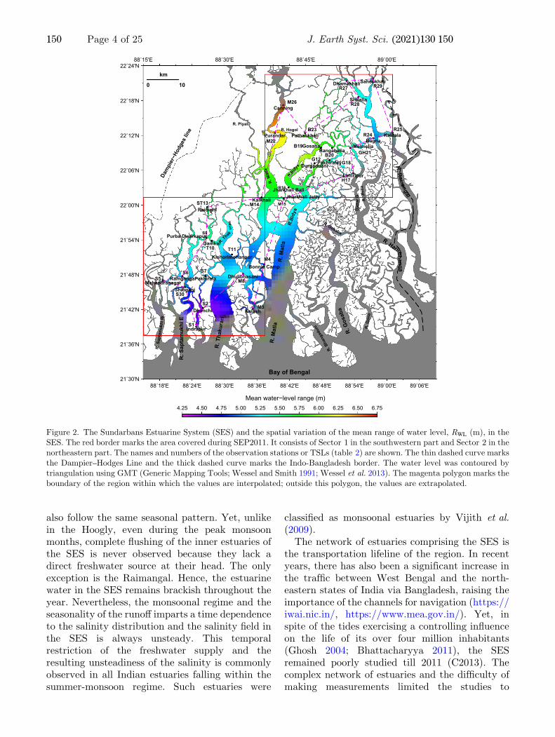
Figure 2. The Sundarbans Estuarine System (SES) and the spatial variation of the mean range of water level, RWL (m), in theSES. The red border marks the area covered during SEP2011. It consists of Sector 1 in the southwestern part and Sector 2 in thenortheastern part. The names and numbers of the observation stations or TSLs (table 2) are shown. The thin dashed curve marksthe Dampier–Hodges Line and the thick dashed curve marks the Indo-Bangladesh border. The water level was contoured bytriangulation using GMT (Generic Mapping Tools; Wessel and Smith 1991; Wessel et al. 2013). The magenta polygon marks theboundary of the region within which the values are interpolated; outside this polygon, the values are extrapolated.


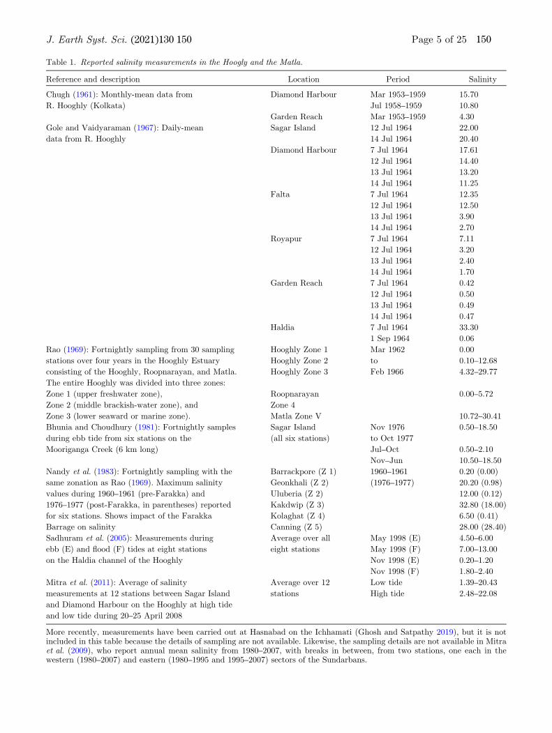
Table 1. Reported salinity measurements in the Hoogly and the Matla.

Reference and description Location Period Salinity

Chugh (1961): Monthly-mean data from Diamond Harbour Mar 1953–1959 15.70

R. Hooghly (Kolkata) Jul 1958–1959 10.80

Garden Reach Mar 1953–1959 4.30

Gole and Vaidyaraman (1967): Daily-mean Sagar Island 12 Jul 1964 22.00

data from R. Hooghly 14 Jul 1964 20.40

Diamond Harbour 7 Jul 1964 17.61

12 Jul 1964 14.40

13 Jul 1964 13.20

14 Jul 1964 11.25

Falta 7 Jul 1964 12.35

12 Jul 1964 12.50

13 Jul 1964 3.90

14 Jul 1964 2.70

Royapur 7 Jul 1964 7.11

12 Jul 1964 3.20

13 Jul 1964 2.40

14 Jul 1964 1.70

Garden Reach 7 Jul 1964 0.42

12 Jul 1964 0.50

13 Jul 1964 0.49

14 Jul 1964 0.47

Haldia 7 Jul 1964 33.30

1 Sep 1964 0.06

Rao (1969): Fortnightly sampling from 30 sampling Hooghly Zone 1 Mar 1962 0.00

stations over four years in the Hooghly Estuary Hooghly Zone 2 to 0.10–12.68

consisting of the Hooghly, Roopnarayan, and Matla. Hooghly Zone 3 Feb 1966 4.32–29.77

The entire Hooghly was divided into three zones:

Zone 1 (upper freshwater zone), Roopnarayan 0.00–5.72

Zone 2 (middle brackish-water zone), and Zone 4

Zone 3 (lower seaward or marine zone). Matla Zone V 10.72–30.41

Bhunia and Choudhury (1981): Fortnightly samples Sagar Island Nov 1976 0.50–18.50

during ebb tide from six stations on the (all six stations) to Oct 1977

Mooriganga Creek (6 km long) Jul–Oct 0.50–2.10

Nov–Jun 10.50–18.50

Nandy et al. (1983): Fortnightly sampling with the Barrackpore (Z 1) 1960–1961 0.20 (0.00)

same zonation as Rao (1969). Maximum salinity Geonkhali (Z 2) (1976–1977) 20.20 (0.98)

values during 1960–1961 (pre-Farakka) and Uluberia (Z 2) 12.00 (0.12)

1976–1977 (post-Farakka, in parentheses) reported Kakdwip (Z 3) 32.80 (18.00)

for six stations. Shows impact of the Farakka Kolaghat (Z 4) 6.50 (0.41)

Barrage on salinity Canning (Z 5) 28.00 (28.40)

Sadhuram et al. (2005): Measurements during Average over all May 1998 (E) 4.50–6.00

ebb (E) and Cood (F) tides at eight stations eight stations May 1998 (F) 7.00–13.00

on the Haldia channel of the Hooghly Nov 1998 (E) 0.20–1.20

Nov 1998 (F) 1.80–2.40

Mitra et al. (2011): Average of salinity Average over 12 Low tide 1.39–20.43

measurements at 12 stations between Sagar Island stations High tide 2.48–22.08

and Diamond Harbour on the Hooghly at high tide

and low tide during 20–25 April 2008

More recently, measurements have been carried out at Hasnabad on the Ichhamati (Ghosh and Satpathy 2019), but it is notincluded in this table because the details of sampling are not available. Likewise, the sampling details are not available in Mitraet al. (2009), who report annual mean salinity from 1980–2007, with breaks in between, from two stations, one each in thewestern (1980–2007) and eastern (1980–1995 and 1995–2007) sectors of the Sundarbans.


sporadic observations that were largely restrictedto the Hoogly (hydrodynamical, morphological,chemical, and biological observations) and a fewsporadic observations, mostly biological andchemical, conducted in the Matla and the Sapta-mukhi. As noted by C2013, even water-level mea-surements in the SES were restricted to the vicinityof jetties. Salinity measurements were even morelimited and sporadic (see table 1 for a summary)than water-level measurements (C2013) in spite ofits obvious implications: the Dampier–Hodges line,which marks the northern limit of the SES(Bgure 2), is based on salinity.The Brst comprehensive measurements in the

SES were carried out under the Sundarbans Estu-arine Programme in March 2011 (C2013); here-after, this set of measurements is referred to asSEP2011. The water-level measurements fromSEP2011 were reported by C2013, but the pro-gramme also included measurements of salinity.Though earlier studies had suggested that salinitydecreases during the summer monsoon andincreases during the dry season (table 1), thechanges over a tidal cycle and in space were map-ped for the Brst time during SEP2011. A briefdescription of SEP2011 is deferred to section 2, butwe note here the importance of salinity measure-ments in the SES.First, salinity data are required for the man-

agement and adequate distribution of ‘sweet’ orpotable water for domestic and agricultural use.

Nearly 3155 km2 (� 59%) of the northern settle-ments have been cleared for cultivation (Depart-ment of Sundarban Affairs, Government of WestBengal; https://www.sundarbanaffairswb.in/).The main crop grown consists of three varieties ofrice in three cropping seasons: Aman, cultivatedduring the summer monsoon (Kharif), is com-pletely rainfed; Aus, cultivated soon after thesummer monsoon withdraws, and Boro, cultivatedduring the winter (Rabi), depend heavily on irri-gation. All three are freshwater varieties of rice,have some salinity tolerance (2 psu), but perishcompletely when salinities increase to 7 psu (Deb-nath 2014). Water for irrigation, drinking andother domestic use is obtained mostly throughfreshwater (rainwater harvested) or from brackishwater ponds present in every agricultural Beld orthrough river lift irrigation. Freshwater is alsoextracted through medium- and high-capacitydeep-water tube wells that tap water from fresh-water aquifers situated more than 300 m below

ground level (Water Investigation and Develop-ment Department, Government of West BengalEconomic Review 2011–2012; https://bengalchamber.com/economics/west-bengal-statistics-2011-2012.pdf), but this method cannot work in thesouthern, seaward part of the delta. While salinewater ingress occurs periodically owing to the veryhigh tidal water levels and also remotely generatedswell waves, a greater threat is posed by extremeweather events like depressions and cyclones andthe surges due to these events (Das 1972; Murtyet al. 1986; Mohapatra et al. 2012; Dube 2012).Second, salinity matters for the Bshery of the

Sundarbans, which also serve as the spawninggrounds for the Bsh. The important species includeshrimps, prawns, crabs, and the Hilsa (Hilsa ilisha).The salinity and water temperature tolerance is spe-cies-speciBc. The Bsh normally inhabit the seawardregime of the estuaries and the foreshore areas of thesea andmigrate upstream for spawning (Kuttyamma1982; Chanda et al. 2015). The Hilsa, perhaps themostpopularBsh inWestBengalandBangladesh (De1986), prefers the Sundarbans owing to the presenceof sub-surface oxygen, relatively low salinity, strongtidal action, high turbidity, heavy siltation, and richgrowth of plankton (Pillay and Rosa 1963). It toomigrates upstream for spawning (Hora 1938; Pillay1958; De 1986). Though the Hilsa is very tolerant ofchanges in salinity (Bhaumik and Sharma 2011), itsyield has declined in recent years, necessitating ananalysis of the causes.Third, though the exact number of the mangrove

species is still debated and reported variously as 69(Gopal and Chauhan 2006; Mandal and Naskar2008) to 84 (Raha et al. 2013; Barik and Chowdhury2014; Ghosh et al. 2015), the mangroves in theIndian Sundarbans are known to harbour the richestspecies diversity. Their natural forest resourcesprovide the means of livelihood for the majority ofthe inhabitants of the region. All mangrove plants inthe SES have medicinal value, which is well-knownlocally, but is yet to receive serious scientiBcattention (Bandaranayake 1998; Pattanaik et al.2008; Sarkar 2011). The mangroves of the Sundar-bans also act as a buAer that absorbs and mitigatesthe eAect of the storms, providing protection to thedensely populated city, Kolkata, to the north(Bgure 1). In addition, the mangroves are the big-gest sink of carbon in the region and function as anatural Blter for pollutants, including heavy metalsreleased in its industrialised northern reaches (Maitiand Chowdhury 2013). Mangroves dominate the


Sundarbans because the conditions required fortheir proliferation are fulBlled there, but an increasein salinity can lead to either changes in species ordrive some to extinction. The most striking exampleis the once proliBc Sundari tree (Heritiera fomes),from which the Sundarbans got its name. TheSundari grows fastest in low-salinity (0–5 psu)water, and is usually found in the northern (head-ward) stretches of the SES estuaries. Thoughhuman exploitation has contributed to its decline, agradual increase in salinity, driven by natural geo-logical changes over the last few centuries, in thewestern part of the SES has led to the gradual dis-appearance of the Sundari from these parts. At

present, the Sundari is an endangered species and isfound only eastward of the Matla (Kathiresan et al.2010), where salinities are lower, and are relativelymore abundant in the easternmost parts of theBangladesh Sundarbans (Das 2012).Therefore, a good understanding of the spatio-

temporal variations of salinity in the SES overshort (daily, sub-tidal) and long (seasonal, annual)time scales is essential for gaining insight into andresolving several issues that have become criticalfor this region. The focus of this paper is on thechanges seen over a tidal cycle. The rest of thispaper is organised as follows. In section 2, we pre-sent a brief description of SEP2011. The salinity

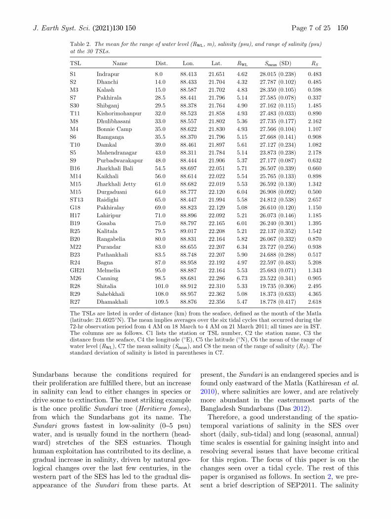
Table 2. The mean for the range of water level (RWL, m), salinity (psu), and range of salinity (psu)at the 30 TSLs.

TSL Name Dist. Lon. Lat. RWL Smean (SD) RS

S1 Indrapur 8.0 88.413 21.651 4.62 28.015 (0.238) 0.483

S2 Dhanchi 14.0 88.433 21.704 4.32 27.787 (0.102) 0.485

M3 Kalash 15.0 88.587 21.702 4.83 28.350 (0.105) 0.598

S7 Pakhirala 28.5 88.441 21.796 5.14 27.585 (0.078) 0.337

S30 Shibganj 29.5 88.378 21.764 4.90 27.162 (0.115) 1.485

T11 Kishorimohanpur 32.0 88.523 21.858 4.93 27.483 (0.033) 0.890

M8 Dhulibhasani 33.0 88.557 21.802 5.36 27.735 (0.177) 2.162

M4 Bonnie Camp 35.0 88.622 21.830 4.93 27.566 (0.104) 1.107

S6 Ramganga 35.5 88.370 21.796 5.15 27.668 (0.141) 0.908

T10 Damkal 39.0 88.461 21.897 5.61 27.127 (0.234) 1.082

S5 Mahendranagar 43.0 88.311 21.784 5.14 23.873 (0.238) 2.178

S9 Purbadwarakapur 48.0 88.444 21.906 5.37 27.177 (0.087) 0.632

B16 Jharkhali Bali 54.5 88.697 22.051 5.71 26.507 (0.339) 0.660

M14 Kaikhali 56.0 88.614 22.022 5.54 25.765 (0.133) 0.898

M15 Jharkhali Jetty 61.0 88.682 22.019 5.53 26.592 (0.130) 1.342

M15 Durgaduani 64.0 88.777 22.120 6.04 26.908 (0.092) 0.500

ST13 Raidighi 65.0 88.447 21.994 5.58 24.812 (0.538) 2.657

G18 Pakhiralay 69.0 88.823 22.129 5.08 26.610 (0.120) 1.150

H17 Lahiripur 71.0 88.896 22.092 5.21 26.073 (0.146) 1.185

B19 Gosaba 75.0 88.797 22.165 6.01 26.240 (0.301) 1.395

R25 Kalitala 79.5 89.017 22.208 5.21 22.137 (0.352) 1.542

B20 Rangabelia 80.0 88.831 22.164 5.82 26.067 (0.332) 0.870

M22 Purandar 83.0 88.655 22.207 6.34 23.727 (0.256) 0.938

B23 Pathankhali 83.5 88.748 22.207 5.90 24.688 (0.288) 0.517

R24 Bagna 87.0 88.958 22.192 4.97 22.597 (0.483) 5.208

GH21 Melmelia 95.0 88.887 22.164 5.53 25.683 (0.071) 1.343

M26 Canning 98.5 88.681 22.286 6.73 23.522 (0.341) 0.905

R28 Shitalia 101.0 88.912 22.310 5.33 19.735 (0.306) 2.495

R29 Sahebkhali 108.0 88.957 22.362 5.08 18.373 (0.633) 4.365

R27 Dhamakhali 109.5 88.876 22.356 5.47 18.778 (0.417) 2.618

The TSLs are listed in order of distance (km) from the seaface, deBned as the mouth of the Matla(latitude: 21.6025�N). The mean implies averages over the six tidal cycles that occurred during the72-hr observation period from 4 AM on 18 March to 4 AM on 21 March 2011; all times are in IST.The columns are as follows. C1 lists the station or TSL number, C2 the station name, C3 thedistance from the seaface, C4 the longitude (�E), C5 the latitude (�N), C6 the mean of the range ofwater level (RWL), C7 the mean salinity (Smean), and C8 the mean of the range of salinity (RS). Thestandard deviation of salinity is listed in parentheses in C7.


variation during SEP2011 is described in section 3and the results are discussed in section 4.

2. The Sundar bans Estuarine Programme2011 (SEP2011)

This section begins with a brief description ofSEP2011 and the astronomical and weather con-ditions during the observations. This backgroundinformation is followed by a description of theobservational and analytical methods. The sectionends with a summary of the results of C2013, whodescribed the water-level measurements.

2.1 SEP2011 overview

SEP2011, conducted during 18–21 March 2011, wasa systematically planned observational programmeaimed at mapping the nature and characteristics oftidal propagation and spatio-temporal variation of

surface salinity in the SES, an area of � 9600 km2

lying between 88.25–89.50�E and 21.25–22.50�N. Acomprehensive description is provided in C2013 and

we provide but a brief overview in this paper. C2013divided the SES region into two sectors: Sector 1(88.250–88.625�E, 21.625–22.022�N), covering

� 1814 km2, was located in the southwestern por-tion of the SES, with the Bay of Bengal as itssouthern boundary, and Sector 2 (88.625–89.017�E,

22.022–22.375�N), covering � 1800 km2, was loca-ted in thenorthwesternportion of the SES (Bgure 2).The observations consisted of simultaneous and

continuous measurements of water level, surfacetemperature, air temperature, and surface salinityfor 72 hrs at 30 selected time-series locations(called TSLs hereafter). These TSLs, spread over

� 3600 km2 of the SES and therefore representing� 40% of its total area, provide a comprehensivecoverage of the region and the data obtained rep-resent a wide range of estuarine and environmentalconditions. The choice of the TSLs was dictated bylogistic considerations such as existence of settle-ments and jetties, which, in turn, were mostlylocated at or near channel conCuences. This con-straint and the proliBc existence of channel con-Cuences, a consequence of the high channel density,led to many of the TSLs being located at or near

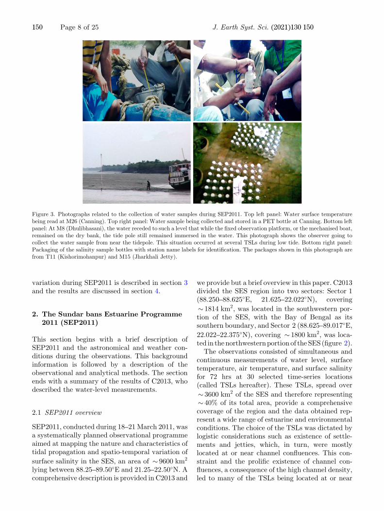
Figure 3. Photographs related to the collection of water samples during SEP2011. Top left panel: Water surface temperaturebeing read at M26 (Canning). Top right panel: Water sample being collected and stored in a PET bottle at Canning. Bottom leftpanel: At M8 (Dhulibhasani), the water receded to such a level that while the Bxed observation platform, or the mechanised boat,remained on the dry bank, the tide pole still remained immersed in the water. This photograph shows the observer going tocollect the water sample from near the tidepole. This situation occurred at several TSLs during low tide. Bottom right panel:Packaging of the salinity sample bottles with station name labels for identiBcation. The packages shown in this photograph arefrom T11 (Kishorimohanpur) and M15 (Jharkhali Jetty).


channel conCuences. Fourteen of the TSLs lay inSector 1: eight on the Saptamukhi System, two onthe Thakuran and four are on the southern stretchof the Matla, extending downstream of M14 (Kai-khali) up to its mouth. The remaining 16 TSLswere located in Sector 2: three on the northernstretch of the Matla, four on the Bidya, two eachon the Gomdi and Harinbhanga, and Bve on the

Raimangal. Since the mouth of the Matla is thesouthernmost, its latitude, 21:603�N, has beentaken to represent the seaface. All distances northof the seaface are measured along the respectivechannels from this latitude (table 2). FollowingC2013, the Brst letter of the name of the estuary onwhich it is situated has been preBxed to the TSLnumber, implying a two-letter preBx for TSLs

0

2

4

6

8

0 12 24 36 48 60 72Hours since 00 hrs 18 March 2011

BidyaIndrapur (S1)Jharkhali Bali (B16)Gosaba (B19)

Rangabelia (B20)Pathankhali (B23)

18 March 19 March 20 March

0

2

4

6

8

0 12 24 36 48 60 72

Indrapur (S1)Kalash (M3)Dhulibhasani (M8)

Bonnie (M4)Jharkhali (M15)

Kaikhali (M14)Purandar (M22)

Canning (M26)Matla

0

2

4

6

8

Wat

er le

vel (

m)

0 12 24 36 48 60 72

ThakuranIndrapur (S1)Kishorimohanpur (T11)

Damkal (T10)Raidighi (ST13)

0

2

4

6

8

0 12 24 36 48 60 72

SaptamukhiIndrapur (S1)Dhanchi (S2)Shibganj (S30)

Mahendranagar (S5)Ramganga (S6)Pakhirala (S7)

Purbadwarakapur (S9)Raidighi (ST13)

0

2

4

6

8

0 12 24 36 48 60 72

GomdiIndrapur (S1)Pakhirala (S7)

Durgaduani (G12)Melmelia (GH21)

0

2

4

6

8

0 12 24 36 48 60 72

HarinbhangaIndrapur (S1)Lahiripur (H17)Melmelia (GH21)

0

2

4

6

8

0 12 24 36 48 60 72Hours since 00 hrs 18 March 2011

RaimangalIndrapur (S1)Bagna (R24)Kalitala (R25)

Shitalia (R28)Dhamakhali (R27)Sahebkhali (R29)

18 March 19 March 20 March

Distance from the mouth

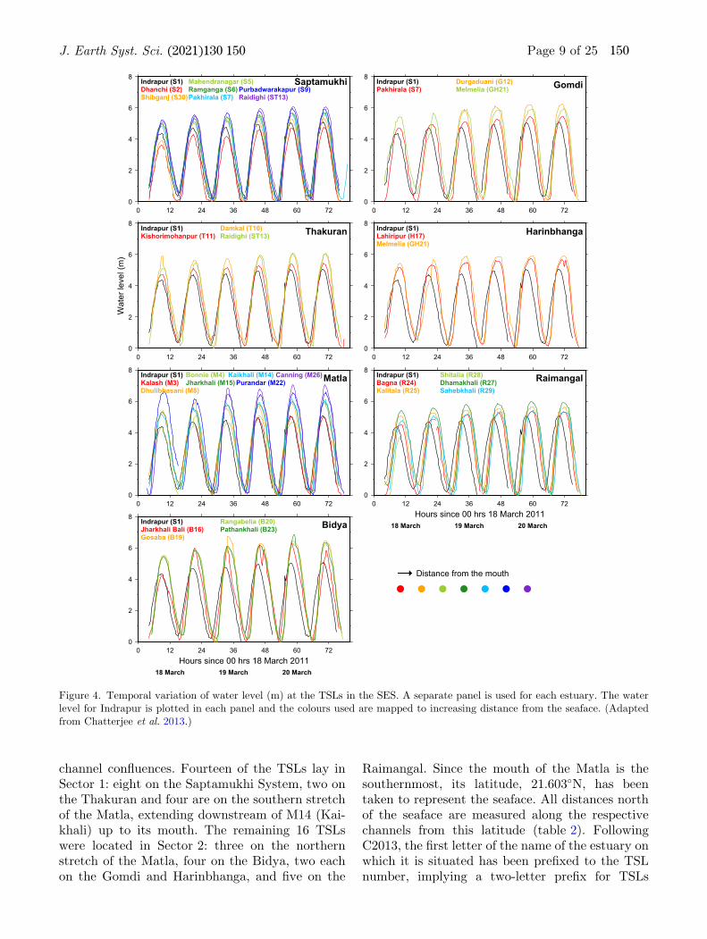
Figure 4. Temporal variation of water level (m) at the TSLs in the SES. A separate panel is used for each estuary. The waterlevel for Indrapur is plotted in each panel and the colours used are mapped to increasing distance from the seaface. (Adaptedfrom Chatterjee et al. 2013.)


located at the conCuence of two estuaries. Forexample, ST13 (Raidighi) is at the conCuence ofthe Saptamukhi (S) and the Thakuran (T) andGH21 (Melmelia) is at the conCuence of the Gomdi(G) and Harinbhanga (H).For convenience, in spite of the lack of a riverine

source of freshwater at the head of six of the sevenestuaries constituting the SES, we use the con-ventional term ‘upstream’ (‘downstream’) to referto movement along the channel away from(towards) the mouth.

2.2 Astronomical and weather conditionsduring SEP2011

The spatio-temporal variations of surface salinityin all estuaries is known to be a result of theinteractions between several oceanographic andmeteorological processes: the tides, freshwaterinCow, residual estuarine circulation (gravitationalcirculation), bathymetry and the geometry of thechannels, wind, precipitation, and solar radiation(Lewis and Uncles 2003; Eaton 2007). It is rea-sonable to assume that the surface salinity in theSES will be determined by the same set of pro-cesses. Though we refrain from analysing the pro-cesses in this paper, a description of theastronomical and meteorological conditions is anecessary component of the background.The SEP observations were conducted during

the Full-Moon phase of the Equinoctial Spring,with the Full Moon (termed popularly as the SuperMoon) occurring at 11 PM (Indian Standard Timeor IST, which is UTC +0530) on 19 March.18 March 2011 was unique in the sense that thiswas the day of maximum tidal forcing, with thesemi-diurnal tidal amplitudes at 1.88 times that ofthe equilibrium tide (Pugh 1987). The reason forthis higher high tide was the near coincidence ofthe times of occurrences of zero solar declinationand lunar perigee. Such an astronomical event hadoccurred earlier in 1980, 1993, 1997, 1998 and 2002,and the next occurrence after 2011 will be in 2028(Pugh 1987).The most notable meteorological feature during

the 72-hr period, which started at 4 AM on18 March and ended at 4 AM on 21 March 2011,was the extremely strong and steady southerly-southwesterly wind that blew throughout thisperiod. A qualitative idea of the wind speed at10 m is obtained from the METAR (METeorolog-ical Aerodrome Reports) records (at 30-min

intervals) from the Netaji Subhash InternationalAirport at Dumdum, Kolkata, � 150 km northwestof Nandakumarpur and Gadkhali (Bgure 1). AtDumdum, the wind speed at 10 m varied between

5–7.5 ms�1 and the sea-level pressure lay between1004–1005 hPa. This strong, southerly wind,directed along the north–south orientation of themain estuarine channels, is a usual feature inMarch. Since SEP2011 was conducted during thepeak of the ‘dry season’, there was no rainfallbefore or during 18–21 March 2011. Fair weatherexisted all over the SES, with occasional cloudinessin the late afternoons.

2.3 Observational and analytical methods

2.3.1 Water level

As described by C2013, water level was measuredevery 15 min using tide poles (C2013). At eachTSL, mechanised boats, anchored Brmly next tothe tide poles, were used as observation platformsfrom which the reading on the tide poles could betaken even during the night. The position of theseboats and the tide poles remained Bxed throughoutthe 72 hrs of observation. Each boat had on boarda teams consisting of six observers and a supervi-sor; several boats also had a scientist on boardthroughout the observation period. All observersand supervisors consisted of local people recruitedthrough three local non-governmental organisa-tions: Sabuj Sangha (SS) in Sector1 and the Cal-cutta Wildlife Society (CWS) and the TagoreSociety for Rural Development (TSRD) in Sec-tor 2. All observation teams were trained throughseveral training sessions organised before SEP2011at the SS and TSRD head quarters at Nandaku-marpur and Rangabelia (Bgure 2), respectively.In addition, there were three supervision teams,

which were expected to ensure that at least one ofthem visited each TSL daily to check the obser-vations and ensure the general well-being of theobservation teams. While a visit to most of thestations was possible on at least one of the threedays, it proved impossible to reach M3 (Kalash),the southernmost and most remote of the TSLs.All together, six tidal cycles – from low water

(LW) to high water (HW) to LW – occurred duringthe period of observation; the 72-hr period startedaround low tide on 18 March. Logistic problems,however, delayed the start at M3 (Kalash) and G12(Durgaduani), and the observations at M4 (Bonnie


Camp) had to be abandoned after the Bfth tidalcycle because the tide pole broke and could not berepaired. The few data gaps that existed in thetime series of the water levels were Blled followingthe harmonic analysis of the data. The harmonicanalysis was carried out using Tidal AnalysisSoftware Kit (TASK-2000) software (Bell et al.1998). Since the measurements were restricted tojust 72 hrs, we determined only eight constituent

bands (following Shetye et al. 1995). We assumedthe period of the semi-diurnal and diurnal bands tobe 12.42 hrs (M2) and 23.92 hrs (K1), respectively.The frequencies of the eight constituent bands areavailable in table 7 of C2013.The mean tide level was computed as the

arithmetic mean of the hourly water levelsextracted from the 15-min time series. The meantidal ranges, however, are as reported in C2013,

10

20

30

40

50

60

70

80

90

100

110

Dis

tanc

e no

rth o

f sea

face

(km

)

4.0 4.5 5.0 5.5 6.0 6.5 7.0Range of water level (m)

S1

S30

S6

S5

S9

ST13 ST13

T10

M3

M8

M14

M15

M26

B16

B19

B20

B23

G18

GH21

H17

GH21

R24

R28

R29R27

S2

S7

T11

M4

M22

G12

R25

a

18 20 22 24 26 28 30Mean salinity (psu)

b

0 1 2 3 4 5 6Range of salinity (psu)

Indrapur

Shibganj

Ramganga

Mahendranagar

Purbadwarakapur

Raidighi Raidighi

Damkal

Kalash

Dhulibhasani

Kaikhali

JharkhaliJetty

Canning

JharkhaliBali

Gosaba

Rangabelia

Pathankhali

Pakhiralay

Melmelia

Lahiripur

Melmelia

Bagna

Shitalia

SahebkhaliDhamakhali

Dhanchi

Pakhirala

Kishorimohanpur

BonnieCamp

Purandar

Durgaduani

Kalitala

c

Saptamukhi Thakuran Matla Bidya Gomdi Harinbhanga Raimangal

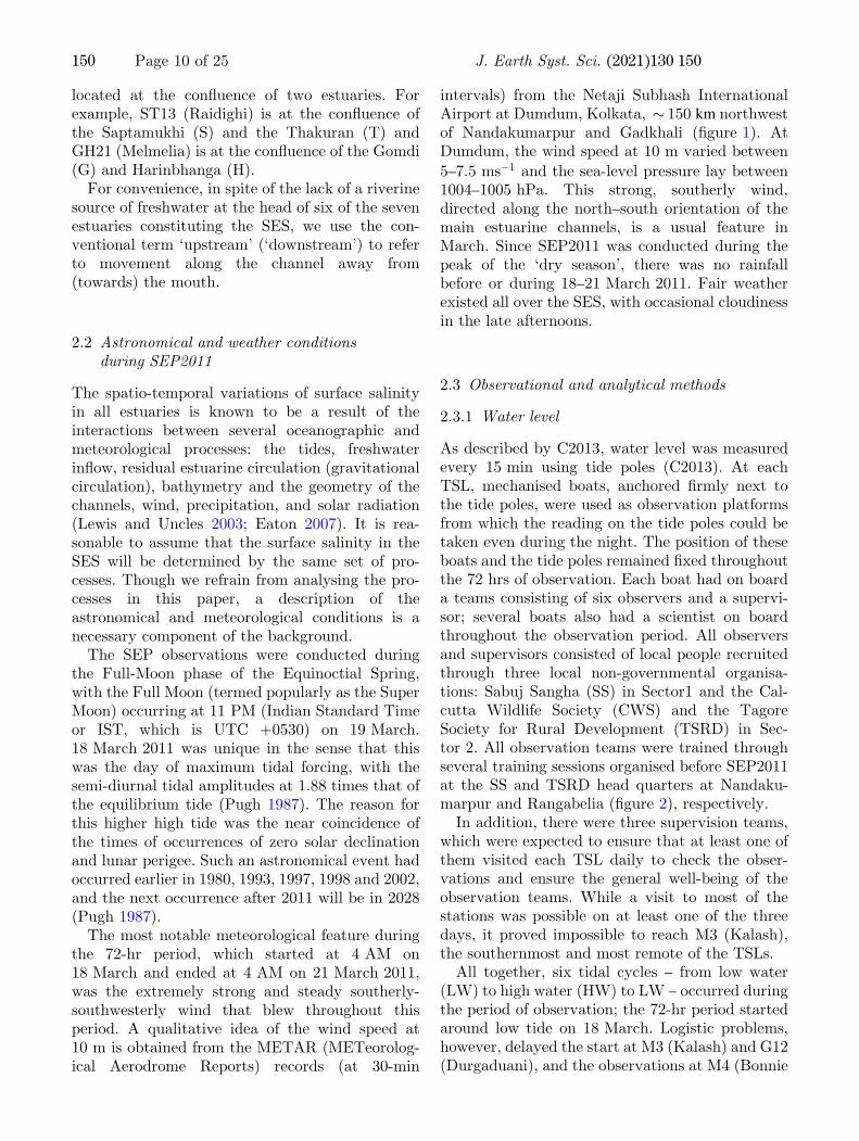
Figure 5. Along-channel variation of (a) the range of water level, RWL (m), (b) the mean salinity, Smean (psu), over the six tidalcycles, and (c) the mean of the salinity range, RS (psu), averaged over the six tidal cycles. The ordinate is the distance (km) fromthe seaface, which is taken to be the mouth of the Matla (21.603�N); the station number (name) is labelled on the left (right).Fitting a line to the three curves yields the following relations: y ¼ 0:0099x þ 4:7842 with r ¼ 0:57 for RWL, y ¼ �0:0763x þ29:9900 with r ¼ 0:81 for Smean, and y ¼ 0:0190x þ 0:2918 with r ¼ 0:49 for RS .


and were computed from the 15-min time seriesas the difference between HW level (HWL) andLW level (LWL) during a tidal cycle. Thus, therange for each tidal cycle, RWL, has been calcu-lated as the difference in the maximum andminimum values attained in that cycle, and themean range is the arithmetic mean of the sixvalues.

2.3.2 Salinity

Water samples were collected every hour for sub-sequent analysis to estimate the surface salinity.The temperature was read from the bucket(Bgure 3a) and the samples were collected in200 ml PET (Polyethylene terephthalate) bottles(Bgure 3b) with an inner lid and cap that were

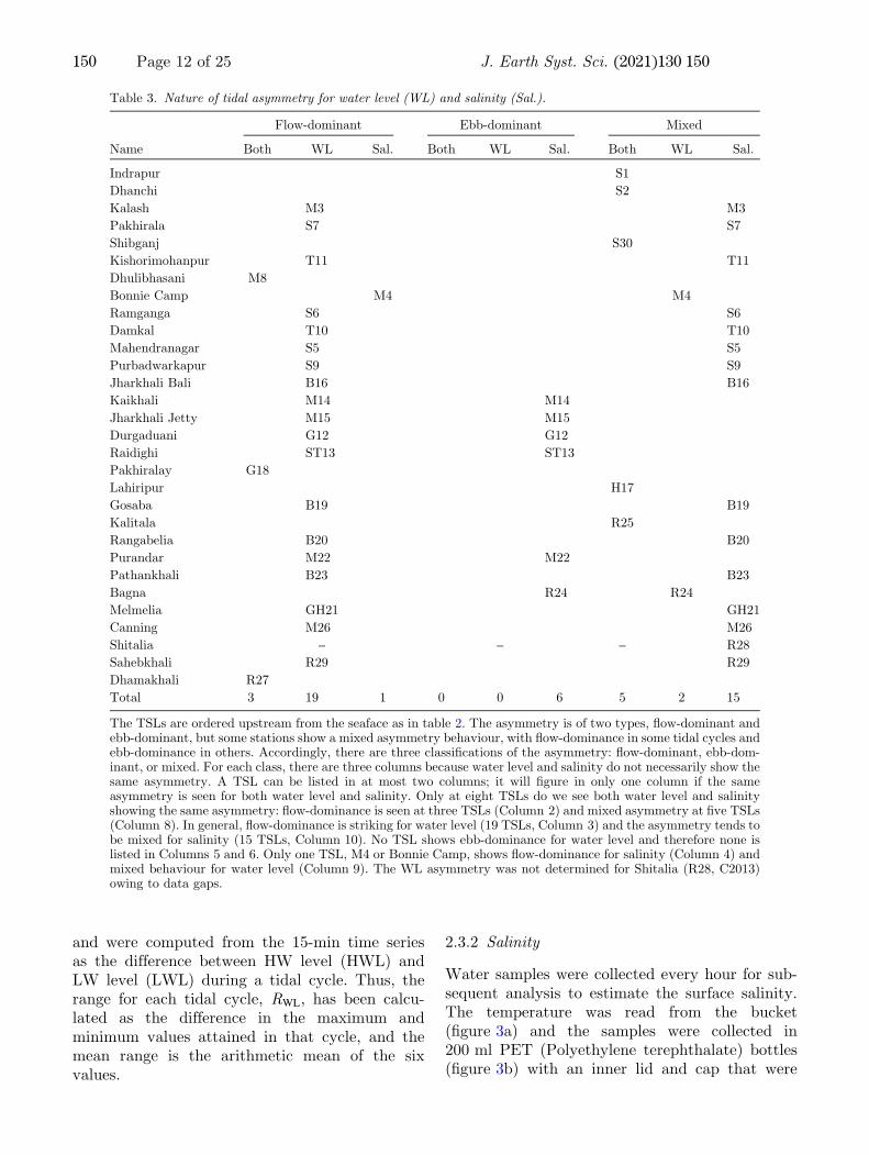
Table 3. Nature of tidal asymmetry for water level (WL) and salinity (Sal.).

Name

Flow-dominant Ebb-dominant Mixed

Both WL Sal. Both WL Sal. Both WL Sal.

Indrapur S1

Dhanchi S2

Kalash M3 M3

Pakhirala S7 S7

Shibganj S30

Kishorimohanpur T11 T11

Dhulibhasani M8

Bonnie Camp M4 M4

Ramganga S6 S6

Damkal T10 T10

Mahendranagar S5 S5

Purbadwarkapur S9 S9

Jharkhali Bali B16 B16

Kaikhali M14 M14

Jharkhali Jetty M15 M15

Durgaduani G12 G12

Raidighi ST13 ST13

Pakhiralay G18

Lahiripur H17

Gosaba B19 B19

Kalitala R25

Rangabelia B20 B20

Purandar M22 M22

Pathankhali B23 B23

Bagna R24 R24

Melmelia GH21 GH21

Canning M26 M26

Shitalia – – – R28

Sahebkhali R29 R29

Dhamakhali R27

Total 3 19 1 0 0 6 5 2 15

The TSLs are ordered upstream from the seaface as in table 2. The asymmetry is of two types, Cow-dominant andebb-dominant, but some stations show a mixed asymmetry behaviour, with Cow-dominance in some tidal cycles andebb-dominance in others. Accordingly, there are three classiBcations of the asymmetry: Cow-dominant, ebb-dom-inant, or mixed. For each class, there are three columns because water level and salinity do not necessarily show thesame asymmetry. A TSL can be listed in at most two columns; it will Bgure in only one column if the sameasymmetry is seen for both water level and salinity. Only at eight TSLs do we see both water level and salinityshowing the same asymmetry: Cow-dominance is seen at three TSLs (Column 2) and mixed asymmetry at Bve TSLs(Column 8). In general, Cow-dominance is striking for water level (19 TSLs, Column 3) and the asymmetry tends tobe mixed for salinity (15 TSLs, Column 10). No TSL shows ebb-dominance for water level and therefore none islisted in Columns 5 and 6. Only one TSL, M4 or Bonnie Camp, shows Cow-dominance for salinity (Column 4) andmixed behaviour for water level (Column 9). The WL asymmetry was not determined for Shitalia (R28, C2013)owing to data gaps.


pre-labelled with the station name, sample num-ber, and date. To avoid contamination of thesamples by unwanted sediment and the Cotsamwashed up at the edge of the bank, each team wasinstructed to collect the water sample a little awayfrom the bank. This distance implied the need toget down from the boat, which led to difBcultiesduring low tide, when a significant part of theislands tends to become exposed (Bgure 3c), andalso at night. At S2 (Dhanchi), for example, thesamples were collected by the team even at night inspite of the danger posed by crocodiles. In total,2190 water samples were collected.The method of sample collection generally fol-

lowed Shetye et al. (1995), but the Sundarbansposed problems that demanded additional steps foreach observation. The new bucket supplied for thepurpose was at Brst thoroughly rinsed at least thricewith the estuarine water. The PET bottle, lid, andcap were rinsed with the water in the bucket at leastthree times. The water sample was then poured intothe bottle through a Bne muslin cloth to Blter outsediment and other particulates. To prevent evap-oration and crystallisation of dissolved salts, thebottle was then Blled up to the neck and the inner lidand inner sides of the neck were wiped clean withtissue paper. Care was taken to avoid contact withthe bottled water or hands. Once the inner lid was inplace, the inner side of the cap was dried similarlyand the bottle was capped. The outer surface of thecapped bottle was then wiped dry, and, as a pre-caution against leakages during subsequent trans-portation to the laboratory, the cap was sealed bywinding cellotape around it (Bgure 3d).In addition to the water samples, salinity data

were collected at three stations on the Matla usinga portable SeaBird CTD (conductivity–tempera-ture–depth) of make SBE19plus; moving upstreamfrom the seaface, these stations were Kalash, Kai-khali, and Purandar (Bgure 2). The CTD wasdeployed at all three stations from a separate boatthat moved to roughly the middle of the Matlachannel at each station to ensure sufBcient depth ofwater for the deployment. At Kalash, logisticalproblems precluded deployment of the CTD on the18 March, the Brst day; hence, the CTD data areavailable for only two days at this station.

2.3.3 Analysis of water samples

The water samples were analysed using an autosal(Make Guildline 8400B) at CSIR-NIO, Goa and

the regional centre of CSIR-NIO at Visakhapat-nam. In spite of the Bltering with the muslin cloth,several samples, particularly those collected duringlow tide (see, for example, Bgure 3c), were turbid.All samples were allowed to settle for over 12 hrsbefore the autosal analysis.Mean salinities were computed as time averages

over each tidal cycle using the trapezoidal rule.The mean salinities and the mean values of RWL arelisted in table 2.

2.4 Variation of water level in the SESduring SEP2011

In this subsection, we summarise the results of C2013.The water-level data and their harmonic analysisshowed a dominant semi-diurnal tide (Bgure 4). Thethree-day time series is not sufBcient to separate thetwo dominant semi-diurnal constituents, M2 and S2,but the dominance of theM2 tide in the northern Bayof Bengal (Sindhu and Unnikrishnan 2013) impliesthat the semi-diurnal oscillation observed in the waterlevel in the SES is due to this constituent. In general,the tidal range,RWL, increasedupstreamwithdistancefrom the mouth (Bgures 2, 5a). The minimum HWL,3.61 m,was observed at S2 (Dhanchi) on the SEGandthe maximum HWL, 7.08 m, was observed at M26(Canning), � 98 km from the seaface (Bgure 2). RWL

varied between a minimum of 4.32 m at S2 and amaximum of 6.73 m at M26 (table 2). The upstreamampliBcation of the tide along the main north–south-oriented channels, all of which are funnel-shaped,convergent channels, can be attributed to the domi-nance of the channel geometry over frictional dissipa-tion (Friedrichs and Aubrey 1994; Shetye et al. 1995).A different pattern of tidal ampliBcation existed in thetwo parallel channels, the Bidya and the Gomdi (Go-mor). TheBidya is a long, highlymeandering channel,while the Gomdi is the narrowest and shortest of thechannels surveyed. Tidal amplitudes increased anddecreased without any Bxed pattern over the varioustidal cycles at each of the observation locations situ-ated in these two estuaries. The complexity of theestuarine network also led to complex patterns of theobserved rates of tidal ampliBcation and decay invarious estuarine stretches.Harmonic analysis of the observed tidal water-

level data from the SES revealed that the M2 con-stituent was dominant. For the majority of the 30locations, the next two bands were the 6-hourly M4

and 4-hourly M6 bands. Upstream ampliBcation inthese bandswas stronger (factor of 4–5) compared to


the ampliBcation of theM2 band (factor of � 2). Asnoted by C2013, the generation of these two higherharmonic bands suggests the existence of non-lineareAects that are a consequence of the interaction ofthe semi-diurnal tide with the channel geometry: forexample, the interaction of the semi-diurnal tidewith the bottom of the channel (nonlinear friction),can generate theM4 andM6 bands, which amplify asthe tide progresses headward (see, for example,Pingree and GrifBths 1979; Speer and Aubrey 1985;Speer et al. 1991; Song et al. 2011). This superposi-tion of the M4 and M6 bands on the M2 band led toasymmetries of the tide, of which two types wereevident in the data.The Brst asymmetry is the better-known tidal-

duration asymmetry (Pugh 1987), which is of twotypes, Cow-dominant and ebb-dominant. For waterlevel, the asymmetry was of the Cow-dominanttype in the SES, but at some locations and duringsome tidal cycles, existence of ebb-dominance andthe vanishing of the tidal-duration asymmetrywere also observed (C2013, table 3).The second typeof tidal asymmetry is referred to as

the tidal stand or stand of the tide or a platform tideand is known to exist in otherparts of theworld (Pugh1987). Its identiBcation in the SES was, however, theBrst report of a tidal stand from an Indian estuary. Inthis type of asymmetry of the tide, water levels nearthe times of HW and LW change so slowly that thechange appears to be imperceptible, resulting in anapparent stationarity of the water level to theobserver. HW stands exceeding 30 min were seen at27 of the 30TSLs, the exceptions beingM3,M26, andB16, but longer stands with duration exceeding75 min, implying that the water level changedimperceptibly around the HWL for 105 min, wereseen in the northeastern TSLs on the Bidya, Gomdi,Harinbhanga, and Raimangal (Bgure 4).C2013 pointed out that the existence of the tidal

stand in the SES, which is prone to cyclones andstorm surges, would increase the duration overwhich high water levels are experienced during astorm surge. This increased duration has implica-tions for engineering constructions such as jetties,embankments, and bridges.

3. Variation of salinity in the SES

The spatial and temporal variation of surfacesalinity in the SES is described in this section,which ends with a brief description of the verticalstructure seen in the CTD data.

3.1 Spatial variation of mean surface salinity

The mean salinity, Smean, over the observationperiod varied spatially. We split this variation intotwo parts, along the channels, which are generallyoriented north–south (the exceptions are the Bidyaand Gomdi, which are oriented more north-east–southwest), and zonally (east–west) acrossthe SES.

3.1.1 Along-channel variation

The Smean values in the SES are expected to be highduring March, which marks the local peak of thedry season; there was also no precipitation beforeand during the observation period. The highestvalue of Smean, 28.015 psu, occurred at the south-ernmost TSL, S1 (Indrapur), which is located 8 kmnorth of the seaface (table 2). Though Smean washigher (28.35 psu) at M3 (Kalash), the duration ofmeasurement there was less than 72 hrs. Thissalinity is lower than, but comparable to, the meanclimatological salinity of � 31 psu in the northernBay of Bengal (Chatterjee et al. 2012). Therefore,though we do not have a measure of the salinity inMarch 2011 in the northern bay at the mouths ofthe SES estuaries, it is likely that even the maxi-mum salinity in the SES during the peak of the dryseason is lower than the salinity at the mouths,suggesting that the estuaries of the SES can beclassiBed as positive estuaries (Pugh 1987).Smean decreased upstream along the estuary, with

the minimum Smean, 18.373 psu, recorded at R29(Sahebkhali), which is located � 108 km from theseaface (table 2, Bgure 5b). Use of triangulationpermits a spatial view of the mean salinity Beld: theupstream decrease of Smean is clearly evident in thismap (Bgure 6). The difference of 9.642 psu betweenS1 and R29 implies a salinity gradient of

� 0:096 psu km�1. This gradient is merely indica-tive of the overall trend, however, because thenorthward decrease was not uniform (Bgure 5b,table 2): Smean decreased by just 4.493 psu from S1to M26 (Canning), which is located 98 km from theseaface, but the decrease from M26 to R29, whichis located 108 km from the seaface or just � 10 kmfarther from the seaface compared to M26, washigher (5.149 psu, Bgure 5b). The variation of Smean

with distance from the seaface was not smooth andshowed considerable Cuctuations, with pockets oflow Smean evident in all the estuaries: an example isS5 (Mahendranagar), which had a lower Smean than


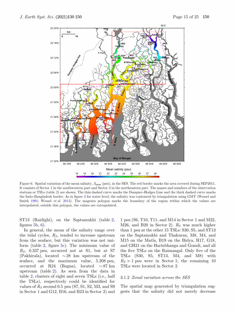
ST13 (Raidighi), on the Saptamukhi (table 2,Bgures 5b, 6).In general, the mean of the salinity range over

the tidal cycles, RS , tended to increase upstreamfrom the seaface, but this variation was not uni-form (table 2, Bgure 5c). The minimum value ofRS , 0.337 psu, occurred not at S1, but at S7(Pakhirala), located � 28 km upstream of theseaface, and the maximum value, 5.208 psu,occurred at R24 (Bagna), located � 87 kmupstream (table 2). As seen from the data intable 2, clusters of eight and seven TSLs (i.e., halfthe TSLs), respectively could be identiBed forvalues of RS around 0.5 psu (S7, S1, S2, M3, and S9in Sector 1 and G12, B16, and B23 in Sector 2) and

1 psu (S6, T10, T11, and M14 in Sector 1 and M22,M26, and B20 in Sector 2). RS was much higherthan 1 psu at the other 15 TSLs: S30, S5, and ST13on the Saptamukhi and Thakuran, M8, M4, andM15 on the Matla, B19 on the Bidya, H17, G18,and GH21 on the Harinbhanga and Gomdi, and allthe Bve TSLs on the Raimangal. Only Bve of theTSLs (S30, S5, ST13, M4, and M8) withRS [ 1 psu were in Sector 1; the remaining 10TSLs were located in Sector 2.

3.1.2 Zonal variation across the SES

The spatial map generated by triangulation sug-gests that the salinity did not merely decrease

88˚18'E 88˚24'E 88˚30'E 88˚36'E 88˚42'E 88˚48'E 88˚54'E 89˚00'E 89˚06'E21˚30'N

21˚36'N

21˚42'N

21˚48'N

21˚54'N

22˚00'N

22˚06'N

22˚12'N

22˚18'N

22˚24'N

18 19 20 21 22 23 24 25 26 27 28

Mean salinity (psu)

0

km

10

S1

S2M3

S5S6 S7

M8

T10 T11

G12

ST13 M14

H17

G18B20

M22

B23R24

R25

M26

R27

R28

R29

S30

GH21B19

M4

B16

M15

S9

Indrapur

Dhanchi Kalash

MahendranagarRamgangaPakhirala Dhulibhasani

Damkal

Kishorimohanpur

Durgaduani

Raidighi

Kaikhali

Lahiripur

Pakhiralay

Rangabelia

Purandar PathankhaliBagna

Kalitala

Canning

Dhamakhali

Shitalia

Sahebkhali

Shibganj

MelmeliaGosaba

Bonnie Camp

Jharkhali BaliJharkhali Jetty

Purba Dwarkapur

Bay of Bengal

Dam

pier

−Hod

ges

line

R. S

apta

muk

hi W

R. S

apta

muk

hi E

R. T

haku

ran

R. Thak

uran

R. M

atla

R. B

hang

adun

i

R. G

osab

a

R. G

ona

R. HarinbhangaR. Raimangal

R. M

atla

R.Bi

dya

R.Bidy

a

R. M

atla

R. PiyaliR. Hogol

R. J

hillaGo

mdi

K.

R. Gosaba

Dat

tar G

.

89˚E

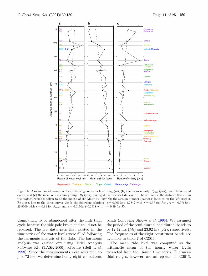
Figure 6. Spatial variation of the mean salinity, Smean (psu), in the SES. The red border marks the area covered during SEP2011.It consists of Sector 1 in the southwestern part and Sector 2 in the northeastern part. The names and numbers of the observationstations or TSLs (table 2) are shown. The thin dashed curve marks the Dampier–Hodges Line and the thick dashed curve marksthe Indo–Bangladesh border. As in Bgure 2 for water level, the salinity was contoured by triangulation using GMT (Wessel andSmith 1991; Wessel et al. 2013). The magenta polygon marks the boundary of the region within which the values areinterpolated; outside this polygon, the values are extrapolated.


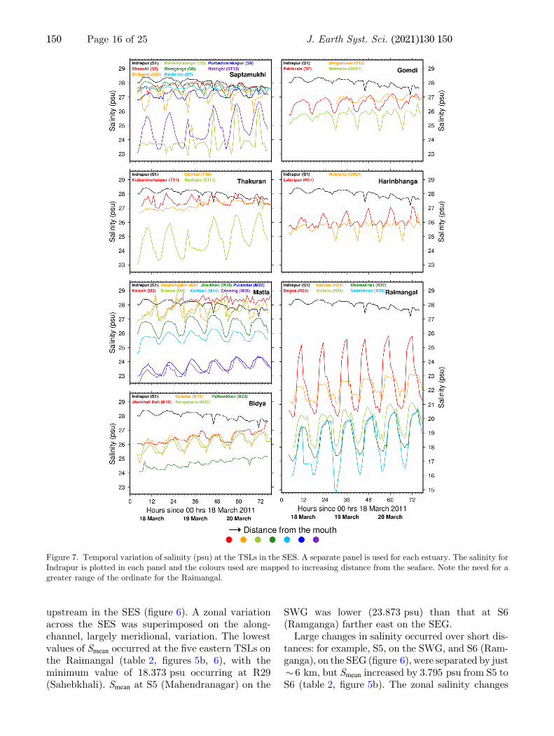
upstream in the SES (Bgure 6). A zonal variationacross the SES was superimposed on the along-channel, largely meridional, variation. The lowestvalues of Smean occurred at the Bve eastern TSLs onthe Raimangal (table 2, Bgures 5b, 6), with theminimum value of 18.373 psu occurring at R29(Sahebkhali). Smean at S5 (Mahendranagar) on the

SWG was lower (23.873 psu) than that at S6(Ramganga) farther east on the SEG.Large changes in salinity occurred over short dis-

tances: for example, S5, on the SWG, and S6 (Ram-ganga), on the SEG (Bgure 6), were separated by just� 6 km, but Smean increased by 3.795 psu from S5 toS6 (table 2, Bgure 5b). The zonal salinity changes

Figure 7. Temporal variation of salinity (psu) at the TSLs in the SES. A separate panel is used for each estuary. The salinity forIndrapur is plotted in each panel and the colours used are mapped to increasing distance from the seaface. Note the need for agreater range of the ordinate for the Raimangal.


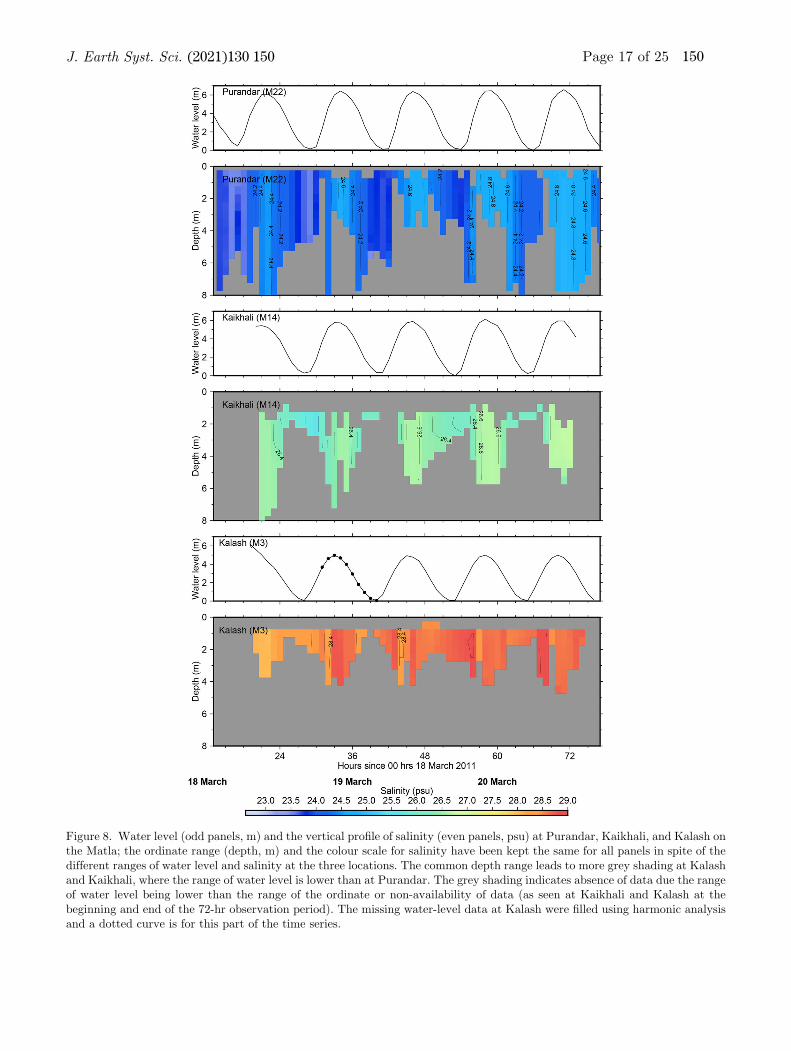
Figure 8. Water level (odd panels, m) and the vertical proBle of salinity (even panels, psu) at Purandar, Kaikhali, and Kalash onthe Matla; the ordinate range (depth, m) and the colour scale for salinity have been kept the same for all panels in spite of thedifferent ranges of water level and salinity at the three locations. The common depth range leads to more grey shading at Kalashand Kaikhali, where the range of water level is lower than at Purandar. The grey shading indicates absence of data due the rangeof water level being lower than the range of the ordinate or non-availability of data (as seen at Kaikhali and Kalash at thebeginning and end of the 72-hr observation period). The missing water-level data at Kalash were Blled using harmonic analysisand a dotted curve is for this part of the time series.


were not monotonic, however, and Smean changedmuch less from S6 to S7 (Pakhirala), which waslocated on a branch of the SEG (Bgure 6). S7 lay� 11 kmeast of S6, but Smean decreased fromS6 to S7by just 0.083 psu (table 2, Bgure 5b). Similarly,though Smean generally decreased eastward in Sec-tor 2, an eastward increase in Smean was seen in someparts.For example,Smean increased eastwardby0.961psu from M22 (Purandar) to B23 (Pathankhali),which are separated by � 11 km, and by 1.552 psufrom B23 to B19 (Gosaba), which were separated by� 8 km. Similar differences in Smean were observedbetween TSLs situated on the opposite banks of anestuary: Smean (25.765 psu) at M14 (Kaikhali, westbank of the Matla) was 0.827 psu lower than that at(26.592 psu) at M15 (Jharkhali Jetty, east bank ofthe Matla).

3.2 Temporal variation of surface salinity

For several TSLs, the tidal half-cycle from 4 to9 AM on 18 March 2011 is incomplete because theLW level occurred about an hour earlier. For thistidal cycle, we designate the Brst reported data at4 AM as LW1. Though there are differences in thetemporal variation of salinity across the TSLsand even across tidal cycles at some TSLs, a fewpatterns can still be inferred.

The time series of hourly salinity at the 30 TSLsis plotted in Bgure 7; the mean range is listed intable 2. At the peak of the dry season and in theabsence of precipitation, the major source ofsalinity variation in the monsonal estuaries of theSES is the twice-daily incursion of the saline seawater due to the semi-diurnal tidal cycle (Vijithet al. 2009). Therefore, a majority of the TSLsshowed a dominance of the semi-diurnal cycle insalinity. This semi-diurnal tide-driven oscillation,which was roughly sinusoidal, is clearly discerniblein the salinity curves for 20 (S6, S9, ST13, T10,T11, M15, M16, M22, M26, B19, B20, G12, G18,GH21, H17, R25, R24, R28, R29, and R27) of the30 TSLs. At these 20 TSLs, the observed salinityincreased (decreased) with the rise (fall) in waterlevel, attaining the maximum (minimum) salinityfor a tidal cycle at or around the HWL (LWL).The time taken for salinity to decrease from the

maximum to the minimum value was longer thanthe the time taken for salinity to increase from theminimum to the maximum value. Though thesampling temporal interval for salinity (one hour)is coarser compared to water level (15 min), it ispossible to infer the nature of tidal asymmetry. Thesalinity variation also displayed a duration asym-metry, but the type of asymmetry tended to varybetween Cow-dominance and ebb-dominance at 20of the 30 TSLs (table 3). Ebb-dominance was seenin the salinity variation at six TSLs and Cow-dominance at the other four TSLs. The sameasymmetry was seen for both water level andsalinity only at eight TSLs: Cow-dominance wasseen at three TSLs and mixed asymmetry at BveTSLs (table 3). Thus, though Cow-dominance wasstriking for water level (22 TSLs), the asymmetrytended to be mixed for salinity.The observed patterns of salinity variations were

complex and different at each of the 10 TSLs that didnot show a clear semi-diurnal cycle (Bgure 7). At twoof these 10TSLs, S7 andB23, therewas a semi-diurnaloscillation, but the range was low (table 2, Bgure 5c).AtM4andM8too, therewasa semi-diurnal oscillationin salinity, but the variationwas not smooth, unlike atthe 20 TSLs that showed a clear semi-diurnal oscilla-tion; at these two TSLs, the salinity was also out ofphase with the tide. Likewise, the semi-diurnal oscil-lation at B16was also not smooth. At two other TSLs,both on the Saptamukhi, the semi-diurnal oscillationwas evident in some,butnot all, tidal cycles.AtS5, thewesternmost TSL, the salinity was low and showedalmostnovariationover theBrst twocycles,butaclearsemi-diurnal oscillationwas seen in the remaining four

24

26

28S

alin

ity (C

TD)

24 26 28

Salinity (Autosal)

Purandar (M22); r=0.96

Kaikhali (M14);r=0.88

Kalash (M3); r=0.73

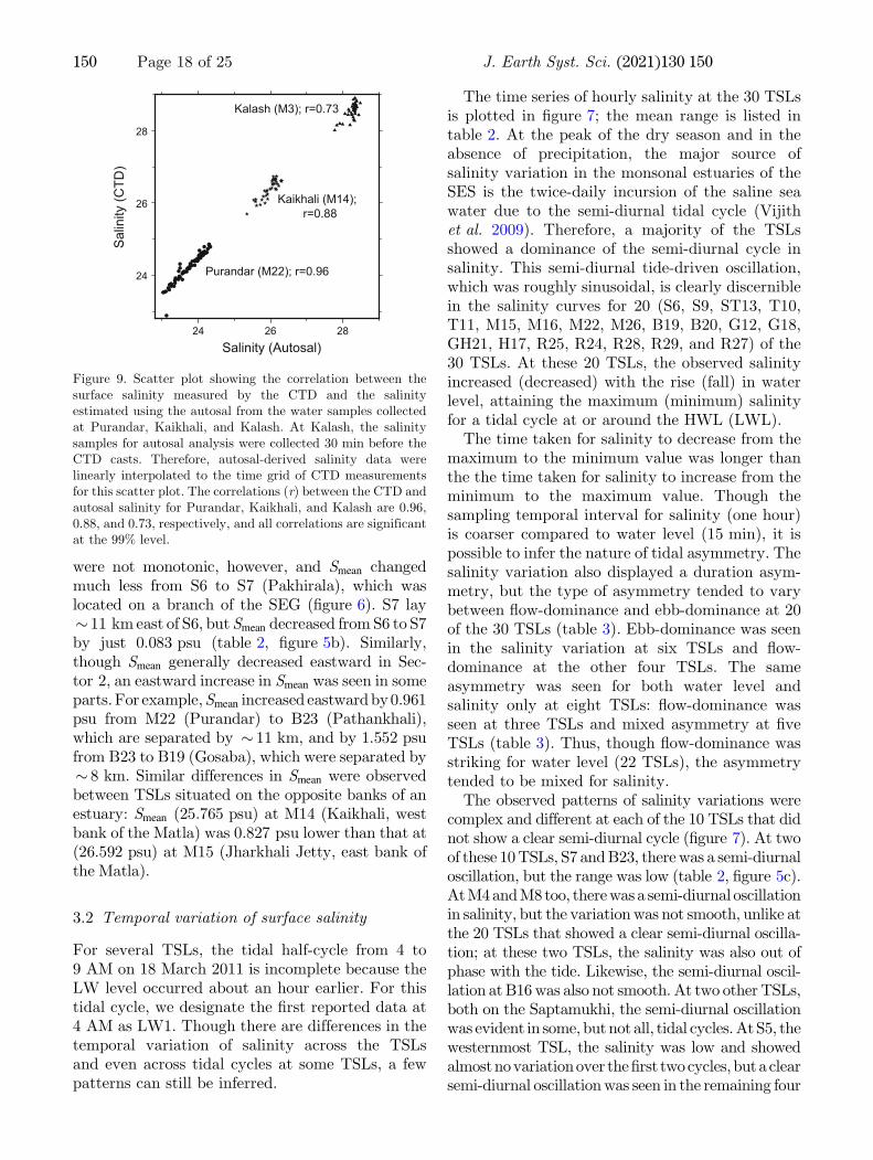
Figure 9. Scatter plot showing the correlation between thesurface salinity measured by the CTD and the salinityestimated using the autosal from the water samples collectedat Purandar, Kaikhali, and Kalash. At Kalash, the salinitysamples for autosal analysis were collected 30 min before theCTD casts. Therefore, autosal-derived salinity data werelinearly interpolated to the time grid of CTD measurementsfor this scatter plot. The correlations (r) between the CTD andautosal salinity for Purandar, Kaikhali, and Kalash are 0.96,0.88, and 0.73, respectively, and all correlations are significantat the 99% level.


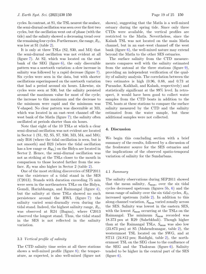
cycles. In contrast, at S1, the TSL nearest the seaface,the semi-diurnal oscillation was seen over the Brst twocycles, but the oscillation went out of phase (with thetide) and the salinity showed a decreasing trend overthe remaining four cycles.Furthermore, the range,RS ,was low at S1 (table 2).It is only at three TSLs (S2, S30, and M3) that

the semi-diurnal oscillation was not evident at all(Bgure 7). At S2, which was located on the eastbank of the SEG (Bgure 6), the only discerniblepattern was a sawtooth variation: a slow increase insalinity was followed by a rapid decrease (Bgure 7).Six cycles were seen in the data, but with shorteroscillations superimposed on the sawtooth variationthat had a period around six hours. Likewise, sixcycles were seen at S30, but the salinity persistedaround the maximum value for most of the cycle;the increase to this maximum and the decrease tothe minimum were rapid and the minimum wasV-shaped. No clear pattern was discernible at M3,which was located in an east–west channel oA thewest bank of the Matla (Bgure 7); the salinity oftenoscillated at periods shorter than six hours.Note that eight of the 10 TSLs at which a clear

semi-diurnal oscillation was not evident are locatedin Sector 1 (S1, S2, S5, S7, S30, M3, M4, and M8);only B16 (where the tidal oscillation is seen, but isnot smooth) and B23 (where the tidal oscillationhas a low range or RWL) on the Bidya are located inSector 2. Hence, the semi-diurnal oscillation wasnot as striking at the TSLs closer to the mouth incomparison to those located farther from the sea-face. RS was also higher in Sector 2 (table 2).One of the most striking discoveries of SEP2011

was the existence of a tidal stand in the SES(C2013). Stands with duration exceeding 75 minwere seen in the northeastern TSLs on the Bidya,Gomdi, Harinbhanga, and Raimangal (Bgure 4),but the salinity at these TSLs showed no suchpersistence around the HWL (Bgure 7): thesalinity varied semi-diurnally even during thetidal stand. Indeed, the highest salinity range, RS ,was observed at R24 (Bagna), where C2013observed the longest stand. Thus, the tidal standin the SES is not reCected in the salinityvariation.

3.3 Vertical proBle of salinity

The CTD salinity time series at all three stationsshows a well-mixed proBle (Bgure 8); the temper-ature, as expected, is also well-mixed (Bgure not

shown), suggesting that the Matla is a well-mixedestuary during the spring tide. Since only threeCTDs were available, the vertical proBles arerestricted to the Matla. Nevertheless, since theKalash TSL was not located on the main Matlachannel, but in an east–west channel oA the westbank (Bgure 6), the well-mixed nature may extendbeyond the Matla to the other SES estuaries.The surface salinity from the CTD measure-

ments compares well with the salinity estimatedfrom the autosal at the three stations (Bgure 9),providing an independent veriBcation of the qual-ity of salinity analysis. The correlation between thetwo estimates is high (0.96, 0.88, and 0.73 atPurandar, Kaikhali, and Kalash, respectively) andstatistically significant at the 99% level. In retro-spect, it would have been good to collect watersamples from the CTD boats in addition to theTSL boats at these stations to compare the surfacesalinity measured by the CTD and the salinityestimated from the water sample, but theseadditional samples were not collected.

4. Discussion

We begin this concluding section with a briefsummary of the results, followed by a discussion ofthe freshwater source for the SES estuaries andthe implications of the observed spatio-temporalvariation of salinity for the Sundarbans.

4.1 Summary

The salinity observations during SEP2011 showedthat the mean salinity, Smean, over the six tidalcycles decreased upstream (Bgures 5b, 6) and themean range of salinity over the six tidal cycles, RS ,increased upstream (table 2). In addition to thisalong-channel variation, Smean varied zonally acrossthe SES. Salinity was lowest in the eastern SES,with the lowest Smean occurring at the TSLs on theRaimangal. The minimum Smean recorded was18.373 psu at R29 (Sahebkhali). Though higherthan at the Raimangal TSLs, Smean was also low(23.873 psu) at S5 (Mahendranagar, table 2), thewesternmost TSL located on the SWG, and atST13 (24.812 psu; Raidighi, table 2), the north-ernmost TSL on the SEG close to the conCuence ofthe SEG and the Thakuran (Bgure 6). Salinitytended to be higher in the central part of the SES(Bgure 6).


At 20 of the 30 TSLs (three on the Saptamukhi,two each on the Thakuran and the Bidya, four onthe Matla, three on the Gomdi, one on Har-inbhanga, and all the Bve TSLs on the Raimangal),the salinity exhibited a semi-diurnal variation(Bgure 7), like the water level (Bgure 4), withmaximum (minimum) salinity tending to occur ator around HW (LW). The temporal variation wasmore complex at the other 10 TSLs, of which Bvewere located on the Saptamukhi, three on theMatla, and two on the Bidya. Thus, eight of these10 TSLs were located in Sector 1 in the south-western part of the SES and only two were locatedin Sector 2. Two of these 10 TSLs showed a semi-diurnal oscillation, but with a low range (RS), threeTSLs showed a semi-diurnal oscillation that wasnot smooth and the salinity was out of phase withthe water level, and two TSLs (S1 and S5 on theSaptamukhi) showed a semi-diurnal oscillation insome cycles and not in others. At two TSLs (S2 andS30), there was no sinusoidal semi-diurnal oscilla-tion, but the salinity did vary with a period ofroughly six hours; in contrast, no clear periodicitywas evident at M3, where the salinity tended tovary at periods shorter than six hours.Though the tidal asymmetry tended to be of the

Cow-dominant type for water level (22 TSLs), ittended to vary between Cow-dominance and ebb-dominance for salinity at 20 of the 30 TSLs(table 3). Even at the TSLs at which a tidal standexceeding 75 min was seen in the water level(C2013; Bgure 4), the salinity oscillated with asemi-diurnal period (Bgure 7). Thus, the salinityvariation was unaffected by the stand of the tide.CTD data from three stations on the Matla show

that it was well-mixed; it is possible that all theSES estuaries are of the well-mixed type during thespring tide.

4.1.1 Freshwater sources

The tides are the main agents that carry salt inand out of an estuary and eventually lead to themixing of salt and various nutrients, sediments,and other particulates within it. In general, theobserved large-scale salinity in an estuary isdetermined by this tidal action, and the domi-nance, or vice versa, of dilution by freshwaterover evaporation. For most estuaries, the mainsource of freshwater is the runoA from rivers atthe head. Other sources are precipitation, whichwas absent before and during the 72-hr

observation period in the SES, and local runoA.In the case of the SES, there is no riverinefreshwater discharge to the principal estuaries,with the exception of the Hoogly and theRaimangal.

Therefore, during SEP2011, which was con-ducted at the peak of the dry season in the SES, themain source of salinity variation in the estuaries isthe tide. Evidence of this tidal eAect was seen allover the SES, with the salinity oscillating semi-diurnally at 20 TSLs; variation with a period ofroughly six hours also seen at nine of the other 10TSLs (Bgure 7).

The salinity decreased upstream in all thechannels (Bgures 5b, 6, table 2), suggesting thatthe observed along-channel variation of salinity isdue to the preceding summer monsoon, when theinCow of freshwater into the channels would havelowered salinity throughout the SES estuaries.Following the cessation of rains, the ingress of saltfrom the seaward end owing to the tides isexpected to lead to an along-channel gradient insalinity that is typical of monsoonal estuaries(Vijith et al. 2009, 2016). The freshwater receivedfrom the Raimangal via its parent river, R. Ich-hamati (a distributary of R. Ganga), led to thelowest salinities occurring at the Bve TSLs on thisestuary (Bgure 6, table 2). Equally intriguing isthat the salinity was also low at S5 (Bgures 5b, 6,table 2), the westernmost TSL (Bgure 6), wherethe salinity showed almost no variation during theBrst two cycles and varied semi-diurnally over thelast four cycles (Bgure 7). The possible source ofthe freshwater that lowers salinity at S5 isR. Hoogly, to which the Saptamukhi is connectedvia numerous east–west channels.

The Farakka Barrage was constructed to keepKolkata port functional by diverting a part of theCow in the Ganga into the Bhagirathi – knownfarther downstream as the Hoogly – at Farakka(Bgure 1). A treaty, signed in 1996 between Indiaand Bangladesh (Anonymous 2017), states how theCow is to be divided during the dry season (Jan-uary–May). During the peak of the dry season in

March–April, 35,000 cusecs (� 991m3s�1) is to bereleased in alternate 10-day blocks to India(Hooghly) and Bangladesh. The main point is thatthe Hoogly carries freshwater throughout Marcheach year, but the amount of freshwater variesthrough the month. The Hoogly and SWG areconnected by a complex network of channels,which must be transporting freshwater from the


Hoogly to the SWG. An analysis of the salinityvariation at S5 is beyond the scope of this paper,but we conjecture that the low, nearly invariantsalinity over the Brst two cycles at S5 is due to anincreased supply of freshwater. The later increasein salinity and the switch to a semi-diurnal oscil-lation suggests a dominance of the tidal circulationand weaker freshwater inCow. It may be just acoincidence that the intermittency in the fresh-water diversion into the Hoogly at Farakka iscaptured in the salinity variation at S5.Curiously, as noted earlier, the behaviour at S1,

which is nearest the seaface, is in contrast to thatat S5. At S1, there was a semi-diurnal oscillationduring all six cycles, but the salinity showed adecreasing trend after the Brst two cycles. Since thesalinity tends to be lower in the northeastern Bayof Bengal or the coastal regime oA Bangladesh incomparison to the salinity in the northwestern bayor the coastal regime oA the Sundarbans (seeBgure 19 of Chatterjee et al. 2012), advection ofthe fresher water from the east may lead to thedecrease in salinity at S1. We note, however, that asimilar decrease in salinity should then occur atM3, which lies east of S1, but salinity tends toincrease instead at M3 over the last four cycles(Bgures 7, 8). Another possible cause of thisdecreasing trend may be the inCow from the Hoo-gly, which can occur via the Bay of Bengal inaddition to the possibility of being driven via theSWG. The complex geometry of the SES estuarieswill play role in determining local salinity varia-tions by the process of tidal trapping (Medeirosand Kjerfve 2005) observed in other estuarinesystems. What makes it difBcult to draw inferencesfor the Saptamukhi is the multiplicity of lateralfreshwater sources, unlike the more direct andcommon source at the head of the Raimangal.Mapping the salinity variation in the southwesternSES is a challenge.

4.1.2 Implications for the Sundarbans

In the introduction, we noted the importance ofsalinity in determining the availability ofpotable water for domestic and agricultural uses,Bshery, and the mangroves.The absence of a direct freshwater source at the

head in six of the seven estuaries (Raimangal beingthe exception) suggests that salinity can be expectedto be low only in the northeastern SES (Sector 2)during the dry season. Therefore, ingress of saline

water is more likely in the southwestern SES (Sec-tor 1). An implication is that it will be more difBcultto tap potable water in the southwestern SES. Themigration of the Hilsa and the restriction of theSundari tree, which require fresher water, to theeastern part of the SES is also likely to be driven bythe higher salinity in the western SES.Therefore, from the viewpoint of salinity and

freshwater, the eastern SES is more conducive tohuman habitation than the western SES, with theregion around the Hoogly being the exception. Thenorthern part of the eastern SES, Sector 2, isinhabited, but the southern part constitutes thereserved forest. Yet, as noted by C2013, thenortheastern SES (Sector 2) is more prone to theeAect of the storms and the surges, with the longtidal stand during HW increasing the probability ofthe surge coinciding with the high tide. Thus, bothinhabited parts of the Sundarbans suffer from sig-nificant disadvantages. The advantage of lowersurge levels in Sector 1 is compensated by thepoorer availability of potable water and theadvantage of better availability of potable water inSector 2 is compensated by the higher propensityfor damage from surges. In both regions, the dis-advantages are due to natural causes: natural,geological changes over a few centuries have led tothe higher salinity in Sector 1 and the geometry ofthe SES to the ampliBcation of the higher har-monics, and therefore a more damaging surge, inSector 2.Thus, life in the Sundarbans has been (Ab�ul-Fazl-

Allami 1589–1598; Bandopadhyay 1936) – and is(Ghosh 2004; Bhattacharyya 2011) – a constantstruggle against the forces of nature. Any attempt atmitigating the hardships in the region will have tocounter the problems posed by the natural obstaclesprovided by saline water and the surges due tostorms. Whether human ingenuity can overcomethese significant obstacles to improve the quality oflife in the Sundarbans remains to be seen. It is clear,however, that future research will have to build onthe results of SEP2011 to provide the baselineinformation and improve predictive capabilities in aterrain that presents a significant observational andmodelling challenge if the natural obstacles are to beovercome.

Acknowledgements

Thisworkwas conducted as part of a research projectat School of Oceanographic Studies (SOS), Jadavpur


University (JU) (Sanction No. F/INCOIS/INDO-MOD-11-2007/2691 dated 20 December 2007) fun-ded by IndianNationalCentre forOcean InformationServices (INCOIS), Ministry of Earth Sciences,Government of India, under the INDOMOD pro-gramme. D Shankar, D Sundar, and G S Michaelacknowledge the support fromCSIRunder theSupra-Institutional Project (SIP13; 2007–2012). We alsoacknowledge the critical comments of two anony-mous reviewers, who have helped improve themanuscript significantly. In particular, we acknowl-edge one of them as the source of the explanation forthe observed upstream decrease in salinity in all theSES estuaries: the role of the preceding monsoon waspointed out by this reviewer. This reviewer alsopointed out the possibility of westward alongshoreadvection in the northern bay leading to the decreasein salinity at Indrapur. The authors gratefullyacknowledge the following organizations and peoplewhose encouragement and active cooperation led tothe successful implementation of the SundarbansEstuarine Programme: INCOIS, Ministry of EarthSciences, Government of India, for funding the pro-gramme; the Department of Forests and the Sun-darbans Development Board, Government of WestBengal for permission to work in some of the ReserveForestareas, accommodation, andother facilities; theTagore Society for Rural Development (TSRD),Sabuj Sangha (SS), and theCalcuttaWildlife Society(CWS) for providing local human resources andlogistic support; the Border Security Force (EasternFrontier),Government of India, and theWestBengalPolice for providing security during the observationperiod. With the announcement of the GeneralAssembly Elections in West Bengal scheduled tobegin from 10 April 2011 and the model code ofconduct already imposed during March, potentialdifBculties for conducting theSEPwere smoothedoutby the eAective intervention of the then DistrictMagistrate of South 24 Parganas, Mr Narayan Swa-roop Nigam, IAS, to whom we express our heartfeltthanks. His prompt permission to carry out the SEPand very clear instructions to the various Depart-ments of the Government of West Bengal mentionedabovewere crucial to the success of the SEP in spite ofthe recalcitrance of the then Field ODcer of theSundarbans Tiger Reserve. The SEP, initiated at thesuggestion of Dr S R Shetye, in September 2010,progressed rapidly to a full Cedged programme byMarch 2011 under the constant and enthusiasticencouragement received from him, Dr S S C Shenoi,and late Prof A D Mukherjee. Dr M Ravichandranand Dr P A Francis were always ready with their

cooperation throughout the preparatory and imple-mentation stages of the programme. The authorsgratefully acknowledge Dr A C Anil, Dr DileepKumar, Dr A S Unnikrishnan, and Dr V Gopalakr-ishna of CSIR-NIO, Goa, and Dr V V S S Sarma,Dr V S N Murty, andDr Y Sadhuramof CSIR-NIORegional Centre, Visakhapatnam for their valuablesuggestions and help in using the autosal facilities.Sincere thanks are extended to the late Mr TusharKanjilal (Founder Director of TSRD), Mr Angshu-man Das (Founder Director of SS), and Mr Debku-mar Biswas (Secretary of CWS) for their permissionand help in managing local human resources andlogistics at Rangabelia, Nandakumarpur, and Jhar-khali, respectively. Sincere thanks are also extendedto the the local coordinators (Mr Kanai Lal Sarkar ofTSRD, Mr Swapan Kumar Das of SS, and Mr NiharMandal of CWS) and the ScientiBc Supervisors(Mr Manik Maity, Mr Nanda Gopal Maity, andMr SumitKoley fromDigha,Mr Jayanta Sutradhar,Mr JoydeepGhosal,Mr PrasantaNandi,Mr PranabKumar Mukherjee, and Mr Shantanu Paramanikfrom Purulia, and Mr Dwaipayan Bhattacharyafrom Bhopal). FriendsMr KalyanMallick, IPS (nowretired IG, West Bengal Police, then Commandant,IndiaReserveBattalion,Durgapur)withhisPersonalSecurityODcer,Mr IndrajitMandal, andMrs. RupaRavindran from Mumbai came over to Kolkata toprovide their immense help, bearing without anycomplaint the discomfort and challenges that cameour way, and enjoying like us every bit of their par-ticipation in the SEP. GKS and MC would like tospecially acknowledge Prof. Sugata Hazra, Director,SOS, JU (since retired) and Dr M Bardhan Roy, thethen Principal, Basanti Devi College for the cooper-ation extended to them during the organization andexecution of the SEP. Finally, the authors take thegreatest pleasure in humbly and sincerely thankingand gratefully acknowledging each of the 180 obser-vers, the 30 local supervisors, the pilots of the 44mechanised boats and their assistants, and also thedrivers of the Beld vehicles for the dedication andsincerity with which they performed their work,mostly under difBcult and often dangerous condi-tions. Their contribution towards the eAectivenessand success of the SEP was priceless and immeasur-able. It is doubtful if the SEP2011 observations couldhave been completed successfully without the timelyinterventions of the late Prof A D Mukherjee, whopassed away in October 2020; we dedicate thispaper to him. This is CSIR-NIO contribution 6701,ESSO-NCPOR contribution J-124/2020-21, andESSO-INCOIS contribution 407.


Author statement

Meenakshi Chatterjee: Co-PI of the project, plan-ning the SEP and the methodology to be followed,overall supervision and logistic coordination duringSEP2011 in Sectors 1 and 2, analysis and interpre-tation of the data, and writing of the manuscript.D Shankar: Planning the SEP and the methodologyto be followed, overall supervision and logisticcoordination during SEP2011 in Sector 1, analysisand interpretation of the data, and writing of themanuscript.V Vijith:Analysis and interpretation ofthe data, preparation of the Bgures, and writing ofthe manuscript. G K Sen: PI of the project andplanning the SEP, overall supervision and logisticcoordination during SEP2011 in Sector 2.D Sundar:Planning the SEP and the methodology to be fol-lowed, overall supervision and logistic coordinationduring SEP2011 in Sectors 1 and 2. G S Michael:Planning the SEP and the methodology to be fol-lowed, overall supervision and logistic coordinationduring SEP2011 in Sectors 1 and 2. P Amol:Supervision of the boat at Kalash (M3) and partic-ipation in data collection, interpretation of the data,and reviewing the manuscript draft and suggestingrelevant changes that have been incorporated in theBnal version.Abhisek Chatterjee: Supervision of theboat at Indrapur (S1) and participation in datacollection, interpretation of the data, and reviewingthe manuscript draft and suggesting relevant chan-ges that have been incorporated in the Bnal version.P Sanyal: Planning the SEPand themethodology tobe followed, and overall supervision and logisticcoordination during SEP2011 in Sector 1. Sid-dhartha Chatterjee: Participation in overall super-vision and logistic coordination during SEP2011 inSector 1, and analysis of salinity samples on theautosal at the regional centre of CSIR-NIO inVishakhapatnam. Anwesha Basu: Participation inoverall supervision and logistic coordination duringSEP2011 in Sector 1, and analysis of salinity sampleson the autosal at the regional centre of CSIR-NIO inVishakhapatnam. Saranya Chakraborti: Assistancein preparation for and participation in overallsupervision during SEP2011 and logistic coordina-tion in Sector 2, and analysis of salinity samples onthe autosal atCSIR-NIO,Goa. Surja KantaMishra:Supervision of the boat at Kaikhali (M14) and par-ticipation in data collection, and analysis of salinitysamples on the autosal at the regional centre ofCSIR-NIO in Vishakhapatnam. K Suprit: Supervi-sion of the boat atPurandar (M22) andparticipationin data collection, interpretation of the data, and

reviewing the manuscript draft and suggestingrelevant changes that have been incorporated in theBnal version. Debabrata Mukherjee: Participationin data collection at Kalash (M3). A Mukherjee:Supervision of the boat at Kaikhali (M14) and par-ticipation in data collection. Soumya Mukhopad-hyay: Participation in data collection at Kaikhali(M14). Gopal Mondal: Analysis of salinity sampleson the autosal at CSIR-NIO, Goa. Aravind Kalla:Participation in data collection at Purandar (M22).Madhumita Das: Assistance in overall supervisionand logistic coordination during SEP2011.

References

Ab�ul-Fazl-Allami 1589–1598 Ain i Akbari, Volume III; RoyalAsiatic Society of Bengal, Kolkata, India; translated fromthe original in Persian by Col. H. S. Jarrett (1894) as SeriesBibliotheca Indica, work number 61 commissioned by theRoyal Asiatic Society of Bengal, Calcutta. Revised andedited by Sir Jadunath Sarkar in 1947.

Amante C and Eakins B W 2009 ETOPO1: 1-arc-minuteglobal relief model: Procedures, data sources and analysis;National Geophysical Data Center, NOAA; USA; https://doi.org/10.7289/V5C8276M.

Anonymous 2017 Treaty Between the Government of thePeoples Republic of Bangladesh and the Government of theRepublic of India on sharing of the Ganga/Ganges watersat Farakka; In: Indo-Bangladesh Cooperation: Ministry ofJal Shakti, Department of Water Resources, RiverDevelopment & Ganga Rejuvenation; http://mowr.gov.in/international-cooperation/bilateral-cooperation-with-neighbouring-countries/indo-bangladesh-cooperation.

Attri S D and Tyagi A 2010 Climate ProBle of India; Met.Monograph No. Environment Meteorology 01/2010; IndiaMeteorological Department, Ministry of Earth Sciences,Government of India.

Bandaranayake W M 1998 Traditional and medicinal uses ofmangroves; Mangrov. Salt Marsh. 2 133–148.

Bandopadhyay M 1936 Padma Nadir Majhi (in Bengali);Gurudas Chatterjee and Sons, Kolkata.

Barik J and Chowdhury S 2014 True mangrove species ofSundarbans delta, West Bengal, Eastern India; CheckList 10 329–334.

Bell C, Vassie J M and Woodworth P L 1998 POL/PSMSLTidal Analysis Software Kit 2000 TASK-2000); Technicalreport, Permanent Service for Mean Sea Level, UK.

Bhattacharyya S 2011 A History of the Social Ecology ofSundarbans: The Colonial Period; Ph.D. thesis; Depart-ment of History, Jadavpur University, Kolkata, India.

Bhaumik U and Sharma A P 2011 The Bshery of Indian Shad(Tenualosa ilisha) in the Bhagirathi–Hooghly river system;Fish. Chimes 31 21–27.

Bhunia A B and Choudhury A 1981 Observations on thehydrology and the quantitative studies on benthic macro-fauna in a tidal creek of Sagar Island, Sundarbans, WestBengal, India; Proc. Ind. Natl. Sci. Acad. B47398–407.


Chakarabarti R 2009 Local people and the global tiger: Anenvironmental history of the Sundarbans; Glob. Environ. 372–95.

Chanda B K, Trivedi R K, Dubey S K, Rout S K, Beg M Mand Das U K 2015 EAect of salinity on survival and growthof giant freshwater prawn Macrobrachium rosenbergii (deMan); Aquacult. Rep. 2 26–33, http://creativecommons.org/licenses/by-nc-nd/4.0/.

Chatterjee M, Shankar D, Sen G K, Sanyal P, Sundar D, MichaelG S, ChatterjeeA,Amol P,MukherjeeD, Suprit K,MukherjeeA,VijithV,Chatterjee S, BasuA,DasM,Chakraborti S, KallaA,Misra S K,Mukhopadhyay S,Mandal G and Sarkar K 2013Tidal variations in the Sundarbans Estuarine System, India; J.Earth. Syst. Sci. 122 899–933, https://doi.org/10.1007/s12040-013-0314-y.

Chatterjee A, Shankar D, Shenoi S S C, Reddy G V, MichaelG S, Ravichandran M, Gopalkrishna V V, RamaRao E P,UdayaBhaskar T V S and Sanjeevan V N 2012 A new atlasof temperature and salinity for the North Indian Ocean;J. Earth Syst. Sci. 121 559–593, https://doi.org/10.1007/s12040-012-0191-9.

Chugh R S 1961 Tides in Hooghly River; Hydrol. Sci. J. 610–26, https://doi.org/10.1080/02626666109493212.

Das P K 1972 Prediction Model for Storm Surges in the Bayof Bengal; Nature 239 211–213, https://doi.org/10.1038/239211a0.

Das S 2012 Salinity Dependent Photosynthetic Response andRegulation of Some Enzymes in Halophytes from IndianSundarbans; In: Applied Photosynthesis (ed.) Najafpour M,;IntechOpen, London, UK, https://doi.org/10.5772/26290.

De D K 1986 Studies on the food and feeding habit of Hilsa,Hilsa ilisha (Hamilton) of the Hooghly estuarine system andsome aspects of its biology; PhD thesis; Calcutta University,Kolkata, India.

Debnath A 2014 Impact of Cyclone Aila on Paddy Cultivationin Gosaba Island of the Indian Sundarban Region; Ind.J. Spat. Sci. 5 7–13.

Dube S K 2012 Prediction of Storm Surges in the Bay ofBengal; Trop. Cycl. Res. Rev. 1 67–74, https://doi.org/10.6057/2012TCRR01.08.

Eaton T T 2007 Analytical estimates of hydraulic parametersfor an urbanized estuary – Flushing Bay; J. Hydrol. 347188–196, https://doi.org/10.1016/j.jhydrol.2007.09.018.

Friedrichs C T and Aubrey D G 1994 Tidal propagationin strongly convergent channels; J. Geophys. Res. 993321–3336.

Ghosh A 2004 The Hungry Tide; Ravi Dayal Publishers, Delhi.Ghosh A and Satpathy B B 2019 Preliminary Observations on

Fish Biodiversity and Some Limno-chemical Parameters ofIchhamati Estuary, Sundarbans, West Bengal; J. Inland.Fish. Soc. India 51 91–94.

Ghosh A, Schmidt S, Fickert T and Nusser M 2015 The IndianSundarban Mangrove Forests: History, Utilization, Con-servation Strategies and Local Perception; Diversity 7149–169.

Gole C V and Vaidyaraman P P 1967 Salinity distributionand eAect of fresh water Cows in the river Hooghly; In:Proc. Tenth Congress of Coastal Engineering, vol. 2,1412–1434.

Gopal B and Chauhan M 2006 Biodiversity and its conserva-tion in the Sundarban Mangrove Ecosystem; Aquat. Sci. 68338–354, https://doi.org/10.1007/s00027-006-0868-8.

Hora S L 1938 A preliminary note on the spawning groundsand bionomics of the so called Indian shad Hilsa ilisha in theriver Ganges; Rec. Indian Muse. 40 147–148.

Kathiresan K, Salmo III S G, Fernando E S, Peras J R,Sukardjo S, Miyagi T, Ellison J, Koedam N E, Wang Y,Primavera J, Eong O J, Yong J W H and Nam V N 2010Heritiera fomes. The IUCN Red List of Threatened Species2010: e.T178815A7615342, https://doi.org/10.2305/IUCN.UK.2010-2.RLTS.T178815A7615342.en.

Kuttyamma K J 1982 The eAect of salinity on the growthof some penaeid prawn; Bull. Depart. Mar. Sci. Univ.Cochin 8 1–34.

Lewis R E and Uncles R J 2003 Factors aAecting longitudinaldispersion in estuaries of different scale; Ocean Dynam. 53197–207, https://doi.org/10.1007/s10236-003-0030-2.

Maiti SandChowdhuryA2013EAects ofAnthropogenicPollutionon Mangrove Biodiversity: A Review; J. Environ. Protect. 41428–1434, https://doi.org/10.4236/jep.2013.412163.

Mandal R N and Naskar K R 2008 Diversity and classiBcationof Indian mangroves: A review; Tropic. Ecol. 49131–146.

Medeiros C and Kjerfve B 2005 Longitudinal Salt and SedimentFluxes in a Tropical Estuary: Itamarac�a, Brazil; J. Coast.Res. 21 751–758, https://doi.org/10.2112/005-NIS.1.

Mitra A, Gangopadhyay A, Dube A, Schmidt A C K andBanerjee K 2009 Observed changes in water mass proper-ties in the Indian Sundarbans (northwestern Bay of Bengal)during 1980–2007; Curr. Sci. 97 1445–1452.

Mitra A, Mondal K and Banerjee K 2011 Spatial and TidalVariations of Physico-Chemical Parameters in the LowerGangetic Delta Region, West Bengal, India; J. Spat.Hydrol. 11 52–69, http://www.spatialhydrology.net/index.php/JOSH/article/view/101/100.

Mohapatra M, Mandal G S, Bandyopadhyay B K, Tyagi Aand Mohanty U C 2012 ClassiBcation of cyclone hazardprone districts of India; Nat. Hazards 63 1601–1620,https://doi.org/10.1007/s11069-011-9891-8.

Murty T S, Flather R A and Henry R F 1986 The storm surgeproblem in the Bay of Bengal; Progr. Oceanogr. 16195–233, https://doi.org/10.1016/0079-6611(86)90039-X.

Nandy A C, Bagchi M M and Majumder S K 1983 Ecologicalchanges in the Hooghly estuary due to water release fromFarakka Barrage; Mahasagar 16 209–220, http://ijs.nio.org/index.php/msagar/article/view/2255.

Oag T M 1939 Report on the River Hooghly and its headwa-ters; Technical report; Commissioners for the Port ofCalcutta, India.

Pattanaik C, Reddy C S and Dhal N K 2008 Phytomedicinalstudy of coastal sand dune species of Orissa; IndianJ. Tradition. Knowl. 7 263–268.

Pillay T V R 1958 Biology of the hilsa, Hilsa ilisha (Hamilton)of the river Hooghly; Indian J. Fish. 5 201–257.

Pillay S R and Rosa H 1963 Synopsis for biological data on thehilsa, Hilsa ilisha (Hamilton) 1822; in FAO FisheriesBiology Synopsis; vol. 25, United Nations.

Pingree R D and GrifBths D K 1979 Sand transport pathsaround the British Isles resulting from M2 and M4 tidalinteractions; J. Mar. Biol. Assoc. UK 59 497–513, https://doi.org/10.1017/S0025315400042806.

Pugh D T 1987 Tides, Surges and Mean Sea Level, Wiley, UK.Raha A K, Zaman S, Sengupta K, Raha S B B S, Banerjee K

and Mitra A 2013 Climate Change and Sustainable


Livelihood Programmes: A case study from the IndianSundarbans; J. Ecol. 107 335–348.

Rao R M 1969 Studies on the prawn Bsheries of the Hooghlyestuarine system; Proc. Nat. Instit. Sci. India 35B 1–27.

Roy N R 1949 Manikchandra Rajar Gan, folk song of Bengal(Bhatiali); In Banglar Itihas; 104; Book Emporium, Kolkata.

Sadhuram Y, Sarma V V S S, Murty T V R and Rao B P 2005Seasonal variability of physico-chemical characteristics of theHaldia channel of Hooghly estuary, India; J. Earth Syst.Sci. 114 37–49, https://doi.org/10.1007/BF02702007.

Sarkar K L 2011 Sundarbaner Itihaas, Rupkatha Prakashan.Seidensticker J and Hai M A 1983 The Sundarbans Wildlife

Management Plan; In: Conservation in the BangladeshCoastal Zone; IUCN, Gland.

Shetye S R, Gouveia A D, Singbal S Y, Naik C G, Sundar D,Michael G S and Nampoothiri G 1995 Propagation of tidesin the Mandovi–Zuari estuarine network; Proceedings of theIndian Acad. Sci. (Earth. Plan. Sci.) 104 667–682.

Sindhu B and Unnikrishnan A 2013 Characteristics of tides inThe Bay of Bengal; Mar. Geodesy 36 377–407, https://doi.org/10.1080/01490419.2013.781088.

Song D, Wang X H, Kiss A E and Bao X 2011 Thecontribution to tidal asymmetry by different combinationsof tidal constituents; J. Geophys. Res. 116 C12,007,https://doi.org/10.1029/2011JC007270.

Speer P E and Aubrey D G 1985 A study of non-linear tidalpropagation in shallow inlet/estuarine systems, part II –

Theory; Estuar. Coast. Shelf Sci. 21 207–224, https://doi.org/10.1016/0272-7714(85)90097-6.

Speer P E, Aubrey D G and Friedrichs C T 1991 Nonlinearhydrodynamics of shallow tidal inlet/bay systems; In: TidalHydrodynam, (ed.) Parker B B, pp. 321–329, Wiley, NewYork.

Vijith V, Shetye S R, Baetens K, Luyten P and Michael G S2016 Residual estuarine circulation in the Mandovi, amonsoonal estuary: A three-dimensional model study;Estuar. Coast. Shelf Sci. 173 79–92, https://doi.org/10.1016/j.ecss.2016.01.041.

Vijith V, Sundar D and Shetye S R 2009 Time-dependence ofsalinity in monsoonal estuaries; Estuar. Coast. ShelfSci. 85 601–608, https://doi.org/10.1016/j.ecss.2009.10.003.

Wessel P and Smith W H F 1991 Free software helps map anddisplay data; Eos, Trans. Amer. Geophys. Union 72441–446, https://agupubs.onlinelibrary.wiley.com/doi/abs/10.1029/90EO00319.

Wessel P, Smith W H F, Scharroo R, Luis J F and Wobbe F2013 Generic Mapping Tools: Improved version released;Eos, Trans. Amer. Geophys. Union 94 409–410, https://doi.org/10.1002/2013EO450001.

Corresponding editor: C GNANASEELAN


Variation of salinity in the Sundarbans Estuarine System ...

Documents